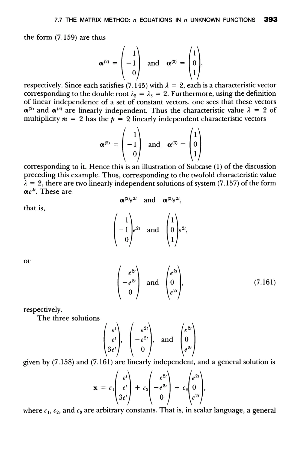
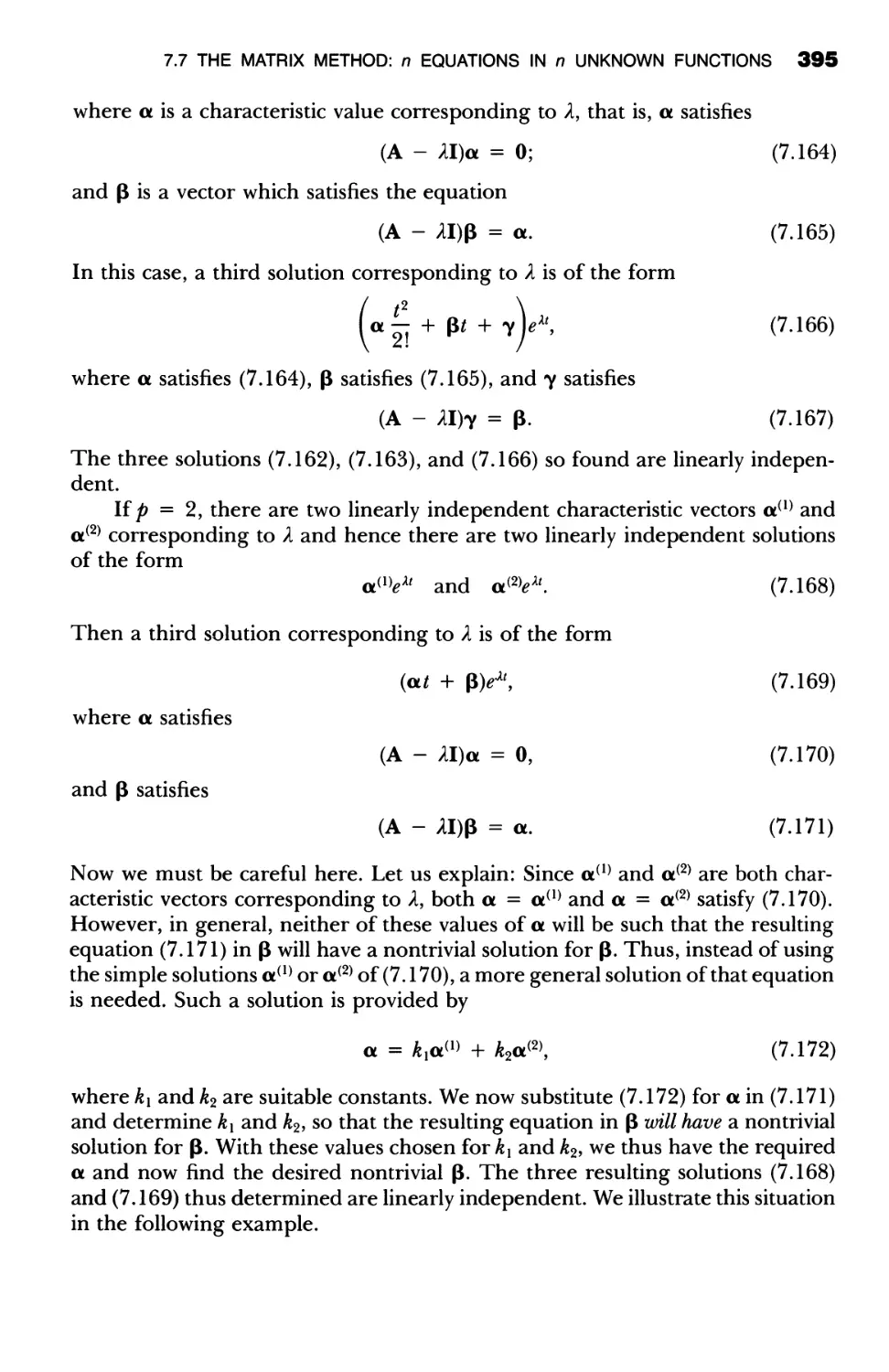
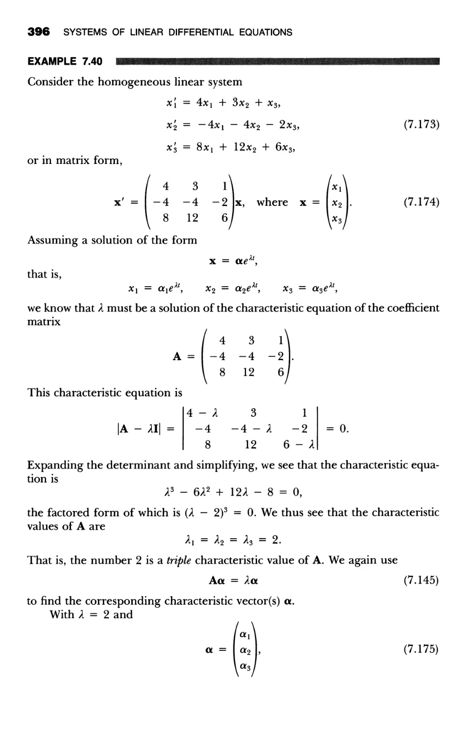
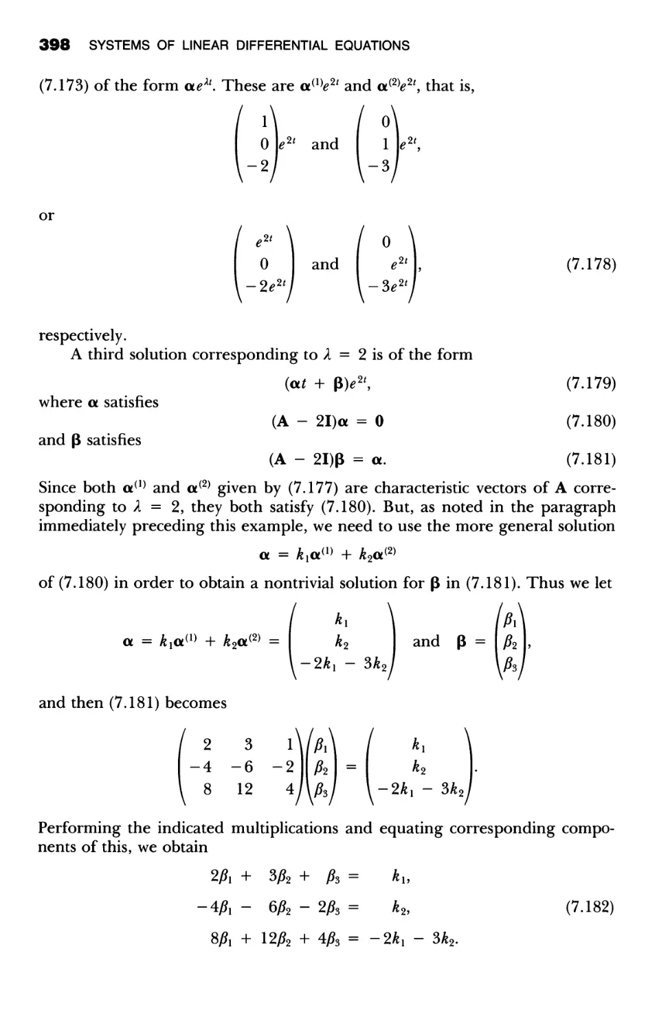
/


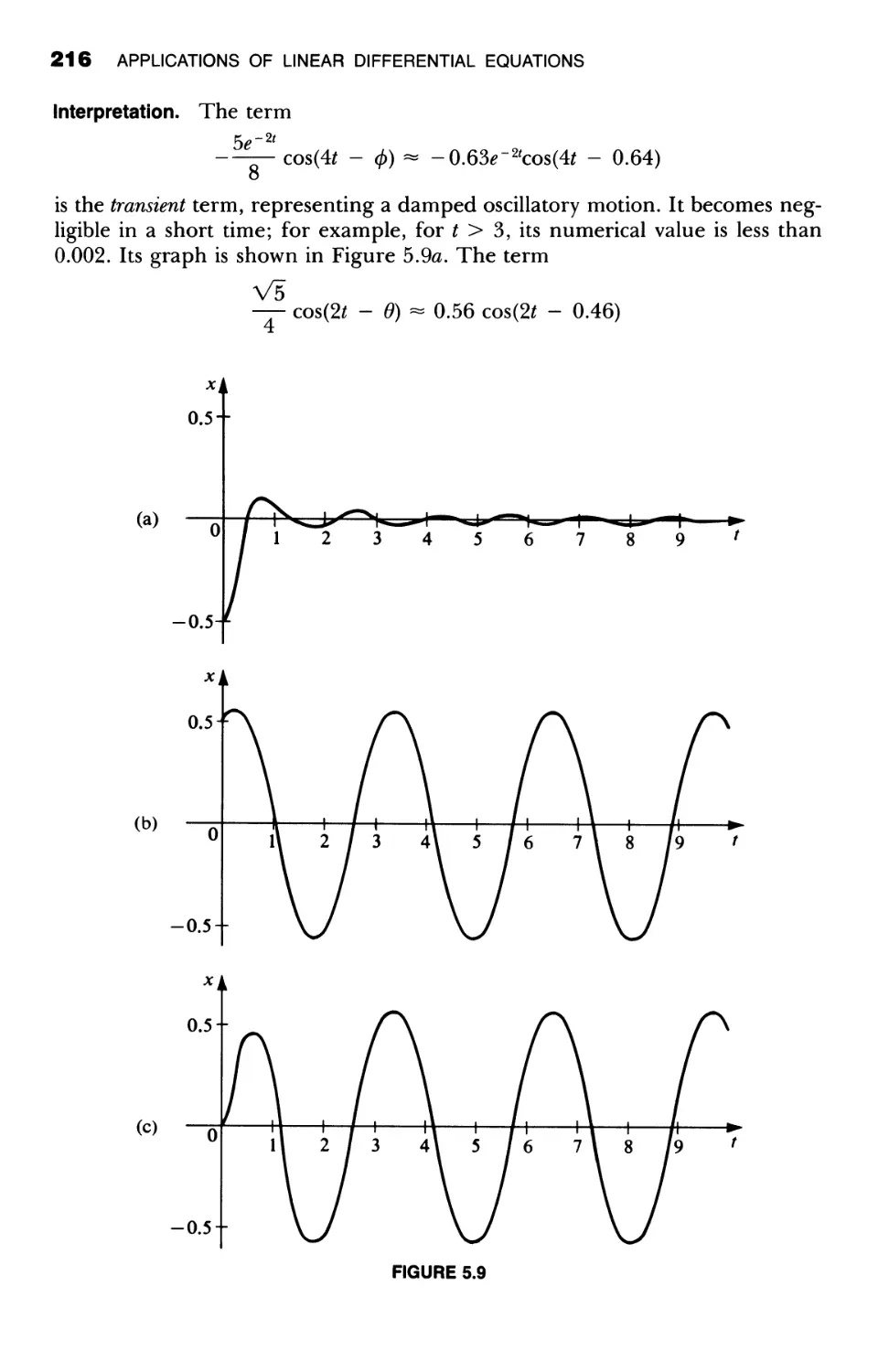


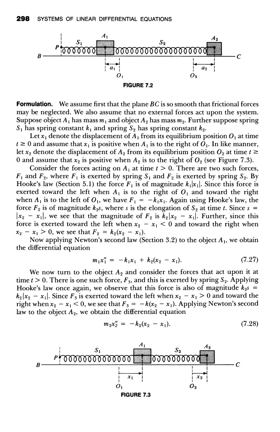


Text
FOURTH EDITION
INTRODUCTION TO
ORDINARY
DIFFERENTIAL
EQUATIONS
FOURTH EDITION
INTRODUCTION TO
ORDINARY
DIFFERENTIAL
EQUATIONS
Shepley L. Ross
University of New Hampshire
With the assistance of
Shepley L. Ross, II
Bates College
II
WILEY
JOHN WILEY & SONS
New York · Chichester · Brisbane · Toronto · Singapore
This book was set in New Baskerville by Techna Type. It was printed and bound by
Halliday. The designer was Sheila Granda. Copyediting was done by Trumbull Rogers.
Elizabeth Austin supervised production.
Copyright @ 1989, by John Wiley & Sons, Inc.
All rights reserved. Published simultaneously in Canada.
Reproduction or translation of any part of
this work beyond that permitted by Sections
107 and 108 of the 1976 United States Copyright
Act without the permission of the copyright
owner is unlawful. Requests for permission
or further information should be addressed to
the Permissions Department, John Wiley & Sons.
Library of Congress Cataloging in Publication Data:
Ross, Shepley L.
Introduction to ordinary differential equations/Shepley L. Ross.
-4th ed.
p. cm.
Bibliography: p.
Includes index.
ISBN 0-471-09881-7
1. Differential equations. I. Title.
QA372.R815 1989
515.3'52-dcI9
88-21589
CIP
Printed in the United States of America
20 19 18 17 16 15 14 13 12
Preface
This is a straightforward introduction to the basic concepts, theory, methods,
and applications of ordinary differential equations. It presupposes a knowledge
of elementary calculus.
Designed for a one-semester course in ordinary differential equations, this
book covers and emphasizes the most fundamental methods of the subject and
also contains traditional applications and brief introductions to fundamental
theory. An examination of the table of contents will reveal just what topics are
presented.
The detailed style of presentation that characterized the first three editions
has been retained. There are over 200 illustrative examples, and each one that
illustrates a method is worked out in great detail. The first six chapters of the
text are essentially as in the third edition, with major textual changes confined
to the last three chapters.
The following additions and modifications are specifically noted:
1. Section 7.6 of the third edition, on the basic theory of linear systems, has
been replaced by a new section on the application of matrix algebra to the
solution of linear systems with constant coefficients in the case of two equations
in two unknown functions. This new section is taken from my longer book,
Differential Equations, 3rd ed. (John Wiley and Sons, New York, 1984). Section
7.7 extends the matrix method of Section 7.6 to the case of linear systems
with constant coefficients involving n equations in n unknown functions. Sev-
eral detailed examples illustrate the method for the case n = 3. This is an
expanded version of the former Section 7.7 and is also taken from Differential
Equations. A new Section 7.8 presents the most basic part of the theory that
formerly appeared in Section 7.6.
v
vi PREFACE
2. Section 8.4 of the third edition, on numerical methods, has been expanded
into the five Sections 8.4 through 8.8 in this edition. The new expanded
treatment includes some improved methods, detailed illustrative examples,
and more attention to errors than had been given previously. Introductory
material on numerical methods for higher order equations and systems has
also been added.
3. Chapter 9 has been reorganized so as to reach the Laplace transform solution
of differential equations more quickly. Step functions and translated functions
have been postponed slightly to a new Section 9.4, and new material on the
Dirac delta function has been added.
4. A brief appendix about polynomial equations has been added. This should
be helpful to students who lack sufficient preparation in college algebra.
5. There are over 360 new exercises, including 160 Chapter Review Exercises.
The Chapter Review Exercise sets appear at the end of each chapter except
the first. Each set consists of a number of straightforward exercises of the
various types considered in that particular chapter and thus provides a good
chapter review.
6. There has been a major change in notation throughout Chapters 4 through
9. In general in these chapters differential equations are now expressed in
the prime notation rather than in the d/dx notation that was employed in the
previous editions.
The text may be covered in the order presented or may be taken up in
various alternate orders. With two exceptions, Chapters 5, 6, 7, 8, and 9 are
essentially independent of one another. The two exceptions are the final sections
of Chapters 8 and 9, which depend on Chapter 7. Thus, in general, the last five
chapters can be taken up in any order. In particular, Sections 9.1 through 9.4
on the Laplace transform can be studied immediately after Chapter 4.
I am grateful to each of the following for reviewing all or part of this edition:
Richard Bagby, New Mexico State University
Andrew G. Bennett, The University of Texas at Austin
Jim D'Archangelo, U.S. Naval Academy
Richard H. Fast, Glendale Community College
Steve Gavazza, Canada College
Paul Krajkiewicz, University of Nebraska
Thomas G. Kudzma, University of Lowell
Forrest Miller, Kansas State University
Jo E. Smith, GMI Engineering and Management Institute
John R. Tucker, Mary Washington College
H. Clare Wiser, Washington State University
John L. Wulff, California State University
PREFACE vii
I thank my colleague Lee Zia, University of New Hampshire, for critically
reading part of the manuscript and making useful suggestions. Additional helpful
comments and suggestions were made by my former colleagues Robert O. Kim-
ball, now retired, and Tom Dick, Oregon State University, and by my former
graduate student Tim Kurtz.
My son, Shepley L. Ross II, Bates College, Lewiston, Maine, is coauthor of
Chapter 8. His work on the numerical methods sections has made this material
much more suitable for this age of calculators and computers. He has also helped
in a variety of other ways, and I am very grateful to him for his important
contributions.
As before, the Wiley staff has been helpful, efficient, and understanding,
and I express my sincere thanks to each person concerned.
Finally, I once again thank my wife for her encouragement, cooperation,
and assistance throughout.
Shepley L. Ross
Contents
1 Differential Equations and Their Solutions 1
1.1 Classification of Differential Equations; Their Origin and
Application 1
1.2 Solutions 6
1.3 Initial-Value Problems, Boundary-Value Problems, and
Existence of Solutions 14
2 First-Order Equations for Which Exact Solutions
Are Obtainable 24
2.1 Exact Differential Equations and Integrating Factors 24
2.2 Separable Equations and Equations Reducible to This Form 38
2.3 Linear Equations and Bernoulli Equations 48
2.4 Special Integrating Factors and Transformations 60
3 Applications of First-Order Equations 71
3.1 Orthogonal and Oblique Trajectories 71
3.2 Problems in Mechanics 78
3.3 Rate Problems 91
4 Explicit Methods of Solving Higher-Order Linear
Differential Equations 110
4.1 Basic Theory of Linear Differential Equations 110
4.2 The Homogeneous Linear Equation with Constant Coefficients 134
4.3 The Method of Undetermined Coefficients 145
4.4 Variation of Parameters 162
4.5 The Cauchy-Euler Equation 171
ix
X CONTENTS
4.6 Statements and Proofs of Theorems on the Second-Order
Homogeneous Linear Equation 177
5 Applications of Second-Order Linear Differential Equations
with Constant Coefficients 189
5.1 The Differential Equation of the Vibrations of a Mass on a
Spring 189
5.2 Free, Undamped Motion 192
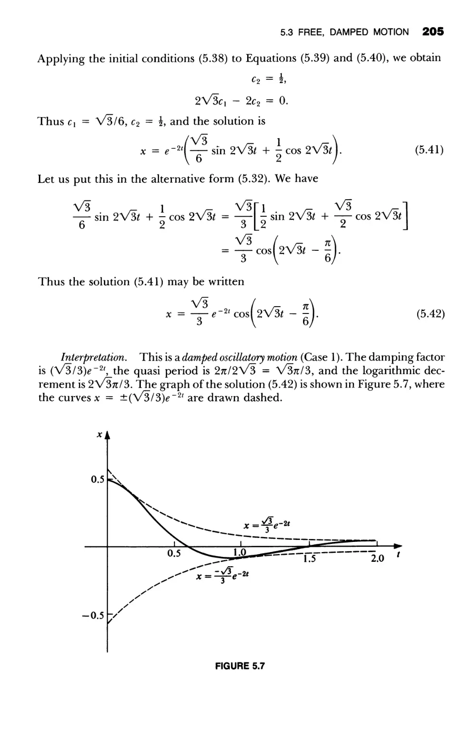
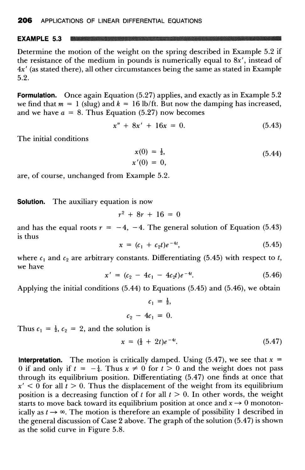
5.3 Free, Damped Motion 200
5.4 Forced Motion 212
5.5 Resonance Phenomena 219
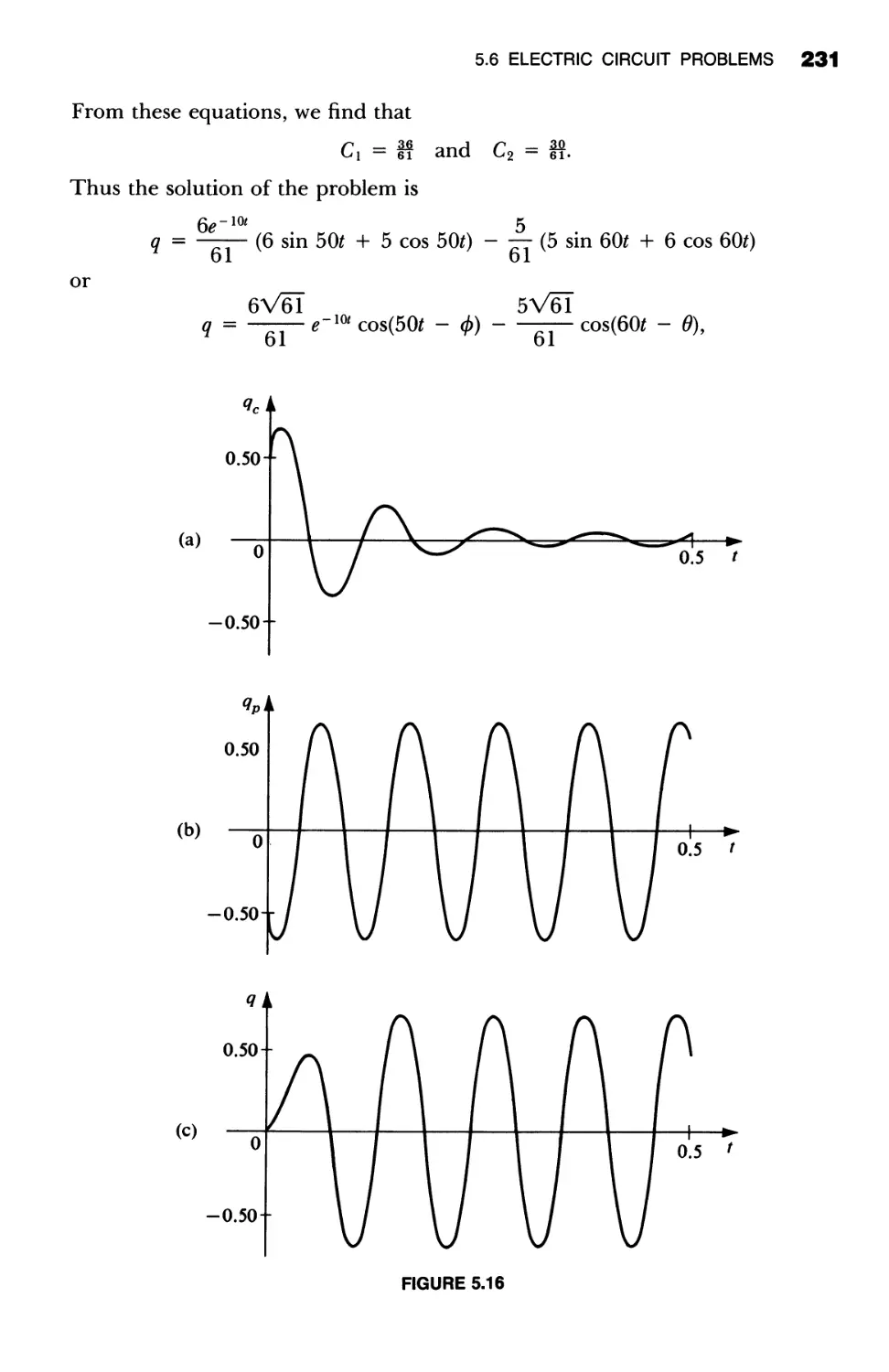
5.6 Electric Circuit Problems 224
6 Series Solutions of Linear Differential Equations 237
6.1 Power Series Solutions About an Ordinary Point 237
6.2 Solutions About Singular Points; The Method of Frobenius 250
6.3 Bessel's Equation and Bessel Functions 270
7 Systems of Linear Differential Equations 283
7.1 Differential Operators and an Operator Method 283
7.2 Applications 297
7.3 Basic Theory of Linear Systems in Normal Form: Two
Equations in Two Unknown Functions 308
7.4 Homogeneous Linear Systems with Constant Coefficients: Two
Equations in Two Unknown Functions 319
7.5 Matrices and Vectors 331
7.6 The Matrix Method for Homogeneous Linear Systems with
Constant Coefficients: Two Equations in Two Unknown
Functions 368
7.7 The Matrix Method for Homogeneous Linear Systems with
Constant Coefficients: n Equations in n Unknown Functions 378
7.8 Statements and Proofs of Basic Theorems on Homogeneous
Linear Systems 402
8 Approximate Methods of Solving First-Order Equations 417
8.1 Graphical Methods 417
8.2 Power Series Methods 428
8.3 The Method of Successive Approximations 434
8.4 Numerical Methods I: The Euler Method 438
8.5 Numerical Methods II: The Improved Euler Method 449
8.6 Numerical Methods III: The Runge-Kutta Method 455
8.7 Numerical Methods IV: The Adams-Bashforth/Adams-
Moulton (ABAM) Method 463
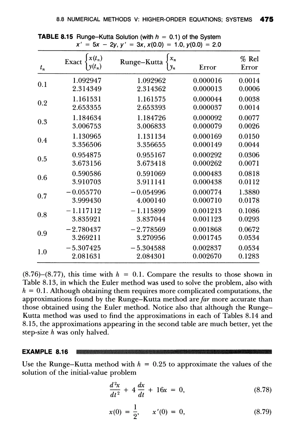
8.8 Numerical Methods V: Higher-Order Equations; Systems 469
CONTENTS xi
9 The Laplace Transform 480
9.1 Definition, Existence, and Basic Properties of the Laplace
Transform 480
9.2 The Inverse Transform and the Convolution 497
9.3 Laplace Transform Solution of Linear Differential Equations
with Constant Coefficients 510
9.4 Laplace Transform Solution of Linear Differential Equations
With Discontinuous Nonhomogeneous Terms 520
9.5 Laplace Transform Solution of Linear Systems 539
Appendix 1 547
Appendix 2 551
Appendix 3 556
Suggested Reading 558
Answers to Odd-Numbered Exercises 559
Index 605
.
Differential Equations
and Their Solutions
The subject of differential equations constitutes a large and very important branch
of modern mathematics. From the early days of the calculus the subject has been
an area of great theoretical research and practical applications, and it continues
to be so in our day. This much stated, several questions naturally arise. Just what
is a differential equation and what does it signify? Where and how do differential
equations originate and of what use are they? Confronted with a differential
equation, what does one do with it, how does one do it, and what are the results
of such activity? These questions indicate three major aspects of the subject:
theory, method, and application. The purpose of this chapter is to introduce the
reader to the basic aspects of the subject and at the same time give a brief survey
of the three aspects just mentioned. In the course of the chapter, we shall find
answers to the general questions raised above, answers that will become more
and more meaningful as we proceed with the study of differential equations in
the following chapters.
1.1 CLASSIFICATION OF DIFFERENTIAL
EQUATIONS; THEIR ORIGIN AND APPLICATION
A. Differential Equations and Their Classification
DEFINITION
An equation involving derivatives of one or more dependent variables with respect
to one or more independent variables is called a differential equation. *
* In connection with this basic definition, we do not include in the class of differential equations those
equations that are actually derivative identities. For example, we exclude such expressions as
d
dx (e ax ) = ae ax ,
d dv du
- (uv) = u - + v-
dx dx dx'
and so forth.
2 DIFFERENTIAL EQUATIONS AND THEIR SOLUTIONS
EXAMPLE 1.1
For examples of differential equations we list the following:
d 2 y ( d y ) 2
dx 2 + xy dx = 0,
d 4 x d 2 x
dt 4 + 5 dt 2 + 3x - sin t,
av av
-+-=v
as at '
(1.1)
( 1.2)
(1.3 )
a 2 u a 2 u a 2 u
iJx2 + iJ y 2 + iJz2 = o.
(1.4)
From the brief list of differential equations in Example 1.1 it is clear that
the various variables and derivatives involved in a differential equation can occur
in a variety of ways. Clearly some kind of classification must be made. To begin
with, we classify differential equations according to whether there is one or more
than one independent variable involved.
DEFINITION
A differential equation involving ordinary derivatives of one or more dependent
variables with respect to a single independent variable is called an ordinary differential
equation.
EXAMPLE 1.2
Equations (1.1) and (1.2) are ordinary differential equations. In Equation (1.1)
the variable x is the single independent variable, and y is a dependent variable.
In Equation (1.2) the independent variable is t, whereas x is dependent.
DEFINITION
A differential equation involving partial derivatives of one or more dependent variables
with respect to more than one independent variable is called a partial differential equa-
tion.
EXAMPLE 1.3
Equations (1.3) and (1.4) are partial differential equations. In Equation (1.3) the
variables sand t are independent variables and v is a dependent variable. In
Equation (1.4) there are three independent variables: x,y, and z; in this equation
u is dependent.
We further classify differential equations, both ordinary and partial, accord-
ing to the order of the highest derivative appearing in the equation. For this
purpose we give the following definition.
1.1 DIFFERENTIAL EQUATIONS; THEIR ORIGIN AND APPLICATION 3
DEFINITION
The order of the highest ordered derivative involved in a differential equation is called
the order of the differential equation.
EXAMPLE 1.4
The ordinary differential equation (1.1) is of the second order, since the highest
derivative involved is a second derivative. Equation (1.2) is an ordinary differential
equation of the fourth order. The partial differential equations (1.3) and (1.4)
are of the first and second orders, respectively.
Proceeding with our study of ordinary differential equations, we now intro-
duce the important concept of linearity applied to such equations. This concept
will enable us to classify these equations still further.
DEFINITION
A linear ordinary differential equation of order n, in the dependent variable y
and the independent variable x, is an equation that is in, or can be expressed in, the form
dny dn-1y dy
ao(x) dx n + al (x) dx n - 1 + ... + an-l (x) dx + an(x)y = b(x),
where ao is not identically zero.
Observe (1) that the dependent variable y and its various derivatives occur
to the first degree only, (2) that no products of y and/or any of its derivatives
are present, and (3) that no transcendental functions of y and/or its derivatives
occur.
EXAMPLE 1.5
The following ordinary differential equations are both linear. In each case y is
the dependent variable. Observe that y and its various derivatives occur to the
first degree only and that no products of y and/or any of its derivatives are
present.
d 2 y dy
dx 2 + 5 dx + 6y = 0,
d 4 y d3 y d y
- + x 2 - + x 3 - = xe X .
dx 4 dx 3 dx
(1.5)
( 1.6)
DEFINITION
A nonlinear ordinary differential equation is an ordinary differential equation
that is not linear.
4 DIFFERENTIAL EQUATIONS AND THEIR SOLUTIONS
EXAMPLE 1.6
Uir
-
The following ordinary differential equations are all nonlinear:
d 2 y dy
dx 2 + 5 dx + 6y2 = 0,
d 2 y ( d y ) 3
dx 2 + 5 dx + 6y = 0,
d 2 y dy
dx 2 + 5y dx + 6y = O.
(1.7)
( 1.8)
(1.9)
Equation (1.7) is nonlinear because the dependent variable y appears to the
second degree in the term 6 y 2. Equation (1.8) owes its nonlinearity to the presence
of the term 5(dy/dx)3, which involves the third power of the first derivative.
Finally, Equation (1.9) is nonlinear because of the term 5y(dy/dx), which involves
the product of the dependent variable and its first derivative
Linear ordinary differential equations are further classified according to the
nature of the coefficients of the dependent variables and their derivatives. For
exam pie, Equation (1.5) is said to be linear with constant coefficients, while Equation
(1.6) is linear with variable coefficients.
B. Origin and Application of
Differential Equations
Having classified differential equations in various ways, let us now consider briefly
where, and how, such equations actually originate. In this way we shall obtain
some indication of the great variety of subjects to which the theory and methods
of differential equations may be applied.
Differential equations occur in connection with numerous problems that are
encountered in the various branches of science and engineering. We indicate a
few such problems in the following list, which could easily be extended to fill
many pages.
1. The problem of determining the motion of a projectile, rocket, satellite, or
planet.
2. The problem of determining the charge or current in an electric circuit.
3. The problem of the conduction of heat in a rod or in a slab.
4. The problem of determining the vibrations of a wire or a membrane.
5. The study of the rate of decomposition of a radioactive substance or the rate
of growth of a population.
6. The study of the reactions of chemicals.
7. The problem of the determination of curves that have certain geometrical
properties.
The mathematical formulation of such problems give rise to differential
equations. But just how does this occur? In the situations under consideration
1.1 DIFFERENTIAL EQUATIONS; THEIR ORIGIN AND APPLICATION 5
in each of the above problems the objects involved obey certain scientific laws.
These laws involve various rates of change of one or more quantities with respect
to other quantities. Let us recall that such rates of change are expressed math-
ematically by derivatives. In the mathematical formulation of each of the above
situations, the various rates of change are thus expressed by various derivatives
and the scientific laws themselves become mathematical equations involving de-
rivatives, that is, differential equations.
In this process of mathematical formulation, certain simplifying assumptions
generally have to be made in order that the resulting differential equations be
tractable. For example, if the actual situation in a certain aspect of the problem
is of a relatively complicated nature, we are often forced to modify this by
assuming instead an approximate situation that is of a comparatively simple
nature. Indeed, certain relatively unimportant aspects of the problem must often
be entirely eliminated. The result of such changes from the actual nature of
things means that the resulting differential equation is actually that of an idealized
situation. Nonetheless, the information obtained from such an equation is of the
greatest value to the scientist.
A natural question now is the following: How does one obtain useful in-
formation from a differential equation? The answer is essentially that if it is
possible to do so, one solves the differential equation to obtain a solution; if this
is not possible, one uses the theory of differential equations to obtain information
about the solution. To understand the meaning of this answer, we must discuss
what is meant by a solution of a differential equation; this is done in the next
section.
EXERCISES
Classify each of the following differential equations as ordinary or partial dif-
ferential equations; state the order of each equation; and determine whether the
equation under consideration is linear or nonlinear.
1. ! + x 2 y = xe X ,
d 3 y d 2 y
2. dx 3 + 4 dx 2
5 : +3y
SIQ, x.
a 2 u a 2 u
3. 2 + - = o.
ax ay2
d 4 y ( d 2y ) 5
5. dx 4 + 3 dx 2 + 5y - O.
d 2 y
7. dx 2 + y sin x = o.
4. x 2 dy + y2 dx - O.
a 4 u a 2 u a 2 u
6 + - + - + u - O.
· ax 2 ay2 ax 2 ay2
d 2 y .
8. dx 2 + x SIn y = O.
d 6 x
9. 6
dt
+ ( d 4 x ) ( d3X )
dt 4 dt 3
+ x - t.
10.
( dr ) 3 =
ds d;2 + 1.
6 DIFFERENTIAL EQUATIONS AND THEIR SOLUTIONS
1.2 SOLUTIONS
A. Nature of Solutions
We now consider the concept of a solution of the nth-order ordinary differential
equation.
DEFINITION
Consider the nth-order ordinary differential equation
[ dy d ny ]
F x, y, dx ' . · · , dx n = 0,
dy dny
where F is a real function of its (n + 2) arguments x, y, d -, · · · , d -.
x x n
(1.10)
1. Let f be a real function defined for all x in a real interval I and having an nth derivative
(and hence also all lower ordered derivatives) for all x E I. The function f is called
an explicit solution of the differential equation (1.10) on I if it fulfills the following
two requirements:
F[x,f(x),f'(x), . . . ,f(n)(x)]
(A)
is defined for all x E I, and
F[x,f(x),f'(x), . . . ,f(n)(x)] = 0
(B)
for all x E I. That is, the substitution of f(x) and its various derivations for y and its
corresponding derivatives, respectively, in (1.10) reduces (1.10) to an identity on I.
2. A relation g(x,y) = 0 is called an implicit solution of(1.10) if this relation defines
at least one real function f of the variable x on an interval I such that this function is
an explicit solution of (1.10) on this interval.
3. Both explicit solutions and implicit solutions will usually be called simply solutions.
Roughly speaking, then, we may say that a solution of the differential equa-
tion (1.10) is a relation-explicit or implicit-between x and y, not containing
derivatives, which identically satisfies (1.10).
EXAMPLE 1.7
The function f defined for all real x by
f(x) = 2 sin x + 3 cos x
is an explicit solution of the differential equation
d 2 y + Y = 0
dx 2
(1.11)
( 1.12)
1.2 SOLUTIONS 7
for all real x. First note thatf is defined and has a second derivative for all real
x. Next observe that
f'(x) = 2 cosx - 3 sin x,
f"(x) = - 2 sin x - 3 cos x.
Upon substituting f"(x) for d 2 y/dx 2 and f(x) for y in the differential equation
(1.12), it reduces to the identity
( - 2 sin x - 3 cos x) + (2 sin x + 3 cos x) = 0,
which holds for all real x. Thus the function f defined by (1.11) is an explicit
solution of the differential equation (1.12) for all real x.
EXAMPLE 1.8
/ x: -: u < ,,' '/ ' ::' r, ,>, " ,::< ' : :;:' ; ,/ ; <, ;
The relation
x 2 + y2 - 25 = 0
is an implicit solution of the differential equation
x+y dy =O
dx
on the interval I defined by - 5 < x < 5 . For the relation (1.13) defines the two
real functions fl and f2 given by
fl(x) = Y 25 - x 2
( 1.13)
( 1.14)
and
f2(x) = - Y 25 - x 2 ,
respectively, for all real x E I, and both of these functions are explicit solutions
of the differential equations (1.14) on I.
Let us illustrate this for the functio n fl' Sin ce
fl (x) = Y 25 - x 2 ,
we see that
-x
j;(x) = V25 _ x 2
for all real x E I. Substitutingfl(x) for y andf (x) for dy/dx in (1.14), we obtain
the identity
x + ( V25 - X 2 )( V2; x 2 ) = 0 or x - x = 0,
which holds for all real x E I. Thus the function fl is an explicit solution of (1.14)
on the interval I.
Now consider the relation
x 2 + y2 + 25 = O.
(1.15)
8 DIFFERENTIAL EQUATIONS AND THEIR SOLUTIONS
Is this also an implicit solution of Equation (1.14)? Let us differentiate the relation
(1.15) implicitly with respect to x. We obtain
2x + 2y dy = 0 or dy =
dx dx
x
y
Substituting this into the differential equation (1.14), we obtain the formal identity
x + y( - ; ) = O.
Thus the relation (1.15) formally satisfies the differential equation (1.14). Can we
conclude from this alone that (1.15) is an implicit solution of (1.14)? The answer
to this question is "no," for we have no assurance from this that the relation
(1.15) defines any function that is an explicit solution of (1.14) on any real interval
I. All that we have shown is that (1.15) is a relation between x and y that, upon
implicit differentiation and substitution,formally reduces the differential equation
(1.14) to aformal identity. It is called aformal solution; it has the appearance of a
solution; but that is all that we know about it at this stage of our investigation.
Let us investigate a little further. Solving (1. 15) for y, we find that
y = +y - 25 - x 2 .
Since this expression yields nonreal values of y for all real values of x, we conclude
that the relation (1.15) does not define any real function on any interval. Thus
the relation (1.15) is not truly an implicit solution but merely a formal solution of
the differential equation (1.14).
In applying the methods of the following chapters we shall often obtain
relations that we can readily verify are at least formal solutions. Our main ob-
jective will be to gain familiarity with the methods themselves and we shall often
be content to refer to the relations so obtained as "solutions," although we have
no assurance that these relations are actually true implicit solutions. If a critical
exanlination of the situation is required, one must undertake to determine whether
or not these formal solutions so obtained are actually true implicit solutions which
define explicit solutions.
In order to gain further insight into the significance of differential equations
and their solutions, we now examine the simple equation of the following ex-
ample.
EXAMPLE 1.9
} , ;;; ,',' ' ;; '.. ..''; ' ';..'':, .. .. ......;..: ..;..::N.. :.... .... .. .. ....
Consider the first-order differential equation
: = 2x.
The function fo defined for all real x by fo(x) = x 2 is a solution of this equation.
So also are the functions fl, f2, and f3 defined for all real x by fl (x) = x 2 + 1,
( 1.16)
1.2 SOLUTIONS 9
f2(x) = x 2 + 2, andf3(x) = x 2 + 3, respectively. In fact, for each real number c,
the function Ie defined for all real x by
Ie(x) = x 2 + c (1.17)
is a solution of the differential equation (1.16). In other words, the formula (1.17)
defines an infinite family of functions, one for each real constant c, and every
function of this family is a solution of (1.16). We call the constant c in (1.17) an
arbitrary constant or parameter and refer to the family of functions defined by (1.17)
as a one-parameter family of solutions of the differential equation (1.16). We write
this one-parameter family of solutions as
y = x 2 + c. (1.18)
Although it is clear that every function of the family defined by (1.18) is a solution
of (1.16), we have not shown that the family of functions defined by (1.18)
includes all of the solutions of (1.16). However, we point out (without proof)
that this is indeed the case here; that is, every solution of (1.16) is actually of
the form (1.18) for some appropriate real number c.
Note. We must not conclude from the last sentence of Example 1.9 that
every first-order ordinary differential equation has a so-called one-parameter fam-
ily of solutions which contains all solutions of the differential equation, for this
is by no means the case. Indeed, some first-order differential equations have no
solution at all (see Exercise 7(a) at the end of this section), while others have a
one-parameter family of solutions plus one or more "extra" solutions which
appear to be "different" from all those of the family (see Exercise 7(b) at the end
of this section).
The differential equation of Exam pie 1.9 enables us to obtain a better un-
derstanding of the analytic significance of differential equations. Briefly stated,
the differential equation of that example defines functions, namely, its solutions.
We shall see that this is the case with many other differential equations of both
first and higher orders. Thus we may say that a differential equation is merely
an expression involving derivatives which may serve as a means of defining a
certain set of functions: its solutions. Indeed, many of the now familiar functions
originally appeared in the form of differential equations that define them.
We now consider the geometric significance of differential equations and
their solutions. We first recall that a real function F may be represented geo-
metrically by a curve y = F(x) in the xy plane and that the value of the derivative
of F at x, F'(x), may be interpreted as the slope of the curve y = F(x) at x. Thus
the general first-order differential equation
dy
dx = f(x, y),
( 1.19)
where f is a real function, may be interpreted geometrically as defining a slope
f(x, y) at every point (x, y) at which the functionf is defined. Now assume that
10 DIFFERENTIAL EQUATIONS AND THEIR SOLUTIONS
the differential equation (1.19) has a so-called one-parameter family of solutions
that can be written in the form
y = F(x, c),
( 1.20)
where c is the arbitrary constant or parameter of the family. The one-parameter
family of functions defined by (1.20) is represented geometrically by a so-called
one-parameter family of curves in the xy plane, the slopes of which are given by the
differential equation (1.19). These curves, the graphs of the solutions of the
differential equation (1.19), are called the integral curves of the differential equa-
tion (1.19).
EXAMPLE 1.10
f. fl : ;trff)&;: ? !: ?: J \ ;: ; ; / ; :>/ ,/ ::» < ; ( ; > ;, / \,f: , ';; : ',';: 1:, 1:, ;,>:' ;:>:;:/ ;:' ": , ;;"/ -,> ,; \:; "/ x y.:' ';;, ; u' u ' " ,, :?' ;, ;
Consider again the first-order differential equation
dy = 2 x
dx
of Example 1.9. This differential equation may be interpreted as defining the
slope 2x at the point with coordinates (x, y) for every real x. Now, we observed
in Example 1.9 that the differential equation (1.16) has a one-parameter family
of solutions of the form
( 1.16)
y = x 2 + c,
( 1.18)
where c is the arbitrary constant or parameter of the family. The one-parameter
family of functions defined by (1.18) is represented geometrically by a one-
parameter family of curves in the xy plane, namely, the family of parabolas with
Equation (1.18). The slope of each of these parabolas is given by the differential
equation (1.16) of the family. Thus we see that the family of parabolas (1.18)
defined by differential equation (1.16) is that family of parabolas, each of which
has slope 2x at the point (x, y) for every real x, and all of which have the y axis
as axis. These parabolas are the integral curves of the differential equation (1.16).
See Figure 1.1.
B. Methods of Solution
When we say that we shall solve a differential equation we mean that we shall
find one or more of its solutions. How is this done and what does it really mean?
The greater part of this text is concerned with various methods of solving dif-
ferential equations. The method to be employed depends upon the type of
differential equation under consideration, and we shall not enter into the details
of specific methods here.
But suppose we solve a differential equation, using one or another of the
various methods. Does this necessarily mean that we have found an explicit
solution f expressed in the so-called closed form of a finite sum of known ele-
mentary functions? That is, roughly speaking, when we have solved a differential
equation, does this necessarily mean that we have found a "formula" for the
1.2 SOLUTIONS 11
y
x
FIGURE 1.1
solution? The answer is "no." Comparatively few differential equations have
solutions so expressible; in fact, a closed-form solution is really a luxury in
differential equations. In Chapters 2 and 4 we shall consider certain types of
differential equations that do have such closed-form solutions and study the exact
methods available for finding these desirable solutions. But, as we have just noted,
such equations are actually in the minority and we must consider what it means
to "solve" equations for which exact methods are unavailable. Such equations
are solved approximately by various methods, some of which are considered in
Chapters 6 and 8. Among such methods are series methods, numerical methods,
and graphical methods. What do such approximate methods actually yield? The
answer to this depends upon the method under consideration.
Series methods yield solutions in the form of infinite series; numerical meth-
ods give approximate values of the solution functions corresponding to selected
values of the independent variables; and graphical methods produce approxi-
mately the graphs of solutions (the integral curves). These methods are not so
desirable as exact methods because of the amount of work involved in them and
because the results obtained from them are only approximate; but if exact meth-
ods are not applicable, one has no choice but to turn to approximate methods.
Modern science and engineering problems continue to give rise to differential
equations to which exact methods do not apply, and approximate methods are
becoming increasingly more important.
EXERCISES
1. Show that each of the functions defined in Column I is a solution of the
corresponding differential equation in Column lIon every interval a < x <
b of the x axis.
12 DIFFERENTIAL EQUATIONS AND THEIR SOLUTIONS
I
(a) f(x) = x + 3e- x
II
dY +y=x+l
dx
(b) f(x) = 2e 3x - 5e 4x
d 2 y dy
- - 7 - + 12y = 0
dx 2 dx
(c) f(x) = eX + 2X2 + 6x + 7
d 2 d
J - 3 -2 + 2y = 4x 2
dx 2 dx
1
( d) f(x) = 1 2
+x
d 2 d
(1 + x 2 )---1 + 4x-2 + 2y = 0
dx 2 dx
2. (a) Show thatx 3 + 3 xy 2 = 1 is an implicit solution of the differential equation
2xy(dy/dx) + x 2 + y2 = 0 on the interval 0 < x < 1.
(b) Show that 5x 2 y2 - 2x 3 y2 = 1 is an implicit solution of the differential
equation x(dy/dx) + y = x 3 y3 on the interval 0 < x < i.
3. (a) Show that every functionf defined by
f(x) = (x 3 + c)e -3x,
where c is an arbitrary constant, is a solution of the differential equation
Z + 3y = 3x 2 e -3x.
(b) Show that every functionf defined by
f(x) = 2 + ce -2x2,
where c is an arbitrary constant, is a solution of the differential equation
dy + 4xy = 8x.
dx
4. (a) Show that every functionf defined by f(x) = cle 4x + C2e-2X, where CI and
C2 are arbitrary constants, is a solution of the differential equation
d 2 y dy
- - 2 - - 8y = O.
dx 2 dx
(b) Show that every function g defined by g(x) = cle 2x + C2xe2x + C3e-2X,
where CI, C2, and C3 are arbitrary constants, is a solution of the differential
equation
d 3 y d 2 y dy
dx 3 - 2 dx 2 - 4 dx + 8y = O.
1.2 SOLUTIONS 13
5. (a) For certain values of the constant m the functionf defined by f(x) = e mx
is a solution of the differential equation
d 3 y d2y dy
- - 3 - - 4 - + 12y = O.
dx 3 dx 2 dx
Determine all such values of m.
(b) For certain values of the constant n the function g defined by g(x) = x n
is a solution of the differential equation
d 3 y d 2 y dy
x 3 - + 2X2- - 10x dx - 8y = O.
dx 3 dx 2
Determine all such values of n.
6. (a) Show that the functionf defined by f(x) = (2x 2 + 2e 3x + 3)e- 2x satisfies
the differential equation
dy + 2y = 6e X + 4xe-2x
dx
and also the condition f(O) = 5.
(b) Show that the functionfdefined byf(x) = 3e 2x - 2xe 2x - cos 2x satisfies
the differential equation
d 2 y dy
- - 4 - + 4y = - 8 sin 2x
dx 2 dx
and also the conditions that f(O) = 2 and f' (0) = 4.
7. (a) Show that the first-order differential equation
dy + Iyl + 1 = 0
dx
has no (real) solutions.
(b) Show that the first-order differential equation
( : r - 4y = 0
has a one-parameter family of solutions of the formf(x) = (x + C)2, where
c is an arbitrary constant, plus the "extra" solution g(x) = 0 that is not a
member of this family f(x) = (x + C)2 for any choice of the constant c.
14 DIFFERENTIAL EQUATIONS AND THEIR SOLUTIONS
1.3 INITIAL-VALUE PROBLEMS, BOUNDARY-
VALUE PROBLEMS, AND EXISTENCE
OF SOLUTIONS
A. Initial-Value Problems and Boundary-
Value Problems
We shall begin this section by considering the rather simple problem of the
following example.
EXAMPLE 1.11
:;: .. :""/"; """" ..": ;;:.. " .............. ..;........N ..:.... /........ .. .... .. ":..:-:.' :..:" .. ..........';:....:.. ':;:.......... .. z...... ;.... .. ;......':.. .. '" .... .. ......
Problem. Find a solution f of the differential equation
dy = 2 x
dx
such that at x = 1 this solutionf has the value 4.
(1.21 )
Explanation. First let us be certain that we thoroughly understand this problem.
We seek a real function f which fulfills the two following requirements:
1. The function f must satisfy the differential equation (1.21). That is, the func-
tion f must be such that f' (x) = 2x for all real x in a real interval I.
2. The functionf must have the value 4 at x = 1. That is, the functionf must
be such thatf(l) = 4.
Notation. The stated problem may be expressed in the following somewhat
abbreviated notation:
dy = 2 x
dx '
y(l) = 4.
In this notation we may regard y as representing the desired solution. Then the
differential equation itself obviously represents requirement 1, and the statement
y( 1) = 4 stands for requirement 2. More specifically, the notation y( 1) = 4 states
that the desired solution y must have the value 4 at x = 1; that is, y = 4 at
x = 1.
Solution. We observed in Example 1.9 that the differential equation (1.21) has
a one-parameter family of solutions which we write as
y = x 2 + c, (1.22)
where c is an arbitrary constant, and that each of these solutions satisfies re-
quirement 1. Let us now attempt to determine the constant c so that (1.22) satisfies
requirement 2, that is, y = 4 at x = 1. Substituting x = 1, Y = 4 into (1.22), we
1.3 INITIAL- AND BOUNDARY-VALUE PROBLEMS, EXISTENCE OF SOLUTIONS 15
obtain 4 = 1 + c, and hence c = 3. Now substituting the value c = 3 thus
determined back into (1.22), we obtain
y = x 2 + 3,
which is indeed a solution of the differential equation (1.21), which has the value
4 at x = 1. In other words, the function f defined by
f(x) = x 2 + 3,
satisfies both of the requirements set forth in the problem.
Comment on Requirement 2 and Its Notation. In a problem of this type, re-
quirement 2 is regarded as a supPlementary condition that the solution of the
differential equation must also satisfy. The abbreviated notation y(l) = 4, which
we used to express this condition, is in some way undesirable, but it has the
advantages of being both customary and convenient.
In the application of both first- and higher-order differential equations the
problems most frequently encountered are similar to the above introductory
problem in that they involve both a differential equation and one or more sup-
plementary conditions which the solution of the given differential equation must
satisfy. If all of the associated supplementary conditions relate to one x value, the
problem is called an initial-value problem (or one-point boundary-value problem).
If the conditions relate to two different x values, the problem is called a two-point
boundary-value problem (or simply a boundary-value problem). We shall illustrate
these concepts with examples and then consider one such type of problem in
detail. Concerning notation, we generally employ abbreviated notations for the
supplementary conditions that are similar to the abbreviated notation introduced
in Example 1.11.
EXAMPLE 1.12
:'.:,,>: 0 't:: \ :::' '; ;,,/(;; :' :',:,! :<{; ' >': :' 'n:,' > >': : ' /' / " ' /' , ,<,' , ''x', "
d 2 y 0,
dx 2 + Y -
y(l) 3,
y'(I) - -4.
This problem consists in finding a solution of the differential equation
d 2 y
+ Y = 0 ,
dx 2
which assumes the value 3 at x = 1 and whose first derivative assumes the value
- 4 at x = 1. Both of these conditions relate to one x value, namely, x = 1. Thus
this is an initial-value problem. We shall see later that this problem has a unique
solution.
16 DIFFERENTIAL EQUATIONS AND THEIR SOLUTIONS
EXAMPLE 1.13
d 2 y 0,
dx 2 + Y -
y(O) - 1,
y( ; ) 5.
In this problem we again seek a solution of the same differential equation, but
this time the solution must assume the value 1 at x = 0 and the value 5 at x =
n/2. That is, the conditions relate to the two different x values, 0 and n/2. This
is a (two-point) boundary-value problem. This problem also has a unique solu-
tion; but the boundary-value problem
d 2 y
dx 2 + Y = 0,
y(O) = 1,
y(n) = 5,
has no solution at all! This simple fact may lead one to the correct conclusion
that boundary-value problems are not to be taken lightly!
We now turn to a more detailed consideration of the initial-value problem
for a first-order differential equation.
DEFINITION
Consider the first-order differential equation
dy
dx = f(x, y),
( 1.23)
where f is a continuous function of x and y in some domain* D of the xy plane; and let
(xo, Yo) be a point of D. The initial-value problem associated with (1.23) is to find a
solution 4J of the differential equation (1.23), defined on some real interval containing Xo,
and satisfying the initial condition
4J(xo) = Yo.
In the customary abbreviated notation, this initial-value problem may be written
dy
dx = f(x, y),
y(xo) = Yo.
To solve this problem, we must find a function 4J that not only satisfies the
differential equation (1.23) but that also satisfies the initial condition that it has
* A domain is an open, connected set. For those unfamiliar with such concepts, D may be regarded
as the interior of some simple closed curve in the plane.
1.3 INITIAL- AND BOUNDARY-VALUE PROBLEMS, EXISTENCE OF SOLUTIONS 17
the value Yo when x has value Xo. The geometric interpretation of the initial
condition, and hence of the entire initial-value problem, is easily understood.
The graph of the desired solution 4J must pass through the point with coordinates
(xo, Yo). That is, interpreted geometrically, the initial-value problem is to find an
integral curve of the differential equation (1.23) that passes through the point
(xo, Yo).
The method of actually finding the desired solution 4J depends upon the
nature of the differential equation of the problem, that is, upon the form of
f(x,y). Certain special types of differential equations have a one-parameter family
of solutions whose equation may be found exactly by following definite proce-
dures (see Chapter 2). If the differential equation of the problem is of some such
special type, one first obtains the equation of its one-parameter family of solutions
and then applies the initial condition to this equation in an attempt to obtain a
"particular" solution 4J that satisfies the entire initial-value problem. We shall
explain this situation more precisely in the next paragraph. Before doing so,
however, we point out that in general one cannot find the equation of a one-
parameter family of solutions of the differential equation; approximate methods
must then be used (see Chapter 8).
Now suppose one can determine the equation
g(x, y, c) = 0
( 1.24)
of a one-parameter family of solutions of the differential equation of the problem.
Then, since the initial condition requires that y = Yo at x = Xo, we let x = Xo and
y = Yo in (1.24) and thereby obtain
g(xo, Yo, c) = O.
Solving this for c, in general we obtain a particular value of c which we denote
here by co. We now replace the arbitrary constant c by the particular constant Co
in (1.24), thus obtaining the particular solution
g(x, y, co) = O.
The particular explicit solution satisfying the two conditions (differential equation
and initial condition) of the problem is then determined from this, if possible.
We have already solved one initial-value problem in Example 1.11. We now
give another example in order to illustrate the concepts and procedures more
thoroughly.
EXAMPLE 1.14
Solve the initial-value problem
dy = x
dx Y
(1.25)
y(3) = 4,
( 1.26)
18 DIFFERENTIAL EQUATIONS AND THEIR SOLUTIONS
given that the differential equation (1.25) has a one-parameter family of solutions
which may be written in the form
x 2 + y2 = c 2 . (1.27)
The condition (1.26) means that we seek the solution of (1.25) such thaty = 4
atx = 3. Thus the pair of values (3,4) must satisfy the relation (1.27). Substituting
x = 3 and y = 4 into (1.27), we find
9 + 16 = c 2 or c 2 = 25.
Now substituting this value of c 2 into (1.27), we have
x 2 + y2 = 25.
Solving this for y, we obtain
y = +\1 25 - x 2 .
Obviously the positive sign must be chosen to give y the value + 4 at x = 3. Thus
the function f defined by
f(x) = \1 25 - x 2 , - 5 < x < 5,
is the solution of the prob lem. In the usual abbreviated notation, we write this
solution as y = \1 25 - x 2 .
B. Existence of Solutions
In Example 1.14 we were able to find a solution of the initial-value problem
under consideration. But do all initial-value and boundary-value problems have
solutions? We have already answered this question in the negative, for we have
pointed out that the boundary-value problem
d 2 y
dx 2 + Y - 0,
y(O) 1,
y(n) - 5,
mentioned at the end of Example 1.13, has no solution! Thus arises the question
of existence of solutions: given an initial-value or boundary-value problem, does
it actually have a solution? Let us consider the question for the initial-value
problem defined on page 16. Here we can give a definite answer. Every initial-
value problem that satisfies the definition on page 16 has at least one solution.
But now another question is suggested, the question of uniqueness. Does such
a problem ever have more than one solution? Let us consider the initial-value
problem
dy = Y l/3
dx '
y(O) = O.
1.3 INITIAL- AND BOUNDARY-VALUE PROBLEMS, EXISTENCE OF SOLUTIONS 19
One may verify that the functions fl and f2 defined, respectively, by
fl(x) = 0 for all real x;
and
f2(x) = (iX)3/2, x > 0;
f2(x) = 0, X < 0;
are both solutions of this initial-value problem! In fact, this problem has infinitely
many solutions! The answer to the uniqueness question is clear: the initial-value
problem, as stated, need not have a unique solution. In order to ensure unique-
ness, some additional requirement must certainly be imposed. We shall see what
this is in Theorem 1.1, which we shall now state.
THEOREM 1.1 BASIC EXISTENCE AND UNIQUENESS THEOREM
Hypothesis. Consider the differential equation
dy
dx = f(x, y),
( 1.28)
where
1. The function f is a continuous function of x and y in some domain D of the xy
Plane, and
2. The partial derivative iJf/ iJy is also a continuous function of x and y in D;
and let (xo, Yo) be a point in D.
Conclusion. There exists a unique solution 4J of the differential equation (1.28), defined
on some interval Ix - xol < h, where h is sufficiently small, that satisfies the condition
4J(xo) = Yo.
( 1.29)
Explanatory Remarks. This basic theorem is the first theorem from the theory
of differential equations which we have encountered. We shall therefore attempt
to explain its meaning in detail.
1. It is an existence and uniqueness theorem. This means that it is a theorem which
tells us that under certain conditions (stated in the hypothesis) something
exists (the solution described in the conclusion) and is unique (there is only one
such solution). It gives no hint whatsoever concerning how to find this solution
but merely tells us that the problem has a solution.
2. The hypothesis tells us what conditions are required of the quantities involved.
It deals with two objects: the differential equation (1.28) and the point (xo,
Yo). As far as the differential equation (1.28) is concerned, the hypothesis
requires that both the function f and the function iJf/ iJy (obtained by differ-
entiatingf(x, y) partially with respect to y) must be continuous in some domain
D of the xy plane. As far as the point (xo, Yo) is concerned, it must be a point
20 DIFFERENTIAL EQUATIONS AND THEIR SOLUTIONS
in this same domain D, where f and iJf/ iJy are so well behaved (that is, con-
tinuous).
3. The conclusion tells us of what we can be assured when the stated hypothesis
is satisfied. It tells us that we are assured that there exists one and only one
solution 4J of the differential equation, which is defined on some interval
Ix - xol < h centered about Xo and which assumes the value Yo when x takes
on the value Xo. That is, it tells us that, under the given hypothesis onf(x, y),
the initial-value problem
dy
dx = f(x, y),
y(xo) = Yo,
has a unique solution that is valid in some interval about the initial point Xo.
4. The proof of this theorem is omitted. It is proved under somewhat less re-
strictive hypotheses in Chapter 10 of the author's Differential Equations.
5. The value of an existence theorem may be worth a bit of attention. What good
is it, one might ask, if it does not tell us how to obtain the solution? The
answer to this question is quite simple: An existence theorem will assure us
that there is a solution to look for! It would be rather pointless to spend time,
energy, and even money in trying to find a solution when there was actually
no solution to be found! As for the value of the uniqueness, it would be
equally pointless to waste time and energy finding one particular solution
only to learn later that there were others and that the one found was not the
one wanted!
We have included this rather lengthy discussion in the hope that the student,
who has probably never before encountered a theorem of this type, will obtain
a clearer idea of what this important theorem really means. We further hope
that this discussion will help him to analyze theorems which he will encounter
in the future, both in this book and elsewhere. We now consider two simple
examples which illustrate Theorem 1.1.
EXAMPLE 1.15
Consider the initial-value problem
dy = x 2 + y2,
dx
y(l) = 3.
Let us apply Theorem 1.1. We first check the hypothesis. Here f(x, y) = x 2 + y2
and iJf(x, y)/iJy = 2y. Both of the functionsf and iJf/iJy are continuous in every
domain D of the xy plane. The initial condition y( 1) = 3 means that Xo = 1 and
Yo = 3, and the point (1, 3) certainly lies in some such domain D. Thus all
hypotheses are satisfied and the conclusion holds. That is, there is a unique
1.3 INITIAL- AND BOUNDARY-VALUE PROBLEMS, EXISTENCE OF SOLUTIONS 21
solution 4J of the differential equation dy/dx = x 2 + y2, defined on some interval
Ix - 11 < h about Xo = 1, which satisfies that initial condition, that is, which is
such that 4J(1) = 3.
EXAMPLE 1.16
:<: : tC < t:;: >::: ;;:.,:< :' f/ft; ); t- " {> :, /. ,: (=?-,;;;;,);: : Y.jt, <; :, ,'1': ", , ' -',' ,' , ', , ,',' , ,,' " "
Consider the two problems:
dy y
1. dx = '
dy Y
2. dx = '
y(l) = 2,
y(O) = 2.
Here
f(x, y) = /2
X
d af(x, y) -
an - 1/2 .
ay x
These functions are both continuous except for x = 0 (that is, along the y
axis). In problem 1, Xo = 1, Yo = 2. The square of side 1 centered about (1, 2)
does not contain the y axis, and so both f and af/ ay satisfy the required hypotheses
in this square. Its interior may thus be taken to be the domain D of Theorem
1.1; and (1, 2) certainly lies within it. Thus the conclusion of Theorem 1.1 applies
to problem 1 and we know the problem has a unique solution defined in some
sufficiently small interval about Xo = 1.
Now let us turn to problem 2. Here Xo = 0, Yo = 2. At this point neither f
nor af/ ay are continuous. In other words, the point (0, 2) cannot be included in
a domain D where the required hypotheses are satisfied. Thus we can not conclude
from Theorem 1.1 that problem 2 has a solution. We are not saying that it does
not have one. Theorem 1.1 simply gives no information one way or the other.
EXERCISES
1. Show that
y = 4e 2x + 2e- 3x
is a solution of the initial-value problem
d 2 y dy 0,
-+--6y
dx 2 dx
y(O) 6,
y' (0) 2.
Is Y = 2e 2x + 4e- 3x also a solution of this problem? Explain why or why not.
22 DIFFERENTIAL EQUATIONS AND THEIR SOLUTIONS
2. Given that every solution of
dy + Y = 2xe- x
dx
may be written in the form y = (x 2 + c)e-X, for some choice of the arbitrary
constant c, solve the following initial-value problems:
(a) dy + Y = 2xe-X,
dx
y(O) = 2.
(b) : + y = 2xe- x ,
y( - 1) = e + 3.
3. Given that every solution of
d 2 y _ dy _ 12y = 0
dx 2 dx
may be written in the form
y = Cte4x + C2 e - 3 X,
for some choice of the arbitrary constants CI and C2, solve the following initial-
value problems:
(a) d 2 y _ dy _ 12y = 0,
dx 2 dx
(b) d 2 y _ dy - 12y = 0,
dx 2 dx
y(O) = 5,
y'(O) = 6.
4. Every solution of the differential equation
d 2 y
dx 2 + Y = 0
y(O) = -2,
y'(O) = 6.
may be written in the form y = CI sin x + C2 cos x, for some choice of the
arbitrary constants CI and C2' Using this information, show that boundary
problems (a) and (b) possess solutions but that (c) does not.
d7 d7
(a) dx 2 + y = 0, (b) dx 2 + Y = 0,
y(O) = 0, y(O) - 1,
y(n/2) = 1. y' (n/2) - -1.
(c) d 2 y
dx 2 + Y = 0,
y(O) = 0,
y(n) = 1.
1.3 INITIAL- AND BOUNDARY-VALUE PROBLEMS, EXISTENCE OF SOLUTIONS 23
5. Given that every solution of
d 3 y d 2 y dy
x 3 - - 3x 2 - + 6x - - 6y = 0
dx 3 dx 2 dx
may be written in the form y = CIX + C2X2 + C3X3 for some choice of the
arbitrary constants CI, C2, and C3, solve the initial-value problem consisting of
the above differential equation plus the three conditions
y(2) = 0,
y'(2) = 2,
y"(2) = 6.
6. Apply Theorem 1.1 to show that each of the following initial-value problems
has a unique solution defined on some sufficiently small interval Ix - 11 < h
about Xo = 1:
(a)
dy = x2 sin Y
dx '
(b)
dy =
dx
y2
X - 2'
y(l) = -2.
7. Consider the initial-value problem
= P(X)y2 + Q(x)y,
y(l) = O.
y(2) = 5,
where P(x) and Q(x) are both third-degree polynomials in x. Has this problem
a unique solution on some interval Ix - 21 < h about Xo = 2? Explain why or
why not.
8. In this section we stated that the initial-value problem
dy = Y I/3
dx '
y(O) = 0,
has infinitely many solutions.
(a) Verify that this is indeed the case by showing that
{ O, x < C,
Y = [i(x - C)]3/2, x > c,
is a solution of the stated problem for every real number C > O.
(b) Carefully graph the solution for which C = O. Then, using this particular
graph, also graph the solutions for which C = 1, C = 2, and C = 3.
.
First-Order Equations for
Which Exact Solutions
Are Obtainable
In this chapter we consider certain basic types of first-order equations for which
exact solutions may be obtained by definite procedures. The purpose of this
chapter is to gain the ability to recognize these various types and to apply the
corresponding methods of solutions. Of the types considered here, the so-called
exact equations considered in Section 2.1 are in a sense the most basic, while the
separable equations of Section 2.2 are in a sense the "easiest." The most impor-
tant, from the point of view of applications, are the separable equations of Section
2.2 and the linear equations of Section 2.3. The remaining types are of various
very special forms, and the corresponding methods of solution involve various
devices. In short, we might describe this chapter as a collection of special "meth-
ods," "devices," "tricks," or "recipes," in descending order of kindness!
2.1 EXACT DIFFERENTIAL EQUATIONS AND
INTEGRATING FACTORS
A. Standard Forms of First-Order
Differential Equations
The first-order differential equations to be studied in this chapter may be ex-
pressed in either the derivative form
: = f(x, y)
(2.1)
or the differential form
M(x, y) dx + N(x, y) dy = O.
(2.2)
An equation in one of these forms may readily be written in the other form.
2.1 EXACT DIFFERENTIAL EQUATIONS AND INTEGRATING FACTORS 25
For example, the equation
dy = X 2 + y2
dx x - Y
is of the form (2.1). It may be written
(x 2 + y2) dx + (y - x) dy = 0,
which is of the form (2.2). The equation
(sin x + y) dx + (x + 3y) dy = 0,
which is of the form (2.2), may be written in the form (2.1) as
dy _ sin x + y
dx x + 3y .
In the form (2.1) it is clear from the notation itself that y is regarded as the
dependent variable and x as the independent one; but in the form (2.2) we may
actually regard either variable as the dependent one and the other as the in-
dependent. However, in this text, in all differential equations of the form (2.2)
in x and y, we shall regard y as dependent and x as independent, unless the
contrary is specifically stated.
B. Exact Differential Equations
DEFINITION
Let F be a function of two real variables such that F has continuous first partial
derivatives in a domain D. The total differential dF of the function F is defined by the
formula
dF(x, Y ) = iJF(x, Y) dx + iJF(x, Y) d y
ax ay
for all (x, y) E D.
EXAMPLE 2.1
Let F be the function of two real variables defined by
F(x, y) = xy2 + 2x 3 y
for all real (x, y). Then
aF(x,y) 2 6 2
= Y + x y,
ax
aF(x, Y ) 2 2 3
= xy + x,
ay
and the total differential dF is defined by
dF(x, y) = (y2 + 6x 2 y) dx + (2xy + 2x 3 ) dy
for all real (x, y).
26 FIRST-ORDER EQUATIONS FOR WHICH EXACT SOLUTIONS ARE OBTAINABLE
DEFINITION
The expression
M(x, y) dx + N(x, y) dy
(2.3)
is called an exact differential in a domain D if there exists a function F of two real
variables such that this expression equals the total differential dF (x, y) for all (x, y) ED.
That is, expression (2.3) is an exact differential in D if there exists a function F such that
aF y) = M(x, y) and aF y) = N(x, y)
for all (x, y) E D.
If M (x, y) dx + N (x, y) dy is an exact differential, then the differential equation
M(x, y) dx + N(x, y) dy = 0
is called an exact differential equation.
EXAMPLE 2.2
:.:/> y/ :.:y u r ,;, <':f / ) ,', ': >: ;: ;,;/;i ,: , ,;;' : ;':', ><: <, >:: ''', ;", ",' ,"': ;' : ,,;- ' '; ': , , ',' ,'u(; , y > (' ;, ," ',z';' /; :' ;: ,U,,» , :;', ',' '," ;' ;',
The differential equation
y2 dx + 2 xy dy = 0
(2.4)
is an exact differential equation, since the expression y2 dx + 2xy dy is an exact
differential. Indeed, it is the total differential of the function F defined for all
(x, y) by F(x, y) = xy2, since the coefficient of dx is iJF(x, y)/(iJx) = y2 and that of
dy is iJF(x,y)/(iJy) = 2xy. On the other hand, the more simple appearing equation
y dx + 2x dy = 0, (2.5)
obtained from (2.4) by dividing through by y, is not exact.
In Example 2.2 we stated without hesitation that the differential equation
(2.4) is exact but that the differential equation (2.5) is not. In the case of Equation
(2.4), we verified our assertion by actually exhibiting the function F of which the
expression y2 dx + 2xy dy is the total differential. But in the case of Equation
(2.5), we did not back up our statement by showing that there is no function F
such that y dx + 2x dy is its total differential. It is clear that we need a simple
test to determine whether or not a given, differential equation is exact. This is
given by the following theorem.
THEOREM 2.1
Consider the differential equation
M(x, y) dx + N(x, y) dy = 0,
(2.6)
where M and N have continuous first partial derivatives at all points (x, y) in a rectangular
domain D.
2.1 EXACT DIFFERENTIAL EQUATIONS AND INTEGRATING FACTORS 27
1. If the differential equation (2.6) is exact in D, then
aM (x, y) aN (x, y)
ay ax
(2.7)
for all (x, y) E D.
2. Conversely, if
aM(x,y) _ aN(x,y)
ay ax
for all (x, y) E D, then the differential equation (2.6) is exact in D.
Proof. Part 1. If the differential equation (2.6) is exact in D, then M dx + N dy
is an exact differential in D. By definition of an exact differential, there exists a
function F such that
aF : y) = M(x, y) and aF y) = N(x, y)
for all (x, y) E D. Then
a 2 F(x, y) = aM (x, y) and a 2 F(x, y) = aN(x, y)
ay ax ay ax ay ax
for all (x, y) E D. But, using the continuity of the first partial derivatives of M
and N, we have
a 2 F(x, y) a 2 F(x, y)
ay ax ax ay
and therefore
aM(x,y) _ aN(x,y)
ay ax
for all (x, y) E D.
Part 2. This being the converse of Part 1, we start with the hypothesis that
aM (x, y) aN (x, y)
ay ax
for all (x, y) E D, and set out to show that M dx + N dy = 0 is exact in D. This
means that we must prove that there exists a function F such that
aF : y) = M(x, y)
(2.8)
and
aF , y) = N(x, y) (2.9)
for all (x, y) E D. We can certainly find some F(x, y) satisfying either (2.8) or (2.9),
but what about both? Let us assume that F satisfies (2.8) and proceed. Then
F(x, y) = f M(x, y) ax + ljJ(y),
(2.10)
28 FIRST-ORDER EQUATIONS FOR WHICH EXACT SOLUTIONS ARE OBTAINABLE
where J M(x, y) ax indicates a partial integration with respect to x, holding y
constant, and 4J is an arbitrary function of y only. This 4J(y) is needed in (2.10)
so that F(x, y) given by (2.10) will represent all solutions of (2.8). It corresponds
to a constant of integration in the "one-variable" case. Differentiating (2.10)
partially with respect to y, we obtain
aF(x, y) _ i. J M( ) d4J(y)
- x, y ax + d .
y
Now if (2.9) is to be satisfied, we must have
a J d4J(y)
N (x, y) = - M (x, y) ax + d
ay y
(2.11 )
and hence
d4J(y) a J
d = N(x, y) - - M(x, y) ax.
y ay
Since 4J is a function of y only, the derivative d4J/dy must also be independent of
x. That is, in order for (2.11) to hold,
N(x, y) - i. J M(x, y) ax
ay
(2.12)
must be independent of x.
We shall show that
i. [ N(X, y) - i. J M(x, y) a x ] = o.
ax ay
We at once have
a [ a J ] aN (x, y) a 2 J
- N(x, y) - - M(x, y) ax = - M(x, y) ax.
If (2.8) and (2.9) are to be satisfied, then using the hypothesis (2.7), we must
have
a 2 J M (x, ) iJx = iJ2F(x, y) = iJ2F(x, y) = iJ2 J M (x, ) ax.
ax ay y ax ay ay ax ay ax y
Thus we obtain
i. [ N(X, y) - i. J M(x, y) a x ] = aN (x, y) - a 2 J M(x, y) ax
and hence
a [N( ) a JM( ) ] _ aN(x,y) aM(x,y)
- x, y - - x, y ax - - .
But by hypothesis (2.7),
aM(x,y) _ aN(x,y)
ay ax
2.1 EXACT DIFFERENTIAL EQUATIONS AND INTEGRATING FACTORS 29
for all (x, y) E D. Thus
[ N(X' y) - J M(x, y) ax ] = 0
ax ay
for all (x, y) E D, and so (2.12) is independent of x. Thus we may write
cjJ(y) = J [ N(x, y) - J aM ;, y) ax ] dy.
Substituting this into Equation (2.10), we have
F(x, y) = J M(x, y) ax + J [ N(x, y) - J aM , y) ax ] dy. (2.13)
This F(x, y) thus satisfies both (2.8) and (2.9) for all (x, y) E D, and so M dx +
N dy = 0 is exact in D. Q.E.D.
Students well versed in the terminology of higher mathematics will recognize
that Theorem 2.1 may be stated in the following words: A necessary and sufficient
condition that Equation (2.6) be exact in D is that condition (2.7) hold for all (x, y)
E D. For students not so well versed, let us emphasize that condition (2.7),
aM(x,y) _ aN(x,y)
ay ax
is the criterion for exactness. If (2.7) holds, then (2.6) is exact; if (2.7) does not
hold, then (2.6) is not exact.
EXAMPLE 2.3
We apply the exactness criterion (2.7) to Equations (2.4) and (2.5), introduced
in Example 2.2. For the equation
y2 dx + 2xy dy = 0 (2.4)
we have
M(x, y) = y2, N(x, y) = 2xy,
aM(x, y) _ 2 _ aN(x, y)
ay -:y- ax
for all (x, y). Thus Equation (2.4) is exact in every rectangular domain D. On the
other hand, for the equation
Y dx + 2x dy = 0,
(2.5)
we have
M(x, y) = y, N(x, y) = 2x,
aM (x, y) = 1 =F 2 = aN(x, y)
ay ax
for all (x, y). Thus Equation (2.5) is not exact in any rectangular domain D.
30 FIRST-ORDER EQUATIONS FOR WHICH EXACT SOLUTIONS ARE OBTAINABLE
EXAMPLE 2.4
rr
Consider the differential equation
(2x sin y + y3 e x) dx + (x 2 cos y + 3y 2 e x ) dy = O.
Here
M(x, y) = 2x sin y + y 3 ex,
N(x, y) = x 2 cos y + 3y 2 eX,
aM (x, y) 2 3 2 aN (x, y)
= x cos y + Y eX =
ay ax
in every rectangular domain D. Thus this differential equation is exact in every
such domain.
These examples illustrate the use of the test given by (2.7) for determining
whether or not an equation of the form M(x, y) dx + N(x, y) dy = 0 is exact. It
should be observed that the equation must be in the standard form M(x, y) dx +
N(x, y) dy = 0 in order to use the exactness test (2.7). Note this carefully: an
equation may be encountered in the nonstandard form M(x, y) dx = N(x, y) dy,
and in this form the test (2.7) does not apply.
C. The Solution of Exact Differential Equations
Now that we have a test with which to determine exactness, let us proceed to
solve exact differential equations. If the equation M(x, y) dx + N(x, y) dy = 0 is
exact in a rectangular domain D, then there exists a function F such that
aF (x, y) M ( ) d aF (x, y) N( ) £' II ( ) D
ax = x, y an ay = x, y lor a x, y E ·
Then the equation may be written
aF y) dx + aF y) dy = 0 or simply dF(x, y) = O.
The relation F(x, y) = c is obviously a solution of this, where c is an arbitrary
constant. We summarize this observation in the following theorem.
THEOREM 2.2
Suppose the differential equation M (x, y) dx + N (x, y) dy = 0 satisfies the differentiability
requirements of Theorem 2.1 and is exact in a rectangular domain D. Then a one-parameter
family of solutions of this differential equation is given by F(x, y) = c, where F is afunction
such that
aF y) = M(x, y) and aF y) = N(x, y) for all (x, y) E D.
and c is an arbitrary constant.
2.1 EXACT DIFFERENTIAL EQUATIONS AND INTEGRATING FACTORS 31
Referring to Theorem 2.1, we observe that F(x, y) is given by formula (2.13).
However, in solving exact differential equations it is neither necessary nor de-
sirable to use this formula. Instead one obtains F(x, y) either by proceeding as
in the proof of Theorem 2.1, Part 2, or by the so-called "method of grouping,"
which will be eXplained in the following examples.
EXAMPLE 2.5
Solve the equation
(3X2 + 4xy) dx + (2x 2 + 2y) dy = O.
Our first duty is to determine whether or not the equation is exact. Here
M(x, y) = 3x 2 + 4xy,
aM (x, y) = 4x
ay ,
N(x, y) = 2X2 + 2y,
aN(x, y) = 4x
ax '
for all real (x, y), and so the equation is exact in every rectangular domain D.
Thus we must find F such that
aF(x, y) aF(x, y)
ax = M(x, y) = 3x 2 + 4xy and ay = N(x, y) = 2X2 + 2y.
From the first of these,
F(x, y) = J M(x, y) ax + ljJ(y) = J (3X2 + 4xy) ax + ljJ(y)
= x 3 + 2x2y + 4>(y).
Then
aF(x, y) _ 2 2 d4>(y)
iJy - x+ dy'
But we must have
aF(x, y)
iJy = N(x, y) = 2X2 + 2y.
Thus
d4>(y)
2X2 + 2y = 2X2 +
dy
or
d4>(y) - 2
dy - y.
Thus 4>(y) = y2 + Co, where Co is an arbitrary constant, and so
F(x, y) = x 3 + 2x2y + y2 + Co.
Hence a one-parameter family of solution is F(x, y) = c., or
x 3 + 2 x 2 y + y2 + Co = C 1 .
32 FIRST-ORDER EQUATIONS FOR WHICH EXACT SOLUTIONS ARE OBTAINABLE
Combining the constants Co and c} we may write this solution as
x 3 + 2x2y + y2 = c,
where c = c} - Co is an arbitrary constant. The student will observe that there
is no loss in generality by taking Co = 0 and writing 4>(y) = y2. We now consider
an alternative procedure.
Method of Grouping. We shall now solve the differential equation of this exam pie
by grouping the terms in such a way that its left member appears as the sum of
certain exact differentials. We write the differential equation
(3x 2 + 4xy) dx + (2x 2 + 2y) dy = 0
in the form
3x 2 dx + (4xy dx + 2X2 dy) + 2y dy = O.
We now recognize this as
d(x 3 ) + d(2x 2 y) + d(y2) = d(c),
where c is an arbitrary constant, or
d(x 3 + 2x2y + y2) = d(c).
From this we have at once
x 3 + 2x2y + y2 = c.
Clearly this procedure is much quicker, but it requires a good "working knowl-
edge" of differentials and a certain amount of ingenuity to determine just how
the terms should be grouped. The standard method may require more "work"
and take longer, but it is perfectly straightforward. It is recommended for those
who like to follow a pattern and for those who have a tendency to jump at
conclusions.
Just to make certain that we have both procedures well in hand, we shall
consider an initial-value problem involving an exact differential equation.
EXAMPLE 2.6
f.J ;1 ,; : j' /' :Z/ , {4J :>, /:. //:, >:" ;",,U;,>: ,' ';z"; , /u,'"", ',/ :" ,:, ;'> , ' '((;,;: >,' ': "',':':' '>, ", ' '>"':' " " '
Solve the initial-value problem
(2x cos y + 3x 2 y) dx + (x 3 - x 2 sin y - y) dy - 0,
y(O) - 2.
We first observe that the equation is exact in every rectangular domain D, since
aM (x, y) aN(x, y)
= -2x siny + 3x 2 =
ay ax
for all real (x, y).
2.1 EXACT DIFFERENTIAL EQUATIONS AND INTEGRATING FACTORS 33
Standard Method. We must find F such that
aF(x, y)
ax = M(x, y) = 2x cos y + 3x 2 y
and
aF(x, y) 3 2 .
iJy = N(x, y) = x - x SIll Y - y.
Then
F(x, y) = J M (x, y) iJx + ljJ(y)
= J (2x cos y + 3x 2 y) iJx + ljJ(y)
= x 2 cos y + x 3 y + 4>(y),
aF(x, y) 2 . 3 d4>(y)
= - x SIn y + x + d .
ay .y
But also
aF(x, y) 3 2 .
iJy = N(x, y) = x - x SIll Y - Y
and so
d4>(y)
dy = - Y
and hence
y2
4>(y) = - 2" + Co.
Thus
y2
F(x, y) = x 2 COS y + x 3 y - 2" + Co.
Hence a one-parameter family of solutions is F(x,y) = c}, which may be expressed
as
2
x 2 COS y + x 3 y - = c.
Applying the initial condition y = 2 when x = 0, we find c = - 2. Thus the
solution of the given initial-value problem is
2
x 2 cos y + x 3 y - L = - 2.
2
Method of Grouping. We group the terms as follows:
(2x cos y dx - x 2 sin y dy) + (3x 2 y dx + x 3 dy) - y dy = O.
Thus we have
d(x 2 COS y) + d(x 3 y) - d( 2 ) = d(c);
34 FIRST-ORDER EQUATIONS FOR WHICH EXACT SOLUTIONS ARE OBTAINABLE
and so
2
X 2 CoS y + x 3 y - L = c
2
is a one-parameter family of solutions of the differential equation. Of course the
initial condition y(O) = 2 again yields the particular solution already obtained.
D. Integrating Factors
Given the differential equation
M(x, y) dx + N(x, y) dy = 0,
if
aM (x, y) _ aN (x, y)
ay ax
then the equation is exact and we can obtain a one-parameter family of solutions
by one of the procedures explained above. But if
aM (x, y) =F aN (x, y)
ay ax'
then the equation is not exact and the above procedures do not apply. What shall
we do in such a case? Perhaps we can multiply the nonexact equation by some
expression that will transform it into an essentially equivalent exact equation. If
so, we can proceed to solve the resulting exact equation by one of the above
procedures. Let us consider again the equation
y dx + 2x dy = 0,
(2.5)
which was introduced in Example 2.2. In that example we observed that this
equation is not exact. However, if we multiply Equation (2.5) by y, it is transformed
into the essentially equivalent equation
y2 dx + 2xy dy = 0,
(2.4)
which is exact (see Example 2.2). Since this resulting exact equation (2.4) is
integrable, we call y an integrating factor of Equation (2.5). In general, we have
the following definition:
DEFINITION
If the differential equation
M(x, y) dx + N(x, y) dy = 0
is not exact in a domain D but the differential equation
J1(x, y)M(x, y) dx + J1(x, y)N(x, y) dy = 0
(2.14 )
(2.15 )
is exact in D, then J1(x, y) is called an integrating factor of the differential equation
(2.14).
2.1 EXACT DIFFERENTIAL EQUATIONS AND INTEGRATING FACTORS 35
EXAMPLE 2.7
Consider the differential equation
(3y + 4Xy2) dx + (2x
This equation is of the form (2.14), where
M(x, y) - 3y + 4xy2,
aM (x, y)
ay
+ 3x 2 y) dy = O.
(2.16)
- 3 + 8xy,
N (x, y)
aN (x, y)
ax
2x + 3x 2 y,
- 2 + 6xy.
Since
aM(x, y) # aN(x, y)
ay ax
except for (x, y) such that 2xy + 1 = 0, Equation (2.16) is not exact in any
rectangular domain D.
Let p,(x, y) = x2y. Then the corresponding differential equation of the form
(2.15) is
(3x2y2 + 4x 3 y3) dx + (2x 3 y + 3x 4 y2) dy = O.
This equation is exact in every rectangular domain D, since
a[p,(x, y)M(x, y)] 6 2 12 3 2 a[p,(x, y)N(x, y)]
= xy + xy =
ay ax
for all real (x, y). Hence p,(x, y) = x2y is an integrating factor of Equation (2.16).
Multiplication of a nonexact differential equation by an integrating factor
thus transforms the nonexact equation into an exact one. We have referred to
this resulting exact equation as "essentially equivalent" to the original. This so-
called essentially equivalent exact equation has the same one-parameter family
of solutions as the nonexact original. However, the multiplication of the original
equation by the integrating factor may result in either (1) the loss of (one or
more) solutions of the original, or (2) the gain of (one or more) functions which
are solutions of the "new" equation but not of the original, or (3) both of these
phenomena. Hence, whenever we transform a nonexact equation into an exact
one by multiplication by an integrating factor, we should check carefully to
determine whether any solutions may have been lost or gained. We shall illustrate
an important special case of these phenomena when we consider separable equa-
tions in Section 2.2. See also Exercise 22 at the end of this section.
The question now arises: How is an integrating factor found? We shall not
attempt to answer this question at this time. Instead we shall proceed to a study
of the important class of separable equations in Section 2.2 and linear equations
in Section 2.3. We shall see that separable equations always possess integrating
factors that are perfectly obvious, while linear equations always have integrating
factors of a certain special form. We shall return to the question raised above in
Section 2.4. Our object here has been merely to introduce the concept of an
integrating factor.
36 FIRST-ORDER EQUATIONS FOR WHICH EXACT SOLUTIONS ARE OBTAINABLE
EXERCISES
In Exercises 1-10 determine whether or not each of the given equations is exact;
solve those that are exact.
1. (3x + 2y) dx + (2x + y) dy = O.
2. (y2 + 3) dx + (2xy - 4) dy = O.
3. (2xy + 1) dx + (x 2 + 4y) dy = O.
4. (3x 2 y + 2) dx - (x 3 + y) dy = O.
5. (6xy + 2 y 2 - 5) dx + (3x 2 + 4xy - 6) dy = O.
6. (0 2 + l)cos r dr + 20 sin r dO = O.
7. (y sec 2 x + sec x tan x) dx + (tan x + 2y) dy = O.
8. ( ;2 + x) dx + ( : + Y) dy = O.
( 2S-1 ) ( S-S2 )
9. t ds + t 2 dt = O.
2 3/2 + 1
10. Y 1/2 dx + (3X 1 / 2 yl/2 - 1) dy = O.
x
Solve the initial-value problems in Exercises 11-16.
11. (2xy - 3) dx + (x 2 + 4y) dy = 0,
y(l) = 2.
12. (3x2y2 - y3 + 2x) dx + (2x 3 y - 3xy2 + 1) dy = 0, y( - 2) = 1.
13. (2y sin x cos x + y2 sin x) dx + (sin 2 x - 2y cos x) dy = 0, y(O) = 3.
14. (ye X + 2e x + y2) dx + (eX + 2xy) dy = 0, y(O) = 6.
15. ( 3 Y ) dx + ( y2x 22X ) dy = 0, y(-I) = 2.
1 + 8 xy 2/3 2X 4 / 3 y2/3 - X 1 / 3
16. 2/3 1/3 dx + 4/3 dy = 0,
x y y
y(l) = 8.
17. In each of the following equations determine the constant A such that the
equation is exact, and solve the resulting exact equation:
(a) (x 2 + 3xy) dx + (Ax 2 + 4y) dy = O.
(b) ( :2 + :2 ) dx + ( AX y I ) dy = O.
2.1 EXACT DIFFERENTIAL EQUATIONS AND INTEGRATING FACTORS 37
18. In each of the following equations determine the constant A such that the
equation is exact, and solve the resulting exact equation:
(a) (Ax2y + 2y2) dx + (x 3 + 4xy) dy = O.
(b) ( AY + .1... ) dx + ( 1- - ! ) dy = O.
x 3 x 2 x 2 X
19. In each of the following equations determine the most general function
N(x, y) such that the equation is exact:
(a) (x 3 + xy2) dx + N(x, y) dy = O.
(b) (x- 2 y -2 + xy -3) dx + N(x, y) dy = O.
20. In each of the following equations determine the most general function
M(x, y) such that the equation is exact:
(a) M(x, y) dx + (2x 2 y3 + x 4 y) dy = O.
(b) M(x, y) dx + (2ye X + y 2 e 3x ) dy = O.
21. Consider the differential equation
(4x + 3y2) dx + 2xy dy = O.
(a) Show that this equation is not exact.
(b) Find an integrating factor of the form x n , where n is a positive integer.
(c) Multiply the given equation through by the integrating factor found in
step (b) and solve the resulting exact equation.
22. Consider the differential equation
(y2 + 2xy) dx - x 2 dy = O.
(a) Show that this equation is not exact.
(b) Multiply the given equation through by yn, where n is an integer, and
then determine n so that yn is an integrating factor of the given equation.
(c) Multiply the given equation through by the integrating factor found in
step (b) and solve the resulting exact equation.
(d) Show that y = 0 is a solution of the original nonexact equation but
is not a solution of the essentially equivalent exact equation found in
step (c).
(e) Graph several integral curves of the original equation, including all
those whose equations are (or can be written) in some "special" form.
23. Consider a differential equation of the form
[y + xf(x 2 + y2)] dx + [yf(x 2 + y2) - x] dy = O.
(a) Show that an equation of this form is not exact.
(b) Show that 1/(x 2 + y2) is an integrating factor of an equation of this
form.
24. Use the result of Exercise 23(b) to solve the equation
[y + x(x 2 + y2)2] dx + [y(x 2 + y2)2 - x] dy = O.
38 FIRST-ORDER EQUATIONS FOR WHICH EXACT SOLUTIONS ARE OBTAINABLE
2.2 SEPARABLE EQUATIONS AND EQUATIONS
REDUCIBLE TO THIS FORM
A. Separable Equations
DEFINITION
An equation of the form
F(x)G(y) dx + f(x)g(y) dy = 0
(2.1 7)
is called an equation with variables separable or simPly a separable equation.
For example, the equation (x - 4)y4 dx - X 3 (y2 - 3) dy = 0 is a separable
equation.
In general the separable equation (2.17) is not exact, but it possesses an
obvious integrating factor, namely 1 /f(x)G(y). For if we multiply Equation (2.17)
by this expression, we separate the variables, reducing (2.17) to the essentially
equivalent equation
F(x) g(y)
f(x) dx + G(y) dy = O.
(2.18)
This equation is exact, since
i. [ F(X) ] = 0 = i. [ g(y) ]
iJy f(x) iJx G(y) .
Denoting F(x)/f(x) by M(x) and g(y)/G(y) by N(y), Equation (2.18) takes the form
M(x) dx + N(y) dy = O. Since M is a function of x only and N is a function of y
only, we see at once that a one-parameter family of solutions is
J M(x) dx + J N(y) dy = c,
(2.19)
where c is the arbitrary constant. Thus the problem of finding such a family of
solutions of the separable equation (2.17) has reduced to that of performing the
integrations indicated in Equation (2.19). It is in this sense that separable equa-
tions are the simplest first-order differential equations.
Since we obtained the separated exact equation (2.18) from the nonexact
equation (2.17) by multiplying (2.17) by the integrating factor 1/f(x)G(y), solu-
tions may have been lost or gained in this process. We now consider this more
carefully. In formally multiplying by the integrating factor 1/f(x)G(y), we actually
divided by f(x)G(y). We did this under the tacit assumption that neither f(x) nor
G(y) is zero; and, under this assumption, we proceeded to obtain the one-pa-
rameter family of solutions given by (2.19). Now, we should investigate the
possible loss or gain of solutions that may have occurred in this formal process.
In particular, regarding y as the dependent variable as usual, we consider the
situation that occurs if G(y) is zero. Writing the original differential equation
2.2 SEPARABLE EQUATIONS AND EQUATIONS REDUCIBLE TO THIS FORM 39
(2.17) in the derivative form
f(x)g(y) : + F(x)G(y) = 0,
we immediately note the following: If Yo is any real number such that G(yo) =
0, then y = Yo is a (constant) solution of the original differential equation; and
this solution may (or may not) have been lost in the formal separation process.
In finding a one-parameter family of solutions of a separable equation, we
shall always make the assumption that any factors by which we divide in the
formal separation process are not zero. Then we must find the solutions y = Yo
of the equation G(y) = 0 and determine whether any of these are solutions of
the original equation which were lost in the formal separation process.
EXAMPLE 2.8
, , ,
, ' ;.:,;, ; " '" ',,::: ,'.;., " ,,' " ," ' , ;.: "
Solve the equation
(x - 4)y4 dx - X 3 (y2 - 3) dy = O.
The equation is separable; separating the variables by dividing by x 3 y4, we obtain
(x - 4) dx _ (y2 - 3) dy = 0
x3 y4
or
(x- 2 - 4x- 3 ) dx - (y-2 - 3y-4) dy = O.
Integrating, we have the one-parameter family of solutions
121 1
--+-+---=c
X x 2 Y y3 '
where c is the arbitrary constant.
In dividing by x 3 y4 in the separation process, we assumed that x 3 ¥= 0 and
y4 ¥= O. We now consider the solution y = 0 of y4 = O. It is not a member of the
one-parameter family of solutions which we obtained. However, writing the
original differential equation of the problem in the derivative form
dy _ (x - 4)y4
dx - X 3 (y2 - 3)'
it is obvious that y = 0 is a solution of the original equation. We conclude that
it is a solution which was lost in the separation process.
EXAMPLE 2.9
Solve the initial-value problem that consists of the differential equation
x siny dx + (x 2 + 1) cosy dy = 0 (2.20)
40 FIRST-ORDER EQUATIONS FOR WHICH EXACT SOLUTIONS ARE OBTAINABLE
and the initial condition
n
y(l) = 2"'
(2.21 )
We first obtain a one-parameter family of solutions of the differential equation
(2.20). Separating the variables by dividing by (x 2 + 1) sin y, we obtain
x cos Y
2 1 dx + . dy = O.
x + SIn y
Thus
J x dx + J c s y d = CO,
x 2 + 1 SIn y Y
where Co is an arbitrary constant. Recall that
J dU
-;; = In lul + C and lul =
{ u
if u :> 0,
if U < o.
Then, carrying out the integrations, we find
lln (x 2 + 1) + In Isin yl = Co.
(2.22)
We could leave the family of solutions in this form, but we can put it in a neater
form in the following way. Since each term of the left member of this equation
involves the logarithm of a function, it would seem reasonable that something
might be accomplished by writing the arbitrary constant Co in the form In leI I.
This we do, obtaining
lln(x 2 + 1) + In Isinyl = In IeII.
Multiplying by 2, we have
In (x 2 + 1) + 2 In I sin y I = 2 In Ie 11.
Since
2 In Isin yl = In (sin y)2,
and
2 In Ie 11 = In CT = In c,
where
c = CT :> 0,
we now have
In (x 2 + 1) + In sin 2 y = In c.
Since In A + In B = In AB, this equation may be written
In (x 2 + l)sin 2 y = In c.
From this we have at once
(x 2 + l)sin 2 y = c. (2.23)
Clearly (2.23) is of a neater form than (2.22).
In dividing by (x 2 + 1 )sin y in the separation process, we assumed that sin
y ¥= O. Now consider the solutions of sin y = O. These are given by y = nn (n =
2.2 SEPARABLE EQUATIONS AND EQUATIONS REDUCIBLE TO THIS FORM 41
0, + 1, + 2, . . .). Writing the original differential equation (2.20) in the derivative
form, it is clear that each of these solutions y = nn(n = 0, + 1, + 2, . . .) of sin
y = 0 is a constant solution of the original differential equation. Now, each of
these constant solutions y = nn is a member of the one-parameter family (2.23)
of solutions of (2.20) for c = O. Thus none of these solutions was lost in the
separation process.
We now apply the initial condition (2.21) to the family of solutions (2.23).
We have
( 1 2 + 1) sin 2 n = c
2
and so c = 2. Therefore the solution of the initial-value problem under consid-
eration is
(x 2 + l)sin 2 y = 2.
B. Homogeneous Equations
We now consider a class of differential equations that can be reduced to separable
equations by a change of variables.
DEFINITION
The first-order differential equation M(x, y) dx + N(x, y) dy = 0 is said to be
homogeneous if, when written in the derivative form (dy/dx) = f(x, y), there exists a
function g such that f (x, y) can be expressed in the form g(y / x).
EXAMPLE 2.10
The differential equation (x 2 - 3y2) dx + 2xy dy = 0 is homogeneous. To see
this, we first write this equation in the derivative form
dy = 3y2 - x 2
dx 2 xy
,:;" ',' :. ',; N/n: ' h, 'r.' x", N' ''x >', ', ",<;'>" , ; ,'> ,', ",> ," " , ,,,':' "',' , }, ,:' ,'t' '; , " ' : ' ";,: ' l: ,
Now observing that
3y2 - x 2 = 3y _ = 3 ( y ) _ 1- ( )
2xy 2x 2y 2 x 2 y/x '
we see that the differential equation under consideration may be written as
: = : ( ) - C x ),
in which the right member is of the form g(y/x) for a certain function g.
EXAMPLE 2.11
'", x" /z 'u,_ , :<,'>X ' >, '::> , ,! <'} '; ,",x'''',' " 'n' ,', " \-' \ ', ',:'< ;';': , ,'{: , \ ' t ' S: {:';\ }0*\Jl lli '
The equation
(y + Yx 2 + y2) dx - x dy = 0
42 FIRST-ORDER EQUATIONS FOR WHICH EXACT SOLUTIONS ARE OBTAINABLE
is homogeneous. When written in the form
dy _ Y + Yx 2 + y2
dx x
the right member may be expressed as
y Yx 2 + y2
-+
x- W
or
+ ,
depending on the sign of x. This is obviously of the form g(y/x).
Before proceeding to the actual solution of homogeneous equations we shall
consider a slightly different procedure for recognizing such equations. A function
F is called homogeneous of degree n if F(tx, ty) = tnF(x, y). This means that if tx and
ty are substituted for x and y, respectively, in F(x, y), and if t n is then factored
out, the other factor that remains is the original expression F(x, y) itself. For
example, the function F given by F(x, y) = x 2 + y2 is homogeneous of degree 2,
SInce
F(tx, ty) = (tX)2 + (ty)2 = t 2 (X 2 + y2) = t 2 F(x, y).
Now suppose the functions M and N in the differential equation M(x, y)
dx + N(x, y) dy = 0 are both homogeneous of the same degree n. Then since
M(tx, ty) = tnM(.x:, y), if we let t = l/x, we have
M C .x, 'Y) = c rM(X,y).
Clearly this may be written more simply as
M( I, ) = c r M(x, y);
and from this we at once obtain
M(x,y) - C rn M(I, ).
Likewise, we find
N(x,y) = c )-n N(I, ).
Now writing the differential equation M(x, y) + N(x, y) dy = 0 in the form
dy = M(x, y)
dx N(x, y) ,
2.2 SEPARABLE EQUATIONS AND EQUATIONS REDUCIBLE TO THIS FORM 43
we find
dy =
dx
( ) -n M( 1, ;)
C ) -n N( 1, ;)
M( 1, ;)
N( 1, ;)'
Clearly the expression on the right is of the form g(y/x), and so the equation
M(x, y) dx + N(x, y) dy = 0 is homogeneous in the sense of the original definition
of homogeneity. Thus we conclude that if M and N in M(x, y) dx + N(x, y) dy =
o are both homogeneous functions of the same degree n, then the differential
equation is a homogeneous differential equation.
Let us now look back at Examples 2.10 and 2.11 in this light. In Example
2.10, M(x, y) = x 2 - 3y2 and N(x, y) = 2xy. Both M and N are homogeneous of
degree 2. Thus we know at once that the equation (x 2 - 3y2) dx + 2xy dy = 0
is a homogeneous equation. In Example 2.11, M(x, y) = y + Yx 2 + y2 and
N(x, y) = -x. Clearly N is homogeneo us of degre e 1. Sin ce
M(tx, ty) = ty + Y (tX)2 + (ty)2 = t(y + Yx 2 + y2) = tIM(x, y),
we see that M is also homogeneous of degree 1. Thus we conclude that the
equation
(y + Yx 2 + y2) dx - x dy = 0
is indeed homogeneous.
We now show that every homogeneous equation can be reduced to a sep-
arable equation by proving the following theorem.
THEOREM 2.3
If
M(x, y) dx + N(x, y) dy = 0
(2.24)
is a homogeneous equation, then the change of variables y = vx transforms (2.24) into a
separable equation in the variables v and x.
Proof. Since M(x, y) dx + N(x, y) dy = 0 is homogeneous, it may be written in
the form
dy = g ( y ) .
dx x
Let y = vx. Then
dy dv
-=v+x-
dx dx
and (2.24) becomes
dv
v + x dx = g(v)
or
[v - g(v)] dx + x dv = O.
44 FIRST-ORDER EQUATIONS FOR WHICH EXACT SOLUTIONS ARE OBTAINABLE
This equation is separable. Separating the variables we obtain
dv + dx = o.
v - g(v) x
(2.25)
Q.E.D.
Thus to solve a homogeneous differential equation of the form (2.24), we
let y = vx and transform the homogeneous equation into a separable equation
of the form (2.25). From this, we have
J dv J dx
v - g(v) + -; = c,
where c is an arbitrary constant. Letting F(v) denote
J dv
v - g(v)
and returning to the original dependent variable y, the solution takes the form
F( ) + In Ixl = c.
EXAMPLE 2.12
-: ,> ,;' ' ,u:' " : ';" , ",' ': ', < ', _', ' ';,;- , } ,>,/ \ ,' '::' ' , ,<, ;':- H, <': : '<',' ' n"':; < ,, '} : , > r}">: N,:{:, ::;, ,:' (,' , >' '/", , '
Solve the equation
(x 2 - 3y2) dx + 2xy dy = O.
We have already observed that this equation is homogeneous. Writing it in the
form
dy = _ + 3y
dx 2y 2 x
and letting y = vx, we obtain
dv 1 3v
v+x-=--+-
dx 2v 2 '
or
dv 1 v
x-=--+-
dx 2v 2'
or, finally,
dv v 2 - 1
x- =
dx 2v
This equation is separable. Separating the variables, we obtain
2v dv
v 2 - 1
dx
x
2.2 SEPARABLE EQUATIONS AND EQUATIONS REDUCIBLE TO THIS FORM 45
Integrating, we find
and hence
Inlv 2 - 11 = In Ix I + In lei,
Iv 2 - 11 = lex I,
where c is an arbitrary constant. The reader should observe that no solutions
were lost in the separation process. Now, replacing v by y/x we obtain the solutions
in the form
y2
- - 1 = Icxl
x 2
or
ly2 - x 2 1 = Icxlx 2 .
If y :> X :> 0, then this may be expressed somewhat more simply as
y2 - x 2 = cx3.
EXAMPLE 2.13
Solve the initial-value problem
(y + Yx 2 + y2) dx - x dy = 0,
y(l) = O.
We have seen that the differential equation is homogeneous. As before, we write
it in the form
dy = y + Vx 2 + y2
dx x
Since the initial x value is 1, we consider x > 0 and take x = Wand obtain
: = + 1 + ( r.
We let y = vx and obtain
dv
v + x dx = v + V I + v 2
or
x dv = Yl + v 2 .
dx
Separating variables, we find
dv
Y v 2 + 1
dx
x
Using tables, we perform the re quired integrations to obtain
In Iv + Y v 2 + 11 = In Ixl + In Icl,
46 FIRST-ORDER EQUATIONS FOR WHICH EXACT SOLUTIONS ARE OBTAINABLE
or
v + Y v 2 + 1 = cx.
Now replacing v by y/x, we obtain the general solution of the differential equation
in the form
1. + y2 + 1 = ex
x x 2
or
y + Yx 2 + y2 = cx2.
The initial condition requires that y = 0 when x = 1. This gives c = 1, and
hence
y + Yx 2 + y2 = x2,
from which it follows that
y = l(x 2 - 1).
EXERCISES
Solve each of the differential equations in Exercises 1-14.
1. 4xy dx + (x 2 + 1) dy = O.
2. (xy + 2x + y + 2) dx + (x 2 + 2x) dy = O.
3. 2r(s2 + 1) dr + (r 4 + 1) ds = O.
4. csc y dx + sec x dy = O.
5. tan 0 dr + 2r dO = O.
6. (e V + l)cos u du + eV(sin u + 1) dv = O.
7. (x + 4)(y2 + 1) dx + y(x 2 + 3x + 2) dy = O.
8. (x + y) dx - x dy = O.
9. (2xy + 3y2) dx - (2xy + x 2 ) dy = O.
10. v 3 du + (u 3 - uv 2 ) dv = O.
11. (x tan + y) dx - x dy = O.
12. (2s 2 + 2st + t 2 ) ds + (S2 + 2s t - t 2 ) dt = O.
13. (x 3 + y2 Yx 2 + y2) d x - xy Yx 2 + y2 dy = O.
14. ( Yx + y + Yx - y) dx + ( Yx - y - Yx + y) dy = O.
2.2 SEPARABLE EQUATIONS AND EQUATIONS REDUCIBLE TO THIS FORM 47
Solve the initial-value problems in Exercises 15-20.
15. (y + 2) dx + y(x + 4) dy = 0, y( - 3) = - 1.
16. 8 cos 2 Y dx + csc 2 x dy = 0, y C ) = .
17. (3x + 8)(y2 + 4) dx - 4y(x 2 + 5x + 6) dy = 0, y(l) = 2.
18. (x 2 + 3y2) dx - 2xy dy = 0, y(2) = 6.
19. (2x - 5y) dx + (4x - y) dy = 0, y(l) = 4.
20. (3x 2 + 9xy + 5y2) dx - (6x 2 + 4xy) dy = 0, y(2) = - 6.
21. (a) Show that the homogeneous equation
(Ax + By) dx + (Cx + Dy) dy = 0
is exact if and only if B = C.
(b) Show that the homogeneous equation
(Ax2 + Bxy + Cy2) dx + (Dx2 + Exy + Fy2) dy = 0
is exact if and only if B = 2D and E = 2C.
22. Solve each of the following by two methods (see Exercise 21(a»:
(a) (x + 2y) dx + (2x - y) dy = O.
(b) (3x - y) dx - (x + y) dy = O.
23. Solve each of the following by two methods (see Exercise 21 (b»:
(a) (x 2 + 2y2) dx + (4xy - y2) dy = O.
(b) (2x 2 + 2xy + y2) dx + (x 2 + 2xy) dy = O.
24. (a) Prove that if M dx + N dy = 0 is a homogeneous equation, then the
change of variables x = uy transforms this equation into a separable
equation in the variables u and x.
(b) Use the result of (a) to solve the equation of Example 2.12 of the text.
(c) Use the result of (a) to solve the equation of Example 2.13 of the text.
25. Suppose the equation M dx + N dy = 0 is homogeneous. Show that the
transformation x = r cos (), y = r sin () reduces this equation to a separable
equation in the variables rand ().
26. (a) Use the method of Exercise 25 to solve Exercise 8.
(b) Use the method of Exercise 25 to solve Exercise 9.
27. Suppose the equation
M dx + N dy = 0
(A)
is homogeneous.
48 FIRST-ORDER EQUATIONS FOR WHICH EXACT SOLUTIONS ARE OBTAINABLE
(a) Show that Equation (A) is invariant under the transformation
x = k(,
y = k17,
(B)
where k is a constant.
(b) Show that the general solution of Equation (A) can be written in the
form
x = Cq)( ),
(C)
where c is an arbitrary constant.
( c) Use the result of (b) to show that the solution (C) is also invariant under
the transformation (B).
(d) Interpret geometrically the results proved in (a) and (c).
2.3 LINEAR EQUATIONS AND
BERNOULLI EQUATIONS
A. Linear Equations
In Chapter 1 we gave the definition of the linear ordinary differential equation
of order n; we now consider the linear ordinary differential equation of the first
order.
DEFINITION
A first-order ordinary differential equation is linear in the dependent variable y and
the independent variable x if it is, or can be, written in the form
: + P(x)y = Q(x).
(2.26)
For example, the equation
x : + (x + l)y = x 3
is a first-order linear differential equation, for it can be written as
dy + ( 1 + .!. ) y = x2,
dx x
which is of the form (2.26) with P(x) = 1 + (l/x) and Q(x) = x 2 .
Let us write Equation (2.26) in the form
[P(x)y - Q(x)] dx + dy = O.
Equation (2.27) is of the form
M(x,y) dx + N(x,y) dy = 0,
(2.27)
2.3 LINEAR EQUATIONS AND BERNOULLI EQUATIONS 49
where
M (x , y) = P (x)y - Q (x) and N (x , y) = 1.
Since
aM(x,y) = P ( x ) and aN(x,y) = 0
ay ax'
Equation (2.27) is not exact unless P(x) = 0, in which case Equation (2.26)
degenerates into a simple separable equation. However, Equation (2.27) possesses
an integrating factor that depends on x only and may easily be found. Let us
proceed to find it. Let us multiply Equation (2.27) by /l(x), obtaining
[/l(x )P(x)y - /l(x )Q(x)] dx + /l(x) dy = O.
(2.28)
By definition, /l(x) is an integrating factor of Equation (2.28) if and only if
Equation (2.28) is exact; that is, if and only if
a a
- [/l(x )P(x)y - /l(x )Q(x)] = - [/l(x )].
ay ax
This condition reduces to
d
/l(x)P(x) = dx [/l(x)].
(2.29)
In (2.29), P is a known function of the independent variable x, but /l is an
unknown function of x that we are trying to determine. Thus we write (2.29) as
the differential equation
d/l
/lP ( x) = dx '
in the dependent variable /l and the independent variable x, where P is a known
function of x. This differential equation is separable; separating the variables,
we have
d/l
- = P(x) dx.
/l
Integrating, we obtain the particular solution
In IJiI = J P(x) dx
or
/l = eIP(x)dx,
(2.30)
where it is clear that /l > O. Thus the linear equation (2.26) possesses an inte-
grating factor of the form (2.30). Multiplying (2.26) by (2.30) gives
eJP(x)dx : + eJP(x)dx P(x)y = Q(x )eJP(x)dx,
which is precisely
d
dx [eJP(x)dx y ] = Q(x )eJP(x)dx.
50 FIRST-ORDER EQUATIONS FOR WHICH EXACT SOLUTIONS ARE OBTAINABLE
Integrating this we obtain the solution of Equation (2.26) in the form
eJP(x)dx y = J eJP(x)dxQ(x) dx + c,
where c is an arbitrary constant.
Summarizing this discussion, we have the following theorem.
THEOREM 2.4
The linear differential equation
: + P(x)y
Q(x)
(2.26)
has an integrating factor of the form
eIP(x)dx.
(2.30)
A one-parameter family of solutions of this equation is
yeJP(x)dx = J eJP(x)dxQ(x) dx + c;
that is,
y = e - JP(x)dx [J eJP(x)dxQ(x) dx + c J.
Furthermore, it can be shown that this one-parameter family of solutions of the linear
equation (2.26) includes all solutions of (2.26).
We consider several examples.
EXAMPLE 2.14
','/. .."/......... ;........: .. .......:..n<.. .. /....,.. ..: n" '....... ..:.. ........ ..: : "..t\ " :'/' .. -:.'';\'' < ...'..;"z :.. :-\...; .. ;.... ..../.. >::.. ........ .. .. ".;.: .....'.... ..
dy ( 2X + 1 ) _ 2
- + Y = e x.
dx x
(2.31 )
Here
P(x)
2x + 1
x
and hence an integrating factor is
exp[J P(x) dX] = ex p [J( 2X x+ 1 ) dX] = exp(2x + In Ixl)
= exp(2x) exp(ln Ixl) = x exp(2x).*
* The expressions eX and exp x are identical.
2.3 LINEAR EQUATIONS AND BERNOULLI EQUATIONS 51
Multiplying Equation (2.31) through by this integrating factor, we obtain
xe 2x dy + e2X(2x + l)y = x
dx
or
d
- (xe 2x y) = x.
dx
Integrating, we obtain the solutions
x 2
xe 2x y = - + c
2
or
c
y = Ixe- 2x + - e- 2x ,
x
where c is an arbitrary constant.
EXAMPLE 2.15
::;:: ',; ;:-' ,; , :; ::, ,': ;;; ,';; .... z' "
".. ..
Solve the initial-value problem that consists of the differential equation
(x 2 + 1) dy + 4 xy = x
dx
(2.32)
and the initial condition
y(2) = 1.
(2.33)
The differential equation (2.32) is not in the form (2.26). We therefore divide
by x 2 + 1 to obtain
dy + 4 x x
dx x 2 + 1 Y = X 2 + l'
Equation (2.34) is in the standard form (2.26), where
P ( x ) = 4x
x 2 + l'
(2.34)
An integrating factor is
exp[f P(x) dX] = exp(f x x :x 1 ) = exp[ln(x 2 + 1)2] = (x 2 + 1)2,
Multiplying Equation (2.34) through by this integrating factor, we have
(x 2 + 1)2 dy + 4x(x 2 + l)y = x(x 2 + 1)
dx
or
d
- [(x 2 + 1)2y] = x 3 + x.
dx
52 FIRST-ORDER EQUATIONS FOR WHICH EXACT SOLUTIONS ARE OBTAINABLE
We now integrate to obtain a one-parameter family of solutions of Equation
(2.23) in the form
x 4 X 2
(X 2 + 1)2y = "4 + "2 + c.
Applying the initial condition (2.33), we have
25 = 6 + c.
Thus c = 19 and the solution of the initial-value problem under consideration
IS
x 4 x 2
(x 2 + 1)2y = "4 + "2 + 19.
EXAMPLE 2.16
Consider the differential equation
y2 dx + (3xy - 1) dy = O.
Solving for dy/dx, this becomes
(2.35)
dy _ y2
dx 1 - 3xy'
which is clearly not linear in y. Also, Equation (2.35) is not exact, separable, or
homogeneous. It appears to be of a type that we have not yet encountered; but
let us look a little closer. In Section 2.1, we pointed out that in the differential
form of a first-order differential equation the roles of x and yare interchangeable,
in the sense that either variable may be regarded as the dependent variable and
the other as the independent variable. Considering differential equation (2.35)
with this in mind, let us now regard x as the dependent variable and y as the
independent variable. With this interpretation, we now write (2.35) in the de-
rivative form
dx 1 - 3 xy
dy y2
or
dx 3 1
-+-X=-.
dy y y2
(2.36)
Now observe that Equation (2.36) is of the form
dx
dy + P(y)x = Q(y)
and so is linear in x. Thus the theory developed in this section may be applied
to Equation (2.36) merely by interchanging the roles played by x and y. Thus
an integrating factor is
exp[J P(y) d Y ] = exp(J d Y ) = exp(ln lyl3) = y3.
2.3 LINEAR EQUATIONS AND BERNOULLI EQUATIONS 53
or
Multiplying (2.36) by y3 we obtain
dx
y3 - + 3y2x = Y
dy
d
dy [y 3 x) = y.
Integrating, we find the solutions in the form
2
y 3 x = + c
2
or
1 c
x=-+-
2y y 3 '
where c is an arbitrary constant.
B. Bernoulli Equations
We now consider a rather special type of equation that can be reduced to a linear
equation by an appropriate transformation. This is the so-called Bernoulli equa-
tion.
DEFINITION
An equation of the form
dy + P(x)y = Q(x)yn
dx
is called a Bernoulli differential equation.
(2.37)
We observe that if n = 0 or 1, then the Bernoulli equation (2.37) is actually
a linear equation and is therefore readily solvable as such. However, in the general
case in which n 0 or 1, this simple situation does not hold and we must proceed
in a different manner. We now state and prove Theorem 2.5, which gives a
method of solution in the general case.
THEOREM 2.5
Suppose n 0 or 1. Then the transformation v = y 1 - n reduces the Bernoulli equation
dy + P(x)y = Q(x)yn
dx
(2.37)
to a linear equation in v.
Proof. We first multiply Equation (2.37) by y-n, thereby expressing it in the
equivalent form
y-n : + P(x)yl-n = Q(x).
(2.38)
54 FIRST-ORDER EQUATIONS FOR WHICH EXACT SOLUTIONS ARE OBTAINABLE
If we let v = y 1 - n, then
dv dy
- = (1 - n)y-n -
dx dx
and Equation (2.38) transforms into
1 dv
1 d - + P(x)v = Q(x)
- n x
or, equivalently,
dv
dx + (1 - n)P(x)v = (1 - n)Q(x).
Letting
PI (x) = (1 - n)P ( x )
and
QI(X) = (1 - n)Q(x),
this may be written
dv
dx + PI(X)V = QI(X),
which is linear in v.
Q.E.D.
EXAMPLE 2.17
f.?? ( :/; i;;jJ ;J;;; 73 , / ; r:; ', > , ", ;, :, > ' <' -',:'<>':' ,< ,' , /L'-;' '. .',': <:' "'u: ' :, >.: " ,' "", '>': ' ' ' u', ", '
: + Y = xy3.
(2.39)
This is a Bernoulli differential equation, where n 3. We first multiply the
equation through by y-3, thereby expressing it in the equivalent form
y-3 : + y-2 = x.
Ifwe let v = yl-n = y-2, then dv/dx = -2y-3(dy/dx) and the preceding differ-
ential equation transforms into the linear equation
1 dv
- 2 dx + v = x.
Writing this linear equation in the standard form
dv
- - 2v = -2x
dx '
(2.40)
we see that an integrating factor for this equation is
eIP(x)dx = e - I2dx = e- 2x .
Multiplying (2.40) by e -2x, we find
dv
e- 2x - -2e- 2x v = -2xe- 2x
dx
2.3 LINEAR EQUATIONS AND BERNOULLI EQUATIONS 55
or
d
- (e- 2x v) = -2xe- 2x .
dx
Integrating, we find
e - 2 x V = ie - 2 x (2 x + 1) + c,
v = x + i + ce 2x ,
where c is an arbitrary constant. But
1
v = "2'
Y
Thus we obtain the solutions of (2.39) in the form
1
- = x + i + ce 2x .
y2
Note. Consider the equation
d ; :Y + P(x)f(y) = Q(x),
where f is a known function of y. Letting v = f(y), we have
dv _ dv dy _ df(y) dy
dx - dy dx - dy dx '
and Equation (2.41) becomes
(2.41 )
dv
dx + P(x)v = Q(x),
which is linear in v. We now observe that the Bernoulli differential equation
(2.37) is a special case of Equation (2.41). Writing (2.37) in the form
y -/I dy + P (x )y I -/I = Q ( x)
dx
and then multiplying through by (1 - n), we have
(1 - n)y -/I : + PI (x )y I -/I = Q I ( X ),
where PI(X) = (1 - n)P(x) and QI(X) = (1 - n)Q(x). This is of the form (2.41),
where f(y) = y 1-11; letting v = y I-n, it becomes
dv
dx + PI ( x)v = Q 1 ( X ),
which is linear in v. For other special cases of (2.41), see Exercise 37.
56 FIRST-ORDER EQUATIONS FOR WHICH EXACT SOLUTIONS ARE OBTAINABLE
EXERCISES
Solve the given differential equations in Exercises 1-18.
dy 3y
1. d - + - = 6x 2 .
X X
2. x 4 dy + 2x 3 y = 1.
dx
3. : + 3y = 3x 2 e- 3x ,
dx x 1
5. dt + t 2 = t 2 .
dy 2 x + 1
7.x d -+ l y=x-l.
x x +
dy
4. dx + 4xy = 8x.
dv
6. (u 2 + 1) du + 4uv = 3u.
8. (x 2 + x - 2) : + 3(x + l)y = x-I.
9. x dy + (xy + Y - 1) dx = O.
10. Y dx + ( xy 2 + x - y) dy = O.
dr:
11. dO + r tan 0 = cos O.
12. cos 0 dr + (r sin 0 - cos 4 0) dO = O.
13. (cos 2 x - Y cos x) dx - (1 + sin x) dy = O.
14. (y sin 2x - cos x) dx + (1 + sin 2 x) dy = O.
15. dy _ Y = _ y2 . 16. x dy + Y = _ 2x6y4,
X X
17. dy + (4y - 8y-3)X dx = O.
18 dx t + 1 _ t + 1
. d + 2 x- .
t t xt
Solve the initial-value problems in Exercises 19-30.
19. x : - 2y = 2x\ y(2) = 8.
20. : + 3x 2 y = x 2 , y(O) = 2.
21. eX[y - 3(e X + 1)2] dx + (eX + 1) dy = 0, y(O) = 4.
22. 2x(y + 1) dx - (x 2 + 1) dy = 0, y(l) = -5.
dr 0 - 2 0
23. dO + r tan - cos ,
24. : - x = sin 2t,
r( : ) - 1.
x(O) = o.
2.3 LINEAR EQUATIONS AND BERNOULLI EQUATIONS 57
dy Y x
25. d - + _ 2 = 3' Y (1) = 2.
x x Y
26. x dy + Y = (xy)3/2, y(l) = 4.
dx
7 dy { 2, 0 < x < 1,
2 · dx + Y = f(x), where f(x) = 0, x > 1,
dy { 5, 0 < x < 10,
28. dx + y = f(x), where f(x) 1, x > 10,
dy { e-x,0 < x<2,
29. dx + Y = f(x), where f(x) = -2 > 2
e , x - ,
30. (x + 1) d d y x + Y = f(x), where f(x) = { X, 0 < x < 3,
3, x > 3,
31. Consider the equation a(dy/dx) + by = ke-AX, where a, b, and k are positive
constants and A is a nonnegative constant.
(a) Solve this equation.
(b) Show that if A = 0 every solution approaches k/b as x 00, but if A >
o every solution approaches 0 as x 00.
32. Consider the differential equation
y(O) = O.
y(O) = 6.
y(O) = 1.
y(O) = 1/2.
: + P(x)y = O.
(a) Show that if f and g are two solutions of this equation and Cl and C2
are arbitrary constants, then c 1 f + c2g is also a solution of this equation.
(b) Extending the result of (a), show that if f., f2,' . ., fn are n solutions
of this equation and c., C2, . . . , C n are n arbitrary constants, then
n
L ckfk
k=l
is also a solution of this equation.
33. Consider the differential equation
: + P(x)y = 0,
(A)
where P is continuous on a real interval I.
(a) Show that the function f such that f(x) = 0 for all x E I is a solution
of this equation.
(b) Show that if f is a solution of (A) such that f(xo) = 0 for some Xo E
I, then f(x) = 0 for all x E I.
(c) Show that if f and g are two solutions of (A) such that f(xo) = g(xo)
for some Xo E I, then f(x) = g(x) for all x E I.
58 FIRST-ORDER EQUATIONS FOR WHICH EXACT SOLUTIONS ARE OBTAINABLE
34. (a) Prove that if I and g are two different solutions of
: + P(x)y = Q(x),
(A)
then I - g is a solution of the equation
: + P(x)y = O.
(b) Thus show that if I and g are two different solutions of Equation (A)
and c is an arbitrary constant, then
c(I - g) + I
is a one-parameter family of solutions of (A).
35. (a) Let II be a solution of
: + P(x)y = QI(X)
and I2 be a solution of
dy
dx + P(x)y = Q2(X),
where P, QI, and Q2 are all defined on the same real interval I. Prove
that II + I2 is a solution of
: + P(x)y = QI(X) + Q2(X)
on I.
(b) Use the result of (a) to solve the equation
: + y = 2 sin x + 5 sin 2 x.
36. (a) Extend the result of Exercise 35(a) to cover the case of the equation
d n
d + P(x)y = t-I (b(x),
where P, Qk (k = 1, 2, . . . , n) are all defined on the same real interval I.
(b) Use the result obtained in (a) to solve the equation
dy + Y = sin kx.
dx k = I
37. Solve each of the following equations of the form (2.41):
) dy 1. 1
( a cos y d - + - SIn y = .
x x
(b) (y + 1) : + X(y2 + 21) = x.
2.3 LINEAR EQUATIONS AND BERNOULLI EQUATIONS 59
38. The equation
: = A(x)l + B(x)y + C(x)
(A)
is called Riccati's equation.
(a) Show that if A(x) = 0 for all x, then Equation (A) is a linear equation,
whereas if C(x) = 0 for all x, then Equation (A) is a Bernoulli equation.
(b) Show that if f is any solution of Equation (A), then the transformation
1
y=f+-
v
reduces (A) to a linear equation in v.
In each of Exercises 39-41, use the result of Exercise 38(b) and the given
solution to find a one-parameter family of solutions of the given Riccati
equation:
39. : = (1 - X)y2 + (2x - l)y - x; given solution f(x) = 1.
40. : = _y2 + xy + 1; given solution f(x) = x.
41. : = -8xl + 4x(4x + l)y - (8x 3 + 4x 2 - 1); givensolutionf(x) = x.
EXERCISES: MISCELLANEOUS REVIEW
Solve each of the differential equations in Exercises 1-14. Several can be solved
by at least two different methods.
1. 6x)1 dx - (x 3 + 1) dy = O.
2. (3X)12 - x) dy + (2 xy 3 - y) dx = O.
3. (y - l)dx + x(x + l)dy = O.
4. (x 2 - 2y) dx - x dy = O.
5. (3x - 5y) dx + (x + y) dy = O.
6. e 2x y2 dx + (e 2x y - 2y) dy = O.
7. (8x 3 y - 12x 3 ) dx + (x 4 + 1) dy = O.
8. (2x 2 + xy + y2) dx + 2X2 dy = O.
dy _ 4x 3 y2 - 3x)1
9. d - 3 4 '
X X - 2x y
10. (x + 1) : + xy = e- X .
60 FIRST-ORDER EQUATIONS FOR WHICH EXACT SOLUTIONS ARE OBTAINABLE
11. dy = 2 x - 7 y .
dx 3y - 8x
12. x 2 : + xy = xy3.
13. (x 3 + 1) : + 6x 2 y = 6x 2 .
dy 2 x 2 + y2
14. - = 2 .
dx 2 xy - x
Solve the initial-value problems in Exercises 15-24.
15. (x 2 + y2) dx - 2xy dy = 0, y(l) = 2.
16. 2(y2 + 4) dx + (1 - x 2 )y dy = 0, y(3) = O.
17. (e 2x y2 - 2x) dx + e 2x y dy = 0, y(O) = 2.
18. (3x 2 + 2xy2) dx + (2x 2 y + 6y2) dy = 0, y(l) = 2.
19. 4xy dy = y2 + 1, y(2) = 1.
dx
20. dy = 2x + 7y , y(l) = 2.
dx 2 x - 2y
21. dy = xy y( VI5 ) = 2.
dx x 2 + 1 '
dy
22. dx + y = f(x), where
23. (x + 2) : + y = f(x),
24. x 2 dy + xy = y3
dx x'
f(x) - _ { I, 0 < x < 2,
y(O) = o.
0, x > 2,
where f(x) = { 2X, 0 < x < 2, y(O) = 4.
4, x > 2,
y(l) = 1.
2.4 SPECIAL INTEGRATING FACTORS
AND TRANSFORMATIONS
We have thus far encountered five distinct types of first-order equations for
which solutions may be obtained by exact methods, namely, exact, separable,
homogeneous, linear, and Bernoulli equations. In the case of exact equations,
we follow a definite procedure to directly obtain solutions. For the other four
types definite procedures for solution are also available, but in these cases the
procedures are actually not quite so direct. In the cases of both separable and
linear equations we actually multiply by appropriate integrating factors that
reduce the given equations to equations that are of the more basic exact type.
2.4 SPECIAL INTEGRATING FACTORS AND TRANSFORMATIONS 61
For both homogeneous and Bernoulli equations we make appropriate transfor-
mations that reduce such equations to equations that are of the more basic
separable and linear types, respectively.
This suggests two general plans of attack to be used in solving a differential
equation that is not of one of the five types mentioned. Either (1) we might
multiply the given equation by an appropriate integrating factor and directly
reduce it to an exact equation, or (2) we might make an appropriate transfor-
mation that will reduce the given equation to an equation of some more basic
type (say, one of the five types already studied). Unfortunately no general di-
rections can be given for finding an appropriate integrating factor or transfor-
mation in all cases. However, there is a variety of special types of equations that
either possess special types of integrating factors or to which special transfor-
mations may be applied. We shall consider a few of these in this section. Since
these types are relatively unimportant, in most cases we shall simply state the
relevant theorem and leave the proof to the exercises.
A. Finding Integrating Factors
The so-called separable equations considered in Section 2.2 always possess in-
tegrating factors that may be determined by immediate inspection. While it is
true that some nonseparable equations also possess integrating factors that may
be determined "by inspection," such equations are rarely encountered except in
differential equations texts on pages devoted to an exposition of this dubious
"method." Even then a considerable amount of knowledge and skill are often
required.
Let us attempt to attack the problem more systematically. Suppose the equa-
tion
M(x, y)dx + N(x, y)dy = 0
(2.42)
is not exact and that J.1(x, y) is an integrating factor of it. Then the equation
J.1(x, y)M(x, y)dx + J.1(x, y)N(x, y)dy = 0
(2.43)
is exact. Now using the criterion (2.7) for exactness, Equation (2.43) is exact if
and only if
a a
- (J.1(x, y)M(x, y)] = - (J.1(x, y)N(x, y)].
ay ax
This condition reduces to
N( ) aJ.1(x, y) _ M( ) aJ.1(x, y) = [ aM (x, y) _ aN(x, y) ] ( )
x,y x,y J.1 x,y .
ax ay ay ax
Here M and N are known functions of x and y, but J.1 is an unknown function
of x and y that we are trying to determine. Thus we write the preceding condition
in the form
N(x, ) djl _ M(x, ) djl = [ aM(X, y) _ aN(x, Y) ] J.1'
y ax y ay ay ax
(2.44 )
62 FIRST-ORDER EQUATIONS FOR WHICH EXACT SOLUTIONS ARE OBTAINABLE
Hence J.1 is an integrating factor of the differential equation (2.42) if and only if
it is a solution of the differential equation (2.44). Equation (2.44) is a partial
differential equation for the general integrating factor J.1, and we are in no position
to attempt to solve such an equation. Let us instead attempt to determine in-
tegrating factors of certain special types. But what special types might we con-
sider? Let us recall that the linear differential equation
: + P(x}y = Q(x}
always possesses the integrating factor efP(x)dx, which depends only upon x. Per-
haps other equations also have integrating factors that depend only upon x. We
therefore multiply Equation (2.42) by J.1(x), where J.1 depends upon x alone. We
obtain
/l(x)M(x, y)dx + J.1(x)N(x, y)dy = O.
This is exact if and only if
a a
- (J.1(x)M(x, y)] = - (J.1(x)N(x, y)].
ay ax
Now M and N are known functions of both x and y, but here the integrating
factor J.1 depends only upon x. Thus the above condition reduces to
( ) aM(x, y) _ ( ) aN(x, y) N( ) dJ.1(x)
/lX -J.1X + x,y d
ax x
or
dJ.1(x) = 1 [ aM (x, y) _ aN(x, Y) ] dX.
J.1(x) N(x, y) ay ax
1 [ aM(X, y) _ aN(x, y) ]
N(x, y) ay ax
involves the variable y, this equation then involves two dependent variables and
we again have difficulties. However, if
1 [ aM(X, y) _ aN(x, y) ]
N(x, y) ay ax
(2.45)
If
d6pends upon x only, Equation (2.45) is a separated ordinary equation in the
single independent variable x and the single dependent variable J.1. In this case
we may integrate to obtain the integrating factor
J.1(x) = ex {J 1 [ aM(X, y) - aN (x, Y) ] dX }
p N(x, y) ay ax
In like manner, if
1 [ aN(X, y) _ aM(x, y) ]
M(x, y) ax ay
2.4 SPECIAL INTEGRATING FACTORS AND TRANSFORMATIONS 63
depends upon y only, then we may obtain an integrating factor that depends
only on y.
We summarize these observations in the following theorem.
THEOREM 2.6
Consider the differential equation
M(x, y)dx + N(x, y)dy = O.
(2.42)
If
1 [ aM(X, y) _ aN(x, y) ]
N(x, y) ay ax
depends upon x only, then
ex {J 1 [ aM(X,y) _ aN(X,y) ] dX }
p N(x, y) ay ax
is an integrating factor of Equation (2.42). If
1 [ aN (x, y) _ aM(x, y) ]
M(x, y) ax ay
depends upon y only, then
ex {J 1 [ aN(X, y) - aM(x, Y) ] d }
P M(x,y) ax ay Y
is an integrating factor of Equation (2.42).
(2.46)
(2.47)
(2.48)
(2.49)
We emphasize that, given a differential equation, we have no assurance in
general that either of these procedures will apply. It may well turn out that (2.46)
involves y and (2.48) involves x for the differential equation under consideration.
Then we must seek other procedures. However, since the calculation of the
expressions (2.46) and (2.48) is generally quite simple, it is often worthwhile to
calculate them before trying something more complicated.
EXAMPLE 2.18
r*;y/gf./;.;zi , ;t% J\ : +111) ! ')Ji /::: 3> :'< T(: "r: rV' 1>t ',?<'>,, , '/n' (} ' ' ':: ' /', >,', :", , " ,',,' ",; "" ," ,
Consider the differential equation
(2x 2 + y)dx + (x 2 y - x) dy = O.
(2.50)
Let us first observe that this equation is not exact, separable, homogeneous, linear,
or Bernoulli. Let us then see if Theorem 2.6 applies. Here M(x, y) = 2X2 + y,
and N(x, y) = x2y - x, and the expression (2.46) becomes
1
2 [1 - (2 xy
x y - x
1)] = 2(1 - xy)
x(xy - 1)
2
x
64 FIRST-ORDER EQUATIONS FOR WHICH EXACT SOLUTIONS ARE OBTAINABLE
This depends upon x only, and so
ex p ( - J dx )
1
= exp( -2 In Ix I) = -
x 2
is an integrating factor of Equation (2.50). Multiplying (2.50) by this integrating
factor, we obtain the equation
(2 + 2 ) dx + (Y - ) dy = o. (2.51)
The student may readily verify that Equation (2.51) is indeed exact and that the
solution is
2
2x + Y2 - = c.
More and more specialized results concerning particular types of integrating
factors corresponding to particular types of equations are known. However,
instead of going into such special cases we shall now proceed to investigate certain
useful transformations.
B. A Special Transformation
We have already made use of transformations in reducing both homogeneous
and Bernoulli equations to more tractable types. Another type of equation that
can be reduced to a more basic type by means of a suitable transformation is an
equation of the form
(at x + bly + cI)dx + (a2 x + b 2 y + c2)dy = O.
We state the following theorem concerning this equation.
THEOREM 2.7
Consider the equation
(at x + b1y + cI)dx + (a2 x + b 2 y + c2)dy
0,
(2.52)
where a}, b}, c}, a2, b 2 , and C2 are constants.
Case 1. If a2/ a l ¥= b 2 /b}, then the transformation
x = X + h,
y = Y + k,
where (h, k) is the solution of the system
a1h + b1k + CI - 0,
a2 h + b 2 k + C2 = 0,
2.4 SPECIAL INTEGRATING FACTORS AND TRANSFORMATIONS 65
reduces Equation (2.52) to the homogeneous equation
(alX + blY) dX + (a2X + b 2 Y) dY = 0
in the variables X and }t:
Case 2. If a2/ a l = b 2 /b l = k, then the transformation z = alx + b1y reduces the
equation (2.52) to a separable equation in the variables x and z.
Examples 2.19 and 2.20 illustrate the two cases of this theorem.
EXAMPLE 2.19
(x - 2y + 1) dx + (4x - 3y - 6) dy = O.
Here al - 1, b l - -2, a2 = 4, b 2 = -3, and so
a2 b 2 3 a2
- = 4 but - = - ¥= -.
al b l 2 al
Therefore this is Case 1 of Theorem 2.7. We make the transformation
x = X + h,
(2.53)
y = Y + k,
where (h, k) is the solution of the system
h - 2k + 1 = 0,
4h - 3k - 6 = O.
The solution of this system is h = 3, k = 2, and so the transformation is
x = X + 3,
y = Y + 2.
This reduces Equation (2.53) to the homogeneous equation
(X - 2Y) dX + (4X - 3Y) dY = O.
(2.54)
Now following the procedure in Section 2.2 we first put this homogeneous equa-
tion in the form
d _ 1 - 2(Y/X)
dX 3(Y/X) - 4
and let Y = vX to obtain
dv 1 - 2v
v + X dX = 3v - 4'
This reduces to
(3v - 4) dv
3v 2 - 2v - 1
dX
X'
(2.55)
66 FIRST-ORDER EQUATIONS FOR WHICH EXACT SOLUTIONS ARE OBTAINABLE
Integrating (we recommend the use of tables here), we obtain
3v - 3
Un 13v 2 - 2v - 11 -!In 3v + 1 = -in Ixl + in lcd,
or
3v - 3
In(3v 2 - 2v - 1)2 - In
3v + 1
3 ( c1 )
= In X4 '
or
(3v + 1)5 ( c 1 )
In v-I = In X4 '
or, finally,
X 4 1(3v + 1)51 = clv - 11,
where c = c1. These are the solutions of the separable equation (2.55). Now
replacing v by Y/X, we obtain the solutions of the homogeneous equation (2.54)
in the form
13Y + xI5 = clY - xl.
Finally, replacing X by x - 3 and Y by y - 2 from the original transformation,
we obtain the solutions of the differential equation (2.53) in the form
13(y - 2) + (x - 3)1 5 = cly - 2 - x + 31
or
Ix + 3y - 91 5 = cly - x + 11.
EXAMPLE 2.20
(x + 2y + 3) dx + (2x + 4y - 1) dy = O.
(2.56)
Here al = 1, b l = 2, a2 = 2, b 2 = 4, and a2/al = b 2 /b l = 2. Therefore, this is
Case 2 of Theorem 2.7. We therefore let
z = x + 2y,
and Equation (2.56) transforms into
(z + 3)dx + (2z - l)( dZ; dX ) = 0
or
7 dx + (2z - 1) dz = 0,
which is separable. Integrating, we have
7 x + Z2 - Z = c.
Replacing z by x + 2y, we obtain the solution of Equation (2.56) in the form
7 x + (x + 2y)2 - (x + 2y) = c
or
x 2 + 4xy + 4y2 + 6x - 2y = c.
2.4 SPECIAL INTEGRATING FACTORS AND TRANSFORMATIONS 67
c. Other Special Types and Methods;
An Important Reference
Many other special types of first-order equations exist for which corresponding
special methods of solution are known. We shall not go into such highly spec-
ialized types in this book. Instead we refer the reader to Differentialgleichungen:
Losungsmethoden und Losungen, by E. Kamke (Chelsea, New York, 1948). This
volume contains discussions of a large number of special types of equations and
their solutions. We strongly suggest that the reader consult this book whenever
he encounters an unfamiliar type of equation. Of course one may encounter an
equation for which no exact method of solution is known. In such a case one
must resort to various methods of approximation. We shall consider some of
these general methods in Chapter 8.
EXERCISES
Solve each differential equation in Exercises 1-4 by first finding an integrating
factor.
1. (5xy + 4y2 + 1) dx + (x 2 + 2xy) dy = O.
2. (2x + tany) dx + (x - x 2 tany) dy = O.
3. [y2(X + 1) + y] dx + (2xy + 1) dy = O.
4. (2 xy 2 + y) dx + (2 y 3 - x) dy = O.
In each of Exercises 5 and 6 find an integrating factor of the form xPyq and solve.
5. (4 xy 2 + 6y) dx + (5x + 8x) dy = O.
6. (8X 3 - 2y4) dx + (5x 3 y2 - 8xy3) dy = O.
Solve each differential equation in Exercises 7-10 by making a suitable trans-
formation.
7. (5x + 2y + 1) dx + (2x + y + 1) dy = O.
8. (3x - y + 1) dx - (6x - 2y - 3) dy = O.
9. (x - 2y - 3) dx + (2x + y - 1) dy = O.
10. (lOx - 4y + 12) dx - (x + 5y + 3) dy = O.
Solve the initial-value problems in Exercises 11-14.
11. (6x + 4y + 1) dx + (4x + 2y + 2) dy = 0, y(l) = 3.
12. (3x - y - 6) dx + (x + y + 2) dy = 0, y(2) = - 2.
13. (2x + 3y + 1) dx + (4x + 6y + 1) dy = 0, y( - 2) = 2.
14. (4x + 3y + 1) dx + (x + y + 1) dy = 0, y(3) = -4.
15. Prove Theorem 2.6.
16. Prove Theorem 2.7.
68 FIRST-ORDER EQUATIONS FOR WHICH EXACT SOLUTIONS ARE OBTAINABLE
17. Show that if J.1 (x, y) and v (x, y) are integrating factors of
M(x, y) dx + N(x, y) dy = 0
such that J.1(x,y)/v(x,y) is not constant, then
J.1(x,y) = cv(x,y)
is a solution of Equation (A) for every constant c.
18. Show that if the equation
M(x, y) dx + N(x, y) dy = 0 (A)
is homogeneous and M(x, y)x + N(x, y)y ¥= 0, then 1/[M(x, y)x + N(x, y)y]
is an integrating factor of (A).
19. Show that if the equation M(x, y) dx + N(x, y) dy = 0 is both homogeneous
and exact and if M(x, y)x + N(x, y)y is not a constant, then the solution of
this equation is M(x, y)x + N(x, y)y = c, where c is an arbitrary constant.
20. An equation that is of the form
(A)
y = px + f(p),
(A)
where p = dy/dx and f is a given function, is called a Clairaut equation. Given
such an equation, proceed as follows:
1. Differentiate (A) with respect to x and simplify to obtain
[x + f'(P)] = O.
(B)
Observe that (B) is a first-order differential equation in x and p.
2. Assume x + f'(p) ¥= 0, divide through by this factor, and solve the
resulting equation to obtain
p = c,
where c is an arbitrary constant.
(C)
3. Eliminate p between (A) and (C) to obtain
y = cx + f(c).
(D)
Note that (D) is a one-parameter family of solutions of (A) and com-
pare the form of differential equation (A) with the form of the family
of solutions (D).
4. Remark. Assuming x + f' (P) = 0 and then eliminating p between
(A) and x + f' (P) = 0 may lead to an "extra" solution that is not a
member of the one-parameter family of solutions of the form (D).
Such an extra solution is usually called a singular solution. For a specific
example, see Exercise 21.
2.4 SPECIAL INTEGRATING FACTORS AND TRANSFORMATIONS 69
21. Consider the Clairaut equation
y = px + p2, where p = : .
(a) Find a one-parameter family of solutions of this equation.
(b) Proceed as in the Remark of Exercise 20 and find an "extra" solution
that is not a member of the one-parameter family found in part (a).
(c) Graph the integral curves corresponding to several members of the
one-parameter family of part (a); graph the integral curve correspond-
ing to the "extra" solution of part (b); and describe the geometric re-
lationship between the graphs of the members of the one-parameter
family and the graph of the "extra" solution.
CHAPTER REVIEW EXERCISES
Solve the differential equations in Exercises 1-14.
1. 3X2y2 dx + 2x 3 y dy = O.
2. x dy + (x 2 y + 2y - 3) dx = O.
3. (y4 + 2y2) sin x dx + (y3 + y) cos x dy = O.
4. (sin x + sin y) dx + (y + x cos y) dy = O.
5. (6x + y) dx + (4x + y) dy = O.
dy 1
6. (x 2 + x) d - + (5x + 2)y = -.
x x
7. X 2 (y2 + 1) dx + y(x 3 + 1) dy = O.
dy x
8. d - + 4xy = 2'
x Y
9. (x 2 + 2x)e X y dx + (x 2 e x + 2y) dy = O.
10. (x 2 - xy + 2y2) dx + (x 2 - 2xy) dy = O.
dy 2
11. (x + 1) dx + x 2y = e - x /2.
12. Y dx = (4x + 2y) dy. [Assume x > 0, y > 0.]
13. (2x 2 y - e- X2 ) dx + (x + 1) dy = O.
14. : = (x 2 + y)2 - 2x. [Hint: Let u = x 2 + y.]
70 FIRST-ORDER EQUATIONS FOR WHICH EXACT SOLUTIONS ARE OBTAINABLE
Solve the initial-value problems in Exercises 15-20.
15. (2ye 2x + y2) dx + (e 2x + 2xy) dy = 0,
y(O) = 2.
16. x : + (2x 2 + I)y = x,
y(l) = i.
17. (2x 2 + 3xy + y2) dx + (x 2 + xy) dy = 0,
y (2) = 1.
18. (x + I) : + 2y = f(x), where f(x) = {: '
y(O) = 5.
19. (2 xy 2 + 4x 3 y) dx + (2x2y + x 4 + 4y) dy = 0,
y(l) = 2.
dy { I,
20. (x + I) dx + y = 4 - x,
y(O) = 2.
o <:: X < 3,
x > 3,
o <:: X < 3,
x > 3,
.
Applications of First-
Order Equations
In Chapter 1 we pointed out that differential equations originate from the math-
ematical formulation of a great variety of problems in science and engineering.
In this chapter we consider problems that give rise to some of the types of first-
order ordinary differential equations studied in Chapter 2. First, we formulate
the problem mathematically, thereby obtaining a differential equation. Then we
solve the equation and attempt to interpret the solution in terms of the quantities
involved in the original problem.
3.1 ORTHOGONAL AND
OBLIQUE TRAJECTORIES
A. Orthogonal Trajectories
DEFINITION
Let
F(x, y, c) = 0
(3.1 )
be a given one-parameter family of curves in the xy Plane. A Curve that intersects the
cuves of the family (3.1) at right angles is called an orthogonal trajectory of the given
family.
EXAMPLE 3.1
Consider the family of circles
x 2 + y2 = c2
(3.2)
72 APPLICATIONS OF FIRST-ORDER EQUATIONS
with center at the origin and radius c. Each straight line through the origin,
y = kx, (3.3 )
is an orthogonal trajectory of the family of circles (3.2). Conversely, each circle
of the family (3.2) is an orthogonal trajectory of the family of straight lines (3.3).
The families (3.2) and (3.3) are orthogonal trajectories of each other. In Figure
3.1 several members of the family of circles (3.2), drawn solidly, and several
members of the family of straight lines (3.3), drawn with dashes, are shown.
The problem of finding the orthogonal trajectories of a given family of
curves arises in many physical situations. For example, in a two-dimensional
electric field the lines of force (flux lines) and the equipotential curves are or-
thogonal trajectories of each other.
We now proceed to find the orthogonal trajectories of a family of curves
F(x, y, c) = o.
(3.1 )
We obtain the differential equation of the family (3.1) by first differentiating
Equation (3.1) implicitly with respect to x and then eliminating the parameter c
between the derived equation so obtained and the given equation (3.1) itself. We
assume that the resulting differential equation of the family (3.1) can be expressed
in the form
dy
dx = f<x, y).
(3.4)
Thus the curve C of the given family (3.1) which passes through the point (x,y)
y
"
"
"
"
"
"
\
\
/
/
/
/
/
/
---.
x
--'
--.-
/
/
/
/
/
/
I
I
\
\
"
"-
"
"
"
,
FIGURE 3.1
3.1 ORTHOGONAL AND OBLIQUE TRAJECTORIES 73
has the slope f(x, y) there. Since an orthogonal trajectory of the given family
intersects each curve of the family at right angles, the slope of the orthogonal
trajectory to C at (x, y) is
1
f(x, y}"
Thus the differential equation of the family of orthogonal trajectories is
dy =
dx
1
f(x, y f
(3.5)
A one-parameter family
G (x, y, c) = 0
y = F(x, c)
of solutions of the differential equation (3.5) represents the family of orthogonal
trajectories of the original family (3.1), except possibly for certain trajectories
that are vertical lines.
We summarize this procedure as follows:
or
Procedure for Finding the Orthogonal
Trajectories of a Given Family
of Curves
Step 1. From the equation
F(x,y, c) = 0
of the given family of curves, find the differential equation
= f(x, y)
(3.1 )
(3.4)
of this family.
Step 2. In the differential equation dy / dx = f(x ,y) so found in Step 1, replace
f(x, y) by its negative reciprocal -1/f(x, y). This give the differential equation
dy =
dx
1
f(x, Y )
(3.5)
of the orthogonal trajectories.
Step 3. Obtain a one-parameter family
G (x, y, c) = 0 or y = F (x, c)
of solutions of the differential equation (3.5), thus obtaining the desired family
of orthogonal trajectories (except possibly for certain trajectories that are vertical
lines and must be determined separately).
74 APPLICATIONS OF FIRST-ORDER EQUATIONS
Caution: In Step 1, in finding the differential equation (3.4) of the given
family, be sure to eliminate the parameter c during the process.
EXAMPLE 3.2
In Example 3.1 we stated that the set of orthogonal trajectories of the family of
circles
x 2 + y2 = c2
(3.2)
is the family of straight lines
y = kx.
Let us verify this using the procedure outlined above.
(3.3)
Step 1. Differentiating the equation
x 2 + y2 = c2
(3.2)
of the given family, we obtain
x + Y dy = O.
dx
From this we obtain the differential equation
dy _ _
dy Y
of the given family (3.2). (Note that the parameter c was automatically eliminated
in this case.)
(3.6)
Step 2. We replace -x/y by its negative reciprocal y/x in the diffential
equation (3.6) to obtain the differential equation
dy =!
dx x
(3.7)
of the orthogonal trajectories.
Step 3. We now solve the differential equation (3.7). Separating variables,
we have
dy dx
- --.
- ,
y x
integrating, we obtain
y = kx.
(3.3)
This is a one-parameter family of solutions of the differential equation (3.7) and
thus represents the family of orthogonal trajectories of the given family of circles
3.1 ORTHOGONAL AND OBLIQUE TRAJECTORIES 75
(3.2) (except for the single trajectory that is the vertical line x = 0 and this may
be determined by inspection).
EXAMPLE 3.3
' /><.../:; , :' / , >u,><:/ "'"':;,,:;u:',,,/' ' ;L, :" 'z :' ,',x,:, ',",'''' ,', '" ,\ , "
Find the orthogonal trajectories of the family of parabolas y = cx 2 .
Step 1. We first find the differential equation of the given family
y = cx 2 . (3.8)
Differentiating, we obtain
= 2cx.
Eliminating the parameter c between Equations (3.8) and (3.9), we obtain the
differential equation of the family (3.8) in the form
(3.9)
dy = 2y
dx x
(3.10)
Step 2. We now find the differential equation of the orthogonal trajectories
by replacing 2y/x in (3.10) by its negative reciprocal, obtaining
dy = x
dx 2y'
(3.11 )
Step 3. We now solve the differential equation (3.11). Separating variables,
we have
2ydy = -xdx.
Integrating, we obtain the one-parameter family of solutions of (3.11) in the
form
x 2 + 2y2 = k 2
where k is an arbitrary constant. This is the family of orthogonal trajectories of
(3.8); it is clearly a family of ellipses with centers at the origin and major axes
along the x axis. Some members of the original family of parabolas and some of
the orthogonal trajectories (the ellipses) are shown in Figure 3.2.
B. Oblique Trajectories
DEFINITION
Let
F (x, y, c) = 0
(3.12)
be a one-parameter family of curves. A curve that intersects the curves of the family (3.12)
at a constant angle a 90° is called an oblique trajectory of the given family.
76 APPLICATIONS OF FIRST-ORDER EQUATIONS
y
FIGURE 3.2
Suppose the differential equation of a family is
dy
dx = f(x, y).
Then the curve of the family (3.13) through the point (x, y) has slopef(x, y) at
(x, y) and hence its tangent line has angle of inclination tan -1 [f(x, y)] there. The
tangent line of an oblique trajectory that intersects this curve at the angle a will
thus have angle of inclination
(3.13)
tan - 1 [f(x, Y )] + a
at the point (x, y). Hence the slope of this oblique trajectory is given by
{ -I } _ f(x,y)+tana
tan tan [f(x,y)] + a - 1 f( ) ·
- x, y tan a
Thus the differential equation of such a family of oblique trajectories is given
by
dy = f(x,y) + tan a
dx 1 - f(x,y)tan a'
Thus to obtain a family of oblique trajectories intersecting a given family of
curves at the constant angle a 90°, we may follow the three steps in the above
procedure (page 73) for finding the orthogonal trajectories, except that we re-
place Step 2 by the following step:
Step 2'. In the differential equation dy / dx
replace f(x, y) by the expression
f(x, y) + tan a
1 - f(x, y)tan a'
= f(x, y) of the given family,
(3.14)
3.1 ORTHOGONAL AND OBLIQUE TRAJECTORIES 77
EXAMPLE 3.4
Find a family of oblique trajectories that intersect the family of straight lines
y = cx at angle 45°.
Step 1. From y - cx, we find dy/dx - c. Eliminating c, we obtain the
differential equation
dy =
dx x
(3.15)
of the given family of straight lines.
Step 2'. We replacef(x,y) = y/x in Equation (3.15) by
f(x, y) + tan a _ y/x + 1 _ x + Y
- -
1 - f(x, y)tan a 1 - y/x x - y
(tan a = tan 45° = 1 here). Thus the differential equation of the desired oblique
trajectories is
dy = x + Y
dx x-y
(3.16)
Step 3. We now solve the differential equation (3.16). Observing that it is
a homogeneous differential equation, we let y = vx to obtain
dv 1 + v
v+x-=
dx I-v
After simplifications this becomes
(v - l)dv
v 2 + 1
dx
x
Integrating, we obtain
lln(v 2 + 1) - arctan v = -In Ix I -In lei
or
In C 2 X 2 (V 2 + 1) - 2 arctan v = o.
Replacing v by y/x, we obtain the family of oblique trajectories in the form
In C 2 (X 2 + y2) - 2 arctan = o.
x
78 APPLICATIONS OF FIRST-ORDER EQUATIONS
EXERCISES
In Exercises 1-9 find the orthogonal trajectories of each given family of curves.
In each case sketch several members of the family and several of the orthogonal
trajectories on the same set of axes.
1. Y = cx 3 . 2. y 2 = cx.
3. cx 2 + y2 = 1. 4. Y = e CX .
cx 2
6. y = 1 .
x +
5. Y = x-I + ce -x.
7. X 2 + Y 2 = cx 3 .
y2 C
9. x = "4 + y2 "
8. x 2 = 2y - 1 + ce -2)'
10. x 2 - y2 = cx 3 .
11. Find the orthogonal trajectories of the family of ellipses having center at
the origin, a focus at the point (c, 0), and semimajor axis of length 2c.
12. Find the orthogonal trajectories of the family of circles which are tangent
to the y axis at the origin.
13. Find the value of K such that the parabolas y = c}x 2 + K are the orthogonal
trajectories of the family of ellipses x 2 + 2 y 2 - Y = C2'
14. Find the value of n such that the cuves x n + yn = c} are the orthogonal
trajectories of the family
x
y =
1 - C2X
15. A given family of curves is said to be self-orthogonal if its family of orthogonal
trajectories is the same as the given family. Show that the family of parabolas
y2 = 2cx + c 2 is self orthogonal.
16. Find a family of oblique trajectories that intersect the family of circles x 2 +
y2 = c 2 at angle 45°.
17. Find a family of oblique trajectories that intersect the family of parabolas
y2 = cx at angle 60°.
18. Find a family of oblique trajectories that intersect the family of curves x +
y = cx 2 at angle a such that tan a = 2.
3.2 PROBLEMS IN MECHANICS
A. Introduction
Before we apply our knowledge of differential equations to certain problems in
mechanics, let us briefly recall certain principles of that subject. The momentum
3.2 PROBLEMS IN MECHANICS 79
of a body is defined to be the product mv of its mass m and its velocity v. The
velocity v and hence the momentum are vector quantities. We now state the
following basic law of mechanics:
Newton's Second Law. The time rate of change of momentum of a body is
proportional to the resultant force acting on the body and is in the direction of
this resultant force.
In mathematical language, this law states that
d
- ( mv ) = KF
dt '
where m is the mass of the body, v is its velocity, F is the resultant force acting
upon it, and K is a constant of proportionality. If the mass m is considered
constant, this reduces to
dv
m - = KF
dt '
or
F
a=K-
,
m
(3.1 7)
or
F = kma,
(3.18)
where k l/K and a = dv/dt is the acceleration of the body. The form (3.17)
is a direct mathematical statement of the manner in which Newton's second law
is usually expressed in words, the mass being considered constant. However, we
shall make use of the equivalent form (3.18). The magnitude of the constant of
proportionality k depends upon the units employed for force, mass, and accel-
eration. Obviously the simplest systems of units are those for which k = 1. When
such a system is used (3.18) reduces to
F = ma.
(3.19)
It is in this form that we shall use Newton's second law. Observe that Equation
(3.19) is a vector equation.
Several systems of units for which k = 1 are in use. In this text we shall use
only three: the British gravitational system (British), the centimeter-gram-second
system (cgs), and the meter-kilogram-second system (mks). We summarize the
various units of these three systems in Table 3.1.
TABLE 3.1
British System cgs System mks System
force pound dyne newton
mass slug gram kilogram
distance foot centimeter meter
time second second second
acceleration ft/ sec 2 cm/sec 2 m/sec 2
80 APPLICATIONS OF FIRST-ORDER EQUATIONS
-I
o
o
8
L
-2
2
3
+
x
FIGURE 3.3
Recall that the force of gravitational attraction that the earth exerts on a
body is called the weight of the body. The weight, being a force, is expressed in
force units. Thus in the British system the weight is measured in pounds; in the
cgs system, in dynes; and in the mks system, in newtons.
Let us now apply Newtons's second law to a freely falling body (a body falling
toward the earth in the absence of air resistance). Let the mass of the body be
m and let w denote its weight. The only force acting on the body is its weight
and so this is the resultant force. The acceleration is that due to gravity, denoted
by g, which is approximately 32 ft/sec 2 in the British system, 980 cm/sec 2 in the
cgs system, and 9.8 m/sec 2 in the mks system (for points near the earth's surface).
Newton's second law F = ma thus reduces to w = mg. Thus
w
m
,
g
(3.20)
a relation that we shall frequently employ.
Let us now consider a body B in rectilinear motion, that is, in motion along
a straight line L. On L we choose a fixed reference point as origin 0, a fixed
direction as positive, and a unit of distance. Then the coordinate x of the position
of B from the origin 0 tells us the distance or displacement of B. (See Figure
3.3) The instantaneous velocity of B is the time rate of change of x:
dx
v =-'
dt'
and the instantaneous acceleration of B is the tilne rate of change of v:
dv d 2 x
a----
- dt - dt 2 '
Note that x, v, and a are vector quantities. All forces, displacements, veloci ies,
and accelerations in the positive direction on L are positive quantities; while those
in the negative direction are negative quantities.
If we now apply Newton's second law F = ma to the motion. of B along L,
noting that
dv dv dx dv
-----v-
dt - dx dt - dx'
3.2 PROBLEMS IN MECHANICS 81
we may express the law in any of the following three forms:
dv
m dt = F, (3.21)
d 2 x
m dt 2 = F, (3.22)
dv
mv - = F
dx '
(3.23)
where F is the resultant force acting on the body. The form to use depends upon
the way in which F is expressed. For example, if F is a function of time t only
and we desire to obtain the velocity v as a function of t, we would use (3.21);
whereas if F is expressed as a function of the displacement x and we wish to find
v as a function of x, we would employ (3.23).
B. Falling Body Problems
We shall now consider some examples of a body falling through air toward the
earth. In such a circumstance the body encounters air resistance as it falls. The
amount of air resistance depends upon the velocity of the body, but no general
law exactly expressing this dependence is known. In some instances the law
R = kv appears to be quite satisfactory, while in others R = kv 2 appears to be
more exact. In any case, the constant of proportionality k in turn depends on
several circumstances. In the examples that follow we shall assume certain rea-
sonable resistance laws in each case. Thus we shall actually be dealing with
idealized problems in which the true resistance law is approximated and in which
certain comparatively negligible factors are disregarded.
EXAMPLE 3.5
A body weighing 8 lb falls from rest toward the earth from a great height. As it
falls, air resistance acts upon it, and we shall assume that this resistance (in
pounds) is numerically equal to 2v, where v is the velocity (in feet per second).
Find the velocity and distance fallen at time t seconds.
:;, <"_-- : <s ": ' ', :' ::):;' :; ,',; ( :,:; , i 'u ,', " , ' ,: :,: <: />{':"3: t;;' :Nj: < ' ,> ;,\, , "', ' ' ,',' ': ,',"\ ,-', / , ' n, , X '," ','
Formulation. We choose the positive x axis vertically downward along the path
of the body B and the origin at the point from which the body fell. The forces
acting on the body are:
1. F., its weight, 8 lb, which acts downward and hence is positive.
2. F 2 , the air resistance, numerically equal to 2v, which acts upward and hence
is the negative quantity - 2v.
See Figure 3.4, where these forces are indicated.
Newton's second law, F = ma, becomes
dv
m - = Fl + F 2
dt
82 APPLICATIONS OF FIRST-ORDER EQUATIONS
o
x
F 2 = -2v
8
Fl =8
+
Earth
FIGURE 3.4
or, taking g = 32 and using m = wig = /2 = 1,
1 dv
4 dt = 8 - 2v.
(3.24)
Since the body was initially at rest, we have the initial condition
v(O) = o.
(3.25)
Solution. Equation (3.24) is separable. Separating variables, we have
dv
8 - 2v = 4 dt.
Integrating we find
-! In 18 - 2vl = 4t + Co,
which reduces to
8 - 2 v = C 1 e - 8t.
Applying the condition (3.25) we find Cl = 8. Thus the velocity at time t is given
by
v = 4 (1 - e - 8t) .
(3.26)
Now to determine the distance fallen at time t, we write (3.26) in the form
dx = 4(1 - e- s /)
dt
and note that x(O) = O. Integrating the above equation, we obtain
x = 4 (t + ie - 8t) + C 2'
3.2 PROBLEMS IN MECHANICS 83
Since x = 0 when t = 0, we find C2 = - i and hence the distance fallen is given
by
x = 4 (t + ie - 8t - !).
(3.27)
Interpretation of Results. Equation (3.26) shows us that as t 00, the velocity v
approaches the limiting velocity 4(ft/sec). We also observe that this limiting velocity
is approximately attained in a very short time. Equation (3.27) states that as t
00, x also 00. Does this imply that the body will plow through the earth and
continue forever? Of course not; for when the body reaches the earth's surface
its motion will certainly cease. How then do we reconcile this obvious end to the
motion with the statement of Equation (3.27)? It is simple: When the body reaches
the earth's surface, the differential equation (3.24) and hence Equation (3.27)
no longer applyl
EXAMPLE 3.6
A skydiver equipped with parachute and other essential equipment falls from
rest toward the earth. The total weight of the man plus the equipment is 160
lb. Before the parachute opens, the air resistance (in pounds) is numerically
equal to iv, where v is the velocity (in feet per second). The parachute opens 5
sec after the fall begins; after it opens, the air resistance (in pounds) is numerically
equal to V2, where v is the velocity (in feet per second). Find the velocity of the
skydiver (A) before the parachute opens, and (B) after the parachute opens.
Formulation. We again choose the positive x axis vertically downward with the
origin at the point where the fall began. The statement of the problem suggests
that we break it into two parts: (A) before the parachute opens; (B) after it opens.
We first consider problem (A). Before the parachute opens, the forces acting
upon the skydiver are:
1. F., the weight, 160 lb, which acts downward and hence is positive.
2. F 2 , the air resistance, numerically equal to iv, which acts upward and hence
is the negative quantity - iv.
We use Newton's second law F = ma, where F = Fl + F 2 , let m = wIg, and
take g = 32. We obtain
dv 0 1
5 dt = 16 - 2V.
Since the skydiver was initially at rest, v = 0 when t = O. Thus, problem (A),
concerned with the time before the parachute opens, is formulated as follows:
dv 0 1
5 dt = 16 - 2V ·
(3.28)
v(O) = O.
(3.29)
84 APPLICATIONS OF FIRST-ORDER EQUATIONS
We now turn to the formulation of problem (B). Reasoning as before, we
see that after the parachute opens, the forces acting upon the skydiver are:
1. F 1 = 160, exactly as before.
2. F 2 = -iv 2 (instead of -lv).
Thus, proceeding as above, we obtain the differential equation
dv 0 5 2
5 dt = 16 - gV .
Since the parachute opens 5 sec after the fall begins, we have v = VI when t =
5, where VI is the velocity attained when the parachute opened. Thus, problem
(B), concerned with the time after the parachute opens, is formulated as follows:
5 dv = 160 - Qv 2 ( 3.30 )
dt 8 ,
v(5) = VI'
(3.31)
Solution. We shall first consider problem (A). We find a one-parameter family
of solution of
5 dv = 160 - lv.
dt
(3.28)
Separating variables, we obtain
dv
V - 320
- - lo dt.
Integration yields
In(v - 320)
- lo t + co,
which readily simplifies to the form
V = 320 + ce -1110.
Applying the initial condition (3.29) that V = 0 at t = 0, .we find that c = - 320.
Hence the solution to problem (A) is
V = 320(1 - e- ll10 ), (3.32)
which is valid for 0 <: t <: 5. In particular, where t = 5, we obtain
VI = 320(1 - e- 1/2 ) = 126,
(3.33)
which is the velocity when the parachute opens.
Now let us consider problem (B). We first find a one-parameter family of
solutions of the differential equation
5 dv = 160 - iv 2 ,
dt
(3.30)
3.2 PROBLEMS IN MECHANICS 85
Simplifying and separating variables, we obtain
dv
V 2 - 256
dt
8"
Integration yields
1 v 16
32 In v + 16
or
In v - 16
v + 16
t
-- + c
8 2
- 4t + c..
This readily simplifies to the form
v 16
= c e - 4t
V + 16 '
(3.34)
and solving this for v we obtain
v =
16(ce -4t + 1)
1 - ce -4t .
(3.35)
Applying the initial condition (3.31) that v = VI at t = 5, where VI is given by
(3.33) and is approximately 126, to (3.34), we obtain
C - 110 e 20
- 142 .
Substituting this into (3.35) we obtain
16(llie 20 - 4t + 1)
1 - 11 0 e 20 - 4t '
142
v =
(3.36)
which is valid for t >- 5.
Interpretation of Results. Let us first consider the solution of problem (A), given
by Equation (3.32). According to this, as t 00, v approaches the limiting velocity
320 ft/sec. Thus if the parachute never opened, the velocity would have been
approximately 320 ft/sec at the time when the unfortunate skydiver would have
struck the earth! But, according to the statement of the problem, the parachute
does open 5 sec after the fall begins (we tacitly and thoughtfully assume 5 < <
T, where T is the time when the earth is reached!). Then, referring to the solution
of problem (B), Equation (3.36), we see that as t 00, v approaches the limiting
velocity 16 ft/sec. Thus, assuming that the parachute opens at a considerable
distance above the earth, the velocity is approximately 16 ft/sec when the earth
is finally reached. We thus obtain the well-known fact that the velocity of impact
with the open parachute is a small fraction of the impact velocity that would
have occurred if the parachute had not opened. The calculations in this problem
are somewhat complicated, but the moral is clear: Make certain that the parachute
opens!
86 APPLICATIONS OF FIRST-ORDER EQUATIONS
c. Frictional Forces
If a body moves on a rough surface, it will encounter not only air resistance but
also another resistance force due to the roughness of the surface. This additional
force is called friction. It is shown in physics that the friction is given by J.LN,
where
1. J.L is a constant of proportionality called the coefficient of friction, which depends
upon the roughness of the given surface; and
2. N is the normal (that is, perpendicular) force which the surface exerts on the
body.
We now apply Newton's second law to a problem in which friction is involved.
EXAMPLE 3.7
An object weighing 48 lb is released from rest at the top of a plane metal slide
that is inclined 30° to the horizontal. Air resistance (in pounds) is numerically
equal to one-half the velocity (in feet per second), and the coefficient of friction
is one-quarter.
A. What is the velocity of the objec 2 sec after it is released?
B. If the slide is 24 ft long, what is the velocity when the object reaches the
bottom?
Formulation. The line of motion is along the slide. We choose the origin at the
top and the positive x direction down the slide. If we temporarily neglect the
friction and air resistance, the forces acting upon the object A are:
1. Its weight, 48 lb, which acts vertically downward; and
2. The normal force, N, exerted by the slide which acts in an upward direction
perpendicular to the slide. (See Figure 3.5.)
The components of the weight parallel and perpendicular to the slide have
magnitude
48 sin 30° = 24
o
FIGURE 3.5
3.2 PROBLEMS IN MECHANICS 87
and
48 cos 30° = 24 \/3,
respectively, The components perpendicular to the slide are in equilibrium and
hence the normal force N has magnitude 24 \/3.
Now, taking into consideration the friction and air resistance, we see that
the forces acting on the object as it moves along the slide are the following:
1. F I' the component of the weight parallel to the plane, having numerical value
24. Since this force acts in the positive (downward) direction along the slide,
we have
F 1 = 24.
2. F 2 , the frictional force, having numerical value JlN = t(24\/3). Since this
acts in the negative (upward) direction along the slide, we have
F 2 = -6\/3.
3. F 3 , the air resistance, having numerical value lv. Since v > 0 and this also
acts in the negative direction, we have
F3 = -iv.
We apply Newton's second law F = ma. Here F = FI + F 2 + F3 = 24
6\/3 - lv and m = wig = H = !. Thus we have the differential equation
3 dv " 1
2 dt = 24 - 6 v 3 - 2V.
(3.37)
Since the object is released from rest, the initial condition is
v(O) = o.
(3.38)
Solution. Equation (3.37) is separable; separating variables we have
dv dt
48 - 12\/3 - v = 3'
Integrating and simplifying, we find
v = 48 - 12\/3 - cle- t / 3 .
The condition (3.38) gives CI = 48 - 12\/3. Thus we obtain
v = (48 - 12\/3)(1 - e- t / 3 ).
(3.39)
Question A is thus answered by letting t = 2 in Equation (3.39). We find
v(2) = (48 - 12V3)(1 - e- 2 / 3 ) = 13.2(ft/sec).
In order to answer question B, we integrate (3.39) to obtain
x = (48 - 12\/3)(t + 3e- t / 3 ) + C2'
Since x(O) = 0, C2 = - (48 - 12\/3)(3). Thus the distance covered at time t is
88 APPLICATIONS OF FIRST-ORDER EQUATIONS
given by
x = (48 - 12V3)(t + 3e- t / 3 - 3).
Since the slide is 24 ft long, the object reaches the bottom at the time T determined
from the transcendental equation
24 = (48 - 12V3)(T + 3e- T / 3 - 3),
which may be written as
3e- T / 3 _
47 + 2\13
13
T.
The value of T that satisfies this equation is approximately 2.6. Thus from
Equation (3.39) the velocity of the object when it reaches the bottom is given
approximately by
(48 - 12\13)(1 - e- O . 9 )= 16.2 (ft/sec).
EXERCISES
1. A stone weighing 4 lb falls from rest toward the earth from a great height.
As it falls it is acted upon by air resistance that is numerically equal to lv(in
pounds), where v is the velocity (in feet per second).
(a) Find the velocity and distance fallen at time t sec.
(b) Find the velocity and distance fallen at the end of 5 sec.
2. A ball weighing 6 lb is thrown vertically downward toward the earth from
a height of 1000 ft with an initial velocity of 6 ftl sec. As it falls it is acted
upon by air resistance that is numerically equal to iv (in pounds), where v
is the velocity (in feet per second).
(a) What is the velocity and distance fallen at the end of one minute?
(b) With what velocity does the ball strike the earth?
3. A ball weighing lb is thrown vertically upward from a point 6 ft above the
surface of the earth with an initial velocity of 20 ftl sec. As it rises it is acted
upon by air resistance that is numerically equal to l4 V (in pounds), where v
is the velocity (in feet per second). How high will the ball rise?
4. A ship which weighs 32,000 tons starts from rest under the force of a constant
propeller thrust of 100,000 lb. The resistance in pounds is numerically equal
to 8000v, where v is in feet per second.
(a) Find the velocity of the ship as a function of the time.
(b) Find the limiting velocity (that is, the limit of v as t .+ (0).
(c) Find how long it takes the ship to attain a velocity of 80% of the limiting
velocity.
5. A body of mass 100 g is dropped from rest toward the earth from a height
3.2 PROBLEMS IN MECHANICS 89
of 1000 m. As it falls, air resistance acts upon it, and this resistance (in
newtons) is proportional to the velocity v (in meters per second). Suppose
the limiting velocity is 245 m/sec.
(a) Find the velocity and distance fallen at time t secs.
(b) Find the time at which the velocity is one-fifth of the limiting velocity.
6. An object of mass 100 g is thrown vertically upward from a point 60 cm
above the earth's surface with an initial velocity of 150 cm/sec. It rises briefly
and then falls vertically to the earth, all of which time it is acted on by air
resistance that is numerically equal to 200v (in dynes), where v is the velocity
(in cm/sec).
(a) Find the velocity 0.1 sec after the object is thrown.
(b) Find the velocity 0.1 sec after the object stops rising and starts falling.
7. Two people are riding in a motorboat and the combined weight of individ-
uals, motor, boat, and equipment is 640 lb. The motor exerts a constant
force of 20 lb on the boat in the direction of motion, while the resistance
(in pounds) is numerically equal to one and one-half times the velocity (in
feet per second). If the boat started from rest, find the velocity of the board
after (a) 20 sec, (b) 1 min.
8. A boat weighing 150 lb with a single rider weighing 170 lb is being towed
in a certain direction at the rate of 20 mph. At time t = 0 the tow rope is
suddenly cast off and the rider begins to row in the same direction, exerting
a force equivalent to a constant force of 12 lb in this direction. The resistance
(in pounds) is numerically equal to twice the velocity (in feet per second).
(a) Find the velocity of the boat 15 sec after the tow rope was cast off.
(b) How many seconds after the tow rope is cast off will the velocity be
one-half that at which the boat was being towed?
9. A bullet weighing 1 oz is fired vertically downward from a stationary heli-
copter with a muzzle velocity of 1200 ft/sec. The air resistance (in pounds)
is numerically equal to 16- s v 2 , where v is the velocity (in feet per second).
Find the velocity of the bullet as a function of the time.
10. A shell weighing lib is fired vertically upward from the earth's surface with
a muzzle velocity of 1000 ft/sec. The air resistance (in pounds) is numerically
equal to 10-4v 2 , where v is the velocity (in feet per second).
(a) Find the velocity of the rising shell as a function of the time.
(b) How long will the shell rise?
11. An object weighing 16 lb is dropped from rest on the surface of a calm lake
and thereafter starts to sink. While its weight tends to force it downward,
the buoyancy of the object tends to force it back upward. If this buoyancy
force is one of 6 lb and the resistance of the water (in pounds) is numerically
equal to twice the square of the velocity (in feet per second), find the formula
for the velocity of the sinking object as a function of the time.
12. An object weighing 12 lb is placed beneath the surface of a calm lake. The
90 APPLICATIONS OF FIRST-ORDER EQUATIONS
buoyancy of the object is 30 lb; because of this the object begins to rise. If
the resistance of the water (in pounds) is numerically equal to the square of
the velocity (in feet per second) and the object surfaces in 5 sec, find the
velocity of the object at the instant when it reaches the surface.
13. A man is pushing a loaded sled across a level field of ice at the constant
speed of 10 ft/sec. When the man is halfway across the ice field, he stops
pushing and lets the loaded sled continue on. The combined weight of the
sled and its load is 80 lb; the air resistance (in pounds) is numerically equal
to v, where v is the velocity of the sled (in feet per second); and the coefficient
of friction of the runners on the ice is 0.04. How far will the sled continue
to move after the man stops pushing?
14. A girl on her sled has just slid down a hill onto a level field of ice and is
starting to slow down. At the instant when their speed is 5 ftl sec, the girl's
father runs up and begins to push the sled forward, exerting a constant
force of 15 lb in the direction of motion. The combined weight of the girl
and the sled is 96 lb, the air resistance (in pounds) is numerically equal to
one-half the velocity (in feet per second), and the coefficient of friction of
the runners on the ice is 0.05. How fast is the sled moving 10 sec after the
father begins pushing?
15. A case of canned milk weighing 24 lb is released from rest at the top of a
plane metal slide which is 30 ft long and inclined 45° to the horizontal. Air
resistance (in pounds) is numerically equal to one-third the velocity (in feet
per second) and the coefficient of friction is 0.4.
(a) What is the velocity of the moving case 1 sec after it is released?
(b) What is the velocity when the case reaches the bottom of the slide?
16. A boy goes sledding down a long 30° slope. The combined weight of the
boy and his sled is 72 lb and the air resistance (in pounds) is numerically
equal to twice their velocity (in feet per second). If they started from rest
and their velocity at the end of 5 sec is 10 ft/sec, what is the coefficient of
friction of the sled runners on the snow?
17. An object weighing 32 lb is released from rest 50 ft above the surface of a
calm lake. Before the object reaches the surface of the lake, the air resistance
(in pounds) is given by 2v, where v is the velocity (in feet per second). After
the object passes beneath the surface, the water resistance (in pounds) is
given by 6v. Further, the object is then buoyed up by a buoyancy force of
8 lb. Find the velocity of the object 2 sec after it passes beneath the surface
of the lake.
18. A rocket of mass m is fired vertically upward from the surface of the earth
with initial velocity v = Vo. The only force on the rocket that we consider is
the gravitational attraction of the earth. Then, according to Newton's law
of gravitation, the acceleration a of the rocket is given by a = - klx 2 , where
k > 0 is a constant of proportionality and x is the distance "upward" from
the center of the earth along the line of motion. At time t = 0, x = R (where
3.3 RATE PROBLEMS 91
R is the radius of the earth), a = - g (where g is the acceleration due to
gravity), and v = Vo. Express a = dv/dt as in Equation (3.23), apply the
appropriate initial data, and note that v satisfies the differential equation
dv gR2
v- = --
dx x 2 .
Solve this differential equation, apply the appropriate initial condition, and
thus express v as a function of x. In particular, show that the minimum value
of Vo for which the rocket will escape from the earth is Y2gR . This is the
so-called velocity of escape; and using R = 4000 miles, g = 32 ft/sec 2 , one
finds that this is approximately 25,000 mph (or 7 mi/sec).
19. A body of mass m is in rectilinear motion along a horizontal axis. The
resultant force acting on the body is given by - kx, where k > 0 is a constant
of proportionality and x is the distance along the axis from a fixed point O.
The body has initial velocity v = Vo when x = Xo. Apply Newton's second
law in the form (3.23) and thus write the differential equation of motion in
the form
dv
mv - = - kx.
dx
Solve the differential equation, apply the initial condition, and thus express
the square of the velocity v as a function of the distance x. Recalling that
v = dx/dt, show that the relation between v and x thus obtained is satisfied
for all time t by
mvij . ( (k )
xij + T Sill y;;; t + t/J ,
x =
where QJ is a constant.
3.3 RATE PROBLEMS
In certain problems the rate at which a quantity changes is a known function of
the amount present and/or the time, and it desired to find the quantity itself. If
x denotes the amount of the quantity present at time t, then dx/dt denotes the
rate at which the quantity changes and we are at once led to a differential
equation. In this section we consider certain problems of this type.
A. Rate of Growth and Decay
EXAMPLE 3.8
,'i xt(f: it:, J ;f r ! + ;',f);,,' : i,{ ( " n :f' ' ::' ,; , x , ' -, :,' ,' ,; x ::, -', ', , > ' , -":" , , " , :
The rate at which radioactive nuclei decay is proportional to the number of such
nuclei that are present in a given sample. Half of the original number of radio-
active nuclei have undergone disintegration in a period of 1500 years.
92 APPLICATIONS OF FIRST-ORDER EQUATIONS
1. What percentage of the original radioactive nuclei will remain after 4500
years?
2. In how many years will only one-tenth of the original number remain?
Mathematical Formulation Let x be the amount of radioactive nuclei present after
t years. Then dx/dt represents the rate at which the nuclei decay. Since the nuclei
decay at a rate proportional to the amount present, we have
dx
- = Kx
dt '
(3.40)
where K is a constant of proportionality. The amount x is clearly positive; further,
since x is decreasing, dx/dt < O. Thus, from Equation (3.40), we must have K <
O. In order to emphasize that x is decreasing, we prefer to replace K by a positive
constant preceded by a minus sign. Thus we let k = - K > 0 and write the
differential equation (3.40) in the form
dx
- - -kx. (3.41)
dt
Letting Xo denote the amount initially present, we also have the initial condition
x(O) = Xo.
(3.42)
We know that we shall need such a condition in order to determine the arbitrary
constant that will appear in a one-parameter family of solutions of the differential
equation (3.41). However, we shall apparently need something else, for Equation
(3.41) contains an unknown constant of proportionality k. This "something else"
appears in the statement of the problem, for we are told that half of the original
number disintegrate in 1500 years. Thus half also remain at that time, and this
at once gives the condition
x(1500) = !xo.
(3.43)
Solution The differential equation (3.41) is clearly separable; separating vari-
ables, integrating, and simplifying, we have at once
x = ce -kt.
Applying the initial condition (3.42), x = Xo when t = 0, we find that c = Xo and
hence we obtain
x = xoe -kt.
(3.44 )
We have not yet determined k. Thus we now apply condition (3.43), x -
!xo when t = 1500, to Equation (3.44). We find
I x - X e - 1500k
2 0 - 0 ,
or
(e -k) 1500 = !,
3.3 RATE PROBLEMS 93
or finally
e -k = (l)1I1500.
From this we find
In 2
k - 1500 = 0.00046.
Using this, (3.44) becomes
x = x oe - 0.00046t .
(3.45)
Alternately, we note that we do not actually need k itself in (3.44), but rather
only e- k , which we have already obtained. We found
e - k = (l ) 1/ 1500,
and we now substitute this into (3.44) to obtain
x = xo(e-k)l = XO[(i)11l500]t
or
x = XO(l)tIl500.
(3.46)
Each of the two equivalent expressions (3.45) and (3.46) gives the number x of
radioactive nuclei that are present at time t. We shall use formula (3.46) to answer
questions 1 and 2.
Question 1 asks what percentage of the original number will remain after
4500 years. We thus let t = 4500 in Equation (3.46), and find
X - X ( .1 ) 3 - .1 x
- 0 2 - 8 O.
Thus, one-eighth or 12.5% of the original number remain after 4500 years.
Question 2 asks us when only one-tenth will remain. Thus we let x = ioxo in
Equation (3.46) and solve for t. We have
...L _ ( .1 ) t/ 1500
10 - 2 .
Using logarithms, we then obtain
( 1 ) ( 1 ) t / 1500
In - = In -
10 2
1;00 lu G ) ·
From this it follows at once that
t
1500
In -fo
--
In l
or
t = 1500 In 1 0 = 4985 ( )
In 2 years .
EXAMPLE 3.9
Newton's Law of Cooling states that the rate of change of the temperature of a
cooling body is porportional to the difference between the temperature of the
94 APPLICATIONS OF FIRST-ORDER EQUATIONS
body and the constant temperature of the medium surrounding the body. Apply
this law to the following problem.
A body of temperature 80°F is placed in a room of constant temperature
50°F at time t = 0; and at the end of 5 minutes, the body has cooled to a
temperature of 70°F. Determine the temperature of the body as a function of
time for t > O. In particular answer the following questions:
1. What is the temperature of the body at the end of 10 minutes?
2. When will the temperature of the body be 60°F?
3. After how many minutes will the temperature of the body be within 1°F of
the constant 50° temperature of the room?
Solution. Let x be the Fahrenheit temperature of the body at time t. By New-
ton's Law of Cooling, we at once have the differential equation
dx
- = k ( x - 50 )
dt '
where k is the constant of proportionality. The initial temperature of 80° gives
the initial condition
(3.47)
x(O) = 80;
(3.48)
and the 70° temperature at the end of 5 minutes gives the additional condition
x(5) = 70.
(3.49)
The differential equation (3.47) is both separable and linear. We solve it as
a separable equation, and write
dx
x-50 = k dt.
Integrating, we find
In Ix - 501 = kt + Co,
and from this,
Ix - 501 = ce kt .
Since x :> 50, Ix - 501 = x-50, and so we have
x = 50 + ce kt .
(3.50)
We apply the initial condition (3.48) to this. We let x = 80 and t = 0 in
(3.50) to obtain 80 = 50 + c, from which c = 30. Thus (3.50) becomes
x = 50 + 30e kt . (3.51)
We now apply the additional condition (3.49) to (3.51). We let x = 70 and t =
5 to obtain 70 = 50 + 30e 5 k, from which
e 5k -
- 3.
(3.52)
3.3 RATE PROBLEMS 95
From this, k = ! In i, and then a calculator or table gives k = -0.08109. Using
this, (3.51) becomes
x = 50 + 30e -0.08109t.
(3.53)
Alternately, we note that we do not need k itself in (3.51), but rather only
e k . From (3.52), we have
e k = (i)I/5.
Using this (3.51) becomes
x = 50 + 30(i)tl5. (3.54)
Each of the equivalent expressions (3.53) and (3.54) gives the temperature of
the body as a function of the time for t > O. We shall use form (3.54) to answer
questions 1, 2, and 3.
Question 1 asks for the temperature at the end of 10 minutes. Thus we let
t = 10 in (3.54). We find
x = 50 + 30(i)2 = 63.33°F.
Question 2 asks when the temperature x will be 60°. Thus we letx = 60 in (3.54)
and solve for t. We have
60 = 50 + 30(i)t/5,
from which
( ! ) t/5 - 1
3 - 3.
From this,
( In i ) 3 . )
t = 5 In i = 1 .55 (mmutes ·
Question 3 asks after how many minutes the temperature will be within 1 ° of
the constant 50° room temperature. Thus we seek the time when the temperature
x is 51. Thus letting x = 51 in (3.54), we quickly find
(i)t/5 = lo ,
from which
( In ) .
t = 5 In i = 41.94 (mmutes).
So in approximately 42 minutes the temperature of the body will be within 1 °
of that of the room.
B. Population Growth
We next consider the growth of a population (for example, human, an animal
species, or a bacteria colony) as a function of time. Note that a population actually
increases discontinuously by whole-number amounts. However, if the population
is very large, such individual increases in it are essentially negligible compared
to the entire population itself. In other words, the population increase is ap-
96 APPLICATIONS OF FIRST-ORDER EQUATIONS
proximately continuous. We shall therefore assume that this increase is indeed
continuous and in fact that the population is a continuous and differentiable
function of time.
Given a population, we let x be the number of individuals in it at time t. If
we assume that the rate of change of the population is proportional to the number
of individuals in it at any time, we are led to the differential equation
dx
- = kx ( 3.55 )
dt '
where k is a constant of proportionality. The population x is positive and is
increasing, and hence dx/dt > O. Therefore, from (3.55), we must have k > O.
Now suppose that at time to the population is Xo. Then, in addition to the dif-
ferential equation (3.55) we have the initial condition
x(t o ) = Xo. (3.56)
The differential equation (3.55) is separable. Separating variables, integrating,
and simplifying, we obtain
x = ce kt .
Applying the initial condition (3.56), x = Xo at t = to, to this, we have Xo =
ce kto . From this we at once find c = xoe- kto , and hence obtain the unique solution
x = xoek(t-t o ) (3.57)
of the differential equation (3.55) which satisfies the initial condition (3.56).
From (3.57) we see that a population governed by the differential equation
(3.55) with k > 0 and initial condition (3.56) is one that increases exponentially
with time. This law of population growth is called the Malthusian law. We should
now inquire whether or not there are cases in which such a model for population
growth is indeed realistic. III answer to this, it can be shown that this model,
with a suitable value of k, is remarkably accurate in the case of the human
population of the earth during the last several decades (see Problem 14(b». It
is also known to be outstandingly accurate for certain mammalian species, with
suitable k, under certain realizable conditions and for certain time periods. On
the other hand, turning back to the case of the human population of the earth,
it can be shown that the Malthusian law turns out to be quite unreasonable when
applied to the distant future (see Problem 14(e». It is also completely unrealistic
for other populations (for example, bacteria colonies) when applied over suffi-
ciently long periods of time. The reason for this is not hard to see. For, according
to (3.57), a population modeled by this law always increases and indeed does so
at an ever increasing rate; whereas, observation shows that a given population
simply does not grow indefinitely.
Population growth is represented more realistically in many cases by assum-
ing that the number of individuals x in the population at time t is described by
a differential equation of the form
dx
- = kx - Ax 2 ( 3.58 )
dt '
3.3 RATE PROBLEMS 97
where k > 0 and A > 0 are constants. The additional term - AX 2 is the result of
some cause that tends to limit the ultimate growth of the population. For example,
such a cause could be insufficient living space or food supply, when the population
becomes sufficiently large. Concerning the choice of - AX 2 for the term repre-
senting the effect of the cause, one can argue as follows: Assuming the cause
affects the entire population of x members, then the effect on anyone individual
is proportional to x. Thus the effect on all x individuals in the population would
be proportional to x · x = x 2 .
We thus assume that a population is described by a differential equation of
the form (3.58) with constants k > 0 and A > 0, and an initial condition of the
form (3.56). In most such cases, it turns out that the constant A is very small
compared to the constant k. Thus for sufficiently small x, the term kx predom-
inates, and so the population grows very rapidly for a time. However, when x
becomes sufficiently large, the term - AX 2 is of comparatively greater influence,
and the result of this is a decrease in the rapid growth rate. We note that the
differential equation (3.58) is both a separable equation and a Bernoulli equation.
The law of population growth so described is called the logistic law of growth.
We now consider a specific example of this type of growth.
EXAMPLE 3.10
) \:n A ;;:'< i/r¥ );> f 4t ;/ '> :/ )'; yf/fL : , 'f' ,> , " / ,h,', ' :; " ' , " ' " ' " , ' ,
The population x of a certain city satisfies the logistic law
tix 1 1 2
dt = 100 x - (10)8 x
where time t is measured in years. Given that the population of this city is 100,000
in 1980, determine the population as a function of time for t > 1980. In particular,
answer the following questions:
(3.59)
(a) What will be the population in 2000?
(b) In what year does the 1980 population double?
(c) Assuming the differential equation (3.59) applies for all t > 1980, how large
will the population ultimately be?
Solution. We must solve the separable differential equation (3.59) subject to the
initial solution
x(1980) = 100,000.
Separating variables in (3.59) we obtain
dx = dt
(10)-2 x - (10)-8 x 2
(3.60)
and hence
dx
(lO)-2 x [1 - (lO)-6 x ] = dt.
98 APPLICATIONS OF FIRST-ORDER EQUATIONS
Using partial fractions, this becomes
[ 1 (10)-6 ]
100 x + 1 _ (10)-6 x dx = dt.
Integrating, assuming 0 < x < 10 6 , we obtain
100{ln x - In[1 - (10)-6 x ]} = t + Cl
and hence
In [ 1 _ ( 0)-6J = lAo t + C2'
Thus we find
x
= cell 100
1 - (10)-6 x ·
Solving this for x, we finally obtain
cetll00
(3.61)
x =
1 + (10)-6 ce tll00'
Now applying the initial condition (3.60) to this, we have
ce 19.8
(10)5 = 1 + (10)-6 ce I9.8 '
from which we obtain
(10)5
C =
e I9 . 8 [1 - (10)5(10)-6]
(10)6
-
ge 19.8 .
Substituting this value for c back into (3.61) and simplifying, we obtain the
solution in the form
(10)6
X =
1 + geI9.8-tll00'
(3.62)
This gives the population x as a function of time for t > 1980.
We now consider the questions (a), (b), and (c) of the problem. Question (a)
asks for the population in the year 2000. Thus we let t = 2000 in (3.62) and
obtain
(10)6
X = 1 + ge -0.2 119,495.
Question (b) asks for the year in which the population doubles. Thus we let
x = 200,000 = 2(10)5 in (3.62) and solve for t. We have
5 _ (10)6
2( 10) - 1 + ge 19.8-lII00 '
from which
e 19.8-//100 - 1-
- 9
and hence
t 2061.
3.3 RATE PROBLEMS 99
Question (c) asks how large the population will ultimately be, assuming the
differential equation (3.59) applies for all t > 1980. To answer this, we evaluate
lim x as t 00 using the solution (3.62) of (3.59). We find
(10)6
lim x = lim 1 9 198 t/lOO - (10)6 = 1,000,000.
t oo t oo + e .-
c. Mixture Problems
We now consider rate problems involving mixtures. A substance S is allowed to
flow into a certain mixture in a container at a certain rate, and the mixture is
kept uniform by stirring. Further, in one such situation, this uniform mixture
simultaneously flows out of the container at another (generally different) rat.e;
in another situation this may not be the case. In either case we seek to determine
the quantity of the substance S present in the mixture at time t.
Letting x denote the amount of S present at time t, the derivative dx/dt
denotes the rate of change of x with respect to t. If IN denotes the rate at which
S enters the mixture and OUT the rate at which it leaves, we have at once the
basic equation
dx = IN - OUT
dt
(3.63)
from which to determine the amount x of S at time t. We now consider examples.
EXAMPLE 3.11
,:I/, /,'//'/;,: {,.((} / /, :, ';"',';,' , '
A tank initially contains 50 gal of pure water. Starting at time t = 0 a brine
containing 2 lb of dissolved salt per gallon flows into the tank at the rate of 3
gal/min. The mixture is kept uniform by stirring and the well-stirred mixture
simultaneously flows out of the tank at the same rate.
1. How much salt is in the tank at any time t > O?
2. How much salt is present at the end of 25 min?
3. How much salt is present after a long time?
Mathematical Formulation. Let x denote the amount of salt in the tank at time
t. We apply the basic equation (3.63)
; = IN - OUT.
The brine flows in at the rate of 3 gal/min, and each gallon contains 2 lb of salt.
Thus
IN = (2 Ib/gal)(3 gal/min) = 6Ib/min.
Since the rate of outflow equals the rate of inflow, the tank contains 50 gal of
the mixture at any time t. This 50 gal contains x lb of salt at time t, and so the
100 APPLICATIONS OF FIRST-ORDER EQUATIONS
concentration of salt at time t is lo x lb/ gal. Thus, since the mixture flows out at
the rate of 3 gal/min, we have
OUT = ( ;0 Ib/gal)(3 gal/min) = : lb/min.
Thus the differential equation for x as a function of t is
dx = 6 _ 3x
dt 50 .
(3.64 )
Since initially there was no salt in the tank, we also have the initial condition
x(O) = O.
(3.65)
Solution. Equation (3.64) is both linear and separable. Separating variables, we
have
dx 3
100 - x = 50 dt.
Integrating and simplifying, we obtain
x = 100 + ce -3t/50.
Applying the condition (3.65), x = 0 at t = 0, we find that c = -100. Thus we
have
x = 1 OO( 1 - e -3t/50).
(3.66 )
This is the answer to question 1. As for question 2, at the end of 25 min, t -
25, and Equation (3.66) gives
x(25) = 100(1 - e-1.5) = 78(lb).
Question 3 essentially asks us how much salt is present as t 00. To answer this
we let t 00 in Equation (3.66) and observe that x 100.
EXAMPLE 3.12
:?; f} :v ;'F>:-4j ;f. fJ. ;:/;t >: ; ; ;::</;: :<f :y. ;:'if :,;,::J '.::/j/ :,:', /v :" /:'/ _: : ', x':/> x ), :' !: ';"" (/', ' ,/ ,".," : : ./'. . x..x '> ',' / . u' .: .
A large tank initially contains 50 gal of brine in which there is dissolved 10 lb
of salt. Brine containing 2 lb of dissolved salt per gallon flows into the tank at
the rate of 5 gal/min. The mixture is kept uniform by stirring, and the stirred
mixture simultaneously flows out at the slower rate of 3 gal/min. How much salt
is in the tank at any time t > O?
Mathematical Formulation. Let x = the amount of salt at time t. Again we shall
use Equation (3.63)
dx
- - IN - OUT.
dt
Proceeding as in Example 3.10,
IN = (2 Ib/gal)(5 gal/min) - 10Ib/min;
3.3 RATE PROBLEMS 101
also, once again
OUT = (C Ib/gal)(3 gal/min),
where C lb/gal denotes the concentration. But here, since the rate of outflow is
different from that of inflow, the concentration is not quite so simple. At time
t = 0, the tank contains 50 gal of brine. Since brine flows in at the rate of 5
gal/min but flows out at the slower rate of 3 gal/min, there is a net gain of
5 - 3 = 2 gal/min of brine in the tank. Thus at the end of t minutes the
amount of brine in the tank is
50 + 2t gal.
Hence the concentration at time t minutes is
x
50 + 2t lb/gal,
and so
OUT = 50 3: 2t Ib/min.
Thus the differential equation becomes
dx 3x
dt = 10 - 50 + 2t '
(3.67)
Since there was initially 10 lb of salt in the tank, we have the initial condition
x(O) = 10.
(3.68)
Solution. The differential equation (3.67) is not separable but it is linear. Putting
it in standard form,
dx 3
dt + 2t + 50 x = 10,
we find the integrating factor
exp(f 2t : 50 dt) - (2t + 50)3/2,
Multiplying through by this, we have
dx
(2t + 50)3/2 - + 3(2t + 50)1/2 X = 10(2t + 50)3/2
dt
or
d
dt [(2t + 50)3/2 X ] = 10(2t + 50)3/2.
Thus
(2t + 50)3/2 X = 2(2t + 50)5/2 + C
or
c
x = 4(t + 25) + (2t + 50)3/2'
102 APPLICATIONS OF FIRST-ORDER EQUATIONS
Applying condition (3.68), x = 10 at t = 0, we find
c
10 = 100 + (50)3/2
C = - (90)(50)3/2 = - 22,500\12.
Thus the amount of salt at any time t > 0 is given by
22,500\12
x = 4t + 100 - (2t + 50)3/2
or
EXERCISES
1. Assume that the rate at which radioactive nuclei decay is proportional to the
number of such nuclei that are present in a given sample. In a certain sample
10% of the original number of radioactive nuclei have undergone disinte-
gration in a period of 100 years.
(a) What percentage of the original radioactive nuclei will remain after
1000 years?
(b) In how many years will only one-fourth of the original number remain?
2. A certain chemical is converted into another chemical by a chemical reaction.
The rate at which the first chemical is converted is proportional to the amount
of this chemical present at any instant. Ten percent of the original amount
of the first chemical has been converted in 5 min.
(a) What percent of the first chemical will have been converted in 20 min?
(b) In how many minutes will 60% of the first chemical have been con-
verted?
3. A chemical reaction converts a certain chemical into another chemical, and
the rate at which the first chemical is converted is proportional to the amount
of this chemical present at any time. At the end of one hour, 50 gm of the
first chemical remain; while at the end of three hours, only 25 gm remain.
(a) How many grams of the first chemical were present initially?
(b) How many grams of the first chemical will remain at the end of five
hours?
(c) In how many hours will only 2 gm of the first chemical remain?
4. A chemical reaction converts a certain chemical into another chemical, and
the rate at which the first chemical is converted is proportional to the amount
of this chemical present at any time. At the end of one hour, two-thirds kg
of the first chemical remains, while at the end of four hours, only one-third
kg remains.
(a) What fraction of the first chemical remains at the end of seven hours?
(b) When will only one-tenth of the first chemical remain?
3.3 RATE PROBLEMS 103
5. In a certain bacteria culture the rate of increase in the number of bacteria
is proportional to the number present.
(a) If the number triples in 5 hr, how many will be present in 10 hr?
(b) When will the number present be 10 times the number initially present?
6. A mold grows at a rate that is proportional to the amount present. Initially
there is 3 oz of this mold, and 10 hours later there is 5 oz.
(a) How much mold is there at the end of 1 day?
(b) When is there 10 oz of the mold?
7. Assume Newton's Law of Cooling to solve the following problem: A body
of temperature 100°F is placed at time t = 0 in a medium the temperature
of which is maintained at 40°F. At the end of 10 min, the body has cooled
to a tem perature of 90°F.
(a) What is the temperature of the body at the end of 30 min?
(b) When will the temperature of the body be 50°F?
8. Assume Newton's Law of Cooling to solve the following problem: A body
cools from 60°C to 50°C in 15 min in air which is maintained at 30°C. How
long will it take this body to cool from 100°C to 80°C in air that is maintained
at 50°C?
9. A hot pie is taken directly from an oven and placed outdoors on a porch
table to coolon a day when the surrounding outdoor temperature is a
constant 80°F. The temperature of the pie was 350°F at the instant t = 0
when it was placed on the table, and it was 300°F 5 minutes later.
(a) What was the temperature 10 minutes after it was placed on the table?
(b) When was its temperature 100°F?
10. At 10 A.M. a woman took a cup of hot instant coffee from her microwave
oven and placed it on a nearby kitchen counter to cool. At this instant the
temperature of the coffee was 180°F, and 10 minutes later it was 160°F.
Assume the constant temperature of the kitchen was 70°F.
(a) What was the temperature of the coffee at 10:15 A.M.?
(b) The woman of this problem likes to drink coffee when its temperature
is between 130°F and 140°F. Between what times should she have drunk
the coffee of this problem?
11. Assume that the population of a certain city increases at a rate proportional
to the number of inhabitants at any time. If the population doubles in 40
years, in how many years will it triple?
12. The population of the city of Bingville increases at a rate proportional to
the number of its inhabitants present at any time t. If the population of
Bingville was 30,000 in 1970 and 35,000 in 1980, what will be the population
of Bingville in 1990?
13. The rodent population of a certain isolated island increases at a rate pro-
portional to the number of rodents present at any time t. If there are Xo
rodents on the island at time t = 0 and twice that many at time T > 0, how
104 APPLICATIONS OF FIRST-ORDER EQUATIONS
many rodents will there be at (a) time 2T, (b) time 3T, (c) time nT, where
n is a positive integer.
14. Assume that the rate of change of the human population of the earth is
proportional to the number of people on earth at any time, and suppose
that this population is increasing at the rate of 2% per year. The 1979 World
Almanac gives the 1978 world population estimate as 4219 million; assume
this figure is in fact correct.
(a) Using this data, express the human population of the earth as a function
of time.
(b) According to the formula of part (a), what was the population of the
earth in 1950? The 1979 World Almanac gives the 1950 world population
estimate as 2510 million. Assuming this estimate is very nearly correct,
comment on the accuracy of the formula of part (a) in checking such
past populations.
(c) According to the formula of part (a), what will be the population of
the earth in 2000? Does this seem reasonable?
(d) According to the formula of part (a), what was the population of the
earth in 1900? The 1970 World Almanac gives the 1900 world population
estimate as 1600 million. Assuming this estimate is very nearly correct,
comment on the accuracy of the formula of part (a) in checking such
past populations.
(e) According to the formula of part (a), what will be the population of
the earth in 2100? Does this seem reasonable?
15. The human population of a certain island satisfies the logistic law (3.58) with
k = 0.03, A = 3(10)-8, and time t measured in years.
(a) If the population in 1980 is 200,000, find a formula for the population
in future years.
(b) According to the formula of part (a), what will be the population in the
year 2000?
(c) What is the limiting value of the population at t oo?
16. This is a general problem about the logistic law of growth. A population
satisfies the logistic law (3.58) and has Xo members at time to.
(a) Solve the differential equation (3.58) and thus express the population
x as a function of t.
(b) Show that as t 00, the population x approaches the limiting value
k/ A.
(c) Show that dx/dt is increasing if x < k/2A and decreasing if x > k/2A.
(d) Graph x as a function of t for t > to.
(e) Interpret the results of parts (b), (c), and (d).
17. The human population of a certain small island would satisfy the logistic
law (3.58), with k = 4Ao , A = (10)-8, and t measured in years, provided the
annual emigration from the island is neglected. However, the fact is that
every year 100 people become disenchanted with island life and move from
3.3 RATE PROBLEMS 1 05
the island to the mainland. Modify the logistic differential equation (3.58)
with the given k and A so as to include the stated annual emigration. Assuming
that the population in 1980 is 20,000, solve the resulting initial-value problem
and thus find the population of the island as a function of time.
18. Under natural circumstances the population of mice on a certain island
would increase at a rate proportional to the number of mice present at any
time, provided the island had no cats. There were no cats on the island from
the beginning of 1970 to the beginning of 1980, and during this time the
mouse population doubled, reaching an all-time high of 100,000 at the
beginning of 1980. At this time the people of the island, alarmed by the
increasing number of mice, imported a number of cats to kill the mice. If
the indicated natural rate of increase of mice was thereafter offset by the
work of the cats, who killed 1000 mice a month, how many mice remained
at the beginning of 1981?
19. An amount of invested money is said to draw interest compounded continuously
if the amount of money increases at a rate proportional to the amount
present. Suppose $1000 is invested and draws interest compounded contin-
uously, where the annual interest rate is 6%.
(a) How much money will be present 10 years after the original amount
was invested?
(b) How long will it take the original amount of money to double?
20. Suppose a certain amount of money is invested and draws interest com-
pounded continuously.
(a) If the original amount doubles in two years, then what is the annual
interest rate?
(b) If the original amount increases 50% in six months, then how long will
it take the original amount to double?
21. A tank initially contains 100 gal of brine in which there is dissolved 20 lb of
salt. Starting at time t = 0, brine containing 3 lb of dissolved salt per gallon
flows into the tank at the rate of 4 gal/min. The mixture is kept uniform
by stirring and the well-stirred mixture simultaneously flows out of the tank
at the same rate.
(a) How much salt is in the tank at the end of 10 min?
(b) When is there 160 lb of salt in the tank?
22. A large tank initially contains 100 gal of brine in which 10 lb of salt is
dissolved. Starting at t = 0, pure water flows into the tank at the rate of 5
gal/min. The mixture is kept uniform by stirring and the well-stirred mixture
simultaneously flows out at the slower rate of 2 gal/min.
(a) How much salt is in the tank at the end of 15 min and what is the
concentration at that time?
(b) If the capacity of the tank is 250 gal, what is the concentration at the
instant the tank overflows?
106 APPLICATIONS OF FIRST-ORDER EQUATIONS
23. A tank initially contains 100 gal of pure water. Starting at t = 0, a brine
containing 4 lb of salt per gallon flows into the tank at the rate of 5 gal/min.
The mixture is kept uniform by stirring and the well-stirred mixture flows
out at the slower rate of 3 gal/min.
(a) How much salt is in the tank at the end of 20 min?
(b) When is there 50 lb of salt in the tank?
24. A large tank initially contains 200 gal of brine in which 15 lb of salt is
dissolved. Starting at t = 0, brine containing 4 lb of salt per gallon flows
into the tank at the rate of 3.5 gal/min. The mixture is kept uniform by
stirring and the well-stirred mixture leaves the tank at the rate of 4 gal/min.
(a) How much salt is in the tank at the end of one hour?
(b) How much salt is in the tank when the tank contains only 50 gal of
brine?
25. A 500 liter tank initially contains 300 liters of fluid in which there is dissolved
50 gm of a certain chemical. Fluid containing 30 gm per liter of the dissolved
chemical flows into the tank at the rate of 4 liters/min. The mixture is kept
uniform by stirring, and the stirred mixture simultaneously flows out at the
rate of 2.5 liters/min. How much of the chemical is in the tank at the instant
it overflows?
26. A 200 liter tank is initially full of fluid in which there is dissolved 40 gm of
a certain chemical. Fluid containing 50 gm per liter of this chemical flows
into the tank at the rate of 5 liters/min. The mixture is kept uniform by
stirring, and the stirred mixture simultaneously flows out at the rate of 7
liters/min. How much of the chemical is in the tank when it is only half full?
27. The air in a room whose volume is 10,000 cu ft tests 0.15% carbon dioxide.
Starting at t = 0, outside air testing 0.05% carbon dioxide is admitted at the
rate of 5000 cu ft/min.
(a) What is the percentage of carbon dioxide in the air in the room after
3 min?
(b) When does the air in the room test 0.1 % carbon dioxide.
28. The air in a room 50 ft by 20 ft by 8 ft tests 0.2% carbon dioxide. Starting
at t = 0, outside air testing 0.05% carbon dioxide is admitted to the room.
How many cubic feet of this outside air must be admitted per minute in
order that the air in the room test 0.1 % at the end of 30 min?
29. A useful new product is introduced into an isolated fixed population of
1,000,000 people, and 100 of these people adopt this product initially, that
is, at time t = O. Suppose the rate at which the product is adopted is pro-
portional to the number of the people who have adopted it already multiplied
by the number of them who have not yet done so. If we let x denote the
number of people who have adopted the product at time t, measured in
3.3 RATE PROBLEMS 107
weeks, then we have the initial-value problem
dx
dt = kx (1,000,000 - x),
x(O) = 100,
where k is the constant of proportionality.
(a) Solve this initial-value problem.
(b) How many people have adopted the product after two weeks?
(c) When will one half of the given population have adopted it?
30. Exactly one person in an isolated island population of 10,000 people comes
down with a certain disease on a certain day. Suppose the rate at which this
disease spreads is proportional to the product of the number of people who
have the disease and the number of people who do not yet have it. If 50
people have the disease after 5 days, how many have it after 10 days?
31. Two chemicals CI and C2 react to form a third chemical C3' The rate of change
of the number of pounds of C3 formed is proportional to the amounts of c.
and C2 present at any instant. The formation of C3 requires 3 lb of C2 for each
pound of CI' Suppose initially there are 10 lb of c. and 15 lb of C2 present,
and that 5 lb of C3 are formed in 15 minutes.
(a) Find the amount of C3 present at any time.
(b) How many lb of C3 are present after 1 hour?
Suggestion Let x be the number of pounds of C3 formed in time t > O. The
formation requires three times as many pounds of C2 as it does of c., so to
form x lb of C3, 3x/4 lb of C2 and x/4 lb of CI are required. So, from the given
initial amounts, there are 10 - x/4 lb of c. and 15 - 3x/4 lb of C2 present
at time t when x lb of C3 are formed. Thus we have the differential equation
dx = k ( 10 _ x ) ( 15 _ 3X )
& 44'
where k is the constant of proportionality. We have the initial condition
x(O) = 0
and the additional condition
x(15) = 5.
32. The rate at which a certain substance dissolves in water is proportional to
the product of the amount undissolved and the difference c. - C2, where c.
is the concentration in the saturated solution and C2 is the concentration in
the actual solution. If saturated, 50 gm of water would dissolve 20 gm of
the substance. If 10 gm of the substance is placed in 50 gm of water and
half of the substance is then dissolved in 90 min, how much will be dissolved
in 3 hr?
108 APPLICATIONS OF FIRST-ORDER EQUATIONS
CHAPTER REVIEW EXERCISES
1. Find the orthogonal trajectories of the family of curves
y = c(x + ) .
2. Find the orthogonal trajectories of the family of curves
x 3 + 3xy 2 = c.
3. An object weighing 4 lb is thrown vertically downward toward the earth
from a height of 2000 ft with an initial velocity of 2 ft/ sec. As it falls it is
acted upon by air resistance that is numerically equal to v/2 (in pounds),
where v is the velocity (in feet per second).
(a) What is the velocity and distance fallen at the end of 1 second?
(b) With what velocity does the object strike the earth?
4. A person is riding in a motorboat, and the combined weight of the person,
motor, boat, and equipment is 480 lb. The motor exerts a constant force of
16 lb on the boat in the direction of motion, whereas the resistance (in
pounds) is numerically equal to the square of the velocity (in feet per second).
Suppose the boat started from rest. What is the velocity of the boat after (a)
2 seconds? (b) 5 seconds?
5. A piece of wood weighing 160 lb is pushed from the top of a plane slide
which is 50 feet long and inclined 30° to the horizontal. Air resistance (in
pounds) is numerically equal to the velocity (in feet per second), the coef-
ficient of friction is 0.5, and the wood starts sliding with initial velocity 8 ft/
sec.
(a) How fast is the wood moving 2 seconds after it starts sliding?
(b) How far has it slid 2 seconds after it starts sliding?
6. A mold grows at a rate that is proportional to the amount present. In 24
hours the amount of it has grown from 2 grams to 3 grams. How many
grams of it are present at the end of 24 more hours?
7. Assume that the rate at which radioactive nuclei decay is proportional to the
number of such nuclei that are present in a given sample. In a certain sample
one-fourth of the original number of radioactive nuclei have undergone
disintergration in a period of 500 years.
(a) What fraction of the original radioactive nuclei will remain after 1000
years?
(b) In how many years will one-half of the original number remain?
8. A pan of hot water is removed from the stove and placed nearby to cool.
At this instant the temperature of the water was 200°F, and five minutes
later it was 190°F. Assuming that Newton's Law of Cooling applies and that
the temperature surrounding the pan of cooling water is 60°, what will be
the temperature of the water 20 minutes after it was set down to cool?
3.3 RATE PROBLEMS 109
9. The human population of a small Pacific island satisfies the logistic law (3.58)
with k = 0.04, A = 2(10)-7, and time t measured in years. The population
at the start of 1980 is 50,000.
(a) Find a formula for the population in future years.
(b) According to the formula of part (a), what will be the population at the
start of 2000?
(c) When will the population double?
10. A tank initially contains 300 gal of brine in which 20 lb of salt is dissolved.
Starting at t = 0, brine containing 3 lb of salt per gallon flows into the tank
at the rate of 3 gal/min. The mixture is kept uniform by stirring, and the
well-stirred mixture leaves the tank at the rate of 5 gal/min. How much salt
is in the tank at the end of 15 minutes?
.
Explicit Methods of
Solving Higher-Order
Linear Differential
Equations
The subject of ordinary linear differential equations is one of great theoretical
and practical importance. Theoretically, the subject is one of simplicity and el-
egance. Practically, linear differential equations originate in a variety of appli-
cations to science and engineering. Fortunately many of the linear differential
equations that thus occur are of a special type, linear with constant coefficients,
for which explicit methods of solution are available. The main purpose of this
chapter is to study certain of these methods. First, however, we need to consider
certain basic theorems that will be used throughout the chapter. These theorems
are stated and illustrated in Section 4.1, but proofs are omitted in this intro-
ductory section. By far the most important case is that of the second-order linear
differential equation, and we shall explicitly consider and illustrate this case for
each important concept and result presented. In the final section of the chapter
we return to this fundamental theory and present theorems and proofs in this
important special case. Proofs in the general case are given in Chapter 11 of the
author's Differential Equations.
4.1 BASIC THEORY OF LINEAR
DIFFERENTIAL EQUATIONS
A. Definition and Basic Existence Theorem
NOTATION
.. ...., .... .. .... .. ....' ..
.. .... .... :-: .. n.. :.. .. .... .. ............ .. .... .. .. .. .. / ..
In the preceding chapters we used the dy/dx notation to denote the derivative
of a function y of x. In this and the following chapters we shall generally use the
4.1 BASIC THEORY OF LINEAR DIFFERENTIAL EQUATIONS 111
prime notation to denote derivatives. Thus, for example, instead of writing
d 2y dy
x + 3x 2 - + 6x y = eX
dx 2 dx '
we write
xy" + 3x 2 y' + 6xy = eX.
DEFINITION
A linear ordinary differential equation of order n in the dependent variable y
and the independent variable x is an equation that is in, or can be expressed in the form
ao(x)y(n) + al(x)y(n-l) + ... + an-l(x)y' + an(x)y = F(x), (4.1)
where ao is not identically zero. We shall assume that ao, aI, . . . , an and F are continuous
real functions on a real interval a <: X <: b and that ao(x) 0 for any x on a <: X <: b.
The right-hand member F (x) is called the nonhomogeneous term. If F is identically
zero, Equation (4.1) reduces to
ao(x)y(n) + al(x)y(n-l) + ... + an-l(x)y' + an(x)y = 0 (4.2)
and is then called homogeneous.
For n = 2, Equation (4.1) reduces to the second-order nonhomogeneous
linear differential equation
ao(x)y" + al (x)y' + a2(x)y = F (x)
(4.3)
and (4.2) reduces to the corresponding second-order homogeneous equation
ao(x)y" + al (x)y' + a2(x)y = O.
(4.4)
Here we assume that ao, aI, a2, and F are continuous real functions on a real
interval a <: X <: b and that ao(x) 0 for any x on a <: X <: b.
EXAMPLE 4.1
: :,:",.,',, /,,:-,"v,:..::..v....: ..," ..:...............".. ',....'.., ,........,.. ....(:...:.. .. '.. ....' ,..: ......".. " "',',',,' ',:::, :,' ,': ':.,,' ,,:-;',','
The equation
y" + 3 xy' + x 3y = eX
is a linear ordinary differential equation of the second order.
EXAMPLE 4.2
:-: ,,,," ::-=- ,.... .. .... ..: :.'.. .. /......: ...... .. /..... ........... .. .; ,,'.., , ' .., ,,', , " ' v :-. " , ::.,..
The equation
y'" + xy" + 3x 2 y' - 5y = sin x
is a linear ordinary differential equation of the third order.
112 METHODS OF SOLVING HIGHER-ORDER LINEAR DIFFERENTIAL EQUATIONS
We now state the basic existence theorem for initial-value problems associ-
ated with and nth-order linear ordinary differential equation:
THEOREM 4.1
Hypothesis
1. Consider the nth-order linear differential equation
ao(x)y(n) + al(x)y(n-l) + ... + an-l(x)y' + an(x)y = F(x), (4.1)
where ao, aI, . . . , an and F are continuous real functions on a real interval a <: X <: b
and ao(x) Ofor any x on a <: X <: b.
2. Let Xo be any point of the interval a <: X <: b, and let co, Cb . . . , Cn-l be n
arbitrary real constants.
Conclusion. There exists a unique solution f of (4.1) such that
f(xo) = co,f'(xo) = Cb . . . ,f(n-l)(xo) = Cn-b
and this solution is defined over the entire interval a <: X <: b.
Suppose that we are considering an nth-order linear differential equation
(4.1), the coefficients and nonhomogeneous term of which all possess the con-
tinuity requirements set forth in Hypothesis 1 of Theorem 4.1 on a certain
interval of the x axis. Then, given any point Xo of this interval and any n real
numbers co, Cb . . . , C n - b the theorem assures us that there is precisely one solution
of the differential equation that assumes the value Co at x = Xo and whose kth
derivative assumes the value Ck for each k = 1, 2, . . . , n - 1 at x = Xo. Further,
the theorem asserts that this unique solution is defined for all x in the above-
mentioned interval.
For the second-order linear differential equation,
ao(x)y" + al (x)y' + a2(x)y = F (x),
(4.3)
the requirements of Hypothesis 1 of Theorem 4.1 are that ao, ab a2, and F be
continuous on a real interval a <: X <: b and that ao(x) 0 for any x on this
interval. Then, if Xo is any point of the interval a <: X <: b and Co and c} are any
two real numbers, the theorem assures us that there is precisely one solution f of
the second-order differential equation (4.3) which assumes the value Co at x =
Xo and whose first derivative assumes the value Cl at x = Xo:
f(xo) = co,
f' (xo) = C 1 .
(4.5)
Moreover, the theorem asserts that this unique solutionfofEquation (4.3) which
satisfies conditions (4.5) is defined for all x on the interval a <: X <: b.
4.1 BASIC THEORY OF LINEAR DIFFERENTIAL EQUATIONS 113
EXAMPLE 4.3
Consider the initial-value problem
y" + 3xy' + x 3 y = eX,
y(l) - 2,
y'(I) - -5.
The coefficients 1, 3x, and x 3 , as well as the nonhomogeneous term eX, in this
second-order differential equation are all continuous for all values of x, - 00 <
x < 00. The point Xo here is the point 1, which certainly belongs to this interval;
and the real numbers Co and CI are 2 and - 5, respectively. Thus Theorem 4.1
assures us that a solution of the given problem exists, is unique, and is defined
for all x, -00 < x < 00.
EXAMPLE 4.4
Consider the initial-value problem
2y'" + xy" + 3x 2 y' - 5y = SIn x,
y(4) - 3,
y'(4) - 5,
y"(4) - _L
2.
Here we have a third-order problem. The coefficients 2, x, 3x 2 , and - 5, as well
as the nonhomogeneous term sin x, are all continuous for all x, - 00 < x < 00.
The point Xo = 4 certainly belongs to this interval; the real numbers Co, CI, and
C2 in this problem are 3, 5, and -f, respectively. Theorem 4.1 assures us that
this problem also has a unique solution which is defined for all x, - 00 < x < 00.
A useful corollary to Theorem 4.1 is the following:
COROLLARY
Hypothesis. Let f be a solution of the nth-order homogeneous linear differential equa-
tion
ao(x)y(n) + al(x)y(n-l) + ... + an-l(x)y' + an(x)y = 0 (4.2)
such that
f(xo) = 0, f' (xo) = 0, . . . , f<n -1)(XO) = 0,
where Xo is a point of the interval a <: X <: b in which the coefficients ao, aI, . . . , an are
all continuous and ao(x) O.
Conclusion. Then f(x) = 0 for all x on a <: X <: b.
114 METHODS OF SOLVING HIGHER-ORDER LINEAR DIFFERENTIAL EQUATIONS
Let us suppose that we are considering a homogeneous equation of the form
(4.2), all the coefficients of which are continuous on a certain interval of the x
axis. Suppose further that we have a solution f of this equation which is such
that f and its first n - 1 derivatives all equal zero at a point Xo of this interval.
Then this corollary states that this solution is the "trivial" solution f such that
f(x) = 0 for all x on the above-mentioned interval.
EXAMPLE 4.5
//t ',:';.,' ;,"<' )'{'t< :':, / ,,>' / ; :: ,:,}f';::": ,\, '/' 'f*':'N' " < ;H/ /<:: : u/ < ', :'"k ) ':',: < ,' '",'>;' «{<' :: ' ', ': / :<,: :, :\ 'J ;' '>' >':; }! '<:C'(/;;'
The unique solution f of the third-order homogeneous equation
y'" + 2y" + 4xy' + x 2 y = 0,
which is such that
f(2) = f' (2) = f"(2) = 0
is the trivial solution f such that f(x) = 0 for all x.
B. The Homogeneous Equation
We now consider the fundamental results concerning the homogeneous equation
ao(x)y(n) + aI(x)y(n-I) + ... + an-I(x)y' + an(x)y = O. (4.2)
We first state the following basic theorem:
THEOREM 4.2 BASIC THEOREM ON LINEAR HOMOGENEOUS
DIFFERENTIAL EQUATIONS
Hypothesis. Let fl , f2, . . . , fm be any m solutions of the homogeneous linear differential
equation (4.2).
Conclusion. Then CUI + c2f2 + ... + cmfm is also a solution of (4.2), where CJ, C2,
. . . , C m are m arbitrary constants.
Theorem 4.2 states that if m known solutions of (4.2) are each multiplied
by an arbitrary constant and the resulting products are then added together, the
resulting sum is also a solution of (4.2). We may put this theorem in a very simple
form by means of the concept of linear combination, which we now introduce.
DEFINITION
If fl , f2, . . . , fm are m given functions, and c I, C 2, . . . , C m are m constants, then the
expression
CJI + C2f2 + ... + cmfm
is called a linear combination of fl , f2, . . . , fm.
4.1 BASIC THEORY OF LINEAR DIFFERENTIAL EQUATIONS 115
In terms of this concept, Theorem 4.2 may be stated as follows:
THEOREM 4.2 (RESTATED)
Any linear combination of solutions of the homogeneous linear differential equation (4.2)
is also a solution of (4.2).
In particular, any linear combination
clfl + c2f2 + ... + cmfm
of m solutions fl, f2, . . . , fm of the second-order homogeneous linear differential
equation
ao(x)y" + al (x)y' + a2(x)y = 0
is also a solution of (4.4).
(4.4)
EXAMPLE 4.6
The student will readily verify that sin x and cos x are solutions of
y" + Y = O.
Theorem 4.2 states that the linear combination CI sin x + C2 cos x is also a solution
for any constants CI and C2' For example, the particular linear combination
5 sin x + 6 cos x
is a solution.
EXAMPLE 4.7
The student may verify that eX, e -x, and e 2x are solutions of
y'" - 2y" - y' + 2y = O.
Theorem 4.2 states that the linear combination cle x + C2e-x + C3e2x is also a
solution for any constants c}, C2, and C3' For example, the particular linear com-
bination
2e x - 3e -x + ie 2x
is a solution.
We now consider what constitutes the so-called general solution of (4.2). To
understand this we first introduce the concepts of linear dependence and linear
independence.
116 METHODS OF SOLVING HIGHER..ORDER LINEAR DIFFERENTIAL EQUATIONS
DEFINITION
The n functions fl, f2, . . . , fn are called linearly dependent on a -< x -< b if there
exist constants CJ, C2, . . . , c n , not all zero, such that
clfl (x) + c2f2(x) + ... + cnfn(x) = 0
for all x such that a -< x -< b.
In particular, two functions fl and f2 are linearly dependent on a -< x -< b if there
exist constants CJ, C2, not both zero, such that
clfl (x) + c2f2(x) = 0
for all x such that a -< x -< b.
EXAMPLE 4.8
We observe that x and 2x are linearly dependent on the interval 0 < x -< 1. For
there exist constants CI and C2, not both zero, such that
CIX + c2(2x) = 0
for all x on the interval 0 -< x -< 1. For example, let CI
2, C2
-1.
EXAMPLE 4.9
We observe that sin x, 3 sin x, and - sin x are linearly dependent on the interval
-1 -< x < 2. For there exist constants CJ, C2, C3, not all zero, such that
CI sin x + c2(3 sin x) + C3( - sin x) = 0
for all x on the interval -1 -< x -< 2. For example, let CI = 1, C2 = 1, C3 = 4.
DEFINITION
The n functions fl, f2, . . . , fn are called linearly independent on the interval
a -< x -< b if they are not linearly dependent there. That is, the functions fJ,f2, · · . ,fn
are linearly independent on a -< x < b if the relation
C lfl (x) + c2f2(x) + ... + cnfn(x) = 0
for all x such that a -< x -< b implies that
CI = C2 = ... = C n = O.
In other words, the only linear combination of fl , f2, . . . , fn that is identically zero on
a -< x -< b is the trivial linear combination
o · fl + 0 · f2 + ... + 0 · fn.
In particular, two functions fl and f2 are linearly independent on a < x < b if
the relation
clfl(x) + c2f2(x) = 0
4.1 BASIC THEORY OF LINEAR DIFFERENTIAL EQUATIONS 117
for all x on a -< x -< b implies that
Cl = C2 - O.
EXAMPLE 4.10
: : " 1 , ' : ",' ;\ : ;: ,' , > /:<:' ': :': ,J:;',t, :": ;: <{(,',' n",; : ': '" ,: ":, (, ': " ' " ' ," " '\ , " , \
We assert that x and x are linearly independent on 0 -< x -< 1, since CIX +
C2 X2 = 0 for all x on 0 -< x -< 1 implies that both Cl = 0 and C2 = O. We may
verify this in the following way. We differentiate both sides of CIX + C2X2 = 0 to
obtain Cl + 2C2X = 0, which must also hold for all x on 0 -< x -< 1. Then from
this we also have CIX + 2C2X2 = 0 for all such x. Thus we have both
C.x + C2X2 = 0 and CIX + 2C2X2 = 0
(4.6)
for all x on 0 -< x -< 1. Subtracting the first from the second gives C2X2 = 0 for
all x on 0 -< x -< 1, which at once implies C2 = O. Then either of (4.6) show
similarly that c. = O.
The next theorem is concerned with the existence of sets of linearly inde-
pendent solutions of an nth-order homogeneous linear differential equation and
with the significance of such linearly independent sets.
THEOREM 4.3
The nth-order homogeneous linear differential equation
ao(x)y(n) + al(x)y(n-l) + ... + an-l(x)y' + an(x)y = 0 (4.2)
always possesses n solutions that are linearly independent. Further, if fl ,f2' . . . ,fn are n
linearly independent solutions of (4.2), then every solution f of (4.2) can be expressed as
a linear combination
Clfl + c2f2 + ... + C n fll
of these n linearly independent solutions by proper choice of the constants c., C2, . . . , Cn'
Given an nth-order homogeneous linear differential equation, this theorem
assures us first that a set of n linearly independent solutions actually exists. The
existence of such a linearly independent set assured, the theorem goes on to tell
us that any solution whatsoever of (4.2) can be written as a linear combination of
such a linearly independent set of n solutions by suitable choice of the constants
c., C2, . . . , Cn'
For the second-order homogeneous linear differential equation
ao(x)y" + al(x)y' + a2(x)y = 0,
(4.4)
Theorem 4.3 first assures us that a set of two linearly independent solutions
exists. The existence of such a linearly independent set assured, let fl and 12 be
a set of two linearly independent solutions. Then iff is any solution of (4.4), the
118 METHODS OF SOLVING HIGHER..ORDER LINEAR DIFFERENTIAL EQUATIONS
theorem also assures us thatf can be expressed as a linear combination clfl +
c2f2 of the two linearly independent solutions fl and f2 by proper choice of the
constants C 1 and C2.
EXAMPLE 4.11
We have observed that sin x and cos x are solutions of
y" + Y = 0
(4.7)
for all x, - 00 < x < 00. Further, one can show that these two solutions are linearly
independent. Now supposef is any solution of (4.7). Then by Theorem 4.3 f can
be expressed as a certain linear combination C 1 sin x + C2 cos x of the two linearly
independent solutions sin x and cos x by proper choice of Cl and C2' That is, there
exist two particular constants Cl and C2 such that
f(x) = Cl sin x + C2 cos x (4.8)
for all x, - 00 < x < 00. For example, one can easily verify that f(x) =
sin(x + n/6) is a solution of Equation (4.7). Since
. ( n ) . n . n \/3. 1
SIn x + 6 = SIn x cos 6 + cos x SIn 6 = 2 SIn x + 2 cos x,
we see that the solution sin(x + n/6) can be expressed as the linear combination
\/3
2 sin x + l cos x
of the two linearly independent solutions sin x and cos x. Note that this is of the
form in the right member of (4.8) with Cl = \/3/2 and C2 = l.
Now letfbf2, . . . ,fn be a set of n linearly independent solutions of (4.2).
Then by Theorem 4.2 we know that the linear combination
clfl + c2f2 + ... cnfn, (4.9)
where Cb C2, . . . , C n are n arbitrary constants, is also a solution of (4.2). On the
other hand, by Theorem 4.3 we know that if I is any solution of (4.2), then it
can be expressed as a linear combination (4.9) of the n linearly independent
solutions fb f2, . · . , fn, by a suitable choice of the constants CJ, C2, . . . , C n . Thus
a linear combination (4.9) of the n linearly independent solutionsfbf2' . . . ,In
in which Cb C2, . . . , C n are arbitrary constants must include all solutions of (4.2).
For this reason, we refer to a set of n linearly independent solutions of (4.2) as
a "fundamental set" of (4.2) and call a "general" linear combination of n linearly
independent solutions a "general solution" of (4.2), in accordance with the fol-
lowing definition:
4.1 BASIC THEORY OF LINEAR DIFFERENTIAL EQUATIONS 119
DEFINITION
If fl , f2, · · · , fn are n linearly independent solutions of the nth-order homogeneous
linear differential equation
ao(x)y(n) + al(x)y(n-l) + ... + an-l(x)y' + an(x)y = 0 (4.2)
on a < x < b, then the setfbf2, . . . ,fn is called a fundamental set of solutions of (4.2)
and the function f defined by
f(x) = clfl(x) + c2f2(x) + ... + cnfn(x), a < x < b,
where Cb C2, . . . , C n are arbitrary constants, is called a general solution of (4.2) on
a < x < b.
Therefore, if we can find n linearly independent solutions of (4.2), we can
at once write the general solution of (4.2) as a general linear combination of
these n solutions.
The reader who has studied linear algebra will observe that the set of all
solutions of (4.2) forms a real vector space of dimension n, of which any subset
of n linearly independent solutions is a basis.
For the second-order homogeneous linear differential equation
ao(x)y" + al(x)y' + a2(x)y = 0
(4.4)
a fundamental set consists of two linearly independent solutions. If fl and f2 are a
fundamental set of (4.4) on a < x < b, then a general solution of (4.4) on a <
x < b is defined by
Clfl(x) + c2f2(x),
where Cl and C2 are arbitrary constants.
a < x < b,
EXAMPLE 4.12
We have observed that sin x and cos x are solutions of
y" + Y = 0
for all x, - 00 < x < 00. Further, one can show that these two solutions are linearly
independent. Thus, they constitute a fundamental set of solutions of the given
differential equation, and its general solution may be expressed as the linear
combination
Cl sin x + C2 cos x,
where Cl and C2 are arbitrary constants. We write this as y = Cl sin x + C2 cos X.
EXAMPLE 4.13
The solutions eX, e-X, and e 2x of
y'" - 2y" - y' + 2y = 0
120 METHODS OF SOLVING HIGHER-ORDER LINEAR DIFFERENTIAL EQUATIONS
may be shown to be linearly independent for all x, - 00 < x < 00. Thus, eX, e-X,
and e 2x constitute a fundamental set of the given differential equation, and its
general solution may be expressed as the linear combination
c eX + C e-X + c e 2x
I 2 3,
where Cb C2, and C3 are arbitrary constants. We write this as
y = c.e x + C2 e - x + C3 e2x .
The next theorem gives a simple criterion for determining whether or not
n solutions of (4.2) are linearly independent. We first introduce another concept.
DEFINITION
Let fl , f2, . . . , fn be n real functions each of which has an (n - 1 )st derivative on
a real interval a < x < b. The determinant
fl f2 fn
W (/bf2, . . . ,fn) f f2 f
-
f n - I) f n - I) f n - .)
in which primes denote derivatives, is called the Wronskian of these n functions. We
observe that W (fb f2, . . . , fn) is itself a real function defined on a < x < b. Its value
at x is denoted by W(fbf2, . . . ,In)(x) or by W[fl(x),f2(x), . . . ,fn(x)],
THEOREM 4.4
The n solutions fl , f2, . . . , fn of the nth-order homogeneous linear differential equation
(4.2) are linearly independent on a < x < b if and only if the Wronskian of II, f2, . . . ,
fn is different from zero for some x on the interval a < x < b.
We have further:
THEOREM 4.5
The Wronskian of n solutions fl, f2, . . . , fn of (4.2) is either identically zero on a < x < b
or else is never zero on a < x < b.
Thus if we can find n solutions of (4.2), we can apply the Theorems 4.4 and
4.5 to determine whether or not they are linearly independent. If they are linearly
independent, then we can form the general solution as a linear combination of
these n linearly independent solutions.
In the case of the general second-order homogeneous linear differential equa-
tion
ao(x)y" + al (x)y' + a2(x)y = 0,
(4.4)
4.1 BASIC THEORY OF LINEAR DIFFERENTIAL EQUATIONS 121
the Wronskian of two solutions fl and f2 is the second-order determinant
fl f2
W (fl ,f2) = I; 12 = 1212 - 1:/2'
By Theorem 4.4, two solutions fl and f2 of (4.4) are linearly independent on
a < x < b if and only if their Wronskian is different from zero for some x on
a < x < b; and by Theorem 4.5, this Wronskian is either always zero or never
zero on a < x < b. Thus if W[fl(x),f2(x)] # 0 on a < x < b, solutionsfl andf2 of
(4.4) are linearly independent on a < x < b and the general solution of (4.4) can
be written as the linear combination
CUI (x) + c2f2(x),
where CI and C2 are arbitrary constants.
Note About Determinants. It should be clear that the correct evaluation of
the Wronskian determinant is essential. The reader who is unfamiliar with de-
terminants is referred to Appendix 1 for some useful background material on
evaluating them.
EXAMPLE 4.14
We apply Theorem 4.4 to show that the solutions sin x and cos x of
y" + Y = 0
are linearly independent. We find that
. SIn x
W (sIn x, cos x) =
cos x
cos x
- sIn x
= - sin 2 x - cos 2 X = - 1 # 0
for all real x. Thus, since W(sin x, cos x) # 0 for all real x, we conclude that
sin x and cos x are indeed linearly independent solutions of the given differ-
ential equation on every real interval.
EXAMPLE 4.15
The solutions eX, e -x, and e 2x of
y'" - 2y" - y' + 2y = 0
are linearly independent on every real interval, for
eX e -x 2x 1 1 1
e
W (eX, e-X, e 2x ) eX -e- X 2e 2x = e 2x 1 -1 2 - - 6e 2x # 0
eX e- X 4e 2x 1 1 4
for all real x.
122 METHODS OF SOLVING HIGHER-ORDER LINEAR DIFFERENTIAL EQUATIONS
EXERCISES
1. Theorem 4.1 applies to one of the following problems but not to the other.
Determine to which of the problems the theorem applies and state precisely
the conclusion which can be drawn in this case. Explain why the theorem
does not apply to the remaining problem.
(a) y" + 5y' + 6y = eX,
(b) y" + 5y' + 6y = eX,
y(O) = 5,
y(O) = 5,
y'(O) = 7.
y'(I) = 7.
2. Answer orally: What is the solution of the following initial-value problem?
Why?
y" + xy' + x 2y = 0,
y(l) = 0,
y'(I) = o.
3. Prove Theorem 4.2 for the case m = n = 2. That is, prove that iffl(x) and
!2(X) are two solutions of
ao(x)y" + al (x)y' + a2(x)y = 0,
then clfl(x) + C2!2(X) is also a solution of this equation, where Cl and C2 are
arbitrary constants.
4. Consider the differential equation
y" - 4y' + 3y = O.
(A)
(a) Show that each of the functions eX and e 3x is a solution of differential
equation (A) on the interval a < x < b, where a and b are arbitrary real
numbers such that a < b.
(b) What theorem enables us to conclude at once that each of the functions
5e x + 2e 3 X,
6e x - 4e 3 X, and -7 eX + 5e 3x
is also a solution of differential equation (A) on a < x < b?
( c) Each of the functions
3ex,
- 4eX,
5e x and 6e x
,
is also a solution of differential equation (A) on a < x < b. Why?
5. Again consider the differential equation (A) of Exercise 4.
(a) Use the definition of linear dependence to show that the four functions
of part (c) of Exercise 4 are linearly dependent on a < x < b.
(b) Use Theorem 4.4 to show that each pair of the four solutions of dif-
ferential equation (A) listed in part (c) of Exercise 4 are linearly de-
pendent on a < x < b.
6. Again consider the differential equation (A) of Exercise 4.
(a) Use the definition of linear independence to show that the two functions
eX and e 3x are linearly independent on a < x < b.
(b) Use Theorem 4.4 to show that the two solutions eX and e 3x of differential
equation (A) are linearly independent on a < x < b.
4.1 BASIC THEORY OF LINEAR DIFFERENTIAL EQUATIONS 123
7. Consider the differential equation
y" - 5 y' + 6y = O.
(a) Show that e 2x and e 3x are linearly independent solutions of this equation
on the interval - 00 < x < 00.
(b) Write the general solution of the given equation.
(c) Find the solution that satisfies the conditionsy(O) = 2,y'(0) = 3. Explain
why this solution is unique. Over what interval is it defined?
8. Consider the differential equation
y" - 2y' + Y = O.
(a) Show that eX and xe X are linearly independent solutions of this equation
on the interval - 00 < x < 00.
(b) Write the general solution of the given equation.
(c) Find the solution that satisfies the condition y (0) = 1, y' (0) = 4. Explain
why this solution is unique. Over what interval is it defined?
9. Consider the differential equation
x 2 y" - 2xy' + 2y = O.
(a) Show that x and x 2 are linearly independent solutions of this equation
on the interval 0 < x < 00.
(b) Write the general solution of the given equation.
(c) Find the solution that satisfies the conditions y (1) = 3, y' (1) = 2. Explain
why this solution is unique. Over what interval is this solution defined?
10. Consider the differential equation
x 2y" + xy' - 4 Y = O.
(a) Show thatx 2 and 1 /x 2 are linearly independent solutions of this equation
on the interval 0 < x < 00.
(b) Write the general solution of the given equation.
(c) Find the solution that satisfies the conditions y (2) = 3, y' (2) = - 1.
Explain why this solution is unique. Over what interval is this solution
defined?
11. Consider the differential equation
y" - 5y' + 4y = O.
(a) Show that each of the functions eX, e 4x , and 2e x - 3e 4x is a solution of
this equation on the interval - 00 < x < 00.
(b) Show that the solutions eX and e 4x are linearly independent on - 00 <
x < 00.
(c) Show that the solutions eX and 2e x - 3e 4x are also linearly independent
on-oo<x<oo.
(d) Are the solutions e 4x and 2e x - 3e 4x still another pair of linearly in-
dependent solutions on -00 < x < oo? Justify your answer.
124 METHODS OF SOLVING HIGHER-ORDER LINEAR DIFFERENTIAL EQUATIONS
12. Given that e -x, e 3 X, and e 4x are all solutions of
y'" - 6y" + 5y' + 12y = 0,
show that they are linearly independent on the interval - 00 < x < 00 and
write the general solution.
13. Given that x, x 2 , and x 4 are all solutions of
x 3 y'" - 4x 2 y" + 8xy' - 8y = 0,
show that they are linearly independent on the interval 0 < x < 00 and write
the general solution.
c. Reduction of Order
In Section 4.2 we shall begin to study methods for obtaining explicit solutions
of higher-order linear differential equations. There and in later sections we shall
find that the following theorem on reduction of order is often quite useful.
THEOREM 4.6
Hypothesis. Let f be a nontrivial solution of the nth-order homogeneous linear differential
equation
ao(x)y(n) + al(x)y(n-l) + ... + an-l(x)y' + an(x)y = O. (4.2)
Conclusion. The transformation y = f(x)v reduces Equation (4.2) to an (n - l)st-
order homogeneous linear differential equation in the dependent variable w = dv / dx.
This theorem states that if one nonzero solution of the nth-order homo-
geneous linear differential equation (4.2) is known, then by making the appro-
priate transformation we may reduce the given equation to another homoge-
neous linear equation that is one order lower than the original. Since this theorem
will be most useful for us in connection with second-order homogeneous linear
equations (the case where n = 2), we shall now investigate the second-order case
in detail. Suppose f is a known nontrivial solution of the second-order homoge-
neous linear equation
ao(x)y" + al (x)y' + a2(x)y = O.
Let us make the transformation
(4.10)
y = f(x)v,
(4.11)
where f is the known solution of (4.10) and v is a function of x that will be
determined. Then, differentiating, we obtain
y' = f(x)v' + f' (x)v,
y" = f(x)v" + 21' (x)v' + f"(x)v.
(4.12)
(4.13)
4.1 BASIC THEORY OF LINEAR DIFFERENTIAL EQUATIONS 125
Substituting (4.11), (4.12), and (4.13) into (4.10), we obtain
ao(x)[f(x)v" + 21' (x)v' + f"(x) v ] + al (x) [f(x)v ' + f' (x)v] + a2(x)f(x)v = 0
or
ao(x)f(x)v" + [2ao(x)f'(x) + al(x)f(x)]v'
+ [a o(x)f" (x) + a.(x)f'(x) + a2(x)f(x)]v = O.
Since f is a solution of (4.10), the coefficient of v is zero, and so the last equation
reduces to
ao(x)f(x)v" + [2ao(x)f' (x) + al (x)f(x)]v ' = O.
Letting w = v', this becomes
dw
ao(x)f(x) dx + [ 2a o(x)f'(x) + al(x)f(x)]w = O.
( 4.14)
This is a first-order homogeneous linear differential equation in the dependent
variable w. The equation is separable; thus, assumingf(x) # 0 and ao(x) # 0, we
may write
dw
_ [ 2 f '(X) + al(x) ] dx.
f(x) ao(x)
w
Thus integrating, we obtain
In Iwl = -In[f(x)]2 - J al(X» dx + In lei
ao(x
or
[ J a 1 (x) ]
c exp - dx
[f(x)] 2
w=
This is the general solution of Equation (4.14); choosing the particular solution
for which c = 1, recalling that dv/dx = w, and integrating again, we now obtain
[ J a 1 (x) ]
exp - ao(x) dx
v = J [f(x)]2 dx.
Finally, from (4.11), we obtain
ex p [ - J :: : dx ]
y = f(x) J [f(x)]2 dx.
The function defined in the right member of (4.15), which we shall henceforth
denote by g, is actually a solution of the original second-order equation (4.10).
Furthermore, this new solution g and the original known solutionf are linearly
(4.15)
126 METHODS OF SOLVING HIGHER-ORDER LINEAR DIFFERENTIAL EQUATIONS
independent, since
f(x) g(x) f(x) f(x)v
f' (x) g , (x) f' (x) f (x) v' + f' (x) V
[f(x)]2v' = ex p [ - J : : dX] # O.
Thus the linear combination
W(f, g)(x)
clf + C2g
is the general solution of Equation (4.10). We now summarize this discussion in
the following theorem.
THEOREM 4.7
Hypothesis. Let f be a nontrivial solution of the second-order homogeneous linear dif-
ferential equation
ao(x)y" + al (x)y' + a2(x)y = O.
(4.10)
Conclusion 1. The transformation y = f(x)v reduces Equation (4.10) to the first-order
homogeneous linear differential equation
dw
ao(x)f(x) dx + [ 2a o(x)f'(x) + al(x)f(x)]w = 0
( 4.14)
in the dependent variable w, where w = v'.
Conclusion 2. The particular solution
ex p [ - J dX]
[f(x) ]2
of Equation (4.14) gives rise to the function v, where
ex p [ - J : : dx ]
v(x) = J [f(x)]2 dx.
The function g defined by g(x) = f(x)v(x) is then a solution of the second-order equation
(4.10).
w=
Conclusion 3. The original known solution f and the "new" solution g are linearly
independent solutions of (4.1 0), and hence the general solution of (4.1 0) may be expressed
as the linear combination
clf + C2g.
4.1 BASIC THEORY OF LINEAR DIFFERENTIAL EQUATIONS 127
Let us emphasize the utility of this theorem and at the same time clearly
recognize its limitations. Certainly its utility is by now obvious. It tells us that if
one solution of the second-order equation (4.10) is known, then we can reduce
the order to obtain a linearly independent solution and thereby obtain the general
solution of (4.10). But the limitations of the theorem are equally obvious. One
solution of Equation (4.10) must already be known to us in order to apply the
theorem. How does one "already know" a solution? In general one does not. In
some cases the form of the equation itself or related physical considerations
suggest that there may be a solution of a certain special form: for example, an
exponential solution or a linear solution. However, such cases are not too com-
mon and if no solution at all can be so ascertained, then the theorem will not
aid us.
We now illustrate the method of reduction of order by means of the following
example.
EXAMPLE 4.16
Given that y = x is a solution of
(x 2 + l)y" - 2xy' + 2y = 0,
find a linearly independent solution by reducing the order.
(4.16)
Solution. First observe that y = x does satisfy Equation (4.16). Then let
Then
y = xv.
y' = xv' + v
and y" = xv" + 2v'.
Substituting the expressions for y, y', and y" into Equation (4.16), we obtain
(x 2 + 1)(xv" + 2v') - 2x(xv' + v) + 2xv = 0
or
x(x 2 + l)v" + 2v' = O.
Letting w = v' we obtain the first-order homogeneous linear equation
dw
x(x 2 + 1) dx + 2w = O.
Treating this as a separable equation, we obtain
dw 2 dx
--
W x(x 2 + 1)
or
dw = ( _ 2 + 2x ) dx.
w X x 2 + 1
128 METHODS OF SOLVING HIGHER-ORDER LINEAR DIFFERENTIAL EQUATIONS
Integrating, we obtain the general solution
c(x 2 + 1)
x 2
w=
Choosing c - 1, we recall that v' = wand integrate to obtain the function v
given by
1
v(x) = x - -.
x
Now forming g = fv, where f(x) denotes the known solution x, we obtain the
function g defined by
g(x) = x(x - ) = x 2 - 1.
By Theorem 4.7 we know that this is the desired linearly independent solution.
The general solution of Equation (4.16) may thus be expressed as the linear
combination CIX + C2(X 2 - 1) of the linearly independent solutions f and g. We
thus write the general solution of Equation (4.16) as
y = CIX + C2(X 2 - 1).
D. The Nonhomogeneous Equation
We now return briefly to the nonhomogeneous equation
ao(x)y(n) + al(x)y(n-l) + ... + an-l(x)y' + an(x)y = F(x). (4.1)
The basic theorem dealing with this equation is the following.
THEOREM 4.8
Hypothesis
(1) Let v be any solution of the given (nonhomogeneous) nth-order linear differential
equation (4.1). (2) Let u be any solution of the corresponding homogeneous equation
ao(x)y(n) + al(x)y(n-l) + ... + an-l(x)y' + an(x)y = O. (4.2)
Conclusion. Then u + v is also a solution of the given (nonhomogeneous) equation
(4.1).
EXAMPLE 4.17
Observe that y = x is a solution of the nonhomogeneous equation
y" + Y = x.
4.1 BASIC THEORY OF LINEAR DIFFERENTIAL EQUATIONS 129
and that Y
sin x is a solution of the corresponding homogeneous equation
y" + Y = O.
Then by Theorem 4.8 the sum
sIn x + x
is also a solution of the given nonhomogeneous equation
y" + Y = x.
The student should check that this is indeed true.
Now let us apply Theorem 4.8 in the case where v is a given solution YP of
the nonhomogeneous equation (4.1) involving no arbitrary constants, and u is
the general solution
Yc = CIYl + C2Y2 + ... + CnYn
of the corresponding homogeneous equation (4.2). Then by this theorem,
Yc + YP
is also a solution of the nonhomogeneous equation (4.1), and it is a solution
involving n arbitrary constants Cl, C2, . . . , Crt' Concerning the significance of such
a solution, we now state the following result.
THEOREM 4.9
Hypothesis
(1) Let YP be a given solution of the nth-order nonhomogeneous linear equation (4.1)
involving no arbitrary constants. (2) Let
Yc = CIYl + C2Y2 + ... + cnYn
be the general solution of the corresponding homogeneous equation (4.2).
Conclusion. Then every solution <p of the nth-order nonhomogeneous equation (4.1) can
be expressed in the form
Yc + YP'
that is,
CIYl + C2Y2 + ... + cnYn + YP
for suitable choice of the n arbitrary constants Cl, C2, . . . , Cn'
130 METHODS OF SOLVING HIGHER-ORDER LINEAR DIFFERENTIAL EQUATIONS
This result suggests that we call a solution of Equation (4.1) of the form
Yc + YP' a general solution of (4.1), in accordance with the following definition:
DEFINITION
Consider the nth-order (nonhomogeneous) linear differential equation
ao(x)y(n) + al(x)y(n-l) + ... + an-l(x)y' + an(x)y = F(x) (4.1)
and the corresponding homogeneous equation
ao(x)y(n) + al(x)y(u-l) + ... + an-l(x)y' + an(x)y = O. (4.2)
1. The general solution of (4.2) is called the complementary function of Equation
(4.1). We shall denote this by YC'
2. Any particular solution of (4.1) involving no arbitrary constants is called a particular
integral of (4.1). We shall denote this by yp'
3. The solution Yc + YP of (4.1), where Yc is the complementary function and YP is a
particular integral of (4.1) is called the general solution of (4.1).
Thus to find the general solution of (4.1), we need merely find:
1. The complementary function, that is, a "general" linear combination of n linearly
independent solutions of the corresponding homogeneous equation (4.2); and
2. A particular integral, that is, any particular solution of (4.1) involving no ar-
bitrary constants.
EXAMPLE 4.18
Consider the differential equation
y" + Y = x.
The complementary function is the general solution
Yc = Cl sin x + C2 cos x
of the corresponding homogeneous equation
y" + Y = O.
A particular integral is given by
YP = x.
Thus the general solution of the given equation may be written
y = Yc + YP = Cl sin x + C2 cos x + x.
In the remaining sections of this chapter we shall proceed to study methods
of obtaining the two constituent parts of the general solution.
We point out that if the nonhomogeneous member F(x) of the linear dif-
4.1 BASIC THEORY OF LINEAR DIFFERENTIAL EQUATIONS 131
ferential equation (4.1) is expressed as a linear combination of two or more
functions, then the following theorem may often be used to advantage in finding
a particular integral.
THEOREM 4.10
Hypothesis.
1. Let fl be a particular integral of
ao(x)y(n) + al(x)y(n-l) + ... + an-l(x)y' + an(x)y = Fl(X).
2. Let f2 be a particular integral of
ao(x)y(n) + al(x)y(n-l) + ... + an-I(X)y' + an(x)y = F 2 (x).
( 4.17)
( 4.18)
Conclusion. Then kJl + kJ'2 is a particular integral of
ao(x)y(n) + al(x)y(n-l) + ... + an-l(x)y' + an(x)y = klFl(X) + k 2 F 2 (x),
( 4.19)
where k land k 2 are constants.
EXAMPLE 4.19
Suppose we seek a particular integral of
y" + Y = 3x + 5 tan x.
We may then consider the two equations
y" + Y = x
( 4.20)
y" + Y = tan x.
(4.21 )
( 4.22)
and
We have already noted in Example 4.18 that a particular integral of Equation
(4.21) is given by
y = x.
Further, we can verify (by direct substitution) that a particular integral of Equa-
tion (4.22) is given by
y = -(cos x)ln Isec x + tan xl.
Therefore, applying Theorem 4.10, a particular integral of Equation (4.22) is
y = 3x - 5(cos x)ln Isec x + tan xl.
This example makes the utility of Theorem 4.10 apparent. The particular integral
y = x of (4.21) can be quickly determined by the method of Section 4.3 (or by
132 METHODS OF SOLVING HIGHER-ORDER LINEAR DIFFERENTIAL EQUATIONS
direct inspection!), whereas the particular integral
y = - (cos x)ln Isec x + tan xl
of (4.22) must be determined by the method of Section 4.4, and this requires
considerably greater computation.
EXERCISES
1. Given that y = x is a solution of
x 2 y" - 4xy' + 4y = 0,
find a linearly independent solution by reducing the order. Write the general
solution.
2. Given that y = x + 1 is a solution of
(x + 1)2y" - 3(x + l)y' + 3y = 0,
find a linearly independent solution by reducing the order. Write the general
solution.
3. Given that y = x is a solution of
(x 2 - l)y" - 2xy' + 2y = 0,
find a linearly independent solution by reducing the order. Write the general
solution.
4. Given that y = x is a solution of
(x 2 - X + 1 ) y" - (x 2 + x) y' + (x + 1 ) Y = 0,
find a linearly independent solution by reducing the order. Write the general
solution.
5. Given that y = e 2x is a solution of
(2x + l)y" - 4(x + l)y' + 4y = 0,
find a linearly independent solution by reducing the order. Write the general
solution.
6. Given that y = x 2 is a solution of
(x 3 - x 2 )y" - (x 3 + 2X2 - 2x)y' + (2x 2 + 2x - 2)y = 0,
find a linearly independent solution by reducing the order. Write the general
solution.
7. Given that y = x is a solution of
(x 2 - 2 x + 2) y" - X 2y' + xy 0,
4.1 BASIC THEORY OF LINEAR DIFFERENTIAL EQUATIONS 133
find a linearly independent solution by reducing the order. Write the general
solution.
8. Given that y = eX is a solution of
(x 2 + x)y" - (x 2 - 2)y' - (x + 2)y = 0,
find a linearly independent solution by reducing the order. Write the general
solution.
9. Prove Theorem 4.8 for the case n = 2. That is, prove that if u is any solution
of
ao(x)y" + al(x)y' + a2(x)y = 0
and v is any solution of
ao(x)y" + al(x)y' + a2(x)y = F(x),
then u + v is also a solution of this latter nonhomogeneous equation.
10. Consider the nonhomogeneous differential equation
y" - 3y' + 2y = 4x 2 .
(a) Show that eX and e 2x are linearly independent solutions of the corre-
sponding homogeneous equation
y" - 3y' + 2y = O.
(b) What is the complementary function of the given nonhomogeneous
equation?
(c) Show that 2X2 + 6x + 7 is a particular integral of the given equation.
(d) What is the general solution of the given equation?
11. Given that a particular integral of
y" - 5y' + 6y
1
IS Y
1
6'
a particular integral of
y" - 5y' + 6y = x
x 5
IS Y = 6 + 36 '
and a particular integral of
y" - 5y' + 6y = eX is y
eX
2'
use Theorem 4.10 to find a particular integral of
y" - 5y' + 6y = 2 - 12 x + 6e x .
134 METHODS OF SOLVING HIGHER-ORDER LINEAR DIFFERENTIAL EQUATIONS
4.2 THE HOMOGENEOUS LINEAR EQUATION
WITH CONSTANT COEFFICIENTS
A. Introduction
In this section we consider the special case of the nth-order homogeneous linear
differential equation in which all of the coefficients are real constants. That is,
we shall be concerned with the equation
aoy(n) + aly(n-l) + ... + a n -1Y' + anY = 0
( 4.23)
where ao, aI, . . . , a n -., an are real constants. We shall show that the general
solution of this equation can be found explicitly.
In an attempt to find solutions of a differential equation we would naturally
inquire whether or not any familiar type of function might possibly have the
properties that would enable it to be a solution. The differential equation (4.23)
requires a function f having the property such that if it and its various derivatives
are each multiplied by certain constants, the ai, and the resulting products, aJ(n-i),
are then added, the result will equal zero for all values of x for which this result
is defined. For this to be the case we need a function such that its derivatives
are constant multiples of itself. Do we know of functions f having this property
that
d k
dx k If(x)] = cf(x)
for all x? The answer is "yes," for the exponential functionf such thatf(x)
emX, where m is a constant, is such that
d k
- (e mX ) = mke mx .
dx k
Thus we shall seek solutions of (4.23) of the form y = emX, where the constant
m will be chosen such that e mx does satisfy the equation. Assuming then that y =
e mx is a solution for certain m, we have:
y' = me mx ,
y" = m 2e m x,
y(n) = mnemx.
Substituting in (4.23), we obtain
aomne mx + almn-lemx + ... + an_lmemx + ane mx = 0
or
emX(aomn + al mn - l + ... + an-1m + an) = O.
Since e mx # 0, we obtain the polynomial equation in the unknown m:
aomn + alm n - l + ... + an-1m + an = O.
(4.24)
This equation is called the auxiliary equation or the characteristic equation of the
4.2 THE HOMOGENEOUS LINEAR EQUATION WITH CONSTANT COEFFICIENTS 135
given differential equation (4.23). If Y = e mx is a solution of (4.23), then we see
that the constant m must satisfy (4.24). Hence, to solve (4.23), we write the
auxiliary equation (4.24) and solve it for m. Observe that (4.24) is formally ob-
tained from (4.23) by merely replacing the kth derivative in (4.23) by mk(k = 0,
1, 2, . . . , n). Three cases arise, according as the roots of (4.24) are real and
distinct, real and repeated, or complex.
Note About Cubic and Quartic Equations. The auxiliary equation of a third-
order homogeneous linear differential equation is a cubic equation, that of a
fourth-order differential equation is a quartic equation, and so on. The reader
who is unfamiliar with such equations is referred to Appendix 2 for some useful
background material on solving them.
B. Case 1. Distinct Real Roots
Suppose the roots of (4.24) are the n distinct real numbers
m 1, m2, . . . , m n .
Then
e mlX e m2X e mllx
, , . . . ,
are n distinct solutions of (4.23). Further, using the Wronskian determinant one
may show that these n solutions are linearly independent. Thus we have the
following result.
THEOREM 4.11
Consider the nth-order homogeneous linear differential equation (4.23) with constant
coefficients. If the auxiliary equation (4.24) has the n distinct real roots ml, m2, . . · , m n ,
then the general solution of (4.23) is
= cle 1n1X + C2e1n2X + ... + cnemllX,
where Cl, C2"'" C n are arbitrary constants.
EXAMPLE 4.20
(,," .. :-'>...... :: :/.. ..........::;::........ ...... .......... ..::...... .. .... > + '
Consider the differential equation
y" - 3y' + 2y = O.
The auxiliary equation is
m 2 - 3m + 2 = O.
Hence
(m - 1)(m - 2) = 0,
ml = 1,
m2 = 2.
The roots are real and distinct. Thus eX and e 2x are solutions and the general
solution may be written
y = cle x + C2 e2x .
136 METHODS OF SOLVING HIGHER-ORDER LINEAR DIFFERENTIAL EQUATIONS
We verify that eX and e 2x are indeed linearly independent. Their Wronskian is
eX e 2x
W (eX e 2x ) = = e 3x ¥= O.
, eX 2e 2x
Thus by Theorem 4.4 we are assured of their linear independence.
EXAMPLE 4.21
; 1I; ! 1,>n31 ;;: ;t;.,/n;,, ,, :L;' : ",'}n', ' 2>;1, >J.; > ':,' x ", ' :n:: x;, '1':> {'{,'> '}. ': ,;ff :,",':: '<; ,/. ':' <u f, ',',>, '> ,,' : : :, n' x ,; :, :, ,' ' 'x>,' ':, ,u, " ,, ',':
Consider the differential equation
y'" - 4y" + y' + 6y = O.
The auxiliary equation is
m 3 - 4m 2 + m + 6 = O.
We observe that m = - 1 is a root of this equation. By synthetic division we
obtain the factorization
(m + 1)(m 2 - 5m + 6) = 0
or
(m + 1)(m - 2)(m - 3) = O.
Thus the roots are the distinct real numbers
ml = - 1,
m2 = 2,
m3 = 3,
and the general solution is
y = cle -x + C2 e2x + C3 e3x .
C. Case 2. Repeated Real Roots
We shall begin our study of this case by considering a simple example.
EXAMPLE 4.22: Introductory Example
Consider the differential equation
y" - 6y' + 9y
« »> , ,: ;":' ',' ;: ',{,',: ;/.', ,f : " , {: ; , ":': ':;,/ ", :< ,;', L, x :' : ':, ", :' < ," ' :"
o.
(4.25)
The auxiliary equation is
m 2 - 6m + 9 = 0
or
(m - 3)2 = O.
The roots of this equation are
ml = 3,
m2 = 3
(real but not distinct).
Corresponding to the root ml we have the solution e 3 X, and corresponding
to m2 we have the same solution e 3x . The linear combination cle 3x + C2e3x of these
4.2 THE HOMOGENEOUS LINEAR EQUATION WITH CONSTANT COEFFICIENTS 137
"two" solutions is clearly not the general solution of the differential equation
(4.25), for it is not a linear combination of two linearly independent solutions. Indeed
we may write the combination cle 3x + C2e3x as simply coe 3 X, where Co = CI + C2;
and clearly y = coe 3 X, involving one arbitrary constant, is not the general solution
of the given second-order equation.
We must find a linearly independent solution; but how shall we proceed to
do so? Since we already know the one solution e 3 X, we may apply Theorem 4.7
and reduce the order. We let
y = e 3x v,
where v is to be determined. Then
y' = e 3x v' + 3e 3x v,
y" = e 3x v" + 6e 3x v' + ge 3x v.
Substituting into Equation (4.25) we have
(e 3x v" + 6e 3x v' + ge 3x v) - 6(e 3x v' + 3e 3x v) + ge 3x v 0
or
e 3x v" = o.
Letting w = v', we have the first-order equation
dw
e 3x - = 0
dx
or simply
dw = 0
dx .
The solutions of this first-order equation are simply w = c, where c is an arbitrary
constant. Choosing the particular solution w = 1 and recalling that v' = w, we
find
v(x) = x + Co,
where Co is an arbitrary constant. By Theorem 4.7 we know that for any choice
of the constant Co, v(x)e 3x = (x + co)e 3x is a solution of the given second-order
equation (4.25). Further, by Theorem 4.7, we know that this solution and the
previously known solution e 3x are linearly independent. Choosing Co = 0, we
obtain the solution
y = xe 3x ,
and thus corresponding to the double root 3 we find the linearly independent
solutions
e 3x and xe 3x
of Equation (4.25).
Thus the general solution of Equation (4.25) may be written
y = cle 3x + C2 xe3x
( 4.26)
or
y = (CI + C2 X )e 3x .
( 4.27)
138 METHODS OF SOLVING HIGHER-ORDER LINEAR DIFFERENTIAL EQUATIONS
With this example as a guide, let us return to the general nth-order equation
(4.23). If the auxiliary equation (4.24) has the double real root m, we would surely
expect that e mx and xe mx would be the corresponding linearly independent solu-
tions. This is indeed the case. Specifically, suppose the roots of (4.24) are the
double real root m and the (n - 2) distinct real roots
m b m2, . · · , m n - 2'
The linearly independent solutions of (4.23) are
e mx xe mx e mlX e m2X e mn-2X
, , , ,..., ,
and the general solution may be written
y = cle mx + C2 xemx + C3 emiX + C4 em2X + ... + cnemn-2X
or
Y = ( c + c X ) e mx + c e mlX + c e m2X + ... + c e mn - 2X
1 2 3 4 n'
In like manner, if the auxiliary equation (4.24) has the triple real root m,
corresponding linearly independent solutions are
e mx , xe mx , and x 2 e mx .
The corresponding part of the general solution may be written
(CI + C2X + c3 x2 )e mx .
Proceeding further in like manner, we summarize Case 2 in the following theo-
rem:
THEOREM 4.12
1. Consider the nth-order homogeneous linear differential equation (4.23) with con-
stant coefficients. If the auxiliary equation (4.24) has the real root m occurring k times,
then the part of the general solution of (4.23) corresponding to this k10ld repeated root
zs
(CI + C2X + C3X2 + ... + Ckxk-I)e mx .
2. If,further, the remaining roots of the auxiliary equation (4.24) are the distinct
real numbers mk+ I' . . . , m n , then the general solution of (4.23) is
y = (CI + C2X + C3X2 + ... + Ckxk-I)e mx + ck+le mk + 1X + ... + cne mnx .
3. If, however, any of the remaining roots are also repeated, then the parts of the
general solution of ( 4 .23) corresponding to each of these other repeated roots are expressions
similar to that corresponding to m in part 1.
We now consider several examples.
4.2 THE HOMOGENEOUS LINEAR EQUATION WITH CONSTANT COEFFICIENTS 139
EXAMPLE 4.23
l$ , j ftt:t t, (:?f) 1 FfJ.t ;i;: fi ( 2 t '? f.:7;j(! ;;'J {: r r \ r; ': ',; : < :' < :, :, ,< >' ", ' , ,:: '-, " " ,"" ' , " '" , " ' ,': ,' ,' ", % '
Find the general solution of
y ", - 4y" - 3y' + 18y O.
The auxiliary equation
m 3 - 4m 2 - 3m + 18 0
has the roots, 3, 3, - 2. The general solution is
y = cIe 3x + C2 xe3x + C3 e -2x
or
y = (CI + C2 X )e 3x + C3 e -2x.
EXAMPLE 4.24
: jk t! {iif.? f r (fl ,; , )':t : j ; t4 ,: r l? i 'i : ');' :: ;{' ; " ;, t):i ;, ,: ,: ,;;- ; ::: ,:/ ', , , ', ' ' :' " , ' " "" : , ' , :'
Find the general solution of
ylV - 5y'" + 6y" + 4y' - 8y O.
The auxiliary equation is
m 4 - 5m 3 + 6m 2 + 4m - 8 = 0,
with roots 2, 2, 2, - 1. The part of the general solution corresponding to the
three- fold root 2 is
YI = (CI + C2X + c3 x2 )e 2x
and that corresponding to the simple root - 1 is simply
-x
Y 2 = C 4 e .
Thus the general solution is y = YI + Y2, that is,
y = (CI + C2X + c3x2)e2x + C4 e -x.
D. Case 3. Conjugate Complex Roots
Now suppose that the auxiliary equation has the complex number a + bi (a, b
real, i 2 = - 1, b 0) as a nonrepeated root. Then, since the coefficients are real,
the conjugate complex number a - bi is also a nonrepeated root. The corre-
sponding part of the general solution is
k e(a+bi)x + k e(a-bi)x
1 2,
where k I and k 2 are arbitrary constants. The solutions defined by e(a+bi)x and e(a-bl)X
are complex functions of the real variable x. It is desirable to replace these by
two real linearly independent solutions. This can be accomplished by using Euler's
formula,
e i6 = cos e + i sin e,*
* We borrow this basic identity from complex variable theory, as well as the fact that e ax + blX = eaxe 'bx
holds for complex exponents.
140 METHODS OF SOLVING HIGHER-ORDER LINEAR DIFFERENTIAL EQUATIONS
which holds for all real e. Using this, we have
kle(a+bi)x + k 2 e(a-bi)x = kleaxe bix + k2eaxe -bix
= eax[kleibx + k 2 e -ibx]
= eax[kl(cos bx + i sin bx) + k 2 (cos bx - i sin bx)]
= eax[(k l + k 2 )cos bx + i(k l - k 2 )sin bx]
= eax[ci sin bx + C2 COS bx],
where CI = i(k l - k 2 ), C2 = k l + k 2 are two new arbitrary constants. Thus the
part of the general solution corresponding to the nonrepeated conjugate complex
roots a + bi is
eax[ci sin bx + C2 COS bx].
Combining this with the result of Case 2, we have the following theorem covering
Case 3.
THEOREM 4.13
1. Consider the nth-order homogeneous linear differential equation (4.23) with con-
stant coefficients. If the auxiliary equation (4.24) has the conjugate complex roots a + bi
and a - bi, neither repeated, then the corresponding part of the general solution of (4.23)
may be written
y = eax(ci sin bx + C2 COS bx).
2. If, however, a + bi and a - bi are each kjold roots of the auxiliary equation
(4.24), then the corresponding part of the general solution of (4.23) may be written
y = eax[(ci + C2X + C3X2 + ... + ckxk-I)sin bx
+ (Ck+1 + Ck+2 X + Ck+3 X2 + ... + C2kXk-I)COS bx].
We now give several examples.
EXAMPLE 4.25
" ' :-:" .. " :: '.... ;.... ......: :,..../.... ....'{'. :.... ! .. ,' .. ';.. '......;' ../,....:/....' "....:.. .. ..,.... .."
Find the general solution of
y" + Y = O.
We have already used this equation to illustrate the theorems of Section 4.1. Let
us now obtain its solution using Theorem 4.13. The auxiliary equation m 2 +
1 = 0 has the roots m = + i. These are the pure imaginary complex numbers
a + bi, where a = 0, b = 1. The general solution is thus
y = eOX(cl sin 1 · x + C2 COS 1 · x),
which is simply
y = C I SIn x + C 2 COS x.
4.2 THE HOMOGENEOUS LINEAR EQUATION WITH CONSTANT COEFFICIENTS 141
EXAMPLE 4.26
Find the general solution of
y" - 6y' + 25y = o.
The auxiliary equation is m 2 - 6m + 2 5 = O. Solving it, we find
6 :t V36 - 100
2
m=
6 + 8i 3 4 .
= + l
2 -.
Here the roots are the conjugate complex numbers a + bi, where a = 3, b = 4.
The general solution may be written
y = e 3x (cl sin 4x + C2 cos 4x).
EXAMPLE 4.27
: :: / ,/, ' :, ,;; ;;'; ",,," " ' '
Find the general solution of
yiv - 4y'" + 14y" - 20y' + 25y O.
The auxiliary equation is
m 4 - 4m 3 + 14m 2 - 20m + 25 = O.
The solution of this equation presents some ingenuity and labor. Since our
purpose in this example is not to display our mastery of the solution of algebraic
equations but rather to illustrate the above principles of determining the general
solution of differential equations, we unblushingly list the roots without further
apologies.
They are
1 + 2i,
1 - 2i,
1 + 2i,
1 - 2i.
Since each pair of conjugate complex roots is double, the general solution is
y = eX[(cl + c2 x )sin 2x + (C3 + C4X)COS 2x]
or
y = cle x sin 2x + C2xex sin 2x + C3ex cos 2x + C4xex cos 2x.
E. An Initial-Value Problem
We now apply the results concerning the general solution of a homogeneous
linear equation with constant coefficients to an initial-value problem involving
such an equation.
EXAMPLE 4.28
Solve the initial-value problem
y" - 6y' + 25y = 0,
y(O) -3,
y' (0) - - 1.
4.28)
(4.29)
( 4.30)
142 METHODS OF SOLVING HIGHER-ORDER LINEAR DIFFERENTIAL EQUATIONS
First let us note that by Theorem 4.1 this problem has a unique solution defined
for all x, - 00 < x < 00. We now proceed to find this solution; that is, we seek the
particular solution of the differential equation (4.28) that satisfies the two initial
conditions (4.29) and (4.30). We have already found the general solution of the
differential equation (4.28) in Example 4.26. It is
Y = e 3x (cI sin 4x + C2 cos 4x). (4.31)
From this, we find
y' = e 3X [(3c} - 4c2)sin 4x + (4cI + 3C2)COS 4x].
We now apply the initial conditions. Applying condition (4.29), y(O)
Equation (4.31), we find
( 4.32)
- 3, to
- 3 = eO(cl sin 0 + C2 COS 0),
which reduces at once to
C2 = - 3.
Applying condition (4.30), y' (0) = - 1, to Equation (4.32), we obtain
- 1 = eO[(3c} - 4c2)sin 0 + (4cI + 3C2)COS 0],
(4.33)
which reduces to
4 c 1 + 3c 2 = - 1.
Solving Equations (4.33) and (4.34) for the unknowns c} and C2, we find
( 4.34)
CI = 2,
C2 == - 3.
Replacing c} and C2 in Equation (4.31) by these values, we obtain the unique
solution of the given initial-value problem in the form
y = e 3X (2 sin 4x - 3 cos 4x).
Recall from trigonometry that a linear combination of a sine term and a
cosine term having a common argument cx may be expressed as an appropriate
constant multiple of the sine of the sum of this common argument cx and an
appropriate constant angle 4>. Thus the preceding solution can be reexpressed
in an alternative form involving the fac tor sin(4x + 4» for some suitable 4>. To
do this we first multiply and divide by V (2)2 + (- 3)2 = Vl3, thereby obtaining
y = Vl3e 3 { sin 4x - cos 4x J.
From this we may express the solution in the alternative form
y = Vl3e 3x sin(4x + 4»,
where the angle 4> is defined by equations
sin 4> =
3
Vl3'
2
cos <P = Vl3 '
13
4.2 THE HOMOGENEOUS LINEAR EQUATION WITH CONSTANT COEFFICIENTS 143
EXERCISES
Find the general solution of each of the differential equations in Exercises 1-
36.
1. y" - 5y' + 6y = O.
3. 4y" - 12y' + 5y = O.
5. 21" + y' - 6y = O.
6. 2y" + 3y' - 2y = O.
7. 4y" - 4y' + Y = O.
8. y" - 4y' + 4y = O.
9. y" + 61' + 11 Y = O.
10. 16y" + 32y' + 25y = O.
11. y'" - 3y" - y' + 3y = O.
13. y'" - 5y" + 7 y' - 3y = O.
14. 4y'" + 4y" - 7y' + 2y = O.
15. y'" - y" + y' - y = O.
16. y'" + 4y" + 5y' + 6y = O.
17. y" - 8y' + 16y = O.
19. y" - 4y' + 13y = O.
21. y" + 9y = O.
23. y'" - 6y" + 12y' - 8y = O.
24. 8y'" + 121" + 61' + Y = O.
25. yiv = O.
26. Y iv - Y = O.
27. y iv + 8y" + 16y = O.
28. yiv - y'" - 3y" + y' + 21 = O.
29. Y iv - 3y'" - 2y" + 2y' + 12y = O.
30. yiv + 61'" + 15y" + 20y' + 12y = O.
31. yV - 2 y iv + y'" = O.
32. Y v + 5y iv + 1 Oy '" + 1 Oy" + 5y' + Y = O.
2. y" - 2y' - 3y = O.
4. 3y" - 14y' - 5y = O.
12. y'" - 6y" + 5y' + 121 = o.
18. 4y" + 4y' + Y = O.
20. y" + 6y' + 25y = O.
22. 4y" + Y = O.
33. yvi + 3 y iv + 3y" + Y = O.
144 METHODS OF SOLVING HIGHER-ORDER LINEAR DIFFERENTIAL EQUATIONS
34. yvi - 2y'" + Y = O.
35. Y iv + Y = O.
36. yvi + 64y = O.
Solve the initial-value problems in Exercises 37-56.
37. y" - y' - 12y = 0, y(O) = 3, y'(O) = 5.
38. y" + 7y' + IOy = 0, y(O) = -4, y'(O) = 2.
39. y" - 6y' + 8y = 0, y (0) = 1, Y , (0) = 6.
40. 3y" + 4y' - 4y = 0, y (0) = 2, y , (0) = - 4.
41. y" + 6y' + 9y = 0, y(O) = 2, y'(O) = -3.
42. 4y" - 12y' + 9y = 0, y (0) = 4, Y , (0) = 9.
43. y" + 4y' + 4y = 0, y (0) = 3, Y , (0) = 7.
44. 9y" - 61' + Y = 0, y (0) = 3, Y , (0) = - 1.
45. y" - 4y' + 29y = 0, y (0) = 0, y , (0) = 5.
46. y" + 61' + 58y = 0, y(O) = -1, y'(O) = 5.
47. y" + 6y' + 13y = 0, y (0) = 3, Y , (0) = - 1.
48. y" + 2y' + 5y = 0, y (0) = 2, y , (0) = 6.
49. 9y" + 6y' + 5y = 0, y (0) = 6, Y , (0) = O.
50. 4y" + 4y' + 37 Y = 0, y (0) = 2, y , (0) = - 4.
51. y'" - 51" + l1y' - 61 = 0, y(O) = 0, y'(O) = 0, y"(O) = 2.
52. y'" - 2y" + 4y' - 8y = 0, y (0) = 2, y , (0) = 0, y" (0) = O.
53. Y III - 3y" + 4y = 0, y (0) = 1, Y , (0) = - 8, y" (0) = - 4.
54. Y III - 5y" + 9y' - 5y .= 0, y (0) = 0, y , (0) = 1, Y "( 0) = 6.
55. yiv - 3y'" + 2y" = 0, y(O) = 2, y'(O) = 0, y"(O) = 2,
y"'(O) = 2.
56. Y iv - 16y = 0, y (0) = 1, Y , (0) = - 4, y" (0) = 4, y'" (0) = O.
57. Given that
m 4 + 4m 3 + 10m 2 + 6m + 9 = (m 2 + 2m + 3)2,
find the general solution of
y iv + 4y'" + 1 Oy" + 61' + 9y = o.
58. Given that
m 4 + 2m 3 + 5m 2 + 4m + 4 = (m 2 + m + 2)2,
find the general solution of
y iv + 2y III + 5y" + 4y' + 4y = O.
4.3 THE METHOD OF UNDETERMINED COEFFICIENTS 145
59. The roots of the auxiliary equation, corresponding to a certain 10th-order
homogeneous linear differential equation with constant coefficients, are
4, 4, 4, 4, 2 + 3i, 2 - 3i, 2 + 3i, 2 - 3i, 2 + 3i, 2 - 3i.
Write the general solution.
60. The roots of the auxiliary equation, corresponding to a certain 12th-order
homogeneous linear differential equation with constant coefficients, are
2, 2, 2, 2, 2, 2, 3 + 4i, 3 - 4i, 3 + 4i, 3 - 4i, 3 + 4i, 3 - 4i.
Write the general solution.
61. Given that sin x is a solution of
yiv + 2y'" + 6y" + 2y' + -5y 0,
find the general solution.
62. Given that eX sin 2x is a solution of
yiv + 3y'" + y" + 13y' + 30y 0,
find the general solution.
4.3 THE METHOD OF UNDETERMINED
COEFFICIENTS
A. Introduction; An Illustrative Example
We now consider the (nonhomogeneous) differential equation
aoy(n) + aIy(tl-I) + ... + an-IY' + anY = F(x),
(4.35)
where the coefficients ao, a}, . . . , an are constants, but where the nonhomoge-
neous term F is (in general) a nonconstant function of x. Recall that the general
solution of (4.35) may be written
y = Yc + YP'
where Yc is the complementary function, that is, the general solution of the corre-
sponding homogeneous equation (Equation (4.35) with F replaced by 0), and YP
is a particular integral, that is, any solution of (4.35) containing no arbitrary
constants. In Section 4.2 we learned how to find the complementary function;
now we consider methods of determining a particular integral.
We consider first the method of undetermined coefficients. Mathematically
speaking, the class of functions F to which this method applies is actually quite
restricted; but this mathematically narrow class includes functions of frequent
occurrence and considerable importance in various physical applications. And
this method has one distinct advantage-when it does apply, it is relatively simple!
146 METHODS OF SOLVING HIGHER-ORDER LINEAR DIFFERENTIAL EQUATIONS
EXAMPLE 4.29: Introductory Example
y" - 2y' - 3y = 2e 4x . (4.36)
We proceed to seek a particular integral YP; but what type of function might
be a possible candidate for such a particular integral? The differential equation
(4.36) requires a solution which is such that its second derivative, minus twice
its first derivative, minus three times the solution itself, add up to twice the
exponential function e 4x . Since the derivatives of e 4x are constant multiples of
e 4x , it seems reasonable that the desired particular integral might also be a con-
stant multiple of e 4x . Thus we assume a particular integral of the form
{ < :: , : : ,\, ,: ....., / '\" '?;,'L";/ ' ," : / >,", ",: <' :, ::' " ,'( ' , ," ,'> ',' " "
YP = Ae 4 X,
( 4.37)
where A is a constant (undetermined coefficient) to be determined such that
(4.37) is a solution of (4.36). Differentiating (4.37), we obtain
Y; = 4Ae 4x and Y; = 16Ae 4x .
Then substituting into (4.36), we obtain
16Ae 4x - 2(4Ae 4X ) - 3Ae 4x = 2e 4x
or
5Ae 4x = 2e 4x .
( 4.38)
Since the solution (4.37) is to satisfy the differential equation identically for all
x on some real interval, the relation (4.38) must be an identity for all such x, and
hence the coefficients of e 4x on both sides of (4.38) must be respectively equal.
Equating these coefficients, we obtain the equation
5A = 2,
from which we determine the previously undetermined coefficient
A -
- 5.
Substituting this back into (4.37), we obtain the particular integral
Y = e 4x
p 5 .
Now consider the differential equation
y" - 2y' - 3y = 2e 3 X, (4.39)
which is exactly the same as Equation (4.36) except that e 4x in the right member
has been replaced by e 3x . Reasoning as in the case of differential equation (4.36),
we would now assume a particular integral of the form
YP = Ae 3x . (4.40)
Then differentiating (4.40), we obtain
y; = 3Ae 3x and y; = 9Ae 3x .
Then substituting into (4.39), we obtain
9Ae 3x - 2(3Ae 3x ) - 3(Ae 3x ) 2e 3x
4.3 THE METHOD OF UNDETERMINED COEFFICIENTS 147
or
o · Ae 3x = 2e 3x
or simply
o = 2e 3 X,
which does not hold for any real x. This impossible situation tells us that there
is no particular integral of the assumed form (4.40).
As noted, Equations (4.36) and (4.39) are almost the same, the only difference
between them being the constant multiple of x in the exponents of their respective
nonhomogeneous terms 2e 4x and 2e 3x . The equation (4.36) involving 2e 4x had a
particular integral of the assumed form Ae 4 X, whereas Equation (4.39) involving
2e 3x did not have one of the assumed form Ae 3x . What is the difference in these
two so apparently similar cases?
The answer to this is found by examining the solutions of the differential
equation
y" - 2y' - 3y = 0,
(4.41 )
which is the homogeneous equation corresponding to both (4.36) and (4.39).
The auxiliary equation is m 2 - 2m - 3 = 0 with roots 3 and - 1; and so
e 3x and e- X
are (linearly independent) solutions of (4.41). This suggests that the failure to
obtain a solution of the form YP = Ae 3x for Equation (4.39) is due to the fact that
the function e 3x in this assumed solution is a solution of the homogeneous equa-
tion (4.41) corresponding to (4.39); and this is indeed the case. For, since Ae 3x
satisfies the homogeneous equation (4.41), it reduces the common left member
y" - 2y' - 3y
of both (4.41) and (4.39) to 0, not 2e 3 X, which a particular integral of Equation
(4.39) would have to do.
Now that we have considered what caused the difficulty in attempting to
obtain a particular integral of the form Ae 3x for (4.39), we naturally ask what
form of solution should we seek? Recall that in the case of a double root m for
an auxiliary equation, a solution linearly independent of the basic solution e mx
was xe 'TlX . While this in itself tells us nothing about the situation at hand, it might
suggest that we seek a particular integral of (4.39) of the form
YP = Axe 3x .
( 4.42)
Differentiating (4.42), we obtain
y; = 3Axe 3x + Ae 3 X,
y; = 9Axe 3x + 6Ae 3x .
Then substituting into (4.39), we obtain
(9Axe 3x + 6Ae 3x ) - 2(3Axe 3x + Ae 3x ) - 3Axe 3x = 2e 3x
or
(9A - 6A - 3A)xe 3x + 4Ae 3x = 2e 3x
or simply
Oxe 3x + 4Ae 3x = 2e 3x .
(4.43)
148 METHODS OF SOLVING HIGHER-ORDER LINEAR DIFFERENTIAL EQUATIONS
Since the (assumed) solution (4.42) is to satisfy the differential equation identically
for all x on some real interval, the relation (4.43) must be an identity for all such
x, and hence the coefficients of e 3x on both sides of (4.43) must be respectively
equal. Equating coefficients, we obtain the equation
4A = 2,
from which we determine the previously undetermined coefficient
A -I
- 2.
Substituting this back into (4.42), we obtain the particular integral
YP = lxe 3x .
We summarize the results of this example. The differential equations
y" - 2y'
2e 4x
(4.36)
y" - 2y'
3y
3y
2e 3x
(4.39)
and
each have the same corresponding homogeneous equation
y" - 2y' - 3y = O.
This homogeneous equation has linearly independent solutions
e 3x and e -x
,
(4.41 )
and so the complementary function of both (4.36) and (4.39) is
Yc = cle 3x + C2 e -x.
The right member 2e 4x of (4.36) is not a solution of the corresponding homo-
geneous equation (4.41), and the attempted particular integral
YP = Ae 4x (4.37)
suggested by this right member did indeed lead to a particular integral of this
assumed form, namely, YP = ie 4x . On the other hand, the right member 2e 3x of
(4.39) is a solution of the corresponding homogeneous equation (4.41) [with
CI = 2 and C2 = 0], and the attempted particular integral
YP = Ae 3x (4.40)
suggested by this right member failed to lead to a particular integral of this form.
However, in this case, the revised attempted particular integral,
YP = Axe 3 X,
( 4.42)
obtained from (4.40) by multiplying by x, led to a particular integral of this
assumed form, namely, YP = lxe 3x .
The general solutions of (4.36) and (4.39) are, respectively,
y = cle 3x + C2 e -x + ie4x
and
y = cle 3x + C2 e -x + lxe3x.
4.3 THE METHOD OF UNDETERMINED COEFFICIENTS 149
The preceding example illustrates a particular case of the method of un-
determined coefficients. It suggests that in some cases the assumed particular
integral YP corresponding to a nonhomogeneous term in the differential equation
is of the same type as that nonhomogeneous term, whereas in other cases the
assumed YP ought to be some sort of modification of that nonhomogeneous term.
It turns out that this is essentially the case. We now proceed to present the method
systematically.
B. The Method
We begin by introducing certain preliminary definitions.
DEFINITION
We shall call a function a DC function if it is either (1) a function defined by one
of the following:
(i) x n , where n is a positive integer or zero,
(ii) e ax , where a is a constant 0,
(iii) sin(bx + c), where band c are constants, b 0,
(iv) cos( bx + c), where band c are constants, b 0,
or (2) a function defined as a finite product of two or more functions of these four types.
EXAMPLE 4.30
Examples of DC functions of the four basic types (i), (ii), (iii), (iv) of the preceding
definition are those defined, respectively, by
; , 'x-;'" ; , ,'" " , , 't " , '" ' ' :-:' , ' , :, ':::': ',':. '
x 3
,
-2x
e ,
sin(3x/2),
cos(2x + 11'/4).
Examples of DC functions defined as finite products of two or more of these
four basic types are those defined, respectively, by
x 2 e 3x
,
x cos 2x,
e 5x sin 3x,
x 3 e 4x sin 5x.
sin 2x cos 3x,
The method of undetermined coefficients applies when the nonhomoge-
neous function F in the differential equation is a finite linear combination of UC
functions. Observe that given a UC function f, each successive derivative off is
either itself a constant multiple of a DC function or else a linear combination of
DC functions.
DEFINITION
Consider a UC function f The set of functions consisting of f itself and all linearly
independent UC functions of which the successive derivatives of f are either constant
multiPles or linear combinations will be called the DC set off.
150 METHODS OF SOLVING HIGHER-ORDER LINEAR DIFFERENTIAL EQUATIONS
EXAMPLE 4.31
The functionf defined for all real x by f(x) = x 3 is a DC function. Computing
derivatives off, we find
f' (x) = 3x 2 ,
f"(x) = 6x,
fIll (x) = 6 = 6 · 1,
f(n)(x) = 0 for n > 3.
The linearly independent UC functions of which the successive derivatives off
are either constant multiples or linear combinations are those given by
x 2
,
x,
1.
Thus the UC set of x 3 is the set S = {x 3 , x 2 , x, I}.
EXAMPLE 4.32
The functionf defined for all real x by f(x) = sin 2x is a DC function. Computing
derivatives off, we find
f'(x) = 2 cos 2x,
f"(x) = - 4 sin 2x,
The only linearly independent UC function of which the successive derivatives
off are constant multiples or linear combinations is that given by cos 2x. Thus
the UC set of sin 2x is the set S = {sin 2x, cos 2x}.
These and similar examples of the four basic types of DC functions lead to
the results listed as numbers 1, 2, and 3 of Table 4.1.
TABLE 4.1
DC function
UC set
1 x n
2 e ax
3 sin(bx + c) or
cos(bx + c)
4 xneax
5 x n sin(bx + c) or
x n cos(bx + c)
{ n n-l n-2 I}
x , x , x , . . . , x,
{ e ax }
{sin(bx + c), cos(bx + c)}
7
e ax sin(bx + c) or
e ax cos(bx + c)
xneax sin(bx + c) or
xneax cos( bx + c)
{xneax, xn-1eax, xn- 2 e a X, . . . , xe ax , e ax }
{x n sin(bx + c), x n cos(bx + c),
x n - l sin(bx + c), x n - l cos(bx + c),
. . . , x sin(bx + c), x cos(bx + c),
sin(bx + c), cos(bx + c)}
{e ax sin(bx + c), e ax cos(bx + c)}
6
{xneax sin(bx + c), xneax cos(bx + c),
xn-1e ax sin(bx + c), xn-1e ax cos(bx + c), . . . ,
xe ax sin(bx + c), xe ax cos(bx + c),
e ax sin(bx + c), e ax cos(bx + c)}
4.3 THE METHOD OF UNDETERMINED COEFFICIENTS 151
EXAMPLE 4.33
The functionf defined for all real x by f(x) = x 2 sin x is the product of the two
UC functions defined by x 2 and sin x. Hencefis itself a UC function. Computing
derivatives off, we find
f'(x) - 2x sin x + x 2 cos x,
f"(x) - 2 sin x + 4x cos x - x 2 sin x,
f"'(x) 6 cos x - 6x sin x - x 2 cos x,
: n ' , ;'/ ,,/,,' ,\;,Y :';> : "" " , ,, u ,: ': ';',::,x"<u:" ,
No "new" types of functions will occur from further differentiation. Each deriv-
ative of f is a linear combination of certain of the six UC functions given by
x 2 sin x, x 2 cos x, x sin x, x cos x, sin x, and cos x. Thus the set
S = {x 2 sin x, x 2 cos x, x sin x, x cos x, sin x, cos x}
is the UC set of x 2 sin x. Note carefully that x 2 , x, and 1 are not members of this
UC set.
Observe that the UC set of the product x 2 sin x is the set of all products
obtained by multiplying the various members of the UC set {x 2 , x, I} of x 2 by
the various members of the UC set {sin x, cos x} of sin x. This observation
illustrates the general situation regarding the UC set of a UC function defined
as a finite product of two or more UC functions of the four basic types. In
particular, suppose h is a UC function defined as the productfg of two basic UC
functions f and g. Then the UC set of the product function h is the set of all the
products obtained by multiplying the various members of the UC set off by the
various members of the UC set of g. Results of this type are listed as numbers
4, 5, and 6 of Table 4.1 and a specific illustration is presented in Example 4.34.
EXAMPLE 4.34
The function defined for all real x by f(x) = x 3 cos 2x is the product of the two
UC functions defined by x 3 and cos 2x. Using the result stated in the preceding
paragraph, the UC set of this product x 3 cos 2x is the set of all products obtained
by multiplying the various members of the UC set of x 3 by the various members
of the UC set of cos 2x. Using the definition ofUC set or the appropriate numbers
of Table 4.1, we find that the UC set of x 3 is
{x 3 , x 2 , x, I}
}t e,, ;:} :.,, :/:y ;.; r;:',:i r ' >I' }, \ < }; 't ? ,; '<', ;'Y :', /',X, , ,x
and that of cos 2x is
{sin 2x, cos 2x}.
Thus the UC set of the product x 3 cos 2x is the set of all products of each of x 3 ,
x 2 , x, and 1 by each of sin 2x and cos 2x, and so it is
{x 3 sin 2x, x 3 cos 2x, x 2 sin 2x, x 2 cos 2x, x sin 2x, x cos 2x, sin 2x, cos 2x}.
152 METHODS OF SOLVING HIGHER-ORDER LINEAR DIFFERENTIAL EQUATIONS
Observe that this can be found directly from Table 4.1, number 5, with n - 3,
b = 2, and c = o.
We now outline the method of undetermined coefficients for finding a par-
ticular integral YP of
aoy(n) + aly(n-l) + ... + an-IY' + anY = F(x),
where F is a finite linear combination
F = A1UI + A 2 u 2 + ... + Amum
of DC functions u., U2, . . . , Um, the Ai being known constants. Assuming the
complementary function Yc has already been obtained, we proceed as follows:
1. For each of the DC functions
U., U2, . . . , U m
of which F is a linear combination, form the corresponding UC set, thus
obtaining the respective sets
S., S2, . . . , Sm.
2. Suppose that one of the UC sets so formed, say Sj, is identical with or com-
pletely included in another, say Sk' In this case, we omit the (identical or
smaller) set Sj from further consideration (retaining the set Sk)'
3. We now consider in turn each of the UC sets which still remain after Step 2.
Suppose now that one of these UC sets, say Sz, includes one or more members
which are solutions of the corresponding homogeneous differential equation.
If this is the case, we multiply each member of Sz by the lowest positive integral
power of x so that the resulting revised set will contain no members that are
solutions of the corresponding homogeneous differential equation. We now
replace Sz by this revised set, which has been so obtained. Note that here we
consider one DC set at a time and perform the indicated multiplication, if
needed, only upon the members of the one UC set under consideration at
the moment.
4. In general there now remains:
(i) certain of the original UC sets, which were neither omitted in Step 2 nor
needed revision in Step 3, and
(ii) certain revised sets resulting from the needed revision in Step 3.
Now form a linear combination of all of the sets of these two categories, with
unknown constant coefficients (undetermined coefficients).
5. Determine these unknown coefficients by substituting the linear combination
formed in Step 4 into the differential equation and demanding that it iden-
tically satisfy the differential equation (that is, that it be a particular solution).
This outline of procedure at once covers all of the various special cases to
which the method of undetermined coefficients applies, thereby freeing one from
the need of considering separately each of these special cases.
4.3 THE METHOD OF UNDETERMINED COEFFICIENTS 153
Before going on to the illustrative examples of Part C following, let us look
back and observe that we actually followed this procedure in solving the differ-
ential equations (4.36) and (4.39) of the Introductory Example 4.29. In each of
those equations, the nonhomogeneous member consisted of a single term that
was a constant multiple of a DC function; and in each case we followed the
outline procedure step by step, as far as it applied.
For the differential equation (4.36), the DC function involved was e 4 X, and
we formed its DC set, which was simply {e 4x } (Step 1). Step 2 obviously did not
apply. Nor did Step 3, for as we noted later, e 4x was not a solution of the cor-
responding homogeneous equation (4.41). Thus we assumed YP = Ae 4x (Step 4)
substituted in differential equation (4.36), and found A and hence YP (Step 5).
For the differential equation (4.39), the DC function involved was e 3 X, and
we formed its DC set, which was simply {e 3x } (Step 1). Step 2 did not apply here
either. But Step 3 was very much needed, for e 3x was a solution of the corre-
sponding homogeneous equation (4.41). Thus we applied Step 3 and multi-
plied e 3x in the UC set {e 3x } by x, obtaining the revised DC set {xe 3x }, whose
single member was not a solution of (4.41). Thus we assumed YP = Axe 3x
(Step 4), substituted in the differential equation (4.39), and found A, and hence
YP (Step 5).
The outline generalizes what the procedure for the differential equation of
Introductory Example 4.29 suggested. Equation (4.39) of that example has al-
ready brought out the necessity for the revision described in Step 3 when it
applies. We give here a brief illustration involving this critical step.
EXAMPLE 4.35
: , ',';' , ; " ": """;;,, " " " " "",, "
Consider the two equations
y" - 3y' + 2y = x 2 e x
( 4.44 )
and
y" - 2y' + Y = x 2e x
(4.45)
The DC set of x 2 e x is
S = {x 2 ex, xeX, eX}.
The homogeneous equation corresponding to (4.44) has linearly indepen-
dent solutions eX and e 2 X, and so the complementary function of (4.44) is Yc =
cle x + C2e2x. Since member eX of DC set S is a solution of the homogeneous
equation corresponding to (4.44), we multiply each member of DC set S by the
lowest positive integral power of x, so that the resulting revised set will contain
no members that are solutions of the homogeneous equation corresponding to
(4.44). This turns out to be x itself; for the revised set
S' = {x 3 ex, x 2 eX, xe x }
has no members that satisfy the homogeneous equation corresponding to (4.44).
The homogeneous equation corresponding to (4.45) has linearly indepen-
dent solutions eX and xeX, and so the complementary function of (4.45) is Yc =
cle x + C2xex. Since the two members of eX and xe X of DC set S are solutions of the
154 METHODS OF SOLVING HIGHER-ORDER LINEAR DIFFERENTIAL EQUATIONS
homogeneous equation corresponding to (4.45), we must modify S here also.
But now x itself will not do, for we would get S', which still contains xe X . Thus
we must here multiply each member of S by x 2 to obtain the revised set
S" = {x 4 ex, x 3 eX, x 2 e x },
which has no member that satisfies the homogeneous equation corresponding
to (4.45).
c. Examples
A few illustrative examples, with reference to the above outline, should make
the procedure clear. Our first example will be a simple one in which the situations
of Steps 2 and 3 do not occur.
EXAMPLE 4.36
;:/, ! ; ',,' '/.',' /,:::} ;;' h;:L'i.: :::;k' : :.;,';; ;,r' ;/} ':' ,:'/"' ' r : :Y) : i: ';}1;' :,;/: >t<'; :> ,/;.,':/.:, ::<, ">,, ",N N:"' '>, :/ /", __ <, ,/,n'",'" ' ',:"",>', /.
y" - 2y' - 3y = 2e X - 10 sinx.
The corresponding homogeneous equation is
y" - 2y' - 3y = 0
and the complementary function is
yc = cle 3x + C2 e -x.
The nonhomogeneous term is the linear combination 2e x - 10 sin x of the two
DC functions given by eX and sin x.
1. Form the DC set for each of these two functions. We find
Sl - {ex},
S2 {sin x, cos x}.
2. Note that neither of these sets is identical with nor included in the other;
hence both are retained.
3. Furthermore, by examining the complementary function, we see that none
of the functions eX, sin x, cos x in either of these sets is a solution of the
corresponding homogeneous equation. Hence neither set needs to be revised.
4. Thus the original sets S I and S2 remain intact in this problem, and we form
the linear combination
Ae x + B sin x + C cos x
of the three elements eX, sin x, cos x of S I and S2, with the undetermined
coefficients A, B, C.
5. We determine these unknown coefficients by substituting the linear combi-
nation formed in Step 4 into the differential equation and demanding that it
satisfy the differential equation identically. That is, we take
YP = Ae X + B sin x + C cos x
4.3 THE METHOD OF UNDETERMINED COEFFICIENTS 155
as a particular solution. Then
Y p = Ae x + B cos x - C sin x,
y; = Ae X - B sin x - C cos x.
Actually substituting, we find
(Ae X - B sin x - C cos x) - 2(Ae X + B cos x - C sin x)
- 3(Ae X + B sin x + C cos x) = 2e x - 10 sin x
or
-4Ae x + (-4B + 2C)sin x + (-4C - 2B)cos x = 2e x - 10 sin x.
Since the solution is to satisfy the differential equation identically for all x on
some real interval, this relation must be an identity for all such x, and hence
the coefficients of like terms on both sides must be respectively equal. Equating
coefficients of these like terms, we obtain the equations
-4A = 2,
-4B+2C=-10,
- 4C - 2B = O.
From these equations, we find that
A - _1
- 2,
B = 2,
C = -1
,
and hence we obtain the particular integral
YP = -lex + 2 sin x - cos x.
Thus the general solution of the differential equation under consideration is
Y = Yc + YP = cle 3x + C2 e - x - lex + 2 sin x - cos x.
EXAMPLE 4.37
y" - 3y' + 2y = 2X2 + eX + 2xe x + 4e 3x .
The corresponding homogeneous equation is
y" - 3y' + 2y = 0
and the complementary function is
Yc = cle x + C2 e2x .
The nonhomogeneous term is the linear combination
2X2 + eX + 2xe x + 4e 3x
of the four DC functions given by x 2 , eX, xeX, and e 3x .
1. Form the DC set for each of these functions. We have
Sl = {x 2 , x, I},
S2 = {ex},
S3 = {xex, eX},
S4 = {e 3x }.
156 METHODS OF SOLVING HIGHER-ORDER LINEAR DIFFERENTIAL EQUATIONS
2. We note that S2 is completely included in S3, so S2 is omitted from further
consideration, leaving the three sets
Sl = {x 2 , X, I},
S3 = {xex, eX},
S4 = {e 3x }.
3. We now observe that S3 = {xex, ex} includes eX, which is included in the com-
plementary function and so is a solution of the corresponding homogeneous
differential equation. Thus we multiply each member of S3 by x to obtain the
revised family
S 3 = {x 2 ex, xe x },
which contains no members that are solutions of the corresponding homo-
geneous equation.
4. Thus there remain the original UC sets
Sl = {x 2 , x, I}
and
S4 = {e 3x }
and the revised set
S 3 = {x 2 ex, xe x }.
These contain the six elements
X 2 X
, ,
1 , e 3x,
x 2 e x
,
xe X .
We form the linear combination
AX2 + Bx + C + De 3x + Ex 2 e x + Fxe X
of these six elements.
5. Thus we take as our particular solution,
YP = Ax2 + Bx + C + De 3x + Ex 2 e x + Fxe x .
From this, we have
Yp = 2Ax + B + 3De 3x + Ex 2 e x + 2Exe x + Fxe X + FeX,
YP = 2A + 9De 3x + Ex 2 e x + 4Exe X + 2Ee x + Fxe X + 2Fe x .
We substitute YP' YP' YP into the differential equation for y, y', y", respectively,
to obtain:
2A + 9De 3x + Ex 2 e x + (4E + F)xe X + (2E + 2F)e X
3[2Ax + B + 3De 3x + Ex 2 e x + (2E + F)xe X + Fe X ]
+ 2(Ax 2 + Bx + C + De 3x + Ex 2 e x + Fxe X )
= 2X2 + eX + 2xe x + 4e 3 X,
or
(2A - 3B + 2C) + (2B - 6A)x + 2Ax2 + 2De 3x + (- 2E)xe X + (2E - F)e X
= 2X2 + eX + 2xe X + 4e 3x .
4.3 THE METHOD OF UNDETERMINED COEFFICIENTS 157
Equating coefficients of like terms, we have:
2A - 3B + 2C = 0,
2B 6A - 0,
2A 2,
2D = 4,
- 2E = 2,
2E - F = 1.
From this A = 1, B = 3, C = i, D = 2, E = -1, F = -3, and so the
particular integral is
YP = x 2 + 3x + i + 2e 3x - x 2 e x - 3xe x .
The general solution is therefore
Y = Yc + YP = cle x + C2 e2x + x 2 + 3x + i + 2e 3x - x 2 e x - 3xe X .
EXAMPLE 4.38
yiv + y" = 3x 2 + 4 sin x - 2 cos x.
The corresponding homogeneous equation is
Y iv + y" = 0,
and the complementary function is
Yc = CI + C2 X + C3 sin x + C4 cos x.
The nonhomogeneous term is the linear combination
3x 2 + 4 sin x - 2 cos x
of the three DC functions given by
x 2 , SIn x, and cos x.
1. Form the DC set for each of these three functions. These sets are, respectively,
Sl = {x 2 , x, I},
S2 = {sin x, cos x}
S3 = {cos x, sin x}.
2. Observe that S2 and S3 are identical and so we retain only one of them, leaving
the two sets
S I = {x 2 , x, I}, S2 = {sin x, cos x}.
3. Now observe that S I = {x 2 , x, I} includes 1 and x, which, as the complementary
function shows, are both solutions of the corresponding homogeneous dif-
158 METHODS OF SOLVING HIGHER-ORDER LINEAR DIFFERENTIAL EQUATIONS
ferential equation. Thus we multiply each member of the set S I by x 2 to obtain
the revised set
S' = { X 4 X 3 X 2 }
I ",
none of whose members are solutions of the homogeneous differential equa-
tion. We observe that multiplication by X instead of x 2 would not be sufficient,
since the resulting set would be {x 3 , x 2 , x}, which still includes the homogeneous
solution x. Turning to the set S2, observe that both of its members, sin x and
cos x, are also solutions of the homogeneous differential equation. Hence we
replace S2 by the revised set
S2 = {x sin x, x cos x}.
4. None of the original DC sets remain here. They have been replaced by the
revised sets S and S 2 containing the five elements
x 4
,
x 3
,
x 2
,
x SIn x,
x cos x.
We form a linear combination of these,
Ax 4 + Bx 3 + Cx 2 + Dx sin x + Ex cos x,
with undetermined coefficients A, B, C, D, E.
5. We now take this as our particular solution
YP = Ax 4 + Bx 3 + Cx 2 + Dx sin x + Ex cos x.
Then
YP = 4Ax 3 + 3Bx 2 + 2Cx + Dx cos X'+ D sin x - Ex sin x + E cos x,
YP = 12Ax2 + 6Bx + 2C - Dx sin x + 2D cos x - Ex cos x - 2E sin x,
YP' = 24Ax + 6B - Dx cos x - 3D sin x + Ex sin x - 3E cos x,
y iv) = 24A + Dx sin x - 4D cos x + Ex cos x + 4E sin x.
Substituting into the differential equation, we obtain
24A + Dx sin x - 4D cos x + Ex cos x + 4£ sin x + 12Ax2 + 6Bx + 2C
- Dx sin x + 2D cos x - Ex cos x - 2E sin x
= 3x 2 + 4 sin x - 2 cos x.
Equating coefficients, we find
24A + 2C = 0
6B - 0
12A - 3
- 2D - - 2
2E - 4.
Hence A = ;, B = 0, C = - 3, D = 1, E = 2, and the particular integral is
YP = ;x 4 - 3x 2 + x sin x + 2x cos x.
4.3 THE METHOD OF UNDETERMINED COEFFICIENTS 159
The general solution is
Y = Yc + YP
= C} + C2X + C3 sin x + C4 cos x + !x 4 - 3x 2 + x sin x + 2x cos x.
EXAMPLE 4.39: An Initial-Value Problem
We close this section by applying our results to the solution of the initial-value
problem
y" - 2y' - 3y = 2e x - 10 sin x,
y(O) = 2,
y'(O) = 4.
( 4.46)
(4.47)
( 4.48)
By Theorem 4.1, this problem has a unique solution, defined for all x,
- 00 < x < 00; let us proceed to find it. In Example 4.36 we found that the general
solution of the differential equation (4.46) is
y = c}e 3x + C2e-x - lex + 2 sin x - cos x.
From this, we have
dy = 3c\e3x - C2 e -x - lex + 2 cos x + sin x.
dx
Applying the initial conditions (4.47) and (4.48) to Equations (4.49) and (4.50),
respectively, we have
( 4.49)
( 4.50)
2 = cleo + C2eO - leO + 2 sin 0 - cos 0,
4 = 3c}e o - C2eo - le o + 2 cos 0 + sin O.
These equations simplify at once to the following:
C} + C2 = !,
3c} - C 2 = i.
From these two equations we obtain
c} = !, C2 = 2.
Substituting these values for c} and C2 into Equation (4.49) we obtain the unique
solution of the given initial-value problem in the form
y = !e 3x + 2e -x - lex + 2 sin x - cos x.
EXERCISES
Find the general solution of each of the differential equations in Exercises
1-34.
1. y" - 3y' + 2y = 4x 2 .
160 METHODS OF SOLVING HIGHER-ORDER LINEAR DIFFERENTIAL EQUATIONS
2. y" - 2y' - 8y = 4e 2 x - 21 e - 3x.
3. y" + 2y' + 5y = 6 sin 2x + 7 cos 2x.
4. y" + 2y' + 2y = 10 sin 4x.
5. y" + 2y' + 4y = 13 cos 4x.
6. y" - 3y' - 4y = 16x - 12e 2 X.
7. y" + 6y' + 5y = 2 eX + 1 Oe 5x .
8. y" + 2y' + 10y = 5xe- 2x .
9. 2y" + 3y' - 2y = 6x 2 e x - 4x 2 + 12.
10. y" + 6y' + 8y = 6xe 2x + 8x 2 .
11. y" + 4y = 4 sin 2x + 8 cos 2x.
12. y" - 4y = 16xe 2x .
13. 4y" - 4y' + Y = e x / 2 + e -x/2.
14. y" - 6y' + 9y = 6e 3x + 5xe 4x .
15. y'" + 4y" + y' - 6y = - 18x 2 + 1.
16. y'" + 2y" - 3y' - lOy = 8xe -2x.
17. y'" + y" + 3y' - 5y = 5 sin 2x + 10x 2 + 3x + 7.
18. 4y'" - 4y" - 5y' + 3y = 3x 3 - 8x.
19. y" + y' -- 6y = 10e 2x - 18e 3x - 6x - 11.
20. y" + y' - 2y = 6e- 2x + 3e X - 4x 2 .
21. y" - 6y' + 5y = 24x 2 e x + 8e 5x .
22. y" - 4y' + 5y = 6e 2x cos x.
23. y'" - 3y" + 4y = 4e X - 18e - X .
24. y'" - 2y" - y' + 2y = ge 2x - 8e 3x .
25. y'" + y' = 2X2 + 4 sin x.
26. yiv - 3y'" + 2y" = 3e -x + 6e 2x - 6x.
27. y'" - 6y" + lly' - 6y = xe X - 4e 2x + 6e 4x .
28. y'" - 4y" + 5y' - 2y = 3x 2 e x - 7e x .
29. y'" - 4y" + 4y' = 24xe 2x + 16 + ge 3 X.
30. y'" - 4y' = 32xe 2x - 24x 2 .
31. y" + Y = x sin x.
32. y" + 4y = 12x2 - 16x cos 2x.
4.3 THE METHOD OF UNDETERMINED COEFFICIENTS 161
33. yiv + 2y'" - 3y" = 18x 2 + 16xe x + 4e 3x - 9.
34. yiv - 5y'" + 7y" - 5y' + 6y = 5 sin x - 12 sin 2x.
Solve the initial-value problems in Exercises 35-50:
35. y" - 4y' + 3y = 9x 2 + 4, Y (0) = 6, Y , (0) = 8.
36. y" + 5y' + 4y = 16x + 20eX, y (0) = 0, y , (0) = 3.
37. y" - 8y' + 15y = 9xe 2 X, y(O) = 5, y'(O) = 10.
38. y" + 7 y' + lOy = 4xe - 3x, Y (0) = 0, y , (0) = - 1.
39. y" + 8y' + 16y = 8e - 2 X, Y (0) = 2, y , (0) = O.
40. y" + 6y' + 9y = 27 e - 6x, Y (0) = - 2, y , (0) = O.
41. y" + 4y' + 13y = 18e - 2x, Y (0) = 0, y , (0) = 4.
42. y" - 1 Oy' + 29y = 8e 5 X, y (0) = 0, y , (0) = 8.
43. y" - 4y' + 13y = 8 sin 3x, y(O) = 1, y'(O) = 2.
44. y" - y' - 6y = 8e 2x - 5e 3 X, y(O) = 3, y'(O) = 5.
45. y" - 2y' + Y = 2 xe 2x + 6eX, y (0) = 1 , Y , (0) = O.
46. y" - Y = 3x 2 eX, y(O) = 1, y'(O) = 2.
47. y" + Y = 3x 2 - 4 sin x, y(O) = 0, y'(O) = 1.
48. y" + 4y = 8 sin 2 x, y (0) = 6, Y , (0) = 8.
49. y'" - 4y" + y' + 6y = 3xe x + 2e x - sin x,
33
y(O) = 40 '
y'(O) = 0,
y"(O) = O.
50. y'" - 6y" + 9y' - 4y = 8x 2 + 3 - 6e 2 X,
y(O) = 1, y'(O) = 7, y"(O) = 10.
For each of the differential equations in Exercises 51-64 set up the correct linear
combination of functions with undetermined literal coefficients to use in finding
a particular integral by the method of undetermined coefficients. (Do not actually
find the particular integrals.)
51. y" - 6y' + 8y = x 3 + x + e -2x.
52. y" + 9y = e 3x + e -3x + e 3x sin 3x.
53. y" + 4y' + 5y = e- 2X (1 + cos x).
54. y" - 6y' + 9y = x 4 e x + x 3 e 2x + x 2 e 3x .
55. y" + 6y' + 13y = xe -3x sin 2x + x 2 e -2x sin 3x.
56. y'" - 3y" + 2y' = x 2 e x + 3xe 2x + 5x 2 .
57. y'" - 6y" + 12y' - 8y = xe 2x + x 2 e 3x .
162 METHODS OF SOLVING HIGHER-ORDER LINEAR DIFFERENTIAL EQUATIONS
V3
58. yiv + 3y'" + 4y" + 3y' + Y = x 2 e -x + 3e -x/2 cos 2 x.
59. yiv - 16y = x 2 sin 2x + x 4 e 2x .
60. yvi + 2 y v + 5 y iv = x 3 + x 2 e -x + e -x sin 2x.
61. yiv + 2y" + Y = x 2 cos x.
62. yiv + 16y = xe Y2x sin V2x + e-V2x cos V2x.
63. yiv + 3y" - 4y = cos 2 X - cosh x.
64. yiv + IOy" + 9y = sin x sin 2x.
4.4 VARIATION OF PARAMETERS
A. The Method
While the process of carrying out the method of undetermined coefficients is
actually quite straightforward (involving only techniques of college algebra and
differentiation), the method applies in general to a rather small class of problems.
For example, it would not apply to the apparently simple equation
y" + Y = tan x.
We thus seek a method of finding a particular integral that applies in all cases
(including variable coefficients) in which the complementary function is known.
Such a method is the method of variation of parameters, which we now consider.
We shall develop this method in connection with the general second-order
linear differential equation with variable coefficients
ao(x)y" + al (x)y' + a2(x)y = F(x).
(4.51 )
Suppose that YI and Y2 are linearly independent solutions of the corresponding
homogeneous equation
ao(x)y" + al (x)y' + a2(x)y = O.
Then the complementary function of Equation (4.51) is
clYI (x) + C2Y2(X),
where YI and Y2 are linearly independent solutions of (4.52) and CI and C2 are
arbitrary constants. The procedure in the method of variation of parameters is
to replace the arbitrary constants CI and C2 in the complementary function by
respective functions VI and V2 which will be determined so that the resulting
function, which is defined by
( 4.52)
VI (X)YI (x) + V2(X)Y2(X), (4.53)
will be a particular integral of Equation (4.51) (hence the name, variation of
parameters) .
4.4 VARIATION OF PARAMETERS 163
We have at our disposal the two functions VI and V2 with which to satisfy the
one condition that (4.53) be a solution of (4.51). Since we have two functions but
only one condition on them, we are thus free to impose a second condition,
provided this second condition does not violate the first one. We shall see when
and how to impose this additional condition as we proceed.
We thus assume a solution of the form (4.53) and write
yp(x) = VI (X)YI (x) + V2(X)Y2(X).
Differentiating (4.54), we have
Yp(x) = VI (x)y (x) + V2(X)Y2(X) + v (X)YI (x) + V2(X)Y2(X),
( 4.54)
(4.55)
where we use primes to denote differentiations. At this point we impose the
aforementioned second condition; we simplify YP by demanding that
V (X)Yl (x) + V2(X)Y2(X) = O.
With this condition imposed, (4.55) reduces to
Yp(x) = VI(X)Y (x) + V2(X)Y2(X), (4.57)
Now differentiating (4.57), we obtain
Yp(x) = Vl(X)Y'{(x) + V2(X)Y2(X) + v (x)y (x) + V2(X)Y2(X), (4.58)
We now impose the basic condition that (4.54) be a solution of Equation (4.51).
Thus we substitute (4.54), (4.57), and (4.58) for y, y', and y", respectively, in
Equation (4.51) and obtain the identity
( 4.56)
aO(X)[VI (x)y'{(x) + V2(X)Y2(X) + v (x)y (x) + V2(X)Y2(X)]
+ al (X)[VI (x)y (x) + V2(X)Y2(X)] + a2(x)[vl (X)Yl (x) + V2(X)Y2(X)] = F(x).
This can be written as
Vl(x)[aO(x)y'{(x) + al(x)y (x) + a2(x)Yl(X)]
+ v2( )[aO(x)Y2(X) + al (X)Y2(X) + a2(x)Y2(X)]
+ ao(x)[v (x)y (x) + V2(X)Y2(X)] = F(x). (4.59)
Since YI and Y2 are solutions of the corresponding homogeneous differential
equation (4.52), the expressions in the first two brackets in (4.59) are identically
zero. This leaves merely
" " F(x)
VI (X)YI (x) + V2(X)Y2(X) = - ( ) .
ao x
( 4.60)
This is actually what the basic condition demands. Thus the two imposed
conditions require that the functions VI and V2 be chosen such that the system
of equations
Yl (x)v (x) + Y2(X)V2(X) = 0,
_ F(x)
yi (x)vi (x) + y2(x)v2(x) - ao(x)'
(4.61 )
164 METHODS OF SOLVING HIGHER-ORDER LINEAR DIFFERENTIAL EQUATIONS
is satisfied. The determinant of coefficients of this system is precisely
YI (x) Y2(X)
W[YI(X), Y2(X)] = ' ( ) ' ( ) '
YI X Y2 x
Since YI and Y2 are linearly independent solutions of the corresponding homo-
geneous differential equation (4.52), we know that W[YI(X),Y2(X)] -# O. Hence the
system (4.61) has a unique solution. Actually solving this system, we obtain
0 Y2(X)
F(x) Y2(X)
ao(x)
v (x) = Y 1 (x) Y2(X)
Y (x) Y2(X)
Y 1 (x) 0
Y (x) F(x)
ao(x)
V2(X) = Yl (x) Y2(X)
Y (x) Y2(X)
F(X)Y2(X)
ao(x) W[YI (x), Y2(X)]
F(X)YI (x)
ao(x) W[YI (x), Y2(X)]
Thus we obtain the functions VI and V2 defined by
VI (x) = - J X F(t)Y2(t) dt
ao(t) W[YI (t), Y2(t)] ,
V2(X) = J x F(t)YI (t) dt .
ao(t) W[YI (t), Y2(t)]
Therefore a particular integral YP of Equation (4.51) is defined by
Yp(x) = VI (X)YI (x) + V2(X)Y2(X),
where VI and V2 are defined by (4.62).
( 4.62)
B. Examples
EXAMPLE 4.40
Consider the differential equation
y" + Y = tan x.
The complementary function is defined by
Yc(x) = CI sin x + C2 COS X.
( 4.63)
We assume
Yp(x) = VI (x)sin x + V2(X)COS x, (4.64)
where the functions VI and V2 will be determined such that this is a particular
4.4 VARIATION OF PARAMETERS 165
integral of the differential equation (4.63). Then
Yp(x) = VI (x)COS X - v2(x)sin x + v (x)sin x + V2(X)COS x.
We impose the condition
V (x)sin x + V2(X)COS x = 0,
(4.65)
leaving
Yp(x) = VI (x)cosX - v2(x)sinx.
From this
Yp(x) - VI (x)sin x - V2(X)COS x + v (x)cos x - v2(x)sin x.
Substituting (4.64) and (4.66) into (4.63), we obtain
v (x)cos x - v2(x)sin x = tan x.
( 4.66)
( 4.67)
Thus we have the two equations (4.65) and (4.67) from which to determine v (x),
V2(X):
V (x)sin x + V2(X)COS x
v (x)cos x - v2(x)sin x
0,
tan x.
Solving we find:
V (x)
0 eos x
tan x - SIn x
SIn x cos x
cos x - SIn x
SIn x 0
cos x tan x
SIn x cos x
cos x - SIn x
-COS x tan x
-1
= SIn x,
V2(X)
sin x tan x
-1
- sin 2 x
cos x
cos 2 x-I
cos x
= cos x - sec x.
Integrating we find:
VI (x) = - cos x + C3, V2(X) = SIn x - In Isec x + tan xl + C4'
Substituting (4.68) into (4.64) we have
Yp(x) ( - cos x + c3)sin x + (sin x - In Isec x + tan xl + C4)COS x
-sin x cos x + c3sin x + sin x cos x
-In Isec x + tan xl (cos x) + C4COS x
= c3sin x + C4COS x - (cos x)(ln Isee x + tan xl).
Since a particular integral is a solution free of arbitrary constants, we may assign
any particular values A and B to C3 and C4, respectively, and the result will be the
particular integral
A sin x + B eos x - (cos x)(ln Isee x + tan xl).
( 4.68)
166 METHODS OF SOLVING HIGHER-ORDER LINEAR DIFFERENTIAL EQUATIONS
Thus Y = Yc + YP becomes
Y = CI sin x + C2 cos x + A sin x + B cos x - (cos x)(ln Isec x + tan xl),
which we may write as
Y = C I sin x + C 2 cos x - (cos x)(ln Isec x + tan xl),
where C I = CI + A, C 2 = C2 + B.
Thus we see that we might as well have chosen the constants C3 and C4 both
equal to 0 in (4.68), for essentially the same result,
Y = CI sin x + C2 cos x - (cos x)(ln Isec x + tan xl),
would have been obtained. This is the general solution of the differential equation
(4.63).
The method of variation of parameters extends to higher-order linear equa-
tions. We now illustrate the extension to a third-order equation in Example 4.41,
although we hasten to point out that the equation of this example can be solved
more readily by the method of undetermined coefficients.
EXAMPLE 4.41
Consider the differential equation
y'" - 6y" + 11y' -, 6y = eX.
The complementary function is
Yc(x) = cle x + C2e2x + C3 e3x .
We assume as a particular integral
yp(x) = VI (x)e X + V2(x)e 2x + V3(x)e 3x .
(4.69)
(4.70)
Since we have three functions V I, V2, V3 at our disposal in this case, we can apply
three conditions. We have:
Yp(x) = VI (x)e X + 2V2(x)e2x + 3V3(x)e3x + V (x)e X + V2(x)e 2x + v (x)e3x.
Proceeding in a manner analogous to that of the second-order case, we impose
the condition
V (x)e X + v2(x)e 2x + v3(x)e 3x = 0,
(4.71)
lea ving
YP (x) = VI (x)e X + 2v2(x)e2x + 3v3(x)e3x.
( 4.72)
Then
Yp(x) = VI (x)e X + 4v2(x)e2x + 9v3(x)e3x + v (x)e X + 2v2(x)e2x + 3v3(x)e3x.
We now impose the condition
v (x)e X + 2v2(x)e2x + 3v3(x)e3x = 0,
(4.73)
4.4 VARIATION OF PARAMETERS 167
leaving
Yp(x) = VI (x)e X + 4V2(x)e2x + 9V3(x)e3x.
(4.74)
From this,
YP'(x) = vl(x)e X + 8v2(x)e2x + 27v3(x)e3x + v (x)eX + 4v (x)e2x + 9v3(x)e3x.
(4.75)
We substitute (4.70), (4.72), (4.74), and (4.75) into the differential equation (4.69),
obtaining:
VI (x)e X + 8V2(x)e2x + 27v3(x)e3x + V (x)e X + 4v (x)e2x + 9V3(x)e3x
- 6Vl (x)e X - 24v2(x)e2x - 54v3(x)e3x + 11vl (x)e X + 22v2(x)e2x + 33v3(x)e3x
- 6VI (x)e X - 6V2(x)e2x - 6V3(x)e3x = eX
or
V (x)e X + 4v (x)e2x + 9V3(x)e3x = eX.
(4.76)
Thus we have the three equations (4.71), (4.73), (4.76) from which to determine
v (x), v (x), V3(X):
V (x)e X + v (x)e2x + v3(x)e 3x = 0,
v (x)eX + 2v (x)e2x + 3v3(x)e3x = 0,
v (x)e X + 4v (x)e2x + 9v3(x)e3x = eX.
Solving, we find
0 e 2x e 3x
0 2e 2x 3e 3x e 6x 1 1
V (x) eX 4e2 ge 3x 2 3 1
- - - -
eX e 2x e 3x 1 1 1 2'
eX 2e 2x 3e 3x e 6x 1 2 3
6 X 4e 2x ge 3x 1 4 9
eX 0 e 3x
eX 0 3e 3x -e 5x 1 1
eX eX ge 3x 1 3
v (x) -x
- e 3x 2e 6x -e ,
eX e 2x
eX 2e 2x 3e 3x
eX 4e 2x ge 3x
eX e 2x 0
eX 2e 2x 0 e 4x 1 1
eX 4e 2x eX 1 2 1
V3(X) - e 3x - 2e 6x = 2 e- 2x .
eX e 2x
eX 2e 2x 3e 3x
eX 4e 2x ge 3x
168 METHODS OF SOLVING HIGHER-ORDER LINEAR DIFFERENTIAL EQUATIONS
We now integrate, choosing all the constants of integration to be zero (as the
previous example showed was possible). We find:
VI (x) = lx, V2(X) = e -x, V3(X) = -!e -2x.
Thus
Yp(x) = lxe x + e -Xe 2x - !e -2x e 3x = lxe X + ex.
Thus the general solution of Equation (4.53) is
Y = Yc + YP = cle x + C2 e2x + C3 e3x + !xe x + ex
or
Y = c ex + C2e2x + C3 e3x + lxex,
h '- + 3
were C I - C I 4 .
In Examples 4.40 and 4.41 the coefficients in the differential equation were
constants. The general discussion at the beginning of this section shows that the
method applies equally well to linear differential equations with variable coeffi-
cients, once the complementary function Yc is known. We now illustrate its ap-
plication to such an equation in Example 4.42.
EXAMPLE 4.42
< ' Y / < / :},',','tx ' , , , ,:'u'<::,,;-' :",' 'Z' ,"::': ': ,';" ',:", :.," ', "//;:"" :"'"',;(/' ,, ';" ,',' , " "<"',Z? ,'3':<, '",,,
Consider the differential equation
(x 2 + l)y" - 2xy' + 2y = 6(x 2 + 1)2.
In Example 4.16 we solved the corresponding homogeneous equation
(x 2 + l)y" - 2xy' + 2y = O.
From the results of that example, we see that the complementary function of
equation (4.77) is
(4.77)
Yc(x) = CI x + C2(X 2 - 1).
To find a particular integral of Equation (4.77), we therefore let
yp(x) = VI (x)x + V2(X)(X 2 - 1).
(4.78)
Then
yp(x) = VI (x) · 1 + V2(X) · 2x + v (x)x + V2(X)(X 2 - 1).
We impose the condition
V (x)x + V2(X)(X 2 - 1) = 0,
(4.79)
leaving
yp(x) = VI (x) · 1 + V2(X) · 2x.
( 4.80)
From this, we find
yp(x) = v (x) + 2V2(X) + V2(X) · 2x.
(4.81)
4.4 VARIATION OF PARAMETERS 169
Substituting (4.78), (4.80), and (4.81) into (4.77) we obtain
(x 2 + I)[v (x) + 2V2(X) + 2xv (x)] - 2X[VI (x) + 2XV2(X)]
+ 2[Vl(X)X + V2(X)(X 2 - 1)] = 6(x 2 + 1)2
or
(X2 + I)[v (x) + 2xv (x)] = 6(x 2 + 1)2. (4.82)
Thus we have the two equations (4.79) and (4.82) from which to determine v (x)
and v (x); that is, v (x) and v (x) satisfy the system
v (x)x + v (X)[X2 - 1] = 0,
v (x) + v (x)[2x] = 6(x 2 + 1).
Solving this system, we find
o
6(x 2 + 1)
x 2 - 1
2x
-6(x 2 + I)(x 2 - 1)
x 2 + 1
- -6(x 2 - 1),
v (x) -
X x 2 - 1
1 2x
x 0
1 6(x 2 + 1)
X x 2 - 1
1 2x
6x(x 2 + 1) _ 6
- x2 + 1 - x.
v (x) =
Integrating, we obtain
Vl(X) = -2x 3 + 6x,
V2(X) = 3x 2 ,
( 4.83)
where we have chosen both constants of integration to be zero. Substituting
(4.83) into (4.78), we have
yp(x) = (- 2x 3 + 6x)x + 3x 2 (X 2 - 1)
= x 4 + 3x 2 .
Therefore the general solution of Equation (4.77) may be expressed in the form
y = yc + yp
= CIX + C2(X 2 - 1) + x 4 + 3x 2 .
EXERCISES
Find the general solution of each of the differential equations in Exercises
1-18.
1. y" + Y = cot x.
3. y" + Y = sec .x.
2. y" + Y = tan 2 x.
4. y" + Y = sec 3 x.
170 METHODS OF SOLVING HIGHER-ORDER LINEAR DIFFERENTIAL EQUATIONS
5. y" + 4y = sec 2 2x.
6. y" + Y = tan x sec x.
7. y" + 4y' + 5y = e- 2x sec x.
8. y" - 2y' + 5y = eX tan 2x.
e- 3x
9. y" + 6y' + 9y = .
x
10. y" - 2y' + Y = xe X In x (x > 0).
11. y" + Y = sec x csc x.
12. y" + Y = tan 3 x.
13. y" + 3y' + 2y =
1 + eX
1
14. y" + 3y' + 2y =
1 + e 2x '
1
1
15. y" + Y = 1
+ sin x
16. y" - 2y' + Y = eX sin - I x.
e- X
17. y" + 3y' + 2y = -
x
18. y" - 2y' + Y = x In x (x > 0).
19. Find the general solution of
x 2 y" - 6xy' + 10y = 3x 4 + 6x 3 ,
given that y = x 2 and y = x 5 are linearly independent solutions of the cor-
responding homogeneous equation.
20. Find the general solution of
(x + 1)2y" - 2(x + l)y' + 2y = 1,
given that y = x + 1 and y = (x + 1)2 are linearly independent solutions of
the corresponding homogeneous equation.
21. Find the general solution of
(x 2 + 2x)y" - 2(x + l)y' + 2y = (x + 2)2,
given that y = x + 1 and y = x 2 are linearly independent solutions of the
corresponding homogeneous equation.
22. Find the general solution of
x2y" - x(x + 2)y' + (x + 2)y = x 3 ,
4.5 THE CAUCHY-EULER EQUATION 171
given that y = x and y = xe X are linearly independent solutions of the cor-
responding homogeneous equation.
23. Find the general solution of
x(x - 2)y" - (x 2 - 2)y' + 2(x - l)y = 3x 2 (x - 2)2ex,
given that y = eX and y = x 2 are linearly independent solutions of the cor-
responding homogeneous equation.
24. Find the general solution of
(2x + l)(x + l)y" + 2xy' - 2y = (2x + 1)2,
given that y = x and y = (x + 1) - I are linearly independent solutions of the
corresponding homogeneous equation.
25. Find the general solution of
(sin 2 x)y" - (2 sin x cos x)y' + (cos 2 x + l)y = sin 3 x,
given that y = sin x and y = x sin x are linearly independent solutions of
the corresponding homogeneous equation.
26. Find the general solution of
2e x
xy" - (2 x + 1) y' + (x + 1) Y = 2""'
x
given that y = eX and y = x 2 e x are linearly independent solutions of the
corresponding homogeneous equation.
In each of Exercises 27 and 28, find the general solution by two methods:
27. y" - 2y' = 8xe 2x .
28. y'" - 3y" - y' + 3y = x 2 e x .
4.5 THE CAUCHY-EULER EQUATION
A. The Equation and the Method of Solution
In the preceding sections we have seen how to obtain the general solution of the
nth-order linear differential equation with constant coefficients. We have seen that
in such cases the form of the complementary function may be readily determined.
The general nth-order linear equation with variable coefficients is quite a different
matter, however, and only in certain special cases can the complementary func-
tion be obtained explicity in closed form. One special case of considerable prac-
tical importance for which it is fortunate that this can be done is the so-called
Cauchy-Euler equation (or equidimensional equation). This is an equation of the
form
aoxny(n) + alxn-Iy(n-I) + ... + an-Ixy' + anY = F(x),
( 4.84)
172 METHODS OF SOLVING HIGHER-ORDER LINEAR DIFFERENTIAL EQUATIONS
where ao, a}, . . . , a n - b an are constants. Note the characteristic feature of this
equation: Each term in the left member is a constant multiple of an expression
of the form
xky(k).
How should one proceed to solve such an equation? About the only hopeful
thought that comes to mind at this stage of our study is to attempt a transfor-
mation. But what transformation should we attempt and where will it lead us?
While it is certainly worthwhile to stop for a moment and consider what sort of
transformation we might use in solving a "new" type of equation when we first
encounter it, it is certainly not worthwhile to spend a great deal of time looking
for clever devices which mathematicians have known about for many years. The
facts are stated in the following theorem.
THEOREM 4.14
The transformation x = e t reduces the equation
aoxny(n) + alxn-1y(n-l) + ... + an-Ixy' + anY = F(x)
to a linear differential equation with constant coefficients.
( 4.84)
We shall prove this theorem for the case of the second-order Cauchy-Euler
differential equation
2 d 2 y dy
aox dx 2 + alx dx + a2Y = F(x).
The proof in the general nth-order case proceeds in a similar fashion. Letting
x = e t , assuming x > 0, we have t = In x. Then
(4.85)
dy = dy dt = .! dy
dx dt dx x dt
and
d 2 y 1 d ( d Y ) dy d ( 1 ) _ 1 ( d 2y dt )
dx 2 = x dx dt + dt dx x - X dt 2 dx
1 ( d 2y 1 ) 1 dy 1 ( d 2y dY )
X dt 2 x - x 2 dt = x 2 dt 2 - dt ·
_ ! dy
x 2 dt'
Thus
x dy = dy and x 2 d 2 y = d 2 y _ dy
dx dt dx 2 dt 2 dt .
Substituting into Equation (4.85) we obtain
( d 2y dY ) dy _ t
ao dt 2 - dt + al dt + a2Y - F(e )
4.5 THE CAUCHY-EULER EQUATION 173
or
d 2 y dy
Ao dt 2 + Al dt + A 2 y = G(t),
( 4.86)
where
Ao = ao,
Al = al - ao,
A 2 = a2,
G(t) = F(e t ).
This is a second-order linear differential equation with constant coefficients, which
was what we wished to show.
Remarks. 1. Note that the leading coefficient aoxn in Equation (4.84) is zero
for x = O. Thus the basic interval a <: X <: b, referred to in the general theorems
of Section 4.1, does not include x = O.
2. Observe that in the above proof we assumed that x > O. If x < 0, the
substitution x = - e t is actually the correct one. Unless the contrary is explicitly
stated, we shall assume x > 0 when finding the general solution of a Cauchy-
Euler differential equation.
B. Examples
EXAMPLE 4.43
d 2 y dy
x 2 - - 2x dx + 2y = x 3 .
dx 2
( 4.87)
Let x = e t . Then, assuming x > 0, we have t = In x, and
dy _ dy dt _ 1. dy
dx - dt dx - x dt'
d 2 y 1 ( d 2y dt ) 1 dy 1 ( d 2y dY )
dx 2 = x dt 2 dx - x 2 dt = x 2 dt 2 - dt .
Thus Equation (4.87) becomes
d 2 y _ dy
dt 2 dt
2 + 2y
= e 3t
or
d 2 y _ dy
3 dt + 2y = e 3t.
dt 2
( 4.88)
The complementary function of this equation is Yc = clet + C2e2t. We find a
particular integral by the method of undetermined coefficients. We assume YP =
Ae 3t . Then YP = 3Ae 3t , y;= 9Ae 3t , and substituting into Equation (4.88) we obtain
2Ae 3t = e 3t .
Thus A = I and we have YP = le 3t . The general solution of Equation (4.88) is
then
y = clet + C2 e2t + le 3t .
174 METHODS OF SOLVING HIGHER-ORDER LINEAR DIFFERENTIAL EQUATIONS
But we are not yet finished! We must return to the original independent variable
x. Since e t = x, we find
Y = CIX + C2X2 + lX3.
This is the general solution of Equation (4.87).
Remarks. 1. Note carefully that under the transformation x = e t the right
member of (4.87), X3, transforms into e 3t . The student should be careful to trans-
form both sides of the equation if he or she intends to obtain a particular integral
of the given equation by finding a particular integral of the transformed equation,
as we have done here.
2. We hasten to point out that the following alternative procedure may be
used. After finding the complementary function of the transformed equation
one can immediately write the complementary function of the original given
equation and then proceed to obtain a particular integral of the original equation
by variation of parameters. In Example 4.43, upon finding the complementary
function c}e t + C2e2t of Equation (4.88), one can immediately write the comple-
mentary function CIX + C2X2 of Equation (4.87), then assume the particular in-
tegral Yp(x) = VI (x)x + V2(X)X 2 , and from here proceed by the method of variation
of parameters. However, when the nonhomogeneous function F transforms into
a linear combination of UC functions, as it does in this example, the procedure
illustrated is generally simpler.
EXAMPLE 4.44
::&:: ; : :: 1 I L:? , >{, ;,{ '/ir<' :. : , ;./ " j,' ,: <';) ) <';'; <, , ;,' :;,( ' ,;.,: "' ' ; "> ';/ ) 's X:"X .' ' ;Z )/) <'/ '.< ' ::;/') x; . , ,J: <';' :/: ' > !;' 'i , fJ:':: ,Z ')'=-=( '»
d 3 y
x 3 -
dx 3
4 2 d 2 y 8 dy 8
x + x-- 1'\1
dx 2 dx ..f
4 In x.
( 4.89)
Assuming x > 0, we let x = e t . Then t = In x, and
dy _ 1. dy
dx - x dt'
d 2 y ! ( d 2y _ d Y )
dx 2 x 2 dt 2 dt
d 3
Now we must consider d :
d 3 y 1 d ( d 2y dY ) 2 ( d 2y dY )
dx 3 = x 2 dx dt 2 - dt - x 3 dt 2 - dt
1 ( d 3y dt d 2 y dt ) 2 ( d 2y dY )
= x 2 dt 3 dx - dt 2 dx - x 3 dt 2 - dt
1 ( d 3y d2y ) 2 ( d 2y dY )
= x 3 dt 3 - dt 2 - x 3 dt 2 - dt
1 ( d 3y d2y d Y )
= x3 dt3 - 3 dt 2 + 2 dt .
4.5 THE CAUCHY-EULER EQUATION 175
Thus, substituting into Equation (4.89), we obtain
( d 3y _ 3 d 2 y + 2 d Y ) _ 4 ( d 2y _ d Y ) + 8 ( d d " t ) - 8y = 4t
dt 3 dt 2 dt dt 2 dt
or
d 3 y d 2 y dy
dt 3 - 7 dt 2 + 14 dt - 8y = 4t.
(4.90)
The complementary function of the transformed equation (4.90) is
Yc = c}e t + C2 e2t + C3 e4t .
We proceed to obtain a particular integral of Equation (4.90) by the method of
undetermined coefficients. We assume YP = At + B. Then y; = A, YP = y'P' = O.
Substituting into Equation (4.90), we find
14A - 8At - 8B = 4t.
Thus
- 8A = 4,
14A - 8B = 0,
and so A
- i, B = -1. Thus the general solution of Equation (4.90) is
y = c}e t + C2e2t + C3 e4t - it - 1,
and so the general solution of Equation (4.89) is
y = CIX + C2X2 + C3 X4 - i In x - 1.
Remarks. In solving the Cauchy-Euler equations of the preceding exam-
ples, we observe that the transformation x = e t reduces
dy dy d 2 y d 2 y _ dy
x to x 2 - to
dx dt ' dx 2 dt 2 dt '
and
d 3 y d 3 y d 2 y dy
x 3 - to - - 3 dt 2 + 2 dt '
dx 3 dt 3
We now show (without proof) how to find the expression into which the general
term
dny
x n -
dx n '
where n is an arbitrary positive integer, reduces under the transformation x = e t .
We present this as the following formal four-step procedure.
1. For the given positive integer n, determine
r(r - l)(r - 2) ... [r - (n - 1)].
2. Expand the preceding as a polynomial of degree n in r.
dky
3. Replace r k by dt k ' for each k = 1, 2, 3, . . . , n.
176 METHODS OF SOLVING HIGHER-ORDER LINEAR DIFFERENTIAL EQUATIONS
dny
4. Equate x n - d to the result in Step 3.
x n
For example, when n = 3, we have the following illustration.
1. Since n = 3, n - 1 = 2 and we determine r(r - 1)(r - 2).
2. Expanding the preceding, we obtain r 3 - 3r 2 + 2r.
3 I' 3 b d 3 y 2 b d2y d b dy
. Rep aCIng r y dt 3 ' r y dt 2 ' an r y dt ' we have
d 3 y d 2 y dy
dt 3 - 3 dt 2 + 2 dt '
4. Equating x 3 to this, we have the relation
d 3 y d 3 y d 2 y 2 dy
x 3 dx 3 = dt 3 - 3 dt2 + dt .
Note that this is precisely the relation we found in Example 4.44 and stated
above.
EXERCISES
Find the general solution of each of the differential equations in Exercises 1-
22. In each case assume x > O.
1. x 2 y" - 3xy' + 3y = O.
3. 4x 2 y" - 4xy' + 3y = O.
5. x 2 y" + xy' + 4y = O.
7. 3x 2 y" - 4xy' + 2y = O.
8. x 2 y" + xy' + 9y = O.
9. 9x 2 y" + 3xy' + Y = O.
10. x 2 y" - 5xy' + 10y = O.
11. x 3 y'" - 3x 2 y" + 6xy' - 6y = O.
12. x 3 y'" + 2x2y" - 10xy' - 8y = O.
13. x 3 y'" - x 2 y" - 6xy' + 18y = O.
14. X 4 y iv - 4x 2 y" + 8xy' - 8y = O.
15. x 2 y" - 4xy' + 6y = 4x - 6.
16. x 2 y" - 5xy' + 8y = 2x 3 .
17. x 2 y" + 4xy' + 2y = 4 In x.
2. x 2 y" + xy' - 4y = O.
4. x 2 y" - 3xy' + 4y = O.
6. x 2 y" - 3xy' + 13y = O.
4.6 STATEMENTS AND PROOFS OF THEOREMS 177
18. x 2 y" + xy' + 4y = 2x In x.
19. x 2 y" + xy' + Y = 4 sin In x.
20. x 2 y" - 3xy' + 5y = 5x 2 .
21. x 3 y'" - 8x 2 y" + 28xy' - 40y - - 9/x.
22. x 3 y'" - x 2 y" + 2xy' - 2y = x 3 .
Solve the initial-value problem in each of Exercises 23-30. In each case assume
x > O.
23. x 2 y" - 2xy' - 10y = 0, y( 1) = 5, y' (1) = 4.
24. x 2 y" - 4xy' + 6y = 0, y(2) = 0, y' (2) = 4.
25. x 2 y" + 5xy' + 3y = 0, y(I) = 1, y'(l) = -5.
26. x 2 y" - 2y = 4x - 8, y(l) = 4, y'(I) = - 1.
27. x 2 y" - 4xy' + 4y = 4x 2 - 6x 3 , y(2) = 4, y'(2) - -1.
28. x 2 y" + 2xy' - 6y = IOx 2 , y(l) = 1, y'(I) = - 6.
29. x 2 y" - 5xy' + 8y = 2x 3 , y(2) = 0, y'(2) = -8.
30. X 2y" - 6y = In x, y ( 1 ) = i, y , ( 1) = - i.
31. Solve:
(x + 2)2y" - (x + 2)y' - 3y = O.
32. Solve:
(2x - 3)2y" - 6(2x - 3)y' + 12y = O.
4.6 STATEMENTS AND PROOFS OF
THEOREMS ON THE SECOND-ORDER
HOMOGENEOUS LINEAR EQUATION
Having considered the most fundamental methods of solving higher-order linear
differential equations, we now return briefly to the theoretical side of the subject
and present detailed statements and proofs of the basic theorems concerning the
second-order homogeneous equation. The corresponding results for both the
general nth-order equation and the special second-order equation were intro-
duced in Section 4.1 B and employed frequently thereafter. By restricting atten-
tion here to the second-order case we shall be able to present proofs which are
completely explicit in every detail. However, we point out that each of these
proofs may be extended in a straightforward manner to provide a proof of the
corresponding theorem for the general nth-order case. For general proofs, we
again refer to Chapter 11 of the author's Differential Equations.
We thus consider the second-order homogeneous linear differential equation
ao(x)y" + al(x)y' + a2(x)y = 0,
(4.91 )
178 METHODS OF SOLVING HIGHER-ORDER LINEAR DIFFERENTIAL EQUATIONS
where ao, a., and a2 are continuous real functions on a real interval a < x < b
and ao(x) # 0 for any x on a < x < b.
In order to obtain the basic results concerning this equation, we shall need
to make use of the following special case of Theorem 4.1 and its corollary.
THEOREM A
Hypothesis. Consider the second-order homogeneous linear equation (4.91), where ao,
aI, and a2 are continuous real functions on a real interval a < x < band ao (x) # 0 for
any x on a < x < b. Let Xo be any point of a < x < b; and let Co and Cl be any two real
constants.
Conclusion 1. Then there exists a unique solutionf of Equation (4.91) such thatf(xo) =
Co and f' (xo) = C 1, and this solution f is defined over the entire interval a < x < b.
Conclusion 2. In particular, the unique solution f of Equation (4.91), which is such
that f(xo) = 0 and f'(xo) = 0, is the function f such that f(x) = 0 for all x on a <
x < b.
Besides this result, we shall also need the following two theorems from
algebra.
THEOREM B
Two homogeneous linear algebraic equations in two unknowns have a nontrivial solution
if and only if the determinant of coefficients of the system is equal to zero.
THEOREM C
Two linear algebraic equations in two unknowns have a unique solution if and only if the
determinant of coefficients of the system is unequal to zero.
We shall now proceed to obtain the basic results concerning Equation (4.91).
Since each of the concepts involved has already been introduced and illustrated
in Section 4.1, we shall state and prove the various theorems without further
comments or examples.
THEOREM 4.15
Hypothesis. Let the functions fl and f2 be any two solutions of the homogeneous linear
differential equation (4.91) on a < x < b, and let c 1 and C2 be any two arbitrary constants.
Conclusion. Then the linear combination clfl + c2f2 of fl and f2 is also a solution of
Equation (4.91) on a < x < b.
4.6 STATEMENTS AND PROOFS OF THEOREMS 179
Proof. We must show that the function f defined by
f(x) = clfl (x) + c2f2(x),
a < x < b,
(4.92)
satisfies the differential equation (4.91) on a < x < b. From (4.92), we see that
f' (x) = clfi (x) + c2f2(x),
a < x < b,
(4.93)
and
f"(x) = clf'{(x) + c2f'2(x), a < x < b. (4.94)
Substitutingf(x) given by (4.92),f'(x) given by (4.93), andf"(x) given by (4.94)
for y, y', and y", respectively, in the left member of differential equation (4.91),
we obtain
ao(x)[clf'{(x) + c2f'2(x)] + al (x)[clfi (x) + c2f2(x)]
+ a2(x)[clfl (x) + c2f2(x)]. (4.95)
By rearranging terms, we express this as
cI[ao(x)f'{(x) + al(x)fi(x) + a2(x)fl(x)]
+ c2[ao(x)f'2(x) + al (x)f2(x) + a2 (x)f2 (x)]. (4.96)
Since by hypothesis,fl andf2 are solutions of differential equation (4.91) on a <
x < b, we have, respectively,
ao(x)f'{(x) + al (x)fi (x) + a2(x)fl (x) = 0
ao(x)f'2(x) + al (x)f2(x) + a2(x)f2(x) = 0
for all x on a < x < b.
Thus the expression (4.96) is equal to zero for all x on a < x < b, and therefore
so is the expression (4.95). That is, we have
and
ao(x)[clf'{(x) + c2f'2(x)] + al (x)[clfi (x) + c2f2(x)] + a2(x)[clfl (x) + c2f2(x)] = 0
for all x on a < x < b, and so the function clfl + c2f2 is also a solution of
differential equation (4:91) on this interval. Q.E.D.
THEOREM 4.16
Hypothesis. Consider the second-order homogeneous linear differential equation (4.91),
where ao, a., and a2 are continuous on a < x < band ao(x) 0 on a < x < b.
Conclusion. There exists a set of two solutions of Equation (4.91) that are linearly
independent on a < x < b.
Proof. We prove this theorem by actually exhibiting such a set of solutions. Let
Xo be a point of the interval a < x < b. Then by Theorem A, Conclusion 1, there
exists a unique solutionfl of Equation (4.91) such that
fl (xo) = 1 and fi (xo) = 0
(4.97)
180 METHODS OF SOLVING HIGHER-ORDER LINEAR DIFFERENTIAL EQUATIONS
and a unique solutionf2 of Equation (4.91) such that
f2(xo) = 0 and f2(xo) = 1.
(4.98)
We now show that these two solutionsfl andf2 are indeed linearly indepen-
dent. Suppose they were not. Then they would be linearly dependent; and so by
the definition of linear dependence, there would exist constants Cl and C2, not
both zero, such that
Clfl (x) + c2f2(x) = 0
for all x such that a < x < b. Then also
(4.99)
Clf (x) + c2f2(x) = 0 (4.100)
for all x such that a < x < b. The identities (4.99) and (4.100) hold at x = Xo,
giving
Clfl (xo) + c2f2(xo) = 0, clf (xo) + c2f2(xo) = o.
Now apply conditions (4.97) and (4.98) to this set of equations. They reduce to
cl(l) + C2(0) = 0, Cl(O) + c2(1) = 0
or simply Cl = C2 = 0, which is a contradiction (since Cl and C2 are not both zero).
Thus the solutionsfl andf2 defined, respectively, by (4.97) and (4.98) are linearly
independent on a < x < b. Q.E.D.
THEOREM 4.17
Two solutions fl and f2 of the second-order homogeneous linear differential equation (4.91)
are linearly independent on a < x < b if and only if the value of the Wronskian of fl and
f2 is different from zero for some x on the interval a < x < b.
Method of Proof. We prove this theorem by proving the following equivalent
theorem.
THEOREM 4.18
Two solutions fl and f2 of the second-order homogeneous linear differential equation (4.91)
are linearly dependent on a < x < b if and only if the value of the Wronskian of fl and
f2 is zero for all x on a < x < b:
fl (x) f2(x)
f (x) f2(x)
= 0 for all x on a < x < b.
Proof. Part I. We must show that if the value of the Wronskian of fl and f2 is
zero for all x on a < x < b, thenfl andf2 are linearly dependent on a < x < b.
We thus assume that
fl (x) f2(x)
f (x) f2(x)
= 0
4.6 STATEMENTS AND PROOFS OF THEOREMS 181
for all x such that a < x < b. Then at any particular Xo such that a < Xo < b, we
have
fl (xo) f2 (xo)
f (xo) f2(xo)
= o.
Thus, by Theorem B, there exist constants Cl and C2, not both zero, such that
clfl (xo) + c2f2(xo) = 0,
(4.101)
Clf (xo) + c2f2(xo) = o.
Now consider the functionf defined by
f(x) = clfl (x) + c2f2(x),
a < x < b.
By Theorem 4.15, sincefl andf2 are solutions of differential equation (4.91), this
functionfis also a solution of Equation (4.91). From (4.101), we have
f(xo) = 0 and f'(xo) = o.
Thus by Theorem A, Conclusion 2, we know that
f(x) = 0 for all x on a < x < b.
That is,
Clfl (x) + c2f2(x) = 0
for all x on a < x < b, where Cl and C2 are not both zero. Therefore the solutions
fl and f2 are linearly dependent on a < x < b.
Part 2. We must now show that iffl andf2 are linearly dependent on a <
x < b, then their Wronskian has the value zero for all x on this interval. We thus
assume that fl and f2 are linearly dependent on a < x < b. Then there exist
constants Cl and C2, not both zero, such that
Clfl (x) + c2f2(x) = 0
for all x on a < x < b. From (4.102), we also have
(4.102)
Clf (x) + c2f2(x) = 0
(4.103)
for all x on a < x < b. Now let x = Xo be an arbitrary point of the interval a <
x < b. Then (4.102) and (4.103) hold at x = Xo. That is,
clfl (xo) + c2f2(xo) = 0,
clf (xo) + c2f2(xo) = 0,
where Cl and C2 are not both zero. Thus, by Theorem B, we have
11 (xo) f2 (xo)
f (xo) f2(xo)
= 0
182 METHODS OF SOLVING HIGHER-ORDER LINEAR DIFFERENTIAL EQUATIONS
But this determinant is the value of the Wronskian offl andf2 at x = Xo, and Xo
is an arbitrary point of a < x < b. Thus we have
fl (x) f2(x) = 0
f (x) f2(x)
for all x on a < x < b.
Q.E.D.
THEOREM 4.19
The value of the Wronskian of two solutions fl and f2 of differential equation (4.91) either
is zero for all x on a < x < b or is zero for no x on a < x < b.
Proof. Iffl andf2 are linearly dependent on a < x < b, then by Theorem 4.18,
the value of the Wronskian offl andf2 is zero for all x on a < x < b.
Now letfl andf2 be linearly independent on a < x < b; and let W denote
the Wronskian of fl and f2, so that
fl (x) f2(x)
W(x) = I; (x) 12 (x)
Differentiating this, we obtain
f (x) f2(x) + fl (x) f2(X)
W'(x) = I; (x) 12 (x) f'j(x) 1'2 (x) ,
and this reduces at once to
fl (x) f2(X)
W'(x) = f'j(x) 1'2 (x)
Since fl and f2 are solutions of differential equation (4.91), we have, respectively,
( 4.1 04 )
ao(x)f'{(x) + al (x)f (x) + a2(x)fl (x) = 0,
ao(x)f'2(x) + al (x)f2(x) + a2(x)f2(x) = 0,
and hence
f'j(x) = - al (x) I; (x) - a2(x) II (x),
ao(x) ao(x)
1'2(x) = - al (x) 12 (x) - a2(X) 12 (x)
ao(x) ao(x)
on a < x < b. Substituting these expressions into (4.104), we obtain
fl (x)
W' (x) = _ at (x) I; (x) _ a2(x) II (x)
ao(x) ao(x)
f2 (x)
_ at (x) 12 (x) _ a2(X) f2(x) ·
ao(x) ao(x)
4.6 STATEMENTS AND PROOFS OF THEOREMS 183
This reduces at once to
fl (x)
W'(x) = _ al(x) f;(x)
ao (x)
f2 (x)
_ al (x) f2(x) +
ao (x)
fl (x)
- a2(X) fl (x)
ao (x)
f2 (x)
- a2(X) h(x) ,
ao (x)
and since the last determinant has two proportional rows, this in turn reduces
to
_ al (x) fl (x) f2(X)
W' (x) =
ao(x) f (x) f2(X) ,
which is simply
W' (x) = - al ( X » W (x).
ao x
Thus the Wronskian W satisfies the first-order homogeneous linear differ-
ential equation
dW + al (x) W = O.
dx ao(x)
Integrating this from Xo to x, where Xo is an arbitrary point of a < x < b, we obtain
W(x) = c ex p [ - t : : dt] ·
Letting x = Xo, we find that c = W(xo). Hence we obtain the identity
W(x) = w(xo)ex p [ - t : : dt] ,
valid for all x on a < x < b, where Xo is an arpitrary point of this interval.
Now assume that W(xo) = O. Then by identity (4.105), we have W(x) = 0
for all x on a < x < b. Thus by Theorem 4.18, the solutions fl and f2 must be
linearly dependent on a < x < b. This is a contradiction, since fl and f2 are linearly
independent. Therefore the assumption that W(xo) = 0 is false, and so W(xo) =1=
O. But Xo is an arbitrary point of a < x < b. Thus W(x) is zero for no x on a <
x < b. Q.E.D.
(4.105)
THEOREM 4.20
Hypothesis. Let fl and f2 be any two linearly independent solutions of differential equation
(4.91) on a < x < b.
Conclusion. Then every solution f of differential equation (4.91) can be expressed as a
suitable linear combination
clfl + C2f2
of these two linear independent solutions.
184 METHODS OF SOLVING HIGHER-ORDER LINEAR DIFFERENTIAL EQUATIONS
Proof. Let Xo be an arbitrary point of the interval a < x < b, and consider the
following system of two linear algebraic equations in the two unknowns k i
and k 2 :
kIf I (xo) + k 2 f2(xo) = f(xo),
kIf (xo) + k 2 f2(xo) = f' (xo).
Since fl and f2 are linearly independent on a < x < b, we know by Theorem 4.17
that the value of the Wronskian of fl and f2 is different from zero at some point
of this interval. Then by Theorem 4.19 the value of the Wronskian is zero for
no x on a < x < b, and hence its value at Xo is not zero. That is,
(4.106)
fl (xo) f2(xo) =1= 0
f (xo) f2(xo) .
Thus by Theorem C, the algebraic system (4.106) has a unique solution k i = Cl
and k 2 = C2' Thus for k i = C} and k 2 = C2, each left member of system (4.106)
is the same number as the corresponding right member of (4.106). That is, the
number cifl (xo) + c2f2(xo) is equal to the number f(xo), and the number
cI/ (xo) + c2f2(xo) is equal to the number f'(xo). But the numbers cifl (xo) + C2
f2(xo) and cIf (xo) + c2f2(xo) are the values of the solution cifl + c2f2 and its first
derivative, respectively, at Xo; and the numbersf(xo) andf'(xo) are the values of
the solution f and its first derivative, respectively, at Xo. Thus the two solutions
cIII + c2f2 andfhave equal values and their first derivative also have equal values
at Xo. Hence by Theorem A, Conclusion 1, we know that these two solutions are
identical throughout the interval a < x < b. That is,
f(x) = cifl (x) + c2f2(x)
for all x on a < x < b, and so f is expressed as a linear combination of fl and f2'
Q.E.D.
EXERCISES
1. Consider the second-order homogenous linear differential equation
y" - 3y' + 2y = O.
(a) Find the two linearly independent solutions fl and 12 of this equation
which are such that
and
fI(O) = 1 and f (O) = 0
f2(0) = 0 and f2(0) = 1.
(b) Express the solution
3e x + 2e 2x
as a linear combination of the two linearly independent solutionsfi and
f2 defined in part (a).
4.6 STATEMENTS AND PROOFS OF THEOREMS 185
2. Consider the second-order homogeneous linear differential equation
ao(x)y" + al (x)y' + a2(x)y = 0,
(A)
where ao, a., and a2 are continuous on a real interval a < x < b, and ao(x) =1=
o for all x on this interval. Letfl andf2 be two distinct solutions of differential
equation (A) on a < x < b, and suppose f2(x) =1= 0 for all x on this interval. Let
W[fl(x),f2(x)] be the value of the Wronskian offl andf2 at x.
(a) Show that
[ fl(X) ] = _ W[fl(x),f2(x)]
dx f2(x) [f2(x)]2
for all x on a < x < b.
(b) Use the result of part (a) to show that if W[fl(x),f2(x)] = 0 for all x such
that a < x < b, then the solutionsfl andf2 are linearly dependent on this
in terval.
(c) Suppose the solutionsfl andf2 are linearly independent on a < x < b,
and let f be the function defined by f(x) = fl (x) /f2 (x), a < x < b. Show
thatf is a monotonic function on a < x < b.
3. Let fl and f2 be two solutions of the second-order homogeneous linear dif-
ferential equation (A) of Exercise 2.
(a) Show that iffl andf2 have a common zero at a point Xo of the interval
a < x < b, thenfl andf2 are linearly dependent on a < x < b.
(b) Show that iffl andf2 have relative maxima at a common point Xo of the
interval a < x < b, thenfl andf2 are linearly dependent on a < x < b.
4. Consider the second-order homogeneous linear differential equation (A) of
Exercise 2.
(a) Let fl and f2 be two solutions of this equation. Show that if II and 12 are
linearly independent on a < x < b and A., A 2 , B., and B 2 are constants
such that AIB2 - A2BI =1= 0, then the solutions Alfl + A 2 f2 and BIll +
B 2 f2 of Equation (A) are also linearly independent on a < x < b.
(b) Let {fl ,f2} be one set of two linearly independent solutions of Equation
(A) on a < x < b, and let {gl, g2} be another set of two linearly indepen-
dent solutions of Equation (A) on this interval. Let W[fl (x),f2(x)] denote
the value of the Wronskian of fl and f2 at x, and let W[gl (x), g2(X)] denote
the value of the Wronskian of gl and g2 at x. Show that there exists a
constant c =1= 0 such that
W[fl (x),f2(x)] = cW[gl (x), g2(X)]
for all x on a < x < b.
5. Let fl and f2 be two solutions of the second-order homogeneous linear dif-
ferential equation (A) of Exercise 2. Show that if fl and f2 are linearly inde-
pendent on a < x < b and are such thatf'{(xo) = f'2(xo) = 0 at some point Xo
of this interval, then a I (xo) = a2(xO) = O.
186 METHODS OF SOLVING HIGHER-ORDER LINEAR DIFFERENTIAL EQUATIONS
CHAPTER REVIEW EXERCISES
1. Find the general solution of each of the following differential equations.
(a) y" = x.
(c) y" =y'.
( e ) y" = x + y'.
(b) y" = y.
(d) y" = x + y.
(f) y" = y + y'.
2. Each of y = x and y = eX is a solution of the differential equation
(x - 1) y" - xy' + Y = 0
(A)
on the interval a < x < b, where a and b are real numbers satisfying
1 < a < b.
(a) State the theorem that enables one to conclude that each ot
2x + 3eX,
x - eX, and 3e X - 5x
is also a solution of (A) on a < x < b.
(b) Use the definition of linear independence to show that x and eX are
linearly independent on a < x < b.
(c) Use the appropriate theorem to show that the solutions y = x and y =
eX of (A) are linearly independent on a < x < b.
(d) What is the general solution of (A)?
(e) Answer orally: What is the solution of the initial-value problem
(x - 1) y" - xy' + Y = 0.,
y(2) = 0,
y'(2) = O?
Explain.
(f) Find the solution of the initial-value problem
(x - 1) y" - xy' + Y = 0,
y(2) = 2,
y' (2)
1.
Is the solution unique? Explain.
Find the general solution of each of the differential equations In Exercises
3-18.
3. y" + 4y' + 7 y = O.
4. 4y" - 2 4y , + 61 Y = O.
5. y" - 4y' + 3y = 9x 2 + 16e- x - 5.
6. y" + 4y' + 5y = 2e- 2x + 8 sin x.
7. y" + 2y' 8y = 24e 2x + 32xe 4x .
8. y" + 4y = 16x cos 2x + 12 cos 2x.
9. y" + 4y' + 4y = x- 4 e- 2x .
10. y" + Y = csc 2 x.
11. x " - 6xy' + 10y = 4x 3 .
4.6 STATEMENTS AND PROOFS OF THEOREMS 187
12. 2xj1" - xy' - 5y = 6x 2 .
13. 2y'" - 11 y" + 12y , + 9y = O.
14. y'" + 6y" + 12y' + 8y = O.
15. y'" + 4y' = 2x + 6 sin x.
16. y'" + 3y" - 4y = 18e x + 16e 2x .
17. yiv - 2y'" + y" = 4e X + 6x.
18. yiv + y" = 6x + 4e x + 8 sin x.
Solve each of the initial-value problems in Exercises 19-24.
19. 4y" - 12y' + 9y = 0, y(O) = 2, y'(O) = 7.
20. y" + 1 Oy , + 34y = 0, y (0) = 1, Y , (0) = 4.
21. 3y" + 7y' + 2y = 4x + 56e 2 X, y(O) = 0, y'(O) = 1.
22. y" + 8y' + 25y = 27e- 4 x, y(O) = 5, y'(O) = 1.
23. y" + y' - 2y = 18xeX, y(O) = 6, y'(O) = 1.
24. y'" - 3y" + 4y' - 12y = 0, y(O) = 5, y'(O) = 0, y"(O) = 6.
25. Given that
m 4 + 6m 3 + 11m 2 + 6m + 1 = (m 2 + 3m + 1)2,
find the general solution of
yiv + 6y'" + 11 y" + 6y' + Y = O.
26. Given that
m 4 + 2m 3 + 9m 2 + 8m + 16 = (m 2 + m + 4)2,
find the general solution of
yiv + 2y'" + 9y" + 8y' + 16y = O.
In each of Exercises 27 and 28, set up the correct linear combination of functions
with undetermined literal coefficients to use in finding a particular integral by
the method of undetermined coefficients. (Do not actually find the particular
integral.)
27. 4 y v - 4yiv + y'" = x 2 (e x / 2 + 1) + 100.
28. yiv - 2y'" + 6y" + 22y' + 13y = x 2 e- x + xe 2x sin 3x.
29. Given that y = eX is a solution of
(x - 1) y" - (x + 1 ) y' + 2y = 0,
find a linearly independent solution by reducing the order. Write the general
sol u tion.
188 METHODS OF SOLVING HIGHER-ORDER LINEAR DIFFERENTIAL EQUATIONS
30. Find the general solution of
(x 2 - l)y" - 2xy' + 2y
(x 2 - 1)2
x
given that y = x and y = x 2 + 1 are linearly independent solutions of the
corresponding homogeneous equation.
In each of Exercises 31 and 32, find the general solution by two methods.
31. y" + y' - 6y = 28e 4x .
32. y'" - 3y" + 2y' = 12e 3x .
.
Applications of Second-
Order Linear Differential
Equations with
Constant Coefficients
Higher-order linear differential equations, which were introduced in the previous
chapter, are equations having a great variety of important applications. In par-
ticular, second-order linear differential equations with constant coefficients have
numerous applications in physics and in electrical and mechanical engineering.
Two of these applications will be considered in the present chapter. In Sections
5.1-5.5 we shall discuss the motion of a mass vibrating up and down at the end
of a spring, while in Section 5.6 we shall consider problems in electric circuit
theory.
5.1 THE DIFFERENTIAL EQUATION OF THE
VIBRATIONS OF A MASS ON A SPRING
The Basic Problem
A coil spring is suspended vertically from a fixed point on a ceiling, beam, or
other similar object. A mass is attached to its lower end and allowed to come to
rest in an equilibrium position. The system is then set in motion either (1) by
pulling the mass down a distance below its equilibrium position (or pushing it
up a distance above it) and subsequently releasing it with an initial velocity (zero
or nonzero, downward or upward) at t = 0; or (2) by forcing the mass out of
its equilibrium position by giving it a nonzero initial velocity (downward or
upward) at t = O. Our problem is to determine the resulting motion of the mass
on the spring. In order to do so we must also consider certain other phenomena
that may be present. For one thing, assuming the system is located in some sort
of medium (say "ordinary" air or perhaps water), this medium produces a re-
sistance force that tends to retard the motion. Also, certain external forces may
be present. For example, a magnetic force from outside the system may be acting
upon the mass. Let us then attempt to determine the motion of the mass on the
190 APPLICATIONS OF LINEAR DIFFERENTIAL EQUATIONS
spring, taking into account both the resistance of the medium and possible
external forces. We shall do this by first obtaining and then solving the differential
equation for the motion.
In order to set up the differential equation for this problem we shall need
two laws of physics: Newton's second law and Hooke's law. Newton's second law
was encountered in Chapter 3, and we shall not go into a further discussion of
it here. Let us then recall the other law that we shall need.
Hooke's Law
The magnitude of the force needed to produce a certain elongation of a spring
is directly proportional to the amount of this elongation, provided this elongation
is not too great. In mathematical form,
IFI = k5,
where F is the magnitude of the force, s is the amount of elongation, and k is a
constant of proportionality which we shall call the spring constant.
The spring constant k depends upon the spring under consideration and is
a measure of its stiffness. For example, if a 30-lb weight stretches a spring 2 ft,
then Hooke's law gives 30 = (k)(2); thus, for this spring k = 15Ib/ft.
When a mass is hung upon a spring of spring constant k and thus produces
an elongation of amount s, the force F of the mass upon the spring therefore
has magnitude k5. The spring at the same time exerts a force upon the mass
called the restoring force of the spring. This force is equal in magnitude but
opposite in sign to F, and hence has magnitude -k5.
Let us formulate the problem systematically. Let the coil spring have natural
(unstretched) length L. The mass m is attached to its lower end and comes to
rest in its equilibrium position, thereby stretching the spring an amount I so that
its stretched length is L + l. We choose the axis along the line of the spring,
with the origin 0 at the equilibrium position and the positive direction downward.
Thus, letting x denote the displacement of the mass from 0 along this line, we
see that x is positive, zer.o, or negative according to whether the mass is below,
at, or above its equilibrium position. (See Figure 5.1.)
Forces Acting Upon the Mass
We now enumerate the various forces that act upon the mass. Forces tending to
pull the mass downward are positive, while those tending to pull it upward are
negative. The forces are:
1. F 1 , the force of gravity, of magnitude mg, where g is the acceleration due to
gravity. Since this acts in the downward direction, it is positive, and so
Fl = mg. (5.1)
2. F 2 , the restoringforce of the spring. Since x + l is the total amount of elongation,
by Hooke's law the magnitude of this force is k(x + l). When the mass is below
the end of the unstretched spring, this force acts in the upward direction and
so is negative. Also, for the mass in such a position, x + l is positive. Thus,
5.1 THE VIBRATIONS OF A MASS ON A SPRING 191
:'\
o
FIGURE 5.1
when the mass is below the end of the unstretched spring, the restoring force
is given by
F 2 = -k(x + I).
(5.2)
This also gives the restoring force when the mass is above the end of the
unstretched spring, as one can see by replacing each italicized word in the
three preceding sentences by its opposite. When the mass is at rest in its
equilibrium position the restoring force F 2 is equal in magnitude but opposite
in direction to the force of gravity and so is given by -mg. Since in this
position x = 0, Equation (5.2) gives
-mg = -k(O + l)
or
mg = kl.
Replacing kl by mg in Equation (5.2) we see that the restoring force can thus
be written as
F 2 = -kx - mg.
(5.3)
3. F 3 , the resisting force of the medium, called the damping force. Although the
magnitude of this force is not known exactly, it is known that for small velocities
it is approximately proportional to the magnitude of the velocity:
dx
IF31 = a dt '
(5.4)
where a > 0 is called the damping constant. When the mass is moving downward,
F3 acts in the upward direction (opposite to that of the motion) and so F3 <
O. Also, since m is moving downward, x is increasing and dx/dt is positive. Thus,
assuming Equation (5.4) to hold, when the mass is moving downward, the
192 APPLICATIONS OF LINEAR DIFFERENTIAL EQUATIONS
damping force is given by
dx
F3 = -a-
dt
(a > 0).
(5.5)
This also gives the damping force when the mass is moving upward, as one
may see by replacing each italicized word in the three preceding sentences
by its opposite.
4. F 4 , any external impressed forces that act upon the mass. Let us denote the
resultant of all such external forces at time t simply by F(t) and write
F4 = F(t).
We now apply Newton's second law, F = ma, where F
F3 + F4' Using (5.1), (5.3), (5.5), and (5.6), we find
d dx
m - = mg - kx - mg - a - + F(t)
dt 2 dt
(5.6)
Fl + F 2 +
or
mx" + ax' + kx = F(t), (5.7)
where the primes denote derivatives with respect to t. This we take as the
differential equation for the motion of the mass on the spring. Observe that
it is a nonhomogeneous second-order linear differential equation with con-
stant coefficients. If a = 0, the motion is called undamped; otherwise, it is
called damped. If there are no external impressed forces, F(t) = 0 for all t
and the motion is called free; otherwise, it is called forced. In the following
sections we consider the solution of (5.7) in each of these cases.
5.2 FREE, UNDAMPED MOTION
We now consider the special case of free, undamped motion, that is, the case in
which both a = 0 and F(t) = 0 for all t. The differential equation (5.7) then
reduces to
mx" + kx = 0
,
(5.8)
where m(>O) is the mass and k(>O) is the spring constant. Dividing through by
m and letting k/m = A 2 , we write (5.8) in the form
x" + A 2 x = O.
(5.9)
The auxiliary equation
r 2 + A 2 = 0
has roots r = + Ai and hence the general solution of (5.8) can be written
x = C 1 sin At + c 2 cos At,
(5.10)
where Cl and C2 are arbitrary constants.
Let us now assume that the mass was initially displaced a distance Xo from
its equilibrium position and released from that point with initial velocity Vo. Then,
5.2 FREE, UNDAMPED MOTION 193
in addition to the differential equation (5.8) [or (5.9)], we have the initial con-
ditions
x(O) = xo,
x'(O) = Vo.
Differentiating (5.10) with respect to t, we have
x' = CIA cos At - C2A sin At.
(5.11)
(5.12)
(5.13)
Applying conditions (5.11) and (5.12) to Equations (5.10) and (5.13), respectively,
we see at once that
C2 = xo,
CIA = Vo.
Substituting the values of CI and C2 so determined into Equation (5.10) gives the
particular solution of the differential equation (5.8) satisfying the conditions
(5.11) and (5.12) in the form
vo. 1 1
X = I SIn At + Xo cos At.
We put this in an alternative form by first writing it as
[ (VolA) . Xo ]
x = C C SIn At + -; cos At ,
(5.14)
where
c = .J(j) + xij > O.
(5.15)
Then, letting
(vo/ A)
C
- - sin 4J,
(5.16)
Xo
- = cos 4J,
C
Equation (5.14) reduces at once to
x = C COS(At + 4J), (5.17)
where C is given by Equation (5.15) and 4J is determined by Equations (5.16).
Since A = , we now write the solution (5.17) in the form
x = c cos( t + ).
(5.18)
This, then, gives the displacement x of the mass from the equilibrium position
o as a function of the time t(t > 0). We see at once that the free, undamped
194 APPLICATIONS OF LINEAR DIFFERENTIAL EQUATIONS
motion of the mass is a simple harmonic motion. The constant c is called the amplitude
of the motion and gives the maximum (positive) displacement of the mass from
its equilibrium position. The motion is a periodic motion, and the mass oscillates
back and forth between x = c and x = -c. We have x = c if and only if
-Ii t + cfJ = + 2nll,
n = 0, 1,2,3, . . . ; t > O. Thus the maximum (positive) displacement occurs if
and only if
t = .J!i ( + 2nll - cfJ) > 0,
(5.19)
where n = 0, 1,2,3, . . . .
The time interval between two successive maxima is called the period of the
motion. Using (5.19), we see that it is given by
2n 2n
=T'
(5.20)
The reciprocal of the period, which gives the number of oscillations per second,
is called the natural frequency (or simply frequency) of the motion. The number 4J
is called the Phase constant (or Phase angle). The graph of this motion is shown in
Figure 5.2.
EXAMPLE 5.1
/ / / / / :/ , ; " ,;.: ," I ",:'< "..'" "; ;;.. .." ;:-;;':....:,.. ..; /' : : , ' 'v'/. .. ,: :.'/"';;::i,i;;,}f ; <:, , :." /n;;:Y;,;=.::,, /,} , r,: ' ' ";" l:,',' ""' ':"/ ','
An 8-lb weight is placed upon the lower end of a coil spring suspended from
the ceiling. The weight comes to rest in its equilibrium position, thereby stretch-
ing the spring 6 in. The weight is then pulled down 3 in. below its equilibrium
position and released at t = 0 with an initial velocity of 1 ft/sec, directed down-
ward. Neglecting the resistance of the medium and assuming that no external
x
Period
t
FIGURE 5.2
5.2 FREE, UNDAMPED MOTION 195
forces are present, determine the amplitude, period, and frequency of the re-
sulting motion.
Formulation. This is clearly an example of free, undamped motion, and hence
Equation (5.8) applies. Since the 8-lb weight stretches the spring 6 in. = I ft,
Hooke's law F = ks gives 8 = k(l), and so k = 16 lb/ft. Also, m = wig = 3 8 2
(slugs), and so Equation (5.8) gives
8
- x" + 16x = 0
32
or
x" + 64x = O.
(5.21)
Since the weight was released with a downward initial velocity of 1 ft/sec from
a point 3 in. (= t ft) below its equilibrium position, we also have the initial
conditions
x(O) = t,
x'(O) = 1.
(5.22)
Solution. The auxiliary equation corresponding to Equation (5.21) is r 2 + 64
= 0, and hence r = + 8i. Thus the general solution of the differential equation
(5.21) may be written
x = CI sin 8t + C2 cos 8t,
(5.23)
where CI and C2 are arbitrary constants. Applying the first of conditions (5.22) to
this, we find C2 = t. Differentiating (5.23), we have
x' = 8CI cos 8t - 8C2 sin 8t.
Applying the second of conditions (5.22) to this, we have 8CI = 1, and hence
CI = 1. Thus the solution of the differential equation (5.21) satisfying the con-
ditions (5.22) is
x = ! sin 8t + t cos 8t.
(5.24)
Let us put this in the form (5. 18). We find
G r + G r
V5
8 '
and thus write
V5 ( V5 2V5 )
x = 8 5 sin 8t + 5 cos 8t .
Thus, letting
2V5
cos 4J =
5 '
V5
(5.25)
sin 4J =
5'
196 APPLICATIONS OF LINEAR DIFFERENTIAL EQUATIONS
we write the solution (5.24) in the form
V5
x = 8 cos(8t + 4J),
(5.26)
where 4J is determined by Equations (5.25). From these equations we find that
4J :::::: - 0.46 radians. Taking V5 :::::: 2.236, the solution (5.26) is thus given ap-
proximately by
x = 0.280 cos(8t - 0.46).
The amplitude of the motion V5/8 :::::: 0.280 (ft). By formula (5.20), the period
is 2n/8 = n/4 (sec), and the frequency is 4/n oscillations/sec. The graph is shown
in Figure 5.3.
Before leaving this problem, let us be certain that we can set up initial
conditions correctly. Let us replace the third sentence in the statement of the
problem by the following: "The weight is then pushed up 4 in. above its equilibrium
position and released at t = 0, with an initial velocity of 2 ft/ sec, directed upward."
The initial conditions (5.22) would then have been replaced by
1
- -3,
x(O)
x' (0)
- 2.
The minus sign appears before the i because the initial position is 4 in. = i foot
above the equilibrium position and hence is negative. The minus sign before the
2 is due to the fact that the initial velocity is directed upward, that is, in the negative
direction.
x
Amplitude
J5/8
0.4
0.3
0.2
0.1
Period *
t
-0.1
-0.2
-0.3
-0.4
FIGURE 5.3
5.2 FREE, UNDAMPED MOTION 197
EXERCISES
Note In Exercises 1-9 neglect the resistance of the medium and assume that
no external forces are present.
1. A 12-lb weight is placed upon the lower end of a coil spring suspended from
the ceiling. The weight comes to rest in its equilibrium position, thereby
stretching the spring 1.5 in. The weight is then pulled down 2 in. below its
equilibrium position and released from rest at t = O. Find the displacement
of the weight as a function of the time; determine the amplitude, period,
and frequency of the resulting motion; and graph the displacement as a
function of the time.
2. A 16-lb weight is placed upon the lower end of a coil spring suspended
vertically from a fixed support. The weight comes to rest in its equilibrium
position, thereby stretching the spring 6 in. Determine the resulting dis-
placement as a function of time in each of the following cases.
(a) If the weight is then pulled down 4 in. below its equilibrium position
and released at t = 0 with an initial velocity of 2 ft/ sec, directed down-
ward.
(b) If the weight is then pulled down 4 in. below its equilibrium position
and released at t = 0 with an initial velocity of 2 ft/ sec, directed upward.
(c) If the weight is then pushed up 4 in. above its equilibrium position and
released at t = 0 with an initial velocity of 2 ft/sec, directed downward.
3. A 250-gm mass is placed upon the lower end of a coil spring suspended
from the ceiling. The mass comes to rest in its equilibrium position, thereby
stretching the spring 2 cm. At time t = 0, the mass is then struck so as to
set it into motion with an initial velocity of 3 cm/sec, directed upward. Find
the displacement of the weight as a function of the time; determine the
amplitude, period, and frequency of the resulting motion; and graph the
displacement as a function of the time.
4. A 450-gm mass is placed upon the lower end of a coil spring suspended
from the ceiling. The mass comes to rest in its equilibrium position, thereby
stretching the spring 5 cm. The mass is then pulled down 3 cm below its
equilibrium position and released at t = 0 with an initial velocity of 2 ft/sec,
directed downward. Find the amplitude, period, and frequency of the re-
sulting motion.
5. A 4-lb weight is attached to the lower end of a coil spring suspended from
the ceiling. The weight comes to rest in its equilibrium position, thereby
stretching the spring 6 in. At time t = 0 the weight is then struck so as to
set it into motion with an initial velocity of 2 ft/ sec, directed downward.
(a) Determine the resulting displacement and velocity of the weight as
functions of the time.
(b) Find the amplitude, period, and frequency of the motion.
198 APPLICATIONS OF LINEAR DIFFERENTIAL EQUATIONS
(c) Determine the times at which the weight is 1.5 in. below its equilibrium
position and moving downward.
(d) Determine the times at which it is 1.5 in. below its equilibrium position
and moving upward.
6. A 64-lb weight is placed upon the lower end of a coil spring suspended from
a rigid beam. The weight comes to rest in its equilibrium position, thereby
stretching the spring 2 ft. The weight is then pulled down 1 ft below its
equilibrium position and released from rest at t = O.
(a) What is the position of the weight at t = 5n/12? How fast and which
way is it moving at the time?
(b) At what time is the weight 6 in. above its equilibrium position and
moving downward? What is its velocity at such time?
7. A coil spring is such that a 25-lb weight would stretch it 6 in. The spring is
suspended from the ceiling, a 16-lb weight is attached to the end of it, and
the weight then comes to rest in its equilibrium position. It is then pulled
down 4 in. below its equilibrium position and released at t = 0 with an initial
velocity of 2 ft/ sec, directed upward.
(a) Determine the resulting displacement of the weight as a function of
the time.
(b) Find the amplitude, period, and frequency of the resulting motion.
(c) At what time does the weight first pass through its equilibrium position
and what is its velocity at this instant?
8. An 8-lb weight is attached to the end of a coil spring suspended from a beam
and comes to rest in its equilibrium position. The weight is then pulled down
A feet below its equilibrium position and released at t = 0 with an initial
velocity of 3 ft/sec, directed downward. Determine the spring constant k
and the constant A if the amplitude of the resulting motion is W and the
period is n/2.
9. An 8-lb weight is placed at the end of a coil spring suspended from the
ceiling. After coming to rest in its equilibrium position, the weight is set into
vertical motion and the period of the resulting motion is 4 sec. After a time
this motion is stopped, and the 8-lb weight is replaced by another weight.
After this other weight has come to rest in its equilibrium position, it is set
into vertical motion. If the period of this new motion is 6 sec, how heavy is
the second weight?
10. A simple pendulum is composed of a mass m (the bob) at the end of a straight
wire of negligible mass and length l. It is suspended from a fixed point S
(its point of support) and is free to vibrate in a vertical plane (see Figure
5.4). Let SP denote the straight wire; and let e denote the angle that SP
makes with the vertical SP o at time t, positive when measured counterclock-
wise. We neglect air resistance and assume that only two forces act on the
mass m: F., the tension in the wire; and F 2 , the force due to gravity, which
acts vertically downward and is of magnitude mg. We write F 2 = F T + F N ,
5.2 FREE, UNDAMPED MOTION 199
s
......---
/
/
/
/
./
P
FIGURE 5.4
where F T is the component of F 2 along the tangent to the path of m and FN
is the component of F 2 normal to FT' Then FN = -F. and F T = -mg sin (),
and so the net force acting on m is F. + F 2 = F. + F T + FN = -mg sin (),
along the arc PoP. Letting s denote the length of the arc PoP, the acceleration
along this arc is s". Hence applying Newton's second law, we have ms"
- mg sin (). But since s = l(), this reduces to the differential equation
mLO" = -mg sin 0 or 0" + f sin 0 = O.
(a) The equation
()" + g sin () = 0
l
is a nonlinear second-order differential equation. Now recall that
()3 ()S
sin () = () - - + - - ....
3! 5!
Hence if () is sufficiently small, we may replace sin () by () and consider
the approximate linear equation
0" + 0 = o.
Assume that () = ()o and ()' = 0 when t = O. Obtain the solution of this
approximate equation that satisfies these initial conditions and find the
amplitude and period of the resulting solution. Observe that this period
is independent of the initial displacement.
200 APPLICATIONS OF LINEAR DIFFERENTIAL EQUATIONS
(b) Now return to the nonlinear equation
{J" + sin {J = O.
Multiply through by 2(}', integrate, and apply the initial condition
() = (}o, ()' O. Then separate variables in the resulting equation to
obtain
d{J = + 2g dt
Y cos () - cos () 0 - l .
From this equation determine the angular velocity ()' as a function of
(). Note that the left member cannot be integrated in terms of elementary
functions to obtain the exact solution O(t) of the nonlinear differential
equation.
5.3 FREE, DAMPED MOTION
We now consider the effect of the resistance of the medium upon the mass
on the spring. Still assuming that no external forces are present, this is then
the case of free, damped motion. Hence with the damping coefficient a > 0 and
F(t) = 0 for all t, the basic differential equation (5.7) reduces to
mx" + ax' + kx = O.
(5.27)
Dividing through by m and putting k/m = ,{2 and aim
we have the differential equation (5.27) in the form
x" + 2bx' + ,{2X = O.
2b (for convenience)
(5.28)
Observe that since a is positive, b is also positive. The auxiliary equation is
r 2 + 2br + ,{2 = O. (5.29)
Using the quadratic formula we find th at the roots of (5.29) are
-2b + Y 4b 2 - 4,{2
= -b + Y b 2 - ,{2.
2
(5.30)
Three distinct cases occur, depending upon the nature of these roots, which in
turn depends upon the sign of b 2 - ,{2.
Case 1. Damped, Oscillatory Motion or Underdamped Motion. Here we con-
sider the case in which b < ,{, which implies that b 2 - ,{2 < O. Then the roots
(5.30) are the conjugate complex numbers - b + y ,{2 - b 2 i and the general
solution of Equation (5.28) is thus
x = e -bt(CI sin y ,{2 - b 2 t + C2 cos y ,{2 - b 2 t), (5.31)
where C} and C2 are arbitrary constants. We may write this in the alternative form
x = ce -bt COS( y ,{2 - b 2 t + 4», (5.32)
5.3 FREE, DAMPED MOTION 201
where c - V ci + c > 0 and 4> is determined by the equations
c}
= - sin 4>,
V ci + c
C2
= cos 4>.
V ci + c
The right member of Equation (5.32) co nsists of two factors,
ce -bt and cos( V A 2 - b 2 t + 4».
The factor ce -bt is called the damPing factor, or time-varying amPlitude. Since c >
0, it is positive; and since b > 0, it tends to zero monotonically as t 00. In other
words, as time goes on this positive factor becomes smalle r and s maller and
eventually becomes negligible. The remaining factor, COS( V A 2 - b 2 t + 4», is,
of course, of a periodic, oscillatory character; indeed it represents a simple har-
monic motion. The product of these two factors, which is precisely the right
member of Equation (5.32), therefore represents an oscillatory motion in which
the oscillations become successively smaller and smaller. The oscillations are said
to be "damped out," and the motion is described as damped, oscillatory motion or
underdamped motion. Of course the motion is no longer periodic. The time interval
between two successive (positive) maximum displacements is called the quasi
period. This is given by
2n
V A 2 - b 2 '
The graph of such a motion is shown in Figure 5.5, in which the damping factor
ce -bt and its negative are indicated by dashed curves.
x
Quasi period
I
. 1
I
I
I
I
I
I
I
I
I
,
'........ x = ce- bt
.......
............
..............
..............
......----
------------
t
//
,.,/
,.,
./ X = -ce- bt
./
/
/
/
/
/
I
FIGURE 5.5
202 APPLICATIONS OF LINEAR DIFFERENTIAL EQUATIONS
The ratio of the amplitude at any time T to that at time
T _ 2n
Y A 2 - b 2
one quasi period before T is the constant
ex p ( - VA n b 2 ).
Thus the quantity 2nb/ Y A 2 - b 2 is the decrease in the logarithm of the amplitude
ce -bt over a time interval of one quasi period. It is called the logarithmic decrement.
If we now return to the original notation of the differential equation (5.27),
we see from Equation (5.32) that in terms of the original constants m, a, and k,
the general solution of (5.27) is
x = ce-(a/2m)t c os ( k a2 t + c/J ) . (5.33)
m 4m 2
Since b < A is equivalent to a/2m < yIJJ;;z, we can say that the general solution
of (5.2711s given by (5.33) and that damped, oscillatory motion occurs when
a < 2 . The frequency of the oscillations
cos ( k a 2 t + c/J ) (5.34)
m 4m 2
IS
1 H a 2
- ---
2n m 4m 2 '
If damping were not present, a would equal zero and the natural frequency
of an undamped system would be (1/2n)\fjJ;;z. Thus the frequency of the os-
cillations (5.34) in the damped, oscillatory motion (5.33) is less than the natural
frequency of the corresponding undamped system.
Case 2. Critical Damping. This is the case in which b = A, which implies
thatb 2 - A 2 = O. The roots (5.30) are thus both equal to the real negative number
-b, and the general solution of Equation (5.28) is thus
x = ( C 1 + c 2 t) e - bt . ( 5.35 )
The motion is no longer oscillatory; the damping is just great enough to prevent
oscillations. Any slight decrease in the amount of damping, however, will change
the situation back to that of Case 1 and damped oscillatory motion will then
occur. Case 2 then is a borderline case; the motion is said to be critically damped.
From Equation (5.35) we see that
I . c 1 + c 2 t
- 1m b - O.
t e t
lim x
t
5.3 FREE, DAMPED MOTION 203
Hence the mass tends to its equilibrium position as t 00. Depending upon the
initial conditions present, the following possibilities can occur in this motion:
1. The mass neither passes through its equilibrium position nor attains an ex-
tremum (maximum or minimum) displacement from equilibrium for t > O.
It simply approaches its equilibrium position monotonically as t 00. (See
Figure 5.6a.)
2. The mass does not pass through its equilibrium position for t > 0, but its
displacement from equilibrium attains a single extremum for t = TI > O.
After this extreme displacement occurs, the mass tends to its equilibrium
position monotonically as t 00. (See Figure 5.6b.)
3. The mass passes through its equilibrium position once at t = T 2 > 0 and then
attains an extreme displacement at t = T3 > T 2 , following which it tends to
its equilibrium position monotonically as t 00. (See Figure 5.6c.)
Case 3. Overcritical Damping. Finally, we consider here the case in which
b > A, which implies that b 2 - A 2 > O. Here the roots (5.30) are the distinct, real
negative numbers
r} =
-b + Y b 2 - A 2
and
r2 = -b - Y b 2 - A 2 .
x
(a)
1
x
(b)
Tl
t
x
t
(c)
FIGURE 5.6
204 APPLICATIONS OF LINEAR DIFFERENTIAL EQUATIONS
The general solution of (5.28) in this case is
x = Cler)t + C2er',!t.
(5.36)
The damping is now so great that no oscillations can occur. Further, we can no
longer say that every decrease in the amount of damping will result in oscillations,
as we could in Case 2. The motion here is said to be overcritically damped (or
simply overdamped).
Equation (5.36) shows us at once that the displacement x approaches zero
as t 00. As in Case 2 this approach to zero is monotonic for t sufficiently large.
Indeed, the three possible motions in Cases 2 and 3 are qualitatively the same.
Thus the three motions illustrated in Figure 5.6 can also serve to illustrate the
three types of motion possible in Case 3.
EXAMPLE 5.2
A 32-1b weight is attached to the lower end of a coil spring suspended from the
ceiling. The weight comes to rest in its equilibrium position, thereby stretching
the spring 2 ft. The weight is then pulled down 6 in. below its equilibrium position
and released at t = O. No external forces are present, but the resistance of the
medium in pounds is numerically equal to 4x', where x' is the instantaneous
velocity in feet per second. Determine the resulting motion of the weight on the
sprIng.
Formulation. This is a free, damped motion and Equation (5.27) applies. Since
the 32-lb weight stretches the spring 2 ft, Hooke's law, F = ks, gives 32 = k(2)
and so k = 16 Ib/ft. Thus, since m = wig = = 1 (slug), and the damping
constant a = 4, Equation (5.27) becomes
x" + 4x' + 16x = O. (5.37)
The initial conditions are
x(O) = !,
x'(O) = O.
(5.38)
Solution. The auxiliary equation of Equation (5.37) is
r 2 + 4r + 16 = O.
Its roots are the conjugate complex numbers - 2 + 2v3i. Thus the general
solution of (5.37) may be written
x = e -2t(CI sin 2v3t + C2 cos 2v3t), (5.39)
where Cl and C2 are arbitrary constants. Differentiating (5.39) with respect to t
we obtain
x' = e-2t[(-2cl - 2v3c2)sin2v3t + (2v3cl - 2C2)cos2v3t]. (5.40)
5.3 FREE, DAMPED MOTION 205
Applying the initial conditions (5.38) to Equations (5.39) and (5.40), we obtain
C - 1
2 - 2,
2v3c} - 2C2 = o.
Thus c} = v3/6, C2 = !, and the solution is
x = e-2{ sin 2v3t + cos 2v3t).
Let us put this in the alternative form (5.32). We have
(5.41 )
v3 1 v3 [ 1 v3 ]
6 sin 2v3t + 2 cos 2v3t = 3 2 sin 2v3t + 2 cos 2v3t
v3 ( n )
= - cos 2v3t - -
3 6 .
Thus the solution (5.41) may be written
v3 ( n )
x = 3 e -2/ cos 2v3t - 6 ·
(5.42)
Interpretation. This is a damped oscillatory motion (Case 1). The damping factor
is (v3/3)e- 2t , the quasi period is 2n/2v3 = v3n/3, and the logarithmic dec-
rement is 2v3n/3. The graph of the solution (5.42) is shown in Figure 5.7, where
the curves x = + (v3/3)e- 2t are drawn dashed.
x
"
.............
......,.............. x = ./3 3 3 e-2t
--
----------
----["5------2.0 t
0.5
--
"..-
,," -
""",," x = 3'e- 2t
",/
/
",
/
/
/
/
-0.5
FIGURE 5.7
206 APPLICATIONS OF LINEAR DIFFERENTIAL EQUATIONS
EXAMPLE 5.3
, ' :';,- y.z{ 'n/',,::': , :" : Z' :' "">"n' , , <,U,,' '," '/,' ,> ,,/'; / }< ", ,,:, ,/"',,,:'> <,' : :,/./;"",<",:;::",: :,,'<', ' , ,>, , , "
Determine the motion of the weight on the spring described in Example 5.2 if
the resistance of the medium in pounds is numerically equal to 8x', instead of
4x' (as stated there), all other circumstances being the same as stated in Example
5.2.
Formulation. Once again Equation (5.27) applies, and exactly as in Example 5.2
we find that m = 1 (slug) and k = 16 Ib/ft. But now the damping has increased,
and we have a = 8. Thus Equation (5.27) now becomes
x" + 8x' + 16x = O.
(5.43)
The initial conditions
x(O) - i,
x'(O) = 0,
are, of course, unchanged from Example 5.2.
( 5.44)
Solution. The auxiliary equation is now
r 2 + 8r + 16 = 0
and has the equal roots r
is thus
- 4, - 4. The general solution of Equation (5.43)
x = (CI + c2 t )e -4t, (5.45)
where CI and C2 are arbitrary constants. Differentiating (5.45) with respect to t,
we have
x' = (C2 - 4CI - 4c2t)e -4t.
(5.46 )
Applying the initial conditions (5.44) to Equations (5.45) and (5.46), we obtain
C - 1
1 2,
C 2 - 4c 1 = O.
Thus CI = i, C2 = 2, and the solution is
x = (i + 2t)e -4t.
(5.47)
Interpretation. The motion is critically damped. Using (5.47), we see that x =
o if and only if t = - 1. Thus x¥:. 0 for t > 0 and the weight does not pass
through its equilibrium position. Differentiating (5.47) one finds at once that
x' < 0 for all t > O. Thus the displacement of the weight from its equilibrium
position is a decreasing function of t for all t > O. In other words, the weight
starts to move back toward its equilibrium position at once and x 0 monoton-
ically as t 00. The motion is therefore an example of possibility 1 described in
the general discussion of Case 2 above. The graph of the solution (5.47) is shown
as the solid curve in Figure 5.8.
5.3 FREE, DAMPED MOTION 207
x
0.5
0.5
1.0
1.5
1
FIGURE 5.8
EXAMPLE 5.4
/ /,< :'/(> ,' /; '/" ,n v': ': /'/'}'; ; u:;'::" , "; ' '> <; :<\': ,;:;<-':, ' ; ",,' ';{ < ,;, ',H ;, " ," :<::.;" , ,:::,'\ > "
Determine the motion of the weight on the spring described in Example 5.2 if
the resistance of the medium in pounds is numerically equal to lOx', instead of
4x' (as stated there), all other circumstances being the same as stated in Example
5.2.
Formulation. The only difference between this and the two previous examples
is in the damping constant. In Example 5.2, a = 4; in Example 5.3, a = 8; and
now we have even greater damping, for here a = 10. As before m 1 (slug)
and k = 16 Ib/ft. The differential equation (5.27) thus becomes
x" + lOx' + 16x = O.
(5.48)
The initial conditions (5.44) or (5.38) still hold.
Solution. The auxiliary equation is now
r 2 + lOr + 16 = 0
and its roots are r
- 2, - 8. Thus the general solution of Equation (5.48) is
x = c}e -2t + C2 e -8t,
where c} and C2 are arbitrary constants. Differentiating this with respect to t to
obtain
x' = -2c}e- 2t - 8c2e-St,
and applying the initial conditions (5.44), we find the following equations for
the determination of c} and C2:
c} + C2 = 1,
-2c} - 8C2 = O.
The solution of this system is c} = i, C2 = -1; thus the solution of the problem
IS
x = ie - 2t - 1e - 8t.
(5.49)
208 APPLICATIONS OF LINEAR DIFFERENTIAL EQUATIONS
Interpretation. Clearly the motion described by Equation (5.49) is an example
of the overdamped case (Case 3). Qualitatively the motion is the same as that of
the solution (5.47) of Example 5.3. Here, however, due to the increased damping,
the weight returns to its equilibrium position at a slower rate. The graph of
(5.49) is shown as the dashed curve in Figure 5.8. Note that in each of Examples
5.2, 5.3, and 5.4, all circumstances (the weight, the spring, and the initial con-
ditions) were exactly the same, except for the damping. In Example 5.2, the
damping constant a = 4, and the resulting motion was the damped oscillatory
motion shown in Figure 5.7. In Example 5.3 the damping was increased to such
an extent (a = 8) that oscillations no longer occurred, the motion being shown
by the solid curve of Figure 5.8. Finally in Example 5.4 the damp"ing was further
increased (a = 10) and the resulting motion, indicated by the dashed curve of
Figure 5.8, was similar to but slower than that of Example 5.3.
EXERCISES
1. An 8-1b weight is attached to the lower end of a coil spring suspended from
the ceiling and comes to rest in its equilibrium position, thereby stretching
the spring 0.4 ft. The weight is then pulled down 6 in. below its equilibrium
position and released at t = O. The resistance of the medium in pounds is
numerically equal to 2x', where x' is the instantaneous velocity in feet per
second.
(a) Set up the differential equation for the motion and list the initial con-
ditions.
(b) Solve the initial-value problem set up in part (a) to determine the dis-
placement of the weight as a function of the time.
(c) Express the solution found in step (b) in the alternative form (5.32) of
the text.
(d) What is the quasi period of the motion?
(e) Graph the displacement as a function of the time.
2. A 16-1b weight is placed upon the lower end of a coil spring suspended from
the ceiling and comes to rest in its equilibrium position, thereby stretching
the spring 8 in. At time t = 0 the weight is then struck so as to set it into
motion with an initial velocity of 2 ft/ sec, directed downward. The medium
offers a resistance in pounds numerically equal to 6x', where x' is the in-
stantaneous velocity in feet per second. Determine the resulting displacement
of the weight as a function of time and graph this displacement.
3. An 8-1b weight is attached to the lower end of a coil spring suspended from
a fixed support. The weight comes to rest in its equilibrium position, thereby
stretching the spring 6 in. The weight is then pulled down 9 in. below its
equilibrium position and released at t = O. The medium offers a resistance
in pounds numerically equal to 4x', where x' is the instantaneous velocity
in feet per second. Determine the displacement of the weight as a function
of the time and graph this displacement.
5.3 FREE, DAMPED MOTION 209
4. A 16-lb weight is attached to the lower end of a coil spring suspended from
a fixed support. The weight comes to rest in its equilibrium position, thereby
stretching the spring 6 in. The weight is then pulled down 3 in. below its
equilibrium position and released at t = O. The medium offers a resistance
in pounds numerically equal to lOx', where x' is the instantaneous velocity
in feet per second. Determine the displacement of the weight as a function
of the time and graph this displacement.
5. A 70-gm mass is attached to the lower end of a coil spring suspended from
the ceiling. The mass comes to rest in its equilibrium position, thereby
stretching the spring 5 cm. The mass is then pulled down 4 cm below its
equilibrium position and released at t = O. A damping mechanism provides
a resistance numerically equal to 280x', where x' is the instantaneous velocity
in centimeters per second. Find the displacement of the mass as a function
of time.
6. A spring is such that a force of 4 newtons would stretch it 5 cm. The spring
hangs vertically and a 2-kg mass is attached to the end of it. After this 2-kg
mass comes to rest in its equilibrium position, it is pulled down 2 cm below
this position and released at t = 0 with initial velocity of 4 cm/sec, directed
downward. A damping mechanism provides a resistance numerically equal
to 16x', where x' is the instantaneous velocity in meters per second. Find
the displacement of the mass as a function of the time.
7. A spring is such that a force of 20 lb would stretch it 6 in. The spring hangs
vertically and a 4-lb weight is attached to the end of it. After this 4-lb weight
comes to rest in its equilibrium position, it is pulled down 8 in. below this
position and then released at t = O. The medium offers a resistance in pounds
numerically equal to 2x', where x' is the instantaneous velocity in feet per
second.
(a) Determine the displacement of the weight as a function of the time
and express this displacement in the alternative form (5.32) of the text.
(b) Find the quasi period and determine the logarithmic decrement.
(c) At what time does the weight first pass through its equilibrium position?
8. A 24-lb weight is attached to the lower end of a coil spring suspended from
a fixed beam. The weight comes to rest in its equilibrium position, thereby
stretching the spring 1 foot. The weight is then pulled down 1 foot below
its equilibrium position and released at t = O. The medium offers a resistance
in pounds numerically equal to 6x', where x' is the instantaneous velocity
in feet per second.
(a) Determine the resulting displacement of the weight as a function of
the time and express this displacement in the alternate form (5.32) of
the text.
(b) Find the quasi period and time-varying amplitude.
(c) At what time does the weight first attain a relative maximum displace-
ment above its equilibrium position, and what is this maximum dis-
placement?
210 APPLICATIONS OF LINEAR DIFFERENTIAL EQUATIONS
9. A 4-1b weight is hung upon the lower end of a coil spring hanging vertically
from a fixed support. The weight comes to rest in its equilibrium position,
thereby stretching the spring 8 in. The weight is then pulled down a certain
distance below this equilibrium position and released at t = O. The medium
offers a resistance in pounds numerically equal to ax', where a > 0 and x'
is the instantaneous velocity in feet per second. Show that the motion is
oscillatory if a < \13, critically damped if a = \13, and overdamped if a >
\13.
10. A 4-lb weight is attached to the lower end of a coil spring that hangs vertically
from a fixed support. The weight comes to rest in its equilibrium position,
thereby stretching the spring 6 in. The weight is then pulled down 3 in.
below this equilibrium position and released at t = O. The medium offers a
resistance in pounds numerically equal to ax', where a > 0 and x' is the
instantaneous velocity in feet per second.
(a) Determine the value of a such that the resulting motion would be
critically damped and determine the displacement for this critical value
of a.
(b) Determine the displacement if a is equal to one-half the critical value
found in step (a).
(c) Determine the displacement if a is equal to twice the critical value found
in step (a).
11. A 10-lb weight is attached to the lower end of a coil spring suspended from
the ceiling, the spring constant being 20 lb/ft. The weight comes to rest in
its equilibrium position. It is then pulled down 6 in. below this position and
released at t = 0 with an initial velocity of 1 ft/sec, directed downward. The
resistance of the medium in pounds is numerically equal to ax', where a >
o and x' is the instantaneous velocity in feet per second.
(a) Determine the smallest value of the damping coefficient a for which
the motion is not oscillatory.
(b) Using the value of a found in part (a), find the displacement of the
weight as a function of the time.
(c) Show that the weight attains a single extreme displacement from its
equilibrium position at time t = io , determine this extreme displace-
ment, and show that the weight then tends monotonically to its equi-
librium position as t 00.
(d) Graph the displacement found in step (b).
12. A 64-lb weight is attached to the lower end of a coil spring suspended from
a fixed beam. The weight comes to rest in its equilibrium position, thereby
stretching the spring! foot. The weight is then pulled down 2 feet below
its equilibrium position and released at t = O. The medium offers a resistance
in pounds numerically equal to ax', where a > 0 and x' is the instantaneous
velocity in feet per second.
(a) Find a if the resulting motion of the weight is critically damped, and
show that in this case the displacement of the weight from its equilib-
rium position decreases monotonically for all t > O.
5.3 FREE, DAMPED MOTION 211
(b) Find a if the resulting motion is underdamped with quasi period n/2,
and determine the time-varying amplitude in this case.
13. A 32-lb weight is attached to the lower end of a coil spring suspended from
the ceiling. After the weight comes to rest in its equilibrium position, it is
then pulled down a certain distance below this position and released at t =
O. If the medium offered no resistance, the natural frequency of the resulting
undamped motion would be 4/n cycles per second. However, the medium
does offer a resistance in pounds numerically equal to ax', where a > 0 and
x' is the instantaneous velocity in feet per second; and the frequency of the
resulting damped oscillatory motion is only half as great as the natural
frequency.
(a) Determine the spring constant k.
(b) Find the value of the damping coefficient a.
14. The differential equation for the vertical motion of a mass m on a coil spring
of spring constant k in a medium in which the damping is proportional to
the instantaneous velocity is given by Equation (5.27). In the case of damped
oscillatory motion the solution of this equation is given by (5.33). Show that
the displacement x so defined attains an extremum (maximum or minimum)
at the times t n (n = 0, 1, 2, . . .) given by
t n = J arc tan( - 2:wJ + nn - <p l
where
WI = 4 2 '
5. The differential equation for the vertical motion of a unit mass on a certain
coil spring in a certain medium is
x" + 2bx' + b 2 x = 0,
where b > O. The initial displacement of the mass is A feet and its initial
velocity is B feet per second.
(a) Show that the motion is critically damped and that the displacement is
given by
x = (A + Bt + Abt)e- bt .
(b) If A and B are such that
A B
and
B + Ab b(B + Ab)
are both negative, show that the mass approaches its equilibrium po-
sition monotonically as t 00 without either passing through this equi-
librium position or attaining an extreme displacement from it for
t > O.
(c) If A and B are such that -A/(B + Ab) is negative but B/b(B + Ab) is
positive, show that the mass does not pass through its equilibrium po-
212 APPLICATIONS OF LINEAR DIFFERENTIAL EQUATIONS
sition for t > 0, that its displacement from this position attains a single
extremum at t = B/b(B + Ab), and that thereafter the mass tends to
its equilibrium position monotonically as t 00.
(d) If A and B are such that -A/(B + Ab) is positive, show that the mass
passes through its equilibrium position at t = - A/ (B + Ab), attains an
extreme displacement at t = B/b(B + Ab), and thereafter tends to its
equilibrium position monotonically as t 00.
5.4 FORCED MOTION
We now consider an important special case offorced motion. That is, we not only
consider the effect of damping upon the mass on the spring but also the effect
upon it of a periodic external impressed force F defined by F(t) = F I cos rot for
all t :> 0, where F I and ro are constants. Then the basic differential equation (5.7)
becomes
mx" + ax' + kx = F I cos rot.
(5.50)
Dividing through by m and letting
k
- = A 2
,
m
= 2b,
m
F I
and - = E I,
m
this takes the more convenient form
x" + 2bx' + A 2 X = E I cos rot.
(5.51)
We shall assume that the positive damping constant a is small enough so that
the damping is less than critical. In other words, we assume that b < A. Hence
by Equation (5.32) the complementary fu nction o f Equation (5.51) can be written
Xc = ce- bt COS( Y A 2 - b 2 t + 1J). (5.52)
We shall now find a particular integral of (5.51) by the method of undetermined
coefficients. We let
x p = A cos rot + B sin rot.
(5.53)
Then
x; - - roA sin rot + roB cos rot,
x; = - ro 2 A cos rot - ro 2 B sin rot.
Substituting into Equation (5.51), we have
[ - 2broA + (A 2 - ro 2 )B]sin rot + [(A 2 - ro 2 )A + 2broB]cos rot = E I cos rot.
Thus, we have the following two equations from which to determine A and B:
- 2broA + (A 2 - ro 2 )B = 0,
(A 2 - ro 2 )A + 2broB = E I .
5.4 FORCED MOTION 213
Solving these, we obtain
A = E}(A 2 - ( 2 )
(A 2 - ( 2 )2 + 4b 2 w 2 '
B = 2bwE}
(A 2 - ( 2 )2 + 4b 2 w 2 '
Substituting these values into Equation (5.53), we obtain a particular integral in
the form
(5.54)
X p = (),2 _ W l + 4b 2 w 2 [(),2 - w 2 )cos wt + 2bw sin wt].
We now put this in the alternative "phase angle" form; we write
(A 2 - ( 2 )cos wt + 2bw sin wt
[ A 2 - w 2
= Y (;.2 - ( 2 )2 + 4b 2 w 2 cos wt
Y (A 2 - ( 2 )2 + 4b 2 w 2
2bw . ]
+ sIn wt
Y (A 2 - ( 2 )2 + 4b 2 w 2
= Y (A 2 - ( 2 )2 + 4b 2 w 2 [cos wt cos () + sin wt sin ()]
= Y (A 2 - ( 2 )2 + 4b 2 w 2 cos(wt - (),
where
A 2 - w 2
cos () = ,
Y (A 2 - ( 2 )2 + 4b 2 w 2
. () 2bw
SIn = .
Y (A 2 - ( 2 )2 + 4b 2 w 2
'Thus the particular integral appears in the form
E}
x p = y(),2 _ W 2 )2 + 4b 2 w 2 cos(wt - 0), (5.56)
where () is determined from Equations (5.55). Thus, using (5.52) and (5.56) the
general solution of Equati on (5.51 ) is
x = Xc + x p = ce- bt COS( y ),2 - b 2 t + cjJ) + y 12 2 cos(wt - 0).
(A 2 - w) + 4b 2 w
(5.55)
(5.57)
Obser ve that this solution is the sum of two terms. The first term,
ce- bt COS( Y A 2 - b 2 t + 1J), represents the damped oscillation that would be the
entire motion of the system if the external force F} cos wt were not present. The
second term,
E}
cos(wt - ()
Y (A 2 - ( 2 )2 + 4b 2 w 2 '
214 APPLICATIONS OF LINEAR DIFFERENTIAL EQUATIONS
which results from the presence of the external force, represents a simple har-
monic motion of period 2n/w. Because of the damping factor ce- bt the contri-
bution of the first term will become smaller and smaller as time goes on and will
eventually become negligible. The first term is thus called the transient term. The
second term, however, being a cosine term of constant amplitude, continues to
contribute to the motion in a periodic, oscillatory manner. Eventually, the tran-
sient term having become relatively small, the entire motion will consist essentially
of that given by this second term. This second term is thus called the steady-state
term.
EXAMPLE 5.5
A 16-lb weight is attached to the lower end of a coil spring suspended from the
ceiling, the spring constant of the spring being 10 lb/ft. The weight comes to
rest in its equilibrium position. Beginning at t = 0 an external force given by
F(t) = 5 cos 2t is applied to the system. Determine the resulting motion if the
damping force in pounds is numerically equal to 2x', where x' is the instantaneous
velocity in feet per second.
Formulation. The basic differential equation for the motion is
mx" + ax' + kx = F(t). (5.58)
Here m = wig = it = l(slug), a = 2, k = 10, and F(t) = 5 cos 2t. Thus Equation
(5.58) becomes
1
-x" + 2x' + lOx = 5 cos 2t
2
or
x" + 4x' + 20x
lOcos 2t.
(5.59)
The initial conditions are
x(O)
x' (0)
0,
O.
(5.60)
Solution. The auxiliary equation of the homogeneous equation corresponding
to (5.59) is r 2 + 4r + 20 = 0; its roots are - 2 + 4i. Thus the complementary
function of Equation (5.59) is
Xc = e- 2t (cl sin 4t + C2 cos 4t),
where CI and C2 are arbitrary constants. Using the method of undetermined
coefficients to obtain a particular integral, we let
x p = A cos 2t + B sin 2t.
Upon differentiating and substituting into (5.59), we find the following equations
for the determination of A and B.
-8A + 16B 0,
16A + 8B 10.
5.4 FORCED MOTION 215
Solving these, we find
A - 1
- 2,
B _1
- 4.
Thus a particular integral is
x p = l cos 2t + ! sin 2t
and the general solution of (5.59) is
x = Xc + x p = e- 2t (cl sin 4t + C2 cos 4t) + l cos 2t + i sin 2t. (5.61)
Differentiating (5.61) with respect to t, we obtain
x' = e- 2t [( - 2CI - 4c2)sin 4t + (- 2C2 + 4CI)COS 4t]
- sin 2t + l cos 2t. (5.62)
Applying the initial conditions (5.60) to Equations (5.61) and (5.62), we see that
C2 + l = 0,
4CI - 2C2 + l = O.
From these equations we find that
C - 3
I - - 8,
C2 =
1
-2.
Hence the solution is
x = e- 2t ( -I sin 4t - l cos 4t) + l cos 2t + i sin 2t.
Let us write this in the "phase angle" form. We have first
3 sin 4t + 4 cos 4t = 5(i sin 4t + ! cos 4t) = 5 cos(4t - 1J),
(5.63)
where
cos 1J = !,
sin 1J = i.
( 5.64)
Also, we have
2 cos 2t + sin 2t = V5 ( ..5s cos 2t + .Js sin 2t) = V5 cos(2t - 0),
where
2
cos () = V5 '
. () 1
SIn = V5 '
(5.65)
Thus we may write the solution (5.63) as
5e- 2t V5
x = -8 cos(4t - 1J) + 4 cos(2t - (),
where 1J and () are determined by Equations (5.64) and (5.65), respectively. We
find that 1J = 0.64 (rad) and () = 0.46 (rad). Thus the solution (5.66) is given
approximately by
(5.66)
x = - 0.63e- 2 tcos(4t - 0.64) + 0.56 cos(2t - 0.46).
216 APPLICATIONS OF LINEAR DIFFERENTIAL EQUATIONS
Interpretation. The term
5e - 2t
-8 cos(4t - 1J) = - 0.63e- 2 tcos(4t - 0.64)
is the transient term, representing a damped oscillatory motion. It becomes neg-
ligible in a short time; for example, for t > 3, its numerical value is less than
0.002. Its graph is shown in Figure 5.9a. The term
V5
4 cos(2t - 8) = 0.56 cos(2t - 0.46)
x
0.5
(a)
t
-0.5
(b)
o
1
x
0.5
-0.5
x
(c)
o
1
0.5
-0.5
FIGURE 5.9
5.4 FORCED MOTION 217
is the steady-state term, representing a simple harmonic motion of amplitude
v'5
4 = 0.56
and period lr. Its graph appears in Figure 5.9b. The graph in Figure 5.9c is that
of the complete solution (5.66). It is clear from this that the effect of the transient
term soon becomes negligible, and that after a short time the contribution of
the steady-state term is essentially all that remains.
EXERCISES
1. A 6-lb weight is attached to the lower end of a coil spring suspended from
the ceiling, the spring constant of the spring being 27 lb/ft. The weight
comes to rest in its equilibrium position, and beginning at t = 0 an external
force given by F(t) = 12 cos 20t is applied to the system. Determine the
resulting displacement as a function of the time, assuming damping is neg-
ligible.
2. A 16-lb weight is attached to the lower end of a coil spring suspended from
the ceiling. The weight comes to rest in its equilibrium position, thereby
stretching the spring 0.4 ft. Then, beginning at t = 0, an external force
given by F(t) = 40 cos 16t is applied to the system. The medium offers a
resistance in pounds numerically equal to 4x', where x' is the instantaneous
velocity in feet per second.
(a) Find the displacement of the weight as a function of the time.
(b) Graph separately the transient and steady-state terms of the motion
found in step (a) and then use the curves so obtained to graph the
entire displacement itself.
3. A 10-lb weight is hung on the lower end of a coil spring suspended from
the ceiling, the spring constant of the spring being 20 lb/ft. The weight
comes to rest in its equilibrium position, and beginning at t = 0 an external
force given by F(t) = 10 cos 8t is applied to the system. The medium offers
a resistance in pounds numerically equal to 5x', where x' is the instantaneous
velocity in feet per second. Find the displacement of the weight as a function
of the time.
4. A 4-lb weight is hung on the lower end of a coil spring suspended from a
beam. The weight comes to rest in its equilibrium position, thereby stretching
the spring 3 in. The weight is then pulled down 6 in. below this position
and released at t = O. At this instant an external force given by F(t) =
13 sin 4t is applied to the system. The resistance of the medium in pounds
is numerically equal to twice the instantaneous velocity, measured in feet
per second.
(a) Find the displacement of the weight as a function of the time.
(b) Observe that the displacement is the sum of a transient term and a
steady-state term, and find the amplitude of the steady-state term.
218 APPLICATIONS OF LINEAR DIFFERENTIAL EQUATIONS
5. A 6-1b weight is hung on the lower end of a coil spring suspended from the
ceiling. The weight comes to rest in its equilibrium position, thereby stretch-
ing the spring 4 in. Then beginning at t = 0 an external force given by
F(t) = 27 sin 4t - 3 cos 4t is applied to the system. If the medium offers a
resistance in pounds numerically equal to three times the instantaneous
velocity, measured in feet per second, find the displacement as a function
of the time.
6. A certain coil spring having spring constant 10 lb/ft is suspended from the
ceiling. A 32-lb weight is attached to the lower end of the spring and comes
to rest in its equilibrium position. Beginning at t = 0 an external force given
by F(t) = sin t + sin 2t + sin 3t is applied to the system. The medium
offers a resistance in pounds numerically equal to twice the instantaneous
velocity, measured in feet per second. Find the displacement of the weight
as a function of the time, using Chapter 4, Theorem 4.10 to obtain the
steady-state term.
7. A coil spring having spring constant 20 lb/ft is suspended from the ceiling.
A 32-lb weight is attached to the lower end of the spring and comes to rest
in its equilibrium position. Beginning at t = 0 an external force given by
F(t) = 40 cos 2t is applied to the system. This force then remains in effect
until t = lr, at which instant it ceases to be applied. For t > lr, no external
forces are present. The medium offers a resistance in pounds numerically
equal to 4x', where x' is the instantaneous velocity in feet per second. Find
the displacement of the weight as a function of the time for all t :> O.
8. Consider the basic differential equation (5.7) for the motion of a mass m
vibrating up and down on a coil spring suspended vertically from a fixed
support; and suppose the external impressed force F is the periodic function
defined by F(t) = F 2 sin wt for all t :> 0, where F 2 and ware constants. Show
that in this case the steady-state term in the solution of Equation (5.7) may
be written
E 2 . ()
X = sln(wt - )
P V (;'2 - ( 2 )2 + 4b2w2 '
where b = a/2m, A,2 = kim, E 2 = F 2 /m, and () is determined from Equations
(5.55).
9. A 32-1b weight is attached to the lower end of a coil spring suspended
vertically from a fixed support and comes to rest in its equilibrium position,
thereby stretching the spring 6 in. Beginning at t = 0 an external force
given by F(t) = 15 cos 7t is applied to the system. Assume that the damping
is negligible.
(a) Find the displacement of the weight as a function of the time.
(b) Show that this displacement may be expressed as x = A(t)sin(15t/2),
where A(t) = 2 sin it. The function A(t) may be regarded as the "slowly
varying" amplitude of the more rapid oscillation sin(15t/2). When a
phenomenon involving such fluctuations in maximum amplitude takes
place in acoustical applications, beats are said to occur.
5.5 RESONANCE PHENOMENA 219
(c) Carefully graph the slowly varying amplitude A(t) = 2 sin(t/2) and its
negative - A(t) and then use these "bounding curves" to graph the
displacement x = A(t)sin( 15t/2).
10. A 16-1b weight is attached to the lower end of a coil spring that is suspended
vertically from a support and for which the spring constant k is 10 lb/ft. The
weight comes to rest in its equilibrium position and is then pulled down 6
in. below this position and released at t = O. At this instant the support of
the spring begins a vertical oscillation such that its distance from its initial
position is given by ! sin 2t for t > O. The resistance of the medium in pounds
is numerically equal to 2x', where x' is the instantaneous velocity of the
moving weight in feet per second.
(a) Show that the differential equation for the displacement of the weight
from its equilibrium position is
.!.x" = -lO(x - y) - 2x',
2
h I. 2
were y = 2 SIn t,
and hence that this differential equation may be written
x" + 4x' + 20x = 10 sin 2t.
(b) Solve the differential equation obtained in step (a), apply the relevant
initial conditions, and thus obtain the displacement x as a function of
time.
5.5 RESONANCE PHENOMENA
We now consider the amplitude of the steady-state vibration that results from
the periodic external force defined for all t by F(t) = FI cos wt, where we assume
that FI > O. For fixed b, A, and EI we see from Equation (5.56) that this is the
function f of w defined by
EI
Y (A 2 - ( 2 )2 + 4b 2 w 2 '
If w = 0, the force F(t) is the constant FI and the amplitude f(w) has the value
E 1/ A,2 > O. Also, as w 00, we see from (5.67) thatf(w) O. Let us consider the
function f for 0 < w < 00. Calculating the derivative f' (w) we find that this
derivative equals zero only if
f( w )
(5.67)
4w[2b 2 - (A, 2 - ( 2 )] = 0
and hence only if w = 0 or w = Y A 2 - 2b 2 . If A,2 < 2b 2 , Y A 2 - 2b 2 is a complex
number. Hence in this case f has no extremum for 0 < w < 00, but rather f
decreases monotonically for 0 < w < 00 from the value E 1/ A,2 at w = 0 and
approaches zero as w 00. Let us assum e that A 2 > 2b 2 . Then the function f has
a relative maximum at WI = Y A 2 - 2b 2 , and this maximum value is given by
EI EI
f(Wi) = V (2b 2 )2 + 4b 2 (;'2 - 2b 2 ) 2b V;'2 - b 2 "
220 APPLICATIONS OF LINEAR DIFFERENTIAL EQUATIONS
When the frequency of the forcing function F I cos wt is such that w = Wt, then
the forcing function is said to be in resonance with the system. In other words,
the forcing function defined by F} cos wt is in resonance with the system when
w assumes the value WI at whichf(w) is a maximum. The value Wt/2n is called
the resonance frequency of the system. Note carefully that resonance can occur
only if A,2 > 2b 2 . Since then A,2 > b 2 , the damping must be less than critical in
such a case.
We now return to the original notation of Equation (5.50). In terms of the
quantities m, a, k, and Ft of that equation, the function f is given by
F}
f( w )
m
(5.68)
( W 2 Y + ( : YW 2
In this original notation the resonance frequency is
1- k a 2
2n m 2m 2 '
Since the frequency of the corresponding free, damped oscillation is
1- k a 2
2n m 4m 2 '
(5.69)
we see that the resonance frequency is less than that of the corresponding free,
damped oscillation.
The graph of f(w) is called the resonance curve of the system. For a given
system with fixed m, k, and Fh there is a resonance curve corresponding to each
value of the damping coefficient a > O. Let us choose m = k = F} = 1, for
example, and graph the resonance curves corresponding to certain selected val-
ues of a. In this case, we have
1
I(w) = Y(1 - ( 2 )2 + a 2 w 2
and the resonance frequency is given by (1/2n) V l - a 2 /2. The graphs appear
in Figure 5.10.
Observe that resonance occurs in this case only if a < -v2. As a decreases
from -v2 to 0, the value Wt at which resonance occurs increases from 0 to 1 and
the corresponding maximum value of f(w) becomes larger and larger. In the
limiting case a = 0, the maximum has disappeared and an infinite discontinuity
occurs at w = 1. In this case, our solution actually breaks down, for then
1 1
I(w) = Y (1 - ( 2 )2 - 1 - w 2
and f( 1) is undefined. This limiting case is an example of undamped resonance, a
phenomenon that we shall now investigate.
5.5 RESONANCE PHENOMENA 221
f(w)
II
I :
4
3
a = 0.25
I
2
o
2
w
FIGURE 5.10
Undamped resonance occurs when there is no damping and the frequency
of the impressed force is equal to the natural frequency of the system. Since
in this case a = 0 and the frequency w/2n equals the natural frequency
(1/2n) , the differential equation (5.50) reduces to
rnx" + kx = F) cos t
or
k
x" + - x = E I COS - t,
m m
(5.70)
where E}
= FI/m. Since the complementary function of Equation (5.70) is
. {k (k
Xc = C} SIn 'V ;;; t + C2 COS 'V ;;; t,
(5.71)
we cannot assume a particular integral of the form
. (k (k
A SIn V;;;, t + B cos V;;;, t.
222 APPLICATIONS OF LINEAR DIFFERENTIAL EQUATIONS
Rather we must assume
X p = At sin t + Bt cos t.
Differentiating this twice and substituting into Equation (5.70), we find that
A = I and B = O.
Thus, the particular integral of Equation (5.70) resulting from the forcing func-
tion E 1 cos t is given by
El . (k
x p = 2 VI; t SIn V ; t.
Expressing the complementary function (5.71) in the equivalent "phase-angle"
form, we see that the general solution of Equation (5.70) is given by
( (k ) El . (k
x = c cos y; t + <I> + 2 V k t SIn y; t.
(5.72)
The motion defined by (5.72) is thus the sum of a periodic term and an oscillatory
term whose amplitude (El/2) t increases with t. The graph of the function
defined by this latter term,
El .
- - t SIn - t
2 k m '
appears in Figure 5.11. As t increases, this term clearly dominates the entire
motion. One might argue that Equation (5.72) informs us that as t 00 the
oscillations will become infinite. However, common sense intervenes and con-
vinces us that before thi.s exciting phenomenon can occur the system will break
down and then Equation (5.72) will no longer apply!
EXAMPLE 5.6
' N , ; '; ;,;U," ..: .... .. "-=-:.. .. .. '.. :,.... ...., ,..........', .. ..,.... '..;.: .......' .. :.....: n ..' ':':, ..,:-:" '........: .. o.. ''':..:
A 64-1b weight is attached to the lower end of a coil spring suspended from the
ceiling, the spring constant being 18 lb/ft. The weight comes to rest in its equi-
librium position. It is then pulled down 6 in. below its equilibrium position and
released at t = O. At this instant an external force given by F(t) = 3 cos rot is
applied to the system.
1. Assuming the damping force in pounds is numerically equal to 4x', where x'
is the instantaneous velocity in feet per second, determine the resonance
frequency of the resulting motion.
2. Assuming there is no damping, determine the value of ro that gives rise to
undamped resonance.
5.5 RESONANCE PHENOMENA 223
X p
",
","
",
".."
","
".."
".."
,,"
"
t
..............
...............
FIGURE 5.11
Solution. Since m = wig = g = 2 (slugs), k = 18, and F(t)
differential equation is
3 cos wt, the
2x" + ax' + 18x = 3 cos wt,
where a is the damping coefficient. In Part 1, a = 4, and so in this case the
differential equation reduces to
2x" + 4x' + 18x = 3 cos wt.
Here we are not asked to solve the differential equation but merely to determine
the resonance frequency. Using formula (5.69), we find that this is
1 18 1 ( 16 ) 1
2n 2 - 2 4 = 2n v7 = 0.42 (cycles/see).
Thus resonance occurs when w = v7 = 2.65.
In Part 2, a = 0 and so the differential equation reduces to
x" + 9x = ! cos wt.
(5.73)
Undamped resonance occurs when the frequency w/2n of the impressed force
is equal to the natural frequency. The complementary function of Equation (5.73)
IS
Xc = c} sin 3t + C2 cos 3t,
and from this we see that the natural frequency is 3/2n. Thus w = 3 gives rise
to undamped resonance and the differential equation (5.73) in this case becomes
x" + 9x = ! cos 3t.
(5.74)
224 APPLICATIONS OF LINEAR DIFFERENTIAL EQUATIONS
The initial conditions are x(O) = !, x'(O) = O. The reader should show that the
solution of Equation (5.74) satisfying these conditions is
x = ! cos 3t + it sin 3t.
EXERCISES
1. A 12-1b weight is attached to the lower end of a coil spring suspended from
the ceiling. The weight comes to rest in its equilibrium position, thereby
stretching the spring 6 in. Beginning at t = 0 an external force given by
F(t) = 2 cos rot is applied to the system.
(a) If the damping force in pounds is numerically equal to 3x', where x' is
the instantaneous velocity in feet per second, ,determine the resonance
frequency of the resulting motion and find the displacement as a function
of the time when the forcing function is in resonance with the system.
(b) Assuming there is no damping, determine the value of ro that gives rise
to undamped resonance and find the displacement as a function of the
time in this case.
2. A 20-lb weight is attached to the lower end of a coil spring suspended from
the ceiling. The weight comes to rest in its equilibrium position, thereby
stretching the spring 6 in. Various external forces of the form F(t) = cos rot
are applied to the system and it is found that the resonance frequency is 0.5
cycles/sec. Assuming that the resistance of the medium in pounds is numer-
ically equal to ax', where x' is the instantaneous velocity in feet per second,
determine the damping coefficient a.
3. The differential equation for the motion of a unit mass on a certain coil spring
under the action of an external force of the form F(t) = 30 cos rot is
x" + ax' + 24x = 30 cos rot,
where a > 0 is the damping coefficient.
(a) Graph the resonance curves of the system for a = 0, 2, 4, 6, and 4 v3.
(b) If a = 4, find the resonance frequency and determine the amplitude of
the steady-state vibration when the forcing function is in resonance with
the system.
(c) Proceed as in part (b) if a = 2.
5.6 ELECTRIC CIRCUIT PROBLEMS
In this section we consider the application of differential equations to series
circuits containing (1) an electromotive force, and (2) resistors, inductors, and
capacitors. We assume that the reader is somewhat familiar with these items and
so we shall avoid an extensive discussion. Let us simply recall that the electro-
motive force (for example, a battery or generator) produces a flow of current in
5.6 ELECTRIC CIRCUIT PROBLEMS 225
a closed circuit and that this current produces a so-called voltage drop across each
resistor, inductor, and capacitor. Further, the following three laws concerning
the voltage drops across these various elements are known to hold:
1. The voltage drop across a resistor is given by
E R = Ri,
(5.75)
where R is a constant of proportionality called the resistance, and i is the current.
2. The voltage drop across an inductor is given by
E L = Li',
(5.76)
where L is a constant of proportionality called the inductance, and i again denotes
the current.
3. The voltage drop across a capacitor is given by
1
Ec = C q,
(5.77)
where C is a constant of proportionality called the capacitance and q is the in-
stantaneous charge on the capacitor. Since i = q', this is often written as
Ec = f i dt.
The units in common use are listed in Table 5.1
The fundamental law in the study of electric circuits is the following:
Kirchhoff's Voltage Law (Form 1). The algebraic sum of the instantaneous
voltage drops around a closed circuit in a specific direction is zero.
Since voltage drops across resistors, inductors, and capacitors have the op-
posite sign from voltages arising from electromotive forces, we may state this
law in the following alternative form:
Kirchhoff's Voltage Law (Form 2). The sum of the voltage drops across resis-
tors, inductors, and capacitors is equal to the total electromotive force in a closed
circuit.
TABLE 5.1
Quantity and Symbol
emf or voltage E
current i
charge q
resistance R
inductance L
capacitance C
Unit
volt (V)
ampere
coulomb
ohm (0)
henry (H)
farad
226 APPLICATIONS OF LINEAR DIFFERENTIAL EQUATIONS
R
c
L
FIGURE 5.12
We now consider the circuit shown in Figure 5.12.
Here and in later diagrams the following conventional symbols are employed:
-0- E Electromotive force (battery or generator)
-'\NVv- R Resistor
ooo r- L Inductor
--4J- c Capacitor
Let us apply Kirchhoff's law to the circuit of Figure 5.12. Letting E denote
the electromotive force, and using the laws 1, 2, and 3 for voltage drops that
were given above, we are led at once to the equation
0' R o 1 E
Lz + z+ C q = .
(5.78)
This equation contains two dependent variables z and q. However, we recall that
these two variables are related to each other by the equation
o ,
z = q .
(5.79)
Using this we may eliminate i from Equation (5.78) and write it in the form
1
Lq " + Rq ' + E
C q = .
(5.80)
Equation (5.80) is a second-order linear differential equation in the single de-
pendent variable q. On the other hand, if we differentiate Equation (5.78) with
respect to t and make use of (5.79), we may eliminate q from Equation (5.78)
and write
L ." R 0' ! . - E '
z+ z+Cz- .
This is a second-order linear differential equation in the single dependent vari-
able i.
(5.81)
5.6 ELECTRIC CIRCUIT PROBLEMS 227
Thus we have the two second-order linear differential equations (5.80) and
(5.81) for the charge q and current i, respectively. Further observe that in two
very simple cases the problem reduces to afirst-order linear differential equation.
If the circuit contains no capacitor, Equation (5.78) itself reduces directly to
Li' + Ri = E;
while if no inductor is present, Equation (5.80) reduces to
1
Rq' + C q = E.
Before considering examples, we observe an interesting and useful analogy.
The differential equation (5.80) for the charge is exactly the same as the differ-
ential equation (5.7) of Section 5.1 for the vibrations of a mass on a coil spring,
except for the notations used. That is, the electrical system described by Equation
(5.80) is analogous to the mechanical system described by Equation (5.7) of
Section 5.1. This analogy is brought out by Table 5.2.
EXAMPLE 5.7
A circuit has in series an electromotive force given by E = 100 sin 40t V, a resistor
of 10 0 and an inductor of 0.5 H. If the initial current is 0, find the current at
time t > O.
Formulation. The circuit diagram is shown in Figure 5.13. Let i denote the
current in amperes at time t. The total electromotive force is 100 sin 40t V. Using
the laws 1 and 2, we find that the voltage drops are as follows:
1. Across the resistor: E R = Ri = 10i.
2. Across the inductor: E L = Li' = i'.
Applying Kirchhoff's law, we have the differential equation
i' + lOi = 100 sin 40t,
or
i' + 20i = 200 sin 40t.
(5.82)
TABLE 5.2
Mechanical System
Electrical System
inductance L
resistance R
reciprocal of capacitance l/C
impressed voltage or emf E
charge q
current i = q'
mass m
damping constant a
spring constant k
impressed force F(t)
displacement x
velocity v = x'
228 APPLICATIONS OF LINEAR DIFFERENTIAL EQUATIONS
R
L
FIGURE 5.13
Since the initial current is 0, the initial condition is
i(O) = O.
(5.83)
Solution. Equation (5.82) is a first-order linear equation. An integrating factor
IS
ef20dt = e 20t .
Multiplying (5.82) by this, we obtain
e 20t i' + 20e 20t i = 200e 20t sin 40t
or
[e 20t i]' = 200e 20t sin 40t.
Integrating and simplifying, we find
i = 2(sin 40t - 2 cos 40t) + Ce- 20t .
Applying the condition (5.83), i = 0 when t = 0, we find C
solution is
4. Thus the
i = 2(sin 40t - 2 cos 40t) + 4e -20t.
Expressing the trigonometric terms in a "phase-angle" form, we have
l = 2V5 ( Js sin 40t - ..5s cos 40t) + 4e- 20t
or
z = 2V5 sin( 40t + fjJ) + 4e -20t,
where fjJ is determined by the equation
cP = arccos .Js = arcsin ( - ..5s ).
We find fjJ = - 1.11 rad, and hence the current is given approximately by
i = 4.47 sin(40t - 1.11) + 4e- 20t .
( 5.84)
Interpretation. The current is clearly expressed as the sum of a sinusoidal term
and an exponential. The exponential becomes so very small in a short time that
its effect is soon practically negligible; it is the transient term. Thus, after a short
5.6 ELECTRIC CIRCUIT PROBLEMS 229
i
5
o
-5
FIGURE 5.14
time, essentially all that remains is the sinusoidal term; it is the steady-state current.
Observe that its period n/20 is the same as that of the electromotive force. How-
ever, the phase angle cP - 1.11 indicates that the electromotive force leads the
steady-state current by approximately lo (1.11). The graph of the current as a
function of time appears in Figure 5.14.
EXAMPLE 5.8
/i'::;:i ;::;: ;t//:/ f' ;': ( ) '(:"',,,::,,,:'/':::>",«t" ,<:,';m' ' ,',', (-"", '> ,',,' ' ',' ' " " , ,',
A circuit has in series an electromotive force given by E = 100 sin 60t V, a resistor
of 2 0, an inductor of 0.1 H, and a capacitor of 2Ao farads. (See Figure 5.15.) If
the initial current and the initial charge on the capacitor are both zero, find the
charge on the capacitor at any time t > O.
Formulation 1, by directly applying Kirchhoff's law: Let i denote the current and q
the charge on the capacitor at time t. The total electromotive force is 100 sin 60t
(volts). Using the voltage drop laws 1, 2, and 3 we find that the voltage drops
are as follows:
1. Across the resistor: E R = Ri = 2i.
2. Across the inductor: E L = Li' = /0 i'
3. Across the capacitor: Ec = q = 260q.
R = 2 ohms
I
C = 260 farads
L = I henries
FIGURE 5.15
230 APPLICATIONS OF LINEAR DIFFERENTIAL EQUATIONS
Now applying Kirchhoff's law we have at once:
/0 i' + 2i + 260q = 100 sin 60t.
Since i = q', this reduces to
1
- q" + 2q' + 260q = 100 sin 60t.
10
(5.85)
Formulation 2, applying Equation (5.80) for the charge: We have L lo , R = 2,
C = 2 O , E = 100 sin 60t. Substituting these values directly into Equation (5.80)
we again obtain Equation (5.85) at once.
Multiplying Equation (5.85) through by 10, we consider the differential
equation in the form
q" + 20q' + 2600q = 1000 sin 60t. (5.86)
Since the charge q is initially zero, we have as a first initial condition
q(O) = o.
(5.87)
Since the current i is also initially zero and i
condition in the form
q " we take the second initial
q'(O) = o.
(5.88)
Solution. The homogeneous equation corresponding to (5.86) has the auxiliary
equation
r 2 + 20r + 2600 = O.
The roots of this equation are - 10 + 50i and so the complementary function
of Equation (5.86) is
qc = e-10t(C 1 sin 50t + C 2 cos 50t).
Employing the method of undetermined coefficients to find a particular integral
of (5.86), we write
qp = A sin 60t + B cos 60t.
Differentiating twice and substituting into Equation (5.86) we find that
A - 25 and B - - 30
- - 61 - 61,
and so the general solution of Equation (5.86) is
q = e-10t(C I sin 50t + C 2 cos 50t) - sin 60t - ? cos 60t.
Differentiating (5.89), we obtain
q' = e - IOt( ( - 1 OC I - 50C 2 )sin 50t + (50C I - 10C 2 )cos 50t]
- 1 ?O cos 60t + 1 ?O sin 60t.
(5.89)
(5.90 )
Applying condition (5.87) to Equation (5.89) and condition (5.88) to Equation
(5.90), we have
C 2 - i¥ = 0 and 50C 1 - 10C 2 - 1 ?O = o.
5.6 ELECTRIC CIRCUIT PROBLEMS 231
From these equations, we find that
C 1 = if and C 2 = H.
Thus the solution of the problem is
6e - lOt 5
q = 61 (6 sin 50t + 5 cos 50t) - 61 (5 sin 60t + 6 cos 60t)
or
6V6I 5V6I
q = 61 e- 10t cos(50t - 4» - 61 cos(60t - 0),
0.50
(a)
-0.50
0.50
(b)
-0.50
0.50
(c)
-0.50
qc
o
qp
o.
q
o
FIGURE 5.16
0.5 t
0.5 t
0.5 t
232 APPLICATIONS OF LINEAR DIFFERENTIAL EQUATIONS
where cos cP = 5/V6I, sin cP = 6/V6I and cos () = 6/V6I, sin () = 5/V6I.
From these equations we determine cP 0.88 (radians) and () 0.69 (radians).
Thus our solution is given approximately by
q = 0.77e- 10t cos(50t - 0.88) - 0.64 cos(60t - 0.69).
Interpretation. The first term in the above solution clearly becomes negligible
after a relatively short time; it is the transient term. After a sufficient time essen-
tially all that remains is the periodic second term; this is the steady-state term. The
graphs of these two cqmponents and that of their sum (the complete solution)
are shown in Figure 5.16.
EXERCISES
1. A circuit has in series a constant electromotive force of 40 V, a resistor of 10
0, and an inductor of 0.2 H. If the initial current is 0, find the current at
time t > O.
2. Solve Exercise 1 if the electromotive force is given by E(t) = 150 cos 200t V
instead of the constant electromotive force given in that problem.
3. A circuit has in series a constant electromotive force of 100 V, a resistor of
10 0, and a capacitor of 2 x 10- 4 farads. The switch is closed at time t = 0,
and the charge on the capacitor at this instant is zero. Find the charge and
the current at time t > O.
4. A circuit has in series an electromotive force given by E(t) = 5 sin lOOt V, a
resistor of 10 0, an inductor of 0.05 H, and a capacitor of 2 x 10- 4 farads.
If the initial current and the initial charge on the capacitor are both zero,
find the charge on the capacitor at any time t > O.
5. A circuit has in series an electromotive force given by E(t) = 100 sin 200t V,
a resistor of 40 0, an inductor of 0.25 H, and a capacitor of 4 x 10- 4 farads.
If the initial current is zero, and the initial charge on the capacitor is 0.01
coulombs, find the current at any time t > O.
6. A circuit has in series an electromotive force given by E(t) = 200e- 100t V, a
resistor of 80 0, an inductor of 0.2 H, and a capacitor of 5 x 10- 6 farads.
If the initial current and the initial charge on the capacitor are zero, find the
current at any time t > O.
7. A circuit has in series a resistor R 0, and inductor of L H, and a capacitor of
C farads. The initial current is zero and the initial charge on the capacitor is
Qo coulombs.
(a) Show that the charge and the current are damped oscillatory functions
of time if and only if R < 2 YL/C , and find the expressions for the charge
and the current in this case.
(b) If R > 2 YL/C , discuss the nature of the charge and the current as
functions of time.
5.6 ELECTRIC CIRCUIT PROBLEMS 233
8. A circuit has in series an electromotive force given by E(t) = Eo sin wt V, a
resistor of R 0" an inductor of L H, and a capacitor of C farads.
(a) Show that the steady-state current is
. Eo ( R . X )
'l = - - SIn wt - - cos wt
Z Z Z '
where X = Lw - I/Cw and Z = YX 2 + R2. The quantity X is called
the reactance of the circuit and Z is called the impedance.
(b) Using the result of part (a) show that the steady-state current may be
written
. Eo. ( )
'l = - SIn wt - 0/ ,
Z
where cP is determined by the equations
R
cos = -
0/ Z'
sin cP
X
- -
Z
Thus show that the steady-state current attains its maximum absolute
value Eo/Z at times t n + cP/w, where
= [ (2n - l)n ]
t n w 2
are the times at which the electromotive force attains its maximum ab-
solute value Eo.
(c) Show that the amplitude of the steady-state current is a maximum when
(n = 1,2,3, . . .),
1
w = vLC'
For this value of w electrical resonance is said to occur.
(d) If R = 20, L = 1, C = 10- 4 , and Eo = 100, find the value of w that
gives rise to electrical resonance and determine the amplitude of the
steady-state current in this case.
CHAPTER REVIEW EXERCISES
1. A 10-1b weight is placed upon the lower end of a coil spring suspended from
the ceiling. The weight comes to rest in its equilibrium position, thereby
stretching the spring 1.5 in. The weight is then pulled down 2 in. below its
equilibrium position and released from rest at t = O. Neglect the resistance
of the medium.
(a) Find the displacement and velocity of the weight as a function of the
time.
(b) Determine the amplitude, period, and frequency of the motion.
(c) Determine the times at which the weight passes through its equilibrium
position.
234 APPLICATIONS OF LINEAR DIFFERENTIAL EQUATIONS
(d) Determine the times at which the weight is 1 in. above its equilibrium
position and moving upward.
2. A 50-lb weight is placed upon the lower end of a coil spring suspended from
the ceiling. The weight comes to rest in its equilibrium position, thereby
stretching the spring 2 ft. The weight is then pulled down 1.5 ft below its
equilibrium position and released at t = 0 with an initial velocity of 1 ft/ sec,
directed upward. Neglect the resistance of the medium.
(a) Find the displacement of the weight as a function of the time.
(b) Express this displacement in the form (5.17) of the text, and determine
the phase constant 4>.
(c) Determine the times at which the weight is 1 ft below its equilibrium
position.
(d) Graph the displacement as a function of the time.
3. A 20-lb weight is attached to the lower end of a coil spring suspended from
a beam and comes to rest in its equilibrium position. The weight is then
pulled down 1 ft below its equilibrium position and released at t = 0 with
an initial velocity of Vo ft/sec, directed downward. Neglect the resistance of
the medium. Determine the spring constant k and the initial velocity Vo if
the amplitude of the resulting motion is Vl7/4 and the period is n/4.
4. A 48-lb weight is attached to the lower end of a coil spring suspended from
the ceiling. The weight comes to rest in its equilibrium position, thereby
stretching the spring 1.6 ft. The weight is then pulled down 1 ft below its
equilibrium position and released at t = 0 with initial velocity 2 ft/ sec,
directed downward. The medium offers a resistance in pounds numerically
equal to 6x', where x' is the instantaneous velocity in feet per second. De-
termine the displacement of the weight as a function of the time and express
this displacement in the alternate form (5.32) of the text.
5. A 40-1b weight is attached to the lower end of a coil spring suspended from
the ceiling. The weight comes to rest in its equilibrium position, thereby
stretching the spring ! ft. The weight is then pulled down 2 ft below its
equilibrium position and released at t = 0 with initial velocity 2 ft/ sec,
directed downward. The medium offers resistance in pounds numerically
equal to 5x', where x' is the instantaneous velocity in feet per second. De-
termine the displacement of the weight as a function of the time and express
this displacement in the alternate form (5.32) of the text.
6. A 32-1b weight is attached to the lower end of a coil spring suspended from
the ceiling. The weight comes to rest in its equilibrium position, thereby
stretching the spring 0.8 ft. The weight is then pulled down 6 in. below its
equilibrium position and released at t = 0 with initial velocity 1 ft/ sec,
directed upward. The medium offers a resistance in pounds numerically
equal to ax', where a > 0 and x' is the instantaneous velocity in feet per
second. If the resulting motion of the weight is underdamped with quasi
period n/3, find the damping coefficient a and determine the displacement
of the weight as a function of the time.
5.6 ELECTRIC CIRCUIT PROBLEMS 235
7. A 12-lb weight is attached to the lower end of a coil spring that hangs
vertically from a fixed support. The weight comes to rest in its equilibrium
position, thereby stretching the spring 6 in. The weight is then pulled down
1 ft below its equilibrium position and released at t = 0 with initial velocity
of 2 ft/sec, directed downward. The medium offers a resistance in pounds
numerically equal to ax', where a > 0 and x' is the instantaneous velocity in
feet per second. (a) Determine the value of a such that the resulting motion
would be critically damped, and determine the displacement of the weight
for this critical value of a. (b) Determine the displacement if a is equal to
one-half the critical value found in part (a). (c) Determine the displacement
if a is equal to twice the critical value found in part (a).
8. An 8-lb weight is attached to the lower end of a coil spring suspended from
the ceiling. The weight comes to rest in its equilibrium position, thereby
stretching the spring 8 in. At time t = 0 the weight is then struck so as to
set it into motion with an initial velocity of 1 ft/ sec, directed downward. The
medium offers a resistance in pounds numerically equal to ax', where a >
o and x' is the instantaneous velocity in feet per second. (a) Determine the
smallest value ao of the damping coefficient a for which the motion is not
oscillatory, and determine the displacement of the weight if a = ao. (b)
Determine the displacement if a = ao/2.
9. An 8-1b weight is hung on the lower end of a coil spring suspended from
the ceiling. The weight comes to rest in its equilibrium position, thereby
stretching the spring ! ft. The weight is then pulled down 1 ft below this
position and released at t = O. At this instant an external force given by
F(t) = 17 cos 5t is applied to the system. The resistance of the medium in
pounds is numerically equal to three times the instantaneous velocity, mea-
sured in feet per second. Determine the displacement of the weight as a
function of the time, and find the amplitude of the steady-state term.
10. A 48-lb weight is hung on the lower end of a coil spring suspended vertically
from a fixed support. The weight comes to rest in its equilibrium position,
thereby stretching the spring 1.6 ft. The weight is then pulled down 0.4 ft
below this position and released at t = 0 with initial velocity 1 ft/ sec, directed
downward. At this instant an external force given by F(t) = 30 sin lOt is
applied to the system. The resistance of the medium in pounds is numerically
equal to six times the instantaneous velocity, measured in feet per second.
Determine the displacement of the weight as a function of the time t, and
express this displacement in the alternative form (5.57) of the text.
11. A 16-1b weight is attached to the lower end of a coil spring suspended from
the ceiling. The weight comes to rest in its equilibrium position, thereby
stretching the spring t ft. Beginning at t = 0, an external force given by
F(t) = 20 cos rot is applied to the system.
(a) If the damping force in pounds is numerically equal to 2x', where x'
is the instantaneous velocity in feet per second, determine the resonance
frequency of the resulting motion and find the displacement as a func-
236 APPLICATIONS OF LINEAR DIFFERENTIAL EQUATIONS
tion of the time when the forcing function is in resonance with the
system.
(b) Assuming there is no damping, determine the value of OJ which gives
rise to undamped resonance and find the displacement as a function
of time in this case.
12. A circuit has in series an electromotive force (EMF) given by E(t) =
325 sin 200t, a resistor of 4 0" an inductor of 0.1 H, and a capacitor of
(2.6) -l( 10- 3 ) farads. If the initial current and the initial charge on the ca-
pacitor are both zero, find the charge on the capacitor at any time t > O.
.
Series Solutions of
Linear Differential
Equations
In Chapter 4 we learned that certain types of higher-order linear differential
equations (for example, those with constant coefficients) have solutions that can
be expressed as finite linear combinations of known elementary functions. In
general, however, higher-order linear equations have no solutions that can be
expressed in such a simple manner. Thus we must seek other means of expression
for the solutions of these equations. One such means of expression is furnished
by infinite series representations, and the present chapter is devoted to methods
of obtaining solutions in infinite series form.
6.1 POWER SERIES SOLUTIONS ABOUT AN
ORDINARY POINT
A. Basic Concepts and Results
Consider the second-order homogeneous linear differential equation
ao(x)y" + al(x)y' + a2(x)y = 0,
(6.1)
and suppose that this equation has no solution that is expressible as a finite linear
combination of known elementary functions. Let us assume, however, that it
does have a solution that can be expressed in the form of an infinite series.
Specifically, we assume that it has a solution expressible in the form
00
Co + Cl(X - xo) + C2(X - xo)2 + ... = 2: cn(x - xo)\ (6.2)
n=O
where Co, C}, C2, . . . are constants. An expression of the form (6.2) is called a
power series in x - Xo. We have thus assumed that the differential equation (6.1)
has a so-called power series solution of the form (6.2). Assuming that this assumption
is valid, we can proceed to determine the coefficients Co, c., C2, . . . in (6.2) in such
a manner that the expression (6.2) does indeed satisfy the Equation (6.1).
238 SERIES SOLUTIONS OF LINEAR DIFFERENTIAL EQUATIONS
But under what conditions is this assumption actually valid? That is, under
what conditions can we be certain that the differential equation (6.1) actually
does have a solution of the form (6.2)? This is a question of considerable impor-
tance; for it would be quite absurd to actually try to find a "solution" of the form
(6.2) if there were really no such solution to be found! In order to answer this
important question concerning the existence of a solution of the form (6.2), we
shall first introduce certain basic definitions. For this purpose let us write the
differential equation (6.1) in the equivalent normalized form
y" + p.(x)y' + P 2 (x)y = 0,
(6.3)
where
p.(x) = a. « x » ) and P2(X) = a2(x)
ao x ao(x)'
DEFINITION
A function f is said to be analytic at Xo if its Taylor series about Xo,
::xJ f (n) ( )
" X 0 ( _ ) n
L.J , x Xo,
n=O n.
exists and converges to f(x) for all x in some open interval including Xo.
We note that all polynomial functions are analytic everywhere; so also are
the functions with values eX, sin x, and cos x. A rational function is analytic except
at those values of x at which its denominator is zero. For example, the rational
function defined by 1/ (x 2 - 3x + 2) is analytic except at x = 1 and x = 2.
DEFINITION
The point Xo is called an ordinary point of the differential equation (6.1) if both
of the functions p. and P 2 in the equivalent normalized equation (6.3) are analytic at Xo.
If either (or both) of these functions is not analytic at Xo, then Xo is called a singular
point of the differential equation (6.1).
EXAMPLE 6.1
: :'; :t0:1 ;:J:/ ;' ; \ ;; ' ,;/ '; j ': :, "; ';t,' : -_ // ,/ ;' ,>" , i'; ;;s ,',:'J:; :i*,\,' , //' " < / ' ',,' ;', , ; Z ',< -- ;j ; > ; ,/ ,;: ;', ,z ' "";, ' " , ,,,' -- ' : " ' z'
Consider the differential equation
y" + xy' + (x 2 + 2)y = O. (6.4)
Here p.(x) = x and P 2 (x) = x 2 + 2. Both of the functions p. and P 2 are polynomial
functions and so they are analytic everywhere. Thus all points are ordinary points
of this differential equation.
EXAMPLE 6.2
t/,Z ;,,; ,: ;; 1 ;1{ f>':z:" ,'//\/ ::'!"" < ' :/,' ,'u /, ,,;;:, , ' <, /' ; ; '; >": Z;' / ', :'; /' z.;" / ,,' :': ,Z ,' , ' :,' n< :"; 7' " :, z ',', :,",: ::' , , --' , ' : ,', z' ,
Consider the differential equation
1
(x - l)y" + xy' + - y - O.
x
(6.5)
6.1 POWER SERIES SOLUTIONS ABOUT AN ORDINARY POINT 239
Equation (6.5) has not been written in the normalized form (6.3). We must first
express (6.5) in the normalized form, thereby obtaining
x
y" +
x -
, 1 0
1 Y + x (x - 1) Y = .
Here
x
1
1
and P 2 (x) = (
xx
1)'
P I (x) =
x
The function P I is analytic, except at x = 1, and P 2 is analytic, except at x = 0
and x = 1. Thus x = 0 and x = 1 are singular points of the differential equation
under consideration. All other points are ordinary points. Note clearly that x =
o is a singular point, even though PI is analytic at x = O. We mention this fact
to emphasize that both PI and P 2 must be analytic at Xo in order for Xo to be an
ordinary point.
We are now in a position to state a theorem concerning the existence of
power series solutions of the form (6.2).
THEOREM 6.1
Hypothesis. The point Xo is an ordinary point of the differential equation (6.1).
Conclusion. The differential equation (6.1) has two nontrivial linearly independent
power series solutions of the form
00
2: cn(x - xo)",
11=0
(6.2)
and these power series converge in some interval Ix - xol < R (where R > 0) about Xo.
This theorem gives us a sufficient condition for the existence of power series
solutions of the differential equation (6.1). It states that if Xo is an ordinary point
of equation (6.1), then this equation has two power series solutions in powers of
x - Xo and that these two power series solutions are linearly independent. Thus if
Xo is an ordinary point of (6.1), we may obtain the general solution of (6.1) as a
linear combination of these two linearly independent power series. We shall omit
the proof of this important theorem.
EXAMPLE 6.3
In Exam pie 6.1 we noted that all points are ordinary points of the differential
equation (6.4). Thus this differential equation has two linearly independent so-
lutions of the form (6.2) about any point Xo.
240 SERIES SOLUTIONS OF LINEAR DIFFERENTIAL EQUATIONS
EXAMPLE 6.4
In Example 6.2 we observed that x = 0 and x = 1 are the only singular points
of the differential equation (6.5). Thus this differential equation has two linearly
independent solutions of the form (6.2) about any point Xo 0 or 1. For example,
the equation has two linearly independent solutions of the form
00
2: cn(x - 2)n
n=O
about the ordinary point 2. However, we are not assured that there exists any
solution of the form
00
2: cnx n
n=O
about the singular point 0 or any solution of the form
00
2: cn(x - l)n
n=O
about the singular point 1.
B. The Method of Solution
Now that we are assured that under appropriate hypotheses Equation (6.1) ac-
tually does have power series solutions of the form (6.2), how do we proceed to
find these solutions? In other words, how do we determine the coefficients Co,
C I, C2, . . . in the expression
00
2: Cn(X - Xo)n
n=O
(6.2)
so that this expression actually does satisfy Equation (6.1)? We shall first give a
brief outline of the procedure for finding these coefficients and shall then illus-
trate the procedure in detail by considering specific examples.
Assuming that Xo is an ordinary point of the differential equation (6.1), so
that solutions in powers of x - Xo actually do exist, we denote such a solu-
tion by
00
y = Co + CI(X - xo) + C2(X - xo)2 + ... = 2: cn(x - xo)n. (6.6)
n=O
Since the series in (6.6) converges on an interval Ix - xol < R about Xo, it may
be differentiated term by term on this interval twice in succession to obtain
00
y' Cl + 2C2(X - xo) + 3C3(X - XO)2 + ... = 2: ncn(x - xo)n-l (6.7)
n=l
6.1 POWER SERIES SOLUTIONS ABOUT AN ORDINARY POINT 241
and
:xJ
y" = 2C2 + 6C3(X - xo) + 12c4(x - XO)2 + ...
2: n(n
n=2
l)c n (x - XO)n-2,
(6.8)
respectively. We now substitute the series in the right members of (6.6), (6.7),
and (6.8) for y and its first two derivatives, respectively, in the differential equation
(6.1). We then simplify the resulting expression so that it takes the form
Ko + Kl(X - xo) + K 2 (x - xo)2 + ... = 0, (6.9)
where the coefficients Ki(i = 0, 1, 2, . . .) are functions of certain coefficients C n
of the solution (6.6). In order that (6.9) be valid for all x in the interval of
convergence Ix - xol < R, we must set
Ko = Kl = K 2 = ... = O.
In other words, we must equate to zero the coefficient of each power of x - Xo
in the left member of (6.9). This leads to a set of conditions that must be satisfied
by the various coefficients C n in the series (6.6) in order that (6.6) be a solution
of the differential equation (6.1). If the C n are chosen to satisfy the set of conditions
that thus occurs, then the resulting series (6.6) is the desired solution of the
differential equation (6.1). We shall illustrate this procedure in detail in the two
examples which follow.
EXAMPLE 6.5
':' ; ,'v' :/ :,>" :;/:;, / ,':", : ,:x;',::',n '» >, ',"7';, ,; ,'/,:' ", ""
Find the power series solution of the differential equation
y" + xy' + (X2 + 2)y = 0
in powers of x (that is, about Xo = 0).
(6.4)
Solution. We have already observed that Xo = 0 is an ordinary point of the
differential equation (6.4) and that two linearly independent solutions of the
desired type actually exist. Our procedure will yield both of these solutions at
once.
We thus assume a solution of the form (6.6) with Xo = O. That is, we assume
00
y = 2: cnx n .
n=O
(6.10)
Differentiating term by term we obtain
00
y' = 2: ncnx n - 1
n=l
(6.11 )
and
:xJ
y" = 2: n(n - 1)c n x n - 2 .
n=2
(6.12)
242 SERIES SOLUTIONS OF LINEAR DIFFERENTIAL EQUATIONS
Substituting the series (6.10), (6.11), and (6.12) into the differential equation
(6.4), we obtain
00
00
00
00
2: n(n - l)c n x n - 2 + x 2: ncnx n - l + x 2 2: cnx n + 2 2: cnx n = O.
n=2 n=l n=O n=O
Since x is independent of the index of summation n, we may rewrite this as
00
00
00
00
2: n(n - l)c n x n - 2 + 2: ncnx n + 2: c n x n + 2 + 2 2: cnx n = O. (6.13)
n=2 n=l n=O n=O
In order to put the left member of Equation (6.13) in the form (6.9), we
shall rewrite the first and third summations in (6.13) so that x in each of these
summations will have the exponent n. Let us consider the first summation
00
2: n(n - l)c n x n - 2
n=2
(6.14)
in (6.13). To rewrite the summation (6.14) so thatx will have the desired exponent
n, we replace n by n + 2 throughout (6.14). Doing so, the exponent becomes
(n + 2) - 2 = n, as desired, and the entire sum (6.14) becomes
00
2: (n + 2)(n + l)c n +2 xn .
n+2=2
(6.15)
The lower index on the summation sign, n + 2 = 2, is equivalent to n = 0, and
so (6.15) may be written
00
2: (n + 2)(n + l)c n +2 xn .
n=O
(6.16)
The reader who is somewhat skeptical about this procedure should write out
several terms of both (6.14) and (6.16) and observe that they are indeed identical.
In like manner, we consider the third summation
00
2: c n x n + 2
n=O
(6.17)
in (6.13), and we replace n by n - 2 throughout it. The exponent becomes
(n - 2) + 2 = n, as desired, and the entire sum (6.17) becomes
00
2: C n _2 Xn .
n-2=O
(6.18)
The lower index n - 2 = 0 is equivalent to n
be written
2, and so the sum (6.18) may
00
2: C n _2 Xn .
n=2
(6.19)
6.1 POWER SERIES SOLUTIONS ABOUT AN ORDINARY POINT 243
Thus replacing (6.14) by its equivalent (6.16) and (6.17) by its equivalent (6.19),
Equation (6.13) may be written
00
00
00
00
2: (n + 2)(n + l)c n +2 xn + 2: ncnx n + 2: C n _2 Xn + 2 2: CnX n = O. (6.20)
n=O n=I n=2 n=O
Although x has the same exponent n in each summation in (6.20), the ranges
of the various summations are not all the same. In the first and fourth summations
n ranges from 0 to 00, in the second n ranges from 1 to 00, and in the third the
range is from 2 to 00. The common range is from 2 to 00. We now write out
individually the terms in each summation that do not belong to this common
range, and we continue to employ the "sigma" notation to denote the remainder
of each such summation. For example, in the first summation
00
2: (n + 2)(n + l)c n +2 xn
n=O
of (6.20) we write out individually the terms corresponding to n
1 and denote the remainder of this summation by
o and n -
00
2: (n + 2)(n + l)c n +2 xn .
n=2
We thus write
00
2: (n + 2)(n + l)c n +2 xn
n=O
in (6.20) as
00
2C2 + 6C3X + 2: (n + 2)(n + l)c n +2 xn .
n=2
In like manner, we write
00
nc x n
L.J n
n=I
in (6.20) as
00
CIX + 2: ncnx n
n=2
and
00
2 2: cnx n
n=O
in (6.20) as
00
2cO + 2CIX + 2 2: cnx n .
n=2
244 SERIES SOLUTIONS OF LINEAR DIFFERENTIAL EQUATIONS
Thus Equation (6.20) is now written as
00
00
2C2 + 6C3X + 2: (n + 2)(n + l)c n +2 xn + CIX + 2: ncnx n
n=2 n=2
00
00
+ 2: C n _2 Xn + 2co + 2CIX + 2 2: CnX n = O.
n=2 n=2
We can now combine like powers of x and write this equation as
(2co + 2C2) + (3CI + 6C3)X
00
+ 2: [(n + 2)(n + l)c n +2 + (n + 2)c n + C n _2]X n = O. (6.21)
n=2
Equation (6.21) is in the desired form (6.9). For (6.21) to be valid for all x
in the interval of convergence Ix - xol < R, the coefficient of each power of x
in the left member of (6.21) must be equated to zero. This leads immediately to
the conditions
2 c o + 2C2 = 0,
3 C I + 6c 3 = 0,
(6.22)
(6.23)
and
(n + 2)(n + l)c n +2 + (n + 2)c n + C n -2 = 0, n :> 2. (6.24)
The condition (6.22) enables us to express C2 in terms of Co. Doing so, we
find that
C2 = -Co.
(6.25)
The condition (6.23) enables us to express C3 in terms of CI' This leads to
1
C3 = - 2 C I'
(6.26)
The condition (6.24) is called a recurrence formula. It enables us to express each
coefficient C n +2 for n :> 2 in terms of the previous coefficients C n and C n -2, thus
gIvIng
C n + 2 =
(n + 2)c n + C n -2
(n + 1)(n + 2) ,
n :> 2.
(6.27)
For n = 2, formula (6.27) is
C4 =
4C2 + Co
12
Now using (6.25), this reduces to
C4 = !co,
(6.28)
which expresses C4 in terms of Co. For n = 3, formula (6.27) is
5C3 + CI
Cs = - 20
6.1 POWER SERIES SOLUTIONS ABOUT AN ORDINARY POINT 245
Now using (6.26), this reduces to
C S = lo c I ,
(6.29)
which expresses Cs in terms of CI' In the same way we may express each even
coefficient in terms of Co and each odd coefficient in terms of CI'
Substituting the values of C2, C3, C4, and cs, given by (6.25), (6.26), (6.28),
and (6.29), respectively, into the assumed solution (6.10), we have
_ + 2 1 3 + 1 4 + 3 S + ...
y - Co CIX - CoX - 2 C I X 4 C O X 40 C I X
Collecting terms in Co and CI, we have finally
y = C o( 1 - x 2 + i x 4 + ...) + C I (x - i x 3 + lo x s + ...) ,
(6.30)
which gives the solution of the differential equation (6.4) in powers of x through
terms in x S . The two series in parentheses in (6.30) are the power series expan-
sions of two linearly independent solutions of (6.4), and the constants Co and CI
are arbitrary constants. Thus (6.30) represents the general solution of (6.4) in
powers of x (through terms in X S ).
EXAMPLE 6.6
'z ;; y. ';; ; ;; .. , ' " ': ",' ' " \'"
Find a power series solution of the initial-value problem
(x 2 - l)y" + 3xy' + xy = 0,
y(O) = 4,
y'(O) = 6.
(6.31 )
(6.32)
(6.33)
Solution. We first observe that all points except x = + 1 are ordinary points for
the differential equation (6.31). Thus we could assume solutions of the form
(6.6) for any Xo # + 1. However, since the initial values of y and its first derivative
are prescribed at x = 0, we shall choose Xo = 0 and seek solutions in powers of
x. Thus we assume
00
y = 2: cnx n .
n=O
(6.34)
Differentiating term by term we obtain
00
y' = 2: ncnx n - l
n=l
(6.35 )
and
00
y" = 2: n(n - l)c n x n - 2 .
n=2
(6.36)
246 SERIES SOLUTIONS OF LINEAR DIFFERENTIAL EQUATIONS
Substituting the series (6.34), (6.35), and (6.36) into the differential equation
(6.31), we obtain
00
00
00
00
2: n(n
n=2
l)c n x n - 2: n(n - l)c n x n - 2 + 3 2: ncnx n + 2: CnX n + 1 = O.
n=2 n=l n=O
(6.37)
We now rewrite the second and fourth summations in (6.37) so that x in each
of these summations has the exponent n. Doing this, Equation (6.37) takes the
form
00
00
00
:xJ
2: n(n
n=2
l)c n x n - 2: (n + 2)(n + l)c n +2 xn + 3 2: ncnx n + 2: Cn_IX n = O.
n=O n=l n=l
(6.38)
The common range of the four summations in (6.38) is from 2 to 00. We can
write out the individual terms in each summation that do not belong to this
common range and thus express (6.38) in the form
:xJ
:xJ
2: n(n - l)c n x n - 2C2 - 6C3X - 2: (n + 2)(n + l)c n +2 xn
n=2 n=2
oc
oc
+ 3CIX + 3 2: ncnx n + cox + 2: Cn_IX n = O.
n=2 n=2
Combining like powers of x, this takes the form
- 2C2 + (co + 3CI - 6C3)X
:xJ
+ 2: [- (n + 2)(n + l)c n -2 + n(n + 2)c n + C n - .Jxn = O. (6.39)
n=2
For (6.39) to be valid for all x in the interval of convergence Ix - xol < R, the
coefficient of each power of x in the left member of (6.39) must be equated to
zero. In doing this, we are led to the relations
- 2C2 = 0,
(6.40)
(6.41 )
Co + 3CI - 6C3 = 0,
and
- (n + 2)(n + l)c n +2 + n(n + 2)c n + Cn-l = 0,
n :> 2.
(6.42)
From (6.40), we find that C2 = 0; and from (6.41), C3 = lco + !CI' The recurrence
formula (6.42) gives
C n + 2 =
n(n + 2)c n + Cn-l
(n + 1)(n + 2) ,
n :> 2.
6.1 POWER SERIES SOLUTIONS ABOUT AN ORDINARY POINT 247
U sing this, we find successively
8C2 + CI
12
C4 =
1
= 12 Ch
15c3 + C2 1 3
Cs = 20 = 8 Co + 8 CI'
Substituting these values of C2, C3, C4, CS, . . . into the assumed solution (6.34), we
have
( Co CI ) CI ( Co 3CI )
Y = C + C x + - + - x 3 + - x 4 + - + - x 5 + ...
o 1 6 2 12 8 8
or
Y = Co ( 1 + i x 3 + k x 5 + ...) + C 1 (x + i x 3 + l2 x 4 + i x 5 + "'). (6.43)
The solution (6.43) is the general solution of the differential equation (6.31) in
powers of x (through terms in x 5 ).
We must now apply the initial conditions (6.32) and (6.33). Applying (6.32)
to (6.43), we immediately find that
Co = 4.
Differentiating (6.43), we have
y' = C o( l x 2 + x 4 + ...) + C 1 ( 1 + ! x 2 + i x 3 + 18 5 x 4 + "').
Applying (6.33) to (6.44), we find that
CI = 6.
Thus the solution of the given initial-value problem in powers of x (through
terms in x 5) is
(6.44 )
y = 4 ( 1 + i x 3 + k x 5 + ...) + 6(x + i x 3 + l2 x 4 + i x 5 + ...)
or
y = 4 + 6x + II x 3 + l x 4 + 1i x 5 + ....
Remark 1. Suppose the initial values of y and its first derivative in conditions
(6.32) and (6.33) of Example 6.6 are prescribed at x = 2, instead of x = O. Then
we have the initial-value problem
(x 2 - 1) d 2 y + 3x dy + xy = 0,
dx 2 dx
(6.45)
y(2) = 4,
y , (2) = 6.
Since the initial values in this problem are prescribed at x 2, we would seek
solutions in powers of x - 2. That is, in this case we would seek solutions of the
form
00
y = 2: cn(x - 2Y'.
n=O
(6.46)
248 SERIES SOLUTIONS OF LINEAR DIFFERENTIAL EQUATIONS
The simplest procedure for obtaining a solution of the form (6.46) is first to
make the substitution t = x - 2. This replaces the initial-value problem (6.45)
by the equivalent problem
d 2 d
(t 2 + 4t + 3) dt{ + (3t + 6) + (t + 2)y = 0,
y(O) = 4, y'(O) = 6,
(6.47)
in which t is the independent variable and the initial values are prescribed at
t = O. One then seeks a solution of the problem (6.47) in powers of t,
00
y = 2: cnt n .
n=O
(6.48)
Differentiating (6.48) and substituting into the differential equation in (6.47),
one determines the C n as in Examples 6.5 and 6.6. The initial conditions in (6.47)
are then applied. Replacing t by x - 2 in the resulting solution (6.48), one obtains
the desired solution (6.46) of the original problem (6.45).
Remark 2. In Examples 6.5 and 6.6 we obtained power series solutions of
the differential equations under consideration, but made no attempt to discuss
the convergence of these solutions. According to Theorem 6.1, if Xo is an ordinary
point of the differential equation
ao(x)y" + a I (x)y , + a2(x)y = 0,
(6.1 )
then the power series solutions of the form (6.2) converge in some interval
Ix - xol < R (where R > 0) about Xo. Let us again write (6.1) in the normalized
form
y" + PI(x)y' + P 2 (x)y = 0,
(6.3)
where
aI(x) a2(x)
PI(x) = - ( ) and P 2 (x) = - ( ) .
ao x ao x
If Xo is an ordinary point of (6.1), the functions PI and P 2 have Taylor series
expansions about Xo that converge in intervals Ix - xol < R I and Ix - xol <
R 2 , respectively, about Xo. It can be proved that the interval of convergence
Ix - xol < R of a series solution (6.2) of (6.1) is at least as great as the smaller
of the intervals Ix - xol < R I and Ix - xol < R 2 .
In the differential equation (6.4) of Examples 6.5, PI (x) = x and P 2 (x) =
x 2 + 2. Thus in this example the Taylor series expansions for PI and P 2 about
the ordinary point Xo = 0 converge for all x. Hence the series solutions (6.30)
of (6.4) also converge for all x.
In the differential equation (6.31) of Example 6.6,
3x x
PI(x) = x 2 _ 1 and P 2 (x) = x 2 - l '
In this example the Taylor series for PI and P 2 about Xo = 0 both converge for
Ixl < 1. Thus the solutions (6.43) of (6.31) converge at least for Ixl < 1.
6.1 POWER SERIES SOLUTIONS ABOUT AN ORDINARY POINT 249
EXERCISES
Find power series solutions in powers of x of each of the differential equations
in Exercises 1-14.
1. y" + xy' + Y = O.
3. y" - y' + 2xy = O.
5. y" + xy' + (2x 2 + l)y = O.
7. y" + xy' + (3x + 2)y = O.
9. y" - (x 3 + 2)y' - 6x 2 y = O.
10. y" - (x 2 + x)y' + Y = O.
11. (x 2 + l)y" + xy' + xy = O.
12. (x - l)y" - (3x - 2)y' + 2xy = O.
13. (x 3 - l)y" + x 2 y' + xy = O.
14. (x + 3)y" + (x + 2)y' + Y = O.
Find the power series solution of each of the initial-value problems in Exercises
15-20.
2. y" + 8xy' - 4y = O.
4. y" + y' + 3x 2y = O.
6. y" + xy' + (x 2 - 4)y = O.
8. y" - xy' + (3x - 2)y = O.
15. y" - xy' - y = 0, y(O) = 1, y'(O) = O.
16. y" + xy' - 2y = 0, y(O) = 0, y'(O) = 1.
17. y" + x 2y' + x 2y = 0, y (0) = 2, y , (0) = 4.
18. (x 2 + l)y" + xy' + 2xy = 0, y(O) = 2, y'(O) = 3.
19. (2x 2 - 3)y" - 2xy' + Y = 0, y(O) = -1, y'(O) = 5.
20. (x 2 - l)y" + 4xy' + 2y = 0, y(O) = 1, y'(O) = -1.
Find power series solutions in powers of x-I of each of the differential equations
in Exercises 21 and 22.
21. x 2 y" + xy' + Y = O. 22. x 2 y" + 3xy' - Y = O.
23. Find the power series solution in powers of x-I of the initial-value problem
xy" + y' + 2y = 0,
y(l) = 2,
y'(I) = 4.
24. The differential equation
(1 - x 2 )y" - 2xy' + n(n + l)y = 0,
where n is a constant, is called Legendre's differential equation.
(a) Show that x = 0 is an ordinary point of this differential equation, and
find two linearly independent power series solutions in powers of x.
(b) Show that if n is a nonnegative integer, then one of the two solutions
found in part (a) is a polynomial of degree n.
250 SERIES SOLUTIONS OF LINEAR DIFFERENTIAL EQUATIONS
6.2 SOLUTIONS ABOUT SINGULAR POINTS;
THE METHOD OF FROBENIUS
A. Regular Singular Points
We again consider the homogeneous linear differential equation
ao(x)y" + aI(x)y' + a2(x)y = 0, (6.1)
and we assume that Xo is a singular point of (6.1). Then Theorem 6.1 does not
apply at the point Xo, and we are not assured of a power series solution
00
y = 2: cn(x - xo)n
n=O
(6.2)
of (6.1) in powers of x - Xo. Indeed an equation of the form (6.1) with a singular
point at Xo does not, in general, have a solution of the form (6.2). Clearly we
must seek a different type of solution in such a case, but what type of solution
can we expect? It happens that under certain conditions we are justified in
assuming a solution of the form
00
y = Ix - xolr 2: cn(x - xo)n,
n=O
(6.49)
where r is a certain (real or complex) constant. Such a solution is clearly a power
series in x - Xo multiplied by a certain power of Ix - xol. In order to state conditions
under which a solution of this form is assured, we proceed to classify singular
points.
We again write the differential equation (6.1) in the equivalent normalized
form
y" + PI(x)y' + P 2 (x)y = 0,
(6.3)
where
PI(X) = aI ( x » ) and P2(X) = a2(x)
ao x ao(x)"
DEFINITION
Consider the differential equation (6.1), and assume that at least one of the functions
PI and P 2 in the equivalent normalized equation (6.3) is not analytic at Xo, so that Xo is
a singular point of (6.1). If the functions defined by the products
(x - xo)PI(x) and (x - xo)2P2(X) (6.50)
are both analytic at Xo, then Xo is called a regular singular point of the differential
equation (6.1). If either (or both) of the functions defined by the products (6.50) is not
analytic at Xo, then Xo is called an irregular singular point of (6.1).
EXAMPLE 6.7
/ :;.: /. "/.// :: / :;.::,""'", /" , ,_", , , ' ,: ,"" 'U'" "" " " ,, , ,'", , " """,", ,' ,,': "
Consider the differential equation
2x2y" - xy' + (x - 5)y = O.
(6.51 )
6.2 SOLUTIONS ABOUT SINGULAR POINTS; THE METHOD OF FROBENIUS 251
Writing this in the normalized form (6.3), we have
" 1, x-5 0
Y - 2x y + 2X2 Y = .
Here PI (X) = -1/2x and P 2 (x) = (x - 5)/2x 2 . Since both PI and P 2 fail to be
analytic at x = 0, we conclude that x = 0 is a singular point of (6.51). We now
consider the functions defined by the products
1 x - 5
xPJ(x) = - 2 and X 2 P2(X) = 2
of the form (6.50). Both of these product functions are analytic at x = 0, and
so x = 0 is a regular singular point of the differential equation (6.51).
EXAMPLE 6.8
/;.: / , " .. " "', , , x,:"' , ,"', ', ' : ",,': , ' :
Consider the differential equation
x 2 (x - 2)2y" + 2(x - 2)y' + (x + l)y = O.
In the normalized form (6.3), this is
(6.52)
" 2 , x+l
Y 2( 2 Y + x2(x _ 2)2 Y = O.
+x x- )
Here
2 x + 1
PJ(x) = X2(X _ 2) and P 2 (x) = X2(X _ 2)2'
Clearly the singular points of the differential equation (6.52) are x = 0 and x =
2. We investigate them one at a time.
Consider x = 0 first, and form the functions defined by the products
_ 2 2 _ x+ 1
xPJ(x) - x(x _ 2) and x P 2 (x) - (x - 2)2
of the form (6.50). The product function defined by X 2 P2(X) is analytic at x = 0,
but that defined by xPI(x) is not. Thus x = 0 is an irregular singular point of
(6.52).
Now consider x = 2. Forming the products (6.50) for this point, we have
2 x + 1
(x - 2)P I (x) = 2 and (x - 2)2P 2 (X) = 2 '
X X
Both of the product functions thus defined are analytic at x
x = 2 is a regular singular point of (6.52).
2, and hence
Now that we can distinguish between regular and irregular singular points,
we shall state a basic theorem concerning solutions of the form (6.49) about
regular singular points. We shall later give a more complete theorem on this
topic.
252 SERIES SOLUTIONS OF LINEAR DIFFERENTIAL EQUATIONS
THEOREM 6.2
Hypothesis. The point Xo is a regular singular point of the differential equation (6.1).
Conclusion. The differential equation (6.1) has at least one nontrivial solution of the
form
00
Ix - xolr 2: cn(x - xo)n,
n=O
(6.49)
where r is a definite (real or comPlex) constant which may be determined, and this solution
is valid in some deleted interval 0 < Ix - xol < R (where R > 0) about Xo.
EXAMPLE 6.9
In Example 6.7 we saw that x = 0 is a regular singular point of the differential
equation
2x2y" - xy' + (x - 5)y = O.
(6.51 )
By Theorem 6.2 we conclude that this equation has at least one nontrivial solution
of the form
Ixlr 2: cnx n ,
n=O
valid in some deleted interval 0 < Ix I < R about x = o.
EXAMPLE 6.10
In Example 6.8 we saw that x = 2 is a regular singular point of the differential
equation
x 2 (x - 2)7" + 2(x - 2)y' + (x + l)y = O.
(6.52)
Thus we know that this equation has at least one nontrivial solution of the form
:X>
Ix - 21 r 2: cn(x - 2)n,
n=O
valid in some deleted interval 0 < Ix - 21 < R about x = 2.
We also observed that x = 0 is a singular point of Equation (6.52). However,
this singular point is irregular and so Theorem 6.2 does not apply to it. We are
not assured that the differential equation (6.52) has a solution of the form
00
Ixlr 2: cnx n
n=O
in any deleted interval about x = o.
6.2 SOLUTIONS ABOUT SINGULAR POINTS; THE METHOD OF FROBENIUS 253
B. The Method of Frobenius
Now that we are assured of at least one solution of the form (6.49) about a regular
singular point Xo of the differential equation (6.1), how do we proceed to deter-
mine the coefficients C n and the number r in this solution? The procedure is
similar to that introduced in Section 6.1 and is commonly called the method of
Frobenius. We shall briefly outline the method and then illustrate it by applying
it to the differential equation (6.51). In this outline and the illustrative example
that follows we shall seek solutions valid in some interval 0 < x - Xo < R. Note
that for all such x, Ix - xol is simply x - Xo. To obtain solutions valid for
- R < x - Xo < 0, simply replace x - Xo by - (x - xo) > 0 and proceed as in
the outline.
Outline of the Method of Frobenius
1. Let Xo be a regular singular point of the differential equation (6.1), seek
solutions valid in some interval 0 < x - Xo < R, and assume a solution
00
y = (x - xo)r 2: cn(x - xo)n
n=O
of the form (6.49), where Co # O. We write this solution in the form
00
y = 2: cn(x - xo)n+r,
n=O
(6.53)
where Co # O.
2. Assuming term-by-term differentiation of (6.53) is valid, we obtain
00
y' = 2: (n + r )cn(x - xo)n+r-l
n=O
(6.54)
and
00
y" = 2: (n + r)(n + r - l)c n (x - xo)n+r-2.
n=O
(6.55 )
We now substitute the series (6.53), (6.54), and (6.55) for y and its first two
derivatives, respectively, into the differential equation (6.1).
3. We now proceed (essentially as in Section 6.1) to simplify the resulting expres-
sion so that it takes the form
Ko(x - xo)r+k + K I(X - XO)r+k+ 1 + K 2 (x - XO)r+k+2 + ... = 0, (6.56)
where k is a certain integer and the coefficients Ki(i = 0, 1, 2, . . .) are functions
of r and certain of the coefficients C n of the solution (6.53).
4. In order that (6.56) be valid for all x in the deleted interval 0 < x - Xo < R,
we must set
Ko = Kl = K 2 = ... = O.
5. Upon equating to zero the coefficient Ko of the lowest power r + k of
(x - xo), we obtain a quadratic equation in r, called the indicial equation of the
254 SERIES SOLUTIONS OF LINEAR DIFFERENTIAL EQUATIONS
differential equation (6.1). The two roots of this quadratic equation are often
called the exponents of the differential equation (6.1) and are the only possible
values for the constant r in the assumed solution (6.53). Thus at this stage
the "unknown" constant r is determined. We denote the roots of the indicial
equation by r} and r2, where Re(r}) > Re(r2)' Here Re(rj) denotes the real
part of rj(j = 1, 2); and of course if rj is real, then Re(rj) is simply rj itself.
6. We now equate to zero the remaining coefficients Kb K 2 , . . . in (6.56). We
are thus led to a set of conditions, involving the constant r, which must be
satisfied by the various coefficients C n in the series (6.53).
7. We now substitute the root r} for r into the conditions obtained in Step 6,
and then choose the C n to satisfy these conditions. If the C n are so chosen, the
resulting series (6.53) with r = r} is a solution of the desired form. Note that
if r} and r2 are real and unequal then r} is the larger root.
8. If r2 # r}, we may repeat the procedure of Step 7 using the root r2 instead
of r}. In this way a second solution of the desired form (6.53) may be obtained.
Note that if r} and r2 are real and unequal, then r2 is the smaller root. However,
in the case in which r} and r2 are real and unequal, the second solution of
the desired form (6.53) obtained in this step may not be linearly independent
of the solution obtained in Step 7. Also, in the case in which r} and r2 are real
and equal, the solution obtained in this step is clearly identical with the one
obtained in Step 7. We shall consider these "exceptional" situations after we
have considered an example.
EXAMPLE 6.11
/ ',,;.:, :-:: : ',", .. ;.... .... " .. .. :.... :-:.... , ..:....:.... .......... .... ../. " ..,.." .. .. .... ...... .... ;.:" .. .. "..:;: .... ;.:.... .... ........
Use the method of Frobenius to find solutions of the differential equation
2x2y" - xy' + (x - 5)y = 0
(6.51 )
in some interval 0 < x < R.
Solution. Since x = 0 is a regular singular point of the differential equation
(6.51) and we seek solutions for 0 < x < R, we assume
:x.
y = 2: cnx n + r ,
n=O
(6.57)
where Co # O. Then
:x.
y' 2: (n + r )cnx n +r- }
n=O
and
:X>
y" = 2: (n + r)(n + r - l)c n x n + r - 2 .
n=O
(6.58)
(6.59)
6.2 SOLUTIONS ABOUT SINGULAR POINTS; THE METHOD OF FROBENIUS 255
Substituting the series (6.57), (6.58), and (6.59) into (6.51), we have
00
00
2 2: (n + r)(n + r - l)c n x n + r - 2: (n + r)cnx n + r
n=O n=O
00
00
+ 2: CnX n + r + 1 - 5 2: CnX n + r = O.
n=O n=O
Simplifying, as in the examples of Section 6.1, we may write this as
00
00
2: [2(n + r)(n + r - 1) - (n + r) - 5]c n xn+r + 2: Cn_lX n + r = 0
n=O n=l
or
[2r(r - 1) - r - 5]coxr
00
+ 2: {[2(n + r)(n + r - 1) - (n + r) - 5]c n + Cn_l}X n + r = O. (6.60)
n=l
This is of the form (6.56), where k = O.
Equating to zero the coefficient of the lowest power of x (that is, the coefficient
of x r ) in (6.60), we are led to the quadratic equation
2r(r - 1) - r - 5 = 0
(since we have assumed that Co # 0). This is the indicial equation of the differential
equation (6.51). We write it in the form
2r 2 - 3r - 5 = 0
and observe that its roots are
rl = i and r2 = - 1.
These are the so-called exponents of the differential equation (6.51) and are the
only possible values for the previously unknown constant r in the solution (6.57).
Note that they are real and unequal.
Equating to zero the coefficients of the higher powers of x in (6.60), we
obtain the recurrence formula
[2(n + r)(n + r - 1) - (n + r) - 5]c n + Cn-l = 0,
Letting r = rl = i in (6.61), we obtain the recurrence formula
n > 1. (6.61)
[2(n + i)(n + !) - (n + i) - 5]c n + Cn-l = 0,
n > 1,
corresponding to the larger root i of the indicial equation. This simplifies to the
form
n(2n + 7)c n + Cn-l = 0,
n > .1,
or, finally,
C n
Cn-l
n(2n + 7)'
n > 1.
(6.62)
256 SERIES SOLUTIONS OF LINEAR DIFFERENTIAL EQUATIONS
Using (6.62) we find that
Co
CI = - 9 '
_.£!.. - -
C2 = 22 198'
_ C2 _ _
C3 =
39
Co
7722' · · · .
Letting r = i in (6.57), and using these values of CI, C2, C3, . . . , we obtain the
solution
Y - C (X 5/2 1. X 7/2 + ---L X 9/2 ----L. X ll/2 + ... )
- 0 - 9 198 - 7722
- 5/2 ( 1 1. + ---L 2 1 3 + )
- CoX - 9 X 198 X - 7722 X ... ,
(6.63)
corresponding to the larger root rl = i.
We now let r = r2 = - 1 in (6.61) to obtain the recurrence formula
[2(n - 1)(n - 2) - (n -1) - 5]c n + Cn-l = 0,
n > 1,
corresponding to this smaller root of the indicial equation. This simplifies to the
form
n(2n - 7)c n + Cn-l = 0,
n > 1,
or finally
C =
n
Cn-l
n(2n - 7)'
n > 1.
Using this, we find that
CI = !co,
C2 = l c i = nco,
C - 1 c - -L c
3 - 3 2 - 90 0, · · · ·
Letting r = - 1 in (6.57), and using these values of c}, C2, C3, . . . , we obtain the
solution
y = co(x- l + ! + lo x + ?Jox 2 - ...)
= cox-I(1 + !x + ioX2 + ?Jox 3 - "'),
corresponding to the smaller exponent r2 = - 1.
The two solutions (6.63) and (6.64) corresponding to the two roots i and
-1, respectively, are linearly independent. Thus the general solution of (6.51)
may be written
y = C 1 X 5/2 (1 - Ix + mx 2 - 7l22 X 3 + ...)
+ C 2 x -1(1 + !x + lo x 2 + 9 1 0 X3 - "'),
(6.64 )
where C 1 and C 2 are arbitrary constants.
Observe that in Exam pie 6.11 two linearly independent solutions of the form
(6.49) were obtained for x > O. However, in Step 8 of the outline preceding
Example 6.11, we indicated that this is not always the case. Thus we are led to
ask the following questions:
1. Under what conditions are we assured that the differential equation (6.1) has
6.2 SOLUTIONS ABOUT SINGULAR POINTS; THE METHOD OF FROBENIUS 257
two linearly independent solutions
00
Ix - xolr 2: cn(x - xo)n
n=O
of the form (6.49) about a regular singular point xo?
2. If the differential equation (6.1) does not have two linearly independent so-
lutions of the form (6.49) about a regular singular point Xo, then what is the
form of a solution that is linearly independent of the basic solution of the
form (6.49)?
In answer to these questions we state the following theorem.
THEOREM 6.3
Hypothesis. Let the point Xo be a regular singular point of the differential equation
(6.1 ). Let r 1 and r 2 [where Re( r I) > Re( r 2)] be the roots of the indicial equation associated
with Xo.
Conclusion 1. Suppose rl - r2 # N, where N is a nonnegative integer (that is, rl -
r2 # 0, 1, 2, 3, . . .). Then the differential equation (6.1) has two nontrivial linearly
independent solutions YI and Y2 of the form (6.49) given, respectively, by
00
YI(x) = Ix - xolrl 2: cn(x - xo)n,
n=O
(6.65)
where Co # 0, and
00
Y2(X) = J Ix - xolr2 2: c:(x - xo)n,
n=O
(6.66)
where c # O.
Conclusion 2. Suppose rl - r2 = N, where N is a positive integer. Then the differential
equation (6.1) has two nontrivial linearly independent solutions YI and Y2 given, respec-
tively, by
00
Y 1 (x)
Ix - xolrl 2: cn(x - xo)n,
n=O
(6.65)
where Co # 0, and
00
Y2(X) - Ix - xolr2 2: c:(x - xo)n + CYI(x)ln Ix - xol,
n=O
(6.67)
where c # 0 and C is a constant which mayor may not be zero.
258 SERIES SOLUTIONS OF LINEAR DIFFERENTIAL EQUATIONS
Conclusion 3. Suppose rl - r2 = O. Then the differential equation (6.1) has two
nontrivial linearly independent solutions Yl and Y2 given, respectively, by
00
Yl(X) = Ix - xolTt 2: cn(x - xo)n,
n=O
(6.65 )
where Co # 0, and
00
Y2(X) = Ix - xoIT!+l 2: c;(x - xo)n + Yl(x)ln Ix - xol.
n=O
(6.68)
The solutions in Conclusions 1, 2, and 3 are valid in some deleted interval 0 <
Ix - xol < R about Xo.
In the illustrative examples and exercises that follow, we shall again seek
solutions valid in some interval 0 < x - Xo < R. We shall therefore discuss the
conclusions of Theorem 6.3 for such an interval. Before doing so, we again note
that if 0 < x - Xo < R, then Ix - xol is simply x - Xo.
From the three conclusions of Theorem 6.3 we see that if Xo is a regular
singular point of (6.1), and 0 < x - Xo < R, then there is always a solution
00
Yl(X) = (x - XO)Tt 2: cn(x - xo)n
n=O
of the form (6.49) for 0 < x - Xo < R corresponding to the root r} of the indicial
equation associated with Xo. Note again that the root rl is the larger root if rl and
r2 are real and unequal. From Conclusion 1 we see that if 0 < x - Xo < Rand
the difference rl - r2 between the roots of the indicial equation is not zero or a
positive integer, then there is always a linearly independent solution
00
Y2(X) = (x - XO)T2 2: c;(x - xo)n
n=O
of the form (6.49) for 0 < x - Xo < R corresponding to the root r2' Note that
the root r2 is the smaller root if r} and r2 are real and unequal. In particular,
observe that if r} and r2 are conjugate complex, then rl - r2 is pure imaginary,
and there will always be a linearly independent solution of the form (6.49) cor-
responding to r2' However, from Conclusion 2 we see that if 0 < x - Xo < R
and the difference rl - r2 is a positive integer, then a solution that is linearly
independent of the "basic" solution of the form (6.49) for 0 < x - Xo < R is of
the generally more complicated form
00
Y2(X) = (x - XO)T2 2: c;(x - xo)n + Cy}(x)ln Ix - xol
n=O
for 0 < x - Xo < R. Of course, if the constant C in this solution is zero, then it
reduces to the simpler type of the form (6.49) for 0 < x - Xo < R. Finally, from
Conclusion 3, we see that if rl - r2 is zero, then the linearly independent solution
6.2 SOLUTIONS ABOUT SINGULAR POINTS; THE METHOD OF FROBENIUS 259
Y2(X) always involves the logarithmic term Yl (x)ln Ix - xol and is never of the simple
form (6.49) for 0 < x - Xo < R.
We shall now consider several examples that will (1) give further practice in
the method of Frobenius, (2) illustrate the conclusions of Theorem 6.3, and (3)
indicate how a linearly independent solution of the more complicated form
involving the logarithmic term may be found in cases in which it exists. In each
example we shall take Xo = 0 and seek solutions valid in some interval 0 < x <
R. Thus note that in each example Ix - xol = Ixl = x.
EXAMPLE 6.12
Use the method of Frobenius to find solutions of the differential equation
2x2y" + xy' + (x 2 - 3)y = 0
in some interval 0 < x < R.
(6.69)
Solution. We observe at once that x = 0 is a regular singular point of the
differential equation (6.69). Hence, since we seek solutions for 0 < x < R, we
assume a solution
00
y = 2: cnx n + r ,
n=O
(6.70)
where Co O. Differentiating (6.70), we obtain
00
00
y' = 2: (n + r)c n x n + r - 1 and y" = 2: (n + r)(n + r - 1)c n x n + r - 2 .
n=O n=O
Upon substituting (6.70) and these derivatives into (6.69), we find
00
00
2 2: (n + r)(n + r - l)c n x n + r + 2: (n + r)cnx n + r
n=O n=O
00
00
+ 2: c n x n + r + 2 - 3 2: cnx n + r = O.
n=O n=O
Simplifying, as in the previous examples, we write this as
00
00
2: [2(n + r)(n + r - 1) + (n + r)
n=O
3]c n xn+r + 2: C n _2 Xn + r = 0
n=2
or
[2r(r - 1) + r - 3]coxr + [2(r + l)r + (r + 1)
3]CIXr+ 1
00
+ 2: {[2 (n + r) (n + r - 1) + (n + r) - 3 ]c n + C n _ 2}X n + r = O. (6.71 )
n=2
This is of the form (6.56), where k = O.
260 SERIES SOLUTIONS OF LINEAR DIFFERENTIAL EQUATIONS
Equating to zero the coefficient of the lowest power of x in (6.71), we obtain
the indicial equation
2r(r - 1) + r - 3 = 0 or 2r 2 - r - 3 = O.
The roots of this equation are
r -
1 - 2
and r2=-1.
Since the difference rl - r2 = i between these roots is not zero or a positive
integer, Conclusion 1 of Theorem 6.3 tells us that Equation (6.69) has two linearly
independent solutions of the form (6.70), one corresponding to each of the roots
rl and r2'
Equating to zero the coefficients of the higher powers of x in (6.71), we
obtain the condition
[2(r + l)r + (r + 1) - 3]cI = 0
(6.72)
and the recurrence formula
[2(n + r)(n + r - 1) + (n + r) - 3]c n + C n -2 = 0,
n > 2. (6.73)
Letting r = rl = t in (6.72), we obtain 7cI = 0 and hence CI = O. Letting r =
rl = t in (6.73), we obtain (after slight simplifications) the recurrence formula
n(2n + 5)c n + C n -2 = 0, n > 2,
corresponding to the larger root t. Writing this in the form
C =
n
C n -2
n(2n + 5)'
n > 2,
we obtain
Co
C2 = - 18 '
C3 = - = 0 (since CI = 0),
33
_ C2 _
C4 = 52 - 936' . . . .
Note that all odd coefficients are zero, since CI = O. Letting r = t in (6.70) and
using these values of c., C2, C3, . . . , we obtain the solution corresponding to the
larger root rl = t. This solution is Y = YI(X), where
YI (x) = COX 3 / 2 ( 1 - lsx 2 + 9la x 4 - ...).
(6.74)
Now let r = r2 = - 1 in (6.72). We obtain - 3cI = 0 and hence CI = O.
Letting r = r2 = - 1 in (6.73), we obtain the recurrence formula
n(2n - 5)c n + C n -2 = 0,
n > 2,
corresponding to the smaller root - 1. Writing this in the form
C n -2 n > 2,
C = - 5)'
n n(2n
we obtain
Co CI o (since CI = 0), C2 Co
C2 = 2' C3 -- = C4 = --
3 12 24' . . . .
6.2 SOLUTIONS ABOUT SINGULAR POINTS; THE METHOD OF FROBENIUS 261
In this case also all odd coefficients are zero. Letting r = - 1 in (6.70) and using
these values of c., C2, C3, . . . , we obtain the solution corresponding to the smaller
root r2 = -1. This solution is Y = Y2(X), where
Y2( x) = COx - 1 (1 + !x 2 - l4 X 4 + "'). (6. 75)
Since the solutions defined by (6.74) and (6.75) are linearly independent,
the general solution of (6.69) may be written
Y = C1Yl(X) + C 2 Y2(X),
where C 1 and C 2 are arbitrary constants andYl(x) andY2(x) are defined by (6.74)
and (6.75), respectively.
EXAMPLE 6.13
r-, ' , ; >:,: .. '}"x,.. :, """ , ", "',;':" ,," .. .. ....: :' .. .. .. " .. ' , " ",,, ,
Use the method of Frobenius to find solutions of the differential equation
x 2 y" -xy' - (x 2 + i)y = 0 (6.76)
in some interval 0 < x < R.
Solution. We observe that x = 0 is a regular singular point of this differential
equation and we seek solutions for 0 < x < R. Hence we assume a solution
00
y = 2: cnx n + r ,
n=O
(6.77)
where Co O. Upon differentiating (6.77) twice and substituting into (6.76), we
obtain
00
00
2: (n + r)(n + r - l)c n x n + r - 2: (n + r)cnx n + r
n=O n=O
00 5 00
- 2: c n x n + r + 2 - - 2: cnx n + r = O.
n=O 4 n=O
Simplifying, we write this in the form
00
00
2: [(n + r)(n + r - 1) - (n + r) - i]cnx n + r - 2: C n _2 Xn + r = 0
n=O n=2
or
[r(r - 1) - r - i]coX r + [(r + l)r - (r + 1) - i]CIX r + 1
00
+ 2: {[(n + r)(n + r - 1) - (n + r) - i]c n - C n _2}X n + r = O. (6.78)
n=2
Equating to zero the coefficient of the lowest power of x in (6.78), we obtain
the indicial equation
r 2 - 2r - i = O.
262 SERIES SOLUTIONS OF LINEAR DIFFERENTIAL EQUATIONS
The roots of this equation are
r - 12
1 - 2,
r2 =
1
-2.
Although these roots themselves are not integers, the difference rl - r2 between
them is the positive integer 3. By Conclusion 2 of Theorem 6.3 we know that
the differential equation (6.76) has a solution of the assumed form (6.77) cor-
responding to the larger root rl = i. We proceed to obtain this solution.
Equating to zero the coefficients of the higher powers of x in (6.78), we
obtain the condition
[( r + l)r - (r + 1) - ]C 1 = 0
and the recurrence formula
(6.79)
[(n + r)(n + r - 1) - (n + r) - ]cn - C n -2 = 0,
Letting r = rl = i in (6.79), we obtain
4Cl = 0 and hence Cl = O.
Letting r = rl = i in (6.80), we obtain the recurrence formula
n > 2. (6.80)
n(n + 3)c n - C n -2 = 0,
n > 2,
corresponding to the larger root i. Since n > 2, we may write this in the form
C n -2
C n = n(n + 3)'
From this we obtain successively
n > 2.
Co
C2 = 2 · 5'
C3 =
Cl
3,6
o (since Cl - 0),
C2
C4 = 4 · 7 -
Co
2 · 4 · 5 · 7' . . · ·
We note that all odd coefficients are zero. The general even coefficient may be
written
Co
[2 · 4 · 6 ... (2n)][5 · 7 · 9 ... (2n + 3)]'
Letting r = i in (6.77) and using these values of C2n, we obtain the solution
corresponding to the larger root rl = i. This solution is Y = Yl(X), where
Yl(X) = cox 5 / 2 [ 1 + X2 + X4 + ... J
2.5 2.4'5.7
= coX 5 / 2 [ 1 + i x2n J (6 81)
n=l [2 · 4 · 6 ... (2n)][5 · 7 · 9 ... (2n + 3)] ·
C2n =
n > 1.
We now consider the smaller root r2 = -1. Theorem 6.3 does not assure us
that the differential equation (6.76) has a linearly independent solution of the
assumed form (6.77) corresponding to this smaller root. Conclusion 2 of that
6.2 SOLUTIONS ABOUT SINGULAR POINTS; THE METHOD OF FROBENIUS 263
theorem merely tells us that there is a linearly independent solution of the form
00
L c xn+r2 + CYl(x)ln x,
n=O
(6.82)
where C mayor may not be zero. Of course, if C = 0, then the linearly inde-
pendent solution (6.82) is of the assumed form (6.77) and we can let r = r2 =
-1 in the formula (6.79) and the recurrence formula (6.80) and proceed as in
the previous examples. Let us assume (hopefully, but without justification!) that
this is indeed the case.
Thus we let r = r2 = -1 in (6.79) and (6.80). Letting r = -1 in (6.79), we
obtain - 2Cl = 0 and hence Cl = O. Letting r = -1 in (6.80), we obtain the
recurrence formula
n(n - 3)c n - C n -2 = 0,
n > 2,
(6.83)
corresponding to the smaller root -1. For n 3, this may be written
C n -2
C n = n(n - 3)'
n > 2,
n 3.
(6.84)
For n = 2, formula (6.84) gives C2 = -co/2. For n = 3, formula (6.84) does not
apply and we must use (6.83). For n = 3 formula (6.83) is 0 · C3 - Cl = 0 or
simply 0 = 0 (since Cl = 0). Hence, for n = 3, the recurrence formula (6.83) is
automatically satisfied with any choice of C3' Thus C3 is independent of the arbitrary
constant co; it is a second arbitrary constant! For n > 3, we can again use (6.84).
Proceeding, we have
C2
C4 = - =
'4
Co
2 · 4'
C5 =
C3
2 · 5'
C6 =
C4
6,3
Co
2 · 4 · 6 · 3'
C5 C3
C7 = 4 · 7 = 2 · 4 · 5 · 7' · . . .
We note that all even coefficients may be expressed in terms of Co and that all
odd coefficients beyond C3 may be expressed in terms of C3' In fact, we may write
Co
C2n = - [2 · 4 · 6 ... (2n )][3 · 5 · 7 ... (2n - 3)]'
n > 3
(even coefficients C6 and beyond), and
C3
C 2n + 1 = [2 . 4 · 6 ... (2 n - 2) ] [5 · 7 · 9 ... (2 n. + 1 ) ]'
n > 2
(odd coefficients C5 and beyond). Letting r = -1 in (6.77) and using the values
of C n in terms of Co (for even n) and C3 (for odd n beyond C3), we obtain the
solution corresponding to the smaller root r2 = -1. This solution is y = Y2(X),
264 SERIES SOLUTIONS OF LINEAR DIFFERENTIAL EQUATIONS
where
[ X2 X 4
Y2(X) = coX- 1 / 2 1 - _ 2 - 2 . 4
2.4.6.3
+ C X- 1 / 2 [ X 3 + X5 + X7 +
3 2.5 2.4.5.7
[ X2 X4
= COX - 1/2 1 - "2 - 2 . 4
it x 2n J
n=3 [2 · 4 · 6 ... (2n)][3 · 5 · 7 ... (2n - 3)]
+C X- 1 / 2 [ X 3 + L J
3 n: 2 [2 · 4 · 6 ... (2n - ;;[:1. 7 · 9 ... (2n + 1)] ,
(6.85 )
X6
- ... J
...J
and Co and C3 are arbitrary constants.
If we now let Co = 1 in (6.81), we obtain the particular solution Y = Yll(X),
where
Yll(X) = X 5 / 2 [ 1 + it x 2n J
n=l [2 · 4 · 6 ... (2n)][5 · 7 · 9 ... (2n + 3)]
corresponding to the larger root i; and if we let Co = 1 and C3 = 0 in (6.85), we
obtain the particular solution Y = Y21(X), where
[ X2 X4 00 x2n J
Y21(X) = X- 1 / 2 1 - - - - L
2 2 . 4 n=3 [2 · 4 · 6 ... (2n )][3 · 5 · 7 ... (2n - 3)]
corresponding to the smaller root -1. These two particular solutions, which are
both of the assumed form (6.77), are linearly independent. Thus the general
solution of the differential equation (6.76) may be written
Y = C1Yll(X) + C 2 Y21(X),
(6.86)
where C 1 and C 2 are arbitrary constants.
Now let us examine more carefully the solution Y2 defined by (6.85). The
expressIon
X- 1 / 2 [ X 3 + it X2n+1 J
n=2 [2 · 4 · 6 ... (2n - 2)][5 · 7 · 9 ... (2n + 1)]
of which C3 is the coefficient in (6.85) may be written
X 5 / 2 [ 1 it X 2n - 2 J
+ n=2 [2 · 4 · 6 ... (2n - 2)][5 · 7 · 9 ... (2n + 1)]
= X 5 / 2 [ 1 + it x2n J
n=l [2 · 4 · 6 ... (2n)][5 · 7 · 9 ... (2n + 3)]
and this is precisely Yll(X), Thus we may write
Y2(X) = COY21 (x) + C3Yll (x),
(6.87)
6.2 SOLUTIONS ABOUT SINGULAR POINTS; THE METHOD OF FROBENIUS 265
where Co and C3 are arbitrary constants. Now compare (6.86) and (6.87). We see
that the solution y = Y2(X) by itself is actually the general solution of the differential
equation (6.76), even thoughY2(x) was obtained using only the smaller root -i.
From Example 6.13 we observe that if the difference rl - r2 between the
roots of the indicial equation is a positive integer, it is sometimes possible to
obtain the general solution using the smaller root alone, without bothering to
find explicitly the solution corresponding to the larger root. Indeed, if the dif-
ference rl - r2 is a positive integer, it is a worthwhile practice to work with the
smaller root first, in the hope .that this smaller root by itself may lead directly to
the general solution.
EXAMPLE 6.14
: ';:... " ":; ;;, , ,; ; ;' ; , ;....;
Use the method of Frobenius to find solutions of the differential equation
x 2 y" + (x 2 - 3x)y' + 3y = 0
in some interval 0 < x < R.
(6.88)
Solution. We observe that x = 0 is a regular singular point of (6.88) and we
seek solutions for 0 < x < R. Hence we assume a solution
00
y = 2: cnx n + r ,
n=O
(6.89)
where Co O. Upon differentiating (6.89) twice and substituting into (6.88), we
obtain
00
00
2: (n + r)(n + r - l)c n x n + r + 2: (n + r)cnx n + r + 1
n=O n=O
00
00
3 2: (n + r)cnx n + r + 3 2: cnx n + r = O.
n=O n=O
Simplifying, we write this in the form
00
00
2: [(n + r)(n + r - 1) - 3(n + r) + 3]c n xn+r + 2: (n + r - l)c n _lx n + r = 0
n=O n=l
or
00
[r(r - 1)
3r + 3]coxr + 2: {[(n + r)(n + r - 1) - 3(n + r) + 3]c n
n=l
+ (n + r - l)c n _l}x n + r = O. (6.90)
Equating to zero the coefficient of the lowest power of x in (6.90), we obtain
the indicial equation
r 2 - 4r + 3 = O.
266 SERIES SOLUTIONS OF LINEAR DIFFERENTIAL EQUATIONS
The roots of this equation are
rl = 3,
r2 = 1.
The difference rl - r2 between these roots is the positive integer 2. We know
from Theorem 6.3 that the differential equation (6.88) has a solution of the
assumed form (6.89) corresponding to the larger root rl = 3. We shall find this
first, even though the results of Example 6.13 suggest that we should work first
with the smaller root r2 = 1 in the hopes of finding the general solution directly
from this smaller root.
Equating to zero the coefficients of the higher powers of x in (6.90), we
obtain the recurrence formula
[(n + r)(n + r - 1) - 3(n + r) + 3]c n
+ (n + r - I)C n -l = 0,
n > 1. (6.91)
Letting r = rl
3 in (6.91), we obtain the recurrence formula
n(n + 2)c n + (n + 2)C n -l = 0,
n > 1,
corresponding to the larger root 3. Since n > 1, we may write this in the form
C n -l
n > 1.
C =
n
n
From this we find successively
Cl = -co,
Cl Co
C2 = -2' = 21 '
_ C2 = Co
C3 = 3 - 31 ' . . · , C n =
(- l) nc o
nl
,....
Letting r = 3 in (6.89) and using these values of C n , we obtain the solution
corresponding to the larger root rl = 3. This solution is y = Yl(X), where
[ X 2 X 3 ( - 1) n x n ]
Y ( x ) = C x 3 1 - x + - - - + ... + + ... .
1 0 21 31 n 1
We recognize the series in brackets in this solution as the Maclaurin expansion
for e- X . Thus we may write
Yl (x) = cox 3 e- x
and express the solution corresponding to rl in the closed form
Y = cox 3 e-X,
(6.92)
where Co is an arbitrary constant.
We now consider the smaller root r2 = 1. As in Example 6.13, we have no
assurance that the differential equation has a linearly independent solution of
the assumed form (6.89) corresponding to this smaller root. However, as in that
example, we shall tentatively assume that such a solution actually does exist and
let r = r2 = 1 in (6.91) in the hopes of finding "it." Further, we are now aware
that this step by itself might even provide us with the general solution.
Thus we let r = r2 = 1 in (6.91) to obtain the recurrence formula
n(n - 2)c n + nC n -l = 0,
n > 1,
(6.93)
6.2 SOLUTIONS ABOUT SINGULAR POINTS; THE METHOD OF FROBENIUS 267
corresponding to the smaller root 1. For n 2, this may be written
C n -l
C n = - 2 '
n -
n > 1,
n 2.
(6.94)
For n = 1, formula (6.94) gives Cl = Co. For n = 2, formula (6.94) does not
apply and we must use (6.93). For n = 2 formula (6.93) is 0 · C2 + 2Cl = 0, and
hence we must have Cl = O. But then, since Cl = Co, we must have Co = O.
However, Co 0 in the assumed solution (6.89). This contradiction shows that
there is no solution of the form (6.89), with Co 0, corresponding to the smaller
root 1.
Further, we observe that the use of (6.94) for n > 3 will only lead us to the
solution Yl already obtained. For, from the condition 0 · C2 + 2Cl = 0 we see
that C2 is arbitrary; and using (6.94) for n > 3, we obtain successively
C3 C2
C3 = -C2, C4 = -2" = 21 '
C4 C2 ( - l)n c2
- _ 3 = - 3 , ' . . . , C n + 2 = " . . . , n > 1.
. n.
Cs =
Thus letting r = 1 in (6.89) and using these values of C n , we obtain formally
[ X4 X s ( - 1)nxn+2 ]
y = C2 X x 2 - x 3 + 21 - 31 + ... + n1 + ...
[ X 2 X 3 ( - 1) nxn ]
= C2X3 1 - x + - - - + ... + + ...
21 31 n 1
= C2x3e -x.
Comparing this with (6.92), we see that it is essentially the solution y = Yl(X).
We now seek a solution of (6.88) that is linearly independent of the solution
Yl' From Theorem 6.3 we now know that this solution is of the form
00
L c xn+l + CY1(x)ln x,
n=O
(6.95)
where c 0 and C O. Various methods for obtaining such a solution are
available; we shall employ the method of reduction of order (Section 4.1). We
let y = f(x)v, where f(x) is a known solution of (6.88). Choosing for f the known
solution Yl defined by (6.92), with Co = 1, we thus let
y = x 3 e -xv.
(6.96)
From this we obtain
y' = x 3 e -xv' + (3x 2 e -x - x 3 e -X)v
(6.97)
and
y" = x 3 e -xv" + 2(3x 2 e -x - x 3 e -X)v' + (x 3 e -x - 6x 2 e -x + 6xe -X)v. (6.98)
Substituting (6.96), (6.97), and (6.98) for y and its first two derivatives, respec-
tively, in the differential equation (6.88), after some simplifications we obtain
xv" + (3 - x)v' = O. (6.99)
268 SERIES SOLUTIONS OF LINEAR DIFFERENTIAL EQUATIONS
Letting w = v', this reduces at once to the first-order differential equation
xw' + (3 - x)w = 0,
a particular solution of which is w = x- 3 e x . Thus a particular solution of (6.99)
is given by
v = f x- 3 e x dx,
and hence Y = Y2(X), where
Y2(X) = x 3 e -x f x - 3 e x dx (6.100)
is a particular solution of (6.88) that is linearly independent of the solution YI
defined by (6.92).
We now show that the solution Y2 defined by (6.100) is of the form (6.95).
Introducing the Maclaurin series for eX in (6.100), we have
Y2(X) = x 3 e- x f X- 3 (I + x + 2 + + ;: + ...) dx
= x 3 e- x f ( X-3 + x- 2 + .! X-I + .! + + ... ) dx
2 6 24 ·
Integrating term by term, we obtain
[ 1 1 1 1 1
Y2(X) = x 3 e -x - - - - + - In x + - x + - x 2 +
2X2 x 2 6 48
...J.
Now introducing the Maclaurin series for e -x, we may write
Y2(X) = ( x 3 - x 4 + x 5 _ x 6 + ... )( - _ .! + .!x + 1-x 2 +
2 6 2X2 X 6 48
+ ix 3 e -x In x.
Finally, multiplying the two series involved, we have
Y2(X) = (-!x - ix 2 + !x 3 - !x 4 + ...) + ix 3 e- x In x,
which is of the form (6.95), where YI(X) = x 3 e- x . The general solution of the
differential equation (6.88) may thus be written
... )
Y = CIYI(X) + C 2 Y2(X),
where C I and C 2 are arbitrary constants.
In this example it was fortunate that we were able to express the first solution
YI in closed form, for this simplified the computations involved in finding the
second solution Y2' Of course, the method of reduction of order may be applied
to find the second solution, even if we cannot express the first solution in closed
form. In such cases the various steps of the method must be carried out in terms
of the series expression for YI' The computations that result are generally quite
complicated.
6.2 SOLUTIONS ABOUT SINGULAR POINTS; THE METHOD OF FROBENIUS 269
Exam pIes 6.12, 6.13, and 6.14 illustrate all of the possibilities listed in the
conclusions of Theorem 6.3 except the case in which rl - r2 = 0 (that is, the
case in which the roots of the indicial equation are equal). In this case, it is
obvious that for 0 < x - Xo < R both roots lead to the same solution
00
YI = (x - xo)r L cn(x - xo)n,
n=O
where r is the common value of rl and r2' Thus, as Conclusion 3 of Theorem
6.3 states, for 0 < x - Xo < R, a linearly independent solution is of the form
00
Y2 = (x - xo)r+ 1 L c:(x - xo)n + YI(x)ln(x - xo).
n=O
Once YI(X) has been found, we may obtain Y2 by the method of reduction of
order. This procedure has already been illustrated in finding the second solution
of the equation in Example 6.14. A further illustration is provided in Section
6.3 by the solution of Bessel's equation of order zero.
EXERCISES
Locate and classify the singular points of each of the differential equations in
Exercises 1-4.
1. (x 2 - 3x)y" + (x + 2)y' + Y = O.
2. (x 3 + x 2 )y" + (x 2 - 2x)y' + 4y = O.
3. (x 4 - 2x 3 + x 2 )y" + 2(x - l)y' + x 2 y = O.
4. (x 5 + x 4 - 6x 3 )y" + x 2 y' + (x - 2)y = O.
Use the method of Frobenius to find solutions near x = 0 of each of the differ-
ential equations in Exercises 5-32.
5. 2x2y" + xy' + (x 2 - l)y = O.
6. 2x2y" + xy' + (2x 2 - 3)y = O.
7. x2y" - xy' + (X2 + : )y = O.
8. x 2 y" - xy' + (2x 2 + )y = O.
9. x 2 y" + xy' + (X2 - )y = O.
10. 2xy" + y' + 2y = O.
11. 3xy" - (x - 2)y' - 2y = O.
12. 2x2y" + 5xy' + (2x - 2)y = O.
270 SERIES SOLUTIONS OF LINEAR DIFFERENTIAL EQUATIONS
13. 2x2y" + (4x 3 + 3x)y' - 6y = O.
14. (x 3 + 2X2)y" + (x 2 + x)y' - 10y = O.
15. xy" + 2y' + xy = O.
16. x 2 y" + xy' + (X2 - )y = O.
17. x 2 y" + (x 4 + x)y' - y = O.
18. xy" - (x 2 + 2)y' + xy = O.
19. x 2 y" + x 2 y' - 2y = O.
3
20. x 2 y" - xy' + 4 Y = O.
21. x 2 y" + (2x 2 + 3x)y' + (x - i)y = O.
22. x 2 y" + (x 2 + 5x)y' + (2x + 3)y = O.
23. x 2 y" + (x 2 + 4x)y' + (2x + 2)y = O.
24. x 2 y" + 2x 3 y' - (x 2 + 1 4 5 )y = O.
25. x 2 y" + xy' + (x - l)y = O.
26. x 2 y" + (x 3 - x)y' - 3y = O.
27. x 2 y" - xy' + 8(x 2 - l)y = O.
3
28. x 2 y" + x 2 y' - 4 Y = O.
29. xy" + y' + 2y = O.
30. 2xy" + 6y + Y = O.
31. x 2 y" - xy' + (x 2 + l)y = O.
32. x 2 y" - xy' + (x 2 - 3)y = O.
6.3 BESSEL'S EQUATION AND
BESSEL FUNCTIONS
A. Bessel's Equation of Order Zero
The differential equation
x 2 y" + xy' + (x 2 - p2)y = O. (6.101)
where p is a parameter, is called Bessel's equation of order p. Any solution of Bessel's
equation of order p is called a Bessel function of order p. Bessel's equation and
Bessel functions occur in connection with many problems of physics and engi-
6.3 BESSEL'S EQUATION AND BESSEL FUNCTIONS 271
neering, and there is an extensive literature dealing with the theory and appli-
cation of this equation and its solutions.
If p = 0, Equation (6.101) is equivalent to the equation
xy" + y' + xy = 0, (6.102)
which is called Bessel's equation of order zero. We shall seek solutions of this equation
that are valid in an interval 0 < x < R. We observe at once that x = 0 is a regular
singular point of (6.102); and hence, since we seek solutions for 0 < x < R, we
assume a solution
00
y = 2: cnx n + r ,
n=O
(6.103)
where Co ¥= O. Upon differentiating (6.103) twice and substituting into (6.102),
we obtain
00
00
00
2: (n + r)(n + r - l)c n xn+r-1 + 2: (n + r)cnxn+r-l + 2: cnx n + r + l O.
n=O n=O n=O
Simplifying, we write this in the form
00
00
2: (n + r)2c n xn+r-1 + 2: Cn_2Xn+r-1 0
n=O n=2
or
00
r2cOXr-1 + (1 + r)2clxr + 2: [(n + r)2c n + C n _2]X n + r - 1 = O. (6.104)
n=2
Equating to zero the coefficient of the lowest power of x in (6.104), we obtain
the indicial equation r 2 = 0, which has equal roots rl = r2 = O. Equating to zero
the coefficients of the higher powers of x in (6.104), we obtain
(1 + r)2cI = 0
(6.105)
and the recurrence formula
(n + r)2c n + C n -2 = 0,
n > 2.
(6.106)
Letting r = 0 in (6.105), we find at once that CI = O. Letting r = 0 in (6.106),
we obtain the recurrence formula in the form
n 2 c n + C n -2 = 0,
n > 2,
or
C =
n
C n -2
--
2 '
n
n > 2.
From this we obtain successively
Co
C2 = 2 2 '
C 1 0 ( . 0)
C3 = - 3 2 = since CI - ,
C4
C2
4 2
Co
2 2 · 4 2 ' . . . .
272 SERIES SOLUTIONS OF LINEAR DIFFERENTIAL EQUATIONS
We note that all odd coefficients are zero and that the general even coefficient
may be written
(- l) nc o (- l) nc o
C2 = =
n 22 . 42 . 62 ... (2n)2 (n!)222n'
Letting r = 0 in (6.103) and using these values of C2n, we obtain the solution
Y = Yl(X), where
n > 1.
00 (-l)n ( x ) 2n
Yl(X) = Co o (n !)2 2
If we set the arbitrary constant Co = 1, we obtain an important particular solution
of Equation (6.102). This particular solution defines a function denoted by Jo
and called the Bessel function of the first kind of order zero. That is, the function Jo
is the particular solution of Equation (6.102) defined by
00 (_ l)n ( x ) 2n
lo(x) = o (nl)2 2 ·
(6.107)
Writing out the first few terms of this series solution, we see that
1 ( X ) 2 1 ( X ) 4 1 ( X ) 6
lo(x) = 1 - (11)2 2 + (2!)2 2 - (3!)2 2 +
x 2 x 4 x 6
1 - '4 + 64 - 2304 + ....
(6.108)
Since the roots of the indicial equation are equal, we know from Theorem 6.3
that a solution of Equation (6.102) which is linearly independent of Jo must be
of the form
00
Y = x 2: c:x n + Jo(x)ln x,
n=O
for 0 < x < R. Also, we know that such a linearly independent solution can be
found by the method of reduction of order (Section 4.1). Indeed from Theorem
4.7 we know that this linearly independent solution Y2 is given by
J e - f dx/x
Y2(X) = lo(x) [Jo(x)]2 dx
and hence by
J dx
Y2(X) = lo(x) x [Jo(x)]2'
From (6.108) we find that
x 2 3x 4 5x 6
[J (X)]2 = 1 - - + - - - +
o 2 32 576
and hence
1
[J o(x )]2
x 2 5x 4 23x 6
- 1 + 2" + 32 + 576 +
6.3 BESSEL'S EQUATION AND BESSEL FUNCTIONS 273
Thus
Y2(X) = Jo(x) J ( .! + x + 5X3 + 23x5 + ... ) dx
x 2 32 576
= lo(x) (In x + :2 + ; + ::: + ...)
= lo(x)ln X + (1 - : + : - 2; 4 + ...)( : + ;; + ::: + ...)
x 2 3x 4 11x 6
= Jo(x)ln x + '4 - 128 + 13824 + ....
We thus obtain the first few terms of the "second" solution Y2 by the method of
reduction of order. However, our computations give no information concerning
the general coefficient c n in the above series. Indeed, it seems unlikely that an
expression for the general coefficient can be found. However, let us observe that
_ 2 1 ) -l.-'!
( 1) 22(1!)2 (1 - 2 2 - 4'
3 1 , ( 1 ) 3 3
(- 1) 2 4 (2!)2 1 + 2 2 4 · 2 2 · 2 - 128 '
4 1 ( 1 1 ) 11 11
( - 1) 2 6 (3!)2 1 + 2 + 3 2 6 · 6 2 · 6 13824'
Having observed these relations, we may express the solution Y2 in the following
more systematic form:
Y2(X) = lo(x)ln x + ;: - 24 ;!)2 (1 + ) + 26 ;!)2 (1 + + ) + ....
Further, we would certainly suspect that the general coefficient cfn is given by
( - l)n + I ( 1 1 1 )
c n = 2 2n (n!)2 1 + 2 + 3 + ... + n ' n > 1.
It may be shown (though not without some difficulty) that this is indeed the case.
This being true, we may express Y2 in the form
00 (_ 1) n + IX 2n ( 1 1 1 )
Y2(X) = lo(x)ln x + n l 22n(n!)2 1 + 2 + 3 + ... + n ' (6.109)
Since the solution Y2 defined by (6.109) is linearly independent ofJo, we could
write the general solution of the differential equation (6.102) as a general linear
combination of Jo and Y2' However, this is not usually done; instead, it has been
customary to choose a certain special linear combination of Jo and Y2 and take
this special combination as the "second" solution of Equation (6.102). This special
combination is defined by
2
- [Y2(X) + (y - In 2)Jo(x)J,
11:
274 SERIES SOLUTIONS OF LINEAR DIFFERENTIAL EQUATIONS
where y is a number called Euler's constant and is defined by
y = lim ( 1 + ! + ! + ... + ! - In n ) = 0.5772.
n OO 2 3 n
It is called the Bessel function of the second kind of order zero (Weber's form) and is
commonly denoted by Yo. Thus the second solution of (6.102) is commonly taken
as the function Yo, where
2 [ 00 (_1)n+l x 2n ( 1 1
Yo(x) = 'It ]o(x)ln x + l 22n(n!)2 1 + 2 + 3 +
+ )
+ (y - In 2)]o(x) ]
or
Yo(x) = [ (In ; + y)Jo(X)
00 (_ l)n+ Ix2n (
+ l 2 2n (n !)2 1
+ + +'''+ )J. (6.110)
Therefore if we choose Yo as the second solution of the differential equation
(6.102), the general solution of (6.102) for 0 < x < R is given by
Y = CIJO(X) + C2 Y O(X), (6.111)
where CI and C2 are arbitrary constants, andJo and Yo are defined by (6.107) and
(6.11 0), respectively.
The functionsJo and Yo have been studied extensively and tabulated. Many
of the interesting properties of these functions are indicated by their graphs,
which are shown in Figure 6.1.
B. Bessel's Equation of Order p
We now consider Bessel's equation of order p for x > 0, which we have already
introduced at the beginning of Section 6.3A, and seek solutions valid for 0 <
1
x
o
-1
FIGURE 6.1
6.3 BESSEL'S EQUATION AND BESSEL FUNCTIONS 275
x < R. This is the equation
x 2 y" + xy' + (x 2 - p2)y = 0,
(6.101)
where we now assume that p is real and positive. We see at once that x = 0 is a
regular singular point of Equation (6.101); and since we seek solutions valid for
o < x < R, we may assume a solution
00
y = 2: cnx n + r ,
n=O
(6.112)
where Co ¥= O. Differentiating (6.112), substituting into (6.101), and simplifying
as in our previous examples, we obtain
(r 2 - p2)coxr + [(r + 1)2 - p2]CIx r + 1
00
+ 2: {[(n + r)2 - p2]C n + C n _2}X n + r = O. (6.113)
n=2
Equating to zero the coefficient of each power of x in (6.113), we obtain
r 2 - p2 = 0,
[(r + 1)2 - p2]CI = 0,
(6.114)
(6.115)
and
[(n + r)2 - p2]C n + C n -2 = 0, n > 2. (6.116)
Equation (6.114) is the indicial equation of the differential equation (6.101). Its
roots are rl = p > 0 and r2 = -po If rl - r2 = 2p > 0 is unequal to a positive
integer, then from Theorem 6.3 we know that the differential equation (6.101)
has two linearly independent solutions of the form (6.112). However, if rl -
r2 = 2p is equal to a positive integer, we are only certain of a solution of this
form corresponding to the larger root rl = p. We shall now proceed to obtain
this one solution, the existence of which is always assured.
Letting r = rl = P in (6.115), we obtain (2P + l)cI = O. Thus, since p > 0,
we must have CI - O. Letting r = rl = P in (6.116), we obtain the recurrence
formula
n(n + 2P)c n + C n -2 = 0,
n > 2,
or
C n -2
C = -
n n(n + 2P)'
corresponding to the larger root p. From this one finds that all odd coefficients
are zero (since CI = 0) and that the general even coefficient is given by
n > 2,
(6.117)
(- l) nc o
C2 =
n [2 · 4 ... (2n)][(2 + 2P)(4 + 2P) ... (2n + 2P)]
( - l) nc o
2 2n n![(1 + P)(2 + P) ... (n + P)]'
n > 1.
Hence the solution of the differential equation (6.101) corresponding to the
276 SERIES SOLUTIONS OF LINEAR DIFFERENTIAL EQUATIONS
larger root p is given by Y = Yl(X), where
00 ( _ 1 )n x 2n+ p
Yl(X) = Co o 2 2n n![(1 + P)(2 + P) ... (n + P)]'
If P is a positive integer, we may write this in the form
_ p, 00 ( _ l)n ( x ) 2n +p
Y 1 (X) - co2 'P. 2: , ( ) ' 2 .
n=O n. n + p .
(6.118)
(6.119)
If P is unequal to a positive integer, we need a generalization of the factorial
function in order to express Yl(X) in a form analogous to that given by (6.119).
Such a generalization is provided by the so-called gamma function, which we now
introduce.
For N >
integral
o the gamma function is defined by the convergent improper
F(N) = f e-xx N - 1 dx. (6.120)
If N is a positive integer, it can be shown that
N! = r(N + 1).
(6.121)
If N is positive but not an integer, we use (6.121) to define N! The gamma function
has been studied extensively. It can be shown that r(N) satisfies the recurrence
r(n)
5
3
4
2
1
- 4 -3 -2 -I
t
2
4
n
-1
-2
-3
-4
-5
FIGURE 6.2
6.3 BESSEL'S EQUATION AND BESSEL FUNCTIONS 277
formula
r(N + 1) = Nr(N)
(N > 0).
(6.122)
Values of r(N) have been tabulated and are usually given for the range 1 <
N < 2. Using the tabulated values of r(N) for 1 < N < 2, one can evaluate r(N)
for all N > 0 by repeated application of formula (6.122). Suppose, for example,
that we wish to evaluate (!)!. From the definition (6.121), we have (!)! = r(i).
Then from (6.122), we find that r(i) = !r(!). From tables one finds that
r(!) 0.8862, and thus (!)! = r(i) 1.3293.
For N < 0 the integral (6.120) diverges, and thus r(N) is not defined by
(6.120) for negative values of N. We extend the definition of r(N) to values of
N < 0 by demanding that the recurrence formula (6.122) hold for negative (as
well as positive) values of N. Repeated use of this formula thus defines r(N) for
every nonintegral negative value of N.
Thus r(N) is defined for all N ¥= 0, - 1, - 2, - 3, . . . . The graph of this
function is shown in Figure 6.2. We now define N! for all N ¥= - 1, - 2, - 3, . . .
by the formula (6.121).
We now return to the solution Yl defined by (6.118), for the case in which
p is unequal to a positive integer. Applying the recurrence formula (6.122) suc-
cessively with N = n + p, n + p - 1, n + p - 2, . . . , p + 1, we obtain
r(n + p + 1) = (n + p)(n + p - 1) ... (P + l)r(p + 1).
Thus for p unequal to a positive integer we may write the solution defined by
(6.118) in the form
00 ( _ 1 )n x 2n+ p
Yl(X) = coF(P + 1) L 2 2n IF( 1)
n=O n. n + p +
00 (_ l)n ( x ) 2n+ p
= co2PF(p + 1) L IF( 1) 2 .
n=on. n+p+
(6.123)
Now using (6.121) with N = P and N = n + p, we see that (6.123) takes the
form (6.119). Thus the s01ution of the differential equation (6.101) corresponding
to the larger root p > 0 is given by (6.119), where P! and (n + P)! are defined
by r(p + 1) and r(n + p + 1), respectively, if p is not a positive integer.
If we set the arbitrary constant Co in (6.119) equal to the reciprocal of 2 P p!,
we obtain an important particular solution of (6.101). This particular solution
defines a function denoted by Jp and called the Bessel function of the first kind of
order p. That is, the function Jp is the particular solution of Equation (6.101)
defined by
00 ( _ l)n ( x ) 2n+p
]p(x) = o n!(n + P)! 2 '
(6.124)
where (n + P)! is defined by r(n + p + 1) if P is not a positive integer.
Throughout this discussion we have assumed that p > 0 in (6.101), and
hence that p > 0 in (6.124). If P = 0 in (6.101), then (6.101) reduces to the
Bessel equation of order zero given by (6.102) and the solution (6.124) reduces
to the Bessel function of the first kind of order zero given by (6.107).
278 SERIES SOLUTIONS OF LINEAR DIFFERENTIAL EQUATIONS
If P = 1 in (6.101), then Equation (6.101) becomes
x 2 y" + xy' + (x 2 - l)y = 0, (6.125)
which is Bessel's equation of order one. Letting p = 1 in (6.124) we obtain a
solution of Equation (6.125) that is called the Bessel function of the first kind of order
one and is denoted by J I' That is, the function J 1 is defined by
00 ( _ 1) n ( x ) 2n + 1
l)(x) = n o n!(n + 1)1 2
(6.126)
The graphs of the functionsJo, defined by (6.107), andJ., defined by (6.126),
are shown in Figure 6.3.
Several interesting properties of the Bessel functions of the first kind are
suggested by these graphs. For one thing, they suggest thatJo andJI each have
a damped oscillatory behavior and that the positive zeros of Jo and JI separate
each other. This is indeed the case. In fact, it may be shown that for every p >
o the function Jp has a damped oscillatory behavior as x 00 and the positive
zeros of Jp and Jp+ 1 separate each other.
We now know that for every p > 0 one solution of Bessel's equation of order
p (6.101) is given by (6.124). We now consider briefly the problem of finding a
linearly independent solution of (6.101). We have already found such a solution
for the case in which p = 0; it is given by (6.110). For p > 0, we have observed
that if 2p is unequal to a positive integer, then the differential equation (6.101)
has a linearly independent solution of the form (6.112) corresponding to the
smaller root r2 = -po We now proceed to work with this smaller root.
Lettingr = r2 = -p in (6.115), we obtain
( - 2 P + 1 )c 1 = O. (6.127)
Letting r = r2 = - p in (6.116), we obtain the recurrence formula
n(n - 2P)c n + C n -2 = 0,
n > 2,
(6.128)
or
c =
n
C n -2
n(n - 2P)'
n > 2, n 2p.
(6.129)
1
o
Jo(x)
-I
FIGURE 6.3
6.3 BESSEL'S EQUATION AND BESSEL FUNCTIONS 279
Using (6.127) and (6.128) or (6.129) one finds solutionsy = Y2(X), corresponding
to the smaller root -po Three distinct cases occur, leading to solutions of the
following forms:
1. If 2p ¥= a positive integer,
Y2(X) = COX-p( 1 + l a 2 n X 2n ), (6.130)
where Co is an arbitrary constant and the a2n(n = 1, 2, . . .) are definite con-
stants.
2. If 2p = an odd positive integer,
Y2(X) = COX-p( 1 + ntl P2n X2n ) + C2 PXP ( 1 + l Y2n X2n ), (6.131)
where Co and C2p are arbitrary constants and P2n and Y2n(n = 1, 2, . . .) are
definite constants.
3. If 2p = an even positive integer,
Y2(X) = C2 PXP ( 1 + l <5 2n x 2n ), (6.132)
where C2p is an arbitrary constant and the l5 2n (n = 1, 2,. . .) are definite
constants.
In Case 1 the solution defined by (6.130) is linearly independent of Jp. In
Case 2 the solution defined by (6.131) with C2p = 0 is also linearly independent
of Jp. However, in Case 3 the solution defined by (6.132) is merely a constant
multiple ofJp(x), and hence this solution is not linearly independent ofJp. Thus
if 2p is unequal to an even positive integer, there exists a linearly independent
solution of the form (6.112) corresponding to the smaller root - p. In other
words, if p is unequal to a positive integer, the differential equation (6.101) has
a solution of the form y = Y2(X), where
00
Y2(X) = 2: C2n x2n - p ,
n=O
(6.133)
and this solution Y2 is linearly independent of Jp.
It is easy to determine the coefficients C2n in (6.133). We observe that the
recurrence formula (6.129) corresponding to the smaller root - p is obtained
from the recurrence formula (6.117) corresponding to the larger root p simply
by replacing p in (6.117) by - p. Hence a solution of the form (6.133) may be
obtained from (6.124) simply by replacing p in (6.124) by - p. This leads at once
to the solution denoted by J _p and defined by
00 (_ l)n ( x ) 21l-P
] -P (x) = 2: , ( _ P)' 2 '
n=on.n ·
where (n - P)! is defined by r(n - p + 1).
(6.134)
280 SERIES SOLUTIONS OF LINEAR DIFFERENTIAL EQUATIONS
Thus if P > 0 is unequal to a positive integer, two linearly independent
solutions of the differential equation (6.101) arejp defined by (6.124), andj_p,
defined by (6.134). Hence, if p > 0 is unequal to a positive integer, the general
solution of Bessel's equation or order p is given by
y = C1jp(x) + C 2 j _p(x),
wherejp andj_p are defined by (6.124) and (6.134), respectively, and C 1 and C 2
are arbitrary constants.
If p is a positive integer, the corresponding solution defined by (6.123) is
not linearly independent of jp, as we have already noted. Hence in this case a
solution that is linearly independent of jp must be given by y = yp(x), where
00
yp(X) = x -p 2: c;x n + Cjp(x )In x,
n=O
where C ¥= O. Such a linearly independent solution yp may be found by the method
of reduction of order. Then the general solution of the differential equation
(6.101) may be written as a general linear combination of jp and yp' However, as
in the case of Bessel's equation of order zero, it is customary to choose a certain
special linear combination of jp and yp and take this special combination as the
"second" solution of Equation (6.101). This special combination is denoted by
Y p and defined by
2 { ( ) 1 p - 1 ( 1 )' ( ) 2n - p
Yp(x) = 1t In ; + Y Ijp(x) - 2 o P - :, - · ;
1 00 ( n 1 n + p 1 ) [ 1 ( ) 2n +P ] }
+ - 2: (- l)n + 1 2: - + 2: _ x
2 n=O k=l k k=l k n!(n + p)! 2 '
(6.135)
where y is Euler's constant. The solution Y p is called the Besselfunction of the second
kind of order p (Weber's form).
Thus if p is a positive integer, two linearly independent solutions of differ-
ential equation (6.101) are jp, defined by (6.124), and Y p , defined by (6.135).
Hence if p is a positive integer, the general solution of Bessel's equation of order
p is given by
y = C Ijp(X) + C 2 Y p (x),
wherejp and Y p are defined by (6.124) and (6.135), respectively, and C 1 and C 2
are arbitrary constants.
EXERCISES
1. Show thatjo(kx), where k is a constant, satisfies the differential equation
xy" + y' + k 2X Y = o.
6.3 BESSEL'S EQUATION AND BESSEL FUNCTIONS 281
2. Show that the transformation
u(x)
y=-
reduces the Bessel equation of order p, Equation (6.101), to the form
d 2 u + [ 1 + ( ! _ p2 ) ! ] u = 0
dx 2 4 x 2 ·
3. Use the result of Exercise 2 to obtain a solution of the Bessel equation of
order 1.
4. Using the series definition (6.124) for ]p, show that
d
dx [xP]p(kx)] = kx P ]p-l(kx)
and
d
dx [x-P]p(kx)] = -kX- P ]P+l(kx),
where k is a constant.
5. Use the results of Exercise 4 to show that
d P
dx []p(kx)] = k]p-l(kx) - x ]p(kx),
d P
- []p(kx)] = -k]P+l(kx) + - ]p(kx).
dx x
Hence show that
d k
dx []p(kx)] = 2 []p-l(kx) - ]p+l(kx)],
kx
]p(kx) = 2p [Jp-t(kx) + ]p+1(kx)].
6. Using the results of Exercise 5.
(a) express]l(x) and [JI(X)] in terms of]o(x) andh(x);
(b) express] n + 1I2(X) in terms of] n -1I2(X) and] n - 3/2(X).
CHAPTER REVIEW EXERCISES
1. Locate and classify the singular points of each of the following differential
equations.
(a) (x 3 + 2X2)y" + (x 2 + x)y' + y = O.
(b) x(x - 1)2y" + (x - 2)y' + 2y = O.
(c) (x 2 +. X)2y" + xy' + (x + l)y = O.
282 SERIES SOLUTIONS OF LINEAR DIFFERENTIAL EQUATIONS
Find two linearly independent power series solutions in powers of x of each of
the differential equations in Exercises 2-5, and write the general solution.
2. y" - xy' - y = O.
3. y" - xy' - xy = O.
4. y" + (x + l)y' + Y = O.
5. y" + (x 3 - x)y' - 2y = O.
Use the method of Frobenius to find two linearly independent solutions, valid
near x = 0, of each of the differential equations in Exercises 6-12, and write
the general solution.
6. 2x2y" + 3xy' + (4x - 6)y = O.
7. 2x2y" + (2x 2 - x)y' - 2y = O.
8. x 2 y" + 6xy' + (x 2 + 4)y = O.
9. x 2 y" + 2x 3 y' + (x 2 - i)y = o.
10. x 2 y" + (2x 2 + x)y' - (x + £)y O.
11. x 2 y" + 2xy' + (x - i)y = O.
12. x 2 y" - x 2 y' - 14 5 y = O.
.
Systems of Linear
Differential Equations
In the previous chapters we have been concerned with one differential equation
in one unknown function. Now we shall consider systems of two differential
equations in two unknown functions, and more generally, systems of n differential
equations in n unknown functions. We shall restrict our attention to linear systems
only, and we shall begin by considering various types of these systems. After
this, we shall proceed to introduce differential operators, present an operator
method of solving linear systems, and then consider some basic applications of
this method. We shall then turn to a study of the fundamental theory and basic
method of solution for a standard type of linear system in the special case of two
equations in two unknown functions. Following this, we shall outline the most
basic material about matrices and vectors. We shall then present the basic method
for the standard type of linear system by means of matrices and vectors, first in
the special case of two equations in two unknown functions and then in the more
general case of n equations in n unknown functions. Finally, we shall present
statements and proofs of the most basic theorems. A more complete treatment
of the fundamental theory is given in Chapter 11 of the author's Differential
Equations.
7.1 DIFFERENTIAL OPERATORS AND AN
OPERATOR METHOD
A. Types of Linear Systems
We start by introducing the various types of linear systems that we shall consider.
The general linear system of two first-order differential equations in two un-
known functions x and y is of the form
a}(t)x' + a2(t)y' + a3(t)x + a4(t)y = F1(t),
b}(t)x' + b 2 (t)y' + b 3 (t)x + b 4 (t)y = F 2 (t),
(7.1 )
284 SYSTEMS OF LINEAR DIFFERENTIAL EQUATIONS
where the primes denote derivatives with respect to the independent variable t.
We shall be concerned with systems of this type that have constant coefficients.
An example of such a system is
2x' + 3y' - 2x + Y = t 2 , x' - 2y' + 3x + 4y = e t .
We shall say that a solution of system (7.1) is an ordered pair of real functions
if, g) such that x = f(t), Y = g(t) simultaneously satisfy both equations of the
system (7.1) on some real interval a <: t <: b.
The general linear system of three first-order differential equations in three
unknown functions x, y, and z is of the form
al(t)x' + a2(t)y' + a3(t)z' + a4(t)x + as(t)y + a6(t)z = F1(t),
b1(t)x' + b 2 (t)y' + b 3 (t)z' + b 4 (t)x + bs(t)y + b 6 (t)z = F 2 (t), (7.2)
Cl(t)X' + C2(t)y' + C3(t)Z' + C4(t)X + cs(t)y + C6(t)Z = F 3 (t).
As in the case of systems of the form (7.1), so also in this case we shall be concerned
with systems that have constant coefficients. An example of such a system is
x' + y' - 2z' + 2x - 3y + z = t,
2x' - y' + 3z' + x + 4y - 5z = sin t,
x ' + 2y' + z' - 3x + 2y - z = cos t.
We shall say that a solution of system (7.2) is an ordered triple of real functions
(f, g, h) such that x = f(t), Y = g(t), z = h(t) simultaneously satisfy all three
equations of the system (7.2) on some real interval a <: t <: b.
Systems of the form (7.1) and (7.2) contained only first derivatives, and we
now consider the basic linear system involving higher derivatives. This is the
general linear system of two second-order differential equations in two unknown
functions x and y, and is a system of the form
al(t)x" +a2(t)y" + a3(t)x' + a4(t)y' + as(t)x + a6(t)y = F1(t),
b1(t)x" + b 2 (t)y" + b 3 (t)x' + b 4 (t)y' + bs(t)x + b 6 (t)y = F 2 (t).
(7.3)
We shall be concerned with systems having constant coefficients in this case also,
and an example is provided by
2x" + 5y" + 7x' + 3y' + 2y = 3t + 1,
3x" + 2y" - 2y' + 4x + Y = O.
For given fixed positive integers m and n, we could proceed, in like manner,
to exhibit other general linear systems of n mth-order differential equations in
n unknown functions and give examples of each such type of system. Instead
we proceed to introduce the standard type of linear system referred to in the
introductory paragraph at the start of the chapter, and of which we shall make
a more systematic study later. We introduce this standard type as a special case
of the system (7.1) of two first-order differential equations in two unknowns
functions x and y.
7.1 DIFFERENTIAL OPERATORS AND AN OPERATOR METHOD 285
We consider the special type of linear system (7.1), which is of the form
x' = a II (t) x + a 12 (t)y + F 1 (t),
(7.4)
y' = a21 (t)x + a22(t)y + F 2(t).
This is the so-called normal form in the case of two linear differential equations
in two unknown functions. The characteristic feature of such a system is apparent
from the manner in which the derivatives appear in it. An example of such a
system with variable coefficients is
x' = t 2 x + (t + l)y + t 3 ,
y' = tetx + t 3 y - e t ,
while one with constant coefficients is
x' - 5x + 7y + t 2 ,
y' - 2x - 3y + 2t.
The normal form in the case of a linear system of three differential equations
in three unknown functions x, y, and z is
x' = aII(t)x + aI2(t)y + aI3(t)z + F1(t),
y' = a21 (t)x + a22(t)y + a23(t)z + F 2(t),
z' = a31(t)x + a32(t)y + a33(t)z + F 3 (t),
An example of such a system is the constant coefficient system
x' 3x, + 2y + z + t,
y' - 2x - 4y + 5z - t 2 ,
z' = 4x + Y - 3z + 2t + 1.
The normal form in the general case of a linear system of n differential
equations in n unknown functions XI, X 2, . . . , X n is
x = aII(t)xI + aI2(t)x2 +
x = a21 (t)XI + a22(t)x2 +
+ aln(t)x n + F1(t),
+ a2n(t)x n + F 2(t),
(7.5)
x = anl(t)xI + a n 2(t)x2 + ... + ann(t)x n + Fn(t).
An important fundamental property of a normal linear system (7.5) is its
relationship to a single nth-order linear differential equation in one unknown
function. Specifically, consider the so-called normalized (meaning, the coefficient
of the highest derivative is one) nth-order linear differential equation
x(n) + al(t)x(n-I) + ... + an-I(t)x' + an(t)x = F(t) (7.6)
286 SYSTEMS OF LINEAR DIFFERENTIAL EQUATIONS
in the one unknown function x. Let
XI = x,
- ,
X2 - X ,
(7.7)
X3 - X " X = X (n-2)
- ,..., n-I ,
x n = x(n-l).
From (7.7), we have
x' = x ,
,,_, (n - I) _ ,
x - X2, . . . , x - X n -},
x(n) = x .
(7.8)
Then using both (7.7) and (7.8), the single nth-order equation (7.6) can be
transformed into
,
XI = X2,
, -
X2 - X3,
(7.9)
,
X n -I = x n ,
x = -an(t)xI - a n -l(t)X2 - ... - al(t)x n + F(t),
which is a special case of the normal linear system (7.5) of n equations in n
unknown functions. Thus we see that a single nth-order linear differential equa-
tion of form (7.6) in one unknown function is indeed intimately related to a
normal linear system (7.5) of n first-order differential equation in n unknown
functions.
B. Differential Operators
In this section we shall present a symbolic operator method for solving linear
systems with constant coefficients. This method depends upon the use of so-
called differential operators, which we now introduce.
Let x be an n-times differentiable function of the independent variable t. We
denote the operation of differentiation with respect to t by the symbol D and call
D a differential operator. In terms of this differential operator the derivative
dxldt is denoted by Dx. That is,
Dx = x'.
In like manner, we denote the second derivative of x with respect to t by D2 x .
Extending this, we denote the nth derivative of x with respect to t by Dn x . That
IS,
Dn x = x(n)
(n = 1,2, . . .).
Further extending this operator notation, we write
(D + c)x to denote x' + cx
and
(aDn + bDm)x
to denote ax(n) + bx(m)
,
where a, b, and c are constants.
7.1 DIFFERENTIAL OPERATORS AND AN OPERATOR METHOD 287
In this notation the general linear differential expression with constant coef-
ficients aO,ab'" ,an-b an,
aox (n) + alx (n-I) + ... + a X + a X
n-I' n ,
is written
(aoDn + alDn-1 + ... + an-1D + an)x.
Observe carefully that the operators Dn, Dn -I, . . . , D in this expression do not
represent quantities that are to be multiplied by the function x, but rather they
indicate operations (differentiations) that are to be carried out upon this function.
The expression
aoDn + alDn-1 + ... + an-1D + an
by itself, where ao, aI, . . . , an _ I, an are constants, is called a linear differential
operator with constant coefficients.
EXAMPLE 7.1
;,; , '> ,Y; , ; , >,', < ', , ' ,: : <,}; ,;.; ',' ;.; ',,",:-;;t i :-: x :,' t ,;:v" ,1:
Consider the linear differential operator
3D2 + 5D - 2.
If x is a twice differentiable function of t, then
(3D2 + 5D - 2)x denotes 3x" + 5x' - 2x.
For example, if x = t 3 , we have
d 2 d
(3D2 + 5D - 2)t 3 = 3 dt 2 (t 3 ) + 5 dt (t 3 ) - 2(t 3 ) - 18t + 15t 2 - 2t 3 .
We shall now discuss certain useful properties of the linear differential op-
erator with constant coefficients. In order to facilitate our discussion, we shall
let L denote this operator. That is,
L = aoDn + alDn-1 + ... + an-1D + an,
where ao, ab . . . , an-b an are constants. Now suppose thatfl andf2 are both n-
times differentiable functions of t and that CI and C2 are constants. Then it can
be shown that
L[Clfl + c2f2] = cIL[fl] + c2 L [f2]'
For example, if the operator L = 3D 2 + 5D - 2 is applied to 3t 2 + 2 sin t, then
L[3t 2 + 2 sin t] = 3L[t 2 ] + 2L[sin t]
or
(3D2 + 5D
2)(3t 2 + 2 sin t) = 3(3D 2 + 5D - 2)t 2
+ 2(3D2 + 5D - 2)sin t.
Now let
LI = aoDm + alDm-1 + ... + am-1D + am
288 SYSTEMS OF LINEAR DIFFERENTIAL EQUATIONS
and
L = b Dn + b Dn - 1 + ... + b D + b
2 0 1 n-l n
be two linear differential operators with constant coefficients ao, aI, . . . , am - 1, am,
and b o , b., . . . , b n - ., b n , respectively. Let
Ll(r) = aorm + alr m - l + + am-lr + am
and
L2(r) = born + b1r n - 1 + + b n - l r + b n
be the two polynomials in the quantity r obtained from the operators LI and L 2 ,
respectively, by formally replacing D by r, D2 by r 2 , . . . , Dk by r k . Let us denote
the product of the polynomials LI (r) and L2(r) by L(r); that is,
L(r) = LI(r)L2(r).
Then, iff is a function possessing n + m derivatives, it can be shown that
L 1 L 2 f = L 2 L 1 f = Lf,
(7.10)
where L is the operator obtained from the "product polynomial" L(r) by formally
replacing r by D, r 2 by D2, . . . , rm+n by Dm+n. Equation (7.10) indicates two
important properties of linear differential operators with constant coefficients.
First, it states the effect of first operating on f by L 2 and then operating on the
resulting function by Ll is the same as that which results from first operating on
f by Ll and then operating on this resulting function by L 2 . Second, Equation
(7.10) states that the effect of first operating on f by either L 1 or L 2 and then
operating on the resulting function by the other is the same as that which results
from operating on f by the "product operator" L. We illustrate these important
properties in the following example.
EXAMPLE 7.2
Let Ll = D 2 + 1, L 2 = 3D + 2,f(t) = t 3 . Then
L 1 L 2 f = (D2 + 1) (3D + 2)t 3 = (D2 + 1)(9t 2 + 2t 3 )
= 9(D2 + l)t 2 + 2(D2 + l)t 3
= 9(2 + t 2 ) + 2(6t + t 3 ) = 2t 3 + 9t 2 + 12t + 18
and
L 2 L 1 f = (3D + 2)(D2 + l)t 3 = (3D + 2)(6t + t 3 )
= 6(3D + 2)t + (3D + 2)t 3
= 6(3 + 2t) + (9t 2 + 2t 3 ) = 2t 3 + 9t 2 + 12t + 18.
Finally, L = 3D 3 + 2D2 + 3D + 2 and
Lf = (3D3 + 2D2 + 3D + 2)t 3 = 3(6) + 2(6t) + 3(3t 2 ) + 2t 3
= 2t 3 + 9t 2 + 12t + 18.
Now let L = aoDn + a1Dn-l + ... + an-1D + an, where ao, a., . . · , an-b an
are constants; and letL(r) = aorn + alr n - l + ... + an-Ir + an be the polynomial
7.1 DIFFERENTIAL OPERATORS AND AN OPERATOR METHOD 289
in r obtained from L by formally replacing D by r, D 2 by r 2 , . . . , Dn by r n . Let
r., r2, . . . , r n be the roots of the polynomial equation L(r) = O. Then L(r) may
be written in the factored form
L(r) = ao(r - rl)(r - r2)"'(r - r n ).
Now formally replacing r by D in the right member of this identity, we may
express the operator L = aoDn + a1Dn-l + ... + an-1D + an in the factored
form
L = ao(D - rl)(D - r2)"'(D - r n ).
We thus observe that linear differential operators with constant coefficients
can be formally multipled and factored exactly as if they were polynomials in
the algebraic quantity D.
C. An Operator Method for Linear Systems with
Constant Coefficients
We now proceed to explain a symbolic operator method for solving linear systems
with constant coefficients. We shall outline the procedure of this method on a
strictly formal basis and shall make no attempt to justify it.
We consider a linear system of the form
L1x + L 2 y = fl (t),
L3 X + L 4 y = f2(t),
(7.11 )
where L 1, L 2 , L 3 , and L4 are linear differential operators with constant coefficients.
That is, L 1 , L 2 , L 3 , and L4 are operators of the forms
Ll = aoDm + a1Dm-l + ... + am-1D + am,
L 2 = boD n + b 1 Dn - 1 + ... + b n - 1 D + b n,
L3 = aoDP + a1DP-l + ... + ap_1D + ap,
L4 = PoDq + P1Dq-l + ... + Pq-lD + Pq,
where the a's, b's, a's, and P's are constants.
, A simple example of a system which may be expressed in the form (7.11)
is provided by
2x' - 2y' - 3x = t,
2x' + 2y' + 3x + 8y = 2.
Introducing operator notation this system takes the form
(2D - 3)x - 2Dy = t,
(2D + 3)x + (2D + 8)y = 2.
290 SYSTEMS OF LINEAR DIFFERENTIAL EQUATIONS
This is clearly of the form (7.11), where L 2 = 2D - 3, L 2 = - 2D, L3 = 2D +
3, and L4 = 2D + 8.
Returning now to the general system (7.11), we apply the operator L4 to the
first equation of (7.11) and the operator L 2 to the second equation of (7.11),
obtaining
L4 L I X + L 4 L 2 y = L 4 fl,
L2 L 3 X + L 2 L 4 y = L 2 f2'
We now subtract the second of these equations from the first. Since L 4 L 2 y
L 2 L 4 y, we obtain
L4 L I X - L2 L 3 X = L 4 fl - L 2 f2,
or
(LIL4 - L2 L 3)X = L 4 fl - L 2 f2' (7.12)
The expression LIL4 - L2L3 in the left member of this equation is itself a linear
differential operator with constant coefficients. We assume that it is neither zero
nor a nonzero constant and denote it by Ls. If we further assume that the
functions fl and f2 are such that the right member L 4 fl - L 2 f2 of (7.12) exists,
then this member is some function, say gb of t. Then Equation (7.12) may be
written
Lsx = gl' (7.13)
Equation (7.13) is a linear differential equation with constant coefficients in the
single dependent variable x. We thus observe that our procedure has eliminated
the other dependent variable y. We now solve the differential equation (7.13) for
x using the methods developed in Chapter 4. Suppose Equation (7.13) is of order
N. Then the general solution of (7.13) is of the form
x = CIUl + C2 U 2 + ... + CNUN + Vb
(7.14 )
where Ul, U2, . . . , UN are N linearly independent solutions of the homogeneous
linear equation Lsx = 0, Cb C2, . . . , CN are arbitrary constants, and VI is a
particular solution of Lsx = gl'
We again return to the system (7.11) and this time apply the operators L3
and Ll to the first and second equations, respectively, of the system. We obtain
L3 L I X + L 3 L 2 y = L 3 fb
LIL3 X + L 1 L 4 y = L 1 f2'
Subtracting the first of these from the second, we obtain
(LIL4 - L 2 L 3 )y = L 1 f2 - L 3 fl'
Assuming that fl and f2 are such that the right member L 1 f2 - L 3 fl of this
equation exists, we may express it as some function, say g2, of t. Then this equation
may be written
LsY = g2,
(7.15 )
7.1 DIFFERENTIAL OPERATORS AND AN OPERATOR METHOD 291
where Ls denotes the operator LIL4 - L2L3' Equation (7.15) is a linear differential
equation with constant coefficients in the single dependent variable y. This time
we have eliminated the dependent variable x. Solving the differential equation
(7.15) for y, we obtain its general solution in the form
y = klUl + k 2 U 2 + ... + kNuN + U 2 , (7.16)
where u., U2, . . . , UN are the N linearly independent solutions of LsY = 0 (or
Lsx = 0) that already appear in (7.14), k., k 2 , . . . , k N are arbitrary constants,
and U 2 is a particular solution of LsY = g2'
We thus see that if x and y satisfy the linear system (7.11), then x satisfies
the single linear differential equation (7.13) and y satisfies the single linear dif-
ferential equation (7.15). Thus if x and y satisfy the system (7.11), then x is of
the form (7.14) andy is of the form (7.16). However, the pairs of functions given
by (7.14) and (7.16) do not satisfy the given system (7.11) for all choices of the
constants C., C2, . . . , CN, k., k 2 , . . . , k N . That is, these pairs (7.14) and (7.16) do
not simultaneously satisfy both equations of the given system (7.11) for arbitrary
choices of the 2N constants C., C2, . . . , CN, k., k 2 , . . . , k N . In other words, in order
for x given by (7.14) and y given by (7.16) to satisfy the given system (7.11), the
2N constants C., C2, . . . , C N , k., k 2 , . . . , k N cannot all be independent, but rather
certain of them must be dependent on the others. It can be shown that the
number of independent constants in the so-called general solution of the linear
system (7.11) is equal to the order of the operator L lL4 - L2L3 obtained from
the determinant
Ll L 2
L3 L4
of the operator "coefficients" of x and y in (7.11), provided that this determinant
is not zero. We have assumed that this operator is of order N. Thus in order for
the pair (7.14) and (7.16) to satisfy the system (7.11) only N of the 2N constants
in this pair can be independent. The remaining N constants must depend upon
the N that are independent. In order to determine which of these 2N constants
may be chosen as independent and how the remaining N then relate to the N
so chosen, we must substitute x as given by (7.14) andy as given by (7.16) into
the system (7.11). This determines the relations that must exist among the con-
stants C., C2, . . . , CN, k., k 2 , . . . , k N in order that the pair (7.14) and (7.16)
constitute the so-called general solution of (7.11). Once this has been done,
appropriate substitutions based on these relations are made in (7.14) and/or
(7.16), and then the resulting pair (7.14) and (7.16) contain the required number
N of arbitrary constants and so does indeed constitute the so-called general
solution of system (7.11).
We now illustrate the above procedure with an example.
EXAMPLE 7.3
Solve the system
2x' - 2y' - 3x = t,
2x' + 2y' + 3x + 8y = 2.
(7.17)
292 SYSTEMS OF LINEAR DIFFERENTIAL EQUATIONS
We introduce operator notation and write this system in the form
(2D - 3)x - 2Dy = t,
(2D + 3)x + (2D + 8)y = 2.
We apply the operator (2D + 8) to the first equation of (7.18) and the operator
2D to the second equation of (7.18), obtaining
(7.18)
(2D + 8)(2D - 3)x - (2D + 8)2Dy = (2D + 8)t,
2D(2D + 3)x + 2D(2D + 8)y = (2D)2.
Adding these two equations, we obtain
[(2D + 8)(2D - 3) + 2D(2D + 3)]x = (2D + 8)t + (2D)2
or
(8D2 + 16D - 24)x = 2 + 8t + 0
or, finally
(D2 + 2D - 3)x = t + 1.
The general solution of the differential equation (7.19) is
(7.19)
X - C e t + C e - 3t l. t .11
- I 2 - 3 - 36.
(7.20)
We now return to the system (7.18) and apply the operator (2D + 3) to the first
equation of (7.18) and the operator (2D - 3) to the second equation of (7.18).
We obtain
(2D + 3)(2D - 3)x - (2D + 3)2Dy = (2D + 3)t,
(2D - 3)(2D + 3)x + (2D - 3)(2D + 8)y = (2D - 3)2.
Subtracting the first of these equations from the second, we have
[(2D - 3)(2D + 8) + (2D + 3)2D]y = (2D - 3)2 - (2D + 3)t
or
(8D2 + 16D - 24)y = 0 - 6 - 2 - 3t
or, finally,
(D2 + 2D - 3)y = - it - 1.
The general solution of the differential equation (7.21) is
Y = k let + k 2 e -3t + lt + 1 5 2 .
(7.21 )
(7.22)
Thus if x and y satisfy the system (7.17), then x must be of the form (7.20)
and y must be of the form (7.22) for some choice of the constants CJ, C2, kJ, k 2 .
The determinant of the operator "coefficients" of x and y in (7.18) is
2D - 3 - 2D
2D + 3 2D + 8 = 8D2 + 16D - 24.
Since this is of order 2, the number of independent constants in the general
solution of the system (7.17) must also be two. Thus in order for the pair (7.20)
and (7.22) to satisfy the system (7.17) only two of the four constants c J, C2, k b
and k 2 can be independent. In order to determine the necessary relations that
7.1 DIFFERENTIAL OPERATORS AND AN OPERATOR METHOD 293
must exist among these constants, we substitute x as given by (7.20) and y as
given by (7.22) into the system (7.17). Substituting into the first equation of
(7.17), we have
[2c}e t - 6c2e-3t - i] - [2k 1 e t - 6k 2 e- 3t + 1]
- [3c}e t + 3c2e-3t - t - l ] = t
or
(-Cl - 2k 1 )e t + (-9C2 + 6k 2 )e- 3t = O.
Thus in order that the pair (7.20) and (7.22) satisfy the first equation of the
system (7.17) we must have
- c} - 2k} = 0, (7.23)
-9C2 + 6k 2 = O.
Substitution of x and y into the second equation of the system (7.17) will lead to
relations equivalent to (7.23). Hence in order for the pair (7.20) and (7.22) to
satisfy the system (7.17), the relations (7.23) must be satisfied. Two of the four
constants in (7.23) must be chosen as independent. If we choose c} and C2 as
independent, then we have
k i = -ici and k 2 = !C2'
Using these values for k} and k 2 in (7.22), the resulting pair (7.20) and (7.22)
constitute the general solution of the system (7.17). That is, the general solution
of (7.17) is given by
x = c}e t + C2e-3t - it - lA ,
y = -lc}e t + !C2 e -3t + it + 1 5 2 ,
where c} and C2 are arbitrary constants. If we had chosen k i and k 2 as the inde-
pendent constants in (7.23), then the general solution of the system (7.17) would
have been written
x = - 2k I e t + ik 2 e- 3t - it - lA ,
y = k}e t + k 2 e- 3t + it + 1 5 2 .
An Alternative Procedure. Here we present an alternative procedure for solv-
ing a linear system of the form
L}x + L 2 y = f} (t),
L3 X + L 4 y = f2(t),
(7.11 )
where L 1 , L 2 , L 3 , and L4 are linear differential operators with constant coefficients.
This alternative procedure begins in exactly the same way as the procedure
already described. That is, we first apply the operator L4 to the first equation of
(7.11) and the operator L 2 to the second equation of (7.11), obtaining
L 4 L}x + L 4 L 2 y = L 4 fb
L2 L 3 X + L 2 L 4 y = L 2 f2'
294 SYSTEMS OF LINEAR DIFFERENTIAL EQUATIONS
We next subtract the second from the first, obtaining
(LIL4 - L2 L 3)X = L 4 fl - L 2 f2,
(7.12)
which, under the same assumptions as we previously made at this point, may be
written
L5 X = gl'
(7.13 )
Then we solve this single linear differential equation with constant coefficients
in the single dependent variable x. Assuming its order is N, we obtain its general
solution in the form
x = CIUI + C2U2 + ... + CNUN + U.,
(7.14 )
where UI, U2, . . . , UN are N linearly independent solutions of the homogeneous
linear equation L5X = 0, C., C2, . . . , CN are N arbitrary constants, and U I is a
particular solution of L5X = gl'
Up to this point, we have indeed proceeded just exactly as before. However,
we now return to system (7.11) and attempt to eliminate from it all terms that
involve the derivatives of the other dependent variable y. In other words, we
attempt to obtain from system (7.11) a relation R that involves the still unknown
y but none of the derivatives of y. This relation R will involve x and/or certain of
the derivatives of x; but x is given by (7.14) and its derivatives can readily be
found from (7.14). Finding these derivatives of x and substituting them and the
known x itself into the relation R, we see that the result is merely a single linear
algebraic equation in the one unknown y. Solving it, we thus determine y without
the need to find (7.15) and (7.16) or to relate the arbitrary constants.
As we shall see, this alternative procedure always applies in an easy straight-
forward manner if the operators L I , L 2 , L 3 , and L4 are all of the first order.
However, for systems involving one or more higher-order operators, it is gen-
erally difficult to eliminate all the derivatives of y.
We now give an explicit presentation of the procedure for finding y when
L I' L 2 , L 3 , and L4 are all first-order operators.
Specifically, suppose
L I = aoD + a.,
L 2 = boD + b.,
L3 = aoD + ai,
L4 = PoD + PI'
Then (7.11) is
(aoD + al)x + (boD + bl)y = fl(t),
(aoD + al)x + (PoD + PI)y = f2(t),
(7.24)
Multiplying the first equation of (7.24) by Po and the second by - b o and adding,
7.1 DIFFERENTIAL OPERATORS AND AN OPERATOR METHOD 295
we obtain
[(aopo - boao)D + (a.po - bOal)]X + (b.Po - boP.)y = Pof.(t) - b o f2(t).
Note that this involves y but none of the derivatives ofy. From this, we at once
obtain
Y = (boao - aopo)Dx + (boa. - a .Po)x + Pof. (t) - bof2(t) ,
blPo - boP) (7.25)
assuming b.Po - boP. O. Now x is given by (7.14) and Dx may be found from
(7.14) by straightforward differentiation. Then substituting these known expres-
sions for x and Dx into (7.25), we at once obtain y without the need of obtaining
(7.15) and (7.16) and hence without having to determine any relations between
constants Ci and ki(i = 1, 2, . . . , N), as in the original procedure.
We will illustrate the alternative procedure by applying it to the system of
Example 7.3.
EXAMPLE 7.4
J1
! 1
Solve the system
2x' - 2y' - 3x = t,
2x' + 2y' + 3x + 8y = 2.
of Example 7.3 by the alternative procedure that we have just described.
Following this alternative procedure, we introduce operator notation and
write the system (7.17) in the form
(7.17)
(2D - 3)x - 2Dy = t,
(2D + 3)x + (2D + 8)y = 2.
Now we eliminate y, obtain the differential equation
(D2 + 2D - 3)x = t + !
for x, and find its general solution
x = c. e t + C 2e - 3t - it - AA ,
(7.18)
(7.19)
(7.20)
exactly as in Example 7.3.
We now proceed using the alternative method. We first obtain from (7.18)
a relation that involves the unknown y but not the derivative Dy. The system
(7.18) of this example is so very simple that we do so by merely adding the
equations (7.18). Doing so, we at once obtain
4Dx + 8y = t + 2,
which does indeed involve y but not the derivative Dy, as desired. From this, we
at once find
y = i(t + 2 - 4Dx).
(7.26)
296 SYSTEMS OF LINEAR DIFFERENTIAL EQUATIONS
From (7.20), we find
Dx = cle t - 3C2e -3t - i.
Substituting into (7.26), we get
y = i(t + 2 - 4cle t + 12c2e-3t + t)
-lc let + !C2 e -3t + it + 1 5 2 .
Thus the general solution of the system may be written
x = C let + C 2e - 3t - it - A ,
y = -lc let + !c 2 e - 3t + it + 1 5 2 ,
where CI and C2 are arbitrary constants.
EXERCISES
Use the operator method described in this section to find the general solution
of each of the linear systems in Exercises 1-26.
1. x' + y' - 2 x - 4y = e t , 2. x' + y' - x = - 2 t,
x' + y' - Y = e 4t . x' + y' - 3x - Y = t 2 .
3. 5x' + y' 3x + Y = 0, 4. 2x' + y' - x + 2y = 0,
4x' + y' 3x = - 3t. 3x' + 2y' - 2x + Y = e 2t .
5. x' + y' - x - 3y = e t , 6. x' + y' + 2y = sin t,
x' + y' + x = e 3t . x' + y' - x - y = O.
7. 5x' + y' 5x - Y - 0, 8. 2x' + y' - 3x - Y = t,
4x' + y' 3x = t. x' + y' - 4x - Y = e t .
9. x' + y' - x - 6y = e 3t , 10. x' + y' - x - 3y = 3t,
x' + 2y' - 2x - 6y = t. x' + 2y' - 2x - 3y = 1.
11. 2 x' + y' - x - y = e - t , 12. 3x' + 2y' - x + Y = t 1 ,
x' + Y , + 2x + Y = e t . x' + y' - x = t + 2.
13. x' - y' - 2x + 4y = t, 14. x' + y' - x - 2y = 2e t .
x' + y' - x - y = 1. x' + y' - 3x - 4y = e 2t .
15. 2x' + y' + x + 5y 4t, 16. 2x' + y' + x + Y = t 2 + 4t,
x' + y' + 2x + 2y - 2. x' + y' + 2x + 2y = 2t 2 - 2t.
17. 2x' + 4y' + x - Y - 3e t , 18. 2x' + y' - x - y = - 2t,
x' + y' + 2x + 2y = e t . x' + y' + x - Y = t 2 .
7.2 APPLICATIONS 297
19. 2 x' + y' - 4x + Y = e 2t ,
x' + y' - 5x - 2y = e- t .
21. 2x' + y' - x - y - 1,
x' + y' + 2x - y = t.
23. x" + y' - x + Y - 1,
y" + x' - x + Y - O.
25. x" - y' = t + 1,
x' + y' - 3x + Y = 2t - 1.
20. x' + y' - 5x = 2t - 8,
y' - 8x - Y = -t 2 .
22. x" + y' = e 2t ,
x' + y' - x - y = O.
24. x" - y' = e t ,
x' + y' - 4x - Y = 2e t .
26. x" + 4y' + x - 4y = 0,
x' + y' - x + 9y = e 2t .
In each of Exercises 27-30, transform the single linear differential equation of
the form (7.6) into a system of first-order differential equations of the form (7.9).
27. x" - 3x' + 2x = t 2 .
29. x'" + tx" + 2t 3 x' - 5t 4 = O.
28. x'" + 2x" - x' - 2x = e 3t .
30. Xiv - t 2 x" + 2tx = cos t.
7.2 APPLICATIONS
A. Applications to Mechanics
Systems of linear differential equations originate in the mathematical formulation
of numerous problems in mechanics. We consider one such problem in the
following example. Another mechanics problem leading to a linear system is
given in the exercises at the end of this section.
EXAMPLE 7.5
On a smooth horizontal plane BC (for example, a smooth table top) an object
A I is connected to a fixed point P by a massless spring S I of natural length L l'
An object A 2 is then connected to Al by a massless spring S2 of natural length
L 2 in such a way that the fixed point P and the centers of gravity Al and A 2 all
lie in a straight line (see Figure 7.1).
The object Al is then displaced a distance al to the right or left of its equi-
librium position OJ, the object A 2 is displaced a distance a2 to the right or left of
its equilibirum position O 2 , and at time t = 0 the two objects are released (see
Figure 7.2). What are the positions of the two objects at any time t > O?
B
I Ai A 2
I __ !!-___._ _ _ 2 ___ .
P fOOOOOOOOO = OOOOOOOOOOOO -
, }@)f( . t Itr ;: j g . )j l:;j;
I I
I I I
! Ll I L 2 I
O. O 2
c
FIGURE 7.1
298 SYSTEMS OF LINEAR DIFFERENTIAL EQUATIONS
B
At
A 2
I I
I... I
I a2 I
I I
O 2
c
FIGURE 7.2
Formulation. We assume first that the plane BC is so smooth that frictional forces
may be neglected. We also assume that no external forces act upon the system.
Suppose object A I has mass ml and objectA2 has mass m2' Further suppose spring
S I has spring constant k I and spring S 2 has spring constant k 2 .
LetxI denote the displacement of Al from its equilibrium position 0 1 at time
t > 0 and assume that XI is positive when Al is to the right of 0 1 , In like manner,
let X2 denote the displacement of A 2 from its equilibrium position O 2 at time t >
o and assume that X2 is positive when A 2 is to the right of O 2 (see Figure 7.3).
Consider the forces acting on A I at time t > O. There are two such forces,
FI and F 2 , where FI is exerted by spring SI and F 2 is exerted by spring S2' By
Hooke's law (Section 5.1) the force FI is of magnitude klixil. Since this force is
exerted toward the left when A I is to the right of 0 I and toward the right
when Al is to the left of 0., we have FI = -klxl' Again using Hooke's law, the
force F 2 is of magnitude k 2 s, where s is the elongation of S2 at time t. Since s =
I X 2 - XII, we see that the magnitude of F 2 is k21x2 - xII. Further, since this
force is exerted toward the left when X2 - XI < 0 and toward the right when
X2 - Xl > 0, we see that F 2 = k 2 (X2 - XI)'
Now applying Newton's second law (Section 3.2) to the object A., we obtain
the differential equation
mix'; = - klxl + k 2 (X2 - XI)'
(7.27)
We now turn to the object A 2 and consider the forces that act upon it at
time t > O. There is one such force, F 3, and this is exerted by spring S2' Applying
Hooke's law once again, we observe that this force is also of magnitude k 2 s =
k 2 1 X2 - X II. Since F 3 is exerted toward the left when X2 - X I > 0 and toward the
right whenx2 - XI < 0, we see thatF3 = -k(X2 - XI)' Applying Newton's second
law to the object A 2 , we obtain the differential equation
m2X = - k 2 (X2 - XI)'
(7.28)
B
p t 0-000-0 do 0-0 000 40 0 0;0 Olr
I I I I
1.1 I I
I Xl I I X2 I
I I I I
0 1 O 2
FIGURE 7.3
c
7.2 APPLICATIONS 299
In addition to the differential equations (7.27) and (7.28), we see from the
statement of the problem that the initial conditions are given by
x}(O) = a},
x (O) = 0,
X2(0) = a2,
X2(0) = O.
(7.29)
The mathematical formulation of the problem thus consists of the differ-
ential equations (7.27) and (7.28) and the initial conditions (7.29). Writing the
differential equations in the form
m}x'{ + (k} + k 2 )x} - k2X2 = 0,
m2x2 - k 2 x} + k2X2 = 0,
(7.30)
we see that they form a system of homogeneous linear differential equations with
constant coefficients.
Solution of a Specific Case. Rather than solve the general problem consisting of
the system (7.30) and conditions (7.29), we shall carry through the solution in a
particular case that was chosen to facilitate the work. Suppose the two objects
A} and A 2 are each of unit mass, so that m} = m2 = 1. Further, suppose that the
spinrgs S} and S2 have spring constants k} = 3 and k 2 = 2, respectively. Also,
we shall take a} = -1 and a2 = 2. Then the system (7.30) reduces to
x'{ + 5x} - 2X2 = 0,
X2 - 2x} + 2X2 = 0,
(7.31 )
and the initial conditions (7.29) become
x}(O) = - 1,
x (O) = 0,
X2(0) = 2,
X2(0) = o.
(7.32)
Writing the system (7.31) in operator notation, we have
(D2 + 5)x} - 2X2 = 0,
-2x} + (D2 + 2)X2 = O.
We apply the operator (D2 + 2) to the first equation of (7.33), multiply the
second equation of (7.33) by 2, and add the two equations to obtain
(7.33)
[(D2 + 2)(D2 + 5) - 4]x} = 0
or
(D 4 + 7D2 + 6)x} = O.
(7.34)
The auxiliary equation corresponding to the fourth-order differential equation
(7.34) is
m 4 + 7m 2 + 6 = 0 or (m 2 + 6)(m 2 + 1) = O.
Thus the general solution of the differential equation (7.34) is
x} = c} sin t + C2 cos t + C3 sin\l6t + C4 cos\l6t.
(7.35 )
We now multiply the first equation of (7.33) by 2, apply the operator
300 SYSTEMS OF LINEAR DIFFERENTIAL EQUATIONS
(D2 + 5) to the second equation of (7.33), and add to obtain the differential
equation
(D 4 + 7 D2 + 6)X2 = 0
for X2' The general solution of (7.36) is clearly
X2 = k l sin t + k 2 cos t + k3 sinV6t + k4 cosv'6t.
The determinant of the operator "coefficients" in the system (7.33) is
D2 + 5 - 2
= D 4 + 7 D2 + 6.
- 2 D2 + 2
(7.36)
(7.37)
Since this is a fourth-order operator, the general solution of (7.31) must contain
four independent constants. We must substitute XI given by (7.35) and X2 given
by (7.37) into the equations of the system (7.31) to determine the relations that
must exist among the constants c., C2, C3, C4, k., k 2 , k 3 , and k4 in order that the
pair (7.35) and (7.37) represent the general solution of (7.31). Substituting, we
find that
k l = 2c.,
k 2 = 2C2,
k3 =
1
- 2C 3,
k4 =
1
- 2 C 4'
Thus the general solution of the system (7.31) is given by
XI = CI sin t + C2 cos t + C3 sinv'6t + C4 cosv'6t,
X2 = 2cI sin t + 2C2 cos t - !C3 sinV6t - iC4 cosV6t.
(7.38)
We now apply the initial conditions (7.32). Applying the conditions X I = - 1,
x = 0 at t = 0 to the first of the pair (7.38), we find
- 1 = C2 + C4,
o = CI + v'6C3'
(7.39)
Applying the conditions X2 - 2, X2 = 0 at t - 0 to the second of the pair
(7.38), we obtain
2 = 2C2 - !C4,
v'6
o = 2cI - TC3'
(7.40)
From Equations (7.39) and (7.40), we find that
C I = 0,
C - 3
2 - 5,
C3 = 0,
C - .B.
4 - - 5.
Thus the particular solution of the specific problem consisting of the system
(7.31) and the conditions (7.32) is
XI = !cos t - icosv'6t,
X2 = !cos t + tcosv'6t.
7.2 APPLICATIONS 301
B. Applications to Electric Circuits
In Section 5.6 we considered the application of differential equations to electric
circuits consisting of a single closed path. A closed path in an electrical network
is called a loop. We shall now consider electrical networks that consist of several
loops. For example, consider the network shown in Figure 7.4.
This network consists of the three loops ABMNA, BJKMB, and ABJKMNA.
Points such as Band M at which two or more circuits join are called junction
points or branch points. The direction of current flow has been arbitrarily assigned
and indicated by arrows.
In order to solve problems involving multiple-loop networks we shall need
two fundamental laws of circuit theory. One of these is Kirchhoff's voltage law,
which we have already stated and applied in Section 5.6. The other basic law
that we shall employ is the following:
Kirchhoff's Current Law. In an electrical network the total current flowing
into a junction point is equal to the total current flowing away from the junction
point.
As an application of these laws we consider the following problem dealing
with the circuit of Figure 7.4.
EXAMPLE 7.6
" }' ,.' : .. : ..' : :' .." ..', '
Determine the currents in the electrical network of Figure 7.4, if E is an elec-
tromotive force of 30 V, Rl is a resistor of 10 0, R 2 is a resistor of 20 0, Ll is an
inductor of 0.02 H, L 2 is an inductor of 0.04 H, and the currents are initially
zero.
Formulation. The current flowing in the branch MNAB is denoted by i, that
flowing on the branch BM by i., and that flowing on the branch BJKM by i 2 .
We now apply Kirchhoff's voltage law (Section 5.6) to each of the three loops
ABMNA, BJKMB, and ABJKMNA.
For the loop ABMNA the voltage drops are as follows:
1. Across the resistor R 1: 10i.
2. Across the inductor L 1 : 0.02i .
A
Rl B R 2
. .
i i l ;2
Ll
/1 ;2
.
M
FIGURE 7.4
J
L2
N
K
302 SYSTEMS OF LINEAR DIFFERENTIAL EQUATIONS
Thus applying the voltage law to the loop ABMNA, we have the equation
0.02i + 10i = 30. (7.41)
For the loop BJKMB, the voltage drops are as follows:
1. Across the resistor R 2: 20i 2 .
2. Across the inductor L 2 : 0.04i 2 .
3. Across the inductor L l : - 0.02i .
The minus sign enters into 3 since we traverse the branch MB in the direction
opposite to that of the current i l as we complete the loop BJKMB. Since the loop
BJKMB contains no electromotive force, upon applying the voltage law to this
loop we obtain the equation
- 0.02i + 0.04i 2 + 20i 2 = O.
For the loop ABJKMNA, the voltage drops are as follows:
1. Across the reistor R l: 10i.
2. Across the resistor R 2 : 20i 2 .
3. Across the inductor L 2 : 0.04i 2 .
Applying the voltage law to this loop, we obtain the equation
10i + 0.04i 2 + 20i 2 = 30. (7.43)
We observe that the three equations (7.41), (7.42), and (7.43) are not all
independent. For example, we note that (7.42) may be obtained by subtracting
(7.41) from (7.43). Thus we need to retain only the two equations (7.41) and
(7.43 ).
We now apply Kirchhoff's current law to the junction point B. From this we
see at once that
(7.42)
i = i 1 + i 2 .
(7 .44)
In accordance with this we replace i by i l + i 2 in (7.41) and (7.43) and thus
obtain the linear system
0.02i + 10i l + 10i 2 = 30,
10i l + 0.04i 2 + 30i 2 = 30.
(7.45)
Since the currents are initially zero, we have the initial conditions
i 1 (0) = 0 and i 2 (0) = O.
(7.46)
Solution. We introduce operator notation and write the system (7.45) in the
form
(0.02D + 10)i l + 10i 2 = 30,
10i l + (0.04D + 30)i 2 = 30.
(7.47)
7.2 APPLICATIONS 303
We apply the operator (0.04D + 30) to the first equation of (7.47), multiply
the second by 10, and subtract to obtain
[(0.04D + 30)(0.02D + 10) - 100]i l = (0.04D + 30)30 - 300
or
(0.0008D2 + D + 200)i l = 600
or, finally,
(D2 + 1250D + 250,000)i l = 750,000.
(7.48)
We now solve the differential equation (7.48) for i l . The auxiliary equa-
tion is
m 2 + 1250m + 250,000 = 0
or
(m + 250)(m + 1000) = o.
Thus the complementary function of Equation (7.48) is
i = C e- 250t + c e-IOOOt
I ,e I 2'
and a particular integral is obviously il,p = 3. Hence the general solution of the
differential equation (7.48) is
i l = cIe- 250t + c2e-IOOOt + 3.
(7.49)
Now returning to the system (7.47), we multiply the first equation of the
system by 10, apply the operator (0.02 + 10) to the second equation, and subtract
the first from the second. After simplifications we obtain the differential equation
(D2 + 1250D + 250,000)i 2 = 0
for i 2 . The general solution of this differential equation is clearly
i 2 = kle -250t + k 2 e -IOOOt.
(7.50)
Since the determinant of the operator "coefficients" in the system (7.47) is
a second-order operator, the general solution of the system (7.45) must contain
two independent constants. We must substitute i l given by (7.49) and i 2 given
by (7.50) into the equations of the system (7.45) to determine the relations that
must exist among the constants c., C2, k., k 2 in order that the pair (7.49) and
(7.50) represent the general solution of (7.45). Substituting, we find that
k I = - ic .,
k 2 = C 2'
(7.51 )
thus the general solution of the system (7.45) is given by
i I = C Ie -250t + C2 e -IOOOt + 3,
i 2 = -icIe-250t + c2e-IOOOt.
(7.52)
Now applying the initial conditions (7.46), we find that CI + C2 + 3 = 0
and - iCI + C2 = 0 and hence CI = - 2 and C2 = -1. Thus the solution of the
304 SYSTEMS OF LINEAR DIFFERENTIAL EQUATIONS
linear system (7.45) that satisfies the conditions (7.46) is
i 1 = - 2e -250t - e -lOOOt + 3,
i 2 = e - 250t - e - 1 OOOt .
Finally, using (7.44) we find that
i = - e -250t - 2e -lOOOt + 3.
We observe that the current i 2 rapidly approaches zero. On the other hand, the
currents, i l and i = i l + i 2 rapidly approach the value 3.
c. Applications to Mixture Problems
In Section 3.3C, we considered mixture problems involving the amount of a
substance S in a mixture in a single container, into and from which there flowed
mixtures containing S. Here we extend the problem to situations involving two
containers. That is, we consider a substance S in mixtures in two interconnected
containers, into and from which there flow mixtures containing S. The mixture
in each container is kept uniform by stirring; and we seek to determine the
amount of substance S present in each container at time t.
Let x denote the amount of S present in tank X at time t, and let y denote
the amount of S present in tank Y at time t. We then apply the basic equation
(3.55) of Section 3.3C in the case of each of the unknowns x and y. Now, however,
the "IN" and "OUT" terms in each of the resulting equations also depends on
just how the two containers are interconnected. We illustrate with the following
example.
EXAMPLE 7.7
Two tanks X and Yare interconnected (see Figure 7.5). Tank X initially contains
100 liters of brine in which there is dissolved 5 kg of salt, and tank Y initially
contains 100 liters of brine in which there is dissolved 2 kg of salt. Starting at
time t = 0, (1) pure water flows into tank X at the rate of 6 liters/min, (2) brine
flows from tank X into tank Y at the rate of 8 liters/min, (3) brine is pumped
from tank Y back into tank X at the rate of 2 liters/min, and (4) brine flows out
of tank Y and away from the system at the rate of 6 liters/min. The mixture in
2 liters brine/min
6 liters H 2 O/min 8 liters brine/min
" " ,
Brine Bri
6 liters brine/min
ne
Tank X
Tank Y
FIGURE 7.5
7.2 APPLICATIONS 305
each tank is kept uniform by stirring. How much salt is in each tank at any time
t > O?
Formulation. Let x = the amount of salt in tank X at time t, and let y = the
amount of salt in tank Y at time t, each measured in kilograms. Each of these
tanks initially contains 100 liters of fluid, and fluid flows both in and out of each
tank at the same rate, 8 liters/min, so each tank always contains 100 liters of
fluid. Thus the concentration of salt at time t in tank X is x/ 100 (kg/liter) and
that in tank Y is y /100 (kg/liter).
The only salt entering tank X is in the brine that is pumped from tank Y
back into tank X. Since this enters at the rate of 2 liters/ min and contains y /100
kg/liter, the rate at which salt enters tank X is 2y/l00. Similarly, the only salt
leaving tank X is in the brine that flows from tank X into tank Y. Since this leaves
at the rate of 8 liters/min and contains x/l00 kg/liter, the rate at which salt
leaves tank X is 8x /100. Thus we obtain the differential equation
, 2y 8x
x = 100 - 100 (7.53)
for the amount of salt in tank X at time t. In a similar way, we obtain the
differential equation
, 8x 8y
Y =---
100 100
(7.54)
for the amount of salt in tank Y at time t. Since initially there was 5 kg of salt
in tank X and 2 kg in tank Y, we have the initial conditions
x(O) = 5,
y(O) = 2
(7.55 )
Thus we have the linear system consisting of differential equations (7.53) and
(7.54) and initial conditions (7.55).
Solution. We introduce operator notation and write the differential equations
(7.53) and (7.54) in the forms
(D + l O )X - l O Y = 0,
(7.56)
- l O X + (D + l O )Y = O.
We apply the operator (D + ) to the first equation of (7.56), multiply the
second equation by 150 , and add to obtain
[(D + l O )(D + 1 0 ) - (1 )2 ]X = 0,
which quickly reduces to
[ 2 48 ] _
D + 100 D + (100)2 x - O. (7.57)
We now solve the homogeneous differential equation (7.57) for x. The aux-
306 SYSTEMS OF LINEAR DIFFERENTIAL EQUATIONS
iliary equation is
or
2 16 48
m + 100 m + (100)2 = 0,
(m + l O )(m + 110 ) = 0,
with real distinct roots ( - 1)/25 and ( - 3)/25. Thus the general solution of equa-
tion (7.57) is
x = cle-(1I25)t + C2 e -(3/25)t.
(7.58)
N ow applying the so-called alternative procedure of Section 7.1 C, we obtain
from system (7.56) a relation that involves the unknown y but not the derivative
Dy. The system (7.56) is so especially simple that the first equation of this system
is itself such a relation. Solving this for y, we at once obtain
y = 50Dx + 4x.
(7.59)
From (7.58), we find
Dx = - e -(1/25)t _ 3C2 -(3/25)t
25 25 e .
Substituting into (7.59), we get
y = 2 c le-(1/25)t - 2c2e-(3/25)t.
Thus the general solution of the system (7.56) is
x = cle-(1/25)t + C2 e -(3/25)t,
y = 2cle-(1/25)t - 2c2e-(3/25)t.
(7.60)
We now apply the initial conditions (7.55). We at once obtain
Cl + C2 = 5,
2Cl - 2C2 = 2,
from which we find
Cl = 3, C2 = 2.
Thus the solution of the linear system (7.56) that satisfies the initial conditions
(7.55) is
x = 3e-(l/25)t + 2e-(3/25)t,
y = 6e-(1/25)t - 4e-(3/25)t.
These expressions give the amount of salt x in tank X and the amount of y
in tank Y, respectively, each measured in kilograms, at any time t (min) > O.
Thus, for example, after 25 min, we find
x = 3e- 1 + 2e- 3 = 1.203 (kg),
y = 6e- 1 - 4e- 3 = 2.008 (kg).
7.2 APPLICATIONS 307
Note that as t 00, both x and y O. This is in accordance with the fact that
no salt at all (but only pure water) flows into the system from outside.
EXERCISES
1. Solve the problem of Example 7.5 for the case in which the object Al has
mass m I = 2, the object A 2 has mass m2 = 1, the spring S I has spring constant
k i = 4, the spring S2 has spring constant k 2 = 2, and the initial conditions
are XI(O) = 1, x (O) = 0, X2(0) = 5, and X2(0) = o.
2. A projectile of mass m is fired into the air from a gun that is inclined at an
angle () with the horizontal, and suppose the initial velocity of the projectile
is Vo feet per second. Neglect all forces except that of gravity and the air
resistance, and assume that this latter force (in pounds) is numerically equal
to k times the velocity (in ft/sec).
(a) Taking the origin at the position of the gun, with the x axis horizontal
and the y axis vertical, show that the differential equations of the resulting
motion are
mx" + kx' = 0,
my" + ky' + mg = O.
(b) Find the solution of the system of differential equations of part (a).
3. Determine the currents in the electrical network of Figure 7.6 if E is
an electromotive force of 100 V, R I is a resistor of 20 0, R 2 is a resistor of
40 0, LI is an inductor of 0.01 H, L 2 is an inductor of 0.02 H, and the cur-
rents are initially zero.
4. Set up differential equations for the currents in each of the electrical networks
shown in Figure 7.7. Do not solve the equations.
(a) For the network in Figure 7.7 a assume that E is an electromotive force
of 15 V, R is a resistor of 20 0, L is an inductor of 0.02 H, and C is a
capacitor of 10- 4 farads.
Ll L2
.
; ;1 ;2
Rl R2
/1 ;2
.... ....
FIGURE 7.6
308 SYSTEMS OF LINEAR DIFFERENTIAL EQUATIONS
R
Rl
Rl
R2
L
c
R2
L
C2
(a)
(b)
FIGURE 7.7
(c)
(b) For the network in Figure 7.7b assume that E is an electromotive force
of 100 sin 130t V, R 1 is a resistor of 20 0, R 2 is a resistor of 30 0, and
L is an inductor of 0.05 H.
(c) For the network of Figure 7.7 c assume that E is an electromotive force
of 100 V, R 1 is a resitor of 20 0, R 2 is a resistor of 10 0, C 1 is a capacitor
of 10- 4 farads, and C 2 is a capacitor of 2 x 10- 4 farads.
5. Two tanks are interconnected. Tank X initially contains 90 liters of brine in
which there is dissolved 3 kg of salt, and tank Y initially contains 90 liters of
brine in which there is dissolved 2 kg of salt. Starting at time t = 0, (1) pure
water flows into tank X at the rate of 4.5 liters/min, (2) brine flows from tank
X into tank Y at the rate of 6 liters/min, (3) brine is pumped from tank Y
back into tank X at the rate of 1.5 liters/min, and (4) brine flows out of tank
Y and away from the system at the rate of 4.5 liters/min. The mixture in each
tank is kept uniform by stirring. How much salt is in each tank at any time
t > O?
6. Two tanks X and Yare interconnected. Tank X initially contains 30 liters of
brine in which there is dissolved 30 kg of salt, and tank Y initially contains
30 liters of pure water. Starting at time t = 0, (1) brine containing 1 kg of
salt per liter flows into tank X at the rate of 2 liters/min and pure water also
flows into tank X at the rate of 1 liter/min, (2) brine flows from tank X into
tank Y at the rate of 4 liters/min, (3) brine is pumped from tank Y back into
tank X at the rate of 1 liter/min, and (4) brine flows out of tank Y and away
from the system at the rate of 3 liters/min. The mixture in each tank is kept
uniform by stirring. How much salt is in each tank at any time t > O?
7.3 BASIC THEORY OF LINEAR SYSTEMS IN
NORMAL FORM: TWO EQUATIONS IN TWO
UNKNOWN FUNCTIONS
A. Introduction
We shall begin by considering a basic type of system of two linear differential
equations in two unknown functions. This system is of the form
x' = all(t)x + a12(t)y + Fl(t),
y' = a21 (t)x + a22(t)y + F 2(t).
(7.61 )
7.3 BASIC THEORY OF TWO EQUATIONS IN TWO UNKNOWN FUNCTIONS 309
We shall assume that the functions all, a12, Fb a2b a22, and F 2 are all continuous
on a real interval a <: t <: b. If F1(t) and F 2 (t) are zero for all t, then the system
(7.61) is called homogeneous; otherwise, the system is said to be nonhomogeneous.
EXAMPLE 7.8
: ';?......' ....../........ ;........ <...,.. ;.- ..:::...... .. :.. ..: ../ .. ..:-::-:: , :'>x, ....' ..' .. '..' .,.'..:.. .., ........ .. 'h' " ,,' " '
The system
x' = 2x - y,
y' = 3x + 6y,
(7.62)
is homogeneous; the system
x' = 2x - Y - 5t,
y' = 3x + 6y - 4,
(7.63)
is nonhomogeneous.
DEFINITION
By a solution of the system (7.61) we shall mean an ordered pair of real functions
(f, g),
(7 .64)
each having a continuous derivative on the real interval a <: t <: b, such that
f' (t) = all (t)f(t) + a 12(t)g(t) + F I (t),
g' (t) = a21 (t)f(t) + a22(t)g(t) + F 2 (t),
for all t such that a <: t <: b. In other words,
x = f(t),
Y = g(t),
simultaneously satisfy both equations of the system (7.61) identically for a <: t <: b.
(7.65)
Notation. We shall use the notation
x = f(t),
Y = g(t),
to denote a solution of the system (7.61) and shall speak of "the solution
x = f(t),
Y = g(t)."
Whenever we do this, we must remember that the solution thus referred to is
really the ordered pair of functions (f, g) such that (7.65) simultaneously satisfy
both equations of the system (7.61) identically on a <: t <: b.
(7.65 )
310 SYSTEMS OF LINEAR DIFFERENTIAL EQUATIONS
EXAMPLE 7.9
The ordered pair of functions defined for all t by (e 5t , - 3e 5t ), which we denote
by
x = e 5t
,
(7.66)
y = - 3e 5t ,
is a solution of the system (7.62). That is,
x = e 5t
,
(7.66)
y = - 3e 5t ,
simultaneously satisfy both equations of the system (7.62). Let us verify this by
directly substituting (7.66) into (7.62). We have
d
- (e 5t ) = 2(e 5t ) - (- 3e 5t ),
dt
d
dt ( - 3e 5t ) = 3(e 5t ) + 6( - 3e 5t ),
or
5e 5t = 2e 5t + 3e 5t ,
- 15e 5t = 3e 5t - 18e 5t .
Hence (7.66) is indeed a solution of the system (7.62). The reader should verify
that the ordered pair of functions defined for all t by (e 3t , - e 3t ), which we denote
by
x = e 3t ,
y = - e 3t ,
is also a solution of the system (7.62).
We shall now proceed to survey the basic theory of linear systems. We shall
observe a close analogy between this theory and that introduced in Section 4.1
for the single linear equation of higher order. Theorem 7.1 is the basic existence
theorem dealing with the system (7.61).
THEOREM 7.1
Hypothesis. Let the functions all, a 12, F b a 2 b a 22, and F 2 in the system (7.61) all be
continuous on the interval a <: t <: b. Let to be any point of the interval a <: t :$ b; and
let c 1 and c 2 be two arbitrary constants.
Conclusion. There exists a unique solution
x = f(t),
Y = g(t),
7.3 BASIC THEORY OF TWO EQUATIONS IN TWO UNKNOWN FUNCTIONS 311
of the system (7.61) such that
f(t o ) = c I and g(t o ) = C2,
and this solution is defined on the entire interval a <: t <: b.
EXAMPLE 7.10
Let us consider the system (7.63). The continuity requirements of the hypothesis
of Theorem 7.1 are satisfied on every closed interval a <: t <: b. Hence, given
any point to and any two constants CI and C2, there exists a unique solution x =
f(t), Y = g(t) of the system (7.63) that satisfies the conditions f(t o ) = c}, g(t o ) =
C2' For example, there exists one and only one solution x = f(t), Y = g(t) such
thatf(2) = 5, g(2) = -7.
B. Homogeneous Linear Systems
We shall now assume that F1(t) and F 2 (t) in the system (7.61) are both zero for
all t and consider the basic theory of the resulting homogeneous linear system
x' = a II (t ) x + a 12 (t)y,
(7.67)
y' = a21 (t)x + a22(t)y,
We shall see that this theory is analogous to that of the single nth-order homo-
geneous linear differential equation presented in Section 4.1 B. Our first result
concerning the system (7.67) is the following.
THEOREM 7.2
Hypothesis. Let
x = fl(t)
Y = gl(t),
and
x = f2(t),
Y = g2(t),
(7.68)
be two solutions of the homogeneous linear system (7.67). Let CI and C2 be two arbitrary
constants.
Conclusion. Then
x = C If I (t) + C2f2(t),
Y = clgl(t) + C2g2(t),
is also a solution of the system (7.67).
(7.69)
312 SYSTEMS OF LINEAR DIFFERENTIAL EQUATIONS
DEFINITION
This solution (7.69) is called a linear combination of the solutions (7.68).
This definition enables us to express Theorem 7.2 in the following alternative
form.
THEOREM 7.2. RESTATED
Any linear combination of two solutions of the homogeneous linear system (7.67) is itself
a solution of the system (7.67).
EXAMPLE 7.11
, , ' '.... .... ::....: ,:.: ...... .... .. ..'.... .... ...., '...... .. .. x ....x N.. .... .... ,....::.. .. :.'" '.. /
We have already observed that
x = e 5t
,
x = e 3t
,
and
y = - 3e 5t ,
y = - e 3t ,
are solutions of the homogeneous linear system (7.62). Theorem 7.2 tells us that
x = cle 5t + C2e3t,
y = - 3c le 5t - C2 e3t ,
where c I and C2 are arbitrary constants, is also a solution of the system (7.62).
For example, if CI = 4 and C2 = - 2, we have the solution
x = 4e 5t - 2e 3t ,
y = - 12e 5t + 2e 3t .
DEFINITION
Let
x = fl(t),
Y = gl(t),
x = f2(t),
and
y = g2(t),
be two solutions of the hornogeneous linear system (7.67). These two solutions are linearly
dependent on the interval a <: t <: b if there exi5t constants CI and C2, not both zero,
such that
C If I (t) + C2f2(t) = 0,
clgl(t) + C2g2(t) = 0,
(7.70)
for all t such that a <: t <: b.
7.3 BASIC THEORY OF TWO EQUATIONS IN TWO UNKNOWN FUNCTIONS 313
DEFINITION
Let
x = fl (t),
Y = gl (t),
and
x = f2(t),
Y = g2(t),
be two solutions of the homogeneous linear system (7.67). These two solutions are linearly
independent on a < t < b if they are not linearly dependent on a < t < b. That is, the
solutions x = fl (t), Y = gl (t), and x = f2(t), Y = g2(t) are linearly independent on
a < t < bif
Clfl (t) + c2f2(t) = 0,
C I g I (t ) + C 2g 2 (t ) = 0,
for all t such that a < t < b implies that
C I = C2 = O.
(7.71 )
EXAMPLE 7.12
, ' ;.:, ,,( ' ') ,...., -' : :.. ' .. , ' .. .. ,Z N" ','::, ..
The solutions
x = e 5t
,
x = 2e 5t ,
and
y = - 3e 5t ,
y = - 6e 5t ,
of the system (7.62) are linearly dependent on every interval a < t < b. For in
this case the conditions (7.70) become
C le 5t + 2c2e5t = 0,
- 3c le 5t - 6c2e5t = 0,
(7.72)
and clearly there exist constants CI and C2, not both zero, such that the conditions
(7.72) hold on a < t < b. For example, let CI = 2 and C2 = -1.
On the other hand, the solutions
x = e 5t
,
x = e 3t ,
and
y = - 3e 5t ,
y = - e 3t ,
of system (7.62) are linearly independent on a < t < b. For in this case the
conditions (7.71) are
C le 5t + C2e3t = 0,
- 3c le 5t - C2e3t = O.
If these conditions hold for all t such that a < t < b, then we must have CI
C2 = O.
314 SYSTEMS OF LINEAR DIFFERENTIAL EQUATIONS
We now state the following basic theorem concerning sets of linearly inde-
pendent solutions of the homogeneous linear system (7.67).
THEOREM 7.3
There exist sets of two linearly independent solutions of the homogeneous linear system
(7.67). Every solution of the system (7.67) can be written as a linear combination of any
two linearly independent solutions of (7.67).
EXAMPLE 7.13
</. ;i> : : :........ ..;."..../.../ \ / :.. ; .. .. ':: .....-:" '....;.<:.. .\...... <................ .:;..... .. :.. ,","'.. ......,:.... >u' ..;.:: .. /;. ;...:,........ .... ..'.. ..
We have seen that
x = e 5t
,
x = e 3t
,
and
y = - 3e 5t ,
y = - e 3t ,
constitute a pair of linearly independent solutions of the system (7.62). This
illustrates the first part of Theorem 7.3. The second part of the theorem tells
us that every solution of the system (7.62) can be written in the form
x = cle 5t + C2e3t,
y = - 3c le 5t - C2e3t,
where CI and C2 are suitably chosen constants.
Recall that in Section 4.1 in connection with the single nth-order homo-
geneous linear differential equaiton, we defined the general solution of such
an equation to be a linear combination of n linearly independent solutions.
As a result of Theorems 7.2 and 7.3 we now give an analogous definition of gen-
eral solution for the homogeneous linear system (7.67).
DEFINITION
Let
x = fl(t),
Y = gl(t),
and
x = f2(t),
Y = g2(t),
be two linearly independent solutions of the homogeneous linear system (7.67). Let CI and
C2 be two arbitrary constants. Then the solution
x = C lfl (t) + c2f2(t),
Y = c 19l (t) + C2g2(t),
is called a general solution of the system (7.67).
7.3 BASIC THEORY OF TWO EQUATIONS IN TWO UNKNOWN FUNCTIONS 315
EXAMPLE 7.14
,,' : ' < , ,.... '.. ..'.... , " " ):-:
.. .... .. .. ,
,.. ," ,
Since
x = e 5t
,
x = e 3t
,
and
y = - 3e 5t ,
y = - e 3t ,
are linearly independent solutions of the system (7.62), we may write the general
solution of (7.62) in the form
x = cle 5t + C2e3t,
y = - 3c le 5t - C2e3t,
where CI and C2 are arbitrary constants.
In order to state a useful criterion for the linear independence of two so-
lutions of system (7.67), we introduce the Wronskian of two solutions. Note that
this is similar to, but different from, the now familiar Wronskian of two solutions
of a single second-order linear equation, introduced in Section 4.1.
DEFINITION
Let
x = fl(t),
Y = gl(t),
and
x = f2(t),
Y = g2(t),
be two solutions of the homogeneous linear system (7.67). The determinant
fl(t) f2(t)
gl(t) g2(t)
is called the Wronskian of these two solutions. We denote it by W(t).
(7.73)
We may now state the following useful criterion for the linear independence
of two solutions of system (7.67).
THEOREM 7.4
Two solutions
x = fl(t),
Y = gl(t),
and
x = f2(t),
Y = g2(t),
of the homogeneous linear system (7.67) are linearly independent on an interval a < t <
b if and only if their Wronskian determinant
W(t) = fl(t) f2(t)
gl(t) g2(t)
is different from zero for all t such that a < t < b.
(7.73)
316 SYSTEMS OF LINEAR DIFFERENTIAL EQUATIONS
Concerning the values of W (t), we also state the following result.
THEOREM 7.5
Let W(t) be the Wronskian of two solutions of homogeneous linear system (7.67) on an
interval a <: t <: b. Then either W (t) = 0 for all t E [a, b] or W (t) = 0 for no t E
[a, b].
EXAMPLE 7.15
Let us employ Theorem 7.4 to verify the linear independence of the solutions
x = e 5t
,
x = e 3t ,
and
y = - 3e 5t ,
of the system (7.62). We have
y = -e 3t ,
W(t) =
e 5t
- 3e 5t
e 3t
-e 3t
= 2e 8t =i: 0
on every closed interval a <: t <: b. Thus by Theorem 7.4 the two solutions are
indeed linearly independent on a <: t <: b.
c. Nonhomogeneous Linear Systems
Let us now return briefly to the nonhomogeneous system (7.61). A theorem and
a definition, illustrated by a simple example, will suffice for our purposes here.
THEOREM 7.6
Hypothesis. Let
x = fo(t),
Y = go(t),
be any solution of the nonhomogeneous system (7.61), and let
x = f(t),
Y = g(t),
be any solution of the corresponding homogeneous system (7.67).
Conclusion. Then
x = f(t) + fo(t),
y = g(t) + go(t),
is also a solution of the nonhomogeneous system (7.61).
7.3 BASIC THEORY OF TWO EQUATIONS IN TWO UNKNOWN FUNCTIONS 317
DEFINITION
Let
x = fo(t),
Y = go(t),
be any solution of the nonhomogeneous system (7.61), and let
x = fl(t),
Y = gl(t)
and
x = f2(t),
Y = g2(t),
be two linearly independent solutions of the corresponding homogeneous system (7.67).
Let c I and C2 be two arbitrary constants. Then the solution
x = clfl (t) + c2f2(t) + fo(t),
y = Clgl(t) + C2g2(t) + go(t),
will be called a general solution of the nonhomogeneous system (7.61).
EXAMPLE 7.16
The student may verify that
x = 2t + 1,
y = - t,
is a solution of the nonhomogeneous system (7.63). The corresponding homo-
geneous system is the system (7.62), and we have already seen that
x = e 5t ,
x = e 3t
,
and
y = -3e 5t , y = -e 3t ,
are linearly independent solutions of this homogeneous system. Theorem 7.6
tells us, for example, that
x = e 5t + 2 t + 1,
y = - 3e 5t - t,
is a solution of the nonhomogeneous system (7.63). From the preceding definition
we see that the general solution of (7.63) may be written in the form
x = cle 5t + C2e3t + 2t + 1,
y = - 3cle5t - C2e3t - t,
where CI and C2 are arbitrary constants.
EXERCISES
1. Consider the linear system
x' = 3x + 4y,
y' = 2x + Y
318 SYSTEMS OF LINEAR DIFFERENTIAL EQUATIONS
(a) Show that
x = 2e 5t ,
x = e- t
,
and
y = e 5t ,
y = -e- t ,
are solutions of this system.
(b) Show that the two solutions of part (a) are linearly independent on every
interval a <: t <: b, and write the general solution of the system.
(c) Find the solution
x = f(t),
Y = g(t),
of the system which is such that f(O) = 1 and g(O)
solution unique? Over what interval is it defined?
2. Consider the linear system
2. Why is this
x' = 5x + 3y,
y' = 4x + y.
(a) Show that
x = 3e 7t ,
x = e- t ,
and
y = 2e 7t ,
y = - 2e- t ,
are solutions of this system.
(b) Show that the two solutions of part (a) are linearly independent on every
interval a <: t <: b, and write the general solution of the system.
(c) Find the solution
x = f(t),
Y = g(t),
of the system which is such thatf(O) 0 and g(O) 8.
3. (a) Show that
x - 2e 2t , x = e 7t
,
and
y - - 3e 2t , y = e 7t
,
are solutions of the homogeneous linear system
x' - 5x + 2y,
y' 3x + 4y.
(b) Show that the two solutions defined in part (a) are linearly independent
on every interval a <: t <: b, and write the general solution of the ho-
mogeneous system of part (a).
(c) Show that
x = t + 1,
y = - 5t - 2,
7.4 CONSTANT COEFFICIENTS: TWO EQUATIONS IN TWO UNKNOWN FUNCTIONS 319
is a particular solution of the nonhomogeneous linear system
x' = 5x + 2y + 5t,
y' = 3x + 4y + 17t,
and write the general solution of this system.
4. Let
x = fl(t),
Y = gl(t),
and
x = f2(t),
Y = g2(t),
be two linearly independent solutions of the homogeneous linear system (7.67),
and let W(t) be their Wronskian determinant (defined by (7.73». Show that
W satisfies the first-order differential equation
dW
di = [a 11 (t) + a22(t)] W.
5. Prove Theorem 7.2.
6. Prove Theorem 7.6.
7.4 HOMOGENEOUS LINEAR SYSTEMS WITH
CONSTANT COEFFICIENTS: TWO EQUATIONS
IN TWO UNKNOWN FUNCTIONS
A. Introduction
In this section we shall be concerned with the homogeneous linear system
x' = alx + b1y,
y' = a2 x + b 2 y,
(7.74)
where the coefficients aI, b l , a2, and b 2 are real constants. We seek solutions of
this system; but how shall we proceed? Recall that in Section 4.2 we sought and
found exponential solutions of the single nth-order linear equation with constant
coefficients. Remembering the analogy that exists between linear systems and
single higher-order linear equations, we might now attempt to find exponential
solutions of the system (7.74). Let us therefore attempt to determine a solution
of the form
x = Ae At ,
y = BeAt,
(7.75)
where A, B, and A are constants. If we substitute (7.75) into (7.74), we obtain
AAe At = alAe At + blBe At ,
B Ae At = a2 AeAt + b 2 Be At .
320 SYSTEMS OF LINEAR DIFFERENTIAL EQUATIONS
These equations lead at once to the system
(a I - A)A + bIB - 0,
a2A + (b 2 - A)B = 0,
(7.76)
in the unknowns A and B. This system obviously has the trivial solution A =
B = O. But this would only lead to the trivial solution x = 0, y = 0 of the system
(7.74). Thus we seek nontrivial solutions of the system (7.76). A necessary and
sufficient condition (see Section 7.5C, Theorem A) that this system have a non-
trivial solution is that the determinant
al - A
a2
b I
= O.
b 2 - A
(7.77)
Expanding this determinant we are led at once to the quadratic equation
A 2 - (a I + b 2 )A + (a I b 2 - a2bI) = 0
(7.78)
in the unknown A. This equation is called the characteristic equation associated
with the system (7.74). Its roots A I and A2 are called the characteristic roots. If the
pair (7.75) is to be a solution of the system (7.74), then A in (7.75) must be one
of these roots. Suppose A = AI' Then substituting A = Al into the algebraic
system (7.76), we may obtain a nontrivial solution Ab B b of this algebraic system.
With these values AI, BI we obtain the nontrivial solution
x = A leA)t,
y = BleA)t,
of the given system (7.74).
Three cases must now be considered:
1. The roots Al and A 2 are real and distinct.
2. The roots Al and A2 are conjugate complex.
3. The roots Al and A2 are real and equal.
B. Case 1. The Roots of the Characteristic
Equations (7.78) are Real and Distinct
If the roots A I and A2 of the characteristic equation (7.78) are real and distinct,
it appears that we should expect two distinct solutions of the form (7.75), one
corresponding to each of the two distinct roots. This is indeed the case. Fur-
thermore, these two distinct solutions are linearly independent. We summarize
this case in the following theorem.
THEOREM 7.7
Hypothesis. The roots Al and A2, of the characteristic equation (7.78) associated with
the system (7. 74) are real and distinct.
7.4 CONSTANT COEFFICIENTS: TWO EQUATIONS IN TWO UNKNOWN FUNCTIONS 321
Conclusion. The system (7.74) has two nontrivial linearly independent solutions of the
form
x = A le AIt ,
x = A 2 e A2t ,
and
y = Ble AIt ,
y = B 2 e A2t ,
where A., B I , A 2 , and B 2 are definite contants. The general solution of the system (7.74)
may thus be written
x = cIAleAIt + c2A2eA2t,
y = clB le AIt + c2B2eA2t,
where CI and C2 are arbitrary constants.
EXAMPLE 7.17
j , t :: ,' ,' , ,/,:< ' ;, 'A:«: ; > , ,U :",;:-:<-:", :: ';', _', ,' ",;;" '-:" ,::, :',' , "" ,'... ,\" \ *"",\\,,,,' , \,',,':-: \',,:
x' = 6x - 3y,
y' = 2x + y.
We assume a solution of the form (7.75):
(7.79)
x = Ae At ,
(7.80)
y = BeAt.
Substituting (7.80) into (7.79) we obtain
A Ae At = 6Ae At - 3Be At ,
B Ae At = 2 Ae At + BeAt,
and this leads at once to the algebraic system
(6 - A)A - 3B = 0,
2A + (1 - A)B = 0,
(7.81 )
in the unknown A. For nontrivial solutions of this system we must have
6 - A -3
2 1 - A = O.
Expanding this we obtain the characteristic equation
A 2 -7A+12=0.
Solving this, we find the roots Al = 3, A2 = 4.
Setting A = Al = 3 in (7.81), we obtain
3A - 3B = 0,
2A - 2B = O.
322 SYSTEMS OF LINEAR DIFFERENTIAL EQUATIONS
A simple nontrivial solution of this system is obviously A = B
values of A, B, and A we find the nontrivial solution
1. With these
x = e 3t
,
(7.82)
y = e 3t .
We note that a different solution for A and B here (for instance, A = B = 2)
would only lead to a solution which is linearly dependent of (and generally less
simple than) solution (7.82).
Now setting A = A2 = 4 in (7.81), we find
2A - 3B - 0,
2A - 3B - O.
A simple nontrivial solution of this system is A - 3, B-2. Using these values
of A, B, and A we find the nontrivial solution
x = 3e 4t ,
(7.83 )
y = 2e 4t .
By Theorem 7.7 the solutions (7.82) and (7.83) are linearly independent (one
may check this using Theorem 7.4) and the general solution of the system (7.79)
may be written
x = cle 3t + 3c2e4t,
y = cle 3t + 2c2e4t,
where CI and C2 are arbitrary constants.
C. Case 2. The Roots of the Characteristic
Equation (7.78) are Conjugate Complex
If the roots A I and A2 of the characteristic equation (7.78) are the conjugate
complex numbers a + bi and a - bi, then we still obtain two distinct solutions
x = A * e (a +bi)t
I ,
x = A * e (a - bi)t
2 '
and
(7.84)
Y = B*e(a +bi)t
I ,
y = Bte(a-bi)t,
of the form (7.75), one corresponding to each of the complex roots. However,
the solutions (7.84) are complex solutions. In order to obtain real solutions in this
case we consider the first of the two solutions (7.84) and proceed as follows: We
first express the complex constants Ai and Bi in this solution in the forms Ai
= Al + iA 2 and Bi = BI + iB 2 , where A., A 2 , B., and B 2 are real. We then
apply Euler's formula e i8 = cos () + i sin () and express the first solution (7.84)
in the form
x = (AI + iA 2 )eat(cos bt + i sin bt),
y = (B I + iB 2 )eat(cos bt + i sin bt).
7.4 CONSTANT COEFFICIENTS: TWO EQUATIONS IN TWO UNKNOWN FUNCTIONS 323
Rewriting this, we have
x = e at [(A I cos bt - A 2 sin bt) + i(A 2 cos bt + Al sin bt)],
y = eat[(B 1 cos bt - B 2 sin bt) + i(B 2 cos bt + B 1 sin bt)].
It can be shown that a pair [fl(t) + if2(t), gl(t) + ig 2 (t)] of complex functions
is a solution of the system (7.74) if and only if both the pair [fl(t),gl(t)] consisting
of their real parts and the pair [f2(t), g2(t)] consisting of their imaginary parts
are solutions of (7.74). Thus both the real part
x = e at (A I cos bt - A 2 sin bt),
(7.85)
y = eat(B 1 cos bt - B 2 sin bt),
and the imaginary part
x = e at (A 2 cos bt + Al sin bt),
y = e at (B 2 cos bt + B 1 sin bt),
(7.86)
(7.87)
of the solution (7.85) of the system (7.74) are also solutions of (7.74). Further-
more, the solutions (7.86) and (7.87) are linearly independent. We verify this by
evaluating the Wronskian determinant (7.73) for these solutions. We find
eat (A 1 COS bt - A 2 sin bt) e at (A 2 cos bt + A 1 sin bt)
eat(B 1 cos bt - B 2 sin bt) e at (B 2 cos bt + B 1 sin bt)
= e2at(AIB2 - A 2 B 1 ).
W(t) -
(7.88)
Now, the constant BT is a nonreal multiple of the constant AT. If we assume that
A IB2 - A 2 B 1 = 0, then it follows that BT is a real multiple of AT, which contradicts
the result stated in the previous sentence. Thus A 1 B 2 - A 2 B 1 ¥= 0, and so the
Wronskian determinant W(t) in (7.88) is unequal to zero. Thus by Theorem 7.4
the solutions (7.86) and (7.87) are indeed linearly independent. Hence a linear
combination of these two real solutions provides the general solution of the
system (7.74) in this case. There is no need to consider the second of the two
solutions (7.84). We summarize the above results in the following theoren1:
THEOREM 7.8
Hypothesis. The roots Al and A2 of the characteristic equation (7.78) associated with
the system (7.74) are the conjugate complex numbers a + bi.
Conclusion. The system (7.74) has two real linearly independent solutions of the form
x = e at (A I cos bt - A 2 sin bt), x = e at (A 2 cos bt + Al sin bt),
and
y = eat(B 1 cos bt - B 2 sin bt), y = e at (B 2 cos bt + B 1 sin bt),
where AI' A 2 , B 1, and B 2 are definite real constants. The general solution of the system
324 SYSTEMS OF LINEAR DIFFERENTIAL EQUATIONS
(7.74) may thus be written
x = eat[cI(A I cos bt - A 2 sin bt) + c2(A 2 COS bt + Al sin bt)],
y = eat[cI(B I cos bt - B 2 sin bt) + c2(B 2 COS bt + BI sin bt)],
where CI and C2 are arbitrary constants.
EXAMPLE 7.18
; ;> : / ::. / > (. ;.;: n :t: '0' >:. :. , /. :; ,<' ; ; ,' ,':>': ,/' > /, ,',,', , ::} ,; "':':: , , /',,; ,';, < :' ',;, , ' , " ,:', ,,:' --/} :;' ' , ; ':1 / / ',' / ;:: '; ' :; ' ',; ;'" ;'
x' = 3x + 2y,
y' = -5x + y.
We assume a solution of the form (7.75):
(7.89)
x = Ae At ,
(7.90)
y = BeAt.
Substituting (7.90) into (7.89), we obtain
A Ae At = 3Ae At + 2Be At ,
B Ae At = - 5 Ae At + BeAt,
and this leads at once to the algebraic system
(3 - A)A + 2B = 0,
- 5A + (1 - A)B = 0,
(7.91 )
in the unknown A. For nontrivial solutions of this system we must have
3-A 2
- 5 1 - A = O.
Expanding this, we obtain the characteristic equation
A 2 - 4A + 13 = O.
The roots of this equation are the conjugate complex numbers 2 + 3i.
Setting A = 2 + 3i in (7.91), we obtain
(1 - 3i)A + 2B = 0,
- 5A + (- 1 - 3i)B = O.
A simple nontrivial solution of this system is A = 2, B = - 1 + 3i. Using these
values, we obtain the complex solution
x = 2e(2 +3i)t,
y = (- 1 + 3i)e(2+3i)t,
7.4 CONSTANT COEFFICIENTS: TWO EQUATIONS IN TWO UNKNOWN FUNCTIONS 325
of the given system (7.89). Using Euler's formula this takes the form
x = e 2t [(2 cos 3t) + i(2 sin 3t)],
y = e 2t [( - cos 3t - 3 sin 3t) + i(3 cos 3t - sin 3t)].
Since both the real and imaginary parts of this solution of system (7.89) are
themselves solutions of (7.89), we thus obtain the two real solutions
x = 2e 2t cos 3t,
y = - e 2 t(cos 3t + 3 sin 3t),
(7.92)
and
x = 2e 2t sin 3t,
y = e 2t (3 cos 3t - sin 3t).
Finally, since the two solutions (7.92) and (7.93) are linearly independent we
may write the general solution of the system (7.89) in the form
(7.93)
x = 2e 2t (cl cos 3t + C2 sin 3t),
y = e 2t [cI( - cos 3t - 3 sin 3t) + c2(3 cos 3t - sin 3t)],
where CI and C2 are arbitrary constants.
D. Case 3. The Roots of the Characteristic
Equation (7.78) are Real and Equal
If the two roots of the characteristic equation (7.78) are real and equal, it would
appear that we could find only one solution of the form (7.75). Except in the
special subcase in which al = b 2 ¥= 0, a2 = b l = 0 (see Exercise 39 at the end of
this section) this is indeed true. In general, how shall we then proceed to find a
second, linearly independent solution? Recall the analogous situation in which
the auxiliary equation corresponding to a single nth-order linear equation has
a double root. This would lead us to expect a second solution of the form
x = Ate At ,
y = Bte At .
However, the situation here is not quite so simple (see Exercise 40 at the end of
this section). We must actually seek a second solution of the form
x = (A1t + A 2 )e At ,
y = (B It + B 2 )e At .
(7.94 )
We shall illustrate this in Example 7.19. We first summarize Case 3 in the fol-
lowing theorem.
326 SYSTEMS OF LINEAR DIFFERENTIAL EQUATIONS
THEOREM 7.9
Hypothesis. The roots A I and A2 of the characteristic equation (7. 78) associated with
the system (7.74) are real and equal. Let A denote their common value. Further assume
that system (7.74) is not such that al = b 2 ¥= 0, a2 = b l = O.
Conclusion. The system (7.74) has two linearly independent solutions of the form
x = Ae At x = (Alt + A 2 )e At ,
and
y = BeAt,
y = (B It + B 2) e At ,
where A, B, A I, A 2 , B I' and B 2 are definite constants, A I and B I are not both zero, and
BI/A I = B/A. The general solution of the system (7.74) may thus be written
x = clAe At + c2(A l t + A 2 )e At ,
y = clBe At + c2(B It + B 2 )e At ,
where c I and c 2 are arbitrary constants.
EXAMPLE 7.19
" ' : ,', ' , u<,'"',, ,,' " " u N ' ,f ' \, ;>'/' :/:> // '/"\' ":'(' ' ,! ' \ \,:' ,t:::: : :;,x ::':; ',: , ?',U; _,',:,>,'/; ,
x' = 4x - y,
y' = x + 2y.
We assume a solution of the form (7.75):
(7.95 )
x = Ae At
,
(7.96)
y = BeAt.
Substituting (7.96) into (7.95) we obtain
A Ae AI = 4Ae Al - BeAt,
B Ae AI = Ae At + 2Be At ,
and this leads at once to the algebraic system
(4 - A)A - B = 0,
A + (2 - A)B = 0,
(7.97)
in the unknown A. For nontrivial solutions of this system we must have
4-A -1
1 2 - A = O.
Expanding this we obtain the characteristic equation
A 2 - 6A + 9 = 0
(7.98)
7.4 CONSTANT COEFFICIENTS: TWO EQUATIONS IN TWO UNKNOWN FUNCTIONS 327
or
(A - 3)2 = O.
Thus the characteristic equation (7.98) has the real and equal roots 3, 3.
Setting A = 3 in (7.97), we obtain
A - B = 0,
A - B = O.
A simple nontrivial solution of this system being A
nontrivial solution
- B-1, we obtain the
x = e 3t ,
(7.99)
y = e 3t ,
of the given system (7.95).
Since the roots of the characteristic equation are both equal to 3, we must
seek a second solution of the form (7.94), with A = 3. That is, we must determine
Ab A 2 , Bb and B 2 (with Al and BI not both zero) such that
x = (Alt + A 2 )e 3t ,
y = (B It + B 2 )e 3t ,
is a solution of the system (7.95). Substituting (7.100) into (7.95), we obtain
(7 .1 00)
(3A l t + 3A 2 + A I )e 3t = 4(A}t + A 2 )e 3t - (Bit + B 2 )e 3t ,
(3B l t + 3B 2 + B I )e 3t = (Alt + A 2 )e 3t + 2(B l t + B 2 )e 3t .
These equations reduce at once to
(AI - BI)t + (A 2 - Al - B 2 ) = 0,
(AI - BI)t + (A 2 - BI - B 2 ) = o.
In order for these equations to be identities, we must have
Al - BI = 0,
Al - BI = 0,
A 2 - Al - B 2 = 0,
A 2 - B I - B 2 = O.
(7.101)
Thus in order for (7.100) to be a solution of the system (7.95), the constants AI,
A 2 , B I, and B 2 must be chosen to satisfy the equations (7.101). From the equations
Al - BI = 0, we see that Al = BI' The other two equations of (7.101) show that
A 2 and B 2 must satisfy
A 2 - B 2 = Al = B}_
(7.102)
We may choose any convenient nonzero values for Al and BI' We choose Al =
B I = 1. Then (7.102) reduces to A 2 - B 2 = 1, and we can choose any convenient
values for A 2 and B 2 that will satisfy this equation. We choose A 2 = 1, B 2 = O.
328 SYSTEMS OF LINEAR DIFFERENTIAL EQUATIONS
We are thus led to the solution
x = (t + l)e 3t ,
y = te 3t .
By Theorem 7.9 the solutions (7.99) and (7.103) are linearly independent. We
may thus write the general solution of the system (7.95) in the form
x = cle 3t + C2(t + l)e 3t ,
(7.103)
y = cle 3t + C2 te3t ,
where CI and C2 are arbitrary constants.
We note that a different choice of nonzero values for A I and B I in (7.102)
and/or a different choice for A 2 and B 2 in the resulting equation for A 2 and B 2
will lead to a second solution which is different from solution (7.103). But this
different second solution will also be linearly independent of the basic solution
(7.99), and hence could serve along with (7.99) as one of the two constituent
parts of a general solution. For example, if we choose Al = BI = 2 in (7.102),
then (7.102) reduces to A 2 - B 2 = 2; and if we then choose A 2 = 3, B 2 = 1, we
are led to the different second solution
x = (2t + 3)e 3t ,
y = (2t + l)e 3t .
This is linearly independent of solution (7.99) and could serve along with (7.99)
as one of the two constituent parts of a general solution.
EXERCISES
Find the general solution of each of the linear systems in Exercises 1-26.
1. x' = 5x - 2y, 2. x' = 5x - y,
y' = 4x - y. y' = 3x + y.
3. x' = x + 2y, 4. x' = 2x + 3y,
y' = 3x + 2y. y' = -x - 2y.
5. x' = 3x + y, 6. x' = 6x - y,
y' = 4x + 3y.
7. x' = 3x - 4y,
y' = 2x - 3y.
9. x' = x + 3y,
y' ::::: 3x + y.
y' = 3x + 2y.
8. x' = 2x - y,
y' = 9x + 2y.
10. x' = 3x + 2y,
y' = 6x - y.
7.4 CONSTANT COEFFICIENTS: TWO EQUATIONS IN TWO UNKNOWN FUNCTIONS 329
11. x' = x - 4y,
y' = X + y.
13. x' = x - 3y,
y' = 3x + y.
15. x' = 4x - 2y,
y' = 5x + 2y.
17. x I = 3x - 2y,
y' = 2x + 3y.
19. x' = 3x - y,
Y I = 4x - y.
21. x' = 5x + 4y,
y' = -x + y.
23. x' = 3x - y,
Y I = X + y.
25. x I = X - 2y,
y' = 2x - 4y.
12. x' = 2x - 3y,
Y I = 3x + 2y.
14. x I = 5x - 4y,
y' = 2x + y.
16. x' = x - 5y,
y' = 2x - y.
18. x' = 6x - 5y,
Y I = X + 2y.
20. x' = 7x + 4y,
Y I = - x + 3y.
22. x I = X - 2y,
y' = 2x - 3y.
24. x' = 8x - 4y,
y'=x+4y.
26. x' = 2x - 4y,
Y I = X - 2y.
In each of Exercises 27-34, find the particular solution of the linear system that
satisfies the stated initial conditions.
27. x' = -2x + 7y,
y' = 3x + 2y,
x(O) = 9, y(O) = -1.
28. x' = - 2x + y,
y' = 7x + 4y,
x(O) = 6, y(O) = 2.
29. x' = 2x - 8y,
y'=x+6y.
x(O) = 4, y(O) = 1.
30. x I = 3x + 5y,
y' = - 2x + 5y,
x(O) = 5, y(O) = -1.
32. x' = 7x - y,
Y I = 4x + 3y,
x(O) = l,y(O) = 3.
31. x' = 6x - 4y,
Y I = X + 2y,
x(O) = 2, y(O) = 3.
33. x' = 7x - 4y,
y' = 2x + 3y,
x(O) = 2, y(O) = -1.
34. x I = X - 2y,
y I = 8x - 7y,
x(O) = 6, y(O) = 8.
330 SYSTEMS OF LINEAR DIFFERENTIAL EQUATIONS
35. Consider the linear system
tx' = alx + b1y,
ty' = a2 x + b 2 y,
where a., b., a2, and b 2 are real constants. Show that the transformation t =
e W transforms this system into a linear system with constant coefficients.
36. Use the result of Exercise 35 to solve the system
tx' = x + y,
ty' = - 3x + 5y.
37. Use the result of Exercise 35 to solve the system
tx' - 2 x + 3y,
ty' - 2 x + y.
38. Consider the linear system
x' = alx + b1y,
y' = a 2 x + b 2 y,
where a., b., a2, and b 2 are real constants. Show that the condition a2bl > 0
is sufficient, but not necessary, for the system to have two real linearly in-
dependent solutions of the form
x = Ae At ,
y = BeAt.
39. Suppose that the roots of the characteristic equation (7.78) of the system
(7.74) are real and equal; and let A. denote their common value. Also assume
that the system (7.74) is such that al = b 2 ¥= 0 and a2 = b 1 = O. Show that
in this special subcase there exist two linearly independent solutions of the
form (7. 75).
40. Suppose that the roots of the characteristic equation (7.78) of the system
(7.74) are real and equal; and let A. denote their common value. Also assume
that the system (7.74) is not such that al = b 2 ¥= 0 and a2 = b 1 = O. Then
show that there exists no nontrivial solution of the form
x = Ate At ,
y = Bte At ,
which is linearly independent of the "basic" solution of the form (7.75).
41. Referring to the conclusion of Theorem 7.9, show that B1/A 1 = B/A in the
case under consideration.
7.5 MATRICES AND VECTORS 331
7.5 MATRICES AND VECTORS
A. The Most Basic Concepts
The study of matrices and vectors is a large and important subject, and an entire
chapter the size of this one would be needed to present all of the most funda-
mental concepts and results. Therefore, after defining a matrix, we shall intro-
duce only those very special concepts and results that we shall need and use in
this book. For the reader familiar with matrices and vectors, this section will be
a very simple review of a few select topics. On the other hand, for the reader
unfamiliar with matrices and vectors, the detailed treatment here will provide
just what is needed for an understanding of the material presented in this book.
DEFINITIONS
A matrix is defined to be a rectangular array
all aI2
A= a21 a22
amI a m 2
aln
a2n
a mn
of elements aij (i = 1, 2, . . . , m; j = 1, 2, . . . , n), arranged in m (horizontal) rows
and n (vertical) columns. The matrix is denoted by the boldface letter A, as indicated;
and the element in its ith row and jth column, by aij, as suggested. We write A = (aij),
and call A an m X n matrix.
We shall be concerned with the two following special sizes of matrices.
1. A square matrix is a matrix for which the number of rows is the same as the
number of columns. If the common number of rows and columns is n, we
call the matrix an n X n square matrix. We write
all aI2
A= a21 a22
anI a n 2
aln
a2n
ann
2. A vector (or column vector) is a matrix having just one column. If the vector
has n rows (and, of course, one column), we call it an n X 1 vector (or n X 1
column vector). We write
Xl
X2
x=
X n
332 SYSTEMS OF LINEAR DIFFERENTIAL EQUATIONS
The elements of a matrix (and hence, in particular, of a vector) may be real
numbers, real functions, real function values, or simply "variables." We usually
denote square matrices by boldface Roman or Greek capital letters and vectors
by boldface Roman or Greek lowercase letters.
Let us give a few specific examples.
The matrix
1 3 6 1
A= -2 0 4 -5
7 5 -3 2
4 -1 3 -6
is a 4 X 4 square matrix of real numbers; whereas defined by
( t 2 t + 1
(t) = t t 2
1 0
5 )
3t
2t - 1
is a 3 X 3 square matrix of real functions defined for all real t.
The vector
3
1
c = 2
5
-2
is a 5 X 1 column vector of real numbers; the vector <t» defined by
e t
<t» (t) - tet
2e t + 1
is a 3 X 1 column vector of real functions defined for all real t; and the vector
x=
Xl
X2
X3
X4
is a 4 X 1 column vector in the four variables X., X2, X3, X4'
The elements of a vector are usually called its components. Given an n X 1
column vector, the element in the ith row, for each i = 1, 2, . . . , n, is then
called its ith component.
For example, the third component of the column vector c illustrated above
is 2, and its fourth component is 5.
For any given positive integer n, the n x 1 column vector with all components
7.5 MATRICES AND VECTORS 333
equal to zero is called the zero vector and is denoted by O. Thus if n = 4, we have
the 4 x 1 zero vector
o =
o
o
o
o
DEFINITION
We say that two m X n matrices A = (aij) and B = (b ij ) are equal if and only if
each element of one is equal to the corresponding element of the other. That is, A and B
are equal if and only if aij = bijfor i = 1, 2, . . . , m and j = 1, 2, . . . , n. If A and
B are equal, we write A = B.
Thus, for example, the two 3 x 3 square matrices
all a12 al3 6 5 7
A= a22 a23 and B - -1 0 8
a3l a32 a33 0 -2 -4
are equal if and only if
all = 6,
a12 = 5,
a 13 = 7,
a23 = 8,
a2l =
-1
,
a22 = 0,
a32 = -2, and a33 = -4.
a3l = 0,
We then write A = B.
Likewise, the vectors
Xl -3
X2 and 7
x= c= 2
X3
X4 -6
are equal if and only if
Xl = -3,
We then write x = c.
X2 = 7,
X3 - 2,
X4 = - 6.
DEFINITION Addition of Matrices
The sum of two m X n matrices A = (aij) and B = (b ij ) is defined to be the m X
n matrix C = (Cij), where Cij = aij + bij,for i = 1,2,..., m and} = 1,2,..., n.
We write C = A + B.
We may describe the addition of matrices by saying that the sum of two
m X n matrices is the m X n matrix obtained by adding element-by-element.
334 SYSTEMS OF LINEAR DIFFERENTIAL EQUATIONS
Thus, for example, the sum of the two 3 x 3 square matrices
1 4 -5 -5 4 0
A= 6 2 0 and B= 1 -1 3
9 8 3 6 2 7
is the 3 x 3 square matrix
1 - 5 4 + 4 -5 + 0 -4 8 -5
c= 6 + 1 2 - 1 0+3 - 7 1 3
9 + 6 8 + 2 3 + 7 15 10 10
We write C =' A + B.
Likewise, the sum of the vectors
Xl Yl Xl + Yl
X2 and Y2 x+y= X2 + Y2
x= y= IS
X3 Y3 X3 + Y3
X4 Y4 X4 + Y4
DEFINITION Multiplication by a Number
The product of the m x n matrix A = (aij) and the number c is defined to be
the m X n matrix B = (b ij ), where b ij = caijfor i = 1,2,..., m and} = 1,2, ...,
n. We write B = cA.
We may describe the multiplication of an m X n matrix A by a number c
by saying that the product so formed is the m x n matrix that results from
multiplying each individual element of A by the number c.
Thus, for example, the product of the 3 x 3 square matrix
2 -3 6
A= -7 4 -1
0 5 2
by the number 3 is the 3 x 3 square matrix
3.2 3 · (- 3) 3,6 6 -9 18
B= 3 · (- 7) 3.4 3 · (- 1) - -21 12 -3
3,0 3,5 3.2 0 15 6
We write B = 3A.
7.5 MATRICES AND VECTORS 335
Likewise, the product of the vector
X=
Xl
X2
X3
X4
by the number 5 is the vector
y=
5XI
5X2
5X3
5X4
We write y = 5x.
DEFINITION
Let x., X2, . . . , X m be m n X 1 vectors, and let c., C2, . . . , C m be m numbers. Then
an element of the form
CIXI + C2 X 2 + ... + CmX m
is an n X 1 vector called a linear combination of the vectors x I' X2, . . . , Xm'
For example, consider the four 3 X 1 vectors
2
Xl - - 1
3
3
X2 = 2
1
1
X3 - - 3
-2
4
X4 = 5
o
and the four real numbers 2, 4, 5, and - 3. Then
2 3 1 4
2XI + 4X2 + 5X3 - 3X4 = 2 -1 +4 2 + 5 -3 3 5
3 1 -2 0
4 12 5 -12
- -2 + 8 + -15 + -15
6 4 -10 0
4 + 12 + 5 12 9
- - 2 + 8 - 15 - 15 - -24
6 + 4 - 10 + 0 0
is a linear combination of x., X2, X3, and X4'
336 SYSTEMS OF LINEAR DIFFERENTIAL EQUATIONS
DEFINITION
Let
a 11 a 12
A-
a2l
a22
al n
a2n
and x-
Xl
X2
an 1 a n 2
ann
X n
be an n X n square matrix and an n X 1 vector, respectively. Then the product Ax of
the n x n matrix A by the n x 1 vector x is defined to be the n X 1 vector
Ax -
a11 x l + a12 x 2 +
a2l x l + a22 x 2 +
+ a lnXn
+ a2n x n
anlxl + a n 2 x 2 + ... + .annx n
Note that Ax is a vector. If we denote it by Y and write
y = Ax,
where
Yl
Y - Y2
. ,
.
.
Yn
then we have
Yl = all Xl + a12 x 2 +
Y2 = a2l x l + a22 x 2 +
+ alnx n ,
+ a2n x n,
Yn = anlxl + a n 2 x 2 + ... + annx n ;
that is, in general, for each i = 1, 2, . . . , n,
n
Yi = ailxl + ai2 x 2 + .... + ainxn - L aijXj'
j=l
For example, if
2 -4 7
A - 5 3-8
-3 6 1
and x-
then
2Xl - 4X2 + 7X3
y = Ax - 5Xl + 3X2 - 8X3
- 3X l + 6X2 + X3
7.5 MATRICES AND VECTORS 337
Before introducing the next concept, we state and illustrate two useful re-
sults, leaving their proofs to the reader (see Exercise 7 at the end of this section).
RESULT A. If A is an n X n square matrix and x and yare n X 1 column vectors,
then
A(x + y) = Ax + Ay.
RESULT B. If A is an n X n square matrix, x is an n X 1 column vector, and c is a
number, then
A(cx) = c(Ax).
EXAMPLE 7.20
We illustrate Results A and B using the matrix
: ' ' '{ ; ' " , :, '> }' ' : \' ',« / : u,' '< :' "',: ' , , :-:," ,,' , , 'A ' '
2 1 3
A= -1 41
3 -2 5
2(xI + YI) + (X2 + Y2) + 3(X3 + Y3)
- - (XI + YI) + 4(X2 + Y2) + (X3 + Y3)
3(xI + YI) - 2(X2 + Y2) + 5(X3 + Y3)
2xI + X2 + 3X3 2YI + Y2 + 3Y3
- -XI + 4X2 + X3 + -YI + 4Y2 + Y3
3xI - 2X2 + 5X3 3YI.- 2Y2 + 5Y3
2 1 3 2 1 3
- -1 4 1 + -1 4 1 = Ax + Ay.
3 -2 5 3 -2 5
the vectors
XI
x= X2
X3
and the number c = 3.
Illustrating Result A, we have
A(x + y) -
2 1 3
-1 4 1
3 -2 5
and y =
+ YI
X2 + Y2
X3 + Y3
338 SYSTEMS OF LINEAR DIFFERENTIAL EQUATIONS
Illustrating Result B, we have
2 X I + X2 + 3X3
= 3 -XI + 4X2 + X3 = c(Ax).
3xI - 2X2 + 5X3
6XI + 3X2 + 9X3
- 3xI + 12x2 + 3X3
9xI - 6X2 + 15x3
2 1 3
A(cx) = - 1 4 1
3 -2 5
We have seen examples of vectors whose components are numbers and also
of vectors whose components are real functions defined on an interval [a, b]. We
now distinguish between these two types by means of the following definitions:
DEFINITIONS
1. A vector all of whose components are numbers is called a constant vector.
2. A vector all of whose components are real functions defined on an interval [a, b] is
called a vector function.
DEFINITIONS
Let <f» be the n X 1 vector function defined by
<f»(t) =
<PI(t)
<P2(t)
<Pn(t)
for all t on a real interval [a, b].
(1) Suppose the components <P I (t), <P2( t), . . . , <Pn (t) are differentiable on [a, b]. Then the
derivative of <f» is the vector function defined by
<f»'(t) =
<P; (t)
<P2 (t)
<p (t)
for all t E [a, b].
(2) Suppose the components <PI(t), <P2(t), . . . , <Pn(t) are integrable on [a, b]; and let to
and t E [a, b], where to < t. Then the integral of <f» from to to t is the vector function
defined by
(t cf>(u) du _
Jt o
7.5 MATRICES AND VECTORS 339
'ft cPl(U) du
Jto
1: cP2(U) du .
ft cPn(U) du
Jt o
Thus the derivative of a given vector function all of whose components are
differentiable is the vector function obtained from the given vector function by
differentiating each component of the given vector function. Likewise, the in-
tegral from to to t of a given vector function, all of whose components are
integrable on the given interval, is the vector function obtained from the given
vector function by integrating each component of the given vector function from
to to t.
EXAMPLE 7.21
The derivative of the vector function defined for all t by
4t 3
(t) - 2t 2 + 3t
2e 3t
is the vector function defined for all t by
12t 2
'(t) - 4t + 3
6e 3t
Also, the integral of from 0 to t is the vector function defined for all t by
1: 4u 3 du
1: (2u 2 + 3u) du
J: 2e 3u du
1: cf>(u) du =
t 4
it 3 + ft 2
i(e 3t - 1)
340 SYSTEMS OF LINEAR DIFFERENTIAL EQUATIONS
EXERCISES
1. In each case, find the sum A + B of the given matrices.
(a) A = (; ) and B = (_ - ).
(b) A =
2 1 3
-1 0 5
-4 3 -2
7
and B = 2
5
-1 6
4 -3.
-5 1
(c) A =
-5 0 4
-2 -1 -3
625
and B =
7 -2
6 -3
-2 1
-3
1 .
-3
2. In each case, find the product cA of the given matrix A and the number c.
(a) A = ( _;), c = 3.
1 -3 5
(b) A = 6 - 2 0 , c = -4.
-3 1 2
5 -1
(c) A = 4 -3
o 3
2
- 2 , c = - 3.
-6
3. In each case, find the indicated linear combination of the given vectors
3 -1 2 -1
2 3 4 and 2
Xl = -1 , X2 = 5 , X3 = 0 , X4 = -3
4 -2 6 5
(a) 2XI + 3X2 - X3'
(b) 3XI - 2X2 + 4X4'
(c) -Xl + 5X2 - 2 X 3 + 3X4'
4. In each case, find the product Ax of the given matrix A by the given vec-
tor x.
2
( a) A = 5
1
1
-2
-3
-4
3
2
X=
,
Xl
X2 ·
X3
(b) A =
(c) A =
-3 -5 7
o 4 1 , x =
-2 1 3
1
2
-3
o
-5
1
-3
4, x =
2
7.5 MATRICES AND VECTORS 341
2
3 .
-2
Xl + X2
Xl + 2X2 ·
X2 - X3
5. Illustrate Results A and B of this subsection using the matrix
the vectors
3 -1 2
A = 5 4 -3,
-5 1 2
x=
and the number c = 4.
YI
and y = Y2 ,
Y3
6. In each case, find (i) the derivative and (ii) the integral from 0 to t of the
vector function that is defined.
(a) (t) =
(b) (t) =
(c) (t) =
5t 2
- 6t 3 + t 2 .
2t 2 - 5t
e 3t
(2t + 3)e 3t .
t 2 e 3t
sin 3t
cos 3t
t sin 3t ·
t cos 3 t
7. Prove Results A and B of this section.
342 SYSTEMS OF LINEAR DIFFERENTIAL EQUATIONS
B. Matrix Multiplication and Inversion
DEFINITION Multiplication of Matrices
Let A = (aij) be an m X n matrix and B = (b ij ) be an n X p matrix. The product
AB is defined to be the m X p matrix C = (Cij), where
n
C.. = a' l b l , + a' 2 b 2 ' + ... + a, b ' = '" a; k b k 'i
I} I} I} In n} LJ J
k=l
(7 .104)
for all i = 1, 2, . . . , m and all j = 1, 2, . . . , p. We write C = AB.
Concerning this definition, we first note that A has m rows and n columns,
B has n rows and p columns, and the product C = AB has m rows (the same
number as A has) and p columns (the same number as B has). Next observe that
the number of columns in A is equal to the number of rows in B. Matrix mul-
tiplication is defined only when this is the case, that is, only when the number
of columns in the first matrix is the same as the number of rows in the second.
Then the element Cij in the ith row andjth column of the product matrix C =
AB is the sum of the n products th'at are obtained by multiplying each element
in the i th row of A by the corresponding element in the j th column of B.
EXAMPLE 7.22
Let
2 1
A= -13
4 5
( 4 2 - 2 )
and B = _ 1 3 O'
Matrix A is a 3 X 2 matrix (3 rows, 2 columns), and matrix B is a 2 X 3 matrix
(2 rows, 3 columns). Thus the number of columns in A is equal to the number
of rows in B, and so AB is defined. Also, the number of columns in B is equal
to the number of rows in A, so BA is defined. Thus, for these two matrices A
and B, both of the products AB and BA are defined.
We first find the 3 X 3 matrix AB:
AB = 2 1 ( 4 2 - )
-1 3 -1 3
4 5
(2)(4) + (1)( - 1) (2)(2) + (1)(3) (2)(-2) + (1)(0)
- ( - 1)(4) + (3)( - 1) (- 1)(2) + (3)(3) ( - 1)( - 2) + (3)(0)
(4)(4) + (5)( - 1) (4)(2) + (5)(3) (4)( - 2) + (5)(0)
7 7 -4
- -7 7 2
11 23 -8
7.5 MATRICES AND VECTORS 343
We now find the 2 x 2 matrix BA:
2 1
BA = ( 4 2 - 2 ) _ 1 3
-1 3 0 4 5
= ( (4)(2) + (2)(-1) + (-2)(4)
( - 1)(2) + (3)( - 1) + (0)(4)
= ( - 2 0 )
-5 8
(4)(1) + (2)(3) + (- 2)(5» )
(- 1)(1) + (3)(3) + (0)(5)
For the matrices A and B of Example 7.22, we note that although the
products AB and BA are both defined, they are not of the same size and hence
are necessarily not equal. Now suppose two matrices A and B are such that AB
and BA are both defined and of the same size. (Note that this will always be the
case when A and B themselves are both n X n square matrices of the same si e.)
We are led to inquire whether or not AB and BA are necessarily equal in such
a case. The following example shows that they are not:
EXAMPLE 7.23
, :': ( :';:' .:/ (;<, ,:,,): -,,--,' '- ,,;" , ,;' ' ,', ...
Let
2 1 -1
A = 4 3 -2
-6 2 5
1 3-2
and B = 4 - 1 3.
2 1-1
We observe that A, B, AB, and BA are all 3 X 3 matrices. We find
2 1 -1 1 3-2
AB = 4 3 -2 4 -1 3
-6 2 5 2 1-1
(2)(1) + (1)(4) + (-1)(2)
(4)(1) + (3)(4) + (- 2)(2)
( - 6)(1) + (2)(4) + (5)(2)
(2)(3) + (1)( - 1) + (-1)(1)
(4)(3) + (3)(-1) + (-2)(1)
(- 6)(3) + (2)( - 1) + (5)(1)
(2)(-2) + (1)(3) + (-1)(-1)
(4)( - 2) + (3)(3) + (- 2)( - 1)
( - 6)( - 2) + (2)(3) + (5)( - 1)
4 4 0
- 12 7 3
12 -1513
344 SYSTEMS OF LINEAR DIFFERENTIAL EQUATIONS
and
1 3-2
BA = 4 - 1 3
2 1-1
2 1 -1
4 3 -2
-6 2 5
(1)(2) + (3)(4) + (- 2)( - 6) (1)(1) + (3)(3) + (- 2)(2)
- (4)(2) + (- 1)(4) + (3)( - 6) (4)(1) + (- 1)(3) + (3)(2)
(2)(2) + (1)(4) + (- 1)( - 6) (2)(1) + (1)(3) + (- 1)(2)
(1)(-1) + (3)(-2) + (-2)(5)
(4)( - 1) + (- 1)( - 2) + (3)(5)
(2)(-1) + (1)(-2) + (-1)(5)
26 6 - 17
- 14 7 13
14 3 -9
Thus, even though AB and BA are both of the same size, they are not equal.
We write AB =/; BA in this case.
The preceding example clearly illustrates the fact that matrix multiplication is
not commutative. That is, we do not have AB = BA in general, even when A and
B and the two products AB and BA are all n X n square matrices of the same
size. However, we point out that matrix multiplication is associative,
(AB)C = A(BC),
and distributive,
A(B + C) = AB + AC,
for any three matrices A, B, C for which the operations involved are defined.
Now consider an n X n square matrix A = (aij)' The princiPal diagonal of A
is the diagonal of elements from the upper left corner to the lower right corner
of A; and the diagonal elements of A are the set of elements that lie along this
principal diagonal, that is, the elements all, a22, . . . , ann' Now, for any given
positive integer n, the n X n square matrix in which all the diagonal elements
are one and all the other elements are zero is called the identity matrix and is
denoted by I. That is, I = (aij), where aij = 1 for all i = j and aij = 0 for i j
(i = 1,2, ..., n;j = 1,2, ..., n). Thus ifn = 4, the 4 x 4 identity matrix is
1 000
1= 0100
o 0 1 0
000 1
7.5 MATRICES AND VECTORS 345
If A is an aribtrary n X n square matrix and I is the n x n identity matrix,
then it follows at once from the definition of matrix multiplication that
AI = IA = A.
We now consider the following problem involving matrix multiplication:
Given an n X n square matrix A, we seek another n X n square matrix B such
that AB = I, where I is the identity matrix. In order to discuss the existence of
such a matrix B, we need the following definition.
DEFINITION
Let A be an n X n square matrix. The matrix A is called nonsingular if and only
if its determinant is unequal to zero: IAI O. Otherwise, the matrix A is called singular.
EXAMPLE 7.24
The matrix
2 1 -1
A = 4 3 -2
-6 2 5
of Example 7.23 is nonsingular; for we find
2 1 -1 3 -2 4 -2 4 3
IAI = 4 3 -2 2 = 4 O.
-
-6 2 5 2 5 -6 5 -6 2
We are now in a position to state the following basic result concerning the
existence of a matrix B such that AB = I.
RESULT C. Let A be an n X n square matrix, and let I be the n X n identity matix.
Then there exists a unique n X n square matrix B such that AB = BA = I if and only
if A is nonsingular, that is, if and only if IAI O.
DEFINITION
Let A be an n X n nonsingular matrix, and let I be the n X n identity matrix. The
unique n X n matrix B such that AB = BA = I is called the inverse of A. We denote
the unique inverse of A by A-I and thus write the defining relation between a given matrix
A and its inverse A -1 in the form
AA -1 = A -1 A = I.
(7.105)
Now suppose that A is a nonsingular n X n matrix, so that the existence
346 SYSTEMS OF LINEAR DIFFERENTIAL EQUATIONS
and uniqueness of its inverse A -1 is assured. We now consider the question of
finding A -1. Several distinct methods are known. We shall introduce, illustrate,
and use a method that involves the use of determinants. Although this method
is not very efficient except when n = 2 or n = 3, it wil be sufficiently useful for
our purposes in this text. In order to describe the procedures, several preliminary
concepts will be introduced and illustrated.
DEFINITIONS
Let A be an n X n matrix, and let aij be the element in the ith row and jth column
of A.
(1) The minor of aij is defined to be the determinant of the (n - 1) x (n - 1) matrix
obtained from A by deleting the ith row and jth column of A. We denote it by M ij .
(2) The cofactor of aij is defined to be the minor M ij of aij multiplied by the number
(- l)i+j. We denote it by C ij . Thus we have C ij = (- l)i+ j M ij .
(3) The matrix of cofactors of the elements of A is defined to be the matrix obtained
from A by replacing each element aij of A by its cofactor Cij(i = 1, 2, . . . , n; j =
1, 2, . . . , n) . We denote it by cof A.
Thus the minor M ij of aij is formally obtained simply by crossing out the
row and column in which aij appears and finding the determinant of the resulting
matrix that remains. Then the cofactor C ij of aij is obtained simply by multiplying
the minor Mij by + 1 or - 1, depending upon whether the sum i + j of the row
and column of aij is respectively even or odd.
EXAMPLE 7.25
//, ' ', ;.:, .,' " :'" " , .. : ' , , , " ,{ ,
Consider the 3 x 3 matrix
2 1 -1
A = 4 3 - 2.
-6 2 5
We find the cofactor of the element a23 = - 2 in the second row and third column
of A. We first find the minor M 23 of a23' By definition, this is the determinant
of the 2 x 2 matrix obtained from A by deleting the second row and third
column of A. Clearly this is
M 23 =
2 1
-6 2 = 10.
Now, by definition, the cofactor C 23 of a23 is given by
C 23 = (- 1)2+3M 23 = - 10.
7.5 MATRICES AND VECTORS 347
In like manner, we find the cofactors of the other elements of A. Then, replacing
each element aij of A by its cofactor C ij , we obtain the matrix of cofactors of A,
3 -2 4 -2 4 3
2 5 -6 5 -6 2
cof A = 1 -1 2 -1 2 1
2 5 -6 5 -6 2
1 -1 2 -1 2 1
3 -2 4 -2 4 3
19 -8 26
- -7 4 -10
1 0 2
DEFINITION
Let A = (aij) be an m X n matrix. The transpose of A is the n X m matrix
B = (bij), where bij = aji, i = 1, 2, . . . , m,j = 1, 2, . . . , m. That is, the transpose
of an m X n matrix A is the n X m matrix obtained from A by interchanging the rows
and columns of A. We denote the transpose of A by AT.
For example, the transpose of the 3 X 3 matrix
2 1 -1
A = 4 3 -2
-6 2 5
of Example 7.25 is the 3 x 3 matrix
AT =
2 4
1 3
-1 -2
-6
2 .
5
Note, in particular, that the transpose of the n x 1 column vector
Xl
X2
x=
X n
is the 1 x n row vector
x T = (Xl, X2, . . . , x n ).
DEFINITION
Let A be an n X n square matrix, and let cof A be the matrix of cofactors of A.
The adjoint of A is defined to be the transpose of the matrix of cofactors of A. We denote
348 SYSTEMS OF LINEAR DIFFERENTIAL EQUATIONS
the adjoint of A by adj A, and thus write
adj A = (cof A)T.
EXAMPLE 7.26
In Example 7.25 we found that the matrix of cofactors of the matrix
2 1 -1
A= 4 3 -2
-6 2 5
is the matrix
19 -8 26
cof A = -7 4 -10 .
1 0 2
Thus the adjoint of A, being the transpose of cof A, is given by
19 -7 1
adj A = (cof A)T = - 8 4 0 .
26 - 10 2
We are now in a position to state the following important result giving a
formula for the inverse of a nonsingular matrix.
RESULT D. Let A be an n X n nonsingular matrix. Then the unique inverse A -} of
A is given by the formula
A -) = 11 1 (adj A),
(7 .106)
where IAI is the determinant of A and adj A is the adjoint matrix of A.
Looking back over the preceding definitions, we observe that to find the
inverse A -} of a given nonsingular matrix A, we proceed as follows:
(1) Replace each element aij of A by its cofactor Cij to find the matrix of cofactors
cof A of A;
(2) Take the transpose (interchange the rows and columns) of the matrix of A
found in step (1) to find the adjoint matrix adj A of A; and
(3) Divide each element of the matrix adj A found in step (2) by the determinant
IAI of A. This gives the inverse matrix A - } .
7.5 MATRICES AND VECTORS 349
EXAMPLE 7.27
Consider again the 3 x 3 matrix
A=
2 1
4 3
-6 2
-1
-2 ,
5
already considered in Examples 7.24, 7.25, and 7.26. In Example 7.24 we found
that
IAI = 4
and thus noted that since IAI -:j:: 0, A is nonsingular. Thus by Result C and the
definition immediately following, we know that A has a unique inverse A-I. Now
by Result D we know that A-I is given by
A -) = I I (aclj A) = !(aclj A).
In Example 7.25 we found
cof A =
19 -8
-7 4
1 0
26
-10
2
and then, in Example 7.26, we obtained
19 -7 1
adj A = (cof A)T = -8 4 o .
26 -10 2
Thus we find
19 -7 1 19 7 1
- -- -
1 d' A 1 4 4 4
A-I = 4(a ) = --8 4 0 -2 1 0
4 13 5 1
26 --10 2 - -- -
2 2 2
The reader should now calculate the products AA -1 and A-I A and observe that
both of these products are indeed the identity matrix I.
Just as in the special case of vectors, there are matrices whose elements are
numbers and matrices whose elements are real functions defined on an interval
[a, b]. We distinguish between these two types by means of the following defi-
nitions:
DEFINITIONS
(1) A matrix all of whose components are numbers is called a constant matrix.
(2) A matrix all of whose components are real functions defined on an interval [a, b] is
called a matrix function.
350 SYSTEMS OF LINEAR DIFFERENTIAL EQUATIONS
DEFINITION
Let A defined by
all(t) aI2(t) aIn(t)
A(t) = a21 (t) a22(t) a2n(t)
anI (t) a n 2(t) ann(t)
be an n X n matrix function whose elements aij(t) (i = 1,2, . . . , n;j = 1,2,..., n)
are differentiable on an interval [a, b]. Then A is said to be differentiable on [a, b],
and the derivative of A is the matrix function defined by
a I(t) a 2(t) a n(t)
a2I (t) a22(t) a2n(t)
A' (t)
a I (t) a 2(t) a n (t)
for all t E [a, b].
Thus the derivative of a given matrix function all of whose elements are
differentiable is the matrix function obtained from the given matrix function by
differentiating each element of the given matrix function.
EXAMPLE 7.28
The derivative of the matrix function A defined for all t by
( 3t 2 e4t )
A(t) = 5t 3 3e 2t
is the matrix function defined for all t by
A'(t) = (1 :2
4e 4t )
6e 2t .
We close this section by stating the following useful result on the differ-
entiation of a product of differentiable matrices. Note that the order of the factors
in each product cannot be reversed, since matrix multiplication is not commu-
tative.
RESULT E. Let A and B be differentiable matrices on [a, b]. Then the product AB is
differentiable on [a, b], and
[A(t)B(t)]' = A'(t)B(t) + A(t)B'(t)
for all t E [a, b].
7.5 MATRICES AND VECTORS 351
EXERCISES
In each of Exercises 1-10, given the matrices A and B, find the product AB.
Also, find the product BA in each case in which it is defined.
l.A=( ). B=( ).
2. A = ( - ). B=(- - ).
3 2 B = ( 3 0 - }
3. A = -1 4
5 -2 -1 2
4. A = ( _ ). B=( 3 2 -:).
2 -1
1 2 -3 4 1
5. A = 3 -1 0 B= 3 2 .
,
0 2 4 1 0
321
6. A = 0 1 2
543
B=
,
2 -1 -3
-6 0 1.
1 -3 4
-2 4 6 0 1 2
7. A = 1 3 5 , B = 3 - 2 -1.
o 2 0 5 4 2
4 2 -1 1 1 2
8. A = 1 1 2 , B= 2 3 6 .
3 2 -2 1 -4 -1
2 1 0 1 1 2
0 3
9. A = 0 2 3 -1 B=
, -1 0
1 -2 1 0
1 -2
352 SYSTEMS OF LINEAR DIFFERENTIAL EQUATIONS
10. A =
1 2
4 -1
-1 0
3 6 4 2
-2 , B = 3 -1 -3.
5 0 2-4
11. Given a square matrix A, we define A2 = AA,A3 = AAA, and so forth.
U sing this definition, find A 2 and A 3 if
1 2 -1
A= -2 1 3 .
2 0 1
12. Given the matrix
2 3 3
A= 1 -2 1 .
-3 -1 0
find A2 + 3A + 21, where 1 is the 3 x 3 identity matrix.
Find the inverse of the given matrix A in each of Exercises 13-24.
13. A = ( ). 14. A = (= )
15. A = ( _: = ). 16. A = ( _ - ).
431
17. A = 3 3 2 .
-1 1 1
2 -1 1
18. A = 1 1 2.
-1 3 4
347
19. A = 1 1 2.
254
1 2 -1
20. A = 4 3 1.
201
324
21. A = 1 4 2 .
223
120
22. A = 3 7 1 .
133
1 0 -1
23. A = 4 2 1.
213
-5 -12 6
24. A = 1 5 - 1 .
-7 -10 8
7.5 MATRICES AND VECTORS 353
25. Verify Result E for matrices A and B defined on an arbitrary real interval
[a, b] as follows:
A(t)
t 2 t 1
2t 3t t , B(t)
t t 2 t 3
t 3 t 2 t
3t 2 2t 1
6t 2 0
c. Linear Independence and Dependence
Before proceeding, we state without proof the following two theorems from
algebra.
THEOREM A
A system of n homogeneous linear algebraic equations in n unknowns has a nontrivial
solution if and only if the determinant of coeJficients of the system is equal to zero.
THEOREM B
A system of n linear algebraic equations in n unknowns has a unique solution if and only
if the determinant of coeJficients of the system is unequal to zero.
DEFINITION
A set of m constant vectors Vb V2, . . . , V m is linearly dependent if there exists a
set of m numbers Cb C2, . . . , c m , not all of which are zero, such that
CIVI + C2 V 2 + ... + CmV m = O.
EXAMPLE 7.29
The set of three constant vectors
2
VI - 3
1
1
V2 = - 1
2
7
V3 = 3
8
is linearly dependent, since there exists the set of three numbers 2, 3, and -1,
none of which are zero, such that
2VI + 3V2 + (- l)v3 = O.
354 SYSTEMS OF LINEAR DIFFERENTIAL EQUATIONS
DEFINITION
A set of m constant vectors is linearly independent if and only if the set is not
linearly dependent. That is, a set of m constant vectors v., V2, . . . , V m is linearly inde-
pendent if the relation
CIVI + C2 V 2 + ... + CmV m = 0
implies that
CI = C2 = ... = C m = O.
EXAMPLE 7.30
/ / n:: ;-: : ;-: / ',', ':,.... .. /., ..'...... , .. ;:: , .. ," ........ '.. .. ..
The set of three constant vectors
VI
1
1
1
-1 0
V2 = 2, and V3 = 2
o 1
is linearly independent. For suppose we have
CIVI + C2 V 2 + C3 V 3 = 0;
(7.107)
that is,
CI
1
1
1
+ C2
-1
2
o
o
+ C3 2
1
o
o
o
This is equivalent to the system
CI - C2 = 0,
CI + 2C2 + 2C3 = 0,
(7.108)
CI + C3 = 0,
of three homogeneous linear algebraic equations in the three unknowns c., C2,
C3' The determinant of coefficients of this system is
1 -1 0
1 2 2 - 1 O.
101
Thus by Theorem A, with n = 3, the system (7.108) has only the trivial solution
CI = C2 = C3 = O. Thus for the three given constant vectors, the relation (7.107)
implies CI = C2 = C3 = 0; and so these three vectors are indeed linearly inde-
pendent.
7.5 MATRICES AND VECTORS 355
DEFINITION
The set of m vector functions <f> I, <f>2, . . . , <f>m is linearly dependent on an interval
a < t < b if there exists a set of m numbers CI, C2, . . . , C m , not all zero, such that
CI<f>I(t) + C2<f>2(t) + ... + cm<f>m(t) = 0
for all t E [a, b].
EXAMPLE 7.31
Consider the set of three vector functions <f> I, <f>2, and <f>3, defined for all t by
<f> I (t) = 2e 2t ,
5e 2t
e 2t
e 2t e 2t
<f>2(t) = 4e 2t , and <f>3(t) = e 2t
11 e 2t 2e 2t
respectively. This set of vector functions is linearly dependent on any interval
a < t < b. To see this, note that
e 2t
3 2e 2t
5e 2t
e 2t
+ (- 1) 4e 2t
11 e 2t
e 2t
+ (- 2) e 2t -
2e 2t
o
o
o
and hence there exists the set of three numbers 3, - 1, and - 2, none of which
are zero, such that
3<f>I(t) + (-I)<f>2(t) + (-2)<f>3(t) = 0
for all t E [a, b].
DEFINITION
A set of m vector functions is linearly independent on an interval if and only if
the set is not linearly dependent on that interval. That is, a set of m vector functions <f> I'
<f>2, . · · , <f>m is linearly independent on an interval a < t < b if the relation
CI<f>I(t) + C2<f>2(t) + ... + cm<f>m(t) = 0
for all t E [a, b] imPlies that
CI = C2 = ... = C m = O.
EXAMPLE 7.32
Consider the set of two vector functions <f>l and <f>2, defined for all t by
l(t) = (::) and 2(t) = (2::)
respectively. We shall show that <f>l and <f>2 are linearly independent on any
356 SYSTEMS OF LINEAR DIFFERENTIAL EQUATIONS
interval a < t < b. To do this, we assume the contrary; that is, we assume that
I and 2 are linear dependent on [a, b]. Then there exist numbers CI and C2, not
both zero, such that
CI I(t) + C2 2(t) = 0,
for all t E [a, b]. Then
C let + C2e2t = 0,
clet + 2C2e2t = 0;
and multiplying each equation through by e -t, we have
CI + C2et = 0,
CI + 2c2et = 0,
for all t E [a, b]. This implies that CI + C2et = CI + 2c2et and hence 1 = 2, which
is an obvious contradiction. Thus the assumption that I and 2 are linearly
dependent on [a, b] is false, and so these two vector functions are linearly in-
dependent on that interval.
Note. If a set of m vector functions I' 2' . . . , m is linearly dependent
on an interval a < t < b, then it readily follows that for each fixed to E [a, b],
the corresponding set of m constant vectors I (to), 2(tO)' . . . , m(tO) is linearly
dependent. However, the analogous statement for a set of m linearly independent
vector functions is not valid. That is, if a set of m vector functions I' 2' . . . ,
m is linearly independent on an interval a < t < b, then it is not necessarily true
that for each fixed to E [a, b], the corresponding set ofm constant vectors I(tO)'
2(tO)' . . . , m(tO) is linearly independent. Indeed, the corresponding set of
constant vectors I(tO)' 2(tO)' . . . , m(tO) may be linearly dependent for each to E
[a, b]. See Exercise 7 at the end of this section.
EXERCISES
1. In each case, show that the given set of constant vectors is linearly dependent.
3
(a) VI - - 1 , V2 =
2
13
5 , V3-
-4
2
4
-5
2
(b) VI - 4, V2 =
5
2
6 , V3 =
8
1
-1
-2
(c) VI
1
2 , V2 =
-3
2
1 , V3 =
-3
7
-1
-6
7.5 MATRICES AND VECTORS 357
2. In each case, show that the given set of constant vectors is linearly indepen-
dent.
(a) VI
(b) VI
(c) VI
o
-1
1
2
1 , V2 =
o
1
o , V3 =
3
-2 1
0, V3 = - 1
1 2
1
2 , V2 =
o
1
-1
3
1
2 , V2 =
-1
1
1 , V3 =
1
3. In each case, determine the value of k so that the given set of constant vectors
is linearly dependent.
(a) V I
(b) Vl-
1 3
- 1 , V3 = 7
2 -8
k
2 , V2 =
-1
1 8
- 3 , V3 = 3
2 1
k
3 , V2 =
-1
4. In each case, show that the set of vector functions, <f>., <f>2, <f>3, defined for
all t as indicated, is linearly dependent on any interval a < t < b.
(a) <f> I (t) =
(b) <f> I (t) -
5e 3t
2 e 3t .
e 3t
4e 3t
- 5e 3t , <f>3(t) =
5e 3t
2e 3t
3e 3t , <f>2(t) =
-e 3t
2 sin t
4 sin t - cos t
- sin t
sin t + cos t
2 sin t , <f>2(t) =
- cos t
4 cos t
<f>3(t) = 2 cos t
2 sin t - 4 cos t
358 SYSTEMS OF LINEAR DIFFERENTIAL EQUATIONS
5. In each case, show that the set of vector functions <f>l and <f>2 defined for all
:a: S i: i(: t ed '(;:t)ea: din:2: n de (:::) nY inte al a < t < b.
(b) l(t) = ( 2e e :) and 2(t) = (;e- }
6. Show that the set of two vector functions <f>l and <f>2 defined for all t by
l(t) = ( ) and 2(t) = ( ).
respectively, is linearly independent on any interval a < t < b.
7. Consider the vector functions <f> 1 and <f>2 defined by
l(t) = ( ) and 2(t) = (t;}
respectively. Show that the constant vectors <f> 1 (to) and <f>2(t O ) are linearly
dependent for each to in the interval 0 < t < 1, but that the vector functions
<f>l and <f>2 are linearly independent on 0 < t < 1.
8. Let
a (i) =
ali
a2i
(i = 1,2, . . . , n),
ani
be a set of n linearly independent vectors. Show that
all a12 al n
a21
a22
a2n
=1= O.
an 1 a n 2 ann
D. Characteristic Values and
Characteristic Vectors
Let A be a given n x n square matrix of real numbers, and let S denote the set
of all n x 1 column vectors of numbers. Now consider the equation
Ax = AX
(7.109)
in the unknown vector xES, where A is a number. Clearly the zero vector 0 is
a solution of this equation for every number A. We investigate the possibility of
finding nonzero vectors xES which are solutions of (7.109) for some choice of
7.5 MATRICES AND VECTORS 359
the number A. In other words, we seek numbers A corresponding to which there
exist nonzero vectors x that satisfy (7.109). These desired values of A and the
corresponding desired nonzero vectors are designated in the following defini-
tions.
DEFINITIONS
A characteristic value (or eigenvalue) of the matrix A is a number Afor which
the equation Ax = AX has a nonzero vector solution x.
A characteristic vector (or eigenvector) of A is a nonzero vector x such that
Ax = Axfor some number A.
EXAMPLE 7.33
Observe that
Consider the 2 x 2 square matrix
A=( - }
( - ) ( ) _ ( 1 :) and 4( ) _ ( 1 )
( - )( ) = 4( )
and so
This is of the form Ax = AX, where A is the given 2 x 2 matrix, A = 4, and
x = ( ). Thus A = 4 is a characteristic value of the given matrix A and x = ( )
is a corresponding characteristic vector of A.
On the other hand, we shall now show that A = 2 is not a characteristic
value of this matrix A. For, if it were, then there would exist a nonzero vector
x = ( ) such that
( - )(::) - 2(::)
Performing the indicated multiplications on each side of this equation and then
equating the corresponding components, we would have
6x} - 3X2 = 2xJ,
2x} + X2 = 2X2,
or simply
4x} - 3X2 = 0,
2x} - X2 = o.
Since the determinant of coefficients of this homogeneous linear algebraic system
is unequal to zero, by Theorem A the only solution of the system is the trivial
360 SYSTEMS OF LINEAR DIFFERENTIAL EQUATIONS
solution Xl = X2 = O. That is, we must have
x = 0
,
which is a contradiction.
We proceed to solve the problem of determining the characteristic values
and vectors of an n X n square matrix A. Suppose
all aI2 al n
A-
a21 a22
a2n
an I a n 2 ann
is the given n x n square matrix of real numbers, and let
Xl
X2
x-
X n
Then Equation (7.109) may be written
all aI2 aln Xl Xl
a21 a22 a2n X2 A Xl
-
anI a n 2 ann X n X n
and hence, multiplying the indicated entities,
all Xl + aI2 x 2 +
a21 x l + a22 x 2 +
+ alnxn
+ a2n x n
AXI
AX2
.
anixi + a n 2 x 2 + ... + annx n AX n
Equating corresponding components of these two equal vectors, we have
allxI + aI2 x 2 +
a2Ixi + a22 x 2 +
+ alnxn = AX},
+ a2n x n = AX2,
anixi + a n 2 x 2 + ... + annx n - AX n ;
and rewriting this, we obtain
(all - A)XI + a 12 X 2 + + a InXn - 0,
a2Ix I + (a22 A)X2 + + a2n X n - 0,
(7.110)
an I X I +
a n 2 x 2 + ... + (ann - A)X n - O.
7.5 MATRICES AND VECTORS 361
Thus we see that (7.109) holds if and only if (7.110) does. Now we are
seeking nonzero vectors x that satisfy (7.109). Thus a nonzero vector x satisfies
(7.109) if and only if its set of components x., X2, . . . , X n is a nontrivial solution
of (7.110). By Theorem A of Section 7.5C, the system (7.110) has nontrivial
solutions if and only if its determinant of coefficients is equal to zero, that is, if
and only if
all - A aI2
a2I a22 - A
ain
a2n
- o.
(7.111)
anI
a n 2
ann - A
It is easy to see that (7.111) is a polynomial equation of the nth degree in the
unknown A. In matrix notation it is written
IA - All = 0,
where I is the n x n identity matrix (see Section 7.5 B). Thus Equation (7.109)
has a nonzero vector solution x for a certain value of A if and only if A satisfies
the nth-degree polynomial equation (7.111). That is, the number A is a charac-
teristic value of the matrix A if and only if it satisfies this polynomial equation.
We now designate this equation and also state the alternative definition of char-
acteristic value that we have thus obtained.
DEFINITION
Let A = (aij) be an n X n square matrix of real numbers. The characteristic
equation of A is the nth-degree polynomial equation
all - A aI2
a2I a22 - A
ain
a2n
- 0
(7.111)
anI
a n 2
ann - A
in the unknown A; and the characteristic values of A are the roots of this equation.
Since the characteristic equation (7.111) of A is a polynomial equation of
the nth degree, it has n roots. These roots may be real or complex, but of course
they mayor may not all be distinct. If a certain repeated root occurs m times,
where 1 < m < n, then we say that the root has multiPlicity m. If we count each
nonrepeated root once and each repeated root according to its multiplicity, then
we can say that the n x n matrix A has precisely n characteristic values, say AI'
A2, · · · , An'
Corresponding to each characteristic value Ak of A there is a characteristic
vector Xk (k = 1, 2, . . . , n). Further, if Xk is a characteristic vector of A corre-
sponding to characteristic value Ak, then so is CXk for any nonzero number c. We
shall be concerned with the linear independence of the various characteristic
vectors of A. Concerning this, we state the following two results without proof.
362 SYSTEMS OF LINEAR DIFFERENTIAL EQUATIONS
RESULT F. Suppose each of the n characteristic values AI' A2, . . . , An of the n X n
square matrix A is distinct (that is, nonrepeated); and let x I, X2, . . . , X n be a set of n
respective corresponding characteristic vectors of A. Then the set of these n characteristic
vectors is linearly independent.
RESULT G. Suppose the n X n square matrix A has a characteristic value of multiPlicity
m, where 1 < m < n. Then this repeated characteristic value having multiplicity m has
p linearly independent characteristic vectors corresponding to it, where 1 < P < m.
Now suppose A has at least one characteristic value of multiplicity m, where
1 < m < n; and further suppose that for this repeated characteristic value, the
number p of Result G is strictly less than m; that is, p is such that 1 < P < m.
Then corresponding to this characteristic value of multiplicity m, there are less
than m linearly independent characteristic vectors. It follows at once that the
matrix A must then have less than n linearly independent characteristic vectors.
Thus we are led to the following result:
RESULT H. If the n X n matrix A has one or more repeated characteristic values, then
there may exist less than n linearly independent characteristic vectors of A.
Before giving an example of finding the characteristic values and corre-
sponding characteristic vectors of a matrix, we introduce a very special class of
matrices whose characteristic values and vectors have some interesting special
properties. This is the class of so-called real symmetric matrices, which we shall
now define.
DEFINITION
A square matrix A of real numbers is called a real symmetric matrix if AT = A.
For example, the 3 X 3 square matrix
2 -1 4
A= -1 03
431
is a real symmetric matrix, since AT = A.
Concerning real symmetric matrices, we state without proof the following
interesting results:
RESULT I. All of the characteristic values of a real symmetric matrix are real numbers.
7.5 MATRICES AND VECTORS 363
RESULT J. If A is an n X n real symmetric square matrix, then there exist n linearly
independent characteristic vectors of A, whether the n characteristic values of A are all
distinct or whether one or more of these characteristic values is repeated.
EXAMPLE 7.34
Find the characteristic values and characteristic vectors of the matrix
A = ( )
Solution. The characteristic equation of A is
1
A 2
3 2 - A = O.
Evaluating the determinant in the left member, we find that this equation may
be written in the form
A 2 - 3A - 4 = 0
or
(A - 4)(A + 1) = O.
Thus the characteristic values of A are
A = 4 and A = - 1.
The characteristic vectors x corresponding to a characteristic value A are
the nonzero vectors
x=
( X X 2 1 )
such that Ax = AX.
( )(::) - 4(::).
With A = 4, this is
Performing the indicated multiplications and equating corresponding compo-
nents, we see that Xl and X2 must satisfy
Xl + 2X2 = 4xJ,
3XI + 2X2 = 4X2;
that is,
3XI - 2X2,
3XI - 2X2'
We see at once that Xl = 2k, X2 = 3k is a solution for every real k. Hence the
characteristic vectors corresponding to the characteristic value A = 4 are the
364 SYSTEMS OF LINEAR DIFFERENTIAL EQUATIONS
vectors
x = (: ).
where k is an arbitrary nonzero number. In particular, letting k = 1, we obtain
the particular characteristic vector
(:)
corresponding to the characteristic value A = 4.
Proceeding in like manner, we can find the characteristic vectors corre-
sponding to A - - 1. With A = - 1 and x = ( ), the basic equation Ax = AX
IS
( )(::) - -1(::).
We leave it to the reader to show that we must have X2 = -Xl' Then Xl = k,
X2 = - k is a solution for every real k. Hence the characteristic vectors corre-
sponding to the characteristic value A = - 1 are the vectors
x = ( _ ).
where k is an arbitrary nonzero number. In particular, letting k = 1, we obtain
the particular characteristic vector
( - )
corresponding to the characteristic value A = - 1.
EXAMPLE 7.35
Find the characteristic values and characteristic vectors of the matrix
A=
7
-10
-2
-1 6
4 - 12 .
1 -1
Solution. The characteristic equation of A is
7 - A
-10
-2
-1
4 - A
1
6
-12
-I-A
- o.
Evaluating the determinant in the left member, we find that this equation may
7.5 MATRICES AND VECTORS 365
be written in the form
A 3 - 10A 2 + 31A - 30 = O.
or
(A - 2)(A - 3)(A - 5) = O.
Thus the characteristic values of A are
A = 2,
A = 3, and A = 5.
The characteristic vectors x corresponding to a characteristic value A are
the nonzero vectors
x}
x= X2 such that Ax = AX.
X3
With A = 2, this is
7 -1 6
-10 4 -12 - 2
-2 1 -1
Performing the indicated multiplications and equating corresponding compo-
nents, we see that XJ, X2, X3 must be a nontrivial solution of the system
7x} - X2 + 6X3 = 2xJ,
-lOx} + 4X2 - 12x3 = 2X2,
-2x} + X2 - X3 = 2X3;
that is,
5XI - X2 + 6X3 = 0,
-lOx} + 2X2 - 12x3 = 0,
- 2x} + X2 - 3X3 = O.
Note that the second of these three equations is merely a constant multiple of
the first. Thus we seek nonzero numbers XJ, X2, X3 that satisfy the first and third
of these equations. Writing these two as equations in the unknowns X2 and X3,
we have
-X2 + 6X3 - -5xJ,
X2 - 3X3 - 2x}.
Solving for X2 and X3, we find
X2 = -x} and X3 = - Xl'
We see at once that x} = k, X2 = -k, X3 = -k is a solution of this for every real
k. Hence the characteristic vectors corresponding to the characteristic value A =
366 SYSTEMS OF LINEAR DIFFERENTIAL EQUATIONS
2 are the vectors
k
x = -k,
-k
where k is an arbitrary nonzero number. In particular, letting k = 1, we obtain
the particular characteristic vector
I
-I
-1
corresponding to the characteristic value A. = 2.
Proceeding in like manner, one can find the characteristic vectors corre-
sponding to A. = 3 and those corresponding to A. = 5. We give only a few highlights
of these computations and leave the details to the reader. We find that the
components x., X2, X3 of the characteristic vectors corresponding to A. = 3 must
be a nontrivial solution of the system
4XI - X2 + 6X3 - 0,
-IOXI + X2 - 12x3 - 0,
- 2XI + X2 - 4X3 O.
From these we find that
X2 = - 2XI and X3 = -x.,
and hence Xl = k, X2 = - 2k, X3 = -k is a solution for every real k. Hence the
characteristic vectors corresponding to the characteristic value A. = 3 are the
vectors
k
x = - 2k ,
-k
where k is an arbitrary nonzero number. In particular, letting k = I, we obtain
the particular characteristic vector
1
-2
-1
corresponding to the characteristic value A. = 3.
Finally, we proceed to find the characteristic vectors corresponding to A. =
5. We find that the components x., X2, X3 of these vectors must be a nontrivial
7.5 MATRICES AND VECTORS 367
solution of the system
2x} - X2 + 6X3 = 0,
-lOx} - X2 - 12x3 = 0,
- 2x} + X2 - 6X3 = O.
From these we find that
X2 = - 2x} and 3X3 = - 2x}.
We find that x} = 3k, X2 = - 6k, X3 = - 2k satisfies this for every real k. Hence
the characteristic vectors corresponding to the characteristic value A. = 5 are the
vectors
3k
x = - 6k ,
-2k
where k is an arbitrary nonzero number. In particular, letting k = 1, we obtain
the particular characteristic vector
3
-6
-2
corresponding to the characteristic value A. = 5.
EXERCISES
In each of Exercises 1-14, find all the characteristic values and vectors of the
matrix.
1. ( :} 2. ( - }
3. ( 1 } 4. (-2 7)
32'
5. ( :} 6. (-: -5)
2 ·
1 1 -1 1 -1 -1
7. 2 3 -4 . 8. 1 3 1 .
4 1 -4 -3 -6 6
368 SYSTEMS OF LINEAR DIFFERENTIAL EQUATIONS
1 -1 -1 1 1 0
9. 1 3 1 . 10. 1 0 1 .
-3 1 -1 0 1 1
1 3
11. 0 2
o -1
-6
2 .
5
12.
-5
1
-7
-12
5
-10
6
-1 .
8
13.
-2
-1
3
5 5
4 5 .
-3 2
14.
-2 6
12 - 23
5 -10
-18
66 .
29
7.6 THE MATRIX METHOD FOR
HOMOGENEOUS LINEAR SYSTEMS WITH
CONSTANT COEFFICIENTS: TWO EQUATIONS
IN TWO UNKNOWN FUNCTIONS
A. Introduction
We now return to the homogeneous linear systems of Section 7.4 and obtain
solutions using matrix methods. In anticipation of more general systems, we
change notation and consider the homogeneous linear system in the form
X = allxl + a12x2,
X2 = a21 x l + a22 x 2,
(7.112)
where the coefficients alb a12, a2b a22 are real constants.
We shall now proceed to express this system in a compact manner using
vectors and matrices. We introduce the 2 x 2 constant matrix of real numbers,
A = ( all a12 ) ,
a21 a22
(7.113)
and the vector
x = (: ).
(7.114)
Then by definition of the derivative of a vector,
x' = (:1}
7.6 THE MATRIX METHOD: TWO EQUATIONS IN TWO UNKNOWN FUNCTIONS 369
and by multiplication of a matrix by a vector, we have
Ax = ( all a12 )( Xl ) = ( all Xl + a 12X 2 ) .
a21 a22 X2 a21 x l + a22 x 2
Comparing the components of x' with the left members of (7.112) and the
components of Ax with the right members of (7.112), we see that system (7.112)
can be expressed as the homogeneous linear vector differential equation
x' = Ax.
(7.115)
The real constant matrix A that appears in (7.115) and is defined by (7.113) is
called the coefficient matrix of (7.115).
We seek solutions of the system (7.112), that is, of the corresponding vector
differential equation (7.115). We proceed as in Section 7.4A, but now employing
vector and matrix notation. We seek nontrivial solutions of the form
X 1 - ale At,
X2 a2 eAt ,
(7.116)
where a}, a2, and A are constants. Letting
a = (::) and x= (::}
we see that the vector form of the desired solution (7.116) is x = ae At . Thus we
seek solutions of the vector differential equation (7.115) of the form
x = ae At ,
(7.117)
where a is a constant vector and A is a number.
Now substituting (7.117) into (7.115) we obtain
Aae At = AaeAt
which reduces at once to
Aa = Aa
(7.118)
and hence to
(A - AI)a = 0,
where I is the 2 x 2 identity matrix. Written out in terms of components, this
is the system of two homogeneous linear algebraic equations
(all - A)al + a12 a 2 = 0, (7.119)
a21 al + (a22 - A)a2 = 0,
in the two unknowns al and a2' By Theorem A of Section 7.5C, this system has
a nontrivial solution if and only if
all - A a12
a21 a22 - A
- 0,
(7.120)
370 SYSTEMS OF LINEAR DIFFERENTIAL EQUATIONS
that is, in matrix notation,
IA - All = o.
(7.121 )
Looking back at Section 7.5D, we recognize (7.120) as the characteristic
equation of the coefficient matrix A = (aij) of the vector differential equation
(7.115). Expanding the determinant in (7.120), we express the characteristic
equation (7.120) as the quadratic equation
,12 - (all + a22)A + (alla22 - a12a21) = 0 (7.122)
in the unknown A. We recall that the roots Al and ,12 of this equation are the
characteristic values of A. Substituting each characteristic value Ai, (i = 1, 2), into
system (7.119), or the equivalent vector equation (7.118), we obtain the corre-
sponding nontrivial solution
a(i) = ( a li ) ,
a2i
(i = 1, 2), of (7.119). We recognize the vector a(i) as the characteristic vector
corresponding to the characteristic value Ai, (i = 1, 2).
We thus see that if the vector differential equation
x' = Ax
(7.115)
(7.11 7)
has a solution of the form
x = ae At ,
then the number A must be a characteristic value Ai of the coefficient matrix A
and the vector a must be a characteristic vector a(i) corresponding to this char-
acteristic value Ai'
B. Case of Two Distinct Characteristic Values
Suppose that the two characteristic values Al and ,12 of the coefficient matrix A
of the vector differential equation (7.115) are distinct, and let a(1) and a(2) be a
pair of respective corresponding characteristic vectors of A. Then the two distinct
vector functions x(1) and X(2) defined, respectively, by
x(1) (t) = a (l)e Alt , X(2) (t) = a(2)e A2t (7.123)
are solutions of the vector differential equation (7.115) on every real interval
[a, b]. We show this for the solution x(1) as follows: From (7.118), we have
Ala(1) = Aa(l);
and using this and the definition (7.123) of x(l)(t), we obtain
[x(1)(t)]' = Ala(l)e Alt = Aa(l)e Alt = AX(I)(t),
which states that X(I)(t) satisfies the vector differential equation (7.115) on [a, b].
Similarly, one shows that X(2) is a solution of (7.115).
The Wronskian of solutions x(1) and X(2) is
W (x(l), X(2)(t) =
alle Alt
a21 e Alt
a 12eA2t
a e A..,t
22 -
all
= e (AI + A2)t
a21
al2
a22
7.6 THE MATRIX METHOD: TWO EQUATIONS IN TWO UNKNOWN FUNCTIONS 371
By Result F of Section 7.5D, the characteristic vectors a(1) and a(2) are linearly
independent. Therefore, using Exercise 8 at the end of Section 7.5C, we have
all al2 O.
a21 a22
Then since e O . 1 + A2 )t 0 for all t, we have W(x(1), X(2»(t) 0 for all t on [a, b].
Thus by Theorem 7.4 the solutions x(1) and X(2) of (7.115) defined by (7.123) are
linearly independent on [a, b]; and so a general solution is given by CIX(1) +
C2 X (2), where CI and C2 are arbitrary constants. We summarize the results obtained
in the following theorem.
THEOREM 7.10
Consider the homogeneous linear system
X; = allXI + a12x2,
x = a2l x I + a22x2,
(7.112)
that is, the vector differential equation
x' = Ax
(7.115)
where
A = ( all aI2 ) , x = ( Xl ) ,
a21 a22 X2
and alb a12, a2b a22 are real constants.
Suppose the two characteristic values Al and A2 of A are distinct; and let a(1) and
a(2) be a pair of respective corresponding characteristic vectors of A.
Then on every real interval, the vector functions defined by a(1)e A1t and a(2)e A2t form
a linearly independent set of solutions of (7.115); and
x = C I a (1) e Al t + c 2 a (2) e A.2 t ,
where CI and C2 are arbitrary constants, is a general solution of (7.115) on [a, b].
EXAMPLE 7.36
Consider the homogeneous linear system
x - 6XI 3X2,
x - 2XI + X2,
that is, the vector differential equation
x' = ( - )x, where
(7.124)
x = (: }
(7.125)
372 SYSTEMS OF LINEAR DIFFERENTIAL EQUATIONS
The characteristic equation of the coefficient matrix A = ( -f) is
IA - All = 6 2 A
-3
1 - A = O.
Expanding the determinant and simplifying, this takes the form A 2 - 7 A +
12 = 0 with roots Al = 3, A2 = 4. These are the characteristic values of A.
They are distinct (and real), and so Theorem 7.10 applies. We thus proceed
to find respective corresponding characteristic vectors a(l) and a(2). We use
(7.118) to do this.
With A = Al = 3 and a = a(1) = ( ), (7.118) becomes
( : - )( ::) - 3( ::}
from which we at once find that al and a2 must satisfy
6al - 3a2 = 3a},
al
a2,
or
2 a l + a2 = 3a2,
a 1 = a2'
A simple nontrivial solution of this system is obviously al
characteristic vector corresponding to Al = 3 is
«(1) = ( ).
x = ( )e3t, that is, x = (::)
a2 = 1, and thus a
Then by Theorem 7.10,
(7.126)
is a solution of (7.125).
For A = A2 = 4 and a = a(2) = ( ), (7.118) becomes
( : - )( ::) = 4( ::}
from which we at once find that al and a2 must satisfy
6al - 3a2 = 4a.,
2 a l - 3a2,
or
2 a l + a2 = 4a2, 2al = 3a2.
A simple nontrivial solution of this system is obviously al = 3, a2 = 2, and thus
a characteristic vector corresponding to A2 = 4 is
«(2) = ( ).
7.6 THE MATRIX METHOD: TWO EQUATIONS IN TWO UNKNOWN FUNCTIONS 373
Then by Theorem 7.10,
x=
( 3 ) 4t h . _ ( 3e 4t )
2 e, t at IS, x - 2e 4t '
(7.127)
is a solution of (7.125).
Also by Theorem 7.10 the solutions (7.126) and (7.127) of (7.125) are
linearly independent, and a general solution is
( e 3t ) ( 3e4t )
x = c I e 3t + c 2 2 e 4t '
where CI and C2 are arbitrary constants. That is, in scalar language, a general
solution of the homogeneous linear system (7.124) is
XI = cle 3t + 3c2e4t,
X2 = cle 3t + 2c2e4t,
where CI and C2 are arbitrary constants.
The system (7.124) of this example is, aside from notation, precisely the
system (7.79) of Example 7.17. A comparison of these two illustrations provides
useful insight.
Let us return to the homogeneous linear system (7.112) and further con-
sider the result stated in Theorem 7.10. In that theorem we stated that if the
two characteristic values Al and A2 of A are distinct and if a(l) and a(2) are two
respective corresponding characteristic vectors of A, then the two functions de-
fined by
a(1)e A1t and a(2)e A2t
constitute a pair of linearly independent solutions of (7.112). Note that although
we assume that Al and A2 are distinct, we do not require that they be real. Thus
the case of distinct complex characteristic values is also included here. Since the
coefficients in system (7.112) are real, if complex characteristic values exist, then
they must be a conjugate-complex pair.
Suppose Al = a + bi and A2 = a - bi are a pair of conjugate-complex
characteristic values of the coefficient matrix A of system (7.112). Then the
corresponding linearly independent solutions
a(1)e(a+bi)t and a(2)e(a-bi)t
are complex solutions. In such a case, we may use Euler's formula e i () = cos f) +
i sin f) to replace this linearly independent complex pair of solutions by a related
linearly independent real pair of solutions. This is accomplished exactly as ex-
plained in Section 7.4C and is illustrated in Example 7.18.
C. Case of a Repeated Characteristic Value
Suppose that the two characteristic values Al and A2 of the coefficient matrix A
of the vector differential equation (7.115) are real and equal. Let A denote this
common characteristic value, and let a be a corresponding characteristic vector.
374 SYSTEMS OF LINEAR DIFFERENTIAL EQUATIONS
Thenjust as in the previous subsection, it is readily shown that the vector function
defined by ae At is a solution of (7.115) on every real interval [a, b]. But now,
except in the special subcase in which all = a22 0, a12 = a21 = 0, there is only
one solution of this form. Looking back at the results of Section 7.4D and ex-
pressing them in vector notation, we would now seek a second solution of the
form
x = ('Y t + P) eAt,
(7.128)
where 'Y and p are to be determined so that this is indeed a solution.
We thus assume a solution of differential equation (7.115) of this form
(7.128), differentiate, and substitute into (7.115). We at once obtain
('Y t + P) Ae At + 'Y e At = A ( 'Y t + p)e At.
Then dividing through by eAt 0 and collecting terms in powers of t, we readily
find
(A'Y - A'Y)t + (AP + 'Y - AP) = O.
This holds for all t E [a, b] if and only if
A'Y - A'Y = 0, (7.129)
AP + 'Y - Ap = O.
The first of these gives A'Y = A'Y or (A - AI)'Y = O. Thus we see that 'Y is, in
fact, a characteristic vector a of A corresponding to characteristic value A. The
second of (7.129) with 'Y = a gives Ap - AP = a, from which we have
(A - AI)P = a
(7.130)
as the equation for the determination of p in (7.128). Thus in the assumed
solution (7.128), the vector 'Y is, in fact, a characteristic vector of A corresponding
to characteristic value A, and the vector p is determined from (7.130). Direct
substitution of (7.128) with these choices of 'Y and p verifies that it is indeed a
solution. Moreover, it can be shown that the two solutions thus obtained,
ae At and (at + p)e At ,
are linearly independent; therefore, a linear combination of them constitutes a
general solution of (7.115). We summarize these results in the following theorem.
THEOREM 7.11
Consider the homogeneous linear system
x = allxl + a12x2,
x = a21 x l + a22x2,
(7.112)
that is, the vector differential equation
x' = Ax
,
(7.115)
7.6 THE MATRIX METHOD: TWO EQUATIONS IN TWO UNKNOWN FUNCTIONS 375
where
A = ( all aI2 ) , x = ( XI ) ,
a21 a22 X2
and all, a12, a2b a22 are real constants which are not such that all = a22 ¥: 0, al2 =
a21 = O. Suppose the two characteristic values Al and A2 of A are real and equal and let
A denote their common value. Let a be a corresponding characteristic vector of A and let
p be a vector satisfying the equation
(A - AI)P = a. (7.130)
Then on every real interval, the vector functions defined by
ae At and (at + p )e At
form a linearly independent set of solutions of (7.115); and
(7.131)
x = C I a e At + c 2 ( at + p)e At ,
where c I and c 2 are arbitrary constants, is a general solution of (7.115) on [a, b].
EXAMPLE 7.37
Consider the homogeneous linear system
x = 4xI - X2
X2 = XI + 2X2,
that is, the vector differential equation
(7.132)
( 4 - 1 )
x' = 1 2 x,
( X X2 1 ).
where x =
(7.133)
The characteristic equation of the coefficient matrix
A = ( - ) is IA - All = 4 A 2 1 A = O.
Expanding the detern1inant and simplifying, this takes the form A 2 - 6A +
9 = 0, with the repeated root A = 3. That is, the characteristic values of A are
real and equal and so Theorem 7.11 applies.
Proceeding to apply it, we first find a characteristic vector a corresponding
to the characteristic value A = 3. With A = 3 and a = ( ), (7.118) becomes
( - )( ::) - 3( ::}
376 SYSTEMS OF LINEAR DIFFERENTIAL EQUATIONS
from which we at once find that al and a2 must satisfy
4aI - a2 = 3aI al - a2,
or
Then by Theorem 7.11,
al + 2a2 = 3a2, al = a2'
A simple nontrivial solution of this system is obviously al -
characteristic vector corresponding to A = 3 is
a=( ).
x = ( )e3t, that is, x = (::)
a2 = 1, and thus a
(7.134)
is a solution of (7.133).
By Theorem 7.11, a linearly independent solution is of the form (at +
p)e At , where a = (\), t u 3 , an; r_s:(;es )] ( : ) P ( ),ThUS P = ( )satisfies
which quickly reduces to
( = )( :) - ( ).
From this we at once find that PI and P2 must satisfy
PI - P2 = 1,
PI - P2 = 1.
A simple nontrivial solution of this system is PI - 1, P2 = O. Thus we find the
desired vector
P=( ).
Then by Theorem 7.11,
_ [( 1 ) ( 1 )] 3t h . X = ( t + l)e 3t )
x-I t + 0 e, t at IS, te 3t '
(7.135)
is a solution of (7.133).
Finally, by the same theorem, solutions (7.134) and (7.135) are linearly
independent, and a general solution is
_ ( e 3t ) ( t + l)e 3t )
x - CI 3t + C2 3t '
e te
where CI and C2 are arbitrary constants. That is, in scalar language, a general
7.6 THE MATRIX METHOD: TWO EQUATIONS IN TWO UNKNOWN FUNCTIONS 377
solution of the homogeneous linear system (7.132) is
Xl = C 1 e 3t + C 2 (t + 1 ) e 3t ,
X2 = Cle 3t + C2 te3t ,
where Cl and C2 are arbitrary constants.
EXERCISES
Find the general solution of each of the homogeneous linear systems in Exercises
1-20 using the vector-matrix methods of this section, where in each exercise
x = (Xl)
x2 ·
1. x' = ( -2) 2. x' ( -1)
-1 x - 1 x
3. x' - ( )x 4. x' - (- _ )x
5. x' (: )x 6. x' = ( -1)
- 2 x
7. x' - ( )x 8. x' - (: _ )x
9. x' ( -4) 10. x' ( -3)
- 1 x - 2 x
11. x' ( -3) 12. x' ( -4)
- 1 x - 1 x
13. x' (: -5) 14. x' ( -5)
- -5 x - 6 x
15. x' (: -1) 16. x' = (- :)x
- -1 x
17. x' (- )x 18. x' ( -2)
- - -3 x
378 SYSTEMS OF LINEAR DIFFERENTIAL EQUATIONS
( 6 - 4 )
19. x' = 1 2 x
20. x' - (: - )x
7.7 THE MATRIX METHOD FOR
HOMOGENEOUS LINEAR SYSTEMS WITH
CONSTANT COEFFICIENTS: n EQUATIONS IN
n UNKNOWN FUNCTIONS
A. Introduction
In this section we extend the methods of the previous section to a homogeneous
linear system of n first-order differential equations in n unknown functions and
having real constant coefficients. More specifically we consider a homogeneous
linear system of the form
, - + al2 x 2 + + alnx n ,
Xl - allxl
, + a22 x 2 + + a2n x n,
X2 = a2l x I (7.136)
x; = anixi + a n 2 x 2 + ... + annx n ,
where the coefficientsaij, (i = 1,2,. . . ,n;j = 1,2,... ,n), are real constants.
We proceed to express this system in vector-matrix notation. We introduce
the n x n constant matrix of real numbers
all al2
A= a21 a22
anI a n 2
and the vector
Xl
X2
x=
X n
al n
a2n
(7.137)
ann
(7.138)
Then by definition of the derivative of a vector,
x
X
x' -
X'
n
7.7 THE MATRIX METHOD: n EQUATIONS IN n UNKNOWN FUNCTIONS 379
and by multiplication of a matrix by a vector, we have
all aI2 aln Xl allxI + aI2 x 2 + + alnxn
Ax = a21 a22 a2n X2 a21 Xl + a22 x 2 + + a2n x n
-
anI a n 2 ann X n an 1 X 1 + a n 2 x 2 + . . . + annx n
Comparing the components of x' with the left members of (7.136) and the
components of Ax with the right members of (7.136), we see that system (7.136)
can be expressed as the homogeneous linear vector differential equation
x' = Ax.
(7.139)
The real constant matrix A that appears in (7.139) and is defined by (7.137) is
called the coefficient matrix of (7.139).
DEFINITION
Bya solution of the system (7.136), that is, of the vector differential equation (7.139),
we mean an n X 1 column-vector function
1>1
1>2
4»=
1>n
whose components 1> 1, 1>2' . . . , 1>n each have a continuous derivative on the real interval
a < t < b, and which is such that
1> (t) = all1>I(t) + aI21>2(t) + ... + aln1>n(t),
1> ( t ) = a 21 1> 1 (t) + a 221> 2 ( t ) + ... + a 2n 1> n (t ) ,
1> (t) = a n I1>I (t) + a n 21>2(t) + ... + a nn 1>n(t),
for all t such that a < t < b. In other words, the components 1> 1, 1>2, . · · , 1>n of 4» are
such that
Xl = 1>I(t)
X2 = 1>2(t)
X n = 1>n(t)
simultaneously satisfy all n equations of the system (7.136) identically on a < t < b.
We proceed to introduce the concept of a general solution of system (7.136).
In the process of doing so, we state several pertinent theorems. The proofs of
these results will be found in Section 7.8. Our first basic result is the following.
380 SYSTEMS OF LINEAR DIFFERENTIAL EQUATIONS
THEOREM 7.12
Any linear combination of n solutions of the homogeneous linear system (7.136) is itself
a solution of the system (7.136).
Before going on to our next result, the reader should return to Section
7.5C and review the concepts of linear dependence and linear independence of
vector functions.
We now state the following basic theorem concerning sets of linearly in-
dependent solutions of the homogeneous linear system (7.136).
THEOREM 7.13
There exist sets of n linearly independent solutions of the homogeneous linear system
(7.136). Every solution of the system (7.136) can be written as a linear combination of
any n linearly independent solutions of (7.136).
As a result of Theorems 7.12 and 7.13, we now give the following definition
of a general solution for the homogeneous linear system (7.136) of n equations
in n unknown functions.
DEFINITION
Let
4»1
1>1l
1>21
, 4»2 =
1> 12
1>22
, . . . , 4»n =
1> In
1>2n
1>nl
1>n2
1>nn
be n linearly independent .solutions of the homogeneous linear system (7.136), Let c.,
C2, . . . , C n be n arbitrary constants. Then the solution
x = CI4»I(t) + C24»2(t) + ... + c n 4»n(t),
that is,
Xl = CI1>II(t) + C21>12(t) +
X2 = CI1>21 (t) + C21>22(t) +
+ c n 1>ln(t),
+ C n 1>2n (t),
X n = cl1>nl(t) + c21>n2(t) + ... + c n 1>nn(t),
is called a general solution of the system (7.136).
In order to state a useful criterion for the linear independence of n solutions
of the system (7.136), we introduce the following concept.
7.7 THE MATRIX METHOD: n EQUATIONS IN n UNKNOWN FUNCTIONS 381
DEFINITION
Consider the n vector functions <1> 1, <1>2' · · · , <1>n defined, respectively, by
1>ll(t) 1>12(t) 1>ln(t)
<1>1(t) = 1>21(t) , <1>2(t) = 1>22 (t) , . . . , <1>n(t) = 1>2n(t) (7.140)
1>nl (t) 1>n2 (t) 1>nn (t)
The n x n determinant
1>11 1> 12 1> In
1>21 1>22 1>2n (7.141)
1>nl 1>n2 1>nn
is called the Wronskian of the n vector functions <1> 1, <1>2' · . · , <1>n defined by (7.140).
We will denote it by W(<1>b <1>2' . . . , <1>n) and its value at t by W(<1>b <1>2' . . · , <1>n)(t).
We may now state the following useful criterion for the linear independence of
n solutions of the homogeneous linear system (7.136).
THEOREM 7.14
The n solutions <1>b <1>2' . . . , <1>n of the homogeneous linear system (7.136) are linearly
independent on an interval a < t < b if and only if
W(<1>b <1>2, · . · , <1>n)(t) 0
for all t E [a, b].
Concerning the values of W( <1>b <1>2, . . . , <1>n), we also state the following
result.
THEOREM 7.15
Let <1>b <1>2' . . . , <1>n be n solutions of the homogeneous linear system (7.136) on an
interval a < t < b. Then either W(<1>b <1>2' . . . , <1>n)(t) = Ofor all t E [a, b] or W(<1>b
<1>2' · · · , <1>n)(t) = 0 for no t E [a, b].
Having introduced these basic concepts and results, we now seek solutions
of the system (7.136). We shall proceed by analogy with the presentation in
Section 7.6A. Doing this, we seek nontrivial solutions of system (7.136) of the
382 SYSTEMS OF LINEAR DIFFERENTIAL EQUATIONS
form
XI = ale At ,
X2 = a2 eAt ,
(7.142)
X = a eAt
n n,
where a., a2, . . . , an, and A are constants. Letting
al
a2
and x =
XI
X2
(7.143)
a=
an
X n
we see that the vector form of the desired solution (7.142) is
x = aeAt.
Thus we seek solutions of the vector differential equation (7.139) which are of
the form
x = aeAt
,
(7.144)
where a is a constant vector and A is a number.
Now substituting (7.144) into (7.139), we obtain
Aae At = Aae At
which reduces at once to
Aa = Aa
(7.145)
and hence to
(A - AI)a = 0,
where I is the n x n identity matrix. Written out in terms of components, this
is the system of n homogeneous linear algebraic equations
(all - A)al +
a21 al + (a22
A)a2 +
+
+
alna n - 0,
al2 a 2 +
a2nan - 0,
(7.146)
an I a I +
a n 2 a 2 + ... + (ann - A)a n = 0,
in the n unknowns a., a2, . . . , an' By Theorem A of Section 7.5C, this system
has a nontrivial solution if and only if
all - A al2
a21 a22 - A
al n
a2n
- 0;
(7.147)
anI
a n 2
ann - A
7.7 THE MATRIX METHOD: n EQUATIONS IN n UNKNOWN FUNCTIONS 383
that is, in matrix notation,
IA - All = o.
Looking back at Section 7.5D, we recognize Equation (7.147) as the char-
acteristic equation of the coefficient matrix A = (aij) of the vector differential
equation (7.139). We know that this is an nth-degree polynomial equation in A,
and we recall that its roots AI, A2, . . . , An are the characteristic values of A. Sub-
stituting each characteristic value Ai, (i = 1, 2, . . . , n), into system (7.146), we
obtain the corresponding nontrivial solution
al = ali, a2 = a2i, . · · , an = ani,
(i = 1, 2, . . . , n), of system (7.146). Since (7.146) is merely the component form
of (7.145), we recognize that the vector defined by
a(i) =
ali
a2i
(i - 1, 2, . . . , n),
(7.148)
ani
is a characteristic vector corresponding to the characteristic value Ai(i 1,
2,...,n).
We thus see that if the vector differential equation
x' = Ax
(7.139)
has a solution of the form
x = aeAt
(7.144 )
then the number A must be a characteristic value Ai of the coefficient matrix A
and the vector a must be a characteristic vector a(i) corresponding to this char-
acteristic value Ai.
B. Case of n Distinct Characteristic Values
Suppose that each of the n characteristic values Ab A2, . . . , An of the n x n square
coefficient matrix A of the vector differential equation is distinct (that is, nonre-
peated); and let a(1), a(2), . . . , a(n) be a set of n respective corresponding char-
acteristic vectors of A. Then the n distinct vector functions x I, X2, . . . , X n defined,
respectively, by
x(1)(t) = a(1)e A }t, X(2)(t) = a(2)e A2t , . . . , x(n)(t) = a(n)e Ant
(7.149)
are solutions of the vector differential equation (7.139) on every real interval
[a, b]. This is readily seen as follows: From (7.145), for each i = 1, 2, . . . , n, we
have
A.a(i) = Aa(i).
Z ,
and using this and the definition (7.149) of X(i)(t), we obtain
[x(i)(t)]' = Aia(i)e Azt = Aa(i)eA;t = Ax(i)(t),
384 SYSTEMS OF LINEAR DIFFERENTIAL EQUATIONS
which states that x(i)(t) satisfies the vector differential equation
x' = Ax
,
(7.139)
on [a, b].
Now consider the Wronskian of the n solutions x(1), X(2), . . . , x(n), defined
by (7.149). We find
alle Alt al2 eA2t a e Ant
In
a21 eA1t a22 e A2 t a e Ant
W(x(1), X(2), . . . , x(n»(t) 2n
-
a e A1t a e A2 t a e Ant
nl n2 nn
all al2 al n
e(AI +A2+ ... +An)t a21 a22 a2n
-
l1n1 l1n2 l1nn
By Result F of Section 7.5D, the n characteristic vectors a(1), a(2), . . . , a(n) are
linearly independent. Therefore, using Exercise 8 at the end of Section 7.5C,
we have
all al2 al n
a21
a22
a2n
o.
an I a n 2 ann
Further, it is clear that
e (AI + A2 +... + An)t 0
for all t. Thus W(x(1), X(2), . . . , x(n»(t) 0 for all t on [a, b]. Hence by Theorem
7.14, the solutions x(1), X(2), . . . , x(n), of vector differential equation (7.139) de-
fined by (7.149), are linearly independent on [a, b]. Thus a general solution of
(7.139) is given by
CIX(l) + C2X(2) + ... + cnx(n)
where c., C2, . . . , C n are n arbitrary numbers. We summarize the results obtained
in the following theorem:
THEOREM 7.16
Consider the homogeneous linear system
x = allxl + al2x2 +
x = a21 X I + a22x2 +
+ alnx n ,
+ a2n x n,
(7.136)
x = an I X I + an 2 X 2 + ... + ann x;".,
7.7 THE MATRIX METHOD: n EQUATIONS IN n UNKNOWN FUNCTIONS 385
that is, the vector differential equation
x' = Ax (7.139)
,
where
all al2 al n XI
A= a21 a22 a2n X2
x -
anI a n 2 ann X n
and the aij' (i = 1, 2, . . . , n; j = 1, 2, . . . , n), are real constants.
Suppose each of the n characteristic values A I' A2, . . . , An of A is distinct; and let
a(l), a(2), . . . , a(n) be a set of n respective corresponding characteristic vectors of A.
Then on every real interval, the n vector functions defined by
a(l)eA1t, a(2)eA2t, . . . , a(n)e Ant
form a linearly independent set of solutions of (7.136), that is, (7.139); and
x = c a(l)e A1t + c a(2)e A2t + ... + c a(n)e Ant
I 2 n,
where Ch C2, . . . , C n are n arbitrary constants, is a general solution of (7.136).
EXAMPLE 7.38
.;. ' ,V : ""'....''' '' ...... ;........ : .. ,z..:"" / ...... .... .. '
Consider the homogeneous linear system
x - 7xI - X2 + 6X3,
X2
-lOx I + 4X2 - 12x3,
(7.150)
X - - 2xI + X2 - X3,
that is, the vector differential equation
x' -
7
-10
-2
-1 6
4 - 12 x, where x-
1 -1
(7.151 )
Assuming a solution of (7.151) of the form
x= a e At
,
that is,
XI - a eAt X2 = a eAt X3 - a eAt
I , 2 , 3 ,
we know that A must be a solution of the characteristic equation of the coefficient
matrix
A=
7
-10
-2
-1 6
4 - 12 .
1 -1
386 SYSTEMS OF LINEAR DIFFERENTIAL EQUATIONS
This characteristic equation is
IA - All =
7 - A
-10
-2
-1
4 - A
1
6
-12
-1 - A
- O.
Expanding the determinant and simplifying, we see that the characteristic equa-
tion is
A 3 - 10A 2 + 31A - 30 = 0,
the factored form of which is
(A - 2)(A - 3)(A - 5) = O.
We thus see that the characteristic values of A are
A} = 2, A2 = 3, and A3 = 5.
These are distinct (and real), and so Theorem 7.16 applies. We thus proceed to
find characteristic vectors u(1), U(2), U(3) corresponding, respectively, to A}, A2, A3'
We use the defining equation
Au = AU
(7.145 )
to do this.
For A = A} - 2 and
a}
U = u(1) = a2,
a3
defining equation (7.145) becomes
7
-10
-2
-1 6
4 -12
1 -1
a}
a2
a3
a}
2 a2
a3
Performing the indicated multiplications and equating corresponding compo-
nents of this, we find
7a} - a2 + 6a3 = 2a},
- lOa} + 4a2 - 12a3 = 2a2,
-2a} + a2 - a3 = 2a3'
Simplifying, we find that a}, a2, a3 must satisfy
5a} a2 + 6a3 = 0,
- lOa} + 2a2 - 12a3 = 0, (7.152)
-2a} + a2 - 3a3 = 0,
The second of these three equations is merely a constant multiple of the first.
Thus we seek nonzero numbers a}, a2, a3 that satisfy the first and third of these
7.7 THE MATRIX METHOD: n EQUATIONS IN n UNKNOWN FUNCTIONS 387
equations. Writing these two as equations in the unknowns a2 and a3, we have
-a2 + 6a3 = -5a.,
a2 - 3a3 = 2al'
Solving for a2 and a3, we find
a2 = -al and a3 = -al'
A simple nontrivial solution of this is al = 1, a2 = - 1, a3 = - 1. That is,
al = 1, a2 = - 1, a3 = - 1 is a simple nontrivial solution of the system (7.152).
Thus a characteristic vector corresponding to Al = 2 is
1
a(l) = - 1 .
-1
Then by Theorem 7.16,
x=
1
-1
-1
e 2t
,
that is,
e 2t
- e 2t ,
-e 2t
(7.153)
is a solution of (7.151).
For A = A2 = 3 and
al
a = a(2) - a2
a3
(7.145) becomes
7 -1 6 al al
-10 4 -12 a2 - 3 a2
-2 1 -1 a3 a3
Performing the indicated multiplications and equating corresponding compo-
nents of this and then simplifying, we find that a., a2, a3 must satisfy
4al a2 + 6a3 = 0,
-lOa I + a2 - 12a3 = 0,
-2 a l + a2 - 4a3 = O.
From these we find that
a2 = -2 a l and a3 - - ale
388 SYSTEMS OF LINEAR DIFFERENTIAL EQUATIONS
A simple nontrivial solution of this is al = 1, a2 - -2, a3 - -1. Thus a
characteristic vector corresponding to A2 = 3 is
1
«(2) = - 2 .
-1
Then by Theorem 7.16,
x=
1
-2
-1
e 3t
,
that is,
e 3t
- 2e 3t ,
-e 3t
(7.154)
is a solution of (7.151).
For A = A3 = 5 and
al
« = «(3) - a2
a3
(7.145) becomes
7 -1 6 al al
-10 4 -12 a2 - 5 a2
-2 1 -1 a3 a3
Performing the indicated multiplications and equating corresponding compo-
nents of this, and then simplifying, we find that a., a2, a3 must satisfy
2al
- 10al
a2 + 6a3 = 0,
a2 - 12a3 = 0,
- 2al + a2 - 6a3 = O.
From these we find that
a2 = - 2 a l and 3a3 = - 2al.
A simple nontrivial solution of this is al = 3, a2 = - 6, a3 - - 2. Thus a
characteristic vector corresponding to A3 = 5 is
3
«(3) = - 6 .
-2
7.7 THE MATRIX METHOD: n EQUATIONS IN n UNKNOWN FUNCTIONS 389
Then by Theorem 7.16,
3
x = - 6 e 5t , that is,
-2
3e 5t
- 6e 5t
- 2e 5t
(7.155)
is a solution of (7.151).
Also by Theorem 7.16, the solutions (7.153), (7.154), and (7.155) are linearly
independent, and a general solution is
3e 5t
+ C3 -6e 5t
- 2e 5t
where Cb C2, and C3 are arbitrary constants. That is, in scalar language, a general
solution of the homogeneous linear system (7.150) is
e 2t e 3t
x = CI -e 2t + C2 - 2e 3t
-e 2t -e 3t
Xl Cle 2t + C2 e3t + 3C3e5t,
X2 -Cle 2t 2C2e3t - 6c e 5t
3 ,
X3 - -Cle 2t C2 e3t 2C3e5t,
where Cb C2, and C3 are arbitrary constants.
We return to the homogeneous linear system (7.136), that is, the vector
differential equation
x' = Ax
,
(7.139)
where A is an n X n real constant matrix, and reconsider the result stated in
Theorem 7.16. In that theorem we stated that if each of the n characteristic
I '] '] '] f A . d " d . f (1) (2) (n) . f .
va ues Ab A2, . . . , An 0 IS zstznct an I a , a ,..., a IS a set 0 n respective
corresponding characteristic vectors of A, then the n functions defined by
a(1)eA1t, a(2)eA2t, . . . , a(n)e t
form a fundamental set of solutions of (7.139). Note that although we assume
that AI, A2, . . . , An are distinct, we do not require that they be real. Thus distinct
comPlex characteristic values may be present. However, since A is a real matrix,
any complex characteristic values must occur in conjugate pairs. Suppose Al =
a + bi and A2 = a - bi form such a pair. Then the corresponding solutions are
a(1)e(a+bi)t and a(2)e(a-bi)t,
and these solutions are complex solutions. Thus if one or more distinct conjugate-
complex pairs of characteristic values occur, the fundamental set defined by
a(i)e Ajt , i = 1, 2, . . . , n, contains complex functions. However, in such a case, this
fundamental set may be replaced by another fundamental set, all of whose mem-
bers are real functions. This is accomplished exactly as explained in Section 7.4C
and illustrated in Example 7.18.
390 SYSTEMS OF LINEAR DIFFERENTIAL EQUATIONS
C. Case of Repeated Characteristic Values
We again consider the vector differential equation
x' = Ax,
(7.139)
where A is an n X n real constant matrix; but here we give an introduction to
the case in which A has a repeated characteristic value. To be definite, we suppose
that A has a real characteristic value Al of multiplicity m, where 1 < m -< n, and
that all the other characteristic values Am+" A m +2' . . . , An (if there are any) are
distinct. By Result G of Section 7.5D, we know that the repeated characteristic
value Al of multiplicity m has p linearly independent characteristic vectors, where
1 -< P -< m. Now consider two subcases: (1) p = m; and (2) p < m.
In Subcase (1), P = m, there are m linearly independent characteristic vectors
a(1), a(2), . . . , a(m) corresponding to the characteristic value Al of multiplicity m.
Then the n functions defined by
a(1)eA1t, a(2)eA1t, . . . , a(m)eA1t, a(m+l)eAm+1t, . . . , a(n)eA"t
form a linearly independent set of n solutions of differential equation (7.139);
and a general solution of (7.139) is a linear combination of these n solutions
having n arbitrary numbers as the "constants of combination."
EXAMPLE 7.39
Consider the homogeneous linear system
x = 3xI + X2 - X3,
X2 = XI + 3X2 - X3,
(7.156)
X = 3xI + 3X2 - X3,
or in matrix form,
x'
3 1
1 3
3 3
-1 XI
- 1 x, where x = X2
-1 X3
(7.157)
Assuming a solution of the form
x = ae At ,
that is,
XI = ale At , X2 = a2 eAt , X3 = a3 eAt ,
we know that A must be a solution of the characteristic equation of the coefficient
matrix
3 1 -1
A= 13 -1.
3 3 -1
7.7 THE MATRIX METHOD: n EQUATIONS IN n UNKNOWN FUNCTIONS 391
This characteristic equation is
IA - All =
3 - A
1
3
1
3 - A
3
-1
-1
-1 - A
= O.
Expanding the determinant and simplifying, we see that the characteristic equa-
tion is
A 3 - 5A 2 + 8A - 4 = 0,
the factored form of which is
(A - 1 )(A - 2)(A - 2) = O.
We thus see that the characteristic values of A are
Al = 1, A2 = 2, and A3 = 2.
Note that whereas the number 1 is a distinct characteristic value of A, the number
2 is a repeated characteristic value. We again use
Aa = Aa
(7.145 )
to find characteristic vectors corresponding to these characteristic values.
For A = 1, and
al
a = a2,
a3
(7.145) becomes
3 1 -1 al al
1 3 -1 a2 - 1 a2
3 3 -1 a3 a3
Performing the indicated multiplications and equating corresponding C0I11pO-
nents of this and then simplifying, we find that a., a2, a3 must be a nontrivial
solution of the system
2aI + a2 - a3 = 0,
al + 2a2 - a3 = 0,
3aI + 3a2 - 2a3 = O.
One readily sees that such a solution is given by
al = 1, a2 = 1, a3 = 3.
392 SYSTEMS OF LINEAR DIFFERENTIAL EQUATIONS
Thus a characteristic vector corresponding to Allis
1
a(l) = 1.
3
Then
1
I t h .
x = e, t at IS,
3
e t
e t
3e t
(7.158)
is a solution of (7.157).
We now turn to the repeated characteristic value A2 = A3 = 2. In terms of
the discussion just preceding this example, this characteristic value 2 has mul-
tiplicity m = 2 < 3 = n, where n = 3 is the common number of rows and
columns of the coefficient matrix A. For A = 2 and
al
a = a2,
a3
(7.159)
(7.145) becomes
3 1 -1 al al
1 3 -1 a2 - 2 a2
3 3 -1 a3 a3
Equating corresponding coefficients of this and simplifying, we find that ai' a2,
a3 must be a nontrivial solution of the system
al + a2 - a3 0,
al + a2 - a3 0,
3a} + 3a2 - 3a3 O.
Note that each of these three relations is equivalent to each of the other two,
and so the only relationship among aI' a2, a3 is that given most simply by
al + a2 - a3 = O.
(7.160)
Observe that
al = 1, a2 = - 1, a3 = 0
and
al = 1, a2 = 0, a3 = 1
are two distinct solutions of this relation (7.160). The corresponding vectors of
7.7 THE MATRIX METHOD: n EQUATIONS IN n UNKNOWN FUNCTIONS 393
the form (7.159) are thus
1
a (2) = - 1
o
1
and a(3) = 0,
1
respectively. Since each satisfies (7.145) with A = 2, each is a characteristic vector
corresponding to the double root A2 = A3 = 2. Furthermore, using the definition
of linear independence of a set of constant vectors, one sees that these vectors
a(2) and a(3) are linearly independent. Thus the characteristic value A = 2 of
multiplicity m = 2 has the p = 2 linearly independent characteristic vectors
1
a (2) - - 1
o
1
and a(3) = 0
1
corresponding to it. Hence this is an illustration of Subcase (1) of the discussion
preceding this example. Thus, corresponding to the twofold characteristic value
A = 2, there are two linearly independent solutions of system (7.157) of the form
ae At . These are
a(2)e 2t and
a(3)e 2t
,
that is,
1
- 1 e 2t and
o
1
o e 2t,
1
or
o
(7.161)
e 2t e 2t
-e 2t and 0
e 2t
respectively.
The three solutions
e t
e 2t e 2t
-e 2t , and 0
o e 2t
e t ,
3e t
given by (7.158) and (7.161) are linearly independent, and a general solution is
3e t
e t e 2t
x = CI e t + C2 -e 2t + C3 0
o
where CI, C2, and C3 are arbitrary constants. That is, in scalar language, a general
394 SYSTEMS OF LINEAR DIFFERENTIAL EQUATIONS
solution of the homogeneous linear system (7.156) is
Xl = cle t + (C2 + c3)e 2t ,
X2 = cle t - C2 e2t ,
X3 = 3cle t + C3 e2t .
where CI, C2, and C3 are arbitrary numbers.
One type of vector differential equation (7.139) which always leads to Subcase
(1), p = m, in the case of a repeated characteristic value Al is that in which the
n x n coefficient matrix A of (7.139) is a real symmetric matrix. For then, by
Result J of Section 7.5D, there always exist n linearly independent characteristic
vectors of A, regardless of whether the n characteristic values of A are all distinct
or not.
We now turn to a consideration of Subcase (2), p < m. In this case, there
are less than m linearly independent characteristic vectors a(1) corresponding to
the characteristic value Al of multiplicity m. Hence there are less than m linearly
independent solutions of system (7.136) of the form a(l)e).lt corresponding to AI'
Thus there is not a full set of n linearly independent solutions of (7.136) of the
basic exponential form a<k)e AJrt . where Ak is a characteristic value of A and a<k) is
a characteristic vector corresponding to Ak' Clearly we must seek linearly inde-
pendent solutions of another form.
To discover what other forms of solution to seek, we first look back at the
analogous situation in Section 7.6C. The results there suggest the following:
Let A be a characteristic value of multiplicity m = 2. Suppose p = 1 < m,
so that there is only one type of characteristic vector a and hence only one type
of solution of the basic exponential form ae At corresponding to A. Then a linearly
independent solution is of the form
( at + P) e).t ,
where a is a characteristic vector corresponding to ).., that is, a satisfies
(A - AI)a = 0;
and p is a vector which satisfies the equation
(A - AI)P = a.
Now let ).. be a characteristic value of multiplicity m = 3 and suppose p <
m. Here there are two possibilities: p = 1 and p = 2.
If P = 1, there is only one type of characteristic vector a and hence only
one type of solution of the form
a e ).t
(7.162)
corresponding to )... Then a second solution corresponding to ).. is of the form
(at + p)e).t, (7.163)
7.7 THE MATRIX METHOD: n EQUATIONS IN n UNKNOWN FUNCTIONS 395
where a is a characteristic value corresponding to A, that is, a satisfies
(A - AI)a = 0;
(7.164 )
and p is a vector which satisfies the equation
(A - AI)P = a.
(7.165)
In this case, a third solution corresponding to A is of the form
( a + JJt + y)e ll ,
where a satisfies (7.164), p satisfies (7.165), and 'Y satisfies
(7.166 )
(A - AI)" = p.
(7.167)
The three solutions (7.162), (7.163), and (7.166) so found are linearly indepen-
dent.
If p = 2, there are two linearly independent characteristic vectors a(l) and
a(2) corresponding to A and hence there are two linearly independent solutions
of the form
a(l)e AI and a(2)e AI .
(7.168)
Then a third solution corresponding to A is of the form
(at + p)e'At,
(7.169)
where a satisfies
(A - AI)a = 0,
(7.170)
and p satisfies
(A - AI)P = a.
(7.171)
Now we must be careful here. Let us explain: Since a(l) and a(2) are both char-
acteristic vectors corresponding to A, both a = a(l) and a = a(2) satisfy (7.170).
However, in general, neither of these values of a will be such that the resulting
equation (7.171) in p will have a nontrivial solution for p. Thus, instead of using
the simple solutions a(l) or a(2) of (7.170), a more general solution of that equation
is needed. Such a solution is provided by
a = hIa(l) + h 2 a(2),
(7.172)
where hI and h 2 are suitable constants. We now substitute (7.172) for a in (7.171)
and determine hI and h 2 , so that the resulting equation in p will have a nontrivial
solution for p. With these values chosen for hI and h 2 , we thus have the required
a and now find the desired nontrivial p. The three resulting solutions (7.168)
and (7.169) thus determined are linearly independent. We illustrate this situation
in the following example.
396 SYSTEMS OF LINEAR DIFFERENTIAL EQUATIONS
EXAMPLE 7.40
Consider the homogeneous linear system
x = 4XI + 3X2 + X3,
X2 = - 4X I - 4X2 - 2X3,
(7.173)
X = 8XI + 12x2 + 6X3,
or in matrix form,
x' -
4 3
-4 -4
8 12
1 Xl
-2 x, where x = X2
6 X3
(7.174)
Assuming a solution of the form
x = o.eA.t,
that is,
Xl = aleA.t,
X2 = a2eA.t,
X3 = a3eA.t,
we know that A must be a solution of the characteristic equation of the coefficient
matrix
A=
4 3
-4 -4
8 12
1
-2 .
6
This characteristic equation is
IA - All =
4 - A
-4
8
3
-4 - A
12
1
-2
6 - A
- O.
Expanding the determinant and simplifying, we see that the characteristic equa-
tion is
A 3 - 6A 2 + 12A - 8 = 0,
the factored form of which is (A - 2)3 = O. We thus see that the characteristic
values of A are
Al = A2 = A3 = 2.
That is, the number 2 is a triple characteristic value of A. We again use
Ao. = Ao.
to find the corresponding characteristic vector(s) o..
With A = 2 and
(7.145 )
al
a = a2,
a3
(7.175)
7.7 THE MATRIX METHOD: n EQUATIONS IN n UNKNOWN FUNCTIONS 397
(7.145) becomes
4 3 1 al al
-4 -4 -2 a2 2 a2
8 12 6 a3 a3
Performing the indicated multiplications and equating corresponding compo-
nents of this and then simplifying, we find that a., a2, a3 must be a nontrivial
solution of the system
2al + 3a2 + a3 = 0,
- 4a l 6a2 - 2a3 = 0,
8al + 12a2 + 4a3 = O.
Each of these three relationships is equivalent to each of the other two, and so
the only relationship among a., a2, a3 is that given most simply by
2al + 3 a2 + a3 = O. (7.176)
Observe that
al 1, a2 = 0, a3 -2
and
al 0, a2 = 1, a3 - -3
are two distinct solutions of relation (7.176). The corresponding vectors of the
form (7.175) are thus
1
a(1) = 0
-2
o
and a(2) = 1
-3
respectively. Since each satisfies (7.145) with A = 2, each is a characteristic vector
corresponding to the triple characteristic value 2. Furthermore, it is easy to see
that the two characteristic vectors a(1) and a(2) are linearly independent, whereas
every set of three characteristic vectors corresponding to characteristic value 2
are linearly dependent. Thus the characteristic value A = 2 of multiplicity m =
3 has the p = 2 linearly independent characteristic vectors
1
a(1) - 0
-2
and a(2)
o
1
-3
(7.177)
corresponding to it. Hence this is an illustration of the situation described in the
paragraph immediately preceding this example. Thus corresponding to the triple
characteristic value A = 2 there are two linearly independent solutions of system
398 SYSTEMS OF LINEAR DIFFERENTIAL EQUATIONS
(7.173) of the form ae At . These are a(1)e 2t and a(2)e 2t , that is,
1
o e 2t and
-2
or
e 2t
and
o
- 2e 2t
o
1 e 2t,
-3
o
e 2t ,
- 3e 2t
(7.178)
respectively.
A third solution corresponding to A = 2 is of the form
(at + p)e 2t ,
where a satisfies
(7.1 79)
(7.180)
(7.181)
(A - 2I)a = 0
and p satisfies
(A - 2I)P = a.
Since both a(1) and a(2) given by (7.177) are characteristic vectors of A corre-
sponding to A = 2, they both satisfy (7.180). But, as noted in the paragraph
immediately preceding this example, we need to use the more general solution
a = k I a(1) + k 2 a(2)
of (7.180) in order to obtain a nontrivial solution for p in (7.181). Thus we let
k I
a = k I a(1) + k 2 a(2) = k 2 and p =
-2k I - 3k 2
and then (7.181) becomes
231
-4 -6 -2
8 12 4
k I
k 2
-2k I - 3k 2
Performing the indicated multiplications and equating corresponding compo-
nents of this, we obtain
2PI +
-4PI
8PI +
3P2 + P3 =
6P2 - 2P3 =
12P2 + 4P3 =
k.,
k 2 ,
(7.182)
- 2k I - 3k 2 .
7.7 THE MATRIX METHOD: n EQUATIONS IN n UNKNOWN FUNCTIONS 399
Observe that the left members of these three relations are all proportional to
one another. Using any two of the relations, we find that k 2 -2k l . A simple
nontrivial solution of this last relation is k I = 1, k 2 = - 2. With this choice of k I
and k 2 , we find
1
(X = -2
4
(7.183)
and the relations (7.182) become
2PI + 3P2 + P3 = 1,
-4PI 6P2 - 2P3 = -2,
8PI + 12P2 + 4P3 = 4.
Each of these is equivalent to
2PI + 3P2 + P3 = 1.
A nontrivial solution of this is
PI = P2 = 0, P3 = 1;
and thus we obtain
o
p = O.
1
Therefore, with (X given by (7.183) and p given by (7.184), the third solution
(7.1 79) is
(7.184 )
1 0
- 2 t + 0 e 2t ,
4 1
that is,
te 2t
- 2te 2t (7.185)
(4t + l)e 2t
The three solutions defined by (7.178) and (7.185) are linearly independent,
and a general solution is the linear combination
e 2t 0 te 2t
c I 0 + c 2 e 2 t + c 3 - 2 te 2 t
- 2e 2t - 3e 2t (4t + 1 )e 2t
400 SYSTEMS OF LINEAR DIFFERENTIAL EQUATIONS
of these three, where c., C2, C3 are arbitrary constants. That is, in component
form, a general solution of system (7.173) is
X 1 - C 1 e 2 t + c 3 te 2 t ,
X2 - C2e2t - 2c3te2t,
X3 = - 2cle2t - 3c2e2t + c3(4t + l)e 2t ,
where c., C2, C3 are arbitrary constants.
EXERCISES
Find the general solution of each of the homogeneous linear systems in Exercises
1-28, where in each exercise
x=
X3
1 1 -1 1 -1 -1
1. x' 2 3 -4 x. 2. x' 1 3 1 x.
4 1 -4 -3 -6 6
3. x' -
-1
1 x.
-1
1 3
4. x' - 0 2
o -1
1
1
-3
-1
3
1
5. x' -
6. x' -
122
2 0 3 x.
230
1 1
1 0
o 1
7. x'
-1 3
-3 5
3 3
1 -2 0
- 2 3 0 x.
002
8. x' -
9. x'
3 7
10. x' - 1 2
1 6
1
1
-2
o
1
-4
2
o x.
-1
-6
2 x.
5
o
1 x.
1
-3
-3 x.
-7
-3
-2 x.
-2
7.7 THE MATRIX METHOD: n EQUATIONS IN n UNKNOWN FUNCTIONS 401
7 0 4 1. 2 1
5 5 -5
11. x' 8 3 8 x. 12. x' 4 j! 2 X.
- - 5 5 -5
-8 0 -5 2 2 4
5 5 5
1 -3 9
13. x' = 0 - 5 18 x.
o - 3 10
3 2 4
7 -7
14. x' 0 li! 4 X.
- 7 7
0 .2 j!
7 7
11 6 18
15. x' = 9 8 18 x.
-9 -6 -16
199
16. x' = 0 19 18 x.
o 9 10
- 5 - 12 6
17. x' = 1 5 - 1 x.
-7 -10 8
-2 5 5
18. x' = - 1 4 5 x.
3 -3 2
19. x' =
-5 -3
8 5
-2 -1
-3
7 x.
-3
20. x'
421
- 4 - 3 - 4 x.
1 1 4
6 -3 -4
21. x' = 4 - 2 - 3 x.
6 -3 -4
3 -2 -1
22. x' = - 4 2 4 x.
5 -3 -3
744
23. x' = - 6 - 4 -7 x.
-2 -1 2
145
24. x' = 2 7 9 x.
-4 -4 -7
25. x' =
431
- 4 - 4 - 2 x.
8 12 6
4 -1
26. x' = 2 1
2 -1
-1
-1 x.
1
8 12 - 2
27. x' = - 3 - 4 1 x.
-1 -2 2
4 6-1
28. x' = - 1 - 2 1 x.
-2 -8 4
402 SYSTEMS OF LINEAR DIFFERENTIAL EQUATIONS
7.8 STATEMENTS AND PROOFS OF
BASIC THEOREMS ON HOMOGENEOUS
LINEAR SYSTEMS
In this section we state and prove the basic theorems concerning a homogeneous
linear system of n first-order differential equations in n unknown functions XI'
X2, . . . , Xn' We consider such a system in normal form, that is,
x = all(t)xl + aI2(t)x2 + + aln(t)x n ,
X = a21(t)xI + a22(t)x2 +
+ a2n(t)x n ,
(7.186)
X = anI (t ) X 1 + an 2( t ) X 2 + ... + ann (t ) X n .
Throughout this section we assume that each of the functions defined by aij(t),
i = 1,2,..., n,j = 1, 2, . . . , n, are continuous on a real interval a < t < b.
We introduce the matrix A defined by
all(t) a 12( t) aln(t)
A(t) a21(t) a22(t) a2n(t)
an I (t) a n 2(t) ann(t)
and the vector
XI
X2
x=
X n
and write the system (7.186) as the equivalent homogeneous linear vector dif-
ferential equation
x' = A(t)x.
(7.187)
DEFINITION
By a solution of the homogeneous linear vector differential equation (7.187) we
mean an n x 1 column vector function
4>1
4>2
(7.188)
=
4>n
whose components 4> I, 4>2' . . . , 4>n each have a continuous derivative on the real interval
a < t < b, which is such that
' (t) = A(t) (t)
(7.189)
for all t such that a < t < b. In other words, x = (t) satisfies the vector differential
equation (7.187) identically on a < t < b. That is, the components 4>., 4>2, . . . , 4>n of
7.8 STATEMENTS AND PROOFS OF BASIC THEOREMS 403
are such that
Xl = 4>1(t),
X2 = 4>2(t),
(7.190)
X n = 4>n(t),
simultaneously satisfy all n equations of the scalar form (7.186) of the vector differential
equation (7.187)for a < t < b. Hence we say that a solution of the system (7.186) is
an ordered set of n real functions 4>., 4>2' . . . , 4>n, each having continuous derivatives
on a < t < b, such that
Xl = 4>1(t),
X2 = 4>2(t),
(7.190)
X n = 4>n (t),
simultaneously satisfy all n equations of the system (7.186)for a < t < b.
Theorem 7.17 is the basic existence and uniqueness theorem dealing with
the vector differential equation (7.187). The statement and proof of this theorem,
expressed in the scalar form, are outlined in Chapter 11 of the author's Differential
Equations.
THEOREM 7.17
Consider the homogeneous linear vector differential equation
x' = A(t)x
(7.187)
corresponding to the linear system (7.186) of n equations in n unknown functions. Let
the components a .(t), i = 1, 2, . . . , n, j = 1, 2, . . . , n, of the matrix A(t) all be
continuous on the real interval a < t < b. Let to be any point of the interval a < t < b,
and let
CI
C2
c=
c n
be an n x 1 column vector of any n numbers c., C2, . . . , c n .
Then there exists a unique solution
4>1
4>2
=
4>n
404 SYSTEMS OF LINEAR DIFFERENTIAL EQUATIONS
of the vector differential equation (7.187) such that
(to) = c;
(7.191 )
that is,
4>1(t O ) = c.,
4>2(t O ) = C2,
(7.192)
4>n(t O ) = c n ,
and this solution is defined on the entire interval a < t < b.
Interpreting this theorem in terms of the scalar form of the vector differential
equation (7.187); that is, the system (7.186); we state the following: Under the
stated continuity hypotheses on the functions aij, given any point to in the interval
a < t < b and any n numbers c., C2, . . . , c n , then there exists a unique solution
Xl = 4>1(t),
X2 = 4>2(t),
X n = 4>n(t),
such that
4>1(t O ) = c.,
4>2(t O ) = C2,
(7.192)
4>n(t O ) = c n ,
and this solution is defined for all t such that a < t < b.
COROLLARY TO THEOREM 7.17
Consider the homogeneous linear vector differential equation
x' = A(t)x.
Let to be any point of a < t < b; and let
(7.187)
4>1
4>2
=
4>n
be a solution of (7.187) such that (to) = 0, that is, such that
4>1 (to) = 4>2(t O ) = ... = 4>n (to) = O.
(7.193)
7.8 STATEMENTS AND PROOFS OF BASIC THEOREMS 405
Then (t) = 0 for all t on a < t < b; that is,
4>1 (t) = 4>2(t) = ... = 4>n(t) = 0
for all t on a < t < b.
Proof. Obviously defined by (t) = 0 for all t on a < t < b is a solution of
the vector differential equation (7.187) that satisfies conditions (7.193). These
conditions are of the form (7.192), where Cl = C2 = ... = C n = 0; and by Theorem
7.17 there is a unique solution of the differential equation satisfying such a set
of conditions. Thus such that (t) = 0 for all t on a < t < b is the only solution
of (7.187) such that (to) = O. Q.E.D.
THEOREM 7.18
A linear combination of m solutions of the homogeneous linear vector differential equation
x' = A(t)x
(7.187)
is also a solution of (7.187). That is, if the vector functions b 2' . . . , m are m
solutions of (7.187) and c b c 2' . . . , C m are m numbers, then the vector function
m
= 2: Ck k
k=1
i5 also a solution of (7.187).
Proof. We have
[ Ck k(t) J - [Ck k(t) J -
m
2: Ck (t)
k=1
Now, since each k is a solution of (7.187),
(t) = A(t) k(t) for k = 1, 2, . . . , m.
Thus we have
[ Ck k(t)]' = I ckA(t) k(t).
We now use Results A and B of Section 7.5A. First applying Result B to each
term in the right member above, and then applying Result A (m - 1) times, we
obtain
m m m
2: ckA(t) k(t) = 2: A(t)[Ck k(t)] = A(t) 2: Ck k(t).
k=1 k=1 k=1
Thus we have
[ Ck k(t)]' = A(t) [ Ck k(t)];
that is,
' (t) = A(t) (t),
406 SYSTEMS OF LINEAR DIFFERENTIAL EQUATIONS
for all t on a < t < b. Thus the linear combination
m
= 2: Ck k
k=1
is a solution of (7.187).
Q.E.D.
Before proceeding, the student should return to Section 7.5C and review
the concepts of linear dependence and linear independence of vector functions.
In each of the next four theorems we shall be concerned with n vector
functions, and we shall use the following common notation for the n vector
functions of each of these theorems. We let ., 2' . . . , n be the n vector
functions defined, respectively, by
1 (t)
4>l1(t)
4>21 (t )
, 2(t) -
4>12(t)
4>22(t)
, · · · , n (t ) =
4>ln(t)
4>2n(t)
(7.194 )
4>nl(t)
4>n2(t)
4> nn ( t )
Carefully observe the notation scheme. For each vector, the first subscript of a
component indicates the row of that component in the vector, whereas the second
subscript indicates the vector of which the component is an element. For instance,
4>35 would be the component occupying the third row of the vector 5'
DEFINITION
The n x n determinant
4>11 4>12 4>ln
4>21 4>22 4>2n (7.195)
4>n 1 4>n2 4>nn
is called the Wronskian of the n vector function ., 2"'" n defined by (7.194). We
will denote it by W( I' 2' . . . , n) and its value at t by W( I' 2' . . . , n)(t).
THEOREM 7.19
If the n vector functions ., 2' . . . , n defined by (7.194) are linearly dependent on
a < t < b, then their Wronskian W( I' 2' . . . , n)(t) equals zero for all t on a <
t < b.
Proof. We begin by employing the definition of linear dependence of vector
functions on an interval: Since ., 2' . . . , n are linearly dependent on the
interval a < t < b, there exist n numbers c., C2, . . . , c n , not all zero, such that
Cl l(t) + C2 2(t) + ... + cn n(t) = 0
for all t E [a, b]. Now using the definition (7.194) of 1' 2' . . . , n' and writing
7.8 STATEMENTS AND PROOFS OF BASIC THEOREMS 407
the preceding vector relation in the form of the n equivalent relations involving
corresponding components, we have
CI4>l1(t) + C24>12(t) +
CI4>21(t) + C24>22(t) +
+ c n 4>ln(t) = 0,
+ c n 4>2n(t) = 0,
cl4>nl(t) + c24>n2(t) + ... + c n 4>nn(t) = 0,
for all t E [a, b]. Thus, in particular, these must hold at an arbitrary point to E
[a, b]. Thus, letting t = to in the preceding n relations, we obtain the homogeneous
linear algebraic system
4>11 (t o )Cl + 4>12(t O )C2 +
4>21 (t o )Cl + 4>22(t O )C2 +
+ 4>ln (to)C n = 0,
+ 4>2n(t O )C n = 0,
4>nl(t O )Cl + 4>n2(t O )C2 + ... + 4>nn(t O )C n = 0,
in the n unknowns c., C2, . . . , C n . Since c., C2, . . . , C n are not all zero, the deter-
minant of coefficients of the preceding system must be zero, by Theorem A of
Section 7.5C. That is, we must have
4>l1(t O ) 4>12(t o )
4>21 (to) 4>22(t O )
4>nl(t O ) 4>n2(t O )
4>ln(t O )
4>2n (to) = O.
4>nn (to)
But the left member of this is the Wronskian W( ., 2' . . . , n)(tO)' Thus we
have
W( ., 2' · · · , n)(tO) = O.
Since to is an arbitrary point of [a, b], we must have
W( ., 2' · · . , n)(t) = 0
for all t on a < t < b.
Q.E.D.
Examine the proof of Theorem 7.19 and observe that it makes absolutely
no use of the properties of solutions of differential equations. Thus it holds for
arbitrary vector functions, whether they are solutions of a vector differential
equation of the form (7.187) or not.
THEOREM 7.20
Let the vector functions ., 2' . . . , n defined by (7.194) be n solutions of the ho-
mogeneous linear vector differential equation
x' = A(t)x.
(7.187)
408 SYSTEMS OF LINEAR DIFFERENTIAL EQUATIONS
If the Wronskian W( ., 2' . . . , n)(tO) = 0 at some to E [a, b], then ., 2' . . . ,
n are linearly dependent on a < t < b.
Proof. Consider the linear algebraic system
CI4>ll(t O ) + C24>12(t O ) +
CI4>21(t O ) + C24>22(t O ) +
+ c n 4>ln(t O ) = 0,
+ c n 4>2n(t O ) = 0,
(7.196)
CI4>nl(t O ) + c24>n2(t O ) + ... + c n 4>nn(t O ) = 0,
in the n unknowns c., C2, . . . , C n . Since the determinant of coefficients is
W( ., 2' · . . , n)(tO) and W( ., 2' . . · , n(tO) = 0
by hypothesis, this system has a nontrivial solution by Theorem A of Section
7.5C. That is, there exist numbers c., C2, . . . , C n , not all zero, that satisfy all n
equations of system (7.196). These n equations are the n corresponding com-
ponent relations equivalent to the one vector relation
CI I(tO) + C2 2(tO) + ... + cn n(tO) = o.
(7.197)
Thus there exist numbers c., C2, . . . , C n , not all zero, such that (7.197) holds.
Now consider the vector function defined by
(t) = CI l (t) + C2 2(t) + ... + cn n (t)
(7.198)
for all t E [a, b]. Since ., 2' . . . , n are solutions of the differential equation
(7.187), by Theorem 7.18, the linear combination defined by (7.198) is also a
solution of (7.187). Now from (7.197), we see that this solution is such that
(to) = O. Thus by the corollary to Theorem 7.17, we must have (t) = 0 for
all t E [a, b]. That is, using the definition (7.198),
CI I(t) + C2 2(t) + ... + cn n(t) = 0
for all t E [a, b], where c., C2, . . . , C n are not all zero. Thus, by definition, b
2' · . . , n are linearly dependent on a < t < b. Q.E.D.
Note. Theorem 7.20 is not true for vector functions ., 2' . . . , n that are
not solutions of a homogeneous linear vector differential equation (7.187). For
example, consider the vector functions l and 2 defined, respectively, by
l(t) = ( ) and 2(t) = ( ).
It can be shown that l and 2 are not solutions of any differential equation of
the form (7.187) for which n = 2 (see I. G. Petrovski, Ordinary Differential Equations
(Prentice-Hall, Englewood Cliffs, N.J., 1966), Theorem, pages 110-111) for the
7.8 STATEMENTS AND PROOFS OF BASIC THEOREMS 409
method of doing so). Clearly
W( l> 2,)(tO) = to tij = 0
o 0
for all to in every interval a < t < b. However, l and 2 are not linearly dependent.
To show this, proceed as in Example 7.32; see Exercise 6 at the end of Section
7.5C.
THEOREM 7.21
Let the vector functions b 2' . . . , n defined by (7.194) be n solutions of the ho-
mogeneous linear vector differential equation
x' = A(t)x
(7.187)
on the real interval [a, b]. Then
either W( b 2' . . . , n)(t) = 0
or W( b 2' . . . , n)(t) = 0
for all t E [a, b],
for no t E [a, b].
Proof Either W( b 2' . . . , n)(t) = 0 for some t E [a, b].
or W( b 2' . . . , n)(t) = 0 for no t E [a, b].
If W( b 2' . . . , n)(t) = 0 for some t E [a, b], then by Theorem 7.20, the
solutions b 2' . . . , n are linearly dependent on [a, b]; and then by Theorem
7.19, W( b 2' . . . , n)(t) = 0 for all t E [a, b]. Thus the Wronskian of <f>.,
2' . . . , n either equals zero for all t E [a, b] or equals zero for no t E [a, b].
Q.E.D.
THEOREM 7.22
Let the vector functions b 2' . . . , n defined by (7.194) be n solutions of the homo-
geneous linear vector differential equation
x' = A(t)x
(7.187)
on the real interval [a, b]. These n solutions b 2' . . . , n of (7.187) are linearly
independent on [a, b] if and only if
W( b 2' . . . , n)(t) ¥: 0
for all t E [a, b].
Proof. By Theorems 7.19 and 7.20, the solutions b 2' . . . , n are linearly
dependent on [a, b] if and only if W( b 2' . . . , n)(t) = 0 for all t E [a, b].
Hence, b 2' · . · , n are linearly independent on [a, b] if and only if W(<f>.,
2' . · . , n)(tO) ¥: 0 for some to E [a, b]. Then by Theorem 7.21, W( b 2' . . . ,
n)(tO) ¥: 0 for some to E [a, b] if and only if W( b 2' . . . , n)(t) ¥: 0 for all
t E [a, b]. Q.E.D.
410 SYSTEMS OF LINEAR DIFFERENTIAL EQUATIONS
DEFINITIONS
Consider the homogeneous linear vector differential equation
x' = A(t)x,
(7.187)
where x is an n X 1 column vector.
1. A set of n linearly independent solutions of (7.187) is called a fundamental set of
solutions of (7.187).
2. A matrix whose individual columns consist of a fundamental set of solutions of (7.187)
is called a fundamental matrix of (7.187). That is, if the vector functions b
2' . . . , n defined by (7.194) make up a fundamental set of solutions of (7.187),
then the n x n square matrix
<Pll(t) <P12(t) <Pln(t)
<P21(t) <P22(t) <P2n(t)
<Pnl(t) <Pn2(t) <Pnn(t)
is a fundamental matrix of (7.187).
EXAMPLE 7.41
In Example 7.38 we saw that the three vector functions b 2' and 3 defined,
respectively, by
;z /{;';";':n";.: .......... n";'; L ...... ";.." ..'" .. ........ ............ ... ....':' ,- ," , .. .. " '.. .. ..' .. .. ....
e 2t
l(t) = -e 2t
-e 2t
e 3t 3e 5t
2(t) = - 2e 3t , and 3(t) = - 6e 5t
- e 3t - 2e 5t
(7.199)
are linearly independent solutions of the differential equation
x'
7
-10
-2
- 1 6 Xl
4 - 12 x, where x = X2
1 - 1 X3
(7.200)
on every real interval [a, b]. Thus these three solutions b 2' and 3 form a
fundamental set of differential equation (7.200), and a fundamental matrix of
the differential equation is
e 2t e 3t 3e 5t
-e 2t - 2 e 3t - 6e 5t .
-e 2t -e 3t - 2e 5t
We know that the differential equation (7.200) of Examples 7.38 and 7.41
has the fundamental set of solutions b 2' 3 defined by (7.199). We now show
that every vector differential equation (7.187) has fundamental sets of solutions.
7.8 STATEMENTS AND PROOFS OF BASIC THEOREMS 411
THEOREM 7.23
There exist fundamental sets of solutions of the homogeneous linear vector differential
equation
x' = A(t)x.
(7.187)
Proof. We begin by defining a special set of constant vectors Ub U2, . . . , Un. We
define
1 0 0
0 1 0
0 0 0
UI - , U2 = , . . . , Un =
0 0
0 0
That is, in general, for each i = 1, 2, . . . , n, Ui has ith component one and all
other components zero. Now let b 2' . . . , n be the n solutions of (7.187)
that satisfy the conditions
i (t 0) = Ui ( i = 1, 2, . . . , n),
that is,
1(tO) = Ub 2(tO) = U2, . . . , n(tO) = Un,
where to is an arbitrary (but fixed) point of '[a, b]. Note that these solutions exist
and are unique by Theorem 7.17. We now find
1 0 0
W( b 2' . · · , n)(tO) W (u b U2, · . . , un) = 0 1 0 1 O.
0 0 1
Then by Theorem 7.21, W( b 2' . . . , n)(t) 0 for all t E [a, b]; and so by
Theorem 7.22 solutions b 2' . . . , n are linearly independent on [a, b]. Thus,
by definition, b 2' . . . , n form a fundamental set of differential equation
(7.187). Q.E.D.
THEOREM 7.24
Let b 2' · · · , n defined by (7.194) be a fundamental set of solutions of the homogeneous
linear vector differential equation
x' = A(t)x
(7.187)
and let be an arbitrary solution of (7.187) on the real interval [a, b]. Then can be
represented as a suitable linear combination of I' 2' . . . , n; that is, there exist numbers
Cb C2, . . . , C n such that
= CI I + C2 2 + ... + cn n
on [a, b].
412 SYSTEMS OF LINEAR DIFFERENTIAL EQUATIONS
Proof. Suppose (to) = 00, where to E [a, b] and
00 =
UIO
U20
UnO
is a constant vector. Consider the linear algebraic system
CI<Pll(t O ) + C2<P12(t O ) +
CI<P21(t O ) + C2<P22(t O ) +
+ Cn<Pln(t O ) = UIO,
+ C n <P2n(t O ) = U20,
(7.201)
CI<Pnl(t O ) + C2<Pn2(t O ) + ... + cn<Pnn(t O ) = UnO,
of n equations in the n unknowns c}, C2, . . . , C n . Since }, 2' . . . , n is a fun-
damental set of solutions of (7.187) on [a, b], we know that }, 2' . . . , n are
linearly independent solutions on [a, b] and hence, by Theorem 7.22, W( },
2' · · . , n)(tO) # O. Now observe that W( }, 2' . . . , n)(tO) is the determinant
of coefficients of system (7.201), and so this determinant of coefficients is unequal
to zero. Thus by Theorem B of Section 7.5C, the system (7.201) has a unique
solution for c}, C2, . . . , C n . That is, there exists a unique set of numbers c}, C2, . . . ,
C n such that
CI I(tO) + C2 2(tO) + ... + cn n(tO) = 00,
and hence such that
n
(to) = 00 = L Ck k(tO)'
k=l
(7.202)
Now consider the vector function'" defined by
n
"'(t) = L .Ck k(t).
k=l
By rrheorem 7.18, the vector function'" is also a solution of the vector differential
equation (7.187). Now note that
n
"'(to) - L Ck k(tO)'
k=l
Hence by (7.202), we obtain "'(to) = (to)' Thus by Theorem 7.17, we must have
"'(t) = (t) for all t E [a, b]. That is,
n
(t) = L Ck k(t)
k=l
7.8 STATEMENTS AND PROOFS OF BASIC THEOREMS 413
for all t E [a, b]. Thus is expressed as the linear combination
= CI 1 + C2 2 + ... + cn n
of b 2' · · · , n' where Cb C2, . . . , C n is the unique solution of system (7.201).
Q.E.D.
As a result of Theorem 7.24 we are led to make the following definition.
DEFINITION
Consider the homogeneous linear vector differential equation
x' = A(t)x,
(7.187)
where x is an n X 1 column vector. By a general solution of (7.187), we mean a
solution of the form
CI 1 + C2 2 + ... + cn n'
where Cb C2, . . . , C n are n arbitrary numbers and b 2' . . . , n is a fundamental set
of solutions of (7.187).
EXAMPLE 7.42
Consider the differential equation
x' -
7 -1
-10 4
-2 1
6 Xl
- 12 x, where x =
-1
(7.200)
In Example 7.41 we saw that the three vector functions b 2' and 3 defined,
respectively, by
l (t)
e 2t
-e 2t
-e 2t
e 3t 3e 5t
2(t) - - 2e 3t , and 3(t) = - 6e 5t
- e 3t - 2e 5t
(7.199)
form a fundamental set of differential equation (7.200). Thus by Theorem 7.24,
if is an arbitrary solution of (7.200), then can be represented as a suitable
linear combination of these three linearly independent solutions l' 2' and <1>3
of (7.200). Further, if Cb C2, and C3 are arbitrary numbers, we see from the
definition that CI 1 + C2 2 + C3 3 is a general solution of (7.200). That is, a
general solution of (7.200) is defined by
CI
e 2t e 3t 3e 5t
-e 2t + C2 - 2e 3t + C3 - 6e 5t
-e 2t . . -e 3t - 2 e 5t
414 SYSTEMS OF LINEAR DIFFERENTIAL EQUATIONS
and can be written as
Xl = Cle 2t + C2e3t + 3C3e5t,
X2 = -Cle 2t - 2C2e3t - 6C3e5t,
X3 = -Cle 2t - C2e3t - 2C3e5t,
where c}, C2, and C3 are arbitrary numbers.
CHAPTER REVIEW EXERCISES
Use the operator method of Section 7.1 to find the general solution of each of
the linear systems in Exercises 1-4:
1. 2x' + y' - 6x - 3y = 2e 4t , 2. 2x' + y' - X - 3y = 5e 3t ,
3x' + 2y' - y = t. 3x' + 2y' - 2x - 4y = e 3t .
3. X' - 4x - 3y -- 8e 2t , 4. x" + y' - 3x = 0,
y' - 2x + Y = 10. y" + x' = O.
Use the method of Section 7.4 to find the general solution of each of the linear
systems in Exercises 5-8:
5. x' = 5x + 3y,
y' = 2x + 4y.
7. x' = 5x - 3y,
y' = 2x - y.
9. Given
6. x' = 7x - 4y,
y' = 2x + 3y.
8. x' = x - 8y,
y' = 4x - 7y.
212
A= 134
503
5 2-1
and B - 0 1 3
-2 -1 0
find AB, BA, A -I, and B- 1 .
10. (a) Determine the value of k, so that the given set
VI
1
o
4
3
V2 = 2
3
k
V3 - 4
2
of constant vectors is linearly dependent.
(b) Using the value of k found in (a), express VI in terms of V2 and V3'
7.8 STATEMENTS AND PROOFS OF BASIC THEOREMS 415
Find the characteristic values and vectors of each of the matrices in Exercises 11
and 12:
( 2 - 2 )
11. A = 1 4'
12. A =
4 -2
-1 3
13 - 13
1
1 .
-1
Use vector-matrix methods to find the general solution of each of the linear
systems in Exercises 13-16, where in each exercise
13. x'
x= (::).
G )X. 14. x' (- _:)X.
( -5) 16. x' (- -1)
-6 x. - -4 x.
15. x'
Use the methods of Sections 7.1, 7.4, and 7.6 to find the general solution of each
of the linear systems in Exercises 1 7 and 18 in three different ways:
17. x' = 4x + 2y,
y' = 3x + 3y.
18. x' = 2x - 2y,
y' = 4x - 2y.
In each of Exercises 19-22, find the particular solution of the linear system that
satisfies the stated initial conditions.
19. x' = 5x + 4y,
y' = x + 2y,
x(O) = 6, y(O) -1.
21. x' = x - 2y,
y' = 4x - 3y,
x(O) = 3, y(O) = 7.
20. x' = 7x - y,
y' = x + 5y,
x(O) = - 2, y(O)
3.
22. x' = x - 3y,
y' = 3x - 5y,
x(O) = 5, y(O) = -1.
Use vector-matrix methods to find the general solution of each of the linear
systems in Exercises 23-26, where in each exercise
x=
416 SYSTEMS OF LINEAR DIFFERENTIAL EQUATIONS
301
23. x' = - 1 4 1 x.
4 -4 2
-6 3 1
24. x' = -15 10 -3 x.
-5 3 0
25. x' =
1 -1
-4 1
4 2
-1
-2 x.
5
26. x' =
-3 8 -8
- 5 10 - 7 x.
-2 3 0
.
Approximate Methods
of Solving First-
Order Equations
In Chapter 2 we considered certain special types of first-order differential equa-
tions having closed-form solutions that can be obtained exactly. For a first-order
differential equation that is not of one or another of these special types, it usually
is not apparent how one should proceed in an attempt to obtain a solution exactly.
Indeed, in most such cases the discovery of an exact closed-form solution in terms
of elementary functions would be an unexpected luxury! Therefore, one con-
siders the possibilities of obtaining approximate solutions of first-order differ-
ential equations. In this chapter we shall introduce several approximate methods.
In the study of each method in this chapter our primary concern will be to obtain
familiarity with the procedure itself and to develop skill in applying it. In general
we shall not be concerned here with theoretical justifications and extended dis-
cussions of accuracy and error. We shall leave such matters, important as they
are, to more specialized and advanced treatises and instead shall concentrate on
the formal details of the various procedures.
8.1 GRAPHICAL METHODS
A. Line Elements and Direction Fields
In Chapter 1 we considered briefly the geometric significance of the first-order
differential equation
y' = f(x, y),
(8.1)
where f is a real function' of x and y. The explicit solutions of (8.1) are certain
real functions, and the graphs of these solution functions are curves in the xy
plane called the integral curves of (8.1). At each point (x, y) at which f(x, y) is
defined, the differential equation (8.1) defines the slope f(x, y) at the point (x, y)
of the integral curve of (8.1) that passes through this point. Thus we may con-
418 APPROXIMATE METHODS OF SOLVING FIRST-ORDER EQUATIONS
struct the tangent to an integral curve of (8.1) at a given point (x, y) without
actually knowing the solution function of which this integral curve is the graph.
We proceed to do this. Through the point (x, y) we draw a short segment
of the tangent to the integral curve of (8.1) that passes through this point. That
is, through (x, y) we construct a short segment the slope of which is f(x, y), as
given by the differential equation (8.1). Such a segment is called a line element of
the differential equation (8.1).
For example, let us consider the differential equation
y' = 2x + y. (8.2)
Here f(x, y) = 2x + y, and the slope of the integral curve of (8.2) that passes
through the point (1, 2) has at this point the value
f( 1, 2) = 4.
Thus through the point (1, 2) we construct a short segment of slope 4 or, in
other words, of angle of inclination approximately 76° (see Figure 8.1). This
short segment is the line element of the differential equation (8.2) at the point
(1, 2). It is tangent to the integral curve of (8.2) which passes through this point.
Let us now return to the general equation (8.1). A line element of (8.1) can
be constructed at every point (x, y) at whichf(x, y) in (8.1) is defined. Doing so
for a selection of different points (x, y) leads to a configuration of selected line
elements that indicates the directions of the integral curves at the various selected
points. We shall refer to such a configuration as a line element configuration.
For each point (x, y) at whichf(x, y) is defined, the differential equation (8.1)
thus defines a line segment with slopef(x,y), or, in other words, a direction. Each
such point, taken together with the corresp'onding direction so defined, consti-
tutes the so-called direction field of the differential equation (8.1). We say that the
differential equation (8.1) defines this direction field, and this direction field is
represented graphically by a line element configuration. Clearly a more thorough
y
3
2
I
o
2
FIGURE 8.1
3
x
8.1 GRAPHICAL METHODS 419
and carefully constructed line element configuration gives a more accurate graph-
ical representation of the dirction field.
For a given differential equation of the form (8.1), let us assume that a
"thorough and carefully constructed" line element configuration has been drawn.
That is, we assume that line elements have been carefully constructed at a rel-
atively large number of carefully chosen points. Then this resulting line element
configuration will indicate the presence of a family of curves tangent to the
various line elements constructed at the different points. This indicated family
of curves is approximately the family of integral curves of the given differential
equation. Actual smooth curves drawn tangent to the line elements as the con-
figuration indicates will thus provide approximate graphs of the true integral
curves.
Thus the construction of the line element config.uration provides a proce-
dure for approximately obtaining the solution of the differential equation in
graphical form. We now summarize this basic graphical procedure and illustrate
it with a simple example.
Summary of Basic Graphical Procedure
1. Carefully construct a line element configuration, proceeding until the family
of "approximate integral curves" begins to appear.
2. Draw smooth curves as indicated by the configuration constructed in Step 1.
EXAMPLE 8.1
Construct a line element configuration for the differential equation
y' = 2x + y,
and use this configuration to sketch the approximate integral curves.
(8.2)
Solution. The slope of the exact integral curve of (8.2) at any point (x, y) is given
by
f(x, y) = 2x + y.
We evaluate this slope at a number of selected points, and so determine the
approximate inclination of the corresponding line element at each point selected.
We then construct the line elements so determined. From the resulting config-
uration we sketch several of the approximate integral curves. A few typical in-
clinations are listed in Table 8.1 and the completed configuration with the ap-
proximate integral curves appears in Figure 8.2.
Comments. The basic graphical procedure outlined here is very general since
it can be applied to any first-order differential equation of the form (8.1). How-
ever, the method has several obvious disadvantages. For one thing, although it
provides the approximate graphs of the integral curves, it does not furnish
analytic expressions for the solutions, either exactly or approximately. Further-
420 APPROXIMATE METHODS OF SOLVING FIRST-ORDER r:aUATIONS
TABLE 8.1
y' Approximate inclination
x y (Slope) of line element
1 1 1 27°
2 -2 2
1 0 1 45°
2
1 1 56°
2 2 2
1 1 2 63°
2
1 1 3 56°
-2 2:
1 0 2 63°
1 1 5 68°
2 2:
1 1 3 72°
--------/
\ \
\ \ '\
\ \ \
\ \ \
/ /
/ /
- -----/ / /
"'-//
/
/
/
/
-//
FIGURE 8.2
8.1 GRAPHICAL METHODS 421
more, it is extremely tedious and time-consuming. Finally, the graphs obtained
are only approximations to the graphs of the exact integral curves, and the
accuracy of these approximate graphs is uncertain. Of course, apparently better
approximations can be obtained by constructing more complete and careful line
element configurations, but this in turn increases the time and labor involved.
We shall now consider a procedure by which the process may be speeded up
considerably. This is the so-called method of isoclines.
EXERCISES
In Exercises 1-6 line element configurations have been drawn for certain dif-
ferential equations. Sketch approximate integral curves suggested by these con-
figurations.
1.
--"'-//.////11 1// /1 1/1/11
---"'-//////1////11111/111/ I
---"'-/////II//IIIIIIII//Il
, ---,.,-/////// 11/11111/11/
,' -- ////////IIIIII/II//
"' --"'-/////I/I/I//I/I/I/
"', -- //// 11/11//11///
"", --- /////IIII//////l
\""' ---"'-//////III//ii//
\\",,' ---"'-////////II/II/
\\\""' ---"'-////////II/II
\\\\""' --- ////////11//
\\ \, " / II II
\\\\\\,'", -- /////////I
\\\\\\\""' -- ///////II
\\\\\\\\"',' ---"'-///////I
\\\\\\\\\"", --,.,-//////I
\\\\\\\\\\"' ' --"'-/////I
\\\\\\\\\\\""' -- /////
\\\\\\\\\\\\, "' --- ////
\\\\\\\\\\\\\ "" --,.,-///
\\\\\\\\\\\\\\""' --,.,-//
\\\\\\\\\\\\\ \""' -- ,.,-/
\\\\\\\\\\\\\\\\""' --
\ \ \ \ \ \ \ \ \ \ \ \ \ \ \ \ \ '\'" '-, ---
\ \ \ \ \ \ \ \ \ \ \ \ \ \ \ \ \ '\ , '" '- , --
422 APPROXIMATE METHODS OF SOLVING FIRST-ORDER EQUATIONS
2.
///--------- ---//// / / / /
I
///..------- -..-/////// / /
///-------- --'"'''////// / /
/ //"...,..------- / / / / / /
I ///------- / / / / I I
/ ///--------- --//// / / / I I
/ / //..---------- / / / / I I I
/ / //./'---"-"--- / / / / I I I /
I / / // -...........'-..'-.., ,,/ / / / I I I I I I
I I I /-""\.'- / I I I I I , , ,
\ \ .
\ \\.-//// \ \ \
\ \ \'-..-./'//./' \ \ \ \
\ \ \ " ........... - -- ./' ./' ..- \ \ \ \ \ \
\
\ \ \."'----------- --,,,\\ \ \ \ \
\ \ "",--------- --,""\\ \ \ \ \ \
\\.'-,------- --''-'' \ \ \ \ \ \
\ "'...........------ -"-,"-\\ \ \ \ \
""",-.....------ -..........'''"'\\ \ \ \ \
'\."-,-------- ---",'\.\ \ \ \ \
",,-------- ---""-,, \ \ \ \
3.
- , "" //////--"" , -
- "', , -//////--, ,"' -
-" \,, //////--"\\\"-
-,\\\\\\ ///II/// \\\\\\'-
-\ \ \ \ \ \ \ \ / 111111/ \ \ \ \ \ \ \ \-
- / 1 I / I 1 / ,\ \ \ \ \ \ "........ / 1 I / I 1 /-
-//// // , \\\, -///////-
-........////// " " -//////........-
-........////// , "" -//////........-
-......../////........ -, ,--//////........-
-........////// ,\\\" -///////-
-//1/1// '\\\\\"-//111//-
- 1 / I / I II \ \ \ \ \ \ \ \./ / I I I l /1-
-\ \ \ \ \ \ \ / / I I / / 1/" \ \ \ \ \ \ \-
-,\\\\\, ///11///-,\\\\\,-
-"\\,,, -//////--""",-
- "' " -//////--" "' -
,,-// //--" , -
-''''\, , -//////--, \""-
-"\\\\' ........//////........-,,\\\,,-
- \ \ \ \ \ \ \ / 1 / / / I 1 / \ \ \ \ \ \ '\-
-1111 I I 1/\ \ \ \ \ \ \ \ 1 I II 1111-
-///11// '\\\\\\'-//11///-
-//////./ '\\\\' -.///////-
-........////// -, ,, ,--//////........-
--////// """--......../////--
x
8.1 GRAPHICAL METHODS 423
// "'-//-"' //-" ///-
///"'-/// "-/// "-///
///-" ///-"'-///"'-//
///-"'-/// "'/// "'-/
///-,"-///-"'-/// "',
///-,", ///-"'-/// ,"
/// -"'-/// "'-////-'
////-"', /// ""-////-
////-""-////-""- ///
//// ""-////-""'-//
/////-""--//// -""-/
/////-""' -//// -"'"
///// -""' -/////- '"
/////--""' -//////--,
//////- """- //////-
////// - ""','- /////
/////// - """"--///
//////// -- """" --
////////// ---"""'"
- /////////// ----"""
- /////////////// --- ,
-- ////////////////////
--- //////////////////
------- /////////////
x
5.
/--........ \ \ /1//---
--" /1/---'........,
-, \ / 1 ----, \ \ \ \
'\//--'\\ 1 III
\ 1/---'\' ////-
, 1 /-, \ I 1 /-- ,
//-,\//---,,\\
1----\/1/-........\\ 1/
/-........, 1/-........\ 11//
/-\ 1 /-'-\ 1 //--
-'-\//-'\1/-''\
-" 1-----\ 1/-' \ ,
-........\1-'-\//-'\\1
-----/ / I 1\........--/
........,'---/11 \,--
\ ,\ \,----// / \ ',-
I I / 1 \ \ '-.-/ 1\'
-/ / / / I \ ,--- / / \
' --/II \ ',-/1 I
\ \ ','----/ 1\'-/1
/ / \\........---1/\----1
///1 \........-// ,........-/
--/1 1 \'--/ 1\-/
'\ ,-/ / \ ,,-/ I \ ,-
,\'--/ I \ --I \ ,-
II /\'-1\'-
\'\.-//
\ \ '--/ /
"'-/1\'\.-//
--/11\'--/1\-/
/// I \........-// ,,-/
/1 \\........---1/\--1
\ \ '\. '---- 1 I \" - / /
'- --/II \ '.-/1 I
---///' \'--/ / \
II/ I \\,-.-//\........
\ , \ \ '...----// / \ '\-
........"---/11 ''\.--
---// / I' \ ........--/
x
\ //-'\'
-........ \ / /-, \ \
-'-\ \ 1/-'-'\
/-\ 1/-'\ 1 //--
/-........\ 1/-'\ 1 1//
/ - - \ / 1 ---........ \ \ I I
/ /-, \ / /---'-'\. \ \
'//-'\ /1/---'
\//---'\/////-
,\//---,\\ 111/
-,,///--,\\\\
--'\.\ /1/---'........,
/--........\' ////---
424 APPROXIMATE METHODS OF SOLVING FIRST-ORDER EQUATIONS
6.
/////;"".----
//////,.,.---
//////,.,.---
//////;""--
//////;""--
///////--
///////-"
/ / / / / / / /
11111111
\\'\",,'-
--''-\\\\
---''-\ \ \ \
--,,\\\ \
--,,,\\\ \
""''\\ \ \ \
""'-\\\ \ \
,'-\ \ \ \,
,\ \ \ \ \ ,
I I I I I I 1
///1111
-'-/// / I
-----"//1
"""'---..-
-----------
-------- -----"",\
--------.........." \
------------- --..--"'\\
--.--.---------- ---"",'-\
------------- ---"',,\
---"" ,
;""------------- ---,,"\\
.,...,.,.,.-.---------- ---",,\\
---,,'\\
-" ,.,.-.--------- ---..........,'\\
---",,\
I I I I / / / /
I I I 1 I / / /
I I I 1 I I / I
I I I I I III
I I I I 1 I I I
I I I I I III
I I I I I I I I
II111111
11I11111
, \ \ \ \ \ \ \
\ \ \ \ \ \ \ \
\\\.,""
///////;""
////////
11//////
I / / / / / / /
I / 1// / / /
I I 1 / / / / /
I I / / / / / /
I / / / / / / /
I I / 1 / / / /
I I / 1 / / / /
I 1 / 1 / / / /
For each of the differential equations in Exercises 7-11 construct a line element
configuration and use it to sketch approximate integral curves.
7. y' = xy.
8. y' = x - 2y.
-x
9. y' = -.
y
10. y' = y sin x.
11. y' = sIn x .
y
12. Match the following differential equations to their corresponding line ele-
ment configurations, which are shown in Exercises 1-6 above:
(a) y' = sin xy. (b) y' = x + y.
(c) , x(y - 1) (d) , x 2 + x
Y = (x - 2)(y - 2) Y =
Y
(e) y' = tan Yx 2 + y2. (f) y' sIn x
-
cos y
8.1 GRAPHICAL METHODS 425
B. The Method of Isoclines
DEFINITION
Consider the differential equation
y' = f(x, y).
(8.1)
A curve along which the slope f(x, y) has a constant value c is called an isocline of the
differential equation (8.1). That is, the isoclines of (8.1) are the curves f(x, y) = c, for
different values of the parameter c.
For example, the isoclines of the differential equation
y' = 2x + Y
(8.2)
are the straight lines 2x + y = c. These are of course the straight lines y -
- 2x + c of slope - 2 and y-intercept c.
Caution. Note carefully that the isoclines of the differential equation (8.1)
are not in general integral curves of (8.1). An isocline is merely a curve along
which all of the line elements have a single, fixed inclination. This is precisely
why isoclines are useful. Since the line elements along a given isocline all have
the same inclination, a great number of line elements can be constructed with
ease and speed, once the given isocline is drawn and one line element has been
constructed upon it. This is exactly the procedure that we shall now outline.
Method of Isoclines Procedure
1. From the differential equation
y' = f(x, y)
determine the family of isoclines
f(x, y) = c,
(8.1)
(8.3)
and carefully construct several members of this family.
2. Consider a particular isocline f(x, y) = Co of the family (8.3). At all points
(x, y) on this isocline the line elements have the same slope Co and hence the
same inclination ao = arctan co, 0° < ao < 180°. At a series of points along
this isocline construct line elements having this inclination ao.
3. Repeat Step 2 for each of the isoclines of the family (8.3) constructed in Step
1. In this way the line element configuration begins to take shape.
4. Finally, draw the smooth curves (the approximate integral curves) indicated
by the line element configuration obtained in Step 3.
EXAMPLE 8.2
Employ the method of isoclines to sketch the approximate integral curves of
' ,; , < "" ', ' " " , ",' , ",', ," " ,; ' ', ",' "<,:,: 't;: ' t : 'f i{ '}« 't1 ,: ";
y' = 2x + y.
(8.2)
426 APPROXIMATE METHODS OF SOLVING FIRST-ORDER EQUATIONS
Solution. We have already noted that the isoclines of the differential equation
(8.2) are the straight lines 2x + y = c or
y = -2x + c. (8.4)
In Figure 8.3 we construct these lines for c = - 2, -!, - 1, . . . , ¥, 5, ll . On
each of these we then construct a number of line elements having the appropriate
inclination a = arctan c, 0° < a < 180°. For example, forc = 1, the corresponding
isocline is y = - 2x + 1, and on this line we construct line elements of inclination
arctan 1 = 45°. In the figure the isoclines are drawn lightly and several of the
approximate integral curves are shown (drawn heavily).
EXAMPLE 8.3
/ / / / /.. .. ,....,....,.. .... .... .... .. .. .. .. .. .. .... < .. ( ,:.. .. .. .. .; .. .. .. >" .... > .. ..,.... .. ..
Employ the method of isoclines to sketch the approximate integral curves of
y' = x 2 + y2. (8.5)
c =-1
FIGURE 8.3
8.1 GRAPHICAL METHODS 427
-2
2 x
-2
FIGURE 8.4
Solution. The isoclines of the differential equation (8.5) are the concentric circles
2 2 0 I F . 8 4 h . I e h . h i 1 9 1 25 9 .4j!
X + Y = C, C > . n 19ure . t e ClrC es lor w IC C = 16 , 4, 16 , , 16 , 4", 16,
and 4 have been drawn lightly, and several line elements having the appropriate
inclination have been drawn along each. For example, for c = 4, the corre-
sponding isocline is the circle x 2 + y2 = 4 of radius 2, and along the circle the
line elements have inclination arctan 4 :::::: 76°. Several approximate integral curves
are shown (drawn heavily).
EXERCISES
Use the method of isoclines to sketch the approximate integral curves of each
of the differential equations in Exercises 1-13.
1. y' = x - 2y.
2. y' = xy.
428 APPROXIMATE METHODS OF SOLVING FIRST-ORDER EQUATIONS
3. y' -x 4. y' x
--
y Y
5. y' 3x - Y 6. y' = x 2 - 2y.
x + Y
7. y' = Y2 ' 8. y' x 2 +x
-
x Y
9. y' _ x2 - y2 10. y' SIn x
xy y
11. y' = y SIn x. 12. y' SIn xy.
13. y' = tan xy.
8.2 POWER SERIES METHODS
A. Introduction
Although the graphical methods of the preceding section are very general, they
suffer from several serious disadvantages. Not only are they tedious and subject
to possible errors of construction, but they merely provide us with the approx-
imate graphs of the solutions and do not furnish any analytic expressions for these
solutions. Although we have now passed the naive state of searching for a closed-
form solution in terms of elementary functions, we might still hope for solutions
that can be represented as some type of infinite series. In particular, we shall
seek solutions that are representable as power series.
We point out that not all first-order differential equations possess solutions
that can be represented as power series, and it is beyond the scope of this book
to consider conditions under which a first-order differential equation does possess
such solutions. In order to explain the power series methods we shall assume that
power series solutions actually do exist, realizing that this is an assumption that
is not always justified.
Specifically, we consider the initial-value problem consisting of the differ-
ential equation
y' = f(x, y)
(8.1)
and the initial condition
y(xo) = Yo
(8.6)
and assume that the differential equation (8.1) possesses a solution that is rep-
resentable as a power series in powers of (x - xo). That is, we assume that the
differential equation (8.1) has a solution of the form
00
y = Co + Cl(X - xo) + C2(X - XO)2 + ... = 2: cn(x - xo)n (8.7)
n=O
that is valid in some interval about the point Xo. We now consider methods of
determining the coefficients Co, C}, C2, . . . in (8.7) so that the series (8.7) actually
does satisfy the differential equation (8.1).
8.2 POWER SERIES METHODS 429
B. The Taylor Series Method
We thus assume that the initial-value problem consisting of the differential equa-
tion (8.1) and the initial condition (8.6) has a solution of the form (8.7) that is
valid in some interval about Xo. Then by Taylor's theorem, for each x in this
interval the value y(x) of this solution is given by
"(x )
y(x) = y(xo) + y'(xo)(x - xo) + y 2,0 (x - XO)2 +
00 (n) ( )
= "" y Xo ( _ ) n
L.J , x Xo.
n=O n.
(8.8)
From the initial condition (8.6), we have
y(xo) = Yo,
and from the differential equation (8.1) itself,
y' (xo) = f(xo, Yo).
Substituting these values of y(xo) and y' (xo) into the series in (8.8), we obtain the
first two coefficients of the desired series solution (8.7). Now differentiating the
differential equation (8.1), we obtain
y" = [f(x, y)] = fx(x, y) + J,(x, y)y'
= fx(x, y) + hex, y)f(x, y),
(8.9)
where we use subscripts to denote partial differentiations. From this we obtain
y"(xo) = fx(xo, Yo) + !;(xo, Yo)f(xo, Yo).
Substituting this value of y"(xo) into (8.8), we obtain the third coefficient in the
series solution (8.7). Proceeding in a like manner, we differentiate (8.9) succes-
sively to obtain
", (iv) (n)
y,y ,...,y ,....
From these we obtain the values
", ( ) (iv) ( ) (n) ( )
y Xo, y Xo,..., y Xo,....
Substituting these values into (8.8), we obtain the fourth and following coefficients
in the series solution (8.7). Thus the coefficients in the series solution (8.7) are
successively determined.
EXAMPLE 8.4
Use the Taylor series method to obtain a power series solution of the initial-
value problem
y' = x2 + y2,
y(O) = 1,
(8.10)
(8.11 )
in powers of x.
430 APPROXIMATE METHODS OF SOLVING FIRST-ORDER EQUATIONS
Solution. Since we seek a solution in powers of x, we set Xo = 0 in (8.7) and
thus assume a solution of the form
00
y = Co + CIX + C2 X2 + ... = 2: cnx n .
n=O
By Taylor's theorem, we know that for each x in the interval where this solution
is valid
"(0)
y(x) = y(O) + y'(O)x + y 2! x 2 +
00 y(n)(o)
= 2: , x n .
n=O n.
(8.12)
The initial condition (8.11) states that
y(O) = 1,
and from the differential equation (8.10) we see that
y'(O) = 0 2 + 1 2 =.1.
Differentiating (8.10) succcessively, we obtain
y" = 2x + 2yy',
y'" = 2 + 2yy" + 2(y')2,
y(iv) = 2yy'" + 6y'y".
Substituting x = 0, y = 1, y' = 1, into (8.15), we obtain
y"(O) = 2(0) + 2(1)(1) = 2.
Substituting y = 1, y' - 1, y" = 2 into (8.16), we obtain
y'''(O) = 2 + 2(1)(2) + 2(1)2 = 8.
(8.13 )
(8.14)
(8.15)
(8.16)
(8.17)
(8.18)
(8.19)
Finally, substitutingy = 1,y' = 1,y" = 2,y'" = 8 into (8.17), we find that
y(iv)(O) = (2)( 1 )(8) + (6)( 1 )(2) = 28.
(8.20)
By successive differentiation of (8.17), we could proceed to determine
Y (v) Y (vi)
, ,...,
and hence obtain
y(V)(O), y(vi)(O), . . . .
Now substituting the values given by (8.13), (8.14), (8.18), (8.19), and (8.20) into
(8.12), we obtain the first five coefficients of the desired series solution. We thus
find the solution
y = 1
2 8 28
+ x + - x 2 + - x 3 + - x 4 +
21 31 41
4 7
+ x + x 2 + - x 3 + - x 4 +
3 6
(8.21 )
= 1
8.2 POWER SERIES METHODS 431
C. The Method of Undetermined Coefficients
We now consider an alternative method for obtaining the coefficients Co, CI, C2,
. . . in the assumed series solution
00
y = Co + CI(X - xo) + C2(X - xo)2 + ... = 2: cn(x - xo)n (8.7)
n=O
of the problem consisting of the differential equation (8.1) with initial condition
(8.6). We shall refer to this alternative method as the method of undetermined
coefficients. In order to apply it we assume thatf(x,y) in the differential equation
(8.1) is representable in the form
f(x, y) = aOO + alO(x - xo) + aOI(y - Yo) + a20(x - XO)2
+ all (x - xo)(y - Yo) + a02(y - yo)2 + .... (8.22)
The coefficients aij in (8.22) may be found by Taylor's formula for functions of
two variables, although in many simple cases the use of this formula is unnec-
essary. Using the representation (8.22) for f(x, y), the differential equation (8.1)
takes the form
y' = aOO + alO(x - xo) + aOI(y - Yo) + a20(x - xo)2
+ all(x - xo)(y - Yo) + a02(y - yo)2 + .... (8.23)
Now assuming that the series (8.7) converges in some interval Ix - xol <
r(r > 0) about Xo, we may differentiate (8.7) term by term and the resulting series
will also converge on Ix - xol < r and represent y'(x) there. Doing this we thus
obtain
y' = CI + 2C2(X - xo) + 3C3(X - xo)2 + ....
(8.24)
We note that in order for the series (8.7) to satisfy the initial condition (8.6) that
y = yo at x = Xo, we must have Co = Yo, and hence
y - yo = CI(X - xo) + C2(X - xo)2 + .... (8.25)
Now substituting (8.7) and (8.24) into the differential equation (8.23), and
making use of (8.25), we find that
CI + 2C2(X - xo) + 3C3(X - xo)2 + ...
= aOO + alO(x - xo) + aOI[cI(X - xo) + C2(X - xo)2 + ...]
+ a20(x - XO)2 + all(x - XO)[CI(X - xo) + C2(X - xo)2 + ...]
+ a02[cI(X - xo) + C2(X - xo)2 + ...]2 + .... (8.26)
Performing the multiplications indicated in the right member of (8.26) and then
combining like powers of (x - xo), we see that (8.26) takes the form
CI + 2C2(X - xo) + 3C3(X - xo)2 + ...
= aOO + (alO + aOlcl)(X - xo)
+ (aOlc2 + a20 + allC I + a02cT)(X - xo)2 + (8.27)
432 APPROXIMATE METHODS OF SOLVING FIRST-ORDER EQUATIONS
In order that (8.27) be satisfied for all values of x in the interval Ix - xol < r, the
coefficients of like powers of (x - xo) on both sides of (8.27) must be equal.
Equating these coefficients, we obtain
CI = aoo,
2C2 = alO + aOlc}'
3C3 = aOlc2 + a20 + allcl + ao i,
(8.28)
From the conditions (8.28) we determine successively the coefficients c}, C2, C3,
. . . of the series solution (8.7). From the first of conditions (8.28) we first obtain
CI as the known coefficient aoo. Then from the second of conditions (8.28) we
obtain C2 in terms of the known coefficients a-IO and aOI and the coefficient CI just
determined. Thus we obtain C2 = i(alo + aOlaoo)' In like manner, we proceed to
determine C3, C4, . . . . We observe that in general each coefficient C n is thus given
in terms of the known coefficients aij in the expansion (8.22) and the previously
determined coefficients C I, C2, . · . , C n - I'
Finally, we substitute the coefficients Co, CI, C2, . . . so determined into the
series (8.7) and thereby obtain the desired solution.
EXAMPLE 8.5
Use the method of undetermined coefficients to obtain a power series solution
of the initial-value problem
y' = x2 + y2,
y(O) = 1,
(8.10)
(8.11 )
in powers of x.
Solution. Since Xo = 0, the assumed solution (8.7) is of the form
y = Co + CIX + C2X2 + C3 X3 + ....
(8.29)
In order to satisfy the initial condition (8.11), we must have Co = 1, and hence
the series (8.29) takes the form
y = 1 + CIX + C2X2 + C3X3 +
Differentiating (8.30), we obtain
y' = CI + 2C2X + 3C3X2 + 4C4X3 + ....
(8.30)
(8.31 )
For the differential equation (8.10) we havef(x, y) = x 2 + y2. Since Xo = 0
and yo = 1, we must expand x 2 + y2 in the form
00
2: aijxi(y - l)j.
i,j=O
Since
y2 = (y - 1)2 + 2(y - 1) + 1,
8.2 POWER SERIES METHODS 433
the desired expansion is given by
x 2 + y2 = 1 + 2(y - 1) + x 2 + (y - 1)2.
Thus the differential equation (8.10) takes the form
y' = 1 + 2(y - 1) + x 2 + (y - 1)2. (8.32)
Now substituting (8.30) and (8.31) into the differential equation (8.32), we obtain
C} + 2C2X + 3C3X2 + 4C4X3 + ...
= 1 + 2(c}x + C2 X2 + C3 X3 + ...) + x 2 + (c}x + C2 X2 + ...)2. (8.33)
Performing the indicated multiplications and collecting like powers of x in the
right member of (8.33), we see that it takes the form
C} + 2C2X + 3C3X2 + 4C4X3 + ...
= 1 + 2c}x + (2C2 + 1 + C1)X 2 + (2C3 + 2C}C2)X 3 + .... (8.34)
Equating the coefficients of the like powers of x in both members of (8.34), we
obtain the conditions
C} = 1,
2C2 = 2c},
3C3 = 2C2 + 1 + C1, (8.35)
4C4 = 2C3 + 2c lC2,
From the conditions (8.35), we obtain successively
C} = 1,
C2 = C} = 1,
C3 = !(2C2 + 1 + C1) = !,
C4 = !(2C3 + 2CIC2) = !( 13 4 )
(8.36)
_ 7
- 6,
Substituting the coefficients so determined in (8.36) into the series (8.30), we
obtain the first five terms of the desired series solution. We thus find
y = 1 + x + x 2 + !x 3 + ix 4 + ....
We note that this is of course the same series previously obtained by the Taylor
series method and already given by (8.21).
Remark. We have made but little mention of the interval of convergence
of the series involved in our discussion. We have merely assumed that a power
series solution exists and converges on some interval Ix - xol < r(r > 0) about
434 APPROXIMATE METHODS OF SOLVING FIRST-ORDER EQUATIONS
the initial point Xo. In a practical problem the interval of convergence is of vital
concern and should be determined, if possible. Another matter of great impor-
tance in a practical problem is the determination of the number of terms which
have to be found in order to be certain of a sufficient degree of accuracy. We
shall not consider these matters here. Our primary purpose has been merely to
explain the details of the methods. We refer the reader to more advanced treatises
for discussions of the important questions of convergence and accuracy.
EXERCISES
Obtain a power series solution in powers of x of each of the initial-value problems
in Exercises 1-8 by (a) the Taylor series method and (b) the method of unde-
termined coefficients.
I. y' = x + y, y(O) = 1. 2. y' = x 2 + 2 y 2, y(O) = 4.
3. y' = 1 + xy2, y(O) = 2. 4. y' = x3 + y3, y(O) = 3.
5. y' = x + sin y, y(O) = O. 6. y' = 1 + x sin y, y(O) = O.
7. y' = eX + x cos y, y(O) = O. 8. y' = x 4 + y4, y(O) = 1.
Obtain a power series solution in powers of x-I of each of the initial-value
problems in Exercises 9-14 by (a) the Taylor series method and (b) the method
of undetermined coefficients.
9. y' = x2 + y2, y(l) = 4. 10. y' = x3 + y2, y(l) = 1.
II. y' = x + y + y2, y( 1) = 1. 12. y' = x + cos y, y(l) = TC.
13. y' = x 2 + x sin y, TC 14. y' = y + xeX, y(l) = 2.
y(l) = 2 '
8.3 THE METHOD OF
SUCCESSIVE APPROXIMATIONS
A. The Method
We again consider the initial-value problem consisting of the differential equation
y' = f(x, y)
(8.1 )
and the initial condition
y(xo) = Yo.
(8.6)
We now outline the Picard method of successive approximations for finding a
solution of this problem which is valid on some interval that includes the initial
point Xo.
8.3 THE METHOD OF SUCCESSIVE APPROXIMATIONS 435
The first step of the Picard method is quite unlike anything that we have
done before and at first glance it appears to be rather fruitless. For the first step
actually consists of making a guess at the solution! that is, we choose a function
<Po and call it a "zeroth approximation" to the actual solution. How do we make
this guess? In other words, what function do we choose? Actually, many different
choices could be made. The only thing that we know about the actual solution
is that in order to satisfy the initial condition (8.6) it must assume the value Yo
at x = Xo. Therefore it would seem reasonable to choose for <Po a function that
assumes this value yo at x = Xo. Although this requirement is not essential, it
certainly seems as sensible as anything else. In particular, it is often convenient
to choose for <Po the constant function that has the value Yo for all x. While this
choice is certainly not essential, it is often the simplest, most reasonable choice
that quickly comes to mind.
In summary, then, the first step of the Picard method is to choose a function
<Po which will serve as a zeroth approximation.
Having thus chosen a zeroth approximation <Po, we now determine a first
approximation <PI in the following manner. We determine <PI (x) so that (1) it
satisfies the differential equation obtained from (8.1) by replacing y in f(x, y) by
<Po(x) and (2) it satisfies the initial condition (8.6). Thus <PI is determined such
that
<p (x) = f[x, <Po(x)]
(8.37)
and
<PI (Xo) = Yo. (8.38)
We now assume thatf[x, <Po(x)] is continuous. Then <PI satisfies (8.37) and (8.38)
if and only if
<p,(x) = yo + t 1 [t, <Po(t)) dt.
(8.39)
From this equation the first approximation <PI is determined.
We now determine the second approximation <P2 in a similar manner. The
function <P2 is determined such that
<p (x) = f[x, <PI (x)]
(8.40)
and
<P2(XO) = Yo. (8.41)
Assuming thatf[x, <PI (x)] is continuous, then <P2 satisfies (8.40) and (8.41) if and
only if
<P2(X) = Yo + L/[t, <p,(t)) dt.
(8.42)
From this equation the second approximation <P2 is determined.
We now proceed in like manner to determine a third approximation <P3, a
fourth approximation <P4, and so on. The nth approximation <Pn is determined
436 APPROXIMATE METHODS OF SOLVING FIRST-ORDER EQUATIONS
from
<Pn(X) = yo + (x f[t, <Pn-I(t)] dt,
JXQ
(8.43)
where 4>n-1 is the (n - 1 )st approximation. We thus obtain a sequence of functions
4>0, 4> h 4>2, . . . , 4>n, . · · ,
where 4>0 is chosen, 4>1 is determined from (8.39), 4>2 is determined from (8.42),
. . . , and in general4>n is determined from (8.43) for n > 1.
Now just how does this sequence of functions relate to the actual solution
of the initial-value problem under consideration? It can be proved, under certain
general conditions and for x restricted to a sufficiently small interval about the
initial point Xo, that (1) as n 00 the sequence of functions 4>n defined by (8.43)
for n > 1 approaches a limit function 4>, and (2) this limit function 4> satisfies
both the differential equation (8.1) and the initial condition (8.6). That is, under
suitable restrictions the function 4> defined by
4> = lim 4>n
n oo
is the exact solution of the initial-value problem under consideration. Further-
more, the error in approximating the exact solution 4> by the nth approximation
4>n will be arbitrarily small provided that n is sufficiently large and that x is
sufficiently close to the initial point Xo.
B. An Example; Remarks on The Method
We illustrate the Picard method of successive approximations by applying it to
the initial-value problem of Examples 8.4 and 8.5.
EXAMPLE 8.6
;.- " ;. :, , , r'" :........ ,: .. .. ..,..:.. }' .... ,........ , .... .. ..', .... , ..
Use the method of successive approximations to find a sequence of functions
that approaches the solution of the initial-value problem
y' = x2 + y2,
(8.10)
(8.11 )
y(O) = 1.
Solution. Our first step is to choose a function for the zeroth approximation 4>0'
Since the initial value of y is 1, it would seem reasonable to choose for 4>0 the
constant function that has the value 1 for all x. Thus, we let 4>0 be such that
4>o(x) = 1
for all x. The nth approximation 4>n for n > 1 is given by formula (8.43). Since
f(x, y) = x 2 + y2
8.3 THE METHOD OF SUCCESSIVE APPROXIMATIONS 437
in the differential equation (8.10), the formula (8.43) becomes in this case
<Pn(X) = 1 + f: {t 2 + [<Pn-i(t)]2} dt,
n > 1.
U sing this formula for n = 1, 2, 3, . . . , we obtain successively
<Pi(X) = 1 + J: {t 2 + [<Po(t)F} dt
= 1 + f: (t 2 + 1) dt = 1 + x + ,
<P2(X) = 1 + J: {t 2 + [<Pi(t)]2} dt = 1 + J: [t 2 + (1 + t + r] dt
_ 1 + J: (1 + 2t + 2t 2 + 3 + 4 + ) dt
2x 3 x 4 2x s x 7
- 1 + x + x 2 + - + - + - + -
3 6 15 63 '
<P3(X) = 1 + J: {t 2 + [<P2(t)]2} dt
= 1 + (x [ t 2 + ( 1 + t + t 2 + 2t 3 + t 4 + 2t S + ) 2 ] dt
Jo 3 6 15 63
f x [ 10t 3 8t 4 29t S 47t 6 164t 7
- 1 + 1 + 2t + 4t 2 + - + - + - + - +
o 3 3 15 45 315
299t 8 8t 9 184t lO t ll 4t l2 t 14 ]
+ 1260 + 105 + 4725 + 189 + 945 + 3969 dt
4x 3 5x 4 8x s 29x 6 4 7x 7 41x 8 299x 9
- 1 + x + x 2 + - + - + - + - + - + - +
3 6 15 90 315 630 11,340
4x lO 184x ll Xl2 4x 13 XiS
+ 525 + 51,975 + 2268 + 12,285 + 59,535'
We have chosen the zeroth approximation <Po and then found the next three
approximations <Pb <P2, and <P3 explicitly. We could proceed in like manner to
find <P4, <Ps, . . . explicitly and thus determine successively the members of the
sequence {<Pn} that approaches the exact solution of the initial-value problem
under consideration. However, we believe that the procedure is now clear, and
for rather obvious reasons we shall not proceed further with this problem.
Remarks. The greatest disadvantage of the method of successive approxi-
mations is that it leads to tedious, involved, and sometimes impossible calcula-
tions. This is amply illustrated in Example 8.6. At best the calculations are usually
very complicated, and in general it is impossible to carry through more than a
438 APPROXIMATE METHODS OF SOLVING FIRST-ORDER EQUATIONS
few of the successive integrations exactly. Nevertheless, the method is of practical
importance, for the first few approximations alone are sometimes quite accurate.
However, the principal use of the method of successive approximations is
in proving existence theorems. Concerning this, we refer the reader to Chapter
10 of the author's Differential Equations.
EXERCISES
For each of the initial-value problems in Exercises 1-8 use the method of suc-
cessive approximations to find the first three members 4>1, 4>2, 4>3 of a sequence
of functions that approaches the exact solution of the problem.
1. y' = xy, y (0) = 1. 2. y' = x + y, Y (0) = 1.
3. y' = x + y2, y(O) = O. 4. y' = 1 + xy2, y(O) = O.
5. y' = + y2, y(O) = O. 6. y' = sin x + y2, y(O) = O.
7. y' = 2x + y3, Y (0) = O. 8. y' = 1 + 6 xy 4, Y (0) = O.
8.4 NUMERICAL METHODS I:
THE EULER METHOD
A. Introduction; Two Problems for Illustration
In this section we introduce certain basic numerical methods for approximating
the solution of the initial-value problem consisting of the differential equation
y' = f(x, y)
(8.1 )
and the initial condition
y(xo) = yo.
(8.6)
Numerical methods employ the differential equation (8.1) and condition (8.6) to
obtain approximations to the exact values of the solution at various, selected
values of x.
To be more specific, let 4> denote the exact solution of the problem, and let
h denote a small, positive increment in x. Let XI = Xo + h, X2 = XI + h, X3 =
X2 + h, . . . , XN = XN-I + h, and consider 4>(XI)' 4>(X2)' 4>(X3)' . . . , 4>(XN)' A numerical
method will use the differential equation (8.1) and condition (8.6) to successively
approximate these exact values 4>(XI)' 4>(X2)' 4>(X3)' . · · , 4>(XN)'
Let us agree to let Yb Y2, . . . , stand for the approximations to 4>(XI)' 4>(X2)'
. . . , respectively, so that "finding Yn" and "finding an approximation to 4> (xn)"
mean the same thing.
In finding the approximations Yb Y2, . . . , YN, the simpler numerical methods
proceed in the following way: First, the approximation YI is found using the
differential equation (8.1) and the initial value yo, then Y2 is found using (8.1)
and the previously found approximationYh thenY3 is found using (8.1) andY2,
8.4 NUMERICAL METHODS I: THE EULER METHOD 439
and so on, so that in general, Yn+ 1 is found using (8.1) and (the previously found
approximation) Yn' A method which proceeds in this way is called a one-step, or
starting method; "starting" refers to the method's ability to find Yl using only (8.1)
and (8.6). On the other hand, in finding Yn+ 1 some methods actually use several
of the preceding approximations Yn, Yn- b Yn-2, . . . ; such a method cannot find
Yl from just (8.1) and (8.6) alone, and hence is called a continuing, or multistep
method. To use a continuing method, then, the first few of Yb Y2, . . . must be
found by some starting method, until a sufficient number of them are on hand
to begin using the continuing method. Most of our attention in this text will be
devoted to starting methods.
Given an approximation Yn to 4J(xn), the absolute error, or simply error, is
defined as IYn - 4J(x n )l; the error measures how far away the approximation Yn
is from the exact value 4J(xn). Naturally we hope that any given numerical method
will keep the errors small, that is, that the method is accurate. However, the size
of this absolute error alone should not be used to judge accuracy of a method,
for the size of the error must be considered in the light of the size of what is
being approximated. Consider this example: If Yn = 102.35 is an approximation
to 4J(xn) = 102.34, and Ym = 0.67 is an approximation to 4J(xm) = 0.66, then the
error is 0.01 in each case. Yet are these approximations equally good? Most
students would agree that an error of 0.01 is less significant in the first case than
it is in the second. The better measurement of accuracy which we need to in-
troduce is called the percentage relative error, or % Rei Error, and is found by the
formula
error Yn - 4J(xn)
% Rei Error = 100 IcP(xn)1 = 100 cP(x n ) ·
In the above example, the % Rei Error is only 0.0098 in the first case compared
to 1.5152 in the second, so that the first approximation is about 150 times more
accurate, if we measure accuracy using percentage relative error. Notice that the
% Rei Error could be very large when 4J(xn) itself is near zero; in fact, if 4J(xn) =
0, the % Rei Error is undefined. Now, when one method provides more accuracy
than another, there is usually a corresponding increase in its computational
complexity as well. Furthermore, the sizes of the errors often increase in suc-
cessively calculating Yb Y2, Y3, . . . , and there are two reasons why this is not
unreasonable. First, since at each stage finding Yn+ 1 involves using previous ap-
proximations, chances are that Yn+ 1 is just that much less accurate (this does not
always happen-see Exercise 13). Second, although a computer or calculator
may be able to store numbers with, say, 10- or II-digit accuracy, any errors
introduced because such a machine cannot perfectly accurately store (most) real
numbers may eventually add up to significant size after thousands of (or maybe
far fewer) computations.
Our principal objective in the remainder of this chapter is to present the
actual details of certain basic numerical methods for solving first-order initial-
value problems. In general, we shall not consider the theoretical justifications of
these methods, nor enter into detailed discussions of accuracy and error.
Before turning to the details of the numerical methods to be considered,
440 APPROXIMATE METHODS OF SOLVING FIRST-ORDER EQUATIONS
we introduce two initial-value problems that we shall use for purposes of illus-
tration in this and the following two sections.
We first consider Problem A:
y' = 2x + y,
y(O) = 1.
(8.2)
(8.44)
We have already employed the differential equation (8.2) to illustrate the graph-
ical methods of Section 8.1. We note at once that it is a linear differential equation
and so can be solved exactly. Using the methods of Section 2.3, we find at once
that its general solution is
y = - 2(x + 1) + ceX,
(8.45)
where c is an arbitrary constant. Applying the initial condition (8.44) to (8.45),
we find that the exact solution of the initial-value problem consisting of (8.2)
and (8.44) is
y = 4J(x)
We also consider Problem B:
-2(x + 1) + 3 .
(8.46)
1 2
y' = y + 10 xy ,
y(O) = 2.
(8.47)
(8.48)
The differential equation (8.47) is a Bernoulli equation, and so can be solved
exactly by the method of Section 2.3. Doing so, we find that its one-parameter
family of solutions is
1
Y = - /o (x - 1) + ce- x '
where c is an abitrary constant. Applying the initial condition (8.48) to (8.49),
we find that c = i, and hence the exact solution of the initial-value problem
consisting of (8.47) and (8.48) is
(8.49)
1
Y = 4J(x) = 1 -
-lO(X - 1) + ie- x
-10
(x - 1) - 4e- x '
(8.50)
We have chosen the two problems (A) and (B) for illustrative purposes for two
reasons. First, the differential equation in each problem is simple enough so that
numerical methods may be applied to it without introducing involved compu-
tations that might make the main steps of the method obscure to a beginner.
Second, since the exact solution 4> of each of the problems has been found, we
can compare the approximations Yb Y2, . . . , found by a given numerical method
to the exact values 4>(XI)' 4>(X2)' . . . , and thereby gain some insight into the
accuracy of the method.
Of course in practice, one would not find solutions of a differential equation
such as (8.2) or (8.47) using a numerical method, as the exact solution is readily
available. The methods of this section are actually designed for equations that
8.4 NUMERICAL METHODS I: THE EULER METHOD 441
can not be solved exactly and for equations whose exact solution is so unwieldy
that using a numerical method is actually easier (see Exercise 14).
A numerical method involves doing numerical calculations, and it is this
kind of computational work which computers are designed to do. All of the
computations in this chapter were done on a computer. But the illustrations and
exercises are easy enough to do, and in fact, are meant to be done, on a basic,
hand-held calculator, since it is not our aim in this chapter to teach computer
.
programmIng.
A note on the presentation of our calculations: Although the computer used
to produce the numbers in our examples keeps the results of its intermediate
calculations to some 10- or II-digit accuracy, we usually list the results rounded
to some smaller number of places, usually four to six, in the various computations
and tables which follow. It is extremely important to realize that the full 10-11-
digit values are the ones we use in proceeding from step to step, not the rounded
values. Some degradation in accuracy occurs if the rounded values are actually
used in proceeding from step to step, so in doing the exercises the student should
copy and use intermediate results accurate to as many places as his or her cal-
culator displays. Since the errors presented in our tables are rounded from
originall0-l1-digit values, their rounded values may differ by a digit in the last
place from errors calculated simply from the rounded values for the exact so-
lutions and corresponding approximations. Thus, the errors in the tables are not
calculated from the rounded values in the tables, but instead from the unrounded
10-11-digit values for exact solutions and corresponding approximations.
B. The Euler Method
The Euler method is very simple but not very accurate. An understanding of it,
however, paves the way for an understanding of the more accurate (but also
more complicated) methods which follow.
Let </> denote the exact solution of the initial-value problem that consists of
the differential equation
y' = f(x, y)
(8.1 )
and the initial condition
y(xo) = Yo.
(8.6)
Then
</>' (x) = f(x, </>(x». and </>(xo) = yo.
Let h denote a positive increment in x and let Xl = Xo + h. Then
l XI l XI
f(x, l/J(x» dx = </>' (x) dx = l/J(XI) - </>(xo).
Xo Xo
Since Yo is the value </>(xo) of the exact solution </> at Xo, we have
<!>(x,) = Yo + (XI f(x, <!>(x» dx.
Jxo
(8.51 )
If we assume thatf(x, y) varies slowly on the interval Xo <: X <: x., then we can
442 APPROXIMATE METHODS OF SOLVING FIRST-ORDER EQUATIONS
approximate f(x, l/J(x» in (8.51) by its value f(xo, Yo) at the left endpoint Xo. Then
L XI
l/J(XI) = Yo + f(xo, Yo) dx.
Xo
But
L XI
f(xo, Yo) dx = f(xo, YO)(XI - Xo) = hf(xo, Yo).
Xo
Thus
l/J(XI) = Yo + hf(xo, Yo).
Therefore we obtain the approximation YI of l/J(XI) by the formula
Y I = Yo + hf(xo, Yo).
(8.52)
Having obtained YI by formula (8.52), we proceed in like manner to obtain Y2
using the formula Y2 = YI + hf(X., YI), Y3 by the formula Y3 = Y2 + hf(x2' Y2), and
so on. In general, we find Yn+ I in terms of Yn by the formula
Yn+ I = Yn + hf(x n , Yn)' (8.53)
Notice that the Euler method is an example of a one-step or starter method.
Before illustrating the method, we give a useful geometric interpretation.
The graph of the exact solution l/J is a curve C in the xY plane (see Figure 8.5).
Let A be the initial point (xo, Yo) and let I be the tangent line to C at A.
The slope m of I is found by evaluating l/J'(x) at (xo, Yo); since l/J'(x) = f(x, l/J(x»,
we have m = f(xo, l/J(xo» = f(xo, Yo). The equation of I is therefore Y = Yo +
f(xo, Yo)(x - xo). Set XI = Xo + h and let Q be the point where the line X = XI
intersects C; then Q = (X., l/J(XI»' Let B be the point where the lines I and
x = XI intersect. Since B is on I, the Y coordinate of B satisfies Y = Yo +
Y
c
Q: (xI' cP(xI))
1
A: (xo, Yo)
I
I
I
I
I B: (xI' YI)
I
I
--
h I
I
I
I
I
xl = Xo + h
X
Xo
FIGURE 8.5
8.4 NUMERICAL METHODS I: THE EULER METHOD 443
f(xo, YO)(XI - XO) = Yo + f(xo, Yo) . h = YI (see (8.52». Therefore, B = (X., YI), and
so the Y coordinates of Q and B, respectively, represent the exact solution and
its approximation at XI' Furthermore, the segment BQ represents the error in
approximating l/J(XI) by YI; notice that the length of BQ is IYI - l/J(xl)l. The figure
suggests that if h is made smaller, then BQ also becomes smaller, that is, as h is
reduced, the approximation at each X n is better.
Starting with A = (xo, Yo), the Euler method successively determines a se-
quence of points B = (X., YI), C = (X2, Y2), D = (X3, Y3), . . . . If we join consecutive
pairs of these points by straight-line segments, we obtain a piecewise linear graph
ABCD . . . . We refer to the function so obtained as the Euler approximate solution
of the problem for the given h. In each of Figures 8.6 and 8.7 the graphs of
both the exact solution and the Euler approximate solution are shown for a
certain initial-value problem. In the latter figure a smaller value of h is used.
Note that as X increases through x I, X2, X3, . . . , the respective corresponding
errors, represented by BB', CC', . . . , increase as well. This is generally the case,
and after many steps the Euler approximate solution may differ considerably
from the exact solution. Also, we see that choosing a smaller value of h should
make the error smaller at the right-hand endpoint of the interval; compare the
length of EE' in Figure 8.6 to that of II' in Figure 8.7.
It is clear that the Euler method is indeed simple, but it should also be clear
why it is not very practical. If the increment h is not very small, then the errors
in the approximations generally will not be small and thus the method will lead
to quite inaccurate results. If the increment h is small, then the errors should be
smaller, but the number of computations will increase, and so the method will
involve tedious and time-consuming labor.
y
E'
A
I
I
Xo xl X2 X3 X4 X
FIGURE 8.6
444 APPROXIMATE METHODS OF SOLVING FIRST-ORDER EQUATIONS
y
I'
IH
I
I G I
E'
D' F I :
c' I I
B' IE I I I
ID I I I I
IB I C I I I I I
I I I I I I I
I I
Xo xl X2 X3 X4 X5 X6 X7 Xs X
FIGURE 8.7
EXAMPLE 8.7
Use the Euler method to approximate the value of the solution 4J of the initial-
value problem
{ Y' = 2x + y,
Problem A:
y(O) = 1.
(8.2)
(8.44 )
First find approximations to 4J(x) at x = 0.2,0.4,0.6,0.8, and 1.0 by using h =
0.2, and then find approximations for x = 0.1,0.2, . . . ,0.9, 1.0, by using h =
0.1. In a table, list the approximations along with the corresponding exact values;
show the error and percentage relative error for each approximation as part of
the table.
Solution
(1) Let h = 0.2 and f(x, y) = 2x + y in (8.53). From the initial conditions (8.44),
we have Xo = 0, Yo = 1. The first three calculations are shown in detail; full
II-digit accuracy is being maintained by our computer as we proceed from
step to step, but we round off the values of Yn to four digits after the decimal
point as we list them here.
(a) Xl = Xo + h = 0.0 + 0.2 = 0.2.
To find y., we use (8.53) with n = 0: Yl = Yo + hf(xo, Yo) -
1.0000 + (0.2) f(O.O, 1.0000) = 1.0000 + (0.2)(2(0.0) + 1.0000) -
1.2000.
8.4 NUMERICAL METHODS I: THE EULER METHOD 445
(b) X2 = Xl + h = 0.2 + 0.2 = 0.4.
To find Y2, we use (8.53) with n = 1: Y2 = Yl + hf(X., Yl) = 1.2000
+ (0.2)f(0.2, 1.2000) = 1.2000 + (0.2)(2(0.2) + 1.2000) = 1.5200.
(c) X3 = X2 + h = 0.4 + 0.2 = 0.6.
To find Y3, we use (8.53) with n = 2: Y3 = Y2 + hf(x2' Y2) -
1.5200 + (0.2) f(0.4, 1.5200) = 1.5200 + (0.2)(2(0.4) + 1.5200) =
1.9840.
Proceeding in this manner, using (8.53) with n = 3 and n = 4, we successively
obtain Y4 = 2.6208, corresponding to X4 = 0.8, and Y5 = 3.4650, corresponding
to X5 = 1.0. In Table 8.2 we summarize these results and also list the corre-
sponding values of the exact solution, the errors, and the percentage relative
errors.
(2) Now leth = 0.1 andf(x,y) = 2x + y in (8.53). Again from the initial conditions
(8.44), we have Xo = 0, Yo = 1. The first three calculations are shown in
detail.
(a) Xl = Xo + h = 0.0 + 0.1 = 0.1.
To find y., we use (8.53) with n = 0: Yl = Yo + hf(xo, Yo) -
1.0000 + (0.1) f(O.O, 1.0000) = 1.0000 + (0.1 )(2(0.0) + 1.0000) -
1.1000.
TABLE 8.2 Euler Method for the Initial-Value Problem y' =
2x + y, y(O) = 1: Comparing Results Obtained
with h = 0.2 and h = 0.1
Exact Euler % Rei
X n solution method Error Error
h = 0.2
0.2 1.2642 1.2000 0.0642 5.08
0.4 1.6755 1.5200 0.1555 9.28
0.6 2.2664 1.9840 0.2824 12.46
0.8 3.0766 2.6208 0.4558 14.82
1.0 4.1548 3.4650 0.6899 16.60
h = 0.1
0.1 1.1155 1.1000 0.0155 1.39
0.2 1.2642 1;2300 0.0342 2.71
0.3 1.4496 1.3930 0.0566 3.90
0.4 1.6755 1.5923 0.0832 4.96
0.5 1.9462 1.8315 0.1146 5.89
0.6 2.2664 2.1147 0.1517 6.69
0.7 2.6413 2.4462 0.1951 7.39
0.8 3.0766 2.8308 0.2459 7.99
0.9 3.5788 3.2738 0.3050 8.52
1.0 4.1548 3.7812 0.3736 8.99
446 APPROXIMATE METHODS OF SOLVING FIRST-ORDER EQUATIONS
(b) X2 = X I + h = 0.1 + 0.1 = 0.2.
To find Y2, we use (8.53) with n = 1: Y2 = YI + hf(X., YI) -
1.1000 + (0.1) f(O.I, 1.1000) = 1.1000 + (0.1 )(2(0.1) + 1.1000) -
1.2300.
(c) X3 = X2 + h = 0.2 + 0.1 = 0.3.
To find Y3, we use (8.53) with n = 2: Y3 = Y2 + hf(x2' Y2) -
1.2300 + (0.1) f(0.2, 1.2300) = 1.2300 + (0.1)(2(0.2) + 1.2300)
1.3930.
Proceeding in this manner, using (8.53) with n = 3, n = 4, . . . , n = 9, we
successively obtain Y4 = 1.5923, corresponding to X4 = 0.4, Y5 = 1.8315, cor-
responding to X5 = 0.5, . . . , YIO = 3.7812, corresponding to XIO = 1.0, respec-
tively. We summarize by listing in Table 8.2 the resulting approximations along
with the corresponding exact values, errors, and percentage relative errors.
A study of Table 8.2 illustrates two important generalizations concerning
the Euler method. First, for a fixed value of h, the error becomes greater and
greater as we proceed over a larger and larger distance away from the initial
point. Second, for a fixed value of X n , the error is smaller if the value of h is
smaller. In fact, with the Euler method, reducing the step-size h by a factor of
2 generally reduces the sizes of the errors by a factor of about 2.
EXAMPLE 8.8
.. /..;-;....: N .. , .... .. .... :...., .... ...... .......... .... .. .. :...., " ....'.. .. ..
Use the Euler method to approximate the value of the solution 4J of the initial-
value problem
{ Y' = Y + lo xy2,
Problem B:
y(O) = 2.
(8.47)
(8.48)
Find approximations to 4J(x) at x = 0.1,0.2, ... , 1.0 by using h = 0.1. In a
table, list the approximations along with the exact solutions and show the cor-
responding errors and percentage relative errors for each approximation.
Solution. Let h = 0.1 andf(x, Y) = Y + lo xy2 in formula (8.53). From the initial
conditions (8.48), we have Xo = 0, Yo = 2. As in Example 8.7, we again show
only the first three calculations in detail, and we round off the values of Yn to
four digits after the decimal point as we list them here.
(a) XI = Xo + h = 0.0 + 0.1 = 0.1.
To find y., we use (8.53) with n = 0: YI = Yo + hf(xo, Yo) = 2.0000 +
(0.1) f(O.O, 2.0000) = 2.0000 + (0.1)(2.0000 + lo (0.0)(2.0000)2) = 2.0000
+ (0.1)(2.0000) = 2.2000.
(b) X2 = XI + h = 0.1 + 0.1 = 0.2.
To find Y2, we use (8.53) with n = 1: Y2 = YI + hf(X., YI) = 2.2000 +
(O.I)f(O.I, 2.2000) = 2.2000 + (0.1)(2.2000 + lo (0.1)(2.2000)2) = 2.2000
+ (0.1)(2.2484) = 2.4248.
8.4 NUMERICAL METHODS I: THE EULER METHOD 447
TABLE 8.3 Euler Method for the Initial-Value Problem y' =
y + lo xy2, y(O) = 2, using h = 0.1
Exact Euler % Rei
X n solution method Error Error
0.1 2.2127 2.2000 0.0127 0.57
0.2 2.4540 2.4248 0.0292 1.19
0.3 2.7298 2.6791 0.0507 1.86
0.4 3.0476 2.9685 0.0791 2.59
0.5 3.4175 3.3006 O. 1169 3.42
0.6 3.8532 3.6852 0.1680 4.36
0.7 4.3738 4.1352 0.2386 5.46
0.8 5.0067 4.6684 0.3384 6.76
0.9 5.7928 5.3096 0.4833 8.34
1.0 6.7957 6.0942 0.7015 10.32
(c) X3 = X2 + h = 0.2 + 0.1 = 0.3.
To find Y3, we use (8.53) with n = 2: Y3 = Y2 + hf(x2' Y2) = 2.4248 +
(0.1) f(0.2, 2.4248) = 2.4248 + (0.1)(2.4248 + /0 (0.2)(2.4248)2) = 2.4248
+ (0.1)(2.5424) = 2.6791.
Proceeding in this manner we find the remaining values of Yn+ 1 for n = 3,
n = 4, . . . , n = 9; these values are listed in Table 8.3 along with the exact
values, errors, and % Rei Errors.
EXERCISES
For each initial-value problem below, use the Euler method and a calculator to
approximate the values of the exact solution at each given x. Obtain the exact
solution l/J and evaluate it at each x. Compare the approximations to the exact
values by calculating the errors and percentage relative errors.
1. y' = x - 2y,
y(O) = 1.
Approximate l/J at x = 0.2, 0.4, . . . , 1.0.
(h = 0.2)
Approximate l/J at x = 0.25, 0.5, . . . , 1.5.
(h = 0.25)
Approximate l/J at x = 0.25, 0.5, . . . , 1.5.
(h = 0.25)
Approximate l/J at x = - 0.8, - 0.6, . . . ,
O. (h = 0.2)
2. y' = x - 2y,
y(O) = o.
3. y' = x + 2y,
y(O) = o.
4. y' = x + 2y,
y( -1) = 1.
448 APPROXIMATE METHODS OF SOLVING FIRST-ORDER EQUATIONS
5. y' = xy - 2y, y(2) = 1.
Approximate l/J at x = 2.1, 2.2, . . . , 2.5.
(h = 0.1)
_ x2 + y2
6. y' - 2xy' Y ( 1) = 2.
7. y' = sin 2x + y, Y (0) = 1.
Approximate l/J at x = 1.5,2.0, . . . ,3.0.
(h = 0.5)
Approximate l/J at x = 0.25, 0.5, . . . , 2.0.
(h = 0.25)
Approximate l/J at x = 0.2, 0.4, . . . , 1.0.
(h = 0.2)
8. y' = y sIn x, y(O) = 0.5.
9. y' x y(O) = 0.2.
- -
,
Y
10. y' x y(l) = 0.2.
- -
,
Y
11. y' = !, y(l) = 0.5.
x
12. y' = SIn x y(O) =
, 1.
Y
Approximate l/J at x = 0.2, 0.4, . . . , 2.0.
(h = 0.2)
Approximate l/J at x = 1.2, 1.4, . . . , 2.0.
(h = 0.2)
Approximate l/J at x = 1.2, 1.4, . . . , 2.0.
(h = 0.2)
Approximate l/J at x = 0.2, 0.4, . . . , 2.0.
(h = 0.2)
13. In the text we stated that it is not necessarily the case that Yn + 1 is a less accurate
approximation than Yn is. For which of Exercises 1-12 above does the error
not always increase from one approximation to the next? For which of the
exercises does the percentage relative error not always increase from one ap-
proximation to the next?
14. Use the Euler method to approximate the values of the exact solution to
the initial-value problem
, SIn x - y
y = cos y + x'
y( ; ) = n,
at X n = n/2 + nh, for n = 1, . . . , 5, and h = n/ 10. Find the exact solution.
Can it be solved readily for y terms of x?
OPTIONAL COMPUTER EXERCISES
The following is suggested for the student interested in computing: Write a
computer program to solve first-order initial-value problems by the Euler method.
For each of Exercises 1-12 above, first run the program to solve the problem as
stated and then a second time using half the original step-size h. How much better
are the approximations with the smaller h?
8.5 NUMERICAL METHODS II: THE IMPROVED EULER METHOD 449
8.5 NUMERICAL METHODS II: THE IMPROVED
EULER METHOD
In Section 8.4 we observed that the value l/J(Xl) of the exact solution l/J of the
initial-value problem
y' = f(x, y),
y(xo) = Yo,
(8.1 )
(8.6)
at Xl = Xo + h is given by
4>(Xl) = yo + (XI f(x, 4>(x» dx.
Jxo
(8.51 )
In developing the Euler method, we approximatedf(x, l/J(x» in (8.51) by its value
f(xo, Yo) at the left endpoint of the interval Xo <: X <: Xl and thereby obtained the
approximation
Yl = Yo + hf(xo, Yo)
(8.52)
for l/J at Xl' It seems reasonable that a more accurate approximation would be
obtained if we were to approximate f(x, l/J(x» by the average of its values at the
left and right endpoints of Xo <: X <: Xl' instead of simply by its value at the left
endpointxo. This is essentially what is done in the improved Euler method, which
we shall now explain.
In order to approximate f(x, l/J(x» by the average of its values at Xo and Xb
we need to know both its value f(xo, l/J(xo» = f(xo, Yo) at Xo and its value f(Xb
l/J(Xl» at Xl' We know the former of these two values, but we do not know the
value l/J(Xl) of l/J at Xl' Indeed, this is the very thing we are trying to approximate!
What can we do? We use some other method, in this case the Euler method, to
provide us with an initial approximation]l for l/J(Xl)' That is, we take
]1 = Yo + hf(xo, Yo)
(8.54)
as the initial approximation to the value of l/J at X l' Then we approximate f(x 1,
l/J(Xl» by f(xb ]1) using the value]l found by (8.54). From this we obtain
f(xo,yo) + f(xb]l)
2
(8.55)
as an approximation to the average of the values of f(x, y) at the endpoints Xo
and Xl' We now replacef(x, l/J(x» in (8.51) by (8.55) and integrate, obtaining
_ + h f(xo, Yo) + f(Xb ]1)
Yl - Yo 2
(8.56)
as the approximate value of l/J at X l'
Having thus approximated l/J at Xl by Yl as determined by (8.56), we now
move on and approximate l/J at X2 = Xl + h. We proceed in the same way as we
did in finding Yl' First, by the Euler method, we find an initial approximation
]2 = Yl + hf(xb Yl)
(8.57)
450 APPROXIMATE METHODS OF SOLVING FIRST-ORDER EQUATIONS
and use it to obtain
Y2 = Yl + h !(XI>Yl) ; !(X2,Y2) ,
(8.58)
In general, then, we first find
Yn+ 1 = Yn + hf(X n , Yn)
(8.59)
and then use it to find
= + h f(X n , Yn) + f(Xn+b Yn+I)
Yn+I Yn 2 .
(8.60)
The general formula (8.60), with Yn+ 1 given by (8.59), is called the improved Euler
formula or Heun's formula. The improved Euler method is an example of a pre-
dictor-corrector method-it uses (8.59) to predict a value of </J(x n + 1) and then uses
(8.60) to correct this value.
EXAMPLE 8.9
/: /: /', ) ': 0 ,> ( "" , ' , ' "',' ' ,',":' " ', \ ; {' ';;",(:>,;' : :>' ' ; H,, , ," ; ,, >,r , , ,,;;}>; ,U ,"/. ,:,; "
Use the improved Euler method to approximate the value of the solution </J of
the initial-value problem
{ '-2X+
Problem A: Y - y,
y(O) = 1.
(8.2)
(8.44 )
Find approximations to </J(x) at x = 0.2, 0.4,0.6, 0.8, 1.0 by using h = 0.2. In
a table, list the approximations along with the exact values of the solution rounded
to six places after the decimal point; show the error and percentage relative error
for each approximation as part of the table. Compare with the results found in
Example 8.7 in which the basic Euler method was used with h = 0.2.
Solution. Let h = 0.2 andf(x, Y) = 2x + Y in formulas (8.59) and (8.60). From
the initial conditions (8.44), we have Xo = 0, Yo = 1. We show only the first three
calculations in detail, rounding off the values of Yn to six digits after the decimal
point as we list them here.
(a) Xl = Xo + h = 0.0 + 0.2 = 0.2.
To find YI, we use (8.59) and (8.60) with n = O. First using (8.59), we find
]1 = Yo + hf(xo, Yo) = 1.000000 + (0.2) f(O.O, 1.000000)
- 1.000000 + (0.2)(2(0.0) + 1.000000)
- 1.000000 + (0.2)( 1.000000) = 1.200000.
8.5 NUMERICAL METHODS II: THE IMPROVED EULER METHOD 451
Now using (8.60) with this value of]I' we obtain
_ + h f(xo, Yo) + f(X., ]1)
YI - Yo 2
= 1.000000 + (0.2 /(0.0, 1.000000) ; 1(0.2, 1.200000)
= 1.000000 + (0.2) (2(0.0) + 1.000000) ; (2(0.2) + 1.200000)
= 1.000000 + (0.2) 1.000000 ; 1.600000 = 1.260000.
(b) X2 = Xl + h = 0.2 + 0.2 = 0.4.
To find Y2, we use (8.59) and (8.60) with n = 1. First using (8.59), we find
]2 = YI + hf(X., YI) = 1.260000 + (0.2)f(0.2, 1.260000)
= 1.260000 + (0.2)(2(0.2) + 1.260000)
= 1.260000 + (0.2)( 1.660000) = 1.592000.
Now using (8.60) with this value of ]2, we obtain
_ + h f(xI' YI) + f(X2, ]2)
Y2 - YI 2
= 1.260000 + (0.2 /(0.2, 1.260000) ; 1(0.4, 1.592000)
= 1.260000 + (0.2) (2(0.2) + 1.260000) ; (2(0.4) + 1.592000)
= 1.260000 + (0.2) 1.660000 ; 2.392000 = 1.665200.
(c) X3 = X2 + h = 0.4 + 0.2 = 0.6.
To find Y3, we use (8.59) and (8.60) with n = 2. First using (8.59), we find
]3 = Y2 + hf(x2' Y2) = 1.665200 + (0.2) 1(0.4, 1.665200)
= 1.665200 + (0.2)(2(0.4) + 1.665200)
= 1.665200 + (0.2)(2.465200) = 2.158240.
Now using (8.60) with this value of ]3, we obtain
_ + h f(x2, Y2) + f(X3, ]3)
Y3 - Y2 2
= 1.665200 + (0.2 /(0.4, 1.665200) ; 1(0.6, 2.158240)
= 1.665200 + (0.2) (2(0.4) + 1.665200) ; (2(0.6) + 2.158240)
_ 1.665200 + (0.2) 2.465200 ; 3.358240 = 2.247544.
452 APPROXIMATE METHODS OF SOLVING FIRST-ORDER EQUATIONS
TABLE 8.4 Comparison of Numerical Solutions of y' = 2x + y, y(O) = 1, by the Basic
Euler Method and the Improved Euler Method; h = 0.2
Exact Euler % Rei Improved % Rei
X n solution method Error Error Euler Error Error
0.2 1.264208 1.200000 0.064208 5.08 1.260000 0.004208 0.33
0.4 1.675474 1.520000 0.155474 9.28 1.665200 0.010274 0.61
0.6 2.266356 1.984000 0.282356 12.46 2.247544 0.018812 0.83
0.8 3.076623 2.620800 0.455823 14.82 3.046004 0.030619 1.00
1.0 4.154845 3.464960 0.689885 16.60 4.108124 0.046721 1.12
Continuing in this way, we find Yn+l for n = 3 and n = 4; the results for
all Yn appear in Table 8.4. Values of the exact solution, the corresponding errors
and % Rei Errors are listed, and for comparison, results obtained with the basic
Euler method are also shown.
The principal advantage of the improved Euler method over the basic Euler
method is immediately apparent from a study of Table 8.4. The improved method
is, at least in this example, some 15 times more accurate: To see this, consider
the percentage relative errors. Of course, at each step the improved method
involves more lengthy and complicated calculations than does the basic method.
Let us make another table comparing the two methods, this time for the
much smaller value h = 0.01. We do this to illustrate how the accuracy changes
if we use a much smaller value of h. In Table 8.5 we list the approximations for
every tenth value of X n , since to show all our approximations would require a
100-1ine table! Table 8.5 is certainly not the kind of table one wants to construct
using just a calculator; it is a prime example of the kind of "number crunching"
that computers are wonderfully fast at doing!
TABLE 8.5 Comparison of Numerical Solutions of y' = 2x + y, y(O) = 1, by the Basic
Euler Method and the Improved Euler Method; here h = 0.01
Exact Euler % Rei Improved % Rei
X n solution method Error Error Euler Error Error
0.1 1.115513 1.113866 0.001646 0.15 1.115507 0.000005 0.00
0.2 1.264208 1.260570 0.003638 0.29 1.264196 0.000012 0.00
0.3 1.449576 1.443547 0.006030 0.42 1.449556 0.000020 0.00
0.4 1.675474 1.666591 0.008883 0.53 1.675444 0.000030 0.00
0.5 1.946164 1.933895 0.012268 0.63 1.946123 0.000041 0.00
0.6 2.266356 2.250090 0.016266 0.72 2.266302 0.000054 0.00
0.7 2.641258 2.620290 0.020968 0.79 2.641188 0.000070 0.00
0.8 3.076623 3.050146 0.026477 0.86 3.076534 0.000088 0.00
0.9 3.578809 3.545898 0.032911 0.92 3.578699 0.000110 0.00
1.0 4.154845 4.114441 0.040404 0.97 4. 154 711 0.000135 0.00
8.5 NUMERICAL METHODS II: THE IMPROVED EULER METHOD 453
EXAMPLE 8.10
..'n..:: < " / /<,Y:-",,:" "":":;""' :",;":",..'" "{," ".. ...... .." "' , "",' ,:
Use the improved Euler method with h = 0.1 to approximate the value of the
solution <p of the initial-value problem
Problem B: { Y' = Y + /o xy2, (8.47)
y(O) = 2 (8.48)
at x = 0.1, 0.2, . . . , 1.0. In a table, list the approximations along with the exact
values, rounding to six places after the decimal point; show the corresponding
errors and relative percentage errors. Compare with the results obtained in
Example 8.8 by using the basic Euler method.
Solution. Herewehavef(x,y) = y + /o xy2,xo = O,Yo = 2, and we use formulas
(8.59) and (8.60) with h = 0.1. We show the first two calculations in detail.
(a) Xl = Xo + h = 0.0 + 0.1 = 0.1.
To find YI, we use (8.59) and (8.60) with n = O. First using (8.59), we find
]1 = Yo + hf(xo, Yo) = 2.000000 + (0.1) f(O.O, 2.000000)
= 2.000000 + (0.1)(2.000000 + 110 (0.0)(2.000000)2)
= 2.000000 + (0.1)(2.000000) = 2.200000.
Now using (8.60) with this value of]I we obtain
+ h f(xo, Yo) + f(x., ]1)
YI = Yo 2
= 2.000000 + (0.1 /( 0.0, 2.000000) ; 1(0.1, 2.200000)
= 2.000000 + (0.1) 2.000000 ; 2.248400 = 2.212420.
(b) X 2 = Xl + h = O. 1 + 0.1 = 0.2.
To find Y2, we use (8.59) and (8.60) with n = 1. First using (8.59), we find
]2 = YI + hf(x"YI) = 2.212420 + (O.I)f(O.I, 2.212420)
= 2.212420 + (0.1)(2.212420 + /0 (0.1 )(2.212420)2)
= 2.212420 + (0.1)(2.261368) = 2.438557.
Now using (8.60) with this value of]2 we obtain
_ + h f(X., Yl) + f(X2, ]2)
Y2 - YI 2
= 2.212420 + (0.1 /(0.1,2.212420) ; 1(0.2,2.438557)
= 2.212420 + (0.1) 2.261368 ; 2.557488 = 2.453363.
454 APPROXIMATE METHODS OF SOLVING FIRST-ORDER EQUATIONS
TABLE 8.6 Comparison of Numerical Solutions of y' = y + foXy2, y(O) = 2, by the
Basic Euler Method and the Improved Euler Method; h = 0.1
Exact Euler % ReI Improved % ReI
Xn+l solution method Error Error Euler Error Error
0.1 2.212708 2.200000 0.012708 0.57 2.212420 0.000288 0.01
0.2 2.454034 2.424840 0.029194 1.19 2.453363 0.000671 0.03
0.3 2.729799 2.679084 0.050716 1.86 2.728609 0.001190 0.04
0.4 3.047591 2.968525 0.079066 2.59 3.045684 0.001907 0.06
0.5 3.417492 3.300626 0.116866 3.42 3.414574 0.002917 0.09
0.6 3.853198 3.685159 0.168040 4.36 3.848815 0.004383 0.11
0.7 4.373800 4.135157 0.238643 5.46 4.367221 0.006579 0.15
0.8 5.006719 4.668369 0.338350 6.76 4.996723 0.009997 0.20
0.9 5.792808 5.309556 0.483252 8.34 5.777241 0.015566 0.27
1.0 6.795705 6.094234 0.701471 10.32 6.770534 0.025171 0.37
Continuing in this way, we find Yn+ 1 for n = 2,. . . , n = 9; the results for
all Yn appear in Table 8.6. Values of the exact solution, the corresponding errors
and % Rei Errors are listed, and for comparison, results obtained with the basic
Euler method are also shown.
The principal advantage of the improved Euler method over the basic Euler
method is again apparent from a study of Table 8.6. The improved method here
again is much more accurate, as seen by comparing respective % ReI Errors.
Once again, the improved method involves somewhat more lengthy and com-
plicated calculations than does the basic method, but the corresponding im-
provement in accuracy clearly justifies the additional work.
EXERCISES
For each initial-value problem below, use the improved Euler method and a
calculator to approximate the values of the exact solution at each given x. Obtain
the exact solution <p and evaluate it at each x. Compare the approximations to
the exact values by calculating the errors and percentage relative errors.
Approximate <p at x = 0.2, 0.4, . . . , 1.0.
(h = 0.2)
Approximate <p at x = 0.25, 0.5, . . . , 1.5.
(h = 0.25)
Approximate <p at x = 0.25, 0.5, . . . , 1.5.
(h = 0.25)
1. y' =x - 2y, y(O) = 1.
2. y' =x - 2y, y(O) = O.
3. y' =x + 2y, y(O) = o.
8.6 NUMERICAL METHODS III: THE RUNGE-KUTTA METHOD 455
4 ,_ + 2y, y( - 1) = 1.
. Y - x 5. y I = xy - 2y, y(2) = 1.
I x 2 + y2 y(l) = 2.
6. y = 2 '
xy
7. y I = sin 2x + y, y(O) = 1.
8. Y I = Y sin x, y(O) = 0.5.
9. y I X y(O) = 0.2.
- -
,
Y
10. Y I x y(l) = 0.2.
- -
,
Y
11. Y I = y , y( 1) = 0.5.
x
12. y I = sIn x y(O) = 1.
,
Y
Approximate <p at x = - 0.8, - 0.6, . . . ,
O. (h = 0.2)
Approximate <p at x = 2.1, 2.2, . . . , 2.5.
(h = 0.1)
Approximate <p at x = 1.5, 2.0, . . . , 3.0.
(h = 0.5)
Approximate <p at x = 0.25, 0.5, . . . , 2.0.
(h = 0.25)
Approximate <p at x = 0.2, 0.4, . . . , 1.0.
(h = 0.2)
Approximate <p at x = 0.2, 0.4, . . . , 2.0.
(h = 0.2)
Approximate <p at x = 1.2, 1.4, . . . , 2.0.
(h = 0.2)
Approximate <p at x = 1.2, 1.4, . . . , 2.0.
(h = 0.2)
Approximate <p at x = 0.2, 0.4, . . . , 2.0.
(h = 0.2)
OPTIONAL COMPUTER EXERCISES
Write a computer program to solve first-order initial-value problems by >the
improved Euler method. For each of Exercises 1-12 above, first run the program
to solve the problem as stated and then a second time using half the original
step-size h. How much better are the approximations with the smaller h?
8.6 NUMERICAL METHODS III: THE RUNGE-
KUTTA METHOD
We now consider the Runge-Kutta method for approximating the values of the
solution of the initial-value problem
y' =f(x,y),
y(xo) = Yo,
(8.1 )
(8.6)
at Xl = Xo + h, X2 = Xl + h, and so forth. This method gives surprisingly ac-
456 APPROXIMATE METHODS OF SOLVING FIRST-ORDER EQUATIONS
curate results without the need of using extremely small values of the interval
h. We shall give no justification of the method, but shall merely list the formulas
involved and explain how they are to be used.
To approximate the solution of the initial-value problem under consider-
ation at Xl = Xo + h by the Runge-Kutta method, we proceed in the following
way. We calculate successively the numbers k I, k 2 , k 3 , k 4 , and K using the formulas
k I = hf(xo, Yo),
( h hI )
k 2 = hf Xo + 2 ' Yo + 2" '
k3 = hf(Xo + , Yo + 2 ),
k4 = hf(xo + h, Yo + k 3 ),
1
K = -(kI + 2k 2 + 2k3 + k 4 ).
6
(8.61 )
Then we set
YI = Yo + K
(8.62)
and take this as the approximate value of the exact solution at Xl = Xo + h.
Having thus determined YI, we proceed to approximate the value of the
solution atx2 = Xl + h in the same way. Using Xl = Xo + h andYI as determined
by (8.62) we successively calculate new values for kb k 2 , k 3 , k 4 , and K from the
formulas
k I = hf(X., YI),
( h k I )
k 2 = hf XI + 2 ' YI + 2" '
k3 = hf(XI + 'Yl + 2 ),
k4 = hf(xI + h, YI + k 3 ),
1
K = -(hI + 2k 2 + 2k3 + k 4 ).
6
(8.63)
Then we set
Y2 = YI + K
(8.64 )
and take this as the approximate value of the exact solution at X2 = Xl + h.
Proceeding, we find the approximate value of the solution at X3 = X2 + h,
X4 = X3 + h, and so on, in the same way. In general, for each fixed n, letting Yn
denote the approximate value obtained for the solution at X n = Xo + nh, we
8.6 NUMERICAL METHODS III: THE RUNGE-KUTTA METHOD 457
successively calculate new values for kb k 2 , k 3 , k 4 , and K from the formulas
k I = hf(Xn, Yn),
( h k I )
k 2 = hf X n + 2 ' Yn + 2" '
k3 = hf(Xn + 'Yn + 2 ),
k4 = hf(x n + h, Yn + k 3 ),
1
K = 6 (k I + 2k 2 + 2k3 + k 4 ).
(8.65)
Then we set
Yn + I = Yn + K
(8.66 )
and take this as the approximate value of the exact solution at X n + I = X n + h.
EXAMPLE 8.11
Use the Runge-Kutta method to approximate the value of the solution </J of the
initial-value problem
Problem A: { Y' = 2x + y,
y(O) = 1.
Find approximations to </J(x) at x = 0.2, 0.4, 0.6, 0.8, and 1.0 using h = 0.2. In
a table, list the approximations and the exact solutions; show the correspond-
ing errors and percentage relative errors for each approximation as part of the
table; compare to the results as obtained by the improved Euler method in
Example 8.9.
(8.2)
(8.44 )
Solution. We show only the first two calculations in detail, and we round off the
values of Yn to six digits after the decimal point as we list them here.
Let f(x, Y) = 2x + y, Xo = 0.0, Yo = 1.000000, and h = 0.2 in formulas
(8.61). Using these quantities we calculate successively kb k 2 , k 3 , k 4 , and K defined
by (8.61). We first find
k I = hf(xo, Yo) = 0.21(0.0, 1.000000) = 0.2( 1.000000) = 0.200000.
Then since
h 1
Xo + 2 = 0.0 + 2 (0.2) = 0.1
and
k I 1
Yo + 2" = 1.000000 + 2 (0.200000) = 1.100000,
458 APPROXIMATE METHODS OF SOLVING FIRST-ORDER EQUATIONS
we find
( h k I )
k 2 = hf Xo + 2 'Yo + 2" = 0.2f(0.1, 1.100000)
= 0.2( 1.300000) = 0.260000.
Next, since
k 2 1
Yo + 2" = 1.000000 + 2 (0.260000) = 1.130000,
we find
k3 = hf(XO + , Yo + 2 ) = 0.2 (0.1, 1.130000)
= 0.2( 1.330000) = 0.266000.
Since Xo + h -= 0.2 and Yo + k3 = 1.000000 + 0.266000 = 1.266000, we obtain
k4 = hf(xo + h, Yo + k 3 ) = 0.2f(0.2, 1.266000)
= 0.2( 1.666000) = 0.333200.
Finally, we find
K = 1(k 1 + 2k 2 + 2k3 + k 4 )
= 1(0.200000 + 0.520000 + 0.532000 + 0.333200)
= 0.264200.
Then by (8.62) the approximate value of the solution at Xl = 0.2 is
YI = 1.000000 + 0.264200 = 1.264200.
Now using this value Yb we calculate successively new k b k 2 , k 3 , k 4 , and then
K defined by (8.63). We first find
k i = hf(xb YI) = 0.21(0.2, 1.264200) = 0.2(1.664200) = 0.332840.
Then, since
h 1
Xl + 2 = 0.2 + 2 (0.2) = 0.3
and
k 1 1
YI + 2" = 1.264200 + 2 (0.332840) = 1.430620,
we find
( h k I )
k 2 = hf Xl + 2 ' YI + 2" = 0.2f(0.3, 1.430620)
= 0.2(2.030620) = 0.406124.
N ext, since
k 2 1
YI + 2" = 1.264200 + 2 (0.406124) = 1.467262,
8.6 NUMERICAL METHODS III: THE RUNGE-KUTTA METHOD 459
we find
( h k2 )
k3 = hf Xl + 2 ' YI + 2" = 0.2f(0.3, 1.467262)
= 0.2(2.067262) = 0.413452.
Since Xl + h = 0.4andYI + k3 = 1.264200 + 0.413452 = 1.677652, we obtain
k4 = hf(xi + h, YI + k 3 ) = 0.2f(0.4, 1.677652)
= 0.2(2.477652) = 0.495530.
Finally, we find
K = l(k I + 2k 2 + 2k3 + k 4 )
= 1(0.332840 + 0.812248 + 0.826905 + 0.495530)
= 0.411254.
Then by (8.64) the approximate value of the solution at X2 = 0.4 is
Y2 = 1.264200 + 0.411254 = 1.675454.
We leave the details of the calculations done in finding Yn+ I for n = 2, 3, and 4
to the reader. For reference we put the intermediate values for kJ, k 2 , k 3 , k 4 , and
K in Table 8.7, printing them out rounded to four digits after the decimal point.
We list the approximations and exact values in Table 8.8, along with the
errors and % ReI Errors, as well as the corresponding results found using the
improved Euler method.
The remarkable accuracy of the Runge-Kutta method as applied to Problem
A is clearly apparent from a study of Table 8.8. Although in finding each Yn+ I
the Runge-Kutta method requires doing only a few more calculations than does
the improved Euler method, the errors made by the latter are some 500 times
greater!
Remarks. We have noted that the choice of a smaller value of h provides
more accurate approximations when using the Euler and improved Euler meth-
ods, and the same is true for the Runge-Kutta method. For the Euler method,
reducing the size of h by a factor of 2 generally reduces the sizes of the errors
TABLE 8.7 Summary of the Runge-Kutta Solution to y' = 2x + y, y(O) = 1, Using
h = 0.2
X n k l k 2 k3 k4 K Yn
0.2 0.2000 0.2600 0.2660 0.3332 0.2642 1.264200
0.4 0.3328 0.4061 0.4135 0.4955 0.4113 1.675454
0.6 0.4951 0.5846 0.5936 0.6938 0.5909 2.266319
0.8 0.6933 0.8026 0.8135 0.9360 0.8102 3.076562
1.0 0.9353 1.0688 1.0822 1.2318 1.0782 4.154753
460 APPROXIMATE METHODS OF SOLVING FIRST-ORDER EQUATIONS
TABLE 8.8 Comparison of Numerical Solutions of y' = 2x + y, y(O) = 1, by the
Improved Euler Method and the Runge-Kutta Method; h = 0.2.
Exact Improved % ReI Runge- % ReI
X n solution Euler Error Error Kutta Error Error
0.2 1.264208 1.260000 0.004208 0.33 1.264200 0.000008 0.00
0.4 1.675474 1.665200 0.010274 0.61 1.675454 0.000020 0.00
0.6 2.266356 2.247544 0.018812 0.83 2.266319 0.000037 0.00
0.8 3.076623 3.046004 0.030619 1.00 3.076562 0.000060 0.00
1.0 4.154845 4.108124 0.046721 1.12 4.154753 0.000092 0.00
by a factor of about 2. However, with the Runge-Kutta method, we can generally
expect that using half the original value of h will reduce the errors by a factor
of about 161 For example, if we use h = 0.1 (instead of h = 0.2) to solve the
problem in Example 8.11, the error at X n = 1.0 is 0.00000625, which is about
one-fifteenth the error of 0.00009207 obtained using h = 0.2.
EXAMPLE 8.12
Use the Runge-Kutta method to approximate the value of the solution 4J of the
initial-value problem
Problem B: { y' = y + lo xy2, (8.47)
y(O) = 2. (8.48)
Find approximations to 4J(x) at x = 0.1, 0.2, . . . , 1.0 by using h = 0.1. In a
table, list the approximations, exact values, and the corresponding errors. Com-
pare to the corresponding approximations as found by the improved Euler method
in Example 8.10.
Solution. As in Example 8.11, we again show only the first two calculations in
detail, and we round off the values of Yn to seven digits after the decimal point
as we list them here. We havef(x,y) = y + lo xy2,xo = O.O,Yo = 2.0000000, and
we use h = 0.1. In the first step we use formulas (8.61) and (8.62). We first find
k I = hf(xo, Yo) = O.lf(O.O, 2.0000000)
= 0.1(2.0000000) = 0.2000000,
( h k I )
k 2 = hf Xo + 2 'Yo + 2" = 0.lf(0.05, 2.1000000)
= 0.1(2.1220500) = 0.2122050,
k3 = h/(XO + , Yo + ) = 0.1/(0.05,2.1061025)
= 0.1(2.1282808) = 0.2128281,
k4 = hf(xo + h, Yo + k 3 ) = 0.lf(0.10, 2.2128281)
= 0.1(2.2617942) = 0.2261794.
8.6 NUMERICAL METHODS III: THE RUNGE-KUTTA METHOD 461
Then we find
K = l(k l + 2k 2 + 2k3 + k 4 )
= 1(0.2000000 + 0.4244100 + 0.4256562 + 0.2261794)
= 0.2127076,
and so the approximate value of the solution at x I = 0.1 is
Yl = 2.0000000 + 0.2127076 = 2.2127076.
Now using the above value YI, we calculate successively new k I, k 2 , k 3 , k 4 , and
then K defined by (8.63) and (8.64). We first find
k i = hf(X., YI) = O.lf(O.l, 2.2127076)
=0.1(2.2616683) = 0.2261668,
( h kl )
k 2 = hj x. + 2 'Y. +"2 = 0.lj(0.15, 2.3257910)
= 0.1(2.4069306) = 0.2406931,
( h k2 )
k3 = hf XI + 2 ' Yl +"2 = 0.lf(0.15, 2.3330541)
=0.1(2.4147012) = 0.2414701,
k4 = hf(xi + h, YI + k 3 ) = 0.lf(0.20, 2.4541777)
= 0.1(2.5746375) = 0.2574637.
Then we find
K = l(k I + 2k 2 + 2k3 + k 4 )
= 1(0.2261668 + 0.4813861 + 0.4829402 + 0.2574637)
= 0.2413262,
TABLE 8.9 Summary of the Runge-Kutta Solution to y' = y + rl>x y 2, y(O) = 2, Using
h = 0.1
X n k l k 2 k3 k4 K Yn
0.1 0.2000 0.2122 0.2128 0.2262 0.2127 2.2127076
0.2 0.2262 0.2407 0.2415 0.2575 0.2413 2.4540338
0.3 0.2574 0.2750 0.2759 0.2954 0.2758 2.7297988
0.4 0.2953 0.3167 0.3180 0.3419 0.3178 3.0475900
0.5 0.3419 0.3685 0.3702 0.4002 0.3699 3.4174902
0.6 0.4001 0.4337 0.4361 0.4745 0.4357 3.8531960
0.7 0.4744 0.5178 0.5211 0.5714 0.5206 4.3737965
0.8 0.5713 0.6288 0.6337 0.7013 0.6329 5.0067131
0.9 0.7012 0.7797 0.7872 0.8815 0.7861 5.7927969
1.0 0.8813 0.9925 1.0046 1.1418 1.0029 6.7956847
462 APPROXIMATE METHODS OF SOLVING FIRST-ORDER EQUATIONS
TABLE 8.10 Comparison of Numerical Solutions of y' = y + 1 X y2, y(O) = 2, by the
Improved Euler Method and the Runge-Kutta Method; h = 0.1
Exact Improved % Rei Runge-
X n solution Euler Error Error Kutta Error
0.1 2.2127077 2.2124200 0.0002877 0.01 2.2127076 0.0000001
0.2 2.4540341 2.4533628 0.0006713 0.03 2.4540338 0.0000003
0.3 2.7297994 2.7286089 0.0011904 0.04 2.7297988 0.0000006
0.4 3.0475910 3.0456844 0.0019066 0.06 3.0475900 0.0000010
0.5 3.4174918 3.4145744 0.0029174 0.09 3.4174902 0.0000016
0.6 3.8531985 3.8488151 0.0043833 0.11 3.8531960 0.0000024
0.7 4.3738003 4.3672212 0.0065791 0.15 4.3737965 0.0000038
0.8 5.0067194 4.9967228 0.0099966 0.20 5.0067131 0.0000062
0.9 5.7928076 5.7772412 0.0155664 0.27 5.7927969 0.0000107
1.0 6.7957046 6.7705339 0.0251706 0.37 6.7956847 0.0000199
and so the approximate value of the solution at X2 = 0.2 is
Y2 = 2.2127076 + 0.2413262 = 2.4540338.
We leave the details of the calculations done in finding Yn+ 1 for n = 2, . . . ,
9, to the reader. For reference we put the intermediate values for k b k 2 , k 3 , k 4 ,
and K in Table 8.9, printing them out rounded to four digits after the decimal
poin t.
A study of Table 8.10 shows once again the remarkable accuracy of the
Runge-Kutta method. We did not include a column listing the percentage rel-
ative errors for the approximations found by the Runge-Kutta method, since
they are all much less than O.OO%-in fact, at x = 1.0, the percentage relative
error of the Runge-Kutta method is 0.000293%, which is less than one one-
thousanth of that introduced by the improved Euler method.
EXERCISES
For each initial-value problem below, use the Runge-Kutta method and a cal-
culator to approximate the values of the exact solution at each given x. Obtain
the exact solution 4J and evaluate it at each x. Compare the approximations to
the exact values by calculating the errors and percentage relative errors.
1. y' = x - 2y, y(O) = 1. Approximate 4J at x = 0.2, 0.4, . . . , 1.0.
(h = 0.2)
3. y' = x + 2y,
y(O) = O.
Approximate 4J at x = 0.25, 0.5, . . . , 1.5.
(h = 0.25)
Approximate 4J at x = 0.25, 0.5, . . . , 1.5.
(h = 0.25)
2. y' = x - 2y,
y(O) = O.
8.7 NUMERICAL METHODS IV: THE ADAM8-SASHFORTH/ADAM8-MOULTON METHOD 463
4. y' = x + 2y, y( - 1) = 1.
5. y' = xy - 2y, y(2) = 1.
x2 + Y 2
6. y' Y (1) = 2.
2xy ,
7. y' = sin 2x + y, y(O) = 1.
8. y' = y SIn x,
y(O) = 0.5.
9. y'
x
- -
y(O) = 0.2.
,
y
10. y'
x
- -
y(l) = 0.2.
,
Y
II. y' = y ,
x
y(l) = 0.5.
Approximate 4J at x = - 0.8, - 0.6, . . . ,
O. (h = 0.2)
Approximate 4J at x = 2.1, 2.2, . . . , 2.5.
(h = 0.1)
Approximate 4J at x = 1.5, 2.0, . . . , 3.0.
(h = 0.5)
Approximate 4J at x = 0.25, 0.5, . . . , 2.0.
(h = 0.25)
Approximate 4J at x = 0.2, 0.4, . . . , 1.0.
(h = 0.2)
Approximate 4J at x = 0.2, 0.4, . . . , 2.0
(h = 0.2)
Approximate 4J at x = 1.2, 1.4, . . . , 2.0.
(h = 0.2)
Approximate 4J at x = 1.2, 1.4, . . . , 2.0
(h = 0.2)
Approximate 4J at x = 0.2, 0.4, . . . , 2.0.
(h = 0.2)
12 ' - SIn x
. y - ,
Y
13. Repeat Exercise 13 of Section 8.4 using the approximations found by the
Runge-Kutta method.
y(O) = 1.
OPTIONAL COMPUTER EXERCISES
Write a computer program to solve first-order initial-value problems by the
Runge-Kutta method. For each of Exercises 1-12 above, first run the program
to solve the problem as stated and then a second time using half the original
step-size h. How much better are the approximations with the smaller h?
8.7 NUMERICAL METHODS IV: THE
ADAMS-BASH FORTH/ ADAMS-MOULTON
(ABAM) METHOD
The Euler method, the improved Euler method, and the Runge-Kutta method
are all starting methods for the numerical solution of an initial-value problem.
As we have already pointed out, a starting method uses only (8.1) and (8.6) to
find y., and in general only (8.1) and Yn to find Yn+I' Now, because a continuing
method uses several of the preceding values Yn, Yn -., . . . , in finding Yn +., it cannot
be used to find the first few approximations YI, Y2, . . . ; they need to be found
464 APPROXIMATE METHODS OF SOLVING FIRST-ORDE EQUATIONS
by a starting method. One begins using the continuing method after a sufficient
number of Y I' Y2, . . . , have been found by some starting method. In this section,
we consider the Adams-Bashforth/Adams-Moulton method as an example of an
accurate continuing method. Like the improved Euler method, it is also a pre-
dictor-corrector method: Formula (8.67) below is first used to predict an approx-
imation Yn+ I' which is then used (indirectly) in the correcting formula (8.69) to
actually find Yn+ I' Formulas (8.67) and (8.69) are known, respectively, as the
Adams-Bashforth and Adams-Moulton formulas; hence, the rather long name of
the method. Let us refer to the Adams-Bashforth/Adams-Moulton method as
simply the ABAM method. We will not attempt to justify the method, but will
just list the formulas and explain how they are to be used.
The ABAM method can be used to approximate the value 4J(X n +l) of the
solution 4J of the initial-value problem
y' = f(x,y),
y(xo) = Yo,
(8.1 )
(8.6)
atxn+1 = Xo + (n + l)h, provided we have previously found approximationsYn,
Yn - 1 , Yn - 2, and Yn - 3 corresponding to the four previous points X n , X n - I, X n - 2, and
X n -3'
The method proceeds as follows: We use (8.1) to determine y' at each of
X n , Xn-h X n -2' and X n -3' In particular, we set Y = f(xn, Yn), Y -I = f(xn-l, Yn-I),
Y -2 = f(x n -2,Yn-2), andY _3 = f(x n -3,Yn-3)' Using these values, we find an initial
approximation Yn + 1 to 4J(xn + 1) by the predicting formula
Yn+l = Yn + :4 (55y - 59Y -1 + 37Y -2 - 9Y -3)'
(8.67)
Having thus determined Yn + I, we next determine the number
Y +I = f(xn+hYn+i)
(8.68)
to be used in finding Yn + 1 as given by the correcting formula
Yn + I = Yn + :4 (9 Y + I + 19 Y - 5y - I + Y - 2)'
(8.69)
We observe that once the values Yo, Yh Y2, and Y3 have been determined, we
can begin using the ABAM method with n = 3 to determine Y4' Then when Y4
has been calculated, we can use the formulas with n = 4 to determine Y5, and,
continuing in this fashion, we can find Y6, Y7, . . . . But we must have values for
Yo, YI, Y2, and Y3 on hand before we can start using the ABAM method. Of course,
Yo is given exactly by the initial condition (8.6), and we can find Yh Y2, and Y3 by
any of the previously explained starting methods. However, the starting method
to be used should be at least as accurate as the continuing method is expected
to be, and since the ABAM method is quite accurate, the Runge-Kutta method
is generally the preferred choice for the starting method.
8.7 NUMERICAL METHODS IV: THE ADAM8-SASHFORTH/ADAM8-MOULTON METHOD 465
EXAMPLE 8.13
, ;. ":> n... n, ':-'<n /,"/' ': ; ;. n :,': ' U"t /', ';' " '::'- ,',' ", 'J 'u -;,:: ' ," , ,,' ',' ,'
Use the Runge-Kutta and ABAM methods to approximate the value of the
solution 4J of the initial-value problem
{Y ' - 2x + Y
Problem A: -, (8.2)
y(O) = 1. (8.44)
Find approximations to 4J(x) at x = 0.2, 0.4, 0.6, . . . , 2.0 by using h = 0.2. Use
the Runge-Kutta method to find the solutions at x = 0.2, 0.4, and 0.6; use the
ABAM method to continue finding approximations for x = 0.8, 1.0, 1.2, . . . ,
2.0. Also find the Runge-Kutta approximations at these values of X n for the
purpose of comparison. In a table, list both sets of approximations and the
corresponding exact values; show the error for each approximation as part of
the table.
Solution. We show the calculations here in detail only for n = 3 and n = 4,
showing the results of our calculations rounded to seven digits after the decimal
point. Before we can begin using the ABAM method, we need values for Yo, YI,
Y2, and Y3' Now, Yo is given by (8.44), and in Example 8.11 we found values for
Yh Y2, and Y3 using the Runge-Kutta method (see Table 8.8). We therefore have
Xo = 0.0, Yo = 1.0000000,
Xl = 0.2, YI = 1.2642000,
X2 = 0.4, Y2 = 1.6754539,
X3 = 0.6, Y3 = 2.2663194,
and we set X4 = 0.8. Now, usingf(x, Y) = 2x + y, we find
y b = f(xo, Yo) = f(O.O, 1.0000000) = 1.0000000,
Y = f(xh YI) = f(0.2, 1.2642000) = 1.6642000,
Y = f(x2, Y2) = f(0.4, 1.6754539) = 2.4754539,
Y = f(x3, Y3) = f(0.6, 2.2663194) = 3.4663194.
We now use (8.67) with n = 3 and h = 0.2 to determine 14' We have
Y4 = Y3 + .: (55y; - 59Y2 + 37y; - 9yo)
= 2.2663194 + (190.6475653 - 146.05177 :0 61.5754000 - 9.0000000)
= 3.0760793.
Having thus determined 14' we use (8.68) with n = 3 to find 1 ' We obtain
1 = f(x4, 14) = f(0.8, 3.0760793) = 4.6760793.
466 APPROXIMATE METHODS OF SOLVING FIRST-ORDER EQUATIONS
We use this value of 1 in (8.69) with n = 3 and h = 0.2 to finally obtain Y4 as
follows:
0.2 (9 '" , 19 ' 5 ' , )
Y4 = Y3 + 24 Y 4 + Y 3 - Y 2 + Y I
= 2.2663194 + (42.0847133 + 65.860068 2 012.3772694 + 1.6642000)
= 3.0765836.
N ow we set n = 4 in order to calculate Yn + 1 = Y5' Using the value we just
found for Y4, we first calculate
1 = f(x4, Y4) = f(0.80, 3.0765625) = 4.6765836.
We next use (8.67) with n = 4 and h = 0.20 to determine 15' We find
'" 0.2, 9 ' 37 ' 9 ' )
Y5 = Y4 + 24 (55y 4 - 5 Y 3 + Y 2 - Y I
= 3.0765836 + (257.2120999 - 204.51284 0 0 91.5917936 - 14.9778000)
= 4.1541941.
Having thus determined 15' we use (8.68) with n = 4 to find 1 ' We obtain
1 = f(x5, 15) = f(1.0, 4.1541941) = 6.1541941.
We use this value of 1 in (8.69) with n = 4 and h = 0.2 to finally obtain Y5 as
follows:
0.2 (9 "" 19 ' 5 ' ' )
Y5 = Y4 + 24 Y 5 + Y 4 - Y 3 + Y 2
= 3.0765836 + (55.3877465 + 88.855089;2 017.3315968 + 2.4754539)
= 4.1548061.
We recommend that the student organize the computations made in solving
an initial-value problem using the ABAM method by putting intermediate results
into a table. We present Table 8.11 as a way to do this. In the first row of Table
8.11, Yn is given by the initial condition (8.44), while in the next three rows we
find Yn using the Runge-Kutta method with h = 0.2 (see Table 8.8). The values
for Y are then computed and listed in these first four rows. In the fourth row,
where n = 3, we begin using the ABAM method. We set Xn+l = X n + h = 0.8.
Next we find 1n+ 1 = 3.07608 by using (8.67) with the values already listed in the
table for Y , Y , Y , and Y b. From (8.68) we get 1 + I = 4.67608 using the values
just found for Xn+l and Yn+l' Finally, using this value for Y +l and values for
y ,y , andy in formula (8.69) we obtainYn+l = 3.07658, and we simply transfer
this last value into the fifth row (n = 4), in the Yn column. The process is repeated
8.7 NUMERICAL METHODS IV: THE ADAM8-SASHFORTH/ADAM8-MOULTON METHOD 467
TABLE 8.11 Summary: Adams-Bashforth/ Adams-Moulton (ABAM) Solution to the
Initial-Value Problem y' = 2x + y, y(O) = 1, Using h = 0.2
Y A A ,
n X n Yn Xn+l Yn+ I Yn+l Yn+l
0 0.0 1.00000 1.00000
1 0.2 1.26420 1.66420
2 0.4 1.67545 2.47545
3 0.6 2.26632 3.46632 0.8 3.07608 4.67608 3.07658
4 0.8 3.07658 4.67658 1.0 4.15419 6.15419 4.15481
5 1.0 4.15481 6.15481 1.2 5.55956 7.95956 5.56031
6 1.2 5.56031 7.96031 1.4 7.36465 10.16465 7.36557
7 1.4 7.36557 10.16557 1.6 9.65795 12.85795 9.65907
8 1.6 9.65907 12.85907 1.8 12.54756 16.14756 12.54893
9 1.8 12.54893 16.14893 2.0 16.16550 20.16550 16.16717
10 2.0 16.16717
now with n = 4 in the fifth row. In particular, computing Yn+ 1 involves the values
for Y , Y , Y , and Y , this is in turn used to find Y + I' and finally the approximation
Yn+ 1 is obtained using Y + I and Y , Y , and Y ' Proceeding in this way for n = 5,
6, . . . , 9, we fill in the rest of the table.
In Table 8.12 we list the exact values and the approximations at x = 0.2,
0.4, . . . ,2.0 as found by both the ABAM and Runge-Kutta methods, along with
the corresponding errors. For this problem, the ABAM method seems to have
out-performed the Runge-Kutta method, but in general they provide approx-
imations whose errors are of similar magnitude. One advantage the ABAM
method offers over the Runge-Kutta method is that at each step, one calculates
values off(x, Y) only twice: once in finding Y and again in finding Y +l' The
Runge-Kutta method requires four separate evaluations off(x,y) per step: once
TABLE 8.12 Comparison of ABAM and Runge-Kutta Methods: Solutions to the Initial-
Value Problem y' = 2x + y, y(O) = 1, Using h = 0.2
Exact ABAM Runge- Runge-Kutta
X n solution ABAM error Kutta Error
0.2 1.264208 1.264200 0.000008 1.264200 0.000008
0.4 1.675474 1.675454 0.000020 1.675454 0.000020
0.6 2.266356 2.266319 0.000037 2.266319 0.000037
0.8 3.076623 3.076584 0.000039 3.076562 0.000060
1.0 4.154845 4.154806 0.000039 4.154753 0.000092
1.2 5.560351 5.560312 0.000038 5.560216 0.000135
1.4 7.365600 7.365565 0.000035 7.365408 0.000192
1.6 9.659097 9.659070 0.000028 9.658829 0.000268
1.8 12.548942 12.548927 0.000016 12.548574 0.000369
2.0 16,167168 16.167171 0.000003 16.166668 0.000501
468 APPROXIMATE METHODS OF SOLVING FIRST-ORDER EQUATIONS
in finding k l , another in finding k 2 , and likewise for k3 and k4 (see the formulas
in (8.61». For a simple expression likef(x,y) = 2x + Y this is of no consequence,
but with more complicated functions, for example, those involving trigonometric
and/or root functions, fewer evaluations off(x,y) per step can make a noticeable
difference in computation time, especially for calculations done by hand-calcu-
lator, and even for those done on a computer. One advantage that the Runge-
Kutta method offers over the ABAM method is that the step-size h can be changed
at any time during the course of the calculations. (This must not be done with
the ABAM method, since the formulas assume the x coordinates of (x n , Yn), (x n -.,
Yn-I), (X n -2, Yn-2), and (X n -3, Yn-3) are all equally spaced.) There is a method
known as the Runge-Kutta-Fehlberg method, which uses formulas similar to
our Runge-Kutta formulas, but also includes a test for continually checking the
step-size h and a formula for changing its size if necessary. The step-size h is
adjusted in order to obtain approximations whose errors are always less than a
certain, predetermined size B, without h being unnecessarily small; in this way,
computations are kept to a minimum.
One advantage in using two methods so different as the Runge-Kutta and
ABAM methods is that when they give approximations which agree so closely
with one another at each X n as they do in Table 8.12, the amount of confidence
one has in how close the approximations are to the exact solutions is certainly
much greater!
EXERCISES
For each initial-value problem below, use the ABAM method and a calculator
to approximate the values of the exact solution at each given x. Obtain the exact
solution l/J and evaluate it at each x. Compare the approximations to the exact
values by calculating the errors and percentage relative errors. Values for the
approximations at XI' X2, and X3 have been found by the Runge-Kutta method
and are listed following each problem.
1. y' = X - 2y, y(O) = 1. Approximate l/J at X = 0.2, 0.4, . . . , 1.0.
(h = 0.2)
(YI = 0.6880000000, Y2 = 0.5117952000, Y3 = 0.4266275021.)
2. y' = x - 2y, y(O) = O. Approximate l/J at x = 0.25, 0.5, . . . , 1.5.
(h = 0.25)
(YI = 0.0266927083, Y2 = 0.0920427110, Y3 = 0.1808488325.)
3. y' = x + 2y, y(O) = O. Approximate l/J at x = 0.25, 0.5, . . . , 1.5.
(h = 0.25)
(YI = 0.0371093750'Y2 = 0.1793365479'Y3 = 0.4948438406.)
4. y' = x + 2y, y(-l) = 1. Approximatel/Jatx = -0.8, -0.6,...,
O. (h = 0.2)
(YI = 1.2688000000, Y2 = 1.7189512533, Y3 = 2.4396302163.)
8.8 NUMERICAL METHODS V: HIGHER-ORDER EQUATIONS; SYSTEMS 469
5. y' = xy - 2y, y(2) = 1. Approximate 4J at x = 2.1, 2.2, . . . , 2.5.
(h = 0.1)
(YI = 1.0050125208, Y2 = 1.0202013398, Y3 = 1.0460278589.)
6 ' x 2 + y2 y( l ) = 2. Approximate 4J at x = 1.5,2.0,...,3.0.
· Y = 2xy , (h = 0.5 )
(YI = 2.5981271494, Y2 = 3.1623428541, Y3 = 3.7081713580.)
7. y' = sin 2x + y, y(O) = 1. Approximate 4J at x = 0.25,0.5, . . . ,2.0.
(h = 0.25)
(YI = 1.3507033741, Y2 = 1.9237544685, Y3 = 2.7359251027.)
8. y' = y sin x, y(O) = 0.5. Approximate 4J at x = 0.2, 0.4, . . . , 1.0.
(h = 0.2)
(YI = 0.5100667118, Y2 = 0.5410691444, Y3 = 0.5954231442.)
9 ' x (0) 0 2 Approximate 4J at x = 0.2, 0.4, . . . , 2.0.
· y = y' y =.. (h = 0.2)
(YI = 0.2838095238, Y2 = 0.4478806080, Y3 = 0.6329295155.)
10 ' ( 1) 0 2 Approximate 4J at x = 1.2, 1.4, . . . , 2.0.
· y = , y =.. (h = 0.2)
(YI = 0.7257815126, Y2 = 1.0231470898, Y3 = 1.2832916687.)
11. Y ' = l , (1) 0 5 Approximate 4J at x = 1.2, 1.4, . . . , 2.0.
x Y =.. (h = 0.2)
(YI = 0.6000000000, Y2 = 0.7000000000, Y3 = 0.8000000000.)
12. y' = sin::, y(O) = 1. Approximate <p at x = 0.2, 0.4, · · · , 2.0.
Y (h = 0.2)
(YI = 1.0197392647, Y2 = 1.0760493618, Y3 = 1.1616089997.)
OPTIONAL COMPUTER EXERCISES
Write a computer program to solve first-order initial-value problems by the
ABAM method. For each of Exercises 1-12 above, first run the program to solve
the problem as stated and then a second time using half the original step-size h.
How much better are the approximations with the smaller h?
8.8 NUMERICAL METHODS V: HIGHER-ORDER
EQUATIONS; SYSTEMS
In the last four sections we considered numerical methods for solving an initial-
value problem involving a first-order equation. Now suppose we consider the
470 APPROXIMATE METHODS OF SOLVING FIRST-ORDER EqUATIONS
numerical solution of an initial-value problem involving a second-order equation.
Specifically, consider the problem
d 2 x dx
dt 2 + a 1 (t) dt + a2(t)x = F(t),
x(t o ) = Co,
x'(t o ) = CI'
Our first step is to reduce this single second-order equation to a system of two
first-order equations, following the procedure described in Section 7.1A. To be
specific, we let y = dx/dt. Then dy/dt = d 2 x/dt 2 , and the given second-order
equation is transformed into the first-order system
dx
dt = y,
= -a2(t)x - al(t)y + F(t).
(8.70)
The given initial conditions become
x(t o ) = Co,
y(t o ) = CI'
(8.71 )
We can now apply the numerical methods of the preceding sections to the initial-
value problem consisting of the system (8.70) and the initial conditions (8.71).
However, instead of restricting ourselves to the special case of (8.70), we gen-
eralize and consider the system
x' = f(t, x, y),
y' = g( t, x, y)
(8.72)
with the initial conditions
x(t o ) = Xo,
y(t o ) = Yo,
(8.73)
where x' = dx/dt andy' = dy/dt. The system (8.72) and conditions (8.73) can
be solved numerically by suitably generalizing for systems any of the methods
discussed so far. Consider first the basic Euler method of Section 8.4. Then the
approximate values of the exact solution at t l = to + h are given by
XI = Xo + hf(t o , Xo, Yo),
YI = Yo + hg(t o , Xo, Yo).
(8.74)
In general, at t n + 1 = t n + h, they are given by
x n + 1 = X n + hf(t n , x n , Yn),
Yn+ 1 = Yn + hg(t n , x n , Yn),
(8.75)
for n - 1, 2, 3, . . . .
8.8 NUMERICAL METHODS V: HIGHER-ORDER EQUATIONS; SYSTEMS 471
EXAMPLE 8.14
Use the Euler method with h = 0.1 to find approximate values of the solution
of the initial-value problem
X' = 5x - 2y,
(8.76)
y' = 3x,
X(O) = 1,
y(O) = 2,
(8.77)
at t = 0.1 and t = 0.2.
Solution. Here f(t, x, y) = 5x - 2y, g(t, x, y) = 3x, to = 0.0, Xo = 1.00000,
Yo = 2.00000, and h = 0.1. To find the approximate values at t l = 0.0 +
0.1 = 0.1, we use formulas (8.74). We have
x I = Xo + hf(t o , Xo, Yo) = 1.00000 + 0.1 f(O.O, 1.00000, 2.00000)
= 1.00000 + (0.1) 1.00000 = 1.10000,
YI = Yo + hg(t o , Xo, Yo) = 2.00000 + 0.1 g(O.O, 1.00000, 2.00000)
= 2.00000 + (0.1)3.00000 = 2.30000.
That is, we have found the approximate values XI = 1.10000 and YI = 2.30000
to the exact solution at t l = 0.1.
Now to find the approximate values at t 2 = 0.1 + 0.1 = 0.2, we use formulas
(8.75) with n = 1. We have
X2 = XI + hf(t., x., YI) = 1.10000 + O.lf(O.I, 1.10000,2.30000)
= 1.10000 + (0.1)0.90000 = 1.19000,
Y2 = YI + hg(t., XI; YI) = 2.30000 + 0.1 g(O.I, 1.10000,2.30000)
= 2.30000 + (0.1)3.30000 = 2.63000.
That is, we have found the approximate values X2 = 1.19000 and Y2 = 2.63000
to the solutioTl at t 2 = 0.2.
Remarks. The exact solution of (8.76)-(8.77) may be found using the method
of Section 7.4. It is
X = 2e 2t - e 3t ,
Y = 3e 21 - e 3t .
At t = 0.1, its values, rounded to five places, are
x(O.I) = 1.09295,
and at t = 0.2, they are
x(0.2) = 1.16153,
y(O.I) = 2.31435,
y(0.2) = 2.65336.
For reference, we put the approximations as found by the Euler method for
t = 0.1, 0.2, . . . , 1.0 into Table 8.13. A study of the "Error" column in Table
472 APPROXIMATE METHODS OF SOLVING FIRST-ORDER EQUATIONS
TABLE 8.13 Summary: Euler Method Solution (with h = 0.1)
of the System x' = 5x - 2y, y' = 3x, x(O.O) = 1.0,
y(O.O) = 2.0
Exact {X(tn) Euler {X n % Rei
t n y(t n ) Yn Error Error
0.1 1.092947 1.100000 0.007053 0.6453
2.314349 2.300000 0.014349 0.6200
0.2 1.161531 1.190000 0.028469 2.4510
2.653355 2.630000 0.023355 0.8802
0.3 1.184634 1.259000 0.074366 6.2775
3.006753 2.987000 0.019753 0.6570
0.4 1.130965 1.291100 0.160135 14.159
3.356506 3.364700 0.008194 0.2441
0.5 0.954875 1.263710 0.308835 32.343
3.673156 3.752030 0.078874 2.1473
0.6 0.590586 1.145159 0.554573 93.902
3.910703 4.131143 0.220440 5.6368
0.7 - 0.055770 0.891510 0.947280 1698.5
3.999430 4.474691 0.475261 11.883
0.8 -1.117112 0.442327 1.559438 139.60
3.835921 4.742144 0.906223 23.625
0.9 - 2.780437 - 0.284939 2.495498 89.752
3.269211 4.874842 1.605631 49.114
1.0 - 5.307425 -1.402376 3.905048 73.577
2.081631 4.789360 2.707729 130.08
8.13 shows that as we proceed from t = 0.0 to t = 1.0, the approximations grow
steadily worse. The percentage relative errors for the X n are particularly inter-
esting, as they are gigantic for values of t near 0.7. Notice that the exact solution
x is close to zero for these values of t, which explains why the percentage relative
errors are so large. Approximations yielding such gross % Rei Errors are useless.
Now let us consider the Runge-Kutta method of Section 8.6 as generalized
for a system of two differential equations. For the system (8.72) with conditions
(8.73), the approximations x n + 1 and Yn+ 1 of the exact values of the solutions at
t n + 1 = t n + h are given by
Xn+l = X n + K,
Yn+l=Yn+ M ,
(8.78)
where for each n, the values of K and M are given by
K = 1(k 1 + 2k 2 + 2k3 + k 4 ),
M = l(ml + 2m2 + 2m3 + m4)'
(8.79)
8.8 NUMERICAL METHODS V: HIGHER-ORDER EQUATIONS; SYSTEMS 473
where
k 1 = hf(t n , X n , Yn),
( h k 1 m I )
k 2 = hf t n + 2 ' X n + 2' Yn + 2 '
( h k 2 m 2 )
k3 = hf t n + 2 ' X n + 2' Yn + 2 '
k4 = hf(t n + h, X n + k 3 , Yn + m3),
EXAMPLE 8.15
ml = hg(tn, X n , Yn),
( h k 1 m I )
m2 = hg t n + 2 ' X n + 2' Yn + 2 '
( h k 2 m 2 )
m3 = hg t n + 2 ' X n + 2' Yn + 2 '
m4 = hg(tn + h, X n + k 3 , Yn + m3)'
(8.80)
;; ' / ;;; ; '" , ,,"',' ' " ,", , ," ',,':, ," ":. , % , , ;", :';
Use the Runge-Kutta method with h = 0.2 to find approximate values of the
solution of the initial-value problem
X' = 5x - 2y,
y' == 3x,
X(O.O) = 1.0,
at t = 0.2, t = 0.4, . . . , t = 1.0.
y(O.O) = 2.0,
Solution. Here f(t, x, Y) = 5x - 2y, g(t, x, y) = 3x, to = 0.0, Xo = 1.00000,
Yo = 2.00000, and h = 0.2. We show the calculations in detail only for t., sum-
marizing the remaining calculations in Table 8.14. To find the approximate
values at t l = 0.0 + 0.2 = 0.2, we use formulas (8.78), (8.79), and (8.80) with
TABLE 8.14 Computations Summary: Runge-Kutta Solution (with h = 0.2) of the
System x' = 5x - 2y, y' = 3x, x(O.O) = 1.0, y(O.O) = 2.0
kJ, k 2 , k 3 , k 4 , K, XII' Exact
t n m 1 m2 m3 m 4 M YIl solution
0.2 0.2000 0.1800 0.1580 0.0964 0.1621 1.1621 1.1615
0.6000 0.6600 0.6540 0.6948 0.6538 2.6538 2.6534
0.4 0.1005 0.0114 - 0.0392 - 0.2190 - 0.0290 1.1330 1.1310
0.6972 0.7274 0.7007 0.6737 0.7045 3.3583 3.3565
0.6 - 0.2103 - 0.4514 - 0.5593 - 0.9874 - 0.5365 0.5965 0.5906
0.6798 0.6167 0.5444 0.3442 0.5577 3.9160 3.9107
0.8 - 0.9699 - 1.5264 - 1.7465 - 2.6764 - 1.6987 -1.1022 -1.1171
0.3579 0.0669 -0.1000 - 0.6900 - 0.0664 3.8497 3.8359
1.0 - 2.6420 - 3.8308 - 4.2666 - 6.1844 -4.1702 - 5.2724 - 5.3074
- 0.6613 - 1.4539 -1.8105 - 3.2213 - 1. 7352 2. 1144 2.0816
474 APPROXIMATE METHODS OF SOLVING FIRST-ORDER EQUATIONS
n = O. By (8.80) we have
k I = hf(t o , Xo, Yo) = (0.2)f(0.0, 1.00000, 2.00000)
= (0.2) 1.00000 = 0.20000,
m I = hg(t o , Xo, Yo) = (0.2)g(0.0, 1.00000, 2.00000)
= (0.2)3.00000 = 0.60000.
Using these values for k l and ml we now find
( h k l m l )
k 2 = hf to + 2 ' Xo + 2' Yo + 2 = (0.2)f(0.1, 1.10000,2.30000)
= (0.2)0.90000 = 0.18000,
( h k l m l )
m2 = hg to + 2 ' Xo + 2' Yo + 2 = (0.2)g(0.1, 1.10000,2.30000)
= (0.2)3.30000 = 0.66000.
Next, the above values for k 2 and m2 are used to obtain
k3 = hf(t o + , Xo + 2 , Yo + 2 ) = (0.2)f(0.1, 1.09000,2.33000)
= (0.2)0.79000 = 0.15800,
( h k 2 m 2 )
m3 = hg to + 2 ' Xo + 2' Yo + 2 = (0.2)g(0.1, 1.09000,2.33000)
= (0.2)3.27000 = 0.65400.
With these values for k3 and m3 we find
k4 = hf(t o + h, Xo + k 3 , Yo + m3) = (0.2)f(0.2, 1.15800,2.65400)
= (0.2)0.48200 = 0.09640,
m4 = hg(t o + h, Xo + k 3 , Yo + m3) = (0.2)g(0.2, 1.15800,2.65400)
= (0.2)3.47400 = 0.69480.
Then from (8.79) we set
K = 1(0.20000 + 2(0.18000) + 2(0.15800) + 0.09640)
= 1(0.97240) = 0.16207,
M = 1(0.60000 + 2(0.66000) + 2(0.65400) + 0.69480)
= 1(3.92280) = 0.65380.
Finally from (8.78) we obtain
XI = 1.00000 + 0.16207 = 1.16207,
YI = 2.00000 + 0.65380 = 2.65380.
Remarks. In Table 8.15 we use the Runge-Kutta method to again solve
8.8 NUMERICAL METHODS V: HIGHER-ORDER EQUATIONS; SYSTEMS 475
TABLE 8.15 Runge-Kutta Solution (with h = 0.1) of the System
x' = 5x - 2y, y' = 3x, x(O.O) = 1.0, y(O.O) = 2.0
Exact {X(t n ) Runge-Kutta {x n % Rei
t n y(t n ) Yn Error Error
0.1 1.092947 1.092962 0.000016 0.0014
2.314349 2.314362 0.000013 0.0006
0.2 1.161531 1.161575 0.000044 0.0038
2.653355 2.653393 0.000037 0.0014
0.3 1.184634 1.184726 0.000092 0.0077
3.006753 3.006833 0.000079 0.0026
0.4 1.130965 1.131134 0.000169 0.0150
3.356506 3.356655 0.000149 0.0044
0.5 0.954875 0.955167 0.000292 0.0306
3.673156 3.673418 0.000262 0.0071
0.6 0.590586 0.591069 0.000483 0.0818
3.910703 3.911141 0.000438 0.0112
0.7 - 0.055770 - 0.054996 0.000774 1.3880
3.999430 4.000140 0.000710 0.0178
0.8 -1.117112 - 1.115899 0.001213 0.1086
3.835921 3.837044 0.001123 0.0293
0.9 - 2.780437 -2.778569 0.001868 0.0672
3.269211 3.270956 0.001745 0.0534
1.0 - 5.307425 - 5.304588 0.002837 0.0534
2.081631 2.084301 0.002670 0.1283
(8.76)-(8.77), this time with h - 0.1. Compare the results to those shown in
Table 8.13, in which the Euler method was used to solve the problem, also with
h = 0.1. Although obtaining them requires more complicated computations, the
approximations found by the Runge-Kutta method are far more accurate than
those obtained using the Euler method. Notice also that although the Runge-
Kutta method was used to find the approximations in each of Tables 8.14 and
8.15, the approximations appearing in the second table are much better, yet the
step-size h was only halved.
EXAMPLE 8.16
Use the Runge-Kutta method with h = 0.25 to approximate the values of the
solution of the initial-value problem
d 2 x dx
dt 2 + 4 dt + 16x = 0,
1
x(O) = 2 '
(8.78)
x'(O) = 0,
(8.79)
476 APPROXIMATE METHODS OF SOLVING FIRST-ORDER EQUATIONS
at t = 0.25, 0.50, . . . , 2.0. Use these values to sketch the graph of the solution
on the interval [0, 2].
Solution. Following the procedure described in Section 7.1A, we let y = dxldt,
so that dyldt = d 2 xldt 2 and the given second-order equation becomes
dx
dt = y,
dy = _ 16x - 4 y
dt '
with initial conditions x(O) = !, y(O) = O. Rather than showing details, we sum-
marize the computations involved in solving this system by the Runge-Kutta
method in Table 8.16. The exact solution of (8.78)-(8.79) was found in Section
5.2 to be
V3 ( n )
x = 3 e- 2t cos 2V3t - 6 ·
For comparison we list its values alongside the approximations in the table.
Plotting pairs (tn, x n ), using corresponding approximate slopes Yn, and drawing
a smooth curve between them, we obtain the graph in Figure 8.8. Compare this
to the graph of the exact solution in Figure 5.7.
TABLE 8.16 Summary: Runge-Kutta Solution (with h = 0.25) of the System x' =
y, y' = - 16x - 4y, x(O.O) = 0.5, y(O.O) = 0.0
kJ, k 2 , k 3 , k 4 , K, X n , Exact
t n m 1 m2 m3 m 4 M Yn solution
0.25 0.0000 - 0.2500 - 0.1250 - 0.2500 - 0.1667 0.3333 0.3299
- 2.0000 - 1.0000 - 1.0000 - 0.5000 - 1.0833 - 1.0833 - 1.0670
0.50 - 0.2708 - 0.3021 - 0.2188 - 0.2344 - 0.2578 0.0755 0.0753
- 0.2500 0.4167 0.1458 0.4792 0.2257 - 0.8576 - 0.8386
0.75 - 0.2144 -0.1450 -0.1261 -0.0914 -0.1413 - 0.0658 - 0.0622
0.5556 0.7066 0.4922 0.5677 0.5868 - 0.2708 - 0.2665
1.00 - 0.0677 -0.0010 -0.0174 0.0 160 -0.0147 - 0.0805 - 0.0766
0.5340 0.4024 0.3347 0.2689 0.3795 0.1087 0.0991
1.25 0.0272 0.0539 0.0337 0.0471 0.0416 - 0.0390 - 0.0373
0.2135 0.0524 0.0796 -0.0010 0.0794 0.1881 0.1759
1.50 0.0470 0.0430 0.0333 0.0312 0.0385 - 0.0005 -0.0011
- 0.0322 -0.1101 - 0.0631 -0.1021 -0.0801 0.1079 0.1018
1.75 0.0270 0.0137 0.0136 0.0070 0.0148 0.0143 0.0128
-0.1059 -0.1069 - 0.0799 - 0.0805 - 0.0933 0.0 146 0.0153
2.00 0.0037 - 0.0053 -0.0017 - 0.0062 - 0.0028 0.0115 0.0105
-0.0717 - 0.0432 - 0.0395 - 0.0252 -0.0437 -0.0291 - 0.0254
8.8 NUMERICAL METHODS V: HIGHER-ORDER EQUATIONS; SYSTEMS 477
x
0.5
-0.5
FIGURE 8.8
EXERCISES
For each of Exercises 1-13, use the Euler method and a calculator to approximate
the values of the exact solution at t = 0, 0.1, . . . , 0.5 by using h = 0.1. For
Exercises 1-8 find the exact solutions x and y; for Exercises 9-13 find the exact
solution x. Evaluate the exact solutions at t = 0, 0.1, . . . , 0.5. Compare the
approximations to the exact values by calculating the errors and percentage
relative errors. Repeat the exercise using the Runge-Kutta method in place of
the Euler method. How much better are the approximations obtained using the
Runge-Kutta method?
1. x' = 5x - 2y,
y' = 4x - y,
x(O) = 2, y(O) = 4.
3. x' = x + 2y,
y' = 3x + 2y,
x(O) = 3, y(O) = 2.
5. x' = x - 4y,
y' = x + y,
2. x' = 5x - 2y,
y' = 4x - y,
x(O) = 2, y(O) = O.
7. x' = 6x - 3y + e 2t ,
y' = 2x + Y - e 2t ,
x(O) = 2, y(O) = 2.
4. x' = x + 2y,
y' = 3x + 2y,
x(O) = 1, y(O) = -1.
6. x' = 3x - 4y,
y' = 2x - 3y,
x(O) = 3, y(O) = 2.
8. x' = 6x - 3y + e 2t ,
y' = 2x + Y - e 2t ,
x(O) = 4, y(O) = 4.
x(O) = 2, y(O) = 3.
10. x" - 8x' + 16x = 0,
9. x" - 5x' + 6x = 0,
x(O) = 1, x' (0) = 2.5.
x(O) = 1, x '(0) = 3.
478 APPROXIMATE METHODS OF SOLVING FIRST-ORDER EQUATIONS
11. x" + 9x = 0,
12. x" - 3x' + 2x = 4t 2,
x(O) = -1, x'(O) = 3.
x(O) = 8, x '(0) = 8.
13. x" - 3x' + 2x = 4t 2 ,
x(O) = 7, x'(O) = 7.
OPTIONAL COMPUTER EXERCISES
Write a computer program to solve linear systems of differential equations with
initial conditions by the Runge-Kutta method. For each of Exercises 1-13 above,
first run the program to solve the problem as stated and then a second time
using half the original step-size h. How much better are the approximations with
the smaller h?
CHAPTER REVIEW EXERCISES
Employ the method of isoclines to sketch the approximate integral curves of
each of the differential equations in Exercises 1 and 2.
x 2
1. y' = "2' 2. y' = y + SIn x.
y
Obtain a power series solution in powers of x of each of the initial-value problems
in Exercises 3 and 4 by (a) the Taylor series method and (b) the method of
undetermined coefficients.
3. y' = xy + Y 2 , Y (0) = - 2.
4. y' = e XY , y (0) = O.
For each of the initial-value problems in Exercises 5 and 6 use the method of
successive approximations to find the first three members 4J 1, 4J2, 4J3 of a sequence
of functions that approaches the exact solution of the problem.
5. y' = 1 + x 2y 2, Y (0) = O.
6. y' = x + y + 1, y(O) = 1.
In each of Exercises 7-10 proceed as follows:
(a) Use the Euler method and a calculator to approximate the values of the
exact solution of the stated initial-value problem at each stated x.
(b) Proceed as in (a) using the improved Euler method in place of the Euler
method.
(c) Proceed as in (a) using the Runge-Kutta method in place of the Euler method.
8.8 NUMERICAL METHODS V: HIGHER-ORDER EQUATIONS; SYSTEMS 479
(d) Using the first three approximations found in (c) by the Runge-Kutta method,
proceed as in (a) using the ABAM method to approximate the values of the
exact solution at each remaining stated x.
(e) Find the exact solution <p and evaluate it at each stated x.
(f) Compare the approximations found by the various methods to the corre-
sponding exact values by calculating the errors and percentage relative errors.
7'Y'=2x- , y(1)=2.
Approximate <p at x = 1.2, 1.4, . . . , 2.0. (h = 0.2)
8. y' = 2x - y + 1, y(O) = O.
Approximate <p at x = 0.25, 0.5, . . . , 2.0. (h = 0.25)
9. y' = y In x, y( 1) = 1.
Approximate <p at x = 1.2, 1.4, . . . , 2.0. (h = 0.2)
10. y' = cosx - y tan x, y(O) = 1.
. n 2n 5n n
ApproxImate <p at x = 20 ' 20 ' . . . , 20 = 4 . (h = n/20)
In each of Exercises 11-14, proceed as follows:
(a) Use the Euler method and a calculator to approximate the values of the
exact solution at t = 0.1, 0.2, . . . , 0.5, using h = 0.1.
(b) For each of Exercises 11 and 12 find the exact solutions x and y; for Exercises
13 and 14 find the exact solution x. Evaluate the exact solutions at t = 0.1,
0.2, . . . , 0.5. Compare the approximations to the exact values by calculating
the errors and the percentage relative errors.
(c) Proceed as in (a) using the Runge-Kutta method in place of the Euler method,
and compare as in (b). How much better are the approximations obtained
using the Runge-Kutta method?
11. x' = 3x + y,
y' = 4x + 3y,
x(O) = 1, y(O) = - 2.
12. x' = 3x + Y - 2 sin t,
y' = 4x + 3y + 6 cos t,
x(O) = 2, y(O) = - 5.
14. x" + x' - 2x = 2 + 2t - 2t 2,
13. x" - x = 0
,
x(O) = 2, x '(0) = O.
x(O) = 2, x' (0) = - 1.
.
The Laplace Transform
In this chapter we shall introduce a concept that is especially useful in the solution
of initial-value problems. This concept is the so-called Laplace transform, which
transforms a suitable function f of a real variable t into a related function F of
a real variable s. When this transform is applied in connection with an initial-
value problem involving a linear differential equation in an "unknown" function
of t, it transforms the given initial-value problem into an algebraic problem
involving the variable s. In Section 9.3 we shall indicate just how this transfor-
mation is accomplished and how the resulting algebraic problem is then employed
to find the solution of the given initial-value problem. First, however, in Section
9.1 we shall introduce the Laplace transform itself and develop certain of its
most basic and useful properties.
9.1 DEFINITION, EXISTENCE, AND BASIC
PROPERTIES OF THE LAPLACE TRANSFORM
A. Definition and Existence
DEFINITION
Let f be a real-valued function of the real variable t, defined for t > O. Let s be a
variable that we shall assume to be real, and consider the function F defined by
F(s) = {O e-sJ(t) dt, (9.1)
for all values of s for which this integral exists. The function F defined by the integral
(9.1) is called the Laplace transform of the function f We shall denote the LaPlace
transform F of f by 2{f} and shall denote F(s) by 2{f(t)}.
9.1 DEFINITION, EXISTENCE, AND BASIC PROPERTIES 481
We recall from calculus that the improper integral Io <jJ(t) dt of a function
<jJ on 0 < t < 00 is defined as the limit limR oo IC cp(t) dt, provided this limit exists.
Thus the Laplace transform of a function f is given by
F(s) = (oo e-Sj(t) dt = lim (R e-Sj(t) dt.
Jo R oo Jo
In order to be certain that the integral (9.1) does exist for some range of
values of s, we must impose suitable restrictions upon the function f under
consideration. We shall do this shortly; however, first we shall directly determine
the Laplace transforms of a few simple functions.
EXAMPLE 9.1
z :::/" ";/",/:,: ,;,:"";,,:... ,,,,...,,,, " :",, .." ..
Consider the function f defined by
f(t) = 1, for t > O.
Then
{1} = (00 e-st . 1 dt = lim (R e- st . 1 dt = lim [ _e-st ] H.
Jo R oo Jo R oo S 0
[ 1 -SR ]
= lim - -
R oo S S
1
s
for all s > O. Thus we have
1
{1} = -
s
(s > 0).
(9.2)
EXAMPLE 9.2
':' ' .. : .. .. r ....' .. ," " ::.. ' ..: .. ,;:: .. .. .... .. .. .. .. ....:, .. ...., : .. / .. ..
Consider the function f defined by
f(t) = t, for t > O.
Then
J oo . J R . [ e -st
{t} = e- st . t dt = hm e- st · t dt = hm - 2 (st +
o R oo 0 R oo S
1) J:
[ 1 -sR ]
= lim - - (sR + 1)
R oo S2 S2
1
S2
for all s > O. Thus
1
{t} = -
S2
(s > 0).
(9.3)
482 THE LAPLACE TRANSFORM
EXAMPLE 9.3
"' ,/.' ...... :.... ...... '.. ....( ..,...;... ..>: ...... /N.., ........'.. :-:, "," ...... ..
Consider the function f defined by
f(t) = eat, for t > O.
{eat} = r ) e -steat dt = lim (R e(a -s)t dt = lim [ e(a -s)t ] R
J 0 R oo J 0 R oo a - s 0
. [ e(a -s)R - a s] 1 1 for all
= hm - - s > a.
R oo a - s a - s s - a
Thus
{eat} = 1 (s > a). (9.4)
s - a
EXAMPLE 9.4
, .., .... .. .. , ...." .;. .. " .. ... ; .. .... ' .. ," ....
.. .. .. , .., .. .. .. .. ,
Consider the function f defined by
f(t) = sin bt for t > O.
{sin bt} = (00 e- st · sin bt dt = lim (R e- st · sin bt dt
Jo R Jo
[ -st ] R
= lim - 2 e b 2 (s sin bt + b cos bt)
R oo S + 0
[ b -sR ]
= lim 2 b 2 - 2 e b 2 (s sin bR + b cos bR)
R oo S + s +
b
2 b 2 for all s > O.
s +
Thus
.£{sin bt} = 2 b b 2
s +
(s > 0).
(9.5)
EXAMPLE 9.5
.. .. ...... :'..'.......... , '; .... ..,.. .. .. ...... ...... .. ..'......:.. '.... ,
Consider the function f defined by
f(t) = cos bt for t > O.
{cos bt} = (00 e -st · cos bt dt = lim (R e -st cos bt dt
Jo R oo Jo
[ -st ] R
= lim 2 e b 2 ( - S cos bt + b sin bt)
R oo S + 0
9.1 DEFINITION, EXISTENCE, AND BASIC PROPERTIES 483
= L/:R b2 (-s cos bR + b sin bR) + S2 b 2 ]
S
2 b 2 for all s > O.
s +
Thus
s
{cos bt} = 2 b 2
s +
(s > 0).
(9.6)
In each of the above exam pies we have seen directly that the integral (9.1)
actually does exist for some range of values of s. We shall now determine a class
of functions f for which this is always the case. To do so we first consider certain
properties of functions.
DEFINITION
A function f is said to be piecewise continuous (or sectionally continuous) on a
finite interval a <: t <: b if this interval can be divided into a finite number of subintervals
such that (1) f is continuous in the interior of each of these subintervals, and (2) f(t)
approaches finite limits as t approaches either endpoint of each of the subintervals from its
interior.
Suppose f is piecewise continuous on a <: t <: b, and to, a < to < b, is an
endpoint of one of the subintervals of the above definition. Then the finite limit
approached by f(t) as t approaches to from the left (that is, through smaller values
of t) is called the left-hand limit of f(t) as t approaches to, denoted by limt to- f(t)
or by f(t o -). In like manner, the finite limit approached by f(t) as t approaches
to from the right (through larger values) is called the right-hand limit off(t) as t
approaches to, denoted by limt to+ f(t) or f(t o +). We emphasize that at such a
point to, both f(t o -) and f(t o +) are finite, but they are not in general equal.
fft)
1
o
1
2
3
4
5
6
t
-I
FIGURE 9.1
484 THE LAPLACE TRANSFORM
We point out that iff is continuous on a < t < b, it is necessarily piecewise
continuous on this interval. Also, we note that if f is piecewise continuous on
a < t < b, then f is integrable on a < t < b.
EXAMPLE 9.6
Consider the function f defined by
f(t) = { 1,
o < t < 2,
t > 2.
f is piecewise continuous on every finite interval 0 < t < b, for every positive
number b. At t = 2, we have
f(2 -) = lim f(t)
t---+ 2 -
-1
,
f(2 +) = lim f(t)
t---+ 2 +
+ 1.
The graph off is shown in Figure 9.1.
DEFINITION
A function f is said to be of exponential order if there exists a constant a and
positive constants to and M such that
If(t) I < Meal
(9.7)
for all t > to at which f(t) is defined. More explicitly, if f is of exponential order corre-
sponding to some definite constant a in (9.7), then we say that f is of exponential order
eat.
Iff is of exponential order and the values f(t) off become infinite as t 00,
these values cannot become infinite more rapidly than a multiple M of the
corresponding values eat of some exponential function. From (9.7) we have
e-atlf(t)1 < M
(9.8)
for all t > to at which f(t) is defined. Thus we say that f is of exponential order
if a constant a exists such that the product e - atlf(t) I is bounded for all sufficiently
large values of t. We note that iff is of exponential order eat, then f is also of
exponential order e Pt for any P > a.
EXAMPLE 9.7
: / / ,'''' ' , ' , '::.. ..
.. .. , , ..
Every bounded function is of exponential order, with the constant a = O. For
iff is bounded for all t, then there exists a constant M > 0 such that If(t) I < M
for all t. That is, If(t) I < Meat with a = O. Thus in particular, sin bt and cos bt
are of exponential order.
9.1 DEFINITION, EXISTENCE, AND BASIC PROPERTIES 485
EXAMPLE 9.8
The function f such thatf(t) = eat sin bt is of exponential order with the constant
a = a. For we have
If(t) I = eatlsin btl < eat, and so If(t)1 < Meat
for any M > 1 and a = a.
EXAMPLE 9.9
Consider the function f such that f(t) = tn, where n > O. For any a > 0, limt :x>
e-att n = O. Thus there exists constants M > 0 and to > 0 such that e-att n < M
for t > to. Since e-att n = e-atlf(t)l, we have shown that
e-atlf(t)1 < M and so If(t)1 < Meat
for t > to. Hence f(t) = t n is of exponential order, with the constant a equal to
any positive number.
, , , ', ' , :> ", " " ,:';,,' ' ,: ,",':::' ":' ' "" \
EXAMPLE 9.10
The functionf such thatf(t) = e t2 is not of exponential order, for in this case
e-atlf(t)1 is e t2 - at , and this becomes unbounded as t 00, no matter what is the
value of a.
, ' z, ,""', ",' , ' '\ " ,:.;',' ,:, ," ' , , ','-,; :',\
We shall now proceed to obtain a theorem giving conditions on f that are
sufficient for the integral (9.1) to exist. To obtain the desired result we shall need
the following two theorems from advanced calculus, which we state without proof.
THEOREM A: COMPARISON TEST FOR IMPROPER INTEGRALS
Hypothesis
1. Let g and G be real functions such that
o < g(t) < G(t) on a < t < 00.
2. Suppose f: G(t) dt exists.
3. Suppose g is integrable on every finite closed subinterval of a < t < 00.
Conclusion. Then f: g(t) dt exists.
THEOREM B
Hypothesis
1. Suppose the real function g is integrable on every finite closed subinterval of a <
t < 00.
486 THE LAPLACE TRANSFORM
2. Suppose f: Ig(t)1 dt exists.
Conclusion. Then f: g(t) dt exists.
We now state and prove an existence theorem for Laplace transforms.
THEOREM 9.1
Hypothesis. Let f be a real function that has the following properties:
1. f is piecewise continuous in every finite closed interval 0 < t < b (b > 0).
2. f is of exponential order; that is, there exists a, M > 0, and to > 0 such that
If(t) I < Meat for t > to.
Conclusion. The Laplace transform
LX> e -'<1(t) dt
of f exists for s > a.
Proof. We have
1 00 1 to 1 00
e -SJ(t) dt = e -SJ(t) dt + e -SJ(t) dt.
o 0 to
By Hypothesis 1, the first integral of the right member exists. By Hypothesis 2,
e-stlf(t)1 < e-stMe at = Me-(s-a)t
for t > to. Also
1 00 Me-(s-a)t dt = lim l R Me-(s-a)t dt = lim [ _ Me-(S-a)t ] R
to R---+oo to R---+oo S - a to
= lim [ M ] [e -(s-a)t o - e -(s-a)R]
R---+oo S - a
- L M a ]e-<.<-a>t o if s > a.
Thus
1 00 Me-(s-a)t dt exists for s > a.
to
Finally, by Hypothesis 1, e-stlf(t)1 is integrable on every finite closed subinterval
of to < t < 00. Thus, applying Theorem A with g(t) = e-stl f(t) I and G(t) = Me-(s-a)t,
9.1 DEFINITION, EXISTENCE, AND BASIC PROPERTIES 487
we see that
f'» e - '111(t) 1 dt exists if s > a.
J to
In other words,
(", ie-'1(t) I dt exists if s > a,
J to
and so by Theorem B
(oo e -'1(t) dt
Jt o
also exists if s > a. Thus the Laplace transform off exists for s > a.
Q.E.D.
Let us look back at this proof for a moment. Actually we showed that iff
satisfies the hypotheses stated, then
(oo e -SI11(t) I dt exists if s > a.
J to
Further, Hypothesis 1 shows that
(to
J o e -SI11(t) 1 dt
exists.
Thus
r e -stI1(t) I dt exists if s > a.
In other words, iff satisfies the hypotheses of Theorem 9.1, then not only does
{f} exist for s > a, but also {Ifl} exists for s > a. That is,
r e- S 1(t) dt is absolutely convergent for s > a.
We point out that the conditions onf described in the hypothesis of Theorem
9.1 are not necessary for the existence of 2{f}. In other words, there exist
functions f that do not satisfy the hypotheses of Theorem 9.1, but for which
{f} exists. For instance, suppose we replace Hypothesis 1 by the following less
restrictive condition. Let us suppose that f is piecewise continuous in every finite
closed interval a < t < b, where a > 0, and is such that Itj'(t) I remains bounded
as t 0+ for some number n, where 0 < n < 1. Then, provided Hypothesis 2
remains satisfied, it can be shown that {f} still exists. Thus for example, iff(t) =
t- I / 3 , t > 0, .£{f} exists. For although f does not satisfy Hypothesis 1 of Theorem
9.1 [f(t) 00 as t 0 +], it does satisfy the less restrictive requirement stated
above (take n = i), and f is of exponential order.
488 THE LAPLACE TRANSFORM
EXERCISES
In each of Exercises 1-8, use the definition of the Laplace transform to find
i:.{f(t)} for the given f(t).
1. f(t) = t 2 .
2. f(t) = sinh t.
{ 5,
3. f(t) = 0,
{ 4,
4. f(t) = 2,
{ t,
5. f(t) = 3,
{ a,
6. f(t) = t,
1,
{ t,
7. f(t) = 2 - t,
0,
{ 2t,
8. f(t) = 2,
8 - 2t,
o < t < 2,
t > 2.
o < t < 3,
t > 3.
o < t < 2,
t > 2.
o < t < 1,
1 < t < 2,
t > 2.
o < t < 1,
1 < t < 2,
t > 2.
o < t < 1,
1 < t < 3,
t > 3.
B. Basic Properties of the Laplace Transform
THEOREM 9.2 THE LINEAR PROPERTY
Let fl and f2 be functions whose Laplace traniforms exist, and let CI and C2 be constants.
Then
f£{Clfl(t) + c2f2(t)} = c1f£{fl(t)} + c 2 f£{f2(t)}.
(9.9)
Proof. This follows directly from the definition (9.1).
EXAMPLE 9.11
Use Theorem 9.2 to find f£{sin 2 at}.
Since sin 2 at = (1 - cos 2at)/2, we have
f£{sin 2 at} = {l - I cos 2at}.
/ .... .. /::: ," /..;; I.";" :<:: :';:-:': ;;.:; />'/' ';, :, '; ;,..',:::; ; ::,',', '," "
9.1 DEFINITION, EXISTENCE, AND BASIC PROPERTIES 489
By Theorem 9.2,
{i - i cos 2at} = i {l} - i {cos 2at}.
By (9.2), {1} = l/s, and by (9.6), {cos 2at} = S/(S2 + 4a 2 ). Thus
<> { ' 2 } _ ! . ! _ 1- . s 2a 2
SIn at - 2 2 2 4 2 - ( 2 4 2 ) .
S S + a ss + a
(9.10)
THEOREM 9.3
Hypothesis
1. Let f be a real function that is continuous for t :> 0 and of exponential order eat.
2. Let f' (the derivative of f) be piecewise continuous in every finite closed interval 0 <
t < b.
Conclusion. Then {f'} exists for s > a; and
{f' (t)} = s {f(t)} - f(O).
(9.11 )
Proof. By definition of the Laplace transform,
{f'(t)} = lim fR e-stp(t) dt,
R-+ J 0
provided this limit exists. In any closed interval 0 < t < R, f' (t) has at most a
finite number of discontinuities; denote these by t., t 2 , . . . , tn, where
o < t 1 < t 2 < ... < t n < R.
Then we may write
fR ft l f t,> f R
J e- S 1'(t) dt = J e- s 1'(t) dt + - e- S 1'(t) dt + ... + e- S 1'(t) dt.
o 0 t I tll
Now the integrand of each of the integrals on the right is continuous. We may
therefore integrate each by parts. Doing so, we obtain
r e- S 1'(t) dt =
[e-S1(t) ] - + s t e- S 1(t) dt + [e- S1 (t) r:
+ s f t 2 e-Sf(t) dt + ... + [ e-Sf(t) ] R-
t I t n +
+ s f e- S 1(t) dt.
tll
By Hypothesis l,f is continuous for t :> O. Thus
f(t 1 -) = f(t 1 +),f(t 2 -) = f(t 2 +),... ,f(t n -) = f(t n +).
Thus all of the integrated "pieces" add out, except for e-Sf(t)lt=o and e-sf(t)lt=R-'
490 THE LAPLACE TRANSFORM
and there remains only
r e-SJ'(t) dt = -f(O) + e-SRf(R) + s r e-sJ(t) dt.
But by Hypothesis 1 f is of exponential order eat. Thus there exists M > 0 and
to > 0 such that e-atjf(t)1 < M for t > to. Thus le-sRf(R)1 < Me-(s-a)R for R > to.
Thus if s > a,
lim e-sJ(R) = O.
R-+
Further,
Iims fR e-sJ(t)dt = s.f{f(t)}.
R-+ Jo
Thus, we have
Iim fR e-sJ'(t) dt = -f(O) + s.f{f(t)},
R-+ J 0
and so {f' (t)} exists for s > a and is given by (9.11).
Q.E.D.
EXAMPLE 9.12
Consider the function defined by f(t) = sin 2 at. This function satisfies the hy-
potheses of Theorem 9.3. Since f' (t) = 2a sin at cos at and f(O) = 0, Equation
(9.11) gives
{2a sin at cos at} = s {sin2 at}.
By (9.10),
{ . 2 } _ 2a 2
sIn at - ( 2 4 2 ) '
S S + a
Thus,
. 2a 2
{2asinatcosat} = 2 4 2 '
S + a
Since 2a sin at cos at = a sin 2at, we also have
.f{sin 2at} = 2 2a 4 2 '
S + a
Observe that this is the result (9.5), obtained in Example 9.4, with b = 2a.
EXAMPLE 9.13 APPLICATION OF LAPLACE TRANSFORMS TO
DIFFERENTIAL EQUATIONS
We are now in a position to give a first example of the way in which Laplace
transforms are used in solving initial-value problems. Consider the problem
(I)
{ y' - 3y = 4e 5t ,
y(O) = 6.
(9.12)
(9.13)
9.1 DEFINITION, EXISTENCE, AND BASIC PROPERTIES 491
We take the Laplace transform of both members of differential equation
(9.12) and apply Theorem 9.2 (the linear property) to the left member, obtaining
{y' (t)} - 3 {y(t)} = 4 {e5t}. (9.14)
By Theorem 9.3, {y'(t)} = s {y(t)} - y(O). Applying the initial condition (9.13),
this becomes
{y'(t)} = s {y(t)} - 6.
Using this in (9.14), the left member of (9.14) becomes
s {y(t)} - 6 - 3 {y(t)}.
By Example 9.3, {e5t} = 1/(s - 5), and so the right member of (9.14) becomes
4/(s - 5). Thus equation (9.14) reduces to the equation
4
s {y(t)} - 6 - 3 {y(t)} = s _ 5 '
or simply
4
(s - 3) {y(t)} - 6 = s - 5 '
Thus we have transformed the initial-value problem (I) into this algebraic equa-
tion in the unknown 2{y(t)}.
We solve this for {y(t)}, obtaining
£{y(t))} = 5 3 [ 6 + 5 5 J.
and thus
6 4
£{y(t)} = 5 - 3 + (5 - 3)(5 - 5) '
(9.15 )
In order to simplify this, we apply partial fractions to the second term on the
right. We write
4 A B
= +
(s - 3)(s - 5) s - 3 s - 5'
where A and B are constants to be determined. Clearing fractions, we have
4 = A(s - 5) + B(s - 3).
This must hold for all s. If s = 3, we find that A = - 2; and if s = 5, we find
that B = 2. Thus we have
4
(s - 3)(s - 5)
2 2
- - + .
s-3 s-5
Thus (9.15) becomes
4 2
2{y(t)} = s - 3 + s - 5 '
(9.16 )
We have the Laplace transform of y(t), and we want y(t) itself. Instead of
492 THE LAPLACE TRANSFORM
taking a Laplace transform, we must now do the "opposite." We must find a
function whose Laplace transform is 4/(s - 3) plus a function whose Laplace
transform is 2/(s - 5). From Example 9.3,
1
{eat} =
s - a
Thus
4 2
{4e3t} = and i>{2e 5t } =
s - 3 s - 5'
and so (9.16) becomes
£{y(t)} = 2{4e 3t } + 2{2e 5t }.
From this we conclude that
y(t) = 4e 3t + 2e 5t
is the solution of the given initial-value problem. We drop the "(t)" on the left
and express this solution simply as
y = 4e 3t + 2e 5t ,
as in previous chapters.
We note that this problem can also be solved by the method of Section 2.3A
or those of Sections 4.2 and 4.3. We have solved it by Laplace transforms to
illustrate their use in initial-value problems, and so provide some justification of
the lengthy development of Laplace transforms which preceded and follows.
After obtaining further useful results, we shall return in Section 9.3 to the Laplace
transform solution of initial-value problems. The most difficult part of the La-
place transform solution of an initial-value problem occurs after we have found
and simplified {y(t)} (equation (9.16) in the current problem). At this point we
must do the "opposite" of taking Laplace transforms in order to find y(t) itself.
This "opposite" process is referred to as finding the inverse transform and will
be considered in Section 9.2.
We now generalize Theorem 9.3 and obtain the following result:
THEOREM 9.4
Hypothesis
1. Let f be a real function having a continuous (n - l)st derivative f(lI-l) (and hence f,
f', · · · , f(n - 2) are also continuous) for t :> 0; and assume that f, f', . . . , f(r1 - I) are
all of exponential order eat.
2. Suppose f(n) is Piecewise continuous in every finite closed interval 0 < t < b.
Conclusion. {f(n)} exists for s > a and
2{f(n)(t)} = s n 2{f(t)} - sn- 1j(0) - sn-2j'(O) - sn-y"(o)
- f(n-I)(O).
(9.17)
9.1 DEFINITION, EXISTENCE, AND BASIC PROPERTIES 493
Outline of Proof. One first proceeds as in the proof of Theorem 9.3 to show that
{f(n)} exists for s > a and is given by
{f(n)} = s {f(11-1)} - f(n -1)(0).
One then completes the proof by mathematical induction.
Special Cases. The cases of formula (9.17) which will be most useful to us
in this text are those for which n = 1 and n = 2. These are, respectively,
{f' (t)} = s {f (t )} - f (0),
which was previously obtained in Theorem 9.3, and
{f"(t)} = s2 {f(t)} - sf(O) - f' (0).
(9.11 )
(9.18)
EXAMPLE 9.14
We apply Theorem 9.4, with n = 2, to find {sin bt}, which we have already
found directly and given by (9.5). Clearly the functionf defined by f(t) = sin bt
satisfies the hypotheses of the theorem with a = O. For n = 2, Equation (9.17)
becomes
{f"(t)} = s 2 2{f(t)} - sf(O) - f'(O). (9.18)
We havef'(t) = b cos bt,f"(t) = -b 2 sin bt,f(O) = O,f'(O) = b. Substituting into
Equation (9.18), we find
{ - b 2 sin bt} = s22{sin bt} - b,
and so
(S2 + b2) {sin bt} = b.
Thus,
.f{sin bt} = 2 b b 2
s +
(s > 0),
which is the result (9.5), already found directly.
EXAMPLE 9.15
Use (9.11) and (9.18) to find {f(t)} if
{ f"(t) - 6f' (t) + 5f(t) = 0,
1(0) = 3, f'(O) = 7.
(9.19)
(9.20)
Solution. We take the Laplace transform of each side of (9.19) and apply Theo-
rem 9.2 (the linear property) to the left member, obtaining
{f"(t)} - 6 {f'(t)} + 5 {f(t)} = O.
(9.21 )
We now use (9.18) and (9.11) and apply the initial conditions (9.20), respectively,
494 THE LAPLACE TRANSFORM
obtaining
, {f"(t)} = s2,t{f(t)} - sf(O) - f'(O) = s2 {f(t)} - 3s - 7,
. {f' (t ) } = s, {f (t ) } - f (0) = s, {f (t ) } - 3.
Substituting into (9.21), we have
s2, {f(t)} - 3s - 7 - 6[s {f(t)} - 3] + 5 {f(t)} = O.
Collecting like terms, this becomes
[S2 - 6s + 5]x>{f(t)} - 3s + 11 = O.
Thus, solving, we obtain
3s - 11
{f(t)} = 2 6 5 .
s - s +
THEOREM 9.5 TRANSLATION PROPERTY
Hypothesis. Suppose f is such that {f} exists for s > a.
Conclusion. For any constant a,
{ear(t)} = F(s - a)
for s > a + a, where F(s) denotes 2{f(t)}.
(9.22)
Proof. F(s) = {f(t)} = fo e -sJ(t) dt.
Replacing s by s - a, we have
F(s - a) = Loa e-(s-a>ij(t) dt = f e-S/[eaij(t)] dt = 2{e a ij(t)}.
Q.E.D.
EXAMPLE 9.16
Find {eatt}. We apply Theorem 9.5 withf(t) = t.
2{e at t} = F(s - a),
where F(s) = {f(t)} = {t}. By (9.3), 2{t} = l/s 2 (s > 0). That is, F(s) = l/s 2 and
so F(s - a) = l/(s - a)2. Thus
1
i>{eatt} = (s > a). (9.23)
(s - a)2
9.1 DEFINITION, EXISTENCE, AND BASIC PROPERTIES 495
EXAMPLE 9.17
Find {eat sin bt}. We let f(t) = sin bt. Then {eat sin bt} = F(s - a), where
F(s) = 2{sin bt} = b (s > 0).
S2 + b 2
.. .. .. ..
.... A .. ..
.. ' ..... ;.;.. ....Yo'" '.. ..;.: .... ... ,
Thus
b
F(s - a) = ( ) 2 b 2
S - a +
and so
2{e al sin bt} = b
(s - a)2 + b 2
(s > a).
(9.24)
THEOREM 9.6
Hypothesis. Suppose f is a function satisfying the hypotheses of Theorem 9.1 , with Laplace
transform F, where
F(s) = f" e -'1(t) dt.
(9.25)
Conclusion
d n
{C1(t)} = (- l)n - [F(s)].
ds n
(9.26)
Proof. Differentiate both sides of Equation (9.25) n times with respect to s. This
differentiation is justified in the present case and yields
F' (s) = (- 1) I Jo"" e -.ttf(t) dt,
F"(s) = (- 1)2 r e-. t t2j(t) dt,
F(n)(s) = (- l)n r e -'It"f(t) dt,
from which the conclusion (9.26) is at once apparent.
Q.E.D.
EXAMPLE 9.18
Find {t2 sin bt}. By Theorem 9.6,
d 2
{t2 sin bt} = (- 1)2 ds 2 [F(s)],
," ' "',u " .... .... ../ :::: ...... .. .... .... .. ..'.. .;... /' .. , ,
496 THE LAPLACE TRANSFORM
where
F(s) = {sin bt} = 2 b b 2
s +
(using (9.5». From this,
d 2bs
- [F(s)] = -
ds (S2 + b 2 )2
and
d 2 6bs 2 - 2b 3
ds2 [F(s)] = (S2 + b 2 )3 ·
Thus,
6bs 2 - 2b 3
{t2 sin bt} = (S2 + b 2 )3 ·
EXERCISES
1. Use Theorem 9.2 to find {COS2 at}.
2. Use Theorem 9.2 to find {sin at sin bt}.
3. Use Theorem 9.2 to find {sin3 at} and then employ Theorem 9.3 to obtain
{sin2 at cos at}.
4. Use Theorem 9.2 to find {COS3 at} and then employ Theorem 9.3 to obtain
{COS2 at sin at}.
5. If {t2} = 2/s 3 , use Theorem 9.3 to find {t3}.
6. If {t2} = 2/s 3 , use Theorem 9.4 to find {t4}.
7. Use (9.11) and (9.13) to find {f(t)} if
f"(t) + 3f' (t) + 2f(t) = 0, f(O) = 1, and f' (0) = 2.
8. Use (9.11) and (9.13) to find {f(t)} if
f"(t) + 4f' (t) - 8f(t) = 0, f(O) = 3, f' (0) = - 1.
9. Use formulas (9.17) and (9.11) to find {f(t)} if
f"'(t) = f' (t),
f"(O) = 2, f' (0) = 1, and f(O) = O.
10. Use formulas (9.17) and (9.18) to find {f(t)} if
jiv(t) = f"(t),
f"'(O) = 1, f"(O) = 0, f' (0) = 0, and f(O) = - 1.
9.2 THE INVERSE TRANSFORM AND THE CONVOLUTION 497
11. Use formulas (9.11) and (9.18) and Example 9.3 to find {f(t)} if
2f"(t) + 3f'(t) + 4f(t) = eSt,
f(O) = -3, and f'(O) = 2.
12. Use formulas (9.11) and (9.18) and Example 9.4 to find ){f(t)} if
3f"(t) - 5f'(t) + 7f(t) = sin 2t,
f(O) = 4, and f'(O) = 6.
13. Use Theorem 9.5 to find S?{e at t 2 }.
14. Use Theorem 9.5 to find {eat sin 2 bt}.
15. Use Theorem 9.6 to find {t2 cos bt}.
16. Use Theorem 9.6 to find f{t 3 sin bt}.
17. Use Theorem 9.6 to find .f{t 3 e at }.
18. Use Theorem 9.6 to find f{t 4 e at }.
9.2 THE INVERSE TRANSFORM AND
THE CONVOLUTION
A. The Inverse Transform
Thus far in this chapter we have been concerned with the following problem:
Given a function f, defined for t > 0, to find its Laplace transform, which we
denoted by 2{f} or F. Now consider the inverse problem: Given a function F,
to find a function f whose Laplace transform is the given F. We introduce the
notation 2- 1 {F} to denote such a function f, denote -l{F(s)} by f(t), and call
such a function an inverse transform of F. That is,
f(t) = -l{F(s)}
means thatf(t) is such that
{f(t)} = F(s).
Three questions arise at once:
1. Given a function F, does an inverse transform of F exist?
2. Assuming F does have an inverse transform, is this inverse transform unique?
3. How is an inverse transform found?
In answer to Question 1 we shall say "not necessarily," for there exist func-
tions F that are not Laplace transforms of any functionf. In order for F to be a
transform it must possess -certain continuity properties and also behave suitably
as s 00. To reassure the reader in a practical way we note that inverse transforms
corresponding to numerous functions F have been determined and tabulated.
498 THE LAPLACE TRANSFORM
Now let us consider Question 2. Assuming that F is a function that does have
an inverse transform, in what sense, if any, is this inverse transform unique? We
answer this question in a manner that is adequate for our purposes by stating
without proof the following theorem.
THEOREM 9.7
Hypothesis. Let f and g be two functions that are continuous for t :> 0 and that have
the same Laplace transform F.
Conclusion. f(t) = g(t) for all t :> O.
Thus if it is known that a given function F has a continuous inverse transform
f, thenfis the only continuous inverse transform of F. Let us consider the following
example.
EXAMPLE 9.19
By Equation (9.2), {I} = I/s. Thus an inverse transform of the function F
defined by F(s) = l/s is the continuous functionf defined for all t by f(t) = 1.
Thus by Theorem 9.7 there is no other continuous inverse transform of the
function F such that F(s) = l/s. However, discontinuous inverse transforms of
this function F exist. For example, consider the function g defined as follows:
{ I,
g(t) = 2,
I ,
o < t < 3,
t = 3,
t > 3.
Then
2{g(t)} = f' e-Slg(t) dt = J: e- SI dt + Loa e- st dt
[ e-st J 3 . [ e-st J R 1
- - - + hm - - =-
s 0 R-+oo S 3 S
if s > o.
Thus this discontinuous function g is also an inverse transform of F defined by
F(s) = I Is. However, we again emphasize that the only continuous inverse trans-
form of F defined by F(s) = l/s isf defined for all t by f(t) = 1. Indeed we write
2-1{ }=1,
with the understanding thatf defined for all t by f(t) = 1 is the unique continuous
inverse transform of F defined by F(s) = l/s.
9.2 THE INVERSE TRANSFORM AND THE CONVOLUTION 499
Finally, let us consider Question 3. Assuming a unique continuous inverse
transform of F exists, how is it actually found? The direct determination of inverse
transforms will not be considered in this book. Our primary means of finding
the inverse transform of a given F will be to make use of a table of transforms.
As already indicated, extensive tables of transforms have been prepared. A short
table of this kind appears on page 500.
In using a table of transforms to find the inverse transform of a given F,
certain preliminary manipulations often have to be performed in order to put
the given F(s) in a form to which the various entries in the table apply. As a first
example of this, we consider the following.
EXAMPLE 9.20
Using Table 9.1, find
, ..., '" , ,
' , ,,' ," , .....:.., '
{ I }
f- l
s 2 + 6s + 13 ·
Solution. Looking in the F(s) column of Table 9.1, we would first look for
1
F(s) = .
as 2 + bs + c
However, we find no such F(s); but we do find
b
F(s) = ( ) 2 b 2
s + a +
(number 11). We can put the given expression
1
S2 + 6s + 13
in this form as follows:
1
S2 + 6s + 13
1
(s + 3)2 + 4
1
- -.
2
2
(s + 3)2 + 2 2 '
Thus, using number 11 of Table 9.1, we have
{ I } 1 { 2 }
-l _ _ -l
S2 + 6s + 13 - 2 (s + 3)2 + 2 2
= e- 3t sin 2t.
The method of partial fractions is often very useful in finding inverse trans-
forms. The next three examples illustrate certain types of cases frequently en-
countered.
TABLE 9.1 Laplace Transforms
f(t) = f-l{F(s)} F(s) = f{f(t)}
1
1 1
s
1
2 eat
S - a
b
3 sin bt S2 + b 2
S
4 cos bt S2 + b 2
b
5 sinh bt S2 - b'2
S
6 cosh bt S2 - b 2
n!
7 tn(n = 1, 2, . . .) sn+ 1
n!
8 tneat(n = 1,2, . . .) (s - a)n+l
2bs
9 t sin bt (S2 + b 2 )2
S2 - b 2
10 t cos bt (S2 + b 2 )2
b
11 e -at sin bt (s + a)2 + b 2
S + a
12 e -at cos bt (s + a)2 + b 2
sin bt - bt cos bt 1
13 2b 3 (S2 + b 2 )2
t sin bt s
14 2b (S2 + b 2 )2
e -as
15 ua(t) s
[see Equations
(9.73) and (9.75)]
16 ua(t)f(t - a) e -asF(s)
[see Theorem 9.9]
500
9.2 THE INVERSE TRANSFORM AND THE CONVOLUTION 501
EXAMPLE 9.21
Using Table 9.1, find
_I { 7s + 2 }
(s + 2)(s - 1 )(s - 2) .
Solution. We first employ partial fractions to express this in a form involving
entries in the table. Since the denominator consists of the three distinct linear
factors (s + 2), (s - 1), and (s - 2), we have
7s + 2 ABC
= + 1 + 2 '
(s + 2)(s - 1 )(s - 2) s + 2 s - s -
where A, B, and C are constants. Multiplying through by the lowest common
denominator (s + 2)(s - l)(s - 2), we have
7s + 2 = A(s - l)(s - 2) + B(s + 2)(s - 2) + C(s + 2)(s - 1). (9.27)
Multiplying factors and collecting like terms in powers of s, we have
7s + 2 = (A + B + C)S2 + (- 3A + C)s + (2A - 4B - 2C).
We want this to hold for all values of s. Comparing coefficients of S2, s, and 1 on
the right and left, we have, respectively
A + B + C = 0,
- 3A + C = 7,
2A - 4B - 2C = 2.
From these, we find A = -1, B = -3, C = 4.
We note that an alternate and simpler way to find these three numbers is
to let s = - 2, s = 1, and s = 2 in (9.27). This gives
- 12 = 12A, 9 = - 3B, 16 = 4C,
respectively; and from these we at once obtain A = - 1, B = - 3, C = 4.
Thus
7s + 2 - 1 - 3 4
2 2 = 2 + 1 + 2 '
(s + )(s - 1 )(s - ) s + s - s -
and so
_I { 7s + 2 } _
(s + 2)(s - l)(s - 2)
_ _I { 1 }
s + 2
- 32- I L I } + 42- I L 2 }.
The three fractions on the right are each of the form l/(s - a) of number 2 of
Table 9.1, with a = - 2, 1, and 2, respectively. Thus by number 2, we have
{ 7s + 2 }
2- 1 = -e- 2t - 3e t + 4e 2t .
(s + 2)(s - l)(s - 2)
502 THE LAPLACE TRANSFORM
EXAMPLE 9.22
Using Table 9.1, find
1 { S2 + 5s - 3 }
£ - (s + 2)(s - 1)2 .
Solution. We start by employing partial fractions to express this in a form in-
volving entries in the F(s) column of the table. Since the denominator consists
of the linear factor s + 2 to the first power and the linear factor s - 1 to the
second power, we have
S2 + 5s - 3
(s + 2)(s - 1)2
A B
+
s + 2 s-
C
+ 2 '
1 (s - 1 )
Multiplying through by the lowest common denominator (s + 2)(s - 1)2, we
have
S2 + 5s - 3 = A(s - 1)2 + B(s + 2)(s - 1) + C(s + 2).
Multiplying factors and collecting like terms in powers of s, we have
S2 + 5s - 3 = (A + B)S2 + (- 2A + B + C)s + (A - 2B + 2C).
We want this to hold for all values of s. Comparing coefficients of S2, s, and 1 on
the right and left, we have, respectively,
(9.28)
A + B = 1, - 2A + B + C = 5, A - 2B + 2C = - 3.
From this, we find A = -1, B = 2, C = 1.
Alternately, letting s = - 2, s = 1, and s = 0 in (9.28), we find
- 9 = 9A, 3 = 3C, - 3 = A - 2B + 2C,
respectively; and from these we obtain A = - 1, B = 2, C = 1.
Thus
S2 + 5s - 3
(s + 2)(s - 1)2
-1 2
+
s + 2 s-
1
+ 2 '
1 (s - 1 )
and so
2-1 Lss +2 ; = )2 } = -2- I L 2 } + 2£-I L I } + 2- 1 Ls 1 1)2 }.
The first two fractions on the right are of the form l/(s - a) of number 2 of
Table 9.1, with a = - 2 and a = 1, respectively. The third fraction is of the form
n!/(s - a)n+l of number 8 with n = 1, a = 1. Thus by numbers 2 and 8, we have
{ S2 + 5s - 3 }
2- 1
(s + 2)(s - 1)2
= -e- 2l + 2e l + tel.
9.2 THE INVERSE TRANSFORM AND THE CONVOLUTION 503
EXAMPLE 9.23
Using Table 9.1, find
{ 5S2 - S - 2 }
2- 1
(S + 2)(S2 + 1) .
Solution. We use partial fractions to express this in a form involving entries in
the F(s) column of the table. Since the denominator consists of the linear factor
s + 2 and the irreducible quadratic factor S2 + 1, neither repeated, we have
5s 2 - s - 2 A Bs + C
+
(s + 2)(S2 + 1) s + 2 S2 + 1 '
where A, B, and C are constants. Multiplying through by the lowest common
denominator (s + 2)(S2 + 1), we have
5s 2 - S - 2 = A(S2 + 1) + (Bs + C)(s + 2).
Multiplying and collecting like terms in powers of s, we have
5s 2 - s - 2 = (A + B)S2 + (2B + C)s + (A + 2C).
We want this to hold for all values of s. Comparing coefficients of S2, s, and 1 on
the right and left, we have, respectively,
(9.29)
A + B = 5,
2B + C = - 1,
A + 2C = - 2.
From this we find A = 4, B = 1, C = -3.
Alternately, letting s = - 2, s = 0, and s = 1 in (9.29), we find
20 = 5A, - 2 = A + 2C, 2 = 2A + 3B + 3C,
respectively; and from these we obtain A = 4, B = 1, C = - 3.
Thus
5s 2 - S - 2
(s + 2)(S2 + 1)
4 s - 3
- s + 2 + S2 + l'
and so
{ 5S2 - S - 2 } { I } { S } { I }
2- 1 = 4 -1 + f- 1 - 32- 1
(s + 2)(S2 + 1) s + 2 S2 + 1 S2 + 1 .
The first fraction on the right is of the form 1/ (s - a) of number 2 of Table 9.1
with a = - 2; the second is of the form S/(S2 + b 2 ) of number 4 with b = 1; and
the third is of the form b/(S2 + b 2 ) of number 3 with b = 1. Thus by numbers
2, 4, and 3, we have
{ 5S2 - S - 2 }
-1
(s + 2)(S2 + 1)
= 4e - 2t + cos t - 3 sin t.
504 THE LAPLACE TRANSFORM
EXERCISES
Use Table 9.1 to find f-I{F(s)} for each of the functions F defined in Exercises
1-30.
2 3
1. F(s) = - +
s s - 5
4 7
2. F(s) = 2 + -.
s + s
2
3. F(s) = 2 9 .
s +
2s
4. F(s) = 2 9 .
s +
5
5. F(s) = (s _ 2)4'
s + 2
7. F(s) = 2 4 7 '
s + s +
5s + 6
6. F(s) = 3 '
S
s + 10
8. F(s) = 2 8 20 '
s + s +
3s
9. F(s) = 2 4 '
s -
2s + 3
10. F(s) = 2 4 .
s -
s - 2
11. F(s) = 2 5 6 '
s + s +
2s + 6
12. F(s) = 8 2 2 3 .
s - s-
5s
13. F(s) = 2 4 4 .
s + s +
s + 1
14. F(s) = 3 2 .
s + s
5
15. F(s) = (s + 2)5'
7
17. F (s) = (2s + 1 )3 '
S + 3
19. F(s) = ( 2 4 2'
S + )
2s + 12
21. F(s) = 2 6 13 '
s + s +
2s + 7
16. F(s) = (s + 3)4'
8(s + 1)
18. F(s) = (2s + 1)3'
S2 - 4s - 4
20. F(s) = (S2 + 4)2 '
5s + 1 7
22. F(s) = 2 4 13 '
s + s +
10s + 23
23. F(s) = 2 7 12 '
s + s +
s + 7
24. F(s) = 2 2 1 .
s + s -
1
25. F(s) = 3 4 2 3 '
s + s + s
s + 5
26. F(s) = 4 3 3 2 2'
S + s + s
27. F(s) = 7s 2 : 8S 4 + 8 ,
s + s
3s 3 + 4s 2 - 16s + 16
28. F(s) = S3(S _ 2)2
5s 2 - 18s + 9
30. F (s) = S 4 + 18s 2 + 81 '
S 3 + 16s
29. F(s) = (S2 + 4)2'
9.2 THE INVERSE TRANSFORM AND THE CONVOLUTION 505
B. The Convolution
Another important procedure in connection with the use of tables of transforms
is that furnished by the so-called convolution theorem which we shall state below.
We first define the convolution of two functions f and g.
DEFINITION
Let f and g be two functions that are Piecewise continuous on every finite closed
interval 0 < t < b and of exponential order. The function denoted by f * g and defined
by
f(t) * g(t) = J f('r)g(t - T) dT
(9.30)
is called the convolution of the functions f and g.
Let us change the variable of integration in (9.30) by means of the substi-
tution u = t - T. We have
f(t) * g(t) = {f(T)g(t - T) dT = - r f(t - u)g(u) du
= J g(u)f(t - u) du = g(t) * f(t).
Thus we have shown that
f*g=g*f
(9.31 )
Suppose that both f and g are piecewise continuous on every finite closed
interval 0 < t < b and of exponential order eat. Then it can be shown thatf * g
is also piecewise continuous on every finite closed interval 0 < t < b and of
exponential order e(a+e)t, where G is any positive number. Thus f{f * g} exists
for s sufficiently large. More explicitly, it can be shown that !t{f * g} exists for
s > a.
We now prove the following important theorem concerning !t{f * g}.
THEOREM 9.8
Hypothesis. Let the functions f and g be Piecewise continuous on every finite closed
interval 0 < t < b and of exponential order eat.
Conclusion
{f * g} = 2{f}!t{g}
(9.32)
for s > a.
506 THE LAPLACE TRANSFORM
Proof. By definition of the Laplace transform, S!.{f * g} is the function defined
by
r e-s{J f(r)g(t - r) dr] dt.
(9.33 )
The integral (9.33) may be expressed as the iterated integral
r E e- S 1(r)g(t - r) dr dt.
(9.34)
Further, the iterated integral (9.34) is equal to the double integral
J J e-Y(r)g(t - r) dr dt,
RJ
(9.35)
where R 1 is the 45° wedge bounded by the lines!
9.2). We now make the change of variable
o and t
r (see Figure
u = t - !,
(9.36)
v = !,
to transform the double integral (9.35). The change of variables (9.36) has Ja-
cobian 1 and transforms the region R I in the !, t plane into the first quadrant
of the u, v plane. Thus the double integral (9.35) transforms into the double
integral
J J e-S(u+v>j(v)g(u) du dv,
R 2
(9.37)
where R 2 is the quarter plane defined by u > 0, v > 0 (see Figure 9.3). The
t
o
T
FIGURE 9.2
9.2 THE INVERSE TRANSFORM AND THE CONVOLUTION 507
v
FIGURE 9.3
double integral (9.37) is equal to the iterated integral
f f e- S (Il+t'>j(v )g(u) du dv.
But the iterated integral (9.38) can be expressed in the form
f e-s'i(v) dv Jo"" e-'<llg(u) du.
But the left-hand integral in (9.39) defines {f} and the right-hand integral
defines {g}. Therefore, the expression (9.39) is precisely {f} {g}.
We note that since the integrals involved are absolutely convergent for s >
a, the operations performed are indeed legitimate for s > a. Therefore, we have
shown that
(9.38)
(9.39)
ff{f * g} = ff{f} {g} for s > a.
Q.E.D.
Denoting 2{f} by F and ff{g} by G, we may write the conclusion (9.32) in
the form
ff{f(t) * g(t)} = F(s )G(s).
Hence, we have
f-l{F(s)G(s)} = f(t) * g(t) = J f(r)g(t - T) dT,
and using (9.31), we also have
f-l(F(s )G(s)} = g(t) * f(t) = J g(T)f(t - T) dT.
(9.40)
(9.41 )
Suppose we are given a function H and are required to determine
ff-1{H(s)}. If we can express H(s) as a product F(s)G(s), where -I{F(s)} = f(t)
and -l{G(S)} = g(t) are known, then we can apply either (9.40) or (9.41) to
determine ff-1{H(s)}.
508 THE LAPLACE TRANSFORM
EXAMPLE 9.24
Find
f- 1 L(S2 1) }
using the convolution and Table 9.1.
Solution. We write 1/s(s2 + 1) as the product F(s)G(s), where F(s) = l/s and
G(s) = 1/(s2 + 1). By Table 9.1, number 1,f(t) = f-l{l/s} = 1, and by number
3, g(t) = f-l{l / (S2 + I)} = sin t. Thus by (9.40),
f- 1 L(S2 IJ = f(t) * g(t) = J 1 · sin(t - .) d.,
and by (9.41),
f- 1 L(S2 1) } = g(t) * f(t) = {sin.. 1 d.,
The second of these two integrals is slightly more simple. Evaluating it, we have
-l { 1 } _
f s (s 2 + 1) - 1 - cos t,
Observe that we may also obtain this result by partial fractions.
In many instances, the inverse transform of a function can be obtained using
either partial fractions or the convolution. But this is not always the case, and
the following example illustrates one instance in which partial fractions does not
apply but the convolution does.
EXAMPLE 9.25
By number 13 of Table 9.1,
f- 1 L s 2 h 2 )2 }
sin bt - bt cos bt
2b 3
where b is a constant. Verify this using the convolution.
We write
1
(S2 + b 2 )2
as the product F(s)G(s), where
1 1
F(s) = 2 b 2 and G(s) = 2 b 2 '
s + s +
By Table 9.1, number 3,
f(t) = .£-I{F(s)} = Si ht and g(t) = .£-I{G(S)} = Si ht ,
9.2 THE INVERSE TRANSFORM AND THE CONVOLUTION 509
Thus by (9.40),
,)-l { 1 } _ _ ft sin b1: sin b(t - 1:)
f (S2 + b2)2 - f(t) * g(t) - Jo b b d..
We could work out the second sine, multiply factors, and then carry out the
resulting integrations, but it is easier to first use some trigonometry and proceed
as follows.
Subtract the formula
(9.42)
cos(A + B) = cos A cos B - sin A sin B
from the formula
cos(A - B) = cos A cos B + sin A sin B
to obtain
sin A sin B -
cos(A - B) - cos(A + B)
2
Applying this with A = b1: and B = b(t - 1:), we have
sin bt sin b(t - 1:) = i[cos b(21: - t) - cos bt].
Thus from (9.42),
-I Ls2: b 2 )2 } = 2 2 L[COSb(2. - t) - cosbt]d.
_ [ sin b(21: - t) _ ( b ) ] t
- 2b 2 2b cos t 1: 0
_ [ sin bt _ b _ sin( -bt) ]
- 2 b 2 2 b t cos t 2 b
sin bt - bt cos bt
-
2b 3
as we wished to verify.
EXERCISES
In each of Exercises 1-6 find -l{H(s)} using the convolution and Table 9.1.
1 1
1. H(s) = 2 5 6 ' 2. H(s) = 2 3 4 .
s+s+ s+s-
1
3. H(s) = S(S2 + 9)'
1
5. H(s) = S2(S + 3)'
1
4. H(s) = ( 2 4
ss + s +
1
6. H(s) = (s + 2)(S2 + 1)'
13) .
510 THE LAPLACE TRANSFORM
9.3 LAPLACE TRANSFORM SOLUTION OF
LINEAR DIFFERENTIAL EQUATIONS WITH
CONSTANT COEFFICIENTS
A. The Method
We now consider how the Laplace transform may be applied to solve the initial-
value problem consisting of the nth-order linear differential equation with con-
stant coefficients
aoy[n] + aly[n-I] + ... + an-IY' + anY = b,
where b is a function of t, plus the initial conditions
(9.43)
y(O) = Co,
' (0) - [n-IJ (O) -
y - Cb ..., y - Cn-I'
(9.44)
Theorem 4.1 (Chapter 4) assures us that this problem has a unique solution.
We now take the Laplace transform of both members of Equation (9.43).
By Theorem 9.2, we have
ao'£{ y[n]} + a I'£{ y[n-I]} + ... + a n - 1 2{ y'} + a n '£{ y} = '£{b}.
(9.45)
We now apply Theorem 9.4 to each of
2 { Y [n J} , 2 { Y [n - I J} , ..., 2 { Y '}
in the left member of Equation (9.45). Applying the initial conditions (9.44), we
have
2{y[n]} = sn.£{y} - sn-Iy(O) - sn-2y'(0) - ... - y[n-I](O)
= S n 2 { Y } - c" {' n - I - C S n - 2 - ... - C
U'-' I n-b
2{y[n-IJ} = sn- 1 2{y} - sn-2 y (0) - sn-3 y '(0) - ... - y[n-2J(0)
= sn- 1 2{y} - co.s n - 2 - CIS n - 3 - ... - C n -2,
2{y'} = s2{y} - y(O) = s.£{y} - Co.
Thus, letting Y(s) denote 2{y} and B(s) denote 2{b}, Equation (9.45) becomes
[ao.s n + als n - 1 + ... + an-Is + an]Y(s)
-co[ao.s n - 1 + als n - 2 + ... + an-d
-cI[ao.s n - 2 + als n - 3 + ... + a n -2]
(9.46)
- ... - c n -2[ao.s + ad - Cn-laO = B(s).
Since b is a known function of t, then B, assuming it exists and can be
determined, is a known function of s. Thus Equation (9.46) is an algebraic equa-
tion in the "unknown" Y(s). We now solve the algebraic equation (9.46) to de-
termine Y(s). Once Y(s) has been found, we then find the unique solution
y = 2- I {y(s)}
of the given initial-value problem using the table of transforms.
9.3 LAPLACE TRANSFORM SOLUTION OF LINEAR DIFFERENTIAL EQUATIONS 511
We summarize this procedure as follows:
Summary of Procedure for Solving Linear Differential Equations Using Laplace
Transforms
1. Take the Laplace transform of both sides of the differential equation (9.43),
applying Theorem 9.4 and using the initial conditions (9.44) in the process,
and equate the results to obtain the algebraic equation (9.46) in the "unknown"
Y(s ).
2. Solve the algebraic equation (9.46) thus obtained to determine Y(s).
3. Having found Y(s), employ the table of transforms to determine the solution
y = 2 - l{Y(S)} of the given initial-value problem.
B. Examples
We shall now consider several detailed examples that will illustrate the procedure
outlined above. The first of these is very much like Example 9.13.
EXAMPLE 9.26
: ' (;' > ' -,' " ,: ,;'" ' ' :.' , , '
Solve the initial-value problem
y' - 2y = e 5t ,
y(O) = 3
(9.47)
(9.48)
Step 1. Taking the Laplace transform of both sides of the differential equa-
tion (9.47), we have
2{y'} - 22{y} = 2{e 5t }.
(9.49)
Using Theorem 9.4 with n = 1 (or Theorem 9.3) and denoting {y} by Y(s), we
may express {y'} in terms of Y(s) and y(O) as follows:
2{ y'} = sY(s) - y(O).
Applying the initial condition (9.48), this becomes
2{y'} = sY(s) - 3.
Using this, the left number of Equation (9.49) becomes sY(s) - 3 - 2Y(s). From
Table 9.1, number 2, 2{e 5t } = l/(s - 5). Thus Equation (9.49) reduces to the
algebraic equation
[s - 2]Y(s) - 3
1
s - 5
(9.50)
in the unknown Y(s).
Step 2. We now solve Equation (9.50) for Y(s). We have
3s - 14
[s - 2]Y(s) = s - 5
512 THE LAPLACE TRANSFORM
and so
3s - 14
Y(s) = (s - 2)(s - 5)'
Step 3. We must now determine
l { 3s - 14 }
- (s - 2)(s - 5) ·
We employ partial fractions. We have
3s - 14 A B
= +
(s - 2)(s - 5) s - 2 s - 5'
and so 3s - 14 = A(s - 5) + B(s - 2). From this we find that
A = and B = 1,
and so
_ 1 { 3s - 14 } = 8 _ 1 { 1 } + ! _ 1 { 1 }
(s - 2)(s - 5) 3 s - 2 3 s - 5 .
Using number 2 of Table 9.1,
- 1 { 1 } = e 2t and f. - 1 { 1 } = eSt.
s - 2 s - 5
Thus the solution of the given initial-value problem is
y = e2t + leSt.
EXAMPLE 9.27
"f/ y}; ; /;' ; t>::';h'Y. " ;:",' /<,", ';: -3/" :SJ};Y.d":' /x',: t ;: : .;':', >1'>':,:\,\ 'x,' ;x<,:: ' ',"'>t':x "", '/';"X}v',' ,';,<, ";;' :' ; ", :: '/ ' ';z ,',', ' ' '
Solve the initial-value problem
y" - 2y' - 8y = 0,
y(O) = 3,
y'(O) = 6,
(9.51)
(9.52)
(9.53)
Step 1. Taking the Laplace transform of both sides of the differential equa-
tion (9.51), we have
2{y"} - 22{y'} - 82{y} = 2{0}.
(9.54)
Since 2{0} = 0, the right member of Equation (9.54) is simply O. Denote {y}
by Y(s). Then, applying Theorem 9.4, we have the following expressions for
{y"} and 2{y'} in terms of Y(s), y(O), and y'(O):
2 { y"} = S 2 Y (s) - sy (0) - y' (0) ,
2{ y'} = sY(s) - y(O).
9.3 LAPLACE TRANSFORM SOLUTION OF LINEAR DIFFERENTIAL EQUATIONS 513
Applying the initial conditions (9.52) and (9.53) to these expressions, they be-
come:
{y"} = s 2 y(S) - 3s - 6,
{y'} = sY(s) - 3.
Now, using these expressions, Equation (9.54) beconles
s 2 y(s) - 3s - 6 - 2sY(s) + 6 - 8Y(s) = 0
or
[S2 - 2s - 8]Y(s) - 3s = O.
(9.55)
Step 2. We now solve Equation (9.55) for Y(s). We have at once
3s
Y(s) = (s - 4)(s + 2)'
Step 3. We must now determine
1 { 3s }
- (s - 4)(s + 2) .
We shall again employ partial fractions. From
3s A B
= +
(s - 4)(s + 2) s - 4 s + 2
we find that A = 2, B = 1. Thus
2- 1 { } = 2 -1 { } + .t>-l { }
(s - 4 ;S + 2) s 4 s 2 ·
By Table 9.1, number 2, we find
2 - 1 { 1 } = e4t and - 1 { 1 } = e - 2/.
S - 4 s + 2
Thus the solution of th.e given initial-value problem is
y = 2e 4t + e- 2t .
EXAMPLE 9.28
, , :,; >', ' ":",',,,' , ;.:, ,,', "',' "',','" ': ;.: /', ',:', , , " , ;':" '" '" '
Solve the initial-value problem
y" + Y = e- 2t sin t,
y(O) = 0,
y'(O) = o.
(9.56)
(9.57)
(9.58)
Step 1. Taking the Laplace transform of both sides of the differential equa-
514 THE LAPLACE TRANSFORM
tion (9.56), we have
2{y"} + 2{y} = {e-2t sin t}. (9.59)
Denoting 2{y} by Y(s) and applying Theorem 9.4, we express {y"} in terms of
Y(s), y(O), and y' (0) as follows:
2 { y"} = S 2 Y (s) - sy (0) - y' (0) .
Applying the initial conditions (9.57) and (9.58) to this expression, it becomes
simply
2{ y"} = s 2 y(s),
and thus the left member of Equation (9.59) becomes s 2 y(s) + Y(s). By number
11, Table 9.1, the right member of Equation (9.59) becomes
1
(s + 2)2 + l'
Thus Equation (9.59) reduces to the algebraic equation
1
(S2 + I)Y(s) = (s + 2)2 + 1
(9.60)
is the unknown Y(s).
Step 2. Solving Equation (9.60) for Y(s), we have
1
Y(s) = (S2 + 1)[(s + 2)2 + I)'
Step 3. We must now determine
-I Ls2 + 1)[(s 1+ 2)2 + 1] }.
We may use either partial fractions or the convolution. We shall illustrate both
methods.
1. Use of Partial Fractions. We have
1
(S2 + 1)(s2 + 4s + 5)
From this we find
As+B Cs+D
- S2 + 1 + S2 + 4s + 5'
1 = (As + B)(S2 + 4s + 5) + (Cs + D)(s2 + 1)
= (A + C)S3 + (4A + B + D)s2 + (5A + 4B + C)s + (5B + D).
Thus we obtain the equations
A + C = 0,
4A + B + D = 0,
5A + 4B + C = 0,
5B + D = 1.
9.3 LAPLACE TRANSFORM SOLUTION OF LINEAR DIFFERENTIAL EQUATIONS 515
From these equations we find that
A - _1
- 8,
B _1
- 8,
C -1
- 8,
D - a.
- 8,
and so
f- 1 L s 2 + 1)(S/ + 4s + sJ = - f- 1 L2 : I } + f- 1 L2 I }
+ -l { }
S2 + S + S
+ - f- I { }
: S2 + S + S ·
(9.61)
In order to determine
1 { s } 3 { I }
£-1 + -l
8 S2 + 4s + 5 8 S2 + 4s + 5 '
(9.62)
we write
s s + 2
-
S2 + 4s + 5 (s + 2)2 + 1
2
(s + 2)2 + l'
Thus the expression (9.62) becomes
1 { s+2 } 1 { I
-l + -l
8 (s + 2)2 + 1 8 (s + 2)2 +
and so (9.61) may be written
r 1 L s 2 + I)(S/ + 4s + sJ =
I}'
_.! -l { s } +.!£-l { 1 }
8 S2 + 1 8 S2 + 1
+ 1 -l { S + 2 }
8 (s + 2)2 + 1
+ _ -l { }
(s + 2\2 + 1 ·
Now using Table 9.1, numbers 4, 3, 12, and 11, respectively, we obtain the
solution
y = -1 cos t + 1 sin t + 1e - 2t cos t + he - 2t sin t
or
1 -2t
Y = 8 (sin t - cos t) + e 8 (sin t + cos t).
(9.63)
2. Use of the Convolution. We write
1
(S2 + 1)[(s + 2)2 + 1]
as the product F(s)G(s), where
1 1
F(s) = S2 + 1 and G(s) = (s + 2)2 + l'
516 THE LAPLACE TRANSFORM
By Table 9.1, number 3,
f(t)
-I L2 I }
sin t,
and by number 11,
g (t ) = - 1 { 1 I } = e - 2t sin t.
(s + 2)2 +
Thus by Theorem 9.8 using (9.40) or (9.41), we have, respectively,
-1 { 1 } = f(t) * g(t) ( o t sin T · e- 2 (t-r) sin(t - T) dT
(S2 + 1)[(s + 2)2 + 1] J(
or
-1 { 1 } = g(t) * f(t) = (I e- 2r sin T · sin(t - T) dT.
(S2 + 1)[(s + 2)2 + 1] Jo
The second of these integrals is slightly more simple; it reduces to
(sin t) E e- 2r sin T CDS T dT - (CDS t) E e- 2r sin 2 T dT.
Introducing double-angle formulas, this becomes
sin t i t. cos t i t cos t i t
- e- 2r SIn 2T dT - - e- 2r dT + - e- 2r cos 2T dT.
2 0 2 0 2 0
Carrying out the indicated integrations we find that this becomes
[ - 2T ] t t [ ] t [ - 2T ] t
-sin t e 8 (sin 2, + cos 2,) 0 + co: e- 2r 0 + cos t e 8 (sin 2, - cos 2,) 0
e - 2t sin t e - 2t cos t cos t
= -8 (sin t sin 2t + sin t cos 2t) + 8 + 4 - 4
e - 2t cos t
+ 8 (cos t sin 2t - cos t cos 2t) + S'
Using double-angle formulas and simplifying, this reduces to
1 -2t
8 (sin t - CDS t) + e 8 (sin t + CDS t),
which is the solution (9.63) obtained above using partial fractions.
EXAMPLE 9.29
rrr:{ ;;?: :'i 2;;;:;;::d); L; / :' 7 ';;}{ ; ',::i::,<?<: '{ / ' v ' ;: ' :':\ :: , :'::. /r;,:' , ,; >' ;:' ':/; \",<\Y. : Y.:'t: ' ,' , :;0i1 'f;;.; :( ': f;: ,;: ' 't,<', :':;'( <?':', ( ';; :,/, ; "
Solve the initial-value problem
y'" + 4y" + 5y' + 2y = 10 cos t,
y(O) = 0,
(9.64 )
(9.65)
9.3 LAPLACE TRANSFORM SOLUTION OF LINEAR DIFFERENTIAL EQUATIONS 517
y' (0) = 0, (9.66)
y"(O) = 3. (9.67)
Step 1. Taking the Laplace transform of both sides of the differential equa-
tion (9.64), we have
2{ y"'} + 42{ y"} + 5 { y'} + 2 {y} = 1 O {cos t}. (9.68)
We denote 2{y(t)} by Y(s) and then apply Theorem 9.4 to express
2{ y"'}, {y"}, and £{ y'}
in terms of Y(s), y (0), y' (0), and y"(O). We thus obtain
2{ y"'} = s 3 y(s) - s2y (0) - sy' (0) - y"(O),
{ y"} = S 2 Y (s) - sy (0) - y' (0) ,
2{y'} = sY(s) - y(O).
Applying the initial conditions (9.65), (9.66), and (9.67), these expressions be-
come
2{ y"'} = s3y(S) - 3,
2{ y"} = s2y(S),
2{y'} = sY(s).
Thus the left member of Equation (9.68) becomes
s3y(S) - 3 + 4s 2 y(s) + 5sY(s) + 2Y(s)
or
[S3 + 4s 2 + 5s + 2]Y(s) - 3.
By number 4, Table 9.1,
10s
102 {cos t} = 2 1 .
s +
Thus Equation (9.68) reduces to the algebraic equation
10s
(S3 + 4s 2 + 5s + 2)Y(s) - 3 = S2 + 1
is the unknown Y(s).
(9.69)
Step 2. We now solve Equation (9.69) for Y(s). We have
3s 2 + 10s + 3
(S3 + 4s 2 + 5s + 2)Y(s) = S2 + 1
or
Y(s) = 3s 2 + IOs + 3 .
(S2 + 1)(s3 + 4s 2 + 5s + 2)
518 THE LAPLACE TRANSFORM
Step 3. We must now determine
I { 3S2 + 10s + 3 }
- (S2 + 1 )(S3 + 4s 2 + 5s + 2) ·
Let us not despair! We can again employ partial fractions to put the expression
for Y(s) into a form where Table 9.1 can be used, but the work will be rather
involved. We proceed by writing
3s 2 + 10s + 3
(S2 + 1)(s3 + 4s 2 + 5s +. 2)
3s 2 + 10s + 3
(S2 + 1)(s + 1)2(s + 2)
ABC Ds + E
= + + + .
s + 2 s + 1 (s + 1)2 S2 + 1
(9.70)
From this we find
3s 2 + 10s + 3 = A(s + 1)2(s2 + 1) + B(s + 2)(s + 1)(s2 + 1) (9.71)
+ C(s + 2)(S2 + 1) + (Ds + E)(s + 2)(s + 1)2,
or
3s 2 + 10s + 3 = (A + B + D)s4 + (2A + 3B + C + 4D + E)s3
+ (2A + 3B + 2C + 5D + 4E)s2
+ (2A + 3B + C + 2D + 5E)s + (A + 2B + 2C + 2E).
From this we obtain the system of equations
A + B + D = 0,
2A + 3B + C + 4D + E = 0,
2A + 3B + 2C + 5D + 4E = 3,
2A + 3B + C + 2D + 5E = 10,
A + 2B + 2C + 2E = 3.
(9.72)
Letting s = -1 in Equation (9.71), we find that C = -2; and letting s = -2
in this same equation results in A = - 1. Using these values for A and C, we
find from the system (9.72) that
B = 2,
D = -1, and E = 2.
Substituting these values thus found for A, B, C, D, and E into Equation (9.70),
we see that
2- 1 { 3s2+10s+3 } __ _I { 1 } +2 -1 { I }
(s 2 + 1) (s 3 + 4s 2 + 5s + 2) s + 2 s + 1
{ I }
22- 1
(s + 1)2
+ 2 -I L2 I }'
- -I L2 : I }
9.3 LAPLACE TRANSFORM SOLUTION OF LINEAR DIFFERENTIAL EQUATIONS 519
Using Table 9.1, numbers 2,2,8,4, and 3, respectively, we obtain the solution
y = -e- 2t + 2e- t - 2te- t - cos t + 2 sin t.
EXERCISES
Use the Laplace transforms to solve each of the initial-value problems in Exercises
1-22.
1. y' - y = e 3t ,
y(O) = 2,
3. y' + 4y = 6e- t ,
y(O) = 5.
5. y" - 5y' + 6y = 0,
y(O) = 1, y'(O) = 2.
7. y" - 6y' + 9y = 0,
y(O) = 2, y'(O) = 9.
9. y" + 4y = 8,
y(O) = 0, y'(O) = 6.
11. y" + 6y' + 8y = 16,
y(O) = 0, y'(O) = 10.
13. Y iv - Y = 0,
y(O) = 0,
y"(O) = 1,
y' (0) = 1,
y"'(O) = O.
15. y" - y' - 2y = 18e -t sin 3t,
y(O) = 0, y'(O) = 3.
17. y" + 7y' + 10y = 4te- 3t ,
y(O) = 0, y'(O) = -1.
19. y" + 3y' + 2y = 10 cos t,
y(O) = 0, y'(O) = 7.
21. y'" - 5y" + 7y' - 3y :::% 20 sin t,
y(O) = 0, y'(O) = 0,
y"(O) = - 2.
2. y' + Y = 2 sin t,
y (0) = - 1.
4. y' + 2y = 16t 2 ,
y(O) = 7.
6. y" + y' - 12y = 0,
y(O) = 4, y'(O) = -1.
8. y" + 2y' + 5y = 0,
y(O) = 2, y'(O) = 4.
10. y" + 9y = 36e- 3t ,
y(O) = 2, y'(O) = 3.
12. 2y" + y' = 5e 2t ,
y(O) = 2, y'(O) = O.
14. Y iv - 2y" + Y = 0,
y(O) = 0,
y"(O) = 0,
y'(O) = 4,
y"'(O) = 8.
16. y" + 2y' + Y = te - 2t ,
y(O) = 1, y'(O) = O.
18. y" - 8y' + 15y = 9te 2t ,
y(O) = 5, y'(O) = 10.
20. y" + 5y' + 4y = (6t + 8)e- t ,
y(O) = 1, y'(O) = 1.
22. y'" - 6y" + 11 y' - 6y = 36te 4t ,
y(O) = -1, y'(O) = 0,
y"(O) = - 6.
520 THE LAPLACE TRANSFORM
9.4 LAPLACE TRANSFORM SOLUTION OF
LINEAR DIFFERENTIAL EQUATIONS WITH
DISCONTINUOUS NONHOMOGENEOUS TERMS
A. Laplace Transforms of Step Functions,
Translated Functions, and Periodic Functions
In Section 9.4C we shall apply the Laplace transform to the solution of initial-
value problems in which the nonhomogeneous function in the differential equa-
tion has one or more finite discontinuities. In doing this we shall need to find
the Laplace transform of such a function, and we shall do so in this subsection.
In dealing with such functions we shall find the concept of the so-called unit
step function to be very useful.
For each real number a :> 0, the unit step function U a is defined for nonnegative
t by
{ O,
ua(t) =
1,
t < a,
t > a.
(9.73)
(See Figure 9.4a.) In particular, if a = 0, this formally becomes
{ O, t < 0,
uo(t) = 1, t > 0,
but since we have defined U a in (9.73) only for nonnegative t, this reduces to
uo(t) = 1 for t > O.
(9.74)
(See Figure 9.4b.)
The function U a so defined satisfies the hypotheses of Theorem 9.1, so
2{u a (t)} exists. Using the definition of the Laplace transform, we find
2{u a (t)} = r e-S1ua(t) dt = 1: e-SI(O) dt + r e-sl(l) dt
= 0 + lim f R e-st dt = lim [ -e-st J R
R oo a R oo S a
- e- sR + e- sa e- as
= lim - - for s > O.
R oo S S
Thus we have
e- as
2{u a (t)} = - (s > 0).
s
(9.75)
1 1
t t
0 a 0
(a) (b)
FIGURE 9.4
9.4 DIFFERENTIAL EQUATIONS WITH DISCONTINUOUS NONHOMOGENEOUS TERMS 521
A variety of so-called step functions can be expressed as suitable linear com-
binations of the unit step function u a . Then, using Theorem 9.2 (the linear
property), and £{ua(t)}, we can readily obtain the Laplace transform of such step
functions.
EXAMPLE 9.30
Consider the step function defined by
0,
f(t) = 3,
0,
o < t < 2,
2 < t < 5,
t > 5.
The graph off is shown in Figure 9.5. We may express the values off in the
form
o - 0,
f(t) = 3 - 0,
3 - 3,
o < t < 2,
2 < t < 5,
t > 5.
Hence we see that f is the function with values given by
{ O,
3,
o < t < 2,
t > 2,
minus the function with values given by
{ O,
3,
o < t < 5,
t > 5.
Thus f(t) can be expressed as the linear combination
3U2(t) - 3us(t)
of the unit step functions U2 and us. Then using Theorem 9.2 and formula (9.75),
we find
3 e - 25 3 e - S5 3
£{f(t)} = £{3U2(t) - 3us(t)} = - = - [e- 2 .\ - e- sJ ].
s s s
3
o
t
FIGURE 9.5
522 THE LAPLACE TRANSFORM
t
o
Graph of [(t)
(a)
o a
t
Graph of ua(t)[(t-a)
(b)
FIGURE 9.6
Another useful property of the unit step function in connection with Laplace
transforms is concerned with the translation of a given function a given distance
in the positive direction. Specifically, consider the function f with values f(t)
defined for t > 0 (see Figure 9.6a). Suppose we consider the new function that
results from translating the given function f a distance of a units in the positive
direction (that is, to the right) and then assigning the value 0 to the new function
for t < a. Then this new function is defined by
{ 0,
f(t - a),
o < t < a,
t > a.
(9.76)
(See Figure 9.6b.) Then since the unit step function U a is defined by
{ O,
ua(t) =
1,
o < t < a,
t > a,
we see that the function defined by (9.76) is ua(t)j(t - a). That is,
{ 0,
ua(t)f(t - a) =
f(t - a),
o < t < a,
t > a.
(9.77)
(Note Figure 9.6b again.)
Concerning the Laplace transform of this function we have the following
theorem.
THEOREM 9.9
Hypothesis. Suppose f is a function satisfying the hypotheses of Theorem 9.1 with Laplace
9.4 DIFFERENTIAL EQUATIONS WITH DISCONTINUOUS NONHOMOGENEOUS TERMS 523
transform F, so that
F(s) = r e- S 1(t) dt;
and consider the translated function defined by
{ 0,
ua(t)f(t - a) =
f(t - a),
o < t < a,
t > a.
(9.78)
Conclusion. Then,
that is,
If{ua(t)f(t - a)} = e- as {f(t)}
If { u a ( t )f ( t - a)} = e - as F (s ) .
(9.79)
Proof
f.{Ua(t)f(t - a)} = r e-stua(t)j(t - a) dt
= I: e- st . Odt + f e- S 1(t - a)dt
= f e- S 1(t - a) dt.
Letting t - a = T, we obtain
f e- S 1(t - a) dt = f e-s(r+a>j(r:) dr:
= e- as 10 00 e-s'i'(r:) dr: = e-a., f.{f(t)}.
Thus,
2.{u a (t)f(t - a)} = e - £{f(t)} = e-a'\F(s).
Q.E.D.
In applying Theorem 9.9 to a translated function of the from (9.78), one
must be certain that the functional values for t > a are indeed expressed in terms
of t - a. In general, this will not be so; and if it is not, one must first express
these functional values for t > a so that this is so. We shall illustrate this in each
of Examples 9.31 and 9.32.
EXAMPLE 9.31
Find the Laplace transform of
{ O,
g(t) =
t - 3,
o < t < 5,
t > 5.
Before we can apply Theorem 9.9 to this translated function, we must express
the functional values t - 3 for t > 5 in terms of t - 5, as required by (9.78).
524 THE LAPLACE TRANSFORM
That is, we express t - 3 as (t - 5) + 2 and write
o < t < 5,
t > 5.
{ O,
g(t) = (t - 5) + 2,
This is now of the form (9.78), and we recognize it as
{ O, 0 < t < 5,
U5(t)j(t - 5) = (t - 5) + 2, t > 5,
wheref(t) = t + 2, t > O. Hence we apply Theorem 9.9 withf(t) = t + 2. Using
Theorem 9.2 (the Linear Property) and formulas (9.2) and (9.3), we find
1 2
F(s) = {t + 2} = {t} + 2 {1} = - + -.
S2 S
Then by Theorem 9.9 with a = 5, we obtain
{u5(t)f(t - 5)} = e- 5 .5F(s) = e-5S ( ! + 2 ) .
S2 S
This then is the Laplace transform of the given function g(t).
EXAMPLE 9.32
Find the Laplace transform of
0,
rc
o < t < -,
2
g(t) =
sin t,
rc
t >-
2'
Before we can apply Theorem 9.9, we must express sin t in terms of t - rc/2,
as required by (9.78). We observe that sin t = cos(t - rc/2) for all t, and hence
write
0,
rc
o < t < -,
2
g(t) =
cos(t - ; ),
rc
t >-
2'
This is now of the form (9.78), and we recognize it as
0,
rc
o < t < 2 '
U 71 /2(t)f(t - rc/2) =
cos(t - ; ),
rc
t>-
2'
wheref(t) = cos t, t > O. Hence we apply Theorem 9.9 withf(t) = cos t. Using
formula (9.6) with b = 1, we obtain
s
F (s) = 2 {cos t} = 2 1 .
S +
9.4 DIFFERENTIAL EQUATIONS WITH DISCONTINUOUS NONHOMOGENEOUS TERMS 525
Then by Theorem 9.9 with a = rc/2, we obtain
se - (n/2)s
2{g(t)} = {un/2(t)f(t - rc/2)} = 2 1 ·
s +
We next obtain a result concerning the Laplace transform of a periodic
function. A function f is periodic of period P, where P > 0, if f(t + P) = f(t) for
every t for whichf is defined. For example, the functions defined by sin bt and
cos bt are periodic of period 2rc / b.
THEOREM 9.10
Hypothesis. Suppose f is a periodic function of period P which satisfies the hypotheses
of Theorem 9.1.
Conclusion. Then
.s>{f(t)} = f e-s1(tl/t .
- e s
(9.80)
Proof. By definition of the Laplace transform,
.s>{f(t)} = f' e- s 1(t) dt.
(9.81 )
The integral on the right can be broken up into the infinite series of integrals
f p f 2P J 3P
e- S 1(t) dt + e- S 1(t) dt + e- S 1(t) dt + ...
o P 2P
J (U + l)P
+ e- S 1(t) dt +
llP
(9.82)
We now transform each integral in this series. For each n = 0, 1, 2, . . . , let t =
u + nP in the corresponding integral
J (U + l)P
e- S 1(t) dt.
uP
Then for each n = 0, 1, 2, . . . , this becomes
J: e-S(u+nP>j(u + nP) duo
But by hypothesis,fis periodic of period P. Thusf(u) = f(u + P) = f(u + 2P)
= ... = f(u + nP) for all u for whichfis defined. Also e-s(u+uP) = e-sue-upS, where
the factor e- nps is independent of the variable of integration u in (9.83). Thus
for each n = 0, 1, 2, . . . , the integral in (9.83) becomes
e- nps J: e-SUf(u) duo
(9.83)
526 THE LAPLACE TRANSFORM
Hence the infinite series (9.82) takes the form
1: e-SUf(u) du + e- Ps 1: e- S1 j(u) du
+ e- 2Ps 1: e-S'j(u) du + ... + e- nPs 1: e-'''j(u) du + ...
= [1 + e- Ps + e- 2Ps + ... + e- nps + "'J 1: e-'''j(u) duo (9.84)
Now observe that the infinite series in brackets is a geometric series of first term
1 and common ratio r = e- Ps < 1. Such a series converges to 1/(1 - r), and
hence the series in brackets converges to 1/(1 - e- PS ). Therefore the right mem-
ber of (9.84) and hence that of (9.82) reduces to
It; e-SUf(u) du
1 - e - Ps
Then, since this is the right member of (9.81) upon replacing the dummy variable
u by t, we have
{f(t)} = f;e! t!p t .
Q.E.D.
EXAMPLE 9.33
Find the Laplace transform off defined on 0 < t < 4 by
f(t) = { I,
-1
,
o < t < 2,
2 < t < 4,
and for all other positive t by the periodicity condition
f(t + 4) = f(t).
The graph off is shown in Figure 9.7. Clearly this function f is periodic of period
l'
t
o
-1
FIGURE 9.7
9.4 DIFFERENTIAL EQUATIONS WITH DISCONTINUOUS NONHOMOGENEOUS TERMS 527
P = 4. Applying formula (9.80) of Theorem 9.10, we find
2{f(t)} = It t -:!e(: sdt
= 1 _ [ (2 e - 5t ( 1) dt + f 4 e - 5t ( - 1) dt ]
1 - e 45 Jo 2
1 [ -e-st 2 + e-st 4 ]
1 - e - 45 S 0 S 2
1 ( .!. ) [_ e- 25 + 1 + e- 45 _ e-25]
1 - e - 45 S
1 - 2 e - 25 + e - 4s (1 - e - 25) 2
-
S ( 1 - e - 45) S ( 1 - e - 25) ( 1 + e - 25)
1 - e -25
s ( 1 + e - 25 f
EXERCISES
Find 2{f(t)} for each of the functions f defined in Exercises 1-24.
1. f(t) = {O, o < t < 6, 2. f(t) = { _ : o < t < 10,
5, t > 6. t > 10.
3. f(t) = { : o < t < 6, 4. f(t) = { : o < t < 5,
t > 6. t > 5.
{O, o < t < 5, { 0, o < t < 3,
5. f(t) = 2, 5 < t < 7, 6. f(t) = - 6, 3 < t < 9,
0, t > 7. 0, t > 9.
1, o < t < 2, 9, o < t < 5,
7. f(t) = 2, 2 < t < 4, 8. f(t) = 6, 5 < t < 10,
3, 4 < t < 6, 3, 10 < t < 15,
0, t > 6. 0, t > 15.
{2, o < t < 3, { 4, o < t < 5,
9. f(t) = 0, 3 < t < 6, 10. f(t) = 0, 5 < t < 10,
2, t > 6. 3, t > 10.
11. f(t) = {O, o < t < 2, 12. f(t) = { ;, o < t < 4,
t, t > 2. t > 4.
13. f(t) = {t, o < t < 3, 14. f(t) = {iri, o < t < 5.
3, t > 3. t > 5.
528 THE LAPLACE TRANSFORM
15. f(t) = { 0,
cos t,
{ O,
17. f(t) = t - 4,
3,
{ O,
19. f(t) = sin t,
0,
{ O,
20. f(t) = cos t,
0,
{ 4'
21. f(t) = 0,
f(t + 6) = f(t),
{ t,
22. f(t) = 1,
f(t + 2) = f(t),
{ t,
23. f(t) = 2 - t,
f(t + 2) = f(t),
_ f Isin tl,
24. f(t) - It(t + n) = f(t),
16. f(t) = { O t
e ,
{ 6'
18. f(t) = 8 - 2t,
2,
o < t < rc /2.
t > rc/2.
o < t < 4.
4 < t < 7,
t > 7.
o < t < 2rc
2rc < t < 4rc,
t > 4rc.
o < t < 3rc/2,
3rc/2 < t < 9rc/2,
t > 9rc/2.
o < t < 3,
3 < t < 6,
for all t > o.
o < t < 1,
1 < t < 2,
for all t > o.
o < t < 1,
1 < t < 2,
for all t > o.
o < t < rc,
for all t > O.
o < t < 2,
t > 2.
o < t < 1,
1 < t < 3,
t > 3.
B. Inverse Transforms of Functions of the
Form e-aSF(s)
From formula (9.75), we have
2-1 { e: as } = ua(t) = { :
t < a,
t > a,
for each a > O. Also, from Theorem 9.9, if
then
2-] {F(s)} = f(t),
2 - 1 {e -as F (s)} = U a (t) f (t - a) = {J (t _ a),
o < t < a,
t > a.
(9.85 )
(9.86)
We now consider two examples of finding inverse transforms of functions of this
form.
9.4 DIFFERENTIAL EQUATIONS WITH DISCONTINUOUS NONHOMOGENEOUS TERMS 529
EXAMPLE 9.34
Find
{ 5 3e - 35 _ 2 e s - 7 5 } .
-I __
S S
Solution. By number 1 of Table 9.1, we at once have
-l { } = 5 -1 { } = 5(1) = 5.
Next apply formula (9.85)[or equivalently, use number 15 of Table 9.1 and the
defining formula (9.73)] with a = 3 and a = 7, respectively. We have
- 1 { e : 3S } = U 3 (t) = { :
o < t < 3,
t > 3,
(9.87)
and
-l { e: 7S } = U7(t) = { :
o < t < 7,
t > 7.
(9.88)
Thus we obtain
{ 5 3e - 35 2 e - 7 5 }
-I - S - S = 5 - 3U3(t) - 2U7(t).
Now using (9.87) and (9.88) we see that this equals
{ 5 - 0 - 0,
5 - 3 - 0
,
5 - 3 - 2,
o < t < 3,
3 < t < 7,
t > 7'
,
and hence
{ 5 3e - 35 2 e - 75 } { 5 ,
-I - - - = 2,
s s s 0
,
o < t < 3,
3 < t < 7,
t > 7.
EXAMPLE 9.35
Find
-l{ e- C + ) }.
Solution. Thisisoftheform -I{e-a5F(s)},wherea = 4andF(s) = 2/s 2 + 51s.
By number 1 of Table 9.1, 2- 1 {lis} = 1; and by number 7 with n = 1,
530 THE LAPLACE TRANSFORM
-1 {I / S2} = t. Thus
f(t) = .f-l{F(s)} = .f-l L + } = 2t + 5,
and so
f(t - 4) = 2(t - 4) + 5 = 2t - 3.
Thus by formula (9.86) with a = 4,
.f -l{e -4SF(s)} = u4(t)f(t - 4) = {Jit - 4),
that is,
.f-l{e-4s C + )} = u4(t)[2t - 3] = { _ 3,
o < t < 4,
t > 4;
o < t < ,
t > 4.
EXERCISES
Use Table 9.1 to find -1{F(s)} for each of the functions F defined in Exercises
1-14.
4s 2 + 6
1. F(s) = 3 e - 35
S
_ 3s + 1 _ 55
2. F(s) - (s _ 2)2 e
12 _ 45
4. F(s) = S2 + s _ 2 e
_ s + 10 -2s
6. F(s) - 2 2 8 e .
s + s-
3 s_
. F(s) = S2 _ 5s + 6 e
5s + 6
5. F(s) = 2 9 e- n5 .
s +
s + 8
7 F( ) e - (n5)/2
. S = 2 4 13 ·
s + s +
2s + 9 _ 35
8. F(s) = 2 4 13 e ·
s + s +
e - 45 - e - 7 5
9. F(s) = 2 ·
S
e - 35 - e - 85
10. F(s) = 3 ·
S
1 + e - n5
11. F(s) = 2 4 '
s +
2 [1 + e - (n5)/2]
13. F(s) = 2 2 5 .
s - s +
2 - e - 35
12. F(s) = 2 9 '
s +
4 ( e - 25 - 1 )
14. F(s) = ( 2 4 .
s s + )
c. Solution of Differential Equations with
Discontinuous Nonhomogeneous Terms
We consider the following example, and proceed as in Section 9.3.
9.4 DIFFERENTIAL EQUATIONS WITH DISCONTINUOUS NONHOMOGENEOUS TERMS 531
EXAMPLE 9.36
Solve the initial-value problem
y" + 2y' + 5y = h(t),
(9.89)
where
h(t) =
{ I, O<t<n,
0, t > n,
y(O) = 0,
y'(O) = o.
(9.90)
(9.91)
(9.92)
Step 1. We take the Laplace transform of both sides of the differential
equation (9.89) to obtain
{y"} + 2 {y'} + 5 {y} = {h(t)}.
(9.93)
Denoting {y} by Y(s), using Theorem 9.4 as in the previous examples, and then
applying the initial conditions (9.91) and (9.92), we see that the left member of
Equation (9.93) becomes [S2 + 2s + 5]Y(s).
We can find {h(t)} in either of two ways:
(i) We can write
h(t) = { I - 0,
1 - 1,
o < t < n,
t > n,
and so express
h(t) = uo(t) - un(t).
Then by formula (9.75),
1 e - ns 1 - e - ns
{h(t)} = - - - =
s s s
(ii) Alternately, we can go back to the beginning of this chapter and use the
definition of the Laplace transform. Doing this, we have
f oo f n [ e -SI ] n 1
2{h(t)} = e-Slh(t) dt = e- sl dt = - =
o 0 -s 0
- e - ns
s
Thus Equation (9.93) becomes
1 - e - ns
[S2 + 2s + 5]Y(s) =
s
(9.94 )
Step 2. We solve the algebraic equation (9.94) for Y(s) to obtain
1 - e - ns
Y(5) = 5(52 + 25 + 5)'
532 THE LAPLACE TRANSFORM
Step 3. We must now determine
{ I - e - ns }
-1
S(S2 + 2s + 5) .
Let us write this as
{ I } { e - ns }
-1 _ -1
S(S2 + 2s + 5) S(S2 + 2s + 5) ,
and apply partial fractions to determine the first of these two inverse transforms.
Writing
1 A Bs -t- C
=-+
S(S2 + 2s + 5) S S2 + 2s + 5'
We find at once that A = !, B = -!, C = - i. Thus
,£-1 { 1 } 1 -1 { I } 1 -1 { S + 2 }
S(S2 + 2s + 5) = 5 f- -; - 5 f- (s + 1)2 + 4
1 -1 { I } 1 -1 { S + 1 }
= 5 f- -; - 5 f- (s + 1)2 + 4
- I f- -I Ls + 1 2 + 4 }
lIt 1. 2
= - - - e- cos 2t - - e- t SIn t
5 5 10 '
using Table 9.1, numbers 1,12, and 11 , respectively. Letting
1
F(s) =
S(S2 + 2s + 5)
(9.95)
and
f(t) = ! - !e -t cos 2t - lo e -t sin 2t,
(9.96)
we thus have
,£-I{F(s)} = f(t).
We now consider
,£-1 { e-ns } = ,£-I{e- nS F(s»}.
s (S2 + 2s + 5)
By formula (9.86),
£ -I{e -nsF(s)} = un(t)f(t - n), = {Jit - n),
o < t < 1t,
t > 1t.
9.4 DIFFERENTIAL EQUATIONS WITH DISCONTINUOUS NONHOMOGENEOUS TERMS 533
Applying this with F(s) given by (9.95) andf(t) given by (9.96), we have
1 { e -ns }
S(S2 + 2s + 5)
{ 0, 0 < t < 1t,
- ! - !e-(t-n) cos 2(t - 1t) - lo e-(t-n) sin 2(t - 1t), t > 1t
f 0, 0 < t < 1t,
- 1..! - !e-(t-n) cos 2t - lo e-(t-n) sin 2t, t > 1t.
Thus the solution is given by
y = ,f-l L(S/+-2:-: 5J =f(t) - u,,(t)f(t - 1l)
{ ! - !e- t cos 2t - lo e- t sin 2t - 0, 0 < t < 1t,
= ! - !e -t cos 2t - lo e t sin 2t - ! + !e -(t-n)
cos 2t + lo e-(t-n) SIn 2t, t > 1t,
or
y =
[1 - e-t(cos 2t + sin 2t) J.
e -t [ ( en - 1 ) ]
5 (en - 1) cos 2t + 2 sIn 2t ,
o < t < 1t,
t > 1t.
EXERCISES
Use Laplace transforms to solve each of the initial-value problems in Exercises
1-12.
1. y' + 2y = h(t), where h(t) =
{ 4,
0,
o < t < 6,
t > 6,
y(O) = 5.
2. 3y' - 5y = h(t), where h(t) = { o,
y(O) = 4.
o < t < 6,
t > 6,
3. y" - 3y' + 2y = h(t), where h(t) =
{ 2,
0,
o < t < 4,
t > 4,
y(O) = 0,
y'(O) = O.
4. y" + 5y' + 6y = h(t), where h(t) =
{ 6,
0,
o < t < 2,
t > 2,
y(O) = 0,
y'(O) = o.
534 THE LAPLACE TRANSFORM
5. y" + 4y' + 5y = h(t), where h(t) =
{ I,
0,
y(O) = 0,
y'(O) = 1.
6. y" + 6y' + 8y = h(t), where h(t) =
{ 3,
0,
y(O) = 1, y'(O) = -1.
{ -4t + 8n
7. y" + 4y = h(t), where h(t) = 0, ,
y(O) = 2, y'(O) = o.
_ { t,
n,
o < t < n,
t > n,
8. y" + Y = h(t), where h(t)
y(O) = 2, y'(O) = 3.
9. y" + 5y' - 6y = 3U4(t),
y(O) = 8, y'(O) = 1.
10. y" + 6y' + 25y = 25[U2(t) - U4(t)],
y(O) = 3, y'(O) = -9.
11. y' - 3y = h(t), where h(t) = { 10 sin t,
0,
y(O) = O.
12. y" - y' = h(t), where h(t)
_ { 4 - 2t,
0,
y(O) = 1,
y'(O) = -2.
o < t < n/2,
t > n/2,
o < t < 2n,
t > 2n,
o < t < 2n,
t > 2n,
o < t < 2n,
t > 2n,
o < t < 2, .
t > 2,
D. Dirac Delta Function and Differential
Equations in Which it Appears in the
Nonhomogeneous Term
The differential equation of Example 9.36 can be interpreted as that describing
the motion of a mass on a coil spring in which an external impressed force of
one unit was applied during the finite time period 0 < t < n. Now suppose we
want to investigate a problem in which an external impressed force of very large
magnitude is applied only over a very short time period. For example, the mass
on the spring might be subjected to a powerful hammer blow.
To be definite, suppose the constant large external force 1/28, where 8 > 0
is small, is applied over the small time interval [to - 8, to + 8), where we assume
to - 8 > O. That is, consider
l5 e (t - to) -
0,
1
28'
0,
- 00 < t < to - 8,
to - 8 < t < to + 8,
to + 8 < t < 00,
9.4 DIFFERENTIAL EQUATIONS WITH DISCONTINUOUS NONHOMOGENEOUS TERMS 535
1
2E
-- T
I I
I I
I I
I I
I I
I I
I I
I I
I I
I I
to -E to to + E t
FIGURE 9.8
o
where 8 is a small position number, to is a positive number, and to - 8 > 0 (see
Figure 9.8).
Using the unit step function we can also express this as
1
l5 e (t - to) = 28 [u[to-e] (t) - u[to+e] (t)].
(9.97)
We note that this function has the integral property
f oo l5e(t - to) dt = f to + e 2 1 dt = 1 (9.98)
-00 -e 8
for all positive values of 8. In a mechanical system, such as that of a mass on a
spring, this integral is the total impulse of the force l5 E (t - to) = 1/28 over the
interval [t - to, t + to).
Now let 8 0, and consider
l5(t - to) = lim l5 E (t - to).
e-+O
(9.99)
Figures 9.9a, b, and c show the graphs of l5 E (t - 2) for 8 = l, 8 = 1, 8 = n,
respectively. These graphs suggest the limiting situation as 8 O. In the limit
we have l5(t - to) being 0 except at t = to and "being positively infinite" at t =
to. Further, since (9.98) holds for all 8 > 0, we are led to conclude that
f oo l5(t - to) dt = lim f to + e 2 1 dt = 1.
- 00 e-+O to - e 8
In this way we characterize the so-called Dirac delta function l5(t - to) as
having the two properties
(1) (t - to) = {oo, t = to,
0, t to,
and foo (t - to) dt =
(2) 1.
(9.100)
(9.101)
536 THE LAPLACE TRANSFORM
5 ---
1
1
2
--
I
1
1
2--
4
1
2+-
4
1
2--
10
t
1
2--
2
t
t
(a)
(b)
FIGURE 9.9
(c)
Note that l5(t - to) is not a function in the sense of elementary calculus. Rather
it is an example of a so-called generalized function.
We consider finding the Laplace transforms of l5 e (t - to) and l5(t - to). Under
the stated assumption to - 8 > 0, the function l5 e (t - to) satisfies the hypothesis
of Theorem 9.1 for every 8 > O. Thus {l5e(t - to)} exists. Using the definition
of the Laplace transform, we have
1 ';10 1 j, to+e
{ l5 e (t - to)} = e - t l5 e ( t - to) dt = - e - st dt
o 28 to - e
1 1
= - - [e-s(to+e) _ e-s(to-e)] _
28 (- s)
e -sto (e Se - e -se)
28S
That is, in summary,
e -sto(e Se - e -se)
{I5.(t - to)} = 2 ' (9.102)
8S
Now l5(t - to) does not satisfy the hypothesis of Theorem 9.1, so that theorem
gives us no assurance that {l5(t - to)} exists. But, as we defined
l5(t - to) = lim l5 e (t - to),
o
we now formally take
2{l5(t - to)} = lim {l5e(t - to)}.
e O
Now using (9.102) we have
. e -sto(e Se - e -se)
lim 2{l5 e (t - to)} = hm 2 '
o o
which is the indeterminant form 0/0. Applying L'Hospital's rule, we find
. e -sto(e Se - e -se) . e -sto(e Se + e -se) (s)
hm - hm
o 28S e O 2s
. e -sto(e Se + e -se)
- hm 2 = e- sto .
o
9.4 DIFFERENTIAL EQUATIONS WITH DISCONTINUOUS NONHOMOGENEOUS TERMS 537
That is, we have
{<5(t - to)} = e -Sio.
(9.103)
EXAMPLE 9.37
Solve the initial value problem
y" + 2y' + 5y = <5(t - n/2),
y(O) = 1
y'(O) = -1,
where <5(t - n/2) denotes the Dirac delta function.
(9.104)
(9.105)
(9.106)
Step 1. We take the Laplace transform of both sides of the differential
equation (9.104) to obtain
£{y"} + 2 {y'} + 5 {y} = {<5(t - n/2)}. (9.107)
We denote {y} by Y(s) and then apply Theorem 9.4 to expres {y"} and {y'}
in terms of Y(s), y(O), and y'(O). We thus obtain
{y"} = s2y(S) - sy(O) - y' (0),
{y'} = sY(s) - y(O).
Applying the initial conditions (9.105) and (9.106), these expressions become
{y"} = s2y(S) - s + 1,
{y'} = sY(s) - 1.
Thus the left member of Equation (9.107) becomes
s2y(S) - s + 1 + 2sY(s) - 2 + 5Y(s)
or
[S2 + 2s + 5]Y(s) - s - 1.
By formula (9.103),
2{<5(t - n/2)} = e- ns / 2 .
Thus Equation (9.107) reduces to the algebraic equation
[S2 + 2s + 5]Y(s) - s - 1 = e- ns / 2
in the unknown Y(s).
Step 2. We now solve Equation (9.108) for Y(s). We find
s + 1 e- ns / 2
Y(s) = S2 + 2s + 5 + S2 + 2s + 5'
Step 3. We must now determine
(9.108)
{ s + 1 e - ns/2 }
2- 1 +
S2 + 2s + 5 S2 + 2s + 5 .
Consider the inverse transform of the first term in this sum. By number 12 of
(9.109)
538 THE LAPLACE TRANSFORM
Table 9.1 with a = 1 and b = 2, we have
- 1 L2 : ;s 5 } = f -I Ls +s 1 2 2 2 }
= e- t cos 2t.
Now consider the inverse transform of the second term in (9.109). Let
1
F(s) = 2 2 5 '
s + s +
(9.110)
By number 11 of Table 9.1 with a = 1 and b = 2, we have
f(t) = -I L2 +:s + 5 } = f-I Ls+ l + 2 2 }
= e -I sin 2t.
That is, we have
-1 { 1 } = -I{F(s)} = f(t)
S2 + 2s + 5
= e- I sin 2t.
Then by formula (9.86), with a = n/2,
F ( s ) - 1
S2 + 2s + 5'
andf(t) = le- t sin 2t, we have
{ e -ns/2 }
-1
s2 + 2s + 5
= -1 {e- a .5F(s)} = Ua(t)f(t - a)
_ { O,
f(t - a),
_ { O,
le-(t-n/2) sin 2(t - n/2), t > n/2,
_ { 0, 0 < t < n/2,
- le-(t-n/2) sin 2t, t > n/2.
o < t < a,
t > a,
o < t < n/2,
(9.111 )
Thus from (9.109), (9.110), and (9.111), the solution is given by
{ e- t cos 2t, 0 < t < n/2,
Y = e -t cos 2t - le -(t-n/2) sin 2t, t > n/2,
_ { e- t cos 2t, 0 < t < n/2,
- e -t [cos 2t - le n / 2 sin 2t], t > n/2,
The graph is shown in Figure 9.10. Observe the abrupt change in the nature of
the function which occurs at t = n/2 where the Dirac delta function is applied.
9.5 LAPLACE TRANSFORM SOLUTION OF LINEAR SYSTEMS 539
o
1.0
FIGURE 9.10
EXERCISES
Use Laplace transforms to solve each of the initial-value problems in Exercises
1-6.
1. y' - 4y = t5 (t - 2), y (0) = 3.
2. y" + 4y' + 5y = t5(t - 2n), y(O) = 0, y'(O) = O.
3. y" + Y = t5(t - n), y(O) = 0, y' (0) = 1.
4. y" + 3y' + 2y = t5(t - 4), y(O) = 2,
5. y" + 4y' + 3y = t5(t - n), y(O) = 1,
6. y" + 4y' + 5y = t5 (t - n), y (0) = 1,
y'(O) = -6.
y'(O) = -3.
Y , (0) = - 2.
9.5 LAPLACE TRANSFORM SOLUTION OF
LINEAR SYSTEMS
A. The Method
We apply the Laplace transform method to find the solution of a first-order
system
alX' + a2Y' + a3 x + a4Y = PI(t),
b1x' + b 2 y' + b 3 x + b 4 y = P2(t),
(9.112)
where ah a2, a3, a4, b h b 2 , b 3 , and b 4 are constants and PI and P2 are known
functions, that satisfies the initial conditions
x(O) = CI and y(O) = C2,
(9.113)
where CI and C2 are constants.
The procedure is a straightforward extension of the method outlined in
540 THE LAPLACE TRANSFORM
Section 9.3. Let X(s) denote {x} and let Y(s) denote {y}. Then proceed as
follows:
1. For each of the two equations of the system (9.112) take the Laplace transform
of both sides of the equation, apply Theorem 9.3 and the initial conditions
(9.113), and equate the results to obtain a linear algebraic equation in the
two "unknowns" X(s) and Y(s).
2. Solve the linear system of two algebraic equations in the two unknowns X(s)
and Y(s) thus obtained in Step 1 to explicitly determine X(s) and Y(s).
3. Having found X(s) and Y(s), employ the table of transforms to determine the
solution x = -l{X(S)} a dy = -l{y(S)} of the given initial-value problem.
B. An Example
EXAMPLE 9.38
Use Laplace transforms to find the solution of the system
x' - 6x + 3y = 8e t ,
y' - 2x - y = 4e t ,
that satisfies the initial conditions
(9.114)
x(O) = - 1,
y(O) = O.
(9.115)
Step 1. Taking the Laplace transform of both sides of each differential
equation of system (9.114), we have
{x'} - 6£{x} + 3 {y} = {8et}, (9.116)
{y'} - 2 {x} - {y} = {4et},
Denote {x} by X(s) and {y} by Y(s). Then applying Theorem 9.3 and the initial
conditions (9.115), we have
{x'} = sX(s) - x(O) = sX(s) + 1,
£{y'} = sY(s) - y(O) = sY(s).
Using Table 9.1, number 2, we find
8 4
2 { 8e t } = and £ { 4e t } =
s - 1 s - l'
Thus, from (9.117) and (9.118) we see that Equations (9.116) become
(9.117)
(9.118)
sX(s) + 1 - 6X(s) + 3Y(s) = 8
l'
s -
sY(s) - 2X(s) - Y(s) = 4
l'
s -
9.5 LAPLACE TRANSFORM SOLUTION OF LINEAR SYSTEMS 541
which simplify to the form
(s - 6)X(s) + 3Y(s) =
8
1 - 1,
s -
- 2X(s) + (s - I)Y(s) =
4
1 ,
s -
or
-s + 9
(s - 6)X (s) + 3 Y (s) = s _ 1 '
4
- 2X(s) + (s - l)(Y(s) = s _ l '
(9.119)
Step 2. We solve the linear algebraic system of two equations (9.119) in the
two "unknowns" X(s) and Y(s). We have
(s - l)(s - 6)X(s) + 3(s - l)Y(s) = -s + 9,
12
-6X(s) + 3(s - l)Y(s) = s _ l '
Subtracting we obtain
12
(S2 - 7s + 12)X(s) = -s + 9 - ,
s - 1
from which we find
-S2 + 10s - 21
X(s) =
(s - l)(s - 3)(s - 4)
-s + 7
-
(s - l)(s - 4)"
In like manner, we find
Y(s) = 2s - 6
(s - l)(s - 3)(s - 4)
2
-
(s - l)(s - 4)"
Step 3. We must now determine
x = £-I{X(S)} = £-I Ls _- ) 4) }
and
y = £-I{y(S)} = £-I Ls _ l S - 4) }.
We first find x. We use partial fractions and write
-s + 7 A B
= + .
(s - l)(s - 4) s - 1 s - 4
542 THE LAPLACE TRANSFORM
From this we find
A = - 2 and B = 1.
Thus
-2 -1 { 1 } + £-l { 1 } ,
s-1 s-4
and using Table 9.1, number 2, we obtain
x =
x = - 2e t + e 4t .
(9.120)
In like manner, we find y. Doing so, we obtain
y = - ie t + ie 4t .
(9.121)
The pair defined by (9.120) and (9.121) constitute the solution of the given
system (9.114) that satisfies the given initial conditions (9.115).
EXERCISES
In each of the following exercises, use the Laplace transform to find the solution
of the given linear system that satisfies the given initial conditions.
1. x' + Y = 3e 2t , 2. x' - 2y = 0,
y' + x = 0, y' + x - 3y = 2,
x(O) = 2, y(O) = o. x(O) = 3, y(O) = O.
3. x' - 5x + 2y = 3e 4t ,
y' - 4x + Y = 0,
x(O) = 3, y(O) = O.
5. x' - 4x + 2y = 2t,
y' - 8x + 4y = 1,
x(O) = 3, y(O) = 5.
4. x' - 2x - 3y = 0,
y' + x + 2y = t,
x(O) = -1, y(O) = O.
6. x' + x + Y = 5e 2t ,
y' - 5x - Y = - 3e 2t ,
7. 2x' + y' - x - y = e - t,
X ' + y' + 2x + Y = e t ,
x(O) = 3, y(O) = 2.
8. 2x' + y' + x + 5y = 4t,
x' + y' + 2x + 2y = 2,
x(O) = 3, y(O) = - 4.
x(O) = 2,y(0) = 1.
9. 2x' + 4y' + x - Y = 3e t ,
x' + y' + 2x + 2y = e t ,
x(O) = 1,y(0) = O.
10. x" - 3x' + y' + 2x - y = 0,
x' + y' - 2x + Y = 0,
x(O) = 0, y(O) = -1, x'(O) = O.
9.5 LAPLACE TRANSFORM SOLUTION OF LINEAR SYSTEMS 543
CHAPTER REVIEW EXERCISES
1. Use the definition of the Laplace transform to find {f(t)} if
{ 6' 0 < t < 2,
f(t) = 3, 2 < t < 4,
0, t > 4.
2. Use the definition of the Laplace transform to find {f(t)} if
f(t) = { 2 - t, 0 < t < 2,
0, t > 2.
3. Use Theorem 9.2 and Table 9.1 to find
{ cos at cos bt}
4. Use Theorem 9.4 to express {t3} in terms of {t}.
5. Use formulas (9.11) and (9.18) and Table 9.1 to find {f(t)} if
f"(t) + 2f' (t) + 3f(t) = e 4t ,
f(O) = 5, and f' (0) = 6.
6. Use formulas (9.11) and (9.18) and Table 9.1 to find {f(t)} if
3f"(t) - 5f' (t) = sin 2t,
f(O) = - 4, and f' (0) = 6.
7. Use Theorem 9.5 and Table 9.1 to find
{e3tt sin 2t}.
8. Use Theorem 9.6 to find {t3 cos 3t}.
Use the results of Section 9.4A to find {f(t)} for each of the functionsf(t)
in Exercises 9-12.
{ 6'
9. f(t) = 3,
0,
10. f(t) = { 2 - t,
0,
{ -I
11. f(t) = 2t 7,
3,
12. f(t) = { O, .
- SIn t,
o < t < 2,
2 < t < 4,
t > 4.
o < t < 2,
t > 2.
o < t < 3,
3 < t < 5,
t > 5.
o < t < 11:,
t > 11:.
544 THE LAPLACE TRANSFORM
Use Table 9.1 to find -l{F(s)} for each of the functions F defined in Exercises
13-24.
4 5s + 6
13. F(s) = 3 + 2 3 ·
s + s +
2s + 3 1
14. F(s) = S3 + (2s + 3)2'
s + 3
15. F(s) = 2 4 6 '
s + s +
2s + 3
16. F(s) = 2 4 4 "
s + s +
7s + 11
17. F(s) = 2 4 3 '
s + s +
2s + 4
18. F(s) = 2 4 l '
s + s +
19. F(s) = 5s 2 - 25s + 27 ,
S3 - 6s 2 + 9s
3s 2 + 2s + 9
20. F(s) = (S2 + 9)2 '
4s - 5
21. F(s) = 2 4 e- n5 .
s +
2s - 2
22. F (s) = 2 4 3 e - 55 ·
S + s +
e - 25 - 2 e - 55
23. F(s) = 3 .
S
[3 S 3 + 8s 2 + 18][e- 2n5 + 1]
24. F(s) = 4 9 2
S + s
Use Laplace transforms to solve each of the initial-value problems in Exercises
25-34.
25. y" - 6y' - 7y = 0,
y(O) = 7, y'(O) = 9.
26. y" - 4y = 16 cos 2t,
y(O) = 0, y'(O) = O.
27. y" - y' - 2y = 20 sin 2t,
y(O) = O,y'(O) = -2.
9.5 LAPLACE TRANSFORM SOLUTION OF LINEAR SYSTEMS 545
28. y" + 4y = 6 sin 4t - 3 cos 4t,
y(O) = 1,y'(0) = -2.
29. y" + 6y' + 13y = 5e- 2t ,
y(O) = 3, y'(O) = 2.
30. y" + y' - 2y = 6e t + 8,
y(O) = - 3, y'(O) = O.
31. 2y" + y' = 5 cos t,
y(O) = 3, y'(O) = O.
32. y' - 3y = h(t), where h(t) = { 0,
2,
o < t < 5,
t > 5,
y(O) = 4.
33. y" + 2y' + 5y = h(t), where h(t) = { 0,
10,
o < t < 21t,
t > 21t,
y(O) = 0, y'(O) = 4.
34. y" + 5y' + 6y = h(t), where h(t) = { '
y(O) = 1, y'(O) = 2.
In each of Exercises 35-36, use the Laplace transform to find the solution of
the given linear system that satisfies the given initial conditions.
o < t < 2,
t > 2,
35. x' - 4x - Y = 0,
y' - 2x - 3y = 6e 3t ,
x(O) = 4, y(O) = - 5.
36. x' - 2x - 4y = 4,
y' + 2x + 2y = t,
x(O) = 3,y(0) = 1.
APPENDIX
Second- and Third-
Order Determinants
Determinants played an important role on a number of occasions in several
chapters. Although certain definitions and theorems involved nth-order deter-
minants, the relevant illustrative examples and exercises were concerned almost
entirely with second- and third-order determinants. In this brief appendix, we
discuss the evaluation of these two simple cases.
The second-order determinant denoted by
a 11 a 12
a 21 a 22
is defined to be
a lla22 - a 12 a 21'
Thus, for example, the second-order determinant
6 5
-3 2
is given by
(6)(2) - (5)( - 3) 27.
The third-order determinant denoted by
all a12 al3
a21 a22 a23
a31 a32 a33
may be defined as
all a22 a23 - a12 a21 a23 + a13 a21 a22
a32 a33 a31 a33 a31 a32
(1)
(2)
548 APPENDIX 1
where each of the three second-order determinants involved is evaluated as
eXplained in the preceding paragraph. Thus, for example, the third-order de-
terminant
1 2 -3
3 4 -2 (3)
-1 5 6
is given by
(1) 4 -2 - (2) 3 -2 + (- 3) 3 4
5 6 -1 6 -1 5
= (1)[(4)(6) - (- 2)(5)] - (2)[(3)(6) - (- 2)( - 1)] + (- 3)[(3)(5) - (4)( - 1)]
= (24 + 10) - 2(18 - 2) - 3(15 + 4) = -55.
The expression (2) for the third-order determinant (1) is sometimes called
its expansion by cofactors along its first row. Similar expansions exist along each
remaining row and along each column, and each of these also gives the value
defined by (1). We list these other five expansions for evaluating (1):
-a21 a 12 a13 + a22 all a13 - a23 all a12
a32 a33 a31 a33 a31 a32
a31 a 12 a 13 - a32 all a13 + a33 all a12
a22 a23 a21 a23 a21 a22
all a22 a23 - a21 al2 al3 + a31 a 12 al3
a32 a33 a32 a33 a22 a23
-a12 a21 a23 + a22 all a 13 - a32 all a13
a31 a33 a31 a33 a21 a23
al3 a21 a22 - a23 a II a12 + a33 all a12
a31 a32 a31 a32 a21 a22
(4)
(5)
(6)
(7)
(8)
For example, we evaluate the determinant (3) using the expansion (7), its so-
called expansion along its second column. We have
3 -2 1 -3 1-3
- (2) _ 1 6 + (4) - 1 6 - (5) 3 - 2
- (2)[(3)(6) - (- 2)( - 1)] + (4)[(1)(6) - (- 3)( - 1)] - (5)[(1)( - 2)
- (- 3)(3)]
-2(18 - 2) + 4(6 - 3) - 5(-2 + 9) = -55.
Of course, one does not need all six of the expansions (2), (4), (5), (6), (7),
and (8) to evaluate the determinant (1). Anyone will do. In particular, the
expansion (2) which we gave initially is quite sufficient for the evaluation. How-
ever, we shall see that under certain conditions it may happen that a particular
one of these six expansions involves considerably less calculation than the other
five.
SECOND- AND THIRD-ORDER DETERMINANTS 549
We now state and illustrate certain results that facilitate the evaluation of
determinants. We first have:
Result A. If each element in a row (or column) of a determinant is zero,
then the determinant itself is zero.
Result B. If each element in a row (or column) of a determinant is multiplied
by the same quantity c, then the value of the determinant itself is also multiplied
by c.
Thus, for the third-order determinant (1), if each element in its second row
is multiplied by c, we have
all a12 a13 all a12 a13
ca21 ca22 ca23 = c a21 a22 a23 .
a31 a32 a33 a31 a32 a33
For example, we have
1 2 -3 1 2 -3 1 2 -3
12 16 -8 4(3) 4(4) 4( - 2) =4 3 4 -2
-1 5 6 -1 5 6 -1 5 6
Result C. If two rows (or columns) of a determinant are identical or pro-
portional, then the determinant is zero.
For example,
124
- 1 2 5 0,
3 6 12
because the first and third rows of this determinant are proportional.
Result D. (1) Suppose each element of the first row of a third-order deter-
minant is expressed as a sum of two terms, thus
all = b ll + C1b a12 = b 12 + C12, a13 = b 13 + C13'
Then the given determinant can be expressed as the sum of two determinants,
where the first is obtained from the given determinant by replacing all by h 11 ,
a12 by b 12 , and a13 by b 13 , and the second is obtained from the given determinant
by replacing all by C1b a12 by C12, and a13 by C13' That is,
b ll + Cll
a21
a31
b 12 + C12
a22
a32
b 13 + C13
a23
a33
b ll
- a21
a31
b 12 b 13
a22 a23 +
a32 a33
Cll
a21
a31
C12
a22
a32
C 13
a23
a33
(2) Analogous results hold for each of the other rows and for each column.
550 APPENDIX 1
For example, we see that
3 + 5 6 + 2 7 + 1 3 6 7 5 2 1
4 8 -2 4 8 -2 + 4 8 -2
9 -4 -7 9 -4 -7 9 -4 -7
and similarly that
-2 1 + 8 7 -2 1 7 -2 8 7
3 5 - 3 -1 3 5 -1 + 3 -3 -1
4 6 + 9 5 4 6 5 4 9 5
Result E. The value of a determinant is unchanged if each element of a
row (or column) is multiplied by the same quantity c and then added to the
corresponding element of another row (or column).
Thus, for the third-order determinant (1), if each element of the second
row is multiplied by c and then added to the corresponding element of the third
row, we have
all a12 a13 all a12 a13
a21 a22 a23 - a21 a22 a23
a31 a32 a33 a31 + ca21 a32 + ca22 a33 + ca23
For example, we have
5 7 -1 5 7 -1 5 7 -1
1 4 -2 - 1 4 -2 1 4 -2
6 -5 8 6 + (3)(1) - 5 + (3)(4) 8 + (3)( - 2) 9 7 2
Result E is very useful in evaluating third-order determinants. It is applied
twice to introduce two zeros, one after the other, in a certain row (or column).
Then when one employs the expansion of the determinant along that particular
row (or column), two of the second-order determinants in the expansion are
multiplied by zero and hence drop out. Thus the given third-order determinant
is reduced to a multiple of a single second-order determinant. We illustrate by
evaluating determinant (3) in this manner, introducing two zeros in the first
column and then using expansion (6) along this column:
1 2 -3 1 2 -3
3 4 -2 - 3 + (-3)(1) 4 + (- 3)(2) -2 + (-3)(-3)
-1 5 6 -1 + (1)(1) 5 + (1)(2) 6 + (1)(-3)
1 2 -3
- 0 -2 7
0 7 3
(1) -2 7 (0) 2 -3 + (0) 2 -3
- 7 3 7 3 -2 7
-2 7 ( - 2)(3) - (7)(7) -55.
7 3 - -
APPENDIX
About Polynomial
Equations
A polynomial of degree n with real coefficients is an expression of the form
P(x) = aoxn + alX n - 1 + a2Xn-2 + ... + an-IX + an,
where the coefficients ao, a I, a2, . . . , an - I' an are real numbers, the leading coef-
ficient ao 0, and n is a positive integer. A polynomial equation is an equation of
the form P(x) = 0, that is,
aoxn + alX n - 1 + ... + an-IX + an = O.
In particular, if n - 2, we have the quadratic equation
aox2 + alx + a2 = 0;
if n - 3, we have the cubic equation
aox 3 + alx 2 + a2 x + a3 = 0;
and if n = 4, we have the quartic equation
aox 4 + alx 3 + a2 x2 + a3 x + a4 = O.
A fundamental result concerning polynomial equations is the following:
THEOREM A FACTOR THEOREM
The number r is a root of the polynomial equation P(x) - 0 if and only if X - r zs a
factor of P(x).
Suppose we want to find all three roots of the cubic equation
x 3 - 5x 2 + 2x + 8 = O.
552 APPENDIX 2
We observe that x
2 is a root, since
(2)3
5(2)2 + 2(2) + 8 = 8 - 20 + 4 + 8 = O.
Then by Theorem A we know that x - 2 is a factor of x 3 - 5x 2 + 2x + 8. We
next divide x 3 - 5x 2 + 2x + 8 by the known factor x - 2. We obtain x 2
3x - 4 = (x - 4)(x + 1), and thus we have
x 3 - 5x 2 + 2x + 8 = (x - 2)(x - 4)(x + 1).
Then using Theorem A again, we find the three roots x = 2, x = 4, and x =
- 1 of the given cubic equation.
As the preceding example illustrates, it is frequently necessary to divide a
polynomial P(x) by a linear factor x - r. The division is facilitated by the process
of synthetic division. We outline the steps in this procedure, applied to dividing
the cubic polynomial
P(x) = aox 3 + alx 2 + a2 x + a3
by the linear factor x - r.
1. Write the number r and the coefficients ao, a I, a2, a3 in order as indicated on
the first line below:
r ao
al
aor
a2
aor2 + air
aor2 + air + a2
a3
aor 3 + alr 2 + a2 r
aor 3 + alr 2 + a2 r + a3
ao
aor + a I
If any term is missing, insert 0 in the corresponding place on the first line.
2. Write the leading coefficient ao on the third line directly below where it appears
on the first line.
3. Multiply ao on line three by r and insert the result aor below al on the second
line. Add the numbers aor and al in this column and write their sum aor +
a I in the third line of this column.
4. Multiplyaor + al on line three by r and insert the result aor2 + air below a2
on the second line. Add the numbers aor2 + air and a2 in this column and
write the sum aor2 + air + a2 in the third line of this column.
5. Multiply aor2 + air + a2 in the third line by r and insert the result aor 3 +
alr 2 + a2r below a3 on the second line. Add the numbers aor 3 + alr 2 + a2r
and a3 in this column and write the sum aor 3 + alr 2 + a2r + a3 in the third
line of this column and box this number off as indicated.
The number aor 3 + a Ir 2 + a2r + a3, boxed off in the final place in the third
line, is zero if and only if r is a root of P(x) = O. Then the first three numbers
ao, aor + ai, aor2 + air + a2 on the third line are the coefficients of the reduced
quadratic polynomial
aox2 + (aor + al)x + (aor2 + air + a2)'
ABOUT POLYNOMIAL EQUATIONS 553
We have thus found the factorization
(x - r)[aox 2 + (aor + aI)x + (aor2 + aIr + a2)]
of the original cubic aox 3 + aIx 2 + a2 x + a3'
The procedure outlined extends to quartic polynomials and polynomials of
higher degree in a straightforward manner.
For example, consider the synthetic division of x 3 - 5x 2 + 2x + 8 by
x - 2. We have
2
1
-5
(2)( 1)
(2)(1) - 5
\.. y \..
2
(2)( - 3)
(2)(-3) + 2
8
(2)( - 4)
2(-4) + 8
1
".. J\...
= -3 = -4
We do the arithmetic mentally and write simply
"..
= 0
J
2
1 -5 2 8
2 -6 -8
1 -3 -4 0
The number zero boxed off in the last place in the third line indicates that
x = 2 is a root of the cubic equation x 3 - 5x 2 + 2x + 8 = O. The numbers 1,
- 3, - 4 on the third line indicate that the reduced quadratic polynomial is
x 2 - 3x - 4. Thus we obtain the factorization
x 3 - 5x 2 + 2x + 8 = (x - 2)(x 2 - 3x - 4),
from which it follows that
x 3 - 5x 2 + 2x + 8 = (x - 2)(x - 4)(x + 1).
Thus the roots of the cubic equation x 3 - 5x 2 + 2x + 8 = 0 are x = 2, x = 4,
and x = - 1.
As a second example, we shall find all four roots of the quartic equation
x 4 - 3x 3 - 12x - 16 = O.
We omit arithmetical details. We see by inspection that x = - 1 is a root, and so
by Theorem A, x - (-1) = x + 1 is a factor of x 4 - 3x 3 - 12x - 16. To find
the other factors, we divide x 4 - 3x 3 - 12x - 16 by x + 1 employing synthetic
division. Note that the missing second-degree term is represented by the zero
in the corresponding place on the first line:
-1
1 -3 0 -12 -16
-1 4 -4 16
1 -4 4 -16 0
554 APPENDIX 2
Thus the reduced cubic factor is x 3 - 4x 2 + 4x - 16 and we have
x 4 - 3x 3 - 12x - 16 = (x + 1)(x 3 - 4x 2 + 4x - 16).
We see by inspection that the reduced cubic equation x 3 - 4x 2 + 4x - 16 = 0
has the root x = 4. Thus by Theorem A, x - 4 is a factor of x 3 - 4x 2 + 4x -
16. We now divide x 3 - 4x 2 + 4x - 16 by x - 4, again employing synthetic
divi ion. We have
4 1
-4 4
4 0
o 4
-16
16
o
1
The reduced quadratic factor is x 2 + 4 and we have
x 4 - 3x 3 - 12x - 16 = (x + 1)(x - 4)(x 2 + 4).
Thus the roots of the quartic equation x 4 - 3x 3 - 12x - 16 = 0 are x = -1,
x = 4, x = 2i, and x = - 2i.
The following result is also useful in solving polynomial equations.
THEOREM B RATIONAL ROOTS THEOREM
Consider the polynomial equation
aoxn + a IX n - I + ... + an -IX + an = 0,
(A)
where the coefficients ao, a., . . . , an-I, an are integers, ao 7'= 0, an 7'= 0, and n is an
integer > 1. Let r be a rational root of equation (A); and let r be expressed in the form
r = p/q, where p and q are integers that have no common factors and q 7'= O. Then p is
a factor of an, and q is a factor of ao.
We see that this theorem provides us with the only rational numbers p/q
that might possibly be roots of (A). The numerator p of each such "candidate"
is a factor of the constant term au, and the denominator q of each is a factor of
the leading coefficient ao.
For example, consider the cubic equation
2x 3 + 3x 2 - lOx - 15 = O.
The factors of the constant term - 15 are + 1, + 3, + 5, and + 15; and the factors
of the leading coefficient 2 are + 1, + 2. Thus the candidates for rational roots
of this equation are + 1, + 3, + 5, + 15, + l, + i, + i, +1 2 5 . We substitute each into
the equation to determine which of them (if any) actually do satisfy it. We find
that x = - i is a root, and so x + i is a factor. Using synthetic division we have
-i 2 3
-3
-10
o
-15
15
o
2
o -10
ABOUT POLYNOMIAL EQUATIONS 555
and hence obtain the factored form of the equation
2(x + !)(x 2 - 5) = O.
We see from this that x = -! is the only rational root of the given cubic equa-
tion and that the other roots are the irrational numbers x = V5 and x =
-V5.
APPENDIX
x In x x In x x In x x In x
3.0 1.099 6.0 1.792 9.0 2.197
0.1 - 2.303 3.1 1.131 6.1 1.808 9.1 2.208
0.2 - 1.609 3.2 1.163 6.2 1.825 9.2 2.219
0.3 - 1.204 3.3 1. 194 6.3 1.841 9.3 2.230
0.4 -0.916 3.4 1.224 6.4 1.856 9.4 2.241
0.5 - 0.693 3.5 1.253 6.5 1.872 9.5 2.251
0.6 - 0.511 3.6 1.281 6.6 1.887 9.6 2.262
0.7 - 0.357 3.7 1.308 6.7 1.902 9.7 2.272
0.8 - 0.223 3.8 1.335 6.8 1.917 9.8 2.282
0.9 -0.105 3.9 1.361 6.9 1.932 9.9 2.293
1.0 0.000 4.0 1.386 7.0 1.946 10 2.303
1.1 0.095 4.1 1.411 7.1 1.960 20 2.996
1.2 0.182 4.2 1.435 7.2 1.974 30 3.401
1.3 0.262 4.3 1.459 7.3 1.988 40 3.689
1.4 0.336 4.4 1.482 7.4 2.001 50 3.912
1.5 0.405 4.5 1.504 7.5 2.015 60 4.094
1.6 0.470 4.6 1.526 7.6 2.028 70 4.248
1.7 0.531 4.7 1.548 7.7 2.041 80 4.382
1.8 0.588 4.8 1.569 7.8 2.054 90 4.500
1.9 0.642 4.9 1.589 7.9 2.067 100 4.605
2.0 0.693 5.0 1.609 8.0 2.079
2.1 0.742 5.1 1.629 8.1 2.092
2.2 0.788 5.2 1.649 8.2 2.105
SECOND- AND THIRD-ORDER DETERMINANTS 557
x In x x In x x In x x In x
2.3 0.833 5.3 1.668 8.3 2.116
2.4 0.875 5.4 1.686 8.4 2.128
2.5 0.916 5.5 1.705 8.5 2.140
2.6 0.956 5.6 1.723 8.6 2.152
2.7 0.993 5.7 1.740 8.7 2.163
2.8 1.030 5.8 1.758 8.8 2.175
2.9 1.065 5.9 1.775 8.9 2.186
x eX e- X x eX e- X
0.0 1.000 1.0000 3.0 20.086 0.0498
0.1 1.105 0.9048 3.1 22.198 0.0450
0.2 1.221 0.8187 3.2 24.533 0.0408
0.3 1.350 0.7408 3.3 27.113 0.0369
0.4 1.492 0.6703 3.4 29.964 0.0334
0.5 1.649 0.6065 3.5 33.115 0.0302
0.6 1.822 0.5488 3.6 36.598 0.0273
0.7 2.014 0.4966 3.7 40.447 0.0247
0.8 2.226 0.4493 3.8 44.70 1 0.0224
0.9 2.460 0.4066 3.9 49.402 0.0202
1.0 2.718 0.3679 4.0 54.598 0.0183
1.1 3.004 0.3329 4.1 60.340 0.0166
1.2 3.320 0.3012 4.2 66.686 0.0150
1.3 3.669 0.2725 4.3 73.700 0.0136
1.4 4.055 0.2466 4.4 81.451 0.0123
1.5 4.482 0.2231 4.5 90.017 0.0111
1.6 4.953 0.2019 4.6 99.484 0.0101
1.7 5.474 0.1827 4.7 109.947 0.0091
1.8 6.050 0.1653 4.8 121.510 0.0082
1.9 6.686 0.1496 4.9 134.290 0.0074
2.0 7.389 0.1353 5 148.4 0.00674
2.1 8.166 0.1225 6 403.4 0.00248
2.2 9.025 0.1108 7 1096.6 0.00091
2.3 9.974 0.1003 8 2981.0 0.00034
2.4 11.023 0.0907 9 8103.1 0.00012
2.5 12.182 0.0821 10 22026.5 0.00005
2.6 13.464 0.0743
2.7 14.880 0.0672
2.8 16.445 0.0608
2.9 18.174 0.0550
.
Suggested Reading
The following are other standard introductions to ordinary differential equations:
Boyce, W., and R. Diprima. Elementary Differential Equations, 4th ed. (Wiley, N ew York,
1986).
Derrick, W., and S. Grossman. A First Course in Differential Equations with Applications, 3rd
ed. (West, St. Paul, Minn., 1987).
Zill, D. A First Course in Differential Equations with Applications, 3rd ed. (Prindle, Weber &
Schmidt, Boston, 1986).
Matrices and vectors, introduced in Section 7.5, are a part of linear algebra; the following
is a standard introduction to this subject:
Anton, H. Elementary Linear Algebra, 3rd ed. (Wiley, New York, 1981).
The following is a recommended reference for Sections 8.4 through 8.8, which deal with
numerical methods:
Burden, R., andJ .D. Faires. Numerical Analysis, 3rd ed. (Prindle, Weber & Schmidt, Boston,
1985).
The last five chapters of the following introduce additional areas of differential equations:
Ross, S. Differential Equations, 3rd ed. (Wiley, New York, 1984).
The following are intermediate works on various aspects of ordinary differential equations:
Cronin, J. Differential Equations, Introduction and Qualitative Theory (Dekker, N ew York,
1980).
Jordan, D., and P. Smith. Nonlinear Ordinary Differential Equations, 2nd ed. (Oxford Univ.
Press (Clarendon), London/New York, 1987).
Waltman, P. A Second Course in Elementary Differential Equations (Academic Press, Orlando,
Fla., 1986).
.
Answers to Odd-
Numbered Exercises
SECTION 1.1
1. Ordinary; first; linear.
3. Partial; second; linear.
5. Ordinary; fourth; nonlinear.
7. Ordinary; second; linear.
9. Ordinary; sixth; nonlinear.
SECTION 1.2
5. (a) 2, 3, - 2. (b) - 1, - 2, 4.
SECTION 1.3
1. No; one of the supplementary conditions is not satisfied.
3. (a) y = 3e 4x + 2e- 3x . (b) y = - 2e- 3x .
5. y = 2x - 3x 2 + x 3 .
7. Yes.
SECTION 2.1
1. 3x 2 + 4xy + Y 2 = c.
3. x + x 2y + 2y 2 = c.
5. 3x 2 y + 2y 2 x - 5x - 6y = c.
7. y tan x + sec x + y 2 = c.
9. s 2 - S = ct.
11. x 2y - 3x + 2y 2 = 7.
13. Y 2 cos X - Y sin 2 x = 9.
15. - 3y + 2x + y2 = 2xy.
17. (a) A = i; 2 x 3 + 9 x 2y + 12y 2 = c.
(b) A = - 2; 2X2 - 21 2 - X = cxy2.
19. (a) x 2 y + c. (b) 2x-ly -3 - !X 2 y-4 + c.
21. (b) x 2 . (c) x 4 + x 3 y2 = c.
560 ANSWERS TO ODD-NUMBERED EXERCISES
SECTION 2.2
1. (X 2 + 1 )2y = e.
3. r 2 + s = e( 1 - r 2 s).
5. r sin 2 0 = e.
7. (x + I)6(y2 + 1) = e(x + 2)4.
9. Y 2 + X Y = ex 3 .
11. sin.! = ex.
x
13. (x 2 + y2)3/2 = x 3 In ex 3 .
15. x + 4 = (y + 2)2 e -(y+ I).
1 7. I6(x + 3) (x + 2)2 = 9 (y 2 + 4)2.
19. (2x + y)2 = I2(y - x).
23. (a) x 3 - y3 + 6xy2 = e.
(b) 2x 3 + 3x 2 y + 3xy2 = e.
SECTION 2.3
1. Y = X 3 + ex - 3.
3. Y = (x 3 + e)e- 3x .
5. x = 1 + ee llt .
7. 3(x 2 + x)y = x 3 - 3x + e.
9. y = x-I(I + ee- X ).
11. r = (0 + e)cos O.
13. 2(1 + sin x)y = x + sin x cos x + e.
15. y = (1 + ex-I)-I.
17. y = (2 + ee- 8X2 )1/4.
19. y = x 4 - 2x 2 .
21. Y = (eX + 1)2.
23. 2r = sin 20 + V2 cos O.
25. x 2 y4 = x 4 + 15.
_ { 2(1 - e- X ),
27. y - 2 (e - 1 )e - X,
_ { e-X(x + 1),
29. Y - 2 -x + -2
e e,
o < x < 1,
x > 1.
o < x < 2,
x > 2.
31. (a)
ke- h
y = + ee- bx / a
b - aA
if A b fa;
kxe - bx/a
y = + ee- bx / a if A = bfa.
a
35. (b) y = sin x - cos x + sin 2x - 2 cos 2x + ee -x.
37. (a) 2x sin y - x 2 = e.
(b) y2 + 2y + ee- x2 - 1 = O.
39. Y = (x - 2 + ee -X) - I + 1.
41. Y = (2 + ee- 2X2 )-1 + x.
SECTION 2.3. MISCELLANEOUS EXERCISES
1. (x 3 + 1)2 = Icy I.
3. xy + 1 = e (x + 1).
ANSWERS TO ODD-NUMBERED EXERCISES 561
5. (3 x - y)2 = 1 c (y - x) I.
7. y = ! + c(x 4 + 1)-2.
9. x 4 y2 - x 3 y = c.
11. (2x + 3y)2 = Ic(y - X )1.
13. y = 1 + c(x 3 + 1)-2.
15. Y = (x 2 + 3X)1/2.
17. Y = e- x (2x 2 + 4)1/2.
19. (y2 + 1)2 = 2x.
21. Y = (x 2 + 1 ) 1/2/2.
23. (x + 2)y = x 2 + 8, 0 < X < 2,
(x + 2)y = 4x + 4, X > 2.
SECTION 2.4
1. 4x 5 y + 4x 4 y2 + x 4 = C.
3. xy 2 e x + ye X = c.
5. x 3 y4(xy + 2) = c.
7. 5x 2 + 4xy + y2 + 2x + 2y = c.
9. In[c(x 2 + y2 - 2x + 2y + 2)] + 4 arctan ( ) = o.
11. 12 x 2 + 16xy + 4y 2 + 4 X + 8y - 89 = O.
13. x + 2y - Inl2x + 3y - 1/ - 2 = O.
21. (a) y = cx + c 2 . (b) y = -x 2 /4.
CHAPTER 2. CHAPTER REVIEW EXERCISES
1. x 3 y2 = C.
2. y = X -2[3 + ce _X2/2].
3. y4 + 2 y 2 = C cos 4 X.
4. y2 + 2x sin y - 2 cos X = c.
5. (2x + y)2 = cl3x + yl.
6. y = I/3x 2 + cx- 2 (x + 1)-3.
7. (x 3 + I)2(y2 + 1)3 = C.
8. y = [! + ce - 6x 2 ] 1/3.
9. x 2 e x y + y2 = C.
10. y2 - xy = x2[lnlxl + c].
11. Y = (x + 1) - Ie _X2/2[ - 1 + ce X ].
12. y4 = c(3x + 2y).
13. Y = (x + 1) 2e-x2[ - 2x : 3 + ce 2x J.
14. Y = -x 2 - (x + C)-I.
15. e 2x y + xy2 = 2.
1
16. Y = 2x '
17. Y = 6x - I - x.
562 ANSWERS TO ODD-NUMBERED EXERCISES
18. Y = (x + 1)_{ 2;3 + x 2 + 5 J.
y = 2, x > 3.
19. x 2 y2 + x 4 y + 2y2 = 14.
o < x < 3,
x + 2
20. y = x + l '
-x 2 /2 + 4x - 5/2
1 ' x > 3.
x +
o < x < 3,
y =
SECTION 3.1
1. x 2 + 3y2 = k 2 .
EXERCISE 1
ANSWERS TO ODD-NUMBERED EXERCISES 563
3. x 2 + y2 - In y2 = k.
y
x
EXERCISE 3
5. x = Y - 1 + ke -Y.
y
x
EXERCISE 5
564 ANSWERS TO ODD-NUMBERED EXERCISES
7. x 2 y + y3 = k.
y
EXERCISE 7
9. y2 = 2x - 1 + ke- 2x .
y
EXERCISE 9
x
x
ANSWERS TO ODD-NUMBERED EXERCISES 565
11. Y = CX 4 / 3 .
13. K = 1-
6 2V3 y - x
17. In12V3 x 2 - xy + V3y21 - rr;;; arctan V23 = c.
v 23 23x
SECTION 3.2
1. (a) v = 8(1 - e- 4t ), x = 2(4t - 1 + e- 4t ).
(b) 8 ft/sec; 38 feet.
3. Rises 10.92 feet.
5. (a) v = 245( 1 - e- t / 25 ), x = 245[t + 25(e- t / 25 - 1 )].
(b) t = 5.58.
7. (a) 10.36 ft/sec. (b) 13.19 ft/sec.
256[91 + 5ge -t/4]
9. v = 91 _ 5ge- t / 4
V5(1 - e- SV5t )
11. v = 1 + e - Sv5t .
13. 16.18 feet.
15. (a) 10.96 ft/sec. (b) 20.46 ft/sec.
17. 4.03 ft/ sec.
19. v 2 = - (k / m ) x 2 + v g + (k / m ) x g.
SECTION 3.3
1. (a) 59.05%. (b) 2631 years.
3. (a) 50V2 grams. (b) 12.5 grams. (c) 10.29 hours.
5. (a) 9 times original number. (b) 10.48 hours.
7. (a) 74.72°. (b) 98 min., 17 sec.
9. (a) 259.26°. (b) 63 min., 32 sec.
11. 63.5 years.
13. (a) 4xo. (b) 8xo. (c) 2nxo.
15. (a)
(10)6
X = .
1 + 4e 59 .4 - 3t/ 100'
(b) 312,966; (c) 1,000,000.
(10)5[3e I5 (l9S0-t)/(l0)4 - 2]
17. x = 6eI5(l9S0-t)/(l0)4 _ 1 .
19. (a) $1822.10. (b) approx.l1.52years.
21. (a) 112.31 lb. (b) 17.33 minutes
23. (a) 318.53 lb. (b) 2.74 minutes.
25. 11,179.96 grams.
27. (a) 0.072%. (b) 1.39 minutes.
(10)6 [ 4(9999) ] t
9996
29. (a) x =
9999 + [ 4(9999) ] t.
9996
(b) 1599.
(c) 6.64 weeks.
566 ANSWERS TO ODD-NUMBERED EXERCISES
40[ (1)1115 - 1]
31. (a) x = 2(1)1115 _ 1 .
(b) 12. 61 lb.
CHAPTER 3. CHAPTER REVIEW EXERCISES
1. x 2 + y2 + In(x 2 - 1)2 = C.
2. y2 - x 2 = cy.
3. (a) 7.89 ft./ sec.; 6.53 ft.
(b) Approx. 8 ft./ sec.
4. (a) 1.95 ft./sec.
(b) 3.48 ft./sec.
5. (a) 8.90 ft./sec.
(b) 30.55 ft.
6. 9.5 grams.
7. (a) 1\.
(b) 1204.55 years.
8. 164.09°.
9. (a)
2( IO)5 e t/25
x = .
3 + e t / 25
(b) 85,179.
(c) 27.47 years.
10. 133.78 lb.
SECTION 4.1 B
7. (c) y = 3e 2x - e 3x .
9. (c) y = 4x - x 2 .
SECTION 4.1 D
1. Y = CIX + C2 X4 .
3. y = CIX + C2(X 2 + 1).
5. Y = cIe 2x + C2(X + 1).
7. y = (x - 2)e x .
11. y p = - t - 2 x + 3e x .
SECTION 4.2
1. Y = c I e 2x + C2 e3x .
3. y = C I e x / 2 + C2 e5x / 2 .
5. y = cIe 3x / 2 + C2e-2x.
7. y = (CI + c2 x )e x / 2 .
9. y = e- 3x (cl sin v2x + C2 cos v2x).
11. Y = cle x + C2e-x + C3 e3x .
13. y = (CI + c2x)eX + C3 e3x .
15. y = cle x + C2 sin x + C3 cos x.
17. Y = (CI + c2 x )e 4x .
19. y = e 2x (cl sin 3x + C2 cos 3x).
21. y = CI sin 3x + C2 cos 3x.
23. Y = (CI + C2X + c3 x2 )e 2x .
25. Y = CI + C2X + C3X2 + C4 X3 .
ANSWERS TO ODD-NUMBERED EXERCISES 567
27. Y = (CI + c2 x )sin 2x + (C3 + C4X)COS 2x.
29. Y = cle 2x + C2 e3x + e- X (c3 sin x + C4 COS x).
31. Y = C} + C2X + C3X2 + (C4 + c5 x )e x .
33. Y = (CI + C 2 x + c3 x2 )sin x + (C4 + C5X + C6X2)COS x.
35. y = e '/2(CI sin V;X + C2 COS V; X)
( V2x V2x )
+ e- V2xI2 C sin - + C cos-
3 2 4 2'
37. y = 2e 4x + e- 3x .
39. Y - -e 2x + 2e 4x .
41. Y = (3x + 2)e- 3x .
43. Y = (13x + 3)e- 2x .
45. Y = e 2x sin 5x.
47. Y = e- 3X (4 sin 2x + 3 cos 2x).
49. Y = 3e-(l/3)X[sin Ix + 2 cos Ix].
51. Y = eX - 2e 2x + e 3x .
53. Y = Ye- x - if e 2x + Ixe 2x .
55. Y = 2(e X - x).
57. Y = e-X[(ci + c2 x )sin V2x + (C3 + C4X)COS V2x].
61. Y = CI sin x + C2 COS x + e- X (c3 sin 2x + C4 COS 2x).
SECTION 4.3
1. Y = cle x + C2 e2x + 2X2 + 6x + 7.
3. y = e-X(ci sin 2x + C2 COS 2x) + 2 sin 2x - cos 2x.
5. Y = e-X(ci sin V3x + C2 COS V3x) + !sin 4x - i - cos 4x.
7. Y = cle- X + C2e-5x + l(e X + e 5x ).
9. Y = cle- 2x + C2exI2 + 2xe x - 14e x /3 + 2X2 + 6x + 7.
11. Y = C I sin 2 x + C2 COS 2 x + 2 x sin 2 x - x cos 2 x.
13. y = (CI + c2 x )e xl2 + x 2 e x12 /8 + e- xI2 /4.
15. y = cle x + C2 e -2x + C3 e - 3x + 3x 2 + x + 4.
17. Y = cle x + e- X (c2 sin 2x + C3 COS 2x) - (/'-)sin 2x + (ft)cos 2x - 2X2 - 3x - 4.
19. Y = cle 2x + C2e-3x + 2xe 2x - 3e 3x + x + 2.
21. Y = cle x + C2e5x - 2x 3 e x - 3x 2 e x /2 - 3xe x /4 + 2xe 5x .
23. Y = cle- x + (C2 + c3x)e2x + 2e x - 2xe- x .
25 . 2x 3 4 2 .
. y = C1 + C2 sIn x + C3 COS x + 3 - x - x sIn x.
27.
x 2 e x 3xe x
Y = cle x + C2 e2x + C3 e3x + 4 + 4 + 4xe 2x + e 4x .
29. Y = CI + (C2 + c3x)e2x + 2x 3 e 2x - 3x 2 e 2x + 4x + 3e 3x .
31. y = CI sin x + C2 COS x - !X2 COS x + lx sin x.
x 4 4x 3 19 e 3x
33. Y = CI + C2 X + C3 ex + C4 e - 3x - 2' - 3 - 6 X2 + 2x 2 e x - 9xe X + 27'
35. Y = -6e X + 2e 3x + 3x 2 + 8x + 10.
37. Y = 3e 3x - 2e 5x + 3xe 2x + 4e 2x .
39. Y = 4xe- 4x + 2e- 2x .
568 ANSWERS TO ODD-NUMBERED EXERCISES
41. Y = e- 2x (t sin 3x - 2 cos 3x) + 2e- 2x .
43. y = ![e 2X (sin 3x + 2 cos 3x) + sin 3x + 3 cos 3x].
45. Y = (x + 5)e X + 3x 2 e x + 2xe 2x - 4e 2x .
47. Y = 6 cosx - sin x + 3x 2 - 6 + 2x cosx.
7 e- X 31e 2x 3xe X 5e x sin x
49. y = 20 - 40 + 4 + 4 - 10'
51. YP = Ax 3 + BX2 + Cx + D + Ee- 2x .
53. YP = Ae- 2x + Bxe- 2x sin x + Cxe- 2x cos x.
55. YP = Ax 2 e- 3x sin 2x + Bx 2 e- 3x cos 2x + Cxe- 3x sin 2x
+ Dxe- 3x cos 2x + Ex 2 e- 2x sin 3x + Fx 2 e- 2x cos 3x
+ Gxe- 2x sin 3x + Hxe- 2x cos 3x + Ie- 2x sin 3x + Je- 2x cos 3x.
57. YP = Ax 4 e 2x + Bx 3 e 2x + Cx 2 e 3x + Dxe 3x + Ee 3x .
59. YP = Ax 3 sin 2x + Bx 3 COS 2x + Cx 2 sin 2x + Dx2 COS 2x + Ex sin 2x
+ Fx cos 2x + Gx 5 e 2x + Hx 4 e 2x + Ix 3 e 2x + Jx 2 e 2x + Kxe 2x .
61. YP = Ax 4 sin x + Bx 4 <.:os x + Cx 3 sin x + Dx 3 COS x + EX2 sin x
+ FX2 COS x.
63. YP = A + Bx sin 2x + Cx cos 2x + Dxe X + Exe- X
or YP = Ax sin 2 x + Bx cos 2 x + Cx sin x cos x + Dx sinh x + Ex cosh x.
SECTION 4.4
1. Y = CI sin x + C2 COS x + (sin x)[In Icsc x - cot xl].
3. Y = CI sin x + C2 COS x + (cos x)[In Icos xl] + x sin x.
. si n 2 x 1
5. Y = CI sIn 2x + C2 COS 2x + 4 [In Isec 2x + tan 2xl] 4'
7. Y = e- 2x (cl sin x + C2 COS x) + xe- 2x sin x + (In Icos xl)e- 2X cos x.
9. y = (C 1 + C2X + 21x )e- 3x ,
11. Y = CI sin x + C2 COS x + [sin x][In Icsc x - cot xl]
13. Y = cle- x + C2e-2x + (e- X + e- 2X )[In (1 + eX)].
[cos x ][In Isec x + tan xl].
cos 2 x
15. Y = CI sin x + C2 cosx + (sinx)[In (1 + sin x)] - x cosx -
1 + sin x'
J eX
17. Y = cle- x + C2 e - 2x + e- X In Ixl - e- 2x x dx.
19. Y = CIX 2 + C2X5 - 3x 3 - ix 4 .
21. Y = CI(X + 1) + C2X2 - x 2 - 2x + x 2 In Ix I.
23. Y = cle x + C2X2 + x 3 e x - 3x 2 e x .
. . x 2 .
25. Y = C I sIn x + C2 X sIn x + 2" sIn x.
27. Y = C I + C2e2x + 2x 2 e 2x - 2xe 2x .
SECTION 4.5
1. Y = CIX + C2 X3 .
3. Y = CIXl/2 + C2 X3 / 2 .
5. Y = CI sin(ln x 2 ) + C2 cos(ln x 2 ).
ANSWERS TO ODD-NUMBERED EXERCISES 569
7. y = CIX 2 + C2XI/3.
9. Y = (CI + C2 In x)xl/ 3 .
11. Y = CIX + C2X2 + C3 X3 .
13. Y = (CI + C2 In x)x 3 + C3 X - 2 .
15. Y = CIX 2 + C2 X3 + 2x - 1.
CI C2
17. Y = -; + x 2 + 2 In x - 3.
. . J cos In x J sin In x
19. Y = CI sIn In x + C2 cos In x + sIn (1nx) 1 + x dx - cos(1nx) 1 + x dx.
X-I
21. Y = Ci X2 + C2 X4 + C3 X5 + 10.
3
23. Y = '2 + 2x 5 .
x
1 2
25. Y = -- + -.
x x 3
5x 23x 4
27. Y = "3 - 2X2 + 3x 3 - 24'
29. Y = 4x 2 - 2x 3 .
31. y = c.(x + 2)3 + c{ x 2 ].
SECTION 4.6
1. (a) fl(X) = 2e x - e 2 X,f2(x) = -eX + e 2x . (b) 5f}(x) + 7f2(X).
CHAPTER 4. CHAPTER REVIEW EXERCISES
x 3
1. (a) Y = CI + C2 X + '6'
(b) Y = cle x + C2 e - x . .
(c) Y = CI + C2 ex .
(d) Y = cle x + C2 e - x - x.
(e) Y = CI + C2ex - !X2 - x.
(f) Y = cle O + V5 )x/2 + C2 eO - v5 )x/2.
2. (a) Theorem 4.2.
(d) Y = CIX + C2 ex .
( f) Y = x.
3. Y = e- 2x (cl sin V3x + C2 COS V3x).
4. Y = e 3 {c. Sin( 5 2 X ) + C2 cos( 5 2 X )].
5. Y = cle x + C2e3x + 3x 2 + 8x + 7 + 2e- x .
6. y = e -2x(CI sin x + C2 COS x) + 2e- 2x + sin x - cos x.
5e 4x
7. y = cle 2x + C2 e - 4x + 4xe 2x + 2xe 4x - 4'
570 ANSWERS TO ODD-NUMBERED EXERCISES
8. Y = CI sin 2x + C2 COS 2x + 2X2 sin 2x + 3x sin 2x + x cos 2x.
9. Y = (CI + c2x)e-2x + 1x- 2 e- 2x .
10. Y = CI sin x + C2 COS x-I - [cos x]In[lcsc x - cot xl].
11. Y = CIX 2 + C2X5 - 2x 3 .
12. Y = CIX 5 / 2 + C2X-1 - 2x 2 .
13. Y = Cle -x/2 + (C2 + C3 X )e 3x .
14. Y = (CI + C2X + c3 x2 )e- 2x .
x 2
15. Y = C I + C2 sin 2 x + C 3 COS 2 x + 4' - 2 cos x.
16.
17.
18.
19.
20.
21.
22.
23.
24.
25.
Y = c1e x + (C2 + c3x)e-2x + 2xe x + e 2x .
Y = CI + C2 X + (C3 + c4x)eX + 2x 2 e x + x 3 + 6x 2 .
Y = CI + C2 X + C3 sin x + C4 COS x + x 3 + 2e x + 4x cos x.
Y = (2 + 4x)e 3x / 2 .
Y = e- 5X (3 sin 3x + cos 3x).
Y = 2e- 2x + 3e- x / 3 + 2x - 7 + 2e 2x .
Y = e- 4X (7 sin 3x + 2 cos 3x) + 3e- 4x .
Y = 5e x + e -2x + 3x 2 e x - 2xe x .
Y = 2e 3 kx - 3 sin 2x + 3 cos 2x.
Y = (CI + c2 x )e<-3+v5)x/2 + (C3 + c4 x )e<-3-v5)x/2.
[ ( V15x ) ( V15x ) ]
Y = e- x / 2 (CI + c2 x )sin 2 + (C3 + C4X)COS 2 .
26.
27.
28.
Yp = Ax 4 e x / 2 + Bx 3 e x / 2 + Cx 2 e x / 2 + Dx 5 + Ex 4 + Fx 3 .
Yp = Ax 4 e -x + Bx 3 e -x + Cx 2 e -x + Dx 2 e 2x sin 3x + Ex 2 e 2x cos 3x + Fxe 2x sin 3x +
Gxe 2x cos 3x.
Y = x 2 + I;y = cle x + C2(X 2 + 1).
x 3
Y = CIX + C2(X 2 + 1) + '2 + x - x In x.
29.
30.
31. Y = c 1 e 2x + C2e-3x + 2 e 4x .
32. Y = CI + C2ex + C3e2x + 2e 3x .
SECTION 5.2
1. x = COS 6 16t ; !(ft), n/8 (sec), 8/n oscillations/sec.
x
t
1
6
1
6
EXERCISE 5.1
ANSWERS TO ODD-NUMBERED EXERCISES 571
( 3v'lO ) . 3v'lO nv'lO 35 ..
3. x = - 70 sm 7v'lOt; 70 (em); 35 (see); nv'lO oSCillations/sec.
X
aJiO
"""70
aJiO
70
EXERCISE 5.3
5 ( ) X - - s in 4 8t . (b) 1 f / / . 1 ' /
. a 4 ( t), n 4 (sec), 4 n OSCI latIons sec.
n nn 5n nn
(c) t = 48 + 4" (n = 0, 1, 2, . . .). (d) t = 48 + 4" (n = 0, 1, 2, . . .).
( a ) = _ sin lOt cos lOt (b) V34
7. x 5 + 3 ' 15 (ft); n/5 (sec); 5/n oscillations/sec.
(c) 0.103 (sec); - 3.888 ft/sec.
9. 18 lb.
SECTION 5.3
1
1. (a) 4 x" + 2x' + 20x = 0, x(O) = 1, x'(O) = O.
( b ) - _4t ( sin 8t cos 8t )
x-e 4 + 2 .
V5
(c) x = 4 e- 4t cos(8t - (jJ), where (jJ = 0.46.
(d) n/4 (sec).
(e) x
1
2
EXERCISE 5.1(e)
572 ANSWERS TO ODD-NUMBERED EXERCISES
3. x = (6t + i)e- 8t .
x
3
4
0.5
t
EXERCISE 5.3
5. x = r2{ sin SV3t + 4 cos SV3tJ .
( sin I6t 2 cos I 6t ) V5
7. (a) x = e- St 3 + 3 ; x = 3 e- St cos(16t - (jJ), where
(jJ = 0.46.
(b) n/8 (sec); n. (c) 0.127.
11. (a) a = 5.
(b) x = !e- St + 5te -St.
(c) ie- 1 / 5 .
(d) x
1
2
0.5
t
EXERCISE 5.11 (d)
ANSWERS TO ODD-NUMBERED EXERCISES 573
13. (a) 64. (b) sV3.
SECTION 5.4
cos 12t - cos 20t
4
1. x =
sin St
3. x = - 2 te - 8f + 4 .
5. x = e-s {V; sin 4Y2t + cos 4Y2t) + sin 4t - cos 4t.
7. x = e- 2 { - 3 si; 4t - 2 cos 4t) + sin 2t + 2 cos 2t, 0 <:: t <:: 1[;
( 3 sin 4t )
x = (e 271 - l)e -2f 2 + 2 cos 4t , t > 7!.
9. (a) x = cos 7t - cos St.
x
2
t
-2
EXERCISE 5.9(c)
SECTION 5.5
2Y2
1. ( a) -; x =
7!
e- 4t ( - V3 sin 4V3t - cos 4V3t) Y2 sin 4Y2t + cos 4Y2t
IS + IS
(b) S . _ t sin St
,x- 3 .
574 ANSWERS TO ODD-NUMBERED EXERCISES
3. (a)
f(w)
5
a=O
4
1
3
2
EXERCISE 5.3(8)
2 3V5
(b) n ; 4'
V22 15V23
(c) ; 23 .
SECTION 5.6
I. i = 4(1 - e- 50t ).
1 - e- 5OOt .
3. q = 50 ; z = IOe- 500t .
5. i = e- 80t ( - 4.588 sin 60t + 1.2 47 cos 60 t) - 1.247 cos 2 00t + 1.3 31 sin 200t.
7 q = e- Rt / 2L [ Qo\!7:R sin ( V4L - R 2 c t ) + Qo c os ( V4L - R 2 c t )] ,
. y' 4L - R 2 c 2 \!7:L 2\!7:L
. 2 Qo . ( V 4L - R 2 c )
Z = - e- Rt / 2L sIn t .
y' 4Lc - R 2 c 2 2\!7:L
CHAPTER 5. CHAPTER REVIEW EXERCISES
I. (a) x = 1 cos 16t; x' = -1 sin 16t.
(b) (ft); ; (see); (oscillations/see).
ANSWERS TO ODD-NUMBERED EXERCISES 575
(c) t = (n + ) 1 1l 6 ,(n = 0,1,2,...).
(d) t = (n + ) ; , (n = 0, 1, 2, . . .).
2. (a) x = -1 sin 4t + f cos 4t.
V37
(b) x = 4 cos(4t + 4J); 4J = 0.1652 (radians).
nn
(c) t = 0.1720 + '2' (n = 0, I, 2, . . .),
nn
t = - 0.2546 + '2' (n = 1, 2, 3, . . .).
(d)
x
t
EXERCISE 5.2(d)
3. k = 40; Vo = 2.
4. x = V2e- 2t COS( 4t - : ).
5. x = V5e- 2t cos(6t - 4J), where 4J = 0.4637 (radians).
6. a = 4; x = !e- 2t cos 6t.
7. (a) 6; x = (lOt + I)e- St .
(b) x = e- 4 { '? sin4\1'3t + COS4\1'3t).
(c) x = (9 + 4\1'3)e<-16+SV3)t/S\1'3 + (4\1'3 - 9)e<-16-SV3)t/sV1
S. (a) 2\1'3; x = te -4V3t.
(b) x = (1)e- 2V3t sin 6t.
576 ANSWERS TO ODD-NUMBERED EXERCISES
9. x = -10e- 6t sin 2t + 4 sin 5t + cos 5t; 17.
10. x = ( '? )e- t cos(4t - 4» - ( )COS(lOt - 8), where
4J = () = 1.1072 (radians).
11. (a) 2 ; x = - e- 2t (V5 sin 2V5t + cos 2V5t) + 2 sin 4t + cos 4t.
n
(b) 2%; x = C )t sin 2v'6t.
12. q = e- 20t [(/;o)sin 160t + (fo)cos 160t]
- (to) sin 200t - (fo)cos 200t.
SECTION 6.1
[ 00 (-I)nx 2n ] [ 00 (_I)nx2n+l ]
1. Y = Co 1 + L + Cl x + L .
n=l [2 · 4 · 6"'(2n)] n=l [3 . 5, 7"'(2n + 1)]
3. Y = co( I _ _ ;; _ + ..-) + c.(x + 2 + _ 4 _ 5 + ..}
5. Y = co( I - 2 - ;: + ..-) + Cl( x - - ; + ..}
7. Y = co( I _ x2 _ 3 + 4 + 1 5 + ..-) + c.(x _ _ :4 + + ..}
( X4 x 5 x 6 ) ( 2X3 x 4 29x 5 77x 6 )
9 Y = Co 1 + - + - + - + ... + C x + x 2 + - + - + - + - + ...
. 2 5 15 1 3 3 60 180 .
II. Y = co( I _ + 5 + ...) + c.(x _ _ ;; + 5 + ..}
13. Y = C o( 1 + x 3 + + ... ) + C ( X + x 4 + 1 7 x 7 + ... )
6 18 I 6 252 .
ex: 2n oc 2n
15. Y = I + l [2 · 4 · ... (2n)] = o 2 r
( X4 x 7 x 8 ) ( X4 x 5 X 7 x 8 )
17. Y = 2 1 - 12 + 126 + 672 + ... + 4 x - 12 - 20 + 126 + 168 + ... .
19. Y = -1 + 5x - lx2 + ....
[ (x - 1 )2 (x - 1 )3 5(x - 1 )4 (x - 1 )5 ]
21. Y = Co 1 - 2 + 2 - 12 + 3 +...
+ C 1 [ (x _ 1) _ (x - 1 )2 + (x - 1 )3 _ (x - 1 )5 + ... ]
2 6 12 .
4(x - 1)3 (x - 1)4 2(x - 1)5
23. y = 2 + 4(x - 1) - 4(x - 1)2 + 3 - 3 + 15 + ....
SECTION 6.2
1. x = 0 and x = 3 are regular singular points.
3. x = 1 is a regular singular point; x = 0 is an irregular singular point.
25.
ANSWERS TO ODD-NUMBERED EXERCISES 577
5. Y = C1X( 1 - ;: + 6XI - ...) + C 2 X- 1I2 ( 1 _ 2 + = - ..}
7. Y = C 1 X 4/3 ( 1 _ 2 + ::; _ ..-) + C2X2/3( 1 _ 3;2 + :; _ ..}
9. Y = CIX l/3 ( 1 _ 2 + ::; _ ..-) + C2X-1/{ 1 _ 3;2 + :; _ ..}
II. Y = C l( 1 + x + 3X2 + ... ) + C X 1 / 3 ( 1 + 7x + 5x 2 + ... )
10 2 12 36 .
13. Y = C X-2 ( 1 _ 4X 2 ) + C X 3 / 2 ( 1 _ 3X3 + 7X4 _ 7X6 + ... )
1 3 2 II 110 570 .
15. Y = C1X- 1 ( 1 - ;; + :; - ..-) + C 2 X- 1 (X - ; + ; - ..-)
= ! (C 1 COS X + C 2 sin x).
x
17. Y = c1x( 1 - 115 X3 + I O X6 - ..-) + C 2 X- 1 ( 1 + X3 - 3 1 6 X6 + ..}
19. Y = C 1 X 2 ( 1 - x + :0 X2 - ..-) + C 2 X- 1 (1 - X).
x ( 2)n
Y = C 1 X- S / 2 (1 - 2x + 2X2) + C 2 X 1 / 2 :L - , x n .
n=O (n + 3).
x ( _ I )nxn
Y = C 1 X- 2 + C 2 x- 1 :L ( 1)1 = C 1 X- 2 + C 2 (l - r X ).
n=O n + .
[ X ( _ I )nxn ]
Y = C1x 1 + 2 n!(n + 2)!
+ C{X-l( _ _ ; + 2 +..-) + Yl(x)lnlxll
21.
23.
where Yl(X) denotes the solution of which C 1 is the coefficient.
27. Y = C 1 X 4 ( 1 - 2 + ; - ..-) + c{ X-2( - - 2 - + ...) + Yl(X) In Ixl].
where Yl(X) denotes the solution of which C 1 is the coefficient.
[ X (_ l )n 2 n x n ] [ 22x3 ]
29. Y = C 1 1 + l (n!)2 + C 2 4x - 3X2 + --:; + ... + Yl(X) In Ixi ,
where Yl(X) denotes the solution of which C 1 is the coefficient.
[ oc (_ Itx 2n ]
Y = C1x I + :L
n = 1 [2 · 4 · 6 ... (2n) F
[ x 3 3X5 IIx 7 ]
+ C 2 '4 - 128 + 13824 + ... + Yl(X) In Ixl ,
31.
where Yl(X) denotes the solution of which C 1 is the coefficient.
578 ANSWERS TO ODD-NUMBERED EXERCISES
SECTION 6.3
3 - C 1 sin x + C2 COS x
. Y - .
CHAPTER 6. CHAPTER REVIEW EXERCISES
1. (a) x = 0 and x = - 2 are regular singular points.
(b) x = 0 is a regular singular point; x = 1 is an irregular singular point.
( c) x = 0 is a regular singular point; x = - 1 is an irregular singular point.
2. Y = Co [ 1 + x 2 + + x 6 + ... + x2m + ... J
2 2 · 4 2 · 4 · 6 2 · 4 · 6 ... (2m)
[ X3 x 5 X 7 X2m - 1 J
+ Cl x + '3 + W + 3 · 5 . 7 + ... + 1 . 3 · 5 ... (2m - 1) + ... .
[ X3 x 5 x 6 J [ X3 x 4 x 5 x 6 J
3. Y = Co 1 + '6 + 40 + 180 + ... + Cl x + '6 + 12 + 40 + 60 + ... .
4. Y = co[ 1 - 2 + + ;; - ; - I O - ... J
[ X2 x 3 x 4 x 6 J
+ Cl x - "2 - '6 + '6 - 36 + ... .
5. Y = co[ 1 + x 2 + 4 - :; + ... J + c{ x + + - + ..1
6. Y = C 1 X 3/ { 1 _ x + 2 _ ::: + ...J
[ 4x 8x 2 32x 3 32x 4 J
+ C x- 2 1 + - + - + - - - + ...
2 5 15 45 45 .
[ 4x 4x 2 32 x 3 80x 4 J
7. Y = C 1 X 2 1 - ...., + 21 - 693 + 9009 + ...
[ X x 2 x 3 5x 4 J
+ C 2 X-I /2 1 - 3 - '6 + '6 - 72 + ... .
8. Y = C1X-{1 - ; + 2 - 15 620 + ...J
[ X2 x 4 x 6 x 8 J
+ C 2 X- 4 1 + '2 - "8 + 144 - 5760 + ... .
00 (-I)nx 2n
9. Y = C 1 X- I / 2 + C 2 X 3 / 2 2: I)"
n=O (n + .
00 (-I)n2 n + 1
10. y = C1X -3/2(1 - 2x + 2X2) + C 2 X 3 / 2 2: 3 , X n .
n=O (n + ).
[ X X 2 X 3 X 4 J
11. Y = C 1 X 1 / 2 1 - 3 + 24 - 360 + 8640 - ...
C2X-3/{ ( - - ; + 2 + ..-) + Yl(x)lnlxlJ.
where Yl(X) denotes the solution of which C 1 is the coefficient.
ANSWERS TO ODD-NUMBERED EXERCISES 579
[ X 7x 2 X 3 IIx 4 ]
12. Y = C I X 5/2 1 + 2 + 48 + 32 + 2048 + ...
+ C{X-3/2( - - ; - :; + ..-) + 92 9 16 Y1 (X)ln 1 xl].
where YI(X) denotes the solution of which C I is the coefficient.
SECTION 7.1
1. x = ce - 2t, Y = - ice - 2t + !-e 4t - let.
3. x = C let + c 2e3t + t + t,
Y = -cle t - 3c2e3t + 3t + 1.
e t
5. x = ce- 3t + - Y
4'
2 ce - 3t
3
e 3t e t
+ 3 - 2 '
7. x = cle t + C2e-3t - it + l,
Y = -cle t - 5c2e-3t + it - t.
9. x = cle v6t + C2e-v6t - t + i,
Wc I e v6t
6
WC2e -v6t t 1 e 3t
6 + 6 - 6 - 3°
Y =
11. x = CI sin t + C2 cos t,
( 3C I + C2 ) . ( C I - 3C2 ) et e- t
Y = - 2 SIn t + 2 cos t + 2 - 2'
13. x = Cle 3t + C2et - it - ti
Y = Cle 3t + !-C2 et + it - -h
15. x = cle 4t + C2e-2t - t + 1, Y - - cle 4t + C2e-2t + t.
1 7. x = C let + C 2 e - 2t - te t ;
Y = (!- - cI)e t - !-C2 e - 2t + tet.
19. x = e 2t (cl sin 3t + C2 cos 3t),
Y = e 2t (c2 - cI)sin 3t - (CI + C2)COS 3t + e 2t /3 - e- t /3.
21.
t 2 5cle 3t
x = c l e 3t + 3 - 9 ' Y = C2 et - 2
t 4
- - --
3 9'
23.
t 2
X = CI + C2 t + C3 et + C4 e - t - '2'
t 2
Y = (CI - C2 + 1) + (C2 + I)t + C4 e - t - '2'
t 2 I4t
x = C I + C2 et + C3 e - 3t - 6 - 9'
25.
27.
Y = (3C 1 + I; )
dXI
dt = X2,
dX2 = _ 2x 3 2
dt I + x 2 + t .
t 2 4t
+ C2 et - 3C3e-3t - '2 - 3'
580 ANSWERS TO ODD-NUMBERED EXERCISES
dXI
29. dt = X2,
dX2
dt = X3,
dX3
- = -2t 3 x - tx + 5t 4 .
dt 2 3
SECTION 7.2
1. x I = 2 cos t - cos 2 t, X 2 = 4 cos t + cos 2 t.
1 Oe -1000t
3. Zl = -
5e -4oo0t
3 + 5,
. 10 e - 1000t 5 e - 4000t
Z2 = - 3 + 6
3
5. x = e- t / IO + 2e- t / 30 , y = - 2e- t / 1O + 4e- t / 30 .
SECTION 7.3
1. (c) x = 2e 5t - e- t , y = e 5t + e- t .
SECTION 7.4
1. x = cle t + C2e3t, y = 2 c le t + C2e3t.
3. x = 2c l e 4t + C2e-t, y = 3cle4t - C2e-t.
5. x = clet + C2e5t, y = - 2 c le t + 2c2e5t.
7. x = 2clet + C2e-t, y = clet + C2e-t.
9. x = cle 4t + C2e-2t, y = cle 4t - C2e-2t.
11. x = 2e 3t (cl cos 3t + C2 sin 3t),
y = e 3t [cl (cos 3t + 3 sin 3t) + c2(sin 3t - 3 cos 3t)].
13. x = e 3t (cl cos 2t + C2 sin 2t), y = e 3t (cl sin 2t - C2 cos 2t).
15. x = clet + C2tet, y = 2clet + C2(2t - l)e t .
17. x = - 2cle3t + c2(2t + 1)e 3t , y = cle 3t - C2te3t.
19. x = 2e t ( -CI sin 2t + C2 cos 2t), Y = et(ci cos 2t + C2 sin 2t).
21. x = et(ci cos 3t + C2 sin 3t), y = et(ci sin 3t - C2 cos 3t).
23. x = c l e 2t + C2(t + l)e 2t ,
y = cle 2t + C2 te2t .
25. x = c l e- 3t + 2C2,
y = 2 c le- 3t + C2'
27. x = 2e 5t + 7e- 5t , y = 2e 5t - 3e- 5t .
29. x = 2e 4t - 8te 4t , y = 3e 4t - 4te 4t .
31. x = 4e 4 t[cos 2t - 2 sin 2t], y = e 4 t[cos 2t + 3 sin 2t].
33. x = e 5t (4 sin 2t + 2 cos 2t),
Y = e 5t (3 sin 2t - cos 2t).
37. x = 3c l t 4 + C2t-l, Y = 2c l t 4 - C2 t - l .
SECTION 7.5A
909
1. (b) 1 4 2.
1 -2 -1
5
+ 2 '
ANSWERS TO ODD-NUMBERED EXERCISES 581
-4 12 -20
2. (b) -24 8 o .
12 -4 -8
7
3. (b) 8
-25
36
-35
4. (b) 10 .
-7
3e 3t
6. (b) (i) (6t + 11 )e 3t
(3t 2 + 2t)e 3t
(e 3t - 1)/3
(ii) [e 3t (6t + 7) - 7]/9
[e 3t (9t 2 - 6t + 2) - 2]/27
SECTION 7.58
1 AB = ( 22 23 )
. 18 13'
7 4
3. AB = - 7 8
17 -4
7 5
5. AB = 9 1 , BA not defined.
10 4
42 14 4 1 7 5
7. AD = 34 15 9 , BA = -8 4 8 .
6 -4 -2 -6 36 50
3 5
9. AB = -4 8 , BA not defined.
0 -4
B A = ( 18 62 )
7 17'
o
- 14, BA = ( _ 19 0
16 2
1:)
1 4 4 1 -6 21
11. A2= 2 -3 8 , A3= 12 1 -3 .
4 4 -1 6 12 7
13. A-I = (- - ).
582 ANSWERS TO ODD-NUMBERED EXERCISES
15. A-I ( /6 =:)
-
-I
1 2 3
-5 5 -5
17. A-I - 1 -1 I
-I 7 3
5 -5
-2 V- I
3
19. A-I 0 2 I
- -3 3
I -i 1
-3
4 I -6
21. A-I I I -I
- 2 2
-3 -I 5
1 I 2
-5 5
23. A-I - -2 1 -1
0 I 2
-5 5
SECTION 7.5C
3. (a) k = 3. (b) k - 2.
SECTION 7.5D
1. Characteristic values: - I and 4;
Respective corresponding characteristic vectors:
( k) and (::),
where in each vector k is an arbitrary nonzero real number.
3. Characteristic values: - 1 and 6;
Respective corresponding characteristic vectors:
(_k 4k ) and (:k)'
where in each vector k is an arbitrary nonzero real number.
5. Characteristic values: 7 and - 2;
Respective corresponding characteristic vectors:
(:) and (_::),
where in each vector k is an arbitrary nonzero real number.
7. Characteristic values: I, 2, and - 3;
Respective corresponding characteristic vectors:
k
, 2k , and
k
k
7k ,
Ilk
where in each vector k is an arbitrary nonzero real number.
ANSWERS TO ODD-NUMBERED EXERCISES 583
9. Characteristic values: 2, 3, and - 2;
Respective corresponding characteristic vectors:
k
o
-k
k
-k
-k
and
k
-k
4k
where in each vector k is an arbitrary nonzero real number.
11. Characteristic values: 1, 3, and 4;
Respective corresponding characteristic vectors:
k 0
o , 2k , and
o k
-k
k
k
where in each vector k is an arbitrary nonzero real number.
13. Characteristic values: - 1, 2, and 3;
Respective corresponding characteristic vectors:
5k
3k
-2k
5k
5k
-k
and
k
k .
o
where in each vector k is an arbitrary nonzero real number.
SECTION 7.6
1. XI = cle t + C2e3t, X2 - 2cle t + C2e3t.
3. XI = 2c l e 4t + C2e-t, X2 = 3c l e 4t - C2e-t.
5. XI = cle t + C2e5t, X2 = - 2c l e t + 2c2e5t.
7. XI = cle 4t + C2e-2t, X2 = c l e 4t - C2e-2t.
9. XI = 2e t ( -C I sin 2t + C2 cos 2t), X2 = et(ci cos 2t + C2 sin 2t)
11. XI = et(c i cos 3t + C2 sin 3t), X2 = et(ci sin 3t - C2 cos 3t).
13. XI = 5e- t (cl cos 2t + C2 sin 2t),
X2 = 2e- t [cl (2 cos 2t + sin 2t) + c2(2 sin 2t - cos 2t)].
15. XI = cle t + C2tet, X2 = 2clet + c2(2t - I)e t .
17. XI - - 2cle3t + c2(2t + I)e 3t , X2 = c l e 3t - C2te3t.
19. XI = 2cle4t + c2(2t + I)e 4t , X2 = cle 4t + C2te4t.
SECTION 7.7
1. XI = cle t + C2e2t + C3e-3t,
X2 = cle t + 2c2e2t + 7c3e-3t,
X 3 = cle t + C2 e2t + IIc3e-3t.
3. XI = c l e 2t + C2e3t + C3e-2t,
X2 = -C2e3t - C3 e - 2t ,
X3 = -cle 2t - C2e3t + 4c3e-2t.
5. XI = cle 5t + 2c2e-t,
X2 = cle 5t - C2e-t + C3 e - 3t ,
X3 = cle 5t - C2e-t - C3 e - 3t .
7. XI = - 2 c le(2+V5)t + 2c2e(2-v5)t,
X2 = (1 + V5)cle(2+v5)t + (- 1 + V5)C2e(2-v5)t,
X3 = C3 e2t .
584 ANSWERS TO ODD-NUMBERED EXERCISES
9. Xl = - 2Cle- t - 2c2et sin 2t + 2c3et cos 2t,
X2 = cle- t + C2et cos 2t + C3et sin 2t,
X3 = 2cle- t - 2c2et cos 2t - 2c3et sin 2t.
11. Xl = cle- t + C3e3t,
X2 = 2cle- t + C2 e3t ,
X3 = -2cle- t - C3e3t.
13. Xl = cle 4t + C2et,
X2 = 2cle 4t + 3c2et + 3c3et,
X3 = cle 4t + C2et + C3et.
15. Xl = cle- t + 2c2e2t,
X2 = cle- t + 3c3e2t,
X3 = -cle- t - C2e2t - C3 e2t .
17. Xl = cle t + 2c3e4t,
X2 = C2e3t - C3 e4t ,
X3 = cle t + 2c2e3t + C3 e4t .
19. Xl = cle t + C3e-2t,
X2 = -2cle t + C2e-2t + C3(t - I)e- 2t ,
X3 = -C2e-2t - C3te-2t.
21. Xl = 3cle t + C2 e - t + C3,
X2 = cle t + C2 e - t + 2 C 3,
X3 = 3cle t + C2 e - t .
23. Xl = cle- t + C3e3t,
X2 = -2cle- t + C2e3t + C3(t - I)e 3t ,
X 3 = - C2 e3t - C3 te3t .
25. XI = cle 2t + C3te2t,
X2 = C2e2t - 2c3te2t,
X3 - - 2cle 2t - 3c2e2t + c3(4t + I)e 2t .
27. Xl = 2cle 2t + 2c2te2t + C3(t 2 + 1)e 2t ,
X2 = - C I e 2t - C2te2t - !C3t2e2t,
X3 = -C2e2t - C3(t - 3)e 2t .
CHAPTER 7. CHAPTER REVIEW EXERCISES
t 1
1. X = cle 2t + C2 e3t + 7e 4t + 2 + 4 '
y = - 2cle 2t - !C2 e3t - 12e 4t - t - !.
2. X = cle t + C2 e - 2t + e 3t ,
y = cle t /2 - C2 e - 2t - 3e 3t .
3. X = c l e 5t + C2e-2t - 2e 2t - 3,
Y = cle 5t /3 - 2c2e-2t - 4e 2t /3 + 4.
4. X = CI + C2e2t + C3e-2t,
y = C4 + 3c l t - C2e2t/2 + C3e-2t/2.
5. X = cle 2t + 3c2e7t,
y = -c l e 2t + 2 c 2 e7t .
6. X = e 5t [ci (cos 2t - sin 2t) + C2(COS 2t + sin 2t)],
y = e 5t (ci cos 2t + C2 sin 2t).
7. X = c l e 2t + C2(t + !)e 2t ,
y = cle 2t + C2 te2t .
8. X = 2e- 3t (c i cos 4t + C2 sin 4t),
y = e- 3t [ci (cos 4t + sin 4t) + c2(sin 4t - cos 4t)].
21.
22.
23.
24.
25.
26.
ANSWERS TO ODD-NUMBERED EXERCISES 585
9.
1
-I
-I
-I
1
!
¥
-3
10.
11.
6 3 1 7 15
- 3 1 8 16 3
19 7 -5 -5-5
(a) 5. (b) VI = 2V2 - V3'
Characteristic values: 3 + i and 3 - i;
Respective corresponding characteristic vectors:
kC --1 i) and kC -+1 i),
where in each vector k is an arbitrary nonzero number.
Characteristic values: - 1, 2, and 5;
Respective corresponding characteristic vectors:
15
13
-8
4
-5
12.
k
, k , and
o
25k
7k
39k
k
k
-3k
13.
where in each vector k is an arbitrary nonzero number.
Xl = 3CI e 5t + C2 e -2t,
X2 = 4Cle 5t - C2 e - 2t .
Xl = 2Cle-2t + c2(2t + !)e- 2t ,
X2 = -c 1 e- 2t - C2 te - 2t .
Xl = 5e- 2t (2 sin 3t + cos 3t),
X2 = e- 2t (II sin 3t - 2 cos 3t).
X I = C I e - 5t + C 2 (t - 1 ) e - 5t,
X2 = -Cle- 5t - C2 te - 5t .
X = 2Cle t + C2e6t,
y = - 3Cle t + C2 e6t .
X = CI cos 2t + C2 sin 2t,
y = (CI - C2)COS 2t + (CI + c2)sin 2t.
X = 2e t + 4e 6t
,
y = -2e t + e 6t .
X = 3e 6t - 5(t + l)e 6t ,
y = 3e 6t - 5te 6t .
x = e- t ( -4 sin 2t + 3 cos 2t),
Y = e- t ( - sin 2t + 7 cos 2t).
x = -e- 2t + 6(t + I)e- 2t ,
y = - e- 2t + 6te- 2t .
Xl = Cle 2t + C2e3t + 2C3e4t,
X2 = Cle 2t + C2e3t + C3e4t,
X3 = -Cle 2t + 2C3e4t.
Xl = Cle t + 2C2e-t + C3e4t,
X2 = 2Cle t + 3C2e-t + 3C3e4t,
X3 = Cle t + C2e-t + C3 e4t .
Xl = cle t + C2 e3t ,
X2 = 2Cle t - 2C2e3t + C3 e3t ,
X3 = - 2Cle t - C3 e3t .
Xl = 4Cle t + 4C3e3t,
X2 = 3Cle t + C2e3t + C3(t + 3)e 3t ,
X3 = Cle t + C2e3t + C3 te3t .
14.
15.
16.
17.
18.
19.
20.
3
-6
2
1
-2
1
7
-15
5
586 ANSWERS TO ODD-NUMBERED EXERCISES
SECTION 8.1 A
1.
EXERCISE 8.1
3.
-......""'.........
-.......""'.........
-.......,\\'\"
EXERCISE 8.3
x
ANSWERS TO ODD-NUMBERED EXERCISES 587
5.
x
t
EXERCISE 8.5
7.
x
---- -- -- -
/ --
//
\
\
EXERCISE 8.7
588 ANSWERS TO ODD-NUMBERED EXERCISES
9.
EXERCISE 8.9
11.
------------
--------------
----------""---
------------------.--
- -- -- -
-------- ""-------
---------- -----------
EXERCISE 8.11
x
x
SECTION 8.1 B
1.
3.
ANSWERS TO ODD-NUMBERED EXERCISES 589
y
x
EXERCISE 8.1
x
EXERCISE 8.3
590 ANSWERS TO ODD-NUMBERED EXERCISES
5.
EXERCISE 8.5
7.
y
EXERCISE 8.7
x
x
ANSWERS TO ODD-NUMBERED EXERCISES 591
9.
y
x
EXERCISE 8.9
11.
x
EXERCISE 8.11
592 ANSWERS TO ODD-NUMBERED EXERCISES
13.
EXERCISE 8.13
SECTION 8.2
00 x n
1. y = 1 + x + 2 L , = - x-I + 2e x .
n=2 n.
4x 3 9x 4
3. y = 2 + x + 2X2 + 3 + 4 + ....
x 2 x 3 x 4 x 5
5. y = 2 + 6 + 24 + i20 + ....
x 3 x 4
7. y = x + x 2 + 6 - 12 + ....
9 1 2( 1) 7(x - 1)2 I4(x - 1)3 + 73(x - 1)4 + ....
. y = + X - + 2 + 3 12
(x - 1 )2 (X - 1 )5
11. Y = 'It + 2 + 40 +. · · .
SECTION 8.3
x 2 x 2 x 4 x 2 x 4 x 6
1. cPl(X) = 1 + 2' cP2(X) = 1 + 2 + 8' cP3(X) = 1 + 2 + 8 + 48 "
x 2 x 2 x 5 x 2 x 5 X 8 XlI
3. cPI(X) = 2' cP2(X) = 2 + 20 ' cP3(X) = 2 + 20 + 160 + 4400 '
x
ANSWERS TO ODD-NUMBERED EXERCISES 593
e 2x 1
5. cP 1 (x) = eX - 1, cP2 (x) = 2 - eX + x + 2 '
e 4x e 3x xe 2x e 2x x 3 x 2 x 107
cP3(X) = - - - + - + - - 2xe x + 2e x + - + - + - - -
16 3 2 2 3 2 4 48 .
X 7 X 7 X 12 3x 17 X 22
7. cPI(X) = x 2 , cP2(X) = x 2 + 7' cP3(X) = x 2 + 7 + 28 + 833 + 7546 '
SECTION 8.4
Exact Euler % Rei
Problem X n solution approximation Error Errors
1. 0.20 0.687900 0.600000 0.087900 12.778027
1.00 0.419169 0.347200 0.071969 17.169468
3. 0.25 0.037180 0.000000 0.037180 100.000000
1.50 4.021384 1.847656 2.173728 54.054222
5. 2.10 1.005013 1.000000 0.005013 0.498752
2.50 1.133148 1.103550 0.029598 2.612033
7. 0.25 1.350717 1.250000 0.100717 7.456589
2.00 10.757496 8.302670 2.454827 22.819686
9. 0.20 0.282843 0.200000 0.082843 29.289323
2.00 2.009975 2.000000 0.009975 0.496281
11. 1.20 0.600000 0.600000 0.000000 0.000000
2.00 1.000000 1.000000 0.000000 0.000000
13. 1, 2,9, 10, 11, 12; 1, 2, 3, 9, 10, 11, 12.
SECTION 8.5
Exact Improved % ReI
Problem X n solution Euler Error Errors
1. 0.20 0.687900 0.700000 0.012100 1.758968
1.00 0.419169 0.431742 0.012573 2.999408
3. 0.25 0.037180 0.031250 0.005930 15.950153
1.50 4.021384 3.603204 0.418180 10.398918
5. 2.10 1.005013 1.005000 0.000013 0.001246
2.50 1.133148 1.133051 0.000097 0.008574
7. 0.25 1.350717 1.341178 0.009539 0.706236
2.00 10.757496 10.470754 0.286742 2.665513
9. 0.20 0.282843 0.300000 0.017157 6.066016
2.00 2.009975 2.012642 0.002667 0.132673
11. 1.20 0.600000 0.600000 0.000000 0.000000
2.00 1.000000 1.000000 0.000000 0.000000
594 ANSWERS TO ODD-NUMBERED EXERCISES
SECTION 8.6
Exact Runge- % Rei
Problem X n solution Kutta Error Errors
1. 0.20 0.687900 0.688000 0.000100 0.014529
1.00 0.419169 0.419270 0.000101 0.024075
3. 0.25 0.037180 0.037109 0.000071 0.190806
1.50 4.021384 4.016201 0.005183 0.128893
5. 2.10 1.005013 1.005013 0.000000 0.000000
2.50 1.133148 1.133148 0.000000 0.000001
7. 0.25 1.350717 1.350703 0.000014 0.001042
2.00 10.757496 10.756825 0.000672 0.006244
9. 0.20 0.282843 0.283810 0.000967 0.341818
2.00 2.009975 2.010124 0.000149 0.007427
11. 1.20 0.600000 0.600000 0.000000 0.000000
2.00 ] .000000 1.000000 0.000000 0.000000
13. 1,2,9, 10, 11, 12; 1,2,3,6,9, 10, 11, 12.
SECTION 8.7
Exact ABAM % Rei
Problem X n sol u tion approximation Error Errors
1. 0.80 0.402371 0.402029 0.000342 0.084886
1.00 0.419169 0.418650 0.000519 0.123749
3. 1.00 1.097264 1.095707 0.001557 0.141928
1.50 4.021384 4.013748 0.007636 0.189892
5. 2.40 1.083287 1.083288 0.000001 0.000094
2.50 1.133148 1.133151 0.000002 0.000219
7. 1.00 3.790194 3.790152 0.000042 0.001101
2.00 10.757496 10.756786 0.000711 0.006606
9. 0.80 0.824621 0.822641 0.001980 0.240070
2.00 2.009975 2.008851 0.001124 0.055916
11. 1.80 0.900000 0.900000 0.000000 0.000000
2.00 1.000000 1.000000 0.000000 0.000000
SECTION 8.8. Using the Euler Method
Exact{ x(tn) EUler{ X n % Rei
Problem t n y(t n )* Yn Errors Errors
1. 0.100 2.21034 2.20000 0.01034 0.468
4.42068 4.40000 0.02068 0.468
0.500 3.29744 3.22102 0.07642 2.318
6.59489 6.44204 0.15285 2.318
ANSWERS TO ODD-NUMBERED EXERCISES 595
SECTION 8.8. Using the Euler Method (Continued)
Exact{ x(t n ) EUler{ X n % Rei
Problem t n y(tn )* Yn Errors Errors
3. 0.100 3.88849 3.70000 0.18849 4.847
3.57064 3.30000 0.27064 7.580
0.500 15.38464 11.34697 4.03767 26.24
21.56064 15.54423 6.01641 27.90
5. 0.100 2.60541 2.60000 0.00541 0.208
- 0.86358 - 0.90000 0.03642 4.218
0.500 4.55632 4.90906 0.35274 7.742
0.49654 0.28071 0.21583 43.47
7. 0.100 5.56842 5.30000 0.26842 4.820
5.29800 5.10000 0.19800 3.737
0.500 23.12204 17.46039 5.66166 24.49
18.45127 14.48166 3.96960 21.51
9. 0.100 1.28563 1.25000 0.03563 2.771
3.24619 3.15000 0.09619 2.963
0.500 3.59999 3.10062 0.49936 13.87
9.44082 8.05771 1.38310 14.65
11. 0.100 - 0.65982 -0.70000 0.04018 6.090
3.75257 3.90000 0.14743 3.929
0.500 0.92676 1.09193 0.16517 17.82
3.20470 4.11879 0.91409 28.52
13. 0.100 7.73623 7.70000 0.03623 0.468
7.73763 7.70000 0.03763 0.486
0.500 11.56956 11.28244 0.28712 2.482
11.78784 11.41959 0.36825 3.124
* In Exercises 9, 11, and 13, y(t n ) denotes the derivative x' (t n ) of solution x(t n ).
SECTION 8.8. Using the Runge-Kutta Method
{ x(t n ) Runge-Kuua{ x. % Rei
Problem t n Exact y(t n )* Yn Errors Errors
1. O. 100 2.2103418 2.210341 7 0.0000002 0.00001
4.4206837 4.4206833 0.0000003 0.00001
0.500 3.2974425 3.2974413 0.0000013 0.00004
6.5948851 6.5948826 0.0000025 0.00004
3. 0.100 3.8884868 3.8883042 0.0001826 0.00470
3.5706367 3.5703625 0.0002742 0.00768
0.500 15.3846429 15.3801184 0.0045245 0.02941
21.5606376 21.5538502 0.0067874 0.03148
5. 0.100 2.6054093 2.6054083 0.0000010 0.00004
- 0.8635775 - 0.8635708 0.0000067 0.00077
0.500 4.5563180 4.5562416 0.0000765 0.00168
0.4965432 0.4965754 0.0000321 0.00647
596 ANSWERS TO ODD-NUMBERED EXERCISES
SECTION 8.8. Using the Runge-Kutta Method (Continued)
Exact{ x(t n ) Runge- Kuua{ x. % Rei
Problem t n y(t n )* Yn Errors Errors
7. 0.100 5.5684208 5.5681910 0.0002298 0.00413
5.2979989 5.2978365 0.0001624 0.00306
0.500 23.1220429 23.1161805 0.0058624 0.02535
18.4512686 18.4472544 0.0040143 0.02176
9. 0.100 1.2856308 1.2856187 0.0000120 0.00094
3.2461910 3.2461562 0.0000347 0.00107
0.500 3.5999854 3.5997932 0.0001922 0.00534
9.4408154 9.4402542 0.0005613 0.00594
11. O. 100 - 0.6598163 -0.6598375 0.0000212 0.00322
3.7525701 3.7525125 0.0000576 0.00153
0.500 0.9267578 0.9266299 0.0001279 0.01380
3.2046966 3.2048888 0.0001923 0.00600
13. 0.100 7.7362318 7.7362317 0.0000002 0.00000
7.7376346 7.7376350 0.0000004 0.00001
0.500 11.5695606 11.5695512 0.0000093 0.00008
11.7878424 11.7878282 0.0000142 0.00012
*In Exercises 9, 11, and 13, y(t n ) denotes the derivative x'(tn) of solution x(tn)'
CHAPTER 8. CHAPTER REVIEW EXERCISES
1.
x
EXERCISE 8.1
ANSWERS TO ODD-NUMBERED EXERCISES 597
2.
y
x
EXERCISE 8.2
56x 3 467x 4
3. Y = - 2 + 4x - 9x 2 + 3 - 12 +. .. .
4. Y = x + ix 3 + ix 5 + -Ax 7 + ....
x 5 x 5 2x 9 X 13
5. cPl(X) = x, cP2(X) = x + 5' cP3(X) = x + 5 + 45 + 300 '
x 2 3x 2 x 3
6. cPl (x) = 1 + 2x + 2' cP2(X) = 1 + 2x + "2 + 6"'
3x 2 x 3 x 4
cP3(X) = 1 + 2x + "2 + 2 + 24 '
Exact % Rei
Problem X n solution Approximations Error Errors
Approximations by the Euler method:
7. 1.20 2.229025 2.200000 0.029025 1.302117
2.00 3.639184 3.542940 0.096244 2.644658
8. 0.25 0.278801 0.250000 0.028801 10.330238
2.00 3.135335 3. 1 00 113 0.035222 1.123400
9. 1.20 1.018963 1.000000 0.018963 1.861051
2.00 1.471518 1.352465 0.119053 8.090476
598 ANSWERS TO ODD-NUMBERED EXERCISES
Exact % Rei
Problem X n solution Approximations Error Errors
10. n/20 1.142834 1.157080 0.014246 1.246513
n/4 1.262467 1.365400 0.102933 8.153283
Approximations by the improved Euler method:
7. 1.20 2.229025 2.230000 0.000975 0.043763
2.00 3.639184 3.642455 0.003271 0.089873
8. 0.25 0.278801 0.281250 0.002449 0.878483
2.00 3.135335 3.138778 0.003443 0.109800
9. 1.20 1.018963 1.018232 0.000731 0.071767
2.00 1.471518 1.467493 0.004025 0.273494
10. n/20 1.142834 1.141719 0.00 1115 0.097552
n/4 1.262467 1.254538 0.007929 0.628033
Approximations by the Runge-Kutta method:
7. 1.20 2.229025 2.229025 0.000000 0.000022
2.00 3.639184 3.639186 0.000002 0.000045
8. 0.25 0.278801 0.278809 0.000008 0.002802
2.00 3.135335 3.135346 0.000011 0.000346
9. 1.20 1.018963 1.018963 0.000001 0.000050
2.00 1.471518 1.471515 0.000002 0.000166
10. n/20 1.142834 1.142833 0.000001 0.000079
n/4 1.262467 1.262455 0.000012 0.000966
Approximations by the ABAM method:
7. 1.80 3.221920 3.221920 0.000001 0.000024
2.00 3.639184 3.639182 0.000002 0.000065
8. 1.00 1.367879 1.367857 0.000022 0.001609
2.00 3.135335 3.135280 0.000055 0.001756
9. 1.80 1.294360 1.294368 0.000008 0.000625
2.00 1.471518 1.471539 0.000021 0.001457
10. n/5 1.317337 1.317350 0.000013 0.000966
n/4 1.262467 1.262494 0.000027 0.002120
Exact{ x(tn) Approximate { X n % Rei
Problem t n y(t n )* Yn Errors Errors
Approximations by the Euler method:
11. 0.100 1.1051 7 1.10000 0.00517 0.468
- 2.21034 - 2.20000 0.01034 0.468
0.500 1.64872 1.61051 0.03821 2.318
- 3.29744 - 3.22102 0.07642 2.318
12. 0.100 2.100 18 2.10000 0.00018 0.008
- 5.09552 -5.10000 0.00448 0.088
0.500 2.52630 2.50981 0.01650 0.653
- 5.45076 -5.47211 0.02135 0.392
ANSWERS TO ODD-NUMBERED EXERCISES 599
CHAPTER 8. Review Exercises (Continued)
E xact { X« t t n » * APproximate { Xn
Problem t n Y n Y11 Errors
13. 0.100 2.0100 1 2.00000 0.0100 1
0.20033 0.20000 0.00033
0.500 2.25525 2.20100 0.05425
1.04219 1.02002 0.02217
14. 0.100 1.93390 1.90000 0.03390
- 0.33229 - 0.30000 0.03229
0.500 2.26660 2.13628 0.13032
1.91296 1.93686 0.02390
Approximations by the Runge-Kutta method:
11. 0.100 1.1051709 1.1051708 0.0000001
- 2.2103418 - 2.2103417 0.0000002
0.500 1.6487213 1.6487206 0.0000006
- 3.2974425 - 3.2974413 0.0000013
12. 0.100 2.1001751 2.1001717 0.0000034
- 5.0955209 - 5.0955278 0.0000069
0.500 2.5263038 2.5262518 0.0000520
- 5.4507647 - 5.4508690 0.0001043
13. 0.100 2.0100083 2.0100083 0.0000000
0.2003335 0.2003333 0.0000002
0.500 2.2552519 2.2552516 0.0000004
1.0421906 1.0421897 0.0000009
14. 0.100 1.9339017 1.9339046 0.0000029
- 0.3322906 - 0.3322971 0.0000065
0.500 2.2666007 2.2666070 0.0000062
1.9129624 1.9129454 0.0000170
% Rei
Errors
0.498
0.166
2.406
2.127
1.753
9.718
5.749
1.249
0.00001
0.00001
0.00004
0.00004
0.00016
0.00013
0.00206
0.00191
0.00000
0.00008
0.00002
0.00009
0.00015
0.00195
0.00028
0.00089
*In Exercises 13 and 14, y(t n ) denotes the derivative x'(t n ) of solution x(t n ).
SECTION 9.1 A
2
1. "3'
s
5
3. - (1 - e - 25) .
S
1 e - 25 e - 25
5. - + - - -
S2 S S2
1
7. -; (1 - 2 e -5 + e - 25).
S
SECTION 9.1 B
S2 + 2a 2
1. .
S(S2 + 4a 2)
600 ANSWERS TO ODD-NUMBERED EXERCISES
3. {' 3 } _ 6a 3
2 sIn at - (2 2)( 2 9 2)'
s+as+a
2{sin 2 at cos at} = 2a 2 s
(S2 + a 2 )(s2 + 9a 2 )"
5. 6
4'
S
7. s + 5
S2 + 3s + 2'
9. s + 2
S3 - s
11. -6s 2 + 25s + 26
(s - 5 )(2s 2 + 3s + 4)'
13. 2
(s - a)3'
15. 2S(S2 - 3b 2 )
(S2 + b 2 )3
17. 6
(s - a)4'
SECTION 9.2A
1. 2 + 3e 5t .
2 sin 3t
3. 3
5t 3 e 2t
5.
6 .
7. e- 2t cosV3t.
9. 3 cosh 2t.
11. - 4e- 2t + 5e- 3t .
13. 5e- 2t (I - 2t).
15. /4t 4 e - 2t .
17. -ht 2 e -t/2.
4t sin 2t + 3 sin 2t - 6t cos 2t
19. 16
21. e -3t(2 cos 2t + 3 sin 2t).
23. -7e- 3t + 17e- 4t .
1 e- t e- 3t
25. 3 - 2 + 6'
27. 2 + 5 cos 2t + 4 sin 2t.
29. cos 2t + 3t sin 2t.
ANSWERS TO ODD-NUMBERED EXERCISES 601
SECTION 9.28
1 . e - 21 - e - 3/.
3. (1 - cos 3t)/9.
5. ( - 1 + 3t + e- 3/ )/9.
SECTION 9.3
3e t + e 31
1. y =
3.
5.
7.
9.
11.
13.
15.,
17.
19.
21.
2
y = 2e- t + 3e- 4/ .
y = e 2t .
y = (3t + 2)e 3t .
y = 2 - 2 cos 2t + sin 2t.
y = e- 2t - 3e- 4t + 2.
y = !(e t - cos t + sin t).
y = 2e 2t - 3e- t - e- t sin 3t + e- t cos 3t.
y = e - 2t - e - 3t - 2 te - 3t.
Y = 2e- t - 3e- 2t + cos t + 3 sin t.
y = (3 - 4t )e t + sin t - 3 cos t.
SECTION 9.4A
5e - 6s
1.
s
4
3. - (1 - e - 6s) .
S
5 2. 7
. - (e - s - e - S).
S
7. 1 + e- + e- - 3e- fu
s
9. 2(1 - e - 3s + e - 6s)
s
11. e- 2S (-!- + 2 ).
S2 S
13. 1
2 (1 - e- 3s ).
s
15. - e -ns/2
S2 + 1 .
17. e- 4s - e- 7s
S2
19. e -2ns - e -4ns
S2 + 1
21. 4
s(I + e - 3s) .
23. 1 - e- S
S2( 1 + e -s) .
602 ANSWERS TO ODD-NUMBERED EXERCISES
SECTION 9.48
{ O, 0 < t < 3,
1. f(t) = 3t2 - 1St + 31, t > 3.
{ O, 0 < t < 2,
3. f(t) = _ 2e2(t-2) + 3e3(t-2), t > 2.
{ O, 0 < t < n,
5. f(t) =
- 5 cos 3t - 2 sin 3t, t > n.
{ O, 0 < t < n/2,
7. f(t) =
e- 2 (t-7l/2)[2 cos 3t - sin 3t], t > n/2.
0, 0 < t < 4,
9. f(t) = t - 4, 4 < t < 7,
3, t > 7.
f { ! sin 2 t, 0 < t < n.
11. (t) = .
sIn 2t, t > n.
{ e t sin 2t, 0 < t < n/2,
13. f(t) = (1 - e- 7l / 2 )e t sin 2t, t > n/2.
SECTION 9.4C
1. Y = 3e - 2t + 2, 0 < t < 6,
Y = 3e- 2t + 2e- 2 (t-6), t > 6.
3. Y = - 2e t + e 2t + 1, 0 < t < 4,
Y = 2(e- 4 - I)e t + (1 - e- 8 )e 2t , t > 4.
5. Y = 1[1 + e- 2t (3 sin t - cos t)], 0 < t < n/2,
-2t
y = [(e 7l + 3)sin t - (2e 7l + l)cos t], t > n/2.
5
7. y = - t + 2n + i sin 2t + (2 - 2n)cos 2t, 0 < t < 2n,
y = (2 - 2n)cos 2t, t > 2n.
9. Y = e - 6t + 7 e t , 0 < t < 4;
Y = [ 1 + e 24 ] e_ 6t + [ 7 + 3e- 4 ] e t - .!. t > 4
14 7 2' .
11. Y = e 3t - cos t - 3 sin t, 0 < t < 2n,
y = e 3t (I - e- 67l ), t > 2n.
SECTION 9.4D
1. Y = 3e 4t , 0 < t < 2,
y = 3e 4t + e 4 (t-2), t > 2.
3. Y = sin t, 0 < t < n,
y = 0, t > n.
5. Y = e - 3t, 0 < t < n,
e 7l
y=-e- t +
2
[ e37l ]
1 - 2 e -3t, t > n.
ANSWERS TO ODD-NUMBERED EXERCISES 603
SECTION 9.5
e t e - t e t e - t
1. x = - - + - + 2e 2t Y = - + - - e 2t
2 2 ' 2 2 .
3. x = - 2e t + 5e 4t , y = - 4e t + 4e 4t .
5. x = 3 + 2t + !t 3 , Y = 5 + 5t - 2t 2 + it 3 .
7. x = 8 sin t + 2 cos t,
e t e - t
Y = - 13 sin t + cos t + 2 - 2.
9. x = e- 2t - tet, y = let - le- 2t + tet.
CHAPTER 9. CHAPTER REVIEW EXERCISES
3
1. - (2 - e- 2s - e- 4s ).
s
2. 2 1
- + - (e-2 - 1).
s S2
3. S(S2 + a 2 + b 2 )
[S2 + (a - b)2][S2 + (a + b)2]'
4. 6 {t}
S2
5. 5s 2 - 4s - 63
(s - 4)(S2 + 2s + 3)'
6. -I2s3 + 38s 2 - 48s + 152
S(S2 + 4)(3s - 5)
7. 4(s - 3)
(S2 - 6s + 13)2'
8. 6(S4 - 54s 2 + 81)
(S2 + 9)4
9. 3
- (2 - e- 2s - e- 4S ).
s
10. 2 1
- + - (e- 2s - 1).
s S2
11. 1 2
- - + - (e- 3s - e- SS ).
s S2
12. e - 7lS
S2 + l'
13. 4e- 3t + 5 cosV3t + 2V3 sinV3t.
14. 3t 2 t
2t + 2 + 4 e- 3t / 2 .
15. e- 2 t[cosV2t + (V2/2)sinV2t].
16. 2e- 2t - te- 2t .
17. 2 e - t + 5e - 3t.
604 ANSWERS TO ODD-NUMBERED EXERCISES
18. e -2t(e V3t + e -V3t).
19. 3 + 2e 3t - te 3t .
20 t. 3 3 4.
. 3 sIn t - t cos t + 3 sIn 3t.
21. f(t) = { O, 0 < t < n,
4 cos 2t - i sin 2t, t > n.
2 { O, 0 < t < 5,
2. f(t) = _ 2e-('-5) + 4e- 3 ('-5), t > 5.
0, 0 < t < 2,
t 2
23. f(t) = 2 - 2t + 2, 2 < t < 5,
-t 2
2" + Bt - 23, t > 5.
{ 2t + 3 cos 3t + 2 sin 3t, 0 < t < 2n,
24. f(t) = 4(t - n) + 6 cos 3t + 4 sin 3t, t > 2n.
25. y = 2e 7t + 5e- t .
26. y = e 2t + e- 2t - 2 cos 2t.
27. y = e 2t - 2e- t + cos 2t - 3 sin 2t.
28. y = i cos 2t + ! cos 4t - ! sin 4t.
29. y = e- 3t (2 cos 2t + 5 sin 2t) + e- 2t .
30. y = e- 2t + 2te t - 4.
31. Y = 3 + 2e- t / 2 + sin t - 2 cos t.
32. Y = 4e 3t , 0 < t < 5,
Y = 4e 3t - i + ie 3t - 15 , t > 5.
33. Y = 2e- t sin 2t, 0 < t < 2n,
y = 2 + (2 - e 21l )e- t sin 2t - 2e 21l - t cos 2t, t > 2n.
34. Y = - e - 2t + 2, 0 < t < 2,
y = (6e 4 - l)e- 2t - 4e 6 - 3t , t > 2.
35. x = 5e 2t + 2e 5t - 3e 3t ,
y = - 10e 2t + 2e 5t + 3e 3t .
36. x = 2 + t + cos 2t + Y- sin 2t,
y = - : - + e; )cos 2t - ( )sin 2t.
Index
Adams- Bashforth/ Adams- Moulton (ABAM)
method, for solution of differential
equations, 463-468
Applications:
to compound interest problems, 105
first-order equations, mechanics, 78-91
to frictional forces, 86-91
to Malthusian law problems, 96
to mixture problems, 99-102
to Newton's second law, 79-81
to population growth problems, 95-99
to radioactive decay problems, 91-93
to rate problems, 91-95
to rectilinear motion, 80
to temperature change rate problems, 93-95
to velocity and acceleration, 80
Arrays, rectangular, 331
Basic existence theorem, 110-113
Bernoulli equations, 53-55, 97
Bessel function of the first kind of order one,
278
Bessel function of the first kind of order p, 277
Bessel functions, 270, 272, 274
Bessel's equation,
of order, p, 270, 274-280
of order zero, 270-274
Boundary-value problems, 14, 15
Cauchy-Euler equation, 171-176
general solution, 175
Characteristic equations, 383, 385-387
Characteristic values, 383, 385
distinct, 391
repeated, 390
Characteristic vectors, 383, 388
Clairaut equation, 69
Classification, 1, 2
Coefficient of friction, 86
Coefficient matrices:
real and equal values, 373-377
two distinct characteristic values, 370-373
Coefficient matrix, 369, 379
characteristic equation, 370
Coefficients:
constant, 4
variable, 4
Coil springs:
with attached mass, vibrations, equations,
189-190
damped motion, 192
force of gravity, 190
undamped motion, 192-196
Column vector(s), 331, 410
Compound interest problems, 105
Conjugate complex roots, of homogeneous
linear differential equations, 139-141
Constant coefficients, 4, 135
Constant matrix, 349
Constant vector, 338
Constan t vectors:
linear dependence, 353-356
linear independence, 354-356
Continuing methods, 463-468
Continuous first partial derivatives, 25
Continuous functions, 16
606 INDEX
Convergence interval, 433-434
Convolution, in Laplace transform, 515-516
Convolution theorem, of Laplace transform,
505 - 509
Cubic equations, 135
Curves, families, 10
Damping constant, 191
Damping force, on a spring, 191
Determinants, 121
second- and third-order, 547-550, 556-557
Differential operators, 283-296
Dirac delta function, as nonhomogeneous term
in linear differential equations, 534-539
Direction fields, 417-421
Discontinuous nonhomogeneous terms, in
linear differential equations, solutions,
520-539
Distinct real roots, of homogeneous linear
differential equations, 135
Domains, 25, 26, 30
Eigenvalues, 359
Eigenvectors, 359
Electric circuits, 301
linear differential equations, 224-232
Ellipses, 75
Equation with variables separate, 38
Equidimensional equation, 171
Escape velocity, 91
Euler method:
improved, for solution of differential
equarions,449-454
for solution of differential equations,
441-447
for solution of higher-order differential
equarions, 471, 475
Exact differential equations, 24-27
Exactness criterion, 29
Existence theorem, 19-20
Explicit solutions, 7, 17
Exponential order, of functions, 484-485
Falling body problems, 81-85
First order differential equations:
closed-form solutions, 24, 417
line elements in solutions, 417-421
First-order equations, 24
curves, 71-77
Frictional force problems, 86-91
Functions:
convolution, 505-509
piecewise continuity, 483-484, 492
real, 485-486
sectional continuity, 483-484
Fundamental set of solutions, 119
Gamma function, 276
Generalized function, in Laplace transform,
536
Graphic methods, for solution of differential
equations, 417-427
Grouping method, exact equations, solution,
33
Heun's formula, 450
Higher-order equations, numerical solution
methods, 469-477
Higher-order linear differential equations:
constant coefficients, 172
method of variation of parameters, 166
variable coefficients, 171
Homogeneous equations, 41-44, III
Homogeneous linear differential equation,
solutions, 117
Homogeneous linear differential equations,
125
auxiliary equations, ] 35
complex solutions, 389
conjugate complex roots, 139-141
with constant coefficients, 134-142
constant coefficients, in initial-value
problems, 141-142
repeated real roots, 136-139
second order, 126
solutions, 380
distinct real roots, 135-136
theorems, 402 -414
third order, 135
vector functions, 405-406
Homogeneous linear equations:
coefficient matrix, 369
nontrivial solutions, 353
unique solutions, 353
HOlnogeneous linear systenls:
basic theory, 311-316
complex solutions, 373
with conjugate complex roots, 322-325
with constant coefficients, 319-328
solutions:
n equations, 378-400
two equations, 368-377
detenninant, 315
matrix solution:
n equations, 378-400
two equations, 368-377
with real and distinct roots, 320-322
with real and equal roots, 325-328
solutions, 311-316
Wronskian, 315-316
Homogeneous linear vector differential
equations:
fundamental sets of solutions, 411-413
solutions, 402-414
Hooke's law, 190, 298
Identity matrix, 344
Implicit solutions, 7-8
Improper integrals, test, theorem, 485
Improved Euler formula, 450
Improved Euler method, for solution of
differential equations, 449-454
Initial-value problems, 14, 15, 16, 18, 112
solutions, 141-142, 159
Integral curves, 417
Integrating factors, 34-35, 60-64
Interval of convergence, 433-434
Inverse transform, of Laplace transform,
497 - 503
Inverse transforms, of special forms of Laplace
transforms, 528-530
Isoclines, as differential equation solution
method, 425 -427
Kirchoff's current law, 301
Kirchoff's voltage laws, 225, 301
Laplace transform, 480-542
definition and existence, 480-487
properties, 488-496
solution of linear systems, 539-542
Laplace transforms:
application:
to higher-order differential equations,
510-519
to initial-value problems, 490-492
of periodic functions, 520, 525-527
of step functions, 520-521
of translated functions, 520, 522-525
translation property theorem, 494-495
Limits, of functions, 483-484
Line element configurations, 418
Line elements, 417-421
Linear dependence, 115 -11 7
Linear dependent solutions, of homogeneous
linear differential equations, 137
Linear differential equations, 101
coefficient matrix, 379
with constant coefficients, Laplace transform
solution, 510-519
with discontinuous nonhomogeneous terms,
solutions, 520-539
first order, 125
first-order, Laplace transform solution,
539-542
INDEX 607
general solution, 119
higher order, reduction of order, 124-128
infinite series solutions, 237-280
linearly independent solutions, 183-184
second-order:
applications, 189-232
determinant of coefficients, 178
electric circuit problems, 224-232
theorems, 177-184
unique solutions, 178
Wronskian, 180
Linear equations, 3, 48-53
Linear homogeneous differential equations,
basic theorem, 114-115
Linear independence, 115 -11 7
Linear ordinary differential equations:
first order, 112
second order, 112-113, 115, 117
solutions, 110-132
third order, 113-114
Linear property, of Laplace transform,
488-489
Linear systems:
applications:
to electric circuits, 301-304
to mechanics, 297-300
to mixture problems, 304-307
with constant coefficients, 289-296
general type, 283-284
normal form, 285-286
basic theory, 308-317
Logistic law of growth, 97
Malthusian law problems, 96
Matrices, 331-367
addition, 333-334
adjoints,347-348
characteristic values and vectors, 358-367
cofactors, 346
diagonal elements, 344
inverses, 348
matrix of cofactors, 346
minors, 346
multiplication, of, 342-350
associative and distributive, 344
not commutative, 344
multiplication by a number, 334-337
singularity, 345
square, 331-337
symmetry, 362
transposes, 347
Matrix function, 349
derivative, 350
Mechanics, 297-300
Method of Frobenius, 250, 253-269
608 INDEX
Method of grouping, 31, 32
Method of isoclines, 425-427
Method of successive approximations, for
solution of differential equations, 434-438
Method of undetermined coefficients, 145-159
for solution of differential equations,
431-434
Mixture problems, 99-102, 304-307
Momentum, 79
Motion:
amplitude, 195-196
critical damping, 202-203, 206
damped and free, 200-208
damping, 192
forced, 212-217
steady-state terms, 214
transient terms, 214
frequency, 194
overcritical damping, 203-204
undamped and free, 192 -196
underdamped,200-201
Newton's Law of Cooling, 93-95
Newton's second law, 79, 298
Nonhomogeneous equations, III
Nonhomogeneous linear differential equations,
128-132
complementary function, 145
complementary functions, 130
general solution, 130
method of undetermined coefficients,
145-159
particular integrals, 130, 145
Nonhomogeneous linear systems, theorem,
316-317
Nonlinear equations, 3
Numerical methods, for solution of differential
equations, 438-477
Oblique trajectories, 75-77
Operations, 287
Operator systems, symbolic, 289
Order, 3
Ordinary equations, 3
Orthogonal trajectories, 71-75
Oscillatory motion, 200-201
damped, 205-206
Parabolas, 10
Parameters, 9-10
Partial derivatives, 2
Partial fractions, in Laplace transform,
514-515
Particular integrals, 131
variation of parameters solution, 162-169
Periodic functions, Laplace transforms, 520,
525-527
Picard method, of successive approximations,
434-436
Polynomial equations, 361
factor theorem, 551
roots, 551-555
Population growth problems, 95-99
Power series:
convergent, 239
as differential equation solution method,
428-434
Power series solutions:
for higher-order linear differential equations,
237-248
linear independence, 239
method of Frobenius, 250, 253-269
regular singular points of equations,
250-252
Predictor-corrector method, for solution of
differential equations, 450, 464
Quartic equations, 135
Radioactive decay problems, 91-95
Rate problems, 91- 95
Rational roots theorem, of polynomial
equations, 554
Real functions, 6, 14, 120
Real symmetric matrix, 362
Real variables, 25
Real vector space, 119
Rectangular domain, 30
Recurrence formula:
in method of Frobenius, 255
in power series solutions, 244
Reduction of order, transformations, 124-128
Repeated real roots, of homogeneous linear
differential equations, 136-139
Resonance, undamped, 220
Resonance phenomena, equations, 219-224
Riccati's equation, 59
Runge- Kutta approximation method, for
solution of differential equations, 455-462
Runge-Kutta method, for solution of higher-
order differential equations, 472-474, 476
Runge-Kutta-Fehlberg method, 468
Separable equations, 38, 43, 97
Solutions, 6
methods, 10-11
Square matrix, 331-337
Standard method, exact equations, solution, 32
Step functions, Laplace transforms, 520-521
Successive approximations method, for solution
of differential equations, 434-438
Supplementary conditions, 15
Taylor series, 238, 248
for solution of differential equations,
429-430
Tranformations, 60, 64-66
in solution of higher-order linear differential
equations, 172
Translated functions, Laplace transforms, 520,
522-525
Two-point boundary-value problem, 15
Undetermined coefficients method, 145-159
for solution of differential equations,
431-434
Uniqueness theorem, 19-20
Variable coefficients, 4
Variables:
dependent, 1, 2
INDEX 609
functions, Laplace transform, 480-483
independent, 1, 2
Variation of parameters, 162-169
Vector differential equations:
coefficient matrix, characteristic equation,
383
repeated characteristic values, 394
solutions, 379, 402-403
Vector functions:
defined, 407-408
derivatives, 339
Vector quantities, 79
Vectors, 331-367
column, 331
components, 332, 338
Velocity and acceleration, 80
Vibrations of mass on spring, differential
equation, 189-192
Wronskian, 120, 180-182,381,384,406,
408-409