/


Author: Shepley L. Ross
Year: 1989


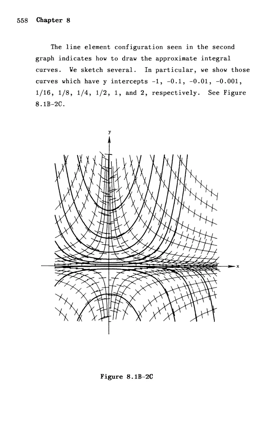
Text
Student Solutions Manual
to accompany
INTRODUCTION TO
ORDINARY DIFFERENTIAL
EQUATIONS
Fourth Edition
Shepley L. Ross
University of New Hampshire
With the assistance of
Shepley L. Ross, II
Bates College
JOHN WILEY & SONS
New York Chichester Brisbane Toronto Singapore
Copyright @ 1989 by John Wiley & Sons, Inc.
All rights reserved.
This material may be reproduced for testing- or
instructional purposes by people using the text.
ISBN 0 471 63438 7
Printed in the United states of America
10 9 8 7 6 5 4 3 2 1
Preface
This manual is a supplement to the author's text, Introduction
to Ordinary Differential Equations, Fourth Edition. It contains
the answers to the even-numbered exercises and detailed
solutions to approximately one half of both the even- and
odd-numbered exercises in the regular exercise sets.
The following abbreviations have been used:
. D.E. differential equation
. G.S. general solution
. I.F. integrating factor
. I.C. initial condition
. I.V.P. initial value problem.
The author expresses his thanks to his son Shepley L. Ross,
II, of Bates College for his many contributions, especially the
solutions and graphs of Chapter 8. The author also thanks his
colleague Ellen O'Keefe and his graduate students Rita
Fairbrother and Chris McDevitt for providing solutions.
Shepley L. loss
Contents
Chapter 1:
Chapter 2:
Chapter 3:
Chapter 4:
Chapter 5:
Chapter 6:
Chapter 7:
Chapter 8:
Chapter 9:
Differential Equations and Their
Solutions ................................... 1
First-Order Equations for Which Exact
Solutions Are Obtainable .................... 10
Applications of First-Order Equations ....... 88
Explicit Methods of Solving Higher-Order
Linear Differential Equations ............... 131
Applications of Second-Order Linear
Differential Equations with Constant
Coefficients ................................ 262
Series Solutions of Linear Differential
Equa t ion s ................................... 301
Systems of Linear Differential Equations .... 373
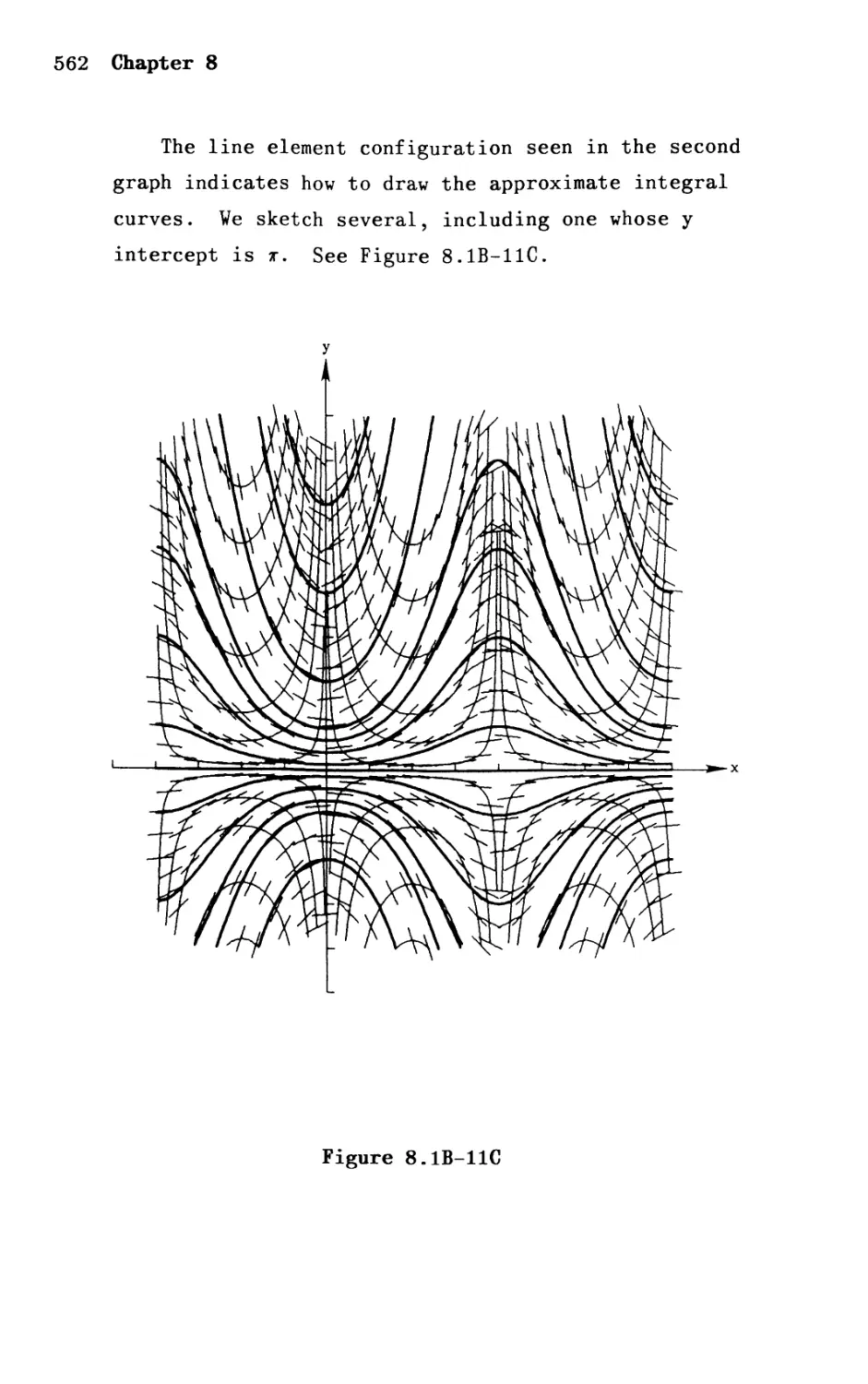
Approximate Methods of Solving First-Order
Equa t ions ................................... 556
The Laplace Transform ....................... 669
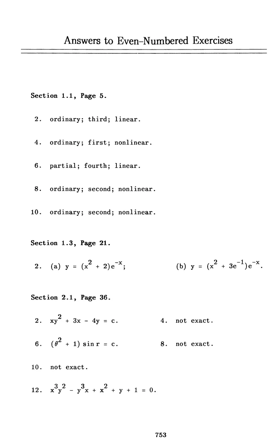
Answers to Even-Numbered Exercises ........................ 753
Chapter 1
Section 1.2, Page 11
1. (d) We must show that f(x) = (1 + x 2 )-1 satisfies the D.E.
(1 + X 2 )yH + 4xy' + 2y = o. Differentiating f(x), we
find f'(x) = -(1 + x 2 )-2(2x) and fH(x) = (6x 2 - 2)
(1 + x 2 )-3. We now substitute f(x) for y, f'(x) for
y', and fH(x) for yH in the stated D.E. We obtain
(1 + x 2 )(6x 2 - 2)(1 + x 2 )-3 - 4x(1 + x 2 )-2(2x)
2 -1
+ 2(1+x) = O.
This reduces to
(6x 2 - 2 - 8x 2 ) (1 + x 2 )2 + 2(1 + x 2 )-1 = 0,
and hence to
2 2 2 -2
[(-2x - 2) + (2 + 2x )J(1 + x) = 0,
2 -2
that is, 0(1 + x )
is satisfied by f(x) =
= 0 or 0 = O.
2 -1
(1 + x) .
Hence the given D.E.
2.
3 2
(a) We must show that the relation x + 3xy = 1 defines
at least one real function which is an explicit
solution of the given D.E. on 0 < x < 1. Solving the
glven relation for y, we obtain
2
Y
=
3
1 - x
3x
, y
= * [ 1 ;/3 ]
1/2
(1)
1
2 Chapter 1
We choose the plus sign and consider the function f
defined by
f(x) = [ 1 ;xx 3 ]1/2
,
o < x < 1.
3
We note that (1 - x )/3x > 0 for 0 < x < 1, and hence
f(x) is indeed defined on 0 < x < 1. Now differenti-
ating and simplifying, we find
f' (x) - - H1 ;/3 r 1/2[ 2X 3 2 + 1 ].
x
Substituting f(x) for y and f'(x) for y' ln the glven
D . E., we find
2x[1 _ x 3 ]1/2 {_ [1 3] -1/2 [2 3 1J}
- x x +
3x 3x 2
x
2
+ x
+
3
1 - x
3x
= o.
3 3
Th . . l . f . 2x + 1 2 1 - x 0 d
lS slmp 1 les to - 3x + x + 3x = an
o
thence to 3x = o. Thus f(x) is an explicit solution
of the D.E. on 0 < x < 1, and so the given relation
x 3 + 3xy2 = 1 lS an implicit solution on 0 < x < 1.
We note that choosing the minus slgn ln (1) would also
have led to an explicit solution of the D.E. on
o < x < 1.
Differential Equations and Their Solutions 3
( ) T.1 h h f ( ) ( 3 ) -3x . f . h
3. a"e must s ow t at x = x + c e satls les t e
2 -3x
D.E. y' + 3y = 3x e . Differentiating f(x), we find
3 -3x -3x 2
f'(x) = (x + c)(-3e ) + e (3x). We not
substitute f(x) for y and f'(x) for y' ln the stated
D.E. We obtain
3 -3x -3x 2 3 -3x 2 -3x
(x + c) (-3e ) + e (3x) + 3(x + c)e = 3x e .
2 -3x
The left member reduces to 3x e , so we have
2 -3x 2 -3x
3x e = 3x e ; and thus the D.E. is satisfied by
3 -3x
f(x) = (x + c)e .
4.
(b) We must show that g(x)
2x
= c 1 e
2x
+ c 2 xe
-2x
+ c 3 e
satisfies the D.E. ym 2yH - 4y' + 8y = o.
Differentiating g(x), we find g'(x) = 2c 1 e 2x + 2c 2 xe 2x
2x -2x u 2x 2x 2x
+ c 2 e - 2c 3 e , g (x) = 4c 1 e + 4c 2 xe + 4c 2 e +
4 -2x and g m ( ) 8 2x 2x 12 2x
c 3 e, x = c 1 e + 8c 2 xe + c 2 e -
2x
8c 3 e · We now substitute g(x) for y, g'(x) for y'.
gH(X) for yH, and gm (x) for ym in the stated D.E. We
obtain
2x
8c 1 e
2x 2x
+ 8c 2 xe + 12c 2 e - 8c 3
2x 2x
- 2(4c 1 e + 4c 2 xe +
2x 2x
- 4(2c 1 e + 2c 2 xe +
2x 2x
+ 8(c 1 e + c 2 xe
-2x
e
2x
4c 2 e
2x
c 2 e
-2x
+ c 3 e ) = o.
-2x
+ 4c 3 e )
-2x
2c 3 e )
4 Chapter 1
This reduces to
2x
8c 1 e
2x -2x
+ 12c 2 e - 8c 3 e
2x 2x
8c 2 xe - 8c 2 e -
2x 2x
8c 2 xe - 4c 2 e +
2x -2x
8c 2 xe + 8c 3 e
2x
+ 8c 2 xe
2x
- 8c e -
1
2x
- 8c e -
1
2x
+ 8c 1 e +
= 0
-2x
8c 3 e
-2x
8c 3 e
and hence to
(8c 1 + 12c 2 - 8c 1 - 8c - 8c 1 - 4c 2 2x
+ 8c 1 )e
2
(8c 2 - 8c 2 - 8c + 8c 2 ) xe 2x
+
2
(-8c 3 - 8c 3 + 8c 3 + -2x
+ 8c 3 )e = 0,
h . 0 2x 2x -2x 0 H
t at lS, .e + O.xe + O.e =, or 0 = O. ence
2x 2x
the given D.E. is satisfied by g(x) = c 1 e + c 2 xe +
-2x
c 3 e
5.
mx
(a) To determine the values of m for which f(x) = e
satisfies the given D.E., we differentiate f(x) the
required number of times and substitute into the D.E.
We have f(x) = e InX , f'(x) = me mx , f"(x) = m 2 e mx , fill (x)
3mx
= m e Then substituting f(x) for y, f'(x) for y',
3mx 2mx
fH(x) for yH, and f"'(x) for y"', we find m e - 3m e
- 4me mx + 12e InX = 0 or e mx (m 3 - 3m 2 - 4m + 12) = O.
Th e InX 4 0 f all m d t h 3
en since T or an x, we mus ave m
2 mx
3m - 4m + 12 = O. That is, if f(x) = e lS a
solution of the given D.E., then the constant m must
t f th b " t " m 3 - 3m 2 4 12 0
sa is y e cu lC equa 10n m + =.
By
inspection we observe that m = 2 is a root, and so
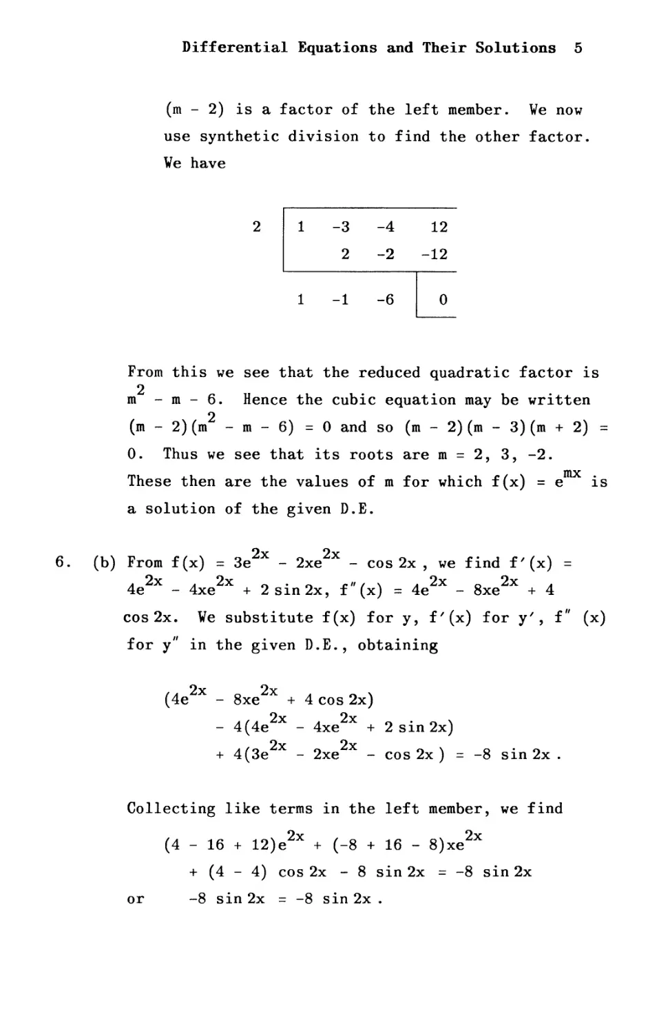
Differential Equations and Their Solutions 5
(m - 2) is a factor of the left member. We now
use synthetic division to find the other factor.
We have
2 1 -3 -4 12
2 -2 -12
1 -1 -6 0
From this we see that the reduced quadratic factor is
m 2 - m - 6. Hence the cubic equation may be written
(m 2)(m 2 - m - 6) = 0 and so (m - 2)(m - 3)(m + 2) =
O. Thus we see that its roots are m = 2, 3, -2.
These then are the values of m for which f(x) = e rnx lS
a solution of the given D.E.
6. (b) From f(x) 2x 2x - cos 2x, we find f' (x)
= 3e - 2xe =
4e 2x _ 4xe 2x + 2 sin 2x, f" (x) 2x 2x + 4
= 4e - 8xe
cos 2x. We substitute f(x) for y, f' (x) for y' , fIt (x)
for y " the . D.E. , obtaining
ln glven
(4e 2x _ 8xe 2x +
_ 4(4e 2x
+ 4(3e 2x
4 cos 2x)
2x
- 4xe + 2 sin 2x)
2x
- 2xe - cos 2x) = -8 sin 2x .
Collecting like terms in the left member, we find
2x 2x
(4 - 16 + 12)e + (-8 + 16 - 8)xe
+ (4 - 4) cos 2x - 8 sin 2x = -8 sin 2x
or -8 sin 2x = -8 sin 2x .
6 Chapter 1
Thus f(x) satisfies the D.E.
3e 0 - 2 ( 0 ) e O - co s 0 = 3 0
4(0)e O + 2 sin 0 = 4 0 + 0
Now note that f(O) =
1 = 2 and f'(O) = 4e O -
= 4. Hence f(x) also
satisfies the stated conditions.
7. (a) We must show that the D.E. Iy'l + Iyl + 1 = 0 has no
(real) solutions. Assume, to the contrary, that this
D.E. has a real differentiable function f as a
solution on some interval I. Since f is a solution on
I, we must have If/(x)1 + If(x)1 + 1 = 0 for all x E
I. But for a real function f, both If'(x)1 0 and
If(x)1 0, so If'(x)1 + If(x)1 + 1 1 for all x E I.
Thus we obtain two contradictory statements about
If'(x)1 + If(x)1 + 1, and so our original assumption
that the D.E. has a real solution is incorrect. So it
has no real solutions.
Section 1.3, Page 21
2. (a) We apply the I.C. y(O) = 2 to the glven family of
solutions. That lS, we let x - 0, y = 2 in
-
(x 2 + c)e -x We obtain 2 = (0 + c)e 0 and hence
y = .
c = 2. We thus obtain the particular solution y =
(x 2 + 2)e -x satisfying the stated I.V.P.
3. (a) We first apply the I.C. y(O) = 5 to the glven family
of solutions. That lS, we let x = 0, y = 5 ln y -
-
4x -3x We obtain = 5. We next
c 1 e + c 2 e c 1 + c 2
4x
differentiate the given family to obtain y' = 4c 1 e
3c 2 e- 3x . We apply the I.C. y'(O) = 6 to this derived
Differential Equations and Their Solutions 7
relation. That is, we let x = 0, y' = 6 1n y' =
4x -3x
4c 1 e - 3c 2 e . We obtain 4c 1 - 3c 2 = 6. The two
equations
c 1 + c 2 = 5,
4c 1 - 3c 2 - 6
-
determine c 1 and c 2 uniquely.
Solving this system, we find c 1 = 3, c 2 = 2. Substi-
4x -3x
tuting these values back into y = c 1 e + c 2 e we obtain
th t . 1 1 . 3 4x 2 -3x . f . h
e par 1CU ar so ut10n y = e + e sat1s Ylng t e
stated I.V.P.
4. (a) We first apply the B.C. y(O) = 0 to the given family
of solutions. That 1S, we let x = 0, y = 0,
y = c 1 sin x + c 2 cos x. We obtain c 2 = o. We next
apply the B.C. Y(7r/2) = 1 to the given family of
solutions. That 1S, we let x = 7r/2, Y - 1 1n
-
y = c 1 Sln x + c 2 co s x. We obtain c 1 = 1 . Substi-
tuting the values c 1 = 1, c 2 = 0 back into
y = c 1 Sln x + c 2 cos x, we obtain the particular
solution y = sin x satisfying the stated boundary-
value problem.
(c) We first apply the B.C. y(O) = 0 to the glven family
of solutions. That 1S, we let x = 0, y = o in
y = c 1 Sln x + c 2 co s x. We obtain c 2 = o. We next
apply the B.C. Y(7r) = 1 to the given family of
8 Chapter 1
solutions. That is, we let x = , y = 1 in
y = c 1 sin x + c 2 cosx. We obtain -c 2 = 1, so c 2 = -1.
At this point we have both c 2 = 0 and, at the same
time, c 2 = -1. This is impossible! So the given
boundary-value problem has no solution.
5. We are given that every solution of the stated D.E. may be
written in the form
2
Y = c 1 x + c 2 x
3
+ c 3 x
(1)
for some choice of the constants c 1 , c 2 , c 3 . We must
determine these constants so that (1) will satisfy the
three stated conditions. We differentiate (1) twice to
obtain
y' + 2c 2 x + 3c 3 x 2
= c 1
and
" 2c 2 x + 6c 3 x
y -
-
(2)
(3)
We now apply the condition y(2) = 0 to (1), letting x = 2,
y = 0 in (1). We obtain 2c 1 + 4c 2 + 8c 3 = o. Similarly,
we apply the condition y'(2) = 2 to (2), thereby obtaining
c 1 + 4c 2 + 12c 3 = 2. Finally, we apply the condition
yH(2) = 6 to (3), obtaining 2c 2 + 12c 3 = 6. Thus we have
the three equations
Differential Equations and Their Solutions 9
2c 1 + 4c 2 + 8c 3 = 0,
c 1 + 4c 2 + 12c 3 = 2,
2c 2 + 12c 3 = 6,
ln the three unknowns. These can be solved 1n var10US
way s . One easy way 1S to eliminate c 1 from the first two
equations, obtaining the equivalent of c 2 + 4c 3 = 1 .
Combining this last with c 2 + 6c 3 = 3, which 1S equivalent
to the third equation of the system, we readily find
c 2 = -3, c 3 = 1. Then from the second equation one finds
c 1 = 2. Thus c 1 = 2, c 2 = -3, c 3 = 1 . Substituting these
values back into (1) , we find the solution of the stated
I.V.P. 1S
2 3
y = 2x - 3x + x .
(a)
Let us apply Theorem 1.1.
hypothesis. Here f(x,y) =
a f ( x y ) 2
a y , = x cos y · Both f and
We first check the
2. d
x Sln y an
af . .
ay are cont1nuous 1n
every domain D in the xy plane. The initial condition
y(l) = -2 means that Xo = 1 and Yo = -2, and the point
(1, -2) certainly lies in some such domain D. Thus
all hypothesis are satisfied and the conclusion holds.
That is, there is a unique solution; of the D.E.
y' = x 2 sin y, defined on some interval 1 x - 11 h
about Xo = 1, which satisfies the initial condition,
that 18, which is such that ;(1) = -2.
Chapter 2
Section 2.1, Page 36
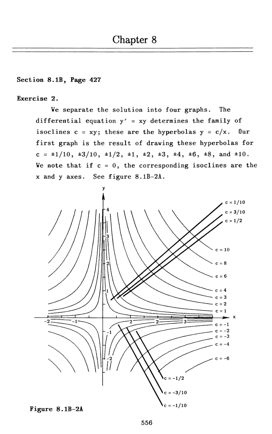
In these solutions we denote derivatives by primes and
partial derivatives by subscripts. The solutions of
Exercises 3, 5, 6, 7, and 9 follow the pattern of Example
2.5 on page 31.
3. Here M(x,y) = 2xy + 1 , N(x,y) 2 + 4y. From these we
= x
find M (x,y) = 2x = N (x,y), so the D.E. is exact. We
y x
seek F(x,y) such that
F (x,y) = M(x,y) = 2xy + 1 and F (x,y) = N(x,y)
x y
2
= x + 4y.
From the first of these, we find
F(x,y) = fM(x,y)Dx + (y) = f(2xy + l)Dx + (y)
2
= x y + x + ;(y). From this,
2
F(x,y) = x + ;'(y).
But we must have F (x,y)
y
= N(x,y)
2
= x + 4y.
Therefore
2 2
x + ;'(y) = x + 4y
or d d ) = 4y.
x + 2y2 + c .
o
Then (y) = 2y2 + cO'
2
Thus F(x,y) = x y +
The one-parameter family of solutions
2
F(x,y) = c 1 1S x y + x +
2y 2 h
= c, were c = c 1 - cO.
10
First-Order Equations 11
Alternatively, by the method of group1ng, we first
2
write the D.E. in the form 2xy dx + x dy + dx +
4y dy = o. We recognize this as d(x 2 y) + d(x) + d( 2y 2) =
d(c) or d(x 2 y + x + 2y2) = d(c). Hence we obtain the
1 t . 2 2y 2
so u 10n x y + x + - c.
4.
2 3
Here M(x,y) = 3x y + 2, N(x,y) = -(x + y). From these we
2 2
find M (x,y) = 3x t -3x = N (x,y). Since M (x,y) t
y x Y
N (x,y), the D.E. is not exact.
x
5. Here M(x,y) = 6xy + 2y2 - 5, N(x,y) = 3x 2 + 4xy - 6. From
these we find M (x,y) = 6x + 4y = N (x,y), so the D.E. is
y x
exact. We seek F(x,y) such that F (x,y) = M(x,y) = 6xy
x
2
- 3x + 4xy 6. From the
2
+ 2y 5 and F (x,y) = N(x,y)
y
first of these, we find F(x,y) = fM(x,y)D x + ;(y)
f(6xy + 2l- 5)Dx + ;(y) = 3x 2 y + 2y 2 x - 5x + ;(y).
2
From this, F (x,y) = 3x + 4xy + ;(y). But we must have
y
2
F (x,y) = N(x,y) = 3x + 4xy - 6. Therefore
y
2 2
3x + 4xy + ;'(y) = 3x + 4xy - 6,
or ;'(y) = -6. Then ;(y) = -6y + cO. The one-parameter
2 2
family of solutions F(x,y) = c 1 1S 3x y + 2y x - 5x - 6y =
c, where c = c 1 - cO.
12 Chapter 2
Alternatively, by the method of grouping, we first
2 2
writetheD.E. in the form (6xydx +3xdy) + (2ydx+
4xy dy) - 5dx - 6dy = O. We recognize this as d(3x 2 y) +
d( 2y 2 x ) - d(5x) - d(6y) = d(c) or d(3x 2 y + 2y 2 x - 5x - 6y)
2 2
= d(c). Hence we obtain the solution 3x y + 2y x - 5x -
6y = c.
6.
2
Here M(r,O) = (0 + l)cos r , N(r,O) = 20 sin r. From these
we find MO(r,O) = 20 cos r = Nr(r, 0), so the D.E. is exact.
We seek F(r,O) such that F (r,O) = M(r,O) = (0 2 + 1) cosr
r
and F 0 ( r , 0) = N ( r , 0) = 2 0 sin r . F rom the fir s t 0 f the s e ,
we find F(r,O) = JM(r,O) Or + (O) = J(02 + 1) cosrOr +
(0) = (0 2 + 1) sin r + (0). From this, F 0 (r, 0) = 20 sin r
+ ,p' (0). But we must have F OCr, 0) = N(r,O) = 20 sin r.
Therefore
20 sin r + ,p' (0) = 20 sin r
or ;'(0) = o. Then ;'(0) = cO.
2
Thus F(r,O) = (0 + 1)
slnr + cO. The one-parameter family of solutions F(r,O) =
c 1 is (0 2 + 1) sinr = c 1 where c = c 1 - cO.
Alternately, by the method of grouping, we first write
the D. E. in the form (0 2 co s r dr + 20 sin r dO) + co s r dr =
o. We recognize this as d(02 sin r) + d(sin r) = d(c) or
d (0 2 sin r + sin r) = d (c) . Hence we obtain the solution
0 2 sin r + sin r = c, 0 r (()2 + 1) sin r = c.
First-Order Equations 13
2
7. Here M(x,y) = y sec x + secxtanx, N(x,y) = tanx + 2y.
2
From these we find M (x,y) = sec x = N (x,y), so the D.E.
y x
is exact. We seek F(x,y) such that F (x,y) = M(x,y) = y
x
2
sec x +secxtanx andF (x,y) =N(x,y) = tan x +2y.
y
From the first of these, we find F(x,y) = fM(x,y)Dx +
;(y) = f(y sec 2 x + secxtanx)Dx + ;(y) = y tan x +
s e c x + ; (y) . From t his, F ( x , y) = t an x + ;' (y). But we
y
must have F (x,y) = N(x,y) = tan x + 2y. Therefore, tan x
y
+ ;' (y) = t an x + 2y 0 r ;' (y) - 2y.
2
Thus F(x,y) = y tan x + sec x + y
Then ;(y) = y2 + cO.
+ cO.
The one-
parameter family of solutions F(x,y) = c 1 is y tan x +
2
sec x + y = c, where c = c 1 - cO.
Alternatively, by the method of grouping, we first
write D.E. in the form (y sec 2 x dx + tan x dy) +
sec x tan x dx + 2y dy = o. We recognize thi s as d (y tan x )
+ d(sec x) + d(y2) = d(c), and hence obtain the solution
2
y tan x + sec x + y = c.
8.
x
Here M(x,y) = + x. N(x,y) =
Y
-2x 2x
M (x,y) = t = Nx(x,y).
y y y
the D.E. is not exact.
2
x
+ y. From these we find
y
Since M (x,y) t N (x,y),
y x
14 Chapter 2
9.
Here M(s,t) =
28 - 1
t
N(s,t) =
2
s - s
t 2
From these we find
1 - 2s
Mt(s,t) = t 2 = Ns(s,t), so the D.E. is exact.
2s - 1
F ( s , t) such t hat F s ( s , t ) = M ( s , t ) = t and F t (s , t) =
We seek
N(s,t) =
2
s - s
t 2
From the first of these, we find F(s,t)
JM(s,t)8s J2S t- 1 2
+ ;(t) ;(t) = s - s + ;(t).
= = a s +
t
2 2
From this, Ft(s,t) s - s + ;'(t). Therefore, s - s
= t 2 +
t 2
;'(t) =
2
s - s
t 2
or ;'(t) = O.
Then ; ( t )
= c .
o
Thus
F(s,t) =
2
s - s
t + cO.
The one-parameter family of
2
s
solutions F(s,t) = c 1 1S
- s
t
2
+ Co = c 1 or s
- s
= ct,
where c = c - c .
1 0
The solutions of Exercises 12, 13, 14, and 16 follow
the pattern of Example 2.6 on page 32.
12. Here M(x,y) 3 22
= x y
From these we find
is exact. 'We seek
M (x,y)
Y
F(x,y) such that F (x,y) -
x
3x 2 y2 - y3 + 2x and F (x,y) = N(x,y) = 2x 3 y
y
y3 + 2x, N(x,y) = 2x 3 y 3xy2 + 1.
2 2
= 6x y 3y = N (x,y), so D.E.
x
M(x,y) =
2
3xy + 1.
From the first of these, we have
F(x,y) = JM(x,y)8x + (y) = J (3x2y2 y3 + 2x)8x +
;(y) = x 3 y2 _ xy3 + x 2 + ;(y)
First-Order Equations 15
3 2
From this, F (x,y) = 2x y - 3xy + ;'(y). But we must
y
323
have F (x,y) = N(x,y) - 2x y 3xy + 1. Therefore, 2x y
y
3xy2 + ;'(y) = 2x 3 y 3xy2 + 1, or ;'(y) = 1. Then ;(y)
3 2 3 2
= y + cO. Thus F(x,y) = x y - xy + x + y + cO. The
one-parameter family of solutions F(x,y) = c 1 1S
3 2 3 2
x y xy + x + y = c,
(*)
where c -
c 1 - cO.
Applying the I.C. y(-2) = 1 , we let x = -2, y = 1 In
(*) , obtaining -8 + 2 + 4 + 1 = c, from which c = -1.
Thus the particular solution of the stated I.V. problem 1S
3 2 3 2 -1
x Y xy + x + y = or
3 2 3 2 + y + 1 O. (**)
x y xy + x =
Alternately, the one-parameter family of solutions (*)
could also be found by the method of grouping. We write
.22 3 3 2
the D.E. 1n the form (3x y dx + 2x ydy) - (y dx + 3xy dy)
+ 2x dx + dy = o. We recognize this as d(x 3 y2) - d(xy3) +
d(x 2 ) + d(y) = d(c), and so again obtain the one-parameter
family of solutions
3 2
x y
3 2
xy + x + y = c.
(*)
The I.C. aga1n yields the particular solution (**).
16 Chapter 2
13. Here M(x,y) = 2y sinxcosx + y2 sinx, N(x,y) = sin 2 x-
2y cos x. From these we find M (x,y) = 2 sin x cos x +
y
2y sin x = N (x,y), so D.E. 1S exact. We first seek F(x,y)
x
such that F (x,y) = M(x,y) = 2y sin x cos x + y2 sin x and
x
F (x,y) = N(x,y) = sin 2 x - 2y cos x. From the first of
y
these, we have F(x,y) = M(x,Y)Dx + (y) =
(2Y sinxcosx + l sinx)Dx + (y) = y sin 2 x -l cosx
+ ;(y). From this, F (x,y) = sin 2 x - 2ycosx + ;'(y).
Y
But we must have F (x,y) = N(x,y) = sin 2 x - 2y cos x .
y
Therefore, sin 2 x - 2y cos x + ;' (y) = sin 2 x - 2y cos x or
'(y) = O. Then (y) = cO' Thus F(x,y) = y sin 2 x _ y2
cos x + cO. The one-parameter family of solutions F(x,y)
= c is
1
.22
Y Sln x y cos x = c,
(*)
where c =
c 1 - cO.
Applying the I.C. y(O) = 3, we let x = 0, y = 3 in
(*), obtaining 3 sin 2 0 - 9 cos 0 = c, from which c = -9.
Thus the particular solution of the stated I.V. problem is
.22 9
Y Sln x - y cos x = - or
2 . 2 9
y cos x - y Sln x = .
(**)
Alternatively, the one-parameter family of solutions
(*) could also be found by the method of grouping. To do
First-Order Equations 17
so, we first write the D.E. in the form (2y sinxcosxdx +
sin 2 x dy) + (y2 sinxdx - 2y cosxdy) = o. We recognize
this as d(y sin 2 x) + d(_y2 cosx) = d(c) and hence again
obtain the solution (*) in the form y sin 2 x - y2 cos x =
c. The I.C. aga1n yields the particular solution (**).
14.
x x 2 x
Here M(x,y) = ye + 2e + y , N(x,y) = e + 2xy. From
x
these we find M (x,y) = e + 2y = N (x,y), so the D.E. 1S
Y x
exact. We first seek F(x,y) such that F (x,y) = M(x,y) =
x
x x 2 x
ye + 2e + y and F (x,y) = N(x,y) = e + 2xy. From the
y
first of these, we have F(x,y) = fM(x,y)Ox + ;(y) =
f x x 2 x x 2
(ye + 2e + y )ax + ;(y) = ye + 2e + xy + ;(y).
x
From this, F (x,y) = e + 2xy + ;'(y). But we must have
y
F (x,y) = N(x,y) = eX + 2xy. Therefore, eX + 2xy + ;'(y)
Y
= eX + 2xy or ;'(y) = O. Then ;(y) = cO. Thus F(x,y) =
x x 2
ye + 2e + xy + cO. The one-parameter family of
solutions F(x,y) = c 1 IS
x x 2 (*)
ye + 2e + xy = c,
where c =
c 1 - cO.
Applying the I.C. y(O) = 6, we let x = 0, y = 6 in
(*), obtaining 6eO + 2e O + 0(6 2 ) = c, from which c = 8.
Thus the particular solution of the stated I.V. problem 1S
x x 2
ye + 2e + xy = 8 or
x 2 x
e y + xy + 2e = 8.
(**)
18 Chapter 2
Alternatively, the one-parameter family of solutions
(*) could also be found by the method of grouping. To do
so, we first write the D.E. in the form (yeXdx + eXdy) +
(y 2 dx + 2xydy) + 2e x dx = o. We recognize this as d(eXy)
+ d(xy2) + d(2e x ) = d(c) and hence once again obtain the
solution (*) 1n the form eXy + xy2 + 2e x = c. The I.C.
again yields the particular solution (**).
16.
-2 / 3 -1 / 3 1 / 3 1 / 3 4 / 3 -2 / 3
Here M(x,y) = x y + 8x y , N(x,y) = 2x Y
- x1/3y-4/3. From these we find My(x,y) = _ x- 2 / 3 y-4/3
8 1/3 -2/3
+ 3 x y = Nx(x,y) so the D.E. is exact. We first
-2 / 3 -1 / 3
F (x,y) = M(x,y) = x y +
x
_ N( ) - 2 4/3 -2/3 1/3 -4/3
- x,y - x y - x y .
seek F(x,y) such that
8x 1 / 3 y1/3 and F (x,y)
y
From the first of these, we have F(x,y) = fM(x,y)Ox +
f -2 / 3 -1 / 3 1 / 3 1 / 3 1 / 3 -1 / 3
;(y) = (x y + 8x y )ax + ;(y) = 3x y +
6x 4 / 3 y1/3 + ;(y). From this, Fy(x,y) = _x 1 / 3 y-4/3 +
2x 4 / 3 y-2/3 + ;'(y). But we must have Fy(x,y) = N(x,y) =
2 4/3 -2/3 1/3 -4/3 Th 1/3 -4/3 2 4/3 -2/3
x y - x y . us -x y + x y +
4 / 3 -2 / 3 1 / 3 -4 / 3
;'(y) = 2x y - x y or ;'(y) = O. Then ;(y) =
1 / 3 -1 / 3 4 / 3 1 / 3
cO. Thus F(x,y) = 3x y + 6x y . The
one-parameter family of solutions F(x,y) = c 1 1S
3 1/3 -1/3 6 4/3 1/3
x y + x y = c 2 ' where c 2 = c 1 - cO.
We can
simplify this slightly by dividing through by 3 and
replacing c 2 /3 by c, thus obtaining
1/3 -1/3 2 4/3 1/3
x y + x y = c.
(*)
First-Order Equations 19
Applying the I.C. y(l) = 8, we let x = 1, Y = 8 ln (*)
to obtain + 4 = c, from which c = 9/2. Thus the
particular solution of the stated I.V. problem lS
1/3 -1/3 2 4/3 1/3 9/2
x y + x y = or
2x 1 / 3 y-1/3 + 4x 4 / 3 y1/3 = 9.
(**)
Alternatively, the one-parameter family of solutions
(*) could also be found by the method of grouping. To do
so, we first write the D.E. In the form (x- 2 / 3 y-1/3dx
1/3 -4/3 d ) (8 1/3 1/3 d 2 4/3 -2/3 d ) - 0 H e
x y y + x y x + x y y - . w
1 / 3 -1 / 3 4 / 3 1 / 3
recognize this as d(3x y ) + d(6x y ) = d(c 2 ) and
hence obtain the solution 3x 1 / 3 y-1/3 + 6x 4 / 3 y1/3 = c 2 .
Once again, this quickly reduces to (*), and the I.C.
again yields the particular solutions (**).
18. (a) Here M(x,y) 2 2 , N(x,y) 3 + 4xy. From
= Ax y + 2y - x
-
these we find M (x,y) = 2 and N (x,y) 2
Ax + 4y = 3x +
y x
4y. The given D.E. lS exact if and only if M (x,y) -
-
Y
N (x,y) , 1.e. , if and only if Ax 2 + 4y = 3x 2 + 4y.
x
So the given D.E. lS exact if and only if A = 3.
Substituting 3 for A in the glven D.E. yields the
exact D.E. 2 2 3 4xy)dy = O. We
(3x y + 2y )dx + (x + now
proceed to solve this D.E.
223
Here M(x,y) = 3x y + 2y , N(x,y) = x + 4xy. From
2
these we find M (x,y) = 3x + 4y = N (x,y), so
y x
20 Chapter 2
the D.E. lS exact. We seek F(x,y) such that F (x,y) =
x
M ( ) 3 2 2y 2 d F ( ) N ( ) 3 4
x,y = x y + an x,y = x,y = x + xy.
y
From the first of these, we find F(x,y) = M(x,Y)Dx +
;(y) = (3x2y + 2y2)Dx + ;(y) = x 3 y + 2xy2 + ;(y).
3 3
From this, F (x,y) = x + 4xy + ;'(y). Therefore x +
y
3
4xy + ;'(y) = x + 4xy, or ;'(y) = O. Then ;(y) = cO.
3 2
Thus F(x,y) = x y + 2xy + cO. The one - parameter
f 0 1 f 1 0 F( ) 0 3 2 2
aml y 0 so utlons x,y = c 1 lS x y + xy = c,
where c = c 1 - cO.
Alternatively, by the method of grouplng, we first
232
write the D.E. in the form (3x y dx + x dy) + (2y dx +
4xydy) = o. We recognize this as d(x 3 y) + d( 2xy 2) =
d(c) or d(x 3 y + 2xy2) = d(c). Hence we obtain the
1 . 3 2 2
so ut10n x y + xy = c.
20.
(b)
x 2 3x x
Here N(x,y) = 2ye + y e , so N (x,y) = 2ye +
x
3y2e3x. For the stated D.E. to be exact, we need
M (x,y) = N (x,y) = 2ye X + 3y2e3x. From this, we find
y x
f f x 2 3x
M(x,y) = My(x,y)ay + ;(x) = (2ye + 3y e )ay +
2 x 3 3x
;(x) = y e + y e + ;(x). Hence the most general
function M(x,y) such that the stated D.E. is exact lS
2 x 3 3x
M(x,y) = y e + y e + ;(x), where ;(x) is an
arbitrary function of x.
First-Order Equations 21
21.
2
Here M(x,y) = 4x + 3y , N(x,y) = 2xy.
(c)
(a) Since M (x,y) = 6y f 2y = N (x,y), the D.E. IS not
y x
exact.
(b)
We multiply the given equation through by x n to obtain
n+1 n 2 n+l ..
(4x + 3x y )dx + 2x ydy = O. For thIS equatIon,
n+1 n 2 n+l
we have M(x,y) = 4x + 3x y , N(x,y) = 2x y. For
this equation to be exact, we must have M (x,y) = 6x n y
y
6 = 2(n + 1), from
n
= 2(n + l)x y = N (x,y), and hence
x
which n = 2. Thus an I.F. of the form x n is x 2 .
2
We multiply the given equation through by the I.F. x ,
obtaining (4x 3 + 3x 2 y2)dx + 2x 3 y dy = o. Here M(x,y)
32232
= 4x + 3x y , N(x,y) = 2x y. Since M (x,y) = 6x y =
y
N (x,y), this D.E. is indeed exact. We seek F(x,y)
x
such that F (x,y) = M(x,y) = 4x 3 + 3x 2 y2 and F (x,y) =
x Y
N(x,y) = 2x 3 y. From the first of these, F(x,y) =
JfM(x,y)Ox + ;(y) = Jf(4x 3 + 3x 2 y2)Ox + ;(y) = x 4 +
323
x y + ;(y). From this F (x,y) = 2x y + ,'(y). But
Y
3
we must have F (x,y) = N(x,y) = 2x y, so ;'(y) = O.
Y
432
Then ;(y) = cO. Thus F(x,y) = x + x y + cO. The
one-parameter family of solutions F(x,y)
. 4
= C 1 IS x +
3 2
x Y = c, where c = c 1 - cO. Alternatively, by the
method of grouping, we first write the D.E. (4x 3 +
223 322
3x y )dx + 2x y dy = 0 in the form 4x dx + (3x y dx +
2x 3 y dy) = o. We recognize this as d(x 4 ) + d(x 3 y2) =
d(c), and hence we obtain the solutions x 4 + x 3 y2 = c.
22 Chapter 2
23.
(a)
Here M(x,y) =
2
y )-x.
2
f' (x +
222
Y + x f(x + y ) and N(x,y) = y f(x +
Since M (x,y) = 1 + 2xy f'(x 2 + y2) f 2xy
y
2
y ) -1 = N (x,y), the given D.E. is not exact.
x
2 2
(b) Ye multiply the glven D.E. through by l/(x + y ) to
obtain
[x 2 y xf ( x 2 + y2 ) ]d [ Yf ( X2 + y2 )
2 + 2 2 x + 2 2
+ y x + y x + y
x 2 : l]d Y = O.
For this equation, we have
2 2
M(x,y) = y xf ( x + y ) and
2 2 + 2 2
x + y x + y
2 2
N(x,y) yf ( x + y ) x
= -
2 2 2 2
x + y x + y
From these we find
2 2 2 2 2 2 2 2
M (x,y) = 2xy(x + Y )f'(x + Y ) - 2xyf(x + y ) + x - y
y ( 2 2 ) 2
x + Y
= N (x,y)
x
So the D.E. of part (b) is exact, and hence
2 2
l/(x + y ) lS an I.F. of the given D.E.
First-Order Equations 23
24. Applying Exercise 23(a) with f(x 2 + y2) = (x 2 + y2)2, we
see that the given D.E. is not exact. By Exercise 23(b),
we know that 1/(x 2 + y2) is an I.F. of the given D.E.
2 2
Hence we multiply the given D.E. through by l/(x + y ) to
obtain the equivalent D.E.
[ x 2 : y2 + x(x 2 + y2)]dX + [y(X 2 + y2)
x 2 : l ]d Y = 0,
2 2
which is therefore exact. Here M(x,y) = y/(x + y ) +
x(x 2 + y2), N(x,y) = y(x 2 + y2) _ x/(x 2 + y2), M (x,y) =
Y
(x 2 - y2)/(x 2 + y2)2 + 2xy = N (x,y). We seek F(x,y) such
x
that F (x,y) = M(x,y) = y/(x 2 + y2) + x(x 2 + y2) and
x
F (x,y) = N(x,y) = y(x 2 + y2) _ x/(x 2 + y2). From the
y
first of these, we find F(x,y) = M(x,y)Ox + ;(y) =
[y/(x2 + y2) + x(x 2 + y2)]Ox + ;(y) = arc tan (x/y) +
42222
x /4 + x y /2 + ;(y). From this, F (x,y) = -x/ex + y ) +
y
2 2 3
x y + ;'(y). But we must have F (x,y) = N(x,y) = x y + y
y
2 2 3 d ( y ) 3
- x/ (x + y ). Therefore, (J' (y) = y or Y'dy = Y .
4
Then, ;(y) = y /4 + cO. Thus F(x,y) = arc tan (x/y) +
422 4
x /4 + x y /2 + Y /4 + cO' or more simply, F(x,y) = arc
222
tan (x/y) + (x + y ) /4 + cO. The one-parameter family
222
of solutions F(x,y) = c lS arc tan(x/y) + (x + y ) /4 =
c, where c = c 1 - cO.
24 Chapter 2
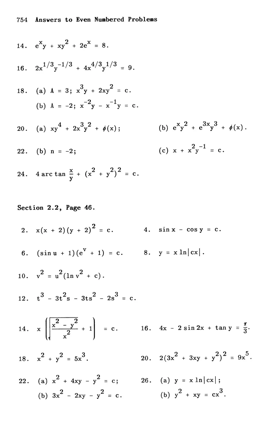
Section 2.2, Page 46
The equations ln Exercises 1-7 and 15-17 are
separable, and those in Exercises 8-14 and 18-20 are
homogeneous.
2. Since xy + 2x + y + 2 = x(y + 2) + l(y + 2) = (x + 1)
(y + 2), the D.E. can be rewritten as (x + l)(y + 2)dx +
2
(x + 2x)dy = O. The D.E. is separable. We first
separate variables to obtain (x + l)dx + dy - 0 Next
x 2 + 2x y + 2 - ·
we integrate:
f ( x 2 + l ) dx = 1 I 2 I f dy
2 In x + 2x and y + 2 =
x + 2x
Inly + 21.
Hence we find the one-parameter family of solutions in the
1 2
form 2 Inlx + 2xl + Inly + 21 = In c 1 (where we write
In c 1 for the arbi trary constant, since each term on the
left is an In term). W multiply by 2 and simplify to
2 2 2
obtain Inlx + 2 x l + In(y + 2) = In c 1 or
In[lx2 + 2xl(y + 2)2] = lnc 1 2 . From this, we have
Ix 2 + 2xl(y + 2)2 = c. If x 0 (or x -2), this may be
2 2
expressed somewhat more simply as (x + 2x)(y + 2) = c or
x(x + 2)(y + 2)2 = c.
3. The D.E. is separable. We first separate variables to
obtain 2r dr/(r 4 + 1) + ds/(s2 + 1) = o. Next we
integrate. By a well-known formula, f ds/(s2 + 1) =
arc tan s. We next apply the same formula wi th s = r 2 , ds
= 2r dr. Thus we obtain f2r dr/(r 4 + 1) = arc tan r 2 .
First-Order Equations 25
Hence we find the one-parameter family of solutions ln the
form
2
arc tan r + arc tan s = arc tan c, (*)
(where we write arc tan c for the arbitrary constant,
Slnce each term on the left lS an arc tan). We could
leave the solutions in this form, but they are unweildy.
We take the tangent of each side of (*), applying the
formula tan(A + B) = 1t nt n+At: nBB with A = arc tan r 2
and B = arc tan s, to the left member. We obtain
2
tan(arc tan r ) ; tan(arc tan s) = tan(arc tan c),
1-tan(arc tan r )tan(arc tan s)
which reduces to
2
r + s
2
1 - r s
2
= c or r
+ s
= c(l - r 2 s).
6. The D.E. is separable. We first separate variables to
d e V dv
bt . co s u u 0 N t . t t
o aln. 1 + =. ex we ln egra e:
Sln u + e V + 1
f cos u du
sin u + 1
v
f V e dv
= In(sin u + 1) and
e + 1
= In(e v + 1).
Hence we find the one-parameter family of solutions in the
form In(sin u + 1) + In(e v + 1) = In c (where we write
In c for the arbitrary constant, since each term on the
26 Chapter 2
left is a In term). We simplify to obtain In[(sin u + 1)
v
(e + l)J = Inc. From this, we have
(8 in u + 1) (e v + 1) = c.
7. This equation is separable. We first separate variables
to obtain (x + 4) dx j(x 2 + 3x + 2) + y dy j(y2 + 1) = O.
Next we integrate: f dy = ; In (y2 + 1). To integrate
y + 1
the dx term, we use partial fractions. We set
x + 4 x + 4
=
x 2 + 3x + 2 - (x + l)(x + 2)
A
+
x + 1
B
2 ' x + 4 =
x +
A(x + 2) + B(x + 1). Then x = -1 gives A = 3 and x = -2
glves B = -2. Thus we find f x + 4) dx = 3f x d+x 1
x + 3x + 2
f dx J X+1 13
2 x + 2 = 3 Inlx + 11 - 2 lnlx + 21 = In . . Hence
(x + 2)
. J x + 1 L: 1 2 )
we obtain solutions ln the form In 2 + 2 In (y + 1
(x + 2)
= In c 1 (where we write In c 1 for the arbitrary constant,
81nce each term on the left 18 a In term). We multiply by
2 and simplify to obtain In (x + 1)6 + In (y2 + 1) +
(x + 2)4
1 ) = In c 2
1
2
In c 1 or
6 2
1 (x + 1) (y +
n 4
(x + 2)
6 2
1) (y + 1) = c (x +
From this, we
have (x +
2)4.
9.
We first write the D.E. in the form
2
= 2xy + 3y and
2
2xy + x
thence
dx
= 2(y/x) + 3(y/x)2
2(y/x) + 1
In this form we recognize
First-Order Equations 27
the D.E. 1S homogeneous. We let y = vx. Then = v +
x dv and v = y
dx x
We make these substitutions to obtain
dv 2v + 3v 2 dv 2
2v + 3v
v + x - = or x - = - v =
dx 2v + 1 dx 2v + 1
2v + 3v 2 2v 2 dv 2
- v v + v We now separate
2v + 1 or x- = 1 ·
dx 2v +
variables to obtain (2v + 1) dv = dx
2 x
v + v
obtain Inlv 2 + vi = In Ix I + Inlcl, or Inlv 2 + vi = Inlcxl.
From this, we have Iv 2 + vi = Icxl. We now resubstitute
We integrate to
2
v = Y to obtain L+ y = I cxl. We simplify to obtain
x 2 x
x
Iy 2 + xyl Icxlx 2 from which we find 2 3
= , y + xy = cx .
du 2 3
10. We first write the D.E. the uv - u from
ln form dv =
3
v
which we at once obtain du u ( )3 In this form we
dv = - -
v
recognlze that the D.E. lS homogeneous in u and v. If a
D.E. = f ( ) is homogeneous in x and y, we introduce a
new variable v by letting y = vx. Here u and v are the
original variables, so we introduce a new variable w by
du dw u
letting u = wv. Then dv - w + v dv and w = v
du u
Substituting into the D.E. dv = v
dw 3 dw 3
v dv = w - w" Hence v dv = -wand separating variables,
3
( ) ,
we obtain w +
we have -3 dv
-w dw -
-
v
1 = 2 In Ivl
+ c 1 or 2
w
Integrating we obtain
-2
w_ 2 = 1 n I v I
+ 2c 1 "
Resubstituting w
u
=
v '
we have
2
v _ _ In V 2 2 2 (1 2 )
2 + c or v = u n v + c .
u
28 Chapter 2
11. Ye first write the D.E. in the form = tan( ) + . In
this form we recognize that the D.E. is homogeneous. We
let y = vx. Then = v + x : and v = Ye make these
dv
substitutions in the D.E. to obtain v + x dx = tan v + v
dv
or x - = tan v. We now separate variables to obtain
dx
dx
cot v dv =
x
We integrate to obtain In I sin v I = In I x I +
In I c I,
I cxl.
or In I sin v I = In I cx I. From this we have I sin v I =
We now resubstitute v = Y to obtain Isin Y I = Icxl.
x x
For suitable x and y, this may be expressed somewhat more
simply as sin y = cx.
x
13.
We first write the D.E. ln the form dy
dx
= x3 + y2 j x2 + y2
xy j x 2 + y2
and denominator by x 3 to obtain
dy =
dx
We then divide numerator
2
1 + L j 2 2
3 x + y
x
j x2 + y2
x
=
.. 'f j 2
1 Y 2
+ - x + y
x x
y 1 j x 2 + 2
-
x x y
" .. ..
2
Assuming
x > 0 so that x = J':2, this becomes
=
dx
1 ..
, 2 L ,
1 + y J':2 Ij x 2 2
x + y
[ ] 1
J':2 j x 2 2
+ Y
1 +
2 j 2 2
l 1 + Y /x
x
'i. j 2 2
x 1 + y Ix
=
or
dy =
dx
1 +
y 2 j 1 + (y Ix) 2
x
j 1 + (y /x2)
In this form we recognize the
D.E. lS homogeneous.
We let y = vx.
dy
Then dx =
dv
v + x dx
First-Order Equations 29
and v = l. We make these substitutions to obtain
x
dv 1 + v 2 j 1 + 2 dv 1 + v 2 j 1 + 2
v v
v + x- = or x- = - v
dx v j 1 2 dx v j 1 2
+ v + v
1 + v 2 j 1 2 v 2 j 1 2 dv 1
+ v + v We
= or x- =
v j 1 + 2 dx v j 1 2
v + v
now separate variables to obtain v j 1 + v 2 dv = dx Ve
x
integrate to obtain 1/3 (1 + v 2 )3/2 = lnlxl + lnicol
(where we have chosen to write Inicol for the arbitrary
constant). We multiply by 3 and simplify to obtain
(1 + v 2 )3/2 3 Inlcoxl 2 3/2 3 3
= or (1 + v ) = In I Co I I x I .
Since we have assumed x > 0, this may be expressed
somewhat more simply as (1 + v 2 )3/2 = Incx 3 , where c =
I c o l 3 . Ve now resubstitute v = to obtain (1 + ( )2)3/2
= In c x 3 . Ve simplify to obtain [ x2 :2 y2 ]3/2 = In c x 3 or
Ix2 + lr/ 2 =
3
x
x 3 In c x 3 .
3 ( 2 2 ) 3/2
In c x , from which we find x + y =
14. This D.E. is homogeneous. Recognizing this, we could let
y = vx and substitute in order to separate the variables.
However, the resulting separable equation is not readily
tractable. This being the case, we assume x > y > 0 and
30 Chapter 2
divide the entire equation through by . Then we solve
for dx/dy, putting the D.E. in the form
dx
dy
= V x/y + 1 - V x/y - 1
V x/y + 1 + V x/y - 1
We now let x = uy (see Exercise 24 concerning this). Then
dx du
dy = u + y dy and x/y = u. Substituting in the D.E. it
takes the form
du
u + y dy
= V u + 1 - V u - 1
V u + 1 + V u - 1
We simplify the right member b y multi plyi ng bot h its
numerator and denominator by V u + 1 - V u - 1 and then
simplifying. As a resu lt of this, the D.E. takes the form
u + y ; = u - j u 2 - 1 which readily simplifies to the
du
j u 2 - 1
are useful! ), we o btain In I u + j u 2 - 11 = - In I y I + In I c I
or lnlu + j u 2 - 11 = In I C I. Since x > y > 0 and u =
y
x/y, we can write this more simply as In(u + j u 2 1 ) =
In (c/y) , from which we at once have u + j u 2 - 1 = c/y.
separable equation
= _ dy
y
Integrating (tables
Now substituting u = x/y, we have x/y + j (x/y)2 - 1 = c/y
which readily simplifies to x + j x 2 - y2 = c.
First-Order Equations 31
17. The D.E. is separable. We separate variables to obtain
(3x + 8)
2
x + 5x + 6
4y dy =
2 o.
y + 4
tegrate the dx term, we
use partial fractions.
3x + 8
We write 2
x + 5x + 6
B
3' and so 3x + 8 = A(x + 3) +
=
3x + 8 A
= +
(x + 2)(x + 3) x + 2 x +
B(x + 2). Then x = -2 glves A = 2; and x =
-3 gives B =
1 .
f 2
x
Thus we find
3x + 8 dx =
+ 5x + 6
2 f x d+x 2 + f x d+x 3 = 2 In I x + 21 +
In Ix + 31 = In(x + 2)2(x + 3). Using this, we obtain
solutions in the form In (x + 2)2(x + 3) - 2 In (y2 + 4) =
lnlcl or In {x +2 2 )2(x 2 + 3) = lnlcl. Take Ix + 31 - x + 3
(y + 4)
0 and Icl = c 0, and we have (x + 2)2(x + 3) = c(y2 +
4)2. We now apply the I.C. y(l) = 2 to this, obtaining 36
= 64c, c = ;6 ' Thus we find the particular solution
16(x + 2)2(x + 3) = 9(y2 + 4).
19. We first write the D.E. in the form dy = 5y - 2x or
dx 4x - Y
dy = 5 ( y / x ) - 2 We that this D.E.
dx 4 - y/x . recognlze lS
homogeneous. We let Then = v dv and
y = vx. + x-
dx
v = y/x. Making these substitutions, the D.E. becomes
dv 5v - 2 dv v 2 + v - 2
v + x dx = 4 _ v or x dx = 4 - v
( 4 - v ) dv _ _ dx
variables to obtain - -
2 x
v + v - 2
We now separate
Next we integrate:
32 Chapter 2
jI = lnlxl. To integrate the dv term, we use partial
fractions. We set 4 - v 4 - v A
- = +
2 - (v + 2)(v - 1) v + 2
v + v - 2
B so 4 - v = A(v 1) + B(v + 2). Then v -2
1 ' = glves
v -
A = -2 and v = 1 gives B = 1. Thus we find jI { - v) dv =
v + v - 2
2 r dv + r dv = -2 In 1 v + 21 + In I v - 11 =
- J v + 2 J v - 1
In J v - 1 . Hence we obtain solutions in the form
(v + 2)
In J v - 1 = In I xl + In c or In J v - 1 1 2 = In c 1 xl. From
(v + 2) (v + 2)
this we have Jv - 1 = clxl or Iv - 11 = clxl (v + 2)2,
(v + 2)
We resubstitute v = y/x to obtain Iy/x - 11 =
1 22
c xl (y/x + 2) . We multiply both sides by x to obtain
Iyx - x 2 1 = clxl(y + 2x)2 or Ixl Iy - xl = clxl(y + 2x)2
from which we obtain Iy - xl = c(y + 2x)2. Taking y x,
this may be expressed somewhat more simply as y - x =
c(y + 2x)2.
Applying the I.C. y(l) = 4 we let x = 1, Y = 4 and
find 3 = c(6 2 ), from which we find c =1/12. We thus
obtain the particular solution y - x = (1/12)(y + 2x)2, or
(2x + y)2 = 12(y - x).
20. We first write the D.E. ln the form
dy 3x 2 + 9xy + 5y2
dx =
6x 2 + 4xy
or
First-Order Equations 33
2
dy _ 3 + 9(y/x) + 5(y/x)
dx 6 + 4 (y/x)
We recognlze that this D.E. is homogeneous. We let y =
dy dv y
vx, and then dx = v + x dx and v = x Making these
substitutions, the D.E. becomes
dv
v + x dx =
2
3 + 9v + 5v
6 + 4v
or
dv
x- =
dx
2
v + 3v + 3
4v + 6
We now separate variables to obtain
4v + 6
dx
dv =
2
v + 3v + 3
x
Integrating, we find 2 Inlv 2 + 3v + 31 = In Ix I + Inlcl or
2 2 2 2
In (v + 3v + 3) = Inlcxl. From this, (v + 3v + 3) =
Inlcxl. We resubstitute v = y/x to obtain
[ 2 2 ] 2
Y + 3: + 3x = lex I .
We simplify, taking Ixl = x > 0, thereby obtaining
(y2 + 3xy + 3x 2 )2 =
5
cx .
Applying the I.C. y(2) = -6, we let x = 2, Y = -6 and find
144 = 32c or c = 9/2. e thus obtain the particular
. 2 225
solutlon 2(y + 3xy + 3x) = 9x .
34 Chapter 2
21. (b) Here M(x,y) 2 2 Dx 2 + Exy +
= Ax + Bxy + Cy , N(x,y) =
2 From these we find M (x,y) 2Cy and
Fy . = Bx +
y
N (x,y) = 2Dx + Ey. Now the glven homogeneous D.E. 18
x
exact if and only if M (x,y) = N (x,y), i.e., if and
y x
only if Bx + 2Cy = 2Dx + Ey. But Bx + 2Cy = 2Dx + Ey
if and only if B = 2D and 2C = E. Therefore, we have
it that the given homogeneous D.E. is exact if and
only if B = 2D and E = 2C.
23. (a) The given D.E. is of the form (Ax 2 + Bxy + Cy2)dx +
2 2
(Dx + Exy + Fy )dy = 0, where A = 1, B = 0, C = 2,
D = 0, E = 4, F = -1. From exercise 21(b), we know
the D.E. lS homogeneous. Also, since B = 0 = 2D and
E = 4 = 2C, we know from Exercise 21(b) that the glven
D.E. is also exact.
First, let us solve the glven D.E. as a
homogeneous D.E. We first write the D.E. ln the form
222
= x + 2y or = 1 +2 2 (y/x) . In this form
y2 _ 4xy (y/x) - 4(y/x)
we recognize that the D.E. is homogeneous. We let
y = vx. Then = v + x : and v = y/x. We make
dv
these substitutions to obtain v + x - =
dx
2
1 + 2v
2
v - 4v
or
dv 1 2 3
+ 6v - v W'e now separate variables to
x- =
dx 2
v - 4v
2 dv dx
obtain ( v - 4v ) W'e integrate to obtain
-
2 3 -
x
1 + 6v - v
1 2 v 3 1 In Ix I
3 In\l + 6v = + In Co or
In 11 + 6v 2 - v 3 \ = In Co Ixl. We multiply by -3
First-Order Equations 35
and simplify to obtain In 11 + 6v 2 - v 3 1 = -3 In Co I x I
or Inl1 + 6v 2 - v 3 1 = co-3Ixl-3 or 1 1 + 6v 2 _ v 3 1 =
I 1 -3 -3
c x , where c = Co We now resubstitute v = yjx
to obtain 11 + 6(yjx)2 - (yjx)3 1 = clxl- 3 . We
multiply by Ixl3 to obtain Ix 3 + 6xy2 - y31 = c. For
suitable values of x and y, this may be expressed
323
somewhat more simply as x + 6xy - y = c, or
332
x - y + 6xy = c.
Now let us solve the glven D.E. as an exact D.E.
222
Here M(x,y) = x + 2y , N(x,y) = 4xy - y. From these
we find M (x,y) = 4y = N (x,y), so the D.E. lS exact.
y x
2 2
We seek F(x,y) such that F (x,y) = M(x,y) = x + 2y
x
y2. From the first of
and F (x,y) = N(x,y) = 4xy -
y
these, F(x,y) = M(x,Y)8x + ;(y) = (x2 + y2)8x +
x 3 2
;(y) = + 2xy + ;(y). From this, Fy(x,y) = 4xy +
;/(y). But we must have
F (x,y) = N(x,y) 4xy - 2
- Y
- .
Y
4xy - Y 2 or ;'(y) 2 So
= -y .
3 2 3
F(x,y) x 2xy Y
- - + - - + c .
- 3 3 0
Therefore 4xy + ;'(y) =
3
;(y) = - Y3 + cO. Thus
The one-parameter family of solutions F(x,y) = c 1 lS
3 2 3
x 2xy Y - c where We multiply
- + - 2' c 2 = c 1 - cO.
3
by 3 to obtain x 3 + 6xy 2 3 where 3c 2 . So
y = c, c -=
the one-parameter family of solutions of the glven
D E . 3 3 6 2
. . lS X - Y + xy = c.
36 Chapter 2
25. Since the D.E. is homogeneous, it can be expressed in the
form = g( ). Let x = r cos B, y = r sin B. Then
dy =
dx
r cos
-r Sln
() d () + s ln e dr
e de + cos e dr
= r cos e + sin e dr/d()
-r sin e + cos e dr/de
Substituting into = g( ). The D.E. reduces
t O r co s e + sin e d r / de - ( t an
successively -r sin e + cos e dr/de - g e),
dr . dr
r co s () + sin () d () = g ( t an ()) [ - r s 1 n e + co s e d e J ,
dr
[sin () - cos () g(tan ())J d() = -[g(tan e) sin e + cos OJr,
dr Sln e g( tan e ) + cos e
= e de, which lS separable ln r
r co s e g ( tan e) - s 1 n
and e.
26. (a) The D.E. of Exercise 8 is (x + y) dx - xdy = O. This
can be written = 1 + y/x, and so 1S homogeneous.
Using the method of Exercise 25, we let x = r cos e ,
. e Th dy r cos e de + sin e dr We
y = r s 1 n. en dx = _ r sin e de + co s e dr.
substitute this into = 1 + y/x. The D.E. reduces
successively to
r cos e de + sin e dr
-r sin e de + cos e dr = 1 + tan e,
r cos e de + sin edr = (1 + tan e ) (-r sin e de +
cos edr), [sin e - (1 + tan e) cos eJ dr = -r[cos e +
( 1 + tan e) sin e] de,
First-Order Equations 37
dr cos () + 1 + tan () s. in () d () .
= ()) cos () -
r 1 + tan s ln ()
[cos () + sin () + tan () sin ()] d()
= cos ()
(1 + tan () 2
= + tan ()) d () ,
2
= ( s e c () + tan () ) d () ,
or finally
dr 2
= ( s e c () + tan () ) d () .
r
This lS separable. Integrating, assumlng r > 0, cos ()
> 0, we 0 bt a in 1 n r = tan () - 1 n co s () + 1 n c , where c
> o. Now resubstitute, ac cording to x = r cos (), y =
rsin(); that is, let r = j x 2 + y2,tan() = y/x. We
obtain successively
ln j x 2 2 y/x - In(x/ j x 2 + y2) In c ,
+ y =
ln j x 2 2 + In x/ j x 2 + y2 + In c = y/x,
+ y
In(cx) - y/x, or finally y = x In(cx).
-
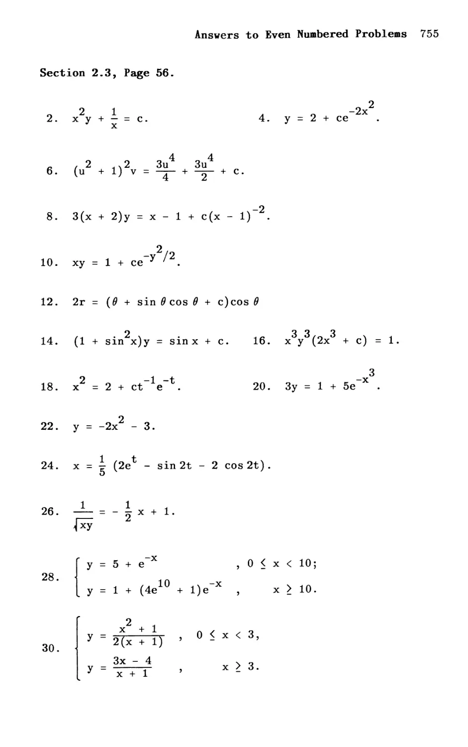
Section 2.3, Page 56
The equations of Exercises 1 through 14 are linear. In
solving, first express the equation in the standard form
of equation (2.26) and then follow the procedure of
Example 2.14.
38 Chapter 2
1. The D.E. is already ln the standard form (2.26), with P(x)
= 3/x, Q(x) = 6x 2 . An I.F. is eJP(x)dx = e J (3/x)dx =
3
e3lnlxl = elnlxl = Ixl 3 = *x 3 (+ if x 0, - if x < 0).
Ve multiply the D.E. through by this I.F. to obtain x3
3 2 6 5 d ( 3 ) 5 I . b . 3
+ x = x or dx x y = 6x. ntegratlng, we 0 taln x y
6 3-3
= x + e or y = x + ex
3. The D.E. is already in the standard form (2.26), wih P(x)
= 3, Q(x) = 3x 2 e -3x. An I.F. is e J P(x) dx = eJ 3 dx = e 3x
Ye multiply the D.E. through by the I.F. to obtain
3x dy 3 3x 3x 2
e dx + e y =
d (3X) 2 Integrating we obtain 3x 3
or - e y = 3x . e y = x + e
dx
y = (x 3 + ) -3x
or e e .
6.
2
This equation is linear in v. Ye divide through by u + 1
dv 4u 3u
to put it in the standard form du + 2 v = 2
u + 1 u + 1
with P(u) =
4u
and Q(u) =
u 2 + 1
3u
u 2 + 1
An I.F. lS
eJP(u)du =
f 4u
exp 2
u +
du
1
= e 2ln(u 2 +1) =
2 2
(u + 1) .
Ye multiply the standard form equation through by this to
. ( 2 2 dv 2 2
obtaln u + 1) du + 4u(u + l)v = 3u(u + 1) or
d 2 2 3
du [(u + 1) v] = 3u + 3u. Integrating, we obtain
2 2 3u 4 3u 2
(u + 1) v = + 2 + e.
First-Order Equations 39
7.
dy 2x + 1
Ye first divide through by x to obtain dx + 2 y =
x + x
x - 1
x
h P( ) 2x 2 + 1 and Q(x) - _ x X - 1
were x =
x + x
An I.F. lS
eJp(x)dx = exp[ : : : dX) = elnlx2+xl = Ix 2 + xl = * (x 2
+ x) (+ if x < -lor x > 0, - if -1 < x < 0). In any
case, upon multiplying the standard form equation through
by the I. F., we obtain (x 2 + x) + (2x + 1) y = (x +
l)(x - 1) 2 dy (2x + 1) 2 - 1 that
or (x + x) dx + y = x , lS,
d 2 2 Integrating, we find 2 x)y
dx [( x + x) Y ] = x - 1. (x + =
323
x /3 - x + c/3 or 3(x + x)y = x - 3x + c.
8.
2
Ye first divide through by x + x - 2 to put the equation
th t d d f dy 3(x + 1) 1 U here
ln e s an ar orm dx + (x + 2 ) (x - 1) Y = x + 2' "
3 ( x + 1 ) d 1
P(x) = (x + 2)(x _ 1) an Q(x) = x + 2 . An I.F. lS
J P ( x ) dx _ r [ 3 ( x + 1) ] d =
e - exp J ( x + 2) (x _ 1) x
elnlx+21+21nlx-11 = Ix + 21(x - 1)2 = *(x + 2)(x - 1)2,
(+ if x -2, - if x -2), where partial fractions have
been used to perform the integration. In either case (x >
-2 or x -2), upon multiplying the standard form equation
through by the 1. F ., we obtain (x + 2)(x - 1) 2 +
3(x + l)(x - l)y = (x - 1)2, that is, d: [(x + 2)(x -1)2yJ
= (x - 1)2. Integrating, we find (x + 2)(x - 1)2y =
3
{x -3 1) + 0 r 3 ( x + 2) Y = x - 1 + c (x - 1) - 2 .
40 Chapter 2
9. Ye first put the equation in the form
dy xy + y - 1 =
dx + x 0,
and then ln the standard form
+ (1 + ; )y = ; ,
where P(x) = 1 + l/x and Q(x) = l/x. An I.F. 18 eJP(x)dx
= e(1+1/x) dx = eX+lnlxl = Ixle x = * xe x , (+ if x 0,
- if x < 0). In either case, we multiply the standard
form equation through by the I.F. and obtain
x dy x x
xe dy + (x + 1) e y = e
d x x x x
or dx [x e yJ = e. Integrating, we find x e y = e + c
-1 -x
or y = x (1 + c e ).
10. This D.E. is linear ln x (like Example 2.16). We divide
through by y and dy to put it in the standard form
2
dx xy
dy +
+ x
y
- y
= 0,
dx
or - +
dy
I. F. is
(y + ) x = 1, where P(y)
1
- y + y '
Q(y) = 1.
An
2 2
eJP(y)dy = e J (y+1/y)dy = e Y /2+1nlyl = lyle Y /2 =
2/2
:I: ye y (+ if y 0; - if y < 0). Mul t iplying the
standard form equation through by this, we obtain
First-Order Equations 41
y2/2 dx 2 y2/2
ye dy + (y + l)e x
2 / 2
= ye Y
d 2/2
or dy (ye Y x) =
2 / 2
e Y + e or xy =
2 / 2
ye Y
2/2
Integrating, we find ye Y x-
2 / 2
1 + ee- y .
12. This D.E. lS linear in r. Ye first divide through by dO
b 0 0 dr 0 fj 4 0 0 0 dr
to 0 taln eos dO + r Sln u - eos = or eos dO +
r sin 0 = eos 4 0 . Next we di vide through by eos 0 to put
dr 3
the equation ln the standard form dO + (tan 0) r = eos 0,
where P(O) = tan 0 and Q(O) = eos 3 0. An I.F. is
e J P ( 0) dO = e J t an 0 d 0 = e In I see 0 I = I see 0 I = * see 0 ( +
O f 4k - 1 0 4k + 1 f . k d 1 . f
1 2 1r < < 2 1r 0 r some 1 n t eger , an -
4k + 1 4k + 3 0
2 1r < () < 2 1r for some lnteger k). In any case,
upon multiplying the standard form equation through by the
I.F., we obtain seeO + (seeOtanO)r = eos 2 0, that is,
d 2
dO [1" see OJ = eos O. Upon integrat ing, we find r see 0
= 0 + sin 20 + cO' where the right-side was integrated
as follows: f eos 2 0 d 0 = f 1 + e 2 0s 2 0 d 0 = 0 + sin 20.
Substituting 2 sin () eos 0 for sin 2 (), the solutions may be
expressed as r see 0 = 0 + sin 0 eos 0 + cO' Finally, we
mul t iply through by 2 eos () to obtain
2r = (0 + sin Oeos ()+ e)eos 0, where e = 2e O .
42 Chapter 2
13. Ye first put the D.E. in the form
(1 + sin x ) + (cos x)y =
2
cos x,
and then ln the standard form
dy cos x
dx + 1 + sin x
2
cos x
Y = 1 + sin x '
where P(x)
cox x
=
1 + sin x '
Q(x) = 1
2
cos x
+ Sln x
An I.F. lS
f cos x dx
/P(x)dx 1 + sin x Inl1+sinx I 11 + sin x I = 1
e = e = e =
+ sin x , since 1 + Sln x > o. Multiply the standard form
equation through by this, to obtain
( 1 + s in x ) + (cos x ) y =
2
cos x,
which is in fact the form preceding the standard form. Ye
observe that this is d: [(1 + sin x )y] = cos 2 x.
x sin 2x
Integrating we obtain (1 + sin x)y = 2 + 4 + c 1 or
2(1 + sinx)y = x + sinxcosx + c, where c = 2c 1 and we
have employed double-angle formulas.
14. This D.E. lS linear ln y. We first divide through by dy
to obtain y sin 2x - cos x + (1 + sin 2 x) = 0 or
( 1 . 2 ) dy ( . 2 ) N d . . d
+ Sln x dx + Sln x y = cos x . ext we lVl e
through by 1 + sin 2 x to put the equation in the standard
First-Order Equations 43
form +
1
sin 2x
o 2
+ Sln x
y =
cos x where P ( x ) =
o 2 '
1 + Sln x
sin 2x
1 . 2
+ Sln x
and Q(x) =
COS x
1 02
+ Sln x
An I. F. i S
eJP(x)dx =
exp
[ f sin 2.X 2 dX ] = exp
1 + Sln x
[ f 2 s in x .co 2 s x dx ]
1 + Sln x
e ln (1+sin 2 x) _ _ 1 2
= + sin x. Upon multiplying
the standard form equation through by the I.F., we obtain
(1 + sin 2 x) + (sin 2x)y = cos x, that lS,
d: [(1 + sin 2 x)y] = cos x. Integrating, we find
(1 + sin 2 x)y = sin x + c.
15. This lS a Bernoulli D.E., where n = 2. Ye multiply
-2 -2 dv 1 -1 1
through by y to obtain y - x y - - x Let
l-n -1 dv -2
v = y = y ; then dx = -y dx. The preceeding D. E.
d O l f 0 h 1 0 . dv 1 1
rea 1 y trans orms lnto t e lnear equatlon - d + - v =
x x x
An I.F. lS e Jdx / x = elnlxl = Ixl = * x. Multiplying
through by this, we find x : + v = 1 or d: (xv) = 1.
-1
Integrating, we find xv = x + c, from which v = 1 + cx
But v = l/y. Thus we obtain the solution in the form l/y
= 1 + cx- 1 .
18.
This is a Bernoulli D.E. in the dependent variable x and
independent variable t, where n = -1. Ye multiply tprough
o dx t + 1 2 t + 1 1- n
by x to obtaln x dt + 2t x = t Let v = x
2 dv dx
x ; then dt = 2x dt . The preceeding D. E. readily
=
44 Chapter 2
t f . h 1 . . dv
rans orms lnto t e lnear equatlon dt +
t + 1
t v =
t + 1 dt
2( t; 1 ). An I.F. is ef 1 = et+lnltl = It let
= * t e t. Multiplying through by this, we find t e t +
t t d t t
(t + 1) e v = 2 (t + 1) e or dt [t e v J = 2 (t + 1) e .
I . b . t 2 t 2
ntegrat lng, we 0 taln t e v = t e + c or v = +
c t -1 e -t. But v = x 2 . Thus we obtain the solution ln
2 -1 -t
the form x = 2 + c t e .
The equations of Exercises 19 through 24 are linear.
21.
x
Ye divide thru by (e + 1) and dx to put ln the form
x x -1 x dy
e [y(e + 1) - 3(e + l)J + dx = 0 and thence in the
standard form
dy
- +
dx
x
e
= 3e x (e x + 1),
y
eX + 1
where P(x) =
x
e
, Q(x)
- 3e x (e x + 1).
An I.F. lS
JP(x)dx
e
x
e + 1
x
= exp f x e
e +
x
dx = e 1 n (e + 1 ) = eX + 1.
1
Ye
multiply
obtaining
d x
dx [( e +
(ex + l)y
the standard form equation through by this,
x dy x x x 2
( e + 1) dx + e y = 3e (e + 1) or
l)yJ = 3e x (e x + 1)2. Integrating, we obtain
x 3
= (e + 1) + c or
x 2 x -1
Y = (e + 1) + c(e + 1). (*)
First-Order Equations 45
Ye apply the I.C. y(O) = 4: Let x = O,y = 4 in (*) to
obtain 4 = 4 + c/2. Thus c = 0, and the particular
x 2
solution of the stated I.V.P. lS Y = (e + 1) .
24. This equation is linear in the dependent variable x with t
as the independent variable, and is already in the
standard form, with pet) = -1, Q (t) = sin 2t. An I.F. lS
eJP(t)dt =
e J (-l)dt =
-t
e
Ye multiply the equation
-t dx -t -t.
through by this to obtain e dt -e x = e Sln 2t or
d -t -t
dt (e x) = e sin2t. Ye next integrate, using
integration by parts twice, or an integral table, on the
right. We obtain
-t -t -Sln 2t - 2 cos 2t
e x = e + c
5
or
- ( sin 2t + 2 cos 2t ) t (* )
x = + ce
5 .
Ye apply the I.C. x(O) = 0: Let t = x = 0 in (*). Ye
obtain 0 = - 1/5(0 + 2) + c from which c = 2/5. Thus the
general solution of the stated I.V.P. is
x =
2 t . 2 2 2
e - Sln t - cos t
5
25. This is a Bernoulli D.E. with n - 3. Ye first multiply
3 3 d y 4 1-n
throu g h b y Y to obtain Y + y - x Now let v = Y
dx 2x - .
= y 4 . Then : = 4 y3 and the preceeding D. E.
46 Chapter 2
transforms into : + 2 v x = x, which is linear In v. In
dv 2
the standard form this linear equation is dx + x v = 4x,
with P(x) = 2/x, Q(x) = 4x. An I.F. is
eJP(x)dx = e J (2/x)dx = e 21n / x / =
2
x .
Ye multiply the standard form through by this to obtain
2 dv 3 d 2 3 .
x dx + 2 x v = 4x or dx (x ) = 4x. Ye lntegrate to
obtain x 2 v = x 4 + c. But v = y4. Hence we obtain the
one-parameter family of solutions of the given Bernoulli
Equation in the form
244
x y = x + c.
(*)
We apply the I.C. y(l) - 2. Let x = 1, Y = 2 ln (*)
-
to obtain 16 = 1 + c, so c = 15. Thus the particular
solution of the stated I.V.P. 2 4 4 + 15.
lS x y = x
26. Ve first wri te the D. E. In the form x + y = x 3 / 2 y3/2
and multiply through by l/x to obtain dy + !. y = x 1 / 2 y3/2.
dx x
Ye recognlze this D.E. as a Bernoulli D.E. with n = 3/2.
Ve now multiply through by y -3/2 to obtain y -3/2 +
1 -1 / 2 1/2 1-n -1 / 2
x y = x · Now let v = y = y . Then
: = - ; Y -3/2 and the preceeding D.E. transforms into
-2 dv
dx
1
+ -v
x
1/2 h . h . 1 . .
= x , W lC IS lnear In v.
In the standard
First-Order Equations 47
dv ( - 2x 1 ) V = x1/2
form this linear D.E. lS dx + 2 ' with P(x) =
x 1 / 2 An I F . JP(x)dx _ J(- 1/2x)dx =
2 . . . lS e - e
1 1 I 1 -1/2
-1 / 21n x In x 1 1 -1 / 2 -1 / 2
e = e = x = x (assuming x >
0). We multiply the standard form through by this I.F. to
b . -1 /2 d v 1 _ 1 d ( -1 /2 ) 1 T.T
o ta1n x dx - 2x 3 / 2 v - - 2 or dx x v = - 2 ' "e
-1/2 1 -1/2
integrate to obtain x v = - 2 x + c. But v = Y .
1
- 2x '
Q(x) =
Hence we obtain the one-parameter family of solutions of
-1/2 -1/2
the glven Bernoulli equation in the form x y =
1
2 x + c or
1
fXY
1
=- 2 x + c
(*)
We apply the I.C. y(l) = 4.
b . 1 1 1
to 0 taln 2 = - 2 + c, so c = ·
Let x = 1, Y = 4 in (*)
Thus the particular
solution of the stated I.V.P. lS
1
fXY
1
= - 2x + 1.
27. Here we actually have two I.V. problems:
(I) For 0 < x < 1 , (II) For x > 1 ,
dy y = 2, dy y = 0,
- + - +
dx dx
y(O) = 0, Y (1) = a,
where a is the value of lim (x) and denotes the
x-+1-
solution of (I). This is prescribed so that the solution
of the entire problem will be continuous at x = 1.
48 Chapter 2
We first solve (I). The D.E. of this problem 1S
linear in standard form with P(x) = 1, Q(x) = 2. An I.F.
is eJP(x)dx = e J (l)dx = eX. Ve multiply the D.E. of (I)
h h b h . b . x dy x x d [ X J
t roug y t lS to 0 taln e dx + e y = 2e or dx e y =
2e x . We integrate to obtain eXy = 2e x + c or y = 2 +
-x
ce We apply the I.C. of (I), y(O) = 0, to this,
obtaining 0 = 2 + c or c = -2. Thus the particular
-x
solution of problem (I) is y = 2 - 2e . This is valid
for 0 < x < 1.
Letting denote the solution just obtained, we note
that lim (x) = lim (2 - 2e- x ) = 2 - 2e- 1 . This is the
x-+1 x-+1
a of Problem (II); that lS, the I.C. of (II) is y(l) =
2 - 2e- 1 .
Now solve (II). The D.E. of this problem is linear lS
standard form with P(x) = 1, Q(x) = o. An I.F., as ln
x
problem (I), is e. We multiply through by this to obtain
x dy x d x
e dx + e y = 0 or dx (e y) = o. Ye integrate to obtain
eXy = c or y = c e -x Now apply the I. C. of (II), y (1) =
2 - 2e- 1 , to this. Let x = 1, Y = 2 - 2e- 1 . We obtain
2 - 2e- 1 = c e- 1 , from which c = 2e - 2. Thus the
particular solution of problem (II) is y = (2e - 2)e- x .
This is valid for x > 1.
We write the solution of the entire problem, showing
intervals where each part is valid, as
2(1 - e- x ), 0 < x < 1,
y =
-x
2(e - l)e , x 1
First-Order Equations 49
29. As ln Exercise 27, we actually have two I.V. problems:
(I) For 0 < x < 2, (II) For x 2,
dy -x dy -2
- + y = e , - + y = e
dx dx
y(O) = 1 , y(2) = a,
where a is the value of lim (x) and denotes the
x 2
solution of (I). This is prescribed so that the solution
of the entire problem will be continuous at x = 2.
We first solve (I). The D.E. of this problem is
linear in standard form with P(x) = 1, Q(x) = e- x An
. fP(x)dx f(l)dx x .
I.F. lS e = e = e. We multlply the D.E. of
(I) through by this to obtain eX + eXy = 1 or d: (eXy)
x -x
= 1. Integrating we obtain e y = x + c or y = e (x + c).
We apply the I.C. of (I), y(O) = 1 to this, obtaining 1 =
o + c, or c = 1. Thus the particular solution of problem
(I) is y = e-x(x + 1). This is valid for 0 < x < 2.
lim
x 2
Letting denote the solution just obtained, we find
-x -2
;(x) = lim e (x + 1) = 3e . This is the a of
x-+2
Problem (II); that lS,
-2
the I.C. of (II) is y(2) = 3e .
Now solve (II). The D.E. of this problem is linear in
-2
standard form with P(x) = 1, Q(x) = e . An I.F., as in
Problem (I), is eX. We multiply through by this to obtain
x dy x x-2 d x x-2
e dx + e y = e or dx [e yJ = e · We integrate to
50 Chapter 2
obtain x x-2 -x x-2 c) -x
e y = e + c or y = e (e + or y = ce +
-2 Now apply the I.C. of (II) , y(2) 3e -2 to this.
e = ,
Let x 2, -2 We obtain 3e -2 -2 -2 from
= y = 3e . = ce + e ,
which c = 2. Thus the particular solution of problem (II)
-x -2
is y = 2e + e This is valid for x > 2.
Ye write the solution of the entire problem, showing
intervals where each part lS valid, as
-x
e (x + 1),
o < x < 2 ,
y =
-x -2
2e + e ,
x > 2
30. As in Exercises 27 and 29, we actually have two I.V.
problems:
(I) For o < x < 3, (II) For x 3,
(x + 1) dy y (x + 1) dy y 3,
- + = x, - + =
dx dx
y(O) = 1/2. y(3) = a,
where a is the value of lim (x) and denotes the
x-+3
solution of (I). This is prescribed so that the solution
of the entire problem will be continuous at x = 3.
We first solve (I). Ye first express the D.E. ln the
standard form d d x Y + 1 Y = x l ' where P(x)
x + 1 x +
= l/(x + 1), Q(x) = x/ex + 1). An I.F. is eJP(x)dx =
e Jdx/x+1 - - e ln l x+1 1 _ - Ix + 11 .
Since x + 1 1 > 0 ln
(I), we have Ix + 11 = x + 1. Ye multiply the standard
First-Order Equations 51
form equation through by this to obtain (x + 1) + Y = x,
which turns out to be exactly the equation that we started
with. Ve note that this is d [(x + l)yJ = x.
2
Integrating we obtain (x + l)y = x /2 + c. Applying the
I.C. y(O) = 1/2, we obtain c = 1/2. Thus the particular
1 2
solution of Problem (I) is (x + l)y = 2 (x + 1) or
y -
2
x +
2(x +
1
1) .
This is valid for 0 < x < 3.
Letting denote the solution just obtained, we find
2 )] 5
lim (x) = 1. [x + This the a of Problem
1m _ 2(x + = 4 . lS
x 3 x 3
(II) ; that is, the I.C. of (II) lS y(3) = 5/4.
Now solve (II). We put the D.E. ln standard form
dy + 1 3 and find, as ln Problem (I), that an
dx x + 1 y = x + 1
I.F. lS (x + 1). We multiply the standard form equation
through by this to obtain (x + 1) + y = 3, which 18
exactly what we started with here ln Problem (II). We
d
note that this is dx [(x + l)yJ = 3. Integrating we
obtain (x + l)y = 3x + c.
we obtain 5 = 9 + c or c =
Applying the I.C. y(3) = 5/4,
-4. Thus the particular
solution of Problem (II) is (x + l)y = 3x - 4 or
3x - 4
Y This is valid for x > 3
= x + 1 . .
The solution of the entire problem lS
52 Chapter 2
x 2 + 1
2(x + 1)'
o < x < 3,
y =
3x - 4
x + 1 '
x > 3
31. (a) The D.E. is linear. In the standard form it is dy
- +
dx
b k - x with P(x) b Q(x) k - x An I.F.
-y = - e = a ' = - e
a a a
. fP(x)dx f(b/a)dx (b/a)x Multiplying the
lS e = e = e .
standard form equation through by this, we obtain
e (b/a)x dy + b e (b/a)x y = k e (b/a- )x
dx a a
d [e (b/a)x yJ
or dx
= k e(b/a- )x.
a
(1)
Ve now consider two cases: (i) f ; and (ii) =
In case (i), where f b , integrating (1) we obtain
a
e (b/a)x y = : ( _ r 1 e (b/a- )x + c or
y =
- x
ke
b - a
-bx/a
+ ce .
(2)
b d (b/a)x
In case (ii), where = a ' (1) becomes dx [e yJ -
k Integrating, we obtain e(b/a)x y = kx + c or
a a
k -bx/a
x e
y =
-bx/a
+ ce .
(3)
a
First-Order Equations 53
(b) Suppose = o.
Then since b > 0 we can have onl y
a '
case (i), * b , here. Then with = 0, (2) becomes y
a
= + ce -bx/a. As x !D, e -bx/a 0 and y .
Suppose > o. Then either case (i) or case (ii)
can occur. In case (i), y is given by (2); and since
e- x 0 and e- bx / a 0 as x CD, we have y 0 as
x CD. In case (ii), y is given by (3); and since
-bx/a 0 -bx/a
xe and e 0 as x CD , we again have y 0
as x m .
33. (a) The function f such that f(x) = 0 for all x E I has
derivative f'ex) = 0 for all x E I. We substitute
this f(x) for you and f'(x) for in the D.E. Ve
obtain f/(x) + P(x)f(x) = 0 + P(x)O = 0 for all x E I,
so f(x) is a solution.
(b) By the Theorem 1.1, there is a unlque solution f of
the D.E. satisfying the I.C. f(x O ) = 0, where Xo E I.
By (a), ;(x) = 0 for all x E I is a solution of the
D.E. and obviously it satisfies the I.C. Thus by the
uniqueness of Theorem 1.1, we must have f(x) = ;(x),
that is, f(x) = 0 for all x E I.
(c) Since f and g are solutions of the D.E., so is their
difference h = f - g (by Exercise 32(a)). Also h(x O )
= f(x O ) - g(x O ) = o. So h is a solution such that
h(x O ) = 0 for some Xo E I. By part (b), hex) = 0 for
all x E I. But this means f(x) - g(x) = 0 and hence
f(x) = g(x) for all x E I.
54 Chapter 2
34. (a) Since f lS a solution of (A),
f'(x) + P(x)f(x) = Q(x).
(1)
Since g lS a solution of (A),
g'(x) + P(x)g(x) = Q(x).
(2)
Then, subtracting (2) from (1), we have
f/(X) + P(x)f(x) - g'(x) - P(x)g(x) = Q(x) - Q(x)
or
f'(x) - g'(x) + P(x) [f(x) - g(x)J = 0
or, finally,
[f(x) - g(X)J' + P(x) [f(x) - g(x)J = o.
This shows that f - g is a solution of the D.E.
dy
dx + P(x)y = O.
(b) Since f lS a solution of Equation (A), we have
f'(x) + P(x)f(x) = Q(x).
(3)
By part (a), since f and g are solutions of (A), their
difference f - g is a solution of dy/dx + P(x)y = O.
Thus we have
[f(x) - g(x)J' + P(x) [f(x) - g(x)J = o.
First-Order Equations 55
Multiplying this by c, where C lS an arbitrary
constant, we have
c[f(x) - g(x)J' + cP(x) [f(x) - g(x)J = o. (4)
Adding (3) and (4), we have
{f'(x) + P(x)f(x)} + {c[f(x) - g(x)J'
+ cP(x) [f(x) - g(x)J} = Q(x).
Rearranging terms, this takes the form
{c[f(x) - g(x)J' + f'(x)}
+ P(x){c[f(x) - g(x)J + f(x)} = Q (x) .
or
{c[f(x) - g(x)J + f(x)}'
+ P(x){c[f(x) - g(x)J + f(x)} = P(x).
We see from this that c(f - g) + f satisfies equation
(A). That is, since c is an arbitrary constant,
c(f - g) + f is a one-parameter family of solutions of
(A) .
37. (a) This is of the form (2.41) with fey) = Sln y, P(x) =
1
- , an d Q (x) = 1. Ye 1 et v = f (y ) = sin y , from w hi ch
x
dv _ dy
dx - (cos Y ) dx . Substituting this into the stated
D E o b dv 1 1 h 0 h 0 1 0 0
· ., lt ecomes - d + -v = , W lC lS lnear ln v.
x x
An I.F. is eJP(x)dx = e J (l/x)dx = elnlxl = Ixl.
56 Chapter 2
Multiplying the linear equation through by this, we
have x : + v = x or d: (xv) = x. Integrating, we
2 2
find xv = x 2 + cO' or 2xv = x + c, where c = 2c O .
Now replacing v by Sln y, we obtain the solution in
2
the form 2x sin y - x = c.
40. This 18 a Riccati Equation of the form (A) of Exercise 38,
with A(x) = -1, B(x) = x, C(x) = 1. The solution f(x) = x
is given. By Exercise 38(b), we make the transformation y
= f(x) 1 1 from which dy = 1 ( ) dV
+ - = x + - -
v v' dx 2 dx.
v
Substituting ln the given D.E., it takes the form
1 dv
1 - 2" dx =
v
(x + )2 + x(x + ) + 1.
1 dv
This reduces to - -- -- =
2 dx
v
1
- -- -
2
v
x dv
or -- - xv = 1, which
v dx
is linear in v, with P(x) = -x, Q(x) = 1. An I.F. is
fP(x)dx _ f(-x)dx _ -x2/2
e - e - e . Multiplying the linear D.E.
through by this, we obtain
_x2/2 dv -x2/2
e dx - e x v =
2
-x /2
e
or
2
d: (e- X /2 v ) =
2
-x /2
e .
2 2
Integrating, we obtain e -x /2v = f e -x /2 dx + c. Since
the integral on the right cannot be expressed as a finite
sum of known elementary functions, we leave it as
First-Order Equations 57
indicated..
1
But from the transformation y = x + v ' we see
that v =
1
(y - x).
We replace v accordingly and thus
obtain the solution,
2
-x /2
e
y - x
2
= f e -x /2 dx + c.
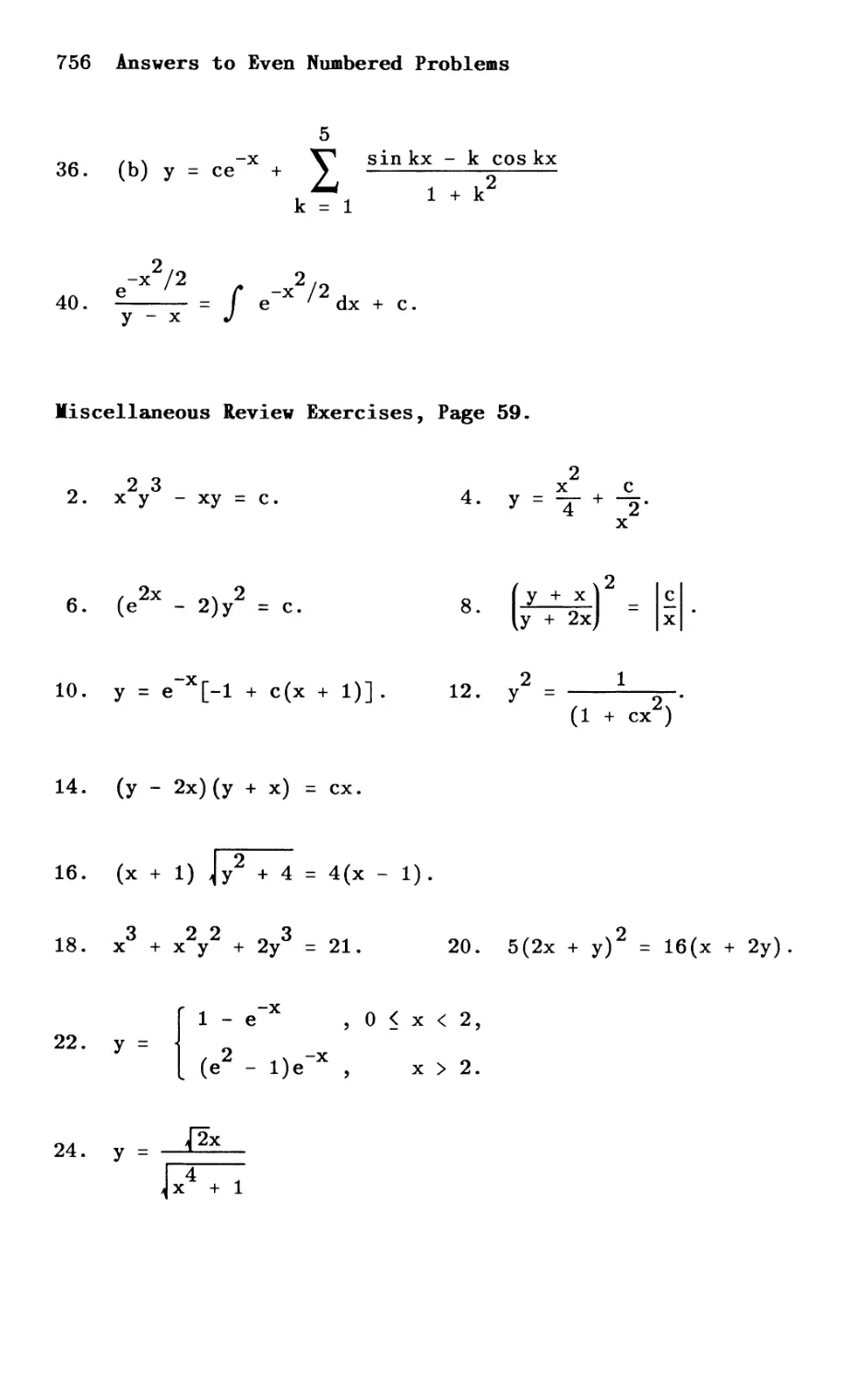
Section 2.3, Miscellaneous Review Exercises, Page 59
The solution of each of these review problems 1S
given, but most of these solutions are presented 1n
abbreviated form with many details omitted.
1. The D.E. is both separable and linear. Upon separating
variables and integrating, we obtain 2 In (x 3 + 1) + In I c I
= Inlyl, from which we find y = c(x 3 + 1)2.
The solution as a linear equation lS almost as easy.
3 -2
The I.F. is (x + 1) .
2.
The D.E. lS exact. We seek F(x,y) such that F (x,y) =
x
M(x,y) = 2xy3 - y and F (x,y) = N(x,y) = 3x 2 y2 - x.
y
2 3
the first of these, we find F(x,y) = x y -
From this F (x,y) = 3x 2 y2 - x + '(y). But
y
= N(x,y) = 3x 2 y2
2 3
F(x,y) = x Y
2 3
x y - xy = c.
From
xy + (y).
since F (x,y)
y
find '(y) = 0, (y) = cO. Thus
x, we
xy + cO' and the family of solutions lS
58 Chapter 2
3. The D.E. is both separable and linear. First consider it
as a separable equation. Upon separating variables and
using partial fractions (preparatory to integrating), we
+ dy - 0 Integrat ion gives In I x 1 -
y - 1 - .
11 = In c 1 . Upon simplifying and
find Ix(y - 1)1 = IC 1 (x + 1)1.
find [ - 1 l]dX
x +
lnlx + 11 + lnly -
taking antilogs, we
Assuming x > 0, y > 1 and simplifying, we can write this
as xy = c x + (c - 1), or xy + 1 = c (x + 1), where
c = 1 + c 1 .
Alternately, consider the D.E. as a linear equation.
The I.F. [ x (x d: 1) ] = % x Multiplying the
lS exp 1 .
x +
I' standard form" of the D.E. through by this we have
[ xy ]' = (x + 1)-2. Integrating, we find xy =
x + 1 x + 1
-1 this we find xy + 1 = c(x + 1) ,
-(x + 1) + c. From as
before.
4. The D.E. is linear. The I.F. is x. Multiplying the
"standard form" of the equation through by this, we find
2 3 2 3
x y' + 2xy = x and hence (x y)' = x. Integration and
2
simplification at once give y = x 4 + .
x
5.
Writin g the D.E. ln the form dy
dx
5 [ 1 - 3
= ,
1 + y
x
we recognlze
that it lS homogeneous. We let y = vx. Then the D.E.
dv 5v - 3
becomes v + x - d = 1 . Simplification yields
x + v
First-Order Equations 59
(v + l)dv
v 2 - 4v + 3
to the left member, we find
-dx
x
Then upon applying partial fractions
=
[- v 1 +
v -
2 3 ]dV = - :
Integration glves -lnlv - 11 + 2ln Iv - 31 = -lnlxl +
Inlc/. Simplification and taking of antilogarthims
2
i v - 3 ) _ c y
results ln l v _ 11 - x But v - x Upon
resubstituting accordingly and simplifying, we find
(3x - y)2 = Ic(y - x)l.
6. The D.E. lS exact, separable, and linear. Considered as
an exact equation, we seek F(x,y) such that F (x,y) =
x
M(x,y) 2x 2 and F (x,y) = N(x,y) 2x Y - 2y. From the
= e y = e
y
2
first of these, we find F(x,y) 2x y (y) . From
= e - +
2
this, F (x,y) = e 2x y2 + '(y). But since F (x,y) = N(x,y)
y y
= e 2x y _ 2y, we find '(y) = -2y, (y) = _y2 + cO' Thus
2x 2 2
F(x,y) e y and the family of solutions
= y + cO' lS
2
2x 2 2y2 [ where we have set F(x,y)
e y = c = c ,
, 1
multiplied through by 2, and let c = 2(c 1 - cO)].
Assuming e 2x - 2 0, this can also be written as y =
c 2 (e 2x - 2)-1/2 where c 2 = JC.
We also consider the D.E. as a linear equation. We
.. ( 2x 2) ' 2x 0 d th t .
rewrlte It as e - y + e y = an en pu It ln
2x 2x
the "standard form" y' + e yj(e - 2) = o. From this we
60 Chapter 2
find the I.F. is (e 2x - 2)1/2, where we assume e 2x - 2 >
O. Multiplying the standard form through by the I.F., we
f o d ( 2x 2) 1/2 I 2x ( 2x 2) -1/2
ln e - y + eye - = 0 or
[(e 2x _ 2)1/2yJI = O. Integration and simplification
readily yield y = c(e 2x _ 2)-1/2.
7. The D.E. is both separable and linear. We first solve
this as a separable equation. Separating variables, we
h 4x3dx dy 4
ave 4 + 2 3 = O. Integration yields In(x + 1) +
x + 1 y -
1
2 1n 12y - 31 = Inl c 1 1. Simplify, assumlng 2y - 3 0, to
obtain In(x 4 + 1)(2y - 3)1/2 = Inl c 1 1. From this we at
422
once have (x + 1) (2y - 3) = c 1 . Then y = 3/2 +
2
4 -2 c 1
c(x + 1) , where c = 2 ·
Consider the D.E. as a linear equation. In standard
3 3
8x y _ 12x
form the D.E. is y' + 4 - 4 . The I.F. is
x + 1 x + 1
4 2
(x + 1) . Multiplying the standard form equation through
by this we find [(x 4 + 1)2yJ' = (x 4 + 1) (12x 3 ).
I t t o d d o . ° b ( 4 1) 2 h ° 3
negra lon an lV1Slon y x + t en glve y = 2 +
4 -2
c (x + 1) .
8. Vriting the D.E. in the form =
I 2 + + [ P L we
2 '
see that the D.E. is homogeneous. Let y = vx. Then =
dv dv v v 2
v + x dx ' and the D.E. becomes v + x dx = -1 - 2 - 2.
First-Order Equations 61
2
S . l . f . t . . ld dv - (v + 3v + 2) and hence
lmp 1 lca lon Yle s x dx - - 2 '
2 dv dx
= - -- Use of partial fractions glves
v 2 + 3v + 2 x
2 [ 1
v + 1
v 2 ]dV =
dx
x
Integration and immediate
simplification 2 In v + 1 In c Further
glve = -
v + 2 x
1 2
silJlplification v + c But = y
glves = - v .
v + 2 x x
Resubstituting accordingly and again simplifying, we
2
obtain [ : ++ 2: ] =
9.
322
Rewriting the D.E. 1n the form (4x y - 3x y)dx +
(2x 4 y - x 3 )dy = 0, we find that it is exact. Ve
322
F(x,y) such that F (x,y) = M(x,y) = 4x y - 3x y
x
F (x,y) = N(x,y) = 2x 4 y - x 3
Y
F(x,y) = x 4 y2 _ x 3 y + (y).
x 3 + ;'(y). But since F (x,y) = N(x,y) =
y
seek
and
From the first of these,
4
From this, F (x,y) = 2x Y -
Y
4 3
2x y - x , we
must have '(y) = 0, (y) = cO. Thus F(x,y)
+ cO' and the solution is x 4 y2 - x 3 y = c.
423
= x Y - x Y
10.
The D.E. is linear.
The standard form is y' + xy
x + 1
=
e -x(x + 1), and the I. F. is % eX (x + 1). Mul tiplying the
standard form through by this, we obtain the equivalent of
x '
[ x e + Y l ] = (x + 1)-2. Integration and multiplication by
(x + l)e- x result in y = e- x [-l + c(x + l)J.
62 Chapter 2
, ..
11 .
Vritin g the D.E. ln the form dy =
dx
2 - 7 Y
x
3 Y
x
...
we recognlze
,
- 8
Then dy = v +
dx
that it is homogeneous. Ve let y = vx.
dv
x dx ·
dv
The D.E. becomes v + x- =
dx
2 - 7v
3v - 8.
Simplification
gives (3v - 8)dv =
3v 2 - v - 2
dx
x
Partial fractions decomposition
puts this in the form [ 3V: 2 - v = 1 ] dv = - .
Integration gives 2ln (3v + 2) - In Iv - 11 = - In Ix I +
Inlcl. Simplification and taking of antilogarithms
. c y
results 1n nnrv = X But v = x Resubstituting
2
accordingly and simplifying gIves (3y +22X) . =
x
c
x
2
and hence (2x + 3y) = Ic(y - x)l.
12. The D.E. is a Bernoulli Equation with n = 3. Ve multiply
-3 2 -3 dy -2
through by y to obtain x y dx + xy = x. Let v =
l-n -2. dv _ -3
Y = Y , then dx - -2y dx. The preceeding D. E.
readily transforms into the linear equation dv - 2 v
dx x
2
An I.F.
- J 2 / x dx
lS e =
1
2.
x
Multiplying through by
=
x
this, we obtain d: [ :2] = - :3 ' Integrating, we find X =
1 -2 2
+ c. Replacing v by y and simplifying, we find y
x
=
1
2.
1 + cx
First-Order Equations 63
13. This is a linear equation. The standard form is
2 6x2
y' + x y = 3 An I.F. is (x 3 + 1)2. Multiplying
x + 1 x + 1
through by this we obtain [(x 3 + l)yJ' = (x 3 + 1)(6x 2 ).
Integration and division by (x 3 + 1)2 then give the
3 -2
solutions y = 1 + c(x + 1) .
14.
dy
Writing the D.E. ln the form dx =
,. .. 2
2 + y
x
2 Y - 1
x
we recognize
that it is homogeneous. Ve let y = vx. Then = v +
dv
x dx ·
The D.E. becomes v + x :
2 + v 2
=
2v - 1.
Simplification
gives (2v - l)dv =
v 2 - v - 2
dx
x
Integration gives Inlv 2 - v - 21
c
= In -. Taking antilogarithms and simplifying slightly,
x
we obtain 2 - 2 = c/x. But v = y/x. Resubstituting
v - v
accordingly and simplifying, we find 2 2
Y - xy - 2x = cx or
(y - 2x)(y + x) = cx.
15. The D.E. lS both homogeneous and Bernoulli. Ve first
consider it as a homogeneous equation, which form we
,. .. 2
1 + I.
x
recognize by writing it as =
2 Y
x
Ve let y =
vx.
Then = v + x : .
dv
The D.E. becomes v + x dx =
dx
=
- x'
2
1 + v
2v
2vdv
Simplification quickly leads to 2
v - 1
integration glves Inlv 2 - 11 = In c .
x
and then
From this, we
2
readily find v
c
1 = -.
x
simplifying, we find y2
Resubstituting v
2
- x = cx.
= I. and
x
64 Chapter 2
Now apply the initial condition y(l) = 2. Letting x =
1, y = 2, we get 3 = c, and he nce obta in the solution in
the form y2 = x 2 + 3x or y = j x 2 + 3x.
Alternatively, we recognize that the given D.E. is a
Bernoulli equation, with n = -1, by writing in the
dy 2 -1
equivalent form 2x dx - Y = x Y We rewrite this as
and transform
2 2 2 dv dv
Y = x · let v = Y and -- = 2 y .
, dx dx '
the D.E. into the linear equation x - v =
standard form of this lS dv - 1:. v = x, and an
dx x
2xy dy
dx
2
x .
The
I.F.
-1
lS x
Multiplying the standard form equation through by this, we
obtain (x- 1 v)' = 1. Integration then gives x- 1 v = x + c.
Now resubstituting v = y2 and simplifying slightly, we
find y2 = x 2 + cx. Application of the I.C. a gain giv es
the particular solution y2 = x 2 + 3x or y = j x 2 + 3x.
16. The D.E. is both a separate equation and a Bernoulli
Equation. We first solve it as a separable equation.
Separating variables, we get 2 dx 2 + dy = O. We can
1 - x y + 4
use partial fractions or an integral table to integrate
the dx term. Integrating the equation and simplifying
slightly, we find
In 1 + x + In(y2 + 4)1/2 = Inlcl.
1 - x
Further simplification results ln the one-parameter family
of solutions
1(1 + x)(y2 + 4)1/21 = Ic(l - x)l.
First-Order Equations 65
Now apply the I.C. y(3) = O. Letting x = 3, y = 0 in the
preceeding gives 8 = 21cl, so Icl = 4. Substituting this
value of Icl back into the equation of the family of
solutions, we get
1(1 + x)(y2 + 4)1/21 - 41 1 - xl.
Since the initial x value is 3 > 1 , we take x > 1 and 1 -
x < 0, so 11 - xl = x-i. Thus we obtain the particular
solution
2 1/2 4(x - 1).
(x + l)(y + 4) -
-
Alternately, we now solve the given D.E. as a
Bernoulli Equation. We first rewrite it as +
1
2
2 Y
- x
= 8 2 Y -1 , in which we recogn1ze that it 1S indeed a
1 - x
1-n 2
Bernoulli D.E. with n = -1. We thus let v = y = y ,
f . d dv 2 dy d f h D E .
ln dx - y dx ' an trans orm t e . . lnto
dv
- +
dx
4
16
2 v =
1 - x
2'
1 - x
which 18 linear in v, with P(x) =
4 -16
2' Q(x) = 2 .
1 - x 1 - x
eJP(x)dx = eJ4dx/(1-x2) = e 2ln I (l+x)/(l-x) I =
An I.F. is
2
(1 1 _ + x x ) .
Multiplying the linear D.E. through by this, we
obtain
66 Chapter 2
2
d [( + ) y] =
16(1 + x)
3 ·
(1 - x)
To integrate the right member, we note that
16 (1 + x) [ 1 +
(1 - x)3 = -16 - (1 _ x)2
2 3 ] .
(1 - x)
Integrating the D.E., we thus find
( + )2y = -16 [_ 1 1
- x
+ (1 _1 x) 2 ]
+ c,
which readily simplifies into
( 1 + x ) 2y = -16x + c.
1 - x (1 _ x)2
Application of the I.C. x = 3 at y = 0 glves c = 12.
2
Substituting this back and multiplying by (1 - x) , we
obtain (1 + x)2y2 = -16x + 12(1-x). Adding 4(1 + x)2 to
2
both sides of this and simplifying, we find (1 + x)
(y2 + 4) = 16(x - 1)2, from which the solution previously
found is readily obtained.
17. This D.E., with M(x,y) = e 2x y2 - 2x and N(x,y) = e 2x y, lS
2x
exact; for M (x,y) = 2e y = N (x,y). We seek F(x,y) such
y y
that F (x,y) = M(x,y) = e 2x y2 2x and F (x,y) = N(x,y) =
x Y
2
2x 2x Y 2
e y. From the first of these, F(x,y) = e 2 - x +
(y). From this, F (x,y) = e 2x y + /(y). But this must
y
First-Order Equations 67
2x
equal N(x,y) = e y. Thus we must have ;'(y) = 0 and
2
2x y 2
hence ;(y) = cO' Thus F(x,y) = e - x + cO; and from
2
2x y 2
this the solution F(x,y) = c 1 take the form e - x =
c, where c = c 1 - cO. Now apply the given I.C. y(O) = 2
to this. Thus letting x = 0, y = 2, we find c = 2. Thus
2x 2 2 2 2x 2
obtain the solution y
we e - - x = 2 or y e = 2x + 4
2
finally, -x 2 + 4)1/2.
or, y = e (2x
18.
This D.E., with M(x,y) = 3x 2 + 2xy2 and N(x,y)
2
+ 6y , is exact; for M (x,y) = 4xy = N (x,y).
y x
2 2
F(x,y) such that F (x,y) = M(x,y) = 3x + 2xy
x
2 2
= N(x,y) = 2x y + 6y .
x 3 + x 2 y2 + ;(y). From this,
2
= 2x y
We seek
this must equal
2
;'(y) = 6y and
322
x + x y
F (x,y)
Y
2 2
N(x,y) = 2x y + 6y .
hence ;(y) = 2y3 + cO.
and F (x,y)
y
From the first of these, F(x,y) =
= 2x2y + ;(y). But
Thus we must have
Thus F(x,y) =
+ 2y3 + cO; and from this the solutions F(x,y) =
322 3
c 1 take the form x + x y + 2y - c, where c = c 1 - cO.
Applying the I.C. y(1) = 2, we let x = 1, Y = 2, to obtain
322
c = 21. Thus we obtain the solution in the form x + x y
3
+ 2y = 21.
19. This ,D.E. is both a separable equation and a Bernoulli
Equation. We first solve it as a separable D.E., writing
4 y dy dx 2
it as 2 - x Integration then gives 2 In (y + 1) =
y + 1
Inlxl + Inlcl. Simplifying we find In(y2 + 1)2 = Inlcxl
and hence (y2 + 1)2 = Icxl. Applying the I.C. y(2) = 1,
68 Chapter 2
we set x = 2, y = 1 in this to obtain 4 = 21cl and hence
2 2
Icl = 2. Thus we obtain the solution (y + 1) = 21xl.
Since the initial x value lS 2 ) 0, we take x .) 0 and
write the solution as (y2 + 1)2 = 2x. Alternately,
writing the D.E. as 4x - y = y-l we recognize that it
1-n
is a Bernoulli Equation with n = -1. Thus we let v = y
- Y 2 dv = 2 y dy and substitute into the stated e q uation
- , dx dx '
4 dy 2 1 b o. 2 dv 1 dv 1
xy dx = y + , 0 taInIng x dx = v + or dx - 2x v =
1 Th . 0 1 0 0 . h I F - J ( 1 /2x ) dx -1/2
2x · 1 S 1 SIn ear 1 n v, w 1 t .. e = x .
Multiplying the standard form linear equation through by
-3/2
h . f 0 d d ( -1/2 ) - x I 0 b .
t lS, we ln dx x v - 2 ntegratIng, we 0 taln
x- 1 / 2 v = _x-1/2 + c or v = -1 + cx 1 / 2 . But v = y2, so we
have y2 = -1 + cx 1 / 2 . Applying the I.C. y(2) = 1 gives c
= Ii. Thus we obtain the solution y2 = -1 + Ii x 1 / 2 , from
which we readily obtain the solution (y2 + 1)2 = 2x
previously found.
dy 2 + 7 [B
20. Writing the D.E. In the form - we see that
dx - ,
[ ]
2 - 2
dy dv
it is homogeneous. Thus we let y = vx, dx - v + x dx .
dv 2 + 7v dv
The D. E. successi vely reduces to v + x dx = 2 _ 2v ' x dx -
2
2v + 5v + 2
2 - 2v
(2v - 2)dv
2v 2 + 5v + 2
lS separable, with the variables separated. Using partial
2v - 2 2 2
fractions, we find 2 = - 1 + 2 . We
2v + 5v + 2 2v + v +
and
dx
x
This last equation
First-Order Equations 69
thus have [ 2V-: 1 + v : 2 ]dV = - d: Integrating, we
obtain -lnl2v + 11 + 2ln Iv + 21 = -In Ix I + In lei, which
reduces to
2
In (v + 2) = In c
1 2v + 1 r x
2
From this we find f;v++2 r = But v =
resubstituting and simplifying, we find
Y . and
x'
2
(y + 2x) . J l___u_ =
2 · f2Y+XT
x
c
x
(2x + 2 Ie (2y + x) I . Applying the I.C. y (1)
or y) = = 2,
we let x = 1, Y = 2, to obtain 16 = Ic15, from which 1 cl =
16 Replacing I c 1 with this value, and taking x + 2y 0,
5.
2
we express the solution as 5(2x + y) = 16(x + 2y).
21.
This equation is both separable and linear. Treating it
dy x dx
as a separable equation, we have -- - Integrating
y x 2 + 1
then glves 2ln Iyl = In(x 2 + 1) + In Ie/ , which quickly
simplifies to y2 - c(x 2 + 1), with c > o. Applying the
I.C. y(JI5) = 2, we let x = JI5, y - 2, to obtain 16c = 4,
c = . Thus we find the solution y2 = (x 2 ; 1) or y =
(x 2 + 1)1/2
2
Now treating the equation as a linear
equation, we have dy -
dx
x -x
2 Y = O. with P(x) = 2
x + 1 x + 1
70 Chapter 2
2
Q(x) = o. An I.F. is efP(x)dx = e-f[x/(x +l)Jdx =
2
e -(1/2)ln(x +1) _ _ (x 2 -1/2
+ 1) . Multiplying the D.E.
h h b h . b . d [ ( 2 1 ) -1 /2 yJ 0
t roug y t lS, we 0 taln dx x + = ·
Integrating, we find (x 2 + 1)-1/2y = c or y =
c(x 2 + 1)1/2. Applying the I.C. y(J15) = 2 glves c
_ _ ( x2 + 1 } 1/2
Thus we agaln obtain y - 2
1
=
2 .
22. Here we actually have two I.V. problems
(I) For 0 < x < 2, (II) For x 2,
dy y = 1, dy y = 0,
- + - +
dx dx
y(O) - O. y(2) = a.
- , ,
where a is the value of lim ;(x) and ; denotes the
x 2
solution of (I). This is prescribed so that the solution
of the entire problem will be continuous at x = 2.
We first solve (I). The D.E. is linear in standard
form, with P(x) = 1, Q(x) = 1. An I.F. is eJP(x)dx = e Jdx
x
= e. Multiplying the D.E. through by this we obtain
x dy x x d x x
e dx + e y = e or dx (e y) = e. Integrating, we find
x x -x
e y = e + c or y = 1 + ce . Applying the I.C. y(O) = 0
gives 0 = 1 + ceO, c = -1. Hence the solution of Problem
(I) is y = 1 - e- x , valid for 0 x < 2.
First-Order Equations 71
Letting; denote the solution just obtained, we note
that lim ;(x) = lim (1 - e- x ) = 1 - e- 2 This lS the a
x 2 x 2
of problem (II); that is, the I.C. of problem (II) is y(2)
-2
= 1 - e .
We now solve problem (II). The D.E. lS linear in
standard form, with P(x) = 1, Q(x) = o. An I.F., as ln
Problem (I), is eX. Multiplying the D.E. through by this
d . . b . x dy x d ( x )
an lntegratlng, we 0 taln e dx + e y = 0 or dx e y =
x -x
o. Integrating, we find e y = c or y = ce Now apply
-2
the I.C. of problem (II), namely, y(2) = 1 - e . We have
1 - e- 2 = ce- 2 , from which we find c = e 2 - 1. Thus the
solution of problem (II) is y = (e 2 - l)e- x , valid for
x > 2.
We write the solution of the entire problem, showing
intervals where each part lS valid, as
1 -x 0 < 2,
- e x <
y =
(e 2 l)e -x 2.
- , x >
23. Here, as in problem 22, we actually have two I.V.
problems:
(I) For o x < 2, (II) For x > 2,
(x + 2) dy + y - 2x, (x + 2) dy y 4,
- + =
dx - dx
y(O) = 4; y(2) = a;
72 Chapter 2
where a is the value of lim (x) and denotes the
x-+2
solution of (I).
We first solve (I). The D.E. of this problem is
linear. In standard form it dy (x 1 ) 2x with
lS - + 2 y = x + 2
dx +
P(x) 1 Q(x) = 2x An I.F. JP(x)dx
- lS -
- + 2' 2. e -
x x +
e J [1/(x+2)]dx = elnlx+21 = I x + 21. Multiplying the
standard form equation through by this, we obtain
originally stated D.E., (x + 2) + Y = 2x, or
d
dx [(x + 2)yJ = 2x. Integrating, we find (x + 2)y
2
= x + c.
the
Thus the particular solution of Problem (I) IS
2
(x + 2)y = x + 8, valid for 0 < x < 2.
2
x + 8
We can write this solution as y = x + 2 .
Denoting this solution by;, we note that lim ;(x) =
x-+2
2
lim [ x + 8 ] = 3. This lS the a of problem (II) ; that lS
- x + 2
x-+2
the I.C. of problem (II) IS y(2) = 3.
We now solve (II). The D.E. is linear. In standard
form it is + ( x : 2 )y = 4. Just as in (I), an I.F. is
Ix + 21. Multiplying the standard form equation through
by this, we obtain the originally stated D.E.,
( X + 2 ) d dx Y 4 d [ ( 2 ) ] 4 I t t .
+ y = or dx x + Y = . negra lng, we
find (x + 2)y = 4x + c. Applying the I.C. of (II), y(2) =
3, we find c = 4. Thus the particular solution of problem
(I) is (x + 2)y = 4x + 4, valid for x > 2.
First-Order Equations 73
We write the solution of the entire problem as
{ (x + 2)y =
2
- x + 8, 0 x < 2,
(x + 2)y
4x + 4, x > 2.
24. This D.E. is both a Bernoulli D.E. and a homogeneous D.E.
We
We first solve it as a Bernoulli Equation, with n = 3.
-3 .
y , expresslng the D.E. in the
thus multiply through by
equivalent form x 2 y -3 dy
dx
2 1-n
= - . We let v = y
x
-2 = x- 1 or _2 y -3 dy _ 2 Y -2
+ xy dx x
-2 dv -3 dy
- y , d = -2y dx . The D. E.
x
dv
then transforms into the linear D.E. ln v, dx
2
-v =
x
2
- . This linear equation is in standard form with P(x)
x
=
2
x'
2
Q(x) = - .
x
An I.F. is eJP(x)dx = e- J (2/x)dx =
e-2lnlxl = x- 2 Multiplying the linear equation through
-2 dv -3 -5 d -2
by this we get x dx - 2x v = -2x or dx (x v) =
-4
x
-2
Integrating, we find x v =
-2
x
-5
-2x .
2
+ c or v
=2+
2
c x .
But v
-2
= y
-2
thus we obtain y
-2
x 2
= 2 + c x ·
Applying the I.C. y(1) = 1 to this, we find c = 1/2. Thus
-2 2
-2 x x
we obtain the solution y - + , which can be
written as y2 =
2x 2
x 4 + 1
or y -
fix
(x 4 + 1)1/2.
74 Chapter 2
Now we express the D.E. in the form dy = - y + ( y ) 3 and
dx x x
dy
solve it as a homogeneous equation. We let y = vx, dx = v
dv and obtain the transformed separable equation
+ x- v +
dx
dv 3 , which reduces to dv dx We
x- = -v + v =
dx 2 x
v(v - 2)
rewrite the left member, uSlng partial fractions, and thus
have (- 1 v 2 )dV = 2 dx
- + 2
v x
v
I t t 1 I I + .!EJ v 2 2 - 2 L - - 2 In I X I
negra ion glves - n v
+ Inl c 1 1.
This simplifies to
-In v 2 + In I v 2 - 21
4
= In x + In c ,
2
J v - 2 L 4
In 2 = In cx .
v
From this,
224
Iv - 21 = cv x
y 2 2 2 4
Resubstituting v = -, we find Iy - 2x I = cy x .
x
Applying the I.C. y(1) = 1, we find c = 1. Thus we find
the solution 1 y2 - 2x 2 1 = y2 x 4 . Since y2 2x 2 lS
initially -1, we take ly2 - 2x 2 1 = 2x 2 - y2, and write the
.2242 4 222
solutl0n as 2x - y = x y or (x + l)y = 2x or y =
2x 2
as we obtained before.
x 4 + l'
Section 2.4, Page 67
1. This equation is of the form (2.42) of Theorem 2.6 with
M(x,y) = 5xy + 4y2 + 1, N(x,y) = x 2 + 2xy. To apply that
theorem, we first find
First-Order Equations 75
M (x,y) - N (x,y)
y x
N(x,y)
_ 5x + 8y - 2x - 2y =
2
x + 2xy
3(x + 2y) _ 3
x(x + 2y) x
This depends on x only, so
e J (3/x)dx = e31nlxl = elnlxl3 = Ixl 3
lS an I.F. of the given equation. Multiplying the given
equation through by this and simplifying, we find (5x 4 y +
32354
4x y + x )dx + (x + 2x y)dy = O. For this equation
432 3 5 4
M(x,y) = 5x y + 4x y + x , N(x,y) = x + 2x y, and
M (x,y) = 5x 4 + 8x 3 y = N (x,y). Thus this equation is
y x
exact. We seek F(x,y) such that F (x,y) = M(x,y) and
x
F (x,y) = N(x,y). From the first of these, F(x,y)
y
4
jlM(x,y)Ox = jI(5x 4 y + 4x 3 y2 + x 3 )Ox = x 5 y + x 4 y2 + x 4 +
5 4
x + 2x y + ;'(y). But we
;(y). From this, F (x,y) =
y
must have F (x,y) = N(x,y)
y
;(y) = cO.
5 4
= x + 2x y. Thus ;'(y) - 0,
5 4 2 x 4
Hence F(x,y) = x y + x y + + cO. The
family of solutions is then F(x,y) = c 1 ' and multiplying
through by 4 we express this as 4x 5 y + 4x 4 y2 + x 4 = c,
where c = 4(c 1 - cO).
76 Chapter 2
2. This equation lS of the form (2.42) of Theorem 2.6 with
2
M(x,y) = 2x + tan y , N(x,y) = x - x tan y. To apply that
theorem, we use 1 + tan 2 y = sec 2 y and find
N (x,y) - M (x,y)
x Y
M(x,y)
2
_ 1 - 2 x tan y - see y
2 x + tan y
2
- 2 x tan y - tan y
- 2 = - tan y ·
x + tan y
This depends on y only, so e - f tan y dy = e ln I cos y I
= Icosyl is an I.F. of the given equation. We assume
cos y 0, and take I cos y I = cos y . Multiplying the
given equation through by this and simplifying, we find
(2 x cos y + sin y )dx + (x cos y - x 2 sin y )dy = o. For this
equation M(x,y) = 2 x cos y + sin y , N(x,y) = cos y -
x 2 siny, and M (x,y) = -2xsiny + cosy = N (x,y). Thus
y x
this equation is exact. We seek F(x,y) such that F (x,y)
x
= M(x,y)
and F (x,y) = N(x,y). From the first of these
y
= fM(x,y)lJx = f (2 x cos y + sin y )lJx = x 2 cos y +
2 .
= -x Sln y + x cos y +
;(y). From this, F (x,y)
y
But we must have F (x,y) -
y
N (x, y) = x cos y -
F(x,y)
x Sln y +
;' (y) .
x 2 sin y. Thus;' (y) = 0, ;(y) = cO' The family of
solutions is then F(x,y) = c 1 . We express this as
2
x cos y + x sin y = c, when c = c 1 - cO.
4.
This equation lS of the form (2.42) of Theorem
M(x,y) = 2xy2 + y, N(x,y) = 2y3 - x. To apply
M (x,y) - N (x,y)
theorem, we first find y x
N(x,y)
2.6 with
that
= 2(2xy + 1) . but
3 '
2y - x
First-Order Equations 77
slnce this depends on y as well as x, we cannot proceed
N (x,y) - M (x,y) -2 ( 1 + 2xy )
this. Ye next find x y
uSlng M(x,y) = y(l + 2xy)
2 This depends only,
= -- on y so
y
e-J(2/y)dy = e-21nlyl = elnlyl-2 = lyl-2 _
Y
is an I.F. of the gIven equation. Multiplying the glven
equation through by this and simplifying, we find
-1 -2
(2x + y )dx + (2y - xy )dy = O.
-1 -2
For this equation M(x,y) = 2x + Y N(x,y) = 2y - xy
-2
M (x,y) = -y = N (x,y). Thus this equation lS exact.
y x
We seek F(x,y) such that F (x,y) = M(x,y) and F (x,y) =
x Y
N(x,y). From the first of these, F(x,y) = JfM(x,y)ox =
r -1 2 -1
J (2x + y )ax = x + xy + ,(y).
-2
-xy + ,'(y). But we
From this, F (x,y) -
y
must have F (x,y) = N(x,y) =
y
;'(y) = 2y, ;(y) = y2 + cO' Hence F(x,y)
-2
2y - xy
2 -1
= x + xy
Thus
2
+ Y
+ cO.
The family of solutions F(x,y) =
2 -1 2
c 1 is then expressed as x + xy + y = c, where c =
c 1 - cO.
78 Chapter 2
5. We first multiply the stated equation through by xPyq to
obtain (4x p + 1 yq+2 + 6x P yq+1)dx + (5x p + 2 yq+1 + 8x p + 1 yq)dy =
o. For this equation, we have M(x,y) = 4x p + 1 yq+2
P q +1 P +2 q +l P +1 q
+ 6x y , N(x,y) = 5x y + 8x y, My(x,y) =
4(q + 2)x p + 1 yq+1 + 6(q + l)x P yq, and N (x,y) =
x
5(p + 2)x p+1 y q+l 8( ) P q I d f h
+ p + 1 x y. n or er or t e
equation to be exact, we must have M (x,y) = N (x,y), and
y x
hence
6(q + 1)
8(p +
1), that
{ 5p
8p
4q = -2
6q - -2.
-
{ 4(q + 2) =
= 5(p + 2)
lS,
Solving these, we find p = 2, q = 3. Thus the desired
I.F. of the form xPyq is x 2 y3.
Now multiplying the original equation through by this
I.F. x 2 y3, we obtain the equivalent exact equation
3 5 2 4 4 4 33.
(4x y + 6x y )dx + (5x y + 8x y )dy = o. It 1S easy to
check that this is indeed exact. We seek F(x,y) such that
F (x,y) = M(x,y) = 4x 3 y5 + 6x 2 y4 and F (x,y) = N(x,y) =
x Y
4 4 3 3
5x y + 8x y. From the first of these,
F(x,y) = JfM(x,Y)Bx = Jf(4x 3 y5 + 6x 2 y4)Bx
4 5 3 4
= x y + 2x y + ;(y).
From this, F (x,y) = 4 4 3 3 But we must
5x y + 8x y + ;'(y).
Y
have F (x,y) = N(x,y) = 4 4 3 3 Thus ;'(y) = 0,
5x y + 8x y .
y
;(y) Thus F(x,y) 4 5 3 4 and the
= cO. = x y + 2x y + cO'
First-Order Equations 79
solution F(x,y) = c 1 1S x 4 y5 + 2x 3 y4 = c or x 3 y4(xy + 2)
= c, where c = c 1 - cO.
7. For this equation a 1 = 5, b 1 = 2, a 2 = 2, b 2 = 1 , so
a 2 2 f 1 b 2
- = = .
a 1 5 2 b 1
Therefore this 1S Case 1 of Theorem 2.7. Ye make the
transformation
t:
X + h
Y + k,
where (h,k) lS the solution of the system
{ 5h + 2k + 1 = 0
2h + k + 1 = O.
The solution of this system lS h = 1, k = -3 and so the
,
transformation is
t = X + 1
= Y 3.
This reduces the glven equation to the homogeneous
equation
(5X + 2Y)dX + (2X + Y)dY = o.
80 Chapter 2
Ye write this ln the form
dY
dX
5 + 2 y"
X
2 + y
X
..
and let Y = vX to obtain
v + X dv =
dX
5 + 2v
2 + v ·
This reduces to
X dv
dX
2
= 5 - v or (v + 2)dv
2 + v 2
v + 4v + 5
dX
=
- X.
Integrating we find
Inlv 2 + 4v + 51 = -2 In IX I + Inl c 1 1.
or
Inlv 2 + 4v + 51 = In(l c 1 I X - 2 ).
From this, Iv 2 + 4v + 51 = Ic1IX-2.
y
Now replacing v by X '
and simplifying, we obtain
15x2 + 4XY + y21 = I c 1 1.
Finally replacing X by x - 1 and Y by y + 3, we obtain the
solutions of the original D.E. in the form
First-Order Equations 81
15(X - 1)2 + 4(x - l)(y + 3) + (y + 3)21 = I c 1 1
or
15x 2 + 4xy + y2 + 2x + 2y + 141 = I c 1 1.
Assuming x > 0, y > 0, and writing c = c 1 - 14, this takes
the form
2 2
5x + 4xy + y + 2x + 2y = c.
8.
a 2
Here a 1 = 3, b i = -1, a 2 = -6, b 2 = 2, and a i
b 2
= -2 = b.
1
Therefore this is Case 2 of Theorem 2.7. Ye therefore let
z = 3x - y. Then dy - 3dx - dz, and the glven D.E.
transforms into (z + l)dx - (2z - 3) (3dx - dz) = 0 or
(-5z + 10)dx + (2z 3)dz = 0, which is separable.
Separating variables, we obtain
2z - 3
dx + -5z + 10 dz = 0
or
dx + (-
2
5
5 (z 1_ 2) ) d z = O.
Integrating, we have
2
x - 5 z
1
- 5 In I z - 21 = c 1 .
or
5x - 2z - In Iz - 21 = 5c 1 .
82 Chapter 2
Replacing z by 3x - y and simplifying, we obtain the
solution of the given D.E. in the form x - 2y +
Inl3x - y - 21 = c, where c = -5c 1 .
10.
For this equation a 1
a 2 1 5 b 2
a 1 = 10 f 4 = b 1 "
= 10, b 1 = -4, a 2 = -1, b 2 = -5, so
Therefore this lS Case 1 of Theorem
2.7. Ye make the transformation
t:
X + h,
Y + k,
where (h,k) is the solution of the system
eo: 4k + 12 = 0,
+ 5k + 3 = o.
The solution of this system lS h =
4
3' k =
1
3' and so
the transformation is
t
X 4
= - 3'
Y 1
= - 3 .
This reduces the gIven D.E. to the homogeneous equation
(lOX - 4Y)dX - (X + 5Y)dY = o.
We write this ln the form
dY = 10 - 4(Y/X)
dX 1 + 5(Y/X)
First-Order Equations 83
and let Y = vX to obtain
dv 10 - 4v
v + X
dX - 1 + Sv .
This reduces to
X dv = 5v 2 + 5v - 10
dX 5v + 1
or
(Sv + l)dv _
2
v + v - 2
_ 5 dX
X.
2
We write v + v - 2 = (v + 2)(v - 1) and use partial
fractions to integrate the left member. Ye find
3 In I v + 21 + 2 In 1 v - 11 = -5 In I X I + In 1 c I
or
In Iv + 213(v - 1)2 = In
IXI 5
and hence
Iv + 213(v - 1)2 -
IXI S .
Now replacing v by YjX and simplifying, we find
3 2
IY + 2XI (Y - X) = Icl.
Finally, replacing X by x + 4/3 and Y by y + 1/3 and
simplifying, we obtain
12x + y + 313(x - y + 1) = Icl.
84 Chapter 2
Ye assume 2 x + y + 3 > 0, take c > 0, and express this ln
the form
3 2
(2x + y + 3) (x - y + 1) = c.
12. The D.E. of this problem lS of the form (2.52) of Theorem
a 2
2.7, within a 1 = 3, b 1 = -1, a 2 = 1, b 2 = 1, and hence a 1
1
= - f -1
3
b 2
=
b.
1
Therefore this is Case 1 of the theorem.
We let x = X + h, y = Y + k, where (h,k) is the solution
of the {3h - k - 6 = 0 The solution of this is h
system h + k + 2 = O.
= 1, k = -3, and the transformation . {x = X + 1
so lS = Y - 3.
y
This reduces the given equation to the homogeneous
equation (3X - Y)dX + (X + Y)dY = O. Ye write this ln the
form
dY _ (Y/X) - 3
dX (Y/X) + 1
and let Y = vX to obtain
dv
v + X dX -
v - 3
v + 1.
This reduces to
X dv =
dX
v 2 + 3
v + 1 or
(v + l)dv =
v 2 + 3
dX
- X.
First-Order Equations 85
Integrating (tables may be needed!), we find
1 2 1 v I I
2 1n (v + 3) + -arctan --In X + c
13 13
or
2 2
In(v +3)+-arctan
13
v
2
= - In X + c 1 .
13
y
Now replacing v by X ' we obtain
222
In [Y IX + 3J + - arc tan
13
y
J3X
2
= - In X + c 1 .
Combining the In terms, this takes the form
In(y2 + 3X2) + arc tan
/3
Y
J3X
= C 1 .
Finally replacing X by x - 1 and Y by y + 3, we obtain the
solutions of the original D.E. in the form
In[3(x - 1)2 + (y + 3)2J + arctan y + 3
13 /3(x - 1)
- c 1 .
We now apply the I.C.y(2) = -2 to this, obtaining
2
In 4 + - arc tan
13
1
13
= c 1
or In4 + (2/13)( /6) = c 1 .
\
Thus we obtain the solution
of the stated I.V. problem as
86 Chapter 2
In[3(x - 1)2 + (y + 3)2J + arctan y + 3
(x'- 1)
=
In 4 +
'X
3
13. Here a 1 = 2, b = 3, a = 4, b = 6, and a /a = 2 =
1 2 2 2 1
b 2 /b 1 . Thus this lS Case 2 of Theorem 2.7. We let
z = 2x + 3y. Then dy = (dz - 2dx)/3, and the given D.E.
transforms into
(z + 1) dx + (2z + 1) ( dZ -3 2 dX ) = 0
or
-(z - l)dx + (2z + l)dz = 0,
which is separable ln x and z. Separating variables, we
obtain
dx - 2z + 1 dz = 0
z - 1
or
dx - (2 + Z 1 ) dz = O.
Integrating, we find
x - 2z + 3 In 1 z - 11 = c 1 .
Replacing z by 2x + 3y and simplifying, we obtain
x + 2y - In 1 2x + 3y - 11 = c 2 .
First-Order Equations 87
Applying the I.C. y(-2) = 2, we find c 2 = 2 and hence
obtain
x + 2y - 2 - lnl2x + 3y - 11 = o.
21. (a) The D.E. is of the form (A) of Exercise 20, with f(p)
2
= p .
Following the procedure outlined there, we
differentiate y = p x + p2 with respect to x, to
b . dy dp 2 dp. dy h . ·
o taln dx = p + x dx + P dx ' Slnce p = dx ' t 1S lS
[x + 2pJ = 0, which is of form (B) of Exercise 20.
Assume x + 2p f 0, divide through by it, and we are
1 f · h . dp 0 f h . h ( h ·
e t WI t Just dx = , rom w lC p = C were c 1S an
arbitrary constant). Then, returning to the given
D.E., we find the one-parameter family of solutions y
2
= cx + c.
(b) Now assume x + 2p = 0, and eliminate p between this
and the given D.E. From this, p = -x/2. Substituting
this into the glven D.E. and simplifying, we obtain y
= _x2j4. This is the desired "extra" solution.
Chapter 3
Section 3.1, Page 78
1 .
Step 1.
3
y = cx .
We first find the D.E. of the given family
Differentiating, we obtain = 3 ex 2.
Eliminating the parameter c between the equation of the
given family and its derived equation, we obtain the D.E.
of the given family in the form d d Y = 3(y/x 3 )x 2 or d d Y = 3y .
x x x
Step 2. We now find the D.E. of the orthogonal
trajectories by replacing 3y in the D.E. (of Step 1) by
x
x
its negative reciprocal - 3y ' thus obtaining
dy =
dx
x
- 3y .
Step 3.
We solve this last D.E. Separating variables, we
3 2 2
Integrating, we find = -(x /2) +
2
where k = -2k 1 > O. This is the
have 3ydy = -x dx .
222
k 1 or x + 3y = k ,
family of orthogonal trajectories of the given family of
cubics. It is a family of ellipses with centers at the
origin and major axes along the x axis.
4. Step 1. We first find the D.E. of the given family y =
cx . dy cx
e Differentiating, we obtaln dx = ce . We eliminate
the parameter c between the equation of the given family
and its derived equation.
have y > 0 and In y = cx.
From the given equation, we
Thus c = In y Substituting ln
x
88
Applications of First-Order Equations 89
the derived equation we find dy _ y ln y
dx x
This lS the D.E.
of the given family.
Step 2. We now find the D.E. of the orthogonal
trajectories by replacing y n y by its negative reciprocal
- t ' thereby obtaining the D.E.
y n y
dy _ x
dx y 1 n y .
Step 3. We solve this last D.E. Separating variables, we
have y In y dy = -x dx. Integrating (by parts), we find
2 1 2 2 2 2
Y2 ny - Y4 =_ x 2 +k 1 ory(lny -1/2)=-x +k.
This is the family of orthogonal trajectories of the glven
family of exponentials.
5. Step 1. We first find the D.E. of the given family y =
i -x D . ff .. b . dy i -x
x- + C e . 1 erentlatlng, we 0 taln dx = - c e .
Eliminating the parameter c between the equation of the
given family and its derived equation, we obtain = 1 -
(y - x + 1) or dy = x - y.
dx
Step 2. We now find the D.E. of the orthogonal
trajectories by replacing x - y by itf negative reciprocal
1 thereby obtainin g the D.E. d d x Y = 1
Y - x' Y - x
90 Chapter 3
Step 3. We solve this last D.E. We regard x as the
dx
dependent variable and write the equation in the form dy =
y - x or ; + x = y. This is linear in x, with I.F. e J1dy
= e Y . Multiplying ; + x = y through by this, we have
e Y d dx + eYx = y e y or [x e Y ] = ye Y . Integrating, we
y dy
obtain xe Y = eY(y - 1) + k or x = Y - 1 + ke- Y . This is
the family of orthogonal trajectories of the given family.
6. Step 1. We first find the D.E. of the given family Y =
cx 2 /(x + 1). Differentiating we obtain, = c(x 2 + 2x)/
(x + 1)2. From the given equation, c = (x + 1)yjx 2 ; and
substituting this into the derived equation and
. l . f . b . dy - (x + 2)y Th . . h D E f
slmp 1 Ylng, we 0 taln dx - x(x + 1). lS lS t e.. 0
the given family.
Step 2. We now find the. D.E. of the orthogonal
. . b 1 . (x + 2) y . h D E f 1
traJectorles y rep aClng x(x + 1) ln t e . . 0 step
x ( x + 1 )
by its negative reciprocal - (x + 2)y ' thereby obtaining
dy _ x ( x + 1 )
the D.E. dx = (x + 2)y .
Step 3.
have y dy
We solve this last D.E. Separating variables, we
= x(x + 2 1 } dx, which can be rewritten as y dy
x +
= (-x + 1
2
x
2 + x -
x : 2 ) dx.
2
Integrating this, we have Y2 =
224
21n Ix + 21 + k 1 or x + y - 2x + In(x + 2)
k.
Applications of First-Order Equations 91
8.
2
Step 1. We first find the D.E. of the given family x =
-2y dy
2y - 1 + ce . Differentiating, we obtain 2x = 2y dx -
2ce- 2y . We eliminate the parameter c between these two
equations as follows. From the given equation, c =
(x 2 - 2y + 1)e 2y . Substituting this into the second
equation, we get
x = dy _ (x 2 _ 2y + 1) dy or dy =
dx dx dx
x
2
2y - x
This lS the D.E. of the gIven family.
Step 2. We now find the D.E. of the orthogonal
trajectories by replacing
x
2 by its negative
2y - x
2
. 1 x - 2y h b b .. h D E
reClproca , t ere y 0 talnlng t e . .
x
dy
dx
2
= x - 2y
x
Step 3. We solve this last D.E.
dy 2
Writin g it as - + -y =
dx x
x, we recognize that it is a linear equation in standard
form with P(x) = 2 and Q(xJ = x. An I.F. is eJP(x)dx =
x
e J (2/x)dx = e2lnlxl = x 2 . Multiplying through by this, we
2 dy 3 d 2 3
have x dx + 2xy = x or dx [x yJ = x. Integrating, we
2
find x y
4
x
= 4 + k.
This lS the equation of the
one-parameter family of orthogonal trajectories.
92 Chapter 3
10. Step 1. We first find the D.E. of the glven family
2 2 3 Differentiating, obtain 2x - 2 dy
x - y = cx we -
. y dx -
2 From the given equation, 223
3cx . c = (x - y )/x .
Substituting this in the derived equation and simplifying,
dy 2 2
we obtain successively 2x 2y dx = 3 (x - y ) /x or
222
d y Y d y 3 y - x
2 y = -x + 3 - or - =
dx x dx 2xy
Step 2. We now find the D.E. of the orthogonal
2 2
3y - x
trajectories by replacing by its negative
2xy
reciprocal 2 2xy 2 ' thereby obtaining the D.E.
x 3y
dy _
dx 2
x
2xy
3y2
Step 3. We solve this last D.E. Yriting it in the form
dy _ 2(yjx) we recognize that it is homogeneous. We
dx - 1 _ 3(yjx)2'
let y = vx. Then = v + x , and the D.E. becomes v +
dv 2v dv 3v 3 + v Separating variables,
x- = 2 or x- -
dx dx - 2.
1 - 3v 1 - 3v
we have [1 3V 2 ] dv = dx Using partial fractions, this
3v + v x
becomes [ ;v ] dv =:x Integrating, we find lnlvl
3v + 1
- In(3v 2 + 1) = Inlxl + In k,
where k > 0, or In -fL = In klxJ. From this,
3v + 1
Applications of First-Order Equations 93
= klxl. Now replacing v by y/x and taking
3v 2 + 1
x > 0 and y > 0, we have
y/x
2 2
3y /x + 1
- kx, from which
2 2
Y = k(x + 3y ).
11.
Step 1.
2
x
The glven family of ellipse has the equation
4c 2
2
+ L- =
3c 2
2 2
1 or + Y3 =
2
c .
We first find the D.E. of this
2 2 2
given family. Differentiating x L find
- + = c we +
4 3 ,
2y dy o. From this, have dy 3x which is the
= we = - 4y '
3 dx dx
D.E. of the given family.
Step 2. The D.E. of the orthogonal trajectories is
obtained from this by replacing -3x/4y by its negative
reciprocal 4y/3x, and so it is = .
Step 3. We solve this lost D.E.
dy 4 dx
have = 3 }C. Integrating, we find
In Ikl; and simplifying, we obtain y =
Separating variables, we
4
In I y I = 3 In I x 1+
k x 4/3 .
13. We first find the D.E. of the given family of parabolas
y = c 1 x 2 + K. Differentiating, we obtain = 2c 1 x.
Eliminating the parameter c between the given equation and
the derived equation, we obtain the D.E. of the family of
parabolas in the form d d Y = 2y - 2K . It will be convenient
x x
to rewrite this slightly, as follows: dy = 4y - 4K Then
dx 2x
the D.E. of the family of orthogonal trajectories of the
given family of parabolas lS
94 Chapter 3
dy
dx
2x
=
4K - 4y.
(*)
Ye now find the D.E. of the glven family of ellipses
x 2 + 2y2 - Y = c 2 . Differentiating, we obtain 2x + 4y
- dy = 0, from which we at once obtain the D.E. of the
dx
family of ellipses, that is,
dy =
dx
2x
1 - 4y.
(**)
Comparing (*) amd (**) we see that the two glven families
1
are orthogonal provided K = 4 .
14.
Step 1.
x
1 - c 2 x
We first find the D.E. of the glven family y =
Differentiating, we obtain = 1/(1 - c 2 x)2.
x
From the given D.E., 1 - c 2 x = y
the derived equation, we have dy =
dx
Substituting this into
2
Y2 . This lS the D.E.
x
of the glven family.
Step 2. The D.E. of the orthogonal trajectories is
obtained from this by replacing
. 1 2 / 2 d ..
reclproca -x y , an so lt IS
2 / 2 b .
y x Y ltS
2
dy _ x
dx - - 2".
y
negative
Step 3. We solve this last D.E. Separating variables, we
2 2
have y dy = -x dx. Then integrating and simplifying, we
3 3
find x + y = c 1 . Thus the value of n is 3.
Applications of First-Order Equations 95
18. Step 1. Ye first find the D.E. of the glven family
2 dy
x + y = cx. Differentiating, we obtain 1 + dx = 2cx.
Eliminating the parameter c between the given equation and
the derived equation, we obtain the D.E. of the given
f dy x + 2y
family in the orm dx = x
f(x,y) + tan a =
1 - f (x , y) t an a
f(x,y) + 2
1 - 2f(x,y)
+ 2y in this D.E. by
x
x + 2y + 2
x
= =
1 - 2(x + 2y)
x
3x + 2y
x + 4y ·
Step 2.
x
We replace f(x,y) =
We have the D.E. =
3x + 2y of the desired oblique
x + 4y
trajectories.
Step 3.
3
1
We now solve this D.E.
Writing it in the form
=
we see that it is homogeneous.
We let y =
dx
vx to obtal . n V + dv 3 + 2v (4v + l)dv
x dx = - 1 + 4v or 4v 2
+ 3v + 3
Integrating this (we recommend tables), we find
(1/2)lnI4v 2 + 3v + 31 - (1/2) (2/{39) arc tan 8v + 3 =
{39
-In x + (1/2)c, where the final 1/2 is for conven1ence.
We multiply through by 2 and replace v by y/x to obtain
=
x
2 2
In 4y + 3xy + 3x
2
x
_ ( 2 ) arc tan [ 8 Y + 3x l =
{39 J 39 x J
2
-In x +
c. Thus we find the desired family of oblique
trajectories in the form Inl3x 2 + 3xy + 4y21 =
- ( ) arc tan [ 3: 8: ] = c.
96 Chapter 3
Section 3.2, Page 88
1. We choose the positive x aX1S vertically downward along
the path of the stone and the origin at the point from
which the body fell. The forces acting on the stone are:
(1) F 1 , its weight, 4 Ibs., which acts downward and so lS
positive, and (2) F 2 , the air resistance, numerically
equally to v/2, which acts upward and so is the negative
quantity -v/2. Newton's Second Law gives m ; = F 1 + F 2 "
Using g = 32 and m = ; = 3 4 2 = , this becomes
!. dv = 4 _ v
8 dt 2 .
The initial condition lS v(O) = o.
The D.E. is separable. We write it as
dv
4 - v /2 = 8 dt ·
Integrat ing we find - 2 In 14 - v /21 = 8t + Co which
I I -4t
reduces to 4 - v/2 = c 1 e . Applying the I.C. v(O) = 0
to this, we find c 1 = 4. Thus the velocity at time t 1S
given by v = 8 - -4t Y .. h . dx 8 - 8e- 4t
8e . rltlng t lS as dt =
and integrating, we find x = 8t -4t Applying
+ 2e + c 2 .
the I.C. x(O) = 0, we find c 2 = -2. Thus the distance
-4t
fallen is x = 8t + 2e - 2. Thus the answers to part
(a) are: v = 8(1 - e- 4t ) and x = 2(4t + e- 4t - 1).
Applications of First-Order Equations 97
To answer part (b), we simply let t = 5 ln these
f d Thus v(5) 8(1 e -20 ) 8
expressions or v an x. - .-
ft/sec and x(5) - 2(19 + e- 20 ) 38 feet.
3. We choose the positive x aX1S vertically upward along the
path of the ball and the orlgln at the ground level. The
forces acting on the ball are: (1) F 1 , its weight, (3/4)
Ib, which acts downward and so lS negative and (2) F 2 , the
alr resistance, numerically equal to v/64, which also acts
downward and so is the negative quantity - v/64. Newton's
Second Law gives m = F 1 + F 2 . Using g = 32, and m =
3/4 3 3 dv 3 v
wig = 32 = 128 ' this becomes The
128 dt = - 4 - 64 .
initial condition is v(O) = 20.
The D.E. lS separable. We write it as
3dv
= -dt.
2v + 96
Integrating we find (3/2) Inl2v + 961 = -t + Co which
1 1 -2t/3
reduces to v + 48 = c 1 e . Applying the I.C. v(O) -
20 to this, we find c 1 = 68. Thus the velocity at time t
lS given by v = 68e- 2t / 3 - 48.
From this we obtain x - _102e- 2t / 3 - 48t + c 2 . Applying
the I.C. x(O) = 6, we obtain c 2 = 108. Thus we have the
distance x = _102e- 2t / 3 - 48t + 108.
98 Chapter 3
The question asks how high the ball will rlse. It
will stop rising and start falling when the velocity v =
O. Thus we set 68e- 2t / 3 - 48 = 0, obtaining e- 2t / 3 = ;
and t 0.5225 (seconds). For this value of t, we find x
10.92, which lS the height above the ground that the
ball will rise.
4. The forces acting on the ship are: (1) F 1 , the constant
propeller thrust of 100,000 lb., which moves the ship
forward and so is positive, and (2) F 2 , the resistence,
numerically equal to 8000v, which acts against the forward
motion of the ship and so is the negative quantity -8000v.
dv
Newton's Second Law gives m dt = F 1 + F 2 . Using g = 32
( 2000 Ibs / ton )
and m = wig = (32000 tons) 32 - = 2,000,000,
this becomes
dv
2,000,000 dt = 100,000 - 8000v.
The initial condition 18 v(O) = O.
The D.E. lS separable. We write it as
dv 1 v dv dt
= - or - 500 .
dt 20 250 25 - 2v -
Integrating we find lnl25 - 2vl = - 2;0 + Co which reduces
to 125 - 2vl = cle-t/250. Applying the I.C. v(O) - 0 to
this, we find c 1 = 25. Thus the velocity at time t lS
glven by
Applications of First-Order Equations 99
v = 2; (1 _ e- t / 2SO )
(*)
This is the answer to part (a). The answer to part
(b) is then lim v = lim 2; (1 - e -t/2S0) = 12.S(ft/sec).
t ro t ro
To answer part (c), let v = (0.80)(12.5) ln (*) and solve
for t. We obtain 0.80 = 1 - e- t / 250 and hence e- t / 250 =
l/S. Thus - 2io = In(l/S), from which t = 402 (sec.).
6. We break the problem into two parts: (1) while the body
is r1s1ng, and (2) while the body is falling back toward
earth.
We consider part (1). We choose the positive X-axlS
upward along the path of the object. The forces acting on
the object are: (1)F 1 , its weight, - 98000 dynes; and (2)
F 2 , air resistance, - 200 v dynes. Each is negative,
since each acts in the downward direction. Newton's
S d L . dv F F 100 dv 98000
econ aw gl ves m dt = 1 + 2 or dt = - -
200v. The I.C. is v(O) = 150.
We simplify the D.E. to read ; =
(2v + 980). It lS
dv
separable; and separating variables, we have 2v + 980
= -dt. Integrating, we find Inl2v + 9801 = - 2t + cO.
-2t
Since v 0 in part (1), this reduces to 2v + 980 = c 1 e
-2t
or v = - 490 + c e Applying the I.C., v(O) = 150 to
this, we find c = 640. Hence
-2t
v = - 490 + 640 e .
(*)
100 Chapter 3
The object stops rlslng and starts falling when v = o.
-2t 49
Thus this happens at t such that e = 64 . We find
t 0.1336 (sec.).
In (a) we seek the velocity 0.1 second after the
object is thrown. Since 0.1 < 0.1336, we let t = 0.1 ln
(*), and find v = - 490 + 640 e - 1 . 2 33.99 cm/ sec.
Now consider part (2). We choose the positive x-aX1S
vertically downward from the highest point reached. Now
the weight is + 98000, since it acts in this downward
direct ion. The D. E. is now 100 ; = 98000 - 200v, and the
I.C. is v(O) = O. Simplifying the D.E. and separating
dv
variables, we have 980 _ 2v = dt. Integrating, we find
Inl980 - 2vl = - 2t + cO. Since 980 - 2v 0, upon,
-2t
simplifying we have v = 490 - c e . The I. C. gives
c = 490, and so
v - 490(1 - e- 2t ).
(**)
In (b) we seek the velocity 0.1 second after the
object stops rising and starts falling. So we let t - 0.1
in (**) and obtain v = 490(1 - e- 0 . 2 ) 88.82cm./sec.
8. We choose the positive x-aXIS horizontally along the glven
direction of motion. The forces acting on the boat and
rider are: (1) F 1 , the constant force of 12 lb., which
acts in the given direction and so is positive, and (2)
F 2 , the resistance force, numerically equal to 2v, which
Applications of First-Order Equations 101
acts opposite to the glven direction and so lS the
negative quantity -2v.
dv
Newton's Second Law glves m dt = F 1 + F 2 . Using g = 32
and m = : - 15° 3 + 2 170 = 10, this becomes
10 dv = 12 - 2v.
dt
The initial velocity lS 20 m.p.h.
I.C. is v(O) = 8: .
88
- 3 ft/sec.
Thus the
The D.E. 1S separable. Ye write it as
5 dv
6 - v
= dt.
Integrating we find 5 lnlv - 61 = -t + Co which reduces to
I 61 -t/5 A l . h I C (0) 88 h .
v - = c e . pp Ylng t e . . v = 3 to t lS,
we find c = 73°. Thus the velocity at time t 1S given by
v = 6 + ( 7 3 0) e -t/5. (*)
To answer part (a), we let t = 15 in (*) to obtain
( 70 ) -3
v(15) = 6 + 3 e 7.16 ft/sec. To answer part (b),
let v = ( )( 8 ) = 4 1n (*) and solve for
( 70 ) -t/5 -t/5
6 + 3 e = (44)(3), from which e
this, - ; -0.99 and t 4.95 (seconds).
t . Ye have
13 From
= 35 .
102 Chapter 3
10. Ye choose the positive x-aX1S vertically upward along the
path of the shell with the origin at the earth's surface.
The forces acting on the shell are: (1) F 1 , its weight, 1
lb. , which acts downward and so is the negative quantity
-1. and (2) F 2 , the air resistance numerically equal to
,
10-4v 2 , which also acts downward (against the rising
h 11) d . th . . 10 - 4 2 N '
sean so lS e negatlve quantlty - v. ewton s
Second Law g1ves m ; = F 1 + F 2 . Using g = 32 and m = ; =
;2 ' this becomes
1 dv
--
32 dt
-4 2
= -1 - 10 v .
The initial condition lS v(O) = 1000.
The D.E. 1S separable. We write it as
1 dv 10 4 + v 2 dv 32 dt
-- = or =
32 dt 10 4 2 + 10 4 10 4
v
Integrating we find ( 1 0 ) arc tan ( 1 0 ) 32t
= -- + c or
10 4
arc tan ( 1 O ) 32t Application of the initial
= - 100 + c.
condition at once glves c = arc tan 10. Thus we obtain the
solution in the form
arc tan ( 1 0 ) - arc tan 10 - ( ).
Taking the tan of each side and multiplying by 100 glves
v = 100 tan(arc tan 10 - O.32t).
Applications of First-Order Equations 103
This is the answer to part (a). To answer part (b),
note that the shell will stop rising when v = O. Setting
v = 0, we at once have arctan 10 - 0.32t = 0, and thus t
= ar c tan 10/ ( 0 . 32) 4. 60 ( s e c) .
13. We choose the positive x-aX1S horizontally along the glven
direction of motion and the orlgln at the point at which
the man stops pushing. The forces acting on the loaded
sled as it continues are: (1) F 1 , the air resistance,
· 11 1 3v h e h . th
numerlca y equa to , w lC acts Opposlte to e
3v
direction of motion and so is given by - , and (2) F 2 ,
the frictional force, having numerical value p, N = (0.04)
dv
Law gl ves m dt
, this becomes
(80), which also acts opposite to the direction of motion
and so is given by -(0.04)(80) = - 1: . Newton's Second
w 80
= F 1 + F 2 - Using g = 32 and m = g = 32 =
5 dv 3v 16
2 dt = - 4 - 5.
The initial velocity is 10 ft/sec., so the I.C. is v(O) =
10. The D.E. is separable. Ye write it as
dv
15v + 64
dt
=
- 50 .
Integrating, we find Inl15v + 641 =
reduces to 115v + 6 4 1 = c e -3t/10 .
v(O) = 10 to this, we find c = 214.
given by
3t h e h
- 10 + Co W lC
Applying the I.C.
Thus the velocity lS
104 Chapter 3
V = ( 214 ) -3t/10 _ 64
15 e 15 ·
From this, integration and simplification give x =
- ( 4 8) e -3t/l0 _ 61 t + c 1 . Application of the condition
x(O) = 0 then gives c 1 = 4 8 . Hence the distance x is
given by
x = ( 4 8) (1 _ e -3t/l0) - 61 t .
To answer the stated question, note that the sled will
continue until the velocity v = o. Thus we set v = 0 and
1 f t f . d . -3t/l0 32 f h . h t 4 02
so ve or , ln lng e = 107 rom w lC ..
We now evaluate x at t 4.02 to determine the distance
which the sled will continue. We find
x ( 4 . 02) ( 4 8) (1 - 1 3 0 2 7 ) - 64 ( i 5 02} 16. 18 feet.
15. We choose the positive x direction down the slide with the
origin at the top. The forces acting on the case are:
(1) F 1 , the component of its weight parallel to the slide,
(2) F 2 , the frictional force; and (3) F 3 , the alr
resistance. The case weighs 24 Ibs., and the component
parallel to the slide has numerical value 24 sin 450 = 24 .
{2
Since this acts in the positive (downward) direction along
the slide, F 1 = 24 The frictional force F 2 , has
{2
numerical value p, N , where J.L lS the coefficient of the
friction and N is the normal force. Here p, = 0.4 and the
Applications of First-Order Equations 105
24
magni tude of N is 24 cos 450 =
J2
Since the force F 2
acts in the negative (upward) direction along the slide,
we have F 2 = -(0.4)( ;: ). Finally, the air resistance F3
has numerical value;, Since this also acts in the
negative direction, we thus have F3
v
=
- 3 .
Newton's
Second Law now gives m ; - F 1 + F 2 + F3' With g = 32,
w 24 3
m = g = 32 = 4 and the above forces, this becomes
( ) ( ; ) = ( ;;- ) - (0.4) ( ;;- ) - ;
The initial condition lS v(O) - o.
Th D E o bl U e U rl " te l O t as ( 4 3 ) ( d d V t )
e . . lS separa e. w "
= (-5v + 108J2)
15 or
5v - 10SJ2
I 4t (7) 1
find In 5v - 108J21 = - "9 + Co or 15v - 108v 2 =
-4 t /9 A 1 0 h ." 0 I d " 0 f . d
c e . pp Ylng t e lnltla con ltlon, we at once ln
c = 108J2. Thus the velocity is given by
=
4
45 dt
Integrating we
dv
v = 108 5 J2 (1 - e -4t/9 ) .
(*)
To answer (a), simply let t = 1 in (*). Ye obtain
v(l) = (1085 (1 - e 4 ) 10.96(ft/sec). To answer (b),
more work is required. We first integrate (*) to find the
distance x from the top of the slide. We have
106 Chapter 3
x - ( 10 J:f )t + ( 24 J:f )e-4t/9 + c.
Since x = 0 at t - 0, we find c =
243J:f and hence
5 '
= ( 108 v021 t ( 243J:f ) -4t/9 _ 243
x 5-) + 5 e 5 .
The slide being 30 ft. long, we let x = 30 in this to
determine the time t at which the case reaches the bottom.
That is, we must find t such that
30 = (1085 t + ( 243 )e-4t/9 _ 243 .
We simplify this so that it takes the form
-4t/9 _
68. 72 e - -30. 54t + 98. 72.
A little trial-and-error calculation with a hand
calculator shows that the two sides of this are
approximately equal for t = 2.49. This is the time at
which the case reaches the bottom. Letting t = 2.49 in
(*), we find the velocity at that time to be approximately
20.46 (ft/sec).
16. We choose the positive x direction down the hill with the
origin at the starting point. The forces acting on the
boy and sled are: (1) F 1 , the component of their weight
parallel to the hill; (2) F 2 , the frictional force; and
F 3 , the air resistance. The boy and sled weigh 72 Ibs.,
Applications of First-Order Equations 107
and the component parallel to the hill has nume ical value
72 sin 300 = 36. Since this acts in the positive
(downward) direction on the hill, F 1 = 36. The frictional
force F 2 has numerical value J-L N , where J-L > 0 is the
coefficient of friction and N is the normal force. The
magnitude of N is 72 cos 300 = 36/3; the J-L is an unknown
which will be determined in due course from the given data
of the problem. Since the force F 2 acts in the negative
(upward) direction on the hill, we have F 2 = -J-L(36/3).
Finally, the air resistance F3 has numerical value 2v.
Since this also acts in the negative direction, we thus
have F 3 = -2v. Newton's Second Law now gi yes m ; =
. w 72 9
F 1 + F 2 + F3. W1th g = 32, m = g = 32 = 4 ' and the above
forces, this becomes
( :)( ; ) = 36 - It 36/3 - 2v.
The initial condition is v(O) = o. Another condition is
also glven, that is v(5) = 10; and this extra condition
will be sufficient for us to eventually determine p.
The D.E. is separable. We write it as
dv ( ) (18 - J-L18/3 - v)
dt =
or
dv 8 dt
=
18 (J-L 13 - 1) 9
v +
108 Chapter 3
8t
Integrating we find Inlv + 18( - 1)1 = - If + Co or
Iv + lS( - 1) I = c e -8t/9. Applying the initial
condition, we at once find that c = 118( - 1)1. Thus
we obtain the solution in the form v + 18( - 1) =
lS( - 1)e- 8t / 9 or v = lS(l - )(1 - e- St / 9 ). Now
we apply the extra condition v(5) = 10 to this to
determine #. We have 10 = 18(1 - )(1 - e- 40 / 9 ) and
hence 1 - p = ( )(O.988)-1, from which we obtain p =
0.25.
17. This problem has two parts: (A), before the object
reaches the surface of the lake; and (B), after it passes
beneath the surface. We consider (A) first. We take the
positive x-axis vertically downward with the origin at the
point of release of the object. The forces acting on the
body are: (1) F 1 , its weight, 32 lbs., which acts
downward and so is positive; and (2) F 2 , the air
resistance, numerically equal to 2v, which acts upward and
so is the negative quantity -2v. Applying Newton's Second
Law, with m ; = ; = 1, we at once obtain the D.E.
dv
= 32 - 2v.
dt
The initial condition is v(O) = o. The D.E. lS separable.
We write it dv dt. Integrating we find
as 32 - 2v =
Inl32 - 2vl = -2t + Co or 132 - 2vl -2t Applying
= c 1 e
the initial condition we find c = 32. Yith this, we at
once have
Applications of First-Order Equations 109
-2t
v = 16(1 - e )
(*)
This glves the velocity at each time t before the
object reaches the surface of the lake. To solve problem
(B), we will need to know the velocity at the instant when
the object reaches the surface. To find out when this IS,
we need to know distance fallen as a function of time.
This is found by integrating (*). Ye at once obtain
16t + -2t + k.
x = 8e
Since x(O) = 0, we have k = -8, and hence the distance
fallen (before striking the water) is given by'
-2t
x = 16t + 8e - 8.
Since the point of release was 50 feet above the water, if
we let x = 50 in this, it will determine the time at which
the object hits the surface. Thus we must solve
-2t
50 - 16t + Be - 8
for t. We write this in the form 58 - 16t = 8e- 2t . A
little trial-and-error calculation with a hand calculator
leads to the approximate solution t = 3.62. The velocity
at this instant is then found by letting t = 3.62 in (*).
The result is approximately 15.99 (ft/sec).
We now turn to problem (B). Ye again take the
positive x-axis vertically downward, but now we take the
origin at the point where the object hits the surface of
the lake. The forces now acting on the body are given by
110 Chapter 3
F 1 = 32, F 2 = -6v, and F3 = -8. The last two (the water
resistance and the buoyancy) have negative signs since
they act upward. Newton's Second Law leads to the D.E.
= 32 - 6v - 8.
By part (A), the velocity of the object at the surface of
the lake is 15.99 (ft/sec). Ye take this as the I.C.
here: v(O) = 15.99.
Separating variables, the D.E. becomes 24 v6v = dt.
Integrating, we find Inl24 - 6vl = -6t + c 1 or 124 - 6vl =
-6t
ce Applying the I.C. gives c = 71.94. Thus we obtain
-6t -6t
-(24 - 6v) = 71.94 e and hence v = 4 + 11.99 e .
This is the velocity after the object passes beneath the
surface. We want to know what this is 2 sec. after.
Hence we let t = 2 in this to obtain v 4.00 (ft/sec).
Section 3.3, Page 102
1. Let x be the amount of radioactive nuclei present after t
years. Then x satisfies the D.E. = -kx, where k > O.
Letting xo denote the amount initially present, we have
the I.C. x(O) = xO. Also, since 10% of the original
number have undergone disintegration ln 100 years, 90%
remain, and so we have the additional condition x(100) =
9x O
JR). The D.E. is separable; and separating variables and
-kt
integrating, we at once obtain x = c e Application
of the I.C. immediately glves Xo = c. Hence we have
Applications of First-Order Equations 111
-kt
x = xOe
Now apply the additional condition to
9x O -lOOk
determine k. We have JR) = xOe , which reduces to
e - k ( 1 9 0) 1/100
= Thus the solution takes the form
= ( ) t/l00
x Xo 10
(*)
To answer question (a), we let t = 1000 in (*). We find
x(1000) = Xo b 9 0 fO 0.3487 xo' Thus the answer to
x
34.87%. To answer question (b), we let x = 4 0 in (*). We
xo = ( ) t/l00 ( ) ( )
have 4 Xo 10 From this, 1 0 In 1 9 0 = In '
In 1
4
9
In 10
from which t = 100
1315.28.
Thus t 1315
years.
4.
Let x = the amount
satisfies the D.E.
of the first chemical present. Then x
dx
dt = -kx, where k > O. Two conditions
and x(4) = . The D.E. 1S separable;
are glven: x(l) =
and separating variables and integrating, we at once
b . - k t A 1 . h d .. bt .
o ta1n x = ce . pp Ylng t e two con 1t10ns, we 0 aln
. -k 2 -4k 1
respectlvely ce = 3 and ce = 3 . These two equations
will determine c and k. Dividing the first by the second
gives e 3k = 2, from which e k = 21/3. Then from the second
( 1 ) 4k 2 4 / 3
equation for c and k, c = 3 e = 3 . Thus the
solution of the D.E. which satisfies the two given
112 Chapter 3
( 2 4 / 3 ) k-t
conditions is x = 3 (e) =
2(4-t)/3
3
( 2 4 / 3 ) 1/3-t
3 (2 ) or
x =
(*)
To answer question (a), let t = 7 in (*). This gives
2- 1 1
x(7) = 3 = 6 (kg) Now compare this wi th the orignial
amount, which is x(O) =
24/3
3 (kg)
Tie have x(7)
x(O)
1
6
= =
24/3
3
1
3 0.1984. Thus 19.8% of the first chemical rema1ns
4 {2
at the end of seven hours.
To answer question (b), we first note that one tenth
( 0 ) 24/3
of the first chemical is x 10 = 30 (kg). We thus let x
2 4 / 3 . 2(4-t)/3 2 4 / 3
= 30 ln (*) and solve for t. Tie have 3 = 30 ·
[ 4 - t ] 24/3
From this 3 [In 2 ] = In 10 ; and sol ving for t, we
find t 9.97. Thus the answer is 9 hours, 58 minutes.
7. Let x = the temperature of the body at time t. Assuming
dx
Newton's Law of Cooling, we have the D.E. dt = k(x - 40).
We also have the I.C. x(O) = 100 and the additional
condition x(10) = 90. The D.E. is separable. We write it
in the form x x40 = kdt. Integrating, we obtain
Inlx - 401 = kt + Co and hence Ix - 401 = c e kt Since
kt
x 40, I x - 40 I = x - 40, so we have x = 40 + c e .
Application of I.C. x(O) = 100 gives 100 = 40 + c or c =
60. Thus x = 40 + 60 e kt . Then application of the
Applications of First-Order Equations 113
additional condition x(10) = 90 gives 90 = 40 + 60e 10k
from which e 10k = or e k = ( )1/10 Thus e kt = ( )t/l0,
and we have the solution
( 5 ) t/10
x = 40 + 60 6
(*)
(a) Let t = 30 1n (*). e find x(30) - 40 + 60( )3
74.720 F.
5 t/10
(b) Let x = 50 in (*) . e have 50 = 40 + 60( 6 ) , from
which ( )t/l0 1 Then t - 10 In ( 1 / 6 ) 98.29.
= 6.
- In (5/6)
Hence t 98 minutes, 17 seconds.
9. Let x = the temperature of the ple at time t. Assuming
dx
Newton's Law of Cooling, we have the D.E. dt = k(x - 80).
We also have the I.C. x(O) = 350 and the additional
condition x(5) =
dx
we have
x - 80
300. Separating variables in the D.E.,
= kdt; and integrating, we find Inlx - 801
kt
= kt + cO' and hence I x - 80 I = c e Since x 80, this
kt
simplifies to x = 80 + c e Applying the I. C. x(O) =
350, we have 350 = 80 + c, so c = 270. Thus x =
80 + 270e kt . Application of the additional condition
5k 5k 220
x(5) = 300 gives 300 = 80 + 270 e , from which e = 270
k
or e
= ( ; )1/5
Thus we obtain the solution
( 22 ) t/5
x = 80 + 270 27 .
(*)
114 Chapter 3
( 22 ) 2
(a) Let t = 10 ln (*). We find x(10) = 80 + 270 27
259 . 26 ° .
(b) Let x = 100 in (*). We have 100 (22)t/5
= 80 + 270 27 '
(22)t/5 2 Then t 5 In ( 2 / 27 )
from which 27 = N
27 . = N
In(22/27)
63.54. Hence t 63 minutes, 32 seconds.
10. Let x. = the temperature of the coffee at time t. Assuming
dx
Newton's Law of Cooling, we have the D.E. dt = k(x - 70).
We also have the I.C. x(O) = 180 and the additional
condition x(10) = 160. Separating variables in the D.E.,
dx
we have x _ 70 = k dt ; and integrating, we find In 1 x - 70 I
kt
= kt + cO' and hence Ix - 701 = c e Since x 70, this
kt
simplifies to x = 70 + c e Applying the I.C. x(O) =
180, we have 180 = 70 + c, so c = 110. Thus x =
70 + 110 e kt . Application of the additional condition
x(10) = 160 gives 160 = 70 + 110 e 10k , from which e 10k =
90 k = ( 1 9 1 ) 1/10
110 or e Thus we obtain the solution
( 9 ) t/10
x = 70 + 110 IT
(*) .
( 9 ) 3/2
(a) Let t = 15 ln (*). We have x(15) = 70 + 110 IT
151.41°.
Applications of First-Order Equations 115
(b)
Let x = 140 in (*).
( 1 9 1 ) t/l0
from which -
22.52. So x = 140 at
( 9 ) t /10
We have 140 = 70 + 110 II '
_ 10 In(7/11) N
11. Then t - In(9/11) N
t 22 minutes, 31 seconds. Now
( 9 ) t/l0
We have 130 = 70 + 110 II '
6 Th t _ 10 In(6/11) N
II- en - In(9/11) N
t 30 minutes, 12 seconds.
let x = 130 in (*).
( 1 9 1 ) t/l0
from which -
30.20. So x = 130 at
Thus the woman should have drunk the coffee between 22
minutes, 31 seconds past 10 and 30 minutes, 12 seconds
past 10.
11. Let x = the population at time t. Then we at once have
the D.E. = kx. Letting xo denote the population at the
start of the given 40 year period, we have the I.C. x(O) =
xO. Since the population doubles in 40 years, we have the
additional condition x(40) = 2xO. The solution of the
D. E. is x = c e kt Applying the I. C _ to this we at once
have c = xo' and hence x = xoe kt . Now applying the
additional condition to this, we have 2x O = x O e 40k , from
which e 40k = 2 and k = In 4 0.0173. Thus the solution
of the D.E. which satisfies the two given conditions lS x
0.0173t
= xOe To answer the stated question, we let x =
3x O in this, from which eO.0173t = 3 and 0.0173t = In 3.
From this we find t 63.5. Thus the population triples
in approximately 63.5 years.
116 Chapter 3
12. Let x = the population at time t. We at once have the
dx
D.E. dt = kx. We take 1970 as the zeroth year of the
problem and have the I.C. x(O) = 30,000. Then 1980 is the
tenth year, and we have the additional condition x(10) =
35,000. The one-parameter family of solutions of the D.E.
is x = c e kt Applying the I. C. to this, we have c =
30,000. Thus x = 30,000 e kt . We apply the additional
10k
condition to this, obtaining 35,000 = 30,000 e . From
. k ( 7 ) 1/10
thlS, e = 6
( 7 ) t/l0
30,000 6 · We seek the population in 1990, which is
Thus we obtain the solution x =
the twentieth year on or scale. Letting t = 20 in the
solution, we find x = 30,000( )2 40,833.
15. The population x satisfies the D.E.
dx
=
dt
3x
--
100
3x 2
10 8 .
The I.C. lS x(1980) = 200,000. The D.E. lS separable. We
write it ln the form
10 6 dx 3 dt
= 100 ·
6
x(x - 10 )
To integrate the left member, we use partial fractions.
Thus we obtain
[ x _1106 - :] dX =
3
100 dt
Applications of First-Order Equations 117
6
In x - 10 =
x
-3t/l00 T.T e
ce . "
3t
- 100 + cO.
6 I 3t
10 ! - In!x = 100 + Co or
x - 10 6
From this we obtain
=
Integrating we find In Ix
x
to this.
apply the I.C. x(1980) = 200,000 = (2)(10 5 )
1( 2 )( 10 5 ) - 106 1 - -3(198)/10 C - -
We have 5 - ce , or
2(10)
_4e 59 . 4 . Thus we obtain the solution in the form x - 10 6
x
= _4e59.4-3t/l00. We solve this for x, obtaining
x + 4x e59.4-3t/l00 = 10 6 and hence
10 6
x =
1 + 4e59.4-3t/l00
(*)
This 1S the answer to part (a). To answer part (b),
10 6
we let t = 2000 in (*). We find x(2000) =
[ 1 + 4e 0 · 6J
312,966. To answer (c), simply find limx, where x is
t-+CD
glven by (*). Since lim e59.4-3t/l00 = 0, we have
t-+CD
lim x
t-+CD
10 6
= -y- = 1,000,000.
16.
dx 2
(a) We have the initial-value problem dt = k x - x ,
2
x(t O ) = xO' where we assume k x - x > o. The D.E.
is separable. We separate variables and use partial
fractions to obtain [ + k _"" x ] dx = dt. Then
integration gives [ln x - In(k - "x)] = t + In Co .
x kt
Simplifying, we obtain k _ ,\ x = c e Applying the
118 Chapter 3
-kt
xOe 0
I.C. x(t O ) = X o to this, we find c = Before
k - x ·
o
using this, we solve the one-parameter
solutions for x. We have x = k c e kt -
family of
kt
,\ c x e , from
k kt
ce
kt
l+ ce
which (1 + c ekt)x = k c e kt and hence x =
kc
-kt.
AC + e
the value of c already determined from the initial
condition. We find
or finally x -
We now substitute into this
x =
r -k t ..
k xOe 0
k - A x
0
-k t
xOe 0 -kt
k - x + e
0
'- -
We simplify this by multiplying numerator and
denominator through by (k - ,\ Xo )e k to. "We obtain
x -
k Xo
, (k ' Xo ) e -k (t - t o ).
It Xo + - "
17. Let x = the population at time t. Since 100 people leave
the island every year, the D.E. (3.58) is correctly
modified by subtracting 100 from its right member. Thus
we have the D.E.
dx
dt
= ( 4 O )x -
10- 8 x 2 - 100.
We also have the I.C. x(1980) = 20,000. The D.E. is
separable. We write it in the successive forms
Applications of First-Order Equations 119
dx (10)6 x - 4x 2 - 4(10)10
dt = 4(10)8 '
dx
=
[x 2 _ 25(10)4 x + (10)10 J
dt
(10)8'
dx
=
[x - 5(10)4 J [x - 20(10)4 J
dt
(10)8.
We now apply partial fractions to the left member and
multiply through by (15)(10)4 to obtain
[ x -
1
20(10)4
1 ]
dx -
4 -
x - 5(10)
15 dt
(10)4.
Integrating and simplification give
In [ x - 20(10)4 4 ] -
x - 5(10)
15t
4 + Co
(10)
or
x - 20(10)4 = ce- 15t /(10)4
x - 5(10)4
We apply the I.C. x(1980) = 20,000 = (20)(10)3 to this.
With x = (20)(10)3, the left member reduces thus:
( 20 )( 10 ) 3 ( 1 - 10 ) =
3 6.
(5) (10) (4 - 10)
4
Thus we find 6 = c e -(15) (1980)/(10) , and so c =
6 e(15) (1980)/(10)4. Thus the solution takes the form
120 Chapter 3
x - (20)(10}4 = 6 e 15 (1980-t)/(10)4
x - 5(10)4
We must solve this for x. After some algebraic
manipulations, we obtain the desired result
4
x = (10)5[3 e 15 (1980-t)/(10) - 21
6 e 15 (1980-t)/(10)4 - 1
18. This falls into two problems: (A) Before the cats
arrived, and (B) after the cats arrived. We let x = the
number of mice on the island at time t and proceed to
solve problem (A). During this time, in the absence of
cats killing mice, the D.E. is simply = kx, with
solution x = c e kt Choosing January 1, 1970 as time
t = 0, the I.C. is x(O) = 50,000. Then, measuring t 1n
years, Jan. 1, 1980 is time t = 10; and we have the
additional condition x(10) = 100,000. Applying the I.C.
x(O) = 50,000, we at once find c = 50,000 and hence
kt
x = 50,000 e . The additional condition now gives
e 10k = 2, from which k = In ;0 ' Vith this, the solution
takes the form x = 50,000 e t In(2/10). But this solution
only holds until 1980 and so will not help us to answer
the stated question. It is the number k, which represents
the natural rate of population increase, which we need
here to solve problem (B) and answer the stated question.
Turning to problem (B), Slnce the cats kill 1000 mice/
month = 12,000 mice/year, the D.E. of problem (A) must be
modified by subtracting 12,000 from its right member.
Applications of First-Order Equations 121
dx 2
Thus we have dt = kx - 12,000, where k = In 10 was found
in problem (A). The D.E. is separable, and we write it In
dx
the form kx _ 12 000 = dt. Integrating we obtain kx =
,
kt
12,000 + ce Now we have an I.C. here, for on Jan. 1,
1980, there were 100,000 mice. Taking this date as time t
= 0 for problem (B), we thus have the I.C. x(O) = 100,000.
Application of this gives c = 100,000 k - 12,000. With
this value of c and k = In 1 ' we obtain the solution of
problem (B):
x = ( 1 02 ) [12,000 + (10,000 In 2 - 12,000)e t In 2/10 J
The answer to the stated question is now found by letting
t = 1 in this expresslon. We have
x(l) = (14.427)[12,000 + (6931 - 12,000)(1.0718)J
= 94,742.
19. Let x = the amount of money at time t. We have the D.E.
= kx. Since the annual rate is 6%, we let k = .06 and
dx
so have the D.E. dt = .06x. We also have the I.C. x(O) =
1000. Solving the D.E., we find x = c e. 06t The I.C.
gl ves c = 1000, so we have the solut ion x = 1000 e. 06t .
(a) We let t = 10 in the solution. We find x = 1000 e 0.6
1822.12. Thus there will be $1822.12.
122 Chapter 3
(b) Ye let x = 2000 in the solution. Ye obtain 2000 =
1000 e .06t .06t = 2. From this .06t = In 2 and t
or e
N 11.55. Thus the amount will double In approximately
N
11.55 years.
20. From 19, have the D.E. dx kx, where k
exerC1se we = glves
dt
the annual rate. Ye have the I.C. x(O) = xO' where Xo
denotes the original amount. Solving the D.E., we find x
kt
= c e Applying the I. C. to this, we find c = Xo and so
h h 1 . kt
ave t e so ut10n x = xOe .
(a) If the original amount doubles ln two years, then x =
2x O when t = 2. Applying this to the solution, we
obtain 2x O 2k From this k = In 2 0.3466.
= xOe
2
Thus the annual rate is a remarkable 34.66%.
(b) Here we have the additional condition x(1/2) = 3xO/2.
Ye apply this to the solution. Ye have 3xO/2 =
k/2 k
xOe , from which e = 9/4. Then the solution
becomes x = xo( )t. We ask how long it will take the
original amount to double, so we let x = 2x O in this
solution and solve for t. We find ( )t = 2, from
h . h In 2 0 8547 S h d bl
w 1 c t = In ( 9/4 ) . . 0 team 0 un t 0 u e s 1 n
approximately 0.85 years.
Applications of First-Order Equations 123
21. Let x = the amount of salt at time t. We use the basic
equation (3.63), = IN - OUT. We find IN = (3 lb./gal)
(4 gal./min.) = 12(lb./min.); and OUT = (C lb./gal.)
(4 gal./min.) where C lb./gal. is the concentration.
Since the rates of inflow and outflow are the same, there
x
is always 100 gal. in the tank and so this is simply 100 .
Thus we have OUT = l xO (lb./min.) Hence the D.E. of the
problem IS = 12 - l xO ' The I.C. is x(O) = 20.
The D.E. separable. We write it as dx 300 - X
1S = or
dt 25
dx dt Integrating, find Inl300 - xl t
= 25 . we = - - +
300 - x 25
Co or 1300 - xl -t/25 Applying the I.C., we find
= c e .
280 = c; and since 300 - x > 0, we take 1300 - xl = 300
x. Thus we obtain the solution ln the form 300 - x =
280 e -t /25 or
x = 300 - 280 e -t/25
(*)
To answer question (a), let t = 10 in (*).
112.31 (lb.). To answer question (b), let x -
(*). We have 280 e- t / 25 = 140 or e- t / 25 = 0.5.
We find x
160 in
t
Then - 25
= In 0.5, from which we find t 17.33 (min.).
22. Let x = the amount of salt at time t. We use the basic
dx
equation (3.63), dt - IN - OUT. Ve have IN = 0, since
pure water flows into the tank; and we find OUT = (C Ib./
gal.)(2gal/min), where c lb./gal. is the concentration.
Since water flows in at 5 gal/min. and the mixture flows
124 Chapter 3
out at 2 gal/min., there is a gaIn of 3 gal/min of brine
in the tank. Since there was initially 100 gal. there,
the amount of brine at time t 18 100 + 3t. Thus the
.. x Th A UT 2x ( I b /
concentratlon lS 100 + 3t . us = 100 + 3t ·
min.). Hence the D.E. of the problem is = 100 2 : 3t '
The I.C. is x(O) = 10.
The D.E. is separable.
U . . dx 2 d t
we wrIte lt as )( = - 3t + 100.
2
3 In (3t + 100) + In Co ' from
Integrat ing, we find In x =
c
which x = Ye now apply the I.C., obtaining
(3t + 100)2/3.
c 2/3
2/3 or c = 10(100) Thus we have the
(100)
10 ( 100 ) 2/3
solution x = - -
(3t + 100)2/3.
10 =
(a) Ye let t = 15 in the solution.
10 ( 100 ) 2/3
We find x = - -
(145)2/3
7.81. So there is approximately 7.81 lb. The
concentration is 7;4 8 ; 0.0539 lb./gal.
(b) Since there was initially 100 gallons of brine in the
tank and the amount is increasing at the rate of 3
gal./min., the number of minutes t needed to obtain a
full tank of 250 gallons is given by 100 + 3t = 250;
so t = 50. Ye let t = 50 in the solution and find
2/3
x = 10(100) 5.4279. The concentration is then
(250)2/3
5.4279
250 0.021 7 lb. / gal.
Applications of First-Order Equations 125
25. Let x = the amount of salt at time t. Ye use the basic
equation = IN - OUT. We find IN - (30 gm/liter)(4
liters/min) = 120 (gm/min); and OUT = (C gm/liter)
( liters/min), where C gm/liter is the concentration.
The rate of inflow is 4 liters/min and that of outflow 1S
liters/min, so there is a net gain of liters/min of
fluid in the tank. Hence at the end of t minutes the
f fl ° d 0 h k 0 300 3t l O t Th th
amount 0 Ul ln t e tan IS + 1 ers. us e
concentration at time t is
x
3t gm/liter, and so OUT -
300 + 2
5x 5x
3t J 3t + 600 (gm/min).
2 L 300 + 2"" =
problem is = 120 - 3t x600 '
Hence the D.E. of the
The I.C. lS x(O) = 50.
The D.E. 1S linear. Ye write it ln the standard form
dx 5 120.
dt + x =
3t + 600
An I.F. is e J [(5/(3t+600)]dt = e(5/3)ln(3t+600) =
(3t + 600)5/3. Multiplying through by this we have
(3t + 600)5/3 + 5(3t + 600)2/3 x = 120(3t + 600)5/3
or
d [(3t + 600)5/3x] = 120(3t + 600)5/3.
Integration glves (3t + 600)5/3 x = 15(3t + 600)8/3 + c or
x = 15(3t + 600) + c(3t + 600)-5/3.
126 Chapter 3
Applying the I.C. x(O) = 50 gives 50 = (15)(600) +
c(600)-5/3, from which c = -8950(600)5/3. Thus the
solution is given by
x = 15(3t + 600) - (8950) (600)5/3(3t + 600)-5/3. (*)
The stated question asks for x at the instant when the
tank overflows. Since the amount of fluid increases at
the rate of liter/min and the 500 liter tank originally
had 300 liters in it, this time t is given by 3; = 200 or
t = 4 0 . Ve thus let t = 4 0 ln (*) and obtain x ( 4 0 ) =
( ) 5/3
1500(1000) - (8950)(600)5/3(1000)5/3 = 15000 - 8950
11,179.96 (grams).
26. Let x = the amount of salt at time t. Ye use the basic
equation = IN - OUT. Ve find IN = (50 gm/liter)
(5 liters/min) = gm : n ; and OUT = (C gm/liter)(7
liter/min), where C gm/liter lS the concentration. The
rate of inflow is 5 liters/min. and that of outflow 1S 7
liters/min., so there is a net loss of 2 liters/min of
fluid in the tank. Hence at the end of t minutes the
amount of fluiq in the tank is 200 - 2t liters. Thus the
concentration at time t is 200 2t gm/liter, and so OUT =
7x . dx 7x
200 - 2t (gm/min). Hence the D.E. lS dt = 250 - 200 - 2t .
The I.C. is x(O) = 40.
The D.E. 1S linear. Ve write it ln the standard form
Applications of First-Order Equations 127
dx 7
dt + 200 _ 2t x = 250.
An I.F. is e J [7/(200-2t)]dt = e-(7/2)ln(200-2t) -
(200 - 2t)-7/2. Multiplying through by this, we have
(200 - 2t)-7/2 + 7(200 - 2t)-9/2 x = 250(200 _ 2t)-7/2
or
d [(200 - 2t)-7/2 x ] = 250(200 2t)-7/2.
Integration gives (200 - 2t)-7/2 x = 50(200 - 2t)-5/2 + c
or
x = 50(200 - 2t) + c(200 - 2t)7/2.
Applying the I.C. x(O) = 40, we find 40 = 10,000 +
c(200)7/2, from which c = -9960(200)-7/2. Thus the
solution is given by
( t ) 7/2
x = 50(200 - 2t) - 9960 1 - 100 .
(*)
The tank will be half full when it contains 100
liters. Since it initially contained 200 liters and it
loses 2 liters/min., it will contain 100 liters after 50
mln. Thus we let t = 50 in (*). Ve find
7/2
x(50) - 5000 - 9960( ) 4119.65 (gm).
128 Chapter 3
30. Let x = the number of people who have the disease after t
days. Then 10,000 - x people do not have it, and we have
dx lJe also have the I.C. x(O)
the D.E. dt = kx(10,000 - x).
= 1. The D.E. is separable; and separating variables, we
h dx k d U . . 1 f . d
ave x(lO,OOO _ x) = t. slng partla ractlons an
integrating, we find 10 OO [lnlxl-lnll0,OOO - xl] =
kt + cO. Noting that x 0 and 10,000 - x 0, we
x
simplify and obtain In 10 000 _ x = 10,000 kt + c 1 . Then
,
x 10,000kt
we have 10 000 _ x = c e . We apply the I.C. to
,
obtain c = 1/9999.
10 ,000 kt
e
9999
Thus we obtain the solution x
10,000 - x
=
We solve this for x ln terms of t. lJe find
(1 el0,000 kt ) _ 10,000 10,000 kt
+ 9999 x - 9999 e and hence
10,000
x =
1 + 9999 e -10 ,000 kt ·
Now besides the I.C., we also have the additional
condition x(5) = 50. We apply this to the preceeding
solution. We have
50 = 10,000
1 + 9999 e -50,000 k.
Then (50) (9999) e -50,000 k =
-10 ,000 kt ( 199 ) t / 5
so e = 9999
form
9950,
-50,000 k
e
199
= 9999 ' and
Thus the solution takes the
Applications of First-Order Equations 129
x =
10,000
[ 199 ] t/5.
1 + 9999 9999
We are asked how many people have the disease after 10
days. We let t = 10 ln this to obtain
x(10) -
10 ,000 N
N
[ 199 ] 2
1 + 9999 9999
478.88.
Thus about 479 people have the disease at that time.
31. Let x = the number of Ibs. of c 3 formed ln time t. We
have the D.E.
= k(lO - )(15 - 3 4 X ),
the I.C. x(O) = 0, and the additional condition x(15) = 5.
Separating variables and simplifying, the D.E. takes the
16 dx
form 3 ( x _ 40) (x _ 20) - k d t .
In(x
partial fractions, we have l [ X ! 40 - x ! 20 ]dX
Integrating, we obtain l [In(x - 40)
20)J = kt + c o or In - 40 = 15 kt + C 1 . From
- 20 4
Applying
= k dt .
this,
x -
x -
15 kt
40 4
= c e
20
(*)
130 Chapter 3
We apply the I.C. x(O) = 0 to this, and at once obtain
c = 2. We set c = 2 in (*), and apply the additional
condition x(15) = 5.
35 ( 1; k ) 15 1; k
We have 15 = 2 e and hence e =
Thus we obtain the solution
( )1/15
x -
x -
= 2( )t/15
We solve this for x In terms of t, obtaining
x = [( )t/15 - 11
2 [ r /15 - 1
This is the answer to part (a). To answer (b), let t = 60
in this. We have
x(60)
_ ( )4 _ 11_ N
4 '"
2 [ ] - 1
40(0.8526) '"
2.7052 '"
12.6068
Thus we find x 12.61 (lb).
Chapter 4
Section 4.1.B, Page 122
6.
x 3x
(a) Suppose c 1 e + c 2 e = 0 for all x on a x b.
x 3x
Differentiating, we obtain c 1 e + 3c 2 e = 0 for all x
on a x b. Subtracting the first of these from the
second, have 2c 2 e 3x = 0 for all x a x < b.
we on
S . 2 3x f. 0 for all such x, we must have c 2 = o.
lnce e
Then c 1 e x 3x = 0 reduces to x = 0 for all x
+ c 2 e c 1 e on
a x b. Since eX f 0 for all such x, we must have
x 3x
c 1 = o. Thus c 1 e + c 2 e = 0 for all x on a x b
- l - h x d 3x 1 - 1
lmp 1es t at c 1 = c 2 = 0, so e an e are ..1near y
independent on a < x < b.
x 3x
(b) W (e , e ) =
x
e
3x
e
4x
= 2e f 0 on a < x < b, so
x
e
3e 3x
e x and e 3x 1 - 1 . d d th - - t 1
are lnear y 1n epen ent on 1S 1n erva .
7. (a) One readily verifies by direct substitution into the
D.E. that each of these functions is indeed a
solution. To show that they are linearly independent,
we apply Theorem 4.4. We have
W(e 2x ,e 3x ) =
2x
e
3x
e
= 3e 5x _ 2e 5x - e 5x f 0
2e 2x
3e 3x
131
132 Chapter 4
for all x, -CD < X < CD. Thus the two solutions are
linearly independent on -CD < x < CD.
(b) 2x 3x
y = c 1 e + c 2 e
(c) To satisfy the condition y(O) = 2, we let x = 0, y = 2
ln the general solution of part (b) . We have
c 1 + c 2
= 2.
(*)
Now we differentiate the general solution, obtaining
y' = 2c 1 e 2X + 3c 2 e 3x . To satisfy the condition y'(O)
= 3, we let x = 0, y' = 3 in this derived equation.
We have
2c 1 + 3c 2 - 3.
(**)
Solving the two equations (*) and (**) for c 1 and c 2 , -
we find c = 3, c 2 = -1. Substituting these values of
1
c 1 and c 2 into the general solution of part (b) , we
3 2x 3x
have the desired particular solution y = e - e .
This is unique by Theorem 4.1; and it is defined on
-CD < x < CD.
8. (a) One readily verifies by direct substitution into the
D.E. that each of these functions is indeed a
solution. To show that they are linearly independent,
we apply Theorem 4.4. We have
Higher-Order Linear Differential Equations 133
x
e
x
xe
W(ex,xe x ) =
x
e
x
(x + l)e
- e 2x f 0
for all x, -00 < x < 00. Thus the two solutions are
linearly independent on the interval -00 < x < 00.
(b) x x
y = c e + c 2 xe .
1
(c) To satisfy the condition y(O) - 1 , we let x = 0, y = 1
-
ln the general solution of part (b) . We have c 1 = 1 .
Now we differentiate the general solution, obtaining
y' = c 1 e x + c 2 (x + 1) eX. To satisfy the condition
y'(O) = 4, we let x = 0, y' = 4 in the derived
equation. We have c 1 + c 2 = 4. Since c 1 = 1, this
yields c 2 = 3. Substituting these values of c 1 and c 2
into the general solution, we have the desired
particular solution y = eX + 3xe x . This is unique by
Theorem 4.1; and it is defined on --00 < x < 00.
10. (a) One readily verifies by direct substitution into the
D.E. that each of these functions is indeed a
solution. To show that they are linearly independent,
we apply Theorem 4.4. We have
2 1
x 2
V(x2, :2 ) x 2 2 4 f 0
= = - - - -
-
2 x x x
2x - -
3
x
for all x, 0 < x < 00. Thus the two solutions are
linearly independent on 0 < x < 00.
134 Chapter 4
(b)
2
Y = c x
1
c 2
+ 2.
x
(c) To satisfy the condition y(2) = 3, we let x = 2, Y = 3
in the general solution of part (b). We have
c 2
4c 1 + 4 = 3.
(*)
Now we differentiate the general solution, obtaining
y' = c 1 e x + c 2 (x + l)e x . To satisfy the condition
y'(O) = 4, we let x = 0, y' = 4 in the derived equation.
We have c 1 + c 2 = 4. Since c 1 = 1, this yields c 2 = 3.
Substituting these values of c 1 and c 2 into the general
solution, we have the desired particular solution y =
eX + 3xe x . This is unique by Theorem 4.1; and it lS
defined on - CD < X < (I).
10. (a) One readily verifies by direct substitution into the
D.E. that each of these functions is indeed a
solution. To show that they are linearly independent,
we apply Theorem 4.4. We have
2 1
x 2
x
(v 2 :2 ) 2 2 4 f 0
x , = = =
2 x x x
2x
3
x
for all x, 0 < x < (I). Thus the two solutions are
linearly independent on 0 < x < 00.
Higher-Order Linear Differential Equations 135
(b) Y
2
= c 1 x
c 2
+ 2"-
x
(c) To satisfy the condition y(2) = 3, we let x = 2, Y = 3
ln the general solution of part (b) . We have
4c 1 + c 2 3 (*) -
=
4
Now we differentiate the general solution, obtaining
-3
y' = 2c 1 x - 2c 2 x To satisfy the condition y'(2) =
-1, we let x = 2, y' = -1 in this derived equation.
We have
C 2
4c - - = -1
1 4
(**) .
Solving the two equations (*) and (**) for c 1 and c 2 ,
1
we find c 1 = 4 ' c 2 = 8. Substituting these values of
C 1 and c 2 into the general solution of part (b) we
- _ ( 4 1 ) X 2
have the desired particular solution y
8
+ 2".
x
This is unlque by Theorem 4.1; and it lS defined on 0
< x < (I).
136 Chapter 4
12. We use Theorem 4.4. We have
-x 3x 4x
e e e
W( -x 3x 4x) -x 3e 3x 4e 4x
e ,e ,e = -e
-x ge 3x 16e 4x
e
1 1 1
-x 3x 4x -1 3 4
= e e e -
-
1 9 16
6x { 3 4 -1 4 -1 3 }
= e +
9 16 1 16 1 9
= e 6x [12 + 20 - 12J = 20e 6x f 0
for all x, -00 < x < 00. Thus the three solutions are
linearly independent on -00 < x < 00. The general solution
. -x 3x 4x
lS y = c 1 e + c 2 e + c 3 e
13. We have
2 4
x x x
2 4 4x 3
W(x,x ,x ) = 1 2x
0 2 12x 2
2x 4x 3 2 4
x x
= x
2 12x 2 2 12x 2
4 4 6x 4 f 0
-= 16x - lOx =
Higher-Order Linear Differential Equations 137
on 0 < x < 00. Thus by Theorem 4.4, the three glven
solutions are linearly independent on 0 < x < 00. The
1 1 . . 2 4 h
genera so ut10n 1S y = c 1 x + c 2 x + c 3 x , were c 1 ' c 2
and c 3 are arbitrary constants.
Section 4.1.D, Page 132
L illi
1. et y = vx. Then y' = xv' + v and y = xv + 2v'.
Substituting these into the glven D.E., we obtain
x 2 (xv H + 2v') - 4x(xv' + v) + 4xv = 0 or x 3 v H - 2x 2 v' = 0
or xv" - 2v' = O. Letting w = v', we obtain x : - 2w = 0
or dw = 2 dx . Integrating, we find
w x
2
lnlwl = 21n Ixl + Inlcl or w = cx. We choose c = 1,
3
x
recall v' = w, and integrate to obtain v = . Now
4
x
forming y = xv, we obtain y = . This or any nonzero
constant multiple thereof serves as the desired linearly
independent solution. Choosing multiple 3, we have
y = x 4 . The general solution is then y = c 1 x + c 2 x 4 .
4. Let y = xv. Then y' = xv' + v and yH = xv H + 2v'.
Substituting these into the given D.E., we obtain
(x 2 - x + 1) (xv H + 2v') - (x 2 + x) (xv' + v) + (x + l)xv =
o or x(x 2 - x + l)v H + (_x 3 + x 2 - 2x + 2)v' = 0 or
x(x 2 - x + l)v H + (x 2 + 2)(1 - x)v' = O. Letting w = v',
. 2 dw 2 dw
weobtalnx(x -x+1) dx +(x +2)(1-x)w=0,or w =
(x -2 1 )(x 2 + 2) dx. Using long division and partial
x(x - x + 1)
138 Chapter 4
f . h " " h f dw
ractlons, we express t lS ln t e orm -- =
w
[ 1 - + 22x - 1 ] dX. Integration now yields
x - x + 1
In I wi = x - 2 In I x I + In I x 2 - x + 11 + In I c I
and so
Inlwl
2
=x+ln J c ( x
- x +
2
x
1) L
We choose c = 1 , recall w = y' and obtain
,
y' (1 - 1 1) x
= + x 2 e ·
x
x f 1 x
Thus y x f : dx Integrating
= e + 2" e dx.
x
f 1 x x x
by obtain e + f : dx · Thus
2" e dx parts, we - -
x
x
v = eX - or y = e X (l - ). Now forming y = xv, we find
the desired linearly independent solution y = (x - l)e x .
x
Thus the general solution is y = c 1 x + c 2 (x - l)e ·
5.
2x 2x 2x
Let y = e v. Then y' = e v' + 2e v and
H 2x H 4 2x, 4 2x S b " . h "
Y = e v + e v + e v. u stltutlng t lS
. D E ( )( 2x u 2x
glven . ., we obtain 2x + 1 e v + 4e v' +
into the
4e 2x v)
Higher-Order Linear Differential Equations 139
4( )( 2x 2 2x ) 4 2x 0
- x + 1 e v' + e v + e v =
or
( ) 2x u 2x
2x + 1 e v + 4xe VI = 0
or
(2x + l)v H + 4xv' = O.
Letting w = v', we obtain (2x + 1) : + 4xw = 0 or
dw dx
w = -4x 2x + 1 . Using long division on the right member,
we rewrite this as d: = (-2 + 2x : l )dx. Integrating, we
have Inlw/ = -2x + Inl2x + 11 + Inlcl or
-2x
w = c(2x + l)e . We choose c = 1 and recall w = v' to
obtain : = (2x + 1)e- 2x . Integrating this, we obtain
V - - _ (x + 1)e -2x . N f 2x bt
ow orming y = e v, we 0 ain
y = -(x + 1). This or any nonzero constant multiple
thereof serves as the desired linearly independent
solution. Choosing multiple -1, we have y = x + 1. The
2x
general solution is then y = c 1 e + c 2 (x + 1).
8.
x x x
Let y = e v. Then y' = e v' + e v and
" x" 2 x ' x Sb . .
y = e v + e v + e v. u stltutlng into the glven
D E b . ( 2 ) ( x" x x )
. ., we 0 taln x + x e v + 2e v' + e v
- (x 2 - 2) (exv' + eXv) - (x + 2) (exv) = 0 or
2 2
(x + x)v H + (x + 2x + 2)v' = O. Letting w = v', we
obtain (x 2 + x) + (x 2 + 2x + 2)w = 0 or
dw
w
=
2
x + 2x + 2
2 dx. Using long division and partial
x + x
fractions, we express this ln the form
d: = _ [1 + ; - x : l ]dX. Integration now yields
140 Chapter 4
Inlwl = -x - 2 In Ix I + In Ix + 11 + Inlcl and so
Inlwl = -x + In Jc(x ; l}L
x
We choose c = 1, recall w = v', and obtain
( 1 l ) -x
y' = x + x 2 e ·
Thus
-x -x
y = f ex dx + f e 2 dx.
x
Integrating f e-xdx by parts, we obtain
-x -x -x
- f dx. Thus we have v = _ e
x 2 x
x
y = eXv, we find the desired linearly independent solution
y = -l/x. Thus the general solution is y = c 1 e x + c 2 /x.
Now forming
11. We first apply Theorem 4.10 to obtain the solution of the
D.E.
H 1
y - 5y' + 6y = 2 - 2x.
(*)
From the first two glven D.E.'s, F 1 (x) = 1, F 2 (x) = x,
with respective given particular integrals f 1 (x) = 1/6,
f 2 (x) = x/6 + 5/36. The right member of (*) is 2F 1 (x) -
12F 2 (x). Then by the theorem, a particular integral of
(*) is y = 2f 1 (x) - 12f 2 (x) = 1/3 - 2x - 5/3 = -2x - 4/3.
Higher-Order Linear Differential Equations 141
We now apply the theorem over agaln, this time to the
third glven D.E. and the D.E.(*), with F 1 (x) = 2 - 12x,
F 2 (x)
x x
- e , f l (x) = -2x - 4/3, f 2 (x) = e /2, k l = 1, and
k 2 = 6. Doing so, we find the particular integral
x
y = -2x - 4/3 + 3e of the fourth given D.E.
Section 4.2, Page 143
1 .
2
The auxiliary equation is m - 5m + 6 = O.
2 and 3 (real and distinct). The G.S. is
2x 3x
Y = c l e + c 2 e
Its roots are
4. The auxiliary equation is 3m 2 - 14m - 5 = O. Its roots
5 and 1 distinct). The G.S
are - 3 (real and lS
5x -x/3
y = c l e + c 2 e ·
6. The auxiliary equation is 2m 2 + 3m - 2 = O. Its roots are
1 (real and distinct). The G.S.
- and -2 lS
2
x/2 -2x
Y = c e + c e
1 2
7. The auxiliary equation lS 4m 2 - 4m + 1 = O. Its roots are
1 1 root). The G.S.
2 and 2 (a double real lS
x/2
y = (c l + c 2 x)e ·
142 Chapter 4
10.
2
The auxiliary equation is 16m + 32m + 25 = O. We
solve,using the quadratic formula, and obtain
= -32 * J(32 2 - (4)(16)(25) =
m 2(32)
-32 24i 3
32 = -1 4 1.
-32 64(-9)
32
=
Thus these conjugate complex members are the roots of the
auxiliary equation. The G.S. is
-x
y = e (c 1 sin 3x/4 + c 2 cos 3x/4).
11 . The auxiliary equation 3 3m 2 3 = 0, which
1S m - m + can
be written m 2 (m - 3) - (m - 3) = 0 or (m + l)(m - 1)
(m - 3) = o. Hence its roots are 1, -1 and 3 (real and
,
distinct). The G.S. x -x 3x
lS Y = c 1 e + c 2 e + c 3 e
14. The auxiliary equation is 4m 3 + 4m 2 - 7m + 2 = o. Observe
by inspection that -2 is a root. Then by synthetic
division,
-2
4 4
-8
4 -4
-7 2
8 -2
1
o
Find the factorization (m + 2) (4m 2 - 4m + 1) = 0 and hence
(m + 2)(2m - 1)2 = O. Thus the roots are -2 (real simple
1 1
root) 2 ' 2 (real double root). The G.S. is
Higher-Order Linear Differential Equations 143
-2x (1/2)x
Y = c 1 e + (c 2 + c 3 x) e
or
Y -2x + (1/2)x (1/2)x
= c 1 e c 2 e + c 3 xe .
15. The auxiliary equation 3 2 - 1 0, which can
lS m m + m =
be written m 2 (m - 1) (m - 1) 2 l)(m - 1)
+ = 0 or (m + = o.
Thus the roots are the real simple root 1 and the
conjugate complex pair %i. The G.S. is
x
y = c 1 e + c 2 sinx + c 3 cosx.
16 Th 1 t m 3 + 4m 2 + 5m + 6 0 Db
. e auxi iary equa ion is =. serve
by inspection that -3 is a root. Then by synthetic
division,
-3 1 4 5 6
-3 -3 -6
1
1
2
o
find the factorization (m + 3)(m 2 + m + 2) = O. From
2
m + m + 2 = 0, obtain
= -1 % 1 - 8 =
m 2
1 % IT
2 2 1.
Thus the roots are the real simple root -3 and the
conjugate complex roots - * ( )i. The G.S. lS
Y = c 1 e- 3x + e-X/2[c2Sin( x + c3COS( )x].
144 Chapter 4
17.
2
The auxiliary equation is m
8m + 16 = o.
Its roots are
4,4 (real, double root). The G.S 1S
4x
Y = (c 1 + c 2 x)e
or
4x
y = c 1 e
4x
+ c 2 xe
19. The auxiliary equation 1S m 2 - 4m + 13 = o. Solving it,
obtain
= 4 % 16 - 52 =
m 2
2 % 3i.
So the roots are the conjugate complex numbers 2 % 3i.
The G.S. is y = e 2X (c 1 sin3x + c 2 cos3x).
22. The auxiliary equation is 4m 2 + 1 = O. Its roots are
m = * ( ) i. The G.S. is y = clsin( )x + c2COS( ) X.
24. The auxiliary equation is 8m 3 + 12m 2 + 6m + 1 = O. By
inspection, we find that -1/2 is a root. Then by
synthetic division,
-1/2 8 12 6 1
-4 -4 -1
8
8
2
o
We find the factorization (m + 1/2)2(8m2 + 8m + 2) = 0 or
2(m + 1/2)3 = O. Thus -1/2 is a triple real root. The
. 2 -x/2
G.S. lS Y = (c 1 + c 2 x + c 3 x )e .
Higher-Order Linear Differential Equations 145
27.
4 2
The auxiliary equation is m + 8m + 16 = 0 or
2 2
(m + 4) = o. The roots are %2i, %2i. That is, each of
the conjugate complex pair %2i is a double root. The G.S.
is y = (c 1 + c 2 x)sin 2x + (c 3 + c 4 x)cos 2x.
28.
Th " I " "" 4 3 3 2 2 0
e aUXl lary equatlon lS m - m - m + m + = .
Observe by inspection that -1 is a root. Then by
synthetic division
-1
1 -1 -3
-1 2
1 -2 -1
1 2
1 -2
2
o
we find the factorization (m + 1)(m 3 - 2m 2 - m + 2) = 0
which can be written (m + 1) [m 2 (m - 2) (m - 2)J = 0 or
(m + 1)(m 2 - l)(m - 2) = 0 or (m + 1)2(m - l)(m - 2) = o.
Thus the roots are 1, 2 (real and distinct) and -1, -1
(real double root). The G.S. lS
x 2x (c 3 + c 4 x)e -x
y = c 1 e + c 2 e +
or
x 2x -x -x
Y = c 1 e + c 2 e + c 3 e + c 4 xe
30 Th " I " "" 4 6 3 15 2 20 12 0
. e aUX1 lary equatlon lS m + m + m + m + =.
Observe by inspection that -2 is a root. Then by
synthetic division,
-2
1
6 15
-2 -8
4 7
20 12
-14 -12
6 0
1
146 Chapter 4
find the factorization (m + 2)(m 3
Now observe by inspection that -2
reduced cubic m 3 + 4m 2 + 7m + 6 = O.
2
+ 4m + 7m + 6) = o.
lS also a root of the
Then by synthetic
division,
-2 1 4 7 6
-2 -4 -6
1 230
find the factorization (m + 2)(m 2 + 2m + 3) = 0 of the
reduced cubic. Hence the auxiliary equation has the
2 2
factored form (m + 2) (m + 2m + 3) = O. The factor
(m + 2)2 yields the real double root -2, -2. The factor
m 2 + 2m + 3 = 0 glves the conjugate complex roots
= -2 % 4 - 12 =
m 2
-2 % 2@ =
2
-1:i: ,[2i.
Thus the roots are -2, -2, -1 :i: ,[2i. The G.S. lS
-2x x
y - (c 1 + c 2 x)e + e- (c 3 sin,[2x + c 4 cos,[2x)
or
-2x -2x x
Y = c 1 e + c 2 xe + e- (c 3 sin[2x + c 4 cos[2x).
31. The auxiliary equation is S 4 3 O. Factoring
m - 2m + m =
3 2 3 2
glves m (m - 2m + 1) = 0 or m (m - 1) = o. Thus the
are 0, 0, 0 [ triple from 3 1 ,
roots root, factor m ] , 1 ,
[double root, from factor 2 The G.S.
(m - 1) J. lS
( 2 Ox x
Y = c 1 + c 2 x + c 3 x)e + (c 4 + cSx)e ,
Higher-Order Linear Differential Equations 147
that lS,
2 (c 4 + cSx)e x
y = c 1 + c 2 x + c 3 x +
or
2 x x
Y = c 1 + c 2 x + c 3 x + c 4 e + cSxe .
32. The auxiliary equation lS
m 5 + 5m 4 + 10m 3 + 10m 2 + Sm + 1 = O. We recognize this as
S
a binomial expansion, and write it as (m + 1) = o. Thus
-1 is a five-fold root of the auxiliary equation. The
general solution of the D.E. is
2 3 4-x
Y = (c 1 + c 2 x + c 3 x + c 4 x + cSx)e .
34. The auxiliary equation is 6 2m 3 + 1 o or
m =
(m 3 _ 1)2 = 0 2 2 1)2 O. From
or (m - 1) (m + m + =
2 find the double real Solving the
(m - 1) = 0, we root 1.
quadratic m 2 + 1 = 0, we obtain
+ m
= -1 1 - 4 =
m 2
1 II
2 2 1,
which is a conjugate complex palr.
auxiliary equation are 1, 1,
1
- - +
2
Thus the roots of the
ll. 1 ll.
2 1, - 2 + 2 1,
-!_lli
2 2 '
-!-ll l
22.
Note that each root is double.
The general solution of the D.E.
X
lS Y = (c 1 + c 2 x)e
+ c 6 x)cos qx ] .
-X/2 [( ) . II (
+ e c 3 + c 4 x Sln 2 x + c 5
148 Chapter 4
35. The auxiliary equation is 4 1 = O. Hence seek m
m + we
such that m 4 = -1; that is, seek the four fourth roots
we
of z = -1. We express this ln the so-called polar form
z = 1 (cos 'K + i sin 'K) . From complex number theory, we
know that the n nth roots of z = r(cos () + i sin ()) are
glven by the formula
1/ n n r:: [ ( () + 2k 'K )
z = 1 r cos
n
. . ( () + 2k 'K ) ]
+ 1 sln ,
n
k = 0,1,2,...,n - 1.
(*)
Since z = 1 (cos 'K + i sin 'K), we have r = 1, () = 'K here;
and since we want the four fourth roots, we take n = 4.
Thus the formula (*) becomes
1/4 4 f1 1 [ ( 'K + 2k 'K ) .. ( 'K + 2k 'K ) ]
z = 1.1. COS 4 + 1 S ln 4 '
k = 0,1,2,3.
Letting k = 0, 1, 2, and 3 successively ln this, we find
'K 'K
cos - + 1 sln = + 1
4 4 2 2 '
3'K 3'K
cos - + 1 sln = + 1
4 4 2 2 '
5'K 5'K
cos - + 1 sln = 1
4 4 2 2 '
7'K 7'K
cos - + 1 sln = 1
4 4 2 2 '
respectively. These are the four fourth roots of -1.
Thus they are the four roots of the auxiliary equation
Higher-Order Linear Differential Equations 149
4
m + 1 = o. Observe that they are in fact the two palrs
of conjugate complex numbers * i and * i .
4
Alternatively, the auxiliary equation is m + 1 = 0,
which can be written as (m 4 + 2m 2 + 1) - 2m 2 = 0 or
(m 2 + 1)2 - (f2m)2 = o. Factoring this as a difference of
squares gives (m 2 + 1 - f2m)(m 2 + 1 + f2m) = 0 or
(m 2 - f2m + 1)(m 2 + f2m + 1) = O. The factor m 2 - f2m + 1
gives the conjugate complex roots
m = [2 2 - 4 _ - E E.
2 - 2 - 2 2 1,
while the factor m 2 + f2m + 1 gives the conjugate complex
roots
m = =f2 2 - 4
2
= -_E E.
2 - 2 2 1.
Thus the roots are E E i - E E i
2 2' 2 2 ·
Thus the G.S. of the D.E. lS
E
2 X( E E)
y = e C 1 Sln 2 x + c 2 cos 2 x
- E X( Ex + x).
2 .
+ e c 3 s1n 2 c 4 cos
150 Chapter 4
36. The auxiliary equation is m 6 + 64 = o. So we seek m such
that m 6 = -64; that is, we seek the SlX sixth roots of
z = -64. In the so-called polar form, this is
z = 64(cos + i sin ). We use the formula (*) glven ln
the solution of Exercise 35, with r = 64, 0 = , and
n = 6. The formula becomes
zl/6 = 6 64 [COS( r +6 2kr ) + 1 Sin( r +6 2kr )],
k = 0,1,2,...,5.
Letting k = 0, 1, 2, 3, 4, and 5 successively ln this, we
find
2[COS ] 2[q + i( )] ,[3+
- + 1 sln = = 1 ,
6
2 [ co S r] _ 2[0 + i(l)J 2i,
- + 1 sln =
2 2 -
[ 5
2 cos If + 1 sln
5 6 r] =
2[- q + i g )] =
-,[3 + 1,
2 [ cos 7 sin 7 6 r] 2[ - E + i(- )] -,[3 -
- + 1 = = 1 ,
6 2
2 [ cos 3 3;] 2[0 + i(-l)J -2i
- + 1 sln = =
2 ,
[ 11
2 cos 6 + 1
S1n l r]
= 2[q + i(- )] = ,[3 - 1,
respectively. These are the six sixth roots of -64. Thus
they are the six roots of the auxiliary equation m 6 + 64 =
O. Note that they are in fact the three pairs of
Higher-Order Linear Differential Equations 151
conjugate complex numbers 2i, [3 1, and -[3 1. Thus
the G.S. of the D.E. is
y = c 1 sin2x + c 2 cos2x + e[3x(c 3 Sinx + c 4 cosx)
-[3x
+ e (c 5 sin x + c 6 cos x) .
37. The auxiliary equation is m 2 - m - 12 = o. Its roots are
4, -3 (real and distinct). The G.S. is
4x
Y = c e
1
-3x
+ c 2 e
(A)
From this,
4x
y' = 4c e
1
-3x
3c 2 e
(B)
Apply condition y(O) = 3 to (A) to obtain c 1 + c 2 = 3.
Apply condition y'(O) = 5 to (B) to obtain 4c 1 3c 2 = 5.
From these two equations in c 1 and c 2 , find c l = 2,
c 2 = 1. Thus the solution of the stated I.V.P. is
4x -3x
y = 2e + e
40. The auxiliary equation is 3m 2 + 4m - 4 = 0, which can be
written (3m - 2)(m + 2) = o. Its roots are 2/3, -2 (real
and distinct). The G.S. lS
2
-x -2x
3 (A)
y = c l e + c 2 e
152 Chapter 4
From this,
2
2 3 x
y' = c e
3 1
-2x
2c 2 e
(B)
Apply condition y(O) = 2 to (A) to obtain c 1 + c 2 = 2.
Apply condition y'(O) = -4 to (B) to obtain
c 1 - 2c 2 = -4. From these two equations 1n c 1 and c 2 ,
find c 1 = 0, c 2 = 2. Thus the solution of the stated
. -2x
I.V.P. 1S Y = 2e .
41. The auxiliary equation is m 2 + 6m + 9 = O. Its roots are
-3, -3 (real double root). The G.S. is
-3x
y = (c 1 + c 2 x)e ·
(A)
From this,
-3x
y' = (-3c 1 + c 2 - 3c 2 x)e. (B)
Apply condition y(O) = 2 to (A) to obtain c 1 = 2. Apply
condition y'(O) = -3 to (B) to obtain -3c 1 + c 2 = -3.
From this, find c 2 = 3. Thus the solution of the stated
. -3x
I.V.P. lS Y = (2 + 3x)e .
44. The auxiliary equation is 9m 2 - 6m + 1 = 0, which can be
written (3m - 1)2 = O. Its roots are 1/3, 1/3 (real
double root). The G.S. is
Higher-Order Linear Differential Equations 153
1
3 x
y = (c 1 + c 2 x)e
(A)
From this,
1
y' = ( c 1 + c 2 + c 2 x)e 3 X (B)
Apply condition y(O) = 3 to (A) to obtain c 1 = 3. Apply
condition y'(O) = -1 to (B) to obtain c 1 + c 2 = -1.
From this, find c 2 = -2. Thus the solution of the stated
1
-x
I.V.P 1S Y - (3 - 2x)e 3
45.
2
The auxiliary equation is m - 4m + 29 = o.
obtain the conjugate complex roots
Solving,
= 4 16 - 116 =
m 2
4 10i
2
= 2 5i.
The G.S. 1S
y = e 2x ( c 1 sin 5x + c 2 cos 5x)
(A)
From this,
2x
y' = e [(2c 1 - 5c 2 )sin5x + (5c 1 + 2c 2 )cos5x]. (B)
Apply condition y(O) = 0 to (A) to obtain
eO(c 1 sinO + c 2 cosO) = °
or c 2 = o.
154 Chapter 4
Apply condition y'(O) = 5 to (B) to obtain
e O [(2c 1 - 5c 2 ) sin 0 + (5c 1 + 2c 2 ) cos OJ = 5
or
5c 1 + 2c 2 = 5.
From this, c 1 = 1. Thus the solution of the stated I.V.P.
. 2x . 5
lS Y = e Sln x.
49. The auxiliary equation is 9m 2 + 6m + 5 = O. Solving,
obtain the conjugate complex roots
m = -6 36 - (36)(5) =
18
-6 12i
18
=
1 2
3 3 1.
The G.S. lS
1
Y = e- 3 X(c 1 sin x + c 2 cos x). (A)
From this,
1
y' - 3 X[(_ 1 2 ). 2
= e c 1 - 3 c 2 Sln 3 x
3
+ ( 1 c 2 ) cos x] ·
c - 3
1
(B)
Apply condition y(O) = 6 to (A) to obt in c 2 = 6. Apply
condition y'(O) = 0 to (B) to obtain c 1 - ; c 2 = o.
Higher-Order Linear Differential Equations 155
From this, c 1 = 3. Thus the solution of the stated I.V.P.
is
1
- 3 X(3sin 2 + 6 CDS x)
Y = e -x
3
or
1
3e - 3 X( . 2 + 2 CDS x).
Y = sln -x
3
50. The auxiliary equation is 4m 2 + 4m + 37 - o. Solving,
obtain the conjugate complex roots
m = -4 16 - 16(37) =
8
-4 24i
8
=
1
2 3i.
-x/2
The G.S. lS Y = e (c 1 sin 3x + c 2 cos 3x). (A). From
this, y' = e- X / 2 [ (- ; c 1 - 3C 2 ) sin 3x + (3C 1 - C 22 ) CDS 3X]'
(B). Apply condition y(O) = 2 to (A) to obtain c 2 = 2.
c 2
Apply condition y'(O) = -4 to (B) to obtain 3c 1 - = -4.
From this, c 1 = -1. Thus the solution of the stated
I. V . P. is y = e -x/2 (-sin 3x + 2 cos 3x) .
51.
Th . 1 . .. 3 6 2 11 6 0
e aUXl lary equatlon lS m - m + m - = .
by inspection that 1 is a root. Then by synthetic
division,
Observe
1 1 -6 11 -6
1 -5 6
1 -5
6
o
156 Chapter 4
find the factorization 2 = 0, which can
(m - l)(m - 5m + 6)
be written (m - l)(m - 2)(m - 3) = o. Thus the roots are
1 , 2, 3 (real and distinct). The G.S. lS
x 2x
Y = c 1 e + c 2 e
3x
+ c 3 e
(A)
From this,
y' x 2c 2 e 2x 3c 3 e 3x (B)
= c 1 e + +
" x 4c 2 e 2x 9c 3 e 3x (C)
y = c 1 e + +
Apply condition y(O) = 0 to (A) to obtain c 1 + c 2 + c 3 =
o. Apply condition y'(O) = 0 to (B) to obtain
c 1 + 2c 2 + 3c 3 = o. Apply condition y"(O) = 2 to (C) to
obtain c 1 + 4c 2 + 9c 3 = 2. The solution of these three
equations ln c 1 ' c 2 ' c 3 lS c 1 = 1, c 2 = -2, c 3 = 1. Thus
the solution of the stated I.V.P. is
x 2x 3x
y = e - 2e + e
53.
3
The auxiliary equation is m
2
3m + 4 = O.
Observe by
inspection that -1 is a root. Then by synthetic division,
-1 1 -3 0 4
-1 4 -4
1 -4 4 0
Higher-Order Linear Differential Equations 157
find the factorization (m + 1)(m 2 - 4m + 4) = 0, which can
2
be written (m + l)(m - 2) = o. Thus the roots are -1
(real simple root) and 2,2 (real double root). The G.S.
lS
-x 2x
Y = c 1 e + (c 2 + c 3 x)e
(A)
From this,
-x 2x
y' = -c 1 e + (2c 2 + c 3 + 2c 3 x)e
/I -x ( ) 2x
Y = c 1 e + 4c 2 + 4c 3 + 4c 3 x e
(B)
(C)
Apply condition y(O) = 1 to (A) to obtain c 1 + c 2 = 1.
Apply condition y'(O) = -8 to (B) to obtain
-c 1 + 2c 2 + c 3 = -8. Apply condition y"(O) = -4 to (C) to
obtain c 1 + 4c 2 + 4c 3 = -4. The solution of these three
equations ln c 1 , c 2 ' c 3 lS c 1 = 32/9, c = -23/9,
2
c 3 = 2/3. Thus the solution of the stated I.V.P. lS
32 -x (- 23 2 ) 2x
Y = - e + - + - x e
9 9 3
or
32 -x 23 2x 2 2x
Y = - e - - e + - xe
9 9 3
54.
3 2
The auxiliary equation lS m - 5m + 9m - 5 = o. Observe by
inspection that 1 is a root. Then by synthetic division,
1
1 -5
1
1 -4
9
-4
5
-5
5
o
158 Chapter 4
Find the factorization (m - 1)(m 2 - 4m + 5) - o. From
2
m - 4m + 5 = 0, obtain
= 4 :!: 16 - 20 _
m 2
2 :!: 1.
Thus the roots are the real simple root 1 and the
conjugate complex roots 2 :!: 1. The G.S. is
x 2x ( . )
y = c 1 e + e c 2 s1n x + c 3 cos x ·
(A)
From this,
y' = c 1 e x + e 2X [(2c 2 - c 3 )sinx
+ (c 2 + 2c 3 )cosx],
(B)
y" = c 1 eX + e 2x [(3c 2 - 4c 3 ) sin x
+ (4c 2 + 3c 3 )cos x]
(C)
Apply condition y(O) = 0 to (A) to obtain c 1 + c 3 = o.
Apply condition y'(O) = 1 to (B) to obtain
c 1 + c 2 + 2c 3 = 1. Apply condition yH(O) = 6 to (C) to
obtain c 1 + 4c 2 + 3c 3 = 6. The solution of these three
equations ln c 1 ' c 2 ' c 3 lS c 1 = 1, c 2 = 2, c 3 = -1. Thus
the solution of the stated I.V.P. is y = eX + e 2x (2sinx
- cos x) .
Higher-Order Linear Differential Equations 159
The auxiliary equation is 4 3 2 o or
55. m - 3m + 2m =
2 and so its
m (m - l)(m - 2), roots are m = 0, 0, 1 , 2.
Thus the general solution of the D.E. lS
x 2x
Y = c 1 + c 2 x + c 3 e + c 4 e
(1)
Its first three derivatives are
y' = c 2 +
x 2x
c 3 e + 2c 4 e
2x
+ 4c 4 e ,
2x
+ 8c 4 e ,
(2)
(3)
(4)
" x
y = c 3 e
and
", x
Y = c 3 e
respectively. Apply I.C. y(O) = 2 to (1), I.C. y'(O) = 0
to (2), I.C. yH(O) = 2 to (3), and I.C. y"'(O) = 2 to (4).
We obtain respectively
c 1 + c 3 + c 4 = 2,
c 3 + 4c 4 = 2,
c 2 + c 3 + 2c 4 = 0,
c 3 + 8c 4 = 2.
and
From the last two of these four, c 3 = 2, c 4 = o. Then the
second of the four gives c 2 = -2 + 0 = -2. Finally, the
first equation gives c 1 = 2 - 2 + 0 = o. Substituting
these values into (1), we have the solution y = -2x + 2e x .
59. Since 4 is the 4-fold real root of the auxiliary equation,
the part of the general solution corresponding to it is
2 3 4x
(c 1 + c 2 x + c 3 x + c 4 x)e .
160 Chapter 4
Since the conjugate complex numbers 2 + 3i and 2 - 3i are
each 3-fold roots of the auxiliary equation, the
corresponding part of the general solution is
2x 2 . 2
e [(c 5 + c 6 x + c 7 x )sln 3x + (c S + cgx + c 10 x )cos 3xJ.
Thus the general solution 1S
2 3 4x
Y - (c 1 + c 2 x + c 3 x + c 4 x )e
+ e 2x [( C s + c 6 x + c 7 x 2 ) sin 3x
2
+ (c S + cgx + c 10 x )cos3xJ.
61. Since Sln x 18 a solution of the D. E., m = :!: i must be
roots of the auxiliary equation m 4 + 2m 3 + 6m 2 + 2m + 5 =
0, and hence (m - i)(m + i) = m 2 + 1 must be a factor of
m 4 + 2m 3 + 6m 2 + 2m + 5. By long division, we find the
other factor is m 2 + 2m + 5. Hence in factored form the
auxiliary equation is
(m 2 + 1)(m 2 + 2m + 5) = o.
The factor m 2 + 2m + 5 = 0 glves
= -2 :!: 4 - 20 =
m 2
-1 :!: 2i.
Thus the roots of the auxiliary equation are the two pairs
of conjugate complex numbers :!:i and -1 :!: 2i. The G.S. of
the D.E. is
-x )
y = c 1 sin x + c 2 cos x + e (c 3 sin 2x + c 4 cos 2x ·
Higher-Order Linear Differential Equations 161
62. Since eXsin 2x is a solution of the D. E., m = 1 :!: 2i must
be roots of the auxiliary equation
m 4 + 3m 3 + m 2 + 13m + 30 = 0, and hence [m - (1 + 2i)]
[m - (1 - 2i)J = m 2 - 2m + 5 must be a factor of
m 4 + 3m 3 + m 2 + 13m + 30. By long division, we find the
h f . 2 5 6 S . 2 5 6
ot er actor 18 m + m + . lnce m + m + =
(m + 2)(m + 3) , the auxiliary equation in factored form is
(m + 2)(m + 2 and its roots
3)(m - 2m + 5) - o. are m = -2,
- ,
-3 1 :I: 2i. Thus the general solution is
,
-2x -3x + e X (c 3 sin 2x + c 4 cos 2x) .
y = c 1 e + c 2 e
Section 4.3, Page 159
Exercises 1 through 24 follow the pattern of Examples
4.36, 4.37 and 4.38 on Pages 154-159 of the text. The
five steps of the method outlined on pg. 152 are indicated
in each solution.
1 . The corresponding homogeneous D.E. is " - 3y' + 2y = o.
y
The auxiliary equation is m 2 3m + 2 = 0, with roots 1 ,
-
2. The complementary function x 2x The
lS y = c e + c 2 e
c 1
NH term is a constant multiple of the DC function given by
2
x .
Step 1 : Form the DC set of
2
x .
2
It is Sl = {x ,x,l}.
Step 2 : This step does not apply, since there lS only one
UC set present.
Step 3 : An examination of the complementary function shows
that none of the functions in Sl is a solution of
162 Chapter 4
the corresponding homogeneous D.E. Hence Sl does not need
revision.
Step 4 : Thus the original set Sl remalns. Form a linear
combination of its three members.
Step 5 : Thus we take
2
Y = Ax + Bx + C
p
as a particular solution. Then
y , = 2Ax + B,
p
y " = 2A.
P
We substitute ln the D.E., obtaining
2
2A - 3(2Ax + B) + 2(Ax + Bx + C)
= 4x 2
or
2 2
2Ax + (-6A + 2B)x + (2A - 3B + 2C) = 4x .
We equate coefficients of like terms on both sides of this
to obtain
2A = 4, -6A + 2B - 0, 2A - 3B + 2C - o.
From these, we find A = 2, B = 6, C - 7. Thus we obtain
the particular integral
Y p = 2x 2 + 6x + 7.
Higher-Order Linear Differential Equations 163
The G.S. of the D.E.is
x 2x 2
Y = c 1 e + c 2 e + 2x + 6x + 7.
4. The corresponding homogeneous D.E. lS y" + 2y' + 2y = o.
The auxiliary equation 2 2m + 2 0, with roots
lS m + =
-1 :!:: 1. The complementary function lS
-x c 2 cos x) . The NH
Yc - e (c 1 sin x + term lS a constant
-
multiple of the UC function glven by sin4x.
Ste p 1: Form the UC set of sin 4x. It lS
Sl = {sin 4x, cos 4x}.
Ste p 2: This step does not apply.
Steo 3 : An examination of the complementary function shows
that none of the functions in Sl is a solution of the
corresponding homogeneous D.E. Hence Sl does not need
reVlslon.
Steo 4 : Thus the original set Sl remalns. Form a linear
combination of its two members.
Step 5 : Thus we take y = A sin 4x + B cos 4x as a
p
particular solution. Then
y' = 4Acos4x - 4Bsin4x.
p
"
yp
= -16A sin 4x - 16B cos 4x.
164 Chapter 4
We substitute in the D.E., obtaining
-16A sin 4x - 16B cos 4x + 8A cos 4x - 8B sin 4x
+ 2A sin 4x + 2B cos 4x = 10 sin 4x
(-14A - 8B)sin 4x + (8A - 14B)cos 4x = 10 sin 4x.
or
We equate coefficients of like terms on both sides of this
to obtain
-14A - BB - 10, 8A - 14B = O.
7
From these, we find A = - 13 ' B -
the particular integral
4
- 13 .
Thus we obtain
Y p = -( t3) sin 4x - ( 1 ) cos 4x.
The G.S. of the D.E.is
Y = e- x (c 1 sinx + c 2 cosx) - ( 1 7 3 ) sin4x - ( 1 ) cos4x.
8. The corresponding homogeneous D.E. is y" + 2y' + 10y = o.
The auxiliary equation is m 2 + 2m + 10 = 0, with roots
-1 3i. The complementary function is
-x
y c = e (c 1 sin 3x + c 2 cos 3x) . The NH term lS a constant
-2x
multiple of the UC function glven by xe
-2x
SteD 1 : Form the UC set of xe
-2x -2x
Sl = {xe ,e }.
It lS
SteD 2 : This step does not apply.
Higher-Order Linear Differential Equations 165
Step 3 : An examination of the complementary function shows
that none of the functions in Sl is a solution of the
corresponding homogeneous D.E. Hence Sl does not need
. .
reV1Slon.
Step 4 : Thus the original set Sl remalns. Form a linear
combination of its two members.
-2x -2x
Step 5 : Thus we take y = Axe + Be as a particular
p
solution.
Then
y ,
p
-2x -2x
= -2Axe + (A - 2B)e ,
"
yp
-2x -2x
= 4Axe + (-4A + 4B)e .
We substitute into the D.E., obtaining
4Axe- 2x + (-4A + 4B)e- 2x - 4Axe- 2x
+ (2A 4B)e- 2x + 10Axe- 2x + 10Be- 2x =
-2x
5xe
or
-2x -2x -2x
10Axe + (-2A + 10B)e = 5xe .
We equate coefficients of like terms on both sides of this
to obtain lOA = 5, -2A + lOB = O. From these, we find A =
1 1
2 ' B = 10 . Thus we obtain the particular integral
-2x
xe
Y p = 2
+
-2x
e
10 .
The G.S. of the D.E.is
-2x
-x xe
y = e (c 1 sin 3x + c 2 cos 3x) + 2
+
-2x
e
10 .
166 Chapter 4
11. The corresponding homogeneous D.E. is y" + 4y = o. The
auxiliary equation is m 2 + 4 = 0, with conjugate complex
roots m = 2i. The complementary function lS
y C = c 1 sin 2x + c 2 cos 2x. The NH member is a linear
combination of the UC functions sin 2x and cos 2x.
Steo 1 : Form the UC set of each of these two DC functions:
Sl = {sin 2x,cos 2x}, S2 = {cos 2x,sin 2x}.
Steo 2 : Each set is identical with the other, so we only
keep one of them, say 8 1 .
Steo 3 : Observe that each member of Sl is included ln the
complementary function and so is a solution of the
corresponding homogeneous equation. Thus we multiply each
member of Sl by x to obtain the revised set
8 1 ' = {xsin2x,xcos2x}, whose members are not solutions
of the homogeneous D.E.
SteD 4 : We now have only the revised set
Sl' = {x sin 2x,x cos 2x}. We form a linear combination
Ax sin 2x + Bx cos 2x of its two elements.
SteD 5 : Thus we take y = Ax sin 2x + Bx cos 2x as a
p
particular integral. Then
y' = 2Axcos2x + Asin2x - 2Bxsin2x + Bcos2x,
p
y " = -4Ax sin 2x + 4A cos 2x - 4Bx cos 2x - 4B sin 2x.
p
Higher-Order Linear Differential Equations 167
We substitute into the D.E., obtaining
[-4Ax sin 2x + 4A cos 2x - 4Bx cos 2x - 4B sin 2x]
+ 4 [Ax sin 2x + Bx cos 2x] = 4 sin 2x + 8 cos 2x
or 4A cos 2x - 4B sin 2x = 4 sin 2x + 8 cos 2x.
We equate coefficients of like terms on both sides of this
to obtain 4A = 8, -4B = 4. From this, A = 2, B = -1.
Thus we obtain the particular integral y = 2x sin 2x - x
P
cos 2x. The G. S. is
y = c 1 sin 2x + c 2 cos 2x + 2x sin 2x - x cos 2x.
12. The corresponding homogeneous D.E. is y" - 4y - O. The
auxiliary equation is m 2 4 = 0 or (m + 2)(m 2) = 0,
with roots m = 2, -2. The complementary function lS
2x -2x The NH member is a constant multiple
Yc = c 1 e + c 2 e
of the UC functions xe 2x
.
SteD 1 : Form the UC set of xe 2x
2x 2x
Sl = {xe ,e }.
SteD 2 : This step does not apply.
Step 3 : Observe that the member of e 2x of Sl is included
in the complementary function and so lS a solution of the
corresponding homogeneous equation. Thus we multiply each
member of Sl by x to obtain the revised set
, 2 2x 2x
Sl = {x e ,xe }, whose members are not solutions of the
homogeneous D.E.
168 Chapter 4
Step 4 : We now have only the revised set
, 2 2x 2x
Sl = {x e ,xe }. We form a linear combination
2 2x 2x .
Ax e + Bxe of ltS two elements.
St 5 Th k A 2 2x B 2x . 1
ep : us we ta e y = x e + xe as a partlcu ar
p
integral. Then
y ,
p
= 2Ax 2 e 2x + (2A + 2B)xe 2x + Be 2x ,
= 4Ax 2 e 2x + (8A + 4B)xe 2x + (2A + 4B)e 2x .
"
yp
We ubstitute into the D.E., obtaining
2 2x 2x 2x
[4Ax e + (8A + 4B)xe + (2A + 4B)e ]
2 2x 2x 2x
- 4[Ax e + Bxe J = 16xe or
2x 2x 2x
8Axe + (2A + 4B)e = 16xe .
We equate coefficients of like terms on both sides of this
to obtain 8A = 16, 2A + 4B = O. From this, we find A = 2,
B = -1. Thus we obtain the particular integral y =
p
2x -2x 2 2x
The G.S. is y = c 1 e + c 2 e + 2x e
2 2 2x 2x
x e - xe
2x
xe
15. The corresponding homogeneous D.E. m 4y " + y' - 6y
lS Y + -
-
o. The auxiliary equation 3 4m 2 - 6 O. By
lS m + + m =
inspection note that m = 1 lS a root. From this (by
synthetic division or otherwise) we obtain the factored
form (m - l)(m + 2)(m + 3). Thus the roots of the
auxiliary equation are m = 1, -2, -3. The complementary
f t .. x - 2x -3x Th NH t .
unc 10n lS Yc = c 1 e + c 2 e + c 3 e e erm lS a
iinear combination of the UC functions x 2 and 1.
Higher-Order Linear Differential Equations 169
SteD 1 : Form the UC set of each of these two UC functions:
2
Sl = {x ,x,l}, S2 = {1}.
SteD 2 : Set S2 is completely included ln 51' so S2 lS
omitted, leaving just Sl.
SteD 3 : An examination of the complementary function shows
that none of the functions in Sl is a solution of the
corresponding homogeneous D.E. Hence Sl does not need
revision.
SteD 4 : Thus the original set Sl remalns. We form a
linear combination of its three members.
SteD 5 : Thus we take y
p
2Ax + B, y H = 2A, Y m
p p
obtaining
= Ax 2 + Bx + C. Then y , =
p
= O. We substitute into the D.E.,
o + 4(2A) + (2Ax + B) - 6(Ax 2 + Bx + C) = -18x 2 + 1
or
2 2
-6Ax + (2A - 6B)x + (8A + B - 6C) = -18x + 1.
We equate coefficients of like terms on both sides of this
to obtain -6A = -18, 2A 6B = 0, 8A + B - 6C = 1 . From
these, we find A = 3, B = 1 , C = 4. Thus we obtain the
particular solution
2
Y = 3x + x + 4.
p
170 Chapter 4
The G.S. of the D.E. lS
x -2x -3x 2
Y = c 1 e + c 2 e + c 3 e + 3x + x + 4.
17. The corresponding homogeneous D.E. '" " + 3y' - 5y
lS Y + Y =
o. The auxiliary equation 3 2 + 3m - 5 = O. By
lS m + m
inspection note that m = 1 lS a root. From this (by
synthetic division or otherwise) we obtain the factored
form (m - 2 5) From this, the roots of
l)(m + 2m + = o.
the auxiliary equation are 1 and -1 % 2i. The
x -x
complementary function is Yc = c 1 e + e (c 2 sin2x
+ c 3 cos2x). The NH term lS a linear combination of the
UC functions given by sin 2x, x 2 , x, and 1.
Step 1 : Form the UC set of each of these four UC
2
functions: Sl = {sin 2x,cos 2x}, S2 = {x ,x, 1},
S3 = {x,l}, S4 = {1}.
Step 2 : Sets S3 and S4 are completely included in S2; so
8 3 and 8 4 are omitted, leaving the two sets Sl and S2.
Step 3 : An examination of the complementary function shows
that none of the functions in Sl or 52 is a solution of
the corresponding homogeneous D.E. Hence neither Sl nor
S2 needs revision.
Step 4 : Thus the original sets Sl and 52 remaln. Ye form
a linear combination of their five members.
Higher-Order Linear Differential Equations 171
SteD 5 : Thus we take
y = A sin 2x + B cos 2x + Cx 2 + Dx + E
p
as a particular solution. Then
Yp , = 2A cos 2x - 2B sin 2x + 2Cx + D,
" -4A sin 2x 4B cos 2x + 2C,
Yp =
III -SA cos 2x + SB sin 2x.
Yp =
We substitute ln the D. E _ , obtaining
(-SA cos 2x + SB sin 2x) + (-4A sin 2x - 4B cos 2x + C)
+ 3(2A cos 2x - 2B sin 2x + 2Cx + D)
- 5(A sin 2x + B cos 2x + Cx 2 + Dx + E)
= 5 sin 2x + 10x 2 + 3x + 7
or
(-9A + 2B) sin 2x + (-2A - 9B) cos 2x
- 5Cx 2 + (6C - 5D)x + (2C + 3D - 5E)
- 5 sin 2x + 10x 2 + 3x + 7.
We equate coefficients of like terms on both sides of this
to obtain -9A + 2B = 5, -2A - 9B = 0, -5C = 10, 6C - 5D =
3, 2C + 3D - 5E = 7. From these, we find A - - ;7 ' B =
2
17 ' C = -2, D = -3, E = -4. Thus we obtain the particular
integral
y =
p
9 sin 2x
17
2 cos 2x 2 2 9x 82
+ 17 - x - 1r - 25 -
172 Chapter 4
The G.S. of the D.E. lS
x -x
y = c 1 e + e (c 2 sin 2x + c 3 cos 2x)
9 sin 2 x
17
+
2 cos 2x 2
- 2x - 3x - 4.
17
19.
The corresponding homogeneous D.E.
The auxiliary equation is m 2 + m -
-3. The complementary function is
lS y" + y' - 6y = O.
6 = 0, with roots 2,
2x -3x
Y c = c 1 e + c 2 e
The NH term is a linear combination of the UC functions
2x 3x
e , e , x and 1.
SteD 1 : Form the UC set of each of these four functions:
2x 3x
Sl = {e }, S2 = {e }, S3 = {x,l}, S4 = {1}.
SteD 2 : Set S4 is completely included in S3; so S4 lS
omitted, leaving the three sets Sl' S2' and S3.
Step 3 : Observe that the only member e 2x of 8 1 = {e 2x } 1S
included ln the complementary function and so is a
solution of the corresponding homogeneous D.E. Thus we
2x
multiply the member e of Sl by x to obtain the revised
set
S '
1
2x
= {xe },
whose only member lS not a solution of the homogeneous
D.E.
2x
SteD 4 : We now have the three sets Sl' = {xe },
8 2 = {e 3x }, 8 3 = {x,l}. Ve form a linear combination of
their four elements.
Higher-Order Linear Differential Equations 173
Steo 5 : Thus we take
2x 3x
Y p = Axe + Be + Cx + D
as a particular solution. Then
Y , 2Axe 2x A 2x 3Be 3x + C,
= + e +
p
H 4Axe 2x 4Ae 2x + 9Be 3x ,
Y p = +
We substitute 1n the D.E., obtaining
2x 2x 3x
(4Axe + 4Ae + 9Be )
+ (2Axe 2x + Ae 2x + 3Be 3x + C)
- 6(Axe 2x + Be 3x + Cx + D)
= 10e 2x - 18e 3x - 6x - 11
5Ae 2x + 6Be 3x - 6Cx + (C - 6D)
= 10e 2x - 18e 3x - 6x - 11.
or
We equate coefficients of like terms on both sides of this
to obtain 5A = 10, 6B = -18, -6C = -6, C - 6D = -11.
From this, we find A = 2, B = -3, C = 1, D = 2. We thus
obtain the particular integral
2x 3x
Y = 2xe - 3e + x + 2.
p
The G.S. of the D.E. 1S
2x -3x 2x 3x
Y = c 1 e + c 2 e + 2xe - 3e + x + 2.
174 Chapter 4
22. The corresponding homogeneous D.E. is y" - 4y' + 5y = o.
The auxiliary equation is m 2 - 4m + 5 = 0, with roots
2 % 1. The complementary function is
2x ( . )
Y c = e c 1 Sln x + c 2 cos x. The NH term lS a constant
2x
multiple of the UC function glven by e cosx.
2x
Steo 1 : Form the UC set of e cos x.
2x 2x .
Sl = {e cosx, e slnx}.
It lS
Steo 2 : This step does not apply.
St 3 B h b 2x d 2x. f S
eo : ot mem ers e cos x an e SIn x 0 1 are
included in the complementary function and so are
solutions of the corresponding homogeneous D.E. Thus we
multiply each member of set Sl by x to obtain the revised
S ' { 2x 2x. } h . h h b
set 1 = xe cos x, xe Slnx, w lC as no mem ers
which are solutions of the homogeneous D.E.
S 4 T.T h h S { 2x 2x. }
teo :" e now a ve t e set l' = xe co s x, xe s 1 n x ,
and we form a linear combination of its two members.
Steo 5 Thus we take
A 2x. B 2x
Y = xe Sln x + xe cos x
p
as a particular solution. Then
y ,
p
2x . 2x
= (2A - B)xe Sln x + (A + 2B)xe cos x
2x . 2x
+Ae slnx+Be cosx,
= (3A - 4B)xe 2x sin x + (4A + 3B)xe 2 xcos x
+ (4A - 2B)e 2x sin x + (2A + 4B)e 2 xcos x.
"
yp
Higher-Order Linear Differential Equations 175
Ye substitute 1n the D.E., obtaining
[(3A - 4B)xe 2x sin x + (4A + 3B)xe 2x cos x
+ (4A - 2B)e 2x sin x + (2A + 4B)e 2x cos xJ
2x
+ (A + 2B)xe cos x
- 4[(2A - B)xe 2x sin x
2x . 2x
+ Ae Slnx + Be cosxJ
2x . 2x 2x
+ 5 [Axe slnx+Bxe cosxJ=6e cosx or
- 4B - SA + 4B + 5A)xe 2x sin x
2x
-4A-8B+5B)xe cosx
- 4A) e 2x sin x + (2A + 4B - 4B) e 2 xcos x
or simply
(3A
+ (4A + 3B
+ (4A - 2B
2x
= 6e cos x
2x . 2x 2x
-2Be Sln x + 2Ae cos x = 6e cos x.
We equate coefficients of like terms on both sides of this
to obtain
-2B = 0,
2A = 6.
From this, we find A = 3, B = o. Ye thus obtain the
particular solution
3 2x.
Yp= xe Slnx.
The G.S. of the D.E. lS
2x ( . ) 3 2x.
Y = e c 1 s1nx + c 2 cosx + xe Slnx.
176
Chapter 4
24.
The corresponding homogeneous D.E. is
ym 2yH _ y' + 2y = O. The auxiliary equation lS
322
m - 2m - m + 2 = 0, that is (m - l)(m - 2) = O. From
this, the roots are 1, -1, 2. The complementary function
x -x 2x
lS Yc = c 1 e + c 2 e + c 3 e
The NH term is a linear
combination of the UC functions given by e 2x and e 3x .
SteD 1 : Form the UC set of each of these two functions:
2x 3x
Sl = {e }, S2 = {e }.
Ste o 2: Neither set is identical with nor included ln the
other, so both are retained.
Ste o 3: Observe that the only member 2x of Sl = {e 2x }
e lS
included 1n the complementary function, and so lS a
solution of the corresponding homogeneous D.E. Thus we
multiply the member e 2x of Sl by x to obtain the revised
2x
set Sl' = {xe } whose only member lS not a solution of
the homogeneous D.E.
S u S { 2x } S {e 3x }.
teo 4 : we now have the two sets l' = xe , 2 =
We form a linear combination of their two elements.
2x 3x
Steo 5 : Thus we take y = Axe + Be as a particular
p
2x 2x 3x
solution. Then y , = 2Axe + Ae + 3Be .
p
" 4Axe 2x
yp = +
m SAxe 2x
yp = +
4Ae 2x + 9Be 3x ,
12Ae 2x + 27Be 3x .
Higher-Order Linear Differential Equations 177
Ve substitute 1n the D.E., obtaining
(SAxe 2x + 12Ae 2x + 27e 3x ) _ 2(4Axe 2x + 4Ae 2x + 9Be 3x )
_ (2Axe 2x + Ae 2x + 3Be 3x ) + 2(Axe 2x + Be 3x )
= ge 2x _ Se 3x
or
3Ae 2x + SBe 3x =
ge 2x _ 8e 3x .
Ve equate coefficients of like terms on both sides of this
to obtain 3A = 9, SB = -8, and hence A = 3, B = -1. Thus
2x 3x
we obtain the particular integral y = 3xe - e . The
p
G.S. of the D.E. is
x -x 2x 2x 3x
y = c 1 e + c 2 e + c 3 e + 3xe - e
25. The corresponding homogeneous D.E. is ym + y' = O. The
auxiliary equation is m 3 + m = 0, with roots m = 0, % i.
The complementary function is y c = c 1 + c 2 sin x + c 3 cos x.
The NH term is a linear combination of the UC functions
. b 2 d .
glven y x an Sln x.
SteD 1 : Form the UC set of each of these two UC functions:
2
Sl = {x ,x,l}, S2 = {sin x, cosx}.
SteD 2 : Neither set is identical with nor included ln the
other, so both are retained.
SteD 3 : Observe that the member 1 of Sl is included in the
complementary function (in the c 1 = c 1 · 1 term) and so is
a solution of the corresponding homogeneous D.E. Thus we
178 Chapter 4
multiply each member of set Sl by x to obtain the revised
3 2
set Sl' = {x ,x ,x}, which has no members which are
members of S2 are included in the complementary function.
Thus we multiply each member of S2 by x to obtain the
revised set S2' = {x sin x, xcosx}, which has no members
which are solutions of the homogeneous D.E.
3 2
Step 4 : Ve now have the two sets S1' = {x ,x ,x},
S2' = {x sin x, xcosx}. We form a linear combination of
their five elements.
Step 5 : Thus we take yp
cos x. Then
= Ax 3 + Bx 2 + Cx + Dx sin x + Ex
2 - Ex s in x
yp , = 3Ax + 2Bx + C + Dx cos x
+ D sin x + E cos x,
" 6Ax + 2B - Dx sin x - Ex cos x
yp =
+ 2D cos x - 2E sin x,
III 6A - Dx cos x + Ex sin x - 3D sin x
yp =
- 3E cos x.
Ve substitute ln the D.E., obtaining
(6A - Dx cos x + Ex sin x - 3D sin x - 3E cos x)
2
+ (3Ax + 2Bx + C + Dx cos x - Ex sin x + D sin x
+ E cos x) = 2x 2 + 4 sin x
3Ax 2 + 2Bx + (6A + C) - 2D sin x - 2E cos x
= 2x 2 + 4sinx.
or
Higher-Order Linear Differential Equations 179
"We equate coefficients of like terms on both sides of this
to obtain 3A = 2, 2B = 0, 6A + C = 0, -2D = 4, -2E = 0,
and hence 2 B 0, C -4 D E o. Thus
A = -, = = = -2 = we
3 , ,
- _ ( 2 3 ) X 3
obtain the particular integral yp
The G.S. of the D.E. is
4x - 2x sinx.
( 2 3 ) X 3 - 4x - 2x S 1 " n X .
Y = C 1 + c 2 s1n x + c 3 cos x +
26.
The corresponding homogeneous D.E. is ylV ym + 2yH = o.
Th . 1 . .. 4 3 3 2 2 0
e aUXl lary equatl0n lS m - m + m = , or
m 2 (m - l)(m - 2) = 0, with roots 0,0 (real double root),
1, 2. The complementary function is
x 2x
Yc = c 1 + c 2 x + c 3 e + c 4 e
The NH term is a linear
-x 2x
combination of the UC functions given bye, e , and x.
Step 1 : Form the UC set of each of these three UC
-x 2x
functions: 51 = {e }, S2 = {e }, 53 = {x,l}.
Step 2 : No set lS identical with nor included ln any
other, so each lS retained.
Step 3 : Observe that the member e 2x of S2 is included in
the complementary function and so lS a solution of the
corresponding homogeneous D.E. Thus we multiply each
2x
member of S2 by x to obtain the revised set S2' = {xe },
whose member lS not a solution of the homogeneous D.E.
Next observe that both members x and 1 of 53 are included
in the complementary function. Thus we multiply each
member of 53 by x 2 to obtain the revised set
180 Chapter 4
8 3 ' = {x 3 ,x 2 }, whose members are not solutions of the
homogeneous D.E. (note that multiplication by x, instead
of x 2 , is not sufficient here).
-x
SteD 4 : Ve now have the three sets 51' = {e },
8 2 ' = {xe 2x }, 8 3 ' = {x 3 ,x 2 }. Ve form a linear combination
of their four elements.
x 2x 3 2
Step 5 : Thus we take Y p = Ae- + Bxe + Cx + Dx as a
particular solution. Then
-x + 2Bxe 2x 2x 2
Yp , = -Ae + Be + 3Cx + 2Dx,
" -x 4Bxe 2x 4Be 2x + 6Cx + 2D,
Yp = Ae + +
III -x + SBxe 2x 12Be 2x + 6C,
Yp = -Ae +
. 2x 32Be 2x .
1V -x
yp = Ae + 16Bxe +
Ve substitut into the D.E., obtaining
-x 2x 2x -x 2x
(Ae + 16Bxe + 32Be ) - 3(-Ae + SBxe
+ 12Be 2x + 6C) + 2(Ae- x + 4B e2x + 4Be 2x
-x 2x
+ 6Cx + 2D) = 3e + 6e - 6x or
-x 2x
6Ae + 4Be + 12Cx + (-lSC + 4D)
-x 2x
= 3e + 6e - 6x.
Ve equate coefficients of like terms on both sides of this
to obtain 6A = 3, 4B = 6, 12C = -6, -18C + 4D = 0, and
Higher-Order Linear Differential Equations 181
1 B 3 C 1 D 9 Thus obtain the
hence A = 2 ' = 2 ' = - 2 ' = - 4 . we
particular integral 1 -x 3 2x 1 3 9 2
y =-e + -xe - -x - -x .
p 2 2 2 4
x
The G.S. of the D.E. is y = c l + c 2 x + c 3 e
1 -x 3 2x 1 3 9 2
+ 2 e + 2 xe - 2 x - 4 x ·
2x
+ c 4 e
27. The corresponding homogeneous D.E. lS
III - 6y " lly' - 6y = O. The auxiliary equation
y + lS
3 2 11m - 6 = O. By inspection we find that m 1
m 6m + =
lS a root. Then by synthetic division, we have
(m 1)(m 2 - 5m + 6) = 0 or (m - l)(m - 2)(m - 3) = O.
Thus the roots are m = 1, 2, 3. The complementary
x 2x 3x
function lS Yc = c l e + c 2 e + c 3 e The NH member lS a
x 2x 4x
linear combination of the UC functions xe , e , and e .
SteD 1 : Form the UC set of each of these three UC
x x 2x 4x
functions: Sl = {xe ,e }, S2 = {e }, S3 = {e }.
SteD 2 : No set is identical with nor included ln another,
so each lS retained.
x
SteD 3 : Observe that member e of Sl lS included in the
complementary function and so is a solution of the
corresponding homogeneous equation. Thus we multiply each
member of Sl by x to obtain the revised set
S ' { 2 x X } h b t 1 t o f th
1 = x e ,xe , w ose mem ers are no so u 10ns 0 e
homogeneous D.E. Similarly, member e 2x of S2 is included
in Yc' so we multiply each member of 52 by x to obtain the
revised set S2' = {xe 2x }.
182 Chapter 4
Step 4 : Ve now have the two revised sets Sl' = {x 2 e x ,xe x }
2x 4x
and 52' = {xe } and also the original set S3 = {e }. We
2 x x 2x 4x
form a linear combination Ax e + Bxe + Cxe + De of
their four elements.
2 x x 2x 4x
Step 5 : Thus we take y = Ax e + Bxe + Cxe + De as a
p
particular solution. Then
2 x + B)xe x x 2x
y , = Ax e + (2A + Be + 2Cxe
p
2x 4x
+ Ce + 4De ,
" 2 x x x
Y p = Ax e + (4A + B)xe + (2A + 2B)e
+ 4Cxe 2x 4Ce 2x + 16De 4x ,
+
", 2 x x x
Y p = Ax e + (6A + B)xe + (6A + 3B)e
+ SCxe 2x 2x 64De 4x .
+ 12Ce +
We substitute ln the D.E., obtaining
2 x x x 2x
[Ax e + (6A + B)xe + (6A + 3B)e + 8Cxe
2x 4x 2 x x
+ 12Ce + 64De ] - 6[Ax e + (4A + B)xe
x 2x 2x 4x
+ (2A + 2B)e + 4Cxe + 4Ce + 16De ]
+ 11 [Ax 2 e x + (2A + B)xe x + Be x + 2Cxe 2x
+ Ce 2x + 4De 4x ] _ 6[Ax 2 e X + Bxe x
C 2x D 4x ] x 4 2x 6 4x
+ xe + e = xe e + e or
x x 2x 4x
4Axe + (-6A + 2B)e - Ce + 6De
x 4 2x 6 4x
= xe - e + e .
Higher-Order Linear Differential Equations 183
"We equate coefficients of like terms on both sides of this
to obtain 4A = 1 , -6A + 2B = 0, -c = -4 6D = 6. From
,
these equations, we find A 1 B 3 C = 4, D 1 . Thus
= 4 ' = 4 ' =
we obtain the particular integral
1 2 x 3 x 2x 4x
yP = 4 x e + 4 xe + 4xe + e
The G.S. of the D.E. is
x
y = c 1 e
2x
+ c 2 e
3x
+ c 3 e
1 2 x
+ - x e
4
3 x 2x 4x
+ 4 xe + 4xe + e .
28.
The corresponding homogeneous D.E. is
ym 4yH + 5y' - 2y = O. The auxiliary equation is
m 3 4m 2 + 5m - 2 = O. By inspection we find that m = 1
1S a root. Then by synthetic division, we have
(m - 1)(m 2 - 3m + 2) = 0 or (m - 1)2(m - 2) = O. Thus the
roots are m = 1, 1 (real double root), and 2. The
1 f .. ( ) x 2x
comp ementary unctlon lS Yc = c 1 + c 2 x e + c 3 e
The
2 x
NH member is a linear combination of the UC functions x e
and eX.
SteD 1 : Form the UC set of each of these two UC functions:
2x x x x
51 = {x e ,xe ,e }, 52 = {e }.
SteD 2 : "We have S2 ( Sl' so we discard 52' leaving only
Sl.
184 Chapter 4
x x
Step 3 : Observe that the members e and xe of S1 are both
included in the complementary function and so are
solutions of the corresponding homogeneous equation. Thus
we multiply each member of 51 by x 2 to obtain the revised
4 x 3 x 2 x
set S1' = {x e ,x e ,x e }, whose members are not
solutions of the homogeneous D.E.
Step 4 : Ve now have the set S1'
4 x 3 x 2 x .
= {x e ,x e ,x e }, WhlCh
was revised in Step 3. Ve form the linear combination
4 x 3 x 2 x
Ax e + Bx e + Cx e of the three elements of 51'.
4 x 3 x 2 x
Step 5 : Thus we take y = Ax e + Bx e + Cx e as a
p
particular integral. Then
y ,
p
4 x 3 x 2 x x
= Ax e + (4A + B)x e + (3B + C)x e + 2Cxe ,
"
Yp
= Ax 4 e x + (SA + B)x 3 e x + (12A + 6B + C)x 2 e x
x x
+ (6B + 4C)xe + 2Ce ,
III
Yp
4 x 3 x 2 x
= Ax e + (12A + B)x e + (36A + 9B + C)x e
x x
+ (24A + 1SB + 6C)xe + (6B + 6C)e .
Ve substitute into the D.E., obtaining
[A 4 x ( A ) 3 x ( A B C)x 2 e x
x e + 12 + B x e + 36 + 9 +
x x 4 x
+ (24A + 1SB + 6C)xe + (6B + 6C)e ] - 4[Ax e
3x 2x ) x
+ (SA + B)x e + (12A + 6B + C)x e + (6B + 4C xe
x 4 x 3 x 2 x
+ 2Ce ] + 5[Ax e + (4A + B)x e + (3B + C)x e
x 4 x 3 x 2 x
+ 2Cxe ] - 2[Ax e + Bx e + Cx e ]
2 x x
= 3x e - 7e
Higher-Order Linear Differential Equations 185
or
2 x x x
-12Ax e + (24A - 6B)xe + (6B - 2C)e
2 x x
= 3x e - 7e .
We equate coefficients of like terms on both sides of this
to obtain -12A = 3, 24A - 6B = 0, 6B 2C = -7. From
these equations, we find A = -1/4, B = -1, C = 1/2. Thus
we obtain the particular integral
1 4 x
yP = - 4 x e
3 x
- x e
1 2 x
+ 2 x e ·
The G.S. of the D.E. lS
x 2x
Y = (c 1 + c 2 x) e + c 3 e
1 4 x
- x e
4
3 x
x e
1 2 x
+ 2 x e ·
31. The corresponding homogeneous D.E. is yH + Y = O. The
auxiliary equation is m 2 + 1 = 0, with roots *i. The
complementary function is y c = c 1 Sln x + c 2 cos x. The NH
term is the UC function x sin x.
SteD 1 : Form the UC set of this UC function. It lS
Sl = {x sin x, xcosx, sin x, cosx}.
SteD 2 : This step does not apply.
SteD 3 : Observe that the members sin x and cos x of Sl are
included in the complementary function and so are
solutions of the corresponding homogeneous D.E. Thus we
multiply each member of Sl by x to obtain the revised set
S ' { 2. 2 } h b
1 = x slnx, x cosx, xSlnx, xcosx W ose mem ers are
not solutions of the homogeneous D.E.
186 Chapter 4
Step 4 : Ve now have the set Sl'. We form a linear
b . . f . f 1 2 . 2 .
com lnatlon 0 ltS our e ements x Sln x, x cos x, x Sln x,
and x cos x.
Step 5 : Thus we take
A 2 . B 2 C . D
y = XSlnx+ xcosx+ XSlnx+ xcosx
p
as a particular solution. Then
y , - Ax 2 cos x - Bx 2 sin x + (2A - D)x sin x
p
+ (2B + C)x cos x + C sin x + D cos x and
= -Ax 2 sinx - Bx 2 cosx + (-4B - C)xsinx
"
Yp
+ (4A - D)x cos x + (2A - 2D)sin x
+ (2B + 2C) cos x.
Ve substitute into the D.E., obtaining
-4Bx sin x + 4Ax cos x + (2A - 2D) sin x
+ (2B + 2C)cosx = XSlnx.
Ve equate coefficients of like terms on both sides of this
to obtain -4B = 1, 4A = 0, 2A - 2D = 0, 2B + C = O. From
this, A = 0, B = - , C = , D = O. Thus we obtain the
particular integral yp = _ x2cosx + xsinx. The G.S.
of the D.E. is
. 1 2 1.
y = c 1 Sln x + c 2 cos x - 4 x cos x + 4 x Sln x ·
Higher-Order Linear Differential Equations 187
33.
Th d " h D E " 1 V 2 III 3 II
e correspon lng omogeneous . . lS Y + Y - Y =
Th " I " "" 4 2 3 3 2 0
e aUXl lary equatlon lS m + m - m = or
2
m (m - l)(m + 3) = 0, with roots 0, 0 (real double root),
1, -3. The complementary function is
x -3x
Yc = c 1 + c 2 x + c 3 e + c 4 e
The NH term is a linear
" 2 x 3x
combination of the UC functions glven by x , xe , e , and
1 .
Ste p 1: Form the UC set of each of these four UC
functions: Sl 2 S - {xe x x
= {x ,x,l}, ,e },
2 -
3x S4 {1}.
S3 = {e }, =
Step 2 : Set S4 is completely included in Sl' so S4 lS
omitted, leaving the three sets Sl' S2' 53.
Step 3 : Observe that members x and 1 of 51 are included III
the complementary function and so are solutions of the
corresponding homogeneous D.E. Thus we multiply each
member of Sl by x 2 to obtain the revised set Sl' =
432
{x ,x ,x }, whose members are not solutions of the
homogeneous D.E. (Note that multiplication by x, instead
2
of x , lS not sufficient here.) Next observe that the
member eX of 52 is included in the complementary function.
Thus we multiply each member of 52 by x to obtain the
2 x x
revised set S2' = {x e ,xe }, whose members are not
solutions of the homogeneous D.E.
Step 4 : e now have the three sets Sl' = {x 4 ,x 3 ,x 2 },
, 2 x x { 3x
S2 = {x e ,xe }, S3 = e }.
We form the linear
188 Chapter 4
combination x 4 + Bx 3 + Cx 2 + Dx 2 e x + Exe x + Fe 3x of their
six elements.
SteD 5 : Thus we take
4 3 2 2 x x 3x
y = Ax + Bx + Cx + Dx e + Exe + Fe .
p
Then
y , 4Ax 3 2 2 x
= + 3Bx + 2Cx + Dx e
p
+ (2D + E)xe x x 3Fe 3x ,
+ Ee +
" 2 D 2 x
Yp = 12Ax + 6Bx + 2C + x e
+ (4D + E)xe x (2D + x 9Fe 3x ,
+ 2E)e +
III 24Ax + 6B + D 2 x (6D + E)xe x
Yp = x e +
x 27Fe 3x ,
+ (6D + 3E)e +
lV 2 x E)xe x
Yp = 24A + Dx e + (8D +
x 81Fe 3x .
+ (12D + 4E)e +
We substitute into the D.E., obtaining
2 x x
24A + Dx e + (8D + E)xe +
3x
+ 81Fe + 2[24Ax + 6B +
x 3x
+ (6D + 3E)e + 27Fe ]
2 x x
+ Dx e + (4D + E)xe +
2 x 3x
= 18x + 16xe + 4e -
x
(12D + 4E)e
2 x x
Dx e + (6D + E)xe
2
- 3[12Ax + 6Bx + 2C
x 3x
(2D + 2E)e + 9Fe ]
9
or
-36Ax 2 + (48A - 18B)x + (24A + 12B - 6C)
x x 3x
+ 8Dxe + (18D + 4E)e + 108Fe
= 18x 2 + 16xe x + 4e 3x - 9.
Higher-Order Linear Differential Equations 189
We equate coefficients of like terms on both sides of this
to obtain -36A = 18, 48A - 18B = 0, 24A + 12B - 6C = -9
,
8D = 16, 18D + 4E = 0, 108F - 4. From this, we find A =
-
1/2, B = -4/3, C = -19/6, D = 2, E = -9, F = 1/27. Thus
we obtain the particular integral
1 4 4 3 19 2 2 x
yp = - x x -x + 2x e
2 3 6
- 9xe x 1 3x
+ 27 e
The G.S. of the D.E. is
x -3x
y = c 1 + c 2 x + c 3 e + c 4 e
1 4
- - x
2
4 3
- - x
3
19 2 2 x x 1 3x
- If x + 2x e - 9xe + 27 e
34. The corresponding homogeneous D.E. lS
1V 5 III 7" 5y' + 6y = O. The auxiliary equation
y - y + y - lS
4 3 2 - 5m + 6 = O. By inspection find that m
m - 5m + 7m we
= 2 is a root. Then by synthetic division, we have
(m - 2)(m 3 - 3m 2 + m - 3) = 0 or (m - 2)(m - 3)(m 2 + 1) =
o. Thus the roots are m = 2, 3, % i. The complementary
f .. 2x 3x Th
unctlonlsYc=c1e +c 2 e +c 3 s1nx+c 4 cosx. e
NH term is a linear combination of the UC functions glven
by sin x and sin 2x.
SteD 1 : Form the UC set of each of these two UC functions:
S1 = {sin x, cosx}, S2 = {sin2x, cos2x}.
SteD 2 : Neither set lS identical with nor included ln the
other, so both are retained.
190 Chapter 4
Step 3 : Observe that both members of S1 are included in
the complementary function and so are solutions of the
corresponding homogeneous D.E. Thus we multiply each
member of Sl by x to obtain the revised set
Sl' = {x sin x, x cos x}, whose members are not solutions of
the homogeneous D.E.
Step 4 : Ye now have the two sets S1' = {x sin x, x cos x},
S2 = {sin 2x, cos 2x}. Ye form a linear combination of
their four elements.
Step 5 : Thus we take y = Ax sin x + Bx cos x + C sin 2x
p
+ D cos 2x as a particular solution.
Then y , =
p
Ax cos x - Bx sin x + A sin x + B cos x
+ 2Ccos2x - 2Dsin2x, y" = -Ax sin x - Bxcosx
p
+ 2A cos x - 2B sin x - 4C sin 2x - 4D cos 2x,
Y III = -Ax cos x + Bx sin x - 3A sin x - 3B cos x
p
- 8Ccos2x + 8Dsin2x, y lV = Axsinx + Bxcosx
p
- 4A cos x + 4B sin x + 16C sin 2x + 16D cos 2x.
Ye 9ubstitute into the D.E., obtaining (Ax sin x
+ Bx cos x - 4A cos x + 4B sin x + 16C sin 2x
+ 16Dcos2x) - 5(-Axcosx + Bxsinx - 3Asinx
- 3Bcosx - 8Ccos2x + 8Dsin2x) + 7(-Axsinx
- Bxcosx + 2Acosx - 2Bsinx - 4Csin2x
- 4Dcos2x) - 5(Axcosx - Bxsinx + Asinx
+ Bcosx + 2Ccos2x - 2Dsin2x) + 6(Axsinx
+ Bx cos x + C sin 2x + D cos 2x) = 5 sin x - 12 sin 2x
or (lOA - lOB) sin x + (lOA + lOB) cos x
+ (-6C - 30D) sin 2x + (30C - 6D) cos 2x
= 5 sin x - 12 sin 2x. Ye equate coefficients of like terms
Higher-Order Linear Differential Equations 191
on both sides of this to obtain
lOA - lOB = 5, lOA + lOB = 0, -6C - 30D = -12,
30C - 6D = O. The equations in A and Bare equivalent to
2A - 2B = 1 , A + B 0, from which A = 1 B 1 The
= 4' = 4.
equations ln C and D are equivalent to C + 5D = 2, 5C - D
= 0, from which C = 1 5 Thus we obtain the
13' D = 13 .
particular integral 1 1 1 . 2
yP = 4 x Sln x - 4 x cos x + 13 Sln x +
5
13 cos 2x. The G. S. of the D. E. is
2x
Y = c 1 e
3x
+ c 2 e
+ c 3 s1nx + c 4 cosx
1. 1 1 . 2
+ 4 x Sln x - 4 x cos x + 13 Sln x.
5
+ 13 cos 2x.
37. The auxiliary equation of the corresponding homogeneous
D.E. is m 2 - 8m + 15 = 0, with roots 3, 5. The
3x 5x
complementary function lS yc = c 1 e + c 2 e The UC set
2x 2x 2x
of UC function xe lS Sl = {xe ,e }. This does not
2x 2x
need revision, so we take y = Axe + Be as a
p
. l . 1 T A 2x (A 2B)e 2x d
partlcu ar lntegra. hen y , = 2 xe + + an
p
y H = 4Axe 2x + (4A + 4B)e 2x . We substitute in the D.E.
p
obtaining
4Axe 2x + (4A + 4B)e 2x - 8[2Axe 2x + (A + 2B)e 2x ]
2x 2x 2x
+ 15(Axe + Be = 9xe or
2x 2x 2x
3Axe + (-4A + 3B)e = 9xe .
192 Chapter 4
We equate coefficients of like terms on both sides of this
to obtain 3A = 9, -4A + 3B = o. From these, we find
A = 3, B = 4. Thus we obtain the particular integral
2x 2x
y = 3xe + 4e . The G.S. of the D.E. is
p
2x 5x 2x 2x
Y = c 1 e + c 2 e + 3xe + 4e ·
We apply the I.C. y(O) = 5 to this. We find c 1 + c 2 +
4 = 5 or c 1 + c 2 = 1. (*) We next differentiate the G.S.
3x 5x 2x 2x
to obtain y' = 3c 1 e + 5c 2 e + 6xe + l1e . Ye apply
the I.C. y'(O) = 10 to this. We find 3c 1 + 5c 2 + 11 = 10
or 3c 1 + 5c 2 - -1. (**) From (*) and (**) we find c 1 -
3, c 2 = -2. Thus we obtain the particular solution
3 3x 2 5x 3 2x 4 2x
Y = e - e + xe + e .
38. The corresponding homogeneous equation is
yH + 7y' + 10y = 0; and the auxiliary equation lS
m 2 + 7m + 10 = 0, with roots m = -2, -5. Thus the
-2x -5x
complementary function lS Yc = c 1 e + c 2 e The UC
-3x -3x -3x
set of UC function 4xe is {xe ,e }. Ye assume a
-3x -3x
particular integral y = Axe + Be . Then
p
-3x -3x
y , = -3Axe + (A - 3B)e ,
p
-3x -3x
ypH = 9Axe + (-6A + 9B)e . Substituting ln the glven
D.E., we obtain
-3x -3x -3x
[9Axe + (-6A + 9B)e ] + 7[-3Axe
-3x -3x -3x -3x
+ (A - 3B)e ] + 10[Axe + Be ] = 4xe .
Higher-Order Linear Differential Equations 193
Simplifying, we find
-3x -3x -3x
-2Axe - (A + 2B)e = 4xe .
From this, we have the equations -2A = 4, A - 2B = 0, with
the solution A = -2, B = -1. Thus we find the particular
-3x -3x
integral y = -2xe - e and the general solution
p
-2x -5x -3x -3x
y = c 1 e + c 2 e - 2xe - e
We now apply the initial condition y(O) - 0 to this. Ye
have
c 1 + c 2
= 1.
Differentiating the general solution, we find
-2x
y' = -2c e
1
-5x -3x -3x
5c 2 e + 6xe + e ·
Applying the initial condition y/(O) = -1 to this, we find
2c 1 + 5c 2 - 2.
The solution of the two equations ln c 1 and c 2 lS c 1 = 1,
c 2 = O. Thus the solution is
-2x -3x -3x
Y = e - 2xe - e
194 Chapter 4
39. The auxiliary equation of the corresponding homogeneous
equation is m 2 + 8m + 16 = 0 or (m + 4)2 = 0, with double
real root -4. Thus the complementary function is
-4x -2x .
y = (c + C 2 x)e . The UC set of UC function 8e lS
c 1
{e- 2x }.
-2x
Ye assume the particular integral y = Ae .
p
-2x H -2x
Then yp' = -2Ae , yp = 4Ae . Substituting into the
given D.E., we find
4Ae- 2x _ 16Ae- 2x + 16Ae- 2x = 8e- 2x
4Ae -2x -2x
or = 8e . From this 4A = 8, and so A = 2.
-2x
we obtain the particular integral y = 2e and the
p
-4x -2x
general solution y = (c 1 + c 2 x)e + 2e .
Thus
Ye apply the initial condition y(O) = 2 to this,
obtaining c 1 = o. Ye differentiate the general solution
to obtain y'
-2x -4x -2x
= (-4c 1 + c 2 - 4c 2 xe ) e - 4e .
From
this, (-4c 1 + c 2 ) - 4 = o. Since c 1 = 0, this gives
c 2 = 4. Thus we obtain
-4x -2x
y = 4xe + 2e .
40. The auxiliary equation of the corresponding homogeneous
D.E. is m 2 + 6m + 9 = 0, with double real root -3. The
-3x
complementary function is y = (c 1 + c 2 x)e . The UC set
-6x -6x
of the UC function 27e is {e }. We assume the
Higher-Order Linear Differential Equations 195
-6x -6x
particular integral y = Ae . Then y I = -6Ae ,
p p
Y p . = 36Ae- 6x . Substituting in the given D.E., we obtain
36Ae- 6x - 36Ae- 6x + 9Ae- 6x = 27e- 6x
-6x
or 9A = 27e . From this, 9A = 27, and so A = 3. Thus
we obtain the particular integral y = 3e- 6x and the
p
-3x -6x
general solution y = (c 1 + c 2 x)e + 3e . Now apply
the I.C. y(O) = -2 to the general solution. Ye obtain
c 1 + 3 = -2 so c l = -5. Differentiate the general
,
solution to obtain y' (-3c 1 - 3c 2 x)e -3x 18e- 6x .
= + c 2 -
Apply the I.C. y'(O) = 0 to this. Ye obtain
-3c 1 + c 2 - 18 = O. Since c l = -5, we find c 2 = 3. Thus
-3x -6x
we obtain the solution y = (3x - 5)e + 3e .
42. The auxiliary equation of the corresponding homogeneous
D.E. is m 2 - 10m + 29 = 0, with roots 5 2i. The
complementary function is Yc = e 5X (c l sin 2x + c 2 cos 2x).
5x . 5x
The UC set of the UC function e lS Sl = {e }. This
d d k _ - Ae 5x
oes not nee revlslon, so we ta e y as a
p
5x 5x
particular integral. Then y , = 5Ae and y H = 25Ae .
p p
Ye substitute in the D.E., obtaining
25Ae 5x 10(5Ae 5x ) + 29Ae 5x = 8e 5x
5x 8 5x Ye at once see that A 2 and hence
or 4Ae = e . =
196 Chapter 4
obtain the particular integral y = 2e 5x . The G.S. of the
p
D. E. is
5x . 5x
y = e (c 1 s1n 2x + c 2 cos 2x) + 2e .
Ye apply the I.C. y(O) = 0 to this. We find c 2 + 2 =
0, so c 2 = -2. Ye next differentiate the G.S. to obtain
5x. 5x
y' = e [(5c 1 - 2c 2 ) Sln 2x + (2c 1 + 5c 2 ) cos 2x] + 10e ·
We apply the I.C. y'(O) = 8 to this. Ye find
2c 1 + 5c 2 + 10 = 8 or 2c 1 + 5c 2 = -2. Since c 2 = -2, this
glves c 1 = 4. Thus we obtain the particular solution
y = 2e 5x (2 sin 2x - cos 2x + 1).
44. The auxiliary equation of the corresponding homogeneous
D.E. . 2 - m - 6 = 0 (m - 3)(m + 2) 0, with roots
lS m or -
-
3, -2. The complementary function 3x -2x
lS Y = c 1 e + c 2 e
c
The UC sets of the UC functions in the right member of the
2x 3x
D.E. are Sl = {e }, S2 = {e }. Neither is completely
contained ln the other so both are retained. The member
3x
e of S2 lS contained ln the complementary function and
so lS a solution of the corresponding homogeneous D.E.
Thus we multiply the member of S2 by x to obtain the
3x
revised set S2' = {xe }, whose member lS not a solution
of the homogeneous D.E.
Higher-Order Linear Differential Equations 197
2x , 3x
Now we have the two sets Sl = {e }, S2 = {xe }. We
take a linear combination of their two members as a
2x 3x
particular integral. That is, we take y = Ae + Bxe .
p
2x 3x 3x " 2x 3x
Then y , = 2Ae + Be + 3Bxe and y = 4Ae + 6Be
p p
3x
+ 9Bxe . We substitute into the D.E., obtaining
4Ae 2x + 6Be 3x + 9Bxe 3x _ (2Ae 2x + Be 3x + 3Bxe 3x )
_ 6(Ae 2x + Bxe 3x ) = Se 2x _ 5e 3x
_4Ae 2x + 5Be 3x = Se 2x _ 5e 3x .
or
We equate coefficients of like terms on both sides of this
to obtain -4A = S, 5B = -5. From these, we find A = -2, B
2x
= -1. Thus we obtain the particular integral y = -2e -
p
3x
xe The G.S. of the D.E. is
3x -2x 2x 3x
Y = c 1 e + c 2 e - 2e - xe
Ve apply the I.C. y(O) = 3 to this. We find
c 1 + c - 2 = 3 or c 1 + c 2 = 5 (*) . We next
2
differentiate the G.S. to obtain y' 3c 1 e 3x 2c 2 e -2x
=
_ 4e 2x - 3xe 3x 3x We apply the I.C. y' (0) = 5 to
- e
this. We find
3c 1 - 2c 2 - 4 - 1 = 5
or
3c 1 - 2c 2 = 10
(**) .
198 Chapter 4
From the two equations (*) and (**) in the unknowns c 1 and
c 2 , we find that c 1 = 4, c 2 = 1. Thus we obtain the
4 3x -2x 2 2x 3x
particular solution y = e + e - e - xe .
45. The auxiliary equation of the corresponding homogeneous
D.E. is m 2 - 2m + 1 = 0 or (m - 1)2 = 0, with roots 1, 1
(double root). The complementary function is
x x
Yc = c 1 e + c 2 xe. The UC sets of the UC function ln the
right member of the D.E. are Sl 2x 2x S2 x
= {xe ,e }, = {e }.
Neither is completely contained in the other, so both are
retained. The member x of S2 is included in the
e
complementary function and so is a solution of the
corresponding homogeneous D.E. Thus we multiply the
member of 52 by x2 to obtain the revised set 52' = {x 2 e x },
whose member lS not a solution of the homogeneous D.E.
(note that multiplication by x, instead of x 2 , is not
sufficient here).
2x 2x
Now we have the two sets Sl = {xe ,e },
52' = {x 2 e x }. We take a linear combination of their three
members as a particular integral. That is, we take
2x 2x 2 x 2x
yp = Axe + Be + Cx e. Then yp' = 2Axe +
(A +
(4A
the
2B)e 2x + Cx 2 e x
2x 2 x
+ 4B)e + Cx e
D. E., obtaining
x d H A 2x
+ 2Cxe an y = 4 xe +
p
+ 4Cxe x + 2Ce x . We substitute into
Higher-Order Linear Differential Equations 199
2x 2x 2 x x x
4Axe + (4A + 4B)e + Cx e + 4Cxe + 2Ce
2x 2x 2 x x
- 2[2Axe + (A + 2B)e + Cx e + 2Cxe ]
+ Axe 2x + Be 2x + Cx 2 e x -
A 2x ( A ) 2x C x
xe + 2 + B e + 2 e =
2x X
2xe + 6e
2x x
2xe + 6e .
or
We equate coefficients of like terms on both sides of this
to obtain A = 2, 2A + B = 0, 2C = 6. From these, we find
A = 2, B = -4 C = 3. Thus we obtain the particular
,
integral 2xe 2x 2x 2 x The G.S. of the D.E.
yp = 4e + 3x e .
x x 2xe 2x 2x 2 x
lS y = c 1 e + c 2 xe + - 4e + 3x e .
We apply the I.C. y(O) = 1 to this. We find
c 1 - 4 = 1 or c 1 = 5. We next differentiate the G.S. to
obtain y' x x x + 4xe 2x 2x 8e 2x
= c e + c 2 xe + c 2 e + 2e -
1
2 x 6xe x We apply the I.C. y' (0) = 0 to this. We
+ 3x e + .
find c 1 + c 2 + 2 - 8 = 0 or c 1 + c 2 = 6. Since c = 5,
1
this glves c 2 = 1. Thus we obtain the particular solution
5e x x 2 2x 4 2x 3 2 x
Y = + xe + xe e + x e
( ) x 2 x 2 2x 4 2x
= x + 5 e + 3x e + xe - e .
47. The auxiliary equation of the corresponding homogeneous
D.E. is m 2 + 1 - 0, with roots *i. The complementary
function is y c = c 1 sin x + c 2 cos x. The UC sets of the UC
functions in the right member of the D.E. are
Sl = {x 2 ,x,1}, S2 = {sin x, cosx}. Neither is completely
contained in the other, so both are retained. The members
sin x and cos x of 52 are included in the complementary
200 Chapter 4
function and so are solutions of the corresponding
homogeneous D.E. Thus we multiply each member of S2 by x
to obtain the revised set S2' = {x sin x, x cos x}, whose
members are not solutions of the homogeneous D.E.
2
Now we have the two sets Sl = {x ,x,l},
S2' = {x sin x, xcosx}. We take a linear combination of
their five members as a particular integral. That 1S, we
take y = Ax 2 + Bx + C + Dx sin x + Excosx. then
p
yP , = 2Ax + B + Dx cos x + D sin x Ex sin x + E cos x and
"
Yp
substitute into the D.E., obtaining
= 2A - Dxsinx + 2Dcosx - Excosx - 2Esinx.
We
2A - Dx sin x + 2D cos x - Ex cos x
- 2E sin x + Ax 2 + Bx + C + Dx sin x
+ Ex cos x = 3x 2 4 sin x
Ax 2 + Bx + (2A + C) + 2D cos x - 2E sin x
= 3x 2 - 4sinx.
or
We equate coefficients of like terms on both sides of this
to obtain A = 3, B
From these we find
Thus we obtain the
cosx. The G.S. of the D.E. is y = c l sinx + c 2 cosx + 3x 2
- 6 + 2x cos x.
= 0, 2A + C = 0, 2D = 0, -2E = -4.
A = 3, B = 0, C = -6 D = 0, E = 2.
,
particular integral 3x 2 6 2x
yp = - +
Higher-Order Linear Differential Equations 201
We apply the I.C. y(O) = 0 to this. We find c 2 - 6 =
0 or c = 6. We next differentiate the G.S. to obtain
2
y' = c 1 cos x - c 2 sin x + 6x - 2x sin x + 2cosx. We apply
the I.C" y'(O) = 1 to this. We find c 1 + 2 = 1 or c 1 =
-1. Thus we obtain the particular solution
y = 6 cos x - sin x + 3x 2 - 6 + 2x cos x.
48. The auxiliary equation of the corresponding homogeneous
D.E. is m 2 + 4 = 0, with pure imaginary conjugate complex
roots :2i. Thus the complementary function lS
y C = c 1 sin 2x + c 2 cos 2x. The UC set of the UC function
8 sin 2x is S = {sin 2x, cos 2x}. Since each member of this
set is a solution of the corresponding homogeneous
equation, we multiply each by x and replace S by
S' = {x sin 2x, x cos 2x}. We then form the particular
integral y = Axsin2x + Bxcos2x. Then
p
y , = -2Bx sin 2x + 2Ax cos 2x + A sin 2x + B cos 2x and
p
yp" = -4Ax sin 2x 4Bx cos 2x 4B sin 2x + 4A cos 2x.
Substituting in the given D.E., we obtain
(-4Ax sin 2x - 4Bx cos 2x - 4B sin 2x
+ 4A cos 2x) + (4Ax sin 2x + 4Bx cos 2x)
= 8 sin 2x or
-4B sin 2x + 4A cos 2x = 8 sin 2x.
From this, 4A = 0, -4B = 8, and hence A = 0, B = -2. Thus
we obtain the particular integral y = -2x cos 2x and the
p
general solution y = c 1 sin 2x + c 2 cos 2x - 2x cos 2x.
202 Chapter 4
We apply the I.C. y(O) = 6 to this, obtaining c 2 = 6.
Differentiating the general solution, we obtain
y' = 2c 1 cos 2x - 2c 2 sin 2x + 4x sin 2x - 2 cos 2x. Applying
the I.C. y'(O) = 8 to this, we find 2c 1 - 2 = 8, from
which c 1 = 5. Thus we obtain the solution
y = 5sin2x + 6cos2x - 2xcos2x.
49. The auxiliary equation of the corresponding homogeneous
D.E. . 3 4 2 6 = 0 or (m + l)(m - 3)(m - 2) 0,
lS m - m + m + =
with roots -1 2, 3. The complementary function is
,
-x 2x 3x The UC sets of the UC
y = c 1 e + c 2 e + c 3 e
c
functions in the right member of the D.E. are
Sl {xe x x x and S3 = {sin x, cos x}. Since
= ,e }, S2 = {e },
Sl ) S2' we omit S2' retaining Sl and S3. Neither of
these need revision, so we take a linear combination of
their four members as a particular integral. That lS, we
take y = Axe x x C sin x + D cos x. Then
+ Be +
p
, Axe x (A + B)e x + C cos x - D sin x,
yp = +
" Axe x (2A + B)e x C sin x D cos x,
yp = +
III Axe x (3A + B)e x C cos x + D s in x. We substitute
yp = +
into the D.E., obtaining Axe x + (3A + B)e x - C cos x +
x x
Dsinx - 4[Axe + (2A + B)e - Csinx - DcosxJ +
[Axe x + (A + B)e x + C cos x - D sin xJ + 6[Axe x + Be x
+ C sin x + D cos xJ = 3xe x + 2e x - sin x or 4Axe x
+ (-4A + 4B)e x + 10C sin x + 10D cosx = 3xe x + 2e x - Slnx.
We equate coefficients of like terms on both sides of this
to obtain 4A = 3, -4A + 4B = 2, 10C = -1, 10D = o. From
Higher-Order Linear Differential Equations 203
these, we find A = 3/4, B = 5/4, C = -1/10, D = O. Thus
we obtain the particular integral,
3 x
y p = 4 xe
5 x
+ -e
4
1 .
10 Slnx.
The G.S. of the D.E. lS
-x 2x
Y = c 1 e + c 2 e
3x
+ c 3 e
3 x
+ -xe
4
5 x
+ -e
4
1 .
- 10 Sln x.
We apply the I.C. y(O) = 33/40 to this. We find
c 1 + c 2 + c 3 + 5/4 = 33/40 or
c 1 + c 2 + c 3 = - 17/40.
(*)
We next differentiate the G.S. to obtain
-x 2x 3x
y' = -c 1 e + 2c 2 e + 3c 3 e
x 1
+ 2e - 10 cosx.
3 x
+ -xe
4
We apply the I.C. y'(O) = 0 to this. We find
1
-c 1 + 2c 2 + 3c 3 + 2 - 10 = 0
or
-c 1 + 2c 2 + 3c 3
19
=
- 10 .
(**)
204 Chapter 4
We differentiate once more, obtaining
H -x 2x 3x
y = c 1 e + 4c 2 e + 9c 3 e
3 x
+ -xe
4
11 x
+ -e
4
1 .
+ 10 Slnx.
We apply the I.C. yH(O) = 0 to this. We find
11
c 1 + 4c 2 + 9c 3 + 4 = 0
or
c 1 + 4c 2 + 9c 3
11
=
- 4.
(***)
The three equations (*), (**), (***) determine c 1 , c 2 , c 3 .
Adding (*) and (**), we have 3c 2 + 4c 3 = -93/40. Adding
(**) and (***), we have 6c 2 + 12c 3 = -93/20. Solving
these two resulting equations in c 2 and c 3 , we find
c 2 = -31/40, c 3 = O. Then (*) gives c 1 = -c 2 - c 3 - 17/40
= 7/20. Thus we obtain the desired particular solution
7 -x
y = 20 e
31 2x
40 e
3 x
+ -xe
4
5 x
+ -e
4
1 .
10 Slnx.
50. The auxiliary equation of the corresponding homogeneous
D.E. is m 3 6m 2 + 9m - 4 = o. Observe by inspection that
1 is a root. Then, by synthetic division, we obtain
1 1 -6 9 -4
1 -5 4
1 -5 4 0
Higher-Order Linear Differential Equations 205
Thus we find the factorization (m - 1)(m 2 - 5m + 4) = 0 or
2
(m - 1) (m - 4) = O. Thus the roots are 1, 1 (double real
root) and the simple real root 4. The complementary
x 4x
function is Yc = (c 1 + c 2 x)e + c 3 e . The UC sets of the
UC functions in the right member of the D.E. are
Sl = {x 2 ,x,1}, S2 = {1}, S3 = {e 2x }. Since Sl ) S2' we
omit S2' retaining Sl and S3. Neither of these need
reVlslon, so we take a linear combination of their four
members as a particular integral. That is, we take
y = Ax 2 + Bx + C + De 2x . Then y , = 2Ax + B + 2De 2x ,
p p
y H = 2A + 4De 2x , y H, = SDe 2x . We substitute into the
p p
D.E, obtaining
SDe 2x - 6(2A + 4De 2x ) + 9(2Ax + B + 2De 2x )
- 4(Ax 2 + Bx + C + De 2x ) = Sx 2 + 3 - 6e 2x
or
2 2x
-4Ax + (lSA - 4B)x + (-12A + 9B - 4C) - 2De
= Sx 2 + 3 - 6e 2x .
We equate coefficients of like terms on both sides of this
to obtain -4A = S, lSA - 4B = 0, -12A + 9B - 4C = 3,
-2D = -6. From these, we find A = -2, B = -9, C = -15,
D = 3. Thus we obtain the particular integral
2 2x
yp = -2x - 9x - 15 + 3e . The G.S. of the D.E. lS
x 4x 2 2x
y = (c 1 + c 2 x)e + c 3 e - 2x - 9x - 15 + 3e ·
206 Chapter 4
We apply the I.C. y(O) = 1 to this. We find
C 1 + c 3 - 15 + 3 = 1
or
c 1 + c 3
= 13.
(*)
We next differentiate the G.S. to obtain
x 4x 2x
y' = (c 1 + c 2 + c 2 x)e + 4c 3 e - 4x - 9 + 6e ·
We apply the I.C. y'(O) = 7 to this. We find
c 1 + c 2 + 4c 3 - 9 + 6 = 7
or
c 1 + c 2 + 4c 3 = 10.
(**)
We differentiate once more, obtaining
H ( ) x 4x 2x
Y = c 1 + 2c 2 + c 2 x e + 16c 3 e - 4 + 12e ·
We apply the I.C. yU(O) = 10 to this. We find
c 1 + 2c 2 + 16c 3 - 4 + 12 = 10
or
c 1 + 2c 2 + 16c 3 = 2.
(***)
Solving the three equations (*), (**), (***) for
c 1 , c 2 , c 3 , we find c 1 = 122/9, c 2 = -4/3, c 3 = -5/9.
Higher-Order Linear Differential Equations 207
Thus we obtain the desired particular solution
y = ( 1 2 _ x)e X _ e 4x _ 2x 2 _ 9x _ 15 + 3e 2x .
53. The auxiliary equation of the corresponding homogeneous
2
D.E. lS m + 4m + 5 = 0 with conjugate complex roots
-2x
-2 % 1. The complementary function is Yc = e
(c 1 sin x + c 2 cos x). The NH member can be written as the
-2x -2x
linear combination e + e cos x of the two UC
-2x -2x
functions e and e cos x. The UC sets of these
-2x
functions are, respectively, Sl = {e } and S2 =
-2x . -2x
{e Slnx, e cosx}. Neither is contained ln the other,
so each is retained.
Both members of S2 are contained ln the complementary
function and so are solutions of the corresponding
homogeneous D.E. Thus we multiply each member of S2 by
the lowest integral power of x so that the resulting
revised set will contain no members that are solutions of
the corresponding homogeneous D.E. It turns out that the
first power of x, x itself, will accomplish this. So we
multiply each member of S2 by x to obtain the revised set
-2x -2x
S2' = {xe sin x, xe cosx}, whose members are not
solutions of the homogeneous D.E.
-2x -2x .
We now have sets Sl = {e } and 8 2 ' = {xe Slnx,
-2x
xe cosx}. We form a linear combination of their
members
20S Chapter 4
-2x -2x . -2x
yp=Ae +Bxe Slnx+Cxe cosx.
54. The auxiliary equation of the corresponding homogeneous
D.E. is m 2 - 6m + 9 = 0, with roots 3, 3 (double root).
3x
The complementary function is y = (c + C 2 x)e . The NH
c 1
member is a linear combination of the three UC functions
x 4 e x , x 3 e 2x x 2 e 3x The UC sets of these functions are
Sl 4 x 3 x 2 x x x
= {x e ,x e ,x e ,xe ,e },
S2 3 2x 2 2x 2x 2x and
= {x e ,x e ,xe ,e },
S3 2 3x 3x 3x respectively.
= {x e ,xe ,e },
None is completely contained in any other, so each is
retained. The members xe 3x and e 3x of S3 are included In
the complementary function and so are solutions of the
corresponding homogeneous D.E. Thus we multiply each
member of S3 by x 2 to obtain the revised set
, 4 3x 3 3x 2 3x
S3 = {x e ,x e ,x e }, whose members are not solutions
of the homogeneous D.E. (Note that multiplication by x,
2
instead of x , is not sufficient here.) We now have the
three sets Sl' S2' and S3'. We form a linear combination
of their twelve members. Thus:
4 x 3 x 2 x + Dxe x Ee x
yp = Ax e + Bx e + Cx e +
3 2x G 2 2x Hxe 2x Ie 2x
+ Fx e + x e + +
4 3x K 3 3x L 2 3x
+ Jx e + x e + x e .
Higher-Order Linear Differential Equations 209
55.
The auxiliary equation of
D.E. is m 2 + 6m + 13 = 0,
complementary function lS
the corresponding homogeneous
with roots -3 % 2i. The
-3x
y c = e (c 1 sin 2x + c 2 cos 2x) .
The NH member is a linear combination of the two UC
f t . -3x . 2 d 2 -2x . 3 Th UC f
unc 10ns xe Sln x an x e Sln x. e sets 0
these functions are
-3x -3x -3x . -3x
Sl = {xe sin 2x, xe cos 2x, e Sln 2x, e cos 2x}
and
2 -2x . 2 -2x -2x .
S2 = {x e Sln 3x, x e cos 3x, xe Sln 3x,
-2x -2x . -2x
xe cos 3x, e Sln 3x, e cos 3x},
respectively. Neither is completely contained ln the
other, so each is retained.
-3x -3x
The members e sin 2x and e cos 2x of Sl are
included in the complementary function and so are
solutions of the corresponding homogeneous D.E. Thus we
multiply each member of Sl by x to obtain the revised set.
S '
1
2 -3x . 2 -3x -3x .
= {x e Sln 2x, x e cos 2x, xe Sln 2x,
-3x
xe cos 2x},
whose members are not solutions of the homogeneous D.E.
We now have the two sets Sl ' and S2. We form a linear
combination of their ten members. Thus:
210 Chapter 4
2 -3x . 2 -3x -3x .
y p = Ax e Sln 2x + Bx e cos 2x + Cxe Sln 2x
-3x 2 -2x . 2 -2x
+ Dxe cos 2x + Ex e Sln 3x + Fx e cos 3x
-2x -2x -2x
+ Gxe sin 3x + Hxe cos 3x + Ie sin 3x
-2x
+ Je cos 3x.
57. The auxiliary equation of the corresponding homogeneous
3 2 3
D.E. is m - 6m + 12m - 8 = 0 or (m - 2) = 0, with roots
2,2,2 (three-fold root). The complementary function 1S
2 2x
Yc = (c 1 + c 2 x + c 3 x)e . The NH member is a linear
2x 2 3x
combination of the two UC functions xe and x e The
UC sets of these functions are, respectively,
2x 2x 2 3x 3x 3x
Sl = {xe ,e } and S2 = {x e ,xe ,e }. Neither lS
contained in the other, so each is retained.
Both members of Sl are contained ln the complementary
function and so are solutions of the corresponding
homogeneous D.E. Thus we multiply each member of Sl by
the lowest integral power of x so that the resulting
revised set will contain no members that are solutions of
the corresponding homogeneous D.E. By trial, we see that
multiplying by x or x 2 will not accomplish this. Rather,
we must multiply each member of Sl by x 3 , obtaining
S ' { 4 2x 3 2x } h b 1 . f
1 = x e ,x e , w ose mem ers are not so utlons 0
the homogeneous D.E.
u h S { 4 2x 3 2x } d
we now ave sets l' = x e ,x e an
{ 2 3x 3x 3x
S2 = x e ,xe ,e }. We form a linear combination of
Higher-Order Linear Differential Equations 211
h " f " b A 4 2x B 3 2x C 2 3x D 3x
t elr lve mem ers y = x e + x e + x e + xe
p
3x
+ Ee .
60. The auxiliary equation of the corresponding homogeneous
D.E. is m 6 + 2m 5 + Sm 4 = 0, with roots 0, 0, 0, 0
(four-fold root) and -1 % 2i. The complementary function
2 3 -x
lS Y c = c 1 + c 2 x + c 3 x + c 4 x + e (cSsin 2x + c 6 cos 2x).
The NH member is a linear combination of the three UC
3 2 -x -x "
functions x , x e , and e Sln 2x. The UC sets of these
3 2 2 -x -x -x
functions are Sl = {x ,x ,x,l}, S2 = {x e ,xe ,e }, and
-x -x
S3 = {e sin2x, e cos2x}. None is completely contained
ln any other, so all three are retained.
All four members of Sl are contained in the
complementary function and so are solutions of the
corresponding homogeneous D.E. Thus we multiply each
member of Sl by the lowest positive integral power of x so
that the resulting revised set will contain no members
that are solutions of the corresponding homogeneous D.E.
By actual trial, we see that multiplying by x, x 2 , or x 3
will not accomplish this. Rather, we must multiply each
4
member of Sl by x , obtaining
S I
1
7 6 S 4
- {x ,x ,x ,x }
whose members are not solutions of the homogeneous D.E.
212 Chapter 4
Also, both members of S3 are included in the
complementary function and so are solutions of the
corresponding homogeneous D.E. Thus we multiply each
member of S3 by x to obtain the revised set
S '
3
-x -x
= {xe sin 2x, xe cos 2x}.
whose members are not solutions of the homogeneous D.E.
We now have the three sets Sl', S2' and S3'. We form a
linear combination of their nine members. Thus:
7 6 5 4 2 -x -x
yp = Ax + Bx + Cx + Dx + Ex e + Fxe
+ Ge- x + Hxe- x sin2x + Ixe-xcos2x.
63. The auxiliary equation of the corresponding homogeneous
.4222
D.E. lS m + 3m - 4 = 0 or (m + 4)(m - 1) = 0, with
roots 1, -1, %2i. The complementary function is
x -x
y c = c 1 e + c 2 e + c 3 sin 2x + c 4 cos 2x. The NH member lS
a linear combination of cos 2 x and cosh x. Since
x -x
2 1 + cos 2x e + e
cos x = 2 and cosh x = 2 ' we see that the
NH member lS ln fact the linear combination
1 1 1 x
2 + 2 cos 2x - 2 e
1 -x
2 e
of the four UC functions 1, cos2x, eX, and e- x The UC
sets of these are Sl = {1}, S2 = {cos 2x, sin 2x},
{ X -x
S3 = e}, and S4 = {e }, respectively.
Higher-Order Linear Differe tial Equations 213
Both members cos 2x and sin 2x of S2 are contained in
the complementary function and so are solutions of the
corresponding homogeneous D.E. Thus we multiply each
member of S2 by x to obtain the revised set
S2' = {x cos 2x, x sin 2x}, whose members are not solutions
of the homogeneous D.E. Thus we replace S2 by the revised
set S2'. The situation is exactly the same for each of S3
and S4' so we replace S3 by the revised set S3' = {xe x }
-x
and S4 by the revised set S4' = {xe }. Thus we have the
x
sets Sl = {1}, S2' = {xsin2x, xcos2x}, S3' "= {xe }, and
S4' = {xe- x }. We form a linear combination of their five
members. Thus
Y = A + Bx sin 2x + Cx cos 2x + Dxe x + Exe -x .
p
Alternatively, we regard the NH member of the D.E. as
a linear combination of the UC function cos 2 x =
x
(cos x) (cos x) and the UC combination cos h x = e
-x
+ e
2
. 1 S { . 2 2
respectlve y 1 = Sln x, cos x,
The UC sets of these are
sinxcosx} and S2 = {sinh x , cosh x}.
One finds by
direct substitution that the member sin x cos x of Sl lS a
solution of the corresponding homogeneous D.E. Thus we
multiply each member of Sl by x to obtain the revised set
S ' { .2 2 . } h b
1 = xSlnx,xcosx, xSlnxcosx,wosememersare
not solutions of the homogeneous D.E. So we replace Sl by
the revised set 8 1 '. In like manner, one finds coshx is
214 Chapter 4
a solution of the homogeneous D.E.; and so we replace S2
by the revised set S2' = {x sinh x, xcoshx}. So we now
have the two revised sets Sl ' and S2'. We form a linear
combination of their five members. Thus:
Y p = Ax sin 2 x + Bx cos 2 x + Cx sin x cos x
+ Dxsinhx + Excoshx.
64. The auxiliary equation of the corresponding homogeneous
D.E. is m 4 + 10m 2 + 9 = 0 or (m 2 + 9)(m 2 + 1) = 0 with
roots %i, %3i. The complementary function lS
y C = c 1 sin x + c 2 cos x + c 3 sin 3x + c 4 cos 3x. The NH member
lS the UC function sin x sin 2x.
The UC set of this
function is Sl = {sin x sin 2x, sin x cos 2x, cos x sin 2x,
cos x cos 2x}. One finds by direct substitution that the
member sin x sin 2x of Sl is a solution of the
corresponding homogeneous D.E. Thus we multiply each
member of Sl by x to obtain the revised set
S ' = {x sin x sin 2x, x sin x cos 2x, x cos x sin 2x,
1
x cos x cos 2x}, whose members are not solutions of the
homogeneous D.E. So we replace Sl by the revised set Sl' ·
We form a linear combination of its four members. Thus:
yp = Axsinxsin2x + Bxsinxcos2x
+ Cxcosxsin2x + Dxcosxcos2x. (*)
Alternatively, using the trigonometric identify
sin u sin v = ; [cos(u - v) - cos(u + v)] with u = 2x,
Higher-Order Linear Differential Equations 215
v = x, we see that the NH member is equal to
; [cos x - cos 3xJ and thus is a linear combinat ion of the
simple UC functions cos x and cos 3x. The UC sets of these
two functions are S2 = {cos x, sin x} and S3 = {cos 3x,
sin 3x} , respectively.
Both members of S2 are contained ln the complementary
function and so are solutions of the corresponding
homogeneous D.E. Thus we multiply each member of S2 by x
to obtain the revised set S2' = {xcosx, xsinx} whose
members are not solutions of the homogeneous D.E. Thus we
replace S2 by the revised set S2'. The situation lS
exactly the same for the set S3' so we replace S3 by the
revised set S3' = {xcos3x, xsin3x}. We now have the two
revised sets S2' and S3'. We form a linear combination of
their four members. Thus:
y = Ex cos x + Fx sin x + Gx cos 3x
p
+ Hx sin 3x (**)
The student should conVlnce himself that the y glven by
p
(*) can be expressed in the form given by (**), and vice
versa.
Section 4.4, Page 169.
3. The complementary function lS defined by
y c (x) = c 1 sin x + c 2 cos x. We assume a particular integral
of the form
216 Chapter 4
Yp(x) = v 1 (x)sin x + v 2 (x)cos x. (1)
Then y p' (x) = v 1 (x) cos x - v 2 (x) sin x + v l' (x) sin x
+ v 2 ' (x)cos x. We impose the condition
v 1 '(x)sinx + v 2 '(x)cosx = 0, (2)
leaving Y p ' = v 1 (x)cos x - v 2 (x) sin x. Then from this
y p" (x) = -v 1 (x) sin x - v 2 (x) cos x + v l' (x) cos x
- v 2 ' (x) sin x.
(3)
Substituting (1) and (3) into the given D.E., we obtain
v 1 '(x)cosx - v 2 '(x) sin x = secx. (4)
We now have conditions (2) and (4) from which to determine
v 1 '(x) and v 2 '(x):
sln x v 1 '(x) + cos x v 2' (x) = 0,
cos x v 1 '(x) - Sln x v 2' (x) = sec x .
Solving, we find
Higher-Order Linear Differential Equations 217
0 cos x
sec x -Sln x
v 1 '(x) -sec x cos x 1 .
= = =
-1
Sln x cos x
cos x -Sln x
sln x 0
cos x sec x
, Slnxsecx -tan x.
v 2 = = =
-1
Sln x cos x
cos x -sec x
Integrating, we find v 1 (x) = x, v 2 (x) = Inl cos xl.
Substituting into yp(x) = v 1 (x)sinx + v 2 (x) cosx, we find
y (x) = x sin x + cos x [lnl cos x IJ. The G.S. of the D.E.
p
1S
y = c 1 Sln x + c 2 cos x + x Sln x + cos x [In I cos x I] .
6. The complementary function lS defined by
y c (x) = c 1 sin x + c 2 cos x. We assume a particular
integral of the form
y p (x) = v 1 (x) sin x + v 2 (x) cos x . (1)
Then yp'(x) = v 1 (x)cosx - v 2 (x)sinx + v 1 '(x)sinx
+ v 2 ' (x)cos x. We impose the condition
v 1 '(x)sinx + v 2 '(x)cosx = O. (2)
218 Chapter 4
leaving Yp' (x) = v 1 (x)cos x - v 2 (x)sin x. Then from this
Yp"(x) = -v 1 (x)sinx - v 2 (x)cosx + v 1 '(x)cosx
- v 2 '(x)sinx. (3)
Substituting (1) and (3) into the glven D.E., we obtain
v 1 ' (x) co s x - v 2' (x) s in x = t an x s e C x. ( 4 )
We now have conditions (2) and (4) from which to determine
v 1 '(x) and v 2 '(x):
{ sin x
cos x
v 1 ' (x) + cos x
v 1 '(x) Slnx
v 2' (x) = 0
v 2' (x) = t an x S e C x.
Solving, we find
o
cos x
tan x sec x
-sln x
-cos x tan x see x
=
-1
v 1 '(x) =
sln x
eos x
cos x
-Sln x
= tan x.
Sln x 0
eos x tan x see x sin x tan x see x
v 2' (x) = =
-1
Sln x eos x
eos x -Sln x
-tan 2 1 2
= x = - see x.
Higher-Order Linear Differential Equations 219
Integrating, we find vi (x) = -In I cos x I, v 2 (x) =
x - tan x . Substituting into y p (x) = vi (x) sin x
+ v 2 (x)cosx, we find yp(x) = -sinxlnlcosxl
+ (x - tanx)cosx = -sinxlnlcosx I + xcosx - Slnx.
The G.S. of the D.E. 1S
y = c 1 s1nx + c 2 cosx - sinxlnlcosx I + xcosx - Slnx,
which may be more simply written as
y = cOsln x + c 2 cos x - sin x In I cos x I + x cos x,
where Co = c 1 - 1.
7.
The auxiliary equation 2 + 4m + 5 = 0 has the conjugate
m
complex roots -4 :i: 16 - 20 -2 :i: so the
m = = 1,
2
complementary function y (x) -2x
lS = c 1 e Sln x
c
-2x
+ c 2 e cos x. We assume a particular integral of the
form
y (x)
p
-2x -2x
= vi (x)e sin x + v 2 (x)e cos x.
(1)
-2x -2x
Then yp' (x) = vi (x)e cos x - 2v 1 (x)e sin x
-2x -2x -2x
+ v 1 '(x)e sinx - v 2 (x)e sinx - 2v 2 (x)e cosx
-2x
+ v 2 ' (x)e cos x. We impose the condition
-2x -2x
v 1 '(x)e sin x + v 2 '(x)e cosx = 0,
(2)
220 Chapter 4
leaving
y , (x)
p
-2x -2x
= vi (x)e cos x - 2v 1 (x)e sin x
-2x -2x
- v 2 (x)e sin x - 2v 2 (x)e cos x .
(3)
Then, differentiating this and collecting like terms, we
find
y "(x)
p
-2x -2x
= 3v 1 (x)e sin x - 4v 1 (x)e cos x
-2x -2x
+ vi' (x) [e cos x - 2e sin x]
-2x -2x
+ 3v 2 (x)e cos x + 4v 2 (x)e sin x
-2x -2x
- v 2 ' (x) [e sin x + 2e cos xJ.
(4)
Then substituting (1), (3), and (4) into the given D.E.
and collecting like terms, we obtain
-2x -2x -2x
v 1 '(x)[e cosx - 2e sinxJ - v 2 '(x)[e sin x
-2x -2x
+ 2e cos xJ = e sec x. (5)
We now have conditions (2) and (5) from which to determine
vi' (x) and v 2 '(x):
-2x .
e Sln x
vi' (x) +
-2x
e cos x
v 2 ' (x) = 0,
-2x -2x
e (cos x - 2sin x ) vi' (x) + e (-sin x
-2x
- 2 cos x) v 2' (x) = e see x.
Higher-Order Linear Differential Equations 221
Solving, we find:
o
-2x
e cos x
-2x
e sec x
-2x .
e (-sln x - 2 eos x)
vi' (x) =
-2x .
e Sln x
-2x
e cos x
-2x
e (cosx - 2sinx)
-2x .
e (-sln x - 2 cos x)
=
-4x
-e cos x see x
e- 4x (_1)
= 1.
-2x .
e Sln x
o
-2x
e (cosx - 2sinx)
-2x
e sec x
v 2 '(x) =
-2x .
e Sln x
-2x
e cos x
-2x
e (cos x - 2 sin x)
-2x .
e (-sln x - 2 cos x)
=
-4x .
e sec x Sln x
e- 4x (_1)
= -tan x.
Integrating, we find vi (x) = x, v 2 (x) = In I cos xl.
S b . t .. ( ) ( ) -2x · ( ) -2x
ust1tuln g 1nto y p x =v i xe slnx+v 2 xe cosx,
we find y (x) = xe- 2x sinx + [lnlcosxlJ e- 2 xeosx. The
p
G.S. of the D.E. 1S
-2x . -2x .
Y = e (c i s1nx + c 2 cosx) + xe Slnx
I I -2x
+ [In cos x ] e eos x.
10. The auxiliary equation m 2 - 2m + 1 = 0 has roots -1, -1,
x
so the complementary function is yc(x) = (c 1 + e 2 x)e ,
222 Chapter 4
x x
which we rewrite slightly as Yc(x) = c 1 e + c 2 xe. We
assume a particular integral of the form
x x
yp(x) = v 1 (x)e + v 2 (x)xe .
(1)
Then Y'p(x) = v l (x)e x + v 2 (x) [(x + l)e x ] + v l '(x)e x
+ v 2 '(x)xe x . We impose the condition
x x
v 1 '(x)e + v 2 '(x)xe = 0
(2)
leaving
y '(x)
p
x x
= v 1 (x)e + v 2 (x) [(x + l)e J.
(3)
Then
y "(x)
p
x x x
- v 1 (x)e + v 2 (x) [(x + 2)e J + v 1 '(x)e
+ v 2 '(x) [(x + l)e x J. (4)
Then substituting (1), (3), and (4) into the glven D.E.,
we obtain
x x x
v 1 (x)e + v 2 (x) [(x + 2)e J + v 1 '(x)e
x x
+ v 2 '(x)[(x + l)e J - 2{v 1 (x)e
x X ) x
+ v 2 (x) [(x + l)e J} + v 1 (x)e + v 2 (x xe
x
= xe In x
Higher-Order Linear Differential Equations 223
or
x x x
v 1 ' (x) e + v 2' (x) [(x + 1) e J = xe In x.
(5)
We now have conditions(2) and (5) from which to determine
v 1 '(x) and v 2 '(x):
x x
v 1 '(x)e + v 2 '(x)xe = 0,
x x x
v l' (x) e + v 2' (x) [(x + 1) e J = xe In x.
Dividing out eX f 0, these simplify to
v 1 '(x) + xv 2 '(x) = 0,
v 1 '(x) + (x + 1)v 2 '(x) = xlnx.
Subtracting the first from the second, we find
v 2 '(x) = xlnx;
and then the first equation glves
2
v l' (x) = -x In x.
Integrating (using either tables or integration by parts),
we find
v 1 (x) 1 3 1 3
= -x 3 x In x
9
v 2 (x) 1 2 1 2
= 2 x ln x -x
4
224 Chapter 4
Substituting into Yp(x) = v l (x)e x + v 2 (x)xe x , we find
Yp = ( x 3 - x 3 1n x )e x + ( x 2 1n x - x 2 )xe x or
5 3x 13x
Yp = - 36 x e + 6 x e Inx. The G.S. of the D.E. lS
x x 5 3x 13x
y = c 1 e + c 2 xe - 36 x e + 6 x e In x.
12. The complementary function 1S defined by
y c (x) = c 1 sin x + c 2 cos x. We assume a particular
integral of the form
y p (x) = v 1 (x) sin x + v 2 (x) cos x. (1)
Then y p' (x) = vi (x) cos x - v 2 (x) sin x + vi' (x) sin x +
v 2 ' (x) cos x. We impose the condition
vi' (x) sin x + v 2' (x) cos x = 0, (2)
leaving y p' (x) = vi (x) cos x - v 2 (x) sin x. Then from this,
yp" (x) = -vi (x) sin x - v 2 (x) cos x
+ vi' (x) cos x - v 2' (x) sin x.
(3)
Substituting (1) and (3) into the glven D.E., we obtain
3
vi' (x) co s x - v 2' (x) s in x = t an x. ( 4)
We now have conditions (2) and (4) from which to determine
v 1 '(x) and v 2 '(x):
Higher-Order Linear Differential Equations 225
Slnx v 1 '(x) + cosx v 2 '(x) = 0,
cosx v 1 '(x) - Slnx
v 2' (x)
3
= tan x.
Solving, we find
0 cos x
3 3
tan x -Sln x
v 1 '(x) -tan x cos x
= =
-1
Sln x cos x
cos x -Sln x
_ _ (1 - cos 2 x) sin x _ _ [( ) -2 1J
2 cosx - Slnx,
cos x
Sln x 0
3 3 . 4
cos x tan x
v 2' (x) tan x Sln x Sln x
= = =
-1 3
Sln x cos x cos x
cos x -Sln x
( 1 2 2
- cos x ) 1 2
= - = + - cos x
3 3 cos x
cos x cos x
3 2 sec x
= -sec x + - cos x.
Integrating (we recommend uS1ng tables), we find
v l (x) = (cosx)-l + cosx,
v 2 (x) =
1
2 tan x sec x
+ Inlsecx + tanxl - sinx.
226 Chapter 4
Substituting into y (x)
p
= vi (x)sin x + v 2 (x)cos x, we find
-1
Y (x) = [( cos x) +
p
+ [ tan x see x
- sin x] eosx =
cosxJsinx
3
+ 2 In I see x + tan x I
tan x 3 I I
2 + 2 eos x In see x + tan x .
The G.S. of the D.E. lS
tan x 3 I I
y - c 1 sin x + c 2 cos x + 2 + 2 cos x In sec x + tan x .
13.
2
The auxiliary equation m + 3m + 2 = 0 has roots -1, -2,
-x -2x
so the complementary function is y (x) = c e + C 2 e
c 1
We assume a particular integral of the form
y (x)
p
-x -2x
- v 1 (x)e + v 2 (x)e
(1)
-x -2x -x
Then yp'(x) = -v 1 (x)e - 2v 2 (x)e + v 1 '(x)e
-2x
+ v 2 '(x)e · We impose the condition
-x -2x
v 1 '(x)e + v 2 '(x)e = 0
(2)
leaving
y ,(x)
p
-x -2x
= -v 1 (x)e - 2v 2 (x)e ·
(3)
From this,
Higher-Order Linear Differential Equations 227
y "(x)
p
-x -2x -x
= v 1 (x)e + 4v 2 (x)e - v 1 '(x)e
-2x
- 2v 2 '(x)e
(4)
Substituting (1), (3), and (4) into the glven D.E., we
obtain
-x -2x -x -2x
v 1 (x)e + 4v 2 (x)e - v 1 '(x)e - 2v 2 '(x)e
-x -2x -x
+ 3[-v 1 (x)e - 2v 2 (x)e ] + 2[v 1 (x)e
-2x
+ v 2 (x)e ] =
1
1
x
+ e
or
-x -2x
-v 1 '(x)e - 2v 2 '(x)e
1
(5)
=
x
1 + e
We now have conditions (2) and (5) from which to obtain
v 1 '(x) and v 2 '(x):
-x -2x
e v 1 '(x) + e v 2 '(x) = 0,
-x -2x
-e V 1 '(x) - 2e v '(x) =
2 1
1
x
+ e
228 Chapter 4
Solving, we find
0 -2x
e
1
1 x -2e -2x
+ e x
v l' (x) e
= = x'
-x -2x 1 + e
e e
-x -2e -2x
-e
-x 0
e
1
-x 1 x 2x
-e + e
v 2' (x) e
= =
-2x 1 x
-x + e
e e
-x -2e -2x
-e
Integrating, we find
v 1 (x)
x
= In(1 + e )
v 2 (x)
= f _e 2x x dx = f [ eX X - ex ] dx
1 + e 1 + e
x x
= In(1 + e) e
-x -2x
Substituting into Yp(x) = v 1 (x)e + v 2 (x)e , we find
x x x x -2x
Yp(x) = [In(1 + e )Je- + [In(1 + e ) - e Je . The G.S.
of the D.E. is
-x -2x x -x
y = c 1 e + c 2 e + [In(l + e )Je
+ [In(l + eX) - e X Je- 2x
Higher-Order Linear Differential Equations 229
or
-x -2x -x -2x x
Y = c 3 e + c 2 e + (e + e )[In(l + e )],
where c 3 = c 1 - 1.
15. The complementary function 1S defined by
y c (x) = c 1 sin x + c 2 cos x. We assume a particular
integral of the form
y p (x) = v 1 (x) sin x + v 2 (x) co s x . ( 1 )
Then y p' (x) = v 1 (x) cos x - v 2 (x) sin x + v l' (x) sin x
+ v 2 ' (x)cos x. We impose the condition
v l' (x) sin x + v 2' (x) cos x = 0, (2)
leaving yp' (x) = v 1 (x)cos x - v 2 (x) sin x. Then from this
yp" (x) = -v 1 (x)sin x - v 2 (x) cos x
+ v l' (x) cos x - v 2' (x) sin x.
(3)
Substituting (1) and (3) into the glven D.E., we obtain
v 1 '(x)cosx - v 2 '(x)sinx =
1
1 + Sln x
(4)
We now have conditions (2) and (4) from which to determine
v 1 '(x) and v 2 '(x):
230 Chapter 4
sin x v 1 '(x) + cosx v 2 '(x) = 0,
cosx v 1 '(x) - sin x
v 2 '(x) =
1
1 + Sln x
Solving, we find
o
cos x
1
1 + Sln x
-Sln x
v 1 '(x) =
COS x
=
1 + sin x '
Sln x
COS x
COS x
-Sln x
Sln x 0
1
cos x 1
+ Sln x
v 2' (x) Sln x
= =
1 + Sln x
Sln x cos x
cos x -Sln x
Integrating, we find
v 1 (x) = In(1 + sin x),
v 2 (x)
= - J 1 s:n sXi xx = J (-1
1 )
+ . dx
1 + Sln x
COS x
= -x -
1 + Sln x
Substituting into Yp(x) = v 1 (x)sinx + v 2 (x)cosx, we find
y (x)
p
2
cos x
= sin x [In(1 + sin x) ] - x cos x - 1 + Sln x
Higher-Order Linear Differential Equations 231
The G.S. of the D.E. 1S
y = c 1 sin x + c 2 cos x + sin x [In (1 + sin x) ]
2
cos x
- x cos x - 1
+ Sln x
16.
2
The auxiliary equation m - 2m + 1 = 0 has roots 1, 1
(double root), so the complementary function is
Yc(x) = (c 1 + c 2 x)e x , which we rewrite slightly as
x x
y c (x) = c 1 e + c 2 x e. We assume a particular integral of
the form
y (x)
p
x x
- v 1 (x)e + v 2 (x)xe ·
(1)
Then
) x [ X
Yp'(x = v 1 (x)e + v 2 (x) (x + l)e ]
x x
+ v 1 '(x)e + v 2 '(x)xe .
We lmpose the condition
x x
v 1 '(x)e + v 2 '(x)xe = 0
(2)
leaving
Yp'(X) = v l (x)e x + v 2 (x) [(x + l)e x J. (3)
Then
Y " (x) ( ) x ( ) [ ( 2 ) X ] ( ) x
p = v 1 x e + v 2 x x + e + v 1 ' x e
x
+ v 2 '(x)[(x + l)e ]. (4)
232 Chapter 4
Then substituting (1), (3), and (4) into the glven D.E.,
we obtain
x x x
v 1 (x)e + v 2 (x) [(x + 2)e ] + v 1 '(x)e
x x
+ v 2 / (x)[(x + 1)e ] - 2{v 1 (x)e
x x x
+ v 2 (x) [(x + 1)e ]} + v 1 (x)e + v 2 (x)xe
x . -1
= e Sln x
or
v 1 '(x)e x + v 2 '(x) [(x + 1)e x ]
x . -1
= e Sln x.
(5)
We now have conditions (2) and (5) from which to determine
v 1 '(x) and v 2 '(x):
x x
e v l' (x) + xe v 2' (x) = 0,
x x . -1
e v 1 ' (x) + (x + 1)e v 2 ' (x) = e Sln x.
Dividing out eX f 0, these simplify to
v 1 ' (x) + x v 2 ' (x) = 0,
v 1 '(x) + (x + 1)v 2 '(x)
. -1
= Sln x.
Subtracting the first from the second, we find
v 2' (x)
. -1
= Sln x;
Higher-Order Linear Differential Equations 233
and then the first equation glves
v 1 '(x) = -xv 2 '(x)
. -1
= -x SIn x.
Integrating (using tables), we find
( 2) ( ) sin-lx - ( ) 1 - 2
v 1 (x) x .-1
= - SIn x + x ,
. -1
= x Sln x
+ h -
v 2 (x)
2
x .
Substituting into yp(x) = v l (x)e x + v 2 (x)xe x , we find
y (x) =
p
( 2 X ) ( )
x e . -1 1 x.-1
2 Sln x + 4 xe Sln x
( )xex 1 - x 2
2 x . -1
+ x e Sln x
+ xex l _ x 2
x . -1
e SIn x
4
The G.S. of the D.E. IS
=
+
2 x . -1
x e Sln x
2
3xe x J l
+ 4
2
- x
x . -1
x e Sln x
y = (c 1 + c 2 x) e + 4 +
3xe x Jl - x 2
+ 4
2 x . -1
x e Sln x
2
17. The auxiliary equation m 2 + 3m + 2 o has the roots -1
=
,
-2 so the complementary function is y (x) -x
- c e
, c - 1
-2x We assume a particular integral of the form
+ c 2 e
234 Chapter 4
y (x)
p
-x -2x
= v 1 (x)e + v 2 (x)e .
(1)
Then
y '(x)
p
-x -2x -x -2x
= -v 1 (x)e - 2v 2 (x)e + v 1 '(x)e + v 2 '(x)e .
We lmpose the condition
-x -2x
v 1 '(x)e + v 2 '(x)e = 0
(2)
leaving
y '(x)
p
-x -2x
= -v 1 (x)e - 2v 2 (x)e ·
(3)
Then from this,
y "(x)
p
-x -2x -x
= v 1 (x)e + 4v 2 (x)e - v 1 '(x)e
-2x
- 2v 2 ' (x) e ·
(4)
Substituting (1), (3), and (4) into the glven D.E., we
obtain
-x -2x -x -2x
v 1 (x)e + 4v 2 (x)e - v 1 '(x)e - 2v 2 '(x)e
-x -2x -x
+ 3[-v 1 (x)e - 2v 2 (x)e ] + 2[v 1 (x)e
-2x e- x
+ v 2 (x)e J = -X-
or
-x -2x
-v 1 '(x)e - 2v 2 '(x)e
=
-x
e
x
(5)
We now have conditions (2) and (5) from which to determine
v 1 '(x) and v 2 '(x):
Higher-Order Linear Differential Equations 235
-x , (x) -2x , (x) 0
e vi + e v 2 =
2 - 2x , -x
-x , (x) (x) e
-e vi - e v 2 =
x
Solving, we find
0 -2x
e
-x -2x
e -2e
-
x 1
vi' (x) = = x '
-x -2x
e e
-x -2e -2x
-e
-x 0
e
-x
-x e
-e -
x x
v 2' (x) e
= = - -
-2x x
-x
e e
-x -2e -2x
-e
Integrating, we find v i (x) = Inlxl. We also have v 2 (x) =
- ( )dX' Since ( )dX cannot be expressed ln closed
form in terms of a finite number of elementary functions,
we simply leave it
-x
yp(x) = v i (x)e +
y (x) = e-xlnlxl
p
as indicated.
-2x
v 2 (x)e , we
e-2X ( )dX'
Substituting into
find
The G.S. of the D.E. lS
-x
y = c i e
-2x -x I I -2x r ( e )
+ c 2 e + e In x - e J xX dx.
236 Chapter 4
18. The auxiliary equation m 2 - 2m + 1 = 0 has the roots 1, 1
(double root), so the complementary function is
Yc(x) = (c 1 + c 2 x)e x , which we rewrite slightly as
x x
Yc(x) = c 1 e + c 2 xe. We assume a particular integral of
the form
y (x)
p
x x
= v 1 (x)e + v 2 (x)xe ·
(1)
Then
x x x
= v 1 (x)e + v 2 (x) [(x + 1)e ] + v 1 '(x)e
+ v 2 '(x)xe x .
We impose the condition
y ,(x)
p
x x
v 1 '(x)e + v 2 '(x)xe = 0,
(2)
leaving
Yp'(x) = v l (x)e x + v 2 (x) [(x + l)e x J. (3)
Then
y "(x)
p
x x x
- v 1 (x)e + v 2 (x) [(x + 2)e ] + v 1 '(x)e
x
+ v 2 '(x)[(x + 1)e J.
(4)
Then substituting (1), (3), and (4) into the glven D.E.,
we obtain
Higher-Order Linear Differential Equations 237
x x x
v 1 (x)e + v 2 (x) [(x + 2)e J + v 1 '(x)e
x x
+ v 2 '(x)[(x + l)e J - 2{v 1 (x)e
x
+ v 2 (x) [(x + l)e J}
x x
+ v 1 (x)e + v 2 (x)xe = x In x
or
x x
v l' (x) e + v 2' (x) [(x + 1) e J = x In x. (5)
We now have conditions (2) and (5) from which to determine
v 1 '(x) and v 2 '(x):
x x
e v 1 '(x) + xe v 2 '(x) = 0,
x x
e v l' (x) + (x + 1) e v 2' (x) = x In x.
x
Dividing out e f 0, these simplify to
v 1 '(x) + xv 2 '(x) = 0,
v 1 '(x) + (x + 1)v 2 '(x) =
-x
e x In x.
Subtracting the first from the second, we find
-x
v ' ( x ) - e x In x ·
2 - ,
and then the first equation gives
-x 2
v 1 '(x) = -e x Inx.
238 Chapter 4
2
Th h ( ) f X In x d d
us we ave v 1 x = - x x an
e
f x In x
v 2 ( x ) = x dx;
e
and since neither of these integrals can be expressed ln
closed form in terms of a finite number of elementary
functions, we simply leave them as indicated.
Substituting into
y (x)
p
x x
= v 1 (x)e + v 2 (x)xe ,
we find
y (x)
p
X f x 2 1n x X f x In x
= -e dx + xe dx.
x x
e e
The G.S. of the D.E. lS
2
x e X f x l x n x X f x In x
y = (c 1 + c 2 x) e - dx + xe x dx.
e e
21. Since x + 1 and x 2 are linearly independent solutions of
the corresponding homogeneous equation, the complementary
2
function is defined by Yc(x) = c 1 (x + 1) + c 2 x. We
assume a particular integral of the form
2
yp(x) = v 1 (x)(x + 1) + v 2 (x)x . (1)
Then
y '(x)
p
2
= v 1 (x) + 2v 2 (x)x + v 1 '(x)(x + 1) + v 2 '(x)x .
Higher-Order Linear Differential Equations 239
We lmpose the condition
2
v 1 '(x)(x + 1) + v 2 '(x)x = 0, (2)
leaving
Yp'(x) = v 1 (x) + 2v 2 (x)x.
(3)
Then from this,
YpH(x) = v 1 '(x) + 2v 2 (x) + 2v 2 '(x)x. (4)
Substituting (1), (3), and (4) into the glven D.E., we
obtain
2
(x + 2x)[v 1 '(x) + 2v 2 (x) + 2v 2 '(x)xJ
- 2(x + 1) [v 1 (x) + 2v 2 (x)x] + 2[v 1 (x)(x + 1)
2 2
+ v 2 (x)x J = (x + 2) ,
or
2 2
(x + 2x)[v 1 '(x) + 2v 2 '(x)x] - (x + 2) ,
or finally,
x + 2
v 1 '(x) + 2v 2 '(x)x = x ·
(5)
We now have conditions (2) and (5) from which to determine
v 1 '(x) and v 2 '(x):
240 Chapter 4
2
(x + 1)v 1 ' (x) + x v 2 ' (x) = 0,
v 1 ' (x) + 2x v 2' ( x) =
x + 2
x
Solving, we find
0 2
x
x + 2 2x
x -x ( x + 2 )
v 1 '(x) - = = -1
- x(x + 2) ,
2
x + 1 x
1 2x
x + 1 0
1 x + 2 r( X + l )J X + 2 )]_ =
x 1 1
V 2' (x) = = - + 2".
2 x(x + 2) x
x
x + 1 x
1 2x
Substituting into yp(x) = v 1 (x)(x +
I I -1 2
Y (x) = -x (x + 1) + (In x - x )x
p
The G.S. of the D.E. is
I -1
Integrating we find v 1 (x) = -x, v 2 (x) = In Ix - x
2
1) + v 2 (x)x , we have
= _x2 - 2x + x 2 1nlxl .
y = c l (x + 1) + c 2 x 2 x 2 - 2x + x 2 1nlxl.
22.
x
Since x and xe are linearly independent solutions of the
corresponding homogeneous equation, the complementary
function is defined by Yc(x) = c 1 x + c 2 xe x . We assume a
particular integral of the form
Higher-Order Linear Differential Equations 241
x
Yp(x) = v 1 (x)x + v 2 (x)xe . (1)
Then
x x
Yp'(x) = v 1 (x) + v 2 (x) [(x + l)e ] + v 1 '(x)x + v 2 '(x)xe ·
We impose the condition
v 1 '(x)x + v 2 '(x)xe x = 0,
(2)
leaving
x
Yp'(x) = v 1 (x) + v 2 (x) [(x + l)e J. (3)
Then from this,
Yp"(X) = v l '(x) + v 2 (x) [(x + 2)e x ]
x
+ v 2 '(x) [(x + l)e J.
(4)
Substituting (1), (3), and (4) into the glven D.E., we
obtain
2 x x
x {v 1 '(x) + v 2 (x) [(x + 2)e J + v 2 '(x) [(x + l)e J}
x
- x(x + 2){v 1 (x) + v 2 (x) [(x + l)e J}
x 3
+ (x + 2) [v 1 (x)x + v 2 (x)xe J = x
or
2 x 3
x {v 1 '(x) + v 2 '(x)[(x + l)e J} = x
242 Chapter 4
or finally,
v 1 ' (x) + v 2 ' (x) [(x + 1) eX] = x. ( 5 )
We now have conditions (2) and (5) from which to obtain
v 1 '(x) and v 2 '(x):
x
v 1 '(x)x + v 2 '(x)xe = 0,
x
v 1 '(x) + v 2 '(x)[(x + l)e J = x.
Solving, we find
0 x
xe
x
x (x + l)e
v 1 ' (x) = = -1
,
x
x xe
(x x
1 + l)e
x 0
1 x
v 2' (x) -x
= = e
x
x xe
1 (x + l)e x
-x
Integrating, we find v 1 (x) = -x, v 2 (x) = -e
x
Substituting into yp(x) = v 1 (x)x + v 2 (x)xe , we have
2
y (x) = -x - x. The G.S. of the D.E. is
p
x
y = c 1 x + c 2 xe
2
- x
- x.
Higher-Order Linear Differential Equations 243
24. Since x and (x + 1)-1 are linearly independent solutions
of the corresponding homogeneous equation, the
complementary function is defined by
-1
YC(x) = c 1 x + C 2 (x + 1) . We assume a particular
integral of the form
-1
yp(x) = v 1 (x)x + v 2 (x) (x + 1). (1)
Then
-2
Yp'(x) = v 1 (x) - v 2 (x) (x + 1) + v 1 '(x)x
-1
+ v 2 ' (x) (x + 1) ·
We lmpose the condition
-1
v 1 '(x)x + v 2 ' (x) (x + 1) = 0, (2)
leaving
-2
Yp'(x) = v 1 (x) - v 2 (x) (x + 1). (3)
Then from this,
" -3
Y p (x) = v 1 '(x) + 2v 2 (x) (x + 1)
-2
- v 2 '(x)(x + 1) ·
(4)
Substituting (1), (3), and (4) into the glven D.E., we
obtain
244 Chapter 4
-3
(2x + l)(x + 1)[v 1 '(x) + 2v 2 (x) (x + 1)
- V 2 ' (x) (x + 1)-2J + 2x[v l (x) - v 2 (x) (x + 1)-2J
-1 2
- 2[v 1 (x)x + v 2 (x) (x + 1) J = (2x + 1) ,
or
-2 2
(2x + l)(x + 1)[v 1 '(x) - v 2 '(x)(x + 1) J - (2x + 1) ,
or finally,
-2 -1
v 1 '(x) - V 2 ' (x) (x + 1) = (2x + l)(x + 1) . (5)
We now have conditions (2) and (5) from which to determine
v 1 '(x) and v 2 '(x):
-1
xv!' (x) + (x + 1) v 2 ' (x) = 0,
-2 -1
v l' ( x ) - ( x + 1) v 2' ( x ) = ( 2x + 1) (x + 1) ·
Solving, we find
0 (x + 1)-1
(2x + -1 -(x + 1)-2
l)(x + 1)
v 1 '(x) =
1)-1
x (x +
1 -(x + 1)-2
=
-2
-(2x + l)(x + 1)
-2 -1
-x(x + 1) - (x + 1)
= 1,
Higher-Order Linear Differential Equations 245
x 0
1 (2x + -1
l)(x + 1)
v 2' (x) =
1)-1
x (x +
1 -(x + 1)-2
=
-1
x(2x + l)(x + 1)
-2 -1
-x(x + 1) - (x + 1)
= -x(x + 1).
Integrating, we find v 1 (x) = x, v 2 (x)
Substituting into
3 2
x x
= - --
3 2.
y (x)
p
-1
= v 1 (x)x + v 2 (x) (x + 1) ,
we have
y (x)
p
= 2 _ (2x 3 + 3x 2 ) (x + 1)-1
x 6
The G.S. of the D.E. lS
-1 2 _ ( 2x 3 + 3x 2 ) ( x + 1 ) -1
y = c 1 x + c 2 (x + 1) + x 6
25. Since Sln x and x sin x are linearly independent solutions
of the corresponding homogeneous equation, the
complementary function is defined by Yc(x) = c 1 s1nx
+ c 2 x sin x. We assume a particular integral of the form
yp(x) = v 1 (x)sin x + v 2 (x)x sin x. (1)
246 Chapter 4
Then
Yp'(x) = v 1 (x)cosx + v 2 (x) [xcosx + sinxJ
+ v 1 '(x)sinx + v 2 '(x)xsinx.
We Impose the condition
v 1 '(x)sinx + v 2 '(x)xsinx = 0, (2)
leaving
Yp'(x) = vi(x)cosx + V 2 (x) [xcosx + sinxJ. (3)
Then from this,
Yp"(x) = -v 1 (x)sinx + V 1 '(x)cosx
+ v 2 (x) [-x sin x + 2cosx]
+ v 2 '(x)[xcosx + sinxJ.
(4)
Substituting (1), (3), and (4) into the glven D.E., we
obtain
sin 2 x{ -v 1 (x) sin x + v l' (x) cos x
+ v 2 (x) [-x sin x + 2cosxJ
+ v 2 '(x)[xcosx + sinxJ}
- 2 sin x cos x{v 1 (x)cos x
Higher-Order Linear Differential Equations 247
+ v 2 (x) [x cos x + sin x]}
+ (COS 2 x + 1) [v l (x)sin x
+ v 2 (x)x sin xJ = sin 3 x,
or
sin 2 x{v l ' (x)cos x + v 2 ' (x) [x cos x + sin xJ }
. 3
= Sln x,
or finally
v 1 '(x)cosx + v 2 '(x)[xcosx + sinxJ = Slnx. (5)
We now have conditions (2) and (5) from which to obtain
v 1 '(x) and v 2 '(x):
v l' (x) sin x + v 2' (x)x sin x = 0,
v 1 '(x)cosx + v 2 '(x)[xcosx + sinxJ - Slnx.
Solving, we find
0 x Sln x
Sln x x cos x + Sln x
v 1 '(x) = = -x,
Sln x x Slnx
cos x x cos x + Sln x
Sln x 0
cos x Sln x
v 2' (x) = = 1 .
Sln x x Sln x
cos x x cos x + Sln x
248 Chapter 4
2
x
Integrating, we find Vi (x) = - , v 2 (x) = x.
Substituting into Yp(x) = v 1 (x)sinx + v 2 (x)xsinx, we
have
y (x) =
p
2 .
x Sln x
2
2 .
+ x Sln x
or
y (x) =
p
2 .
x Sln x
2
The G.S. of the D.E. 1S
2 .
x Sln x
y = c 1 sin x + c 2 x sin x + 2
Section 4.5, Page 176
1 .
t
= e ; then t =
In x; and (as on page 172 of the
Let x
text)
dy dy
x dx = dt '
X 2 d2y = d 2 y _ dy
dx 2 dt2 dt .
The D.E. transforms into
d 2 y _
dt2 dt
3 dy + 3 y = 0
dt
d 2 y d
or dt 2 - 4 at + 3y = O.
The auxiliary equation of this is
m 2 - 4m + 3 = 0, and it has the roots m = 1, 3. Thus the
general solution of the D.E. ln y and t is
t 3t
y = c 1 e + c 2 e We return to the original independent
Higher-Order Linear Differential Equations 249
. bl d 1 e t by X and e 3t by 3
var1a e x an rep ace x .
we find that the general solution of the given
3
y = c 1 x + c 2 x ·
Doing this,
D. E. is
3.
Let x
t
= e ;
then t
d d 2 d d 2 y _ dy
= In X X Y - Y X 2y =
, dx - dt ' dx 2 dt2 dt .
into 4 [ d 2y _ d Y ] _ 4 dy + 3y = 0 or
dt2 dt dt
The D.E. transforms
2
4 dy -s
dt2 dt
2
4m - Sm + 3
+ 3y = O. The auxiliary equation of this 1S
0, and it has the roots m = 1 3 Thus the
= 2 ' 2 .
general solution of the D.E. in y and t 1S
t/2 3t/2
Y = c 1 e + c 2 e · We return to the original
independent variable x and replace e t / 2 by x 1 / 2 and e 3t / 2
by x 3 / 2 . Doing this, we find that the general solution of
h · D E . 1/2 3/2
t e g1ven · . 1S Y = c 1 x + c 2 x .
6.
Let x
t
= e ;
then t
= In dy
x, x dx
= X 2 d2y = d 2 y _ dy
dt' dx 2 dt2 dt .
d 2 y _ dy _ 3 dy
The D.E. transforms into + 13y = 0 or
dt2 dt dt
d 2 d
2 - 4 d + 13y = O. The auxiliary equation of this is
dt t
2
m - 4m + 13 = 0, and it has the conjugate complex roots
2 % 3i. The general solution of the D.E.in y and t is
y = e 2t (c l sin 3t + c 2 cos 3t). 'We return to the original
. d d . bl d 1 2t by 2 d b
1n epen ent var1a e x an rep ace e x an t y
In x. Doing this, we find that the general solution of
the given D.E. is y = x 2 [c 1 sin(3lnx) + c 2 cos(3lnx)], or
y = x 2 [c l sin(ln x 3 ) + c 2 cos(ln x 3 ) ] .
250 Chapter 4
t dy dy 2 d 2 d 2 y _ dy
8. Let x = e . then t = In x, x- = dt ' x -.X.. = dt .
, dx dx 2 dt 2
The D.E. transforms into d 2 y _ dy + 9y = o or
dt 2 dt +
d 2 y + 9y = o. The auxiliary equation of this lS
dt 2
2 + 9 = 0, and it has roots %3i. Thus the general
m
solution of the D.E. in y and t 1S Y =
c l sin 3t + c 2 cos 3t · 'We return to the original
independent variable x and replace t by In x. Doing this,
we find that the general solution of the given D.E. lS Y =
c l sin(3 In x) + c 2 cos(3 In x) or y = c l sin (In x 3 )
3
+ c 2 cos (In x ).
9. Let x = e t ; then t = In x, x = ,
The D.E. transforms into 9[ :: - ]
d 2 y _ 6 dy 0
9 dt 2 dt + y = · The auxiliary equation of this
is 9m 2 - 6m + 1 = 0, and it has the real double root .
2 d 2 d 2 y _
x -.X.. =
dx 2 dt 2 dt.
dy Y = 0
+ 3 dt + or
The general solution of the D.E. in y and t is
t/3
y = (c l + c 2 t)e · 'We return to the original independent
variable x and replace e t / 3 by x l / 3 and t by In x. Doing
this, we find that the general solution of the given D.E.
is y = (c l + c 2 lnx) x l / 3 .
Higher-Order Linear Differential Equations 251
11.
Let x
t
= e · then t =
,
In x,
dy
x-
dx
= dy x 2 d 2 y =
dt ' dx2
d 2 y _
dt2 dt'
3 d 3
and (as on page 174 of the text) x
dx 3
= d 3 y _ 3 d 2 y
dt 3 dt 2
dy d 3 y _ d 2
+ 2 dt . The D.E. transforms into 3 +
dt 3 dt 2
3 [ d 2y _ d Y ] + 6 dy _ 6y = 0 or d 3 y _ 6 d 2 y +
dt 2 dt dt dt 3 dt2
2 dy
dt
11 dy
dt
- 6y = O. The auxiliary equation of this 1S
3 2
m - 6m + 11m - 6 = 0, and its roots are 1, 2, 3. The
general solution of the D.E. in y and t 1S
t 2t 3t
Y = c l e + c 2 e + c 3 e We return to the original
independent variable x and replace e t by x, e 2t by x 2 , and
3t 3
e by x. Doing this, we find that the general solution
2 3
of the given D.E. is y = c l x + c 2 x + c 3 x ·
14.
Let x
t
= e ;
then t
= In x,
dy
x-
dx
- dy and
dt'
X 2 d2y = d 2 y _ dy
dx 2 dt2 dt .
4 d 4 y
To transform x , we apply the
dx
four-step procedure outlined in the Remarks on page 175 of
the text. With n = 4, we determine
r(r - l)(r - 2)(r - 3) . We expand this to obtain
4 3 2 6r. Replacing r k by dky for k = 1, 2,
r - 6r + llr - dt k
d 4 y d 3 d 2 y _ dy
3, 4, we have dt 4 - 6 + 11 6 dt . This lS
dt 3 dt 2
4 d 4 y 4 d 4 4 d 3 y d 2 y _ dy
d Y _ 6
x 4. That 1S, x J = + 11 6 dt -
dx 4 dt 4 dt 3 dt 2
dx
252 Chapter 4
d 4 d 3 d 2 y d
The D.E. transforms into 4 - 6 Y 3 + 11 2 - 6 dt
dt dt dt
4 [ d 2y _ ] + 8 dy _ 8y = 0 or d 4 y _ 6 d 3 y + 7 d 2 y
dt 2 dt dt dt 4 dt 3 dt 2
dy
+ 6 dt - Sy = O. The auxiliary equation of this lS
m 4 _ 6m 3 + 7m 2 + 6m -
S = 0, and its roots are 1, 2, 4,
and -1. The G.S. of the D.E. in y and t is
t 2t 4t -t
Y = c 1 e + c 2 e + c 3 e + c 4 e
t
original variable x and replace e by x,
4 -t -1
x , and e by x Doing this, we find
2 4
the given D.E. lS Y = c 1 x + c 2 x + c 3 x
'We return to the
2t 2
e by x
that the
-1
+ c 4 x
4t b
e y
G.S. of
15.
t dy dy 2 d 2 y _ d 2 y _ dy
Let x = e ; then t = In x, x dx = dt ' x dx 2 - dt 2 dt ·
The D.E. transforms into
d 2 y _ 5 dy + 6y =
dt2 dt
t
4e - 6
(1)
(note that x 1n the right member has transformed into e t ;
see Remark 1, page 174 of text). The auxiliary equation
of the corresponding homogeneous D.E. is m 2 - 5m + 6 = 0,
with roots m = 2, 3. Thus the complementary function of
. 2t 3t
(1) 1S yc = c 1 e + c 2 e · 'We find a particular integral
by the method of undetermined coefficients. 'We assume
t B. Then y , t " t and substituting
yP = Ae + = Ae , yP = Ae ,
p
into D.E. (1) , quickly t + 6R 4e t - 6. From
we have 2Ae =
this, 2A = 4, 6B = -6 and hence A - 2, B = -1. Thus the
, -
particular integral of (1) is y t 1 , and its
= 2e -
p
Higher-Order Linear Differential Equations 253
2t 3t t
general solution 1S y = c 1 e + c 2 e + 2e - 1.
Returning to the original independent variable x by
replacing t by et c. , find the general solution of
e x, we
the D.E. : 2 3 + 2x - 1.
glven y = c 1 x + c 2 x
16.
t
Let x = e ; then t = In x,
dy
x -
dx
= x 2 d 2 y
dt ' dx2
= d 2 y _
dt2 dt.
The D.E. transforms into
d 2 y _ 6 dy + 8y = 2e 3t .
dt2 dt
(1)
The auxiliary equation of the corresponding homogeneous
D.E. is m 2 - 6m + 8 = 0, with roots m = 2, 4. Thus the
2t 4t
complementary function of (1) 1S yc = c 1 e + c 2 e We
find a particular integral by the method of undetermined
coefficients. Ve assume yp = Ae 3t . Then yp' = 3Ae 3t ,
II 9A 3t d b . . . D E ( 1 ) . kl
Y = e , an su stltut1ng 1nto .. , we qU1C y
P
have _Ae 3t = 2e 3t . From this, -A
= 2 and so A = -2. Thus
3t
1S Y = -2e , and its
p
4t 3t
+ c 2 e - 2e . Returning
the particular integral of (1)
2t
general solution is y = c 1 e
to the original independent variable x by replacing e t by
x, etc., we find the general solution of the given D.E.:
243
Y = c 1 x + c 2 x - 2x ·
18. Let x = t then t = In x, dy dy and
e . x =
, dx dt '
2 d 2 d 2 y _
x -L = The D.E. transforms into
dx 2 dt 2 dt.
254 Chapter 4
d 2 t
Y 2 + 4y = 2t e ·
dt
(1)
The auxiliary equation of the corresponding homogeneous
D.E. is m 2 + 4 = 0 with roots m = :i: 2i. Thus the
complementary function of (1) lS Y c = c 1 sin 2t + c 2 cos 2t.
We find a particular integral by the method of
undetermined coefficients. We assume y = Ate t + Bet.
p
Then y , = Ate t + (A + B)e t , y H = Ate t + (2A + B)e t , and
p p
substituting into the D.E. (1), we have
5Ate t + (2A + 5B)e t = 2te t . From this 5A = 2,
2A + 5B = 0, hence 2 B -4 Thus the particular
A = -, = 25 .
5
integral of (1) 2 t 4 t and its general
lS yP - -te - -e ,
- 5 25
2 t 4 t
solution is y = c 1 sin 2t + c 2 cos 2t + 5 te - 25 e ·
Returning to the original independent variable by
t
replacing e by x, t by In x, we find the general solution
of the given D.E.:
y = c 1 sin (2 In x) + c 2 cos (2 In x)
2
+ 5 x In x
4
- -x
25
or
2 2 x In x 2
y = c 1 sin(lnx) + c 2 cos(lnx) + 5
4x
- 25 .
20. Let x = t then t = In x, dy dy and,
e . x =
, dx dt '
2 d 2 y 2
_ dy The D.E. transforms into
x =
dx 2 dt 2 dt.
Higher-Order Linear Differential Equations 255
2 dy 5e 2t
!.L _ dy _ 5y
3 dt + = or
dt 2 dt
d 2 y _ 5y - 5e 2t . (1)
dt 2 4 dt + -
The homogeneous equation corresponding to this has
auxiliary equation m 2 - 4m + 5 = 0, with roots 2 % 1. The
complementary function of (1) is Yc = e 2t (c l sint
+ c 2 cost). We find a particular integral of (1) by the
method of undetermined coefficients. We assume y = Ae 2t
p
and readily find A = 5. Thus the G.S. of (1) 1S
2t . 2t
Y = e (c 1 Sln t + c 2 cos t) + 5e . We return to the
original independent
t by In x. Thus the
y=x 2 [c l sin(lnx) +
variable x by replacing e 2t
G.S. of the given D.E. 1S
2
c 2 cos(lnx) ] + 5x .
2
by x and
21.
Let x
t
= e · then t
,
dy _ dy X 2 d2y
- In x, x
dx - dt' dx2
= d 2 y _
dt2 dt'
3 d 3
and (as on page 174 of the text) x --I
dx 3
= d 3 y _ 3 d 2 y
dt 3 dt 2
dy
+ 2 dt .
The D.E. transforms into d 3 y _ 3 d 2 y + 2 dy
dt 3 dt2 dt
d 2 y dy d y t
- 8 8 28 -- - 40y = -ge- or
dt2 + dt + dt
d 3 y _ 11 d2r + dy =
dt 3 dt 2 38 dt - 40y
-t
-ge .
(1)
256 Chapter 4
The auxiliary equation of the homogeneous D.E.
d o th O 0 3 11 2 38 40 0 0 h
correspon 1ng to lS 1S m - m + m - =, W1t
roots 2, 4, 5. The complementary function of (1) 1S
2t 4t 5t 0
Yc = c 1 e + c 2 e + cae We find a part1cular integral
of (1) by the method of undetermined coefficients. We
-t
assume yp = Ae . Differentiating and substituting into
(1), we find -A - 11A - 38A - 40A = -9 or -90A = -9;
1
and so A = 10 . Thus the G.S. of (1) 1S
2t
Y = c 1 e
4t
+ c 2 e
5t
+ c 3 e
1 -t
+ 10 e
Returning to the
original independent variable x by replacing e 2t by
etc., we have the G.S. of the glven D.E., that 1S,
2
x ,
2
Y = c 1 x
4
+ c 2 x
5
+ c 3 x
1 -1
+ 10 x
23. Let x t then t In x, dy _ 2 d 2 y d 2 y _ dy
= e . = x x =
, dx - dt' dx 2 dt 2 dt.
The D.E. transforms into d 2 y _ a - 10y = O. The
dt 2 dt
auxiliary equation of this is m 2 - 3m - 10 = 0, with roots
m = 5, -2. The general solution of the D.E. 1n y and t is
5t -2t
Y = c 1 e + c 2 e Returning to the original independent
variable x, t et c. , and obtain the
we replace e by x,
general solution of the glven D.E. 1n the form
5 -2 (1)
Y = c 1 x + c 2 x
Differentiating (1), we find
4
y' = 5c 1 x
-3
2c 2 x
(2)
Higher-Order Linear Differential Equations 257
Now apply the I.C.'s. Applying y(l) = 5 to (1), we have
c 1 + c 2 = 5; and applying y'(l) = 4 to (2), we have
5c 1 - 2c 2 = 4. Solving these two equations ln c 1 and c 2 ,
we find c 1 = 2, c 2 = 3. Substituting these values back
into (1), we find the particular solution of the stated
5 -2
I.V.P.: y = 2x + 3x .
26. Let x = t then t = In x, dy _ dy and
e . x
, dx - dt'
2 d 2 d 2 y dy
= The D.E. transforms into
x dx 2 dt 2 - dt .
d 2 y _ dy _ 2y =
dt2 dt
t
4e - 8.
(1)
The auxiliary equation of the corresponding homogeneous
D.E. is m 2 - m - 2 = 0 with roots m = -1, 2. Thus the
-t 2t
complementary function of (1) 1S Yc = c 1 e + c 2 e We
find a particular integral by the method of undetermined
coefficients. We assume y = Ae t + B. Then y , = Ae t ,
p p
yp. = Ae t , and substituting into the D.E. (1), we have
t t
-2Ae - 2B = 4e - 8. From
this, A = -2, B = 4. Thus the
t
y = -2e + 4, and its
p
2t
+ c 2 e
t
2e + 4.
particular integral of (1) is
-t
general solution lS y = c 1 e
t
Returning to the original variable by replacing e by x,
etc., we find the general solution of the given D.E.
-1 2
Y = c 1 x + c 2 x - 2x + 4.
(2)
258 Chapter 4
Differentiating (2), we find:
-2
y' = -c 1 x + 2c 2 x - 2.
(3)
Now apply the I.C.'s. Applying y(l) = 4 to (2), we have
c 1 + c 2 = 2; and applying y'(l) = -1 to (3), we have
-c 1 + 2c 2 = 1. Solving these two equations in c 1 and c 2 ,
we find c 1 = 1, c 2 = 1. Substituting these values back
into (2), we find the particular solution of the stated
-1 2
I.V.P.: y = x + x - 2x + 4.
27.
L t t th t 1 dy dy and
e x = e; en = n x, x dx = dt'
2 d 2
x --L=
dx 2
d 2 y _ dy
dt2 dt .
d 2 y _ dy dy =
dt 2 dt - 4 dt + 4y
The D.E. transforms into
4 2t 6 3t
e - e
or
d 2 y _ 5 dy + 4y = 4e 2t _ 6e 3t . (1)
dt2 dt
The auxiliary equation of the homogeneous D.E.
corresponding to (1) is m 2 - 5m + 4 = 0 with roots 1, 4.
t 4t
The complementary function of (1) lS Yc = c 1 e + c 2 e
Ye find a particular integral of (1) by the method of
2t 3t
undetermined coefficients. Ye assume y = Ae + Be .
p
Differentiating, substituting into (1), and simplifying,
we obtain _2Ae 2t - 2Be 3t = 4e 2t - 6e 3t . Thus A = -2,
. t 4t 2t 3t
B = 3. The G.S. of (1) 1S Y = c 1 e + c 2 e - 2e + 3e .
Returning to the original independent variable x, we
Higher-Order Linear Differential Equations 259
t
replace e by x, etc., and obtain the G.S. of the given
D.E. ,
y = c l x + c 2 x 4 - 2x 2 + 3x 3 .
(2)
Applying the I.C. y(2) = 4 to this, we obtain 2c 1 + 16c 2 -
-12. Differentiating (2), we have y' =
c l + 4c 2 x 3 - 4x + 9x 2 . Applying the I.C. y'(2) = -1 to
this, we obtain c 1 + 32c 2 = -29. The system of
{ C 1 + 8c 2 - -6
equations
c 1 + 32c 2 -
has the solution c 1
-29
- 5/3,
c 2 = -23/24. Thus we obtain the solution
y = x - 2x 2 + 3x 3 _ ; x 4
30.
Let x =
t
e ·
,
then t
2 d 2
- In x and x --L
dx 2
= d 2 y _ dy
dt2 dt .
The D.E.
transforms into
d 2 y _ dy =
dt 2 dt - 6y t.
(1)
The auxiliary equation of the corresponding homogeneous
equation is m 2 - m - 6 = 0, with roots 3, -2. The
complementary function of (1) 3t -2t 'We
lS y = c e + c 2 e
c 1
find a particular integral of (1) by the method of
undetermined coefficients. 'We assume yp = At + B.
Differentiating and substituting into (1), we find
-A - 6At - 6B = t. From this, -6A = 1, -A - 6B = O.
260 Chapter 4
1 1
Thus A = - 6 ' B = 36 .
3t
The G.S. of (1) lS Y = c 1 e
-2t
+ c 2 e
1 1
6 t + 36 . Returning to the original
t
independent variable x, we replace e by x, etc., and
obtain the G.S. of the given D.E.
3
y = c 1 x
-2
+ c 2 x
1 1
6 In x + 36 .
(2)
Ve apply the I.C. y(l) = 1/6 to (2), obtaining
5
c 1 + c 2 = 36 . Differentiating (2), we have
y' 3c 1 x 2 - 2c x -3 1 Applying the I.C. y'(l) -1/6
= - - . =
2 6x
to this, we obtain 3c 1 - 2c 2 = o. From the .
pa1r
c 1 + c 2 = 5/36, 3c 1 - 2c 2 = 0, we find c 1 = 1/18,
c 2 = 1/12. Thus we obtain the solution
1 3 1 -2 1 In x + 1
y = 18 x + 12 x or
6 36
y = ( x3 3 +
-2
x
--
2
In x + ) .
31. Although this is not a Cauchy-Euler equation, it is
t
similar to one. Let x + 2 = e. Then t = In (x + 2),
d d 2 d 2 = d 2 y _ dy
(x + 2) = and (x + 2) Th D E
d dt ' 2 dt2 dt · e..
x dx
d 2 y _ d y d y _
transforms into 3y = 0
dt2 dt - dt
or
2
U- 2 -
2 dt 3y = O.
dt
The corresponding auxiliary equation
is m 2 - 2m - 3 = 0, with roots 3, -1.
D E . d t . 3t-t
. . 1n y an lS y = c 1 e + c 2 e
The G.S. of the
Returning to the
Higher-Order Linear Differential Equations 261
original independent variable x, we replace e 3t by
3 -t -1
(x + 2) and e by (x + 2) . Thus the G.S. of the given
. 3 -1
D.E. lS Y = c 1 (x + 2) + c 2 (x + 2) .
Chapter 5
Section 5.2, Page 197
1. This is an example of free, undamped motion; and equation
(5.8) applies. Since the 12 lb. weight stretches the
spr1ng 1.5 in. = ft., Hooke's Law F = ks gives 12 = ( ),
w 12 3
so k = 96 Ib./ft. Also, m = g = 32 = 8 (slug). Thus by
(5.8) we have the D.E.
x" + 96x = 0
or
x" + 256x = O.
(1)
Since the weight was released from rest from a position 2
1n. = ft. below its equilibrium position, we also have
1
the I.C. x(O) = 6 ' x'(O) = o. The auxiliary equation of
the D.E. (1) is r 2 + 256 = 0 with roots r = 16i. The
G.S. of the D.E. is
x = c 1 sin 16t + c 2 cos 16t ·
(2)
Differentiating this, we obtain
x' = 16c 1 cos 16t - 16c 2 sin 16t. (3)
Applying the first I.C. to (2), we find c 2 = ; and
applying the second to (3) glves c 1 = O. Thus the
solution of the D.E. satisfying the stated I.C.'s is
262
Applications of Linear Equations 263
x = ( ) cos 16t. The amplitude is (ft.); the period =
; (sec); and the frequency is ( 8) = oscillations/sec.
2. This is an example of free, undamped motion; and equation
(5.8) applies. Since the 16 lb. weight stretches the
sprlng 6 in. = ; foot, Hooke's Law F = ks gives 16 = k( ),
w 16 1
so k = 32 Ib./ft. Also, m - g = 32 = 2 (slug). Thus by
(5.8), we have the D.E.
; x" + 32x = 0
or
x" + 64x = o.
(1)
The auxiliary equation corresponding to (1) is r 2 + 64 = 0
with roots r = 8i. The G.S. of the D.E. (1) is
x = c 1 sin 8t + c 2 cos 8t .
(2)
Differentiating this, we obtain
x' = 8c l cos 8t - 8c 2 sin 8t.
(3)
The three cases (a), (b), (c) lead to different I.C.'s.
In (a), the
; ft. below its
1
I.C. x(O) = 3 .
weight is released from a position 4 In. -
equilibrium position, so we have the first
Since it is released with initial velocity
of 2 ft./sec., directed downward, we have the second I.C.
x'(O) = 2. Applying the first I.C. to (2), we find c 2 =
; and applying the second to (3), we have 8c 1 = 2, so
264 Chapter 5
1
c 1 = 4 . Thus we obtain the particular solution
x = ( ) sin 8t + ( ) cos 8t.
In (b), we again have the first I.C. x(O) = . But
here the weight is released with initial velocity of 2
ft./sec., directed upward, so the second I.C. is x'(O) =
-2.
1
Ve again find c 2 = 3 ; but applying the second I.C.
1
to (3) gives c 1 = - 4 . Thus we obtain the particular
solution x = - ( ) sin 8t + ( ) cos 8t.
In (c), the weight is released from a position 4 In. -
1
3 ft. above its equilibrium position, so we have the first
1
I.C. x(O) = - 3 . Since it is released with initial
velocity of 2 ft./sec., directed downward, we have the
second I.C. x'(O) = 2, just as in part (a). Applying the
first I.C. to (2), we find c 2
(a), the second I.C. glves c 1
1
= - 3 ' and just as in part
= . Thus we obtain the
particular solution
x = ( ) sin 8t - ( ) cos 8t .
5. Equation (5.8) applies. Since the 4 lb. weight stretches
the spring 6 in. = ft., Hooke's law F = ks gives 4 =
( 1 ) w 4 1 )
k 2 ' so k = 8 Ib./ft. Also, m = g = 32 = 8 (slug. By
(5.8) we have the D.E.
Applications of Linear Equations 265
x" + 8x = 0
or
x" + 64x = o.
(1)
Since the weight was released from its equilibrium
position with an initial velocity of 2 ft./sec., directed
downward, we have the I.C.'s x(O) = 0, x'(O) = 2. The
auxiliary equation of the D.E. (1) is r 2 + 64 = 0 with
roots r = :i: 8 i. The G.S. of the D.E. lS
x = c 1 sin 8t + c 2 cos 8t.
(2)
Differentiating this, we obtain
x' = 8c 1 cos 8t - 8c 2 sin 8t.
(3)
Applying the first I.C. x(O) = 0 to (2), we find c 2 = 0;
and applying the second x'(O) = 2 to (3), we get 8c 1 = 2,
1
so c 1 = 4 .
Thus the solution of the D.E. satisfying the glven
I.C.'s is
x = ( ) sin 8t,
(4)
and its derivative lS
x' = 2cosSt.
(5)
These are the displacement and velocity, respectively, and
hence provide the answer to part (a). From the solution
266 Chapter 5
(4), we see that the amplitude is (ft.), the period 1S
2 1 4
8 = 4 (sec.), and the frequency lS ( /4) =
oscillations/sec. These are the answers to (b).
To answer (c) , we seek times t at which x = 1.5 In. =
1 and x' o. Thus first 1 1 . solution (4)
8 ft. > we et x = - ln
8
and find sin 8t 1 From this, 8t 2nif 8t 5
= 2 . - - + or = - +
- 6 6
2n , and hence t n or t 5 n where
= + - = 48 + 4' n =
48 4
0, 1,2,.... Ye must choose these t for which x' > o.
From (5), we see that x' ( 4 + 7") = 2 cos ( + 2n1") > 0,
but x' ( ; + 7" ) = 2 cos ( 5 6 1" + 2n1") < O. Thus the answer
n
to part (c) lS t = 48 + 4. (n = 0, 1,2, ...). To answer
(d), we seek times t at which x = 1.5 In.
1
= 8 ft. and
x' < O. From our work in (c), we see these are glven by
5 nif
t = 48 + 4' ( n = 0, 1, 2, ...).
8. Equation (5.8) applies, with m = ; = 3 = (slug) and the
spring constant k > 0 to be determined. Thus (5.8)
becomes
1 " k
- x + x = 0
4
or
x" + 4kx - o.
(1)
Since the weight is released from a position A ft. below
its equilibrium position with an initial velocity of 3
Applications of Linear Equations 267
ft.jsec., directed downward, we have the I.C.'s x(O) = A >
2
0, x'(O) = 3. The auxiliary equation of D.E. (1) is r +
4k = 0 wit h ro 0 t s r = :i: 2 Jk i . The G. S. of the D. E . is
x - c 1 sin 2 Jkt + c 2 cos 2 Jkt. (2)
Differentiating we obtain
x' = 2 Jkc 1 cos 2Jkt - 2Jkc 2 sin 2Jkt. (3)
Applying the first I.C. x(O) = A to (2), we find c 2 = A;
and applying the second x'(O) = 3 to (3), we have 2Jk c 1 -
3
3, so c 1 = ---. Thus the solution of the D.E. satisfying
2Jk
the given LC.'s lS x = ( 2 ) sin2Jk t + A cos2Jk t. Ve
express this ln the form (5.18) of the text. Multiplying
and dividing by
c = J( 2 t+ A 2 j g + 4kA 2
=
2Jk
we have x = c[(2; c) sin2Jk t + ( ) cos2Jk t]. Then
letting A cos " 3 " we have x =
C = - -Sln
-
2Jk c
c cos(2Jk t + ,) . From this, h . d. 21" 1" but
t e perlO lS--- - -.
- ,
2Jk Jk
the period 1" Thus Jk= 2, and hence k
lS g1,ven to be 2 . =
4. The amplitude lS c = J( 2 )2 + A 2 = J( )2 + A2j but
268 Chapter 5
the amplitude lS gzven to be jl = J5. Hence ( )2 + A 2 =
5, from which A
={ff
4.
9. There are two different D.E.'s of form (5.8) here, one
involving the 8 lb. weight and the other involving the
other weight. Concerning the 8 lb. weight, m = ; = 3 =
(slug), and the corresponding D.E. of form (5.8) lS
x" + kx = 0
or
x" + 4kx = 0,
where k > 0 lS the spring constant. The auxiliary
equation is 2 + 4k = o with roots r = %2Jk The G.S.
r 1 .
of the D.E. lS x = c sin 2Jk t + c 2 cos 2Jk t. From this,
1
21"
the period of the motion is
2Jk
But the period is given
as 4.
Thus 21" =
2Jk
4, from which k
2
r
=
16 .
Now let w be the other weight.
w w
For this, m = g = 32
(slugs), and the corresponding D.E. of form (5.8) lS
w "
32 x
2
1"
+ 16 x = 0
or
"
x
21"2
+ - x = o.
w
Th 0 1 ° ° ° 2 21"2 0 ° th t
e aUXl lary equatlon lS r + --- = Wl roo s
w
.
r = % w 1" 1.
The G.S. of the D.E. is
x = c l Sln r t + c 2 cos r t.
Applications of Linear Equations 269
From this the period of the motion 21" V 2w . But the
lS 1" =
period of this motion is glven to be 6. Thus V2w = 6,
from which we find w = 18 (lb.).
Section 5.3, Page 208
1. (a) This is a free damped motion, and Equation (5.27)
applies. Since the 8 lb. weight stretches the spring
0.4 ft., Hooke's Law F = ks gives 8 = k(0.4), so k =
w 8 1
20 lb.jft. Also, m = g = 32 = 4 (slug), and a = 2.
Thus equation (5.27) becomes
x" + 2 x' + 20x = O.
(1)
1
Since the weight is then pulled down 6 in. = 2 ft.
below its equilibrium position and released from rest
at t = 0, we have the I.C.'s
x(O)
1
= 2 ' x'(O) = O.
(2)
(b) The D.E. (1) may be written as " + 8 x' + 80x = O.
x
The auxiliary equation 2 + 8r + 80 0, with roots
lS r =
r = -4 :t: 8i. The G.S. of the D.E. lS
-4t sin 8t + c 2 cos 8t) · (3)
x = e (c 1
Differentiating this, we find
-4t
x' = e [(-4c 1 - 8c 2 ) sin 8t
+ (8c 1 - 4c 2 ) cos 8tJ . (4)
270 Chapter 5
1
Applying the first I.C. (2) to (3), we find c 2 = 2'
and applying the second to (4), we have 8c 1 - 4c 2 = 0,
c 2 1
from which c 1 = 2 = 4 . Thus the solution is
x = e -4t [( ) sin 8t + ( ; ) cos 8t] (5)
- _ J( 4 1 ) 2 + ( 2 1 ) 2 - _
(c).We first multiply and divide (5) by c
4, obtaining x = ( 1 ) e- 4t [( ) sin8t + ( ; ) cos8t].
We can now write this as x = ( 1) e- 4t cos(8t - ,),
2 1
where , is such that cos, = , sin, = , and hence
J5 J5
, 0.46 (rad.).
(d) The period
21" 1"
lS 8 = 4 (sec.).
3. This is a free damped motion, and Equation (5.27) applies.
1
Since the 8 lb. weight stretches the spring 6 in. = 2 ft.,
Hooke's Law F - ks gives 8 = k( ; ), so k = 16 lb./ft.
w 8
Also, m = =
g 32
(5.27) becomes
1
- 4 (slug), and a = 4.
Thus equation
XU + 4 x' + 16x = O.
Applications of Linear Equations 271
The I.C.'s are x(O)
3
- 4 ' x/CO) = o.
The D.E. may be
written in the form
X II + 16 / 64 0
x + x = .
2
The auxiliary equation lS r + 16r + 64 = 0 with roots -8,
-8 (double root). The C.S. of the D.E. is x =
( t) -8t D O ff 0 0 h o f o d dx
c 1 + c 2 e . 1 erentlatlng t lS, we ln dt =
-8t
(-8C 1 - 8c 2 t + c 2 )e . Applying the first I.C. to the
G.S., we find c l = ; and applying the second to its
derivative, we have -8c 1 + c 2 = 0, from which c 2 = 6.
Thus we find the solution x = ( + 6t) e- 8t ,
6. This is a free damped motion, and Equation (5.27) applieso
The mks system of units is used. Since a force of 4
newtons stretches the spring 5 cm = 0.05 meters, Hooke's
Law F = ks gives 4 = k(0.05), so k = 80 newtons/meter.
Also, we are gIven that m = 2 and a = 16. Thus equation
(5.27) becomes
2 x" + 16 x' + 80x = 0
The I.C.'s are x(O) = 0.02 (in meters), x/(O) = 0.04 (in
meters). Dividing the D.E. by 2, we have the auxiliary
equation r 2 + 8r + 40 = 0, with roots r = -4 * 2J6 i. The
G.S. of the D.E. lS
-4t $ $
x = e (c 1 sin2y6 t + c 2 cos2y6 t).
(1)
272 Chapter 5
Differentiating this, we find
-4 t Iii Iii
x' = e [(-4c 1 - 2 y 6 c 2 ) sin 2y6 t
+ (2,;6 c 1 - 4c 2 ) cos 2,;6 tJ . (2)
Applying the first I.C. x(O) = 0.02 to (1), we find c 2 =
2/100; and applying the second, x'(O) = 0.04, to (2), we
find 2,;6 c 1 - 4 c 2 = 4/100, from which c 1 = ,;6/100. Thus
the solution lS
-4t
x = e 100 [,;6 sin 2,;6 t + 2 cos 2,;6 tJ ·
7. This is a free damped motion, and Equation (5.27) applies.
Since a force of 20 lb. would stretch the spring 6 in. = ;
ft., Hooke's Law F = ks glves 20 = k( ; ), so k = 40 lb./ft.
w 4 1
The weight is 4 lb., so m = g = 32 = 8 (slug); and a = 2.
Thus equation (5.27) becomes
XU + 2 x' + 40x = O.
Since the weight is released from rest from a position 8
inches = ft. below its equilibrium position, we have the
2
I.C.'s x(O) = 3 ' x'(O) = o. The D.E. may be written x H +
16 x' + 320x = O.
2
The auxiliary equation lS r + 16r +
320 = 0, with roots -8 * 16i. The G.S. of the D.E. is
-8t )
x = e ( c 1 sin 16t + c 2 co s 16t ·
Applications of Linear Equations 273
Differentiating we obtain
-8t
x' = e [(-8c 1 - 16c 2 ) sin 16t + (16c 1 - 8c 2 ) cos 16tJ.
Applying the first I.C. to the G.S., we find c 2
2
= 3 ; and
applying the second to the derived equation, we have 16c 1
c 2 1
- 8c 2 = 0, from which c 1 = 2 = 3 . Thus we have the
displacement
( -8t )
x = e 3 (sin 16t + 2 cos 16t).
To pu t this ln t he form (5.32), we multiply and divide by
c = I(1)2 + (2)2 = J5, obtaining x = ( J5 e;8t )
[[ I sin 16t + [ ] cos 16t]. We can now write this as
x = ( J5 e;8t ) cos (16t - ?). (1)
where cos, = , sin, = 1-, and hence, 0.46 (rad.).
J5 J5
We have thus answered part (a).
To answer part (b), we see from (1) that the period is
21" 1"
16 = 8 (sec.). In the notation of page 202 of the text,
274 Chapter 5
the logarithmic decrement is
2rb
j ,\2 _ b2
Here b = 2: =
2 2 k 40 = 320. Thus we find the
(2) ( ) = 8 and A = - = m
m
logarithmic decrement lS ( 211" ) 8 - %'.
-
";256
To answer part (c) , we let x = 0 ln (1) and solve for
We have cos(16t - ;) 0, 16t %' from which
t . = so - , = 2 '
%'
, + -
t 2 With; 0.46, this t o . 127 (sec. ) .
- - glves =
16 . -
8. This is a free damped motion, and Equation (5.27) applies.
Since the 24 lb. weight stretches the spring 1 ft.,
Hooke's Law F = ks gives 24 = k(l), so k = 24 lb.jft.
w 24 3 .
Also, m = g = 32 - (slug), and a = 6. Thus equatlon
(5.27) becomes
x" + 6 x' + 24x = O.
or
x" + 8 x' + 32x - o.
The I.C.'s are x(O) - 1, x'(O) = o. The auxiliary
equation is m 2 + 8m + 32 = 0, with roots m = -4 * 4i. The
G.S. of the D.E. lS
-4t ( )
x = e (c 1 sin 4t + c 2 cos 4t) . 1
Applications of Linear Equations 275
Differentiating this, we find
-4t
x' = e [(-4c 1 - 4c 2 ) sin4t
+ (4c 1 - 4c 2 ) cos 4tJ. (2)
Applying the first I.C. x(O) = 1, to (1), we find c 2 = 1;
and applying the second, x'(O) = 0, to (2), we have 4c 1 -
4c 2 = 0, from which c 1 = 1. Thus the solution lS
-4t
x = e (sin4t+ cos4t).
(3)
This is the first answer to part (a). Top determine
the a lternate fo rm (5.32), we multiply and divide (3) by
c = j( 1)2 + (1)2 = 12, obtaining
x = 12 e -4t ( 1- sin 4t + 1- cos 4t ) . Ye can express this as
12 12
f;) -4t
x = v2 e cos(4t - 1:/4).
(4)
This lS the displacement In the desired alternate form.
(b) The quasi period is 2 /4 - 1:/2, and the time-varying
1 0 d o f;) 2 -4t
amp ltu e lS v e
(c) The weight first attains a relative maXlmum
displacement above its equilibrium position at the
first time t > 0 at which the derivative x' of (4)
equals zero. Differentiating (4) and equating it to
zero, we obtain
{i) -4t (
-4 v 2 e [sin(4t - /4) + cos 4t - 1:/4)J = o.
(5)
276 Chapter 5
This holds when sin(4t - /4) + cos(4t - /4) = 0 and
hence when tan (4t - /4) = -1. Thus (5) lS satisfied
at 4t - /4 = - /4 + k , that lS, t = k /4, where k
lS an integer. The first t > 0 for which this is
valid lS for k = 1, and this gives t = r/4. This lS
the time desired. The displacement at this time is
found by letting t = /4 in (4). Doing so, we find
x = J2 e -r cos 31f' / 4 -0.0432. The minus sign simply
indicates that the mass is above the equilibrium
position. Thus the first maximum displacement above
it is approximately 0.04 feet.
11 .
w 10 5 (
Equation (5.27) applies, with m = g = 32 = 16 slug),
a > 0, and k = 20 Ib./ft. Thus we have the D.E.
5 "
16 x + a x' + 20x = O.
Writing this as 5 x" + 16ax' + 320x = 0, the auxiliary
. . 5 2 16 3 0 0 Th b
equatlon lS r + ar + 2 =. e roots are glven y
= -16a * j 256a 2 - 6400
r 10
(1)
In part (a), we seek the smallest value of a for
which damping is nonoscillatory. This is the value of
a for which damping is critical. It occurs when the
two roots given by (1) are real and equal. Thus we set
2 . 2 6400 80
256a - 6400 = 0 and flnd a = 256 and hence a = 16 = 5.
In part (b), we let a = 5 in (1) and obtain the roots
r = -8, -8 (double root). Then the displacement is given
Applications of Linear Equations 277
-8t
by x = (c 1 + c 2 t)e ·
-8t
(-8c 1 - 8c 2 t + c 2 )e .
Differentiating this, we have x' =
1
The I.C.'s are x(O) = 2 ' x'(O) =
1. Applying them to the preceding expressions for x and
x', we find c l = ; and -8c l + c 2 = 1, from which c 2 = 5.
Thus we obtain the displacement x = ( ; + 5t)e- 8t .
For part (c), we note that the extrema of the
displacement are found by setting x' = (1 - 40t)e- 8t
equal to zero and solving for t. We at once have
t 1 Then x ( ) _ ( 5 ) -1/5 N 0.51(sec.). For t > 1
= 40 . 40 - 8 e N 40 '
1 - 40t < 0 and x' < o. Also using L'Hospital's Rule,
lim x' = o. Thus the weight approaches its position
t -+00
monotonically.
12. This is a free damped motion, and Equation (5.27) applies.
Since the 64 lb. weight stretches the sprlng 4/3 foot,
Hooke's Law F = ks gives 64 = k(4/3), so k = 48 lb./ft.
w 64
Also, m = = = 2 (slugs). The damping constant is a >
g 32
O. Thus equation (5.27) becomes
2x"+ ax' + 48x = O.
(1)
The I.C.'s are x(O) = 2, x/CO) = O. The auxiliary
. . 2 2 48 0 . h
equatlon lS m + am + =, Wlt roots
-a :t:
j a 2 - 384
4
(2)
m =
(a) We must determine a so that the resulting motion is
critically damped. This occurs when the auxiliary
278 Chapter 5
equation has a double root. This occurs if and only
if a 2 - 384 = 0 and hence if a = V384 = 8J6 (recall
a > 0). In this case the auxiliary equation has the
double root m = -2J6, and the G.S. of the D.E. (1) lS
-2J6 t
x = (c 1 + c 2 t) e ·
(3)
Differentiating this, we obtain
Iii -2J6 t
x' = [(C 2 - 2 y 6 c 1 ) - 2y6 c 2 tJe ·
(4)
Applying the I.C. x(O) = 2 to (3), we find c 1 -
applying the I.C. x/(O) = 0 to (4), we have
c 2 - 2J6 c 1 = 0, from which c 2 = 4J6. Thus the
2; and
displacement is given by
-2J6 t
x = (2 + 4 y 6 t) e ,
which is positive for all t > O. The derivative of
this is
x' = -48 t e- 2J6t .
Since x' < 0 for all t > 0, x decreases monotonically
for all t > O.
(b) The motion is underdamped if 0 < a < 8J6. Then a 2
384 < 0, the roots (2) are the conjugate complex
Applications of Linear Equations 279
numbers [-a * j 384 - a 2 i ) /4, and the G. S. of D. E.
(1) lS of the form
-at/4 [ . j 384 - a 2 t
x = e c 1 Sln 4
j 384 _ 2 ]
+ c 2 cos 4 a t. (5)
From the discussion on pages
see that the quasi period is
200-201 o f the text, w e
gi ven by I 21f ] .
j 384 - a 2
4
Equating this to the glven value /2 in the present
case, we obtain j 384 - a 2 = 16, from which a = 8J2.
This is the desired value of a in part (b).
Vith this value of a, the solution (5) becomes
-2J2t
x = e (c 1 sin 4t + c 2 cos 4t) , (6)
with derivative
x' = e- 2J2t [(_2J2 c 1
4 c 2 ) sin 4t
+ (4 c 1 - 2J2 c 2 ) cos4tJ.
Applying the I.C.'s x(O) = 2, x' (0) = o to these glves
c 2 = 2, 4 c 1 - 2J2 c 2 = 0, from which c 1 = J2. Thus
the solution (6) becomes
280 Chapter 5
- 2/it Ii)
x=e (y2sin4t+2cos4t)
= ../6 e -2/it [ 12 sin 4t + cos 4t ]
../6 ../6
-2/it
= y6 e cos(4t - ),
where cos = 2/../6, sin = 12/../6. From this we see
that the time-varying amplitude is ../6e- 2 /it.
13.
Here m = w =
g
32
32
= 1 (slug).
If there were no resistance,
the D.E. would be m x" + kx = 0, that
. "
lS, X
+ kx = 0,
where k > O. The auxiliary equation of this lS
r 2 + k = 0, with roots Jki. The G.S. of this D.E. lS
then x = c 1 sin Jkt + c 2 cos Jkt. The period of this
27r
undamped motion is , and hence the natural frequency lS
Jk
Jk
2r .
But this IS glven to be 4 .
7r
Hence we have t = ;,
from which Jk = 8 and k = 64. This answers (a).
To answer (b), we take the resistance into account
and have the D.E. mx" + ax' + kx = 0, that is, x" + ax' +
64x = o. The auxiliary equation of this is r 2 + ar + 64 -
o with roots -a ) a 2 _ 256 where 2 < 256.
r = 2 a
G.S. of this D.E. lS
The
x = e- at / 2 (c l sin ) 256
a 2 ; + c 2 cos ) 256 - a 2 ; ) .
Applications of Linear Equations 281
The period of the trigonometric factor of this is
2r 47r Hence the frequency of this
=
[ j 256 - a 2 ] j 256 - 2
a
2
motion lS
j 256
47r
2
- a
But the frequency of this damped
motion half the natural frequency 4 and so is
lS glven as
7r
2 j 256 - 2 2 2
Thus a Thus 256 - 64, from which
4r = a =
r 7r
a = 8J3.
Section 5.4, Page 217
1 . The D.E. is of the form (5.58) of the text, with
w 6 3 a = 0 (since damping is
m = g = 32 = 16 (slugs),
negligible), k = 27 lb.jft., and F(t) = 12 cos 20t.
Thus we have
3" 7
16 x + 2 x =
12 cos 20t
or
" 4
x + 144. x = 6 cos 20t .
(1)
The I.C.'s are x(O) = 0, x/(O) = O. The auxiliary
equation of the homogeneous D.E. corresponding to (1) lS
r 2 + 144 = 0, with pure imaginary conjugate complex roots
r = % 12i. Thus the complementary function of (1) lS
x = c 1 sin 12t + c 2 cos 12t. Ve use undetermined
coefficients to find a particular integral of (1).
Ve let x = A sin 20t + B cos 20t. Then x' = 20A cos 20t -
p p
20B sin 20t, x" = -400A sin 20t - 400B cos 20t . Substituting
p
into (1), we obtain -256A sin 20t -256B cos 20t = 64 cos 20t.
282 Chapter 5
From this, we find A = 0, B = -1/4; and hence we have the
1
4 cos 20t of (1). Thus the G. S.
particular integral x
p
=
of (1) is
1
x = c 1 sin 12t + c 2 cos 12t - 4 cos 20t. (2)
Differentiating, we find
x' = 12 c 1 cos 12t - 12 c 2 sin 12t + 5 sin 20t. (3)
Applying the I.C. x(O) = 0 to (2), we have c 2 - (1/4) = 0,
so c 2 = 1/4. Applying the I.C. x' (0) = 0 to (3) , 12 c 1 =
0, so c = O. Thus we have
1
x =
cos 12t - cos 20t
4
3.
w
The D.E. is of the form (5.58) of the text, with m = =
g
10 5
32 = 16 ( slug), a = 5, k = 20, and F ( t ) = 10 co s 8 t . Th us
we have
5 "
16 x + 5 x' + 20x = 10 cos 8t
or
x" + 16 x' + 64x = 32 cos 8t.
(1)
The I.C.'s are x(O) = 0, x/(O) = O. The auxiliary
equation of the homogeneous D.E. corresponding to (1) lS
r 2 + 16r + 64 = 0 or (r + 8)2 = 0, with roots -8, -8
(double root). Thus the complementary function of (1) 18
Applications of Linear Equations 283
-8t
Xc = (c 1 + c 2 t)e . Ve use undetermined coefficients to
find a particular integral.
Ve let X = A cos 8t +
p
B sin 8t. Then Xl = -8A sin 8t + 8B cos 8t and x" =
p p
-64A cos 8t - 64B sin 8t. Substituting into (1) and
simplifying, we find 128B cos 8t - 128A sin 8t = 32 cos 8t.
1
Hence -128A = 0, 128B = 32, so A = 0, B = 4 . Thus we have
the particular integral x p = ( ) sin 8t, and the G.S. of
D.E. (1) is x = (c l + c 2 t)e- 8t + ( ) sin8t. Differentia-
-8t
ting this, we obtain Xl = (-Sc l - 8c 2 t + c 2 )e +
2 cos 8t. Applying the stated I. C. to these, we have c 1 =
0, - 8c 1 + c 2 + 2 = 0, and hence c 2 = -2. Thus we obtain
the solution x = _2te- 8t + ( ) sin8t.
4. The D.E. is of the form (5.58) of the text, with m = w =
g
4 1
32 = 8 (slug), a = 2, and F(t) = 13sin4t. Also, by
Hooke's Law F = ks, we have 4 = k( ), so k = 16 lb./ft.
Thus we have
1 " + 2Xl 16x 13 sin 4t ,
x + -
8 -
or
1/ 16x l 128x 104 sin 4t . (1)
x + + =
1
The I.C.'s are x(O) = 2 and x/(O) = o. The auxiliary
equation of the homogeneous D.E. corresponding to (1) lS
r 2 + 16r + 128 = 0 with roots r = -8 8i. Thus the
complementary function of (1) lS
284 Chapter 5
-8t
x = e (c 1 sin 8t + c 2 cos 8t) ·
Ve use undetermined coefficients to find a particular
integral.
We let x = A sin 4t + B cos 4t.
P
Then
x' = 4A cos 4t - 4B sin 4t, x" = -16A sin 4t - 16B cos 4t.
P P
Substituting into (1) and simplifying, we find (112A -
64B) sin 4t + (64A + 112B) cos 4t = 104 sin 4t. Thus we have
the equations 112A - 64B = 104 and 64A + 112B = O. These
reduce to 14A - 8B = 13 and 8A + 14B = 0, from which we
find A - ;0 ' B = -;. Thus we have the particular
integral x p = ( 1 7 0 ) sin 4t - ( ; ) cos 4t and the G.S. of the
D.E. (1) lS
x = e- 8t (c l sin 8t + c 2 cos 8t) + ( 1 7 0 ) sin 4t - ( ; ) cos 4t.
Differentiating this, we obtain
-8t
x' = e [(-8c 1
8c 2 ) sin 8t + (8c 1 - 8c 2 ) cos 8tJ
+ ( 15 4 ) cos 4t + ( ) sin 4t.
2
Applying the stated I.C. to these, we have c 2 - 5 =
1 and
2
14
8c 1 - 8c 2 + = o.
Hence c 2
9
- 10 and c 1
11
=
20.
Thus we
obtain the solution
x = e - 8 t [( ; ) sin 8t + ( 1 9 0 ) co s 8t ]
+ ( 1 7 0 ) sin 4t - ( ; ) cos 4t.
Applications of Linear Equations 285
This lS the answer to part (a). Concerning part (b), we
note that the steady-state term is ( 1 7 0 ) sin 4t - ( ) cos 4t.
The amplitude of this IS gIven by c = ( ;0 )2 + ( ; )2 = 6; .
6. The D.E. is of the form (5.58) of the text, with
w 32
m = g = 32 = 1 (slug), a = 2, k = 10 lb.jft., and
F(t) = sin t + sin 2t + sin 3t. Thus we have
x" + 2x' + lOx = sin t + sin 2t + sin 3t . (1)
The I.C.'s are x(O) = 0, x'(O) = o. The auxiliary
equation of the homogeneous D.E. corresponding to (1) lS
m 2 + 2m + 10 = 0, with conjugate complex roots -1 % 3i.
Thus the complementary function of (1) is
-t
Xc = e (c 1 sin 3t + c 2 cos 3t) . (2)
The problem tells us to find x uSlng Theorem 4.10 of
p
Chapter 4. Ve first find the particular integral x p,k of
" + 2x' + lOx = sin kt, (k constant), (3)
x
by the method of undetermined coefficients. Ve let x k -
p,
kA cos kt - kB sin kt ,
A sin kt + B cos kt. Then x I k -
p,
x ,k = _k 2 A sin kt - k 2 B cos kt. Substituting into (3) and
simplifying, we obtain [( 10 - k 2 ) A - 2kBJ sin kt +
[2kA + (10 - k 2 ) BJ cos kt = sin kt. From this,
286 Chapter 5
A -
10 - k 2
(10 - k 2 )2 + 4k 2 '
B -
-2k
(10 - k 2 )2 + 4k 2 .
Thus we find
10 - k 2
x k = 2 2 2 sin kt
p , ( 10 - k) + 4k
2k
2 2 2 cos kt (4)
(10 - k) + 4k
as the particular integral of (3) . Letting k = 1 ln (4) ,
we have the particular integral
9 . 2 (5)
x = 85 Sln t 85 cos t
p,l
of the D.E. " + 2X' lOx = sin t. Letting k 2 (4) ,
x + = ln
we have the particular integral
3 . 2 1 (6)
x = 26 Sln t 13 cos 2t
p,2
of the D.E.
"
x + 2x I + lOx = sin 2t .
Letting k = 3 ln
(4), we have the particular integral
x
p,3
=
1 6
sin 3t - 37 cos 3t
37
(7)
of the D.E. x" + 2X' + lOx = sin 3t .
We are now ready to apply Theorem 4.10 of Chapter 4,
and we essentially do so twice. We first use the theorem
with (5) and (6) to obtain the particular integral
Applications of Linear Equations 287
9 .
x p = 85 s1nt
2
85 cos t
+ [ 2 3 6 sin 2t - 113 CDS 2t] (8)
f h D E /I 2 ' 10 . 1. 2
o t e . . x + x + x = S ln t + 4 s ln t.
We then use
the theorem with (7) and (8) to obtain the particular
integral
[ 9. 2 1 ( 3 . 2 1 2 )]
x p = 85 Sln t - 85 cos t + 4 26 Sln t - 13 cos t
+ [ 3\ sin 3t - 3 6 7 CDS 3t]
of the D.E.
x" + 2x' + lOx = sin t + sin2t + sin 3t. (1)
Thus the G.S. of (1) lS
-t
x = e (c 1 sin3t + c 2 cos3t)
9 2 3 1
+ 85 sin t - 85 ,cos t + 104 sin 2t - 52 cos 2t
1 6
+ 333 sin 3t - 333 cos 3t.
(9)
Differentiating this, we obtain
-t
x' = e [( -c 1 - 3c 2 ) sin 3t + (3c 1 - c 2 ) cos 3tJ
923 1
+ 85 cos t + 85 sin t + 52 cos 2t + 26 sin 2t
1 3 6 . 3
+ 111 cos t + 111 Sln t.
(10)
288 Chapter 5
Applying the I.C. x(O) = 0 to (9), we obtain
2 1
c 2 - 85 - 52
6
333
= 0,
so
29,819
c 2 = 490,620.
Applying the I.C. x'(O) = 0 to (10), we obtain
3c l - c 2 + ;5 + ;2 + 1 1 = 0, from which c l =
54,854
1,471,860.
Substituting these values of c 1 and c 2 into (9) gives the
desired solution.
7. There are two problems here, one for 0 t < If, and the
other for t > '/r. We first consider that for which
o < t < If. Here the D.E. is of the form (5.58) , with
-
w 32 1 (slug), a = 4, k = 20, and F(t) 40 cos 2t.
m = - = = =
g 32
Thus we have
x" + 4x' + 20x = 40 cos 2t.
The I.C.'s are x(O) = 0, x'(O) = o. The auxiliary
equation of the homogeneous D.E. corresponding to (1)
is r 2 + 4r + 20 = 0, with roots -2 % 4i. Thus the
complementary function of (1) is x = e- 2t (c l sin4t +
(1)
c 2 cos 4t). We use undetermined coefficients to find a
particular integral.
We let x = A sin 2t + B cos 2t .
P
Then x' = 2A cos 2t - 2B sin 2t, x" = -4A sin 2t - 4B cos 2t.
P P
Substituting into (1) and simplifying, we find
(16A - 8B) sin 2t + (8A + 16B) cos 2t = 40 cos 2t. Thus we
have 16A - 8B = 0 and 8A + 16B = 40, from which we find
A = 1, B = 2. Thus we have the particular integral of
(1), x = sin 2t + 2 cas 2t; and the G.S. of D.E. (1) is
p
Applications of Linear Equations 289
x = e- 2t (c l sin4t + c 2 cos4t) + sin2t + 2 cos2t.
Differentiating this, we obtain
-2t
x' = e [(-2c 1 - 4c 2 ) sin 4t + (4c 1 - 2c 2 ) cos 4tJ
+ 2 cos 2t - 4 sin 2t.
Applying the stated I.C. to these, we have c 2 + 2 = 0 and
4c l - 2c 2 + 2 = 0, from which we find c l = - , c 2 = -2.
Thus we obtain the solution
x = e -2t [( - ) sin 4t - 2 cos 4t]
+ sin 2t + 2 cos 2t
(2)
valid for 0 < t < .
Now we consider the problem for which t > . The D.E.
1S agaln of the form (5.58), where m = 1, a = 4, k = 20,
but here F(t) = o. Thus we have
"
x + 4x' + 20x - O.
(3)
Assuming the displacement lS contjnuous at t = , the
solution of (3) m t take the value given by (2) at t = .
That lS, we must impose the I.C.
-2
x( ) = -2e + 2
(4)
on the solution of (3). Similarly, assuming the velocity
lS continuous at t = , the derivative of the solution of
290 Chapter 5
(3) must take the value glven by the derivative of (2) at
t = . The derivative of (2) is x' =
-2t
e [11 sin 4t - 2 cas 4tJ + 2 cos 2t - 4 sin 2t. From this,
we see that we must therefore lmpose the I.C.
X/( )
-2
= -2e + 2
(5)
on the solution of (3). The auxiliary equation of (3) lS
r 2 + 4r + 20 = 0 with roots -2 % 4i. Thus the G.S. of (3)
-2t
1 s x = e ( k 1 sin 4 t + k 2 co s 4 t), and its der i vat i ve is
-2t
x' = e [ ( - 2k 1 - 4 k 2) sin 4 t + (4k 1 - 2k 2 ) co s 4 t ] .
-2,.-
Applying the I.C. (4) to this G.S., we have k 2 e
=
-2 2
-2e + 2, from which k 2 = 2(e - 1). Applying the I.C.
(5) to the derivative of this G.S., we have (4k 1 -
2k2)e-2 = -2e-2 + 2, from which k l = ( )(e2 - 1). Thus
we obtain the solution
x = (e 21r - l)e -2t [( ) sin 4t + 2 cas 4t] ,
valid for t > 'Ir.
Section 5.5, Page 224
1 .
1
(a) Since the 12 lb. weight stretches the spring 6 in. = 2
ft., Hooke's Law, F = ks, gives 12 = k( ), so k = 24
w 12 3 )
Ib./ft. Then since m - g = 32 = 8 (slugs, a = 3, and
F (t) = 2 cas wt, The D. E. is
Applications of Linear Equations 291
3 "
8 x
+ 3x / + 24x = 2 cos wt .
(1)
The I.C.'s are x(O) = 0, x/CO) = O. The resonance
frequency is given by formula (5.69) of the text. It
lS
21 J 2 4
9
2( )2
= 2{2
1r
w 1
This is 21r' where w l is the value of w for which the
forcing function is in resonance with the system.
w 1 2{2
Thus 21r = -;-, and so w l = 4{2.
We now let w - w l = 4{2 ln (1), obtaining
XU + 3x' + 24x = 2 CDS 4{2t
or
"
x + 8x/ + 64x
16
= 3 cos 4{2t ·
(2)
The auxiliary equation of the corresponding
homogeneous D.E. is r 2 + 8r + 64 = 0, with roots
r = -4 % 4J3i. Thus the complementary function of
(2) lS
-4t n
Xc = e (c l sin 4 y 3t + c 2 cos 4 y 3t).
We use undetermined coefficients to find a particular
integral. e let
292 Chapter 5
x - A sin 4/it + B cos 4/it.
p
Differentiating twice and substituting into (1), we
find
{ 32A - 32/iB
32/iA + 32B
= 0,
16
= --
3 ,
/i 1
and from these A = 18 ' B = 18 . Thus we obtain the
general solution of (2) in the form
-4t
x = e (c 1 sin 4 y 3t + c 2 cos 4 y 3t)
+ sin 4/it + 118 cos 4.fit ·
Differentiating, we find
-4t
x' = e [( -4c 1 - 4 y 3c 2 ) sin 4 y 3t
+ (4J3c 1 - 4c 2 ) cos 4J3tJ
+ cos 4/it - 2f sin 4/it.
Applying the I.C. 's to these expreSSlons for x and x'
,
we obtain 1 0, 4J3c 1 - 4c 4 o. From
c 2 + = + - -
18 2 9 -
these, find -J3 -1 Thus we obtain the
we c 1 = 18 ' c 2 = IS.
solution of (2) in the form
Applications of Linear Equations 293
_ -4t -/3 sin 4/3t - cos 4/3t
x - e 18
/2 sin 4/2t + cos 4/2t
+ 18
(b) In this part m, k, and F(t) are as ln (1), but a = 0,
so we have the D.E.
x" + 24x = 2 co s wt.
(3)
The auxiliary equation of the corresponding
homogeneous equation is ( )r2 + 24 = 0 with roots r =
%8i. Thus the complementary function is
Xc = c 1 sin 8t + c 2 cos 8t. (4)
w
Undamped resonance occurs when the frequency -- of the
21f
impressed force equals the natural frequency 4 and
If
hence when w = 8. Letting w = 8 in (3), we have the
D.E.
x" + 24x = 2 cos 8t.
(5)
The complementary function is given by (4). We find a
particular integral using undetermined coefficients.
We modify the UC set {s in 8t, cos 8t} of cos 8t by
multiplying each member by t, obtaining {t sin8t,
t cos 8t}. Thus we assume x = At sin 8t + Bt cos 8t.
P
Differentiating twice and substituting into (5), we
find A = , B = o. Thus we obtain the general
solution of (5) in the form
294 Chapter 5
x - c l sin 8t + c 2 cos 8t + t sin 8 3 t .
Differentiating this, we find
, 8 8 8 . 8 8 8t . St
x = c 1 cos t - c 2 Sln t + t cos"3" + Sln 3.
The I.C.'s are the same as ln part (a). Applying
them to these expressions for x and x', we readily
find c 1 = 0, c 2 = O. Thus we obtain the solution of
(5) in the form x
. 8t
= t SIn T.
2. The 20 lb. weight stretches the spring 6 inches; so
by Hooke's Law, F = ks, we have 20 = k( ; ), from which
w 20 5
k = 40 Ib./ft. Also, m = g = 32 = 8 (slugs). Thus the
D.E. is
5 " ax' + 40x cos wt
-x + =
8
or
11 8 ax' 64x S cos wt . (1)
x + - + =
5 5
The auxiliary equation of the corresponding homogeneous
2
D.E. lS r + (8a/5)r + 64 = 0, with roots
r = - : a * I ; a 2 - 64. For resonance the system must be
16 2
underdamped, so 25 a - 64 < o. Then the complementary
function can be written
Xc = ce-(4a/5)tcoS(J64 - 1 ;2 t + ;). (2)
Applications of Linear Equations 295
The D.E. (1) is of the form (5.51) on page 212 of the
text, and the complementary function (2) is of the form
(5.52), where 2b = a, A 2 = 64.
The resonance frequency is glven as 0.5 (cycles/sec.).
From t he text, pages 219-220, this is wl/2 , where
w l = j A 2 - 2b 2 . With the values of 2b and A 2 just noted
ln this problem, as have A 2 - 2b 2 = 64 - a 2 . Thus we
obtain
j 64
32 2
- - a
25
2
= 0.5.
Thus j 64 - a 2 = r, and from this a 2 = (64 - r 2 ).
Thus recall ing that a > 0, we find a = 5 J 2 - ;. .
Section 5.6, Page 232
1. Let i denote the current in amperes at time t. The total
electromotive force is 40 V. Using the voltage drop laws
1 and 2 of the text (page 225) we find the following
voltage drops:
1 . across the resistor: E R = Ri = 10i.
2. across the inductor: E L = Li' = o . 2 i' .
Applying Kirchhoff's Law, we have the D.E.
O.2i ' + lOi = 40.
(1)
296 Chapter 5
Since the initial current lS 0, the I.C. lS
i(O) = o.
The D.E. (1) lS a first order linear D.E. In standard
form it is
i' + 50 i = 200;
(2)
. J 50t d 50t
an I.F. lS e = e
this, we obtain
Multiplying (2) through by
e 50t i' + 50e 50t i = 200e 50t
or
[e 50t iJ' = 200e 50t .
Integrating and simplifying, we find
1 - 4 + ce- 50t
Applying the I.C. i = 0 at t - 0 to this, we find c = -4.
Thus we obtain the solution
i = 4(1 _ e- 50t ).
3. Let i denote the current and let q denote the charge on
the capacitor at time t. The electromotive force is
100 V. Using the voltage drop laws 1 and 3, we find the
following voltage drops:
1. across the resistor: E R = Ri = 10i.
2. across the capacitor: EC = q = (10)4 i
Applications of Linear Equations 297
Applying Kirchhoff's Law, we have the equation
10i + (10)4 i = 100.
Since 1 = q', this reduces to
10q' + (10)4 i = 100.
(1)
Since the charge is initially zero, we have the I.C.
q(O) = O.
The D.E. (1) lS a first order linear D.E. In standard
form it is
q' + 500q = 10,
(2)
and an I. F .
lS e f 500 dt =
500t
e
Multiplying (2) through
by this, we obtain
500t, 500 500t 10 500t
e q + e q = e
or
[ 500t J ' _ 10 500t
e q - e .
Integrating and simplifying, we find
1 -500t
q = 50 + ce
Applying the I.C. q = 0 at t - 0 to this, we find c
-1
=
50.
Thus we obtain the solution
298 Chapter 5
q -
1 _ e- SOOt
SO
This is the charge. To find the current, we return to
10i + (10)4 i = 100, substitute the expression for q just
found, and solve for 1. We find i = -SOOq + 10 and hence
1 - 10e- SOOt .
6. Let i denote the current in amperes at time t. The total
1 . f . 200 -lOOt U . h 1 d
e ectromotlve orce lS e . slng t e vo tage rop
laws 1, 2, and 3, we find the following voltage drops:
1 . across the resistor: E R = Ri - 80i.
-
2. across the inductor: E L = Li' = 0.2i'
3. the capacitor: E 1 10 6 q
across = - q = S .
c c
Applying Kirchhoff's Law, we have the D.E.
0.2i' + 80i + 10 6 q = 200e- 100t .
S
Since 1 = q' , this reduces to
O.2q " + 80q' 10 6 q 200e- 100t . (1)
+ -
S -
Since the charge q IS initially zero, we have the first
I.C.
q(O) = o.
Since the current 1 IS initially zero and 1 = q', we have
the second I.C.
Applications of Linear Equations 299
q'(O) = O.
The homogeneous D.E. corresponding to D.E. (1) has the
auxiliary equation
1 2
5 r + 80r + 200,000 = 0,
and the roots of this are -200 979.Si. Thus the
complementary function of D.E. (1) is
-200t .
qc = e (c 1 Sln 979.8t + c 2 cos 979.8t).
We use undetermined coefficients to find a particular
integral. We write
_ Ae- 100t .
qp
Differentiating twice and substituting into (1), we find A
1
= 970 0.0010. Thus the general solution of D.E. (1) is
-200t . e- 100t
q = e (c 1 Sln 979.8t + c 2 cos 979.St) + 970 .
Differentiating this, we obtain
-200t .
q' = e [( -200c 1 - 979. Sc 2 ) Sln 979. St
10e- 100t
+ (979.8c 1 - 200c 2 ) cos 979.StJ - 97 (2)
Applying the I.C.'s to these expresslons for q and q', we
have
300 Chapter 5
1 10
c 2 + 970 - 0, 979.8c 1 - 200c 2 - 97 = 0,
. -10
from these we flnd that c 1 = (97)(979.8) -0.0001 and
-1
c 2 = 970 -0.0010. Thus we obtain
-200t .
q = e (-0.0001 Sln 979.8t - 0.0010 cos 979.8t)
+ 0.0010 e- 100t .
Since i = q', using formula (2) for q' and the values of
c 1 and c 2 determined above, we find
-200t .
1 = e (1.0311 Sln 979.8t + 0.1031 cos 979.8t)
_ 0.1031e- 100t .
Chapter 6
Section 6.1, Page 249
(I)
2.
We assume y
=L
n=O
Then y'
=L
n=l
n
c x
n
(I)
y" = Ln(n
n=2
obtain
(I)
n-1
nc x
n
,
n-2
l)c x . Substituting into the D.E., we
n
(I) (I)
Ln(n - 1)C n X n - 2 + 8x Lnc n x n - 1
n=2 n=l
or
(I) (I)
n-2 n
n(n - l)c n x + 8 ncnx
n=2 n=l
(I)
4 L cnx n = 0
n=O
(I)
4 Lcnx n = O.
n=O
We rewrite the first summation so that x has the exponent
n. Doing so, we have:
(I) (I)
L (n + 2) (n + 1)c n + 2 x n + 8 Lncnx n
n=O n=l
(I)
4 Lcnx n = O.
n=O
The common range of these three summations is from 1 to
(I). We write out the individual terms in each that do not
belong to this common range. Thus we have
(I)
(2c 2 - 4c O ) + L [en + 2) (n + 1)C n + 2 + 4(2n - l)C n JX n - O.
n=l
301
302 Chapter 6
Equating to zero the coefficient of each power of x, we
obtain
2c 2 - 4c O = 0, (1)
(n + 2)(n + 1)c n + 2 + 4(2n - l)c n = 0, n 1. (2)
From (1) we have c 2 = 2c O . From (2), we obtain
c n + 2 =
4(2n - l)c
n
(n + l)(n + 2)'
n > 1.
2c
Using this, we find c 3 = - , c 4 = -c 2 = -2c O '
2c 1
C s = -c 3 = . Substituting these values into the
assumed solution, we have
2
Y = Co + c 1 x + 2c O x
2c 1 3
-x
3
4
2c O x
2c 1 5
+ -x
3
+ ...
or
2 4 ( 23
Y - c O (l + 2x - 2x + ...) + c 1 x - 3 x
+ x 5 + ...).
CD
4. We assume y = L cnx n ·
n=O
CD
n-1
Then y' = ncnx ,
n=l
CD
y" = Ln(n
n=2
n-2
l)c x . Substituting into the D.E., we
n
obtain
CD
Ln(n
n=2
n-2
- l)c x +
n
CD
L n-1
nc x
n
n=l
CD
+ 3x 2 L cnx n = 0
n=O
Series Solutions of Linear Differential Equations 303
or
CD
Ln(n
n=2
n-2
- l)c x +
n
CD
L n-1
nc x
n
n=l
CD
3 L n+2
+ c x = O.
n
n=O
We rewrite the summations so that x has the same exponent
ln each. We choose n - 2 as this common exponent, leave
the first summation alone, and rewrite the second and
third accordingly. We have
CD CD
Ln(n
n=2
n-2
- l)c n x + (n
n=2
n-2
- 1)c n _ 1 x
CD
+ 3 L c n _ 4 x n - 2 = O.
n=4
The common range of these three summations is from 4 to CD.
We write out the individual terms in each that do not
belong to this common range. Thus we have
(2c 2 + c 1 ) + (6c 3 + 2c 2 )x
CD
n-2
+ [n(n - l)c n + (n - 1)c n _ 1 + 3c n _ 4 Jx = O.
n=4
Equating to zero the coefficient of each power of x, we
obtain
2c 2 + c 1 = 0, 6c 3 + 2c 2 = 0, (1)
n(n - l)c n + (n - 1)c n _ 1 + 3c n _ 4 = 0, n > 4. (2)
From (1), we have c 2
obtain
c 1
= - 2' c 3
c 2 c 1
= - - =
3 6.
From (2), we
304 Chapter 6
C =
n
(n - 1)c n _ 1 + 3c n _ 4
n(n - 1)
n > 4.
Using this, we find c 3 + Co Co c 1
c 4 = = - -- 24 '
4 4
4c 4 + 3c 1 1 (- Co c l ) 3 Co 17c 1
C =- - - - - - c 1 - - -
5 20 - 5 4 24 20 - 20 120 .
Substituting these values into the assumed solution, we
have
C 1 2
y = Co + c 1 x - x
C 1 x 3 _ ( Co + C 1 ) x 4
+ 6 4 24
( Co 17C1 ) 5
+ 20 - 120 x
+ ...
or
C O (l 1 4 + 1- x 5 + ... J
y = -x
4 20
c l (x 1 2 1 3 1 4 17 5 + ...J.
+ - - x + - x - - x - 120 x
2 6 24
(I)
5. We assume y = L cnx n ·
n=O
CD
n-1
Then y' = ncnx ,
n=l
CD
y" = Ln(n
n=2
obtain
n-2
l)c x . Substituting into the D.E., we
n
CD
CD
n-2 n-1
- l)c n x + x ncnx
n=l
Ln(n
n=2
CD CD
+ 2x 2 L cnx n + L cnx n = 0
n=O n=O
Series Solutions of Linear Differential Equations 305
or
00 00 00 00
Ln(n - 1)C n X n - 2 + Lncnx n + L 2 c n x n + 2 + Lcnx n - o.
n=2 n=1 n=O n=O
We rewrite the first and third summations so that x has
the exponent n in each. Thus we have
00 00
L (n + 2) (n + 1)c n + 2 x n + Lncnx n
n=O n=l
00 CD
+ L 2 C n _ 2 X n + Lcnx n - o.
n=2 n=O
The common range of these four summations lS from 2 to 00.
Ve write out the individual terms in each that do not
belong to this range. Thus we have:
(co + 2c 2 ) + (2c 1 + 6c 3 )x
00
+ [en + 2) (n + 1)c 2 + (n + 1)c + 2c 2 Jxn = O.
n+ n n-
n=2
Equating to zero the coefficient of each power of x, we
obtain
Co + 2c 2 = 0, 2c 1 + 6c 3 = 0,
(n + 2)(n + 1)c 2 + (n + 1)c
n+ n
(1)
+ 2c 2 = 0, n > 2.
n-
(2)
From (1), we find c 2
find
-co
= 2' c 3 =
-c
3
3
-c
1
3.
From (2), we
306 Chapter 6
c
n+2
(n + l)c + 2c 2
n n-
(n + 1) (n + 2)
n > 2.
Using this, we find c 4 -
3c 2 + 2c O
12
-co
= 24 ;
C s = -
4c 3 + 2c 1
20
-c
1
30 ·
Substituting these values into
the assumed solution, we have
y = Co + c 1 x -
( :o )x 2 _ ( C; )x 3 _ ( )x4 _ ( : )x5 + .'.
or
y = Co (1 - x 2 2
4
x
24 +
...) + c l (x
3
x
- --
3
+ ...).
CD
9. W'e assume y = L, cnx n .
n=O
CD
Then y' = L, nc n x n - 1 ,
n=l
CD
y" = L,n(n
n=2
n-2
l)c x . Substituting into the D.E., we
n
obtain
CD CD
L,n(n - 1)C n X n - 2 - x 3 L,nc n x n - l
n=2 n=l
CD
n-l
2 ncnx
n=l
CD
- 6X 2 L, cnx n = °
n=O
Series Solutions of Linear Differential Equations 307
or
CD CD CD
Ln(n - 1)C n X n - 2 - Lnc n x n + 2 - 2 Lnc n X n - 1
n=2 n=l n=l
CD
6Lc n x n + 2 = O.
n=O
Ve write the first and third summations so that x has the
exponent n + 2 in each, as it already has in the second
and fourth summations. Ve have
CD CD
L (n + 4)(n + 3)c 4x n+2 L n+2
- nc x
n+ n
n=-2 n=l
CD CD
2 L (n + 3)c 3x n+2 6 L c n x n + 2 o.
- -
-
n+
n=-2 n=O
The common range of these four summations lS from 1 to CD.
We write out the individual terms in each that do not
belong to this common range. We have
2
(2c 2 - 2c 1 ) + (6c 3 - 4c 2 )x + (12c 4 - 6c 3 - 6c O )x
CD
+ L [en + 4) (n + 3)C n + 4 - 2(n + 3)c n + 3
n=l
n+2
- (n + 6)c n Jx = o.
Equating to zero the coefficient of each power of x, we
obtain
30S Chapter 6
2c 2 - 2c 1 = 0, 6c 3 - 4c 2 = 0,
12c 4 - 6c 3 - 6c O = 0,
(n + 4)(n + 3)c 4 - 2(n + 3)c 3
n+ n+
- (n + 6)c n = 0, n 1.
(1)
(2)
From (1) , find 2c 2 2c 1
we C = c 1 ' c 3 = = ,
2 3 3
Co + c 3 Co c 1 From (2) , obtain
c 4 = - - + 3. we
2 - 2
(n + 6)c + 2(n + 3)c 3
n n+
c n + 4 = (n + 3) ( n + 4)
n > 1.
7c 1 + SC 4
Using this, we find C s = 20
Co
= - +
S
29c 1
60 ·
Substituting these values into the assumed solution, we
have
( Co
+ 5 +
2 2c 1 3 ( CO Cl ) 4
c 1 x + . x + + 3 x
29C 1 ) x S + ...
60
y = Co + c 1 x +
or
C O (l + 4 x 5 5 + ...)
y = . - +
2
C l (X 2 2x 3 4 29x S + ...).
x
+ + x + - + - + 60
3 3
CD
10. We assume y = L cnx n ·
n=O
CD
Then y' = Lnc n x n - l ,
n=l
CD
y" = Ln(n
n=2
obtain
n-2
l)c x . Substituting into the D.E., we
n
Series Solutions of Linear Differential Equations 309
ro ro
Ln(n - 1)C n X n - 2 - x 2 Lnc n X n - l
n=2 n=l
ro ro
x L nc n x n - l + L cnx n = 0
n=l n=O
or
ro ro
Ln(n - 1)C n x n - 2 - Lnc n x n + 1
n=2 n=l
ro ro
Lncnx n + Lcnx n = o.
n=l n=O
We rewrite the summations so that x has the common
exponent n in each. We have
ro ro
L (n + 2) (n + 1)c n + 2 x n - L (n - l)C n _ l x n
n=O n=2
ro ro
Lncnx n + Lcnx n = o.
n=l n=O
The common range of these four summations lS from 2 to roe
We write out the individual terms in each that do not
belong to this common range. Thus we have
(2c 2 + cO) + (6c 3 - c 1 + c 1 )x
ro
+ [en + 2) (n + 1) c 2 - (n - 1) c 1
LJ n+ n-
n=2
n
- (n - l)c Jx = O.
n
Equating to zero the coefficients of each power of x, we
obtain
310 Chapter 6
2c 2 + Co = 0, 6c 3 = 0,
(n + l)(n + 2)c n + 2 - (n - 1)c n _ 1
- (n - l)c n = 0, n 2.
(1)
(2)
From (1), we have c 2
obtain
Co
= - and c 3 - o.
From (2), we
(n - 1) (c n - 1 + c n )
c n + 2 = (n + 1) (n + 2)
n > 2.
Using this, we find c 4 =
C 1 + c 2
12
Co c 1
= - - +
24 12'
C -
5 -
C 2 + c 3
10
Co
= c-
- 20 ' 6-
C 3 + c 4
10
Co c 1
= - 240 + 120 .
Substituting these values into the assumed solution, we
have
Co 2 ( CO C 1 ) 4
y = Co + c 1 x x + - 24 + 12 x
_ Co x 5 + ( _ Co + 2 ) x 6 + ...
20 240 120
or
C O (l 1 2 1 4 1 5 1 6 .. . )
y = - x 24 x 20 x 240 x
2
c l (x 1 4 1 6 + ...).
+ + 12 x + 120 x
CD
11. We assume y = L cnx n .
n=O
CD
n-1
Then y' = ncnx ,
n=l
CD
y" = Ln(n
n=2
obtain
n-2
l)c x . Substituting into the D.E., we
n
Series Solutions of Linear Differential Equations 311
CD
CD
2 n-2 n-2
x n(n - l)c n x + n(n - l)c n x
n=2 n=2
CD CD
+ x Lnc n x n - l + x Lcnx n = 0
n=l n=O
or
CD
CD CD
n n-2 n
- l)c n x + n(n - l)c n x + ncnx
n=2 n=l
Ln(n
n=2
CD
+ Lc n x n + l = o.
n=O
We rewrite the second and fourth summations so that x has
the exponent n in each. We have:
CD CD
Ln(n - l)C n x n + L (n + 2) (n + 1)C n + 2 x n
n=2 n=O
CD CD
+ Lncnx n + Lc n _ l x n = o.
n=l n=l
The common range of these four summations lS from 2 to CD.
We write out the individual terms in each that do not
belong to this range. Thus we have:
2c 2 + (cO + c 1 + 6c 3 )x
CD
+ L {(n
n=2
n
+ c n _ 1 }x
+ 2)(n + l)c 2 + [n(n - 1) + nJc
n+ n
= O.
312 Chapter 6
Equating to zero the coefficients of each power of x, we
obtain
2c 2 = 0, Co + c 1 + 6c 3 = 0,
(n + 2)(n + l)c 2 + [n(n - 1) + nJc
n+ n
+ c 1 = 0, n 2
n-
(1)
(2)
From (1), we find c 2 = 0, c 3 =
find
Co + c 1
6
From (2), we
c n + 2 =
2
n c + c 1
n n-
(n + l)(n + 2)'
n > 2.
Using this, we find c 4 = - 4c 2 + c 1 c 1
= -.
12 12'
9c 3 + c 2 ( io ) (cO + c 1 ) · Substituting these
c =- =
5 20
values into the assumed solution, we have
y = Co + c 1 x -
3
(cO + c 1 )x
6
4
c 1 x
12
5
3(c O + c 1 )x
40
+ ...
+
or
y = C O (l -
x 3 3x 5
"6 + 40 +
...) + c l (x
3
x
6
x 4 3x 5
12 + 40
+ ...).
CD
13. \Ie assume y = L cnx n ·
n=O
CD
n-1
Then y' = ncnx ,
n=l
CD
y" = Ln(n
n=2
obtain
n-2
l)c x . Substituting into the D.E., we
n
Series Solutions of Linear Differential Equations 313
00 00
3 n-2 n-2
x n(n - l)c n x - n(n - l)c n x
n=2 n=2
00 00
2 n-1 n
+ x ncnx + x cnx = 0
n=l n=O
or
00
00
n+1 n-2
n(n - l)c n x - n(n - l)c n x
n=2 n=2
00
n+1
+ ncnx +
n=l
00
Lc n x n + l = o.
n=O
We rewrite the second summation so that x has the
exponent n + 1 in it (since this lS the exponent of x 1n
all the other summations). Thus we have:
00
n+l
n(n - l)c n x -
n=2
00
L
n=-l
n+l
(n + 3)(n + 2)c 3 x
n+
00
n+1
+ ncnx +
n=l
00
Lc n x n + l - o.
n=O
The common range of these four summations lS from 2 to 00.
We write out the individual terms in each that do not
belong to this range. Thus we have:
314 Chapter 6
2
-2c 2 + (cO - 6c 3 )x + (2c 1 - 12c 4 )x
CD
+ L {-en + 3) (n + 2)C n + 3
n=2
+ [n(n - 1) + n + 1]c }x n = O.
n
Equating to zero the coefficients of each power of x, we
obtain
-2c 2 = 0, Co - 6c 3 = 0, 2c 1 - 12c 4 - 0,
-en + 3)(n + 2)C 3 + [n(n - 1)
n+
+ n + 1]c n = 0, n 2.
(1)
(2)
From (1), we find c 2 = 0, c 3
find
Co c 1
= 6' c 4 - 6.
From (2), we
c
n+3
2
(n + 1)c
n
(n + 2)(n + 3)'
n > 2.
Using this, we find c 5
5c 2
= 20 = 0; c 6 -
10c 3
30
=
c 3
3
Co
= --
18'
17c 4
and c 7 = 42
17c 1
=
252 .
Substituting these values into the
assumed solution, we have
3
cOx
y = Co + c 1 x + 6
4
c 1 x
6
6
c x
o
18
7
17c 1 x
252
+ ...
+
+
+
or
y = C O ( l + x3 + x 6 + ... ) + c ( X + x 4 + 17x 7 + ... ) .
6 18 1 6 252
Series Solutions of Linear Differential Equations 315
CD
15. \Ie assume y = L cnx n ·
n=O
CD
Then y' = L nc n x n - l ,
n=l
CD
y" = Ln(n
n=2
obtain
n-2
l)c x . Substituting into the D.E., we
n
CD
CD
n-2 n-1
- l)c n x - x ncnx
n=l
CD
Lcnx n = 0
n=O
Ln(n
n=2
or
CD CD CD
Ln(n - 1)C n x n - 2 + L (-ncn)x n + L (-cn)x n = o.
n=2 n=l n=O
We rewrite the first summation so that x has an exponent
n. Thus we have:
CD CD CD
LCn+ l)(n + 2)c n + 2 x n + L(-ncn)x n + L(-cn)x n - o.
n=O n=l n=O
The common range of these three summations is from 1 to CD.
We write out the terms from the 1st and 3rd that do not
belong in this range. Thus we have:
(2c 2 - cO)
CD
+ [en + 1) (n + 2)c 2 + (-n - l)c Jxn = O.
n+ n
n=l
Equating the coefficients of each power of x to zero we
obtain
316 Chapter 6
2c 2 - Co = 0, ( 1 )
(n + l)(n + 2)c 2 + (-n - l)c = 0, n 1. (2)
n+ n
From (1), we find c 2
1
= 2 cO.
From (2), we find
1
c n + 2 = n + 2 c n '
n > 1.
111
Using this, we find c 3 = 3 c 1 ; c 4 = 4 c 2 = 8 cO;
1 1
c 5 = 5 c 3 = 15 c 1 ; c 6
the D.E. is
1
= 6 c 4 =
1
48 cO.
Thus the G.S. of
y = C O (l
1 2
+ - x
2
1 4
+ - x
8
1 6
+ 48 x
+ ...J
+ ...J.
( 1 3 1 5
+ c 1 x + 3 x + 15 x
We now apply the I.C. y(O) = 1 to this, obtaining Co = 1.
Differentiating we find
1 3
y' = x + - x
2
1 5
+ - x
8
+ ... + C l (l + x 2 + x 4 + ...J.
Applying the I.C. y'(O) = 0 to this, we have c 1 = O. Thus
we have the solution
1 2
Y = 1 + - x
2
1 4
+ - x
8
1 6
+ 48 x
+ ...
Writing this as
1 1 2 1 4 1 6
y = + x + x + x + . . .
2 1 1! 22 2 ! 2 3 3!
and observing that for n > 1,
c 2n = 2 · 4 ·
6 ...
=
(2n)
1
,
2 n ,
n.
1
Series Solutions of Linear Differential Equations 317
we express the solution simply as
m
y =
2n
?; ;n!
m
18. "We assume y = L,cnxn.
n=O
m
Then y' = L, nc n x n - l ,
n=l
m
y" = L,n(n
n=2
obtain
n-2
l)c x . Substituting into the D.E., we
n
m m
2 n-2 n-2
x n(n - l)c n x + n(n - l)c n x
n=2 n=2
m m
n-l n
+ x ncnx + 2x cnx = 0
n=l n=O
or
m
m
L,n(n
n=2
n n-2
- l)c n x + n(n - l)c n x
n=2
m m
+ L,ncnx n + L,2C n X n + 1 = O.
n=l n=O
Ve rewrite the second and fourth summations so that x has
the exponent n in each. Thus we have:
318 Chapter 6
CD
CD
Ln(n - l)C n x n + L (n + 2) (n + 1)C n + 2 x n
n=2 n=O
CD CD
+ Lncnx n + L2Cn_1Xn = O.
n=l n=l
The common range of these four summations lS from 2 to m.
We write out the individual terms in each that do not
belong to this range. Thus we have:
CD
2c 2 + (6c 3 + c l + 2c O )x + L ([n(n - 1) + nJ C n
n=2
n
+ (n + 2)(n + 1)c n + 2 + 2c n _ 1 }x = O.
Equating to zero the coefficients of each power of x, we
obtain
2c 2 = 0, 2c O + c 1 + 6c 3 = 0,
(1)
[n(n - 1) + nJc + (n + 2)(n + l)c 2
n n+
+ 2c n _ 1 = 0, n 2.
(2)
From (1), we find c 2 = 0, c 3 =
find
2c O + c 1
6
From (2), we
c n + 2 =
2
n c + 2c 1
n n-
(n + l)(n + 2)'
n > 2.
Using this, we find c 4 =
4c 2 + 2c 1
12
c 1
=
- 6'
c -
5 -
9c 3 + 2c 2
20
=
3(2c O + c 1 )
40
Substituting these values
into the assumed solution, we have
Series Solutions of Linear Differential Equations 319
y = Co + c 1 x -
3
(2c O + c 1 )x
6
4
c 1 x
6
5
3(2c O + c 1 )x
40
+ ...
+
or
C O (l 3 3x 5 + ...)
x
Y = - - + 20
3
C l (X 3 4 + 3: 0 5 + ...).
x x
+ - --
6 6
We now apply the I.C. y(O) = 2 to this, obtaining Co = 2.
Differentiating we find
y' Co (_X2 3x 4 .. . )
= + -+
4
c 1 (1 2 2x 3 3x 4 ...).
x
+ - - - -+ -+
2 3 8
Applying the I.C. y'(O) = 3 to this, we have c 1 = 3. Thus
we have the solution
y = 2(1 3 3x 5 + ...)
x
- - + 20
3
+ 3(X 3 4 3x 5 .. . )
x x
- -- + 40 +
6 6
or
7x 3 x 4 21x 5
y = 2 + 3x - - + 40
+ ...
320 Chapter 6
CD
20. We assume y = L,cnxn.
n=O
CD
n-l
Then y' = ncnx ,
n=l
CD
y" = Ln(n
n=2
obtain
n-2
l)c x . Substituting into the D.E., we
n
CD CD
2 n-2 n-2
x n(n - l)c n x - n(n - l)c n x
n=2 n=2
CD CD
+ 4x Lnc n x n - l + 2 Lcnx n = 0
n=l n=O
or
CD
CD
Ln(n - l)c n x n - Ln(n - 1)C n x n - 2
n=2 n=2
CD
+ 4 Lncnx n
n=l
CD
+ 2Lc n x n = O.
n=O
Ve rewrite the second summation so that x has the exponent
n, as ln the other three summations. We have:
CD
CD
Ln(n - l)c n x n - L (n + 2) (n + 1)C n + 2 x n
n=2 n=O
CD CD
+ 4Lnc n x n + 2Lc n x n = O.
n=l n=O
The common range of these summations IS from 2 to CD.
Ve write out the individual terms that do not belong to
this common range. We have:
Series Solutions of Linear Differential Equations 321
(-2c 2 + 2c O ) + (-6c 3 + 6c 1 )x
CD
+ LHn(n - 1) + 4n + 2Jc n
n=2
(n + 2)(n + l)c 2 }xn = O.
n+
Noting that n(n - 1) + 4n + 2 = (n + l)(n + 2), we equate
to zero the coefficients of each power of x, to obtain
-2c + 2c O = 0, -6c 3 + 6c = 0,
2 1
(n + l)(n + 2)c
n
- (n + l)(n + 2)c = 0, n > 2.
n+2
(1)
(2)
From (1), we have c 2 = Co and c 3 = c 1 . From (2), we
obtain c 2 = c , n > 2. From this we observe that
n+ n
C 2n = Co and c 2n + 1 = c 1 for all n 1. Thus we obtain the
G.S.
C O (l + 2 + x 4 + ...) + c l (x + 3 5 + ...)
Y = x x + x
CD CD
L 2n L 2n+l
= Co x + c 1 x ·
n=O n=O
We now apply the I.C. y(O) = 1 to this, obtaining Co = 1.
Then differentiating we have
324
y' = (2x + 4x + ...) + c 1 (1 + 3x + 5x + ...).
Applying the I.C. y'(O) = -1 to this, we find c 1 = -1.
Thus we obtain the desired solution
CD
Y=1-x+x2 x 3 +x 4 x 5 +"'=L(-1)n X n.
n=O
322 Chapter 6
CD
22. "We assume y = L,cn(x - l)n.
n=O
CD
Then y' = L nC n (x - l)n-l,
n=l
CD
y" = Ln(n
n=2
n-2
l)c (x - 1) . Substituting into the D.E.,
n
we obtain
CD CD
2 n-2 n-1
x n(n - l)c n (x - 1) + 3x ncn(x - 1)
n=2 n=l
CD
LCn(X - l)n - O.
n=O
Since the summations involve powers of x - 1, we must
express the respective "coefficients" x 2 and 3x of the
first two summations in powers of x - 1. Thus we have
CD
2 n-2
[(x - 1) + 2(x - 1) + 1J n(n - l)c n (x - 1)
n=2
CD
n-1
+ [3(x - 1) + 3J ncn(x - 1)
n=l
CD
LCn(X - l)n = O.
n=O
Series Solutions of Linear Differential Equations 323
or
CD
CD
Ln(n - l)c n (x - l)n + L 2 n(n - l)c n (x - l)n-l
n=2 n=2
CD CD
+ Ln(n - l)c n (x - 1)n-2 + L 3 nc n (x - l)n
n=2 n=l
CD CD
+ L 3 nc n (x - l)n-l - LCn(x - l)n = O.
n=l n=O
Ve rewrite the second, third, and fifth summations so
that x - 1 has the exponent n In each. Thus we have:
CD
CD
Ln(n - l)c n (x - l)n + L2(n + l)nc n + l (x - l)n
n=2 n=l
CD CD
+ L(n + 2)(n + 1)c n + 2 (x - l)n + L 3 nc n (x - l)n
n=O n=l
CD CD
+ L3(n + l)c n + l (x - l)n - LCn(x - l)n = O.
n=O n=O
The common range of these SlX summations lS from 2 to CD.
Ve write out the individual terms in each that do not
belong to this range. Thus we have:
(-co + 3c 1 + 2c 2 ) + (2c 1 + 10c 2 + 6c 3 ) (x - 1)
CD
+ LHn(n - 1) + 3n - l]c n
n=2
+ [2(n + l)n + 3(n + 1)]c n + 1
n
+ (n + 2)(n + 1)c n + 2 } (x - 1) = o.
324 Chapter 6
Equating to zero the coefficients of each power of x, we
obtain
-c + 3c 1 + 2c 2 = 0, 2c 1 + 10c 2 + 6c 3 - 0, (1)
0 -
2 (2n + 3)(n + l)c 1
(n + 2n - l)c +
n n+
+ (n + 2)(n + l)c 2 = 0, n > 2. (2)
n+
Co - 3c c 1 + 5c 2
From (1), we find c 2 1
= c 3 =
2 3
-5c + 13c 1
0 From (2) , find
= we
6
c n + 2 =
(n 2 + 2n - l)c + (2n + 3)(n + l)c 1
n n+
(n + l)(n + 2)
n > 2.
7c + 21c 3
Using this, we find c 4 = - 2 12 =
7(2c O - 5c 1 )
12
Substituting these values into the assumed solution, we
have
2
c 1 (x - 1) + (cO - 3c 1 )(x - 1)
y = Co + 2
(-5c O + 3
13c 1 )(x - 1)
+ 6
4
7(2c O - 5c 1 )(x - 1)
+ 12 + ...
or
C O [l 2 5 ( x - 1 ) 3 7 ( x - 1 ) 4 + .. .]
y = ( x - 1 ) +
+ 2 6 6
+ c 1 [(X - 1) 3 ( x - 1 ) 2 + 13 ( x - 1 ) 3
2 6
35 ( x - 1 ) 4 + ...].
12
Series Solutions of Linear Differential Equations 325
23. Since the initial value is 1 , we assume that
CD CD
Y = ::L,cn(X - l)n. Then y' = L nC n (x _ l)n-l, and
n=O n=l
CD
y" = L(n - l)(n)c n (x - 1)n-2. In order to obtain
n=2
multiples of (x - 1) we rewrite the original D.E. as
follows:
(x - l)yH + 1yH + y' + 2y = 0
Substituting into this D.E. we obtain:
CD
(x - 1) L(n - 1) (n)cn(x - 1)n-2
n=2
CD
n-2
+ (n - l)(n)c n (x - 1)
n=2
CD CD
+ Lncn(x - l)n-l + 2 LCn(X - l)n - 0
n=l n=O
or
CD
n-l
(n - l)(n)c n (x - 1)
n=2
CD
n-2
+ (n - l)(n)c n (x - 1)
n=2
CD CD
+ Lncn(x - l)n-l + L 2 C n (X - l)n = O.
n=l n=O
326 Chapter 6
We rewrite the first three summations so that (x - 1) has
an exponent of n in each one. Thus we have:
CD
L (n)(n + l)c n + l (x - l)n
n=l
CD
+ L (n + 1) (n + 2)c n + 2 (x - l)n
n=O
CD CD
+ L (n + 1)c n + 1 (x - l)n + L2cn(x - l)n = o.
n=O n=O
The common range of these summations lS from 1 to CD.
We write out the terms that are not in this range
separately. Thus we have:
CD
(2c 2 + c l + 2c O ) + L [en + 1) (n + 2)C n + 2
n=l
n
+ (n + l)(n + l)c 1 + 2c J(x - 1) = O.
n+ n
Equating the coefficients of each power of (x - 1) to 0 we
obtain
2c 2 + c 1 + 2c O = 0, (1)
2
(n + l)(n + 2)c 2 + (n + 1) c 1 + 2c = O. (2)
n+ n+ n
c 1
From (1), we find c 2 = - Co - . From (2), we find
2
2c + (n + 1) c 1
n n+
c n + 2 = ( n + l)(n + 2 )
n > 1.
Series Solutions of Linear Differential Equations 327
Using this, c 3 =
C 1 + 2c 2
3
2c O
c -
3' 4-
C 2
- --
6
3c 3
4
=
C 3
- --
10
4c 4
5
Co
5
C 1
15 .
Thus the G.S. of
Co c 1
3" + 12 ' c 5 =
the D.E. is
Co [1 - 2 2 3 1 1)4
y = (x - 1) + - (x - 1) - - (x -
3 3
1 5 + ...] c l [ (x - 1) 1 2
+ - (x - 1) + 2 (x - 1)
5
1 415 .. . ] .
+ 12 (x - 1) - - (x - 1) +
15
Applying the I.C. y(l) = 2 to this, we find Co = 2.
Differentiating, we find
y' =
2
[-2(x - 1) + 2(x - 1) -...]
+ c 1 [1 - (x - 1) + ...J.
Applying the I.C. y'(1) = 4 to this, we find c 1 = 4. Thus
we obtain the solution
[ 2 2 3 1 4
y = 2 1 - (x - 1) + 3 (x - 1) 3 (x - 1)
+ (x - 1)5 + ...] + 4[(X - 1) - (x - 1)2
+ (x - 1)4 - (x - 1)5 + .. . ]
12 15
or
243
Y = 2 + 4(x - 1) - 4(x - 1) + 3 (x - 1)
- ! ( X - 1 ) 4 + (x - 1)5 +
3 15
328 Chapter 6
Section 6.2, Page 269
1. We write the D.E. ln the normalized form (6.3) of the
text. This lS:
"
y
+
x + 2
2
x - 3x
1
y' + Y
x 2 - 3x
= o.
Here P 1 (x) x + 2 and P 2 (x) 1 We from
- x(x - 3) = x(x - 3) . see
this that the singular points are x = 0 and x = 3.
We consider x = 0, and the functions formed by the
products
x + 2
xP 1 (x) = x - 3
and
2 x
x P 2 (x) = x - 3 .
Both of the product functions are defined at x = 0, so
x = 0 is a regular singular point.
We now consider x = 3, and form the product functions
(x - 3)P (x) = x + 2 and
1 x
2 x - 3
(x - 3) P 2 (x) = x ·
Both of these product functions are defined at x = 3, so
x = 3 is a regular singular point.
2. We write the D.E. ln the normalized form (6.3) of the
text. This lS:
" x - 2
Y + y' +
x(x + 1)
4
2
x (x + 1)
y = o.
x - 2 4
Here P ( x ) - and P 2 ( x ) = 2
1 - x(x + 1)
x (x + 1)
this that the singular points are x = 0 and x = -1.
We see from
We consider x = 0 and form the functions defined by
the products
Series Solutions of Linear Differential Equations 329
xP1(x) =
x - 2
x + 1
and
X2P 2( X ) = 4
x + 1.
Both of the product functions thus defined are analytic at
x = 0; so x = 0 is a regular singular point.
We now consider x = -1 and form the functions defined
by the products
(x + 1)P 1 (x) x - 2 and 2 4 ( x + 1 )
= (x + 1) P 2 (x) =
x 2
x
Both of these product functions thus defined are analytic
at x = -1; so x = -1 is a regular singular point.
4. We write the D.E. ln the normalized form (6.3) of the
text. This lS:
" 1 , 1 o.
y + x(x + 3)(x - 2) Y + Y =
3
x (x + 3)
Here P l (x) = ( 1 P 2 (x) 1 From
3)(x - 2) and = 3
x x + x (x + 3)
this, we see that the singular points are x = 0, x = -3
and x = 2.
We consider x = 0, and form the product functions
1
xP l (x) = (x + 3)(x - 2)
and
2 1
x P 2 (x) = x(x + 3) .
Although xPl(x) is defined at x = 0, x 2 P 2 (x) is not
defined at x = O. Therefore x = 0 is an irregular
singular point.
Consider x = -3, and form the product functions:
1
(x + 3)P 1 (x) = x(x - 2)
and
2
(x + 3) P2(x) =
x + 3
3 .
x
330 Chapter 6
Both are defined at x = -3 so x - -3 lS a regular
, -
singular po in t .
Consider x = 2, and form the product functions:
1
(x - 2)P1(x) = x(x + 3)
2
and (x - 2)2p 2(x) = x - 2} .
x (x + 3)
Both are defined at x = 2,
po in t .
so x = 2 lS a regular singular
CD
n+r
5. We assume y = cnx where Co * o.
n=O
Then
CD
Y'=L(n+
n=O
r)c xn+r-l and
n
CD
" ( ) ( ) n+r-2
y = n + r n + r - 1 cnx .
n=O
into the D.E., we obtain
Substituting these
CD
2 n+r-2
2x (n + r)(n + r - l)c n x
n=O
CD
) n+r-l
+ x (n + r cnx
n=O
CD
+ (x 2 - 1) Lcnx n + r = O.
n=O
Simplifying, we obtain
Series Solutions of Linear Differential Equations 331
CD
L n+r
[en + r)(n + r - l)c + (n + r)c - c Jx
n n n
n=O
CD
n+r
+ cn_2x = 0
n=2
or
r
[2r(r - 1) + r - 1Jc o x + [2(r + l)(r)
1J r+1
- c 1 x
+ (r + 1)
CD
+ L [(2n + 2r + l)(n + r - l)c n
n=2
+ c - 2Jxn+r = O.
n
(1)
Equating the coefficient of the lowest power of x to zero
yields the indicial equation 2r(r - 1) + r - 1 = 0 or
2r 2 - r - 1 = 0 with roots r l = 1 and r 2 = -1/2. Since
the difference between these roots is not zero or a
positive integer, Conclusion 1 of Theorem 6.3 tells us
that the D.E. has two linearly independent solutions of
the assumed form, one corresponding to each of the roots
r 1 and r 2 . Equating the coefficients of the higher powers
of x in (1) to zero we obtain
[2(r + l)r + rJc 1 = 0
(2)
and
(2n + 2r + 1) (n + r - 1) c + c 2 = 0, n > 2. (3)
n n-
332 Chapter 6
Letting r = r 1 = 1 ln (2) we obtain SC 1 = 0 so c 1 = O.
Letting r = r 1 = 1 In (3) we obtain
(2n + 3)(n)c + c - 0, n > 2
n-2 -
n
or
c n-2
c = (2n + 3)n' n > 2.
n
From this c 2 -1 -1 = 0, -1 1
= cO' c = 27 c 1 c 4 = 44 c = 616 Co
14 3 2
-1 O. Using these values, we obtain the
C s = 6S c 3 =
solution corresponding to the larger root r = 1 :
1
Y1(x) = C O X(l 1 2 1 4 ...).
- 14 x + 616 x +
Letting r = r 2 = -1/2 In (2) , we obtain -c = 0 so c 1 = O.
1
Letting r = r 2 = -1/2 In (3) we obtain
(n - 3/2) (2n)c + C = 0
n n-2
or
C =
n
C
n-2
(2n 3)n'
n > 2.
F h o 1
rom t lS, c 2 = - 2 cO' c 3
1
= - 9 c 1 = 0,
1 1
c 4 = - 20 c 2 = 40 cO' C s = o. Using these values, we
obtain the solution corresponding to the smaller root
r 2 = -1/2
-1/2 ( x2 x 4
Y2(x) = cOx 1 - + 40 +
...).
The G.S. of the D.E. lS Y = C 1 Y l(x) + C 2 y 2 (x).
Series Solutions of Linear Differential Equations 333
CD
n+r
7. We assume y = cnx where Co * O.
n=O
Then
CD
y' = L (n +
n=O
r)c x n + r - 1 and
n
CD
y" = L (n
n=O
into the D.E., we obtain
n+r-2
+ r)(n + r - l)c x .
n
Substituting these
CD
n+r
(n + r)(n + r - l)c n x
n=O
CD
- x L (n
n=O
n+r
+ r)c x
n
CD
L n+r+2
+ c x +
n
n=O
CD
L
n=O
n+r
c x
n
= O.
Simplifying as 1n the solutions of Section 6.1, we write
this as
CD
L[(n
n=O
8 ] n+r
+ r)(n + r - 1) - (n + r) + 9 cnx
CD
n+r
+ cn_2x = 0
n=2
334 Chapter 6
or
[ r (r - 1) - r + ] cOx r + [( r + 1 ) r - (r + 1 )
CD
8 ] r+ 1 { [
+ 9 c 1 x + (n + r)(n + r - 1)
n=2
- (n + r) + ] cn + c n _ 2 }x n + r = O.
(1)
Equating to zero the coefficient of the lowest power of x
we have the indicial equation r(r - 1) - r + ( ) = 0 or
r 2 - 2r + ( ) = 0 with roots r l = and r 2 = . Since the
difference between these roots is not zero or a positive
integer, Conclusion 1 of Theorem 6.3 tells us that the
D.E. has two linearly independent solutions of the assumed
form, one corresponding to each of the roots r 1 and r 2 .
Equating to zero the coefficients of the higher powers of
x in (1), we have
[(r + l)r - (r + 1) + ( )]cl = 0
(2)
and
[ (n + r) (n + r - 1) - ( n + r) + ] c n
+ c 2 = 0, n > 2.
n-
(3)
Letting 4 (2) obtain ( ) c 1 = 0 so o.
r = r 1 = ln we c =
3 1
Letting 4 (3) we obtain n(n + 2 )c + 0,
r = r 1 = ln c =
3 3 n n-2
or
3c n-2
c = n(3n + 2)' n > 2.
n
Series Solutions of Linear Differential Equations 335
. 3c O c 1
From thlS c 2 = - JUf' c 3 = - 11
3c 2
= 0, C 4 = - 56
9c O
=
896 .
Using these values, we obtain the solution corresponding
4
to the larger root r 1 = 3 :
Y1(x)
= 4/3 (1
cOx
3x 2
- - +
16
9x 4
--
896
...).
Letting r 2 (2) , c 1 O. O.
= r 2 = - In we obtain 3 - so c 1 -
3 - , -
Letting 2 (3) we obtain n(n - 2 )c + 0
r = r 2 = ln c =
3 3 n n-2
or
c =
n
3c n _ 2
n(3n - 2)'
n > 2.
. 3c O c 1
From thlS, c 2 = - -S-' c 3 = - = 0, c 4 =
3c 2
- -=
40
9c O
320 .
Using these values, we obtain the solution corresponding
2
to the smaller root r 2 = 3 :
Y2(X) = C O x2/3(1
3x 2
- - +
8
9x 4 _ ... )
320 ·
The G.S. of the D.E. lS Y = C 1 y 1 (x) + C 2 y 2 (x).
CD
9. We assume Y L n+r where Co * O. Then
= c x
n
n=O
CD
y' L(n + r)c x n+r-1 and
=
n
n=O
336 Chapter 6
CD
" ( ) ( n+r-2
y = n + r n + r - l)c n x .
n=O
into the D.E., we obtain
Substituting these
CD
L(n + r)(n + r - l)c n x n + r
n=O
CD
CD
n+r L n+r+2
+ r)c x + c x
n n
n=O
CD
1 n+r
9 cnx = o.
n=O
+ L(n
n=O
Simplifying, as In the solutions of Section 6.1, we write
this as
CD
L[(n
n=O
1 ] n+r
+ r)(n + r - 1) + (n + r) - 9 cnx
CD
n+r
+ cn_2x = 0
n=2
or
[ r (r - 1) + r - ] cOx r + [( r + 1) r + (r + 1 ) - ] C 1 X r+ 1
CD
+ L {[ (n + r)( n + r - 1) + (n + r) - ] C n
n=2
+ c n _ 2 }x n + r = O.
(1)
Equating to zero the coefficient of the lowest power of x
we have the indicial equation r 2 - = 0 with roots
1
r 1 = 3 '
1
r 2 = - 3 .
Since the difference between these
roots is not zero or a positive integer, Conclusion 1 of
Theorem 6.3 tells us that the D.E. has two linearly
Series Solutions of Linear Differential Equations 337
independent solutions of the assumed form, one
corresponding to each of the roots r 1 and r 2 . Equating to
zero the coefficients of the higher powers of x ln (1) we
have
[ (r + 1) r + (r + 1) - ] C 1 = 0
(2)
and
[(n + r) (n + r - 1) + (n + r) - ] c n
+ c 2 = 0, n > 2.
n-
(3)
Letting r 1 . (2) obtain 5 O. o.
= r 1 = ln we c 1 = so c 1 =
3 3 ,
Letting 1 (3) obtain
r = r 1 = ln we
3
n(n + )Cn + c = 0
n-2
or
c =
n
3c n _ 2
n(3n + 2)'
n > 2.
. 3c O c 1
From thlS, c 2 = - , c 3 = - 11 = 0, c 4
3c 2
= --
56
9c O
=
896 '
c ODD = 0 for n 1. Using these values, we obtain the
1
solution corresponding to the larger root r 1 = 3 :
Y1(x)
1/3 [ 3x2 9x 4
= cOx 1 - + 896 -
.. .] .
Letting r = r 2 = ln (2), we obtain c l = OJ so
c l = O. Letting r = r 2 = - in (3) we obtain
n(n - ; )C n + c n _ 2 = 0
338 Chapter 6
or
c =
n
3c n _ 2
n(3n - 2)'
n > 2.
. 3c O c 1 3c 2
From thlS, c 2 = - -S-' c 3 = - , c 4 = - 40
9c O
=
320'
c ODD = 0 for n 1. Using these values, we obtain the
1
solution corresponding to the smaller root r 2 = - 3 :
Y2(X) = C O x- l / 3 [1 _ 3 2 + ; - ...J.
The G.S. of the D.E. is
y = C 1 Y 1(x) + C 2 y 2 (x).
ro
n+r
12. We assume Y = cnx where Co * O.
n=O
Then
ro
) n+r-1
y' = cn(n + r x and
n=O
ro
" ( ( n+r-2
Y = cn n + r) n + r - l)x .
n=O
into the D.E., we obtain
Substituting these
Series Solutions of Linear Differential Equations 339
ro
n+r
2 cn(n + r)(n + r - l)x
n=O
ro
5 ( ) n+r
+ c n n + r x
n=O
ro
2L n+r+1
+ c x
n
n=O
ro
2 Lcnx n + r = o.
n=O
Simplifying, as ln the solutions of Section 6.1, we write
this as
ro
L [2(n + r) (n + r - 1) + 5(n + r) - 2]c n x n +r
n=O
ro
n+r
+ 2 cn_1x = 0
n=l
or
[2r(r - 1) + 5r - 2Jc O xr
ro
+ L{[2(n + r)(n + r - 1) + 5(n + r) - 2]c n
n=l
n+r
+ 2c n _ 1 }x = O.
(1)
Equating to zero the coefficient of the lowest power of
have the indicial equation 2 0, that
x, we 2r + 3r - 2 = lS
(2r - l)(r + 2) = 0, with roots r 1 1 -2. Since
= 2 and r 2 =
the difference between these roots is not zero or a
positive integer, Conclusion 1 of Theorem 6.3 tells us
that the D.E. has two linearly independent solutions of
340 Chapter 6
the assumed form, one corresponding to each of the roots
r 1 and r 2 . Equating to zero the coefficients of the
higher powers of x in (1), we have
[2(n + r)(n + r - 1) + 5(n + r) - 2Jc
n
+ 2c 1 = 0, n > 1.
n-
(2)
Letting 1 (2) we obtain 2 5n)c
r = r 1 = In (2n +
2 n
+ 2c = 0 or
n-1
2c n-1
c = n(2n + 5)' n > 1 .
n
From this c 1 2c O 2c 1 c 1 2c O
= -- , c -- 2(9) = - - = 63 '
7 2 - 9
2c 2 4c O Using these values, obtain the
c =- - we
3 33 - 2079.
solution corresponding to the larger root 1
r 1 - -.
2.
Y1(x) = C O xl/2[1 2x 2x 2 4x 3 ...J.
- - + -- +
7 63 2079
Letting r = r =-2 In (2) , we obtain (2n 2 - 5n)c
2 n
+ 2c = 0 so c 1 = o or
n-1
c =
n
2c n _ 1
n(2n - 5)'
n > 1.
From this, c 1 =
2c O
=
(-3)
2c O
3 ' c 2 =
2c 1
2 ( -1) = c 1 =
2c O
3 '
2c 2
c =-
3 3
4c O
- - 9.
Using these values, we obtain the
solution corresponding to the smaller root r 2 = -2:
Series Solutions of Linear Differential Equations 341
-2 [ 2
Y2(x) = cOx 1 + 3 x
2 2
+ - x
3
4 3
- - x
9
+ ...].
The G.S. of the D.E. is
y = C 1 Y 1(x) + C 2 y 2 (x).
ro
n+r
14. We assume Y = cnx where Co f O.
n=O
Then
ro
y' = L (n +
n=O
r)c x n + r - 1 and
n
ro
" ( ) ( ) n+r-2
y = n + r n + r - 1 cnx .
n=O
into the D.E., we obtain
Substituting these
ro
n+r+1
(n + r)(n + r - l)c n x
n=O
ro
n+r
+ 2 (n + r)(n + r - l)c n x
n=O
ro
ro
+ L(n
n=O
) n+r+1
+ r C x +
n
L(n
n=O
n+r
+ r)c x
n
ro
10 L cnx n + r = o.
n=O
Simplifying, as In the solutions of Section 6.1, we write
this as
342 Chapter 6
CD
n+r
[2(n + r)(n + r - 1) + (n + r) - 10]c n x
n=O
CD
+ L [en + r - 1) (n + r - 2) +
n=l
(n + r - l)Jc x n + r = 0
n-1
or
r
[2r(r - 1) + r - 10Jc O x
+ L{[2(n + r)(n + r - 1) + (n + r) - 10]c n
n=l
+ (n + r - 1)2c l }x n + r = O.
n-
(1)
Equating to zero the coefficient of the lowest power of
x, we have the indicial equation 2r 2 - r - 10 = 0 or
(2r - 5)(r + 2) = 0, with roots r 1 = 5/2 and r 2 = -2.
Since the difference between these roots is not zero or a
positive integer, Conclusion 1 of Theorem 6.3 tells us
that the D.E. has two linearly independent solutions of
the assumed form, one corresponding to each of the roots
r 1 and r 2 . Equating to zero the coefficients of the
higher powers of x in (1), we have
[2(n + r) (n +
+ (n + r -
r - 1) + (n + r) - 10Jc
n
2
1) c = 0, n > 1.
n-1
(2)
Letting r = r 1 = 5/2 in (2) we obtain n(2n + 9)c n
+ (n + )2Cn_l = 0 or
Series Solutions of Linear Differential Equations 343
c =
n
2
(2n + 3) c n - 1
4n(2n + 9)
n ) 1.
25c O 49c 1
From this c 1 = - 44 ' c 2 = - 104
1225c O
=
4576 ·
Using these
values, we obtain the solution corresponding to the larger
root r 1 = 5/2:
5/2 [ 25x 1225x 2 ]
y = cOx 1 - 44 + 4576 - ... ·
Letting r = r = -2 in (2), we obtain n(2n - 9)c
2 n
2
+ (n - 3) c n - 1 = 0 or
c =
n
2
(n - 3) c n - 1
n(2n - 9)
n 1.
From this, 4c O c 1 2c O OC 2 o. and
c 1 - c 2 = = 35 ' c = =
- 7 , 10 3 9 ,
hence c = o for all n ) 3. The solution corresponding to
n
the smaller root r 2 = -2 is the finite sum
-2 ( 4x 2X )
y(x) = cOx 1 + l' + 3: ·
The G.S. of the D.E. is
y = C 1 Y 1(x) + C 2 Y 2(x).
15.
We assume Y
ro
L n+r
= c x ,
n
n=O
where Co f o.
Then
ro
y' = L (n +
n=O
) n+r-1
r c x ,
n
344 Chapter 6
ro
y" = L Cn
n=O
into the D.E., we obtain
n+r-2
+ r)(n + r - 1)c x .
n
Substituting these
ro
ro
n+r-1 ) n+r-1
(n + r)(n + r - 1)c n x + 2(n + r cnx
n=O n=O
ro
L n+r+1
+ c x = 0,
n
n=O
Simplifying, as ln the solutions of Section 6.1, we write
this as
ro
n+r-1
[(n + r)(n + r - 1) + 2(n + r)Jcnx
n=O
ro
L n+r-1 0
+ c 2 x =
n-
n=2
or
r-1
[r(r - 1) + 2rJc O x + [(r + 1)r
ro
+ 2(r + l)]c l x r + L{[Cn + r)(n + r - 1)
n=2
} n+r-1
+ 2(n + r)Jc + c 2 x = O.
n n-
(1)
Equating to zero the coefficient of the lowest power
2
of x, we have the indicial equation r - r + 2r = 0 or
2
r + r = 0, with roots r 1 = 0, r 2 = -1. Note that the
difference between these roots lS a positive integer. By
Conclusion 2 of Theorem 6.3, the D.E. has a solution of
Series Solutions of Linear Differential Equations 345
the assumed form corresponding to the larger root r 1 = O.
Equating to zero the coefficients of the higher powers of
x in (1), we have
[(r + l)r + 2(r + 1)]c 1 = 0, (2)
[en + r)(n + r - 1) + 2(n + r)]c + c 2 =0,
n n-
n > 2. (3)
Letting r = r 1 = 0 in (2), we obtain 2c 1 = 0; so
c 1 = o. Letting r = r 1 = 0 in (3), we obtain
n(n + l)c + c = 0 -or
n n-2
c n-2
c = n(n + 1) , n > 2.
n
From this, Co c 1 0, c 2
c 2 = - 3! ' c 3 = - 4! = c 4 = - ( 4) ( 5 )
Co Using these values, obtain the solution
= 5! ' we
corresponding to the larger root r 1 = O.
Y1( x ) - c ( 1 _ x 2 + x 4 _ ... )
o 3! 5!
= c o x-l(x - ; + - ...)
or
-1 .
Y 1 (x) = cOx Sln x.
(4)
Letting r =
r =-1
2
ln (2),
we obtain OC 1 =
0; so c 1
lS arbitrary. Letting r = r 2 = -1 in (3), we obtain
n(n - l)c + c 2 = 0 or
n n-
346 Chapter 6
c =
n
c
n-2
n(n - 1)'
n ) 2.
From this, c 2
Co
= - 2! ' c 3
c 1
= c-
- 3! ' 4-
c 2
(4)(3)
Co
=
4! '
c 3
c 5 = - ( 5)(4)
c 1
=
5! '
Using these values, we obtain
the solution corresponding to the smaller root r = -1:
2
-1( 2 4 . . . )
Y2(x) x x
= cOx 1- 2! + 4! -
-1( 3 5 .. . )
x x
+ c 1 x x- 3! + Sf -
or
-1 -1
Y 2 (x) = cOx cos x + c 1 x sin x.
(5)
The situation here is analogous to that of Example
6.13 of the text (in particular, see text, page 261). In
like manner to the case of that example, we see from (4)
and (5) that the G.S. of the given D.E. is of the form
( 2 4 . . . )
-1 x x
Y = C 1 x 1 - 2T + 4! -
-1( 3 5 ...)
x x
+ C 2 x x- 3! + Sf -
or
-1
Y = x (C 1 cos x + C 2 sin x) .
Series Solutions of Linear Differential Equations 347
16.
We assume y
CD
L n+r
= C x ,
n
n=O
where Co f. o.
Then
CD
y' = L (n +
n=O
) n+r-l
r C x ,
n
CD
II ( ) ( ) n+r-2
y = n + r n + r - 1 cnx .
n=O
into the D.E., we obtain
Substituting these
CD
2 n+r-2
x (n + r)(n + r - 1)c n x
n=O
CD
+ x L (n
n=O
) n+r-1
+ r C x
n
CD
+ (x 2 - 1/4) L cnxn+r = o.
n=O
Simplifying, we obtain
CD
n+r
[(n + r)(n + r - 1) + (n + r)- 1/4Jc n x
n=O
CD
n+r
+ cn_2x = 0
n=2
348 Chapter 6
or
[r(r - 1) + r - 1/4Jc O xr + [(1 + r)(r)
CD
l+r
+ (1 + r) - 1/4Jc 1 x + {[(n + r)(n + r - 1)
n=2
+ (n + r) - 1/4Jc + c 2 }x n + r = o.
n n-
(1)
Equating the coefficient of the lowest power of x to
zero yields the indicial equation r(r - 1) + r - 1/4 = 0
or r 2 - 1/4 = 0 with roots r l = 1/2 and r 2 - -1/2. Note
that the difference between these roots 1S a positive
integer. By Conclusion 2 of Theorem 6.3, the D.E. has a
solution of the assumed form corresponding to the larger
root r 1 = 1/2. However, as in Example 6.13 of the text,
if the smaller root r 2 = -1/2 has a solution, it will
include that of the larger root. Therefore let us try the
smaller root first.
Letting r = r 2 = -1/2 in (1), we obtain
[-1/4 + 1/2 - 1/4Jc 1 = 0 so c 1 1S arbitrary. Next we
obtain [en - 1/2)(n 3/2) + (n - 3/4)Jc + c = 0 or
n n-2
1
c n = 2 c n - 2 ; n > 2. Since n 2, we have no
n - n
undefined terms and we will obtain two linearly
independent solutions from this one root.
1
Using successive values of n we obtain c 2 = - 2 cO'
1 1 1 1 1
c 3 = - 6 c 1 ' c 4 = - 12 c 2 = 24 cO' C s = - 20 c 3 = 120 c 1 '
Series Solutions of Linear Differential Equations 349
1 1 1 1 Thus
c 6 = - - c 4 = -- cO' c = - - c = c 1 .
30 720 7 42 5 5040
-1/2( 2 4 6 .. . )
x x x
y = cOx 1 - - + - - -+
2 24 720
-1/2( x 3 5 ...)
x
+ cx x-- + 120 -
1 6
or
-1/2(1 2 4 - ...)
x x
y = c x - - + 24
0 2
+ C 1 X l / 2 (1 - x 2 + x 5 _ ...)
6 120 .
The second part of this solution is the same expression
that r = r 1 = 1/2 will yield.
17.
'We assume y
CD
L n+r
- ex,
n
n=O
where Co f. o.
Then
CD
y' = L (n +
n=O
) n+r-1
r c x ,
n
CD
II ( ( ) n+r-2
y = n + r) n + r - 1 cnx .
n=O
into the D.E., we obtain
Substituting these
CD
CD
L(n
n=O
n+r
+ r)(n + r - 1)c x +
n
L(n
n=O
) n+r+3
+ r c x
n
CD CD
+ L (n + r)cnx n + r - L cnx n + r = o.
n=O n=O
350 Chapter 6
Simplifying, as ln the solutions of Section 6.1, we write
this as
CD
n+r
[(n + r)(n + r - 1) + (n + r) - l]c n x
n=O
CD
+ L(n
n=3
n+r
+ r - 3)c 3 x = 0
n-
or
r r+1
[r(r - 1) + r - l]c O x + [(r + l)r + r]c 1 x
+ [(r + 2)(r + 1) + r + 1]c 2 x r + 2
CD
+ L [en + r + 1) (n + r - l)C n
n=3
n+r
+ (n + r - 3)c 3 ]x = O.
n-
(1)
Equating to zero the coefficient of the lowest power
of x, we have the indicial equation r(r - 1) + r - 1 = 0
or r 2 - 1 = 0, with roots r l = 1, r 2 = -1. Equating to
zero the coefficients of the higher powers of x in (1), we
have
(r 2 2r)c 1 = 0, (2)
+
(r 2 + 4r + 3)c 2 = 0, (3)
(n + r + l)(n + r - l)c
n
+ (n + r - 3)c 3 = 0, n > 3. (4)
n-
Letting r = r = 1 ln (2) , we obtain 3c l = 0, so
1
c 1 = o. Letting r = r 1 = 1 ln (3) , we obtain 8c 2 = 0, so
c 2 = o. Letting r = r 1 = 1 in (4) , we obtain
Series Solutions of Linear Differential Equations 351
(n + 2)nc n + (n - 2)c n _ 3 = 0 or
C =
n
(n - 2)c n _ 3
n(n + 2)
n > 3.
Co c 1
From this, c 3 = - 15 ' c 4 = - 12 = 0, c 5 =
3c 2
- 35 = 0,
C =-
6
C 3
12
Co
=
lS0'
Using these values we obtain the
solution corresponding to the larger root r 1 = 1 :
cOx ( 1 3 6 ...).
Yl(x) x x (5)
= - - + --
15 180
Letting r = r 2 = -1 ln (2) , we obtain -c = 0, so c 1 = O.
1
Letting r = r 2 = -1 1n (3) , we obtain OC 2 - 0, so c 2 lS
-
arbitrary. Letting r = r 2 = -1 ln (4) , we obtain
n(n - 2)c + (n - 4)c n _ 3 = 0 or
n
(n - 4)c n _ 3 n > 3.
c -
- n(n - 2)
n
Co c 2 c 3
From this, c 3 = 3' c 4 = 0, c 5 = - 15 ' c 6 = - 12
Co
= --
36'
3c 4
c 7 = - 35 = 0, C s =
c 5
- - =
12
c 2
180 '
Using these values
we obtain the solution corresponding to the smaller root
r 2 = -1:
-1( 3 6 + ...)
x x
y 2 (x) = cOx 1 + -- 36
3
-1( 2 x 5 + x 8 _ ...) (6)
+ c 2 x x - 15 lS0 .
352 Chapter 6
The situation here is analogous to that of Example
6.13 of the text. In like manner to the case of that
example, we see from (5) and (6) that the G.S. of the D.E.
is of the form
C 1 X(1 - : + 6 .. . )
x
y = --
180
( 3 6 + ...).
-1 x x
+ C x 1 + - -
2 3 36
22.
'We assume y
CD
L n+r
= ex,
n
n=O
where Co f. O.
Then
CD
y' = L (n +
n=O
) n+r-1
r c x ,
n
CD
II ( ) ( ) n+r-2
y = n + r n + r - 1 cnx .
n=O
D.E., we obtain
Substituting into the
CD
CD
L(n
n=O
n+r
+ r)(n + r - l)c x +
n
L(n
n=O
) n+r+1
+ r c x
n
CD CD
+ 5 L (n + r)cnx n + r + 2 L c n x n + r + 1
n=O n=O
CD
+ 3Lc n x n + r = o.
n=O
Simplifying, as ln the solutions of Section 6.1, we obtain
Series Solutions of Linear Differential Equations 353
CD
CD
L(n
n=O
n+r
+ r)(n + r - 1)c x +
n
L(n
n=1
n+r
+ r - 1)c 1 x
n-
CD CD CD
+ 5 L (n + r) cnx n + r + 2 L c n _ l x n + r + 3 L cnx n + r = 0
n=O n=1 n=O
or
CD
[r(r - 1) + 5r + 3Jc O xr + L{[(n + r)(n + r - 1)
n=1
+ 5(n + r) + 3]c + [en + r - 1)
n
n+r
+ 2]c n _ 1 }x = o.
(1)
Equating to zero the coefficient of the lowest power of x
in (1), we have the indicial equation r 2 + 4r + 3 = 0,
with roots r = -1 r 2 = -3. Equating to zero the
1 ,
coefficients of the higher powers of x 1n (1) , we obtain
(n + r + 1)(n + r + 3)c + (n + r + 1)c 1 = 0
n n-
or
(n + r + 1)[(n + r + 3)c n + c n - 1 ] = 0, n 1. (2)
Letting r = r 1
= -1 ln (2), we obtain n[(n + 2)c
n
c n-1
+ c n - 1 ] = 0 and so c - n > 1 . From this,
- (n 2) ,
n +
Co 2c O c 1 2c O and general,
c 1 = - - = - 3! c 2 = - - = ln
3 , 4 4! ,
n
(-1) 2c O
c n = (n + 2)!.
corresponding to the larger root r 1 = -1:
From this we obtain the solution
354 Chapter 6
CD
Yl (x) = 2C O x- l L
n=O
(_1)n x n
(n + 2)!.
Letting r = r 2 = -3 in (2), we obtain
(n - 2) (nc n + c n - 1 ) = 0, n 1, and so
c =
n
c
n-1
n '
n 1, n f. 2.
(3)
From (3) with n = 1, we find c 1 = -cO. For n = 2, we go
back to (n - 2)(nc + c 1 ) = o. When n = 2, this becomes
n n-
0(2c 2 + c 1 ) = o. Thus c 2 is independent of c 1 and is a
second arbitrary constant. Then from (3) with n = 3,
c 3 = -c 2 /3 =
2c 2
; with n = 4, c 4 =
-c 3 /4
2c 2
= 4!; and 1n
n
(-1) 2c 2
general c = -c 1 /n = , . From this we obtain the
n n- n.
solution corresponding to the smaller root r 2 = -3:
CD
n n
(-1) 2c 2 x
n!
(4)
-3 X -3
Y2(x) = cOx (1 - x) +
n=2
The situation here is analogous to that of Example
6.13 of the text. In like manner to the case of that
example, we see from (3) and (4) that the G.S. of the D.E.
is of the form
CD
-3 -1 ( _1 ) n x n
y = C 1 x (1 - x) + C 2 x (n + 2)! .
n=O
Series Solutions of Linear Differential Equations 355
24.
'We assume y
CD
L n+r
= C x ,
n
n=O
where Co f. o.
Then
CD
y' = L (n +
n=O
) n+r-l
r c x ,
n
CD
y" - L (n
n=O
D.E., we obtain
n+r-2
+ r)(n + r - l)c x .
n
Substituting into the
CD
CD
n+r ) n+r+2
(n + r)(n + r - l)c n x + 2 (n + r cnx
n=O n=O
CD CD
C x n + r + 2 _ 15 c x n + r = O.
n 4 n
n=O n=O
Simplifying, as ln the solutions of Section 6.1, we obtain
CD
CD
n+r n+r
+ r)(n + r - l)c n x + 2 (n + r - 2)c n _ 2 x
n=2
L(n
n=O
CD CD
c 2 xn + r - 15 c x n + r = 0
n- 4 n
n=2 n=O
or
[r(r -1) _ l;] c Q xr + [(r + l)r - 1;] c l x r + 1
CD
+ L {[ (n + r)(n + r - 1) - 1;] c n
n=2
+ [2(n + r - 2) - lJCn_2}xn+r = Q.
(1)
356 Chapter 6
Equating to zero the coefficient of the lowest power of
x 1n
2 15
(1), we have the indicial equation r - r - - 0,
with roots r 1 = 5/2, r 2 = -3/2. Equating to zero the
coefficients of the higher powers of x in (1), we obtain
(r 2 + r - 15 )c = 0, (2)
4 1
[ (n + r)(n + r - 1) _ 15] c
4 n
+ [2(n + r - 2)- 1]c n _ 2 = 0, n > 2. (3)
Letting r = r 1 5 (2) , we obtain 5c 1 = 0,
= ln so
2
= O. Letting r 5 (3) , we obtain n(n + 4)c
c 1 = r 1 = In
2 n
2c n-2
+ 2nc n-2 - o and hence c = n + 4' n > 2. From this,
n
Co
c 2 = - 3' c 4 =
c 2
- - =
4
Co
12 ' and c 2n + 1 = 0 for n o.
Using
these values we obtain the solution corresponding to the
5
larger root r 1 = 2 :
5/2(1 2 4 . .. ) .
Y1(x) x x (4)
= cOx - - + - -
3 12
Letting r = 3 (2) , we obtain
r 2 = - ln
2
-3c = 0, o. Letting r 3 (3) ,
Slnce c 1 = - r = - ln we
1 - 2 2
obtain n(n - 4)c + 2(n - 4)c n _ 2 = 0, n > 2, and hence
n
c =
n
2c n _ 2
n
n 2, n f. 4.
(5)
From (5) with n = 2, we find c 2 = -cO; and with n = 3,
c 3 = -2c 1 /3.
For n = 4, we return to n(n - 4)c
n
Series Solutions of Linear Differential Equations 357
+ 2(n - 4)c n _ 2 = O. With n = 4, this becomes OC 4 + OC 2
= o. Thus c 4 is independent of c 2 and so lS a second
arbitrary constant. Then from (5) with n = 6, c = -c /3.
6 4 '
and with n = 8, c - -c 6 /4 = c 4 /12. Also note that
8 -
c 2n + 1 = 0 for n o. Using these values we obtain the
3
solution corresponding to the smaller root r 2 = - 2 :
-3/2 2
Y2(x) = cOx (1 - x )
+ c x- 3 / 2 ( x 4 _ x 6 + x 8 _ ... J
4 3 12 ·
(6)
The situation here is analogous to that of Example
6.13 of the text. In like manner to the case in that
example, we see from (4) and (6) that the G.S. of the D.E.
is of the form
-3 / 2 2 5 / 2 ( 2 4 J
y = C 1 x ( 1 - x ) + C x 1 - + - ...
2 3 12 ·
25.
We assume y
CD
L n+r
= c x ,
n
n=O
where Co t O.
Then
CD
y' = L (n +
n=O
) n+r-1
rex ,
n
CD
" ( ( ) n+r-2
Y = n + r) n + r - 1 cnx .
n=O
into the D.E., we obtain
Substituting these
358 Chapter 6
CD
CD
n+r
+ r)(n + r - l)c n x + (n
n=O
n+r
+ r)c x
n
L(n
n=O
CD
L n+r+1
+ c x
n
n=O
CD
L n+r
c x - o.
n
n=O
Simplifying, as In the solutions of Section 6.1, we write
this as
CD
n+r
[(n + r)(n + r - 1) + (n + r) - 1Jc n x
n=O
CD
n+r
+ cn_1x = 0
n=l
and hence as
CD
[r(r - 1) + r - lJc O + L [en + r + l)(n + r - l)C n
n=l
n+r
+ c 1 Jx = o.
n-
Equating to zero the coefficient of the lowest power
of x, we have the indicial equation r(r - 1) + r - 1 = 0
or (r + l)(r - 1) = 0, with roots r 1 = 1, r 2 = -1.
Equating to zero the coefficients of the higher powers of
x, we have
(n + r + l)(n + r - l)c n + c n - 1 = 0, n 1. (1)
Letting r = r 1 = 1 in (1), we find (n + 2)nc n
+ c 1 = 0 and hence
n-
Series Solutions of Linear Differential Equations 359
From this, c 1 =
c 2
c 3 - (3)(5) =
c =
n
c
n-1
n(n + 2)'
n > 1.
Co 2c O c 1 2c O
(1)(3) = 1 ! 3! ' c =- (2)(4) = 2!4! '
2
2c O and, in general,
3!5! '
2c O
C - - (_l) n U . h 1 bt .
slng t ese va ues, we 0 aln
, n n!(n + 2)!.
the solution corresponding to the larger root r 1 = 1 and
given by y [ 2x 2x 2 2x 3 .. .] . Choosing
= cOx 1 - 1!3! + 2!4! - 3!5! +
c = 1, we obtain the particular solution denoted by Y1(x)
0
and defined by
Yl (x) = X[l
= x[ 1
2x 2x 2
1!3! + 2!4!
+ ...]
2x 3
3!5!
CD ]
( _l ) n x n
+2L n!(n+2)! ·
n=l
(2)
Letting r = r 2 = -1 ln (1), we find
n(n - 2)c + c 1 = 0
n n-
and hence
(3)
c =
n
c
n-1
n(n _ 2) ' n 1, n t 2.
(4)
For n = 1, (4) glves c 1 = cO. For n = 2, (4) does not
apply and we must use (3) . For n = 2, (3) lS OC 2 + c 1
= 0, and hence c 1 = o. But then, since c 1 = cO' we must
have Co = O. However, we assumed Co f 0 at the start.
This contradiction shows there is no solution of the
360 Chapter 6
assumed form with Co f 0 corresponding to the smaller root
r 2 = -1. Moreover, use of (4) for n 3 will only lead us
to the solution Y1(x) already obtained and given by (2)
(the student should check that this is true).
We now seek a solution that is linearly independent of
the solution Y1(x). From Theorem 6.3, we know that it is
CD
of the form l/n*x n - l + CYl (x)lnx, where c o * f 0 and
n=O
C t o. We shall use reduction of order to find it. We
let
Y = y 1 (x)v.
From this we obtain
y' = y 1 (x)v' + y 1 '(x)v and
yH = Y1(x)v U + 2Y1'(x)v' + Y1U(x)v.
Substituting these into the given D.E., after some
simplifications we obtain
xY1(x)vU + [ 2xY 1'(x) + Y1(x)]v' = o.
(5)
Letting w = v', this reduces to
) dw
xY1(x dx + [2xy 1 '(x) + Y1(x)]w = o.
From this, we have
dw [ Y l' (x) 1 ]
- = - 2 () + - dx,
w Y1 x x
and integrating we obtain the particular solution
Series Solutions of Linear Differential Equations 361
w =
1
2.
x [y 1 (x) J
Writing out the first three terms of Y1(x) defined by
(2), we have
2 3
x x
Y1(x) = x - + 24 +
(6)
From this, using basic multiplication and division, we
find
2
[y 1 (x) ] =
2 2x 3
x - 3 +
7x 4
36
+ ...
and
1
=
2
[y 1 (x) ]
1 2 1
2 + 3x + 4 +
x
Hence we obtain
1 1 2 1
w = = - + -+ - +
2 3 3x 2 4x
x [y 1 (x) ] x
Integrating we obtain the particular solution of (5) given
by
1
v=---
2x 2
2
- +
3x
!EM + ...
4 ·
(7)
Multiplying (6) by (7), we obtain the desired linearly
independent solution of the gIven D.E. We thus find
y = x-1 ( _! _ x + 29x 2 + ... ) + Yl(x)lnlxl (8)
2 2 144 4
The general solution is a linear combination of (2) and
(S) .
362 Chapter 6
28.
We assume y
CD
L n+r
= c x ,
n
n=O
where Co =1= o.
Then
CD
y' = L (n +
n=O
) n+r-1
r c x ,
n
CD
y" = L (n
n=O
into the D.E., we obtain
n+r-2
+ r)(n + r - l)c x .
n
Substituting these
CD
CD
n+r
+ r)(n + r - l)c n x + (n
n=O
) n+r+1
+ r c x
n
L(n
n=O
CD
L
n=O
n+r
c x
n
= o.
Simplifying, as In the solutions of Section 6.1, we write
this as
CD
L[(n
n=O
3 ] n+r
+ r)(n + r - 1) - 4 cnx
CD
+ L(n
n=l
n+r
+ r - l)c 1 x
n-
= 0
and hence as
CD
[r(r - 1) - ] coxr + L{[(n + r)(n + r - 1) - ] Cn
n=l
} n+r
+ (n + r - 1)c n _ 1 x = o.
Series Solutions of Linear Differential Equations 363
Equating to zero the coefficient of the lowest power
of x, we have the indicial equation r 2 - r
3
4 = 0, with
3
roots, r 1 = 2 ' r 2 -
1
- 2 .
Equating to zero the
coefficients of the higher powers of x, we have
[(n + r)(n + r - 1) - ] c n
+ (n + r - 1)C n _ 1 = 0, n > 1.
(1)
Letting r
+ (n + ; )C n - l =
3 .
- r = - ln
1 2
(1), we obtain (n 2 + 2n)c
n
o and hence
c
n
=
(2n + 1)c n _ 1
2n ( n + 2 )
,
n > 1.
From this, c 1
Co 5c 1
- - 2' c 2 = - 16 =
5c O
c =-
32 ' 3
7c 2
30
7c O
=
- 192 '
Observe that we can also write
c =
1
3c O
2 0 1!3!' c 2 =
(3)(5)c O
2 1 2!4! ' c 3 =
(3)(5)(7)c O
223!5!
,
and ln general,
(3)(5)(7)...(2n + l)c O
= ( _l ) n
c n n-1
2 n! (n + 2)!
n > 1.
Using these values we obtain the solution corresponding
3
to the larger root r 1 = 2 and given by
y = C o x 3 / 2 (1 - + x: - r : + ...). Choosing Co = 1, we
obtain the particular solution denoted by Y1(x) and
defined by
364 Chapter 6
Y 1( X ) = x 3/2 ( 1 _ x + 5x 2 _ 7x 3 + ... )
2 32 192
CD
= x 3 / 2 1 + L
n=l
(-1)n[(3)(5)(7)...(2n + 1)1 x n
n-1
2 n! (n + 2)!
(2)
Letting r = r 2 =
+ ( n - 3 ) c = 0, or
2 n-1
1
2
ln (1), we obtain (n 2 - 2n)c
n
n(n - 2)c + 2 1 (2n - 3)c 1 = 0
n n-
(3)
and hence
c
n
=
(2n - 3)c n _ 1
2n(n - 2)
, n 1, n * 2.
(4)
Co
For n = 1, (4) glves c 1 = - . For n = 2, (4) does not
apply and we must use (3). For n = 2, (3) lS
oC 2 c 1 0, and hence o.
+ = c 1 -
-
Co must have o.
c 1 = - 2' we Co =
But then, since
However, we assumed
Co t 0 at the start. This contradiction shows there lS no
solution of the assumed form with Co * 0 corresponding to
1
the smaller root r 2 = - 2 . Moreover, use of (4) for n > 3
will only lead us to the solution Y1(x) already obtained
and given by (2) (the student should check that this is
true).
We now seek a solution that is linearly independent of
the solution Y1(x). From Theorem 6.3, we know that it is
of the form
Series Solutions of Linear Differential Equations 365
CD
* n-1/2
cnx + CY 1(x)lnx,
n=O
where c O * t 0 and C t o.
We shall use reduction of order to find it. We let
Y = Y 1 (x)v. From this we obtain y' = Y1(x)v' + y 1 '(x)v
and y" = Y 1 (x)v" + 2y 1 '(x)v' + Y 1 "(x)v. Substituting
these into the given D.E., after some simplifications, we
obtain
Y 1 (x)V" + [2y 1 '(x) + Y1(x)]v' = o.
(5)
Letting w = v', this reduc s to
dw
y 1 (x) dx + [2y 1 '(x) + y 1 (x)]w = o.
dw _ [ 2 Y 1 ' (x) ]
From this, we have -- - - () + 1 dx, and integrating
w Y 1 x
we obtain the particular solution
w =
-x
e
2.
[y 1 (x)]
From (2), uSlng basic multiplication and division, we
find
2 3
[y 1 (x)] = x
4
x
9x 5
+ --
16
11x 6
48
+ ...
and
1
2
[y 1 (x) ]
-3 -2
= x + x +
-1
7x
16
5
+ 48 +
366 Chapter 6
-x
Thus uSlng e
2
x
= 1 - x + - -
2
3
x
- +
6
we obtain
-x
e
-3
= x
-1
x
- 16 +
w =
2
[y 1 (x) ]
Integrating we obtain the particular solution of (5) glven
by
-2
x (6)
v = - -- + . . .
2 16 ,
where the next nonzero term in this expanSlon lS the term
2 Multiplying (2) by (6), we obtain the desired
ln x .
linearly independent solution of the given D.E. We thus
find
( 2 ...) _ Y 1 (x)lnlxl
Y = X - 1 / 2 _ ! + x 5x
2 4 - 64 + 16
(7)
The general solution 1S a linear combination of (2) and
(7) .
31.
We assume y
CD
L n+r
= C x ,
n
n=O
where Co t o.
Then
CD
Y'=L(n+
n=O
) n+r-l
r c x ,
n
CD
" ( ) ( ) n+r-2
y = n + r n + r - 1 cnx .
n=O
into the D.E., we obtain
Substituting these
Series Solutions of Linear Differential Equations 367
CD
CD
n+r n+r
(n + r)(n + r - l)c n x - (n + r)cnx
n=O n=O
CD CD
L n+r+2 L n+r
+ c x + c x = o.
n n
n=O n=O
Simplifying, as In the solutions of Section 6.1, we write
this as
CD
n+r
[(n + r)(n + r - 1) - (n + r) + l]c n x
n=O
CD
n+r
+ cn_2x = 0
n=2
and hence as
r
[r(r - 1) - r + l]c O x + [(r + l)r
r+1
- (r + 1) + 1]c 1 x
CD
+ L ([en + r) (n + r - 1)
n=2
n+r
- (n + r) + l]c + c 2 }x = O.
n n-
Equating to zero the coefficient of the lowest power
2
of x, we have the indicial equation r - 2r + 1 = 0, with
the coefficients
the double root r = 1. Equating to zero
of the higher powers of x, we have
[(r + l)r - (r + 1) + 1] c 1 = 0,
(1)
[en + r)(n + r - 1) - (n + r) + 1Jc
n
+ c 2 = 0, n > 2.
n-
(2)
368 Chapter 6
Letting r = 1 ln (1), we have c 1 = o. Letting r = 1
2
ln (2), we obtain n c + c = 0 and hence
n n-2
c =
n
c
n-2
2 '
n
n > 2.
From this, c 2
Co c 1
= - , c 3 = - If = 0, c 4 =
c 2
- -
16
Co
=
64'
Note that all odd coefficients are zero and we can write
the general even coefficients as
c 2n =
(_l)n
2'
[(2)(4)(6)...(2n)]
n > 1.
Using these values we obtain the solution of the assumed
form corresponding to the double root r = 1 and given by
y = C O X(1
246 )
x x x
- + 64 - 2304 + ... ·
Choosing Co = 1, we obtain the particular solution denoted
by y 1 (x) and defined by
Y1(x)
= X(l _ x2
- +
4
4
x
64
6
x
2304
+ ...)
ro
( _1 ) n x 2n
2 .
[ (2) ( 4) (6) · · · (2n)]
(3)
= x 1 + L
n=l
Since the indicial equation has the double root r = 1,
by Conclusion 3 of Theorem 6.3, a linearly independent
solution is of the form
CD
* n+2 ( )
k c n x + y 1 x In x.
n=O
Series Solutions of Linear Differential Equations 369
We shall use reduction of order to find it. We let
y = Yl(x)v. From this we obtain
y' = y (x ) v' + Y '(x)v and
1 1
yH = Yl(x)v H + 2y 1 '(x)v' + Y1H(x)v.
Substituting these into the glven D.E., after some
simplifications, we obtain
xy 1 (x)v H + [2xy 1 '(x) - y 1 (x)]v' = o.
(4)
Letting w
dv
= dx ' this reduces to
dw
xY1(x) dx + [2xy 1 '(x) - y 1 (x)]w = O.
From this, we have
dw = [ ! _ 2 Y l '(X) ] dX
w x Y 1 (x)
and integrating, we obtain the particular solution
x
w =
2-
[y 1 (x)]
From (3), llslng basic multiplication and division, we
find
2
[y 1 (x)]
2
= x
4
x
- +
2
3x 6
--
32
5x 8
576 +
and
1
2
[y 1 (x)]
-2
= x
1
+ - +
2
5x 2 23x 4
32 + 576
+ ...
Thus we obtain
-1
w = x
x
+ - +
2
5x 3 23x 5
32 + 576
+ ...
370 Chapter 6
Integrating we obtain the particular solution of (4) glven
by
2 5 4 23x 6
v = Inlxl + x 4 + 1;8 + 3456 + ....
(5)
Multiplying (3) by (5) we obtain the desired linearly
independent solution of the given D.E. We thus find
x 3 3x 5 11x 7
y = - 128 + 13824
+ ... +
Y1 (x)lnlxl.
(6)
The general solution is a linear combination of (3) and
(6) .
Section 6.3, Page 280
2. Differentiating y = twice and simplifying, we obtain
fX
y' =
2xu' - u
3/2 '
2x
"
y
=
4X 2 U H - 4xu' + 3u
4x 5 / 2
2 22
Substituting these into x yH + xy' + (x - P )y = 0, we
have
4 2 " 2 2
x u - 4xu' + 3u 2xu' - u ( x - p ) u 0
+ + =
4fX 2fX fX
which reduces to
4 2 H 4 ( 2 2 )
x u + u + x - p u =
o.
4fX
Now dividing through by x 3 / 2 , this quickly reduces to
u" + [1 + ( - p2) x12] U = o.
Series Solutions of Linear Differential Equations 371
3. The Bessel equation of order 1
p = lS
2
2 " xy' (X2 )y = o.
x y + +
(1)
To use the result of Exercise 2, we let y =
u
and reduce
fX
(1) to
U II + [1 + ( - ) x12] u = 0
or simply u H + u = o. The auxiliary equation of this lS
2
m + 1 = 0, with roots m = %i, and the G.S. is
u = c 1 s1nx + c 2 cosx. Thus, since y = u/fX, the G.S. of
(1) lS
c 1 Sln x + c 2 cos x
y =
fX
4. From the series definition (6.124), we at once have
(I)
(_l)n ( k ) 2n+ p 2n+2p
n!(n + p)! 2 x ·
xPJ (kx)
P
=L
n=O
We may differentiate this serles term-by-term to obtain
d: [XPJp(kX)]
= f [ (_l)n ( k 2 ) 2n+Px2n+2P ]
£..J dx n! (n + p)!
n=O
(I)
_ (-1)n 2 (n + p) ( k 2 ) 2n+px2n+2P-l
£..J n!(n + p)!
n=O
372 Chapter 6
CD
(-1)n 2x P k ( k 2 ) 2n+p-lx2n+p-l
n!(n + p - 1)!2
-L
n=O
CD
= kxP (_l)n ( k ) 2n+p-l 2n+p-l
n!(n + P - 1)! 2 x
n=O
= kxPJ l (kx).
P-
The other identity lS verified In a similar manner.
Chapter 7
Section 7.1, Page 296
1. We introduce operator notation and write the system in the
form
{ (D - 2)x + (D
Dx + (D
t
= e ,
4)y
l)y
4t
= e
(1)
We apply the operator (D - 1) to the first equation and
the operator (D - 4) to the second, obtaining
t
{ (D - l)(D - 2)x + (D - l)(D - 4)y = (D - l)e ,
4t
(D - 4)Dx + (D - 4)(D - l)y = (D - 4)e
Subtracting the second equation from the first, we obtain
[(D - l)(D - 2) - (D - 4)DJx = (D - l)e t - (D - 4)e 4t or
(D + 2)x = O. The G.S. of this D.E. lS
-2t
x = c e
(2)
Now there are two ways to obtain y, and we give both
here. First, we proceed by returning to the system (1),
applying the operator D to the first operator and the
operator (D - 2) to the second equation, obtaining
{ D(D - 2)x + D(D - 4)y = De t ,
(D - 2)Dx + (D - 2)(D - l)y = (D - 2)e 4t .
373
374 Chapter 7
Subtracting the first equation from the second, we obtain
[(D - 2)(D - 1) D(D - 4)Jy = (D - 2)e 4t - De t or
(D + 2)y = 2e 4t = e t . Using undetermined coefficients, we
find the G.S. of this D.E. to be
-2t 4t t
e e (3)
y = ke + -- 3 ·
3
Now the determinant of the operator "coefficients" of
x and y in (1) is
D - 2
D - 4
= D + 2.
D D - 1
Since this is of order 1, only one of the two constants c
and k ln (2) and (3) can be independent. To determine the
relation which must thus exist between c and k, we
substitute x given by (2) and y given by (3) into system
(1). Substituting into the second equation of (1), we
have
-2 t [ + 4 e 4t _ e t ]
-2ce + _2ke- 2t
3 3
_ [ke-2t + e: t _ e 3 t ] = e 4t
-2t
or (-2c - 3k)e = o.
Thus k
2c
=
- 3.
Hence we obtain
the G.S. of (1) in the form
Systems of Linear Differential Equations 375
-2t
x = ce
-2t 4t t (4)
2ce e e
y - + --
- 3 3 3
We now obtain y by the alternative procedure of the
text, pages 293-295. We return to system (1) and subtract
the second equation from the first, thereby eliminating Dy
b d h b .. 2 3 t 4t F
ut not y, an t us 0 talnlng - x - y = e - e rom
2 4t t
x e e
this, y = - 3 + 3 - 3.
Substituting x
-2t 4t
2ce e
(2), we at once obtain y = - 3 + 3 -
this and (2), we again have the G.S. (4) of
into this from
t
e
3.
Using
the original
system.
2. We introduce operator notation and write the system ln the
form
r D l)x + Dy = -2t
t 2 . (1)
(D 3)x + (D - l)y =
We apply the operator (D - 1) to the first equation and
the operator D to the second to obtain
{ (D - 1)2x + (D - l)Dy =
D(D - 3)x + D(D - l)y =
(D - 1)(-2t),
Dt 2 .
Subtracting the second equation from the first, we obtain
[(D - 1)2 - D(D - 3)Jx = (D-1)(-2t) - Dt 2 or (D + 1) x =
-2. The G.S. of this D.E. is
-t
x=ce -2
(2)
376 Chapter 7
There are two ways to obtain y, and we glve both.
First, we return to (1) and apply the operator (D - 3) to
the first equation and the operator (D - 1) to the second
equation. We obtain
{ (D
(D
3)(D
l)(D
l)x + (D
3)x + (D
3)Dy = (D
1)2y - (D
3)(-2t)
1)t 2 .
Subtract the first equation from the second, to obtain
[(D - 1)2 - (D - 3)DJy = (D - 1)t 2 - (D - 3)(-2t), or
(D + l)y = _t 2 - 4t + 2.
The G.S. of this D.E. lS
-t 2
y = k e - t - 2t + 4.
(3)
The determinant of the operator "coefficients" of x
and y in (1) is
D - 1 D
= D + 1.
D - 3
D - 1
Since this is of order 1, only one of the two constants c
and k ln (2) and (3) can be independent. To determine the
relation which must thus exist between c and k, we
substitute x given by (2) and y given by (3) into system
(1). Substituting into the first equation of (1), we have
-c e -t - c e -t + 2 - k e -t - 2t - 2 = -2t or (2c + k) e -t =
O. Thus k = -2c. Hence we obtain the G.S. of (1) in the
form
Systems of Linear Differential Equations 377
-t
t : ce
2,
-2c e -t - t 2 - 2t + 4.
(4)
We now obtain y by the alternative procedure of the
text, pages 293-295. We return to the system (1) and
subtract the second equation from the first, thereby
eliminating Dy but not y, and thus obtaining
2
2x + y = -t - 2t.
Substituting x into this from (2) and solving for y, we at
once find
-t 2
Y = -2c e - t - 2t + 4.
Using this and (2), we aga1n have the G.S. (4) of the
original system.
4. Ve introduce operator notation and write the system 1n the
form
r 2D l)x + (D + 2)y = 0,
4e 2t . (1)
(3D 2)x + (2D + l)y -
-
We apply the operator (2D + 1) to the first equation and
the operator (D + 2) to the second, obtaining
f (2D + 1)(2D
l ( D + 2)(3D
l)x + (2D + 1)( D + 2)y - (2D + 1)0,
2)x + ( D + 2)(2D + l)y = ( D + 2)e 2t .
Subtracting the second equation from the first, we obtain
2 2t 2 2t
(D - 4D + 3)x = -(D + 2)e or (D - 4D + 3)x = -4e .
378 Chapter 7
The G.S. of this is
t 3t 2t
x = c 1 e + c 2 e + 4e ·
(2)
Ve find y using the alternative procedure of the text,
pages 293-295. Ve subtract the second equation of (1)
from 2 times the first, thereby eliminating Dy but not y.
Ve have
Dx + 3y
2t
= -e
(3)
Differentiating (2), we find
t 3t 2t
dx = c 1 e + 3c 2 e + 8e ·
Ve substitute this into (3) and solve for y. Ve find
!.[-c e t 3c 2 e 3t ge 2t ]
y =
3 1
or
c 1 t 3t _ 3e 2t .
y = -e c 2 e
3
The G.S. of (1) lS this
t 3t 4 2t
x = c 1 e + c 2 e + e ,
c 1 t 3t _ 3e 2t .
y = -e c 2 e
3
Systems of Linear Differential Equations 379
6. We introduce operator notation and write the system in the
form
LD- Dx + (D + 2)y = sin t ,
(1)
l)x + (D l)y = 0
Ve apply the operator (D - 1) to the first equation and
the operator (D + 2) to the second, obtaining
f (D - l)Dx + (D l)(D + 2)y =
l(D + 2)(D - l)x + (D + 2)(D l)y =
(D 1) sin t ,
(D + 2)0.
Subtracting the first equation from the second, we obtain
[ ( D + 2) (D - 1) - (D - 1) DJ x = - ( D - 1) sin tor ( 2D - 2') x
= -(D - l)sin t or finally (D - l)x = ; sin t - ; cos t.
The G.S. of this is
t
x = c e
1 .
2 Sln t
(2) .
We find y using the alternative procedure of the text,
pages 293 - 295. Ve subtract the second equation of (1)
from the first, thereby eliminating Dy but not y. Ve have
x + 3y = sin t. Ve substitute x glven by (2) into this
1 t 1
and solve for y, obtaining y = - 3 ce + 2 sint. The G.S.
of (1) is thus
t 1.
x = c e - 2 Sln t ,
1 t 1.
Y = - 3 c e + 2 Sln t.
380 Chapter 7
7. \le introduce operator notation and write the system ln the
form
r 5D 5)x + (D - l)y = 0,
(1)
(4D 3)x + D y = t .
Ve apply the operator D to the first equation and the
operator (D - 1) to the second, thereby obtaining
{ D(5D 5)x + D(D - l)y = DO,
(D - 1)(4D 3)x + (D - l)Dy - (D - l)t.
-
Ve subtract the second equation from the first, obtaining
(D 2 + 2D - 3)x = -(D - l)t, that is, (D 2 + 2D - 3)x = t -
1. The G.S. of this lS
t
x = c 1 e
-3t
+ c 2 e
! t 1
3 + 9 .
(2)
Ve find y uSlng the alternative procedure of the text,
pages 293-295. Ve subtract the second equation of (1)
from the first, obtaining
Dx - 2x - y = -t,
which involves y but does not involve Dy. From this,
y = Dx - 2x + t. (3)
Differentiating (2), we have
t
Dx = c 1 e
-3t 1
3c 2 e - 3 .
(4)
Systems of Linear Differential Equations 381
Now substituting x from (2) and Dx from (4) into (3), we
find
t 3c 2 e -3t 1 2c 1 e t 2c 2 e -3t 2 t 2 t
Y = c 1 e - - - + - +
3 3 9
or
t 5c 2 e -3t 5 5
y = -c e + -t - 9 .
1 3
The G.S. of system (1) is thus
t -3t !.t 1
x = c 1 e + c 2 e + 9 '
3
t 5c 2 e -3t 5 t 5
y - -c e + - 9 .
- 1 3
9. We introduce operator notation and write the system in the
form
r D l)x + (D 6)y 3t
= e ,
(1)
(D 2)x + (2D 6)y = t .
Ve apply the operator (2D - 6) to the first equation and
the operator (D - 6) to the second equation, obtaining
3t
f(2D - 6)(D - l)x + (2D - 6)(D - 6)y = (2D - 6)e ,
l (D - 6)(D - 2)x + (D - 6)(2D - 6)y = (D - 6)t.
Subtracting the second equation from the first, we obtain
[(2D - 6)(D - 1) - (D - 6)(D - 2)Jx = (2D - 6)e 3t -
2
(D - 6)t or (D - 6)x = 6t - 1. Using the undetermined
coefficients, the G.S. of this D.E. is found to be
382 Chapter 7
J6t - J6t 1
x = c 1 e + c 2 e - t + 6 . (2)
We find y uSlng the alternate procedure of the text,
pages 293-295. We multiply the first equation of (1) by
2, obtaining (2D - 2)x + (2D - 12)y - 2e 3t . Ve now
subtract the second equation of (1) from this, obtaining
3t
Dx - 6y = 2e - t, which involves y but not Dy. From
this,
y =
Dx - 2e 3t + t
6
(3)
rF /6t .rF - J6t
From (2), Dx = V 6 c 1 e - V 6 c 2 e
Substituting this into (3), we get
- 1.
rF 6 /6t
V v c 1 e
6
rF 6 - J6t
V v c 2 e
6
t 1
+ 6 - 6
3t
e
3.
(4)
y =
The palr (2) and (4) together constitute the G.S. of
system (1).
11. Ve introduce operator notation and write the system ln the
form
{ (2D l)x + (D l)y
(D + 2)x + (D + l)y =
-t
= e
t
e .
(1)
We apply the operator (D + 1) to the first equation and
the operator (D - 1) to the second, obtaining
Systems of Linear Differential Equations 383
{ (D + 1)(2D - l)x + (D + l)(D l)y
(D - 1)( D + 2)x + (D l)(D + l)y = (D
= (D + l)e- t
t
l)e .
Subtracting the second from the first, we obtain [(D + 1)
(2D - 1) - (D - l)(D + 2)Jx = (D + l)e- t - (D - l)e t or
2
(D + l)x = O. The G.S. of this D.E. is
x = c 1 sin t + c 2 cos t ·
(2)
Ve now find y uS1ng the alternate procedure of the
text, pages 293-295. We subtract the second equation of
(1) from the first, thereby eliminating Dy but not y, and
thus obtaining (D - 3)x - 2y = e- t - e t From this,
Dx - 3x - e- t + e t
2
y =
From (2), Dx = c 1 co s t - c 2 sin t .
Substituting into the preceding expression for y, we get
c 1 cos t - c 2 sin t - 3c 1 sin t - 3c 2 cos t + t t
e - e
y = or
2
[ (3c 1 + c 2 )sin t ] [c 1 - 3c 2 ) cos t ] t -t
e e
y = - 2 + 2 + -- 2 .
2
The G.S. of system (1) is thus:
x = c 1 sin t + c 2 co s t ,
3c 1 + c 2 c 1 - 3c t -t
sin t 2 cos t e e
y = + + -- 2 .
2 2 2
12. Ve introduce operator notation and write the system 1n the
form
r 3D l)x + (2D + l)y = t 1 ,
(1)
(D l)x + Dy = t + 2.
384 Chapter 7
We apply the operator D to the first equation and the
operator (2D + 1) to the second, thereby obtaining
L2D D(3D l)x + D(2D + l)y = D(t - 1),
+ 1)( D l)x + (2D + l)Dy - (2D + 1) (t + 2).
-
Ve subtract the second equation from the first, obtaining
[D(3D - 1) (2D + l)(D - l)Jx = D(t - 1) -
(2D + l)(t + 2) or (D 2 + l)x = - t - 3. The auxiliary
equation of this D.E. is m 2 + 1 = 0 with roots % i, and
the complementary function 1S Xc = c 1 sin t + c 2 cos t . A
particular integral is - t - 3, and so the G.S. is
X = c 1 sin t + c 2 cos t - t - 3. (2)
e find y uSlng the alternative procedure of the text,
pages 293-295. e multiply the second equation of (1) by
2 to obtain (2D - 2)x + 2Dy = 2t + 4. Then we subtract
this from the first equation of (1) to obtain Dx + x + y =
- t - 5, which involves y but does not involve Dy. From
this,
y = - x - Dx - t - 5.
(3)
Differentiating (2), we have
Dx = c 1 cos t - c 2 sin t - 1.
(4)
Now substituting x from (2) and Dx from (4) into (3), we
find y = - c 1 sin t - c 2 cos t + t + 3 - c 1 cos t + c 2 sin t +
1 - t - 5 or y = (c 2 - c 1 ) sin t - (c 1 + c 2 ) cos t - 1.
Systems of Linear Differential Equations 385
The G.S. of system (1) is thus
x = c 1 sin t + c 2 cos t
t - 3
,
y = (c 2 - c 1 ) sin t - (c 1 + c 2 ) cos t - 1.
15. \le introduce operator notation and write the system . the
ln
form
{(2D + 1)x + (D + 5)y = 4t,
(1)
(D + 2)x + (D + 2)y = 2.
Ve apply the operator (D + 2) to the first equation and
the operator (D + 5) to the second, thereby obtaining
{ (D + 2)(2D + 1)x + (D + 2)(D + 5)y =
(D + 5)( D + 2)x + (D + 5)(D + 2)y =
(D + 2)4t,
(D + 5)2.
\le subtract the second equation from the first, obtaining
(D 2 - 2D - 8)x = 8t - 6. The auxiliary equation of this
2
D.E. is m 2m - 8 = 0, that is, (m - 4)(m + 2) = 0, with
roots m = 4, -2; and the complementary function is x =
c
4t
c 1 e
-2t
+ c 2 e
A particular integral is x = -t + 1, so
p
the G.S. is
4t -2t
x = c 1 e + c 2 e - t + 1.
(2)
Ve find y using the alternative procedure of the text,
pages 293-295. We subtract the second equation of (1)
from the first to obtain Dx - x + 3y = 4t - 2, which
involves y but does not involve Dy. From this,
386 Chapter 7
y = ; [x - Dx + 4t - 2J.
(3)
Differentiating (2), we have
4t
Dx = 4c 1 e
-2t
2c 2 e - 1.
(4)
Now substituting x from (2) and Dx
. 1 [ 4t -2t
flnd y = 3 c 1 e + c 2 e - t + 1
4t
- 4c e
1
from (4) into (3), we
-2t ]
+ 2c 2 e + 1 + 4t - 2
4t -2t
or y = -c 1 e + c 2 e + t. The G.S. of system (1) is
thus
4t -2t t 1 ,
x = c 1 e + c 2 e +
4t -2t + t.
y = -c e + c 2 e
1
17. e introduce operator notation and write the system ln the
form
f(2D + l)x + (4D l)y
t (D + 2)x + ( D + 2)y =
t
= 3e ,
t
e .
(1)
e apply the operator (D + 2) to the first equation and
the operator (4D - 1) to the second equation, obtaining
r D + 2)(2D + 1) x + (D + 2)(4D l)y (D t
= + 2)3e ,
(4D - l)(D + 2)x + (4D - l)(D + 2)y t
= (4D - l)e .
We subtract the first equation from the second, obtaining
2 t 2 t
(2D + 2D - 4)x = -6e, that is, (D + D - 2)x = -3e .
Systems of Linear Differential Equations 387
The auxiliary equation of this D.E. is m 2 + m - 2 = 0,
with roots m = 1, -2; and the complementary function is
t -2t
Xc = c 1 e + c 2 e Using the method of undetermined
coefficients, we assume a particular integral of the form
t t
x = Ate. Ve quickly find A = -1, so x = -t e . Thus,
p p
the G.S. of
the D.E. lS
t -2t - t e t (2)
x = c 1 e + c 2 e .
Ve find y uSlng the alternative procedure of the text,
pages 293-295. Ye multiply the second equation of (1) by
4 to obtain
(4D + 8)x + (4D + 8)y
t
- 4 e .
Ve then subtract the first equation of (1) from this,
obtaining 2 Dx + 7x + 9y = e t, which involves y but does
not involve Dy. From this
1 t
Y = 9 [- 7x - 2 Dx + e J.
(3)
Differentiating (2), we have
t
Dx = c 1 e
2 -2t _ t e t _ t
c 2 e e .
(4)
Now substituting x from (2) and Dx from (4) into (3), we
. 1 [ t -2t t
flnd y = 9 - 7c 1 e - 7c 2 e + 7t e
- 2c l e t + 4c 2 e- 2t + 2t e t + 2e t + e t ]
388 Chapter 7
t c 2 - 2t t 1 t
or y = - c 1 e - 3 e + t e + 3 e
The G.S. of system
(1) is thus
x =
t
c 1 e
-2t t
+ c 2 e t e ,
t -2t t
c 1 )e - (1/3) c 2 e + t e ·
y =
(1/3
20. Ye introduce operator notation and write the system 1n the
form
r D 5)x + Dy = 2t - 8,
_t 2 . (1)
- 8 x + (D - l)y =
Ve apply the operator (D - 1) to the first equation and
the operator D to the second, obtaining
rD + 2)(D
5)x + (D - l)Dy = (D - 1)(2t - 8),
8Dx + D(D - l)y = - Dt 2 .
Ve subtract the second equation from the first, obtaining
(D 2 + 2D + 5)x = 10.
The auxiliary equation of this D.E. is m 2 + 2m + 5 = 0,
with roots m = -1 % 2 i; and the complementary function lS
Xc = e- t (c l sin2t + c 2 cos2t). A particular integral is
x = 2; and the G.S. is
p
-t
x = e (c 1 sin2t + c 2 cos2t) + 2. (2)
Systems of Linear Differential Equations 389
Ye find y uSlng the alternative procedure of the text,
pages 293-295. Ye subtract the second equation of (1)
from the first to obtain Dx + 3x + y = t 2 + 2t - 8, which
involves y but does not involve Dy. From this,
2
Y = -3x - Dx + t + 2t - 8.
(3)
Differentiating (2), we find
Dx = e -t [( -c l - 2c 2 ) sin 2t + (2c l - c 2 ) cos 2t ] . (4)
Now substituting x glven by (2) and Dx glven by (4) into
(3), we obtain
-t
Y = - 3e (c 1 sin2t + c 2 cos2t) - 6
+ e -t [ (c l + 2c 2 ) sin 2t + (c 2 - 2c l ) cos 2t ]
+ t 2 + 2t - 8
or
y = e- t [2(c 2 - c l )sin2t - 2(c 1 + C 2 )Cos2t]
2
+ t + 2t - 14.
The G.S. of the system (1) lS thus
-t + c 2 co s 2t) + 2,
Y = e (c 1 sin2t
-t [ c 1 )sin 2t - 2(c 1 + c 2 )cos 2t ]
y = e 2(c 2 -
2 14.
+ t + 2t -
390 Chapter 7
21. Ye introduce operator notation and write the system ln the
form
{ (2D - l)x + (D
(D + 2)x + (D
l)y = 1,
(1)
l)y = t.
For this system we merely have to subtract the second
equation from the first to eliminate both y and Dy. Ye
have
[(2D - 1) - (D + 2)Jx = 1 - t or (D - 3)x = 1 - t.
The G.S. of this lS
3t t 2
x = c 1 e + 3 - 9 .
(2)
Ve cannot apply the alternate procedure of pages
293-295 to find y here; for, as noted above, elimination
of Dy from (1) also results in elimination of y itself.
Thus we proceed to eliminate x and Dx from (1). Ve apply
the operator (D + 2) to the first equation of (1) and the
operator (2D - 1) to the second equation, obtaining
{ (D + 2)(2D - l)x + (D + 2)(D - l)y = (D + 2)1,
(2D - l)(D + 2)x + (2D - l)(D - l)y = (2D -l)t.
Subtracting the first from the second, we obtain
[(2D - l)(D - 1) - (D + 2)(D - l)Jy = (2D - l)t
- (D + 2)1
Systems of Linear Differential Equations 391
or (D 2 - 4D + 3)y = -t. Using undetermined coefficients,
the G.S. of this D.E. lS found to be
t 3t
Y = k 1 e + k 2 e
t 4
- 3 - 9 .
(3)
The determinant of the operator "coefficients" of x and y
in (1) is
2D - 1
D + 2
D - 1
D - 1
2
= D - 4D + 3.
Since this lS of order 2, only two of the three constants
c 1 , k 1 , k 2 ln (2) and (3) can be independent. To
determine the relations which must thus exist among these
three constants, we substitute x given by (2) and y given
by (3) into system (1). Substituting into the first
equation of (1), we have
( 3t + ) (t 3t )
2 3c 1 e + k 1 e + 3k 2 e -
_ (c e 3t + t _ 2) (t 3t t - ) 1
9 - k 1 e + k 2 e =
1 3 3
or
3t t
(5c 1 + 2k 2 )e + Ok 1 e = O.
5c 1
Thus k 2 = - and k 1 is arbitrary. Thus k 1 is the
"second" arbitrary constant of the G.S., and we now write
it as c 2 . Hence we have the G.S. in the form
392 Chapter 7
3t t 2
x = c 1 e + 9 '
3
5c 1 e 3t
t t 4
y = c 2 e - - - 9 .
2 3
22. Ye introduce operator notation and write the system ln the
form
2 2t
D x + Dy = e
(1)
(D - 1) x + (D - l)y = O.
Ye apply the operator (D - 1) to the first equation and
the operator D to the second equation, obtaining
(D - 1)D 2 x + (D - l)Dy = (D - 1)e 2t ,
D(D - l)x + D(D - l)y = DO.
Subtracting the second equation from the first, we obtain
[(D - 1)D 2 - D(D - l)Jx = (D - 1)e 2t - 0
or
3 2 2 t
(D - 2D + D)x = e
The auxiliary equation of this D.E. is m 3 - 2m 2 + m = 0
with roots m = 0, 1, 1 (double root); and the G.S., found
by using undetermined coefficients, is
t e 2t
x = c 1 + (c 2 + c 3 t)e + .
(2)
Ye find using the alternate procedure of pages 293-295
of the text. Ye subtract the second equation of (1) from
Systems of Linear Differential Equations 393
the first, thereby eliminating Dy but not y, and thus
obtaining D 2 x - Dx 2t From this,
+ x + y = e
-x + Dx - D 2 x 2t (3)
Y = + e
( ) ( ) t 2t D 2 x
From 2 , we find Dx = c 2 + c 3 + c 3 t e + e, =
t 2t
(c 2 + 2c 3 + c 3 t)e + 2e · Substituting x from (2) and
these derivatives into (3), we get
y -
[ t + e 2 2t ]
c 1 + (c 2 + c 3 t)e
[ ( ) t e 2t J
+ c 2 + c 3 + c 3 t e +
[ ( 2 t ) t + 2e 2t ]
- c 2 + c 3 + c 3 e
2t
+ e
or
t e 2t
y = -c 1 - (c 2 + c 3 + c 3 t)e - . (4)
The pair (2) and (4) together constitute the G.S. of
system (1).
26. Ve introduce operator notation and write the system 1n the
form
2
(D + l)x + (4D - 4)y = 0,
(1)
2t
(D - l)x + (D + 9)y = e .
394 Chapter 7
Ye apply the operator (D + 9) to the first equation and
the operator (4D - 4) to the second equation, obtaining
2
(D + 9)(D + 1)x + (D + 9)(4D 4)y = (D + 9)0,
1)x + (4D - 4)(D + 9)y = (4D - 4)e 2t .
(4D - 4)(D
Subtracting the second equation from the first, we obtain
2 2t
[(D + 9)(D + 1) - (4D - 4)(D - 1)Jx = 0 - (4D - 4)e
or
3 2
(D + 5D + 9D + 5)x
= _4e 2t .
The auxiliary equation of this D.E. lS m 3 + 5m 2 + 9m + 5 -
2
o or (m + l)(m + 4m + 5) = 0, with roots m = -1, m =
-2 % 1. Using this information and undetermined
coefficients, the G.S. of this D.E. lS found to be
-t -2t 4e 2t
x = c 1 e + e (c 2 sin t + c 3 cos t) - 51 . (2)
Ve find y uSlng the alternate procedure of pages
293-295 of the text. Ye multiply the second equation of
(1) by 4, obtaining (4D - 4)x + (4D + 36)y = 4e 2t . Ye now
subtract this from the first equation of (1), obtaining
D 2 4D 5 40 4 2t F h o
x - x + x - y = - e . rom t lS,
y =
D 2 x - 4Dx + 5x + 4e 2t
40
(3)
Systems of Linear Differential Equations 395
From (2),
-t -2t -2t
Dx = -c 1 e + e (-2c 2 - c 3 ) sin t + e (c 2 - 2c 3 ) cos t
8e 2t
51 '
2 -t -2t -2t
D x = c 1 e + e (3c 2 + 4c 3 )sin t + e (-4c 2 + 3c 3 )cos t
16e 2t
51 .
Substituting x from (2) and these derivatives into (3), we
get
-t -2t -2t 16e 2t
c 1 e +e (3c 2 + 4c 3 )sint +e (-4c 2 + 3c 3 )cost - 51
Y = 40
-t -2t -2t 8e 2t
4 -c 1 e - e (-2c 2 - c 3 )sin t + e (c 2 - 2c 3 )cos t - 51
40
_r -t -2t 4e2t l
+ :1 cle + e (c 2 sin t + c 3 cos t) - 51 _ + 4e 2t
40 40
or
396 Chapter 7
-t
(c 1 + 4c 1 + 5c 1 )e
40
y =
-2t
e (3c 2 + 4c 3 + 8c 2 + 4c 3 + 5c 2 ) (sin t )
40
+
-2t
e (-4c 2 + 3c 3 - 4c 2 + 8c 3 + 5c 3 ) (cos t )
40
+
+ (-16 + 32 - 20 + 204)e 2t
(40)(51)
or finally
-t
c 1 e
4
-2t [ ( 2C2 C3 )
+ e 5 + 5 sin t
y =
+ (_ c; + 2:3) cos t + 5 :t .
(4)
The pa1r (2) and (4) constitute the G.S. of system (1).
30. By text, page 286, equations (7.7), we let xl = xl' x 2 =
x', x 3 = XH, x 4 = x ffl . From these and the given fourth
order D.E., we have
x' x' x' " x' ffl
= = x 2 ' = x = x 3 ' = x = x 4 '
1 2 3
x' lV -2tx t 2 x" -2tx 2 cos t
= x = + + cos t = + t x 3 + .
4 1
Systems of Linear Differential Equations 397
Thus we have the system
x' = x 2 , x' = x 3 , x' - x 4 ,
1 2 3 -
x' -2tx 2 cos t .
= + t x 3 +
4 1
Section 7.2, Page 307.
3. Ve apply Kirchhoff's voltage law (text, Section 5.6) to
each of the three loops indicated in Figure 7.6. For the
left hand loop, the voltage drops are as follows:
1 . across the resistor R 1 : 20i 1 .
2. across the inductor L 1 : 0.01 i' .
Thus applying the voltage law to this loop, we have the
D.E.
0.01 i' + 20i 1 = 100.
(1)
For the right hand loop, the voltage drops are as follows:
1 . across the resistor R 1 : -20i 1 .
2. across the resistor R 2 : 40i 2 .
3. across the inductor L 2 : 0.02i 2 .
Thus applying the voltage law to this loop, we have the
D.E.
o . 02 i 2 - 20i 1 + 40i 2 = O. (2)
For the outside loop, the voltage drops are
1 . across the resistor R 2 : 40i 2 -
2. across the inductor L 1 : 0.01 i' .
3. across the inductor L 2 : 0.02i 2 .
398 Chapter 7
Thus applying the voltage law to this loop, we have the
D.E.
0.02 i 2 + 0.01 i' + 40i 2 = 100. (3)
The three equations are not all independent. Equation (3)
may be obtained by adding equations (1) and (2). Hence we
retain only equations (1) and (2).
Ve now apply Kirchhoff's current law to the upper
junction point in the figure. Ve have 1 = 1 1 + 1 2 . Hence
we replace i by 1 1 + i 2 in (1), retain (2) as is, and
obtain the linear system
0.01 ii + 0.01 i 2 + 20i 1 = 100,
(4)
0.02 i 2 - 20i 1 + 40i 2 = O.
The initially zero currents g1ve the I.C.'s
i 1 (0) = 0, i 2 (0) = o.
Ve introduce operator notation and write (4) ln the form
(O.OlD + 20)i 1 + 0.01Di 2 = 100,
-20i 1 + (0.02D + 40)i 2 = O.
(5)
We apply the operator 0.02D + 40 to the first equation
of (5) and the operator O.OlD to the second and subtract
to obtain
Systems of Linear Differential Equations 399
[(O.OlD + 20)(0.02D + 40) + 0.2DJil - (0.02D + 40)100
or
(.0002D 2 + D + 800)i l = 4000
or finally
(D 2 + 5000D + 4,000,000)i l = 20,000,000. (6)
The auxiliary equation of the corresponding homogeneous
D.E. is m 2 + 5000m + 4,000,000 = 0, with roots m = -1000,
-4000. Using this information and the method of
undetermined coefficients, we see that the solution of (6)
1S
-1000t -4000t
1 1 = c 1 e + c 2 e + 5. (7)
Ve use the alternative procedure of page 293 of the
text to find i 2 . Returning to (5), we multiply the first
equation by 2 and then subtract the second equation from
this, obtaining
.02Di 1 + 60i 1 - 40i 2 = 200.
Note that this contains 1 2 but not Di 2 - From it, we have
3i 1
1 2 = + .0005Di 1 - 5.
(8)
400 Chapter 7
From (7), we find
Di l = -100ocle-l000t
400oc2e-4000t
Now substituting i 1 from (7) and Di 1 just obtained into
(S) and simplifying, we obtain
-1000t
1 2 = c 1 e
-4000t
c 2 e
2
5
+ 2 .
(9)
Finally, applying the I. C. ' s to (7) and (9) , we have c 1 +
c 2 + 5 = 0 and c 1 c 2 5 0, from which we find c 1
- - + 2 = =
2
10 5 Thus we obtain
- 3' c 2 = - 3 .
10e-1000t 5e-4000t + 5,
1 1 = 3
3
10e-1000t 5e-4000t 5
1 2 = + + 2 .
3 6
6. Let x = the amount of salt in tank X at time t, and let y
= the amount of salt in tank Y at time t, each measured ln
kilograms. Each tank always contains 30 liters of fluid,
so the concentration of salt in tank X is 3 x O (kg/liter)
and that in tank Y is 10 (kg/liter). Salt enters tank X
two ways: (a) 1 kg. of salt per liter of brine enters at
the rate of 2 liters/min. from outside the system, and (b)
salt ln the brine pumped from tank Y back to tank X at the
rate of 1 liter/min. By (a) , salt enters tank X at the
Systems of Linear Differential Equations 401
rate of 2 kg./min.; and by (b), it enters at the rate of
lo kg./min. Salt only leaves tank X in the brine flowing
from tank X into tank Y at the rate of 4 liters/min. Thus
salt leaves tank X at the rate of kg./min. Hence we
obtain the D.E.
x' = 2 + lo - (1)
for the amount of salt in tank X at time t. The D.E. for
the amount in tank Y is obtained similarly. It is
4x
y' = - -
30
4y
30 .
(2)
Since initially there was 30 kg. of salt in tank X and
pure water in tank Y, the I.C.'s are x(O) = 30, y(O) = O.
Ve introduce operator notation and write the D.E.'s
(1) and (2) in the forms
(D + 1 2 5) x 1 2,
30 Y =
(3)
2 (D 2)
- -x + + 15 y = O.
15
Ve apply the operator (D + 1 2 5 ) to the first equation (3) ,
multiply the 1 and add to obtain
second by 30 '
[ (D + 1 2 5 ) 2 - 2 5] x =
4
15
402 Chapter 7
or
(D 2 + 4 D 3 ) = 4
15 + 225 x 15 .
(4)
The auxiliary equation of the corresponding homogeneous
D.E. is
2 4m 3
m + 15 + 225 - 0
" th 1 1
Wl roots m = - 5 ' - 15 .
Using this information and the
method of undetermined coefficients, we see that the
solution of (4) is
-t/5 -t/15
x = c 1 e + c 2 e + 20.
(5)
To find y, we return to (3), multiply the first
equation by ;5 ' apply the operator (D + ;5) to the second,
and add. After simplification, we obtain
( 2 4 3 ) 4
D + 15 D + 225 y = 15 .
Comparing this with (4) and its solution (5), we see that
its solution is
-t/5 -t/15
y = c 3 e + c 4 e + 20.
(6)
Only two of the four constants c 1 , c 2 , c 3 , c 4 ln (5)
and (6) are independent. To determine the relations which
Systems of Linear Differential Equations 403
must exist among these, we substitute (5) and (6) into the
second equation of (3). Ve find
(-2c - c ) e- t/5
1 3
15
) -t/15
(-2c 2 + c 4 e
15
- O.
+
Hence we must have c 3 = -2c 1 , c 4 = 2c 2 . Thus we have
-t/5 -t/15
x = c 1 e + c 2 e + 20,
-t/5 -t/15
Y - -2c 1 e + 2c 2 e + 20.
Finally we apply the I.C.'s. We have c 1 + c 2 + 20 = 30,
-2c 1 + 2c 2 + 20 = 0, from which we find c 1 = 10, c 2 = o.
Thus we obtain the solution
x = 10e- t/5 + 20,
y = _20e- t/5 + 20.
Section 7.3, Page 317.
3 7t and t -t
{x = e , = e
2. (a) Let 2e 7t .
-t
y = - -2e .
-
C d th f - t dx - 21 7t and 5 3
onsi er e 1rs pa1r: dt - e, x + y =
5(3e 7t ) + 3(2e 7t ) = 15e 7t + 6e 7t = 21e 7t . So =
5x + 3y. Now, = 14e 7t , and 4x + y = 4(3e 7t ) + 2e 7t
= 12e 7t + 2e 7t = 14e 7t . So = 4x + y. Thus the
first pair satisfies the linear system.
404 Chapter 7
Consider the second pa1r:
dx
dt =
-t
6e
-t
= -e
So = 5x +
4(e- t ) + (-2e- t ) =
-t
-e
and 5x + 3y =
5(e- t ) + 3(-2e- t ) = 5e- t
dy -t
3y. Now, dt = 2e , and 4x + y =
-t -t -t dy
4e - 2e = 2e · So dt = 4x + y.
Thus the second
palr satisfies the linear system. Hence each pair is
a solution of the system.
3e 7t -t
e (3e 7t ) (-2e- t ) (2e 7t ) (e- t )
(b) Consider 2e 7t =
-t
-2e
= _6e 6t _ 2e 6t = _8e 6t f. o.
Thus these two solutions are linearly independent for
all a < t < b.
(c) The general solution of the system is
3c 1 e 7t -t
x = + c 2 e
2c 1 e 7t 2c 2 e -t
y -
-
The I.C. £(0) = 0 glves 3c 1 + c - o. and the I.C.
2 - ,
g(O) = 8 glves 2c 1 - 2c = 8. The unlque solution of
2
this system in c 1 and c 2 lS c 1 = 1 , c 2 = -3. Thus
3e 7t 3e -t
x = ,
2e 7t 6e -t
y = + ,
Systems of Linear Differential Equations 405
is the solution of the given linear system that
satisfies the two initial conditions.
4. The Vronskian determinant of f 1 and f 2 is
Wet) =
f 1 (t)
gl (t)
f 2 (t)
= f 1 (t)g2(t) - f 2 (t)gl(t).
g2(t)
Differentiating, we find
V'et) = f 1 (t)g2(t) + f 1 (t)g2(t)
- f 2 (t)gl(t) - f 2 (t)gl (t). (1)
Since x = f 1 (t), Y = gl(t) is a solution of system (7.67),
we have fi(t) = a 11 (t)f 1 (t) + a 12 (t)gl(t) and gi(t) =
a 21 (t)f 1 (t) + a 22 (t)gl(t). Since x = f 2 (t), y = g2(t) lS
a solution of system (7.67), we have f 2 (t) = a 11 (t)f 2 (t) +
a 12 (t)g2(t) and g2(t) = a 21 (t)f 2 (t) + a 22 (t)g2(t).
Substituting these derivatives into (1), we find
W'(t) = f 1 (t) [a 21 (t)f 2 (t) + a 22 (t)g2(t)]
+ g2(t) [a 11 (t)f 1 (t) + a 12 (t)gl(t)]
- f 2 (t) [a 21 (t)f 1 (t) + a 22 (t)gl(t)]
- gl(t) [a 11 (t)f 2 (t) + a 12 (t)g2(t)]
= a 11 (t) [f 1 (t)g2(t) - f 2 (t)gl(t)]
+ a 22 (t) [f 1 (t)g2(t) - f 2 (t)gl(t)]
= [a 11 (t) + a 22 (t)] [f 1 (t)g2(t) - f 2 (t)gl(t)].
406 Chapter 7
But
f 1 (t)
f 2 (t)
f 1 (t)g2(t) - f 2 (t)gl(t) =
= Vet),
gl(t)
g2(t)
so we have proved V'(t) = [a 11 (t) + a 22 (t)] Wet), as
required.
Section 7.4, Page 328.
1 .
'\t Be '\t .
Ve assume a solution of the form x = Ae , y =
Substituting into the given system, we obtain
AAe At = 5Ae At
2Be'\t,
BAe At = 4Ae At
B At
e ,
which leads at once to the algebraic system
{ (5 - A) A - 2B = 0,
4A + (-1 - A)B = o.
(1)
For nontrivial solutions of this, we must have
5 - A -2
= o.
4 -1 - A
This leads to the characteristic equation ,\2 - 4,\ + 3 - 0,
whose roots are A 1 = 1, A 2 = 3.
Systems of Linear Differential Equations 407
Setting = 1 = 1 in (1), we obtain 4A - 2B = 0
(twice), a nontrivial solution of which is A = 1, B = 2.
With these values of A, B, and , we find the nontrivial
solution
t t
x = e , y = 2e .
(2)
Setting = 2 = 3 in (1), we obtain 2A - 2B = 0 and
4A - 4B = 0, a nontrivial solution of which is A = B = 1.
With these values of A, B, and , we find the nontrivial
solution
3t 3t
x = e , y = e
(3)
The G.S. of the given system is a linear combination
t 3t t
of (2) and (3). Thus we find x = c 1 e + c 2 e , y = 2c 1 e
3t
+ c 2 e
2. We assume a solution of the form x = Ae t, y = Be t,
Substituting into the glven system, we obtain
'A e t = 5Ae t - Be t,
B e t = 3Ae t + Be t,
which leads at once to the algebraic system
{ (5 - )A - B = 0,
3A + (1 - )B = o.
(1)
408 Chapter 7
For nontrivial solutions of this, we must have
5 - " -1
= o.
3 1 - "
This leads to the characteristic equation ,,2 - 6" + 8 = 0,
whose roots are "1 = 4, "2 = 2.
Setting" = "1 = 4 in (1), we obtain A - B = 0,
3A - 3B = 0, a nontrivial solution of which is A = B = 1.
With these values of A, B, and ", we find the nontrivial
solution
4t 4t
x = e y = e
(2)
Setting" = "2 = 2 in (1), we obtain 3A - B = 0
(twice), a nontrivial solution of which is A = 1, B = 3.
Vith these values of A, B, and A, we find the nontrivial
solution
2t 2t
x = e , y = 3e .
(3)
The G.S. of the glven system lS a linear combination
of (2) and (3). Thus we find
4t
x = c e
1
2t
+ c 2 e
4t 2t
Y = c 1 e + 3c 2 e
5.
. "t "t
We assume a Solutlon of the form x = Ae , y = Be .
Substituting into the given system, we obtain
Systems of Linear Differential Equations 409
A e t = 3Ae t + Be t,
B e t = 4Ae t + 3Be t,
which leads at once to the algebraic system
{ (3 - )A + B = 0,
4A + (3 - )B = o.
(1)
For nontrivial solutions of this, we must have
3 - -1
= o.
4 3 -
This leads to the characteristic equation 2 - 6 + 5 = 0,
whose roots are 1 = 1, 2 = 5.
Setting = = 1 ln (1) , we obtain 2A + B = 0,
1
4A + 2B = 0, a nontrivial solution of which lS A = 1 , B =
-2. With these values of A, B, and , we find the
nontrivial solution
t t
x = e , y = -2e .
(2)
Setting = 2 = 5 in (1), we obtain -2A + B = 0, 4A
2B = 0, a nontrivial solution of which is A = 1, B = 2.
With these values of A, B, and , we find the nontrivial
solution
5t
x = e
y = 2e 5t .
(3)
410 Chapter 7
The G.S. of the glven system is a linear combination
of (2) and (3). Thus we find
t
x = c 1 e
5t
+ c 2 e
t
Y = -2c e
1
5t
+ 2c 2 e
6.
At
We assume a solution of the form x = Ae , y =
Substituting into the given system, we obtain
BeAt.
AAe At = 6Ae At
B At
e ,
BAe At = 3Ae At + 2Be At ,
which leads at once to the algebraic system
{ (6 - A)A - B = 0,
3A + (2 - A)B = o.
(1)
For nontrivial solutions of this, we must have
6 - A -1
= o.
3 2 - A
This leads at once to the characteristic equation A 2 - 8A
+ 15 = 0, whose roots are A 1 = 5, A 2 = 3.
Setting A = A 1 = 5 in (1), we obtain A - B = 0,
3A - 3B = 0, a nontrivial solution of which is A = 1, B =
1. With these values of A, B, and A, we find the
nontrivial solution
5t 5t
x = e y = e
(2)
Systems of Linear Differential Equations 411
Setting = 2 = 3 in (1), we obtain 3A - B = 0
(twice), a nontrivial solution of which is A = 1, B = 3.
With these values of A, B, and , we find the nontrivial
solution
3t
x = e
y - 3e 3t .
(3)
The G.S. of the glven system lS a linear combination
of (2) and (3). Thus we find
5t
x = c 1 e
3t
+ c 2 e
5t
Y = c 1 e
3t
+ 3c 2 e
7. We assume a solution of the form x = Ae t, y = Be t.
Substituting into the given system, we obtain
A e t = 3Ae t
4Be t,
B e t = 2Ae t
3Be At ,
which leads at once to the algebraic system
{ (3 - A) A - 4B = 0,
2A + (-3 - )B = o.
(1)
For nontrivial solutions of this, we must have
3 -
-4
- o.
-
-3 - A
2
This leads to the characteristic equation A 2 - 1 = 0,
whose roots are Ai = 1, "2 = -1.
412 Chapter 7
Setting = 1 = 1 in (1), we obtain 2A - 4B = 0
(twice), a nontrivial solution of which is A = 2, B = 1.
With these values of A, B, and , we find the nontrivial
solution
t t
x = 2e , y = e .
(2)
Setting = 2 = -1 in (1), we obtain 4A - 4B = 0, 2A
- 2B = 0, a nontrivial solution of which is A = B = 1.
With these values of A, B, and , we find the nontrivial
solution
-t -t
x = e y = e
(3)
The G.S. of the glven system lS a linear combination
of (2) and (3). Thus we find
t
x = 2c 1 e
-t t
+ c 2 e , y = c 1 e
-t
+ c 2 e
8.
. t t
We assume a Solutl0n of the form x = Ae , y = Be .
Substituting into the given system, we obtain
A e t = 2Ae t
B t
e ,
B ' e t t t
" = 9Ae + 2Be ,
which leads at once to the algebraic system
{ (2 - )A - B = 0,
9A + (2 - )B = o.
(1)
Systems of Linear Differential Equations 413
For nontrivial solutions of this, we must have
2 - " -1
= o.
92- "
This leads to the characteristic equation ,,2 - 4" + 13 =
0, whose roots are" = 2 3i.
Letting" = 2 + 3i in (1), we obtain -3iA - B = 0, 9A
- 3iB = 0, a nontrivial solution of which is A = 1, B =
-3i. With these values of A, B, and ", we find the
complex solution
_ (2+3i)t
- e ,
- 3 - (2+3i)t
y - - le .
Using Euler's formula this takes the form
x = e 2t (cos 3t + i sin 3t) ,
y = e 2t (3 sin 3t - 3i cos 3t).
Both the real and imaginary parts of this are solutions.
Thus we obtain the two linearly independent solutions
2t cos 3t 2t sin 3t
x = e x - e
-
and
3 2t - 3 2t
y = e Sln t y = -3e cos 3t
414 Chapter 7
The G.S. of the system lS thus
2t
x = e (c 1 cos 3t + c 2 sin 3t) ,
y = e 2t (3c l sin 3t - 3c 2 cos 3t) .
11. We assume a solution of the form x = Ae t, y = Be t.
Substituting into the glven system, we obtain
A e t = Ae t - 4Be t,
B ' e t Ae t At
" = + Be ,
which leads at once to the algebraic system
{ (1 - )A - 4B = 0,
A + (1 - )B = o.
(1)
For nontrivial solutions of this, we must have
1 - -4
= o.
1 1 -
This leads to the characteristic equation 2 - 2A + 5 = 0,
whose roots are 1 2i.
Letting = 1 + 2i in (1), we obtain -2iA - 4B = 0, A
- 2iB = 0, a nontrivial solution of which is A = 2i, B =
1. With these values of A, B, and , we find the complex
solution
Systems of Linear Differential Equations 415
x = 2. (1+2i)t,
le
y (1+2i)t.
= e
Using Euler's formula this takes the form
x = 2iet(cos2t + i sin 2t) ,
t i sin 2t) .
y = e (cos 2t +
Both the real and imaginary parts of this are solutions.
Thus we obtain the two linearly independent solutions
-2e t sin 2t 2e 2t cos 2t
x = x =
and
t co s 2t . t sin 2t
y = e y = e
The G.S. of the system lS thus
x = 2e t (-c l sin 2t + c 2 cos 2t) ,
t c 2 sin 2t) ·
Y = e (c 1 cos 2t +
15.
At
We assume a solution of the form x = Ae , y =
Substituting into the given system, we obtain
BeAt.
AAe At
= 4Ae At - 2Be At
,
BAe At = 5Ae At + 2Be At ,
which leads at once to the algebraic system
{ (4 - A)A - 2B = 0,
5A + (2 - A)B = o.
(1)
416 Chapter 7
For nontrivial solutions of this, we must have
4 - " -2
= o.
52- "
This leads to the characteristic equation ,,2 - 6" + 18 =
0, whose roots are" = 3 3i.
Letting " = 3 + 3i ln (1) , we obtain (1 - 3i)A - 2B =
0, 5A - (1 + 3i)B = 0, a nontrivial solution of which lS A
= 2, B = 1 - 3i. With these values of A, B, and ", we
find the complex solution
x = 2e(3+3i)t,
y = (1 - 3i)e(3+3i)t.
Using Euler's formula this takes the form
x = 2e 3t (cos 3t + i sin 3t) ,
y = (1 - 3i) e 3t (cos 3t + i sin 3t) .
Both the real and imaginary parts of this are solutions.
Thus we obtain the two linearly independent solutions
3t
x = 2e cos 3t
3t + 3 sin 3t) ,
Y = e (cos 3t
and
2 3t . 3
x = e Sln t
3t ( . 3 - 3 cos 3t) .
Y = e Sln t
Systems of Linear Differential Equations 417
The G.S. of the system lS thus
x = 2e 3t (c l cos 3t + c 2 sin 3t),
y = e 3t [c l (COS3t + 3sin3t) + c 2 (sin3t - 3cos3t)J.
17. Ve assume a solution of the form x = Ae t, y = Be t.
Substituting into the given system, we obtain
A e t = 3Ae t
2Be At ,
B ' e '\t '\t At
A = 2Ae + 3Be ,
which leads at once to the algebraic system
{ (3 - '\)A - 2B = 0,
2A + (3 - '\)B = o.
(1)
For nontrivial solutions, we must have
3 - ,\ -2
= O.
2 3 - ,\
This leads to the characteristic equation ,\2 - 6,\ + 13 =
0, whose roots are ,\ = 3 % 2i.
Letting'\ = 3 + 2i in (1), we obtain -2iA - 2B = 0, 2A
2iB = 0, a nontrivial solution of which is A = i, B = 1.
Vith these values of A, B, and '\, we find the complex
solution
418 Chapter 7
x . (3+2i)t
= le ,
y (3+2i)t
= e .
Using Euler's formula this takes the form
. 3t ( 2 .. 2 )
x = le cos t + 1 sln t ,
y = e 3t (cos 2t + i sin 2t) .
Both the real and imaginary parts of this are solutions.
Thus we obtain the two linearly independent solutions
3t sin 2t 3t cos 2t
x = -e x = e
and
3t co s 2t , 3t sin 2t
y = e y = e
The G.S. of the system lS thus
3t ( . 2 + c 2 co s 2t) ,
x = e -c 1 Sln t
3t c 2 sin2t).
y = e (c 1 cos 2t +
18.
At
Ve assume a solution of the form x = Ae , y =
Substituting into the given system, we obtain
BeAt.
AAe At = 6Ae At _ 5Be At ,
B eAt = Ae At + 2Be At ,
which leads at once to the algebraic system
{ (6 - A)A - 5B = 0,
A + (2 - A)B = o.
(1)
Systems of Linear Differential Equations 419
For nontrivial solution of this, we must have
6 - -5
= o.
1 2 -
This leads to the characteristic equation A 2 - 8 + 17 =
0, whose roots are = 4 % i.
Letting = 4 + 1 ln (1) , we obtain (2 - i)A - 5B = 0,
A - (2 + i)B = 0, a nontrivial solution of which is A =
-5 B = 1 - 2. Vith these values of A, B, and , we find
,
the complex solution
x = _5e(4+i)t
,
y = (i - 2)e(4+i)t.
Using Euler's formula this takes the form
5 4t ( . . )
x = - e cos t + 1 Sln t ,
( . ) 4t ( . . )
y = 1 - 2 e cos t + 1 Sln t .
Both the real and imaginary'parts of this are solutions.
Thus we obtain the two linearly independent solutions
4t 5 4t .
x = -5e co s t , x = - e Sln t
and
4t sin t ) 4t 2sint).
y = e (-2 cos t - Y = e (cos t -
420 Chapter 7
The G.S. of the system lS thus
x = -5e 4t (c l cos t + c 2 sin t),
y = e 4t [(c 2 - 2c l )cost - (c l + 2c 2 )sintJ.
19. Ve assume a solution of the At Be t.
form x = Ae , y =
Substituting into the glven system, we obtain
A e t 3Ae t B At
= e ,
B e t 4Ae t B t
= e ,
which leads at once to the algebraic system
r 3 - )A - B = 0
(1)
4A + (-1 - )B = o.
For nontrivial solutions of this, we must have
3 - -1
= o.
4 -1 -
This leads to the characteristic equation 2 - 2 + 1 = 0,
whose roots are 1, 1 (real and equal).
Setting = 1 in (1), we obtain 2A - B = 0, 4A - 2B =
0, a nontrivial solution of which is A = 1, B = 2. Vith
these values of A, B, and , we find the nontrivial
solution
t t
x = e , y = 2e .
(2)
Systems of Linear Differential Equations 421
Ye now seek a second solution of the form x =
t t
(A 1 t + A 2 )e , y = (B 1 t + B 2 )e. Substituting these into
the glven system, we obtain
(A 1 t + A 2 + t 3(A 1 t t (B 1 t t
A 1 )e - + A 2 )e + B 2 )e ,
-
t t t
(B 1 t + B 2 + B 1 )e = 4(A 1 t + A 2 )e - (B 1 t + B 2 )e ·
These equations reduce to
(2A 1 - B 1 )t + (2A 2 - A 1 - B 2 ) = 0,
(4A 1 - 2B 1 )t + (4A 2 - B 1 - 2B 2 ) = o.
Thus we must have
2A 1 - B = 0, 2A - A 1 - B = 0,
1 2 2
4A 1 - 2B = 0, 4A 2 B 1 2B 2 = o.
1
A simple nontrivial solution of these is A 1 = 1, B 1 = 2,
A 2 = 0, B 2 = -1. This leads to the solution
x = te t , y = (2t - l)e t .
(3)
The G.S. of the glven system lS a linear combination
of (2) and (3) . Thus we find
t t 2c 1 e t + c 2 (2t - l)e t
x = c 1 e + c 2 te , y = .
422 Chapter 7
At Be At .
20. Ye assume a solution of the form x = Ae , y =
Substituting into the given system, we obtain
A e t = 7Ae t + 4Be At ,
BAe t = _Ae At + 3Be At ,
which leads at once to the algebraic system
{ (7 - )A + 4B = 0,
-A + (3 - )B - o.
(1)
For nontrivial solutions of this, we must have
7 - 4
= o.
-1 3 -
This leads to the characteristic equation 2 - 10 + 25 =
0, whose roots are = 5, 5 (real and equal).
Setting = 5 in (1), we obtain 2A + 4B =
o -A - 2B =
,
0, a nontrivial solution of which is A = 2, B = -1. Vith
these values of A, B, and , we find the nontrivial
solution
x = 2e 5t ,
5t
Y = -e
(2)
Ye now seek a second solution of the form x =
5t 5t
(A 1 t + A 2 )e , y = (Bit + B 2 )e · Substituting these into
the given system, we obtain
Systems of Linear Differential Equations 423
5t 5t 5t
(5A 1 t + 5A 2 + A 1 )e = 7(A 1 t + A 2 )e + 4(B 1 t + B 2 )e ,
5t 5t 5t
(5B 1 t + 5B 2 + B 1 )e = -(A 1 t + A 2 )e + 3(B 1 t + B 2 )e .
These equations reduce to
(2A 1 + 4B 1 )t + (2A 2 + 4B 2 A 1 ) = 0,
(A 1 + 2B 1 )t + (A 2 + 2B 2 + B i ) = o.
Thus we must have
2A 1 + 4B 1 = 0, 2A 2 + 4B 2 A 1 = 0,
A 1 + 2B 1 = 0, A 2 + 2B 2 + B 1 = o.
A simple nontrivial solution of this is A 1 = 2, B 1 = -1,
A 2 = 1, B 2 = O. This leads to the solution
x = (2t + 1)e 5t , y = -t e 5t .
(3)
The G.S. of the glven system is a linear combination
of (2) and (3). Thus we find the G.S. in the form
2c 1 e 5t c 2 (2t + l)e 5t
x = + ,
5t c 2 t e 5t
y = -c e .
1
424 Chapter 7
22. Ye assume a solution of the form x = Ae At , y = Be t.
Substituting into the given system, we obtain
A e t
= Ae t - 2Be At ,
B e t
= 2Ae t - 3Be At
,
which leads at once to the algebraic system
{ (1 - )A - 2B = 0,
2A + (-3 - )B = o.
(1)
For nontrivial solutions of this, we must have
1 -
-2
= o.
-3 -
2
2
This leads to the characteristic equation A + 2 + 1 = 0,
whose roots are -1, -1 (real and equal).
Setting = -1 in (1), we obtain 2A - 2B = 0 (twice),
a nontrivial solution of which is A = 1, B = 1. With
these values of A, B, and , we find the nontrivial
solution
-t -t
x = e , y = e
(2)
Ye now seek a second solution of the form x =
-t -t
(A 1 t + A 2 )e , y = (B 1 t + B 2 )e · Substituting these into
the given system, we obtain
Systems of Linear Differential Equations 425
(-A 1 t
-t
A 2 + A 1 )e
=
-t
(A 1 t + A 2 )e
-t
2(B 1 t + B 2 )e ,
-t -t -t
(-B 1 t - B 2 + B 1 )e = 2(A 1 t + A 2 )e - 3(B 1 t + B 2 )e .
These equations reduce to
(2A 1 2B 1 )t + (2A 2 2B 2 A 1 ) = 0,
(2A 1 2B 1 )t + (2A 2 2B - B 1 ) = o.
2
Thus we must have
2A 1 2B 1 = 0, 2A 2 2B 2 A 1 = 0,
2A 1 - 2B 1 = 0, 2A 2 - 2B 2 - B 1 = o.
A simple nontrivial solution of these is A 1 = 2, B 1 = 2,
A 2 = 1, B 2 = O. This leads to the solution
x = (2t + l)e- t , y
-t
= 2te .
(3)
The G.S. of the g1ven system lS a linear combination
of (2) and (3). Thus we find
-t -t -t -t
x = c 1 e + c 2 (2t + l)e , y = c 1 e + 2c 2 te ·
23. Ve assume a solution of the form x = Ae t, y = Be t.
Substituting into the given system, we obtain
AAe At = 3Ae At
B At
e ,
At Ae At At
B e = + Be ,
426 Chapter 7
which leads at once to the algebraic system
{ (3 - A)A - B = 0,
A + (1 - )B = o.
(1)
For nontrivial solutions of this, we must have
3 - -1
= o.
1 1 -
2
This leads to the characteristic equation - 4 + 4 = 0,
whose roots are 2,2 (real and equal).
Setting = 2 in (1), we obtain A - B = 0, (twice), a
nontrivial solution of which is A = B = 1. Yith these
values of A, B, and , we find the nontrivial solution
2t 2t
x = e y = e
(2)
Ve now seek a second solution of the form x =
2t 2t
(A 1 t + A 2 )e , y = (B 1 t + B 2 )e . Substituting these into
the given system, we obtain
2t
(2A 1 t + 2A 2 + A 1 )e
2t
= 3(A 1 t + A 2 )e
2t
(B1t + B 2 )e ,
2t
(2B 1 t + 2B 2 + B 1 )e
=
2t 2t
(A 1 t + A 2 )e + (B 1 t + B 2 )e ·
These equations reduce to
(A 1 B 1 )t + (A 2 B 2 A 1 ) = 0,
(A 1 - B i )t + (A 2 B - B i ) = o.
2
Systems of Linear Differential Equations 427
Thus we must have
A 1 B 1 = 0, A 2 B 2 A 1 = 0,
A 1 - B = 0, A 2 - B 2 - B 1 - o.
1 -
A simple nontrivial solution of this lS A 1 = B 1 - A 2 - 1,
B 2 = O. This leads to the solution
x = (t + 1)e 2t , y = te 2t .
(3)
The G.S. of the glven system is a linear combination
of (2) and (3). Thus we find the G.S. ln the form
2t + c 2 (t + l)e 2t
x = c 1 e ,
2t 2t
Y = c 1 e + c 2 te .
26. Ve assume a solution of the form x = Ae At , y = BeAt.
Substituting into the given system, we obtain
AAe At = 2Ae At
4Be At ,
BAe At = Ae At
2Be At ,
which leads at once to the algebraic system
{ (2 - A)A - 4B = 0,
A + (-2 - A)B = O.
(1)
428 Chapter 7
For nontrivial solutions of this, we must have
2 - ,\ -4
= O.
1 -2 - ,\
This leads to the characteristic equation ,\2 = 0, whose
roots are ,\ = 0,0 (real and equal).
Setting ,\ = o in (1) , we obtain 2A 4B = 0, A - 2B =
0, a nontrivial solution of which is A - 2, B - 1 . With
- -
these values of A, B, and '\, we find the nontrivial
solution
2e Ot 2, Ot 1 . (2)
x = = y = e =
We now seek a second solution of the form x =
Ot Ot
(A 1 t + A 2 )e = A 1 t + A 2 , y = (B 1 t + B 2 )e = B 1 t + B 2 .
Substituting these into the given system, we obtain
A 1 = 2(A 1 t + A 2 ) - 4(B 1 t + B 2 ),
B 1 = (A 1 t + A 1 ) - 2(B 1 t + B 1 ).
These equations reduce to
(2A 1 4B 1 )t + (2A 2 4B 2 A 1 ) = 0,
(A 1 - 2B 1 )t + (A 2 - 2B 2 - B 1 ) - O.
-
Systems of Linear Differential Equations 429
Thus we must have
2A 1 4B 1 = 0, 2A 2 4B 2 A 1 = 0,
A 1 - 2B 1 = 0, A 2 - 2B 2 - B 1 = o.
A simple nontrivial solution of this is A 1 = 2, B 1 = 1, A 2
= 1, B 2 = O. This leads to the solution
x = 2t + 1, y = t.
(3)
The G.S. of the glven system lS a linear combination
of (2) and (3). Thus we find
x = 2c 1 + c 2 (2t + 1),
(4)
y = c 1 + c 2 t.
Here 1S an alternative way to solve the glven system.
From the glven D.E.'s themselves, we see that x' = 2y'.
Then integrating, x = 2y + k 1 , where k 1 is an arbitrary
constant. Now substitute x = 2y + k 1 into the second
given D.E. y' = x - 2y. We obtain y' = 2y + k 1 - 2y = k 1 .
Integrating this, we obtain y = k 1 t + k 2 , where k 2 is a
second arbitrary constant. Then since x = 2y + k 1 , we
have x = 2k 1 t + 2k 2 + k 1 . Thus we have found
x = 2k 1 t + 2k 2 + k 1 ,
y = k 1 t + k 2 ,
430 Chapter 7
which is G.S. (4).
27. We assume a solution of the form x = Ae At , y = BeAt.
Substituting into the given system, we obtain
AAe At = _2Ae At + 7Be At ,
BAe At = 3Ae At + 2Be At ,
which leads at once to the algebraic system
{ (-2 - A)A + 7B = 0,
3A + (2 - A)B = O.
(1)
For nontrivial solutions of this, we must have
-2 - A 7
= O.
3 2 - A
This leads to the characteristic equation A 2 - 25, whose
roots are A 1 = 5, A 2 = -5.
Setting A = A 1 = 5 in (1), we obtain -7A + 7B = 0,
3A - 3B = 0, a nontrivial solution of which is A = 1, B =
1. With these values of A, B, and A, we find the
nontrivial solution
5t 5t
x = e y = e
(2)
Setting A = A 2 = -5 in (1), we obtain 3A + 7B = 0
(twice), a nontrivial solution of which is A = 7, B = -3.
Systems of Linear Differential Equations 431
With these values of A, B, and , we find the nontrivial
solution
-5t -5t
x - 7e , y = -3e .
(3)
The G.S. of the glven system lS a linear combination
of (2) and (3). Thus we find
5t -5t
x = c 1 e + 7c 2 e , y =
5t
c 1 e
-5t
3c 2 e
(4)
Ve apply the I.C.'s x(O) = 9, y(O) = -1 to (4) , obtaining
c 1 + 7c - 9, c 1 - 3c 2 = -1. The solution of this is c 1 -
2 - -
2, c - 1. Substituting these values back into (4) , we
2 -
get the desired particular solution
5t -5t 5t -5t
x = 2e + 7e , y = 2e - 3e .
t Be t .
29. Ve assume a solution of the form x = Ae , y =
Substituting into the given system, we obtain
A e t = 2Ae t
8Be t,
B e t = Ae t + 6Be t,
which leads at once to the algebraic system
{ (2 - )A - 8B = 0,
A + (6 - )B = o.
(1)
432 Chapter 7
For nontrivial solutions of this, we must have
2 - ,\ -8
= o.
1 6 - ,\
This leads to the characteristic equation ,\2 - 8,\ + 20 =
0, whose roots are 4 % 2i.
Letting'\ = 4 + 2i in (1), we obtain (2 - 2i)A - SB -
0, A + (2 - 2i)B = 0, a nontrivial solution of which is A
= 2(i - 1), B = 1. With these values of A, B, and '\, we
find the complex solution
x = 2(i - 1)e(4+2i)t
(4+2i)t
y = e .
Using Euler's formula this takes the form
x = 2 (i - 1) e 4t (cos 2t + i sin 2t) ,
y = e 4t (cos 2t + i sin 2t) .
Both the real and imaginary parts of this are solutions.
Thus we obtain the two linearly independent solutions
4t sin 2t )
x = -2e (cos 2t +
4t cos 2t ,
Y = e
and
4t - sin 2t ) ,
x = 2e (cos 2t
4t sin 2t .
Y = e
Systems of Linear Differential Equations 433
The G.S. of the system lS thus
4t
x = 2e [(-c 1 + c 2 )cos 2t - (c 1 + c 2 )sin 2t J,
y = e 4t (c l cos 2t + c 2 sin 2t).
(2)
We apply the I.C.'s x(O) = 4, y(O) = 1 to (2), obtaining
2(-c 1 + c 2 ) = 4, c 1 = 1. Thus c 1 = 1, c 2 = 3.
Substituting back into (2), we get the desired particular
solution
4t
x = 4e (cos2t - 2sin2t),
4t
Y = e (cos2t + 3sin 2t).
31. We assume a solution of the form x = Ae At , y = BeAt.
Substituting into the given system, we obtain
AAe At = 6Ae At
4Be At ,
BAe At = Ae At + 2Be At ,
which leads at once to the algebraic system
{ (6 - A)A - 4B = 0,
A + (2 - A)B = O.
(1)
For nontrivial solutions of this, we must have
6 - A -4
= O.
1 2 - A
434 Chapter 7
2
This leads to the characteristic equation A - 8A + 16 =
0, whose roots are 4,4 (real and equal).
Setting A = 4 in (1), we obtain 2A 4B = 0, A - 2B =
0, a nontrivial solution of which is A = 2, B = 1. With
these values of A, B, and A, we find the nontrivial
solution
x = 2e 4t , y =
4t
e
(2)
We now seek a second solution of the form x =
4t 4t
(A 1 t + A 2 )e , y = (B 1 t + B 2 )e · Substituting these into
the given system, we obtain
4t
(4A 1 t + 4A 2 + A 1 )e
4t 4t
= 6(A 1 t + A 2 )e - 4(B 1 t + B 2 )e ,
4t
(4B 1 t + 4B 2 + B 1 )e
=
4t 4t
(A 1 t + A 2 )e + 2(B 1 t + B 2 )e .
These equations reduce to
(2A 1 - 4B 1 )t + (2A 2 - 4B 2 - A 1 ) = 0,
(A 1 - 2B 1 )t + (A 2 - 2B 2 - B 1 ) = o.
Thus we must have
2A 1 4B 1 = 0, 2A 2 4B 2 A 1 - 0,
-
A 1 - 2B 1 = 0, A - 2B 2 - B = o.
2 1
Systems of Linear Differential Equations 435
A simple nontrivial solution of this is A 1 = 2, B 1 = 1, A 2
= 1, B 2 = O. This leads to the solution
x = (2t + 1)e 4t , y = te 4t .
(3)
The G.S. of the glven system is a linear combination
of (2) and (3). Thus we find the G.S. in the form
4t 4t 4t 4t
x = 2c 1 e + c 2 (2t + l)e , y = c 1 e + c 2 te . (4)
We apply the I.C.'s x(O) = 2, y(O) = 3 to (4), obtaining
2c 1 + c 2 = 2, c 1 + 0 = 3. Thus c 1 = 3, c 2 = -4.
Substituting these values back into (4), we get the
desired particular solution
x = 6e 4t - 4(2t + 1)e 4t , y = 3e 4t - 4te 4t ;
or
x = 2e 4t - Ste 4t , y = 3e 4t _ 4te 4t .
34. We assume a solution of the form x = Ae At , y = BeAt.
Substituting into the given system, we obtain
AAe At = Ae At
2Be At ,
BAe At = 8Ae At
7Be At ,
which leads at once to the algebraic system
f(l - A)A - 2B = 0,
\SA + (-7 - A)B = o.
(1)
436 Chapter 7
For nontrivial solutions of this, we must have
1 - A -2
- o.
8 -7 - A
This leads to the characteristic equation A 2 + 6A + 9 = 0,
that lS, (A + 3)2 = 0, with roots A = -3, -3 (real and
equal).
Setting A = -3 in (1), we obtain 4A - 2B = 0, 8A - 4B
= 0, a nontrivial solution of which is A = 1, B = 2. With
these values of A, B, and A, we find the nontrivial
solution
-3t -3t
x = e y = 2e .
(2)
We now seek a second solution of the form x =
-3t -3t
(A 1 t + A 2 )e , y = (B 1 t + B 2 )e · Substituting these
into the given system, we obtain
(-3A l t - 3A 2 + A l )e- 3t -
-3t -3t
(A 1 t + A 2 )e - 2(B 1 t + B 2 )e ,
(-3B l t - 3B 2 + B l )e- 3t =
-3t -3t
8(A 1 t + A 2 )e - 7(B 1 t + B 2 )e ·
Systems of Linear Differential Equations 437
These equations reduce to
(4A 1 2B 1 )t + (4A 2 2B 2 A 1 ) = 0,
(SA 1 - 4B i )t + (SA 2 - 4B B 1 ) = o.
2
Thus we must have
4A 1 2B i = 0, 4A 2 2B 2 Ai = 0,
SA 1 - 4B 1 = 0, SA 2 - 4B 2 - B i = o.
A simple nontrivial solution of this is Ai = 1, B 1 - 2, A 2
= 1/4, B 2 = o. This leads to the solution
x = (t + 1/4)e- 3t , y = 2te- 3t . (3)
The G.S. of the glven system is a linear combination
of (2) and (3). Thus we find the G.S.
-3t + c 2 (t + 1/4)e -3t
x = c i e ,
(4)
2c 1 e -3t -3t
Y = + 2c 2 te .
Ve apply the I.C.'s x(O) = 6, y(O) = 8 to (4), obtaining
1
c 1 + 4 c 2 = 6, 2c 1 = S. Thus c i = 4, c 2 = S.
Substituting these values back into (4), we get the
desired particular solution
x = 4e- 3t + 8(t + 1/4)e- 3t , y = 8e- 3t + 16te- 3t
438 Chapter 7
that lS,
x = (8t + 6)e- 3t ,
y = (16t + 8)e- 3t .
36.
w
Ve let t = e , where we assume t > o.
Then w = In t , and
dx
dt
- ( : ) ( :; ) = ( ) : .
dx dx
Thus t dt = dw ; and similarily
t dy
dt
_ dy
dw .
Substituting into the original system, we
obtain the constant coefficient system
dx
= x + y,
dw
(1)
dy = -3x + 5y.
dw
AW
We assume a solution of (1) of the form x = Ae , y =
Be AW . Substituting this into (1), we obtain
AAe Aw
A AW B AW
= e + e ,
BAe AW
= _3Ae Aw + 5Be AW ,
which leads at once to the algebraic system
f(l - A)A + B = 0,
l-3A + (5 - A)B = O.
(2)
For nontrivial solutions of this, we must have
1 - A 1
= o.
-3 5 - A
Systems of Linear Differential Equations 439
This leads to the characteristic equation A 2 - 6A + 8 = 0,
whose roots are A 1 = 2, A 2 = 4.
Setting A = A 1 = 2 in (2), we obtain -A + B = 0,
-3A + 3B = 0, a nontrivial solution of which is A = 1, B =
1. Vith these values of A, B, and A, we find the
nontrivial solution of (1),
2w 2w
x = e , y = e
Setting A = A 2 = 4 in (2), we obtain -3A + B = 0
(twice), a nontrivial solution of which is A = 1, B = 3.
,
With these values of A, B, and A, we find the nontrivial
solution of (1),
4w
x = e
y = 3e 4w .
2w
The G.S. of (1) is thus x = c 1 e
4w
+ c 2 e
2w
, Y = c 1 e
+
4w
3c 2 e · We must now return to the original variable t.
w
Since t = e , we see that the G.S. of the original system
lS
2 4
x = c 1 t + c 2 t , y
2 4
- c 1 t + 3c 2 t ·
38. The characteristic equation of the glven linear system (S)
is A 2 - (a l + b 2 )A + (a l b 2 - a 2 b l ) = 0, an d its roots are
= a l + b 2 * J (a l - b 2 )2 + 4a 2 b l
2
given by A
440 Chapter 7
2
O bserve that if (a 1 - b 2 ) + 4a 2 b 1 > 0, then
j (a l - b 2 )2 + 4a 2 b l is real and positive, so the roots A l
and A 2 of the characteristic equation are real and
distant. Then by Theorem 7.7, the system has two real
linearly independent solutions of the stated form.
Now note that if a 2 b l > 0, then (a l - b 2 )2 + 4a 2 b l > 0
and the reasonlng of the previous paragraph follows. Thus
a 2 b 1 > 0 is sufficient for the system to have two
solutions of the stated type and form.
But now observe that there exist systems for which
a 2 b l 0, but (a l - b 2 )2 + 4a 2 b l > o. For example,
consider the system (5) ln which a 1 = 3, b 1 = -1, a 2 = 1,
2
b 2 = o. Then a 2 b 1 = -1 < 0, but (a 1 - b 2 ) + 4a 2 b 1 = 5 >
O. Since (a l - b 2 )2 + 4a 2 b l > 0, by the reasoning of the
first paragraph, the system (S) has two solutions of the
stated type and form. But for the system (5), a 2 b 1 > 0
does not hold. Thus the condition a 2 b 1 > 0 is not
necessary for a system to have two solutions of the stated
type and form.
40. Suppose there exists a nontrivial solution of the form
At At
x=Ate , y=Bte .
(1)
If indeed (1) is a solution of the given system, then it
must satisfy the equations of the system. So,
Systems of Linear Differenti l Equations 441
differentiating (1) and substituting into the system, we
must have
(A ' t + A)e At A At b B At
A = a 1 t e + 1 t e ,
(B ' t + B)e At A At b B At
A = a 2 t e + 2 t e .
These equations quickly reduce to
[(a 1 A)A + b 1 BJt A = 0,
[a 2 A + (b 2 - A)BJt - B = o.
Thus we must have
(a 1
A)A + b 1 B = 0,
A = 0,
a 2 A + (b 2 - A)B = 0,
B = o.
To satisfy these we must have A = B = 0, which means that
(1) must be the trivial solution. This lS a contradic-
tion. Thus our supposition is invalid, so there exists no
nontrivial solution of the stated form.
Section 7.5 A, Page 340.
Here and following, we shall indicate vectors and
matrices by placing a bar over the corresponding letter.
Thus, for example, we write A, v, etc.
1 .
(b) A + B =
2 + 7
-1 + 2
-4 + 5
1 - 1
0+4
3 - 5
3 + 6
5 3
-2 + 1
9
= 1
1
o 9
4 2
-2 -1
442 Chapter 7
-5 + 7 0-2 4 - 3 2 -2 1
(c) A + B = -2 + 6 -1 - 3 -3 + 1 = 4 -4 -2
6 - 2 2 + 1 5 - 3 4 3 2
-4(1) -4(-3) -4(5) -4 12 -20
2. (b) -4A = -4(6) -4(-2) -4(0) = -24 8 0
-4(3) -4 ( 1) -4(2) 12 -4 -8
-3(5) -3(-1) -3( 2) -15 3 -6
(c) -3A = -3(4) -3(-3) -3(-2) = -12 9 6
-3(0) -3 ( 3 ) -3(-6) 0 -9 18
3. (b) Ve have
3 -1 -1
2 3 2
- -
3x 1 - 2x 2 + 4x 4 = 3 -1 - 2 5 + 4 -3
4 -2 5
9 2 -4 7
6 -6 8 8
= + + = -25
-3 -10 -12 .
12 4 20 36
(c) Ve have
3 -1 2 -1
2 3 4 2
- - -
-x + 5x 2 - 2x 3 + 3x = - + 5 - 2 + 3
1 4 -1 5 0 -3
4 -2 6 5
Systems of Linear Differential Equations 443
-3 -5 -4 -3 -15
-2 15 -8 6 11
= + + + = .
1 25 0 -9 17
-4 -10 -12 15 -11
4. (b) We have
-3 -5 7 2
Ax = 0 4 1 3
-2 1 3 -2
-3(2) - 5(3) + 7(-2) -35
= 0(2) + 4(3) + 1(-2) = 10
-2(2) + 1(3) + 3(-2) -7
(c) We have
1 0 -3 xl + x 2
Ax = 2 -5 4 xl + 2x 2
-3 1 2
x - x 3
2
(xl + x 2 ) + 0 - 3(x - x )
2 3
= 2(x 1 + x 2 ) 5(x 1 + 2x 2 ) + 4(x 2 x 3 )
-3(x + x 2 ) + (xl + 2x 2 ) + 2(x 2 - x )
1 3
444 Chapter 7
Xl - 2x + 3x 3
2
= -3x - 4x 4x 3
1 2
-2x + x - 2x 3
1 2
5. Ve have
3 -1 2 xl Y1
A = 5 4 -3 , x = x 2 , Y = Y 2 , c = 4. Then
-5 1 2
x 3 Y 3
3 -1 2 xl + Yl
A(x + y) = 5 4 -3 x 2 + Y 2
-5 1 2
x 3 + Y 3
3(x 1 + Y1) + (-1)(x 2 + Y 2 ) + 2(x 3 + Y 3 )
= 5(x 1 + Y 1 ) + 4(x 2 + Y 2 ) + (-3)(x 3 + Y 3 )
(-5) (xl + Y 1 ) + 1(x 2 + Y 2 ) + 2(x 3 + Y 3 )
(3x 1 - x 2 + 2x 3 ) + ( 3y - Y2 + 2Y3)
1
(5x 1 + 4x 2 - 3x 3 ) + ( 5Y 1 + 4Y 2 - 3y 3 )
(-5x + x 2 + 2x 3 ) + (- 5Y 1 + Y 2 + 2y 3 )
1
3x 1 - x 2 + 2x 3 3y - Y 2 + 2Y 3
1
= 5x 1 + 4x 2 3x 3 + 5Yl + 4y - 3Y 3
2
-5x + x 2 + 2x 3 -5y + Y 2 + 2Y3
1 1
Systems of Linear Differential Equations 445
3 -1 2 xl 3 -1 2 Y1
= 5 4 -3 x 2 + 5 4 -3 Y2 = A x + A y .
-5 1 2 -5 1 2
x 3 Y 3
Also,
3 -1 2 4x 1 12x - 4x 2 + 8x 3
1
A(4x) = 5 4 -3 4x 2 = 20x 1 + 16x - 12x 3
2
-5 1 2 4x 3 -20x 1 + 4x 2 + 8x 3
3x 1 - x 2 + 2x 3
= 4 5x 1 + 4x 2 - 3x 3 = 4(Ax).
-5x + x 2 + 2x 3
1
Section 7.5B, Page 351.
1 . AE = [: :] [: :]
[(3)(4) + (5)(2) (3)(6) + (5)(1)] [22 23].
= =
(1)(4) + (7)(2) (1) (6) + (7) (1) 18 13
EA = [: :] [: :]
[(4)(3) + (6) (1) (4)(5) + (6)(7)] [1: 62].
= =
(2)(3) + (1) (1) (2)(5) + (1) (7) 17
446 Chapter 7
2. AE = [: -:] [-: -:]
[(5)(-1) + (-2)(2) (5)(8) + (-2)(-5)] [-: 50] .
= =
(4)(-1) + ( 3)(2) (4)(8) + ( 3)(-5) 17
BA = [-1 -: ] [ : -:]
2
[(-1)(5) + ( 8)(4) (-1)(-2) + ( 8)(3)]
-
-
( 2)(5) + (-5)(4) ( 2)(-2) + (-5)(3)
[ 27 26]
=
-10 -19
= [: -:] [: 3 2 -:]
4. AE
2 -1
[(6)(1) + ( 1)(0) (6) (3) + ( 1) (2)
(5)(1) + (-2)(0) (5)(3) + (-2)(2)
(6)(2) + ( 1)(-1) (6)(4) + ( 1)(-3)]
(5)(2) + (-2)(-1) (5)(4) + (-2)(-3)
[: 20 11 21].
=
11 12 26
B A is not defined.
Systems of Linear Differential Equations 447
3 2 1 2 -1 -3
6. A B = 0 1 2 -6 0 1
543
1 -3 4
(3)(2) + (2)(-6) + (1)(1) (3)(-1) + (2)(0) + (1)(-3)
= (0)(2) + (1)(-6) + (2)(1) (0)(-1) + (1)(0) + (2)(-3)
(5)(2) + (4)(-6) + (3)(1) (5)(-1) + (4)(0) + (3)(-3)
(3)(-3) + (2)(1) + (1)(4)
(0)(-3) + (1)(1) + (2)(4) =
(5)(-3) + (4)(1) + (3)(4)
2 -1 -3 3 2 1
B A = -6 0 1 0 1 2
1 -3 4 5 4 3
(2)(3)+(-1)(0)+(-3)(5)
= (-6)(3)+ (0)(0)+ (1)(5)
(1)(3)+(-3)(0)+ (4)(5)
(2)(1)+(-1)(2)+(-3)(3)
(-6)(1)+ (0)(2)+ (1)(3) =
(1)(1)+(-3)(2)+ (4)(3)
-2 4 6 0 1 2
7 . A B-1 3 5 3 -2 -1
020 542
-5 -6 -3
-4 -6 9
-11 -14 1
(2)(3)+(-1)(1)+(-3)(4)
(-6)(2)+ (0)(1)+ (1)(4)
(1)(2)+(-3)(1)+ (4)(4)
-9 -9 -9
-13 -8 -3
23 15 7
448 Chapter 7
(-2)(0)+(4)(3)+(6)(5)
= (1)(0)+(3)(3)+(5)(5)
(0)(0)+(2)(3)+(0)(5)
(-2)(1)+(4)(-2)+(6)(4)
(1)(1)+(3)(-2)+(5)(4)
(0)(1)+(2)(-2)+(0)(4)
(-2)(2)+(4)(-1)+(6)(2) 42 14 4
(1)(2)+(3)(-1)+(5)(2) = 34 15 9
(0)(2)+(2)(-1)+(0)(2) 6 -4 -2
012
B A = 3 -2 -1
542
-2 4 6
135
020
(0)(-2)+ (1)(1)+ (2)(0)
= (3)(-2)+(-2)(1)+(-1)(0)
(5)(-2)+ (4)(1)+ (2)(0)
(0)(6)+ (1)(5)+ (2)(0)
(3)(6)+(-2)(5)+(-1)(0) =
(5)(6)+ (4)(5)+ (2)(0)
210 1
9. AE = 0 2 3 -1
1 -2 1 0
1
o
-1
1 -2
(0)(4)+ (1)(3)+ (2)(2)
(3)(4)+(-2)(3)+(-1)(2)
(5)(4)+ (4)(3)+ (2)(2)
175
-8 4 8
-6 36 50
2
3
o
(2)(1)+ (1)(0)+(0)(-1) + (1)(1)
= (0)(1)+ (2)(0)+(3)(-1) +(-1)(1)
(1)(1)+(-2)(0)+(1)(-1) + (0)(1)
(2)(2)+ (1)(3)+(0)(0)+ (1)(-2) 3 5
(0)(2)+ (2)(3)+(3)(0)+(-1)(-2) = -4 8
(1)(2)+(-2)(3)+(1)(0)+ (0)(-2) 0-4
Since the number of columns in B,2, is unequal to the
number of rows in A,3, the product B A is not defined.
Systems of Linear Differential Equations 449
1 2 -1
11. -2 =A A -2 1 3
A =
2 0 1
(1)(1)+(2)(-2)+(-1)(2)
= (-2)(1)+(1)(-2)+ (3)(2)
(2)(1)+(0)(-2)+ (1)(2)
1 2 -1
-2 1 3
201
(1)(2)+(2)(1)+(-1)(0)
(-2)(2)+(1)(1)+ (3)(0)
(2)(2)+(0)(1)+ (1)(0)
(1)(-1)+(2)(3)+(-1)(1) -5 4 4
(-2)(-1)+(1)(3)+ (3)(1) = 2 -3 8 ,
(2)(-1)+(0)(3)+ (1)(1) 4 4 -1
-5 4 4 1 2 -1
-3 = A A A -2- 8 3
A = A A = 2 -3 -2 1
4 4 -1 2 0 1
(-5)(1)+ (4)(-2)+ (4)(2)
= (2)(1)+(-3)(-2)+ (S)(2)
(4)(1)+ (4)(-2)+(-1)(2)
(-5)(2)+ (4)(1)+ (4)(0)
(2)(2)+(-3)(1)+ (8)(0)
(4)(2)+ (4)(1)+(-1)(0)
(4) (1)+(4)(-2)+(-1)(2) -5 -6 -6
( 4) (2) + ( 4) (1) + ( -1) (0) = 24 1 12
(4)(-1)+(4) (3)+(-1)(0) -6 12 8
233 233
-2
12 . TJ e have A = A A = 1 - 2 1 1 -2 1
-3 -1 0 -3 -1 0
(2)(2)+ (3)(1)+(3)(-3) (2)(3)+ (3)(-2)+(3)(-1)
= (1)(2)+(-2)(1)+(1)(-3) (1)(3)+(-2)(-2)+(1)(-1)
(-3)(2)+(-1)(1)+(0)(-3) (-3)(3)+(-1)(-2)+(0)(-1)
(2)(3)+ (3)(1)+(3)(0) -2 -3 9
(1)(3)+(-2)(1)+(1)(0) = -3 6 1
(-3)(3)+(-1)(1)+(0)(0) -7 -7 -10
450 Chapter 7
Then
-2 -3 9 6 9 9
-2 + 3A + 21 = -3 6 3 -6 3
A 1 +
-7 -7 -10 -9 -3 0
[ 0 0 6 6 18
+ 2 0 = 0 2 4
0 2 -16 -10 -8
14.
13. A = [: :]. We have cof A = [_: -:]; adj A = (cof A)T =
[_: -:] j and IAI - [: :] = -1. Thus A -1 = rlT(ad j A) -
[ -5 3 ] .
2 -1
A - _ _ [ -1 5 ]. [ 8 2 ] - T
We have cof A = · adj A - (cof A) =
-2 8 -5 -1 '
[ 8 -5 ] ; and IAI =
2 -1
[ -1 5 ] = 2. Thus A -1 = h(adj A) _
-2 8 IAI
[:
-5/2 ] .
-1/2
Systems of Linear Differential Equations 451
17. We find
3 2 3 2 3 3
1 1 -1 1 -1 1
3 1 4 1 4 3
cof A =
1 1 -1 1 -1 1
3 1 4 1 4 1
3 2 3 2 3 2
1 -5 6
-2 -7 adj A - T
= 5 - (cof A)
-
3 -5 3
1 -2 3 4 3 1
- -5 5 -5 and IAI - 3 3 2 - -5.
- - -
6 -7 3 -1 1 1
Thus
-1/5 2/5 -3/5
- -1 = (adj A)
A = 1 -1 1
IAI -6/5 7/5 -3/5
18. We find
452 Chapter 7
1 2 1 2 1 1
3 4 -1 4 -1 3
-1 1 2 1 2 -1
cof A =
3 4 -1 4 -1 3
-1 1 2 1 2 -1
1 2 1 2 1 1
-2 -6 4
= 7 7 -5
-3 -3 3
-2 7 -3 2 -1 1
adj A = - T -6 9 -3 A = 1 1 2 = 6.
(cof A) = .
4 -5 3 -1 3 4
Thus
- -1 1 -
A = -(adj A)
I A I
-2 7 -3 -1/3 7/6 -1/2
1 -6 9 -3 -1 3/2 -1/2
= =
6
4 -5 3 2/3 -5/6 1/2
21. We find
4 2 1 2 1 4
2 3 2 3 2 2
2 4 3 4 3 2 8 1 -6
cof A = = 2 1 -2
2 3 2 3 2 2 -12 -2 -10
2 4 3 4 3 2
4 2 1 2 1 4
Systems of Linear Differential Equations 453
S 2 -12 3 2 4
adj A = - T and A 4 2
(cof A) - 1 1 -2 = 1 = 2.
-
-6 -2 10 2 2 3
4 1 -6
Thus - -1 = (adj A) 1/2 1/2
A - -1
-
IAI -3 -1 5
22. We have
7 1 3 1 3 7
3 3 1 3 1 3
2 0 1 0 1 2 18 -s 2
cof A = = -6 3 -1
3 3 1 3 1 3 2 -1 1
2 0 1 0 1 2
7 1 3 1 3 7
18 -6 2 1 2 0
adj A = - T -6 and A 7 2.
(cof A) = 3 -1 = 3 1 =
2 -1 1 1 3 3
9 -3 1
Thus A -1 = (adj A) = -4 3/2 -1/2
I A I 1 -1/2 1/2
Section 7.5C, Page 356.
1 . a. Ve must show there exist numbers c 1 , c 2 , c 3 , not all
zero, such that - - - This is
c 1 v 1 + c 2 v 2 + c 3 v 3 = o.
3 13 - I 0
c 1 -1 + c 2 5 + c 3 = 0
2 -4 0
454 Chapter 7
This lS equivalent to the homogeneous linear system
3c 1 + 13c + 2c 3 = 0,
2
-c + 5c 2 + 4c 3 - 0, (1)
1 -
2c 1 4c 5c 3 = 0,
2
the determinant of coefficients of which lS
3 13 2
-1 5 4 - o.
-
2 -4 -5
Hence, by Theorem A (text, page 353), the system (1)
has a nontrivial solution for c 1 , c 2 , c 3 . For
example, one solution lS c 1 - 3, c 2 = -1 c 3 - 2.
- , -
- -
Thus vi' v 2 ' v 3 are linearly dependento
2. Here if - then
a. we must show that c 1 v 1 + c 2 v 2 + c 3 v 3 = 0,
c 1 = c 2 = c = o. Thus, we suppose
3
2 1 0 0
c 1 1 + c 2 0 + c 3 -1 - 0
-
0 3 1 0
This lS equivalent to the homogeneous linear system
2c 1 + c 2 - 0,
-
c c 3 = 0, (1)
1
3c 2 + c 3 = 0,
Systems of Linear Differential Equations 455
the determinant of which is
2 1 0
1 0 -1 - 5 f- O.
-
0 3 1
Thus by Theorem A (text, page 353), the system (1) has
only the trivial solution c 1 = c 2 = c 3 = 0, and so
- - -
v 1 , v 2 , v 3 are linearly independent.
3. a. The glven vectors are lineraly dependent if and only
if there exist numbers c 1 ' c 2 ' c 3 ' not all zero, such
that
c 1 v 1 + c 2 v 2 + c 3 v 3
= o.
(1)
This 1S
k 1 3 0
c 1 2 + c 2 -1 + c 3 7 - 0
-
-1 2 -8 0
This lS equivalent to the homogeneous linear system
kC 1 + c 2 + 3c 3 = 0,
2c 1 + c 2 + 7c 3 - 0, (2)
-
-c + 2c 2 8c 3 = 0,
1
the determinant of coefficient of which is
456 Chapter 7
k
2
-1
1 3
-1 7 = -6k + 18.
2 -8
(3)
By Theorem A (text, page 353), the system (2) has a
nontrivial solution for c 1 , c 2 , c 3 , and hence there
exist c 1 , c 2 ' c 3 , not all zero, such that (1) holds,
if and only if the determinant (3) is zero. Thus we
have -6k + 18 = 0, and hence k = 3.
4. b. Note that
4 1(t) - 2 2(t) - 3(t)
=
4 sint + 4 cos t
8 sin t
-4 cos t
-4 sin t
+ -8 sin t + 2 cos t
2 sin t
+
-4 cos t
-2 cos t
-2 sin t + 4 cos t
o
= 0
o
Thus there exists the set of three numbers 4, -2, -1,
none of which are zero, such that 4 1(t) + (-2) 2(t) +
(-1) 3(t) = 0 for all t such that a t b, for any a
and b. Therefore 1' 2' and 3 are linearly
dependent on a t b.
Systems of Linear Differential Equations 457
5. b. Suppose there exist numbers c 1 and c 2 such that
c1 1(t) + c2 2(t) = o for all t on a t < b. Then
-
2c 1 e 2t -t 0,
+ c 2 e =
2t + 3c 2 e -t 0, for all t on a < t < b.
-c e =
1
From this, we have both
2c 1 + -3t 0, 6c 1 e 3t + 3c 2 0,
c 2 e = =
and (1)
-2c + 6c 2 e -3t 0, 3t - 3c O.
= c 1 e =
1 2
From the former of (1), 7c 2 e -3t = 0 on a t < b,
so
0; and from the latter of (1), 7c 1 e 3t 0 a
c 2 = = on
t b, so c 1 = o. Thus if cl l(t) + c2 2(t) = o for
all t on a t b, we must have c 1 = c 2 = 0, and
hence ;1 and ;2 are linearly independent on a < t < b,
for any a and b.
Section 7.5D, Page 367.
1. The characteristic equation IS
1 - ,\ 2
= 0,
32- ,\
that is, ,\2 - 3,\ - 4 = 0 or (,\ + 1)('\ - 4) = o. Thus, the
characteristic values are ,\ = -1 and 4.
458 Chapter 7
The characteristic vectors corresponding to A = -1
have components xl and x 2 such that
[ 1 2 ] xl
3 2 x 2
Xl
- (-1)
X 2
Thus xl and x 2 must satisfy the system
xl + 2x 2 = -x 2x 1 + 2x 2 = 0
1
or
3x 1 + 2x 2 = -x 3x 1 + 3x 2 = o.
2
We find xl = k, x 2 = -k for every real k. Hence the
characteristic vectors corresponding to = -1 are [_:]
for every nonzero real k.
The characteristic vectors corresponding to A = 4 have
components xl and x 2 such that
[ 1 2 ] xl
3 2 x 2
Xl
= 4
x 2
Thus xl and x 2 must satisfy the system
xl + 2x 2 = 4x 1 -3x + 2x 2 = 0
1
or
3x 1 + 2x 2 = 4x 2 3x 1 - 3x 2 = o.
Systems of Linear Differential Equations 459
We find xl = 2k, x 2 = 3k for every real k. Hence the
characteristic vectors corresponding to A = 4 are [ 2k ] for
3k
every nonzero real k.
2. The characteristic equation lS
3 - A 2
= 0,
6 -1 - A
that is, A 2 - 2A - 15 = 0 or (A - 5)(A +3) = O. Thus, the
characteristic values are A = 5 and A = -3.
The characteristic vectors corresponding to A = 5 have
components xl and x 2 such that
[: -:]::
Xl
= 5
X 2
Thus xl and x 2 must satisfy the system
3x 1 + 2x 2 = 5x l -2x + 2x 2 - 0,
1 -
or
6x l - x 2 - 5x 2 xl - x 2 = O.
-
We find xl = x 2 = k for every real k. Hence the
characteristic vectors corresponding to A = 5 are I:] for
every nonzero real k.
460 Chapter 7
The characteristic vectors corresponding to A = -3
have components xl and x 2 such that
[: -:1::
Xl
= (-3)
X 2
Thus xl and x 2 must satisfy the system
3x 1 + 2x 2 = -3x
1,
6x 1 - x 2 = -3x 2 .
From these, 6x 1 + 2x 2 = 0, so x 2 = -3x 1 . Thus we find
x = k, x 2 = -3k for every real k. Hence the
1
characteristic vectors corresponding to ,\ = -3 are [-3:]
for every nonzero real k.
7. The characteristic equation 1S
1 - ,\ 1 -1
2 3 - ,\ -4 = 0,
4 1 -4 - ,\
which reduces to
3 - A -4 2 -4 2 3 - ,\
(1 - ,\) = 0
1 4 - ,\ 4 -4 - ,\ 4 1
or ,\3 - 7,\ + 6 = 0 or (,\ - 1)('\
2)('\ + 3) = O. Thus,
the characteristic values are ,\ = 1, 2, -3.
Systems of Linear Differential Equations 461
The characteristic vectors corresponding to = 1 have
components xl' x 2 ' x 3 such that
1 1 -1 xl xl
2 3 -4 x 2 = 1 x 2
4 1 -4
x 3 x 3
Thus xl' x 2 ' x 3 must satisfy the system
xl + x - x 3 = xl' x 2 x 3 = 0,
2
2x 1 + 3x 2 - 4x = x 2 ' 2x 1 + 2x - 4x 3 = 0,
3 2
4x 1 + x 2 - 4x = x 3 ' or 4x l + x - 5x 3 = o.
3 2
From the first of these, x 3 = x 2 ; and then the second and
third become
2x 1 - 2x = 0,
2
4x 1 - 4x = 0,
2
a solution of which is xl = x 2 = k. Thus we find xl = k,
x 2 = k, x 3 = k for every real k. Hence the characteristic
k
vectors corresponding to = 1 are k for every nonzero
k
real k.
The characteristic vectors corresponding to = 2 have
components xl' x 2 ' x 3 such that
462 Chapter 7
1 1 -1 xl xl
2 3 -4 x 2 = 2 x 2
4 1 -4
x 3 x 3
Thus xl' x 2 ' x 3 must satisfy the system
xl + x 2 x 3 = 2x l , -x + x 2 x 3 = 0,
1
2x 1 + 3x 2 4x 3 = 2x 2 , 2x 1 + x 2 4x 3 = 0,
4x 1 + x 2 4x 3 = 2x 3 , or 4x 1 + x 2 6x 3 = o.
From the first and second, 3x 1 - 3x 3 = 0, so x 3 = xl' and
3x 2 - 6x 3 = 0, so x 2 = 2x 3 . Thus we find xl = k, x 2 = 2k,
x 3 = k for every real k. Hence the characteristic vectors
k
corresponding to A = 2 are 2k for every nonzero real k.
k
The characteristic vectors corresponding to A = -3
have components xl' x 2 ' x 3 such that
1 1 -1 xl xl
2 3 -4 x 2 = -3 x 2
4 1 -4
x 3 x 3
Thus xl' x 2 ' x 3 must satisfy the system
Systems of Linear Differential Equations 463
Xl + x 2 x 3 = -3x 1 , 4x 1 + x 2 x 3 = 0,
2x 1 + 3x 2 4x 3 - -3x 2 , 2x 1 + 6x 2 4x 3 = 0,
-
4x 1 + x 2 4x 3 = -3x 3 , or 4x 1 + x 2 x 3 = o.
Regarding the first and second equations as two equations
ln x 2 and x 3 ' we find x 2 = 7x 1 , x 3 = llx 1 . Thus we find
xl = k, x 2 = 7k, x 3 - llk for every real k. Hence the
k
characteristic vectors corresponding to ,\ = -3 are 7k
llk
for every nonzero real k.
8. The characteristic equation is
1 - ,\ -1
1 3 - ,\
-3 -6
-1
1 = 0,
6 - ,\
which reduces to
3 - ,\ 1 1 1 1 3 - ,\
(1 - ,\) + = 0
-6 6 - ,\ -3 6 - ,\ -3 -6
or ,\3 - 10,\2 + 31,\ - 30 = 0 or (,\ - 2)('\ - 3)('\ - 5) = O.
The characteristic vectors corresponding to ,\ = 2 have
components xl' x 2 ' x 3 such that
464 Chapter 7
1 -1 -1 xl xl
1 3 1 x 2 = 2 x 2
-3 -6 6
x 3 x 3
Thus xl' x 2 ' x 3 must satisfy the system
xl x 2 x 3 = 2x 1 , -x x 2 x 3 = 0,
1
xl + 3x 2 + x 3 = 2x 2 , xl + x 2 + x 3 = 0,
-3x 6x 2 + 6x 3 = 2x 3 , or -3x + 6x 2 + 4x 3 = O.
1 1
The first two of these are essentially the same. We write
the second and third as
Xl + x 2 = -x 3 ,
3x 1 + 6x 2 = 4x 3 ,
and solve for xl and x 2 in terms of x 3 . We find xl
10 7 Letting x 3 -3k, find 10k,
= - 3 x 3 ' x 2 = 3 x 3 · = we xl =
x 2 = -7k, x 3 = -3k for every real k. Hence the
10k
characteristic vectors corresponding to = 2 are -7k
-3k
for every nonzero real k.
The characteristic vectors corresponding to = 3 have
components xl' x 2 ' x 3 such that
Systems of Linear Differential Equations 465
1 -1 -1 xl xl
1 3 1 x 2 = 3 x 2
-3 -6 6
x 3 x 3
Thus xl' x 2 ' x 3 must satisfy
xl x 2 x 3 = 3x 1 , -2x - x 2 x 3 = 0,
1
xl + 3x 2 + x 3 = 3x 2 , xl + x 3 = 0,
-3x 6x 2 + 6x 3 = 3x 3 , or -3x - 6x 2 + 3x 3 = o.
1 1
From the second equation, x 3 = -xl; and then the first and
third become
-x - x 2 = 0,
1
-6x - 6x 2 = o.
1
From these x 2 = -xl. Thus we find xl = k, x 2 = -k,
x 3 = -k, for every real k. Hence the characteristic
k
vectors to = 3 are -k for every nonzero real k.
-k
The characteristic vectors corresponding to = 5 have
components xl' x 2 ' x 3 such that
1 -1 -1 xl xl
1 3 1 x 2 = 5 x 2
-3 -6 6
x 3 x 3
466 Chapter 7
Thus xl' x 2 ' x 3 must satisfy
xl x 2 x 3 = 5x 1 , -4x x 2 x 3 = 0,
1
xl + 3x 2 + x 3 = 5x 2 , xl 2x 2 + x 3 - 0,
-
-3x 6x 2 + 6x 3 = 5x 3 , or -3x 6x 2 + x 3 = o.
1 1
Adding the first two of these, we obtain -3x 1 - 3x 2 = 0,
from which x 2 = -xl. Then the third equation becomes 3x 1
+ x 3 - 0, from which x 3 = -3x 1 . Thus we find xl = k, x 2 -
-k, x 3 = -3k for every real k. Hence the characteristic
k
vectors corresponding to A - 5 are
-k for every nonzero
-3k
real k.
10. The characteristic equation lS
1 - A 1
1 -A
o 1
0
1 - 0,
-
1 - A
which reduces to
-A 1 1 1
(1 - A) - 0
-
1 1 - A 0 1 - A
or A 3 - 2A - A + 2 = 0 or (A - l)(A - 2)(A + 1) = O.
Thus, the characteristic values are A = 1, 2, -1.
Systems of Linear Differential Equations 467
The characteristic vectors corresponding to A - 1 have
components xl' x 2 ' x 3 such that
1 1 0 xl xl
1 0 1 x 2 - 1 x 2
-
0 1 1
x 3 x 3
Thus xl' x 2 ' x 3 must satisfy the system
xl + x 2 - xl' x 2 - 0,
- -
xl + x 3 - x 2 ' xl x 2 + x 3 - 0,
- -
x 2 + x 3 - x 3 ' or x 2 - o.
- -
From these, we see at once that x 2 = 0 and then x 3 = -xl.
Thus we find xl = k, x 2 = 0, x 3 = -k for every real k.
Hence the characteristic vectors corresponding to A = 1
k
are 0 for every nonzero real k.
-k
The characteristic vectors corresponding to A - 2 have
components xl' x 2 ' x 3 such that
1 1 0 xl xl
1 0 1 x 2 - 2 x 2
-
0 1 1
x 3 x 3
468 Chapter 7
Thus xl' x 2 ' x 3 must satisfy the system
xl + x 2 - 2x 1 , xl + x 2 = 0
-
xl + x 3 = 2x 2 , xl 2x 2 + x 3 = 0,
x 2 + x 3 = 2x 3 , or x 2 x 3 = o.
We find xl = k, x 2 = k, x 3 = k for every real k. Hence
k
the characteristic vectors corresponding to A = 2 are k
k
for every nonzero real k.
The characteristic vectors corresponding to A = -1
have components xl' x 2 ' x 3 such that
1 1 0 xl xl
1 0 1 x 2 = (-1) x 2
0 1 1
x 3 x 3
Thus xl' x 2 ' x 3 must satisfy the system
xl + x 2 = -xl' 2x 1 + x 2 = 0,
xl + x 3 = -x 2 , xl + x 2 + x 3 = 0,
x 2 + x 3 - -x 3 , or x 2 + 2x 3 = o.
-
We find xl = k, x 2 = -2k, x 3 = k for every real k. Hence
the characteristic vectors corresponding to A = -1 are
Systems of Linear Differential Equations 469
k
-2k for every nonzero real k.
k
11. The characteristic equation lS
1 - 3 -6
0 2 2 - 0,
-
0 -1 5 -
which reduces to
2 - ,\ 2
(1 - ) = 0
-1 5 - ,\
or 3 - 8,\2 + 19,\ - 12 = 0 or (,\ - 1)('\ - 3)('\ - 4) = O.
Thus, the characteristic values are ,\ = 1, 3, 4.
The characteristic vectors corresponding to ,\ = 1 have
components xl' x 2 ' x 3 such that
1 3 -6 xl xl
0 2 2 x 2 = (1) x 2
0 -1 5
x 3 x 3
Thus xl' x 2 ' x 3 must satisfy
xl + 3x 2 6x 3 = xl' 3x 2 6x 3 - 0,
-
2x 2 + 2x 3 = x 2 ' x 2 + 2x 3 = 0,
-x + 5x 3 = x 3 , or -x + 4x 3 = O.
2 2
470 Chapter 7
From these we see that xl lS arbitrary and x - x 3 = o.
2 -
Thus we find xl - k, x 2 = x 3 = 0 for every real k. Hence
-
k
the characteristic vectors corresponding to A - 1 are 0
o
for every nonzero real k.
The characteristic vectors corresponding to A = 3 have
components xl' x 2 ' x 3 such that
1 3 -6 xl xl
0 2 2 x 2 - 3 x 2
-
0 -1 5
x 3 x 3
Thus xl' x 2 ' x 3 must satisfy the system
xl + 3x 2 6x 3 = 3x l , -2x + 3x 2 6x 3 = 0,
1
2x 2 + 2x 3 = 3x 2 , -x + 2x 3 = 0,
2
-x + 5x 3 - 3x 3 , or -x + 2x 3 - o.
2 - 2 -
The last two equations are identical. From the second, x 2
= 2x 3 .Then the first equation becomes -2x l + 6x 3 - 6x 3 =
0, from which xl = O. Thus we find xl = 0, x 2 = 2k, x 3 =
k for every real k. Hence the characteristic vectors
o
corresponding to A = 3 are 2k for every nonzero real k.
k
Systems of Linear Differential Equations 471
The characteristic vectors corresponding to A - 4 have
components xl' x 2 ' x 3 such that
1 3 -6 xl xl
0 2 2 x 2 = 4 x 2
0 -1 5
x 3 x 3
Thus xl' x 2 ' x 3 must satisfy the system
xl + 3x 2 6x 3 = 4x 1 , -3x + 3x 2 6x 3 = 0,
1
2x 2 + 2x 3 = 4x 2 , -2x + 2x 3 = 0,
2
-x + 5x 3 - 4x 3 , or -x + x 3 = o.
2 - 2
The last two equations are equivalent, and from them, x 2 -
x 3 . Then from the first equation, xl = x 2 - 2x 3 = -x 3 .
Thus we find xl = -k, x 2 = k, x 3 = k for every real k.
Hence the characteristic vectors corresponding to A = 4
-k
are k for every nonzero real k.
k
14. The characteristic equation lS
-2 - A 6 -18
12 -23 A 66 - 0,
-
5 -10 29 - A
472 Chapter 7
which reduces to
-23 - ,\
66
12
66
(-2 - ,\)
- 6
-10
29 - ,\
5
29 - ,\
12 -23 - ,\
= 0
5 -10
or ,\3 - 4,\2 - ,\ + 4 = 0 or (,\ - 1)('\ + 1)('\ - 4) = o.
Thus the characteristic values are ,\ = 1, -1, 4.
The characteristic vectors corresponding to ,\ = 1 have
components xl' x 2 ' x 3 such that
-2 6 -18 xl xl
12 -23 66 x 2 = 1 x 2
5 -10 29
x 3 x 3
Thus xl' x 2 ' x 3 must satisfy the system
-2x + 6x 2 18x 3 = xl' -3x + 6x 2 18x 3 = 0,
1 1
12x 1 23x 2 + 66x 3 = x 2 ' 12x 1 24x 2 + 66x 3 = 0,
5x 1 10x 2 + 29x 3 = x 3 ' or 5x 1 10x 2 + 28x 3 = O.
Adding four times the first to the second, we find -6x 3 =
0, and so x 3 = O. Then the first reduces to -3x l + 6x 2 -
-
0, from which x = 2x 2 . Thus we find xl = 2k, x 2 = k, x 3
1
= 0 for every real k. Hence the characteristic vectors
Systems of Linear Differential Equations 473
2k
corresponding to A = 1 are k for every nonzero real k.
o
The characteristic vectors corresponding to A - -1
have components xl' x 2 ' x 3 such that
-2 6 -18 xl xl
12 -23 66 x 2 = (-1) x 2
5 -10 29
x 3 x 3
Thus xl' x 2 ' x 3 must satisfy the system
-2x + 6x 2 18x 3 = -xl' -x + 6x 2 18x 3 = 0,
1 1
12x 1 23x 2 + 66x 3 = -x 2 , 12x 1 22x 2 + 66x 3 = 0,
5x 1 10x 2 + 29x 3 = -x 3 , or 5x 1 10x 2 + 30x 3 = O.
Adding 3/5 the third equation to the first glves 2x 1 = 0,
so xl = O. Then the first equation becomes 6x 2 - 18x 3 =
0, from which x 2 = 3x 3 . Thus we find xl = 0, x 2 = 3k,
x 3 = k, for every real k. Hence the characteristic
o
vectors corresponding to A = -1 are 3k for every nonzero
k
real k.
474 Chapter 7
The characteristic vectors corresponding to A - 4 have
components xl' x 2 ' x 3 such that
-2 6 -18 xl xl
12 -23 66 x 2 = 4 x 2
5 -10 29
x 3 x 3
Thus xl' x 2 ' x 3 must satisfy the system
-2x + 6x 2 18x 3 - 4x l , -6x + 6x 2 18x 3 = 0,
1 - 1
12x 1 23x 2 + 66x 3 - 4x 2 , 12x 1 27x 2 + 66x 3 - 0,
- -
5x 1 10x 2 + 29x 3 - 4x , or 5x 1 10x 2 + 25x 3 - O.
- -
"
The first and third reduce to
-x + x 2 3x 3 - 0,
1 -
xl - 2x 2 + 5x 3 = O.
Regarding these as two equations in xl and x 2 ' we find xl
- -x 3 , x 2 = 2x 3 . Letting x 3 - -k we find xl = k, x 2 =
- - ,
-2k x 3 - -k for every real k. Hence the characteristic
, -
k
vectors corresponding to A - 4 are -2k for every nonzero
-k
real k.
Systems of Linear Differential Equations 475
Section 7.6, Page 377.
1. The characteristic equation of the coefficient matrix
[ 5 -2 ]
X = is
4 -1
5 - ,\
-2
= 0,
-1 - ,\
IX - XII =
4
Expanding the determinant and simplifying, this takes the
form A 2 - 4A + 3 = 0 with roots A l = 1, A 2 = 3. These are
the characteristic values of A. They are distinct (and
real), and so Theorem 7.10 of the text applies. We use
equation (7.118) of the text to find corresponding
characteristic vectors.
Vi th A = A 1 = 1 and a = Ii ( 1 ) =
a 1
, (7.118) becomes
a 2
[ 5 -2 ] a1
4 -1 a 2
a 1
= 1
,
a 2
from which we find that a 1 and a 2 must satisfy
5a 1 2a 2 - a 1 2a 1 = a 2 ,
-
,
or
4a 1 - a 2 = a 2 , 2a 1 = a 2 -
A simple nontrivial solution is a 1 = 1, a 2 = 2, and thus a
characteristic vectors corresponding to = 1 is
476 Chapter 7
a (1) = [:]. A solution 1S X =[:]e t , that is,
t
e
x =
(*)
2e t
a 1
= _ a ( 2 ) =
Vith A = A 2 = 3 and a , (7.118) becomes
a 2
[ 5 -2 ] a1
4 -1 a 2
a 1
= 3
a 2
from which we find that a 1 and a 2 must satisfy
5a 1 2a 2 = 3a 1 a 1 = a 2 ,
,
or
4a - a 2 = 3a 2 , a 1 = a 2 .
1
A simple nontrivial solution is a 1 = a 2 = 1, and thus a
characteristic vectors corresponding to A 2 = 3 is
a (2) = [:]. A solution is x =[:]e 3t , that is,
3t
e
x =
(**)
3t
e
Systems of Linear Differential Equations 477
By Theorem 7.10 the solutions (*) and (**) are
linearly independent, and a general solution lS
t 3t
e e
x = c 1
2e t
+ c 2
3t
e
where c 1 and c 2 are arbitrary constants. In scalar
language,
t
xl = c 1 e
t
x 2 = 2c 1 e
3t
+ c 2 e
3t
+ c 2 e
5. The characteristic equation of the coefficient matrix
A = [: :] is
3 - A
1
IX - XII -
= 0,
4
3 - ..\
Expanding the determinant and simplifying, this takes the
form A 2 - 6A + 5 = 0 with roots A l = 1, A 2 = 5. These are
the characteristic values of A. They are distinct (and
real), and so Theorem 7.10 of the text applies. We use
equation (7.118) of the text to find corresponding
characteristic vectors.
478 Chapter 7
With A = A l = 1 and a = ;(1) =
°1
, (7.118) becomes
°2
[: :] ::
°1
= 1
°2
from which we find that a 1 and a 2 must satisfy
3a 1 + a 2 = a 1 2°1 = - a 2 ,
,
or
4a 1 + 3a 2 = a 2 , 4°1 = -2°2.
A simple nontrivial solution is a 1 = 1, a 2 = -2, and thus
a characteristic vector corresponding to A 1 = 1 is
; (1) = L:]. A solution is x =[_:]e t , that 1S,
t
e
x =
t
-2e
a 1
= _ a ( 2 ) =
With A = A 2 = 5 and a , (7.118) becomes
a 2
[: :] ::
a 1
= 5
a 2
Systems of Linear Differential Equations 479
from which we find that a 1 and a 2 must satisfy
3a 1 + a 2 = 5a 1 2a 1 = a 2 ,
,
or
4a 1 + 3a 2 = 5a 2 , 4a 1 - 2a 2 .
-
A simple nontrivial solution is a 1 = 1, a 2 = 2, and thus a
characteristic vector corresponding to A 2 = 5 is
a (2) = [:]. A solution is x = [:] e 5 t, that is,
5t
e
x =
(**)
2e 5t
By Theorem 7.10 the solutions (*) and (**) are
linearly independent, and a general solution 1S
t
e
5t
e
x = c 1
t
-2e
+ c 2
2e 5t
where c 1 and c 2 are arbitrary constants. In scalar
language,
t 5t
xl = c 1 e + c 2 e
-2c e t + 2c 2 e 5t
x 2 =
1
480 Chapter 7
6. The characteristic equation of the coefficient matrix
A = [: -:1 is
6 - A
-1
IX - All =
= 0,
3
2 - A
Expanding the determinant and simplifying, this takes the
form A 2 - 8A + 15 = 0 with roots A l = 3, A 2 = 5. These
are the characteristic values of A. They are distinct
(and real), and so Theorem 7.10 of the text applies. We
use equation (7.118) of the text to find corresponding
characteristic vectors.
Wit h A = A = 3 and a = a ( 1 ) =
1
a 1
, (7.118) becomes
a 2
[ 6 -1 ] a1
3 2 a 2
a 1
= 3
a 2
from which we find that a 1 and a 2 must satisfy
6a 1
a 2 = 3a 1
,
3a 1 = a 2 ,
or
3a 1 = a 2 .
3a 1 + 2a 2 = 3a 2 ,
Systems of Linear Differential Equations 481
A simple nontrivial solution is 01 = 1, a 2 = 3, and thus a
characteristic vector corresponding to A 1 = 3 is
a (1) = [:]. A solution is x =[:]e 3t , that is,
3t
e
x =
(*)
3e 3t
T,{ it h ,\ = ,\ 2 = 5 and a = a ( 2 ) =
°1
, (7.118) becomes
°2
[: -:] ::
°1
= 5
°2
from which we find that 01 and 02 must satisfy
6°1 °2 = 5°1 °1 = °2'
,
or
3°1 + 2a 2 = 5°2' °1 = °2.
A simple nontrivial solution is 01 = 02 = 1, and thus a
characteristic vector corresponding to A 2 = 5 1S
a (2) = I:]. A solution is x =[:]e 5t , that 1S,
5t
e
x =
(**)
5t
e
482 Chapter 7
By Theorem 7.10 the solutions (*) and (**) are
linearly independent, and a general solution lS
3t 5t
e e
x = c 1
3e 3t
+ c 2
5t
e
where c 1 and c 2 are arbitrary constants. In scalar
language,
3t
xl = c 1 e
3t
x 2 = 3c 1 e
5t
+ c 2 e
5t
+ c 2 e
9. The characteristic equation of the coefficient matrix
A = [: -:] is
1 - A
-4
II - All =
= 0,
1
1 - A
Expanding this determinant and simplifying, this takes the
form A 2 - 2A + 5 = 0 with roots 1 % 2i. These are the
characteristic values of I. They are distinct conjugate
complex numbers, and Theorem 7.10 applies. We use
equation (7.118) of the text.
Systems of Linear Differential Equations 483
W' i t h ,\ = ,\ 1 = 1 + 2 i and a = a (1) =
a 1
, (7.118)
a 2
becomes
[ : -: ] ::
a 1
= (1 + 2i)
a 2
from which we find that a 1 and a 2 must satisfy
a 1 4a 2 = (1 + 2i)a 1 2i a 1 = -4a
, 2
or
a 1 + a 2 = (1 + 2i)a 2 , a 1 = 2 i a 2 .
A simple nontrivial solution is a 1 = 2i, a 2 = 1, and thus
a characteristic
a (1) = [2:].
vectors corresponding to Ai = 1 + 2i 18
" " _ [ 2i ] (1+2i)t
A 801ut1on 18 x = 1 e , that 18,
2 " (1+2i)t
1 e
x -
(*)
(1+2i)t
e
We could now let A = A 2 = 1 - 2i in (7118) and find a
corresponding characteristic vector 0(2) and a linearly
independent complex solution 0 (2) e(1-2i)t. Instead we
proceed as in Example 7.18 of Section 7.4C and apply
i ()
Euler's formula e = cos () + i sin () to each component of
(*). We have
484 Chapter 7
Xl 2- (1+2i)t
= 1e
x 2 (1+2i)t
= e
and applying the formula and simplifying, this takes the
form
Xl = 2e t ( -sin 2t + i cos 2t) ,
x 2 = et(cos 2t + i sin 2t).
The real and imaginary parts of this solution are
themselves solutions, so we obtain
-2e t sin2t, t
xl = xl = 2e cos 2t ,
and
t co s 2t , t sin 2t .
x 2 = e x 2 = e
These two solutions are linearly independent, so a G.S.
may be written
Xl = 2e t (-c l sin 2t + c 2 cos 2t),
x 2 = e t (c l cos 2t + c 2 sin 2t).
where c i and c 2 are arbitrary constants.
Systems of Linear Differential Equations 485
10. The characteristic equation of the coefficient matrix
A = [: -:1 is
2 - A
-3
IA - All =
= 0,
3
2 - ,\
Expanding the determinant and simplifying, this takes the
2
form'\ - 4,\ + 13 = 0 with roots ,\ = 2 % 3i. These are
the characteristic values of A. They are distinct
conjugate complex numbers, and Theorem 7.10 applies. We
use equation (7.118) of the text.
With J = "1 = 2 + 3i and a = a (1) =
a 1
, (7.118)
a 2
becomes
[: -:1 ::
a 1
= (2 + 3i)
,
a 2
from which we find that a 1 and a 2 must satisfy
2a 1
3a 2
= (2 + 3i)a 1
,
.
-a = 1 a 1 '
2
or
a 1 = 1 a 2 .
3a 1 + 2a 2 = (2 + 3i)a 2 ,
A simple nontrivial solution is a 1 = i, a 2 = 1, and thus a
characteristic vector corresponding to '\1 = 2 + 3i is
486 Chapter 7
a (1) = [:]. A solution 1S x =[:]e(2+3i)t, that 1S,
. (2+3i)t
1 e
x =
(*)
(2+3i)t
e .
As in our solution to Exercise 9 just preceding this
solution, we now proceed as in Example 7.18 of Section
7 . 4C. We apply Euler's formula e i () = cos () + i sin () to
each component of (*). We have
xl . (2+3i) t
= 1 e ,
X 2 (2+3i)t
= e
and applying the formula and simplifying, this takes the
form
Xl = e 2t (-sin 3t + i cos 3t),
x 2 = e 2t (cos 3t + i sin 3t).
The real and imaginary parts of this solution are
themselves solutions, so we obtain
2t sin 3t 2t cos 3t ,
xl = -e xl = e
and
2t cos 3t , 2t sin 3t .
x 2 = e x 2 = e
Systems of Linear Differential Equations 487
These two solutions are linearly independent, so a G.S.
may be written
2t ( . 3 3 )
xl = e -c 1 Sln t + c 2 cos t ,
X 2 - e 2t ( c 1 co s 3t + c 2 sin 3 t) .
12. The characteristic equation of the coefficient matrix
A = [: -:] is
5 - ,\
-4
IX - ,\11 =
= 0,
2
1 - ,\
Expanding this determinant and simplifying, this takes the
form ,\2 - 6,\ + 13 = 0 with roots 3 2i. These are the
characteristic values of X. They are distinct conjugate
complex numbers, and Theorem 7.10 applies. We use
equation (7.118) of the text.
With ,\ = ,\ 1 = 3 + 2i and a = a (1) =
a 1
, (7.118)
a 2
becomes
[: -:1 ::
a 1
= (3 + 2i)
a 2
488 Chapter 7
from which we find that a 1 and a 2 must satisfy
5a 1 4a 2 = (3 + 2i)a 1 (1 - i) a 1 = 2a 2 ,
,
or
2a 1 + a 2 = (3 + 2i)a 2 , a 1 = (1 + i)a 2 .
A simple nontrivial solution is a 1 = 2, a 2 = 1 - 1, and
thus a characteristic vector corresponding
is a (1) = [1 2 i]. A solution is x =[1 :
to "1 = 3 + 2i
] (3+2i)t
e ,
.
1
that
.
1S,
2 e (3+2i)t
x =
(*)
(1 - i)e(3+2i)t
As in our solutions to Exercises 9 and 10, we apply
Euler's formula e i (J = cos (J + i sin (J to each component of
(*). Ve have
Xl 2 (3+2i)t
= e ,
x 2 (1 .) (3+2i)t
= - 1 e ;
and applying the formula and simplifying, this takes the
form
3t
xl = 2e (cos2t + i sin2t),
x 2 = e 3 t[(cos 2t + sin 2t) + i(sin 2t - cos 2t)].
Systems of Linear Differential Equations 489
The real and imaginary parts of this solution are
themselves solutions, so we obtain
3t 2 3t . 2
xl = 2e cos 2t , xl = e Sln t,
and
3t + sin 2t ) , 3t ( . 2 - cos 2t ).
x 2 = e (cos2t x 2 = e S1n t
These two solutions are linearly independent, so a G.S.
may be written
Xl = 2e 3t (c l cos 2t + c 2 sin 2t),
x 2 = e 3t [c l (cos 2t + sin 2t) + c 2 (sin 2t - cos 2t),
where c 1 and c 2 are arbitrary constants.
14. The characteristic equation of the coefficient matrix
I = [: -:1 is
4 - "
-5
II - "II =
= 0,
1
6 - "
Expanding the determinant and simplifying, this takes the
form ,,2 - 10" + 29 = 0 with roots 5 2i. These are the
characteristic values of A. They are distinct conjugate
complex numbers, and Theorem 7.10 applies. We use
equation (7.118) of the text.
490 Chapter 7
With" = "1 = 5 + 2i and a = a (1) =
a 1
, (7.118)
a 2
becomes
[: -:] ::
a 1
- (5 + 2i)
a 2
from which we find that a 1 and a 2 must satisfy
4a 1
5a 2
= (5 + 2i)a 1
,
(1 + 2i)a 1 + 5a 2 = 0,
or
a 1 + 6a 2 = (5 + 2i)a 2 ,
a 1 + (1 - 2i)a 2 = o.
A simple nontrivial solution is a 1 = 5, a 2 = -(1 + 2i),
and thus a characteristic vector corresponding to Ai =
5 + 2i lS a (1) = [ 5 ] . A solution is x =
-(1 + 2i)
[ 5 ] e(5+2i)t, that lS,
-(1 + 2i)
5 e (5+2i)t
x =
(*)
_(1+2i)e(5+2i)t .
As in our solution to Exercises 9, 10, and 12 we apply
i ()
Euler's formula e = cos () + i sin () to each component of
(*). We have
Systems of Linear Differential Equations 491
Xl 5 (5+2i)t
= e ,
x 2 = _(1+2i)e(5+2i)t,
and applying the formula and simplifying, this takes the
form
5t
xl = 5e (cos 2t + i sin 2t) ,
X 2 = _e 5t [( cos 2t - 2 sin 2t) + i (2 cos 2t) + sin 2t )] .
The real and imaginary parts of this solution are
themselves solutions, so we obtain
5t
xl = 5e co s 2t ,
X 2 = -e 5 t(cos 2t - 2 sin 2t),
and
5 5t . 2
xl - e Sln t,
X 2 = -e 5 t(2cos2t + sin2t).
These two solutions are linearly independent, so a G.S.
may be written
5t
xl = 5e (c l cos 2t + c 2 sin 2t) ,
X 2 = -e 5t [c l (cos 2t - 2 sin 2t) + c 2 (2 cos 2t + sin 2t)].
492 Chapter 7
15. The characteristic equation of the coefficient matrix
x = [ 3 -1 ] is
4 -1
3 - " -1
IX - III = = 0,
4 -1 - "
Expanding the determinant and simplifying, this takes the
form A 2 - 2A + 1 = 0 with double root A l = 1. That is the
characteristic values of A are real and equal and so
Theorem 7.11 applies. Ve use equation (7.118) to find a
characteristic vector 0.
°1
Vith " = 1 and ° =
, (7.118) becomes
°2
[ 3 -1 ] °1
4 -1 02
°1
= 1
,
°2
from which we find that 01 and 02 must satisfy
3°1 °2 = °1 2°1 = °2'
,
or
4°1 - °2 = °2' 2°1 = °2.
A simple nontrivial solution is 01 = 1, 02 = 2, and thus a
lS h - - [2 1 ] .
characteristic vector corresponding to A = 1 u
Systems of Linear Differential Equations 493
A solution 1S X =[:]e t , that 1S,
t
e
x =
2e t
(*)
the ::r:h:;:em+7 :: t: :::::r Y=i[:j:e:d:n:,S:::t;on is of
{31
satisfies (A AI)P = a. Thus 73 = satisfies
{32
[[: :] - [: :]] {31 [:] ,
=
{32
which reduces to
[: :]:: = [:].
From this we find that {31 and {32 must satisfy
2{31 {32 = 1,
4{31 2{32 = 2.
494 Chapter 7
A simple nontrivial solution is fi 1 = 0, fi 2 = -1. Thus we
find 13 = [_:], and the "second" solution is
x = [ [:]t + [_:] Jet, that 1S,
te t
x =
(**)
t
(2t - l)e
By Theorem 7.11 the solutions (*)(**) are linearly
independent, and a general solution lS
t
e
x = c 1
2e t
te t
+ c 2
t
(2t - l)e
where c 1 and c 2 are arbitrary constants. In scalar
language,
t t
xl = c 1 e + c 2 te ,
t t
x 2 = 2c 1 e + c 2 (2t - l)e ·
16. The characteristic equation of the coefficient matrix
A = [_: :] 1S
7 - A
4
IX - XII =
= 0,
-1
3 - A
Systems of Linear Differential Equations 495
Expanding the determinant and simplifying, this takes the
form A 2 - lOA + 25 = 0 with double root A = 5. That is
the characteristic values of A are real and equal and so
Theorem 7.11 applies. We first use equation (7.118) to
-
find a characteristic vector a.
a 1
With A = 5 and a =
, (7.118) becomes
a 2
[-: :] ::
a 1
= 5
a 2
from which we find that a 1 and a 2 must satisfy
7a 1 + 4a 2 = 5a 1 a 1 = -2a 2 ,
,
or
-a + 3a 2 = 5a 2 , a 1 = -2a 2 .
1
A simple nontrivial solution is a 1 = -2, a 2 = 1, and thus
a characteristic vector corresponding to A = 5 is
a = [-:]. A solution 1S X =[-:]e 5t , that 1S,
_2e 5t
x =
(*)
5t
e
496 Chapter 7
By Theorem 7.11, a linearly in [ 1 P ] e , ndent solution
- - At -
the form (a t + {3) e , w her e a = A = 5, and 73
is of
{31
satisfies (A AI)/J = a. Thus /J = satisfies
{32
[[-: :] [: :J ] {31 [-:1 '
-5 =
{32
which reduces to
[-: -:1:: = [-:1.
From this we find that {31 and {32 must satisfy
2{31 + 4/3 2
-{31 2{32
= -2
,
= 1.
A simple nontrivial solution is {31 = -1, {32 = o. Thus we
find p = [-:], and the "second" solution is
x = [ [-:It + [-:] Je 5t , that is,
5t
-(2t + 1)e
x = (**)
te 5t
Systems of Linear Differential Equations 497
By Theorem 7.11 the solutions (*) and (**) are
linearly independent, and a general solution 1S
_2e 5t
5t
-(2t + l)e
5t
e
+ c 2
,
x = c 1
te 5t
where c 1 and c 2 are arbitrary constants. In scalar
language,
5t 5t
xl = -2c 1 e - c 2 (2t + l)e ,
5t 5t
x 2 = c 1 e + c 2 te ·
19. The characteristic equation of the coefficient matrix
I = [: -:1 is
6 - ,\
-4
II - ,\11 =
= 0,
1
2 - ,\
Expanding the determinant and simplifying, this takes the
form ,\2 - 8,\ + 16 = 0 with double root ,\ = 4. That is,
the characteristic values of A are real and equal and so
Theorem 7.11 applies. We first use equation (7.118) to
-
find a characteristic vector a.
498 Chapter 7
a 1
With A = 4 and a =
, (7.118) becomes
a 2
[: -:] ::
a 1
= 4
a 2
from which we find that a 1 and a 2 must satisfy
6a 1 4a 2 = 4a 1 2a 1 = 4a 2 ,
,
or
a 1 + 2a 2 = 4a 2 , a 1 = 2a 2 -
A simple nontrivial solution is a 1 = 2, a 2 = 1, and thus a
characteristic vector corresponding to A
= 4 IS a = [-:].
A solution is x =[:]e 4t , that IS,
2e 4t
x =
(*)
4t
e
By Theorem 7.11, a linearly independent solution lS of
the form (a t +.8) eAt, where a = [:1, ,\ = 4, and .8
Systems of Linear Differential Equations 499
{31
satisfies (A "1);8 = a. Thus ;8 - satisfies
-
{32
[ [: -:] [: :] ] {31 [:] ,
-4 =
{32
which reduces to
[: :]:: = [:].
From this we find that {31 and {32 must satisfy
2{31 4{32 - 2,
{31 2{32 = 1.
A simple nontrivial solution is {31 = 1, {32 - o. Thus we
find /3 = [:], and the "second" solution 1S
x = [ [:]t + [:] ]e 4t , that lS,
(2t + 1)e 4t
x = (**)
te 4t
500 Chapter 7
By Theorem 7.11 the solutions (*) and (**) are
linearly independent, and a general solution 1S
2e 4t
(2t + 1)e 4t
x = c 1
4t
e
+ c 2
,
te 4t
where c 1 and c 2 are arbitrary constants. In scalar
language,
2 4t (2t 1)e 4t ,
xl = c 1 e + c 2 +
4t 4t
x 2 = c 1 e + c 2 te ·
Section 7.7, Page 400.
We assume a solution of the form x - ,\t that
1. = ae , lS,
,\t ,\t ,\t We know that ,\ must
xl = ale , x 2 = a 2 e , x 3 = a 3 e
be a solution of the characteristic equation of the
coefficient matrix
1 1 -1
A = 2 3 -4
4 1 -4 .
The characteristic equation lS
1 - ,\ 1 -1
2 3 ,\ -4 = o.
4 1 -4 - ,\
Expanding the determinant and simplifying, it reduces to
,\3 _ 7,\ + 6 = 0 or (,\ - 1)('\ - 2)('\ + 3) = 0 (see solution
Systems of Linear Differential Equations 501
of Exercise 7 of Section 7.5D). Its roots are the
characteristic values A 1 = 1, A 2 = 2, A3 = -3.
We use A a = A a to find the corresponding
characteristic vectors. With A = 1 this is
1 1 -1 a 1 a 1
2 3 -4 a 2 = 1 a 2
4 1 -4
a 3 a 3 .
Thus a 1 , a 2 , a 3 must satisfy
a 1 a 3 = 0,
2a 1 + 2a 2 4a 3 = 0,
4a 1 + a 2 5a 3 = o.
A nontrivial solution of this is a 1 = 1, a 2 = 1, a 3 = 1
(see solution of Exercise 7 of Section 7.5D, where x's
there are used in place of a's here). Thus a
characteristic vector corresponding to A = 1 is
1
a = 1
1
and a corresponding solution lS
t
1 e
1 t that is, t
e , e
1 t
e
(*)
502 Chapter 7
With A = 2, Aa = A£1 lS
1 1 -1 £1 1 a 1
2 3 -4 £1 2 = 2 a 2
4 1 -4
£1 3 a 3 .
Thus ai' a 2 , a 3 must satisfy
-a + a 2 a 3 = 0,
1
2a 1 + a 2 4£1 3 = 0,
4a 1 + a 2 6a 3 = o.
A nontrivial solution of this is a 1 = 1, a 2 = 2, £1 3 = 1.
Thus a characteristic vector corresponding to A = 2 lS
1
a = 2
1
and a corresponding solution lS
1
2 e 2t
1
that lS,
2t
e
2e 2t
2t
e
(**)
With A = -3, A a = A a 1S
Systems of Linear Differential Equations 503
1 1 -1 a 1 a 1
2 3 -4 £1 2 = -3 a 2
4 1 -4
a 3 a 3 .
Thus a 1 , a 2 , £1 3 must satisfy
4a 1 + a 2 a 3 = 0,
2a 1 + 6a 2 4£1 3 = 0,
4a 1 + a 2 a 3 = o.
A nontrivial solution of this is a 1 = 1, £1 2 = 7, £1 3 = 11.
Thus a characteristic vector corresponding to A = -3 is
1
a = 7
11
and a corresponding solution lS
-3t
1 e
7 -3t that -3t
e lS, 7e
11 lle- 3t
(***)
By Theorem 7.16, the solutions (*), (**), and (***)
are linearly independent, and a G.S. 1S
t 2t -3t
e e e
t 2e 2t -3t
x = c 1 e + c 2 + c 3 7e
t 2t l1e- 3t
e e
504 Chapter 7
where c 1 , c 2 , c 3 are arbitrary constants. In component
form, this is
t 2t -3t
xl = c 1 e + c 2 e + c 3 e
t 2c 2 e 2t 7c 3 e -3t
x 2 = c 1 e + + ,
t 2t llc 3 e -3t
x 3 = c 1 e + c 2 e + .
2.
We assume a solution of the form x =
At At At
xl = ale , x 2 = a 2 e x 3 = a 3 e
be a solution of the characteristic equation of the
- At
a e that is,
We know that A must
coefficient matrix
1 -1 -1
A = 1 3 1
-3 -6 6 .
The characteristic equation is
1 - A -1 -1
1 3 - A 1 = o. (*)
-3 -6 6 - A
We evaluate the determinant In (*) by expanding by
cofactors along its first row. We obtain
3 - A 1 1 1
(1 - A) - (-1)
-6 6 - A -3 6 - A
1 3 - A
+ (-1) = o.
-3 -6
Systems of Linear Differential Equations 505
This reduces to
(1 - A)[(3 - A)(6 - A) + 6J + [6 - A + 3J
- [-6 + 9 - 3AJ = 0
which simplifies to
(A - 1)(A 2 - 9A + 24) - (-A + 9) + (-3A + 3) = 0
and hence to
A 3 - lOA 2 + 31 A - 30 = O.
Thus the characteristic equation of A reduces to the cubic
equation A 3 - 10A 2 + 31 A - 30 = O. We see by inspection
that A = 2 is a root of this, and then by synthetic
division we obtain (A - 2)(A 2 - SA + 15) = O. Finally,
then, we obtain the characteristic equation in the
factored form (A - 2)(A - 3)(A - 5) = o. The roots of
this are the characteristic values Ai = 2, A 2 = 3, A3 = 5.
We have gone through the preceeding evaluation and
solution in some detail. In third-order problems it is
essential that we carry out the evaluation and solution of
the characteristic equation carefully and correctly.
Making an error here can be very time-consuming and
frustrating. We shall omit the corresponding details from
future solutions in this manual. We refer the reader ln
need of help to Appendices 1 and 2 of the text.
506 Chapter 7
Going on with the present solution, we use A a
to find the corresponding characteristic vectors.
= 2, this is
= ,\ a
With ,\
1 -1 -1 a 1 a 1
1 3 1 a 2 = 2 a 2
-3 -6 6
a 3 a 3 .
Thus ai' a 2 , a 3 must satisfy
-a a 2 a 3 = 0,
1
a 1 + a 2 + a 3 = 0,
-3a 6a 2 + 4a 3 = O.
1
The first two equations are equivalent. Solving the last
two for a 1 and a 2 in terms of a 3 , we find a 1 = -(10/3)a 3 ,
a 2 = (7/3)a 3 . Thus a nontrivial solution of the algebraic
system is a 1 = 10, a 2 = -7, a 3 = -3. Thus a character-
istic vector corresponding to ,\ = 2 is
10
a = -7
-3
and a corresponding solution lS
10 10e 2t
-7 2t that _7e 2t
e lS,
-3 _3e 2t
(**)
Systems of Linear Differential Equations 507
With A = 3, Aa = Aa lS
1 -1 -1 a 1 a 1
1 3 1 a 2 = 3 a 2
-3 -6 6
a 3 a 3 .
Thus ai' a 2 , a 3 must satisfy
-2a - a 2 a 3 = 0,
1
a 1 + a 3 = 0,
-3a - 6a 2 + 3a 3 = o.
1
A nontrivial solution of this is a 1 = 1, a 2 = -1, a 3 = -1.
Thus a characteristic vector corresponding to A = 3 is
1
a = -1
-1
and a corresponding solution lS
3t
1 e
-1 3t that 3t
e lS, -e
-1 3t
-e
(***)
With A = 5, A a = Aa lS
508 Chapter 7
( 1 -1 -1 a 1 a 1
l-: 3 1 a 2 = 5 a 2
-6 6
a 3 a 3
.
Thus a 1 , a 2 , a 3 must satisfy
-4a a 2 a 3 = 0,
1
a 1 2a 2 + a 3 = 0,
-3a 6a 2 + a 3 = o.
1
Adding the first two equations, we obtain -3a 1 - 3a 2 = 0,
from which a 2 = -ale Then the third equation gives a 3 =
3a 1 + 6a 2 = -3a l . So a nontrivial solution of the
algebraic system is a 1 = 1, a 2 = -1, a 3 = -3. Thus a
characteristic vector corresponding to = 5 is
1
a = -1
-3
and a corresponding solution lS
5t
1 e
-1 5t that 5t
e lS, -e
-3 _3e 5t
(****)
Systems of Linear Differential Equations 509
By Theorem 7.16, the solutions (**), (***), and (****)
are linearly independent, and a G.S. lS
10e 2t 3t 5t
e e
_7e 2t 3t 5t
x = c 1 + c 2 -e + c 3 -e
_3e 2t 3t _3e 5t
-e
where c l ' c 2 ' c 3 are arbitrary constants. In component
form, this is
10c 1 e 2t 3t 5t
xl = + c 2 e + c 3 e
-7c e 2t 3t 5t
x 2 = c 2 e c 3 e
1
-3c e 2t 3t 3c 3 e 5t
x 3 = c 2 e .
1
6.
- t
= u e , t hat is,
We know that A must
Ve assume a solution of the form x
t t t
xl = ale , x 2 = a 2 e , x 3 = u 3 e
be a solution of the characteristic equation of the
coefficient matrix
1
A = 1
o
The characteristic equation is
1 - A 1
1 -A
o 1
1
o
1
o
1
1 .
0
1 = O.
1 -
510 Chapter 7
Expanding the determinant and simplifying, it reduces to
A 3 - 2A 2 - A + 2 = 0 or (A - l)(A - 2)(A + 1) = O. Its
roots are the characteristic values Ai = 1, A 2 = 2, A3 =
-1.
We use A a = A a to find the corresponding
characteristic vectors. With A = 1 this is
1 1 0 a 1 a 1
1 0 1 a 2 = 1 a 2
0 1 1
a 3 a 3 .
Thus ai' a 2 , a 3 must satisfy
a 1 = 0,
a 1 a 2 + a 3 = 0,
a 1 = O.
A nontrivial solution of this is a 1 = 1, a 2 = 0, a 3 = -1.
Thus a characteristic vector corresponding to A = 1 lS
1
a = 0
-1
and a corresponding solution lS
Systems of Linear Differential Equations 511
t
1 e
0 t that 0 (*)
e , lS,
-1 t
-e
With A = 2, A a - A a lS
1 1 0 a 1 a 1
1 0 1 a 2 = 2 a 2
0 1 1
a 3 a 3 .
Thus a 1 , a 2 , a 3 must satisfy
-a + a 2 = 0,
1
a 1 2a 2 + a 3 = 0,
a 1 a 3 = o.
A nontrivial solution of this is a 1 = 1, a 2 = 1, a 3 = 1.
Thus a characteristic vector corresponding to A = 2 is
1
a = 1
1
and a corresponding solution lS
2t
1 e
1 2t that 2t
e lS, e
1 2t
e
(**)
512 Chapter 7
With A = -1 Aa = Aa is
,
1 1 0 a 1 a 1
1 0 1 a 2 = -1 a 2
0 1 1
a 3 a 3 .
Thus a 1 , a 2 , a 3 must satisfy
2a 1 + a 2 - 0,
-
a 1 + a 2 + a 3 = 0,
a 2 + 2a 3 = o.
A nontrivial solution of this is a 1 = 1, a 2 = -2, a 3 = 1.
Thus a characteristic vector corresponding to = -1 1S
1
a = -2
1
and a corresponding solution lS
1
-t
e
-2 e- t
1
that lS,
-t
-2e
(***)
-t
e
By Theorem 7.16, the solutions (*), (**), and (***)
are linearly independent, and a G.S. is
Systems of Linear Differential Equations 513
t 2t -t
e e e
0 2t -t
x = c + c 2 e + c 3 -2e
1
t 2t -t
-e e e
where c 1 , c 2 , c 3 are arbitrary constants. In component
form, this is
t 2t -t
xl = c 1 e + c 2 e + c 3 e ,
2t 2c 3 e -t
x 2 = c 2 e ,
t 2t -t
x 3 = c 1 e + c 2 e + c 3 e
7.
We assume a solution of the form x
At t t
xl = ale , x 2 = u 2 e x 3 = u 3 e
be a solution of the characteristic equation of the
- At
= u e , that is,
We know that A must
coefficient matrix
1
A = -2
0
-2 0
3 0
02.
The characteristic equation is
1 - A -2 0
-2 3 A 0 = o.
0 0 2 - A
Expanding the determinant and simplifying, it reduces to
3 _ 6A 2 + 7A + 2 = 0 or (A - 2)(A 2 - 4A - 1) = o. Its
roots are the characteristic values A - 2 + [5, ,\ =
1 - 2
2 - [5, A - 2.
3 -
514 Chapter 7
We use A a = Aa to find the corresponding characteris-
tic vectors. With A = 2 + this lS
1 -2 0 a 1 a 1
-2 3 0 a 2 = (2 + ) a 2
0 0 2
a 3 a 3 .
Thus a 1 , a 2 , a 3 must satisfy
(-1 - )a1 - 2a 2 = 0,
-2a + (1 - )a2 = 0,
1
- a = o.
3
A nontrivial solution of this is a 1 = -2, a 2 = 1 + ,
a 3 = o. Thus a characteristic vector corresponding to
A = 2 + is
-2
a= 1+
o
and a corresponding solution lS
-2
1 + e(2+ )t, that
o
_2e(2+ )t
(1 + )e(2+ )t
(*)
IS,
o
Systems of Linear Differential Equations 515
With A = 2 - {5, Au = Aa lS
1 -2 0 a 1 a 1
-2 3 0 a 2 = (2 - {5) a 2
0 0 2
a 3 a 3 .
Thus ai' a 2 , a 3 must satisfy
(-1 + {5)a 1 - 2a 2 = 0,
-2a + (1 + {5)a 2 = 0,
1
{5a 3 = o.
A nontrivial solution of this is a 1 = 2, a 2 = -1 + {5, a 3
= o. Thus a characteristic vector corresponding to A = 2
- {5 is
2
-1 + {5
o
and a corresponding solution lS
2
1 + {5 e(2-{5)t, that
o
2e(2-VS)t
(-1 + {5)e(2-{5)t
(**)
lS,
o
516 Chapter 7
With A = 2, Au = Aa is
1 -2 0 a 1 a 1
-2 3 0 a 2 = 2 a 2
0 0 2
a 3 a 3 .
Thus a 1 , a q , a 3 must satisfy
-a 2a 2 = 0,
1
-2a + a 2 = 0,
1
Oa 3 = O.
A nontrivial solution of this is a 1 = 0, a 2 = 0, a 3 = 1.
Thus a characteristic vector corresponding to A = 2 is
o
a = 0
1 ,
and a corresponding solution lS
0 0
0 2t that 0
e lS,
1 2t
e
(***)
By Theorem 7.16, the solutions (*), (**), and (***)
are linearly independent, and a G.S. is
Systems of Linear Differential Equations 517
_2e(2+J1;)t 2e(2- )t
x = c l (1 + J1;)e(2+J1;)t + c 2 (-1 + J1;)e(2-J1;)t
o
o
o
+ c 3
o
2t
e
where c 1 ' c 2 ' c 3 are arbitrary constants. In component
form, this is
= 2 (2+J1;)t 2 (2-J1;)t
xl - c 1 e + c 2 e ,
x 2 = (1 + J1;)c l e(2+J1;)t + (-1 + J1;)c 2 e(2-J1;)t,
2t
xa = cae
10.
We assume a solution of the form x
t t t
xl - ale , x 2 = a 2 e , xa = aa e
be a solution of the characteristic equation of the
- t
= a e that is,
We know that must
coefficient matrix
3 7 -a
A - 1 2 -2
-
1 6 -2 .
The characteristic equation is
a - 7 -a
1 2 A -2 = o.
1 6 -2 - A
518 Chapter 7
Expanding the determinant and simplifying, it reduces to
3 _ 3 2 + 4 - 12 = 0, or ( - 3)( 2 + 4) = O. Its roots
are the characteristic values 1 = 3, 2 = 2i, 3 = -2i.
We use A a = a to find the corresponding characteris-
tic vectors. With = 3 this is
3 7 -3 a 1 a 1
1 2 -2 a 2 = 3 a 2
1 6 -2
a 3 a 3 .
Thus a 1 , a 2 , a 3 must satisfy
7a 2 3a 3 = 0,
a 1 a 2 2a 3 = 0,
a 1 + 6a 2 5a 3 = o.
A nontrivial solution of this is a 1 = 17, a 2 = 3, a 3 = 7.
Thus a characteristic vector corresponding to = 3 is
17
a = 3
7
and a corresponding solution lS
17 17e 3t
3 3t that 3e 3t
e lS,
7 7e 3t
(*)
Systems of Linear Differential Equations 519
With A = 2i, Aa = Aa lS
3 7 -3 a 1 a 1
1 2 -2 a 2 = 2i a 2
1 6 -2
a 3 a 3 .
Thus ai' a 2 , a 3 must satisfy
(3 2i)a 1 + 7a 2 3a 3 = 0,
a 1 + (2 - 2i)a 2 2a 3 = 0,
a 1 + 6a 2 + (-2 - 2i)a 3 = o.
Subtracting the second equation from the third, we obtain
(4 + 2i)a 2 - 2ia 3 = 0
and hence (2 + i)a 2 = 1 a 3 . A nontrivial solution of this
lS a 2 = 1, a 3 = 1 - 2i. Then a 1 = (-2 + 2i)a 2 + 2a 3 =
(-2 + 2i)(1) + 2(1 - 2i) = -2i. Thus a characteristic
vector corresponding to A = 2i lS
- 2i
a = 1
1 - 2i
and a corresponding solution lS
520 Chapter 7
-2i
2 . 2i t
- le
1
1 - 2i
2i t
e
,
that
lS,
2i t
e
(1_2)e2i t
Proceeding as in Section 7.6, we apply Euler's formula
i () () .. () h t u bt . th
e = cos + 1 sln to eac componen. we 0 aln e
solution
- 2 i ( co s 2t + i sin 2t )
cos 2t + i sin 2t
(1 - 2i) (cos 2t + i sin 2t) ,
which simplifies to
2 sin 2t + i (-2 cos 2t)
cos 2t + i sin 2t
cos 2t + 2 sin 2t + i(-2 cos 2t + sin 2t)
The real and imaginary parts of this solution are
themselves solutions, so we obtain the solutions
2 sin 2t
cos 2t
cos 2t + 2 sin 2t
-2 cos 2t
and
sin 2t
-2 cos 2t + sin 2t
(**)
The solution (*) and the two solutions (**) are linearly
independent, so a G.S.is
Systems of Linear Differential Equations 521
17e 3t 2 sin 2t
x = c 1 3e 3t + c 2 cos 2t
7e 3t cos 2t + 2sin2t
-2 cos 2t
+ c 3 sin 2t
sin 2t - 2 cos 2t .
where c 1 , c 2 , c 3 are arbitrary constants. In component
form, this is
17c 1 e 3t + 2c 2 sin 2t 2c 3 cos 2t ,
xl =
3c 1 e 3t c 2 cos 2t + c 3 sin 2t,
x 2 = +
7c 1 e 3t c 2 (cos 2t + 2 sin 2t)
x 3 = +
+ c 3 (sin2t - 2 cos 2t) .
13.
Ve assume a solution of the form x
t t t
xl - ale , x 2 = a 2 e x 3 = a 3 e
be a solution of the characteristic equation of the
- t
= ae , that is,
Ve know that must
coefficient matrix
1 -3 9
A = 0 -5 18
0 -3 10 .
The characteristic equation is
1 - -3
0 -5 -
0 -3
9
18 = O.
10 - A
522 Chapter 7
Expanding this determinant and simplifying, it reduces to
( - 1)( 2 - 5 + 4) = 0 or ( - 1)2( - 4) = O. Its
roots are the characteristic vectors 1 = 4, 2 = 3 = 1.
Ye use A a = a to find the corresponding characteris-
tic vectors. Yith = 4 this is
1 -3 9 a 1 a 1
0 -5 18 a 2 = 4 a 2
0 -3 10
a 3 a 3 .
Thus ai' a 2 , a 3 must satisfy
-3a 3a 2 + 9a 3 = 0,
1
9a 2 + 18a 3 = 0,
3a 2 + 6a 3 = O.
From either the second or third equation a 2 = 2a 3 . Then
the first equation gives a 1 = -a + 3a 3 = a 3 . A non-
2
trivial solution of this is a 1 = 1 , a = 2, a 3 = 1 . Thus
2
a characteristic vector corresponding to = 4 lS
1
a = 2
1
Systems of Linear Differential Equations 523
and a corresponding solution lS
1
2 e 4t
1
4t
e
that lS,
2e 4t
4t
e
(*)
With ,\ = 1 , Aa = '\a lS
1 -3 9 a 1 a 1
0 -5 18 a 2 - (1) a 2
-
0 -3 10
a 3 a 3 .
Thus ai' a 2 , a 3 must satisfy
-3a + 9a 3 = 0,
2
-6a + 18a 3 = 0,
2
-3a + 9a 3 = o.
2
Each of these three relationships lS equivalent to the one
relation
a 2 = 3a 3 ,
(**)
and this the only relationship which ai' a 2 , a 3 must
satisfy. In particular, observe that a 1 lS arbitrary.
Two linearly independent solutions of (**) are a 1 = 0,
a = 3, a - 1 and a 1 = 1 , a 2 = 3, a 3 = 1 . That lS,
2 3 -
524 Chapter 7
corresponding to the double characteristic value = 1, we
have the two linearly independent characteristic vectors
o
3
1
and
1
3
1 .
Respective corresponding solutions are
o
1
t
3 e ,
and
t
3 e ,
1
1
that is,
0 t
e
3e t and 3e t (***)
t t
e e
The three solutions . by (*) and (***)
glven are
linearly independent, and a G.S. lS
4t t 0
e e
x = c 1 2e 4t + c 2 3e t + c 3 3e t
4t t t
e e e
where c 1 , c 2 , c 3 are arbitrary constants. In component
form, this is
Systems of Linear Differential Equations 525
4t t
xl = c 1 e + c 2 e ,
2c 1 e 4t + ac 2 e t + acae t
x 2 = ,
4t t t
xa = c 1 e + c 2 e + cae .
15.
Ye assume a solution of the form x
t t t
xl = ale x 2 = a 2 e , xa = aa e
be a solution of the characteristic equation of the
- t
= a e , that is,
Ye know that must
coefficient matrix
11 6
A = 9 8
-9 -6
18
18
-16 .
The characteristic equation lS
11 - 6 18
9 8 18 = o.
-9 -6 -16 -
Expanding the determinant and simplifying, it reduces to
a 2 ( + 1)( _ 2)2 = o. Its
- a + 4 = 0 or roots are
the characteristic vectors 1 = -1 = = 2.
, 2 a
We use A a = a to find the corresponding characteris-
tic vectors. Yith = -1 this is
11 6 18 a 1 a 1
9 8 18 a 2 = (-1) a 2
-9 -6 -16
aa aa .
526 Chapter 7
Thus a 1 , a 2 , a 3 must satisfy
12a 1 + 6a 2 + 18a 3 = 0,
9a 1 + 9a 2 + 18a 3 = 0,
-9a 6a 2 15a 3 = o.
1
These simplify to
2a 1 + a 2 + 3a 3 = 0,
a 1 + a 2 + 2a 3 = 0,
3a 1 + 2a 2 + 5a 3 = o.
A nontrivial solution of this is a 1 = 1, a 2 = 1, a 3 = -1.
Thus a characteristic vector corresponding to = -1 is
1
a = 1
-1
and a corresponding solution lS
-t
1 e
1 -t that -t
e lS, e
-1 -t
-e
(*)
Systems of Linear Differential Equations 527
With A = 2, Aa = Aa lS
11 6 18 a 1 a 1
9 8 18 a 2 = 2 a 2
-9 -6 -16
a 3 a 3 .
Thus ai' a 2 , a 3 must satisfy
9a 1 + 6a 2 + 18a 3 = 0,
9a 1 + 6a 2 + 18a 3 = 0,
-9a 6a 2 18a 3 = o.
1
Each of these three relationships lS equivalent to the one
relation
3a 1 + 2a 2 + 6a 3 = 0,
and this the only relationship which ai' a 2 , a 3 must
satisfy. Two linearly independent solutions of it are a 1
= 2, a 2 = 0, a 3 = -1 and a 1 = 0, a 2 = 3, a 3 = -1. That
is, corresponding to the double characteristic value A =
2, we have the two linearly independent characteristic
vectors
2
o
-1
and
o
3
-1 .
528 Chapter 7
Respective corresponding solutions are
2 0
0 2t and 3 2t
e e
-1 -1
that lS,
2e 2t 0
0 and 3e 2t (**)
2t 2t
-e -e
The three solutions given by (*) and (**) are linearly
independent, and a G.S. lS
-t 2e 2t 0
e
-t 0 3e 2t
x = c 1 e + c 2 + c 3
-t 2t 2t
-e -e -e
where c 1 , c 2 , c 3 are arbitrary constants. In component
form, this is
-t 2c 2 e 2t
xl = c 1 e + ,
-t 3c 3 e 2t
x 2 = c 1 e + ,
-t 2t 2t
x 3 = -c e + c 2 e c 3 e
1
16.
We assume a solution of the form x
At At At
xl = ale , x 2 = a 2 e , x 3 = a 3 e
- At
= a e , that is,
Ye know that A must
Systems of Linear Differential Equations 529
be a solution of the characteristic equation of the
coefficient matrix
1
A = 0
o
9
19
9
8
18
10 .
The characteristic equation lS
1 - ,\ 9 9
0 19 ,\ 18 = o.
0 9 10 - ,\
Expanding the determinant and simplifying, it reduces to
,\3 _ 30,\2 + 57,\ - 28 = 0 or (,\ - 1)2(,\ - 28) = o. Its
roots are the characteristic vectors '\1 = 28, '\2 = '\3 = 1.
We use A a - ,\ a to find the corresponding characteri s-
tic vectors. With,\ = 28 this is
1 9 9 a 1 a 1
0 19 18 a 2 = 28 a 2
0 9 10
a 3 a 3 .
Thus ai' a 2 , a 3 must satisfy
-27a + 9a 2 + 9a 3 = 0,
1
-9a + 18a 3 = 0,
2
9a 2 18a 3 = O.
530 Chapter 7
A nontrivial solution of this is a 1 = 1, a 2 = 2, a 3 = 1.
Thus a characteristic vector corresponding to A = 28 is
1
a - 2
1
and a corresponding solution lS
1
2 e 28t
1
28t
e
that lS,
2e 28t
28t
e
(*)
With A = 1 , Aa = Aa is
1 9 9 a 1 a 1
0 19 18 a 2 = 1 a 2
0 9 10
a 3 a 3 .
Thus a 1 , a 2 , a 3 must satisfy
9a 2 + 9a 3 = 0,
18a 2 + 18a 3 = 0,
9a 2 + 9a 3 = o.
Each of these three relationships lS equivalent to the one
relation
a 2 + a 3 = 0,
Systems of Linear Differential Equations 531
and this the only relationship which a 1 , a 2 , a 3 must
satisfy. Note that it allows a 1 to be arbitrary. Two
linearly independent solutions of it are a 1 = 1, a 2 = a 3 =
0, and a 1 = 0, a 2 = 1, a 3 = -1. That is, corresponding to
the double characteristic value A = 1, we have the two
linearly independent characteristic vectors
1
o
o
and
o
1
-1 .
Respective corresponding solutions are
1 0
0 t and 1 t
e , e ,
0 -1
that lS,
t 0
e
0 and t (**)
e
0 t
-e
The three solutions glven by (*) and (**) are linearly
independent, and a G.S. lS
28t t 0
e e
2e 28t 0 t
x = c 1 + c 2 + c 3 e
28t 0 t
e -e
532 Chapter 7
where c 1 , c 2 , c 3 are arbitrary constants. In component
form, this is
28t t
xl = c 1 e + c 2 e ,
2c 1 e 28t t
x 2 = + c 3 e ,
28t t
x 3 = c 1 e c 3 e .
17.
We assume a solution of the form x
At At At
xl = ale x 2 = a 2 e x 3 = a 3 e
be a solution of the characteristic equation of the
- At
= a e , that is,
We know that A must
coefficient matrix
-5 -12 6
A = 1 5 -1
-7 -10 8 .
The characteristic equation lS
-5 - A -12 6
1 5 - A -1 = o.
-7 -10 8 - A
This reduces to A 3 - 8A 2 + 19A - 12 = 0, that is,
(A l)(A - 3)(A - 4) = O. Its roots are A 1 = 1, A 2 = 3,
A3 = 4.
We use A a = A a to find the corresponding characteri s-
tic vectors. With A = 1 this is
Systems of Linear Differential Equations 533
-5 -12 6 a 1 a 1
1 5 -1 a 2 = (1) a 2
-7 -10 8
a 3 a 3
Thus a 1 , a 2 , a 3 must satisfy
-6a 12a 2 + 6a 3 = 0,
1
a 1 + 4a 2 a 3 = 0,
-7a 10a 2 + 7a 3 = o.
1
A nontrivial solution of this is a 1 = 1, a 2 = 0, a 3 = 1.
Thus a characteristic vector corresponding to A = 1 1S
1
a = 0
1
and a corresponding solution is
t
1 e
0 t that 0
e , lS,
1 t
e
(*)
With A = 3, Aa = Aa lS
-5 -12 6 a 1 a 1
1 5 -1 a 2 = 3 a 2
-7 -10 8
a 3 a 3 .
534 Chapter 7
Thus ai' a 2 , a 3 must satisfy
-8a 12a 2 + 6a 3 = 0,
1
a 1 + 2a 2 a 3 = 0,
-7a 10a 2 + 5a 3 - O.
1 -
A nontrivial solution of this is a 1 = 0, a 2 = 1, a 3 = 2.
Thus a characteristic vector corresponding to A = 3 lS
o
a = 1
2
and a corresponding solution lS
o
o
1 e 3t
2
that lS,
3t
e
(**)
2e 3t ·
With A = 4, Aa - Aa lS
-
-5 -12 6 a 1 a 1
1 5 -1 a 2 = 4 a 2
-7 -10 8
a 3 a 3 .
Thus ai' a 2 , a 3 must satisfy
Systems of Linear Differential Equations 535
-9a 12a 2 + 6a 3 = 0,
1
a 1 + a 2 a 3 = 0,
-7a 10a 2 + 4a 3 = O.
1
A nontrivial solution of this is a 1 = 2, a 2 = -1, a 3 = 1.
Thus a characteristic vector corresponding to A = 4 is
2
a - -1
1
and a corresponding solution lS
2 2e 4t
-1 4t that 4t
e lS, -e
1 4t .
e
(***)
By Theorem 7.16, the solutions (*), (**), and (**) are
linearly independent, and a G.S. is
t 0 2e 4t
e
0 3t 4t
x = c 1 + c 2 e + c 3 -e
t 2e 3t 4t
e e
where c 1 , c 2 , c 3 are arbitrary constants. In component
form, this is
536 Chapter 7
t 4t
xl = c 1 e + 2c 3 e
3t
x 2 = c 2 e
t
x 3 = c 1 e
4t
- c 3 e
3t
+ 2c 2 e
4t
+ c 3 e
19.
We assume a solution of the form x
t t t
xl = ale x 2 = a 2 e x 3 = a 3 e
be a solution of the characteristic equation of the
- '\t
= a e , t hat is,
We know that ,\ must
coefficient matrix
-5 -3 -3
A = 8 5 7
-2 -1 -3 .
The characteristic equation 15
-5 - ,\ -3 -3
8 5 - 7 = o.
-2 -1 -3 - ,\
Expanding the determinant and simplifying, it reduces to
3 2 (,\ 1)('\ + 2)2 Its roots
,\ + 3 - 4 = 0, or - = o. are
the characteristic values '\1 = 1, '\2 = '\3 = -2.
We use A a = ,\ a to find the corresponding characteri s-
tic vectors. With,\ = 1 this is
-5 -3 -3 a 1 a 1
8 5 7 a 2 = (1) a 2
-2 -1 -3
a 3 a 3 .
Systems of Linear Differential Equations 537
Thus ai' a 2 , a':) must satisfy
v
-6a 3a 2 3a 3 = 0,
1
8a 1 + 4a 2 + 7a 3 = 0,
-2a a 2 4a 3 = o.
1
Adding the second equation to four times the third
equation, we find -9a 3 = 0, from which a 3 = O. With a 3 =
0, each equation is equivalent to a 3 = -2a 1 . Hence a
nontrivial solution of the algebraic system lS a i = 1, a 2
= -2, a 3 = o. Thus a characteristic vector corresponding
to ,\ = 1 lS
1
a = -2
0 ,
and a corresponding solution lS
1
t
e
t
-2 e, that lS,
t
-2e
(*)
o
o
With ,\ = -2 Ali = '\a is
,
-5 -3 -3 a 1 a i
8 5 7 a 2 = -2 a 2
-2 -1 -3
a 3 a 3 .
538 Chapter 7
Thus a 1 , a 2 , a 3 must satisfy
-3a 3a 2 3a 3 = 0,
1
8a 1 + 7a 2 + 7a 3 = 0,
-2a a 2 a 3 = o.
1
Adding the first equation to (-3) times the third, we find
3a 1 = 0, from which a 1 = o. With a 1 = 0, each equation lS
equivalent to a 3 = -a 2 . Hence a nontrivial solution of
the algebraic system is a 1 = 0, a 2 = 1, a 3 = -1. Thus a
characteristic vector corresponding to = -2 is
o
a = 1
-1
and a corresponding solution lS
o
o
-2t
1 e
that lS,
-2t
e
(**)
-1
-2t .
-e
A second solution corresponding to = -2 is of the
- - -2t - - - - -
form (at + p)e , where p satisfies (A + 2I)P = a. This
lS
-3 -3 -3 {31 0
8 7 7 {32 = 1
-2 -1 -1 {33 -1 .
Systems of Linear Differential Equations 539
Multiplying this out yields
-38 3{32 3{33 = 0,
, 1
8{31 + 7{32 + 7{33 = 1 ,
-2/3 /3 2 {33 = -1.
1
a solution of which lS {31 = 1, {32 = -1, {33 = O. Thus we
obtain
1
13 = -1
0
and the second solution (at 13)e -2t
+ lS
-2t
0 1 e
1 -1 -2t that (t - l)e -2t
+ e lS,
-1 0 -2t
-te
(***)
The three solutions (*), (**), and (**) are linearly
independent. Thus a G.S. is
t 0 -2t
e e
t -2t (t l)e -2t
x = c 1 -2e + c 2 e + c 3 -
0 -2t -2t
-2e -te
where c 1 , c 2 , c 3 are arbitrary constants. In component
form, this is
540 Chapter 7
t -2t
xl = c 1 e + c 3 e
-2c e t -2t c 3 (t l)e -2t
x 2 = + c 2 e + - ,
1
-2c e -2t c 3 te -2t
x 3 = .
2
22.
Ve assume a solution of the form x
t t t
xl = ale x 2 = a 2 e x 3 = a 3 e
be a solution of the characteristic equation of the
- t
= a e , that is,
We know that must
coefficient matrix
3 -2 -1
A = -4 2 4
5 -3 -3 .
The characteristic equation is
3 - -2 -1
-4 2 - 4 = o.
5 -3 -3 -
It reduces to 3 - 2A 2 = o. Its roots are the
characteristic values 1 = 2, 2 = 3 = O.
We use A a = a to find the corresponding characteris-
tic vectors. With = 2 this is
3 -2 -1 a 1 a 1
-4 2 4 a 2 = 2 a 2
5 -3 -3
a 3 a 3 .
Systems of Linear Differential Equations 541
Thus ai' a 2 , a 3 must satisfy
a 1 - 2a 2 a 3 = 0,
4a 1 + 4a 3 = 0,
5a 1 - 3a 2 5a 3 = o.
A nontrivial solution of this is a 1 = 1, a 2 = 0, a 3 = 1.
Thus a characteristic vector corresponding to = 2 lS
1
a = 0
1
and a corresponding solution lS
2t
1 e
0 2t that 0
e lS,
1 2t
e
(*)
We now consider the repeated characteristic value 2 =
'\3 = o. With = 0, A a = a becomes
3 -2 -1 a 1 a 1
-4 2 4 a 2 = 0 a 2
5 -3 -3
a 3 a 3 .
542 Chapter 7
Thus ai' a 2 , a 3 must satisfy
3a 1 2a 2 a 3 = 0,
-4a + 2a 2 + 4a 3 = 0,
1
5a 1 3a 2 3a 3 = O.
Adding the first two equations, we obtain -ai' + 3a = O.
3
From this a 1 = 3a 3 . Then 2a 2 - 3a 1 - a 3 - 8a 3 , so a 2 =
- -
4a 3 . Thus a simple nontrivial solution lS a 1 = 3, a 2 = 4,
a 3 = 1. A characteristic vector corresponding to = 0 lS
3
a = 4
1
and the corresponding solution lS
3 3
4 Ot that 4 (**)
e lS,
1 1 .
A second solution corresponding to = 0 lS of the
form (at + )e Ot - + , where satisfies (X - I)P
= at
= a, that is X = a. This is
3 -2 -1 {31 3
-4 2 4 {32 = 4
5 -3 -3 {33 1 .
Systems of Linear Differential Equations 543
Multiplying this out yields
3,81 2,82 ,83 = 3,
-4,8 + 2,82 + 4,83 = 4,
1
5,81 3,82 3,83 = 1 .
Multiplying the first equation by 4, the second by 3, and
adding, we find -2,82 + 8,83 = 24 and so ,82 = 4,83 - 12. The
first equation gi yes fJ l = fJ 2 + fJ 3 + 1. Then
substituting ,82 = 4,83 - 12 into this, we have ,81 = 3,83 -
7. One quickly checks that the pair ,81 = 3,83 - 7, ,82 =
4,83 - 12 satisfies the third equation for arbitrary ,83.
Choosing ,83 = 3, we have the simple nontrivial solution ,81
= 2, ,82 = 0, ,83 = 3. Thus we obtain
2
- 0
3
- ,8
and the second solution at + lS
3 2 3t + 2
4 t + 0 that lS, 4t (***)
1 3 t + 3 .
The three solutions (*), (**), and (**) are linearly
independent. Thus a G.S. is
544 Chapter 7
2t
e 3 3t + 2
x = c 1 0 + c 2 4 + c 3 4t
2t 1 t + 3
e
where c 1 , c 2 , c 3 are arbitrary constants. In component
form, this is
2t + 3c 2 + c 3 (3t + 2),
xl = c 1 e
x 2 = 4c 2 + 4c 2 t,
2t c 3 (t + 3).
x 3 = c 1 e + c 2 +
23.
Ve assume a solution of the form x
At At At
xl = ale x 2 = a 2 e x 3 = a 3 e
be a solution of the characteristic equation of the
- At
= a e , that is,
We know that A must
coefficient matrix
7 4 4
A = -6 -4 -7
-2 -1 2 .
The characteristic equation is
7 - A 4 4
-6 -4 A -7 - o.
-
-2 -1 2 - A
It reduces to A 3 _ 5A 2 + 3,\ + 9 = 0, that lS, (,\ + 1)
(,\ 3)2 = o. Its roots are the characteristic values
'\1 = -1 '\2 = '\3 = 3.
,
Systems of Linear Differential Equations 545
We use A a = ,\ a to find the corresponding characteris-
tic vectors. With,\ = -1 this is
7 4 4 a 1 a 1
-6 -4 -7 a 2 = -1 a 2
-2 -1 2
a 3 a 3 .
Thus a 1 , a 2 , a 3 must satisfy
Sa 1 + 4a 2 + 4a 3 = 0,
-6a 3a 2 7a 3 = 0,
1
-2a a 2 + 3a 3 = o.
1
A nontrivial solution of this is a 1 = 1, a 2 = -2, a 3 = o.
Thus a characteristic vector corresponding to ,\ = -1 lS
1
a = -2
o
and the corresponding solution is
-t
1 e
-2 -t that -t
e lS, -2e
0 0
(*)
We now consider the repeated characteristic value '\2 =
'\3 = 3. With,\ = 3, A a = '\a becomes
546 Chapter 7
7 4 4 a 1 a 1
-6 -4 -7 a 2 = 3 a 2
-2 -1 2
a 3 a 3 .
Thus ai' a 2 , a 3 must satisfy
4a 1 + 4a 2 + 4a 3 = 0,
-6a 7a 2 7a 3 = 0,
1
-2a a 2 a 3 = o.
1
A solution of this is a 1 = 0, a 2 = 1, a 3 = -1. Thus a
characteristic vector corresponding to = 3 is
o
a = 1
-1
and the corresponding solution lS
o
o
1 e 3t
-1
that lS,
3t
e
(**)
3t
-e
A second solution corresponding to = 3 is of the
- - 3t -
form (at + )e , where satisfies (A - 3I)P = a. This
lS
Systems of Linear Differential Equations 547
4 4 4 {31 0
-6 -7 -7 {32 = 1
-2 -1 -1 {33 -1 .
Multiplying this out yields
4{31 + 4{32 + 4{33 = 0,
-6{3 - 7{3 7{33 = 1 ,
1 2
-2{3 {32 {33 = -1.
1
a solution of which 18 {31 = 1, {32 = -1, {33 = o. Thus we
obtain
1
{3 = -1
0
and the second solution (at {3)e 3t
+ lS
3t
0 1 e
1 t + -1 3t that (t - l)e 3t (***)
e lS,
-1 0 _te 3t
The three solutions (*), (**), and (***) are linearly
independent. Thus a G.S. is
-t 0 3t
e e
-t 3t (t - l)e 3t
x = c 1 -2e + c 2 e + c 3
0 3t _te 3t
-e
548 Chapter 7
where c 1 , c 2 , and c 3 are arbitrary constants. In
component form, this lS
-t 3t
xl = c 1 e + c 3 e
-2c e -t 3t + c 3 (t - l)e 3t
x 2 = + c 2 e ,
1
3t 3t
x 3 = -c e c 3 te ·
2
26.
'We assume a solution of the form x
t t t
xl = ale x 2 = a 2 e x 3 = a 3 e
be a solution of the characteristic equation of the
- At
= a e , that is,
Ve know that must
coefficient matrix
4 -1 -1
A = 2 1 -1
2 -1 1 .
The characteristic equation is
4 - -1 -1
2 1 - -1 = o.
2 -1 1 -
It reduces to 3 - 6 2 + 12 - 8 = 0, that is, ( - 2)3 -
O. Its roots are the characteristic values 1 = 2 =
3 = 2.
'We use A a = a to find the corresponding characteris-
tic vectors. 'With = 2 this is
Systems of Linear Differential Equations 549
4 -1 -1 a 1 a 1
2 1 -1 a 2 = 2 a 2
2 -1 1
a 3 a 3 .
Each of the three resulting relationships in a 1 , a 2 , a 3 is
2a 1 - a 2 - a 3 = O. Both a 1 = 1, a 2 = 2, a 3 = 0 and a 1 =
1, a 2 = 0, a 3 = 2 are distinct solutions of this. Thus we
obtain the characteristic vectors
1
a (1) = 2
o
1
and a (2) = 0
2
and the corresponding solutions a (1) e 2t and a (2) e 2t ,
that is
2t 2t
e e
2e 2t and 0 (*)
0 2e 2t .
A third solution corresponding to = 2 is of the form
(at + p)e 2t , where a satisfies (A - 2I)a = 0 and p
satisfies (A - 2I)P = a. Ye apply this last equation with
1 1 k 1 + k 2
- (1) + k a (2) k 1 2 + k 2 0 2k 1
a = k 1 a = =
2
0 2 2k 2
550 Chapter 7
Thus we have
2 -1 -1 {31 k 1 + k 2
2 -1 -1 {32 = 2k 1
2 -1 -1 {33 2k 2
Multiplying this out yields
2{31 - {32 {33 = k 1 + k 2 ,
2{31 - {32 {33 = 2k 1 , (**)
2{31 - {32 {33 = 2k 2 .
From these k 1 + k 2 = 2k 1 = 2k 2 , a nontrivial solution of
which is k 1 = k 2 = 1. Thus
2
a = 2
2
and relations (**) each become 2{31 - {32 - {33 = 2. A
solution of this is {31 = 1, {32 = {33 = 0; and we obtain
1
{3 - 0
0 .
Systems of Linear Differential Equations 551
Thus the third solution (at + P)e 2t lS
2 1 (2t + 1)e 2t
2 t + 0 2t that 2t e 2t
e lS,
2 0 2t e 2t
This solution and the two solutions (*) are linearly
independent, and a G.S. is the linear combination
2t 2t (2t + 1)e 2t
e e
2e 2t 0 2t e 2t
x = c 1 + c 2 + c 3
0 2e 2t 2t e 2t
where c 1 , c 2 , c 3 are arbitrary constants. In component
form, this is
2t 2t + c 3 (2t + l)e 2t
xl = c 1 e + c 2 e ,
2c 1 e 2t + 2c 3 te 2t
x 2 -
- ,
2c 2 e 2t + 2c 3 t e 2t
x 3 = .
28.
Ye assume a solution of the form x
At At At
xl = ale x 2 = a 2 e x 3 = a 3 e
be a solution of the characteristic equation of the
- At
= a e , that is,
Ye know that A must
coefficient matrix
4 6
A = -1 -2
-2 -8
-: ]
4 .
552 Chapter 7
The characteristic equation is
4 - 6 -1
-1 -2 1 = o.
-2 -8 4 -
It reduces to 3 - 6 2 + 12 - 8 = 0, that is, ( - 2)3 =
o. Its roots are the characteristic values 1 = 2 =
3 = 2.
'We use A a = a to find the corresponding characteris-
tic vectors. 'With = 2 this is
4 6 -1 a 1 a 1
-1 -2 1 a 2 = 2 a 2
-2 -8 4
a 3 a 3 .
The resulting relationships ln a 1 , a 2 , a 3 are
2a 1 + 6a 2 a 3 = 0,
-a 4a 2 + a 3 = 0,
1
-2a 8a 2 + 2a 3 = o.
1
'We find that a 1 = 2, a 2 = -1, a 3 = -2 is a nontrivial
solution of these. Thus we obtain the characteristic
vector
2
a = -1
-2 .
Systems of Linear Differential Equations 553
. - 2t
and the corresponding solutlon ae , that lS,
2e 2t
2t
-e
(*)
_2e 2t .
A second solution corresponding to = 2 is of the
- - 2t -
form (at + p)e , where P satisfies (A - 2I)P = a. This
lS
2 6 -1 Pi 2
-1 -4 1 P 2 = -1
-2 -8 2 P 3 -2 .
Multiplying this out yields
2P 1 + 6P 2 P 3 = 2,
-P 4P 2 + P 3 = -1
, 1 ,
-2p 8P 2 + 2P 3 = -2
1 ,
a solution of which lS Pi = 1 , P 2 = P 3 = o. Thus we
obtain
1
{3 = 0
0
and the second solution (at {3)e 2t
+ lS
554 Chapter 7
(2t + l)e 2t
2 1
-1 t + 0 2t that -t e 2t (**)
e lS,
-2 0 -2t e 2t
(- 2 -) 2t
A third solution if of the form at (Jt
-+ + 1 e ,
2
where , satisfies (A - 21)1 = (3. This lS
2 6 -1 '1 1
-1 -4 1 '2 = 0
-2 -8 2 0 .
'3
Multiplying this out yields
2'1 + 6'2 13 = 1 ,
-, 4'2 + '3 = 0,
1
-2, 8'2 + 2'3 = o.
1
A solution of this lS '1 = 1, '2 - 0, 13 = 1; and we
obtain
1
, = 0
1 .
Thus the third solution ( a;2 + fit + 1)e 2t 1S
Systems of Linear Differential Equations 555
2 1 1 (t 2 + t + 1)e 2t
-1 t 2 0 t + 0 2t that (_ 1/2)t 2 e 2t
- + e lS,
2
-2 0 1 (_t 2 + 1)e 2t
This and the two solutions (*) and (**) are linearly
independent, and a general solution is the linear
combination
2e 2t (2t + 1)e 2t (t 2 + t + 1)e 2t
2t -t e 2t (_ 1/2)t 2 e 2t
x = c 1 -e + c 2 + c 3
_2e 2t -2t e 2t (_t 2 + 1)e 2t
where c 1 , c 2 , c 3 are arbitrary constants. In component
form, this lS
2t 2t 2 2t
xl = 2c 1 e + c 2 (2t + l)e + c 3 (t + t + l)e ,
2t 2t 2 2t
x 2 = -c e c 2 te - (c 3 /2)t e ,
1
-2c e 2t 2t 2 2t
x 3 = 2c 2 te + c 3 (-t + l)e ·
1
Chapter 8
Section 8.1B, Page 427
Exercise 2.
Ye separate the solution into four graphs. The
differential equation y' = xy determines the family of
isoclines c = xy; these are the hyperbolas y = c/x. Our
first graph is the result of drawing these hyperbolas for
c = %1/10, %3/10, %1/2, %1, %2, %3, %4, %6, %8, and %10.
Ye note that if c = 0, the corresponding isoclines are the
x and y axes. See figure 8.1B-2A.
y
c = 1/10
c = 3/10
c = 1/2
x
/C=-6
Figure 8.1B-2A
556
Approximate Methods 557
Now, on each of the isoclines drawn in our first
graph, we draw several line elements having the
appropriate slope, or, angle of inclination. The slope of
each line element on the fixed isocline y = cO/x 1S cO;
the corresponding angle of inclination is then
a O = arctan cO. We obtain the graph found in Figure
8.1B-2B.
y
Figure 8.1B-2B
c=1/10; Q 60
c=3/10; Q 170
c = 1/2; a 27 0
c = 10; a 84 0
c = 8; Q 83 0
c = 6; Q 81 0
c = 4; a 76 0
c = 3; a 72 0
c = 2; Q 63 0
c 1; Q 45 0
x
c 1; a -45 0
c = -2; a -63 0
c -3; Q 72 0
c = -4; Q 76°
c = -6; a -81 0
c = -1/2; a -27 0
c = -3/10; Q 77 0
c=-1/10; Q -60
558 Chapter 8
The line element configuration seen in the second
graph indicates how to draw the approximate integral
curves. We sketch several. In particular, we show those
curves which have y intercepts -1, -0.1, -0.01, -0.001,
1/16, 1/8, 1/4, 1/2, 1, and 2, respectively. See Figure
8.1B-2C.
y
x
Figure 8.1B-2C
Approximate Methods 559
Our last graph just shows how the integral curves
appear without the background of isoclines and the
corresponding line elements. See Figure 8.1B-2D.
y
x
Figure 8.1B-2D
560 Chapter 8
Exercise 11.
We separate the solution into four graphs. The
differential equation y' = y Sln x determines the family
of isoclines c = y Sln x, or equivalently, y = c csc x. Our
first graph is the result of drawing these isoclines for
c = *1/10, *1/2, *1, *2, *3, *4, and -5. See Figure
8.1B-11A.
y
x
6
A
A
c=3
c =-3
c=3
Figure 8.1B-ll!
Approximate Methods 561
Now, on each of the isoclines drawn in our first
graph, we draw several line elements having the
appropriate slope, or, angle of inclination. The slope of
each line element on the fixed isocline y = Co CSCX lS cO;
the corresponding angle of inclination is then
a O = arctan cO. We obtain the graph found in Figure
8.1B-l1B.
y
x
Figure 8.1B-11B
562 Chapter 8
The line element configuration seen in the second
graph indicates how to draw the approximate integral
curves. We sketch several, including one whose y
intercept is . See Figure 8.1B-11C.
y
x
Figure 8.1B-l1C
Approximate Methods 563
Our last graph just shows how the integral curves
appear without the background of isoclines and the
corresponding line elements. See Figure 8.1B-11D.
y
x
Figure 8.1B-llD
564 Chapter 8
Section 8.2, Page 434.
3. a. We have
2 3
y(x) = y(O) + y'(O)x + y"(O) ;! + y"'(O) !
4
+ ylV(O) ! +
(1)
The I.C. states y(O) = 2, and the D.E. glves y'(O) =
2
1 + (0)(2) = 1. Differentiating the D.E., we obtain
" 2
Y = 2xyy' + y ,
(2)
'" 2 " 2 ( ) 2 4
y = xyy + x y' + yy',
(3)
lV III " " ( ) 2
y = 2xyy + 6xy'y + 6yy + 6 y' .
(4)
Substituting x = 0, y = 2, y' = 1 into (2), we obtain
yH(O) = 2(0)(2)(1) + (2)2 = 4.
Substituting x = 0, y = 2, y' = 1, yH = 4 into (3), we
obtain
y"'(O) = (2)(0)(2)(4) + (2)(0)(1)2 + (4)(2)(1) = 8.
Substituting x = 0, y = 2, y' = 1, yH = 4, y'" = 8 into
(4), we obtain
ylV(O) = (2)(0)(1)(8) + (6)(0)(1)(4) + (6)(2)(4)
+ (6)(1)2 = 54.
Approximate Methods 565
Now substituting the values of y(O), y'(O), yH(O), ym(O),
and ylV(O) so determined into (1), we obtain
4x 2 8x 3 54x 4
y = 2 + 1x + 2! + 3! + + . . .
4!
2 4x 3 9x 4
= 2 + x + 2x + -+ -+
3 4
b. We assume
2
y = Co + c 1 x + c 2 x
3
+ c 3 x
4
+ c 4 x
+ ...
To satisfy the I.C. y(O) = 2, we must have Co = 2, and
hence
2
y = 2 + c 1 x + c 2 x
3
+ c 3 x
4
+ c 4 x
+ ...
(5)
Differentiating this, we find
2 3
y' = c 1 + 2c 2 x + 3c 3 x + 4c 4 x +
(6)
Since the initial y value lS 2, we must express y2 in the
D.E. in powers of y - 2. Then the D.E. takes the form
2
y' = 1 + x[(y - 2) + 4(y - 2) + 4J.
Now substituting (5) and (6) into this, we obtain
566 Chapter 8
2 3
c 1 + 2c 2 x + 3c 3 x + 4c 4 x + ...
2 2
= 1 + x[(c 1 x + c 2 x + ...)
2 3
+ 4(c 1 x + c 2 x + c 3 x + ...) + 4J
or
2 3
c 1 + 2c 2 x + 3c 3 x + 4c 4 x + ...
223
= 1 + 4x + 4c 1 x + (c 1 + 4c 2 )x + ...
From this, 1 , 2c 2 4, 3c 3 4c 1 , 4c 4 2 4c 2 ;
c 1 = = = = c 1 +
and from these, 1 , 2, 4c 1 4
c 1 = c 2 = c 3 = = 3 '
3
2
c 1 + 4c 2
4
9
=
4 .
Substituting these into (5) we agaln
c 4 =
obtain
2 4x 3 9x 4
y = 2 + x + 2x + 3 + 4 +
4. a. We have
2 3
y(x) = y(O) + y'(O)x + y"(O) ;! + y"'(O) ;!
4
Y 1V (0) x
+ 4! +
(1)
The I.C. states that y(O) = 3, and the D.E. glves y'(O) =
3 3
(0) + (3) = 27. Differentiating the D.E., we obtain
Approximate Methods 567
" 2 2 (2)
y = 3x + 3y y I ,
", 3 2 " 2 (3)
y = 6x + y y + 6y(y/) ,
lV 6 + 3 2 ", " ()3 (4)
y - y y + 18yy/y + 6 y'
-
Substituting x = 0, y = 3, y' = 27 into (1), we obtain
y"(O) = 3(0)2 + 3(3)2(27) = 729.
Substituting x = 0, y = 3, y' = 27, y" - 729 into (3), we
obtain
ym(O) = 6(0) + 3(3)2(729) + 6(3)(27)2 = 32,805.
Substituting y = 3, y' = 27, y" = 729, ym - 32,805 into
(4), we obtain
ylV(O) = 6 + 3(3)2(32,805) + (18)(3)(27)(729)
3
+ 6(27) = 2,066,721.
Now substituting the values of y(O), y/(O), y"(O), y"'(O)
.
and ylV(O) so determined into (1), we obtain
729x 2 3 4
3 + 27x + 32,805x 2,066,721x
y = + + + . . .
2 6 24
729x 2 3 4
3 + 27x + 10,935x 688,907x
= + + + . . .
2 2 8
568 Chapter 8
b.
2
Ye assume y = Co + c 1 x + c 2 x
3
+ c 3 x
4
+ c 4 x
+ ....
To
satisfy the I.C. y(O) = 3, we must have Co = 3, and hence
2
Y = 3 + clx + c 2 x
3
+ c 3 x
4
+ c 4 x
+ ...
(5)
Differentiating this, we find
2 3
y' = c 1 + 2c 2 x + 3c 3 x + 4c 4 x +
(6)
Since the initial y value lS 3, we must express y3 in
the D.E. in powers of y - 3. Then the D.E. takes the form
y' = x 3 + (y - 3)3 + 9(y - 3)2 + 27(y - 3) + 27.
Now substituting (5) and (6) into this, we obtain
2 3
c 1 + 2c 2 x + 3c 3 x + 4c 4 x + ...
32322
= x + (c 1 x + c 2 x + ...) + 9(c 1 x + c 2 x + ...)
2 3
+ 27(c 1 x + c 2 x + c 3 x + ...) + 27
or
2 3
c 1 + 2c 2 x + 3c 3 x + 4c 4 x + ...
2 2
= 27 + 27c 1 x + (9c l + 27c 2 )x
3 3
+ (1 + c 1 + l8c l c 2 + 27c 3 )x +
From this, c l = 27, 2c 2 = 27c l , 3c 3
2
= 9c l + 27c 2 ,
Approximate Methods 569
4c 4 = 1 + 3 27c 3 ; and from these, 27,
c 1 + 18c 1 c 2 + c 1 =
27c 1 729 2 + 9c 2 3(27)2 + 9 729 - 10,935
c 2 = = c 3 = 3c 1 =
2 2 , 2 - 2 ,
1 + 3 18c 1 c 2 + 27c 3
c 1 +
c 4 =
4
1 + 19,683 + 177 ,147 + 295,245
2 688,907
= =
4 8
Substituting these into (5) , we agaln obtain
729x 2 3 4
3 + 27x + 10,935x 688,907x
y = + + + . . .
2 2 8
5. a. 'We have
y(x) y(O) " ( 0 ) 2 y"' ( O ) 3
= + y'(O)x + y 2! x + 3! x
ylV ( O ) 4 yV ( O ) 5
+ 4! x + 5! x + . . .
The I.C. states y(O) = 0, and the D.E. glves y'(O) = 0 +
sin 0 = O. Differentiating the D.E., we obtain
y" = 1 + (cos y)y',
III ( ) " ( . )( ) 2
y = cos y y - Sln y y' .
lV
Y
= (cosy)y'" - 3(siny)y'y" - (cosy)(y,)3,
570 Chapter 8
yV = (cos y)ylV 4(sin y)y'y'" _ 3(sin y) (y,,)2
- 6(cosy)(y,)2y" + (siny)(y,)4.
Substituting x = 0, y = 0, y' = 0 into these, we find
y"(O) = 1 , y"'(O) = 1 , ylV(O) = 1 , yV(O) = 1 .
Thus the assumed Taylor Series solution lS
1 2
y = - x
2
1 3
+ - x
6
1 4
+ 24 x
1 5
+ 120 x
+ ...
b. 'We assume
2
y = Co + c 1 x + c 2 x
3
+ c 3 x
4
+ c 4 x
5
+ c 5 x
+ ...
The I.C. y(O) = 0 gives Co = 0, so
2
Y = c 1 x + c 2 x
3
+ c 3 x
4
+ c 4 x
S
+ c 5 x
+ ...
(1)
Differentiating, we find
234
y' = c 1 + 2c 2 x + 3c 3 x + 4c 4 x + ScSx + (2)
Also, the Maclaurin Series for slny lS
sln y
1 3
= y - - Y
6
+ ...
Approximate Methods 571
Thus the D.E. takes the form
1 3
y' - X + y - - y + ...
6
Now substituting (1) and (2) into this, we obtain
234
c 1 + 2c 2 x + 3c 3 x + 4c 4 x + 5c 5 x + ...
234
= x + [c 1 x + c 2 x + c 3 x + c 4 x + ...]
13324
6 [c 1 x + 3c 1 c 2 x + ...] +
or
234
c 1 + 2c 2 x + 3c 3 x + 4c 4 x + Sc 5 x
+ ...
2
= (1 + c 1 )x + c 2 x + (c 3
133
6 c 1 )x
124
+ (c 4 - 2 c 1 c 2 )x +
From this, c 1 = 0, 2c 2 = 1 + c 1 ' 3c 3 = c 2 '
1 3 1 2
4c 4 = c 3 - 6 c 1 ' 5c 5 = c 4 - 2 c 1 c 2 '
and from these, c 1
1
= 0, c 2 = 2 ' c 3
1
= 3 c 2
1
=
6 '
1
c 4 = 4 c 3 =
1 1
24 ; C s = 5
1
c 4 - 120 .
Substituting this into (1), we agaln obtain
1 2
y = - x
2
1 3
+ - x
6
1 4
+ 24 x
1 S
+ 120 x
+ ...
572 Chapter 8
8. a. 'We have
y(x) y(O) + y'(O)x + y" ( O ) 2 y"' ( O ) 3
= 2! x + 3! x
ylV ( O ) 4
+ x + . . .
4!
The I.C. states that y (0) = 1, and the D.E.
1 . Differentiat'ing the D.E., we obtain
" 3 3
y = 4x + 4y y',
", 2 4 3 " 12 2( ,)2
y - 12x + y y +
- y y ,
lV 24x + 4 3 ", 36 2 , " 3
Y = Y Y + Y y Y + 24y (y' ) .
glves y'(O) =
Substituting x = 0, y = 1 , y' = 1 into these, we find
y"(O) = 4, y"'(O) = 28, ylV(O) = 280.
Thus the assumed Taylor Series lS
y = 1 + x + 2x 2 + 4 x 3 + 3: x 4 + ...
b. 'We assume
2
Y = Co + c 1 x + c 2 x
3
+ c 3 x
4
+ c 4 x
+ ...
The I.C. y(O) = 1 glves Co = 1 , so
1 2 3 4 (1)
Y = + c 1 x + c 2 x + c 3 x + c 4 x + . . .
Approximate Methods 573
Differentiating we find
2 3
y' = c 1 + 2c 2 x + 3c 3 x + 4c 4 x + ...
(2)
Since the initial y value lS 1, we express y4 in the D.E.
in powers of y - 1. Then the D.E. takes the form
y' - x 4 + 1 + 4(y - 1) + 6(y - 1)2 + 4(y - 1)3
+ (y _ 1)4.
Substituting (1) and (2) into this, we obtain
234
c 1 + 2c 2 x + 3c 3 x + 4c 4 x + 5c 5 x +
4 234
= x + 1 + 4(c 1 x + c 2 x + c 3 x + c 4 x + ...)
22324
+ 6[c 1 x + 2c 1 c 2 x + (2c 1 c 3 + c 2 )x + ...J
3 3 2 4 4 4
+ 4[c 1 x + 3c 1 c 2 x + ...J + [c 1 x + ...]
or
234
c 1 + 2c 2 x + 3c 3 x + 4c 4 x + 5c 5 x
+ ...
2 2 3 3
= 1 + 4c 1 x + (4c 2 + 6c 1 )x + (4c 3 + 12c 1 c 2 + 4c 1 )x
2 244
+ (1 + 4c 4 + 12c 1 c 3 + 6c 2 + 12c 1 c 2 + c 1 )x +
From these, c 1 = 1, 2c 2 = 4c 1 , 3c 3
2
= 4c 2 + 6c 1 ,
4c 4
3
= 4c 3 + 12c 1 c 2 + 4c 1 ,
. . . ;
574 Chapter 8
and from these, c 1 = 1 , c 2 = 2c = 2,
1
4 2 14 3c 1 c 2 3 35
c 3 = 3 c 2 + 2c 1 = 3' c 4 = c 3 + + c 1 + 3'
Substituting these into (1), we agaln obtain
y = 1 + x + 2x 2 + 4 x 3 + 3; x 4 + ...
12. a. 'We have
2
y(x) = y(l) + y'(l)(x - 1) + y"(l) (x ;!1)
3
+ y"'(l) (x ;!1) + .,.
CD
=
L
n = 0
n
/n) (1) {x ! 1)
(1)
The I.C. states that y(l) = , and the D.E. glves
y'(l) = 1 + cos = o. Differentiating the D.E., we
obtain
" 1 - (sin y)y' , (2)
y =
", -(sin y)y " 2 (3)
Y = - (cosy)(y') ,
lV - (sin y) y III - 3(cos y)y"y'
Y =
+ (siny)(y/)2, (4)
Approximate Methods 575
yV = -(sin y)ylV _ 4(cos y)y"'y'
_ 3(cos y) (y,,)2 + 3(sin y)y" (y,)2
+ 2(sin y)y/y" + (cos y) (y,)3.
(5)
Substituting x = 1, Y = , y' = 0 into (2),
we obtain yH(l) = 1 - (sin )(O) = 1.
Substituting y = , y' = 0, yH = 1 into (3),
we obtain y"'(l) = -(sin ) (1) - (cos ) (0)2 = o.
Substituting y = , y' = 0, yH = 1, yIlt = 0 into (4),
we obtain
ylV (1) = -(sin 11") (0) - (3 cos ) (1) (0)
+ (sin )(0)2 = o.
S . "", lV O .
ubstltuting y = , y' = 0, y = 1, Y = 0, Y = lnto
(5), we obtain
yV (1) = -(sin ) (0) - 4(cos ) (0) (0) - 3(cos ) (1)2
+ 3(sin ) (1) (0)2 + 2(sin ) (0) (1)
3
+ (cos 11") (0) = 3.
Now substituting the values of y(l), y'(l),
determined into (1), we obtain
yV(l) so
( x - 1 ) 2 ( x - 1 ) 5
Y = + + 3 + . . .
2! 5!
( x - 1 ) 2 ( x - 1 ) 5
= 11" + + + . . .
2 40
576 Chapter 8
(b) 'We assume
y = Co + c 1 (x
2 3
1) + c 2 (x - 1) + c 3 (x - 1)
4 5
+ c 4 (x - 1) + c 5 (x - 1) + ...
To satisfy the I.C. y(l) = , we must have Co = , and
hence
y = r + c 1 (x
2 3
1) + c 2 (x - 1) + c 3 (x - 1)
4 5
+ c 4 (x - 1) + c 5 (x - 1) +
(6)
Differentiating this, we find
y' = c 1 + 2c 2 (x
2
1) + 3c 3 (x - 1) + 4c 4 (x
1)3
4
+ 5c 5 (x - 1) + (7)
Since the initial y value is , we must express cosy
In the D.E. in powers of y - . By Taylor's Theorem,
CD
;(n) ( ) n
n! (y - )
;(y) =
L
n = 0
with ;(y) = cos y, we obtain
cos y
= -1 + (y - )2 _ (y _ )4
2! 4!
+ ...
Approximate Methods 577
We also express x ln powers of x - 1, and then the D.E.
takes the form
y' = [(x - 1) + 1J + [ -1 + (y -,r2 2 _ {y - r)4 + ... J
2. 4!
or
2
y' = x - 1 + (y - r)
2
4
(y - r)
24 +
Now substituting (6) and (7) into this, we obtain
2 3
c 1 + 2c 2 (x - 1) + 3c 3 (x - 1) + 4c 4 (x - 1)
4
+ 5c 5 (x - 1) + ...
2 2
[c 1 (x - 1) + c 2 (x - 1) + ...J
- x - 1 + 2
2 4
[c 1 (x - 1) + c 2 (x - 1) + ...J
24
+ ...
- Cx - 1) + [ cl ]cx - 1)2 + c 1 c 2 (x - 1)3
+ [C 1 C 3 +
2
c 2
- +
2
4 ]
c 1 4
24 (x - 1)
+ ...
From this, c 1 = 0, 2c 2 =
1, 3c 3
2
c 1
= 2' 4c 4 =
c 1 c 2 ,
5c S
2 2
c 2 c 1
= c 1 c 3 + + 24 ; and from these c 1 =
0, c 2
1
=
2 '
578 Chapter 8
o + 1 0
- + 1
0, 0, 8 Substituting these
c - c - c 5 = = .
3 - 4 - 5 40
into (6) , we agaln obtain
y = r +
2
(x - 1)
2
5
(x - 1)
+ 40
+ ...
14. (a) We have
y(x)
" ( 1 ) 2
= y(l) + y'(l)(x - 1) + y 2! (x - 1)
y'" ( 1 ) 3
+ 3! (x - 1) +
The I.C. states that y(l) = 2, and the D.E. glves
y'(l) = e + 2. Differentiating the D.E., we obtain
" ( ) x
y = y' + x + 1 e ,
III " (x + 2)e x
y - y +
- ,
lV III (x + 3)e x
y - y +
- .
Substituting x = 1, Y = 2, y' = e + 2 into these, we find
y"(l) = 3e + 2,
y'" (1) = 6e + 2,
ylV(l) = 10e + 2.
Thus the assumed Taylor Series is
y = 2 + (e + 2)(x 1) + ( e + 1) (x _ 1)2
+ (e + )(x _ 1)3 + ( 1 5 2 e + 11 2 ) (x - 1)4 +
Approximate Methods 579
(b) We assume
y = Co + C 1 (x
2 3
1) + c 2 (x - 1) + c 3 (x - 1)
( 1) 4 +
+ c 4 x -
The I.C. y(l) = 2 gives Co = 2, so
y = 2 + c 1 (x
2 3
1) + c 2 (x - 1) + c 3 (x - 1)
( 1) 4 +
+ c 4 x -
Differentiating, we find
2
y' = c 1 + 2c 2 (x - 1) + 3c 3 (x - 1)
4 ( 1) 3 +
+ c 4 x -
x
We also need to expand xe ln powers of x - 1.
(1)
(2)
We have
x [ ( 1 ) J e ( X - 1 )
xe = e 1 + x
= e[l + (x
1 2
l)J [1 + (x - 1) + 2T (x - 1)
1 3
+ 3T (x - 1) + ...J.
Thus the D.E. takes the form
1 2
y' = y + e[l + (x - l)J [1 + (x - 1) + 2 (x - 1)
+ (x - 1)3 + ...J
580 Chapter 8
Now substituting (1) and (2) into this and multiplying the
bracketed x factors together, we obtain
C l + 2c 2 (x - 1) + 3c 3 (x - 1)2 + 4c 4 (x - 1)3 + ...
2 3
= 2 + C 1 (x - 1) + c 2 (x - 1) + c 3 (x - 1) + ...
322 3
+e + 2e(x - 1) + 2 e(x - 1) + 3 e(x - 1) + ...
= (e + 2) + (2e + c l )(x - 1) + ( e + c 2 )(x - 1)2
+ ( ; e + c 3 )(x - 1)3 +
From this, c 1 = e + 2, 2c 2 = 2e + c 1 '
3c 3 3 4c 4 2
= - e + c 2 ' = - e + c 3 ;
2 3
and from these, 2, 1 3 1 ,
c 1 = e + c - e + c 1 = e +
2 - 2 2
1 1 1 1 1 5 1
c 3 = e + c = e + c 4 = e + c 3 = e + 12 .
2 3 2 3' 6 4 12
Substituting these into (1) , we agaln obtain
y = 2 + (e + 2)(x
1) + ( e + l)(X - 1)2
( 1 ) 3 ( 5 1 ) 4
+ e + 3 (x - 1) + 12 e + 12 (x - 1) +
Section 8.3, Page 438.
4. Since the initial y value is 0, we choose the zeroth
approximation ;0 to be the function defined by ;O(x) = 0
for all x. The nth approximation n for n 1 is given by
Approximate Methods 581
x
n(X) = YO + f[t, n_l(t)J dt
xo
= 0 + j(X {1 + t[ n_l(t)2} dt, n > 1.
o
Using this formula for n = 1, 2, 3,
successively
we obtain
'l(x)
= j(X {1 + t[ O(t)J2} dt
o
= j(X
o
(1 + 0) dt - x,
'2(x)
x x
= j( {1 + t[ l (t)J2} dt = j( (1 + t 3 ) dt
o 0
4
x
= x + 4'
'3(x)
= j(X {1 + t[ 2(t)J2} dt
o
= X [1 + t (t + t 4 4 )2] dt
X (1 + t 3 t 6 t 9 )
= + - + 16 dt
2
4 7 10
x x x
= x + 4 + 14 + 160 .
582 Chapter 8
5. Since the initial y value is 0, we choose the zeroth
approximation ;0 to be the function defined by ;O(x) = 0
for all x. The nth approximation; for n > 1 is given by
n
, (x) =
n
Yo +
IX
Xo
f[t, ;n-l(t)] dt
x
= 0 + Jl {e t + [ n_l(t)J2} dt, n > 1.
o
Using this formula for n = 1, 2, 3,
successively
we obtain
;l(x)
= rX t t
J (e + 0) dt = e
o
x
x
= e - 1.
o
;2(X)
= IX
o
t t 2
[e + (e - 1) ] dt
x
- I (e 2t - e t + 1) dt
o
2t
e
= --
2
x
2x
e x
= - - e
2
1
+ x + 2'
t
e + t
o
3(X) = J:X [e t + ( e t _ e t + t + ; )2] dt
Approximate Methods 583
= x ( e: t _
3t 2t 3e 2t
e + te + 2
- 2te t + t 2 + t + ) dt
= [ e 4t _ e 3t 2t ( 2t - 1 ) 3e2t
16 3 + e 4 + 4
t t 3 t 2 + t ] x
- 2e (t - 1) + __ 3 +
2 4 0
4x 3x 2x 2x
e e xe e
= -- -+ +-
16 3 2 2
3 2 107
2xe x x x x x
- + 2e + -- + -- + - - 48 .
3 2 4
7. As in the solutions of Exercises 4 and 5, we choose
;o(x) = 0 for all x.
For n 1, ; (x) lS given by
n
;n(x) = YO +
I x
f[t, ;n-1(t)] dt
Xo
x
= 0 + j( {2t + [ n_l(t)J2} dt.
o
Using this formula for n = 1, 2, 3,
successively
we obtain
584 Chapter 8
x
;1 (x) = i [2t + (0)3J dt =
o
2
x ,
x 7
;2(x) = i [2t + (t 2 )3J dt = x 2 + x 7 '
o
;3(x) - J:X [2t + [t 2 + t; )3J dt
J: x [2t 6 3t 11 3t 16 t 21 )
= + t + + + 343 dt
7 49
2 7 12 3x 17 22
x x x
= x + - + -+ + 7546.
7 28 833
NOTE In the solutions of Sections 8.4 through 8.7, the
exact solutions of the problems in Exercises 1, 4,
5,8,9, and 12 are required. The D.E.'s ln
Exercises 1 and 4 are linear (see Section 2.3A),
the ones in Exercises 9 and 12 are separable (see
Section 2.2A), and the ones ln Exercises 5 and 8
are both linear and separable.
We list the exact solution of each of these
problems here:
1 .
1 -2x
y = 4 (2x - 1 + 5e ).
4. 1 (-2x - 1 3 2 2x)
y = 4 + e e .
2
5. y x /2 - 2x + 2
= e .
Approximate Iethods 585
8. 1 1 - cos x
y = - e
2
9. Y = 1:. j 25x 2 + 1 .
5
12. Y = y3 - 2 cos x.
Section 8.4, Page 447.
General Information: For each problem below, we show the
first three calculations in detail, while summarizing
calculations at each value of x ln a table. The problems
n
were done maintaining 11 to 12 digit accuracy from step to
step; however, we've rounded the results to fewer places
(usually four to six) as we tabulate them below.
1. Let h = 0.2 and f(x,y) = x - 2y ln (8.53);
we have Xo = 0 and Yo = 1.
(a) xl = Xo + h = 0.0 + 0.2 = 0.2.
To find Yl' we use (8.53) with n = 0: Y1 = Yo + h
f(x O ' YO) = 1.0000 + (0.2)f(0.0, 1.0000) = 1.0000 +
(0.2)(0.0 - 2(1.0000)) = 0.6000.
(b) x 2 = xl + h = 0.2 + 0.2 = 0.4.
To find Y2' we use (8.53) with n = 1: Y2 = Yl +
hf(x 1 'Y1) = 0.6000 + (0.2)f(0.2, 0.6000) = 0.6000 +
(0.2)(0.2 - 2(0.6000)) = 0.4000.
586 Chapter 8
(c) x 3 = x 2 + h = 0.4 + 0.2 = 0.6.
To find Y3' we use (8.53) with n = 2: Y 3 = Y2 +
hf(x 2 ,y 2 ) = 0.4000 + (0.2)£(0.4, 0.4000) = 0.4000 +
(0.2)(0.4 - 2(0.4000)) = 0.3200.
Proceeding in this manner, uSlng (8.53) with n = 3 and
n = 4, we successively obtain Y4 = 0.3120 corresponding
to x 4 = 0.8, and Y 5 = 0.3472 corresponding to x 5 = 1.0.
All results and errors are summarized in Table 8.4.1.
The exact solution of the differential equation lS glven
in the pages immediately preceding this section of this
manual.
TABLE 8.4.1
Euler Method for y' = x - 2y, y(O) = 1,
with h = 0.2.
Exact Euler Error % ReI
X n Solution Method Error
0.2 0.687900 0.600000 0.087900 12.778027
0.4 0.511661 0.400000 0.111661 21.823270
0.6 0.426493 0.320000 0.106493 24.969419
0.8 0.402371 0.312000 0.090371 22.459553
1.0 0.419169 0.347200 0.071969 17.169468
4. Let h = 0.2 and f(x,y) = x + 2y ln (8.53);
we have Xo = -1 and Yo = 1.
(a) xl = x + h = -1.0 + 0.2 = -0.8.
0
To find Y1' we use (8.53) with n = 0: Y1 = yO +
hf(xO'YO) = 1.0000 + (0.2)£(-1.0, 1.0000) = 1.0000 +
(0.2)(-1.0 + 2(1.0000)) = 1.2000.
Approximate Methods 587
(b) x 2 = xl + h = -0.8 + 0.2 = -0.6.
To find Y2' we use (8.53) with n = 1: Y 2 = Y 1 +
hf(x 1 ,y 1 ) = 1.2000 + (0.2)f(-0.8, 1.2000) = 1.2000 +
(0.2)(-0.8 + 2(1.2000)) = 1.5200.
(c) x 3 = x + h = -0.6 + 0.2 = -0.4.
2
To find Y3' we use (8.53) with n = 2: Y 3 = Y 2 +
hf(x 2 ,y 2 ) = 1.5200 + (0.2)f(-0.6, 1.5200) = 1.5200 +
(0.2)(-0.6 + 2(1.5200)) = 2.0080.
Proceeding in this manner, using (8.53) with n = 3 we
successively obtain Y4 = 2.7312 corresponding to
x 4 = -0.2, and Y 5 = 3.7837 corresponding to x 5 = 0.0.
All results and errors are summarized in Table 8.4.4. The
exact solution of the differential equation is glven ln
the pages immediately preceding this section of this
manual.
TABLE 8.4.4
Euler Method for y' = x + 2y, y(-l) = 1,
with h = 0.2.
Exact Euler Error % ReI
X n Solution Method Error
-0.8 1.268869 1.200000 0.068869 5.427554
-0.6 1. 719156 1.520000 0.199156 11. 584506
-0.4 2.440088 2.008000 0.432088 17.707876
-0.2 3.564774 2.731200 0.833574 23.383649
0.0 5.291792 3.783680 1.508112 28.499080
588 Chapter 8
5. Let h = 0.1 and f(x,y) = xy - 2y ln (8.53);
we have Xo = 2 and YO = 1 .
(a) xl = x + h = 2.0 + 0.1 = 2.1.
0
To find Yl' we use (8.53) with n - o. Y1 = Y +
- .
0
hf(xo'YO) = 1.0000 + (0.1)f(2.0, 1.0000) = 1.0000 +
(0.1)((2.0)(1.0000) - 2(1.0000)) = 1.0000 +
(0.1)(0.0000) = 1.0000.
(b) x 2 = x + h = 2.1 + 0.1 = 2.2.
1
To find Y 2 , we use (8.53) with n = 1: Y 2 = Y +
1
hf(x 1 'Yl) = 1.0000 + (0.1)f(2.1,1.0000) = 1.0000 +
(0.1)((2.1)(1.0000) - 2(1.0000)) = 1.0000 +
(0.1)(0.1000) = 1.0100.
(c) x 3 = x 2 + h = 2.2 + 0.1 = 2.3.
To find Y3' we use (8.53) with n = 2: Y3 = Y 2 +
hf(x 2 ,y 2 ) = 1.0100 + (0.1)f(2.2, 1.0100) = 1.0100 +
(0.1)((2.2)(1.0100) - 2(1.0100)) = 1.0100 +
(0.1)(0.2020) = 1.0302.
Proceeding in this manner, uSlng (8.53) with n = 3 and
n = 4, we successively obtain Y4 = 1.0611 corresponding to
x 4 = 2.4, and Y5 = 1.1036 corresponding to x 5 = 2.5. All
results and errors are summarized in Table 8.4.5. The
exact solution of the differential equation is given ln
the pages immediately preceding this section of this
manual.
Approximate Methods 589
TABLE 8.4.5
Euler Method for y' = xy - 2y, y(2) = 1,
with h - 0.1
Exact Euler Error % Rei
X n Solution Method Error
2.1 1.005013 1.000000 0.005013 0.498752
2.2 1.020201 1.010000 0.010201 0.999934
2.3 1.046028 1.030200 0.015828 1.513139
2.4 1.083287 1.061106 0.022181 2.047571
2.5 1.133148 1.103550 0.029598 2.612033
8. Let h = 0.2 and f(x,y) - y Sln x ln (8.53);
-
we have Xo = 0 and YO - 0.5.
-
(a) xl = x + h = 0.0 + 0.2 = 0.2.
0
To find Yl' we use (8.53) with n = 0: Y1 = YO +
hf(x O ' yO) = 0.5000 + (0.2)f(0.0, 0.5000) = 0.5000 +
(0 .2) (0.5000 sin (0.0)) = 0.5000 + (0.2) (0 . 0000) =
0.5000.
(b) x 2 = xl + h = 0.2 + 0.2 = 0.4.
To find Y2' we use (8.53) with n = 1: Y2 = Yl +
hf(x 1 'Yl) = 0.5000 + (0.2)f(0.2, 0.5000) = 0.5000 +
(0.2) (0.5000 sin (0.2)) = 0.5000 + (0.2) (0.0993) =
0.5199.
(c) x 3 = x 2 + h = 0.4 + 0.2 = 0.6.
To find Y3' we use (8.53) with n = 2: Y3 = Y2 +
hf(x 2 'Y2) = 0.5199 + (0.2)£(0.4, 0.5199) = 0.5199 +
(0.2) (0.5199 sin (0.4)) = 0.5199 + (0.2) (0.2024) =
0.5604.
590 Chapter 8
Proceeding in this manner, uSlng (8.53) with n = 3 and
n = 4, we successively obtain Y4 = 0.6236 corresponding to
x 4 = 0.8, and Y5 = 0.7131 corresponding to x 5 = 1.0. All
results and errors are summarized in Table 8.4.8. The
exact solution of the differential equation is given ln
the pages immediately preceding this section of this
manual.
TABLE 8.4.8
Euler Method for y' = y Slnx, y(O) = 0.5,
with h = 0.2.
Exact Euler Error % Rei
X n Solution Method Error
0.2 0.510067 0.500000 0.010067 1.973607
0.4 0.541069 0.519867 0.021202 3.918579
0.6 0.595423 0.560356 0.035067 5.889452
0.8 0.677156 0.623636 0.053520 7.903582
1.0 0.791798 0.713110 0.078687 9.937829
9. Let h = 0.2 and f(x,y) = x/y ln (8.53);
we have Xo = 0 and Yo = 0.2.
(a) xl = Xo + h = 0.0 + 0.2 = 0.2.
To find Yl' we use (8.53) with n = 0: Yl = Yo +
hf(xo'YO) = 0.2000 + (0.2)f(0.0, 0.2000) = 0.2000 +
(0.2)(0.0/0.2000) = 0.2000.
(b) x 2 = xl + h = 0.2 + 0.2 = 0.4.
To find Y2' we use (8.53) with n = 1: Y2 = Y1 +
hf(x 1 'Yl) = 0.2000 + (0.2)£(0.2, 0.2000) = 0.2000 +
(0.2)(0.2/0.2000) = 0.4000.
Approximate Methods 591
(c) x 3 = x 2 + h = 0.4 + 0.2 = 0.6.
To find Y3' we use (8.53) with n = 2: Y3
hf(x 2 'Y2) = 0.4000 + (0.2)f(0.4,0.4000) =
(0.2)(0.4/0.4000) = 0.6000.
= Y +
2
0.4000 +
Proceeding in this manner, uSlng (8.53) with n = 3,
n = 4, ..., n = 9, we successively obtain Y4 = 0.8000
corresponding to x 4 = 0.8, Y 5 = 1.000 corresponding to
x 5 = 1.0, ..., and finally Y 10 = 2.0000 corresponding
to x 10 = 2.0.
Results for all x and the errors are
n
summarized in Table 8.4.9. The exact solution of the
differential equation is given in the pages immediately
preceding this section of this manual.
TABLE 8.4.9
Euler Method for y' - x/y, y(O) = 0.2,
with h = 0.2.
Exact Euler Error % Rei
X n Solution Method Error
0.2 0.282843 0.200000 0.082843 29.289322
0.4 0.447214 0.400000 0.047214 10.557281
0.6 0.632456 0.600000 0.032456 5.131670
0.8 0.824621 0.800000 0.024621 2.985750
1.0 1.019804 1.000000 0.019804 1.941932
1.2 1.216553 1.200000 0.016553 1. 360608
1.4 1.414214 1.400000 0.014214 1.005051
1.6 1.612452 1.600000 0.012452 0.772212
1.8 1.811077 1.800000 0.011077 0.611627
2.0 2.009975 2.000000 0.009975 0.496281
592 Chapter 8
12. Let h = 0.2 and f(x,y) = (sinx)/y ln (8.53);
we have Xo = 0 and YO = 1.
(a) xl = Xo + h = 0.0 + 0.2 = 0.2.
To find Yl' we use (8.53) with n = 0: Yl = YO +
hf(xo'Y O ) = 1.0000 + (0.2)f(0.0, 1.0000) = 1.0000 +
(0.2)(sin(0.0)/1.0000) = 1.0000 + (0.2)(0.0000) =
1.0000.
(b) x 2 = xl + h = 0.2 + 0.2 = 0.4.
To find Y 2 , we use (8.53) with n = 1: Y 2 = Y 1 +
hf(x 1 ,y 1 ) = 1.0000 + (0.2)f(0.2, 1.0000) = 1.0000 +
(0.2)(sin(0.2)/1.0000) = 1.0000 + (0.2)(0.1987) =
1.0397.
(c) x 3 = x 2 + h = 0.4 + 0.2 = 0.6.
To find Y3' we use (8.53) with n = 2: Y3 = Y 2 +
hf(x 2 ,y 2 ) = 1.0397 + (0.2)f(0.4, 1.0397) = 1.0397 +
(0.2)(sin(0.4)/1.0397) = 1.0397 + (0.2)(0.3745) =
1.1146.
Proceeding in this manner, uSlng (8.53) with n = 3,
n = 4, ..., n = 9, we successively obtain Y4 = 1.2160
corresponding to x 4 = 0.8, Y5 = 1.3339 corresponding
to x 5 = 1.0, ..., and Yl0 = 1.9352 corresponding to
x 10 = 2.0. Results for all x n and corresponding errors
Approximate Methods 593
are summarized in Table 8.4.12. The exact solution of the
differential equation is given in the pages immediately
preceding this section of this manual.
TABLE 8.4.12 Euler Method for y' = (sinx)/y, y(O) = 1 ,
with h = 0.2.
Exact Euler Error % Rei
X n Solution Method Error
0.2 1.019739 1.00000o 0.019739 1.935654
0.4 1.076047 1.039734 0.036314 3.374715
0.6 1.161606 1.114641 0.046965 4.043104
0.8 1.267512 1.215955 0.051557 4.067577
1.0 1. 385422 1.333946 0.051477 3.715614
1.2 1.508405 1.460108 0.048296 3.201819
1.4 1.630971 1.587775 0.043195 2.648449
1.6 1.748828 1.711905 0.036923 2.111296
1.8 1.858603 1.828684 0.029919 1.609740
2.0 1.957624 1.935192 0.022432 1.145899
Section 8.5, Page 454.
General Information: For each problem below, we show the
first three calculations in detail, while summarizing
calculations at each value of x ln a table. The problems
n
were done maintaining 11 to 12 digit accuracy from step to
step; however, we've rounded the results to fewer places
(usually four to six) as we tabulate them below.
1. Let h = 0.2 and f(x,y) = x - 2y in (8.59) and (8.60);
we have xo = 0 and Yo = 1.
(a) xl - x + h = 0.0 + 0.2 = 0.2.
- 0
To find Y1' we use (8.59) and (8.60) with n = o.
First using (8.59) , we find
594 Chapter 8
A
Y1 = YO + hf(xo,y o ) = 1.0000 + (0.2)f(0.0, 1.0000)
= 1.0000 + (0.2)(-2.0000) = 0.60000.
Now using (8.60) with this value of Y1 we obtain
f(xo'YO) + f(x 1 'Y1)
Y1 = YO + h 2
= 1.0000 + (0.2) f(O.O, 1.0000) ; f(0.2, 0.6000)
= 1.0000 + (0.2) -2.0000 ; 1.0000 = 0.7000.
(b) x 2 = x 2 + h = 0.2 + 0.2 = 0.4.
To find Y 2 , we use (8.59) and (8.60) with n = 1.
First using (8.59), we find
Y 2 = Y 1 + hf(x 1 ,y 1 ) = 0.7000 + (0.2)f(0.2, 0.7000)
= 0.7000 + (0.2)(-1.2000) = 0.4600.
Now using (8.60) with this value of Y2 we obtain
f(x 1 ,y 1 ) + f(x 2 ,y 2 )
Y 2 = Y 1 + h 2
= 0.7000 + (0.2) f(0.2, 0.7000) ; f(0.4, 0.4600)
- 0.7000 + (0.2) -1.2000 ; 0.5200 - 0.5280.
Approximate Methods 595
(c) x 3 - x + h = 0.4 + 0.2 = 0.6.
- 2
To find Y3' we use (8.59) and (8.60) with n = 2.
First using (8.59) , we find
"
Y3 = Y 2 + hf(x 2 ,y 2 ) = 0.5280 + (0.2)f(0.4,0.5280)
= 0.5280 + (0.2)(-0.6560) = 0.3968.
"-
Now uSlng (8.60) with this value of Y 3 we obtain
f(x 2 ,y 2 ) + f(x 3 'Y3)
Y3 = Y 2 + h 2
= 0.5280 + (0.2) f{0.4, 0.5280) ; f(0.6, 0.3968)
= 0.5280 + (0.2) -0.6560 ; 0.1936 = 0.4430.
These results and those for the remaining x 's, as well as
n
the errors are summarized in Table 8.5.1. The exact
solution of the differential equation is given in the
pages immediately preceding Section 8.4 of this manual.
TABLE 8.5.1
Improved Euler Method for y' = x - 2y,
y(O) = 1, with h = 0.2.
Exact Improved Error % Rei
X n Solution Euler Error
0.2 0.687900 0.700000 0.012100 1. 7590
0.4 0.511661 0.528000 0.016339 3.1933
0.6 0.426493 0.443040 0.016547 3.8798
0.8 0.402371 0.417267 0.014897 3.7022
1.0 0.419169 0.431742 0.012573 2.9994
596 Chapter 8
4. Let h = 0.2 and f(x,y) - x + 2y ln (8.59) and (8 .60) ;
-
we have x =-1 and YO = 1 .
0
(a) xl = x + h = -1.0 + 0.2 = -0.8.
0
To find Yl' we use (8.59) and (8.60) with n = o.
First uSlng (8.59), we find
Y 1 = YO + hf(xo'YO) = 1.0000 + (0.2)f(-1.0, 1.0000)
= 1.0000 + (0.2)(1.0000) = 1.2000.
Now uSlng (8.60) with this value of Y 1 we obtain
f(xo'YO) + f(x 1 ,y 1 )
Yl = YO + h 2
= 1.0000 + (0.2) f ( -1.0, 1.0000 ) + f ( -0.8, 1.2000 )
2
1.0000 + (0.2) 1.0000 + 1.6000 1.2600.
= =
2
(b) x 2 = x + h = -0.8 + 0.2 = -0.6.
1
To find Y2' we use (8.59) and (8.60) with n = 1 .
First uSlng (8.59) , we find
Y 2 = Yl + hf(x 1 'Yl) = 1.2600 + (0.2)f(-0.8, 1.2600)
= 1.2600 + (0.2)(1.7200) = 1.6040.
Now uSlng (8.60) with this value of Y 2 we obtain
Approximate lIethods 597
f(x 1 'Y1) + f(x 2 'Y2)
Y 2 = Y 1 + h 2
= 1.2600 + (0.2) f ( -0.8, 1.2600 ) + f ( -0.6, 1.6040 )
2
1.2600 + (0.2) 1.7200 + 2.6080 1.6928.
= =
2
(c) x 3 = x + h = -0.6 + 0.2 = -0.4.
2
To find Y 3 , we use (8.59) and (8.60) with n = 2.
First uSlng (8.59), we find
.....
Y 3 = Y 2 + hf(x 2 ,y 2 ) = 1.6928 + (0.2)f(-0.6, 1.6928)
= 1.6928 + (0.2)(2.7856) = 2.2499.
Now using (8.60) with this value of Y 3 we obtain
f(x 2 ,y 2 ) + f(x 3 ,y 3 )
Y 3 = Y2 + h 2
= 1.6928 + (0.2) f ( -0.6, 1.6928 ) + f ( -0.4, 2.2499 )
2
1.6928 + (0.2) 2.7856 + 4.0998 2.3813.
= -
2 -
These results and those for the remaining x 's, as well as
n
the errors are summarized in Table 8.5.4. The exact
solution of the differential equation is given in the
pages immediately preceding Section 8.4 of this manual.
598 Chapter 8
TABLE 8.5.4
Improved Euler Method for y' = x + 2y,
y(-l) = 1, with h = 0.2.
Exact Improved Error % ReI
X n Solution Euler Error
-0.8 1.268869 1. 260000 0.008869 0.6989
-0.6 1. 719156 1.692800 0.026356 1.5331
-0.4 2.440088 2.381344 0.058744 2.4074
-0.2 3.564774 3.448389 0.116385 3.2649
0.0 5.291792 5.075616 0.216176 4.0851
5. Let h = 0.1 and f(x,y) = xy - 2y ln (8.59) and (8.60);
we have Xo = 2 and YO = 1.
(a) xl = x + h = 2.0 + 0.1 = 2.1.
0
To find Yl' we use (8.59) and (8.60) with n = o.
First using (8.59) , we find
A
Yl = YO + hf(xo'Yo) = 1.0000 + (0.1)f(2.0, 1.0000)
= 1.0000 + (0.1)(0.0000) = 1.0000.
A
Now uSlng (8.60) with this value of Y l we obtain
f(xo'YO) + f(x 1 'Yl)
Yl = YO + h 2
= 1.0000 + (0.1) f(2.0, 1.0000) ; f(2.1, 1.0000)
= 1.0000 + (0.1) 0.0000 ; 0.1000 = 1.0050.
(b) x 2 = xl + h = 2.1 + 0.1 = 2.2.
To find Y2' we use (8.59) and (8.60) with n = 1.
Approximate Methods 599
First using (8.59), we find
Y2 = Yl + hf(x 1 ,y 1 ) = 1.0050 + (0.1)f(2.1, 1.0050)
= 1.0050 + (0.1)(1.1005) = 1.0150.
Now using (8.60) with this value of Y2 we obtain
f(x 1 ,y 1 ) + f(x 2 'Y2)
Y2 = Y 1 + h 2
= 1.0050 + (0.1) f{2.1, 1.0050) ; f(2.2, 1.0150)
= 1.0050 + (0.1) 0.1005 ; 0.2030 = 1.0202.
(c) x 3 = x 2 + h = 2.2 + 0.1 = 2.3.
To find Y 3 , we use (8.59) and (8.60) with n = 2.
First using (8.59), we find
Y 3 = Y 2 + hf(x 2 ,y 2 ) = 1.0202 + (0.1)f(2.2, 1.0202)
= 1.0202 + (0.1)(0.2040) = 1.0406.
Now using (8.60) with this value of Y 3 we obtain
f(x 2 ,y 2 ) + f(x 3 ,y 3 )
Y 3 = Y 2 + h 2
= 1.0202 + (0.1) f ( 2.2, 1.0202 ) + f ( 2.3, 1.0406 )
2
1.0202 + (0.1) 0.2040 + 0.3122 1.0460.
= =
2
600 Chapter 8
These results and those for the remaining x '8, as well as
n
the errors are summarized in Table 8.5.5. The exact
solution of the differential equation is given in the
pages immediately preceding Section 8.4 of this manual.
TABLE 8.5.5 Improved Euler Method for y' = xy - 2y,
y(2) = 1, with h = 0.1.
Exact Improved Error % ReI
X n Solution Euler Error
2.1 1.005013 1.005000 0.000013 0.0012
2.2 1.020201 1.020175 0.000026 0.0025
2.3 1.046028 1.045986 0.000042 0.0040
2.4 1.083287 1.083223 0.000064 0.0059
2.5 1.133148 1.133051 0.000097 0.0086
8. Let h = 0.2 and f(x,y) = y Sln x ln (8.59) and (8.60);
we have Xo = 0 and Yo = 0.5.
(a) xi = x + h = 0.0 + 0.2 = 0.2.
0
To find Yl' we use (8.59) and (8.60) with n = o.
First using (8 .59) , we find
Yl = yO + hf(xo'YO) = 0.5000 + (0.2)f(0.0, 0.5000)
- 0.5000 + (0.2)(0.0000) = 0.5000.
Now uSlng (8.60) with this value of Yl we obtain
Approximate Methods 601
f(xo'YO) + f(x 1 'Yl)
Y 1 = YO + h 2
= 0.5000 + (0.2) f(O.O, 0.5000) ; f{0.2, 0.5000)
= 0.5000 + (0.2) 0.0000 ; 0.0993 = 0.5099.
(b) x 2 = xl + h = 0.2 + 0.2 = 0.4.
To find Y 2 , we use (8.59) and (8.60) with n = 1.
First using (8.59), we find
Y2 = Yl + hf(x 1 ,y 1 ) = 0.5099 + (0.2)f(0.2, 0.5099)
= 0.5099 + (0.2)(0.1013) = 0.5302.
Now using (8.60) with this value of Y 2 we obtain
f(x 1 ,y 1 ) + f(x 2 ,y 2 )
Y2 = Y 1 + h 2
= 0.5099 + (0.2) f(0.2, 0.5099) ; f{0.4, 0.5302)
= 0.5099 + (0.2) 0.1013 ; 0.2065 - 0.5407.
(c) x 3 = x + h = 0.4 + 0.2 = 0.6.
2
To find Y 3 , we use (8.59) and (8.60) with n - 2.
-
First uSlng (8.59), we find
Y 3 = Y 2 + hf(x 2 ,y 2 ) = 0.5407 + (0.2)f(0.4, 0.5407)
= 0.5407 + (0.2)(0.2106) = 0.5828.
602 Chapter 8
"
Now uSlng (8.60) with this value of Y3 we obtain
f(x 2 'Y2) + f(x 3 'Y3)
Y 3 = Y 2 + h 2
= 0.5407 + (0.2) f(0.4, 0.5407} ; feO.6, 0.5828)
= 0.5407 + (0.2) 0.2106 ; 0.3291 = 0.5947.
These results and those for the remalnlng x 's, as well
n
as the errors are summarized ln Table 8.5.8. The exact
solution of the differential equation is given in the
pages immediately preceding Section 8.4 of this manual.
TABLE 8.5.8 Improved Euler Method for y' = y sin x,
y(O) = 0.5, with h = 0.2.
Exact Improved Error % ReI
X n Solution Euler Error
0.2 0.510067 0.509933 0.000133 0.0261
0.4 0.541069 0.540711 0.000358 0.0662
0.6 0.595423 0.594676 0.000747 0.1255
0.8 0.677156 0.675731 0.001425 0.2104
1.0 0.791798 0.789224 0.002574 0.3251
9. Let h = 0.2 and f(x,y) = x/y ln (8.59) and (8.60);
we have Xo = 0 and Yo = 0.2.
(a) xl - x + h - 0.0 + 0.2 = 0.2.
- 0 -
To find Yl' we use (8.59) and (8.60) with n = o.
First using (8.59) , we find
Approximate Methods 603
Yl= YO + hf(xo'YO) = 0.2000 + (0.2)f(0.0, 0.2000)
= 0.2000 + (0.2)(0.0000) = 0.2000.
Now using (8.60) with this value of Y 1 we obtain
f(xo'YO) + f(x 1 ,y 1 )
Y 1 = YO + h 2
= 0.2000 + (0.2) f(O.O, 0.2000) ; f(0.2, 0.2000)
= 0.2000 + (0.2) 0.0000 ; 1.0000 = 0.3000.
(b) x 2 = xl + h = 0.2 + 0.2 = 0.4.
To find Y2' we use (8.59) and (8.60) with n = 1.
First using (8.59), we find
Y 2 = Yl + hf(x 1 ,y 1 ) = 0.3000 + (0.2)f(0.2, 0.3000)
= 0.3000 + (0.2)(0.6667) = 0.4333.
Now using (8.60) with this value of Y 2 we obtain
f(x 1 ,y 1 ) + f(x 2 ,y 2 )
Y 2 = Y 1 + h 2
= 0.3000 + (0.2) f{0.2, 0.3000) ; f(0.4, 0.4333)
= 0.3000 + (0.2) 0.6667 ; 0.9231 = 0.4590.
604 Chapter 8
(c) x 3 = x + h = 0.4 + 0.2 = 0.6.
2
To find Y3' we use (8.59) and (8.60) with n = 2.
First using (8.59) , we find
.....
Y3 = Y2 + hf(x 2 ,y 2 ) = 0.4590 + (0.2)f(0.4, 0.4590)
= 0.4590 + (0.2)(0.8715) - 0.6333.
Now using (8.60) with this value of Y3 we obtain
f(x 2 ,y 2 ) + f(x 3 'Y3)
Y 3 = Y 2 + h 2
= 0.4590 + (0.2) f(0.4, 0.4590) ; f(0.6, 0.6333)
= 0.4590 + (0.2) 0.8715 ; 0.9475 = 0.6409.
These results and those for the remalnlng x 's, as
n
well as the errors are summarized in Table 8.5.9. The
exact solution of the differential equation lS glven ln
the pages immediately preceding Section 8.4 of this
manual.
Approximate Methods 605
TABLE 8.5.9 Improved Euler Method for y' = x/y,
y(O) = 0.2, with h = 0.2.
Exact Improved Error % ReI
X n Solution Euler Error
0.2 0.282843 0.300000 0.017157 6.0660
0.4 0.447214 0.458974 0.011761 2.6298
0.6 0.632456 0.640871 0.008415 1.3305
0.8 0.824621 0.831098 0.006477 0.7854
1.0 1.019804 1.025049 0.005245 0.5144
1.2 1.216553 1.220953 0.004401 0.3617
1.4 1.414214 1.418001 0.003787 0.2678
1.6 1.612452 1.615774 0.003323 0.2061
1.8 1.811077 1.814036 0.002959 0.1634
2.0 2.009975 2.012642 0.002667 0.1327
12. Let h = 0.2 and f(x,y) = (sinx)/y ln (8.59) and (8.60);
we have Xo = 0 and YO = 1.
(a) xl - x + h = 0.0 + 0.2 = 0.2.
- 0
To find Yl' we use (8.59) and (8.60) with n = o.
First uSlng (8.59) , we find
Yl = YO + hf(xo'YO) = 1.0000 + (0.2)f(0.0, 1.0000)
= 1.0000 + (0.2)(0.0000) = 1.0000.
Now uSlng (8.60) with this value of Yl we obtain
f(xo'YO) + f(x 1 ,y 1 )
Yl = YO + h 2
00 (0.2) f ( O.O, 1.0000 ) + £ ( 0.2, 1.0000 )
= 1.00 + 2
0.0000 + 0.1987
= 1.0000 + (0.2)
2
= 1.0199.
606 Chapter 8
(b) x 2 = x + h = 0.2 + 0.2 = 0.4.
1
To find Y2' we use (8.59) and (8.60) with n = 1 .
First using (8.59) , we find
.....
Y 2 = Y 1 + hf(x 1 ,y 1 ) = 1.0199 + (0.2)f(0.2, 1.0199)
= 1.0199 + (0.2)(0.1948) = 1.0588.
Now uSlng (8.60) with this value of Y2 we obtain
f(x 1 'Y1) + f(x 2 ,y 2 )
Y2 = Y1 + h 2
= 1.0199 + (0.2) f(0.2, 1.0199) ; f(0.4, 1.0588)
= 1.0199 + (0.2) 0.1948 ; 0.3678 = 1.0761.
(c) x 3 - x + h = 0.4 + 0.2 = 0.6.
- 2
To find Y 3 , we use (8.59) and (8.60) with n = 2.
First using (8.59) , we find
Y 3 = Y 2 + hf(x 2 ,y 2 ) = 1.0761 + (0.2)f(0.4, 1.0761)
= 1.0761 + (0.2)(0.3619) = 1.1485.
Now using (8.60) with this value of Y 3 we obtain
Approximate Methods 607
f(x 2 'Y2) + f(x 3 'Y3)
Y 3 = Y 2 + h 2
= 1.0761 + (0.2) f(0.4, 1.0761) + f(0.6, 1.1485)
2
= 1.0761 + (0.2) 0.3619 ; 0.4916 = 1.1615.
These results and those for the remalnlng x 's, as
n
well as the errors are summarized in Table 8.5.12. The
exact solution of the differential equation lS glven ln
the pages immediately preceding Section 8.4 of this
manual.
TABLE 8.5.12 Improved Euler Method for y' = (sin x) /y,
y(O) = 1, with h = 0.2.
Exact Improved Error % Rei
X n Solution Euler Error
0.2 1.019739 1.019867 0.000128 0.0126
0.4 1.076047 1.076125 0.000078 0.0072
0.6 1.161606 1.161476 0.000130 0.0112
0.8 1.267512 1.267082 0.000430 0.0340
1.0 1.385422 1.384659 0.000764 0.0551
1.2 1.508405 1.507310 0.001095 0.0726
1.4 1.630971 1.629565 0.001405 0.0862
1.6 1.748828 1.747140 0.001688 0.0965
1.8 1.858603 1.856666 0.001937 0.1042
2.0 1.957624 1.955473 0.002152 0.1099
Section 8.6, Page 462.
General Information: For each problem below, we show
the first two calculations ln detail, while summarizing
calculations at each value of x ln a table. The problems
n
were done maintaining 11 to 12 digit accuracy from step to
608 Chapter 8
step; however, we've rounded the results to fewer places
as we tabulate them below.
1. Let h = 0.2 and f(x,y) = x - 2y ln (8.59) and (S.60);
we have Xo = 0 and YO = 1.
k 1 = hf(xo'YO) = 0.2f(0.0, 1.0000000) = 0.2(-2.0000000)
= -0.4000000,
k 2 = hf(x O + h/2, YO + k 1 /2) = 0.2f(0.1, O.SOOOOOO)
= 0.2(-1.5000000) = -0.3000000,
k3 = hf(x O + h/2, YO + k 2 /2) = 0.2f(0.1, 0.S500000)
= 0.2(-1.6000000) = -0.3200000,
k4 = hf(x O + h, YO + k 3 ) = 0.2f(0.2, 0.6S00000)
= 0.2(-1.1600000) = -0.2320000.
Therefore
K = (k 1 + 2k 2 + 2k3 + k 4 )/6
= (-0.4000000 - 0.6000000 - 0.6400000 - 0.2320000)/6
= -0.3120000,
and so the approximate value of the solution at xl = 0.2
lS
Y1 = 1.0000000 - 0.3120000 = 0.6880000.
Approximate Methods 609
Now using the above value Y1' we calculate successively
new k 1 , k 2 , k 3 , k 4 , and then K. Ye first find
k 1 = hf(x 1 ,y 1 ) = 0.2f(0.2, 0.6880000) = 0.2(-1.1760000)
= -0.2352000,
k 2 = hf(x 1 + h/2, Y 1 + k 1 /2) = 0.2f(0.3,0.5704000)
= 0.2(-0.8408000) = -0.1681600,
k3 = hf(x 1 + h/2, Y1 + k2/2) = 0.2f(0.3,0.6039200)
= 0.2(-0.9078400) = -0.1815680,
k4 = hf(x 1 + h, Y1 + k 3 ) = 0.2f(0.4, 0.5064320)
= 0.2(-0.6128640) = -0.1225728.
Therefore
K = (k 1 + 2k 2 + 2k3 + k 4 )/6
- (-0.2352000 - 0.3363200 - 0.3631360 - 0.1225728)/6
= -0.1762048,
and so the approximate value of the solution at x 2 = 0.4
lS
Y 2 = 0.6880000 - 0.1762048 = 0.5117952.
We summarize the calculations for these and the
remaining y 's in Table 8.6.1. The exact solution of the
n
610 Chapter 8
differential equation 1S glven 1n the pages immediately
preceding Section 8.4 of this manual.
TABLE 8.6.1 Runge-Kutta Method for x - 2y,
y(O) = 1 , with h = 0.2.
k 1 k 2 k3 k4 K Exact Runge- Error % ReI
X n Solution Kutta Error
0.2 -0.4000 -0.3000 -0.3200 -0.2320 -0.3120 0.687900 0.688000 0.000100 0.014529
0.4 -0.2352 -0.1682 -0.1816 -0.1226 -0.1762 0.511661 0.511795 0.000134 0.026188
0.6 -0.1247 -0.0798 -0.0888 -0.0492 -0.0852 0.426493 0.426628 0.000135 0.031592
0.8 -0.0507 -0.0205 -0.0265 0.0000 -0.0241 0.402371 0.402491 0.000120 0.029930
1.0 -0.0010 0.0192 0.0152 0.0329 0.0168 0.419169 0.419270 0.000101 0.024075
4. Let h = 0.2 and f(x,y) = x + 2y 1n (8.59) and (8.60);
we have xo = -1 and YO = 1.
k 1 = hf(xo'YO) = 0.2f(-1.0, 1.0000000)
= 0.2(1.0000000) = 0.2000000,
k 2 - hf(x O + h/2, YO + k 1 /2) = 0.2£(-0.9, 1.1000000)
= 0.2(1.3000000) = 0.2600000,
k3 = hf(x O + h/2, YO + k2/2) = 0.2f(-0.9, 1.1300000)
= 0.2(1.3600000) = 0.2720000,
k4 = hf(x O + h, YO + k 3 ) = 0.2£(-0.8, 1.2720000)
= 0.2(1.7440000) = 0.3488000.
Approximate Methods 611
Therefore
K =
=
=
(k 1 + 2k 2 + 2k3 + k 4 )/6
(0.2000000 + 0.5200000 + 0.5440000 + 0.3488000)/6
0.2688000,
and so the approximate value of the solution at xl = -0.8
lS
Y1 = 1.0000000 + 0.2688000 = 1.2688000.
Now using the above value Y1' we calculate successively
new k 1 , k 2 , k 3 , k 4 , and then K. We first find
k 1 = hf(x 1 ,y 1 ) = 0.2f(-0.8, 1.2688000) = 0.2(1.7376000)
= 0.3475200,
k 2 = hf(x 1 + h/2, Y 1 + k 1 /2) = 0.2£(-0.7, 1.4425600)
= 0.2(2.1851200) = 0.4370240,
k3 = hf(x 1 + h/2, Y 1 + k 2 /2) = 0.2£(-0.7, 1.4873120)
= 0.2(2.2746240) = 0.4549248,
k4 = hf(x 1 + h, Y 1 + k 3 ) = 0.2f(-0.6, 1.7237248)
= 0.2(2.8474496) = 0.5694899.
612 Chapter 8
Therefore
K = (k 1 + 2k 2 + 2k3 + k 4 )/6
= (0.3475200 + 0.8740480 + 0.9098496 + 0.5694899)/6
= 0.4501513,
and so the approximate value of the solution at x 2 = -0.6
1S
Y2 = 1.2688000 + 0.4501513 = 1.7189513.
We summarlze the calculations for these and the
remaining y 's in Table 8.6.4. The exact solution of the
n
differential equation is glven in the pages immediately
preceding Section 8.4 of this manual.
TABLE 8.6.4
Runge-Kutta Method for y' = x + 2y,
y(-1) = 1, with h = 0.2.
k 1 k 2 ks k4 K Exact Runge- Error % ReI
X n Solution Kutta Error
-0.8 0.2000 0.2600 0.2720 0.3488 0.2688 1.268869 1.268800 0.000069 0.005400
-0.6 0.3475 0.4370 0.4549 0.5695 0.4502 1.719156 1.718951 0.000204 0.011892
-0.4 0.5676 0.7011 0.7278 0.8987 0.7207 2.440088 2.439630 0.000457 0.018748
-0.2 0.8959 1.0950 1.1349 1.3898 1.1242 3.564774 3.563864 0.000910 0.025526
0.0 1.3855 1.6827 1.7421 2.1224 1. 7262 5.291792 5.290095 0.001697 0.032064
Approximate Methods 613
5. Let h = 0.1 and f(x,y) = xy - 2y In (8.59) and (8.60);
we have Xo = 2 and YO = 1.
k 1 = hf(xo'YO) = 0.lf(2.0, 1.0000000) = 0.1(0.0000000)
= 0.0000000,
k 2 = hf(x O + h/2, YO + k 1 /2) = 0.lf(2.05, 1.00000000)
= 0.1(0.0500000) = 0.0050000,
k3 = hf(x O + h/2, YO + k 2 /2) = 0.lf(2.05, 1.0025000)
= 0.1(0.0501250) = 0.0050125,
k4 = hf(x O + h, YO + k 3 ) = 0.lf(2.10, 1.0050125)
= 0.1(0.1005012) = 0.0100501.
Therefore
K =
=
=
(k 1 + 2k 2 + 2k3 + k 4 )/6
(0.0000000 + 0.0100000 + 0.0100250 + 0.0100501)/6
0.0050125,
and so the approximate value of the solution at xl = 2.1
lS
Y1 = 1.0000000 + 0.0050125 = 1.0050125.
614 Chapter 8
Now using the above value Y1' we calculate successively
new k 1 , k 2 , k 3 , k 4 , and then K. Ye first find
k 1 - hf(x 1 'Y1) = 0.1f(2.1, 1.0050125 = 0.1(0.1005013)
= 0.0100501,
k 2 = hf(x 1 + h/2, Y 1 + k1/2) = 0.1f(2.15, 1.0100376)
= 0.1(0.1515056) = 0.0151506,
k3 = hf(x 1 + h/2, Y 1 + k2/2) = 0.1f(2.15, 1.0125878)
= 0.1(0.1518882) = 0.0151888,
k4 = hf(x 1 + h, Y 1 + k 3 ) = 0.1f(2.20, 1.0202013)
= 0.1(0.2040403) = 0.0204040.
Therefore
K =
=
=
(k 1 + 2k 2 + 2k3 + k 4 )/6
(0.0100501 + 0.0303011 + 0.0303776 + 0.0204040)/6
0.0151888,
and so the approximate value of the solution at x 2 = 2.2
lS
Y 2 = 1.0050125 + 0.0151888 = 1.0202013.
Approximate Methods 615
We summarize the calculations for these and the
remaining y 's in Table 8.6.5. The exact solution of the
n
differential equation lS glven in the pages immediately
preceding Section 8.4 of this manual.
TABLE 8.6.5
Runge-Kutta Method for y' = xy - 2y,
y(2) = 1, with h = 0.1.
k 1 k 2 ks k4 K Exact Runge- Error % Rei
X n Solution Kutta Error
2.1 0.0000 0.0050 0.0050 0.0101 0.0050 1.005013 1.005013 0.000000 0.000000
2.2 0.0101 0.0152 0.0152 0.0204 0.0152 1.020201 1.020201 0.000000 0.000000
2.3 0.0204 0.0258 0.0258 0.0314 0.0258 1.046028 1.046028 0.000000 0.000000
2.4 0.0314 0.0372 0.0373 0.0433 0.0373 1.083287 1.083287 0.000000 0.000000
2.5 0.0433 0.0497 0.0499 0.0567 0.0499 1.133148 1.133148 0.00000o 0.000001
8. Let h = 0.2 and f(x,y) = y Sln x ln (8.59) and (8.60);
we have Xo = 0 and YO = 0.5.
k 1 = hf(xo'YO) = 0.2f(0.0, 0.5000000) = 0.2(0.0000000)
= 0.0000000,
k 2 = hf(x O + h/2, Yo + k 1 /2) = 0.2f(0.1, 0.5000000)
= 0.2(0.0499167) = 0.0099833,
k3 = hf(x O + h/2, YO + k 2 /2) = 0.2f(0.1, 0.5049917)
= 0.2(0.0504150) = 0.0100830,
k4 = hf(x O + h, YO + k 3 ) = 0.2f(0.2, 0.5100830)
= 0.2(0.1013379) = 0.0202676.
616 Chapter 8
Therefore
K =
=
=
(k 1 + 2k 2 + 2k3 + k 4 )/6
(0.0000000 + 0.0199667 + 0.0201660 + 0.0202676)/6
0.0100667,
and so the approximate value of the solution at xl = 0.2
lS
Yl = 0.5000000 + 0.0100667 = 0.5100667.
Now using the above value Y1' we calculate successively
new k 1 , k 2 , k 3 , k 4 , and then K. We first find
k 1 = hf(x 1 ,y 1 ) = 0.2f(0.2, 0.5100667) = 0.2(0.1013346)
= 0.0202669,
k 2 = hf(x 1 + h/2, Y1 + k1/2) = 0.2f(0.3, 0.5202002)
= 0.2(0.1537297) = 0.0307459,
k3 = hf(x 1 + h/2, Y1 + k 2 /2) = 0.2f(0.3, 0.5254397)
= 0.2(0.1552780) = 0.0310556,
k4 = hf(x 1 + h, Y 1 + k 3 ) = 0.2f(0.4, 0.5411223)
= 0.2(0.2107230) = 0.0421446.
Approximate Methods 617
Therefore
K = (k 1 + 2k 2 + 2k3 + k 4 )/6
= (0.0202669 + 0.0614919 + 0.0621112 + 0.0421446)/6
= 0.0310024,
and so the approximate value of the solution at x 2 = 0.4
1S
Y2 = 0.5100667 + 0.0310024 = 0.5410691.
We summarlze the calculations for these and the
remaining y 's in Table 8.6.8. The exact solution of the
n
differential equation lS glven in the pages immediately
preceding Section 8.4 of this manual.
TABLE 8.6.8 Runge-Kutta Method for y' = y Sln x,
y(O) = 0.5, with h = 0.2.
k 1 k 2 k3 k. K Exact Runge- Error % Rei
z" Solution Kutta Error
0.2 0.0000 0.0100 0.0101 0.0203 0.0101 0.510067 0.510067 0.00000o 0.00000o
0.4 0.0203 0.0307 0.0311 0.0421 0.0310 0.541069 0.541069 0.00000o 0.000003
0.6 0.0421 0.0539 0.0545 0.06 73 0.0544 0.595423 0.595423 0.00000o 0.000016
0.8 0.0672 0.0810 0.0819 0.0972 0.0817 0.677156 0.677155 0.00000o 0.000055
1.0 0.0972 0.1137 0.1150 0.1333 0.1146 0.791798 0.791796 0.000001 0.000139
618 Chapter 8
9. Let h = 0.2 and f(x,y) = x/y In (8.59) and (8.60); we have
Xo = 0 and YO = 0.2.
k 1 = hf(xo'YO) = 0.2f(0.0, 0.2000000) = 0.2(0.0000000)
= 0.0000000,
k 2 = hf(x O + h/2, YO + k 1 /2) = 0.2f(0.1, 0.2000000)
= 0.2(0.5000000) = 0.1000000,
k3 = hf(x O + h/2, YO + k 2 /2) = 0.2f(0.1, 0.2500000)
= 0.2(0.4000000) = 0.0800000,
k4 = hf(x O + h, YO + k 3 ) = 0.2f(0.2, 0.2800000)
= 0.2(0.7142857) = 0.1428571.
Therefore
K = (k 1 + 2k 2 + 2k3 + k 4 )/6
= (0.0000000 + 0.2000000 + 0.1600000 + 0.1428571)/6
= 0.0838095,
and so the approximate value of the solution at xl = 0.2
lS
Y2 = 0.2000000 + 0.0838095 = 0.2838095.
Now using the above value Yl' we calculate successively
new k 1 , k 2 , k 3 , k 4 , and then K. Ve first find
Approximate Methods 619
k 1 = hf(x 1 'Y1) = 0.2f(0.2, 0.2838095) - 0.2(0.7046980)
= 0.1409396,
k 2 = hf(x 1 + h/2, Y 1 + k1/2) = 0.2f(0.3, 0.3542793)
= 0.2(0.8467895) = 0.1693579,
k3 = hf(x 1 + h/2, Y1 + k 2 /2) = 0.2f(0.3, 0.3684885)
= 0.2(0.8141367) = 0.1628273,
k4 = hf(x 1 + h, Y1 + k 3 ) = 0.2f(0.4, 0.4466369)
= 0.2(0.8955821) = 0.1791164.
Therefore
K =
=
=
(k 1 + 2k 2 + 2k3 + k 4 )/6
(0.1409396 + 0.3387158 + 0.3256547 + 0.1791164)/6
0.1640711,
and so the approximate value of the solution at x 2 = 0.4
lS
Y2 = 0.2838095 + 0.1640711 = 0.4478806.
Ve summarlze the calculations for these and the
remaining y 's in Table 8.6.9. The exact solution of the
n
differential equation lS gIven in the pages immediately
preceding Section 8.4 of this manual.
620 Chapter 8
TABLE 8.6.9 Runge-Kutta Method for y' = x/y,
y(O) = 0.2, with h = 0.2.
k 1 k 2 k3 k. K Exact Runge- Error % Rei
X n Solution Kutta Error
0.2 0.0000 0.1000 0.0800 0.1429 0.0838 0.282843 0.283810 0.000967 0.341819
0.4 0.1409 0.1694 0.1628 0.1791 0.1641 0.447214 0.447881 0.000667 0.149149
0.6 0.1786 0.1862 0.1849 0.1897 0.1850 0.632456 0.632930 0.000474 0.074943
0.8 0.1896 0.1924 0.1920 0.1940 0.1921 0.824621 0.824985 0.000364 0.044113
1.0 0.1939 0.1952 0.1951 0.1961 0.1951 1.019804 1.020098 0.000294 0.028848
1.2 0.1961 0.1968 0.1967 0.1972 0.1967 1.216553 1.216799 0.00024 7 0.020273
1.4 0.1972 0.1977 0.1976 0.1980 0.1976 1.414214 1.414426 0.000212 0.015002
1.6 0.1980 0.1982 0.1982 0.1984 0.1982 1.612452 1.612638 0.000186 0.011541
1.8 0.1984 0.1986 0.1986 0.1988 0.1986 1.811077 1.811243 0.000166 0.009148
2.0 0.1988 0.1989 0.1989 0.1990 0.1989 2.009975 2.010124 0.000149 0.007427
12. Let h = 0.2 and f(x,y) = (sinx)/y in (8.59) and (8.60);
we have Xo = 0 and YO = 1.
k 1 = hf(xo'YO) = 0.2£(0.0, 1.0000000) = 0.2(0.0000000)
= 0.0000000,
k 2 = hf(x O + h/2, YO + k 1 /2) = 0.2f(0.1, 1.0000000)
= 0.2(0.0998334) = 0.0199667,
k3 = hf(x O + h/2, YO + k 2 /2) = 0.2f(0.1, 1.0099833)
= 0.2(0.0988466) = 0.0197693,
k4 = hf(x O + h, YO + k 3 ) = 0.2£(0.2, 1.0197693)
= 0.2(0.1948179) = 0.0389636.
Approximate Methods 621
Therefore
K = (k 1 + 2k 2 + 2k3 + k 4 )/6
- (0.0000000 + 0.0399334 + 0.0395386 + 0.0389636)/6
- 0.0197393,
and so the approximate value of the solution at xl = 0.2
lS
Yl = 1.0000000 + 0.0197393 = 1.0197393.
Now using the above value Y 1 , we calculate successively
new k 1 , k 2 , k 3 , k 4 , and then K. We first find
k 1 = hf(x 1 'Yl) = 0.2£(0.2, 1.0197393) = 0.2(0.1948237)
= 0.0389647,
k 2 = hf(x 1 + h/2, Yl + k 1 /2) = 0.2f(0.3, 1.0392216)
= 0.2(0.2843669) = 0.0568734,
k3 = hf(x 1 + h/2, Y 1 + k 2 /2) = 0.2f(0.3, 1.0481760)
= 0.2(0.2819376) = 0.0563875,
k4 = hf(x 1 + h, Yl + k 3 ) = 0.2f(0.4, 1.0761268)
= 0.2(0.3618703) = 0.0723741.
622 Chapter 8
Therefore
K =
=
=
(k 1 + 2k 2 + 2k3 + k 4 )/6
(0.0389647 + 0.1137467 + 0.1127750 + 0.0723741)/6
0.0563101,
and so the approximate value of the solution at x 2 = 0.4
lS
Y2 = 1.0197393 + 0.0563101 = 1.0760494.
We summarlze the calculations for these and the
remaining y 's in Table 8.6.12. The exact solution of the
n
differential equation lS given in the pages immediately
preceding Section 8.4 of this manual.
TABLE 8.6.12
Runge-Kutta Method for y' = (sin x)/y,
y(O) = 1, with h = 0.2.
k 1 k 2 k3 k. K Exact Runge- Error % Rei
X n Solution Kutta Error
0.2 0.0000 0.0200 0.0198 0.0390 0.0197 1.019739 1.019739 0.000001 0.000064
0.4 0.0390 0.0569 0.0564 0.0724 0.0563 1.076047 1.076049 0.000002 0.000182
0.6 0.0724 0.0862 0.0857 0.0972 0.0856 1.161606 1.161609 0.000003 0.000248
0.8 0.0972 0.1065 0.1061 0.1132 0.1059 1.267512 1.267515 0.000003 0.000251
1.0 0.1132 0.1183 0.1181 0.1215 0.1179 1.385422 1.385426 0.000003 0.000225
1.2 0.1215 0.1233 0.1232 0.1236 0.1230 1.508405 1.508408 0.000003 0.000196
1.4 0.1236 0.1227 0.1228 0.1208 0.1226 1.630971 1.630974 0.000003 0.000173
1.6 0.1208 0.1179 0.1181 0.1143 0.1179 1. 748828 1.748831 0.000003 0.000156
1.8 0.1143 0.1098 0.1100 0.1048 0.1098 1.858603 1.858605 0.000003 0.000144
2.0 0.1048 0.0990 0.0992 0.0929 0.0990 1.957624 1.957627 0.000003 0.000137
Approximate Methods 623
Section 8.7, Page 468.
General Information: For each problem below, we show
the first two calculations ln detail, while summarizing
calculations at each value of x ln a table. The problems
n
were done maintaining 11 to 12 digit accuracy from step to
step; however, we've rounded the results to fewer places
as we tabulate them below.
1. Let h = 0.2 and f(x,y) = x - 2y ln (8.67), (8.68) and
(8.69); we have Xo = 0 and Yo = 1.
Before we can begin uSlng the ABAM method, we need to
have values for yO' Yl' Y2' and Y3. The first of these lS
given by the initial condition y(O) = 1.0, while values
for the other three are supplied by the text and were
found using the Runge-Kutta method. We have
Xo = 0.0, yo = 1.0000000000,
xl = 0.2, Yl = 0.6880000000,
x 2 = 0.4, Y2 = 0.5117952000,
x 3 = 0.6, Y3 = 0.4266275021,
and we set x 4 = 0.8. Now we find
Yo = f(xo'YO) = £(0.0, 1.0000000) = -2.0000000,
yi = f(x 1 'Yl) = f(0.2, 0.6880000) = -1.1760000,
Y2 = f(x 2 'Y2) = f(0.4, 0.5117952) = -0.6235904,
Y3 = f(x 3 'Y3) = £(0.6, 0.4266275) = -0.2532550.
624 Chapter 8
We now use (8.67) with n = 3 and h
""
0.2 to determine Y4.
We have
Y4 = Y3 + °24 2 (55Y 3 - 59Y2 + 37Yt - 9y O )
= 0.4266275
+ (-13.9290252 + 36.7918336 - 43.5120000 + 18.0000000)
120.0
= 0.4045509.
Having thus determined Y4' we use (8.68) with n = 3 to
find Y4. We obtain
Y 4 = f(x 4 'Y4) = f(0.8, 0.4045509) = -0.0091018.
Ve use this value of Y4 ln (8.69) with n = 3 and h = 0.2
to finally obtain Y4 as follows:
Y4 = Y 3 + 0.2 (9"'" + 19y ' - 5y' + y/)
24 Y4 321
= 0.4266275
( -0.0819163 - 4.8118451 + 3.1179520 - 1.1760000 )
+ 120.0
= 0.4020291.
Now we set n = 4 in order to calculate Yn+1 = Y5. Using
the value we just found for Y 4 , we first calculate
Y4 = f(x 4 'Y4) = f(0.80, 0.4020291) = -0.0040582.
Approximate Methods 625
We next use (8.67) with n = 4 and h = 0.20 to determine
Y5. We find
Y5 = Y4 + °ii ( 55Y 4 - 59Y3 + 37Y 2 - 9Yi)
= 0.4020291
(-0.2232000 + 14.9420452 - 23.0728448 + 10.5840000)
+ 120.0
= 0.4206124.
Having thus determined Y 5 , we use (8.68) with n = 4 to
find YS. We obtain
Y s = f(x 5 ,y 5 ) = f(1.0, 0.4206124) = 0.1587751.
We use this value of Y S ln (8.69) with n = 4 and h = 0.2
to finally obtain Y5 as follows:
0.2 ( 9 A, 19 I 5 I I )
Y5 = Y4 + 24 Y 5 + Y4 - Y 3 + Y 2
= 0.4020291
+
(1.4289763 - 0.0771054 + 1.2662750 - 0.6235904)
120.0
= 0.4186504.
The exact solution of the differential equation is
given in the pages immediately preceding Section 8.4 of
this manual.
626 Chapter 8
TABLE 8.7.1! ABAM Method (Calculations Summary) for
y' = X - 2y, y(O) = 1, with h = 0.2.
y'n A AI
n X n Yn Xn+l Yn+l Yn+l Yn+l
0 0.0 1.000000 - 2.000000
1 0.2 0.688000 -1.176000
2 0.4 0.511795 -0.623590
3 0.6 0.426628 -0.253255 0.8 0.404551 -0.009102 0.402029
4 0.8 0.402029 -0.004058 1.0 0.420612 0.158775 0.418650
5 1.0 0.418650
TABLE 8.7.1B
ABAM Method (Comparisons and Errors) for
y' = X - 2y, y(O) = 1, with h = 0.2.
X n
Exact ABAM
Solution Method
Error
% ReI
Error
0.8 0.402371 0.402029 0.000342 0.084886
1.0 0.419169 0.418650 0.000519 0.123749
4. Let h = 0.2 and f(x,y) = x + 2y in (8.67), (8.68) and
(8.69); we have Xo = -1 and Yo = 1.
Before we can begin uSlng the ABAM method, we need to
have values for Yo' Yl' Y2' and Y3. The first of these is
given by the initial condition y(-l) = 1.0, while values
for the other three are supplied by the text and were
found using the Runge-Kutta method. We have
Xo = -1.0, Yo = 1.0000000000,
xl = -0.8, Yl = 1.2688000000,
x 2 = -0.6, Y2 = 1.7189512533,
x 3 = -0.4, Y3 = 2.4396302163,
Approximate Methods 627
and we set x 4 = -0.2. Now we find
Yo = f(xo'YO) = f(-1.0, 1.0000000) = 1.0000000,
yi = f(x 1 'Yl) - f(-0.8, 1.2688000) - 1.7376000,
Y2 = f(x 2 ,y 2 ) = f(-0.6, 1.7189513) = 2.8379025
Y 3 = f(x 3 ,y 3 ) - f(-0.4, 2.4396302) = 4.4792604.
We now use (8.67) with n - 3 and h = 0.2 to determine Y4.
We have
Y4 = Y3 + °ii (55Y 3 - 59Y2 + 37Yi - 9y O )
= 2.4396302
(246.3593238 - 167.4362479 + 64.2912000 - 9.0000000)
+ 120.0
= 3.5580825.
Having thus determined Y4' we use (8.68) with n = 3 to
find Y 4 . We obtain
Y4 = f(x 4 'Y4) = f(-0.2, 3.5580825) - 6.9161650.
e use this value of Y4 ln (8.69) with n = 3 and h = 0.2
to finally obtain Y4 as follows:
628 Chapter 8
0.2 ( " + 19y' - 5y' + y,)
Y4 = Y3 + 24 9Y4
321
= 2.4396302
+ ( 62.2454853 + 85.1059482 - 14.1895125 + 1.7376000 )
120.0
- 3.5637929.
-
Now we set n = 4 in order to calculate Yn+1 = Y5.
Using the value we just found for Y4' we first calculate
Y 4 = f(x 4 'Y4) - f(-0.20, 3.5637929) = 6.9275858.
Ve next use (8.67) with n - 4 and h = 0.20 to determine
"
Y5.
'We find
Y5 = Y4 + °ii (55Y 4 - 59Y 3 + 37Y2 - 9y t )
= 3.5637929
+ (381.0172180 - 264.2763655 + 105.0023927 - 15.6384000)
120.0
= 5.2813333,
"
Having thus determined Y 5 we use (8.68) with n - 4 to find
" ,
Y 5 .
'We obtain
Y s = f(x 5 ,y 5 ) = f(O.O, 5.2813333) = 10.5626665.
We use this value of YS ln (8.69) with n = 4 and h = 0.2
to finally obtain Y 5 as follows:
Approximate Methods 629
0.2 ( A )
Y5 = Y4 + 24 9yS + 19Y4 - 5Y 3 + Y 2
= 3.5637929
+ (95.0639988 + 131.6241299 - 22.3963022 + 2.8379025)
120.0
= 5.2898740.
The exact solution of the differential equation is
given in the pages immediately preceding Section 8.4 of
this manual.
TABLE 8.7.41 ABAM Method (Calculations Summary) for
y' = x + 2y, y(-l) = 1, with h = 0.2.
n X n Yn y'n ,.. "'1 Yn+l
xn+l Yn+l Y n +l
0 -1.0 1.000000 1.000000
1 -0.8 1.268800 1.737600
2 -0.6 1.718951 2.837903
3 -0.4 2.439630 4.479260 -0.2 3.558083 6.916165 3.563793
4 -0.2 3.563793 6.927586 0.0 5.281333 10.562667 5.289874
5 0.0 5.289874
TABLE 8.7.4B
ABAM Method (Comparisons and Errors) for
y' = x + 2y, y(-l) = 1, with h = 0.2.
Exact ABAM
X n Solution Method
Error
% ReI
Error
-0.2 3.564774 3.563793 0.000981 0.027531
0.0 5.291792 5.289874 0.001918 0.036247
5. Let h = 0.1 and f(x,y) = xy - 2y in (8.67), (8.68) and
(8.69); we have Xo = 2 and Yo = 1.
Before we can begin uSIng the ABAM method, we need to
have values for yO' Yl' Y2' and Y3. The first of these is
630 Chapter 8
glven by the initial condition y(2) = 1.0, while values
for the other three are supplied by the text and were
found using the Runge-Kutta method. We have
Xo = 2.0, YO = 1.0000000000,
xl = 2.1, Yl - 1.0050125208,
-
x 2 = 2.2, Y2 - 1.0202013398,
-
x 3 = 2.3, Y 3 = 1.0460278589,
and we set x 4 = 2.4. Now we find
y' = f(xo'YO) = f(2.0, 1.0000000) = 0.0000000,
0
y' = f(x 1 'Y1) = f(2.1, 1.0050125) = 0.1005013,
1
y' = f(x 2 'Y2) = f(2.2, 1.0202013) = 0.2040403,
2
y' = f(x 3 ,y 3 ) = f(2.3, 1.0460279) = 0.3138084.
3
We now use (8.67) with n = 3 and h - 0.1 to determine Y4.
We have
Y4 = Y3 + °i1 (55Y 3 - 59Y 2 + 37Yi - 9y O )
= 1.0460279
(17.2594597 - 12.0383758 + 3.7185463 - 0.0000000)
+ 240.0
= 1.0832763.
Having thus determined Y4' we use (8.68) with n = 3 to
find Y4. We obtain
Approximate Methods 631
Y4 = f(x 4 'Y4) = £(2.4, 1.0832763) - 0.4333105.
We use this value of Y4 ln (8.69) with n - 3 and h - 0.1
to finally obtain Y4 as follows:
Y4 = Y 3 + 0.1 (9"" + 19y' - 5y' + y')
24 Y4 321
= 1.0460279
+ ( 3.8997947 + 5.9623588 - 1.0202013 + 0.1005013 )
240.0
= 1.0832881.
Now we set n = 4 in order to calculate Yn+1 = Y 5 .
Using the value we just found for Y4' we first calculate
Y4 = f(x 4 'Y4) = f(2.40, 1.0832881) = 0.4333152.
We next use (8.67) with n = 4 and h = 0.10 to determine
"
Y 5 . We find
Y s = Y4 + °ii (SSY 4 - S9Y 3 + 37Y2 - 9Yi)
= 1.0832881
+ (23.8323378 - 18.5146931 + 7.5494899 - 0.9045113)
240.0
= 1.1331323.
Having thus determined Y5' we use (8.68) with n = 4 to
find YS. Ye obtain
632 Chapter 8
Y s = f(x 5 ,y 5 ) = f(2.5, 1.1331323) = 0.5665662.
We use this value of Y s ln (8.69) with n = 4 and h = 0.1
to finally obtain Y5 as follows:
0.1 (9 A , 19 ' 5 ' ' )
Y5 - Y4 + 24 Y 5 + Y4 - Y 3 + Y 2
= 1.0832881
+ (5.0990956 + 8.2329894 - 1.5690418 + 0.2040403)
240.0
= 1.1331509.
The exact solution of the differential equation is
given in the pages immediately preceding Section 8.4 of
this manual.
TABLE 8.7.5A ABAM Method (Calculations Summary) for
y' = xy - 2y, y(2) = 1, with h = 0.1.
y'n A AI Yn+l
n X n Yn Xn+l Yn+l Y n +l
0 2.0 1.000000 0.000000
1 2.1 1.005013 0.100501
2 2.2 1.020201 0.204040
3 2.3 1.046028 0.313808 2.4 1.083276 0.433311 1.083288
4 2.4 1.083288 0.433315 2.5 1.133132 0.566566 1.133151
5 2.5 1.133151
TABLE 8.7.5B
ABAM Method (Comparisons and Errors) for
y' = xy - 2y, y(2) = 1, with h = 0.1.
Exact
X n Solution
2.4 1.083287
2.5 1.133148
ABAM
Method
Error
% Rei
Error
1.083288 0.000001 0.000094
1.133151 0.000002 0.000219
A.pproximate Methods 633
8 . Le t h = O. 2 and f (x , y) = y S 1 n x 1 n (8. 67), ( 8 . 68) and
(8.69); we have Xo = 0 and YO = 0.5.
Before we can begin uSlng the ABAM method, we need to
have values for YO' Y1' Y2' and Y3. The first of these lS
given by the initial condition y(O) = 0.5, while values
for the other three are supplied by the text and were
found using the Runge-Kutta Method. Ye have
Xo = 0.0, YO = 0.5000000000,
xl = 0.2, Y1 = 0.5100667118,
x 2 = 0.4, Y2 = 0.5410691444,
x 3 = 0.6, Y3 = 0.5954231442,
and we set x 4 = 0.8. Now we find
y' = f(xo'YO) = £(0.0, 0.5000000) = 0.0000000,
0
y' = f(x 1 'Y1) - £(0.2, 0.5100667) = 0.1013346,
-
1
y' = f(x 2 'Y2) - £(0.4, 0.5410691) = 0.2107022,
-
2
y' = f(x 3 'Y3) - f(0.6, 0.5954231) - 0.3362012.
- -
3
We now use (8.67) with n = 3 and h = 0.2 to determine Y4.
We have
634 Chapter 8
A 0.2 (55 ' - 59y' + 37y' - 9y')
Y4 = Y 3 + 24 y 3
210
= 0.5954231
( 18.4910658 - 12.4314327 + 3.7493807 - 0.0000000 )
+ 120.0
= 0.6771649.
Having thus determined Y4' we use (8.68) with n - 3 to
find Y4. We obtain
Y4 = f(x 4 ,y 4 ) = f(0.8, 0.6771649) - 0.4857684.
We use this value of Y 4 ln (8.69) with n = 3 and h - 0.2
to finally obtain Y4 as follows:
Y4 = Y3 + 0.2 (9 A , + 19y' - 5y' + y,)
24 Y4 3 2 1
= 0.5954231
+ ( 4.3719155 + 6.3878227 - 1.0535112 + 0.1013346 )
120.0
= 0.6771528.
Now we set n = 4 in order to calculate Yn+1 = Y5.
Using the value we just found for Y4' we first calculate
Y4 = f(x 4 'Y4) = f(0.80, 0.6771528) = 0.4857597.
We next use (8.67) with n = 4 and h = 0.20 to determine
A
Y5.
We find
Approximate Methods 635
A 0.2 (55 I - 59y' + 37yl - 9y')
Y5 = Y 4 + 24 y 4
321
= 0.6771528
( 26.7167836 - 19.8358706 + 7.7959832 - 0.9120115 )
+ 120.0
= 0.7918602.
Having thus determined Y 5 , we use (8.68) with n = 4 to
find YS. Ye obtain
Y s = f(x 5 ,y 5 ) = f(1.0, 0.7918602) = 0.6663274.
We use this value of Y S ln (8.69) with n = 4 and h = 0.2
to finally obtain Y5 as follows:
Y5 = Y4 + 0.2 (9 A , + 19 y 1 - 5y' + y')
24 Y5 432
= 0.6771528
+ ( 5.9969464 + 9.2294344 - 1.6810060 + 0.2107022 )
120.0
= 0.7917868.
The exact solution of the differential equation is
given in the pages immediately preceding Section 8.4 of
this manual.
636 Chapter 8
TABLE 8.7.8A ABAM Method (Calculations Summary) for
y' = y s in x, y ( 0 ) = 0.5, with h = 0.2.
n X n Yn y'n Xn+l A AI
Yn+l Y n +l Yn+l
0 0.0 0.500000 0.000000
1 0.2 0.510067 0.101335
2 0.4 0.541069 0.210702
3 0.6 0.595423 0.336201 0.8 0.677165 0.485768 0.677153
4 0.8 0.677153 0.485760 1.0 0.791860 0.666327 0.791787
5 1.0 0.791787
TABLE 8.7.8B
ABAM Method (Comparisons and Errors) for
y' = y sinx, y(O) = 0.5, with h = 0.2.
X n
Exact ABAM
Solution Method
Error
% ReI
Error
0.8 0.677156 0.677153 0.000003 0.000440
1.0 0.791798 0.791787 0.000011 0.001363
9. Let h = 0.2 and f(x,y) = x/y ln (8.67), (8.68) and (8.69);
we have Xo = 0 and YO = 0.2.
Before we can begin USlng the ABAM method, we need to
have values for YO' Yl' Y2' and Y3. The first of these lS
given by the initial condition y(O) = 0.2, while values
for the other three are supplied by the text and were
found using the Runge-Kutta method. We have
Xo = 0.0, YO = 0.2000000000,
xl = 0.2, Yl = 0.2838095238,
x 2 = 0.4, Y2 = 0.4478806080,
x 3 = 0.6, Y3 = 0.6329295155,
Approximate Methods 637
and we set x 4 = 0.8. Now we find
y' = f(xo'YO) = f(O.O, 0.2000000) = 0.0000000,
0
y' = f(x 1 'Y1) = f(0.2, 0.2838095) = 0.7046980,
1
y' = f(x 2 'Y2) = f(0.4, 0.4478806) = 0.8930952,
2
y' = f(x 3 'Y3) = f(0.6, 0.6329295) = 0.9479729.
3
Ve now use (8.67) with n =
3 and h
"-
= 0.2 to determine Y4-
Ve have
Y4 = Y3 + °ii (55Y 3 - 59Y 2 + 37Yi - 9Yb)
= 0.6329295
+ (52.1385070 - 52.6926140 + 26.0738255 - 0.0000000)
120.0
= 0.8455938.
A
Having thus determined Y4' we use (8.68) with n = 3 to
find Y4. Ve obtain
Y4 = f(x 4 ,y 4 ) = f(0.8, 0.8455938) = 0.9460807.
Ve use this value of Y4 In (8.69) with n = 3 and h = 0.2
to finally obtain Y4 as follows:
638 Chapter 8
0.2 ( " + 19y' - 5y' + y,)
Y4 = Y 3 + 24 9y 4
3 2 1
= 0.6329295
+ ( 8.5147262 + 18.0114843 - 4.4654758 + 0.7046980 )
120.0
= 0.8226415.
Now we set n = 4 in order to calculate Yn+1 = Y5.
Using the value we just found for Y4' we first calculate
Y4 = f(x 4 ,y 4 ) = f(0.80, 0.8226415) = 0.9724771.
Ve next use (8.67) with n = 4 and h = 0.20 to determine
"
Y5.
Ve find
" 0.2 (55 ' - 59y' + 37y' - 9y')
Y 5 = Y 4 + 24 y 4
321
= 0.8226415
+ ( 53.4862421 - 55.9303985 + 33.0445207 - 6.3422819 )
120.0
= 1.0247921.
Having thus determined Y 5 , we use (8.68) with n = 4 to
find YS. Ve obtain
Y s = f(x 5 ,y 5 ) = f(1.0, 1.0247921) = 0.9758076.
We use this value of Y s In (8.69) with n = 4 and h = 0.2
to finally obtain yS as follows:
Approximate Methods 639
0.2 ( A + 19y' - 5y' + y')
Y5 = Y 4 + 24 9yS
432
= 0.8226415
+ ( 8.7822688 + 18.4770655 - 4.7398643 + 0.8930952 )
120.0
= 1.0177462.
The exact solution of the differential equation is
given in the pages immediately preceding Section 8.4 of
this manual.
TABLE 8.7.9A ABAM Method (Calculations Summary) for
y' = x/y, y(O) = 0.2, with h = 0.2.
n X n Yn y'n ,. ,.,
Xn+l Yn+l Y n +l Yn+l
0 0.0 0.200000 0.000000
1 0.2 0.283810 0.704698
2 0.4 0.447881 0.893095
3 0.6 0.632930 0.947973 0.8 0.845594 0.946081 0.822641
4 0.8 0.822641 0.972477 1.0 1.024792 0.975808 1.017746
5 1.0 1.017746 0.982563 1.2 1.215263 0.987441 1.214757
6 1.2 1.214757 0.987852 1.4 1.413178 0.990675 1.412631
7 1.4 1.412631 0.991058 1.6 1.611193 0.993053 1.611055
8 1.6 1.611055 0.993138 1.8 1.809868 0.994547 1.809831
9 1.8 1.809831 0.994568 2.0 2.008869 0.995585 2.008851
10 2.0 2.008851
TABLE 8.7.9B
ABAM Method (Comparisons and Errors) for
y' = x/y, y(O) = 0.2, with h = 0.2.
Exact ABAM Error % Rei
X n Solution Method Error
0.8 0.824621 0.822641 0.001980 0.240070
1.0 1.019804 1.017746 0.002058 0.201778
1.2 1.216553 1.214757 0.001796 0.147619
1.4 1.414214 1.412631 0.001583 0.111901
1.6 1.612452 1.611055 0.001396 0.086603
1.8 1.811077 1. 809831 0.001246 0.068800
2.0 2.009975 2.008851 0.001124 0.055916
640 Chapter 8
12. Let h = 0.2 and f(x,y) = (sinx)/y in (8.67), (8.68) and
(8.69); we have xo = 0 and YO = 1.
Before we can begin uSlng the ABAM method, we need to
have values for YO' Yl' Y2' and Y3. The first of these lS
given by the initial condition y(O) = 1.0, while values
for the other three are supplied by the text and were
found using the Runge-Kutta method. Ve have
Xo = 0.0, YO = 1.0000000000,
xl = 0.2, Yl = 1.0197392647,
x 2 = 0.4, Y2 = 1.0760493618,
x 3 = 0.6, Y3 = 1.1616089997,
and we set x 4 = 0.8. Now we find
y' = f(xo'YO) = f(O.O, 1.0000000) = 0.0000000,
0
y' = f(x 1 'Yl) = f(0.2, 1.0197393) = 0.1948237,
1
y' = f(x 2 'Y2) = f(0.4, 1.0760494) = 0.3618964,
2
y' = f(x 3 'Y3) = f(0.6, 1.1616090) = 0.4860865.
3
Ve now use (8.67) with n = 3 and h = 0.2 to determine Y4.
Ve have
Approximate Methods 641
Y4 = Y3 + °ii (55Y 3 - 59Y 2 + 37Y 1 - 9Yb)
= 1.1616090
+ (26.7347585 - 21.3518850 + 7.2084752 - 0.0000000)
120.0
= 1.2665369.
A
Having thus determined Y4' we use (8.68) with n = 3 to
find Y4. Ve obtain
Y 4 = f(x 4 'Y4) = f(0.8, 1.2665369) = 0.5663918.
Ve use this value of Y4 ln (8.69) with n = 3 and h = 0.2
to finally obtain Y4 as follows:
= 0.2 (9 A , 19 ' 5 ' ' )
Y4 Y 3 + 24 Y4 + Y 3 - Y 2 + Y 1
= 1.1616090
+ (5.0975260 + 9.2356438 - 1.8094818 + 0.1948237)
120.0
= 1.2675966.
Now we set n = 4 in order to calculate Y n + 1 = Y 5 .
Using the value we just found for Y4' we first calculate
Y4 = f(x 4 ,y 4 ) = f(0.80, 1.2675966) = 0.5659183.
Ve next use (8.67) with n = 4 and h = 0.20 to determine
A
Y5.
Ve find
642 Chapter 8
A 0.2 (55 I - 59y' + 37y' - 9y')
Y5 = Y 4 + 24 y 4
321
= 1.2675966
( 31.1255056 - 28.6791045 + 13.3901652 - 1.7534129 )
+ 120.0
= 1.3849562.
Having thus determined Y 5 , we use (8.68) with n = 4 to
find Y 5 . Ye obtain
Y s = f(x 5 ,y 5 ) = f(1.0, 1.3849562) = 0.6075795.
Ye use this value of Y s ln (8.69) with n = 4 and h = 0.2
to finally obtain Y5 as follows:
Y5 = Y4 + 0.2 (9'" + 19y' - 5y' + y,)
24 Y5 432
= 1.2675966
+ ( 5.4682154 + 10.7524474 - 2.4304326 + 0.3618964 )
120.0
= 1.3855310.
The exact solution of the differential equation is
given in the pages immediately preceding Section 8.4 of
this manual.
Approximate Methods 643
TABLE 8.7.12A ABAM Method (Calculations Summary) for
y' = (sin x)/y, y(O) = 1, with h = 0.2.
n X n Yn y'n A AI
Xn+l Yn+l Yn+l Yn+l
0 0.0 1.00000o 0.00000o
1 0.2 1.019739 0.194824
2 0.4 1.076049 0.361896
3 0.6 1.161609 0.486087 0.8 1.266537 0.566392 1.267597
4 0.8 1.267597 0.565918 1.0 1.384956 0.607579 1.385531
5 1.0 1.385531 0.607327 1.2 1.508381 0.617907 1. 508505
6 1.2 1.508505 0.617856 1.4 1.631121 0.604155 1.631054
7 1.4 1.631054 0.604180 1.6 1.749006 0.571509 1.748897
8 1.6 1. 748897 0.571545 1.8 1.858756 0.523924 1.858660
9 1.8 1.858660 0.523951 2.0 1.957744 0.464462 1.957674
10 2.0 1.957674
TABLE 8.7.12B ABAM Method (Comparisons and Errors) for
y' = (sin x)/y, y(O) = 1, with h = 0.2.
Exact ABAM Error % Rei
X n Solution Method Error
0.8 1.267512 1.267597 0.000085 0.006677
1.0 1.385422 1.385531 0.000109 0.007833
1.2 1.508405 1.508505 0.000100 0.006654
1.4 1.630971 1.631054 0.000084 0.005132
1.6 1. 748828 1.748897 0.000069 0.003923
1.8 1.858603 1.858660 0.000057 0.003090
2.0 1.957624 1.957674 0.000050 0.002540
Section 8.8, Page 477.
General Information: For each problem below, we show
1n detail the first two steps for the Euler Method, and
the first for the Runge-Kutta method. All calculations
for each value of t are summarized in tables. The
n
problems were done maintaining 11 to 12 digit accuracy
from step to step; however, we've rounded the results to
fewer places (usually four to seven) as we tabulate them
below.
644 Chapter 8
1 . The exact solution t t First we find the
lS x = 2e , y = 4e .
solution by the Euler method. Ye have f(t,x,y) = 5x - 2y,
g(t,x,y) = 4x - y, to = 0.0, x = 2.0000, YO = 4.0000, and
0
h = 0.1. To find the approximate values at t 1 = 0.0 + 0.1
= 0.1, we use Formulas (8.74). Ye have
xl = Xo + h£(to'xo'YO)
= 2.0000 + 0.1£(0.0, 2.0000, 4.0000)
= 2.0000 + (0.1)2.0000 = 2.2000,
Yl = YO + hg(to'xo'YO)
= 4.0000 + O.lg(O.O, 2.0000, 4.0000)
= 4.0000 + (0.1)4.0000 = 4.4000.
Now to find the approximate values at t 2 = 0.1 + 0.1 =
0.2, we use Formulas 8.75 with n = 1. Ye have
x 2 = xl + h£(t 1 ,x 1 'Yl)
= 2.2000 + 0.1£(0.1,2.2000, 4.4000)
= 2.2000 + (0.1)2.2000 = 2.4200,
Y2 = Yl + hg(t 1 ,x 1 'Yl)
= 4.4000 + O.lg(O.l, 2.2000, 4.4000)
= 4.4000 + (0.1)4.4000 = 4.8400.
The results for all t and the corresponding errors have
n
been summarized in Table 8.8.1-Euler.
Approximate Methods 645
Now we solve the problem by the Runge-Kutta method.
Again, f(t,x,y) = 5x - 2y, g(t,x,y) = 4x - y, to = 0.0,
Xo = 2.0000000, YO = 4.0000000, and h = 0.1. To find the
approximate values at t 1 = 0.0 + 0.1 = 0.1, we use
Formulas (8.78-80) with n = o. By (8.80) we have
k 1 = hf(to'xo'YO)
= (O.l)f(O.O, 2.0000000, 4.0000000)
= (0.1)2.0000000 = 0.2000000,
m 1 = hg(to'xo'YO)
= (O.l)g(O.O, 2.0000000, 4.0000000)
= (0.1)4.0000000 = 0.4000000.
Using these values for k 1 and m 1 we now find
k 2 = hf(t o + , Xo + k i , YO + ffi i )
= (0.1)f(0.05, 2.1000000, 4.2000000)
= (0.1)2.1000000 = 0.2100000,
( h k 1 m 1 )
m 2 = hg to + 2 ' xo + , yo +
= (0.1)g(0.05, 2.1000000, 4.2000000)
= (0.1)4.2000000 = 0.4200000.
Next, the above values for k 2 and m 2 are used to obtain
( h k 2 m 2 )
k3 = hf to + 2 ' Xo + , yO +
= (0.1)f(0.05, 2.1050000, 4.2100000)
= (0.1)2.1050000 = 0.2105000,
646 Chapter 8
( h k 2 m 2 )
m 3 = hg to + 2 ' Xo + , YO +
= (0.1)g(0.05, 2.1050000, 4.2100000)
= (0.1)4.2100000 = 0.4210000.
Vith these values for k3 and m 3 we find
k4 = hf(t o + h, Xo + k 3 , YO + m 3 )
= (O.l)f(O.l, 2.2105000, 4.4210000)
= (0.1)2.2105000 = 0.2210500,
m 4 = hg(t o + h, Xo + k 3 , YO + m 3 )
= (O.l)g(O.l, 2.2105000, 4.4210000)
= (0.1)4.4210000 = 0.4421000.
Then from (8.79) we set
K = (0.2000000 + 2(0.2100000) + 2(0.2105000)
+ 0.2210500)
= (1.2620500) = 0.2103417,
M = (0.4000000 + 2(0.4200000) + 2(0.4210000)
+ 0.4421000)
= (2.5241000) = 0.4206833.
Finally from (8.78) we obtain
Xl = 2.0000000 + 0.2103417 = 2.2103417,
Y 1 = 4,0000000 + 0.4206833 = 4.4206833.
Approximate Methods 647
These calculations and those for the remaining tare
n
summarized in Table 8.8.1-RK.
TABLE 8.8.1-Euler
Summary:
(with h
Euler Method Solution
= 0.1) of the System
x' = 5x - 2y, y' = 4x - y, x(O.O) = 2.0, y(O.O) = 4.0.
t n E t { x(t n ) Euler { X n Errors % ReI
xac y(t n ) Yn Errors
0.1 2.21034 2.20000 0.01034 0.4679
4.42068 4.40000 0.02068 0.4679
0.2 2.44281 2.42000 0.02281 0.9336
4.88561 4.84000 0.04561 0.9336
0.3 2.69972 2.66200 0.03772 1.3971
5.39944 5.32400 0.07544 1.3971
0.4 2.98365 2.92820 0.05545 1.8584
5.96730 5.85640 0.11090 1.8584
0.5 3.29744 3.22102 0.07642 2.3176
6.59489 6.44204 0.15285 2.3176
648 Chapter 8
- 1"'"4 1"'"4 "'" "'"
Q,) .... 00 00 00 00 00
0 88 88 88 88 88
00 00 00 00
00 00 00 00 00
0 "'" t- (.O 0')00 "'" 1..0
88 81"'"4 1"'"4
.... 88 88
0 88
II 00 00 00
00 00 00 00
= do 00 . .
0 0 00 00 00
· rot e .
Q) 0
........, t- "'" ,.... "'" 00 1..00 "",(.0
,....j en H 1"'"4 "'" 1..00 t- 00 t- 1"'"4
0 oo 01"'"4 1"'"4 "'" O') oo
tf)tf) "- 88 S;
0 1"'"4 oo 0')0') 0')0')
ro Q) . I oo (.0"", 1..0
. . . .
..c:: C"I 1..0 1..0 "",(.0
II
tH
I 0 00 t- 1..00 (.O oo 1..0 ,....
Q) 0 ......., .......,
H ,.... CW') 1..0 ,.... t- 1..0 0')00 1..0
bO .
0
. ........, .. 1..0 "'" t- t-
o >< ..... 00 8 0')0')
oo 1..0
II "- 1..0 N..o cO
..c::
CW') t- 1..00') 0')00 0')0') 00(.0
ro..c:: ;g "'" t- "'" t-
e >< - 00(.0 ,....
e .rot N 1..0 N 1..0 "",(.0
==' do dd 00 00 00
tf) ........, II
..... 0"'" 88 8
- ,....
.J1E 00 t- 1..0
"- N 1..0 N 1..0 CW')(.O
I 00 00 00 00 00
= C"I
I
I 1..00 (OCW') ,.... ,.... CW') 0"'"
. - ('I) 0"'" 1..0 t- oo oo
00 >< E ..... CW')(.O 1..0 ..... 00(.0 ,....
N 1..0 1..0 CW')(.O
. 00 00 00 00 00
00
II
88 ,.... N 1..00 1..00') CW')(.O
..... (.0"", CW')(.O
>< ie ,.... CW')(.O 1..0 ,.... ,....
1..0 1..0 CW')(.O
E-4 00 00 00 00 00
88 0"'" CW')(O 80') t-
- .... C:: 8
E t-
1..0 1..0
00 00 00 00 00
..... ,.... CW') 1..0
0 0 0 0 0
Approximate Methods 649
4. The exact solution -t -t First we find
lS x = e , y = -e
the solution by the Euler method. \Ie have £(t,x,y)
= x + 2y, g(t,x,y) = 3x + 2y, t = 0.0, Xo = 1.0000,
0
YO = -1.0000, and h = 0.1. To find the approximate values
at t 1 = 0.0 + 0.1 = 0.1, we use Formulas (8.74). We have
xl - Xo + hf(to'xo'YO)
= 1.0000 + O.lf(O.O, 1.0000, -1.0000)
= 1.0000 + (0.1)(-1.0000) = 0.9000,
Yl =
=
=
Yo + hg(to'xo'YO)
-1.0000 + O.lg(O.O, 1.0000, -1.0000)
-1.0000 + (0.1)1.0000 = -0.9000.
Now to find the approximate values at t 2 = 0.1 + 0.1 =
0.2, we use Formulas 8.75 with n = 1. \Ie have
x 2 = xl + h£(t 1 ,x 1 'Yl)
= 0.9000 + 0.1£(0.1, 0.9000, -0.9000)
= 0.9000 + (0.1)(-0.9000) = 0.8100,
Y2 + Y1 + hg(t 1 ,x 1 'Yl)
= -0.9000 + O.lg(O.l, 0.9000, -0.9000)
= -0.9000 + (0.1)0.9000 = -0.8100.
The results for all t and the corresponding errors have
n
been summarized in Table 8.8.4-Euler.
650 Chapter 8
Now we solve the problem by the Runge-Kutta method.
Again, f(t,x,y) = x + 2y, g(t,x,y) = 3x + 2y, to = 0.0,
Xo = 1.0000000, YO = -1.0000000, and h = 0.1. To find the
approximate values at t 1 = 0.0 + 0.1 = 0.1, we use
Formulas (8.78-80) with n = O. By (8.80) we have
k 1 = hf(to'xo'YO)
= (0.1)£(0.0, 1.0000000, -1.0000000)
= (0.1)(-1.0000000) = -0.1000000,
m 1 = hg(tO'xo'YO)
= (O.l)g(O.O, 1.0000000, -1.0000000)
= (0.1)1.0000000 = 0.1000000.
Using these values for k 1 and m 1 we now find
k 2 hf(t o h k 1 + m 21 )
= + 2 ' xo + 2' Yo
= (0.1)£(0.05, 0.9500000, -0.9500000)
- (0.1)(-0.9500000) = -0.0950000,
-
( h k 1 m 1 )
m 2 = hg to + 2 ' xo + 2' Yo + 2
= (0.1)g(0.05, 0.9500000, -0.9500000)
= (0.1)0.9500000 = 0.0950000.
Approximate Methods 651
Next, the above values for k 2 and m 2 are used to obtain
k3 ( h k 2 m 2 )
= hf to + 2 ' Xo + , YO +
= (0.1)f(0.05, 0.9525000, -0.9525000)
= (0.1)(-0.9525000) = -0.0952500,
( h k 2 m 2 )
m 3 = hg to + 2 ' Xo + , YO +
= (0.1)g(0.05, 0.9525000, -0.9525000)
= (0.1)0.9525000 = 0.0952500.
Vith these values for k3 and m 3 we find
k4 = hf(t o + h, Xo + k 3 , YO + m 3 )
- (O.l)f(O.l, 0.9047500, -0.9047500)
= (0.1)(-0.9047500) - -0.0904750,
m 4 = hg(t O + h, Xo + k 3 , YO + m 3 )
- (O.l)g(O.l, 0.9047500, -0.9047500)
= (0.1)0.9047500 = 0.0904750.
Then from (8.79) we set
K 1 (-0.1000000 + 2(0.0950000) + 2(-0.0952500)
-
- 6
+ -0.0904750)
1 (-0.5709750) = -0.0951625,
=
6
652 , Chapter 8
M 1 (0.1000000 + 2(0.0950000) + 2(0.0952500)
=
6
+ 0.0904750)
1 (0.5709750) = 0.0951625.
=
6
Finally from (8.78) we obtain
Xl = 1.0000000 + -0.0951625 = 0.9048375,
Yl = -1.0000000 + 0.0951625 = -0.9048375.
These calculations and those for the rema1n1ng tare
n
summarized in Table 8.8.4-RK.
TABLE 8.8.4-Euler
Summary:
(with h
Euler Method Solution
= 0.1) of the System
x' = x + 2y, y' = 3x + 2y, x(O.O) = 1.0, y(O.O) = -1.0.
t" E t { :I:(t..) Euler { :1:.. ErroR % ReI
ac !/(t,,) Yn ErroR
0.1 0.90484 0.90000 0.00484 0.5346
-0.90484 -0.90000 0.00484 0.5346
0.2 0.81873 0.81000 0.00873 1.0664
-0.81873 -0.81000 0.00873 1.0664
0.3 0.74082 0.72900 0.01182 1.5953
-0.74082 -0.72900 0.01182 1.5953
0.4 0.67032 0.65610 0.01422 2.1214
-0.67032 -0.65610 0.01422 2.1214
0.5 0.60653 0.59049 0.01604 2.6447
-0.60653 -0.59049 0.01604 2.6447
Approximate Methods 653
,..... 1"'"4 1"'"4 "'" "'" U":) U":)
Go) .... 00 00 00 00 00
0 88 88 88
J; 00
00 00 00 00 00
1"'"4 1"'"4 1"'"4 1"'"4 "'" "'"
88 00 00 00 00
0 .... 88 88 00
0 88
M J; 88
I 00 00
00 . . 00
II 00 00 00
=
0 0 U":)U":) 0')0') ""' 0')0')
· rot e . H ;)) t-t- 0 0 COCO 00 00
+=> Q) 0 '-.,-I "",,,,,, "",,,,,, "",,,,,,
+J ........." t-t- "",,,,,, 8
0000 00
,....j en 1"'"41"'"4 t-t-
0 , oo t-t- co <C
.
tf)tf) "- '0 '0 '0 '0 '0
0 0, 0, 0, 0, 0,
ro Q)
+=>..c:: ---..
+=>
II 0000 N t-t-
'--'--
tH H t-t- g CO 00 gg
I 0 "",,,,,,
'-.,-I 0000 t-t- CO 00 "",,,,,,
Q) 0 0000 00 00
bO . .. t-t-
M 0 oo t-t- co
. ........." '0 '0 '0 '0 '0
o >< 0, 0, 0, 0, 0,
II "-
N 1"'"41"'"4
..c:: C"I - U":)U":) COco
8 0000 t-t- t-t-
ro..c:: + o o 00
e o' 0' o . 0' o '
e orot >< ,0 ,0 ,0 ,0 ,0
M
tf) ........." U":)U":) 0')0') 00
II g 1"'"4 t-t-
- 0000 t-t-
..... ';E ,0 o 00
0' O' 0' o . o ·
,0 ,0 ,0 ,0 ,0
I
= N 00 0000
I C"I
- CI') 8 0000
E t-t-
. + o o 00 o
00 0' o' o · o' o .
. >< ,0 ,0 ,0 ,0 ,0
00
II 00 COco t-t-
..... if U":)U":) t-t- 00 ""''''''
>< 80') 0000 t-t- t-t-
.0 o o 00
o ' o' o . o' o .
E-4 ,0 ,0 ,0 ,0 ,0
U":)U":) C7)C7) 1"'"4 00
- .... 8 1"'"4 t-t-
E oo bt- 8
.1"""4 .0 .0 .0
o · o . o . o' o .
,0 ,0 ,0 ,0 ,0
..... 1"'"4 "'" U":)
0 0 0 0 0
654
Chapter 8
7.
3t 4t 2t 3t
The exact solution is x = -e + 3e + 2e , y = -e +
2e 4t + 3e 2t . First we find the solution by the Euler
2t
method. Ye have f(t,x,y) = 6x - 3y + e , g(t,x,y) = 2x +
2t
y - e , to = 0.0, Xo = 4.0000, YO = 4.0000 and h = 0.1.
To find the approximate values at t 1 = 0.0 + 0.1 = 0.1, we
use Formulas (8.74). Ye have
Xl = Xo + hf(to'xo'YO)
= 4.0000 + O.lf(O.O, 4.0000, 4.0000)
= 4.0000 + (0.1)13.0000 = 5.3000,
Yl = YO + hg(t O ' xo' yO)
= 4.0000 + O.lg(O.O, 4.0000, 4.0000)
= 4.0000 + (0.1)11.0000 = 5.1000.
Now to find the approximate values at t 2 = 0.1 + 0.1 =
0.2, we use Formulas 8.75 with n = 1. Ye have
x 2 = xl + hf(t 1 ,x 1 'Yl)
= 5.3000 + O.lf(O.l, 5.3000, 5.1000)
= 5.3000 + (0.1)17.7214 = 7.0721,
Y2 = Yl + hg(t 1 ,x 1 'Yl)
= 5.1000 + O.lg(O.l, 5.3000, 5.1000)
= 5.1000 + (0.1)14.4786 = 6.5479.
The results for all t and the corresponding errors have
n
been summarized in Table 8.8.7-Euler.
Approximate Methods 655
Now we solve the problem by the Runge-Kutta method.
. 2t 2t
Agaln, f(t,x,y) = 6x - 3y + e , g(t,x,y) = 2x + y - e ,
to = 0.0, xo = 4.0000000, YO = 4.0000000, and h = 0.1. To
find the approximate values at t 1 = 0.0 + 0.1 = 0.1, we
use Formulas (8.78-80) with n = O. By (8.80) we have
k 1 = hf(to'xo'YO)
- (0.1)£(0.0, 4.0000000, 4.0000000)
- (0.1)13.0000000 = 1.3000000,
m 1 = hg(tO'xo'YO)
= (O.l)g(O.O, 4.0000000, 4.0000000)
= (0.1)11.0000000 = 1.1000000.
Using these values for k 1 and m 1 we now find
( h k 1 m 1 )
k 2 = hf to + 2 ' xo + , YO +
= (0.1)f(0.05, 4.6500000, 4.5500000)
= (0.1)15.3551709 = 1.5355171,
( h k 1 m 1 )
ffi 2 - hg to + 2 ' xo + , YO +
= (0.1)g(0.05, 4.6500000, 4.5500000)
= (0.1)12.7448291 = 1.2744829.
656 Chapter 8
Next, the above values for k 2 and m 2 are used to obtain
k3 ( h k 2 m 2 )
= hf to + 2 ' xo + , YO +
= (0.1)f(0.05, 4.7677585, 4.6372415)
= (0.1)15.7999978 = 1.5799998,
( h k 2 m 2 )
m 3 = hg to + 2 ' xo + , YO +
= (0.1)g(0.05, 4.7677585, 4.6372415)
= (0.1)13.0675876 = 1.3067588.
Vith these values for k3 and m 3 we find
k4 = hf(t o + h, Xo + k 3 , YO + m 3 )
= (O.l)f(O.l, 5.5799998, 5.3067588)
= (0.1)18.7811252 = 1.8781125,
m 4 = hg(t O + h, Xo + k 3 , YO + m 3 )
= (O.l)g(O.l, 5.5799998, 5.3067588)
= (0.1)15.2453556 = 1.5245356.
Then from (8.79) we set
K 1 (1.3000000 + 2(1.5355171) + 2(1.5799998)
=
6
+ 1.8781125)
1 (9.4091463) = 1.5681910,
=
6
Approximate Iethods 657
M = (1.1000000 + 2(1.2744829) + 2(1.3067588)
+ 1.5245356)
= (7.7870189) = 1.2978365.
Finally from (8.78) we obtain
Xl = 4.0000000 + 1.5681910 = 5.5681910,
Yl = 4.0000000 + 1.2978365 = 5.2978365.
These calculations and those for the remalnlng tare
n
summarized in Table 8.8.7-RK.
TABLE 8.8.7-Euler
Summary: Euler Method Solution
(with h = 0.1) of the System
2t 2t
x' = 6x - 3y + e , y' = 2x + Y - e , x(O.O) = 4.0,
y(O.O) = 4.0.
t n Exact { z(t n ) Euler { Zn Errors % Rei
y(t n } Yn Errors
0.1 5.56842 5.30000 0.26842 4.8204
5.29800 5.10000 0.19800 3.7372
0.2 7.83815 7.07214 0.76601 9.7729
7.10444 6.54786 0.55658 7.8342
0.3 11.14499 9.50025 1.64474 14.758
9.64699 8.46789 1.17910 12.222
0.4 15.99006 12.84224 3.14782 19.686
13.26257 11.03252 2.23005 16.815
0.5 23.12204 17.46039 5.66166 24.486
18.45127 14.48166 3.96960 21.514
658 Chapter 8
c
o
.r-! e
.+J Q)
;:j.+J
....-4 00
o
en en
ro Q)
.+J..r::::
.+J.+J
;:j
I 0
Q)
bD
;:j
O
II
..r::::
H
ro..r::::
e.+J
e .r-!
;:j
en '-'
I
=
I
t--
.
00
.
00
o
II
o
.
o
><
.+J
C'1
Q)
I
+
><
C'1
"
"
.+J
C'1
Q)
+
0
M
II
><
co
o
II ·
o
"
><
0
I'1J
J-t
o
ti
'-v--I
I
...-...-
--
ti
'-v--I
..
CJ
E
(I')
..QE
if
....
E
00
N(O
N
8 0
08
00
OU')
00
00 t-
(00)
U') N
. .
U') U')
0(0)
000
;.i
oot--
(00)
U') N
. .
U') U')
N 00
b;
U') N
. .
t- N
00 U')
. .
8
000
U') (\")
. .
U') U')
U')
(\") t-
U') N
. .
. .
O
00 00
oo
80
00
0)00
(O
00
88
00
(000
N
(OU')
O)
t-
(\")0
00
. .
t- t-
(\") t-
oo
o
00
8
N 00
N
N U')
t--
N (\")
t-
NN
O)
(00)
00 P"'4
N 00
N
U')O)
0P"'4
Nt-
Nt-
. .
N P"'4
t-- (\")
(\") P"'4
t- N
00 U')
o
000
O)N
P"'4
00
00
8
U') 00
U')O
00
00
(0(0
U')
.<0
.
O)
(\")
U')t--
;(0
.(0
.
O)
00
8;.i
(\") U')
. .
N
00
O
(\")
(\")0)
NO
(\")(0
(\") U')
.
(\") N
OU')
(\")
(\")0)
N
(\") N
U') t-
gs
t-
N N
N
o
N
U') N
0)(0
00
00
8
N U')
N
88
00
O)t-
00
N
O)
U')
P"'4
Nt--
NO
O)N
. .
U')
U') U')
00 <0
(\")
0)(0
U')
00 (\")
. .
U')
O(\")
N
oo
oo
O)
O)
(\")
t- U')
(\")
U') P"'4
P"'4
t-
O)
o
U')(O
t-
U')
N N
00
00
N
(O
000
U')
8
00
U')
O
00 U')
N
(Ot-
P"'4
00
N P"'4
0)(0
N 00
(O
ON
N
N U')
00
N
N 00
P"'4
t- U')
U')
ON
P"'4
<0 N
00 <0
O)
00 t-
oo N
P"'4 N
.
t- U')
00 N
U')(O
(Ot-
0)0
u-5
(00)
8
00
U')
o
U')
o
Approximate Iethods 659
9. Before we begin uSlng the Euler method, we convert the
given second order D.E. into a system, following the
procedure described in section 7.1A. We have f(t,x,y) =
y, g(t,x,y) = -6x + 5y, to = 0.0, Xo = 1.0000, yO =
2.5000, and h = 0.1. To find the approximate values at t 1
= 0.0 + 0.1 = 0.1, we use Formulas (8.74). We have
Xl = Xo + hf(to'xo'YO)
= 1.0000 + O.lf(O.O, 1.0000, 2.5000)
= 1.0000 + (0.1)2.5000 = 1.2500,
Yl = yo + hg(to'xo'YO)
- 2.5000 + O.lg(O.O, 1.0000, 2.5000)
= 2.5000 + (0.1)6.5000 = 3.1500.
Now to find the approximate values at t 2 = 0.1 + 0.1 =
0.2, we use Formulas 8.75 with n = 1. We have
x 2 - xl + hf(t 1 ,x 1 'Yl)
- 1.2500 + O.lf(O.l, 1.2500, 3.1500)
= 1.2500 + (0.1)3.1500 = 1.5650,
Y2 = Y 1 + hg(t 1 ,x 1 'Yl)
= 3.1500 + O.lg(O.l, 1.2500, 3.1500)
= 3.1500 + (0.1)8.2500 = 3.9750.
The results for all t and the corresponding errors have
n
been summarized in Table 8.8.9-Euler.
660 Chapter 8
Now we solve the problem by the Runge-Kutta method.
Again, f(t,x,y) = y, g(t,x,y) = -6x + 5y, to = 0.0, xo =
1.0000000, YO = 2.50000000, and h = 0.1. To find the
approximate values at t 1 = 0.0 + 0.1 = 0.1, we use
Formulas (8.78-80) with n = O. By (8.80) we have
k 1 =
=
=
hf(to'xo'YO)
(O.l)f(O.O, 1.0000000, 2.5000000)
(0.1)2.5000000 = 0.2500000,
m 1 = hg(to'xo'YO)
= (O.l)g(O.O, 1.0000000, 2.5000000)
= (0.1)6.5000000 = 0.6500000.
Using these values for k 1 and m 1 we now find
( h k 1 m 1 )
k 2 = hf to + 2 ' xo + , YO +
= (0.1)f(0.05, 1.1250000, 2.8250000)
= (0.1)2.8250000 = 0.2825000,
( h k 1 m 1 )
m 2 = hg to + 2 ' xo + , YO +
= (0.1)g(0.05, 1.1250000, 2.8250000)
= (0.1)7.3750000 = 0.7375000.
Approximate Iethods 661
Next, the above values for k 2 and m 2 are used to obtain
( h k 2 m 2 )
k3 = hf to + 2 ' Xo + , YO +
= (0.1)f(0.05, 1.1412500, 2.8687500)
= (0.1)2.8687500 = 0.2868750,
( h k 2 m 2 )
m 3 = hg to + 2 ' xo + , YO +
= (0.1)g(0.05, 1.1412500, 2.8687500)
= (0.1)7.4962500 = 0.7496250.
With these values for k3 and m 3 we find
k4 = hf(t o + h, Xo + k 3 , YO + m 3 )
= (O.l)f(O.l, 1.2868750, 3.2496250)
= (0.1)3.2496250 = 0.3249625,
m 4 = hg(t o + h, Xo + k 3 , YO + m 3 )
= (O.l)g(O.l, 1.2868750, 3.2496250
= (0.1)8.5268750 = 0.8526875.
Then from (8.79) we set
K = (0.2500000 + 2(0.2825000) + 2(0.2868750)
+ 0.3249625)
= (1.7137125) = 0.2856187,
662 Chapter 8
M 1 (0.6500000 + 2(0.7375000) + 2(0.7496250)
=
6
+ 0.8526875)
1 (4.4769375) = 0.7461562.
=
6
Finally from (8.78) we obtain
Xl = 1.0000000 + 0.2856187 = 1.2856187,
Yl = 2.5000000 + 0.7461562 = 3.2461562.
These calculations and those for the remalnlng tare
n
summarized in Table 8.8.9-R.K. The exact solution to the
1 2t 3t
stated problem is x = 2 (e + e ); we have also y = x' =
!. (2 2t 3 3t )
2 e + e .
TABLE 8.8.9-Euler
Summary: Euler Method Solution
(with h = 0.1) of the System
x' = y, y' = -6x + 5y, x(O.O) = 1.0, y(O.O) = 2.5.
t n E t { z( t n ) Euler { Zn Errors % ReI
xac y(t n ) Yn Errors
0.1 1.28563 1.25000 0.03563 2.7715
3.24619 3.15000 0.09619 2.9632
0.2 1.65697 1.56500 0.09197 5.5506
4.22500 3.97500 0.25000 5.9172
0.3 2.14086 1.96250 0.17836 8.3313
5.51152 5.02350 0.48802 8.8546
0.4 2.77283 2.46485 0.30798 11.107
7.20572 6.35775 0.84797 11. 768
0.5 3.59999 3.10062 0.49936 13.871
9.44082 8.05771 1.38310 14.650
Approximate Iethods 663
- I'1J t- o 9"""'40')
Q,) 5-c 0')0 O')N O 9"""'4(.0 O')
0 88 88
00
00 00 00 00 00
ot- 9"""'40 9"""'4 O')U') N (\")
'-C N N t- N 9"""'4
9"""'4 (\") O') (.000 9"""'4 0')(.0
. 0 8 c;8 88
C'1
C II 00 88 00
0 00 00 00 00 00
OM e
.+J Q) 0
;:j .+J . t- N 8 U') 9"""'4 00 N N
,..-4 00 0 ti 00(.0 8 9"""'4
0 9"""'4 U') O 9"""'4 00 O')U')
Cf) Cf) '-v--I ca 0')0') t- t- S
(.O 09"""'4 N U')
ro Q) OO U') N 9"""'4 t-O O')
I NN co N 9"""'4 U') t- N U')
.+J..c: 0 o 0 o 0
.+J.+J 9"""'4 (\") 9"""'4 N U') N t- (\")O')
;:j
--
I 0 II
Q) 'W 'W 000 t-O') OU') O')
"'"-"' "'"-"'
bD ti 09"""'4 9"""'4N 9"""'4 00(.0 U') U')
c 0 '-v--I S;8 N 9"""'4 a6
;:j 00 t-
U')(.O (.OU') 09"""'4 N U') 0')0
o 0 OO U') N 9"""'4 t-O O')
NN 9"""'4 U') t- N U')
II >< o 0 o 0 N
9"""'4 (\") 9"""'4 N U') O')
..c:
H
ro..c: '-C (.ON (\") 00 O') 0')0 9"""'40')
e.+J ... 9"""'4 00 &C5
e oM + t-t--
;:j N t-- (\")0') N (.0(.0 00 N
Cf) >< 00 00 O O ON
co
I
;6
II ... 9"""'4 9"""'4
..JE N U') N 9"""'4 U')t-- N CO
00 U') t-O') O')U')
I "- 00 O o ON
= 09"""'4
I
$8 O OU') 00 N O')t--
.
... (I') (\") (.ON N OU')
00 ..QE OO t- 00 000') (\")0 (\")
. II Nt- t-: 00 N
00 00 00 09"""'4 09"""'4 ON
"-
><
U') U') N N t--co U')t--
if Nt-- t- t- oo 9"""'4 (\") t- t-
00 (\") t-- t- N t- ...-40
N t-- N 00 N
00 00 O 09"""'4 ON
(.Ot-- U') 9"""'4 N U') 9"""'4
... .... ;6 N 00 9"""'4 9"""'4
E N 9"""'4 U') t--
(\") 00 t-:
o .
00 00 09"""'4 09"""'4 09"""'4
9"""'4 N U')
0 0 0 0 0
'W
664 Chapter 8
12. Before we begin using the Euler method, we convert the
given second order D.E. into a system, following the
procedure described in section 7.1A. Ve have f(t,x,y) =
2
y, g(t,x,y) = 3y - 2x + 4t , to = 0.0, Xo = 8.0000, YO =
8.0000, and h = 0.1. To find the approximate values at t 1
= 0.0 + 0.1 = 0.1, we use Formulas (8.74). Ve have
xl = Xo + hf(to'xo'YO)
= 8.0000 + O.lf(O.O, 8.0000, 8.0000)
= 8.0000 + (0.1)8.0000 = 8.8000,
Yl = YO + hg(to'xo'YO)
= 8.0000 + O.lg(O.O, 8.0000, 8.0000)
= 8.0000 + (0.1)8.0000 = 8.8000.
Now to find the approximate values at t 2 = 0.1 + 0.1
= 0.2, we use Formulas 8.75 with n = 1. Ve have
x 2 = xl + hf(t 1 ,x 1 'Yl)
= 8.8000 + O.lf(O.l, 8.8000, 8.8000)
= 8.8000 + (0.1)8.8000 = 9.6800,
Y 2 = Y 1 + hg(t 1 ,x 1 ,y 1 )
= 8.8000 + O.lg(O.l, 8.8000, 8.8000)
= 8.8000 + (0.1)8.8400 = 9.6840.
The results for all t and the corresponding errors have
n
been summarized in Table 8.8.12-Euler.
Approximate Iethods 665
Now we solve the problem by the Runge-Kutta method.
2
Again, f(t,x,y) = y, g(t,x,y) = 3y - 2x + 4t , to = 0.0,
Xo = 8.0000000, YO = 8.0000000, and h = 0.1. To find the
approximate values at t 1 = 0.0 + 0.1 = 0.1, we use
Formulas (8.78-80) with n = O. By (8.80) we have
k 1 - hf(to'xo'YO)
= (0.1)£(0.0, 8.0000000, 8.0000000)
= (0.1)8.0000000 = 0.8000000,
m 1 = hg(t o ' xO' yO)
= (O.l)g(O.O, 8.0000000, 8.0000000)
= (0.1)8.0000000 = 0.8000000.
Using these values for k 1 and m 1 we now find
k 2 hf(t o h k 1 + )
= + 2 ' Xo + 2' yo
= (0.1)£(0.05, 8.4000000, 8.4000000)
- (0.1)8.4000000 0.8400000,
-
( h k 1 m 1 )
m 2 = hg to + 2 ' xo + 2' yo + 2
= (O.l)g(O.OS, 8.4000000, 8.4000000)
= (0.1)8.4100000 = 0.8410000.
666 Chapter 8
Next, the above values for k 2 and m 2 are used to obtain
( h k 2 m 2 )
k3 = hf to + 2 ' xo + , YO +
= (0.1)f(0.05, 8.4200000, 8.4205000)
= (0.2)8.4205000 = 0.8420500,
( h k 2 m 2 )
m 3 = hg to + 2 ' Xo + , YO +
= (0.1)g(0.05, 8.4200000, 8.4205000)
= (0.1)8.4315000 = 0.8431500.
Vith these values for k3 and m 3 we find
k4 = hf(t o + h, Xo + k 3 , YO + m 3 )
= (O.l)f(O.l, 8.8420500, 8.8431500)
= (0.1)8.8431500 = 0.8843150,
m 4 = hg(t O + h, Xo + k 3 , YO + m 3 )
= (O.l)g(O.l, 8.8420500, 8.8431500)
= (0.1)8.8853500 = 0.8885350.
Then from (8.79) we set
K = (0.8000000 + 2(0.8400000) + 2(0.8420500)
+ 0.8843150)
= (5.0484150) = 0.8414025,
Approximate Methods 667
M 1 (0.8000000 + 2(0.8410000) + 2(0.8431500)
=
6
+ 0.8885350)
1 (5.0568350) = 0.8428058.
=
6
Finally from (8.78) we obtain
Xl - 8.0000000 + 0.8414025 = 8.8414025,
Yl = 8.0000000 + 0.8428058 = 8.8428058.
These calculations and those for the remalnlng tare
n
summarized in Table 8.8.12-R-K.
TABLE 8.8.12-Euler Summary: Euler Method Solution
(with h = 0.1) of the System
2
x' = y, y' = 3y - 2x + 4t , x(O.O) = 8.0, y(O.O) = 8.0.
t n E t { z(t n ) Euler { Zn Errors % ReI
xac y(t n } Yn Errors
0.1 8.84140 8.80000 0.04140 0.4683
8.84281 8.80000 0.04281 0.4841
0.2 9.77182 9.68000 0.09182 0.9397
9.78365 9.68400 0.09965 1.0185
0.3 10.80212 10.64840 0.15372 1.4230
10.84424 10.66920 0.17504 1.6141
11.94554 11. 71532 0.23022 1.9273
0.4 12.05108 11. 77628 0.27480 2.2803
13.21828 12.89295 0.32533 2.4612
0.5 13.43656 13.03010 0.40646 3.0251
668 Chapter 8
"i) O eW') N 1/)CO 00
00 00 8 0
0 00 00 08
Ji 88 00
00 00
dd dd dd dd dd
C"I
0 Sew') t- t- 1/) N 8 +J
. N 1/)t- C"I
88 8
00 0 +
II Ji 88 8 +J
= dd dd dd dd dd C"I
0 Q)
OM e 0
.
+J Q) 0 II
=' +J '--" J:€ .e 00 COO O) to- 0)0)
,.....f 00 S eW')0) CO .e 00 >< co
o eW') eW') to- t-
N 1/)0 1/)
00 00 oo 00 CO s; :;; 00 +
N eW')
OM
Q) 0 to- 00 0000 +J
+J . I 00 00 t- t- dd e
00 o 0 0)0) N
+J+J 00 00 Q)
=' II ,.....f +
..0
I 0 O+J
Q) 0 ow 00 .e t- 00 CO 0)0) oot- f-tC"l
bO ---------- 00 t- 09'""4 CW') Q)
. ti 1/) O) eW') oo 00 CO
r:: 0 i 1/)0 1/) C"I
=' . ""0
=0 '--" 9'""4 eW') s; :;; Q) II
>< .... t- 00
00 00 t- t- oo 00 N +J
II o 0 0)0) dd N c.,) ro ...
.. 00 00 9'""4 +J ><
C"I 00
f-t +J II
ro Q)
oo oo oo t- 1/)
E+J + - ; 8 :2
EOM +J
=' >< 00 00 0)0) CW') Q)
00 '--" dd dd o 0 o 0 0 >
C"I
+J ro
:2 8 Ie r::
- . 0 0
E 00 00 t-o) 00 oo OM 00
M 00 00 0)0) +J
dd dd o 0
II 9'""4 9'""4 9'""4 =' ro
I
N ... 09'""4 1/) CON 0 Q)
?"'I .e 9'""4 eW') 00
. - (f) N eW') 9'""4 9'""4 9'""4 oo t-
00 ..QE eW') O t-oo +J
00 00 0)0) 9'""4 N eW')
. dd 00 o 0 o 0 C,) t"-
oo 9'""4 9'""4 ro
II >< +
8 t- O)t- 8 Q)
t-:::! " 00 00 00 t- ON +J
>< E eW') 1/) O CO 00 Q) co
00 00 0)0) qq eW') ..c=
E-4 00 00 . . o . +
9'""4 9'""4
CW')CO t- oo 9'""4
- .... 8 8
E 00 00 00 00 0)0) N
dd do do ° .
9'""4 eW') 1/)
0 0 0 d 0
ow
Chapter 9
Section 9.1A, Page 488
1 . We have
ro ro
£{f(t)} = f e -stf(t)dt = f t 2 e -st dt
0 0
[- -st 2) ] R
lim e 2 2
= (s t + 2st +
3
R ro 8 0
-sR 22] 2
lim [- e
= (8 R + 2sR + 2) + -
3 3
R ro s s
o + 2 2 where s > o.
= = 3'
3
s s
4. We have
ro
£{f(t)} = f e-stf(t)dt
o
3 ro
= f 4e- st dt + f 2e- st dt
o 3
-st 3 [-2e s - st ] R
-4e lim
= +
8 0 R oo
3
-38 4 [ -sR -3S]
-4e lim -2e 2e
= + - + +
s 8 R ro s s
-3s 4 -38
-4e o + 2e
= + - +
8 s s
= 2 ( 2 _ e -3s ) where 8 > O.
S ,
669
670 Chapter 9
5. We have
00 2 00
£{f(t)} = J: e-stf(t)dt = J: te-stdt + J: 3e- st dt
002
-st 2 [ -st] R
= e ( st + 1 ) + lim -3e s
2
s o R--+oo 2
-28 1 ) [ -sR -2S]
e ( 2s + 1 lim -3e s 3e
- + - + +
- 2 2
8
8 8 R--+oo
-2s 1 ) + 1- + -28
-e ( 2s + o + 3e
=
2 2 s
s s
1 -2s -2s
e e where 8 > o.
= - + 2 '
2 s
s s
8. We have
00 1 3
l{f(t)} = J: e-stf(t)dt = J: 2te- st dt + j( 2e- st dt
001
00
+ J: (8 - 2t)e- st dt
3
-st 1 -st 3
2e (-st - 1) 2e
=
2 s
s 0 1
-8t -st (-st - 1)] R
+ lim [- 8e 2e
R--+oo 8 2
8 3
-s 2 -38 -8
2e 2e 2e
= 2 (s + 1) + 2 - +
s 8
s s
-sR -sR 1)]
lim [ - 8e 2e (8R +
+ + 2
s
R--+oo s
The Laplace Transform 671
[ -38 -3s (38 + 1)]
8e 2e
+ 2
8
8
-8 -s 2 -3s -8
2e 2e 2e 2e
= + -- +
s 2 2 8 S
S s
-3s -3s -38
+ 0 + 8e 6e 2e
s s 2
s
2 -s -3s
2e 2e
= - -
2 2 2
s s s
2 (1 -8 -3s where s > o.
= e - e ) ,
2
8
Section 9.1B, Page 496.
2. We use the identity
1 1
sin at sin bt = 2 cos(a - b)t - 2 cos(a + b)t.
Applying Theorem 9.2, we have
1 1
£{sin at sin bt} = 2 £{cos(a - b)t} - 2 £{cos(a + b)t}.
By (9.6) , £{cosct} s (s > 0) , where c is a
= 2'
2
8 + c
constant. Applying this with c = a - band c = a + b, we
have
672 Chapter 9
£{sin at sin bt}
1
= - .
2
s
s2 + (a _ b)2
1
- - .
2
s
s2 + (a + b)2
s
= - .
2
222 2
Is + (a + b) s + (a - b) 1
[s2 + (a - b)2] [s2 + (a + b)2]
=
2abs
2222.
[s + (a - b) ] [s + (a + b) J
3.
Ve use the identity sin 3 at =
3 sin at - sin 3at
4
Applying
Theorem 9.2, we have
£{sin 3 at}
= 3£{sin at} _ £{sin3at}
4 4
By (9.5), £{sin at} =
2 a 2 and £{sin 3at}
s + a
3a
=
2 2.
s + 9a
Thus
£{sin 3 at} 3a 3a
-
- 2 a 2 ) 2 2
4(s + 4(s + 9a )
6a 3
= 2 2 2.
2
(s + a )(s + 9a )
Now note that (sin 3 at)' = 3a sin 2 at cos at. Then by
Theorem 9.3, £{f'(t)} = s£{f(t)} - £(0), so with
f(t) = sin 3 at we have, £{3a sin 2 at cos at} = s£{sin 3 at}
- o.
Thus £{sin 2 at cos at}
= s£{sin 3 at}
3a
2a 2 s
=
(s2 + a 2 )(s2 + 9a 2 ).
6.
Ve apply Theorem 9.4 with n = 2. Ye have
£{fH(t)} = s2£{f(t)} - sf(O) - f'(O). Letting f(t) =
t 4
,
The Laplace Transform 673
f'(t) = 4t 3 , f"(t) = 12t 2 , this becomes £{12t 2 } = s2£{t 4 }
_ 0 - 0 r {t 4 } _ £{12t 2 } _ 24
, so L, - 2 - 5 ·
s s
7. Ve apply Theorem 9.2 to obtain £{f"(t)} + 3£{f'(t)}
+ 2£{f(t)} = £{O}. Then, using (9.11) and (9.13), we have
[s2£{f(t)} - sf(O) - f'(O)J + 3[s£{f(t)} - f(O)J
+ 2£{f(t)} = o. Now applying the conditions f(O) = 1,
f'(O) = 2, this becomes
s2£{f(t)} - s - 2 + 3s£{f(t)} - 3 + 2£{f(t)} = 0,
or (s2 + 3s + 2)£{f(t)} = s + 5. Hence
£{f(t)} = 2 s + 5 .
s + 3s + 2
9. Ve take the Laplace Transform of both sides of
fm(t) = f'(t) to obtain
£{fm(t)} = £{f'(t)}.
(1)
By (9.17) with n = 3, we have
£{fm(t)} = s3£{f(t)} - s2 f (O) - sf'(O) - fH(O).
By (9.11), £{f'(t)} = s£{f(t)} - f(O). Using these
expressions, (1) becomes
s3£{ft)} - s2 f (0) - sf'(O) - f"(O) = s£{f(t)} - f(O).
Now apply the conditions f(O) = 0, f'(O) = 1, f"(O) = 2 to
obtain
3
s £{f(t)} - s - 2 = s£{f(t)}.
674 Chapter 9
From this,
(s3 - s)£{f(t)} = s + 2
and hence
£{f(t)} =
S + 2
3
s - s
10. We take the Laplace Transform of both sides of
flV(t) = fH(t), to obtain
£{f lV (t)} = £{fH(t)}.
(1)
By (9.17), with n = 4, we have
£{fiv(t)} = s4£{f(t)} - s3 f (0) - s2f'(0)
- sfH(O) - fm(O).
By (9.18), £{fH(t)} = s2£{f(t)} - sf(O) - f'(O). Using
these expressions, (1) becomes
s4£{f(t)} - s3 f (0) - s2f'(0) - sfH(O) - fm(O)
= s2£{f(t)} - sf(O) - f'(O).
Now apply the conditions f(O) = -1, f'(O) = 0, f"(O) = 0,
fm(O) = 1 to obtain
s4£{f(t)}
3
+ s -
2
1 = s £{f(t)} + s.
423
From this, (s - s )£{f(t)} = -s + s + 1, and hence
3
£{f(t)} = -8 4+ 8 ; 1
s - s
12. Ye apply Theorem 9.2 to obtain
3£{f H (t)} - 5£{f'(t)} + 7£{f(t)} = £{sin 2t}. (1)
The Laplace Transform 675
Then by formula (9.18), £{f"(t)} = s2£{f(t)} - sf(O)
- f'(O); and by formula (9.11), £{f'(t)} = s£{f(t)}
- f(O). By the given conditions, these become £{f"(t)}
= s2£{f(t)} - 4s - 6 and £{f'(t)} = s£{f(t)} - 4.
Substituting these expressions into the left member of
(1), the left member becomes 3s 2 £{f(t)} - 12s - 18
- 5s£{f(t)} + 20 + 7l{f(t)} or (3s 2 - 5s + 7)l{f(t)}
- 12s + 2.
By Example 9.4, £{sin 2t}
2
= 2 ; and so the
s + 4
right member of (1) becomes 2 Thus (1) becomes
s2 + 4
(3s 2 - 5s + 7)£{f(t)} - 12s + 2 =
2
2
s + 4
From this,
(3s 2 - 5s + 7)l{f(t)} = 12s - 2 +
2
2
s + 4
and hence
l{f(t)} =
12s - 2
+
3s 2 - 5s + 7
2
2 2
(3s - 5s + 7)(s + 4)
13. We let f(t) = t 2 . Then, uSlng information provided in
Exercises 5 or 6, F(s) = £{f(t)} = £{t 2 } = . Then by
s
Theorem 9.5, we have
£{e at t 2 } = £{eatf(t)} = F(s - a) =
2
3.
(s - a)
16. Ye let f(t) = sin bt. Then F(s) = £{f(t)} = £{sin bt}
b
- 2 2 . Then by Theorem 9.6,
s + b
676 Chapter 9
£{t 3 sin bt}
3
= ( -1) 3 L [F ( s ) J .
ds 3
(1)
d 2
As in Example 9.18, [F(s)] =
ds
6bs 2 - 2b 3
(s2 + b 2 )3.
From this,
d 3
[F ( s )] =
ds 3
2 2
24bs(b - s )
(s2 + b 2 )4 ·
Hence by (1),
2 2
£{t 3 sin bt} = 24bs(s - b )
(s2 + b 2 ) 4 ·
Section 9.2A, Page 504.
1.
£-1 { 2 + 3 } = 2 + 3e 5t , where we used Table 9.1, number
s s - 5
1, and number 2 with a = 5, respectively.
4.
£-1 { 22S } = 2£-1 { 2 s } = 2 cos 3t, when we used Table
s + 9 s + 3 2
9.1, number 4, with b = 3.
6. £-1{ 5S s ; 6 } = 5£-1{ :2} + 3£-1{ :3} = 5t + 3t 2 , where we
used Table 9.1, number 7, with n = 1 and n = 2,
respectively.
7. Ve write
F(s) =
s + 2 s + 2
=
s2 + 4s + 7 (s + 2)2 + (f3)2.
The Laplace Transform 677
Then uSlng Table 9.1, number 12, with a = 2, b = [3, we
have
-1 r-l { s + 2 } -2t r?
£ {F(s)} = 2 2 = e cos1 3t .
(s + 2) + ([3)
10.
Ve write 2s + 3
2
s - 4
= 2 ( 2 s ) + ( 2 2 ) . By Table 9. 1 ,
s - 4 s - 4
4} = cosh 2t ; and by number 5,
number 6, £-1 { 2 s
s -
[l t2 2 _ 4 } = sinh2t. Thus [1{ :;: : } = 2[l t2 4 }
3 -1 { 2 } -1 3
+ 2 £ 2 = 2£ cosh 2t + 2 sinh 2t.
s - 4
12. Ve employ partial fractions. Ve have
2s + 6
8s 2 - 2s - 3
A B
= +
4s - 3 2s + 1
and hence 2s + 6 - A(2s + 1) + B(4s 3). Letting
s = - ; , we find B = -1; and letting s = . we find A = 3.
Thus we have the partial fractions decomposition
2s + 6
=
8s 2 - 2s - 3
3
4s - 3
1
2s + 1
3 1
= 4(8 - ) - 2(S + ;)"
Then, using Table 9.1, number 2, we find
3tj4
[1 {F(s)} = 3e 4 -
-tj2
e
2
678 Chapter 9
13. Ye express F(s) as follows:
F(s) 5s 5 ( s + 2 ) - 10 5 10
= = =
2 2 s + 2 + 2)2-
s + 4s + 4 (s + 2) (s
Now, using Table 9.1, number 2 with a = -2, and number 8
with a = -2 and n = 1, we find
£-l{F(s)} = 5£-1 { 1 } _ 10.c- 1 { 1 }
s + 2 (s + 2)2
= 5e- 2t _ 10te- 2t = 5e- 2t (1 - 2t).
14.
Ye first employ partial fractions. Ye have s + 1
s3 + 2s
1 = (A + B)s2 + Cs + 2A. Thus
A Bs + c and hence
= - + s +
s 2 + 2
s
A + B = 0, C = 1 , 2A = 1.
1 1
Hence A = 2 ' B = - 2' C = 1;
and we have the partial fractions decomposition
s + 1
s3 + 2s
1
= --
2s
s
2
2(s + 2)
1
s2 + 2
so
£-l{ S; : s } = £-1{ } - £-1{ s2: 2 }
+ [1 t 2 : 2} .
Then uSlng Table 9.1, numbers 1, 4, and 3, respectively,
we find
[I t; : J =
1
2
! cosf2t + sinf2t.
2 f2
The Laplace Transform 679
16. Ye write
F(s) =
2s + 7
4
(s + 3)
= 2(s + 3) + 1 =
(s + 3)4
2
3
(s + 3)
1
+
(s + 3)4.
Then
£-l{F(s)} = £-1 { } £ { }
(s :!3)3 + -1 (s !3)4 ·
Using Table 9.1, number 8, with a = -3 and n = 2 and 3,
respectively, we find
3 -3t ( )
£-l{F(s)} = t 2 e- 3t + t = t 2 e- 3t 1 + .
18.
Ye write 8(s + 1) =
(2s + 1)3
1
8 s + - + 4
2
2 s +1. 3
2
I... I _
1
-
l s + 2" )
1
+ - .
4
2
R 3.
s + -
2
By Table 9.1, number 8, with n = 1,
[l{ R} =
[l{ A} =
-t/2
te ; and by number 8, with n = 2,
t 2 -t/2
e .
Thus £-1 { 8(s + 1) } =
(2s 1)3
-t/2
te
1 t 2 -t/2
+ 4 e -
20. Yrite
2
s - 4s - 4
(s2 + 4)2
=
2
s - 4
(s2 + 4)2
4s
(s2 + 4)2-
680 Chapter 9
By Table 9.1, number 10, with b = 2,
-1 { s2 - 4 }
[, 2 2 = t cos 2t ·
(s + 4)
By number 9, with b = 2,
[l t s 2 :s 4)2 } = t sin2t.
-1 { s2 - 4s - 4 }
Thus [, 2 2 = t cos 2t - t sin 2t
(s + 4)
= t (cos 2t - sin 2t) .
22. Yrite
5s + 17
2
s + 4s + 13
7
5(s + 2) + 3 (3)
=
(s + 2)2 + (3)2
= 5[ (S + ); (3)2 ]
+ [ (s + 2) + (3)2 ].
By Table 9.1, number 12, with a = 2, b = 3,
[1{ s + (3)2} -2t co s 3t .
+ 2)2 = e
(s
By number 11, with a = 2, b = 3,
[1{ 3 + (3)2} -2t
= e sin 3t .
(s + 2)2
Thus £-1 { 2 5S + 17 } - 5e- 2 tcos3t
s + 4s + 13
= e -2t [5 cos 3t + sin 3t ] .
7 -2t .
+ 3 e s ln 3t
The Laplace Transfora 681
23. Ve first employ partial fractions,
10s + 23 A B
= +
s2 + 7s + 12 s + 3 s + 4.
and hence 10s + 23 = A(s + 4) + B(s + 3). Letting s = -3,
we find A = -7; and letting s = -4, we find B = 17. Thus
£-1 { 2108 + 23 } =
s + 7s + 12
_7£-1 { 1 } + 17£-1 { 1 }
s + 3 s + 4
= _7e- 3t + 17e- 4t ,
when we used Table 9.1, number 2, with a = -3 and a =
respectively.
-4
,
25. We first employ partial fractions
1 1 A B C
3 4s 2 = s ( s l )( s 3 ) = - + 1 + S 3.
+ 3s + + s s + +
s +
Then, clearing fractions,
1 = A(s + 1)(s + 3) + Bs(s + 3) + Cs(s + 1).
Letting s = 0, we find A = 1/3; letting s = -1, we find
B = -1/2; and letting s = -3, we find C = 1/6. Thus
£-1 { 1 } = ! £-1 { ! } _ ! £-1 { 1 }
3 4 2 3 3 s 2 s + 1
s + s + s
1 -1 { 1 }
+ 6 £ s + 3 .
By Table 9.1, number 1 , [1{ } = 1. By number 2,
[1{ 1 } -t and [1{ 1 3} -3t Thus
1 = e = e
s + s +
-1{ 1 + 3J 1 1 -t 1 -3t
{, 3 2 = - e + - e
3 2 6
s + 4s
682 Chapter 9
26. We first employ partial fractions. We have
s + 5 s + 5
4 2s2 =
3 2 l)(s + 2)
s + 3s + s (s +
A B C D
= - + - + + 1 + s + 2.
s 2 s
s
and hence
2
+ Cs (s +
5
so B = -;
2
s + 5 = As(s + l)(s + 2) + B(s + l)(s + 2)
2
2) + Ds (s + 1). Letting s = 0, we find 2B = 5
letting s = -1, we find C = 4; letting s = -2,
find -4D = 3, D 3 and letting 1 , have
we so = - -. s = we
4'
6A 6B 3C + 2D = 6 so A = 1 C D 13 Thus
+ + - B---- = - 4.
2 3
we have the partial fractions decomposition
8 + 5 = - 1: ( ) + ( S 12 ) + 4 ( 8 1 )
s4 + 3s3 + 2s 2
( 8 : 2 )'
Then uSlng Table 9.1, numbers 1, 7, 2, and 2 respectively,
we find
£-l{F(S)}
13 5t -t 3e- 2t
= - 4" + ""2 + 4e - 4
27. Ve first employ partial fractions,
2 8 2 A Bs + C
7s + 8s + 7s + 8s + 8
- = - +
3 - 2 2
+ 4s + 4) s + 4
s s(s s
Clearing fractions, we have
7s 2 + 8s + 8 = A(s2 + 4) + s(Bs + C)
= (A + B)s2 + Cs + 4A.
The Laplace Transfora 683
Equating coefficients of like powers of s, we have
A + B = 7, C = 8, 4A = 8, and hence A = 2, B = 5, C = 8.
Thus
[1{7S 2 S3 + +8:s+ 8} =
By Table 9.1, number
= 2[1{ ; }
1, [1{ ; } = 1.
£-1 { 2 + 5s + 8 }
s 2 4
s +
+ 5£-1 { 2 s
s +
} + 4£-1 { 2 2 } .
4 s + 4
By number 4, with
b = 2, £-1 { 2 s } = cos2t. By number 3, with
s + 4
b = 2, £-1 { 2 2 } = sin 2t. Thus
s + 4
.c- l { 7s 2 s2 + +8:s+ 8 } - 2 + 5 cos 2t + 4 sin 2t.
28. Ye can first employ partial fractions,
3s3 2 16s + 16 A B C D E
+ 4s -
3 2)2 = - + - + - + 2 + 2.
s 2 3 s -
s (s s s (s - 2)
Clearing fractions, expanding and multiplying, and then
rearranging terms, we find
3s3 + 4s 2 - 16s + 16 = As 2 (s - 2)2 + Bs(s - 2)2
+ C(s - 2)2 + Ds 3 (s - 2) + Es 3
= (A + D)s4 + (-4A + B - 2D + E)s3
+ (4A - 4B + C)s2 + (4B - 4C)s + (4C). (*)
Letting s = 0, one quickly obtains 16 = 4C, so C = 4.
Letting s = 2, one easily finds 24 = 8E, so E = 3. Then
equating coefficients of s in the extreme members of (*),
684 Chapter 9
one obtains 4B - 4C = -16, from which B = C - 4. But
C = 4, so B = O. Next equating coefficients of s2 in (*),
one has 4A - 4B + C = 4; but B = 0 and C = 4, so this
reduces to 4A + 4 = 4, so A = O. Finally, equating
coefficients of 4 (*) gives A + D = 0; and since
s 1n
A = 0, D = 0 also. Thus
3s3 2 16s + 16 4 3
+ 4s -
_ 2)2 = - + 2.
3 3
s (s s (s - 2)
Alternatively, we could have done this by careful
observation. For, we have
3s3 2 3s3 2
+ 4s - 16s + 16 4 ( s - 4s + 4 )
= 3 2 + 3 2
3 2)2
s (s - s (s - 2) s (s - 2)
3 4
= 2 + 3".
(s - 2) s
Thus
£-1 { 3S 3 + 4s 2 - 16s + 16 }
s3(s _ 2)2
-1 { 4 } -1 { 3 }
=£ - +£
s3 (s 2)2.
By Table 9.1, number 7, with n = 2, £-l{ s } = 2£-1{ :3}
= 2t 2 . By number 8, with n = 1 and a = 2, [l Ls 3 2 )2 }
= 3[ 1 { 1 } = 3te 2t . Thus, finally,
(s - 2)2
[1{ 3S 3 2 16s + 16} 2t 2 + 3te 2t .
+ 4s -
=
3 _ 2)2
s (s
The Laplace Transform 685
Section 9.2B, Page 509.
4.
Ve write
1
as the product F(s)G(s), where
2
s(s + 4s + 13)
1 1
F(s) = sand G(s) = 2
s + 4s + 13
-1 -1 { 1 }
1, f(t) = £ {F(s)} = £ s = 1, and by number 11,
-1 -1 { 1 } 1 -1 { 3 }
get) = £ {G(s)} = £ 2 = 3 £ 2
s + 4s + 13 (s + 2) + 9
1 -2t .
= 3 e Sln 3t. Then
By Table 9.1, number
-1 -1
£ {R(s)} = £ {F(s)G(s)} = f(t)*g(t)
t
= J: f(r)g(t - r)dr
o
= t[lJ[ e- 2 (t-r)sin3(t - r) ]dT
or
-1 -1
£ {R(s)} = £ {G(s)F(s)} = g(t)*f(t)
t
= J: g(r)f(t - r)dr
o
t [ ]
1 -2r
= 3 e sin 3r [lJdro
Ve evaluate the latter of these two integral expressions.
-1 1 e- 2r
[, {R(s)} = 3 13 (-2 sin 3r - 3 cos 3r)
o
t
1 -2t )]
= 39 [3 - e (2 sin 3t + 3 cos 3t ·
686 Chapter 9
5. We write R(s) = 2 1 as the product F(s)G(s), where
s (s + 3)
1 1
F(s) = and G(s) = By Table 9.1, number 7,
s s + 3
f(t) = £-l{F(s)} = £-1{ :2} = t, and by number 2,
get) = £-l{G(s)} = £-l{ s : 3 } = e- 3t . Then
-1 -1
£ {R(s)} = £ {F(s)G(s)} = f(t)*g(t)
t
= J: f(r)g(t - r)dr
o
t
r -3(t-r)
= J re dr.
o
or
-1 -1
£ {R(s)} = £ {G(s)F(s)} = g(t)*f(t)
t
= J: g(r)f(t - r)dr
o
t
r -3r
= J e (t - r)dr.
o
Ve evaluate the former of these two integral expresslons.
Ve find
r l {R(S)} = e- 3t [e 3r (3r 9- 1) ]: =
-1 + 3t + e- 3t
9
6.
Ye write R(s) = 1 as the product F(s)G(s),
(s + 2)(s2 + 1)
1 1
where F(s) = s + 2 and G(s) = 2 By Table 9.1,
s + 1
The Laplace Transfora 687
= £-1 { 1
s +
and 3, respectively, f(t) = £-l{F(s)}
2} = e- 2t and get) = £-l{G(s)} = £-1{ s2 1 }
Then
numbers 2
= sin t .
£-l{H(s)} = £-l{F(s)G(s)} = f(t)*g(t)
t
= J: f(T)g(t - T)dT
o
t
= J: e- 2T sin(t - T)dT
o
or
£-l{H(s)} = £-l{G(s)F(s)} = g(t)*f(t)
t
= i g(T)f(t - T)dT
o
t
= J: [sin T]e- 2 (t-T)dTo
o
We evaluate the latter of these two integral expreSSIons.
We find
£-l{H(s)}
-2t
= e
2T
e
. -
5
t
[2 sin T - COS T J
o
-2t [ e 2t 1 ]
= e 5 (2 sin t - cos t) + 5
-2t
2 sin t - cos t + e
=
5
688 Chapter 9
Section 9.3, Page 519.
3. Step 1. Taking the Laplace Transform of both sides of the
D . E., we have
-t
£{y'} + 4£{y} = 6l{e }.
(1)
Denoting £{y} by yes) and applying Theorem 9.3, we have
£{y'} = sY(s) - y(O).
Applying the I.C., this becomes
£{y'} = sY(s) - 5.
Substituting this into the left member of (1) it becomes
sY(s) - 5 + 4Y(s). By Table 9.1, number 2, the right
member becomes 6 l ' Thus (1) becomes
s +
(s + 4)Y(s) - 5 =
6
s + 1.
Step 2. Solving this for yes), we obtain
5
yes) = 4 + (
s + s
6
+ l ) (s + 4)'
that lS
yes)
5s + 11
=
(s + l)(s + 4).
Step 3. We must now determine
_ £-1 { 5s + 11 }
Y - ( s + l )( s + 4) ·
We employ partial fractions. We have
5s + 11 A B
- +
( s + l)(s + 4) - s + 1 s + 4.
The Laplace Transform 689
Then 5s + 11 = A(s + 4) + B(s + 1). Letting s = -1, we
find A = 2; and letting s = -4, we find B = 3. Thus
5s + 11 2 3
(s + l)(s + 4) = s + 1 + s + 4.
Thus
= 2£-1 { 1 } + 3£-1 { 1
y s + 1 s +
4}.
Then uSlng Table 9.1, number 2, with a =
respectively, we obtain
-1 and a
= -4
,
y = 2e- t + 3e- 4t .
4. Step 2. Taking the Laplace Transform of both sides of the
D . E., we have
2
£{y'} + 2£{y} = 16£{t }.
(1)
Denoting £{y} by yes) and applying Theorem 9.3, we have
£{y'} = sY(s) - y(O). Applying the I.C., this becomes
£{y'} = sY(s) - 7. Substituting this into the left member
of (1) it becomes sY(s) - 7 + 2Y(s). By Table 9.1, number
32
7, the right member becomes . Thus (1) becomes
s
(s + 2)Y(s) - 7
32
=
3.
s
Step 2. Solving this for yes) , we obtain
7 32 3
yes) 7s + 32
= 2 + = .
s + 3 3
s (s + 2) s (s + 2)
690 Chapter 9
Step 3. We must now determine
y = £-1 { 7; 3 + 32 }
s (s + 2) ·
We employ partial fractions. We have
3
7s + 32
3
s (s + 2)
ABC D
= S + + + s + 2.
s s
Then 7s 3 + 32 = As 2 (s + 2) + Bs(s + 2) + C(s + 2) + Ds 3
= (A + D)s3 + (2A + B)s2 + (2B + C)s + 2C. Letting s = 0
in this, we obtain 2C = 32, so C = 16; letting s = -2, we
have -8D = -24, so D = 3. Then equating coefficients of
3
s , we have A + D = 7, so A = 4; and equating coefficients
2
of s , we have 2A + B = 0, so B = -8. Thus we find
3
7s + 32
3
s (s + 2)
4
s
8 16 3
+ + s + 2.
s s
=
Then
y = 4£-1{ } - 8£-1{ :2} + 8£-1{ :3}
+ 3[1{ s 2 }.
Finally, uSlng Table 9.1, numbers 1,7 (with n = 1), 7
(with n = 2), and 2, respectively, we find
2 -2t
Y = 4 - 8t + 8t + 3e .
5. Step 1. Taking the Laplace Transform of both sides of the
D . E ..' we have
£{yH} _ 5£{y'} + 6£{y} = £{O}.
(1)
The Laplace Transform 691
Denoting £{y(t)} by yes) and applying Theorem 9.4, we have
the following expressions for £{yH} and £{y'}:
£{yH} = s2 y (s) - sy(O) - y'(O),
£{y'} = sY(s) - y(O).
Applying the I.C.'s to these, they become
£{yH} = s2 y (s) - s - 2, £{y'} = sY(s) - 1.
Substituting these expressions into the left member of (1)
and using £(0) = 0, (1) becomes [s2 y (s) - s - 2J
- 5[sY(s) - lJ + 6Y(s) = 0 or (s2 - 5s + 6)Y(s) - s + 3
= o.
Step 2. Solving the preceding for yes), we have
yes) =
s - 3 1
2 - s - 2.
s - 5s + 6
Step 3. We must now determine
-1 { 1 }
yet) = £ s - 2 ·
By Table 9.1, number 2, we immediately find
2t
Y = e
7. Step 1. Taking the Laplace Transform of both sides of the
D.E., we have
£{yH} _ 6£{y'} + 9£{y} = £(0).
(1)
Denoting £{y} by yes) and applying Theorem 9.4, we have
£{yH} = s2 y (s) _ sy(O) - y'(O), ley'} = sY(s) - y(O).
Applying the I.C.'s, these become l{yH} = s2 y (s) - 2s - 9,
£{y'} = sY(s) - 2. Substituting into the left member of
(1) and using £(0) = 0, (1) becomes
692 Chapter 9
2
s yes) - 2s - 9 - 6sY(s)
+ 12 + 9Y(s) = 0
or
(s2 - 6s + 9)Y(s) - 2s + 3 = o.
Step 2. Solving for yes), we obtain
yes) =
2s - 3 2s - 3
2 - 2.
s - 6s + 9 (s - 3)
Step 3. We must now determine
y = l-l { 2s - 3 2 } = l-1 { 2 ( S - 3 ) + 3 }
(s 3) (s - 3)2
= 2[ 1 {s 1 3} + 3[ 1 L s 1 3) 2} ·
By Table 9.1, numbers 2 and 8, respectively,
l-l { 1 } = e 3t and l-l { 1 2} = te 3t . Thus
s - 3 (s 3)
3t 3te 3t ( ) 3t
Y = 2e + = 3t + 2 e .
10. Step 1. Taking the Laplace Transform of both sides of the
D . E., we have
l{yH} + 9l{y} = 36l{e- 3t }.
(1)
Denoting l{y} by yes) and applying Theorem 9.4, we have
the following expression for l{yH}:
l{yH} = s2 y (s) - sy(O) - y'(O).
The Laplace Transform 693
Applying the I.C.'s to this, it becomes
l{yH} = s2 y (s) - 2s - 3.
2
Thus the left member of (1) becomes s yes) - 2s - 3
+ 9Y(s). By Table 9.1, number 2, the right member of
36
(1) becomes 3 . Thus equation (1) reduces to
s +
(s2 + 9)Y(s) - 2s - 3 =
36
s + 3.
Step 2. Solving this for yes), we obtain
yes) = 2s + 3 + 36
s2 + 9 (s + 3)(s2 + 9)
that lS,
yes) =
2
2s + 9s + 45
2 .
(s + 3)(s + 9)
Step 3. Ve must now determine
y = l-l { 282 + 98 2 + 45 } .
(s + 3)(s + 9)
We employ partial fractions. We have
2s2 + 9s + 45
(s + 3)(s2 + 9)
=
A Bs + C
3 + 2
s + s + 9
Then 2s2 + 9s + 45 = A(s2 + 9) + (Bs + C)(s + 3)
= (A + B)s2 + (3B + C)s + (9A + 3C). From this,
A + B = 2, 3B + C = 9, 9A + 3C = 45; and hence A = 2,
B = 0, C = 9. Thus
694 Chapter 9
2s2 + 9s + 45
(s + 3)(s2 + 9)
=
2 9
3 + 2
s + s + 9
Therefore,
-1 { 1 } -1 { 3 }
Y = 2£ s + 3 + 3£ s2 + 9 ·
Then by Table 9.1, numbers 2 and 3, respectively, we find
-3t
Y = 2e + 3 sin 3t.
12. Step 1. Taking the Laplace Transform of both sides of the
D . E., we have
2l{yH} + l{y'} = 5l{e 2t }.
(1)
Denoting l{y} by yes) and applying Theorem 9.4, we have
l{y"} 2 - y'(O),
= s yes) - sy(O)
l{y'} = sY(s) - y(O).
Applying the I.C. to these, they become
l{y"}
l{y'}
2
= s yes) - 2s,
= sY(s) - 2.
2
Thus the left member of (1) becomes 2s yes) - 4s
+ sY(s) - 2. By Table 9.1, number 2, the right member
of (1) becomes s 2 ' Thus equation (1) reduces to
2 5
(2s + s)Y(s) - 4s - 2 = 2 .
s -
Step 2. Solving for yes), we obtain
y ( s ) = 4S 2 + 2 + 5 2
2s + s (s - 2)(2s + s)
The Laplace Transform 695
that 1S,
yes)
2 5
= - +
s s(s - 2)(2s + 1)'
or
yes)
4s 2 - 6s + 1
=
s(s - 2)(2s + 1).
Step 3. We must now determine
-1 { 4s - 6s + 1 }
Y = £ s(s 2)(2s + 1) ·
(2)
We first employ partial fractions.
We have
4s 2 - 6s + 1
=
s(s 2)(2s + 1)
A B C
s + S - 2 + 2s + 1.
Then 4s 2 - 6s + 1 = A(s - 2)(2s + 1) + Bs(2s + 1)
2). Letting s = 0, we find A = -1/2; letting
we find B = 1/2; and letting s = -1/2, we find
Thus
+ Cs(s
s = 2,
C = 4.
4s 2 - 6s + 1
=
s(s - 2)(2s + 1)
_ 1:. ( 1:. ) + 1:. ( 1 )
2 s 2 s 2
4
+
2s + 1.
Thus
y = £-1( ) + £-l{ s 1 2 }
-1 { 1 }
+ 2£ s + 1/2 ·
Then by Table 9.1, numbers 1, 2, and 2, respectively, we
find
y =
1 1 2t -t/2
2 + 2 e + 2e ·
696 Chapter 9
14. Step 1. Taking the Laplace Transform of both sides of the
D . E., we have
l{ylV} _ 2l{yH} + l{y} = l{O}.
(1)
Denoting l{y} by yes) and applying Theorem 9.4 with n = 4
and n = 2, respectively, we obtain
l{yiv} = s4 y (s) _ s3 y (0) - s2y'(0)
_ syH(O) _ ym(O),
l{yH} = s2 y (s) - sy(O) - y'(O).
Applying the I.C.'s to these, they become
l{ylV} = s4 y (s) - 4s 2 - 8,
l{yH} = s2 y (s) - 4.
Substituting into the left member of (1) and using
422
l{O} = 0, (1) becomes s yes) - 4s - 8 - 2s yes) + 8
+ yes) = 0 or
(s4 - 2s2 + 1)Y(s) - 4s 2 = o.
Step 2. Solving for yes), we find
yes) 4s 2 4s 2
= 4 =
2 (s2 _ 1)2
s - 2s + 1
4s 2
= + 1)2.
2
(s - 1) (s
Step 3. We must now find
{ 2 }
-1 4s
l 22 .
(s - 1) (s + 1)
The Laplace Transform 697
Ye employ partial fractions
4s 2
=
(s - 1)2(s + 1)2
A
s -
B
+
1 (s _ 1)2
C D
+ +
s + 1 (s + 1)2.
2 2 '2
Then 4s = A(s - l)(s + 1) + B(s + 1)
+ C(s + l)(s 1)2 + D(s - 1)2 = (A + C)s3
2
+ (A + B - C + D)s + (-A + 2B - C - 2D)s
+ (-A + B + C + D) = O. First, letting s = 1 ln this
gives 4B = 4, so B-1. Then letting s = -1, we get
4D = 4, so D = 1. Next, equating coefficients of s3 gives
A + C - 0, so C = -A. Equating coefficients of s2 then
gives A + B - C + D = 4. Since B - D = 1 and C = -A, this
reduces to 2A + 2 = 4, from which A = 1, and then C = -1.
Thus we find
4s 2
=
(s - 1)2(s + 1)2
1
s -
1
+
1 (s _ 1)2
1 1
+
s + 1 (s + 1)2.
So
y - [l{ s = 1 } + [l Ls 11)2 }
[l{ s 1 } + [l Ls +1 1)2 }'
Using Table 9.1, numbers 2, 8, 2, and 8, respectively, we
find
y = e t + te t - e- t + te- t
t -t
= (t + l)e + (t - l)e .
698 Chapter 9
15. Step 1. Taking the Laplace Transform of both sides of the
D . E., we have
H -t
.c{y } - .c{y'} - 2.c{y} = .c{18e sin 3t}.
(1)
Denoting .c(y(t)} by yes) and applying Theorem 9.4, we have
the following expressions for .c{yH} and .c{y'}:
.c{yH} = s2 y (s) - sy(O) - y'(O),
.c{y'} = sY(s) - y(O).
Applying the I.C.'s to these, they become
.c{y"}
.c{y'}
2
= s Y(s) - 3,
= sY(s).
Substituting these expressions into the left member of
(1), this left member becomes [s2 y (s) - 3J - sY(s) - 2Y(s)
or (s2 - s - 2)Y(s) - 3. By Table 9.1, number 11, the
right member of (1) becomes,
54
2 9
(s + 1) +
Thus (1) reduces to
2 2)Y(s) - 3 54
(s - s - =
(s + 1)2 + 9
Step 2. Solving the preceding for Y(s), we have
yes)
3s 2 + 6s + 84
=
(s + l)(s - 2)[(s + 1)2 + 9J
Step 3. Ye must now determine
{ 2 }
y(t)=r l 3s +6s 2 +84 .
(s + l)(s - 2)(s + 28 + 10)
The Laplace Transform 699
Ye employ partial fractions. Ye have
3s 2 + 6s + 84
(s + l)(s - 2)(s2 + 2s + 10)
B Cs + D
+ 2 + 2
s - s + 2s + 10
=
A
s + 1
or
2 2
3s + 6s + 84 = A(s - 2)(s + 2s + 10)
+ B(s + 1)(s2 + 2s + 10)
+ (Cs + D)(s + l)(s - 2)
(2)
or
3s 2 + 6s + 84 = (A + B + C)s3
+ (3B - C + D)s2
+ (6A + 12B - 2C - D)s
+ (-20A + lOB - 2D).
From this, we obtain
{ A + B + C = 0, 3B - C + D = 3, (3)
6A + 12B - 2C - D = 6, -20A + lOB - 2D = 84.
Letting s = -1 in (2), we find -27A = 81, so A = -3; and
letting s = 2 in (2), we find 54B = 108, so B = 2. Using
the values for A and B, we find from (3), that C = 1,
D = -2. Thus we have
= _3£-1 { 1 } + 2£-1 {
s + 1 s
10J
1 2 }
{ 2
£-1 3s + 6s + 84
(s + l)(s - 2)(s2 + 2s +
700 Chapter 9
-1 { s - 2 }
+ [, 2
s + 2s + 10
= _3£-1{ 1 } + 2£-1{ 1 2}
s + 1 s -
-1{ s + 1 9}
+ [, 2
(s + 1) +
-1{ 3 9} ·
- [,
(s + 1)2 +
Then by Table 9.1, numbers 2, 2, 12, and 11, respectively,
we find
-t 2t -t -t
Y = -3e + 2e + e cos 3t - e sin 3t.
19. Step 1. Taking the Laplace Transform of both sides of the
D . E., we have
[,{yH} + 3['{y'} + 2['{y} = 10[,{cost}.
(1)
Denoting [,{y} by yes) and applying Theorem 9.4 we have
[,{yH} = s2 y (s) - sy(O) - y'(O),
[,{y'} = sY(s) - y(O).
Applying the I.C.'s to these, they become
[,{y"}
[,{y'}
2
= s yes) - 7,
= sY(s).
The Laplace Transform 701
Substituting into the left member of (1), it becomes
s2 y (s) - 7 + 3sY(s) + 2Y(s). By Table 9.1, number 4,
the right member becomes ;os . Thus (1) becomes
s + 1
(s2 + 3s + 2)Y(s) - 7 =
10s
s2 + 1
Step 2. Solving for yes), we obtain
yes) =
7
10s
2 2
(s + 3s + 2)(s + 1)
+
s2 + 3s + 2
Step 3. Ye must now determine
-1{ 7 10s +lJ
y = [, 2 +
2 2
s + 3s + 2 (s + 3s + 2)(s
-1{ 2 1)} ·
7s + 10s + 7
= [, 2
(s + 1)(s + 2)(s +
Ve first employ partial fractions.
Ye have
7s 2 + 10s + 7
(s + 1)(s + 2)(s2 + 1)
A B
= s + 1 + s + 2
Cs + D
+
s2 + 1
Then 7s 2 + 10s + 7 - A(s + 2)(s2 + 1)
+ B(s + 1)(s2 + 1) + (Cs + D)(s + 1)(s + 2). Letting
s = -1, we have 2A = 4, so A = 2; and letting s = -2,
gives -5B = 15, so B = -3. Letting s = 0, we obtain
2A + B + 2D = 7. Yith A = 2, B = -3, this gives D = 3.
Finally, letting s = 1, we find 6A + 4B + 6(C + D) = 24.
Yith A = 2, B = -3, D = 3, this gives C - 1. Thus we have
702 Chapter 9
7s 2 + 10s + 7
(s + l)(s + 2)(s2 + 1)
=
2
s + 1
3 s + 3
2 + 2
s + S + 1
Thus
y = 2£-1{ S 1 } - 3£-1{ S 2 } + £-1{ S2 : 1 }
+ 3.c- 1 { 21 } .
s + 1
Then uSlng Table 9.1, numbers 2, 2, 4, and 3, we have
-t -2t
Y = 2e - 3e + cos t + 3 sin t.
20. Step 1. Taking the Laplace Transform of both sides of the
D .E., we have
.c{yH} + 5.c{y'} + 4.c{y} = 6.c{te- t }
+ S.c{e- t }.
(1)
Denoting .c{y} by yes) and applying Theorem 9.4 we have
.c{yH} = s2 y (s) - sy(O) - y'(O),
l{y'} = sY(s) - y(O).
Applying the I.C.'s, these become
.c{y"} -
.c{y'} =
2
s yes) - s - 1,
sY(s) - 1.
Substituting into the left member of (1), it becomes
2 2
s yes) - s - 1 + 5sY(s) - 5 + 4Y(s) or (s + 5s + 4)Y(s)
- s - 6. Using Table 9.1, numbers 8 and 2, the right
member of (1) becomes 6 + 8 l ' Thus (1) becomes
(s + 1)2 s +
(S2 + 5s + 4)Y(s) - s - 6 = 6 +
(s + 1)2
8
s + 1.
The Laplace Transform 703
Step 2. Solving for yes), we obtain
yes) =
s + 6
8
+
(s2 + 5s + 4)(s + 1)
6
2
s + 5s + 4
+
(s2 + 5s + 4)(s + 1)2
Adding fractions and observing that s2 + 5s + 4
= (s + l)(s + 4), we find
yes) =
s3 + 8s 2 + 21s + 20
(s + 1)3(s + 4)
Step 3. Thus we must determine
y = £-1 { 8 3 + 88 2 ; 218 + 20 } .
(s + 1) (s + 4)
(2)
Ve employ partial fractions, writing
s3 + 8s 2 + 21s + 20
(s + 1)3(s + 4)
A B
1 + 2
s + (s + 1)
C
+
(s + 1)3
D
+
s + 4.
322
Then s + 8s + 21s + 20 = A(s + 1) (s + 4)
3
+ B(s + l)(s + 4) + C(s + 4) + D(s + 1) . Letting s = -1,
we find 3C = 6, so C = 2; and letting s = -4, we find
D = o. Then letting s = 0, we obtain 4A + 4B + 4C + D
= 20. Yith C = 2, D = 0, this glves A + B-3. Finally,
letting s = 1, we obtain 20A + lOB + 5C + 8D = 50, which,
with C = 2 and D = 0, reduces to 2A + B = 4. From the two
equations in A and B, we find A = 1, B = 2. Thus
704 Chapter 9
3 2
s + 8s + 21s + 20
3
(s + 1) (s + 4)
2
+ 3.
(s + 1)
=
1 2
1 + 2
s + (s + 1)
(3)
Alternatively, an astute observer might have noticed that
322
s + 8s + 21s + 20 = (s + 4s + 5)(s + 4) and reduced the
fraction in (2) to
2
s + 4s + 5
3 ·
(s + 1)
Applying partial fractions to this, one writes
2
s + 4s + 5
3
(s + 1)
ABC
= s + 1 + (s + 1)2 + (s + 1)3'
Then s 2 + 4s + 5 = A(s + 1)2 + B(s + 1) + C
2 (2A + B)s + (A + B + C). From this, A = 1,
= As +
2A + B = 4, A + B + C = 5, and we find A = 1, B = 2,
C = 2. So . obtain (3) , and this time with an
we aga1n
easier use of partial fractions. Therefore
y = [l{ s 1 } + 2[l Ls +11)2 } + £ Ls +2 1 )3 }'
By Table 9.1, numbers 2, 8, and 8, respectively, we find
t t 2 -t 2 -t
Y = e- + 2te- + t e = (t + 1) e .
21. Step 1. Taking the Laplace Transform of both sides of the
D . E., we have
£{ym} _ 5£{yH} + 7£{y'} - 3£{y}
= £{20 sin t}.
(1)
The Laplace Transform 705
Denoting £{y(t)} by yes) and applying Theorem 9.4, we have
the following expressions for £{yffl}, £{yH}, and £{y'}:
£{y"'} 3 2 - y"(O),
= s yes) s y(O) - sy' (0)
£{y"} 2 sy(O) - y'(O),
= s yes)
£{y'} = sY(s) - y(O).
Applying the I.C.'s to these, they become
£{yffl} 3 2,
= s yes) +
£{y"} 2
= s yes),
£{y'} = sY(s).
Substituting these expressions into the left member of
(1), this left member becomes
s3 y (s) + 2 - 5s 2 y(s) + 7sY(s) - 3Y(s)
or
3 2
(s - 5s + 7s - 3)Y(s) + 2.
By Table 9.1, number 3, the right member of (1) becomes
20
2
s + 1
Thus (1) reduces to
3 2
(s - 5s + 7s - 3)Y(s) + 2
20
=
2
s. + 1
Step 2. Solving the preceding for yes), we have
yes) =
2
18 - 2s
322
(s - 5s + 7s - 3)(s + 1)
or
yes)
= -2(8 2 - 9)
(s - 1)2(8 - 3)(8 2 + 1)
706 Chapter 9
or finally
yes)
= -2 (s + 3)
(s - 1)2(s2 + 1)
Step 3. Ye must now determine
( t ) - .c- 1 { -2s - 6
y - 2 2
(s - 1) (s +
1) } ·
Ve employ partial fractions. Ve have
-2s - 6 A
= +
2 2 s - 1
(s - 1) (s + 1) (s
B
1)2
Cs + D
+
s2 + 1
or -2s - 6 = A(s - 1)(s2 + 1) + B(s2 + 1)
+ (Cs + D)(s - 1)2 or -2s - 6 = (A + C)s3
+ (-A + B - 2C + D)s2 + (A + C - 2D)s + (-A + B + D).
From this, we obtain
{ A + C = 0,
A + C - 2D = -2,
-A + B - 2C + D = 0,
-A + B + D = -6.
The first and third of these give C = -A, D = 1.
second and fourth reduce to A + B = -1, -A + B =
Then the
-7
,
respectively, from which A = 3, B = -4. Hence A = 3,
B = -4, C = -3, D = 1; and we have
-1 { -2s - 6 } = 3.c-1 { 1 }
.c 2 2 s - 1
(s - 1) (s + 1)
- 4.c- 1 { 1 2 } - 3.c- 1 { 2 s }
(s - 1) s + 1
-1 { 1 }
+ .c 2 .
s + 1
The Laplace Transform 707
Then by Table 9.1, numbers 2, 8, 4, and 3, respectively,
we find
y = 3e t - 4te t - 3cost + sint.
Section 9.41, Page 527.
1 .
The glven function is 5u 6 (t).
-6s
5e
Using formula (9.75), we
have £{5u 6 (t)} =
s
4. We may express the values of f in the form
{ 2 - 0
f(t) = '
2 - 2
,
o < t < 5,
t > 5.
Thus f(t) can be expressed as 2 - 2u S (t). Then uSlng
formulas (9.2) and (9.75) we find £{f(t)}
2 2e- Ss
= 2£{1} - 2£{u 5 (t)} = s - s
-Ss
= 2(1 - e )
s
6. We may express the values of f in the form
0 + 0, 0 < t < 3,
f(t) = -6 + 0, 3 < t < 9,
-6 + 6, t > 9.
Thus f can be expressed as
-6u 3 (t) + 6u 9 (t).
Then uSlng formula (9.75), we find
708 Chapter 9
£{f(t)} = -6£{u 3 (t)} + 6£{u 9 (t)}
-3s -9s
-6e 6e
= +
s s
6 -9s -3s
= - (e - e ).
s
7. Ve may express the values of f in the form
f(t) =
1 + 0 + 0 - 0, 0 < t < 2,
1 + 1 + 0 - 0, 2 < t < 4,
1 + 1 + 1 - 0, 4 < t < 6,
1 + 1 + 1 - 3, t > 6.
Thus f(t) can be expressed as
1 + u 2 (t) + u 4 (t) - 3u 6 (t).
Then using formulas (9.2) and (9.75) we find
£{f(t)} = £{1} + £{u 2 (t)} + £{u 4 (t)} - 3£{u 6 (t)}
1 -2s -4s 3e -6s
e e
= - + +
s s s s
1 -2s -4s 3e -6s
+ e + e
-
-
s
9. Ve may express the values of f in the form
2 - o + 0, 0 < t < 3,
f(t) = 2 2 + 0, 3 < t < 6,
2 - 2 + 2, t > 6.
Thus f can be expressed as
2 - 2u 3 (t) + 2u 6 (t).
Then uSlng formulas (9.2) and (9.75), we find
The Laplace Transform 709
L{f(t)} = 2£{1} - 2£{u 3 (t)} + 2£{u 6 (t)}
2
-3s
2e
-6s
2e
=
+
s
s
s
= 2 (1 _ e - 3s -6s )
+ e .
s
11. Ve must first express f(t) for t > 2 ln terms of t - 2.
That is, we express t as (t - 2) + 2 and write
{ 0, 0 < t < 2,
f(t) =
(t - 2) + 2, t > 2.
This is the translated function defined by
{ 0, 0 < t < 2,
u 2 (t);(t - 2) =
;(t - 2), t > 2,
where ;(t) = t + 2. By Theorem 9.9,
-2s -2s
£{u 2 (t);(t - 2)} = e £{;(t)} = e £{t + 2}
= e- 2S ( :2 + ; ), where we have used (9.3) and (9.2).
14. Ve express the values of f in the form
{ 2t - 0, 0 < t < 5,
f(t) =
2t - 2(t - 5), t > 5.
Thus f(t) can be expressed as f(t) = 2t - u 5 (t);(t - 5),
2
where ;(t) = 2t. By Formula (9.3), £{2t} = . By
s
Theorem 9.9, £{uS(t);(t - S)} = e-Ss£{;(t)} = e- Ss £{2t}
710 Chapter 9
=
-5s
2e
2 ·
s
Thus £{f(t)} = £{2t} - £{u 5 (t);(t - 5)}
2
= --
2
s
-5s
2e
2
s
-5s
= 2(1 - e )
2
s
16. We express the values of f in the form
{ 0, 0 < t < 2,
f(t) = -2 -(t-2)
e e , t > 2.
This is the translated function defined by
{ 0, 0 < t < 2,
u 2 (t);(t - 2) =
;(t - 2), t > 2,
-2 -t
where ;(t) = e e . By Theorem 9.9,
£{u 2 (t);(t - 2)} = e- 2s £{;(t)}
-2s -2-t -28 -2( 1 1)
= e £{e e } = e e
s +
-2(s+1)
e
= ,
s + 1
where we have used (9.4).
17. Ve express the values of f in the form
o - 0, 0 < t < 4,
f(t) - (t 4) 0, 4 < t < 7,
(t - 4) - (t - 7), t > 7.
Thus f(t) can be expressed as
f(t) = u 4 (t);(t - 4) - u 7 (t),(t - 7),
The Laplace Transform 711
where ;(t) = t and ,(t) = t. By formula (9.3),
£{;(t)} = £{.Ct)} = £{t} = . Then by Theorem 9.9,
s
£{f(t)} = £{u 4 (t);(t - 4)} - £{u 7 (t),(t - 7)}
= e- 4s £{;(t)} _ e- 7s £{;(t)}
-4s -7s
e e
=
2 2
s s
-4s -7s
e - e
=
2
s
19. Ve express the values of f in the form
o - 0, 0 < t < 2 ,
f(t) = sin(t - 2 ) - 0, 2 < t < 4 ,
sin(t - 2 ) - sin(t - 4r), t > 4 .
Thus f(t) can be expressed as
u2 (t)sin(t - 2 ) - u4 (t)sin(t - 4 )
or
u2 (t);(t - 2 ) - u4 (t),(t - 4 ),
where ; (t) = sin t, ; (t) = sin t . By Theorem 9. 9 ,
£{f(t)} = £{u2 (t);(t - 2 )} - £{u4 (t),(t - 4 )}
= e-2 s£{;(t)} _ e-4 s£{,(t)}
-2 s -4 s }
= e £{sin t} - e £{sin t
712 Chapter 9
= e -2 s [ 2 1 ] - e -4rs [ 2 1 ]
s + 1 s + 1
-2 s -4 s
e - e
s2 + 1
=
where we have used formula (9.5).
22. The period P = 2. By Theorem 9.10, formula (9.80),
2
i e-stf(t)dt
£{f(t)} 0
= -2s
1 - e
1 [ lte-stdt + 2e-stdt]
= -2s
1 - e
1 [ e ::t 1 1 -st :]
= -2s (-st - 1) - - e
s
1 - e 0
1 [ -s -2S]
1 e e
= -2s 2-2- s ·
1 - e s s
24. The period P = . By Theorem 9.10, formula (9.80),
i e-stf(t)dt
£{f(t)} 0
=
- s
1 - e
1 [ re-stsin t dt]
=
1 - s
- e
[ -st cos t) ]
1 e (-s sin t -
= 2
- s
1 - e s + 1 0
=
1 + e- s
(1 - e- s)(s2 + 1)
The Laplace Transform 713
Section 9.4B, Page 530.
( ) -as
2. F s lS of the form e (s), where a = 5 and
(s) 3s + 1 By formula (9.86) £-l{e-as (s)}
- (s - 2)2.
= u (t);(t - a), where u lS defined by (9.73) and
a a
-1
;(t) = £ { (s)}. [See Theorem 9.9.J We must find ;(t).
Using Table 9.1, numbers 2 and 8, respectively,
;(t) = £-1 { 3s + 1 } = 3£-1 { 1 } + 7£-1 { 1 }
(s 2)2 (s - 2) (s 2)2
= 3e 2t + 7te 2t = e 2t (7t + 3). Thus ;(t - 5)
= e 2 (t-5) [7(t - 5) + 3J = e 2 (t-5)(7t - 32). Then by
formula (9.86) [or Table 9.1, number 16J,
£-1 { 3s + 1 e- 5S } = u (t);(t - 5)
(s _ 2)2 5
{ 0, 0 < t < 5,
- e 2 (t-5)(7t - 32), t > 5.
-as
4. F(s) lS of the form e (s), where a = 4 and
«p(s) = 2 12 By formula (9.86) [l{e- as «p(s)}
s + s - 2
= u (t);(t - a), where u IS defined by (9.73) and
a a
;(t) = £-l{ (s)} [see Theorem 9.9J. We must find ;(t).
We first employ partial fractions. We write
12 A B Clearing fractions, we at
= + + 2.
2 s - 1 s
s + s - 12
once find A = 4, B = -4. Thus, using Table 9.1, number 2,
714 Chapter 9
twice, we have ;(t) = [l t2 + ls2 _ 12 } = 4[1{ s = 1 }
- 4£-1 { 1 } = 4e t _ 4e- 2t . Thus ;(t - 4) = 4e t - 4
s + 2
- 4e- 2 (t-4). Then by formula (9.86) [or Table 9.1,
number 16J,
-1 { 2 12 e - 4S }
L, = u 4 (t);(t - 4)
s + s - 2
{ 0, 0 < t < 4,
- 4e t - 4 _ 4e- 2 (t-4) t > 4.
5. F(s) is of the form e-as (s), where a = and
(s) = 5 + 6 . By formula (9.86), £-l{e-as (s)}
s + 9
= u (t);(t - a), where u is defined by (9.73) and
a a
;(t) = £-l{ (s)}. [See Theorem 9.9.J Ye must find ;(t).
Using Table 9.1, numbers 4 and 3, respectively, we find
;(t) = £-l{ (s)} = £-1 { 5; + 6 } = 5£-1 { 2 s }
s + 9 s + 9
+ 2£-1 { 2 3 } = 5 cos 3t + 2 sin 3t. Thus
s + 9
; (t - a) = ; (t - ) = 5 cos 3 (t - ) + 2 sin 3 (t - )
= -5cos3t - 2sin3t. Then by formula (9.86) [or Table
-1 - s
9.1, number 16J, £ {e (s)} = u (t);(t - ), that is,
-1
[, {F(s)} = u (t) (-5 cos 3t - 2 sin 3t)
= { 0, 0 < t < ,
-5 cos 3t - 2 sin 3t, t > .
The Laplace Transform 715
7.
( ) -as
F s lS of the form e (s), where a = /2 and
s + 8
<P(s) =
By formula (9.86),
s2 + 4s + 13
-1 -as
£ {e <P(s)} = u (t);(t - a), where u is defined by
a a
-1
(9.73) and ;(t) = L {<P(s)} [see theorem 9.9J. Ve must
find ;(t). Ye write
s + 8 s + 2 6
= +
2 + 4s + (s 2 (s 2
s 13 + 2) + 9 + 2) + 9
and proceed to use Table 9.1, numbers 12 and 11.
respective entries, we find
By these
;(t) = [lt 2 s + 8 13]
+ 4s +
[1{ s + 2 2] + 2[1{ 3 + 3 2 ]
=
2 + 2)2
(s + 2) + 3 (s
-2t -2t
= e cos 3t + 2e sin 3t
-2t
= e (cos 3t + 2 sin 3t) .
Thus ;(t - /2) = e-2(t- /2) [cos 3(t - /2)
+ 2 sin 3(t - /2)J = e -2t+1f (2 cos 3t - sin 3t) . Then by
formula (9.86) [or Table 9.1, number 16J,
£-1 { 2 s + 8 e - ( .,-s ) /2 ] = u ( t ) ; (t - /2 )
s + 4s + 13 ( /2)
= { 0, 0 < t < 1f/2,
-2t+r
e (2 cos 3t - sin 3t) , t > /2.
716 Chapter 9
( -as
8. F s) is of the form e (s), where a = 3 and
(s) = 2 2s + 9 . By formula (9.86), £-l{e-as (s)}
s + 4s + 13
= u (t);(t - a), where u is defined by (9.73) and
a a
;(t) = £-l{ (s)}. Ye must find ;(t). Ye have
2s + 9
s2 + 4s + 13
=
2(s + 2) 5
2 2 + 2 2 .
(s + 2) + (3) (s + 2) + (3)
Using number 12 and 11, respectively, we find
;(t) = £-l{ (s)} = £-1 { 2 2s + 9 ]
s + 4s + 13
= 2£-1 { s ; 2 2 ] + £-1 { 3 ]
(s + 2) + (3) (s + 2)2 + (3)2
-2t ( 5 ) -2t
= 2e cos 3t + 3 e sin 3t.
Thus
;(t - a) = ;(t - 3)
= e- 2 (t-3)[2COS 3(t - 3) + n )Sin3(t - 3)]
Then by formula (9.86) [or Table 9.1, number 16J,
-1 -3s
£ {e (s)} = u 3 (t);(t - 3), that is,
-1 -2 ( t-3 ) ( 5 ) (
£ {F(s)} = u 3 (t)e [2 cos 3(t - 3)J + 3 sin 3 t - 3)
0, 0 < t < 3,
=
e- 2 (t-3) [2 cos 3(t - 3) + ( )Sin 3(t - 3) ], t > 3.
The Laplace Transfo 717
10. We first write
{ -3s -8S } { -3S } { -8S }
-1 e - e -1 e -1 e
{, 3 ={, 3 -{, 3 .
s s s
Each of the two inverse transforms on the right is of the
-1 -as
form {, {e (s)}. By formula (9.86),
-1 -as
{, {e (s)} = u (t);(t - a), where u is defined by
a a
(9.73) and ;(t) = {,-l{ (s)}.
First consider £-l{ e:: S }. Here a = 3, (s) = :3 ;
and from Table 9.1, number 7, ;(t) = {,-l{ (s)}
= -1 { s 1 3} t2 ( t 3 ) 2
L, = 2. Thus ;(t - 3) = -2 By formula
(9.86),
-l { e - s 3 3 S }
L, = u 3 (t);(t - 3) =
0, 0 < t < 3,
(t - 3)2
2 '
t > 3.
Now consider £-l{ e:: S }. This 1S similar to the
1 t 2
preceding, with a = 8, (s) = , and ;(t) = 2. Thus
s
2
; (t - 8) = (t -2 8) , and
_1 { e- 8S } _
{, 3 - u 8 (t);(t - 8) =
s
(t - 8)2
2 '
t > 8.
0, 0 < t < 8,
718 Chapter 9
Thus
{ -3s -SS }
-1 e - e
£ s3 = u 3 (t);(t - 3) - u 8 (t);(t - 8)
0-0 o < t < 3,
,
= ( t - 3 ) 2 - 0 3 < t < 8,
2 ,
( t - 3 ) 2 - ( t - 8 ) 2 t > 8,
2 2 ,
0, 0 < t < 3,
= ; (t 2 - 6t + 9), 3 < t < 8,
55
5t - 2' t > 8.
13. We write
F(s) 2 2e-(rs)/2 (1)
= + 2 ,
2
s - 2s + 5 s - 2s + 5
and first determine £-1 {s 2 }
- s + 5 ·
number 11, we have
By Table 9.1,
-1 { 2 } -1 { 2 }
£ 2 = £ 2
s - 2s + 5 (s - 1) + 4
t. 2
= e Sln t.
(2)
Now letting (s) = 2 2
s - 2s + 5
and ;(t) = etsin 2t, we
see that (2) is £-l{ (s)} = ;(t). Then by formula (9.86)
[or Table 9.1, number 16J,
The Laplace Transfo 719
-1 { 2 2e -(rS)/2 } =
t,-1{e-(rs)/2 (s)}
s - 2s + 5
0,
r
o < t < 2 '
= u r / 2 (t);(t - ; ) =
;(t - ; ),
r
t > 2 '
0, o < t r
< 2 '
=
t-r/2 . 2 (t - ; ), t > r
e Sln 2 .
That 1S,
0, o < t < r
£-1{ e-(rS)/2 } 2 '
=
s - 2s + 5 t-r/2 . 2t t > r
-e s 1n , 2 .
Then, using (1) , (2), and (3), we find
(3)
t . 2 0
e Sln t -
,
r
o < t < 2 '
t,-l{F(s)} =
etsin 2t e t - r / 2 sin 2t. t > ; ,
t · 2
e Sln t,
r
o < t < 2 '
=
(1 - e -1(" /2) e t sin 2t ,
r
t > 2 .
Section 9.4C, Page 533.
2. Step 1. Taking the Laplace Transform of both sides of the
D. E., we have
3£{y'} - 5£{y} = £{h(t)}.
(1)
720 Chapter 9
Denoting £{y} by yes), applying Theorem 9.3, and then
applying the I.C., we find that
£{y'} = sY(s) - 4.
Substituting this into the left member of (1), it becomes
3[sY(s) - 4J - 5Y(s) or (3s - 5)Y(s) - 12. By the
definition of the Laplace Transform
(I) (I)
£{h(t)} = i e -sth(t)dt = i 10e -st dt
0 6
1. [ 10 -st R] = 10e -6s
= 1m - - e
s 6 s
R (I)
Alternatively, we note that h(t) = 10u 6 (t); and then
using Table 9.1, number 15, we have
£{h(t)} = 10£{u 6 (t)} =
10e- 6s
s
Thus, (1) reduces to
(3s - 5)Y(s) - 12 =
10e- 6s
s
Step 2. Solving for yes), we obtain
yes)
12 10e- 6s
= 3s - 5 + s(3s - 5).
Step 3. We must now determine
-1 { 12 tOe -6s }
y = £ 3s - 5 + s(3s - 5) .
(2)
We first determine
£-i { 12 } = 4£-1 { 1 } = 4 (5/3)t
3s - 5 s - 5/3 e ,
(3)
The Laplace Transform 721
where we have used Table 9.1, number 2. Now consider
£ { } We first employ partial fractions to
-1 St30Se 6S5) .
1 1 A B
s(s - 5/3) ' and write s(s - 5/3) = s + s - 5/3 . Clearing
fractions, we at once find A = -3/5, B = 3/5. Then
10 _ 10 [ -3/5 + 3/5 ] _ _ 2 + 2 Th e n by
s(3s - 5) - 3 s s - 5/3 - s s - 5/3.
Table 9.1, numbers 1 and 2, respectively,
-1 { 10 } -1 { 1 } -1 { 1 }
£ s(3s - 5) = -2£ S + 2£ s - 5/3
= -2 + 2e(5/3)t.
Now letting F(s) = 10 and f(t) = -2 + 2e(5/3)t we
s(3s - 5)
thus have £-l{F(s)} = f(t). Then by Theorem 9.9,
£-1{F(s)e- 6s } = £-1 { 10e-6s }
s(3s - 5)
{ a, ° < t < 6,
- u 6 (t)f(t - 6) =
f(t - 6), t > 6,
= {: +02:(:/;) _6), t > 6.
(4)
Then from (2), (3), and (4), we obtain
4e(5/3)t, ° < t < 6,
y -
-
4e(5/3)t - 2 + 2 (5/3)(t-6) t > 6,
e ,
4e(5/3)t, ° < t < 6,
=
-2 + (4 + 2 -10) (5/3)t t > 6.
e e ,
722 Chapter 9
3. Step 1. Taking the Laplace Transform of both sides of the
D. E., we have
!{yH} _ 3!{y'} + 2!{y} = !{h(t)}.
(1)
Denoting !{y(t)} by yes), applying Theorem 9.4 as in the
preVlOUS exercises, and then applying the I.C.'s we find
that
!{y"} = s2 y (s)
and !{y'} = sY(s).
Substituting these expressions into the left member of
(1), this left member becomes
s2 y (s) - 3sY(s) + 2Y(s)
2
or (s - 3s + 2)Y(s). By the definition of the Laplace
Transform,
(I)
£{h(t)} = J: e-sth(t)dt
o
= 2 (1 _ e- 4s ).
s
4
= J: 2e -st dt
o
Alternatively, writing
{ 2 - 0, 0 < t < 4
h(t) =
2 - 2 t > 4,
,
we have h(t) = 2 - 2u 4 (t). Then using Table 9.1, numbers
1 and 15, respectively, we have
£{h(t)} =
-4s
2e
s
= 2 (1 _ e- 4s ).
s
2 2 -4s
Thus (1) reduces to (s - 3s + 2)Y(s) = - (1 - e ).
s
The Laplace Transfo 723
Step 2. Solving the preceding for yes), we obtain
-4s
yes) = 2(1 - e )
s(s - l)(s - 2).
Step 3. We must now determine
yet) = £-l{ S(S _ l)(S - 2) }
- £-l{ S(S _2 : _ 2) }.
(2)
We first apply partial fractions to the first term on the
right of (2). We have
2
s ( s - l) ( s - 2)
ABC
= - + +
s s - 1 s - 2'
and from this we readily find A = 1, B = -2, C = 1. Thus
£-l{ S(S _ l)(S _ 2) } = £-1{ ; } - 2£-1{ s 1 }
+ £-l{ s 2 }.
By Table 9.1, numbers 1, 2, and 2, respectively, we find
£ 1 { 2 } 1 _ 2e t + e 2t .
- s(s - l)(s - 2) =
Letting F(s) = s(s _ l)(S _ 2) and f(t) = 1 - 2e t + e 2t
we thus have £-l{F(s)} = f(t). Ye now consider
{ -4s }
-1 2e -1 -4s
£ s(s _ l)(s _ 2) = £ {F(s)e }. By Theorem 9.9,
724 Chapter 9
£-1{F(s)e- 4s } - u 4 (t)f(t - 4),
{ 0, 0 < t < 4,
=
f(t - 4), t > 4,
= { 0, 0 < t / 4,
.....
1 - t-4 2 2(t-4) t > 4.
2e + e ,
Thus from (2), we find y = f(t) - u 4 (t)f(t - 4)
=
1 - 2e t + e 2t 0 < t < 4,
1 - 2e t + e 2t - [1 - 2e t - 4 + e 2 (t-4)J, t > 4.
Hence y =
1 - 2e t + e 2t , 0 < t < 4,
2(e- 4 - l)e t + (1 - e- S )e 2t , t > 4.
6. Step 1. Taking the Laplace Transform of both sides of the
D . E., we have
!{yH} + 6!{y'} + 8!{y} = !{h(t)}. (1)
Denoting !{y(t)} by yes), applying Theorem 9.4 as ln
preV10US exercises, and then applying the I.C.'s, we find
that
!{yH} = s2 y (s) - s + 1, !{y'} = sY(s) - 1.
Substituting these expressions into the left member of
(1), this left member becomes [s2 y (s) - s + 1J
+ 6[sY(s) - 1J + 8Y(s) or (s2 + 6s + 8)Y(s) - s - 5. By
the definition of the Laplace Transform,
The Laplace Transform 725
(I)
£{h(t)} = J: e-sth(t)dt
o
21("
= J: 3e -st dt =
o
3 (1 _ e- 2rs ).
s
Alternatively, writing
h(t) = { 3 3 - 0,
- 3,
o < t < 21(",
t > 2r,
we have h(t) = 3 - 3u 2r (t). Then uS1ng Table 9.1, numbers
1 and 15, respectively, we have
3 -2rs 3 (1 _ e- 2rs ).
£{h(t)} = 3e
= -
s s s
Thus (1) reduces to (s2 + 6s + 8)Y(s) - s - 5
3 -2rs
= - (1 - e ).
s
Step 2. Solving the preceding for yes), we obtain
s + 5 3 ( 1 -2rs
yes) - e )
= +
2 2
s + 6s + 8 s(s + 6s + 8)
Step 3. We must now determine
y =
£-1 { s + 5 }
(s + 2)(s + 4)
-1 { 3 ( 1 _ e- 2rs ) }
+ £ s(s + 2)(s + 4) .
(2)
We first apply partial fractions to the first term on the
right of (2). We have
s + 5
=
(s + 2 )( s + 4)
A B
s + 2 + s + 4'
726 Chapter 9
and from this we readily find A = 3/2, B = -1/2. Thus
£-1 { s + 5 }
( s + 2)(s + 4 )
_ ! £-1 { 1 } .
2 s + 4
= 3 £-1 { 1 }
2 s + 2
By Table 9.1, number 2, we find
£-1 { ( s s + 5 }
+ 2) ( s + 4 )
3 -2t
- - e
- 2
1 -4t
- - e
2
(3)
. -1 { 3 ( 1 - e -2rs ) }
We now conslder £ s(s + 2)(s + 4) · We first apply
3
partial fractions to s(s + 2)(s + 4) . We have
3 A B C
s(s + 2)(s + 4) = - + 2 + s + 4'
s s +
and from this we readily find A = , B 3 C 3 Thus
= 4 ' = 8 .
-1 { 3 } 3 -1 { 1 } 3 -1 { 1 }
£ s(s + 2)(s + 4) = 8 £ S - 4 £ s + 2
3 -1 { 1 }
+ 8 £ s + 4 ·
By Table 9.1, numbers 1, 2, and 2, respectively, we find
-1 { 3 } 3 3 -2t 3 -4t
£ s(s + 2)(s + 4) = 8 - 4 e + 8 e ·
3 3 3 -2t
Letting F(s) = s(s + 2)(s + 4) and f(t) = 8 - 4 e
3 -4t -1
+ 8 e , we thus have £ {F(s)} = f(t). We now consider
£-1 { 3e-2rs } £-1{F(s)e-2rs}.
s ( s + 2 )( s + 4 ) =
By Theorem 9.9,
The Laplace Transfora 727
£-1 { F (s)e - 2rs } = ( )f( 2 )
u 2r t t - r
= { 0, 0 < t < 2r
f(t - 2r), t > 2r,
= { 0, 0 < t < 2r,
3 _ 3 e - 2 (t-2r) 3 -4(t-2r) t > 2 .
8 4 + 8 e , n
Thus
=
3
8
3
8
£-1 { 3(1 - e -2rs) }
s(s + 2) ( s + 4)
3 -2t 3 -4t
-e +-e
4 8
,
o < t < 2r,
3 e-2t + 3 e-4t _ 3 + 3 e-2(t-2r)
4 8 8 4
_ 3 e-4(t-2r)
8 '
t > 2r,
3 3 -2t 3 -4t
8 - 4 e + 8 e
o < t < 2r,
=
: (e 4r _ 1)e- 2t + : (1 - e 8r )e- 4t , t > 2r.
(4)
Hence, using (3) and (4), (2) becomes
y =
3 3 -2t
- + - e
8 4
1 -4t
- - e
8
,
o < t < 2r,
3 ( 4r 1) -2t 1 (1 3 8r ) -4t
- e + e - - + e e
48'
t > 2r.
8. Step 1. Taking the Laplace Transform of both sides of the
D . E., we have
£{yH} + £{y} = £{h(t)}.
(1)
Denoting £{y(t)} by Y(s), applying Theorem 9.4 as ln
previous exercises, and then applying the I.C.'s, we find
that
728 Chapter 9
£{yH} = s2 y (s) _ 2s - 3.
Substituting this expression into the left member of (1),
this left member becomes (s2 + l)Y(s) - 2s - 3. We now
find £{h(t)}. We have
f' 0 < t < r,
h(t) =
r, t > r,
= f - 0, o < t < r,
t - (t - r), t > r,
and hence h(t) = t - u (t)f(t - r), where f(t) = t. Thus,
r
using Theorem 9.9 and Table 9.1, number 7, we find
=
1 -rs
- e
2
s
Thus (1) reduces
1 -rs ( 1 )
r)} = 8 2 - e 8 2
2
to (s + l)Y(s) - 2s
- 3
£{h(t)} = £{t} - £{u (t)f(t -
r
=
1 -rs
- e
2
s
Step 2. Solving the preceding for yes), we obtain
Y(s) =
2s + 3
+
s2 + 1
-rs
1 - e
22.
s (s + 1)
Step 3. We must now determine
y = £-1 { 2 + 3 } + .c- 1 { 2 2 1 }
s + 1 s (s + 1)
- £-1{ 82(:;r: 1) }' (2)
The Laplace Transform 729
Using Table 9.1, numbers 4 and 3, we at once find
-1 { 2S + 3 } .
{, 2 = 2 cos t + 3 Sln t ·
s + 1
(3)
We now apply partial fractions to the second term ln the
right member of (2). We have
1
2 2
s (s + 1)
A B Cs + D
= 8 + 8 2 + 8 2 + 1
and from this we readily find A = 0, B = 1, C = 0, D = -1.
Thus
1:- 1 { 2 2 1 } = 1:- 1 { 12 } - 1:- 1 { 2 1 } .
s (s + 1) s s + 1
Then using Table 9.1, numbers 7 and 3, we find
1: { } - t - sin t .
-1 8 2 (8 21 + 1) -
(4)
Now letting F(8) = 2 i and f(t) = t - 81n t,
s (s + 1)
-1
(4) states that 1: {F(s)} = f(t). Using Theorem 9.9, we
now find
-1 { e-rs }
1: 22 =
s (s + 1)
1:- 1 {F(s)e- rs }
= u (t)f(t - r)
r
{ 0, 0 < t < if,
=
f(t - if) , t > if,
{ 0, 0 < t < if,
=
t - r - sin(t - r) , t > r.
730 Chapter 9
That is,
{ -rs 1)} e' o < t < r,
-1 e
£ 2 2 = (5)
s (s + - r + Sln t, t > r,
Thus, uSlng (3) , ( 4), and ( 5), ( 2 ) becomes
y = { (2 cos t + 3 sin t) + (t - sin t) - 0, 0 < t < r,
(2cost + 3sint)+(t - sint) - (t - r + sint), t>r
{ 2 sin t + 2 cos t + t,
- sin t + 2 cos t + r,
o < t < r,
t > r.
10. Step 1. Taking the Laplace Transform of both sides of the
D . E., we have
£{yH} + 6£{y'} + 25£{y} = 25[£{u 2 (t)}
- £{u 4 (t)}J.
(1)
Denoting £{y} by yes), applying Theorem 9.4, and then
applying the I.C.'s, we have
£{yH} = s2 y (s) - 3s + 9, £{y'} = sY(s) - 3.
Substituting these into the left member of (1), it becomes
s2 y (s) - 3s + 9 + 6sY(s) - 18 + 25Y(s) or
2
(s + 6s + 25)Y(s) - 3s - 9. By Table 9.1, number 15,
[ -2s -4S ]
twice, the right member becomes 25 e s - e s . Thus (1)
becomes
(s2 + 6s + 25)Y(s) - 3s - 9
= 25 [e- 2s _ e-4sJ.
s
Step 2. We solve this for yes) to obtain
yes)
= 3s + 9 [e-2s - e- 4s 1
2 + 2
s + 6s + 25 s(s + 6s + 25)
The Laplace Transfora 731
Step 3. We must find
y = £-1 { 2 3s + 9 + -2S - e-4S1 } (2)
s + 6s + 25 s(s + 6s + 25)
Using Table 9.1, number 12, we first find
£-1{ S2 :S6: : 25 } =
= 3e -3t cos 4t .
3£-1 { s + 3 }
(8 + 3)2 + 4 2
(3)
-1{ 25 } and employ partial
Now consider £ 2
s(s + 6s + 25)
fractions. We have
25 A Bs + C
2 = - +
+ 25) s 2 + 6s +
s(s + 6s s 25
Clearing fractions, we find 25 = A(s2 + 6s + 25)
+ s(Bs + C) = (A + B)s 2 + (6A + C)s + 25A. From this,
A = 1, B = -1, C = -6. Thus
-1{ 25 25J = [1 {:} -1{ s + 6 25}
£ 2 + 6s + £ 2 + 6s +
s(s s
-1{1} -1{ s + 3 4 2 }
= £ - - £
2
s (s + 3) +
3 -1{ 4 }
- 4 £ (s + 3)2 + 4 2
-3t 3 -3t .
= 1 - e cos 4t - 4 e Sln 4t,
where we have used Table 9.1, numbers 1, 12, and 11,
respectively.
732 Chapter 9
25
Letting F(s) = 2 and
s(s + 6s + 25)
-3t 3 -3t
f(t) = 1 - e cos4t - 4 e sin4t, we thus have
-1
£ {F(s)} = f(t). Then by Table 9.1, number 16, we find
- 1{ 25e -2s } 1 2
£ 2 = £- {F(s)e- s}
s(s + 6s + 25)
= u 2 (t)f(t - 2)
= { O, 0 < t < 2,
f(t - 2), t > 2,
=
0, 0 < t < 2,
3 ( t 2 ) 3 -3 ( t-2 )
l-e - - cos 4 (t - 2) - 4 e sin 4 (t - 2),
t > 2.
(4)
Similarly, we find
-1 { 25e-4s }
£ 8(8 2 + 68 + 25)
= { O, 0 < t < 4,
f(t - 4), t > 4,
= { O, 0 < t < 4,
-3(t-4) 3 -3(t-4) (5)
l-e cos4(t-4) - 4 e sin4(t-4), t>4.
Finally, uSlng (2), (3), (4), and (5), we find
y =
-3t
3e cos4t, 0 < t < 2,
3e- 3t co84t+l-e- 3 (t-2)co84(t-2) - e- 3 (t-2)8in4(t-2),
2 < t < 4,
-3t -3(t-2) 3 -3(t-2)
3e cos4t-e cos4(t-2) - 4 e sin4(t-2)
-3(t-4) 3 -3(t-4)
+ e cos4(t-4) + 4 e sin4(t-4), t > 4.
12. Step 1. Taking the Laplace Transform of both sides of the
D. E., we have
The Laplace Transform 733
£{yH} _ £{y,} = £{h(t)}.
(1)
Denoting £{y} by yes), applying Theorem 9.4, and then
applying the I.C.'s, we have
£{yH} = s2 y (s) - s + 2, £{y'} = sY(s) - 1.
Substituting these into the left member of (1) and
simplifying, it becomes (s2 - s)Y(s) - s + 3. Now observe
that
r- 2t, 0 < t < 2,
h(t) =
0, t > 2,
r- 2t + 0, 0 t 2,
=
4 - 2t + 2(t - 2), t > 2,
= 4 2t + 2u 2 (t)(t - 2)
= 4 2t + 2u 2 (t)f(t - 2),
where f(t - 2) = t - 2. Then by Table 9.1, numbers 1, 7,
and 16, respectively, we have
.c{h(t)}
4 2 -2s
= s - + 2e F(s),
s
where F(s) = l{f(t)} = l{t} = , using number 7 aga1n.
s
4
Thus the right member of (1) becomes
s
2
- +
2
s
2e- 2s
2 ' and
s
(1) becomes
(s2 _ s)Y(s) - s + 3 = 4
s
2
- +
2
s
-2s
2e
2 ·
s
734 Chapter 9
Step 2. We solve this for yes), obtaining
yes)
s - 3 4
= s(s - 1) + 2
s (s - 1)
2e- 2s
3 ·
s (s - 1)
2
s3(s - 1)
+
Step 3. We must find
y = [ 1 { s (: -- 3 1 ) + s 2 ( s 4 - 1)
+ £-1{ s3 :-:Sl) }'
2
3
s (s -
1) }
(2)
Ve first find the first of these two lnverse transforms.
Ve write the expression ln the first palr of braces over a
lowest common denominator and then employ partial
fractions.
We have
3 2 + 4s - 2 A B C D
s - 3s
= - + - + - + 1 ·
3 - 1) s 2 3 s -
s (s s s
Clearing fractions, we obtain
3
s
3s 2 + 4s - 2 = As 2 (s - 1) + Bs(s - 1)
+ C(s - 1) + Ds 3 = (A + D)s3 + (B - A)s2
+ (C - B)s - C.
From this we easily find A = 1, B - -2, C = 2, D = o.
Hence we seek
£-1{ } _ 2£-1{ :2} + £-l{ s;} ;
and using Table 9.1, numbers 1, 7, and 7, respectively, we
obtain 1 - 2t + t 2 . Thus
The Laplace Transfora 735
r l { s- 3 4
s ( s - 1) + 2
s (s - 1)
= 1 - 2t + t 2 .
S3(S2_ lJ
(3)
We now return to (2) and proceed to find
1 { 2e } 2
We consider , and again employ
£- S3(S-:Sl) ' s3(s - 1)
partial fractions. We have
2 ABC D
3 = s + + + S - 1.
s (s - 1) s s
Clearing fractions and simplifying, we obtain
2 = (A + D)s3 + (B - A)s2 + (C - B)s - C,
from which A = B = C = -2 and D = 2. Thus
£-1{ S3(S2 1) } = _2£-1{ } - 2£-1{ :2}
- £-1{ :3} + 2£-1{ s 1 }'
Then by Table 9.1, numbers 1, 7, 7, and 2, respectively,
we obtain
-1 { 2
{, 3
s (s
1)} =
2 t
-2 - 2t - t + 2e .
Letting F(s) = 3 2 and f(t) = -2 - 2t - t 2
s (s - 1)
+ 2e t , we thus have (,-l{F(s)} = f(t). Then by Table 9.1,
number 16, we find
736 Chapter 9
-1{ 2e- 2s } = £-1{F(s)e- 2s }
£ s3(s - 1)
= u 2 (t)f(t - 2)
r' 0 < t < 2,
=
f(t - 2), t > 2,
{: _ 0 < t < 2,
= 2 t-2
2(t - 2) - (t - 2) + 2e , t > 2,
= r' o < t < 2,
(4)
2 t-2
-2 + 2t - t + 2e , t > 2.
Then, uSlng (2) , (3), and (4) , we obtain
y = r t - 1)2, 0 < t < 2,
t-2
-1 + 2e , t > 2.
Section 9.4D, Page 539.
1. Step 1. We take the Laplace Transform of both sides of
the D.E. to obtain
£{y'} - 4£{y} = £{5(t - 2)}.
(1)
We denote £{y} by yes) and apply Theorem 9.3 and then the
I . C., to obtain
£{y'} = sY(s) - y(O) = sY(s) - 3.
Then the left member of equation (1) becomes
(s - 4)Y(s) - 3. By formula (9.103), £{5(t - 2)} =
Thus (1) reduces to
-2s
e
(s - 4)Y(s) - 3
-2s
= e
The Laplace Transform 737
Step 2. We solve this for yes), obtaining
yes)
-2s
3 e
= s - 4 + S - 4.
Step 3. We must now determine
{ } { -2S }
-1 1 -1 e
y = 3£ s - 4 + £ s - 4 ·
Using Table 9.1, numbers 2 and 16, respectively, we find
4t 4t
Y = 3e + u 2 (t)f(t - 2), where f(t) = e . Thus
3 4t u 2 (t)e 4 (t-2)
y = e +
r e4t , o < t < 2,
= 3 4t 4(t-2)
t > 2.
e + e ,
3. Step 1. We take the Laplace Transform of both sides of
the D.E. to obtain
£{yH} + £{y} = £{6(t - r)}.
(1)
Ve denote £{y} by yes) and apply Theorem 9.3 and then the
I.C., to obtain
£{y"}
2
= s yes)
= s2 y (s)
sy(O) - y'(O)
1 .
Then the left member of equation (1) becomes
(s2 + l)Y(s) - 1. By formula (9.103), £{8(t - r)} =
Thus (1) reduces to
-rs
e
(S2 + l)Y(s) - 1 =
-rs
e
738 Chapter 9
Step 2. We solve this for yes), obtaining
yes) =
1
2
s + 1
-rs
e
+ 2 ·
s + 1
Step 3. We must now determine
{ } { -rs }
-1 1 -1 e
y = £ 2 + £ 2 ·
s + 1 s + 1
Using Table 9.1, numbers 3 and 16, respectively, we find
y = sin t + u ( t ) f (t - r), where f ( t ) = sin t . Thus
r
y = sin t + u (t) sin (t - r)
r
r n t , o < t < r,
=
Sln t - sin t, t > r,
rin t , o < t < r,
=
0, t > r.
4. Step 1. We take the Laplace Transform of both sides of
the D.E. to obtain
£{yH} + 3£{y'} + 2£{y} = 6(t - 4).
(1)
We denote £{y} by yes) and apply Theorem 9.4 and then the
I.O.'s, to obtain
£{yH} = s2 y (s) _ sy(O) - y'(O) = s2 y (s) - 2s + 6,
£{y'} = sY(s) - y(O) = sY(s) - 2.
Substituting these into the left member of (1) that left
member becomes
S2 y (S) - 2s + 6 + 3sY(s) - 6 + 2Y(s)
The Laplace Transform 739
or
2
(s + 3s + 2)Y(s) - 2s.
-4s
By formula (9.103), £{8(t - 4)} = e . Thus (1) reduces
to
2 -4s
(s + 3s + 2)Y(s) - 2s = e
Step 2. We solve this for yes), obtaining
2s -4s
yes) e
= +
2 2
s + 3s + 2 s + 3s + 2
Step 3. We must now determine
-1 { 2s }
y = £ (s + l)(s + 2)
{ -4s }
+ £-1 (s + )(s + 2) ·
(2)
We employ partial fractions to find the first of the two
inverse transforms needed. We write
2s A B
(s + l)(s + 2) - s + 1 + s + 2 ' and upon clearing
fractions, at once find A = -2, B = 4. Thus
£-l{ CS + l)(S + 2) } = -2£-1{ s : 1 } + 4£-1{ s : 2 }.
Then uSlng Table 9.1, number 2, twice, we find
[l{(s 2s } -t -2t (3)
+ l)(s + 2) = -2e + 4e .
-1{ -4s + 2)}.
Now we e
proceed to determine £ (s + l)(s
740 Chapter 9
Again uSlng partial fractions, we find
1 1
=
(s + l)(s + 2) s + 1
1
s + 2.
-1 { 1 }
Thus by Table 9.1, number 2, £ (s + l)(s + 2)
-t -2t
= e - e Then by Table 9.1, number 16,
{ -4s
£-1 (s e }
+ l)(s + 2) = u 4 (t)f(t - 4),
(4)
where f(t)
we find
-t -2t
= e - e
Hence using (2), (3), and (4),
{ -t -2t o < t < 4,
-2e + 4e ,
y = -(t-4) -2(t-4)
-t -2t
-2e + 4e + e - e , t > 4,
{ -t -2t 0 < t < 4,
-2e + 4e ,
=
(-2 + 4 -t (4 - 8 -2t t > 4.
e)e + e)e ,
Section 9.5, Page 542.
3. Step 1. Taking the Laplace Transform of both sides of
each D.E. of the system, we have
{ 4t
£{x'} - 5£{x} + 2£{y} = 3£{e },
£{y'} - 4£{x} + £{y} = £{O}.
(1)
We denote £{x} by Xes) and £{y} by yes).
Applying Theorem 9.3 and the given I.C.'s, we express
£{x'} and £{y'} in terms of Xes) and yes), respectively,
as follows
The Laplace Transform 741
{ £{X'} = sX(s) - x(O) = sX(s) - 3,
(2)
£{y'} = sY(s) - y(O) = sY(s).
4t 1
By Table 9.1, number 2, £{e } = Thus, from this
s - 4.
and (2), we see that (1) becomes
{ SX(S) - 3 - 5X(s) + 2Y(s) =
sY(s) - 4X(s) + yes) = 0,
3
s - 4'
or
{ 3s - 9
(s - 5) X ( s ) + 2Y ( s) = s _ 4 '
-4X(s) + (s + l)Y(s) = o.
Step 2. We solve this system for the two unknowns Xes)
and yes). We have
{ (S + l)(s - 5)X(s) + 2(s + l)Y(s) =
-8X(s) + 2(s + l)Y(s) = o.
(3s - 9)(s + 1)
s - 4
,
Subtracting, we obtain
(S2 - 4s + 3)X(s)
= (3s - 9)(s + 1)
s - 4 '
from which we find
3 ( s - 3 )( s + 1 )
Xes) = (s - l)(s - 3)(s - 4)
= 3(s + 1)
(s - l) ( s - 4 ) .
In like manner, we find
12
yes) = (s - l)(s - 4) .
742 Chapter 9
Step 3. We must now determine
-1 -1 { 3 ( s + 1 ) }
x = £ {Xes)} = £ (s - l)(s - 4) ·
and
-1 -1 { 12 }
Y = £ {yes)} = £ (s - l)(s - 4) ·
We first find x.
We employ partial fractions. We have
= s 1 + s 4 ' from which we readily find
3(s + 1)
(s - l)(s 4)
A = -2, B = 5.
Thus
x = -2£-1{ s 1 } + 5£-1{ s 4 }'
and using Table 9.1, number 2, we obtain
t 4t
x = -2e + 5e .
Similarly, we find y. Again employing partial fractions,
we obtain
-1 { 1 } -1 { 1 }
y = -4£ s _ 1 + 4£ s - 4 ·
Again using Table 9.1, number 2, we obtain
t 4t
y = -4e + 4e .
4. Step 1. Taking the Laplace Transform of both sides of
each D.E. of the system, we have
{ £{X'} - 2£{x} - 3£{y} = 0,
£{y'} + £{x} + 2£{y} = £{t}.
(1)
Denote £{x} by Xes) and £{y} by yes). Applying Theorem
9.3 and the glven I.C.'s, we express £{x} in terms of X(s)
and £{y} in terms of Y(s) as follows:
The Laplace Transform 743
{ l{X'} = sX(s) - x(O) = sX(s) + 1,
l{y'} = sY(s) - y(O) = sY(s).
(2)
1
By Table 9.1, number 7, l{t} = . Substituting this and
s
the expressions for l{x'} and l{y'} given by (2) into (1),
we see that (1) becomes
{ SX(S) + 1 - 2X(s) - 3Y(s) = 0,
sY(s) + Xes) + 2Y(s) = 1/s2.
or
{ (S - 2)X(s) - 3Y(s) = -1,
Xes) + (8 + 2)Y(s) = 1/s2.
Step 2. We solve this system for the two unknowns Xes)
and yes). We have
{ (S - 2)(s + 2)X(s) - 3(s +22)Y(S) =
3X(s) + 3(s + 2)Y(s) = 3/s .
-(s + 2),
Adding, we obtain
2 2
(s - l)X(s) = -(s + 2) + 3/s ,
from which we find
3 3 2
Xes) s + 2 -s - 2s + 3
= - + = 2 2 .
2 2 2
s - 1 s (s - 1) s (s - 1)
In like manner, we find
s - 2 2 + s - 2
yes) 1 s
= + = 2 2 .
2 2 2
s - 1 s (s - 1) s (s - 1)
744 Chapter 9
Step 3. We must now determine
-1 { -S3 - 2s2 + 3 }
x=[, 22 ·
s (s - 1)
Y = £-1{ : (:2S -1 }.
We first determine x. Using partial fractions, we write
3 2 A B C D
-s - 2s + 3 Clearing
= - + - + 1 + 1 "
2 s 2 s - s +
s (s - l)(s + 1) s
fractions, we obtain _s3 - 2s2 + 3 = As(s - l)(s + 1)
+ B(s - l)(s + 1) + Cs 2 (s + 1) + Ds 2 (s - 1)
= (A + C + D)s3 + (B + C - D)s2 - As - B. From this, we
find A = 0, B = -3, C = 0, D = -1. Thus
x = _3[,-1 { } _ [,-1 { 1 } .
2 s + 1 '
s
and using Table 9.1, numbers 7 and 2, respectively, we
find
x = -3t + e- t
In like manner, using partial fractions, we obtain
y = _£-1{ } + 2£-1{ :2} + £-l{ s : 1 };
and using Table 9.1, numbers 1, 7, and 2, respectively, we
find
y = -1 + 2t + e- t
The Laplace Transform 745
7. Step 1. Taking the Laplace Transform of both sides of
each D.E. of the system, we have
{ -t
2£{x'} + £{y'} - £{x} - £{y} = £{e }
£{x'} + £{y/} + 2£{x} + £{y} = £{e t }.
(1)
We denote £{x} by Xes) and £{y} by yes). Applying Theorem
9.3 and the given I.C.'s, we express £{x'} and £{y'} ln
terms of Xes) and yes), respectively, as follows:
£{x'} = sX(s) - x(O) = sX(s) 2,
£{y'} = sY(s) - y(O) = sY(s) 1.
(2)
-t 1 t 1
By Table 9.1, number 2, £{e } = s + l' £{e } = s - 1 ·
Thus, from this and (2), we see that (1) becomes
2sX(s) 4 + sY(s) 1 - Xes) yes) 1
= 1 '
s +
sX(s) - 2 + sY(s) - 1 + 2X(s) + yes) =
1
s - l'
or
(2s - l)X(s) + (s - l)Y(s)
5s + 6
=
s + 1 '
(s + 2)X(s) + (s + l)Y(s)
3s - 2
=
s - 1 .
Step 2. We solve this system for the two unknowns Xes)
and yes). We have
{ (S + 1)(2s - l)X(s) + (s + l)(s - l)Y(s) = 5s + 6,
(s - l)(s + 2)X(s) + (s + l)(s - l)Y(s) = 3s - 2.
Subtracting, we obtain (s2 + l)X(s) = 2s + 8, from which
we find
746 Chapter 9
Xes) 2s + 8
=
2
s + 1
In like manner, we find
3 2 - s + 14
yes) s - 12s
= .
2
(s + 1)(s - 1)(s + 1)
Step 3. We must now determine
-1 -1 { 2S + + 8 1}
x = £ {Xes)} = £ s2
and
y = £-l{y(s)} = £-1 { s3 - 12s 2 - s ; 14 } .
(s + l)(s - l)(s + 1)
We first obtain x. Using Table 9.1, numbers 4 and 3, we
find
x = 2£-1{ s2: 1 } + 8£-1{ s2 1 }
= 2 cos t + 8 sin t.
We proceed to find y. We first employ partial fractions.
3 2 14 A B Cs + D
We have s - 12s - s +
= + 1 + 2 or
(s + 1)(s - 1)(s2 + 1) s - 1 s + + 1
s
s3 - 12s 2 - s + 14 = A(s + 1)(s2 + 1)
+ B(s - 1)(s2 + 1) + (Cs + D)(s - 1)(s + 1). (3)
The Laplace Transform 747
or
s3 - 128 2 - s + 14 = (A + B + C)s3
+ (A - B + D)s2 + (A + B - C)s
+ (A - B - D).
From this, we have
r+ B + C = 1 , A B + D = -12
,
(4)
A + B C = -1 A B D = 14.
,
Letting s = 1 in (3), we find A = ; and letting s = -1 in
1
(3), we find B = - 2 . Using these values and (4), we find
C = 1, D = -13. Thus we have
= ! £-1 { 1 } 1 -1 { 1 }
Y 2 s - 1 - 2 £ s + 1
+ [l t2 s+ J - 13[l t2 1 + J .
Using Table 9.1, numbers 2, 2, 4, and 3, respectively, we
find
y = e t e -t + cos t - 13 sin t .
8. Step 1. Taking the Laplace Transform of both sides of
each D.E. of the system, we have
{ 2£{X / } + £{y/} + £{x} + 5£{y} =
£{x'} + £{y/} + 2£{x} + 2£{y} =
4£{t},
2£{1}.
(1)
Denote £{x} by Xes) and £{y} by yes). Applying Theorem
9.3 and the given I.C.'s, we express £{x} in terms of Xes)
and £{y} in terms of yes) as follows:
748 Chapter 9
{ l{ x I} =
l{y'} =
sX(s) - x(O) = sX(s) - 3,
sY(s) - yea) = sY(s) + 4.
(2)
By Table 9.1, numbers 7 and 2, respectively, we find
lit} = 1/s2 and l{l} = l/s. Substituting these and the
expressions for l{x'} and l{y'} given by (2) into (1), we
see that (1) becomes
{ 2SX(S) - 6 + sY(s) + 4 + Xes) + 5Y(s)
sX(s) - 3 + sY(s) + 4 + 2X(s) + 2Y(s) =
2
= 4/s ,
2/s.
or
2
{ (2S + l)X(s) + (s + 5)Y(s) = 2 + 4/s ,
(s + 2)X(s) + (s + 2)Y(s) = -1 + 2/s.
Step 2. Ve solve this system for the two unknowns Xes)
and yes). Ve have
{ (S+2)(2S+1)X(S) + (s+2)(s+5)Y(s) = (s+2)(2+4/s 2 ),
(s+2)(s+5)X(s) + (s+2)(s+5)Y(s) = (s+5)(-1+2/s).
Subtracting, we obtain
(S2 - 2s - 8)X(s) =
6 8
3s + 7 - - + -
s 2'
s
from which we find
x (s) = 3s + 7
s2 - 2s - 8
6
2
s(s - 2s - 8)
=
8
+
s2(s2 - 2s - 8)
3s3 + 7s 2 - 6s + 8
2 ·
s (s - 4)(s + 2)
The Laplace Transform 749
In like manner, we find
yes) = -4s - 1
s2 - 2s - 8
2
s(s2 - 2s - 8)
=
8
2 2
s (s - 2s - 8)
-4s3 - s2 - 2s - 8
2 ·
s (s - 4)(s + 2)
Step 3. Ve must now determine
{3 2 + 8},
x = £-1 38 2 + 78 - 68
S (s - 4)(s + 2)
-1{-48 3 2 - 2s ) 8} ,
- s
y = {, 2
s (s - 4)(s +
Ve first determine x. Using partial fractions, we write
3s 3 + 7s 2 - 68 + 8 ABC D
- + -- + + Clearing
8 2 (8 _ 4)(8 + 2) = 8 8 2 8 - 4 8 + 2'
fractions, we have 3s 3 + 7s 2 - 6s + 8 = As(s 4)(s + 2)
+ B(s - 4)(s + 2) + Cs 2 (s + 2) + Ds 2 (s - 4)
= (A + C + D)s3 + (-2A + B + 2C - 4D)s2 + (-8A - 2B)s
- 8B. From this, we find A = 1, B = -1, C = 3, D = -1.
Thus
x = £-1{ } - £-1{ :2} + 3£-1{ 8 4 } - £-1{ 8 2 }'
Then, uSlng Table 9.1, numbers 1, 7, 2, and 2,
respectively, we find
x = 1 - t + 3e 4t _ e- 2t
750 Chapter 9
In like manner, uSlng partial fractions, we obtain
= £-1 { } _ 3£-1 { 1 } _ £-1 { 1 } .
Y 2 s - 4 s + 2
s
Then, uSlng Table 9.1, numbers 7, 2, and 2, respectively,
we find
y = t - 3e 4t _ e- 2t
10. Step 1. Taking the Laplace Transform of both sides of
each D.E. of the system, we have
£{x H } 3£{x'} + £{y'} + 2£{x} - £{y} = 0,
(1)
£{x'} + £{y'} - 2£{x} + £{y} = o.
Ve denote £{x} by Xes) and £{y} by yes). Applying Theorem
9.4 and the given I.C.'s, we express £{x"} and £{x'} ln
terms of Xes) and £{y'} in terms of yes) as follows:
£{x"} = s2 X (s), £{x'} = sX(s),
£{y'} = sY(s) + 1.
Substituting these expressions into (1), we see that (1)
becomes
{ S2 X (S) - 3sX(s) + sY(s) + 1 + 2X(s) - yes) = 0,
sX(s) + sY(s) + 1 - 2X(s) + yes) = 0,
or
{ (S2 - 3s + 2)X(s) + (s - l)Y(s) = -1,
(s - 2)X(s) + (s + l)Y(s) = -1.
Step 2. We solve this system for the two unknowns Xes)
and Y(s). We have
The Laplace Transform 751
2
{ (S - 3s + 2)(s + l)X(s) + (s - l)(s + l)Y(s) = -(s + 1),
(s - 2)(s - l)X(s) + (s + l)(s - l)Y(s) = -(s - 1).
Subtracting, we obtain (s3 - 3s 2 + 2s)X(s) = -2 from which
we find
2
Xes) = - s(s - l)(s - 2) .
In like manner, we find
yes) =
s - 2
s(s - 1 ) .
Step 3. Ve must now determine
x =
£-l{X(s)} = £-l { s(s -2
- l)(s
-1 -1 { -s
y = £ {yes)} = £ s(s
- 2)}'
+ 2 }
1) ·
and
Ve first find x uSlng partial fractions. Ve have
-2 A B C
s ( s - l) ( s - 2) = s + S - 1 + S - 2 or
-2 = A(s - l)(s - 2) + Bs(s - 2) + Cs(s - 1). Letting
s = 0, we find A = -1; letting s = 1, we find B = 2; and
letting s = 2, we find C = -1. Thus we have
x = _£-1 { ! } + 2£-1 { 1 } _ £-1 { 1 } .
s s - 1 s - 2
Now uS1ng Table 9.1, numbers 1, 2, and 2, respectively, we
find x(t) = -1 + 2e t _ e 2t
Ve now find y, again using partial fractions. Ve have
-s + 2 A B Ye readily find A = -2, B = 1; and
s ( s 1 ) = - + 1 ·
s s -
hence
_2£-1{ } + £-l{s 1 1}'
Y =
752 Chapter 9
Then from Table 9.1, numbers 1 and 2, we find
t
Y = -2 + e .
Answers to Even-Numbered Exercises
Section 1.1, Page 5.
2. ordinary; third; linear.
4. ordinary; first; nonlinear.
6. partial; fourth; linear.
8. ordinary; second; nonlinear.
10. ordinary; second; nonlinear.
Section 1.3, Page 21.
2.
(a) y
2 -x
= (x + 2)e ;
(b) y
2 -l-x
= (x + 3e )e .
Section 2.1, Page 36.
2. 2 + 3x - 4y 4. not exact.
xy = c.
6. (()2 + 1) sin r = c. 8. not exact.
10. not exact.
12.
3 2
x Y
3 2
Y x + x + y + 1 = O.
753
754 Answers to Even Numbered Problems
14. x 2 x
e y + xy + 2e = 8.
16. 2 1/3 -1/3 4 4/3 1/3 9.
x y + x y =
18. (a) A 3. 3 2xy 2
= x y + = c.
,
(b) A -2. -2 -1
= x Y - x Y = c.
,
20. (a) 4 3 2 + ,(x);
xy + 2x y
(b) e X y2 + e 3x y3 + ,(x).
22. (b) n = -2;
2 -1
(c) x + x y = c.
24. 4 arc tan + (x 2 + y2) 2 = c.
y
Section 2.2, Page 46.
2.
2
x(x + 2)(y + 2) = c.
4.
Sln x - cos y = c.
6. (s in u + 1) (e v + 1) - c.
-
10. 2 2 2
v = u (In v + c).
12. t 3 2 2 3
3t s - 3ts - 28 = c.
8 . y - x In I cx I ·
14. x [ jx2 :/2 + 1] 16. 4x - 2 sin 2x + tan y 'K
= C . = 3 .
18. 2 2 3 2(3x 2 2 2 5
x + Y = 5x . 20. + 3xy + y ) = 9x .
22. (a) 2 + 4xy - Y 2 26. (a) y = x In I cx I ;
x = c;
(b) 2 2 (b) 2 3
3x - 2xy - Y = c. y + xy = cx .
Answers to Even Numbered Problems 755
Section 2.3, Page 56.
2. 2 1
x y + - = c.
x
6. (u 2 1)2v 3u 4 3u 4
+ = -+ -+ c.
4 2
8.
3(x + 2)y
-2
= x - 1 + c(x - 1) .
2
10. xy = 1 + ce- Y /2.
4.
2
-2x
y - 2 + ce
12. 2r = (() + sin () cos () + c) cos ()
14. (1 . 2 ) 333 c) 1 .
+ Sln x Y = Sln x + c. 16. x y (2x + =
2 -1 -t 3
18. 2 + 20. 3y 1 -x
x = ct e . = + 5e .
22. 2 - 3.
y = -2x
24. 1 (2e t - sin 2t - 2 cos 2t) .
x =
5
26. 1 1 1 .
-- - - x +
xY 2
{ : 5 + -x 0 < x < 10.
= e
,
28. (4e 1O
1 + l)e -x x > 10.
= +
2 + 1
x 0 < x < 3,
Y = 2 ( x + 1)
30.
3x - 4 x > 3.
Y = x + 1 ,
756 Answers to Even Numbered Problems
36.
5
(b) y = ce -x + L
k = 1
sin kx - k cos kx
1 + k 2
2
-x /2
e
y - x
2
= f e -x /2 dx + c.
40.
Miscellaneous Review Exercises, Page 59.
2.
2 3
x y - xy = c.
2
4. x c
y = - + 2.
4
x
2
8. (y+x) _ c
y + 2x - -
x
12. 2 1
Y = .
2
(1 + cx )
6. (e 2x - 2)y2 = c.
10. y = e- x [-l + c(x + l)J.
14. (y - 2x)(y + x) = cx.
16. (x + 1) J y2 + 4 - 4(x - 1).
-
18. 3 2 2 3 2 16(x + 2y).
x + x y + 2y - 21. 20. 5(2x + y) =
-
{ -x 0 < 2,
1 - e x <
-
22. y =
2 -x
(e - l)e , x > 2.
24.
=
Y
x4 + 1
Answers to Even Numbered Probleas 757
Section 2.4, Page 67.
2.
2 .
x cos y + x Sln y = c.
4.
2 -1 2
x + xy + y = c.
6.
2 / 3 5 / 3 2
x y (x - y) = c.
8.
x - 2y + Inl3x - y - 21 = c.
10.
3 2
(2x + y + 3) (x - y + 1) = c.
12.
2 2
In[3(x - 1) + (y + 3) J
2
+ - arc tan
[3
y + 3
[3(x - 1)
r
= In 4 + - .
3[3
14. In 12x + y - 11 + 2 x - 2 1 = 1.
x + y -
Section 3.1, Page 78.
2.
222
Y + 2x = k .
4.
l(ln 1yl - ) =
2
-x + k.
6. x 2 + y2 - 2x + In (x + 2)4 = k.
2 4
8. x
x y = T + k.
12. 2 2 = ky.
x + y
10.
2 2
y = k(x + 3y ).
14.
n = 3.
16. In(x 2 + y2) + 2 arc taney/x) = k.
18. Inl3x 2 + 3xy + 4y21 - (2/ 39 ) arctan[(3x + 8y)/ 39x J = k.
758 Answers to Even Numbered Problems
Section 3.2, Page 88.
2. (a) v = 9 ft./sec.; x = 539.16 ft.;
(b) v = 9 ft./sec.
4. (a) v = 22 5 (1 _ e- t / 250 );
(c) 402 sec.
(b) 12.5 ft./sec.;
6. (a) 33.99 cm/sec.;
(b) 88.82 cm/sec.
8. (a) 7.16 ft./sec.;
(b) 4.95 sec.
10 . ( a) v = 100 tan (arc tan 10 - O. 32t) ;
(b) 4.60 sec.
12. 3.06 ft./sec. 14. 17.5 ft./sec.
[2 R 2 2 r/ 2
16. 0.25 18. v = gx + v 0 - 2gR .
Section 3.3, Page 102.
2 . ( a) 34.5%;
(b) t = 43.4 min.
4. (a) 19.8%;
(b) 9 hrs., 58 min.
6. (a) 10.22 oz.;
(b) 23 hrs., 34 min.
8. 18.91 mln.
10. (a) 151.410;
(b) Between 22 min., 31 sec., after 10 A.M., and 30 mln.,
12 sec., after.
Answers to Even Numbered Probleas 759
12. 40,833.
14. (a) x = (4219) (10 6 )e O . 02 (t-1978) .
(b) 2410 million. (c) 6551 million.
(d) 886 million. (e) 48,405 million.
16.
(a) x =
kx O
-k(t-t O )
'\x O + (k - '\xO)e
18. 94,742
20 . ( a) 34. 66% ;
(b) 0.85 years
22. (a) 7.81 Ibs; concentration 1S 0.0539 Ib./gal.
(b) 0.0217 Ib./gal.
24 . (a) 466.12 lb.;
(b) 199.99 lb.
26. 4,119.65 gm.
28. 292.96 (ft.)3/ min .
30. 2016.
32. 7.14 grams.
Section 4.1B, Page 122.
2. Y = 0 for all real x.
4.
(b) and (c). Theorem 4.2.
8.
x x
(b) y = c 1 e + c 2 xe .
(c)
x x
y = e + 3xe ; -00 < x < 00.
760 Answers to Even Numbered Problems
10. (b) 2 c 2
y = c 1 x + 2.
x
(c) 1 2 8 Theorem 4.1; o < x < (I).
y = -x + -.
4 2'
x
12. -x 3x 4x
y = c 1 e + c 2 e + c 3 e
Section 4.1D, Page 132.
2.
3
Y = c 1 (x + 1) + c 2 (x + 1) ·
4. c 2 (x - l)e x
y = c 1 x + .
6. x 2 x
y = xe . y = c 1 x + c 2 xe
, .
8. x -1
Y = c 1 e + c 2 x
10. (b) x 2x
y = c 1 e + c 2 e
(d) x 2x 2 + 6x + 7.
y = c 1 e + c 2 e + 2x
Section 4.2, Page 143.
2. 3x -x 4. 5x -x/3
y = c 2 e + c 2 e y = c 1 e + c 2 e ·
6. x/2 -2x 8. (c 1 + c 2 x)e 2x
y = c 1 e + c 2 e · y = .
10. -x( . 3x 3X)
y = e c 1 Sln 4 + c 2 cos 4 .
Answers to Even Numbered Problems 761
12. -x 3x 4x
y = c 1 e + c 2 e + c 3 e
14. -2x ( x/2
y = c 1 e + c 2 + c 3 x)e .
16. -3x -X/2( IT x + x).
y = c 1 e + e c 2 Sln c 3 cos
2
18. -x/2
y = (c 1 + c 2 x)e ·
20. -3x
y = e (c 2 sin 4x + c 2 cos 4x).
22. 7 x x
= c1s:tn - + c 2 cos 2 .
2
24. (c 1 + 2 -x/2
y = c 2 x + c 3 x )e ·
26. x -x + c 3 sin x
y = c 1 e + c 2 e + c 4 cos x.
28. x 2x (c 3 + c 4 x)e -x
y = c 1 e + c 2 e + .
30. (c 1 + c 2 x)e -2x e- x (c 3 sin,f2x + c 4 cos,f2x).
y = +
32. (c 1 + c 2 x + 2 3 4 -x
y = c 3 x + c 4 x + c 5 x)e ·
34.
x
y = (c 1 + c 2 x)e
+ e- X / 2 [(C 3 + c 4 x)sin x + (c 5 + c 6 x)cos x]
762 Answers to Even Numbered Problems
36. Y = c l sin2x + c 2 cos2x + e.[3X(c 3 Sinx + c 4 cosx)
-.[3x
+ e (c 5 sin x + c 6 cos x) .
38.
-2x -5x
y = -6e + 2e .
40.
-2x
y = 2e .
42. y = 3xe 3x / 2 + 4e 3x / 2 .
44. y = (3 - 2x)e x / 3 .
46.
y = e -3X( sin 7x - cos 7X) .
48.
-x
y = e (4 sin 2x + 2 cos 2x) .
50.
y = e -x/2(_sin 3x + 2 cos 3x).
52.
2x
Y = e
sin2x + cos2x.
54.
y = eX + e 2x (2 sin x - cos x) .
56.
-2x
Y = e - sin 2x.
58. -X/2[( + c 2 x)sin [7x (c 3 + &]
y = e c l 2 + c 4 x)cos 2 ·
60. (c l + c 2 x + c 3 x 2 3 4 5 2x
Y = + c 4 x + c 5 x + c 6 x )e
3x c g x2) sin 4x
+ e [(c 7 + c 8 x +
+ (c l0 + 2
c ll x + c 12 x ) cos 4x] .
62. -2x -3x + e X (c 3 sin2x + c 4 cos2x).
y = c l e + c 2 e
Answers to Even Numbered Problems 763
Section 4.3, Page 159.
2.
4x
y = c 1 e
-2x
+ c 2 e
1 2x -3x
2 e - 3e ·
4. -x c 2 cos x) 7 4
y = e (c 1 sinx + - - sin 4x - co S 4x.
13 13
6. 4x -x 2x 3.
y = c 1 e + c 2 e + 2e - 4x +
8. -x 1 -2x 1 -2x
y = e (c 1 sin 3x + c 2 cos 3x) + - xe + 10 e
2
10. -2x -4x -4x 1 2x 5 2x
y = c 1 e + c 2 e + c 2 e + - xe - - e
4 48
2 3 7
+ x - - x + 8 .
2
12. 2x -2x 2 2 2x 2x
y = c 1 e + c 2 e + x e xe
14. (c 1 c 2 x)e 3x 2 3x 4x 10e 4x .
y = + + 3x e + 5xe -
16. 2x -2x -2x 1 -2x
y = c 1 e + e (c 2 sin x + c 3 cos x) - 2xe - e
2
18. -x x/2 3x/2 3 2 42.
Y = c 1 e + c 2 e + c 3 e + x + 5x + 22x +
20. x -2x x -2x 2
y = c 1 e + c 2 e + xe - 2xe + 2x + 2x + 3.
22. 2x( . c 2 cos x) + 3xe 2x
y = e c 1 Sln x + Sln x.
24. x -x 2x + 3xe 2x 3x
y = c 1 e + c 2 e + c 3 e - e
764 Answers to Even Numbered Problems
26. x 2x 1 -x 3 2x
y = c 1 + c 2 x + c 3 e + c 4 e + - e + - xe
2 2
1 3 9 2
- - x - - x .
2 4
28. (c 1 c 2 x)e x 2x 1 4 x 1 2 x
y = + + c 3 e - x e + - x e .
4 2
30. 2x -2x 2 2x 2x 3 3x.
y = c 1 + c 2 e + c 3 e + 2x e - 3xe + 2x +
32. c 1 sin2x + c 2 cos 2x 2 3 - 2x 2 sin 2x - x cos 2x.
y = + 3x -
2
34. 2x 3x c 3 sin x + 1 sin 2x
y = c 1 e + c 2 e + c 4 cos x +
13
5 cos 2x + 1 1
+ 13 4 x Sln x - 4 xcosx.
36. -x x - 5.
y = 3e + 2e + 4x
38. -2x 2xe -3x -3x
y = e e
40. (3x - 5)e -3x -6x
y = + 3e .
42. y = 2e 5x (2 sin 2x cos 2x + 1) .
44. -2x 4 3x _ 2e 2x 3x
y - e + e xe
-
ge x -x 3 x 3 2 x 3xe x
46. e x e x e
y - -- -+ +
- 8 8 2 4 4 .
48. y = 5 sin 2x + 6 cos 2x - 2x cos 2x.
50. ( 122 _ 4 x)ex _ 5 4x 2 2x
y = e - 2x - 9x - 15 + 3e .
939
Answers to Even Numbered Problems 765
52. A 3x -3x 3x . 3x
Y p = e + Be + Ce sln3x + De cos3x.
54. 4x 3x 2x x x F 3 2x
Y p = Ax e + Bx e + Cx e + Dxe + Ee + x e
2 2x Hxe 2x I 2x J 4 3x K 3 3x 2 3x
+ Gx e + + e + x e + x e + Lx e .
56. 3 x 2 x Cxe x 2 2x 2x 3
Y p = Ax e + Bx e + + Dx e + Exe + Fx
2
+ Gx + Hx.
58. 4 -x 3 -x 2 -x -x/2 l!
Y p = Ax e + Bx e + Cx e + Dxe sin 2 x
-x/2 l!
+ Exe cos 2 x.
60. 7 6 5 4 2 -x + Fxe -x -x
Y p = Ax + Bx + Cx + Dx + Ex e + Ge
+ Hxe -x sin 2x + Ixe -x co s 2x.
62. Y p = Ax 2 ef2x sin f2x + Bx 2 ef2xcosf2x + Cxef2x sin f2x
+ Dxef2xcosf2 x + Exe-f2xsinf2x + Fxe-f2xcosf2 x .
64.
Y p = Axsinxsin2x + Bxsinxcos2x + Cxcosxsin2x
+ Dx cos x cos 2x.
Section 4.4, Page 169.
2.
y = c 1 sinx + c 2 cosx + (sinx)[lnlsecx + tanxlJ - 2.
4.
sec x
Y = c 1 sin x + c 2 cos x + sin x tan x - 2 .
766 Answers to Even Numbered Problems
OR y
( sin x tan x )
= c 1 sin x + c 2 cos x + 2
6. y = c 1 s1nx + c 2 cosx - Slnx Inlcosxl + xcosx.
8. y = e X (c 1 sin 2x + c 2 cos 2x)
1 x I
- 4 e cos 2x [In sec 2x + tan x I J ·
5 3 x 3 x
x x x e
10. y = c 1 e + c 2 xe + x e In x
36 6
tan x 3
12. Y = c 1 sin x + c 2 cos x + + 2 cosx[lnlsecx + tanxlJ.
2
14. -x -2x -x x 1 -2x 2x
y = c 1 e + c 2 e + e arctane - 2 e In(l + e ).
x . -1 2 x . -1 3xe x J l 2
16. x x e Sln x x e Sln x - x
y = c 1 e + c 2 xe + + +
4 2 4
18. x x [f x2: x dX] x [f x In x dX] .
y = (c 1 + c 2 x)e - e + xe
x
e
20. c 1 (x + 1) + 2 1
Y = c 2 (x + 1) + 2 .
22. x 2
Y = c 1 x + c 2 xe x - x.
-1 2 3 2 1 ) -1
24. ( 2x + 3x )( x +
y = c 1 x + c 2 (x + 1) + x -
6
26. x 2 x 2 x -1
y = c 1 e + c 2 x e + - e x
3
Answers to Even Numbered Problems 767
28.
x
y = c 1 e
-x
+ c 2 e
3x
+ c 3 e
3 x
x e
12
x
xe
- 8.
Section 4.5, Page 176.
2.
2
y = c 1 x
c 2
+ 2.
x
4.
2 2
y=c 1 x +c 2 xlnx.
6. x 2 [C l sin (In x 3 ) 3
y = + c 2 cos(lnx )J.
8. c l sin(ln x 3 ) 3
y = + c 2 cos(lnx ).
10. y = x 3 [c l sin(lnx) + c 2 cos (In x) ] .
12.
c 1 c 2 4
y = )( + 2 + c 3 x ·
x
14. -1 2 4
y = c 1 x + c 2 x + c 3 x + c 4 x .
16. 2 4 3
y = c 1 x + c 2 x - 2x .
c l sin(ln x 2 ) 2 x Inx 2 4x
18. y = + c 2 cos(lnx ) + - 25 .
5
20. x 2 [c l sin(ln x) c 2 cos (In x) ] 2
Y = + + 5x .
2 3
22. (c 1 + c 2 In x)x + x
y = c 3 x + "4.
2 3 26. -1 2 - 2x + 4.
24. Y = -2x + x Y = x + x
768 Answers to Even Nuabered Problems
28.
y = _x2 + 2x -3 + 2x 2 1n x.
30.
y = ( x 2 + x 3 3 _ In x + ).
32.
3
y = c l (2x - 3) + c 2 (2x - 3) ·
Section 4.6, Page 184.
1.
x 2x x 2x
(a) f l (x) = 2e - e , f 2 (x) = -e + e
(b) 5f l (x) + 7f 2 (x).
Section 5.2, Page 197.
2. (a) x = sin8t + cos8t.
(b) x = - sin 8t + cos 8t .
() 1. 8 1 8
c x = 4 S1n t - 3 cos t.
4.
442 /7 (cm); r/7 (sec.); 7/r (cycles/sec.).
6.
1
(a) 2 (ft.); 2(3 ft./sec.
) r 2nr
(b 3 + sec.; 2(3 ft./sec.
8.
k - 4 . A -ill
- , - 4 ·
Answers to Even Nuabered Problems 769
10. (a) 0 = clsin t + c2cos t ; A = 0 0 ; period = 2.... 11-
dO _ I
(b) dt - * {"T .oIcos 0 - cos 0 0 .
Section 5.3, Page 208.
2.
-6t r?
x = T e sin 2 1 3t.
4.
1 -16t 1 -4t
x = - -- e + - e
12 3
-4t
6. x = OO ({6 sin 2{6t + 2 cos 2{6t).
8. (a) x = e- 4t (sin4t + cos4t); x = ,f2e- 4 tcos(4t - ) ;
(b) ..../2; ,f2e- 4t ; (c) ..../4; 0.04(ft.)
10. (a) x = ( + 2t )e- St .
-4t ( l! r? 1 r? )
(b) x = e 12 sin4 1 3t + 4 cos4 1 3t .
( ) _ ( (-16+Sf3)t ( (-16-Sf3)t
c x - Je + Je
12 . ( a) 8{6;
(b) 8,f2
Section 5.4, Page 217.
-4t ( 21. 11 )
2. (a) x = e - 74 Sln 8t + 37 cos 8t
8 11
+ 37 sin 16t - 37 cos 16t.
770 Answers to Even Numbered Problems
-8t ( 11. 9 ) 7 2
4. (a) x = e 20 Sln 8t + 10 cos 8t + 10 sin 4t - 5 cos 4t.
(b) amplitude:
@
10 ·
6 -t ( . 3 3 ) 9 . t 2
. x = e c 1 Sln t + c 2 cos t + 85 Sln - 85 cos t
+ 1 4 sin 2t - 5 1 2 cos 2t + 3 3 sin 3t - 3 3 cos 3t ,
where
c 1 = -54,854/1,471,860,
c 2 = 29,819/490,620.
10.
37 -2t
(b) x = 8 e [cos(4t - )J + 4 [cos(2t - O)J,
where; = cos- l :7 and 0 = cos- l (- )
or x = e-2t[ cos4t + sin4t] + sin2t - cos2t.
Section 5.5, Page 224.
2.
a = 5 I2
2
r
- 32 .
Section 5.6, Page 232.
2.
15 -50t
1 = 17 (COS 200t + 4 sin 200t - e ) .
4.
_ ( t ) -lOOt _ 1
q - 200 + 2 e 200 cas lOOt.
Answers to Even Nuabered Problems 771
6.
-200t .
1 = e (1.0311 Sln 979.8t + 0.1031 cas 979.8t)
- 0.1031 e- 100t .
8.
(d) w =
100
(-187.5)2 + (20)2
100
N
N 190 .
50; ampl.:
Section 6.1, Page 249.
10.
2.
y = c O (l + 2x 2 - 2x 4 + ...) + c l (x
2 5
+ - x
3
+ ...).
2 3
-x
3
4.
y = C O (l
_! x 4 + x 5 _ ... )
4 20
( 12 13 14
+ c 1 x - 2 x + 6 x - 24 x
17 5
- 120 x
+ ...).
6. Y = C O (l + 2x 2 + x 4 + ...)
+ c l (x
1 5
- - x
20
+ ...).
1 3
+ - x
2
8.
y = C O (l
Y = C O (l
1 6
240 x
+ ...)
x 3 + ...) + c l (x + ; x 3
2
+ x
1 4
-x
4
+ ...).
1 2
-x
2
1 4
24 x
1 5
20 x
+ c l (x + :2 x 4 + 1 0 x 6 + ...).
12. Y = C O (l + x 3 + 5X + ...) + c l (x + x 2 + x 3 + ...J.
14. Y = C O (l x 2 + :8 x 3 - ...J
+ c l (x -
1 4
+ 36 x
+ ...J.
1 2
-x
3
772 Answers to Even Numbered Problems
16. 1 3 1 5
y = x + -x - 120 x + . . .
6
7x 3 4 21x 5
18. 2 3x x
y = + - -- - + + . . .
6 2 40
20.
CD
Y = L ( -1) U xU .
n=O
22.
Y = Co [ 1
1 2 5 3 ]
+ 2 (x - 1) - 6 (x - 1) + ...
[ 3 2 13 3 ]
+ c 1 (x - 1) - 2 (x - 1) + If (x - 1) - ... ·
[ n ( n + 1 ) 2
24. (a) y = Co 1 2! x
n ( n - 2 )( n + l )( n + 3 ) 4 .. .]
+ 4! x -
+ c l [x - ( n - l )( n + 2 ) x3
3!
( n - l )( n - 3 )( n + 2 )( n + 4 ) 5 .. .] .
+ x -
5!
Section 6.2, Page 269.
2. x = 0 and x = -1 are regular singular pts.
4. x = o is an irregular singular pt.;
x = -3 and x = 2 are regular singular pts.
6. 3/2( 1 2 1 4 .. . )
y = Cx l--x + 234 x -
1 9
-1( 2 1 4 .. . ) .
+ C 2 x 1 + x - - x +
6
10.
Answers to Even Numbered Problems 773
8.
y = C X 5 / 3 ( 1 - x 2 + x 4 + ... )
1 10 320
+ C 2 X l / 3 (1 - x2 + ;2 x 4 + ...).
y = C X 1 / 2 ( 1 _ 2 x + x 2 _ ... )
1 3 15
( 2 2 4 3
+ C 2 1 - 2x + 3 x - 45 x
+ ...).
1/2 ( 2x 2x 2 4x 3 )
12. Y = C 1 x 1 - lr + 63 - 2079 + ...
-2 ( 2x 2x 2 4x 3 ...).
+ C x 1 + -- + --- - --- +
2 3 3 9
14.
16.
18.
y = C 1 X S / 2 (1
1225x 2 _ ... ) -2 ( 4x 2X2 )
4576 + C 2 x 1 + lr + 35 ·
25x
- -+
44
2 4
= C1X 1/2 (1 x X... )
Y - 6 + 120 -
-1/2 ( x2 x 4
+Cx 1--+--
2 2 24
...).
m
y =
2n
C 1 1 +
t1 2:n!
(I)
2n
x
1 5 · 7 · 9 ... ( 2n + 3 )T
3
+ C 2 x 1 +
L
n=l
= C l (l
2 4
x X
+-+-+
2 8
...) + C 2 X 3 (1 + XS2 + : + ...).
774 Answers to Even Numbered Problems
20.
= C 1/2 C 3/2
y 1 x + 2 x ·
(I)
22. -l L ( _l ) n x n -3
y = C 1 x (n + 2)! + C 2 x (1 - x).
n=O
C l x 5 / 2 (1 2 4 ) -3/2 2
24. x x
y = - - + - - · · · + C 2x ( 1 - x ).
3 12
26.
y = C l x 3 (1 - x 2 + 1 8 x 4 - ...J
+ C 2 [x- l (1 - x + 1 2 x 5 - ...J + ;6 Yl(x)ln 1 x l ],
where Y1(x) denotes the solution of which C 1 is the
coefficient.
(I)
28.
= C 3/2 1
Y l x +
L
n=l
(-1)n[3 · 5 · 7 ...(2n + 1)1 xn
n-1
2 n! (n + 2)!
+ C 2 [x- l / 2 (- + x - :4 x 2 + ...J
- ;6 yl(x)ln1xl], where Yl(x) denotes the solution
of which C 1 is the coefficient.
(I)
= ( _l ) n x n
30. Y C 1 1 + n-1
n=12 n!(n + 2)!
[ -2 ( 1 1 29 2
+ C 2 x - 2 - 4 x + 576 x +
+ ;6 y l (x)ln 1 x l ], where y l (x)
of which C 1 is the coefficient.
. . . J
denotes the solution
Answers to Even Numbered Problems 775
32.
(I)
y = C 1 x 3 1 + ( _1 ) n x 2n
£.J n-l
n=12 n!(n + 2)!
[ -1 ( 1 1 2 29 4 )
+ C 2 x - 4 - 16 x + 4608 x + ...
+ i4 Yl(X)ln1xl], where Y l (x) denotes the solution
of which C 1 is the coefficient.
Section 7.1, Page 296.
x = ce- t - 2,
2.
y = -2ce- t - t 2 - 2t + 4.
t 3t
x = c 1 e + c 2 e
4. c 1 t 3t _ 3e 2t .
y = -e c 2 e
3
t
6. t sin t c 1 e sin t
x = c 1 e , y = +
2 3 2
-t + t 1 1 t
x = c 1 e - - e
2 ,
8.
t 5 -t 1 t - 4t 1 .
y = c 2 e 2 c 1 e - te +
2
x = f3t -f3t + 3t - 3,
c 1 e + c 2 e
10.
f3t _ -f3t - 2t 4
y = 3 c 1 e 3 c 2 e + 3 .
776 Answers to Even Numbered Problems
x = c 1 sin t + c 2 cos t - t - 3,
12.
y = (c 2 - c 1 )sin t - (c 1 + c 2 )cos t - 1.
3e t
x = ,
14. t 1 2t
Y = -2e - - e
2
-2t 2
x = c 1 + c 2 e + 2t + t,
16. -2t _ t 2
y = (1 c 1 ) - 3c e - 3t.
2
2t 123 3
x = c 1 e + 2 t + 2 t + 4 '
18. 2t t !. t 2 3 15
y = -3c e + c 2 e - + - t + 4.
1 2 2
-t
x = e (c 1 sin 2t + c 2 cos 2t) + 2,
20.
-t
Y = e [2(-c 1 + c 2 )sin2t - 2(c 1 + c 2 )cos2tJ
2
+ t + 2t - 14.
22.
t t 1 2t
x = c 1 + c 2 e + c 3 te + - e ,
2
t - c 3 (t + l)e t 1 2t
Y = -c - c e - - e .
1 2 2
2t -2t 2 t
x = c 1 + c 2 e + c 3 e - e ,
3
24. 2t -2t 5 t
Y = -4c + 2c 2 e 2c 3 e - e .
1 3
Answers to Even Numbered Problems 777
-t -2t 4 2t
x = c 1 e + e (c 2 sin t + c 3 cos t) - e
51
26. 1 -t - 2t (2 1) .
Y = 4 c 1 e + e 5 c 2 + 5 c 3 S In t
+ (- ; C 2 + ; c 3 )cost + 55 1 e 2t
28.
dX 1
dt = x 2 ,
dX 2
dt = x 3 ,
dX 3 3t
dt = 2x 1 + x 2 - 2x 3 + e
dX 1
dt = x 2 ,
dX 2
30. dt = x 3 ,
dX 3
dt = x 4 '
dX 4 -2tx 2
dt = + t x 3 + cos t .
1
Section 7.2, Page 307.
x = c 1 -kt/m
+ c 2 e ,
2. (b) -kt/m t
Y = c 3 + c 4 e - k .
x = 10e- t / 5 + 20,
6. _20e- t / 5 + 20.
y =
778 Answers to Even Numbered Problems
Section 7.3, Page 317.
3c 1 e 7t -t
x = + c 2 e ,
2. (b)
2c 1 e 7t - 2c e -t
y =
2
3e 7t -t
x = - 3e ,
(c)
7t -t
Y = 2e + 6e .
Section 7.4, Page 328.
4t 2t
x = c 1 e + c 2 e ,
2.
4t + 3c 2 e 2t
y = c 1 e
t -t
x = c 1 e + c 2 e
4.
-3c e t -t
Y = c 2 e
1
5t 3t
x = c 1 e + c 2 e
6.
5t + 3c 2 e 3t
y = c 1 e
2t c 2 sin 3t) ,
x = e (c 1 cas 3t +
8.
y = e 2t (3c l sin 3t - 3c 2 cos 3t) .
Answers to Even Numbered Problems 779
5t -3t
x = c 1 e + c 2 e
10.
5t 3c 2 e -3t
y = c 1 e
2t c 2 sin 3t) ,
x = e (c 1 cos 3t
12.
2t + c 2 sin 3t).
y = e (c 1 cos 3t
3t + c 2 sin 2t),
x = 2e (c 1 cos 2t
14.
Y = e 3t [c l (cos 2t + sin 2t) + c 2 (sin 2t - cos 2t)J .
x = 5 (c 1 cos 3t + c 2 sin 3t) ,
16.
Y = -c 1 (cos 3t + 15sin3t) + c 2 (3 cas 3t - 5 sin 3t) .
x = -Se 4t (c l cos t + c 2 sin t),
18.
4t - 2c 1 ) cos t - (c 1 + 2c 2 sintJ.
y = e [ ( c 2
2c 1 e 5t + c 2 (2t + l)e 5t
x = ,
20.
5t 5t
Y = -c e c 2 te ·
1
-t c 2 (2t l)e -t
x = c 1 e + + ,
22.
-t 2c 2 te -t
y = c 1 e + .
780 Answers to Even Numbered Problems
2c 1 e 6t + c 2 (2t + l)e 6t
x = ,
24.
6t 6t
y = c 1 e + c 2 te ·
x = 2c 1 + c 2 (2t + 1) ,
26.
Y = c 1 + c 2 t.
5t -3t
x = e + 5e ,
28.
7 5t 5 -3t
Y = e - e .
4t ( 10.)
x = e 5 cos 3t - 3 Sln 3t ,
30.
4t ( 11 . 3 )
Y = -e cos 3t + 3 S In t ·
5t t 5t (8t + 6)e- 3t ,
x = e e , x =
32. 34.
3e 5t _ 2te 5t . -3t
y = y = (16t + 8)e .
2 4
x = c 1 t + c 2 t ,
36.
2 4
Y = c 1 t + 3c 2 t ·
Section 7.5A, Page 340.
[2: -:] -4 12 -20
2. (a) (b) -24 8 0
12 -4 -8
Answers to Even Numbered Problems 781
-15 3 -6
(c) -12 9 6
0 -9 18
2x 1 + x 2 - 4x 3 -35
4. (a) 5x 1 - 2x 2 + 3x 3 (b) 10
xl - 3x 2 + 2x 3 -7
xl - 2x 2 + 3x 3
(c) -3x - 4x - 4x
1 2 3
-2x + x 2 - 2x 3
1
6. (a) (i.)
lOt
-18t 2 + 2t
4t - 5
(ii.)
3e 3t
(b) (i.) (6t + 11)e 3t
(3t 2 + 2t)e 3t
(e 3t - 1)
3
(ii.)
3t
1(6t + 7)e - 71
9
2 3t
I(9t - 6t + 2)e - 21
27
5t 3
3
3t 4 t 3
-2+3"
2t 3 5t 2
---
3 2
782 Answers to Even Numbered Problems
(c) (i.)
3 cos 3t
-3 sin 3t
3t cos 3t + sin 3t
-3t sin 3t + cos 3t
( 1 - cos3t )
3
1 . 3
3 S1n t
(ii.)
1 . 3 t 3t
9 S1n t - 3 cos
cos 3t + sin 3t
1
9
Section 7.5B, Page 351.
[-: 50] [ 27 26]
2. AB = ; BA = -19 ·
17 -10
[: 20 11 21] ;
4. AB = BA not defined.
11 12 26
-5 -6 -3 -9 -9 -9
6. AB = -4 -6 9 BA = -13 -8 -3
-11 -14 1 23 15 7
7 14 21 11 7 -3
8. AB = 5 -4 6 BA = 29 19 -8
5 17 20 -3 -4 -7
12 8 -16 20 8 20
10. AB = 21 13 19 . BA = 2 7 -4
,
-6 6 -22 12 -2 -24
Answers to Even Numbered Problems 783
6 6 18 4 5
12. 0 2 4 14. 2
.
-16 -10 -8 1 1
2
1 7 1
5 3 6 2
2
16. 3 18. -1 3 1
2 2 .
2
1
3 2 5 1
3 6 2
3 2 1 9 -3 1
5 5
20. 2 3 -1 22. -4 3 1
5 5 2 2 .
6 4 -1 1 1 1
5 5 2 2
5 3 3
2 2
24. 1 1 1
- - .
12 6 12
25 17 13
- -
12 6 12
Section 7.5D, Page 367.
2. Characteristic values: 5 and -3; Respective corresponding
characteristic vectors:
( : )
and
( -3: ),
where in each vector k is an arbitrary nonzero real
number.
784 Answers to Even Numbered Problems
4. Characteristic values: 5 and -5; Respective corresponding
characteristic vectors:
( : )
and
( -:: ),
where in each vector k 1S an arbitrary nonzero real
number.
6. Characteristic values: 7 and -2; Respective corresponding
characteristic vectors:
( -:: )
and
( : ),
where in each vector k 1S an arbitrary nonzero real
number.
8. Characteristic values: 2, 3, and 5; Respective
corresponding characteristic vectors:
10k
-7k
-3k
,
k
-k
-k
,
and
k
-k
-3k
,
where in each case k 1S an arbitrary nonzero real number.
10. Characteristic values: 1 , 2, and -1; Respective
corresponding characteristic vectors:
k k k
0 , k , and -2k ,
-k k k
where 1n each case k is an arbitrary nonzero real number.
Answers to Even Numbered Problems 785
12. Characteristic values: 1, 3, and 4; Respective
corresponding characteristic vectors:
k
o
k
,
o
k
2k
,
and
2k
-k
k
where in each vector k 1S an arbitrary nonzero real
number.
14. Characteristic values: 1, -1, and 4; Respective
corresponding characteristic vectors:
2k 0 k
k , 3k , and -2k ,
0 k -k
where in each vector k . arbitrary real
lS an nonzero
number.
Section 7.6, Page 377.
4t 2t t -t
xl = c 1 e + c 2 e , xl = c 1 e + c 2 e
2. 4t 2t 4. t -t
x 2 = c 1 e + 3c 2 e x 2 = -3c e c 2 e
1
5t 3t 5t -3t
xl = c 1 e + c 2 e xl = c 1 e + c 2 e ,
6. 5t 3t 8. 5t -3t
x 2 = c 1 e + 3c 2 e x 2 = c 1 e 3c 2 e
786 Answers to Even Numbered Problems
2t c 2 sin 3t) ,
xl = e (c 1 cos3t
10.
2t + c 2 sin 3t).
x 2 = e (c 1 cos3t
3t c 2 sin 2t) ,
xl = 2e (c 1 cos 2t +
12.
3t + sin 2t) + c 2 (sin 2t - cos 2t)] .
x 2 = e [c 1 (cos 2t
5t c 2 sin 2t) ,
xl = 5e (c 1 cos 2t +
14.
5t 2 sin 2t) + c 2 (2 cos 2t + sin 2t) J
x 2 = -e [c 1 (cos 2t
-2c e 5t c 2 (2t 5t
xl = + l)e ,
1
16.
5t c 2 t e 5t
x 2 = c 1 e + .
-t + c 2 (2t + l)e -t
xl = c 1 e ,
18.
-t -t
x 2 = c 1 e + 2c 2 te .
5t + c 2 (t + l)e 5t
xl = c 1 e ,
20.
2c 1 e 5t + c 2 (2t + l)e 5t
x 2 = .
Answers to Even Numbered Problems 787
Section 7.7, Page 400.
6.
8.
10.
12.
2.
4.
2t
xl = 10c 1 e
x 2 = -7c l e 2t
x 3 = -3c l e 2t
3t
+ c 2 e
3t
c 2 e
3t
c 2 e
5t
+ c 3 e
5t
- c e
3
5t
3c 3 e ·
t 4t
xl = c 1 e + c 3 e
3t
x 2 = 2c 2 e
3t
x 3 = c 2 e
4t
- c e
3
4t
c 3 e
t 2t
xl = c 1 e + c 2 e + c 3 e
2t -t
x 2 = c 2 e 2c 3 e,
t 2t
x 3 = -c 1 e + c 2 e
-t
-t
+ c 3 e
2t -t -4t
xl = c 1 e + c 2 e + c 3 e
2t -t -4t
x 2 = 2c 1 e + c 2 e + c 3 e ,
2t -t -4t
x 3 = c 1 e + c 2 e + 2c 3 e ·
3t
xl = 17c 1 e + 2c 2 sin 2t - 2c 3 cos 2t,
3t
x 2 = 3c 1 e + c 2 cos 2t + c 3 sin 2t,
3t
x 3 = 7c 1 e + c 2 (cos2t + 2sin2t) + c 3 (sin2t - 2cos2t).
2t t
xl = c 1 e + c 2 e ,
2t t
x 2 = 2c 1 e - c 2 e
2t t
x 3 = c 1 e + 2c 3 e .
t
+ c 3 e ,
788
14.
16.
18.
20.
22.
24.
Answers to Even Numbered Problems
t 3t
xl = c 1 e + c 2 e
t 3t
x 2 = -c 1 e + 2c 3 e ,
t 3t
x 3 = 3c 1 e + c 3 e
28t t
xl = c 1 e + c 2 e ,
28t t
x 2 = 2c 1 e + c 3 e ,
28t t
x 3 = c 1 e - c 3 e .
2t
5c 2 e
2t
+ 5c 2 e
2t
- c e
2
3t
+ c 3 e
3t
+ c 3 e
-t
xl = 5c 1 e +
-t
x 2 = 3c 1 e
x 3 = -2c l e- t
-t 3t 3t
xl - 3c 1 e + c 2 e + c 3 te ,
-t 3t
x 2 = -8c 1 e + 2c 3 e ,
-t 3t 3t
x 3 = c 1 e c 2 e - c 3 (t + 3)e ·
2t
xl = c 1 e + 3c 2 + c 3 (3t + 2),
x 2 = 4c 2 + 4c 2 t,
2t
x 3 = c 1 e + c 2 + c 3 (t + 3).
Xl = c l e- t + 3c 2 e t + C 3 (3t - )et,
-t t t
x 2 = 2c 1 e + 5c 2 e + 5c 3 te ,
x 3 = -2c l e- t - 4c 2 e t + C 3 (-4t + )et.
Answers to Even Numbered Probleas 789
26.
2t 2t 2t
xl = c 1 e + c 2 e + c 3 (2t + l)e ,
2t 2t
x 2 = 2c 1 e + 2c 3 te ,
2t 2t
x 3 = 2c 2 e + 2c 3 te ·
Xl = 2c 1 e 2t 2t 2 + l)e 2t
+ c 2 (2t + 1)e + c 3 (t + t ,
28. 2t 2t 1 2 2t
x 2 = -c 1 e - c te - - c t e
2 2 3 ,
-2c e 2t 2t 2 1)e 2t
x - - 2c 2 te + c 3 (-t + .
3 - 1
Section 8.1A, Page 421.
2.
///..--------
///--------
///,..",.------
\ "'-,'-------
,,"'-...........--------
",,--------
790 Answers to Even Numbered Problems
4.
6.
.......-----
Answers to Even Numbered Problems 791
8.
10.
\ -
\ -
\ -
\ -
\ -
\ -
" -
/ -
/ -
/ -
12. (a) 4; (b) 1; (c) 6; (d) 2; (e) 5; (f) 3.
792 Answers to Even Nuabered Probleas
Section 8,.lB, Page 427
2.
4.
Answers to Even Numbered Problems 793
6.
8.
794 Answers to Even Numbered Problems
10.
12.
Answers to Even Numbered Problems 795
Section 8.2, Page 434.
2. 4 + 2 6145 3
y = 32x + 256x + x + . . .
3
4. 3 + 27x + 729 2 10,935 3
Y = -x + x + . . .
2 2
6. 1 3 1 5
Y = x + -x + 15 x + . . .
3
8. 1 2 14 3 35 4
y = + x + 2x + - x + - x + . . .
3 3
10. Y = 1 + 2(x - 1) 7 ( x - 1 ) 2 + 14 ( x - 1 ) 3
+ 2 3
+ 73 ( x - 1 ) 4 + . . .
12
( x - 1 ) 2 5
12. Y = !" + + ( x - 1 ) + . . .
2 40
14. Y = 2 + (e + 2)(x - 1) + ( e + l)(X - 1)2
+ (e + )(X - 1)3 + ( :2 e + :2 ) (x - 1)4 +
Section 8.3, Page 438.
2 2 3
2. '1(x) 1 + x + x '2(x) = 1 x
= 2 ' + x + x + 6'
2 3 4
;3(x) 1 + x + x x
= x + - + 24 .
3
4 4 7 10
x ;3 (x) x x x
4. ;1 (x) = x, '2(x) = x + 4' = x + - + 14 + 160 .
4
796 Answers to Even Numbered Problems
6. 'l(x) = 1 - cosx,
J. ( ) 1 3 2 . 1. 2
Y'2 x = + 2 x - cos x - Sln x + 4 Sln x.
8.
'1 (x) = x, '2(x)
6
= x + x ,
'3(x)
6 24 11 9 16 8 21 6 25
= x + x + 11 x + 4 x + 7 x + 25 x
Section 8.4
x
n
Exact
Sol'n
Euler
Approx.
Error
% ReI
Errors
2. 0.25 0.026633 0.000000 0.026633 100.0
1.50 0.512447 0.503906 0.008541 1.666615
4. -0.80 1.268869 1.200000 0.068869 5.427554
0.00 5.291792 3.783680 1.508112 28.499080
6. 1.50 2.598076 2.625000 0.026924 1.036297
3.00 4.242641 4.304352 0.061711 1.454539
8. 0.20 0.510067 0.500000 0.010067 1.973606
1.00 0.791798 0.713110 0.078687 9.937829
10. 1.20 0.692821 1.200000 0.507179 73.204864
2.00 1.743560 2.000000 0.256440 14.707844
12. 0.20 1.019739 1.000000 0.019739 1.935654
2.00 1.957624 1.935192 0.022432 1.145899
Answers to Even Numbered Proble.s 797
Section 8.5
x
n
Exact
Sol'n
Improved
Euler
Error
% ReI
Errors
2. 0.25 0.026633 0.031250 0.004617 17.337112
1.50 0.512447 0.514901 0.002454 0.478956
4. -0.80 1.268869 1.260000 0.008869 0.698932
0.00 5.291792 5.075616 0.216176 4.085122
6. 1.50 2.598076 2.602679 0.004602 0.177145
3.00 4.242641 4.251370 0.008730 0.205757
8. 0.20 0.510067 0.509933 0.000133 0.026123
1.00 0.791798 0.789224 0.002574 0.325092
10. 1.20 0.692821 0.800000 0.107179 15.469910
2.00 1.743560 1.789042 0.045482 2.608548
12. 0.20 1.019739 1.019867 0.000128 0.012583
2.00 1.957624 1.955473 0.002152 0.109918
Section 8.6
x
n
Exact
Sol'n
Runge-
Kutta
Error
% ReI
Errors
2. 0.25 0.026633 0.026693 0.000060 0.225450
1.50 0.512447 0.512476 0.000030 0.005776
4. -0.80 1.268869 1.268800 0.000069 0.005400
0.00 5.291792 5.290095 0.001697 0.032064
798 Answers to Even Numbered Problems
6. 1.50 2.598076 2.598127 0.000051 0.001961
3.00 4.242641 4.242717 0.000077 0.001805
8. 0.20 0.510067 0.510067 0.000000 0.000000
1.00 0.791798 0.791796 0.000001 0.000139
10. 1.20 0.692821 0.725782 0.032960 4.757407
2.00 1.743560 1.756940 0.013380 0.767424
12. 0.20 1.019739 1.019739 0.000001 0.000064
2.00 1.957624 1.957627 0.000003 0.000137
Section 8.7
x
n
Exact
Sol'n
ABAM
approx.
Error
% ReI
Errors
2. 1.00 0.283834 0.283619 0.000215 0.075706
1.50 0.512447 0.512201 0.000245 0.047869
4. -0.20 3.564774 3.563793 0.000981 0.027531
0.00 5.291792 5.289874 0.001918 0.036247
6. 3.00 4.242641 4.242756 0.000116 0.002724
8. 0.80 0.677156 0.677153 0.000003 0.000440
1.00 0.791798 0.791787 0.000011 0.001363
10. 1.80 1.509967 1.539989 0.030021 1.988212
2.00 1.743560 1.769706 0.026146 1.499599
12. 0.80 1.267512 1.267597 0.000085 0.006677
2.00 1.957624 1.957674 0.000050 0.002540
Answers to Even Numbered Problems 799
Section 8.8 using the Euler method
t
n
{ X(t )
Exact yet:)
Euler { X n
Y n
Error
% ReI
Errors
2. 0.100 2.69972 2.60000 0.09972 3.694
2.69972 2.60000 0.09972 3.694
0.500 8.96338 7.42586 1.53752 17 .15
8.96338 7.42586 1.53752 17 .15
4. 0.100 0.90484 0.90000 0.00484 0.535
-0.90484 -0.90000 0.00484 0.535
0.500 0.60653 0.59049 0.01604 2.645
-0.60653 -0.59049 0.01604 2.645
6. 0.100 3.11518 3.10000 0.01518 0.487
2.01001 2.00000 0.01001 0.498
0.500 3.90397 3.81151 0.09246 2.368
2.25525 2.20100 0.05425 2.406
8. 0.100 2.44281 2.40000 0.04281 1.752
3.66421 3.60000 0.06421 1.752
0.500 5.43656 5.03860 0.39797 7.320
8.15485 7.43811 0.71673 8.789
10. 0.100 1.34264 1.30000 0.04264 3 . 1 76
3.87874 3.80000 0.07874 2.030
0.500 3.69453 3.45744 0.23709 6.417
7.38906 8.45152 1.06246 14.38
12. 0.100 8.84140 8.80000 0.04140 0.468
8.84281 8.80000 0.04281 0.484
0.500 13.21828 12.89295 0.32533 2.461
13.43656 13.03010 0.40646 3.025
800 Answers to Even Numbered Problems
Section 8.8 using the Runge-Kutta method
t
n
{ X(t )
Exact yet:)
R-K { X n
Y n
Error
% ReI
Errors
2. o . 100 2.6997176 2.6996750 0.0000426 0.00158
2.6997176 2.6996750 0.0000426 0.00158
0.500 8.9633781 8.9626707 0.0007074 0.00789
8.9633781 8.9626707 0.0007074 0.00789
4. 0.100 0.9048374 0.9048375 0.0000001 0.00001
-0.9048374 -0.9048375 0.0000001 0.00001
0.500 0.6065307 0.6065309 0.0000003 0.00005
-0.6065307 -0.6065309 0.0000003 0.00005
6. 0.100 3.1151793 3.1151792 0.0000001 0.00000
2.0100083 2.0100083 0.0000000 0.00000
0.500 3.9039732 3.9039722 0.0000010 0.00003
2.2552519 2.2552516 0.0000004 0.00002
8. 0.100 2.4428055 2.4428285 0.0000230 0.00094
3.6642083 3.6642073 0.0000010 0.00003
0.500 5.4365637 5.4371347 0.0005710 0.01050
8.1548455 8.1550023 0.0001568 0.00192
10. 0.100 1.3426422 1.3426667 0.0000244 0.00182
3.8787442 3.8789333 0.0001891 0.00488
0.500 3.6945280 3.6960378 0.0015098 0.04087
7.3890561 7.3973576 0.0083015 0.11235
12. 0.100 8.8414028 8.8414025 0.0000003 0.00000
8.8428055 8.8428058 0.0000003 0.00000
0.500 13.2182818 13.2182719 0.0000100 0.00008
13.4365637 13.4365489 0.0000148 0.00011
Answers to Even Numbered Problems 801
Section 9.1!, Page 488
2. 1 4. 2 (2 - e- 3s ).
2 -
8
8 - 1
6. -8 -28 (1 1 ) 2 (1 - -s -3s
(e - e ) 8 + 8 2 · 8. 2 e - e ).
s
Section 9.1B, Page 496.
2
2. 2abs
222 b ) 2J ·
[s + (a - b) J [s + (a +
3 2 2 3
4. s + 7a s as + 3a
.
222 2 ' 2 2 2 9a 2 ) ·
(s + a )(s + 9a ) (s + a )(s +
6.
24
5.
s
8.
3s + 11
8 2 + 48 - 8
10.
3
-s + 8 + 1
4 2
s - s
12.
128 - 2 2
+
3s 2 - 5s + 7 (3s 2 - 5s + 7)(s2 + 4)
14.
2b 2
22.
(s - a)[(s - a) + 4b J
16.
2 2
24bs(s - b )
(s2+ b1 4 ·
18.
24
5.
(s - a)
802 Answers to Even Numbered Problems
Section 9.2A, Page 504.
10.
14.
18.
22.
2.
4e - 2t 7
+ .
6.
2
5t + 3t .
2 cosh 2t + sinh 2t .
1 1 1
2 - 2 cos[2t + -- sin[2t.
[2
te- t / 2 (1 + t).
-2t ( 7 )
e 5 cos 3t + 3 sin 3t .
26. - + t + 4e- t - : e- 2t
28. 2t 2 + 3te 2t .
12.
16.
20.
24.
30. sin 3t - 3t sin 3t + 2t cos 3t.
Section 9.2B, Page 509.
2.
(e t _ e- 4t )
5
4.
-2t
13 - e (2 sin 3t + 3 cos 3t) 1
39
6.
-2t
(2 sin t - cos t + e )
5
4.
2 cos 3t .
8.
-4t
e (3 sin 2t + cos 2t) .
1 -t/2 3 3t/4
- 2 e + 4 e ·
t 2 e- 3t (1 + : ).
t ( co s 2t - sin 2t) .
e t / 2 _ 2e- t .
Answers to Even Numbered Problems 803
Section 9.3, Page 519.
2. Y sin t cos t . 4. 8t 2 - 8t + 4 + 3e -2t
= - y =
.
6. ( 15e 3t + 13e- 4t )
y =
7
8..
-t
Y = e (3 sin 2t + 2 C08 2t) .
10.
y = 3 sin 3t + 2e -3t .
12.
14.
y = (t + l)e t + (t - l)e- t .
16.
-t -t -2t -2t
Y = -e + 2te + 2e + te .
18.
y = 3e 3t _ 2e 5t + 4e 2t + 3te 2t .
20.
y = (t + 1)2e- t .
22.
y = -4e t + 14e 3t + 6te 4t _ l1e 4t .
Section 9.41, Page 527.
-108
2. -3e
8
6. 6 (e -98 -3s
- - e ) .
8
8. 3 (3 - -5s -108 -15s
- e e - e ).
s
1
Y = - - +
2
2 -t/2 1 2t
e + 2 e ·
4. 2 (1 _ e- 5s ).
8
10. 1 (4 _ 4e- 5s + 3e- 1 0S).
s
12.
3 -48 ( 1 4 )
e '2" + s ·
s
804 Answers to Even Numbered Problems
2 (1 - e- 58 ). -2(8+1)
14. 16. e
2 8 + 1 .
8
6 -8 -3s -31"8/2 -91"8/2
18. 2e 2e 20. e + e
2 + 2 . 2
8 + 1
8 8 8
1 - e -8 -28 1 [ e - s + 1].
22. - 8e 24.
8 2 (1 _ e- 28 ) .
1 -1"8
- e 8 + 1
Section 9.4B, Page 530.
{ 0, o < t < 5,
2. e 2 (t-S)(7t - 32),
t > 5.
{ 0, 0 < t < 4,
4. t-4 -2(t-4)
4e - 4e t > 4.
,
{ 0, 0 < t < 2,
6. -4(t-2) 2 2(t-2)
-e + e , t > 2.
8.
0, 0 < t < 3,
e - 2 ( t -3) [ 2 cos 3 (t - 3) + sin 3 (t - 3)], t > 3.
0, o < t < 3,
10. ( t - 3 ) 2 3 < t < 8,
2 ,
5t _ 55 t > 8.
2 '
Answers to Even Numbered Problems 805
2(sin 3t)
3
,
o < t < 3,
12.
2(si; 3t) _ sin 3(t - 3), t > 3.
14.
{ cos 2t - 1,
o < t < 2,
cos 2t - cos 2 (t - 2),
t > 2.
Section 9.4C, Page 533.
2.
y =
5t/3
4e , 0 < t < 6,
2 (4 2 -10 ) 5t/3
- + + e e ,
t > 6.
4. Y =
3(e 4 - 1)e- 2t + 2(1 - e 6 )e- 3t , t > 2.
1 3 -2t 2 -3t
- e + e ,
o < t < 2.
3 3 -2t 1 -4t o < t < 21',
- + - e - - e ,
8 4 8
6. y = 41') 1 -4 t ( 1 3 8 1')
e- 2t (1
+ e - - e + e t > 21'.
8 '
{ 2 sin t + 2 cos t + t, o < t < r.
8. y =
sin t + 2 cos t + 1', t > r.
806 Answers to Even Numbered Problems
-3t o < t < 2,
3e cos 4t ,
-3t -3(t-2) - 2)
3e cos 4t + 1 - e cos 4 (t
10. Y 3 -3(t-2) . 4(t 2) 2 < t < 4,
= - - e Sln-
4 '
-3t -3(t-2)
3e cos4t-e cos4(t-2)
3 -3(t-2) . 4(t 2) -3(t-4) - 2)
- - e Sln- + e cos 4 (t
4
3 -3(t-4) . 4(t - 2), t > 4.
+ 4 e Sln
(t - 1)2, 0 < t < 2,
12. Y = t-2
-1 + 2e , t > 2.
Section 9.4D, Page 539.
2. Y =
0, 0 < t < 21',
-2(t-2r) . t t > 2 .- .
e Sln , II
4. y =
-t -2t
-2e + 4e , 0 < t < 4,
(e 4 _ 2)e- t - (e 8 - 4)e- 2t , t > 4.
6.
y =
-2t
e cos t , 0 < t < 1',
-2t ( 21'. )
e cos t - e SIn t ,
t > r.
Answers to Even Numbered Problems 807
Section 9.5, Page 542.
2 t 2t
x = + 2e - e
2. t 2t
Y = e - e
6.
2t
x = e + 2 cos 2t - sin 2t ,
Y = 2e 2t + 5sin2t.
1 t 3e 4t -2t
x = - + - e
8. 4t -2t
Y = t - 3e - e .
2e t 2t 1 ,
x = - e -
10. t
Y = e - 2.
-3t -t
x = - e
4. -t
Y = 2t - 1 + e .