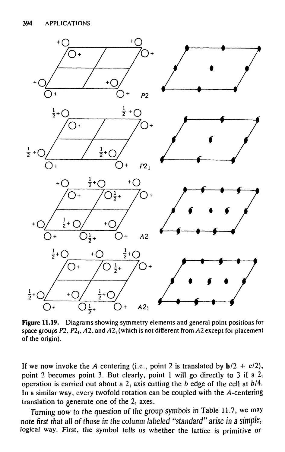
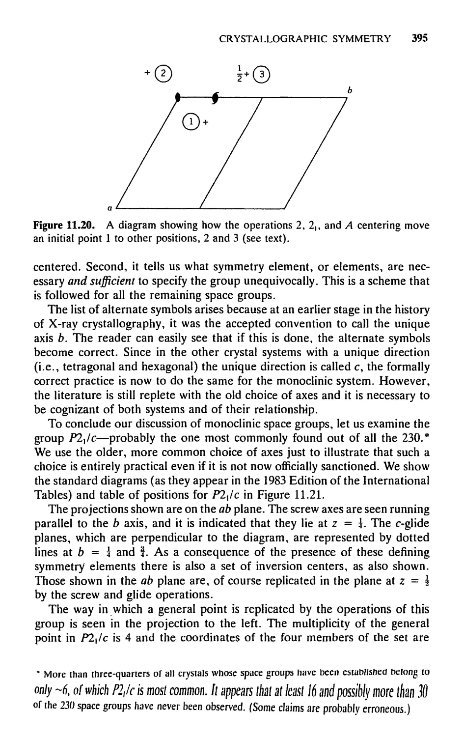
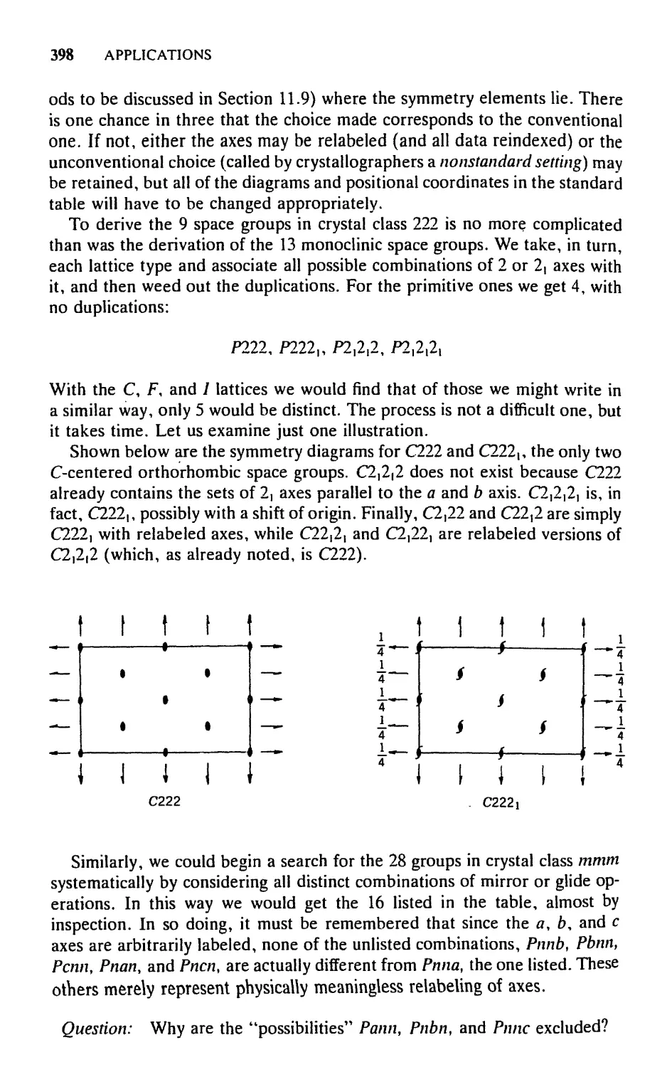
/


Text
CHEMICAL
APPLICATIONS
OF GROUP THEORY
F. Albert Cotton
Department of Chemistry, Texas A&M University
College Station, Texas
THIRD EDITION
WILEY
A WILEY-INTERSCIENCE PUBLICATION
JOHN WILEY & SONS
New York / Chichester / Brisbane / Toronto / Singapore
Copyright © 1990 by F. Albert Cotton
Copyright © 1963, 1971 by John Wiley & Sons, Inc.
AH rights reserved. Published simultaneously in Canada.
Reproduction or translation of any part of this work
beyond that permitted by Section 107 or 108 of the
1976 United States Copyright Act without the permission
of the copyright owner is unlawful. Requests for
permission or further information should be addressed to
the Permissions Department, John Wiley & Sons. Inc.
Library of Congress Cataloging in Publication Data:
Cotton, F. Albert (Frank Albert), 1930-
Chemical applications of group theory / F. Albert Cotton.—3rd ed.
p. cm.
"A Wiley-Interscience Publication."
Bibliography: p.
ISBN 0-471-51094-7
1. Molecular theory. 2. Group theory. I. Title.
OD461.C65 1990 89-16434
541'.22'015122-dc20 CIP
Printed in the United States of America
20 19 18 17 16 15 14 13
PREFACE
The aim, philosophy, and methodology of this edition are the same as they
were in earlier editions, and much of the content remains the same. However,
there are changes and additions to warrant the publication of a new edition.
The most obvious change is the addition of Chapter 11, which deals with
the symmetry properties of extended arrays—that is, crystals. My approach
may not (or it may) please crystallographic purists; I did not have them in
mind as I wrote it. I had in mind several generations of students I have taught
to use crystallography as a chemist's tool. I have tried to focus on some of
the bedrock fundamentals that I have so often noticed are not understood
even by students who have learned to "do a crystal structure."
Several of the chapters in Part I have been reworked in places and new
exercises and illustrations added. I have tried especially to make projection
operators seem a bit more "user-friendly."
In Part II, besides adding Chapter 11,1 have considerably changed Chapter
8 to place more emphasis on LCAO molecular orbitals and somewhat less
on hybridization. A section on the basis for electron counting rules for clusters
has also been added.
Finally, in response to the entreaties of many users, I have written an
Answer Book for all of the exercises. This actually gives not only the "bottom
line" in each case, but an explanation of how to get these in many cases. The
Answer Book will be available from the author at a nominal cost.
I am indebted to Bruce Bursten, Richard Adams, and Larry Falvello for
helpful comments on several sections and to Mrs. Irene Casimiro for her
excellent assistance in preparing the manuscript.
F. Albert Cotton
College Station, Texas
December 1989
PREFACE TO THE
SECOND EDITION
In the seven years since the first edition of Chemical Applications of Group
Theory was written, I have continued to teach a course along the lines of this
book every other year. Steady, evolutionary change in the course finally led
to a situation where the book and the course itself were no longer as closely
related as they should be. I have, therefore, revised and augmented the book.
The new book has not lost the character or flavor of the old one—at least,
I hope not. It aims to teach the use of symmetry arguments to the typical
experimental chemist in a way that he will find meaningful and useful. At the
same time I have tried to avoid that excessive and unnecessary superficiality
(an unfortunate consequence of a misguided desire, evident in many books
and articles on "theory for the chemist," to shelter the poor chemist from
the rigors of mathematics) which only leads, in the end, to incompetence and
its attendant frustrations. Too brief or too superficial a tuition in the use of
symmetry arguments is a waste of whatever time is devoted to it. I think that
the subject needs and merits a student's attention for the equivalent of a one-
semester course. The student who masters this book will know what he is
doing, why he is doing it, and how to do it. The range of subject matter is
that which, in my judgment, the great majority of organic, inorganic, and
physical chemists are likely to encounter in their daily research activity.
This book differs from its ancestor in three ways. First, the amount of
illustrative and exercise material has been enormously increased. Since the
demand for a teaching textbook in this field far exceeds what I had previously
anticipated, I have tried now to equip the new edition with the pedagogic
paraphernalia appropriate to meet this need.
Second, the treatment of certain subjects has been changed—improved, I
hope—as a result of my continuing classroom experience. These improve-
vii
vffi PREFACE TO THE SECOND EDITION
ments in presentation are neither extensions in coverage nor rigorizations;
they are simply better ways of covering the ground. Such improvements will
be found especially in Chapters 2 and 3, where the ideas of abstract group
theory and the groups of highest symmetry are discussed.
Finally, new material and more rigorous methods have been introduced
in several places. The major examples are A) the explicit presentation of
projection operators, and B) an outline of the F and G matrix treatment of
molecular vibrations. Although projection operators may seem a trifle for-
forbidding at the outset, their potency and convenience and the nearly universal
relevance of the symmetry-adapted linear combinations (SALCs) of basis
functions which they generate justify the effort of learning about them. The
student who does so frees himself forever from the tyranny and uncertainty
of "intuitive" and "seat-of-the-pants" approaches. A new chapter which de-
develops and illustrates projection operators has therefore been added, and
many changes in the subsequent exposition have necessarily been made.
Because chemists seem to have become increasingly interested in employ-
employing vibration spectra quantitatively—or at least semiquantitatively—to obtain
information on bond strengths, it seemed mandatory to augment the previous
treatment of molecular vibrations with a description of the efficient F and G
matrix method for conducting vibrational analyses. The fact that the conve-
convenient projection operator method for setting up symmetry coordinates has
also been introduced makes inclusion of this material particularly feasible and
desirable.
In view of the enormous impact which symmetry-based rules concerning
the stereochemistry of concerted addition and cyclization reactions (Wood-
(Woodward-Hoffmann rules) have had in recent years a detailed introduction to this
subject has been added.
In conclusion, it is my pleasant duty to thank a new generation of students
for their assistance. Many have been those whose questions and criticisms
have stimulated me to seek better ways to present the subject. I am especially
grateful to Professor David L. Weaver, Drs. Marie D. LaPrade, Barry G.
DeBoer and James Smith and to Messrs. J. G. Bullitt, J. R. Pipal, С. М.
Lukehart and J. G. Norman, Jr. for their generous assistance in correcting
proof. Finally, Miss Marilyn Milan, by the speed and excellence of her typing,
did much to lighten the task of preparing a new manuscript.
F. Albert Cotton
Cambridge, Massachusetts
May 1970
PREFACE TO THE
FIRST EDITION
This book is the outgrowth of a one-semester course which has been taught
for several years at the Massachusetts Institute of Technology to seniors and
graduate students in chemistry. The treatment of the subject matter is un-
unpretentious in that I have not hesitated to be mathematically unsophisticated,
occasionally unrigorous, or somewhat prolix, where I felt that this really helps
to make the subject more meaningful and comprehensible for the average
student. By the average student, I mean one who does not aspire to be a
theoretician but who wants to have a feel for the strategy used by theoreticians
in treating problems in which symmetry properties are important and to have
a working knowledge of the more common and well-established techniques.
I feel that the great power and beauty of symmetry methods, not to mention
the prime importance in all fields of chemistry of the results they give, make
it very worthwhile for all chemists to be acquainted with the basic principles
and main applications of group theoretical methods.
Despite the fact that there seems to be a growing desire among chemists
at large to acquire this knowledge, it is still true that only a very few, other
than professional theoreticians, have done so. The reason is not hard to
discover. There is, so far as I know, no book available which is not likely to
strike some terror into the hearts of all but those with an innate love of
apparently esoteric theory. It seemed to me that ideas of the sort developed
in this book would not soon be assimilated by a wide community of chemists
until they were presented in as unpretentious and down-to-earth a manner
as possible. That is what I have tried to do here. I have attempted to make
this the kind of book which "one can read in bed without a pencil," as my
x PREFACE TO THE FIRST EDITION
colleague, John Waugh, once aptly described another textbook which has
found wide favor because of its down-to-earth character.*
Perhaps the book may also serve as a first introduction for students in-
intending to do theoretical work, giving them some overall perspective before
they aim for depth.
I am most grateful for help I have received from many quarters in writing
this book. Over the years students in the course have offered much valuable
criticism and advice. In checking the final draft and the proofs I have had
very welcome and efficient assistance from Dr. A. B. Blake and Messrs.
R. C. Elder, T. E. Haas, and J. T. Mague. I, of course assume sole responsibil-
responsibility for all remaining errors. Finally, I wish to thank Mrs. Nancy Blake for ex-
expert secretarial assistance.
F. Albert Cotton
Cambridge, Massachusetts
January 1963
* This statement is actually (and intentionally) not applicable to parts of Chapter 3 where I have
made no concessions to the reader who refuses to inspect steric models in conjunction with study
of the text.
CONTENTS
Part I. Principles
1. INTRODUCTION 3
2. DEFINITIONS AND THEOREMS
OF GROUP THEORY
2.1 The Defining Properties of a Group, 6
2.2 Some Examples of Groups, 8
2.3 Subgroups, 12
2.4 Classes, 13
Exercises, 16
3. MOLECULAR SYMMETRY AND THE
SYMMETRY GROUPS 17
3.1 General Remarks, 17
3.2 Symmetry Elements and Operations, 18
3.3 Symmetry Planes and Reflections, 18
3.4 The Inversion Center, 22
3.5 Proper Axes and Proper Rotations, 22
3.6 Improper Axes and Improper Rotations, 27
3.7 Products of Symmetry Operations, 29
3.8 Equivalent Symmetry Elements and Equivalent
Atoms, 32
3.9 General Relations Among Symmetry Elements and
Operations, 33
xii CONTENTS
3.10 Symmetry Elements and Optical Isomerism, 34
3.11 The Symmetry Point Groups, 39
3.12 Symmetries with Multiple High-Order Axes, 44
3.13 Classes of Symmetry Operations, 50
3.14 A Systematic Procedure for Symmetry Classification of
Molecules, 54 .
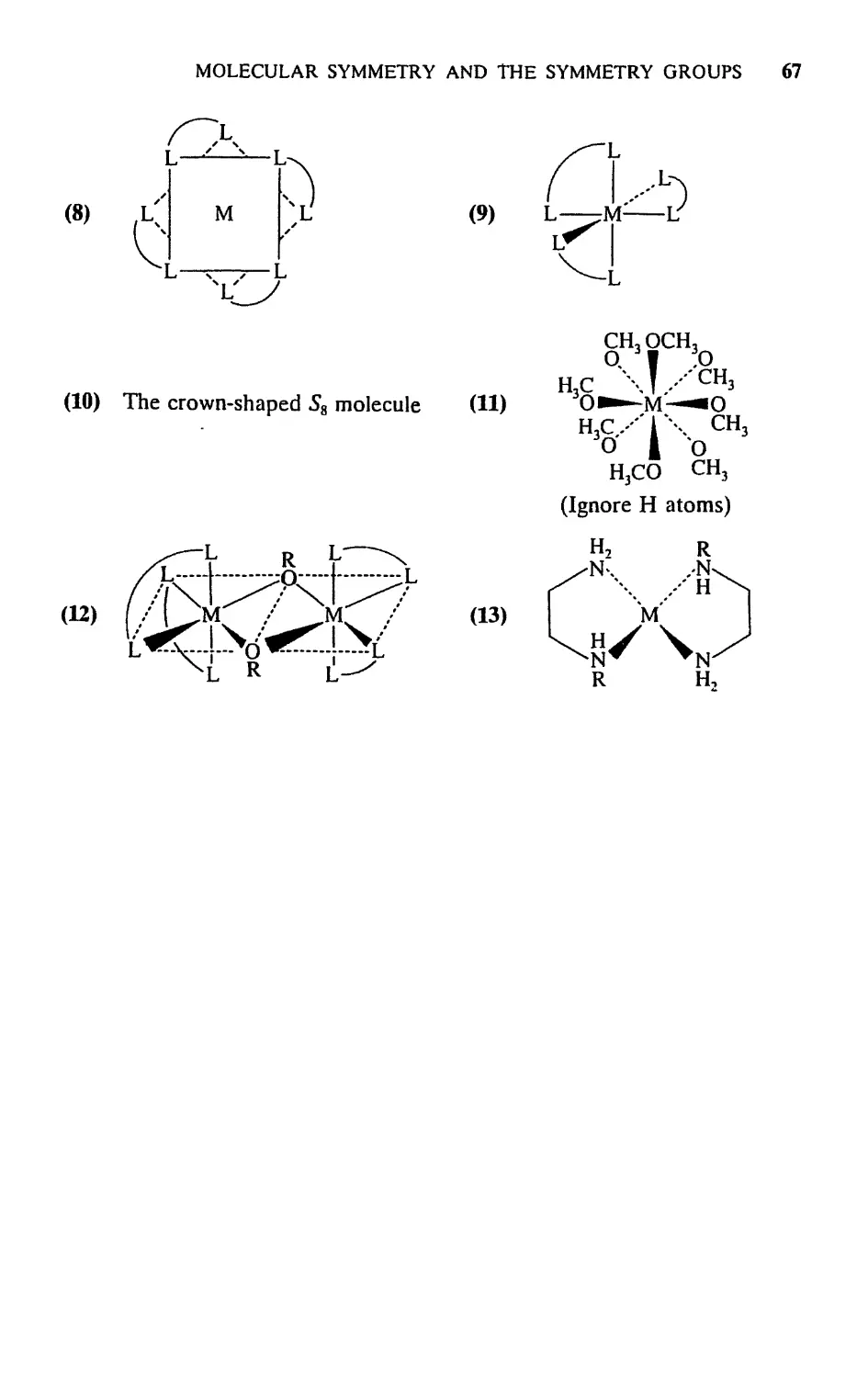
3.15 Illustrative Examples, 56
Exercises, 61
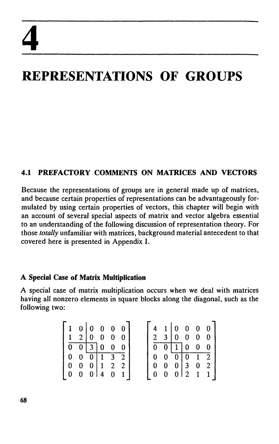
4. REPRESENTATIONS OF GROUPS 68
4.1 Prefactory Comments on Matrices and Vectors, 68
4.2 Representations of Groups, 78
4.3 The "Great Orthogonality Theorem** and Its
Consequences, SI
4.4 Character Tables, 90
4.5 Representations for Cyclic Groups,. 95
Exercises, 99
5. GROUP THEORY AND QUANTUM MECHANICS 100
5.1 Wave Functions as Bases for Irreducible
Representations, 100
5.2 The Direct Product, 105
5.3 Identifying Nonzero Matrix Elements, 109
Exercises, 113
6. SYMMETRY-ADAPTED LINEAR COMBINATIONS 114
6.1 Introductory Remarks, 114
6.2 Derivation of Projection Operators, 115
6.3 Using Projection Operators to Construct SALCs, 119
Exercises, 129
Part П. Applications
7. MOLECULAR ORBITAL THEORY AND ITS
APPLICATIONS IN ORGANIC CHEMISTRY 133
7.1 General Principles, 133
7.2 Symmetry Factoring of Secular Equations, 140
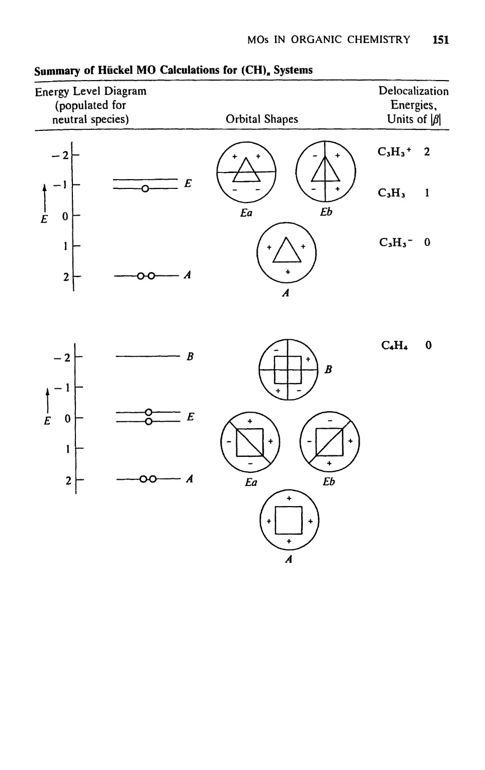
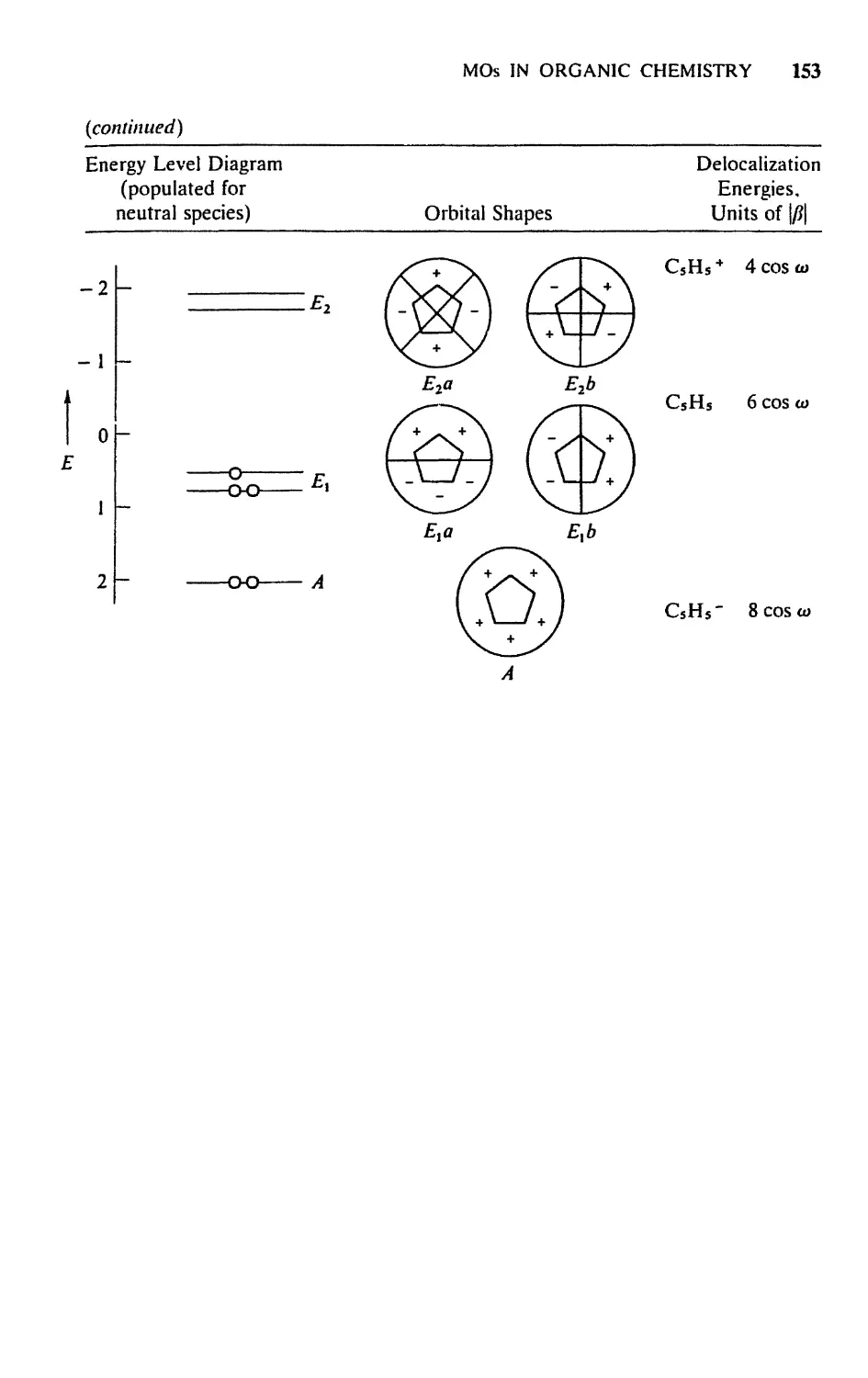
7.3 Carbocyciic Systems, 142
7.4 More General Cases of LCAO-MO n Bonding, 159
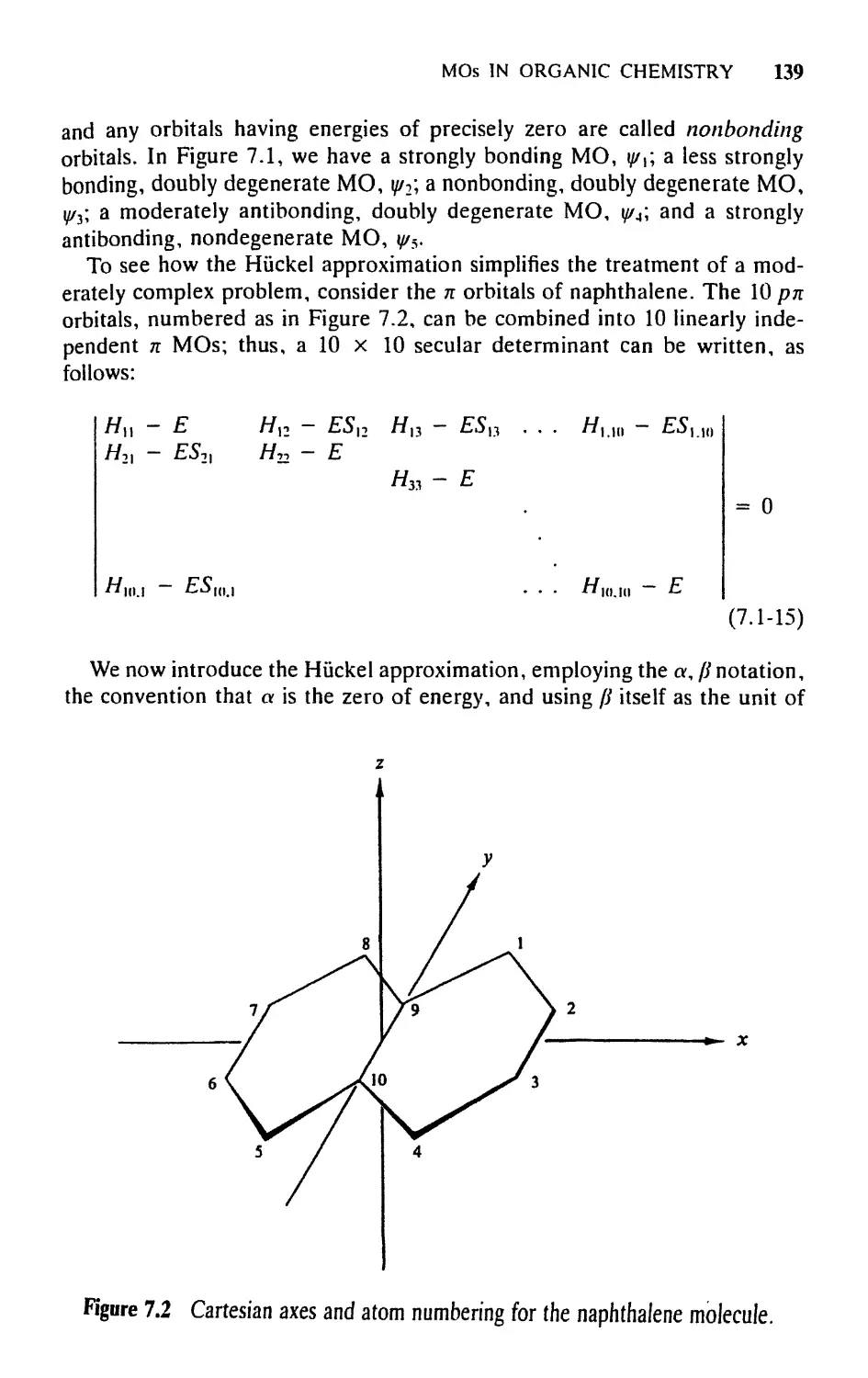
7.5 A Worked Example: Naphthalene, 172
7.6 Electronic Excitations of Naphthalene: Selection Rules and
Configuration Interaction, 176
CONTENTS xiu
7.7 Three-Center Bonding, 180
7.S Symmetry-Based "Selection Rules*' for Cyclization
Reactions, 188
Exercises, 201
8. MOLECULAR ORBITAL THEORY FOR INORGANIC
AND ORGANOMETALLIC COMPOUNDS 204
8.1 Introduction, 204
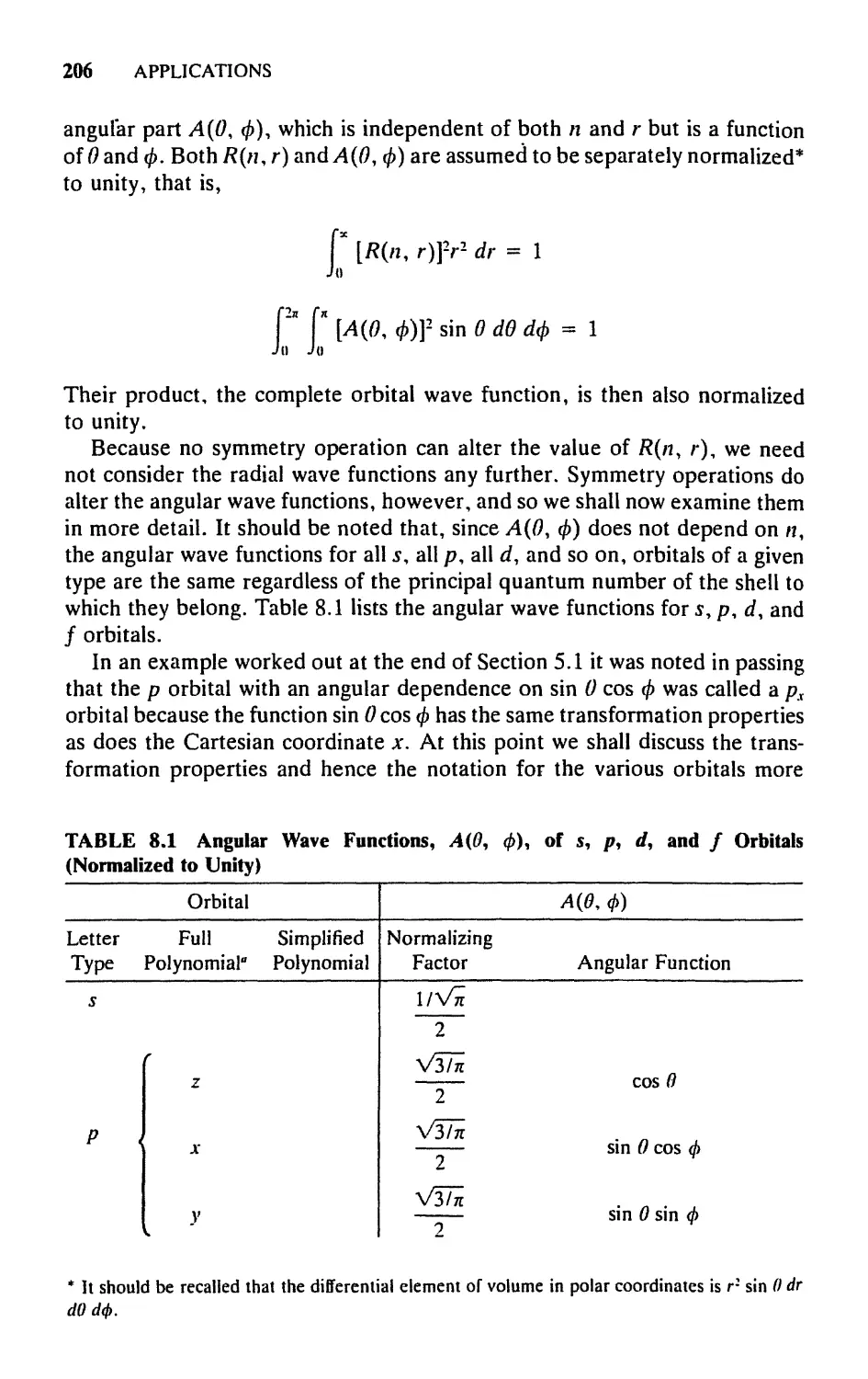
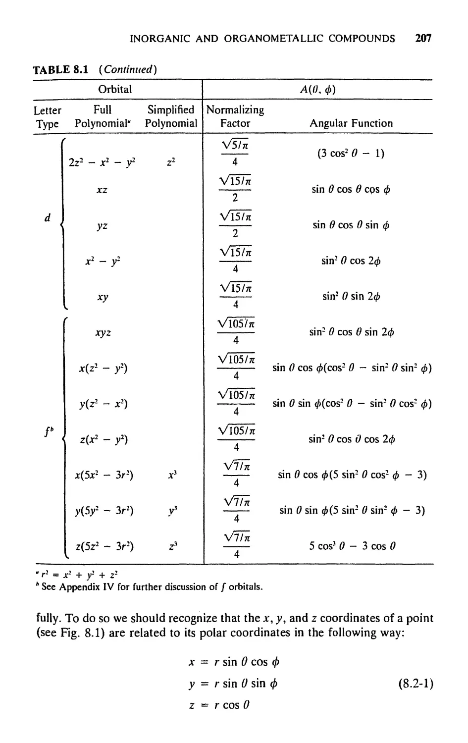
8.2 Transformation Properties of Atomic Orbitals, 205
8.3 Molecular Orbitals for a Bonding in АВ„ Molecules:
The Tetrahedral АВЦ Case, 209
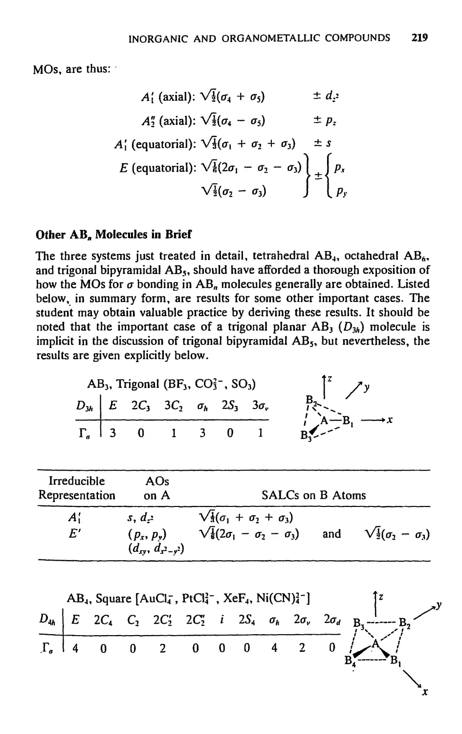
8.4 Molecular Orbitals for о Bonding in Other АВ„
Molecules, 214
8.5 Hybrid Orbitals, 222
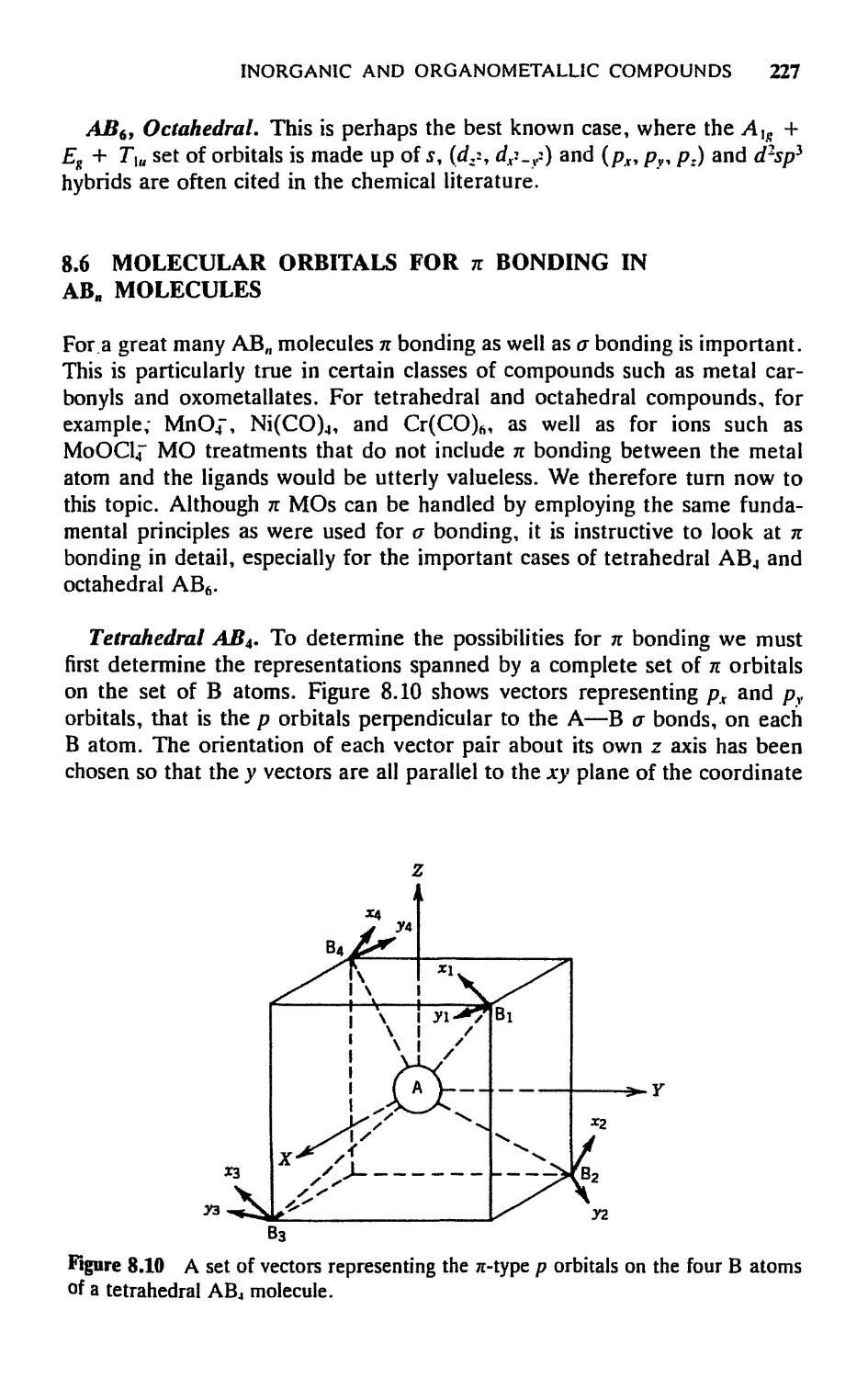
8.6 Molecular Orbitals for n Bonding in АВ„ Molecules, 227
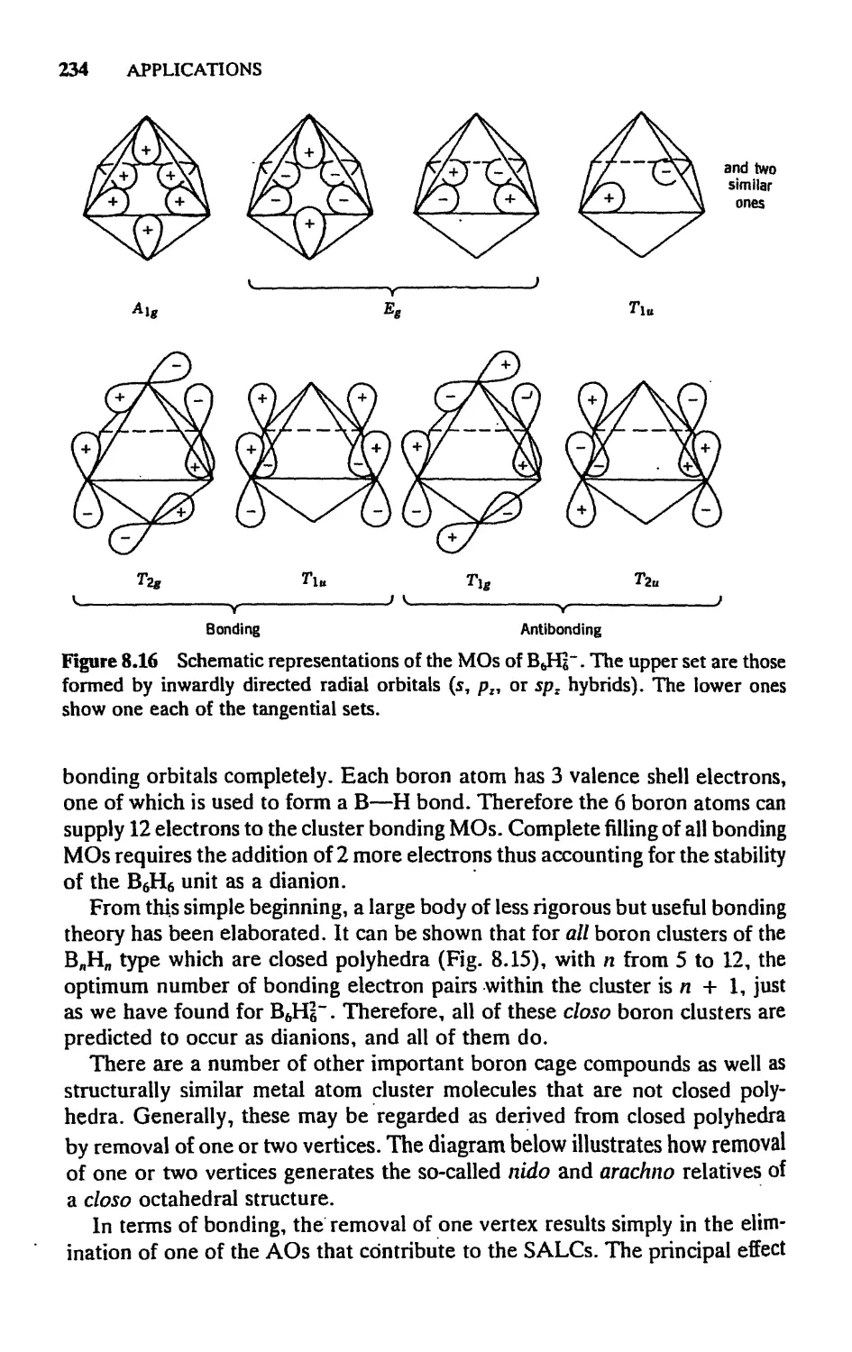
5.7 Cage and Cluster Compounds, 230
5.8 Molecular Orbitals for Metal Sandwich Compounds, 240
Exercises, 251
9. LIGAND HELD THEORY 253
9.1 Introductory Remarks, 253
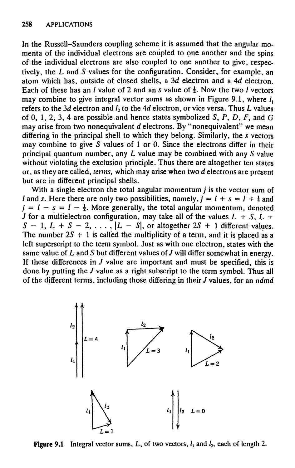
9.2 Electronic Structures of Free Atoms and Ions, 254
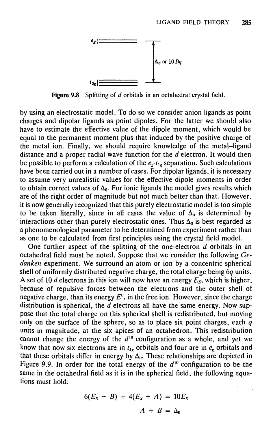
9.3 Splitting of Levels and Terms in a Chemical
Environment, 260
9.4 Construction of Energy Level Diagrams, 265
9.5 Estimation of Orbital Energies, 2S1
9.6 Selection Rules and Polarizations, 289
9.7 Double Groups, 297
Exercises, 302
10. MOLECULAR VIBRATIONS 304
10.1 Introductory Remarks, 304
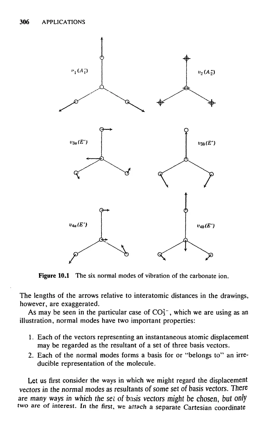
10.2 The Symmetry of Normal Vibrations, 305
10.3 Determining the Symmetry Types of the Normal
Modes, 309
10.4 Contributions of Particular Internal Coordinates to Normal
Modes, 315
10.5 How to Calculate Force Constants: The Fand С Matrix
Method, 317
10.6 Selection Rules for Fundamental Vibrational
Transitions, 324
10.7 Illustrative Examples, 328
10.8 Some Important Special Effects, 338
Exercises, 346
xiv CONTENTS
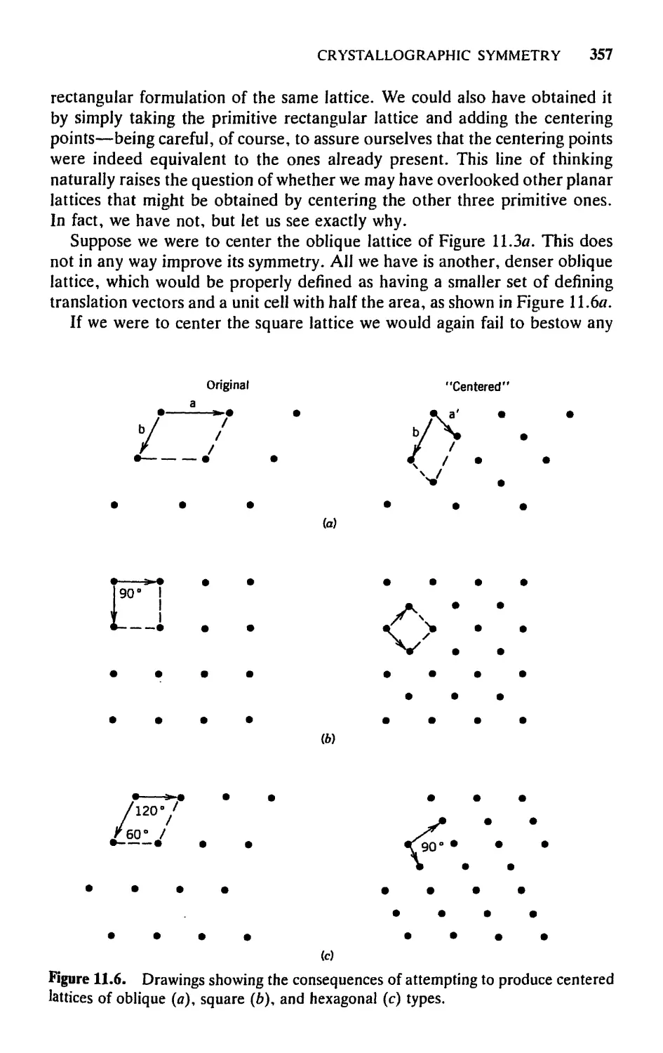
11. CRYSTALLOGRAPHIC SYMMETRY 348
11.1 Introduction, 348
11.2 The Concept of a Lattice—In Two Dimensions, 350
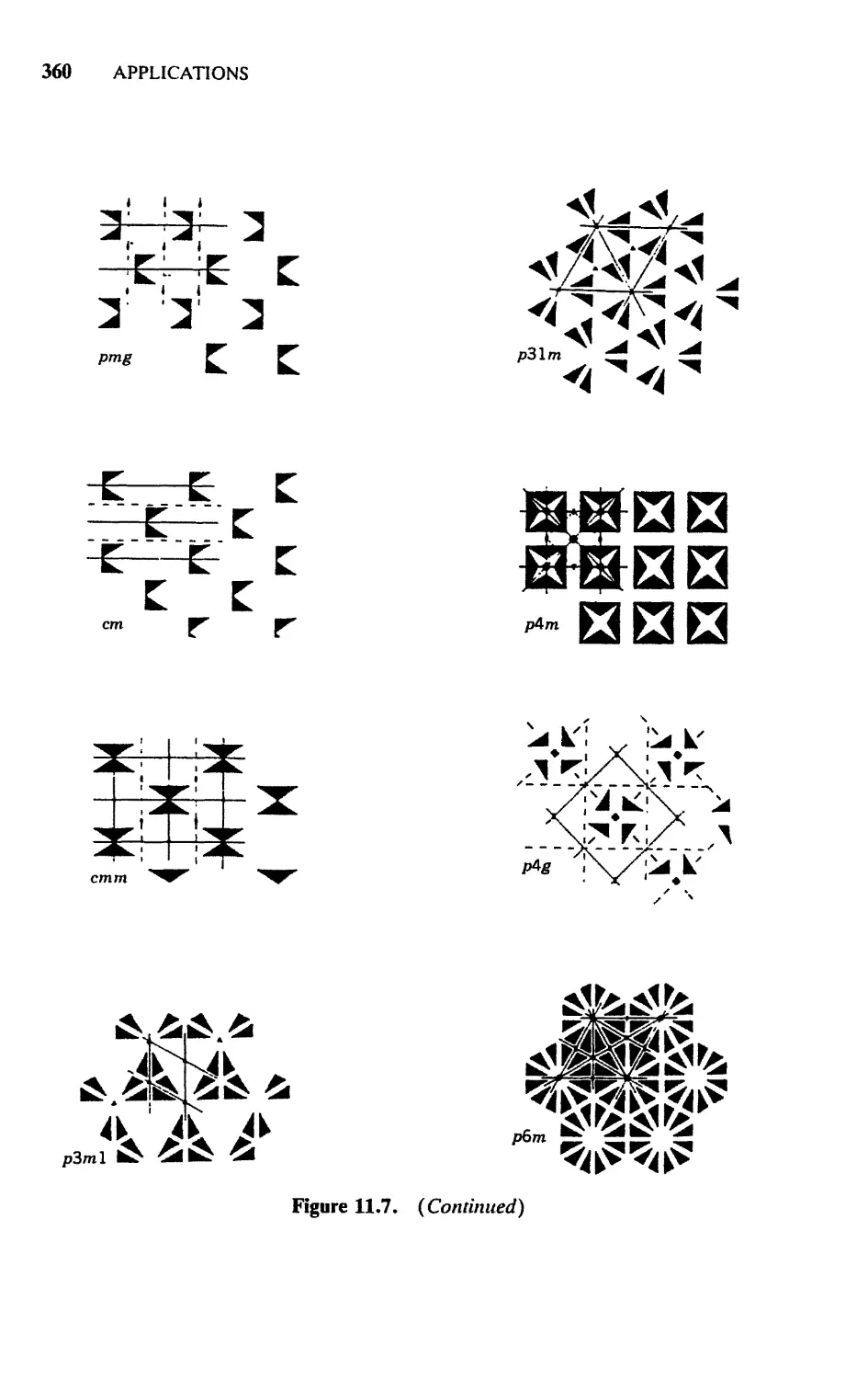
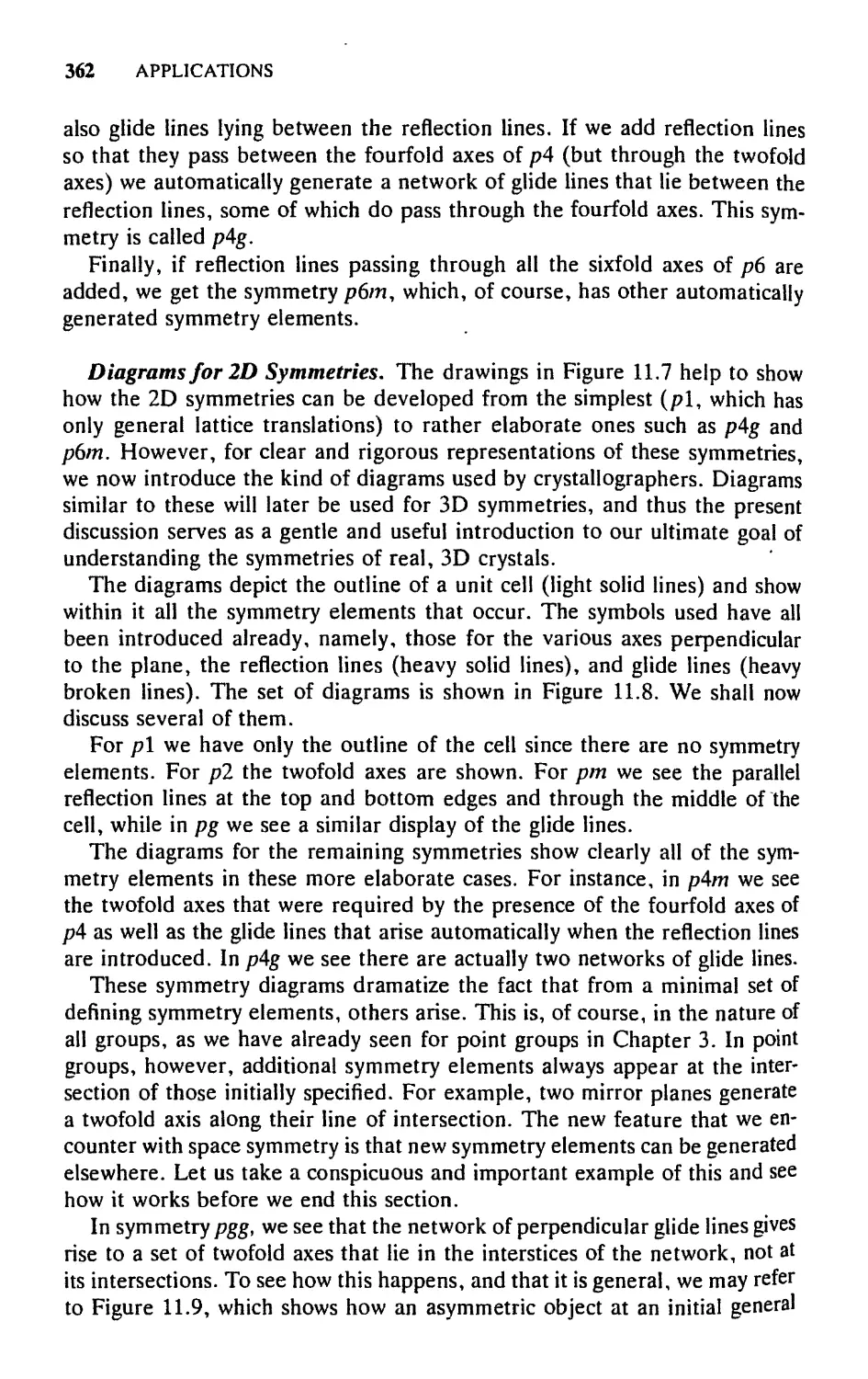
11.3 Two-Dimensional Space Symmetries, 358
11.4 Three-Dimensional Lattices and Their Symmetries, 368
11.5 Crystal Symmetry: The 32 Crystallographic Point
Groups, 375
11.6 Interrelating Lattice Symmetry, Crystal Symmetry, and
Diffraction Symmetry, 380
11.7 Additional Symmetry Elements and Operations: Glide
Planes and Screw Axes, 384
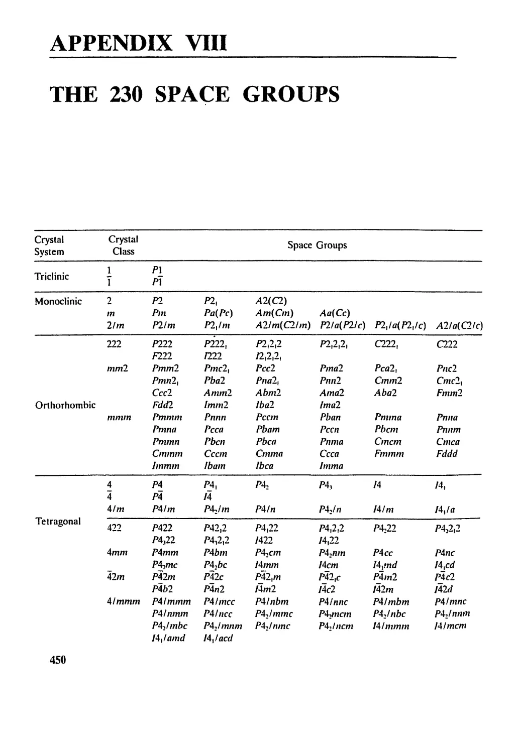
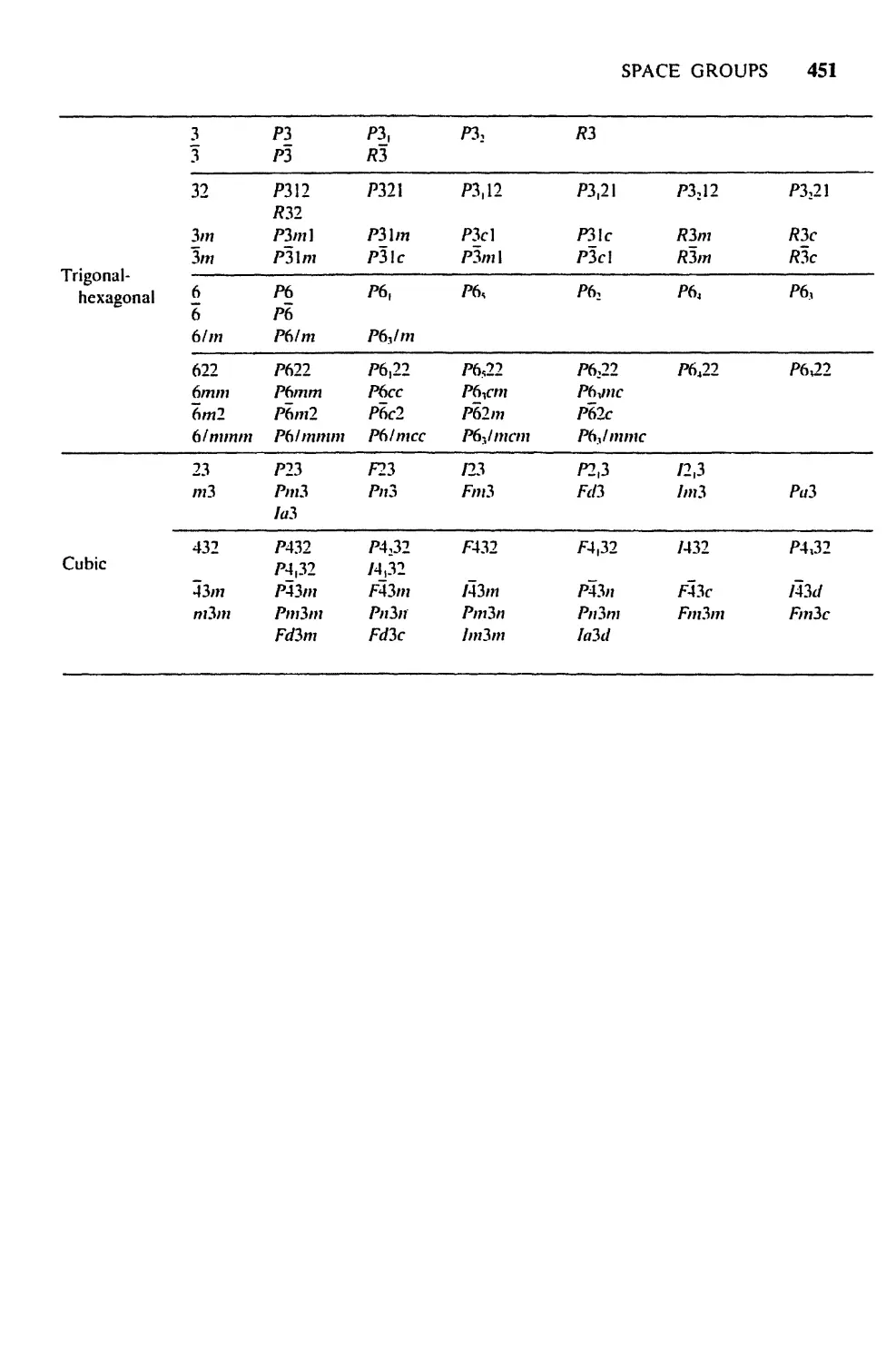
11.8 The 230 Three-Dimensional Space Groups, 388
11.9 Space Groups and X-Ray Crystallography, 400
Exercises, 410
Part III. Appendices
I. MATRIX ALGEBRA 417
IIA. CHARACTER TABLES FOR CHEMICALLY
IMPORTANT SYMMETRY GROUPS 426
IIB. CORRELATION TABLE FOR GROUP Ob 437
III. SOME REMARKS ABOUT THE RESONANCE
INTEGRAL P 438
IV. THE SHAPES OF / ORBITALS 441
V. CHARACTER TABLES FOR SOME DOUBLE
GROUPS 443
VI. ELEMENTS OF THE g MATRIX 444
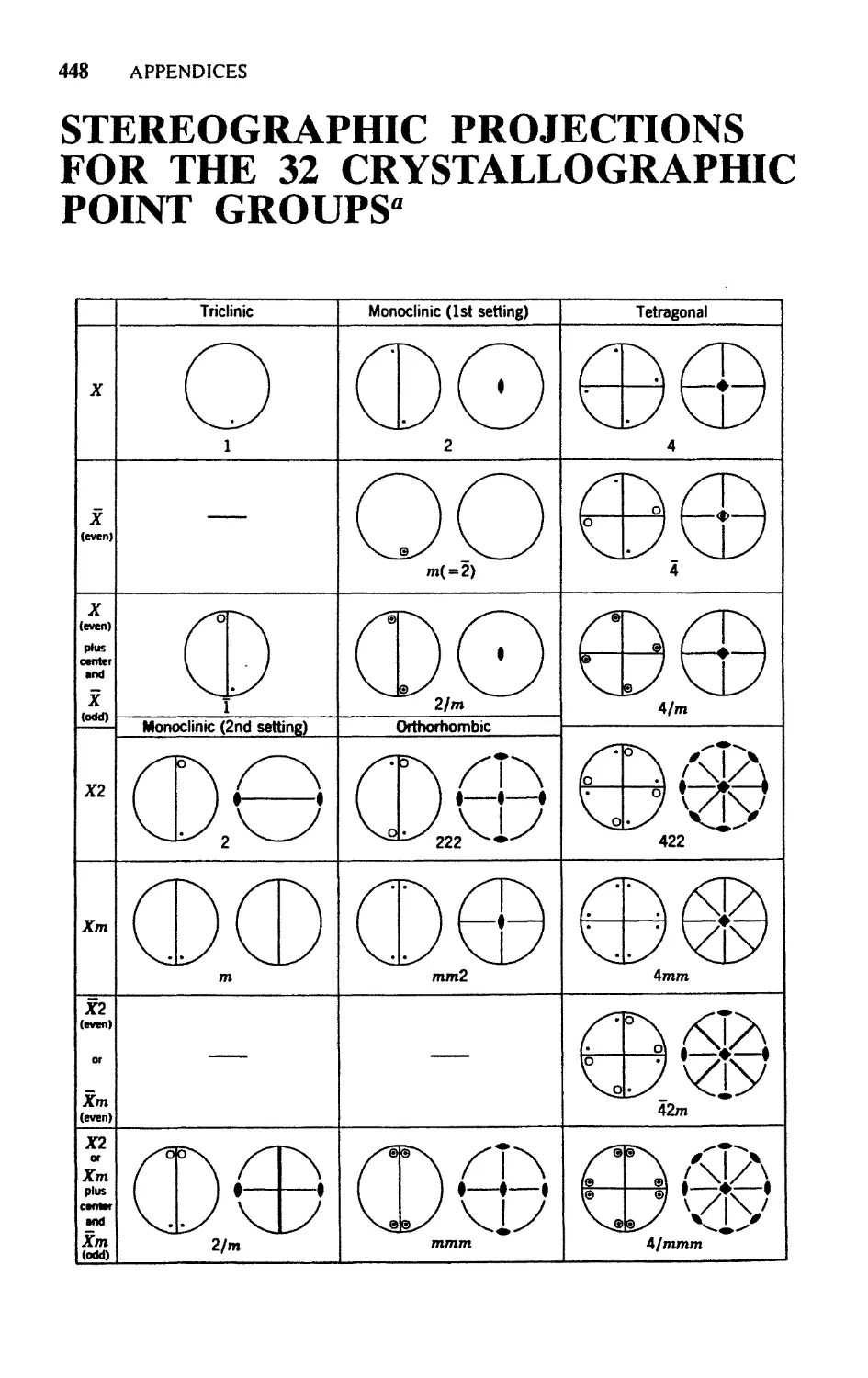
VII. STEREOGRAPHIC PROJECTIONS FOR THE 32
CRYSTALLOGRAPHIC POINT GROUPS 448
VIII. THE 230 SPACE GROUPS 450
IX. READING LIST 452
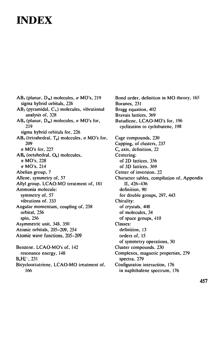
Index 457
CHEMICAL
APPLICATIONS
OF GROUP THEORY
PART I
PRINCIPLES
1
INTRODUCTION
The experimental chemist in his daily work and thought is concerned with
observing and, to as great an extent as possible, understanding and inter-
interpreting his observations on the nature of chemical compounds. Today, chem-
chemistry is a vast subject. In order to do thorough and productive experimental
work, one must know so much descriptive chemistry and so much about
experimental techniques that there is not time to be also a master of chemical
theory. Theoretical work of profound and creative nature, which requires a
vast training in mathematics and physics, is now the particular province of
specialists. And yet, if one is to do more than merely perform experiments,
one must have some theoretical framework for thought. In order to formulate
experiments imaginatively and interpret them correctly, an understanding of
the ideas provided by theory as to the behavior of molecules and other arrays
of atoms is essential.
The problem in educating student chemists—and in educating ourselves—
is to decide what kind of theory and how much of it is desirable. In other
words, to what extent can the experimentalist afford to spend time on the-
theoretical studies and at what point should he say, "Beyond this I have not the
time or the inclination to go?" The answer to this question must of course
vary with the special field of experimental work and with the individual. In
some areas fairly advanced theory is indispensable. In others relatively little
is useful. For the most part, however, it seems fair to say that molecular
quantum mechanics, that is, the theory of chemical bonding and molecular
dynamics, is of general importance.
As we shall see in Chapter 5, the number and kinds of energy levels that
an atom or molecule may have are rigorously and precisely determined by
the symmetry of the molecule or of the environment of the atom. Thus, from
4 PRINCIPLES
symmetry considerations alone, we can always tell what the qualitative fea-
features of a problem must be. We shall know, without any quantitative calcu-
calculations whatever, how many energy states there are and what interactions
and transitions between them may occur. In other words, symmetry consid-
considerations alone can give us a complete and rigorous answer to the question
"What is possible and what is completely impossible?'* Symmetry consider-
considerations alone cannot, however, tell us how likely it is that the possible things
will actually take place. Symmetry can tell us that, in principle, two states of
the system must differ in their energy, but only by computation or measure-
measurement can we determine how great the difference will be. Again, symmetry
can tell us that only certain absorption bands in the electronic or vibrational
spectrum of a molecule may occur. But to learn where they will occur and
how great their intensity will be, calculations must be made.
Some illustrations of these statements may be helpful. Let us choose one
illustration from each of the five major fields of application that are covered
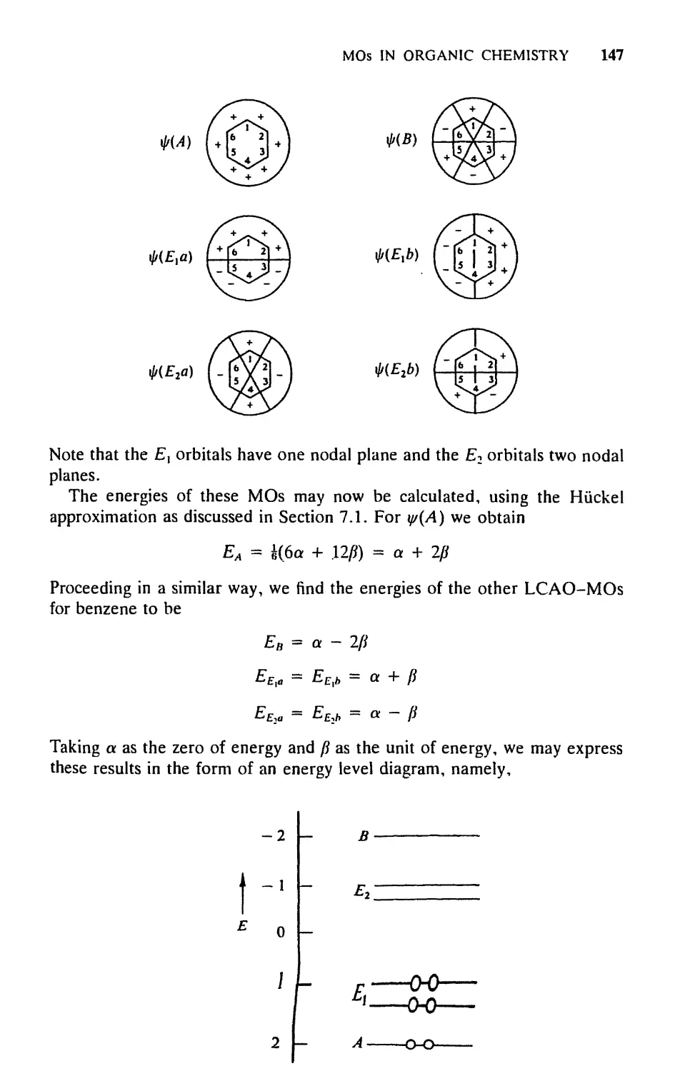
in Part II. In Chapter 7 the symmetry properties of molecular orbitals are
discussed, with emphasis on the n molecular orbitals of unsaturated hydro-
hydrocarbons, although other systems are also treated. It is shown how problems
involving large numbers of orbitals and thus, potentially, high-order secular
equations can be formulated so that symmetry considerations simplify these
equations to the maximum extent possible. It is also shown how symmetry
considerations permit the development of rules of great simplicity and gen-
generality (the so-called Woodward-Hoffmann rules) governing certain concerted
reactions. In Chapter 8, the molecular orbital approach to molecules of the
АВЯ type is outlined. In Chapter 9 the symmetry considerations underlying
the main parts of the crystal and ligand field treatments of inner orbitals in
complexes are developed.
In Chapter 10, it is shown that by using symmetry considerations alone we
may predict the number of vibrational fundamentals, their activities in the
infrared and Raman spectra, and the way in which the various bonds and
interbond angles contribute to them for any molecule possessing some sym-
symmetry. The actual magnitudes of the frequencies depend on the interatomic
forces in the molecule, and these cannot be predicted from symmetry prop-
properties. However, the technique of using symmetry restrictions to set up the
equations required in calculations in their most amenable form (the F-G
matrix method) is presented in detail.
In Chapter 11 of this edition, the symmetry properties of extended arrays,
that is, space group rather than point group symmetry, is treated. In recent
years, the use of X-ray crystallography by chemists has increased enormously.
No chemist is fully equipped to do research (or read the literature critically)
in any field dealing with crystalline compounds, without a general idea of the
symmetry conditions that govern the formation of crystalline solids. At least
the rudiments of this subject are covered in Chapter 11.
The main purpose of this book is to describe the methods by which we
can extract the information that symmetry alone will provide. An understand-
INTRODUCTION 5
ing of this approach requires only a superficial knowledge of quantum me-
mechanics. In several of the applications of symmetry methods, however, it would
be artificial and stultifying to exclude religiously all quantitative considera-
considerations. Thus, in the chapter on molecular orbitals, it is natural to go a few
steps beyond the procedure for determining the symmetries of the possible
molecular orbitals and explain how the requisite linear combinations of atomic
orbitals may be written down and how their energies may be estimated. It
has also appeared desirable to introduce some quantitative ideas into the
treatment of ligand field theory.
It has been assumed, necessarily, that the reader has some prior familiarity
with the basic notions of quantum theory. He is expected to know in a general
way what the wave equation is, the significance of the Hamiltonian operator,
the physical meaning of a wave function, and so forth, but no detailed knowl-
knowledge of mathematical intricacies is presumed. Even the contents of a rather
qualitative book such as Coulson's Valence should be sufficient, although, of
course, further background knowledge will not be amiss.
The following comments on the organization of the book may prove useful
to the prospective reader. It is divided into two parts. Part I, which includes
Chapters 1-6, covers the principles that are basic to all of the applications.
The applications are described in Part II, embracing Chapters 7-11. The
material in Part I has been written to be read sequentially; that is, each chapter
deliberately builds on the material developed in all preceding chapters. In
Part II, however, the aim has been to keep the chapters as independent, of
each other as possible without excessive repetition, although each one, of
course, depends on all the material in Part I. This plan is advantageous to a
reader whose immediate goal is to study only one particular area of appli-
application, since he can proceed directly to it, whichever it may be; it also allows
the teacher to select which applications to cover in a course too short to
include all of them, or, if time permits, to take them all but in an order
different from that chosen here.
Certain specialized points are expanded somewhat in Appendixes in order
not to divert the main discussion too far or for too long. Also, some useful
tables are given as Appendixes. Finally, Appendix IX provides a reference
list for each of the five chapters in Part II, indicating where further discussion
and research examples of the various applications may be found.
2
DEFINITIONS AND THEOREMS OF
GROUP THEORY
2.1 THE DEFINING PROPERTIES OF A GROUP
A group is a collection of elements that are interrelated according to certain
rules. We need not specify what the elements are or attribute any physical
significance to them in order to discuss the group which they constitute. In
this book, of course, we shall be concerned with the groups formed by the
sets of symmetry operations that may be carried out on molecules or crystals,
but the basic definitions and theorems of group theory are far more general.
In order for any set of elements to form a mathematical group, the following
conditions or rules must be satisfied.
1. The product of any two elements in the group and the square of each
element must be an element in the group. In order for this condition to have
meaning, we must, of course, have agreed on what we mean by the terms
"multiply" and "product." They need not mean what they do in ordinary
algebra and arithmetic. Perhaps we might say "combine71 instead of "multi-
"multiply" and "combination" instead of "product" in order to avoid unnecessary
and perhaps incorrect connotations. Let us not yet commit ourselves to any
particular law of combination but merely say that, if A and В are two elements
of a group, we indicate that we are combining them by simply writing AB or
В A. Now immediately the question arises if it makes any difference whether
we write AB or В A. In ordinary algebra it does not, and we say that multi-
multiplication is commutative, that is xy = yx, or 3 x 6 = 6 x 3. In group the-
theory, the commutative law does not in general hold. Thus А В may give С
while BA may give D, where С and D are two more elements in the group.
DEFINITIONS AND THEOREMS OF GROUP THEORY 7
There are some groups, however, in which combination is commutative, and
such groups are called Abelian groups. Because of the fact that multiplication
is not in general commutative, it is sometimes convenient to have a means
of stating whether an element В is to be multiplied by A in the sense А В or
BA. In the first case we can say that В is left-multiplied by Л, and in the
second case that В is right-multiplied by A.
2. One element in the group must commute with all others and leave them
unchanged. It is customary to designate this element with the letter ?, and
it is usually called the identity element. Symbolically we define it by writing
EX = XE = X.
3. The associative law of multiplication must hold. This is expressed in the
following equality:
A(BC) = (AB)C
In plain words, we may combine В with С in the order ВС and then combine
this product, S, with A in the order AS, or we may combine A with В in the
order AB, obtaining a product, say R, which we then combine with С in the
order RC and get the same final product either way. In general, of course,
the associative property must hold for the continued product of any number
of elements, namely,
(AB)(CD)(EF){GH) = A(BC)(DE)(FG)H = (AB)C{DE){FG)H -
4. Every element must have a reciprocal, which is also an element of the
group. The element R is the reciprocal of the element S if RS = SR - ?,
where E is the identity. Obviously, if R is the reciprocal of 5, then S is the
reciprocal of R. Also, E is its own reciprocal.
At this point we shall prove a small theorem concerning reciprocals which
will be of use later. The rule is
The reciprocal of a product of two or more elements b equal to the product
of the reciprocals, in reverse order.
This means that
(ABC - XY)~l = Y~lX-1 - C~lB-lA~x
PROOF. For simplicity we shall prove this for a ternary product, but it will be
obvious that it is true generally. If A, B, and С are group elements, their
product, say D, must also be a group element, namely,
ABC = D
8 PRINCIPLES
If now we right-multiply each side of this equation by C~xB~lA ~\ we obtain
B-lA~l = DC~]B~lA-1
E = DC-lB-]A~l
Since D times C"XB"XA-X = ?, C-'tf-U is the reciprocal of D, and since
D = ABC, we have
D = (ABC)'* = С-'Б-'Л
which proves the above rule.
2.2 SOME EXAMPLES OF GROUPS
Most of our attention in this book, until we reach Chapter 11, will be con-
concentrated on a type of symmetry group called a point group. The significance
of these terms, "symmetry group" and "point group." need not detain us
here (see Chapter 3). Most of them contain a finite number of elements, but
two (to which linear molecules belong) are infinite. The number of elements
in a finite group is called its order, and the conventional symbol for the order
is h. To illustrate the above defining rales, we may consider an infinite group
and then some finite groups.
As an infinite group we may take all of the integers, both positive and
negative, and zero. If we take as our law of combination the ordinary algebraic
process of addition, then rale 1 is satisfied. Clearly, any integer may be
obtained by adding two others. Note that we have an Abelian group since
the order of addition is immaterial. The identity of the group is 0, since 0 +
n = n + 0 = л. Also, the associative law of combination holds, since, for
example, [( + 3) + (-7)] + ( + 1043) = ( + 3) + [(-7) + ( + 1043)]. The
reciprocal of any element, л, is (-л), since ( + «) + ( — л) = О.
Group Multiplication Tables
If we have a complete and nonredundant list of the h elements of a finite
group and we know what all of the possible products (there are /r) are, then
the group is completely and uniquely defined—at least in an abstract sense.
The foregoing information can be presented most conveniently in the form
of the group multiplication table. This consists of h rows and h columns. Each
column is labeled with a group element, and so is each row. The entry in the
table under a given column and along a given row is the product of the
elements which head that column and that row. Because multiplication is in
DEFINITIONS AND THEOREMS OF GROUP THEORY 9
general not commutative, we must have an agreed upon and consistent rule
for the order of multiplication. Arbitrarily, we shall take the factors in the
order: (column element) x (row element). Thus at the intersection of the
column labeled by X and the row labeled by У we find the element, which
is the product XY.
We now prove an important theorem about group multiplication tables,
called the rearrangement theorem.
Each row and each column in the group multiplication table lists each of
the group elements once and only once. From this, it follows that no two rows
may be identical nor may any two columns be identical. Thus each row and
each column is a rearranged list of the group elements.
Proof. Let the group consist of the h elements ?, A2, Аъ, . . . , Ah. The
elements in a given row, say the nth row, are
EAn, A2Ain . . . , AnAn, . . . , AhAn
Since no two group elements, Л, and A, for instance, are the same, no two
products, A%An and Л;Л„, can be the same. The h entries in the /ith row are
all different. Since there are only h group elements, each of them must be
present once and only once. The argument can obviously be adapted to the
columns.
Groups of Orders 1, 2, and 3
Let us now systematically examine the possible abstract groups of low order,
using their multiplication tables to define them. There is, of course, formally
a group of order 1, which consists of the identity element alone. There is only
one possible group of order 2. It has the following multiplication table and
will be designated G2.
G2
E
A
E
E
A
A
A
E
For a group of order 3, the multiplication table will have to be, in part,
as follows:
E
A
В
E
E
A
В
A
A
В
В
10 PRINCIPLES
There is then only one way to complete the table. Either AA = В or AA
E. If AA = ?, then BB = E and we would augment the table to give
E
A
В
E
E
A
В
A
A
E
В
В
E
But then we can get no further, since we would have to accept BA = A and
А В = A in order to complete the last column and the last row, respectively,
thus repeating A in both the' second column and the second row. The alter-
alternative, AA = B, leads unambiguously to the following table:
?
A
В
E
E
A
В
A
A
В
E
В
В
E
A
Cyclic Groups
G3 is the simplest, nontrivial member of an important set of groups, the cyclic
groups. We note that AA = B, while А В (=AAA) = E. Thus we can consider
the entire group to be generated by taking the element A and its powers,
A2( = B) and A*( = E). In general, the cyclic group of order h is defined as
an element X and all of its /i powers up to Xh = E. We shall presently examine
several other cyclic groups. An important property of cyclic groups is that
they are Abelian, that is, all multiplications are commutative. This must be
so, since the various group elements are all of the form AT", Xn\ and so on,
and, clearly, XnXm = XmXn for all m and n.
Groups of Order 4
To continue, we ask how many groups of order 4 there are and what their
multiplication table(s) will be. Obviously, there will be a cyclic group of order
4. Let us employ the relations.
X = A
X2 = В
X* = С
X4 = E
From this we find that the multiplication table, in the usual format, is as
follows:
DEFINITIONS AND THEOREMS OF GROUP THEORY 11
G<"
E
A
В
С
E
E
A
В
С
A
A
В
С
E
В
В
С
Е
А
С
С
Е
А
В
That there is a second type of G4 group, Gf\ is fairly obvious. We note
that for G\l) only one element, namely B, is its own inverse. Suppose, instead,
we assume that each of two elements, A and B, is its own inverse. We shall
then have no choice but to also make С its own inverse, since each of the
four ?Ts in the table must lie in a different row and column, Thus, we would
obtain
E
A
В
С
E
E
A
В
С
A
A
E
В
В
E
С
С
E
A moment's consideration will show that there is only one way to complete
this table:
E
A
В
С
E
E
A
В
С
A
A
E
С
В
В
в
с
Е
А
С
С
В
А
Е
It is also clear that there are no other possibilities.* Thus, there are two
groups of order 4, namely Gjl) and Gi2), which may be considered to be
defined by their multiplication tables.
Groups of Orders 5 and 6
It is left as an exercise (Exercise 2.2) to show that there is only one group of
order 5. Similarly, a systematic examination of the possibilities for groups of
* If we make up a table in which only one element (other than E) is its own inverse and let that
element be Л or С instead of В as in the CV table given, we are not inventing a different GA.
We are only permuting the arbitrary symbols for the group elements.
12
PRINCIPLES
order 6 is also left as an exercise (Exercise 2.9). To provide illustrative material
for several topics that we shall take up next, the multiplication table for one
of the groups of order 6 is given.
Ci21
E
A
В
С
D
F
E
E
A
В
С
D
F
A
A
E
F
D
С
В
В
В
D
Е
F
А
С
С
С
F
D
Е
В
А
D
D
В
С
А
F
Е
F
F
С
А
В
Е
D
2.3 SUBGROUPS
Inspection of the multiplication table for the group GJ,2) will show that within
this group of order 6 there are smaller groups. The identity ? in itself is a
group of order 1. This will, of course, be true in any group and is trivial. Of
a nontrivial nature are the groups of order 2, namely, ?, A; ?", B\ ?, C; and
the group of order 3, namely, ?, Z), F. The last should be recognized also
as the cyclic group G3, since D2 = F, ?>3 = DF = FD = E. But to return
to the main point, smaller groups that may be found within a larger group
are called subgroups. There are, of course, groups that have no subgroups
other than the trivial one of E itself.
Let us now consider whether there are any restrictions on the nature of
subgroups, restrictions that are logical consequences of the general definition
of a group and not of any additional or special characteristics of a particular
group. We may note that the orders of the group C?2) and its subgroups are
6 and 1, 2, 3; in short, the orders of the subgroups are all factors of the order
of the main group. We shall now prove the following theorem:
The order of any subgroup g of a group of order h must be a divisor of h.
In other words, li/g = к where к is an integer.
Proof. Suppose that the set of g elements, Аь А2, Л3, . . . , Ag, forms a
subgroup. Now let us take another element В in the group which is not a
member of this subgroup and form all of the g products: BAU ВАЪ . . . ,
BAg. No one of these products can be in the subgroup. If, for example,
BA2 = A4
DEFINITIONS AND THEOREMS OF GROUP THEORY 13
then, if we take the reciprocal of A2, perhaps A5, and right-multiply the above
equality, we obtain
BA2A5 = AAA5
BE = AAA5
В = ААА5
But this contradicts our assumption that В is not a member of the subgroup
Л,, Л2, • . • , Ag4 since A4A5 can only be one of the A,-. Hence, if all the
products BAj are in the large group in addition to the A,- themselves, there
are at least 2g members of the group. If h > 2g, we can choose still another
element of the group, namely C, which is neither one of the Д nor one of
the BAh and on multiplying the Д by С we will obtain g more elements, all
members of the main group, but none members of the A,- or of the BA, sets.
Thus we now know that h must be at least equal to 3g. Eventually, however,
we must reach the point where there are no more elements by which we can
multiply the A,- that are not among the sets Ah BAh CAh and so forth, already
obtained. Suppose after having found к such elements, we reach the point
where there are no more. Then h = kg, where к is an integer, and hlg -
k, which is what we set out to prove.
Although we have shown that the order of any subgroup, g, must be a
divisor of Л, we have not proved the converse, namely, that there are subgroups
of all orders that are divisors of /2, and, indeed, this is not in general true.
Moreover, as our illustrative group proves, there can be more than one
subgroup of a given order.
2.4 CLASSES
We have seen that in a given group it may be possible to select various smaller
sets of elements, each such set including E, however, which are in themselves
groups. There is another way in which the elements of a group may be
separated into smaller sets, and such sets are called classes. Before defining
a class we must consider an operation known as similarity transformation.
If A and X are two elements of a group, then X~lAX will be equal to
some element of the group, say B. We have
В = X~]AX
We express this relation in words by saying that В is the similarity transform
of A by X. We also say that A and В are conjugate. The following properties
of conjugate elements are important.
14 PRINCIPLES
(i) Every element is conjugate with itself. This means that if we choose
any particular element A it must be possible to find at least one element X
such that
A - X"lAX
If we left-multiply by A "' we obtain
Л-'Л = E = A~lX~]AX = (XA)~\AX)
which can hold only if A and X commute. Thus the element X may always
be ?, and it may be any other element that commutes with the chosen element,
A.
(ii) If A is conjugate with B, then В is conjugate with A. This means that
if
A = X-'BX
then there must be some element Y in the group such that
В « Y'lAY
That this must be so is easily proved by carrying out appropriate multipli-
multiplications, namely,
XAX-1 = XX'lBXX~l = В
Thus, if У = X (and thus also Y'1 = X), we have
В = Y-lAY
and this must be possible, since any element, say AT, must have an inverse,
say Y.
(iii) If A is conjugate with В and С, then В and С are conjugate with each
other. The proof of this should be easy to work out from the foregoing
discussion and is left as an exercise.
We may now define a class of elements.
A complete set of elements that are conjugate to one another is called a class
of the group.
In order to determine the classes within any particular group we can begin
with one element and work out all of its transforms, using all the elements
in the group, including itself, then take a second element, which is not one
of those found to be conjugate to the first, and determine all its transforms,
and so on until all elements in the group have been placed in one class or
another.
Let us illustrate this procedure with the group Gf\ All of the results given
below may be verified by using the multiplication table. Let us start with E.
DEFINITIONS AND THEOREMS OF GROUP THEORY 15
E-]EE = EEE = E
A-lEA = A'lAE = E
B-]EB = B']BE = E
Thus E must constitute by itself a class, of order 1, since it is not conjugate
with any other element. This will, of course, be true in any group. To continue,
E-*AE = A
A']AA = A
B~lAB = С
C-]AC = 5
Z)-UD = В
F'lAF = С
Thus the elements A, 5, and С are all conjugate and are therefore members
of the same class. It is left for the reader to show that all of the transforms
of В and С are either Л, B, or C. Thus Л, 5, and С are in fact the only
members of the class.
Continuing we have
E'lDE = D
A~lDA = F
B-*DB = F
C-lDC = F
D-lDD = D
F-*DF = D
It will also be found that every transform of F is either D or F. Hence, D
and F constitute a class of order 2.
It will be noted that the classes have orders 1, 2, and 3, which are all
factors of the group order, 6. It can be proved* by a method similar to that
used in connection with the orders of subgroups, that the following theorem
is true:
The orders of all classes must be integral factors of the order of the group.
16 PRINCIPLES
We shall see later (Section 3.13) that in a symmetry group the classes have
useful geometrical significance.
EXERCISES
2.1. Prove that in any Abelian group, each element is in a class by itself.
2.2. Show that there can be only one group of order /?, when h is a prime
number.
2.3. Write down the multiplication table for the cyclic group of order 5.
Show by trial and error that no other one is possible.
2.4. Why can we not have a group in which A1 = В2 ^ El
2.5. If we start with the multiplication table for group Сл and add another
element, C, which commutes with both A and B, what multiplication
table do we end up with?
2.6. Show that for any cyclic group, A\ A'2, A'3, . . . , Xh(=EL there must
be one subgroup corresponding to each integral divisor of the order /?.
Give an example.
2.7. Invent as many different noncyclic groups of order 8 as you can and
give the multiplication table for each.
2.8. For each of the groups of order S, show how it breaks down into
subgroups and classes.
2.9. Derive the multiplication table for all other groups of order 6 besides
the one shown in the text. This will require you to show that a group
of order 6 in which every element is its own inverse is impossible.
2.10. For the groups G(Ai], G52) and the cyclic group of order 6, show what
classes and subgroups each one has.
3
MOLECULAR SYMMETRY AND
THE SYMMETRY GROUPS
3.1 GENERAL REMARKS
It is perhaps appropriate to begin this chapter by sketching what we intend
to do here. It is certainly intuitively obvious what we mean when we say that
some molecules are more symmetrical than others, or that some molecules
have high symmetry whereas others have low symmetry or no symmetry. But
in order to make the idea of molecular symmetry as useful as possible, we
must develop some rigid mathematical criteria of symmetry. To do this we
shall first consider the kinds of symmetry elements that a molecule may have
and the symmetry operations generated by the symmetry elements. We shall
then show that a complete but nonredundant set of symmetry operations (not
elements) constitutes a mathematical group. Finally, we shall use the general
properties of groups, developed in Chapter 2, to aid in correctly and system-
systematically determining the symmetry operations of any molecule we may care
to consider. We shall also describe here the system of notation normally used
by chemists for the various symmetry groups. An alternative system used
primarily in crystallography is explained in Chapter 11.
It may also be worthwhile to offer the following advice to the student of
this chapter. The use of three-dimensional models is extremely helpful in
learning to recognize and visualize symmetry elements. Indeed, it is most
unlikely that any but a person of the most exceptional gifts in this direction
can fail to profit significantly from the examination of models. At the same
time, it may also be said that anyone with the intelligence to master other
aspects of modem chemical knowledge should, by the use of models, surely
succeed in acquiring a good working knowledge of molecular symmetry.
17
18 PRINCIPLES
3.2 SYMMETRY ELEMENTS AND OPERATIONS
The two things, symmetry elements and symmetry operations, are inextricably
related and therefore are easily confused by the beginner. They are, however,
different kinds of things, and it is important to grasp and retain, from the
outset, a clear understanding of the difference between them.
Definition of a Symmetry Operation
A symmetry operation is a movement of a body such that, after the movement
has been carried out, every point of the body is coincident with an equivalent
point (or perhaps the same point) of the body in its original orientation. In
other words, if we note the position and orientation of a body before and
after a movement is carried out, that movement is a symmetry operation if
these two positions and orientations are indistinguishable. This would mean
that, if we were to look at the body, turn away long enough for someone to
carry out a symmetry operation, and then look again, we would be completely
unable to tell whether or not the operation had actually been performed,
because in either case the position and orientation would be indistinguishable
from the original. One final way in which we can define a symmetry operation
is to say that its effect is to take the body into an equivalent configuration—
that is, one which is indistinguishable from the original, though not necessarily
identical with it.
Definition of a Symmetry Element
A symmetry element is a geometrical entity such as a line, a plane, or a point,
with respect to which one or more symmetry operations may be carried out.
Symmetry elements and symmetry operations are so closely interrelated
because the operation can be defined only with respect to the element, and
at the same time the existence of a symmetry element can be demonstrated
only by showing that the appropriate symmetry operations exist. Thus, since
the existence of the element is contingent on the existence of the operation(s)
and vice versa, we shall discuss related types of elements and operations
together.
In treating molecular symmetry, only four types of symmetry elements and
operations need be considered. These, in the order in which they will be
discussed, are listed in Table 3.1.
3.3 SYMMETRY PLANES AND REFLECTIONS
A symmetry plane must pass through a body, that is, the plane cannot be
completely outside of the body. The conditions which must be fulfilled in
order that a given plane be a symmetry plane can be stated as follows. Let
MOLECULAR SYMMETRY AND THE SYMMETRY GROUPS 19
TABLE 3.1 The Four Kinds of Symmetry Elements and Operations Required in
Specifying Molecular Symmetry
Symmetry Element Symmetry Operation (s)
1. Plane Reflection in the plane
2. Center.of symmetry or Inversion of all atoms, through the center
center of inversion
3. Proper axis One or more rotations about the axis
4. Improper axis . One or more repetitions of the sequence: rotation
followed by reflection in a plane 1 to the rotation axis
us apply a Cartesian coordinate system to the molecule in such a way that
the plane includes two of the axes (say x and y) and is therefore perpendicular
to the third (i.e., z). The position of every atom in the molecule may also be
specified in this same coordinate system. Suppose now, for each and every
atom, we leave the x and у coordinates fixed and change the sign of the z
coordinate: thus the /th atom, originally at (*,-, yh z;), is moved to the point
(jc,-, yf, — Z;). Another way of expressing the above operation is to say, "Let
us drop a perpendicular from each atom to the plane, extend that line an
equal distance.on the opposite side of the plane, and move the atom to this
other end of the line." If, when such an operation is carried out on every
atom in a molecule, an equivalent configuration is obtained, the plane used
is a symmetry plane.
Clearly, atoms lying in the plane constitute special cases, since the oper-
operation of reflecting through the plane does not move them at all. Consequently,
any planar molecule is bound to have at least one plane of symmetry, namely,
its molecular plane. Another significant and immediate consequence of the
definition is a restriction on the numbers of various kinds of atoms in a
molecule having a plane of symmetry. All atoms of a given species that do
not lie in the plane must occur in even numbers, since each one must have
a twin on the other side of the plane. Of course, any number of atoms of a
given species may be in the plane. Furthermore, if there is only one atom of
a given species in a molecule, it must be in each and every symmetry plane
that the molecule may have. This means that it must be on the line of
intersection between two or more planes or at the point of intersection of
three or more planes (if there is such a point), since this atom must lie in all
of the symmetry planes simultaneously.
The standard symbol for a plane of symmetry is a. The same symbol is
also used for the operation of reflecting through the plane.
It should be explicitly noted that the existence of one symmetry plane gives
rise to, requires, or, as usually stated, generates one symmetry operation. We
may also note here, for future use, that the effect of "applying the same
reflection operation twice is to bring all atoms back to their original positions.
Thus, while the operation a produces a configuration equivalent to the original,
20 PRINCIPLES
the application of the same a twice produces a configuration identical with
the original. Now we can conveniently denote the successive application of
the operation a n times by writing a". We can then also write, o1 = E, where
we use the symbol E to represent any combination of operations which takes
the molecule to a configuration identical with the original one. We call ?, or
any combination of operations equal to ?, the identity operation. It should
be obvious that a" = E when n is even and a" = a when n is odd.
Let us now consider some illustrative examples of symmetry planes in
molecules. At one extreme are molecules that have no symmetry planes at
all. One such general class consists of those which are not planar and which
have odd numbers of all atoms. An example is FC1SO, seen below.
At the other extreme are molecules possessing an infinite number of sym-
symmetry planes, that is, linear molecules. For these any plane containing the
molecular axis is a symmetry plane, and there is obviously an infinite number
of these planes. Most small molecules fall between these extremes; that is,
they have one or a few symmetry planes. If, instead of FCISO, we take F2SO
or C12SO, we have a molecule with one symmetry plane, which passes through
S and О and is perpendicular to the Cl, Cl, О or the F, F, О plane. The H2O
molecule has two symmetry planes. One is, of course, coextensive with the
molecular plane. The other includes the oxygen atom (it must, since there is
only one such atom) and is perpendicular to the molecular plane. The effect
of reflection through this second plane is to leave the oxygen atom fixed but
to exchange the hydrogen atoms, while reflection through the first plane leaves
all atoms unshifted. A tetrahedral molecule of the type AB2C2 (e.g., CH2C12)
also has two mutually perpendicular planes of symmetry. One contains AB2,
and reflection through it leaves these three atoms unshifted while interchang-
interchanging the С atoms; the other contains AC2, and reflection through it interchanges
only the В atoms.
The molecules NH3 and CHC13 are representative of a type containing
three planes of symmetry. For NH3, any plane of symmetry would have to
include the nitrogen atom and either one or all three of the hydrogen atoms.
Since NH3 is not planar, there can be no symmetry plane including N and all
three H atoms; hence we look for planes including N and one H and bisecting
the line between the remaining two H atoms. There are clearly three such
planes. For CHC13, the situation is quite analogous except that the hydrogen
atom must also lie in the symmetry planes.
The NH3 molecule is only one example of the general class of pyramidal
AB3 molecules. Let us see what happens as we begin flattening such a molecule
by pushing the A atom down toward the plane of the three В atoms. It should
MOLECULAR SYMMETRY AND THE SYMMETRY GROUPS 21.
be easily seen that this does not disturb the three symmetry planes, even in
the limit of coplanarity. Nor does it introduce any new planes of symmetry
except in the limit of coplanarity. Once AB3 becomes planar there is then a
fourth symmetry plane, which is the molecular plane. Molecules and ions of
the planar AB3 type possessing four symmetry planes, three perpendicular to
the molecular plane, are fairly numerous and important. There are, for ex-
example, the boron halides, CO5", NO3"\ and SO3.
A planar species of the type [PtClJ2" or [AuClJ" possesses Jive symmetry
planes. One is the molecular plane. There are also two, perpendicular to the
molecular plane and perpendicular to each otheT, which pass through three
atoms. Finally, there are two more, also perpendicular to the molecular plane
and perpendicular to each other, which bisect Cl—Pt—Cl or Cl—Au—Cl
angles.
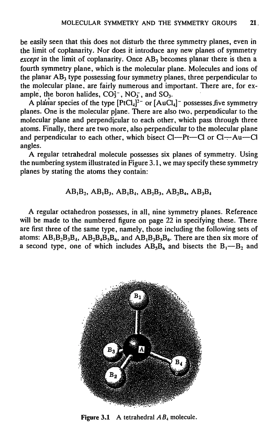
A regular tetrahedral molecule possesses six planes of symmetry. Using
the numbering system illustrated in Figure 3.1, we may specify these symmetry
planes by stating the atoms they contain:
AB,B2, AB,B3, AB,B4, AB2B3, AB2B4, AB3B4
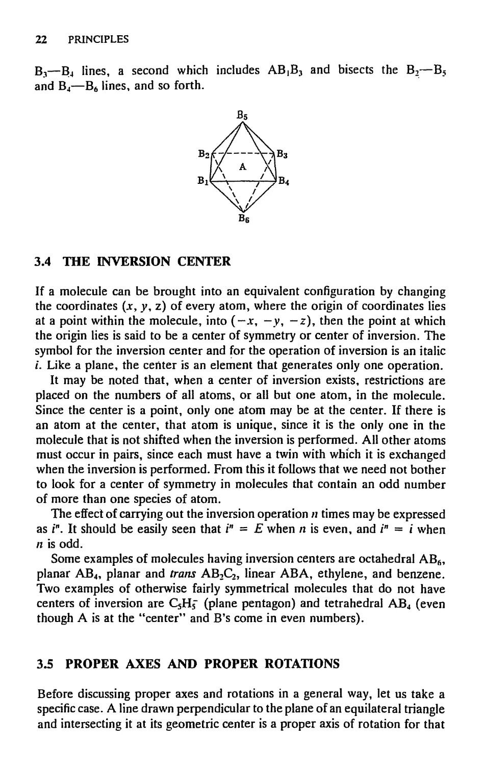
A regular octahedron possesses, in all, nine symmetry planes. Reference
will be made to the numbered figure on page 22 in specifying these. There
are first three of the same type, namely, those including the following sets of
atoms: AB,B2B3B4, AB2B4B5B6, and AB^B^. There are then six more of
a second type, one of which includes AB5B6 and bisects the B,—B2 and
Figure 3.1 A tetrahedral ABA molecule.
22 PRINCIPLES
B3—B4 lines, a second which includes AB,B3 and bisects the B2—B5
and B4—B6 lines, and so forth.
3.4 THE INVERSION CENTER
If a molecule can be brought into an equivalent configuration by changing
the coordinates (x, y, z) of every atom, where the origin of coordinates lies
at a point within the molecule, into (-л:, -у, -z), then the point at which
the origin lies is said to be a center of symmetry or center of inversion. The
symbol for the inversion center and for the operation of inversion is an italic
i. Like a plane, the center is an element that generates only one operation.
It may be noted that, when a center of inversion exists, restrictions are
placed on the numbers of all atoms, or all but one atom, in the molecule.
Since the center is a point, only one atom may be at the center. If there is
an atom at the center, that atom is unique, since it is the only one in the
molecule that is not shifted when the inversion is performed. All other atoms
must occur in pairs, since each must have a twin with which it is exchanged
when the inversion is performed. From this it follows that we need not bother
to look for a center of symmetry in molecules that contain an odd number
of more than one species of atom.
The effect of carrying out the inversion operation n times may be expressed
as /". It should be easily seen that i" = E when n is even, and i" = i when
n is odd.
Some examples of molecules having inversion centers are octahedral AB6,
planar AB4, planar and trans AB2C2, linear ABA, ethylene, and benzene.
Two examples of otherwise fairly symmetrical molecules that do not have
centers of inversion are QH5" (plane pentagon) and tetrahedral AB4 (even
though A is at the "center" and B's come in even numbers).
3.5 PROPER AXES AND PROPER ROTATIONS
Before discussing proper axes and rotations in a general way, let us take a
specific case. A line drawn perpendicular to the plane of an equilateral triangle
and intersecting it at its geometric center is a proper axis of rotation for that
MOLECULAR SYMMETRY AND THE SYMMETRY GROUPS 23
triangle. Upon rotating the triangle by 120° Bя/3) about this axis, the triangle
is brought into an equivalent configuration. It may be noted that a rotation
by 240 B x 2я/3) also produces an equivalent configuration.
The general symbol for a proper axis of rotation is С„, where the subscript
n denotes the order of the axis. By order is meant the largest value of n such
that rotation through 2nln gives an equivalent configuration. In the above
example, the axis is a C3 axis. Another way of defining the meaning of the
order n of an axis is to say that it is the number of times that the smallest
rotation capable of giving an equivalent configuration must be repeated in
order to give a configuration not merely equivalent to the original but also
identical to it. The meaning of "identical" can be amplified if we attach
numbers to each apex of the triangle in our example. Then the effects of
rotating by 2л/3, 2 x 2л:/3, and 3 x 2л/3 are seen to be
A
1 П
2 ^^^ 3
г/Лз 2Х2./3 > 2Z\
1 Ш
2 s~\ 2
l/ \3 Зх2тг/3 д/ \3
IV
Configurations II and III are equivalent to I because without the labels
(which are not real, but represent only our mental constructions) they are
indistinguishable from I, although with the labels they are distinguishable.
However, IV is indistinguishable from I not only without labels but also with
them. Hence, it is not merely equivalent; it is identical.
The C3 axis is also called a threefold axis. Moreover, we use the sym-
symbol C3 to represent the operation of rotation by 2л/3 around the C3 axis.
For the rotation by 2 x 2я/3 we use the symbol Q, and for the rotation by
3 x 2я/3 the symbol C]. Symbolically we can write Cj = C3, and hence only
C3, C3, and C] are separate and distinct operations. However, C\ produces
an identical configuration, and hence we may write C\ = E.
After consideration of this example, it is easy to accept some more general
statements about proper axes and proper rotations. In general, an /z-fold axis
is denoted by C» and a rotation by 2nln is also represented by the symbol
24 PRINCIPLES
Cn. Rotation by 2n/n carried out successively m times is represented by the
symbol C™. Also, in any case, Cnn = E, C"n+l = С Q+2 = C*, and so on.
In discussing planes of symmetry and inversion centers, attention was di-
directed to the fact that only one operation, reflection, is generated by a sym-
symmetry plane, and only one operation, inversion, by an inversion center. A
proper axis of order л, however, generates n operations, namely С„, CJ,
One last general consequence of the existence of а С„ axis concerns the
requirement that there be certain numbers of each species of atom in a
molecule containing the axis. Naturally, any atom that lies on a proper axis
of symmetry is unshifted by any rotation about that axis. Thus there may be
any number, even or odd, of each species of atom lying on an axis (unless
other symmetry elements impose restrictions). However, if one atom of a
certain species lies off а С„ axis, there must automatically be n - 1 more, or
a total of n such atoms, since on applying С„ successively n times, the first
atom is moved to a total of n different points. Had there not been identical
atoms at all the other n - 1 points to begin with, the new configurations
would not be equivalent configurations; this would mean that the axis would
not be а С„ symmetry axis, contrary to the original assumption.
The symbol C™ represents a rotation by m x 2nln. Let us consider the
operation Cj, which is one of those generated by a C4 axis. This is a rotation
by 2 x 2л/4 = 2л/2, and can therefore be written just as well as C2. Similarly,
among the operations generated by a C6 axis, we find Cg, CJ, and C?, which
may be written, respectively, as C3, C2, and Cj. It is frequent though not
invariable practice to write an operation Cj1 in what, by considering the
fraction (m/n) in (m/nJn, can be called lowest terms, and the reader should
be familiar with this practice so that he immediately recognizes, for example,
that the sequence C6, C3, C2, C5, Cjj, E is identical in meaning with Ch, Cj|,
act a a
Let us now consider some further illustrative examples chosen from com-
commonly encountered types of molecules. Again we may begin by considering
extremes. Many molecules possess no axes of proper rotation; FC1SO, for
example, does not. (Actually, FC1SO is a gratuitous example, since as we
saw earlier, it possesses no symmetry elements whatsoever.) Neither C12SO
nor F2SO possess an axis of proper rotation. At the other extreme are linear
molecules which possess 00-fold axes of proper rotation, colinear with the
molecular axes. Since all atoms in a linear molecule lie on this axis, rotation
by any angle whatever, and hence by all @0 number) angles, leaves a config-
configuration indistinguishable from the original. Again, as with planes of symmetry,
most small molecules possess one axis or a few axes, generally of low orders.
Among examples of molecules with a single axis of order 2 are H2O and
CH2C12. No molecules possess just two twofold axes; this will be shown later
to be mathematically impossible. There are many examples of molecules
possessing three twofold axes, for example, ethylene (QH4). One C2 is col-
colinear with the С—С axis. A second is perpendicular to the plane of the
MOLECULAR SYMMETRY AND THE SYMMETRY GROUPS 25
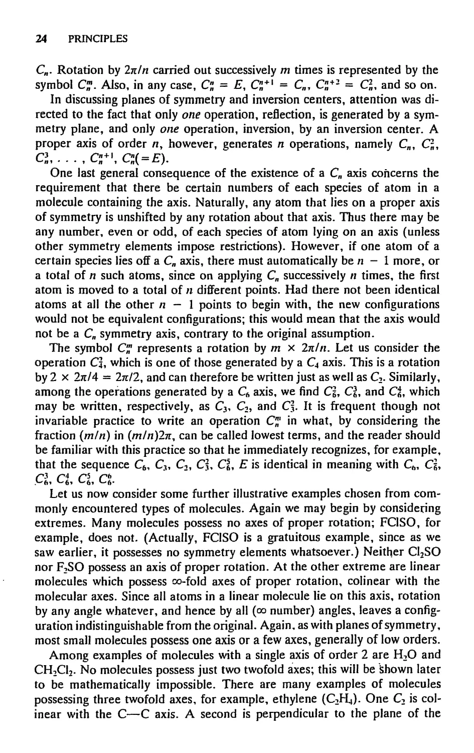
Figure 3.2 A tetrahedral molecule inscribed in a cube.
molecule and bisects the С—С line. The third is perpendicular to the first
two and intersects both at the midpoint of the С—С line. A regular tetrahedral
molecule also possesses three twofold axes, as shown in Figure 3.2.
Threefold axes are quite common. Both pyramidal and planar AB3 mol-
molecules possess threefold proper axes passing through the atom A and per-
perpendicular to the plane of the three В atoms. A tetrahedral molecule, AB4,
possesses four threefold axes, each passing through the atom A and one of
the В atoms. An octahedral molecule, AB6, also possesses four threefold
axes, each passing through the centers of two opposite triangular faces and
the A atom.
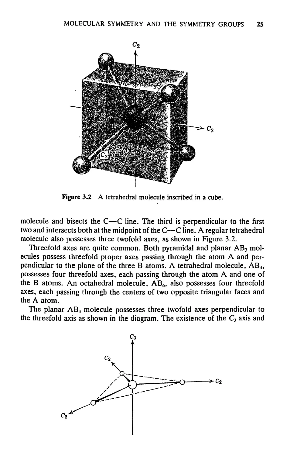
The planar AB3 molecule possesses three twofold axes perpendicular to
the threefold axis as shown in the diagram. The existence of the C3 axis and
26 PRINCIPLES
one C2 axis perpendicular to the C3 axis means that the other two C2 axes,
at angles of 2я/3 and 4я/3 to the first, must exist. For, on carrying out the
rotation C3, we generate the second C2 axis from the first, and on carrying
out the rotation C|, we generate the third C2 axis from the first.
The effect of the operations Cn, C2n,. . ., Cnn~l in replicating other symmetry
elements may profitably be discussed more fully at this point. The other
symmetry elements of interest are planes and axes. It will also be sufficient
to limit the discussion to axes perpendicular to the axis of the replicating
rotations and to planes that contain the axis of the replicating rotations.
A plane perpendicular to the axis of the replicating rotations is obviously
not replicated, since all rotations carry it into itself. Although a completely
general discussion might be given, it seems more instructive to consider
separately each of the replicating axes that can be encountered in practice
(С, К п ^ 8).
An axis perpendicular to a C2 axis or a plane containing a C2 goes into
itself on carrying out the operation C2; hence no further axes or planes of the
same type are required to exist in this case. We have just seen that from one
axis perpendicular to a C3 axis two similar ones are generated. The same is
true for a plane of symmetry containing a C3 axis. We may also deal with the
C5 and C7 cases (and, indeed, any Cn where n is odd) for they all behave in
the same way. One axis perpendicular to a C5 or C7 axis or one plane containing
a C5 or C7 will be made to generate four or six more separate and distinct
axes or planes by the operations that the C5 or C7 axis makes possible.
For cases where n in Cn is even, the results are less straightforward. Suppose
that we have one axis C2(l) perpendicular to a C4 axis. On carrying out the
rotation C4, C2(l) is rotated by 2я/4 and a second C2 axis, C2B), is thus
produced. On carrying out the rotation Cj( = C2) about the C4 axis, however,
C2(l) merely goes into itself, and C2B) also goes into itself. The operation
Cj takes C2(l) into C2B) and C2B) into C2(l). Hence, because C\ is really
only C2 and C\ is only C4 followed by C2, the C4 axis requires only that the
axis C2(l) be accompanied by one other such axis and not three others.
A completely analogous argument holds regarding planes. In the Q case,
using the same line of argument, it will easily be seen that, if one axis per-
perpendicular to a C6 or one plane containing a C6 exists, it must be accompanied
by two more of the same type. Similarly, a C8 axis will replicate a C2 axis
perpendicular to it so as to produce a set of four such C2 axes.
Continuing with examples of proper axes in typical molecules, we may cite
the planar PtCl4~ ion, which has a C4 axis perpendicular to the plane of the
ion and four C2 axes in the plane of the ion. The cyclopentadienyl anion,
Cfts, possesses a C5 axis perpendicular to the molecular plane and five C2
axes in the molecular plane. Benzene possesses a C6 axis and two sets of three
C2 axes. Probably the only known example of a molecule with a C7 axis is
the planar [C7H7]+, the tropyhum ion. An example of a molecule with a C8
axis is (CgHg^U (uranocene).
MOLECULAR SYMMETRY AND THE SYMMETRY GROUPS 27
3.6 IMPROPER AXES AND IMPROPER ROTATIONS
An improper rotation may be thought of as taking place in two steps: first a
proper rotation and then a reflection through a plane perpendicular to the
rotation axis. The axis about which this occurs is called an axis of improper
rotation or, more briefly, an improper axis, and is denoted by the symbol ?„,
where again n indicates the order. The operation of improper rotation by
2nln is also denoted by the symbol Sn. Obviously, if an axis Cn and a perpendic-
perpendicular plane exist independently, then Sn exists. More important, however, is
that an Sn may exist when neither the Cn nor the perpendicular a exist sep-
separately.
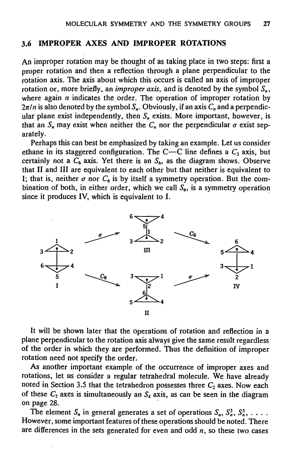
Perhaps this can best be emphasized by taking an example. Let us consider
ethane in its staggered configuration. The С—С line defines a C3 axis, but
certainly not a C6 axis. Yet there is an «S6, as the diagram shows. Observe
that II and III are equivalent to each other but that neither is equivalent to
I; that is, neither о nor C6 is by itself a symmetry operation. But the com-
combination of both, in either order, which we call 56, is a symmetry operation
since it produces IV, which is equivalent to I.
It will be shown later that the operations of rotation and reflection in a
plane perpendicular to the rotation axis always give the same result regardless
of the order in which they are performed. Thus the definition of improper
rotation need not specify the order.
As another important example of the occurrence of improper axes and
rotations, let us consider a regular tetrahedral molecule. We have already
noted in Section 3.5 that the tetrahedron possesses three C2 axes. Now each
of these C2 axes is simultaneously an S4 axis, as can be seen in the diagram
on page 28.
The element Sn in general generates a set of operations 5„, 5J, 5J, . . . .
However, some important features of these operations should be noted. There
are differences in the sets generated for even and odd /z, so these two cases
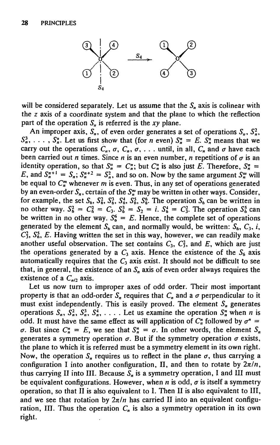
28 PRINCIPLES
will be considered separately. Let us assume that the Sn axis is colinear with
the z axis of a coordinate system and that the plane to which the reflection
part of the operation S,, is referred is the лгу plane.
An improper axis, Sn, of even order generates a set of operations Stll 5J,
5J, . . . , 5J. Let us first show that (for n even) S"n = E. S"n means that we
carry out the operations С„, o\ С„, a, . . . until, in all, Cn and a have each
been carried out n times. Since n is an even number, n repetitions of о is an
identity operation, so that S"a = Cnn\ but Q is also just E. Therefore, S"n =
?, and Si*1 = Sn; Snn+2 = SJ, and so on. Now by the same argument S™ will
be equal to C? whenever m is even. Thus, in any set of operations generated
by an even-order ?„, certain of the S"' may be written in other ways. Consider,
for example, the set 56, Sg, Si, St S56, 5g. The operation 56 can be written in
no other way. SI = Q = C3. SI = S2 = L Si = C5. The operation S5b can
be written in no other way. ?? = E. Hence, the complete set of operations
generated by the element Sb can, and normally would, be written: 56, C3, /,
C5, SI, E. Having written the set in this way, however, we can readily make
another useful observation. The set contains C3, C5, and ?, which are just
the operations generated by a C3 axis. Hence the existence of the S6 axis
automatically requires that the C3 axis exist. It should not be difficult to see
that, in general, the existence of an Sn axis of even order always requires the
existence of a Cnf2 axis.
Let us now turn to improper axes of odd order. Their most important
property is that an odd-order Sn requires that Cn and а о perpendicular to it
must exist independently. This is easily proved. The element Sn generates
operations 5Я, 5J, 5J, 5J, . . . . Let us examine the operation S" when n is
odd. It must have the same effect as will application of C" followed by an =
a. But since Q = E, we see that S" = a. In other words, the element Sn
generates a symmetry operation a. But if the symmetry operation о exists,
the plane to which it is referred must be a symmetry element in its own right.
Now, the operation Sn requires us to reflect in the plane o, thus carrying a
configuration I into another configuration, II, and then to rotate by 2я/л,
thus carrying II into III. Because Sn is a symmetry operation, I and III must
be equivalent configurations. However, when n is odd, a is itself a symmetry
operation, so that II is also equivalent to I. Then II is also equivalent to III,
and we see that rotation by 2nln has carried II into an equivalent configu-
configuration, III. Thus the operation Cn is also a symmetry operation in its own
right.
MOLECULAR SYMMETRY AND THE SYMMETRY GROUPS 29
To gain further familiarity with odd-order improper axes, let us consider
how many distinct operations are generated by some such axis, say S5. The
sequence begins S5, SI, S\, Sj4. . .. Using relations and conventions previously
developed, we can write certain of these operations in alternative ways, as
follows:
S5
Si
si
si
si
si
si
st
si
s?
sv
= c5
= c\
= c\
"Ci
= G
= Q
= ci
= C5
= ?
then
then
then
then
then
0 (or cr then C5)
(T
(T
cr
0
We see that for S5 through Sl5ti (in general, Sn through SJ"), the operations
are all different ones, but commencing with S2nn+l repetition of the sequence
begins. Of the 10 operations, however, 4 plus E can be expressed as a single
operation only by using symbols Sg, whereas the other 5 can be written either
as Q or as o. Thus there are operations which, although they may be ac-
accomplished by using C% and g successively, cannot be represented as unit
operations in any other way than S%. We also see that in general the element
Sn with n odd generates 2n operations.
3.7 PRODUCTS OF SYMMETRY OPERATIONS
In Sections 3.3-3.6 we have often discussed the question of how we can
represent the net effect of applying one symmetry operation after another to
a molecule, but only in a limited way. In this section we shall discuss this
question with regard to a broader range of possibilities. First, we shall establish
a conventional shorthand for stating that "operation X is carried out first and
then operation Y, giving the same net effect as would the carrying out of the
single operation Z." This we express symbolically as
YX = Z
Note that the order in which the operations are applied is the order in which
they are written from right to left, that is, YX means X first and then Y. In
general, the order makes a difference although there are cases where it does
not. When the result of the sequence XY is the same as the result of the
30 PRINCIPLES
sequence YX, the two operations, X and Y, are said to commute. It is also
normal to speak of an operation that produces the same result as does the
successive application of two or more others as the product of the others.
One way in which we may approach the problem of finding a single op-
operation which is the product of two others is to consider a general point with
coordinates [х1ч yt, zj. On applying a certain operation, this point will be
shifted to a new position with coordinates [jc2, y?, z2]\ if still another operation
is applied, it will again be shifted so that its coordinates are now [л, y3, z3].
The net effect of applying the two operations successively is to shift the point
from [jc,, уi, z,] to jx3, y3, z3]. We now look for a way of accomplishing this
in one step. The operation which does so will be the product of the first two.
Let us illustrate this procedure by proving the statement made earlier that,
if there are two twofold axes at right angles to one another, there must
necessarily be a third at right angles to both. Suppose that the two given axes
coincide with the x and у axes; we can designate them C2(x) and C2{y). On
applying first C2(x) and then C2(y) to a general point, the following trans-
transformations of its coordinates take place:
[-JClf -yl9 Zj]
That is , the value of x3 is -jc,, the value of y3 is -y,, and the value of z3 is
Z\. If now we apply C2(z) to the general point, it is shifted to [-xu —y,f zj.
Thus we may write
Сг(У)Сг(х) = C2(z)
Thus, whenever C2(x) and C2(y) exist, C2(z) must also exist, because it is
their product.
As a second example of how the existence of two symmetry elements may
automatically require that a third one exist, we shall consider a case having
a C4 axis and one plane containing this axis. We have already seen that the
operation C4 wiil generate a second plane from the first one at right angles
to it. It is also true, however, though less obvious, that when the C4 axis and
one of these planes exist there must then be a second plane also containing
C4 at an angle of 45° to the first one. We can prove this by the method just
used. The effect of reflecting a general point [xu y,, zj through the xz plane
is given by
cr(xz)[xu y,, z,] -* [xu -y,, z,]
whereas the effect of a clockwise C4 rotation about the z axis upon the point
is given by
C4(z)[xuyb z,]-»^,, -xlf z,]
MOLECULAR SYMMETRY AND THE SYMMETRY GROUPS 31
From these relations we can determine the effect of applying successively
a(xz) and then Ct(z), namely,
CA(z)a(xz)[xuyu z,]-» C4(z)[xu -yb 2,] -» [-y,, -xu 2,]
Now let us consider the effect of reflecting the point through a plane ad, which
also contains the z axis and bisects the angles between the +y and — x axes
and the +jc and — у axes. This transformation is
0d[xu Уи Z\] -* [ -yx, -xlt 2,]
We see that
C4(z)a(xz) = ad
which means that the existence of C4{z) and cr(xz) automatically requires that
<jd exist. The C4 rotation then generates from ad another plane, ad, which
passes through the first and third quadrants. The final result is that, if there
is one plane containing a C4 axis, there is automatically a set of four planes.
It may be shown in a very similar way that if C4(z) and C2(y) axes exist a
C2 axis lying in the first and third quadrants of the xy plane at 45° to C2(y)
must also exist. This is left as an exercise.
Examination of the shifts in a general point may also be employed to show
a commutative relation, for example, that C2(z) and cr(xy) commute. Thus,
we may write, in a notation that uses x instead of — jc> у instead of — y, and
2 instead of -2:
C2(z)[x,y,z]^ [x,y,z]
Фу)[х, У, А -+ [*> У* Щ
Gff[x, y, 2] -» C2[x, y, z] -^ [xy y, 2]
and
We see also that the product in each case is equivalent to L
In these examples, where only C2 and C4 rotations and certain kinds of
planes are concerned, the transformation of the coordinates [лг, у, z] to
[jc, y, 2] by a twofold rotation about the x axis, for example, is fairly obvious
by inspection. It is also obvious that a fourfold rotation about the x axis will
transform the coordinates into [jc, 2, y]. It is also easy to see by inspection
the effects of the inversion operation, an improper rotation by 2к/2 or 2я/4
and reflection in a plane that is the xy, xz, or yz plane or a plane rotated by
32 PRINCIPLES
45° from these. However, the transformations effected by more general sym-
symmetry operations, such as rotation by 2nln or rnlnln and reflections in planes
other than those just mentioned, are not easily handled by the simple methods
and notation used above. Further discussion along this line will therefore
employ some geometrical methods and also the more powerful methods of
matrix algebra, which will be introduced in Chapter 4.
3.8 EQUIVALENT SYMMETRY ELEMENTS AND
EQUIVALENT ATOMS
If a symmetry element A is carried into the element В by an operation
generated by a third element X, then of course В can be carried back into
A by the application of X~l. The two elements A and В are said to be
equivalent. If A can be carried into still a third element C, then there will
also be a way of carrying В into C, and the three.elements, A, #, and C,
form an equivalent set. In general, any set of symmetry elements chosen so
that any member can be transformed into each and every other member of
the set by application of some symmetry operation is said to be a set of
equivalent symmetry elements.
For example, in a plane triangular molecule such as BF3, each of the twofold
symmetry axes lying in the plane can be carried into coincidence with each
of the others by rotations of 2л/3 or 2 x 2л/3, which are symmetry operations.
Thus all three twofold axes are said to be equivalent to one another. In a
square planar AB4 molecule, there are four twofold axes in the molecular
plane. Two of them, C2 and C2, lie along BAB axes, and the other two, C?
and C7, bisect BAB angles. Such a molecule also contains four symmetry
planes, each of which is perpendicular to the molecular plane and intersects
it along one of the twofold axes. Now it is easy to see that C2 may be carried
into C2 and vice versa, and that CJ may be carried into Cj and vice versa,
by rotations about the fourfold axis and by reflections in the symmetry planes
mentioned, but there is no way to carry C2 or C2 into either CJ or C2" or vice
versa. Thus C2 and C2 form one set of equivalent axes, and C{ and C2" form
another. Similarly, two of the symmetry planes are equivalent to each other,
but not to either of the other two, which are, however, equivalent to each
other.
As other illustrations of equivalence and nonequivalence of symmetry ele-
elements, we may note that all three of the symmetry planes in BF3 that are
perpendicular to the molecular plane are equivalent, as are the three in NH3,
whereas the two planes in H2O are not equivalent. The six twofold axes lying
in the plane of the benzene molecule can be divided into two sets of equivalent
axes, one set containing those that transect opposite carbon atoms and the
other set containing those that bisect opposite edges of the hexagon.
Equivalent atoms in a molecule are those that may all be interchanged with
one another by symmetry operations. Naturally, equivalent atoms must be of
MOLECULAR SYMMETRY AND THE SYMMETRY GROUPS 33
the same chemical species. Examples of equivalent atoms include all of the
hydrogen atoms in methane, ethane, benzene, or cyclopropane, all of the
fluorine atoms in SF6i and all of the carbon and oxygen atoms in Cr(CO)b.
Examples of chemically identical atoms which are not equivalent in molecular
environment are the apical and equatorial fluorine atoms in PF5; no symmetry
operation possible for this molecule ever interchanges these fluorine atoms.
The a and 0 hydrogen and carbon atoms of naphthalene are not equivalent.
All six carbon atoms of cyclohexane are equivalent in the chair configuration,
but four are different from the other two in the boat configuration.
3.9 GENERAL RELATIONS AMONG SYMMETRY ELEMENTS
AND OPERATIONS
We present here some very general and useful rules about how different kinds
of symmetry elements and operations are related. These deal with the way
in which the existence of some two symmetry elements necessitates the ex-
existence of others, and with commutation relationships. Some of the statements
are presented without proof; the reader should profit by making the effort to
verify them.
Products
1. The product of two proper rotations must be a proper rotation. Thus,
although rotations can be created by combining reflections (see rule 2), the
reverse is not possible. The special case Cz(x)Ci(y) = C2(z) has already been
examined (page 30).
2. The product of two reflections, in planes A and 5, intersecting at an
angle фАВ, is a rotation by 2фАВ about the axis defined by the line of inter-
intersection. The simplest proof of this is a geometric one, as indicated in Figure
3.3. It is clear that this rule has some far-reaching consequences. If the two
planes are separated by the angle фАВч а С„ axis, where n = 2п/2фАВ, is
required to exist. Here n must be an integer, and the Cn axis will then assure
that a total of n such planes exists. Thus, the two planes imply that the entire
set of operations constituting the Cnv group (see below) is present.
3. When there is a rotation axis, С„, and a plane containing it, there must
be n such planes separated by angles of 2n/2n. This follows from rule 2.
4. The product of two C2 rotations about axes that intersect at an angle в
is a rotation by 20 about an axis perpendicular to the plane of the C2 axes.
This can be proved geometrically by a diagram similar to Figure 3.3. It also
implies that a Cn axis and one perpendicular C2 axis require the existence of
a set of n C2 axes and thus generate what we shall soon recognize as the Dn
group of operations.
34 PRINCIPLES
Figure 3.3 A geometric proof that the two reflection planes A and В require the
existence of a Cn axis along their line of intersection with n ~ 2п12флп. фАП - a +
/?, X = a + a + /? + p = 2(a + P). :. X = 2флв.
5. A proper rotation axis of even order and a perpendicular reflection
plane generate an inversion center, that is C^a = сС?я = C2a = aC2 = i.
Similarly C^i = iC"n = C2i - iC2 = a.
Commutation
The following pairs of operations always commute:
1. Two rotations about the same axis.
2. Reflections through planes perpendicular to each other.
3. The inversion and any reflection or rotation.
4. Two C2 rotations about perpendicular axes.
5. Rotation and reflection in a plane perpendicular to the rotation axis.
3.10 SYMMETRY ELEMENTS AND OPTICAL ISOMERISM
Although we have followed conventional practice—and for general purposes
will continue to do so—in setting out four kinds of symmetry elements and
operations, cr, /, С„, and Sn, we should note that the list can in principle be
reduced to only two Cn and Sn. A reflection operation can be regarded as an
St operation, that is» th& (trivisrf) rotation by 2к/1 together With ГСП*ССШЭП.
% t S\ k i on a general point, x, y, z. We
MOLECULAR SYMMETRY AND THE SYMMETRY GROUPS 35
suppose that the axis coincides with the z axis of a Cartesian coordinate
system; the reflection component then takes place through the xy plane:
S2(x, y, z) = oC2(x, уч z) -> a(x, y, z) -* (x, У, z)
But it is also true, by definition, that
|(дс, )>, z) -> (x, y, z)
Thus S2 and / are merely two symbols for the same thing.
All symmetry operations that we wish to consider can be regarded as either
proper or improper rotations.
Molecules that are not superimposable on their mirror images are termed
dissymmetric. This term is used rather than asymmetric, since the latter means,
literally, have no symmetry; that is, it is applicable only to a molecule be-
belonging to point group Сi. All asymmetric molecules are dissymmetric, but the
converse is not true. Dissymmetric molecules can and often do possess some
symmetry. It is possible to give a very simple, compact rule expressing the
relation between molecular symmetry and dissymmetric character:
A Molecule That Has No Improper Rotation Axis Must Be Dissymmetric.
Since improper rotation axes include 5, = a, and S2 = /, the more familiar
[but incomplete!) statement about optical isomerism existing in molecules that
lack a plane or center of symmetry is subsumed in this more general one. In
this connection, the tetramethylcyclooctatetraene molecule (page 37) should
be examined more closely. This molecule possesses neither a center of sym-
symmetry nor any plane of symmetry. It does have an SA axis, and inspection will
show that it is superimposable on its mirror image.
To show the validity of this rule, we first prove that if an Sn axis does exist
the molecule cannot be dissymmetric; that is, it must have a superimposable
mirror image.
1. A molecule has one and only one mirror image. It makes no difference
where or in what orientation we place the mirror plane; we may place and
orient it wherever convenient. We may therefore allow it to pass through the
molecule.
2. If the molecule has an Sn axis, we may place the plane so it coincides
with the plane through which the reflectional part of an Sn operation takes
place. If the Stt axis is of odd order, the pure reflection operation (Sj or 5j)
will actually exist as a symmetry operation. The molecule is then obviously
superimposable on its mirror image.
3. It the improper axis is of even order and <xh does not exist independently,
reflection will give a figure that is not superimposed on the original but needs
36 PRINCIPLES
(a)
(с)
Figure 3.4 The labeled cube 1 has as its only symmetry element an inversion center.
In step (a) the inversion operation is carried out on 1. In step (b) we rotate by к about
the 2 axis and thus orient it in space so it can be directly superimposed on 3. The
labeled cube 3 is the mirror image of 1 obtained by reflection, step (c), in a plane
perpendicular to z.
only to be rotated by 2nln in order to come into coincidence. This rotation
of the molecule as a whole does not change its structure, and thus the molecule
and its mirror image are superimposable.
If a molecule is superimposable on its mirror image, that mirror image will
be produced by applying one of the symmetry operations in the point group
for the molecule. This is obvious for all point groups having an Sn (n odd
axis), since these have the or operation as such.
For the special case of S2 s i, the mirror image is produced by the inversion
operation, but must be rotated by 180° to bring it into an exact reflective
relationship to the original. This can be seen in Figure 3.4 and is conveniently
expressed by using the matrices for the coordinate transformations. (Readers
unfamiliar with matrix algebra may consult Appendix I.) Thus, we represent
the operation S2 s / by the first matrix shown below and a rotation by к
MOLECULAR SYMMETRY AND THE SYMMETRY GROUPS 37
around the z axis by the second one. The product of these is the third matrix
and this clearly describes the process of reflection in a mirror plane perpen-
perpendicular to z. Since the / operation gives a molecule indistinguishable from the
original, and the rotation by к cannot change that indistinguishability, it is
clear that the symmetry operation i generates a mirror image superimposable
on the original.
-1 О 01Г-1 0 0
0 -1 0 0-10
0 0-10 0 1
We now turn to the only remaining cases, those that have only Sn axes of
even order ^4. In practice only 54 is likely to be encountered, although rare
examples of S6 and S8 are known. We shall analyze that specific case, but it
will be evident that the analysis is easily adaptable to all S» {n even) axes.
The matrix describing the action of an SA rotation about z on any point in
the molecule, (дг, у, z) is shown at the top of page 38. If this is multiplied by
the matrix for a proper rotation by nil, we obtain the matrix for reflection
in a mirror plane perpendicular to z. Thus, the operation Бл converts the
molecule into its superimposable mirror image. For the specific case of 1,3,5,7-
tetramethylcyclooctatetraene, which belongs to point group ?,, this is shown
pictorially in Figure 3.5.
Rrllrrt
in Inni/iitiial
mirntr
1
Figure 3.5 Drawings showing that 1,3,5,7-tetramethylcyclooctatetraene, which be-
belongs to point group ?,, is converted by the SA operation into its mirror image. The
direct result of the S4 operation needs to be turned 90° to become coincident with the
mirror image at lower left.
38 PRINCIPLES
0 -1 О*
1 О О
О О 1
Finally, we turn to the principle that if a molecule has no Sn axis, it cannot
be superimposable on its mirror image. The symmetry group of a molecule
must include every operation capable of converting the molecule into one
indistinguishable from the original. If its mirror image is indistinguishable, it
must result from at least one of the symmetry operations. We have shown
that all improper rotation axes generate operations that produce a mirror
image that is superimposable. However, proper rotations are incapable of
producing any mirror image, because all they do, singly, or however combined
with one another, is reorient the molecule in space. If a molecule has a
superimposable mirror image, it must belong to a symmetry group that con-
contains at least one operation that will make that manifest, and only some kind
of Sn operation is able to do so. If, therefore, a molecule belongs to a symmetry
group having no Sn operation, that is, to a group consisting only of proper
rotations, its mirror image must be nonsuperimposable.
Are There Exceptions?
There are no genuine exceptions to the above prescriptions concerning dis-
dissymmetric molecules, but when we deal with molecules in which internal
rearrangement, say by rotation about bonds, may occur, these prescriptions
may not tell the whole story from the point of view of the chemist. Such cases
are rare, but let us mention one that has been in the chemical literature for
some years [cf. K. Mislow and R. Bolstad, J. Am. Chem. Soc, 71, 6712
A955)]. It has been stated—correctly—that the compound shown as 1 in
Figure 3.6 is "optically inactive and configurationally pure" even though its
"individual molecules are asymmetric." This molecule is, however, dissym-
dissymmetric, as the drawings in Figure 3.6 clearly show: Molecule 2 is the mirror
image of 1, and in 3 it is simply flipped top to bottom and rotated 90° clockwise.
This causes the lower half to coincide with the lower half of 1, but the upper
half does not then coincide. In short 1 and its mirror image do not coincide,
and these molecules are members of a dissymmetric pair.
The reason 1 (and, equally 3) are not optically active is because internal
rotation about one С—С bond can take place so as to interconvert 1 and 3.
While that is chemically of importance, it has nothing to do with the math-
mathematical question of the symmetry properties of these molecules.
The fact that optical isomers of amines of the type NRR'R" cannot be
isolated is the same sort of nongenuine "exception." Such a molecule is truly
dissymmetric. The only reason optical isomers are not isolable is that its
internal structure is not rigid. Here it is not an internal rotation but an
MOLECULAR SYMMETRY AND THE SYMMETRY GROUPS 39
0
Figure 3.6 Structure 1 is a molecule that has been shown experimentally to be
optically inactive, but which is dissymetric. In step (a) it is reflected in a vertical mirror
perpendicular to the plane of the paper. In step (b) the mirror image 2 is flipped
vertically and rotated to make the bottom half of 3 coincide with the bottom half
ofl.
umbrella-type inversion that allows the two dissymmetric isomers to inter-
convert.
3.11 THE SYMMETRY POINT GROUPS
Suppose that we have, by inspection, compiled a list of all of the symme-
symmetry elements possessed by a given molecule. We can then list all of the sym-
symmetry operations generated by each of these elements. Our first objective
in this section is to demonstrate that such a complete list of symmetry
operations satisfies the four criteria for a mathematical group. When this
has been established, we shall then be free to use the theorems concern-
concerning the behavior of groups to assist in dealing with problems of molecular
symmetry.
Let us first specify what we mean by a complete set of symmetry operations
for a particular molecule. A complete set is one in which every possible
product of two operations in the set is also an operation in the set. Let us
consider as an example the set of operations which may be performed on a
planar AB3 molecule. These are E, C3, Cj, C2, C{, CJ, <т„ <?'„, oj, (Th, S3, and
?3. It should be clear that no other symmetry operations are possible. If we
number the В atoms as indicated, we can systematically work through all
binary products; for example:
40 PRINCIPLES
Hence we see that gvC3 - a[.. Proceeding in this way, we can check all the
combinations and we will find that the set given is indeed complete. This is
suggested as a useful exercise.
Now, we can see that, because our set of operations is complete in the
sense defined above, it satisfies the first requirement for mathematical groups,
if we take as our law of combination of two symmetry operations the successive
application of these operations.
The second requirement—that there must exist a group element E such
that for every other element in the group, say X, EX = XE = X—is also
seen to be satisfied. The "operation" of performing no operation at all, or
that which results from a sequence of operations which sends the molecule
into a configuration identical with the original (e.g., a2, CJ), is our identity,
?, and we have been calling it that all along.
The associative law is obviously valid for products of symmetry operations.
The final requirement, that every element of the group have an inverse,
is also satisfied. For a group composed of symmetry operations, we may define
the inverse of a given operation as that second operation, which will exactly
undo what the given operation does. In more sophisticated terms, the recip-
reciprocal S of an operation R must be such that RS = SR = E. Let us consider
each type of symmetry operation. For a, reflection in a plane, the inverse is
clearly a itself: a x a = cr - E. For proper rotation, C™, the inverse is
Q~m, for C? x Cj"m = CJ = E. For improper rotation, S™, the reciprocal
depends on whether m and n are even or odd, but a reciprocal exists in each
of the four possible cases. When n is even, the reciprocal of S% is Snn~m whether
m is even or odd. When n is odd and m is even, S'" - C™, the reciprocal of
which is Cl~m. For S™ with both n and m odd we may write S'H = Cfa. The
reciprocal would be the product C"n~ma, which is equal to Cl"~ma, and which
in turn may be written as a single operation, Sj;"".
We have shown that complete sets of symmetry operations do constitute
groups. Now we shall systematically consider what kinds of groups will be
obtained from various possible collections of symmetry operations.
MOLECULAR SYMMETRY AND THE SYMMETRY GROUPS 41
In the trivial case where there are no symmetry operations other than ?,
we have a group of order 1 called C\*
Let us next consider molecules whose sole symmetry element is a plane.
This element generates only two operations, namely, a and a2 = E. Hence
the group is of order 2. The symbol normally given to this group is Q. It is
also possible to have a molecule whose sole symmetry element is an inversion
center. The only operations generated by the inversion center are i and i1 =
E. Again we have a group of order 2; this one is conventionally desig-
designated C,.
Let us consider now the cases where the only symmetry element is a proper
axis, Cn. This generates a set of operations Cn,C2n,Cl,. . . , Q = E. Hence
a molecule with С„ as its only symmetry element would belong to a group of
order я, which is designated Cn. It may be noted that a Cn group is a cyclic
group (see Section 2.2) and hence also Abelian.
When an improper axis is present, we must consider whether it is even or
odd. When the axis, S,,, is of even order, the group of operations it generates
is called Sn and consists of the n elements E, 5n, Cn/2, 5J, . . . , S;-'. The
group S2 is a special case because, as shown earlier, the symmetry element
S2 is equivalent to z. Thus the group that might be called the S2 group is
actually called C,. The group of operations generated by an Sn axis when n
is odd has been shown to consist of In elements, including ah and the oper-
operations generated by Cn. By convention such groups are denoted Cnh. This
symbol emphasizes that there is а С„ axis and a horizontal plane; this com-
combination of symmetry elements of course implies the existence of Sn just as
Sn (n odd) implies the existence of Cn and a,,. The Cnh groups will be discussed
in more detail shortly.
Next we turn to groups that arise when two or more symmetry elements
are present. In so doing, we shall divide the discussion into two parts. First,
we deal with cases where there is no more than one axis of order higher than
2. Then, in the next section, we shall take up the groups that arise when
there are several high-order (n > 2) axes. In each part, we shall proceed in
a systematic way which should suggest strongly, if not actually prove rigor-
rigorously, that all possibilities have been included.
We have already seen that, if a molecule possesses a proper axis, Cni and
also a twofold axis perpendicular to it, there must then necessarily be n such
twofold axes. The n operations, ?, Cn, CJ, . . . ,. С"„~\ plus the n twofold
rotations constitute a complete set of symmetry operations, as may be verified
* This symbol and the other ones for the symmetry groups, for example, С Dni Cnh, Ст, Dnh.
DnJ which will be introduced are called the Sclwnflies symbols after their inventor. The
symmetry groups are also frequently called point groups, since all symmetry elements in a
molecule will intersect at a common point, which is not shifted by any of the symmetry operations.
There are also symmetry groups, called space groups, which contain operations involving trans-
latory motions. The latter are considered in Chapter II.
42 PRINCIPLES
by actually carrying through all of the binary products. Thus such a group
consists of a total of In elements. The symbol for a group of this kind is Dn.
We have now reached a point of departure in the process of adding further
symmetry elements to a Cn axis. We shall consider A) the addition of different
kinds of symmetry planes to the С„ axis only, and B) the addition of symmetry
planes to a set of elements consisting of the Cn axis and the n C2 axes per-
perpendicular to it. In the course of this development it will be useful to have
some symbols for several kinds of symmetry planes. In defining such symbols
we shall consider the direction of the С„ axis, which we call the principal axis
or reference axis, to be vertical. Hence, a symmetry plane perpendicular to
this axis will be called a horizontal plane and denoted ah. Planes that include
the Cn axis are generally called vertical planes, but there are actually two
different types. In some molecules all vertical planes are equivalent and are
symbolized av. In others there may be two different sets of vertical planes (as
in PtClJ"; cf. page 32), in which case those of one set will be called av and
those of the other set ad, the d standing for dihedral. It will be best to discuss
these differences more fully as we meet them.
If to the Cn axis we add a horizontal plane, we expand the original group
of n operations, Cn, CJ, ...,?, to include all of the products ahCn, ahC2n,
crhCl, . . . , ahE = ahl making In operations in all. Now the operation
GhC™ = C%(Th, since ah affects only the z coordinate of a point while Cj1 affects
only its x and у coordinates, so that the order in which a and C? are performed
is inconsequential. Furthermore, all of the new operations of the type aC™
can be expressed as single operations, namely, as improper rotations. This
new set of 2n operations can easily be shown to be a complete set and hence
to constitute a group. Such a group has the general symbol C^.
Let us look next at the consequences of adding a vertical plane to the С„
axis. First we recall (Section 3.5) that the operations generated by С„ when
n is odd will require that an entire set of /i such vertical planes exist. All of
these planes are properly called vertical planes and symbolized av. When n
is even, however, we have seen (Section 3.5) that only /z/2 planes of the same
type will exist as a direct consequence of the Cn axis. However, we have also
shown (Section 3.7) that another set of nil vertical planes must exist as the
various products C™gv. These vertical planes in this second set are usually
called dihedral planes, since they bisect the dihedral angles between members
of the set of ov's, and they are denoted ad. Obviously, it is completely arbitrary
which set is considered vertical and which dihedral. In either case, n even or
n odd, the set of operations generated by the Cn and by all of the cr's constitutes
a complete set, and such a group is called Cnv.
We might naturally ask now about what happens when we add both the
horizontal plane and the set of n vertical planes to the Cn, This gives a group
called Dnh, which we shall now develop by a different procedure.
Let us consider the consequences of adding a ah to the group Dn. The
group generated is denoted Dnh. We must first look at all of the products of
07, with the operations generated by the C2 axes and by the Cn axis. Suppose
MOLECULAR SYMMETRY AND THE SYMMETRY GROUPS 43
we choose a coordinate system such that the Cn axis coincides with the z axis,
and one of the C2 axes, Сг(х)% coincides with the a* axis. We can indicate the
effect of rotation about the C2(x) axis followed by ah on a general point
[x, y, z] thus:
The effect of reflection in the xz plane on the same point will be
[x,y,z]-**[x,y,z]
Thus we can write
ahC2(x) = a(xz) = C2(x)ah
where the second equality simply states that the rotation and the ah commute-,
which we have previously shown to be generally true. Of course, it now follows
that, if one of the C2 axes lies in a vertical symmetry plane, so must all of
the others. There must then be a set of n operations av. We may now left-
multiply the above equation by ah, obtaining
GhGhCi - GhGv = C2
and we see that all of the products of ah with the ov's are C2's. Thus we might
also take the simultaneous existence of Cn, ah, and the a/s as the criterion
for the existence of the group Dnh. It is only by reason of convention and not
because of any mathematical requirement that we take instead the simulta-
simultaneous existence of С„, /zC2's, and ah as the criterion.
We have now shown that the operations in a group Dnh include ?,
(л — 1) proper rotations about С„, п reflections in vertical planes, a^ and n
rotations about C2 axes. These Ъп 4- 1 operations still do not constitute the
complete set, however. It will be found that among the products C™ah =
ohCH are n - 1 additional operations which are all improper rotations. For
the general case where n is even, we obtain the new operations: Sny Snf2,
i ( = С2/2аЛ), . . . , Sjjf !\ Si'1. In the group D^, for example, we have S6t
S3l i, S]y and Si. When n is odd we obtain in the general case the following
n - 1 improper rotations: Sn, S3n, 5J, . . . , S*"~3, Sl"~l except S"n ( = <7Л);
S% where m is even being, of course, either E or one of the proper rotations
which we have already recognized. Thus, we now have a total of An operations
in the group D^. Systematic examination will show that the set is complete.
Our next and final task is to consider the consequences of adding to Cn
and the n C2s a set of dihedral planes, ajs. These are vertical planes that
bisect the angles between adjacent pairs of C2 axes. The groups generated by
this combination of symmetry elements are denoted Dnd. The products of a
od with the various C™ operations are all other ad operations. However, among
44 PRINCIPLES
the various products of the type adC2 there is a set of n new operations
generated by an S2n axis colinear with С„. These 4/7 operations now constitute
the complete group Dnd.
Linear Molecules
These constitute a somewhat special case, although their possible point groups
are closely related to the scheme just developed. Any linear molecule has an
axis of symmetry coinciding with all the nuclei. The order of this axis is oo;
that is, rotations by any and all angles about this axis constitute symmetry
operations. Also, any plane containing the molecule is a plane of symmetry.
There is an infinite number of such planes, all intersecting along the molecular
axis. Proceeding from this, we have just two possibilities: A) the molecule is
of the type OCO, NCCN, and so on, such that it consists of two equivalent
halves, or B) it is of the type NNO, HCN, and so on, and does not consist
of two equivalent halves.
In the first case, the equivalence of the two halves means that any line
which is a perpendicular bisector of the molecular axis is a C2 symmetry axis;
there is an infinite number of such C2 axes. The equivalence of the two
halves of the molecule also means that there is a plane of symmetry perpen-
perpendicular to the molecular axis. Since there is an infinity of rotations about a
unique, vertical axis, C», there is also an infinity of C. axes perpendicular to
C*, and there is a horizontal plane of symmetry. The group is, very reasonably,
designated Dxh.
For linear molecules which do not consist of equivalent halves, the only
symmetry operations are the rotations about C* and reflections in the vertical
planes. The group is called C»,..
3.12 SYMMETRIES WITH MULTIPLE HIGH-ORDER AXES
We have so far considered how groups of symmetry operations may be sys-
systematically built up by beginning with one proper axis of rotation (the ref-
reference axis) and the operations that it generates and adding to this group (a
pure rotation group, С„) the operations generated by additional symmetry
elements, these being restricted to planes or twofold axes. We have not yet
inquired about the possibility of adding to the operations generated by one
higher-order (n > 2) axis additional high-order axes. That is the subject we
must now investigate.
It turns out that there are not actually very many possibilities (only seven,
to anticipate); some of these, however, are among the most important point
groups we shall encounter in nature, and thus they deserve careful consid-
consideration. An interesting and systematic way to approach the subject is to
recognize that groups involving several equivalent, intersecting, higher-order
axes will be represented by polyhedra having faces perpendicular to such
MOLECULAR SYMMETRY AND THE SYMMETRY GROUPS 45
axes. For example, the tetrahedron, with four equilateral triangular faces,
must have four equivalent, intersecting C3 axes. By first making a demon-
strably complete list of all such polyhedra, and then systematically considering
their symmetry groups and all subgroups thereof in which the multiple axes
are retained, we may expect to obtain a complete list of the symmetry groups
with multiple high-order axes.
The Five Platonic Solids
To implement the above plan we consider the regular polyhedra, sometimes
called the Platonic solids, of which there are five. By a regular polyhedron
we mean a polyhedron
A) whose faces are all some regular polygon (i.e., equilateral triangle,
square, regular pentagon, hexagon, etc.) and equivalent to one an-
another;
B) whose vertices are all equivalent; and
C) whose edges are all equivalent.
By "equivalent" we mean, as usual, interchangeable by symmetry operations.
The five regular polyhedra are depicted and their essential characteristics
listed in Table 3.2.
Our first task is to show that the five Platonic solids do, in fact, represent
all the possibilities. This is quite easy to do.
In order to construct a polyhedron, three or more of the desired faces must
meet at a point so as to produce a closed, pyramidal {not planar) arrangement.
Using equilateral triangles, we have the following possibilities:
1. Three triangles with a common vertex.
2. Four triangles with a common vertex.
3. Five triangles with a common vertex.
If six equilateral triangles share a common vertex, the sum of the angles
around the vertex is 6 x 60 = 360°. The array is planar and cannot form
part of a regular polyhedron. It is clear that the three possibilities listed give
rise to the tetrahedron, the octahedron, and the icosahedron, as shown in
Table 3.2.
For the next higher regular polygon, the square, there is only one possi-
possibility, namely, three squares with a common vertex, and this gives rise to the
cube. Four squares having a common vertex would all lie in one plane.
With regular pentagons (internal* angle, 108°), there is only one possibility,
namely, three pentagons meeting at a common, vertex C x 108° = 324°),
since four or more could not be fitted together D x 108° = 432°). This single
conjunction of pentagons can be replicated to produce the dodecahedron.
46 PRINCIPLES
TABLE 3.2 The Five Regular Polyhedra or Platonic Solids
Tetrahedron
Faces: 4 equilateral triangles
Vertices: 4
Edges: 6
Cube
Faces: 6 squares
Vertices: 8
Edges: 12
Octahedron
Faces: 8 equilateral triangles
Vertices: 6
Edges: 12
Dodecahedron
Faces: 12 regular pentagons
Vertices: 20
Edges: 30
Icosahedron
Faces: 20 equilateral triangles
Vertices: 12
Edges: 30
With hexagons, there is no way to construct a regular polyhedron, since
even three hexagons sharing a vertex lie in the same plane. With all higher
polyhedra not even three can be fitted together at a common vertex.
It is clear, therefore, that the five Platonic solids are the only regular
polyhedra possible. Let us now examine them to see what symmetry opera-
operations may be performed on each one.
MOLECULAR SYMMETRY AND THE SYMMETRY GROUPS 47
Inspection of the tetrahedron (see Fig. 3.7) reveals the following symmetry
elements and operations.
(i) Three S4 axes coinciding with the *, }', and z axes. Each of these
generates the operations S4, 5J = C2, and SI.
(ii) Three C2 axes coinciding with the x, y, and z axes, each of which
generates an operation C2- These operations have already been generated,
however, by the S4's.
(iii) Four C3 axes, each of which passes through one apex and the center
of the opposite face. Each of these generates C3- and C\ operations, that is,
eight operations in all.
(iv) Six planes of symmetry, each of which generates a symmetry opera-
operation.
The entire set of operations thus consists of the following 24, which are
listed by classes (as will be explained in Section 3.13):
?, 8C3, 3C;, 6S4, ва,,
This group is called Tj.
The octahedron has the following symmetry elements.and operations.
(i) Three SA axes, each passing through a pair of opposite apices. Each
generates the operations 54, C2, S].
Figure 3.7 A tetrahedron within a cube, showing a set of Cartesian axes.
48 PRINCIPLES
(ii) Three C2 axes colinear with the S4's. The C2 operations generated
by these axes, however, are already accounted for under (i).
(iii) Three C, axes colinear with the S4's and CVs. Each generates a set
of operations C4, C2, and CI, but only C4 and C4 are new.
(iv) Six C{ axes, which bisect opposite edges. Each generates an oper-
operation C'2.
(v) Four Sb axes, each passing through the centers of a pair of opposite
triangular faces. Each generates a set of operations 56, C3, /, Cjy Sj.
(vi) Four C3 axes colinear with the S6's. Each generates two operations,
C3 and C3, which are also generated by the colinear 56.
(vii) An inversion center which generates an operation /, also generated
by each of the Sb axes.
(viii) Three planes of symmetry each of which passes through four of the
six apices and generates an operation ah.
(ix) Six planes of symmetry each of which passes through two apices,
bisects two opposite edges and generates an operation ad.
The entire set of operations thus consists of the following 4S, grouped by
classes (as will be explained in Section 3.13):
E, 8C3, 6C4, 6C2, 3C2( = Q, /, 6S4, 8S6, 3<7/f, 6ad
This is the group called Oh.
Inspection will show that the cube has precisely the same set of symmetry
operations as the octahedron; it, too, belongs to the point group <9A. It is
worthwhile noting that the cube and the octahedron are very closely related.
Each is obtainable from the other by shaving off corners, as shown in Figure
3.8 for the cube-to-octahedron conversion. In a cube the faces are penetrated
by C4 axes and the vertices by C3 axes; in the octahedron the vertices lie on
Ci axes and the faces are penetrated by the C3 axes. The nonregular poly-
polyhedron obtained as an intermediate when the triangular faces just meet is
called a cuboctahedron. It, too, has Oh symmetry, as does every polyhedron
which is transitional, in the sense of Figure 3.8, between the cube and the
octahedron. The cuboctahedron occurs in nature as B,2 cages in certain borides
and has an interesting relationship to the icosahedron (cf. Exercise B3.1).
Finally, we turn to the pentagonal dodecahedron and the icosahedron.
These two polyhedra have the same symmetry. They are related to each other
as the cube and octahedron are related. The symmetry elements and oper-
operations are as follows.
(i) Each polyhedron has a set of six Sm axes. In the dodecahedron these
pass through opposite pairs of pentagonal faces; in the icosahedron they pass
through opposite vertices. Each Sw axis generates these operations: SiU,
Si, - C5, Slh SI = Ci SI = /, Sfc, - Cl $!„, 5ft, - Ci, SJllf E.
MOLECULAR SYMMETRY AND THE SYMMETRY GROUPS 49
^J—
Cube
Cuboctahedron
U'
Octahedron
(inscribed in the
original cube)
Figure 3.8 Conversion of the cube to the octahedron via the cuboctahedron.
(ii) Each polyhedron has 10 Se axes. In the dodecahedron they pass.through
opposite pairs of vertices; in the icosahedron they pass through pairs of
opposite faces. Each of these generates these operations: 56, SI =
C3, Si •= S2 - /, S4b = C5, Si, E. Of these, / and E have already been noted,
(iii) There are 6 C3 axes, colinear with the Stn axes. They generate C5,
C5, Cl, Cj operations, which have already been counted under Sm.
' (iv) There are 10 C3 axes, colinear with the Sb axes. These generate C3
and C\ operations, which have already been counted under Sh.
(v) There are 15 C2 axes, which in each case bisect opposite edges. These
generate 15 C2 operations.
(vi) There are 15 mirror planes, each containing 2 C2 axes and 2 C5 axes.
They generate 15 reflection operations.
Altogether there are 120 operations, which form the following classes:
?, 12C5, 12CI 2OC3, 15G, /, 125»,, 125?e, 2056, 15a
The group that they constitute is called /,,.
By direct inspection of the ftvt regular polyhedra we have discovered three
50 PRINCIPLES
point groups: Г,/, Ол, Д. There are, however, several more, which we will
now obtain straightforwardly from these. As noted earlier (page 33), products
of rotations can only be rotations. Thus there are pure rotation groups. If
from any group containing reflections we remove the reflections and all their
products with the proper rotations, there will remain a subgroup consisting
entirely of proper rotations.
Thus the group Td has a pure rotational subgroup, Г, of order 12. It consists
of the following classes:
E, 4C3, 4CI 3C2
The group Oh has a pure rotational subgroup О of order 24. It consists of
the following classes:
?, 6C4, 3C2( = C42), 8C3, 6C2
The group Ih has a pure rotational subgroup, /, consisting of the following
60 operations:
?, 12C5, 12Cs, 20C3, 15C2
Finally, there is one more group, called Th. This can be derived by adding
to Г a set of planes, a,n which contain pairs of C2 axes (as opposed to planes
OV/, which contain one C2 axis and bisect another pair, thus giving Td). When
all the distinct products of these planes with the operations of T are enum-
enumerated and collected into classes, we have
?, 4C3, 4CI 3C2, i\ 456, ASl 3ah
All together, we now have the following seven groups containing multiple
high-order axes:
TO I
Th Oh lh
Td
From the systematic way in which they were obtained it should be clear that
this is an exhaustive list.
3.13 CLASSES OF SYMMETRY OPERATIONS
In Section 2.4 the concept of classes of elements within a group was intro-
introduced. This concept is utilized in dealing with symmetry groups. As we shall
see in Chapter 4, it is convenient and customary in writing what is caJled the
character table of a group to consider all the elements of a given class together,
MOLECULAR SYMMETRY AND THE SYMMETRY GROUPS 51
Figure 3.9 The relationship of ov and oa planes in C...
since they ail behave identically in the properties covered by the character
table. It is the purpose of this section to explain the manner in which the
symmetry operations are arranged into classes and to discuss the geometrical
significance of the classes.
Of course, the general definition of a class and the method of arranging
the elements of a group into classes given in Section 2.4 is perfectly applicable
to a symmetry group. Let us consider, for example, the group CAv. This group
of operations arises when the following symmetry elements are present: CA
and av. There are eight operations in the complete set generated by these
symmetry elements, namely, ?, C4, CI = C2, C-J, 2o\., 2ad. The a*s are planes
perpendicular to one another, intersecting along the C4 axis, and so are the
o-rf's. The ajs make 45° angles with the cr,.'s (see Fig. 3.9). By methods pre-
previously explained and illustrated for determining the products of symmetry
operations, a multiplication table for this group can be worked out.
Then, using this to carry out all of the possible similarity transformations,
we find that there are the following classes:
E
C4, Ci
C2
52 PRINCIPLES
It may be noted parenthetically that this result provides a good example of
the fact that, although the orders of all classes must be integral divisors of
the group order, not all integral divisors of the group order need be repre-
represented among the orders of the classes. Observe that, while 4 is an integral
divisor of 8, there is no class of order 4 in this group.
With symmetry groups the classes have a geometrical significance that may
be stated as follows: Two operations belong to the same class when one may
be replaced by the other in a new coordinate system which is accessible by a
symmetry operation. The italicized part of this prescription is quite important.
Let us consider the group C4(. and its subgroup C4 to see what this means.
The operation C\ shifts every point in the molecule by 3 x 2л/4 in, let us
say, the clockwise direction. This, however is the same thing as shifting every
point by 2л/4 in the counterclockwise direction. Let us then for the moment
think of the operation C4 as rotation by 2л/4 clockwise and C4 = C\ as
rotation by 2л/4 counterclockwise. Now suppose that the coordinate system
in which we have been working is (a) such that clockwise rotation by 2л/4
(a)
(b)
converts a point [x, y] into [у, -л], while counterclockwise rotation by
2я/4 converts [л\ y] into [—у, лг]. Symbolically
C(z)[A-,y]-»[y, -л]
In coordinate system F), however, the effects of C4 (clockwise) and C'A (coun-
(counterclockwise) are
Ci(z)[x, )>]->[ j\ -*]
In short, the roles of C4 and C4 are interchanged in coordinate systems (b)
from what they are in coordinate system (a). Now (and this is the important
point) there is a symmetry operation in the group C4(. which will convert
coordinate system (a) into coordinate system (b), namely, a{jK Thus, in the
MOLECULAR SYMMETRY AND THE SYMMETRY GROUPS 53
group C4l., C4 and С а = C\ are in the same class. However, in the group CA
(which contains only the operations E, C4, C2, CJ) they are not in the same
class because none of these four operations has the effect of transforming
coordinate system (a) into system (b). Of course, since any Cn group is cyclic
and hence Abelian, we can see that all operations must be in different classes,
since each operation is conjugate only with itself in an Abelian group.
Returning to the group CAv again, we note that C2 is in a class by itself.
This is so on geometrical grounds, because clearly there can be no way of
shifting the coordinate system so that the effects of a rotation by 180° can be
produced by a rotation by 90°, or by a reflection of any kind. Also, the ct,.'s
and ajs form separate classes. Only a rotation by 2л/8 could change the
orientation of the coordinate system to a new one in which ad would accom-
accomplish what av did in the old one, and rotation by 2л78 is not a symmetry
operation that occurs in the group.
It might be suspected intuitively that there would be a close relationship
between the classes of operations and the various sets of equivalent operations
in a group. In fact, the classes correspond directly to the sets of equivalent
operations. The reason is easy to see. The geometrical criterion for putting
two operations, A and B, in the same class is that there be some third op-
operation, C, which can be applied to the coordinate system so that operation
В in the transformed coordinate system is analogous to operation A in the
original coordinate system. At the same time, we say that operations A and
В are equivalent if one is converted into the other (in the same coordinate
system) by applying operation С to operations A and B. Now to say that
operation С interchanges operations A and В when applied to them, leaving
the coordinate system fixed, is perfectly equivalent to saying that operation
С interchanges the functions of A and В when applied to the coordinate
system, leaving the operations fixed in space. Hence, the simplest way of
arranging the operations of a symmetry group into classes is to arrange them
into sets of equivalent operations. These sets will be the classes.
A practical consequence of collecting all operations in the same class when
writing down the complete set, for example, at the head of a character table,
is that the notation used is a little different from what we have Ьеед using
thus far. This new and final form of notation will now be explained and
illustrated for the four kinds of symmetry operations.
(i) Inversion. Only one inversion operation is possible in a molecule. If
one exists it is denoted /. It will always be in a class by itself.
(ii) Reflections. Reflection in a horizontal plane is denoted a,,. This op-
operation will always be in a class by itself. When there is a set of n vertical
planes all in the same class, we write simply /ia,M and for a set of cr/s, паи.
When there are some vertical planes in one class and some in another, some
may be called ct,.'s and the set will be indicated by лог,., while the second set
may be denoted na\. or nad (the use of a[ or ad for the second set is somewhat
arbitrary).
54 PRINCIPLES
(iii) Proper rotations. In the cyclic groups each of the operations, Cn,
C;t4 CJ, . . . , Q~l, constitutes a class by itself and we continue to use this
notation. However, in all other groups of higher symmetry, the number of
classes spanned by these operations will be reduced in the following way. A
C™ will fall into the same class with Cnn~m. We have seen an example of this
in the group C,,., where CA and C\ are in the same class. In these cases, we
use the notation illustrated below for the various operations generated by a
C7 and a C6 axis.
Old Notation
(Grouped by classes) New Notation
2C7
гс]
1С]
a 2Q
сы a = c3, a = ci icy
\c\ = c2 c2
In short, when two operations such as C7 and C7 are in the same class, one
will be the same as the other only in the reverse direction, so that C7 and
C7 may both be called simply C7, and so on.
(iv) Improper rotations. Just as with proper rotations, when two improper
rotations fall in the same class it will be because one is really the same as the
other except that the rotation is in the opposite sense. Thus Sh and SI may
both be considered Sh's and are so written.
3.14 A SYSTEMATIC PROCEDURE FOR SYMMETRY
CLASSIFICATION OF MOLECULES
In Section 3.11 we have shown that a complete and nonredundant set of
symmetry operations for any molecule constitutes a mathematical group, and
the various groups or kinds of groups (i.e., Cn, Dn, Sn, Cm., C,l/t, Dnd, Tdj. . .)
that we may expect to encounter among real molecules have been described.
In this section we shall present a systematic procedure for deciding to what
point group any molecule belongs. This will be done in a practical, "how-to-
do-it" manner, but the close relationship of this procedure to the arguments
used in deriving the various groups should be evident. The following sequence
of steps will lead systematically to a correct classification.
1. We determine whether the molecule belongs to one of the "special"
groups, that is, СЖ1„ D^n or one of those with multiple high-order axes. Only
linear molecules can belong to C, or ЬжЛ, so these cannot possibly involve
any uncertainty. The specially high symmetry of the others is usually obvious.
All of the cubic groups, Г, Th, Td, O, and Oh, require four C3 axes, while /
MOLECULAR SYMMETRY AND THE SYMMETRY GROUPS 55
and Ih require ten C37s and six C57s. These multiple C3's and C5's are the key
things to look for. In practice only molecules built on a central tetrahedron,
octahedron, cuboctahedron, cube, pentagonal dodecahedron, or icosahedron
will qualify, and these figures are usually very conspicuous.
2. If the molecule belongs to none of the special groups, we search for
proper or improper axes of rotation. If no axes of either type can be found,
we look for a plane or center of symmetry. If a plane only is found, the group
is Cs. If a center only is found (this is very rare), the group is Q. If no symmetry
element at all is present, the group is the trivial one containing only the
identity operation and designated C,.
3. If an even-order improper axis (in practice only S4, Sb, and 5S are likely)
is found but no planes of symmetry or any proper axis except a colinear one
(or more), whose presence is automatically required by the improper axis,
the group is S4, 56, 58, . . . . An SA axis requires a C? axis; an Sb axis requires
a C3 axis; an 5Я axis requires C, and C2 axes. The important point here is that
the Sn (n even) groups consist exclusively of the operations generated by the
Sn axis. If any additional operation is possible, we are dealing with a Dntl or
Oni, type of group. Molecules belonging to these Sn groups are relatively rare,
and the conclusion that a molecule belongs to one of these groups should be
checked thoroughly before it is accepted.
4. Once it is certain that the molecule belongs to none of the groups so
far considered, we look for the highest-order proper axis. It is possible that
there will be no one axis of uniquely high order but instead three C2 axes.
In such a case, we look to see whether one of them is geometrically unique
in some sense, for example, in being colinear with a unique molecular axis.
This occurs with the molecule allene, which is one of the examples to be
worked through later. If all of the axes appear quite similar to one another,
then any one may be selected at random as the axis to which the vertical or
horizontal character of planes will be referred. Suppose that Cn is our ref-
reference or principal axis. The crucial question now is whether there exists a
set of n C2 axes perpendicular to the С„ axis. If so, we proceed to step 5. If
not, the molecule belongs to one of the groups С„, С„г, and Cnh. If there are
no symmetry elements except the С„ axis, the group is С„. If there are n
vertical planes, the group is Cnv. If there is a horizontal plane, the group
is Cnh.
5. If in addition to the principal Cn axis there are n C2 axes lying in a plane
perpendicular to the С„ axis, the molecule belongs to one of the groups D,n
Dnh, and Dnd. If there are no symmetry elements besides Cn and the n C2
axes, the group is Dn. If there is also a horizontal plane of symmetry, the
group is Dnh. A Dnh group will also, necessarily, contain n vertical planes;
these planes contain the C2 axes. If there is no ah but there is a set of /1 vertical
planes which pass between the C2 axes, the group is Dnd.
The five-step procedure just explained is summarized in the flow chart of
Figure 3.10.
56 PRINCIPLES
Start
(step !)
(step 2)
(step 3)
Special Groups
(a) linear molecules: Cx0,
(b) Multiple high-order axes:
Г, Гл, Тй% 0, OhJ /, Д
No proper or improper rotation
axes: С„ С„ С,
Ол/v 5Я (/? еге/i) axis: S±% Sb, S
Си axis (not simple consequence of S2n)
(step 4) _^.—" -^fstep 5)
Figure 3.10 A five-stage procedure for the symmetry classification of molecules.
3.15 ILLUSTRATIVE EXAMPLES
The scheme just outlined for allocating molecules to their point groups will
now be illustrated. We shall deal throughout with molecules that do not belong
to any of the special groups, and we shall also omit molecules belonging to
Ch С and C/. Thus, each illustration will begin at step 3, the search for an
even-order Su axis.
Example 1. H2O
3. H2O possesses no improper axis.
4. The highest-order proper axis is a C2 axis passing through the oxygen
atom and bisecting a line between the hydrogen atoms. There are no other
C2 axes. Therefore H2O must belong to Съ C2l., or Clh. Since it has two
MOLECULAR SYMMETRY AND THE SYMMETRY GROUPS 57
vertical planes, one of which is the molecular plane, it belongs to the
group C2l..
Example 2. NH3
3. There is no improper axis.
4. The only proper axis is a C3 axi^; there are no C2 axes at all. Hence,
the point group must be C3, C3l., or C^. There are three vertical planes, one
passing through each hydrogen atom. The group is thus C3l..
Example 3. Allene (Fig. 3.11)
3. There is an S4 axis coinciding with!the main, molecular (C=C=C) axis.
However, there are also other symmetry elements besides the C2 axis that
is a necessary consequence of the S4. i/fost obvious, perhaps are the planes
of symmetry passing through the Н2С=Ю=С and C=C=CH2 sets of atoms.
Thus, although an SA axis is present, tjiie additional symmetry rules out the
point group SA.
4. As noted, there is a C2 axis lying along the C=C=C axis. There is no
higher-order proper axis. There are two more C2 axes perpendicular to this
one, as shown in Figure 3.11. Thus, !lhe group must be a D type, and we
proceed to step 5.
5. Taking the C2 axis lying along thd C=O=C axis of the molecule as the
reference axis, we look for a ah. There ijs none, so.the group D2h is eliminated.
There are, however, two vertical plants (which lie between C'2 axes), so the
group is Dld.
C2'
I
Figure 3.11 The allene molecule.
58 PRINCIPLES
C2
N—н
Figure 3.12 The hydrogen peroxide molecule in its nonplanar form.
Example 4. H2O2 (Fig. 3.12)
A. The nonplanar equilibrium configuration
3. There is no improper axis.
4. As indicated in Figure 3.12, there is a C2 axis and no other proper axis.
There are no planes of symmetry. The group is therefore C2. Note that the
C2 symmetry is in no way related to the value of the angle 0 except when 0
equals 0° or 90°, in which case the symmetry is higher. We shall next examine
these two nonequilibrium configurations of the molecule.
B. The cis-planar configuration [0 = 0°)
3. Again there is no even-order Sn axis.
4. The C2 axis, of course, remains. There are still no other proper axes.
The molecule now lies in a plane, which is a plane of symmetry, and there
is another plane of symmetry intersecting the molecular plane along the C2
axis. The group is C2v.
C. The trans-planar configuration @ = 90°)
3. Again, there is no even-order Sn axis, (except S2 = /).
4. The C2 axis is still present, and there are no other proper axes. There
is now a <jh, which is the molecular plane. The group is C2h.
Example 5. 1^,5,7-Tetramethylcyclooctatetraene (Fig. 3.13)
3. There is an S4 axis. There are no additional independent symmetry
elements; the set of methyl groups destroys all the vertical planes and hori-
horizontal C2 axes that exist in QH8 itself. The group is therefore S4.
It may be noted that this molecule contains no center of symmetry or any
plane of symmetry and yet it is not dissymmetric. It thus provides an excellent
illustration of the rule developed in Section 3.10.
MOLECULAR SYMMETRY AND THE SYMMETRY GROUPS 59
S4
Figure 3.13 The 1,3,5,7-tetramethylcyclooctatetraene molecule.
Example 6. Cyclooctatetraene (Fig. 3.14)
3. There is an S4 axis. However, there are also numerous other symmetry
elements that are independent of the S4 axis. We thus proceed to step 4.
4. Coincident with the S4 axis there is (by necessity) a C2 axis. No proper
axis of higher order can be found, but there are two more, equivalent C2
axes in a plane perpendicular to the S4-C2 axis. Thus we are dealing with a
D2 type of group.
5. There is no ahi thus ruling out D2h. There are, however, vertical planes
of symmetry bisecting opposite double bonds. These pass between the C2
axes, and the point group is D2d.
Figure 3.14 The cyclooctatetraene molecule.
60 PRINCIPLES
Example 7. Benzene
3. There is an Sb axis, perpendicular to the ring plane, but there are also
other symmetry elements independent of the Sb axis.
4. There is a C6 axis perpendicular to the ring plane and six C2 axes lying
in the ring plane. Hence the group is a D6 type.
5. Since there is а ah, the group is D6h. Note that there are vertical planes
of symmetry, but they contain the C2 axes.
Example 8. PF5 (Trigonal Bipyramidat)
3. There is no even-order Sn axis.
4. There is a unique C3 axis, and there are three C2 axes perpendicular
to it.
5. There is a ah; the group is ?>зл.
Example 9, Ferrocene (Fig. 3.15)
A. The staggered configuration
3. There is an even-order improper axis, S,o, as indicated in Figure 3.15,
but there are also other unrelated symmetry elements, so the group is
not Sl0.
Figure 3.15 The ferrocene molecule in its staggered configuration.
MOLECULAR SYMMETRY AND THE SYMMETRY GROUPS 61
Figure 3.16 The ferrocene molecule in its eclipsed configuration.
4. The unique, high-order, proper axis is a C5 axis, as shown. Perpendicular
to this there are five C2 axes.
5. Because of the staggered relationship of the rings there is no a,r There
are, however, five vertical planes of symmetry which pass between the C2
axes. The group is thus D5d.
B. The eclipsed configuration (Fig. ЗЛ6)
3. There is no even-order Sn axis.
4. There is a C5 axis as seen in Figure 3.16. There are five C2 axes per-
perpendicular to the C5 axis.
5. There is a ahj so the group is D5h.
C. Any intermediate configuration
3. There is no Sn axis at all.
4. There is a Q axis, as in Parts A and B. There still remain five C2 axes
perpendicular to C$.
5. There are now no planes of symmetry. Hence, the point group is Ds.
Thus, as one ring in ferrocene is rotated relative to the other the symmetry
changes from D5d (staggered) through a continuum of D5 conformations to
D5h (eclipsed).
EXERCISES
Set A. Properties of Symmetry Groups
A3.1 What are the highest-order pure rotational subgroups of Q/,, Du, C5v?
62 PRINCIPLES
A3.2 What group is obtained by adding to or deleting from each of the
following groups the indicated symmetry operation?
(a) C3 plus i (d) S6 minus / (g) D^ minus Sb
(b) C3, plus / (e) Td plus i (h) 54 plus i
(c) C5l, plus orA (f) C3 plus 56 (i) Сзл minus 5i
A3.3 What is the conventional designation for the group of operations gen-
generated by an Sn axis when n is odd?
A3.4 Write out all the operations generated by S5 and S8 axes, and express
each one in conventional notation.
Set B. Symmetry of Polyhedra and Other Nonmolecular Objects
B3.1 Show how a cuboctahedron may be transformed into an icosahedron
by converting each square face into a pair of triangular faces with a
common edge.
B3.2 There are three relatively common types of dodecahedron. In addi-
addition to the pentagonal dodecahedron (point group /л) there are the
trigonal dodecahedron (a) and the rhomboidal dodecahedron (b). To
what point group does each of these belong?
B3.3 To what symmetry is a tetrahedron with all black edges reduced if
two edges that do not intersect are made red?
B3.4 If you begin with an octahedron having eight black faces and paint
four of them, no two of which have a common edge, white, to which
symmetry group does the octahedron then belong?
B3.5 What is the symmetry of a cube when a line is drawn across each of
its faces in the manner shown below?
MOLECULAR SYMMETRY AND THE SYMMETRY GROUPS 63
1
1
1
1
у
у
B3.6 Suppose that the line on each face of the cube shown in Exercise
B3.5 is rotated by 0, where 0 < 0 < 45°, in the clockwise direction
as seen from the outside. What is the point group now? If the angle
of rotation is 45°, what is the point group?
B3.7 If alternate vertices of the marked cube in Exercise B3.5 are painted
black, what is the symmetry?
B3.8 Suppose that we begin with an octahedron, on each face of which
is drawn a smaller equilateral triangle oriented so that each vertex
of the small triangle points directly toward a vertex of the larger one;
the small triangles do not disturb the Oh symmetry. If each small
triangle is now twisted clockwise by an angle 0, where 0 < в < 60°,
what symmetry does the figure possess?
B3.9 Yet another dodecahedron, called a pyritohedron is shown below. To
what point group does it belong? Why is it not one of the Platonic
solids?
Pyritohedron.
B3.10 What is the point group of the polyhedron called a hexagonal sca-
lenohedron shown below?
Hexagonal scalenohedron.
B3.ll A tennis ball (including the seam).
64 PRINCIPLES
Set С. Some Relatively Easy Molecules
A) SF5C1
B) Chlorobenzene
C) 1,2-Dichlorobenzene
D) 1,3-Dichlorobenzene
E) 1,4-Dichlorobenzene
F) 1,3,5-Trichlorobenzene
G) 1,2,3-Trichlorobenzene
(8) 1,2,4-Trichlorobenzene
(9) toms-[CrCl2(H2OL] + (ignore H atoms)
A1) OPC13
A2) trans-?t(NH3JC\2 (ignore H atoms)
A3) cw-Pt(NH3JCl2 (ignore H atoms)
A4) B1C1F
A5) What is the point group for each of the following substituted cyclo-
butanes? Assume that C4H8 itself has D4h symmetry and that replacing
an H by X or Y changes no other structure parameters.
X X
I
(a)
MOLECULAR SYMMETRY AND THE SYMMETRY GROUPS
X
(*)
Set D. Some Less Obvious Molecules
A) /ac-Cr(COK(PR3K (ignore R groups)
Cl
B)
Cl
.S*
C)
E) Cl-Jle'—
F)
Cl—:Re—
of
N-
V
66 PRINCIPLES
G)
(9) Ethylene
A0) Ethane (staggered)
A1) Be(CH3COCHCOCH3J (ignore H atoms; Be is "tetrahedral")
A2) 1,3-Dichloroallene
Set E. Some Tricky Molecules
A)
B) с
(all bonds of each type, a, b, c, are equal)
C) Cr
D)
Cr
E) ( Cr
F)
a- .
/>о-;
G)
;
NCS
С
MOLECULAR SYMMETRY AND THE SYMMETRY GROUPS 67
(8) A
I • ч
M
L ч • L.
en) [/\ж / jm: /
4L
L
(9) L-^M Ly
A0) The crown-shaped Ss molecule A1)
A3)
CHjOCH,
0. 31 3.0
H,C \" .-•''СНз
н,с/ '¦¦.. сн3
о i о
н3со сн3
(Ignore H atoms)
H2
R
.-•' н
M
H,
4
REPRESENTATIONS OF GROUPS
4.1 PREFACTORY COMMENTS ON MATRICES AND VECTORS
Because the representations of groups are in general made up of matrices,
and because certain properties of representations can be advantageously for-
formulated by using certain properties of vectors, this chapter will begin with
an account of several special aspects of matrix and vector algebra essential
to an understanding of the following discussion of representation theory. For
those totally unfamiliar with matrices, background material antecedent to that
covered here is presented in Appendix I.
A Special Case of Matrix Multiplication
A special case of matrix multiplication occurs when we deal with matrices
having all nonzero elements in square blocks along the diagonal, such as the
following two:
1
1
0
0
0
0
0
2
0
0
0
0
0
0
3
0
0
0
0
0
0
1
1
4
0
0
0
3
2
0
0
0
0
2
2
1
4
2
0
0
0
0
1
3
0
0
0
0
0
0
1
0
0
0
0
0
0
0
3
2
0
0
0
1
0
1
0
0
0
2
2
1
68
REPRESENTATIONS OF GROUPS 69
The product of these two matrices taken in the above order is
4
8
0
0
0
0
1
7
0
0
0
0
0
0
3
0
0
0
0
0
0
13
10
2
0
0
0
3
3
5
0
0
0
10
8
9
The most conspicuous feature of this product matrix is that it is blocked
out in exactly the same way as are its factors. It is not difficult to see that this
sort of result must always be obtained. Moreover, it should also easily be
seen that the elements of a given block in the product matrix are determined
only by the elements in the corresponding blocks in the factors. Thus, when
two matrices which are blocked out along the diagonal in the same way are
to be multiplied, the corresponding blocks in each may be considered inde-
independently of the remaining blocks in each. Specifically, in the above case,
fl 0]f4 l] Г 4 l]
[l 2JL2 3J-L8 7j
[3] x [1] = [3]
1 3 2|Г0 1 2
12 2 3 0 2
4 0 12 11
Characters of Conjugate Matrices
An important property of a square matrix is its character. This is simply the
sum of its diagonal elements, and it is usually given the symbol % (Greek chi).
Thus
We shall now prove two important theorems concerning the behavior of
characters.
s/JB and #
characters of€ and & are equal.
70 PRINCIPLES
PROOF
x< = 2 ch = 2 2 4
к к
= 2 2 V/* = 22 «1кьщ = *<•
; * i к
Conjugate matrices have identical characters.
Conjugate matrices are related by a similarity transformation in the same way
as are conjugate elements of a group. Thus, if matrices //? and//> are con-
conjugate, there is some other matrix J such that
Since the associative law holds for matrix multiplication, the theorem is proved
in the following way.
PROOF
X of //? = / ofJ~l//>J = x of (J-1//') J
= xofJ{J-{.4>) = /of (JJ~l)//>
= / of //>
Matrix Notation for Geometric Transformations
One important application of matrix algebra is in expressing the transfor-
transformations of a point—or the collection of points that define a body—in space.
We have employed previously five types of operations in describing the sym-
symmetry of a molecule or other object: E, ст, i, Crt, Sn. Each of these types of
operation can be described by a matrix.
The Identity. When a point with coordinates x, yy z is subjected to the
identity operation, its new coordinates are the same as the initial ones, namely,
x, y, z. This may be expressed in a matrix equation as
"l
0
0
0
1
0
o"
0
1
Thus, the identity operation is described by a unit matrix.
REPRESENTATIONS OF GROUPS 71
Reflections. If a plane of reflection is chosen to coincide with a principal
Cartesian plane (i.e., an xy, xz, or yz plane), reflection of a general point
has the effect of changing the sign of the coordinate measured perpendicular
to the plane while leaving unchanged the two coordinates whose axes define
the plane. Thus, for reflections in the three principal planes, we may write
the following matrix equations:
a(xy):
a(xz):
1 0 0
0 1 0
0 0-1
1 0 0"
0-10
0 0 1
-1 0 0*
0 1 0
0 0 1
X
У
z
X
У
z
X
У
z
=
=
X
У
z
X
У
z
X
У
z
Inversion. To simply change the signs of all the coordinates without per-
permuting any, we clearly need a negative unit matrix, namely,
Proper Rotation. Defining the rotation axis as the z axis, we note first
that the z coordinate will be unchanged by any rotation about the z axis.
Thus, the matrix we seek must be, in part,
The problem of finding the four missing elements can then be solved as a
two-dimensional problem in the xy plane.
Suppose that we have a point in the xy plane with coordinates x, and y,,
as shown in the diagram. This point defines a vector, Г|, between itself and
the origin. Now suppose that this vector is rotated through an angle в so that
a new vector, r2, is produced with a terminus at the point x2 and y2. We now
inquire about how the final coordinates, x2 and y2, are related to the original
coordinates, x, and yu and the angle 0. The relationship is not difficult to
work out. When the x component of xh xb is rotated by 0, it Decomes a vector
x' which has an x component of x, cos в and а у component of дг, sin ft
72 PRINCIPLES
Similarly, the 3; component of rb j>,, upon rotation by 0 becomes a new vector
y\ which has an x component of -j>, sin 0 and а у component of y, cos 0.
Now, x2 and y2, the components of r2, must be equal to the sums of the x and
у components of x' and y', so we write
x2 = x, cos 0 - yx sin 0
y2 = x, sin 0 + j>, cos 0
D.1-1)
The transformation expressed by 4.1-1 can be written in matrix notation in
the following way:
= Гх2
cos0 -s
[sin0 c
This result is for a counterclockwise rotation. Because cos ф - cos( - ф) while
sin ф = -sin(-<?), the matrix for a clockwise rotation through the angle ф
must be
cos ф sin
-sin ф cos <
Thus, finally, the total matrix equation for a clockwise rotation through ф
about the z axis is
cos ф sin ф 0 |Гх, I |Jt2
-sin ф cos ф 0 „Vi = У2
0 0 1 \\zA \z2
Improper Rotation. Since an improper rotation through the angle ф about
the z axis produces the same transformation of the x and у coordinates as
does a proper rotation through the same angle, but in addition changes the
REPRESENTATIONS OF GROUPS 73
sign of the 2 coordinate, we may infer directly from the equation just derived
that the matrix for clockwise rotation is
cos ф
-sin ф
0
sin ф
cos ф
0
0
0
-1
It will be clear that one could also have obtained this matrix by explicitly
multiplying the matrices for rotation and reflection in the xy plane.
In general, the matrices that describe symmetry operations can be multi-
multiplied together so that the product of any two is the matrix for some (usually
other) operation. For instance, we previously showed (page 33) somewhat
tediously that the line of intersection of two perpendicular planes of symmetry
must be a twofold axis of symmetry. We may employ the matrices to show
the same thing very neatly. Thus, for oxz, ayz, and C2(z) we have
0 0
-10
0 1
C2{z)
Symbolically, if a set of geometrical operations, A, B, C, D, . . . , applied
successively gives the same net effect as a single operation X, that is,
••• DCBA = X
then the products of the matrices representing these operations will multiply
together in the same order to give a matrix corresponding to X4 namely,
••• i/6 .¦#}.?./ = //'
Hie inverse, // -1, of a matrix,//, is defined by the equation
where t? is the unit matrix.
All of the matrices we have just worked out, as well, as all others which
describe the transformations of a set of orthogonal coordinates by proper and
improper rotations, are called orthogonal matrices. They have the convenient
property that their inverses are obtained merely by transposing rows and
columns. Thus, for example, the inverse of the matrix
0
0
1
1
0
0
0
1
0
0
is 1
0
0
0
1
-1
0
0
74 PRINCIPLES
as confirmed by
Г 0 1 0~|Г0 О -Г
0 0 110 О
-10 0 0 1 О
[О О -1|Г 0 1 О
10 0 0 0 1
0 1 0-100
1 О О I
О 1 О
О 0 1 |
Since rotations by ф clockwise and counterclockwise are inverse operations,
their matrices must be inverse to each other. Thus the relation between the
matrices for these two operations could now be deduced simply by saying
that one must be the transpose of the other.
As a more general illustration of how matrices can be used to express
symmetry operations, consider the eight C3 operations of a tetrahedron as
shown in the following Figure 4.1. Let us first consider the effect on a general
point, with coordinates jc, y, and z, of a clockwise rotation by 2л/3 about the
axis СзП. This sends у into jc, z into y, and x into z; that is, [jc, y, z] becomes
[y, z, jc]. Writing the two sets of coordinates as column matrices, we see that
the rotation operation can be described by the matrix equation
0
0
1
1
0
0
0
1
0
x
\y\
\z\
\y
= \z
\x
Similarly, counterclockwise rotation (or C] in a clockwise direction) is de-
described by
0
1
0
0
0
1
1
0
0
1*1
\y
к
Г*
= \x
к
Figure 4.1 A tetrahedron inscribed in a cube, with the four threefold axes shown.
REPRESENTATIONS OF GROUPS
75
The matrices for C3 and C\ rotations about the other C3 axes are as follows:
c\
Го o-i
C\ = 1 0 0
0-1 0
Since the rotations C3 and C\ in any pair about a given C3 axis are inverse
to each other, the matrices representing them should also be inverse. More-
Moreover, since we are dealing with orthogonal matrices, it should be true that
each matrix in each pair is the transpose of the other. It will be seen that this
is so.
With this set of matrices it can be shown that the product of any two
threefold rotations about different axes is either a twofold rotation about one
of the Cartesian axes or a threefold rotation about another C3 axis. The
following three matrix equations illustrate how the C2 operations, C2(x),
C2(y), and C2(z), respectively, arise as products of certain pairs of C3 oper-
operations:
10 1 0|Г0 0 -1
0 0 11 0 0
i о oj[o -l о
1 0T 0 0 -l"
0 0 1-1 0 0
1 0 OJL 0 -1 0
Го i о~|Г о о i"
0 0 1-1 0 0
10 0 0-10
1 0 0
0-1 0
0 0-1
-1 0 0"
0 1 0
0 0-1
-1 0 0"
0-10
0 0 1
It can easily be shown that any product of a C2 and a C3 operation is
another C3 operation and any product of one C2 operation with another gives
the third C2 operation. Thus, the existence of 4 C3 axes as shown in Figure
76 PRINCIPLES
4.1 (page 74) leads to a set of 8 C3 operations, 3 C2 operations, and an identity
operation. These'12 operations constitute the pure rotation group T.
What we have just done is to substitute the algebraic process of multiplying
matrices for the geometric process of successively applying symmetry oper-
operations. The matrices multiply together in the same pattern as do the symmetry
operations; it is clear that they must, since they were constructed to do just
that. It will be seen in the next section that this sort of relationship between
a set of matrices and a group of symmetry operations has great importance
and utility.
Vectors and Their Scalar Products
Since many of the basic arguments in Section 4.3 will lean heavily on the
concept of orthogonal vectors in generalized, multidimensional space, a brief
summary of the essentials will be included here.
A vector in /?-dimensional space may be defined by the lengths of its
projections on each of a set of p orthogonal axes in that space. For instance,
a vector A, in real space, with the coordinates xu yx, zx for its outer terminus,
has a projection Ax of length jc, on the x axis, a projection Av of length yx on
the у axis, and a projection Az of length z, on the z axis.
One type of product of two vectors is called the scalar product because it
is merely a number, a scalar. This may be defined as the product of the lengths
of the two vectors times the cosine of the angle between them. The scalar
product is indicated by placing a dot between the symbols. We denote a vector
as A, its length by A, and its projections on coordinate axes by, for example,
If two vectors С and D are orthogonal, their scalar or "dot" product will
be zero, for
С • D = CD cos 90° = 0
If they are parallel or colinear, their scalar product is equal to the product
of their lengths since cos 0° = 1.
There is an equivalent but more generally useful way of writing the scalar
product of two vectors. Suppose that we have two vectors A and B, both
lying in the xy plane. Let A make an angle ф to the a- axis and В a greater
REPRESENTATIONS OF GROUPS 77
angle y/. The angle between A and B, 0, is then (у - ф). Thus
A • В = AB cos 0 = AB cos (^ - ф) D.1-2)
Now the components of A, that is, its projections on the x and у axes, are
Ax = A cos ф ,4 j-,4
Д, = Л sin ф
and similarly for В
Br = Bcos^ DM)
?v = В sin y/
Using a trigonometric identity, we can write 4.1-2 as
A • В = v4B(cos ф cos \f/ + sin ф sin y)
which may be rearranged to
A • В = A cos ф В cos у + A sin ф В sin у
Substituting the relations 4.1-3 and 4.1-4, we obtain
А- В = AXBX + AyBy
Thus the scalar product of vectors A and В in two-dimensional space is equal
to the sum of the products of their components with no cross terms (e.g.,
AxBy). This result is actually only a special case of the general rule in /?-
dimensional space:
We can now restate the rule for orthogonality of two vectors in /7-dimen-
sional space as requiring that
? Aflx = 0
and the square of the length of a vector may be written as
A" = ? Af
78
PRINCIPLES
4.2 REPRESENTATIONS OF GROUPS
A representation of a group of the type we shall be interested in may be
defined as a set of matrices, each corresponding to a single operation in the
group, that can be combined among themselves in a manner parallel to the
way in which the group elements—in this case, the symmetry operations—
combine. Thus, if two symmetry operations in a symmetry group, say C2 and
g, combine to give a product Ci, then the matrices corresponding to C? and
a must multiply together to give the matrix corresponding to C2. But we have
already seen that, if the matrices corresponding to all of the operations have
been correctly written down, they will naturally have this property.
As an example, let us work out a representation of the group C2v, which
group consists of the operations E, C2, gv, a'v. Let us say that the C2 axis
coincides with the z axis of a Cartesian coordinate system, and let av be the
xi plane and a[, be the yz plane. The matrices representing the transformations
effected on a general point can easily be seen to be as follows:
E:
Now the group multiplication table is:
E
Q
(Ту
E
E
c2
(Ту
<
c2
c2
E
a[.
Gv
Gy
О у
E
Сг
<
Gv
c2
E
It can easily be shown that the matrices multiply together in the same fashion.
For example,
GvCl =
and
1
0
0
0
-1
0
0
0
1
-1
0
0
0
-l
0
0
0
1
-1
0
0
0
1
0
0
0
1
REPRESENTATIONS OF GROUPS 79
Again, each element in the group C2v is its own inverse, so the same must be
true of the matrices. This is easily shown to be so; for example,
1
0
0
0
-1
0
0
0
1
1
0
0
0
-1
0
0
0
1
1
= 0
0
0
1
0
0
0
1
We have now, by one procedure, namely, by considering the transfor-
transformations of a general point, generated a set of matrices which form a repre-
representation for the group C2v. It will be recalled that we have also done the
same thing (pages 74-76) for the group T.
A question that naturally arises at this point is: How many representations
can be found for any particular group, say C2v, to continue with that as an
example? The answer is: A very large number, limited only by our ingenuity
in devising ways to generate them. There are first some very simple ones,
obtained by assigning 1 or -1 to each operation, namely,
o'v
1
1
1
1
1
1
-1
1
1
1
-1
_ 1
1
-1
1
-1
Then there are many representations of high order. For example, if we were
to assign three small unit vectors directed along the x, yt and z axes to each
of the atoms in H2O and write down matrices representing the changes and
interchanges of these upon applying the operations, a set of four 9x9
matrices constituting a representation of the group would be obtained. Using
CH2C12 in the same way, we could obtain a representation consisting of
15 x 15 matrices. However, for any group, only a limited number of rep-
representations are of fundamental significance, and we shall now discuss the
origin and properties of these.
Suppose that we have a set of matrices, S, .r/, /A, С , . . . , which form a
representation of a group. If we make the same similarity transformation on
each matrix, we obtain a new set of matrices, namely,
80
PRINCIPLES
It is easy to prove that the new set of matrices is also a representation of the
group. Suppose that
then
',s/\ /A', . . . , will run parallel
; hence the primed set also con-
conClearly, all products in the set of matrices
to those in the representation <r,..?/, /A, . .
stitutes a representation.
Let us now suppose that, when the matrix//is transformed to//' using J
or some other matrix, we find//' to be a block-factored matrix, namely,
V = j-i.'/J
for example. If now each of the matrices//', //)',(¦ ', and so forth is blocked
out in the same way, then, as shown on page 69, corresponding blocks of
each matrix can be multiplied together separately. Thus we can write such
equation as:
Therefore the various sets of matrices
are in themselves representations of the group. We then call the set of matri-
matrices, /,.f/,.У>\ о , Г/, . . . , a reducible representation, because it is possible,
REPRESENTATIONS OF GROUPS 81
using some matrix, J in this case, to transform each matrix in the set into a
new one so that all of the new ones can be taken apart in the same way to
give two or more representations of smaller dimension. (The dimension of a
representation is the order of the square matrices that constitute it.) It if is
not possible to find a similarity transformation which will reduce all of the
matrices of a given representation in the above manner, the representation
is said to be irreducible. It is the irreducible representations of a group that
are of fundamental importance, and their main properties will now be de-
described.
4.3 THE "GREAT ORTHOGONALITY THEOREM"
AND ITS CONSEQUENCES
All of the properties of group representations and their characters, which are
important in dealing with problems in valence theory and molecular dynamics,
can be derived from one basic theorem concerning the elements of the matri-
matrices which constitute the irreducible representations of a group. In order to
state this theorem, which we shall do without proof,! some notation must be
introduced. The order of a group will, as before, be denoted by /2. The
dimension of the /th representation, which is the order of each of the matrices
which constitute it, will be denoted by /,. The various operations in the group
will be given the generic symbol R. The element in the mth row and the «th
column of the matrix corresponding to an operation R in the /th irreducible
representation will be denoted Г,(Л)ШП. Finally, it is necessary to take the
complex conjugate (denoted by *) of one factor on the left-hand side whenever
imaginary or complex numbers are involved.
The great orthogonality theorem may then be stated as follows:
X Wmm'dnn: D.34)
This means that in the set of matrices constituting any one irreducible rep-
representation any set of corresponding matrix elements, one from each matrix,
behaves as the components of a vector in /z-dimensional space such that all
these vectors are mutually orthogonal, and each is normalized so that the
square of its length equals /2//,. This-interpretation of 4.3-1 will perhaps be
more obvious if we take 4.3-1 apart into three simpler equations, each of
which is contained within it. We shall omit the explicit designation of complex
conjugates for simplicity, but it should be remembered that they must be used
t The proof, which is not trivial, may be found elsewhere, for example, H. Eyring, J. Walter,
and G. E. Kimball, Quantum Chemistry, John Wiley & Sons, New York, 1944, p. 371.
82 PRINCIPLES
when complex numbers are involved. The three simpler equations are as
follows:
= о if i*j D.3-2)
R
2 r,(«L№v = 0 if m ft m' and/or n * n1 D.3-3)
2 = А//, D.3-4)
Thus, if the vectors differ by being chosen from matrices of different repre-
representations, they are orthogonal D.3-2). If they are chosen from the same
representation but from different sets of elements in the matrices of this
representation, they are orthogonal D.3-3). Finally, 4.3-4 expresses the fact
that the square of the length of any such vector equals A//,-.
Five Important Rules
We shall now discuss five important rules about irreducible representations
and their characters.
1. The sum of the squares of the dimensions of the irreducible representa-
representations of a group is equal to the order of the group, that is,
2/2 = /2 + ii + /2 + ... = л D.3-5)
proof. A complete proof is quite lengthy and will not be given. It is, however,
easy to show that 2/,2 < h. In a matrix of order / there are /2 elements. Thus
each irreducible representation, Г,, will provide 1} /i-dimensional vectors. The
basic theorem requires this set of /f + /? + /5 + ••• vectors to be mutually
orthogonal. Since there can be no more than h orthogonal /z-dimensional
vectors, the sum I] + l\ + /5 + ••• may not exceed h. Since /,(?), the character
of the representation of E in the /th irreducible representation, is equal to
the order of the representation, we can also write rule 1 as
= h D.3-5*)
2. The sum of the squares of the characters in any irreducible representation
equals h, that is,
2 MR)]1 = h D.3-6)
REPRESENTATIONS OF GROUPS 83
proof. From 4.3-1 we may write
Summing the left side over m and m', we obtain
2 2 2 r,.(flur,.(«)mV = 2 [2 r,(*u 2 r,(«)mVl
= 2 *(*)*#(*)
R
= 2 Ы«)]2
while summing the right side over m and m\ we obtain
thus proving the equality 4.3-6.
3. The vectors whose components are the characters of two different irre-
irreducible representations are orthogonal, that is,
2*/(л)Х/(Я) = 0 when i*j D.3-7)
R .
PROOF. Setting m = n in 4.3-2, we obtain
2 r,(«U Г,(Л)«, = 0 if i ?-}
R
2 x,(R)x,(R) = 2 [2 г((л)тт 2 г;(яи1
Л Л L m m J
= 2 \l r,(/?u ry(/?u] = о
m L R J
4. //t a given representation (reducible or irreducible) the characters of all
matrices belonging to operations in the same class are identical.
proof. Since all elements in the same class are conjugate to one another,
all matrices corresponding to elements in the same class in any representation
84 PRINCIPLES
must be conjugate. But we have shown on page 70 that conjugate matrices
have identical characters.
5. The number of irreducible representations of a group is equal to the
number of classes in the group.
PROOF. As for rule 1, a complete proof will not be given; we can, however,
easily prove that the number of classes sets an upper limit on the number of
irreducible representations. We can combine 4.3-6 and 4.3-7 into one equa-
equation, namely,
2 X,WXj(R) = H D.3-8)
If now we denote the number of elements in the mth class by gm, the number
in the nth class by ?„, and so on, and if there are к classes altogether, 4.3-8
can be rewritten:
2 Xi{Rp)X,(RP)8p = bdv D.3-9)
where Rp refers to any one of the operations in the /7th class. Equation
4.3-9 implies that the к quantities #(/?р), in each representation Г/ behave
like the components of a ^-dimensional vector and that these к vectors are
mutually orthogonal. Since only к ^-dimensional vectors can be mutually
orthogonal, there can be no more than к irreducible representations in a
group which has к classes.
Illustrations of the Five Rules
Let us now consider the irreducible representations of several typical groups
to see how these rules apply. The group C2v consists of four elements, and
each is in a separate class. Hence (rule 5) there are four irreducible repre-
representations for this group. But it is also required (rule 1) that the sum of the
squares of the dimensions of these representations equal /1. Thus we are
looking for a set of four positive integers, /,, /2, /3, and /4, which satisfy the
relation
I] + II + l\ + l\ = 4
Clearly the only solution is
l\ = l2 - h - h - ^
Thus the group C2v has four one-dimensional irreducible representations.
REPRESENTATIONS OF GROUPS 85
We can actually work out the characters of these four irreducible repre-
representations—which are in this case the representations themselves because the
dimensions are 1—on the basis of the vector properties of the representations
and the rules derived above. One suitable vector in 4-space which has a
component of 1 corresponding to E will obviously be
E C2 av o\,
Г,
1 1 1
for
2 lxi(R)Y = l2 + i2 + i2 + l2 = 4
R
thus satisfying rule 2. Now all other representations will have to be such that
2 lx,(R)Y = 4
which can be true only if each #(#) = ±1. Moreover, in order for each of
the other representations to be orthogonal to Ft (rule 3 and 4.3-7), there will
have to be two +Ts and two -l's. Thus
Therefore we will have
r,
r2
Гз
г4
E
1
1
1
1
c2
1
-1
-1
1
Gv
1
-1
1
-1
a I
1
1
-1
-1
All of these representations are also orthogonal to one another. For example,
taking Г2 and Г4, we have
(-1)(-1) + A)(-1) =0
and so on. These are then the four irreducible representations of the group
C*.
As another example of the working of the rules, let us consider the group
Qv This consists of the following elements, listed by classes:
E 2Q 3<x,
86
PRINCIPLES
We therefore know at once that there are three irreducible representations.
If we denote their dimensions by /,, /2, and /3, we have (rule 1)
/J + Й + /J = A = 6
The only values of the /, that will satisfy this requirement are 1, 1, and 2.
Now once again, and always in any group, there will be a one-dimensional
representation whose characters are all equal to 1. Thus we have
E 2C3 За,
Note that (from 4.3-9)
1 1
I2 + 2AJ + 3AJ = 6
We now look for a second vector in 6-space all of whose components are
equal to ±1 which is orthogonal to Г|. The components of such a vector must
consist of three + Vs and three - l's. Since /(?) must always be positive and
since all elements in the same class must have representations with the same
character, the only possibility here is
г.
г.
E
1
1
2C3
1
1
Зет,
1
-1
Now our third representation will be of dimension 2. Hence ?»(?) = 2.
In order to find out the values of /3(C3) and /3(err) we make use of the
orthogonality relationships (rule 3, 4.3-7):
*3(<7Г)] = О
(aJ] = 0
=-[lpJ
Solving these, we obtain
+ 3/,(ffr) = -2
- 3/з(<т,.) = -2]
= 0
) = о
REPRESENTATIONS OF GROUPS 87
and
2д(С3) + 3@) = -2
Thus the complete set of characters of the irreducible representations is
г,
г,
Г3
Е
1
1
2
2С3
1
1
-1
За,.
1
-1
0
We may note that there is still a check on the correctness of Г3: the square
of the length of the vector it defines should be equal to h (rule 2), and we
see that this is so:
22 + 2(-lJ + 3@J = 6
An Important Practical Relationship
We shall conclude this section by deriving a relationship between any reducible
representation of a group and the irreducible representations of that group.
In terms of practical application of group theory to molecular problems, this
relationship is of pivotal importance. We know already that for any reducible
representation it is possible to find some similarity transformation which will
reduce each matrix to one consisting of blocks along the diagonal, each of
which belongs to an irreducible representation of the group. We also know
that the character of a matrix is not changed by any similarity transformation.
Thus we may express /(#), the character of the matrix corresponding to
operation R in a reducible representation, as follows
D.3-10)
where af- represents the number of times the block constituting the yth irre-
irreducible representation will appear along the diagonal when the reducible
representation is completely reduced by the necessary similarity transfor-
transformation. Now we do not need to bother about the difficult question of how
to find out what matrix is required to reduce completely the reducible rep-
representation in order to find the values of the ar We can obtain the required
relationship by working only with the characters of all representations in the
following way. We multiply each side of 4.3-10 by #¦(/?) and then sum each
88 PRINCIPLES
side over all operations, namely,
)z№ = 22 a,z,(RM
R
Now for each of the terms in the sum overy, we have from 4.3-8
since the sets of characters #_,(/?) and x,(R) define orthogonal vectors, the
squares of whose lengths equal h. Thus, in summing over all /, only the sum
over R in which / = / can survive, and in that case we have
i(R) = ha,
which we rearrange to read
Thus we have an explicit expression for the number of times the /th irreducible
representation occurs in a reducible representation where we know only the
characters of each representation.
Illustrative Examples
Let us take an example. For the group C3l. we give below the characters of
the irreducible representations. Г,, Г2, and Г3, and the characters of two
reducible representations, Г(/ and Vh.
г,
г,
г,
г.
г
Е
1
1
2
*5
7
2С3
1
1
-1
2
1
За,.
1
0
-1
-3
REPRESENTATIONS OF GROUPS
89
Using 4.3-11, we find for Г„
and for Гь
a, = *[7A)E) + 2A)B) + J(l)(-1)] = 1
a2 = 1[2A)E) + 2A)B) + 3(-l)(-l)] = 2
а, ш i[/B)E) + 2(-l)B) + J@)(-l)] = 1
a, = «/A)G) + 2A)A) + 5(l)(-3)] = 0
«2 = *[JA)G) + 2A)A) + J(-l)(-3)] = 3
3@)(-3)J = 2
The numbers in italics are the numbers of elements in each class. The results
obtained above will be found to satisfy 4.3-10, as of course they must. For
Г. we have
r,
I\
r\
Гз
гя
?
1
1
1
2
5
2C3
1
1
1
-1
2
Ъаг
1
-1
— 1
0
-1
and for Th
г2
г2
г2
Гз
Гз
г„
Е
1
1
1
2
2
7
2С3
1
1
1
-1
-1
1
3<х„
— 1
-1
-1
0
0
-3
Indeed, in simple cases, a reducible representation may often be reduced
very quickly by using 4.3-10, that is, by looking for the rows of characters
which add up to the correct total in each column. For more complicated cases,
it is usually best to use 4.3-11; however, 4.3-10 then provides a valuable check
on the results.
90
PRINCIPLES
4.4 CHARACTER TABLES
Throughout all of our applications of group theory to molecular symmetry
we will utilize devices called character tables. A set of these for all symmetry
groups likely to be encountered among real molecules is given in Appendix
HA.* In this section we shall explain the meaning and indicate the source of
the information given in these tables. For this purpose we shall examine in
detail a representative character table, one for the group C3,., reproduced
below. The fourt main areas of the table have been assigned Roman numerals
for reference in the following dicussion.
с»
А\
А,
Е
Е
1
1
2
2Q
1
1
1
3<х„
1
-1
0
2
Я,
(л:, y)(Rx, ^v)
А'2 + V2,
(*2 " У2
22
, Ху)(Х2,
У?)
II
I
III
IV
In the top row are these entries: In the upper left corner is the Schonflies
symbol for the group. Then, along the top row of the main body of the table,
are listed the elements of the group, gathered into classes; the notation is the
kind explained in Section 3.13.
Area /. In area I of the table are the characters of the irreducible repre-
representations of the group. These have been fully discussed in preceding sections
of this chapter and require no additional comment here.
Area. IF, We have previously designated the /th representation, or its set
of characters, by the symbol Г, in a fairly arbitrary way. Although this practice
is still to be found in some places and is common in older literature, most
books and papers—in fact, virtually all those by English-speaking authors—
now use the kind of symbols found in the C-$v table above and all tables in
Appendix II. This nomenclature was proposed by R. S. Mulliken, and the
symbols are normally called Mulliken symbols. Their meanings are as follows:
1. All one-dimensional representations are designated either A or B; two-
dimensional representations are designated E; three-dimensional species are
designated T (or sometimes F).
2. One-dimensional representations that are symmetric with respect to
rotation by Inln about the principal Cn axis [symmetric meaning: /(С„) = 1]
* Appendix IIA will be found as a separate booklet in a pocket in the back of this book.
t Sometimes areas III and IV are combined.
REPRESENTATIONS OF GROUPS 91
are designated A, while those antisymmetric in this respect [/(C,,) = -1]
are designated B.
3. Subscripts 1 and 2 are usually attached to A's and /Ts to designate those
which are, respectively, symmetric and antisymmetric with respect to a C2
perpendicular to the principal axis or, if such a C2 axis is lacking, to a vertical
plane of symmetry.
4. Primes and double primes are attached to ail letters, when appropriate,
to indicate those which are, respectively, symmetric and antisymmetric with
respect to 07,.
5. In groups with a center of inversion, the subscript g (from the German
gerade, meaning even) is attached to symbols for representations which are
symmetric with respect to inversion and the subscript и (from the German
ungerade, meaning uneven) is used for those which are antisymmetric to
inversion.
6. The use of numerical subscripts for E's and Ts also follows certain
rules, but these cannot be easily stated precisely without some mathematical
development. It will be satisfactory here to regard them as arbitrary labels.
Area III. In area III we will always find six symbols: jc, y, z, Rx, Ry, Rz.
The first three represent the coordinates jc, _y, and z, while the /?'s stand for
rotations about the axes specified in the subscripts. We shall now show in an
illustrative but by no means thorough way why these symbols are assigned
to certain representations in the group С3,„ and this should suffice to indicate
the basis for the assignments in other groups.
Any set of algebraic functions or vectors may serve as the basis for a
representation of a group. In order to use them for a basis, we consider them
to be the components of a vector and then determine the matrices which
show how that vector is transformed by each symmetry operation. The re-
resulting matrices, naturally, constitute a representation of the group. We have
previously used the coordinates x, )\ and z as a basis for representations of
groups Civ (page 78) and T (page 74). In the present case it will be easily
seen that the matrices for one operation in each of the three classes are as
follows:
E Съ av
cos In/3 — sin 2л/3 О
sin 2я/3 cos 2я/3 О
0 0 1
Now the first thing we can observe about these matrices is that they never
mix z with л* or y\ that is, z' is always a function of z only. Hence z by itself
forms an independent representation of the group. On the other hand C3
mixes up x and у to give x' and /, so jc and у jointly form a representation.
92 PRINCIPLES
This is equivalent to observing that the three matrices are all block-factored
in the same way, namely, into the following submatrices:
E C3
1 О
О 1
[si
cos 2я/3 — sin 2тг/3 J
sin 2я/3 cos 2n/3J
0
1
o"
-1
Гг 1 1
We see that I\ is the Ax irreducible representation. This means that the
coordinate z forms a basis for the Л, representation, or, as we also say, "z
transforms as (or according to) Л,." If we examine the characters of Txr we
find them to be those of the E representation B cos 2я/3 = -1), so that the
coordinates x and у together transform as or according to the E representation.
It is important to grasp that л* and у are inseparable in this respect, since the
representation for which they form a basis is irreducible.
A thorough treatment of how the transformation properties of the rotations
are determined would be an unnecessary digression from this discussion. In
simple cases we can obtain the answer in a semipictorial way by letting a
curved arrow about the axis stand for a rotation. Thus such an arrow around
the z axis is transformed into itself by E, it is transformed into itself by C3,
and its direction is reversed by ov. Thus it is the basis for a representation
with the characters 1, 1, -1, and so we see that Rz transforms as A2.
Area IV, In this part of the table are listed all of the squares and binary
products of coordinates according to their transformation properties. These
results are quite easy to work out using the same procedure as for x, у, and
z, except that the amount of algebra generally increases, though not always.
For example, the pair of functions xz and yz must have the same transfor-
transformation properties as the pairx, y, since z goes into itself under all symmetry
operations in the group. Accordingly, (xz, yz) are found opposite the E
representation.
The Character Table for DA: An Illustration of all the Concepts in Sections
4.1-4.4.
1. The pure rotation group Z>4 consists of all operations generated by the
symmetry elements C4 and four C2 axes perpendicular to the C4. We may
place the C4 axis in the z direction, two of the C2 axes along x and y, and the
other axes, Q's bisecting the angles between the C2's, as shown below. The
reader should be able to confirm that this group comprises the following eight
operations:
E C4 Ci Cl C2(x) C2(y) C'2(xy) C'2(xy)
This list may be rewritten with the operations collected into five classes:
E 2C4 C2(z) = Q 2C2 2C2
REPRESENTATIONS OF GROUPS
93
2. To produce the character table for this group we ask: (a) How many
irreducible representations? (b) Of what dimensions? Rule 5 tells us that since
г
C2(xy)
c&w
there are five classes there will be five irreducible representations. The di-
dimensions of these, /,, /2, . . . , /5, must obey rule 1, namely,
/f + /J + /3 + /J + /i = A = 8
The only set of positive integers that satisfies this requirement is 1, 1, 1,
1,2.
3. It is relatively easy to deduce the four one-dimensional representations.
As in every group, there must be the so-called totally symmetric representation,
in which every symmetry operation is represented by the one-dimensional
matrix 1. At this point, we have in hand the following part of the character
table:
2C4
C2(z)
2C2
2CJ
4. The characters of the remaining three one-dimensional representations
may be obtained by the orthogonality requirements, rule 3. To make a rep-
representation orthogonal to the first one we shall have to assign -f-1 to the
operation C2(z) and to those in one of the other classes, with -1 being
assigned to the remaining two classes. Thus, we have
2C4
2G
1
1
1
1
2
1
1
-1
-1
1
1
1
1
1
-1
1
-1
1
-1
-1
1
94 PRINCIPLES
It can be shown that all other possible pairs of these are orthogonal, for
example, the next to last and the last:
1+ 2 +1-2-2=0
5. To find the two-dimensional representation, we might take a point (л\
у, z) and examine the matrices describing its transformation by one operation
in each class. A little prior reflection will show that we can omit z because it
is carried only into ±1 times itself by all operations and thus forms a basis
for one of the one-dimensional representations. (The reader should be able
to see, without pencil and paper, that this is the second one.) Working, then,
only with a point (jc, y) in the xy plane, the matrices and their characters are
as follows:
[J -!]
«-> [J -!] «-
-? o]
Since these matrices are not all blocked out, this representation cannot be
separated into two one-dimensional representations. In addition, we can easily
see that it is normalized (i.e., obeys rule 2, 4.3-6):
22 + 2@J + (-2J + 2@J + 2@J = 8
Moreover, its set of characters is orthogonal to those of all four one-dimen-
one-dimensional representations, for example,
- 0
Hence, we have found the two-dimensional irreducible representation and
we may add its characters to the table.
6. We can also assign Mulliken symbols to each representation. The first
two, being symmetric with respect to C4 are Ax and A2 while the next two
are #| and B2. The unique two-dimensional representation is called E. We
have now developed the table to the extent shown below.
Ax
A->
B]
B->
E
E
1
1
1
1
2
2C4
1
1
-1
-1
0
C2(z)
1
1
1
1
-2
2C2
1
-1
1
-1
0
2c;
l
-l
-l
l
0
REPRESENTATIONS OF GROUPS 95
7. The remaining task is to assign the Cartesian coordinates, the rotations
and certain algebraic functions of Cartesian coordinates to their representa-
representations. We have already seen that z belongs to the A2 representation (or, as
is commonly said, "has A2 symmetry") and x and у jointly belong to the E
representation. By using curved arrows about the three Cartesian axes, it is
not difficult to determine the symmetries of the rotations.
The functions of Cartesian coordinates normally included in character ta-
tables are those associated with the d orbital wave functions, namely z\ л:2 +
у2, л:2 - у2, ху, xz, and yz. Since we already know how each of the individual
coordinates behaves, it is simple to work out the results for these combina-
combinations. To illustrate let us take л:2 - у2:
C4 This causes x -» у and у -> -х л x2 - y2 -> y1 - x1 = - (x2 - y1)
C2(z) This causes x -» -x and у -> -у л x2 - у2 -» x2 - у2
C2(x) This causes x -» x and у -> -у л л:2 - у2 -» х2 - у2
С2(ху) This causes х-* у and у -> х л л:2 - у2-» у2 - х2 = -(х2 - у2)
The function x2 - у2 therefore has the following transformation properties
under the symmetry elements of the group in the order E ••• CJ: 1, -1, 1,
1, -1. It is therefore assigned to the #i representation. It is left as an exercise,
which can be done in one's head, to assign the other five functions listed
above. The results can be checked using the DA character table in Appen-
Appendix II.
4.5 REPRESENTATIONS FOR CYCLIC GROUPS
As noted earlier, a cyclic group is Abelian, and each of its h elements is in
a separate class. Therefore, it must have h one-dimensional irreducible rep-
representations. To obtain these there is a perfectly general scheme which is
perhaps best explained by an example. It will be evident that the example
may be generalized. Let us consider the group C5, consisting of the five
commuting operations C5, C\, Cj, C45, C$ з* Е; we seek a set of five one-
dimensional representations, Г1, Г2, Г\ Г4, Г5, which are orthonormal in the
sense
2 [Г'(СГ)][ГЧСГ)Г = h8pq D.5-1)
We shall use the exponentials
ехрBя//7/5) = cos 2npl5 + i sin 2npl5 D.5-2)
96 PRINCIPLES
as the ГР(С5). Abbreviating these exponentials as ep [i.e., ? = ехрBя//5)],
we write the first column of the following table:
П
p
p
Г4
p
?
?2
?3
?4
?5
Cs
E2
E4
Eb
?8
c10
Q
E3
?6
?9
?12
?<5
a
?4
?8
?J2
?.ft
?20
q = e
?5
ew
?15
?20
fi25
The remaining columns follow from the group multiplications. It will now be
shown that these representations satisfy the orthonormalization condition of
4.5-1.
Consider any two representations, say Гр and Г\ where q - p - r. The
left-hand side of 4.5-1 takes the form
D 5.3)
D.5-За)
This may be rewritten as
(FP\*FPFr 4- (p-P\*F2pF2r .
Since for exponentials in general
*vr = л-& -1
expression 4.5-3a reduces to the relatively simple sum
Er + E2r + ?3r + ?4r + ?5r
D.5-3b)
It is then clear that the representations are normalized, because if P* =
P\ r = 0 and 4.5-3b is simply uve times e° = 1, namely, 5.
If Гр and Г4 are different, r is some number from 1 to 4. Because ?5 = 1
(see 4.5-2), we have such equalities as
D.5-4)
Therefore any sum of the type 4.5-3b reduces to
ехрBлш/5)
D.5-5)
REPRESENTATIONS OF GROUPS 97
Because of the trigonometric identities
cos Inn 11 = 0
sin Innll = 0
it follows that the sum in 4.5-5 equals 0, thus proving the orthogonality of
the representations.
If we now replace all ?n's, such as ?5, ?10, ?15, . . . , which are equal to unity
by the number 1, and reduce all other exponents in excess of 5 to their lowest
values as indicated in 4.5-4, we can rewrite the table in the following form:
г1
г2
г3
г4
г5
с5
?
Е2
?3
?4
1
Ci
Е2
?4
?
?3
1
Ci
?3
?
?4
?2
1
Ci
?4
?3
?2
?
1
ci
1
1
1
1
1
Inspection of D.5-2) will show that two ?''s whose exponents add up to 5
are complex conjugates of each other. For example,
(?4)* = (cos 24 + i sin 2ni)* = cos 2я| - i sin 2т&
= cos 2fti + i sin 2ni = e
We now rewrite the table once more, replacing e3 by (?2)* and ?4 by e*
and also rearranging the rows and columns, and obtain
New
Designation
А
?, {
Г
2 1
Е
1
1
1
1
1
с5
1
?
?*
?2
?2*
с*
1
?2
?2*
Е*
Е
ci
1
?2*
?2
?
?*
с54
1
?*
?
Е2
Old
Designation
Р
Г1
Г4
Р
Р
The new arrangement of columns is such as to place the CI = E column
first. The new ordering of rows places the totally symmetric representation
at the top; it is denoted A. The remaining representations are then associated
98 PRINCIPLES
in pairs, such that the elements of one row in each pair are the complex
conjugates of the other. Each member of these pairs must be regarded as a
separate representation in order to satisfy the requirements as to the number
and dimensions of the irreducible representations. However, for certain ap-
applications to physical problems we shall prefer to add them, thus obtaining a
set of characters for a representation of dimension 2. Because we are always
adding a complex number to its complex conjugate, the sums are invariably
pure real numbers. Because of this property of adding to give characters like
those for a two-dimensional representation, the pairs of representations are
jointly denoted by the Mulliken symbol E.
Let us take the group C, as an example. Its correct character table is, in
part,
c3
A
E
E C3
1 1
A e
c\
1
ri
e = ехрB7и/3)
and when we combine the two parts of the "? representation" we obtain
E C3 C\
A
E
1
1
2 cos 2л/3 2 cos 2я/3
To show that the table in this form is serviceable for physical problems, let
us work out the transformation properties of the x, y, and z coordinates in
the same way as we did above for the group C3r. Here we obtain the matrices
[1
0
0
0
1
0
°1
0
1
Гс<к2тг/3
sin2jr/3
0
-sin 2jt/3
cos 2я/3
0
ol
0
1
cos
sin
47Г/3
47Г/3
0
-sin4w/3
cos 4я/3
0
0
0
1
Again we see that these matrices give a reducible representation which can
be reduced on inspection to two representations having the following char-
characters:
I\
1 1 1
2 2 cos 2я/3 2 cos 4я/3
REPRESENTATIONS OF GROUPS 99
Thus x and v transform according to E, and z transforms according to Ль
which are the results stated in the complete form of the mathematically correct
table. (Note: cos 4n/3 = cos 2л/3.)
EXERCISES
4.1 Using matrix methods, verify all the rules concerning the products and
the commutation of symmetry operations given on pages 33-34.
4.2 Derive the complete matrices for all representations of the group C3l>.
Hint: Write out and reduce matrices for expressing the transformations
of the general point (x, y, z), and use matrix multiplication.
4.3 Using matrix multiplication, carry out the required similarity transfor-
transformations to determine the arrangement of the twelve operations in the
group T into classes.
4.4 For the group О show that the sets of functions (x, y, z), and (xy, xz,
yz), correspond to the irreducible representations Г, and Тъ respec-
respectively.
4.5 Prove that all irreducible representations of Abelian groups must be one
dimensional.
4.6 Work out the character table for the group C4. Present it in the con-
conventional format, reducing all exponentials to their simplest form.
4.7 Consider the group D3. Let the C3 axis coincide with the z axis and one
of the C2 axes coincide with the x axis. Write out the complete matrices
for all irreducible representations of this group. Derive from these the
character table.
4.8 Write the matrices describing the effect on a point (x, y4 z) of reflections
in vertical planes which lie halfway between the xz and yz planes. By
matrix methods determine what operations result when each of these
reflections is followed by reflection in the xy plane.
5
GROUP THEORY AND
QUANTUM MECHANICS
5.1 WAVE FUNCTIONS AS BASES FOR
IRREDUCIBLE REPRESENTATIONS
It will be appropriate to give first a brief discussion of the wave equation. It
is not necessary that the reader have any very extensive knowledge of wave
mechanics in order to follow the development in this chapter, but the infor-
information given here is essential. The wave equation for any physical system is
ЖФ = ЕУ E.1-1)
Here,#'is the Hamiltonian operator, which indicates that certain operations
are to be carried out on a function written to its right. The wave equation
states that, if the function is an eigenfunction, the result of performing the
operations indicated by Ж will yield the function itself multiplied by a constant
that is called an eigenvalue. Eigenfunctions are conventionally denoted Ф,
and the eigenvalue, which is the energy of the system, is denoted E.
The Hamiltonian operator is obtained by writing down the expression for
the classical energy of the system, which is simply the sum of the potential
and kinetic energies for systems of interest to us, and then replacing the
momentum terms by differential operators according to the postulates of wave
mechanics. We need not concern ourselves with this construction of the Ham-
Hamiltonian operator in any detail. The only property of it which we shall have
to use explicitly concerns its symmetry with respect to the interchange of like
particles in the system to which it applies. The particles in the system will be
electrons and atomic nuclei. If any two or more particles are interchanged
by carrying out a symmetry operation on the system, the Hamiltonian must
100
GROUP THEORY AND QUANTUM MECHANICS 101
be unchanged. A symmetry operation carries the system into an equivalent
configuration, which is, by definition, physically indistinguishable from the
original configuration. Clearly then, the energy of the system must be the
same before and after carrying out the symmetry operation. Thus we say that
any symmetry operator, R, commutes with the Hamiltonian operator, and
we can write
RM' = :/(R E.1-2)
The Hamiltonian operator also commutes with any constant factor c. Thus
E.1-3)
It has been more or less implied up to this point that for any eigenvalue
Ej there is one appropriate eigenfunction 4V This is often true, but there are
also many cases in which several eigenfunctions give the same eigenvalue,
for example,
E
In such cases we say that the eigenvalue is degenerate, and in the particular
example given above we would say that the energy Et is fc-fold degenerate.
Now in the case of a degenerate eigenvalue, not only does the initial set of
eigenfunctions provide correct solutions to the wave equation, but any linear
combination of these is also a solution giving the same eigenvalue. This is
easily shown as follows:
= Efli^fn + EjufWa + ¦¦¦ + E,aiktyjk
= ?/2)оЛ EЛ-5)
i
One more important property of eigenfunctions must be mentioned. Ei-
Eigenfunctions are so constructed as to be orthonormal, which means that
jvr%dT = 5H E.1-6)
where the integration is to be carried out over all of the coordinates, collec-
102 PRINCIPLES
tively represented by т, which occur in ?,- and У}. When an eigenfunction
belonging to the eigenvalue ?, is expressed as a linear combination of a set
of eigenfunctions, we have, from 5.1-6,
| VfV, dx = J (b 4,4^B a,,*,?} dr
Now all products where у Ф ]' will vanish, for example,
a$f *«„¦%• dx = «„«„• I ?,•?„• rfr = 0
and, assuming that each ^ is normalized, we are left with
f 2«/^7«M^- 5>/ = 1 E-1-7)
We can now show that the eigenfunctions for a molecule are bases for
irreducible representations of the symmetry group to which the molecule
belongs. Let us take first the simple case of nondegenerate eigenvalues. If
we take the wave equation for the molecule and carry out a symmetry op-
operation, /?, upon each side, then, from 5.1-1 and 5.1-2 we have
.KRV, = EiRVi E.1-8)
Thus Rty, is itself an eigenfunction. Since Ч?{ is normalized, we must require,
in order that Rtyj also be normalized,
Hence, by applying each of the operations in the group to an eigenfunction
4?j belonging to a nondegenerate eigenvalue, we generate a representation
of the group with each matrix, Г,(Я), equal to ±1. Since the representations
are one dimensional, they are obviously irreducible.
If we take the wave equation for the case where E, is A:-fold degenerate,
then we must write, in analogy to 5.1-8.
JfR4>H = ?,-/??„ . E.1-9)
But here R4?u may in general be any linear combination of the 4*/y, that is,
R%, = ? Л E.1-10)
GROUP THEORY AND QUANTUM MECHANICS 103
For some other operation, 5, we have similarly,
Because R and S are members of a symmetry group, there must be an element
T - SR; its effect on 4*G can be expressed as
TV,, - S f.w-. E.1-12)
However, by combining the preceding expressions for the separate effects of
S and /?, we obtain
к к к
SRy,, - S 2 w = X ? V//V"« EЛ3)
Comparing 5.1-12 with 5.1-13, we see that
But this is just the expression that gives the elements of a matrix .-7", which
is the product./;^? of two other matrices. Thus the matrices that describe the
transformations of a set of к eigenfunctions corresponding to a A:-fold de-
degenerate eigenvalue are a A>dimensional representation for the group. More-
Moreover, this representation is irreducible. If it were reducible we could divide
the к eigenfunctions Ч^, Ч^, . . . , 4*rt, or Ac linear combinations thereof, up
into subsets such that the symmetry operations would send one member of
the subset into a linear combination of only members of its own subset. Then
the eigenvalue for members of one subset could be different from the eigen-
eigenvalue for members of another subset. But this contradicts our original as-
assumption that all of the Ч?ц must have the same eigenvalue.
To illustrate this explicitly, let us consider the 2px and 2pv orbitals of the
nitrogen atom in ammonia, which belongs to the group C3l,. These orbitals
are represented or described by the following eigenfunctions:
px = ^r sin 0 cos ф
pv = ^r sin 0 sin ф
where ^r is angle independent and thus a constant insofar as symmetry op-
operations are concerned; we shall therefore omit it henceforth. 0 and ф are
104 PRINCIPLES
angles in a polar coordinate system (see Fig. 8.1). 0 stands for an angle
measured down from a reference axis, say the z axis, and ф denotes an angle
measured in the counterclockwise direction from the x axis in the xy plane.
Let us now work out the matrices that represent the transformations of these
functions by each of the symmetry operations in the group C>. We consider
what happens to a line whose direction is fixed initially by the angles 0\ and
ф]. First of all we note that none of the operations in the group will affect 0,
so that 02, the value of 0 after application of a symmetry operation, will always
equal 0,. Hence
sin 02 = sin flj
If we rotate by 2я/3 about the z axis, however, we have
ф: = Ф1 + 2л73
and hence
cos ф2 = cos (ф, + 2я/3) = cos Ф1 cos 2л73 - sin ф, sin 2я/3
= -|cos0, - (V3/2)sin0,
sin ф2 = sin (Ф1 + 2я/3) = sin ф, cos 2я/3 + cos ф, sin 2л73
= -J sin ф, + (V5/2) cos ф,
If we reflect in the xz plane, we have
ф-> == —0|
and hence
cos фг = cos ф,
sin ф2 = -sin 0i
We can now use use this information to work out the required matrices.
E:
Epx = ?(sin 0} cos фх) = sin 02 cos 02 = sin 0, cos 0t = px
EpY - E(s\n 0l sin 0i) = sin 02 sin 02 = sin 6/, sin 0, = pv
C3:
Q/7r = C3(sin 0, cos 0i) = sin 02 cos 02
= (sin #i)(— |)(cos 0i + V3 sin 0i)
= -i sin 0, cos 0, - (V5/2) sin 0, sin 0,
= -i/>, ~ (V3/2)/7,
GROUP THEORY AND QUANTUM MECHANICS 105
C3/?r = C3(sin 0, sin 0,) = sin 02 sin ф2
= (sintf.X-iXsin^, - V3cos^,)
= (V3/2) sin 0, cos ф1 - I sin 0, sin ф1
= (V3/2)/7x - ipy
GvPx = 0v(sin 0} cos $,) = sin 0z cos </>2 = sin 0x cos ^, = px
ax.pv = (T,.(sin 0j sin фх) = sin 02 sin ф2 = -sin fA sin 0, = -p,
Expressing these results in matrix notation, we write
The characters are seen to be those of the E representation of C3l.. Thus we
see that the px and pv orbitals, as a pair, provide a basis for the E represen-
representation. It will be noted that the coordinates л- and у are shown as transforming
according to the E representation in the character table for the group C3l..
Thus the functions sin 0 cos ф and sin 0 sin ф transform in the same way as
x and y. For this reason the p orbital that has an eigenfunction sin 0 cos ф is
called px and the one that has an eigenfunction sin 0 sin ф is called pr.
5.2 THE DIRECT PRODUCT
Suppose that R is an operation in the symmetry group of a molecule and Xs,
^G, • • • , Xm and Yu У3, . . . , Yn are two sets of functions (perhaps eigen-
functions of the wave equation for the molecule), which are bases for re-
representations of the group. As shown earlier, we may write
RX, = 5 *»*!
It is also true that
RX,Yk = 22 WaXJ, = 2
/•-I /«I /
106
PRINCIPLES
Thus the set of functions X,Yk, called the direct product of X{ and Yk, also
forms a basis for a representation of the group. The zjUk are the elements of
a matrix *T of order (mn) x (mn).
We now have a very important theorem about the characters of the %
matrices for the various operations in the group:
The characters of the representation of a direct product are equal to the
products of the characters of the representations based on the individual sets
of functions.
proof: This theorem is easily proved as follows:
= 2
H
xijyn =
Thus, if we want to know the characters x(R) of a representation that is
the direct product of two other representations with characters %\(R) and
X2(#), these are given by
X(R)
E.2-1)
for each operation R in the group.
For example, the direct products of some irreducible representations of
the group C4l. are as follows:
c4l.
A,
Bi
E
AXA,
B,E
A^EB,
E2
E
1
1
1
1
2
1
2
2
4
c2
1
1
1
1
-2
1
-2
-2
4
1С,
1
1
-1
-1
0
1
0
0
0
2G,
1
-1
1
-1
0
-1
0
0
0
2G,
1
-1
-1
1
0
-1
0
0
0
It should be clear from the associative property of matrix multiplication
that what has been said regarding direct products of two representations can
be extended to direct products of any number of representations.
In general, though not invariably, the direct product of two or more ir-
irreducible representations will be a reducible representation. For example,
GROUP THEORY AND QUANTUM MECHANICS 107
the direct product representations of the group given above reduce in the
following way:
Л,Л2 = A2 E2 = Л, + A2 + Bx + B2
BXE = E
A,EB2 = E
How Direct Products Are Used
We shall now explain the importance of direct products in the solution of
problems in molecular quantum mechanics. Whenever we have an integral
of the product of two functions, for example,
f Ыв dx
the value of this integral will be equal to zero unless the integrand is invariant
under all operations of the symmetry group to which the molecule belongs
or unless some term in it, if it can be expressed as a sum of terms, remains
invariant. This is a generalization of the familar case in which an integrand
is a function of only one variable. In that case, if у - /(л), the integral
у dx
с
equals zero if у is an odd function, that is, if/(jr.) = -f(-x). In this simple
case we say that у is not invariant to the operation of reflecting all points in
the second and third quadrants into the first and fourth quadrants and vice
versa.
Now when we say that the integrand fAfB is invariant to all symmetry
operations, this means that it forms a basis for the totally symmetric repre-
representation. But from what has been said above, we know how to determine
the irreducible representations occurring in the representation ГАВ for which
/л/я forms a basis if we know the irreducible representations for which fA
and fB separately form bases. In general:
ГАВ - a sum of irreducible representations
Only if one of the irreducible representations occurring in the sum is the
totally symmetric one will the integral have a value other than zero. There
is a theorem concerning whether the totally symmetric representation will be
present in this sum:
The representation of a direct product, ГАВ, will contain the totally symmetric
representation only if the irreducible ГА = the irreducible Гв.
108 PRINCIPLES
proof: Equation 4.3-11 tells us that the number of times, ah the /th irre-
irreducible representation, Г,, occurs in a reducible representation, say Г4Д, is
given by
E.2-2)
If flj and /] refer to the totally symmetric representation, for which all X\(R)
equal 1, we have
" R
But from 5.2-1
Xar(R) = X
hence
E.2-3)
According to the properties of characters of irreducible representations as
components of vectors D.3-8), we obtain
a, = 5AB Q.E.D.
We also see that if Г| occurs at all it will occur only once. It is very easy to
check this theorem by using the character tables in Appendix IIA, as the
following illustrative example shows. Many other examples may be selected
by the reader to develop familiarity with the manipulation of direct products.
Illustrative Example
Group D4
The character table for this group should be very familiar, since it was
derived in toto earlier. It should be obvious that the direct product of any
two different irreducible representations must yield a representation contain-
containing two -l's, which will not, therefore be an A\ representation. It is also
apparent that no direct product of Л,, Л2, Ви or B2 with ?can be other than
E. The only remaining direct product is E x E. This has the characters
E 2C4 C2 2C2 2C{
GROUP THEORY AND QUANTUM MECHANICS 109
Jt should contain the Ax representation, and it does:
aAi = i [4 + 0 + 4 + 0 + 0] = 1
From the foregoing discussion of the integrals of products of two functions
it is easy to derive some important rules regarding integrands that are products
of three, four, or more functions. The case of a triple product is of particular
importance. In order for the integral
\ hfafc dT
to be nonzero, the direct product of the representations of fA, fB, and fc
must be or contain the totally symmetric representation. That this can happen
only if the representation of the direct product of any two of the functions is
or contains the same representation as is given by the third function follows
directly from this theorem. This corollary is applicable chiefly in dealing with
matrix elements of the type
di E.2-4)
where y/, and ^ are wave functions, and P is some quantum mechanical
operator.
5.3 IDENTIFYING NONZERO MATRIX ELEMENTS
Integrals of the general type 5.2-4 occur frequently in quantum mechanical
problems. They are often termed matrix elements, since they occur as such
in the secular equations which commonly provide the best way of formulating
the problem (see Chapters 7, 8, and 10 for examples of secular equations).
In order to give the results just presented in Section 5.2 some concrete mean-
meaning, we shall discuss here the two commonest examples of the type of matrix
element represented in 5.2-4.
Energy Elements
If we take the wave equation
H?i - E^i E-3-1)
left-multiply it by y/j, integrate both sides, and rearrange slightly, we obtain
l = E E.3-2)
110 PRINCIPLES
We thus have an explicit expression for an energy, which can be thought of
as the energy of interaction between two states described by the wave func-
functions y/i and ij/r If the integral that occurs in the numerator of the left-hand
side of this equation is in fact required to have a value identically equal to
zero, it will be helpful to know this at the earliest possible stage of a calculation
so that no computational effort will be wasted on it. This information may
be obtained very simply from a knowledge of the irreducible representations
to which the wave functions \p{ and у/, belong.
We note first that the Hamiitonian operator must have the full symmetry
of the molecule; it is simply an operator expression for the energy of the
molecule, and clearly the energy of the molecule cannot change in either sign
or magnitude as a result of a symmetry operation. The Hamiitonian operator
then belongs to the totally symmetric representation, and the symmetry of
the entire integrand у/,Ну/^ depends entirely on the representations contained
in the direct product of the representations of у/{ and y/r The totally symmetric
representation can occur in this direct product representation only if yi{ and
y/, belong to the same irreducible representation. Thus we have the completely
general and enormously useful theorem that:
An energy integral Jy/jHy/, dx may be nonzero only if y/, and y/f belong to
the same irreducible representation of the molecular point group.
Spectral Transition Probabilities
Perhaps the second commonest case in which the simple question of whether
or not a matrix element is required by symmetry considerations to vanish
occurs in connection with selection rules for various types of transition from
one stationary state of a system to another with the gain or loss of a quantum
of energy. If the energy difference between the states is represented by
?, - ?,-, then radiation of frequency v will be either absorbed or emitted by
the transition, if it is allowed, with v being required to satisfy the equation
hv = ?, - ?,
In general the intensity, /, of a transition from a state described by y/t to
another described by y/, is given by an equation of the type
dx E.3-3)
The symbol // is a transition moment operator, of which there are various
kinds, namely, those corresponding to changes in electric or magnetic dipoles,
higher electric or magnetic multipoles, or polarizability tensors.
The commonest type of transition, and the only one to be considered right
GROUP THEORY AND QUANTUM MECHANICS HI
now, is the electric dipole-allowed transition. In this type the charge distri-
distributions in the two states differ in a manner corresponding to an electric dipole.
Such a transition can therefore couple with electromagnetic radiation by in-
interaction with the oscillating electric vector and thereby transfer energy to or
from the electromagnetic field. Both theory and experiment show that nor-
normally this is by far the most powerful intensity-giving process, and the state-
statement that a transition is "allowed," without further qualification, means ex-
explicitly "electric dipole allowed."
The electric dipole operator has the form
/i = 2 e*xi + 2 *tf. + 2 eizi E.3-4)
where e, represents the charge on the /th particle, and л,, yh and z, are its
Cartesian coordinates. When this expression is introduced into 5.3-3, we
obtain a result which is usefully expressed as three separate equations because
of the orthogonality of the Cartesian coordinates:
Ix a I y/jXlf/jdr
dx E.3-5)
/, « I ViZy/jdr
In these equations scalar quantities such as the ef have been omitted, and
summation over all particles is assumed.
These equations mean that the transition from the /th to the /th state (or
the reverse) may acquire its intensity in any of three ways, namely, by in-
interacting with an electric vector oscillating in the x, the y, or the z direction.
If it is only the integral / y/iXif/j di that is nonzero, we say that the transition
is polarized in the x direction or that it is л* polarized. In cases of sufficiently
high molecular symmetry, where x and у jointly form the basis for an irre-
irreducible representation, the integrals involving .v and у will not be independent
of each other. If both are nonzero, the transition is said to be xy polarized.
In problems with some kind of cubic or higher symmetry (point groups 7\
7/n 7j, 0, Oh, /, /л), where the three Cartesian coordinates jointly form a
basis for some three-dimensional representation, no polarization effect exists.
Radiation with an electric vector in any direction will excite the transition, if
it is allowed at all.
Thus the problem of deciding whether a certain transition is electric dipole
allowed, and what the polarization is, reduces to that of deciding wKicK. if
щ, of the three integrals in 5.3-5 are nonzero. We can always ascertain to
what representations the Cartesian coordinates belong by inspection of the
112 PRINCIPLES
character table of the molecular point group. Then, according to the consid-
considerations of Section 5.2, we have the following rule:
An electric dipole transition will be allowed with x, y, or z polarization if
the direct product of the representations of the two states concerned is or contains
the irreducible representation to which л\ у, or z, respectively, belongs.
Illustrative Example
Metal-Based Electronic Excitations of MojXJ' Species
The Mo;Xr" ions, for example, Mo:C1r", have the square parallepiped
structure shown below, and therefore belong to point group DAh. Their highest
occupied molecular orbital (HOMO) is a 3 orbital and the lowest unoccupied
molecular orbital (LUMO) is a 3* orbital. These two orbitals are composed
almost entirely of the atomic dn orbitals, combined as shown below.
i
Cl- ;?C1
/^Mo"' / y
C'1^_____>C]
We can ask whether the 3 —> 3* transition of an electron is allowed and,
if so, with what polarization (a coordinate system is shown). We must first
determine the irreducible representations for which each of the orbitals, 3
and J*, forms a basis. This can easily be done using the DAh character table.
Each of these orbitals forms the basis for a one-dimensional representation
(and thus an irreducible one); when subjected to each of the symmetry op-
operations (or one from each class) the following results are obtained. 1 means
the orbital goes into itself (no signs changed) and - 1 means it goes into the
negative of itself (all signs changed):
3
3*
E
1
1
2C4
i
-1
c2
1
1
2C>2
1
-1
2c;
1
i
1
-1
2S4
-1
1
oh
1
-1
2cr,.
1
1
2od
-1
-1
Reference to the DAh character table shows that these are of Blfi(S) and B2u{S*)
symmetries.
GROUP THEORY AND QUANTUM MECHANICS 113
The intensity of a S—¦> 6* transition will be governed by the magnitude of
the integral(s).
J ?„(*, у, zLV dx
Our task here is to determine whether any of the three Cartesian com-
components is nonzero. Since, in D4h the z vector transforms according to the
Alu representation and л* and у jointly according to the Eu representation, we
need to know whether either of the direct products, BlK x A2u x B2u or
BiH x Eu x Blu contains the Alg representation. It is a simple matter to show
that the first one is equal to Aif, while the second is equal to ?„. Thus, the
d—> S* transition is electric-dipole allowed with z polarization and forbidden
for radiation with its electric vector in the xy plane.
EXERCISES
5.1 Write out the characters of the representations of the following direct
products, and determine the irreducib'e representations which comprise
them for group Dbh: AiK x Bifi; AUl x Л,„; Blu x ?ljf; E,A. x ?,„;
E]g x B2K x A2u x ?1b;
5.2 In determining vibrational selection rules (Section 10.6) we shall need
to determine whether integrals of the types J ^"fvl ^T are nonzero,
where the function / is .v, y, 2, jr, y2, z2, xy\ yz, za\ or any combinations
or sets thereof. Also, ц/" is totally symmetric and y/|. may belong to any
irreducible representation. Identify the irreducible representations to
which ц/\, may belong in order to give nonzero integrals for molecules
of symmetry C4t. and Dyd.
5.3 In connection with certain forms of spectroscopy (e.g., circular dichroism
and magnetic circular dichroism) it is necessary to know what electronic
transitions are magnetic dipole allowed. The operators for this have the
symmetry properties of RX4 /?,., and Rz. For a molecule of Ttl symmetry,
determine what pairs of states could be connected by a magnetic dipole
allowed transition.
6
SYMMETRY-ADAPTED
LINEAR COMBINATIONS
6.1 INTRODUCTORY REMARKS
In nearly all of the ways in which chemists employ symmetry restrictions to
aid them in understanding chemical bonding and molecular dynamics—for
example, constructing hybrid orbitals, constructing molecular orbitals (MOs),
finding proper orbital sets under the action of a ligand field, and analyzing
the vibrations of molecules, to name those subjects which will be covered
explicitly in later chapters of this book—there is a common problem. This
problem is to take one or more sets of orthonormal functions, which are
generally either atomic orbitals (AOs) or internal coordinates of a molecule,
and to make orthonormal linear combinations of them in such a way that the
combinations form bases for irreducible representations of the symmetry group
of the molecule.
It will be obvious from the content of Chapter 5 why such combinations
are desired. First, only such functions can, in themselves, constitute acceptable
solutions to the wave equation or be directly combined to form acceptable
solutions, as shown in Section 5.1. Second, only when the symmetry properties
of wave functions are defined explicitly, in the sense of their being bases for
irreducible representations, can we employ the theorems of Section 5.2 in
order to determine without numerical computations which integrals or matrix
elements in the problem are identically zero.
The kind of functions we need may be called symmetry-adapted linear
combinations (SALCs). It is the purpose of this chapter to explain and illus-
illustrate the methods for constructing them in a general way. The details of
adaptation to particular classes of problems will then be easy to explain as
the needs arise.
114
SYMMETRY-ADAPTED LINEAR COMBINATIONS 115
The fundamental, universally applicable tool for constructing SALCs is the
projection operator. A complete projection operator is capable of generating
a complete set of SALCs without, so to speak, human intervention. You just
put the machine in gear, push the start button, and collect the answer. How-
However, complete projection operators require a knowledge of the entire matrix
for each operation. In practice, we prefer to employ the usual character tables,
which provide only the characters of the matrices. There is an "incomplete"
projection operator that functions by using only the characters, but since
there is no such thing as a free lunch, (not even with the help of group theory)
one cannot automatically obtain complete SALCs with these operators. To
obtain the complete result in cases of two- and higher-dimensional represen-
representations, "human intervention" is required. In the next section, we shall show
how both the complete and the incomplete projection operators are derived.
We shall then show how they work, in progressively more elaborate cases,
with particular emphasis on showing how the incomplete operators in con-
conjunction with standard character tables can always provide a complete set of
SALCs.
6.2 DERIVATION OF PROJECTION OPERATORS
Let us assume that we have an orthonormal set of /, functions ф',, ф'2, . . . ,
ф[, which form a basis for the /th irreducible representation (of dimension
/,-) of a group of order h. For any operator, R, in the group we may then, by
definition, write
F.2-1)
This equation is then multiplied by [Г(/?)?у]*, and each side summed over
all operations in the group, giving
]* F.2-2)
We note that the <j>'s's are functions independent of R; hence the right side of
6.2-2 may be rewritten as
2 Ф1,2 Г(Л);,[Г(Л);,.]*
s R
Thus, we have a series of /, terms, each of which is а ф[ multiplied by a
coefficient; each coefficient is itself expressed as a sum of products over the
operations R in the group. These coefficients, however, are governed by the
116 PRINCIPLES
great orthogonality theorem (page 81), which states that
Thus all ф'5 except ф[> have coefficients of zero, and only when / = j and
/ = /' can even the term in ф5> survive. Thus 6.2-2 simplifies to
() <%<V F.2-3)
We now introduce the symbol
fa h Л F.2-4)
and rewrite 6.2-3 as
Hvti = Ф'ЛА F-2-5)
The operator Р{у is called a projection operator. It may be applied to an
arbitrary function ф'п and only if that function itself or some term in к happens
to be ф[>ъ will the result be other than zero. If ф\< is a component of the
arbitrary function, ф{> will be "projected" out of it and the rest will be
abolished. Thus, we have
Р'уф'. = ф>,.
In the very important special case where we use P[<t> we have
Р'уф' = ф\'6и6п' F.2-6)
which means that Pjy projects ф{> out of an arbitrary function ф\. Thus, by
using the /, projection operators based on the /; diagonal matrix elements, we
may generate from some arbitrary function, ф{, the functions that form a
basis for theyth irreducible representation.
An Illustrative Application of the Complete Projection Operator
To illustrate how 6.2-6 works, let us consider the general function, xz +
yz + z2, in the group C3r (which is isomorphous to G&l}). We shall use the
projection operators to obtain from this arbitrary function a pair of functions
which form a basis for the E representation. The matrices for this represen-
representation are given in Table 6.1. Table 6.2 shows how the arbitrary function
xz'+ yz + z2 is transformed by each of the six symmetry operators in the
group.
SYMMETRY-ADAPTED LINEAR COMBINATIONS 117
Table 6.1 Matrices for the ? Representation of the Group C3l.
Operation
Matrix
Operation
Matrix
\
1
V3
2
1
2
V3
2
V5
2
1
2
V5
2
1
2
[i-:]
1
V3
2
2
V3
2
V5
2
1
2 _
vr
2
1
2
We shall first use the projection operator Ff,.
Pf, (JC2 + yz + z2) = 'i {(l)(xz + yz + z2)
+ (-!)[-1A + V3)xz + i(V5 -
+ (-i)[i(V3 - \)xz - 1A V
+ (l)(xz - yz + z~)
+ (-i)[-*(l + V3)a-z + 1A -
3 - 1)a-z + 1A
z2]
]
л'2]}
We now collect terms. The coefficients of the az, yz, and z2 terms are as
follows:
1 + J(l + V3) - J(V3 - 1) + 1 + J(l + Vi) - \ЫЪ - lj]
= §[1 + J + i + 1 + } + i + V3(i - i + i - i)]
= 1C + 0) = 1
1) + J(l + V5) - 1 - J(l - V3) - i(l + V3)]
V5
= «@) - 0
z2: 1A - 1 - 1 + 1 - 1 - 1) = 1@) = 0
Table 6.2 Transformations of Some Simple Functions of л, v, and
Operator
Functions
Z
A'2 4- V2 4- 2-
E
Q
Q
x у _ z xz 4- yz +_z2
~ x + V3v) i(- у - V3x) 2 ?[-(l_+ V3)a-z + (V3 -J)yz] + z2
(- a- - V3y) К" У + V5jc) 2 1[(V3 - 1)az - A + V3)vz] + z-
A* _ — V 2 _A'Z — )'2 + Z2
(- A - V3V) i(v - V3A) 2 ^[-A 4- V3)A2 + A - V5)VZ] + 22
(- A 4- V3.V) 1(_V 4- \/3a) 2 *[(V3 - 1)A2 4- A 4- V3)VZ] 4- Z2
118 PRINCIPLES
Next we use the projection operator, Pf2.
/>? (xz + yz + z2) = KA)(jc2 + yz + z2)
+ (-«[- 1A + V3)x2 + 1(V3 - 1)^2 + z-}
+ (- l)[i(V3 - 1)jcz - i(l + V^)>'z + z2]
+ (- 1)(a-z - yz_+ z2)
[- 1A + V3)a-z + 1A ~ ^2)yz + z2]
V - l)xz + Kl + V3)yz + z2]}
Again, we collect terms and evaluate the coefficients, obtaining
xz: l[l + i(l + V3) - J(V3 - 1) - 1 - J(l + V3) + J(V3 - 1)]
- l[l + 1 + * - 1 - 1 - i + Vi(J - J - J + J)]
= 1@) = 0
yz: |[1 - J(V5 - 1) + «1 + V5) + 1 + i(l ~ V3) + «1 + V3)]
= i[l + i + i + 1 + } + i + V3(- J + i - | + i)]
= 1C) = 1
z2: 1A - 1 - 1 - 1 + 1 + 1) = 1@) = 0
Thus we have projected out of the function xz + yz + z2 the two functions
xz and yz, which form a basis for the E representation. The component z2
has been abolished; it cannot, in whole or in part, contribute to a basis set
for the E representation.
The "Incomplete" Projection Operators
It will be clear from the foregoing discussion that in order to use the type of
projection operator we have developed so far we need to know the individual
diagonal elements of the matrices. This is inconvenient, since normally the
only information readily accessible is the set of characters—the sum of all the
diagonal matrix elements—for each matrix of the representation in question.
For one-dimensional representations, this is a distinction without a difference,
but for two- and three-dimensional cases it is advantageous to have a
projection operator that employs only the characters. It is not difficult to
derive the desired operator, beginning with the explicit expression for ?{y,
namely,
F.2-7)
SYMMETRY-ADAPTED LINEAR COMBINATIONS 119
If we sum each side over all values of f\ we obtain
i' " i' Я
F.2-8)
In this development we have employed the interchangeability of the order of
the summations and the definition of the character of the matrix.
Let us now see what happens when we apply PE to xz + yz + z2.
PE(xz + yz + z2) = !{B)(.vz + yz + z2)
+ (~ 1)[- 40 + V3).vz + J(V3 - \)yz + z2]
+ (- 1)[1(VS - \)xz - 1A + V3).yz + z2]
+ 0 + 0 + 0}
= i{[2 + 1A +_V3) - i(V3 - \)}xz
+ [2 - i(V3 - 1) + 1A + V3)]yz
+ B - 1 - l)z2}
= iCxz + 3yz + Oz2)
= XZ + >'Z
We see that this operator has abolished the irrelevant part of the function
and projected out a linear combination of the two separate functions, xz and
yz, which we were able to obtain by employing the projection operators,
Pf, and PS,- This should not be surprising. We obviously cannot get two
separate results with only one operator. Moreover, since the operator is
derived by adding the individual operators, a sum of the results given by the
individual operators is what we must expect. Thus, the projection operators
of the type P1 cannot be as powerful and explicit as those of the type P{f•.
However, they usually suffice for solving practical problems, as we shall dem-
demonstrate in the next section.
6.3 USING PROJECTION OPERATORS TO CONSTRUCT SALCs
The most important and frequent use for projection operators is to determine
the proper way to combine atomic wave functions on individual atoms in a
molecule into MOs that correspond to the molecular symmetry. As pointed
out in Chapter 5, it is essential that valid MOs form bases for irreducible
represenfarions of the molecular point group, we encounter me problem ot
writing SALCs when we deal with molecules having sets of symmetry-equiv-
120 PRINCIPLES
alent atoms (e.g., the С atoms of benzene, the F atoms of SF6, or the Cl
atoms of Mo2C1k~) each contributing atomic wave functions to the formation
of MOs. What we need to know are A) the irreducible representations to
which any given set of equivalent AOs will contribute, and B) the explicit
form of the linear combinations of atomic orbitals (LCAOs) that satisfy the
symmetry properties of each representation. In short, we need SALCs con-
constructed from atomic orbitals. In this section we shall present a number of
examples of how this is done.
SALCs Belonging Only to One-Dimensional Representations:
Sigma Bonding in C2H4
Clearly, for a one-dimensional representation the character and the full matrix
are the same thing. Hence, the "incomplete" projection operator is "com-
"complete" in these cases, and will provide the appropriate SALC unambiguously
and automatically. Let us illustrate by asking what SALCs can be formed by
the Is orbitals of the four hydrogen atoms in ethylene.
The three preliminary steps before the SALCs can actually be constructed
are, in this and all other cases, the following:
1. We identify the point group: D2/l.
2. We use the four H Is orbitals as the basis for a representation; we chose
the coordinates and label the a functions as shown below. It is necessary to
see how the set of four basis functions, that is, G\ - • • <r4, is affected by each
symmetry operation. If we list the four basis functions as a column vector
before and after the application of some symmetry operation, say C2(zL this
is simply a way of stating that the C2(z) operation takes a, from its initial
position to the third position, a2 to the fourth position, o> to the first position,
and a4 to the second position.
G2
Gy
GA_
»
0-4
O\
_G2_
Before
After
SYMMETRY-ADAPTED LINEAR COMBINATIONS
121
We can now write a matrix that expresses this transformation:
0
0
1
0
0
0
0
1
1
0
0
0
о"
1
0
0
to*
to'
оч
o-4
~0з~
a4
a,
Clearly, the only way that any such matrix can have 1 rather than 0 at any
diagonal position is when it carries one of the basis functions into itself. The
C2{z) operation moves every basis function from its original position to some-
somewhere else, and thus has all of its l's in off-diagonal positions. Its character
could thus have been recognized to be 0 without the bother of writing out
the entire matrix. The criterion is: Any basts function that moves contributes
nothing to the character. Thus the only operations in Dlh that leave any basis
function in place are the two that leave them all in place, E and c(xy), and
these have a character of 4. Hence we obtain the following reducible rep-
representation:
E C2(z) C2{y) C2(x)
o(xy) g{xz) a{yz)
0
0 0
0
0
3. We reduce this to its irreducible components: Ag + Blf, + Blu + ВЪи.
With these preliminaries settled, we now apply the appropriate projection
operator, P', F.2-8) for each of these representations to one of the members
of the basis set, that is, to any one of the four a functions. In this and sub-
subsequent examples, we shall drop the numerical factor, IJh since we are in-
interested only in the functional form of the SALC; its normalization is a trivial
matter that can be attended to at the end. For each of the representations
we have the following results:
E C(z) C2(y) C2{x)
i фу) a(xz) o{yz)
= 2(a, + o2 + Oj + a4)
= (l)ff, + A)C73 + (-1)
+ A)C73
= 2(o-, - a2 + 03 - o-4) = с, - <ь +
PB* (a,) = (l)o-, + (-IK, + AH-4 + (-l)o-i
РВз- (О",) ~ 0", + G2 -
122 PRINCIPLES
As a check on these results, each one can be subjected to the symmetry
operations to be sure it responds (i.e., goes into +1 or -1 times itself) as
required by the representation to which it belongs.
A Case of Involving a Two-Dimensional Representation:
Sigma Bonding in PtClJ"
We again take the first three steps and obtain:
Point Group: DAh
Irreducible representations: AXfi + BH + Eu
Cl o, Cl
For the two one-dimensional representations, the procedure is routine, but
note that we must explicitly apply every one of the 16 operations in the class:
A4* (cr,) « cr, + a2 + cr3 + cr4
Now let us go after the Eu SALC. Note that only the operations ?, Сд, /,
and ah have nonzero characters, so these are the only ones that need to be
considered. We obtain
E Ci i cr,,
P*» (ffl) = B)*, + (
For a two-dimensional representation, we require two orthogonal func-
functions, which jointly form a basis for the representation. We have one, but we
require its partner. To obtain it, we recall that any member of a set of functions
forming the basis for a representation must be affected by the symmetry
operations of the group in one of two ways:
1. It will go into ±1 times itself.
SYMMETRY-ADAPTED LINEAR COMBINATIONS 123
2. It will go into another member of the set or a combination of members
of the set.
If we look at the effect of the operations E, C2, 2С'2ч /, Gh, and 2crt., we
see that they give ±l(cr, - g^). This is as it should be, but uninformative.
However, the remaining operations have the second type of effect, and thus
enable us to find the partner function:
С, (a, -
?" (ffl -
s4 (a, -
? (rr, -
СГ3) = (^2
cr3) - (cr2
cr3) = (g2
aA = (^
~ СГ4)
- CT4)
-C74)
~ <74)
or
or
or
or
Since only two orthogonal functions are needed to provide a basis for the
Eu representations, we have clearly, in this simple case, reached the end of
our quest. The two functions, in normalized form, that we require are
^ (cr, - cr3) and ^ fo ~ ff-»)
An Example of SALCs for a Three-Dimensional Representation
In a hypothetical MHft molecule with Oh symmetry, it can be shown that the
set of six M—H g bonds provide the basis for the irreducible representations
Alg + Eg + TUt. (As an exercise, show that this is so.) What are the expres-
expressions for the three SALCs corresponding to the 7,M representation?
To solve this problem, we first recognize that we need not employ all of
the 48 operations of Oh; instead, we can deal with the 7, representation of
the pure rotational subgroup 0, which has only one half as many operations.
Let us label axes and basis functions as shown in the sketch below:
z
I
I/
/3
/3 2
124 PRINCIPLES
If we apply the projection operator PTl to ox and a2 we obtain:
pb (CT|) = 2>ax + Bt7, + 2a2 + 2t72) - (<7, + 2t72)
- (<73 + cr4 + t73 + fi6 + 2a2)
= 4G, - <73 - <74 - f75 - <76
РГ| (<72) = 4f72 - <73 - f74 - f75 - ah
By subtracting one of these from the other we obtain 4a, - 4<72 ~ Q\ ~
a2. Clearly, by proceeding in the same way with <r3 and aA and then with <r5
and rr6, we can obtain the following set of normalized SALCs:
These are clearly mutually orthogonal, and it is easy to show that they do,
indeed, transform according to the Tlu representation of Oh. This last step is
left as an exercise.
A Cyclic 7Г System: n Orbitals for the Cyclopropenyl Group
The cyclopropenyl group, C3H3, is the simplest carbocycle with a delocalized
n system and can serve as a prototype for this class of molecules. Let us see
how the pn orbitals of the individual carbon atoms can be combined into
MOs—or at least the immediate precursors of actual n MOs. Cyclic n systems
will be discussed in general in Chapter 7, and this illustration is intended only
to demonstrate the use of projection operators in making SALCs of AOs on
different atoms.
The usual preliminary steps before the SALCs can actually be set up give
the following results.
Point group: Ол/,
The representation (see sketch below)
E 1С, 3C2 a-,, 253 3crr
3 0 -1-30 1
Irreducible components: Л'2' + E"
SYMMETRY-ADAPTED LINEAR COMBINATIONS 125
C2, ffl
Let us first apply the projection operator PA- to 0,. We thus obtain
i - и), ^ ш, -f~ Ш7 "f* Ф1 -f* <p, -{- (mi -f~ Шт "f* fi{)i ~\~
= 4@, + 0: + 0з) ^ 0, + 02 + 03
The reader may demonstrate by applying the 12 group operations to it that
this function does indeed form a basis for the /4? representation.
Clearly, if we multiply the A" SALC by 1/V3, it will be normalized. Thus
the final result for A" is A/V3)@, + ф2 + 03).
For the E" representation, using again 0,, we have
B)?0,
1)C30, + (-l)C^, + (O)C20,
(O)C;'0, + (-2)^,0, + AM,0,
= 20, - 0Z - 0з + 20, - 02 - 03 ~ 20, - 02 ~ 03
It is easy to show that the normalized function is A/V6)B0, - 0: - фу).
As before, this is but one of two functions, which together form a basis for
the E" representation. We find its partner following the same method as
before.
If we carry out a symmetry operation on one of the two functions, it will
either go into ±1 times itself, into its partner, or into a linear combination
of itself and its partner. Let us chose an operation which does not convert it
into +1 times itself, namely C3:
^= B0, - 02 -
B0: - 0з - 0.)
126 PRINCIPLES
It may easily be shown that the second function is not ±1 times the first, but
in this case it is also not orthogonal to it, as the partner must be. The second
function must therefore be a linear combination of the first and its partner,
and we can find the expression for the partner by subtracting an appropriate
multiple of the first one out of the second one, leaving the partner as the
remainder.
This is most easily done by ignoring, for the moment, normalization, with
the idea of attending to that at the end. Thus we proceed as follows:
B02 - 03 - 0.) - (- |)B0, - ф2 - 03)
= 202 ~ Фу - Ф\ + Ф\ - 202 - 503
= 102 ~ Ul * 02 ~ 03
This may be normalized to A/V2) @2 - 03). It is orthogonal to the first
function and is thus an acceptable partner:
^= B0, - 0: - 03) ~^ @2 - 03) dx
= —Щ B0,02 ~ 20,03 ~ 0S + 0203 ~ 0302 + 0?) dx
B/MldT~2\ф'ф>dr " \ф1с1т + •
" 2@) -1+°-° + 1]=0
TIB
The reader may demonstrate that the pair of functions
—r=B0, - 02 - 0з), ^/j.^2 ~ ф^
do in fact form a basis for the matrices of the E" representation and, moreover,
that each of these is orthogonal to the SALC of A'{ symmetry.
A General Simplification
The procedure just used, although routine and reliable, is lengthy, particularly
for the two-dimensional representation. The results could have been obtained
with less labor by recognizing that the rotational symmetry, the behavior of
the SALCs upon rotation about a principal axis, of order 3 or more, alone
fixes their basic form. Their behavior under the other symmetry operations
is a direct consequence of the inherent symmetry of an individual orbital
toward these operations, ah or a C2 passing through it, being added to the
symmetry properties under the pure rotations about the principal axis. Let
SYMMETRY-ADAPTED LINEAR COMBINATIONS 127
us consider specifically the C3H3+ case, where this can be seen by inspecting
the Dih character table. For all Л-type representations, А[щ A'z, A", and
A2, the characters are the same for the C3 and C\ operations; similarly, the
E' and E" representations are identical within the subgroup C3. The thing
which decides that we are dealing specifically with A ? and E" SALCs is the
inherent nature of the pn basis functions.
On the strength of the above considerations, a procedure that restricts
attention to the pure rotational symmetry about the principal axis may be
used to construct the SALCs. For C3H3, we use the group C3. This group,
like all uniaxial pure rotation groups, is Abelian. Its three operations fall into
three classes, and it must have three irreducible representations of dimension
1. In general, a group Clt has n one-dimensional representations (cf. Section
4.5), so that what we show here for C3 will be generalizable to all Cn groups.
In the subgroup C3, the set of pn orbitals of C3H3 spans the A and E
representations. The latter, however, appears in the character table as two
associated one-dimensional representations; a projection operator may be
written for each of these one-dimensional components individually. Thus, we
shall be able to obtain each of the SALCs belonging to the E representation
directly and routinely, using projection operators. This is the advantage of
using only the principal axis rotational symmetry. Let us now work through
the algebra and see how much this trick expedites our task of constructing
the SALCs.
Application of the projection operators PA, PE(I), and PE{2) to ф1 (neglecting
constant numerical factors) gives:
» (\)Ёфу
= ф, + е
The A SALC has exactly the same form as we previously obtained for the
A'{ SALC, using full D3h symmetry. The two E SALCs are actually satisfac-
satisfactory in the sense of being proper basis functions and being orthogonal to each
other. However, we prefer to have real rather than complex coefficients. This
change can be accomplished very simply because of the fact that the two sets
of coefficients are arranged as pairs of complex conjugates (cf. Section 4.5).
Thus, if we add them term by term, the imaginary components of each pair
are eliminated, leaving a SALC with real coefficients. Also, if one set is
subtracted, term by term, from the other, a set of pure imaginary coefficients
will be obtained and the common factor i may be removed to leave another
128 PRINCIPLES
set of real coefficients. These addition and subtraction procedures are simply
a case of forming new linear combinations of an initial set, and this is an
entirely proper and rigorous thing to do. Thus, we add the two E SALCs
obtained above:
(ф, + еф2 + в*ф3)
+ {фх + Е*ф2 + Ефъ)
2ф} + (8 + ?*)ф2 + (е + ?*)ф3
е + ?* = (cos 2л/3 + / sin 2тг/3) + (cos 2л/3 - / sin 2тг/3)
= 2cos2tt/3 = 2(-|) = -1
The first new SALC is therefore
Next, we subtract the original E SALCs and divide out /:
(ф1 + аф2 + с*ф3)
- (фх + с*ф2 + ефз)
(e - с*) _ (cos 2я/3 + / sin 2n/3) - (cos 2я/3 - / sin 2л:/3)
/ /
= B/ sin 2я/3)//
V3\
-^) = V3
The second new SALC, which should be orthogonal to the first and therefore
its proper partner in forming a basis for the E representation, thus has the
form
Clearly, when the SALCs we have just obtained are properly normalized,
they are identical to those previously obtained by using full Д1Л symmetry.
This second procedure, which was much simpler, may be summarized as
follows:
1. An initial set of SALCs may be written down by inspection of the
character table. Each one is of the form аф, + Ьф2 + сф3, with coef-
coefficients that are the characters for ?, C3, C\.
2. The pairs of SALCs for the E representation are added and subtracted
(dividing the result by /) to get two new orthogonal SALCs which have
all real coefficients.
3. The SALCs are normalized.
SYMMETRY-ADAPTED LINEAR COMBINATIONS 129
EXERCISES
6.1 Consider the naphthalene molecule (point group D2/;). Each carbon
atom has a p. orbital to contribute to the n MOs of the molecule. Take
these 10 pz orbitals as a basis set and answer the following questions:
(a) How do they divide into subsets of symmetry-equivalent orbitals?
(b) What representations are spanned by each subset? (c) What are the
10 normalized SALCs?
6.2 Use the projection operator method to determine the SALCs required
for the formation of M—X a bonds by the eight ligands in an Mo2Xs~
ion of symmetry D4/l.
6.3 Consider a regular pentagonal dodecahedral molecule, С2„Н20. What
irreducible representations are spanned by the set of С—H bonding
orbitals? By the set of C0) С—С bonding orbitals?
6.4 What are the SALCs made up of a orbitals on F atoms that can be
employed in forming P—F bonds in PF5?
6.5 Return to the octahedral MHft molecule, where the о bonding can be
described by MOs of Л,я, E^ and Г,„ symmetry. The SALCs for the
Thl set were derived in the illustration (page 123). Determine those for
the AlK and Eg components.
PART II
APPLICATIONS
7
MOLECULAR ORBITAL THEORY
AND ITS APPLICATIONS IN
ORGANIC CHEMISTRY
7.1 GENERAL PRINCIPLES
In the valence bond theory as developed by Slater, Pauling, and others, all
bonds are considered to be two-center bonds, that is, to subsist between two
atoms. It is only as an afterthought, more or less, that account is taken of
any interaction between such bonds. In addition, there is no a priori way to
decide which pairs of atoms should be considered as bonded and which non-
bonded; we make choices that are supported by chemical knowledge. The
molecular orbital theory begins, at least in principle, with the idea that all
orbitals in a molecule extend over the entire molecule, which means therefore
that electrons occupying these orbitals may be delocalized over the entire
molecule. The theory does, naturally, admit of the possibility that one or
more of these molecular orbitals (MOs) may have significantly large values
of the wave function only in certain parts of the molecule. That is, localized
bonding is a special case which is adequately covered by MO theory, but
localization is not "built in" as a postulate at the outset as in the valence
bond treatment.
Because MO theory treats orbitals which are in general spread over the
entirety of a molecule, considerations of molecular symmetry properties are
extremely useful in this theory. They make it possible to determine the sym-
symmetry properties of the MO wave functions. With these known, it is often
possible to draw many useful conclusions about bonding without doing any
actual quantum computations at all, or by doing only very simple ones. If
elaborate calculations are to be carried out, the use of MO symmetry prop-
properties can immensely alleviate the labor involved by showing that many in-
integrals must be identically equal to zero.
133
134 APPLICATIONS
Although the fundamental principles are the same regardless of the type
of molecules treated, there are differences in the practical procedures em-
employed in handling organic, inorganic, and organometallic molecules. In this
chapter the basic concept will be introduced and the most common applica-
applications to organic molecules described. In the next chapter we shall deal with
the major types of inorganic systems (complexes, metal-metal bonds, clusters)
and organometallic compounds, where the organic and inorganic methodol-
methodologies will be blended.
The LCAO Approximation
By far the commonest approximation employed to reduce the notion of an
MO to an explicit, practical form is the linear combination of atomic orbitals
(LCAO) approximation. Each MO is written as a linear combination of atomic
orbitals on the various atoms. Denoting the /th atomic orbital ф, and the A:th
molecular orbital y/kl we write
The ф/s are a basis set, and it is convenient to choose or adjust them so that
they are normalized. This property, which we shall henceforth take for granted
is defined by the equation
I" ф-didx = 1 G.1-2)
By using LCAO-MOs, a particular form of the wave equation, called the
secular equation is developed in the following way. The wave equation is
written in the form
Ж41 - E41 = (X- E)y/ = 0 G.1-3)
An LCAO expression for y/ is now introduced, giving
YjC-iX- Е)ф, = О G.1-4)
For clarity, without loss of generality, it is easier to continue the devel-
development explicitly for the case of a two-term LCAO-MO; thus 7.1-4 takes
the form
cx(X- Е)ф, + с2{:/Г- Е)ф2 = 0 G.1-5)
MOs IN ORGANIC CHEMISTRY 135
Equation 7.1-5 is now multiplied by фь and the left side integrated over all
spatial coordinates of the wave functions:
Ci [ ф\(Х- Е)фх dx + c2 f ф,(Ж- Е)ф2 dx = 0 G.1-6)
To simplify notation, the following definitions will now be introduced:
,Хф^х G.1-7)
i.WidT G.1-8)
didx G.1-9)
The integral H№ gives the energy of the atomic orbital ф,. The Hi} integrals
give the energies of interaction between pairs of AOs. The S^ are called
overlap integrals. Because the energy, ?, is simply a number
f ф,Еф, dx = E [ ф{ф-} dx = ESu G.1-10)
Equation 7.1-6 may now be written
с,(Ян - E) + c2(Hl2 - ESl2) = 0 G.1-11)
Equation 7.1-5 could also have been multiplied by ф2 and integrated, leading
to
Cl(tf21 - ?52l) + c2(H22 - E) = 0 G.1-12)
These two equations form a system of homogeneous linear equations in c,
and c2. They obviously have the trivial solutions c} = c2 = 0. It is proved in
the theory of homogeneous linear equations that other, nontrivial solutions
can exist only if the matrix of the coefficients of the <Ys forms a determinant
equal to zero (Cramer's theorem). Thus, we have the so-called secular equa-
equation:
Hu - E Hn - ?5I
Нц ~~ ES2\ H22 ~~ E
G.1-13)
The numerical values of the //tf's and #y/s and 5^'s can be guessed, estimated,
or computed at some level of approximation, and the secular equation then
136 APPLICATIONS
solved for the values of E. From the algebra of determinants (cf. Appendix
I) it follows that an n x n determinant will give rise to an «th order polynomial
equation in the energy. Equation 7.1-13, for example, gives the quadratic
equation
A - S]2)E2 - (//„ + Hn - 2HnS]2)E + HuHn - H]2 = 0 G.1-14)
where the relations S,, = S,, and //,, = #,, have been invoked. This equation
can be solved to give two roots, ?, and E2, which can be shown (by the
variational theorem) to be upper limits to the energies of the ground and first
excited states.
If the value E} is inserted into 7.1-11 and 7.1-12, these equations may then
be solved for the coefficients cu and c{2, which give the MO y/\ having the
energy ?,. Similarly, E2 may be substituted to obtain equations for the coef-
coefficients c2, and Ctj giving the MO y/2l which has the energy ?2.
Thus, in summary, by using values of the various integrals (often called
matrix elements) Hih НЦч S,,, the energies of MOs may be calculated in the
LCAO-MO approximation without knowing the explicit form of the LCAO-
MOs. After the energy values are known, it is possible to determine the
coefficients, cih and thus obtain the explicit expressions for the LCAO-MOs.
The Hiickel Approximation
The LCAO-MO approach just outlined is in itself an approximation. Even
so, if no further approximations are made, the evaluation of the integrals
7.1-7, 7.1-8, and 7.1-9 can be time consuming. Some simplifications and fur-
further approximations are often made, the most drastic of which are, as a group,
called the Huckel approximation. For our purposes this relatively crude ap-
approximation will suffice, and it has the advantage of permitting us to carry
treatments in which symmetry arguments can be employed through all stages,
even to numerical results, without becoming bogged down in algebraic and
computational problems.
Two points should be stressed. First, the symmetry arguments themselves
are rigorous and would serve equally well in calculations of whatever degree
of computational rigor one might care to make. Second, the Huckel approx-
approximation is, happily, a successful approximation; for all its apparent crudity it
gives useful results.
The Huckel approximation assumes that all 5y = 0 and that all Н1} = О
unless the /th and /th orbitals are on adjacent atoms^ The setting of all S,j =
0 means that the normalizing factors for LCAOs are obtained very simply.
If
MOs IN ORGANIC CHEMISTRY 137
and we require that
we obtain
I y/i?i dx = 1
The second sum is equal to zero because overlap is assumed to be zero. The
first sum is just equal to 2,- ajh since the ф/s are assumed to be normalized.
Thus
or
For the special but not uncommon case in which all tf,/s are ±1, N is just
l/Vih. where n is the number of atomic orbitals in the linear combination.
When the Hiickel approximation is applied to the n orbitals of hydrocar-
hydrocarbons, the following abbreviations are conventional:
a = Hfa the energy of an electron in a carbon pn orbital before interaction
wi^h others
P = //,,,, the energy of interaction between orbitals on adjacent atoms
Tfie appearance of the secular equations can be further simplified if a is taken
as the zero of energy (i.e., set equal to zero) and /i taken as the unit of energy.
It can be shown that /i is inherently a negative quantity. Thus an MO whose
energy is positive in units of \) has an absolute energy that is negative. An
electron in such an MO is therefore more stable than an electron in an isolated
pn orbital.
138 APPLICATIONS
Energy Level Diagrams
In many instances it is helpful to plot the calculated energies of MOs as in
Figure 7.1. The energy scale is vertical, and each orbital is represented as a
short horizontal line placed at the position corresponding to the energy of
the orbital. For doubly degenerate orbitais a pair of closely spaced lines is
used. The occupation of the orbitals by electrons is indicated by placing small
circles on the lines.
Hund's Rule and the Exclusion Principle
The order of filling of MOs for the ground state of a molecule follows the
same rules as does the filling of orbitals in the ground state of an atom. Thus
an electron will go into the lowest unfilled level subject to the following
restrictions: Only two electrons may occupy a single level, and their spins
must be of opposite sign (exclusion principle). When electrons are to be placed
in a pair of degenerate orbitals, they will (as shown for y/^ in Figure 7.1)
occupy each of the two degenerate orbitals singly, giving a total spin of 1
(Hund's rule).
Bonding Character of Orbitals
It is convenient, as already noted, to choose the zero of our energy scale to
be that of the system in the hypothetical condition in which no interaction
between the separate atomic orbitals is occurring. In the actual state of the
molecule, then, some MOs will be of lower energy, some of higher energy,
and, in certain cases, some of the same energy as this state which we take as
zero. The MOs that are more stable than the separate, noninteracting atomic
orbitals have absolute energies less than zero and are called bonding orbitals.
Those with absolute energies greater than zero are called antibonding orbitals,
_2 -
2- -
о
с
ш
Ф2
Figure 7.1 An example of an energy level diagram.
MOs IN ORGANIC CHEMISTRY 139
and any orbitals having energies of precisely zero are called nonbonding
orbitals. In Figure 7.1, we have a strongly bonding MO, ^,; a less strongly
bonding, doubly degenerate МО, ц*ъ a nonbonding, doubly degenerate MO,
щ\ a moderately antibonding, doubly degenerate MO, y/A\ and a strongly
antibonding, nondegenerate MO, i//5.
To see how the Huckel approximation simplifies the treatment of a mod-
moderately complex problem, consider the n orbitals of naphthalene. The 10 pn
orbitals, numbered as in Figure 7.2, can be combined into 10 linearly inde-
independent n MOs; thus, a 10 x 10 secular determinant can be written, as
follows:
//„ - E
H2X - ES2l
H\t — ES\->
Нт>- Е
**i.iu
- E
~~ E
= 0
G.1-15)
We now introduce the Huckel approximation, employing the a, /i notation,
the convention that a is the zero of energy, and using /i itself as the unit of
Figure 7.2 Cartesian axes and atom numbering for the naphthalene molecule.
140
APPLICATIONS
energy. Explicitly, we have
#11 — #22 — #зз — '" ~ #99 ~
= a = О
'/ Ч
Hij = Hjf = 0, except for #12, #rj, #34, tf5h, #67, #78,
#K9» #9.10» #I9i #4.10i and /i5.io»
which are all equal to /?,
which is equal to 1 unit of energy
The secular equation is then:
-E
1
0
0
0
0
0
0
1
0
1
-E
1
0
0
0
0
0
0
0
0
1
-E
1
0
0
0
0
0
0
0
0
1
-E
0
0
0
0
0
1
0
0
0
0
-E
1
0
0
0
1
0
0
0
0
1
-E
1
0
0
0
0
0
0
0
0
1
-E
1
0
0
0
0
0
0
0
0
1
-E
1
0
1
0
0
0
0
0
0
1
-E
1
0
0
0
1
1
0
0
0
1
-E
= 0
G.1-16)
This is simpler than 7.1-15, in that many of the terms in the lOth-order
polynomial equation which will result on expanding the determinant will now
be equal to zero. Nevertheless, the basic, awkward fact is that a lOth-order
equation still has to be solved. This is not a task to be confronted with
pleasurable anticipation; without the use of a digital computer it would be a
protracted, tedious job. Fortunately, in this case and all others in which the
molecule possesses symmetry, the secular equation can be factored—that is,
reduced to a collection of smaller equations—by using the symmetry prop-
properties in the right way. The method of symmetry factoring will now be ex-
explained and illustrated.
7.2 SYMMETRY FACTORING OF SECULAR EQUATIONS
Even with the simplifications that result from a drastic approximation such
as the Huckel approximation, the secular equation for the MOs of an n-
atomic molecule will, in general, involve at least an unfactored nth-order
determinant, as just illustrated in the case of naphthalene. It is clearly desir-
desirable to factor such determinants, and symmetry considerations provide a
systematic and rigorous means of doing this.
A secular equation such as 7.1-15 is derived from an array of the individual
MOs IN ORGANIC CHEMISTRY 141
atomic orbitals of the basis set. Thus, in general, all of the tf,v and S,y are
nonzero. As an approximation, some may be set equal to zero, as in 7.1-16,
but still there is no logical, a priori reason why any entire classes or sets of
integrals involving the individual AOs as such should systematically vanish.
Suppose that, instead of writing the secular determinant from an n x n
array of atomic orbitals, we use an n x n array of n orthonormal, linear
combinations of the basis set orbitals. Suppose, furthermore—and this is the
key—we require these linear combinations to be SALCs, that is, each one
is required to be a function which forms a basis for an irreducible represen-
representation of the point group of the molecule. Then, as shown in Chapter 5, all
integrals of the types
f/j dr and I xj/jJfy/j
are identically equal to zero unless y/, and y/j belong to the same irreducible
representation.
The foregoing considerations lead to a three-step procedure for setting up
a symmetry-factored secular equation:
1. Use the set of atomic orbitals as the basis for a representation of the
group, and reduce this representation to its irreducible components.
2. Combine the basis orbitals into linear combinations corresponding to
each of the irreducible representations. These SALCs can always be con-
constructed systematically by using the projection operator technique developed
in Chapter 6.
3. List the SALCs so that all those belonging to a given representation
occur together in the list. Use this list to label the rows and columns of the
secular determinant. Only the elements of the secular determinant that lie at
the intersection of a row and a column belonging to the same irreducible
representation can be nonzero, and these nonzero elements will lie in blocks
along the principal diagonal. The secular determinant will therefore be
factored.
As a very persuasive illustration of the effectiveness of symmetry factori-
factorization in reducing a computational task that would be entirely impractical
without a digital computer to one that is a straightforward pencil-and-paper
operation, we shall again consider the naphthalene molecule. It has been
shown in Section 7.1 that the secular equation for the n MOs is the 10 x 10
determinantal equition, 7.1-15, if the set of 1О/77Г orbitals is used directly for
constructing LCAO-MOs.
The naphthalene molecule belongs to the point group Dlh. The set of 10
pn orbitals may be used as the basis for a representation, Гл, of this group.
142 APPLICATIONS
This reducible representation can be decomposed into irreducible represen-
representations as follows:
Yn = 2AU + 2>Bht + 2B2s + 3B3r
When the 10 pn orbitals are combined into SALCs, y/] to y/]iu which are then
listed in order of their symmetry types, namely,
and these 10 SALCs are used to construct the secular determinant, it takes
the form shown in Figure 7.3, where all the empty, off-diagonal places must
contain zeros, for rigorous, symmetry reasons.
It follows from the properties of determinants that, if the entire determinant
is to have the value zero, each block factor separately must equal zero. Thus
the 10 x 10 determinantal equation has been reduced to two 2x2 and two
3x3 secular equations. For example, the energies of the two MOs of Au
symmetry are given by the simple secular equation
n — E H]2
0
We shall return later (page 172) to the symmetry-factored secular equation
for the n MOs of naphthalene and solve for the energies, LCAO-MO coef-
coefficients, and other useful results.
7.3 CARBOCYCLIC SYSTEMS
We begin by considering the most famous and important of such systems,
benzene. This molecule belongs to the point group Dbh. When the set of six
pn orbitals, one on each carbon atom, is taken as the basis for a representa-
representation of the group D6//, we obtain the result
A,,,
Г.
E
6
2C6
0
2C3
0
0
за
-2
ЗС?
0
0
25з
0
256
0
on
-6
Заг
2
3arf
0
We have defined C'2 axes and cr,/s as those passing through opposite carbon
atoms, and C{ axes and сг/s as those bisecting opposite edges of the hexagon.
The above characters can be obtained at once by remembering that the matrix
describing the effect of a given operation on the set of six orbitals obtains a
contribution to its diagonal from each basis orbital according to the following
schedule: 0 if the orbital is shifted to a different position; +1 if the orbital
в,.
Вг.
^8 Ф9
в1и
Н\\ — Е Ни
Нг\ Нгг — Е
Нгг — Е //з* Нгь
Н*з На* — Е Has
Н$з //54 Hs$ — Е
Нее ~ Е #б7
Нп б Нт — Е
Has — Е Нй9 Нв.ю
#98 Н99 — Е Hq, 10
Ню.ъ Hiq,9 Hio.io — Е
Figure 7.3 Symmetry-factored form of the secular equation for the n orbitals of naphthalene.
S
144 APPLICATIONS
goes into itself; -1 if the orbital goes into the negative of itself, which means,
simply, that it is turned upside down.
This representation is reduced (cf. Section 4.3) as follows:
= Л2и
Е1я
Thus we need to form LCAOs of the indicated symmetry types, and this can
be done by using projection operators for these representations of Deh. How-
However, it is advantageous to approach this task from a less direct point of view
in order to arrive ultimately at an easier and more general approach to the
type of problem it represents.
As pointed out in Section 6.3, for the (CHK case, all the essential symmetry
properties of the LCAOs we seek are determined by the operations of the
uniaxial rotational subgroup, Q. When the set of six pn orbitals is used as
the basis for a representation of the group Q, the following results are ob-
obtained:
Q
A
В
1
2
г
E
1
1
П
\l
п
\l
6
Q
l
-l
E
E*
-€*
-a
0
Q
l
l
-?*
-e
— e
-?*
0
Сг
1
-1
-1
-1
1
1
0
ci
1
1
— ?
-?*
-?*
— F.
0
a
!
-1
?*1
В J
-? 1
-?*J
0
Гф = A + В + Ex + E,
Note first that x(E) = 6 while all other characters are zero. The reason
is that the operation E transforms each ф,- into itself while every rotation
operation necessarily shifts every ф,- to a different place. Clearly this kind of
result will be obtained for any /z-membered ring in a pure rotation group С„.
Second, note that the only way to add up characters of irreducible represen-
representations so as to obtain % = 6 for E and / = 0 for every operation other than
E is to sum each column of the character table. From the basic properties of
the irreducible representations of the uniaxial pure rotation groups (see Sec-
Section 4.5), this is a general property for all Cn groups. Thus, the results just
obtained for the benzene molecule merely illustrate the following general
rule:
In a cyclic (CH)n molecule with rotational symmetry Cn, there will always
be n ж molecular orbitals, one belonging to each irreducible representation of
the group Cn.
MOs IN ORGANIC CHEMISTRY 145
The (CHK system discussed in Section 6.3 provides another illustration of
this rule.
The Л, В, ?,, and E2 representations spanned in the pure rotation group
Q become the A2u, Blf,, E]f!, and E2u representations in the group Dbh when
the full symmetry of the benzene molecule and the inherent symmetry of the
individual pn orbitals are considered. The great advantage of working with
the pure rotation group, which has already been illustrated (Section 6.3) in
the very simple case of (CHK, is apparent when we come to determine the
LCAO expressions for the MOs. Since each of the required linear combi-
combinations belongs uniquely to a single one-dimensional representation, the pro-
projection operator technique is extremely simple to apply—so simple, indeed,
that the result can be written down as fast as one can write, simply by in-
inspection of the character table.
Consider the following statement of the effect of applying the projection
operator for any representation of C6 to ф,, the pn orbital on carbon atom 1:
Рфх = Х(Е)Ёф1
+ х(С1)Фз + х(С1)фь
The second expression is simply a list of the six ф/s, in numerical order, each
multiplied by the character for one of the six operations, in the conventional
order ?, Cft, Cl,. . . , C\. This must be true for each and every representation.
Hence, the sets of characters of the group are the coefficients of the LCAO-
MOs. The argument is obviously a general one and applies to all cyclic (CH)M
systems belonging to the point groups Dnh, each of which has a uniaxial pure
rotation subgroup, Cn.
For the sake of concreteness, let us continue to use benzene as an example
and write out the y/'s:
AI y/\ = ф\ -f" ф"> "Ь фз * ф4 ~t~ Фз ~^~ Фь
В: у/2 = ф\ - ф2 + ф3 ~ Фа + Фз ~ Фл
I у/а = ф\ ~Ь г. фч — &ф~\ — Фа — ? фз " ^Фб
^5 = Ф| ~~ ?*ф"» ~ ефз ~^~ Фа ~ &*Фь ~~ йфь
'/(, = ф\ — яф-> ~~ ^*Фз "^ Фа ~ ьф$ ~~ ^*фб
From a practical point of view there are two disadvantages in these LCAO-
MOs. First, they contain imaginary coefficients. Second, they are not nor-
normalized to unity.
As explained in Section 6.3, we can easily convert the pairs of SALCs
146 APPLICATIONS
belonging to each pair of E-type representations into new linear combinations
with real numbers as coefficients by A) adding them, and B) subtracting them
and dividing out L Thus, by adding ^3 and \j/A we obtain
,fl) = 20, + (? + е*)ф2 - (с* + е)фъ - 2ф4 - (с + е*)ф5 + (е* + "г)ф6
which reduces to
y/(E,fl) = 2ф, + ф2 ~ Фъ ~ 2ф4 ~ Фь + Фь
The second linear combination, (i//3 - \//A)/i, is explicitly
= [(e - в*)ф2 - (г* - е)ф> - (в - в*)ф5 + (в* - е)фь]П
In a similar way y/s and ^/6 may be combined to give
i//(E2a) = y5 + щ = 2ф, - ф2 - ф3 + 2ф4 - ф5 - ф
у/{Е2Ь) = (^5 - щ)П =
We now normalize these MO wave functions as described in Section 7.1,
neglecting overlap, and obtain the following final expressions:
y/(A) = -щ (ф, + ф2 + ф3 + ф4 + ф5 + Фб)
Ч>(Ега)
v(E2b)
1
V6
= V12B
= «ф3 +
= 7Ш{2
= №z -
- Фг + Фз - <^4
'4, + ф,- фъ-2
Ф) — Ф5 ~ Фь)
фз + 0S — фб)
ф4 - Фз +
Фб)
In addition to being normalized the MOs should be mutually orthogonal.
That this is true of those given above is easy to verify, although it follows
from the procedure used to construct them that they must be.
It is instructive to examine some diagrams showing how the signs of the
w's vary around the ring. For benzene, using the orbitais constructed above,
we can make the following drawings:
MOs IN ORGANIC CHEMISTRY 147
ф(Е2а)
ф(В)
ф{ЕхЬ)
ф(Е2Ь)
Note that the E, orbitals have one nodal plane and the E2 orbitals two nodal
planes.
The energies of these MOs may now be calculated, using the Hiickel
approximation as discussed in Section 7.1. For y(A) we obtain
EA = iF« + ХЩ = <* + 2/?
Proceeding in a similar way, we find the energies of the other LCAO-MOs
for benzene to be
EB = a - ip
EE,a = EE}h = a + P
Ee2u = ЕЕгЬ = a - /i
Taking a as the zero of energy and p as the unit of energy, we may express
these results in the form of an energy level diagram, namely,
-2
t-
148 APPLICATIONS
Delocalization (Resonance) Energy
If each of the six n electrons in benzene occupied a single atomic n orbital
and there were no interaction, each would have an energy of a. The total
energy would then be 6a, which is zero if we assume, as above, that a is the
zero of our energy scale. However, when the atomic orbitals interact to
produce the MOs, the six electrons will now occupy these MOs according to
Hund's rule and the Pauli exclusion principle. The first two will enter the A
orbital, and the remaining four occupy the E\ orbitals. The total energy of
the system is then
ET = 2B/?) + 4@ = 8/?
Remembering that p is negative, we see that n bonding has stabilized the
molecule by 8/?. Energies expressed in units of /? are not very informative,
however, unless we can estimate the value of fi. We shall next turn to the
calculation of the delocalization energy of benzene in units of /i. Since the
delocalization energy may be estimated experimentally, we shall then be able
to evaluate p. It is not practicable to do this by computation.
Strictly speaking, the concept of delocalization or resonance energy belongs
in valence bond theory. It is defined there as the difference between the
energy of the most stable canonical structure, which is one of the Kekule
structures, and the actual energy. The actual energy is assumed to be cal-
calculable, according to valence bond theory, by taking into account resonance
between all possible canonical structures. Of these, usually only five are
considered sufficiently low in energy to be significant. There are the two
equivalent Kekule structures and three Dewar structures:
Kekule structures Dewar structures
However, it may be assumed that the difference between the energy of one
Kekule structure and the actual energy as calculated by MO theory will also
be the resonance energy except that, in keeping with the basic concept of
MO theory, we shall call it the .delocalization energy.
We have already shown that the energy of the system of six n electrons in
benzene is equal to 8/i. We must now calculate, in units of/i, the energy of
a Kekule structure, that is, the energy of the hypothetical molecule cyclo-
hexatriene. In cyclohexatriene there are three localized n bonds. When two
atomic n orbitals, say ф, and ф2, interact to form a two-center bond, two
MOs, yj) and ул,, are formed. In order that these be real, normalized, and
MOs IN ORGANIC CHEMISTRY 149
orthogonal, they must be
wi = ^ {<t>\ - Фг)
Their energies are readily seen to be
W\ >*V\ dx = - N ф, Жфх dx + | фу Жфг dx
+ I фгЯф\& + ф2-'#Фг<1т\
= hBa + 2/0 = P J J '
E2 = -p
Since v/, is the stable MO, the two n electrons will occupy it and their com-
combined energy will be ip. Thus each of the pairs of localized n electrons in a
Kekule structure contributes 2/? to the energy of the molecule, making the
total n electron energy of the localized, cyclohexatriene structure 6fi.
But the actual energy is 8/?; hence the resonance or delocalization energy is
Experimentally, the delocalization energy of benzene is estimated in the
following way. The actual enthalpy of formation of benzene can be deter-
determined by thermochemical measurements. The energy of the hypothetical
molecule cyclohexatriene can be estimated by using the bond energies for
С—С, C=C, and С—H found in other molecules such as ethane and ethyl-
ene. The difference between these energies is the "experimental" value
of the delocalization energy. We then evaluate |/?|, since
2\P\ = "experimental" delocalization energy
The value of Щ obtained for benzene is 18-20 kcal/mol, depending on
choices of bond energies.* Practically the same value is obtained when other
aromatic molecules, such as naphthalene and anthracene, are treated in the
same way, a fact which lends support to the belief that the LCAO method
is at least empirically valid.
Other carbocyclic systems of the type (СН)„, belonging to the point groups
Д,л, which are of interest are those with n equal to 3, 4, 5, 7, and 8. In some
cases the actual systems (which may be cations, neutral molecules, or anions)
are not necessarily of Dnh symmetry, but there is usually some purpose in
* See Appendix HI for some important qualifications concerning the evaluation of /?.
150 APPLICATIONS
TABLE 7.1
System
(symmetry)
LCAO-MO Expressions
Energies
СзНз
Ф(А) -
а+ 20
MOs IN ORGANIC CHEMISTRY 151
Summary of Hiicke! MO Calculations for (СН)„ Systems
Energy Level Diagram
(populated for
neutral species)
Orbital Shapes
Delocalization
Energies,
Units of Щ
r:
з" 0
-2
г1
E 0
1
2
152 APPLICATIONS
TABLE 7.1
System
(symmetry) .
LCAO-MO Expressions
Energies
C5H5
Ф
к + ф2 cos о» + фъ cos 2а»)
+ Фа, COS 2a» + ф& COS а»)
— ф5 sin а»)
а +
B cos а»)Д
- (^i + фг COS 2а» + ф3 COS а»
cos а» + ф5 cos 2а»)
* /_
V5
фг sin 2а» — ф3 Sin а»
sin а»' — фъ sin 2а»)
B COS 2а»)Д
СбНб See text
Фен)
MOs IN ORGANIC CHEMISTRY 153
(continued)
Energy Level Diagram
(populated for
neutral species)
Orbital Shapes
Delocalization
Energies,
Units of |/?|
-2 -
- 1
C5H5+ 4 cos a>
CSHS 6 cos 10
C5H5" 8cosa>
154 APPLICATIONS
TABLE 7.1
System
(symmetry)
LCAO-MO Expressions
Energies
С FT
o> = 2тг/7 С
+ 06 + 07)
Ф(ЕХ8)
= /- @1 + 02 COS Ш 4- 0з COS 2CO -f 04 COS ЗСО ^
4- 05 cos Зсо 4- 06 cos 2co 4- 07 cos to)
- @2 sin
3 sin 2to 4- Фа sin 3co
— 05 sin 3o> — 06 sin 2co — 07 sin со)
= /
ф(Ег а)
ф(Е2 b)
Ф(Е>а)= Г-
- @J + 02 COS 2CO -b 03 COS ЗСО 4- 04 COS CO
+ 05 COS со -b 06 COS Зсо 4- 07 COS 2co)
= -
4
- @2 sin 2co — 0з sin 3co — 04 sin с
4- 05 sin cu 4- 06 sin 3co — 07 sin 2cu)
- 02 COS 3d) + 03 COS CO + 04 COS 2CO
4- 05 COS 2co 4- 06 COS со + 07 COS Зсо)
0(?з
= /-
x sin Зсо — 0з sin со -Ь 04 sin 2co
— 05 sin 2co -b 06 sin со — 07 sin Зсо)
+ ip cos ш
. + ip cos 2ш
u + iP cos 3w:
MOs IN ORGANIC CHEMISTRY 155
(continued)
Energy Level Diagram
(populated for
neutral species)
Orbital Shapes
Delocalization
Energies,
Units of |/?|
-2-
C7H7+ 8 cos о*-2
C7H7 8 cos to
— 2 cos lot — 2
C7H7" 8 cos to
— 4 cos 2a> — 2
156 APPLICATIONS
TABLE 7.1
System
(symmetry)
LCAO-MO Expressions
Energies
C8H8
ф(ЕгЬ) = — (фг
- фь -
= -д{V2 фг-ф2 + ф+- V2 ф5
—
- фв)
OL + V2P
t-V2p
"For a discussion of the QH, systems, see R. Breslow, Angew. Chem., Int. Ed. Engi.% 7. 565
A968).
The system QH» is only metastable with minimum energy in a rectangular (D^) shape; cf.
P. Reeves, T. Devon, and R. Pettit, J. Am. Chem. Soc4 91, 5890 A969).
rIn obtaining the results for the GH5 and C7H7 systems the relation
V»1 , kin "-^ , kin n
X cos-— = 2>n-— = -
has been used, along with other, more familiar trigonometric identities. Although the energies
of the doubly degenerate orbitals can be obtained by using the expressions given above for them
MOs IN ORGANIC CHEMISTRY 157
(continued)
Energy Level Diagram
(populated for
neutral species)
Orbital Shapes
Delocalization
Energies,
Units of |0|
-2 -
-1
E2
C8H8 4(V2-1)
and the method described for benzene, some rather messy trigonometric algebra is encountered.
A simpler method, which, however, involves some quantum theory not treated in this book, is
available. See H. Eyring, J. Walter, and G. E. Kimball, Quantum Chemistry, John Wiley &
Sons, New York, 1944, pp. 254-255.
'Cyclooctatetraene, G,HH, is of course well known to be nonplanar and nonaromatic. It is properly
described as a conjugated but nonaromatic tetraolefin. An MO treatment of the hypothetical
planar (CH)K is of some interest, however, in respect to the questions of the instability of this
configuration for the free molecule, as well as of the possibility of the stabilization of this
configuration by formation of the anions CKHK" and C«Hii~. There is evidence that the dianion is
planar with a closed shell configuration [cf. M. J. S. Dewar, A. Harget, and E. Haselbach, J.
Am. Chem. Soc, 91, 7521 A969), and references therein].
158 APPLICATIONS
treating them as though they are, if only as a starting point. The treatment
of benzene just developed is applicable, mutatis mutandis, to all of them. The
results are summarized in Table 7.1. The student can obtain practice in ap-
applying the treatment by verifying these results.
The 4/1 + 2 Rule
From the results we have obtained for the systems QH4, Q,Hft, and CHHS we
can infer a rule, first discovered by Huckel and now rather well known,
concerning the aromaticity of planar, carbocyclic systems of the type (СН)„.
According to valence bond theory, any such system in which the number
of carbon atoms is even would be expected to have resonance stabilization
because of the existence of canonical forms of the type illustrated below for
the first three members of the homologous series:
Plus several less stable forms
Plus less stable forms such
as the Dewar structures
Plus many less stable forms
Since a calculation of the resonance energy of benzene by the valence bond
method shows that the greater part of it is a result of the resonance between
the two Kekule structures shown, we might suppose that its homologs would
also have significant resonance stabilization energies. Such conclusions are at
variance with experimental fact, however, since cyclobutadiene appears to
be too unstable to have any permanent existence, and cyclooctatetraene exists
as a nonplanar tetraolefin, having no resonance stabilization of the sort con-
considered.
Simple LCAO-MO theory provides a direct and natural explanation for
the facts. It may be seen that for C4H4, C6H6, and QHH the energy level
diagrams have the same general arrangement of levels, namely, a symmetrical
distribution of a strongly bonding, nondegenerate A level and a strongly
antibonding, nondegenerate В level, with a set of E levels between them. It
can be shown that such a pattern will always develop in an even-membered
C,,Hn system. Now, in order to attain a closed configuration (i.e., one with
all electrons paired) of the general type (улJ(У?,L ••• (Ve)\ it will be nec-
necessary to fill the lowest nondegenerate A level and then to fill completely the
MOs IN ORGANIC CHEMISTRY 159
first a* pairs of degenerate levels above it. For this, 4x + 2 electrons will be
required. It therefore follows that only for systems in which /?, which is both
the number of n electrons and the ring size of С,,Н„, is a number expressible
as 4r + 2 (jc = 1, 2, 3, . . .) can we obtain a closed configuration. The
numbers, л, meeting this requirement are 6, 10, 14 For the other even
integers, namely, 4,8,12,. . . , we shall always have an electron configuration
of the sort {\f/A)\\f/Ey '" (VeJ.
The systems with An electrons (e.g., QH4 and C8H8), which as planar
systems with Dah symmetry would be diradicals, are more stable with a set
of alternating single and double bonds. Thus C,H4 is apparently a reactive
rectangular molecule with two short (double) and two long (single) bonds,
while CrH8 is definitely known to contain four single and four double bonds.
Because of angle strain and H--H repulsions, the planar form of С„Н« is
something like 17 kcal/mol less stable than the boat form.* Even C,6H,h has
been shown to be a polyolefin rather than an aromatic system, while C,8H,K
and certain related macrocyclic С„Н„ systems (called annulenes) show physical
evidence of aromatic character.t
7.4 MORE GENERAL CASES OF LCAO-MO я BONDING
Tetramethylenecyclobutane
This molecule provides an interesting and entirely genuine illustration of the
predictive power of simple Huckel MO theory; it also serves as a good first
example of how to apply symmetry methods in more general cases. The
molecule was predicted** to have —30 kcal/mol of delocalization energy in
1952; in 1962 it was synthesized and shown to be stable.ft
The molecule may oe assumed to be planar, and we shall adopt the num-
numbering scheme shown below.
н2с сн2
* M. J. S. Dewar, A. Harget, and E. Haselbach, J. Am. Chem. Soc, 91, 7521 A969).
+ For an extensive review of annulenes, see F. Sondheimer, Proc. R. Soc. London, 297A, 173
A967).
** J. D. Roberts, A. Streitwieser, Jr., and С. М. Regan, J. Am. Chem. Soc, 74, 4579 A952).
К 0. W. Griffin and L I Peterson, J. Am Chem. Soc, 84, 3.198 A962).
160 APPLICATIONS
The molecule belongs to the point group D4h. By using the set of eight
carbon pn orbitals as a basis we can obtain a reducible representation which
will contain the irreducible representations to which the я MOs must belong:
D4h
г.
?
8
2C4
0
c2
0
2C{
0
2C{
-4
'*
0
254 оit
0 -8
2a,.
0
2od
4
+• 2?„
There is a very important feature of this situation, which we can turn to
advantage. It will be observed that the set of four methylene carbon atoms,
numbers 1, 4, 5, and 8, possess D4h symmetry by themselves and that the set
of four carbon atoms in the ring, numbers 2, 3, 6, and 7, also by themselves
constitute a set having D4h symmetry. Furthermore, the atoms in one set are
not equivalent symmetrically to any of those in the other. None of the outer
atoms is ever interchanged with any of the inner atoms by any symmetry
operation. Thus each of these sets can be used separately as the basis for a
representation of the group, and if this is done we obtain from each set a
representation, Г'п, which reduces as follows:
П = Alu + Blu + E
n
This means that, if we write an expression for an A2u MO as a combination
of all eight orbitals, namely,
y/A2o = М(д,ф, + а2ф2 + аъфъ + а4ф4 4- а5ф5 4- аьфь + я7ф? + якфк)
we can separate it into two components, one made up only of orbitals of the
inner set and one made up only of orbitals of the outer set:
ъфъ а6фь 4- д7ф7) + N(a,<?, 4- а4ф4 + а5ф5 + д8ф8)
Inner set Outer set
Since the symmetry operations cannot interchange orbitals of the two sets,
each of the subsets in the expression for the A2u MO must itself have A2u
symmetry. Thus, in order to construct an orbital of A2u symmetry for the
entire molecule, we can first construct partial orbitals from the atomic orbitals
in each of the subsets and then combine them into a complete MO. A similar
line of reasoning applies to MOs of any other symmetry.
Our immediate problem, then, is to combine the four outer orbitals into
linear combinations having A2u, BUn and ER symmetry and also to combine
the four inner orbitals into linear combinations having these same symmetries.
As in the case of the carbocyclic rings, this process can be simplified by using
only the corresponding rotation group C4 instead of ?>4/l, since the former can
discriminate between the orbitals. That is, if we construct an orbital of A
MOs IN ORGANIC CHEMISTRY 161
symmetry in the group C4, it will automatically turn out to have Alu symmetry
in At/, because of the inherent symmetry of the pn orbitals themselves, namely,
their antisymmetric character with respect to reflection in the molecular plane.
With these considerations in mind, the process of constructing the correct
linear combinations of the subsets proceeds exactly as in the case of the
carbocyclic systems. The correct coefficients of the atomic orbitals are simply
the characters of the representations. For the E orbitals we will obtain some
imaginary coefficients, but these may be eliminated by taking the appropriate
linear combinations. We can thus write, almost by direct inspection of the
character table of the C4 group:
Wa1 = K02 + фз + Фь + Фт)
y/ff = h((jJ - фъ + фь - ф7)
Vir = КФ| - Фа + Ф5 ~ фк)
Уеь> = Т7= (Фз - Фт)
VEh" = —ТЕ (Фа - Фи)
where we use the superscripts / and о to indicate that the combination is made
up of inner or outer orbitals.
We may now solve the secular equation, using these symmetry-correct
MOs, and obtain the MO energies. Thus, for the A orbitals we have the
equation
0
The elements of this determinant are easily evaluated by using the Huckel
approximation:
a'W'v* dx = -1 (ф2 + фз 4-
X (Фг + Фг + Фь + Фт) dx
162 APPLICATIONS
- N
dx +
f ф2Жфг dx
( ф^'/
= JDa 4-
ьйт + •'• 4-
0 + — + a)
= a + 2/?
X (Ф| + 04 + 05 +
iDa) = a
Яд^. = J y/A.,:/
03 + 06 + 07)
As before, it is convenient to choose a as the zero of energy and to take
P as the unit of energy. The secular equation for the A orbitals then takes
the form
2-Е 1
1 -E
- 0
which is expanded into a quadratic equation and solved:
E1 - IE - 1 = 0 EA = A + V2), A - V2)
Following an analogous procedure for the orbitals of В symmetry, we obtain
в' ~~ Е
-2-Е 1
1 -E
= 0
The solutions are
Ев = (VI - 1) and (-V2 - 1)
For the E orbitals we will obtain two two-dimensional determinants, one
involving the Ea orbitals and the other involving the Eb orbitals. It is necessary
MOs IN ORGANIC CHEMISTRY
to solve only one of them. Choosing the Ea determinant, we have
С rj
163
which has the roots
c» — E
EE = ±1
-E 1
1 -E
0
Remembering that /? is intrinsically negative, we may use these results to
construct the following energy level diagram, in which the eight electrons
have been added to the lower four orbitals:
-2/3
-(-1-
-A-
-A+
It can be seen that the order of the levels is such that all of the bonding levels
(those with energies <0) are just filled, and all electrons must have their spins
paired.
The delocalization energy can be calculated easily. The most stable ar-
arrangement of the four electron pairs in localized double bonds would un-
undoubtedly be the one labeled (a) below, all other arrangements, such as (b)
or (c), containing fewer than four short, strong double bonds. The energy of
this arrangement, taking a = 0, can easily be seen, by the argument used in
Section 7.3 for benzene in a Kekule structure, to be 8/?. The total energy of
the eight electrons occupying the MOs as shown in the energy level diagram
164
APPLICATIONS
4 s? К
i
j
i
i
<? *% •/
p on
(a)
/
\
: Сч
\
\
(c)
above is
[2A + V2) 4- 4A) + 2(V2 - 1)]/? = 9.656/У
Hence the resonance or delocalization energy is 1.66/?, which, taking |/i| =
20 kcal/mol, comes to about 33 kcal/mol.
We turn, finally, to the task of finding the actual expressions for the oc-
occupied MOs in order that we may compute such properties of the groundstate
electron distribution as the я bond orders. For example, y/Al\ which has the
energy A + V2)/i, is neither y/A>, which has the energy 2/i, nor ц/А^ which
has the energy 0. It is a linear combination of both, and the problem is to
find the appropriate mixing coefficients. As explained earlier, we do this by
returning to the simultaneous equations from which the secular equations
arose. For the orbitals of A symmetry, we have
and
c,(HaW - ?) + coHa'a" = 0 = c,B - E) + ca
ctHA'A* + co(HA»A.. - E) = 0 = c,: - coE
Either of these equations may be used to express the ratio of c, to co, namely,
q/co = -1/B - E)
or
Cj/co = ?
For the correct values of E, these two equations must give the same ratio. If
we insert the energy of y/(Al), A + V2), we obtain
c./co = - 1/B - 1 - V2) = -1/A - V2) = 1/0.414 = 2.414
qlco = 1 + V2 = 2.414
which are indeed equal as they must be. When this relationship is combined
with the normalization condition
cf + cl = 1
MOs IN ORGANIC CHEMISTRY 165
the actual values of c, and co can be obtained:
co = 0.382 and c, = 0.924
The final expression for the y/^ MO is then
= (O.924)(i)@2 4- 03 + Ф* + 07) + (O.382)(i)@I 4- 04 4- 05 4- 0H)
= 0.191@, + 04 4- 05 + фн) 4- О.462@2 4- ф3 + фь + ф7)
Proceeding in the same way, we obtain the following expressions for the
other occupied MOs:
у,у> = 0.462@, - фА + ф5 - фв) + 0.191(ф2 - 0з + Фв - 07)
^ = 0.500@, + 02 - 05 - 06)
у<& = О.5ОО@з + 04 - 07 - 08)
As examples of the uses of such LCAO-MOs, let us calculate the bond
orders in tetramethylenecyclobutane. The order of the bond between two
atoms is defined as the sum of the products of the coefficients of trie atomic
orbitals of the two atoms in each of the occupied MOs, each product being
weighted with the number of electrons occupying the MQ Thus we have for
one of the equivalent ring bonds, say the one between C2 and C3:
^n: 2 x @.462)@.462) = 0.428
Vli\ 2 x @.191)(-0.191) = -0.074
y/{& 2 x @.500)@) = 0.000
№ 2 x @.500)@) = 0.000
0.354
For one of the exo bonds, say the one between C, and C2:
^I}: 2 x @.191)@.462) = 0.176
Ч/У: 2 x @.462)@.191) = 0.176
yt{&: 2 x @.500)@.500) = 0.500
y/^b: 2 x @)@) = Q.QQQ
0.852
From these numbers we can see that the n electrons are much more heavily
localized in the exo bonds than in the ring bonds.
166 APPLICATIONS
Bicyclooctatriene
The presumed structure of this compound, which was first reported in I960,*
is shown in Figure 7.4л. It belongs to the point group DVr An LCAO-MO
treatment of it has been described,t but not in as much detail as we shall give
here.
Figure 7.46 shows a numbered set of six pn atomic orbitals which will be
used to construct the я MOs. Using these AOs as a basis for a representation
of the group Dm, we obtain the following results:
E 2C3 3C2
2S,
О О
л; + л1;
0 0-2
Е' + Е"
It is to be noted that in this molecule all of the pn orbitals are members of
one equivalent set; there is some symmetry operation that will exchange any
two of them. Thus we must consider all six in making up MOs of the appro-
appropriate symmetries; in fact, it will be entirely impossible to make up orbitals
of the correct symmetry using any fewer than the entire six. We now show
how this can easily be done.
НС
C3 axis
2
"СН
5
СН
v
Figure 7.4 {a) The molecular structure and the numbering of the carbon atoms for
bicyclooctatriene. (b) A sketch showing the orientation of the pn orbitals (ф/s) used
in the MO treatment.
* H. E. Zimmerman and R. M. Paufler, J. Am. Chem. Soc, 82, 1514 A960).
t C. F. Wilcox. Jr., S. Winstein, and W. G. McMillan, J. Am. Chem. Soc, 82, 5450 A960).
MOs IN ORGANIC CHEMISTRY 167
We first note that all types of A orbitals (in D3h) have the same symmetry
properties with respect to the rotations constituting the subgroup C3; also,
both E' and E" orbitals have the same properties with respect to these ro-
rotations. Thus we can use the group C3 to set up some linear combinations
that will be correct to this extent. Since these rotations about the C3 axis do
not interchange any of the orbitals 0,, фъ ф3 with those of the set 04, 05, 06,
we can, temporarily, treat the two sets separately. We thus first write down
linear combinations corresponding to the A and E representations of C3. As
shown in Section 7.3 for such cyclic systems, the characters are the correct
coefficients, and we can thus write, by inspection of the character table for
the group C3:
А: ф\ 4- ф2 + фу and фА + ф5 4- фь
U, + Еф2 + Е*фЛ . U4 + Еф5 + Е*фь\
\фх + ?*Ф2 + ефз/ |> + е*ф5 + ?06J
Again using the procedure explained in Section 7.3, we take linear combi-
combinations of the above expressions for the E orbitals so as to afford real coef-
coefficients, obtaining
2 ~ ФА ' and f2*4
2 - 03J L
We have not bothered to normalize these, since they are not yet actually
wave functions.
We now turn back to the character table for D$h and note that an Л2 orbital
must go into itself on reflection through the horizontal symmetry plane. The
effect of this symmetry operation on the individual atomic orbitals is as follows:
04 Ы04) -* 01
0V.@2) -* 05 0>i@5) -* 02
Thus we must combine the two sums which have A symmetry with respect
to the threefold rotations into one which goes into itself on reflection through
ah, making use of the above transformation properties of the individual AOs.
It is obvious that the correct result must be
Va' = 0i + 02 + 03 + 04 + 05 + 06
We can see from the chmcter table that an A\ orbital would also Iiave flic
same symmetry properties as those which we have SO far consciously built
into this LCAO. However, A\ and A'2 orbitals differ in their behavior upon
168 APPLICATIONS
rotation about a twofold axis or upon reflection in gv. The inherent symmetry
of the p orbitals is responsible for the fact that the type of orbital we require
is A'2 and not A[ without our having explicitly looked after this. We can easily
confirm that an A'2 orbital is needed. If we reflect through the or which passes
through carbon atoms 1 and 4, the atomic orbitals transform as follows:
~0з
Therefore
<7v(Va') = <?АФ\ + 0: + Фу + Фа + 05 + Фь)
= (-0, - 03 - ф2 - Фа ~ фь ~ Ф$)
= -(ф) + ф2 + Фз + Фа + 05 + Фь)
Thus, as stated, this orbital is an A'2 orbital. The correct normalization constant
in the Hiickel approximation is 1/V6.
The A" orbital, which must change sign on reflection through oh and also
on reflection through ov> obviously has the form
VA\ = Г/7 @1 + 02 + 03 - 04 ~ 05 ~ 0b)
Similarly, the characters of the E' and E" representations under ob are 2
and -2, respectively, meaning that each member of an E' pair will go into
itself on reflection through oh while each member of an E" set will go into
the negative of itself on reflection in ah. These requirements are satisfied by
combining the expressions which have E symmetry with respect to the
threefold rotations as follows:
V?a ~ 2фх - 02 ~ 03 + 2ф4 - ф5 - фЬ
WE'b = 02-03 + 05-06
У/Е'а '= 20, - 0, ~ 03 ~ 204 + 05 + 06
Vl?b = 02 - 03 ~ 05 + 06
MOs IN ORGANIC CHEMISTRY 169
Now, collecting all of the above results and normalizing each one, we write
the following final list of the LCAO-MOs for bicyclooctatriene:
V.\\ = Г/= @1 + 02 + 03 + 04 + 05 + 0ft)
?л\ = ~Д @1 + 02 + 03 ~ 04 ~ 05 - 0ft)
B01 ~ 02 ~ 03 + 2ф4 ~ 0з ~ 0„)
02 ~ 03 + 05 ~ 0б)
B01 ~ 02 ~ 03 - 204 + 05 + 0h)
VE'b = И02 ~ 03 ~ 05 + 0ft)
We now consider the energies of these MOs. If we calculate these energies
using the Hiickel approximation, we set all resonance integrals other than
#i4 ~ #4I, #25 = #52. and #3* = Hb7, equal to zero. We then obtain the
following results:
Orbital Energy Orbital Energy
A'{ a - ft A'2 a + fi
E" a - /i ?' a + ji
Thus, in this approximation, the A" orbital is accidentally degenerate with
the E" orbitals and the A'2 orbital is accidentally degenerate with the E'
orbitals.
To employ the Hiickel approximation in this case, however, is to make
the entire process of using an MO treatment pointless, for we then obtain
exactly the same answer as we would obtain by assuming the molecule to
contain three isolated double bonds. Each double bond can be regarded as
resulting from the formation of two two-center MOs, one of energy a + ji
(bonding) and one of energy a - ft (antibonding). In the Huckel approxi-
approximation, therefore, we find that bicyclooctatriene has no resonance stabili-
stabilization energy.
The advantage of the MO treatment is that we can rather easily extend it
to take account of interaction between the double bonds. To do this, we
recognize that the energy of interaction between two orbitals such as 0, and
02, namely, the integral / 0, .'/f ф2 dr, will not be exactly zero but will have
some finite value, say /Г. Also, there will be some finite value for the integrals
170 APPLICATIONS
such as / фкУ( ф5 dx, which we may call /Г. If we recalculate the energies
including these quantities, we will get somewhat different results. Thus for
y/A« we obtain
Eai = ? |@i + 02 + Фъ ~ Фа ~ Фъ ~ Фь)
X :/{\фх + ф2 + Фз - Фа - Ф$ - Фь) dx
= - (J ф| Щх dx + \ фх Жф2 dx + \ фх Хф* dx - f 0, Хф4 dx
- I фхХфьйх - I фхЖфьЛт + [фг.Ъф^Лт + — )
= k{a + F + ft' - ft - $" - Р" + Р' + -)
= а - Р + 2р' ~ 2Р"
Similarly, for \{/е-ь> w^ obtain
Epb = 4 J @2 - 03 - 05 + 0h) ^@2 - 03 - 05 + 0h) dx
= - ( I 02-^0: rfT - j 02-^03 dx - J 02.V^>3 ?/r
+ [ ф2.>гф^х - J фуЖф2ёх + •••)
= i(« - /Г - /? + /Г - /Г + •••)
= a- P - P' + P"
Thus, when allowance is made for these additional interactions, we find
that the accidental degeneracies are removed. In the same way, we find that
the energies of the A'2 and E' orbitals are
EA\ = a + p + IP1 + 2P"
EE, = a + P- P' - P"
Let us now see what effect this allowance for interaction between the double
bonds has on the calculated resonance energy.
The quantity /? is intrinsically negative, since it is a measure of the inter-
interaction between adjacentpn orbitals so oriented (Fig. 7.5a) as to give a bonding
interaction. The integral ft measures the interaction between p orbitals ori-
oriented as in Figure 7.5b. It can be seen that this interaction will be antibonding,
MOs IN ORGANIC CHEMISTRY 171
99
(a)
(b)
Figure 7.5 (я) The relative orientation of pn orbitals on adjacent, bonded carbon
atoms of bicyclooctatriene. (b) The relative orientation of pn orbitals on two non-
adjacent carbon atoms of bicyclooctatriene.
so that P' is positive and also that it should be smaller in absolute magnitude
than /?, since the orbitals concerned are much farther apart and overlap less.
The ratio —p'lfi can be roughly estimated by using overlap integrals: it is
~0.1. Also by means of overlap integrals, it may be shown that /T is still
smaller and for the present we shall neglect it entirely. With these consid-
considerations in mind we can draw the following energy level diagram, in which,
as usual, we take a as the zero of energy:
--/3 + 2/5 '«-1
by
The energy of the six electrons occupying these orbitals as shown is given
4fi ~ П + Щ + 2/?') = 6/У
172 APPLICATIONS
The same answer is obtained even when the complete expressions using /Г
are employed. Thus the conclusion is that, although interaction between the
double bonds causes certain displacements of the energy levels, it does not
result in any increased stabilization of the molecule. The delocalization energy
remains zero.
7.5 A WORKED EXAMPLE: NAPHTHALENE
In order to summarize and illustrate the methods of MO theory as they have
been developed so far, an example that is elaborate enough to be general
and yet is within the scope of noncomputerized numerical solution may be
useful. The naphthalene molecule is suitable for this purpose, and an outline
of an MO calculation in the Huckel approximation is presented here. In
addition, the naphthalene molecule affords an excellent vehicle for introducing
some basic ideas concerning the electronic spectra of unsaturated organic
molecules, including the concept of configuration interaction. These matters
will be considered in the next section. The reader who has mastered the
material in Sections 7.1-7.4 should have no difficulty in verifying all of the
results given in this section, which in turn provide a basis for Section 7.6.
The naphthalene molecule, as mentioned previously, belongs to the point
group ?>2A. A set of coordinate axes and a numbering scheme for the atoms
have already been shown in Figure 7.2. The pn orbitals 0i, 02, • • • , Фю*
form three subsets; the members of each are symmetry equivalent to each
other but not to those in other sets. These sets and the irreducible represen-
representations for which they form bases are as follows:
Set 1:0,, 04, 05, 0R. Atn Blin B2g, B3g
Set 2: 02, 03, 06, 07. Л,„ Bltn B2g, B3g
Set 3: 09, 0JO. #lH, B,g
Thus, there are two Au MOs, two B2g MOs, three BXu MOs, and three B4
MOs. By constructing SALCs corresponding to these representations, the
well-nigh hopeless problem of solving a 10 x 10 determinantal equation is
reduced to the tractable task of solving two quadratic and two cubic equations.
This has already been illustrated in Section 7.2.
Projection operators may be used to obtain the SALCs. The procedure is
straightforward, since only one-dimensional representations are involved. For
example,
(-l)«7r-v02 + A)<ГГг02 + (~l)<7-V-02
MOs IN ORGANIC CHEMISTRY 173
= 02 ~ 06 ~ 07 + 03 - 06 + 02 + 03 ~ 07
885 02 + 03 ~ 06 ~ 07
88 K02 + 03 ~ 06 - 0?)
The complete set of SALCs (which constitute the solution to Exercise 6.1)
is as follows:
A,,'- Vi = i@i ~ 04 + 05 ~ 0r)
if/i - 4@2 ~ 03 + 06 ~ 07)
B\u: V3 = г@1 + 04 + 05 + 0s)
l//A = K02 + 03 + 06 + 0?)
W5 ~ -T7= @9 + 011))
B2g: l//b = K0I + 04 " 05 - 0s)
Vl — 4@2 + 03 - 06 - 07)
#3g: V^8 — K0I ~~ 04 ~ 05 + 0k)
V9 = 4@2 - 03 - 06 + 07)
^•» = 77^ @9 ~ 0i")
The following secular equations may then be set up:
A,:
ft.:
ft,:
a - E
a - P - E
= 0
a - E p V2P
P a + p - E 0
Vlp 0 a + p - E
a - E
a - E
a - p - E
= 0
P V2fi
P a - P - E 0
V2P 0 a - p - E
= 0
These determinants can be expanded into polynomial equations (with ener-
174 APPLICATIONS
gies measured in units of /? and referred to a as the zero of energy):
Au: ?2 + ? - 1 = 0; ? = —| = -1.618, +0.618
BUl: (? - 1)(?2 - ? - 3) = 0; ? - 1
1 ± Vl3
? = = 2.303, -1.303
B2fi: E2 - E - 1 = 0;
1 ± V5
= 1.618, -0.618
ft,: (? + 1)(?2 + E - 3) = 0; ? = -1
-l ± Vi3
? = = -2.303, 1.303
-2
-1
R{3)
- -2.303
¦-1.618
¦ -1.303
¦ -1.000
• -0.618
- 0.618
-1.000
-1.303
• 1.618
- 2.303
Figure 7.6 Energy level diagram for n orbitals of naphthalene.
MOs IN ORGANIC CHEMISTRY 175
These results lead to the energy level diagram shown in Figure 7.6. The
delocalization energy in units of /? is given by
2B.303 + 1.618 + 1.303 + 1.000 + 0.618) - 10 = 3.684
The SALCs y/{ through y/lQ may then be combined into MOs. For the A,,
MOs, the simultaneous equations from which the secular equation originates
are as follows:
c,(a - E) + c2p = 0
сф + c2(a - p - E) = 0
Taking a. as the zero of energy and /? as the unit of energy, we obtain an
expression for the ratio cx!ci'.
cxlc2 = HE = I + E
For the Au orbital of energy 0.618, у/д], we have cxlc2 = 1.618. Normaliza-
Normalization requires that c] + c\ - 1. Solving for c, and c2, we obtain c, = 0.850
and c2 = 0.526; the bonding Au MO may thus be written
уЧ] = 0.850^, +
= 0.425(ф, - ф4 + ф5- ф8) + 0.263(ф2 - ф3 + Фь ~ Фт)
Proceeding in the same way for all the MOs of naphthalene, we obtain the
results shown in Table 7.2. The student may test his understanding of the
procedure by verifying some of these results.
There are four nonequivalent types of С—С bonds in naphthalene, these
b^ing represented by Q—C2» C2—C3, C4—C,o, and C9—C,n. By using the
MO expressions in Table 7.2, the n bond order of each type may be computed.
As before, in treating tetramethylenecyclobutane, the bond order, pmin of the
bond between atoms m and n is defined as the sum of contributions from
each occupied MO, each contribution being given by twice (for two electrons)
the product of the coefficients of фт and ф„ in that MO. For pl2 in naphthalene
we have
у{Ц: 2 x @.301 x 0.231) = 0.139
И?: 2 x @.263 x 0.425) = 0.225
?#?: 2 x @.400 x 0.174) - 0.139
i/Ц: 2 x @.000 x 0.408) = 0.000
f?: 2 X @.425 X 0Ж) = 0.223
0.728
176 APPLICATIONS
TABLE 7.2 Molecular Orbitals of Naphthalene
Energy,
Units of P
MO (a = 0) LCAO Expression
^1!,' 2.303 0.301@, + 04 + 0s + 0L) + 0.231@, + 0д + фь + 07)
+ O.461@~4 + 0,,,)
tfil 1-618 0.263@, + 04 - 05 - 0S) + 0.425@: + Фу - Фь - Фп)
V{b\r 1.303 0.400@, - 04 - 05 + 0S) + 0.174@: - 0, - 06 + 07)
+ 0.347@,, - 0,,,)
у1ш\ш 1.000 0.408@: + 0, + фь + Ф-) - О.4О8@ц + фт)
VaI 0.618 0.425@, - 04 + 05 - 0s) + O.263@2 - 03 + фь ~ Ф~)
y/%g -0.618 0.425@, + 04 - 0s - 0«) - 0.263@: + 0, - фь - 07)
у/1Цп - 1.000 0.408@: - ф3 - фь + 07) ~ О.4О8@Ч - фт)
Ч/§ -1.303 0.400@, + 04 + 05 + 0«) - 0.174@, + 0Я + фь + 07)
- О.347@Ч + фт)
4% -1.618 0.263@, - 04 + 05 - 0«) - 0.425@: ~ Ф* + Фь - Фп)
уЧ1 -2.303 0.301@, - 04 - 0, + 0«) - 0.231@: - 0, - 0, + 07)
- О.461@Ч - фю)
The orders of the other bonds may be figured similarly, to give the results
expressed by the following diagram:
7.6 ELECTRONIC EXCITATIONS OF NAPHTHALENE:
SELECTION RULES AND CONFIGURATION INTERACTION
From the energy level diagram. Figure 7.6, it can be seen that the lowest
energy transition for naphthalene might be expected to involve excitation of
an electron from the A^ orbital to the В$ orbital. The energy should be
equal to the energy difference between the two orbitals, which is 0.618 -
(-0.618) = 1.236/?.* The next two transitions, involving A]" to В($ and
B(u, to B™ excitations, would be expected to have identical energies, namely,
1.618//, but this is not actually the case. In this section we shall look more
closely at the three lowest electronic excitations of naphthalene and shall
discuss selection rules, polarizations, and the effect of what is called config-
configuration interaction on two of these transitions.
* At this point the comments on the value of fi made in Appendix HI should be noted.
MOs IN ORGANIC CHEMISTRY 177
In order to understand the electronic spectra of molecules we must first
recognize that, although we have so far found it convenient to think exclusively
in terms of the configurations of the electrons (i.e., the way in which the one-
electron orbitals are populated), this does not directly provide a satisfactory
basis for describing electronic transitions. One-electron orbitals and the elec-
electron configurations are, in themselves, fictional; it is the states arising out of
electron configurations which are real. Wave functions, to be genuine, must
describe states, not individual orbitals (unless only one electron is present)
or configurations. Therefore, as we apply symmetry arguments to the analysis
of electronic transitions in naphthalene or any other molecule, it is the sym-
symmetries of the states that must always be considered, not directly the sym-
symmetries of the orbitals to which we assign individual electrons. We can, how-
however, determine the symmetries of the states from the symmetries of the
occupied orbitals. In this elementary discussion we wish to emphasize spatial
symmetry properties. We shall therefore omit explicit consideration of elec-
electron spin by dealing only with excited states which, like the ground state,
have a spin quantum number of zero. The designation of state will then refer
only to the spatial or orbital distribution of the electron density.
Finally, it is convenient to introduce a form of notation that allows us to
specify electron configurations as simply as possible. An electron occupying
a BUl orbital will be represented by 6,M, the lower-case letter denoting that
this is the symmetry of the orbital of one electron, not of a true state wave
function. When two electrons occupy the same orbital we shall write b]u. In
this way, the electron configuration of the naphthalene molecule in its ground
state is written
Note that the electrons are listed from left to right in increasing order of the
energies of the orbitals they occupy and that different bh, orbitals are distin-
distinguished oy using a prime instead of the more cumbersome superscript num-
numbers, which might now be confused with the superscripts indicating the pres-
presence of two electrons.
It is important to realize that any configuration of electrons in which there
are only completely filled orbitals, such as that just considered, gives use to
only one state and that state is totally symmetric* Thus, the ground state of
the naphthalene molecule has Alf, symmetry.
The Lower, Singly Excited Configurations
In an excited configuration one or more electrons occupy orbitals other than
the lowest ones available. In a singly excited configuration only one electron
* This can easily be demonstrated, using direct product representations for orbitals alone, when
only nondegenerate orbilals are involved. The same is true when degenerate orbitals are involved,
but more sophisticated methods of proof are required.
178 APPLICATIONS
is promoted from the orbital it occupies in the ground configuration to an
orbital of higher energy. Most observed electronic transitions are from the
ground state to one arising from a singly excited configuration. In addition,
the transitions most likely to be in the conveniently observable spectral regions
(visible, near UV) are to states arising from the excited configurations with
the lowest energies. These energies may be estimated in an approximate
manner by considering the energies of the orbitals whose populations are
changed in going from ground to excited configurations.
For naphthalene, the three lowest-energy, singly excited configurations and
their energies, relative to the ground-state energy as zero, are as follows:
ij}2g E = 0.618 - (-0.618) = 1.236
ВЪи: b\ub\gb\b\laubiR E = 0.618 - (-1.000) = 1.618
ВЪи: b}ub]Rblsb]ualb2g E = 1.000 - (-0.618) = 1.618
Each of these configurations gives rise to a state with the symmetry that
is specified at the left. The state symmetries are determined in the following
way. First, we neglect all of the electrons that are in fully occupied orbitals,
since that part of the entire configuration is in each case totally symmetric.
Second, we invoke the fact that for the remaining electrons a product wave
function can be written. These product wave functions are aublg, aub^ and
b[tlb2g in the three cases above. The symmetry of each is found by forming
the direct product representation, as explained in Section 5.2.
Selection Rules and Polarizations
Transitions from the ground state to each of the excited states just discussed
may or may not be allowed, in the sense discussed in Section 5.3. We can
employ the criterion presented there to find out which transitions are allowed
and to ascertain their polarizations.
The criterion for a transition being electric dipole allowed is that the direct
product representation for the ground and excited states be or contain an
irreducible representation to which one or more of the Cartesian coordinates
belongs. Since the ground state belongs to the totally symmetric represen-
representation, the direct product representations will in each case be the same as the
representations to which the excited states belong; these are #2,,, B3in and
ВЪи. As the Dy, character table shows, the у coordinate belongs to the B^,
representation and the x coordinate belongs to the B3u representation.
Thus, the AlR —> B2u and both of the AlK -* ВЪи transitions are electric
dipole allowed. In all cases (see Fig. 7.2) the transitions are "in-plane'* po-
polarized, the first one occurring by absorption of radiation with its electric
vector vibrating along the у or short axis of the molecule, the other two having
x or "long-axis" polarization.
MOs IN ORGANIC CHEMISTRY 179
Experimentally, three transitions are observed in the near ultraviolet, and
polarization measurements indicate that one is "short-axis" polarized while
the other two are "long-axis" polarized. The results are given in Table 7.3.
Configuration Interaction
Although the results in Table 7.3 seem to be in generally good agreement
with theory, there is one notable discrepancy. From orbital energies we would
have estimated that the two А1я-+ ВЪи transitions have the same energy and
that this energy is higher than that for the AXj. —¦ B2u transition. Experiment
shows, however, that the energy of the A\g-+ B2l, transition lies between the
energies of the two Alg —¦ Biu transitions. The cause of this is configuration
interaction.
Configuration interaction is simply a manifestation of the rule (Section 5.3)
that an integral of the form
may have a nonzero value only if y/x and y/2 belong to the same representation.
Previously, we have emphasized the converse, namely, that the integral must
equal zero when y/\ and \f/2 belong to different representations. Now we are
concerned with the fact that only in special cases—by accident, as it were—
will such an integral be zero if the two wave functions do have the same
symmetry. In the present case this means that the two excited configurations
of ВЪи symmetry will have a net interaction with each other. The result is that
neither of the actual Bh, states will be derived purely from one of the excited
ВЪи configurations, as we have thus far tacitly assumed. Instead, there will be
a mixing and splitting, described by a second-order secular equation,
У - E Ha
Ha E° - E
with
- f
TABLE 7.3 Electronic Transitions in Naphthalene
Energy (cm) Polarization Assignment
31,800 Long axis A,g -* B^
34,700 Short axis AXR -* B^,
45,200 Long axis A l/e -» #3„
180
APPLICATIONS
Obviously, this leads to two different energy values, ?° ± #,2, instead of the
same oneT E°, for both states. The entire situation is formally analogous to
the occurrence of a 2 x 2 determinantal equation for the energies of two
individual orbitals of the same symmetry. In practice, however, it is a little
different, since there is no simple way to estimate the magnitude of tf ,2, the
interaction energy. This is caused by interelectronic repulsion and is difficult
to compute accurately.
The way in which the two excited configurations mix and split apart in
energy is called configuration interaction. It is depicted in the energy level
diagram of Figure 7.7 for the case at hand.
Actually, the example of configuration interaction that we have just ex-
examined is special in the sense that the two interacting configurations have the
same energy before interaction. In its most general form, configuration in-
interaction involves any two configurations with the same symmetry. The result
of the interaction is aJways to produce an energy difference between the two
states which is greater than that between the two configurations.
When this kind of interaction occurs between vibrational states instead of
electronic states it is called Fermi resonance; we shall discuss this later (Sect.
10.8). In fact, the whole qualitative concept of resonance stabilization as used
in the valence bond theory is just the same principle in still another guise.
7.7 THREE-CENTER BONDING
It is now recognized that there are many molecules in which bonding must
be treated with three-atom units as the smallest ones considered. In other
words, the three atoms must be regarded as one indivisible entity instead of
as a pair of two-center systems with an atom in common. We will thus assume
50 I—
i 45
40
35
30 L-
Configurations
States
Figure 7.7 Energy level diagram showing how configuration interaction in the By,
excited configurations of naphthalene leads to two widely separated #*„ states. The
energies are measured from the ground-state energy as zero.
MOs IN ORGANIC CHEMISTRY 181
that electrons may be delocalized over the framework of three atoms instead
of localized between only two of them. If our three-atom framework consti-
constitutes a complete molecule or ion in itself, then our treatment will be an MO
one in the strict sense of the word. If the three-atom entity is instead only a
portion of a larger molecule, then our analysis will not be an MO one in the
strict sense of considering the possibility of delocalization of electrons over
the entire molecule. Nevertheless, its principles and results as they apply to
the selected group of three atoms will not, of course, differ in any essential
way from those obtained when the three atoms are the entire molecule.
As examples of three-center bonding, we will take the following:
(i) Open three-center bonding as found, for example, in the n system of
the allyl ion, [H2CCHCH2]~, and in the bridge bonding in diborane.
(ii) Closed three-center bonding as found, for example, in one of the types
of В—В—В bonding occurring in certain boron hydrides.
Open Three-Center Bonding
The nuclear framework, /?rc.AOs, and a set of reference axes for the allyl ion
are shown below:
The ion belongs to the Clv point group, and the set of three pn orbitals forms
a basis for the following representation:
C,v
E C2
Г. 3 -1 1 -3
Гя = A2 + 25,
We must now write SALCs that belong to these representations. By ap-
applying projection operators to ф} and then normalizing, we readily obtain
Va2 = y^ (Ф\ ~ Фу)
V4 = tt= (Ф\ + Фт)
182
APPLICATIONS
Since ф2 is unique, it must, by itself, form a basis for the Bx representation.
It is easy to confirm this by examining its behavior under each symmetry
operation. Thus, the other SALC of Bx symmetry is
The secular equation to be solved for the B{ orbitals is then
С LJ
BB *-* **bb' n
H И F ~
The elements of the determinant are evaluated as follows:
Hbb = I Фг^'Фг dr - a
= ^(^ + /?) = V2/?
гЖф*
+ Фъ) dr
dx + f фи'/Гф^т
+ I 03.^*01 ^r + I фъ'Нф* dx\
- i(a + 0 + 0 + a) = a
Taking a = 0, as usual, and inserting into the determinant, we obtain
-E
\/ip -E
= 0
which has the roots ±V2/?.
The single A2 orbital, which contains only the nonadjacent pair of orbitals
ф{ and ф3, can be seen on inspection to have the energy а (= 0).
MOs IN ORGANIC CHEMISTRY 183
It is now possible to draw the following energy level diagram for the allyl
anion:
The energy of the allyl ion in the localized form H2C—CH=CH2 would be
2a + Ba + 2/?) or, with a = 0, 2/?. The energy of the electrons distributed
as shown above is 2\Zip. Hence the delocalization energy is calculated to be
BV2 - 2)/? = 0.828/? * 16 kcal/mol.
To find the actual form of the occupied B, orbital, we first write the si-
simultaneous equations from which the Bx secular equation is obtained:
c,(tffiB - E) + c, HBB> - 0
CiHBB' + c2(tfflV - E) = 0
The appropriate value of ?(V2 in units of /?) and the values of the #'s may
then be inserted into either one of these equations, leading to an equation
for the ratio cjc2. For example, with the first of the two equations we obtain
c,@ - V2) + c2V2 = 0
-V2c, + V2c2 = 0
Normalization then requires that
We thus obtain
1
V2
*»]
184 APPLICATIONS
The antibonding Bx orbital, y/l? can similarly be shown to be
Generalization of the Results
We have so far treated only the specific case of n bonding in a three-center
system of identical atoms using identical n orbitals. It is easy to make a
semiquantitative generalization of these results. A few examples should suffice
to show how this is done.
Suppose that we have a system of three atoms each with a n orbital but
with the center atom different from the end atoms, as in NO2 or NOf. The
symmetry is still C2r, and so we still expect MOs belonging to the represen-
representations A2 and 2Я, of C2l. The expression for the A2 orbital will still be, for
reasons of symmetry alone,
and its energy will be a0, where the subscript shows that this is the energy
of an oxygen p orbital. We can again set up the same two linear combinations
of orbitals having Bx symmetry. The elements of the secular determinant will
have the following values:
*N — E v *.,, _ n
yfifi «o ~ E
Because we now have two different as, we cannot obtain the extremely simple
result that we previously did, but qualitatively the results will be very similar,
as indicated in Figure 7.8. The two B\ orbitals are no longer symmetrically
placed with respect to the A2 orbital. The degree to which the diagram be-
ftU-Q ^2 ? = ao = O
^-1.20 for /=0.5
Figure 7.8 Energy level diagram for n bonding in NO2.
MOs IN ORGANIC CHEMISTRY
185
comes unsymmetrical depends on how much «N and ao differ. In Figure 7.8
the difference has been expressed in units of P as //?. Experimental data show
that the value of / is probably in the range 0 < / < 1. If it is assumed that
/ = 0.5, the relative placement of levels turns out as shown in Figure 7.8.
Let us now look at some cases of a bonding instead of n bonding. A three-
center approach to a bonding finds application in the boron hydrides, in
certain cases of very strong hydrogen bonding, and in many compounds of
the heavier post-transition elements, such as XeF2 and SF4. Basically, two
cases arise, as shown in Figure 7.9. In case I the center atom uses an orbital
which is symmetric to reflection in a plane perpendicular to the В ••• В line;
in case II, the center atom uses an antisymmetric orbital. It should especially
be noted that, even if the system happens to be linear, the results of interest
here are unchanged. The only orbital symmetry property of importance to
us is the behavior upon reflection in a plane passing through the center atom
and perpendicular to a line connecting the terminal atoms. Whether that line
happens to go through the center atom is irrelevant. In effect, then, we employ
the group С which is a subgroup of both C2v and Dx/M one of which will be
the full symmetry group of the system. Although Cv symmetry allows only
the distinction between symmetric (A) and antisymmetric (B) orbitals, that
is as much symmetry information as we need. For cases I and II the following
results are easily obtained, assuming that all three orbitals have the same a,
which we set equal to zero:
1. SALCs
Case I
Case II
Л: ^ (ffi + a3)
B:
vf
2. Secular Equations and Energies
/
A:
= 0
-_E V2/?l2
V2/?,2 pti - E
E = ±V2fi^fia = 0)
B: E = 0(?,л - 0)
3. Expressions for Orbitals
B: —^ (a, - ff3), a2
A: E = ОС/»,, = О)
= 0
',2 Аз - E
E = ±V2/i,:(/i,, = 0)
1 ,
- V2a2
186 APPLICATIONS
Case I
Case II
O2
oo
Figure 7.9 The two general cases of three-center bonding. Case I: center atom
employs a symmetric orbital. Case II: center atom employs an antisymmetric orbital.
4. Energy Level Diagrams
Фв О
-Фа
It will be perfectly obvious on inspecting the results that the two seemingly
different cases are essentially similar in their ultimate results; only the labeling
differs. Moreover, bearing in mind that the effect of changing a for the center
atom to a different value from that for the end atoms has only a small qual-
qualitative effect on the end results (unless the difference in «Ts is made very
great), we see that in all open three-center bonding situations we shall be
dealing with essentially the same set of energy levels; one bonding level, one
approximately nonbonding level, one antibonding level. It may be observed
that the question of what happens if the a values differ a great deal is not
really very important because a large difference would lead to poor bonding
and instability.
There are two general types of three-center bonding, based on the number
of electron pairs involved. If only one pair of electrons is available, as in the
В—H—В bonds for В,Нб7 the electrons will occupy the bonding three-center
MOs IN ORGANIC CHEMISTRY 187
MO. The expression for the bonding MO, i(<7, + Vla2 + cr3), shows that
the distribution of electronic charge is roughly even for this case. We thus
have an essentially nonpolar system with two bonding electrons serving to
unite two pairs of atoms.
In the second important type of three-center bonding a total of four elec-
electrons must occupy the MOs. One pair will enter the bonding orbital, tending
to give a fairly even distribution of charge and a strongly bonding contribution.
The second pair will enter the nonbonding MO, where the electrons have
little effect on the bond strength but have a marked effect on the bond polarity.
The nonbonding orbital, described by the expression
concentrates its electrons entirely on the end atoms and thus makes them
more negative than the center atom. The presence of electrons in the non-
nonbonding as well as the bonding MO leads to a situation where one might
speak of "ionic character*' in the bonds. For general and fruitful applications
of these ideas, the reader may consult various articles in the research and
review literature.*
Closed Three-Center Bonding
In the cases treated so far, we have neglected any direct interaction between
the end atoms. Open three-center bonding can be defined as the situation in
which such neglect is justified. When the effect of /?l3 on the results becomes
too great to neglect, we have closed three-center bonding. In the secular
equations written earlier for cases I and II of open three-center bonding, /?i3
was included but then set equal to zero in solving for the energies. Suppose
that we now go to the other extreme for case I and assume that /?l3 = /?12.
The secular equation for the A orbitals takes the form
-E V2P
V p - E
which has the roots -/? and 2/?. Meanwhile the energy of the В orbital is also
changed, becoming -/? instead of 0 (for a = 0). Since there must be a
continuous change in the energies of the MOs as the magnitude of /?,3 changes,
we can draw the following correlation diagram:
* An especially good place to start is the following; R. E. Rundle, Rec. Chem. Prog., 23, 195
A962).
188 APPLICATIONS
-0
It will be seen that, when we set /?!3 - pn and all atoms are assigned the
same a value, we are imposing at least C3 symmetry on the system. Thus,
the results in this limit could have been obtained directly by treating a system
of three equivalent a orbitals on three atoms related by a threefold axis. In
that case we should regard the two orbitals with the same energy (-/?) as
components of a doubly degenerate pair. An entirely analogous situation,
differing only in unimportant details, arises if we rework the treatment of the
allyl radical, including /?,3 = /?I2. The limiting case here is equivalent to the
к system of the cyclopropenyl radical.
7.8 SYMMETRY-BASED "SELECTION RULES"
CYCLIZATION REACTIONS
FOR
It has been shown in Section 5.1 that acceptable molecular wave functions
must form bases for irreducible representations of the point symmetry group
to which the molecule in question belongs. In earlier sections of this chapter
this most basic of symmetry restrictions has been employed to find satisfactory
wave functions for a variety of molecules in their ground or excited states.
The science of chemistry deals not only with what molecules are but also with
what they do—that is, with chemical reactions. In principle a reacting system
must conform at all stages to the requirements of the quantum theory, in-
including symmetry restrictions, but generally the explicit analysis of a reacting
system is forbiddingly complex. There are certain important cases, however,
in which symmetry considerations enter relatively straightforwardly, and by
proper analysis very powerful and general rules may be discovered. Although
rules of this kind have been discussed by several workers, the most compre-
comprehensive studies have been done by R. B. Woodward and R. Hoffmann, and
MOs IN ORGANIC CHEMISTRY 189
such rules are often called ''Woodward-Hoffmann rules." An extended ac-
account of the subject has been published by these workers.*
Symmetry-based ''selection rules" of the Woodward-Hoffmann type are
relevant when two conditions are fulfilled. A) The reaction must have as its
rate-determining step a concerted process. By this is meant a process in which
the reacting entities come together and are transformed into products in one,
continuous, progressive encounter, without any intermediates or any inter-
intervention by nonreacting species, such as catalysts. B) During the entire course
of the concerted process one or more symmetry elements of the entire reacting
system must persist. Wave functions for the system must then continuously
conform to the requirements imposed by these persisting symmetry elements.
As a practical matter, the second condition need not be fulfilled rigorously.
If the reacting skeleton of atoms by itself has certain symmetry elements,
rules based on these symmetry elements may often be expected to hold even
if substituents on some of the skeletal atoms formally destroy the skeletal
symmetry. This will be true when the substituents do not differ much from
each other in an electronic sense. For instance, the diene 7.8-1 has C2v sym-
symmetry. If one methyl group is replaced by an ethyl group, to give 7.8-II, the
symmetry is reduced to no more than Cs. However, the electronic similarity
CH3 CH3
G.8-1) С G.8-11)
CH3 C2H5
of CH3 and C2H5 means that the electronic structure of the skeleton of
7.8-11 will differ very little from that of 7.8-1. Symmetry-based rules pertaining
rigorously to 7.8-1 will hold in practice also for 7.8-11. Clearly, if one methyl
group in 7.8-1 were replaced by a group very different electronically from
CH3, say COOH or F, then the transferability of rules based on C2l symmetry
to the substituted compound might be questionable. The chemist must use
his judgment and be cautious in dealing with symmetry-destroying substitu-
substituents, but experience suggests that a good deal of deviation from the idealized
symmetry is tolerable.
Among the many types of reactions which may be treated by Woodward-
Hoffmann rules, cyclizations in which open-chain olefins are converted, either
thermally or photochemically, to cyclic species are especially important and
can serve well to illustrate the principles involved in this type of analysis. We
* R. B. Woodward and R. Hoffmann, Angew. Chem. Int. Ed. Engi, 8, 781 A969). Idem., The
Conservation of Orbital Symmetry, Verlag Chemie, GmbH, Weinheim, FRG, 1970.
190 APPLICATIONS
shall therefore discuss bimolecular and unimolecular cyclizations, beginning
with the dimerization of ethylene and proceeding to the important and cele-
celebrated Diels-Alder reaction.
Dimerization of Ethylene
This is the simplest practical example of an olefin cyclization. The reaction
is represented schematically as follows:
II + II->D G.8-1)
If the reactant molecules approach each other with their molecular planes
parallel and then pass into the product, cyclobutane, with a planar C4 skeleton,
there are a number of persisting symmetry elements. Until the product mol-
molecule is actually reached, the symmetry is Dy,', for the final product with a
planar ring the symmetry is О4Л. Since Dy, is a subgroup of D4/l, the symmetry
elements giving rise to DVl are the persisting ones.
The group Dyt can be generated by only three symmetry elements, namely,
the three planes of symmetry. Each pair of reflections in the planes generates
a C2 rotation about the axis formed by the intersection of the planes; thus
the symmetry properties of a wave function with respect to the planes will
automatically determine its symmetry with respect to the rotations, and the
latter need not be explicitly considered.
The reaction we are considering transforms two л bonds into two a
bonds—or, more precisely, transfers two electron pairs from л bonding or-
bitals to a bonding orbitals. All other bonds in the molecules remain more
or less unaltered and can be ignored. We focus attention on the electrons and
orbitals that undergo major change. The same strategy will apply in all similar
analyses. Moreover, since all the atomic orbitals to be considered lie in the
plane containing the four carbon atoms, all atomic and molecular orbitals, о
or л, involved will be symmetric to reflection in this plane. Hence, symmetry
with respect to this plane is invariant and may be ignored. Only the symmetry
properties relative to the other two planes, perpendicular to the plane of the
carbon atoms, need be considered. This means that the symmetry group Clv,
a subgroup of both D^ and D4A, is sufficient, and the arguments to follow
will be framed using only the two mutually perpendicular planes which define
the group C2l..
Each С—С л bond is formed by overlap of рл orbitals on the carbon atoms;
positive overlap leads to the bonding orbital, stabilized by the energy |/?| and
containing two electrons. There is also the empty antibonding orbital in which
there is negative overlap; this is destabilized by the energy |/?|. When the two
ethylene molecules are so far apart that interaction between them is negligible,
the energy level diagram shown at the left in Figure 7.10 is appropriate. The
two bonding and the two antibonding л orbitals are degenerate. As the eth-
MOs IN ORGANIC CHEMISTRY 191
-2
I-
1 0
Figure 7.10 An orbital correlation diagram for ethylene dimerization. Left: two
widely separated ethylene molecules. Center: two ethylene molecules close enough
for significant interactions to occur. Right: cyclobutane; electron configurations cor-
correspond to the ground state for each stage.
ylene molecules approach, however, and interaction begins, the diagram will
change in the way shown in the center of Figure 7.10.
The reason for the changes in energy and the basis for the symmetry
designations of the orbitals can be easily understood by referring to Figure
7.11. It is clear from comparison of these sketches with the C2v character table
that the functions shown have the symmetry properties required by the rep-
representations to which they have been assigned. It will also be clear that, as
the ethylene molecules approach closely enough for some intermolecular
overlap to come into play, the positive overlap involved in y/Ai and the negative
overlap in j^fll will cause their energies to diverge as shown in Figure 7.10.
We now turn to the a orbitals, which must arise in order to form the cyclic
product. In the sketches in Figure 7.12 these are drawn schematically. The
right side of Figure 7.10 shows the relative energies of the a orbitals in a
semiquantitative way. Their energies relative to one another follow from the
relative degrees of overlap, which are obvious. Their energies relative to the
energies of the n orbitals have been adjusted to take qualitative account of
the fact that the a overlaps are greater than the л overlaps and, hence, a
bonds are stronger than n bonds.
Inspection of Figure 7.10 as it is now drawn reveals a highly significant
inconsistency. In its present form the figure shows each stage of the system
with the electron configuration of lowest energy, that is, in its ground state.
Since the two symmetry planes oxz and oyz exist continuously, as the relative
importance of the different interactions changes, leading from the left to the
right side of Figure 7.10 (or vice versa), there should be a continuous cor-
192 APPLICATIONS
Antibonding \~S \-S Most
anti bonding
Figure 7.11 Diagrams of the pn orbitals of two approaching ethylene molecules.
relation of the orbitals of each symmetry type. Lines representing these cor-
correlations have been drawn. We see, however, that the B2 orbital changes its
nature from bonding at the left to antibonding at the right. Therefore, the
two electrons occupying an orbital of B2 symmetry would end up in an anti-
antibonding orbital, according to the orbital correlations shown, and the cyclo-
butane molecule would be formed in a high-energy excited state instead of
in the ground state. It could then, of course, lose energy, radiatively or
otherwise, and reach the ground state, but the point is that sufficient en-
energy to reach the excited state in the first place would have to have been ac-
acquired in the course of the concerted transformation. The amount of energy
required is so great as to be unavailable from thermal excitation, and thus
the reaction should be ''thermally forbidden." This is in agreement with
the experimental fact that ethylene dimerization to cyclobutane and other,
essentially similar, intermolecular reactions of monoolefins do not proceed
at a useful rate under purely thermal activation, even though they are ther-
modynamically favorable.
Although the preceding argument is correct as far as it goes, and leads to
a satisfying insight into the source of the inhibition of ethylene dimerization,
it is possible and desirable to carry it a step further and thus obtain an even
better understanding of this kind of problem. As stressed already in Section
MOs IN ORGANIC CHEMISTRY 193
o-.tr
Less
strongly
bonding
Most
antibonding
Antibonding
Figure 7.12 Diagrams of the new a orbitals that form in a planar C4HK molecule.
7.6, orbital descriptions leading to the specification of electron configurations
are a limited and not entirely adequate basis for understanding the electronic
structures of molecules. It is frequently necessary to look explicitly at the
states which arise from the configurations. When degeneracies are not in-
involved, the symmetries of the states can easily be found by forming the direct
product representations of the various occupied orbitals. Let us now do this
for the lowest energy states of both reactants and products in the ethylene
dimerization reaction. In the process we shall employ the shorthand notation
previously (Section 7.6) introduced, whereby an electron in, say, an A2 orbital
is represented by a2 and two electrons occupying this orbital are represented
by*?.
The lowest energy configuration of the я electrons in two weakly interacting
ethylene molecules is, as shown in Figure 7.10, a] b\. The representation of
the direct product Ax x Ax x B2 x B2 is easily seen to be Aj. The next most
stable configuration must be d\b2bu which uniquely defines a state of A2
symmetry. The only other configuration of interest to us here is the one which
would correlate directly with the ground configuration of the product, namely,
the d\b\ configuration, which gives a state of symmetry A j. In a similar fashion,
we find that the lowest and next to lowest configurations for the product, as
well as the configuration of the product which correlates directly with the
194 APPLICATIONS
ground configuration of the reactants, and the states they give are as follows:
a\b}^Ax
a\b\b-> —> A2
a]b\-> Ax
It is now possible to draw a correlation diagram between the states,
as shown in Figure 7.13. The crucial feature to note here is that the Л, to
Л, correlations which would seem to follow from direct orbitaLcorrelations
cannot and do not actually occur, because of what is called the noncross-
ing rule. Two states of the same symmetry cannot cross, in the manner
indicated by the dotted lines, because of electron repulsion. Instead, as they
approach they turn away from each other so that the lowest A j states on each
side are correlated with each other as shown by the full lines. The repulsive
interaction is similar in essence to that involved in configuration interaction
in naphthalene, as discussed in Section 7.6. Indeed, the noncrossing rule is
no more than a special but straightforward instance of configuration inter-
interaction.
Figure 7.13 A correlation diagram for electronic states in the ethylene dimerization
reaction. Left: for the n electrons in the two ethylene molecules. Right: for the new
a electrons in the cyclobutane molecule.
MOs IN ORGANIC CHEMISTRY
195
From Figure 7.13 it is clear that the thermally activated dimerization, that
is, a ground-state to ground-state process, is inhibited by a substantial energy
barrier. We reach the same conclusion as before, namely, that the thermal
reaction is "forbidden.1" But Figure 7.13 tells us something more. We see
that, if one of the reactant molecules is photoexcited, so that the system
comprised of the two reactant molecules is formed in its first excited state,
of A2 symmetry, it may cross directly, without any further electronic excita-
excitation, to the first excited state, also of A2 symmetry, of the product. Thus, the
reaction is photochemically ''allowed/' Although this conclusion could have
been drawn from Figure 7.10, it is shown in a more obvious and certain way
in Figure 7.13. It is an experimental fact that intermolecular olefin dimeri-
zations of the type in question proceed at a useful rate under irradiation.
The Diels-Alder Reaction
In its simplest form this may be shown as follows:
*f + II! —
О
G.8-2)
Experimental data indicate that this reaction proceeds thermally under mild
conditions (often at temperatures below 0°C), apparently in a concerted man-
manner, and that it is not, in general, accelerated by irradiation with visible or
ultraviolet light.
In order for a concerted reaction to occur, the diene and the olefin must
approach each other in the way shown in Figure 7.14. In this configuration
\
у\
i
i
i
i
i
i
i
i
i
i
i
/-\
\ /
\ У
\
\
\
\
\
\
\
\
\
\
Figure 7.14
action.
The approach configuration required for a concerted Diels-Alder re-
196 APPLICATIONS
the only persisting symmetry element is a plane of symmetry which is per-
perpendicular to the single bond in the diene and to the double bonds in the
reactant and product monoolefins. All orbitals that change in the course of
the reaction must now be classified with respect to this symmetry element.
The analysis here will obviously follow along lines similar to those used for
the ethylene dimerization reaction and can be presented in a less discursive
fashion.
As the student will be asked to show in Exercise 7.2, the n MOs for
butadiene have the forms and relative energies shown below. Symmetry des-
designations are relative to the perpendicular plane, A signifying symmetric and
В anti-symmetric.
-2
-1
For the n bonds in both the reactant and the product monoolefins, the
bonding orbitals are of A symmetry and the antibonding orbitals are of В
symmetry. Finally, the symmetries of the new a orbitals, between atom pairs
1, 6 and 4, 5, and their relative energies are as follows:
All of the foregoing discussion of orbital symmetries and relative energies
is summarized in Figure 7.15. From this orbital correlation diagram it is seen
that all filled bonding orbitals in the reactants correlate with filled bonding
MOs IN ORGANIC CHEMISTRY 197
-2
Г"
оз.
о
1 О
>;
I
1
Figure 7.15 An orbital correlation diagram for the Diels-Alder reaction. The * у/л
and + if/n orbitals at the left are for ethylene, while the others at the left are for
butadiene. The orbitals on the right are for the product.
orbitals in the ground state of the product, and thus the reaction would be
expected to be thermally allowed, in agreement with experiment.
It is possible to show very generally that for two olefins, having m\ and m2
n electrons, coming together to form a cyclic olefin with (ш, + m2 ~ 4)/2 n
bonds, as shown below, the reaction will be thermally allowed when m, +
m2 = 4/i + 2 (e.g., 4 + 2 = 6 in the case of the Diels-Alder reaction). On
the contrary, when m, + m2 = 4« (e.g., 2 + 2 = 4 for the ethylene dimer-
ization) the reaction is thermally forbidden but photochemically allowed. For
a discussion of this generalization the article of Woodward and Hoffmann
should be consulted.
198 APPLICATIONS
Intramolecular Cyclization: The Butadiene-Cyclobutene Interconversion
One further example of selection rules for reactions is provided by the intra-
intramolecular conversion of an open-chain, conjugated polyene to a cyclic olefin
with one less pair of n electrons. The simplest example is the butadiene-
cyclobutene interconversion:
while in general we have the following reaction:
c-c
When a reaction like 7.8-3 is carried out thermally with a 1,4-disubstituted
butadiene, the stereochemistry is very specific. Thus we have:
X
X
where X = CH3 or COOR, but not
A sterlc explanation is not adequate, since the second isomer is sterically
as good as the one obtained or even better. Also, the —COOR and —CH)
groups have quite different inductive properties, so that the course of the
MOs IN ORGANIC CHEMISTRY 199
reaction seems to depend on some inherent characteristics of the olefin sys-
systems.
The product obtained in reaction 7.8-5 arises by a concerted bond-breaking/
rotatory rearrangement, as shown in Figure 7.16a. In this process the two
rotations are in the same direction; the process is therefore called co/irotatory.
The processes shown in Figure 7.166 and с would lead to the other geometric
isomers, which do not form to any significant extent in the thermal reaction.
The latter processes involve rotations in opposite directions and hence are
called disrotatory. We could sum up the experimental results neatly by saying
that the ring opening is thermally allowed by a conrotatory process and ther-
thermally forbidden by a disrotatory process. We now seek an explanation for
these simple and striking observations.
In the disrotatory processes, the system has one persisting symmetry ele-
element; a plane perpendicular to the skeleton of carbon atoms. In the conro-
conrotatory process the one persisting element of symmetry is a C2 axis, which is
a bisector of the original double bond. The symmetry groups concerned are
Cs and C2, respectively, and the wave functions must in each case be either
symmetric (A1 or A) or antisymmetric (A" or B) to the relevant symmetry
operation. Figure 7.17 shows the orbital symmetry correlations for the two
cases. The symmetries and relative energies of the orbitals should be evident
without further explanation. The energies and symmetries of the n orbitals
for butadiene have been given on page 196.
Figure 7.17 shows that in conrotatory ring opening bonding orbitals cor-
0
H H H H
Н НУ X H
X X
(с) Disrotatory
Figure 7.16 Conrotatory and disrotatory ring openings.
200 APPLICATIONS
Conrotatory
Disrotatory
Figure 7.17 Orbital correlation diagram for conrotatory and disrotatory ring openings
of cyclobutenes.
relate only with bonding orbitals; thus the reaction should be thermally al-
allowed. In disrotatory ring opening, on the contrary, the product cannot be
produced in the ground state because of correlations of bonding with anti-
bonding orbitals and such a process should be thermally forbidden, again in
agreement with experiment.
Finally, let us look at the corresponding state correlation diagram, as shown
in Figure 7.18. In constructing this, we use the direct product rules:
A x А = A
В х В = А
А х В = В
А' х А1 = А']
А" х А" = А'\
А' х А" = А"\
forC2
for
This diagram confirms our earlier conclusion, namely, that conrotatory
ring opening is thermally allowed and disrotatory ring opening is thermally
forbidden. It shows further, however, that a singly excited cyclobutene mol-
molecule can undergo an allowed disrotatory ring opening but is unlikely to
undergo a conrotatory one.
It is possible to extend the results just obtained to the general case of a
cyclic conjugated olefin with m n electrons (say cyclohexadiene, m = 4)
opening to a straight-chain polyolefin with /n + 2 я electrons (hexatriene),
whence the following rules are found. For m = 4л+ 2 (n = 0, 1, 2, . . .) the
ring opening (or closing) is thermally conrotatory and photochemically dis-
disrotatory (as we have just seen for n — 0), whereas for m — 4n (n = 1,
2,. . .) the reaction is thermally disrotatory and photochemically conrotatory.
For further discussion, see the article of Woodward and Hoffmann.
MOs IN ORGANIC CHEMISTRY 201
Disrotatory
Figure 7.18 State correlation diagram for conrotatory and disrotatory ring openings
of cyclobutenes.
EXERCISES
7.1 Derive the results given in Table 7.1 for the systems C4H4 and QHX.
7.2 Show that for butadiene [which may be treated either in its trans-planar
(Cy,) or cis-planar (C2r) form], the four MOs have energies of 1.62/?,
0.62/?, -0.62/?, and -1.62/?, the delocalization energy is 0.48 |/?|, and
the n bond orders are 0.88 and 0.46.
7.3 The following molecules will afford additional practice in using the Huckel
approximation for hydrocarbons. In each case the n bond orders, the
delocalization energy (in units of |/i|), and an indication (Г) of whether
the molecule has a triplet ground state are given.
H
0.65
0.61 [Pjfo.37
H~~
1.21G)
H
0.00
H2C—C,
2 0.83 H
0.47
0.50
0.50
1.15G")
0.72 [
2.47
202 APPLICATIONS
4
%
0.731
0.
1.25(Г)
[ Q 0.90
2.38
0.69
0.67
2.68(Г)
CH2
1.30
0.79
0.89
7.4 Tetramethyleneethane can be detected spectroscopically [P. Dowd, et al.
H2C CH2
с
J. Am. Chem. Soc, 108, 7416 A986)]. Assuming it to be planar, what
does a simple Huckel calculation predict about its delocalization energy
and spin multiplicity?
7.5 Investigate the symmetry restrictions on the reaction of the allyl anion
with the ethylene molecule to form the cyclopentadienyl anion. If the
reaction is not thennalty allowed, which reactant should be singly excited
for an allowed photochemical reaction?
MOs IN ORGANIC CHEMISTRY 203
7.6 The Cope rearrangement is as follows:
Carry out the appropriate symmetry analysis to show that it is thermally
allowed.
8
MOLECULAR ORBITAL THEORY
FOR INORGANIC AND
ORGANOMETALLIC COMPOUNDS
8.1 INTRODUCTION
In Chapter 7 molecular orbital theory was introduced and discussed with
emphasis on its application to organic molecules in which я systems extending
over planar skeletons constitute the major problem. We now turn to inorganic
compounds of two major types and to one class of organometallic com-
compounds.
We shall begin with the very broad class of inorganic molecules (which
also includes a few organic molecules such as methane) consisting of a central
atom A surrounded by a set of n other atoms, Bn, BhCn.b, BhCcDn^h.C4 all
of which are bonded to the central atom but not to each other. Included in
this class are all of the mononuclear coordination complexes, polynuclear
complexes in which direct metal-to-metal interactions are negligible, all of
the oxo anions such as NO3" and SO5", and all of the molecular halides,
oxides, sulfides, and so on, such as BF3, PF5, SF4, XeF4, SO3, OsO4, and
PCI3S.
Another class of molecules that will be discussed contains cluster com-
compounds such as the polyhedral borane anions, B,,H;-~, and some metal con-
containing species such as the metal carbonyl clusters.
Finally, we shall look briefly at the type of organometallic compound in
which unsaturated carbocyclic systems are combined with metal atoms, as in
ferrocene, (C5H3JFe, and related compounds.
204
INORGANIC AND ORGANOMETALLIC COMPOUNDS 205
8.2 TRANSFORMATION PROPERTIES OF ATOMIC ORBITALS
The symmetry group to which an A(B, C, . . .)„ molecule belongs is deter-
determined by the arrangement of the pendent atoms. The A atom, being unique,
must lie on all planes and axes of symmetry. The orbitals that atom A uses
in forming the A—(B, C, . . .) bonds must therefore be discussed and clas-
classified in terms of the set of symmetry operations generated by these axes and
planes—that is, in terms of the overall symmetry of the molecule. Thus, our
first order of business is to examine the wave functions for AOs and consider
their transformation (symmetry) properties under the various operations
which constitute the point group of the A(B, C, . . .)„ molecule.
The wave functions for the hydrogen atom are known exactly. They are
functions of the three spatial coordinates of the electron and take their most
simple form when we choose these coordinates to be the polar coordinates
shown in Figure 8.1 in relation to a set of Cartesian axes. The point at л-, >\
and z in Cartesian coordinates is fixed by r, the radial distance, OP, from
the origin of the coordinate system (always considered positive); 0, the angle
between the z axis and the line OP; and ф, the angle between the x axis and
the projection of OP on the xy plane.
The wave functions for the electron in the hydrogen atom are all products
of two functions. First there is the radial function /?(/?, r), which depends on
the principal quantum number n and the coordinate r. Then there is the
Figure 8.1 Diagram showing the relation of polar coordinates, г, 0ч ф, to Cartesian
coordinates for the point P.
206
APPLICATIONS
angular part A@, ф), which is independent of both n and r but is a function
of 0 and ф. Both R(n4 r) and A@, ф) are assumed to be separately normalized*
to unity, that is,
[/?(/*, r)fr2 dr = 1
Г" f* [A@, Ф)]2 sin OdOdф = 1
Ju Jo
Their product, the complete orbital wave function, is then also normalized
to unity.
Because no symmetry operation can alter the value of R(n, r), we need
not consider the radial wave functions any further. Symmetry operations do
alter the angular wave functions, however, and so we shall now examine them
in more detail. It should be noted that, since A@, ф) does not depend on /i,
the angular wave functions for all s, all /?, all d, and so on, orbitals of a given
type are the same regardless of the principal quantum number of the shell to
which they belong. Table 8.1 lists the angular wave functions for s, p, d, and
/ orbitals.
In an example worked out at the end of Section 5.1 it was noted in passing
that the p orbital with an angular dependence on sin 0 cos ф was called a px
orbital because the function sin Ocos ф has the same transformation properties
as does the Cartesian coordinate x. At this point we shall discuss the trans-
transformation properties and hence the notation for the various orbitals more
TABLE 8.1 Angular Wave Functions, A@, ф), of s, p, d, and / Orbitals
(Normalized to Unity)
Letter
Type
s
P <
Orbital
Full
Polynomial"
z
X
У
Simplified
Polynomial
Normalizing
Factor
1/Vtt
2
V3/n
2
2
2
A{0, ф)
Angular Function
COS0
sin 0 cos ф
sin 0 sin ф
* It should be recalled that the differential element of volume in polar coordinates is r: sin 0 dr
d0d<\i.
INORGANIC AND ORGANOMETALLIC COMPOUNDS 207
TABLE 8.1 (Continued)
Orbital
Letter Full
Type Polynomial"
d
fb
2z2 - x2 - y2
У7-
*-?
xy
xyz
x{?- - f)
** - *">
z(jc2 - y2)
xEx2 - 3r2)
y{5y2 - 3r2)
zEz2 - 3r2)
Simplified
Polynomial
z2
л-3
У3
z3
Normalizing
Factor
V5/*
4
VTSht
2
Vl5/n
2
VlShi
4
VIS/tt
4
V105/7T
4
V105/»
4
ViO57^
4
V105/»
4
VTU
4
VTht
4
VThi
4
Л@, 4)
Angular Function
C cos2 0-1)
sin 0 cos 0 cos ф
sin2 0 cos 2ф
sin2 0 sin 2$
sin2 0 cos 0 sin 2ф
sin 0 cos $(cos2 0 - sin2 0 sin2 ф)
sin 0 sin $(cos2 0 - sin2 0 cos2 ф)
sin- 0 cos 0 cos 2ф
sin 0 cos ф{5 sin2 0 cos2 ф — 3)
sin 0 sin фE sin2 0 sin2 ф - 3)
5 cos3 0 - 3 cos 0
" r- = л- + y2 + z2
ь See Appendix IV for further discussion of / orbitals.
fully. To do so we should recognize that the л*, у, and z coordinates of a point
(see Fig. 8.1) are related to its polar coordinates in the following way:
x = r sin 0 cos ф
у = r sin 0 sin ф
z — r cos 0
(8.2-1)
208 APPLICATIONS
These relations mean that, since x is equal to sin 0 cos ф times a constant,
which is of course unaltered by any transformation of the kind occurring in
a point group, sin 0 cos ф must transform in the same way as does x. On this
basis the assignment of the subscripts a\ ущ and z to the p orbitals is clear.
The notation of the d and / orbitals may be deduced by using relations
8.2-1, as shown in the following examples:
A) sin2 0 sin 2ф = 2 sin2 0 sin ф cos ф
= 2(sin 0 cos 0)(sin 0 sin ф)
= 2{xlr){ylr) = B/r2)xy
= constant • xy
B) 3 cos2 0-1=3 cos2 0 - cosrO - s\n20
= 2 cos2 0 - sin20
Now
(x/rJ = sin2 0 cos2 0
O'//-J = sin2 0 sin2 ф
hence
(l/r2)(jc2 + y2) = sin2 0 (sin2 0 + cos2 ф)
= sin2 0
Therefore we can write
3 cos2 0 - 1 = 2(z2/r2) - (l/r2)(jc2 + y2)
= constant • Bz2 — jc2 — y2)
Thus the d orbital whose angular wave function is a constant times 3cos2 0
- 1 should be written d2zi-x*-f. Since in most groups z1 andx2+y2 transform
in the same way, 2z2-x2-y2 will transform in the same way as z2 and the
shorter notation dzi is used.
C) sin2 0 cos 0 sin 2ф - sin2 в cos 0B sin ф cos ф)
= 2(sin 0 cos 0)(sin 0 sin ф) cos 0
= 2 • a- • у - z
Hence the / orbital with the above angular functions is called the fxy. orbital.
As a result of the fact that the polynomial subscript to an orbital symbol
tells us that the orbital transforms in the same way as the subscript, we can
immediately determine the transformation properties of any orbital on an
atom lying at the center of the coordinate system by looking up its subscript
in the appropriate column on the right of a character table, if it is a p or d
orbital. An s orbital always transforms according to the totally symmetric
INORGANIC AND ORGANOMETALLIC COMPOUNDS 209
representation, since it has no angular dependence. For / orbitals, the usual
character tables do not give the desired information directly because / orbitals
are not used sufficiently often. However, the assignment of each / orbital
to the appropriate irreducible representation can be worked out for any given
group when needed. Consider, for example, the fxy. orbital in the group DVr
The function xyz is transformed into +1 times itself by the operations E,
C2(z), C2M1 anc* C2{y) but into -1 times itself by the operations /, a(xy),
o{xz), and a(yz). Thus it is a basis for the Au representation. In the following
sections we shall not explicitly discuss / orbitals, but it is to be emphasized
that their inclusion would not require any new principles.
As an example of using the character tables directly for p and d orbitals,
we will consider the phosphorus atom in PC13. By looking at the character
table for the group C3l. we immediately learn that the phosphorus orbitals
belong to the following representations:
Л,: s,/?., dzz
A2: none
E: D,, ф.,0(^ dyzl(pX4py)
It should be recalled that, when we say a certain orbital (or group of orbitals)
"belongs" to a certain irreducible representation, we mean that it is a basis
for that irreducible representation.
The preceding discussion of the symmetry properties of AOs has referred
explicitly to the one-electron orbitals of the hydrogen atom. However, the
principles can be carried over to the treatment of many-electron atoms. The
wave functions for these atoms may be written as products of one-electron
wave functions. For each electron in a many-electron atom we write a wave
function consisting of an angular function which is the same as the angular
function of an analogous electron in the hydrogen atom, and a radial function
which differs from the radial function the electron would have in a hydrogen
atom because of mutual shielding and repulsion effects among the electrons.
The important point is that, since the angular properties of an electron in a
many-electron atom can be taken as being the same as those of a correspond-
corresponding hydrogen electron, the symmetry properties of the one-electron wave
functions used to build up the total wave functions for atoms have the same
transformation properties as the simple and exact one-electron wave functions
obtained by solving the wave equation for the hydrogen atom.
8.3 MOLECULAR ORBITALS FOR a BONDING IN
АВ„ MOLECULES: THE TETRAHEDRAL AB4 CASE
The set of n A—В a bonds in АВ„ molecules are often thought of as inde-
independent entities, and no doubt this point of view is pragmatically useful. It
210 APPLICATIONS
is also partly true, in the sense that electron pairs really are concentrated in
the n regions between the A atom and the n В atoms. However, total reliance
on the concept of localized bonds is neither correct, nor advisable. As already
noted, the idea of MOs allows us to begin with a very general and nonre-
strictive framework that is in accord with all symmetry requirements. It is
then possible to learn, by computations, what the wave functions actually
look like. The possibility that they may be highly localized between pairs of
metal atoms is not in any way excluded, but the analysis is also not biased
toward such a result.
Let us first see how we determine the symmetries of the о MOs, and,
having done that, the AOs on A and on the В atoms that will be suitable for
forming the proper MOs. It is perhaps easiest to deal with these questions
by going directly to an example, and a tetrahedral AB4 molecule will do very
well.
We first need to find the reducible representation for which the entire set
of a orbitals forms a basis. The AOs on the central A atom (together with
corresponding SALCs on the В atoms) that can be used to form MOs will
have to belong to (i.e., form bases for) the representations that contribute
to this reducible representation. Thus, we begin by applying all of the op-
operations in the molecular point group to the set of a orbitals. For this purpose
we may represent each a orbital by a vector pointing from A to а В atom,
and number these vectors r,, r2, r3, r4, as shown in Figure 8.2. Applying the
identity operation, we obtain
r, -> r, + 0r2 + 0r3 + 0r4
r2 ~* Or, + т2 + 0r3 + 0r4
r3 -* Or, + 0r2 + r3 + 0r4
r4 -» Or, + 0r2 + 0r3 + r4
The matrix of the coefficients on the right is a unit matrix of dimension 4 and
hence y{E) = 4.
If we rotate the set of vectors by 2л/3 about the C3 axis which is coincident
with r,, we get
r, -» r, + 0r2 + 0r3 + 0r4
r2 -» Or, + 0r2 + r3 + 0r4
r3 —> Or, + 0r2 + Or, + r4
r4 -> Or, + r2 + 0r3 + 0r4
The character of the matrix of the coefficients here, /(C3), is equal to 1.
INORGANIC AND ORGANOMETALLIC COMPOUNDS 211
Figure 8.2 A set of vectors, r,, r2, r,, and r4, representing the four a bonds from A
to the В atoms in a tetrahedra! ABj molecule.
Proceeding in the same way with a C2, an S4, and a a(h we obtain the
following set of characters for the representation generated:
E 8C3 3C2
1
0
0
Reference to the Td character table shows that this representation can be
reduced in the following way:
Г1С1га = Ax
T2
This means that the four MOs that will be equivalent to the set of four a
orbitals must be chosen so as to include one orbital of Л, symmetry and a
set of three orbitals belonging to the T2 representation. The character table
also tells us that AOs of atom A falling into these categories are as follows:
Ax Orbitals T2 Orbitals
S (P.r, Pv, Pz)
D,, dxz, dyz)
We therefore see that to form a complete set of tetrahedrally directed a bonds,
atom A will have to provide an s orbital, as well as a set of/? orbitals or a
set of d orbitals, or both. Let us assume that the identity of the central atom
212 APPLICATIONS
A is such that a set of p orbitals is appropriate. Thus, we might suppose we
are dealing with CH4, SiF4, AICI4", or ZnGJ".
We now know which AOs of the central atom will be used to form the
MOs of A i and T2 symmetry. We next need to construct SALCs from ap-
appropriate a orbitals on the four В atoms that belong to these same represen-
representations. As the a orbital on а В atom we can choose any АО that is cylindrically
symmetrical about an axis directed to the A atom. This could be an s orbital
or a p orbital, as shown below.
В ) or A © В ©
We also know how to generate the SALCs by employing the projection
operator technique. This will be very simple in the case of the /4j SALC but
considerably more time consuming for the 7\ SALC. In this case, and in many
others, there is an easier way to obtain them.
Consider first the At SALC. It must have the same symmetry as the s
orbital on atom A. This requires that it be everywhere positive and unchanged
by all symmetry operations, and thus it must be ox + a2 + <r3 + aA. The T2
SALCs must match the symmetries of the p orbitals on atom A. By "match"
we mean, have positive amplitude where thep orbital is positive and negative
amplitude where it is negative. To match the p orbitals, on a 1:1 basis, the
combinations clearly must be
p:: o*j — a2 ~ °з "*" °4
px: a{ - os + c3 - cr4
p,: as + o2 - <73 - cr4
A similar set of three SALCs could be obtained to match the d orbitals, had
that been required. These three SALCs are all orthogonal to each other as
well as to the A{ SALC, just as the three p orbitals and the s orbital are all
mutually orthogonal.
We are now in a position to form the MOs by allowing overlap of the АО
on A with the SALC of corresponding symmetry on the four В atoms. In
each case, we may bring the central orbital and the SALC together to give
positive overlap or negative overlap, thus forming a bonding or an antibonding
MO. Both of these will have the same symmetry but their energies will be
quite different. The bonding combination, y/A, will go down in energy and the
antibonding one, if/,l4 up by (to a first approximation) the same amount, each
change being measured from the mean energy of the interacting AOs. This
is illustrated for the Л, MOs in Figure S.3.
In a similar diagram for the T2 component of the bonding the p orbitals
will lie at a higher energy, but we shall put the T2 SALCs at about the same
energy as the ,4, SALC since we treat the direct interaction of the cr/s with
INORGANIC AND ORGANOMETALLIC COMPOUNDS 213
\
\
\
\
\
\
\
\
\
\
A atom MOs В atoms
Figure 8.3 By combining the central s orbital with the ligand orbital SALC
either positive overlap or negative overlap, we get y/h and ц/,„ respectively. The expres-
expressions written for these are only meant to express this sign relationship; the actual
expressions for y/a and y/h contain different coefficients.
4>.(A,) \
I
\
\
\\
\
\
МЪ
MA,)
/
г /
' /
/
7
Гсг,
'I'
+
cr-
. + ff j
! + ^3
etc.
+
A atom MOs В atoms
Figure 8.4 An MO energy level diagram for a tetrahedral AB4 molecule showing
both the /4, and T2 type interactions.
214 APPLICATIONS
Figure. 8.5 Qualitative representations of the three Г, type a MOs for an AB., mol-
molecule.
each other as negligible. If we add the T2 contribution to Figure S.3 we get
a complete MO energy level diagram, as shown in Figure 8.4. In Figure 8.5
are sketches showing in a qualitative way the MOs.
8.4 MOLECULAR ORBITALS FOR a BONDING IN OTHER
АВЯ MOLECULES
Octahedral AB6
With the case of tetrahedral AB4 molecules now fully explained, the principles
required to deal with a bonding in any AB,, molecule should be clear. We
take first the important case of an octahedral AB6 molecule. It can easily be
shown that the set of six a bonding orbitals gives rise to the following rep-
representation:
oh
INORGANIC AND ORGANOMETALLIC COMPOUNDS 215
E 8C3 6C2 6C4 3C2 i 6S4 8S6 За,, 3ad
JO 0 2 200042
This representation was determined "easily" because there is a simple way
to determine each character by inspection, without writing out any complete
matrix. If, on carrying out a symmetry operation on a set of a orbitals a
certain orbital remains unshifted, there appears in the matrix a diagonal
element equal to 1. If, however, that vector and some other one are inter-
interchanged by the operation, two corresponding diagonal elements are equal to
0. Hence, to determine the character of the matrix corresponding to a given
operation we can use the following simple rule:
The character is equal to the number of vectors that are unshifted by the
operation.
For the octahedral set of a orbitals, the operation Ё leaves all of them un-
unshifted, and thus / = 6. All the rotation operations that do not coincide with
any bonds shift all of them and thus give / = 0. The rotations about the
x, y, and z axes, the bond axes, leave two bonds unshifted but move all
the others (as does a ad reflection) and for them x = 2. The ah type reflec-
reflection plane contains four bonds, which are thus not shifted, and hence for crA,
The reducible representation can now be reduced giving
Г. = Alg + Es + Г,.
To form a complete set of a bonds, we therefore require AOs on the
central atom A belonging to these representations as well as SALCs on the
В atoms belonging to them. When we examine the right-hand side of the Oh
character table, we see that there are s, p, or d AOs matching each of these
representations, as follows:
Alg: s
Eg: (dj, dxi_y2)
Tiu: (px, яУ, pz)
It is, therefore, going to be possible to make the full set of MOs, because all
of the necessary orbitals on the central atom are available. There is, of course,
no question that the necessary SALCs can be formed from В atom a orbitals
because that set of basis orbitals itself gives the same representation as the
one worked out above.
To write out the actual expressions for the SALCs, we can, of course, have
recourse to the projection operators. For the TUl SALCs this has already been
216 APPLICATIONS
done in Section 6.3. Rather than do it here for the ?д SALCs (although this
can be recommended as a good exercise for the student), we shall turn instead
to the matching procedure already employed in the tetrahedral AB4 case. In
this procedure, we look for those combinations of basis orbitals that have
patterns matching the AOs on the central atom.
For the Л ,A, SALC\ which must match the totally symmetric atomic s orbital,
it is obvious (as it was in the tetrahedral case) that all basis orbitals must
enter with positive signs and equal weight. Thus, the normalized Л,А. SALC
has to be
\/&(G, + 0*2 + Oy + aA + a5 + ab)
For the EK SALCs we require combinations that match the dj and dx^v2
orbitals. The former has positive lobes along the z axis that have twice the
amplitude of the toroidal negative region in the xy plane. To match this we
need the following normalized SALC:
2G6 - <7, - OS - 04, - (TA)
To match the ф_,.2 orbital it should be obvious that we require
з(<х, - (j2 + o-s - aA)
For the Tu, SALCs, we require each one to match one of the p orbitals of
the central atom, and thus we can write by inspection the following ones,
which are identical to those more laboriously derived by the projection op-
operator technique in Section 6.3:
- <r3)
- ab)
The central AOs and the matching ligand atom SALCs must now be com-
combined, in-phase (added) to give bonding MOs and out-of-phase (with opposite
signs) to give antibonding MOs. The final results may be illustrated in a
schematic way for a case, typical of the transition metals, where the d orbitals
of the central atom are of lower energy than the s and p orbitals, as shown
in Figure 8.6.
Trigonal Bipyramidal AB5
A trigonal bipyramidal molecule belongs to point group ZK/l. It differs sig-
significantly from the tetrahedral AB4 and octahedral ABh in that all of the
ligands, the В atoms, are not equivalent. If we use the numbering scheme
INORGANIC AND ORGANOMETALLIC COMPOUNDS 217
^Symmetry
A orbitals MOs B6 oibitals
Figure 8.6 A schematic MO diagram for an octahedral АВ„ molecule in which only
a bonding occurs. Lower case letters are used for MOs as for AOs, and the * denotes
an antibonding orbital.
shown in Figure 8.7, we can show that for the entire set of a bonds we obtain
Pomal (the total representation), but since the two axial bonds and the three
equatorial bonds constitute entirely independent sets, (i.e., are not inter-
interchanged by any symmetry operation) they may be used separately to give the
representations tf and П4, which must, of course, add up to Р„а|. Then, by
the usual procedure, we resolve each of these three representations into their
irreducible components:
Ptoial
1 if
r?
peq
E
5
2
3
2
2
0
3C2
1
0
1
3
0
3
2S3
0
0
0
3<х„
3
2
1
(= 2Л
(= л;
; +
+
+
A
A'i)
E~')
+ ?')
We next look at the D3/t character table to see what central atom orbitals
are available to meet these requirements and we obtain the following results:
A\ A'{ E
S P; (Px, Pv)
Thus, in the usual valence shell, consisting of 5, p, and d orbitals, we can find
all the AOs needed to form a complete set of MOs, but there are two am-
218 APPLICATIONS
Figure 8.7 Coordinate axes and numbering system for PF5.
biguities about how to do so. First, and most obviously, we have our choice
of two sets of E orbitals. In reality, both pairs would probably make some
contribution, but in many cases one or the other might be markedly dominant
owing to its having properties such as shape and energy that best match the
corresponding properties of the E type SALC that is provided by the В atoms.
For PF5 it is the p orbitals that should be best, and for simplicity we shall
assign them the entire role.
The other ambiguity is a little more subtle. We require an A\ orbital for
both ал equatorial MO and an axial MO, and we have two A\ AOs available.
But, which one is to be used in each place? Actually, each orbital may
contribute in each place, and the real problem is to determine the distribution.
Symmetry cannot provide an answer to this question, and it is only by carrying
out an actual calculation that the distribution can be determined. As a very
rough guess, we might expect the ds- orbital to play a greater role in the axial
A\ MO since it has its major amplitude in the ±z directions, whereas an 5
orbital has the same amplitude in all directions and hence no preference.
The A\ SALC on the В atoms may be written down by inspection for the
axial bonding despite this ambiguity, since the form must be a4 + a5 regardless
of whether the central atom uses a d2i, an s or a mixture of the two orbitals.
The A'{ SALC has to match the p2 orbital and is thus of the form a4 - a5.
For the inplane MOs, the one of A\ symmetry must be symmetric to all
symmetry operations and thus of the form a, + a2 + <j3. The E-type SALCs
can be deduced either by writing combinations to match the px and py orbitals
(with due regard to trigonometric factors) or by borrowing the results (Section
6.3) already derived by the projection operator technique for the case of C3
symmetry. The entire set of SALCs, in normalized form, together with the
orbitals of the central atom with which they may be combined to form the
INORGANIC AND ORGANOMETALLIC COMPOUNDS 219
MOs, are thus:
A[ (axial): Vh(&4 + as)
A'{ (axial): Vl(a4 - a5)
A\ (equatorial): Vl^ + a2 + (J3)
E (equatorial): V?iBG, - (j2 - cr3)
± pz
Other АВ„ Molecules in Brief
The three systems just treated in detail, tetrahedral AB4, octahedral AB6,
and trigonal bipyramidal AB5, should have afforded a thorough exposition of
how the MOs for a bonding in АВ„ molecules generally are obtained. Listed
below, in summary form, are results for some other important cases. The
student may obtain valuable practice by deriving these results. It should be
noted that the important case of a trigonal planar AB3 (Dih) molecule is
implicit in the discussion of trigonal bipyramidal AB5, but nevertheless, the
results are given explicitly below.
AB3, Trigonal (BF3, CO5-, SO3) Г /у
E 1C$ 3C2 (Тд 25з 3G,, /\**->«^
0
1
0
1
Irreducible AOs
Representation on A
SALCs on В Atoms
E'
s, d*
(Px, PV)
d
and V|((T2 - gj)
Г.
AB4, Square [AuCl4", PtCU", XeF4, Ni(CN)j-] U
E 2Q C, 2G 2C2 i IS, ah 2av 2ad «J—b.
— /\ SV
00
0004
0
4"
\
220 APPLICATIONS
Irreducible
Representation
AOs
on A
SALCs on В Atoms
(/?r, py)
a2 + cr3 + <t4)
a2 + a3 - (T4)
— <73) and VI (er2 - (т4)
AB5, Square Pyramidal (Ni(CN)^,
с*
pioial
г?
pbasc
?
5
1
4
2С4
1
1
0
с.
1
1
0
3
1
2
2<х,
1
1
0
Irreducible
Representation
pax phase
*¦ a *¦ a
AOs
on A
SALCs on В Atoms
E
dj, pz
(Ps, P,)
0*3 + <74 + (T5)
бг3 + бг4 - бг5)
- бг4) and
6, Trigonal Prism [MoS2, WS2, Re(PhC(S)C(S)PhK]
г„
E 1С, 3C
S3 3G,,
6 0 0 0 0 2
Irreducible
Representation
AOs
on A
SALCs on В Atoms
/4?
?'
s,
Pz
Л/|(бГ,
and
<74 + 6Г5
- бг2 - сг3 - <75 - аь)
INORGANIC AND ORGANOMETALLIC COMPOUNDS 221
E"
dx:y dyz) VSBa, - 2a4 - аг - a3 +
and \{pz - ay - a5 4- afa)
oh
г
?
8
ABR,
8C3
2
cubic
...
... n...
6ad
4
X
-B,
! A
Bf Вб
—в/
Irreducible AOs
Representation on A
SALCs on В Atoms
, Pr)
+ - + <7K)
- a8), etc.
V| — 0*2 + СГ3 — СГ4 — 05 + 0*6 — 07
- 6T6 - <77
- CT2 - (T3
+ бг8), etc.
AB8, Dodecahedral
Irreducible AOs
Representation on A
SALCs on В Atoms
2@*1 + <*2 + ^3 +
i(°5 + ff6 + cr7 +
E
E
/7.
Px, Pv)
, - бг3) and VJ(<t2 - <r4)
a5 - ab) and Vl(<77 - бг8)
¦ dmpe = l,2-bis(dimethylphosphino)ethane
222 APPLICATIONS
This example has several features worthy of comment. The eight В atoms
comprise two nonequivalent subsets, B{ - BA and B5 — B&. However, each
subset gives the same representation D0002) and hence gives rise to SALCs
of the same form which will require central AOs of the same symmetry types
with which to interact. In the above results, we have placed each SALC
opposite to the АО it seems likely to overlap with best when the shapes of
the AOs are considered. For example, the E SALCs formed by the atoms of
the flattened tetrahedron (?, - B4) will overlap better with the px and py
orbitals than the E SALCs formed by the atoms of the elongated tetrahedron
(B5 — Ba). Of course, this is only a crude approximation and a real calculation
would doubtless show that all orbitals of the same symmetry undergo some
degree of mixing.
8.5 HYBRID ORBITALS
The MO approach to a bonding in АВ„ molecules is widely regarded as the
most generally useful one for two reasons. First, it is rigorous with regard to
the symmetry properties of both the basis orbitals and MOs. Second, within
this symmetry-based framework, the numerical accuracy of the results can
then be taken to any level desired if sufficiently elaborate computations are
done.
On the other hand, the results of an MO analysis might seem at odds with
the obvious fact that in molecules such as CH4 or SF6 all of the a bonds are
equivalent. Actually, there is no inconsistency. If the electron density in the
molecule is computed from the wave functions for all of the filled MOs (e.g.,
the Л, and T2 MOs in CH4) the equivalence of all the bonds will be evident.
At the same time, the fact that these equivalent bonds are a result of the
presence of electrons in nonequivalent MOs is also experimentally verifiable
by the technique of photoelectron spectrbscopy.
If all the valence shell electrons of methane (i.e., all but the carbon Is
electrons) were equivalent, the photoionization spectrum of methane would
show only one peak. In fact, as seen in Figure 8.8, it shows two, which have
energies and intensities appropriate to the At and T2 MOs.
Long before it was possible to perform MO calculations on even the sim-
simplest molecules, the equivalence of the bonds led to the development of a
different conception of the bonding in ABn molecules, in which nonequivalent
AOs on the central atom are combined into hybrid orbitals. These hybrid
orbitals provide a set of equivalent lobes directed at the set (or subset) of
symmetry equivalent В atoms. It is therefore obvious that all A—В bonds
to all equivalent В atoms will be equivalent.
In spite of the advances in computational chemistry, which have made the
MO approach highly feasible and widely used, the hybridization approach is
still of value and interest. Moreover, it too has a firm foundation in the
symmetry properties of the molecule. It is therefore worthwhile and appro-
INORGANIC AND ORGANOMETALLIC COMPOUNDS 223
15
18
Ше\0
21
24
Figure 8.8 The photoelectron spectrum of CH4. Adapted by permission from A. W.
Potts and W. C. Price, Proc. R. Soc. London, A326, 165 A972). The Tz ionization
(—14 eV) is more intense than the Л, ionization (—23 eV) partly because of the 3:1
ratio of populations. It is much broader because of a Jahn-Teller effect.
priate to explain and illustrate it. To do so, let us take the case of a trigonal
planar AB3 molecule of D3A symmetry.
To determine how to form a set of trigonally directed hybrid orbitals, we
begin in exactly the same way as we did in the MO treatment. We use the
three a bonds as a basis for a representation, reduce this representation and
obtain the results on page 219. However, we now employ these results dif-
differently. We conclude that the s orbital may be combined with two of the p
orbitals to form three equivalent lobes projecting from the central atom A
toward the В atoms. We find the algebraic expressions for those combinations
by the following procedure.
The hybrid orbitals, which we may designate as Ф,, Ф2, and Ф3, (Fig. 8.9)
will be expressed in terms of the atomic s, px, and pv orbitals by the following
set of equations:
Ф1 = cus + c]2px + cnpy
Ф2 = c2ls + cnpx + Сяру
Ф3 = C3I5 + СЪ2рх + С33/?,
Our problem now is to evaluate the coefficients C,v and the procedure for
224 APPLICATIONS
Figure 8.9 (a) Orientation of AB3 molecule in Cartesian coordinate system, (b) Set
of equivalent hybrid orbitals, Фи Ф2, Фу. (с) Set of equivalent a orbitais on pendent
atoms, cr,, aly crv
doing so is as follows. The set of coefficients we seek forms a matrix, and the
above set of equations can be written in matrix form:
[Ф.1 \cu cl2 c13lp
Ф2 = clx cn cn\\px\
This matrix tells us how to take a set of atomic wave functions, each belonging
to a particular irreducible representation and listed in a specified order, and
combine them into a set of three equivalent functions. It should evidently be
INORGANIC AND ORGANOMETALLIC COMPOUNDS 225
possible to carry out the inverse transformation and to express it in matrix
form, namely,
where the ^ matrix is the inverse of the ^ matrix. Thus, one way to determine
the elements of the if matrix would be to have the #• matrix and take its
inverse. This is a very simple process because the inverse of an orthogonal
matrix is the transpose. Thus, we can obtain the о matrix easily if we know
how to obtain the (j matrix. A little reflection will show that we already
know how to obtain the ?/ matrix. The i/ matrix describes the transformation
of a set of three equivalent basis functions into a set of linear combinations
having the symmetry of the AOs, which, in turn, have symmetry correspond-
corresponding to certain irreducible representations of the molecular symmetry group.
As we know, projection operators generate such symmetry-adapted linear
combinations, the coefficients of which are the elements of the desired matrix.
Thus, if we use the projection operator technique to transform a set of equiv-
equivalent g orbitals—either the hybrid orbitals on the central atom or the a orbitals
on the pendent atoms—into SALCs we obtain a set of coefficients which
constitute the fJ matrix. We can now state and illustrate the three steps in
a systematic procedure for forming hybrid orbitals.
1. Form SALCs from the set of equivalent orbitals on the pendent atoms. As
noted above and emphasized in Figure 8.9, we could use either the hybrid
orbitals on atom A or the a orbitals on the В atoms, since their symmetry
properties are the same. We choose the orbitals on the pendent atoms because
the application of projection operators to these is exactly as previously ex-
explained in Chapter 6. The results obtained are
( + + )
2. The matrix of the coefficients is written and its inverse taken. The matrix
"l/VJ 1/V3 1/V3]
2lVb -1/V6 -1/V6
0 1/V2 -1/V2J
- Г8$
226 APPLICATIONS
and the inverse of this matrix (its transpose) is
[1/V3 2/V6 0
1/V3 -1/V5 1/V2
1/V3 -1/V6 -1/V2_
3. The matrix so obtained is applied to a column vector of the AOs {in the
correct order of the representations to which they belong) to generate the hy-
hybrids. We therefore write
[1/V5 2/V6 0 1 Г s 1
1/V5 -1/V6 1/V2 \\px\
1/V3 -1/V6 -1/V2j[pvj
\ s + B/V6) p, 1 = Ф,
) s - A/Vb) px + A/V2) pr = Ф,
A/V3M - (l/VS)px - {l/y/2)p'r] = Ф3"
These hybrid orbitals are commonly designated spr hybrids, it being under-
understood that the explicit form of mixing is that shown above. In a very similar
way sp* hybrids give rise to four equivalent orbitals directed to the vertices
of a tetrahedron. The explicit forms here can be written virtually by inspection.
With the coordinate system in Figure 8.2 and the hybrids numbered as are
the vectors 17, we can write
Ф1 = Hs + Px + Py + Pz)
Ф2 = i(s ~ Px + Py ~ Pz)
Фз = H* + Px ~ Py ~ Pz)
Ф4 = i {s - Px ~ Py + Pz)
Hybrid Orbitais in Other Important Cases
There are several other symmetries of ABn molecules for which hybrid orbitals
on atom A are often wanted. The results for these are summarized below.
AB4f planar. We require Alg + Blg + Е„ atomic orbitals. The two possible
combinations are dj + ф_,,з + px + py and s + ф_}^ + px + py. The latter
is usually chosen and designated briefly as dsp1 hybridization. However, not
just any choice of d or p orbitals is implied, but rather only the specific one
just mentioned.
ABS, trigonal bipyramidal. We require AOs corresponding to 2A\ +
A'i + E' (of group Dy,). There are two possible A\ orbitals (s, rfri), one A'{
orbital (pr) and two choices for the E' orbitals, (px, py) or (dxvi dx^.yi). We
can have either dsp3 or cPsp hybrids.
INORGANIC AND ORGANOMETALUC COMPOUNDS 227
AB6, Octahedral. This is perhaps the best known case, where the Alg +
Eg + TXu set of orbitals is made up of s, (*/,=, ф_у) and (pr, /?v, pr) and d2sp3
hybrids are often cited in the chemical literature.
8.6 MOLECULAR ORBITALS FOR к BONDING IN
ABn MOLECULES
For.a great many ABn molecules л bonding as well as a bonding is important.
This is particularly true in certain classes of compounds such as metal car-
bonyls and oxometallates. For tetrahedral and octahedral compounds, for
example; MnO4~, Ni(COL, and Cr(CO)ft, as well as for ions such as
MoOG4~ MO treatments that do not include n bonding between the metal
atom and the ligands would be utterly valueless. We therefore turn now to
this topic. Although л MOs can be handled by employing the same funda-
fundamental principles as were used for a bonding, it is instructive to look at n
bonding in detail, especially for the important cases of tetrahedral AB4 and
octahedral AB6.
Tetrahedral AB4. To determine the possibilities for n bonding we must
first determine the representations spanned by a complete set of я orbitals
on the set of В atoms. Figure 8.10 shows vectors representing px and pY
orbitals, that is the p orbitals perpendicular to the A—В a bonds, on each
В atom. The orientation of each vector pair about its own z axis has been
chosen so that the у vectors are all parallel to the xy plane of the coordinate
Figure 8.10 A set of vectors representing the л-type p orbitals on the four В atoms
of a tetrahedral AB4 molecule.
228 APPLICATIONS
system for the complex as a whole. With this vector set as a basis, we obtain
the following results:
E 8C3 3C, 654 6ad
Гл 8 -1 0 0 0
Гя = E + Г, + T2
(The character -1 under C3 comes from the matrix describing the mixing of
x and у under a C3 about z. See Table 6.1.)
This means that SALCs of ?, Tl4 and T2 symmetries can be constructed
from the eight n orbitals of the В atoms. But, я MOs can be formed only if
there are appropriate AOs on atom A with which they can interact. (Strictly
speaking, a SALC on the В atoms alone is also a MO, but it is a nonbonding
one.) Inspection of the Td character table shows that the following AOs are
available.
Г,: None
This result has two important consequences. First, it is impossible to form
a complete set of к bonds (i.e., two to each В atom), because there are no
orbitals on atom A of Г, symmetry (assuming, as always, that we consider
only 5-, /?-, and */-type orbitals). Second, the n bonding will not be entirely
independent of the a bonding, since T2 MOs are required for both. There
are two sets of T2 type AOs and thus it is possible to have both a and n MOs
of T2 symmetry. In the general case, there will be both p and d orbital
contributions to both, although in specific cases it is possible that little mixing
will occur.
An energy level diagram qualitatively applicable to an МСЦ" complex of
a metal from the first transition series is given in Figure 8.11.
Octahedral AB6. As before, we employ a set of vectors (Fig. 8.12) rep-
representing n orbitals on the В atoms to determine the representation corre-
corresponding to a Complete set A2) of A—В п bonds. We obtain the following
results:
? 8C, 6C2 6C4 3C2 / 6SA 856 3<7„ batt
Гя 12 0 0 0 -4 0 0 0 0 0
INORGANIC AND ORGANOMETALLIC COMPOUNDS 229
A atom Molecular В atom
orbitals orbitals orbitals
4p: T2 .
3d:E.T2-
pv SALCs:
Ax, T2
~) рте SALCs:
k E, Tx, T2
crs SALCs:
. Г2(<г) ' Аь ^2
Figure 8.11 An approximate MO diagram for a tetrahedral AB4 molecule or complex,
where A is a +2 ion from the first transition series and the B's are О or C\ atoms.
We now examine the right side of the Oh character table to see what AOs
on A are available to match these requirements. Within an s, p, d manifold,
there are none for Tlg or Tbl. For TlR and Tlu we have, respectively (dxyy dx.y
dyz) and (px, pv, pS). If we look back at our previous treatment of a bonding
in octahedral AB6 we find that the TUl set was also needed there. In view of
the need for strong a bonds and the fact that the set of p orbitals is very well
shaped to form a bonds, this is normally their primary role. We are then left
with only the T2fl type of А—В п bonding.
SALCs to match the T2r orbitals of atom A, namely, the d^, dx=, and dy:
orbitals, can easily be written by inspection, as illustrated in Figure 8.13, the
result being:
Ш + ri + pI + />?)] 1ЧЛ
Vr,t = i i(pl + P5y + Pi + />5) \ matching \ dvz \
[l(p* + Pi + Py + Pi)) M
When these two sets of T2g orbitals are combined with positive overlap (as
230 APPLICATIONS
Figure 8.12 Coordinate system for an octahedral ABh molecule or complex ion.
in Fig. 8.13) to give bonding MOs and with negative overlap to give
antibonding MOs, we have completed our development of n bonding
in the octahedral ABA molecule. There remain SALCs of TUn ТЪп and Г,д
symmetry that are nonbonding in character. When all of these MOs are added
to the diagram we previously had (Fig. 8.6) for the a bonding, we get
the complete MO diagram for an octahedral ABfi molecule as shown in
Figure 8.14. Shown here is the case where filled ligand n orbitals lie lower
than the metal T2g orbitals. Such л-donor ligands destabilize the metal T2lt
orbitals and transfer some n density to the metal atom. There are also ligands
(CO, NO, phosphines) with empty n orbitals that lie above the metal 7^
orbitals. These stabilize the metal TlR orbitals and receive some n density
from them.
8.7 CAGE AND CLUSTER COMPOUNDS
Cluster compounds are those in which a group of atoms forms a polygonal or
polyhedral array to which ligands are attached around the outside. In most
cases, there is nothing in the center, although important cases are known
where a small central atom such as H, Be, B, C, N, or Si is present. For the
empty clusters, the problem of setting up MOs that conform to the symmetry
of the cluster is formally analogous to that of determining the SALCs for a
set of ligands, that is, the В atoms in an ABn molecule.
In this section we shall deal with a few of the principal classes, choosing
for each one a prototypal example with which to illustrate how symmetry
considerations are brought to bear.
INORGANIC AND ORGANOMETALLIC COMPOUNDS 231
B3
(c)
(d)
Figure 8.13 Diagrams showing how the T2s SALCs of В atom n orbitals are derived
by matching to the T2g orbitals (dxr d^ dy.) on the A atom.
Polyhedral Boranes: B6Hg~ as Prototype
Much of the current literature on metal atom cluster species employs bonding
concepts that are derived from MO treatment of the polyhedral borane anions,
B«HJ". We thus begin by discussing these species, of which the most important
examples are shown in Figure 8Л5. We shall deal with the BJlg" ion in detail
to illustrate the general approach to these systems.
Each boron atom has four valence shell orbitals, s, pvl рул and p.. We
choose a local coordinate system for each boron atom so that its z axis is
directed toward the center of the octahedron and the x and у axes are arranged
as for the ligand atoms in Figure 8.12 where we were dealing with an octa-
232 APPLICATIONS
*p: TJu ¦
4sr.Aiu<
3d: Efi, T.^
A atom
orbitals
Molecular
orbitals
•Tula*)
-Aig(a*)
•Ee(a*)
iu<* )
В atom
orbitals
TiK(v).
pa SALCs:
A]g,Eg,
ртг SALCs:
Tu, T2g
Figure 8.14 An approximate MO diagram for an octahedral ABh molecule or ion,
where A is a +2 or +3 ion from the first transition series and the B's are F, O, or
C\ atoms.
hedral AB6 complex. Clearly, the representations for which the six/?., orbitals,
the six s orbitals, and the six pairs of px and pY orbitals form bases are exactly
the same as we obtained when working out SALCs for a and я bonding in
an octahedral AB6 molecule, and from these we obtain the same irreducible
representations, namely, the following:
radial
The 6 s orbitals: Alf, + ER + Tlu
The 6 ps orbitals: Alg + ER + TXu
The 12 psi py pairs: Г,к + T2r + Г,|( + T2l, tangential
INORGANIC AND ORGANOMETALLIC COMPOUNDS 233
Figure 8.15 The shapes of the closo В„Щ~ ions for values of л from 5 to 12. The
conventional numbering scheme and point group for each one are shown.
Here we designate orbitals that point directly in or out of the cluster as radial
and the ones mainly on the surface as tangential.
We next note that to form the set of В—H bonds either the set of s orbitals,
the set of p. orbitals or some mixture of the two must be used, thus leaving
only one set of radial orbitals that point in towards the center of the
octahedron. The Alg SALC formed from these orbitals (Fig. 8.16) wilt be a
strongly bonding MO because each of the AOs overlaps positively with its
four nearest neighbors as well as with the one opposite to it. The other SALCs,
of Eg and Г,„ symmetry, as shown in Figure 8.16, are either distinctly anti-
bonding because they entail negative overlaps of adjacent orbitals (Ея) or
slightly antibonding because of weak negative overlaps across the octahedron
Finally, we turn to the MOs formed by the 12 tangential (px and/?,,) orbitals.
For the T2k type we already have the shapes from our discussion of the я
bonding in an octahedral AB6 molecule. The others can be obtained by use
of projection operators, and one representative of each set is shown in Figure
8.16. For these orbitals the overlaps implied by these drawings show that the
7-»* and the Tlu sets are bonding and the Tlf and T2tl antibonding.
The overall result of the foregoing analysis is that the Bft cluster itself has
the following bonding MOs: Л,,,, T2g, and TUr Since these can hold, 2, 6, and
6 electrons, respectively, a total of 14 electrons are required to occupy the
234 APPLICATIONS
Bonding
Antibonding
Figure 8.16 Schematic representations of the MOs of B^Hg". The upper set are those
formed by inwardly directed radial orbitals (s, pz1 or sp. hybrids). The lower ones
show one each of the tangential sets.
bonding orbitals completely. Each boron atom has 3 valence shell electrons,
one of which is used to form а В—H bond. Therefore the 6 boron atoms can
supply 12 electrons to the cluster bonding MOs. Complete filling of all bonding
MOs requires the addition of 2 more electrons thus accounting for the stability
of the B6H6 unit as a dianion.
From this simple beginning, a large body of less rigorous but useful bonding
theory has been elaborated. It can be shown that for all boron clusters of the
В„Н„ type which are closed polyhedra (Fig. 8.15), with n from 5 to 12, the
optimum number of bonding electron pairs within the cluster is n + 1, just
as we have found for B6H§~. Therefore, all of these closo boron clusters are
predicted to occur as dianions, and all of them do.
There are a number of other important boron cage compounds as well as
structurally similar metal atom cluster molecules that are not closed poly-
polyhedra. Generally, these may be regarded as derived from closed polyhedra
by removal of one or two vertices. The diagram below illustrates how removal
of one or two vertices generates the so-called nido and arachno relatives of
a closo octahedral structure.
In terms of bonding, the removal of one vertex results simply in the elim-
elimination of one of the AOs that contribute to the SALCs. The principal effect
INORGANIC AND ORGANOMETALLIC COMPOUNDS 235
Vertex
removal
A
Nido
octahedror
i
1 =
2 =
t
Arachno
octahedra
; Square
= Butterfly tetrahedron
on the bonding orbitals is that they become slightly less bonding in character.
Most importantly, however, the total number of bonding orbitals remains the
same, n + 1 (or n + 2 if n is the number of vertices in the nido polyhedron).
The antibonding orbitals become less antibonding, and in fact, some of these
disappear. All species of the type В„Ня+4, which can be viewed as ВИН^" ions
for the purpose of electron counting, exhibit nido structures. The reasoning
behind vertex removal can be extended to the bonding orbitals of arachno
structure, and electron counting procedures usually result in a correct predic-
prediction of the structure. We will discuss this in more detail presently when we
develop the concept of the total electron count.
Polyhedral Metal Carbonyl Clusters: Os6(CO)f8~ as Prototype
Bonding in the Os6(CO)yjT ion is obviously more complicated than that in
BfiHg", but some years ago, in an ingenious intuitive leap, K. Wade pointed
out a useful analogy between them. Working from this analogy he then de-
developed a set of guidelines, called Wade's rules, that help to rationalize the
myriad of structures and compositions adopted by the high-nuclearity metal
carbonyl clusters. We shall not present Wade's rules here (there being good
discussions available elsewhere*), but we shall describe the basis for the
important analogy between an Mf,(CO)IR species and the BJrLl~ ion.
The metal atom in an M(COK group having C3l. symmetry uses three AOs
to form a bonds to the CO groups and must also be engaged in some degree
of n bonding as well. By employing the a and я orbitals for the M—С bonds
* K. Wade in Transition Metal Clusters, B. F. G. Johnson, Ed., John Wiley & Sons, New York,
1980, pp. 193-264.
236 APPLICATIONS
as bases, the following representations, and their component irreducible rep-
representations are obtained:
гл
гл
E
3
6
2C3
0
0
За,.
1
0
Г. - Ах + Е
Г„ = Л] + Л2
2?
From the character table we see that there is no s, p, or d orbital of the
A2 type, but for A, and ? we have the results
On the basis of M—С overlaps, the orbitals best suited to form the M—С а
bonds are undoubtedly the s and the (dsz, dy:) orbitals, while the best я bonds
can probably be formed by using the d-? and (rf^-v, dxv) sets. None of these
allocations is rigorous, because to some degree all pairs of ?-type orbitals can
play a part in both a and n bonding, nor is the p. orbital entirely excluded
from a bonding. However, if this prescription is accepted, we see that the
remaining orbitals on the metal atom are the three p orbitals. As the drawings
in Figure 8.17 then show, the M(COK group has the same (or at least a very
similar) set of orbitals available for cluster bonding as did the В—H unit. We
may note in passing that species exhibiting this kind of similarity of orbital
structure have been termed by Hoffmann isolobal.
From this point on, the entire analogy of B6Hg~ to МДСОЯк" is straight-
straightforward. The formation of MOs occurs in the same way and we see that the
ideal electron count for cluster bonding will again be 14. This number is most
easily satisfied by employing M(COK units that (like В—H) provide two
electrons each and then adding two more to give the dianion. The metal we
seek is one that can use six electron pairs to fill the three л-bonding orbitals
Figure 8.17 Schematics showing the similar orbital structures (isolobality) of a BH
and an M(CO), group.
INORGANIC AND ORGANOMETALLIC COMPOUNDS 237
and have two left: Clearly, we need a metal atom from the Fe, Ru, Os group.
The anion Osfi(CO)nf is a stable, well-characterized example.
It is possible to employ other M(CO).r fragments and obtain similar results
for other 1УЦ species. Thus, [Ni6(CO),2]2- and Rh6(CO),6 also utilize 14 elec-
electrons for cluster bonding and possess octahedral arrangements for the 6 metal
atoms. The M^-CsHs) fragment can be considered analogous to M(COK.
As with the ВИН^" polyhedra, it can be shown that the optimum number
of bonding electron pairs should be л + l for other deltahedral clusters (i.e.,
those having entirely triangular faces) of metal atoms М„ (/? ^ 5). For example,
[Os5(CO)l2]2" should have 12 electrons available for cluster bonding and its
metal atoms are arranged in the form of a trigonal bipyramid.
Addition of Capping Groups.* Many metal clusters can be enlarged by
the addition of a metal-containing group to a triangular face of a closo poly-
polyhedron. The process, frequently referred to as "capping", is illustrated in
Figure 8.18. Multiple capping is also possible.
The addition of a capping group affects the bonding orbitals of the cluster
in the following way. The capping group contributes three orbitals, one radial
and two tangential, to the cluster bonding. The principal effect upon the
bonding SALCs is that they will contain an additional component. To the
first approximation, they will become more strongly bonding in character.
Some of the antibonding orbitals may be stabilized and some new orbitals
will appear, but the most strongly bonding orbitals will be the same /? + l
orbitals that existed in the closo polyhedron. The capped polyhedron will
have n pairs of bonding electrons, where n is the number of vertices of the
add a
cap
Figure 8.18 Schematic illustration of the "capping" process.
. M. P. Mingos and M. I. Forsyth, J. Chem. Soc. Dalion Trans.. 610 A977).
238 APPLICATIONS
closo polyhedron plus one for the capping group. The compound Osft(CO),8
can be viewed as a combination of Os3(CO)yf plus Os(COM+. The latter group
would contribute no electrons to the cluster bonding and should assume a
capping site on the [Os5(CO)l2]2~ group. Thus, we obtain the structure shown
below. This is a monocapped trigonal bipyramid although it is often described
in the literature as a bicapped tetrahedron. The latter description, while not
incorrect, fails to emphasize the relationship of the structure to the bonding
principles.
OS6(CO)IB
Monocapped
trigonal bipyramid
The Total Electron Count. Mingos* has formulated the electron counting
procedure for cages and clusters so as to focus on the total number of valence
electrons in the molecule or ion. For elements from the main groups, there
are only four valence orbitals, one s and three p's. Three of these from each
atom are combined to form the n +1 bonding orbitals and these will contain
2n + 2 electrons when they are filled. The one remaining orbital on each atom
will contain 2 electrons (either a lone pair or a bonding pair) and 2/i electrons
will be required to fill these n orbitals. Thus, the total electron count for a
closo cluster containing n vertices is 4л+ 2. The total electron count for the
capped cluster is 4/i, for the derived nido cluster 4/1 + 4, and for the derived
arachno cluster 4/1 + 6.
A transition element has 5 additional valence orbitals, the 5d orbitals, and
therefore 10 additional electrons are required per atom to fill the valence
shell of each metal atom. A closo cluster consisting only of transition metal
atoms should have a total of 14/i + 2 valence electrons. A capped cluster should
have 14/i, a nido cluster 14« + 4, and an arachno cluster 14/i + 6. The combined
formula 4/1 + 2 +10w would represent the total electron count for a closo
cluster, Art_njMm, of/i atoms that contains m transition metal atoms and n-m
main group atoms..Table 8.2 summarizes the main rules, and the following
examples show how the total electron counting scheme is applied.
' D. M. P. Mingos, Ace. Chem. Res., 17, 311 A984).
INORGANIC AND ORGANOMETALLIC COMPOUNDS 239
TABLE 8.2 Formulas Representing the Total Electron Count for Polyhedra
Consisting of Main Group Elements, A, and Transition Metals, M
Capped
Closo
Nido
Arachno
А„ 4л 4п + 2 4л + 4 4/i + 6
Мя 14л 14л + 2 14/i + 4 14л + 6
Ая-тМт 4л + 10л1 4л + 2 + 10л1 14л + 4 + Ют 4л + 6 + 10/л
Example 1
B5H9 5B x 3<r/B = 15e~
9H x 1бГ/Н = 9е~
Total electron count 24e~
л = 5 An 4- 4 = 24 Predict а им/о octahedron, as observed.
Example 2
[Rh7(CO)l5]3- 7Rh x 9
16CO x 26-/CO = 32e"
charge = 3e"
Total electron count 9&e~
14/i = 98 Predict a capped octahedron, as observed.
Example 3
Fe5(C)(COI5 5Fe x &r/Fe = AOe~
15CO x 2e"/CO = 30e"
1C x 4e"/C = 4e"
Total electron count 74e"
n = 5 14/i + 4 = 74 Predict а ли/о octahedron, as observed.
Note: The carbido carbon atom is semi-interstitial and is regarded as a ligand
and not a vertex site, as shown below:
240 APPLICATIONS
Example 4
Fe3(CO)9(SJ 3Fe x &r/Fe = 24*-
9CO x 2e~ICO = lSe~
2S x 6e"/S = Yle-
Total electron count 54e~
n = 5 CFe + 2S) An + 4 + 30 = 54
Predict a mVfo octahedron, as observed.
8.8 MOLECULAR ORBITALS FOR METAL
SANDWICH COMPOUNDS
The term "metal sandwich compounds'* applies strictly to compounds of the
type (СИНЯJМ, such as (QHs^Fe and (QH6JCr, in which a metal atom is
"sandwiched" symmetrically between two parallel carbocyclic ring systems,
but is commonly used in a broader sense to include, in addition, all com-
compounds in which at least one carbocyclic ring, СЯНЯ, such as С,Н4, С5Н5,
ChH6, C7H7, is bound to a metal atom in such a way that the metal atom lies
along the «-fold symmetry axis of the ring and is thus equivalently bonded
to all of the carbon atoms in the ring. Thus, in addition to the highly sym-
symmetrical molecules mentioned above, the term refers also to such mono-
INORGANIC AND ORGANOMETALLIC COMPOUNDS 241
ring compounds as GftNiNO, C6HftCr(COK, [C7H7Mo(COK] + , and
C5H5Fe(COJC2H5, and such mixed-ring systems as (C3H5)(C7H7)V and
n. It should be noted that there are also compounds, such as
з, in which the rings are not exactly parallel, although it is believed
that the metal-ring bonding is still symmetrical about the symmetry axis of
each ring. The bonding in such cases will have essentially the same features
as in the more symmetrical molecules but cannot of course be treated with
the same degree of rigor with regard to symmetry.
A metal sandwich compound does not strictly fit our previous concept of
an AB,,-type molecule, since the ligand atoms interact strongly with each
other as well as with the central atom. It is desirable to extend the discussion
to these molecules, however, since they provide clear and important examples
of how to treat the situation in which the ligands in a complex are themselves
polyatomic entities with an internal set of MOs perturbed by interaction with
the AOs of the central atom.
Using ferrocene, (QHs^Fe, as an example, we can demonstrate all of the
basic ideas in the MO treatment for the whole class of molecules. Accordingly,
we will first treat ferrocene in detail then briefly outline the application of
the method to a few other selected cases.
Ferrocene
The basic strategy is to construct linear combinations of all of the рл orbitals
of the two C5H5 rings belonging to the irreducible representations of the
molecular point group D5li4* to classify the orbitals in the valence shell of the
metal atom according to their symmetry in the point group, and then to
combine metal and ring orbitals into MOs of the entire molecule. The im-
important difference from what has been done earlier in treating ABn molecules
arises from the strong interaction of the various pendent atoms among them-
themselves. Because of this, it is best to first work out the "local" MOs and their
energies and then formulate the A — В interactions in terms of the established
local MOs for groups of ligand atoms—the C5H5 rings, in this case—rather
than between A and each В as an individual atom.
In order to construct the proper linear combinations of pn orbitals, we can
make use of the results we have already obtained for a single C5H5 ring. For
such a ring we have constructed LCAO-MOs transforming correctly under
the rotations belonging to the group C5 (see page 152). These are of Л, ?,,
and E2 symmetry. The set of 10рл orbitals provided by two such rings oriented
* The energy difference between the staggered (?>M) and eclipsed (D*h) rotomers of ferrocene
is apparently very small (si kcal/mol), with the latter being perhaps the more stable |cf. R. K.
Bohn and A. Haaland, J. Organomet. Chem., 5, 470 A966)). The two symmetries are equally
suitable and convenient for a discussion of bonding. Since most of ihe research literature has
used DM, we make the same choice here.
242 APPLICATIONS
as they are in the ferrocene molecule spans the following representations of
D5d:
Ds,
Г,
E 2C5 2Ц 5C2 i
10 0
0 0 0
Гп
Thus we see that for the system of two rings we require two A orbitals, one
symmetric and the other antisymmetric to inversion in the center, two Ex
orbitals, one symmetric and the other antisymmetric, and finally, two E2
orbitals, one symmetric and one antisymmetric to inversion in the center. It
is rather easy to write down expressions for these by making appropriate
combinations of the orbitals that we already have for the individual rings. In
doing this, we will refer to the rings and orbitals as they are shown and labeled
in Figure 8.19. It is very important here to note that we have chosen the
directions of the рл orbitals such that all of their positive lobes point in toward
the metal atom. Thus the +2 axis for ring 1 is in the opposite direction to
the + z axis for ring 2.
Referring to the character table for group D5d, we see that an A lf( orbital
must be symmetric to inversion in the center of symmetry. This requirement
Ring A
Ring В
Figure 8.19 Sketch showing the рл orbitals on the two rings used to construct MOs
for a bis(cyclopentadienyl)metaJ molecule.
INORGANIC AND ORGANOMETALUC COMPOUNDS 243
will be satisfied by the following combination of the A orbitals of the two
rings:
1
where we use subscripts 1 and 2 to refer to the rings. It can also easily be
seen that the if/(Alfi) so obtained satisfies all other symmetry requirements.
To obtain an orbital of the system of two rings which is antisymmetric to
inversion we take the linear combination
1
Again, a simple check will show that this orbital, ^(A-^), satisfies all the
symmetry requirements of the Аъ representation.
For the E, and E2 orbitals we proceed in exactly the same way, choosing
normalized combinations of the ?, and ?2 orbitals of the individual rings so
as to obtain functions which are symmetric and antisymmetric to inversion,
namely,
4/{Elf!a) = ^ [
244 APPLICATIONS
For the metal atom, iron, the valence shell orbitals are the five 3d orbitals,
the 45 orbital, and the three 4p orbitals. The transformation properties of
these orbitals may be ascertained immediately by inspection of the character
table for Ом, the results being
Д„: 45, 3«fc
?„: C4.-. HJ
Eia: Dр„ 4/7,)
Thus we have a total, counting the degeneracies, of nineteen orbitals, but
because of their symmetry properties, as shown in Section 7.1, we do not
have to solve a 19 x 19 secular determinant. Instead we have only the
following small determinants:
One 3 x 3 for the AlR MOs
Two 2 x 2 for the Elg MOs (same roots for both)
Two 2x2 for the ?2j? MOs (same roots for both)
One 2 x 2 for the A^ MOs
Two 2 x 2 for the ?,M MOs (same roots for both)
The Еъ, MOs on the rings are in themselves E^ MOs for the whole molecule,
since there are no E-^ metal orbitals with which they might interact.
The problem is now reduced to one of evaluating the matrix elements. We
shall not discuss the details of this process; the reading list, Appendix IX,
cites several such calculations. Figure 8.20 shows the energy level diagram
for ferrocene produced by one of them.
The energies of the ring orbitals relative to one another have already been
estimated in the Huckel approximation in units of ft (page 152); as explained
in Appendix III, we choose here the "spectroscopic" value of /?, —60 kcal/
mol, for use in constructing the energy level diagram. Moreover, since the
rings are —4 A apart in the molecule, the reasonable assumption is made that
there is no significant direct interaction between them; the g and и orbitals
of the same rotational symmetry are thus taken to have the same energy.
It will be seen that there are 9 more or less bonding orbitals, which are
just filled by the 18 electrons originating in the n systems of the rings and in
the valence shell orbitals of the metal atom. The exact ordering of the levels
varies in some respects from one calculation to another, depending on the
approximations used in evaluating the matrix elements. For other (C5H5JM
INORGANIC AND ORGANOMETALLIC COMPOUNDS 245
Ring
orbitals
Iron
orbitals
5ev
Figure 8.20 An energy level diagram for ferrocene. The MO energies are those
calculated by Shustorovich and Dyatkina, using a self-consistent field procedure. The
positions of the ring and iron orbitals on this diagram are only approximate.
246 APPLICATIONS
compounds, energy level diagrams having the same qualitative features would
be anticipated, but the relative order of the least stable bonding MOs is subject
to change because of variation in both the relative energies of metal and
ligand orbitals and the relative magnitudes of the different interaction ener-
energies. Consequently, some caution must be exercised in attempting to predict
from a diagram constructed specifically for one (C5H5JM compound the elec-
electronic structure of another containing a different metal.
Dibenzenechromium
If this molecule is assumed to consist of two benzene rings placed on either
side of the chromium atom so that their planes are parallel and their Cb axes
colinear, the molecular symmetry may be йы or D^, depending on whether
the rings are staggered or eclipsed. X-ray study of the crystalline compound
shows that the chromium atom is at a center of inversion so that in the
crystalline state at least the molecular point group is D^. There is evidence
from infrared and Raman spectra that the molecule has Da, symmetry in
solution.
Assuming Об/, symmetry we can easily develop an MO bonding scheme
similar to that given above for ferrocene. Again we begin with the LCAO-
MO n orbitals of a single ring and combine them to obtain symmetry orbitals
appropriate to the entire molecule. Using the 12 carbon pn orbitals as the
basis for a representation of the group D^, and breaking this down into the
irreducible representations, we find that the symmetry orbitals must belong
to the following irreducible representations:
By combining the A, 5, ?,, and E2 orbitals for the individual rings into
combinations that are symmetric and antisymmetric to inversion, we readily
obtain expressions for symmetry orbitals of the required types. The relative
energies of these symmetry orbitals in units of /? (again using the spectroscopic
value) are those already calculated (page 147) for benzene.
For the metal atom we find from the character table for the group Ду, that
its valence shell orbitals belong to irreducible representations as follows:
?.<: (<k, dyz)
Eig- (dry., ф-у
Л2и: р,
Е\ы- (Ps, Py)
INORGANIC AND ORGANOMETALLIC COMPOUNDS 247
Figure 8.21 shows an energy level diagram for dibenzenechromium. It will
be noted how similar the MO scheme is to that in ferrocene. This is not too
surprising in view of the fact that the only qualitative difference between the
two systems is in the presence of high energy orbitals of В symmetry in C6H6,
which, however, do not participate in the ring-metal interactions since the
metal has no valence shell orbitals of В symmetry.
Benzenechromium Tricarbonyl
In this molecule we have two halves in which the symmetries are different
(Cbv and C3r), but they share certain symmetry elements, namely, all those
of C5v for either the staggered or eclipsed orientations, (a) or F), but only
C3 for the intermediate case, (c). Actually, only the behavior of wave functions
under C3 rotations is required to sort them out sufficiently to recognize the
bonding possibilities. Rigorously, the entire molecule should be treated in
this way. However, it is helpful to handle the (QH^Cr portion of the molecule
according to its "local rotational symmetry," namely, C6.
We can thus start with the four n MOs of benzene, as determined in Section
7.3, namely, Ai», ?,,., E^ and B2g. For the metal atom the AOs can also be
classified as to their symmetries under C6 rotations. On the basis of these
results we can set up an energy level diagram for the hexagonal pyramidal
(ОН)С moiety as shown on the left side of Figure 8.22.
248 APPLICATIONS
Ь2е.Ь
5ev
\P
Ring
orbitals
Molecular
orbitals
Chromium
orbitals
Figure 8.21 An energy level diagram for dibenzenechromium. The positions of the
ring and chromium orbitals on this diagram are only approximate.
INORGANIC AND ORGANOMETALLIC COMPOUNDS 249
b2g 4p
СбНб Сг СО а
ж SALCs
Figure 8.22 A schematic energy level diagram for СлН„Сг(СОK.
The interaction of the Cr atom with the trigonal set of CO groups is
governed by the symmetry properties of orbitals under C3 rotations. The set
of three a donor orbitals on the carbon atoms will give SALCs of a and e
symmetry. It must be noted that in C3 symmetry there is no ex versus e2
distinction; both sets of d orbitals, (dxx, dyz) and (ф.у, dsy) belong to the E
representation. However, the former have directional properties that make
them far better able to overlap with the CO a orbitals than the latter or the
(Px* Py) pair- Thus, the a bonding in the Cr(COK unit can be qualitatively
described by the energy level diagram on the right side of Figure 8.22.
It can be seen that the set of 18 valence shell electrons of the (C6H6)Cr(COK
molecule are distributed so that 6 are primarily engaged in Cr—CO a bonds,
6 in (С6Нб)—Cr bonding, and 6 others are still essentially "metal d electrons."
This last result is a little unrealistic since the e2 electrons would be seen to
play a role in Cr -» CO я backbonding if we included this aspect of the
bonding in our diagram. The (С6Ыб)Сг(СОK has been treated in the above
fashion in the literature* and has also been the subject of an ab initio cal-
calculation.!
* M: Elian. M. M. L. Chen, D. M. P. Mingos, and R. Hoffmann. Inorg. Chem.. 15, 1148 A976).
t M. F. Guest, I. H. Hillicr. B. R. Higginson. and D. R. Lloyd. Mol. Phys.. 29, 113 A975).
250 APPLICATIONS
Cyclopentadienylmanganese Tricarbonyl
This molecule provides a significant example of the type in which the true or
overall molecular symmetry is very low but the bonding in parts of the mol-
molecule may be treated, at least qualitatively, in terms of relatively high local
symmetries. In this case the (C5H5)Mn part of the molecule may be considered
to have C5l, symmetry and the Mn(COK part taken as having C3l. symmetry,
although the molecule in its entirety can have no more than C5 symmetry,
and that only for two particular orientations of the C5H5 ring relative to the
Mn(COK grouping. In treating the (C5H5)Mn and Mn(COK bonding sepa-
separately, each in terms of its own ideal local symmetry, we make the assumption,
inter alia, that degeneracies permitted in C5r symmetry will not be greatly
split by the presence of C3r symmetry in the other part of the molecule and
vice versa. Because of the particular shapes of the d orbitals such an as-
assumption probably has some validity in this case, but it cannot always be
taken as true.
Figure 8.23 shows a schematic energy level diagram for (C5H5)Mn(COK.
In the center the valence shell orbitals of manganese are shown. They are
labeled on the right with their symmetries in C3 and on the left with their
symmetries in C5. At the extreme left are the n MOs of the C5H5 ring, labeled
with their symmetries in C5 and with the energy of the e, orbitals placed at
C5H5 Mn (СО)з
Figure 8.23 A schematic MO energy level diagram for (C5H3)Mn(COK.
INORGANIC AND ORGANOMETALLIC COMPOUNDS 251
about the same level as the d orbitals of manganese. On the extreme right
are shown the energy levels of the a orbitals for the three CO groups, with
symmetry designations appropriate to C3. These designations were obtained
by taking the set of three a orbitals on the carbon atoms as a basis for a
representation of the group G» and decomposing the representation into its
component irreducible representations. The energy of these symmetry orbitals
constructed from the carbon a orbitals has been assumed to be about the
same as the energy of the a orbital of C5H5. No account has been taken of
the interaction of the metal with the n orbitals of the CO groups. This could
be done by finding the representations spanned by the six n orbitals and then
permitting them to interact with metal orbitals of the same symmetry types.
Although it is certain from the vibrational frequencies of the CO groups in
this molecule that the M—С п interactions are substantial, we have chosen
to omit them here, since they can be only crudely estimated and their inclusion
in the energy level diagram would make it extremely unwieldy.
The only real justification for drawing an entirely schematic diagram such
as this one is that it helps with the "bookkeeping." The diagram makes it
somewhat easier to see how the orbitals of different components of the mol-
molecule may interact in order to produce a satisfactory set of bonding MOs than
is possible by merely inspecting a list of these components. For example, the
shapes of the metal ex orbitals, dxz and dyz, are such that their overlap with
the ring e, orbitals should be fairly substantial and the diagram accordingly
shows a sizable interaction of these orbitals. On the other hand, the metal-e2
orbitals are not strongly directed toward the ring e2 orbitals and the energy
difference is initially greater, so that a much weaker interaction would be
expected, as indicated.
EXERCISES
8.1 Confirm all the results given on pages 219-221 for АВ3(?>ЗЛ), АВ4(А,Л),
AB5(C4r), АВ6(ОЗЛ), АВк@л), and АВ8(О^) type molecules.
8.2 For an MX4 molecule having a flattened tetrahedral (or ruffled planar)
structure of Djd symmetry, determine the SALCs which must be formed
by the set of X atoms and the AOs of the central metal atom that are
required to form a set of M—X a bonds.
8.3 Assume that M is a transition metal and that the MX4 molecule in
Problem 8.2 is only slightly ruffled. Draw an approximate energy level
diagram, similar to those in Figures 8.4 and 8.6.
8.4 What 5, /?, and d orbitals of a central atom can be used to form a hybrid
orbitals for an AB8 molecule having a square antiprism structure?
8.5 For each of the two important nine-coordinate geometries, a trigonal
prism centered on all rectangular faces (?>3/l) and a square antiprism
252 APPLICATIONS
centered on one square face, show how hybrid orbitals suitable for о
bonding can be formed on a central atom by employing an s, p\ d5 set
of valence shell orbitals.
8.6 Give a qualitative analysis of the bonding to be expected in C4HftFe(COK,
where C4H6 is trimethylenemethane, (CH2KC, with intrinsic threefold
symmetry.
9
LIGAND FIELD THEORY
9.1 INTRODUCTORY REMARKS
For conciseness, the title of this chapter is simply "Ligand Field Theory."
However, many of the principles which will be developed are as much a part
of crystal field theory and the molecular orbitai theory of transition metal
complexes as they are of ligand field theory. Indeed the three theories are
very closely related, and hence it seems advisable to begin this chapter with
a brief, historically oriented discussion of the nature of these theories.
The beginning of all three theories can be traced to the year 1929, when
Hans Bethe published his classic paper entitled "Splitting of Terms in Crys-
Crystals."* There are really two completely separate parts to Bethe's paper. The
first is concerned purely with the qualitative consequences of the symmetry of
the surroundings of a cation in a crystal lattice. In this part, Bethe showed
that, in general, the states arising from a particular electronic configuration
of an ion which are degenerate when the ion is free of perturbing influences
must break up into two or more nonequivalent states when the ion is intro-
introduced into a lattice. He showed how it is possible, using the methods of group
theory, to determine just what states will result when an ion of any given
electronic configuration is introduced into a crystalline environment of definite
symmetry.
The second part of Bethe's paper describes a method by which the mag-
magnitudes of the splittings of the free-ion states may be calculated, assuming
* H. Bethe, Ann. Physik, 3, 133-206 A929). An English translation of this paper is available
from Consultants Bureau Enterprises, 227 W. 17 Street, New York, N.Y 10011.
253
254 APPLICATIONS
that the surroundings effect these splittings by purely electrostatic forces. This
assumption that all interactions between the ion and its surroundings may be
treated as electrostatic interactions between point charges is the defining
feature of the crystal field theory. It has the consequence that all electrons
which are in metal-ion orbitals in the free ion are treated as though they
remain in orbitals which are 100% metal-ion orbitals.
It was first pointed out by Van Vleck that the symmetry part of Bethe's
approach will remain entirely valid if we change the computational part from
a purely electrostatic approach to one that admits the existence of some
chemical bonding between the metal ion and its neighbors. If we do so, the
orbitals with which we must deal will be no longer pure metal orbitals, but
only partly metal orbitals. This means that in principle we cannot write down
the same fairly simple expressions for energies, because the orbitals involved
are no longer simple. In practice, however, if the covalence of the metal
ligand bonds is relatively small, energies will be given by equations identical
in form to the equations derived in the crystal field theory. This modified
crystal field theory, which admits that there is some covalent as well as elec-
electrostatic interaction between the ion and its neighbors, is called ligand field
theory.
Van Vleck also pointed out that even in the case of very highly covalent
bonding [as in, e.g., Ni(COL or Fe(CN)J~], which is best treated by using
MO theory, the symmetry properties and requirements remain exactly the
same as for the crystal field model and the ligand field model.
Thus, in order to gain an understanding of any one of these theories, the
same symmetry considerations are required at the outset.
9.2 ELECTRONIC STRUCTURES OF FREE ATOMS AND IONS
We intend in this chapter to consider the manner in which the symmetry of
the chemical surroundings of an ion determines the effect of this environment
on the energy levels of the ion. In the crystal field and ligand field theories
we often wish to regard the effect of the environment as a small perturbation
on the states of the free ion. For the benefit of readers not acquainted with
certain general features of the electronic structures of free atoms and ions, a
brief resume of the subject is given in this section.
Wave Functions and Quantum Numbers for a Single Electron
The wave function 4? for a single electron, in a hydrogen atom for example,
may be written as a product of four factors. These are the radial function
R(r), which is dependent only on the radial distance rfrom the nucleus; two
angular functions 0@) and Ф(ф), which depend only on the angles 0 and ф
LIGAND FIELD THEORY 255
(cf. Fig. 8.1); and a spin function y/s1 which is independent of the spatial
coordinates r, 0, and ф. Thus we write
^ = R(r) • 0@) • Ф{ф) • ys (9.2-1)
This overall wave function and each of its factors separately have a parametric
dependence on certain quantities called quantum numbers, of which there
are four: /7, /, m, s.
The principal quantum number л takes all integral values from 1 to infinity.
It determines the nature of the radial part R(r) of the wave function only.
The quantum number / occurs in the 0@) factor of the wave function. It
may be thought of as representing the angular momentum of the electron, in
units of hlln, because of its orbital motion, and we shall call it the orbital
momentum quantum number.* It may take all values 0, 1, 2, . . . , /?-l,
where n is the principal quantum number. Thus, in the first principal shell,
there exist only wave functions with / — 0; in the second shell there are wave
functions with / = 0 and 1; and so on. For historical reasons, letter symbols
are given to orbitals according to the value of /, as shown in the following
scheme:
/=0123456-
Letter symbol: s p d f g h i —
If we continue to take the classical view of an electron as a discrete charged
particle having angular momentum as a result of its orbital motion, we must
also conclude that because of its charge its orbital motion will generate a
magnetic dipole. The vector representing this magnetic dipole will be colinear
with the vector representing its angular momentum (both are perpendicular
to the plane of the orbit), and the value of this orbital magnetic dipole jti, is
directly proportional to the angular momentum.
The quantum number m occurs in both the 0@) and Ф(ф) parts of the
wave function. It indicates the tilt of the plane of orbital motion with respect
to some reference direction. It can take all integral values from /to —/, or
2/ + 1 values in all. Its relation to the tilt of the orbital plane may be stated,
more explicitly as follows. If the plane is perpendicular to the reference
direction, the length of the projection of the vector representing / on the
reference line is numerically equal to /. The next largest angle of tilt permitted
by quantum mechanics is such that the length of the projection equals /—1,
the next such that the length of the projection is /-2, and so on, until the
value of -/is reached. The quantum number m is simply the length of the
* To be precise, the total orbital angular momentum is not l(h/2n) but V/(/ + 1)(/?/2л), but
this point need not concern us here.
256 APPLICATIONS
projection of / on the reference line. The situation is illustrated for the case
of / = 2 in the sketch below.
m= -1
For given n and / = 0 there is only one possible orbital, namely, one with
m = 0. Thus there is only one s orbital of each principal quantum shell. For
given n and / = 1 there are three possible m values. Hence each principal
shell has three different p orbitals. Similarly, d orbitals come in sets of five,
/ orbitals in sets of seven, and so on. In the absence of any external forces,
the energy of an orbital is independent of its m value. Hence all three np
orbitals, all five nd orbitals, and so on, are of the same energy.
The electron spin quantum number s is the number on which \ps depends,
and it may take only the values +i and -J. It may be interpreted, classically,
as a measure of the spin angular momentum of the electron, that is, as a
measure of angular momentum resulting from the rotation of the electron
about its own axis. We may think of the electron as intrinsicially having spin
angular momentum equal to i(h/2n)* and consider that this may be oriented
with respect to a reference direction so as to produce components of + i or
— | along the reference direction. Again, however, in the framework of this
classical picture, we must also expect that, if a charged body is rotating, a
magnetic dipole is generated. Thus every electron has associated with it a
spin magnetic dipole //„ the direction of which depends on s.
Although these four quantum numbers are always sufficient to specify
completely the state of an electron, there is another quantum number, y,
which is useful in accounting for the energy of the state. In units of Л/2я, /
gives the total angular momentum of the electron, which is a vector sum of
the orbital angular momentum and the spin angular momentum. Quantum
mechanics requires, however, that the vector sum can be made only in certain
ways. The value of/ may be either / + i or / — i. So long as we regard the
* Again, strictly "
LIGAND FIELD THEORY 257
spin wave function, ц/5Л as entirely independent of the orbital wave function,
Я(г)Щ0)Ф(ф), these two/ states have the same energy.
Actually, spin and orbital magnetic moments do interact, so that the state
with у = / — i is of lower-energy than the state with / = / + i. This would
be expected classically, since in the j -I - 1 state the orbital and spin
moments are opposed. In the hydrogen atom, in all hydrogen-like ions, and
in all atoms and ions having one electron outside of a closed core, the splittings
due to this phenomenon of spin-orbit coupling are very small compared to
the energy differences between orbitals differing in their / values. Thus the
effect of spin-orbit coupling in such cases is justifiably regarded as a small
perturbation on an energy level pattern which is basically determined only
by the values of n and /.
Quantum Numbers for Many-Electron Atoms
Although various general cases come under this heading, we need consider
only one: that in which most of the electrons in the atom or ion are in closed
shells and the others are in the same partly filled shell. The closed shells are
spherically symmetric, and the only effect they have on the other electrons
is to diminish the strength of the nuclear attraction for these electrons. This
means that the wave function for the one electron in a partly filled shell
containing only a single electron will have the same angular functions, 0@)
and Ф(ф), as it would if this electron were the only one in the atom, but its
radial function will be different according to the "effective" nuclear charge
which it feels.
To a first approximation each of several electrons in such a partly filled
shell may be assigned its own private set of one-electron quantum numbers,
л, /, m, and 5*. However, there are always fairly strong interactions among
these electrons, which make this approximation unrealistic. In general the
nature of these interactions is not easy to describe, but the behavior of real
atoms often approximates closely to a limiting situation called the L-S or
Russell-Saunders coupling scheme.
In L-S or Russell-Saunders coupling, a quantum number L, which gives
the total orbital angular momentum of all the electrons, and a quantum
number S, which gives the total spin angular momentum of all the electrons,
are used. Note the use of capital letters for quantum numbers characteristic
of the entire configuration, in contrast to the use of lower-case letters for
quantum numbers of individual electrons. This practice is carried further in
assigning letter symbols to states of different L. We have the following scheme,
which is completely analogous to the scheme for single electrons:
L = 0 1 2 3 4 5 6 -
Letter symbol: S P D F G H 1 •••
258 APPLICATIONS
In the Russell-Saunders coupling scheme it is assumed that the angular mo-
momenta of the individual electrons are coupled to one another and the spins
of the individual electrons are also coupled to one another to give, respec-
respectively, the L and S values for the configuration. Consider, for example, an
atom which has, outside of closed shells, a 3d electron and a 4d electron.
Each of these has an / value of 2 and an s value of i- Now the two / vectors
may combine to give integral vector sums as shown in Figure 9.1, where /,
refers to the 3d electron and /2 to the 4d electron, or vice versa. Thus L values
of 0, 1, 2, 3, 4 are possible.and hence states symbolized 5, P, D, F, and G
may arise from two nonequivalent d electrons. By "nonequivalent" we mean
differing in the principal shell to which they belong. Similarly, the s vectors
may combine to give S values of 1 or 0. Since the electrons differ in their
principal quantum number, any L value may be combined with any S value
without violating the exclusion principle. Thus there are altogether ten states
or, as they are called, terms, which may arise when two d electrons are present
but are in different principal shells.
With a single electron the total angular momentum j is the vector sum of
/ and s. Here there are only two possibilities, namely,; = / + s = / 4- J and
; = / — 5 = /~i. More generally, the total angular momentum, denoted
/ for a multielectron configuration, may take all of the values L + 5, L +
S - 1, L + S - 2 \L - Si or altogether 2S + 1 different values.
The number 25 + 1 is called the multiplicity of a term, and it is placed as a
left superscript to the term symbol. Just as with one electron, states with the
same value of L and S but different values of У will differ somewhat in energy.
If these differences in / value are important and must be specified, this is
done by. putting the J value as a right subscript to the term symbol. Thus all
of the different terms, including those differing in their J values, for an ndmd
Figure 9.1 Integral vector sums, L, of two vectors, /, and /2, each of length 2.
LIGAND FIELD THEORY 259
configuration are
% «P, 'D, % lGA
% 3P(, 3D, 3F, 3G,
For the 3S state the triplet character is not actually realized because, when
L = 0, J can only equal S. There is no finite value of L with which S
may combine vectorially.
Now that we have seen how two d electrons in different principal shells
couple to give terms in the Russell-Saunders or L-S coupling scheme, let us
turn to the more directly interesting problem of what terms may arise when
the two d electrons belong to the same principal shell. Straightforward but
lengthy procedures for making certain that we do not violate the exclusion
principle are necessary, since now we cannot count on a difference in /2 values
to prevent this.* It is found that for a d2 configuration only the following
states may arise:
'So *РШ lD2 *F2XA 'G4
This L-S coupling scheme may be considered a useful approximation when
the components of a given multiplet term, that is, states with the same S and
L values but different J values, differ in energy by amounts which are small
compared to the differences between one multiplet term as a whole and
another. Among the transition elements, to which we wish to apply ligand
field theory, the L-S coupling scheme works well enough for many purposes
in the ions of elements in the first and second transition series. In the third
transition series, however, it is not a very good approximation, although it
сал serve as a starting point for more elaborate treatments. In general, the
adequacy of the L-S coupling approximation diminishes steadily as the atomic
number increases. For the actinide elements it is of no use at all.
For convenience, the states that may arise by Russell-Saunders coupling
from all d" configurations are listed in Table 9.1. For quantitative applications
of ligand field theory we must know not only the nature of the states but also
their relative energies in a particular ion. For a great number of the ions of
practical interest these energies are known from experimental measurements.
The standard tabulation of such data is С. Е. Moore's "Atomic Energy
Levels, "t
* These considerations are treated in many books on atomic structure. See, for example, H. E.
White's Introduction to Atomic Spectra, McGraw-Hill, New YorkT 1934, Sections 12.1 and 13.11.
t Circular 467, National Bureau of Standards, for sale by the Superintendent of Documents,
U.S. Government Printing Office, Washington 25, DC, Volume I, Hydrogen-Vanadium; Volume
И, Chromium-Niobium; Volume III, Molybdenum-Lanthanum and Hafnium-Actinium.
260 APPLICATIONS
TABLE 9.1 States for d° Systems in Russell-Saunders Coupling
_ _
d- «E, D, G) \P4 F)
<** 2(D) \P, D, F, G, H) *(P4 F)
dA l(S,D,G) \P,F) >(S4D,F,GJ) \P, ?), F, G, #) 5(D)
d* 2Ф) ^ЛД^СЯ) 4(P, F) '-(S.DtFtGJ) *{D,
d*1 Same as dA
d1 Same as d3
d* Same as d1
d4 Same as dl
9.3 SPLITTING OF LEVELS AND TERMS IN A
CHEMICAL ENVIRONMENT
We may use the set of five d wave functions as a basis for a representation
of the point group of a particular environment and thus determine the manner
in which the set of d orbitais is split by this environment. Let us choose an
octahedral environment for our first illustration. In order to determine the
representation for which the set of d wave functions forms a basis, we must
first find the elements of the matrices which express the effect upon the set
of wave functions of each of the symmetry operations in the group; the
characters of these matrices will then be the characters of the representation
we are seeking.
Although the full symmetry of the octahedron is Ohl we can gain all re-
required information about the d orbitals by using only the pure rotational
subgroup О because Oh may be obtained from О by adding the inversion, i.
However, we already know that d orbitals are even to inversion, so that it is
only the pure rotational operations of О which bring us new information.
We assume that the wave functions of a set of d orbitals are each of the
general form specified by 9.2-1. We shall further assume that the spin function
[}js is entirely independent of the orbital functions and shall pay no further
attention to it for the present. Since the radial function R(r) involves no
directional variables, it is invariant to all operations in a point group and need
concern us no further. The function 0@) depends only upon the angle 0.
Therefore, if all rotations are carried out about the axis from which 0 is
measured (the z axis in Fig. 8.1), 6@) will also be invariant. Thus, by always
choosing the axes of rotation in this way (or, in other words, always quantizing
the orbitals about the axis of rotation), only the function Ф(ф) will be altered
by rotations. The explicit form of the Ф(ф) function, aside from a normalizing
constant, is
Ф{ф) = е** (9.3-1)
LIGAND FIELD THEORY
261
and the five d orbitals are those in which m takes the values /, / — 1, . . . ,
0 , 1 -/, -/, namely, 2, 1, 0, -1, -2.
If we take the function eim* and rotate by an angle a, the function becomes
е'т{ф+а). Thus we can easily see that the set of Ф(ф) wave functions, I, becomes
II on rotation by a:
I II
The matrix necessary to produce this transformation is
e2la
0
0
0
0
0
0
0
0
0
0
e°
0
0
0
0
0
e-ia
0
0
0
0
0
p-2/.
This five-dimensional matrix is only a special case for a set of d functions,
and clearly in the B/ + l)-fold set of functions (/ = 0 for an s level, 1 for a
p level, 3 for an / level, and so on) we shall have
eiia о
e(\-t)ia 0'
0
0
The sum of the diagonal elements x(a) can be shown to be*
sin(/ + h)a
X^a* ~ sin a/2 ^ '
(9.3-2)
We now have the necessary formula to determine the characters of the
representation we seek. Let us proceed to work them out.
* The proof of this will not be given here, but is suggested as a useful exercise. The quantities
being summed form a geometric progression.
262 APPLICATIONS
For a twofold rotation, a = я and hence
sin 5я/2 1
= — = 1
sin я/2 1
Similarly for the threefold and fourfold rotations:
sin 5я/3 —sin я/3
sin я/3
sin 5я/4
sin я/4
sin я/3
— i
The general formula above is inapplicable if a = 0; however, it is obvious
that in this case each diagonal element is equal to I and the character is equal,
in the general case, to 2/ + 1; in the present instance, #(?) = 5. Referring
to the character table for the group О and using the methods developed in
Chapter 4, we easily see that the representation we have derived is reducible
to E + T2. In the group Oh we will have, since the d wave functions are
inherently g in their inversion property:
Thus we have shown that the set of five d wave functions, degenerate in the
free atom or ion (or, more precisely, under conditions of spherical symmetry)
does not remain degenerate when the atom or ion is placed in an environment
with Oh symmetry. The wave functions are split into a triply degenerate set,
Г2й, and a doubly degenerate set, ER.
It is easy to apply the same treatment to electrons in other types of orbitals
than d orbitals. The results obtained are collected in Table 9.2. It will be seen
that an s orbital is totally symmetric in the Oh environment. The set of p
orbitals remains unsplit, transforming as г,„; this same conclusion could have
TABLE 9.2 Splitting of One-Electron Levels in an Octahedral Environment
Type
of
Level
5
P
d
f
8
h
i
I
0
1
2
3
4
5
6
X(E)
1
3
5
7
9
11
13
x(Ci)
1
-1
1
-1
1
i
1
x(Q)
l
0
-l
l
0
-l
l
x(Q)
1
1
-1
-1
1
1
-1
AXt
Ex
A-,
A\
Eu
A*
Irreducible
Representations
Spanned
+ flu + T*.
+ Ек + 7,s + 7,s
+ 2Tiu + 7^
+ /U, + ?, + Tlt + 2Г2,
LIGAND FIELD THEORY 263
been obtained directly from the Oh character table, where it is seen that (jc,
y, z) form a basis for the /,„ representation of Oh. All orbitals with higher
values of the quantum number /, however, are split into two or more sets;
this must be so, since the group Oh cannot allow any state to be more than
threefold degenerate.
In a similar manner, we could determine the splitting of various sets of
orbitals in environments of other symmetries which we may encounter in
complexes, such as Tdi DAfn D2</, and C2l., and indeed for any sort of symmetry
we may encounter. An alternative and simpler way of obtaining this infor-
information is to use the results we have obtained for the octahedral case in
conjunction with the correlation table given in Appendix ИВ. In Table 9.3
are the results for a few point groups of particular interest.
The results we have obtained so far for single electrons in various types
of orbitals apply also to the behavior of terms arising from groups of electrons.
For example, just as a single d electron in a free atom has a wave function
that belongs to a fivefold degenerate set corresponding to the five values
which m may take in the Ф(ф) factor of the wave function, so a D state arising
from any group of electrons has a completely analogous fivefold degeneracy
because of the five values that the quantum number M may take. Moreover,
. the splitting of a D term will be just the same as the splitting of the set of
one-electron d orbitals. This is so because the Ф(ф) factor of the wave function
for a D term is е'Мф in exact analogy to the Ф(ф) factor, е1тф, in the wave
function for a single d electron. Exactly the same relationship exists between
/ orbitals and F states, p orbitals and P states, and so on. Thus all of the
results given in Table 9.2 for the splitting of various sets of one-electron
orbitals apply to the splitting of analogous Russell-Saunders terms.
In Table 9.3 we have used small letters to represent the states for a single
electron in the environments of various symmetries, corresponding with the
use of the small letters, s, /?, d, /, . . . , to represent their states in the free
atom. Similarly, we shall use capital letters to represent the states into which
the environment splits terms of the free ion. Thus, for example, an F state
of a free ion will be split into the states A2, T{, and T2 when the ion is placed
in the center of a tetrahedral environment.
In Table 9.3 the use of subscripts g and и is governed by the following
rules. If the point group of the environment has no center of symmetry, then
no subscripts are used, since they cannot have any meaning. When the en-
environment does have a center of symmetry, the subscripts are determined by
the type of orbital, all AOs for which the quantum number / is even (s, d, g,
• . .) being centrosymmetric and hence of g character, and all AOs for which
/ is odd (p, /, Л,. . .) being antisymmetric to inversion and thus of и character.
In using Table 9.3 for term splittings the following rules apply. Again, if the
environment does not have a center of symmetry, the g and и subscripts are
inapplicable. For point groups having a center to which the inversion operation
may be referred, the g or и character will be determined by the nature of the
one-electron wave functions of the individual electrons making up the con-
264 APPLICATIONS
TABLE 9.3
Type of
Level
Splitting of One-Electron
oh
Levels
in
Various
Symmetries
Symmetry of
s
p
d
f
g
h
i
*¦« +
+ '., + '*
'.« + *„
е + Г, + 2/2
о, + о2 + е + Г, + 2/2
figuration from which the term is derived. We shall be interested only in terms
derived from d" configurations, and all of these will give g states in point
groups possessing a center of symmetry.
One other point needs to be mentioned regarding the splitting of terms of
the free ion in chemical environments, and this concerns the spin multiplicity.
The chemical environment does not interact directly with the electron spins,
and thus all of the states into which a particular term is split have the same
spin multiplicity as the parent term.
In order to illustrate the splitting of terms of a d" configuration, the states
for a d2 ion in several point groups are shown below. The free-ion terms have
been given on page 259.
Free-
Ion Terms
'5
'С
'О
•'F
1 л »Т
States
1
!
1
3
1
3
л
3
in
г,
А,
Е
г,
Е
12
11
It
Point
Groups
2'Л„
2'?s
'?«
2'?s
LIGAND FIELD THEORY 265
Environment
аъ 4- е„
а,6 + Ь1к + I
2а,, 4- а2к +
а,а + 2аъ 4-
2atg + а2к +
>,й + ек
7*. + 2еи
Ьн + ^« ¦
*.. + *ь
2/>lff + 2b2
+ Зе„
, + з*.
я.
я2 н
а, Н
«1 Н
2д,
о, н
Зд,
h e
V 2е
V 2а2 -
+ *ь -
h 2tf, -
+ 2л,
Ь 2е
Н Зе
Н 4е
+ 4е
а,
Ь, 4
а, 4
я, 4
2п,
«i 4
2п,
• е
¦*. н
¦ а2 4
4- а.
' Й7 4
4- а2
D2d
Ь62 +
- Ы +
4-6, 4
- 6, +
+ 2Ь,
е
2е
- Ы +
2Ь, +
+ 2Ь,
2е
Зе
4- Зе
9.4 CONSTRUCTION OF ENERGY LEVEL DIAGRAMS
We have seen in Section 9.3 that all free-ion terms having L > 1 are split by
chemical environments of symmetry Ofn Td, or lower symmetries into two or
more states that we label according to the representation of the point group
describing their transformation properties. We now turn to the question of
what the relative energies of these states are and how these energies depend
on the strength of the chemical interaction of the ion with its surroundings.
Obviously, these energies can be straightforwardly calculated by setting up
and solving the requisite secular equations. It is also possible, however, to
obtain a great deal of information about the energies, especially the relative
energies, almost entirely by use of arguments based on the symmetry prop-
properties of the states, and this is the subject of this section.
Of course, from symmetry arguments alone, quantitative information on
energies cannot be obtained. The procedures we are about to describe require
one piece of quantitative information obtainable only by a calculation. In
Section 9.5 we shall show how this item of information is obtained, but for
the present we will accept it without proof and proceed to the construction
of energy level diagrams.
It will be demonstrated in Section 9.5 that the relative energies of the
doubly and triply degenerate sets of d orbitals into which the set of five d
orbitals is split in a tetrahedral or octahedral environment are as shown in
Figure 9.2. Thus, when there is a single d electron in an ion in an octahedral
environment, it will occupy one of the t2n orbitals and the energy required to
promote it to an eK orbital is До; for the same ion in a tetrahedral environment,
the electron will occupy an e orbital and the energy required to promote it
to a r2 orbital will be A,.
The energy level diagram we wish to construct will show how the energies
of the various states into which the free-ion terms are split depend on the
strength of the interaction of the ion with its environment. The separation of
the two sets of orbitals into which the group of five d orbitals is split can be
taken as our measure of this interaction. Thus our diagram will have the
266 APPLICATIONS
Oh
Free ion
Figure 9.2 Diagram showing the relative energies of e and U orbitals resulting from
the splitting of the set of d orbitals by octahedral and tetrahedral environments.
magnitude of Aq or A, as abscissa and energy as ordinate. At the extreme left,
where Aq or A, is zero, we shall have the free-ion term energies. At the right
side of the diagram we shall have the energies of states which will exist when
the interaction produces such a great separation of the e and t2 orbitals that
the energies resulting from interelectronic interactions become negligible by
comparison.
We will now explain the method of constructing an energy level diagram
by treating the particular case of a d2 ion in an octahedral environment. For
this system the free-ion terms, in order of increasing energy, are
3F lD 3P 'G lS
In the limit of an extremely large splitting of the d orbitals, the following
three configurations, in order of increasing energy, will be possible:
The usage of the symbols here is the same as that for showing free-atoni
configurations. Thus these are A) the configuration in which both electrons
are in t2g orbitals, t\g\ B) the configuration in which one electron is in a b*
orbital while the other is in an en orbital, t2eg\ and C) the highest energy
configuration, e\, in which both electrons are in eg orbitals. The energy increase
from one of these to the next highest is A,,.
Now let us consider what will happen as we begin to relax the strong
interaction of the environment with the ion, so that the electrons start to feel
one another's presence. They will begin to couple in certain ways, giving rise
LIGAND FIELD THEORY 267
to a set of states of the entire configuration. The symmetry properties of these
states can be determined by taking the direct products of the representations
of the single electrons. Thus for the configuration t\K we take the direct product
t2n X /2л, and then decompose it into Alg + Es + T]R + Tls. Similarly the
direct product t2g x eR gives Tlfi + Tls, and the direct product e\ gives A Xr +
Ajg + EK. These are the symmetries of the orbital states produced by the
interaction of the electrons. However, we have yet to determine the spin
multiplicities of these states. Clearly, with two electrons involved, they must
be either singlets or triplets, and we must be careful to observe any restrictions
placed on the multiplicities by the exclusion principle.
Later in this section we shall describe a rigorous and completely general
method of determining the multiplicites of the strong-field states,, but for the
present we shall work out the d2 case by means of a less elegant but instructive
method. Consider first the configuration t\R. We may regard the tlfi levels as
a set of six boxes as shown below:
Spin degeneracy « 2
-i
Orbital degeneracy = 3
The number of ways in which two electrons may occupy these six boxes is
given by F x 5)/2, where the 2 in the denominator takes account of the
indistinguishability of the electrons. Thus the total degeneracy of the t\K con-
configuration is 15. Now as the field is decreased, giving rise to the separate
orbital states, AXg, Eg, Г,к, and T2g, the total degeneracy must remain 15.
Thus, if we write
we may say that the total degeneracy equals 15 by writing
where д, b, с, and d must each be either 1 or 3. It is not difficult to see that
?with this restriction the equation has only three solutions:
I
II
III
a
1
1
3
b
1
1
3
с
1
3
1
d
3
1
1
268 APPLICATIONS
Similarly for the ej configuration we have two electrons to place in four
equivalent boxes, and this may be done in D x 3)/2 = 6 distinguishable
ways. Thus we may write
CEK
and the equation
which admits of only two solutions:
I
II
a
1
3
b
3
1
с
1
1
Now for the tlf,eg configuration we may place one electron in any of six
boxes while we independently place the second electron in any of four boxes,
giving a total of 24 possible arrangements. We also note that there is no
possibility of two electrons being in the same box, so that for all arrangements
their spins may be either paired or unpaired. Thus both the TlR and T2r states
derived from the Ufa configuration may be both triplet and singlet. We thus
get the unique answer that the configuration t2ge}, gives lTlfi, 3Г,Д, lT2g, and
3Г2г The total degeneracy of these four states is 24, in agreement with our
count of the number of arrangements in the boxes.
Now we can determine which of the possible assignments of the multi-
multiplicities in the tlf. and e\ configurations are correct by proceeding to correlate
the states on the two sides of the diagram. To do this we shall use two
principles, neither of which will be proved, but both of which are important
and rather easily remembered. As we go from the weak to the strong inter-
interaction with the environment, we do not in any way change the symmetry
properties of the system. Thus there must be the same number of each kind
of state throughout, and we may accept, almost as an axiom, this principle:
There must exist a one-to-one correspondence between the states at the two
extremes of the abscissa.
The second principle, which has been used earlier (page 194) in constructing
the correlation diagrams for the Woodward-Hoffmann rules, and which has
its ultimate origin in the phenomenon of configuration interaction (page 179)
is called the noncrossing rule:
As the strength of the interaction changes, states of the same spin degeneracy
and symmetry cannot cross.
LIGAND FIELD THEORY 269
In Figure 9.3 we have shown on the extreme left the states of the free ion.
Immediately to the right we have shown the states into which these free-ion
states split under the influence of the octahedral environment. Here we know
the spin multiplicities of all states. Now at the extreme right are the states in
the (hypothetical) case of an infinitely strong interaction with the environ-
environment, and immediately to the left of them are the distinct states which we
have just shown to exist in the case of a very strong, but not infinitely strong,
interaction. In order that each state on the left go over into a state of the
same kind on the right without violation of the noncrossing rule, the con-
connecting lines can be drawn only in the manner shown. The way in which this
was done may be briefly recapitulated.
We note that there are two XA Xg states on the left and no \4 ,я states. Thus
both A[}i states on the right must be singlets. This immediately settles the
multiplicities of the states coming from the e\ configuration and rules out
Free
ion
Weak
interaction
Strong «strong
interaction interaction
Figure 9.3 A correlation diagram for a d2 ion in an octahedral environment. All
states and orbitals are of g type, and this subscript has therefore been omitted.
270 APPLICATIONS
possibility III for the uR configuration. Now we note that there are two
•Tl/? states at the left. The higher one must connect to the 37*|J? state com-
coming from the t2f,es configuration. There is only one Г,л, state below this,
namely, that from t\R, so this state must be a triplet, and this settles the
assignment of spin multiplicites of the states coming from the t\R configuration.
The remaining connections are now drawn in accord with the noncrossing
rule.
The complete diagram is often called a correlation diagram. It shows how
the energy levels of the ion behave as a function of the strength of the chemical
interaction with an octahedrally symmetric environment.
The Method of Descending Symmetry
- In the foregoing pages we have constructed the complete correlation diagram
for a d2 ion in Of, symmetry. In the course of doing so we ran into the problem
of determining the spin multiplicities of the orbital states as they arise from
interelectronic interactions in the configurations e\ and t\R, but we were able
to obtain a solution by the somewhat oblique procedure of requiring the states
to be just those necessary to correlate with the set of weak-field states. Such
a procedure would be rather impractical in more complicated cases, but there
is a straightforward and general method, due to Bethe and known as the
method of descending symmetry, which can always give us the required in-
information. We shall explain this method by showing its application in the d2
case, and it should then be obvious how the same procedure can be used in
any case.
Let us begin with the e\ configuration. We have shown that this must go
over into the states А ,л, AlR, and Eg as the electron interactions take effect.
Suppose now that we take the environment of the ion, which has Oh symmetry,
and lower this symmetry to D4/l, say by taking a trans pair of ligands in an
octahedral MXft complex and moving them out to a greater distance than the
other four. The degeneracy of the one-electron eg orbitals is now lifted, and,
as may be seen from the correlation table in Appendix IIB, we get two
nondegenerate levels of symmetries alg and blg:
Oh Д*
Now the number of ways in which we can place the two electrons in the two
LIGAND FIELD THEORY 271
levels, alg and blg1 are the following:
Direct Possible Spin
Product Multiplicities
Aig Als
A 1A
/\Xg SAlg
Clearly the exclusion principle requires that the Alg states resulting from the
configurations a\g and b}g must be singlets, that is, the spins of the electrons
must be different; for the configuration (t^b^, however, since the two electrons
have different orbital states, there is no restriction on their spins, and the
resulting states lBlg and 3Blg are both permitted. It should be noted that the
total number of arrangements of electrons in the four ^.-type boxes was six
and the total is still six in D4h symmetry, as it must be.
Now just as the one-electron level eg in Oh symmetry goes over into the
levels alg and bXg when the symmetry is lowered to D4h, so the states deriving
from the e\ configuration in Oh symmetry, namely, Alg, A2g, and ?,,, must go
over into states appropriate to D4h symmetry. Inspection of the correlation
table shows that the relationship is
Oh D4h
Lowering the symmetry cannot change the spin degeneracies; hence, if the
Alg state in Oh is a singlet, then the corresponding Alfi state in D4I, must also
be a singlet, and so on. Moreover, whatever is the multiplicity of the EK state
in 0/,, both the A lg and Bls states which arise from it on lowering the symmetry
to D4h must have that same spin multiplicity. Since the only А1ц states available
in D4h are !Л^, it immediately follows that the correlation between the Oh
states and the D4h states must be with the spin multiplicities as shown below:
O,, D4h
•«.»
272 APPLICATIONS
This fixes the multiplicities of the states in Oh and, of course, gives the same
assignments of spin multiplicities that we previously deduced.
Let us now proceed to the states arising from the t\g configuration, namely,
A{g + ER + TlR + TlR. We found previously, it will be recalled, that only
three assignments of multiplicities were possible, consistent with the total
degeneracy A5) of the t\g configuration, which must be conserved. These are
enumerated again in the chart below for convenient reference.
':* x h, - Л., Еп Г,, T2g
Possible spin [1 1 1 3
multiplicity < 1 1 3 1
assignments [з 3 1 1
Corresponding Ag Ag AR AR
representations BR BR AR
in C* BR BR
It is now necessary to look for a subgroup of Oh such that each of the
representations AlR, EgJ Г,я, and TlR of Oh goes over into a different one-
dimensional representation or sum of one-dimensional representations of the
subgroup. Unless these are all different, it will not be possible to obtain a
complete and unambiguous result. Inspection of the correlation table for Oh
in Appendix IIB shows that the subgroups C2/, and C2v will be satisfactory.
We shall use Cy, here; the reader may obtain practice in applying the method
by using C2v to verify the results. In the chart above we have listed under
each of the Oh representations the Ст/, representations that correspond to it
as obtained from the correlation table.
Since tlR in Oh goes over to ag + ag + bg in Ci/,, the direct product t2g x
t2fi goes over into the sum of the six direct products of aR + aR + bR, namely,
aR x bR = BR
ак x ан = As
aR x bR = BR
bRx bR = AR
The first of these represents the occupation of one ag orbital by both electrons
and so must be a singlet, lAg. The second corresponds to the placement of
each electron in a different aR orbital and can therefore give rise to both singlet
and triplet states, lAg + 3AR. The third and the fifth also correspond to placing
the electrons in different orbitals, and these too give rise to both triplet and
LIGAND FIELD THEORY 273
singlet states, namely, 2lBR + 2*BK. The fourth and the sixth correspond to
placing the two electrons in the same orbital and thus give rise only to singlet
states, 2'Лд. In summary, then, the direct product t2f, x t2f!, which goes over
into (uj. + ag + bK) x (ая + aR + bg) in Ci/,, gives rise to the following states
It may be noted that the sum of all the degeneracies, 4A x 1) + C x 1) +
2A x 1) + 2C x 1), equals 15, as it must if no errors have been made.
We can now obtain the result we desire. We can immediately make a unique
assignment of multiplicities to the states listed in the lower part of our chart
by noting that there is only one yAK state and two *BK states. These must
therefore be assigned to the AK and two BK states arising from Г,я, thus
establishing that the T4 state is a spin triplet and, hence, that the Л,,., ER,
and Т2к states are all spin singlets.
Energy Level Diagrams in Tetrahedral Environments
Energy level diagrams for ions in tetrahedral environments can be constructed
by the same procedures as those described in the preceding pages for the
octahedral case. We shall briefly outline here the procedure for d2.
To obtain the left (weak interaction) side we look up each of the free-ion
terms in Table 9.3 and find that these terms split as follows:
*F-+*A2 + 3Г, + -T2
¦G-> 'Л, + '? + T, + '7\
Turning our attention now to the right (strong interaction) side of the diagram,
we observe in Figure 9.2 that the one-electron e orbitals are more stable (by
A,) than the one-electron t2 orbitals. Hence the three configurations under
the influence of a strong interaction with the tetrahedral environment will be,
in increasing order of energy; e:, et2, t]. Taking the direct product represen-
representations of these and obtaining their constituent irreducible representations,
we see that interelectronic coupling will cause the following states to arise:
e2-* Ax + A2 + E
et2-* Г, + T2
t]-* A{ + E + T{ + T2
274 APPLICATIONS
We can now assign the correct spin multiplicity, 1 or 3, to each of these states
by the same methods described in detail for the octahedral case and then
correlate the states on the two sides of the diagram to obtain the complete
correlation diagram shown in Figure 9.4.
The Hole Formalism
The methods illustrated above for working out the correlation diagrams of
d1 ions in octahedral and tetrahedral environments can be applied to all dn
configurations for 2 < л < 9. However, the labor involved increases extraor-
extraordinarily fast as the number of electrons increases. Fortunately, several kinds
of relationships make it possible to obtain certain diagrams from others which
are more readily constructed.
One of these kinds of relationship is the hole formalism. According to this
Free Weak
ion interaction
Strong «о Strong
interaction interaction
Figure 9.4 A correlation diagram for a d2 ion in a tetrahedral environment.
LIGAND FIELD THEORY 275
principle, which is thoroughly rigorous, a dw~" configuration will behave, at
all points along the abscissa of the energy level diagram, in the same way as
the corresponding d" configuration, except that all energies of interaction with
the environment will have the opposite sign. A physical way of looking at
the problem is to say that n holes in the d shell may be treated as n positrons.
In their interactions with one another, n positrons will behave the same as n
electrons. However, where the environment tends to repel an electron, it will
with the same force attract a positron and vice versa.
The consequences of this relationship are most easily seen by considering
the right side of the correlation diagrams. For n electrons in an octahedral
environment the configuration containing as many electrons as possible in the
и orbitals is the most stable, whereas for n positrons such a configuration is
the least stable one. It should be easy indeed to see that quite generally the
states at the extreme right of the diagram for a d" configuration (in either
octahedral or tetrahedral environments) will be inverted for the corresponding
dw~n configuration. Since the energy order of the states which arise from the
free-ion terms of a d" configuration is dictated by the energy order in which
they go into the various el4\ configurations on the right, it follows that the
splitting patterns of the free-ion terms of a d" system will be just inverted for
the corresponding d{U~" system.
Thus, for example, the correlation diagram for a d* system in an octahedral
field is obtainable from Figure 9.3 simply by inverting the vertical arrangement
of the configurations t\, et2, e2 and redrawing the connecting lines.
More General Relations
The prescription given in the preceding paragraph for obtaining the corre-
correlation diagram of a d* configuration in an octahedral environment from that
for a d2 configuration in an octahedral environment is exactly the same as
one for obtaining the diagram of the d2 ion in a tetrahedral environment from
that for the d2 ion in an octahedral environment. Changing the environment
from octahedral to tetrahedral inverts the energies of e and t2 orbitals, and
so also does the change of n electrons to n positrons while keeping the
symmetry of the environment the same.
We may thus state the following very general rule, in which we use the
symbol dn(oci) to mean the energy level order for a d" system in an octahedral
field, with the other symbols having analogous meanings:
d"(oct) = </l0-"(tetr) are inverse to dn(tetr) e dm-"(oct)
Thus for the 18 possible cases, that is, dl - d9 each in tetrahedral and
octahedral environments, correlation diagrams can be obtained by explicitly
working out only those for the following cases, which are the simplest:
tf'(oct) d2(oct) d\od) d*(ocl) d5(oct)
276 APPLICATIONS
d2 В = 860 cm forV(III)
G66 cm for V(U)
20 30 40
А/В
?830 cm for Cr(II)
1140 cm forMn(III)
v1144cmforFe(IV)
20 30 40
AlB
[9б0стЧогМп(И)
(->-l 100 cm-1 for Fe(ni)
Figure 9.5 Energy level diagrams [after Tanabe and Sugano, J. Phys. Soc. Jpn., 9,
753 A954)] for the d2-d* configurations, in octahedral symmetry. Note: For dh this is
the correct diagram—not the incorrect one often encountered [A. C. Hormann and
С F. Shaw, J. Chem. Educ, 64, 918 A987)].
6 A058 спТ1 for Fe(U)
11065 cm 1огСо{1П)
LIGAND FIELD THEORY 277
d1 В-970 cm for Co(II)
I I I I
г«гк<3)
10 20 30 40 50
A/B
0 10 20 30 40 50
A/B
80
70
60
50
40
30
20
10
1
/
- /
1
v
/в
//
///
г/.
//
V
/
\
\ 1
f sfa-
/y/Tx -
_^/_'А,
•г ~
| 3А2(*26Л
0 10 20 30 40 50
А/В
Figure 9.5 (Continued)
The d5 case is special in that all of the four related diagrams here are identical.
The d" and dUi~" are of course the same configurations when /2 = 5 and
^5(oct) s </-s(tetr).
In Figure 9.5 are shown energy ievel diagrams for all of the d" configurations
in octahedral environments. These diagrams are plotted in a manner requiring
some comment. Instead of using absolute units for the ordinate and abscissa
278 APPLICATIONS
scales, which would restrict the application of each diagram to just the one
case in which the separations of the free-ion terms matched those in the
diagram, the energy unit is the interelectronic repulsion parameter B. On
each diagram are given the values of В for the common free ions of the
corresponding d" and dlli~n configurations. In addition, the diagrams are so
drawn that the energy of the ground state is taken as the zero of energy for
all values of Ao. Thus, in cases where the ground state changes there are sharp
changes in the slopes of all lines. It is to be emphasized that these "kinks'1
are artifacts of the diagrams and do not represent real discontinuities in the
energies of the states.
Energy Level Diagrams for Lower Symmetries
We have so far considered only the most highly symmetrical situations of
common occurrence. We have seen that for octahedral and tetrahedral sym-
symmetry the d orbitals split into only two sets, and thus only one parameter, Au
or A,, is required to describe the energy pattern. In cases in which the sym-
symmetry is high and the number of free parameters is small, symmetry consid-
considerations are, as we have seen, highly informative. When the symmetry is
lower, there are more splittings and more parameters, and hence less may
be learned from symmetry considerations alone regarding the relative order
of the levels. Symmetry considerations then tend to become less an end in
themselves and more a necessary preliminary to setting up the equations for
a calculation in the simplest and most expedient form. With regard to the
interpretation of spectral intensity measurements and especially the polari-
polarization of absorption bands, pure symmetry considerations remain immensely
useful, as will be seen in Section 9.6.
One of the most commonly occurring of the lower symmetries in coordi-
coordination compounds is DAh. This is the point group of atoms surrounding and
directly interacting with the metal atom in square planar complexes, of oc-
octahedral complexes which are distorted by elongation or compression along
one of the fourfold axes, and of trans-disubstituted octahedral complexes such
as fra/w-[Co(NH3LCl2]+. We shall discuss this point group as one example to
illustrate the general nature of the problems which arise when the symmetry
is lower than cubic.
As shown in Table 9.3, the d orbitals form a basis for a representation of
the group D4A that contains the irreducible representations А 1л, В1ц„ B2g, and
Ец. By referring to the character table for D4,,, we can obtain the more specific
information that the d orbitals correspond with these representations in the
following way:
BlM: dxW
B2f.: dxv
Eg: dx:4 dv:
LIGAND FIELD THEORY 279
Since there are four different symmetry species of orbitals, we now require
three parameters to specify the energy differences between them. The relative
values of these parameters must be known in order to find the relative energies
of these four types of orbital, so that at least two actual numbers, ratios of
two of the parameters to the third, perhaps, must be known before any sort
of energy level diagram can be constructed. Where the deviation from perfect
octahedral symmetry is small, it can be assumed that the a]R and b]g levels
arising from the splitting of the eR levels in Oh will be separated by an energy
comparable in magnitude to the separation of the b2f. and ея levels arising
from the r2j, levels in 0,,, and that both of these energies will be small relative
to the energy difference, An, initially existing between the eR and t2s levels in
the octahedral environment. Nevertheless, there remains the question of the
relative energies of a4 versus blg and of b2f, versus eR.
Relation of Energy Level Diagrams to Spectral and Magnetic
Properties of Complexes
Among the most important applications of energy level diagrams of the sort
we have been discussing is their use in the interpretation of spectral and
magnetic properties of complexes and other compounds of the transition
elements. For detailed discussion of these applications the reader is referred
to several books dealing more broadly with ligand field theory,* but it is
appropriate to give here a summary account.
The visible and near UV spectra of transition metal ions in chemical en-
environments are a consequence of transitions from their ground states to the
various excited states, as these are shown on the energy level diagrams in
Figure 9.5. As will be discussed more fully in Section 9.6, these transitions
are nominally forbidden by selection rules in first approximation but appear
weakly because of breakdown of these selection rules in higher approxima-
approximations. Transitions to excited states with the same spin multiplicity as the ground
state are some 102 times stronger than those to states differing in spin quantum
number, as might be expected. Thus the spin-forbidden transitions cause
absorption bands which nearly always are too weak to be observed in ordinary
measurements.
By inspection of the energy level diagrams it is possible to see directly what
sort of spectrum the ion should have in the given environment. For example,
it can be seen from Figure 9.3 that a d2 ion in an octahedral complex, say
[V(H2ON]3+, should have three spin-allowed transitions, from the 3Г, ground
state to the upper states 3Г2, 3Г,, and M2. Experimentally, two absorption
bands have been found at —17,000 and —24,000 cm, and these may be
assigned to the Tj —> 3Г2 and 3Г, -* 3Г, transitions if Au is taken as —21,500
cm. The 3Tj —* 3>t, transition would be expected to be at still higher energy
at this value of 4 and has not been definitely observed.
As another example, let us consider (he d1 ion Co(Il) in a tetrahedra/
* See reading list, Appendix IX.
280 APPLICATIONS
environment, for example, in [CoCl4]2". The energy level diagram is the same
as that for a d* ion in an octahedral complex, and from Figure 9.5 we observe
that three spin-allowed bands are to be expected. Again only two have been
observed at —5500 and —14,700 cm. From the energy level diagram it
follows that these must be assigned as the 4A2 -+ ATX(F) and 4A2 -* 4Г,(?)
transitions, and it would then be predicted that the 4A2—> AT2 transition should
lie in the range 3000-3500 cm. In a few other tetrahedral complexes such
a transition has been observed but is extremely weak. The reason for the
weakness is discussed in Section 9.6. It is to be noted that A, here is only
3000-3500 cm, as compared to the value of -21,500 cm for [V(H2O)J3+
found earlier. This great difference results from the combination of two effects.
One is that, for a particular metal ion and ligands, A(, for the octahedral
complex MX6 is about twice as great as A, for the tetrahedral complex MX*.
Second, for octahedral complexes, an increase of 1 unit in the oxidation
number of the metal causes A,, to rise by a factor of 1.5 to 2.0.
Insofar as magnetic properties are concerned, the energy level diagrams
provide a ready explanation of the way in which the symmetry and strength
of interaction of the environment determine the spin multiplicities of the
metal ions in their compounds. Basically, two different situations arise. In
one of these, exemplified by the octahedral d\ d2, d3, d*4 and d4 cases, the
ground state is derived from the lowest term of the free ion for all values of
the parameters A(), however large. Hence the number of unpaired electrons
must be the same as that in the free ion, however strongly the ion may interact
with its environment. In the other cases, namely, d44 ds4 db, and d7, the
ground state is derived from the lowest free-ion term only out to a certain
critical value of A,,, beyond which a state of lower spin multiplicity originating
in a higher free-ion term drops below it and hence becomes the ground state.
For these systems, therefore, we can predict that for complexes and other
compounds in which the perturbing effect of the environment, as measured
by A,,, is weak there will be the maximum number of unpaired electrons,
whereas for compounds in which the perturbing effect of the environment is
very strong, greater than the critical value of An, there will be fewer (two or
four fewer) unpaired electrons. Predictions of this sort have been found to
be in remarkable accord with experimental observations. Although similar
predictions could be made for the various d" systems in tetrahedral environ-
environments, they would be of little practical value, since in real tetrahedral systems
the value of A, never seems to exceed the critical value, and hence all tetra-
tetrahedral complexes known have the highest possible spin multiplicity.
Another way of deducing whether a given d" ion in an octahedral envi-
environment will have only one possible spin multiplicity or several, and what
these multiplicities will be, is so simple that it does not require reference to
any published energy level diagrams or indeed even the use of pencil and
paper. We consider the set of one-electron d orbitals split as shown in Figure
9.2 into the lower-lying t2fi subset and the upper-lying eK subset. When an
electron is to be placed in this set of d orbitals, two energy terms must be
LIGAND FIELD THEORY 281
considered. If the electron enters the t2}, subset, it will be more stable by an
amount Ao than if it enters the eK subset. However, if in order to enter the
bA, subset it will have to enter an orbital that is already occupied by one
electron, there will be a repulsive energy, usually called a pairing energy, P.
If this pairing energy is greater than A,,, the electron will go into an es orbital
despite the fact that this costs an energy An- Thus the critical value of A,, can
be equated (approximately) to the pairing energy P. The latter can be esti-
estimated from spectroscopic data on the free ion.
With these considerations in mind we can make the following statements
about the d electron distributions for the various d" configurations in octa-
octahedral environments. For the d\ d2, and d* cases the electrons can enter the
t2f, orbitals without any need of double occupancy of any orbital. Hence these
ions will have one, two, and three unpaired electrons, respectively, regardless
of the magnitude of Ao. For the dH and d9 ions all possible configurations
require double occupancy of three and four orbitals, respectively, and the
lowest energy configurations will always be those, t%el and t^e^ with the t2g
orbitals fully occupied regardless of the magnitude of An. Thus the ground
states of d\ d2, dy, <iK, and d4 ions in octahedral environments must have the
maximum number of unpaired electrons irrespective of the magnitude of A,,.
For d4, d5, db, and d1 ions, however, the electron distributions will depend
on the magnitude of A(, compared to P, as indicated in the following table.
The numbers in parentheses indicate the numbers of unpaired electrons.
Configuration Д„ < Я Д,, > Я
rf4 /:?ле,D) /j, B)
^6 /^ejD) /^ (О)
t/7 lise№) *%е*{У)
It will be seen that all these results are in accord with the conclusions that
can be drawn from the energy level diagrams of Figure 9.5.
9.5 ESTIMATION OF ORBITAL ENERGIES
The numerical evaluation of the energies of orbitals and states is fundamen-
fundamentally a matter of making quantum mechanical computations. As indicated in
Chapter 1, quantum mechanics per se is not the subject of this book, and
indeed we have tried in general to avoid any detailed treatment of methods
for solving the wave equation, emphasis being placed on the properties that
the wave functions must have purely for reasons of symmetry and irrespective
of their explicit analytical form. However, this discussion of the symmetry
aspects of ligand field theory would be artificial and unsatisfying without some
282 APPLICATIONS
brief outline of the various models which may be used to make computations
and also to visualize the nature of the interaction between the metal ion and
its chemical environment.
Our discussion here of computational procedures will be very superficial
and aimed at bringing out the physical features of the models. For a full
treatment of this subject with references to the original literature, and for
further discussion of the interpretation of the chemical behavior of transition
metal compounds in terms of ligand field theory, the reader is referred to the
publications cited in Appendix IX.
As noted in Section 9.1, there are three closely related theories of the
electronic structures of transition metal complexes, all making quite explicit
use of the symmetry aspects of the problem but employing different physical
models of the interaction of the ion with its surroundings as a basis for
computations. These three theories, it will be recalled, are the crystal field,
ligand field, and MO theories. There is also the valence bond theory, which
makes less explicit use of symmetry but is nevertheless in accord with the
essential symmetry requirements of the problem. We shall now briefly outline
the crystal field and ligand field treatments and comment on their relationship
to the MO theory.
The Crystal Field Theory
This model of a complex or of a crystalline salt of a metal ion in a compound
such as a halide or oxide is of an electrostatic, point charge, or point dipole
type. The ligands or neighbors of the metal ion are treated as structureless,
orbital-less point charges, which set up an electrostatic field. The effect of this
field on electrons in the d orbitals of the metal ion is then investigated.
Group theory alone has shown us that a single d electron in an ion that is
at the center of an octahedron may be in either of two states. In one of these
it will have either of two wave functions or one which is a linear combination
of both, which together provide a basis for the Eg representation of the group
Oh. In the other state it may have one of three wave functions or some linear
combination of these, this set of three being such as to provide a basis for
the Tu representation of the group O,r If we refer to the character table for
the group Ол, we note that the wave functions d^.y2 and dj form a basis for
the Eg representation. Hence we may consider these to be the orbitals which
may be occupied by an eR electron. Similarly а /2ff electron may be assumed
to occupy one of the orbitals dxyt dy2, dxz, since these form a basis for the T2g
representation of the group. We shall now show how the energies of electrons
in these orbitals are estimated according to the electrostatic model of the
crystal field theory.
We assume that each of the six ligands is either an anion such as O2", F",
Cl~, . . . , or a dipolar molecule such as Nd~H$\ О^'Н'Г, . . . , having its
negative end close to the cation. In either case we may then look upon the
environment of the cation as being that shown in Figure 9.6 in relation to a
LIGAND FIELD THEORY 283
Figure 9.6 The electrostatic environment of a cation, C, surrounded by an octahedral
array of anions or dipoles.
specific set of Cartesian axes. Before considering how, on the basis of such
an electrostatic model, the actual magnitude of the energy difference between
the eg and t2f, states of the d electron might be computed, let us first consider
the simpler, qualitative question of which state, eR or uv is the more stable.
Group theory tells us that both eg orbitals have the same energy and that
all three t2g orbitals have the same energy. Hence we need only compare
either of the eg orbitals with any one of the t2g orbitals to obtain the answer.
Let us choose the dj-f and d^. orbitals for our comparison. The shapes of
these orbitais are indicated in Figure 9.7 by drawings intended to show surfaces
enclosing a major fraction, say 90%, of the electron density. Since the electron
has a negative charge and the ligands either are negative or appear so to the
electron, it is apparent that because of electrostatic repulsive forces the elec-
dxz-y2(eg) dxy(t2g)
Figure 9.7 Sketches showing the dj-p and dxv orbitals, representative of the eg and
hg orbitals, respectively, in relation to the coordinate axes.
284 APPLICATIONS
tron is more stable in the dxy than in the dx2.y2 orbital. The interaction of the
electronic charge with the charges of the ligands lying along the z axis will
be the same in either case, but it is evident that the electronic charge is much
more concentrated in the region of the other negative ligands in the ф_,.:
orbital than it is in the dxy orbital. Thus we know, qualitatively, that, insofar
as the electrostatic model is a faithful representation of the true situation,
the eH orbitals are of higher energy than the t2g orbitals.
It is easy to see the correctness of the group theoretical result that the dr,,
dxz, and dy. orbitals must all have the same energy. Each of these is identical
in form to the other two, differing only in the plane in which its maxima lie.
That the ф_,,: and ф orbitals have the same energy is certainly not so obvious,
merely on inspection. However, it is easy to grasp this equivalence by using
the following line of reasoning. We know from wave mechanics that there
can be only five linearly independent solutions to the wave equation with the
same value of the quantum number n (^3) and with / = 2. However, we
may write an infinite number of solutions initially and select any five linearly
independent combinations we desire (see page 101). Accordingly, let us con-
consider the following six functions for the angular parts of nd orbitals:
y/[ «= xy щ * x2 — y2
у/'i ~ xz y/'b = z2 - x2
Of these six the following set of five is usually selected:
ц/^ = ^| яг xy \f/$ = \jj\ ~ XZ
1 ,
y/5 — —jz (y/'s + lj/'b) « 2Z' — X- — у ~ Z~
Thus we see that the da orbital can be regarded as a normalized linear com-
combination of da_vs and d-2-j orbitals. Now the da.vi, ф_,л and <Ь_Д: orbitals
are obviously ail of identical energy in an octahedral field, and, as shown on
page 101, any linear combination of two degenerate wave functions has the
same energy as each of its constitutents. Thus we can see by geometrical
reasoning that the da and ф-^ orbitals are degenerate in an octahedral field,
despite the fact that they may not clearly appear to be equivalent.
We may, on the basis of the foregoing argument, draw the simple energy
level diagram, Figure 9.8, showing the relative energies of the eH and t2s
orbitals. We know that the eK levels are of higher energy than the t2fi levels,
and we have denoted the magnitude of this difference by Ao or 10Dg, which
are the symbols commonly used in the literature.
We may now consider whether it is possible to calculate the value of An
LIGAND FIELD THEORY 285
eg{ = •
До or IQDq
Figure 9.8 Splitting of d orbitals in an octahedral crystal field.
by using an electrostatic model. To do so we consider anion ligands as point
charges and dipolar ligands as point dipoles. For the latter we should also
have to estimate the effective value of the dipole moment, which would be
equal to the permanent moment plus that induced by the positive charge of
the metal ion. Finally, we should require knowledge of the metal-ligand
distance and a proper radial wave function for the d electron. It would then
be possible to perform a calculation of the eK-t2K separation. Such calculations
have been carried out in a number of cases. For dipolar ligands, it is necessary
to assume very unrealistic values for the effective dipole moments in order
to obtain correct values of Ao. For ionic ligands the model gives results which
are of the right order of magnitude but not much better than that. However,
it is now generally recognized that this purely electrostatic model is too simple
to be taken literally, since in all cases the value of A,, is determined by
interactions other than purely electrostatic ones. Thus Ao is best regarded as
a phenomenological parameter to be determined from experiment rather than
as one to be calculated from first principles using the crystal field model.
One further aspect of the splitting of the one-electron d orbitals in an
octahedral field must be noted. Suppose that we consider the following Ge-
danken experiment. We surround an atom or ion by a concentric spherical
shell of uniformly distributed negative charge, the total charge being 6q units.
A set of 10 d electrons in this ion will now have an energy ?5, which is higher,
because of repulsive forces between the electrons and the outer shell of
negative charge, than its energy El\ in the free ion. However, since the charge
distribution is spherical, the d electrons all have the same energy. Now sup-
suppose that the total charge on this spherical shell is redistributed, but moving
only on the surface of the sphere, so as to place six point charges, each q
units in magnitude, at the six apices of an octahedron. This redistribution
cannot change the energy of the d10 configuration as a whole, and yet we
know that now six electrons are in t2n orbitals and four are in eK orbitals and
that these orbitals differ in energy by A,,. These relationships are depicted in
Figure 9.9. In order for the total energy of the dw configuration to be the
same in the octahedral field as it is in the spherical field, the following equa-
equations must hold:
6(?5 - B) + 4(ES + A) = 10Es
A + В = А„
286 APPLICATIONS
oo oo ___
A
f
Ion in spherical field ? I
\
&
Ion in octahedral
field
j?Q OO OO OO OO OO
Free ion
Figure 9.9 An energy diagram showing how the energies of the electrons in a dw
configuration are affected by spherical and octahedral electrostatic fields.
Solving, we obtain
ЪВ = 2A
Hence
A = sA0
ту 2Д
It should be noted that the splitting Ao is generally of the order of 1-3 eV,
whereas the elevation of the set of d levels as a whole is of the order of 20-
40 eV. Thus it should always be borne in mind that the crystal and ligand field
theories focus attention on only one relatively small aspect of the overall
energy of formation of a complex.
For a d electron in the electrostatic field of four anions or dipoles arranged
tetrahedrally around it, the splitting pattern can be derived by an analogous
line of reasoning. Group theory tells us that the fivefold degenerate state of
the d electron in the free ion is split into two states, one twofold degenerate,
?, and one threefold degenerate, Г2. Reference to the character table for the
Td group shows that the former state will be one of the two orbitals dj and
dj-f or a linear combination thereof, and that the T2 state will be one of the
orbitals dxy, dxz, and dy2 or some linear combination of these.
In order to find out the relative energies of the e and и orbitals, let us
place our tetrahedral complex in a set of coordinate axes as shown in Figure
9.10. Once more, we can make a comparison between either of the e orbitals
and any one of the t2 orbitals, and perhaps the best selection in order to
visualize the relative electrostatic energies is again the pair dxy and dxi.y?-. The
difference here is much less striking than in the octahedral case, but it can
be seen that qualitatively an electron in the dxy orbital will have a higher
LIGAND FIELD THEORY 287
Figure 9.10 The electrostatic environment of a cation surrounded by a tetrahedral
array of anions or dipoles.
potential energy than one in the ф_/ orbital. If we call the energy separation
between the e and и orbitals A,, then by an argument exactly analogous to
the one used in the octahedral case we can show that the energies of the t2
and e orbitals relative to their energies in a spherical shell of the same total
charge will be as shown earlier in Figure 9.2.
It is worth noting that, when detailed expressions are written for A,, and
A, in the purely electrostatic crystal field approximation, it turns out that for
equal charges and metal-ligand distances these two quantities are in the ratio
A,/Ao - j}
Even though the absolute values calculated by this model are, as noted before,
grossly inaccurate, the ratio is in approximate agreement with experiment.
The Ligand Field Theory
This is a modification of the crystal field theory in which we drop the as-
assumption that the partially filled electron shell is one consisting of pure d
orbitals. Instead it is admitted that there is overlap between the d orbitals of
the metal and the orbitals of the ligand atoms.
Various lines of evidence indicate that even in complexes in which the
binding might be expected to be most ionic, for example, in hexafluoro com-
complexes such as CoFl" and in aquo ions such as [Fe(H2ON]2+, overlap of metal
and ligand orbitals occurs to a small but significant extent. Thus there is direct
evidence from ESR and NMR studies that spin density of the "d" electrons
288 APPLICATIONS
has a nonzero value at nuclei in the ligand molecules, and that in fact actual
delocalization of the electron into ligand orbitals occurs. Numerical estimates
from these data of the time spent by a "*f' electron in ligand AOs in species
such as MnR~ (in MnF2) and IrClg" are -2-5% per ligand atom. From this
it can be concluded that the "<f' orbitals have only about 80 ± 10% d character
and 10-30% ligand orbital character. In reasonable accord with these ob-
observations is the fact that in complexes the interelectronic repulsion energies,
which are responsible for the energy differences between the different terms
of a dn configuration, are only ~70% of their magnitudes in the free ions.
There are two practical consequences of the recognition of overlap between
metal and ligand orbitals. First, we abandon all hope of making a priori
calculations of orbital splittings by a pure point-charge electrostatic model
using pure d wave functions. The electrostatic expressions for the 4ЧГ' orbital
energies remain valid in their general form, but the crystal field parameters,
the effective charge or dipole of the ligands, the metal-ligand distance, and
the radial part of the d orbital wave functions now lose their literal physical
significance and must be considered as fictitious adjustable parameters.
Second, in constructing the energy level diagrams for d" configurations,
we must leave the separations between the various free-ion terms as functions
of adjustable interelectronic repulsion parameters, rather than simply setting
them down at the free-ion values. Practical energy level diagrams such as
those in Figure 9.5 are interpreted using free-ion term separations equal to
—75% of the separations spectroscopically observed for the free gaseous ions.
Comparison with Molecular Orbital Theory
Inspection of Figures 8.14 and 8.11, the MO energy level diagrams for oc-
octahedral and tetrahedral complexes, respectively, shows how the crystal field
or ligand field treatment of the electronic structure of a complex fits into the
complete picture which an MO treatment provides. The d orbitals of the
metal ion provide the major contribution to the eg and t2g (octahedral) or e
and t2 (tetrahedral) orbitals lying in the center of the diagrams. Moreover,
all MOs lower in energy than these are filled with electrons that originate in
ligand orbitals, and indeed the MOs in which these "ligand" electrons now
reside are made up mainly of the original ligand orbitals. The e and t2 orbitals
contain the electrons that were originally in the pure d orbitals of the un-
complexed metal ion.
The crystal and ligand field theories were developed to deal with only those
properties of the complexes that are derived directly from the set of electrons
originally occupying the d orbitals of the metal ion. Since these orbitals are
the principal parents of the e and t2 MOs of the complex it is not unreasonable
to treat the latter as though they were nothing more than split (crystal field
theory) or split and somewhat diluted (ligand field theory) metal d orbitals.
It is clear, however, that such a view can be only an approximation—indeed,
a fairly ruthless one. Yet, with judicious empirical choice of one or more
LIGAND FIELD THEORY 289
disposable parameters (the splitting energy, at least, and perhaps also the
interelectronic repulsion energy and the spin-orbit coupling constant) the
approximation has great practical utility for certain purposes. Specifically, it
is rather good for fitting electronic spectra when only "d-d" transitions are
involved and for interpreting magnetic behavior when the unpaired electrons
occupy only *4/" orbitals. The crystal and ligand field theories are, however,
formalisms and cannot ever give complete and literal descriptions of the entire
electronic structures of complexes.
9.6 SELECTION RULES AND POLARIZATIONS
In Section 5.3 the general symmetry restrictions on transitions occurring by
dipolar interaction with electromagnetic radiation were discussed. Here they
will be invoked with particular reference to electronic transitions on metal
ions in ligand fields.
Centrosymmetric Complexes, Vibronic Coupling
In a complex that possesses a center of symmetry, all states arising from a
dn configuration have the g character inherent in the d orbitals. Since the
dipole moment vectors belong to odd representations, all of the integrals such
as / y/gXi//g dx are identically zero because the direct product of two g func-
functions can never span any и representations. On this basis alone, we would
predict that transitions between the various states arising from d" configu-
configurations in octahedral environments would have zero absorption intensity. In
fact, these transitions do take place but the absorption bands are only ~10
times the intensity expected for symmetry allowed electronic transitions. Thus
the prediction we have made is substantially correct, but at the same time
there is obviously some intensity giving mechanism that has been overlooked.
It is generally accepted, following Van Vleck, that this mechanism is one
called vibronic coupling—that is, a coupling of Wbrational and electromc
wave functions. In a qualitative sense we may say that some of the vibrations
of the complex distort the octahedron in such a way that the center of sym-
symmetry is destroyed as the vibration takes place. The states of the d" config-
configuration then no longer retain rigorously their g character, and the transitions
become "slightly allowed." Figure 9.11 shows the approximate nature of
several of the modes of vibration of an octahedron which do destroy the
symmetry center.
This phenomenon of vibronic coupling can be treated very effectively by
using group theoretical methods. As will be shown in Chapter 10, the vibra-
tional wave function of a molecule can be written as the product of wave
functions for individual modes of vibration called normal modes, of which
there will be 3« — 6 for a nonlinear, /i-atomic molecule. That is, we can
290 APPLICATIONS
Figure 9.11 Two of the normal vibrations of an octahedral AB,, molecule in which
the displacements of the atoms destroy the center of symmetry. Another type of 7lu
vibration, not shown here, has the same property.
express the complete vibrational wave function, y/v, as a product of 3/? — 6
functions each pertaining to one of the normal modes, namely,
Vr = П wt
It is further shown in Chapter 10 that, when each of the normal modes is in
its ground state, each of the \yt is totally symmetric and hence y/v is totally
symmetric. If one of the normal modes is excited by one quantum number,
the corresponding ^, may then belong to one of the irreducible representations
other than the totally symmetric one, say Г,, and thus the entire vibrational
wave function y/y will belong to the representation Г,. Simple methods for
finding the representations to which the first excited states of the normal
modes belong are explained in Chapter 10. In this section we will quote
without proof results obtained by these methods.
To a first approximation, and usually a rather good one, the complete wave
function ^ for a molecule can be written as a product of an electronic wave
function y/e, a vibrational wave function ^,., and a rotational wave function
y/r:
It is then assumed that none of these factors of the complete wave function
are interdependent, so that instead of having to solve one large wave equation
it is possible to solve three simpler ones:
.'/fy/e = ?>,
.fti//v — Er\f/V
Xyt = Ef\j/r
LIGAND FIELD THEORY 291
and write the total energy as a simple sum of the electronic, vibrational, and
rotational energies, namely,
F — F + F + F
This is, of course, only an approximation. Although it works well for many
purposes, one of its limitations is that it cannot explain the low but nonzero
intensity of the transitions between states of d" configurations in centrosym-
metric environments as we have shown above.
The way out of the difficulty is to drop the assumption that y/e and y/v are
entirely independent, though retaining the approximation that y/r can be treated
as independent of these other two. Thus it is not the values of integrals like
which we must consider, but rather the values of the integrals
It is easy to show by symmetry arguments that the latter do not in general
vanish. First, we note that, if we assume that in the lower state, y^y,,, the
molecule is in its vibrational ground state, y/v is totally symmetric and we can
ignore it. Our problem then is to decide whether there are any vibrational
wave functions belonging to representations such that, although the direct
product representation of у/'сху/е does not contain the totally symmetric rep-
representation, the direct product representation of y/'ey/'vxy/e does. Whenever
this is so the transition will be vibronically allowed. According to the results
of Section 5.2, the integral will be nonzero if there is any normal mode of
vibration whose first excited state, ^', belongs to one of the representations
spanned by \р,ху/е.
In order to show how this is done let us take a simple example. For the ion
[Co(NH3N]3+, the ground state y/e transforms as '/4,r There are two excited
states with the same spin (S = 0), which belong to the representations Tlfl
and T2f.. In the group Oh the coordinates л*, у, z jointly form a basis for the
T]u representation. Thus, for the {AXg —> lTlg transition the direct product
representation of i//'e(x, y, z)y/e is given by
T[y/e(x, y, z)y/e] = Tlg x Tlu x Aig
= Tlg x Tlu
This can be reduced to
A\u + Яы + 7|„ + 12,,
292 APPLICATIONS
Thus, if there are any normal vibrations whose first excited states belong to
any of these representations, there will be nonvanishing intensity integrals.
By the methods of Chapter 10 it is easily found that the symmetries of the
normal modes of an octahedral AB6 molecule are
A E IT T-> T-,
Thus, while the pure electronic transition ]Alg—> lTlg is not allowed, all the
transitions in which there is simultaneous excitation of a vibration of TUt or
Tlu symmetry are allowed.
Similarly, for an lAlg -* *T2g transition, we find
Г[^;(лг, у, z)y/e] = T2g x Г,„ x Aig
= T2g x Г,„
= ^iu + Eu + T)U + 7*2,,
Thus the lAlg-+ *T2g transition can also occur so long as there is simultaneous
excitation of a TUl or T^ vibration.
Vibronic Polarization
For an octahedral complex we see that the direction of vibration of the electric
vector of the light makes no difference, for the directions jc, y, and z are
equivalent in the sense that they are interchangeable by the symmetry op-
operations of the molecule. However, in less symmetrical complexes in which
jc, y, and z do not all belong to the same representation, we encounter the
phenomenon of polarization.
Let us suppose that we place a polarizing prism between the light source
and the sample. If the sample is a single crystal in which all of the molecules
have the same orientation relative to the crystallographic axes, we can so
orient the crystal that the direction of the electric vector of the light will
correspond to the x, y, or z direction in a coordinate system for the molecule.
It is then possible that some transition may occur for only one or two of these
orientations but not for all three.
As an example, let us consider a trans-substituted octahedral complex such
as /rflAU-dichlorobisethylenediaminecobalt(III), which is pictured in Figure
9.12 with a set of coordinate axes. Although the symmetry is no longer cubic,
there is still a center of inversion so that d-d transitions can have nonzero
intensity only if there is vibronic coupling. Since it is only vibrations in the
part of the molecule including and immediately surrounding the cobalt ion
which would be expected to have any appreciable interaction with the elec-
electronic wave functions of the metal ion, we shall restrict attention to the normal
vibrations of a trans-[CoC\2NA] group, which has local symmetry ?>4/r The
LIGAND FIELD THEORY 293
Cl
Figure 9.12 A sketch of the /ratf4iicMorobisethylenediarninecobalt(III) ion showing
a set of reference axes.
methods of Chapter 10 will tell us that for such a group the first excited states
of the normal modes have the following symmetries:
For the fra/w-dichloro complex the ground state will be a lAlg state, as in
a strictly octahedral complex, but the excited singlet states lTlg and lT2g will
be split as follows (cf. the correlation table, Appendix IIB):
T* : A2K + ?,
TlR : B2K + Eg
Thus the possible transitions from the ground state to excited states will be
of the following types so far as the symmetry of the electronic states is con-
concerned:
1. Aig—> AlR
2.A]g-»B2g
3. AlK-+Eg
For these transitions we obtain the following results for the representations
of the purely electronic dipole integrals:
и
zi//e dx
[л\ y)y/e dx
Ab-+Au
A,.
Eu
Aii^Bt,
B,.
Em
A
Ah, + A
\*-*E«
Eu
Ul + В,„ + В2„
294
APPLICATIONS
Comparing these results with the list of the symmetries of the first excited
states of the normal vibrations, we can immediately write the following pre-
predictions for the polarizations of the transitions:
Transition
Polarization with
Vibronic Coupling
(*. v)
Forbidden Allowed
Allowed Allowed
Allowed Allowed
These results have actually been used to analyze experimental data. Figure
9.13 shows the experimental observations of Yamada et a!.* on trans-
[Co(enJCl2]Cl-HCl-2H2O. It can be seen that there are three regions of
absorption. From -27,000 to -40,000 cm the absorption exhibits no sig-
significant polarization. At -22,000 cm there is a strongly polarized band that
is absent for light parallel to z but present for light perpendicular to z, while
at —16,000 cm there is a band that shows some difference in intensity for
the two directions of polarization but is clearly present in both. The results
of the above analysis permit a simple interpretation of these observations.
l./D
1.50
1.25
1.00
0.75
0.50
0.25
0
1 '
-
A
- in
[
%
1 /
! /
1 t t i
i 1 i i i i
-
—
i i i i i i
12,000 20,000 30,000
Frequency, cm"*1
40,000
Figure 9.13 Dichroism of *гдл5-[Со(епJС121* after the results of Yamada et al. on
/rwtf-[Co(enJCl,]Cl-HCl-2H2O. The full line shows the spectrum with light polarized
parallel (or nearly parallel) to the Cl—Co—Cl axis, and the dashed line shows the
spectrum with light polarized perpendicular to the Cl—Co—Cl axis.
* S. Yamada et al., Bull. Chem. Soc. Jpn., 25, 127 A952); 28, 222 A955).
LIGAND FIELD THEORY 295
The bands at —16,000 and —22,000 cm are assigned, respectively, to tran-
transitions to the Eg and A2f, components of the T]fi state existing in Oh symmetry,
since an Ah -* EK transition is vibronically allowed for both directions, but
an A]f.-* A2f, transition is vibronically forbidden for z polarization. The broad
absorption above —27,000 cm may be assigned to the unresolved transitions
from the Alf, ground state to the EK and B2g states coming from the F2j? state
for Oh symmetry. An interpretation along these lines was first given by Ball-
hausen and Moffitt,* who also showed that independent calculations and
experimental evidence would lead to the expectation that the order of the
excited levels should be as postulated in order to explain the polarization
data.
Noncentrosymmetric Complexes
When the complex lacks a center of symmetry even in its equilibrium con-
configuration, the "d-d" transitions become allowed as simple changes in the
electronic wave functions. The breadth of the absorption bands shows that
the electronic transitions are still accompanied by vibrational changes, but
these vibrational changes are not in themselves essential to the occurrence
of the transition. It is believed that the way in which the noncentrosymmetric
ligand field alters the d wave function so that the states of the "d"" config-
configuration no longer have rigorous g character is by making possible the mixing
of d and p orbitals. We have already shown on page 211 that in a tetrahedral
field the p orbitals and the dxy, dx:, and dvz orbitals belong to the same (F2)
representation, and that to some finite degree each of the two sets of T2
orbitals which will be found among, the orbitals arising from the valence shell
atomic orbitals of a transition metal atom must have both p and d character.
Then, if two different electronic states of the "d"" configuration of a metal
ion contain different amounts of p character, a transition from one to the
other will be to a certain extent г. d-* p or p—* d transition, which is highly
allowed even in the free atom since the d orbitals are even to inversion and
the p orbitals odd. The exact extent to which this mixing occurs and the
resulting intensity of the transition must, of course, be computed using explicit
wave functions, but symmetry considerations alone can tell us whether it is
possible for a particular transition to acquire any intensity at all in this way.
As a first illustration let us consider the optical transitions in a tetrahedral
complex of Co(II). The ground state belongs to the A2 representation of the
tetrahedral point group Td, and there are two excited states of F, symmetry
and one of F2 symmetry. The character table for Td tells us that the coordinates
Xy y, and z form a basis for the F2 representation. For the A2 —* F, transitions
we then see that the intensity integral will span the representations in the
direct product of A2 x F, x F2, and this reduces as follows:
A2 x F, x F2 = Ax + E + Fj + F2
* С J. Ballhausen and W. Moffitt, 7. Inorg. Nucl. Chem., 3, 178 A956).
296 APPLICATIONS
Since the A} representation is present, it follows that these transitions are
allowed by the symmetry of the purely electronic wave functions. For the
A2 —» T2 transition we must consider the direct product A2 x T2 x 7\,
which reduces as follows:
A2 x T2 x T2 = A2 + E + T, + Г3
We see that the A2 -» F2 transition is not allowed by the symmetry of the
pure electronic wave functions and that whatever intensity it may have must
be attributed to vibronic interaction. In agreement with this prediction, it has
been found that the A2 —> T2 transition is observed but with an intensity 10
to 100 times smaller than the intensities of the A? -*• F, transitions in the
systems [e.g., Co(II) in ZnO] that have been studied.
Polarization of Electronically Allowed Transitions
Just as with vibronically allowed transitions, in symmetry groups in which all
Cartesian axes are not equivalent (noncubic groups), it is found that, in
general, transitions will be allowed only for certain orientations of the electric
vector of the incident light. One class of compounds in which this phenomenon
has been studied both theoretically and experimentally consists of trischelate
compounds such as tris(acetylacetonato)M(III) and tris(oxalato)M(III) com-
complexes. In these complexes the six ligand atoms form an approximately oc-
octahedral array but the true molecular symmetry is only Dy Since there is no
center of symmetry in these molecules, the pure electronic selection rules
might be expected to be dominant.
For the tris(oxalato)Cr(Hl) ion, [Cr(C2O4K]3-, the electronic states are
those into which the states of a complex of Oh symmetry are reduced when
the symmetry is reduced to ?>3. From the correlation table (Appendix IIB)
we see that the correlation of the Oh and D3 states is as follows:
Oh
A2g
A2 (ground state)
A\ + E
A, + E
Thus in D3 symmetry we want to know the polarizations of the following
types of transitions: A2 —* A j, A2 —> Л2, and A2 -* E. Noting in the character
table for Dy that z belongs to the A2 representation and (jc, y) to the E
representation, we obtain the following results for the irreducible represen-
representations spanned by the dipole integrals for each of these transitions:
LIGAND FIELD THEORY
297
\.z[f/e dx
2-* A2
A2
E
A,-* E
A, + A, + E
Thus the selection rules are
Transition
A,-+A->
A,-* E
Polarization of
Incident Radiation
z (*, У)
Allowed Forbidden
Forbidden Forbidden
Forbidden Allowed
It can be seen that these are very powerful selection rules indeed. On the
other hand, we might have assumed that the symmetry of the environment
of the metal ion could have been adequately approximated by considering
only the six coordinated oxygen atoms. In this case, the symmetry would be
Dm, in which there is a center of inversion and the transitions would be
governed by vibronic selection rules. When these are worked out, it is found
that all of the transitions are vibronically permitted. Thus, experimental study
of the polarizations should provide clear-cut evidence as to the correct effec-
effective symmetry and selection rules. Such a study has been reported* and shows
conclusively that the selection rules followed are those given above for pure
electronic transitions in ?>3 symmetry.
9.7 DOUBLE GROUPS
In Section 9.3 we showed that for an orbital or state wave function having
angular momentum quantum number / (or L) the character of the represen-
representation for which this forms a basis, under a symmetry operation that consists
of rotation by an angle a, is given by
(9.3-2)
sin a/2
* T. S. Piper and R. L. Carlin, J. Chem. Phys., 35, 1809 A961). These authors also give selection
rules and experimental data for the oxalato complexes of the trivalenl ions of Ti, V. Mn, Fe,
and Co.
298 APPLICATIONS
We then applied this formula to various types of single-electron wave functions,
for example .s, /?, d7 /, g, and to wave functions for various Russell-Saunders
terms characterized by integral values of the quantum number L.
There are, however, many cases of interest in which we may want to
determine the splitting of a state that is well characterized by its total angular
momentum, J. This will in fact be the only thing of importance in the very
heavy elements, for example, the rare earth ions, where states of particular
L cannot be used since the various free-ion states of different J are already
separated by much greater energies than the crystal field splitting energies.
Now J - L + 5, and for ions with an odd number of electrons S and
hence J must be half-integral numbers. For states in which J is an integer,
the characters can be obtained by using the above formula with / replaced by
J. However, when J is half-integral a difficulty arises. We know that a rotation
by 2n is an identity operation and therefore it should be true that
X(ot) = x(c* + 2тг)
It can easily be seen that this is true when L or J is an integer. However,
when J is half-integral we have
( , ? , sin G + j)(a + In) _ sin [(/ + j)a + 2n]
УЛа ~П) sin (a + 2n)/2 sin [a/2 + n]
_ sin (J + j)a
-sin a/2
Since the characters of a representation must be uniquely defined, we see
that those we would obtain by the above procedure when J is half-integral
cannot belong to true representations.
A simple device for avoiding this difficulty was proposed by Bethe. We
introduce the fiction (mathematically possible but not physically significant)
that rotation by 2n be treated as a symmetry operation but not as an identity
operation. We must then expand any ordinary rotation group by taking the
product of this new operation, which we shall call R, with all of the existing
rotations. The new group will therefore contain twice as many operations and
more classes and representations (though not twice as many) than the simple
rotation group with which we start. This new group is called a double group.
In working out the various products C"lR and RC"\ we first note that two
rotations about the same axis commute so that C™R — RC™. If n — 2 we
have RC2, which is a special case since
X(n) = уХЪп) = 0
LIGAND FIELD THEORY 299
For rotation by any other angle, namely, mlnln, it is not difficult to show
that the following equality holds generally:
Ximlntn + In) = y\(n - mJnln]
In order to evaluate the characters of E and R, that is /@) and /Bл), we
must evaluate the limit of an indeterminate form, for as a —* 0 or a -» 2л,
sin (J + j)a 0
sin a/2 "~* 0
This may easily be done by using I'HdpitaPs rule, and the results are
/@) - 27 + 1
f 2/ + 1 when У is an integer
| -B7 + 1) when У is a half-integer
_ f 2
After we have worked out the characters for all of the new operations,
C™R, of the double group, we will then collect them into classes, using the
same rule as for simple groups, namely, that all operations having the same
characters are in the same class. Thus in general we shall find the following
classes in double rotation groups:
1. E
2. R
3. C2 and C2R
4. Cn andCJT'fl
5. C? and C'rmR
We can then determine the number and dimensions of the irreducible rep-
representations by using the familiar rules that there are as many irreducible
representations as there are classes and that the sum of the squares of the
dimensions of the irreducible representations must equal the group order.
In order to illustrate this procedure let us consider the group D4 and the
corresponding double group AJ. The 8 operations of D4 are ?, C4, CJ, C2,
2C, 2C. According to the general results given above, the 16 operations of
D'4 may be arranged into the following classes:
E R C4 Ci C2 2Q 2C[
C\R C4R C2R 2C2R 2C2R
Since there are 7 classes, there must be seven irreducible representations,
300 APPLICATIONS
and their orders, /,, must satisfy the equation
l\ + l\ + l\ + Ц + l\ + II + I] = 16
It is easy to convince oneself that the only combination of positive integers
satisfying this equation is 1, 1, 1, 1, 2, 2, 2. Thus there are four one-dimen-
one-dimensional and three two-dimensional irreducible representations of the double
group Di
Double groups are of greatest importance for transition metal complexes.
In Appendix V we give the character tables for the double groups D\ and O'
corresponding to the simple rotation groups D4 and O. Several features of
these tables should be noted. First, there are two systems for labeling the
representations. One is an adaptation of the Mulliken system for simple
groups, in which we use primed Mulliken symbols. The other is Bethe's
original system, in which we use a serially indexed set of Г/s. Second, it will
be noted that among the representations of the double groups are all the
representations of the simple group. Whenever we form a representation using
a wave function having an integral value of angular momentum, /, L, 5, or
/, it will either be one of these representations or it will be reducible to a
sum of only these representations. In other words, when the angular mo-
momentum quantum number used is integral, we have no need of the double
group. However, when the angular momentum quantum number, s4 S, or/,
is half-integral, we will obtain one of the new representations not occurring
in the simple group, or a representation that can be reduced to a sum con-
containing only these new irreducible representations. It will be noted that all
of these new representations have an even order, 2, 4, and so on. Thus all
wave functions of a system must be at least twofold degenerate. This is a
manifestation of Kramer's theorem that in the absence of an external magnetic
field the spin degeneracy of a system having an odd number of electrons
must always persist even when the low symmetry of the environment lifts all
other degeneracies.
The direct products of representations of double groups can be taken in
the usual way and reduced to sums of irreducible representations.
In order to illustrate the utility of double groups let us consider several
examples. Suppose that we have an ion with one d electron in a planar
complex. Real examples of this case are represented by complexes of Gu(II)
and Ag(II) (where we virtually have one positron, but this behaves as one
electron except in the signs of the energies). In each case there will be two
states with / values / ± i = 2 ± 1, namely, / = § and / = §. Using 9.3-2,
we find that these form bases for the following representations:
i R 2C4 1CAR 2Сг 4G 4C?
4-4 0 0 0 0 0
6 -6 -V2 V2 0 0 0
L1GAND FIELD THEORY
301
These can be reduced in the standard way, giving
rOT = г„ + r7
Г,,, = Г6 + 2Г7
The procedure we have used would be particularly appropriate in the case
of Ag(II), where the two / states are already well separated in the free ion
because of a very large spin-orbit coupling. An energy level diagram of the
following sort could then be drawn:
2D
J
1
ыг/
5=4 \
\
J
=4
/
\
/
\
This illustrates how the two/states would be further split by an environment
of DAh symmetry.
If the spin-orbit coupling is relatively small, we might wish to consider first
the splitting of the 2D state by the environment and then the further splitting
of the resulting states by spin-orbit coupling. To do this we first use the D4h
character table to find that the 2D state splits into A lg4 BiK, B2ji, and Er These
representations in D4h can easily be seen to correspond, respectively, to A{,
?,, Въ and E in D4, and to Г,, Г3, Г4, and Г5 in D'A. This analysis has dealt
with the orbital part of the wave function (see Section 9.2, especially 9.2-1).
For the spin part, y/s in 9.2-1, we find the representation for which the spin
angular momentum, s - I, forms a basis in the double group D'4. Using the
formulas given above, we easily obtain
D'4
Г./7
E
2
R
-2-
2C4
V2
2С4Я
-V2
2C2
0
4CJ
0
4C?
0
Thus
Г,/2
Now, to find the representation of a wave function that is a product of two
other functions we must obtain the representation of the direct product of
the two functions. The characters of this representation are the products of
302 APPLICATIONS
the characters of the representations of the two functions. Thus, using the
character table for D\, we obtain the results
Г,хГь= Г„
Гз x Г, = Г7
Г4 х Г6 = Г7
Г5 х Г6 = Г6 + Г7
Of course the final results are the same as those previously obtained. The
manner in which we obtain them is unimportant so far as pure symmetry
considerations are concerned. Normally, however, we would choose the first
method in a case where we expected the splitting between the free-ion states
with J - § and J = I to be greater than the further splittings caused by the
environments, and the second method when we expected the splitting of the
Russell-Saunders term, 2D, by the environment to be much larger than the
splittings resulting from spin-orbit coupling. In the latter case our energy level
diagram for one electron might look somewhat as follows:
In this example the relative order of the orbitals is somewhat arbitrary.
Only by solving an appropriate wave equation could the actual order be
determined in a particular case, but the result would have to correspond with
this diagram in regard to the types and the number of each type of wave
functions obtained.
EXERCISES
9.1 Use the subgroup C2r in the method of descending symmetry to verify
the correlation of Figure 9.3.
9.2 Select an appropriate subgroup of Td and verify Figure 9.4 by the method
of descending symmetry.
LIGAND FIELD THEORY 303
9.3 The selection and polarization rules for magnetic dipole-allowed tran-
transitions are given by a set of integrals of the type 5.3-3 in which the
transition moment operators have the same symmetry properties as the
rotations, Rx% Rv, R:. The magnetic dipole mechanism is weaker by
several orders of magnitude than the electronic dipole one, but in cen-
trosymmetric situations, where d-d transitions are not electric dipole
allowed, magnetic dipole and vibronic mechanisms both need to be
considered to explain the weak bands. Work out the magnetic dipole
polarizations for trans-[Coen2C\2]+. Are they consistent with the obser-
observations or not?
9.4 How will the d orbitals split in a trigonal bipyramidal environment?
Using a crystal field (pure point charge) model, determine what the
relative energies of the orbitals will be.
9.5 If an octahedron is distorted by stretching it along one threefold axis,
it becomes a trigonal antiprism with Dv symmetry. The t/orbital splitting
pattern becomes (dxz, dyz) Д?, above db, and d:* A?2 above (dxvt
4r-v2)- We now choose the z axis to coincide with the C3 and Sb axes of
the trigonal antiprism. Assume that Д?, = ЗА? and work out the
complete weak-field/strong-field correlation diagram.
10
MOLECULAR VIBRATIONS
10.1 INTRODUCTORY REMARKS
A molecule possesses three types of internal energy. These are, in the usual
decreasing order of their magnitudes, electronic, vibrational and rotational
energies. In preceding chapters we have dealt with the use of symmetry
properties for understanding the electronic states of various kinds of mole-
molecules. The rotational energy states have no symmetry properties of importance
in ordinary chemical processes and will not concern us directly in this book.
We are left, then, with the subject of molecular vibrations, to which symmetry
arguments may be very fruitfully applied.
Every molecule, at all temperatures, including even the absolute zero, is
continually executing vibrational motions, that is, motions in which its dis-
distances and internal angles change periodically without producing any net
translation of the center of mass of the molecule or imparting any net ang-
angular momentum (rotatory motion) to the molecule. Of course the molecule
may, and if free certainly will, be traveling through space and rotating, but
we may divorce our attention from these motions by supposing that we are
seated at the center of gravity of the molecule and that we travel and
rotate with it. Then it will not appear to us to be undergoing translation
or rotation, and our full attention may be focused on its internal or
genuine vibrations.
Although a cursory glance at a vibrating molecule might suggest that its
vibratory motion is random, close inspection and proper analysis reveal a
basic regularity and simplicity. It is the underlying basis for this simplicity
that we shall formulate in this chapter. We shall also develop working methods
304
MOLECULAR VIBRATIONS 305
by which all of the analysis of molecular motions which symmetry alone allows
may be rapidly and reliably performed.
10.2 THE SYMMETRY OF NORMAL VIBRATIONS
The complex, random, and seemingly aperiodic internal motions of a vibrating
molecule are the result of the superposition of a number of relatively simple
vibratory motions known as the normal vibrations or normal modes of vibra-
vibration of the molecule. Each of these has its own fixed frequency. Naturally,
then, when many of them are superposed, the resulting motion must also be
periodic, but it may have a period so long as to be difficult to discern.
The first question to be considered regarding the normal modes is that of
their number in any given molecule. This, fortunately, is a very easy question,
and doubtless many readers know the answer already. An atom has three
degrees of motional freedom. It may move from an initial position in the x
direction independent of any displacement that it may or may not undergo
in the у or z direction, in the у direction independent of whether or not it
moves in the x or z direction, and so on. In the molecule consisting of n atoms
there will thus be 3/z degrees of freedom.
Let us now suppose that all n atoms move simultaneously by the same
amount in the x direction. This will displace the center of mass of the entire
molecule in the x direction without causing any alteration of the internal
dimensions of the molecule. Thesame may of course be said of similar motions
in the у and z directions. Thus, of the 3/7 degrees of freedom of the molecule,
three are not genuine vibrations but only translations. Similarly, concerted
motions of all atoms in circular paths about the хч y, and z axes do not
constitute vibrations either but are instead, molecular rotations. Thus, of the
3/7 degrees of motional freedom, only Зн — 6 remain to be combined into
genuine vibratory motions.
We make note here of the special case of a linear molecule. In that instance
rotation of the molecule may occur about each of two axes perpendicular to
the molecular axis, but "rotation" of nuclei about the molecular axis itself
cannot occur since all nuclei lie on the axis. Thus an «-atomic linear molecule
has 3/7-5 normal modes.
Let us now look at the normal modes of vibration of a molecule which is
as simple as possible and yet exemplifies all general features ordinarily en-
encountered. The planar ion CO?~ will serve for this purpose. As a nonlinear
four-atomic species, it must have 3D) -6 = 6 normal modes. In Figure 10.1
we have depicted these vibrations. In each drawing the length of an arrow
relative to the length of another arrow in the same drawing shows how much
the atom to which it is attached is displaced at any instant relative to the
simultaneous displacement of the atom to which the other arrow is attached.
306 APPLICATIONS
Figure 10.1 The six normal modes of vibration of the carbonate ion.
The lengths of the arrows relative to interatomic distances in the drawings,
however, are exaggerated.
As may be seen in the particular case of CO^", which we are using as an
illustration, normal modes have two important properties:
1. Each of the vectors representing an instantaneous atomic displacement
may be regarded as the resultant of a set of three basis vectors.
2. Each of the normal modes forms a basis for or "belongs to" an irre-
irreducible representation of the molecule.
Let us first consider the ways in which we might regard the displacement
vectors in the normal modes as resultants of some set of basis vectors. There
are many ways in which the set of basis vectors might be chosen, but only
two are of interest. In the first, we httzch a separate Cartesian coordinate
MOLECULAR VIBRATIONS 307
system to each atom, with the atom at the origin and all дг axes, all у axes,
and all z axes parallel and pointing in the same direction (cf. Fig. 10.3). In
each small coordinate system we place unit vectors along the л% )\ and z axes.
Now, the vector representing the displacement of a given atom, the /th atom,
may be expressed as the vector sum of Cartesian displacement vectors of this
atom, xh yh and z,. We may call this process resolution of a general displace-
displacement into Cartesian displacements. It will be noted that the three translational
motions and the three (or two) rotational motions may also be resolved into
vector sums of Cartesian displacements. Thus all 3/2 degrees of motional
freedom of the molecule may be represented by suitable combinations of the
Ъп Cartesian displacements.
The second important way of resolving the displacement vectors of the
normal modes is to use basis vectors related to the internal coordinates of
the molecule, that is, the interatomic distances and bond angles. There is no
unique way of doing this, Normally, however, we choose first the changes in
interatomic distances between bonded atoms and then as many changes in
bond angle (taking care that those chosen are all independent) as are necessary
to provide a set of Ъп — 6 internal displacement vectors. For example, in the
carbonate ion we require six internal displacement vectors to represent the
six normal modes. We choose first changes in the three С—О distances. Next
we may choose changes in two of the three OCO angles. Our sixth choice
might be a change in the remaining OCO angle or a change in the angle
between а С—О bond axis and the molecular plane.
Let us consider now the second important property of the normal modes,
namely, their symmetry. It is easy to see by comparison of the diagrams in
Figure 10.1 and the character table for the group D3/n to which the carbonate
ion belongs, that each normal mode (or pair of normal modes) transforms
exactly as required by the characters of the representation to which it belongs.
These representations are noted in parentheses on Figure 10.1. Clearly the
set of vectors representing v, is carried into itself by all operations; hence it
belongs to the Л; representation. It is equally obvious that the set of vectors
representing v2 is carried into itself by the operations ?, C3, and ar but into
the negative of itself by C2, 53, and a,,. Thus this mode belongs to the A'[
representation, as stated in Figure 10.1.
The Уз,, and v2b modes together form the basis for the E' representation of
the group D3/,. Clearly the identity operation takes each component into itself,
as required by the character of 2. We can express this symbolically as follows:
E(v3a) = va. + 0v3b
The matrix of the coefficients on the right side of this set of equations is
308
APPLICATIONS
It is, of course, a two-dimensional unit matrix with the character 2. The effect
of a threefold rotation on either v3fl or v3A is to take the mode into a linear
combination of both v3fl and v3ft. Figure 10.2 illustrates this for the case of a
clockwise rotation of v3<J by 2л73, to give a mode which we have labeled
v'M. The lower part of Figure 10.2 shows in detail how each of the displacement
vectors in v'i, is the vector sum of -iv3e and |v3/,. Thus we can write
It can similarly be shown that application of a clockwise rotation by 2я/3 to
v'v, would produce a mode which could be expressed as the following linear
combination of i^, and v3h;
Figure 10.2 Vector diagrams showing how a threefold rotation transforms
into vi, and how the latter is a linear combination of i% and v36; specifically, vj,
MOLECULAR VIBRATIONS 309
Now the matrix of the coefficients of these two transformations is
R -0
and its character is -1 as required by the character table.
It is easy to see that the operation C2 transforms v^ into the negative of
itself and v3b into itself. Thus a matrix is obtained which has only the diagonal
elements -1 and 1 and the character 0 as required by the character table. It
is equally easy to see that ah carries each component of r3 into itself, so that
the matrix of the transformation has only the diagonal elements 1 and 1 and
hence a character of 2. We could carry out similar reasoning for the remaining
operation applied to \% and vib and also with respect to the application of all
of the operations in the group to v^ and i'4/,, and it would be found that they
satisfy the requirements of the characters of the E' representation in every
respect.
10.3 DETERMINING THE SYMMETRY TYPES OF THE
NORMAL MODES
The two characteristic features of normal modes of vibration that have been
stated and discussed above lead directly to a simple and straightforward method
of determining how many of the normal modes of vibration of any molecule
will belong to each of the irreducible representations of the point group of
the molecule. This information may be obtained entirely from knowledge of
the molecular symmetry and does not require any knowledge, or by itself
provide any information, concerning the frequencies or detailed forms of the
normal modes.
We have illustrated in detail for the case of CO]~ how the normal modes
of genuine vibration have symmetry corresponding to one or another of the
irreducible representations of the molecule. This is true for every molecule,
though we shall not offer proof here.* It is also true that the nongenuine
vibrations, the translational and rotational motions, transform according to
irreducible representations of the molecular point group. Moreover the entire
set of 3/i normal modes may be expressed as functions of a set of Ъп Cartesian
displacements, as described in the preceding section. It is also evident that
we may use the Ъп Cartesian displacement vectors as the basis for a reducible
representation of the molecular symmetry group. This representation will
contain (or, as is sometimes said, span) the set of irreducible representations
to which the normal modes, genuine and nongenuine, belong.
* Rigorous proof, which involves more quantitative discussion of the mechanics of the normal
vibrations and the use of explicit expressions for the kinetic and potential energies, may be found
in more specialized texts, for example, E. B. Wilson, J. С Decius. and P. С Cross, Molecular
Vibrations, McGraw-Hill, New York, 1955.
310 APPLICATIONS
We shall now illustrate this, using COi" as an example. A number of further
examples will be found in Section 10.7. The first step must be to determine
the symmetry group to which the molecule belongs, as described in Chapter
3, especially Section 3.14. We find that CO5" belongs to the DVt group. Figure
10.3 shows the CO]' ion with the sets of Cartesian displacement vectors
attached to.each atom. There are of course Ъп — 12 in all, and the repre-
representation will therefore be of dimension 12.
We turn now to the character table for the group D3h. The first operation,
naturally, is the identity operation. When this is applied to the set of vectors,
each remains in place, that is, remains identical with itself. We may express
this as shown in Figure 10.4. We assume that the symmetry operation is applied
only to the set of vectors, moving them but leaving the nuclei themselves
fixed. Thus we may specify or label each vector before the operation by stating
its direction and the number of the atom to which it is attached, namely, AT,
or Z4. For the same vector after the symmetry operation we use the same
symbol primed, whether the vector has moved in any way or not. The left
vertical column in Figure 10.4 lists the vectors after application of the sym-
symmetry operation, and the top horizontal row lists the original set. The purpose
of Figure 10.4 and a similar device for each symmetry operation is to express
the composition of the primed vectors in terms of those in the original un-
primed set. In this case the results are trivial: Each primed vector is identical
with its unprimed counterpart. The square array of numbers so obtained is
a matrix describing the effect of the symmetry operation upon the set of
vectors, and its character is the character corresponding to the particular
operation in the reducible representation that we are seeking. Thus, for the
identity operation, we have here a character of 12.
We now apply a threefold rotation to the set of Cartesian displacement
vectors with the results pictured in Figure 10.5. Again we wish to construct
the matrix expressing these results. This procedure is a trifle tedious but
requires no more than the simplest trigonometry. For example, as Figure 10.6
shows, X[ can be expressed as —\X2 ~ (V3/2)Y2, and this result has been
Figure 10.3 The set of 2n = 12 Cartesian displacement vectors used in determining
the reducible representation spanning the irreducible representation of the normal
modes of CO5-.
MOLECULAR VIBRATIONS 311
x;
Y[
Хг
z\
x;
Yl
zi
zi
Xt
I
0
0
0
0
0
0
0
0
0
0
0
Yi
0
1
0
0
0
0
0
0
0
0
0
0
z,
0
0
1
0
0
0
0
0
0
0
0
0
X2
0
0
0
1
0
0
0
0
0
0
0
0
Уг
0
0
0
0
1
0
0
0
0
0
0
0
0
0
0
0
0
I
0
0
0
0
0
0
Хг
0
0
0
0
0
0
1
0
0
0
0
0
Уз
0
0
0
0
0
0
0
1
0
0
0
0
z3
0
0
0
0
0
0
0
0
1
0
0
0
X*
0
0
0
0
0
0
0
0
0
1
0
0
Y*
0
0
0
0
0
0
0
0
0
0
1
0
z4
0
0
0
0
0
0
0
0
0
0
0
1
Figure 10.4 The matrix expressing the effect of the identity operation on the set of
Cartesian displacement coordinates (Fig. 10.3) for CO-r2.
entered in the first row of the matrix, Figure 10.7. The reader should have
no difficulty in verifying the other entries in Figure 10.7. The character of
this matrix has the value zero.
Before proceeding further, we take note of a labor-saving procedure. The
operation C3 shifts all of the vectors originally associated with atom 1 to atom
2. Thus, when we write down the components of X[, YJ, and Z[, we find
C3
Figure 10.5 Diagrams showing the effect of a threefold rotation on the set of Cartesian
displacement vectors.
312 APPLICATIONS
Figure 10.6 Diagram showing the resolution of the displacement vector X\ into its
X2 and Y2 components.
that they come entirely from the set Хъ Y2, Z2. This being so, all of the diag-
diagonal elements in the first three rows are zero. Since all of the vectors ini-
initially on atom 2 are rotated to atom 3, there are no nonzero diagonal elements
in the next three rows. For the same reason, there are none in the next three
rows either. Only the vectors Хл, У4, and Z4, which the operation C< merely
shuffles among themselves but does not shift to a different atom, contribute
nonzero diagonal elements. Thus we could have determined the character of
the C3 matrix by ignoring all the vectors that are shifted from one atom to
x[
Y\
z;
Хг
У*
Za
xi
Уз
z3'
xi
Yi
z;
xx
0
0
0
0
0
0
-h
v'2
0
0
0
0
0
0
0
0
0
0
- Vj
-A
o"
0
0
0
z,
0
0
0
0
0
0
0
0
1
0
0
0
X2
~k
0
0
0
0
0
0
0
0
0
0
Уг
-Vj
_?
o"
0
0
0
0
0
0
0
0
0
Z2
0
0
1
0
0
0
0
0
0
0
0
0
Хг
0
0
0
-к
v'i
0
0
0
0
0
0
0
Уз
О
О
О
- Vf
~к
О
О
О
О
О
О
О
z3
О
О
О
О
О
1
О
О
О
О
О
О
X*
О
О
О
О
О
О
О
О
О
-*
\/|
О
г4
О
О
О
О
О
О
О
О
О
-Vj
-к
О
Z*
О
О
О
О
О
О
О
О
О
О
О
1
Figure 10.7 The matrix expressing the effect of the operation C3 on the set of Carte-
Cartesian displacement coordinates for CO5".
MOLECULAR VIBRATIONS 313
another when the molecule is rotated and taking account of only those that
remain associated with the same atom. Henceforth, we shall approach the
task in this way.
When the molecule is subjected to a twofold rotation, we see that vectors
on two of the oxygen atoms, let us say numbers 2 and 3, are shifted. Thus
we know that these vectors will contribute nothing to the character of the
matrix. For each of the other two atoms, O, and C4, however, the Z vectors
are transformed into the negatives of themselves, two Y vectors go over into
their own negatives, while the X vectors remain unchanged. These results
are expressed in the abbreviated matrix of Figure 10.8, in which only the
elements relating to the vectors on atoms 1 and 4 are given. The value of the
character is seen to be - 2.
The character of the matrix corresponding to the operation a,, may be
found without writing out any part of the complete matrix itself. We note
that the operation oh does not shift any vectors from one atom to another.
Hence no set of vectors may be summarily ignored. We note further that each
set of vectors will be affected by ah exactly the same way. Thus whatever
contribution to the character is made by one of the four sets may simply be
multiplied by 4 in order to get the total value of the character. In any one
set, ah transforms the X and Y vectors into themselves and the Z vector into
its own negative. Thus the submatrix for this set of vectors will be diagonal
with the elements 1,1, and —1 and hence a character of 1. The character of
the entire matrix corresponding to the operation ah is thus 4.
The operation S3 shifts all the vectors on oxygen atoms, so we know that
these nine vectors can be ignored. The effect of S3 on the vectors of the carbon
atom can be found quickly by recalling the effect of C3 on the same set, as
shown in the lower right portion of Figure 10.7. Since S3 is simply G, followed
by ah, its effect on XA and Y4 is the same as that of C3. However, whereas C3
left Z4 unaffected, 53 transforms it into its negative. Thus S3 acting on the
displacement vectors of the carbon atom causes the following elements to
appear along the diagonal of the matrix: — i, -i, -1. The character of the
entire matrix is therefore -2.
Finally, we have to consider the operation a,.. Let us choose the plane
x;
г;
z;
Xi
Yi
Zi
xx
1
0
0
r,
0
_1
0
zt
0
0
-1
X*
I
0
0
0
-1
0
z.
0
0
-1
Figure 10.8 Abbreviated matrix for the operation С on the Cartesian displacement
vectors of CO5-.
314
APPLICATIONS
passing through C^ and C4. The vectors on atoms 2 and 3, which are shuffled
by reflection through this plane, may be dismissed from consideration. It is
obvious by inspection that Х]9 Zb Ar4, and Z4, go into themselves, while Y{
and Y4 go into the negative of themselves by reflection of these sets of vectors
through the ov considered. Thus the diagonal elements generated are 1, 1, 1,
1,-1, and -1, and the character of the entire matrix corresponding to cv
has the value 2.
In Figure 10.9 we reproduce the character table of the group Dih and
append to it the results just obtained for the characters of the operations in
the reducible representation for which the 12 Cartesian displacement coor-
coordinates form a basis. This may be reduced by the methods of Section 4.3 with
the following result:
Г, = A[ + A\ + ЪЕ1 + 2A'i + E"
We know that of the 12 normal modes of the molecule only 6 are genuine
vibrations while 3 are translations and 3 are rotations. We can easily strike
the nongenuine ones from the above list by reference to the information on
the right side of the character table. The translatory motions must belong to
the same representations as do the coordinates л:, j\ and z. Thus we delete
from our list one of the E' and one of the A\ species. We see that rotation
about the z axis is a motion having A\ symmetry and that rotations about the
x and у axes are a degenerate pair having E" symmetry. We therefore strike
the A'2 and the E" from our list. This then leaves the following list of the
representations to which the 6 genuine normal modes of the molecule belong:
Tg = A\ + IE1 + A'i
These results are, of course, in agreement with information given in Figure
10.1.
We conclude this section by summarizing the procedure developed and the
A\
А'г
E'
A1
А"г
E"
Г,
E
1
1
2
1
1
2
12
2C3
1
1
-1
1
1
-1
0
ЪС,
1
-1
0
1
— 1
0
-2
0h
1
1
2
-1
-1
-2
4
2S3 3<jv
—
—
— ]
I 1
I -1
I 0
[ -1
I 1
0
-2 2
(*,.v)
z
(R*,R?)
x2 + )'\ z2
(x2-y2txy)
(xz, yz)
Figure 10.9 The character table for the group D3h with the characters for the rep-
representation generated from the 12 Cartesian displacement coordinates appended.
MOLECULAR VIBRATIONS 315
meaning of the results that it provides. In order to find out how many genuine
normal modes of vibration of a molecule there are belonging to each irre-
irreducible representation of the molecular symmetry group, we merely have to
form the reducible representation, which is generated on applying the op-
operations of the group (actually just one operation from each class) to the set
of Cartesian displacement vectors. This gives directly the symmetry types of
both the genuine and the nongenuine modes, and from this list those of the
translations and rotations may be removed immediately by use of information
explicit in the character table. The process of finding the characters of the
reducible representation is greatly simplified by recognizing that none of the
vectors which are shifted to different atoms by a symmetry operation makes
any contribution to the value of the character of the matrix corresponding to
this operation. The final result is a list of irreducible representations of the
molecular symmetry group such that the sum of their dimensions equals the
number of internal or genuine modes of vibration of the molecule. There is
a genuine normal mode having symmetry corresponding to each of the ir-
irreducible representations in the list.
10.4 CONTRIBUTIONS OF PARTICULAR INTERNAL
COORDINATES TO NORMAL MODES
We noted in Section 10.3 that the normal modes could be expressed not only
as functions, that is, vector sums, of a set of Cartesian displacement vectors
but also as functions of a set of internal displacement vectors. We have seen
how the former relationship is utilized in determining the total number of
normal modes of each symmetry type. We use the second relationship mainly
to gain information on how the stretching of bonds and the bending of bond
angles contribute to the normal modes according to their symmetry types.
For instance, inspection of Figure 10.1 reveals that the A[ vibration involves
purely the stretching of С—О bonds while the A\ vibration involves only
bending or deformation of the molecule out of the equilibrium plane. The
E' vibrations, however, are clearly not of this "purity"; both involve a mixture
of С—О stretching and in-plane deformation of the OCO angles. We may
ask: Could these facts have been deduced from symmetry considerations alone
without knowledge of the actual forms of the normal modes? The answer to
this question is in the affirmative, and it is our purpose in this section to
explain how such information is obtained.
Suppose that we choose as a set of three internal displacement coordinates
stretchings of the three С—О bonds, and use these as the basis for a three-
dimensional representation of the symmetry group. The irreducible repre-
representations spanned by this representation will include only those to which
belong normal modes involving С—О stretching. From Figure 10.1, we an-
anticipate that the answer will be A\ + E'. Let us carry through the'procedure
outlined and see whether we do obtain this representation. In so doing we
316 APPLICATIONS
shall make use of the short cut developed above in handling Cartesian dis-
displacement vectors. Any vector that is shifted to a different position by a given
symmetry operation will contribute nothing to the value of the character of
the corresponding matrix.
The various symmetry operations will affect our set of С—О stretchings
in the same way as they will affect the set of С—О bonds themselves. With
this in mind we can determine the desired characters very quickly as follows.
For the operation E the character equals 3, since each С—О bond is carried
into itself. The same is true for the operation ah. For the operations Сл and
S3 the characters are zero because all С—О bonds are shifted by these op-
operations. The operations C2 and av have characters of 1, since each carries
one С—О bond into itself but interchanges the other two. The set of char-
characters, listed in the same order as are the symmetry operations at the top of
the DVt character table, is thus as follows: 3 0 13 0 1. The represen-
representation reduces to A\ + ?\ as it should according to our previous discussion.
Thus we have shown that normal modes of symmetry types A[ and ?' must
involve some degree of С—О stretching. Since there is only one A\ mode,
we can state further that this mode must involve entirely С—О stretching.
As a second set of internal displacement coordinates we may choose the
increments or decrements to the three OCO angles. Before using this set to
form a representation which will tell us the normal coordinates involving in-
plane OCO bends, we must be careful to note that all of the coordinates in
the set are not independent. If all three of the angles were to increase by the
same amount at the same time, the motion would have A\ symmetry. It is
obviously impossible, however, for all three angles simultaneously to expand
within the plane. Thus the A\ representation which we shall find when we
have reduced the representation is to be discarded as spurious.
This problem of spurious or, as they are conventionally called, redundant
coordinates always arises when there are sets of angles that form a closed
group, as in the case just considered, in planar cyclic molecules and also in
three dimensions (e.g., tetrahedral and octahedral molecules). Several of the
examples discussed in Section 10.7 will illustrate the point further. Redundant
coordinates can usually be recognized without much difficulty, though trou-
troublesome cases sometimes arise.
A set of three increases in the three OCO angles will be affected by the
symmetry operations in the same way as the three angles themselves, therefore
we may make use of the angles in determining the characters. The operation
E transforms each angle into itself, giving a character of 3 for this operation.
So also does the operation ah. Since the operations C3 and S3 shift all of the
angles, these operations have characters of 0. The operations C2 and av each
leave one angle unshifted but interchange the other two, thus having char-
characters of 1. The complete set of characters, again in the order in which the
symmetry operations are listed, is as follows: 3 0 13 0 1. This rep-
representation reduces to A\ + ?'. Disregarding the A\ for the reason explained
a|bove, we have the result that in-plane bending of the OCO angles contributes
MOLECULAR VIBRATIONS 317
to vibrations of E' symmetry. This result is seen to be in agreement with the
actual nature of the normal modes as shown in Figure 10.1.
Since there remains only one other kind of internal coordinate, namely,
changes in the angles between the С—О bonds and the plane of the ion, and
only one normal mode is unaccounted for, we may naturally conclude that
this remaining mode of A'± symmetry, must consist entirely of out-of-plane
bending of the ion, which is, of course, correct. However, we may bring more
positive reasoning to bear on the problem. It is evident that normal modes
involving С—О stretching, OCO in-plane angle bending, or both must by
nature be symmetric with respect to reflection through the plane of the mol-
molecule. All vectors used to indicate the displacements in such vibrations will
He in the plane and cannot be affected by reflection through the plane in
which they lie. Since a mode of A\ symmetry must be antisymmetric to oh,
according to the character table, we might have seen that the A\ mode would
not involve С—О stretching or in-plane OCO bending without having any
knowledge as to which vibrations did involve such internal displacements.
Moreover, it is obvious that only a vibration in which all displacements are
perpendicular to the molecular plane can belong to the A'{ representation.
10.5 HOW TO CALCULATE FORCE CONSTANTS: THE F AND
G MATRIX METHOD
Qualitative ways of analyzing a problem in molecular vibrations, that is,
methods for determining the number of normal modes of each symmetry type
which will arise in the molecule as a whole and in each set of equivalent
internal coordinates, have been developed. There is also the quantitative
problem of how the frequencies of these vibrations, which can be obtained
by experiment, are related to the masses of the atoms, the bond angles and
bond lengths, and most particularly the force constants of the individual bonds
and interbond angles. In this section we shall show how to set up the equations
which express these relationships, making maximum use of symmetry to sim-
simplify the task at every stage.
For this purpose we shall adopt, without proof of its validity, Wilson's
method of /and G matrices.* All of the required relations are combined in
the master equation
\FG - EX\ = 0 A0.5-1)
in which /% G, and E are matrices and the entire left-hand side of the equation
is a determinant. Fls a matrix of force constants and thus brings the potential
* For a full exposition of this method see, E. B. Wilson, Jr., J. C. Decius, and P. С Cross,
Molecular Vibrations, McGraw-Hill, New York, 1955.
318 APPLICATIONS
energies of the vibrations into the equation. G is a matrix that involves the
masses and certain spatial relationships of the atoms and thus brings the kinetic
energies into the equation. E is a unit matix, and A, which brings the frequency
v into the equation, is defined by
X = 4tt2cV A0.5-2)
If the atomic masses in the G matrix elements are expressed in atomic mass
units rather than in grams and the frequencies are expressed in reciprocal
centimeters (cm), 10.5-2 may be written
A = 5.8890 x 10-V
The plausibility of 10.5-1 may be appreciated by comparing it with the
equation obtained by treating a diatomic molecule AB as a harmonic oscil-
oscillator, namely,
/.jri - x = 0 A0.5-3)
in which A is defined as above, / is the force constant, and ц is the reduced
mass [i.e., MAMB/(MA + MB)]. Equation 10.5-3 is evidently the limiting case
of the F-G matrix equation when the F, G, and E matrices are one dimen-
dimensional.
Once the elements of the F and G matrices are known for the molecule
in question, the determinantal equation A0.5-1) may be written out explicitly.
This is the secular equation for the vibrational problem, analogous to the
secular equation for energy, which has already been examined in connection
with LCAO-MO theory in Chapter 7. Using known frequencies, we may
apply the secular equation to calculate force constants, or, utilizing force
constants, to calculate the frequencies of the normal modes. However, for a
nonlinear molecule of N atoms this equation will involve a 3N x 3N deter-
determinant, equivalent to a polynomial of order 3N of which only six roots will
equal zero. It is then obviously advantageous to be able to factor this equation
so that several smaller determinantal equations, rather than one large one,
are to be solved. The great virtue of the F and G matrix method is that it
affords a convenient and systematic means of employing the symmetry prop-
properties of the molecules to achieve maximum factorization of the secular equa-
equation.
Symmetry Coordinates
In order to use the F-G matrix method to maximum advantage, it is first
necessary to set up linear combinations of internal coordinates which provide
the proper number of functions, transforming according to each of the irre-
irreducible representations spanned by the 3/V - 6 normal modes of genuine
MOLECULAR VIBRATIONS 319
vibration. To do this, the methods of Sections 10.3 and 10.4 are used to obtain
the full list of irreducible representations involved and the internal coordinates
which contribute to each. Then, using the sets of internal coordinates as basis
functions, we set up the SALCs employing the projection operator technique
developed in Chapter 6. The SALCs should be normalized.
The details of the F-G matrix procedure are best explained by working
through a simple example, such as the water molecule. This belongs to the
point group C2v. The nine Cartesian displacement vectors, three on each atom,
give rise to the representation
E C2 av{xz) av(yz)
9-13 1
where we have placed the molecule in the xz plane. This reduces to
Г = 3A] + A2 + 3?, + 2B2
From the character table we can tell at once that translations and rotations
account for A, + A2 + 2B{ + 2B2. Thus, the three genuine internal vibrations
span the irreducible representations 2A] + Bx.
Displacements of the internal coordinates of the water molecule, the two
О—H distances (dx and d2)y and the HOH angle (АО) are bases for the
following irreducible representations:
Adu Ad2: A{ + Я,
АО: Ax
Writing symmetry coordinates as SALCs of the internal coordinates is very
easy in this simple case, where АО itself is an A, symmetry coordinate. Ap-
Applying projection operators to a member of the set Ad,, Ad2, we obtain
P4' Adx
+ (-I)*, Ad{
The normalizing factor for each of these, assuming Ads and Ad2 to constitute
an orthogonal set (Ad, • Adj = <fy), is 1/V2. Thus, the complete set of
(l)E
Ad,
Ad,
(D*
Ad,
Ad,
:AdL +
+ Ad2
+ Ad2
;Ad, +
- Ad2
- Ad2
(l)Q A,
+ Ad, -
(-DG
+ Adt -
rfi + AЯ
? Ad2
Ad, + A)
- Ad2
320 APPLICATIONS
symmetry coordinates for vibrations is
U = АО
1
-^Arf, + Ad2)
V2 A0.5-4)
B, S3 = ~ (Ad, - Ad2)
The F Matrix
We assume that the nuclei vibrate harmonically. Thus the potential energy
V of the molecule may be written
2V = 2 /*ja A0.5-5)
i.k
where s, and sk are changes in internal coordinates, fik = fkl and the sum
extends over all values of i and к. A term such as fus} represents the potential
energy of stretching a given bond or bending a given angle, while the cross
terms represent the energies of interaction between such motions. The fiks
are called force constants.
For H2O there are three internal coordinates and hence nine force con-
constants. A systematic way to list these is to make a square array, where the
rows and columns are labeled by the internal displacements. Thus we have
the f matrix, a matrix of the /jV.'s; note that this is symmetrical about its
diagonal because fik = fkh For H2O the f matrix is, explicitly,
Ad{
Ad2
A0*
Ad,
h
Idd
1m
Ad,
1m
U
1m
AQ
h»
JdO
U
where the force constant for stretching an О—H bond is fd> the one for
bending the HOH angle is f0, and the constants for interaction of one bond
stretch with the other and with angle bending are fdd and /dfl, respectively.
This is equivalent to writing the appropriate form of 10.5-5 as
2V = fd{Ldty + ULdtf + МЩ2 + 2/«(Д<*, Ad2)
+ 2WA(f, АО) + 2fdfl{Ad2 АО) К }
It is also possible to express the potential energy in terms of symmetry
coordinates. We write 10.5-7 instead of 10.5-5, namely,
iv =
MOLECULAR VIBRATIONS 321
Here the Fjt are again force constants but pertain to vibrations described by
the symmetry coordinates Sr Sh and so on. From the standpoint of physical
insight, it is the fik that have meaning for us, whereas mathematically the Fft
and the associated symmetry coordinates provide the easiest route to calcu-
calculations because of symmetry factorization of the secular equation. Clearly, if
we could express the F,/s in terms of the //A's we would have an optimum
situation. The following considerations will show how to do this.
Each of the two equations for the potential energy, 10.5-5 and 10.5-7, can
be expressed in matrix notation:
2V = s'fs
2V - S'FS
A0.5-6a)
A0.5-7a)
by writing the s/s as a column matrix (vector) s, and the S/s as a column
matrix S, and taking s' and S' as the corresponding row matrices. To illustrate,
for H2O we have
{Ad,Ad2A0)Vfd fdll f
I Sdd id S
\_SdO fdO fo
= (Ad, Ad, АО) \fd Ad, + Ud АЛ + fd0 AOl
\f*Ldx +/„ Ad2 + fdf,A0\
Ifdo Adi + fdo Ad2 + f0 AOj
= /.(Ad, Ad,) + /,,(Ad2 Ad,) + fd0(A0 Ad,) + fdd{Ad> Ad2) + »•
+ ¦- fo(AOAO)
= /,(Ad,)-7 + /,(Ad2J + fo(AOJ + 2/rW(Ad, Ad2) + 2/,w(Ad, АО)
+ 2fd(,(Ad2 АО)
which is equivalent, as shown, to 10.5-6.
It is also possible to write the relationship between the internal coordinates
and the symmetry coordinates, 10.5-4, in matrix form:
where the matrix U is
S = Us
Ad, Ad2
A0.5-8)
A0
s]
0
1V2
1/V2
0
1/V2
-1/V2
1
0
0
322 APPLICATIONS
The inverse of the matrix LJ is simply its transpose, U\ because U describes
a linear, orthogonal transformation. Thus, 10.5-8 may be rewritten as
and we have
s = IT'S = U'S
S' = (U'S)' = S'U
A0.5-8a)
A0.5-9)
since for matrices, as for group operations in general (page 7), the inverse
(or transpose) of a product is the product of the inverses (or transposes) in
reverse order.
We may now equate the right-hand sides of 10.5-6a and 10.5-7a and employ
relations 10.5-8 and 10.5-9:
s'fs = S'FS
(S'U) f(U'S) = S'FS
S'(U fU')S = S'FS
U fU1 = F
We thus obtain a simple matrix equation for transforming the f matrix into
the F matrix. Let us apply this to the water molecule.
F = UfU'
о oil 17* U* иЛ Го i/V2 l/Vfl
1/V2 1/V2 0 fdd fd fd0 0 1/V2 -1/V2
1/V2 -1/V2 oJL/* U /«JL1 ° ° J
fo
V2fd0
0
l/V2(fd
о
1/V2
1/V2 -1/V2 0 U 2/V2(fd(f)
l/V2(fd~fdd)
Vb-L)
0
0
We see that the F matrix is symmetry-factored into a 2 x 2 block for the
two Л, vibrations and a one-dimensional block for the single Bx vibration and
that each element of it is expressed as a linear combination of the various
internal force constants, fd, f(h fd(h fd0.
The G Matrix
The g matrix may be set up by a procedure formaWy analogous to that used
for the F matrix. Thus, in general we have
G = UgU' A0.5-10)
MOLECULAR VIBRATIONS 323
For the water molecule the explicit equation is
[0 0 1"
G = 1/V2 1/V2 0
1/V2 -1/V2 0
where the g matrix elements are given general symbols except that g2l is
replaced by g!2, gn by g13, and g32 by g23 because of the general requirement
that the matrix be symmetrical about its diagonal. We may also make the
substitutions
gl» = gl2, gl3 = gll
because internal coordinates 1 and 2 are equivalent (Ad,, &d2). With these
further substitutions, the result of matrix multiplication is
It now remains to consider how the various gif terms are expressed with
respect to the atomic masses and the dimensions of the molecule. The pro-
procedure, although not difficult or profound, is definitely tedious; it is explained
in Wilson, Decius, and Cross and other specialized textbooks. Fortunately,
it is possible to tabulate the most commonly used ones in the form of general
expressions into which the specific parameters of any molecule may be in-
inserted. Such a tabulation and directions for its use are given in Appendix VI.
It is found that
gtl = /iH + Mo
g,2 = ^0 cos в
gi3 = -WOsin °
g33 = 2(/*H + /*0 - Mo cos 0)/r2
where /iH = the reciprocal of the mass of the H atom, and so on.
The G matrix, which is symmetry-factored in conformity with the F matrix,
then becomes
+ Mo ~ Mo cos 0)/r2 ~(V2fio/r) sin 0 0 1
-(V2|iO/r) sin 0 yuH + /"o(l + cos О) О
0 0 pH + /io(l - cos в)]
When the molecular structure parameters are known, or estimated, this
matrix may be reduced to a set of numbers. Thus, for H2O, using в =- 104°ЗГ
324 APPLICATIONS
and r = 0.9580 A, we obtain
G =
2.332
-0.0893
0
-0.0893
1.0390
0
0
0
1.0702
The problem of expressing, for the H2O molecule, the relationship between
the frequencies of the fundamental modes and a set of force constants has
now been solved in such a way that the equations are as simple as symmetry
will permit them to be. In this case, the secular equation is factored into one
of second order for the two Ax vibrations and one of first order for the sole
#, vibration. The explicit forms of these separate equations are
A . Г if V2/,,, 1 Г 2.332 -0.0893] _ \k O] _
4V2/" /- + /-J L-°-°S93 1.0390J L° ;J
#,: 1.0702(/rf - fM) = X
This is the end of the symmetry analysis; from here on the problem is a purely
computational one.
The computational problem is not a proper subject for discussion here,
but a few remarks about it may be pertinent. In practice one is nearly always
interested in computing force constants from observed frequencies. However,
analytical expressions for force constants as explicit functions of the frequen-
frequencies and geometric parameters cannot generally be obtained. The only efficient
way to calculate force constants from frequencies is to use an iterative ap-
approach, implemented by a digital computer. To do this a starting set of as-
assumed force constants is refined by successive approximations until the set
which yields calculated frequencies in best agreement with the observed ones
is obtained.
An additional problem in computing force constants is that usually—and
H2O as treated here is a case in point—a force field that includes the principal
interaction constants, as well as the stretching and bending constants, will
have more constants to evaluate than there are fundamental frequencies. The
most generally applicable procedure for coping with this problem is to measure
frequencies in isotopically substituted molecules, thereby providing new sets
of equations involving different frequencies and some different G matrix ele-
elements, but the same force constants. For light molecules, which can be ob-
observed in the gas phase, centrifugal distortion effects in rotational fine structure
afford another source of data on force constants.
10.6 SELECTION RULES FOR FUNDAMENTAL
VIBRATIONAL TRANSITIONS
The wave functions of normal modes can be written in the simplest possible
way by using the normal coordinates as the variables. As is shown in many
MOLECULAR VIBRATIONS 325
books on elementary quantum mechanics, these wave functions, assuming
that the oscillations are harmonic (potential energy a function only of the
square of the displacement coordinate), have the form
A0.6-1)
where N, is a normalizing constant, af = Invjh (in which v, is the frequency
of the /th normal mode), Hn is a Hermite polynomial of order «, and c, is
the /th normal coordinate expressed as a SALC of internal displacement
coordinates. The number n is the vibrational quantum number; it is 0 in the
ground state, 1 in the first excited state, and so forth.
The first few Hermite polynomials, #„(*)< are
H0(x) = 1 tf.Cr) = 2x A0.6-2)
H2(x) = 4x2 - 2 H}(x) = 8.r3 - 12x
As shown in Section 5.1, the wave functions must form bases for irreducible
representations of the symmetry group of the molecule, and the same holds,
of course, for all kinds of wave functions, vibrational, rotational, electronic,
and so on. Let us now see what representations are generated by the vibra-
vibrational wave functions of the normal modes. Inserting На{\/7*&) into 10.6-1,
we obtain
In the event that с, represents a nondegenerate vibration, all symmetry op-
operations change it into ±1 times itself. Hence ?} is unchanged by all symmetry
operations. Thus ^,@) is invariant under all symmetry operations and forms
a basis for the totally symmetric representation of the group. If ?• is a normal
coordinate describing one of a set of degenerate vibrations, any symmetry
operation will change it into ±1 times itself or into a linear combination of
all members of the set (cf. Section 10.2). Let us suppose that ?я and Qb are
the normal coordinates of a pair of degenerate vibrations and that some
symmetry operation, /?, acting on ca has the effect:
Rca = H, = rttca + rhcb
tf Ca» ib are normalized, ra and rh will be such that c'a will also be normalized.
We then have, because normal coordinates are orthogonal and normalized,
Thus, in the degenerate case also, ^,@) is invariant to all symmetry opera-
operations.
326 APPLICATIONS
We may therefore state the following important rule:
All wave functions for normal vibrations in their ground states, y/,@), are
bases for the totally symmetric representation of the point group of the molecule.
For the excited vibrational states, ^,-(л), the wave functions are products
of the same exponential as in the ground state, which we have seen is always
totally symmetric, and the nth Hermite polynomial. Therefore у fax) has the
symmetry of the nth Hermite polynomial.
For the first excited state, we then find that the wave function, yf(l), has
the same symmetry as ?,: for the second excited state, ц/,{2) has the symmetry
of ?}y which means that it is totally symmetric, and so on.
Consider a molecule with к normal modes of vibration. At any time each
of these modes will be in a certain quantum state; the wave function for the
/th mode in the /ith state is ^,(/*,). For the total molecular vibrational wave
function, y/v, we may use the product of the ^,(/i;), since the variables in each,
the ?,-, are linearly independent. Thus we write
y/v = ух(щ) - y/2(n2) • ^з(лз) — щ{пк) A0.6-3)
When each of the я, is equal to 0, the molecule is in its vibrational ground
state. If it absorbs radiation so that the /th normal mode is excited to the
state with /i, = 1, while the remaining k - 1 normal modes remain in their
lowest (n = 0) states, the molecule is said to have undergone a fundamental
transition in the /th normal vibration. The к different transitions of this kind
are called the fundamentals of the molecule.
Since the fundamental transitions generally give rise to IR absorption bands
and Raman lines which are more intense by at least an order of magnitude
than any other kinds* of transition, they are of the greatest interest and we
shall deal only with the fundamentals here. Selection rules for other types of
transition can also be obtained by arguments of the type we shall use, but
the reader is cautioned that where degenerate modes are concerned subtle
complications often arise.t
For a fundamental transition of the /th normal mode we may write
* If one mode alone is doubly excited, this transition is called the first overtone of the fundamental;
if one mode alone is triply excited, this is called the second overtone, and so on. Transitions in
which two or more modes are simultaneously excited (by. one or more units each) are called
combination tones. If the molecule initially has one or more fundamentals in an excited (/i > 0)
state, any transitions that it makes are called hot transitions.
\ For details regarding the selection rules for other types of transitions, Molecular Vibrations,
by Wilson, Decius, and Cross, should be consulted, especially pages J5J-155, where compli-
complications arising because of degeneracy are treated.
MOLECULAR VIBRATIONS 327
Abbreviating the total molecular vibrational wave functions in the ground
and excited states by \j/{l and ^(, respectively, we can also write
For a fundamental transition to occur by absorption of infrared dipole
radiation (see Section 5.3) it is necessary that one or more of the integrals
I if/^xif/{. dx
I \i/{lyy/[,dT
be nonzero. The л\ у, and 2 in these integrals refer to the orientation of the
oscillating electric vector of the radiation relative to a Cartesian coordinate
system fixed in the molecule.
Now, by using the results of Section 5.3, it is extremely easy to determine
whether or not such integrals vanish. Since y/{l belongs to the totally symmetric
representation, the coordinate x, y, or 2 and у/{. must belong to the same
representation in order that the representation of their direct product will
contain the totally symmetric representation, whereby the representation given
by the entire integral may contain the totally symmetric representation. Since
^,A) must have the same symmetry as the /th normal coordinate, Q, and
since all of the other wave functions, ^,@), are totally symmetric, y/[. belongs
to the same representation as the normal mode which is undergoing its fun-
fundamental transition.
We therefore have the following very simple rule for the activity of fun-
fundamentals in infrared absorption:
A fundamental will be infrared active (i.e., will give rise to an absorption
band) if the normal mode which is excited belongs to the same representation
as any one or several of the Cartesian coordinates.
Of course the character tables show to which representations the Cartesian
coordinates belong, so that this rule can be used with the utmost ease.
For Raman scattering, it is necessary that at least one integral of the type
[ dx
be nonzero. In these integrals P is one of the quadratic functions of the
Cartesian coordinates, namely, x2, y2, z2, xy, yz, zx, all of which (simply or
in combinations such as xl - y2) arc listed opposite the represefitations that
they generate in the character tables. These Fs are components of the po-
328 APPLICATIONS
larizability tensor, and the requirement that the above integrals be nonzero
means physically that there must be a change in polarizability of the molecule
when the transition occurs. By exactly the same reasoning as used above in
regard to infrared absorption, we obtain the following simple rule for the
Raman activity of fundamentals:
A fundamental transition will be Raman active (i.e., will give rise to a Raman
shift) if the normal mode involved belongs to the same representation as one
or more of the components of the polarizability tensor of the molecule.
We may illustrate these rules, using the carbonate ion. We see in the D3/I
character table that (x, y) form a basis for the E' representation and z for
the A'{ representation. For the polarizability tensor components we see that
one or more of these belong to the A\t E\ and E" representations. Thus, for
any molecule of DVt symmetry, we have the following selection rules:
Raman-active only: A'u E"
Infrared-active only: A\
Both Raman- and infrared-active: ?'
In the particular case of the carbonate ion:
V|(i4J): Raman only
Ы^г)'- Infrared only
v3(E'), v4(?'): Infrared and Raman
10.7 ILLUSTRATIVE EXAMPLES
The Pyramidal AB3 Molecule
This type of molecule will be used to illustrate all of the procedures and
techniques discussed earlier in this chapter, including setting up the vibrational
secular equation by the F-G matrix method.
Symmetry Types of the Normal Modes. For this nonlinear four-atomic
molecule there are 3D) -6 = 6 genuine internal vibrations. Using a set of
three Cartesian displacement coordinates on each atom, we obtain the fol-
following representation of the group C3l,:
C3v E 2C3 3<7V
Г 12 0 2
MOLECULAR VIBRATIONS 329
which can be reduced, giving
Г = ЪАХ + Л2 + 4?
The C3v character table shows that the translations account for A{ + E and
the rotations for A2 + E, leaving, for the genuine, internal vibrations,
2Л, + IE
Selection Rules. The character table shows that A, and E vibrations are
both IR and Raman active. Thus, all four fundamental modes for such a
molecule should be observable in both the IR and the Raman spectra.
Internal Coordinate Contributions. The nature of the vibrations in terms
of changes in internal coordinates may be found by using the three A—В
bond lengths and the three ABA angles as internal coordinates. In this case
no spurious or redundant results will be obtained because all of these six
internal coordinates may change independently. The representation F4fl, given
by the bond lengths, and Гй, given by the bond angles, are readily found to
be the following:
c>
Где
г,
Е
3
3
2С3
0
0
За,
1
1
The two representations are identical; each reduces to Ax + E. Therefore it
follows that each of the Ax normal modes will involve both bond stretching
and deformations of the bond angles, and so also will the E modes.
ftand G Matrices. The internal coordinates are shown in the sketch below.
The SALCs, which constitute symmetry coordinates, have already been de-
derived for an AB3 molecule in Section 6.3 and are reproduced here.
АЛ
5, = ^ (Дг, + Ar2 + Дг3)
S2 = -7= (ДО, + Д02
330 APPLICATIONS
Ve
1
Ve
1
V2
B Д0, - Ав2 - A03)
(A02 - A03)
It should be noted that the displacement coordinates have been labeled and
then combined into the E-type symmetry coordinates in a particular way. The
angles have been indexed so that ft is opposite to r,. This assures that ft and
the change therein, Aft, are related to the molecular symmetry elements in
the same way as are r, and Ar,. Then, when the SALCs are written, Aft and
Ar, occupy corresponding positions in the expressions. Unless this is done the
symmetry factorization will not work out.
We can now write the U matrix. In doing so, the corresponding types of
E symmetry coordinates, 53a, S^ and 53/M «S4/,, are placed in successive rows.
The U matrix is as follows:
Si
Sr
s*
S*a
S*
s4b
1/V3
0
2/V6
0
0
0
r2
1/V5
0
-1/V6
0
1/V2
0
1/V3
0
-1/V6
0
-1/V2
0
0
1/V5
0
2/V6
0
0
o2
0
1/V3
0
-1/V6
0
1/V2
0
1/V3
0
-1/V6
0
-nVi
The f matrix that will be adopted in this illustration is the following.
ДО
ДО,
ДО,
до,
Дг,
fr
frr
frr'
0
fro
Дг,
frr-
fr
frr-
0
Дг,
frr-
frr-
fr
fr,,
frO
0
до.
0
frO
U
0
0
до.
fro
0
frO
0
fo
0
до.
frO
fr,,
0
0
0
fo
MOLECULAR VIBRATIONS 331
It may be noted that a complete f matrix (that is, one containing no zeros)
would have six different force constants: /r, /rr», /,;, frih fri)f, and fm>. The last
two, pertaining to the interaction between Ar, and Д0, (interaction between
stretching a bond and deforming an angle to which that bond does not belong)
and the interaction between two angle deformations, respectively, have been
omitted. Since there are only four fundamental frequencies, it would not be
possible to solve for all six force constants by using the data for only a single
isotopic species. In this case, there are two force constants which seem very
likely to be smaller and less important than the others, and these have been
omitted from the outset, thus bringing the number of force constants carried
into line with the number of experimental data likely to be readily available.
Using the above U and f matrices, we find that
F= UfU' =
The first block, at the upper left, is for the two Ax modes, and the two
remaining blocks, which are identical, are for the a and b components of the
E modes. Thus, the factorization is into two second-order equations, as ex-
expected. If the internal coordinates and the symmetry coordinates (SALCs)
had not been selected and arranged so that the Ar, and Д0, sets matched
correctly, as specified earlier, the factorization of the 4 x 4 ? block into two
identical 2x2 blocks would not have been accomplished.
Finally, the G matrix must be set up. Using the notation defined in Figure
AVI.l of the appendix and omitting elements related by the symmetry about
the diagonal to those given we write the g matrix as follows.
fr + 2fn.
VrO
0
0
0
0
2/,,,
Л
0
0
0
0
0
0
fr - frr'
-frO
0
0
0
0
-/*
fo
0
0
0
0
0
0
fr - frr'
-frO
0
0
0
0
-/„,
fo
Г\
r2
п
0.
°о
gl
gl-
gl
gl'
gl'
o,
g№)
g%
gH)
goo
1 7
grit grO
gritx^) grit
g7o g]M)
gh'W glo'W
gw> gm'W
From this we obtain the equation on page 332.
о
о
о
о
ьо
см
+
-Л
сю
см
-f
r»fc
сю
о
о
о
о
U0
см
+
см
+
гм4
о
о
ею
см
1
г?
ею
ьо
1
гсю
о
о
о
о
ьо
см
1
-а
см
1
см4
о
о
rto
см
1
см"
см
1
"ео
> сю
-t см
to
\
гч fc
ьо
о
о
о
о
1
см
ьо
о
о
о
о
0J3
332
MOLECULAR VIBRATIONS 333
The F and G matrices may now be combined to give two two-dimensional
equations, one for the A, modes and one for the E modes. To illustrate what
these modes actually look like in a real case, they are depicted for ND3 in
Figure 10.10. These drawings are based on calculations (cf. Wilson, Decius,
and Cross for details) from experimentally observed frequencies. The mol-
molecule NDi is used rather than NH3 because the inverse mass dependence of
the amplitudes would make the vectors on the nitrogen atom of NH3 im-
practically small compared to those on the hydrogen atoms.
It will be seen that one each of the A, and E modes involves almost purely
bond stretching, while each of the others involves almost purely angle bending.
Such a situation is not uncommon and makes it easy to interpret qualitatively
the shifts in observed frequencies when molecules or parts of molecules (e.g.,
CF3 or CHt groups) change their chemical environment. It must be empha-
emphasized, however, that the occurrence of such convenient separations is a con-
consequence of the particular values of the masses and force constants, and no
such separation into "stretching modes" and "bending modes" is in general
required. Quite often the normal modes involve complex mixtures of several
internal coordinates; in that case, naive discussions in terms of pure "stretches"
and "bends" can be quite misleading.
Mainly N—D stretching Mainly DND bending
Figure 10.10 The normal vibrations of ND, (after Herzberg).
334 APPLICATIONS
This molecule has the following planar, nonlinear structure:
F
.. /
N=N
/ "
It belongs to the point group C^. Since it is a nonlinear four-atomic molecule
it has 3D) -6 = 6 degrees of internal freedom.
The set of 12 Cartesian displacement vectors for the entire molecule gen-
generates the following reducible representation:
г
E
12
c2
0
'¦
0
4
Ibis can be reduced in the following manner:
Г = AAg + 2Bg + 1AU + ABU
Inspection of the character table shows that the translations and rotations span
the representations Ag + 2Bg + Au + 2BU. On deleting these from the total
number constituting Г, we are left with the following list of the representations
spanned by the genuine normal vibrations:
3Ag + Au + 2BU
The selection rules for the fundamentals of these modes are obtained
immediately from the right columns of the character table and are
IR active: Лм, В„
Raman active: Ag
The nature of these six vibrations may be further specified in terms of the
contribution made to each of them by the various internal coordinates. We
first note that Ag and Bu vibrations must involve only motions within the
molecular plane, since the characters of the representations Ag and Bu with
respect to ah are positive. The Au vibration will, however, involve out-of-
plane deformation, since the character of Au with respect to ah is negative.
Thus we may describe the normal mode of Au symmetry as "the out-of-plane
defamation." In order to treat the remaining five in-plane vibrations we need
a set of ftve internal coordinates so chosen that changes in them may occur
entirely within the molecular plane. A suitable set, related to the bonding in
MOLECULAR VIBRATIONS 335
the molecule, consists of the two N—F distances, the two NNF angles, and
the N=N distance.
It is found that the two N—F distances form the basis for the representation
FNf, the two NNF angles for FNNF, and the N=N distance for FNN, each of
which is given below:
rNF
INNF
L KIKI
E
2
2
1
c2
0
0
1
0
0
1
oh
2
2
1
It is then easily shown that
= Ag
= AK
It therefore follows that the three Raman-active vibrations (Лл) will be com-
compounded of symmetric N—F stretching, symmetric NNF bending, and N=N
stretching, the relative amounts of each involved in each normal mode de-
depending, of course, on the actual values of the force constants and atomic
masses. Similarly, the two В„ vibrations in the IR will involve asymmetric
N—F stretching and NNF angle bending. Again the proportion of each of
these in each of the true normal modes will depend on force constants and
atomic masses.
Tetrahedral Molecules, Such as Methane
Such molecules have Td symmetry. As nonlinear, five-atomic species they
have 3E) -6 = 9 degrees of internal freedom.
The set of 12 Cartesian displacement vectors forms a basis for the following
representation:
Td
E 8C3 3C2 654
15 0 -1-1 3
This reduces as follows:
Г = At + E + Tx + 2T2
The character table shows that the rotations transform as T{ and the trans-
336 APPLICATIONS
lations as Г:; hence the symmetry types of the genuine vibrations are
Л„ ?, 2T2
The character table also shows that the activities of these fundamentals are
as follows:
Raman only: Л, and E
IR and Raman: T2
To find the contributions of the internal coordinates, С—H bond lengths
and HCH angles, to these vibrational modes we first use the set of four С—H
bond lengths as the basis for a representation, obtaining Гсн shown below.
г,
Ген
Гиен
Е
4
6
8С3
1
0
зс.
0
2
0
0
2
2
This is easily found to reduce as follows:
Гсн = Ax + 7\
Similarly, we can use the six interbond angles to generate a representation,
obtaining Гнсн, which reduces thus:
Г„сн = A\ + E + T2
It will be seen that the total dimensionality of these two representations,
ten, is one in excess of the correct number, and specifically, that there is an
extra A, representation. It is easy to determine that the spurious or redundant
representation is the one in ГНСН1 for, although it is.possible for all four
of the С—H distances to change independently, it is not possible for all
six angles to change independently. If any five are arbitrarily altered, the
alteration of the sixth one is then automatically fixed. For an A\ vibration
all six angles would have to change in the same way at the same time
(i.e., all increase or all decrease), and this is clearly impossible. Hence we
obtain the results that the Л, vibration of CH4 consists purely of С—H
stretching, and the E vibration purely of HCH angle deformations, while
both bond stretching and angle bending contribute to each of the normal
vibrations of 7\ symmetry.
MOLECULAR VIBRATIONS 337
Octahedral Molecules, Such as SF6
Such molecules belong to the point group Oh. They have 3G) - 6 = 15
degrees of internal freedom. The 21 Cartesian displacement vectors generate
the representation Г given in the table below:
г
rSF
E
21
6
12
8C3
0
0
0
6C\
-1
0
2
6C,
3
2
0
зс2(= a)
-3
2
0
i
-3
0
0
6S4
-1
0
0
ssh
0
0
0
3*
5
4
4
б*
3
2
2
The representation Г reduces as follows:
Г = Л„ + ER + Г,, + ЗГ|(| + Г2к + Г2и
The character table shows that the rotations and translations belong, respec-
respectively, to the Г,л. and Tu, representations. After deleting these, we obtain the
following list of genuine normal modes, grouped according to the activities
of their fundamentals:
lR-active: 2TUt
Raman-active: Л,я, Ек, 7\K
Inactive: T2u
We encounter here for the first time the occurrence of a normal vibration
which is completely inactive as a fundamental. This phenomenon is not com-
commonplace but is encountered occasionally in relatively symmetrical molecules.
In the table above we also give the representations generated by the set
of six S—F bonds, FSF, and the set of 12 FSF angles, rFSF. These represen-
representations can be reduced as follows:
TSF = Alg + ?, + Tlu
Г^ = A]K + EK + T2, + Tu, + T2u
Obviously there is some redundancy here; since the S—F coordinates are
wholly independent, the redundancy must be entirely in rRF (see the pre-
preceding discussion of CH4). By comparing the total of FSF and FFSF with the
correct list of genuine internal modes we see that the Aig and ?c occurring
in FFSF are the spurious ones. Thus we conclude that each of the two Tu,
modes will involve a combination of bond stretching and angle deformation,
the A]f, and Eg modes will involve only bond stretching, and the T2!i and T2ll
modes will involve only angle deformation.
338 APPLICATIONS
10.8 SOME IMPORTANT SPECIAL EFFECTS
The Exclusion Rule
Consider a molecule that has a center of symmetry. When one of the Cartesian
coordinates, x, y, or 2, is inverted through this center, it goes into the negative
of itself. Hence all representations generated by лс, у, or 2 or any set of these
must belong to а и representation. On the other hand, a binary product of
two Cartesian coordinates, say xy or 22, does not change sign on inversion,
since each coordinate separately does change sign and —1 x —1 = 1. It
therefore follows that all such binary products, which represent components
of the polarizability tensor, belong to g representations.
From these rules, which can be verified by inspection of the character
tables, we conclude that in centrosymmetric molecules only fundamentals of
modes belonging to g representations can be Raman active and only funda-
fundamentals of modes belonging to и representations can be infrared-active. It is
also obvious that the same must be true for other transitions besides funda-
fundamentals, since the reasoning is completely general.
Another way of stating this result, the so-called exclusion rule, is as follows:
In a centrosymmetric molecule no Raman-active vibration is also infrared-
active and no infrared-active vibration is also Raman active.
The reader may refer to the preceding section to see this rule exemplified
for trans-N^Fi ar|d SF6.
Fermi Resonance
The vibrational secular equation as it is normally set up (e.g., by the F-G
matrix method) deals only with the fundamental modes of vibration. The n
fundamental modes with a given symmetry are governed by the appropriate
n x n dimensional block factors of the F and G matrices. When n s* 2 the
frequencies of the various modes are mutually interdependent to a degree
determined by the off-diagonal matrix elements. The usual secular equation
does not take account of overtones or combinations and hence neglects any
influence these may have on the fundamentals. In most cases this approxi-
approximation is very satisfactory, but there are instances in which a combination or
overtone interacts strongly with a fundamental. This may happen when the
two excitations give states of the same symmetry. The phenomenon of in-
interaction is called Fermi resonance because it was first recognized and ex-
explained by Enrico Fermi in the vibrational spectrum of carbon dioxide.
Fermi resonance is only a special example of the general phenomenon
called configuration interaction, which has been discussed earlier in connec-
connection with electronic spectra (page 179). In the latter case each of two different
excited electronic configurations gave rise to states which then mixed and
MOLECULAR VIBRATIONS 339
interacted with each other to give the two actual states, each of which involved
contributions from both electron configurations. Also, the energies of the two
actual states were further separated than the energies calculated for each of
the pure configurations. We will see now that exactly the same type of in-
interaction is involved in Fermi resonance.
Let us suppose that the frequencies, vh r;, and rb of three fundamental
vibrational transitions are related as follows:
v, + vf * vk
and the symmetry of the double excited state
) П
is the same as that of the singly excited state
** = МО П
This will be true when the direct product representation for the /th and /th
normal modes is or contains the irreducible representation for which the kth
normal mode forms a basis. These two excited states of the same symmetry
will then interact in a way which can be represented by the usual sort of
secular equation, namely,
(г, + v,) - v Wu = Q
where the roots, i\ will be the actual frequencies. The magnitude of the
interactions is given by
k dx
The interaction operator W has a nonzero value because the vibrations are
anharmonic. It is also totally symmetric, and for this reason the two states,
Vij and y/k, must belong to the same representation in order for the integral
to have a finite value.
It is clear that one of the roots of the secular equation will be greater than
either (i», + v,) or vk and that the other will be less than either (v, + v;) or
vk. This is an obvious consequence of the nature of the quadratic CQUfttion
represented in dekrminantal form. The closer (\) + i^ and fy are Ю begin
wft, the more the actual roots will diverge from these values. Thus, one
340 APPLICATIONS
effect of Fermi resonance is to displace the two expected frequencies away
from each other.
Fermi resonance also has an effect on the intensities of the two transitions.
Overtone or combination transitions generally have less than one tenth the
intensity of fundamental transitions. However, the interaction between ^
and ?ь which affects the actual energies, also leads to new wave functions
which are linear combinations of these two, as explained for secular equations
generally in Section 7.1. Thus, the actual excited state whose energy is closest
to (v, + v7) will be described by a wave function
where N is a normalizing factor and л: *s 1, while the actual excited state
whose energy is closest to vk will be described by a wave function
Therefore, even though a transition from the ground state, \f/{) to \\jif, has an
inherently low intensity, proportional to the small integral
J ?„(*, y, z)% dx
the transition to the actual excited state, 4^, has an intensity proportional to
f %{л\ у, z)%, dx + л- Г %(a\ у, zL'k dx
where the second integral must be large, because the % —> 4^ transition is
intense. The weak overtone transition "borrows" intensity from the strong
fundamental transition because it is close to it and has an excited state with
the same symmetry. The closer are the energies (v, + »',") and rb the more
the total intensity tends to be shared equally between them. The situation is
illustrated schematically in Figure 10.11.
In the actual case of the CO2 molecule, which provides an excellent ex-
example, the three fundamental transitions have frequencies of 667, 1300, and
2350 cm. The first overtone of the 667-crrT1 vibration, which is doubly
degenerate, has a frequency of 1334 cm, which is quite close to that of the
1300-cm fundamental. Now it can be shown that the excited state for the
1300-cm fundamental and one component of the representation generated
by the excited state corresponding to the first overtone of the 667-cm vi-
vibration do belong to the same representation of the group ?>*,,, and hence a
Fermi resonance occurs. Thus, in the Raman spectrum of CO2 two strong
bands at 1285 and 1388 cm are observed, instead of just one at -1300 cm.
MOLECULAR VIBRATIONS 341
A4 + Vj ) v,.
Figure 10.11 (a) The spectrum expected for the combination (v, + v,) and the fun-
fundamental vk, in the absence of Fermi resonance, (b) The actual spectrum where the
two bands have diverged and shared intensity as a result of Fermi resonance.
This example also serves to emphasize that Fermi resonance occurs in
Raman as well as 1R spectra, although, for the sake of definiteness, the
immediately preceding intensity integrals were written as appropriate for
electric dipolar activity in the 1R. Fermi resonance has been unambiguously
recognized in various other thoroughly analyzed molecules, such as CCl4,
C6H6, and CHCI3. Undoubtedly, it occurs frequently in very complex mole-
molecules, where there is considerable chance of a near coincidence of one of the
many combinations of lower frequency modes with one of the higher fre-
frequency fundamentals of appropriate symmetry. Nevertheless, it should be
noted that papers reporting hasty and superficial vibrational analyses of com-
complex molecules display a deplorable tendency to employ "Fermi resonance"
as an escape from difficulties or inconsistencies without adequate evidence.
Solid-State Effects
The vibrations of an individual molecule in the gas phase are subject only to
the symmetry restrictions based on its own intrinsic point symmetry, and this
chapter has so far been concerned exclusively with symmetry conditions of
that kind. When a molecule resides in a crystal it is, in principle, subject only
to the symmetry restrictions arising out of its crystalline environment. To be
entirely rigorous, the molecule cannot even be treated as a discrete entity:
instead the entire array of molecules must be analyzed. However, such a
completely rigorous approach is essentially impossible for practical reasons
and unnecessary for most purposes, and therefore approximations are justi-
justifiably made. Two levels of approximation have frequently been used: A) the
342 APPLICATIONS
site symmetry approximation, and B) the correlation field (sometimes called
"factor group") approximation. The first is conceptually very simple and very
often is entirely adequate. Sometimes, however, it fails, and then the more
abstruse correlation field treatment must be employed. Each of these ap-
approximations will now be explained and illustrated.
Site Symmetry Approximation. This approximation assumes that the de-
detailed dynamical nature of the interactions between one molecule and the
molecules surrounding it may be ignored. The surroundings are treated as a
static environment whose only relevant property is its symmetry, as seen by
the molecule occupying a site within it.
In general a crystal lattice has various elements of symmetry, as will be
explained in detail in Chapter 11. Some of these are of the same kind as those
occurring in molecules, that is, they generate symmetry operations which
cause no translation of the center of mass of the object to which they are
applied. Thus a given point in a crystal may be a center of inversion, it may
lie on a proper or improper axis, or it may lie in a reflection plane. Of course
several such symmetry elements may intersect at one point in the crystal
lattice. The collection of all the operations made possible by the symmetry
elements intersecting at such a point in the crystal constitute a point group
which can be used to specify the site symmetry of a molecule whose center
of mass is situated at this point. In a rigid, ordered crystal, the site symmetry
can never be such as to contain symmetry elements not belonging to the free
molecule,* and in general the site symmetry is lower than the molecular
symmetry. In other words, of a number of symmetry elements present in the
free molecule, only some will correspond with symmetry elements of the
lattice. The symmetry elements of the free molecule, which do not correspond
with symmetry elements inherent in its crystal environment, are not part of
the site symmetry. In principle, the molecule loses these symmetry elements
when it enters the crystal, and its vibrational behavior must be treated only
in terms of the site symmetry. In general, then, the point group for the site
symmetry will be a subgroup of the molecular point group, though occasionally
the two groups are the same [e.g., for the (SiF6J" ion in the cubic form of
K2SiFj.
In many cases molecules in a crystal occupy what is called a general position
in the unit cell. This is a position through which no symmetry element passes.
* There are some apparent exceptions. In the ammonium halides, which have the rock salt
lattice, the ammonium ions, which do not themselves have centers of symmetry. lie at lattice
points which would, were the ammonium ions not present, be centers of inversion. Depending
on the particular halide and the temperature, either the ammonium ions are freely rotating, so
that the time-averaged symmetry is centric, or else ammonium ions at different sites have different
orientations so that, although any particular site is not centrosymmetric, the crystal as a whole
appears to be centrosymmetric. In this brief discussion we shall consider only cases in which the
crystals are completely ordered and contain no rotating molecules.
MOLECULAR VIBRATIONS 343
The site symmetry for a molecule on a general position is C, (i.e., nil), and
in principle all selection rules and degeneracies for the molecule under its
intrinsic symmetry are lost.
It should be noted that the degree to which the vibrational spectrum of a
molecule in a site of low symmetry will deviate observably from the behavior
of the free molecule depends on just how strongly the molecule interacts with
it surroundings in the crystal. Symmetry considerations alone can of course
tell us nothing about this, and the degree of deviation varies from one case
to another. A few examples now to be considered will give some indication
of the magnitude of such effects in these typical cases.
Qualitatively, the effects of low site symmetry are of two general types:
A) changes in selection rules and B) splitting of degeneracies. A nonde-
generate vibration may be inactive in the high symmetry of the free molecule
but active in the symmetry of one or more subgroups of the same molecule.
For example, the A[ mode of the carbonate ion (totally symmetric С—О
stretching, Fig. 10.1) is not infrared-active under the full D3,, symmetry of
CO5-. The compound CaCO3 occurs in two crystallographically different forms,
calcite and aragonite. In the former, the site symmetry of the CO5" ion is
?>3, in the latter, Cs. Reference to the character tables for these two groups
show that in ZK the totally symmetric mode is still not infrared-active, whereas
in the group Cs totally symmetric vibrations are infrared-active. In agreement
with these expectations, the symmetric С—О stretching mode of CO5" (known
from the Raman spectrum of solutions of carbonates) is not observed in calcite
but appears weakly in aragonite.
The effect of low site symmetry in splitting degeneracies is also nicely
demonstrated in the forms of CaCO3. The E' representation of the group Z>3/,
correlates with the E representation in ZK. Hence, in calcite, both v3 and i»4
(Figure 10.1) are observed as single peaks. In the group Cs there are no
representations of order greater than 1; this means that the degenerate vi-
vibrations of COj~ must be split by the Cs site symmetry of aragonite. Actually
v3 is still observed as a single peak, indicating that the magnitude of the
splitting is too small to permit resolution or that one component has very low
intensity, but vA is distinctly split into two peaks separated by 14 cm'1.
As another example of the effect of low site symmetry in splitting degen-
degeneracy we may consider the thiocyanate ion in KNCS. The SCN" ion is linear
and in the absence of perturbing influences has as one of its normal modes
a doubly degenerate bending vibration. The degeneracy exists in the isolated
ion because bending of the molecule in any given plane containing the mo-
molecular axis is entirely equivalent to bending in a plane perpendicular to the
first one. However, if the site symmetry of the ion in a crystal is such that
these two planes are not equivalent, then the frequencies of bending in the
two planes need not be identical. In Figure 10.12, which shows the structure
of KNCS, it can be seen that planes parallel to the plane of the drawing are
not equivalent to planes perpendicular to the drawing. It was found that,
while the bending vibration gives rise to a single peak at 470 cm in the
344 APPLICATIONS
Figure 10.12 Sketch of the unit cell of KNCS.
infrared spectrum of NCS" in solution, crystalline KNCS has two absorption
peaks at 470 and 484 cm.
The Correlation Field Approximation. In some cases it is not possible to
explain experimental observations in terms of the site symmetry approxi-
approximation, whereby the surroundings of a given molecule are treated as static.
A clear example is provided by the crystalline form of the trans isomer of
[(C5H5)Fe(COJ]2i which has the centrosymmetric structure and the IR spec-
spectrum shown in Figure 10.13. The trans molecule (other isomers exist) has
inherent Cy, symmetry when rotational orientation of the C5H5 rings about
1950
1850
Frequency, cm -
1750
Figure 10.13 The structure and infrared spectrum of/raAZ5-[QH5Fe(COJ];. (The two
weaker bands are I3CO satellites.)
MOLECULAR VIBRATIONS 345
their C5 axes is ignored. With this centric form of symmetry it turns out
straightforwardly that the only infrared-active С—О stretching modes are
those arising from antisymmetrically coupled vibrations of the terminal pair
and the bridged pair.
In the crystalline form of trans-[(C5H5)Fe(COJ]2 each molecule lies on a
crystallographic center of symmetry; the site symmetry is Cr In this site
symmetry it should still be true that vibrations of the molecule can be rig-
rigorously classified as symmetric and antisymmetric with respect to inversion
and that only the antisymmetric ones can be infrared-active. Therefore, ac-
according to the site symmetry approximation, only the two antisymmetric С—О
stretching vibrations should be observed in the crystal spectrum. As Figure
10.13 shows, however, four С—О stretching bands are actually observed.
This can be explained by treating the entire set of molecules in the unit
cell (two, in this case) as the vibrating unit, subject to symmetry restrictions
arising from the symmetry of the entire unit cell. Thus, we have a total of
eight oscillators, four bridging and four terminal, arranged in four pairs. The
members of each pair are related by a center of symmetry that lies between
the molecules. Each pair of centrically related oscillators gives rise to a sym-
symmetrically and an antisymmetrically coupled mode, and the antisymmetric
ones are infrared-active. This is illustrated schematically for the bridging CO
groups in Figure 10.14. Within each molecule there are symmetric and anti-
=c» c=o
Figure 10.14 Upper: two pairs of CO groups centrically related both within each pair
and between the pairs. • denotes center of inversion. Lower: symmetric and anti-
antisymmetric modes of vibration within each pair.
346 APPLICATIONS
symmetric modes, v,, v^, v,, v^. These can then couple mfermolecularly as
follows:
Vs + V's 1
Symmetric л _ ;v, [Antisymmetric
This way of expressing the overall modes for the pair of molecular units is
only approximate, and it assumes that intramolecular coupling exceeds in-
termolecular coupling. The frequency difference between the two antisym-
antisymmetric modes arising in the pair of molecules jointly will depend on both the
intra- and intermolecular interaction force constants. Obviously the algebraic
details are a bit complicated, but the idea of intermolecular coupling subject
to the symmetry restrictions based on the symmetry of the entire unit cell is
a simple and powerful one. It is this symmetry-restricted intermolecular cor-
correlation of the molecular vibrational modes which causes the correlation field
splittings.
The site symmetry method is most likely to fail in just such a case as we
have been discussing, where the crystal contains neutral molecules that lie
close to each other and which also contain highly dipole-active oscillators
(CO groups are among the most strongly dipole active of all oscillators). In
the several CaCO3 crystals and other ionic compounds, the polyatomic ions
are separated from each other by intervening counter ions; since the corre-
correlation field effects depend on dipole-dipole interactions, which vary as r~\
where r is the separation of the dipoles, it is reasonable that effects which
amount to —10 cm "' for adjacent molecules are negligible when the separation
is 2 to 3 times as great: 10 cm x 2.5 = 10/15 cm = 0.7 cm" ".Correlation
field effects have been generally observed in crystalline metal carbonyl com-
compounds.*
The preceding discussion of correlation field effects is mathematically very
superficial. The reader interested in further details should consult the paper
by Vetter and Hornig cited in Appendix IX.
EXERCISES
10.1 Set up the symmetry coordinates for the five in-plane vibrations of the
rra/i5-N2F2 molecule and construct the F matrix. Include force constants
for N—F and N—N stretching (/NF and /NN) N—F/N—F interaction
(/NFNF), and N—F/N—N interaction (/nf.nn), bending (f0) and bend-
bend interaction (/,«,).
10.2 Benzene is a good example of an important molecule with relatively
high symmetry (D6fl). (a) Determine the symmetry types of the genuine
* See. for example, papers by H. J. Buttery et a!.. J. Client. Soc. (A)y 1970, 471.
MOLECULAR VIBRATIONS 347
vibrations, (b) Determine the activities of each type of vibration, (c)
Classify all the in-plane vibrations as to whether they involve С—H
stretching, С—С stretching, or angle bending, (d) What vibrations
involve out-of-plane С—H wagging? (e) Derive the normalized expres-
expressions for the symmetry coordinates of the С—H stretching modes.
10.3 Octahedral metal hexacarbonyls can be substituted by other ligands in
a number of ways, to give MLn(CO)ft_,, molecules. These have char-
characteristic IR spectra in the CO stretching region. The frequencies of
the observed CO stretching modes can be related to one another by a
simple force field model (Cotton-Kraihanzel) in which only the С—О
stretching constants (a different one for each type of CO) and one
interaction constant, A:,, between cis-CO groups are used. It is assumed
that the interaction between a pair of trans-СО groups is given by 2kh
It is also assumed that mechanical coupling is negligible so that the G
matrix is diagonal with the inverse reduced mass of CO, /i, for each
of its elements. With these assumptions, derive the secular equations
for CO vibrations and determine their activities (IR, Raman, inactive)
for each of ihe following species:
M(CON, ML(COM, ris-ML2(COL, mer-ML3(COK,
and/ac-ML3(COK
10.4 The SO:i~ ion can serve as a ligand. When it does so, the effective
symmetry is lowered and this changes the number of S—О stretching
modes and their activities. For each of the following, give the symmetry,
number of S—О stretches, and their activities:
M—О
SO42" M—O—SO3 ^SO2
M—О
(free, Td)
M SO2 M — O-SO
11
CRYSTALLOGRAPHIC SYMMETRY
11.1 INTRODUCTION
All of the other chapters in this book deal with the symmetries of finite
(discrete) objects. We now turn to the symmetry properties of infinite arrays.
The end use for the concepts to be developed here is in understanding the
rules governing the structures of crystalline solids. While an individual crystal
is obviously not infinite, the atoms, ions, or molecules within it arrange them-
themselves as though they were part of an infinite array. Only at, or very close
to, the surface is this not the case; this "surface effect" does not, in practice,
diminish the utility of the theory to be developed.
Our ultimate concern will, of course, be with three-dimensional CD) ar-
arrays, but it is very useful to consider first the properties of one-dimensional
(ID) and two-dimensional BD) arrays. Practically all concepts of importance
pertaining to 3D arrays can be illustrated by using ID and 2D arrays and the
exposition can be done more simply.
The type of array we are concerned with, be it in one, two, or three
dimensions, is obtained by the repetition of some object or unit in a regular
way throughout space of that dimensionality. Let us take, to begin with, as
our object or unit something that has no symmetry of its own: This is called
the motif (or, in crystallography, the asymmetric unit). We repeat it by a
process of translation, namely, by shifting it a defined distance in a certain
direction, and then doing this again and again by the same distance, in the
same direction. The distance is called the unit translation. If there is only one
such direction, the result will be a ID array. When there are two such di-
directions, each with its own unit translation, we have a 2D array. Let us now
examine ID and 2D arrays and their properties systematically and in detail.
348
CRYSTALLOGRAPHIC SYMMETRY 349
One-Dimensional Symmetries. These will not detain us long, but they do
merit examination because they introduce in the simplest possible way several
new concepts. There are seven types of ID symmetry, and they are shown
in Figure 11.1, where a triangle is used as the motif. The simplest symmetry,
class 17 is that having only the translation operation. The unit translation is
the distance from any given point on one triangle to the identical point on
the nearest triangle.
If we introduce a longitudinal reflection operation (i.e., the line of trans-
translation is also a mirror line) we get class 2.
Class 3 is obtained by introducing a twofold axis of rotation, symbolized
by t below the motif on the line of translation. The important thing to note
here is that in addition to the C2 operation explicitly introduced (and all those
just like it obtained by unit translation) a second set of C2 operations, with
axes halfway between those in the first set is created. In space symmetry (even
in ID space) the introduction of one set of (equivalent) symmetry elements
commonly creates another set, which are not equivalent to those in the first
set. It should also be noted that had we chosen to introduce explicitly the
E E E E
П___Г__—ГГ— —PL_ 6
Figure 11.1 The seven classes of one-dimensional symmetry. [Adapted from I. Har-
gittai and G. Lengyel, J. Chem. Educ, 1984,61. 1033.]
350 APPLICATIONS
second set of C2 axes, the first set would automatically have arisen. The
relationship is a reciprocal one.
Class 4 is obtained by introducing a transverse mirror line. Not only is this
line reproduced by the translation operation, but a second set of transverse
mirror lines is created. This is similar to what occurred in class 3. The second
set is not equivalent to the first, but is brought into existence by it.
Class 5 arises by a natural extension of what has been done to make classes
2, 3, and 4. If both types of mirror line are introduced simultaneously, we
obtain this class. Just as in point groups, the intersection between two mirrors
generates a C2 axis and this class therefore also contains two sets of C2 axes.
We could also have generated class 5 by introducing the C2 axes and only one
type of mirror line; the other type would then have arisen as the product of
these. The relationships are exactly as in the case of point group C2r.
With class 6 we encounter a new type of translational symmetry, the glide
reflection. This is a combination of reflection and translation by one half the
unit translation. The glide line is represented by a broken (dashed) line,
whereas the mirror is represented by a solid line.
Finally, in class 7 we have four types of symmetry operation: A) simple
(unit) translation; B) transverse reflection; C) twofold rotation; and D) glide
reflections. As in class 5, not all of these symmetry operations are indepen-
independent. If we begin with class 1 and introduce explicitly only the glide reflection
and one transverse reflection, all the other operations will arise as products
of these. Again, this is analogous to the way point groups behave.
11.2 THE CONCEPT OF A LATTICE—IN TWO DIMENSIONS
Before we proceed to a discussion of the 2D symmetry classes, we must deal
with some of the simpler consequences of having two unit translations. Con-
Consider the portion of an infinite 2D array shown in Figure 11.2a. The whole
thing is built up by taking one of the triangular objects—the asymmetric unit—
and repeating it along each of two directions by the unit translation pertinent
to that direction. What are these directions and the pertinent distances of
translation? The question has no unique answer. To understand this, Jet us
get rid of the repeated object itself and just mark the set of positions where
it is found, using a dot for each one. This is shown in Figure 11.2b. This array
of dots is called a lattice. *
Shown in Figure 11.2c are several pairs of vectors, each pair providing a
way to generate the entire lattice from one point. Clearly, there is an infinite
number of other ways to choose such pairs of vectors. Each pair defines two
directions and the pertinent unit translations. For practical reasons the pre-
* The word lattice is one that suffers terrible abuse at the hands of chemists (and other scientists)
writing about crystals. A lattice is not-a physical thing; it is simply an abstraction, a collection
of points whereon real objects may be placed. A term like "lattice water" is as absurd as it is
common.
CRYSTALLOGRAPHIC SYMMETRY 351
(a)
• • • •
• • • • •
• • • •
• • •
F)
Figure 11.2. (a) A regular two-dimensional array of objects, (b) The lattice cor-
corresponding to this array, (c) Any pair of noncolinear translation vectors can be used
to generate the lattice from one point.
ferred choice is usually the two shortest vectors; in the example shown these
are labeled a and b and the angle between them is called y.
The .vectors a and b can be considered as two edges of a parallogram called
a unit cell. The lattice can also be thought of as an infinite array of unit cells,
all neatly fitted together so as to leave no gaps.
To summarize, a lattice is an infinite array of identical points (i.e., each
one has exactly the same environment of other points) and the points are
obtained one from another by translations only (no rotations or reflections
being required).
The Number of Distinct 2D Lattices. We shall now show that there are
only five different types of lattice in a plane. The one we have already con-
352
APPLICATIONS
sidered is the most general one in the sense that no special relationships are
demanded of the defining vectors. The ratio of a to b may have any value
and the angle у can be chosen arbitrarily. This lattice, called an oblique lattice,
is shown in Figure П.Зя. By drawing lines between the points along the
directions of minimum repeat distances, the array of unit cells is defined.
и
(e)
У У У у
/7
(с)
Figure 11.3. The five distinct plane BD) lattices (a) oblique, (b) primitive rectan-
rectangular, (c) square, {d) and (e) are both centered rectangular but show alternative
choices of unit cell, (/) hexagonal.
CRYSTALLOGRAPHIC SYMMETRY 353
If we introduce one restriction, namely, у = 90°, we get a rectangular
lattice. This is the second of the five types, Figure 11.36. For a reason to be
made clear shortly we describe this more precisely as a primitive rectangular
lattice.
If we not only restrict у to be 90° but require that a = b, we get a square
lattice, Figure 11.3c.
Suppose we require that a = b, but leave the value of"/ arbitrary. We then
get the type of lattice shown in Figure 11.3d. It is clear that all the points on
this lattice are identical (or equivalent), so that it is indubitably a mathe-
mathematically proper lattice. However, it is a lattice that can be looked at in a
different way, and there are advantages to this different point of view. This
is shown in Figure 11.Ъе. It is seen that we now have a rectangular unit cell,
and are thus able to benefit from the trigonometric advantages of dealing
with right angles, whose sine and cosine are simply 1 and 0. However, we
also have a lattice point in the center of the cell. We therefore call this the
centered rectangular lattice, to distinguish it from the primitive rectangular
lattice previously considered, Figure 11.3/?.
These terms, primitive and centered, are widely used in naming 3D lattices
as well. By definition, a primitive lattice has points only at the corners of the
cell, whereas a centered cell has a lattice point at the center of the cell (or,
in 3D, at the centers of some faces of the cell, as we shall see later). The
important idea here is that the point at the center is not different from the
corner points, even though at first glance it might seem to be. If it were, the
lattice would not in fact be a properly defined lattice. Note that in the centered
rectangular lattice we could have used the centering points to define the unit
cell edges, thus putting the other points into the centers of the new cells. But
the arrangement would have been identical.
Another idea to be clear about is that a centered cell or centered lattice
need not necessarily be used. An equivalent primitive lattice can always be
chosen, as illustrated by the relationship between parts (d) and (e) in Figure
11.3.
We have now delineated four lattices by a systematic process of using
various restraints and combinations of restraints on the defining vectors and
the angles between them. It might appear that all possibilities should have
been covered, but in fact, there is one more, namely, the special case of
Figure 11.3d where у = 60° or 120° (which are just two different orientations
of the same thing). This fifth case is shown in Figure 11.3/ and it can be seen
that the reason it differs from all the others is that it has sixfold rotational
symmetry about each lattice point. It is called a hexagonal lattice.
In addition to the primitive rhombic unit cell shown, it is easily seen that
a centered hexagonal cell can also be chosen. This might at times be considered
advantageous because of the higher symmetry it displays, as compared with
the primitive rhombic cell. Note also that we could treat the hexagonal lattice
as though it were a centered rectangular lattice. However, there would nor-
normally be no reason to do this as well as one very good reason why not to do
354 APPLICATIONS
this, namely, that we should thereby obscure rather than illuminate the high-
highest (i.e., hexagonal) symmetry of this lattice.
In considering the hexagonal lattice, our attention is strongly drawn to the
question of the symmetry of lattices. It is a question that must eventually be
addressed in more detail for this as well as the other four plane lattices and
we shall do so shortly. However, we shall first deal with a geometrical aspect
of plane lattices that hinges on just one of their possible symmetry properties,
namely, rotational symmetry. When we have done this it will be clear why
the five lattices just described are the only ones possible. We shall understand
why it is that we need not look for some special value of у that would allow
for fivefold or sevenfold, eightfold, and so on rotational symmetry.
Rotational Symmetry of 2D Lattices, Each of the five lattices has rota-
rotational symmetry about axes perpendicular to the plane of the lattice. For the
oblique lattice and both the primitive and centered rectangular lattices these
are twofold axes, but there are several types in each case. The standard symbol
for a twofold rotation axis perpendicular to the plane of projection is • . In
the case of the square lattice there are fourfold as well as twofold axes. The
symbol for a fourfold axis seen end-on is ¦ ; For the hexagonal lattice there
are two-, three-, and sixfold axes; the latter two are represented by a and
• , respectively. In Figure 11.4 are shown all of the rotation axes possessed
by each lattice.
In Figure 1L4 we also give the symbols used to specify the symmetries of
these lattices. This type of notation will be fully explained in Section 11.4,
but we can point out here that a rotation axis of order n is represented simply
by the number h and mirror lines (or planes) by m. In addition, p and с
specify primitive and centered lattices, respectively.
We shall now prove that the orders of these axes, namely, two- to four-
and sixfold are the only ones possible for a lattice. Consider two adjacent
points, P and <2, of a lattice (Figure 11.5) and assume that there is an /7-fold
rotation axis through each one. Rotation by 2nln about Q will generate P'
from P and, similarly, rotation by —2n/n about P will generate Q' from Q.
Now in order that the ±2n/n rotation operations be valid symmetry opera-
operations, Q' and P' must coincide with other lattice points. For this to happen,
it must be true that the distance between them, /, is equal to, or an integral
multiple of, the lattice spacing a between P and Q. It is easily seen that the
distance / is given by
/ = a - Ba cos 2л//?) = a(l - 2 cos 2n/n)
This means that only those values of 1 - 2 cos 2nln that are integers are
allowed. For what angles, 2л7л, is the value of the cosine equal to 0, ±h, or
an integral multiple thereof. Clearly, only those listed in Table 11.1 have the
appropriate values. We therefore conclude that the only permissible axes of
rotational symmetry for a lattice or for any array of real objects distributed
Г 7
* * *
Г
1 г 1 Гт^тТ
Н» I,
L. -J . . •
-4 (h-
ртт{2)
н. i- -I U-
стт{2)
Г
I- -1
р4{тт2)
р6(т?п32)
Figure 11.4. The symmetry elements of the five 2D lattices. For each pair the lattice is represented on the left by the points
defining one unit cell and on the right are the symmetry elements. Different orientations of the symbols are used to differentiate
nonequivalent axes of the same order. Symmetry symbols in parentheses are redundant, that is, indicate those that arise
automatically from those preceding them.
356 APPLICATIONS
Figure 11.5. A geometrical construction used to show how rotation axes in a lattice
are limited to those with orders 1, 2, 3, 4, and 6.
on a lattice are C,, C2, C3, C4, and C6. A C5 axis and all higher ones produce
results incompatible with the defining properties of a lattice.
Another way to appreciate this point is to ask what kinds of polygons can
be used to create a continuous 2D array of identical polygons that has no
gaps. In everyday terms, it is the question of how many ways there are to
tile a floor with regular polygonal tiles that are all identical. Clearly rhom-
rhombuses, rectangles, squares, and triangles may be used; these have, respec-
respectively, C2, C2, C4, and C3 axes. Hexagons, with C6 axes, may also be used. It
is not at all difficult to convince oneself by trial and error that it is impossible
to tile a floor exclusively with identical tiles the shape of regular pentagons,
heptagons, or any higher regular polygon.
Additional Comments on Centering. In working out systematically the
existence of just five distinct planar lattices, we arrived at the centered rec-
rectangular lattice by regarding it as a centered alternative to a primitive, non-
TABLE 11.1
Angle
Cosine Order of Rotation Axis
60° = 2n/6
90° - 2тг/4
120° = 2л/3
180° = 2л/2
0(«360)° = 2я/1
1/2
0
-1/2
-1
1
6
4
3
2
1
CRYSTALLOGRAPHIC SYMMETRY 357
rectangular formulation of the same lattice. We could also have obtained it
by simply taking the primitive rectangular lattice and adding the centering
points—being careful, of course, to assure ourselves that the centering points
were indeed equivalent to the ones already present. This line of thinking
naturally raises the question of whether we may have overlooked other planar
lattices that might be obtained by centering the other three primitive ones.
In fact, we have not, but let us see exactly why.
Suppose we were to center the oblique lattice of Figure 11.3a. This does
not in any way improve its symmetry. All we have is another, denser oblique
lattice, which would be properly defined as having a smaller set of defining
translation vectors and a unit cell with half the area, as shown in Figure 11.6a.
If we were to center the square lattice we would again fail to bestow any
Original "Centered"
/
(a)
V
о:-:
• • •
• • •
<90° • • «
\ • •
(c)
Figure 11.6. Drawings showing the consequences of attempting to produce centered
lattices of oblique (я), square F), and hexagonal (c) types.
358 APPLICATIONS
improvement—or indeed make any change whatever in its symmetry. We
should simply have another, denser square lattice for which a smaller unit
cell, with half the volume and edges equal to 1/V2 times those we had
previously (see Figure 11.66). If we were to center the rhombic cell of the
hexagonal lattice, we should simply destroy the hexagonal symmetry and
create a primitive rectangular lattice (see Figure 11.6c). We would degrade
the symmetry without creating anything new or useful.
Illustrative Example The array shown below is certainly regular and could
obviously be extended to infinity in all directions. However, it is not a lattice.
Why not?
а а Ф b
Answer
The points are not all equivalent, that is, in identical environments. There
are in fact three distinct kinds. (Select a representative example of each kind
and label them a, /?, and y.) The array shown is three interpenetrating lattices,
of a points, p points, and у points. All three lattices are identical but displaced
from each other by the shortest horizontal and/or shortest vertical distance
shown.
11.3 TWO-DIMENSIONAL SPACE SYMMETRIES
A Building-Up Scheme. There are 17 of these symmetries. We shall first
show how they are built up, and then examine their symmetry elements in
greater detail. The process of building them up is similar to, but more elab-
elaborate than, the process of building up the 7 ID symmetry classes. The starting
point is analogous, however, namely, an array generated only by translations.
With nothing but two unit translations that are unequal and at a random
angle (i.e., not necessarily 60°, 90°, or 120°), we get the symmetry designated
pi shown in Figure 11.7. The letter p is used to indicate that the pattern is
primitive and 1 to indicate that no rotation other than 2nln with n - 1 is a
symmetry operation.
We may create several new 2D space symmetries by adding rotational
symmetry. As we have seen, only axes of orders 2, 3, 4, and 6 are possible.
CRYSTALLOGRAPHIC SYMMETRY 359
pi
Л *
p4
pm
~
Figure 11.7 The 17 two-dimensional space groups; continuation on page 360.
[Adapted from I. Hargittai and G. Lengyel, /. Chem, Educ, 1985,62, 35.]
360 APPLICATIONS
pmg
r r
p4m
tft
P3ml
Figure 11.7. (Continued)
CRYSTALLOGRAPHIC SYMMETRY 361
Upon adding each one of these we create, respectively, the symmetries /?2,
/?3, /?4, and рв. In each case it can be seen in Figure 11.7 that the combined
effect of the explicitly introduced rotation axis and the translational operations
generates further symmetry axes. Thus, inp2, in addition to the set of twofold
axes explicitly introduced, two other sets, lying at the midpoints of the trans-
translations connecting them, arise automatically because of the repetitive nature
of the lattice. In the case of p3 a second, independent set of threefold axes
arises. The reader can see by inspection of Figure 11.7 the additional axes
that arise in p4 and об.
Another way to create new 2D space symmetries is to introduce reflection
lines to the preceding ones. This can be done only for the rectangular, square,
trigonal, and hexagonal lattices. If one set of planes is introduced, parallel
to one of the translation directions, we get the symmetry pm. It is to be noted
that a second set of reflection lines, interleaving the introduced set arises
automatically.
If two perpendicular sets of reflection lines are introduced, we obtain the
symmetry pmm. As always, twofold axes arise wherever the reflection lines
intersect, and therefore the symbol pmm unambiguously specifies this group,
even though it does not explicitly mention the twofold axes.
Continuing with the rectangular lattices, we can add a set of glide lines,
thereby obtaining the symmetry pg. We can, further, introduce mutually
perpendicular sets of glide lines, whereby the symmetry pgg is obtained. Note
that a set of twofold axes arises between the glide lines.
Finally, there are three combinations of m and g symmetry elements to
consider. If we have mutually perpendicular sets of m and g lines, we get the
symmetry pmg, where twofold axes arise on the g lines. If we have alternating
sets of parallel m and g lines we get the symmetry cm. Here we see that the
combined effect of both kinds of lines has been to give a centered rectangular
lattice. We could equally well have arrived at the same result by starting with
the symmetry pm (от pg) and introducing the centering condition. Since the
symbol for centering is c, a perfectly rational designation for this symmetry
is cm, and that, by custom, is the one used.
In a similar way, the symmetry cmm is obtained by adding g lines to pmm.
Twofold axes, of course, again arise.
The remaining five 2D space symmetries are all obtained by adding re-
reflections to the groups /?3, p4, and p6. On adding reflection lines to /?3, there
are two ways to do it. If they are added so as to pass through all threefold
axes, we obtain a symmetry called p3ml, whereas if they are added so as to
pass through only alternate threefold axes, we obtain a different one, P31m.
The numeral 1 does not denote any symmetry but instead serves as a notational
device to allow the formation of different symbols for the two trigonal sym-
symmetries.
There are also two ways to add reflection lines to symmetry p4. In one
case they pass through all fourfold axes, thus giving the symmetry designated
p4m. In this symmetry (as we shall see in more detail presently) there are
362 APPLICATIONS
also glide lines lying between the reflection lines. If we add reflection lines
so that they pass between the fourfold axes of p4 (but through the twofold
axes) we automatically generate a network of glide lines that lie between the
reflection lines, some of which do pass through the fourfold axes. This sym-
symmetry is called pAg.
Finally, if reflection lines passing through all the sixfold axes of p6 are
added, we get the symmetry p6m, which, of course, has other automatically
generated symmetry elements.
Diagrams for 2D Symmetries. The drawings in Figure 11.7 help to show
how the 2D symmetries can be developed from the simplest (pi, which has
only general lattice translations) to rather elaborate ones such as pAg and
pbm. However, for clear and rigorous representations of these symmetries,
we now introduce the kind of diagrams used by crystallographers. Diagrams
similar to these will later be used for 3D symmetries, and thus the present
discussion serves as a gentle and useful introduction to our ultimate goal of
understanding the symmetries of real, 3D crystals.
The diagrams depict the outline of a unit cell (light solid lines) and show
within it all the symmetry elements that occur. The symbols used have all
been introduced already, namely, those for the various axes perpendicular
to the plane, the reflection lines (heavy solid lines), and glide lines (heavy
broken lines). The set of diagrams is shown in Figure 11.8. We shall now
discuss several of them.
For pi we have only the outline of the cell since there are no symmetry
elements. For pi the twofold axes are shown. For pm we see the parallel
reflection lines at the top and bottom edges and through the middle of the
cell, while in pg we see a similar display of the glide lines.
The diagrams for the remaining symmetries show clearly all of the sym-
symmetry elements in these more elaborate cases. For instance, in pAm we see
the twofold axes that were required by the presence of the fourfold axes of
pA as well as the glide lines that arise automatically when the reflection lines
are introduced. In pAg we see there are actually two networks of glide lines.
These symmetry diagrams dramatize the fact that from a minimal set of
defining symmetry elements, others arise. This is, of course, in the nature of
all groups, as we have already seen for point groups in Chapter 3. In point
groups, however, additional symmetry elements always appear at the inter-
intersection of those initially specified. For example, two mirror planes generate
a twofold axis along their line of intersection. The new feature that we en-
encounter with space symmetry is that new symmetry elements can be generated
elsewhere. Let us take a conspicuous and important example of this and see
how it works before we end this section.
In symmetry pgg, we see that the network of perpendicular glide lines gives
rise to a set of twofold axes that lie in the interstices of the network, not at
its intersections. To see how this happens, and that it is general, we may refer
to Figure 11.9, which shows how an asymmetric object at an initial general
CRYSTALLOGRAPHIC SYMMETRY
363
point, x,}', when subjected to all the operations made possible by the glide
lines, generates a set of four such objects within the cell. Also shown are the
closest objects in adjacent unit cells, each of which is equivalent by translation
to one of those in the cell outlined.
Let us first make certain that all of these 10 objects can be interrelated to
w
I
Щ
w
pm
pmm
pmg
pgg
cmm I i I I I
I | I I I
hH-j-i
Figure 11.8. Diagrams showing all symmetry elements for the 17 two-dimensional
symmetry classes; continuation on page 364. (Adapted from the International Tables
Jfo X-ray Crystallography, 1965.)
364 APPLICATIONS
! I
¦ •-
p4m
p3ml
/?31m
\
each other and to the initial one at jc, у by using only the glide operations
and, of course, the lattice translations. In the following list, we use an arrow
to show that one object goes to another and place a symbol over the arrow
to specify the glide plane g,, g2, g3, g4, or lattice translation, a, b, used to
effect the shift.
CRYSTALLOGRAPHIC SYMMETRY 365
ь
83
I
g\
82-
4"
I
-3f
~т
I
I
I
—4-
I
I
4*
— g\
I
i"
Figure 11.9. A diagram showing how an entire set of objects is generated from an
initial one (No. 1) at a general position (x, y) by the combined action of glide lines
and the lattice translations.
3-^4
4-^4'
4' -^ 4"
etc.
This diagram clearly shows that objects 1, Г, . . : , 2. 2\ . . . , 3, 3', . . . ,
4, 4', 4", 4'" are all obtainable with only glides and lattice translations and
also that 1, 2, 3, and 4 are the only ones within a unit cell that are so related.
We can now easily see that 1 and 4" are related also by twofold rotation
about an axis at the origin, while 1 and 4' are related by an axis at a = i, b
= 0, and 1 and 4'" by an axis at a = 0, b = i, and so forth. Thus, we see
that a net of glide lines coupled with the basic translational symmetry gen-
generates an entire set of twofold axes, one in the center of each rectangle
bounded by the glide lines.
366 APPLICATIONS
Examples of2D Symmetry Classes. One thing that distinguishes 2D sym-
symmetries from 3D symmetries is that examples of the former are all around us
in everyday life. To emphasize this, we shall take four examples from the
realm of brickwork. These are shown in Figure 11Л0. It will be obvious that
these are patterns seen very often, but it may not, perhaps, be obvious just
how much symmetry these patterns have.
The reader will derive maximum benefit from these examples by covering
up columns В and С and looking only at the patterns themselves in column
A. He should then try to assign each one to its 2D symmetry class. The other
columns and the text below will give the correct results.
-*н
A)
У
7
\
\
X
ч
\
/
82 y
g\ —
\
\
\
С
А
В
D'
В'
А'
С
\
ч
B)
]
[
Figure 11.10. Four examples of masonry patterns and their symmetries. Column A
shows the patterns; В shows the correct or incorrect choices of lattice vectors and unit
cells; С shows the symmetry elements.
CRYSTALLOGRAPHIC SYMMETRY 367
C)
<\
\
¦ ¦ ¦
¦ ¦ ¦
¦ ¦ ¦
D)
Zl
и
1
у
ф
/
/
u
П
Af
3/ A
гь.
81
Figure 11.10. {Continued)
For each case we show in column A a sample of the pattern itself, in
column В the vectors that define the pertinent lattice, and in column С the
symmetry elements that are present.
Example /. The net of vertical and horizontal reflection lines is rather ob-
obvious, as are the twofold axes. The fourfold axes may be slightly less obvious.
Once they are found, however, it becomes clear that we need to turn the
pattern 45° in order to put it into the standard orientation for one of the
square symmetries, /?4, p4m, or pAg. Since we have seen the net of reflection
lines we know it must be either p4m or /?4g, and when we note that the
reflection lines pass between, not through, the fourfold axes we conclude that
it is pAg. The presence of the two different nets of glide lines, only one net
passing through the fourfold axes, is not obvious. The reader should convince
himself that they are there. The second diagram in column С shows one
example of each type of glide, g, takes brick AB to A'B' while g2 takes brick
368 APPLICATIONS
CD to CD'. This example shows that the symmetry of the pattern can be
higher than that of the object used to create it.
Example 2. This example shows that the symmetry of the pattern can be less
than that of the object used to create it. The blocks may be perfectly square,
but the pattern does not have fourfold symmetry. Again, a net of reflection
lines is perhaps most obvious and, of course, there are twofold axes at their
intersections. If this were all, we would have pmm symmetry. However, it
can be seen that the array is centered, and closer inspection will show that
there are horizontal and vertical glide lines and an additional set of twofold
axes, making this an example of cmm symmetry.
Example 3. This is another example of pAg symmetry, as indicated by the
diagrams in columns В and C. The pattern looks very different from that in
Example 1, but its symmetry is exactly the same. The diagram in column С
shows only the axes. Reflection lines and glide lines are also present.
Example 4. This rather simple-looking arrangement is seen in brick sidewalks
the world over. At first sight it may not seem very symmetrical; it may seem
that the asymmetric unit may be two bricks and the lattice might be taken to
be an oblique one. In fact, the correct lattice is rectangular (a and b) and
there is a net of glide lines. The correct group is pgg. Also shown for this
case are two more "obvious" but incorrect choices of lattice vectors (a' and
b') that would give oblique unit cells and symmetry p2. With this choice the
glide lines are omitted. To emphasize their presence they are shown in a
separate diagram at the bottom. The g,-type line carries brick AB to A'B'
while the g2-type line carries brick CD to CD'.
11.4 THREE-DIMENSIONAL LATTICES AND
THEIR SYMMETRIES
For one who has fully understood the preceding development of lattices,
symmetry, and symmetry groups in 2D, the same fundamental concepts in
3D should be easy to understand. The principles are the same; only the
dimensionality in which they are to be implemented will change.
Again, our first concern must be to see how many ways there are in which
the translation vectors can be related to one another (relative lengths, angles
between them) to give distinct, space-filling patterns of equivalent points. We
have seen (Section 11.2) that in 2D there were only 5 distinct lattices. We
shall now see that in 3D there are 14. These are often designated eponymously
as the Bravais lattices and are shown in Figure 11.11, in the form of one unit
cell of each.
A lattice will be formed in 3D by applying three translational motions to
an initial point. This is shown in Figure 11.12 where we label the vectors and
CRYSTALLOGRAPHIC SYMMETRY 369
Triclinic
Monoclinic
Orthorhombic
/f.
IX
Tetragonal
Isometric
Hexagonal
Figure 11.11. The 14 Bravais lattices arranged into the 6 crystal systems.
the angles between them in the way that is conventional in crystallography.
We shall now discuss why the 14 Bravais lattices are the only ones.
Centering in 3D, A few prefactory remarks are necessary on the property
of centering, possessed by several of the Bravais lattices. In the 2D lattices
we encountered only one case of centering (the centered rectangular lattice),
but it well illustrated the principle involved, that is, that a centered lattice is
used when it has the advantage of explicitly preserving the highest symmetry
of the array. We must remember also that the centering points must be
370
APPLICATIONS
(b) •
Figure 11.12. {a) Conventional labeling of translation vectors and angles used to
generate a 3D lattice from an initial point P. (b) Conventional labeling of unit cell
edges and faces.
equivalent to the others, even if this is not immediately obvious in some
drawings. Were they not equivalent the array would not be a true lattice.
In 2D, there is only one way to introduce a centering point, namely, in
the middle of the rectangle that constitutes the unit cell. In 3D there are
several ways to introduce centering points. If one occurs in the center of the
cell (body centering) the symbol / is used. If only one pair of opposite faces
are centered the symbols A, B, or С are used, depending on which pair of
faces (Figure 11.126) is chosen. If all six faces are centered, the symbol Fis
used. There is also one case in Figure 11.11 in which two points lie within
the unit cell; this is not really "centering" and the reason for it will be discussed
fully at the appropriate place.
Let us now develop systematically the 14 lattices shown in Figure 11.11.
Clearly, if we impose no special requirements on the set of defining vectors
(Figure 11.12я), namely, a # b Ф c, and а Ф ft Ф y, we have the 3D analog
of our 2D oblique lattice. It is called a triclinic lattice. As with the 2D oblique
lattice, there is no unique .way to choose the vector set, but normally one
would choose the three shortest vectors. Even if one angle happens to be 90°
or two of the three vectors happen to be equal, the lattice is still triclinic
because these special relations do not enhance its symmetry. The triclinic
lattice has inversion centers as its only symmetry elements. Moreover, a
triclinic lattice is necessarily primitive, since if any additional points were
introduced at the center of the cell or at any of the face centers, we would
have to redefine our vector set in order to include them in a true lattice.
We next turn to monoclinic lattices, of which there are two types, A
monoclinic lattice is one in which we require one vector to be perpendicular
to the plane of the other two. The lattice then has twofold rotational symme-
symmetry about this unique vector and planes of symmetry perpendicular to it. A
monoclinic lattice (so-called because there is only one nonorthogonal pair of
CRYSTALLOGRAPHIC SYMMETRY 371
translation directions) may be centered as well as primitive. In Figure 11.11
we show this in the form of body centering, /. However, it is possible to retain
the same с axis (which preserves the twofold rotational symmetry and thus
maintains the monoclinic nature of the lattice) but to choose the a and b axes
differently. These other choices, shown along with the original one in Figure
11.13, provide unit cells that are A centered or В centered. These are purely
arbitrary (and equally valid) choices and the lattice itself is the same in all
cases. There are only two monoclinic lattices, P and / (the latter also definable
as A or B).
Note that there would be nothing to gain in defining a C-centered mono-
monoclinic cell since the resulting lattice would still be a primitive monoclinic lattice
with shorter a and b translation vectors, a smaller volume, and the same
symmetry.
We сад continue to apply restrictions to the defining vector set so as to
obtain an orthorhombic lattice in which all three vectors are of different
lengths, but are required to be orthogonal. The lattice now has considerable
symmetry, namely, three mutually perpendicular sets of twofold axes, and
three sets of mutually perpendicular reflection planes.
In addition to the primitive orthorhombic lattice, there are three centered
types, /, C, and F, as shown in Figure 11.11. Because of the unequal lengths
of the a, b, and с translation vectors, none of these three could be recast in
primitive form without loss of one, or all, of the right angles and hence
degradation to monoclinic or triclinic symmetry. Note that A or В centering
are possible, but constitute nothing new since the assignment of labels to the
axes (and hence to the faces) is arbitrary. The important point is that either
any one pair or all three pairs of opposite faces can be centered.
If in addition to orthogonality of the translation vectors we also require
two vectors to be of equal length, say a = b, we have a tetragonal lattice.
This now has the same mirror planes and twofold axes as an orthorhombic
lattice but has fourfold axes parallel to the с direction. In this case there is
only one form of centering possible, namely, / centering.
Figure 11.13. Alternate ways of choosing a unit cell for the centered monoclinic
lattice, я, b, c, define the body-centered (/) cell; a, b\ с define the /4-centered cell;
a', b, с define the ^-centered cell.
372 APPLICATIONS
Worked Example: Why is a C-centered tetragonal lattice not possible? Be-
Because the С faces are square, С centering would be equivalent to redefining
the a and b vectors (as a' and b') to produce a primitive tetragonal lattice
with a unit cell of one half of the volume, as shown below.
90°
90°
A C-centered tetragonal lattice would be nothing more than a primitive te-
tetragonal lattice with two incorrectly chosen vectors.
Worked Example: Why is an Л-centered tetragonal lattice not possible? Be-
Because centering only on the A faces (or only on the В faces) would destroy
the fourfold symmetry and hence the lattice would not be tetragonal. The
question of why centering on both the A and В faces is also disallowed is left
as an exercise for the reader.
If we proceed from the restrictions defining the tetragonal-type lattice to
the severest limitation, namely, a = b = с as well as a = /? = у = 90°, we
have a cubic or isometric lattice. The symmetry is now very high. In addition
to a set of mutually orthogonal fourfold axes, there are all the other symmetry
elements of a cube (point group Oh). Besides the primitive lattice it is possible
to have / centering and F centering, as shown in Figure 11.11.
Lattices with 3 or 6 Axes. The occurrence of six- and/or threefold axes in
actual crystals occasions certain difficulties in classification. So long as we are
concerned only with lattices, however, there need to be no ambiguity, if we
proceed carefully and rigorously. For that reason we shall take a different
(and more fundamental) approach in demonstrating that there are only two
distinct lattice types consistent with the presence of three- or sixfold axes that
are oriented in one direction only. The latter qualification is necessary to
distinguish the present case from that of the isometric lattices where there
CRYSTALLOGRAPHIC SYMMETRY 373
are sets of intersecting threefold axes. All of the preceding 3D lattices could
also have been treated in the following way, but for them the more heuristic
procedure gives correct results unambiguously.
A 3D lattice can be built up by stacking 2D lattices. If a 2D lattice is defined
by two translation vectors, t, and t2, we need to introduce a third translation
vector, t3, that defines the stacking pattern. For example, if we stack a set of
(identical) oblique lattices (defined by t\ and t2) employing a vector t, that is
not orthogonal to the 2D lattice planes, we generate the triclinic lattice, while
if we require t3 to be orthogonal to the 2D lattice planes and connect each
plane with a point in the nearest neighboring plane we get the primitive
monoclinic lattice.
To build up a 3D lattice that has six- and/or threefold symmetry axes, we
must take a set of hexagonal 2D lattices that have symmetry рв (Fig. 11.4)
and stack them in such a way as to retain the six- and/or threefold axes of
symmetry. Obviously, this means that the stacking vector t3 must be perpen-
perpendicular to the planes of the 2D lattices, and some or all of the axes in each
of the nets must coincide. There are only two distinct ways to do this, as
shown in Figures 11.14 and 11.15.
If, as in Figure 11.14, we make the sixfold axes of all 2D nets coincide, we
obtain a primitive lattice that retains all the symmetry present in the 2D lattice
рв. We call this the primitive, hexagonal lattice. However, we can also choose
the stacking pattern shown in Figure 11.15a, where we place the origin of the
cell in the /?th layer over the point i, i in the (n - l)th layer. The result of
this stacking scheme is seen in elevation in Figure 11.15/?. It has several
important properties.
1. Hexagonal symmetry is lost: Since the sixfold axes of the 2D net have
been made coincident with threefold axes, only the threefold symmetry sur-
survives. The reason that this is nevertheless still called a hexagonal lattice will
be given in Section 11.5.
2. If we wish to have a primitive cell, we must choose the one defined by
the vector t3, and two others of equal length related to it by threefold rotation.
We then obtain a rhombohedral cell bounded by six rhombuses.
3. We can, however, retain the original t, and t2 vectors and use tj as the
third one, whereby we obtain a prismatic cell with two internal lattice points—
Figure 11.14. The formation of a primitive hexagonal lattice by stacking 2D lattices
of рв symmetry.
374 APPLICATIONS
(a), plan
(b)
Figure 11.15. The formation of a primitive rhombohedral or triply primitive hex-
hexagonal lattice by stacking of 2D lattices of pb symmetry.
a so-called triply primitive cell that has three times the volume of the primitive
rhombohedral cell. For practical reasons, crystallographers nearly always pre-
prefer to employ the prismatic cell.
Now that we have enumerated all of the 3D lattices, the 14 Bravais lattices,
we can look in more detail at their symmetries. First of all, it must be rec-
recognized that every lattice point is a center of symmetry. The translation vectors
tt, t2, and t3 are entirely equivalent to -t,, -t», and -t,, respectively. There-
Therefore, in determining the point symmetry at each lattice point (which is what
"symmetry of the lattice1' means) we must include the inversion operation
and all its products with the other operations.
For the triclinic lattice there is no symmetry other than the inherent in-
inversion symmetry already noted.
For a monoclinic lattice (primitive or centered) the unique axis, that is,
the one perpendicular to both of the others is a twofold symmetry axis. When
the inversion property is added to this, we have the point symmetry group
Ca.
For the orthorhombic lattices, each translation vector lies on a C2 axis.
These three axes plus the center of inversion result in the point symmetry
group D^.
For all the tetragonal lattices one of the translation vectors is a CA axis and
the other two are C2 axes. These elements plus the center of inversion give
us the point group D4/r
For all the isometric lattices each translation vector lies along a CA axis,
there are C2 axes bisecting each angle between them, and all the body di-
CRYSTALLOGRAPHIC SYMMETRY 375
agonals of the cube are Sb axes. Combining all the operations resulting from
these symmetry elements with the inversion operation, we obtain the group
Oh.
The two hexagonal lattices, however, do not have the same symmetry.
Clearly, when we stack the ID nets of pb symmetry without any offset, we
conserve not only the sixfold axes that pass through the lattice points but also
the two sets of three vertical reflection planes. These alone give rise to the
group C6l,. When the inversion operation is added we have the group D^t.
On the other hand, the off-set stacking pattern that gives the other "hexag-
"hexagonal" lattice destroys the C6 axes, leaving only C3 axes and three vertical
mirrors at each lattice point. This gives rise to the group C3l.. When the
inversion operation and all its products are added, we get the group Dw.
Table 11.2 summarizes these symmetry properties of the 14 crystal lattices.
It is seen that they are grouped into the six crystal systems, although one
system has two subdivisions. Also given in Table 11.2 are the characteristics
of the lattice vectors for each crystal system and another set of group symbols,
the meaning of which will next be explained.
11.5 CRYSTAL SYMMETRY: THE 32 CRYSTALLOGRAPHIC
POINT GROUPS
A crystal consists of an ordered 3D repetition of a fundamental unit (the
asymmetric unit), which may be one molecule or several molecules (all the
same or of several kinds). This ordered array consists of a large number of
unit cells (effectively, an infinite number) that fit together to fill space and
TABLE 11.2 Properties of 3D Lattices
Crystal
System
Triclinic
Monoclinic
Orthorhombic
Tetragonal
Isometric
(cubic)
Trigonal-
hexagonal
Lattice Symmetry
Schonflies
c,
c»
Dih
oh
Aw
A*
Crystallbgraphic"
I
21m
mmm
41 mmm
тЗт
3m
6/mmm
a
a
a
у
a
a
a
a
a
a
a
a
У
Axial
Relations
7*b7±C
*P*y
*b*c
^ a = P =
7s" Ь 7* С
г p s у =
"¦ Ь T^C
= p == у =
= b = c
-/?-)• =
= Ьт±с
- P = 90°
= 120°
90°
90°
90°
90°
P
PJ
P> Л
л /
P, Л
Рог
Cell
Types
(or A or B)
A,F
F
rhombohedral
The use of these symbols is explained in Section 11.5.
376 APPLICATIONS
that are defined by three translation vectors. The termini of these vectors,
repeated over and over, form an array of points called the crystal lattice. We
have devoted the first four sections of this chapter to the properties, especially
the symmetry properties, of the lattices available to 2D crystals (monolayers)
and the more usual 3D crystals.
However, the symmetry properties of the crystals themselves are more
complex than those of the lattices, and we now turn to these. There are, of
course, close connections between lattice symmetries and crystal symmetries
and we shall presently bring our knowledge of lattice symmetries into use in
exploring crystal symmetries.
Point Symmetry Elements and Operations for Crystals
Crystallographers use different conventions and symbols to specify symmetry
than those we have so far employed. There are good reasons for preferring
each system in certain fields (i.e., Schonflies in molecular spectroscopy and
the new ones when dealing with ordered arrays of molecules, namely, crys-
crystals). In developing the crystallographic conventions and notation, we shall
go first to those required to handle point group symmetry. The most crucial
difference is that crystallographers, unlike spectroscopists, define improper
rotation as a combination of rotation and inversion rather than rotation and
reflection. More formally put, they use rotoinversion axes and operations
rather than rotoreflection axes and operations. This, of course, changes noth-
nothing insofar as the realities of symmetry are concerned, but it does change the
descriptors markedly, and it is necessary to explain and illustrate the crys-
crystallographic system of notation and see how it relates to the one we have so
far used in this book (the Schonflies system used by molecular scientists).
Associated with this change from rotoreflections (Sn"s) to rotoinversions,
there are other notational changes and it is most efficient to deal with them
all at once. To describe point symmetry in a crystal we use the following
symmetry elements and operations.
First, there are five pure rotations, by 2n/n where n = 1, 2, 3, 4, and 6.
Previously these axes were symbolized C,, C2, C3, C4, and Q. They are
represented by 1,2, 3, 4, and 6 in crystallographic notation.
Second, there are five rotoinversion operations, symbolized 1, 2, 3, 4, and
6. We need to examine these more closely to see how they relate to the
Schonflies symbols 5M, m, and / (where it is well to recall that m ^ 5, and
i - S2).
The 1 Operation: This entails no net rotation but inverts all the coordi-
coordinates. In short, it converts a point л*, v, z to the point J, )>, 2. Thus 1 is simply
the crystallographer's equivalent of /. The crystallographic notation employs
1, not /.
The 2 Operation: This is a product of a rotation by 2я/2 (which accom-
accomplishes the transformation л\ v, 2 —* Г, у, 2 if we rotate about the 2 axis) and
CRYSTALLOGRAPHIC SYMMETRY 377
inversion (which carries л', y, z_to л\ y, z). Overall, it transforms л\ y, z to
л\ y, z and thus, the effect of 2 about a given axis is the same as reflection
in a plane perpendicular to that axis. The 2 axis can be, and usually is, written
as a mirror, ш, by crystallographers.
The 3 Operation: The easiest way to see how 3 is related to our previous
notation is to examine Figure 11.16a and compare it to Figure 11.16b. These
diagrams show all the points generated by clockwise rotation from an initial
point 1 lying somewhere on the upper half (solid points) of a sphere. The
open points lie on the lower half of the sphere as viewed from above. The
numbers 1 to 6 show the order in which the points are generated, which is
different in the two cases. The set of points, however, is exactly the same and
thus 3 is the crystallographer's equivalent for 56.
(e) if)
Figure 11.16. Diagrams comparing rotoinversion and rotoreflections operations.
378 APPLICATIONS
The 4 Operation: In parts (c) and (d) of Figure 11.16 the sets of points
generated by the 4 and SA operations are shown. Clearly the two operations
give the same result and are equivalent.
The 6 Operation: In parts (e) and (/) of Figure 1L16 we see that the set
of points generated from an initial point by the set of 6jpperations is matched
(not by S6, which we already showed is equivalent to 3) but by S3.
Let us now illustrate how some familiar point groups are denoted in the
crystallographic notation. To begin at the very beginning, Cx and C, are called
1 and 1, and Cs is called m. The groups C2, C3, C4, and C6 are called 2, 3, 4,
and 6.
As we know, in groups with a symmetry axis and one or more symmetry
planes we need a way to indicate whether there is a plane perpendicular to
the axis or a set of planes that intersect along the axis. Previously we used
subscripts to the symbol cr, namely, <тНч av, ad4 or in the group symbols, namely,
Cyh or C3l.. In crystallographic notation we use a slash before the m if it is
perpendicular, as in 2/m, which denotes the Cy, point group. This symbol is
read in words as upon m" or on m." When there are planes that intersect
along the axis we write one m for each independent set directly following the
axis designation. Thus, C^ and C6l. are, respectively, 6/w and 6mm. When
there are both vertical planes and a horizontal plane, as in D^n we write
6/mmm, where the slash applies only to the first m.
The 32 Crystallographic Point Groups
Because only rotations (proper or improper) by 2nln with /2 = 1, 2, 3, 4,
and 6 can occur in 3D lattices, only those point groups that comprise these
and no other rotations are found in crystalline solids. They can be identified
by turning to the list of character tables and selecting all of those that meet
the above qualification, thus leading to the list given in Table 1L3. It is worth
pointing out that while one might have been tempted to put DAd and D^ into
the list based on the group symbol, closer inspection shows that they are
excluded because they contain operations implying that 5K (=8) and 5,2
(^12) axes exist.
Let us now look more closely at these 32 point groups, for each of which
Table 11.3 gives both the familiar Schonflies symbol and the crystallographic
one. For many of the simpler cases we have already discussed the basis for
the crystallographic symbol, but it is worthwhile to do this for a few more.
Let us begin with C2,., D2, and Dy,- The group C2x is described as mm
because two intersecting mirror planes generate a proper axis along the line
of intersection. The symbol 2mm could have been used but contains a re-
redundancy. Djj, is represented as mmm, indicating there are three different
mirror planes. A 2 axis is necessarily generated along each of the three lines
of intersection, as well as an inversion center where all planes and axes meet.
Thus, the entire group of eight operations comprising the group D2/, is implied
CRYSTALLOGRAPHY SYMMETRY 379
TABLE 11.3 The 32 Crystallographic Point Groups
Number
1
2
3
4
5
6
7
8
9
10
11
12
13
14
15
16
17
18
19
20
21
22
23
24
25
26
27
28
29
30
31
32
Schonflies
Symbol
c,
с
Q
c.
c2,
02/,
С
sA
cAh
c4l.
0-w
04
04*
c,
sh
c,,
0Л
0.w
Cv,
с
с*
03*
A
0a*
r
гл
r,,
о
oh
Crystallographi<
Symbol
i )
7 j
2/m J
/77/77 ^
222
/77777/77 J
4
4
4/m
4/77/77
42/77
422
4//77Ш//7 >
3 ^
3
3/77
32
3/77
6
6
6//Я
6/772
6/77/77
622
в/mmm j
23 Л
/773
43/77
432
/723/77 J
: Cr\;stal
System
> Triclinic
Monoclinic
Orthorhombic
Tetragonal
Trigonal—
Hexagonal
Cubic
by the symbol mmm. The group D2 is a pure rotation group consisting of
only three C2 (or 2) operations and the identity A) operation. It is uniquely
specified by the symbol 222. Actually this symbol is redundant since two
perpendicular twofold axes create the third (cf. page 30) but it is the one
conventionally used.
For the groups DA and Z)A the symbols 422 and 622 state the defining
properties, namely, a unique principal axis D or 6) and two sets of twofold
380 APPLICATIONS
axes perpendicular to it. Again these conventional symbols are, strictly speak-
speaking, redundant.
The crystallographic symbols 42m and 6m2 each convey the same three
pieces of information but in different sequences. This difference is arbitrary
and without significance as far as point symmetry per se is concerned, although
in a crystal the sequence in which the 2 and the m are listed may be significant.
In each of these group symbols the necessary and sufficient defining symmetry
elements are named, namely, a principal improper axis D or 6), a (set of)
mirror plane(s) m that intersect along the principal axis, and a set of per-
perpendicular twofold axes. What is most striking to one familiar with the cor-
corresponding Schonflies symbols, namely, D^ and Д1Л, is how different they
appear. This is because the crystallographic point of view always emphasizes
the highest axis of rotation, be it proper or improper. In the group D^ there
are the operations arising from an S4 axisJ54, Si = Съ SJ, and Si = ?); since
4 s~S4) the crystallographer begins with 4 and adds the mirrors and twofold
axes necessary to specify the group. Similarly, in the group D3/l there are 53,
•Я (= C5), Sl(ah), Sj (SC3), and S35 operations a_nd this implies the existence
of an S3 axis. For the crystallographer this is a 6 axis and this highest-order
symmetry axis is featured in the symbol, along with the ov's (as m) and the
CVs (as 2).
The remaining crystallographic group symbols that might cause any puz-
puzzlement are the last five, those for the tetrahedral and octahedral groups.
Here, again, a little thought (while looking at the pertinent character tables)
will show that the crystallographic symbols are models of precision and econ-
economy. They state just enough symmetry elements to imply all the rest and,
hence, all the operations that arise therefrom. The reader should have no
difficulty, though it may take a little time, to convince himself of this. The
use of тЪт to imply the existence of the entire set of 48 operations in the
group having the Schonflies symbol Oh is impressive, since the existence of
fourfold axes is not explicitly mentioned.
11.6 INTERRELATING LATTICE SYMMETRY, CRYSTAL
SYMMETRY, AND DIFFRACTION SYMMETRY
In Section 11.4 the fourteen 3D lattices (Bravais lattices) were derived and
it was shown that they could be grouped into the six crystal systems. For each
crystal system the point symmetry of the lattice was determined (there being
one point symmetry for each, except the hexagonal system that can have
either one of two). These seven point symmetries are the highest possible
symmetries for crystals of each lattice type; they are not the only ones.
Before we can address the question of how many other (i.e., lower) point
symmetries may be assigned to each crystal class, it will be helpful to specify
CRYSTALLOGRAPHY SYMMETRY 381
what symmetry is essential (i.e., the lowest symmetry) to defining each crystal
class. Let us take each class in turn and see what is essential.
Triclinic. The essential requirement is that there be no symmetry (other
than, possibly, T). If a crystal possessed even one twofold axis or one mirror
plane, let alone any more symmetry, it would not be triclinic.
Mono clinic. The essential symmetry for this class is one proper or im-
improper twofold axis, that.is, either 2 or m (S2). This guarantees that one axis
is perpendicular to the plane defined by the other two. It is important to
appreciate that the mere occurrence of an axis that appears to be perpendic-
perpendicular (to within whatever accuracy, however great) does not make the crystal
monoclinic. The perpendicularity must be the rigorous result of the symmetry,
2 or m.
Orthorhombic. This system has three mutually perpendicular unit trans-
translations, whose perpendicularity is rigorously required by symmetry. This can
only be assured if there are three mutually perpendicular twofold axes, either
all proper B22) or the combination 222 (= mml). The lattice itself has mmm
symmetry because when the centering condition is added to either of the
above, it expands them from 222(ZJ) or 2mm(C2v) to mmm{Dy,t).
Tetragonal. The essential requirement here is fourfold symmetry, either
4 or 4. The only symmetry elements that can be added are those perpendicular
or parallel to 4 or 4, so as not to generate additional 4 or 4 axes; otherwise,
the symmetry would increase to some type of cubic symmetry.
Trigonal-Hexagonal. The essential symmetry elements are 3 or 3 (for
trigonal) and 6 or 6 (for hexagonal).
Isometric (cubic). The essential symmetry here is a set of 3 axes that are
carried one into another by rotations about 2 axes (and vice versa), the 2 and
3 axes not being perpendicular to each other.
In Table 11.4 we list the crystal classes along with the minimum symmetry
necessary for each, and the maximum (i.e., lattice) symmetry possible for
each.
In Section 11.5 the 32 point groups to which crystals can belong were
presented. Naturally, the 7 point groups found for lattices are among them.
However, that leaves 25 point groups that we need to associate with the lattice
type with which they are consistent. Of these, 11, listed in column 2 of Table
11.4, are those that have the bare minimum required for that crystal class.
The remaining 14 have intermediate degrees of symmetry.
For the triclinic system, only the two point groups l(d) and 1(C,) are
possible since all others have too much symmetry.
TABLE 11.4 Symmetry Groups for the Six Crystal Systems
System
Essential
Symmetry
Lattice
Symmetry
Point Groups
Diffraction
(Laue) Symmetry
Triclinic
Monoclinic
Orthorhombic
Tetragonal
Trigonal-
hexagonal
Isometric
None
2огш(= 2)
222 or 2mm
4 or 4
ЗогЗ
6 or 6
23
1
21m
mmm
4/mmm
Ът
61 mmm
тЪт
КС,), 1(C)
2(C,), »1(C), 2lm(C2h)
222(D2), 2mm(C2v), mmm(l
4(G), 4(S4), 4/ш(С4„)
422(D4), 4шш(С4„), 1
A2m(Dlti), 4/mmm(DAh)j
32(D3), 3m(C,P), 3m(DM)
6(Q, 6(CV|), 6//;i(C(lft)
622(Dft), 6/7im(C,,.) 1
6m2(D.Vt), 6lmmm(Dm)j
23(Г), /яЗ(Г*)
432@), 43ш(Г(/),/713ш(О/1)
1
21m
mmm
Aim
AI mmm
3
3/ii
6/w
Ыттт
тЪ
тЪт
CRYSTALLOGRAPHIC SYMMETRY 383
For the monoclinic system it is essential to have one twofold axis, either
2(C2) or 2(ш), and it is permitted, of course, to have both. When both are
present the point group is that of the lattice, 2/w(C^). There are no inter-
intermediate symmetries. By proceeding in this way, we can arrive at the results
shown in column 4 of Table 11.4, where each of the 32 crystallographic point
groups (i.e., crystal classes) has been assigned to its appropriate crystal system.
To illustrate further these relationships, let us look at the tetragonal system.
The defining characteristic is the occurrence of a single 4 or 4 axis. To this
may be added further symmetry elements so long as they do not create any
more 4 or 4 axes. Thus, to 4 we may add a horizontal plane, two sets of
vertical planes, or both, thus converting 4(C4) to 4/ш(С4Л), 4mm (C4v), or
Almmm (D4h). We may also add only two sets of perpendicular twofold axes
and obtain 422 (D4). Beginning with 4 (SA) we can add elements leading to
42m {Dv).
It remains now to discuss the entries in the last column of Table 11.4, the
diffraction (Laue) symmetries. It was observed many years ago by Friedel
that the diffraction pattern given by a crystal will display a center of symmetry
whether the crystal actually has one or not. In other words, the diffraction
pattern cannot distinguish among all the 32 point symmetries, but only among
those that differ by something other than having or not having centers of
inversion. The diffraction pattern will show which crystal system we are deal-
dealing with, but within each crystal system it cannot distinguish among those
subsets that all become the same when the inversion operation is added to
those that do not already have it.
The term diffraction symmetry, which is often called Laue symmetry be-
because it can be most conspicuous in a type of X-ray photograph called a Laue
photograph, is applied to those point groups that are recognizably different
in the diffraction pattern.
Consider, for example, the groups 2(C2) and m(Cs). If the inversion op-
operation (and all its products) is added to either of these it becomes the group
2/m(C2A)- Among the five noncentric point groups of the tetragonal system,
however, there are two subsets that respond differently to the addition of the
inversion ojperation. Addition of the inversion operation and all its products
to 4(C4) or 4(S4) creates 4/m^C4A), whereas addition of the inversion operation
to 422 (ZL), 4mm(C4v.), and 42m (D^) gives rise in each case to 4/mmm(DAh).
These, and all of the other relationships of point groups to Laue groups shown
in Table 11.4 can be verified by consulting the group character tables.
To summarize, crystals may have any of 32 point symmetries, but because
of the limitations imposed by the translational repeat patterns, the lattices
themselves can belong to only 7 point groups. By means of X-ray diffraction
it is possible to determine the point group only insofar as the 32 can be sorted
into 11 subsets, each containing 2, 3, or 4 point groups. Those noncentric
point groups that all become the same upon addition of inversion are indis-
indistinguishable from one another or from their centrosymmetric parent group
by X-ray diffraction alone.
384 APPLICATIONS
11.7 ADDITIONAL SYMMETRY ELEMENTS AND
OPERATIONS: GLIDE PLANES AND SCREW AXES
Thus far we have addressed the symmetry of crystalline arrays only in terms
of the proper rotations and the rotation-inversion operations (the latter in-
including simple inversion, as 1, and reflection, as 2) that occur in point sym-
symmetries, along with the lattice translation operations. However, for a complete
discussion of symmetry in crystalline solids, we require two more types of
operation in which translation is combined with either reflection or rotation.
These are, respectively, glide-reflections (or, as commonly called, glides) and
screw-rotations.
Glide-Reflection. This operation is referred to a symmetry element called
a glide plane. We have already employed a glide line (its 2D equivalent) in
developing the 2D space groups.
In 3D a glide operation combines the results of reflecting a point through
a plane and translating it in the direction of some lattice vector (not necessarily
a, b, or c) by one half of the length of that vector. The restriction to one half
of the length arises because a repetition of the operation has to bring the
initial point into coincidence with an equivalent point. Since the net effect of
doing the reflection part twice is to do nothing, the effect of doing the trans-
translation part twice must be equivalent to carrying out a lattice translation.
Otherwise, the assumption that there is a lattice would be violated.
It turns out that three types of glide plane can be differentiated. In the
first type, the translation is in the direction of a principal lattice vector, that
is, it is given by one of the vectors a/2, b/2, or c/2. For each of these, the
plane must be parallel to the plane defined by the translation direction and
one of the other two principal directions. Thus, if we have a glide plane
parallel to the plane of a and c, the glide component may be either a/2 or
c/2. Planes of this type are called axial glide planes and are symbolized a, by
or c, according to the direction of the glide.
There is also a possibility of a diagonal glide plane (or operation). Suppose,
again, that our plane is parallel to that defined by lattice vectors a and c, but
the glide part of the operation is given by a/2 + c/2. This means a motion
parallel to a face diagonal of the unit cell. The symbol for a diagonal glide
is n. In rare cases a glide operation may entail a translation halfway along a
body diagonal, that is, by a/2 + b/2 + c/2.
Finally, there is a rare type of glide called a diamond glide (plane or
operation).-This can occur only for 1 or F lattices where a translation of, for
example, a/4 + b/4 can move a corner lattice point to a face centering lattice
point (or vice versa). The symbol for a diamond glide is d.
Table 11.5 summarizes the symbols and translations for each type of glide.
Screw Axes. An operation in which a point is rotated by 2nln about an
axis and also translated by some distance r parallel to that axis is called a
CRYSTALLOGRAPHIC SYMMETRY 385
TABLE 11.5 The Types of Glide Planes and Opera-
Operations
Glide Type
Axial
Diagonal
Diamond
Translation
a/2
b/2
c/2
(a + b)/2
(a + c)/2
(b + c)/2
(a + b + c)/2
(a ± b)/4
(a ± c)/4
(b ± c)/4
(a ± b ± c)/4
Symbol
a
b
с
n
d
screw-rotation. If the operation is to be a symmetry operation (i.e., move an
initial point to an equivalent point) it is necessary that r be of such a magnitude
that after /2 operations (which complete the rotational cycle) the accumulated
translations are equal to some lattice translation t or an integral multiple m
of that translation, m\. If we are to satisfy this requirement, namely, that
m = mi, the only possible values of r are (m//i)t. For /1, we may have any
of the values allowed for rotational symmetry in a lattice, namely, 1, 2, 3, 4,
6, and in each case we limit m to the integers ^ n. Thus, the possibilities for
screw axes are restricted to 2,, 3,, 32, 4b 4^, 43, 6,, 62, 63, 64, and 65. The
symbols just used are of the form nm.
To grasp the effect of the operations arising from each of these screw axes
it is useful to examine Figures 11.17 and 11.18. In Figure 11.17 we introduce
the conventional symbols (of which, more later) for the screw axes as seen
end-on. We use a dot to represent each of the points that are generated, one
from another by the screw operations. One of the points is assumed to be at
an (arbitrary) initial height of zero and the height of each of the others is
given as a fraction of the total translational distance covered by n applications
of the nm operation.
For a 2, screw axis, the initial point generates another point at i/, but
repetition of the 2, operation takes this to the point that would be obtained
by simply employing the lattice translation t. We are able to see all the
consequences of the successive 2, operations within one unit cell. The same
will be true for the 3,, 4,, and 6, operations, but for the others we shall find
the initial point being carried into the cell above or even beyond. However,
we must keep in mind that the simple lattice translations, t or -t, will always
generate equivalent points in all cells, including the one we start with. For
the screw axis designated 3, it takes three operations to move the initial point
by the lattice repeat vector t. The two points generated along the way, at
386 APPLICATIONS
Nfi/#i
7^#\
3 62
4з
•63
да
зб4
1 ЛИ
6.65
Figure 11.17. Diagrams showing the effects of screw rotations in projection down
the screw axis. Fractions represent the fractional distances of each new point above
the level of the initial point (which carries no fraction).
r/3 and 2f/3 are shown. For the 32 axis, the first application generates a point
at 2r/3 and the second gives a point 4f/3 = t + r/3. This is a point at r/3 in
the next unit cell, but the translation -t gives us the equivalent point in the
unit cell under consideration. It is clear from the diagrams for 3! and 32 that
they can be regarded as having the same translational component but coupled
with rotations in opposite directions.
Clearly the same relationship exists for the V43 and 6t/65 pairs.
With 42 we have still another situation, which is perhaps best shown by
the diagram in Figure 11.18. Here we number the points from 1 for the initial
point through 2, 3, 4 to show the order in which they are generated.
In a similar way, the effects of 62, 63, and 64 operations are evident in
Figures 11.17 and 11.18.
CRYSTALLOGRAPHIC SYMMETRY 387
•Г
4i
•2 5
62 5' 63
Figure 11.18. A second type of diagram showing the way screw operations replicate
an initial point 1, until finally it reaches its original position but translated up by one
vector distance (point Г).
Standard Symbols for Symmetry Elements
We have now introduced all of the symmetry elements required to build up
the 3D space groups, and in the next section, we shall introduce these space
groups. Before doing so, it is convenient to define the complete set of symbols
that are required to represent all of the necessary symmetry elements, as seen
from all possible directions, when representing them in a diagram of a unit
cell. Table 11.6 displays these symbols.
This table is essentially self-explanatory. Each plane that is perpendicular
to the page is shown by a line drawn where it intersects the page. The type
of line shows the type of plane. When the plane is in or parallel to the page
it is shown by a pair of lines, without arrowheads for a simple mirror and
with one or more arrowheads (or an additional arrow) to indicate the direction
of a glide operation. To show the height of a plane above the base of the
cell, its fractional distance will be given.
388 APPLICATIONS
TABLE 11.6 Standard Symbols for Space Group Symmetry Elements
Element
Symbol
1 to Projection
Plane
In or || to
Projection Plane
Simple mirror
Axial glide
Diagonal glide
Diamond glide
Center of inversion
Rotation axis
Rotation-inversion axis
Screw axis
//
d
I
2, 3, 4, 6
3,4,6
2,
3,, 32
4,, 42, 4,
Oj, U-i, &ч, Од, &¦
~l
(glide in projection
plane)
(glide 1 to projection
plane)
n
А Ф ®
As for the remaining symbols, many have already been used, namely, those
for the rotation axes, 2, 3, 4, and 6 and the various screw axes seen end-on.
Symbols not previously used are those for the laxis (inversion center) and
the other three rotation-inversion axes 3, 4, and 6. Recall that 2 is equivalent
to m. Finally, there are the symbols for rotation and screw axes that lie parallel
to the page, which are distinguished by use of full and half-arrowheads,
respectively.
Fractional Coordinates. In specifying the location of a point in a crystal
lattice it is customary to employ coordinates, x, y, z, that give the fraction
of each principal vector distance (a, b, c), which define the unit cell. Thus,
a point at the origin has the fractional coordinates 0,0,0 while the center of
the cell has the coordinates 3,2,2- The face centers are 0,J,i, ?,0,i and k&fi
for the я, b, and с faces, respectively. It is to be emphasized that these
fractional coordinates are not Cartesian except for isometric cells and are not
even orthogonal for triclinic, monoclinic, or hexagonal lattices.
11.8 THE 230 THREE-DIMENSIONAL SPACE GROUPS
In Section 11.3 it was shown how the 17 2D space groups could be built up
by combining, in a nonredundant fashion, all the possible symmetry opera-
CRYSTALLOGRAPHIC SYMMETRY 389
tions with each of the fundamental sets of lattice translations, that is, the 5
2D lattices. In an analogous way we can go from the 14 Bravais lattices through
the 32 crystal classes to develop a total of 230 3D space groups. The derivation
of these 230 space groups is a process that can be carried out in an entirely
rigorous, systematic fashion. In fact, the derivation was carried out as a purely
mathematical exercise around 1890, long before the discovery of X-ray dif-
diffraction A912) provided a way to determine the internal symmetry (as con-
contrasted to that portion revealed by face development) of real crystals.
We cannot present here the complete derivation, as it is very lengthy.*
However, we shall discuss some representative cases in detail and these should
serve to convey the essential ideas. For each illustrative case, we shall give
the space group symbol and the conventional diagrams and tables used by
X-ray crystallographers. On the basis of these specific examples the general
rules for notation and diagrams will be relatively easy to appreciate.
Triclinic Space Groups. The triclinic crystal system allows no axis of ro-
rotation of order higher than one, namely, 1 or T. Since neither of these can
give rise to any additional symmetry, there are just two triclinic space groups.
Both are primitive and are designated PI and PI.
P/. This group is so trivial, having no symmetry apart from the three
independent lattice translations, that we shall not present the diagrams or
coordinate tables.
P7. The action of the lattice translations (i.e., the symmetry of the lattice
itself) upon any one inversion center (I) that we introduce is to generate
others (cf. the 2D groupp2). It is conventional to place one inversion center
at the origin of the unit cell. The translational symmetry of the lattice then
generates another one at the center of the cell (i,i,i)> three more at face
centers (e.g., 0,3,5), and three at the midpoints of the edges (e.g., 2,0,0), for
a total of eight inversion centers, none of which are equivalent.
We now give our first illustration of how the essential features of a given
space group are presented compactly in the master tabulation employed by
X-ray crystallographers throughout the world.f The three most fundamental
features (although there is much additional information given for each space
group), and the only ones we shall discuss here, are
1. A symmetry diagram showing a projection of the unit cell and the
location of all its symmetry elements.
2. A commensurate cell diagram showing equivalent general points that
arise when any one initial point is replicated by the symmetry.
* An excellent recapitulation of the total derivation is given by M. J. Buerger, Elementary
Crystallography, John Wiley & Sons, New York, 1956.
t International Tables for Crystallography, Volume A, Space Group Symmetry, International
Union of Crystallography, D. Riedel, Dordrecht, Holland, and Boston. 1983.
390
APPLICATIONS
3. A list of positions of all possible types within the cell and the symmetry
that exists at each one.
Symmetry Diagram for PI:
In this diagram the origin is at the upper left, the +a axis running down,
and the + b axis running horizontally to the right. The с axis must be imagined
to be coming upwards at the appropriate angle. Thus the я, b, and с axes (as
well as an associated set of fractional coordinates, a:, y, z) form a right-handed
system.
Centers of symmetry, represented by the conventional symbol (Table 11.5)
are also shown. This diagram can show only those in the ab plane and those
above this plane (at sii, 0,0i, iO,i and 0,*i) are not explicitly shown.
These omissions are covered by the list of positions to be discussed below.
General Point Diagram for PI:
-o
-o
-0,
At the upper left within the cell is an open circle with a + sign beside it.
This represents an initial point lying in the octant defined by 0,0,0 and the
vectors a/2, b/2, c/2. The + sign shows that с > 0. Inversion of this point
through |,i,0 gives the other point within the cell. This point is accompanied
by a - sign to show that it has a coordinate of — z. It also has a comma in
CRYSTALLOGRAPHIC SYMMETRY 391
it to show that the inversion operation turned the first point upside down.
The remaining points outside the perimeter of the cell are translation equiv-
equivalents of those inside. They are shown to emphasize that while there are seven
other inversion centers besides the one at 5,2,0, no further points are generated
that cannot be obtained by lattice translations from the first two.
List of Positions for PI:
Number of positions,
Wyckoff notation,
and point symmetry
X,y,Z\
I
1
1
1
1
1
1
1
h
g
f
e
d
с
b
a
1
I
T
I
I
I
I
T
ш.
o,ii
ioi.
ii,o.
i,0,0.
0,1,0.
0,0,i
0,0,0.
This list is reproduced exactly as it appears in the International Tables. It
tells us all the different kinds of locations that exist within one unit cell. In
each instance we are given the "multiplicity" of the type of point, namely,
how many of them there are that are equivalent and obtainable from each
other by application of symmetry operations. There is also an italic letter,
called the Wyckoff letter. This is simply an arbitrary code letter that some
crystallographers sometimes find useful; these letters need not concern us
further. Next there is the symbol for the point symmetry that prevails at the
site. Finally, there is a list of the fractional coordinates for each point in the
set.
The point given at the top of this list (and all such lists) is called the general
position for that space group. It does not lie on any symmetry element and
392 APPLICATIONS
therefore its multiplicity is the highest possible for that space group. All the
other points are called special positions. They lie on one (or, in more elaborate
groups, at the intersection of several) symmetry element(s). Consequently
they have the symmetry characteristic of that element and there are fewer of
them because, unlike the general position, a special position does not get
replicated by the operation(s) on which it lies. In P\ there are eight distinct
special positions, one for each of the eight distinct inversion centers.
MonoclinicSpace Groups. There are 13 monoclinic space groups and space
limitations will not permit us to discuss all of them, let alone present a sys-
systematic derivation of them. We shall, however, use this set of groups to
illustrate in a general way how the process of systematic derivation works.
We have seen in Section 11.6 that the monoclinic system embraces three
point symmetries: 2, m, and 2/m, and that a monoclinic lattice may be either
primitive or centered. The centering may be treated as body centering or
centering in the middle of one of the rectangular faces. The standard choice
among X-ray crystailographers is the latter, and we shall discuss only that
alternative. If the unique direction in the lattice (i.e., the one that is per-
perpendicular to the other two) is called с then we have chosen A or В centering
as opposed to /. It is, of course, always possible to redefine any face-centered
monoclinic cell as an /-centered one by redefining the principal translation
vectors and there are (rare) occasions when this offers some advantage. A
and В centering are interchangeable by simply redefining the a and b lattice
vectors. We shall work only with A centering.
From the foregoing prefactory remarks, we can describe the task of finding
all of the space groups in the monoclinic system in the following explicit
terms. For each lattice type (P or A) we must add one or more of the allowed
symmetry elements, which, for this system are the various forms of twofold
symmetry: 2, 2 (sm) and their related translational elements 2, and a glide,
plane a (or b) or n.
Just as we have previously done with point groups and 2D space groups,
we must test all the possibilities, beginning first with those where we add only
one symmetry element, and then those with combinations. For the latter there
can (and will) be redundancies. Two combinations may seem different, but
because a pair of symmetry elements in combination generates a third one,
they may be no more than two ways of defining the same final result.
Let us note before proceeding that we need not consider both a and n
glides, since they are interconverted by simply redefining the a and b axes.
Table 11.7 lists all of the distinct possibilities, that is, the 13 monoclinic
space groups. This table should suggest two questions, one involving the logic
and another pertaining to the notation. The first question is: What is wrong
with the obvious combinations of Л with 2,, with 2X and ш, and with 2X and
я? That is, why are there not three more monoclinic space groups /12,,
/12,//w, and Aljal The reader can, no doubt, anticipate the general answer:
Because these are simply alternative symbols for groups already listed. It is,
CRYSTALLOGRAPHIC SYMMETRY 393
TABLE 11.7
Lattice
Type
г i
I
л
1
The 13 Space Groups
Added
Symmetry
Elements
r 2
2,
m
a
2 and /7i
2, and m
2 and a
2, and a
2
m
a
2 and m
к 2 and a
in the Monodinic System
Space Group
Standard
F2
P2.
Pm
Pa
Pllm
P2,/m
Plla
nja
Л2
Am
Aa
A2!m
A2la
Symbol
Alternate
Pc
P2lc
P2,/c
C2
Cm
Cc
C2lm
C2!c
in fact, not difficult to show that A2{ is the same as Л2, from which it follows
that A2\lm and /42,la are equivalent to Allm and Alia, respectively.
Figure 11.19 shows the diagrams for each of the groups P2, F2U A2, and
Л2,. For P2 we have a set of 2 axes parallel to the с direction. The symmetry
of the lattice generates all the types of 2 axis from any one that is originally
introduced (see Section 11.3). Similarly for P2, we have only the several types
of 2, axes arising from any one type in conjunction with the fundamental
translation symmetry of the lattice. Now let us turn to the diagrams for A2
and A2}. We can think of the former as being derived from P2 by adding the
A centering and the latter from P2, by adding the A centering. However, it
turns out that each one has interdigitated sets of 2 and 2, axes. In fact, they
are identical and the diagrams appear different only because we have chosen
the origins differently.
Why are A2 and Л2, the same group by two different names? We can give
both a general answer and a specific answer. The general answer is because
of the closure property of all groups (space groups just as surely as point
groups). The operations generated by the principal translations, the twofold
rotations and the A centering are not a group. The products of the A centering
and the rotations generate additional operations, namely, screw rotations
about a set of 2{ axes lying between the 2 axes. Conversely, for Л2,, the
translations, the 2V operations, and the A centering are not a closed group.
The products of the 2, operations and the A centering are a set of twofold
proper rotations about a set of axes that lie between the 2, axes.
To be more specific, let us look at a diagram showing the behavior of a
general point in the group Л2, as shown in Figure 11.20. The initial point
(number 1) becomes point 2 upon rotation about the 2 axis through the origin.
394 APPLICATIONS
+
л
ю/
о
h
/
Ьо/
о
/
V
о*
h
1
ho/
О
/о-
/
О
/о
/
о \-
/о
Ьо/
Oi.
о
V
/
•о/
о
1
2
/
*ю/
о+
ю
/О|+
•о/
f О+
О з
/о*.
1ю/
+о
/°
7
у р2
+о
/°
Р2
+о
/°
ю
/°
О+ Ol+ O+ А2\
Figure 11.19. Diagrams showing symmetry elements and general point positions for
space groups P2, P2,, /42, and /42, (which is not different from /42 except for placement
of the origin).
If we now invoke the A centering (i.e., point 2 is translated by b/2 + c/2),
point 2 becomes point 3. But clearly, point 1 will go directly to 3 if a 2\
operation is carried out about a 2, axis cutting the b edge of the cell at fc/4.
In a similar way, every twofold rotation can be coupled with the ^-centering
translation to generate one of the 2, axes.
Turning now to the question of the group symbols in Table 11.7, we may
note urst that all of those in the column labeled "standard" arise in a simple,
logical way. First, the symbol tells us whether the lattice is primitive or
CRYSTALLOGRAPHIC SYMMETRY
395
Figure 11.20. A diagram showing how the operations 2, 2,, and A centering move
an initial point 1 to other positions, 2 and 3 (see text).
centered. Second, it tells us what symmetry element, or elements, are nec-
necessary and sufficient to specify the group unequivocally. This is a scheme that
is followed for all the remaining space groups.
The list of alternate symbols arises because at an earlier stage in the history
of X-ray crystallography, it was the accepted convention to call the unique
axis b. The reader can easily see that if this is done, the alternate symbols
become correct. Since in the other crystal systems with a unique direction
(i.e., tetragonal and hexagonal) the unique direction is called c, the formally
correct practice is now to do the same for the monoclinic system. However,
the literature is still replete with the old choice of axes and it is necessary to
be cognizant of both systems and of their relationship.
To conclude our discussion of monoclinic space groups, let us examine the
group P2}/c—probably the one most commonly found out of all the 230.*
We use the older, more common choice of axes just to illustrate that such a
choice is entirely practical even if it is not now officially sanctioned. We show
the standard diagrams (as they appear in the 1983 Edition of the International
Tables) and table of positions for P2,/c in Figure 11.21.
The projections shown are on the ab plane. The screw axes are seen running
parallel to the b axis, and it is indicated that they lie at z = J. The c-glide
planes, which are perpendicular to the diagram, are represented by dotted
lines at b = i and f. As a consequence of the presence of these defining
symmetry elements there is also a set of inversion centers, as also shown.
Those shown in the ab plane are, of course replicated in the plane at z = з
by the screw and glide operations.
The way in which a general point is replicated by the operations of this
group is seen in the projection to the left. The multiplicity of the general
point in P2,/c is 4 and the coordinates of the four members of the set are
* More than three-quarters or all crystals whose space groups have been established belong lo
only 4 of which P2,/c is most common. It appears that at least 16 and possibly more than 30
of the 230 space groups have never been observed. (Some claims are probably erroneous.)
396 APPLICATIONS
-О
-о
Oi- "О
О + 7+0
о*~ -о
о+
Number of positions.
Wvckoff notation,
and poim symmetry
a\v,z; -v,v,z;
,1 —2;
2
2
2
2
d
с
b
a
1
I
I
I
1,0,4;
0,0,1;
4,0,0;
0,0,0;
4,1.0.
0,1,0.
1,1,1.
0,1,1.
Figure 11.21. The diagrams and list of positions for space group P2,/c, as given in
the International Tables for X-ray Crystallography A965). The diagrams are projec-
projections on the ab plane.
listed below. There are also four special positions, each having 1 symmetry
and a multiplicity of 2. While at first glance more such positions might have
been expected, a little thought will show that the pairings shown are in accord
with the fact that members of any one pair would be interchanged simply by
choosing the origin differently. These origin changes would not change any
of the spatial relationships of the symmetry elements to one another.
ILLUSTRATIVE EXERCISE
Draw the symmetry elements for a Flxlc unit cell in its other two projections.
The correct results as shown draw attention to several points. First, for the
be projection, the choice of origin (upper right, not left) is dictated by the
CRYSTALLOGRAPHIC SYMMETRY 397
6c
need to maintain a right-hand axis system, since the "missing" axis is always
assumed to have its positive direction upward from the plane of the paper.
The half-arrows for the screw axes now lie in the plane of projection (also at
x = i) and therefore carry no fractional coordinate. Finally, the glide planes
are now indicated by a dashed rather than a dotted line since the glide direction
is parallel to one of the axes shown rather than parallel to the one not shown
as in the ab projection.
In the ac projection, the origin and axes are again chosen to conform with
a right-handed axis set. The screw axes are now represented by the symbol
that shows them to be perpendicular to the projection plane. The glide planes
are now shown by the symbol at the upper left, which gives both the elevation
(у = i and, by implication. If) and glide direction (c).
Orthorhombic Space Groups. There are 59 of these space groups divided
among three crystal classes: 222(D2), mm2(C2l.), and mmmiDy). Within each
class there is at least one group associated with each of the four types of
orthorhombic Bravais lattice, P, С (or Л), F, /. We shall make no attempt
to derive these systematically, but a few examples and some useful obser-
observations are warranted. The complete list of the 230 space groups given in
Appendix VIII should be consulted at this time.
For the orthorhombic system, the assignment of letters to the axes is ar-
arbitrary, except that they should form a right-handed system. We thus have
three possible choices. On the other hand, the three axes are physically quite
distinct, being, in general of different lengths. Moreover, the symmetry ele-
elements are oriented in only one particular way relative to the actual axes. This
means that for each assignment of letters to the axes, a different symbol may
arise. This is illustrated in Figure 11.22 for the case of the group conventionally
designated Pbal. Physically, the fr-glide plane is 1 to the shortest axis я,
while the я-glide is 1 to the medium axis 6. This is an immutable physical
fact. Thus, if we wish to relabel the axes as shown in the other two drawings,
we must also change the group symbol (as shown) so as to be always describing
the same physical reality.
This question of axis labeling can arise in practice if the researcher first
determines the axial lengths for the unit cell and only later, after all data
have been collected and indexed according to that choice, finds out (by meth-
398 APPLICATIONS
ods to be discussed in Section 11.9) where the symmetry elements lie. There
is one chance in three that the choice made corresponds to the conventional
one. If not, either the axes may be relabeled (and all data reindexed) or the
unconventional choice (called by crystallographers a nonstandard setting) may
be retained, but all of the diagrams and positional coordinates in the standard
table will have to be changed appropriately.
To derive the 9 space groups in crystal class 222 is no more complicated
than was the derivation of the 13 monoclinic space groups. We take, in turn,
each lattice type and associate all possible combinations of 2 or 2, axes with
it, and then weed out the duplications. For the primitive ones we get 4, with
no duplications:
P222, F222,, P2.2.2, Fl{l{lx
With the C, F, and / lattices we would find that of those we might write in
a similar way, only 5 would be distinct. The process is not a difficult one, but
it takes time. Let us examine just one illustration.
Shown below are the symmetry diagrams for C222 and C222,, the only two
C-centered orthorhombic space groups. C2,2,2 does not exist because C222
already contains the sets of 2, axes parallel to the a and b axis. C2,2,2, is, in
fact, C222,, possibly with a shift of origin. Finally, C2,22 and C22,2 are simply
C222, with relabeled axes, while C22,2, and C2,22, are relabeled versions of
C2,2,2 (which, as already noted, is C222).
t I f t
—
—
\
f
i
1 1
f
i
—i ,
\
C222i
Similarly, we could begin a search for the 28 groups in crystal class mmm
systematically by considering all distinct combinations of mirror or glide op-
operations. In this way we would get the 16 listed in the table, almost by
inspection. In so doing, it must be remembered that since the я, b, and с
axes are arbitrarily labeled, none of the unlisted combinations, Pnnb, Pbnn,
Pcnn, Pnan, and Pncn, are actually different from Pnna, the one listed. These
others merely represent physically meaningless relabeling of axes.
Question: Why are the "possibilities" Pann, Pnbn, and Pnnc excluded?
a-glide
j. b
CRYSTALLOGRAPHIC SYMMETRY
6 a
399
• 6-glide
j/ Ю
Pbal Pc2a P2cb
Figure 11.22. Diagrams showing how three different choices for labeling the axes
lead to different symbols for the same space group. At left, where the positions of
the glide planes are shown is the standard setting, that is, the conventional, tabulated,
choice.
Let us examine one specific space group, Cmml, in more detail and use
it to illustrate some further important points. The necessary information is
shown in Figure 11.23. The symbol tells us that the cell is С centered, possesses
mirror planes perpendicular to a and />, and has twofold axes in the с direction.
Some twofold axes are along the intersections of the mirror planes but there
is an additional set at x = у = J, and so on, and also two sets of glide planes
c. Perhaps the easiest way to see how these additional symmetry elements
arise is to look at the diagram showing the set of general points.
All eight members of the set of general points may be obtained by using
only the two m's and the С centering. However, it is then seen that the glide
operations and the additional set of twofold rotation operations will also
generate the set of eight general points. All of this behavior is, in fact, exactly
as seen in the 2D group cmm\ Moreover, we could have defined this group
as Cgg2 and proceeded to develop the same total symmetry.
There are two important points to note about the list of special positions
and their symmetries. The point i, *, z is identical to 0, 0, 2, because they
are related by the centering translation. The point at i, 0, 2 may not appear
equivalent to the listed one, 0, ?, 2 since the a and b directions in the lattice
are not equivalent. However, it is because the two twofold axes at the centers
of the a and b edges are interchanged by the twofold rotations about the axes
at a = b = i, and so on.
Space Groups in Other Crystal Systems. There are 68 tetragonal, 52 tri-
trigonal-hexagonal, and 36 isometric space groups. Though they outnumber the
triclinic, monoclinic, and orthorhombic ones by more than 2:1, they are less
commonly encountered. Fundamentally, they involve no new principles al-
although the very high and complex symmetries they often present can provide
some very severe tests of one's understanding of the principles. In any event,
space does not permit us to discuss them any further.
400 APPLICATIONS
O O+
—• —— 1
Number of positions.
Wvckoff notation,
and point symmetry
.\\v\z; -i\v,z; a\)\z; x.\\z.
4
4
4
2
с
d
с
b
m
m
2
mm
0,y,z;
a\0,z;
Liz;
n - -*
.v,0.
2 д mm 0,0,z.
Figure 11.23. The standard diagrams and list of positions for the space group Cmml.
11.9 SPACE GROUPS AND X-RAY CRYSTALLOGRAPHY
Space groups (like point groups) constitute a very pretty branch of mathe-
mathematics, but that (presumably) is not why chemists study them. Space groups
are important to a chemist because they are essential to solving and inter-
interpreting crystal structures. Therefore, we conclude this chapter with three
topics that relate space group theory directly to the use of X-ray crystallog-
crystallography to obtain chemically useful information.
Our topics will be
1. Systematic absences—these are essential to solving crystal structures
and hence defining molecular and solid state structures.
CRYSTALLOGRAPH1C SYMMETRY 401
2. The relationship of molecular symmetry to crystal symmetry.
3. Chirality in molecules and crystals.
Distinguishing Space Groups by Systematic Absences. From the symmetry
and metric properties of an X-ray diffraction pattern we can determine which
of the 6 crystal systems and, further, which of the 11 Laue symmetries we
are dealing with. Since we need to know the specific space group in order to
solve and refine a crystal structure, we would still be in a highly unsatisfactory
situation were it not for the fact that the X-ray data can tell us still more.
Crystal symmetries that entail centering translations and/or those sym-
symmetry operations that have translational components (screw rotations and
glides) cause certain sets of X-ray reflections to be absent from the diffraction
pattern. Such absences are called systematic absences. A general explanation
of why this happens would take more space and require use of more diffraction
theory than is possible here. Thus, after giving only one heuristic demon-
demonstration of how a systematic absence can arise, we shall go directly to a
discussion of how such absences enable us to take a giant step toward spec-
specifying the space group.
Every diffracted X-ray beam can be regarded as a reflection of the incident
beam from a set of planes defined by the lattice points. Each such set of
planes is characterized by a set of numbers that specify its orientation relative
to the lattice and, indirectly, give the distance between planes, d. As shown
by W. L. Bragg, a diffracted beam will appear when a set of planes is so
oriented relative to the incident beam that the condition shown below Figure
11.24л, the Bragg equation, is fulfilled. For a given X-ray wave length, /., a
set of planes with a spacing d will give a diffracted ray at an angle 20 to the
incident beam. The reason for this is that the path difference between rays
reflected by adjacent planes is equal to I (that is all the Bragg equation says),
and thus they are in phase and reinforce one another.
The situation shown in Figure 11.24я involves a primitive rectangular 2D
lattice. Suppose we have a centered rectangular 2D lattice, as shown in Figure
11.24b. We can see that for the 1,1 set of planes, no new ones are introduced;
the centering points lie on the planes already present. Therefore, the Bragg
condition for reflection is unaffected for these planes. For the 2,1 planes,
however, the centering points introduce a whole new set of planes (shown
by broken lines), each lying exactly halfway between the ones already there
(shown by full lines). Since the spacing, d2], in the case of the primitive lattice
creates a phase difference of exactly In between adjacent rays (which is the
same as no phase difference) a halving of the spacing means that adjacent
rays will be n out of phase and thus cancel each other out.
In summary, the introduction of the centering points will cause the 2,1
reflection to disappear, but will not cause the 1,1 reflection to disappear. The
reasoning used can readily be extended. All sets of planes that pass through
the center of the cell (which requires them to have h + k even, that is, h +
k — 2n) continue to produce reflections when centering is introduced. All
402 APPLICATIONS
2,1 Diffracted beam
2,1 Planes
1,1
Planes
(a)
Figure 11.24. (a) A primitive 2D rectangular lattice with two sets of planes shown,
along with constructions leading to the Bragg equation, given below, (b) A centered
2D rectangular lattice showing that additional planes are formed in the 2,1 case but
not in the 1,1 case.
CRYSTALLOGRAPHIC SYMMETRY 403
sets of planes that have h + к odd (/i + к Ф In) will miss the centering
points and the number of planes in the set will be doubled. This will extinguish
all reflections from these planes.
What we have here is the simplest example of a systematic absence. All
reflections from the centered lattice whose indices obey the relationship
h + к Ф In
must have zero intensity.
TABLE 11.8 Conditions for Systematic Absences
Condition
Absent Reflections
1. Lattice Centering
A -centered lattice (A)
Я-centered lattice (B)
C-centered lattice (C)
Face-centered lattice (F)
Body-centered lattice (/)
2. Glides Planes
perpendicular to
translation b/2 (b glide)
c/2 (c glide)
b/2 + c/2 (w glide)
b/4 + c/4 (d glide)
perpendicular to
translation a/2 {a glide)
с/2 (с glide)
a/2 + c/2 (n glide)
a/4 + c/4 (d glide)
perpendicular to
translation a/2 (a glide)
b/2 (b glide)
a/2 + b/2 (n glide)
a/4 + b/4 (d glide)
3. Screw Axes
Twofold screw B,)]
Fourfold screw D2) [-along
Sixfold screw F3)J
Threefold screw C,, 3-,) 1 .
Sixfold screw F,, 6,) J g
Fourfold screw D,, 4^) along
Sixfold screw F,, 6,) along
hkl к + I = 2n + 1
h + I = 2n + 1
h + к = 2n + 1
h + к = 2/? + ll that is, /?, A:, / not
Л + / = 2/i + 1 Ull even or all
к + / = 2/7 + ljodd
h + к + I = 2» + 1
Qkl к = 2/7+1
/ = 2/7 + 1
к + / = 2/7 + 1
к + / = 4/7 + 1,2, огЗ
/70/ /7 = 2/7+1
/ = 2/7 + 1
/7 + / = 2/7 + 1
h + / = 4/7 + 1, 2, or 3
hkO h = 2/7 + 1
к = 2/7 + 1
/7 + к = 2/7 + 1
И + к = 4/i + 1,2, огЗ
Ш /7 = 2/7 + 1= odd
0*0 к = 2/7 + 1
00/ / = 2/7 + 1
до. / = 3/7 + 1, 3/7 + 2,
that is, not evenly divisible by 3
Ш h = 4/7 + 1,2, or 3
OkO к = 4/7 + 1,2, or 3
00/ / = 4/7 + 1,2, or 3
00/ / = 6/7 + 1,2, 3,4, or 5
404 APPLICATIONS
In 3D lattices, face centering will lead to exactly analogous results. Planes
that do not pass through the centering points cannot give rise to diffraction.
In 3D, for a C-centered lattice we have the following systematic absence
condition for a reflection with indices hkl: h + к т* 2л. Similarly, for A and
В centering, the conditions must be к + I ^ 7n and h + / # 2«, respectively.
A lattice centered on all faces will be subject to all three of these conditions
simultaneously. By a straightforward extension of the reasoning, we can show
that for an /-centered lattice, the absence condition is h + к + / Ф In.
Not only do centering operations give rise to systematic absences, but so
also do those other symmetry operations that entail translations, namely,
glides and screw rotations. Geometrical derivations of the conditions for
absences, similar to that used above for the centering operations, are cum-
cumbrous in these cases. However, the conditions are easily discovered if the
proper algebraic expressions for diffraction intensities as a function of the
reflection indices, k, h, /, are inspected. It is well beyond the scope of this
chapter to derive these expressions and we therefore simply present the re-
results, along with those for the centering absences, in Table 11.8.
It will be seen that glide planes give somewhat similar, but less restrictive
conditions. They do not affect completely general reflections but only those
from planes parallel to the glide plane. Similarly, screw axes reveal their
presence in X-ray diffraction by still more limited conditions. Only reflections
from planes perpendicular to the screw axis are affected.
Let us now see how these conditions for systematic absences are used.
Suppose we have established from the X-ray diffraction data that a crystal is
monoclinic. See Table 11.7 for the monoclinic space groups. We can next see
if the unit cell is primitive or centered. If we choose the unique axis to be c,
we look for absences indicative of Л centering (hkl, к + / # In) or В centering
(hkl, h + / Ф In). If we find the latter, we can reassign axes so as to obtain
the standard setting. If we find neither, we have a primitive cell.
Let us suppose we have a primitive cell. There are then two other types
of absences to look for: A) 00/, / # 2/г, which will indicate a 2, axis, and/or
B) hkO, h # In, which will indicate an я-glide. We might find hkO4 к Ф Ъи
indicating a fr-glide, but we can reassign axes. The possible results and con-
conclusions to be drawn are as follows:
Systematic Absence Found Possible Space Groups
None
00/, / Ф In
hkO, h # In
Both
PI, Pm, Film
P2,, Р2,/ш
Pa, Plla
FIJa
Symmetry considerations and systematic absences can take us no further.
It is impossible to tell anything about which /ш/itranslational symmetry ele-
elements are present. The crystallographer will have to resolve the choices be-
between, say, Pa and Plla or P2, Pm, and P2hn, by actually proceeding with
CRYSTALLOGRAPHIC SYMMETRY 405
the solution and refinement of the structure. Often, it is simply a matter of
trial and error, with only one group allowing a satisfactory solution and/or
refinement. These matters are beyond the scope of this discussion.
One other possibility might have arisen in the case of a primitive monoclinic
crystal. A systematic absence hkQ, h + к Ф In might have been seen. This
(Table 11.8) would indicate a diagonal glide, all + b/2. Thus, space groups
designated Pn and Plln, (as well as Flxln if the screw axis is also present)
would be possibilities. These could be retained as such or converted to Ptu
P2la, or P2\la, respectively, by redefining the a and b vectors as
a' = a + b b' = b
The question of whether to do this or not is often decided, in practice, by
which choice gives а у angle closer to 90°, and the literature is filled with
comparable numbers of structures in both Р2,/я (or P2Jc) and P2xln.
In all other crystal systems we encounter the same general situation, namely,
that a few space groups F9, in fact) can be uniquely identified from a knowl-
knowledge of diffraction symmetry and systematic absences, while the rest form
mostly pairs, or small groups that are indistinguishable in this way. Table 11.9
lists for the triclinic, monoclinic, and orthorhombic crystal systems the uniquely
determined space groups and the sets with identical systematic absences.
One final word on this subject is pertinent. In the monoclinic groups, the
systematic absences of different types are independent and observable sep-
separately. This is not always the case. Note, in Table 11.9, that Pnma and Pna2{
are indistinguishable, even though the latter contains 2, axes as well as the
/i- and я-glides. The reason that they remain indistinguishable is that the 00/,
/ # In absences that would signal the presence of the screw axis are already
demanded by the «-glide, for which the condition is Qkl, к + I Ф In. This
latter condition includes the 00/ reflections.
Molecular Symmetry and Crystal Symmetry, In some cases, and with care,
a knowledge of the space group together with the number of molecules in
the unit cell can indicate forthwith something about the symmetry of the
molecule. This can happen when the molecule is required to reside on one
of the special positions and hence on a symmetry element (or several). It is
then said to have "crystallographically required" (or "imposed") symmetry.
Actually, such statements are unjustified, although the literature abounds
with them. We shall see why presently.
It is never possible for a discrete molecule to lie on a screw axis or glide
plane (although a polymer can), so we are concerned only with having point
group symmetries (i.e., one of the 32 appropriate for crystals). A couple of
illustrations will convey the essential concept.
In that commonest of space groups, P2xla, the general position has a
multiplicity of 4, but there are also four, twofold special positions, each on
a center of inversion. If a molecular compound crystallizes in this space group
406
APPLICATIONS
TABLE 11.9 Classification of Space Groups Based on Systematic Absences for the
Triclinic, Monoclinic, and Orthorhombic Systems
System
Triclinic
Monoclinic
Orthorhombic
Uniquely
Determined
PIJa
P222,
P2t2,2
P2.2.2,
C222,
Pnun
Pban
Pnna
Pcca
Pccn
Pbcn
Pbca
Ccca
Fddl
Fddd
Ibca
Sets with Identical Absences
PI, PI
P2, Pm, Pllm
Р2„ Р2,/ш
Pa, Plla
Л2, Am, Allm
Aa, Alfa
P222, Pmm2% Рттт
C222, Cmm2, Amm2, Cmmm
/\222, Fmml, Fnxmm
/222, /2,2,2,, Itnm2% Immm
Pmc2{, Pma2, Pmma
Pcc2, Pccm
Pca2{, Pbcm
Pncl, Pmna
Pmn2u Pmmn
Pba2, Pbam
Ptw2l, Pmna
Р/ш2, Рппт
Сшс2,, Ата2л Cmcm
Ccc2, Cccm
Abm2, Cmma
Aba2, Cmca
/Ья2, I bam
/ш«2, Imma
(which is uniquely specified by diffraction symmetry and systematic absences)
and the unit cell volume and density show that there are only two molecules
per unit cell, it follows that they must reside on one of the pairs of inversion
centers. For example, an "octahedral" molecule MX4Y2 forming such crystals
would have to be the trans rather than the cis isomer.
As an example showing that even higher molecular symmetry can be in-
inferred from space group symmetry together with the number of formula units
present, we may look at [Mo2(O2CCH2NH3L](SO4L, which crystallizes in the
tetragonal space group /4, with only two formula units in_the unit cell. This
requires the cations to reside on a special position of 4(= S4) symmetry.
Moreover, it also requires that the Mo—Mo axes of all molecules be parallel.
It is important to be aware that there are also traps for the unwary in this
sort of reasoning. It need hardly be said that when the symmetry demanded
by the crystal is low, even nil, the molecule may have inherently higher
symmetry. This is, indeed, the usual case. Of course, as a symmetrical molecule
sits in the crystal, amidst surroundings of lower symmetry, it is subject to
CRYSTALLOGRAPHIC SYMMETRY 407
packing distortions that to some extent, however small, degrade its inherent
symmetry. Thus, had the MX4Y2 molecule mentioned above been found to
occupy a general position in its crystal we would learn nothing about the
molecular symmetry. Both isomers have symmetry (DAh or C2v) but the crystal
need not reflect it, or any part of it.
There are occasionally more subtle traps. Some arise out of faulty reasoning
and are thus, in principle, entirely avoidable. If, for example, a crystal is
found to contain a number of molecules equal to the multiplicity of the general
position for its space group, that does not necessarily mean that the molecules
must be on general positions. Consider the simplest possible case, a crystal
in space group PI with two molecules in the unit cell. While in most instances
there are two equivalent molecules on the twofold general position, cases are
also known in which each molecule resides on a different center of inversion.
In every such case this is a logical possibility and only an actual structure
solution can rule it in or out.
By far the most insidious source of error, and also a common one, in
making inferences about molecular symmetry from space group symmetry is
the occurrence of disorder. This usually takes the form of what we may call
a systematic disorder, as opposed to a random one. A molecule, or a com-
component of the formula unit, will lie on a crystallographic symmetry element
that would seem to require more symmetry of it than it is capable of having.
It accomodates to this by systematically taking each of two (or more) ori-
orientations an equal number of times in different unit cells.
A classic case is Fe3(CO),2, which was shown to form monoclinic crystals
in space group Flxlc with two molecules in the unit cell. It was concluded
that the molecule had to have a center of symmetry and hence that the set
of iron atoms was linear and not triangular. This seemed conclusive, and yet
it was very difficult to reconcile with much of the other data on the molecule.
In fact, the crystallographic inference is false because the structure is disor-
disordered. At each inversion center there is a molecule containing a triangular
Fe3 unit buried in a roughly spherical shell of CO groups. The triangle is
oriented up or down, in the sense below, at each site, such that both orien-
orientations occur equally often. On average then the iron atoms appear to define
a "cross of David" consisting of six one-half iron atoms:
Fe
Fe
In many cases an entity that cannot inherently have a true plane of sym-
symmetry will reside on crystallographic plane of symmetry and "satisfy" the
requirement of this site by occupying one half of them with one orientation
and the other one half of them with the opposite orientation. This is likely
408 APPLICATIONS
to occur for molecules whose two halves are similar in nature and size, even
though not identical.
Nearly planar molecules (tetrahydrofuran, occurring as solvent of crystal-
crystallization, is a notorious example) often "lie on a symmetry plane," meaning,
in fact, that some of the atoms are actually in the plane while others are
disordered on either side, as shown below:
A
V
One last example is shown in Figure 11.25. In [N(C4H9L]2[Re2IK], both the
cations and anions lie on threefold crystallographic axes, whereas, clearly,
neither can actually accommodate such an axis. For the cation the threefold
symmetry is satisfied by the lower part of the molecule, N(C4H9K, while the
remaining C4H9 chain is partly disordered over three positions. The Ix portion
of the anion is very nearly a cube and it sits with one of its body diagonals
coincident with the crystallographic threefold axis. Inside, the Re—Re units
are disordered over three orientations, each equally occupied, so that there
appears to be an octahedron of one-third rhenium atoms.
We conclude by returning to the earlier animadversion about the use of
the phrases "crystallographically required" or "crystallographically imposed"
symmetry. While they are a convenient, and common, code for some of the
situations we have just been discussing, it is well to remember that they
actually state the cause-effect relationship entirely backwards. Space groups
neither require anything or nor impose anything upon the chemical substances
that form crystals. It is the substances themselves, that is, the shapes, sizes,
polarities, and so on of their component molecules or ions, that lead to a
certain packing pattern in the solid state. All such patterns then display one
of the 230 space group symmetries. The molecular structure causes the crystal
pattern, and not vice versa.
Chirality in Crystals. When chiral molecules form crystals the space group
symmetry must conform with the chirality of the molecules. In the case of
racemic mixtures there are two possibilities. By far the commonest is that the
racemic mixture persists in each crystal, where there are then pairs of opposite
enantiomorphs related by inversion centers or mirror planes. In rare cases,
spontaneous resolution occurs and each crystal contains only R or only S
molecules. In that event or, obviously, when a resolved optically active com-
compound crystallizes, the space group must be one that has no rotoinversion
axis. According to our earlier discussion (page 34) the chiral molecule cannot
itself reside on such an axis. Neither can it reside elsewhere in the unit cell
unless its enantiomorph is also present.
This requirement excludes PI in the triclinic system as well as all those
monoclinic space groups associated with crystal classes m and 21m. Thus,
CRYSTALLOGRAPHIC SYMMETRY 409
Figure 11.25. The disordered cation and anion in [Ы(СН^]3[Ке:1к]. Each one lies
on a threefold axis of the unit cell. The hatched atoms are ordered, while the open
circles show the sets of atoms (C above, Re below) that are disordered over three
positions about the axis.
410 APPLICATIONS
only P2, P2,, and C2 are possible monoclinic space groups for chiral com-
compounds. It is quite easy to see by examination of Appendix VIII that the only
possible orthorhombic space groups are the nine belonging to crystal class
222, that the only tetragonal ones are those belonging to crystal classes 4 and
422, and so forth.
It is important to note that not all space groups that can accommodate
chiral molecules are necessarily chiral. For example, it is clearly possible to
place 2 nonchiral molecules in a monoclinic unit cell in, say P2, and have a
nonchiral crystal. On the other hand there are 11 enantiomorphous pairs of
space groups that must give chiral crystals because they are inherently chiral,
regardless of what is in them. These are the following, which are all based
on screw axes, and the pairs simply have axes of the same type spiraling in
opposite directions:
P3,(P32)
P4,(P43)
P6,(P65)
P6222(P6422)
P4,32(P4332)
РЗ,12(РЗЛ2)
P4,22(P4322)
P62(P64)
P3,21(P3,21)
P412,2(P432I2)
P6,22(P6522)
While a collection of molecules that are all of the same chirality (e.g., a
D- or L-amino acid or a naturally occurring protein) must form a chiral crystal,
inherently nonchiral molecules are not barred from doing so, if they crystallize
in one of the 11 pairs of enantiomorphous space groups. In that event, which
is rather rare, there will, of course, be an equal probability of forming either
enantiomorph and a batch of crystals will normally contain both. A couple
of real examples are (NH4KTc2Cl8-3H2O (P3,21 and P3221) and Sn(Ta2Cl9J
(P6,22 and P6522).
EXERCISES
11.1. Start with blank paper and a closed book and develop, systematically,
the seventeen 2D space groups, or selected subsets (e.g., those with
only g and m lines, those with fourfold axes).
11.2. The 2D space group p6 arises by explicitly introducing one set of sixfold
axes. Show with a diagram the other symmetry elements that arise
automatically.
11.3. In the following sketches and patterns (a-i) you will find several of
the seventeen 2D space symmetries represented. Examine each sketch,
identify its symmetry group, and draw a diagram that shows all the
symmetry elements.
CRYSTALLOGRAPHIC SYMMETRY 411
A T AT ATA
T A Y A T A Y
A Ў A^ A^ A
Y AT AT AT
(a)
9 9 9 9
t t t
9 9 9 9
t t t
9 9 9 9
412 APPLICATIONS
И)
^ ^ ^ ^
ATATATA
ATATATA
ATATATA
ATATATA
T Ў T
CRYSTALLOGRAPHIC SYMMETRY 413
t—'
¦ ¦ ¦ ¦
¦ ¦ ¦ ¦
¦ ¦ ¦ ¦
414 APPLICATIONS
11.4. Why must a glide-reflection operation entail a translation of i the
repeat distance and no other fraction of it?
11.5. Where are the inversion centers in a triclinic lattice? How many distinct
ones are there?
11.6. Write a matrix that converts an (incorrectly) C-centered monoclinic
lattice to the proper primitive one.
11.7. There is no space group that could be called Pndl. Show why. (Hint:
draw the symmetry diagram implied and examine its effect on a general
point.)
11.8. Why are space groups Cmnil and Amml truly different and not in-
interconvertible simply by relabeling axes?
11.9. To which crystal system must each of the following belong: РпЗп,
P322l, P42,m, Ccca, Plln, Pcmb, U/mmm, and Amam?
11.10. What systematic absences do you expect for each of the following
space groups? Identify any pairs that are indistinguishable on this basis:
Pcca, Cmca, Pbcm, Clcb, 14/mem, and F222.
PART III
APPENDICES
APPENDIX I
MATRIX ALGEBRA
For those with inadequate knowledge of the fundamentals of matrix algebra,
a brief introduction is given here.
Definition of a Matrix
In the most general sense a matrix is a rectangular array of numbers, or
symbols for numbers, which may be combined with other such arrays ac-
according to certain rules. When a matrix is written out in full, it has an ap-
appearance of which the following is typical:
4-7 6 0'
2 9-1-8
2 0 5 4
-8 7 0-3
6 3-47
Note the use of square brackets to enclose the array; this is a conventional
way of indicating that the array is to be regarded as a matrix (instead of,
perhaps, as a determinant).
In order to discuss matrices in a general way, certain general symbols are
commonly used. Thus we may write a symbol for an entire matrix as a script
letter, for example,//, which stands for
«n «12 «o *•* «i«
#21 «22 «23 "" «2л
«31 «32 «33 — «Зл
«
«/«3
417
418 APPENDICES
We may also represent this matrix by [д,7]. The vertical sets are called columns,
and the horizontal ones rows. The symbol afi represents that element of the
matrix// that stands in the /th row and the/th column. The m and n tell us
the order of the matrix; m gives the number of rows and n the number of
columns. A matrix in which m = n is called a square matrix and will be of
special importance to us. The elements in the set ati with / = /, that is, an,
а2Ъ tf33, and so on, in a square matrix are called the diagonal elements because
they lie entirely on the line running diagonally from upper left to lower right
corners. A square matrix in which all of the diagonal elements are equal to
1 and all of the other elements are equal to 0 is called a unit matrix and
conventionally represented by the symbol c*.
A type of matrix that is of considerable importance is the one-column
matrix. To have the convenience of writing such a matrix all on one line, it
is sometimes written out horizontally but enclosed in braces, { }, so as to
distinguish it from a one-row matrix, which is normally written on one line
in square brackets. The chief significance of the column matrix, at least for
our purposes, is that it affords a way of representing a vector. Indeed it is
sometimes actually called a vector.
Let us consider a vector in ordinary three-dimensional space. We can
specify the length and direction of this vector in the following way. We arrange
to have one end of the vector lie at the origin of a Cartesian coordinate
system. The other end is then at a point which may be specified by its three
Cartesian coordinates, jc, y, z. In fact, these three coordinates completely
specify the vector itself provided it is understood that one end of the vector
is at the origin of the coordinate system. We can then write these three
coordinates as a column matrix, in this case one with three rows, {x у z},
and say that the matrix represents the vector in question.
Obviously this notation can easily be generalized for vectors in abstract
spaces of any dimension. In p-dimensional space a vector can be specified by
a column vector of order (p x 1). The geometrical significance of the elements
of this vector matrix is the same as in real space: They give the orthogonal
(Cartesian in a general sense) coordinates of one end of the vector if the
other end is at the origin of the coordinate system.
It should be noted that each of the coordinates of the outer terminus of
the vector is numerically equal to the length of a projection of this vector on
the axis concerned. Thus the set of numbers which define the vector in the
sense discussed above may also be thought of as defining it in the sense of
specifying its projections on a set of p orthogonal axes in the p-dimensional
space in which it exists.
Combination of Matrices
There are certain rules for adding, subtracting, and dividing matrices; these
are the rules of matrix algebra. It should be noted first that two matrices are
equal only if they are identical. If// = sA, then ai} = b{j for all / and/.
To add or subtract two matrices, say //and //}, to give a sum or difference 6,
MATRIX ALGEBRA 419
the three matrices must be of the same dimensions. The elements of f are
given by
Cpq = apq — Dpq
A matrix may be multiplied by a scalar number or by another matrix. For
multiplication of a matrix [c,y] by a scalar, a, we have
Multiplication of a matrix by a matrix is somewhat more complicated. In
the first place, it can be done only if the two matrices are conformable. This
means that, if we wish to take the product//-^ = о , the number of columns
in // must be equal to the number of rows in /A. If this requirement is satisfied,
so that//is of order (n x h) while .^ is of order (h x m), then С will be of
order (n x m). Each element of the product matrix is given by the following
expression:
си = S a'*bki (AM)
к
This sum may be written out explicitly as follows:
where а,л is the last element in the /th row of .r/, and bhi is the last element
in the /th column of Л. Perhaps this will be still clearer if we explicitly write
out the process of multiplying a 3 x 2 matrix into a 2 x 4 matrix.
[~tfn tfi2~|[~t, и и и 1 [cu cn c13 c14l
I I I #11 "P "li "l4 I 1 I
«21 «22 k" i, и и = K2I C22 C23 C24\
I I I D->\ Dt> Urx U->a I I I
L«31 «32JL -' ~ " J LC3l C32 C33 C34J
С,, = AцЬп
C[2 = aub\2 + unbri C22 = «21^12 + «22^22
C14 =
C32 = «31^12 + «32^22
C33 = «31^,3 + «32^23
^34 = «31^14 + «32^24
420 APPENDICES
A mnemonically helpful way of summarizing the process is to say that the
/yth element of the product is obtained by taking the /th row of the first matrix
into the /th column of the second, with emphasis on the "row-into-column"
aspect. From this discussion of the process of multiplication, the conforma-
bility requirement is readily obvious. If a row of matrix// is to be multiplied
into a column of /fi4 then clearly the number of elements in that row, which
is the number of columns in the matrix /7, must be equal to the number of
elements in a column of .^, which is the number of rows in the matrix//).
It should be noted specifically that matrix multiplication is not in general
commutative. If the matrices// and.-/} are conformable in the sense//Vi,
they need not necessarily be conformable in the sense //?//. They will always
be conformable in both ways when both are square and of the same order.
But even when the conformability requirement is satisfied, commutation is
not in general possible. For example, consider the following two products:
5 3
6 2
Г1 31Г2 °1 = f
1.2 2JL1 ij L
Г2 01Г1 3] _ Г2 6]
|_1 lj|_2 2J " |_3 5j
Matrix multiplication does, however, always obey the associative law. This
can easily be proved by extension of AI-1, and working through this proof
is a recommended exercise.
The quotient s/l.-fi may be equally well regarded as the product .<"/¦*?"',
that is, as .r/ multiplied into the inverse of //L We thus reduce the question
of how to carry out a division to the question of how to find an inverse. Tn
order to find the inverse of a matrix certain properties of the corresponding
determinant must be used. The subject is treated in detail later.
The product of a matrix and its inverse is commutative and equals a unit
matrix
Use of Matrices to Express Geometric Transformations
In Chapter 4 this use of matrices will be explored in great detail, but prior
to that (Section 3.10) a few applications to coordinate transformations are
given. We give here the rudiments necessary. We may designate any point in
Cartesian space by a column matrix that gives its coordinates, x, у, z, namely,
MATRIX ALGEBRA
421
Suppose we wish to reflect this point л\ у, z through the origin. Its coor-
coordinates will now be -jc, -y, -z. We may express this by the following matrix
equation
1
0
0
0
-1
0
0
о
-1
H
z
-x
-v
-z
If we want to rotate the point around the z axis by я/2, or reflect it through
the xy plane we can write
and
1
0
0
0
1
0
0
0
-1
У
-x
— z
[¦;]
If we want to do all of these things, one after the other, we may obtain the
matrix to do it by multiplying the individual matrices to get one matrix that
does it all. Since matrix multiplication is associative it does not matter how
we choose the pairs. Thus, we may write
1 0 0
0 1 0
0 0-1
0 -1 0 JJ— 1 0 0
1 0 0 0 -1 0
0 0 10 0-1 i
~0 -1 Olf-1 0 Ol
1 0 0 0-1 0 =
0 0-10 0-1
— —II— —I
0 1 01
-10 0
0 0 1
We can now apply this to the original point and get, as before,
0 0 12 \ Z
Evaluation and Expansion of Determinants
To find the inverse of a matrix we shall have to employ the corresponding
determinant. Determinants are, by definition, square. They consist of a square
422 APPENDICES
of numbers. The number of rows or columns is called the order n of the
determinant, and the determinant contains a total of tr elements.
A determinant, unlike a matrix, is a scalar quantity. Its value is given by
the sum of n\ different products each containing n elements so chosen that
each row and each column is represented but once. The sum of these products
is called the expansion of the determinant. That there are n\ such products
is easily shown. To form one of them we select an element from the first row,
which may be done in n ways. An element from the second row cannot be
chosen from the column to which the element from the first row belongs;
thus for this choice we have only n - 1 possibilities. We can then choose an
element from the third row in only n - 2 ways and so forth. Thus there are
n(n - \){n - 2)(n — 3) ••• 2 • 1 = л! different ways of composing a product.
In addition, each product is given a sign, + or —. The choice of sign is
determined as follows. We write down all of the factors in such a way that
the row (column) indices run serially and count the number of transpositions
(exchanges of neighbors) that are required to put the column (row) indices
in serial order. If this number is even, the sign is +; if it is odd, the sign
is —. Consider, for example, the following product, which would be obtained
from a third-order determinant:
Written with the row indices in serial order, it is
Я12Я23Я31
To put the column indices in serial order we must perform two successive
interchanges of adjacent factors, namely,
Hence this product is given a positive sign.
The value of a determinant \A\ of order 2 is given by
and that of a third-order determinant by
The results for these two simple and frequently occurring cases can easily be
remembered. The positive terms are products obtained by selecting elements
along diagonal lines running from upper left to lower right, and the negative
MATRIX ALGEBRA 423
terms are products of elements on lines running from upper right to lower
left. For determinants of the fourth and higher orders the number of products
B4 for n - 4) exceeds the number which may be enumerated in this way (8
for n = 4), and more labor is required to write down the complete expansion
of the determinant.
Determinants of order ^4 may conveniently be evaluated by the method
of cofactors. Inspection of the list of six products whose algebraic sum is the
value of a determinant of order 3 shows that we may rewrite it in the follov -
ing way:
Each of the terms in parentheses is the expanded form of the determinant
made up of the elements of the original determinant which remain after we
strike from it the elements belonging to the row and column of the element
in front of the parenthesis. It is given a + sign if the sum of the indices of
the element before it is even and a negative sign if the sum of these indices
is odd. The terms in the parentheses are called the cofactors of the elements
in front of the parentheses. Thus we see that the third-order determinant can
be evaluated by finding the sum of the products of each element in the first
row with its cofactor.
A little reflection will show that we could just as well have arranged the
six terms in the expansion so as to have a sum of the products of any row or
any column with their cofactors. For instance, choosing the second column,
we can write
It should also not be difficult to see that a similar process can be carried out
on a determinant of any order. Thus, using A'1 to represent the cofactor of
aih we can write
\a\ = 2 v>* = 2 *и*
(for any j) (for any /)
One further important property of any determinant is that if any two rows
or columns are identical the value of the determinant is zero. This is easily
proved. Suppose that the /?th and rth rows are identical. Then for any term
in the expansion, say
there must be another which is identical except that it will contain ari and apr
Now suppose that the column indices are arranged serially in the term shown
424 APPENDICES
above, thatp > r, and that x transpositions are required to put the row indices
in serial order. Then, if exactly the same x transpositions are carried out in
the term
it will still be necessary to make an additional 2(p — r — 1) + 1 transpositions
to put ari and apj in their proper places, making x + 2(p — r — 1) + 1
transpositions in all. Thus, if x is even, x + 2(p - r - 1) + 1 must be odd
and vice versa. It therefore follows that all the terms in the expansion will
cancel out in a pairwise fashion. Obviously a similar argument could be made
if we assume two columns to be identical.
The Adjoint Matrix
Before defining the adjoint matrix we must define the transpose of a matrix.
This is a matrix of which the columns are the rows, and vice versa, of the
original matrix. Symbolically, the transpose of the matrix [ay] is [я,,]. Now,
the adjoint matrix of a matrix [я,у] is defined as follows:
Adjoint of [a9] = [A*~\
That is, we treat the array of elements constituting [ai}] as a determinant,
write the cofactor AiJ of each element in place of the element giving the matrix
[A'J], and then make the transpose of [A1*]. The matrix adjoint to s/ will be
symbolized j:/.
THE INVERSE OF A MATRIX
The inverse //"' of a matrix s/ is, by definition, such that
Let us now look at the product s№ for a square matrix of order 3:
Я|| Я|2 вцЦЛ" Л21 А
*2, an пЛа* А22 А
«и о32 «33JL-413 ** А'\
аххАи + а и А12 + Q и А1* а и А21 + аХ2А~ + а^А2* аххАм + ОцА32 + ах3Ап I
о;,Ли + ойл12 + аэЛ° а:,Л21 + а*А- + «зз^23 а21Л31 + а^Л32 + а^Л33
We see that each diagonal element is the expansion of the determinant \A\
in terms of a row and its cofactors. On the other hand, each off-diagonal
MATRIX ALGEBRA 425
element is the sum of products of the elements of a certain row, say the /th,
with the cofactors of the elements of some other row, say the/th. Such a sum
is, in fact, the expansion in the elements of the /th row with their cofactors
of a determinant in which the /th and /th rows are identical. Since we have
already seen that the value of such a determinant must be zero, all off-diagonal
elements of the product s/,cY are zero. It is also easy to see that s/s/ =
jYjY.
Thus we have the result
A
0
0
о
\л\
"l 0
0 1
0
0
0
0
0
0
0
0
... о
... о
»¦ \A
... о"
... о
Now, referring to the definition of //"', we see that
¦"- - га
That is, each element of ,r/"' is the element of .,c/ divided by \A |. Since division
by zero is not defined, only matrices for which the corresponding determinants
are nonzero can have inverses. A matrix sY such that \A\ = 0 is said to be
singular (no inverse), whereas matrices of which the corresponding deter-
determinants are nonzero are said to be nonsingular. Only nonsingular matrices
can occur in representations of a group. It is also clear that since only square
matrices can have corresponding determinants, only square matrices can have
inverses.
APPENDIX IIA
CHARACTER TABLES FOR
CHEMICALLY IMPORTANT
SYMMETRY GROUPS*
1. The Nonaxial Groups
A 1
с
А'
А"
Е
I
1
Он
\
-1
х,
2,
У,
R:
Rz
г, Ry
X2
z\
yz,
Уг,
ху
xz
С,
Л„
Е
I
1
1
-1
Rx,R,,Rz
x,y,z
х2, у2, z2
ху, xz, yz
2. The Cn Groups
Е Сг
1 -1
z, Rz
х,у, Rx, *
х , у , 2% дгд»
3'2, Л'2
Сз
?
? Сз С3
I 1 1
\\ е е*
\\ е* в
г
(x,y)(RXiRy)
е = ехр Bтг/УЗ)
А'2 + у2, Z2
(х2 — у2, xy)(yz,xz)
* Appendix IIA is presented in two places: A) here, in its proper location in the sequence of
appendices, and B) as a separate section in a pocket inside the back cover.
426
CHARACTER TABLES 427
The Cn Groups (continued)
с.
А
В
Е
С5
А
Ег
2
сб
А
В
г»
Ь\
Ег
Е
1
1
1
1
Е
1
I
1
1
1
Е
1
1
с4
1
-1
1
-/
С5
1
?
?*
?2
?2*
сб
1
-I
?
?*
-?*
— ?
С
~1
-1
с5
1
?2
?2*
е*
?
i С43
1
— 1
1
г с53
I
?2*
?2
?
?*
Сз
I
I
-?*
— ?
— ?
2, Л-
с/
I
?*
?
?2*
?2
Z,RS
(x,y)(Rx
X2
X3
b>
.X,
С2 Сз2 Сб5
I I
-I I
-I -?
-I -?*
I -?* -
I
I
-I
?*
?
-?
-Е -?*
+ У2* z2
- j'2, xy
Г.Я)
)
? = exp Bтг//5)
JC2-fj>2,22
(j>z, xz)
2,Лг
CRx, Ry)
e = exp Btt//6)
x2 -f- >'2, 22
(xz, yz)
(x2 - y\ xy)
c7
A
Ei
Ег
E3
E
(
(
(
I 1
ft ft
*
?2
I e2*
?3
?3*
C72
1
?2*
?3*
?3
?*
?
c73
I
?3
?3*
?*
?
?2
c7*
1
?3
?
?*
?2*
?2
c75
1
?2
?3
ft ft
c7
I
?* ]
?
?2*
?2
?3
z,Rx
? = exp B7Г//7)
^2 + ^2,22
(xz, yz)
(xz-y\xy)
Q
A
В
E,
E2
E,
E
1
1
t:
0
c«
1
-1
E
-i
— E
-a*
c.
1
1
i
-i
-1
-1
i
c^
1
-1
-?
— i
i
E
c2
1
1
-1
-1
1
1
-1
-1
Q
1
-1
— ?
i
— i
?
?*
C3
1
1
— /
-1
-1
:
Q
l
-l
П
с =
X2
e«
(л-2
= ехрBтг//8)
¦f* V" Z"
r. J'2)
428
3. The
D2
A
By
B2
B3
APPENDICES
A,
E
1
I
t
1
Groups
C2(z)
I
1
— 1
-1
СЛУ)
1
-1
1
-I
C2(a)
1
— 1
-1
1
z,R-_
)',Ry
x, R.x
x\ y\ z2
xy
xz
vz
E
\
1
2
2C3
1
1
-1
ЪСг
1
-1
0
Z,R;
(x,y)(t
l*,R,)
X2
(x2
+• Угу z2
— У2у xy)(xz, yz)
E
1
1
1
I
2
2C4
1
1
-1
-1
0
Сг(=С*2)
I
1
1
1
-2
гс'г
1
-]
1
-1
0
га
i
-i
-i
i
0
z, Rz
(a-, y)(Rx, Ry)
x2 + y\z2
x2-y2
xy
(xz, yz)
1С,2 5Сг
1
1
2
2
I
t
2 cos 72°
2 cos 144°
1
1
2 cos 144°
2 cos 72°
1
-1
0
0
(xz, yz)
(x2 - y2, xy)
?
1
1
I
1
2
2
2Q
1
1
-1
— 1
1
-I
1С,
1
1
t
1
i
-1
d
1
1
-1
— 1
-2
2
зс;
1
-1
1
-1
0
0
зс;
i
i
— i
i
0
0
z, /?=
(x,y){RXtR,)
x2 4-v2» z2
(a-z, yz)
(A*2 — y2, A-.)')
CHARACTER TABLES 429
4. The
Сг,
Аг
Аг
Вг
Вг
cnv
Е
1
1
1
1
Groups
1
1
-1
-1
сгДл-z) a[{yz)
1 1
-1 -1
I -1
-1 1
z
R-.
х, Ry
у, Rx
х2, г2, z2
ху
XZ
уг
С3,
Аг
Аг
Е
Е
1
1
2
2Сз
1
1
-1
За,
1
— 1
0
z
R,
(х,у){
Rx,Ry)
x4-y\z2
(л-2 - у2, лт)(лт, yz)
С*,
Ai
Аг
Вг'
Вг
Е
Е
\
1
1
1
2
га
1
1
— 1
-1
0
1
1
1
1
-2
2а,
1
-1
1
-1
0
2а„
1
-1
-1
1
0
R:
(xyy)(Rx,Ry)
X2+)>2yZ2
х2 - у2
ху
(xz, yz)
c5r
Аг
Аг
Е>
Е2
Е
1
1
2
2
2С5
I
1
2 cos 72^
2 cos 144"
2С52
]
1
2 cos 144°
2 cos 72°
5а„
I
-i
0
0
z
R:
(л-, y)(Rx, Ry)
x2 + y2,z2
(xz, yz)
(x2 - y2, xy)
Ax
42
Bx
Вг
Ex
E2
E 2Сь 1С
\ 1
1 1
1 -1
I -1
2 1 -
2 — 1 —
з С г
1
I
I -1
-1
-2
1 2
3at,
1
-1
1
-1
0
0
3ad
1
-1
-1
1
0
0
z
R:
(x,y)(RXtR>)
x2 + y2,z2
(xz,yz)
(л-2 — у2, ху)
430 APPENDICES
5. The Cnh Groups
Au
E
I
I
I
1
c2
1
— 1
)
— 1
I
1
— 1
— 1
Ob
|
— I
-1
1
Rz
RxtRy
z
v. y
Л'2, ,V2, Z2, .V.I
xz, yz
Сз„
A'
E'
A"
E"
E C3
j
j
1
I
E
E*
I
E
E*
С >2 oh
I
E*
С
I -
E* -
E —
s3
1
с
e*
-I
— E
— E*
S3*
1
Я
J
-E {
(-V, У) '
-
(R R )
с=ехрBтг//3)
a-2+v2,--2
(a-2 - r2. v>0
(v- v)
Л9
J
I 1 1
1 -1
1 1 —
I — / —
I — I
1 1 —
1 — 1 —
I
-I
— i
1 -
-1 -
1
!
-I
/ —
-/ -
— 1 —
1 —
I —1
1 /
S4
1
-1
-i\
-!
I
i\
R-.
iRx,R>)
r
(a\v)
x2 + y2. z2
x2 — y2% xy
(xz,yz)
c5b
A'
Ex'
E2'
A"
Ei"
E2>
E C5
1
1 !
! E
1 E*
I E2
1 E2*
I I
l С
c5
1
c2*
c*
с
1
c5J
I
c2*
с
I
|
e
E2*
E2
1
oh
|
1
1
I
777
1
E
E*
E2
C2*
— I
|
E2
E2*
E*
E
-1
1
E1*
E2
E
E*
-l2*
E*
?2*
-1
— E
R.
(x,y)
k.Ry)
e = exp Bтг//5)
(x2 - y2, xy)
(a-, yz)
E29
Au
Bu
Elu
E2U
E C6
1 1
1 -1
1 E
1 E*
1 -E*
1 — E
1 1
! -1
1 E
1 ?*
! -?*
1 — E
c3 c2
I
! —
-E* -
— E —
— E
-E*
I
I —
-E* -
— E —
— E
-E*
Сз2
1
— ?
— E*
! — E*
— E
1 1
I I
; — E
! -e*
1 -E*
1 — E
cV
1
-1
E*
E
— E
-E*
I
— 1
E*
E
— E
— E*
i
—
—
—
—
—
I
?
E*
-t*
— E
-1
]
— E
— E*
E*
. E
V oh
1
I -
-?» -
— E —
— E
— ?*
— I —
-!
E*
E
E —
E* -
I
1
— E
-E*
-E*
— E
-1
E
E*
e*
e
Si
1
-I
E*
E
-U
-1
1
-E*
— E
?
E*
Rz
r
(
»))
?=ехрBтг/76)
a-2-{-.f2,;2
(xz, yz)
(x2-y2,xy)
6. The Dnh Groups
CHARACTER TABLES 431
D2h
A9
Big
в2в
Au
B2U
E
1
1
I
1
1
1
I
1
C2(r)
— 1
— 1
1
-1
C2(y) C2(x)
—
—
—
— 1
— ]
— I
I 1
i o(xy)
I
1 .
1 -
! —
-1 -
-I
— 1
aixz) o(yz)
— 1 —
1 —
— I
1
-1
1 -
R?
Ry
R*
_
У
X
x2,y2,z2
xy
xz
.v-
A,'
А г
E'
Ax"
A2"
E"
E
1
1
2
1
1
2
2C3
1
1
— 1
1
1
j
зс2
I
-1
0
1
J
0
Oh
1
1
2
-1
-1
-2
2^з
1
!
-I
-I
-I
I
3at,
I
-1
0
—!
1
0
R.
-
(Rx,Ry)
x2 + .v2,:2
(.V2~.V2,.YV)
(xz,yz)
A\g
A29
B2g
Eg
Aiu
A2tt
Blu
B2U
E 2C* C2
1
1
-1
— 1
г о -;
l
i i
i — l
! —1
2 0 -<
2C2
. —
I —
2
'2<Y /
1 ]
— I
-1
I
) .o :
i l -
i -i -
i -i -
25,
—.
—
i l -l
3 0 -
2
v "k 2a,
I
I —
1 —
) -2 (
— I —
-1
2a,
3 (
—
I -1 -1
I —1 1 —
D 2
3
D
Rz
(Rx, Rr)
-
(Х,У)
X2 + V2, Г
Л'2-.,'2
xy
At'
A2
E\'
E2
Ax'
A2
E/
E2"
E
\
I
2
2
|
I
2
2
2C5
I
1
2 cos 72°
2 cos 144°
1
1
2 cos 72°
2 cos 144°
2C5*
!
I
2 cos 144°
2 cos 72°
1
1
2 cos 144°
2 cos 72°
5€2
1
— 1
0
0
I
-1
0
0
\
1
2
2
-1
-1
-2
-2
2S5
1
1
2 cos 72°
2 cos 144°
-I
~I
-2 cos 72°
-2 cos 144°
2ЛУ
1
1
2 cos 144°
2 cos 72°
-I
-1
-2 cos 144°
-2 cos 72°
5ap
1
— ]
0
0
-1
1
0
0
R.
(x\ y)
¦ z
(Rx.Ry)
x2+y\:2
(x2 - y\ xy)
(xz, yz)
I>6H
Ayg
a\\
b129
E2g
Alu
BTu
b2u
Elu
E2u
E 2C
*
i -
2
2 -
> 2C
—
—
; —
I —
з С2 ЪС2
I
1 -
Zi _
~2 (
1 2 (
1 I
I 1 -
1 -1
I — I —
I -2
1 2
' 3C2" / 25
I |
-1 1
1 1 -
) 0 2
) 0 2 -
1 -1 -
— I —1 _
1 -I -I
1 1 —1
3 0 -2 -
3 0 -2
» 256 ah
I —
—
! —
[
1 —
_
—:
. —
—
3ad 3ap
1 1
j |
-1 1
I 0 0
I 0 0
1 -1 -1
1 I I
I -1 1
L ! -1
zoo
1 —
2 0 0
R-.
(Rx, Ry)
-
(x.y)
л.2 _|_ >,2> .2
(.vr, vr)
(x2-y2,xy)
432 APPENDICES
6. The Duh Groups (Continued).
Alg
A2,
Bx9
Bi9
Ex,
E29
Ез9
Alu
A2u
BiU
B2u
Eiu
E2U
E3U
E
I
I
I
1
2
2
2
|
|
I
I
2
2
2
2C8
1
!
-1
-1
V'2
0
-V2
|
|
-1
— 1
V2
0
-\'2
2C83
1
1
-1
— 1
-Vi
0
V'2
[
1
-I
-!
-V2
0
Vi
2C4
1
I
!
!
0
-2
0
I
I
I
I
0
-2
0
c2
1
I
!
1
-2
2
-2
I
1
1
I
-2
2
-2
4CY
1
-I
1
-1
0
0
0
1
-1
i
— i
0
0
0
4C/
I
-1
-!
1
0
0
0
1
-1
_ 1
1
0
0
0
I
1
I
1
1
2
2
2
-!
-I
_ |
-1
-2
-2
-2
2SB
1
1
— i
-1
V2
0
-V2
_ i
-I
1
I
-V'2
0
V2
2V
I
I
-1
-1
- V 2
0
V2
_ l
_ i
I
1
Vi
0
-Vi
2SA
1
I
I
1
0
-2
0
-!
_ |
-1
— I
0
2
0
oh
I
1
1
1
_2
2
-2
j
-1
-1
-I
2
-2
2
4xxd
1
-I
1
— 1
0
0
0
-1
1
— I
I
0
0
0
1
-!
-!
1
0
0
0
-1
I
1
— I
0
0
0
R=
(Rx, Ry)
-
fcc.v)
x2 + y2. z2
(x:,y:)
(x2-y2.xy)
7. The Dnd Groups
Did
Ax
A2
b\
E
E
1
1
1
1
2
2S*
I
I
-1
-I
0
c.
1
1
]
1
-2
2CV
1
j
I
— I
0
2сц
I
-I
-1
I
0
R.
z
(до);
X2+ V2,Z2
x2 - y2
ХУ
(.vr, rr)
Aig
A->g
El
Alu
A2U
Eu
E 2C
I
1
2
1
I
2 -
з 3C2 i 2S
1 I
-1 !
0 2 -
1 -1 -
-1 -1 -
0 -2
i 3<*d
1
-I
0
-1
1
0
Rz
(RXt R )
-
(•V, У)
(x2 - y2, xy)
(.vr, rr)
a\
B~\
B2
?j
E2
E3
E
\
I
1
2
2
2
2S
-
V
— v
!
l
I
'2
0
'2
2C4
j
1
I
0
-2
0
25B
_
—
-V
V
3
1
I
1
2
0
2
c2
j
1
1
-2
2
-2
4СУ
-I
j
-1
0
0
0
4ad
-1
-1
I
0
0
0
R.
r
(л\ у)
(Rx, Ry)
*»¦
(A2
- v2, .v>')
vr)
^2*
/«.«
A2u
Eltt
E2U
E
1
I
2
2
|
|
2
2
2C5
I
1
2 cos 72°
2 cos 144°
I
I
2 cos 72°
2 cos 144°
2Cs2
1
2 cos 144°
2 cos 72°
1
1
2 cos 144°
2 cos 72=
5C2
_ |
0
0
1
-I
0
0
i
1
2
2
_ i
_ i
-2
-2
251O3
,
I
2 cos 72°
2 cos 144°
-1
-1
-2 cos 72°
-2 cos 144°
25,o
,
1
2 cos 144°
2 cos 72°
— 1
j
— 2 cos 144°
-2 cos 72°
1
-1
0
0
-I
1
0
0
R=
(Rxt Ry)
-
(v, y)
x2-h v2,z2
(.vr, it)
(x2-y2,xy)
CHARACTER TABLES 433
7. The DaA Groups (Continued).
D6d
Ax
Ai
Bi
Вг
?,
Ег
?3
?4
Es
E
1
1
1
1
2
2
2
2
2
25,
—
—
V
—
— V
г
1
1
1
1
3
1
0
1
3
2C6
_ 1
-2
— I
1
254 2C3 25,,5
1 1 1
1 ! 1
-1 I -1
-1 1 -1
0 -1 - Vi
-2-1 1
0 2 0
2-1 -1
0 -1 v'3
C2
1
1
1
1
-2
2
_2
2
2
6СУ
1
-1
I
-1
0
0
0
0
0
6a,
j
-1
-I
1
0
0
0
0
0
R.
z
(.v, y)
(tf*, Ry)
V2+ |B .2
(.v2 - r2, xy)
(AT, )Z)
The 5,,
54
A
В
E
E
1
1
A
Groups
5* C2 5*3
I 1 1
-1 1 -1
/ -1 -/)
R.
z
(x,y);(Rx, Ry)
x2 + )'2,z2
X2 — >'Л, AV
(AT, VZ)
s6
A,
17
Eg
Au
Ей
E
1
/1
A
I
С
Сз
I
E
?*
1
E
?*
сг i
1
E
1 -
B* -
E —
565
1
E
E*
-I
— E
-E*
S6
\
-1
if)
R-.
{R.t, Ry)
z
e =
x2-
(x2
Cvz,
exp BттЦЗ)
Vy2, z2
~.v\xy);
yz)
58
A
В
E>
Ег
E,
E
1
1
1
I
1
(l
\\
V
58
I
-1
e
E*
i
-1
-E*
— E
C4
1
1
i
-i
— 1
-1
i
Sa>
1
-1
— ?
— i
i
E
С
:
:]
s 5e5
1
1 -!
— E
-E*
i
— i
E*
E
сг
i
i
—/
/
-1
_J
5s7
I
-1
Г)
-/ \
-E*\
Z
(a',.v);
? = exp Bt7//8)
Jc2 + v2,r2
(.2 ,1
(A* — у , A V)
(a*z, yz)
9. The Cubic Groups
T
A
A
E 4C3 4C32 ЗСг
1 1 1 1
1 E E* 1
1 e* ? 1
3 0 0-1
(R R R )' (v г ~)
?=ехрBтг//3)
(к-2-л-2-)'2
л2-у2) .
{xy, xz, yz)
434 APPENDICES
9. The Cubic Groups (Continued).
Ae
EK
7?
A,,
Eu
Tu
E
1
|J
3
I
||
3
4C,
1
V.*
0
|
r.
c*
0
4C} 3C:
1 1
/:* 1
/: I
() -I
| |
г.* 1
r. I
0 -!
/ 4S,
J I
1 i:
1 /:*
! 0
-1 -1
-1 -/:
— 1 -c*
-I 0
4S*
1
r*
i:
0
-1
—/:*
-?
0
За,,
1
J]
- i
- 1
=!}
l
(Я„ Я,., Rz)
(X..V,2)
X1 +
G2:
(X2,
/: = схрBя/73)
у- + 22
- xz - y2. x2 - y-)
.V*. AT)
T,,
Ay
Ал
E
T,
7\
E
1
I
2
3
3
КС,
!
I
-1
0
0
ЗС
1
1
2
- |
- I
654
1
- |
0
|
-1
I
- |
()
-1
1
(Я„ Я,, Я.)
(X. V, 2)
.V2 + У2 + 22
B22 - X2 - V2, -V2 - V:)
(ху. xz, yz)
о
А,
А,
Е
7",
Г,
?
1
2
3
КС, 3(
1
1
-!
0
0
1
2
-I
-1
) 6С4
-1
0
-1
6С
_!
0
J .
.V2 +
(XV,
У"
Х2
+ г2
х2 - у, х2 - у2)
, YZ)
AiK
Alv
Ее
г1с
Г;,
Л|и
Аъ,
Е„
Ть
?
1
1
2
3
3
!
1
2
3
3
КС,
1
!
-I
0
0
I
I
-1
0
0
6С
,
-!
0
-!
!
1
-1
0
-!
1
6С4 3(
,
-!
0
!
-!
1
-!
0
1
-1
~А - С\
1
!
2
-1
-!
1
1
2
-1
-I
1
1
2
3
3
-!
-1
-2
-3
-3
654
,
-!
0
I
-1
-1
!
0
-1
I
,
!
-I
0
0
-!
-1
1
0
0
3<7„
1
1
t
-I
-1
-!
-!
-2
1
1
bcrd
1
-!
0
-1
!
-1
1
0
!
-1
(Я,. Я,.. Л.)
(х, у, 2)
X2 + V2 + 22
{222 - х2 - у', х2 - у)
(xz, yz. ху)
CHARACTER TABLES 435
10. The Groups Cmv and Dmh for Linear Molecules
E2
?з
2CV
coav
1
2
2
2
1
2 cos Ф
2 cos 2Ф
2 cos ЗФ
-1
0
0
0
(xz, yz)
(x2-y2,xy)
1:
E
1
2
2
1
1
2
2
2Ce
1
2 cos Ф
2 cos 2Ф
1
2 cos Ф
2 cos 2Ф • • •
ooap
I
0
0
1
0
0
1
1
2
2
-1
-2
-2
25Ш
1
— 2 cos Ф
2 cos 2Ф
-1
— 2 cos 2Ф
••• ooC2
0
0
1
0
0
(Л,,/?,)
г
(дг2 - ^2, xy)
11. The Icosahedral Groups*
-a
I
о
Й
h
Ag
Tie
Qg
Hg
Au
Tltt
T2u
Gu
Hu
E
1
3
3
4
5
1
3
3
4
5
12C5
1
id + ^5
id - ^5
— 1
0
1
id + V~5
W - Vs
-1
0
12C$2
1
) id - V$)
) |(i 4. V5)
— l
0
1
) id-V5)
) K14-V5)
— 1
0
2OC3
1
0
0
1
-1
I
0
0
1
-1
\5C2
1
-1
— 1
0
I
1
-1
-1
0
1
*
1
3
3
4
5
-1
-3
-3
-4
-5
\2Sio
1
id - V5)
i(i + V5)
~i
0
— 1
-id-V5)
-*d + Vs)
1
0
12
id
id
-id
— id
1
+ Vs)
— V~5)
-1
0
-1
4* v's)
\/5)
i
0
1
0
0
1
0
0
— 1
l
15a
1
-1
-1
0
1
-1
1
1
0
1
(Rx,Ry,Rz)
(x,y,z)
x2 + y2+ z2
xy, yz, zx)
"For the pure rotation group /, the outlined section in the upper left is the character table; the g subscripts should, of course, be dropped and (л\ у, z)
assigned to the Tx representation.
APPENDIX IIB
CORRELATION TABLE FOR
GROUP Oh
This table shows how the representations of group Oh are changed or decom-
decomposed into those of its subgroups when the symmetry is altered or lowered.
This table covers only representations of use in dealing with the more common
symmetries of complexes. A rather complete collection of correlation tables
will be found as Table X-14 in Molecular Vibrations by E. G. Wilson, Jr.,
J. C. Decius, and P. C. Cross, McGraw-Hill, New York, 1955.
о„
Alg
Aiu
Ей"
TXu
Тги
О
Ai
А2
Е
г,
т2
Ai
А2
Е
7*1
т2
тл
Ах
А2
Е
Tt
т2
А2
Е1
т2
г,
Alg
Al9+Blg
A2g+Eg
B2g+Eg
Alu
Blu
Al2u+ Ей"
D2d
Ai
Bi
Ai 4- Bt
A2+E
B2+E
B\
Ai
Ai 4- Bi
B2 -\- E
A2+E
(
At
A i
A2
B2
A2
B2
A2
Ai
"b Bl
+ E
+ E
+ B2
+ E
+ E
c2v
Ai
A2
Ai -f- A2
A2 + Bi -f B2
Ax + вх + B2
A2
Ai 4- A2
At + Bt + B2
A2 + Bt + B2
D
Ale
Eg
A2g
Aiu
A2u
Eu
A2u
Aiu
3d
+ Eu
+ Eu
D3
Ai
A2
E
A2+E
At-\- E
Ai
A->
e"
A2-\-E
Ai + E
c2h
вв
Ag+Bg
Ag 4- 2Be
2A.+ B.
Bu
Au-\- Bu
Au 4- 2BU
2А„+Ви
437
APPENDIX III
SOME REMARKS ABOUT THE
RESONANCE INTEGRAL fi
On pages 148-149 we described a seemingly straightforward and obvious
method for evaluating the integral /?. This involved equating the so-called
experimental or empirical resonance energy of benzene, defined as the energy
difference between "real" benzene and Kekule benzene, to a multiple of /?.
This procedure is widely used and is of at least empirical validity, as shown
by the fact that it gives essentially the same value of /? in various molecules.
Some results illustrative of this point are given in the following table.
Table of Experimental Resonance Energies and the Derived Value of (i
Compound
Benzene
Diphenyl
Naphthalene
Anthracene
Phenanthrene
Observed
Resonance
Energy,
(kcal/mol)
36
70-80
75-80
105-116
110-125
Theoretical Resonance
Energy,
Huckel
Approximation
2P
4.38)9
3.68)9
5.32)9
5.45)9
-P
18
-17
—21
-20
-21
Vertical Resonance Energy
ll\ the process )USt described we are actually considering not only the energy
of delocalization but also the energy required to stretch and compress the
С—С bonds in KekuJe benzene from the lengths 1.54 and 1.34 A to the
438
RESONANCE INTEGRAL 439
common length 1.39 A found in real benzene. Thus the experimental reso-
resonance energy /?exp is related to the true delocalization energy, or vertical*
resonance energy /?,„ and to the combined energies of bond stretching, bond
compression, and other changes (as, for instance, in repulsive forces between
nonbonded atoms) collectively denoted by ?c, by the following equation:
Now it can be argued that the MO calculation actually applies to Rv and that
in order to evaluate /? we should equate the multiple of /? given by theory
to Rr and not /?cxp. In order to do this, Ec must be calculated. For benzenet
Ec has been estimated to be —37 kcal/mol. From this we estimate that Rv =
36 + 37 = 73 kcal/mol, and hence fi must be about 37 kcal/mol, or about
twice the value used in the calculations of experimental resonance energies.
Thus, for estimating the actual separations of energy levels in the real mol-
molecule, this larger value of P should be more nearly correct.
The Spectroscopic /7
One might reasonably observe that the Huckel assumption of negligible over-
overlap between neighboringpn orbitals seems physically unlikely, since just such
overlap would be required to allow formation of multicenter molecular or-
orbitals. This point has been considered in more detail by Mulliken, Rieke, and
Brown,± and we summarize here their discussion.
Without the assumption that all Sif = 6ri our secular equations will take
form (a) rather than form F), which has been used in the Huckel approxi-
approximation:
(*)
#,, - E Hl2 ~ ?i|2 _ q
//•ji //t> — E
= 0
Thus the true value of/? is not Hl2 = H2] but Hl2 - ?S,2 = H2i - E521. It
can be shown that the value of E (referred to the true zero of energy, which
is the energy of an electron when completely separated from the molecule)
is —50 eV A eV = 23.06 kcal/mol). Moreover, S]2 must have a value between
0.2 and 0.3 so that ESl2 must be between 10 and 15 eV. Mulliken et al. note
* The term vertical is used with respect to a diagram in which we plot energy on the ordinate
against internuclear distances on the abscissa. Thus, if the internuclear distances are held the
same in the hypothetical, nonresonating and the real, resonating molecule, the change in energy
is a purely vertical change on the plot.
t See R. 5. МиШШ and R. G. Parr, J. Chem. Phys., 19, \ll\ [Ш).
X R. S. Mulliken, С A. R/eke, and W. G. Brown, J. Am. Chem. Soc, 63, 41 A941).
440 APPENDICES
that the integral Hn should also be of about this magnitude, which is consistent
with the fact that p turns out to be only 1-2 eV, that is, a small difference
between two larger numbers.
It is therefore rather surprising that p remains substantially constant from
one molecule to another, since relatively small variations in #,: or Ei2 could
cause relatively large variations in p. Empirically, however, this approximate
constancy is observed.
On the other hand, we should perhaps not be too surprised if values of p
derived from different kinds of measurements do not agree exactly, and indeed
this is the case. We have seen above that /?obtained from the vertical resonance
energy of benzene is about 37 kcal/mol, whereas Platt* first showed that the
best overall fit to the spectra of benzene and other unsaturated hydrocarbons
was obtained in the framework of the Htickel approximation by taking /? to
be 55-60 kcal/mol. This high value, which has subsequently been widely
adopted to estimate actual differences in energies between MOs, is generally
known as the spectroscopic value of /?.
* J. R. Platt, /. Chem. Phys., 15. 419 A947).
APPENDIX IV
THE SHAPES OF f ORBITALS
When the wave equation for a hydrogen-like atom is solved in the most direct
way for orbitals with the angular momentum quantum number / = 3, the
following results are obtained for the purely angular parts (i.e.. omitting all
numerical factors):
щ: E cos Ю -
y/±l: sin 0E cos2
y/±2: (sin2 0 cos С
w±3: (sin3 0)е±3(ф
3
Об
costf)
- l)e*»
m, = 0
m, = ±1
W/ = ±2
w/ = ±3
The seven functions are grouped into sets having projections of the orbital
angular momentum on the z axis of 0, ±1, ±2, and ±3. Each of the functions
in the pairs with m, equal to ±1, ±2, and ±3 is complex as written above,
but by taking linear combinations of each pair, for example,
~=(^+3 + y/_3) and
the imaginary parts are eliminated. In this way the seven real, normalized
(to unity) orbitals listed in Table AIV.l are obtained. As given in the table,
the / orbitals are in a convenient form for problems involving only a single
high-order symmetry axis. For instance, in treating bis(cyclooctatetraene)-
metal compounds, where the point group is DHh^ we note that the orbitals are
already grouped into sets belonging to the representations АЪп ?lM, E2u, and
441
442 APPENDICES
TABLE AIV.I
True
Polynomial
zEz2 - Зг2)
xEz2 - r)
Л r-)
z(xy)
z(x* - f)
x{xl — Зу1)
yCx2 y)
Simplified
Polynomial
z3
xz2
Normalizing
Factor
\flln
4
Л/42/я
8
V42/7T
8
л/105/я
4
Л/105/я
4
Л/70/я
8
8
Angular Function
5 cos3 0 - 3 cos 0
sin 0E cos2 0 - 1) cos ф
sin 0E cos2 0 - 1) sin ф
sin2 0 cos 0 sin 2</>
sin2 0 cos 0 cos 20
sin3 0 cos 30
sin3 0 sin 30
ЕЪи. However, for problems involving cubic symmetry, the functions given in
Table AIV.I are awkward to use since they do not directly form triply de-
degenerate sets, despite the fact that the entire set of / functions spans the
representations Аь„ Tlu, and Тъ in the group Oh.
A set of functions directly useful in problems with cubic symmetry can be
obtained by taking the following linear combinations of those in Table AIV. 1.
Лъ\ fxyz = fxy: (as before)
= -J[V6/,S» +
f'J = f=3 (as before)
(/r(.r-r) = /r(.r-v-) (as before)
It is these functions that are given in Table 8.1.
APPENDIX V
CHARACTER TABLES FOR SOME
DOUBLE GROUPS
D
г,
Гз
г4
г5
г6
г7
4
л\
А'2
В\
в2
Е\
Е'г
Е
1
1
1
1
2
2
2
R
1
1
1
1
2
-2
-2
С4
С43Я
1
1
-1
-1
0
л/2
-ч/2
С 3
QK
1
1
— 1
-1
0
-л/2
л/2
с2
С2Я
1
1
1
1
-2
0
0
2С2
2C2R
1
— 1
1
-1
0
0
0
2П
2C'iR
1
-1
-1
1
0
0
0
О
г2
Гз
г4
г5
г6
г7
г8
^1
Е\
Т\
Т2
Е'2
Е'3
G'
Е
1
1
2
3
3
2
2
4
Я
1
1
2
3
3
-2
-2
-4
4С3
4С32Я
1
1
-1
0
0
1
1
-1
4С32
4С3Я
1
1
-1
0
0
-1
-1
1
зс2
3C2R
1
1
2
-1
-1
0
0
0
зс4
ЗС43Я
1
— 1
0
1
-1
ч/*
-л/2
0
зс43
ЗС4Я
1
-1
0
1
-1
-ч/2
72
0
бс;
6С2Я
1
-1
0
-1
1
0
0
0
443
APPENDIX VI
ELEMENTS OF THE g MATRIX
Each element of a g matrix is identified by a double subscript that specifies
the kinds of internal coordinates involved, using r for interatomic distances
and ф for angles. Thus there will be three main classes of g matrix elements:
gm ?**« g^- Within each of these classes subclasses arise based on the number
of atoms which are shared by the internal coordinates; a superscript specifies
this number of shared atoms. For example g1^ is a matrix element involving
a bond, r, and an angle, ф, with two atoms in common; the common atoms
are those forming the bond, r, and one side of the angle. Even this notation
is not entirely unequivocal, and some further distinctions must be made. The
cases to be treated here are represented and assigned symbols in Figure AVI. 1.
In these sketches the atoms common to both coordinates are represented by
double circles.
In some of the formulas for the g-matrix elements it will be necessary to
use two types of dihedral angles, as well as ф and r. In the expressions for
g^(l) and g^B) there occur dihedral angles denoted ^tt//;i, while in the expres-
expressions for gj^'B), g^'(l), gw'B), and g^(l) a dihedral angle denoted г will
be found.
The ул-type dihedral angles are defined by the following diagram:
444
g MATRIX 445
cos
cos
cos
sin
sin
The г-type dihedral angle is defined as that between the planes formed by
atoms 1, 2, 3 and 2, 3, 4 when atoms 1, 2, 3, 4 are bonded in sequence. When
only two such planes are involved, as in g;^'B) and g^(l), г without sub-
subscripts denotes the unique dihedral angle. In the other two cases, subscripts
denote the first atom of the set defining the first plane and the last atom of
the set defining the second plane. For example, in g^'(l), Г25 denotes the
angle between the planes defined by the overlapping atom triplets 2, 1, 4 and
1, 4, 5. It is necessary to have a sign convention for т angles. These angles
are restricted to the range -n < г ^ n and rM is positive if, on viewing the
atoms along the bond 2, 3 with 2 nearer the observer, the angle from the
projection of 2, 1 to the projection of 3, 4 is measured clockwise.
Л-A)
Figure AVI.l Diagrams showing how various common g-matrix elements are defined.
446 APPENDICES
In the following expressions /*, represents the reciprocal mass (in atomic
units) of the /th atom, and рц represents the reciprocal of the distance between
the /th and у th atoms.
gi Mi + Mi
g\r //, cos 0
8фф PhMl + РЪМЗ + (Ph + РЪ ~ 2/7,2/723 COS 0)/b
Е>\ф'{Х) {.р\~> COS Узы)/'| *^~ [(/*12 ~ /*23 COS 0123 ~~ p2A COS Ф\2а)Р\2
x cos ^3,4 + (sin 0,23 sin 0,24 sin2 y/3l4
+ COS 0324 COS Ц/}и)р23р24]М2
g^'B) —/7,2 COS r[(/7,2 ~* /7,4 COS 0,)//| + (/7,2 ~* /7r» COS 02)^]
8ФФ'О) ~Р12Ры(^п Г25 Sin Г34 + COS T25 COS T34 COS 0,)//,
gH'B) . !2 ![(sin 02i4 cos 04,5 cos Г34 - sin 02I5 cos т}5)ры
+ (Sin 02]5 COS 04,5 COS T35 — Sin 02,4 COS Гз4)/7|5]
8фф'C) —.—т :—т—[(cos 04,5 — cos 03,4 cos 01I5 - cos 0-»,4 cos 0-.,5
Sin 02,4 SIP 03,5
+ COS 02,3 COS 02,4 COS 03i5)/7|2/7,3
+ (COS 04,3 - COS 05,4 COS 05K ~ COS 02M COS 02,з
+ COS 02,5 COS 02,4 COS 05,з)/7|2/?|5
+ (COS 02I5 - COS 03,2 COS 03,5 - COS 04,2 COS 04,5
+ COS 04,3 COS 04,2 COS 0з,s)pi4/7,3
+ (COS 02,3 - COS 05,2 COS 05,3 - COS 04,2 COS 04|3
+ COS 04|5 COS 04,2 COS фщз)р\4р\$]
8?ф ~P2?Mi sin 0
SUO) PnM\ sin Ф) cos r
81ф - (Pu sin 02,з cos ^234 + /714 sin 02,4 cos у/2лъ)М\
APPENDIX VII
448 APPENDICES
STEREOGRAPHIC PROJECTIONS
FOR THE 32 CRYSTALLOGRAPHIC
POINT GROUPS0
Triclinic
Monoclimc Ast setting)
Tetragonal
X
(even)
X
(even)
X
(odd)
Monoclimc Bnd setting)
X2
2/m
Orthorhombic
Aim
422
Xm
mm2
4mm
X2
(even)
(even)
X2
Xm
(odd)
42m
I—I—I
2/m
V/l\/
4/mmm
POINT GROUPS 449
Trigonal
Hexagonal
Cubic
23
X
(even)
6/m
тЗ
X
(odd)
?2>.
32
622
432
3m
6mm
Xm
6m2
ф'
43m
(even)
3m
VTW
6/mmm
m3m
APPENDIX VIII
THE 230 SPACE GROUPS
Crystal
System
Triclinic
Monoclinic
Orthorhombic
Crystal
Class
1
I
2
m
21m
222
mm2
mmm
4
4
41m
P\
P\
PI
Pm
Film
P222
F122
Pmm2
Pmn2t
Ccc2
Fdd2
Pmmm
Pmna
Pmmn
Cmmm
lmmm
P4
P4
P4lm
Fly
Pa(Pc)
Flylm
Filly
/222
Pmc2y
Pba2
Animl
Imml
Pnnn
Pcca
Pbcn
Cccm
/bam
/4
/4
PA.Jm
Space
Л2(С2)
Am(Cm)
A2/m(Cl/m)
Flylyl
/2,2,2,
Pcc2
Pnaly
Abml
Ibal
Pccm
Pbam
Pbca
Опта
/bca
PA,
PAIn
Groups
Aa(Cc)
F2fa(Fl/c)
Я2.2.2,
Pmal
Pnnl
Amdl
Imal
Pban
Pccn
Pnma
Ccca
Imma
PA,
PAJn
Flyla{Flylc)
C222,
Pcaly
Onm2
Aba2
Pmma
Pbcm
Cmcm
Fmmm
/A
lAlm
A2la{Cllc)
C222
Pncl
Cmc2,
Fmml
Pnna
Pimm
Cmca
Fddd
/4,
/4,/fl
Amm
42/71
Almmm
PA22
/422
PAmm
PAfnc
PAlm
PAbl
PAImmm
PAInmm
P42lmbc
PA2,2
/42,2
PAbm
PA2bc
PA2c
PAn2
PAImcc
PA/ncc
PAJmnm
lAi/acd
/422
/422
PA2cm
/Amm
PA2>m
/Am2
PA/nbm
PAJmmc
PA.Jnmc
/42,2
/4,22
PA2nm
lAcm
P42yc
/Acl
PA/nnc
PA^mcm
PAilncm
/422
PAcc
IA±md
PAm2
IAbn
PAImbm
PAJnbc
/Almmm
/42,2
PAnc
/Ajcd
PAc2
/Aid
PAImnc
PAJnnm
/A Imem
450
SPACE GROUPS 451
Trigonal-
hexagonal
Cubic
3
3
32
3m
3m
6
6
Ыт
622
6mm
6m2
Ыттт
23
тЗ
432
43m
тЗт
РЗ
РЗ
Р312
Д32
Р3т\
Р3\т
Р6
РЬ
Рв/т
РЬ22
РЬтт
РЬт2
РЫттт
Р23
РтЗ
1аЗ
Р432
P4J2
Р43т
РтЗт
Fd3m
Р3}
R3
Я321
Р3\т
Р3\с
P6f
Р6,1т
Р6.22
Рвсс
Р6с2
РЫтсс
F13
РпЪ
Р4,32
/4,32
F43m
РпЗп
Fd3c
РЗ,
Р3.12
Р3с\
Р3т\
РЫ22
Рв^ст
РЬ2т
P6:Jmcm
/23
Fm3
F432
/43/»
РтЗп
1тЗт
R3
P3.2I
Р3\с
Р3с\
РЬ,
РЫ22
РЫтс
Р62с
Pbylmmc
P2t3
Fd3
F4f32
P43n
РпЪт
Ia3d
РЗЛ2
R3m
R3m
Pb
Р6Л2
/2,3
//«3
/432
^43с
Fm3m
P3,2\
R3c
R3c
P6>
P6U2
Pu3
P432
143d
Fm3c
APPENDIX IX
READING LIST
Presented here is an annotated list of references to more complete or more
advanced treatments of the topics covered in this book. References to basic
theory relevant to all the chapters in Part I are given first, and then references
pertinent to each of the areas of application covered in Part II are presented
separately for each chapter.
Basic Theory
Numerous books on quantum mechanics present the fundamentals as ap-
appropriate for chemical problems. Several which would provide a good basis
to precede the study of this book are listed below. It is not necessary, however,
to be conversant with all of the material in the more advanced of these books
in order to study the present one.
Quantum Chemistry, W. Kauzman, Academic Press, New York, 1957.
Valence Theory, 2nd ed., by J. N. Murrell, S. F. A. Kettle, and J. M. Tedder, John
Wiley & Sons, New York, 1970.
Quantum Mechanics in Chemistry, 3rd ed., M. W. Hanna, Benjamin/Cummings,
Menlo Park, CA, 1981.
Quantum Chemistry, D. A. McQuarrie, University Science Books, Mill Valley, CA
1983.
Many books cover the application of group theory to quantum mechanics
at a more advanced and sophisticated level than this one, and the aspiring
452
READING LIST 453
theoretician will find it necessary to consult some of these. A few of the best
are listed below:
Group Theory, E. P. Wigner, Academic Press, New York, 1960.
Group Theory and Its Applications to Physical Problems, by H. Hammermesh, Ad-
dison-Wesley, Reading, MA, 1962.
Symmetry: An Introduction to Group Theory and Its Applications, R. McWeeny,
Pergamon Press, London, 1963.
Group Theory and Quantum Mechanics, M. Tinkham, McGraw-Hill, New York, 1964.
Group Theory and Its Physical Applications, L. M. Falicov, The University of Chicago
Press, Chicago, IL, 1966.
Chapter 7
Information on the details of various approximations besides the simple Huckel
approximation for organic and heteroorganic molecules and on applications
of these calculations will be found in:
Molecular Orbital Theory for Organic Chemists, A. Streitwieser, Jr., John Wiley &
Sons, New York, 1961.
The Theory of the Electronic Spectra of Organic Molecules, J. N. Murrell, Methuen,
London, 1963.
The Molecular Orbital Theory of Conjugated Systems, L. Salem, W. A. Benjamin,
New York, 1966.
The Molecular Orbital Theory of Organic Chemistry, M. J. S. Dewar, McGraw-Hill,
New York, 1969.
Approximate Molecular Orbital Theory, J. A. Pople and D. L. Beveredge, McGraw-
Hill, New York, 1970.
A tabulation of the results of Huckel calculations for the n systems of many
organic molecules is available:
Dictionary of n-Electron Calculations, C. A. Coulson and A. Streitwieser, Jr., W. H.
Freeman, San Francisco, CA, 1965.
The symmetry-based selection rules for cyclizations and other rearrange-
rearrangements and reactions of oiganic molecules developed by Woodward and Hoff-
Hoffmann are covered in detail in their book:
Conservation of Orbital Symmetry, R. B. Woodward and R. Hoffmann, Academic
Press, New York, 1970.
Chapter 8
A few articles and research papers dealing with the quantitative aspects of
MO calculations for complexes and organometallic compounds are:
454 APPENDICES
C. J. Ballhausen and H. B. Gray, Inorg. Chem., 1, 111 A962) [VO(H2OM]2+.
H. B. Gray and C. J. Ballhausen, /. Am. Chem. Soc, 85, 260 A963) (square
МХГ complexes).
L. L. Lohr and W. N. Lipscomb, Inorg. Chem., 2, 911 A963). (An approach to Jahn-
Teller effects via semiempirical MO theory.)
R. F. Fenske, Inorg. Chem., 4, 33 A965) (the TiF^ ion).
R. S. Berry, M. Tamres, С J. Ballhausen, and H. Johnson, Acta Chem. Scand., 22,
231 A968) (AB5 molecules).
Several semiempirical MO calculations on the electronic structures of
(C5H5JM and (C6H6JCr have been published:
E. M. Shustorovitch and M. E. Dyatkina, Dokl. Akad. Nauk. SSSRy 128, 1234 A959);
J. Strukt. Chem. (USSR), 1, 98 A960).
J. P. Dahl and C. J. Ballhausen, Kong. Danske Vidensk. Selsk., Mat. Fys. Medd.%
33, No. 5 A961).
R. D. Fischer, Theoret. Chim. Ada, 1, 418 A963).
J. H. Schachtschneider, R. Prins, and P. Ros. Inorg. Chim. Acta, 1, 462 A967).
M. F. Rettig and R. S. Drago, /. Am. Chem. Soc, 91, 3432 A969).
An MO treatment of C6H6Cr(COK is reported by:
D. G. Carroll and S. P. McGlynn, Inorg. Chem., 7, 1285 A968).
The type of symmetry-based MO analysis employing extended Huckel cal-
calculations which R. Hoffmann and his students employ is well illustrated in
the following two important papers:
D. L. Thorn and R. Hoffmann, Inorg. Chem., 17, 126 A978).
S. Shaik, R. Hoffmann, C. R. Fisel, and R. H. Summerville, J. Am. Chem. Soc,
102, 4555 A980).
Chapter 9
The best general texts for chemists are:
Introduction to Ligand Field Theory, C. J. Ballhausen, McGraw-Hill, New York,
1962.
Introduction to Ligand Fields, B. N. Figgis, John Wiley & Sons, London, 1966.
Basic Principles of Ligand Field Theory, H. L. Schlafer and G. Glieman, Wiley-
Interscience, New York, 1969.
A very sophisticated treatise is
The Theory of Transition Metal Ions, J. S. Griffith, Cambridge University Press,
Cambridge, 1961.
READING LIST 455
Chapter 10
The definitive book on theory for discrete molecules is:
Molecular Vibrations, E. B. Wilson, Jr., J. C. Decius, and P. C. Cross, McGraw-Hill,
New York, 1955.
The influence of a crystalline environment on the vibrational spectrum of
a molecule is very lucidly covered by:
W. Vedder and D. F. Hornig, in Advances in Spectroscopy, Vol. II, H. W. Thompson,
Ed., Interscience, New York, 1961, p. 189.
Chapter 11
The following books by the late Martin Buerger can be highly recommended
for clear, detailed presentation of fundamentals. Sadly, some are out of print,
but most libraries have them:
X-Ray Crystallography, John Wiley & Sons, New York, 1942.
Elementary Crystallography, John Wiley & Sons, New York, 1956.
Vector Space, John Wiley & Sons, New York, 1959.
Crystal Structure Analysis, John Wiley & Sons, New York, 1960.
Introduction to Crystallography, Krieger, New York, 1977.
Some other useful books on crystallography are:
X-Ray Analysis and the Structure of Organic Molecules, J. D. Dunitz, Cornell Uni-
University Press, Ithaca and London, 1979.
Crystal Structure Analysis, A Primer, 2nd ed., J. P. dusker and K. N. Trueblood,
Oxford University Press, New York, 1985.
Structure Determination by X-Ray Crystallography, 2nd ed., M. F. C. Ladd and
R. A. Palmer, Plenum, New York, 1985.
Essentials of Crystallography, D. McKie and C. McKie, Blackwell Scientific, Oxford,
1986.
INDEX
AB, (planar, D*) molecules, a MO's, 219
sigma hybrid orbitals, 226
А В., (pyramidal, Gv) molecules, vibrational
analysis of, 328
AB4 (planar, D.«,) molecules, a MO's for,
219
sigma hybrid orbitals for, 226
ABj (tetrahedral, TJ molecules, a MO's for,
209
я MO's for, 227
ABft (octahedral, Oh) molecules,
я MO's, 228
a MO's, 214
Abelian group, 7
Allene. symmetry of. 57
Allyl group, LCAO-MO treatment of, 181
Ammonia molecule:
symmetry of, 57
vibrations of. 333
Angular momentum, coupling of, 258
orbital, 256
spin, 256
Asymmetric unit, 348. 350
Atomic orbitals, 205-209, 254
Atomic wave functions, 205-209
Benzene, LCAO-MO's of, 142
resonance energy, 148
B.H;", 231
Bicyclooctatriene, LCAO-MO treatment of,
166
Bond order, definition in MO theory, 165
Boranes, 231
Bragg equation, 402
Bravais lattices, 369
Butadiene, LCAO-MO's for, 196
cyclization to cyclobutene, 198
Cage compounds, 230
Capping, of clusters, 237
С„ axis, definition, 22
Centering:
of 2D lattices, 356
of 3D lattices. 369
Center of inversion, 22
Character tables, compilation of. Appendix
II, 426-436
definition, 90
for double groups, 297, 443
Chirality:
of crystals, 408
of molecules, 34
of space groups, 410
Classes:
definition, 13
orders of, 15
of symmetry operations, 50
Cluster compounds. 230
Complexes, magnetic properties, 279
spectra, 279
Configuraton interaction. 176
in naphthalene spectrum, 176
457
458 INDEX
Conjugate group elements, 13
Conrotatory ring opening, 199
Cope rearrangement, 203
Correlation diagrams, for ligand field
splitting, 265
Correlation field, 344
Correlation table, for Oh and its subgroups,
437
Crystal field theory, 282
Crystallographic point groups, 378
table of, 379
projection diagrams, 447
Crystal systems, 375, 380
Cuboctahedron, 49
Cyclic groups:
definition, 10
representations for, 95
Cyclobutadiene, LCAO-MO treatment of,
150
Cycloheptatricnyl group, LCAO-MO
treatment of, 154
Cyclooctatetraene, LCAO-MO treatment of,
156
symmetry of, 59
1.3,5,7-tetramethyl, 58
Cyclopentadienyl group, LCAO-MO
treatment of, 152
metal complexes of, 241, 250
Cyclopropenyl group, pi orbitals for, 124
Delocalization energy, definition, 148
of benzene, 148
Descending symmetry, method of, 270
Determinants, 421
Diels-Alder reaction, 195
Direct product:
applications, 107
definition, 105
representations of, 106
Disorder, in crystals, 407
of nearly-planar molecules, 408
Disrotatory ring opening, 199
Dodecahedron:
pentagonal, 46
rhombohedral, 62
symmetry of pentagonal, 48
trigonal, 62
d orbitals, wave functions, 207
splitting:
by octahedral field, 266, 282
by tetrahedral field, 266, 276, 283
Double groups, 297
Eigenfunctions, 100
orthonormality of, 101
Eigenvalues, 100
degenerate, 101
Electron count, of a cluster. 238
Energy level diagrams, 13S
ligand field for d" configurations, 276
for pi molecular orbitals, 150
Tanabe-Sugano type, 276
Equivalent atoms, 32
Equivalent symmetry elements, 32
Ethylene, dimerization of, 190
Exclusion rule, in vibrational spectra, 338
Fermi resonance, 338
Ferrocene:
MO treatment of, 241
symmetry of, 60
F-G matrix method, 317
applied:
to H:O, 319
to NH,, 328
F matrix, 320
f orbitals, 441
Force constants, 320
4n + 2 rule, 158
Fundamental transition (vibrational),
definition, 326
selection rules, 324
Glide plane:
definition, 350
axial, 384
diagonal, 384
diamond, 384
table of, 385
G matrix, 322
g matrix elements, 444
Great orthogonality theorem, 81
Group, Abelian, 7
classes of, 13
cyclic, 10
definition, 6
multiplication table for, 8
space, see Space groups
subgroups of, 12
Hamiltoniari operator, 100
Hole formalism. 274
Hiickel approximation, 136
for carbocyclic systems. 147
Hund's rule, 138
Hybrid orbitals, 222
AB, (planar), 223
AB4 (planar), 226
octahedral, 227
INDEX
459
tetrahedral. 226
trigonal bipyramidal, 226
Hydrogen peroxide molecule, symmetry of,
58
fcosahedron, 46
symmetry of. 48
Internal coordinates, 307
contributions to normal modes, 315
Inversion center:
definition, 22
matrix representation of. 71
Lattice. 2D:
definition, 350
hexagonal, 353
oblique, 352
rectangular, centered, 353
rectangular, primitive, 353
rotational symmetry of, 354
symmetry of, 355, 380
types of, 351
Lattice, 3D:
centering of, 370
chiral, 410
cubic, 372
isometric, 372
monoclinic, 370
orthorhombic, 371
properties of, 375
rhombohedral, 373
table of, 375
tetragonal, 371
triclinic. 370
types, 369
Laue symmetry, 383
LCAO approximation, 134
for allyl group, 181
for carbocyclic systems, 142
for tetramethylene cyclobutane, 159
Ligand field theory, 253, 287
Linear molecules, symmetry of, 56
L-S coupling scheme, 257
d" stales in, 259
Matrices, adjoint, 424
block factored, 68
character of, 69
conjugate, 70
definition, 417
F, see F matrix
G, see G matrix
for geometric transformations, 420
inverse, 424
multiplication of, 418
non-singular. 425
orthogonal, 73
square, 62
Metal carbonyl clusters, 235
Methane:
vibrational analysis, 335
photoelectron spectrum of. 223
Molecular orbital theory:
for AB; (planar) molecules, 219
for AB4 (tetrahedral^ molecules, 209
for ABh (octahedral) molecules, 214
for АВ„ type molecules, 209
for carbocyclic systems, 142
for cyclobutadiene sandwich compounds,
240
for dibenzenechromium, 246
for ferrocene, 241
general principles, 133
for metal sandwich compounds, 240
Molecular vibrations, 304
selection rules, 324
wave functions for, 325
Motif, crystallographic, 348
Mulliken symbols, 90
Multiplicity, see Spin, multiplicity
Naphthalene:
electronic spectrum of, 176
LCAO-MO treatment of, 172
MO's, tabulation, 176
secular equation for n bonding in, 139
NDi, vibrational modes, 333
N2F4, vibrational analysis, 334
Normal modes of vibration:
of CO5-, 306
genuine, 305
of ND,, 333
number in a molecule, 305
symmetry of, 304, 309
Optical isomerism, 34
Orbital angular momentum, 255
Orthogonality theorem, 81
Orthonormality, conditions for, 101
Orthorhombic space groups, 397
choice of axes, 399
Pi bonds, MO's for, 227
Planes of symmetry, 18
Platonic solids, 45
Polar coordinates, 205
Polarization, of d-d transitions, 289, 296
vibronic, 292
Polyhedra, regular, 45
460
INDEX
Polyhedral boranes, 231
MO's for, 233
Products:
of group elements, 6
of symmetry operations, 29
Projection operators, 115
Quantum mechanics, relationship to group
theory, 100
Quantum numbers, 254
for many-electron atoms, 257
for single electrons, 254
Reading list (Appendix IX), 451
Reciprocals, of group elements, 7
product of, 7
Redundant symmetry coordinates, 316
Reflection operation, definition, 18
matrix representation of, 71
Reflection plane, 18
Regular polyhedra, 45
Representations, of groups, 78
irreducible, 81
reducible, 80
rules concerning, 81
Resonance energy, 148
Resonance integral, 438
Rotations:
improper, 27
matrix representation of, 71
proper, 22
rotation-inversion, 376
rotation-reflection, 27
Russell-Saunders coupling, 257
d" states arising from, 259
SALC's, 114
Schonflies notation, 41
Sn definition, 27
Secular equations, derivation of, 135
symmetry factoring, 140
vibrational, 318
Selection rules:
for cyclization reactions, 188
for spectra of complexes, 289
vibrational, 327
Woodward-Hoffmann, 189
SF6, vibrational analysis of, 337
Similarity transformation, 11
Solid state, effect on vibrational spectra,
341
Space groups, 2D, 358
diagrams, 362
examples, 366
list of, 359
symmetries, 355
Space groups, 3D, 3S8
isometric, 399
monoclinic, 392
orthorhombic, 397
systematic absences for, 406
tetragonal, 399
tridinic, 389
trigonal/hexagonal, 399
Space symmetry, 348
one-dimensional, 349
three-dimensional, 368
two-dimensional, 358
Spectroscopic /i, 439
Spin, angular momentum, 256
multiplicity, 258
quantum number, 258
Stereographic projections, 448
Subgroups:
definition, 12
orders of, 12
Symmetry, of vibrational modes, 305,
309
Symmetry-adapted linear combinations
(SALCs), 114
Symmetry classification, of molecules, 54
Symmetry coordinates, vibrational, 318
Symmetry elements:
definition, 18
kinds, 19
Symmetry operations:
definition, 18
equivalent, 32
kinds, 19
matrix representation of, 70
products of. 29
relations among, 33
Symmetry point groups, 39
Systematic absences, 4(X)
conditions for, 403
Tanabe-Sugano diagrams, 276
Terms, in L-S coupling, '258
splitting by environment, 260
Tetramethylene cyclobutane, LCAO-MO
treatment, 159
Three-center bonding, 180
Transition probabilities, 110
electric dipole, 111
Translation, unit, 348
Unit cell, defining vectors of, 370
face labels, 370
INDEX 461
2D, 351 Wade's rules, 235
Unit matrix, 418 Water molecule:
symmetry of, 56
Vectors, 76. 418 vibrational analysis of, 319
orthogonal, 76 Wave equation, 100
scalar products of, 76 Wave functions, atomic, 206
Vibrational spectra, 304 vibrational, 325
selection rules for, 324 Woodward-Hoffmann rules, 189
solid state effects on, 341
Vibronic coupling, 289 X-ray crystallography, 400