/


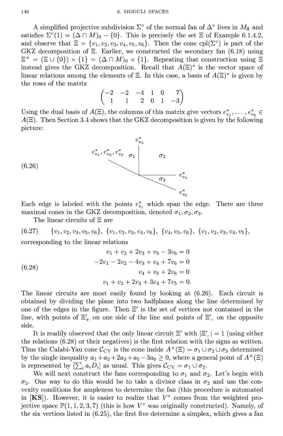


Text
Mirror Symmetry
and Algebraic
Geometry
David A. Cox
Sheldon Katz
American Mathematical Society
Selected Titles in This Series
68 David A. Cox and Sheldon Katz, Mirror symmetry and algebraic geometry, 1999
67 A. Borel and N. Wallach, Continuous cohomology, discrete subgroups, and
representations of reductive groups, Second Edition, 1999
66 Yu. Ilyashenko and Weigu Li, Nonlocal bifurcations, 1999
65 Carl Faith, Rings and things and a fine array of twentieth century associative algebra,
1999
64 Rene A. Carmona and Boris Rozovskii, Editors, Stochastic partial differential
equations: Six perspectives, 1999
63 Mark Hovey, Model categories, 1999
62 Vladimir I. Bogachev, Gaussian measures, 1998
61 W. Norrie Everitt and Lawrence Markus, Boundary value problems and symplectic
algebra for ordinary differential and quasi-differential operators, 1999
60 Iain Raeburn and Dana P. Williams, Morita equivalence and continuous-trace
C*-algebras, 1998
59 Paul Howard and Jean E. Rubin, Consequences of the axiom of choice, 1998
58 Pavel I. Etingof, Igor B. Frenkel, and Alexander A. Kirillov, Jr., Lectures on
representation theory and Knizhnik-Zamolodchikov equations, 1998
57 Marc Levine, Mixed motives, 1998
56 Leonid I. Korogodski and Yan S. Soibelman, Algebras of functions on quantum
groups: Part I, 1998
55 J. Scott Carter and Masahico Saito, Knotted surfaces and their diagrams, 1998
54 Casper Goffman, Togo Nishiura, and Daniel Waterman, Homeomorphisms in
analysis, 1997
53 Andreas Kriegl and Peter W. Michor, The convenient setting of global analysis, 1997
52 V. A. Kozlov, V. G. Maz'ya, and J. Rossmann, Elliptic boundary value problems in
domains with point singularities, 1997
51 Jan Maly and William P. Ziemer, Fine regularity of solutions of elliptic partial
differential equations, 1997
50 Jon Aaronson, An introduction to infinite ergodic theory, 1997
49 R. E. Showalter, Monotone operators in Banach space and nonlinear partial differential
equations, 1997
48 Paul-Jean Cahen and Jean-Luc Chabert, Integer-valued polynomials, 1997
47 A. D. Elmendorf, I. Kriz, M. A. Mandell, and J. P. May (with an appendix by
M. Cole), Rings, modules, and algebras in stable homotopy theory, 1997
46 Stephen Lipscomb, Symmetric inverse semigroups, 1996
45 George M. Bergman and Adam O. Hausknecht, Cogroups and co-rings in
categories of associative rings, 1996
44 J. Amoros, M. Burger, K. Corlette, D. Kotschick, and D. Toledo, Fundamental
groups of compact Kahler manifolds, 1996
43 James E. Humphreys, Conjugacy classes in semisimple algebraic groups, 1995
42 Ralph Freese, Jaroslav Jezek, and J. B. Nation, Free lattices, 1995
41 Hal L. Smith, Monotone dynamical systems: an introduction to the theory of
competitive and cooperative systems, 1995
40.3 Daniel Gorenstein, Richard Lyons, and Ronald Solomon, The classification of the
finite simple groups, number 3, 1998
40.2 Daniel Gorenstein, Richard Lyons, and Ronald Solomon, The classification of the
finite simple groups, number 2, 1995
40.1 Daniel Gorenstein, Richard Lyons, and Ronald Solomon, The classification of the
finite simple groups, number 1, 1994
(Continued in the back of this publication)
This page intentionally left blank
Mirror Symmetry
and Algebraic
Geometry
This page intentionally left blank
Mathematical
Surveys
and
Monographs
Volume 68
^VDED
Mirror Symmetry
and Algebraic
Geometry
David A. Cox
Sheldon Katz
American Mathematical Society
Providence, Rhode Island
Editorial Board
Georgia M. Benkart Michael Renardy
Peter Landweber Tudor Stefan Ratiu, Chair
2000 Mathematics Subject Classification. Primary 14-02; Secondary 81-02.
ABSTRACT. This monograph is an introduction to the mathematics of mirror symmetry, with a
special emphasis on its algebro-geometric aspects. Topics covered include the quintic threefold,
toric geometry, Hodge theory, complex and Kahler moduli, Gromov-Witten invariants, quantum
cohomology, localization in equivariant cohomology, and the recent work of Lian-Liu-Yau and
Givental on the Mirror Theorem. The book is written for algebraic geometers and graduate
students who want to learn about mirror symmetry. It is also a reference for specialists in the
field and background reading for physicists who want to see the mathematical underpinnings of
the subject.
Library of Congress Cataloging-in-Publication Data
Cox, David A.
Mirror symmetry and algebraic geometry / David A. Cox, Sheldon Katz.
p. cm. — (Mathematical surveys and monographs, 0076-5376; v. 68)
Includes bibliographical references and index.
ISBN 0-8218-1059-6 (alk. paper)
1. Mirror symmetry. 2. Geometry, Algebraic. 3. Mathematical physics. I. Katz, Sheldon,
1956- II. Title. III. Series: Mathematical surveys and monographs; no. 68.
QC174.17.S9C69 1999
516.3/62—dc21 98-55564
CIP
AMS softcover ISBN: 978-0-8218-2127-5
Copying and reprinting. Individual readers of this publication, and nonprofit libraries
acting for them, are permitted to make fair use of the material, such as to copy a chapter for use
in teaching or research. Permission is granted to quote brief passages from this publication in
reviews, provided the customary acknowledgment of the source is given.
Republication, systematic copying, or multiple reproduction of any material in this publication
is permitted only under license from the American Mathematical Society. Requests for such
permission should be addressed to the Acquisitions Department, American Mathematical Society,
201 Charles Street, Providence, Rhode Island 02904-2294 USA. Requests can also be made by
e-mail to reprint-permission@ams.org.
© 1999 by the American Mathematical Society. All rights reserved.
The American Mathematical Society retains all rights
except those granted to the United States Government.
Printed in the United States of America.
@ The paper used in this book is acid-free and falls within the guidelines
established to ensure permanence and durability.
Visit the AMS home page at http://www.ams.org/
10 9 8 7 6 5 4 3 15 14 13 12 11 10
To our families, who have endured with good grace our preoccupation
with this book.
D. A. C.
S. K.
This page intentionally left blank
Contents
Preface xiii
Goal of the Book xiii
Relation to Physics xiv
How to Read the Book xv
Acknowledgements xvii
Our Hope xviii
Notation xix
Chapter 1. Introduction 1
1.1. The Physics of Mirror Symmetry 1
1.2. Three-Point Functions 6
1.3. Why Calabi-Yau Manifolds? 10
1.4. The Mathematics of Mirror Symmetry 10
1.5. What's Next? 12
Chapter 2. The Quintic Threefold 15
2.1. The A-Model Correlation Function of the Quintic Threefold 15
2.2. The Quintic Mirror 17
2.3. The Mirror Map 19
2.4. The B-Model Correlation Function 21
2.5. Putting It All Together 22
2.6. The Mirror Theorems 24
Chapter 3. Toric Geometry 31
3.1. Cones and Fans 31
3.2. Polytopes and Homogeneous Coordinates 33
3.3. Kahler Cones and Symplectic Geometry 38
3.4. The GKZ Decomposition 42
3.5. Fano Varieties and Reflexive Polytopes 46
3.6. Automorphisms of Toric Varieties 47
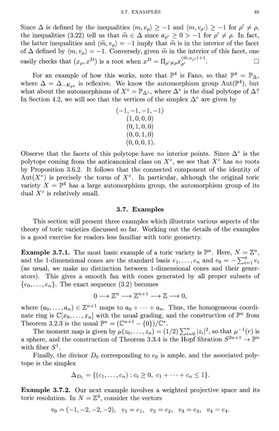
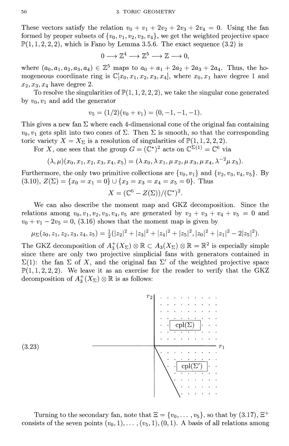
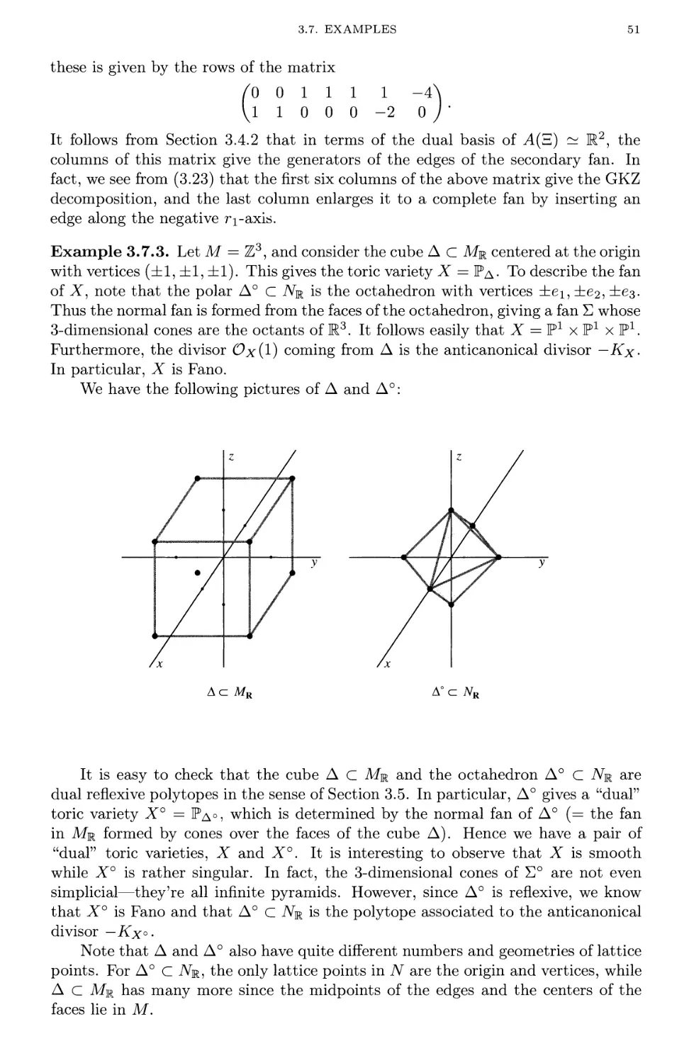
3.7. Examples 49
Chapter 4. Mirror Symmetry Constructions 53
4.1. The Batyrev Mirror Construction 53
4.2. The Quintic Threefold, Revisited 61
4.3. Toric Complete Intersections 62
4.4. The Voisin-Borcea Construction 65
Chapter 5. Hodge Theory and Yukawa Couplings 73
5.1. Hodge Theory 73
x CONTENTS
5.2. Maximally Unipotent Monodromy 78
5.3. The Griffiths-Dwork Method 83
5.4. Examples 87
5.5. Hypergeometric Equations 90
5.6. Yukawa Couplings 102
Chapter 6. Moduli Spaces 113
6.1. Complex Moduli 113
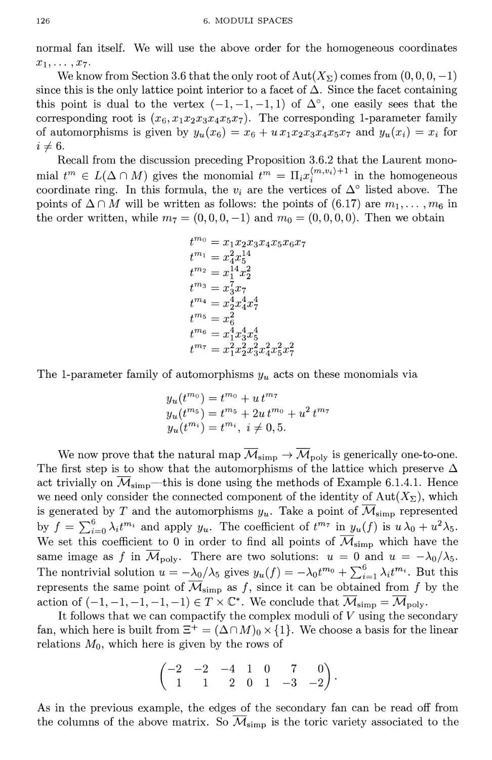
6.2. Kahler Moduli 127
6.3. The Mirror Map 148
Chapter 7. Gromov-Witten Invariants 167
7.1. Definition via Algebraic Geometry 168
7.2. Definition via Symplectic Geometry 184
7.3. Properties of Gromov-Witten Classes 191
7.4. Computing Gromov-Witten Invariants, I 196
Chapter 8. Quantum Cohomology 217
8.1. Small Quantum Cohomology 217
8.2. Big Quantum Cohomology 229
8.3. Computing Gromov-Witten Invariants, II 234
8.4. Dubrovin Formalism 239
8.5. The A-Variation of Hodge Structure 242
8.6. The Mirror Conjecture 257
Chapter 9. Localization 275
9.1. The Localization Theorem 275
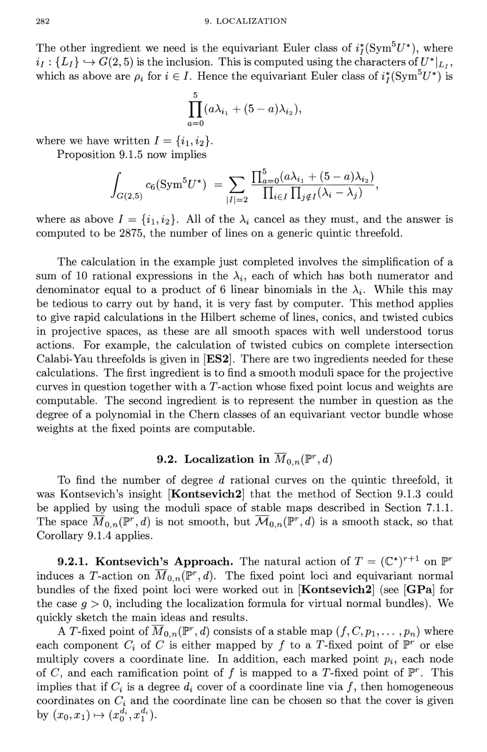
9.2. Localization in M0,n(Pr, d) 282
9.3. Equivariant Gromov-Witten Invariants 298
Chapter 10. Quantum Differential Equations 301
10.1. Gravitational Correlators 301
10.2. The Givental Connection 311
10.3. Relations in Quantum Cohomology 320
Chapter 11. The Mirror Theorem 331
11.1. The Mirror Theorem for the Quintic Threefold 332
11.2. Givental's Approach 356
Chapter 12. Conclusion 397
12.1. Reflections and Open Problems 397
12.2. Other Aspects of Mirror Symmetry 400
Appendix A. Singular Varieties 407
A.l. Canonical and Terminal Singularities 407
A.2. Orbifolds 408
A.3. Differential Forms on Orbifolds 409
A.4. The Tangent Sheaf of an Orbifold 410
A.5. Symplectic Orbifolds 410
Appendix B. Physical Theories
B.l. General Field Theories
411
411
CONTENTS
B.2. Nonlinear Sigma Models
B.3. Conformal Field Theories
B.4. Landau-Ginzburg Models
B.5. Gauged Linear Sigma Models
B.6. Topological Quantum Field Theories
bliography
xi
419
423
426
428
430
437
Index
453
This page intentionally left blank
Preface
The field of mirror symmetry has exploded onto the mathematical scene in recent
years. This is a part of an increasing connection between quantum field theory and
many branches of mathematics.
It has sometimes been said that quantum field theory combines 20th century
physics with 21st century mathematics. Physicists have gained much experience
with mathematical manipulations in situations which have not yet been
mathematically justified. They are able to do this in part because experiment can help
them differentiate between which manipulations are feasible, and which are clearly
wrong. Those manipulations that survive all known tests are presumed to be valid
until evidence emerges to the contrary.
Based on this evidence, physicists are confident about the validity of mirror
symmetry. One of the tools they use with great virtuosity is the Feynman path
integral, which performs integration with complex measures over infinite dimensional
spaces, such as the space of C°° maps from a Riemann surface to a Calabi-Yau
threefold. This is not rigorous mathematics, yet these methods led to the 1991
paper of Candelas, de la Ossa, Green and Parkes [CdGP] containing some
astonishing predictions about rational curves on the quintic threefold. These predictions
went far beyond anything algebraic geometry could prove at the time.
The challenge for mathematicians was to understand what was going on and,
more importantly, to prove some of the predictions made by the physicists. In this
book, we will see that algebraic geometers have made substantial progress, though
there is still a long way to go. The process of creating a mathematical foundation
for aspects of mirror symmetry has given impetus to new fields of algebraic
geometry. Examples include quantum cohomology, Kontsevich's definition of a stable
map, the complexified Kahler moduli space of a Calabi-Yau threefold, Batyrev's
duality between certain toric varieties, and Givental's notion of quantum differential
equations. Mirror symmetry has also led to advances in deformation theory leading
to the theory of the virtual fundamental class, as well as a previously unknown
connection between algebraic and symplectic deformation theory. Even though we
still don't know what mirror symmetry really "is", the predictions that mirror
symmetry makes about Gromov-Witten invariants can now be proved mathematically
in many cases.
Goal of the Book
Perhaps the greatest obstacle facing a mathematician who wants to learn about
mirror symmetry is knowing where to start. Currently, many references are
scattered throughout journals, and many mathematical ideas exist solely in the physics
literature, which is difficult for mathematicians to read. Our primary goal is to give
an introduction to the algebro-geometric aspects of mirror symmetry. We include
xiii
xiv PREFACE
sufficient detail so that the reader will have the major ideas and definitions spelled
out, and explicit references to the literature when space constraints prohibit more
detail. We explain both the rigorous mathematics as well as the intuitions
borrowed from physics which are not yet theorems. We do this because we have two
primary target audiences in mind: mathematicians wanting to learn about mirror
symmetry, and physicists who know about mirror symmetry wanting to learn about
the mathematical aspects of the subject.
Mirror symmetry is connected to several branches of mathematics (and there
are even broader connections between physical theories in various dimensions and
many areas of mathematics). We focus on the connection between algebraic
geometry and mirror symmetry, although we discuss closely related areas such as
symplectic geometry. By restricting our focus in this way, we hope to give a
reasonably self-contained introduction to the subject.
The book begins with a general introduction to the ideas of mirror symmetry in
Chapter 1. Then Chapter 2 discusses the quintic threefold and explains how mirror
symmetry leads to the enumerative predictions of [CdGP]. Chapter 3 reviews toric
geometry, and Chapter 4 describes mirror constructions due to Batyrev, Batyrev-
Borisov, and Voisin-Borcea. The next four chapters (Chapters 5, 6, 7 and 8) flesh
out the mathematics needed to formulate a precise version of mirror symmetry.
These chapters cover maximally unipotent monodromy, Yukawa couplings,
complex and Kahler moduli, the mirror map, Gromov-Witten invariants, and quantum
cohomology. This will enable us to state some Mirror Conjectures at the end of
Chapter 8.
The next three chapters (Chapters 9, 10 and 11) are dedicated to proving some
instances of mirror symmetry. Equivariant cohomology and localization play a
crucial role in the proofs, so that these are reviewed in Chapter 9. These methods also
give powerful tools for computing Gromov-Witten invariants. In order to explain
Givental's approach to the Mirror Theorem, we need the gravitational correlators
and quantum differential equations discussed in Chapter 10. Finally, Chapter 11
describes the work of Lian, Liu and Yau [LLY] and Givental [Givental2, Givental4]
on the Mirror Theorem.
The mathematics discussed in Chapters 1-11 is wonderful but highly nontrivial.
Later in the preface we will give some guidance for how to read these chapters.
The book concludes with Chapter 12, which brings together all of the open
problems mentioned in earlier chapters and discusses some of the many aspects of
mirror symmetry not covered in the text. Finally, there are appendices on singular
varieties and physical theories.
We tried to make the bibliography fairly complete, but it has been difficult to
keep up with the amazing number of high-quality papers being written on mirror
symmetry and related subjects. We apologize to our colleagues for the many recent
papers not listed in the bibliography.
Relation to Physics
For mathematicians, one frustration of mirror symmetry is the difficulty of
getting insight into the physicist's intuition. There is no question of the power of
this intuition, for it is what led to the discovery of the mirror phenomenon. But
getting access to it requires a substantial study of quantum field theory. A glance at
Appendix B, which discusses some of the physical theories involved, will indicate the
HOW TO READ THE BOOK xv
magnitude of this task. Understanding the physics literature on mirror symmetry
requires an extensive background, more than provided in this book. Appendix B
has the more modest goal of introducing the reader to some of the topics in the
physics literature which are relevant to mirror symmetry.
While this book was written to address the mathematics of mirror symmetry,
we also hope to show how the mathematics reflects the spirit of the physics. With
this thought in mind, we begin Chapter 1 with a discussion of the physics which
led to mirror symmetry. We use terminology from physics freely, though we don't
assume that the reader knows any quantum field theory. The idea is to convey
the sense that mirror symmetry is completely natural from the point of view of
certain conformal field theories. This is the most "physical" chapter of the book.
Subsequent chapters will concentrate on the mathematics, though we will pause
occasionally to comment on the relationship between the mathematics and the
physics.
An important aspect of the role of physics is that mathematically
sophisticated physicists helped discover the mathematical foundation for mirror symmetry.
Algebraic geometers can take pride in the wonderful theories they created to
explain parts of mirror symmetry, but at the same time we should also recognize
that physicists provided more than just predictions—they often suggested the
appropriate objects to study, accompanied in some cases by mathematically rigorous
descriptions. This will become clear by checking the references given in the text—
a surprising number, even in the purely mathematical parts of the book, refer to
physics papers. There is no question of the debt we owe to our colleagues in physics.
How to Read the Book
Mirror symmetry is a wonderful story, but its telling requires lots of details in
many different areas of algebraic geometry. It is easy to get lost, especially if you
try to read the book cover-to-cover. Fortunately, this isn't the only way to read
the book.
Our basic suggestion is that you should begin with Chapters 1 and 2. As
already mentioned, Chapter 1 explains some of the physics, and it also introduces
two key ideas, the A-model of a Calabi-Yau manifold V, which encodes the enu-
merative information we want, and the B-model of the mirror V°, which we can
compute using Hodge theory. Then Chapter 2 shows what this looks like in the
case of the quintic threefold V C P4 and in the process derives the enumerative
predictions made in [CdGP]. This chapter ends with a preview of the proofs of
mirror symmetry from Chapter 11.
After reading the first two chapters, there are various ways you can proceed,
depending on your mathematical interests and expertise. To help you choose, here
is a description of some of the highlights of the remaining chapters:
Chapter 3. Readers familiar with toric geometry can skip most of this chapter.
Section 3.5 introduces reflexive polytopes, which are used in the Batyrev mirror
construction.
Chapter 4. Section 4.1 describes the Batyrev mirror construction and gives
some evidence for the mirror relation. Section 4.2 explains how this applies to the
quintic threefold. K3 surfaces are used in Section 4.4 to construct some interesting
mirror pairs of Calabi-Yau threefolds.
xvi PREFACE
Chapter 5. Maximally unipotent monodromy is an important part of mirror
symmetry and is defined in Section 5.2. Readers interested in computational
techniques for projective hypersurfaces, toric hypersurfaces and hyper geometric
equations should look at Sections 5.3, 5.4 and 5.5, while those interested in the Hodge
theory of Calabi-Yau threefolds should read Section 5.6 very carefully.
Chapter 6. We consider complex moduli in Section 6.1 and Kahler moduli in
Section 6.2. The two discussions are interwoven because of the relation between
the two predicted by mirror symmetry. The main example we work out concerns
toric hypersurfaces, so that the reader will need the Batyrev mirror construction
from Chapter 4. Readers interested in moduli of Calabi-Yau manifolds, Kahler
cones, and the global aspects of mirror symmetry will want to read these sections
carefully. Section 6.3 discusses the mirror map and has more on hyper geometric
equations, which are used to construct the mirror map in the toric case.
Chapter 7. With the exception of some examples, Chapter 7 is independent
of the earlier chapters. The main objects of study are Gromov-Witten invariants.
Sections 7.1.1, 7.1.2 and 7.3.1 are essential reading. Otherwise:
• The discussion of the virtual fundamental class in Sections 7.1.3-7.1.6 is
more technical and can be skipped at the first reading. The one exception is
Example 7.1.6.1, which gives an important formula for some Gromov-Witten
invariants of the quintic threefold. The virtual fundamental class is used in
various places in Chapters 9, 10 and 11.
• Readers interested in symplectic geometry should read Sections 7.2 and 7.4.4
carefully.
• Readers interested in enumerative geometry will want to look at Section 7.4.
Some of the examples given here will be revisited in Chapter 8.
One surprise in Section 7.4.4 is the subtle relation between the instanton number
nio and the number of degree 10 rational curves on the quintic threefold.
Chapter 8. This chapter uses the Gromov-Witten invariants of Chapter 7 to
define the two flavors of quantum cohomology, small and big. Everyone should read
Section 8.1.1 for the small quantum product and Section 8.1.2 for some examples.
Also, some knowledge of the Gromov-Witten potential is also useful. This is covered
in Sections 8.2.2, 8.3.1 and 8.3.3. Then:
• Readers interested in enumerative geometry should read Sections 8.1, 8.2
and 8.3 carefully.
• Readers interested in Hodge theory will want to look at Section 8.5, which
uses quantum cohomology to construct the A-variation of Hodge structure
on the cohomology of a Calabi-Yau manifold.
A highlight of the chapter is Section 8.6, which formulates various Hodge-theoretic
versions of the mirror conjecture.
Chapter 9. Sections 9.1 and 9.2.1 are required reading for anyone wanting
to understand the proofs of mirror symmetry given in Chapter 11. This especially
includes Example 9.2.1.3, which computes the Gromov-Witten invariant (/o,o,d)
using an equivariant version of the formula given in Example 7.1.6.1. Sections 9.2.2
and 9.2.3 prove some of the assertions about Gromov-Witten invariants of Calabi-
Yau threefolds made in Section 7.4.4 and require a detailed knowledge of the virtual
fundamental class.
ACKNOWLEDGEMENTS xvii
Chapter 10. Readers only interested in the [LLY] approach to the Mirror
Theorem can skip this chapter. For Givental's approach, however, the reader will
need to read about gravitational correlators (Section 10.1.1-10.1.3), flat sections of
the Givental connection (Section 10.2.1), and the J-function and quantum
differential equations (Section 10.3). For readers with an interest in Hodge theory, the
A-model variation of Hodge structure is discussed in Sections 10.2.2 and 10.3.2.
This leads to a nice connection between Picard-Fuchs operators and relations in
quantum cohomology.
Chapter 11. Here we discuss the recent proofs of the Mirror Theorem. There
are two approaches to consider:
• The [LLY] approach to the Mirror Theorem for the quintic threefold is
covered in Section 11.1. This requires knowledge of the essential sections of
Chapters 7, 8 and 9 mentioned earlier.
• For Givental's version of the Mirror Theorem, one needs in addition the
sections of Chapter 10 indicated above. In Sections 11.2.1, 11.2.3 and 11.2.4,
we discuss the Mirror Theorem for nef complete intersections in Pn, and
then in Section 11.2.5 we consider what happens when the ambient space is
a smooth toric variety.
In particular, we explain how both of these approaches prove all of the
predictions for the quintic threefold made in Chapter 2. Another very interesting case
is presented in Example 11.2.5.1, which concerns Calabi-Yau threefolds which are
minimal desingularizations of degree 8 hypersurfaces in P(l, 1, 2, 2, 2). This
example of a toric hypersurface makes numerous appearances in Chapters 3, 5, 6 and 8,
so that the reader will need to look back at these earlier examples in order to fully
appreciate what we do in Example 11.2.5.1.
We should also mention that in many cases, our proofs are not complete, for
we often refer to the literature for certain details of the argument. The same
applies to background material. For some topics (such as equivariant cohomology
in Chapter 9) we review the basic facts, while for others (such as algebraic stacks
in Chapter 7) we give references to the literature. We hope that this unevenness in
the level is not too unsettling to the reader.
Acknowledgements
We are happy to thank numerous people who have assisted us in various ways.
The authors would in particular like to express their appreciation to P. Aspin-
wall, P. Berglund, C. Borcea, P. Candelas, R. Dijkgraaf, B. Greene, T. Hubsch,
A. Klemm, P. Mayr, G. Moore, D. R. Morrison, M. R. Plesser, D. van Straten,
and C. Vafa, for numerous conversations over the past few years which helped us
develop our views of mirror symmetry and understand the relevant mathematics
and physics.
Thanks also to the Institut Mittag-Leffler for its hospitality during the spring
of 1997. A seminar on mirror symmetry held that spring discussed portions of this
book and helped us improve its exposition immensely. It is a pleasure to thank all
of the participants. At the risk of inadvertently omitting someone, we in particular
want to acknowledge P. Alufrl, V. Batyrev, K. Behrend, P. Belorousski, I. Ciocan-
Fontanine, A. Elezi, G. Ellingsrud, C. Faber, B. Fantechi, W. Fulton, E. Getz-
ler, L. Gottsche, T. Graber, B. Kim, A. Kresch, D. Laksov, J. Li, A. Libgober,
xviii PREFACE
R. Pandharipande, K. Ranestad, E. R0dland, D. E. Sommervoll, S. A. Str0mme,
M. Thaddeus, and E. Tj0tta for their help.
During the process of writing the book, we sent draft chapters to various
colleagues. In addition to some of the above people who helped with this, we also
would like to thank E. Cattani, E. Ionel, B. Lian, K. Liu, A. Mavlyutov, T. Parker,
G. Pearlstein, Y. Ruan, C. Taubes, G. Tian, P. Vermeire and S.-T. Yau for their
helpful comments. We would also like to thank B. Dwork and J. Kollar for useful
conversations. In addition, we would like to thank the reviewers of an earlier draft
of the book for their feedback. We are also very grateful to A. Greenspoon for his
careful reading of the final manuscript. Any errors which remain are, of course, our
responsibility.
We also thank the seminar members at Oklahoma State University and the
Valley Geometry Seminar for listening to many talks on mirror symmetry. Their
feedback and support are greatly appreciated.
During the period when this book was being written, D.A.C. was partially
supported by the NSF, and S.K. was supported by the NSF and NSA. We are
grateful to these organizations for their support.
Finally, we would like to thank Sergei Gelfand and Sarah Donnelly of the AMS
for their editorial guidance and Barbara Beeton of the AMS technical support staff
for her help with Aj^-WH^.
Our Hope
Mirror symmetry is an active area of research in algebraic geometry, with plenty
to keep mathematicians busy for many years. This book should be regarded as a
preliminary report on the current state of the subject—the definitive text on mirror
symmetry has yet to be written. Nevertheless, we hope that the reader will find
the connections explored here to be an exciting and continuing story.
November, 1998
David A. Cox
Sheldon Katz
Notation
Here is some of the notation we will use in the book.
General Notation:
M Complex or symplectic manifold
X and V Algebraic variety and Calabi-Yau variety
Ox and Tx Tangent sheaf and bundle of X
ux and Kx Canonical bundle and divisor of X
Slpx Zariski p-forms on an orbifold X
M(X) Mori cone of effective 1-cycles on X
Ak{X) kth Chow group of X
(a, b) or p(a, b) Cup product pairing on cohomology
Pn and P(go> • • • ? Qn) Projective space and weighted projective space
Toric Varieties and Poly topes (Chapter 3):
E and E(l) Fan and its 1-dimensional cones
A and A° Polytope and its polar (or dual) polytope
L(A) Laurent polynomials with exponents in A
X% and Pa Toric variety of the fan E and the polytope A
cpl(E) Cone of convex support functions on E
Hodge Theory and Yukawa Couplings (Chapter 5):
V = VGM Gauss-Manin connection
J7* and W. Hodge and weight nitrations
H and Hz Hodge bundle J1*0 and its integer subsheaf
Tj and Nj Monodromy transformation and its logarithm
(^:, ^-, -j^-) = Yijk Normalized Yukawa coupling or B-model correlation
function
NOTATION
Complex and Kahler Moduli (Chapter 6):
A4 and A4 Complex moduli and a compactification
.Mpoiy and M.po\y Polynomial moduli and a compactification
A^simp and .MSimp Simplified moduli and a compactification
K(V) and K(V)c Kahler cone and complexified Kahler space
/CM and /CM Kahler moduli and a compactification
/CMtoric and ^C-Mtoric Toric Kahler moduli and a compactification
Gromov-Witten Invariants and Quantum Cohomology (Chapters 7 and 8):
Mgin(X,j3) and Coarse moduli space and fine moduli stack of
A4giTl(X, j3) n-pointed genus g stable maps of class j3
[M9in(X, /3)]virt Virtual fundamental class
^,n,/3(c^i, • • • , ocn) and Gromov-Witten class and invariant
(Ig,nfi){<Xl,- • • ,OLn)
np and rid Instanton number in general and for the quintic
threefold
N/3 = (io,o,/3) and 0-pointed genus 0 Gromov-Witten invariant in
Nd = (^o,o,a) general and for the quintic threefold
*smaii and * Small and big quantum product (*smaii is sometimes
denoted *)
(a, 6, c) Three-point function or A-model correlation
function
$(7) Genus 0 Gromov-Witten potential
V = VGW A-model connection
Chern Classes and Equivariant Cohomology (Chapter 9):
Ci(£) and c[(£) Chern class and equivariant Chern class of £
Euler(£) and EulerT(£) Euler class and equivariant Euler class of £
Jx Equivariant integral
A0,... , An and h Ring generators of H*(BT) and iJ*(£C*), which
generate H*(BG) for G = C* x T, T = (C*)n+1
H and p Hyperplane class and equivariant hyperplane class
#o, • • • , qn Fixed points of standard T-action on Pn
NOTATION
Gravitational Correlators and the J-Function (Chapter 10):
(7"di7i? • • • 5 T~dnJn)g,p Gravitational correlator
(71 > • • • > ln)gfi Alternate notation for (Ig,n,p){lu • • • , In)
((^di7i> • • • > 7"dn7n))<7 Genus g gravitational coupling
$frav(7) Genus g gravitational Gromov-Witten potential
*grav Gravitational quantum product
V5 and Vg Givental connection and dual Givental connection
Sj Flat section of the Givental connection
«fe»0 Symbolic notation for £^0ft~(n+1)<M».Ti>>o
J = Jx Givental J-function of the smooth variety X
The Mirror Theorem (Chapter 11):
V = 0f=10pn(a$) Vector bundle used in the Mirror Theorem
Vd and Vd k Bundle on M0 o(Pn, d) and M0 fc(Pn, d) induced
byV
Md and Nd Compact notation for M0 o(PX x Pn, (1, d)) and
P(fir0(P1,Opi(d))d+1)
Pi?r Fixed points of G-action on Nd, G = C* x T
ft Equivariant hyperplane class in Hq(N(i)
TlT and ftG Field of fractions of H*(BT) and H*(BG)
P and Q Important Euler data
HG[B](t) Cohomology-valued function of B = {Bd}
\&(£) The mirror map
Iy and Jy Givental's cohomology-valued functions
Vdkl A certain subbundle of Vd,k used in defining Jy
*x Modified quantum product on H*(Fn) determined
by a complete intersection IcPn
Iy Cohomology-valued function used in the Quantum
Hyperplane Section Principle
It and Jt Equivariant versions of /y and Jy
Ziy A collection of functions for 0 < i < n which
determine Jt uniquely
Our conventions for citations are explained at the beginning of the Bibliography.
This page intentionally left blank
CHAPTER 1
Introduction
Mirror symmetry has made some surprising predictions in algebraic geometry,
ranging from the number of rational curves on a quintic threefold to the structure of
certain moduli spaces. These are wonderful problems to work on and, as indicated
in the preface, have led to some very interesting mathematics. Yet to understand
where these predictions come from, the algebraic geometer must plunge into the
language of physics, which is unfamiliar and sometimes frustratingly nonrigorous.
Hence, to begin our survey of the algebraic geometry of mirror symmetry, we will
start with the motivations for mirror symmetry and a discussion of what mirror
symmetry means in physics. Our treatment will be somewhat incomplete, since it
will involve many terms from physics which may be new to the reader. Nevertheless,
we hope to convey some of the intuition behind this remarkable phenomenon.
We will then discuss three-point functions (which are crucial to the enumerative
predictions of mirror symmetry) and the physical reasons why Calabi-Yau manifolds
appear in the theory. Finally, at the end of the chapter, we will return to the
more familiar world of mathematics and give the reader a preview of the algebraic
geometry to be explored in the remaining chapters of the book.
1.1. The Physics of Mirror Symmetry
The goal of this section is to give the reader a feeling for why mirror symmetry
should occur and what it should imply. From the point of view of physics, mirror
symmetry arises naturally from standard constructions in supersymmetric string
theory, and our discussion will begin with some elementary remarks about strings
and supersymmetry. The reader should be assured that no previous knowledge of
physics is assumed! Our aim is to convey the flavor of these physical theories and in
the process enhance the reader's intuition for the resulting mathematics. A detailed
understanding of the physics is not necessary, though later chapters will refer to
the physics presented in this chapter. As general references for string theory, the
reader can consult [GSW, Polchinski2].
In string theory, physical processes are described by the propagation of a string
in spacetime. A propagating string traces out a surface, called the world sheet E of
the string. Classical fields can be described as functions, sections of bundles, etc. on
the world sheet, and quantizing leads to a two-dimensional quantum field theory.
This theory has a generalized Hilbert space of states, together with a collection of
observables, which become self-adjoint operators on the space of states. The other
key ingredients of the theory are the action S obtained by integrating a Lagrangian
over the world sheet E, and the correlation functions
(1.1) <0(*i), • • • , <Kxn)) = [[Dfltixi)... </>(xn)eiSM,
1
2
1. INTRODUCTION
where <j> is an observable. This Feynman integral is over all possible world sheets
and is mathematically undefined at present. We discuss such theories in more detail
in Appendix B. For now, let's concentrate on their general features.
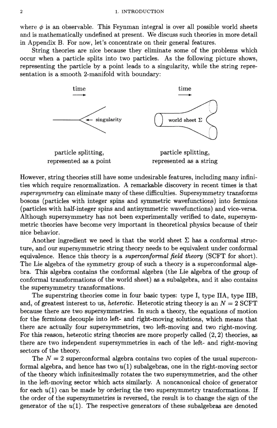
String theories are nice because they eliminate some of the problems which
occur when a particle splits into two particles. As the following picture shows,
representing the particle by a point leads to a singularity, while the string
representation is a smooth 2-manifold with boundary:
time
singularity world
particle splitting, particle splitting,
represented as a point represented as a string
However, string theories still have some undesirable features, including many
infinities which require renormalization. A remarkable discovery in recent times is that
supersymmetry can eliminate many of these difficulties. Supersymmetry transforms
bosons (particles with integer spins and symmetric wavefunctions) into fermions
(particles with half-integer spins and antisymmetric wavefunctions) and vice-versa.
Although supersymmetry has not been experimentally verified to date, supersym-
metric theories have become very important in theoretical physics because of their
nice behavior.
Another ingredient we need is that the world sheet E has a conformal
structure, and our supersymmetric string theory needs to be equivalent under conformal
equivalence. Hence this theory is a superconformal field theory (SCFT for short).
The Lie algebra of the symmetry group of such a theory is a superconformal
algebra. This algebra contains the conformal algebra (the Lie algebra of the group of
conformal transformations of the world sheet) as a subalgebra, and it also contains
the supersymmetry transformations.
The superstring theories come in four basic types: type I, type IIA, type IIB,
and, of greatest interest to us, heterotic. Heterotic string theory is an TV = 2 SCFT
because there are two super symmetries. In such a theory, the equations of motion
for the fermions decouple into left- and right-moving solutions, which means that
there are actually four super symmetries, two left-moving and two right-moving.
For this reason, heterotic string theories are more properly called (2,2) theories, as
there are two independent supersymmetries in each of the left- and right-moving
sectors of the theory.
The N = 2 superconformal algebra contains two copies of the usual
superconformal algebra, and hence has two u(l) subalgebras, one in the right-moving sector
of the theory which infinitesimally rotates the two supersymmetries, and the other
in the left-moving sector which acts similarly. A noncanonical choice of generator
for each u(l) can be made by ordering the two supersymmetry transformations. If
the order of the supersymmetries is reversed, the result is to change the sign of the
generator of the w(l). The respective generators of these subalgebras are denoted
time
1.1. THE PHYSICS OF MIRROR SYMMETRY
3
by (Q, 0) and are only well-defined up to sign. We regard (Q, Q) as operators on
the Hilbert space of states, which decomposes into eigenspaces under the action of
u(l) x u(l). As we will see, these eigenspaces can be very interesting.
So far, we've discussed heterotic string theories in the abstract. The next step
is to actually construct a such a theory, which is where algebraic geometry enters
the picture. There are several ways this can be done, but for us, the most important
is the nonlinear sigma model (sigma model for short) determined by a Calabi-Yau
threefold1 V and a complexified Kahler class uo = B + i J on V. Here, B and J are
elements of iT2(V, R), with J a Kahler class.
From the input data (V,cj), there is a geometric construction of an iV = 2
SCFT which explicitly gives distinct roles for the various supersymmetries; hence
in this context there is a canonical choice for (Q, Q). This gives an explicit choice
of the u(l) x u(l) representation on our Hilbert space, and one can compute that
for p, q > 0, (Q, Q) has eigenspaces:
(p, q) eigenspace ~ Hq(V, APTV)
(—p, q) eigenspace ~ Hq(V, £ly).
Appendix B.2 describes more fully what it means to be a nonlinear sigma model
and Section 1.3 explains how the Calabi-Yau condition arises from the physics.
The most important fields in a heterotic string theory are associated to
elements of i^1(V, TV) and iT1(V, f2y), corresponding to eigenvalues (1,1) and (—1,1)
respectively. The operators corresponding to elements in these spaces are called
marginal operators. These are important partly because they are closely related to
the moduli of sigma models coming from (V, cj). Intuitively, SCFT moduli are
obtained by simultaneously varying the complex structure on V and the complexified
Kahler class u) = B -\-iJ, although there are extra discrete SCFT identifications on
the moduli spaces which we will ignore for the moment. While readers should be
familiar with the complex moduli, the idea of "complexified Kahler moduli" may
be new. We will describe this in more detail in Section 1.4.
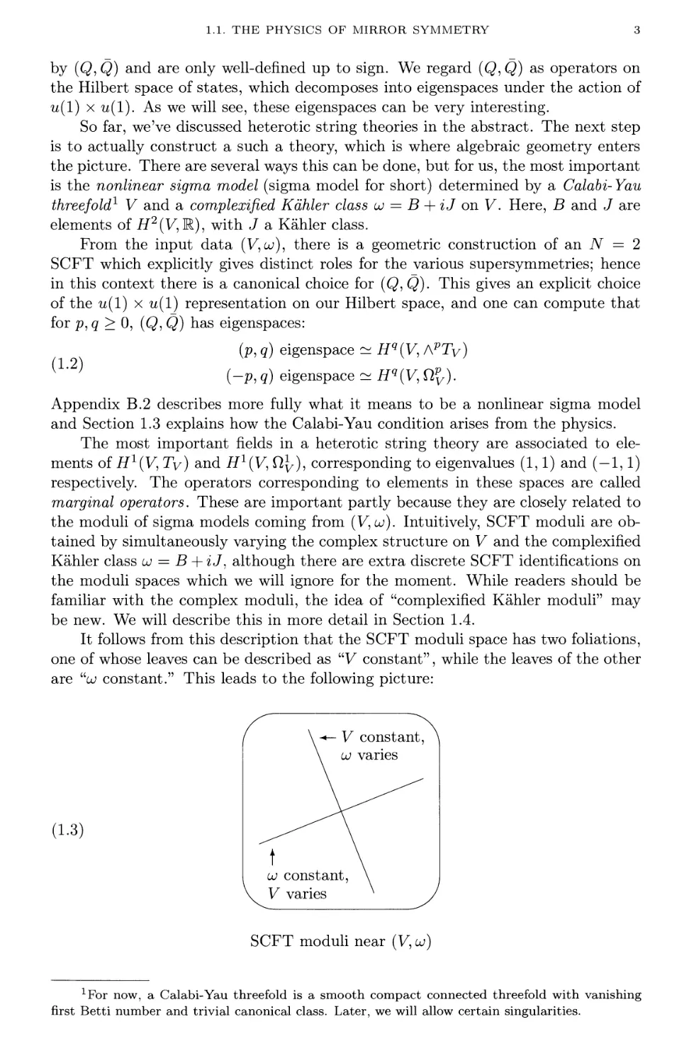
It follows from this description that the SCFT moduli space has two foliations,
one of whose leaves can be described as "V constant", while the leaves of the other
are uuj constant." This leads to the following picture:
(1.3)
V constant,
lo varies
uj constant
V varies
SCFT moduli near (V, uj)
xFor now, a Calabi-Yau threefold is a smooth compact connected threefold with vanishing
first Betti number and trivial canonical class. Later, we will allow certain singularities.
4
1. INTRODUCTION
In spite of this picture, we should emphasize that the SCFT moduli space is
not a product of the complex structure and Kahler structure moduli spaces, not
even locally. In fact, the Kahler moduli space of uj can depend on the complex
structure of V [Wilson2]. In general, this is only well-defined if we have in mind
a fixed complex structure on V. On the other hand, it follows from [Wilson2]
that for a sufficiently generic Calabi-Yau threefold V, the Kahler moduli of uj is
independent of the complex structure of V. These issues will be discussed in more
detail in Chapter 6. Hence, although the above picture is useful at a conceptual
level, it does not reflect the subtleties of the SCFT moduli space.
Now that we have a better idea of how Calabi-Yau threefolds and complexified
Kahler classes gives interesting physical theories, it is time to explain where mirror
symmetry comes from. The basic starting point lies in the sign indeterminacy of
(Q, Q). We mentioned above that (Q, Q) are only well-defined up to sign, yet the
sigma model coming from (V, uj) makes a very specific choice. If we changed Q to
—Q and left Q as is, we would interchange the (p, q) and (—p, q) eigenspaces, which
by (1.2) would interchange Hq(V, APTV) and Hq(V, Slpv). This is not possible since
these are vector spaces of different dimensions in general. Yet from the physical
point of view, such a sign change is reasonable. This asymmetry suggests that
maybe the sign change corresponds to the sigma model arising from a different
pair (V°,uj°). If such a pair (V°,oj°) exists, we say that (V,uj) and (V°,oj°) are a
mirror pair. More formally, we have the following definition from physics.
Physics Definition 1.1.1. (V,uj) and (V°,oj°) form a mirror pair if their
sigma models induce isomorphic superconformal field theories whose N = 2 super-
conformal representations are the same up to the above sign change.
Note that this is not a mathematical definition since the SCFT associated to
(V, cj) is not rigorously defined. However, in Chapter 8, we will give a careful
definition of a mathematical mirror pair. This definition will incorporate many of
the properties predicted by mirror symmetry.
It is these properties to which we now turn our attention. If (V, uj) and (V°, uj°)
are a mirror pair, then we get isomorphic SCFT's. But what does this mean
about the mathematics? One of the major goals of this book is to understand the
mathematical consequences of mirror symmetry.
To see what mirror symmetry tells us about V and V°, first note that if we
combine (1.2) with the eigenvalue change (p,q) <-> (—p, q), we get isomorphisms
H«(V,A*Tv)~H*(V°,Qrvo)
( ' ' Hq(V,Sfy) ~ Hq(V°,ApTVo).
Since V is Calabi-Yau, it has a nonvanishing holomorphic 3-form Q, and cup product
with Q gives a (noncanonical) isomorphism Hq(V, ApTy) ~ Hq(V, ^y_p). The same
is true for V°, so that (1.4) can be written as
Hq(v,n3v-p)c±Hq(vQ,npvo)
Hq(v,npv)~Hq(v°,n3v-p).
These isomorphisms have a nice interpretation in terms of the Hodge diamond.
Since V is a smooth threefold, its Hodge numbers hp,q(V) = dim Hq(V,£iy) have
the symmetries h™(V) = hq*(V) = h?~p^-q(V) - h3~q'3-p(V), and since V is
Calabi-Yau, we also have &i(V) = 0 and Q,y ~ Oy. This implies that /i1'°(F) = 0
and h3'°{V) = 1. Furthermore, h^2(V) = dimH2(V,Ov) = dimH^V.Ov) =
1.1. THE PHYSICS OF MIRROR SYMMETRY
5
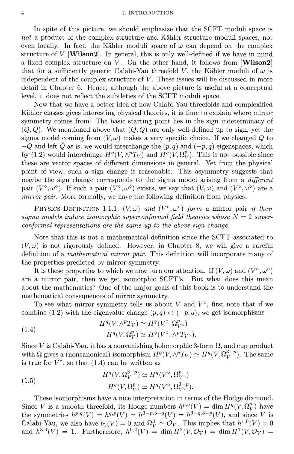
h0'1^) = 0, where the second equality follows from Serre duality and Qy ~ Oy.
Thus the Hodge diamond of V is as follows:
1
0 0
0 h}^(V) 0
1 h2^(V) h2'\V) 1
0 h1'1^) 0
0 0
1
If we now compare the Hodge diamonds of a mirror pair V and V°, (1.5)
implies that hp>q(V) = h3~p'q(V0), which shows that the Hodge diamond of V° is
the reflection (or mirror image) of the Hodge diamond of V about a 45° line. This
is where the name "mirror symmetry" comes from.
The isomorphisms (1.4) and (1.5) are actually the first of a series of increasingly
impressive consequences of mirror symmetry. The next interesting implication of
being a mirror pair concerns moduli spaces. To see where moduli enter the picture,
note that (1.4) gives isomorphisms ^(V.Ty) ~ ff^V0,!^) and H1^^) ^
i71(VAO,Tyo). This naturally identifies the tangent space to the complex moduli
of V with the tangent space to the Kahler moduli of uj° (see Section 1.4 for a
definition), and similarly identifies the tangent space to the Kahler moduli of uj
with the tangent space to the complex moduli of V°. Thus the complex moduli
space of V is locally isomorphic to the Kahler moduli space of cj°, and similarly the
complex moduli space of V° is locally isomorphic to the Kahler moduli space of uj.
These local isomorphisms are collectively called the mirror map. In Chapter 6, we
will study complex and Kahler moduli in more detail and give a careful definition
of the mirror map.
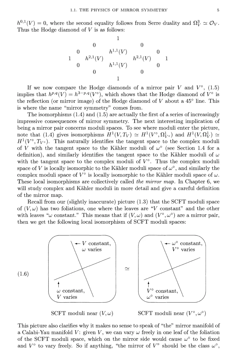
Recall from our (slightly inaccurate) picture (1.3) that the SCFT moduli space
of (V, uj) has two foliations, one where the leaves are "V constant" and the other
with leaves uuj constant." This means that if (V,cj) and (V°,uj°) are a mirror pair,
then we get the following local isomorphism of SCFT moduli spaces:
(1.6)
V constant,
uj varies
uj constant
V varies
or constant,
V° varies
V° constant,
uu° varies
SCFT moduli near (V, uj)
SCFT moduli near (V°,uj°)
This picture also clarifies why it makes no sense to speak of "the" mirror manifold of
a Calabi-Yau manifold V: given V, we can vary uj freely in one leaf of the foliation
of the SCFT moduli space, which on the mirror side would cause uj° to be fixed
and V° to vary freely. So if anything, "the mirror of V" should be the class uj° ,
6
1. INTRODUCTION
together with the moduli space of those deformations of V° on which lo° makes
sense as a complexified Kahler class.
In addition to what we've discussed so far, the existence of a mirror pair has
further consequences, not all of which are understood yet. The basic idea is that
any quantity that can be defined in terms of the SCFT can in principle be computed
using two different constructions for the SCFT. In the best cases, these quantities
can be computed in terms of the geometry of V and V°. Note that due to the
sign change in Q and the fact that Hq(V, Qy) corresponds to Hq(V°, ApTVo), it
is expected that the geometric calculations will be different for the different
models. The best example is given by the correlation functions of the SCFT, already
mentioned in (1.1). These will be discussed in more detail in Section 1.2 and are
the key to the enumerative predictions made by mirror symmetry. We will see that
a computation on the mirror family can yield amazing results about the original
Calabi-Yau manifold.
In the physics literature, mirror symmetry is a rich phenomenon. In addition to
the mirror symmetry for nonlinear sigma models discussed so far, mirror symmetry
has also been observed for some non-geometric types of SCFT's, including minimal
models and Landau- Ginzburg orbifolds. To explain how mirror symmetry works in
these cases, one needs to take the "orbifold" of a SCFT by a finite group. This
begins with the subtheory consisting of invariant fields, but since the resulting
subtheory is not stable under the flow of time (i.e., is not unitary), extra fields
are added to get a unitary theory which is again a SCFT (actually, the physics
is a bit more subtle—see Appendix B.4 for the details). If we quotient out by a
carefully chosen group action, we get the same physical theory we started with, but
with a change in the sign of the Q eigenvalues. This version of "mirror symmetry"
predates the discovery of mirror symmetry for nonlinear sigma models.
Early evidence for mirror symmetry of Calabi-Yau threefolds was given by lists
of Calabi-Yau hypersurfaces in weighted projective spaces (or their quotients by
finite groups). The Hodge numbers of these hypersurfaces exhibited a striking (but
far from perfect) symmetry. For some of these hypersurfaces, mirror symmetry
was demonstrated in [GP1] by first showing mirror symmetry for certain Landau-
Ginzburg theories (as mentioned above) and then relating these theories to the
sigma models of the hypersurfaces. As we will see in Chapter 4, all of these weighted
projective hypersurfaces are a subclass of those that arise from Batyrev's reflexive
polytope construction [Batyrev4], as observed in [CdK]. It is conjectured (and
widely believed) that Calabi-Yau threefolds coming from reflexive polytopes are
mirror symmetric, and more generally, that the larger class of toric complete
intersections [Borisovl] is mirror symmetric. Much evidence has been given in the last
few years [CdGP, Font, Morrisonl, CdFKM, HKTY1, CFKM, HKTY2,
BK1, AGM1, ESI, BKK, Kontsevich2, MP1, Givental2, Givental4, LLY].
In Chapter 11, we will outline two related approaches to the Mirror Theorem, which
establishes the equality of certain correlation functions of Calabi-Yau toric complete
intersections and their conjectured mirrors.
1.2. Three-Point Functions
The correlation functions defined in (1.1) are objects of intrinsic interest in
a SCFT. In physics, they arise naturally in the study of successive generations
of particles. The most common correlation function is the three-point function,
1.2. THREE-POINT FUNCTIONS
7
which describes interactions between particles from three generations, not
necessarily distinct. In the Standard Model of elementary particle physics, a generation
of particles is a collection of particles with particular types of interactions under
the electric, weak nuclear, and strong nuclear forces. Experiments indicate that
there are 3 generations of particles. One of these generations includes the most
familiar particles, namely the electron and its accompanying neutrino, and the up
and down quarks (which are the constituents of the proton and the neutron). The
other known generations contain the more exotic quarks and leptons.
We will consider three-point functions for the nonlinear sigma model coming
from a Calabi-Yau threefold V and a complexified Kahler class uj. The most
interesting three-point functions are the Yukawa couplings, which come from the
marginal operators discussed in the previous section. These correspond to i^1(VA, Q\r)
and i^x(V, Ty), which gives two types of Yukawa coupling to consider.
We begin with the Yukawa coupling coming from H1^, £ly). To each element
of Hx(y, fiy), the sigma model associates a 27-dimensional vector space of fields,
which form an irreducible representation of Eq. In order to connect string theory
to the physical world, this vector space is presumed to contain a generation of
elementary particles. The Yukawa coupling between three generations corresponding
to elements uji of ^(V, f2y), i = 1, 2, 3, is a physically important coupling between
three particles, one from each of the respective generations of particles.
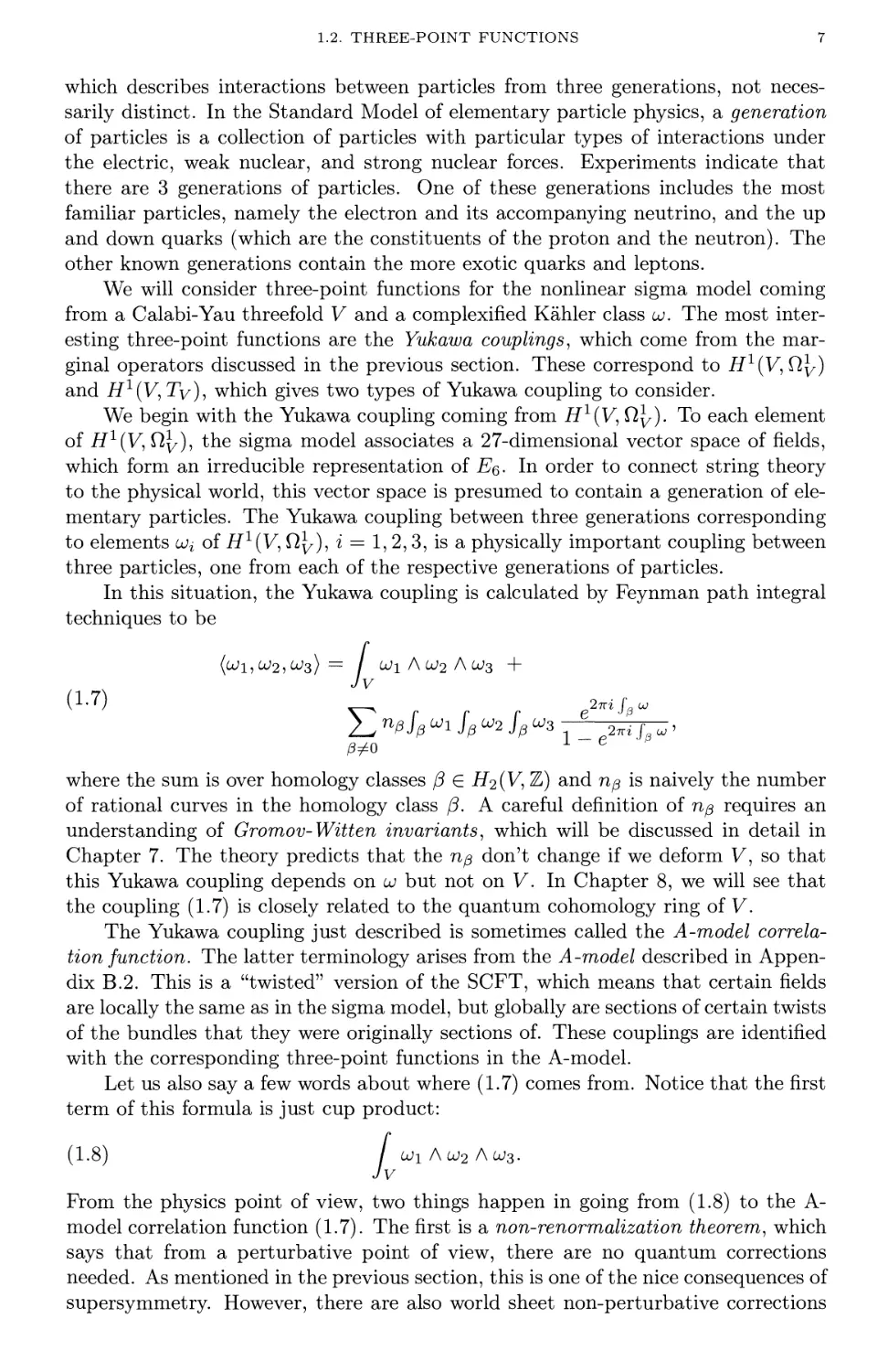
In this situation, the Yukawa coupling is calculated by Feynman path integral
techniques to be
JV
UJ\ A UJ2 A OJ3 +
fv
(1-7) ^-^ z^ifpoj
where the sum is over homology classes /3 G H2(V, Z) and np is naively the number
of rational curves in the homology class /3. A careful definition of n@ requires an
understanding of Gromov-Witten invariants, which will be discussed in detail in
Chapter 7. The theory predicts that the np don't change if we deform V, so that
this Yukawa coupling depends on uj but not on V. In Chapter 8, we will see that
the coupling (1.7) is closely related to the quantum cohomology ring of V.
The Yukawa coupling just described is sometimes called the A-model
correlation function. The latter terminology arises from the A-model described in
Appendix B.2. This is a "twisted" version of the SCFT, which means that certain fields
are locally the same as in the sigma model, but globally are sections of certain twists
of the bundles that they were originally sections of. These couplings are identified
with the corresponding three-point functions in the A-model.
Let us also say a few words about where (1.7) comes from. Notice that the first
term of this formula is just cup product:
(1.8) / uji Auj2 Acj3.
JV
From the physics point of view, two things happen in going from (1.8) to the A-
model correlation function (1.7). The first is a non-renormalization theorem, which
says that from a perturbative point of view, there are no quantum corrections
needed. As mentioned in the previous section, this is one of the nice consequences of
supersymmetry. However, there are also world sheet non-perturbative corrections
8
1. INTRODUCTION
to be considered, which in this case are the holomorphic instantons. These are
nonconstant holomorphic maps £ —» V, where £ is a compact Riemann surface.
When we treat the A-model correlation function more carefully in Chapters 7 and 8,
we will see that £ can have nodal singularities and more than one component. In
the A-model correlation function, the only instantons needed are those where £ has
genus 0. Naively, these are what the rip count in formula (1.7). In the terminology
of Chapter 7, we call rip an instanton number.
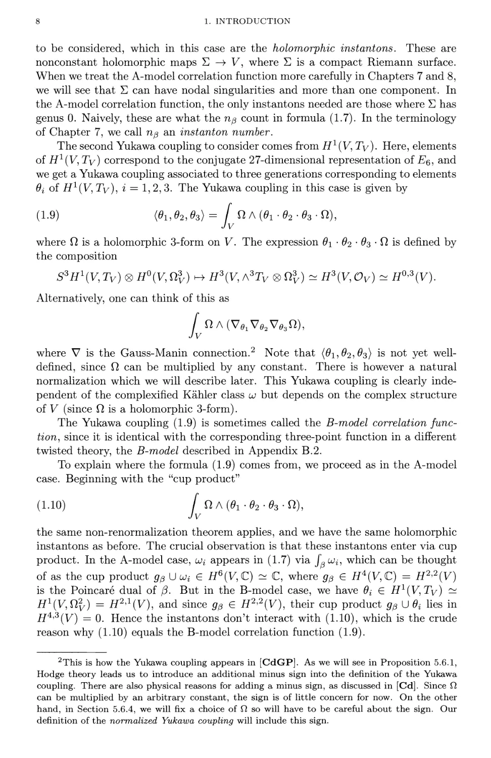
The second Yukawa coupling to consider comes from i^x(V, Ty). Here, elements
of i^1(VA, Ty) correspond to the conjugate 27-dimensional representation of E§, and
we get a Yukawa coupling associated to three generations corresponding to elements
0i of #X(V, Ty), i = 1, 2, 3. The Yukawa coupling in this case is given by
(1.9) <01,02,03>= / ft A (01 -02 -03 'ty,
Jv
where ft is a holomorphic 3-form on V. The expression 0i • 02 • 03 • ft is defined by
the composition
S3H\V, Tv) <g> H°(V, n3v) h-> H3{V, A3TV <g> n3v) ~ H3(V, Ov) ~ H°'3{V).
Alternatively, one can think of this as
/ ft A (V^^ft),
Jv
where V is the Gauss-Manin connection.2 Note that (01,02,03) is not yet well-
defined, since ft can be multiplied by any constant. There is however a natural
normalization which we will describe later. This Yukawa coupling is clearly
independent of the complexified Kahler class uj but depends on the complex structure
of V (since ft is a holomorphic 3-form).
The Yukawa coupling (1.9) is sometimes called the B-model correlation
function, since it is identical with the corresponding three-point function in a different
twisted theory, the B-model described in Appendix B.2.
To explain where the formula (1.9) comes from, we proceed as in the A-model
case. Beginning with the "cup product"
(1.10) / ft A (0i- 02 -03 -ft),
Jv
the same non-renormalization theorem applies, and we have the same holomorphic
instantons as before. The crucial observation is that these instantons enter via cup
product. In the A-model case, uji appears in (1.7) via f*u)i, which can be thought
of as the cup product gpUcj{ G H6(V,C) - C, where gp G H4(V,C) = H2'2(V)
is the Poincare dual of /3. But in the B-model case, we have 6i G H1(V,Tv) —
H1^,^) = H2^(V), and since gp G #2'2(V), their cup product gp U 0* lies in
H4'3(V) = 0. Hence the instantons don't interact with (1.10), which is the crude
reason why (1.10) equals the B-model correlation function (1.9).
2This is how the Yukawa coupling appears in [CdGP]. As we will see in Proposition 5.6.1,
Hodge theory leads us to introduce an additional minus sign into the definition of the Yukawa
coupling. There are also physical reasons for adding a minus sign, as discussed in [Cd]. Since Q
can be multiplied by an arbitrary constant, the sign is of little concern for now. On the other
hand, in Section 5.6.4, we will fix a choice of Q so will have to be careful about the sign. Our
definition of the normalized Yukawa coupling will include this sign.
1.2. THREE-POINT FUNCTIONS
9
The absence of instanton corrections in (1.9) is extremely important. It means
that we can compute the B-model Yukawa coupling exactly using standard methods
of algebraic geometry. This procedure will be explained in Chapter 5.
Suppose now that (V,cj) and (V°,uj0) are a mirror pair, i.e., the sigma model
associated to (V, u) gives the same SCFT as the sigma model associated to (V°, ui°)
with the appropriate sign change. This gives a natural isomorphism Hx(y, Qy) ~
H1(V0,Tyo), and since three-point functions are intrinsic to the SCFT, it should
follow that the A-model correlation function arising from the sigma model on (V, uj)
coincides with the (appropriately normalized) B-model correlation function arising
from the sigma model on (V° ,cj°). This is one of the major mathematical
consequences of mirror symmetry. The actual details of this identification are a bit more
complicated because of the role of the mirror map, but this equality of A-model
and B-model correlation functions is certainly plausible.
Note that the properties of the correlation functions are consistent with mirror
symmetry. We have already observed that the A-model correlation function
associated to (V,cj) depends on u but not on V. It follows from mirror symmetry and
the local identification of moduli spaces discussed above that the B-model
correlation function associated to (V°,uj0) should depend on V° but not on uo°. As noted
above, the B-model does indeed have this property.
As we will see with the example of the quintic threefold, being able to identify
the three-point function of the A-model with the three-point function of the B-
model of its mirror was used in [CdGP] to make some remarkable predictions for
numbers of rational curves on the quint ic threefold. This example is discussed in
detail in the next chapter. In general, some of the most important consequences of
mirror symmetry arise from the combination of the two following facts:
• The equality of the A-model and B-model correlation functions.
• The ability to compute the B-model function exactly.
Together, these allow one to compute Gromov-Witten invariants on Calabi-Yau
threefolds, which in turn give a wealth of enumerative information. All of this, of
course, depends on our ability to prove mathematically that these physical
consequences are indeed correct.
What we have just described can be thought of as the "classical" approach
to the consequences of mirror symmetry, where the A-model and B-model
correlation functions are the primary objects of interest. However, in the years since
the discovery of mirror symmetry, the focus has shifted a bit. In particular, the
relation between the B-model correlation function and the Gauss-Manin connection
is much better understood, which on the A-model side has led to the development
of quantum cohomology and the A-variation of Hodge structure. Also, the work of
Givental and of Lian, Liu, and Yau on the Mirror Theorem has introduced other
new objects of interest—we will see that equivariant cohomology and localization
play an important role in the proofs of the Mirror Theorem. We will address all of
these ideas in subsequent chapters.
We close this section with a final observation about the formulas (1.7) and (1.9).
They seem asymmetric since the first is much more complicated than the second.
Fortunately, mirror symmetry easily accounts for this discrepancy. We noted above
that the A-model correlation function should vary with complexified Kahler class
cj, while the B-model function should vary with complex structure on V. Since the
cup product in (1.8) is a purely topological invariant, it is clear that other terms
are needed if we are to have a nontrivial dependence on uj. On the other hand,
10
1. INTRODUCTION
the cup product in (1.10) already depends on the complex structure, since Q is a
holomorphic 3-form on V. So it is conceivable that no further terms are needed.
1.3. Why Calabi-Yau Manifolds?
Our next task is to explain why mirror symmetry applies only to Calabi-Yau
manifolds, especially Calabi-Yau threefolds. A full explanation of why nonlinear
sigma models need Calabi-Yau manifolds would require a considerable detour into
physics. We give a partial treatment of this topic in Appendices B.2 and B.3.
For now, we will content ourselves with sketching some of the ideas. The starting
point is the assumption that space-time should be a 10-dimensional manifold with
a semi-Riemannian metric of signature (9,1). This manifold should locally be a
product M3?i x V, where M3?i is the usual space-time of special relativity, and V
is a compact 6-dimensional Riemannian manifold. The basic intuition is that V is
too small to be seen at macroscopic scales but is essential for the quantum aspects
of the theory. In any dimension other than 10, the conformal symmetry discussed
earlier in the section does not survive the process of quantization.
As usual, the physics is nontrivial and involves some unfamiliar terms. The idea
is to approach a nonlinear sigma model by first considering other theories which are
more elementary from the physics point of view. In particular, one starts with an
N = 1 supergravity theory in the low energy limit. This gets rid of the fermionic
fields, and then supersymmetry and other consistency requirements impose strong
conditions on the metric on Riemannian manifold V. In particular, one finds that
the holonomy group of the metric equals SU(3). This has some nice consequences:
• (differential geometry) The metric on V is Ricci flat, i.e., its Ricci curvature
tensor vanishes identically. This implies &i(V) = 0.
• (algebraic geometry) V has a complex structure such that c\{V) = 0, and
the metric is Kahler for this complex structure.
Hence we see that V is Calabi-Yau, as desired.
So far, we only have N = 1 supersymmetry in spacetime. After some further
work, this theory can be reinterpreted as an TV = 2 SCFT on the world sheet,
although to preserve superconformal invariance, we need to deform the above Ricci
flat metric. A precise description of this deformation is not known (this is still an
open question in physics), but one can show that the new metric lies in the same
Kahler class as the old one, so that we still have a Calabi-Yau threefold.
For a more complete description of how the Ricci curvature arises (from the
physics point of view) and references to the literature, the reader should consult
Chapter 0 of [Hiibsch].
1.4. The Mathematics of Mirror Symmetry
From a mathematical point of view, the formulation of mirror symmetry given
in Section 1.1 poses serious problems. For example, the definition of an TV = 2
SCFT involves integrals over the space of all maps E —> V. Such integrals have
yet to be defined rigorously. So a mathematical proof of mirror symmetry would
involve an isomorphism between objects (the sigma models of (V,cj) and (V°,(jU°))
which aren't well-defined mathematically. Even the N = 2 SCFT moduli spaces
pictured in Section 1.1 are not well-defined!
What are mathematicians to do in this situation? One approach would be to
avoid SCFT's altogether by concentrating on careful definitions of Kahler moduli
1.4. THE MATHEMATICS OF MIRROR SYMMETRY
11
spaces, Gromov-Witten invariants, etc. and then trying to prove that these objects
behave as predicted by mirror symmetry. Another approach would be to embrace
the physics and use its intuitions to see more deeply into the algebraic geometry,
notably in the predictions mirror symmetry makes concerning the Gromov-Witten
invariants of Calabi-Yau toric complete intersections. A third would be to formulate
a purely mathematical version of mirror symmetry. For example, [Kontsevich3]
proposes that the mirror of a complex manifold V is a certain symplectic manifold
V° and that mirror symmetry might be formulated as an equivalence of derived
categories relating coherent sheaves on V to a category built from Lagrangian sub-
manifolds of V°. Another fascinating although still somewhat speculative approach
is to attempt to geometrically construct the mirror manifold as a moduli space of
special Lagrangian submanifolds [SYZ].3 In practice, all of these approaches have
been used, which is why mirror symmetry is such an exciting field.
In this book, we will follow mainly the first approach, with occasional comments
on the physics of the situation. Thus, our goal is to discuss the algebraic geometry
involved in understanding the mathematical aspects of Sections 1.1 and 1.2. One
difference is that, unlike the physical theories, we will work with Calabi-Yau
manifolds of arbitrary dimension, not just dimension three. However, when we try to
formulate a mathematical definition of mirror pair in Chapter 8, we will be most
successful in the case of Calabi-Yau threefolds.
We begin with a careful definition of Calabi-Yau. Since the mirror symmetry
constructions to be studied in Chapter 4 sometimes produce singular varieties, we
need a definition which allows certain types of singularities.
Definition 1.4.1. A Calabi-Yau variety is a d-dimensional normal compact
variety V which satisfies the following conditions:
(i) V has at most Gorenstein canonical singularities.
(ii) The dualizing sheaf of V is trivial, i.e., Qy ~ Oy.
(Hi) H^V, Ov) = --- = H'-^V, Ov) = {0}.
If in addition V has at most Gorenstein Q-factorial terminal singularities, we say
that V is a minimal Calabi-Yau variety.
In Appendix A, we review the dualizing sheaf £ly and the definitions of
Gorenstein, canonical and terminal singularities. The Calabi-Yau threefolds considered
in Section 1.1 certainly satisfy this definition.
Some other terms used in Section 1.1 deal with moduli of various sorts. The
space of all complex structures on a given manifold V is a well known object in
algebraic geometry, but the idea of K'dhler moduli may be unfamiliar. Recall from
Section 1.1 that we had a Calabi-Yau threefold V with a complexified Kahler class
uj = B + iJ G if2(V, C) such that J was Kahler. However, if we change u by an
integral class, we don't change the physical theory, since the definition of nonlinear
sigma model only uses exp(27rz J*s </)*(uj)) for maps (/) : E —> V.4 This quantity is
unchanged if we change u by an element of H2(V,Z). Thus, in defining Kahler
moduli, we should mod out by the image of if2(V, Z). This leads to the following
definition (which as before allows some singularities).
3In general, symplectic geometry plays an important role in mirror symmetry, though we will
concentrate more on the algebro-geometric aspects.
4You can see this in the A-model correlation function (1.7). The full details can be found in
Appendix B.2.
12
1. INTRODUCTION
Definition 1.4.2. Let V be a projective orbifold with h2'°(V) = 0. Then:
(i) The Kahler cone is the subset K(V) C H2(V,R) = H^tyR) consisting of
all Kahler classes,
(ii) The complexified Kahler space is the quotient
KC(V) = {ue H2(V,C) : Im(o;) € K{V)}/imH2(V, Z),
where imH2(V,Z) is the image of the natural map H2(V,Z) —»> H2(V,C).
(Hi) The complexified Kahler moduli space is the quotient Kc(V)/Aut(V).
Actually, the Kahler moduli space5 as it arises in SCFT differs from this slightly.
The Kahler moduli space as we have defined it receives quantum corrections which
will modify its properties slightly. In particular, the theory may not converge for all
cj, and so we will be forced to restrict our attention to complexified Kahler classes
lo = B + iJ where J is sufficiently positive. Nevertheless, the larger space that we
defined here is mathematically interesting and will be one our primary objects of
study. We will consider some of the related subtleties in Chapter 6.
In Appendix A, we will review the definitions of orbifold and Kahler class
on an orbifold. Since h2,0 = 0, the Kahler cone K(V) is an open convex cone in
H2(V, R). This tells us that the complexified Kahler space Kc(V) is a well-behaved
object. However, in order to determine the structure of the Kahler moduli space
^c(^0/Aut(V), we need to know how the automorphism group Aut(V) acts on the
Kahler cone. We will return to this subject in Chapter 6.
Notice that Definitions 1.4.1 and 1.4.2 seem to involve slightly different types
of singularities. Fortunately, by a result of [Reidl], a Gorenstein orbifold has
canonical singularities. This means that any orbifold satisfying the second and
third parts of Definition 1.4.1 is automatically Calabi-Yau. Hence, for the purposes
of mirror symmetry, Calabi-Yau orbifolds are a natural class to work with.
1.5. What's Next?
We now describe how the next ten chapters will take us from here to a proof
of the Mirror Theorem. We begin in Chapter 2 with a careful description of the
mirror of a smooth quintic threefold V CF4. By carrying out the strategy outlined
in Section 1.2, we will get some explicit predictions for the number of rational curves
on V of given degree. We will revisit this example several times during subsequent
chapters as we develop more mathematical background and eventually justify all of
the computations which appear in Chapter 2.
In trying to generalize the example of the quintic, it was soon realized that toric
geometry had an important role to play in mirror symmetry. Hence Chapter 3 will
explore various ways of describing toric varieties, and then Chapter 4 will describe
the known mirror symmetry constructions, many of which use toric geometry. This
will give us a large supply of examples which should satisfy mirror symmetry and
provide a good testing ground for the mathematics. We should also mention that
there are even physical theories (the gauged linear sigma models of [Witten5] to be
described in Appendix B.5) which explicitly use toric varieties. Support for mirror
symmetry in the context of the gauged linear sigma model is given in [MP1].
Our next task is to describe and compute the B-model Yukawa coupling. This
will be done in Chapter 5. It turns out that finding the correct coordinates for
5In discussing the Kahler moduli space, we frequently drop the adjective "complexified" when
the meaning is clear from context.
1.5. WHAT'S NEXT?
13
calculating this Yukawa coupling requires a good understanding of the moduli space
at certain boundary points. Hence, in Chapter 6 we will study the structure and
compactifications of these moduli spaces. As mentioned above, we will also consider
Kahler moduli. In fact, we will see that certain basic facts about Kahler moduli
give insight into what the compactification of the usual moduli space should look
like. In Chapter 7, we will discuss Gromov-Witten invariants. Definitions have
been given in both the symplectic and algebraic categories, and either can be used
to give a mathematical definition of the A-model Yukawa coupling.
By the end of Chapter 7, we will have everything needed to give a precise
formulation of "classical" mirror symmetry, which asserts that certain correlation
functions are compatible via the mirror map. But starting in Chapter 8, we will
explore a deeper understanding of the subject. Two new ingredients are quantum
cohomology, which can be thought of as working out the algebraic and enumerative
implications of Gromov-Witten invariants, and the A-model variation of Hodge
structure, which is a natural consequence of quantum cohomology. The basic idea
is that mirror symmetry really involves an isomorphism, via the mirror map, of
two variations of Hodge structure: one on the B-model (the usual VHS coming
from complex moduli), and the other on the A-model (the A-variation of Hodge
structure). This version of the Mirror Theorem will be formulated at the end of
Chapter 8. It turns out that the desired equality of correlation functions follows
immediately from this isomorphism of variations of Hodge structure.
The Mirror Theorem, when formulated using variations of Hodge structure, is
still an open question, although recent work of Givental [Givental2, Givental4]
and Lian, Liu and Yau [LLY] represents substantial progress toward proving this
form of the theorem. We will discuss the ideas of these papers in Chapter 11. As
we will see, this will require the introduction of new techniques and new objects of
study. In particular, equivariant cohomology and localization will play an important
role in the proof. In Chapter 9, we will review some of the basic definitions and
theorems, and we will use these methods to prove some interesting results about
Gromov-Witten invariants. Then Chapter 10 discusses an extension of Gromov-
Witten invariants called gravitational correlators. These invariants will enable us to
describe the flat sections of the A-model connection. We will also define the Givental
J-function and explain its relation to quantum differential equations. Finally, in
Chapter 11, we will discuss the Mirror Theorems stated in [Givental2, Givental4]
and [LLY]. A brief preview of what is involved will be given at the end of Chapter 2,
and then the full details for the quintic threefold will be presented in Chapter 11.
These chapters cover a lot of mathematics, and reading them straight through
would be a somewhat daunting task. We suggest that the reader start with
Chapter 2. From here, there are several ways to proceed, depending on the reader's
interests. The preface offers some guidance for what to read, and a glance at the
table of contents may also be useful. Our hope is that once you start reading, the
intrinsic interest of the subject will draw you in. Mirror symmetry is a fascinating
story, and it is fun to see how the various pieces fit together.
This page intentionally left blank
CHAPTER 2
The Quintic Threefold
The quintic threefold was the first example for which mirror symmetry was
used to make enumerative predictions [CdGP]. In this chapter, we will review this
example, following the approach of [CdGP], with some modifications based on the
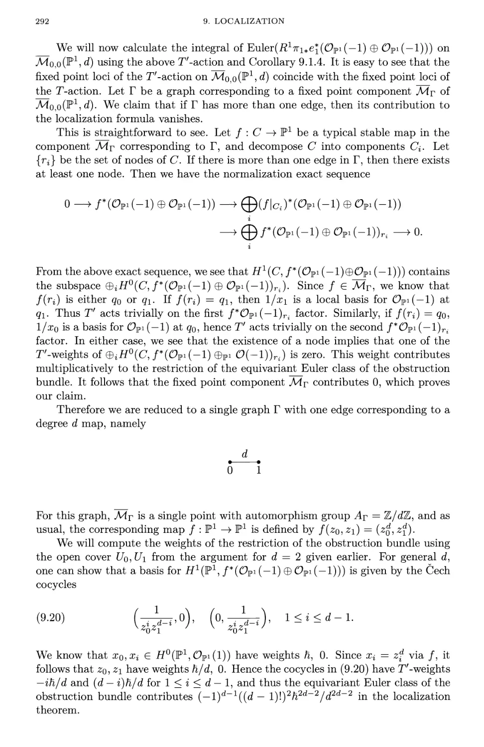
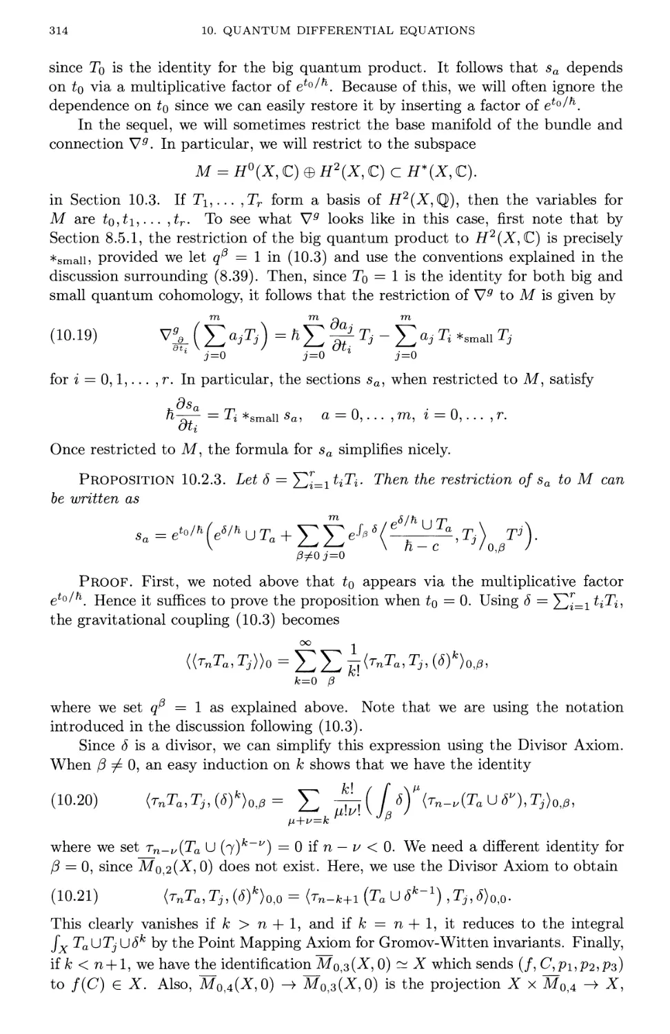
more mathematical exposition of [Morrison2]. In Section 2.6 we will give two
alternative methods for calculating the same enumerative data based on [Givental2]
and [LLY]. We will also revisit the quintic threefold several times in later chapters
to illustrate the various methods used to study mirror symmetry.
2.1. The A-Model Correlation Function of the Quintic Threefold
It is well known that a smooth quintic hypersurface V C P4 is Calabi-Yau
(this also follows from the theory to be developed in Chapter 4). We consider the
nonlinear sigma model associated to (V, cj), where u = B + iJ is a, complexified
Kahler class on V. If H denotes the hyperplane class, then the A-model correlation
function (1.7) from Chapter 1 simplifies to give the formula
oo d
(2.1) {H,H,H) = 5 + J2ndd3T^i.
d=i q
Naively, rid is the number of rational curves of degree d contained in V, and q =
e27Tij£uj^ where £ is a ime m y The formula for q can be written q = e27Tlt if we
put lo = tH. We will see in the next section that q is actually a local coordinate
on the compactified Kahler moduli space. Furthermore, as explained in Chapter 1,
this formula depends on u but not on the complex structure of V, since it is an
A-model correlation function.
When algebraic geometers first learned of (2.1), it seemed a bit strange. For
one thing, we don't even know a general quintic threefold has finitely many rational
curves of a given degree d. According to the Clemens conjecture, this should be
true, but so far the conjecture is known only for d < 9 [JKl]. Yet (2.1) seems to
assume the conjecture for all d. This unsettling beginning is then compounded by
mirror symmetry, which claims to give an explicit formula for the number rid of
such curves, and it does this for all d > 1.
We will give a firm foundation for (2.1) in Chapter 7. The key player is the
Gromov-Witten invariant (7o,3,d)(#, H, H). This invariant can be defined in a
variety of ways. From the symplectic point of view, one considers C°° maps / : P1 —> V
which obey an appropriately deformed Cauchy-Riemann equation. Imposing
appropriate conditions on the image of 3 points in P1, it can be shown that there are
only finitely many such curves in each homology class. Then (Io^^)(H,H,H) is
defined to be the total number of such curves, counted with sign according to
orientation (there is no longer a preferred orientation coming from a complex structure).
15
16
2. THE QUINTIC THREEFOLD
There are actually several ways to make this precise, all of which will be reviewed
in Section 7.2.
A different approach to defining rid has been proposed in [Kontsevich2] using
the moduli space of stable maps / : C —> V, where C has genus 0 (but need
not be irreducible). The resulting definition of Gromov-Witten invariant is rather
sophisticated, involving algebraic stacks and virtual fundamental classes. These
topics will be discussed in Section 7.1.
Once we have a rigorous definition of the Gromov-Witten invariant, we can
then define the A-model correlation function to be the formal sum
oo
(H,H,H) = ^(I0l3,dHH,H,H)qd.
To see how this relates to (2.1), fix d and suppose that k\d. If C C V is a smooth
rational curve of degree k with normal bundle Oy{—1) 0 O^(-l), then a map
/ : P1 —> C of degree d/k gives a stable map of the sort counted by (Jo,3,d)C#? H, H).
We will see in Chapter 7 that the family of such /'s contributes a factor of k3 to
{Io,3,d)(H,H,H). Since this happens for each C of degree fc|d, it makes sense that
(2.2) (I0^d)(H,H,H) = J2n*k3
k\d
when d > 1. Given this equation and the above definition of (H, H,H), (2.1) follows
by easy power series manipulations.
Unfortunately, this argument is far from complete and seems to assume the
Clemens conjecture. So to make everything rigorous, we will define the rid using
equation (2.2). Then the question becomes, how do the rid relate to rational curves
in V? In Section 7.4.4, we will prove that for d < 9, rid is precisely the number
of rational curves of degree d on the quintic threefold. This is less obvious than it
seems, for although the Clemens Conjecture is true for d < 9, some rational curves
in V are singular. In particular, V contains 17,601,000 6-nodal rational curves of
degree 5 [Vainsencher], and some care is required to see how they enter into n$.
For a long time, people expected that once the Clemens Conjecture was proved,
it would follow immediately that in (2.2), rid should be the number of rational curves
of degree d in V. However, it was recently observed by R. Pandharipande that even
if the Clemens Conjecture is true for d = 10, the number nio defined by (2.2) does
not give the number of degree 10 rational curves on V. The reason is that double
covers of the 6-nodal rational curves of degree 5 contribute more than the expected
factor of 53. We will prove this carefully in Chapters 7 and 11. As a consequence, we
will no longer refer to rid as "the number of rational curves of degree d". Rather, in
the terminology of Chapter 7, we adopt the more neutral name instant on number.
Our discussion of nio reflects one of the themes of Chapter 7, which is the subtle
interplay between Gromov-Witten invariants and enumerative geometry. But in
spite of the difficulties which can arise, we will see in Chapter 7 that Gromov-Witten
invariants contain a lot of enumerative information and that mirror symmetry has
stimulated a flurry of activity in enumerative algebraic geometry.
In this chapter, we will use mirror symmetry to compute the A-model
correlation function (2.1) of the quintic threefold V, guided by the strategy outlined
in Chapter 1. The following sections contain some wonderful computations which
will culminate in explicit predictions for the rid- Our discussion will be somewhat
unsatisfying since we use nonrigorous physical theories to compute numbers whose
2.2. THE QUINTIC MIRROR
17
enumerative meaning is unclear. But we will see in subsequent chapters that
every step of the computation can be made rigorous. In particular, we will prove in
Chapter 11 that if we define rid using (2.2) and the symplectic or algebraic
definition of (Io,3,d)(Hi H, H), then the predictions for na made by mirror symmetry are
straightforward corollaries of the Mirror Theorem.
2.2. The Quintic Mirror
Since /i1'1(F) = 1 holds for the quintic threefold V, its mirror should satisfy
dim.H1(V°,Tvo) = 1. The mirror of the quintic is therefore a one-parameter
family of Calabi-Yau manifolds. Greene and Plesser [GP1] describe the mirror as
a resolution of singularities of a family of hypersurfaces in P4/G. Here, G is the
group
(2.3) G = { (ai,... , o5) € Z\ : ^ a, = 0 mod 5}/Z5,
where the Z5 is embedded diagonally, and g = (ai,... , a§) € G acts on P4 as
g- (xi,... ,x5) = (/iaixi,... ,/ia5x5),
where /i = e27™/5 is a primitive fifth root of unity.
Using ^ as a parameter, the hypersurfaces are defined by the equation
(2.4) x\ + x\ + x\ + x\ + x\ + ip x1x2x3x4x5 = 0,
which is invariant under the action of G and hence defines a family of hypersurfaces
in P4/G. (In [CdGP], this equation is written with —5ip in place of ip.) The
quotient P4/G is singular, and the hypersurfaces (2.4) inherit these singularities.
However, as long as ip ^ — 5/i2, 0 < i < 4, the hypersurface is a Calabi-Yau
orbifold in P4/G. Even better, we can resolve singularities (simultaneously for all
V>) without destroying the Calabi-Yau property—this is straightforward to establish
locally. Thus, we define V° to be the family of resolved hypersurfaces coming from
(2.4). To emphasize that we have a one-parameter family of varieties, we will
sometimes denote the mirror family by VI.
This construction of VI is due to Greene and Plesser and involves the super-
conformal field theories discussed in Chapter 1. However, we will see in Chapter 4
that Batyrev gave a purely mathematical description of V^ which generalizes to
Calabi-Yau hypersurfaces in toric varieties.
As noted above, the equation (2.4) defines a singular variety. Since we are
dealing with a threefold, there is no canonical resolution of singularities for (2.4).
An explicit choice of resolution is given in [Morrison2], but there are many others.
Fortunately, different choices still have the same complex moduli and in addition
have the same B-model correlation function. We will let V£ refer to any one of these
choices. (In Chapter 6 we will learn that the different choices reflect the Kahler
moduli of the mirror. In terms of physics, they gives different "phases" in the same
physical theory.)
Our next task is to flesh out the strategy discussed in Section 1.2 for computing
(2.1) in terms of the mirror VI. The first step is to understand the moduli spaces
involved. For the complex moduli of the mirror, notice that the map (#i,..., £5) *-»
(/i-1xi,X2,... ,£5) induces an isomorphism V^ ~ KL-1 Hence ^5 is well-defined
1This is obvious for the hypersurfaces in F^/G, and one can show that the isomorphism
extends to the resolution—see [Morrison2].
18
2. THE QUINTIC THREEFOLD
on the complex structure moduli space of VC?, so that
x = ^~5
is a local coordinate for the complex moduli (we will soon see the reason for this
choice of x). Furthermore, one can check that singularities of V^ occur for i/j =
—5/i2, 0 < i < 4 (noted earlier) and also for if) = oo. In terms of the moduli
coordinate x, this means that the complex moduli space has boundary points x =
-5~5 and x = 0.
According to mirror symmetry, the complex moduli of V° should correspond
to the Kahler moduli of the quintic threefold V. Since H generates if2(V, Z) ~ Z,
we can write uo = tH, and since H is Kahler, uo = tH is a complexified Kahler
class precisely when t is in the upper half plane. According to Definition 1.4.2,
the Kahler space Kc(V) is the quotient of the complexified Kahler classes modulo
if2(V, Z). It follows that q = e27rit induces an isomorphism
q:Kc(V)~A\
Thus q is a local parameter for Kahler moduli space, with q = 0 as a boundary
point. An important but easy observation is that if £ is a line in V, then q can be
written
(2.5) q = e27rit = e27ri^UJ.
Thus the A-model correlation function (2.1) is naturally a function in the local
parameter q for Kahler moduli.
Assuming mirror symmetry, we get a local isomorphism between the Kahler
moduli of V and the complex moduli of V°. In terms of the illustration (1.6),
the "V constant, uj varies" slice maps locally to the uuj° constant, V° varies" slice
on the mirror side. However, the key word is "local": we need appropriate local
coordinates for each moduli space. For the Kahler moduli of V, this coordinate is
clearly q since the three-point function (2.1) is a power series in q. Since q is a local
coordinate at a boundary point, the same should be true on the mirror side.
For the complex moduli of V°, we have two boundary points to choose from,
x = 0 and x = — 5~5. We claim that x = 0 corresponds to q = 0, so that x
is the desired local coordinate. The reason is as follows. Back on the quintic
threefold V, cup product with H gives an endomorphism UH of ®l=0Hp'p(V)
which is maximally nilpotent (meaning (UH)3 ^ 0 but (UH)4 = 0). We will see
in Chapters 5 and 6 that under mirror symmetry, we expect UH to correspond to
the logarithm of the monodromy about the point of the complex moduli space of
V° corresponding to q = 0. Hence, mirror symmetry tells us to look for maximally
unipotent monodromy, and of the above boundary points, this occurs only at x = 0.
Chapter 5 will give a careful definition of maximally unipotent monodromy.
In order to compute the A-model correlation function (2.1), we have two
remaining tasks:
• The local coordinates q and x describe corresponding boundary points of
the Kahler and complex moduli spaces, but the local isomorphism given by
mirror symmetry is not q = x. From the physics point of view, there are
quantum corrections to take into account. Hence we need to compute x as a
function of q, and vice versa. Once this is done, we will have an explicit local
mapping between the complex moduli space of V° and the Kahler moduli
space of V. This is usually called the mirror map.
2.3. THE MIRROR MAP
19
• We have to compute and correctly normalize the B-model correlation
function, and then use the mirror map to write it as a function of q. This will
give an explicit formula for (2.1).
We now turn our attention to the first of these tasks.
2.3. The Mirror Map
One way to think of the mirror map is that q is a canonically chosen coordinate
on the Kahler moduli space of V. Thus we want to find a "canonical" coordinate on
the moduli space of V°. As will be explained in Chapter 6, we can do this because
the monodromy at x = 0 is maximally unipotent. Following [Morrison2], there
is a minimal integral vanishing cycle 70 near x = 0, so that 70 is invariant under
monodromy. Furthermore, there is a minimal integral cycle 71 transforming under
monodromy about x = 0 as 71 h-» 71 + rn^fo for some m € Z. In the case of the
quintic, we have m — 1 [Morrison2]. It follows that for a holomorphic 3-form Q on
V°, the quantity J Q,/ J Q transforms under monodromy into (J f2/ / f2) + 1,
so that
exp (2^X^/4 ft)
is a well-defined function in a neighborhood of x = 0. Furthermore, 70 is unique up
to sign, and 71 is unique up to the same sign and an integer multiple of 70. Hence
the above quantity is canonically determined on the moduli space of V°, and we
also see that it is independent of Q since V° is Calabi-Yau. It is then natural to
assert that the mirror map is given by t = J f2/ J Q and
(2.6) <7 = exp(27ri/7ift//7oft).
A physics argument for this assertion is given in [BCOV2]. This mirror map can be
mathematically proven to be the correct one (Theorem 11.1.1 or Theorem 11.2.2).
To express J Q and J Q explicitly as functions of x, we will follow the
approach of [Morrisonl]. For any 3-cycle 7 on V°, the integral y = J f2 is a period
of the family. It is well known that the periods satisfy the Picard-Fuchs equation,
which for a threefold with h3(V°) = 4 is a differential equation of the form
where the fi depend on the moduli coordinate x and differentiation is with respect
to x. In general, Picard-Fuchs equations can be calculated by several methods:
explicit calculation of the periods [CdGP], the Grifnths-Dwork method of reduction
of pole order [Morrisonl, Font, KTl], generalized hypergeometric equations as in
[BvS, HKTY1], or finally, by an explicit formula for toric complete intersections
according to an assertion in [Givental4]. The last three of these methods will
be discussed in Chapter 5. Alternative ways of organizing the data together with
proofs of different versions of the mirror theorem are given in Chapter 11. We will
give a sneak preview of these approaches in Section 2.6.
If we choose for Q the 3-form
lb
Q = Res(^ ? ; (x\dx2 A dx3 A dx± A dx§ —
xx\ + ... + xg + ^xi •••xs
^ ' ' xidx\ A dx% A dx4 A dx$ + x$dxi A dxi A dx± A dx§ —
x^dx\ A dx2 A dx$ A dx$ + x$dx\ A dx2 A dx$ A dx±)),
20
2. THE QUINTIC THREEFOLD
then the methods of Chapter 5 give the Picard-Fuchs equation
/ d \4 2-55x / d \3 7-54x / d \2
24-5x
2/+ i ■ K.^2/-
(2-8)
2 • 54x / d \ 24 • 5x
+ l + 55x \Xdx)y + l + 55x
This equation has a regular singular point at x = 0. Note also that there is a
singularity at the other boundary point x = — 5~5.
The periods yo = J fi and yi = / Q satisfy this equation, and the mon-
odromy properties of 70 and 71 imply that yo and 27rz yi — (log x)yo are single-valued
at x = 0. Then, using standard methods for solving (2.8), we find that yo and y\
are determined uniquely up to
Vo ^ hyo
yi ^ hyi +&22/0,
where &i, hi G C and b\ ^ 0 (this is similar to the uniqueness for 70,71 except that
we have lost the integer lattice). It follows that we can compute
n = e2iriyi/y0
up to a constant c\ = exp(27rz 62/^1)- The result is that the mirror map is
(2.9) q = c1(x-770x2 + •••),
with inverse
(2.10) x = —+77o(—Y
In Section 2.5, we will use mirror symmetry to show that c\ = — 1. There are
other ways to arrive at this normalization, for example this is a natural choice in
implementing the method of Frobenius in the solution of generalized hypergeometric
functions. This idea appears in [BvS], and we will return to this point in Chapter 6
when we discuss the mirror map in general.
Using methods for solving generalized hypergeometric equations, it is possible
to get closed forms for many of these formulas. For example, up to a constant, yo
is given by
00
V (5n)!
h w5
(2.11) yo = Vf^(-l)V = l-120x-
and the mirror map can be shown to be (assuming c\ = —1)
(2-12) 1 = -* exp ( * V f^ \ £ 11 (-1)»A .
The details of this derivation will appear in Section 6.3. We will see another
approach in Section 2.6. Using (2.12) and Dwork's theory of p-adic hypergeometric
series, one can prove that q is a power series in x with integer coefficients [LY2].
2.4. THE B-MODEL CORRELATION FUNCTION
21
2.4. The B-Model Correlation Function
We now turn to the problem of computing the Yukawa coupling on V°. The
crucial but elementary observation is that the Yukawa coupling also satisfies a linear
differential equation, which can easily be derived from the Picard-Fuchs equations.
By formula (1.9) from Section 1.2, we have
(2.13) <*£,*£,*£> = /v.n Air,
where the prime denotes x-^. Here, we assume that ft is given by (2.7). We could
replace ft with its multiple by any nonvanishing function of x. Which multiple
to choose is the normalization problem, which we will postpone until later in the
section. As noted in the footnote in Section 1.2, normalization will also insert a
minus sign on the right hand side of (2.13). This will be explained in Section 5.6.4.
We claim that the Yukawa coupling Y = Jyo ft A ft'" satisfies the differential
equation
(2.14) (*)Y=f!^Y.
v } \ dxJ l + 55x
To see this, first observe that by Griffiths transversality, ft' and ft" have no (0, 3)
component. Hence
(2.15) / ft Aft = / ftAft'=/ ftAft// = 0.
Jv° Jv° Jv°
Differentiating the last equality twice gives
(2.16) f ft Aft""+ 2/ ft7 Aft7" = 0.
Jv° Jv°
On the other hand, Y = fyo ft A ft7" gives Y' = Jyo ft7 A ft7" + Jyo ft A ft"". Using
(2.16), we conclude that Y' = \ Jyo ft A ft"". However, the Picard-Fuchs equation
(2.8) implies that
(2.17) 0 = ft"" + ^J-n'" + l^-n" + ^^-n' + ^#-ft
v } 1 + 55x 1 + 55x 1 + 55x 1 + 55x
in cohomology. The result (2.14) now follows by wedging ft with the right hand
side of (2.17) and using (2.15).
The solution of (2.14) is
<2-18> y = TrW
where C2 is a constant which will be determined in the next section. Thus we know
the Yukawa coupling up to a constant. Notice that it is singular at the boundary
point x = — 5~5, as might be expected.
However, we are not done, for we still need to normalize the Yukawa coupling,
since the formula (2.7) for ft can be multiplied by any nonvanishing function of x.
A natural way to normalize ft is by demanding that J ft = 1 after normalization.
With the choice of ft from (2.7), we use the period
y0(x) = / ft
and replace ft by il/yo(x). This achieves the desired normalization. Because of
(2.15), one easily shows that the effect of this normalization on the Yukawa coupling
22
2. THE QUINTIC THREEFOLD
Y is to replace Y by Y/yo(x)2. Hence, for this choice of Q, we get the normalized
Yukawa coupling
(2'19) (XhX£iXi;) = (1 + 55^(3)2-
Note that this expression is essentially unaffected by the introduction of the minus
sign mentioned above, since the sign can be incorporated into the choice of C2. This
may be the reason why this sign has not to our knowledge appeared in the
mathematics literature before now. Chapter 5 will give general methods for computing
the normalized Yukawa coupling and discuss its surprisingly strong connection to
the Gauss-Manin connection.
2.5. Putting It All Together
We can now use the formulas from the previous two sections to compute the
A-model correlation function of the quintic threefold. Under mirror symmetry, we
get an isomorphism
which is compatible with the A-model and B-model correlation functions. Thus,
if 0 G H1(V°,Tvo) corresponds to H G i^1(V, Qy) via mirror symmetry, then as
explained in Chapter 1, we should have
(H,H,H) = (e,e,e).
We find 0 as follows. Thinking of /zTl(V,f2y) as the tangent space to the Kahler
moduli, if is a vector field on the Kahler moduli space of V. Writing a general
complexified Kahler class as tH, this vector field is identified with d/dt. In terms
of the local coordinate q = e27Tlt for Kahler moduli, we have ^ = 2iriq^. Under
the mirror map q = q(x), -£- maps to ^^, and it follows that
tt d _ ^ dx d
H = ziriq—- \—> v = ZTriq-— —.
dq dq dx
Then (H, H, H) = (0, 0, 0) gives the equation
lis u u\ fr, ■ dx\3, d d d , / qdx\3, d d d ,
\ dq J ^dx' dx' dx' \ x dq) ^ dx' dx' dx'
This assertion, which is the equality of the A-model and B-model correlation
functions via the mirror map, is mirror symmetry for the quintic threefold.
To make this equation more explicit, note that we calculated (x-^^x-^^x-^)
in (2.19). Hence, using (2.19), the mirror map (2.9) and (2.10), and the formula
for yo(x) given in (2.11), we obtain
^2 /0 . Q dx \ 3
(1 + oiDx)vn[x)z V x dq J
C2
hm ci(l - 770x + ...)(! + 1540-| + • • • )Y
(l + 55x)(l-120x+---)2 V 1V /v c\
Converting wholly to q coordinates via (2.10), this simplifies to
<-> (1+^)+.(2"r%x,+...,(i+7<'+^)
2.5. PUTTING IT ALL TOGETHER
23
We next determine the constants c\ and C2. The basic idea is to choose them
so that the above power series agrees with what we know about the formula
oo ^
(2.22) (H, H,H)=5 + y ndd3—?—-. = 5 + 2875? + • • •
z—' 1 — Qa
d=l H
given in (2.1). First, since the constant term of this series is 5, comparison with
(2.21) shows that
_ 5
C2 ~ (2^)3*
Second, we claim that c\ = — 1. This is because with the above choice of C2, (2.21)
gives a power series expansion
{H,H,H) = 5-2875— + ••• .
It is known classically that the generic quintic threefold contains 2875 lines, which
is why n\ = 2875 in (2.22). Hence, in order for these series to be equal, we must
have c\ = — 1. This assertion is not mere wishful thinking, for the desired value
c\ = — 1 follows from the original calculation in [CdGP]. As mentioned earlier, we
will give a systematic method for determining c\ when we study the mirror map in
Chapter 6.
Given these choices for c\ and C2, we can summarize mirror symmetry for the
quintic threefold V as follows. First, by (2.11),
(2.23) yo{x) = J2)JE(-l)V
n=0 W
is the unique (up to a constant) holomorphic solution of the Picard-Fuchs equation
(2.8) of the mirror V°. There is also the solution
(2.24) yiix)=yo{x)iog{-x) + 5Y,\^E[Yl 7](-!)V
n=l ^ *' j=n+l ^
with a logarithmic singularity, and by (2.12), the mirror map is
(2.25) , = exp^M) = -x exp (-^ g « [£ I] (-1)",").
Then mirror symmetry for the quintic threefold, as stated in (2.20), asserts that
(2.26) 5 + VW-^-= * , J^)\
Recall the left hand side is the A-model correlation function of V and the right hand
side is the B-model correlation function of V°, given by the normalized Yukawa
coupling regarded as a function of q.
If we expand the right hand side of this equation, we obtain
00 d 2
(2.27) 5 + Vn/-—r =5 + 2875—^—+609250'23—^ + ... ,
^—' 1 — qa 1 — q 1 — qz
d=l
so that mirror symmetry implies that n^ = 609250. Computing additional terms
of this series, we get the following predictions for the instanton numbers n^ of the
24
2. THE QUINTIC THREEFOLD
quintic threefold:
d
1
2
3
4
5
rid
2875
609250
317206375
242467530000
229305888887625
The first four entries agree with known enumerative results: ri\ = 2875 is classical
(as noted earlier), n^ = 609250 has been shown in [Katz2], n3 = 317206375 has
been shown in [ESI], and 77,4 = 24246753000 has been shown in [Kontsevich2].
These numbers are computed for all d < 10 in [CdGP].
For general d, equation (2.26) asserts that the numbers 2875, 609250, ...
appearing in the series on the right hand side of (2.27) are precisely the instanton
numbers n^, which are defined in terms of the Gromov-Witten invariants of the
quintic threefold by (2.2). We will prove in Section 7.4.4 that for d < 9, the
numbers rid are indeed equal to the number of rational curves of degree d on a
generic quintic threefold. For d > 10, we still have the numbers n^, but as already
indicated, their relation to the rational curves of degree d is more subtle.
The numbers in the above table suggest that the rid should have some
remarkable divisibility properties. It is easy to see that the rid are rational, but it is
unknown if they are integers (though this is true for all that have been computed).
However, if we assume that the rid are integral, then one can prove that 53|n^ for
all d not divisible by 5 [LY1]. It is conjectured that 53|n^ is true for all d.
So far, we have said nothing about how to prove (2.26). This is the essential
content of the Mirror Theorem, which is our next topic of discussion.
2.6. The Mirror Theorems
The equation (2.26) given in the preceding sections is based on the "classical"
formulation of mirror symmetry, where the primary goal is to prove that certain
correlation functions can be identified via the mirror map. In order to justify these
calculations, one needs to prove a Mirror Theorem. In this section, we will introduce
three different versions of the Mirror Theorem, all of which imply "classical" mirror
symmetry for the quintic threefold. Rather than state the theorems in general, we
will instead discuss what they look like for the quintic threefold V and its mirror
V°. Complete statements will appear in Chapters 8 and 11.
2.6.1. Hodge Theory. The mirror map constructed in Section 2.3 expresses
the Kahler parameter q of the quintic threefold V as an explicit function of the
moduli parameter x of the mirror V°. This allows us to use q as a new local
parameter for the moduli of V°. Then, in Section 2.4, we determined the normalized
Yukawa coupling (2.19). In Chapter 5, this normalized coupling will be denoted Y.
The enumerative predictions of the previous section came by expressing Y in terms
of q and equating it with the A-model correlation function (2.22).
However, we will learn in Chapter 5 that once we express Y in terms of q, we
also completely determine the variation of Hodge structure on if3(V°,C). More
precisely, in the proof of Proposition 5.6.1, we will see that in an appropriate basis,
2.6. THE MIRROR THEOREMS
25
the Gauss-Manin connection V of V° has connection matrix
/ 0 0 0 0 \
f2 28^ 10 0 0
(2'28) 0 Y 0 0
\ 0 0 1 0 /
provided we use q as moduli parameter.
This shows that the normalized B-model correlation function Y is not just
some strange function suggested by physics, but rather is integral to the Hodge
structure of the mirror family. Furthermore, since Y is supposed to correspond to
the A-model correlation function, this suggests that there should be a variation of
Hodge structure on the A-model side. This is our first hint that mirror symmetry
can be formulated in terms of variations of Hodge structure. We will develop this
idea more fully in Chapter 8 when we define the A-variation of Hodge structure.
The associated connection, called the A-model connection, is constructed by means
of quantum cohomology. In particular, for the quintic threefold V, we will see in
Example 8.5.4.1 that the A-model connection has (2.28) as its connection matrix,
provided Y is the A-model correlation function (2.22).
Chapter 8 will give a careful definition of a mathematical mirror pair. For the
quintic threefold and its mirror, this means that the A-variation of Hodge structure
of V should be isomorphic, via the mirror map, to the variation of Hodge structure
coming from the mirror family V°. In Chapter 8, we will show that this version of
mirror symmetry is equivalent to the equality of A-model and B-model correlation
functions given in (2.26).
Proving mirror symmetry, either in its classical form or the more sophisticated
Hodge-theoretic version just discussed, is not easy. In particular, the proof requires
the introduction of some new objects of study. As we will now explain, these new
objects lead in turn to new versions of the Mirror Theorem.
2.6.2. Givental's I and J Functions. In Givental's approach to the Mirror
Theorem, a key role is played by two cohomology-valued formal functions denoted
7y and Jy. Let's first discuss J\>. This function is defined in terms of gravitational
correlators, which can be thought of as generalizations of Gromov-Witten
invariants. We actually begin with the Givental J-function. In Section 10.3.2, we will
see that for the quintic threefold, J is given by the formula
(2.29) J = e(to+t1H)/hf1 + h^YJNdqdd£ - 2/T3 ^ ./Vd <?d pt\
d>0 d>0
where q = e*1, £ is the class of a line in V, pt is the class of a point, and
(2.30) Nd = (I0lo4) = J2nik~3'
k\d
Here, the n^/k are the instanton numbers we want to compute. Earlier in the
chapter, we mentioned the Gromov-Witten invariant (7o,3,d)(#, H, H). Properties
of Gromov-Witten invariants from Chapter 7 imply (/o,3,d)(#, H, H) = d3(/o,o,d),
so that the above formula for Nd is equivalent to (2.2).
The J-function plays a central role in Givental's theory of quantum differential
operators from Section 10.3.1. For our immediate purposes, the key feature of
(2.29) is that J contains all of the enumerative information we're interested in.
26
2. THE QUINTIC THREEFOLD
The function J takes values in the cohomology ring of V. However, in order
to compare this to the function /y described below, we need something that takes
values in H*(F4). We can do this by defining Jy = i\(J), where i : V —> P4 is the
inclusion map and i\ is the Gysin map. In terms of the formula (2.29) for J, one
easily obtains
(2.31) Jv = e^^H^h5H(l + h'2J2NaqddlH2 - 2h'3 ^ Ndqd ±#3).
(In Chapter 11, we will take a slightly different approach to defining J\>.) Here, the
important fact is that the rid are uniquely determined by Jy.
The second of Givental's functions is 7y, which is also a cohomology-valued
function. For the quintic threefold V, the formula for 7y from Example 11.2.1.3 is
Iv = jtn+tl hvHu y- au m + h)--. (5H + UK)
j^0 ((H + h)...(H + dh)f
Although Jy takes values in the cohomology of P4, one of Givental's observations
is that /y is determined by the periods of the mirror V°. Thus 7y contains the
moduli information for the mirror, and Givental's version of the Mirror Theorem
states that /y and Jv are related in an especially nice way. Our explanation of the
proof uses the Quantum Hyperplane Section Principle, which involves localization
formulas for equivariant cohomology on moduli spaces of stable maps. All of this
will be discussed in Chapter 11.
In order to see how this relates to the computations done in earlier sections,
let's simplify the above formula for 7y by taking to = 0 and h = 1. This gives
dt
,IC=1(5H + m)
jd
(2.32) Iv = e^5Hj2 u»
d=0 Um=l(H + my
We can expand I\>, writing
(2.33) /y = 5H {yoih) + yi(h)H + 2/2(*i)#2 + ys(h)H3) .
After the change of variables x = —e*1, we will show in Chapter 5 that 7y satisfies
the Picard-Fuchs equation of the mirror V°, as given in (2.8). In fact, using the
Frobenius method, we will show in Chapter 6 that yo, y\, y2, y% form a basis of
solutions. Furthermore, yo is the series from (2.23), and similarly y\ is (2.24). Hence
the mirror map (2.25) arises naturally in Givental's formulation as q = exp(yi/yo)-
Givental's version of the Mirror Theorem is equivalent to the assertion that
Jv = Jy/yo after changing coordinates via the mirror map (see Theorem 11.2.2).
Since J\> involves the rid by (2.30) and (2.31) and 7y is given by the explicit formula
(2.32), it follows that we can compute as many instanton numbers rid as desired.
However, to complete the circle of ideas, we should explain how this relates to
correlation functions. We first note that the normalized Yukawa coupling Y of V°
from Section 2.5 arises naturally from /y. To see why, consider Iv/yo- If we expand
up to terms containing efl times a polynomial in ti, we obtain
/ t2
Iv/yo = 5H\1 + (h + 770^ + • • • )H + (^ + 770^ + 575e41 + • • • )H2
t3 \
+ (-^ + 385^ + 575£ietl - llSOe*1 + • • • )H3).
2.6. THE MIRROR THEOREMS
27
If we write this in terms of q, we get
Iv/y0 = 5iJ (l + si? + (y + 575q + • • • )H2 + {j + 575sg - 1150g + • • • )#3] ,
where s = logg. Thus, if ' denotes ^ = q£, one computes that
(Jv/s/o)" = 5(1 + 575? + • • • )H3 + 5(5 + hlhsq + • • • )H4
(2-34)
= (5 +2875<? +•••)(#3 + sH )•
Notice that the first factor in the bottom line begins 5 + 2875g + • • •, which agrees
with the normalized Yukawa coupling Y, at least up to terms of degree one in
q. In fact, this factor is precisely the normalized coupling Y—this is Givental's
observation that Jy ls determined by the periods of the mirror. To prove this, we
use the connection matrix (2.28), which implies that the normalized Picard-Puchs
equation can be written in the form
d2 fd2y/ds t =Q
ds2 V Y
One easily sees that this equation has solutions /o,/1, / 2, / 3 such that /0 = 1,
/1 = 5, f<l = Y and f£ = Ys. In (2.33), we wrote down solutions 2/0? 2/1 ? 2/2,2/3 of
the unnormalized Picard-Fuchs equation (2.8). Normalizing means dividing by 2/0,
so that we have solutions 2/0/2/0 = 1? 2/1/2/0 = s, 2/2/2/0 and 2/3/2/0- The wonderful
fact is that 2/2/2/0 and 2/3/2/0 are essentially fi and /3. More formally, we have the
identities
(2.35) ^~=y> ^-=Y°-
ds1 2/0 dsz 2/0
To prove the first equation, note that 2/2/2/0 = a + &5 + c/2 + d/3 for some constants
a, 6, c, d, so that (y2/yo)ff = cf'{ + d/£ = cF + dFs. By (2.34), we have (y2/yo)ff =
1 + 575<? H , and since F = 5 + 2875<? H , it follows that c = 1/5 and d = 0.
This proves the first equation, and argument for the second is similar.
Using (2.35), we see that (/y/2/0)" = Y(H3 + sH4), and we will prove similarly
in Proposition 10.3.4 that J^ = (H,H,H)(H3 + sH*). Hence Theorem 11.2.2, as
described above, implies (if, H, H) = Y, which proves the desired equality (2.26) of
A-model and B-model correlation functions. This gives "classical" mirror symmetry
for the quintic threefold.
2.6.3. Euler Data and the Gromov-Witten Potential. A different
approach to the Mirror Theorem is presented in [LLY]. This paper, which contains
a complete proof of mirror symmetry for the quint ic threefold, will be discussed in
Chapter 11. Here is a small preview of what's involved.
The paper [LLY] introduces several objects of interest for us to consider. The
first is Euler data. This is a compatible collection of elements in the equivariant
cohomology of certain projective spaces which "linearize" the moduli spaces of
stable maps. There are two special sets of Euler data, denoted Q and P, which
roughly speaking code the information for the A-model and B-model correlation
functions respectively.
From Euler data, one can construct certain cohomology-valued functions, where
the values are now in equivariant cohomology. For example, the Euler data P for
28
2. THE QUINTIC THREEFOLD
the quintic threefold gives the function
HG[l(P)](t1) = e^J2rid n^o(5p-m») dtl
(see the discussion following Definition 11.1.8). Here, p is the equivariant hyper-
plane section and the Xk are certain equivariant cohomology classes. If we let
A/e —> 0 (in Chapter 9, we will call this the "nonequivariant limit"), then we get
ordinary cohomology. Thus p becomes H, and then setting h = — 1 gives the formula
for /y given in (2.32). In particular, (2.33) becomes
(2.36) limifG[I(P)](ti) = IV = 5H (2/0(^1) + yMH + y2{ti)H2 + ys(ti)H3).
As before, this allows us to write the mirror map as q = exp(yi/yo)- We will use
^(ti) to denote the quotient yi/yo? so that the mirror map is g = exp(^(ti)). If
we let q = es, then the mirror map is 5 = ^(ti) = (^4-
So far, we've been dealing with the Euler data P which describes the complex
moduli of V°. There is also the Euler data Q which is determined by the Gromov-
Witten invariants of V. The easiest way to understand this is via the Gromov-
Witten potential, which is defined by
00 _ 00
(2.37) <!>(*) = I / + J2 Nd 1d = l*3 + £< W «"'
d=l d=l
where Nd is given by (2.30) (and q = es). The function $(s) is a close cousin of
the A-model correlation function, and in fact one sees easily that (2.22) is j^$(s).
We will study the Gromov-Witten potential in detail in Chapter 8.
Now consider the Euler data Q. This gives the equivariant cohomology-valued
function HG[l(Q)](s), and in Section 11.1, we will show that
(2.38) lim HG[X(Q)](s) = 5iJ ( 1 + sif + — H2 + Hc
where ' is ^. (The version of this formula given in Chapter 11 has an h which
as above we have set to — 1.) This formula reflects the above comment that Q is
determined by Gromov-Witten invariants.
Then the key step in the proof is to show that after the substitution s = ^(h)
coming from the mirror map, the limit (2.38) coincides with the limit (2.36), up to
a factor of yo- More precisely, Lemma 11.1.15 will prove that
lim frG[I(Q)](*(ti)) = - limvHG[I(P)\(h).
A^O y0 A^O
Combining this with the formulas (2.38) and (2.36) and comparing coefficients, one
easily obtains the identity
5 (y\ 2/2 2/3"
(2.39) *(*(*i)) = n 1
y J v K n 2 Vz/oz/o yo
This is the Mirror Theorem for the quintic threefold as presented in [LLY].
Since $(s) is the Gromov-Witten potential (2.37), formula (2.39) enables us
to compute na for arbitrary d. But how does this relate to three-point functions?
We've already noted that ^3$ is the A-model correlation function. Mirror
symmetry for the quintic threefold says that under the mirror map, this equals the
2.6. THE MIRROR THEOREMS
29
B-model correlation function Y. Hence the formulation of mirror symmetry given
in (2.26) follows from (2.39), provided we can show that
(2.40) f-3l(----)=Y
ds6 2 \y0yo 2/0/
(where as usual the yi are functions of s via the mirror map).
To prove this, one first uses (2.35) to show that
d2 5 /yiS/2 _ 2/3 \ = _^5 / 2/2 _ 2/3 \ = 5_^_ 2/2
ds22 V2/0 2/0 2/0/ ds22 \ y0 y0J ds y0'
We leave the straightforward proof to the reader. Then, differentiating a third
time and using (2.35) again, (2.40) follows immediately. This completes the proof
of mirror symmetry for the quintic threefold, modulo some substantial work to be
done between here and Chapter 11.
In this approach to the Mirror Theorem, notice that the normalized Yukawa
coupling Y appears only at the end of the computation—all of the intermediate
steps involve new objects to study. The same thing happens in Givental's approach,
though the intermediate objects are slightly different. Hence, as we develop the
mathematics needed to formulate mirror symmetry in Chapters 3 through 8, the
reader should keep in mind that some fundamentally new ideas will be needed in
Chapter 11 in order to prove mirror symmetry. This will involve a lot of work, but
the wonder of the final result will more than justify the effort.
This page intentionally left blank
CHAPTER 3
Toric Geometry
This chapter will explore the theory of toric varieties over the complex
numbers. We will assume some familiarity with the classical way of describing toric
varieties in terms of cones and fans, as in [Danilov, Fulton3, Oda], though we
will also describe more recent constructions of toric varieties which use polytopes
and homogeneous coordinates. We will also discuss those aspects of toric geometry
most relevant to mirror symmetry, including Kahler cones, symplectic reduction,
the GKZ decomposition, Fano toric varieties and reflexive polytopes, and
automorphism groups. The chapter will end with some examples.
3.1. Cones and Fans
We begin with a summary of toric varieties, mostly to fix notation and
terminology. Proofs can be found in [Danilov, Fulton3, Oda].
Let M ~ Zn be a free Abelian group of rank n, and let TV = Hom(M, Z) be its
dual. The pairing between m G M and v £ N is given by (771, v) G Z. A rational
polyhedral cone a C ./Vr = TV (g) R is a subset of the form
o- = {52i=i*iui : A* ^ °}
where ui,..., us G N. We say that a is strongly convex if a fl (—0") = {0}. The
dimension of a is the dimension of the subspace of ./Vr spanned by a. Every cone
a has a dual cone a defined by
<t = {m G Mr : (m, v) > 0 for all v G cr}.
Standard theory shows that a is also a rational polyhedral cone. Given m G Mn<r,
the subset
r = {v G a : (m, v) = 0} C a
is a face of a. Every face of a is again a rational polyhedral cone and a face of a
face is a face.
A fan E in 7Vr consists of a finite collection of strongly convex rational
polyhedral cones in 7Vr satisfying:
• If a G S, then every face of a is also in E.
• If cr, r G X, then a fl r is a face of each.
The set |E| = U^e^ C ./Vr is the support of E. For each d, E(d) denotes the set of
d-dimensional cones of E.
The 1-dimensional cones, sometimes called the 1-skeleton of the fan, are
especially important. We reserve the letter p to stand for elements of E(l). For each p,
let vp be the unique generator of the semigroup pD N. Using these generators, a
cone a G E can be written
^={EpCaVp:AP>°}-
31
32
3. TORIC GEOMETRY
The vp G a are the generators of a. A standard abuse of notation is to identify p
with vp. Thus we may write vp G E(l). If r = |E(1)| is the number of 1-dimensional
cones, we sometimes denote the vp's by vi,..., vr.
We next recall the classical definition of toric variety. Given a fan E, each cone
(jGS gives the affine toric variety
Xa = Spec(C[Mn<j]),
where C[M fl <r] is the C-algebra with generators xm f°r eacn m G M D <r and
relations xmXm = xm+m • The toric variety X^ is obtained from these afnne
pieces by gluing together Xa and XT along Xar]T.
If E is a fan in N^ ~ Rn, then the toric variety Xy, is a Cohen-Macaulay
algebraic variety of dimension n. Since the affine toric variety corresponding to the
trivial cone {0} is the torus T/v = N ® C* = Spec(C[M]), we see that T/v is an
affine open subset of Xj: . The action of the torus on itself extends to an algebraic
action of T/v on X^. This is where the name toric variety comes from. When there
is no danger of confusion, we will write X instead of Xj:.
The torus action on X has only finitely many orbits, and there is an inclusion-
reversing one-to-one correspondence between orbit closures and cones of E. In
particular, each p G E(l) corresponds to an irreducible T/v-invariant divisor Dp C
X. Furthermore, m G M gives a character xm : 7/v —> C*, and regarding xm as a
rational function on X, we have
(3.i) div(xm) = EPK*v>zv
The properties of the fan E strongly affect the geometry of the toric variety X.
For example:
• X is complete (i.e., compact) if and only if |E| = Nj&. Such a fan is called
complete.
• X is smooth (i.e., nonsingular) if and only if for every cone in E, its
generators are part of a Z-basis of N. Such a fan is called smooth.
• X is an orbifold (i.e., a F-manifold) if and only if the generators of every cone
in E are linearly independent over R. We say that E and X are simplicial.
A general toric variety has only mild singularities (being Cohen-Macaulay), though
we will sometimes require that X be simplicial. As explained in Appendix A, a
simplicial toric variety behaves like a manifold in many ways.
The Chow group An^i(X) of Weil divisors modulo linear equivalence can be
computed directly from the fan. We will always assume that the 1-dimensional
cones span N^. Then, using (3.1), we get an exact sequence
(3.2) 0 —-> M —> ZE^ —> An_i(X) —> 0
where m G M maps to ((m, vp)) G Jp^ and (ap) G Z5^1) maps to the divisor class
of J2 apDp. Thus An-i(X) has rank r — n.
Sitting inside the Chow group An^i(X) is the Picard group Pic(X), which
consists of Cartier divisors modulo linear equivalence. A Weil divisor D = ]P apDp
is Cartier if and only if for each a G E, there is ma G M such that (raa, vp) — —ap
whenever p C a. The function <f>o : |E| —> R, defined by (/>d(v) = (mcr, v) for v G cr,
is the support function of D.
If X is smooth, then Pic(X) = An-i(X). In the simplicial case, the Picard
group has finite index in the Chow group. The Picard group is always torsion free
when X is complete, while An^i(X) can have torsion, even if X is simplicial.
3.2. POLYTOPES AND HOMOGENEOUS COORDINATES 33
If X is complete and the divisor D = ]T apDp is Cartier, we can determine
whether D is ample or generated by global sections as follows:
• D is generated by global sections <^> (raa, vp) > —ap whenever p <f_ a.
• D is ample <^> (raa, vp) > —ap whenever p (j£ a and a is n-dimensional.
We say that (ftp is upper convex in the first case, and strictly upper convex in the
second. In the next section, we will interpret these conditions in terms of certain
polytopes.
3.2. Polytopes and Homogeneous Coordinates
The classical definition of toric variety, as presented in the previous section,
involves gluing together affine toric varieties. Recently, other ways of creating toric
varieties have been discovered, and this section will explore two of these alternate
constructions, one coming from polytopes and the other generalizing the usual
homogeneous coordinates of Pn. A third construction, involving symplectic reduction,
will be discussed in Section 3.3.3.
3.2.1. Polytopes. We begin by setting terminology. A poly tope A C Me is
the convex hull of a finite set of points. The dimension of A is the dimension of
the subspace spanned by the differences {mi — rri2 : rai, 7712 G A}. We say that A
is integral if the vertices of A lie in M (equivalently, A is the convex hull of a finite
subset of M). Finally, a facet is a codimension one face of A.
Given polytopes Ai,..., A& in Me, we can create new polytopes in several
ways. For example, the convex hull of Ai U • • • U A& is denoted
Conv(Ai,...,Afc).
We can also define their Minkowski sum, which is the set
Ai H h Ak = {mi H h rrik : mi G A;}.
If kA = A + • • • + A (k times), note that kA = {km : m G A} by convexity.
The mirror symmetry constructions discussed in Section 4.3 make essential use of
convex hulls and Minkowski sums.
Polytopes arise naturally when dealing with toric varieties. For example, when
X is complete and D = ^ dpDp is Cartier, then
AD = {m G ME : (m, v) > (^dM for all v G iVR}
(3.3)
= {m G Me : (m, vp) > —ap for all p}
is a polytope.1 One also has A^d = kAp, A£>+div(xm) = ^d — m, and
• D is generated by global sections <^> Ap is the convex hull of the set {ma :
o-G £(n)}.
• D is ample <^> ma ^ mT for a ^ r in S(n) and Ad is an n-dimensional
polytope with vertices {ma : a G E(n)}.
In either case, Ap is an integral polytope. Furthermore, when D is ample, there
is a bijective correspondence between nonempty faces of Ad and cones of E. In
particular, facets of A correspond to elements of E(l). Proofs of these assertions
can be found in [Danilov, Fulton3, Oda].
The second equality can still be used to define A^> even if D is not Cartier.
34
3. TORIC GEOMETRY
Another useful observation is that Ap, n M is naturally identified with the T/v
eigenvectors of H°(X, O(D)). In other words, there is a T/y-equivariant map
(3.4) H°(X,0(D))~ 0 CXm.
meADDM
To see why this is true, think of sections of O(D) as rational functions f on X such
that (/) + £>> 0. By (3.1), div(xm) + D > 0 is equivalent to (m, vp) > -ap for all
p, and the isomorphism now follows easily (see [Fulton3, Section 3.4] for details).
3.2.2. Toric Varieties via Poly topes. We now describe how to start with
an n-dimensional integral polytope and construct a toric variety. We will follow
the approach of [Batyrev4]. Given A, consider "monomials" t^x™ where m G A;A.
These monomials multiply by the rule £oXm ■ ^oX™' = t^x771^771' smce m G kA
and m' G /A imply m + m' G (k + I)A. The C-algebra generated by the £oXm *s
denoted 5a, and this ring is graded by declaring that
deg(tgxm) = *■
We call 5a the polytope ring of A. Then let
PA=Proj(5A)
be the corresponding projective variety. We will write P instead of Pa if the context
is clear.
To describe P = Pa as a toric variety, we need to exhibit its fan in ./Vr. Given
a nonempty face F C A, consider the cone
aF = {A(ra - m) : m G A, rri G F, A > 0} C ME.
Its dual is a cone ap C ATr. Putting these cones together gives the fan {ap '•
F is a nonempty face of A}, which we call the normal fan of the polytope A. This
is a complete fan in ./Vr, and one can prove that P is the toric variety determined
by the normal fan [Batyrev4].
When the origin is an interior point of A, the normal fan is especially easy to
visualize. First define the polar polytope
A° = {v e NR: (m, v) > -1 for all m G A} C ./Vr.
The polytope A° contains the origin as an interior point and (A°)° = A.
Furthermore, each z-dimensional face F of A corresponds to a (n — 1 — z)-dimensional face
F° of A°, determined by the condition that (m7, v) — — 1 when m' G F and v G F°.
Using the polytope A°, we can describe P as follows.
Lemma 3.2.1. The fan in N^ obtained from the cones over the proper faces of
A° is the normal fan of A and hence gives the toric variety P = Pa •
PROOF. It suffices to show that ap = {Xv : v G F°, A > 0} for every proper
face F of A. First observe that v G ap if and only if (m, v) > (mf, v) for all m G A
and m' G F. Also note that v ^ 0 implies (mf,v) < 0, since otherwise, we would
have (m,v) > 0 for all m G A. This is impossible since 0 is an interior point of A.
If v G F°, then (m, v) > (mf,v) = —1, so that Xv G ap follows easily. Going
the other way, suppose (m,v) > (mf, v) for all m G A and m! G F. We can assume
v ^ 0. For a fixed mf in the relative interior of F, (mf,v) is negative (as noted
above), so that we can write v = Xv' where A > 0 and (m, v') > (m7, v') = —1 for
all 77i G A. Hence v' G A°, and then (m',v') = — 1 implies v' G F° since m' is in
the relative interior of F. □
3.2. POLYTOPES AND HOMOGENEOUS COORDINATES
35
It follows from Lemma 3.2.1 that in Pa, the T/v orbit closures are in one-to-
one correspondence with the proper faces of A°, hence by the polar duality are in
one-to-one correspondence with the nonempty faces F of A. This correspondence
can in fact be seen directly in terms of the polytope rings as follows.
Let F C A be a face. There is a canonical surjection of polytope rings irp :
5a —> Sf defined by
10 m G kA — kF.
This surjection induces a natural inclusion of toric varieties Fp m> Pa- There is a
particularly simple description of this inclusion if 5a is generated by AflM. In that
case, we can think of Pa as embedded in a projective space whose homogeneous
coordinates are in one-to-one correspondence with the points of A n M. Then P^
is obtained from Pa by setting to zero all the coordinates corresponding to points
of (A - F) H M.
If we start from an integral polytope A containing the origin in its interior,
the polar A° need not be integral. In Section 3.5, we will study a particular class
of polytopes, the reflexive polytopes of Batyrev, where the polar is integral. These
polytopes play an important role in many mirror symmetry constructions.
Returning to the case of an arbitrary n-dimensional integral polytope A, we
observe that the toric variety P = Pa comes equipped with an ample line bundle.
This is because P = Proj(5A) has the ample bundle 0p(l). From the toric point of
view, we describe this line bundle as follows. Consider the function <^a : -Nr —> ^
defined by
<M(^) = min(m, v).
ra£A
One can prove that 4>a is the support function of a divisor Da on P. Furthermore,
(pA is strictly upper convex, Of {Da) — CV(1), and the polytope AnA associated to
Da is exactly A (see [Batyrev4, Oda]). Hence, when a toric variety comes from
a polytope, it is a projective variety with a specific choice of ample divisor.
One way to see Pa and its projective embedding more concretely is to choose
a basis for M. This corresponds to picking coordinates £i,..., tn for the torus T/v.
Then, if m G M is written m = (ai,..., an), we have xm = n^=1t"i, so we can write
t171 instead of xm- Now, given a polytope A, pick k so that kDA is very ample.
The lattice points kADM = {mi,..., ms} give monomials tmi, which define a map
TN -+ F3'1 by sending t e TN to (tmi,..., tms). Then PA is the closure of the
image of this map in Ps-1.
Also, for any k > 0, we have the vector space of Laurent polynomials
(3.5) L(kA) = {/:/ = EmekAnMamtm,am e C}.
Each / G L(kA) gives the affine hypersurface Zf C T/v defined by / = 0, and its
closure Zf C Pa is the corresponding divisor. Thus, by thinking of elements of M
as exponent vectors of Laurent monomials, we can work with Pa using coordinates.
In some situations, one starts with a Laurent polynomial / and defines A to be the
convex hull of its exponent vectors (this is the Newton polytope of /). We will use
the following notation:
l(kA) = \kA n M| = dim(L(/cA))
r(kA) = \{m G A;A n M : m is not in any facet of A;A n M}\.
36
3. TORIC GEOMETRY
The numbers l(kA) and l*(kA) have many interesting properties and appear in
various contexts in mirror symmetry.
We conclude with some remarks about the polytope ring 5a defined above.
First observe that the polynomials £§/, f°r / £ L(kA), are precisely the elements
of degree k in 5a . This gives isomorphisms
(3.7) (SA)k ~ L(kA) ~ H°(F, Or(kDA)),
where the second isomorphism follows from (3.4).
We can also interpret 5a as an affine coordinate ring. Namely, let <ja C R x Mr
be the cone over {1} x A. Note that (A;, m) G <ja H (Z x M) if and only if m G A;A.
Thus, if cta C M. x ./Vr is the dual of <ta, it follows that 5a is the coordinate
ring of the affine toric variety given by a a • By [Danilov], this implies that 5a is
Cohen-Macaulay.
3.2.3. Homogeneous Coordinate Rings. In the discussion immediately
before (3.5), we introduced coordinates ti,... ,tn on the torus of a toric variety.
These coordinates are very useful, but it would also be nice to have global
coordinates, similar to homogeneous coordinates on projective space. With this goal in
mind, we define the homogeneous coordinate ring of a toric variety.
If X = X^ is given by a fan E in ./Vr, introduce a variable xp for each p G S(l),
and consider the polynomial ring
S = C[xp:p€E(l)].
A monomial in 5 is written xD = npXpp, where D = £] apDp is an effective torus-
invariant divisor on X (this uses the correspondence p <-> Dp), and we say that xD
has degree
deg(xD) = [D] G An^(X).
Thus, 5 is graded by the Chow group An-i(X). Given a divisor class a G An_i(X),
Sa denotes the graded piece of 5 of degree a. We often write the variables as
#!,..., xr, where xi corresponds to the cone generator vi and r = |S(1)|. Then
5 = C[#i,... ,xr].
Definition 3.2.2. The ring S\ together with the grading defined above, is the
homogeneous coordinate ring of X.
For Pn, we will see in Section 3.7 that the homogeneous coordinate ring is
C[xo, • • •, xn] with the usual grading. Also, for Pn x Pm, the coordinate ring is the
appropriate graded ring of bihomogeneous polynomials. In the physical theories
associated with mirror symmetry, the variables xp G 5 correspond to certain
observables, though the observables by themselves have no physical meaning. Rather,
one uses certain monomials in the observables, which are taken modulo an ideal of
5—this is the chiral ring.
Note that the graded ring 5 depends only on the 1-skeleton of E. Thus there
are potentially many fans with the same 1-skeleton, and hence many toric varieties
with the same coordinate ring. This will be amplified in Section 3.4.
To represent the full fan E in 5, we use the ideal B(Yi) defined as follows. Given
a cone a G X, let
X(j — YYp<£aX p
3.2. POLYTOPES AND HOMOGENEOUS COORDINATES
37
be the product of the variables "not in" cr, and then define the ideal
£(E) = (xa:aei:) CS.
For Pn, this ideal is just the "irrelevant" ideal (xo,...,xn). In general, J5(E)
determines E uniquely.
The graded pieces of S have a nice coho mo logical interpretation. If a divisor
D = ^2 apDp is not Cartier, it won't determine a line bundle, but we still get a
reflexive sheaf Ox(D). This sheaf is the subsheaf of the sheaf of rational functions
on X whose sections over an open set U G X are rational functions with poles
on U of order at most the order specified by D. (For more details on the sheaves
determined by Weil divisors, see [Reidl, Appendix to §1].) As we saw in (3.7),
there is an isomorphism
H°(X,Ox(D))~L(AD),
where Ap is defined by the second line of (3.3). From here, it is easy to see that the
map sending the Laurent monomial tm to Hpxp,Vp ap induces an isomorphism
(3.8) H\X,Ox{D))^S^
where a = [D] G An_i(X).
In the projective case, we can combine this with the isomorphism (3.7), and it
follows easily that if D is ample and a = [D], then we get a ring isomorphism
where S/\D the poly tope ring from Section 3.2.1. Thus S contains the poly tope
rings Sad coming from all possible ample divisors D on X.
We can also describe differential forms on X in terms of the homogeneous
coordinates. This will be done in Chapter 5 when we compute the Yukawa coupling
for ample hypersurfaces in X.
3.2.4. Toric Varieties via Homogeneous Coordinates. We next show
how the usual construction Pn = (Cn+1 — {0})/C* of projective space generalizes
to an arbitrary toric variety. As in Section 3.1, assume that the 1-dimensional cones
of E span N^ (this is automatically true if E is complete). Define the group
G = Homz(^n_!(X),C*).
If we apply Hom^(—,C*) to the exact sequence (3.2), we get an exact sequence
(3.9) 1 —» G —> (C*)E(1) —+TN—+1.
We have used the fact that Homz(M,C*) = TV (g) C* =TN. Thus G is isomorphic
to (C*)r~n times a finite cyclic group (this finite group is present precisely when
An_i(X) has torsion). Then G -> (C*)^1) gives an action of G on C^1) = Spec(S),
where a = (ap) G C5^1) and g G G map to
g-a=(g([Dp])ap)
(remember g : ^4n_i(X) -» C* by the definition of G). Also, the ideal 5(E) C S
defines a variety Z(E) G C5^1). This data determines X as follows.
Theorem 3.2.3. If the 1-dimensional cones o/E span N$t, then:
(i) X is the categorical quotient of C^1) — Z(E) by G.
(ii) X is the geometric quotient o/C5^1) — Z(E) by G if and only if X is sim-
plicial.
38
3. TORIC GEOMETRY
This result was first proved in [Audin] in the simplicial case, though the idea
of this construction arose independently several times (see [Cox] for a proof and
list of references).
The description of A given in Theorem 3.2.3 yields a simple description of the
inclusion-reversing correspondence between orbit closures and cones of E that was
mentioned in Section 3.1. Namely, to each a G E we associate the linear subspace
{x G CE(1) | xp = 0 for all p G a}.
This subspace descends to a subvariety of A^ which is easily checked to be the
orbit closure corresponding to a. In particular, the toric divisor Di associated to
the edge V{ is simply the hypersurface defined by xi — 0.
The variety Z(E) in Theorem 3.2.3 has a simple structure. A subset S C E(l)
is a primitive collection if S is not the set of 1-dimensional cones of some cone
a G E but every proper subset of S is contained in some cone in the fan. Then
(3.10) Z(E) = U5V(5),
where the union is over all primitive collections S and V(«S) is the subspace defined
by xp = 0 for p G S (see [BC] for a proof).
If X is simplicial, Theorem 3.2.3 tells us that we really have homogeneous
coordinates: a point of X has coordinates a = (ap) G C5^1) — Z(E), and b G
Cs(1) — Z(E) gives the same point of X if and only if b = g • a for some g G G. In
particular, if / G 5 is homogeneous (meaning / G Sa for some a), then the equation
/ = 0 defines a hypersurface in X. More generally, any homogeneous ideal I C S
defines a subvariety V(J) C A. The toric ideal-variety correspondence is explored
in [Cox].
In the non-simplicial case, the relation between C5^1) — Z(E) and A is not
as direct, though homogeneous ideals of S still determine subvarieties of A. One
interesting thing that can happen (even in the simplicial case) is that a hypersurface
Y C A given by a homogeneous equation / = 0 need not be Cartier. This means
that although Y is defined globally by / = 0, it need not be defined by a single
equation locally on A.
3.3. Kahler Cones and Symplectic Geometry
This section will describe the Kahler cone of a simplicial toric variety and
explain how symplectic geometry can be used to construct toric varieties.
3.3.1. The Kahler Cone of a Toric Variety. For a smooth projective toric
variety A, we have An^(X) ~ #2(A,Z), which implies #2(A,R) = H^iX.R).
More generally, if A is simplicial and projective, we have ^4n_i(A)(g)]R ~ H2(X, R),
so that #2(A,R) = Hlfl(X,R) still holds. Recall from Chapter 1 that the Kahler
cone in Jf/"1'1(A, R) consists of all Kahler classes on A (see Appendix A for the
definition of Kahler in the orbifold case). Under the above isomorphism, we get a
cone in An^i(X) (8) R, which we also call the Kahler cone.
Let ^4^_X(A) (8) R be the cone generated by the divisor classes [Di], where
Vi «->• Di for i = 1,..., r. The Kahler cone sits inside ^4^_X(A) (g)R and is described
as follows. Let a = YHz=i ai[Di] ^ ^n-i(^0 ® ^- Since A is simplicial, for each
a G E, we can find ma G Mj& with (ma, Vi) = — ai when Vi G a. We say that a is
3.3. KAHLER CONES AND SYMPLECTIC GEOMETRY
39
convex if (raa, Vi) > —ai for a G E and 1 < z < r. Then define
(3.11) cpl(E) = {a G A+.^X) ® R : a is convex}.
Since X is projective and simplicial, cpl(E) is an (r — n)-dimensional convex cone.
Furthermore, a is in the interior of cpl(E) if and only if a is strictly convex, which
means (ma,Vi) > —ai whenever a is n-dimensional and Vi ^ a (see [OdP]). We
can now describe the Kahler cone of X as follows:
Proposition 3.3.1. If X = X^ is projective and simplicial, then the Kahler
cone of X equals the interior of the cone cpl(E) defined in (3.11).
PROOF. The Kahler cone is contained in the interior of cpl(E) by [Baily2],
and the opposite inclusion is proved in [AGM1, Section 4]. □
Since cpl(E) is a strongly convex polyhedral cone, this proposition shows that
the Kahler cone of a projective simplicial toric variety has an especially nice
structure.
3.3.2. The Mori Cone. If X^ is simplicial and complete, its Mori cone
M(XS) is the cone of effective 1-cycles in Ai(X^) <S> R ^ H2(X^,R). This cone is
sometimes denoted NE(X^)^ or NE(X^)^. For our purposes, we are interested in
M(Xy) because it is dual to the Kahler cone, so that by Proposition 3.3.1, cpl(E)
and M(X^) are dual.
As might be expected, we can describe M(X^) explicitly in terms of the toric
data of the fan E. To see how this can be done, let a G E(n — 1) be a cone of
dimension n— 1, so that the corresponding orbit closure Ca C X^ is a curve. By an
observation of Reid [Reid3, Prop. 1.6], M(X^) is the cone generated by the Ca.
We can turn this into something more explicit as follows. Let ^i,... , vn_i
be the integral generators of <j, and note that a is contained in precisely two n-
dimensional cones. The first of these cones is the span of a and one more primitive
integral generator vn, and similarly the second cone is spanned by a and some other
generator vn+i. It follows that we get a linear relation
n+l
(3.12) £AiVi = 0.
In this relation, we may assume that Ai,... , An+i are relatively prime integers
with An, An+i > 0 since vn and vn+i lie on opposite sides of a. Hence the A^ give
a relation Xa in
(3.13) AQ = {(Ap)pes(1) : Xp G Q, £pVp = 0}.
Taking the dual of (3.2) and tensoring with Q gives a natural isomorphism
Ai(XE)<g>Q-AQ.
Under this isomorphism, we can relate the curve Ca G Ai(X^) ® Q to the relation
Xa G Aq as follows.
Lemma 3.3.2. Let a G E(n — 1). Then there is a positive constant ca such that
under the above isomorphism, Ca corresponds to ca\a, where \a is the relation
determined by (3.12).
40
3. TORIC GEOMETRY
PROOF. First observe that A1(X^)®Q is dual to An-1(X^)®Q via intersection
product, while Aq is dual to An^i(X^) ® Q via dot product on Q5^1) (using (3.2)
and (3.13)). Since the isomorphism Ai(X^) ^)Q ^ Aq is compatible with these
dualities, it suffices to find ca > 0 such that
Dp • Ca = caDp • Xa for all p G E(l).
If p is not one of the i^'s, then one easily sees that both sides of this equation are
0. On the other hand, if p is one of the vi (as usual, we identify p with the unique
generator of p D AT), then DVi • Xa = A^. But [Reid3, Prop. 2.7] shows that
(3.14) Xj Dv% -Ca = Xi DVj -Ca, 1 < i, j < n + 1.
We've already seen that An+i > 0, and since a and vn+i determine an n-dimensional
cone of E, it follows that DVn+1 fi Ca consists of a single point (= the fixed point
corresponding to the n-dimensional cone). Thus DVn+1 • Ca > 0, so that ca =
\n+i/(DVn+1 -Co) is positive. Using (3.14), one sees easily that ca has the desired
property. □
Note that if X^ is smooth in a neighborhood of Ca, then ca = 1 in Lemma 3.3.2
by [Fulton3, p. 99].
One nice consequence of Lemma 3.3.2 is the following ampleness criterion.
Corollary 3.3.3. A divisor D = ^p(E£(i) aPDp is ample if and only if it is
Cartier and satisfies (a/0)/o€s(i) • A^ > 0 for all a G S(n — 1).
PROOF. Suppose that D is Cartier. Since the Ca generate the Mori cone, it
follows that D is ample if and only if D • Ca > 0 for all a £ E(n — 1). The corollary
now follows immediately from Lemma 3.3.2. □
When X^ is smooth, there is a second description of the Mori cone M(X^)
which involves the primitive collections defined in Section 3.2.4. The details can
be found in [Batyrevl], and the corresponding ampleness criterion appears in
[Batyrev2].
3.3.3. Symplectic Geometry. Symplectic geometry plays an important role
in mirror symmetry. Here, we will review some of the basic definitions. A good
reference for symplectic geometry is [Audin].
A symplectic manifold is a real manifold endowed with a closed, nondegenerate
2-form uj. The symplectic structure converts functions into vector fields as follows:
if / is a C°° function on the manifold, then there is a unique vector field Xf on the
manifold with the property that uj(X,Xf) = X(f) for any vector field X. We call
Xf the Hamiltonian of /.
For us, the most important example is Cr endowed with the symplectic form
uj = YH=i d%i A dyi, where Zi = xi + iyi. A special feature of Cr is that the natural
action of U(l)r = (51)r on Cr is symplectic, which means that g*oj = uj for all
geU(iy.
In fact, the action of U(l)r is Hamiltonian, which means the following. The Lie
algebra of U(l)r is Rr, where A = (Ai,..., Ar) G Mr maps under the exponential
map to exp(zA) = (exp(zAi),... ,exp(zAr)) G U(l)r. Given A, we get the flow
v —» exp(ztA) • v on Cr with vector field
3.3. KAHLER CONES AND SYMPLECTIC GEOMETRY
41
Then being Hamiltonian means that for all A in the Lie algebra, the vector field
X\ is the Hamiltonian of some function on Cr.
We will prove this using the moment map
H : Cr —> (Rr)*
defined by /x(^i,... ,zr) = (1/2)(|^i|2,..., \zr\2) (this uses the basis of (Rr)* dual
to the standard basis of Rr). The key point is that A = (Ai,..., Ar) G Rr can be
regarded as a map A : (Rr)* —> R, and composing this with the moment map gives
A o /i : Cr —» R. An easy calculation shows that
X\ = -^Ao/z?
which proves that we have a Hamiltonian action.
In general, moment maps and Hamiltonian actions play an important role in
symplectic geometry. In Chapter 7, we will discuss other aspects of symplectic
geometry when we give the symplectic definition of Gromov-Witten invariant.
3.3.4. Toric Varieties via Symplectic Reduction. We next explain how
toric varieties are related to symplectic geometry by the process known as symplectic
reduction. Let X = X^ be determined by the fan E in Nr ~ Rn. Then, as in
Section 3.2.3, we have the group G = Homz(An_i(X),C*). The maximal compact
subgroup of G is
GR = Homz(An_1(X),£/(l)),
with Lie algebra 0r = Homz(^4n_i(X),R). Thus $^ = An^1(X) 8) R.
If we let r = |E(1)|, the inclusion G C (C*)r induces GR C U(l)r. This gives
a Hamiltonian action of GR on Cr whose moment map is easily seen to be the
composition
/iE : Cr -A (Rry -A fl£ = An^(X) 0E- Rr~n,
where /i is the moment map for U(l)r and p comes from the exact sequence
(3.15) 0 —» ME —» (Rr)* -A 4_i(X) 8> R —» 0
obtained from (3.2) by tensoring with R. The map /i^ is easy to describe explicitly.
First note that in (3.15), (&i,..., br) G Rr annihilates the image of Mr if and only
if Y^z=i ^ivi = 0 in -Nr. All such (&i,..., br) form a subspace Ar C Rr of dimension
r — n (note Ar = Aq8)R, where Aq is from (3.13)). If we pick a basis (fri,j,..., br,j),
1 < j < r — n, of Ar, then we get an isomorphism ^4n_i(X) ®E~ Rr~n such that
p becomes
It follows that /i£ is given by the formula
(3.16) ^(Z!, ...,Zr) = (l/2)(E[=1^,l|^|2, • • ■ , J2l=1kr-n\Zi\2).
We also see that /i£ is constant on GR-orbits.
When X is simplicial, we saw above that An_i(X) 8) R ^ i/^XjR), and by
Proposition 3.3.1, the Kahler cone of X can be identified with the interior of the
cone cpl(E) C An^i(X) 8) R. We can then construct X as follows.
Theorem 3.3.4. If the toric variety X = X^ is projective and simplicial and
a £ An^i(X) 8) R is Kahler, then /^^(a) C Cr — Z(Y,), and the natural map
^\a)/GR —+ (Cr - Z(E))/G = X
42
3. TORIC GEOMETRY
is an orbifold diffeomorphism. Furthermore, the symplectic form lo on Cr, when
restricted to ji^}{a), descends to a symplectic form on ^1(a)/G^ whose cohomology
class is identified with a £ H2(X,R) via the above diffeomorphism.
PROOF. In the statement of the theorem, note that uo is not symplectic when
restricted to /x^1(a). Going to the quotient is exactly what is needed to make it
nondegenerate. This process is called symplectic reduction. Since G^ can have
finite stabilizers, the quotient jjl^1 (a) / G^ has the natural structure of a symplectic
orbifold (see Appendix A).
We will use the notation of (3.11), where a £ An^i(X)<S)R is written in the form
a = Y^i=i ai[Di[- Since a is Kahler, Proposition 3.3.1 tells us a is in the interior of
cpl(E), i.e., a is strictly convex. Then consider the convex set A C Mr defined by
(m,Vi) > —a,i. Although A need not be integral (or even rational), the key point
is that the strict convexity of a implies that the polytope A is combinatorially dual
to E, which means that the proper faces of A are given by {m £ A : (m,Vi) =
—ai for Vi £ a} as a ranges over the cones of E. When the ai are integral, this is
one of the properties of ampleness discussed in Section 3.2.1. The case when the
ai are rational follows easily, and then the general case is proved using a continuity
argument.
Once we know that the fan of X is combinatorially dual to A, we can use
Theorem 1.4 of [Guillemin, Appendix 1] to conclude that jjl^1 (a) / G^ ~ X.
Furthermore, the final assertion of the theorem follows from equation (1.6) of [Guillemin,
Appendix 2] (the A^ Guillemin uses are — ai in our notation). Guillemin's arguments
are given in the smooth case, but can be modified to work when X is simplicial. □
The construction of toric varieties by means of symplectic reduction has some
interesting consequences for physics. In particular, there are certain physical
theories, called gauged linear sigma models, which take as their starting point a toric
variety as described by symplectic reduction. Details can be found in Appendix B.5.
3.4. The GKZ Decomposition
When we study Kahler moduli in Chapter 6, we will see that we need to enlarge
the Kahler moduli space defined in Chapter 1. The rough idea is that two Calabi-
Yau manifolds related by a flop have "adjacent" Kahler cones, which will enable us
to glue together the corresponding Kahler moduli spaces.
In the toric context, the idea of "adjacent" Kahler cones arises naturally in
the GKZ decomposition. To see where this comes from, note that by (3.2), the
Chow group An-i(X) of a toric variety X = X^ depends only on the set E(l) of
1-dimensional cones of E. Thus two toric varieties with the same 1-dimensional
cones have canonically isomorphic Chow groups of divisors. We can then ask how
their respective Kahler cones sit inside the Chow group tensored with R.
3.4.1. The Decomposition. To make this idea precise, fix a finite set of
strongly convex rational 1-dimensional cones S in ./Vr, and let E be a fan with
E(l) = S. Since An^i{X) (g) R depends only on S, we will write this vector space
as A(E). Similarly, the effective divisor classes form the cone A^^X) ® R which
also depends only on S. This will be denoted A+(E). It follows that A+(E) is a
cone in A(E) ~ Rr~n (where r = |S|).
3.4. THE GKZ DECOMPOSITION
43
If E is a projective simplicial fan with E(l) = S, then by Proposition 3.3.1,
the closure of its Kahler cone is cpl(E). Using the above notation, we get the
(r — n)-dimensional cone cpl(E) C A+(E).
Now suppose we vary over all possible such E's. This gives a collection of cones
lying in A+(E). The naive hope would be that these cones fill out all of A+(E). In
practice, this doesn't happen, and to get what remains, we must consider projective
simplicial fans with E(l) C S. Here, An^i(X^) ® R may differ from A(S), but we
can still define a cone cpl(E) C A+(E) as follows. Given a = YH=i ai[Di] £ ^+(^)>
for a € E, we can find ma € Mr such that (raa, Vi) = — a^ whenever vi € a and vi
generates an element of E(l). We say that a is Yi-convex if (ma,Vi) > —ai for all
a € E and 1 < z < r. Then, as in (3.11), we define
cpl(E) = {a £ A+(E) : a is E-convex}.
This cone again has dimension r — n by [OdP]. The remarkable fact is that these
cones fill up A+(E) in a very nice manner, giving what [OdP] call the Gelfand-
Kapranov-Zelevinsky (or GKZ) decomposition. A precise description is as follows.
Theorem 3.4.1. Let S be a finite set of strongly convex rational 1-dimensional
cones in Nr. As E ranges over all projective simplicial fans with E(l) C E, the
cones cpl(E) and their faces form a fan in A(E) whose support is A^(E).
In Section 3.7, we will give an example of a GKZ decomposition consisting of
two cones cpl(E) and cpl(Er) such that E(l) = S and Er(l) ^ H.
In general, one can ask when two cones in the GKZ decomposition have a
common face of codimension one. The answer is very nice: this happens when the
corresponding fans in N^ are related by subdividing (adding or subtracting a single
1-dimensional cone) or by a "flop"—see [OdP] for the details. We will discuss flops
in Section 6.2.3. We should also mention that non-simplicial fans correspond to
certain cones of dimension < r — n in the GKZ decomposition.
3.4.2. Secondary Fans and Gale Transforms. The GKZ decomposition
can be enlarged to give a complete fan whose support is all of A(E). This can
be done as follows. First identify S with a subset of N^ by associating to each
1-dimensional cone in H its primitive integral generator. Then define the subset
5+C^xRto be
(3.17) £+ = (£U{0})x{l}.
The fan of interest is the secondary fan of S+. Its definition is analogous to that
of the GKZ decomposition. We replace the projective simplicial fans occurring in
the GKZ decomposition by regular triangulations T of the convex hull Conv(S+).
The vertices of the simplices in T must be elements of S+, and regularity means
that T can be defined by a strictly convex function in a manner analogous to the
way that a projective simplicial fan E can be defined by a strictly convex support
function a £ cpl(E). To T is associated the cone C(T) C A(E) of strictly convex
support functions which define the same triangulation T. The cones C(T) are the
maximal cones of the secondary fan, which is a complete fan in A(E).
Given a triangulation T, the cone C(T) has an alternate description as follows.
Using (3.2), one sees that S+ C iVK x R gives
(3.18) 0 —> ME 0 R —> RH+ —> A(S) —> 0.
44
3. TORIC GEOMETRY
To each v G S+ we associate the element e* G A(E) which is the image under the
surjection in (3.18) of the standard basis element of R" corresponding to v. The
set of elements {e* : v G S+} is called the Gale transform of S+. The reader can
check that if E(l) = S and v = (p, 1) G S+ — {(0,1)}, then e* = [Dp] is the class of
the toric divisor corresponding to p G 11(1) in A(E) = An-i{X^) (8>K.
Now suppose T is a regular triangulation of Conv(S+) as described above.
Then each simplex a G T gives a cone C(o~) C A(S) whose generators are e* for
those v which are not vertices of <r, and one can show that
C(T) = [\aeTC{a).
If (0,1) is one of the vertices of the triangulation T, then since (0,1) G Conv(S+) C
Ntsl x {1} — ATr is an interior point, we get a complete fan E whose cones are equal
to the cones formed from the vertex (0,1) over the faces of the simplices a G T.
The resulting fan E satisfies E(l) C S and C(T) = cpl(E). This process can be
reversed, and it follows that the secondary fan contains the GKZ fan as a subfan.
A more complete description of the secondary fan can be found in [GKZ2], and its
relation to the GKZ decomposition is given in [OdP].
Using (3.18), we see that the dual space A(E)* is
A(E)* = {X = (Xv) e KE+ : £„€3+A„ • v = 0}.
This is the vector space of linear relations among elements of S+ (and is analogous
to Aq defined in (3.13)). Note that ^4(S)* has an obvious integer lattice consisting
of those relations with integer coefficients. Furthermore, each e* G A(E) in the
Gale transform is a linear functional on A(S)*, and one easily calculates that it is
given by e* (A) = Xv. In Chapter 6, we will use this as follows. Fix a basis of A(E)*.
Then, regarding each basis vector as a row A = (Av), the basis gives a matrix, and
the columns of this matrix give the e*, provided we use the dual basis of A(E).
This description of the e* makes the Gale transform easy to work with.
An especially nice case is when |S+| = n + 3 (n is the rank of the lattices Af and
M). Here, A(S) has dimension 2, and the Gale transform {e*} is a set of vectors
in the plane. The secondary fan in this case is easily seen to be the complete 2-
dimensional fan whose 1-dimensional cones are spanned by the vectors of the Gale
transform, as noted explicitly in [DHSS].
3.4.3. Relation to Symplectic Reduction. We conclude this section by
examining the relation between the moment map and the GKZ decomposition.
First observe that the moment map p^ depends only on E(l), since the exact
sequence (3.15) is determined by E(l). Thus we can write the moment map as
p-E : C" —> A(E). Its image is ^4+(S), so that
pE:CE —>^+(S).
Since the group G acting on C" depends only on S, we write this group as G(S).
Now suppose we have an (r — n)-dimensional cone cpl(E) C A+(E) in the GKZ
decomposition. We can take a in its interior and form the quotient
^\a)/G(E)m.
If E(l) = H and E is projective and simplicial, this is X^ by Theorem 3.3.4. When
E(l) is a proper subset of S, the theorem no longer applies, but the following
generalization tells us that we still get X^.
3.4. THE GKZ DECOMPOSITION
45
Theorem 3.4.2. If E zs a projective simplicial fan with E(l) c S and a G
^4+(S) zs m £fte interior o/cpl(E), £/ien £/iere zs a natural orbifold diffeomorphism
Hz\a)/G(S)n~Xv.
PROOF. Besides the group G(S) and the moment map /x^, we have G(E) and
/iE coming from E. To relate these, let C = E - E(l), so that ZE = 1?W 0 if.
The projection Z~ —» Z5^1) induces an exact sequence
(3.19) 1 —» G(E) —» G(S) —» (C*)c —» 1
such that relative to C" = C5^1) 0 Cc, G(E) acts trivially on the second factor.
Furthermore, we can relate the moment maps through the following commutative
diagram
/xs : CH —> RH —> A(E)
^iC^1) —* R^1) —* 4-i(Ie)M,
where the vertical arrows are the natural projections.
If a = YH=i ai[Di] is in the interior of cpl(E), then the proof of [OdP,
Proposition 3.1] shows that a is strictly convex, which means {ma,Vi) > —ai whenever
a G E is n-dimensional and v\ is not a generator of a. Let a$ be the image of a in
An-i(X^) (g)R. It follows that a0 is also strictly convex. By Theorem 3.3.4, it thus
suffices to show that
Ms1K)/G(S)R~/XH1(a)/G(H)E.
Since E is complete, each vi G G (as usual, we blur the distinction between
1-dimensional cones and their generators) lies in some n-dimensional cone a G E,
so that vi = ^2- CijVj, where Qj > 0 and the summation is over those j for which
Vj is a generator of a (this convention will apply for the rest of this proof). Then
the strict convexity condition (ma,Vi) > —ai gives the inequality
ai > ^2jCijaj f°r Vi £ G.
Let the coordinates of C" be z\,..., zr, and choose indices so that vi,..., v^ G
E(l) and v^+i,..., vr £ C. Then one can show without difficulty that (zi,..., zr) G
/is1(a) ^ an<^ on^y if (^i, • • • ,Zk) G /i^1(ao) and
(3.20) \\Zi\2 = lEjcv\zj\2 + a% - ^CiM for k + 1 < i < r.
Now define a map </> : /i^1(ao) —» /^(a) by sending (zi,..., z/c) £ Me^o) to
(^i,..., Zr) G /^(a), where 2fc+i, • • •, zr are the positive real numbers satisfying
(3.20) (the right hand side is positive by the above inequality). Then <\> is equivariant
with respect to the actions of G(£)r and G(S)r, and every G(S)r orbit meets the
image of </> by (3.19). Finally, suppose g</)(z) = (f)(w) for z,w G /i^1(ao) and
p G G(S)k. Since p doesn't affect absolute values, (3.20) shows that g acts trivially
on 2fc+i,..., zr. Furthermore, these numbers are nonzero, which implies g G G(E)r
by (3.19). We conclude that cf> induces a bijection on orbits, which is easily seen to
be an orbifold diffeomorphism. □
Theorem 3.4.2 shows that the moment map /xs can be used to construct not
just one toric variety but all projective simplicial toric varieties X^ with E(l) C S.
This is related to the phenomenon of multiple mirrors, which will be explored
in Chapter 4. The gauged linear sigma models of [Witten5] are also related to
46
3. TORIC GEOMETRY
this. In these models, an element a € A(E) is a parameter, and one gets different
physical theories depending on where a lies. If a is in the interior of a cone cpl(E),
then the theory involves the corresponding toric variety X^, while if it lies outside
^4+(S), one gets quite different theories (e.g., Landau-Ginzburg theories). This
phenomenon is called phases in the physics literature—see, for example, [MP1].
3.5. Fano Varieties and Reflexive Polytopes
The anticanonical class of projective space is ample, and more generally, any
smooth complete variety with this property is said to be Fano. For the purposes
of mirror symmetry, we need to consider singular Fano varieties as well. To define
this, recall from Appendix A that a Cohen-Macaulay variety V has a dualizing
sheaf fiy, where n = dim(V), and that Sly is a line bundle if and only if V is
Gorenstein.
Being Fano means that the dual of the dualizing sheaf is ample. In particular,
this indicates that we might want Qy to be a line bundle, so that such a variety is
Gorenstein. Hence we have the following definition.
Definition 3.5.1. A complete n-dimensional Gorenstein variety V is Fano if
the dual of the line bundle Qy is ample.
For a toric variety, we can characterize these ideas as follows. First recall that
the dualizing sheaf on an arbitrary toric variety X has the simple description
tinx = Ox(-ZpDP)
(see [Danilov, Fulton3, Oda]). In terms of the canonical divisor Kx, this means
that Kx = ~J2pDp. It follows that X is Gorenstein if and only if ^ Dp is
Cartier. Then Fano toric varieties can be characterized as follows.
Lemma 3.5.2. A complete toric variety X of dimension n is Fano if and only
if ^2 Dp is Cartier and ample.
Since every ample divisor comes from a polytope, the ample divisor — Kx on a
Fano toric variety determines a polytope A, which has some very special properties.
This is where we encounter Batyrev's notion of a reflexive polytope [Batyrev4].
Here is the precise definition.
Definition 3.5.3. A n-dimensional integral polytope A C M^ ~ Rn is
reflexive if the following two conditions hold:
(i) All facets T of A are supported by an affine hyperplane of the form {m €
Mr : (771, vr) = —1} for some vr € N.
(ii) Int(A)nM = {0}.
Reflexive polytopes have a very pretty combinatorial duality. Let A be an
integral polytope, and let A° be the polar polytope defined in Section 3.2.1. Besides
(A°)° = A, [Batyrev4] shows that the basic duality between A and A° is as
follows.
Lemma 3.5.4. A is reflexive if and only if A° is reflexive.
Reflexive polytopes are interesting in this context because of the following
result, which characterizes when Pa is Fano.
Proposition 3.5.5. A is reflexive if and only if Fa is Fano.
3.6. AUTOMORPHISMS OF TORIC VARIETIES
47
PROOF. Let A be reflexive. Then the vr in Definition 3.5.3 are precisely the
cone generators of the fan of Pa • It follows easily that the support function <^a
takes the value —1 on each v?. The corresponding ample divisor on Pa is thus
^2 Dp, which means that Pa is Fano. The converse is equally easy to prove. □
The simplest example of a Fano toric variety is Pn. The next case to consider
is weighted projective space, where the answer is slightly more interesting.
Lemma 3.5.6. Let X = P(go,--- , #n) be a weighted projective space, and let
q = Yl7=o Qi- Then X is Fano if and only if qi\q for all i.
PROOF. The fan of X = P(#o> • • • > Qn) has cone generators vo,... , vn which
satisfy J^ILo Qivi = 0 m the ^-dimensional lattice TV, and the maximal cones of
the fan are generated by the n-element subsets of {^o,... , vn}. We first determine
when the divisor D = Yl7=o ^i is Cartier.
For each z, one easily sees that there is a unique m2 G M (g) Q such that
(rrii, Vj) = —1 for all j ^ i. Then the divisor D is Cartier if and only if ra^ € M for
all i. However, the relation ^2™=o QiVi = ^ impfies that
. v Tsj^iQj q
(mi,Vi) = —— = 1.
Qi Qi
Since vo,... ,vn generate TV, we see that m2 G M if and only if qi\q for all i. Once
we know that D is Cartier, the ampleness criterion of Section 3.1 reduces to the
inequality (ra^, vi) > —1, which is certainly true in this case. □
Section 3.7 will give further examples of toric Fano varieties. In any given
dimension, there are only finitely many reflexive polytopes up to unimodular
transformation, which means that there are only finitely many toric Fano varieties of
dimension n up to isomorphism (see [Batyrev4]). Smooth toric Fano varieties
have been classified in low dimensions (see [Batyrev6, Oda]), and attempts are
underway to classify all 4-dimensional reflexive polytopes (see [KS3, Skarke]).
Since reflexive polytopes come in pairs A, A°, we get toric Fano varieties Pa,
Pa° which are in some sense dual. In Chapter 4, we will use these toric varieties to
create "dual" families of Calabi-Yau hypersurfaces which are important in mirror
symmetry.
3.6. Automorphisms of Toric Varieties
This section will describe the automorphism group of a complete simplicial
toric variety X. These results are due to Demazure [Demazure], who computed
Aut(X) when X was smooth. In [Cox], it was shown that Demazure's description
of Aut(X) also holds in the simplicial case.
If X is given by the fan E, Theorem 3.2.3 gives the quotient representation X =
(CE(!) - Z(E))/G, where G = Homz(^n_i(A), C*). Also recall the homogeneous
coordinate ring S = C[xp : p G S(l)], which is graded by An-i(X).
We will construct automorphisms of X = (C^1) — Z(E))/G by finding
automorphisms of C^1) — Z(T,) which commute with the action of G. One obvious class
of such automorphisms is given by elements of the "big torus" (C*)^1). The exact
sequence (3.9)
1 —> G —> (C*)E(1) —> TN —> 1
48
3. TORIC GEOMETRY
shows that this class gives the automorphisms of X coming from the torus, i.e.,
TN c Aut(X).
The next class of automorphisms comes from roots. A root of X consists of a
pair (xp,xD) where xp is one of our variables and xD € S is a monomial distinct
from xp of the same degree, i.e., deg(xD) = deg(xp) in An-i(X). Note that xp
cannot divide xD, since otherwise xD /xp would be a nontrivial monomial of degree
0, which can't exist since X is complete.
The root (xp,xD) determines an automorphism of C^1) as follows. Write a
point of C5^1) as (xp, x), where x is the vector indexed by E(l) — {p}. Then we get
the 1-parameter family of automorphisms
(3.21) y\(xp,x) = (xp + AxD,x),
where A € C and yp is the monomial xD evaluated at x, which makes sense since
xp doesn't divide xD. One can prove that y\ is an automorphism of C5^1) — Z(T,)
which commutes with the action of G and hence descends to give an element of
Aut(X).
The final class of automorphisms comes from symmetries of the fan E, i.e.,
automorphisms of TV which permute the cones of E. In particular, such automorphisms
permute the 1-dimensional cones and hence give automorphisms of C5^1) — Z(E)
which commute with the action of G.
Theorem 3.6.1. If X is a simplicial complete toric variety, then the three
classes of automorphisms coming from the torus, roots, and fan symmetries
generate Aut(X). Furthermore, the first two classes coming from the torus and roots
generate the connected component of the identity of Aut(X), and
dim(Aut(X)) = n + number of roots = n + Sp(dim(Sdeg(;cp)) — !)•
For example, the homogeneous coordinate ring of Pn is the usual graded ring
C[xo,... , xn]. This implies that the roots are all pairs {xi, Xj) for i ^ j. There are
(n + l)2-(n + l) such pairs, so dim(Aut(Pn)) = (n + l)2-l by Theorem 3.6.1. This,
of course, is the dimension of PGL(n + 1,C). The references [Cox, Demazure,
Oda] give more details about the structure of Aut(X) as an algebraic group.
We next describe a geometric method, due to [AGM1], for computing the
dimension of Aut(X). Suppose that the simplicial toric variety X is Gorenstein.
Hence the anticanonical class — Kx =^2P Dp is C artier, which gives the poly tope
A = A_Xx ={meMR: (m, vp) > -1}.
Note that 0 is in the interior of A, so that dim(A) = n (but A need not be integral).
Proposition 3.6.2. If X is simplicial and Gorenstein, and A is as above, then
dim(Aut(X)) = n + Err(r),
where the sum is over all facets T C A.
PROOF. Recall from (3.6) that l*(T) is the number of lattice points in the
relative interior of the facet T. To prove the proposition, let (xp,xD) be a root,
and write xD = Hp>^px f. By the exact sequence (3.2), we know that deg(xp) =
deg(xD) if and only if there is m G M such that
(m,vp) = -1
(3-22) I
{m,Vpi} = ap> for p ^ p.
3.7. EXAMPLES
49
Since A is defined by the inequalities (m,vp) > — 1 and (ra,iy) > —1 for p' ^ p,
the inequalities (3.22) tell us that m € A since ap> > 0 > — 1 for p' ^ p. In fact,
the latter inequalities and (ra, vp) = —1 imply that m is in the interior of the facet
of A defined by (m,vp) = — 1. Conversely, given m in the interior of this facet, one
easily checks that (xp,xD) is a root when xD = TVp'^px , ,Vp' . □
For an example of how this works, note that P4 is Fano, so that P4 = Pa,
where A = A_xp4 is reflexive. We know the automorphism group Aut(P4), but
what about the automorphisms of X° = Pa°, where A° is the dual polytope of A?
In Section 4.2, we will see that the vertices of the simplex A° are given by
(-1,-1,-1,-1)
(1,0,0,0)
(0,1,0,0)
(0,0,1,0)
(0,0,0,1).
Observe that the facets of this polytope have no interior points. Since A° is the
polytope coming from the anticanonical class on X°, we see that X° has no roots
by Proposition 3.6.2. It follows that the connected component of the identity of
Aut(X°) is precisely the torus of X°. In particular, although the original toric
variety X = P4 has a large automorphism group, the automorphism group of its
dual X° is relatively small.
3.7. Examples
This section will present three examples which illustrate various aspects of the
theory of toric varieties discussed so far. Working out the details of the examples
is a good exercise for readers less familiar with toric geometry.
Example 3.7.1. The most basic example of a toric variety is Pn. Here, TV = Zn,
and the 1-dimensional cones are the standard basis ei,..., en and eo = — Yl7=i ei
(as usual, we make no distinction between 1-dimensional cones and their
generators). This gives a smooth fan with cones generated by all proper subsets of
{eo,..., en}. The exact sequence (3.2) becomes
0 —» Zn —» Zn+1 —> Z —> 0,
where (ao,..., an) G Zn+1 maps to a^ + • • • + an. Thus, the homogeneous
coordinate ring is C[xo,..., xn] with the usual grading, and the construction of Pn from
Theorem 3.2.3 is the usual Pn = (Cn+1 - {0})/C*.
The moment map is given by /x(^o, • • •, zn) = (1/2) ^2™=o l^|2> so ^na^ /i_1(r) ls
a sphere, and the construction of Theorem 3.3.4 is the Hopf fibration 52n+1 —>. pn
with fiber S1.
Finally, the divisor Do corresponding to eo is ample, and the associated
polytope is the simplex
AA) = {(ci» • • • > cn) : c* > 0, ci H h cn < 1}.
Example 3.7.2. Our next example involves a weighted projective space and its
toric resolution. In TV = Z4, consider the vectors
v0 = (-1,-2,-2,-2), v1=e1, v2=e2, v3 = e3, v4 = e4.
50
3. TORIC GEOMETRY
These vectors satisfy the relation vo + vi + 2v2 + 2v3 + 2^4 = 0. Using the fan
formed by proper subsets of {^o, ^1,^2,^3, V4}, we get the weighted projective space
P(l, 1, 2, 2, 2), which is Fano by Lemma 3.5.6. The exact sequence (3.2) is
z4 —> z5 —> z
0
0,
where (ao,ai,a2,a3,a4) G Z5 maps to a^ + ai + 2a2 + 2a3 + 2a4. Thus, the
homogeneous coordinate ring is C[xo, xi, #2, £3, £4], where xo,xi have degree 1 and
x2,x3,X4 have degree 2.
To resolve the singularities of P(l, 1, 2, 2, 2), we take the singular cone generated
by vq, vi and add the generator
v5 = (l/2)(vo + vi) = (0,-l,
-1).
This gives a new fan E where each 4-dimensional cone of the original fan containing
vo, vi gets split into two cones of E. Then E is smooth, so that the corresponding
toric variety X = X^ is a resolution of singularities ofP(l,l,2,2,2).
For X, one sees that the group G = (C*)2 acts on C5^1) = C6 via
(A,/i)(xo,xi,X2,x3,x4,x5) = (Ax0, Axi,/ix2,/ix3,/ix4, A_2/ix5).
Furthermore, the only two primitive collections are {^o, v\] and {v2, ^3,^4,^5}- By
(3.10), Z(E) = {x0 = xi = 0} U {x2 = x3 = x4 = x5= 0}. Thus
X = (C6-Z(E))/(C*)2.
We can also describe the moment map and GKZ decomposition. Since the
relations among ^0,^1,^2,^3,^4,^5 are generated by v2 + V3 + ^4 + ^5 =0 and
^0 + ^i — 2^5 = 0, (3.16) shows that the moment map is given by
fJLv(z0,Z1,Z2,Z3,Z4,Z5) = \{\Z2\2 + \Z$\2 + \z4\
N2,ko|2
M2-2N2).
The GKZ decomposition of A^(X^) <g> R C A3(XS) 0 R = R2 is especially simple
since there are only two projective simplicial fans with generators contained in
E(l): the fan E of X, and the original fan E' of the weighted projective space
P(l, 1,2,2,2). We leave it as an exercise for the reader to verify that the GKZ
decomposition of A^(X^) (8) R is as follows:
(3.23)
T2
■ t^KS) |- • •
V
\
V -| cpl(E') |. •
\::: :::
ri
Turning to the secondary fan, note that S = {^o,... , ^5}, so that by (3.17), S+
consists of the seven points (vq, 1),... , (^5,1), (0,1). A basis of all relations among
3.7. EXAMPLES
51
these is given by the rows of the matrix
'00111
,110 0 0
0
It follows from Section 3.4.2 that in terms of the dual basis of A(E) ~ R2, the
columns of this matrix give the generators of the edges of the secondary fan. In
fact, we see from (3.23) that the first six columns of the above matrix give the GKZ
decomposition, and the last column enlarges it to a complete fan by inserting an
edge along the negative ri-axis.
Example 3.7.3. Let M = Z3, and consider the cube A C Mr centered at the origin
with vertices (dbl, dbl, dbl). This gives the toric variety X = Pa- To describe the fan
of X, note that the polar A° C ./Vr is the octahedron with vertices dbei, dbe2, dbe3.
Thus the normal fan is formed from the faces of the octahedron, giving a fan E whose
3-dimensional cones are the octants of R3. It follows easily that X = P1 x P1 x P1.
Furthermore, the divisor Ox(l) coming from A is the anticanonical divisor —Kx-
In particular, X is Fano.
We have the following pictures of A and A°:
Ac MR
A°ciVR
It is easy to check that the cube A C Mr and the octahedron A° C ./Vr are
dual reflexive polytopes in the sense of Section 3.5. In particular, A° gives a "dual"
toric variety X° = Pa°, which is determined by the normal fan of A° (= the fan
in Mr formed by cones over the faces of the cube A). Hence we have a pair of
"dual" toric varieties, X and X°. It is interesting to observe that X is smooth
while X° is rather singular. In fact, the 3-dimensional cones of E° are not even
simplicial—they're all infinite pyramids. However, since A° is reflexive, we know
that X° is Fano and that A° C ./Vr is the polytope associated to the anticanonical
divisor — Kx°-
Note that A and A° also have quite different numbers and geometries of lattice
points. For A° C ./Vr, the only lattice points in TV are the origin and vertices, while
A C Mr has many more since the midpoints of the edges and the centers of the
faces lie in M.
52
3. TORIC GEOMETRY
We can also describe the GKZ decomposition of X°. The maximal cones of
the decomposition correspond to projective simplicial fans whose cone generators
lie in S°(l) = {vertices of the cube}. It is clear that the only way to do this is to
subdivide each face of the cube into two triangles along a diagonal. For each face,
this can be done in two ways, so that the GKZ decomposition has 26 = 64 cones.
However, in Chapter 4, we will see that for the purposes of mirror symmetry, we
need to form the GKZ decomposition using projective simplicial fans whose cone
generators lie in AflM, which is much larger than just the vertices of the cube.
Hence, the resulting GKZ decomposition has many more than 26 cones.
This example shows how we can start with a smooth toric variety (such as
P1 xP1 x P1) and by a process of "duality" wind up with something singular. It
is no accident that the same sort of thing happened in Chapter 2 with the quintic
threefold and its mirror. Chapter 4 will explore this phenomenon in detail.
CHAPTER 4
Mirror Symmetry Constructions
This chapter will describe various constructions of mirror manifolds. Most (but
not all) of the constructions involve toric varieties, and in particular we will give a
toric interpretation of mirror symmetry for the quintic hypersurface.
4.1. The Batyrev Mirror Construction
In Chapter 1, we discussed why mirror symmetry is reasonable from the point
of view of superconformal field theory, but we didn't explain how to find the mirror
of a given Calabi-Yau threefold. The first explicit examples of mirror manifolds
in physics were given by Greene and Plesser [GP1], who obtained the mirror as a
quotient of a Fermat hypersurface in a weighted projective space. An example of
this construction is the mirror of the quint ic threefold given in Chapter 2. Roan
observed that toric geometry provides a natural framework within which to describe
this class of mirrors [Roanl], and later, Batyrev found a beautiful toric description
which greatly generalizes the Greene-Plesser construction.
Batyrev's construction makes essential use of reflexive polytopes, which were
introduced in Section 3.5. There, we saw that reflexive polytopes A correspond to
toric Fano varieties and that A has a dual A° which is also reflexive. In this section,
we will explain how the duality between A and A° results in a duality between
families of Calabi-Yau hypersurfaces in certain toric varieties closely related to Pa
and Pa° •
4.1.1. Calabi-Yau Toric Hypersurfaces. The first step in Batyrev's
construction is to observe that Calabi-Yau hypersurfaces in toric varieties arise
naturally from reflexive polytopes. A reflexive polytope A gives the toric variety Pa-
For the purposes of mirror symmetry, however, Pa may be too singular. We need
something where we can do Hodge theory, and for this purpose we will use simpli-
cial fans which refine the fan of Pa • Recall that the fan of Pa is the normal fan of
A, which consists of the cones over proper faces of A° C ATr. Furthermore, since
A is reflexive, it follows that the cone generators of the normal fan are the vertices
of A°, which lie in A° P\ N — {0}. We will consider the following fans in Njg>.
Definition 4.1.1. Given a reflexive polytope A c Mr, a fan E in N^ is a
projective subdivision if it has the following properties:
• E refines the normal fan of A.
• E(i) cA°niV-{o}.
• X^ is projective and simplicial.
Furthermore, we say that E is maximal z/E(l) = A° H iV - {0}.
Maximal projective subdivisions E can be shown to exist [OdP]. There are
several choices for such a E, and as indicated in Section 3.4, each choice gives a
53
54
4. MIRROR SYMMETRY CONSTRUCTIONS
different cone in the GKZ decomposition (and a distinct phase in a related gauged
linear sigma model—see Appendix B). This will be discussed in more detail in
Section 4.1.4.
Given a projective subdivision £, we get a toric variety X^ and a birational
morphism / : X^ —> Pa which have the following nice properties.
Lemma 4.1.2. If' £ is a projective subdivision, then:
(i) X^ is a Gorenstein orbifold.
{%%) A is the polytope associated to —Kx^-
{Hi) —Kxv is semi-ample, meaning that —Kx^ is generated by global sections
and (-KXY)n > 0.
(iv) The map f : X^ —> Pa is crepant, meaning that f*(K$>A) = i^xE-
Furthermore, if £ is a maximal projective subdivision, then X^ has terminal
singularities.
PROOF. Since A° is reflexive, each facet r° of A° is defined by (m, v) = —1
for some m = rar° G M. Then (m,vp) = — 1 when up G T°, and it easily follows
that —Kxv = ^2pDp is Cartier by the criterion given in Section 3.1. Hence X =
X^ is Gorenstein, and it is an orbifold since £ is simplicial. Also, the equation
(m,vp) = — 1 shows that the polytope associated to the divisor — Kx is exactly A.
By duality, the ra's are the vertices of A, and it follows from Section 3.2.1 that — Kx
is generated by global sections. Finally, by [Fulton3, Sect. 5.3], the intersection
number (—Kx^)n is n!vol(A), which is positive since A is n-dimensional.
To prove the remaining parts of the lemma, we will study how adding new cone
generators to £ affects the canonical class of X. Recall from the discussion following
Definition 3.5.1 that for any toric variety, Kx is the Weil divisor — X]peE(i) ^p-
Let a G £ be a cone, and let X' be the toric variety obtained by adding a new cone
generator v'GiV which lies in the interior of a. We know that the generators vp of
a lie on some facet r° of A°, so that (m,vp) = — 1 (where m = rar° is as above).
The key calculation is that if g : X' —»> X is the natural map, then
(4.1) Kx,=g*(Kx)-((m,v') + l)D'.
where D' is the divisor on X' corresponding to v'. This equality is to be interpreted
as a linear equivalence of Weil divisors. Equation (4.1) can be proved, for example,
using the techniques of [Reid4, Section 4]. We just have to examine the coefficient
of D' in (4.1). For this, note that on the affine open Xa C X, Kx coincides with
div(xm), and therefore the coefficient of D' in g*Kx is {m,v').
If v' G A°niV, then v' lies in the facet r°, which implies (m,vf) = —1, and
Kx> = g*(Kx) follows immediately from (4.1). Since £(1) C A°niV, XE is
obtained from Pa by adding a succession of new vertices in A° niV, and Kx^ =
f*(KfA) follows easily.
On the other hand, if £ is maximal, then £(1) = A° H./V — {0}. Hence any
new cone generator v' we add must lie outside of A° (since 0 is the only interior
point by the definition of reflexive), which implies {m,v') + 1 < 0 in (4.1). By the
discussion in Appendix A, we see that X has terminal singularities. □
We now show how to create Calabi-Yau varieties using the anticanonical linear
system on X^ and Pa .
4.1. THE BATYREV MIRROR CONSTRUCTION
55
Proposition 4.1.3. If A is a reflexive polytope of dimension n, then the
general member V G | — KFa | is a Calabi-Yau variety of dimension n — 1. Furthermore,
z/E is a projective subdivision and X = X^, then:
(i) The general member V G | — Kx\ is a Calabi-Yau orbifold.
(ii) 7/E is maximal, then the general member V G | — Kx\ is a minimal Calabi-
Yau orbifold.
PROOF. We first consider V. By the definition of Calabi-Yau variety given in
Section 1.4, we must show that V has canonical singularities, a trivial canonical
sheaf, and vanishing cohomology Hk(V', Oy) =0for0<A;<n — 1.
Since the Fano toric variety Pa is Gorenstein, it has at most canonical
singularities (see [Batyrev4]). Then a version of the Bertini theorem guarantees that
the general member V G | — i^pA| also has at most canonical singularities [Reidl,
Theorem 1.13]. Also, note that
where the first isomorphism is the adjunction formula (which holds since Pa is
Cohen-Macaulay and — KfA is Cartier). The final step is to show that Hk(V, Oy) =
0 for 0 < A; < n — 1. Since 0pA (—V") ~ 0pA (i^pA) = ^pA, we get an exact sequence
o —+ fijk —* oFa -+Oy-+o,
which gives the long exact sequence
> Hk(FA,0FA) —+ Hk(V,Oy) —+ fTfc+1(PA,fi?A) —* ...
However, Hk(F&, CVa) = 0 for k > 0 and, by Serre-Grothendieck duality, we have
iJfe+1(PA,nipA) - i?71"^"1^,^)* = 0 for A; < n - 1. This implies the desired
vanishing of Hk(V, Oy), and we conclude that V is Calabi-Yau.
Now let E be a projective subdivision and set X = X^. Since — Kx is semi-
ample by Lemma 4.1.2, the linear system | — Kx\ has no basepoints. Furthermore,
X is an orbifold since E is simplicial, and then the Bertini theorem (applied to
the fixed loci of the local quotients defining X as an orbifold) guarantees that the
general member V G | — Kx\ is a suborbifold of X. Everything we did above
remains true, and it follows that V is a Calabi-Yau orbifold.
Finally, suppose that E is maximal. According to Definition 1.4.1, V is a
minimal Calabi-Yau provided it has Gorenstein Q-factorial terminal singularities.
Since V is already a Gorenstein orbifold, it automatically has Gorenstein Q-factorial
singularities. Hence, we need only show that V has terminal singularities. However,
the ambient space X is terminal by Lemma 4.1.2, so we are done by using Bertini
as in the proof of [Reidl, Theorem 1.13]. □
Since / : Xy, —> Pa is crepant, it follows that the Calabi-Yau hypersurfaces
V C X^ constructed above are the proper transforms via / of general anticanonical
hypersurfaces V C Pa- One can also show that the induced map V —> V is crepant.
When E is a maximal projective subdivision, the variety V C X^ is a minimal
model (in the sense of Mori theory) of V C Pa • Batyrev calls V a maximal projective
crepant partial desingularization of V", or MPCP-desingularization for short.
The situation is especially nice when V is a threefold. Since 3-dimensional
Gorenstein orbifold terminal singularities are smooth by Appendix A, it follows that
for a maximal projective subdivision, the minimal Calabi-Yau threefolds V C X^
constructed in Proposition 4.1.3 are smooth.
56
4. MIRROR SYMMETRY CONSTRUCTIONS
4.1.2. The Mirror of a Calabi-Yau Toric Hypersurface. We can now
describe the Batyrev mirror construction. Fix a reflexive polytope A, and let E be
a maximal projective subdivision of its normal fan, as in Definition 4.1.1. This gives
the family of Calabi-Yau hypersurfaces V C X^ for V G | — Kx^ |, and as explained
in Chapter 1, each member of this family comes equipped with a complexified
Kahler cone, so that we obtain a family {(V, oo)} consisting of all possible pairs of
a Calabi-Yau hypersurface and a complexified Kahler class.
However, A reflexive implies that A° is reflexive, so that we can repeat the
above construction using A°. Thus, for a maximal projective subdivision E° of the
normal fan of A° in Mr, | — Kx^o | yields a family of Calabi-Yau hypersurfaces
V° C X^o. When we add in the complexified Kahler cones, we get a family
{(V°,(jJ°)} called the Batyrev mirror of the original family {(V,o;)}.
In physics, it is believed that these families are mirror pairs in the sense of
Physics Definition 1.1.1. More precisely, we have the following conjecture:
Physics Conjecture 4.1.4. The families {(V,uj)} and {(V°,lu°)} induce
isomorphic superconformal field theories whose N = 2 superconformal representations
are the same, up to the sign change discussed in Section 1.1.
Another way to say this is that the families {(V,u)} and {(V°,uj0)} each
represent open subsets of the same component of the moduli space of TV = 2
superconformal field theories (SCFTs). Strictly speaking, the conjecture only applies to
the case when V and V° are threefolds (so A has dimension four), although the
Batyrev mirror construction applies to reflexive poly topes of arbitrary dimension.
This mirror symmetry conjecture has not been proved in physics (but see [MP2]
for an attempt). The Greene-Plesser [GP1] construction gives a physics proof that
{(V, u)} and {(y°,w°)} form a mirror pair in the special case of Fermat
hypersurfaces of the appropriate degree in certain weighted projective spaces. The general
case is still open.
Given the lack of a rigorous foundation for SCFTs, Physics Conjecture 4.1.4 is
not a conjecture in the standard mathematical sense. But it is possible to formulate
precise mathematical consequences of this equality of SCFTs. In particular, we saw
in Chapter 1 that mirror symmetry implies that the following should be true:
• The cohomology group Jf/"1,1(F) (resp. if1,:L(V0)) should be isomorphic to
Hn'2^(V°) (resp. Hn'2^(V)). (Recall that V and V° have dimension n-1,
where n = dim (A).)
• According to the picture (1.6) of mirror symmetry, the Kahler moduli of V
(resp V°) should be locally isomorphic (via the mirror map) to the complex
moduli of V° (resp V).
• The A-model correlation function of V (resp V°) should correspond (via the
mirror map) to the suitably normalized B-model correlation function of V°
(resp V).
The challenge for mathematicians is to prove these consequences. Substantial
progress has been made when V° is the Batyrev mirror of V. In Section 4.1.3,
we will dispose of the first bullet, and the second will be addressed in Chapter 6
when we study the complex and Kahler moduli of a Calabi-Yau toric hypersurface.
The third bullet will have to wait until Chapter 8, where we will define
mathematical mirror pairs and formulate the Hodge-Theoretic Toric Mirror Conjecture.
Chapter 11 will discuss the proofs of special cases.
4.1. THE BATYREV MIRROR CONSTRUCTION
57
4.1.3. Hodge Numbers of Batyrev Mirrors. In order to show that two
finite dimensional vector spaces are isomorphic, it suffices to show that they have
the same dimension. Hence the first bullet above asks us to compare the Hodge
numbers of a Calabi-Yau toric hypersurface V and its Batyrev mirror V°.
As above, we will assume that A is an n-dimensional reflexive polytope and that
V is a general anticanonical hypersurface in Xy>, where E is a maximal projective
subdivision of the normal fan of A. This process, applied to A°, gives the Batyrev
mirror family V°. As proved in [Batyrev4, AGM1], the Hodge numbers of V and
V° are related as follows:
Theorem 4.1.5. IfV° is the Batyrev mirror ofV, then
h1>1(V) = hn-2>1(V°) and hn'2^(V) = h1'1^0).
PROOF. We will begin by defining some interesting subspaces of H1,1^) and
Hn~2,1(V). For each Vi G S(l), let Di C X^ be the corresponding T^-invariant
divisor. These divisors restrict to divisors D'{ on the hypersurface V C X^ whose
cohomology classes generate a subspace (over C) denoted
(4.2) H&JV) c H^iV).
Turning our attention to iTn~2,1(F) ~ i/1(V,TV), first note that although V may
be singular, it is a Gorenstein orbifold with at worst terminal singularities, so that
iT^V, TV) classifies the infinitesimal deformations of V by Proposition A.4.2. Then
the infinitesimal deformations determined by the hypersurfaces V G | — Kx^ | give
a subspace denoted
(4.3) ff;-yyMcry(F).
We claim that the dimensions of these subspaces can be computed in terms of A
and A° as follows:
(4.4) hl]ic(V) = i(A°) - n - 1 - Erol*(r°)
(4.5) h;-p\v) = i(A) - n -1 - £rr(r),
where the sums are over all facets r° and T of A° and A respectively. Here, / and
/* are as defined in (3.6). Once this claim is proved, the equations
hlL(V)=h;^l(V°) and h^\V) = h^V0)
follow immediately since changing from V to V° interchanges the roles of A and
A° in (4.4) and (4.5). We should also mention that it is possible to construct a
natural isomorphism Ht^ric(V) ~ ^poiy' (^°) caue(i the monomial-divisor mirror
map (see [AGM1]).
We first prove (4.4). Suppose that vi G S(l) is an interior point of a facet of
A°. Then the standard description of toric blowups shows that f(Di) is a point,
where / : Xy, —> Pa is the natural map. It follows immediately that in Xs, Di
is disjoint from a general V G | — Kx^l- Thus, these elements don't contribute to
#toricOO> so tnat ^ we set
£(1/ = {vi G 11(1) : Vi is not in the interior of a facet of A°},
then H^]ic(V) is generated by D[ for v% G ^(l)7. To see what the relations between
the D[ are, note that m G M gives a character xm of Tat, hence a rational function
58
4. MIRROR SYMMETRY CONSTRUCTIONS
on X^. By (3.1), we know the divisor of xm, and if we restrict this formula to V,
we obtain a linear equivalence
(4-6) £„ieS(i)<<™>«i>^~0.
In [AGMl], it is shown that these are the only relations between the D[, which
implies
H^,lc(V)^(Z^y/M)®C,
where the inclusion of M —»> Jp^ is given by m h-» ((m,^)) as required by (4.6).
Hence
htlric(v) = \m,\-n.
In the notation of (3.6), we see that |E(1)| = /(A°)-l since E(l) = A°fW-{0} (this
is where we use the maximality of the projective subdivision E). Then, removing
the interior points of the facets gives |£(1)'| = /(A°) - 1 - ^ro /*(r°), and (4.4)
follows easily.
Now consider h™^ ' (V). We will describe the moduli coming from the family
V G | — Kxv\- Our discussion will be informal, with a careful treatment to follow
in Chapter 6. Lemma 4.1.2 showed that A is the polytope associated to —Kx^-
Thus, a Laurent polynomial / G L(A) gives the affine hypersurface Zf C T/v, and
we can assume that V = Zf C X^. Since multiplying / by a scalar doesn't affect
V, varying / gives a parameter space of polynomial deformations of dimension
1(A) — 1. But we must take into account the automorphisms of X^. Since A is
associated to -KxE, Proposition 3.6.2 implies that the automorphism group has
dimension
dim(Aut(XE)) = n + £r/*(r).
It now follows easily that the polynomial moduli have dimension given in (4.5).
To complete the proof of the theorem, we need to understand the "non-toric"
divisor classes and the "non-polynomial" deformations of V. Batyrev [Batyrev4]
showed that in each case, the "correction term" is determined by the codimension
2 faces of A and A°. The formulas are:
(4.7) ft1'100 = l(A°) -n-1- £ro/*(r0 + Ee°l*(®°)l*(®°)
(4.8) hn^\v) = i(A) -n-i- £r/*(r) + Ee'*(e)/*(e),
where in the first equation, r° refers to codimension 1 faces of A°, 0° refers to
codimension 2 faces of A°, and 0° refers to the face of A dual to 0°. The meanings
for the second equation are similar. As above, applying these formulas to V and
V° interchanges the roles of A and A°, so that the theorem follows immediately
from (4.7) and (4.8).
The correction term in (4.7) arises from divisors Di whose intersection with a
general V is reducible. We've already seen that we can ignore those Di
corresponding to Vi lying in the interior of a facet r°. In general, suppose that Vi lies in the
interior of some face 0° C A°. If 6° C A denotes the dual face, then P^0 C Pa
is an orbit closure, and f(Di) = Pg0 under the blowup map / : Xy, -^ Pa- If
V = f(V) is the corresponding anticanonical hypersurface of Pa, it follows that
D[ = V fl Di and V H Pg0 have the same number of irreducible components.
Recall that the face 6° and its dual B° satisfy dim 6° + dim 6° = n — 1. It
follows that if 0° has codimension > 3, then 0° has dimension > 2. Thus Pa0 has
4.1. THE BATYREV MIRROR CONSTRUCTION
59
dimension > 2, which implies that V H Pg0 is irreducible by Bertini. We conclude
that D\ is irreducible when Vi lies in a face of A° of codimension > 3.
On the other hand, if 0° has codimension 2, then 0° has dimension 1 and Pg0
is a curve. In this situation, [Fulton3, Sect. 5.3] implies that
y-p§0 =voi(e°) = /*(e°) + i,
where vol means normalized volume, and the second equality holds since 0° has
dimension 1. This tells us that V 0 Pg0 consists of Z*(0°) + 1 points, so that D\
has /*(B°) + 1 connected components. One can show that these components give
independent classes in Jf/"1'1(F), and since their sum D[ is already in Ht^r{c(V), we
see that each interior point of 0° adds /*(0°) new classes. Since E is maximal, we
use all interior points of 0°, which explains the correction term in (4.7).
As for the correction term in (4.8), we will explain why the formula is reasonable
and refer to [Batyrev4, Voisin3] for a complete proof. If we let Zf = VflT/v C T/v
be the affine hypersurface determined by V, then the complement V — Zf equals
J^2li V C\ Di, which is a divisor with normal crossings (in the orbifold sense). Hence
the Gysin spectral sequence gives an exact sequence
—+ 0^n"3(^nA,C) —+ iT-^KC) —+ Gr^1Hn'1(Zf,C) —+ 0.
All of these groups have pure Hodge structures, from which one can show that
(4.9) hn-2'\V) = hn^1(Gr^1Hn'1(ZfX)) + Elhn^°(VnDl).
By the work of Danilov and Khovanskii [DK, 5.9], the first term on the right hand
side can be computed to be
^-^(Gr^H^iZfX)) = l*(2A) - (n + 1)/*(A) - £ri*(r).
However, being reflexive implies /*(A) = 1, and I* (2A) = 1(A) also follows from
being reflexive. Hence the above formula simplifies to
ft"-2>1(GrSl1ffn-1(Z/,C)) = 1(A) - n - 1 - £rr(r).
It remains to show that the second term on the right hand side of (4.9) is equal to
the correction term in (4.8).
One way to see this is as follows. Suppose that Vi lies in the interior of a face
0CA°, and let O C A denote the dual face. As above, this gives an orbit closure
Po C Pa such that f(Dt) = PG. Then we get a map V D Dt -+ V n P0, which in
turn induces a natural map
Hn-s,0(y n p@) _^ Hn-3>°(y H Di).
Most of the time, hn~3'°(V fl Pg) =0, but in the special case when O is simplicial
and V fl Pg has dimension n — 3, we have the formula
(4.io) /in-3'0(?nPG) = /*(e)
from [DK, 5.5]. Note that dimF fl Pq = n — 3 is equivalent to O being a face
of codimension 2. It follows that if O C A is simplicial of codimension 2, then
every one of the /*(0) interior lattice points Vi G 0 contributes /*(0) holomorphic
(n — 3)-forms. In this way, the correction term ^e^*(®)^*(®) arises naturally.
Unfortunately, this argument does not work in general. To actually compute the
sum on the right hand side of (4.9), one needs to decompose Di into a disjoint
union of orbits O and compute the appropriate hp,q numbers for each V DO using
60
4. MIRROR SYMMETRY CONSTRUCTIONS
the techniques of [DK]. As mentioned above, the details of this argument can be
found in [Batyrev4, Voisin3]. □
Historically, large numbers of families of Calabi-Yau varieties were first
constructed as quasi-smooth hypersurfaces in weighted projective space—eventually,
7555 examples were found [KS, KS2]. When the Hodge numbers of these
examples were plotted, the resulting graph exhibited a striking partial symmetry, which
was some of the earliest evidence for mirror symmetry. After the publication of
[Batyrev4], it was checked in [CdK] that for each of the 7555 varieties on the list,
the translate to the origin of the Newton polytope of the general Calabi-Yau hyper-
surface is in fact reflexive. Thus these examples are all special cases of the Batyrev
mirror construction. Section 4.4.3 will say more about the techniques involved.
The equality of Hodge numbers given in Theorem 4.1.5 says, for example, that
H^iV) is isomorphic to ^(V^Tyo) ~ Hn'2^(V°), but doesn't specify the
isomorphism. According to mirror symmetry, the mirror map relating the Kahler
moduli of V to the complex moduli of V° should be defined over at least an open
subset of the Kahler moduli space of V, and its derivative should give a canonical
isomorphism H1'1^) ~ Hn~~2,1(V°). Also, in the course of the above proof, we
mentioned the monomial-divisor mirror map, which is a natural isomorphism
between Ht^ric(V) — ^poiy' 0^°)- In Chapter 6, we will discuss this isomorphism in
more detail and explain its relation to the mirror map.
We should also mention that according to (1.5), mirror symmetry suggests that
more generally, we should have equalities of Hodge numbers
(4.11) h™(V) = hn-1-™(y°)
when V° is the Batyrev dual of V (remember that V and V° have dimension
d = n — 1 in this case). Theorem 4.1.5 covers the cases (p, q) = (1,1) and (n — 2,1),
and the case when q = 0 is trivial. For a threefold, this is all that is needed, but
for dimension 4 and greater, it is an open question as to whether (4.11) holds.
In [BB2, BD], the string theoretic Hodge numbers h^q(V) are defined when
V C X^ is a Calabi-Yau toric hypersurface of the type we've been considering.
These numbers agree with the usual Hodge numbers hp,q(V) when V is smooth or
when q = 1. More importantly, these numbers satisfy
K?{v) = K-l-™{v°)
for all p + q = dim(V) when V° is the Batyrev dual of V. It follows that (4.11)
holds in the smooth case when p + q = dim(V), but as already mentioned, this is
still open if either V or V° is a singular minimal Calabi-Yau variety.
4.1.4. Multiple Mirrors. In the Batyrev mirror construction, there may be
more than one choice of maximal projective subdivision for E and E°. This seems
to lead to a multiplicity of mirror families. For example, if E and E' both satisfy
E(l) = E'(l) = A° niV- {0}, then we get two families V C XE and V C XE/. Is it
possible for V° C Xs° to be the mirror of both families? The answer is yes, which
is part of the "multiple mirror" phenomenon discussed in [AGM2]. Chapter 6 will
discuss multiple mirrors in detail. However, if we restrict to toric Kahler moduli as
in (4.2), then the rough idea is that E and Er correspond to distinct cones in the
GKZ decomposition, and the Kahler moduli of the families V and V give disjoint
open sets of the same global Kahler moduli space.
4.2. THE QUINTIC THREEFOLD, REVISITED
61
One can also make different choices on the other side. Here, maximal projective
subdivisions E° and E/0 give families V° and V'°. We want the complex moduli of
these families to correspond to the Kahler moduli of the family V. Hence V° and V'°
should have the same complex moduli. If we restrict to polynomial deformations
as in (4.3), this follows from the proof of Theorem 4.1.5. Namely, the polynomial
moduli of V° correspond to an open subset of L(A°) modulo the action of the
automorphism group of X^°. But V'° is defined by polynomials in the same space
L(A°), and using results of [Cox], one sees that Aut(Xx;o) and Aut(Xxyo) have the
same connected component of the identity. It follows that the polynomial moduli
spaces look the same, at least locally. All of this will be explained carefully in
Chapter 6.
4.2. The Quintic Threefold, Revisited
We now return to the quintic threefold FcP4, which was discussed in
Chapter 2. Since V is an anticanonical hypersurface in the Fano toric variety P4, we can
describe its mirror family using Batyrev's construction.
The anticanonical class Dq + - • --\-D± on P4 corresponds to the reflexive polytope
A C Mr ~ R5 whose vertices are
(-1,-1,-1,-1)
(4,-1,-1,-1)
(4.12) (-1,4,-1,-1)
(-1,-1,4,-1)
(-1,-1,-1,4).
We can think of A as the Newton polytope of quintics in P4. To see this, consider
a Laurent polynomial determined by A as in (3.5), say
/ = £U°i*m<> AnM = {m1,...,m,},
and then observe that its homogenization
F(xo,Xi,X2,X3,X4) = XoXiX2X3X4/(xi/xo,X2/xo,X3/xo,X4/xo),
from (3.8) is an arbitrary quintic in xo,xi,X2,X3,X4.
To find the mirror family of V, we use the dual polytope A° C ATr, which is
easily seen to have vertices
(-1,-1,-1,-1)
(1,0,0,0)
(4.13) (0,1,0,0)
(0,0,1,0)
(0,0,0,1).
The toric variety Pa° is determined by the normal fan of A° in Mr, which is given
by the cones over the faces of A. The cone generators are thus (4.12) and generate
a lattice Mi C M of index 125. The quotient MjMx is
G= {(ao,ai,a2,a3,a4) G (Z5)5 : Y^t=oa^ = 0 mod 5}/Z5
where Z5 C (Z5)5 is the diagonal subgroup. Since Mr = (Mi)r, we can view the
normal fan of A° as a fan in (Mi)r. This fan has generators consisting of a Z-basis
for Mi together with the negative of their sum. This shows that using the lattice
Mi, the normal fan is the standard fan for P4. If we then switch to the larger
62
4. MIRROR SYMMETRY CONSTRUCTIONS
lattice M, standard results in toric geometry imply that Pa° is the quotient of P4
by MjM\ ~ (7, where G acts on P4 exactly as described in Chapter 2.
The homogeneous coordinate ring S of Pa° can be described as follows. It is
the polynomial ring S = C[xo>#i>#2>#3>#4]> which is graded by the Chow group
^3(Pa°)- From (3.2), we get the exact sequence
0 —> Z4 —> Z5 —>Z®G —> 0,
where the first map has the matrix whose rows are the rows of (4.12), and the
second sends (ao,ai,a2,a3,a4) G Z5 to
[ao,ai,a2,a3,a4] = (X^=oa*> (_ai — a2 — a3 — a4,ai, a2,a3,a4)) E Z 0 G.
Thus ^3(Pa°) — Z 0 G and the grading on S is obtained by letting a monomial
#o° '' *Z44 have degree [ao,ai,a2,a3,a4] GZ®G.
It follows that the anticanonical class of Pa° has degree [1,1,1,1,1] = (5,0) G
Z 0 G, and the only monomials in S of this degree are x\ and x^x\X2X^x^. Hence,
we get hypersurfaces V° C Pa° defined by
(4.14) ao #o + ai xi + a2 x\ + ^3X3 + a4 x4 + a$ x^xxx^x^x^ = 0.
In concrete terms, V° is the quotient by G of the hypersurface in P4 defined by
the above equation. Notice that the monomials in (4.14) correspond to the integral
points in A, which are the origin and the points (4.13). Also, the relation
(xl)(x\)(xl)(xl)(xl) = (x0xix2x3x4)5
reflects the fact that the five vectors in (4.13) add up to five times the origin.
The equation (4.14) differs from the 1-parameter family of varieties we discussed
in Chapter 2. But recall that we are interested in the moduli of these hypersurfaces.
The automorphism group of Pa° is the torus Tm, and using these automorphisms,
we can reduce to the 1-parameter family
X%Jrx\+x\Jrx\Jrx\Jrr^) XqX\X2X^X^ = 0
considered in Chapter 2. Chapter 6 will give a systematic method for doing this.
Finally, to get the mirror of the quintic hypersurface V, we pick a maximal
projective subdivision E° in Mr. Such a fan refines the normal fan of A° and
satisfies S°(l) = ARM — {0}. Then the mirror family is given by the hypersurfaces
V° C X^o which are the proper transforms of V° C Pa° •
Note that M n A — {0} has lots of points besides the vertices, and hence there
are many choices for E°. The computational problem of identifying all such E°
greatly exceeds current computer limitations. A specific choice for E° is described
in the appendix to [Morrison2].
4.3. Toric Complete Intersections
Generalizing the toric hypersurfaces studied in Section 4.1, one can also ask
if mirror symmetry holds for Calabi-Yau complete intersections in toric varieties.
In this section, we will answer this question by describing two mirror symmetry
constructions due to Batyrev and Borisov [Borisovl, BB1] which involve nef-
partitions and reflexive Gorenstein cones.
4.3. TORIC COMPLETE INTERSECTIONS
63
4.3.1. Nef-Partitions. Suppose that X = Pa is an n-dimensional toric
variety corresponding to a reflexive poly tope A. Let Dp denote the toric divisor
associated to p G E(l), where E is the normal fan of A. Given a partition
E(l) = I\ U • • • U Ik into k disjoint subsets, we get the divisors Ej = J2peI. Dp
such that — Kx = E\ + V Ek.
Definition 4.3.1. The decomposition E(l) = IiU--U4 is called a nef-
partition if for each j, Ej is a Cartier divisor spanned by its global sections.
If Aj is the polytope corresponding to Ej, then being a nef-partition implies
that
A = Ai + ... + Afc.
By abuse of language, the decompositions — Kx = E\ + • • • + Ek and A = Ai +
• • • + Afc are also called nef-partitions.
General sections of 0{E\),... , 0[E^) define a complete intersection V d X oi
dimension d = n — k. Using — Kx = E\ -\ \- Ek and the adjunction formula, we
see that V C Pa is a Calabi-Yau variety. As in Section 4.1, a maximal projective
subdivision Er of the normal fan of A gives a map X^r —> Pa, and the proper
transform V C X^ of V C Pa is again a complete intersection which is now a
minimal Calabi-Yau [BB1, Prop. 4.15].
To describe the mirror family of V, we as usual regard elements of E(l) as
cone generators, which in the reflexive case are precisely the vertices of the polar
polytope A° C Nj&. Then the nef-partition E(l) = /i U ■ ■ • U 4 gives polytopes
VJ = Conv({0} U Ij) C A^e.
This immediately implies that
A° = Conv(Vi U---U Vfc).
The basic result of [Borisovl] is that the Minkowski sum
V = Vi + • • • + V*
is again a reflexive polytope and, furthermore, V = Vi H h V/e is a nef-partition.
In the terminology of [BB1], this is called the dual nef-partition.
Using the dual nef-partition, we get Calabi-Yau complete intersections V° C
Pv, and choosing a maximal projective subdivision E° of the normal fan of V,
we get a family of minimal Calabi-Yau complete intersections V° C Iso- The
conjecture is that
V° is the mirror family of V.
This conjecture is consistent with a construction of mirror symmetry for complete
intersections in projective space proposed in [LTe].
As evidence for this conjecture, Batyrev and Borisov prove that
(4.15) hp^(V) = hd-p^(V°),
where d = n — k is the dimension of V and V°. More generally, using the string
theoretic Hodge numbers hp^q discussed in Section 4.1.3, one can prove
(4.16) h™(V) = h£™(V°)
(see [BB2]). Since hp^{V) = h^(V), we see that (4.15) is a special case of (4.16).
64
4. MIRROR SYMMETRY CONSTRUCTIONS
4.3.2. Gorenstein Cones. An generalization of the combinatorial duality
of nef-partitions comes from the study of Gorenstein cones, which are defined as
follows. Suppose we have a lattice M with dual N.
Definition 4.3.2. Let a c Mr be a rational polyhedral cone,
(i) a is a Gorenstein cone if a is strongly convex and there is na e N such that
(v,na) = 1 for every generator v of a.
(ii) a is a reflexive Gorenstein cone if both a and its dual a are Gorenstein
cones.
It is clear that a is a reflexive Gorenstein cone if and only if a is. Furthermore,
if a is reflexive, it must have maximal dimension, which implies that na G N is
uniquely determined. Then a has a similarly defined m^ G M, and the integer
r = (ma.ricr)
is called the index of a (or a).
We first explain how reflexive Gorenstein cones relate to the duality of reflexive
poly topes. Given a poly tope A C Mr, we extend the lattice M to M = M x Z, and
similarly we have N = N x Z. We let a C M be the cone spanned by the elements
{ (v, 1) | v G A }. In other words,
(4.17) a = {(\v,\) :i/GA, A > 0}.
Note that a is a Gorenstein cone. Then an easy argument shows that a is reflexive
if and only if A is. Furthermore, when A is reflexive, then the index is r = 1 and
a is constructed from A° in the same way a was constructed from A.
We can also describe the duality of nef-partitions using reflexive Gorenstein
cones. Given a reflexive polytope A C Mr and a nef-partition A = Ai + • • • + A&,
we define the lattice M = M x Zk with dual lattice N = N xZk. Then let a be
the cone
(4.18) a = {(£LiA^ Ai,... , Xk) : v% G A2, \% > 0}.
Notice how this generalizes (4.17).
Proposition 4.3.3. a is a reflexive Gorenstein cone of index k and its dual
cone a is constructed by applying (4.18) to the dual nef-partition V = ViH hV^.
Proof. The proof is given in [BB1]. □
There is an interesting geometric significance to the dual cone <j, where a is as
in (4.18). This cone is the support of a fan E whose associated toric variety is the
total space of the vector bundle
(4.19) o(£i)e...eo(£fc)
on X = Pa- The toric variety X may be thought of as embedded in X^ as the
zero section, so that V can be constructed as a subvariety of X^. Also, E can be
extended to a complete fan whose associated toric variety is the projective bundle
p(0(£i)e..-eO(£fe))
over X. The sections of 0{E\),... , O(Ek) giving the complete intersection V also
determine a global section of (4.19). The corresponding hypersurface
(4.20) Y' C P(0(£i) 0 • • • 0 0{Ek))
is intimately related to V. This is the Cayley trick described in [BB3, GKZ2].
4.4. THE VOISIN-BORCEA CONSTRUCTION
65
The hypersurface Y' of (4.20) is not a Calabi-Yau variety, but it is a generalized
Calabi-Yau variety in the sense of Schimmrigk [BB3, Schimmrigk]. We can create
a generalized Calabi-Yau variety using any reflexive Gorenstein cone a as follows.
From a, we get the semigroup aflM, and we define the degree of m G afiM to be
(m,na). This makes C[<r n M] into a graded ring, which gives the toric variety
Fa =Proj(C[a DM}).
If Ofa (1) is the tautological sheaf on Pa, then a global section of Ofa (1) defines a
subvariety
Yc¥a
which Batyrev and Borisov call the generalized Calabi-Yau variety associated to a.
Of course, since the dual cone a is also a reflexive Gorenstein cone, we get the dual
family
Y° c¥&
which is conjectured to be the mirror of Y C ¥a in the appropriate sense (see [BB3,
Conjecture 2.17]).
This construction includes the Calabi-Yau hypersurfaces and complete
intersections considered so far. More precisely,
• When a is given by (4.17), then ¥a is precisely the toric variety Pa (and
C[crflM] is the ring 5a of Section 3.2.1), and the hypersurfaces Y cFa are
precisely the Calabi-Yau hypersurfaces V C Pa studied in Section 4.1.
• When a is given by (4.18), then there is a birational crepant morphism
P(O(^i)0-0 0(Efc))-)Pa
such that Y C Fa is the image of Y' C P(0(£i) 0 • • • 0 0(Ek)).
Furthermore, in each case, mirror symmetry reduces to the duality of Gorenstein
cones.
Besides these examples we already know, the Gorenstein cone construction
helps explain some cases where the usual formulation of mirror symmetry breaks
down. This is most evident in the case of rigid Calabi-Yau threefolds. These
have no nontrivial deformations, so that Jf/"2'1(F) = 0. A mirror V° in the usual
sense would have H1,1^0) = 0, which is impossible for a Kahler manifold. But
"mirrors" have still been found in some cases. For example, let E be the unique
elliptic curve with an automorphism of order 3, and let V = E3/G, where G is the
group generated by the diagonal action of the automorphism. One can show that
V is a (singular) rigid Calabi-Yau whose mirror, as calculated in [CDP], is a finite
quotient of the 7-dimensional Fermat hypersurface in P8. In [BB3], this is shown
to be consistent with the duality of Gorenstein cones.
4.4. The Voisin-Borcea Construction
In this section, we describe a different construction of mirror families due
independently to Voisin and Borcea. The inspiration comes from the work of Nikulin
on K3 surfaces with involution. He found 75 families of such surfaces whose
invariants exhibited a striking partial symmetry [Nikulin]. Using these surfaces, Voisin
and Borcea construct families of Calabi-Yau threefolds which are conjectured to be
mirror symmetric. We will sketch some of the proofs, though the reader should
refer to the original papers [Voisinl, Borcea2] for full details.
66
4. MIRROR SYMMETRY CONSTRUCTIONS
4.4.1. Threefolds from K3 Surfaces and Elliptic Curves. We begin by
constructing Calabi-Yau threefolds using certain K3 surfaces and elliptic curves
with involution. More precisely, consider the following data:
• A K3 surface S and an involution i : S —> S acting by —1 on H2'°(S). The
fixed locus of i consists of a disjoint union of smooth curves Ci,... , Cat- We
explicitly assume that TV > 0.
• An elliptic curve E and an involution j : E —»> E with quotient P1. We
denote the four fixed points of j by Pi,P2>P3,P4-
The involutions i of S and j of E induce an involution k of E x S defined by
A;(e, s) = (j(e), i(s)) for (e, s) G E x S. The fixed point locus of k consists of the AN
curves Cr?s = {pr} x Cs. If we blow up E x S along these AN curves to obtain the
threefold E x S with smooth exceptional divisor D = UDr?s, then the involution k
naturally lifts to an involution k of E x S. We put
(4.21) V = ErZsjk.
We can regard D = UDr^s as a divisor on V with 4./V irreducible components. Then
one can prove the following.
Lemma 4.4.1. V is a smooth Calabi-Yau threefold.
Let gs denote the genus of the curve Cs C S and put N' = ^2s=1gs- We
compute the Hodge components of V as follows.
Theorem 4.4.2. /^(V) = 11 + 5./V - N' and h2^(V) = 11 + W - N.
Remark. From these formulas, observe that a similarly constructed V° which
reversed the roles of TV and N' would be a candidate for a mirror manifold. This
is precisely what Voisin and Borcea do.
Proof. We begin by giving an explicit decomposition of H1,1^). First, the
components of the divisor D = UDr^s give 4./V classes in i/1'1(VA). Next, we get
some classes from the smooth surface T = S/i. We compute h1,1^) by identifying
each curve Cs C S with its image in T and then calculating the Euler characteristic:
e(T) = e(T-UsCs) + Es<Cs)
= le(S-UsCs) + Zs<Cs)
(4.22) \
= 2(24-Ss(2-2^)) + E,(2-2^)
= 12 + N-N'.
Denote by z* the action on the cohomology of S induced by i. By looking at z*-
invariants of the cohomology of 5, it is immediate that the cohomology of T satisfies
h°(T) = h4(T) = 1 and h^T) = h3(T) = h2$(T) = h^2(T) = 0. Combining these
invariants with (4.22) gives
(4.23) hhl(T) = 10 + ./V -N'.
The cohomology classes in Jf/"1'1(T) can be pulled back to V via the natural
projection 7Ti : V —» T, and the resulting elements of H1,1^) will be identified with
H^(T).
4.4. THE VOISIN-BORCEA CONSTRUCTION
67
Finally, the elements of H1,1(E) pull back to A;-invariant cohomology classes
on H1,1^ x S) via the natural projection E x S —> E, and hence can be identified
with cohomology classes on V.
It turns out that the three types of classes just described are independent over
C and span if1'1^). Thus we get a direct sum decomposition
(4.24) i?1'1 oo = er,sc • [Drt8] e #M(T) e h^\e)
This decomposition implies hhl(V) = AN + (10 + TV - Nf) + 1 = 11 + 5N - N',
which proves the desired formula for h1,1^).
For the second assertion of the theorem, we identify H2,1(V) with the k-
invariants of H2il(E x S) and again list three types of classes. First, note that
DriS is by construction a projective bundle over Cr?s and thus gives a family of
curves in E x S parameterized by Cr?s. There is an associated Abel-Jacobi mapping
#1,0(CV,0 -> H2^(e1Ts) (see [CG]) whose image we identify with H^0(Cr^s).
Next, let Jf/"1'1(5)~ denote the —1 eigenspace for the action of i on Jf/"1'1(5). Since
j induces —1 on HX{E) and i acts as —1 on H2,0(S), we also get classes from
H^iS)-®!!1'0^) and H2^0(S)®H0^(E) via the Kmrneth decomposition. Again,
the three types of classes just described are independent over C and span H2,1(V).
Noting that H1,0(E) and H0,1(E) are each 1-dimensional, we can write this (non-
canonically) as
(4.25) H2^(V) ~ ®risHlfi(Cris) 0 H^(Sy 0 #2'°(S).
This shows that h2^(V) = AN' + /i1'1(5)" + 1. However, if i/1'1(5)+ denotes the
+1 eigenspace for the action of z* on Jf/"1,1(5), then equation (4.23) implies
(4.26) /i1'1(5)+ = 10 +N-N', h^\sy = 10 + N' - N.
The desired formula for h2,1(V) now follows immediately. □
For later purposes, we also need the following invariant of the involution i. The
intersection form (•, •) is unimodular on H2(S, Z), but not necessarily on H2(S, Z)+
or H2(S, Z)~. However, using results of Nikulin on involutions of K3 lattices [AN,
Dolgachev2, Nikulin], one can show that there is an integer a such that
2a = discriminant of (•, •) on #2(S,Z)+
(4.27)
= discriminant of (•, •) on H2(S, Z)~.
We have the following explicit formula for a.
Lemma 4.4.3. a = 12 - N - N'.
Proof. The key step is the construction of an exact sequence
0 —» H2(T, Z) —» H2(S, Z)+ —» (Z2)N'1 —» 0,
the inclusion being induced by pullback. We omit the construction here. Since
the form (•, •) on H2(S,Z)+ restricts to twice the unimodular form on H2(T, Z),
the exact sequence implies that the discriminant is 262(T)~2(iV~1). The lemma now
follows from (4.23). □
68
4. MIRROR SYMMETRY CONSTRUCTIONS
4.4.2. The Voisin-Borcea Mirror. We now describe the mirror family V°
of the Calabi-Yau threefold V = E x S/k. As remarked earlier in Section 4.4.1,
Theorem 4.4.2 shows that if there were a mirror family of the same type, then the
roles of TV and N' would necessarily be reversed. Construction of the family V°
requires the following technical lemma.
Lemma 4.4.4. If (N,Nf) ^ (5,1), then H2(S,Z)~ contains a hyperbolic plane.
The statement in [Voisinl] is in fact slightly stronger. The proof uses the
results mentioned above of Nikulin on involutions of K3 lattices.
Assuming that (N,N') ^ (5,1), we choose a hyperbolic plane P C H2(S, Z)~
and let rp denote the reflection in P. This means that P is the +1 eigenspace of
rp and P1- is the —1 eigenspace. We put i\ = rp -i*. It can be shown (again using
Nikulin's results on involutions of K3 lattices) that i\ is an involution arising from
an involution ii on some K3 surface S\. Furthermore, an easy calculation shows
that
(4.28) #2(Si, Z)" - P 0 #2(S, Z)+.
Now construct the Calabi-Yau threefolds V° from (Si, i\) and an elliptic curve
Ei with involution j\ by the same construction leading to V. As explained in
[Voisinl], there is a natural choice for {E\,j\). Let the invariants for V° be
(7Vi, N[). Then we have the following result.
Proposition 4.4.5. N± = N' and N[ = N.
PROOF. Let 2ai be the discriminant of the intersection form on if2(Si, Z)~.
Since P C H2(S, Z) is unimodular, (4.27) and (4.28) imply a\ = a, so that
12-N1-N[ = 12-N-N'
by Lemma 4.4.3. Equation (4.28) also implies /ilj:L(Si)~ = /iM(S)+. When
combined with (4.26), we obtain
10 + iV{-iVi = 10 +TV-TV'.
The desired equalities Ni = N' and N[ = N follow immediately. □
The resulting family of Calabi-Yau threefolds V° is conjectured to be the mirror
family of V. In support of the mirror relation between V and V°, we get h1,1^) =
h2^(V°) and h2^(V) = h1'1^0) by Theorem 4.4.2 and Proposition 4.4.5. In
addition, Voisin and Borcea offer other evidence for the mirror relation.
The first evidence, due to Voisin, concerns the relation between complex and
Kahler moduli of V and V°. The complex moduli of V can be described as follows.
We start by considering the moduli coming from the K3 surface S. Consider the
domain
D = {uj e F(H2(S, C)") : uo • uj = 0, uj • uj > 0},
which is almost a period domain for K3 surfaces with involution i' such that zr* = i*.
More precisely, a generic point uj G D corresponds to a K3 surface Sf with involution
i' satisfying if* = z* and C • uj = Jf/"2,0(S/), and the moduli space of pairs (S, i) is a
discrete quotient of an explicit second category subset U C D. By fixing the elliptic
curve (E,j), we get an embedding of the moduli space of (S, i) into the complex
moduli space of V. So we think of D as essentially being slightly larger than a leaf
of a foliation of the complex moduli space of V.
4.4. THE VOISIN-BORCEA CONSTRUCTION
69
Turning to the Kahler moduli of V, define the domain
D' = {a e #2(S,C)+ : (Rea)2 > 0}.
Note that D' can be identified with a subset of H2 (T, C) which roughly speaking
is slightly larger the the Kahler moduli space of T. Furthermore, via pullback by
7Ti : V —> T, elements of the Kahler moduli of T can be added to complexified Kahler
classes of V to obtain new complexified Kahler classes. Therefore the Kahler moduli
space of T can be identified with the leaves of a foliation of the Kahler moduli space
of V, and the domain D' is slightly larger than this leaf in the Kahler moduli of V.
Notice how this is similar to what we just did for complex moduli.
The K3 surface S gave the domains D and D' related to complex and Kahler
moduli of V. On the mirror side, we have the surface S\ constructed above. Let D\
and D[ denote the corresponding domains for S±. If V and V° are indeed mirrors,
then it would be consistent for there to be a relationship between D and D[ and
between D' and D\. Voisin proves the following result.
Theorem 4.4.6. D ~ D[ and D' ~ D1.
Another type of evidence provided by Voisin is the asymptotic behavior of the
Yukawa coupling. On JF/"1'1(V), we have the coupling given by cup product, and as
defined in Chapter 1, Jf/"1(V, TV) has the Yukawa coupling
(4.29) (01,02,0s) = [ ftA^V^V^ft),
Jv
where f2 is a holomorphic 3-form on V (see (1.9)). The isomorphism iT1(V, TV) ~
H2,1(V) gives a coupling on H2,1(V) also called the Yukawa coupling.
Using the decompositions given in (4.24) and (4.25), Voisin gives a careful
description of the the couplings on iT1'1(F) and iT2,1(F0) and proves that cup
product on H1,1^) can be identified asymptotically with the Yukawa coupling on
H2>\V°).
To explain this last statement, recall from Chapter 1 that the B-model
correlation function on iT2'1(VAO) is precisely the Yukawa coupling described above, while
the A-model correlation function on iT1'1(F) is given by the formula
(iUl,UJ2,UJ3) = / CJi ALU2 ACJ3 +
Jv
e27Ti Iff w
/3^0 1 - e P
(see (1.7)). Now suppose the complexified Kahler class of V approaches infinity,
meaning L Im(o;) —» oc for all effective curves j3 (this is called the "large radius
limit" in the physics literature). It follows that
JV
UJ\ AiJ2 A CJ3,
fv
which is cup product. In this situation, we say that asymptotically, the A-model
correlation function becomes cup product.
Since the B-model correlation function of a mirror manifold V° coincides with
the A-model correlation function of the original manifold V, we expect that the
B-model correlation function should have similar behavior. This is what Voisin
proves, namely that under suitable hypotheses, the Yukawa coupling on V° has a
limit which coincides with cup product on V [Voisinl, Section 3].
70
4. MIRROR SYMMETRY CONSTRUCTIONS
4.4.3. Relation to the Batyrev Construction. A different kind of
evidence for mirror symmetry between V and its Voisin-Borcea mirror V° is given
by Borcea, who shows that some instances of this construction are special cases of
Batyrev's mirror duality. For instance, consider the anticanonical hypersurface
(4.30) u4 + v4 = y6 + z6 + w6
in the weighted projective space P(3,3,2,2,2) (the variables u,v,y,z,w have
respective weights 3,3,2,2,2). To relate this to the threefolds (4.21), observe that
x2 = u4 + v4 defines an elliptic curve E in P(2,1,1) and x2 = y6 + z6 + w6 defines
a (singular) K3 surface in P(3,1,1,1). In each case, the map sending x to — x is an
involution. Borcea shows that the Calabi-Yau threefold V = E x S/k is a desingu-
larization of above hypersurface in P(3, 3, 2, 2, 2). Notice also that in 5, the fixed
locus of the involution is given by y6 + z6 + w6 = 0, which is a smooth curve of
genus 10. Thus (AT, N') = (1,10) in this case.
Using the Voisin-Borcea construction, the family (4.30) has a mirror family
V^B with invariants (AT, AT') = (10,1). In [Borcea2], Borcea shows that this family
contains the anticanonical hypersurface
(4.31) u4 + v4 = y5 + yz5 + zw6
in the weighted projective space P(25, 25, 20,16,14). In this case, E is again x2 =
u4 + v4 in P(2,1,1), but Si is the singular K3 surface defined by x2 = y5 +
yz5 + zw6 in P(25,10, 8, 7). As above, the desingularization of (4.31) is VV°B =
E x Si/k. The fixed locus of the involution is y5 + yz5 + zw6 = 0 in Si. When
Si is desingularized, the fixed locus becomes an elliptic curve plus nine Px's, which
explains why (TV, N') = (10,1).
The basic claim is that V^B coincides with the Batyrev mirror of (4.30), which
we will denote V^at. Borcea proves this in [Borcea2] using his bipyramid
construction, but we will give a more elementary proof using the generalized Berglund-
Hilbsch transposition rule from [CdK]. The duality between (4.30) and (4.31) is
not obvious because P(3, 3, 2, 2, 2) is a Fano toric variety but P(25, 25, 20,16,14) is
not (see Lemma 3.5.6). So how do we apply Batyrev duality?
The answer involves a technique used in the physics literature whereby a
Batyrev mirror is represented by a hypersurface in a non-Fano weighted
projective space. Rather than describe the general case, we will explain how it works for
P(<2), q = (3,3,2,2,2) (see [CdK, Sect. 3.1] for more details). Thinking of F(q) in
toric terms, we have
M = {aeZ5 :q-a = 0} and TV = Z5/Zq,
and the cone generators of the fan of F(q) are Wi = [e^] G AT, where [e^] denotes
the coset of the zth standard basis vector e$ G Z5. Also, the poly tope of the
anticanonical divisor is
A = {a G MR : (a, wt) > -1} = {a G MR : a • et > -1}.
Note that A is reflexive since F(q) is Fano.
4.4. THE VOISIN-BORCEA CONSTRUCTION
71
Now consider the following points in An M:
a0 = ( 3,-1,-1,-1,-1)
ai = (-l, 3,-1,-1,-1)
(4.32) a2 = (-l,-l, 4, 0,-1)
a3 = (-1,-1,-1, 4, 0)
a4 = (-1,-1,-1,-1, 5).
These points span a simplex with 0 in its interior. Hence some positive linear
combination of the a^'s equals zero, and one can check that
(4.33) 25 a0 + 25 ax + 20 a2 + 16 a3 + 14 a4 = 0.
Furthermore, all other relations are multiples of this one. It follows that q =
(25, 25, 20,16,14) is the unique positive integral relatively prime relation among
the a^'s. This gives the weighted projective space F(q) = P(25, 25, 20,16,14), which
has
M = {aeZ5:q-a = 0} and N = Z5 /Zq.
The fan of P(<J) has the cone generators Wi = [e^] G N.
Since A is reflexive, P(g) = Pa is Fano and the dual polytope A° gives the Fano
toric variety Pa° , which we denote P(g)°. The fan of P(g)° lies in Mr and has cones
determined by the faces of A. To relate P(g)° to the non-Fano weighted projective
space P(<J), we will use the map <\> : N —> M which sends vbi G N to ai G M.
Using (4.33), it is easy to see that <\> is well-defined and induces an isomorphism
NR ~ Mr. Since <\> takes the cone generator wi to ai G A fi M, which is also a
cone generator, we can find a maximal projective subdivision E° compatible with
the fan of ¥(q). This means that the fan in JVr obtained by pulling back E° via <f>
refines the fan of P(g). This gives a toric blowup X —> P(<J), and it follows that <\>
induces a morphism
0* : X —> X^o.
By standard theory, 0* is a finite morphism whose degree is the index of 4>(N) C M.
If we let d = q • (1,1,1,1,1) = 12 and d = q • (1,1,1,1,1) = 100, then the index is
computed by the formula
[M:^)] = det^ + 1)=-^=2,
L ^V n dd 12-100
where A is the 5x5 matrix whose rows are given by (4.32) and 1 is the 5x5 matrix
with all entries equal to 1. This formula is stated in [CdK, Sect. 3.1] without proof,
but the argument is not difficult. Thus 0* : X —> X^° is a 2 : 1 cover.
The next step is to identify V$B C X with the pullback of an anticanonical
hypersurface FB°at C Is°- The vertices of the reflexive simplex A° C Nr are the
wi, which give the Laurent polynomial / = X^=o ci~kWi ^ ^(^°) (this is not the
most general Laurent polynomial in L(A°), but it does have the correct Newton
polytope). Thus we can assume that FB°at is defined by / = 0. To see what this
gives in X, we need to study the map 0* : TV —»> M which is dual to 0. If we think
of Z5 in terms of column vectors and use the natural basis and coordinates for N
and M, then the composition
Z5 —> N -A M —> Z5
72
4. MIRROR SYMMETRY CONSTRUCTIONS
is multiplication by A1, where (as above) A is the matrix whose rows are given by
(4.32). Taking duals, it follows that the composition
Z5 —> N -A M —> Z5
is multiplication by A. This means that (/^(wi) = a$, where d\ is the zth column
of A. Thus / = 0 on X^o pulls back to / = 0, where / = Yji=o c^ai • The final
step is to homogenize with respect to the variables u,v,y, z,w. We leave it to the
reader to show that this is done by adding 1 to every entry of di. It follows that
the exponent vectors we get are the columns of the matrix
/4 0 0 0 0\
0 4 0 0 0
A+l=00510
0 0 0 5 1
\0 0 0 0 6/
Thus, in terms of u, v, y, z, w, we can write / = 0 as
/ = c0 u4 + c\ v4 + c2 y5 + c3 ?/2:5 + c4 zw6 = 0.
Since (4.31) is an equation of this form, we can assume that V^B is defined by / = 0.
All of this proves that 0* induces a 2 : 1 map 0* : V°B —> VB&t. This doesn't
seem quite right, since we want the two to be the same. Fortunately, there is a
simple explanation. In working with V$B = E x Si/k, dividing E by a point of
order 2 gives a degree 2 isogeny E —> E' which commutes with the involution. It
follows that we get a 2 : 1 cover V^B —» V^B = E' x S\/k. One can prove that
cf)^ : V^B —> FB°at is precisely this sort of map, so that we can identify V°at with V^B
(the proof uses Borcea's bipyramid construction—see the remarks following (29) in
[Borcea2]). Now comes the crucial observation: since E and E' are deformations
of each other, so are V$B and V^B. Thus, in terms of mirror families, the Batyrev
mirror of (4.30) is (4.31). This shows that, at least in the case (N, N') = (1,10),
the Voisin-Borcea construction is consistent with Batyrev mirror duality.
The paper [Borcea2] lists other pairs (TV, Nf) for which the Voisin-Borcea
construction can be interpreted in terms of Batyrev mirror duality. However, since
not every Calabi-Yau is a toric hypersurface, it is possible that not all (TV, N') can
be treated in this way. Still, the fact that two vastly different mirror constructions
(Batyrev and Voisin-Borcea) coincide in a case like (4.30) is a strong indication of
the reality of mirror symmetry. On the other hand, the differences between these
constructions also illustrate how far we are from having a truly general method for
finding mirrors.
A final remark concerns the list of 7555 weighted projective spaces mentioned
in Section 4.1.3. Like P(25, 25, 20,16,14), most of the weighted projective spaces
on the list were not Fano. The list exhibited only a partial symmetry, and
people worried about the "missing mirrors". The resolution of this difficulty involved
Batyrev mirror duality together with a variant of the above technique for
interpreting Batyrev duals using non-Fano weighted projective spaces. From this point of
view, the "missing mirrors" correspond to those Batyrev duals which couldn't be
represented by a weighted projective space. See [CdK] for details and examples.
CHAPTER 5
Hodge Theory and Yukawa Couplings
In this chapter, we recall and develop some ideas from Hodge theory, and apply
this to the calculation of the Yukawa couplings of a Calabi-Yau manifold V. To do
this, we must first understand the Picard-Fuchs differential equations satisfied by
the periods of integrals on V. We illustrate two methods for doing this.
In Section 5.1 we review variations of Hodge structures, Picard-Fuchs
equations, and boundary behavior, and in Section 5.2, we define maximally unipotent
boundary points, which will play an important role in determining the mirror map.
In Section 5.3 we explain the method developed by Griffiths and Dwork, whereby
cohomology classes on V are represented by residues of rational differentials on
projective space. Two examples are given in Section 5.4. In Section 5.5, we study an
alternate approach to computing Picard-Fuchs equations which involves the
generalized hypergeometric equations of Gelfand, Kapranov, and Zelevinsky. We then
apply all these to the calculation of Yukawa couplings in Section 5.6.
Two unexpected aspects of this chapter are the cohomology-valued solution
/ of the GKZ system from Section 5.5.3, which will appear in our treatment of
the mirror theorem in Chapter 11, and the relation between normalized Yukawa
couplings and the Gauss-Manin connection from Section 5.6.3, which will play a
prominent role in the A-variation of Hodge structure discussed in Chapter 8.
5.1. Hodge Theory
In this section, we review the Hodge theory used in mirror symmetry. We follow
the spirit of [Morrison2] while generalizing to families with higher dimensional
parameter spaces. Some general references to variations of Hodge structure can be
found in [Griffithsl, Griffiths2, Schmid, CaK]. Particulars about Calabi-Yau
variations can be found in [BG].
5.1.1. Hodge Structures and Their Variations. If X is an n-dimensional
smooth complex projective variety, then Hk(X,C) has a Hodge decomposition
Hk(X,C)^ 0 H™(X).
p+q=k
where H™(X) = Hq*(X) relative to the real structure determined by Hk(X,R).
When we add the integer lattice coming from Hk(X, Z), we get a Hodge structure
of weight k.
We will often formulate the Hodge structure on Hk{X, C) in terms of the Hodge
filtration F\X) = {FP(X)}%=0, which is defined by
Fp(X) = Q)Ha'k-a(X).
73
74
5. HODGE THEORY AND YUKAWA COUPLINGS
Note that FP(X) 0 F^p^X) = Hk(X,C) and that
Hp>q(X) = Fp(X)nF«(X).
We also have Hp'q(X) ~ FP(X)/FP+\X). Thus the Hodge structure on Hk(X, C)
is uniquely determined by the integer structure and the Hodge filtration.
Finally, a Kahler class uo on X determines the primitive cohomology group
H$(X,C) or PHk(X) in Hk(X,C), and the pairing
Q(a, p) = (-l)fc(fc-i)/2 / wn-fc A a A ^ ^ ^ G fffc(Xj c)
makes primitive cohomology into a polarized Hodge structure. This means that
(5.1) Q(ip-qa,a) > 0, for all a ^ 0 in#£'*(X,C), p + q = k.
See [CaK, Griffiths2] for more about polarized Hodge structures.
The subspaces Hp,q(X) do not vary holomorphically with families. However,
the relative version of FP(X) is very nicely behaved. Suppose that we have a
smooth morphism n : X —> S of relative dimension n, where S is smooth and
quasi-projective. Put Xt = vr~1(t) for any t G 5. Then the cohomology groups
iJfe(Xt, C) fit together to form the locally free sheaf T° = Rk7r*C <g> Os on S. The
spaces FP(X^) may be seen to fit together to form a locally free subsheaf Tp.
By construction, J70 contains a local system, the locally constant sheaf Rk7r*C
This uniquely determines a flat connection V on J70, the Gauss-Manin
connection V, whose flat (or horizontal) sections coincide with the local system Rk7r*C.
Concretely, V : J70 -> T° (g> Qxs is defined by
V(s <8> /) = s <8> df,
where s is a section of Rkir*C and / is a function on S. The Gauss-Manin connection
satisfies Griffiths transversality V(J7P) cP_10^.
If we set H = J70, then % has the locally constant subsheaf He = Rkir*C, and
this in turn has the subsheaf Hz of integer sections (the image of Rkir*Z —> Rk7r*C).
We call (HiViHziJ7*) a variation of Hodge structure.
5.1.2. Picard-Fuchs Equations. For the rest of this section, we will study
the variation of Hodge structure on the middle-dimensional cohomology group
Hn(Xt,C), n = dim(Xt). Let Q(t) be a fixed local section of Tn at a point of
p G 5, and let V be the sheaf of linear differential operators on S. In local analytic
coordinates z\,... , zr at p, we have the ring of differential operators
V = C{z1,...,zr}[—,...,_
where C{zi,... , zr} is the ring of convergent power series in z\,... , zr. Then
the Gauss-Manin connection V determines an O^-homomorphism </> : V —> T°
determined by the rule
<t>(X1'"Xi) = VXl'-VxMt)
for vector fields Xi on S. This gives T° the structure of a V-module.
The ideal / = ker(^) consists of the differential operators annihilating f2(s).
We call / the Picard-Fuchs ideal. This ideal plays an important role in the theory.
For example, we will see later that knowing / allows us to calculate the Yukawa
couplings. If the above map <\> is surjective, which happens for Calabi-Yau threefolds
5.1. HODGE THEORY
75
by [BG], then the T>-module structure on T0 is completely determined by the
Picard-Fuchs ideal /.
The equations D • y = 0 for D £ I are the Picard-Fuchs equations, and a local
section y of Os is a solution if D • y = 0 for all D G I. Since
(5.2) A / fi(t) = / Vs/s^t)
ozi jlt jlt
for a (locally) constant homology n-cycle 7^, it follows that the periods y = J Q(t)
of Q are solutions of the Picard-Fuchs equations. We will often write periods as
V = (#(£)> ^W)> wnere pW £ Hn(Xt,C) is the Poincare dual of jt (thus #(£) is a
flat section of V). Note that a differential operator D is in the Picard-Fuchs ideal
if and only if D • y = 0 for all periods y = (#, f2).
Although we have only constructed the Picard-Fuchs equations locally, by
analytic continuation they make sense as algebraic differential equations over all of S
if we restrict our attention to the periods of algebraic differentials.
5.1.3. Degenerations of Hodge Structures. Suppose that the smooth
family 7r : X —> S can be completed to a flat family 7f : X —» 5, where S is a smooth
compactification of S with normal crossings boundary divisor D = U^L^ = S — S.
The bundle T° on S has a canonical extension T0 on S [Delignel]. The Gauss-
Manin connection does not necessarily extend to a connection on T° because it can
acquire singularities. The singularities are very mild (regular singular points), which
means that V extends to a map V : T° -» T° (8) f^(logD). The sheaf f^(logD)
is a subsheaf of the sheaf of rational 1-forms on S. In local coordinates z\,... , zr
for S such that D is defined by z\ • • • z\ =0, the sheaf f^(log D) is generated by
dz1 dzi
,... , —, azi+i,... , azr.
zi zi
There is also monodromy to consider. Let jj = jj(u) be a small loop going
around the boundary divisor Dj based at 7j(0) = 7j(l) = t £ S. A cohomology
class rj e Hn(Xu C) can be uniquely lifted to a V-flat section rj(u) e Hn(X7.^u^C)
over [0,1] such that 77(0) = rj. The monodromy transformation (or Picard-Lefschetz
transformation)
Tj:Hn(XuC)—*Hn(XtX)
is defined by Tj(rj) = rj(l). Up to conjugation, it only depends on Dj and not on
the choice of jj. The monodromy theorem [Landman] says that for some integer
m> 0,
(771 - /)n+1 = 0.
Thus Tj is quasi-unipotent, with index of unipotency at most n + 1. In particular,
the eigenvalues of Tj are roots of unity.
5.1.4. The Limiting Mixed Hodge Structure. Assume that the
monodromy is unipotent and that we are at a point p € S such that D = S — S
is defined by z\ • • • zr = 0, where z\,... , zr are local coordinates at p as before.
Hence we may assume S = (A*)r, S = Ar and p = 0. Let Nj = log(7j), where Tj
is the monodromy given by going counterclockwise around the jth factor of (A*)r.
In this situation, the canonical extension of J70 can be described as follows. Let s be
a flat multi-valued section of 7i = T° over (A*)r. Then exp(—^q Yjj ^°g(zj)Nj) s is
76
5. HODGE THEORY AND YUKAWA COUPLINGS
single-valued and extends to a section of the canonical extension T°. This property
is easily seen to characterize J^.
Furthermore, the nilpotent orbit theorem [Schmid] implies that the bundles
Tv extend to Tv', which are subbundles of the canonical extension. At 0 € Ar, Tv
gives the limiting Hodge filtration Tq = F*im. One can show that Nj(F^m) C F^ .
Thus we get a linear map
NJ : FHm/FHm ► FUm / FUm'
If Sj = Zj d/dzj, then V$. (Tp) C Fp~1 by Griffiths transversality. It follows that
V$. induces a linear map
^Sj : FYimlFYim > Fhm /Fhm'
Using the nilpotent orbit theorem, one sees that these maps are related by
(5.3) V,, = ^Nr
We also have a natural integer structure over 0 G Ar. Let s be a (flat)
multivalued section of Hz over (A*)r. Then, as above, s = exp(—^ V ■ log(zj)Nj) s is
a section of the canonical extension T°, and s(0) is an integral element over 0. If
we transport this back to Hn(Xt, C) using exp(^ ^. log(zj)Nj), then we get the
usual integer structure determined by Hn(Xt,Z).
Another important ingredient is the monodromy weight filtration
W.: Wo C W1 C • • • C W2n-i C W2n = Hn{XuC),
which is defined in terms of the action of TV = V - ajNj, a,j > 0, on Hn(Xt, C). For
instance,
W0 = im(Nn)
Wx =im(A^n~1)nker(A^)
(5>4) W2 = im(Nn'2) H ker(AT) + im^"1) n ker(N2)
W2n-i=ter(Nn).
Formulas for the other Wk can be found in [Griffiths2]. The main properties of
the monodromy weight filtration are:
• N(Wk) C Wk-2.
• Nk induces an isomorphism Nh : Wn+k/Wn+k-i - Wn-k/Wn-k-i.
• ^iim induces a Hodge structure of weight k on Wk/Wk-i-
The last item says that (W.,F*[m) is a mixed Hodge structure. A more complete
discussion can be found in [Griffiths2]. The monodromy weight filtration will play
an important role in Section 5.2.
5.1.5. Monodromy and the Picard-Fuchs Equation. For simplicity,
assume that dim 5 = 1, and let z be a coordinate in a disk A C S centered at
p € S — S. Choosing a basis cji, ... ,uor of ^*° over A, the connection V is
completely determined by its connection matrix (IYj), defined by Vd/dz^i = S?- ^ijUJj.
5.1. HODGE THEORY
77
Tij has at worst a simple pole at z = 0 since V has regular singular points. Then
we get the residue matrix
(5.5) Res(V)=Res,=0(r2J),
which by [Delignel], has the following properties:
• The eigenvalues A of Res(V) are rational and satisfy 0 < A < 1.
• exp(—27rzRes(V)) is conjugate to the monodromy T-
• T is unipotent if and only if Res(V) is nilpotent.
In practice, we might not know a basis of T0. Assume instead that cji, ... ,uor is
a basis over the punctured disk A*. If the connection matrix has at most simple
poles at z = 0, then the residue matrix Res(V) still gives useful information:
• The eigenvalues of the monodromy T are exp(27rzA) as A ranges over the
eigenvalues of Res(V).
• T is unipotent if and only if Res(V) has integer eigenvalues.
• If no two distinct eigenvalues of Res(V) differ by an integer, then T is
conjugate to exp(—27rzRes(V)).
To see what the Picard-Fuchs equations look like in this case, let S — z d/dz.
For a fixed section Q(z) of Tn', suppose that we have a relation in T° of the form
v^fi + h^vf-^ + ■■■ + fm{z)n = o,
where the fi(z) are all analytic at z = 0. As explained above, this implies that
£m + fi(z)Srn~1 + • • • + fm(z) is in the Picard-Fuchs ideal, and the periods y =
J il(z) are solutions of the Picard-Fuchs equation
(5.6) Smy + f1(z)Sm~1y + ■■■ + fm(z)y = 0,
possibly multiple-valued because of the effect of monodromy on jz.
Let's now connect this to ordinary differential equations, as in [CL]. The
equation (5.6) has regular singular points as defined in standard texts in differential
equations. The solutions are governed by the indicial equation, which is obtained
from (5.6) by replacing S with an auxiliary variable A:
Am + /1(0)Am-1 + --- + /m(0)=0.
Suppose that A is a root of the indicial equation with the property that there is
no root A' such that A' — A is a positive integer. Then the Picard-Fuchs equation
(5.6) has a solution of the form yo = zX'fo(z) near 2 = 0, with / analytic and
nonvanishing at 0. Thus analytically continuing yo around z = 0 gives exp(27rzA) yo-
Furthermore, if A is a root of multiplicity /i > 1, then the classical method of
Frobenius gives in addition to y0 = zxf(z) other solutions yi,... ,2/^-1 such that
analytically continuing yi around z = 0 gives exp(27rzA) (y^ + y^_i) for 1 < i < /x —1.
This implies the asymptotic behavior
x /logzy
w~c^(-2fr)' o^"-1
as z —> 0, where c is a nonzero constant. The number /x depends on the Jordan
canonical form of the companion matrix of the indicial equation.
The above Picard-Fuchs equation came from a section Q of Tn'. If we switch to
Q! = g(z)Q, where g(z) is meromorphic on 5, we get a new Picard-Fuchs equation
78
5. HODGE THEORY AND YUKAWA COUPLINGS
with solutions y = g{z)y, where y is a solution of (5.6). In this situation, one can
show that the new equation has regular singular points with indicial equation
(A - l)m + /i(0)(A - 0m_1 + • • • + fm(0) = 0,
where the Laurent expansion of g{z) at z = 0 is g(z) = a\zl + • • •, a\ ^ 0.
In the next section, we will see that if we are at the right kind of boundary
point, then the relation between the Picard-Fuchs equation and the monodromy is
especially close.
5.2. Maximally Unipotent Monodromy
In this section, we will discover that the mirror of the quintic threefold has
some special monodromy behavior which is crucial to mirror symmetry.
5.2.1. 1-Dimensional Moduli. We begin our discussion of maximally
unipotent monodromy with the case of a Calabi-Yau threefold V whose complex moduli
space S is 1-dimensional. An example is the mirror of the quintic threefold
described in Chapter 2. We need not have a universal family over 5, but we can
construct families locally over finite covers of S. The resulting Picard-Fuchs
equations make sense as algebraic differential equations provided that we start with
algebraic sections of J73, and so can be analytically continued over all of S. Let
S as above be a compactification of 5, and suppose we have a boundary point
p G S — S which has maximally unipotent monodromy. This means that the
monodromy T : H3(V,C) -► H3(VX) is unipotent, and since (J - I)4 = 0 by the
monodromy theorem, maximally unipotent implies (T — I)3 y^ 0. It follows that
N = log(T) also satisfies TV3 ^ 0.
Our first goal is to explain how the theory of the last section applies to this
situation. We will see that maximally unipotent monodromy has some strong
consequences concerning periods and the Picard-Fuchs equation. A first observation
is that h2il(V) = 1 since V has 1-dimensional complex moduli. It follows that
h3(V) = 4, and since T is maximally unipotent, we can find a basis go, 9i, 92,93 of
H3(V, C) such that T is given by the matrix
(I 1 0 0\
0 110
0 0 11
\o o o 1/
Each gi is dual to a homology class 7^ G Hs(V, C). Given a fixed local basis Q of
F3 near z = 0, we want to describe the behavior of the periods yj = J Q near 0.
We first follow [Morrison2]. Any g G H3(V, C) extends to a multiple-valued
flat section g(z) of T°, and exp(— -§ff AT) g(z) is single-valued and analytic at z = 0
by the nilpotent orbit theorem. When g = g0, we have exp(—-^fN)go(z) = go(z)
since T(go) = 9o implies N(go) = 0. Thus go(z) is single-valued at z = 0. Since
(5.7) T =
yo
it follows that yo is single-valued and analytic at z = 0. We will also see below
that yo is nonvanishing at z = 0. Turning our attending to 2/1,2/2,2/3, note that
T{g%) = gi H-pi-i for i > 1, and since yi = (gi(z), £l(z)), it follows that analytically
5.2. MAXIMALLY UNIPOTENT MONODROMY 79
continuing yi around z = 0 gives yi + yi-\. Furthermore, since exp(—~^fN) gi{z)
is a single-valued function, one easily gets an asymptotic formula of the form
-log^
/ log z \%
^~c(^)' °^3
as z —» 0, where c is a nonzero constant.
This is reminiscent of the differential equation theory discussed in Section 5.1.5.
So we next explain what the Picard-Fuchs equation looks like in this case. Here is
the key result.
Proposition 5.2.1. Fix a Calabi-Yau threefold V with a 1-dimensional
complex moduli space S and a local coordinate z at a boundary point of S. Also assume
Q is a local section of T° giving a Picard-Fuchs equation
S4y + f1(z)S3y + f2 (z)S2y + f3(z)Sy + U(z)y = 0,
where 5 = zd/dz. Then:
(i) The monodromy T is unipotent if and only if the roots of the indicial equation
are all integers,
(ii) The monodromy T is maximally unipotent if and only if the indicial equation
is of the form (A — /)4 = 0 for some integer I.
PROOF. The above Picard-Fuchs equation implies that in J70, we have
(5.8) v|n + h(z)v3sn + f2(z)v2sn + f3(z)v6n + f4(z)n = o.
By [BG], we also know that f2, V$f2, V^fi, V|f2 must be generically linearly
independent. In particular, we can assume they form a basis of J70 in a punctured
neighborhood A* of z = 0 (since Q might not be a section of T3, we might not
have a basis at z = 0).
The basis f2, Vjf2, V|f2, V|f2 enables us to compute the connection matrix of
V. Applying Vd/dz to the basis and using (5.8) yields
Vd/d*(ft) = -Vaft
vd/d,(vin) = -zv3sn
/ z z z z
The connection matrix has at worst simple poles at z = 0, so we can use the theory
developed in Section 5.1.5. The residue matrix Res(V) in this basis is
(5.9) Res(V)
which is the companion matrix of the indicial equation.
Then T is unipotent <=> the eigenvalues of Res(V) are integers o- the roots of
the indicial equation are integers, which proves the first part of the proposition.
1 °
0
0
\-/4(0)
1
0
0
-/3(o)
0
1
0
-/2(o)
0 \
0 '
1
-/i(0)/
80
5. HODGE THEORY AND YUKAWA COUPLINGS
As for the second part, suppose that the indicial equation is (A — I)4 = 0 for
some integer /. If we replace ft by z~lQ, then the discussion at the end of Section 5.1
shows that we can assume that the indicial equation is A4 = 0. Then (5.9) becomes
Res(V) =
0
0
1
0
0
0
0
1
0
0
°)
0
1
V
Since no two distinct roots differ by an integer, the properties of Res(V) imply that
T is conjugate to exp(27rzRes(V)), which implies that T is maximally unipotent.
Conversely, suppose that T is maximally unipotent. It suffices to find a Picard-
Fuchs equation whose indicial equation is A4 = 0. Let ft be a local basis of F3. We
claim that ft, V<$(ft), V^(ft) and V3(ft) f°rm a basis of F° near z = 0.
We will prove this using the monodromy weight filtration described in
Section 5.1.4. By (5.4), W6 = H3(V,C) and W5 = ker(7V3), where TV = log(T).
Then dim(W6/W5) = 1 follows from (5.7). Since F*im induces a Hodge structure
of weight 6 on W6/W5 and F$m = F?im = Ffim = 0, we must have W6/W5 = H33.
But Wq/Ws and F3[m are both 1-dimensional, and it follows that F3im D W5 = {0}.
This gives the direct sum decomposition
(5.10) F?im®W5 = H3(V,C).
The local basis ft of F3 gives a nonzero element of ft(0) G F3im. Since W$ =
ker(A^3), (5.10) implies A^3(ft(0)) ^ 0, and it follows from (5.7) that ft(0), iV(O(0)),
7V2(ft(0)), A^3(ft(0)) are a basis of H3(V,C)- Iterating (5.3) implies that
vj(n)(o)^(^)j^(n(o))mod^,
and then, using N(F?im) C F?-1 and dim(F^m) = 4 - p, it follows easily that ft,
V^(ft), V^(ft), V3(ft) are linearly independent at z = 0. Hence they form a basis
of F° in a neighborhood of z = 0.
In particular, we can express V|(ft) in terms of this basis, which gives a Picard-
Fuchs equation of the form (5.8). It remains to prove that /i(0) = /2(0) = /3(C)) =
/4(C)) = 0. This is now easy: using our basis to compute the connection matrix and
residue matrix of V as above, we get the formula (5.9) for Res(V). Since we formed
this matrix using a basis of F°, we know from Section 5.1 that Res(V) is nilpotent
since T is unipotent. Thus the indicial equation is A4 = 0, and the proposition is
proved. □
There are two comments to make concerning the proof of Proposition 5.2.1.
First, one can prove W^k — ^2/e+i and
(5.11) Flm e wvi = Flm e w2p.2 = h3(v, c)
for 0 < p < 3, generalizing (5.10). It follows that the mixed Hodge structure
(W.,F{im) is a Hodge-Tate structure in this case. In general, the relevance of Hodge-
Tate structures to mirror symmetry is discussed in [Deligne2].
A second comment concerns the discussion preceding Proposition 5.2.1, where
we claimed that the solution yo = (po, ft) was nonvanishing at z = 0. To see why,
first note that (Wo, W5) = 0 follows easily from (5.4) and
(7V(a), 6) + (a, N(b)) =0, a,b e H3(V, C).
5.2. MAXIMALLY UNIPOTENT MONODROMY
81
Since go G Wo and f2(0) spans Fyim, we must have (go, fi(0)) ^ 0 by (5.10) and the
nondegeneracy of cup product. Thus yo(0) = (go, ^(0)) is nonzero.
For an example of how to use Proposition 5.2.1, consider the quintic mirror
family from Chapter 2. The Picard-Fuchs equation is
j 2 • 54^ / d \ 24-5,2
+ rT5^fe> + rT5^2/
by (2.8) (we will derive this in Section 5.4). In this equation, the variable z (called
x in Chapter 2) is z = ip~5, where ip is the parameter in the defining equation of
the quintic mirror (2.4). Since the indicial equation is A4 = 0, we have maximally
unipotent monodromy at z = 0 by Proposition 5.2.1.
On the other hand, the quintic mirror family has two other boundary points at
z = — 5~5, oo. It is easy to see that the monodromy is not maximally unipotent at
z = oo. This follows from (5.12) by a coordinate change w = \jz and calculating
the roots of the indicial equation to be {1/5,2/5,3/5,4/5}. By Proposition 5.2.1,
oo is not even unipotent. Adapting coordinates to z = — 5~5, we get integral roots
of the indicial equation, hence unipotent monodromy. But the roots are not all
equal, so that the monodromy cannot be maximally unipotent by the proposition.
In fact, one can show that TV2 = 0 in this case.
5.2.2. r-Dimensional Moduli. We next generalize the definition of
maximally unipotent monodromy. For a Calabi-Yau manifold V of dimension d (the
case when V is singular will be considered in Chapter 6), let S be the full
complex moduli space of V. Then 5 is a smooth manifold of dimension r = hd~1,1(V)
[Bogomolov, Tian, Todorov]. Let S as in Section 5.1 be a compactification
of S with normal crossing boundary divisor D = S — S. We focus attention on
boundary points p G S — S which are the intersection of r = dim(5) boundary
divisors D\,... , Dr (we will study natural compactifications of S in more detail in
Chapter 6.) We will be interested in boundary points of the following type.
Definition 5.2.2. [Morrison3] The point p = D1 n • • • D Dr is a maximally
unipotent boundary point if the following conditions hold.
(i) The monodromy transformations % are all unipotent.
(ii) Put Ni = log(7I) and let N = ^2i aiNi be a linear combination with all
ai > 0. If W. is the monodromy weight filtration (5.4) determined by N,
then dim Wo = dim W\ = 1 and dim Wi = 1 + r.
(Hi) Let go,... ,gr be a basis of W2 such that go spans Wo and define mij via
Ni{gj) = mijgo for 1 < z, j < r. Then the matrix (m^) is invertible.
We can explain this definition as follows. Each g0 G Wo gives a solution yo =
(go, fi) of the Picard-Fuchs equations which is analytic at the maximally unipotent
boundary point p. Then dim Wo = 1 savs that up to a constant multiple, the
Picard-Fuchs equations have a unique solution which is holomorphic at p. Also
note that each gi G W2 gives a solution (^, f2) of the Picard-Fuchs equations which
has at worst logarithmic growth along the divisors Dj. Hence dim W2 = 1 + r
means that we have r independent solutions with logarithmic growth along the Dj.
Finally, the invertibility of the matrix (rriij) in condition (Hi) allows us to change
82
5. HODGE THEORY AND YUKAWA COUPLINGS
to a new basis
r
(5.13) g'k = J^W*, (mJk) = K*)"1
j=i
with the property Nj{g'k) = Sjkgo- This implies that yk = (pjt,fi) is a solution of
the Picard-Fuchs equations which is holomorphic at a general point of Dj for j ^ k
and has logarithmic growth along D^. More precisely, locally near p, y^ can be
written in the form
2/fc = Vo o • + holomorphic.
Z7TZ
In practice, this is what one looks for when dealing with a maximally unipotent
boundary point. We will see in Chapter 6 that the mirror map is built from the
functions y0,y1,... ,yr.
Another way to understand condition (Hi) comes from mirror symmetry.
Suppose that V and V° are mirrors. As we will see in Section 6.3, the mirror map
identifies the Kahler moduli space of V° with a neighborhood of a maximally unipotent
boundary point of the complex moduli space of V. On the mirror side, we will
use quantum cohomology in Chapter 8 to construct a flat connection on the Kahler
moduli space of V° called the A-model connection. Locally, this connection lives on
a punctured polydisc (A*)r whose coordinate axes correspond to a set Z;, 1 < i < r,
of generators of the Kahler cone of V°. Each axis gives rise to a monodromy
transformation 71 for this flat connection, and the logarithm Ni = log(71) is the en-
domorphism given by cup product with — Ti on @PHP'P(V°). Conjecturally, the
mirror map identifies the A-model connection with the Gauss-Manin connection in
such a way that:
• Ni is identified with Ni = • U (—T^), and thus TV = £^ CLiNi is identified with
cup product with the negative of an ample class D = £^ a^TV
• go is identified with the cohomology class of a point.
• gi is identified with the Poincare dual of a curve d, where d is a suitable
basis of #2(V0,Z).
Then, under the mirror map, the matrix (rriij) is the matrix of intersection
products (Di • Cj), which is necessarily invertible by Poincare duality. Hence the third
condition of Definition 5.2.2 is completely natural from the point of view of mirror
symmetry.
At a point of maximally unipotent monodromy, Nd : WidjWid-i — Wo
implies that Nd ^ 0, so that TV is unipotent of maximal index (since 7Vd+1 = 0
by the monodromy theorem). In particular, when dealing with threefolds with
1-dimensional complex moduli, it follows easily that Definition 5.2.2 is equivalent
to TV3 ^ 0. More generally, for a Calabi-Yau of dimension d with 1-dimensional
complex moduli, Definition 5.2.2 is equivalent to Nd ^ 0 [Morrison2] .
Finally, we should mention how the integer structure of the weight filtration
interacts with Definition 5.2.2. Suppose that we are at a maximally unipotent
boundary point, and let go,gi, • • • ,#r be a Z-basis of W2- Then one easily shows
that the numbers rrijk defined by Nj(gk) = rrijkgo are integers. In [Morrison6],
Morrison conjectures that the matrix (rrijk) is invertible over Z, or equivalent!/, that
the m?k in (5.13) are integers. This Integrality Conjecture has been verified for the
mirror of the quintic threefold [Morrison2], and other cases of the conjecture are
discussed in [Morrison6].
5.3. THE GRIFFITHS-DWORK METHOD
83
5.3. The Griffiths-Dwork Method
We now turn to a method for calculating the Picard-Fuchs ideal due to Griffiths
and Dwork. This technique was introduced for projective hypersurfaces and more
recently has been extended to hypersurfaces in weighted projective spaces or more
generally projective toric varieties.
5.3.1. Projective Hypersurfaces. We begin with a hypersurface V C Pn of
degree L We have the residue map
Res: Hn(¥n-V)-^Hn-1(V)
which we will describe presently. We can represent elements of Hn(Fn — V) by
holomorphic n-forms on Pn with poles along V. To do this, we define
0>o = Sj(—l)JXjdxo A ... A dxj A ... A dxn.
Note that Qo is a section of fl^n(n +1), which is a trivial sheaf. This means that
Qo is up to scalars the unique holomorphic n-form on Pn which is homogeneous of
degree n + 1.
If V is defined by a degree £ homogeneous equation / = 0, then by [Griffiths!.],
elements of Hn(¥n — V) can be represented by forms
DO
-jiP-, deg(P)=H-(n+l),
where P is also homogeneous. For any topological (n — l)-cycle 7 in V, let T(j)
be the tube over 7 (a circle bundle over 7 contained in Pn — V). Then the residue
is defined by
(5-"» J^W-L-F
Til)
Addition of an exact form to PSl®/fk does not alter the right hand side of (5.14),
so that Res is well-defined on cohomology classes. Since £H ~ V, where H is
the hyperplane class, it follows that Res(PQo///c) • H = 0. Define the primitive
cohomology
PH71'1^) = {rje iT-^V) I rj • H = 0}.
The primitive cohomology is equal to the full cohomology if the dimension of V
is odd. In general, the image of Res is contained in Pi/n-1(V), and the map
Res : Hn(Fn - V) -+ PH71'1^) is surjective by [Griffiths!.]. In the sequel, we
will follow common practice and frequently drop the "Res" from our notation and
view PSIq/fk as a cohomology class or form on V.
It turns out that PQ0/fk actually lies in Fn-kPHn-1(V) by [Griffiths!.]. If a
family V is obtained by letting the defining polynomial / and numerator coefficient
P depend on a parameter 5, we calculate
/Pfi0\ _ (-kPf' + fP')Q0 ^ ^n_k_x
Vd/ds^-fir) ~ jkTi e*
where the primes denote differentiation with respect to s. This verifies Griffiths
transversality for projective hypersurfaces.
84
5. HODGE THEORY AND YUKAWA COUPLINGS
An effective procedure was developed in [Griffiths].] for calculating modulo
exact forms. For each z, let Gi be a homogeneous polynomial of degree (k — 1)£ — n,
and put
rj
Then
/'
-r—j- 2^(xiGj — XjGi)dxQ A • • • A dxi A • • • A dxj A • • ■ A dxn.
i<j
(5.15) drj
((k-1)^0^)00 (E,-^)Oo
The point is that using (5.15), any form PClo/fk with P lying in the Jacobian ideal
J(f) = (df/dx0,...,df/dxn)
can be reduced modulo an exact form to a form having a lower order pole. The
converse is also true: if PQ,q/ fk reduces modulo an exact form to an element of
pn-k-i^ then P lies in the Jacobian ideal. In other words, the map P h-» PQo/fk
defines an isomorphism
(5.16) (S/J(f))kt-(n+i) * PHn~k>k-\V),
where S = C[xo, • •. , xn] and the subscript denotes the graded piece in degree
M — (n + 1). Thus, by choosing a basis of (S/J(f))ke-(n+i)i anV form (PQ0)/fk
with P of degree k£ — (n + 1) can be reduced modulo exact forms and forms with
lower order poles to a linear combination of the forms coming from the basis of
(n+1)
We next compute the Picard-Fuchs equations. For simplicity, we will explain
the method when V is a Calabi-Yau hypersurface in Pn, which means £ = n + 1. In
this case, uo = Res(f2o//) is a holomorphic (n — l)-form on V. Then the Griffiths-
Dwork method proceeds as follows:
• Suppose V is defined by a single equation / depending on a parameter s G 5,
where S is 1-dimensional. Then uj = Res(f2o//) is a holomorphic (n —
Inform on the family of hypersurfaces V defined by / as s varies. We will
assume that / depends on s in a polynomial fashion.
• Choose a basis for the primitive cohomology of V represented by a collection
of conveniently chosen forms uji = P{Q//fki for 1 < i < r (so that r =
/^-i(y)-l).
• Repeatedly differentiate uj with respect to s to get sections
w,Vd/d*(u>),--- ,Vrd/ds(uj)
of J70. Each of these can be expressed in terms of the basis modulo
exact forms. This is done as follows. Working from the highest order pole
downward, we find relations between the polynomials in the numerator of
V^/ds(c<;) and the numerators of the chosen basis modulo J(/), most
conveniently using Grobner basis techniques in the ring C(s)[xo, • • • , xn]. Then
we use (5.15) to express the differentiated form modulo an exact form as a
linear combination of the basis elements and a form tj with a lower order
pole. The coefficients in the linear combination will be rational functions in
the parameter s. Then the process is repeated, this time applied to rj.
5.3. THE GRIFFITHS-DWORK METHOD
85
• Since we have r + 1 sections and J70 has rank r, then there is necessarily a
linear relation between cj, Vd/dsi^), • • • > ^d/dsO^) w^n coefficients in C(s).
This gives an element of the Picard-Fuchs ideal, and the resulting ordinary
differential equation is the Picard-Fuchs equation.
In the next section, we will apply the Griffiths-Dwork method to the quintic mirror.
Also, when the defining equation / of the hypersurface depends on more than one
parameter, it is easy to modify the method to obtain elements of the Picard-Fuchs
ideal.
Furthermore, it is easy to extend the Griffiths-Dwork method to hypersurfaces
in weighted projective spaces, following [Dolgachev2]. If the weighted projective
space is P(go> • • • iQn), then we put
n
do = yj(—iy~1qjXjdxo A • • • A dxj A • • • A dxn
j=o
The other modifications are straightforward. An example of how this works will be
given in the next section.
5.3.2. Toric Hypersurfaces. We will next describe how the Griffiths-Dwork
method applies to ample hypersurfaces in toric varieties. We follow the treatment
in [BC]. Let X = X^ be an n-dimensional projective simplicial toric variety with
E(l) = {pi,... , pr}, and let S = C[#i,... , xr] be its homogeneous coordinate ring,
as defined in Section 3.2.3. Let /3 G An_i(X) be the first Chern class of an ample
line bundle on X, and let Sp be the set of polynomials in S which are homogeneous
of degree /3 in the sense of Section 3.2.3 (recall that S is graded by An-i(X)). Then,
for a general f E Sp, the hypersurface V C X defined by / = 0 is quasi-smooth
with /3 as its divisor class.
The ideas of the Griffiths-Dwork method go over in a natural way. We again
need an analogue of the form Q0 m this context. This is to be a section of f^
which is homogeneous of degree /3o = S[=i[^L since QJ^ ~ Ox(— S[=i ^0- Note
also that if ft = deg(x^), then /30 = YH=i Pi-
Fix a basis ei,... , en for M, and for each subset / = {i^,... , in} C {1,... , r}
with n elements, put
det(ej) = det((ej,/0ifc)i<j,fc<n),
where we abuse notation by letting pi also denote the primitive integral generator
of the edge pi G S(l). Also let
dxi = dxix A • • • A dxin, x7 = TT Xi.
i£I
We now can now define
(5.17) f^o = TJ det(ei)x}dxi.
\I\=n
Note that Qq has degree /3q. Furthermore, Qo is actually a form on X (not just on
Cr), as explained in [BC]. We can again write n-forms on X with poles along V
in the form
fk
deg(P) = fc/3 - A,.
86
5. HODGE THEORY AND YUKAWA COUPLINGS
To reduce the pole order, we need for each 1 < i < r an (n — l)-form Q^ of
degree /3o — ft whose exact definition will not concern us. What will be important
is the formula
(518) ^yjm-jrpn.
We define the Jacobian ideal here to be
j(f) = (df/dxu...,df/dxr).
We can again use Grobner basis techniques and the Jacobian ideal to express
arbitrary forms in terms of a given basis modulo exact forms by reducing the pole
order.
In the toric case, we use a slightly different notion of primitive cohomology:
PH71'1^) = Hn-1(V)/(imHn-1(X)).
This again coincides with the usual cohomology if the dimension of V is odd. We
also have a residue map
Res : Hn(X - V) -> PH71'1^).
In the classical case, Res is an isomorphism, but here, we instead have an exact
sequence
0 —» Hn~2(X) ^3 Hn(X) —» Hn(X - V) ^% PHn-\V) —» 0.
Since Hn(X) = Hn/2'n/2(X), we see that (5.16) gets replaced with the isomorphism
{S/JWU-Po * PHn-k'k-\V), k + (n/2) + 1,
and, for k = (n/2) + 1, the exact sequence
0 -)• Hn~2(X) -+ Hn(X) -+ (5/J(/))((n/2)+1)/3_/3o ^ PH(n/2)-l,n/2{v) ^ Q
(see [BC]). Note that we only have to worry about the exact sequence when n is
even, which occurs when the hypersurface V is odd-dimensional (e.g., a Calabi-Yau
threefold).
It is also possible to avoid the exact sequence by changing J(f) slightly. Instead
of the Jacobian ideal, consider the ideal quotient
Ji(/) = (x1df/dx1,... , xrdf/dxr) :x1--xr.
Then [BC] shows that if V C X is nondegenerate (meaning that V is quasi-smooth
and meets all torus orbits in X quasi-transversely), then we have isomorphisms
for all k. To explain the appearance of the ideal Ji(/), note that the operators
Xid/dxi are invariant under the torus action, and taking the ideal quotient is
necessary in order that J(f) C Ji(/). Also, J\(f) appears naturally in studying gauged
linear sigma models (see [MP1]).
Hence, using either J(f) (when n is odd) or J\(f) (for any n), the Grifflths-
Dwork method for computing the Picard-Fuchs equation of an ample hypersurface
can be applied to any projective simplicial toric variety.
A drawback of this method is the insistence that the hypersurface be ample and
that the ambient space be simplicial. For instance, in the situation of the Batyrev
mirror construction, recall from Section 4.1 that we start with a reflexive polytope
A and an ample anticanonical hypersurface V C Pa- Then, taking a maximal
5.4. EXAMPLES
87
projective subdivision E of the normal fan of A, we get the minimal Calabi-Yau
V C Xj2 which is the proper transform of V. However, P^ may fail to be simplicial,
although V is ample, and V may fail to be ample, although X^ is simplicial. Thus
it can happen that the Grifnths-Dwork method applies to neither V nor V.
5.4. Examples
We will present two examples which illustrate how the methods of the previous
section can be used to compute Picard-Fuchs equations.
Example 5.4.1. We first consider the quintic mirror family, following the spirit of
[Morrisonl]. By (2.4), the quintic mirror is defined by the equation
(5.19) x\ + x\ + x\ + x\ + x\ + tjj X1X2X3X4X5 = 0,
modulo the action of the group G from (2.3). More precisely, as we saw in
Section 4.2, if W C IP4 is defined by the above equation, then the mirror V° is a
resolution of the quotient W/G C P4/G = F°A, where A° has the vertices (4.13).
Furthermore, by equation (4.8) from Chapter 4, we have
h2'1^0) = /(A°) - 5 - Ero^*(r°) + Ego^(©°)^(§°)
(5'20) =^'oiy(^0) + Eeo/*(e0)/*(B0),
where r° refers to codimension 1 faces of A°, 0° refers to codimension 2 faces of
A°, and 0° refers to the 1-dimensional face of A dual to 0°. An easy computation
shows that the only lattice points of A° are the five vertices listed in (4.13), together
with (0,0,0,0). It follows that
fc2.i(y°) = h2p^y(V°) = 6-5-0 + 0 = 1,
so that V° has 1-dimensional complex moduli which comes from varying the i/j in
(5.19). Recall from Chapter 2 that z = ip~5 is a local parameter in the moduli
space (the variable x = ip~5 from Chapter 2 is now called z).
Since V° is a non-ample divisor in a toric blowup of Pa° ? we can't apply the
Griffiths-Dwork method to V°. Fortunately, W/G is ample and Pa° is simplicial,
so that we will instead let V° = W/G since the Picard-Fuchs equations do not
change under resolution. It follows that we can apply the methods of Section 5.3,
provided we use G-invariant forms Pf2o/fk on P4 — W to represent cohomology
classes on V°.
We begin with the G-invariant 3-form uj\ = ipQo/f, which appeared in (2.7)
in Chapter 2. Our goal is to find a relation between cji, 5ui,... , 54cji, where S —
zd/dz = —\ty d/dip. For this purpose, we need a basis for cohomology. Consider
the G-invariant forms
u3 = j. , j = l,...,4.
The factor of ^J has been inserted so that uj is invariant under the substitution
x\ h-» /i-1xi, if) *--» fjiip which induces the isomorphism V? ~ V°, (as discussed in
Section 2.2). In particular, this implies that the Picard-Fuchs equations for cji can
be rewritten in terms of z = ^~5.
Then Res(a;j) G F4~^H3(V°, C), and an easy Grobner basis calculation shows
that this class has nonzero projection into Jf/"4-J'J-1(VAO). Since h3'0 = h2,1 =
h1,2 = h0'3 = 1, it follows that the residues of the ojj, j = 1, 2, 3, 4, are a basis for
5. HODGE THEORY AND YUKAWA COUPLINGS
H3(V°). Thus any G-invariant form P£lo/fk is equivalent modulo exact forms and
forms with lower order poles to a multiple of ojk for k = 1,2,3,4, and any form
with poles of any order is equivalent to a linear combination of these four forms
modulo exact forms. The pole order reduction formula (5.15) can be invoked using
Grobner basis techniques to perform these calculations.
We will apply this process to uj\, 8uj\ ,... , S4uji . Since
(5.21)
for any j, it follows easily that
/"i \ /
(5.22)
Sujj
:(uJj+Uj+1)
6u>\
\63wiJ
V
1
"I
125
0
_1
125
0
0
2_
ii
125
0
0
6
125
A>A
\uj4J
This takes care of uji,5uji,52uji,53uji, and as for 54ui, repeatedly applying the
Grobner basis calculation and reduction of pole order to 84uj\ gives
aV =
5z
-oji +
75z
l + 55z l + 552
modulo exact forms. If we write this as
0J2 ■
250^
l + 55^
^3 +
($V
(r
5z
75z
250z
300z
■b5z l + 55^ l+552; l + 552,
then (5.22) easily gives the Picard-Fuchs equation (5.12).
300^
l + 55^
0J2
UJ3
\UJ4J
UJ4
(5.23)
Example 5.4.2. We next explain how the Griffiths-Dwork method works for the
mirror family of a Calabi-Yau hypersurface in a blowup of P(l, 1, 2, 2, 2). As we
will soon see, the mirror has two-dimensional complex moduli, which means that
the Picard-Fuchs equations will be partial differential equations.
For the standard fan of P(l, 1, 2, 2, 2), the generators of the 1-dimensional cones
are
{(-l,-2,-2,-2),(l,0,0,0),(0,l,0,0),
(0,0,1,0), (0,0,0,1)}.
These are the vertices of a reflexive polytope A° C ATr. Using the methods discussed
in Section 4.2, one easily computes that Pa° is the quotient of P(l, 1, 2, 2, 2) by a
finite group H.
An easy computation shows that the only lattice points of A° are the five
listed above, together with (0,-1,-1,-1) = |(-1, -2, -2, -2) + ±(1, 0, 0, 0) and
(0,0,0,0). It follows from equation (5.20) that
so that V° has two-dimensional complex moduli. Furthermore, they are polynomial
moduli, which means that we can detect them by varying the defining equation of
V°.
As in the previous example, we can assume that V° is an anticanonical
hypersurface in Pa° • Then V° is ample and Pa° is simplicial, so that we can compute
Picard-Fuchs equations using the Griffiths-Dwork method.
5.4. EXAMPLES
89
Since A° is the convex hull of the points (5.23), we compute the polar polytope
A to be the convex hull of the points
[ ' (-1,-1,3,-1), (-1,-1,-1,3)}.
We denote the vertices of A by vi in the order given. The Vi generate the 1-
dimensional cones of the fan of Pa° • Note that Pa = P(1,1,2,2,2), and if E is the
unique maximal projective subdivision of the normal fan of A, we see that X^ is
a single blowup of P(l, 1, 2, 2, 2) obtained by inserting the edge (0,-1,-1,-1) into
the fan determined by (5.23). The family V° is now seen to be the family described
in the first sentence of this example.
The homogeneous coordinate ring of Pa° is just C[#i,... , £5] and is graded
by ^43(Pa°), which in this case contains torsion. We need to determine the
monomials of degree /3q = X^=i deg(a^) € A^F^o), which in concrete terms are the
if-invariant monomials of degree 8 (where Pa° = P(l, 1, 2, 2, 2)/H). The
easiest way to do this is using the isomorphism (3.8), which implies that the desired
monomials are given by
]\x\v'Vi)+\ veA°DN.
Since we already know the points of A° H iV, we get the monomials
8 8 4 4 4 4 4
X-\ , Xo, Xr>^ X4, 3^55 X1X0) X\X2X'iiX ^X§>
These are just the if-invariant monomials of weight 8 in the weighted projective
space. From the point of view of weighted projective spaces, this is precisely the
Greene-Plesser orbifold construction. In general, one can show that the Batyrev
mirror of a weighted projective space which admits a Fermat hyper surf ace always
coincides with the Greene-Plesser construction (see [BK2]).
So the general anticanonical hypersurface in Pa° is given by linear combinations
of these i/-invariant monomials. Using the torus action to rescale the variables xi,
we can put the equation of an anticanonical hypersurface in the form
(5.25) / = Z2 x\ + x\ + z\ x\ + x\ + x\ + X1X2X3X4X5 + x\x\ = 0,
where z\, z2 are parameters. This choice has been made so that z\ = z2 = 0 is a
maximally unipotent boundary point. We will let Si denote Zid/dzi. The Hodge
numbers are h3'0 = h0'3 = 1 and (as computed above) h2,1 = h1,2 = 2. We choose
the basis
*i = t
uj2 = Siuji
Ld3 = S2W\
UJ4 = S2UJ\
UJ5 = S1S2UJ1
uj6 = S2S2lj1
Z2XtQo
p
, 2z\x\SIq
2z-lZ2x\x3£Iq
p
UJ5
6z1Z2X^x^Q,q
p
We can now generate Picard-Fuchs equations by expressing various SjuJi in terms
of this basis.
90
5. HODGE THEORY AND YUKAWA COUPLINGS
For example, we compute
2z%x{6tt0
P
and accordingly attempt to reduce x\6 to an expression involving only £3 and x\x\
using the Jacobian ideal. Using Grobner basis techniques, we compute the relation
*2(1 " ^2)xf - z\x% + izxz2x\x\ € J(/).
In fact, it is easy to verify that
22(1 " ^2)Xf - z\x%+±ZXZ2x\x\ = —(^AiXi^j,
where we have put
l)xf + X1X2X3X4X5 — Ax\x\
At
A2
A3
= 2(4;
= 2x1
■2
= <±Z\X%
162:2X1 — X1X2X3X4X5
and combine this with (5.18) to reduce the pole order of Sfai. Repeating this
process to reduce the pole order further, we arrive at the Picard-Fuchs equation
(5.26) (1 - 4z2)&lu>i - z2{S\ - ASXS2 - <Ji + 2<J2)wi = 0.
This example (using a slightly different form of equation (5.26)) was worked
out in detail in [CdFKM] by different methods (see also [HKTY1]). One can
prove that the point z\ = z2 = 0 is a maximally unipotent boundary point, as
has been remarked earlier. One needs another Picard-Fuchs equation to verify
this in detail. For now, we content ourselves with the observation that the form
of equation (5.26) leads quickly to ./V| = 0, so iV2 by itself cannot define the
monodromy weight filtration of a maximally unipotent boundary point. But any
positive linear combination a\N\ + a2N2 satisfies (ai_/Vi + a2N2)3 ^ 0, and in fact
defines the right kind of monodromy weight filtration.
We will return to this example in Example 5.5.2.1, and again in the next
chapter. Note that a smooth compactification of the moduli space with normal crossings
boundary necessarily has many components. The one constructed in [CdFKM]
nonetheless has only one maximally unipotent boundary point. The other
intersection points of pairs of boundary divisors are not maximally unipotent.
5.5. Hypergeometric Equations
We now describe the hypergeometric systems of Gelfand, Kapranov and Zelevin-
sky and discuss some examples which arise naturally in mirror symmetry.
5.5.1. The ^4-System. Let A = {vi,... ,vk} C Zn+1 be a collection of k >
n + 1 points lying in an integral afflne hyperplane. Denote the coordinates of Vi by
Vij. Introduce variables A^ for each Vi G A, and fix a vector ft = (/3i,... , f3n+i) £
Cn+1. To this data, we can associate the A-system of hypergeometric equations, a
system of differential equations in the A^. We let di denote the differential operator
d/d\i, and we use Si for the logarithmic derivative Xidi = Xid/dXi.
The ^4-system is comprised of two types of differential operators, denoted Zj
and □£. The operators Zj are defined by
(5.27) Zj = (ZiViA) ~h 3 = 1, • • • ,n + 1.
5.5. HYPERGEOMETRIC EQUATIONS
91
To describe the D^, we need some more notation. We let A be the lattice of relations
among the elements of A:
(5.28) A = {£ = (£z) € Zk : £^ = 0}.
By our assumption on A, we have A ^ 0. Then define
(5.29) Dt = Uet>0dt ~ n^<o^> « e A.
Definition 5.5.1. Tfte ^4-system of hypergeometric equations is the system of
differential equations Zj& = 0, 1 < j < n + 1 and D^$ = 0, £ € A, where Zj and
□^ are respectively defined in (5.27) and (5.29).
This system is frequently referred to as the GKZ system, after the work of
Gelfand, Kapranov, and Zelevinsky [GKZ1].
5.5.2. Calabi-Yau Toric Hypersurfaces. Now let A C Mr be a reflexive
polytope of dimension n, and let X^ be the toric variety associated to a
maximal projective subdivision E of the normal fan of A. We consider the family
of anticanonical hypersurfaces in X^, which are minimal Calabi-Yau subvarieties
by Proposition 4.1.3. Our task is to find Picard-Fuchs equations for this family. As
we've already noted, these equations are independent of the choice of subdivision,
and coincide with those for the family V of anticanonical hypersurfaces in Pa ? which
is a family of Calabi-Yau varieties by Proposition 4.1.3. So we need only study this
family of Calabi-Yau hypersurfaces in Pa •
Pick an ordering of the points rrii of A fi M such that rao = 0. Since A is
reflexive, we know that the sections of the anticanonical bundle can be identified
with the Laurent polynomials
(5.30) / = Y.Mmi = ^o + EJ>0^m< e i(A),
where the A^ are parameters. Then the family of Calabi-Yau varieties V C Pa is
defined by the equation / = 0 for / € L(A).
To make contact with hypergeometric equations, let
(5.31) A = (A H M) x {1} c M x Z ~ Zn+1,
and put J3 = (0,... ,0,-1). Note that £ G A implies both X^ ^m* = 0 and
^2i £i = 0. The latter implies that the □£ from (5.29) are homogeneous differential
operators.
We claim that equations of the ^4-system are Picard-Fuchs equations, that is,
the periods of certain differentials on V satisfy the ^4-system of hypergeometric
equations.
Following [Batyrev3], we use the n-form
(5.32) " = 7*7, 77= —A... A—,
J tl tn
where (£i,... , tn) are coordinates for the torus T C Pa- For ! = (4) G A and I a
subset of indices, we put £j = ^2ieI 1% and compute
(-i)tt(ti)mi€itet
(5-33) (nie/9f4)w= fW
Since £ £ A implies ^]f>o^m* = S^ <o(—^)mi> we have
nfiirrii _ TT j.-£irrii
£i>0L — LUi<0L »
*7-
92
5. HODGE THEORY AND YUKAWA COUPLINGS
and then D^cj = 0 easily follows from (5.33) and X^ >o ^ = ^2i <o(—^)- ^ ^ *s
any period of cj, it follows immediately that D^$ = 0.
It is equally easy to show that Zj<& = 0 for 1 < j < n + 1. Consider the
(n — l)-form
dt\ dtj dtn
Vj = -J1 A • • • A -± A • • • A -^, 1 < j < n.
Z\ Zj Zn
One computes that
d(jVj) = (-^(Et^m^^)V,
where rriij are the coordinates of ra^. Since f3j = 0 for 1 < j < n, this easily implies
that ZjLu is exact for j < n +1, and therefore Zj<& = 0 for these j. As for j = n +1,
we have /3n+i = — 1, and since the last coordinate of (ra^, 1) G ^4 is always 1, we
obtain
y^ \trrii
Zn+iu = (EiAift) w + w = - ^-^ rj + w = 0,
as desired.
The form uj in (5.32) is defined on T - Z/, where T C Pa is the torus and
Zf = VnT is the affine hypersurface determined by / G £(A). Then the residue of
a; is an (n — l)-form on Zf. The affine point of view is explained in more detail in
[Batyrev3]. However, we want Picard-Fuchs equations for periods on V and not
just the affine part Zf, This by done by using the homogeneous coordinate ring
C[#i,... , xr] of Pa- The xi relate to the tj via the formula
+ -Tlr x{ej'pz)
and under this substitution, we have
ft0 = x\ • • • xr rj,
where Qq is defined in (5.17). Proofs of these facts can be found in [BC]. The
formula for Q0 is easy to understand, since the form rj has simple poles on the
components Di,... , Dr of Pa — T. On the other hand, the section x\ • • • xr of
^Pa (Sj=i Dj) corresponding to 0 G A vanishes simply on each toric divisor Dj,
and Qo = xi' - -xrrj follows since QJJA ~ OfA ( — Y^j=i Dj) • Then, under the above
change of variables, we have
rj x\ - • • xr rj Qo
/(ti, . . . , tn) Xx"'Xr f(tu ... , *n) f(xi, • • • ,XrY
where /(xi,... , xr) is the homogenization of /(ti,... , tn) as defined in (3.8). Thus
uj is one of the forms considered in Section 5.3, so that its residue is a holomorphic
n-form on V. We conclude that the A- hyper geometric equations are Picard-Fuchs
equations. One technicality is that Pa might not be simplicial, but once we pull
back to a resolution, there is no difficulty.
The A- hyper geometric equations are defined on the space Z/(A), which has
the Xi as coordinates. However, we are interested in differential equations on the
moduli space, which is a quotient of L(A) (more precisely, the quotient gives the
polynomial part of the moduli). This topic will be discussed in detail in Chapter 6,
so for now we will content ourselves with two of the more obvious aspects of moduli.
5.5. HYPERGEOMETRIC EQUATIONS
93
First, we have the natural action of the torus T on L(A) given by
Since this action is induced by the natural action of T on itself, it follows that for
each v G T, / G L(A) and v • / define isomorphic hypersurfaces in Pa, so that /
and v - f give the same point in moduli.
The second action we have is the C* action given by / h-» c • / for c G C*.
Since rescaling gives the same hypersurface, / and c • / also give the same moduli
point. Putting these all together, we get an action of T x C* on L(A) such that
the quotient maps to the moduli space.
Since uj = rj/f is determined by / G £(A), T x C* acts on the period integrals of
uj. One can show that the equations Zj& = 0, 1 < j < n, are the infinitesimal form
of the invariance of the periods under the action of T, and similarly, Zn+iuj = 0
follows from invariance under rescaling. See [HLY1] for the details.
If we work with the subset (C*)AnM c L(A) where A* ^ 0 for all z, the quotient
(C*)AnM/(T x C*) is easy to describe since it is a quotient of tori. This is where
the set A from (5.28) comes into play. Choose a basis £j — (£ji) of A, and define
functions
* = IK"-
i
It is easy to check that the Zj are invariant under the action of T x C* and give
coordinates for the quotient. One of our goals will be to find a basis for A such that
the Zj will be local coordinates on the complex moduli space near the maximally
unipotent boundary point under study. Then the periods which are analytic near
the maximally unipotent boundary point will be analytic in the Zj. We will return
to this point in Chapter 6.
We will want to write the ^4-hypergeometric equations in terms of the variables
Zj. But first, let us put them in a more useful form for dealing with moduli. The
problem is that uj is not invariant under our C* action A^ *-» c\i. For this reason,
we will choose the form
(5.34) uj = X0uj = -j- rj,
which now is homogeneous of degree 0 in the A^. Since the periods of uj satisfy the
^4-system, we see that the periods <£ of uj satisfy the equations
for 1 < j < n + 1 and £ G A.
The equations ZjXq1^ = 0 are the infinitesimal form of the invariance of $
under the action of T x C*, so that once we take the quotient by T x C*, our
remaining task is to change the equations D^A^"1 = 0 into Zj coordinates. We do
this by repeated use of the identity of differential operators
(5.35) SlXpl=Xpl(Sl+p).
We illustrate the method for the quint ic mirror. Here, the relevant generator for
A is £=(1,1,1,1,1,-5) (recall that A consists of relations among the elements of
A = (A H M) x {1}), yielding the coordinate
(5.36) z = X1---X5/Xl
94
5. HODGE THEORY AND YUKAWA COUPLINGS
If we homogenize the equation (5.30) in this case, we get
Ai x\ + A2 x\ + A3 x\ + A4 x\ + A5 x\ + A0 x\x2xzx^x^ = 0.
This gives equation (2.4) by putting Ai = • • • = A5 = 1 and A0 = tp, and then
the above moduli coordinate is z = ip~5, agreeing with the coordinate z chosen in
Chapter 2 (recall that we now use z instead of x for the moduli coordinate). We
must convert the ^4-hypergeometric equation
0^ = (3i---35-30^=0
to an equation in z. Multiplying D^A^"1 on the left by Ao • • ♦ A5 = z\® gives
S1 • • • 55 - zX^IX-1 =51---55- ^A^o(A0-1(50)4A0-1,
and repeated application of (5.35) from right to left yields the equation
S1 • • • 55 - z(S0 - 5)(50 " 4) • • • (S0 - 1) = 0.
Now let 5 denote zd/dz. From (5.36) we obtain the identities
Si = • • • = S$ = 5, Sq = —55
when we restrict attention to functions of z alone. We thus finally arrive at
(5.37) 55 + z(5S + 5)(55 + 4) • • • (55 + 1) = 0.
We immediately see the limitation of this method—the fifth order operator (5.37)
does not generate the Picard-Fuchs ideal, since we are missing the fourth order
operator (5.12).
In general, the system of differential equations in the coordinates Zi arising from
the ^4-system contains the periods among its solutions, but there will typically be
other solutions. The problem is to identify a larger system of differential equations
which vanish only on the periods. There are several strategies for doing this.
One method for finding the full set of Picard-Fuchs equations is to begin with
the hypergeometric equations from the ^4-system and augment them with other
Picard-Fuchs equations. Typically, this is done by adding in lower order equations
found using the Grifnths-Dwork method. See [BKK] for some examples.
Another common method is to factor a Picard-Fuchs equation arising from
the ^4-system. As explained in Section 5.1.2, the resulting lower order operator
D is Picard-Fuchs provided it annihilates all periods. Fortunately, there are many
cases where it suffices to check that D annihilates just one period y. Suppose, for
example, that D • y = 0 and that analytically continuing y over the whole moduli
space gives a basis yi of solutions of the Picard-Fuchs equations. Then D • y = 0
implies D • yi = 0 for all i. It follows that D annihilates all periods and hence is a
Picard-Fuchs operator.
For an example of how this works, consider the quintic mirror. We have the
fifth order equation (5.37), and commuting z to the right, we obtain
S5 + (55)(55 - 1) • • • (55 - 4)2 = 0,
and so factoring out a 5 on the left gives the fourth order equation
(5.38) 54 + 5(55 - 1)(55 - 2)(55 - 3)(55 - 4)z = 0,
5.5. HYPERGEOMETRIC EQUATIONS
95
which is equivalent to (5.12). A systematic method for this sort of factoring is
described in [HKTY1]. To prove that this is a Picard-Fuchs equation, consider
n=0 V 'J
from (2.11). In (6.48) we will see that yo really is a period, and one easily checks
that ?/o is a solution of of (5.38). Furthermore, [CdGP] shows that under analytic
continuation, yo gives a basis of periods. It follows that (5.38) is a Picard-Fuchs
equation for the quintic mirror.
In order to implement this strategy in general, one needs to know an explicit
period satisfying the ^4-system. One such period, taken from [Batyrev3, Prop. 14.6],
will be given in equation (6.48) in Chapter 6. In fact, the period y from (6.48)
leads to a slightly different method for generating Picard-Fuchs equations. Here,
the idea is to deduce the differential equations from recurrence relations among the
coefficients of y. This technique is used for several one parameter families in [BvS].
One drawback of this method is that it is not known in general if analytic
continuation of (6.48) leads to a basis of solutions, though one expects this to be the case
for Calabi-Yau threefolds. See [BvS] for more details.
Unfortunately, factorization might not give all of the missing Picard-Fuchs
operators, because the ^4-system has a second source of incompleteness due to
automorphisms. The GKZ equations Zfe = 0 reflect invariance under the torus
of Pa, but to get the moduli of / = 0, we need to mod out by the action of
Aut(PA). We saw in Section 3.6 that Aut(PA) includes automorphisms arising
from roots. These automorphisms render some of the coordinates A^ ineffective
(the ones associated to interior points of facets of A). Instead of adding more
equations, we can simply omit these A^, remembering that there may be residual
discrete identifications of the moduli space (for an example, see [CFKM]). We
will adopt this approach in Chapter 6 when we define the simplified moduli space
-Msimp °f the toric hypersurface V. A closely related method is to extend the
^4-system by the infinitesimal form of the extra automorphisms, as described in
[HKTY1, HLY1]. These complement the equations Zj<& = 0, which (as just
mentioned) are the infinitesimal form of the automorphisms induced by the torus.
The solution (6.48) of the GKZ-system mentioned above is one of the many
wonderful formulas for solutions of hypergeometric equations. These are generalizations
of the classical hypergeometric power series. This is discussed in [GKZl, HLY1],
and we will give some explicit examples and solution methods when we discuss the
mirror map in Section 6.3.
We illustrate our discussion by returning to an example already considered.
Example 5.5.2.1. In Section 5.4, we discussed the mirror V° of the degree 8 hy-
persurfaces in P(l, 1, 2, 2, 2). In this case, homogenizing (5.30) leads to an equation
of the form
Ai x\ + A2 x\ + A3 x\ + A4 x\ + A5 x\ + A6 x\x\ + A0 X1X2X3X4X5 = 0.
These monomials were computed in Example 5.4.2. Using the reflexive poly-
tope A° determined by (5.23), one computes that a basis of A is given by t\ —
(0, 0,1,1,1,1, —4) and £2 = (1,1,0,0, 0, —2,0). Thus we get moduli coordinates
A3A4A5A6 A1A2
Zl = \4 ' ^ = -7^-.
96
5. HODGE THEORY AND YUKAWA COUPLINGS
Note that setting Ao = \2 = A4 = A5 = A6 = 1 leads to z\ = A3 and z2 = Ai, which
agrees with (5.25). Then from
A0A1A2D,2A0-1 = A0A1A2(9192 - d2)^1 = 0,
we obtain by the methods discussed above
(5.39) 52Z2 - z2(5Zl - 25Z2)(5Z1 - 25Z2 - 1) = 0,
where we have put SZl = z\ d/dzi, SZ2 = z2 d/dz2 and used the identities
(5.40) 61 = 62 = 6Z2, S6 = SZl-2SZ2,
which hold on functions of z\ and z2. The reader should note that some easy
algebra transforms (5.39) into the Picard-Fuchs equation (5.26) found earlier using
the Grimths-Dwork method (the Si appearing in (5.26) are the operators denoted
here by SZi).
A similar computation using (5.40) and the further identities S3 = S4 = S$ =
SZl > ^0 = —^SZl shows that the GKZ equation
AoA3A4A5AeD£1A(j" = A0 A3 A4A5A6 {d^d^d^d^ — 90)Aq" = 0
leads to the Picard-Fuchs equation
S3Z1(SZ1 - 26Z2) - (4SZl)(46Zl - l)(46Zl - 2)(46Zl - 3)z, = 0.
Hence by factorization, we get the third order equation
S2Zl(SZl - 26Z2) - 4(45Zl - 1)(4SZ1 - 2)(4SZl -3)Zl= 0,
which is equivalent to
(5.41) S2Zl(SZl - 2SZ2) - 4Zl(4SZl + l)(4SZl + 2)(45^ + 3) = 0.
This equation is satisfied when applied to the analytic period (6.50), and as shown
in [CdFKM], this period analytically continues to a basis of solutions. By the
discussion preceding this example, we conclude that (5.41) is in fact a Picard-Fuchs
equation.
The Picard-Fuchs equations (5.39) and (5.41) have ranks 3 and 2 respectively
and hence have a solution space of dimension at most 6. Since h3(V°) = 6, we have
found generators for all of the Picard-Fuchs equations.
5.5.3. Nef Complete Intersections. So far, we've discussed Picard-Fuchs
equations and the GKZ system, but we haven't said much about solutions. This
will have to wait until Section 6.3, where we will construct the mirror map using
solutions of the Picard-Fuchs equations. But we thought it worthwhile to describe
here one interesting solution to the GKZ system which arises from a toric complete
intersection.
Let X = Pa be an n-dimensional toric variety corresponding to a reflexive
polytope A C Me with normal fan E. For ease of exposition, we assume that X
is smooth, although this assumption can be weakened somewhat. We consider a
generalization of the complete intersections studied in Section 4.3.1.
Definition 5.5.2. A nef complete intersection on X is a complete intersection
Y = njL^F; such that each Yi is the zero locus of a general section of a line bundle
C{ generated by global sections, and —(Kx + ^2i-i £i) ^s nef-
5.5. HYPERGEOMETRIC EQUATIONS
97
Note that the last condition is slightly stronger than saying that —Ky is nef.
We are requiring that
(^x + EtiA)-C<0
for all curves C C X. By the adjunction formula, saying that —Ky is nef merely
requires this condition only for curves C C Y. The cone of effective curves of Y
and X can differ, as we will discuss in Section 6.2.3.
Note that a nef-partition — Kx = Si=i ^ as defined in Section 4.3.1
automatically defines a nef complete intersection. In this case, Ci — 0{Ei), so that
— {Kx + ^2i-i A) is trivial and hence clearly nef.
We now put N = N (&Zk and for 1 < i < fc choose aip such that
Then consider the set
(5.42) A = {{vp, aip,... , akp) : p G E(l)} U {(0, ex),... , (0, ek)} C N,
where ei is the ith standard basis vector in Ck. Note how this generalizes (5.31),
which is the case fc = 1 and C\ = 0{^2 Dp)-
Let r = |S(1)| as usual. For each p G S(l), we put wp = {vp, a\p,... , a^), and
for 1 < z < fc we put Ui = (0,e^). Then (5.42) can be written as A — {wp, p G
E(l); uh l<i< fc}.
The set A is related to the smooth toric variety X as follows.
Lemma 5.5.3. Let A be the lattice of relations among elements of A. Then
{i) For each f3 G H2{X,Z), we have a relation
Ep(JDp-/3K-Ei(ci(A)-/3K = o
in N. Hence /3 gives an element of the lattice A.
{ii) The induced map H2{X,Z) —> A is an isomorphism.
PROOF. First note that the exact sequence (3.2) implies that for all m G M,
T,P{^Vp)[Dp] = 0 in H2{X,Z). Thus £p(m,t/p)(Dp • 0) = 0 when f3 G H2{X,Z),
and since this holds for all m, we must have ^2p{Dp • /3)i;p = 0 in N. Using this
together with c\{Ci) = ^2po,ipDp and the definitions of wp and Ui, the desired
relation follows easily.
To prove the second part of the lemma, consider the commutative diagram
0 -> A -> ZA -> N
0 -> H2{X,Z) -> Z^1) -> A^
The top row is exact by the definition of A, and the bottom row is exact, arising
from (3.2) by dualizing. The middle vertical map sends wp to vp and ui to 0, while
the rightmost vertical map is the natural projection. The leftmost vertical map is
defined by the commutative diagram. If N' is the image of ZP^ —> AT, then the
image of ZA —> Af is easily seen to be iV' 0 Zfc. From here, a diagram chase shows
that A —> H2 {X, Z) is an isomorphism. One also can check that the inverse of this
map is the map i/2 {X, Z) —> A described in the statement of the lemma. □
For simplicity, we will now assume that the Kahler cone K{X) is simplicial. We
will return to a discussion of issues surrounding this assumption in Section 6.2.3.
This implies that we can choose a basis /3i,... , /3r_n of #2(AT, Z) such that the fa
98
5. HODGE THEORY AND YUKAWA COUPLINGS
generate the integral classes M(X)% of the Mori cone M(X) C H2(X, R) generated
by homology classes of effective curves on X. For the rest of this section, we fix
an ordering of the elements of S(l), although it will frequently be convenient to
continue denoting generators of E(l) by vp. Fixing such an ordering, we associate
variables Ai,... , \r+k to the generators of A in the order given in (5.42). We will
also often denote the variable associated to wp G A as Xp.
We put T = TV ® C*, and introduce the T-invariant variables
(5.43) qj = (lK'*')/(nK^'m), 1 < 5 < r ~ n.
p 2—1
Let Ti,... , Tr_n be the generators of K(X) dual to /3i,... , /3r_n and define
/ = n^Jr/3 for/3GM(X)zCi/2(X,Z).
3
We will see much more of this notation when we discuss quantum cohomology in
Chapter 8. We also put tj = log qj, so that qj = etj.
Inspired by [Givental4], we will consider the cohomology-valued expression
/3GM(X):
(nti mlc{y" (ci(A)+m)) (n, n0™™ (^+™))
^ n.n^oo^P+H
The exponential e^'tjTj is a polynomial in H*(X)[ti,... , tr_n], while the sum can
be viewed as an element of H*(X)[[qi,... , qr-n}}- Note that ci(d)'fi > 0 (since d
is generated by global sections) and all but finitely many factors of Dp + m cancel
from the numerator and denominator. This slightly cumbersome way of defining /
is needed to handle the possibility that Dp • f3 < 0. Since — (Kx + Si=i A) is ne^
it is conjectured that the series for / converges for qj sufficiently small.
Let V be the vector bundle 0f=1>C2, which has Euler class given by Euler(V) =
Y[i=i ci(d)- In Chapter 11, we will see that the cohomology-valued formal function
(5.44) Iv = Euler(V) I
plays an important role in Givental's version of the Mirror Theorem for toric
complete intersections (see (11.73) and Theorem 11.2.16).
In the special case when X = P4, k = 1 and V = d = 0F4(5H), the complete
intersection is the quintic threefold. Then / is given by
(5.45) / = et1gyytin%Li(5ff + ™)
e
and 7y = 5HI becomes
(5.46) /v = etlff5i/fe^2il&^.
This last formula appeared in Chapter 2 as equation (2.32).
The function / is related to hypergeometric equations as follows.
Proposition 5.5.4. The formal function I satisfies the A-system associated
to (5.42) with J3 = 0.
5.5. HYPERGEOMETRIC EQUATIONS
99
PROOF. In the statement of this proposition, /3 of course refers to the vector
needed to define the operators Zi in (5.27). As we discussed in Section 5.5.2, the
assertion that Zi(I) = 0 for all i amounts to the T-invariance of the formal function
/. This follows immediately, since the qj were constructed to be T-invariant, and
the A^ appear in / only through the qj.
We now consider the operators D^ for f3 G H2(X, Z) ~ A. By Lemma 5.5.3, f3
gives the relation ^2p(Dp • fi)wp — E;(ci(^) ' P)ui — 0- It follows that D^ can be
written as
(5.47) □/,= n %*+ n ks™*- n ^ n #tf°*
Dp(3>0 Cl(Ci)-l3<0 Dpf3<0 ci (£<)■£>()
where dp = d/d\p and $r+i = d/d\r+i. We need to show that D^ j = 0,
As usual, we put Sp = Xpdp and £r+^ = \r+idr+i . We also put <S9 = qjd/dqj =
d/dtj. Our methods applied to (5.43) give the identities
(5.48) *p = E,-UVAX
<Wi = -Ej(ci(A) -ft)^
when applied to T-invariant functions. We also compute that
(5.49) 5qj (e^ «< V) = (T, + (T, • /3)) (e^ * V) .
Combining (5.48) and (5.49), we obtain
6P (e^'V) = (Dp + (Dp.p)) (e^'V)
(5 50)
<W* (e^^y) = _(Cl(A) + (Cl(A) • /3)) (e^ V)
In (5.50), we have used the identity of divisors D = ^2j(D • f3j)Tj for D = Dp and
D = ci(£i). This identity follows because Tj is the dual basis to /3j.
The operator D^ is defined in terms of dp and dr+i- In order to write this in
terms of Sp = Xpdp and 5r+i = Ar+;dr+;, we will consider the operator
°* = n ^ n k^™* ^
Dp-/3>0 ci(£i)-/3<0
Then we compute that
(5.51)
YldidypKoSr+iifir+i ~ 1) • • • (5r+i + Ci(d) •/?+!)
9"I1d1)./3<oM*p-1)"-(^ + ^^ + 1)
X
nci(Ci)-p>0Sr+i(fir+i - 1) • • • (<5r+j - Ci(£i) • j3 + 1)
Using (5.51) and (5.50), we can now compute Q^ J to be
/ v fl> (nti nait^' (ci(A)+m>) (nP rfc—oo p,+m>)
(5.52) \,€irWzq nPn^L-m(DP+m)
y. jfl»+g (nti n2iiiH0"+0) (ci(A)+m>)(nP n^-oo (p,+m);
100
5. HODGE THEORY AND YUKAWA COUPLINGS
In this expression for □«/, note that the term in the first sum for f3' G M(X)%
cancels the term in the second sum containing ft" G M(X)z provided f3' = (3" + (3.
After this cancelation, we are left with two classes of terms: those in the first sum
corresponding to /3' G M(X)% such that f3' — f3 £ M(X)%, and those in the second
sum corresponding to (3" G M(X)Z such that (3" + f3 £ M(X)Z.
We begin with the first class of these terms. Thus, suppose /3' G M(X)% and
0 - f3 £ M(X)Z. It follows that eE*JTj)/ appears in the first sum of (5.52)
but not the second. Our goal is to prove that the coefficient of e^tjT^q^ is zero.
Our assumption /3' — f3 £ M(X)z implies there is an ample divisor D such that
D • (j3f — j3) < 0. We may without loss of generality assume that D is T-invariant,
and write D = £] apDp with ap > 0. Let
5 = {PGS(l):Dp.(/3,-/3)<0}.
Note that 5^0 since D • (/3' - 0) < 0.
We claim that the UpesDp = 0 in H*(X). To see this, it suffices to prove that
npesDp = 0. So suppose that this intersection is nonempty. Then DpesDp contains
at least one fixed point of the torus action. If a is the corresponding n-dimensional
cone of E, then p C a for all a G 5. Since D = ^apDp is Cartier, we can find
ma G M with (raa, vp) = — ap for all edges p of a (and in particular, for all elements
of S). Here, vp G ./V is the generator of the edge p. But D is also ample, so the
ampleness criterion given at the end of Section 3.1 implies that {ma,vp) > —ap
for all p G S(l). Then D is linearly equivalent to the divisor D' = D + div(xmcT).
Replacing D by Dy, we may therefore assume that
(5.53) D = ^2apDp, ap > 0.
Intersecting both sides of (5.53) with /3f — /3, we see that the left hand side is negative
and the right hand side is nonnegative, a contradiction. This proves our claim.
Now consider the coefficient of e^tjTj^q^ in the first sum of (5.52), and fix
p G 5. The definition of S implies Dp • (f3f — /3) < 0, and then it follows from (5.52)
that Dp is a factor of this coefficient. This holds for all p G 5, so that the coefficient
is a multiple of HpesDp = 0. Thus the coefficient is zero.
It remains to study the second class of terms, which correspond to 0' G M(X)%
such that (3"+/3 £ M(X)%. The argument is entirely analogous and is omitted. □
An immediate corollary of Proposition 5.5.4 is that the formal function Jy =
Euler(V) / defined in (5.44) is also a solution of the ^4-system.
Proposition 5.5.4 gives interesting solutions to the GKZ system for A as in
(5.42). This means that if we expand I in any basis for H*(X), the coefficients
satisfy the GKZ equations. But how does this relate to Picard-Fuchs equations? In
the case of a Calabi-Yau complete intersection V C X associated to a nef-partition,
we have the mirror family V° constructed in Section 4.3.1, and one can prove that
the ^4-system of differential equations are among the Picard-Fuchs equations of the
mirror family V°, generalizing the case of hypersurfaces considered in Section 5.5.2.
(The reader may worry that we had J3 = (0,... , 0, — 1) for the hypersurface case but
J3 = (0,... , 0) for a complete intersection. This difference is insignificant, arising
from the choice of the holomorphic form uo in (5.34).)
5.5. HYPERGEOMETRIC EQUATIONS
101
As an example of what this means, let X = P4 and V = d = 0^(5H). Then
expanding I from (5.45) using the usual basis of iif* (F4) gives
(5.54) I = y0 + Vl H + y2 H2 + y3 H3 + y4H4.
It follows that 2/0? •• • > 2/4 are solutions of the fifth order GKZ equation (5.37).
However, we have seen that the GKZ system is smaller than the full set of
Picard-Puchs equations contain more than just the GKZ system. Thus, while I
satisfies the GKZ system, it can happen that I does not satisfy all of the Picard-
Fuchs equations. For example, we saw in Section 5.5.2 that (5.37) factors to give
a fourth order equation, which is the Picard-Fuchs equation of the quintic mirror.
Section 6.3.4 will show that in (5.54), only y0? • • • > 2/3 giye solutions of the Picard-
Fuchs equation—2/4 is spurious. This is why we consider 7y = Euler(V) J, which
transforms (5.54) into
(5.55) /y = 5H(y0 + Vi H + y2 H2 + y3 H3)
since H5 = 0. The theory developed in Section 6.3.4 will imply that 2/0, •• • ? 2/3 are
a basis of solutions of the Picard-Fuchs equations of the quintic mirror. We will
also see how the formula for I given in (5.45) arises naturally from the Frobenius
method applied to the Picard-Fuchs equation.
More generally, when the complete intersection determined by the d is Calabi-
Yau, the function 7y = Y\i c\(d) I defined in (5.44) should satisfy the Picard-Fuchs
equations for the mirror. This is asserted without proof in [Givental4]. In explicit
examples, it is often straightforward to check that the coefficients of 7y satisfy
the Picard-Fuchs equations of V°. For example, this is true for the mirror of the
quintic threefold. In these examples, justification typically proceeds by considering
the dimension of various spaces of cohomology classes and using the irreducibility
of the X>-module associated to the Picard-Fuchs system.
In Chapter 11, we will first encounter (5.46) and (5.55) in the more general
form used in [LLY]. Specifically, for Op4(5), equation (11.25) reduces to
ffG[X(P)](t1) = e^/^ n^o(»-^) dtK
This formula takes values in equivariant cohomology, and p is the equivariant hy-
perplane class. If we set h = —1 and reduce to ordinary cohomology by letting
Afc —> 0, then we get
lim HG[l(P)](h) = et'H5HVnrl(5H + ">)ed'',
ronLi(H + m)«
which is precisely 7y in this case. The authors of [LLY] chose the "f/"G" notation
to emphasize the hypergeometric interpretation of these functions.
Some of the items introduced here will play an important role in subsequent
chapters. For example, in Section 6.2.3, we will see how the qj from (5.43) give
natural coordinates on the Kahler moduli space of a Calabi-Yau hypersurface V <Z X.
Also, as already mentioned, the function 7y will appear prominently in Chapter 11
when we discuss the mirror theorem. In particular, Example 11.2.5.2 will show that
Proposition 5.5.4 implies some nontrivial relations in the quantum cohomology ring
of toric complete intersections.
102
5. HODGE THEORY AND YUKAWA COUPLINGS
5.6. Yukawa Couplings
In this section, we will focus on the special case of Calabi-Yau threefolds. As
in Chapter 1, the Yukawa coupling is defined by the formula
<0i,02,03>= / nA(VeiVe2Ve3n)
Jv
for 6i e #x(y, TV) (see (1.9)). If we think of iJ^V, Tv) as the tangent space to the
moduli space at a maximally unipotent boundary point p, the moduli coordinates
2i,... , zr give a basis d/dzi of the tangent space. However, since the Gauss-Manin
connection V has a regular singular point at p, it is more convenient to work with
Si = Zid/dzi. Hence we will be interested in computing
{St,S3,Sk)= I fiA(V^V^.V^fi).
Jv
5.6.1. The 1-Dimensional Case. We start by considering a Calabi-Yau
threefold V with 1-dimensional complex moduli. Suppose we are at a maximally
unipotent boundary point with coordinate z. For S = zd/dz, we can write the
Picard-Fuchs equation as
vjn + /i(*)v?n + f2(z)v2sn + f3(z)vsii + u(z)ii = o.
This equation allows us to determine the Yukawa couplings up to a constant. We
have already seen this done for the quintic mirror in Chapter 2, and the process
generalizes easily. Griffiths transversality implies Jv Q A V|f2 = 0, and differentiating
twice leads to the equation
/ v*n a vfa = ~l J n a v^q,
Jv ^ Jv
just as in (2.16). Letting Y = Jv Q A V|f2 denote the Yukawa coupling, we now
compute
sy = [ n a vjn + J v^ a v^ft
Jv Jv
= iy nAV|n
= -^/i(*)/nAV?n.
The last equality arises from the Picard-Fuchs equation together with the vanishing
of Jv Q A VJfJ for i < 2 by Griffiths transversality. Hence we get
SY = ~f1(z)Y,
which can be solved for Y up to a constant factor, as was done for the quintic
mirror.
5.6.2. The General Case. Essentially the same method works in the general
setting, though the algebra gets messier. For simplicity, suppose that V is a Calabi-
Yau threefold with 2-dimensional complex moduli. Given a maximally unipotent
boundary point with coordinates z\, Z2 such that zi = 0 define the boundary
divisors, we set Si = Zi d/dzi and define
Kab= J fiAV^V^, a + fc = 3.
Jv
5.6. YUKAWA COUPLINGS 103
Thus Kab is one of the Yukawa couplings
{Si, Si, Si), {Si,Si,S2), {Si,S2,S2), (S2,S2,S2).
However, we also have Griffiths transversality, which here becomes
(5.56) /flA V£ Vbd2n = 0, a + b < 2.
Jv
Repeated differentiation yields identities relating the quantities
(5.57) Wab = [ ttAV^V^n, a + b = 4
Jv
to the partial derivatives of the Yukawa couplings Kah. Combining these with
the Picard-Puchs equations, one gets a solvable system of first order differential
equations in the Yukawa couplings. See [HKTY1] for more details.
To see what this means in practice, we return to a familiar example.
Example 5.6.2.1. The mirror V° of the degree 8 hypersurface in P(l, 1,1,2,2)
has 2-dimensional complex moduli with coordinates zi, z2 from Example 5.5.2.1.
There, we worked out two Picard-Fuchs equations(5.39) and (5.41), which after
some algebra can be written as
(5.58) 0 = (1 - 4z2)S% - z2(S\ - 4,SiS2 - Sx + 2S2)
(5.59) 0 = (1 - 25§zi)Sl - 2S\S2 - 8^(48^ + 22SX + 3).
These equations give some immediate relations among the Kab. For example,
the Picard-Fuchs equation (5.59) and Griffiths transversality (5.56) easily imply
0 = (l-256zi)K30 -2K21,
which tells us that
K21 = ^(l-256zi)K30.
Similarly, multiplying (5.58) on the left by Si and S2 and then solving in terms of
K30 gives
Rl2 = z2(-l + 512zi) r30
1 -42:2
03 z2(l - 256zi + 4z2 - 3072ziz2) 30
2(l-422)2 A '
Hence, it suffices to determine the single Yukawa coupling K30. We do this
by finding the first order partial differential equation it satisfies. To begin, first
multiply (5.59) on the left by Si. Proceeding as above and using SiZi = zi(Si + 1),
one easily obtains
(5.60) (1 - 256*i)W40 - 2W31 - 6A0ziK30 = 0
where Wab is from (5.57). However, repeated differentiation of (5.56) gives the
identities
W40 = 261K30
W31 = \hK''
W22 = S1K12 + S2K^.
W31 = f^K21 + \62K30
l22 _ r r^l2 , r rv-21
104 5. HODGE THEORY AND YUKAWA COUPLINGS
A systematic method for writing down all such identities can be found in [HKTYl].
If we combine equation (5.60) with these identities and the above formula for K21,
then we get the equation
(1 - 256^) SiK30 - 2S2K30 - 512ZlK30 = 0.
We can derive a second equation by multiplying (5.58) on the left by S2. This
yields
(1 - Az2)W22 - z2(W40 - AW31 - K30 + 2K21) = 0,
and proceeding as above leads to the equation
-256z1z2 SXK3Q + 1(1- 256^1 + 1024^2) S2K30 = 0.
(There is a lot of cancelation!)
We thus have two first order linear partial differential equations for K30. Using
some algebra and Si = zid/dzi, we can rewrite these equations as
dK30 _ 512(1 - 256^ + 1Q24^2)
dz1 D(zi,z2)
dK30 _ 5122z2
dz2 D(z1,z2y
where
D(zuz2) = (1 - 256^i)2 - 5122zlz2.
It follows easily that the Yukawa coupling K30 is given by the formula
D(zi,z2)
From here, we immediately get formulas for K21, K12 and K03 as well. These
answers agree with those given in the appendix to [HKTYl].
The denominators of the Yukawa couplings Kab all involve D(zi, z2) and l—4z2.
In Section 6.1.4, we will show that in the complex moduli space of V°, the equations
D(z\, z2) = 0 and 1 — Az2 = 0 define the two components of the discriminant locus
(= all points (zi,z2) where the defining equation (5.25) becomes singular). Hence
the appearance of these polynomials in the denominators of the Yukawa couplings
is no surprise.
5.6.3. Normalized Yukawa Couplings and the Gauss-Manin
Connection. Our next task is to discuss the normalized Yukawa coupling. As we will see,
this requires a careful choice of both the 3-form Q and the moduli coordinates.
We begin by noting that Q is far from unique—we can multiply it by any
nonvanishing function on the moduli space. As in Chapter 2, we normalize fl as
follows. At a maximally unipotent boundary point, dim (Wo) = 1. By the definition
of the monodromy weight filtration W., Wo is invariant under monodromy. Let go
be a generator of Wo DH3(V, Z), so that go is well-defined up to sign. Then up to a
constant factor, yo = (go, fi) is the unique period which is analytic at the boundary
point. As in Section 2.4, we then normalize the 3-form by replacing Q by il/yo.
The argument of Chapter 2 shows that this replaces a Yukawa coupling Y with
Y/yoj m perfect analogy with the discussion prior to (2.19). As in [Morrison2],
we note that Y/yfi is independent of the choice of go.
The next step in normalizing the Yukawa coupling is to choose a canonical
moduli variable. Here, we will discover a very interesting relation between Yukawa
5.6. YUKAWA COUPLINGS
105
couplings and the Gauss-Manin connection V. For simplicity, we begin with the
case where the complex moduli of the Calabi-Yau threefold is 1-dimensional, and
assume that we are at a maximally unipotent boundary point. As above, we have
the 3-form Q and the period yo = (po? fi)« Then normalize fl by replacing it with
fi/yo? which as above takes Y to Y/y^. With this replacement, we have (go,ty = 1.
The following proposition shows that this has a dramatic effect on the form of the
Picard-Fuchs equation, provided we pick the correct local coordinate.
Proposition 5.6.1. Let V be a Calabi-Yau threefold with 1-dimensional
complex moduli, and suppose that we are at a maximally unipotent boundary point which
satisfies the integrality conjecture of Section 5.2.2. Then there is a local coordinate
q such that the Picard-Fuchs equation of the normalized 3-form Q is given by
v8(3?)-o.
where 8 denotes 2niq d/dq and Y is the Yukawa coupling defined by
Y=- J 1]AV^.
Jv
PROOF. Our proof is based on ideas from [Deligne2]. We begin with a local
coordinate z at the maximally unipotent boundary point. In a neighborhood of
z = 0, we have the Hodge filtration J7* of 7i = J*0, and the weight filtration W.
gives a filtration W. of 7i. Above z = 0, we know that (Wm, F*im) is Hodge-Tate by
(5.11). As observed in [Deligne2, Sect. 6], this implies that
tv © w2p-i = tv © mP-2 = n
in a neighborhood of 0. It follows that (W., J-*) is a variation of mixed Hodge
structure of Hodge-Tate type, so that for each p, Tv induces on Gr^ a 1-dimensional
pure Hodge structure of type (p,p). If we set IPiP = Y^2V H JF9, then we have a
natural isomorphism
I™ ~ Gr™.
Since W. is flat, V induces a connection V^ on Gr^. We also have N(W2P) C
VV2p-2 = y^2p-i (where TV is the monodromy logarithm), so that TV acts trivially
on Gr^. Hence V^ has trivial monodromy on Gr^, which thus extends naturally
to z = 0. Since Gr^ is 1-dimensional and has a natural structure over Z, it follows
that in a neighborhood of 0, we can find an integer valued V^-flat section which
spans Gr^ and is unique up to zbl. Under the above isomorphism, this gives a
section of Ip'p which we will denote e^-p.
The sections eo, ei, e2, e% have some very nice properties. First, TV is an
infinitesimal automorphism of (a, f3) = Jv a A /3, which in combination with (5.4) and
W4 = W5 implies (WfajW^) = (VV^VV^) = {0}. Hence the only nonzero pairings
are (eo, e^) and (ei, e2), and we can compute these in Grw. It follows that (eo, e^)
and (ei,e2) must be zbl since (•, •) is a perfect pairing over Z. Thus we can pick
^o, ei, e2, e$ such that
(5.61) (e0, e3) = -1 and (ei, e2) = 1.
The reason for this sign choice will soon become clear.
106
5. HODGE THEORY AND YUKAWA COUPLINGS
Now let S = 2niz d/dz. Since e3_p maps to a V^-flat section of Gr^, V(e3_p)
lies in W2p-i = W2p_2. But e^-p is also a section of Tv', so that V^(e3_p) lies in
J7P~1. This shows that V^(e3_p) is a section of jp-1^-1^ and it follows that
V*(e0) = Y1 ei, Va(ei) = Y2 e2, V*(e2) = Y3 e3, V*(e3) = 0
for some functions Yi,!^,!^. However, since (eo,e2) is identically zero, we have
0 = <J(e0, e2> = (Va(e0), e2> + <e0, V*(e2)> = (Yi ex, e2> + (e0, Y3 e3> = Yi - Y3,
where the last equality uses (5.61). It follows that Y\ = Y3.
Since V has regular singular points and S = 2niz d/dz, Y3 is holomorphic at 0.
Let us prove that Y3(0) = ±1. By (5.3), we know that over 0,
Vs = -N
when regarded as a map F^m/F^m -» F®im/F^m. This shows that V<s(e2) = —N(e2).
However, V<$(e2) = Y3 e$ clearly implies V<$(e2) = Y3(0)e3. It follows that N(e2) =
—Y3(0)e3. But over 0, e3 is a Z-basis of Wo and e2,e3 is a Z-basis of W2. Then
N(e2) = ±e3 is a consequence of the integrality conjecture described at the end of
Section 5.2.2. We conclude that Y3(0) = ±1, as desired.
We can then assume that N(e2) = —e^ by replacing ei,e2 with —ei,—e2 if
necessary (note that (5.61) remains true). This implies Y3(0) = 1, and it follows
that the function
= exp(yV3(z)
dz\
z J
gives a local coordinate at 0 such that
Yz(z)2mq
dq
2iriz
dz
Redefining S to be 2'Kiqd/dq yields V<s(e2) = e3, and since Y\ = Y3, we also have
V^(eo) = e\. Thus, relative to the basis eo, ei, e2, e3 and using q as local coordinate,
V<5 has the connection matrix
(5.62)
for Y = Y2. We will eventually identify Y with the normalized Yukawa coupling.
The next step is to show that eo is the normalized 3-form Q. We know that eo
is a nonvanishing section of Tz', so that Q = a(q) eo for some holomorphic function
a(q). The above matrix shows
/o
1
0
\Q
0
0
Y
0
0
0
0
1
°\
0
0
°/
vjn
£J(a) e0 mod ei,e2,e3,
which implies that a(q) satisfies the same Picard-Fuchs equation Q does. Since
we are at a maximally unipotent boundary point, there is only one holomorphic
solution (up to a constant), and since Q is normalized, one solution is (go,ty = 1.
This shows that a(q) is a constant a, hence Q = aeo- However, recall that go is an
integral basis of Wo, so we can assume e3 = go. Then, since (•, •) is odd, we have
1 = (g0, SI) = (e3,ae0) = -a(e0,e3)
5.6. YUKAWA COUPLINGS
107
where the last equality is by (5.61). This proves that eo = ft. From here, one easily
obtains the desired Picard-Fuchs equation
(5.63) V^)=0.
The final step in the proof is to show that Y is the Yukawa coupling. This
is easy, for we've already seen that ft = eo, and then (5.62) shows that V3ft =
S(Y) 62 + Yes, and then (5.61) implies
/ ft A V^ft = f e0 U (S(Y) e2 + Ye3) = <e0, S(Y) e2 + Ye3) = -Y.
Jv Jv
This completes the proof of the proposition. □
After having all of the signs work out so carefully during the proof, it may
seem odd to have the minus sign appear in the final formula for Y. However, this
is completely natural, for in the equation
(5.64) Y = - J ft A V^ft,
Jv
the right hand side is the pairing Q(a, f3) = (—1)3(3-1)/2 Jy a U f3 which polarizes
the Hodge structure on 773(V, C) (see (5.1)). According to mirror symmetry, Y
should correspond to a certain A-model correlation function on the mirror V°,
which can similarly be defined using a polarization on the A-variation of Hodge
structure, which we will discuss in Section 8.5. The need for the sign will become
clear when we compare these two polarized variations of Hodge structure. In the
language of Section 5.6.4, (5.64) is the normalized Yukawa coupling in the case of
1-dimensional moduli.
The proof of Proposition 5.6.1 given in [Deligne2] is more sophisticated than
what we did above. Starting with our original local coordinate z, Deligne fixes
1 < i < 3 and considers the extension of Hodge structures
(5.65) o —» Gr™_2 —► W2i/W2i_4 -+ Gr% —» 0.
Over each point, the extension we get is classified by a number in C*, so that as
(W., J7*) varies in a neighborhood of z = 0, the extension is classified by a function
qi(z). Then the functions we denoted Yi, Y2, Y3 can be expressed in terms of the qi
as Y^^i = — -^S 1 < z < 3. (A minus sign occurs in [Deligne2, Sect. 7] since he is
working in the dual situation.) Thus the special coordinate q of Proposition 5.6.1
is q\ = #3, which classifies (5.65) for i = 1,3.
Proposition 5.6.1 generalizes nicely to the case when the Calabi-Yau
threefold has r-dimensional moduli. If we assume the integrality conjecture from
Section 5.2.2, then we get the following description of the Gauss-Manin connection
near a maximally unipotent boundary point, which we think of as 0 G Ar.
As before, we have 7P'P = W2p flF^ Gr)^, though J1'1 and J2'2 now have
rank r. The basis eo, ei, e2, e% used in the proof of the proposition generalizes to
bases
e0 of 73'3, eJ5 1 < j < r, of 72'2, efc, 1 < k < r, of 71'1, e° of 7°'°
such that
(5.66) (e0,e°) = -l and (eJ5 ek) = 5jk, 1 < j, A; < r,
108
5. HODGE THEORY AND YUKAWA COUPLINGS
and all other pairings vanish. Note how (5.61) is the special case r = 1.
Furthermore, as in the proof of Proposition 5.6.1, we can assume that these basis elements
extend to 0 and are integral there.
The methods used to prove Proposition 5.6.1 (or the more powerful methods
of [Deligne2]) then imply that we can find special local coordinates #i,... , qr of
0 G Ar such that for Sj = 2iriqj d/dqj, we have
V^e°=0
VSiek=Sike°, \<k<r
(5.67) J^
V^ei =Z^YiJke *, 1 < j <r
for some functions Y^. This shows how the matrix (5.62) generalizes to the case
of r-dimensional moduli.
By the argument of Proposition 5.6.1, we know that eo is the normalized 3-form
Q, and then (5.67) implies that the Y^ are given by
ft.
(5.68) Yljk = - f nAVSkVSiVs3
Jv
In Section 5.6.4, we will define the Y^ to be the normalized Yukawa couplings.
Then the above discussion shows that the Gauss-Manin connection is uniquely
determined by the normalized Yukawa couplings.
We next show that the functions Yijk all come from a single "potential
function" . Introduce variables tj such that qj = e27r2tj, so that d/dtj = 2iriqj d/dqj =
Sj. Then we have the following lemma.
Lemma 5.6.2. There is a holomorphic function $(£i,... ,tr) such that
1 d3<S>
Yijk = M .s3 o. ~, r,, for all z, j, k.
PROOF. The key point is that V is flat, so that the composition
is zero (where S = (A*)r). Using (5.67), one computes that
r
0 = V2(e0)= J2 Yijkek®dtiAdtj.
i,j,k=l
This implies that Y^k = Yjik for all z,j, k. Furthermore, one also computes that
for 1 < j < r, we have
r r r^y
0 = V2(ej) = ]T Yijke°®dtk A dU + ]T -—^ek®dt£Adti.
i,k=l i,k,£=l £
This implies first, that Y^k = Ykji for all z, j, A;, and second, that
dYiJ* - dIl2± for all iike
dtt ~ OU ' tor *"*>**>*•
Hence Y^k is completely symmetric with respect to z, j, k. Then, using the above
condition on the partial derivatives, we easily conclude the existence of <1>. □
5.6. YUKAWA COUPLINGS
109
Notice that if we define V by (5.67), then the existence of the potential function
<1> is equivalent to the flatness of V.
We have thus proved that near a maximally unipotent boundary point 0 G Ar
satisfying the integrality conjecture, the Gauss-Manin connection of a family of
Calabi-Yau threefolds is determined by the single function <£. Since <£ is a function
of tj = T^loggj, it is multi-valued on (A*)r, but its third derivatives are the
normalized Yukawa couplings, which are single-valued and extend holomorphically
to Ar. Furthermore, using <I>, one can write down explicitly lots of interesting
things about the variation of Hodge structure on H3(V,C). For example, we will
see in (8.53) that one can write down a basis of multi-valued flat sections in terms
of the potential function <£.
One of the real surprises is that a natural analog of <£ exists on the mirror side,
where it is called the Gromov-Witten potential. We will explore this analogy in
detail in Sections 8.5 and 8.6.
5.6.4. Normalized Yukawa Couplings and the Mirror Map.
Proposition 5.6.1 shows that the Gauss-Manin connection is determined by the Yukawa
coupling, provided we use the normalized 3-form and the correct local coordinate.
Now a miracle occurs: the mysterious coordinate q is precisely the mirror map! We
won't define the mirror map in general until Section 6.3, but we can understand the
case of 1-dimensional moduli if we follow Chapter 2. There, recall formula (2.6),
which gave the mirror map as
(5.69) q = exp(2m^Q/J^n),
where J fl is holomorphic and J f2/ J Q increases by 1 when we go around
z = 0. If we let go,gi be the Poincare duals of 7o,7i, then this translates into
go € Wo, g\ € W2, and AT (pi) = po> where TV is the logarithm of the monodromy.
Hence go, g\ satisfy the definition of maximally unipotent monodromy, and the
formula for q becomes
(5.70) q = exp(2m(gun))
since Q normalized implies (go,Q) = 1.
We can prove that this is the coordinate q from Proposition 5.6.1 as follows.
We have the basis eo, ei, e2, 63 constructed in the proof of the proposition, and the
proof also shows that go = 63, ft = eo, and V<s(e2) = e^. It follows easily that
, log<?
g\ = -e2 + ^— e3
ZTTl
is flat, where q is now the coordinate from Proposition 5.6.1. Going once clockwise
around the origin increases ^fLSL by 1, so that T(gi) = g\ +#0, which in turn implies
N(gi) = go- By definition, e2 and 63 lie in W2 and Wo respectively, and we conclude
that g\ is a flat section in W2 satisfying N(gi) = go. Hence this is the g\ we want,
from which we obtain
It follows that the coordinate q is the mirror map q defined in (5.70).
More generally, once we define the mirror map in general in Chapter 6, it will
follow that in the case of a Calabi-Yau threefold with r-dimensional moduli, the
mirror map is given by the special coordinates #i,... ,qr appearing in our discussion
(5.66) and (5.67) of the r-dimensional generalization of Proposition 5.6.1.
110
5. HODGE THEORY AND YUKAWA COUPLINGS
Assuming this for the time being, we will call #i,... , qr the mirror coordinates,
and using them, we can finally give a formal definition of the normalized Yukawa
coupling.
Definition 5.6.3. Suppose we have a family of Calabi-Yau threefolds which
satisfies the integrality conjecture at a maximally unipotent boundary point. If
q\,... , qr are the mirror coordinates defined above and Q is the normalized 3-form,
then the normalized Yukawa couplings are defined by
Yljk = - [ ftAV^V^V^.ft,
Jv
where Sj = 2niqj d/dq
The Yijk are also often called the B-model correlation functions. There is one
case where we can explicitly compute the normalized Yukawa coupling.
Example 5.6.4.1. Let V° be the quintic mirror. By [Morrison2], we know that
V° satisfies the integrality conjecture, so that its normalized Yukawa coupling Y is
defined. We claim that Y is given by the formula
(57l) Y = - (±—Y
{ ' (l + &z)y0(z)2\zdq) '
where z is the usual moduli variable and
»<«>-£: {$<-'>"«"
n=0 V 'J
oo /p, v. 5n ^
yiw=«.wiog(-*)+5x;S[E -M-irzn
n=l ^ '' j=n+l J
q = exp(y1/y0).
Note that (5.71) is precisely the B-model correlation function which appears in the
statement of mirror symmetry for the quintic threefold (2.26) given in Chapter 2.
Section 6.3.4 will prove that y0 and y\ are solutions of the Picard-Puchs
equation of the quintic mirror. The formula q = exp(yi/yo) is now the mirror map is
defined in [CdGP], and then [Morrison2, App. C] shows that this agrees with the
definition of mirror map given in (5.69). Hence q is the mirror coordinate.
If Q is the 3-form defined in (2.7), then the methods of Section 5.6.1 applied to
the Picard-Fuchs equation (5.12) from Example 5.4.1 show that
I
ft A V, d V, d V, d fl = — x some constant,
yo *"& *"& *"& l + 55£
just as in Chapter 2. Normalizing replaces Q with (l = Q/(g0,^)- Since yo and
(pOjfi) are holomorphic solutions of the Picard-Fuchs equation, yo is a nonzero
constant multiple of (po?fi)j so that as explained in Section 5.6.3,
I
Q A V, d V„ d V„ d Q = r—r—-—7T x another constant.
zd^ zd^ zd^ (l + 55z)y0(z)2
Finally, when we switch from z to the mirror coordinate g, we have
c- d q dz d
o = 2'Kiq — = ziri-—- z — ,
dq z dq dz
5.6. YUKAWA COUPLINGS
111
so that by Griffiths transversality, the normalized Yukawa coupling is
Y = - [ ft A V* VaVafi
(5.72) Jv°
'qdz\3
(l + tfz)y0(z)2\zdqJ
for some nonzero constant c. Then (5.71) will follow once we show c = 5. Since
evaluating the above equation at q — 0 gives Y(0) = c, it suffices to show Y(0) = 5.
In terms of Chapter 2, the constant c was written (27rz)3C2, and we set c2 =
5/(27rz)3 in the discussion following (2.22) to get the correct leading term as
predicted by mirror symmetry. But now, in this chapter, we can predict the constant
in advance by computing the normalized Yukawa coupling. More precisely, we will
compute Y(0) by combining the Hodge theory developed earlier in this chapter
with explicit computations from [CdGP, Morrison2].
We will need the notation of the proof of Proposition 5.6.1. Recall that e0 = f£
is part of a basis eo, ei, e2, £3 of the canonical extension H which over q = 0 is a
basis of the integral structure.
Now consider V3(eo) at q = 0. First, by (5.3), we know that over q = 0,
on the graded pieces of the limiting Hodge filtration, so that modulo F^m, we have
V3(e0)(0) = (--/V)3(e0(0)) . However, we also have V^(e0) = Ye3 + S(Y)e2 from
the connection matrix (5.62). Putting these together, we obtain
iV3(e0(0)) = -y(0)e3(0).
Now let Si be the flat section of 7i such that the value of exp(—tiN)si at q = 0 is
Ci(0). Since the ei are an integral basis at q = 0, the Si are an integral basis of H%.
Then it follows from the previous equation that
(5.73) N3(s0) = -Y(0)s3.
Finally, we use the explicit computation of the monodromy of the quintic mirror
family given in [CdGP]. As explained in [Morrison2, App. C], there are integral
flat sections /32,a2 of 7i which are part of a Z-basis and satisfy (a2,/32) = 1 and
N3(/32) = —5a2- (In [Morrison2], this is written with a + sign because there,
the boundary point is 00, while here it is 0, and the inversion map taking 00 to 0
reverses the orientation of the generator of the monodromy group.)
Comparing (5.73) and N3(f32) = -5a2, we see that S3 and a2 are integral
generators of Wo, so that multiplying /32, a2 by — 1 if necessary, we can assume
a2 = 53. Since TV3 : W6/W5 - W0 and 7V3(F(0)/32 - 5s0) = 0, we infer that
F(0)/32 - 550 e W5. Then {W5,W0) = 0 implies (Y(0)f32 - 550,53) = 0. But
we also know that (a2,/32) = 1, and (5.61) implies (so,ss) = —1. From here, we
immediately conclude that Y(0) = 5, as desired.
There are two further comments we wish to make about the example just
discussed. The first is that Y(0) = 5 and (5.73) imply that
N3(s0) = -5s3.
It turns out that this equation makes perfect sense from the point of view of mirror
symmetry. When we study the A-model connection of the quintic threefold in
Section 8.5, we will see that the monodromy N of this connection is naturally
112
5. HODGE THEORY AND YUKAWA COUPLINGS
isomorphic to cup product with —if, where H is the hyperplane section of the
quintic threefold. Then the above monodromy equation is consistent with H3 = 5.
The second observation to make is that proving (5.71) required some extremely
detailed knowledge about the quintic mirror family. In addition to the types of
computations discussed in this chapter, we also needed explicit facts about the
monodromy so that we could satisfy the integrality conjecture, compute the mirror
map, and determine Y(0).
The moral of this discussion is that although the definition of normalized
Yukawa coupling has wonderful theoretical properties, it is very hard to compute
in practice. What happens more often is that one only partially normalizes the
Yukawa coupling, which means normalizing the 3-form Q and switching to mirror
coordinates, but not worrying about the value at 0. In such cases, we only know the
Yijk up to a constant, though because of Lemma 5.6.2, there is only one constant
to worry about. We will take this approach when we formulate a toric version of
the mirror theorem.
This section began with the Yukawa coupling, then discussed Picard-Fuchs
equations and connection matrices, and wound up with the mirror map and the
notion of a normalized Yukawa coupling. This is a remarkable turn of events, but
the story will get even better. In Chapter 8, we will study the A-model connection,
which is built from quantum cohomology. In particular, Example 8.5.4.1 will show
that if a Calabi-Yau threefold V° has h2(V°) = 1, then the middle cohomology
(&PHP,P(V°) has a basis such that matrix of the A-model connection is precisely
(5.62), except that Y is now the A-model correlation function discussed in
Section 1.2. The situation gets richer in Chapter 10, where Example 10.3.2.1 discusses
V° from the point of view of quantum differential equations and derives the operator
where Y is again the A-model correlation function of V°. This is strikingly
similar to the Picard-Fuchs equation (5.63) (especially if we let q = e27r2tl, so that
6 = d/dti). Finally, when the Calabi-Yau threefold V is a toric hypersurface and
V° is its Batyrev mirror, the Hodge-Theoretic Toric Mirror Conjectures discussed
in Section 8.6.4 assert (roughly speaking) that the Gauss-Manin connection on
H3(V, C) coincides with the A-model connection on ®PHP'P(V°) under the
coordinate change given by the mirror map. An immediate corollary will be the equality
of the two Yukawa couplings.
But there is serious work to be done before this can happen. First of all, we
need to give a careful definition of the mirror map. This requires a detailed study
of complex and Kahler moduli. There are many compactifications of the complex
moduli space, giving potentially many maximally unipotent boundary points to
choose from, and the picture on the Kahler side is equally complicated. These
issues will be explored in Chapter 6.
The other missing ingredient is a careful definition of the A-model correlation
function or three-point function mentioned above. For this, we will need a careful
study of Gromov-Witten invariants. These invariants and their relation to enumer-
ative geometry will be discussed in Chapter 7. Then, when we combine this with
quantum cohomology from Chapter 8, we will have all the ingredients needed to
state a mathematical version of mirror symmetry. Proving some special cases of
this will be the main topic of Chapter 11.
CHAPTER 6
Moduli Spaces
The goal of this chapter is to describe the complex and Kahler moduli spaces
and to explain how to construct the mirror map between the Kahler moduli space
of a Calabi-Yau manifold V and the complex moduli space of its mirror V°.
Our discussion will reveal that the complex and Kahler moduli have a
surprising richness. We will devote special attention to Calabi-Yau hypersurfaces in toric
varieties, for here one can describe explicitly (though somewhat conjecturally) what
the complex and Kahler moduli look like. Actually, we will only examine the
polynomial and toric parts of these moduli spaces, but these will be plenty interesting.
The intimate connection between complex and Kahler moduli is mediated by
the mirror map, which will be defined at the end of the chapter. The difficulty
is that one can't fully understand complex moduli without knowing about Kahler
moduli, and vice versa. Furthermore, both require knowing the mirror map, yet
a full understanding of the mirror map will have to wait until we study quantum
cohomology and quantum differential equations in Chapters 8 and 11. Hence our
discussion, while ostensibly proceeding from complex moduli to Kahler moduli to
the mirror map, will in fact weave back and forth between these topics.
6.1. Complex Moduli
In this section, we will discuss the complex moduli of Calabi-Yau manifolds.
It is shown in [Viehweg] that polarized Calabi-Yau manifolds (V, C) are
parameterized by a smooth quasi-projective variety. We will focus our attention on a
connected component Ad of this moduli space.
Our goal is to find a convenient compactification Ad of Ad. We will adopt
a utilitarian approach, so that we will be flexible in interpreting the meaning of
"convenient". At a minimum, we will want the compactification divisor to have
normal crossings near the maximally unipotent boundary points that are relevant
for mirror symmetry. By resolution of singularities, a compactification with normal
crossings always exists but is far from unique. However, it is not clear why a such
a compactification should have maximally unipotent monodromy.
After a discussion of maximally unipotent monodromy, our primary focus will
be on the moduli space of Calabi-Yau hypersurfaces arising from Batyrev's
construction described in Section 4.1. We will then describe some examples in detail.
6.1.1. Maximally Unipotent Boundary Points. Suppose we have a
family of Calabi-Yau manifolds over the punctured polydisc (A*)r C Ar such that the
monodromy is maximally unipotent at the origin. This is what we call a maximally
unipotent boundary point. Let z\,... , zr be coordinates of Ar, and let go,... ,gr
be as in the definition of maximally unipotent monodromy (Definition 5.2.2). We
113
114
6. MODULI SPACES
then define holomorphic functions q\,... , qr by the formula [Morrison6]
(6.1) ^lo^ = ^|>>^fe>
where mjk is the inverse matrix to the matrix ra^ from Definition 5.2.2.
Let's compute the behavior of q^ near the origin. Prom NiQj = ra^-po? we note
that (#/, fi) ~ rriij(goi ^) ^og(zi) / (2iri) along zi = 0. Substituting these asymptotics
for all Zi into (6.1), we get q\~ ~ czk near the origin for some constant c ^ 0.
Thus (#i,... , qr) define local coordinates near our maximally unipotent boundary
point. Furthermore, these coordinates are almost unique. If we change go,... ,gr
to g'- = X]fc=o cjk9k, then we get new local coordinates (q[,... ,q'r), and one can
show that
(6.2) q'k=e^k°/^qk, ck0 = £;=1cj0m''fe,
where (mfjk) is inverse to the matrix determined by Nj(g'k) = raf-kgf0. In Section 6.3,
we will discuss how to determine the ^^ uniquely.
Unfortunately, the "uniqueness" just mentioned assumes that we're working on
a fixed normal crossings compactification of (A*)r. Hence we need to determine
how the qk change when we pass to a different compactification. This need only be
done locally, so consider a holomorphic map <\> : Ar —> Ar which is an isomorphism
when the source and target are restricted to (A*)r, and which maps coordinate
hyperplanes to coordinate hyperplanes. Shrinking the disks if necessary, it is easy
to see that coordinates w = (w\,... , wr) on the source and z = (z\,... , zr) on the
target can be chosen so that the map is given by
(6.3) Zj=4,(w) = l[w^,
i
where the a^ are nonnegative integers such that the matrix (a^) is invertible over
Z.
We claim that w = 0 is a maximally unipotent boundary point in the source
if and only if z = 0 is maximally unipotent in the target. To prove this, we first
compare the monodromies about the divisors zi = 0 and the divisors wi = 0. Let
Tf and N* respectively denote the monodromy and the logarithm of monodromy
about the divisor zi = 0, and similarly let T™ and N™ denote the monodromy and
the logarithm of monodromy about the divisor Wi = 0. If we follow a path circling
around wi = 0 once, say
0 h-> (pi,... ,£*_!,pie27"",pi+i,... ,pr),
then substituting into (6.3) shows that the composition with <\> gives a path winding
aij times around Zj =0. Thus, for each z, we obtain the formula
ir = i[(T?r>.
3
Now suppose that the T? are unipotent. Since they commute, the T™ are also
unipotent, and the converse follows by the invertibility of (a^). This allows us to
take logarithms, which gives
(6.4) Nr = J2avNJ-
3
6.1. COMPLEX MODULI
115
For later purposes, note that this can be written as
(6.5)
where A = (a^).
We next compare the monodromy weight filtrations. On the source, this is
determined by TV = ]TV CLiN™ with ai > 0. However, by (6.4), we have
n = j2^n? = ^2(J2a*av)NJ-
i j i
We are assuming a^ > 0 for all z, j, and it follows that Yliaiaij > 0 since (a,ij) is
invertible. This shows that we can use N on the target as well, so that source and
target have the same monodromy weight filtration. From here, it is easy to see that
Definition 5.2.2 is satisfied at w = 0 if and only if it holds at z = 0, and our claim
is proved.
In this situation, we also use q\ and qf to denote the coordinates determined
in the differing local compactiflcations by (6.1). Then we compute
(6.6) ^ = n^rry-
i
Note the similarity to (6.3).
It follows that one maximally unipotent boundary point gives rise to lots of
others by means of (6.3), which in turn gives lots of local coordinates (#i,... , qr),
all related by (6.6). In Section 6.2.1, we will see that on the Kahler side, the large
radius limit points have local coordinates with exactly the same indeterminacy.
Returning to the global situation, suppose that M is a smooth normal crossings
compactification of the complex moduli space A4. If M. has a maximally
unipotent boundary point, then the above discussion shows that blowing-up gives other
compactiflcations with several maximally unipotent boundary points. And it could
also happen that M is itself a blow-up. In fact, M could have several maximally
unipotent boundary points which are identified under a blow-down to a singular
compactification.
One way to sort out these possibilities is to introduce an equivalence relation
among maximally unipotent boundary points. Following [Morrison6], we make
the following definition.
Definition 6.1.1. Let Ai be a smooth normal crossings compactification of the
moduli space M.. We say that two maximally unipotent boundary points p,q G A4
are equivalent if there is a connected set E C M. — M containing p and q and
a local system C on the cotangent bundle of M defined on a neighborhood of S
having logarithmic poles on the boundary such that the local system is spanned by
the 1-forms dlogq^ for qk as in (6.1) near each of the points p and q.
It is easy to see that the multiple maximally unipotent boundary points created
by a blow-up are equivalent in this sense.
One of the basic ideas of mirror symmetry is that each equivalence class of
maximally unipotent boundary points of the complex moduli space of the Calabi-
Yau manifold V should correspond to a suitably defined equivalence class of large
116
6. MODULI SPACES
radius limit points (to be discussed in Section 6.2.1) on the Kahler moduli space of
its mirror V°.
In practice, starting from a particular choice of .M, one usually blows down as
much as possible until we get a smooth normal crossings compactification which
can't be blown down any further. This makes the equivalence classes as small as
possible. We will see an example of this in Section 6.1.4.
We also note that the equivalence relation of Definition 6.1.1 can be defined on
more general compactifications of M. This is done in [Morrison3].
Finally, notice that we've said nothing about the existence of maximally unipo-
tent boundary points. This is still conjectural, though they are present in every
example computed to date, and as we will soon see, the moduli of toric
hypersurfaces have naturally occurring compactifications with distinguished boundary points
conjectured to be maximally unipotent (see [HLY2] for a nice partial result). In
general, mirror symmetry predicts the existence of very special compactifications
of A4 which not only have maximally unipotent boundary points but also reflect
the structure of the Kahler moduli of the mirror. We will have more to say about
this later in the chapter.
6.1.2. Complex Moduli of Toric Hypersurfaces. We will study the
complex moduli of the Calabi-Yau toric hypersurfaces. Recall from Section 4.1 that for
a reflexive polytope A, the anticanonical hypersurfaces V C Pa are Calabi-Yau,
though possibly singular. If E is a maximal projective subdivision of the normal fan
of A, then we proved that the proper transform of V is again anticanonical, giving a
family of minimal Calabi-Yau hypersurfaces V C X = X^. Thus V is a Gorenstein
orbifold with at worst terminal singularities and is smooth when dim(V) = 3.
Rather than deal with the whole complex moduli space M of V, we will
concentrate on the "polynomial" part A^poiy C M consisting of those complex structures
which can be realized as hypersurfaces in X. We will see later that if no points
of A are interior points of codimension two faces, then A^poiy is the full complex
moduli space.
To construct the polynomial moduli space, we begin with the vector space
L(AflM) of Laurent polynomials of the form J^meAnM ^rnt171- As in Section 3.2.1,
tm is the character corresponding to m. (In Chapter 3, L(A fi M) was denoted
L(A), but here we want to make the dependence on the lattice more explicit.) By
(3.7), we have a natural isomorphism
H°(X,Ox(-Kx))~L(AnM).
We can think of a polynomial in L(A fi M) as defining the affine part of an anti-
canonical hypersurface in X. Also, — Kx = ^2p Dp implies that
AH M = {m e M : (m,vp) > -1 for all p}.
Since the pullback of a canonical differential is again a canonical differential, the
automorphism group Aut(X) acts naturally on the projective space P(L(A fi M)),
so that the polynomial moduli space is the quotient
Mpoiy = P(L(A n M))/Aut(X).
To make this precise, we need to replace P(L(AflM)) with the subset corresponding
to quasi-smooth hypersurfaces, and we also need to worry about the existence of
the quotient. The latter concern is serious since Aut(X) need not be reductive.
However, as pointed out in [BC, Sect. 13], one can find a nonempty invariant open
6.1. COMPLEX MODULI
117
set U C P(L(A fl M)) such that a geometric quotient A^poiy exists. Hence we can
construct the polynomial moduli, at least generically.
It would be nice to get a clearer picture of this moduli space, and for this
reason, we next discuss the simplified polynomial moduli space A^simp introduced
in [AGM1], Let (A n M)0 be the set of points of A n M which do not lie in
the interior of any facet of A, so that L((A fl M)o) is the vector space of Laurent
polynomials of the form
me(AnM)0
Since the torus T = T/v acts on tm via v • tm = z/m£m for v G T, we get the induced
action on L((A fl M)0), where
(6.7) *"Am = i/mAm, ueT.
It follows that T acts on P(L((AnM)o)), and one can check that under the inclusion
T C Aut(X), this is compatible with the action of Aut(X) on P(L(A n M)).
We now define the simplified polynomial moduli space A^simP to be
Msimp = ¥(L((AnM)0))/T.
As before, we actually need to restrict to the subset of P(L((AflM)o)) corresponding
to quasi-smooth hyper surf aces, and we also need to worry about the existence of
the quotient. Fortunately, the latter is not so bad since T is reductive and (6.7)
linearizes the action. Hence we can not only construct A^SimP but also compactify
it using the GIT quotient [Mumfordl]
ATsimp = P(£((AnM)0))//T.
For our purposes, however, the most interesting compactification is provided by the
Chow quotient from [KSZ1]. We will see below that this compactification has a
natural toric structure given by the secondary fan.
Our basic claim is that the obvious map cf> : A^SimP —> A4poiy is a local
isomorphism, at least generically. This is the dominance conjecture from [AGM1], which
we now prove.
Proposition 6.1.2. The map <\> : A^SimP —> A4poiy is generically etale.
Proof. We will let Auto(X) denote the connected component of the identity
of Aut(X). As noted in [Cox], Auto(X) has finite index in Aut(X), so that it
suffices to show that the natural map
P(L((A n M)0))/T —> P(L(A n M))/Aut0(X)
is dominant.
Let I = (A fl M) — (AH M)o be the set of integral points of A which are in
the interior of a facet. By the proof of Proposition 3.6.2, each m e I determines
a 1-parameter family of automorphisms ymiU : X —> X, where u G C is the
parameter. To describe y<m,u, we use the homogeneous coordinate ring S = C[xp]
from Section 3.2.3. Namely, since m is the interior of a facet, there is p such that
(m,vp) = — 1 and (m,vp/) > — 1 for all p' ^ p. If we let xD = Up^px , ' p> , then
the corresponding 1-parameter family of automorphisms is given by
118
6. MODULI SPACES
Here, as in (3.21), we have represented points of C5^1) by (xp,x), where x is a
vector indexed by E(l) — {p}.
Consider the \I\ parameter family of automorphisms
(6-8) yu = Y[ yrnilUi.
An ordering of I needs to be chosen to define the right hand side of (6.8), since the
Vmi.ui need not commute. If we combine the inclusion T C Auto(X) with the map
u h-» yu, we get a map
TxC1 —>Aut0(X)
which is easily seen to be dominant. Hence it suffices to consider the action of
T x C1 on P(L(A fi M)), and the proposition will follow provided we can show
that generically, the orbits of C1 have dimension \I\ and meet P(L((A D M)o))
transversely.
We begin by computing the action of ym>u on a Laurent monomial ta G
L(A H M). To do this, one needs to map ta to the monomial Upxp ,Vp (see
Section 3.2.3), apply ym,u, and then map back to L(A fl M). If (m,vp) = —1
determines the facet m lies in, then one can compute that
ta \i(a,vp) = -l
ta + u((a, vp> + 1) £a+m + h.o.t. if (a, vp> > -1.
ymlU{t ) Wa , _/7_ _ v , lWa+m
One can check that (a,vp) > —1 implies that a + ra G A DM. See Example 6.1.4.2
for a sample computation, including the higher order terms omitted above.
Since A is reflexive, the origin 0 is contained in (A fl M)o, so that 1 = t° G
L((A fl M)o). Then one easily obtains
2/u(l) = l + 5Z w**mi + h'°-t-
rriiEl
This shows that the orbit of C1 acting on 1 has the correct dimension, and its
tangent space at 1 is clearly complementary to L((AnM)0). Because the constant
term of yu(l) is always 1, the same is true once we projectivize, and the proposition
follows easily. □
This proposition implies that A^SimP is a finite cover of A^poiy From knowledge
of the automorphism group of X, we can calculate the finite group acting on A^Simp
explicitly. This has been done in an example in [CFKM], and Example 6.1.4.2
below will illustrate the technique in a slightly simpler situation.
We next compute the dimensions of .Mpoiy and the full complex moduli space
M. and determine when the two are equal.
Proposition 6.1.3. Let V C X = Xy, be a minimal Calabi-Yau toric hy-
persurface, where E is a maximal projective subdivision of the normal fan of the
n-dimensional reflexive poly tope A. Then:
(i) The polynomial moduli space .Mpoiy ofV has dimension
dim(Mpoly) = /(A) - n - 1 - Er^*(r).
where 1(A) — |A fl M\, the sum is over all facets T of A; and l*(T) is the
number of lattice points in the relative interior ofY.
6.1. COMPLEX MODULI 119
(ii) The complex moduli space AdofV has dimension
dim(M) = 1(A) -n-l- £rr(r) + £©'*(©)'*(©°)>
where the second sum is over all codimension two faces of A, and B° is the
2-dimensional face of A° dual to B.
(Hi) If no points of A fi M are interior points of codimension two faces, then
M = Alpoly-
PROOF. Computing the dimension of A^simP is easy, for generically, the action
of T on P(L((A H M)o)) has finite stabilizers since A has dimension n. Thus
dim(Msimp) = |(A H M)0| -n-l,
which is also the dimension of Mpo\y. Since 1(A) = |(A n M)0| + ]T)r ^*(T)> the
first part of the proposition follows.
For the second part, we note that since V is a minimal Calabi-Yau orbifold, its
infinitesimal deformations are classified by ^(V^Oy) ^ H1^^2) by
Proposition A.4.3 (remember that V has dimension n — 1). Furthermore, by a result of
Ran [Ran2], these deformations are unobstructed since the singularities of V have
codimension at least 4 by Proposition A.2.2. It follows that the dimension of Ad is
/in-2,1(V). This Hodge number is computed in (4.8), which proves the second part
of the proposition. The final part follows immediately from the other two, so we
are done. □
This proposition relates nicely to Proposition 4.1.5 in Chapter 4. The tangent
space to M at a generic point V is HX(V, By) ~ Hn~2,1(V), and what we called
Hpo\y^(y) c Hn~2^(V) in Section 4.1 is the tangent space to A^poiy at V. Thus
the first part of Proposition 6.1.3 gives a rigorous proof of (4.5).
Now that we know more about A^poiy, our next task is to compactify it and
see if we can find some maximally unipotent boundary points. Actually, we will
work with A^simp because it has an especially nice compactification. As mentioned
earlier, we will use the Chow quotient
(6.9) Msimp = P(L((A n M)0))//T
from [KSZ1]. This quotient is a toric variety, and we begin by describing the torus
involved. First note that L((An M)0) contains the torus (C*)(AnMK Homotheties
give a natural map C* —> (C*)(AnM)o (we need this to projectivize), and (6.7) shows
that the action of T comes from the map T —> (C*)(AnM)° given by the characters
tm £or m e (A p| M)0. TnUS We nave tne torUS
(6.10) T0 = (C*)(AnM)°/rm(T x C*)
which is contained in the above quotient. We can get rid of the C* by using the
distinguished point 0 G (A n M)0. More precisely, if we let S = (A n M)0 - {0},
then
T0 = (C*)s/im(T).
The 1-parameter subgroups of To form the lattice
(6.11) N0 = Ir/N modulo torsion,
where the inclusion N —> 1r is given by u h-» ((w,mi),...,(«,ms)) for S =
{mi,... ,mj.
120
6. MODULI SPACES
The lattice No is important, for the GKZ decomposition of S = (AflM)o — {0},
as defined in Section 3.4, lives naturally in the vector space No ® R. Furthermore,
by Theorem 3.4.1, the maximal cones in this fan are the cones cpl(E°) for all fans
E° in Mr which are projective, simplicial, and satisfy E°(l) C S.
This is closely related to the Batyrev mirror of V. Recall how the
construction works: if A° C Nj& is the polar polytope and E° is a maximal projective
subdivision of the normal fan of A°, then the Batyrev mirror is the family of anti-
canonical hypersurfaces V° C Xs°- According to Definition 4.1.1, E° is projective
and simplicial, refines the normal fan of A°, and satisfies E°(l) = ARM — {0}.
However, we will see in Section 6.2.3 that we can replace the last condition with
E°(l) = (A H M)0 - {0} = S without changing V°. Once we do this, V° C XEo
gives one of the cones cpl(E°) in the GKZ decomposition of S.
It follows that for each choice of a Batyrev mirror V° C X^o, we get a
distinguished maximal cone in the GKZ decomposition. In the toric variety
corresponding to the GKZ decomposition, these cones give distinguished points on the toric
boundary. They may be singular points, but as we will soon see, their resolutions
are conjectured to give the desired maximally unipotent boundary points. Also, as
a preview of Section 6.2.3, we should mention that the interior of cpl(E°) is the
Kahler cone of X^o and is naturally isomorphic to the toric part of the Kahler cone
of V°. This is the beginning of the isomorphism between the complex moduli of V
and the Kahler moduli of its mirror V°.
We can now give a careful description of the Chow quotient (6.9). The GKZ
decomposition of S from Theorem 3.4.1 is not complete, but as described in
Section 3.4, can be naturally enlarged to a complete fan called the secondary fan of S.
For later purposes, we note that the secondary fan is constructed from the set
(6.12) S+ = (SU {0}) x {1} = (A H M)0 x {1} C M x Z.
Then [KSZ2] shows that the Chow quotient .MSimp is the toric variety determined
by the secondary fan of S. The relation between the Chow quotient and the various
GIT quotients is explored in [KSZ1]. We should also mention that .Msimp has a
natural projective embedding given by the secondary polytope of [GKZ2].
The toric compactification .Msimp contains distinguished toric boundary points
corresponding to the different choices of the mirror family. However, .Msimp isn't
always smooth, so that we need to resolve singularities before talking about
maximally unipotent boundary points. Hence we pick a refinement of the secondary
fan which gives a smooth toric variety. The resulting smooth compactification of
.Msimp will be denoted .MSimP-
This smooth compactification has the property that each Batyrev mirror V° C
Xs° gives finitely many distinguished boundary points of .Msimp corresponding to
the cones subdividing cpl(E°). Conjecturally, these are the maximally unipotent
boundary points we seek.
Conjecture 6.1.4. Let .Msimp be a smooth toric resolution of the Chow
quotient .Msimp; and let V° C Xs° be a Batyrev mirror of V. Then the points of
.Msimp corresponding to the cones subdividing cpl(E°) are all maximally unipotent
boundary points. Furthermore, these points are all equivalent under the equivalence
relation given in Definition 6.1.1.
An incomplete proof of this conjecture appeared in [BK1]. If if1'1 (V) generates
0pifp'p(V) under cup product, then the conjecture would follow easily from a proof
6.1. COMPLEX MODULI
121
that the coefficients of the formal function 7y defined in (11.73) are indeed the
periods of the mirror family V°, as asserted in [Givental4] (see the discussion in
Section 5.5.3). In particular, this would apply when V is a threefold. It can be
shown that Conjecture 6.1.4 holds for Examples 6.1.4.1 and 6.1.4.2 below. The
proof for Example 6.1.4.1 follows for instance from the computations given in the
paper [CdFKM].
One of the motivations for Conjecture 6.1.4 is that under mirror symmetry, the
logarithm of monodromy around a boundary divisor is identified with cup product
with the negative of the corresponding generator of the cone subdividing cpl(E°), as
mentioned in the discussion following the definition of maximally unipotent
boundary points (Definition 5.2.2). In Chapter 8, we will see this from a more
sophisticated point of view when we discuss the A-variation of Hodge structure.
For the rest of this chapter, we will assume that Conjecture 6.1.4 is true.
The maximally unipotent boundary points described in Conjecture 6.1.4 come
from very special cones in the secondary fan. There are other cones in the GKZ
decomposition that correspond to E° 's which don't use all of the points of S or fail to
refine the normal fan of A°, and there are also the cones we get when we enlarge the
GKZ decomposition to the secondary fan. Conjecture 6.1.4 says nothing about the
boundary points of .MsimP corresponding to such cones. However, in Section 6.2.3,
we will see that all of these cones have interesting physical interpretations—each
one will give a different physical theory.
We should also mention that there is a canonical refinement of the secondary
fan given by the Grobner fan [MR, Sturmfelsl]. This gives a compactification
of A^simp which is a blow-up of M.Simp and hence potentially less singular. This
compactification is used in [HLY1, HLY2], where it is shown that there exist
boundary points of maximal degeneracy, which means that locally there exists a
unique (up to a multiple) holomorphic period integral. This is a necessary condition
for maximally unipotent and hence would follow from Conjecture 6.1.4.
Our discussion so far has concentrated on blowing up A4simp> as if A4simp were
the "minimal" compactification of A4Simp. But there are situations where combining
cones of the secondary fan into a larger cone is completely natural. This gives a
compactification Ais[mp such that A^simp is a blowup of A4s[mp. We will see an
example of this behavior in Example 6.1.4.2, and a careful study of how and when
this should be done can be found in Section 6.2.3.
Another point to note is that besides having multiple mirrors, there are also
multiple versions of our original family V C X^, because of the potentially many
choices for the maximal projective subdivision E. Our description of A^simp makes
no mention of E, for the good reason that these families all have the same
polynomial moduli. What changes is the Kahler cone of V, since each E corresponds
to a different part of the enlarged Kahler moduli space of V to be discussed in
Section 6.2.3. In Chapter 4, the multiple choices for E and E° seemed to be a
nuisance because they prevented us from making a canonical choice for the mirror.
But as we are now learning, the "multiple mirror" phenomenon is essential to a
global understanding of complex and Kahler moduli.
The compactification A4simp has a toric boundary which contains the maximally
unipotent boundary points just discussed. But there are points in A4simP — A4simp
not in the toric boundary, for the torus To C A4SimP has many points which
correspond to singular hypersurfaces V C X^. Actually, since V and X^ may be
122
6. MODULI SPACES
singular, it is usually easier to speak of nondegenerate hypersurfaces. For V C Xs,
this means that for each torus orbit O C Xs, the intersection VDO is either empty
or smooth of co dimension one. Since X^ is an orbifold, it follows easily that every
nondegenerate hypersurface of X^ is a suborbifold.
In L((AflM)o), the discriminant locus V is the set of all Laurent polynomials
/ such that / = 0 fails to be nondegenerate. By [GKZ2, Chap. 10], the defining
equation of V is given by the principal A-determinant. If we let A = (A fi M)o =
S U {0}, this is a polynomial in the coefficients of / and is defined by
EA(f) = BesAfadf/dtu ... , tndf/dtn, /),
where Res^ is the sparse resultant defined in [GKZ2, Chap. 8] and £i,... , tn are
coordinates of the torus T. This polynomial is actually reducible, and one has a
factorization
EA(f)= J] ZW(/r)m(r)-
rcA
We can understand the right hand side as follows. The A-discriminant Da defines
the Zariski-closure of the set of polynomials in L((AflM)o) which have a singular
point in the torus T (so Da = 1 if this set has codimension > 1). Then, for each
face T C A, one defines fr to be the sum of those terms of / corresponding to
elements of T fl A. Finally, in the above equation, the exponent ra(T) is a positive
integer equal to 1 in nice cases.
It follows from this description that the discriminant locus has potentially many
connected components. Fortunately, it often happens that many of the Dadt's are
1. For instance, the discriminant locus in Example 6.1.4.1 below has exactly two
components. We should also mention that the discriminant locus V is precisely the
discriminant locus of the GKZ hypergeometric system (to be described below).
When we descend from L((A fl M)q) to the Chow quotient, the image of the
discriminant locus is again denoted V. The principal component of the
discriminant is the hypersurface defined by Da = 0. When V is a threefold, its generic
point parametrizes hypersurfaces V with a node (three dimensional nodes are
often called conifolds in the physics literature). The other nonempty components of
the discriminant parametrize singular hypersurfaces with singularities that may be
more complicated.
In addition to the discriminant locus just described, the toric boundary of
A^simp also parametrizes singular hypersurfaces, although the parameter values A;
may not be well-defined. If we think of this in terms of a GIT quotient, the problem
is that these parameter values might correspond to non-stable hypersurfaces. Hence
the hypersurfaces themselves may be ill-defined when thought of in .MSimP- For
example, the limit ip —» oo of the quintic mirror family (2.4) can be taken to be
X1X2X3X4X5 = 0, yet after the coordinate change £5 h-» xs/ij), the limit is x\ + x\ +
x\ + x\ + x\ + ^1^2^3^4^5 = 0.
6.1.3. Hypergeometric Equations and Moduli. In Section 5.5, we defined
the GKZ hypergeometric equations and discussed (rather naively) how they behave
on the moduli of V. Now that we know more about complex moduli, we can get a
better idea of what the GKZ system looks like.
The hypergeometric equations constructed in Section 5.5 used A fl M. Here,
because we want to work with the moduli space .Msimp, we will use (A fl M)o
6.1. COMPLEX MODULI
123
instead. Following (5.31), this means that we will use the GKZ system built from
the set
(AnM)0x{l} = £+
identified in (6.12). As in Chapter 5, we label the points of (A n M)o as mi with
77io = 0- Then the module of relations among the points of S+ is
(6.13) M0 = {£ = {li) e ZE+ : ZA™i = 0, ZA = °}-
From (6.10), we see that Mo can be identified as the character group of the torus
To, so that No from (6.11) is the dual of Mo. The GKZ hypergeometric system
consists of operators D^ for £ G Mo and Zj for j = 1,... , n + 1. Precise definitions
of □£ and Zj can be found in Section 5.5.
In Chapter 5, we used (C*)AnM/im(T x C*) as a crude approximation of the
moduli space. The subspace (C*)(AnM)°/mi(T x C*) is precisely the torus T0 C
A^simp. Then / G L((A n M)0) gives the n-form
_ _ Ao dt\ dtn
f t\ tn
on To, and we showed that uj satisfies the equations D^A^cD = 0 and ZjX^uj = 0.
The latter simply express the invariance of uj under the actions of T and C* (because
of the extra factor of Ao in £5), so that uj descends to a rational n-form on .Msimp-
Hence the GKZ system on .Msimp is given by
n^Ao"1^ = 0, £ g M0.
To exploit these equations, we need to express them in local coordinates on
Msimp. Each £ = (Q G M0 gives
(6.14) ^ = 11^
i
which is invariant under T x C*, so picking a basis of Mo gives coordinates z\,... , zr
of the torus To. The methods of Section 5.5 then enable us to write the equations
□^Aq-1^ = 0 in terms of the z^ though Section 5.5 didn't specify which basis of Mq
to use.
Now, given Conjecture 6.1.4, we know exactly how to pick the coordinates. Fix
a smooth toric resolution .Msimp of .MsimP and let a be a maximal cone in the fan
of the resolution which subdivides a cone cpl(E°) coming from a Batyrev mirror
V° C Xs° of V. Since .Msimp is smooth, the generators of a form a basis of iVo,
and the dual basis of Mo gives coordinates z\,... ,zr which are local coordinates
for the point of .Msimp corresponding to a.
We will see a nice example of this in Section 6.1.4 below. We should also
mention that the special coordinates z\,... ,zr constructed above are part of the
mirror map, to be discussed in more detail in Section 6.3.
6.1.4. Examples. We will now give two examples of the complex moduli of
Calabi-Yau toric hypersurfaces.
Example 6.1.4.1. We first consider the mirror family of anticanonical
hypersurfaces in the toric blowup of P(l,l,2, 2,2) which was considered previously in
124
6. MODULI SPACES
Sections 5.4, 5.5 and 5.6. In the notation of Example 5.4.2, we have the reflexive
polytope A° with vertices
(-1,-2,-2,-2), (1,0, 0,0), (0,1,0,0), (0,0,1,0), (0,0,0,1).
We want to study the complex moduli of V° C Xs°, where S° is a maximal
projective subdivision refining the normal fan of A°.
Let's first show that M = A^poiy = A^simP- In Example 5.4.2, we noted
that A° n N consists of the 5 vertices of A° together with (0,-1,-1,-1) =
±(-1,-2,-2,-2) + ^(1,0,0,0) and (0,0,0,0). This gives a codimension 2 face
of A° with an interior lattice point, but the dual dimension 2 face of A has no
interior lattice points, so that M = A^poiy by Proposition 6.1.3.
Note also that the facets of A° have no interior lattice points. Hence Aut(Xso)
has no roots by Proposition 3.6.2, which means that the torus T° of X^o is the
connected component of the identity of the automorphism group. However, we
have Aut(X^o)/T° ~ Z/2Z x 53 because of the automorphisms of the normal fan
of A° (we get Z/2Z by switching the first two vertices of A° and 53 by permuting
the remaining three). We need to show that these automorphisms act trivially on
A^simp- To prove this, note that / G L((A fl M)0) can be written
/ = Ait1 t2 £3 £4 + A2^i + A3^2 + A^3 + A5^4 + Agt2 £3 £4 + Ao-
The automorphism switching £2 and £3 (one of the S3 ones) induces an
automorphism of I/((A fl M)o) which switches A3 and A4. However, one can check that
(1, A4/A3, A3/A4,1) GT° has the same effect on /, so that this automorphism acts
trivially on (T° x C*)-orbits. The other automorphisms are handled similarly, and
we conclude that A^poiy = A4simp-
The next step is to construct the secondary fan, which is built from S+ =
(AHM)o x {1}. Thus
£+ = {(-1,-2,-2,-2,1), (1,0,0,0,1), (0,1,0,0,1),
(0,0,1,0,1), (0,0,0,1,1), (0,-1,-1,-1,1), (0,0,0,0,1)}.
By (6.13), Mo is the lattice of linear relations among the points of S+. A basis is
given by the rows of the matrix
tti^ /0 0 1 1 1 1 -4
[bAb) [l 1 0 0 0 -2 0
We also get the dual basis of iVo- To describe the secondary fan, we use Section 3.4,
which implies that in the rank two case, the secondary fan is the complete fan in
iVo&M which has the columns of the matrix (6.15) as 1-dimensional cone generators.
Thus, the secondary fan is obtained by enlarging the GKZ decomposition (3.23) by
inserting the cone generated by (—1,0) and completing.
Looking back at (3.23), we see that V° has a unique Batyrev mirror, namely
the toric blowup ofP(l,l,2,2,2) described in Example 3.7.2. The corresponding
cone in the GKZ decomposition is the first quadrant, which means that the local
coordinates z\, Z2 we want are given by rows of the matrix (6.15). Using (6.14), the
rows give
_ A3A4A5A6 _ A1A2
6.1. COMPLEX MODULI
125
As noted in Section 5.5, we can transform the general / G L((A fl M)o) into the
form
(6.16) f = z2 t^H^t'2^2 + tx + Zl t2 + t3 + U + tiH-H^1 + 1
using T°xC*. Hence this way of writing /, first used in (5.25), was no accident—it's
precisely what's needed to give a maximally unipotent boundary point by
Conjecture 6.1.4.
Outside of the toric boundary, the discriminant locus V C A^simp has two
components in this case: the principal component defined by Da = 0, for A =
(A fl M)o, and the component DmA = 0 associated to the edge T of A with
r n M = {(-1, -2, -2, -2), (1,0,0,0), (0, -1, -1, -1)} = {mi, ma, m6}.
To determine Da, one writes / in the form (6.16) and determines the values of
zi, z2 for which the equations / = Udf/dti = 0 have a solution in T°. This can be
done by hand, and one finds that
DA{f) = 5122 z\z2 - (1 - 256 z2)2.
Turning to the edge T, we have /r = z2 tmi + tm2 + tm6. Since rai + m2 = 2ra6,
we see that tmitm2 = (tm6)2, and one finds that DAnr(/r) = 1 - 4z2. The Picard-
Fuchs equation (5.26) degenerates when 1 — Az2 = 0, so that this equation picks
out one component of the discriminant locus. As for the other component Da = 0,
the Yukawa couplings computed in Example 5.6.1 show that the GKZ system also
degenerates on this component.
Example 6.1.4.2. We consider the reflexive poly tope A which is the convex hull
of the points
,fi ! 7] (-1, "2, -3, -7), (1, 0,0,0), (0,1, 0, 0),
{ } (0,0,1,0), (0,0,0,1), (0,0,-1,-2)
in Z4 = M. The Batyrev construction gives mirror families V C Xy, and V° C Xs° •
Our goal here is to describe the complex moduli of V. We will consider the Kahler
moduli of V° in Section 6.2.3.
A first observation is that the lattice points of A are the six vertices from (6.17)
together with the origin (0,0,0,0) and the point (0,0,0,-1), which is interior to
the facet spanned by all vertices except the fifth. It follows that M. = A^poiy since
the codimension 2 faces have no interior points (Proposition 6.1.3). Since we have
exactly one interior point in a facet, the same proposition implies that we have
two-dimensional moduli.
Having an interior point in a facet also tells that Aut(X) is larger than the
torus T. However, we still have A^poiy = A4simp, as we will now show. We begin
by describing the action of the extra automorphism arising from (0,0,0,-1) on
the space L(A fl M). Although this can be done directly, it is instructive to do
this using homogeneous coordinates. We recall that the fan E for X^ satisfies
E(l) = A° H N - {0}. One checks that A° is the convex hull of the points
(13,-1,-1,-1), (1,-1,3,-1), (-1,6,-1,-1), (-1,-1,3,-1),
(-1,-1,-1,-1), (-1,-1,-1,1), (-1,0,3,-1).
There are numerous other lattice points of A°. To simplify matters, recall that
the hypersurfaces V are all pullbacks of anticanonical hypersurfaces in Pa • We can
therefore perform the calculation using homogeneous coordinates associated to the
126
6. MODULI SPACES
normal fan itself. We will use the above order for the homogeneous coordinates
Xi,... ,X7.
We know from Section 3.6 that the only root of Aut(Xx;) comes from (0, 0, 0, —1)
since this is the only lattice point interior to a facet of A. Since the facet containing
this point is dual to the vertex (—1,-1,-1,1) of A°, one easily sees that the
corresponding root is (x6,xiX2X3X4X5X7). The corresponding 1-parameter family
of automorphisms is given by yu(xo) = xq + 14x1X2X3X4X5X7 and yu(xi) = X{ for
z^6.
Recall from the discussion preceding Proposition 3.6.2 that the Laurent
monomial t171 G L(A n M) gives the monomial tm = Hix]rn'Vl'' in the homogeneous
coordinate ring. In this formula, the vi are the vertices of A° listed above. The
points of A n M will be written as follows: the points of (6.17) are mi,... , tuq in
the order written, while m^ = (0, 0, 0, —1) and rao = (0, 0, 0, 0). Then we obtain
tm0
r
tm2
tm3
tm4
tm5
tm6
tm7
= X1X2X3X4X5X6X7
2 14
— x4x5
14 2
— Xi X2
= x73x7
_ 4 4 4
— X<jX aX>y
= Xq
4 4 4
— X1X3X5
2 2 2 2 2 2
Jb 1 Jb ^Jb r>Jb AJU C.JU >-7
The 1-parameter family of automorphisms yu acts on these monomials via
yu(trn°)=trn°+utrn7
ySit1715) = t1715 + 2utrno + u2 t1717
yu(trn*) = tm\ z^o,5.
We now prove that the natural map A^simP —> A^poiy is generically one-to-one.
The first step is to show that the automorphisms of the lattice which preserve A
act trivially on A^Simp—this is done using the methods of Example 6.1.4.1. Hence
we need only consider the connected component of the identity of Aut(Xs), which
is generated by T and the automorphisms yu. Take a point of A^Simp represented
by / = ^2i=o^mi and apply yu. The coefficient of t1717 in yu(f) is u\o + u2X^.
We set this coefficient to 0 in order to find all points of A^simP which have the
same image as / in M.po\y. There are two solutions: u = 0 and u = — A0/A5.
The nontrivial solution u = -A0/A5 gives yu(f) = -A0tm° + Y%=i A;£m*. But this
represents the same point of A^simp as /, since it can be obtained from / by the
action of (-1, -1, -1, -1, -1) G T x C*. We conclude that .A/fSimP = A^poiy.
It follows that we can compactify the complex moduli of V using the secondary
fan, which here is built from S+ = (AflM)o x {1}. We choose a basis for the linear
relations Mo, which here is given by the rows of
(-2 -2-4 10 7 0\
\ 1 1 2 0 1-3 -2J *
As in the previous example, the edges of the secondary fan can be read off from
the columns of the above matrix. So A^simp is the toric variety associated to the
6.2. KAHLER MODULI
127
fan given by the following picture:
cri
(6.18)
<?2
&3
CT4
When we compute the Kahler moduli of the mirror V° in Section 6.2.3, we will
see that the GKZ decomposition consists of the cones cri, cr2, cr3 (remember that the
GKZ decomposition is a subfan of the secondary fan). However, only cri and cr2 are
of the form cpl(E°) for an appropriate projective subdivision of the normal fan of
A°. Thus only G\ and cr2 give maximally unipotent boundary points of .MSimp.
Of these two cones, only cr2 is smooth, so to apply our theory to cri, we must
subdivide. This will give several maximally unipotent boundary points of a
resolution M
simp*
However, there is another way to approach this problem, for we
can combine g\ and cr2 into a single cone a = g\ U cr2. If we use a with the
other cones cr3, (J4, cr5 of (6.18), we get a blowdown A^simp ~^ ^simp? and the point
p G Msimp corresponding to a is smooth. One can prove that p is a maximally
unipotent boundary point and that under the blowup .Msimp —> ^simp? an max_
imally unipotent boundary points of A^Simp rnap to p and are equivalent in the
sense of Definition 6.1.1. Hence, from the point of view of maximally unipotent
monodromy, A^simp is the best compactification to use.
In Section 6.2.3, we will return to this example from the perspective of the
Kahler moduli space of the mirror manifold V°. In particular, we will learn the
systematic reason for why we should combine cri and cr2 into the single cone a.
6.2. Kahler Moduli
We now turn to Kahler moduli. A Calabi-Yau manifold V of dimension > 2
has a Kahler cone K(V) and, as in Definition 1.4.2, a complexified Kahler space
^(V) = {uj e H2(V,C) : Im(o;) G K(V)}/imH2(V,Z).
Then the complexified Kahler moduli space is the quotient
JCM(V)=Kc(V)/Aut(V).
When there is no danger of confusion, we will write /CM instead of JCA4(V). The
goal of this section is to understand the structure of /CM and in particular to find
a nice compactification which contains analogs of the maximal unipotent boundary
points studied in Section 6.1. As in that section, it will be convenient to be flexible
in our constructions.
128
6. MODULI SPACES
In Section 6.3, we will discuss the mirror map, which conjecturally takes a
neighborhood of large radius limit points of /CM (V) (to be defined in Section 6.2.1)
to a neighborhood of a maximally unipotent boundary point of the complex moduli
space of V°. This will tie together the similarities that the reader will notice
between this section and Section 6.1. The mirror map can be used to identify
these neighborhoods with subsets of the SCFT moduli space. It is important to
stress at the outset that the mirror map is only locally defined, so at present it is
dangerous to try to identify the entire compactifications constructed in this section
with a part of the SCFT moduli space. On the other hand, we will see in examples
that the compactifications constructed in this section do give a useful geometrical
framework for understanding the global structure of the SCFT moduli space, with
the caveat that it is to be "corrected" by the mirror map. The problem of giving
a precise mathematical description of the SCFT moduli space will be left as one of
the exciting mysteries remaining to be explained.
6.2.1. Large Radius Limit Points. Our first step in studying Kahler
moduli is to find some nice partial compactifications of the complexified Kahler space
Kc(V). For this purpose, fix a maximal dimensional simplicial cone a whose
interior lies in the Kahler cone K(V), and let
Va = (H2(V,R) + ilnt(a)) /imH2(V,Z) C KC(V).
Note that Va is an open subset of Kc(V). Now assume further that a is generated
by a basis 7\,... , Tr of H2(V, Z)/torsion. Note that the Ti lie in the closure of the
Kahler cone. Then Int(cr) = {t\T\ + • • • + trTr : ti,... , tr > 0}, and the map
(6.19) txTi + • • • + trTr h-> (qu ...,(&.) = (e27ritl,... ,e2^)
induces a biholomorphism
Using this isomorphism and the inclusion (A*)r C Ar, we get a partial compacti-
fication
vacV-~ Ar.
In particular, the origin 0 G Ar becomes a distinguished boundary point denoted
For uj G H2(V,W) + zlnt(cr), having a large imaginary part means that under
the map (6.19), the image of uj is close to 0. For this reason, we call 0 G V~ a large
radius limit point. This is the Kahler analog of a maximally unipotent boundary
point. Note that each large radius limit point has canonical coordinates #i,... , qr
as defined above.
For the nef complete intersections defined in Section 5.5.3, we saw a version of
the coordinates #i,... , qr in Proposition 5.5.4. There, we let qj = etj and set
/ = U3QJ/ Tl = exp (JpitiTi + ■■■ + trTr))
for /3 G H2(V,Z) (see the discussion following (5.43)). If we replace tj with 2iritj,
we get exactly the above variables tj and qj, and it follows that aside from an extra
factor of 27rz, the formal function / of Proposition 5.5.4 is intrinsically defined on the
complexified Kahler space Kc(V). Since / is related to the Picard-Fuchs equations
of the mirror V°, we get a hint of the relation between complex and Kahler moduli
spaces given by mirror symmetry.
6.2. KAHLER MODULI
129
Now that we've defined large radius limit points, we next observe that the
different choices of a give lots of such points. If we denote the corresponding
coordinates as q*,... , q° on Z>~, then we can ask what happens to these coordinates if
we change a. For example, suppose that we have two such cones with r C a. This
gives an inclusion VT C Pa, and to relate the corresponding partial compactifica-
tions, we express the generators of r in terms of those of a:
r
Then the inclusion VT C Va extends to a map V~ —> V~ given by
r
i=l
This is reminiscent of (6.4) and (6.6), and the similarity is deeper than one might
expect. First, Section 6.1.1 also has cones, namely those generated by the
logarithms of the monodromy operators, and (6.4) comes from the inclusion of one
cone in another. Furthermore, when we study quantum cohomology in Chapter 8,
we will see that the generators Ti of the cone a considered here are naturally the
logarithms of the monodromy of the A-model connection. So the situations are
incredibly similar, which is exactly what mirror symmetry predicts.
One potential difference between large radius limit points and maximally unipo-
tent boundary points is that local coordinates are unique for the former but not
the latter, because of (6.2). As we will see in Section 6.3.1, this can be corrected by
assuming that go, •.. ,gr in (6.1) are integral. This mirrors the above assumption
that Ti,... , Tr are integral.
We next discuss Kahler moduli in the special case when Aut(V) = {1} and
K(V) is the interior of a rational polyhedral cone in H2(V, M). Here, the Kahler
moduli space is JCM = Kc(V), and we can construct a toric partial compactification
of JCM as follows. The closure K(V) is rational polyhedral with respect to the
lattice TV = H2(V,Z)/torsion, so that we get the affine toric variety 1^/^, which
we denote Xk for simplicity. Then the isomorphism
(6.20) H2(X, C)/N ~ TV <g> C* = TN = the torus of XK
gives a natural inclusion of open sets
(6.21) JCM = KC(V) C Tat C Xk
by the definition of Kc(V). Using the boundary B = XK — T/v of the toric variety,
we define the partial compactification JCM to consist of JCM together with all
points of B which are in the closure of the image of JCM in Xk •
The cone K(V) determines a point in 0 G Xk which is the fixed point of the
torus action and possibly very singular. One can check that 0 G JCM since under
(6.20), the image of a point with large imaginary part is close to 0. Hence JCM is
likely to be singular.
We resolve this singularity by standard toric methods. Let X+ be a fan with
support K(V) such that the toric variety X^+ is smooth. Then (6.21) applies with
X^+ in place of Xk, and we can define JCM exactly as before, so that the boundary
of JCM now consists of points of X^+ — T/v lying in the closure of the image of
JCM.
130
6. MODULI SPACES
The maximal cones of £+ give distinguished points of X^+. We claim that
these are all large radius limit points of /CM. To see why, note that the maximal
cones are all simplicial cones a with Int(cr) C K(V). This is precisely the type of
cone used in the definition of large radius limit point. If we regard /CM as a subset
of X^+, then applying (6.21) with Xa in place of Xk shows that
Va = XanJCM.
Since the affine toric variety Xa is just Cr, it follows easily that X^-H/CM is precisely
the partial compactification V~ discussed earlier.
Hence we get a nice partial compactification with a finite number of large radius
limit points. Furthermore, if the imaginary part of uj G i/2(V,M) + iK(V) goes
to infinity within one of the maximal cones a G £+, then the image of uj in /CM
approaches the corresponding large radius limit point of /CM.
This is a very nice picture, but it is still very special. For a general Calabi-Yau
manifold, the automorphism group need not be trivial, and the Kahler cone need
not be polyhedral. The structure of K(V) can be rather complicated, as we will
see in Section 6.2.2 when we study the threefold case in more detail. In general,
the best we could hope for is the Cone Conjecture [Morrison3]. To state this
conjecture, let K+ be the convex hull of K(V) D H2(V, Q). Then K(V) C K+ by
the openness of K(V), so that K+ consists of K(V) together with the rationally
defined part of its boundary.
Conjecture 6.2.1. Let V be a Calabi-Yau manifold of dimension > 2 with
Kahler cone K(V). Then there exists a rational polyhedral cone II C K+ such that
Aut(V)-II = K+.
The cone conjecture has been verified in a nontrivial example in [GM]. Also,
some interesting finiteness statements concerning the action of Aut(V) on the
Kahler cone are corollaries of Conjecture 6.2.1. For example, it implies that K(V)
has only finitely many edges modulo Aut(V). In [Borceal], this was checked for
a particular Calabi-Yau threefold V which had a nonpolyhedral Kahler cone and
infinite Aut(V). The cone conjecture also implies that certain classes of Calabi-
Yau threefolds admit only finitely many algebraic fiber space structures, and this
is known to be true [Oguiso, OgP]. Another consequence of the cone conjecture
is proved in [Szendroi]. A relative version of the cone conjecture is formulated
in [Kawamata2] and proven there for Calabi-Yau fiber spaces in low dimension.
For us, the key property of the cone conjecture is that we can construct a
partial compactification of /CM for any Calabi-Yau manifold satisfying the
conjecture. Hence we will assume that Conjecture 6.2.1 holds for V. Then Looijenga's
work [Looijenga] on partial compactifications of quotients of tube domains (such
as if2(V, M)-\-iK(V)) shows that we can find an Aut(V)-invariant fan £+ (possibly
infinite) whose support is K+. We can also assume that Aut(V) acts freely on S+
and that the maximal cones of £+ are of the form a as above.
From this data, Looijenga builds a space £>(£+) from strata determined by the
fan E+. The difficult part of the construction is giving £>(£+) the correct topology
so that the quotient P(£+)/Aut(V) is a normal analytic space. This quotient,
called a semi-toric partial compactification, is the partial compactification /CM we
want. A description of how this works can be found in [Morrison3].
6.2. KAHLER MODULI
131
When Aut(V) acts properly discontinuously and K(V) is a homogeneous self-
adjoint cone [AMRT], this construction can be done purely within the toric
context. For the purposes of exposition, we will work in this special case to see how it
relates to what we did earlier. The idea here is that the infinite fan E+ determines
a scheme X^+ which is locally of finite type, and using (6.21) with X^+ in place of
Xk, we get an inclusion of open sets
Kc(V)cXv+.
Since the fan is invariant under Aut(V), this inclusion is equivariant with respect
to Aut(V), so that we get an inclusion
JCM cX^+/Aut(V).
A nice picture of what XE+/Aut(y) looks like can be found in [AMRT] and is
reproduced in [Morrison3]. Using the toric boundary of Xs+/Aut(V), we get a
partial compactification /CM exactly as before. Furthermore, since Aut(V) acts
freely on the fan in this case, every maximal cone in the fan gives a large radius
limit point with a neighborhood isomorphic to V~. (However, because of the action
by Aut(V), infinitely many different cones of E+ can give the same large radius
limit point.) As shown by [Morrison3], this picture continues to hold in the more
general situation considered by Looijenga.
The upshot of all of this is that we have a nice partial compactification /CM
containing finitely many large radius limit points. However, there are many such
compactifications, because given one, we can always create others by subdividing
the fan further. Hence, as with maximally unipotent boundary points, we follow
[Morrison6] and introduce the following equivalence relation among large radius
limit points.
Definition 6.2.2. Let JCM. be a smooth normal crossings partial
compactification of the K'dhler moduli space JCAA. We say that the large radius limit points
p,q G /CM are equivalent if there is a connected set S C Ad — AA containing p and
q and a local system C on the cotangent bundle of /CM defined on a neighborhood
of S having logarithmic poles on the boundary such that the local system is spanned
by the 1-forms dlogqk for qk as in (6.19) near each of the points p and q.
It is easy to see that the multiple large radius points created by further
subdividing the fan E+ are equivalent in this sense.
As explained in Section 6.1, mirror symmetry tells us that the Kahler moduli
of V should be isomorphic (via the mirror map) to part of the complex moduli of
the mirror V° in such a way that each equivalence class of large radius limit points
maps to an equivalence class of maximally unipotent boundary points. In fact, the
mirror map should preserve the local systems mentioned in the two definitions of
equivalence. There is a lot of nonuniqueness in the the construction of /CM, just
as the compactification of the complex moduli of the mirror is not unique. So part
of the mirror conjecture is that compatible compactifications can be found.
In practice, one chooses E+ with cones as large as possible, subject to our
assumption that X^+ is smooth. This makes the equivalence classes smaller,
similar to what we did for complex moduli in Section 6.1. However, if we allow for
singular compactifications of /CM, then there is a canonical smallest one, which
is determined by the fan Esbb consisting of K+ and its faces. Since K+ might
have infinitely many faces, toric methods don't apply, but Looijenga's construction
132
6. MODULI SPACES
still works, and one gets the minimal compactification denoted /CA^sbb- This
construction generalizes the construction of the Satake-Baily-Borel compactification
for quotients of bounded symmetric domains, which explains the notation. When
Aut(V) = 1 and K(V) is rational polyhedral, /CMsbb is the compactification
described earlier coming from the afnne toric variety Xk of K(V).
The existence of a Satake-Baily-Borel style minimal compactification for Kahler
moduli implies, via mirror symmetry, that the complex moduli of the mirror should
have a similar minimal compactification. Precise conjectures along these lines can
be found in [Morrison3].
Finally, we turn to a question which may have already occurred to the reader:
why do we compactify the complex moduli, but only partially compactify the Kahler
moduli? The answer is that JCA4 is actually only a small part of the full Kahler
moduli space, and to get the missing pieces, we need to go "beyond the Kahler
cone" [Morrison5]. The theory of how this works has not been done for general
Calabi-Yau manifolds, but extensive studies have been made in two special cases,
threefolds and toric hyper surf aces. Hence we now discuss the Kahler moduli of
these two very interesting classes of varieties.
6.2.2. Kahler Moduli of Calabi-Yau Threefolds. Let V be a smooth
Calabi-Yau threefold. Our goal here is twofold: first, to describe what is known
about the structure of the Kahler cone K(V) and its closure K(V), and second, to
explain how we can enlarge the Kahler moduli space.
In describing the Kahler cone, an important ingredient is the cubic cone W* C
H2(V, R) defined as the set of all classes D with D3 = 0. The basic idea is that away
from W*, K(V) is easy to understand. We will use the work of Wilson [Wilson2,
Wilsonl], which relates the structure of K(V) to primitive contractions.
Definition 6.2.3. A contraction is a birational morphism V —» V where V
is a projective normal threefold with p(V) < p(V) (where as usual p denotes the
Picard number). A contraction is called primitive if it cannot be factored further
into birational morphisms between normal varieties.
If cf) is a primitive contraction, then one can prove that up to a multiple, there
is a unique numerical class C of 1-cycles on V which is contracted by cf). This
defines the hyperplane H = {D G if2(V,R) : D • C = 0}, and it is easy to see that
this hyperplane supports a codimension one face of K(V). We say that this face
corresponds to the primitive contraction. These faces determine the structure of
K(V) away from the cubic cone W*. More precisely, we have the following result.
Proposition 6.2.4. [Wilson2] Let V be a smooth Calabi-Yau threefold.
(i) Away from W*, the cone K(V) is locally rational polyhedral,
(ii) Away from W*, the codimension one faces of K(V) correspond to primitive
birational contractions.
This still allows the Kahler cone to have a fairly complicated structure. For
example, it can happen that K(V) has infinitely many faces away from W* which
accumulate at W*. We should also mention that W* may contain codimension one
faces of K(V). Such a face is determined by a linear system \D\ which maps V to
a lower dimensional variety, and the general element D of the linear system lies in
the face.
6.2. KAHLER MODULI
133
We next describe how to enlarge the Kahler moduli space of V. The idea is
to extend the Kahler cone K(V) across certain faces of K(V). We will use faces
corresponding to primitive contractions, and recall that such contractions cf> come
in three flavors:
• Type I: There is a curve C C V so that cf> is an isomorphism on V — C, and
cf) maps C to a point.
• Type II: There is a surface S C V so that <\> is an isomorphism on V — 5,
and cf) maps 5 to a point.
• Type III: There is a surface S C V so that <\> is an isomorphism on V — 5,
and (/) maps 5 to a curve.
Now suppose that a face of K(V) corresponds to a primitive contraction cf> :
V —» V of Type I. Then we have a (not necessarily irreducible) curve C C V which
is contracted by (/). A basic theorem of threefold geometry states that C can be
flopped [Reid2, Kollar]. This means in particular that there exists a Calabi-Yau
threefold V', distinct from V, a curve C C V', and a map <// : V" —» V which
contracts C and is an isomorphism on V — C. Since the resulting birational map
V > V is an isomorphism in codimension 1, we have a natural identification
H2(V) ~ H2(V). With this identification, K(V) and K(V) meet along a common
face of each, namely the faces supported by the hyperplanes {D : D • C = 0} and
{D' : D' • C = 0} respectively.
A result of Kawamata [Kawamatal] states that the cones K(V) for Calabi-
Yau threefolds V (including V itself) which can be obtained from V by a sequence
of flops form the chambers of a polyhedral decomposition of the convex hull of their
union, which is called the movable cone Mov(V). Since all birational models of V
are built from sequences of flops, the group Bir(V) of birational automorphisms
of V acts naturally on Mov(V). The birational version of the cone conjecture is
the birational cone conjecture [Morrison5], which asserts that there is a rational
polyhedral cone II such that Bir(V) • II = Mov(F) + , where Mov(F)+ is the convex
hull of Mov(F) fl if2(V, Q). By a construction similar to what we did above, we
can appropriately subdivide Mov(F) and construct a partial compactification of the
Kahler moduli space of all of the V simultaneously. There is somewhat more detail
in [Morrison5], and we will return to this idea in the context of toric hypersurfaces
in Section 6.2.3.
We can enlarge the Kahler moduli space even further. Suppose that ^ is a Type
III contraction containing a ruled surface S over a curve C of genus g > 2 such
that (j) contracts S to C along the ruling. If we deform the complex structure of V
generically, then the generic fiber of S —> C will not remain holomorphic, but 2g — 2
fibers will deform holomorphically. In fact, the obstruction to deforming a fiber of </>
to first order is the image of the Kodaira-Spencer class p G Jf/"1(By) under a natural
map r : Jf/"1(0y) —» H°(Kc), and Up is generic, then r(p) vanishes at 2g — 2 distinct
points. Over these points, the fibers deform to first order [Wilson2]. It can also be
calculated that there are no higher order obstructions. These 2g — 2 deformed curves
can then be simultaneously flopped. The flopped Calabi-Yau threefold lies in the
same complex moduli space, but with a different complex structure. The Kahler
structure changes as well. The resulting isomorphism on H2 can be followed back
to the original complex structure, where it becomes the automorphism of H2(V)
given by
D h-> D + (D- f)E, f = class of a fiber.
134
6. MODULI SPACES
Since E • / = — 2, this is a reflection in the hyperplane {D : D • / = 0}. We then
reflect Mov(V) using the reflections coming from all possible Type III contractions
as above. This yields the reflected movable cone [Morrison5]. If we also enlarge
the birational automorphism group to include the above reflections, then we obtain
a yet larger Kahler moduli space which uses the reflected movable cone and the
enlarged automorphism group just described. Furthermore, a suitable version of
the cone conjecture would then allow us to partially compactify this enlarged moduli
space.
The Kahler moduli space given by the reflected movable cone is constructed
by crossing walls of K(V) corresponding to contractions of Types I and III, though
we only used Type III contractions where a ruled surface is contracted to a curve
of genus g > 2. At present, there is no proposal for how to enlarge the Kahler
moduli space after crossing walls corresponding to Type II and the remaining Type
III contractions. However, we will see in Section 6.2.3 how the Kahler moduli space
can be enlarged even further when dealing with a Calabi-Yau toric hypersurface.
The final topic we want to discuss is how the Kahler cone behaves when we vary
the complex structure of V. In the naive picture drawn in Section 1.1, it looks as
if we can vary the complex structure while holding the Kahler structure constant.
In the threefold case, this is true generically. More precisely, Wilson [Wilson2]
has shown that for a generic complex structure on a Calabi-Yau threefold V, the
Kahler cone is constant under small deformations of complex structure. This generic
rigidity is rather strong. For example, [Wilson3] proves that if two Calabi-Yau
threefolds V\ and V2 are generic in their respective complex moduli spaces and
symplectic deformations of each other, then their Kahler cones are the same, and
[Wilson4] shows that away from the cubic cone W*, the type (i.e., Type I, II, or
III) of a primitive contraction associated to a codimension 1 face of K(Vi) is the
same as the type of the primitive contraction associated to the corresponding face
ofZ(^).
However, things are actually more complicated, as hinted in the footnote below
the picture in Section 1.1. In particular, there are deformations of V which allow
the Kahler cone to vary. Suppose that <\> is a Type III contraction which maps a
ruled surface 5 to a curve C of genus g. When g > 2, we were able to reflect the
movable cone, as described earlier. But when the base curve has g = 1, then the
argument given above shows that no fibers deform along with a general deformation
of complex structure. This means that for the special complex structure containing
E, the cone of effective curves strictly contains the cone of effective curves on
the general complex structure, since the class of / is not present for a general
complex structure. Dually, the Kahler cone becomes smaller for this special complex
structure. It follows that the Kahler moduli space can depend on the complex
structure.
6.2.3. Kahler Moduli of Toric Hypersurfaces. Let A be a reflexive poly-
tope with E a maximal projective subdivision of the normal fan of A. If V C X^
is a general Calabi-Yau hypersurface, recall the description of the restriction map
H2(Xy) —> H2(V) from Chapter 4. Its kernel is generated by the classes [Dp] of
divisors associated to edges p G E(l) spanned by primitive integral vectors which
are in the interior of some facet of A°. The image of the restriction map is by
definition H2or{c(V). Our goal is to construct a Kahler moduli space for the "toric
6.2. KAHLER MODULI
135
part" of V. This construction is in a sense "mirror" to the construction of A^simp
in Section 6.1.2.
As in Section 6.1.2, we change the problem slightly by excluding integral points
of facets of A°. We accordingly modify the definition of maximal projective
subdivision slightly to avoid these points.
Definition 6.2.5. Given a reflexive polytope A c Mjg>, a fan E in N^ is a
simplified projective subdivision if it has the following properties:
• E refines the normal fan of A.
. S(l) = (A°nA0o-{0}.
• X^ is projective and simplicial.
We can now copy Batyrev's construction from Section 4.1, replacing a maximal
projective subdivision E by a simplified projective subdivision, which we will again
call E. Let's show that we get the same class of Calabi-Yau varieties as arise from
Batyrev's construction. First, given a maximal projective subdivision E, we can
remove all of the edges generated by interior points of facets of A° to obtain the fan
of a blowdown of X^. The resulting fan need not be simplicial, so we may need to
further subdivide this fan without adding new edges to get a simplified projective
subdivision E'. We get a commutative diagram
X^ > X^f
(6.22) \^ ^
Pa
By construction, <\> is an isomorphism except over the points of Pa associated to the
facets of A° which contain interior points. Since a generic Calabi-Yau hypersurface
V G | — i^pA| is disjoint from this finite set, we see that its proper transforms
under n and it', which are generic Calabi-Yau hypersurfaces in X^ and X^, are
isomorphic as claimed. Going the other way is simpler, for any simplified projective
subdivision can be refined to a maximal one, and we get isomorphic Calabi-Yau
hypersurfaces as before.
Now fix a simplified projective subdivision E of the normal fan of A and consider
V C X^- Because we are excluding interior lattice points in the facets of A°,
the natural map H2(X^) —> H2(V) is injective. As already noted, the image is
#t2oric(nSOthat
H\Xv)^Hlric(V).
In Section 3.3.3, we saw that the closure of the Kahler cone of X^ is K(X^) =
cpl(E). Hence we can regard cpl(E) as lying in H2oric(V). If we define the toric
part of the Kahler cone of V to be
K(V)tOTic = K(V)nHlric(V),
then we have the obvious inclusion cpl(E) C K(V)toric since ample classes on X^
restrict to ample classes on V.
For the moment, suppose that cpl(E) = K(V)toric always holds. In this
situation, we can easily construct an enlarged toric Kahler moduli space and compactify
it using the secondary fan from Section 3.4. If we set S = (Afl ./V)o — {0}, then the
secondary fan lives naturally in the vector space A(E) ~ H2(X^,W) ~ H2oric(V)
(this is the notation of Section 3.4). The secondary fan and the lattice given by
integer cohomology determine a complete toric variety, which we will temporarily
136
6. MODULI SPACES
call /CMtoric- For each simplified projective subdivision E, cpl(E) is a maximal cone
of the secondary fan, and cpl(E) = K(V)toric would imply that the corresponding
point of /CMtoric is a large radius limit point in the sense of Section 6.2.1 (possibly
subdividing cpl(E) in order to get something smooth).
The problem with this picture is that equality need not hold in the inclusion
cpl(E) C K(V)toric. The closure K(V)tor[c of the toric Kahler cone can be strictly
larger than cpl(E). The reason is that there may exist simplified projective
subdivisions E' ^ E which give isomorphic Calabi-Yau hypersurfaces. It follows that
if (V)toric may contain both cpl(E) and cpl(E'). We will see an example of this
later in the section.
In fact, the precise structure of the toric Kahler cone K(V)toric is not known
at this time. It is suspected to be rational polyhedral, and this is certainly true in
all cases where K(V)toric has been computed. In Conjecture 6.2.8 below, we give
a careful description for what we think K(V)toric should look like in general. The
essence of the conjecture is that K(V)toric is the union of certain cones cpl(E'). If
correct, this would imply that the space JCAitoric constructed from the secondary
fan is a blowup of the "true" compactification of the enlarged toric Kahler moduli
space.
Our plan for the rest of the section is, first, to examine the structure of
if(V)toric, and second, to construct an enlarged Kahler moduli space and then
compactify it.
To begin our study of K(V)toric, we need to look at how the cones cpl(E) fit
together as E varies over all simplified projective subdivisions. For example, how do
we pass from one subdivision to a "nearby" one? This is provided by the language
of linear circuits, which we now define.
Definition 6.2.6. Given E = (A° fl -/V)0 — {0}? a linear circuit is a linearly
dependent subset S'cS with the property that any proper subset of E' is linearly
independent.
We refer the reader to [GKZ2] and the references given there for more
details, remarking that the situation in [GKZ2] is slightly different since there, affine
circuits are studied using affine dependence and triangulations instead of linear
dependence and fans respectively.
In what follows, we will use vi to denote the elements of E. Given a linear
circuit S' C S, we fix a nontrivial linear relation ^2ibiVi = 0 among the elements
Vi G?, and decompose E' = E/|_UE/_, where E+ denotes the set of elements Vi G E'
which appear with positive coefficient bi in the linear relation, and E/_ is defined
similarly.
For any subset S C E, we let C(S) denote the convex cone generated by S.
Given a circuit S'cS with |E'+| > 1, we define E+(E') to be the fan whose top
dimensional cones are C(E' — {vi}) for all V{ G E+. The support of this fan is
C(E/). Similarly, we get the fan E_(E') provided |E/_| > 1. For an example of
what this looks like, suppose that E' = {^1,^2,^3,^4}, where the linear relation is
v\+V2 = v3 + V4. In this case, C(E') is a cone with four generators. There are two
ways of subdividing this into a pair of simplicial cones: E+(Er) gives one way, and
E_(Er) the other.
We next describe how a linear circuit interacts with a fan E.
6.2. KAHLER MODULI
137
Definition 6.2.7. Let E be a projective simplicial fan in N^ with E(l) c S,
and let E' C E 6e a linear circuit. We say that E zs supported on E' (or,
alternatively, E' zs supported by E) zf £fte following conditions are satisfied:
(i) E+(S') zs a subfan of E.
(zz) Le£ a be a top dimensional cone of E+(E/). if £/iere exz'sfc a subset H C E'
siicft £fta£ a U II generates a top dimensional cone of E, then for all other
top dimensional cones a' G E+(E/), a' U II a/so generates a cone of E.
Thus, being supported on E' means that the cones of E touching C(E') are
determined by E+(E') in a particularly strong fashion. An example of a projective
subdivision supported on a circuit will be given when we revisit Example 6.1.4.2
later in this section.
Definition 6.2.7 allows us to use linear circuits to modify the fan E. More
precisely, suppose that E is supported on E' and that |E/_| > 1. Then we obtain a
new simplicial fan E' = flips,(E) by replacing the simplices of E spanned by a UII,
where a are the cones of E+(E/) and II C E', with the simplices spanned by a' UII,
where a' are the cones of E_(5/). For an example of what this looks like, suppose
that E is supported on the linear circuit E' = \y\, V2,v>$, V4} and v 1 + v2 = V3 + v±
(this is the example discussed above). In this case, E will use one way of dividing
C(E') into two simplicial cones, while the flip E' will use the other.
If we start from a simplicial projective fan E satisfying E(l) C E, any flip E'
is clearly simplicial and satisfies E'(l) C E. Furthermore, using the techniques of
[OdP], one can show that E' is also projective. Thus cpl(E') will be a cone in
the GKZ decomposition. But when E subdivides the normal fan of A (as in the
definition of simplified projective subdivision), E' may fail to do the same. However,
if E' is a subset of a proper face of A°, then E' will also subdivide the normal fan
of A.
We next consider the geometric significance of the flip E' = flipS/(E). Suppose
that E is a simplicial projective fan with E(l) C E and that |E'+|, |E'_| > 2. It
follows immediately from the definitions that X^r is obtained from X^ by
blowing down the subvariety Ov.e^_Di, and then blowing up the resulting singularity,
replacing it by the subvariety flies' Di of X^. We will refer to this birational
transformation from X^ to X^ as a generalized flop, and will denote it by flops,.
For example, the classic example of a codimension 2 flop can be thought of as the
generalized flop associated to the circuit {^1,^2^3? ^4} with v\ + v3 = V2 + V4.
Now let E' be a linear circuit supported on E with |E+|, IE7,] > 2. Also assume
that the base locus of floppy is disjoint from V, i.e.,
aieS'_Anv = 0
for generic Calabi-Yau hypersurfaces V C X^. It follows immediately that flop^,
induces isomorphism V ~ V of Calabi-Yau hypersurfaces. Such flops will be called
trivial flops, and the associated flip E' = flippy (E) will be called a trivial flip of E.
When E' is a trivial flip of E, we get a map
H2(Xv)^>H2(V')~H2(V)
which takes Kahler classes to Kahler classes. We therefore conclude that cpl(E') C
K(V)t { . This motivates the following definition. Given our Calabi-Yau toric
138
6. MODULI SPACES
hypersurface V C X^, we consider the cone
(6-23) K00toric = UcPl(S'),
where the union is over all fans E' which may be obtained from E by a sequence of
trivial flips. It follows immediately from the above discussion that
K(V)tovic c K(V)
t
Conjecture 6.2.8. K(V)toric = K(V)
To the best of our knowledge, K(V)toric coincides with K(V)toric in all known
examples. It is also intriguing to note that in these examples, K(V)tor-lc is always
simplicial, even though K(X^) need not be. We will illustrate Conjecture 6.2.8
and some ideas which may be relevant to its eventual proof when we revisit
Example 6.1.2 below.
For the rest of this section, we will assume that Conjecture 6.2.8 is true.
Let's explore what this says about the toric part of the Kahler moduli. We
define the toric part of the (unenlarged) Kahler moduli space to be the quotient
(6.24) KMtonc = W € Hltic(V, C) : Im(w) € K(V)toric}/imHlric(V, Z).
Strictly speaking, we should take the quotient of this by the automorphisms of
V. However, Aut(V) preserves the rational polyhedral cone K(V)toric, and each
automorphism permutes its minimal generators. Hence Aut(V) acts via a finite
group of automorphisms, so that the true toric Kahler moduli space is a finite
quotient of (6.24). This is analogous to what happened in Section 6.1.2, where
A^poiy was a finite quotient of A^simp- Just as we found it more convenient to use
A^simp, here it is simpler to consider /CMtoric as defined above.
With this definition of the toric Kahler moduli space, we see that the cones
cpl(E') in (6.23) give a fan subdividing K(V)toric. As in Section 6.2.1, the resulting
toric variety is a partial compactification of /CMtoric, and if we refine further to get
a smooth partial compactification, we get lots of large radius limit points. These
include the ones coming from cpl(E), but there may be more because of the other
cones cpl(E') which may occur in jftT(V)toric. All of these should correspond to
maximally unipotent boundary points on the mirror side.
If we are looking for a minimal partial compactification of /CMt0ric ? then it is
clear that we should use the affine toric variety given by ^(V")toric. On the mirror
side, we will see later in the chapter that A^SimP needs to be blown down a bit in
order to get the corresponding minimal compactification of the simplified complex
moduli space A^simp, as suggested in Example 6.1.4.2.
We will next discuss some further properties of linear circuits which are useful
for doing examples. We first observe that linear circuits give interesting elements
of the dual space A(E)*. Since A(E) = Rs/Mr, we see that A(E)* is the vector
space of linear relations
A(Ey = {£ = &) e Rs : ^Vi = 0}.
If E' is a linear circuit, we have a relation ^2ibiVi = 0, from which we get the
decomposition Ef = E/+ U E'_. The relation also gives fe = (bi) G A(E)*, which
6.2. KAHLER MODULI
139
is well-defined up to a positive scalar if E/ = £'+ U E'_ is fixed. If we think of an
element D G A(E) as a divisor class D = [J2i aiDi], then
We can now characterize cpl(E) in terms of the linear circuits supported by E.
If E is supported on E/ and E' = flip^, (E), then it is easy to show that £s'(D) > 0
for D G cpl(E), while fe(D') < 0 for D' G cpl(E'). Thus the hyperplane fe' = 0
separates the interiors of the two cones. Furthermore, one can show that the cone
cpl(E) can be defined as
cpl(E) = {D G A(E) : 1*>{D) > 0 for all E' supported by E}.
In fact, the facets of cpl(E) are in one-to-one correspondence with the linear circuits
E' such that E is supported on E''.
We can also use linear circuits to shrink the GKZ decomposition. This is useful
since we're not really interested in the cones cpl(E) for which E(l) is a proper
subset of E = (A° fl N)q — {0}. The idea is as follows. Let E be a simplified
projective subdivision, and suppose that E' C E is any linear circuit with |E/_| = 1,
not necessarily supported by E. We claim that l^ > 0 on cpl(E). To prove this, we
relabel E' so that the linear relation is fro^o = S;>o ^%Vi, where all of the coefficients
are positive. Since vq G E = E(l), we have vq G a for some maximal cone a G E.
Now take D = E;a^A] £ cpl(E). Since a is simplicial, we can find ma G Mr
such that (ma,Vi) = — a^ for all V{ £ a, and note that for any ^ G S, we also have
(ma,Vi) > —di since D G cpl(E) (see Section 3.3.3). Then
~b0a0 = (ma,b0vo) = (ma^ibivi) > ~J2iaibi>
and it follows immediately that £e'(D) > 0. To exploit this, recall that the cone
A+(Z) = {\EiOiDi] € A(3) : fli > 0 for all i}
is the support of the GKZ decomposition. Then we define the Calabi-Yau cone1 to
be
CCY = {De A+(Z) : fe(L>)>0 for all -' with |5'_| = l}.
The point is that if E is a simplified projective subdivision, then cpl(E) C Cqy by
the above paragraph. So we need only study the restriction of the GKZ
decomposition to the cone Ccy-
We will now illustrate the concepts developed so far in an example we've seen
before.
Example 6.1.4.2, revisited. Example 6.1.4 studied the complex moduli of the
Calabi-Yau threefold V C Xy, coming from the reflexive polytope A with vertices
vi,... ,v6 given by
/fi 9- (-1, "2, -3, -7), (1,0,0,0), (0,1,0,0),
{ } (0,0,1,0), (0,0,0,1), (0,0,-1,-2)
We now want to study the the Kahler moduli of the mirror V° C X^o. Since we're
dealing with V°, we need to switch TV and M, A and A°, etc.
A first observation is that K(V°) = K(V0)toriC. This follows from the formulas
of Section 4.1, especially (4.4) and (4.7), which imply h2(V°) = h%or.lc(V°) = 2.
The relevance of this cone was pointed out to us by B. Sturmfels.
140
6. MODULI SPACES
A simplified projective subdivision E° of the normal fan of A° lives in Mr and
satisfies E°(l) = (A n M)0 - {0}. This is precisely the set E of Example 6.1.4.2,
and observe that E = {^1,^2, ^3, ^4, ^5, ^6}- Then the cone cpl(E°) is part of the
GKZ decomposition of E. Earlier, we constructed the secondary fan (6.18) using
S+ = (S U {0}) x {1} = (An M)0 x {1}. Repeating that construction using E
instead gives the GKZ decomposition. Recall that A(E)* is the vector space of
linear relations among the elements of E. In this case, a basis of A(E)* is given by
the rows of the matrix
-2-2-4 10 7>
1 1 2 0 1 -3,
Using the dual basis of A(E), the columns of this matrix give vectors e*l?... , e*6 G
A(E). Then Section 3.4 shows that the GKZ decomposition is given by the following
picture:
e* e* e*
(6.26)
Each edge is labeled with the points e*. which span the edge,
maximal cones in the GKZ decomposition, denoted <Ji, (72,0-3.
The linear circuits of E are
There are three
(6.28)
(6.27) {V1,V2,V3,V5,V6}, {V!,V2,V3,V4,V6}, {V4,V5,V6}, {^1,^2,^3,^4,^},
corresponding to the linear relations
vi + v2 + 2v3 + v5 - 3v6 = 0
-2v1 - 2v2 - 4^ + v4 + 7v6 = 0
V4 + v$ + 2v6 = 0
^i + ^2 + 2^3 + 3^4 + 7^5 = 0.
The linear circuits are most easily found by looking at (6.26). Each circuit is
obtained by dividing the plane into two halfplanes along the line determined by
one of the edges in the figure. Then E' is the set of vertices not contained in the
line, with points of E+ on one side of the line and points of E/_ on the opposite
side.
It is readily observed that the only linear circuit Ef with |E/_| = 1 (using either
the relations (6.28) or their negatives) is the first relation with the signs as written.
Thus the Calabi-Yau cone Cqy is the cone inside A+(E) = <ji Ua2 U0-3 determined
by the single inequality a\ -\-a2 -\-2a3 -\-a^ — 3clq > 0, where a general point of A+(E)
is represented by [J2i aiDi] as usual. This gives Cqy = 0"i U a2.
We will next construct the fans corresponding to g\ and a2. Let's begin with
a2. One way to do this would be to take a divisor class in a2 and use the
convexity conditions for ampleness to determine the fan (this procedure is automated
in [KS]). However, it is easier to realize that V° comes from the weighted
projective space P(l, 1, 2, 3, 7) (this is how V° was originally constructed). Namely, of
the six vertices listed in (6.25), the first five determine a simplex, which gives a fan
6.2. KAHLER MODULI
141
in Mr by taking cones over faces of the simplex. The associated toric variety is
P(l, 1, 2, 3, 7), which is not Fano. However, if we blow-up P(l, 1, 2, 3, 7) by inserting
the 1-dimensional cone generated by (0, 0,-1, —2), then we get a simplicial fan E°
whose top dimensional cones are
C(V2,V3,V4,V5), C(VUV3,V4,V5), C(V!,V2,V4,V5), C(vi,V2,V3,V^),
C(v2,V3,V5,V6), C(vi,V3,V5,Vq), C(vU V2, V5, V6), C(v1,V2,V3,V6).
This fan clearly refines the normal fan of A°. One can also check that E° is
supported on the linear circuits E[ = {vi,v2, v3, v$, v6} and H2 = {vi,v2, v$,v±,vg}
(with signs determined by (6.28)). Since the inequalities £zf.(D) > 0 for i = 1,2
define a2, we see that cpl(E°) = a2.
Furthermore, note that £2 has |(S2) + | = 2 and |(S2)-| = 3, so we get the fan
EQ/ = flipS/(E°) and the birational map flop^/. Using (6.26), one easily checks
that cpl(E°') = a\. Note also that E! is contained in the facet of A supported by
the hyperplane in M^ defined by the equation
(m,(-l,-l,-l,l)) = -l
corresponding to the vertex (—1,-1,-1,1) G A° (see Example 6.1.4.2). By our
earlier remarks, it follows that both E° and EQ/ are simplified projective
subdivisions.
We will now prove that EQ/ is a trivial flip of E°. Since both are simplified
projective subdivisions, we are in the situation of (6.22). Furthermore, one can
check that flop^/ : X^o y ISo/ is an isomorphism except over the point of
Pa° corresponding to the vertex (—1,-1,-1,1) G A°. Since a generic V° C Pa°
misses this point, it follows that a generic V° C Is° misses the base locus of flopH/.
Hence the general Calabi-Yau hypersurfaces in XSo and XEo/ are isomorphic and
Eo/ is a trivial flip of E°.
We have thus shown that K(V°)toric = <j\ U a2. The next step is to show that
this equals ^(^°)toric, i.e., that Conjecture 6.2.8 is true in this case. To begin the
proof, let D G K(V°)toric- First view V° C XEo and define the curve C C V° by
imposing the equations x\ = xq = 0 on V°, using homogeneous coordinates on Xs° •
Then view V° C Iso/ and consider the curve C C V defined by x\ = x2 = 0 using
homogeneous coordinates on X^o/. Since D G K(V°)toric, we have C • D > 0 and
C - D > 0. One can show that these two inequalities are precisely the conditions
defining g\ Ua2. In fact, the first inequality coincides with #=/ (D) > 0, where E[ is
the linear circuit defined above (which is supported on E°). The second inequality
coincides with £S/ (D) > 0, where S3 is the third circuit in (6.27), with signs as
in (6.28). Thus K(V°)tOTic C gx U <t2, and equality follows.
One approach to proving Conjecture 6.2.8 in general is to produce curves like
C, C above such that the linear functionals given by C, C coincide with the linear
functionals £sf defined by appropriate circuits for the various subdivisions used in
the definition of K(V)toric.
Now that we have the Kahler cone K(V°) = K(V°)toric = <j\ U a2, we next
discuss the Kahler moduli space of V°. By Section 6.2.1, a partial compactification
of KM is given by the affine toric variety of K(V°), which is easily seen to be
smooth. Furthermore, natural coordinates near the large radius limit point are
determined by generators of K(V°). The generators D, D' we want are the vectors
D = (-2,1) = e*x and D' = (1,0) = e*4 in (6.26), and it follows that D = D1 and
142
6. MODULI SPACES
D' = D4, where Di now denotes the toric divisor associated to vi restricted to V.
One can compute the intersection numbers
D3 = 0, D2 • D' = 1, D • D'2 = 3, D'3 = 9,
from which we obtain see that the relations D3 = 0, D'2 — 3D • D' = 0 hold in the
cohomology of V°. This will be useful below.
The next step is to compare this to the complex moduli of the mirror V.
In Example 6.1.4.2, we compactified A^SimP using the secondary fan (6.18). But
we now know that we need to combine the cones a and a 2 into a single cone,
which corresponds to blowing down our previous definition of A^SimP- When we
do this, the Kahler cone K(V°) corresponds to a single boundary point of A^SimP
which can be shown to be maximally unipotent. If fact, if we use the natural
coordinates provided by the generators of the cone K(V°), then we get two mon-
odromy transformations with associated logarithms iVi, N2. One can calculate that
N3 = 0, N$ — 3NiN2 = 0.2 This is enough to prove that the corresponding
boundary point of the minimal blowdown is maximally unipotent. Note the similarity
with the relations D3 = 0, D'2 - 3D • D' = 0 satisfied by D,D''. This is no
accident, for under the mirror map, the logarithms of the monodromy are supposed
to match up with cup product with the generators of the corresponding cone in
K(V°). So we have an explicit example of how mirror symmetry works in this case.
We next turn to the global description of the Kahler moduli space. Our goal
is to make this tautologically identical with the global description of the simplified
polynomial complex moduli space of the mirror manifold given in Section 6.1.2.
More formally, let V C X^ be a Calabi-Yau toric hypersurface, where E is a
simplified projective subdivision of the normal fan of the reflexive polytope A, and
as usual, let S = (A° fl N)q — {0}. Then we define the compactified toric Kahler
moduli space /CM toric to be the toric variety associated to the fan in A(H) which is
obtained from the secondary fan of S+ = (A° H N)0 x {1} by replacing collections
of cones cpl(E') by their unions when they can be related by a sequence of trivial
flips (as in Conjecture 6.2.8).
Thus the compactified toric moduli space is essentially the same as the
compactified complex moduli space A^Simp of the mirror family after a minimal blowdown.
Note that by definition, the compactified Kahler moduli space contains the afnne
toric variety associated to the Kahler cone. We have also seen in Section 6.2.1
that this toric variety naturally contains the Kahler moduli space. As already
mentioned, we are ignoring the role of the automorphism group, which (assuming
Conjecture 6.2.8 as always) would give a finite quotient of /CMtoric-
One nice thing about the definition of /CMtoric is the way it effortlessly enlarges
the Kahler moduli space and simultaneously compactifies it. For a general Calabi-
Yau threefold in Section 6.2.2, we first had to enlarge to the movable cone and
then further enlarge to the reflected movable cone. And this only gave a partial
compactification. So although it took some effort to describe the toric Kahler
moduli space, there is no question that Calabi-Yau toric hypersurfaces are much
easier to work with than general Calabi-Yau threefolds, not to mention Calabi-Yau
varieties of arbitrary dimension.
2The calculation was done using the methods of [CdFKM, CFKM], which are more efficient
for this purpose.
6.2. KAHLER MODULI
143
The compactified toric Kahler moduli space, together with the moment map
discussed in Section 3.3.3, give a mathematical description of the phase structure
of the gauged linear sigma model (GLSM) which we outline in Appendix B.5. The
GLSM depends on certain parameters, which can be identified with elements of
H^or[c (Xs, K). This space is naturally identified with the target space of the moment
map. As in our discussion of symplectic reduction, there is a symplectic quotient
which is obtained as a quotient of a fiber of the moment map over a cohomology
class D G ^4+(£). If D is in the cone of cpl(S) in the GKZ decomposition of
^4+(S), then we proved in Theorem 3.4.2 that the symplectic quotient is just X^.
For a general D G A(S), the symplectic quotient is still defined but need not be
a projective toric variety. It follows that the isomorphism classes of the possible
symplectic quotients are in one-to-one correspondence with the top dimensional
cones in the secondary fan.
The additional ingredient in the GLSM is that a subvariety V of the symplectic
quotient is obtained. In this context, the different symplectic quotients
corresponding to different components of the secondary fan are called phases of the GLSM.
If D G cpl(E) for a simplified projective subdivision, then the subvariety V is a
Calabi-Yau hypersurface. In general, V need not even be a hypersurface. In the
example given in Appendix B.5, there are two phases. The corresponding
symplectic quotients are P4 and C5/^5> and the associated subvarieties V are the Fermat
quintic threefold and the origin. The latter case is an example of a Landau-Ginzburg
orbifold, also discussed in Appendix B.4.
One consequence of our definition of the toric Kahler moduli space is that if
V C Xy, and V° C X^o are Batyrev mirrors, then KM toric (V) and MSimp(V°) are
the same space. This may suggest to the reader that the mirror map is the identity,
but as we will see in Example 6.2.4.3, the mirror map is not so simple. The actual
mirror map will be discussed in detail in Section 6.3.
6.2.4. The Boundary of the Kahler Moduli Space. The discussion in
this section is still largely speculative. We will begin with Calabi-Yau threefolds,
and then specialize to those which arise as toric hypersurfaces. We take as our
starting point the observation that one can often blow down a known Calabi-Yau
threefold to a singular variety and then smooth it to get a new Calabi-Yau. More
precisely, we have the following definition from [Morrison9].
Definition 6.2.9. Let V be a Calabi-Yau threefold, and let <\> : V_-» V be a
birational contraction. IfV can be smoothed to a Calabi-Yau threefold V, then the
process of going from V to V is called an extremal transition.
If cf) is a primitive birational contraction, then for emphasis, we will sometimes
refer to this transition as a primitive extremal transition. Recall from Section 6.2.2
that cf) has Type I, II or III, so that (for example) we can speak of a Type I extremal
transition.
In the physics literature, Type I extremal transitions are called conifold
transitions, since physicists often call a three dimensional node a conifold. Conifold
transitions are the transitions appearing in what is commonly called "Reid's
fantasy" . In [Reid5], Reid speculates that if the complex moduli spaces of all possible
V and V are glued together along the space of all possible V, then the resulting
space may be connected.
Here is a nice example of a conifold transition, taken from the paper [GMS].
144
6. MODULI SPACES
Example 6.2.4.1. Let V C P4 be a generic singular quintic threefold containing
the plane in P4 defined by £3 = £4 = 0. Such a V has equation £3g(£0,... , £4) +
x^hfaoi... , £4) =0 for generic quartics g,h. The hypersurface V has 16 nodes at
the points £3 = £4 = g(xo, • • • , £4) = h(xo,... , £4) = 0. Consider now the smooth
Calabi-Yau complete intersection in V C P4 x P1 defined by
2/o^4 - 2/1x3 = 0, yog(xv,... , £4) + yih(x0,... , £4) = 0,
where yo 5 2/1 are homogeneous coordinates on P1 and xo, • • • , £4 are again
homogeneous coordinates on P4. It is easy to see that the Kahler cone of V is isomorphic
to the Kahler cone of P4 x P1, i.e., is generated by the pullbacks of the hyperplane
classes of P4 and P1. The hyperplane class H coming from P4 spans a face of the
Kahler cone and H3 = 5 ^ 0, so the projection map P4 x P1 -} P4 restricts to a
primitive contraction <j> : V —> V. It is of Type I since <\> contracts the curves lying
over the 16 nodes. The singular threefold V can be smoothed to a smooth quintic
threefold V C P4, completing the conifold transition.
Our discussion of extremal transitions from V to V is structured to suggest
that it is more natural to simultaneously glue both the complex and Kahler moduli
spaces of V and V, rather than just the complex moduli spaces. In other words,
we are working with the full SCFT moduli space. As we will see below, identifying
the SCFT moduli spaces of V and V° leads to a surprisingly rich structure.
An extremal transition is naturally thought of as a two-step process in the
SCFT moduli space: a deformation of Kahler structure with fixed complex
structure, followed by a deformation of complex structure with fixed Kahler structure.
In more detail, the space of ample classes on V pulls back via <\> to a face F of K(V)
by the discussion in Section 6.2.2. We first choose a path in KM approaching a
component of the boundary of KM associated to F (keeping the complex structure
fixed). Then we glue the product of this boundary component with the complex
moduli space of V to the product of the compactified Kahler moduli space for V
with the complex moduli space of V. Note that the complex moduli space of V is
a subset of the boundary of the complex moduli space of V. The transition may be
completed by smoothing V, which is done by moving freely in the complex moduli
space of V.
It is conjectured [Morrison9] that this transition is "mirror" to an extremal
transition in the SCFT moduli space of V° performed in the reverse direction.
Mirror symmetry conjecturally identifies the path in the SCFT moduli space of V
with a path in the SCFT moduli space of V°. If V° is the mirror of V, then the
path describing the transition should have the following description: it starts with
a path in complex moduli space of V°, fixing the Kahler structure, and the limiting
singular complex structure arises as a primitive contraction of V°, representable
as a path in the Kahler moduli space of V°. The transition from V° to V° is
conjectured to be the inverse of an extremal transition.
As noticed in [BKK, Morrison9], a nice example of how this works is provided
by the Batyrev mirror construction.
Example 6.2.4.2. Suppose that A and A are distinct reflexive poly topes such
that A C A. For simplicity, we will assume that both have dimension four. We
will first use this data to construct an extremal transition from V to V.
6.2. KAHLER MODULI
145
Since A° C A°, any subdivision E of the normal fan of A can be refined
to a subdivision E of the normal fan of A. This subdivision yields a morphism
7r : X^ —> Xg. The Calabi-Yau hypersurfaces V C X^ are defined by the equations
m^GAnM
Similarly, we get Calabi-Yau hypersurfaces V C Xg defined by equations
(6.29) J^ X*trn% = °-
miEADM
Putting (/) = 7r|y, we get a birational contraction </> : V —> V, where V is defined
by (6.29), except that all coefficients A^ for mi G (A — A) fi M are zero. The
extremal transition is completed by smoothing V to V by allowing arbitrary values
of all the A; in (6.29). The process of going from V to V is called a toric extremal
transition. _
Now comes the crucial observation: since A° C A°, the identical construction
gives a toric extremal transition between the mirrors, now going from V° and V°.
This is exactly as predicted by Morrison's conjecture.
We should also mention that the technique of Example 6.2.4.2 has been applied
to the 7555 reflexive polytopes corresponding to hypersurfaces in weighted
projective spaces discussed in Section 4.1. It can be shown [CGGK, ACJM] that when
the toric extremal transitions are used to connect moduli components, the
resulting space has all of these 7555 irreducible components lying in the same connected
component.
In general, suppose we have an extremal transition from V to V. There is
not yet a good mathematical definition of the structure of the SCFT moduli space
along the intersection of the two components of the moduli space associated to V
and V. The only existing explanation is via physics using type II string theory
and massless black holes in the case of Type I extremal transitions [GMSj. The
type II string theory moduli space is larger than the SCFT moduli space, and
these larger moduli spaces get glued together by an extremal transition in a way
described by physics as follows. The curves which are to be contracted by V —> V
correspond to black holes. As we follow the extremal transition to the boundary of
the Kahler moduli space of V, the black holes become massless. On the other hand,
cohomology classes also correspond to massless particles in type II string theory,
and the difference between the Hodge numbers of V and V are accounted for by
these massless black holes. A similar explanation can be given for certain Type III
extremal contractions based on the physics explained in [KMP]. We will revisit
this circle of ideas briefly in Section 12.2.8. (The type II string theory referred to
here—with lowercase "t"—has no direct relation to the Types I, II, III of extremal
contractions—with uppercase "T".)
We next discuss an example taken from [CdFKM, KMP] of an extremal
transition which reveals the richly detailed structure of the moduli spaces involved.
Surprisingly, it is an example we're already familiar with.
Example 6.2.4.3. We will continue our discussion of the mirror family of anti-
canonical hypersurfaces in the toric blowup of P(l, 1, 2, 2, 2) begun in Examples 5.4.2
146
6. MODULI SPACES
and 6.1.4.1. We have the reflexive polytope A whose polar A° satisfies
S = (A° H AOo - {0} = {(-1, -2, -2, -2), (1,0,0,0), (0,1,0, 0),
(0,0,1,0), (0,0,0,1), (0,-1, -1,-1)}.
We label these points mi,... , ra6- The GKZ decomposition from Example 3.7.2
shows that there is a unique simplified projective subdivision E with E(l) = S. This
gives a Calabi-Yau threefold V C X^. We will construct an extremal transition
starting from V, and we will study what this transition looks like on the Kahler
moduli space of V.
Using the formulas from Section 4.1, one computes that
h1'1(V) = h1t>1tic(V) = 2
h2>l(V) = 86, hgly(V) = 83,
and the Batyrev mirror V° therefore satisfies
h2'\V°) = K$[y{V°) = 2
hl<\V°) = 86, hl^c(V°) = 83.
Let Di,... , Dq denote the toric divisors associated to E(l) = S, which by
H2(Xy) ~ H2(V) can be thought of as on either X^ or V. Then the Kahler cone
of V is spanned by the classes of D\ and D$. The first six columns of the matrix
in Example 6.1.4.1 yield the linear equivalences D^ ~ D\, D4 ~ D$ ~ D3, and
Dq ~ D\ — 2D2, which are useful in subsequent calculations. In particular, this
tells us that V <E | £• D{\ = |4D3|.
We next look for a birational contraction of V. Using the theory developed in
Section 6.2.2, we study the faces of the Kahler cone. It will be convenient to use
homogeneous coordinates #i,... ,x$ of X^ corresponding to E(l) = S. One can
check that \Di\ is the pencil defined by sections £i,#2, which give a K3 fibration
V —> P1, and (Di)3 = 0. Hence \Di\ doesn't give a contraction. On the other
hand, \Ds\ is defined by sections x2xq,xiX2Xq,X2Xq,X3,X4,xs. Since (£>3)3 = 8,
we get a primitive contraction <f> = 4>\d3\ to a degree 8 threefold V C IP5. In fact,
V is a complete intersection of a quadric and a quartic. To see this, we introduce
coordinates yo,... , y$ on P5. Using the sections of | D31 in the order above to define
0, we see that V lies on the singular rank 3 quadric yoy2 = yf, while the section
of I4.D3I defining V C X^ is induced by a degree 4 polynomial in the yi. One
can check that <\> is a primitive contraction of Type III and that it contracts the
exceptional surface xq = 0 to the locus in V cut out by yo = y\ = 2/2 = 0, which is
in fact a plane quartic curve. The exceptional divisor xq = 0 is a ruled surface over
this genus 3 curve. The primitive extremal transition is completed by smoothing
V to a smooth (2,4) complete intersection V CF5. The relevant Hodge numbers
of V are h1'1^) = 1 and h2^(V) = 89.
In terms of Kahler moduli, this transition is described as follows. Since we
obtained V from a face of the Kahler cone of V, it is clear that JCAi(V) should
be attached to JCAi(V) along the subset corresponding to this face. However, this
isn't quite the full story, since a face of the Kahler cone has real codimension one,
yet JCM(V) C JCM(V) has complex codimension one. So further work is needed
to determine the precise locus where we attach JCM(V). We will see below that
the mirror tells us what to do.
6.2. KAHLER MODULI
147
This is almost a complete picture of the SCFT moduli space. So far, we have
looked at the polynomial part of the complex moduli space of V, yet the Hodge
numbers of V indicate that there are non-polynomial deformations. The exceptional
divisor xq = 0 will not survive a general deformation of complex structure of V,
but since this divisor is a ruled surface over a genus 3 curve, 2g — 2 = 4 of the
fibers will deform with a general deformation of complex structure. On this nearby
complex structure, the deformed \D^\ will again induce a primitive contraction, but
now it will be of Type I. Furthermore, the 4 isolated curves can be simultaneously
flopped, resulting in different complex and Kahler structures. One can show that
this flop induces an involution of the SCFT moduli space.
We thus arrive at the following description of the SCFT moduli space of V.
For any complex structure in the 86-dimensional complex moduli space, we have a
2-dimensional Kahler moduli space containing a distinguished curve corresponding
to the primitive contraction 4>\d3\- Furthermore, in terms of the flop involution of
the SCFT moduli space that we constructed above, the 83-dimensional polynomial
subspace is fixed by the involution, but it acts nontrivially on the Kahler moduli
space by a reflection as in Section 6.2.2. The 89-dimensional complex moduli space
of V contains an 83-dimensional subspace of (2,4) complete intersections whose
defining quadric has rank 3 and an 86-dimensional subspace of (2,4) complete
intersections whose defining quadric has rank 2. These get identified with the
complex moduli space and polynomial moduli space of V, while the Kahler moduli
space of V is identified with a curve in the Kahler moduli space of V (this will be
described below).
We next consider the "dual" extremal transition from V° to V°. We have
described V° in Examples 5.4.2 and 6.1.4.1, and V° can be constructed using
the Batyrev-Borisov construction discussed in Section 4.3. When this is done,
an extremal transition from V° to V° can be written down explicitly based on
the calculation in [CdFKM]. This extremal transition induces a map on
moduli M.simp(V°) —>• A^simP(VAO). Using the coordinates 21,22 on A^Simp, one can
show [CdFKM, KMP] that A^simp(^°) is attached along the component of the
discriminant locus defined by DAnr(fr) = 1 — 4^2 = 0 in Example 6.1.4.1. We will
give a brief account of this argument in Section 6.3.3. The appearance of the
discriminant locus should not be surprising since going from V° to V° first contracts
to a singular variety.
Since the transition from V° to V° is compatible via mirror symmetry with
the transition from V to V, we can finally complete our description of the SCFT
moduli space of V. Namely, if we use the mirror map to identify MSimp(V°) with
/CM(V), then by the previous paragraph, the Kahler moduli space of V should be
identified with the curve in the Kahler moduli space of V defined by the equation
1 - 4z2 = 0.
The SCFT moduli space of V° will have the same intricate geometry as that
of V. In addition, we can also see the effect of the flop involution as follows. By
the proof of Theorem 4.1.5, V° is constructed as a hypersurface in a toric variety
Xs° which contains 3 toric divisors Di, each of which has 2 components D'^D"
after restricting to V°. The divisor classes D[ + D" are part of H^lic(V°), but the
individual divisors D[, D" are not. The involution D[ «-» D", i = 1, 2, 3 corresponds
to the effect of the flop involution in the complex moduli space of V. This involution
is trivial on H^tic(V°).
148
6. MODULI SPACES
This example has some interesting consequences concerning the mirror map in
the toric case. By our secondary fan construction, Batyrev mirrors V and V° give
identical moduli spaces /CMtoric(V) and M.s[mp(V°)' This might suggest that the
mirror map is the identity. However, a closer look at Example 6.2.4.3 reveals that
this is wrong. The basic idea is that in order for mirror symmetry to be compatible
with extremal transitions, the mirror map must differ from the identity.
Here are the details of how this works. Returning to Example 6.2.4.3, the
closure of the Kahler cone of V is {t\D^ + t2Di '• ^1^2 > 0}- Note that ti,t2 are
the coordinates labeled r\,r2 in (3.23) in Chapter 3. It follows that the faces of
the Kahler cone are defined by tj =0. Moving to the Kahler moduli space, we now
let tj lie in the upper half plane, and then qj = e2niti is the corresponding local
coordinate of JCA4(V). Hence Im(tj) = 0 corresponds to \qj\ = 1 in the Kahler
moduli space of V. Note that this set has real codimension one in JCA4(V).
On the mirror side, we have the simplified complex moduli of V°, which is given
by the same space. The natural coordinates zi,z2 described in Example 6.1.4.1
came from the matrix (6.15). The rows of this matrix gave a basis of A*(E) and the
dual basis of A(S), which is where the GKZ decomposition lives. This is precisely
the basis D3, D\ used above for the Kahler cone of V. Thus the local coordinates
2:1,2:2. for A^simp(^°) are the same as the coordinates qi,q2 on JCA4(V) under
our identifications of each with a Chow quotient (we will prove this carefully in
Section 6.3.3).
To see why the mirror map is not qi = Zi, we use the extremal transition from
V to V described in Example 6.2.4.3. As we saw above, the face of the Kahler cone
generated by D3 gives the primitive contraction </> = (f>\D3\ '. V -^ V. In Kahler
moduli, this face is defined by Im(t2) = 0, which gives \q2\ = 1. If the mirror map
were the identity, then the "dual" extremal transition from V° to V° would glue in
somewhere along the locus \z2\ = 1. Yet we saw in Example 6.2.4.3 that this locus
is defined by 1 — 42:2 = 0, or z2 = 1/4. The discrepancy between these equations
shows that the mirror map can't be the identity.
A physicist would explain the discrepancy just noted by saying that the Kahler
moduli space "receives instanton corrections". We have seen this phenomenon
before, most notably in how instantons (holomorphic maps from a Riemann surface
to V) cause the A-model correlation function to differ from the intersection number.
We will finally explain the mirror map in Section 6.3.
It is also interesting to note that although \z2\ = 1 and 1—Az2 are not consistent,
they at least involve the same variable. This is no accident and is part of a general
conjecture of Morrison [Morrison9] describing the location of complex and Kahler
moduli identifications for extremal transitions.
Sections 12.2.8 and 12.2.10 will discuss further aspects of extremal transitions.
We will also see in Section 12.2.9 that extremal transitions can be used to construct
mirrors of Calabi-Yau complete intersections in Grassmannians and partial flag
manifolds.
6.3. The Mirror Map
In this section, we will describe the mirror map between the complex
moduli space of a Calabi-Yau manifold V and the Kahler moduli space of its mirror
manifold V°. These moduli spaces are presumed to be isomorphic, and the mirror
6.3. THE MIRROR MAP
149
map is an explicit local isomorphism connecting a natural set of coordinates on the
Kahler moduli space of V° at a large radius limit point and a natural set of
coordinates on the complex moduli space of V near a corresponding maximally unipotent
boundary point.
We will start with a general definition of the mirror map, and then apply the
definition to the case of toric hypersurfaces. We will conclude with some explicit
examples.
6.3.1. Definition of the Mirror Map. The mirror map was written down
in [CdGP] for the quintic threefold, and other examples with 1-dimensional Kahler
moduli were done by essentially the same method [Font, KT1, KT2, Morrisonl].
The mirror map for higher dimensional moduli was worked out in [CdFKM,
HKTYl, CFKM, HKTY2], and a physics argument for the mirror map can
be found in [BCOV2]. In Chapter 8, we will motivate the mirror map
mathematically based on quantum cohomology. In Chapter 11, we will give another way to
calculate the mirror map, a hint of which is given at the end of Example 6.3.4.1.
The purely mathematical definition of the mirror map is due to Morrison, and we
will follow the treatment of [Morrison6].
To define the mirror map, we begin with a maximally unipotent boundary point
in the complex moduli space M(V). Let go,... ,gr be a basis for W2 C Hd(V) as
in Definition 5.2.2 (W2 is from the monodromy weight filtration and d = dim(V)).
Then, as in (6.1), define qk by
mjk,
(6.30) i^ = ^X>^>
where m?k is the inverse matrix to the matrix mij from Definition 5.2.2. By
Section 6.1.1, qi = qi(p) is holomorphic for p in a neighborhood of our maximally
unipotent boundary point.
By the discussion following Definition 5.2.2, we can rewrite the formula for qk
as follows. First, note that y0 = (#o>^) is the unique (up to a constant) solution
of the Picard-Fuchs equations which is holomorphic at the maximally unipotent
boundary point. Furthermore, if we set
r
yk = ^2(gj,n)mjk,
then by Chapter 5, yk is a solution of the Picard-Fuchs equations satisfying
log 2^ _
Vk = Vo 0 . +Vk,
where yk is holomorphic at the boundary point. Using this notation, (6.30) can be
written as
1 , Vk
-—\ogqk = —,
2m y0
which implies that qk is given by
(6.31) qk = zk exp(2vrz yk/yo)-
Note that once yo is fixed, yk is unique up to adding a constant multiple of yo.
Hence qk is unique up to a constant multiple.
150
6. MODULI SPACES
Now let V° be the mirror of V, and assume that the cone conjecture holds
for the Kahler cone of V°. Also choose a subdivision E+ of the cone K+ from
Section 6.2.1 which gives a smooth partial compactification JCAi(V°) (the unen-
larged Kahler moduli space.) Then each cone a G S+ gives a large radius limit
point of JCA4(V°). By (6.19), the generators T{ of the cone a determine canonical
coordinates qi, which are unique up to order.
Since M(V) and JCM(V°) have the same dimension r (this is part of being
mirrors), we can take p in a neighborhood of our maximally unipotent boundary
point in M(V) and define
(6.32) M(p) = (qi(p),..., qr(p)) € KM{V°),
where qi(p) are the holomorphic functions defined above and we are using the
canonical local coordinates of the chosen large radius limit point on the mirror
side. It follows that the mirror map M requires two sorts of data for its definition:
• The functions #i,... , qr from (6.30).
• The generators Ti,... , Tr G H2(V°) of the cone a which gives the large
radius limit point.
The first item is determined purely by the maximally unipotent boundary point of
V, while the second is determined by the large radius limit point of V°.
Once the functions q\,... , qr and cone generators T\,... , Tr are chosen, the
map M from (6.30) and (6.32) is defined. For most choices, M will not be the
map we want, but—and this gets to the heart of mirror symmetry—if the following
conditions are satisfied:
• The classes go, g\,... , gr in Wi are chosen correctly (or equivalently, the
solutions ye? 2/1? • • • ? Vr of the Picard-Fuchs equations are chosen correctly),
and
• The maximally unipotent boundary and large radius limit points are chosen
correctly in compatible compactifications of the moduli spaces,
then the map (6.32) is the mirror map.
To understand how to "choose correctly", we need to explain these two items
in more detail. The first goes back to (6.2), where we noted that if we change
go? • • • ? gr to g'j = 5^=0 Cjkgk, then we get new local coordinates (q[,... ,q'r) with
(6.33) q'k = eW°"*°>qk, ck0 = £;=1ciom"'fc,
where (m/j/c) is inverse to the matrix determined by Nj(g'k) — m'-kg0.
There are two known methods for dealing with this lack of uniqueness. The
first is to use the integral structure [Morrison6]. The spaces Wo C W2 in the
monodromy weight filtration are defined over Q. If W{ fl Hd(V,Z) denotes the
intersection of W{ with the image of Hd(V,Z) in Hd(V, Q), then we can pick go G
Wo H Hd(V, Z) and gu ... , gr G W2 n Hd(V, Z) such that g0 spans W0 H Hd(V, Z)
over Z and #0? #1? • • • ? 9r span W2 nHd(V, Z) over Z. We call #o? 01? • • • ? 9r a Z-basis
of Wo CW2.
Given a a Z-basis po? pi? • • • ? #r? one easily shows that the numbers rrijk defined
by Nj(gk) = Trijkgo are integers. The integrality conjecture from Section 5.2.2
asserts that the matrix (rrijk) is invertible over Z, or equivalently, that the m?h
in (6.30) are integers. This conjecture has been verified for the quintic mirror
[Morrison2], and other cases of the conjecture are discussed in [Morrison6].
6.3. THE MIRROR MAP
151
We will assume that the integrality conjecture is true. Now suppose we have
Z-bases g0, g1,... ,gr and g'0,g[,... ,g'r related by g'- = J2l=o cjk9k> It follows that
coo = ±1 and Cjk G Z. Since we are also assuming m/j/c G Z, (6.33) implies q'k = q^.
Hence the functions (6.30) are unique up to order provided we use a Z-basis.
Example 6.3.1.1. Suppose that V is a smooth Calabi-Yau threefold which satisfies
the integrality conjecture at a maximally unipotent boundary point, which we will
think of as 0 G Ar. In the discussion following Proposition 5.6.1, we explained how
we can find variables q\,... , qr such that the Gauss-Manin connection V is given
by
VSiek = 5ike°, l<k<r
(6-34) x^
k=l
V^eo = ei,
where Sj = 2niqj d/dqj (see (5.67)). Let us show that #i,... ,qr determine the
mirror map in this case.
In the proof of Proposition 5.6.1, we showed that eo is the normalized 3-form
Q and the flat section e° = go is the integral generator of Wo such that (go, SI) = 1-
Furthermore, we also know that e1,... , er are sections of Wi> If we write qj =
exp(2iriuj), then it follows easily that
gj = —eJ + Uje°, 1 < j < r
is a flat section. Since going once counterclockwise around the zth slice of (A*)r
takes Uj to Uj + 5ij, it follows that 71 (gj) = gj + $ijgo, and hence Ni(gj) = S^g^
for 1 < j < r.
Since e°, e1,... , er are sections of W^? the same is true for po?Pij • • • »Pr- We
also claim that these sections are integral. We already know this for g$. For
the others, note that exp(— ^Ji UiNi) gj = eJ for 1 < j < r. As in the proof of
Proposition 5.6.1, the eJ are integral above 0 G Ar, which implies that the same
is true for the flat section gj by the discussion in Section 5.1.4. Thus go,gi, • • • ,#r
are a basis of W^ consisting of flat integral sections such that go spans Wo.
We can now compute the mirror map. Since Ni(gj) = Sijgo, the matrix (rrtij) =
(Sij) is the identity, so that the right hand side of (6.30) reduces to (#j, fi) (remember
that (po,fi) = 1). But
(gj, SI) = (-e3 + Uje°, eo) = u3
since (eJ,eo) = 0 for 1 < j < r by (5.66), and it follows from (6.30) that q^ is
indeed the kth coordinate of the mirror map.
In the toric case, there is a second method for picking the correct go, #i,.. • , gr
in (6.30), which doesn't depend on the integrality conjecture. The basic idea is
that toric geometry gives natural choices for the zi, and by suitably normalizing
the constant term of yk/yo m (6.31), we get a unique choice for qk. We will explain
how this works in Section 6.3.3.
152
6. MODULI SPACES
After computing q\,... , qr, the other aspect of "choosing correctly" is finding
the corresponding large radius limit point of JCM(V°). This is potentially non-
trivial, for as we saw in Sections 6.1.1 and 6.2.1, the compactifications may be
nonunique with possibly many equivalence classes of points to choose from. One
approach is to look for suitably minimal compactifications, where one blows down
the boundary as much as possible. This may lead to a small number of choices for
how to match maximally unipotent boundary points with large radius limit points.
But most of the time, the issue is that one needs to have fairly complete knowledge
of what the moduli spaces look like. In fact, part of V° being the mirror of V is
that the moduli spaces M(V) and JCM(V°) should be understood well enough so
that one knows how to match up maximally unipotent boundary points with large
radius limit points. The best example of this is the toric case, where the moduli
spaces are essentially the same, so that we know precisely how the boundary points
match up. We will explore this in more detail in Section 6.3.3.
Furthermore, once we've picked the correct large radius limit point, we get a
cone a generated by T\,... , Tr. But how are these generators ordered? When we
discuss the derivative of the mirror map in Section 6.3.2, we will see that this is
essentially determined by the isomorphism Hd~1,1(V) ~ i/1'1(VAO) from equation
(1.5) in Chapter 1.
Once all of the correct choices have been made, the key idea is that the mirror
map from M.(V) to JCA4(V°) should be compatible with the A-model and B-model
correlation functions. Furthermore, it is conjectured that this compatibility extends
to variations of Hodge structure. Over M(V), we have a natural variation of Hodge
structure coming from the variation of complex structure on V, and the asymptotic
behavior of this variation is what determines whether a boundary point is maximally
unipotent. In Chapter 8, we will define the A-model variation of Hodge structure
on JCM.(V°), and we will prove that it is maximally unipotent at large radius
limit points. Then the mirror conjecture asserts that the mirror map is compatible
with these variations of Hodge structure, and this would imply compatibility of the
corresponding correlation functions. In Chapter 11, we will see how much of this
conjecture can be proved in the toric context.
6.3.2. The Derivative of the Mirror Map. Let V and V° be Calabi-Yau
manifolds of dimension d > 3, and assume that the mirror map has been defined
as in Section 6.3.1. Our next task is to relate the following three topics:
• The derivative of the mirror map M.
• The isomorphism H^^iV) ~ i/1'1^0) from (1.5) in Chapter 1.
• The "correct choice" of T\,... , Tr once we know q\,... , qr.
In order to study the mirror map, it is convenient to replace the Kahler moduli
space JCAi(V°) with the complexified Kahler space
KC(V°) = (H2(V° ,R) + i K{V°)) /im H2(V° ,Z).
If we assume the cone conjecture from Section 6.2.1, then this is a discrete cover of
JCM.(V°). To avoid this, we will simply regard the mirror map as a map
M:S—*KC(V°),
where 5 is a neighborhood of a maximally unipotent boundary point of the complex
moduli space of V.
6.3. THE MIRROR MAP
153
A large radius limit point of V° is determined by a cone a generated by integral
classes Tu ... , Tr G H2(V°X) = H1'1^0) which lie in the closure of the Kahler
cone of V°. This gives coordinates
(6.35) (e2**1,... , e2^) <—► [£^2)] € KC{V°).
in a neighborhood of the chosen large radius limit point. By (6.32), the mirror
map is M(p) = (qi(p), • • • , qr(p)) f°r P £ S, and then (6.31) easily implies that M
extends to the boundary points and is a local biholomorphism there.
In order to describe the derivative of M, we need to understand the tangent
bundles of S and KC(V°). Let's begin with the latter. Each T G H2(V°,C) gives
a vector field d/dT on H2(V°,R) + iK(V°) which is invariant under translation.
Thus we can regard d/dT as a vector field on Kc(V°). This gives a trivialization
TKc{Vo) ~ H2(V°,C) x KC(V°).
The coordinates (6.35) give vector fields d/dtj on Kc(V°) which are naturally
identified with d/dTj. Under the above isomorphism, d/dtj is identified with Tj.
In terms of this trivialization, the mirror map M : S —> Kc(V°) induces a map
(6.36) DM:TS-^ H2(V°,C) x KC(V°).
since M is a local biholomorphism. Since the functions q\,... , qr can be used as
local coordinates on 5, the vector fields Sj = 2niqj d/dqj on S are a basis of Ts,
and then the above formula for M shows that Dm takes Sj to d/dtj = d/dTj. In
terms of (6.36), Dm takes Sj to Tj.
We next describe the tangent bundle Ts of 5. The complex moduli space of V
is M.(V), and in a neighborhood S of our maximally unipotent boundary point £>o>
we will assume that we have a universal family n : V —> S (strictly speaking, we
should go to a finite cover of 5). Since V is Calabi-Yau, the Kodaira-Spencer map
is an isomorphism [Bogomolov, Tian, Todorov]
k : Ts ^ R17r,ev/S,
where Ts is the tangent bundle of S and Oy/s is the relative tangent bundle.
We also have the Hodge filtration Tv of V, = Rd7r*C (g)c Os> We are most
interested in Td = 7r^Q^,s and Td~x/Td = R1/k*SI<^~,1s. Contraction gives a map
(6.37) fl^ev/g —» Homf^^"1/^),
and, as is well known, the composition
(6.38) Ts —* Eam(Td,Td-1/Td)
of k with (6.37) is the map which sends a vector field X and holomorphic d-form
Q to [Vx(fi)], where [... ] denotes the class in the quotient Td~x/Td.
Since V is Calabi-Yau, we can fix a nonvanishing section Q of Td over S. We
normalize it as usual by setting Q = f2/(po?fi)? where go is from the definition of
maximally unipotent monodromy. Then £7 induces an isomorphism Td ~ O5, so
that (6.38) gives the isomorphism
(6.39) Ts ^ Rx**<dVis ^ R1**^];
defined byl^ [Vj(li)j. This has the following meaning. Suppose V — Vv for
p G 5. If we think of X as the infinitesimal deformation taking V = Vp to V€, then
under this deformation, Qp deforms to Qe = Qp + eVx(^)P + 0(e2).
154
6. MODULI SPACES
We can now bring together the three items discussed earlier. First, if V = Vp
for p e 5, then combining (6.36) and (6.39) gives an isomorphism
(6.40) jff^V,^"1) ~ Ts,p ~ H2(V°,C) = H^iV0).
Thus, the derivative of the mirror map is the <i-dimensional version of the
isomorphism (1.5) from Chapter 1. Furthermore, we saw above that Dm takes
Sj = 27riqjd/dqj to Tj. In terms of (6.40), this says that at V = Vp,
H^V.Q^1) ~ H2(V°,C) is defined by 2mq5— ^ Tj.
oqj
Thus knowing (6.40) is equivalent to knowing the "correct choice" for Ti,... , Tr!
We conclude our discussion with the following lemma, which will be useful in
Chapter 8. The idea is to relate the derivative of the mirror map to the bundle
H=T° = Rd7rX®cOS-
Lemma 6.3.1. Let Q be the normalized d-form near a maximally unipotent
boundary point po- Then:
(i) In a neighborhood S of po, the map
iP:Os®Ts—* Td'x C U
defined by ^(/, X) = /fi + Vx(^) is an isomorphism compatible with (6.39).
(ii) There is a bundle isomorphism
cf) : J*'1 ~ (iJ°(V°, C) 0 H2(V°, C)) x M(S)
such that (/) takes fl to 1 E H°(V°,C) and is the derivative of the mirror
map when restricted to Ts, which is identified with a subset of J7d~1 via ip.
PROOF. The definition of maximally unipotent monodromy implies that Wo =
W\ has dimension 1. Since cup product interacts nicely with the monodromy weight
filtration, it follows that Gr^d has dimension 1 and W^d-i = Wid-i- The arguments
used to prove (5.10) then imply that
fL e w2d^ = Fdm e w2d„2 = Hd(v, c),
where Fdm is from the limiting Hodge filtration. We conclude that the Hodge
structure on Gr^d_2 is purely of type (d — 1, d — 1), and this in turn implies
^!im /Fhm - Gr2d-2'
The definition of maximally unipotent monodromy, together with the duality given
by cup product on Gr™, imply that if g G Wid generates Gr^, then the Nj(g)
form a basis of Gr^d_2. Combining this with (5.3), we see that the lemma is
true at p0 once we go to the canonical extensions. From here, the isomorphism
Os (&Ts — Td~x follows immediately. The remaining statements of the lemma are
now obvious. □
An illustration of this lemma is provided by (6.34), since eo = Q and e^ =
V<ji(f2). Thus, if we use the basis 1 of Os and Si of Ts, then the isomorphism in
the first part of Lemma 6.3.1 takes 1 to Q and Si to e^. In particular, (6.34) contains
an explicit copy of Ts- Also, the isomorphism in the second part of the lemma takes
e0 to 1 G iJ°(V°, C) and e^ to Ti for 1 < i < r. In Chapter 8, we will extend <\> to
an isomorphism of Ti = J70 with the trivial bundle given by ®pH2p(V°, C). As we
will see, this is part of the Hodge-theoretic formulation of mirror symmetry.
6.3. THE MIRROR MAP
155
6.3.3. The Mirror Map for Toric Hypersurfaces. For toric hypersur-
faces, we can be much more precise about what the mirror map should be, and we
can also give an alternate proposal for dealing with the nonuniqueness (6.33).
As usual, we fix a reflexive polytope A and let V C X^ be a Calabi-Yau
hypersurface corresponding to a simplified projective subdivision E of the normal
fan of A. Also let V° C X^o be a Batyrev mirror of V and set
S = (A H M)0 - {0} and S+ = (5U {0}) x {1} = (A n M)0 x {1}.
Note that E°(l) = S since E° is a simplified projective subdivision of the normal
fan of A°. Finally, recall that the GKZ decomposition of S and the secondary fan
of S+ live in the vector space ^4(2).
In order to specify the mirror map, we need more data. The cone cpl(E°) is a
cone the GKZ decomposition of 2. We will subdivide cpl(E°) into smooth cones
a. Hence each a is a simplicial cone whose generators form an integer basis of the
lattice.
Our basic claim is that each cone a gives all the information we need to specify
the mirror map. In other words, a determines corresponding maximally unipotent
boundary points and large radius limit points and chooses the constants in (6.33)
without assuming the integrality conjecture or knowing anything about integer co-
homology. Furthermore, by starting with <j, the "correct choice" for Ti,... , Tr is
made automatically.
Let's begin with the simplified (polynomial) moduli space A^SimP constructed
in Section 6.1.2 using the secondary fan of 2+ (see (6.12)). Since we want a smooth
compactification, we will use a refinement of the the secondary fan which includes
the above cones a refining cpl(E°). We denote this compactification by A^Simp, and
assuming Conjecture 6.1.4 (which we do for the rest of the chapter), each a gives a
maximally unipotent boundary point of A^SimP-
If we fix one of the cr's, we get natural coordinates at the maximally unipotent
boundary point as follows. The generators of a form a basis of the lattice of A(S),
denoted N0 in Section 6.1.2. The dual basis £i,... , £r generates the lattice of
A(S)*, denoted Mo in (6.13). This is the lattice of relations among S+. Thus each
basis element can be written £^ = (£kj)- Then we saw in (6.14) that
(6.41) zk = H^ki
3
are the local coordinates at the maximally unipotent boundary point. Recall that
the A^ are coefficients of the Laurent polynomials
(6.42) Yl x*tmi = Ao + Yl Xi tmi'
mie(AnM)0 m^eE:
where as usual rao = 0. This way of writing the local coordinates emphasizes that
we are dealing with moduli (actually, simplified moduli, since the by the dominance
conjecture, A^Simp is a finite cover of the true polynomial moduli space).
The mirror map will be a function of the coordinates z\,... ,zr from (6.41).
We will see below that each i^ = (£kj) contributes the sign
(6.43) (-1)'*°, fc = l,... ,r
which will play an important role in determining the mirror map.
We now turn to the toric Kahler moduli space JCA4toric(V°) discussed in
Section 6.2.3. We will assume Conjecture 6.2.8, which implies that up to the action of a
156
6. MODULI SPACES
finite group, a compactification of the toric Kahler moduli is given by the secondary
fan of S+, provided we combine cones corresponding to trivial flips. In order to
have a compact ificat ion compatible with the complex moduli of V, we will work
with the smooth blow-up JCAitoric(V°) given by the refinement of the secondary
fan used above. In particular, the cones a refining cpl(E°) give large radius limit
points of JCMtor[c(V°).
For each <j, we get local coordinates #i,... , qr at the corresponding large radius
limit point as follows. First note that we have a natural isomorphism
A(Z)^HLic(V°,m
by the proof of Theorem 4.1.5. If the generators of a are Ti,... , Tr, then the map
(AT -+ {Hlvic(V°,R) + iKtovic(V°))/imHlric(V°,Z)
given by (e27rjtl,... , e27"*r) M- [ Y^j=i tjTj] extends to an open immersion
Ar C ICMtoriciV0)
such that the origin maps to the chosen large radius limit point. Then local
coordinates at this point are given by qj = e2nitj. We will use these coordinates in
defining the mirror map.
The compactifications AdSimp(V) and JCA4toriC(V°) are the same, and fixing
a gives compatible maximally unipotent boundary points and large radius limit
points. We also have local coordinates z\,... , zr of the former and q\,... , qr of the
latter. It may not be obvious, but these coordinates are the same. This is because
the Zj correspond to a basis of the character group of the torus To contained in the
moduli space (this is the notation of Section 6.1.2). Similarly, the qj correspond to
a basis of the 1-parameter subgroups of To- Since the two bases involved are dual
bases, the Zj and the qj clearly give the same coordinates. However, in order to keep
things straight, we will continue to use Zj for MSimp(V) and qj for /CMtoric(V0).
We can now specify the mirror map. We define qk = qk(zi, • • • ? zr) as in
(6.30), and we resolve the lack of uniqueness of qk as follows. By (6.31), we have
qk{z\,... ,zr) rsj czk for some constant c ^ 0. Then, using (6.33), we can arrange
that
(6.44) flfe(*i,... ,^)~(-l/fc0^,
where the sign (—l)^fc0 is as in (6.43). This clearly determines the functions
#i,... , qr uniquely, and defines a unique mirror map (6.32). In terms of the
discussion preceding (6.31), this means finding a solution y^ of the Picard-Fuchs equations
such that
(6.45) yk = y0 — + yk,
Z7TZ
where yk is holomorphic and vanishes at z\ = • • • = zr = 0. Then qk is given by
Qk = (-l)£k0 zkexp(2iriyk/y0).
Although this formula for qk looks unusual, the sign (—l)£k0 was present in our
very first example of mirror symmetry, as we will now explain.
Example 6.3.3.1. In our discussion of the quint ic threefold V in Chapter 2, the
mirror map went from the complex moduli of the mirror V° to the Kahler moduli
6.3. THE MIRROR MAP
157
of V. In homogeneous coordinates, V° is defined by
Ai x\ + A2 x\ + A3 x\ + A4 x\ + A5 X5 + A0 X1X2X3X4X5 = 0,
and the relation between the elements of S+ is £ = (1,1,1,1,1, —5). As in (5.36),
the moduli coordinate of V° is
Ai•• • A5
The discussion following (5.36) shows that z is precisely the coordinate called x in
Chapter 2. We also have the coordinate q for the Kahler moduli of V.
In Example 6.3.4.1 and its continuation, we will show that the Picard-Puchs
equation of V° has the holomorphic solution
n=0 v ''
and there is also the solution
log(-2) 5 ^(5n)!r^ In
n=l v y j=n+l J
which has the required form (6.44). It follows that the toric mirror map for the
quintic threefold is given by
5n
/ 0 v^ [on)i r
q = —zexp
n=l v y j=n+lJ 7
J/oWn=i, , ^
This is the formula given for the mirror map in (2.9). In Chapter 2, we got the
minus sign in front of the right hand side by computing the Yukawa coupling of V°
and using the fact that the generic V has 2875 lines. Now that we know (6.44), we
get the minus sign immediately from (—l)^fc0 = (—1)~5 = — 1.
We can also compare this to the mirror map defined in Section 6.3.1. Since the
quintic mirror satisfies the integrality conjecture [Morrison2], we can find integral
#o, 9i with N(gi) = go such that the mirror map of (6.30) is
1 = (9l,n)
2m °gq fan)'
It is not obvious that this agrees with the above toric formulation. However, as
mentioned in Example 5.6.4.1, this follows from the explicit computations given in
[CdGP, Morrison2]. Furthermore, letting 70,71 be Poincare dual to go,gi, the
above formula implies
g = exp(27ri/7in//7on),
which is the definition of the mirror map given at the beginning of Section 2.3.
Hence we see that for the quintic threefold, all of the various ways of defining the
mirror map agree.
One way to understand (6.44) is to change the sign of Ao: if we replace Ao by
—Ao in (6.42), then by (6.41), each z^ changes sign by (—l)^fc0. If we had set things
up this way, the mirror map would be normalized using q^ ~ Zk instead of (6.44).
This method is used in [BvS]. On the other hand, [HKTY1] uses the same Zk we
do, but then introduces new variables Xk = (—l)£k0Zk and defines the mirror map
in terms of the x^.
158
6. MODULI SPACES
Another way to understand (6.44) is to observe that it is equivalent to specifying
the derivative of the mirror map. Using the ideas of Section 6.3.2, the tangent
space at the maximally unipotent boundary point can be naturally identified with
the space denoted H*oly(V,Tv) ~ H^A(V) in the proof of Theorem 4.1.5, and
similarly, the tangent space at the large radius limit point is H^oric(V°). In terms
of the coordinates z^ and ^, we have the natural bases d/dzk of H™~x ' (V) and
d/dqk of #t2oric(^°)- In these coordinates, the derivative of the mirror map is the
isomorphism
defined by d/dzk *-» £] ■ -^-d/dqj. At the boundary point z\ = • • • = zr = 0,
(6.44) tells us that the derivative takes d/dzk to (—l)£k0d/dqk- If we untangle the
notation, this map takes first order deformations of V determined by monomials
to cohomology classes of V° coming from toric divisors, up to the sign (—l)^fc0.
Hence this map (or more properly, the version without the signs) is called the
monomial-divisor mirror map [AGMlj.
One of the basic conjectures of [AGM1, Sect. 4] is that up to an automorphism
of order 2, the monomial-divisor mirror map is the derivative of the mirror map.
The automorphism of order 2 means that certain signs need to be specified, and
this is precisely what we do in (6.44). In our treatment, this conjecture is true by
definition, given our toric method for defining the mirror map. However, to really
deserve the name "mirror map", the mirror map described here must be compatible
with the correlation functions and variations of Hodge structure mentioned at the
end of Section 6.3.1. This has yet to be proved in complete generality, so that there
is still work to be done.
A final question to ask concerns why (6.44) is the correct way to normalize the
mirror map. A justification from physics can be found in [MP1]. Prom a
mathematical point of view, the sign (—l)£k0 is most easily explained using hyper geometric
functions, which we will discuss in the next section.
We close by partially computing the mirror map of an example we know well.
Example 6.3.3.2. The mirror V° of an anticanonical hypersurface in the toric
blowup of P(l, 1, 2, 2, 2) has been considered several times, most recently in
Section 6.2.4. Rather than compute the whole mirror map, we will concentrate on
studying the part relevant to the extremal transition studied in Example 6.2.4.3.
Recall that there were actually two extremal transitions: the original one, from V
to V", and its "dual" transition, from V° to V°. The original transition involves a
face of the Kahler cone of V, while its dual uses part of the discriminant locus of
V°. The question is, how do these match up under the mirror map?
Using the local coordinates 21,22 from Example 6.1.4.1 for our maximally
unipotent boundary point in A^Simp, we will study the mirror map on the locus
z\ = 0. The calculation presented here first appeared in [AGM3] and has been
amplified in [Morrison9]. Our goal will be to compute #2 as a function of 22,
assuming z\ = 0. Since zi = A1A2/AI, we get the GKZ operator □ = d\d2 — 9|, where
di is partial differentiation with respect to A^. The calculations leading to (5.39)
apply here to give the Picard-Puchs equation
52y - 2z25(25 + l)y = 0
6.3. THE MIRROR MAP
159
for the periods y = 2/(22), where S = z2(d/dz2). The general solution is
(6.46) y(22) = ci + c2 log I —
To calculate the mirror map, we need the analytic and logarithmic solutions near
z2 = 0. The analytic solutions are just the constants, and we accordingly take
2/0(^2) = 1- Since the Taylor expansion of \J\ — Az2 begins 1 — 2z2 — 2z\ + • • •, the
function multiplying c2 in (6.46) has logarithmic growth at z2 = 0. In order that
#2(^2) = exp(27TZ2/i(z2)/2/o(22)) have the asymptotic behavior predicted by (6.44),
we let c\ = 1/2 and c2 = l/(2iri). This gives
, x 1 , fl-2z2-y/l-Az2
yi{z2) = — log f
2ni \ 2z2
and it follows that the mirror map on the locus z\ = 0 is given by
(6.47) g2(z2) = I~2*a-VT=^ =^ + ^ + ^ +
ZZ2
In MSimp(V°), Example 6.2.4.3 showed that the dual extremal transition
occurred along the locus 1 — Az2 = 0, which is part of the discriminant locus. This
locus hits z\ = 0 in the point z2 = 1/4. If we substitute this into (6.47), we get
q2 = 1. However, q2 = exp(27rzt2), so that t2 G Z and in particular the imaginary
part of t2 is zero. The point with coordinates #i, q2 corresponds to the complexified
Kahler class
tiTi + t2T2 = Re(ti)Ti + Re(t2)T2 + i (im(ti)Ti + Im(t2)T2) = B + iu,
and Im(t2) = 0 implies that uj is in the face of the Kahler cone where the original
extremal transition occurs. Hence we get exactly the compatibility predicted by
mirror symmetry, and we also see why we get z2 = 1/4 rather than z2 = 1, which
would be the case if the mirror map were simply q2 = z2.
In the next section, we will return to this example and compute the full mirror
map using hypergeometric functions.
6.3.4. The Mirror Map Via Hypergeometric Functions. In Sections 5.5
and 6.1.3, we used the GKZ hypergeometric system to study Picard-Fuchs equations
on the simplified moduli space of a Calabi-Yau toric hypersurface V C X^. Here,
we will continue our discussion by using hypergeometric methods to construct the
mirror map. We will use the notation of the previous section, and in particular,
we will assume that we are at a maximally unipotent boundary point with local
coordinates z\,... ,zr given by (6.41).
The GKZ system on A^SimP consists of the differential operators n^A^"1
discussed in Section 6.1.3, where £ is in the lattice M0 of relations among S+ (6.13).
For / = Aq + X]m.6H Aftm% we also know that the n-form
~ An dt\
LJ = -r A ■■
/ *1
dtn
■• A —-
^n
is a solution, i.e., D^An^a; = 0 for all L
The form uj lives on X^ — V and its residue on V is the holomorphic (n — l)-form
Q. We also have the cycle 7 on T C X^ defined by \ti\ = • • • = \tn\ = 1, which
160
6. MODULI SPACES
gives a cohomology class g G Hn 1(V). It follows that
dtn
1 f A0 dt!
A ••• A
where we added the constant l/(27rz)n to make the integral easier to compute. By
Chapter 5, we know that this function is a solution of the Picard-Fuchs equations.
The above integral is an example of an Euler integral, and solutions of the GKZ
system of this type are studied in detail in [GKZ1].
To see what this solution looks like, we follow [Batyrev3] and note that
A 1 °°
Suppose that S has s elements. Then substituting this identity into the above
integral and integrating term-by-term gives the formula
(6.48) <fl,n>= £ (~^)!t(-A0rAr---A-%
where the sum is over all £ = (i^i,... ,us,uo) G M0 with i^i,... , i£s > 0. This
follows because £ G M0 implies X^=i uimi = 0 and —^o =u\-\ \-us. The minus
sign in front of Ao in (6.48) is significant.
Here is an example of what the series (6.48) looks like in a specific example.
Example 6.3.4.1. For the mirror V° of the quintic threefold, the only relations
among S+ are multiples of £ — (1,1,1,1,1,-5). Hence we are summing over
(n, n, n, n, n, — 5n) for n > 0, which gives
(6.49) n=°
^ (n\)^ Z) '
where as usual z = A1A2A3A4A5/A0. This is precisely the formula (2.11) for yo(z)
given in Chapter 2.
In general, we can prove that the solution (6.48) is holomorphic at the
maximally unipotent boundary point.
Proposition 6.3.2. If we write the series (6.48) in terms of the coordinates
z\,... ,zr at the maximally unipotent boundary point, then we get a nonvanishing
holomorphic function.
PROOF. The first step of the proof is to write (6.48) in terms of z\,... ,zr and
show that only nonnegative exponents occur. The Zk come from a basis £k = (£kj)
of the lattice of relations among S+, so that any £ in (6.48) is of the form £ =
ni£i + • • • + nr£r for integers ni,... , nr. It follows that we can write the series as
(6.50) £ l"^1"*'*^, Hsr • • • «-i)^r,
where the sum is over all ni,... ,nr such that X)fc=i nk^kj > 0 for j = 1,... , s.
We need to prove that these inequalities imply m,... ,nr > 0, i.e., that every
6.3. THE MIRROR MAP
161
£ = (ui,... ,us,uo) G M0 with m,... , us > 0 is a nonnegative integer combination
ofthe4 = (4j).
This is actually quite easy to see once we unravel the various interpretations of
elements of M0 and its dual N0. Over R, we have N0 <S> R = A(E) = H?or[c(V°, R),
and M0 ® R = ^4(2)* is its dual. Each toric divisor Dj on X^o gives a divisor still
called Dj on V, so we get [A] € #t2oric(V°, R). Since E°(l) = S, [Di],... , [Ds] give
linear functionals on Mq. Furthermore, as a functional on Mq, one can show that
[Dj] picks out the jth coordinate of £ = (ui,... , us,u0) G M0. Thus t^i,... , us > 0
simply says that £ is in the cone dual to the one generated by the [Dj].
The cone generated by the [Dj] is the effective cone of A(E) and is the support of
the GKZ decomposition. Since the cone a which specifies our maximally unipotent
boundary point lies in cpl(E°), we see that a lies in the effective cone, so that its
dual contains the dual of the effective cone. Hence £ lies in the dual of <r, which is
generated by the £k = (£kj)-
We conclude by proving convergence in a neighborhood of the origin. The
elementary bound
(ui-\ \-u8)\
u\\ • • • i
< sut-\ \-us
comes from expanding (1 + • • • + i)^i+-+w^ an(j jf u. — Y^k=ink£kj as above,
then Ylj=i uj — ^Y^k^i nk f°r a suitable constant C independent of the nk since
ri\ ... ,nr > 0. Since the constant term of the series is clearly 1, the proposition
follows easily. □
This proposition shows that the one series (6.48) is holomorphic at every
maximally unipotent boundary point. The proof also suggests an interesting relationship
between the GKZ system and the GKZ decomposition. See [GKZ1] for further
details.
At a maximally unipotent boundary point, the Picard-Fuchs equations have
only one holomorphic solution (up to a constant)—this is what the monodromy
weight filtration having dim (Wo) = 1 means. Thus Proposition 6.3.2 describes the
denominator (go,£l) in our formula (6.30) for the mirror map. For simplicity, we
will let ?/o denote the series given in (6.50).
In order to find the kth component qk of the mirror map, we need to find a
solution of the Picard-Fuchs equations satisfying (6.45). However, when dealing
with hypergeometric functions, it is convenient to drop the factor l/(2iri) in (6.45).
Thus we seek a solution yk such that
(6.51) yk = yo log {(-lYkozk) + yk, l<k<r,
where yk is holomorphic at the origin with 2/^(0) = 0. With this normalization, the
formula for qk becomes
(6.52) qk = {-lYkQzk exp(yk/yo) - (-l/fc0^, l<k<r
since yo (resp. yk) is nonvanishing (resp. vanishing) at the origin. By (6.44), this is
precisely what we want.
There are several ways known to find yk satisfying (6.51). We begin with a
variant of the Frobenius method from [HLY1] which works nicely for
hypergeometric equations. The idea is to replace each rik in (6.50) with rik + Pk, where pk is
a real parameter. This means that a factorial such as ( X^=i nk£kj)]- gets replaced
162
6. MODULI SPACES
with the classical Euler T-function
This also affects exponents, so that ((-l)£kozk)nk becomes ((-l)£k0zk)nk+Pk. Let
the series obtained from (6.50) in this way be denoted yo(z;p), where z stands for
2i,... , zr and p stands for pi,... , pr.
If dPk = d/dpk denotes partial differentiation with respect to pk, then the key
result is that
Vk = (dPkyo(z,p))\p=0, l<k<r
has the desired property (6.51). This follows from the identities
cU(-l)'fc0^)nfc+Pfc = \og((-l)e*°zk) ■ ((-l)^°zfc)nfc+pfc
Pe,dPk]=0.
We will omit the details of the proof. Instead, we will give some examples to show
how this works in practice.
Example 6.3.4.1, continued. For the quintic mirror example begun earlier, the
formula given for yo(z) in (6.49) means that
(6-53) yo(z;P) = J2 r(n+n+,)5(-*)
r(5n +5p+l), ^n+p
^ T(n + p+lf
n=0
Then yo(z) = 2/0(2; 0)> and the above theory tells us that the logarithmic solution
of the GKZ equations is given by
2/1(2) = dpy0(z; p)\p=0 = 3/0(2) log(-2:) + J2 dp( rJ + p+t)5
i-zr.
p=0
In order to simplify this, we need to understand the derivative of the T-function.
Fortunately, we have the following formula for r'(s) when evaluated at a positive
integer:
r'(n + l)=r(n + l)(-7 + $>),
where 7 is Euler's constant. This is proved using induction and the classical fact
r'(l) = —7 [WW, p. 236]. From here, one easily obtains
yAz) = y0(z)log(-z) + 5j2^[Y: -](-z)n,
n=l ^ '' j=n+l J
and then (6.52) gives
5n
This is precisely the formula following (2.11) in Chapter 2 for the mirror map of
the quintic threefold.
We next switch to the standard Frobenius method, which is based on recurrence
relations (and is similar to what is done in [BvS]). To simplify notation, let x = —z.
6.3. THE MIRROR MAP
163
Using this variable, the Picard-Fuchs equation (2.8) for the quintic mirror family
can be written as
S4y = 5x(55 + 1)(55 + 2) (55 + 3) (55 + 4)y,
where S = xd/dx (see (5.37) and the subsequent discussion). Then the standard
Frobenius method [CL] uses the function
oo
y(x;p) = J2*n(p)xn+p.
If L represents the operator given by the Picard-Fuchs equation, then the an(p)
need to be chosen so that y(x\p) satisfies the equation
(6.54) L{y(x;p))=p4x"
since the indicial equation of the Picard-Fuchs equation is p4 = 0 (maximally
unipotent monodromy). We get for n > 0 the recursion relation
(p + n)4an(p) = 5(5p + 5n - l)(5/o + 5n - 2) (5,0 + 5n - 3) (5,0 + 5n - 4)an_i(/o).
Choosing the solution with a$ = 1, we solve the recursion relation to obtain
() _ ntLi(5p + m)
Ilm=l (P + TO)
This gives
(6-55) ^;p) = E^f^^+P>
^o nm=i (p+m)
and then (6.54) easily implies that the functions
(6.56) yl{x)=ld^p)
, 0 < i < 3
p=0
satisfy the Picard-Fuchs equation and in fact give a basis of solutions near x = 0.
Note that we can regard the yi(x) as the coefficients of the Taylor series of
(6.57) y(x;p) =y0 (x) + y1 (x) p + y2 (x) p2 + y3 (x) p3 + • • • .
The reader might worry that this differs from our earlier version of the
Frobenius method, which used the T-function. However, one can easily check that y(x; p)
is related to the function y$(z\p) defined in (6.53) via
( \ -( ^E(5M-l)
y0(z;p) = y(-z;p)r^ + i)5.
Classical formulas (or Mathematica) give the power series expansion
r(5P + i) _ 5tt2 2
r(P + i)5 ~ + 3 p +'"'
and it follows that
dy(-z\p)
dp
= dyo(z-,p)
P=o
Hence both versions of the Frobenius method give the same formula for the
logarithmic solution yi.
The surprise comes when we think about this from a more formal point of view.
First replace x with e*1 (so that S = xd/dx = d/dti), and then replace p by the
164
6. MODULI SPACES
hyperplane class H in the cohomology ring of P4. If we also change the index of
summation from n to d, then (6.55) becomes the function
J = et!H y^ IIm=l(5g + m) edtl
which was considered in Chapter 5 (see (5.45)). Hence, the strange-seeming
cohomology valued function / is completely natural from the point of view of the
Frobenius method (we are grateful to the authors of [LLY] for explaining this to
us). If we expand / in the usual basis of i/*(P4), then we get an expression of the
form
I = 2/0(x) + 2/1 (x) H + 2/2(x) H2 + y3(x) H3 + y4(x) H\
which is just (6.57) with p replaced by H (since H5 =0). It follows that 2/o ? 2/1,2/2 ? 2/3
are the solutions (6.56), while 2/4 is not. This justifies the claims made in connection
with (5.54) in Section 5.5.3. Furthermore, if we define /y to be 5HI as in (5.46),
then we see that
t0 nl=1 (H + mf
= 5H(y0(x) + yi(x) H + y2(x) H2 + y3(x) H3),
where 2/0 ? 2/i ? 2/2 ? 2/3 giye a basis of solutions of the Picard-Fuchs equation of the
quintic mirror. These formulas appeared in Chapter 2 as (2.32) and (2.33). The
solutions to the Picard-Fuchs equations were first written down in this form in
[Giventall]. As indicated at the end of Section 5.5.3, iy appears in [LLY] as
\im\^o HG[T(P)](ti), and the above discussion of solving hypergeometric
equations makes it clear why the "HG" notation is appropriate. The function /y =
\im\^o HG[Z(P)](ti) will play an important role in the treatment of the mirror
theorem in Chapter 11.
Example 6.3.4.2. For our final example, we return to the mirror V° of an anti-
canonical hypersurface in the toric blowup of P(l, 1, 2, 2, 2). In Example 6.3.3.2, we
computed the mirror map assuming z\ = 0. Using hypergeometric functions, we
can now determine the map for all z\ and z2. We will revisit this mirror map and
more in Example 11.2.5.1, using the function / of Section 5.5.3 for this example.
The solution 2/0(^1^2) is easy to write down since the generators of the lattice
M0 are the rows (0,0,1,1,1,1,-4) and (1,1,0,0,0,-2,0) of the matrix (6.15).
Then
(uuu2,u3, u4, u5, u6, u0) = ni(0, 0,1,1,1,1, -4) + n2(l, 1,0, 0,0, -2, 0)
implies that u\ = u2 = ni, u$ = U4 = u§ = n2, uq = n\ — 2n2 and u$ = —4ni in
(6.48), so that (6.50) gives the series
/ x V^ (4nl)! rn n2
^ (ni!)3(n2!)2(ni - 2n2)!
ni>2n2
The condition ri\ > 2n2 shows that 2/0(0, ^2) = 1, which agrees with what we found
in Example 6.3.3.2.
To describe solutions with logarithmic growth, we define 2/0(^1 ? z2\ Pi,P2) as
above and compute yk(zi^z2) = dPkyo(zi,z2; P\, /02) | = =0- This can be done by
6.3. THE MIRROR MAP
165
the methods of the previous example, except that we have to be treat the condition
n\ > 2n2 appropriately. The subtle point here is that yo(zi,z2) ls really the series
MZHZ2)- 2. r(ni + 1)r(n2 + 1)2r(ni_2n2 + 1)^l ^2 •
ni,n2>0 / / '
This agrees with the previous series because the Euler-r function has simple poles
at 0,-1, —2, etc. But when we create yo(^i? zi\ pi, P2) from this series, it will now
have terms for both ri\ > 2n2 and ri\ < 2n2, and so will its derivatives with respect
to p\ and p2.
Let's illustrate what happens with y2 — dP2yo\ _ . If we let p = p2, then
it suffices to work with
(ft ^ V F(4ril + X) 7n. n2 +p
1 j ^ r(n1 + l)r(n2 + p + l)2r(n1-2n2-2p + l) 1 2 '
Differentiating with respect to p and setting p = 0, we get yo log z2 + 2/2, where y2
is obtained by differentiating the coefficients of (6.58). This series will have terms
of two sorts, those with ri\ > 2n2, and those with n\ < 2n2. The former can be
treated by the methods of the previous example, while the latter require some extra
work. Here, one uses the identity
r(s)r(i -S) = -^—
sin(7rs)
from [WW, p. 239] to obtain
0p(r(m - 2n2 - 2p + I)"1) = 2(-l)ni (2n2 - m - 1)!
when n\ — 2n2 < 0. Using this, we get the formula we want:
n1<2n2
ni^n2(n1\nn2\nn1-2n2)\[ ^ j j^j\ ' 2 '
If we write this as y2 = yo log z2 + y2, then the mirror map has q2 — z2 exp(y2/y0) by
(6.52). This gives an explicit (though very complicated) formula for q2, and we can
work out a similar formula for q\. Thus we now know the mirror map completely.
As a check of what we did, suppose we set z\ = 0 as in Example 6.3.3.2. Then
all of the terms with ri\ > 2n2 vanish, and since yo(0, z2) = 1, we have
(6.59) y2(0,*2) =log*2 + 2 £ (2?2~1)!42-
n2 = l W
In contrast, Example 6.3.3.2 found that
(6.60) 2/2(0,2:2) =log
2^2
(this is the formula in the equation preceding (6.47)—the factor l/(27rz) disappears
because of the way we are normalizing things in this section). These two formulas
are equal by (6.46) because the series for 2/2(0, z2) satisfies the Picard-Fuchs equation
S2y — 2z25(25 + l)y = 0 from Example 6.3.3.2. Hence, even though we took a very
different approach to finding the mirror map in Example 6.3.3.2, the results we got
there agree perfectly with what we found here.
166
6. MODULI SPACES
As a final comment, we should mention that the method of computing the
mirror map described in the two examples given here has been applied to a large
number of toric hypersurfaces [HKTYl]. This method (with suitable
modifications) has also been applied to many complete intersections [BvS, HKTY2].
CHAPTER 7
Gromov-Witten Invariants
As we have seen in Section 1.2, the A-model correlation function on a Calabi-
Yau threefold V is expressed in terms of the invariants n^, which naively are the
numbers of rational curves on V which represent the homology class /3—see
especially (1.7). The goal of this chapter is twofold: to give a rigorous definition of the
ri0, and to give a rigorous definition of the related Gromov-Witten invariants. In
fact, the np will be defined in terms of the Gromov-Witten invariants.
We will work in the following general situation. Given a projective algebraic
variety X, we fix a homology class /3 G H2(X, Z) and cycles Zi,... , Zn on X. The
basic question concerns the structure of the following set of curves:
(7.1) Cclof genus #, homology class /3, and C fl Zi ^ 0 for all z,
assuming the Zi are in general position. We will distinguish between Gromov-
Witten invariants, which (roughly speaking) are the number of curves (7.1) when
there are finitely many, and Gromov-Witten classes, which are cohomology classes
obtained when the number is infinite.
The Gromov-Witten invariants have their origins in physics, in the topological
sigma model coupled to gravity. In particular, the genus 0 (sometimes called tree
level) Gromov-Witten invariants originate from the topological sigma model, which
is a topological quantum field theory. In particular, Gromov-Witten invariants are
by design to be unchanged by deformations of the complex structure of X. A brief
description of topological quantum field theories is given in Appendix B.6.
We will see below that (7.1) is a hopelessly naive description of a Gromov-
Witten invariant (or class). In order to get a rigorous definition, considerable
sophistication is required. There are several ways of doing this, using algebraic
geometry or symplectic geometry. The first reasonably general definition was
in the context of semi-positive symplectic manifolds: for genus 0 in [RT1], with
some special cases appearing earlier in [Ruan2], and for higher genus in [RT2].
Since then there have been several generalizations to general symplectic
manifolds, e.g., [LTi3, Siebertl, Ruan3, FO]. Algebraically, the invariants were
first constructed early on for Grassmannians [BDW], then generalized to
homogeneous spaces [LTil, FP]. General algebro-geometric definitions are given in [LTi2]
and [BF, Behrend].
Sections 7.1 and 7.2 will describe the main algebraic and symplectic approaches
to the definition of Gromov-Witten classes. The multiplicity of definitions may seem
a bit daunting, but fortunately they all satisfy the basic axioms of Gromov-Witten
classes stated in Section 7.3.1. It is commonly believed that all of these definitions
agree with each other in their common domain of validity. In Section 7.3.2, we
will see that this has been proved in some cases, though the equivalence is not
known in general. So we are in a sense abusing notation by referring to all of
167
168
7. GROMOV-WITTEN INVARIANTS
these by the same term "Gromov-Witten invariants". Fortunately, as long as what
we do involves only the Gromov-Witten axioms, there is no problem, and when
we speculate on the consequences of the conjectured equivalence of the various
definitions, we will be explicit about which definitions are being discussed.
The chapter will end with some examples of how Gromov-Witten invariants
are computed. Then, in Chapter 8, we will use these invariants to construct the
quantum cohomology ring.
Some excellent introductions to Gromov-Witten theory are available in the
literature. We recommend in particular Voisin's book [Voisin3], Morrison's Park
City notes [Morrison7], and Fulton and Pandharipande's Santa Cruz notes [FP].
7.1. Definition via Algebraic Geometry
In the algebraic approach to Gromov-Witten theory, Kontsevich [Kontsevich2]
made the key observation that curves Cclin (7.1) should be replaced with n-
pointed curves (C,pi,... ,pn) and holomorphic maps / : C —> X. This observation
is consistent with the origins of the notion in the nonlinear sigma model
(Appendix B.2) and two-dimensional topological quantum field theory coupled to gravity.
Then (7.1) tells us to consider maps
(7.2) / :C -> X such that /*[C] = /3 and f(pi) e Z{ for i = 1,... , n.
There is an obvious notion of isomorphism of such maps, so that we need to consider
their moduli. To get a compact moduli space, we will allow certain reducible curves
C of genus g. The Deligne-Mumford coarse moduli space M9>n of n-pointed stable
curves of genus g will play an important role in the theory. A nice introduction to
MgiTl can be found in [FP].
The rough idea of a Gromov-Witten class is that the maps in (7.2) give a
subset of MgiU, which in turn gives a cohomology class in H*(Mg^n, Q). We use Q
coefficients because Mg^n exists and is an orbifold of dimension 3g — 3 + n whenever
n + 2g > 3. To make this more formal, let c^ G H*(X) be the cohomology class
dual to the cycle Zi. Then the Gromov- Witten class
Iginip(au... ,an)GH*(Mgin,Q)
is intuitively supposed to be the cohomology class represented by the set of pointed
curves (C,pi,... ,pn) occurring in (7.2). Thus, Gromov-Witten classes are a system
of maps
(7.3) W : H*(X,Q)®n —> H*(M9tn,Q).
The properties of these maps will be studied in Section 7.3.
Besides cohomology classes, we can also define numerical invariants. This is
done as follows: if Ig,n,(3(ai, • • • > an) is as above, then we get the rational number
(7.4) (75?n?/3)(ai,... ,an) = /_ J^n^(ai,... ,an).
This is a Gromov-Witten invariant. Note that (7.4) vanishes unless the Gromov-
Witten class Ig,n,p(<xi, • • • ,an) has a component of top degree in H*(M9in,Q).
Intuitively, i5,n,/3(^i, • • • ? ®n) should have top degree when (7.2) consists of finitely
many curves, and then the number of such curves is (i^n^H^i,... , an). However,
we will see in Section 7.4 that Gromov-Witten invariants may be fractional or even
negative, so that their enumerative significance is not always straightforward.
7.1. DEFINITION VIA ALGEBRAIC GEOMETRY
169
Everything we've done so far is still extremely naive. To define Gromov-Witten
classes, we need to study the moduli of maps (7.2) more carefully. In particular, we
need to learn about stable maps and virtual fundamental classes. We will discuss
each of these topics separately.
7.1.1. Stable Maps and Their Moduli. In looking for an algebraic
definition of the Gromov-Witten classes, another key idea from [Kontsevich2] was the
construction of a compactification of the moduli space of maps (7.2). This is done
by means of stable maps, which we now define.
Definition 7.1.1. An n-pointed stable map consists of a connected marked
curve (C,pi,... ,pn) and a morphism f : C —> X satisfying the following properties,
(i) The only singularities of C are ordinary double points,
(ii) pi,... iPn are distinct ordered smooth points of C.
(Hi) If Ci is a component of C such that d ~ IP1 and f is constant on Ciy then
Ci contains at least 3 special (i.e., nodal or marked) points,
(iv) If C has arithmetic genus 1 and n = 0, then f is not constant.
Given the first two conditions of this definition, the third and fourth are
equivalent to the assertion that the data (/, C,pi,... ,pn) has only finitely many
automorphisms. The presence of infinitely many automorphisms is precisely the reason
why Mgn does not exist if n + 2g < 3.
We define families of stable maps as follows.
Definition 7.1.2. Let X be a projective algebraic variety and let S be a scheme
over C An n-pointed stable map over S is a flat proper morphism C —» S together
with n sections si,... , sn and a map f : C —» X such that for each geometric point
s of S, the restriction fs : Cs —> X of f to the geometric fibers of C over s, together
with the images of the sections Si, defines a stable map. Furthermore:
(i) We say that f : C —> X has genus g if for each geometric point s of S, the
curve Cs has arithmetic genus g.
(ii) Given a homology class (3 G H2(X,Z), we say that f : C —> X has class f3 if
for each geometric point s of S, (f3)*[C3] = /3.
Then, given /3 G Hi (X, Z), we can define the contravariant functor
M9in(X,(3) : (C-Schemes) —> (Sets)
by sending the scheme S to the set of all isomorphism classes of n-pointed stable
maps over S of genus g and class /3.
In order to solve the moduli problem for stable maps, we need to represent this
functor in some sense. The most straightforward approach is to think about the
coarse moduli space of stable maps / : C —> X. The idea of a coarse moduli space
is discussed in [Mumfordl]. Then we have the following basic existence result.
Theorem 7.1.3. If X is projective and (3 is a homology class in H2(X,Z), then
the functor M.g^n(X, f3) has a coarse moduli space Mg^n(X, /3) which is a projective
scheme over C.
This theorem was first proved by Alexeev [Alexeev]. A fairly explicit
construction of MgiTl(X,f3) is given in [FP].
A more sophisticated approach to moduli questions involves the use of algebraic
stacks. For the language of stacks, see [DM] or [BEFFGK]. For our purposes, it
170
7. GROMOV-WITTEN INVARIANTS
suffices to note that stacks are contravariant functors from the category of schemes
to the category of sets which satisfy certain properties, some of which we will make
explicit as we go along. Schemes are themselves stacks. To a scheme 5, we can
associate the representable functor hs defined by
(7.5) hs(X) = Hom(X, S) = {all morphisms of schemes / : X —> S}
for any scheme X.
In this language, the basic existence result was stated in [Kontsevich2].
Theorem 7.1.4. If X is projective and j3 is a homology class in H2(X, Z), then
the functor M,g^n{X,f}) is an algebraic stack which is proper over C. Furthermore,
the stack A4o^n(Fr, f3) is a smooth stack.
A proof can be found in [BM]. Because of this result, we will use Aig,n(X, (3)
to denote the stack determined by the functor. Also, recall that every algebraic
stack has an underlying algebraic space. For the stack M.9in(X,f3)i the underlying
space is the coarse moduli space Mg,n(X, /3). There is a natural morphism of
stacks Mg,n(X,i3) -» Mg^n{X,f}) which takes an n-pointed stable map over S to
its classifying map S —> M9in(X, /3). Roughly speaking, the existence of this map
shows that the stack has more information than the coarse moduli space itself.
Since stacks are a generalization of schemes, we will frequently discuss stacks
using the language of schemes. Our desire is to give the reader a geometric feel for
Mgin(X,(3) without having to delve into the technical issues surrounding stacks,
at the cost of introducing some imprecision that we trust will not be too
distracting. This places some extra demands on the reader who wants to understand
our precise meaning in the language of stacks. For instance, we will at times
refer to an n-pointed genus g stable map / : (C,pi,... ,pn) —> X of class /3 as a
point of Adg,n(X,f3). This strictly speaking makes no sense, because functors do
not have points. Depending on context, we might mean the corresponding point
of the algebraic space associated to Aig,n(X, /3), or the corresponding element of
Mg,n(X,f3)(Spec(C)).
Let's say a few words about the special case when g = 0 and X = Pr. Here,
we can write f3 = d£, where I is the class of a line. Then A^o,n(Pr,^) is smooth
by Theorem 7.1.4, which means that the underlying algebraic space Mo)n(F,d<)
is an orbifold. One can show that it is an irreducible, normal projective variety
of dimension rd + r + d + n — 3. We will frequently write M5?n(Pr, d) in place of
Ms,n(F\d£).
7.1.2. From Moduli to Gromov-Witten Classes. Now that we have the
moduli space M^?n(X, /3), we get the following natural maps:
n1:Mg<n{X,P)-^Xn
tt2: Mg,n(X,0)—*Mg,n.
These maps are easy to define. Given a stable map / : (C,pi,... ,pn) —> X, we get
a well-defined n-tuple
(f(Pl),.--,f(Pn))€Xn
since pi,... ,pn is an ordered list of points. This gives m set-theoretically, and it is
not hard to check that tti is a morphism. As for 7T2, first observe that if / : C —» X
is a stable map, then C need not be a stable curve in the sense of Deligne and
7.1. DEFINITION VIA ALGEBRAIC GEOMETRY
171
Mumford. However, if n + 2g > 3, then successively contracting the non-stable
components of C gives a stable curve C. Then tt2 is given set-theoretically by
sending / : (C,pi,... ,pn) —> X to the isomorphism class of C. It can be seen to
be a morphism using the techniques of [Knudsen].
We can now explain what the Gromov-Witten classes should look like in the
special case when X is smooth and Mg^n(X, f3) is an orbifold of dimension
(7.7) (l-2)(dimX-3)-J^x+n,
where ujx is the canonical class of X. As we will explain in Section 7.1.3, this is
the "expected dimension" of the moduli space. Given these hypotheses, the maps
(7.6) give natural maps
7T* :#*(X,Q)^n —+iT(Ms,n(^/3),Q)
tt2* :H*(M9in(X,l3),Q) —+H*(M9in,Q),
where we are still assuming n + 2g > 3. Since all of the spaces involved are orbifolds,
Poincare duality (see Appendix A) and 7T2* induce the Gysin map
7r2!:ff*(M5>n(X,/3),Q) —► H2m+*(Ma,n,Q),
where m = (g — 1) dimX+L ujx- Then for n+2# > 3 we define the Gromov-Witten
class I9in,[3((Xii • • • , ot-n) by the formula
(7.8) J^n^(ai,... ,an) =7r2!(7rJ(ai (8) • • • <8>an)).
Note how this gives a precise definition of the cohomology class of the set of curves
in (7.2) (remember that a^ is the Poincare dual of Zi). One easily checks that
Ig,n,p(&i, • • • > an) is a cohomology class of degree
2m + YS=i de£ai = 2(# - !) dimX + 2ff3ujx + EILi deg^-
By (7.4), we also have the Gromov-Witten invariant
{Ig,n^){0i-1, • • • ,«n) = /_ ^,n,/3 («1, • • • , OLn)
JMg,n
whenever /^>n,/3(^i? • • • >#n) has dimension 2(3p — 3 + n), the real dimension of
MgiU. Using (7.8), this easily simplifies to
(7.9) (J^n^>(ai,... ,an) = /_ 7rl(ai <g> • • • <g>an).
Intuitively, this is precisely the number given in (7.2). An important observation is
that (7.9) makes sense when n + 2g < 3. Thus, although Gromov-Witten classes
require n + 2g > 3, Gromov-Witten invariants are defined for n,g > 0. In Chapter 11,
we will frequently adopt the shorthand
(ai,... , an)g^ = (J^n,/3>(ai, • • • ,«n)
for Gromov-Witten invariants when n is clear from the context.
Everything we've done so far assumes that M^n(X, /3) is a smooth orbifold of
the expected dimension (7.7). A nice example which satisfies these hypotheses is
when g = 0 and X = Pr. As noted above, M0iTl(Fr, d) is an orbifold of dimension
rd-\-r-\-d-\-n — 3, which is the expected dimension in this case. Full details can
be found in [BM] or [FP].
Unfortunately, definitions (7.8) and (7.9) don't work in general. For example,
when g > 1, and even when g = 0 for most manifolds X ^ Pr, the space M9in(X, f3)
172
7. GROMOV-WITTEN INVARIANTS
may have components whose dimension exceeds the expected dimension. To see
how to correct this, we need to highlight the role of the fundamental class. In the
above situation, we have the fundamental class
£ = \M9tn(X,P)] G H*(M9in(X,/3),Q),
which under Poincare duality corresponds to 1 G H*(M9in(X,f3),Q). We can
rewrite (7.8) in terms of £ as follows. First note that if e = dimM^n(X, /3), then
Poincare duality PD : H*(M9in(X,P),Q) -+ H2e-*(Mg,n(X, /3),Q) is cap product
with £. Since the maps tti and tt2 of (7.6) give a map
n:M9in(X,P)—+XnxMg,n
such that TTi = pi o 7r, where pi and £>2 are the natural projections, we obtain
*"2!«(ai <8>'--<8>an)) = T^iPi}-1^^! <8> • •• <8> an) n f)
= PD'1^* (ttJ (ai (8) • • • (8) an) n f)
= PD-1p2*7T* (7r*pJ(ai <8> • • • <8> an) n f).
where in the last two equalities, PD refers to Poincare duality for Mgn. Then the
projection formula and (7.8) show that Gromov-Witten classes are given by
(7.10) Ig,nA<xii •••»On) = PD~1p2* (Pi(«i <8> • • • <8> an) n tt*(0)
whenever n + 2p > 3. Similarly, for n,g > 0, the formula (7.9) for Gromov-Witten
invariant can be written using £ as
(7<7?n?/3)(ai,... ,OLn) = I 7rJ(ai (8) • • • <8>an).
It will be convenient for use in later sections to express the map tti from (7.6) in
terms of its components. For 1 < i < n, we define the evaluation map
ez:MgAX^)^X
by sending a stable map / : (C,Pi,... ,pn) ~^ X to /(pi), or equivalently by
composing tti with the projection of Xn onto its zth factor. In this notation, the
Gromov-Witten invariant is given by
(7.11) {Ig,n,p)(<xi, • • • , OLn) = f ej(ai) U • • • U e*n(an).
The key point is that formulas (7.10) and (7.11) make sense whenever we have a
suitable "fundamental class" £ G H*{M9,n{X,/3),Q). A class £ with the desired
properties is usually called the virtual fundamental class. However, as we will soon
see, the definition is quite subtle.
7.1.3. The Normal Cone. We begin with the normal cone, which is a
prototypical example of a virtual fundamental class. Suppose that E is a vector bundle
of rank r on a smooth variety Y. Given a section s G H°(E), let Z = Z(s) C Y be
the zero scheme of s. As s varies, Z can behave badly, even changing dimension.
This is similar to the problem we have with the spaces Mg^n(X, /3). However, the
procedure in the present case is well known (see [Fultonl], or [Fulton2] for a more
7.1. DEFINITION VIA ALGEBRAIC GEOMETRY
173
in-depth treatment). If T is the ideal sheaf of Z in F, then the normal cone to Z
in Y is defined by
oo
(7.12) CzF = Spec(0Xfc/Xfc+1).
fc=0
The normal cone CzY is an affine cone over Z of pure dimension n. The surjection
0(E*) —> X given by multiplication by s induces a surjective map
0Symfc (0{E*)/ZO(E*)) -> 0Ifc/Ife+1.
k k
Applying Spec, we get an embedding of CzY in the bundle E\z on Z. The normal
cone defines a cycle class [CzY] G An(E\z)> Then the class s*[Cz^] is a class in
An-r(Z). Note that the dimension n — r is what we would get for the dimension
of Z if s defines Z as a local complete intersection. Thus, n — r is the "expected
dimension" of Z. We also have the following folklore result about s* [CzY] which
can be proved using the results and techniques of [Fulton2].
Lemma 7.1.5. IfiiZ^^Yis the inclusion map, then i*(s*[CzY]) G An-r(Y)
is the Euler class cr(E) fl [Y] of E.
This lemma shows that s*[Cz^] refines the Euler class cr(E) fl [Y]. The class
s*[Cz^] also behaves well as the section s varies. We remark that s*[Cz^] can
sometimes be calculated as the Euler class of an associated excess normal bundle.
We will have occasion later to work in cohomology rather than in the Chow group.
In that situation, the Euler class of a rank r bundle E will be taken to be the
top Chern class cr(E) G H2r(Y,Z). This differs slightly from common usage in
topology, where the Euler class is defined as the homology class cr(E) fl [Y].
The following example illustrates how normal cones relate to stable maps.
Example 7.1.3.1. Let V C P4 be a smooth quintic threefold. Since a generic
V has precisely 2875 lines, any reasonable definition of Gromov-Witten invariant
should satisfy (io,o,^) = 2875 when £ is a line on V. (Note that (Io,o,e) is a function
of n = 0 arguments, i.e., a number.) We will eventually show that this is the case,
but for now, let's see why normal cones are relevant to this example.
First observe that Mo,o(P4, £) is the Grassmannian (7(2, 5) of lines in P4. Thus
the inclusion V C P4 induces a natural map M0,0(V,f) -+ M0,0(P4,^) = G(2, 5)
which sends a stable map to its image line in P4. Note also that dim (7(2, 5) = 6.
Example 7.1.5.1 will describe this map as follows. If U is the tautological rank 2
subbundle on the (7(2, 5), then the fiber Ut over a line £ is the 2-dimensional sub-
space of C5 whose projectivization is £. An equation for V gives a section s of the
rank 6 bundle E = Sym5f/*. Then M0i0(V,£) is the zero scheme of s.
The above construction produces the class s*[Cz^] G Ao(Mq^(V,£)), where
CZY is the normal cone of M0,0(V^) = Z(s) C Y = (7(2,5). By Example 7.1.5.1
below, this 0-cycle is the virtual fundamental class of M0^(V,£). This is plausible
since V has trivial canonical bundle, so that M0)o(KQ has expected dimension 0
by (7.7). Hence the virtual fundamental class should be a 0-cycle.
If V is a generic quintic, then one can prove that the zero locus of the section s
is a reduced complete intersection, so that Mo,o(V, £) really does have dimension 0.
It follows that in the generic case, (io,o,^) ^s Precisely the number of lines on V.
174
7. GROMOV-WITTEN INVARIANTS
In Example 9.1.3.1, we will calculate this number to be 2875, in agreement with
Chapter 2.
On the other hand, suppose that V C P4 is the Fermat quint ic defined by
Xq -f- X-^ -f- 3?2 t~ 3^3 t~ X ^ = U.
This is a smooth Calabi-Yau threefold with infinitely many lines. To see this, let £
be any fifth root of unity. Then, for any i ^ j, the hyperplane Xi +(xj = 0 intersects
V in a cone over a plane Fermat quint ic curve, which gives a 1-parameter family of
lines lying on V. Furthermore, one can show that the 50 families we get this way
contain all lines on V and that each line has normal bundle TV = O^i (—3) 0(9p>i (1).
Hence Mq^(V^£) is 1-dimensional and has 50 components, each of which is a plane
quintic curve. In addition, the normal bundle satisfies h°(N) = 2, which enables
one to show that M0)o(V,Q is nowhere reduced. In fact, each component has
multiplicity 2 at its generic point, and multiplicity 5 at each of the 375 special
points corresponding to the 375 lines common to more than one cone (for example,
the line defined by xo + x\ = #2 + %3 = %4 = 0 is of this form). All of this is proved
in [AKa] by studying deformations.
Although Mofi(V,£) is complicated, its virtual fundamental class is still the 0-
cycle 5* [CzY] G Ao(Moio(V, £)) given by the normal cone construction, provided s is
induced by the Fermat quintic equation. The structure of the normal cone C = CzY
is described in [CIK, Example 4.2], where more details are given. Over each of
the 50 components in Mo)o(V,£), the normal cone C has a component with fiber
dimension 5 and multiplicity 2, and over each of the special points corresponding
to the 375 lines which lie on more than one cone, there is a component of C with
fiber dimension 6 and multiplicity 5. Thus C has pure dimension 6, as expected.
Turning our attention to the virtual fundamental class s* [C], one can show that
each component of C lying over a component of Mq^(V,£) contributes 20 to the
virtual fundamental class (an Euler class calculation of an excess normal bundle
on a plane quintic curve is needed), while each component over the special points
contributes 5. By (7.11), the Gromov-Witten invariant (Io,o,e) is the degree of this
0-cycle, which is 20 x 50 + 5 x 375 = 2875, as expected.
One can check that the calculation just described corresponds precisely to
[AKa]. In fact, our exposition shows that this correspondence follows from
dynamic intersection theory [Fulton2, Chapter 11]. The virtual fundamental class in
a sense extends the validity of dynamic intersection theory.
7.1.4. The Virtual Fundamental Class. To define the virtual fundamental
class of Mgin(X,f3) for arbitrary g,n,X, /3, we will need something more general
than the normal cone construction. Thus, rather than realizing Mg^n(X,fi) as the
zero scheme of a section of a vector bundle, we will instead endow M5?n(X, f3) with
more structure. In the approach of [LTi2], the structure is called a perfect tangent-
obstruction complex, and in the approach of [BF], it is called a perfect obstruction
theory.
Before we plunge into the details of these definitions, we first indicate why
obstructions are relevant to the virtual fundamental class. The basic reason is that
obstructions arise naturally when computing the expected dimension (7.7) of the
coarse moduli space M^n(X, /3). The explanation is as follows.
The idea of an "expected dimension" occurs often in algebraic geometry and is
perhaps easiest to see in the case of deformations of a compact complex manifold
7.1. DEFINITION VIA ALGEBRAIC GEOMETRY 175
M. The infinitesimal deformations are given by H1(M, 0m) > and the obstructions
lie in H2(M, 0m)- Kuranishi theory [Kuranishi] describes the moduli space of M
locally as the zero locus of a holomorphic obstruction map
(7.13) U-^H2(M,eM),
where U C H1(M,Sm) is an open subset. Thus the expected dimension of the
moduli space of M is
dim#X(M, 0M) - dim H2(M, 6M).
The reasoning is similar in the case of M5?n(X, j3). Let / : (C,pi,... ,pn) —> X
be a stable map. The tangent space of the stack AdgiTl(X,/3) at / is the hyperext
group
Extc(/*fi^ficQXi^),<V)
while the obstructions live in
Here, we are following [LTi2]. In [Kontsevich2], the tangent space and obstruction
space were equivalently written as
m^c&c^rex) and i2(c,e^/*ex),
where Gx is the tangent sheaf of X and B'c is the sheaf of vector fields on C which
vanish at pi,... ,pn.
We will see that (7.13) has an analog in this context. Thus, the expected
dimension of M5?n(X, f3) is
dimExtc (r&x -> fiJ?(Er=iPi),Oc) - dimExtc (/*fi^ -+ nh(YZ=iPi),Oc) ■
We look at the long exact sequence for Ext, which begins
0 -+ Extc (rn^ -»• nUZtiPi), Oc) -»• Extc (fic(£ILift)> Oc) "»•
Ext^ (/*n^, Oc) -> Extc (/*n^ -+ nc(Er=iPi). 0c) -► • • • •
Note that Ext°(Q;k(^™=1^), Oc) is the space of infinitesimal automorphisms of
(C,pi,... ,pn) (these can exist, since C itself need not be stable). Furthermore,
Ext0(f*Qx,Oc) is the space of first order deformations of the map / (with C
fixed). The map connecting these terms is seen to be injective, using the stability
of /. Thus Ext°c(f*nx -+ ^c{YJi=iPi)^°c) = 0. It follows that the expected
dimension can be rewritten as
x(/*Bx) + dim Ext1 (^(EHi^)> Oc) - dim Ext0 (^(E.^iPi), Oc) ,
where we have used the isomorphism Extlc (f*Qx,Oc) — iiP(/*0x)- The Hirze-
bruch-Riemann-Roch theorem gives x(/*©x) = — fn^x + (1 — 9) dimX. As for
the two Ext terms, Ext1(f2j7(^^=1pi), Oc) is the space of first order deformations
of (C,pi,... ,pn) and Ext (Q\j(^Ji=-J>i),Oc) is the space of infinitesimal
automorphisms (recall that (C,pi,... ,pn) need not be stable). Thus the difference is
the dimension of the tangent space to Mgn (in the sense of orbifolds), which is
3g — 3 + n. Thus the expected dimension is
-fpujx + (1 - g) dimX + (3g - 3 + n) = (1 - <?)(dimX - 3) - J^x + n,
in agreement with (7.7).
176
7. GROMOV-WITTEN INVARIANTS
We can now give a precise definition of virtual fundamental class. As indicated
earlier, two ways of doing this are presented in [LTi2] and [BF]. It is anticipated
that these two approaches define the same virtual fundamental class in their
common domain of validity. The proof should be straightforward, though it has not
appeared in the literature. For this reason, we will sometimes give two proofs of
assertions about the virtual fundamental class, one for each approach.
Furthermore, when we use a particular approach, we will be explicit about which one we
are using. To emphasize the idea of virtual fundamental class, our notation for it
will not distinguish between the differing approaches.
We start with the approach of Li and Tian and refer the reader to [LTi2] for
more details. Let
T : (C-Schemes) —> (Sets)
be a contravariant moduli functor sending a scheme S to the set of all isomorphism
classes of geometric objects over 5 of a certain fixed type. The stack A49in(X, /3)
is an example of such a moduli functor.
Let S be an affine scheme over C and let M be an O^-module. Let S^f denote
the trivial extension of S by A/*, which means that Sm — Spec^C^) 0 T(N)),
where V(Os) 0 r(A/*) is the trivial ring extension of V(Os) by r(A/*). In particular,
we get an infinitesimal extension S ^->> S^. The tangent functor TT of T is the
following collection of functors. To each S as above and element a G T(S), we have
a contravariant functor
TT(a) : (Os-modules) —> (Sets)
taking J\f to the set of all elements of T(Sj\f) which restrict to a under the natural
"restriction" map T(Sj^) —> T(S). See [LTi2] for a more precise description. Thus
the tangent functor encodes the data of all "extensions" of a to all infinitesimal
extensions of 5. The various functors making up TT satisfy a natural base change
property.
A tangent-obstruction complex for T consists of a complex of functors
T1 T -> T2T
where the arrow is the zero natural transformation, TXT is the tangent functor
defined above, and T2T gives a reasonable obstruction theory for T. We will not
say more about what an obstruction theory is, except to mention that in particular,
there is associated to the data (a, 5, M) an obstruction class
ob(a, S,A0 G T(T2T(a) ®0s M)
whose vanishing is necessary and sufficient for the existence of an element a G
T(Sj^) extending a. However, an obstruction theory contains more information
than this—see [LTi2] for more details.
A tangent-obstruction complex is perfect if for each (a, S) as above, there is, at
least locally on 5, a 2-term complex of locally free sheaves of C^-modules £x —» £2
such that for any A/*, TlT(a)(J\f) is the zth sheaf cohomology of the induced complex
Suppose now that T is representable by a scheme Z. In the notation of (7.5),
this means T = hz, where \z G hz(Z) = Hom(Z, Z) corresponds to the universal
object a G T(Z). For ease of exposition, let us suppose also that there is a perfect
tangent-obstruction complex for T where the £% of the definition are all induced
from locally free sheaves defined over all of Z (rather than just locally). These
7.1. DEFINITION VIA ALGEBRAIC GEOMETRY
177
sheaves will be denoted by the same symbols £\ We give a simple example of
such a perfect obstruction theory in Example 7.1.4.1 below. For i = 1, 2, we let El
denote the vector bundle with 0(El) = £\ Li and Tian use obstruction theory to
construct a (far from unique) Kuranishi map
F -.E1 -+E2
where E1 is the formal completion of E1 along its zero section. This Kuranishi map
F is a formal relative version of the usual one (7.13). The characteristic property
of F is that on each fiber over z G Z, the zero locus of F is formally isomorphic
to the completion of Z at z. More precisely, the zero locus of F itself is formally
isomorphic to the completion Z of Z x Z along its diagonal. In particular, the
Kuranishi map gives an embedding of Z in E1.
It is now a simple matter to construct a virtual normal cone. Consider the
normal cone to Z in E1. This is a cone over Z. The virtual normal cone ce' is
the restriction of this cone to Z C Z. Note that via Z C E1, Z is embedded as the
zero section of E1. The virtual normal cone has dimension equal to the rank of E1.
The Kuranishi map can now be used to give an embedding of Ce in E2. The
virtual fundamental class is defined to be s* [Cs ], where s is the zero section of E2.
It is immediate to see that it is a cycle class on Z of dimension rk^E1)—rk(E2). This
difference can now be identified with the expected dimension of Z (or rather, this
is now a definition of the expected dimension). It is obvious from the definition of a
perfect tangent-obstruction complex that this difference is completely determined
by the tangent-obstruction complex and not by the choice of the £\ Less obvious,
but shown in [LTi2], is that the virtual fundamental class itself is independent of
the choices of the £% and Kuranishi maps.
Example 7.1.4.1. We bring this into down-to-earth terms by returning to the
context of a smooth scheme Y, vector bundle E, and section s G H°(E). We let T
be the functor represented by Z = Z(s). Said differently,
T(S) = {all morphisms f : S -> Y satisfying f*(s) = 0}.
Given an element / : S —> Y of T(S), we claim that the complex T*F{f) defined
by the kernel and cokernel of
f*eY _^ f*o(E)
satisfies the requirements needed for a perfect tangent-obstruction complex. The
map in the above complex is the differential of the section s : Y —> E composed
with the natural projection Te —> E of the tangent bundle of E to the normal
bundle of the zero section, which is isomorphic E itself. It is clearly induced by a
complex defined globally on Z, namely
(7.15) Qy\z^O(E)\z,
which plays the role of £* above. Following the prescription of [LTi2], the virtual
normal cone Ce is seen to coincide with the normal cone CzY, with precisely the
same embedding into E as was just described. The virtual fundamental class is
then just s*[CzY]. This shows that the virtual fundamental class generalizes the
normal cone construction given in Section 7.1.3.
So far, we've constructed virtual fundamental classes only in the special case
when the functor T is represent able by a scheme and the complex £* exists globally.
178
7. GROMOV-WITTEN INVARIANTS
The paper [LTi2] shows that these assumptions can be relaxed. In particular, the
construction can be applied to define a virtual fundamental class for certain non-
representable functors such as M.g,n(X,f3) which have coarse moduli spaces.
To see how this is done for M.g^n(X, /3), consider a family of n-pointed genus g
stable maps / : C —> X over an affine scheme S (see Definition 7.1.2). The union
of the images of the n sections Si : S —>► C will be denoted as D C C. Li and
Tian consider the tangent-obstruction complex which associates to / the complex
of functors with terms
(7.16) T\Ms,„(X,/3)(/)(A0 = Exti/S(rnjf -»■ nc/s(D),Oc ®os tf)
for i = 1,2. Li and Tian prove that this is a perfect complex. Thus, we can
define the virtual fundamental class of Mg,n(X,f3) to be the virtual
fundamental class of the above perfect tangent-obstruction complex. This class, denoted
[Mg,n(X, /3)]virt, has dimension rk(E1) - rk(E2). Using the display immediately
before (7.14), we see that [Mg,n(X,/3)]virt has the expected dimension (7.7).
We next give a brief treatment of the related construction of the virtual
fundamental class due to Behrend and Fantechi [BF]. We will not go into depth in
describing this natural construction, since it would require a substantial detour into
the world of stacks. We continue to refer to [DM] or [BEFFGK] for the language
of stacks, and to [Vistoli] for intersection theory on algebraic stacks.
A Deligne-Mumford stack is an algebraic stack with unramified diagonal. The
construction of [BF] begins with the observation that any Deligne-Mumford stack
M. has an intrinsic normal cone Cm- This is a stack over M. of pure dimension 0.
We can describe the intrinsic normal cone locally as follows. Since M has an
etale open covering by schemes, we can work over a scheme U. Pick an embedding
U °-> W, where W is smooth. Let X be the ideal sheaf of U in W, and define the
normal cone C\jW by the right hand side of (7.12) as usual. The differentiation
map X —>> Qly takes / to df and induces a map
0xfc/ife+1 -> ®sym* (ntv/mlv).
k k
Applying Spec, we get a map
Twlu^CuW
since Tw = Spec(0^oSymfcf^). There is a notion of a stack quotient, and the
intrinsic normal cone C\j is defined to be the stack quotient of C\jW by Tw\u- The
normal cone Cu is independent of the choice of W, which implies if we pick an etale
covering M. = UiUi where the Ui are schemes, that these local intrinsic normal
cones Cui glue together to give Cm .
Replacing the normal cone C\jW in the above construction with the normal
sheaf, we also arrive at a construction of the intrinsic normal sheaf Mm • It turns
out that Cm embeds in Mm- The embedding is induced locally by the surjection
0Symfc(I/I2)^0Xfc/Xfc+1.
k k
Now M has a cotangent complex L*M [Illusie]. Roughly speaking, h°(L*M)
controls deformations and h~l(L*M) controls obstructions. In [BF], an obstruction
theory for M. roughly speaking denotes a complex of sheaves £* on M. and a
morphism £* —>► L*M which is an isomorphism on h° and a surjection on h~l. To
be more precise, we should work in a derived category. Note the similarity with the
7.1. DEFINITION VIA ALGEBRAIC GEOMETRY
179
tangent-obstruction complex of [LTi2], when the tangent space TXT is fixed but
there is some flexibility in the obstructions T2T.
If £° —>► £x is a 2-term complex of Abelian sheaves on X, we can form the
stack quotient of the action of £° on £l. We have already seen an example of such
a quotient in the construction of the intrinsic normal cone above. Now, if £ * is a
complex of arbitrary length, following [BF] we can define hl /h°(£*) to be the stack
quotient of the kernel of £l —>► £2 by the cokernel of £~l —>► £°.
Proposition 7.1.6.
Proof. This follows from [BF, pp. 66-69]. The symbol (L*M)W denotes a
"dual" in the derived category. □
We can now give the construction of the virtual fundamental class. An
obstruction theory £* is perfect if h1 /h°((£*)v) is smooth over M. It follows from
Proposition 7.1.6 and the definition of a perfect obstruction theory that Mm em_
beds in h1 /h°((£*)v), hence Cm embeds there as well. Let C be the fiber product
of (J?-1)* with CM over hl/h?((£*y), where 0(E~l) = £~l. This is an ordinary
cone contained in the vector bundle (J^-1)*. The virtual fundamental class is then
defined to be the intersection C with the zero section of (E-1)*.
We now continue our previous example using the approach of [BF].
Example 7.1.4.1, revisited. We return to the situation of the zero locus Z cY
of a section s of a vector bundle E. Let £* be the complex 0(E*)\z —> (fiy)|z
dual to (7.15), the terms having degrees —1 and 0. Since Y is smooth, we have
Ly ~ Vty. There is then a morphism £* —> Lz obtained by projecting £* onto its
degree 0 term, then composing with the functorially defined map Ly \z —> Lz. This
makes £* into a perfect obstruction theory. Then hl/h°{{£*)v) becomes the stack
quotient of E\z by Qy\z—compare with (7.15). The virtual fundamental class is
then computed as the intersection of a cone C in the bundle E\z with the zero
section. It follows from the definition of the intrinsic normal cone that C = CzY
with the same embedding into E\z as given at the beginning of this section. Thus,
the virtual fundamental class agrees with 5*[C^^] as claimed.
We now apply this construction to Mgin(X,/3). Following [Behrend], we will
define a relative version of the virtual fundamental class, which can be simpler to
apply. Let 9Jt^n be the stack of n-pointed genus g curves which satisfy conditions
(i) and (ii) of Definition 7.1.1 (such curves are called prestable). Then we have the
map of stacks
(7.17) F:Mgin(X,P)^Wl9tn
which forgets the map but doesn't stabilize. A relative version of the above
constructions shows that F has an intrinsic normal cone Cp and sheaf Mf •
Now consider the map of stacks
7Tn+l : Mg,n+i(X,P) > Mg,n(X,p)
which forgets the last point pn+i and contracts any resulting unstable components.
As explained in Section 10.1.1 and proved in [BM], the universal stable map (in
the stack sense) consists of 7rn_(_i and the evaluation map
,n+l
180
7. GROMOV-WITTEN INVARIANTS
The required perfect obstruction theory is £* = (i?7rn+i*e*+16x)v- Then Cp
embeds into hl/h?((£*)v) = /i1//i°(i?7rn+i*e*+iex)- This can again be pulled back
to an ordinary cone in an ordinary vector bundle, and intersecting with the zero
section gives a relative virtual fundamental class [Mg,n(X, /3)/9K^n, i?7rn+i*e*+16x]
in the bivariant Chow group A*(Mg,n{X,ft) —>► 9Jl9in). (Bivariant Chow groups
are discussed in [Fulton2] and [Vistoli].) Finally, the virtual fundamental class of
Mg,n(X,ft) is defined to be
[M,,n(X,/3)]virt = [m9in] n \Mgin(X^)/mgin,R7rn+ue*n+1ex]
mA*(Mg,n(X,ft)).
Notice that all of our definitions of virtual fundamental classes lie in a Chow
group or bivariant Chow group. In the remainder of this chapter, we will frequently
identify the virtual fundamental class with its associated homology class, forgetting
some information in the process. We do this in order to compare with the symplectic
version of the virtual fundamental class, discussed in Section 7.2. We also do this
to avoid working with equivariant Chow groups in Chapter 9 and later chapters.
7.1.5. Computing the Virtual Fundamental Class. Rather than give an
exhaustive account of how to compute and manipulate virtual fundamental classes,
we will instead indicate four situations where they are relatively well understood.
We begin with a case where [Mo)n(l,/3)]virt is especially easy to find.
Definition 7.1.7. [KoMl] A smooth projective variety X is said to be convex
if Hl(C, f*Tx) = 0 for all genus 0 stable maps f : C -> X.
When X is convex, one can prove that Mo,n(X, ft) is an orbifold of the expected
dimension [FP]. In particular, we have the fundamental class [Mo)n(l,/3)j G
H*(Moin(X,/3),Q). But being convex also implies that the moduli functor of
genus 0 stable maps to X is unobstructed. Using either of the approaches
described above, we are reduced to a trivial intersection in a trivial bundle, which
proves that [Mo)Tl(I, ft)]virt = [M0,n(^,/?)] in this case. Projective spaces, and
more generally homogeneous spaces, are convex.
In Section 7.1.2, we discussed the case when Mg,n(X, ft) was an orbifold of the
expected dimension. For such an X, we again have [Mo,n(^, ft)]virt = [M0,n(^ ft)]-
This is because (in the language of [LTi2]) the tangent-obstruction complex is
induced from the tangent sheaf to the associated moduli stack M9in(X,ft) or (in
the language of [BF]) the perfect obstruction theory is induced from the cotangent
sheaf of the stack. The desired equality now follows for reasons similar to the
previous paragraph.
We next compute a virtual fundamental class for the quintic threefold.
Example 7.1.5.1. Let V C P4 be a smooth quintic threefold, and let d > 0. The
goal of this example is to construct the virtual fundamental class [Mo,o(^5 d£)]virt.
We begin by showing that the natural map Mo,o(V, d£) —>► Mo,o(P45d) is an
embedding. To see why this is true, let s be a section of O^ (5) which vanishes on V.
Then consider the functor
(7.18) F(S) = {f : C -> P4 is a genus 0 stable map over S with f*(s) = 0}/-,
where ~ denotes isomorphism of stable maps over S. This is the functor associated
to M0,o(V, d£), and it follows that we get an embedding M0,o(^, dt) c-^ M0,o(P4, d).
7.1. DEFINITION VIA ALGEBRAIC GEOMETRY
181
We can describe this embedding as follows. Let Vd be the rank bd + 1
vector bundle on the stack Mo,o(^4,d) whose fiber over a stable map / : C —> P4
is H°(C, /*Op4(5)). The section s defining V determines a section s of Vd over
•A^o,o(P45 d), and then (7.18) implies that .Mo,o(^ d£) is the zero locus of s. We use
stacks here because Vd need not be a vector bundle over the orbifold M0,o(P45 d).
This representation of A4o,o(^i d£) implies that we are (almost) in the situation
of Section 7.1.3. We have a vector bundle E = Vd over Y = .Mo,o(P45 d) which is
smooth (as a stack, though not as a variety), and Z(s) = Mo$(y,d() is the zero
locus of the section s. Then the normal cone construction gives s*[Cz^]. This is a
0-cycle since Vd has rank bd + l and .Mo,o(P45 d) has dimension 5d + 1 by (7.7).
We claim that s*[CzY] is the virtual fundamental class \M0t0(V, d£)]virt. To
prove this, we will use the approach of Li and Tian. By Example 7.1.4.1, we know
that 5*[Cz^] is the virtual fundamental class of the perfect tangent-obstruction
complex given by the kernel and cokernel of
(7*19) eM0,o(P4,d) \Mo,o(V,dt) ~^ ^d\M0,o(V,d£)
(see (7.15)). Hence it suffices to prove that the kernel and cokernel of (7.19)
coincides with the tangent-obstruction complex defined in (7.16) for Aio,o(V,d£).
Towards this end, let / : C —>► V be a stable map over a scheme *S, with
7r : C —>► S the structure map. Consider the short exact sequence of complexes
o -+ rew-5) -+ mL -+ ml -+ o
/•Pp. (-5) ->
1
0 -»•
J S2p4
1
o1
lLC/S
-+ r^v
i
- o1
o -)• o ->• nLc/s = nLc/Q -)• o.
We now look at the long exact sequence of relative Ext's.
0 -> Extc/S(/*^ -> ftc, Oc) -> Ext£/S(/* $#* -> fic, Oc) ->
Extc/s(/*e>p4(-5), Oc) ->• Extg/S(r J^ -> nC) Oe) -»• 0,
where the final —>> 0 follows from the convexity of P4.
Let's investigate the nonzero terms of (7.20). The first term is the pullback
to S of the tangent space to Mo,o(V,d£), the second is the pullback to S of
the tangent space to .MojoO^4? d), the third is the pullback to S of Vd, and the
fourth is the obstruction space T2. It follows from the exactness of (7.20) that we
can identify the kernel of (7.19) with Extc/S(f*Qy —>► Q}>,Oc) and the cokernel
with Ext2-/s(f*Qy —>► f^,0c). This is the tangent-obstruction complex defined in
(7.16), and our claim is proved.
The observant reader will notice that we have abused notation slightly in our
claim. The bundle Vd and its Euler class are defined only on the stack Mo,o(V,d)
and not on the space Mo,o(V, d). Yet we have defined the virtual fundamental class
on the coarse moduli space Mo^(V, d). This is because once we have the Euler class
on the stack, it can then be pushed forward to the coarse moduli space without
regard to the existence of a related bundle on Mo,o(V,d). We will continue this
abuse of notation throughout the book.
The equality [Mo,o(V,d£)]virt = 5*[Cz^] has a very nice consequence. Let i :
•Mo,o (V, d£) ^ Ato,o(P>45 d) be the embedding described above. Then Lemma 7.1.5
implies that
(7.21) u([M0)0(y,^)]virt) = u(?[CzY]) = c5d+i(Vd) n [M),o(P4, <*)].
182
7. GROMOV-WITTEN INVARIANTS
This equation takes place on A^o,o(P45 d), and pushing forward to Mo,o(P45 d) gives
a 0-cycle on Mo^fP4, d) which represents the Euler class of the bundle V^. This will
lead to a nice formula for the Gromov-Witten invariants studied in Example 7.1.6.1.
In the notation of Example 7.1.3.1, the bundle Sym5Z7* on G(2, 5) is the bundle
Vi on ¥0,o(P4,1) considered here. Thus the embedding M0,o(V, £) <-+ G(2, 5) given
in that earlier example follows from the above description of Mo,o(V, d£).
The third aspect of computing virtual fundamental classes we wish to discuss
concerns "excess dimension". In intersection theory, excess dimension occurs when
an intersection has greater dimension than expected. In certain nice situations, it
is then possible to compute the intersection class using what's called the excess
normal bundle. See [Fulton2, Sect. 6.3] for a clear discussion.
The idea of "excess dimension" also applies in our situation. We define the
excess dimension of Mg^n(X, ft) to be the difference between dimMg,n(X, ft) and
the expected dimension (7.7). When the excess dimension is positive, the equality
[Mg,n(X, ft)]virt — [M9in(X,ft)] is clearly impossible, but it is sometimes possible
to compute the virtual fundamental class using Euler classes. If Mg,n —> %ftg,n is
the map of stacks (7.17), then we have the following result.
Proposition 7.1.8. If the sheaf Rlnn+i*e*n+iQx which was used to define
[Mg^n(X, ft)]virt is locally free of rank e, where e is the excess dimension, then
[M^,n(X,/3)]virt = ce(it!Vn+1*e;+iex) n \Mgtn(X,0)/fmgin],
where [Mg,n(X, ft)/dJlg^n] G A*(Mg,n(X, ft) —>► SDT^n) is the fundamental class in
the sense of [Fulton2].
Proof. See [Behrend, Getzlerl]. □
We will use this proposition in Example 7.4.5.1 when we discuss genus one
Gromov-Witten invariants. Note that even when M9in(X, ft) is smooth, the
hypotheses of Proposition 7.1.8 need not hold. The point is that the obstructions
for maps in Mg^n(X, ft) do not lie in Hl(C, /*9x)? but rather in its quotient
Ext°(/*f2^ —>► &c(YliPi)i ®c), which is more subtle to work with. We will see an
illustration of this in Section 9.2.3.
Our fourth and final observation concerns the following compatibility between
the virtual fundamental classes of Mg^n(X, ft) and M5)n_i(l, ft). Consider the
commutative diagram
Mg>n+1(X,l3)
■J^n + l
M9tn(X,0)
where the maps fa forget the first marked point (and stabilizes), the maps 7r^ forget
the last marked point, and the maps e* : M9ii(X, ft) —>► X are evaluation at the last
marked point. By base change, we have
X
H1 Mg,n(X,/3)
4'7rn
RlTTn+ue^+iex ^ 4>*nRlitn*e*n®x-
7.1. DEFINITION VIA ALGEBRAIC GEOMETRY
183
This implies that
(7.22) [M9,„(X, /3)]virt = <[Mfl,n_i(A-, /3)]virt.
Said differently, the deformation theory of the nth marked point is unobstructed.
See [Behrend, Axiom IV]. The compatibility (7.22) will be useful in Chapter 10.
We should point out that the forgetful map 4>n : Mg^n(X,/3) —>► M5)n_i(X,/3)
doesn't always exist. The problem is that when (3 = 0, the process of
forgetting a marked point and stabilizing can make the curve vanish. For example,
03 : Mo,3(-X",0) -> M0,2(^,0) doesn't exist since M0,3(X,0) = M0,3 x X and
Mo^pfjO) = 0. Fortunately, one can show without difficulty that 0n exists if
either n + 2#>4or/3^0 and n > 1. The same is true for 7rn.
7.1.6. Defining Gromov-Witten Classes and Invariants. Now that we
have the virtual fundamental class £ = [Mg^n(X, /3)]vir\ we can finally give a
rigorous definition of Gromov-Witten classes and invariants. Recall from (7.6) that we
have a map tt : Mg,n(X, (3) —>► Xn x M^n, and let pi, i = 1,2, be projection onto
the ith factor of Xn x ¥9,n.
Definition 7.1.9. Le£ /3 E H2(X,Z) 6e a homology class and ai,... ,an G
H*(X, Q) 6e cohomology classes.
(i) Ifn + 2g>3, then the Gromov-Witten class Ig^pipti,... , an) zs £/ie co/io-
mology class in H*(M9in,Q) defined by
Ig,n,(3(oti,... ,an) =PJD"1P2*(K(Q;1 ® •••®an)n7T*(£)),
where £ = [M^n(X,/3)]virt zs £/ie virtual fundamental class of Mg,n(X,f3)
and PD is Poincare duality,
(ii) If n,g > 07 then the Gromov-Witten invariant (/^,n,/3)(<^i, • • • 5<^n) ^ the
rational number defined by
{Ig,nip)(oLi,... , an) = / el(ai) U ... U e* (an),
where the ei are as in (7.11).
Notice how these definitions are the same as (7.10) and (7.11), except that £ is
now the virtual fundamental class. Also, if n + 2g > 3, then one can show that
(W)(al'"'>an)= /_ W(al'"-Jan)-
Hence Gromov-Witten invariants are determined by the corresponding Gromov-
Witten classes when n + 2g > 3.
We will study the properties of Gromov-Witten classes and invariants in
Section 7.3 and compute some examples in Section 7.4. We should mention that
although our treatment of Gromov-Witten classes uses homology and cohomology
over Q, many of the papers in the literature use Chow groups instead. A similar
definition of a Gromov-Witten invariant is given in [Behrend], using the relative
version of the virtual fundamental class discussed earlier in Section 7.1.4.
We end this section with a formula from [Kontsevich2] for certain Gromov-
Witten invariants of the quintic threefold. This result will play an important role
in Chapter 11.
184
7. GROMOV-WITTEN INVARIANTS
Example 7.1.6.1. Let V C P4 be a smooth quintic threefold, and as before let
£ G #2(^5 Z) be the class of a line. We have seen in Example 7.1.5.1 that the virtual
fundamental class [M0)o(V, d£)]virt is a 0-cycle. Thus, by Definition 7.1.9, we have
(Io,otdi) = [_ 1 = degree of the 0-cycle \M0t0(V, £)}virt.
JM0,o(V,deyiTt
We can compute this degree by working on M0,o(P45gO via the embedding i :
M0,o(V;^) <-+ M0,0(P4,d). Prom (7.21), we know that
z*[M0,o(^,^)]virt = c5d+i(Vd) n [¥0,o(P4^)],
where Vd is the vector bundle on Mq o(P4> d) whose fiber over a genus 0 stable map
/:C^P4istf°(C,rOp4(5)).
Since c$d+i{Vd) is a cohomology class of top degree, the degree of the 0-cycle
C5d+i(Vd) H [M0,o(P45^)] is given by integration over the fundamental class of
M0,0(P4, d). Thus we obtain
(Io,o,di) = /_ c5d+i(Vd).
^M0,0(P4,d)
This formula first appeared in [Kontsevich2, Sect. 2.2]. We have abused notation
slightly, writing Vd as if it were defined on Mo,o(P4, d), since as already explained,
its Euler class is a well-defined 0-cycle on Mo,o(F4,c(). In Section 9.2.1, we will
show how to compute this integral using equivariant cohomology and localization.
7.2. Definition via Symplectic Geometry
In this section, we give a brief outline of the ideas and techniques used in
the symplectic formulations of Gromov-Witten invariants. These definitions are
based on the theory of J-holomorphic maps in symplectic geometry and led to the
first rigorous treatment of quantum cohomology. Some of the basic ideas appear
in [Witten3], though the first explicit treatment of genus 0 symplectic Gromov-
Witten invariants for semi-positive symplectic manifolds is due to [Ruan2] and
[RT1]. The book [MS] can serve as an introduction to this approach. For higher
genus invariants in the semi-positive case, definitions were given in [RT1] for a
fixed complex structure, and then for varying complex structure in [RT2]. There
are now several definitions of Gromov-Witten invariants for general symplectic
manifolds [LTi3, Siebertl, Ruan3, FO]. We refer the reader to all of these for the
many details that will be omitted from our summary in this section.
7.2.1. Symplectic Manifolds and J-Holomorphic Maps. Let M be a
compact symplectic manifold of (real) dimension 2n. This means that M admits
a closed 2-form uj such that ujn is nondegenerate at every point. Every Kahler
manifold has a natural symplectic structure given by its Kahler form, and one of
the powerful ideas in symplectic geometry is that any symplectic manifold (M, uj)
is almost Kahler. In particular, the complex structure and Kahler metric of a
Kahler manifold get replaced by an almost complex structure and an associated
Riemannian metric which are related to uj.
There are several conditions that can be imposed on an almost complex
structure on a symplectic manifold. We formalize two of them in the following definition.
7.2. DEFINITION VIA SYMPLECTIC GEOMETRY
185
Definition 7.2.1. Let (M,gj) be a symplectic manifold, and let J be an almost
complex structure on M. Then J is tamed by uj if
uj(X, JX) > 0 for allp e M and nonzero X e TpM.
Furthermore, J is compatible with uj if J is tamed by uj and
oj(JX, JY) = u(X, Y) for all vector fields X, Y on M.
Compatibility is equivalent to g(X, Y) = uj(JX, Y) being a Riemannian metric
on M. For either condition, such J's always exist and are all deformations of each
other. This implies, for example, that we can define the Chern classes Ci(TM) of
the tangent bundle on a symplectic manifold by using any u;-tamed J to give the
tangent bundle TM a complex structure. If J is tamed by cj, then
Hj{X, Y) = ± (w(X, JY) + u(Y, JX)).
defines a metric, which reduces to g above if J is compatible with uj.
The use of tamed almost complex structures has the advantage of making it
easier to achieve "generic" situations. On the other hand, more precise statements
can often be made if the stronger condition of compatibility is imposed.
Our main treatment follows the approach initiated in [Ruan2]. We will also
discuss extensions of this approach [RTl, RT2], which develops the theory of
Gromov-Witten invariants for symplectic manifolds which are semi-positive. This
means that for every homology class (3 G ^(M,1!,) which is represented by a map
/ : S2 —>> M, we never have
fpU > 0 and 3 - \ dimMM < f^Cl(TM) < 0.
For example, every Calabi-Yau manifold is semi-positive in its natural symplectic
structure, as is Pr. Also note that every smooth projective variety of complex
dimension < 3 is semi-positive. We caution the reader that in the literature, semi-
positive sometimes has a slightly different meaning.
We next discuss curves lying on a symplectic manifold M. In algebraic
geometry, we define curves (and other subvarieties) by equations. This doesn't work in
symplectic geometry, so instead we let C be a Riemann surface and consider C°°
maps
f :C^ M
which are "holomorphic" in the following sense.
Definition 7.2.2. Let (M,cj) be symplectic and let J be an almost complex
structure tamed by uj. A J-holomorphic map is a C°° map f : C —>► M from a
Riemann surface C to M such that the differential df : TC —)► TM is a map of
complex vector bundles with respect to the complex structure on C and the almost
complex structure on M.
Note that there is a 9-operator which can be applied to maps / : C —> M and
is defined by
(7.23) dj = d + Jodojc,
where jc is the (integrable) almost complex structure on C. Note that being J-
holomorphic is equivalent to the Cauchy-Riemann equations djf = 0 (apply J to
the definition of dj and use J2 = — 1). In particular, if J is integrable, then a
J-holomorphic map is the same as a parametrized complex curve in this case.
186
7. GROMOV-WITTEN INVARIANTS
The basic idea of a symplectic Gromov-Witten invariant is similar to what we
did in (7.2): we want to count the number of curves
(7.24) / :C -+ M such that /* [C] = /3 and f(p{) e Z{ for i = 1,... , n,
where as before, pi,... ,pn are fixed points of C, /3 is a homology class in H2(M, Z),
and Zi,... , Zn are cycles on M in general position. In the approach of [Ruan2,
RT2], this is made precise by requiring / : C —> M to be J-holomorphic for
a fixed generic choice of J (actually, the Cauchy-Riemann equations need to be
perturbed). The effect of genericity is to ensure that the relevant moduli spaces
have the expected dimension. The resulting invariants will depend only on uj and
not on which J we chose. This is consistent with the algebraic case, for we will see
in Section 7.3 that the Gromov-Witten invariants from Section 7.1 don't change
when we deform the complex structure. From the mirror symmetry point of view,
this is reasonable since these invariants appear in A-mo del correlation functions,
which depend only on the Kahler moduli.
One of the nice features of the symplectic approach is that many of the
complications of the algebraic case (e.g., moduli spaces being singular or having the
wrong dimension) go away when we use a generic almost complex structure. In
fact, (7.24) is much closer to the actual definition of Gromov-Witten invariant than
it was in the algebraic case. However, in more recent approaches to symplectic
Gromov-Witten invariants (for which semi-positivity can be dropped), analogs of
the virtual fundamental class are developed. In these situations, it is no longer
necessary to achieve the expected dimension.
To describe any of these approaches, we need to understand the relevant moduli
spaces. We now turn to this.
7.2.2. Moduli Spaces. We first follow the treatment in [Ruan2] (see [MS]
for an exposition). Here, the idea is to study J-holomorphic maps / : C —> M
of class /3 G H2(M, Z). We will fix the complex structure on C and the almost
complex structure J on M. For technical reasons, we need to assume that / is
simple, meaning that / doesn't factor as C —>► C —» M, where C —> C has degree
> 1. (If / is not simple, we say that it is a multiple-cover.) Then we let
M(C, J,/3) = {/ : C -► M : / is J-holomorphic, simple, and f*[C] = /3}.
A first result is that when J is a generic almost complex structure tamed by cj,
the set M(C, J, /3) has the natural structure of a real manifold of dimension
(7.25) (1 - g) dimRM + 2j^cl(TM).
To prove this, one represents Ai(C,J,/3) as the fiber of a map between infinite
dimensional manifolds. For generic J, this map has a Fredholm linearization, and
then the implicit function theorem implies that the fiber M(C, J,/3) is a finite
dimensional manifold. The dimension of the fiber is given by the Fredholm index,
which by the Hirzebruch-Riemann-Roch theorem gives (7.25). We should
mention that similar analyses are used to construct the moduli spaces appearing in
Donaldson theory and Seiberg-Witten theory.
The manifold M(C, J, /3) also depends nicely on J. More precisely, as we vary
J, the different M(C,J,f3) are all cobordant provided J is sufficiently generic.
However, because M.(C, J, /3) is usually non-compact, this result is not as strong as
one would hope. One complication of this non-compactness will be highlighted in
the discussion following Conjecture 7.4.5 in Section 7.4.4.
7.2. DEFINITION VIA SYMPLECTIC GEOMETRY
187
We next describe an alternate approach to these spaces considered by Ruan
and Tian [RT1]. Here, one perturbs the notion of J-holomorphic map.
Perturbations are needed in part to deal with multiple covers, and as we will note, lead to
compactified moduli spaces.
Recall that J-holomorphic means the Cauchy-Riemann equation djf = 0. Over
the product C x M, let
v : p\TC -► p*2TM
be a conjugate linear map, where pi, z = 1,2 is projection onto the ith factor of
C x M. Then consider the inhomogeneous Cauchy-Riemann equation
(djf)(p) = v(P,f(p)), P&C.
We say that / : C —» M is a perturbed J-holomorphic map if it satisfies this
equation. Now suppose that J and v are generic and consider the set
M(C, J,v,p) = {f:C^M:djf = v, /,[C] = 0}.
Notice that we no longer assume that / is simple. This is one of the advantages of
working with perturbed J-holomorphic maps. A discussion of how this relates to
the homogeneous case (when v = 0) can be found in Section 2.10 of [RT1]. One
can show that A4(C, J, z/, ft) has a natural manifold structure of dimension (7.25).
So far, the complex structure of the curve C has been fixed. This is the situation
in [RT1], and it leads to invariants which can be used to define a topological
quantum field theory (Appendix B.6) including all genera. If we let the complex
structure vary (in physics language, the topological theory is coupled to gravity),
then we get symplectic analogs of the moduli spaces Mg^n(X, ft) considered earlier.
Since the spaces Mg^n are needed, we have to assume that 2g + n > 3. Because of
the singularities of Mg^n, however, one has to proceed carefully. In [RT2], Ruan
and Tian define the space -M^n(J, v, ft)i which, roughly speaking, consists of all
perturbed J-holomorphic maps
/:(C,pi,...,pn)—>M
satisfying /*[C] = ft. Here, C is smooth of genus #, and the superscript /x signals
that we are actually working with a finite cover M of Mg^n. This is typically
done by fixing a level structure and is needed in order to get a universal curve. Also,
the subscript / denotes that we are restricting to the subset of Mg^n consisting of
n-pointed curves with trivial automorphism group.
As before, M.gLn(J,v,f3)i has a natural manifold structure, and its dimension
is given by
(7.26) 2(1 - g)(\ dimMM - 3) + 2jf3c1(TM) + 2n.
When M is a projective variety X, we have L C\{TX) = — Jg^Xj and it follows
that this dimension is exactly the expected (real) dimension of Mg^n(X, f3) (compare
with (7.7)).
We thus have two types of spaces built from perturbed J-holomorphic maps,
namely Ai(C, J, ^, /3) and M-^n{ J, ^, /3)j. Each space has a natural compactification
called the Gromov-Uhlenbeck compactification. Because (M, uS) is semi-positive, one
can prove that these compactifications are obtained by adding finitely many strata
of real codimension > 2. We will see below that M(C, J, v, ft) and M^n(J, v, ft)j
lead to two different (but closely related) notions of Gromov-Witten invariant.
188
7. GROMOV-WITTEN INVARIANTS
We now describe a third approach to these moduli spaces due to [LTi3]. This
approach uses almost complex structures J which are compatible with uj. The
notion of a stable C^ map is introduced. These maps are C£ versions of stable
maps / : C —> M. The curves C are exactly the same as those in the notion of
a stable map, and the marked points are again smooth points. Instead of / being
an algebraic morphism, we have the following condition: for each component d of
C, the composition of / with the normalization map d —> Ci is C£. Finally, the
stability condition is imposed for components d such that f*[d] = 0, and not just
for components on which / is constant. There is a natural notion of equivalence of
C£ maps induced by biholomorphisms of C.
There is an also analogous notion of J-holomorphic stable maps in this
situation. Here, we require that the maps d —> d —> M be J-holomorphic.
If we fix the genus g, the number n of marked points, and the homology class
(3 = /* [C], then the resulting set of equivalence classes of stable C£ maps is denoted
by .Fi(M, g,n). This space has a natural topology and is the moduli space of
interest. Similar spaces are used in the approaches of [Ruan3, Siebertl].
7.2.3. Symplectic Gromov-Witten Invariants. The existence of nice com-
pactifications of M(C, J, z/, /3) and A4^n( J, z/, (3)i implies that these spaces almost
have fundamental classes. (The issue is whether the boundary d has a
neighborhood U such that d is a deformation retract of U—see Remark 4.3 of [RT1].) If
we had the correct sort of fundamental class, then we could define Gromov-Witten
invariants using formulas similar to (7.10).
Given that we don't have a nice fundamental class, there are two ways we can
proceed:
• Use transversality arguments to reduce the definition to counting the number
of points in an oriented intersection. This is the approach used in [RT1,
RT2].
• As with virtual fundamental class discussed in Section 7.1, work in a larger
space. In [Ruan3], Ruan uses a virtual neighborhood, which is obtained by
embedding the moduli space into a V-manifold. A related approach can be
found in [Siebertl], and the spaces Tlp(M,g,n) defined above are used in
[LTi3] in a similar manner.
The second approach is more powerful since it applies to all symplectic manifolds,
not just semi-positive ones. Nevertheless, our discussion will focus on the first,
though we will give a quick mention of further ideas from [LTi3] as a representative
of the more general techniques.
Let's begin with the invariants coming from M(C, J, z/, /3). Our goal is to define
the mixed Gromov-Witten invariant
(7.27) *^(ai,... ,afc|ft,... ,&),
where OLi,j3j G H*(M,Z) are cohomology classes satisfying
(7.28) Eto dege* + £5=o deg& = (1 - g) dimMM + 2f^Cl(TM) + 21.
(In [RT1], Ruan and Tian use homology classes, so that our a* and (3j are dual to
theirs.) The rough idea is as follows. Fix points pi,... ,pk on C. Then the mixed
invariant (7.27) should be the number of maps / : C —» M in M(C, J, z/, /3) such
that f(pi) lies in a cycle dual to a* and f(C) meets a cycle dual to (3j.
7.2. DEFINITION VIA SYMPLECTIC GEOMETRY
189
In order to define this precisely, we will represent the cycles dual to c^ and
Pj by pseudo-manifolds of M. By pseudo-manifold, we mean a continuous map
F : Y —>► M where Y is stratified so that each stratum has codimension at least two
in the next and F is smooth on each stratum. If (i^, Yi) and (Gj, Zj) represent the
cycles dual to c^ and /3j, then
F = Uk=1F{ x Ulj=1Gj : Iiki=1Yi x Ulj=1Zj —► Mk+l
is a pseudo-manifold which represents a cycle dual to the cohomology class a.\ 0
• ■ • ® afc ® ft ® • ■ ■ ® # € H*(Mk+\Z).
On the other hand, we also have the fixed points pi,... ,Pfc G C. This gives
the evaluation map
e:M(C,J,v,P)xCl -^Mk+l
defined by sending (/ : C -» M, <?i,... , <#) G M(C,J,v,P)xCl to the point
(/W,-,/W,/fe),-,/W)eM^.
We thus have two maps to Mk+l. For generic J and z/, one can show that
the images of these maps are cycles which intersect transversely (in particular, the
intersections occur at smooth points of the images). Furthermore, the degree
condition (7.28) implies that the images Im(F) and Im(e) are cycles of complementary
dimension. Hence the intersection consists of finitely many points! Since all of the
objects we're dealing with have natural orientations, each P G Im(F) D Im(e) has
a sign e(P) = ±1 determined by the orientations.
Definition 7.2.3. Let (M,cj) be a semi-positive symplectic manifold and (3 G
H2(M,Z) be a homology class. Then, given a.i,f5j G H*(M,Z) satisfying (7.28),
the mixed Gromov-Witten invariant is defined by
^,/3(a1,...,afc|/31,...,A)= Yl <P^'
PGlm(F)nlm(e)
Ruan and Tian [RT1] show that ^^(ai,... , a^ | /3i,... , Pi) is independent
of the choices of J, j/, the points pi,... ,p^ G C, the complex structure of C, and
the pseudo-manifolds representing c^ and Pj. Their paper also includes numerous
properties and applications of the mixed invariants.
We can relate this to the algebraic invariants discussed in Section 7.1. Suppose
that (M, uj) is a smooth projective variety with its Kahler form. Let
ir:Mig,k+i(M,P)^Migtk
be the map which takes a stable map, forgets the map and the last I marked points,
and then contracts any resulting unstable components. This is an extension of the
map 7T2 from (7.6), which is the case I = 0. Also let [pt] denote the cohomology
class of a point in Mg^. This represents a fixed curve C with a fixed set of marked
points (pi,... ,Pfc). Then the invariant ^^(ai,... , a^ | /3i,... , Pi) is morally the
same thing as
nti e?(ai) U n$=1 et+jiPj) U n*\pt].
/[Mffffc+z(M,/3)]virt
However, we are more interested in Gromov-Witten invariants of the type
discussed in Section 7.1. For this reason, we turn our attention to the invariants built
from M^n(J,u,P)j. These are the symplectic Gromov-Witten invariants
(7.29) *0jnj/3(7;ai,... ,an),
/_
J\N.
190
7. GROMOV-WITTEN INVARIANTS
which are defined for cohomology classes 7 G H*(Mg^n,Q) and c^ G if*(M, Z)
satisfying
deg7 + EHo dega, = 2(1 - #)(± dimMM - 3) + 2jfiCl(TM) + 2n.
The naive idea is that if Z is a cycle in Mg^n dual to 7 and Z^ is a cycle in M dual
to c^, then ^,71,^(7; ai,... , an) should be the number of perturbed J-holomorphic
maps / : (C,pi,... ,pn) ->► M such that (C,pi,... ,pn) G Z c M^n, /*[C] = /3,
and /(p^ G Z{.
The precise definition of (7.29) is similar to what we did in the mixed case,
though the details are more complicated because not all classes in H*(M9in,Z)
are represented by pseudo-manifolds, and also because using -M^n(J, v,/3)i means
working with a finite cover Mg^n —>► Mg^n. This allows us to define an invariant
\I/^n 0(7; ai,... , an) which depends on the choice of finite cover. Then, dividing
this by the degree of the covering, we get an invariant ^,71,^(7; ai,... , otn) which
is independent of \i. Rather than give the details here, we will refer the reader to
[RT2] for the full definition.
Notice that if we fix ai,... , an, then knowing ^,71,^(7; ai,... , an) for all 7
determines a unique class ^^(^i, • • • ? otn) £ H*(Mgin, Q) such that
7 U ^,n,/3(«l, • • • ,an) = *P,n,/3(7; «1, ■ ■ • , «n).
We call ^^^(cKi? • • • 5<^n) a symplectic Gromov-Witten class. As in the algebraic
case, the symplectic classes can be regarded as maps
(7.30) ^,n,/3 : H*(M)®n —► H*(M9tn,Q).
We will see later that algebraic and symplectic Gromov-Witten classes have similar
properties.
There are some nice relations between mixed and symplectic Gromov-Witten
invariants. For example, since a mixed invariant fixes the complex structure, it
should be no surprise that
$^(ai,... , an |) = *0,n,/3([p*]; ai> • • • » an)«
To state the general relation between these invariants, let Kkj be the cycle in
M9:k+i obtained by taking the closure of the set
{(C,pi,... ,pfc+z) G M9ik+i : (C,pi,... ,pk) is a fixed point in MPjfc}.
Then one can show that
$<jj/3(ai,... ,afc| /3i,... ,A) = *Pjfc+Zj/3([ii:fcjZ];ai,... ,afc,/3i,... ,/3z).
This implies that aH mixed invariants are special cases of the symplectic invariants.
A particularly relevant case is when g = 0. Since M0,3 is a single point, it follows
that
(7.31) $o,/3(ai, a2, a3 | a4,... , an) = *0,n,/3([p*]; «i, • • • , «n).
A nice explanation of this formula can be found in [Voisin3].
We close this section with a quick mention of some of the ideas in the approach
of [LTi3]. Let .Fi(M, g, n) be the moduli space described at the end of Section 7.2.2.
J M
7.3. PROPERTIES OF GROMOV-WITTEN CLASSES
191
We define a generalized bundle E on J^(M, g, n) as follows. Given a stable C£ map
/ : C —>► M with C smooth, let A*' denote the space of continuous sections v of
Hom(TC, fTM)
such that v o 2c = —J ° ^- These are to be thought of as /*(TM)-valued (0,1)
forms on C. Note that the Cauchy-Riemann operator dj is in Ay , as is calculated
immediately using (7.23), J2 = —1, and 2c ~ — 1- The definition of A*' needs to
be slightly modified when C is not smooth (see [LTi3] for details) and is compatible
with the equivalence which defines Tlp{M,g,n). The result is that the spaces Ay
are the fibers of a generalized bundle E on J^(M, g, n).
By construction, dj induces a global section of E. We thus have a section of an
infinite dimensional bundle on an infinite dimensional space. The idea is that we
would like something that plays the role of the Euler class of a bundle in the finite
dimensional case. It is shown in [LTi3] that if £ > 2, then this section gives E the
structure of an generalized Fredholm orbifold bundle, a notion introduced in [LTi3].
The main result is that to this data is associated an oriented Euler class, which is
a homology class on the base space of the bundle. This class is supported on the
zero locus of a carefully chosen perturbation of the section dj of E. In the case of
interest, the homology class has dimension given exactly by the expected dimension
(7.26). This oriented Euler class plays the role of the virtual fundamental class, and
easily leads to a definition of symplectic Gromov-Witten invariants in the familiar
manner.
The Gromov-Witten invariants of [LTi3] extend the invariants of [RT2], which
are defined only when M is semi-positive. Note that it is not necessary to assume
that 2g + n > 3. There is also a related construction [Siebertl]. It is believed
that the differing symplectic Gromov-Witten invariants agree with each other, but
no proof has been written down as of this writing. In the next section we will
discuss to what extent the various symplectic invariants agree with the algebraic
Gromov-Witten invariants discussed in Section 7.1.
7.3. Properties of Gromov-Witten Classes
Our next task is to study Gromov-Witten classes and the relations between the
various definitions given in the previous two sections. We begin with a description
of the properties common to all of the definitions.
7.3.1. Axioms for Gromov-Witten Classes. In [KoMl], Kontsevich and
Manin propose a system of axioms for Gromov-Witten classes, and it is now known
that both the algebraic classes Ig,n,p from Section 7.1 and the symplectic classes
^g,n,p from Section 7.2 satisfy these axioms. In the algebraic case, this is proved
in [BM, LTi2, BF, Behrend], while in the symplectic case, the proof can be
found in [RTl, RT2, LTi3]. We will add another axiom to these, the Deformation
Axiom, which is proven in the algebraic case in [LTi2] and follows from symplectic
invariance in the symplectic case.
For simplicity, we will state the axioms for Ig,n,p- Recall from Section 7.1 that
if X is a smooth projective variety, then for g > 0, n > 0 and n + 2g > 3, the
Gromov-Witten classes are maps
Ig>n,p : H*(X,Q)®n —► H*(Mgtn,Q).
192
7. GROMOV-WITTEN INVARIANTS
Also, for g, n > 0, the Gromov-Witten invariants are maps
<I9,n,/J):ff*(X,Q)®n—>Q.
When n + 2g > 3, these are related by
(Ig,n,p)((Xu • • • , ^n) = /_ ^,n,/3(«l, • • • , «n)-
In thinking about the axioms given below, the reader should recall the naive
interpretation (7.2) of Gromov-Witten classes. Namely, if Zi is a cycle in X dual
to c^, then Iginip(ai,... , an) should be the cohomology class given by the set of
genus g curves (C,pi,... ,pn) G Mg^n for which we can find / such that
(7.32) / : (C,pi,... ,pn) -+ X is stable, /(p,) G Zis and /*[C] = /3.
With this in mind, we now proceed to the axioms.
Linearity Axiom. The first axiom asserts that I9in,p is linear in each variable.
Naively, this is because a sum of cycles is simply their union.
Effectivity Axiom. The next axiom says that for a smooth projective variety
-X"? Ig,n,p = 0 if /3 is not an effective class. This makes sense because /*[C] is
effective whenever / : C —> X is holomorphic map. In the case of a symplectic
manifold (M, a;), this axiom is replaced by the observation that the invariants vanish
whenever Lw < 0.
Degree Axiom. This axiom asserts that for ai,... , an G H*(X, Q)®n, the
cohomology class Ig^pict!,... , an) G H*(Mg^n, Q) has degree
2(g - 1) dim X + 2fpux + E?=i deS «i
if the ai are homogeneous classes. When the moduli space M^n(X, /3) has the
expected dimension (7.7) and has a nice fundamental class, this follows from (7.8).
In general, the Degree Axiom is a consequence of Definition 7.1.9 because the virtual
fundamental class has the expected degree.
The Degree Axiom implies that Igin,p(&i, • • • ? an) is a top degree class if and
only if
(7.33) £?=! dega, = 2(1 - g) dimX - 2jpux + 2(3# - 3 + n).
It follows that when considering the Gromov-Witten invariant (/^,n,/3)(o;i5 • • • ? <^n)5
we can always assume that (7.33) is satisfied (since the invariant is zero otherwise).
Using Definition 7.1.9, we see that this is valid for all n, g > 0.
In the literature, deg c^ is sometimes replaced by its "algebraic degree" \ deg c^,
so that if Z is a subvariety of codimension i, then [Z] has degree i. This convention
is most useful when dealing with even-dimension cohomology.
Equivariance Axiom. The symmetric group Sn acts naturally on the
cohomology groups H*(X, Q)0n and #*(M^n,Q). For the latter, the action is given by
permuting the points pi of (C,pi,... ,pn)- This axiom asserts that the map
Ig,n,p : fr(X,Q)®n -»• H*(Mgtn,Q)
is *Sn-equivariant. The intuition behind this should be evident from (7.32). For
Gromov-Witten invariants, equivariance means that
{Ig,n,p)(oti,... , a^ ai+i,... , an) =
(-l)degaidegai+1(/,,n,/3)(ai,... ,a2+1,a2,... ,an).
7.3. PROPERTIES OF GROMOV-WITTEN CLASSES
193
Fundamental Class Axiom. If n + 2g > 4, then we get a natural map 7rn :
Mg,n ->► M^n_i by forgetting the last point. If [X] G H°(X, Q) is the fundamental
class of X, then this axiom asserts that
(ai,... ,an_i).
Using (7.32), this makes sense because f(pn) G X puts no condition on pn. When
dealing with a Gromov-Witten invariant, the Fundamental Class Axiom implies
(7.34) (Ig^p)(au... ,an_i,[X])=0.
This follows because the above Gromov-Witten invariant can be nonzero only if
I9in,p(oL\,... , an_i, [X]) is a class of top degree. Thus Igtn-itp((Xi, • • • > «n-i) is
zero, since M^n_i has smaller dimension. Note that (7.34) holds whenever 7rn is
defined. The discussion at the end of Section 7.1.5 shows that this is true if either
n + 2g > 4 or ft ^ 0 and n > 1.
Divisor Axiom. If n + 2g > 4, then let 7rn : Mg^n —>► M5)n_i be as in the previous
axiom. If an G H2(X,Q), then
7Tn*^,n,/3(ai, • • • , «n-lj OLn) = (f^n) Ig.n-l^i^l, • • • j «n-l)-
To see why this should be true in terms of (7.32), let / : (C,pi,... ,pn) -> I be
stable such that /*[C] = /3 and /(pi) G Z; for i = 1,... , n — 1. Then f(pn) must
lie in /(C) fl Zn = ft D Zn, which means that there are L an possible choices for
f(Pn)- Hence we get the above formula.
For Gromov-Witten invariants, we see that if an G H2(X, Q) and (7.33) is
satisfied, then
(Ig,n,(3)(®l, • • • , Q!n_i,an) = /^n (7p,n-l,/3)(aij • • • > «n-l)-
As with the Fundamental Class Axiom, this holds whenever 7rn is defined, so that
by Section 7.1.5, this is true if either n + 2#>4or/3^0 and n > 1.
Point Mapping Axiom. This axiom describes what happens when ft = 0. When
g = 0, it states that if the c^ are homogeneous cohomology classes, then
T , x _ J(/xai u,"Uq«) [Ms,n] if Er=ideSa^ =2dimX
10 otherwise.
To see why this is reasonable, notice that a map satisfying /*[C] = 0 must be
constant. Thus (7.32) reduces to f(C) G Zx n • • • n Zn. When Er=ideSa* =
2dimX, the class has degree 0 by the Degree Axiom. This gives the top formula,
and all other classes vanish in this case.
This has a nice consequence for the Gromov-Witten invariants (io,n,o)- If we
compare the above condition Ym=i dega* = 2dimX to (7.33), we see that n = 3
is special. More precisely,
, . it \( \ i fxaiUa2Ua3 if n = 3
(7.35) (io,n,o)(ai,... ,«n) = <*
I 0 otherwise.
Unfortunately, this reasoning applies only when g = 0. The problem is that
Mg:7l(X, 0) = Mg:7l x X has the expected dimension only when g = 0. There are
formulas for Ig,n,o f°r all #, but they can be rather complicated. We will see what
happens when g = 1 in (7.55) below, and the difficulties of the general case are
discussed in [KoMl, Sect. 2.2.5].
194
7. GROMOV-WITTEN INVARIANTS
Splitting Axiom. This axiom is a bit complicated to state. First suppose that we
have splittings g = g\ + g% and n = m +112 such that ni + 2gi > 2. Notice that if we
have stable curves (Ci,pi,... ?Pni+i) and (C2,<?i,... , <?n2+i) of respective genus
#1 and #2, then the curve C obtained from C\ U C2 by identifying pni+i with qn2+i
gives a stable curve (C,pi,... ,pni, #i,... , gn2) of genus #. Thus we get a map
(7.36) if : MPl,ni+i x M52)n2+i —► M9>n.
Then the splitting axiom asserts that (p*Igin,p{(Xi, • • • ? an) is given by the formula:
X/ X/^:^i.ni+1»/3i(ai'- •' 'a^i'^) ® ^2,nzfl,/32(^jJani+lj- • • >an),
where T^ is a homogeneous basis of H*(X, Q) and (g2-7) is the inverse of the matrix
(gij) defined by g^ = JxTiU Tj. (This means that the cohomology class of the
diagonal in H*(X x X, <Q>) is Ylij 9iJTi ® Tj-) Because of the Effectivity Axiom,
the above sum is finite.
To see where this formula comes from, first note that the inverse image under
(f of the maps (7.32) consists of maps
/ : (CiUC2,Pl,... jPnuPjPm + l,... ,Pn,q) ^> *
where /*[Ci] + /*[C2] = /3, f{p%) G Zi and f(p) = f(q). The first of these conditions
corresponds to the decompositions /3i + fc = /? in the above formula, and the last
condition means we want (f(p),f(q)) to be in the diagonal of X x X. Since the
class of the diagonal is £V #UT; 0 Tj, we get the above formula.
Reduction Axiom. Here, we use the fact that gluing together the last two marked
points gives a natural map ip : Mri)H+2 —» Mg,n. If Aa and gab are as in the
previous axiom, then
^%,n,/3(ai,--- ,an) = ^2idglJ ^-i,n+2,/3(ai,- •• , an, T-, 7}).
This is reasonable because the inverse image under y? of the maps (7.32)
consists of maps / : (C,pi,... ,pn+2) -> -X" of genus <? — 1 such that /*[C] = /3,
/(Pi) G ^ for z = 1,... , n and /(pn+i) = /(pn+2)- The last condition means that
(/(pn+i), /(pn+2)) lies m the diagonal of X x X. As above, the class of the diagonal
is £V • <7u'Ti 0 Tj, and the formula follows.
Deformation Axiom. Let / : X —> T be a smooth proper map with connected
base T, and set Xt = /_1(0 for * € T- Thus> for each £ G T and /3t G H2(Xt,Z),
we get a map
l£iA : JT(Xt)Q)®n —»■ H*(Mg<n,Q).
Then, if (3t is a locally constant section of H2(Xt,Z) and ai,... , an are locally
constant sections of H*(Xt,Q), I*ln 0(0:1,... , an) is constant. The intuition
behind this is that Gromov-Witten classes should be invariant under deformation of
complex structure. This is clear when we use the symplectic definition of Ig,n,p-
Among these axioms, the Splitting Axiom and the Reduction Axiom are
probably the most important. As we will see in Chapter 8, they are closely linked to
proving that quantum cohomology is associative. In the papers of Ruan and Tian,
these two axioms are known collectively as the Composition Law.
Besides these axioms, [KoMl] also includes a Motivic Axiom, which says that
Gromov-Witten classes should be induced by a class of the appropriate degree in
7.3. PROPERTIES OF GROMOV-WITTEN CLASSES
195
the Chow ring of Xn x Mg^n. This axiom follows since algebraic Gromov-Witten
classes are defined using the virtual fundamental class [Mg^n(X, /3)]virt.
We should emphasize that the intuitive explanations given for the above axioms
are not proofs. However, in the symplectic case, some of these "arguments" are
fairly close to the actual proofs (with the exception of the Composition Law—see
[RT1, RT2]). On the other hand, the proofs in the algebraic case [LTi2, Behrend]
are more sophisticated. As explained in [BM], the above axioms reduce to five
essential compatibilities between the virtual fundamental classes [Mg^n(X, /3)]virt.
7.3.2. Equivalence of the Various Definitions. In Sections 7.1 and 7.2 we
saw various definitions of Gromov-Witten classes and invariants. In the algebraic
case, we have two definitions since [LTi2] and [BF, Behrend] give slightly different
constructions of the virtual fundamental class. As we noted in Section 7.1.4, these
definitions should be equivalent, though the proof has not been written down.
In the symplectic case, the invariants defined in [LTi3] extend those of [RT2],
but we also have the symplectic invariants given in [Siebertl]. Again, one expects
these definitions to give the same invariants, but this has not yet been proved.
What's really nice is that there has been substantial progress in proving that
algebraic and symplectic invariants agree. In particular, the algebraic and
symplectic invariants defined in [LTi2] and in [LTi3] are shown to coincide in [LTi4], and
the algebraic and symplectic invariants defined in [Behrend] and [Siebertl] are
shown to coincide in [Siebert2]. Hence it seems likely that all of these definitions
agree on their common domain of definition.
There is one situation where this is known to happen. Let (/^,n,/3)LRT
denote the Gromov-Witten invariant defined by either the algebraic construction in
[LTi2] or the symplectic construction in [LTi3] (which generalizes [RT2]). Also,
let (Ig,n,p)BFS denote the Gromov-Witten invariant defined by either the algebraic
construction in [Behrend] (which uses the relative virtual fundamental class in
[BF]) or the symplectic construction in [Siebertl]. Then the following is true.
Theorem 7.3.1. Let X be a smooth projective variety acted on transitively by
a linear algebraic group. Pick classes ai,... , an G H*(X,Q). Then
(4,n,/3)LRT(ai, • • • , an) = (/o,n,/3)BFS(ai, • • . , OLn).
In addition, these invariants count the number of pointed maps f : P1 —>► X
satisfying (7.2).
Proof. We may as well use the respective algebraic definitions of (/o,n,/3)LRT
and (/o,n,/3)BFS for checking equality. Then Lemma 13 of [FP] shows that the
counting definition gives the algebraic Gromov-Witten invariant. In particular, the
virtual fundamental class coincides with the fundamental class (using any algebraic
definition of the virtual fundamental class). The group action is used to ensure that
we can find cycles Zi dual to c^ which are in general position.
On the symplectic side, using the transitive group action, Li and Tian show in
[LTil] that one gets the same number using the given complex structure J0 of X and
v = 0. A similar comment applies to the symplectic definition of [Siebertl]. □
Theorem 7.3.1 asserts that the invariants are equal, and its proof shows that
they really count the number of rational curves of the appropriate type. As we
will see in the next section, the enumerative significance of general Gromov-Witten
invariants is in general harder to understand.
196
7. GROMOV-WITTEN INVARIANTS
Finally, we should mention that in addition to the algebraic and symplectic
Gromov-Witten invariants discussed so far, there are also related invariants which
are of interest. In Chapters 9 and 10, we will encounter two of these, equivari-
ant Gromov-Witten invariants and gravitational correlators. These play a crucial
role in the work of Givental on mirror symmetry, as well as in related ideas and
developments.
7.4. Computing Gromov-Witten Invariants, I
Now that we know the definition and properties of Gromov-Witten classes and
invariants, it is time to compute some examples. In this section, we will discuss the
Gromov-Witten invariants (/^n^H^i,... ,an) for a variety of different spaces X.
Most of our examples will have genus g = 0 or 1. Given the naive interpretation
(7.2) of Gromov-Witten invariants, we will also ask about their enumerative
significance. As we will discover, these numbers sometimes have a complicated relation
to enumerative geometry.
In Chapter 8, we will see that quantum cohomology is built out of the invariants
(^o,n,/3)- Chapter 8 will also introduce the Gromov- Witten potential, which has some
very interesting properties. In particular, it will shed some light on some of the
examples presented here. Hence this section is really the first of two sections dealing
with the computation and enumerative significance of Gromov-Witten invariants.
7.4.1. Tree-Level Gromov-Witten Classes. When g = 0, the classes /o,n,/3
are a tree-level system of Gromov-Witten classes. The term "tree-level" refers to
the fact that stable curves of genus zero are trees of P1s (corresponding to
treelike Feynman diagrams in quantum field theory, where the terminology originated).
Since we always require that n + 2g > 3, tree-level classes are defined for n > 3.
The moduli space M0,n is an orbifold of dimension n — 3, and its cohomology is
well-understood. This enables us to say a lot about the /o,n,/3- In particular, we
have the following Reconstruction Theorem of Kontsevich and Manin.
Theorem 7.4.1. Let X be a smooth projective variety with the property that
H*(X,Q) is generated by H2(X,Q). Also assume that we know the Gromov-Witten
invariants (/o,3,/3)(<^i, <^2, ^3) for all /3 G H2(X,Z) satisfying — JqUJx < dimX +
1 and dega3 = 2. Then we can determine all tree-level Gromov-Witten classes
^o,n,/3 («i, • • • , OLn) for all (3 e H2 (X, Z).
Proof. We first show that all tree-level classes can be reconstructed from
Gromov-Witten invariants. We will use induction on n, and we can assume n > 3
since M0,3 is a point.
To describe the cohomology of M0,n, notice that the image of the map ip in
(7.36) is a divisor in Mo,n- Furthermore, by permuting the points pi,... ,pn, we
get other versions of the map y?, which give other divisors in Mo,n- By [Keel],
the cohomology of #*(M0,n5 Q) is generated by the classes of these divisors. Using
this, [KoMl] shows that a cohomology class in #*(M0,n,Q) not of top degree is
uniquely determined by its intersections with these divisors.
Now let io,n,/3(aij... , otn) be one of our classes. If it lies in the top degree,
it is (io,n,/3)(aij.. • , an) times the class of a point. If it doesn't, then it is
determined by its intersections with the divisors described above. However, when we
intersect with the divisor given by the image of ip, we get y?*2o,n,/3(ai,... , an). By
the Splitting Axiom, this is built out of Gromov-Witten classes which have smaller
7.4. COMPUTING GROMOV-WITTEN INVARIANTS, I
197
n. Furthermore, the Equivariance Axiom shows that the same is true for the
intersections with the other divisors. It follows that io,n,/3(ai? • • • , otn) is determined
by Gromov-Witten classes with smaller n. By induction, these are determined by
Gromov-Witten invariants, and we are done.
The next step is to study the invariants (io,n,/3)- The idea is that certain linear
relations among the divisors mentioned above give quadratic relations among the
(Io,n,p) f°r different n and /3. These relations enable one to express any Gromov-
Witten invariant in terms of those listed in the statement of the theorem. In
particular, the inequality in the statement of the theorem is easy to explain. If the
cti are homogeneous classes, then (/o,3,/^H^i, 0:2, 0:3) = 0 unless
2 deg(a2) = 2 dim[M0,n(X, /3)]virt = 2 ( - f oox + dim x).
Combining this with the obvious inequality J2 deg(a^) < 2 dimX + 2 (still assuming
deg as = 2) leads to the desired inequality. The full details of the argument can be
found in [KoMl]. Below, we indicate how this works when X = P2. □
7.4.2. Genus Zero Invariants of the Projective Plane. We will compute
the tree-level Gromov-Witten invariants for the plane P2. Here, /3 = d[£], where
£ C P2 is a line and d > 0. To simplify notation, we write (io,n,d) instead of
(^o,n,/3)- We first compute (IoaiKMjMjM)- This is easy! Given a map / :
(P1,Pi,p2,P3) —» P2 such that /(pi) and /(P2) are preassigned points and /(P3) G £,
we get the following picture:
£\
pt \ pt
— — —«- — — — — — \- — — — 0- — —
t t\ t
/(Pl) /(P3)\/(P2)
Since the degree is 1, the image of / is the line determined by the two points. Also,
since f(pi) and /(P2) are fixed and f(jp$) is determined by the intersection £nf(W>1),
we get a unique map. It is then immediate to see that this is the only genus 0 stable
map / : (C,pi,p2?P3) —> P2 with arbitrary source curve C satisfying the required
conditions on the pi. Furthermore, it is straightforward to see that this stable map
occurs with multiplicity 1 in the definition (7.9) of the Gromov-Witten invariant.
Thus
(/0,3,l)(M,[pt],[£]) = l.
Furthermore, according to Theorem 7.4.1, this is the only invariant we need to
compute, since one easily checks that (Io,3,i)(\pt], [pt], [£]) is the only Gromov-Witten
invariant satisfying the conditions of the theorem.
So what are the other invariants? By the Point Mapping Axiom, we can assume
d > 1. To compute (/o,n,d)(<^i, • • • ,<^n)5 we can assume each a* is [P2], [£] or [pt].
Also, by (7.33), we know that
(7.37) £?=i deg a{ = 6d - 2 + 2n.
For n = 0,1 this equation has no solutions, and for n = 2, 3, one can check that
(up to permutation), the only Gromov-Witten invariants are
<J0,2,l)(M, ]pt]) = U0,3,l)(M, M, [i]) = I-
198
7. GROMOV-WITTEN INVARIANTS
The first equality is by the Divisor Axiom or, more simply, (io,2,i)([p£]? \pi\) = 1
since there is a unique line through two points in P2.
If n > 4, note that (io,n,d)(ai, ... , otn) = 0 if some a* = [P2] by the
Fundamental Class Axiom. Similarly, if n > 4 and an = [£], then the Divisor Axiom shows
that
(-fo,n,d)(aij • • • ,an_i, [£]) = d(/0,n-l,d)(«lj- • • j«n-l)j
and we can proceed inductively. The only invariants remaining to compute are the
(^o,n,d)([p£]j • • • , M)- Since deg \pt] = 4, (7.37) implies that n = 3d — 1. Thus we
want to compute
(7.38) iVd = (/0)3d-M>(M,...,M)
v v '
3d—1 times
for d > 1. Because P2 has a transitive linear group action, Theorem 7.3.1 shows
that Nd gives the number of rational curves of degree d in P2 passing through 3d — 1
points in general position.
The numbers Nd can alternatively be defined as the degree of the Severi
variety of degree d rational plane curves. However, traditional methods in algebraic
geometry had previously only yielded the first few numbers. The new feature here
is that by interpreting Nd as a Gromov-Witten invariant, one gets the recursion
formula
(7.39) Nd = Yl Nd^Nd- (didi
d=d1+d2 ^
d1,d2>0
Since Ni = (io,2,i)([p£]? \pt\) = 1, this relation implies
N2 = 1, JV3 = 12, iV4 = 620, iV5 = 87304, ...
This provides an illustration of how stable maps are often easier to work with than
embedded curves, even for answering classical questions about embedded curves!
Our proof of (7.39) will use the strategy outlined in the proof of Theorem 7.4.1.
We start with the Gromov-Witten class
(7.40) £ = /0)3d,d(M, • • • , \pt], 14 M) G tf*(M0,3d,Q)
v v '
3d—2 times
By the Degree Axiom, this is a class of degree 2 dim M0,3d — 2, so that its intersection
with a divisor is a well-defined rational number.
Fortunately, M0,3d has many interesting divisors. We will index the 3d marked
points on a stable curve in Mo,3d by the set X = {1,... , 3d — 4, p, g, r, s}. In terms
of (7.40), this means ot\ = • • • = asd-4 = ap = aq = \pt] and ar = as = [£]. Now
partition X into disjoint sets A and B. As in the Splitting Axiom, this gives a
natural map
¥a,b : M0i|^|+1 x Mqjbi+i —> M0,3d
The image of <pa,b is a divisor in Mo,3d- Furthermore, we have the fundamental
linear equivalence of divisors:
(7.41) ^ Im((fA,B) ~ 51 Im^A.s).
r,s£A p,q£B p,r£A q,s£B
3d-
3di
d\d2
3d-
3di
7.4. COMPUTING GROMOV-WITTEN INVARIANTS, I
199
This follows because of the natural map 0 : Mo,3d —> Mo,4 which forgets the first
3d — 4 points and contracts non-stable components. Under this map, the left hand
side of (7.41) is the fiber of (f> over the stable curve:
in Mo,4. In a similar way, the right hand side of (7.41) is the fiber of <fi over the
stable curve which has p, r on one component and g, s on the other. The cross-
ratio shows that M0,4 ~ P1 — {0,1, 00}, and the above stable curve is one of three
boundary points of Mo,4 — P1. Since the boundary points are clearly linearly
equivalent, the same is true for the fibers of <fi over these points, and (7.41) follows.
The next step of the proof is to intersect each side of (7.41) with the Gromov-
Witten class £ defined in (7.40). Let's start with the left hand side of (7.41). The
intersection of £ with Im(ipA,B) corresponds to the pullback yj*A B£, which we can
compute using the Splitting Axiom. In Section 7.3, we stated the Splitting Axiom
for one particular partition of the index set X, but by the Equivariance Axiom, it
applies to all partitions. Thus, since the class of the diagonal in P2 x P2 is
A = [pt] <8> [P2] + [£] <8> [t\ + [P2] (8) [pi],
the Splitting Axiom and the Equivariance Axiom show that the intersection number
£ • Im(tpA,B) is given by the formula
Ed=d1+d2 ((/o,|A|+Ml)(<M e A, \pt}) • (/o,|£|+M2>(a^ e B, [P2])
(7.42) + {/o^l+MxHai,* € A [t\) ' (/o,|£|+M2)(<M £ B, [t\)
+ {/clAl+MxXai,* € A [P2]) * <Jo,|B|+i,d2)(ai,* € B, M))
since tp*A Bt; is a top degree class.
Although this formula looks complicated, most terms vanish because of the
degree condition for Gromov-Witten invariants. For instance, consider the invariant
(I0,|A|+i,di)(Q;25 ^A 7), where 7 is one of [pt], [£], [P2]. By our condition on A, we
have ar = as = [£] and c^ = [pt] otherwise. Hence (7.33) implies that the invariant
vanishes unless
|A| = 3di+2- |deg7.
Since \A\ is fixed, this equation determines d\ and deg7. Hence at most one term
in (7.42) is nonzero.
Now assume that \A\, \B\ > 3. Then the Fundamental Class Axiom implies
that (I0,|A|+Ml)(a;,z e A,[F2]) = (/0,|b|+M2)(^,z G B, [P2]) = 0. Hence the
nonvanishing term must have 7 = [£], which in turn implies \A\ = 3d\ + 1 and
\B\ = 3d2 - 1. Then (7.42) reduces to
</o,3d1+2)dl>(M,..., [pt], [4 [4 [e\) • </o,3d2)d2>(M,..., M, [fl).
3di — 1 times 3d2 — 1 times
200
7. GROMOV-WITTEN INVARIANTS
By the Divisor Axiom and the definition of Nd, this reduces to d\d2NdxNd2. Thus,
we have
(7.43) £ • Imfou,*) = dld2NdlNd2 when \A\ = Zd1 + 1.
Note also that d\ > 0, c?2 > 1 in this case.
On the other hand, if \B\ = 2, we leave it to the reader to show that the
nonvanishing term of (7.42) is
{i0,3d-i,d-iK\pt], • • •, ]pt], [Q, [(}, [i]) • (/0,3,iXM. \pt], M).
" v '
3d—4 times
Using the Divisor Axiom, this reduces to (d — l)3Nd-iNi, which gives (7.43) with
d\ = d — 1 and d2 = 1.
Finally, if \A\ = 2, the nonvanishing term is
<W([4 14 P?2]) • (/0,3d-i,d)(M, • • •, M, M).
v v ,
3d—2 times
The first term in this product is 1 by the Point Mapping Axiom, and the second is
Nd. Thus, we get
(7.44) £ • Im(<pA,B) = Nd when \A\ = 2, d1 = 0, d2 = d.
Prom here, it is easy to see that the intersection of the class £ with the left
hand side of (7.41) is
Nd + Yl NdiNdAh
d=d1+d<2
di,d2>0
To see why, consider partitions A, B of the index set X = {1,... , 3d — 4, p, g, r, 5}
with r, 5 G A and p,q e B. As we vary over A, £?, (7.44) occurs exactly once, when
A = {r, 5}, and when d = d\ + d2 with di,c?2 > 0, (7.43) occurs exactly (^d~-i)
times since \A\ = 3di +1 means that besides r and 5, A has 3di — 1 elements chosen
from the first 3d — 4 elements of X.
To complete the proof of (7.39), one shows by a similar argument that the
intersection of £ with the right hand side of (7.41) is
e **««.*<£:»)■
d=dx+d2 x 7
di,d2>0
We leave the details to the reader—this is a good exercise in working with the
axioms. Given the linear equivalence (7.41), we know that £ has the same intersection
with each side, and the recursion relation (7.39) follows immediately.
In the argument just presented (due to Kontsevich), notice that intersecting
(7.41) with £ gave Nd on one side but not the other. This was crucial for the proof of
(7.39), but happens much more generally. In fact, the proof of the Reconstruction
Theorem proceeds similarly, by intersecting (7.41) with various Gromov-Witten
classes to show how general tree-level invariants can be expressed in terms of the
special ones listed in the statement of Theorem 7.4.1.
There are other ways to prove the recursion relation for Nd- For example, in
Chapter 8, we will see how the machinery of quantum cohomology automates and
simplifies the argument given above. In particular, the original rigorous proof [RT1]
used the symplectic formulation of quantum cohomology. One can also give a more
3d-4
3di -1
7.4. COMPUTING GROMOV-WITTEN INVARIANTS, I
201
geometric version of the argument which dispenses with the formality of Gromov-
Witten classes but follows the spirit of what we did above (see [FP]). Alternatively,
one can give a completely self-contained argument using other algebro-geometric
methods (see [Rani, CHI, CH2, Vakil3]). Generalizations of the numbers Nd
are discussed in [DI, EK1].
Finally, we should mention that these methods give nice answers in other
varieties with transitive linear group actions. For example, tree-level Gromov-Witten
invariants for P3 and a smooth quadric threefold are computed in [FP], and the
case of Pn is discussed in [Vakil3, GPa]. Other examples may be found in [DI].
7.4.3. Genus Zero Invariants of Calabi-Yau Threefolds. We will discuss
tree-level Gromov-Witten invariants for Calabi-Yau threefolds. Here, V will denote
a smooth Calabi-Yau threefold. If /3 G H2(V^rL) is nonzero, we put Np = (io,o,/3)-
Proposition 7.4.2. The genus 0 Gromov-Witten invariants of V are
completely determined by the Np and the intersection numbers on V.
Proof. We may restrict our attention to those Gromov-Witten invariants
(^o,n,^)(^ij • • • ,an) f°r which the a* are homogeneous. By the Degree Axiom,
we can assume that £V deg a* = 2n. Since either a* is the fundamental class or
degc^ > 2, there are two cases to consider.
• One of the c^ is the fundamental class, or
• degc^ = 2 for all i.
In the first case, the Fundamental Class Axiom, Equivariance Axiom, and Point
Mapping Axiom say that the Gromov-Witten invariant is an intersection number
or 0. In the second case, the Divisor Axiom gives
(Jo,n,/3)(aij • • • j OLn) = Np / ai • • • / an
if fi ^ 0, while if /3 = 0, (7.35) implies that (J0,n,o) = 0 for n ^ 3 and that
(Jo,3,o)(ai,a2,a3) = / aiUa2Ua3.
Jv
This completes the proof of the proposition. □
Example 7.4.3.1. Let V C P4 be a generic quintic threefold and pick a line £ C V
(there are 2875 of them). We write H G H2(V, Z) for the hyperplane class. Then
the only nonzero Gromov-Witten invariants (up to permutation) are
(Jo,3,o)(aija2,l) and (I0,n,d)(#, • • • ,#),
where for simplicity, we write (io,n,d) instead of (Io,n,d[e\) m the above. Here,
n, d > 0 are arbitrary.
By the Fundamental Class Axiom, (J0,3,o)(Q;i5 a2,1) = Jvai U^. Putting
Nd = (-fo,o,d>, we get (I0,n,d)(#, • • • , H) = dnNd by the Divisor Axiom if d > 0.
Finally, (I0,3,o)(#, H, H) = Jv H3 = 5 by the Point Mapping Axiom.
For the quintic threefold V, the above example reduces finding Gromov-Witten
invariants to the problem of determining Nd = (io,o,d)? which by Example 7.1.6.1
is given by
Nd = (/o,o,d) = / cbd+1(Vd).
JMo,o(V,d)
202
7. GROMOV-WITTEN INVARIANTS
The desire, of course, is to compute Nd in terms of rational curves on V. This is
still an open problem, due to the Clemens conjecture and the existence of multiple
covers. We will discuss each of these and explain their relation to the problem of
computing Nd.
As discussed in Chapter 2, one of the striking aspects of mirror symmetry is
the predictions it makes concerning rational curves on the quintic threefold V. The
difficulty is that we don't know in general if V has finitely many rational curves of
a given degree. This leads to the Clemens conjecture, which goes as follows.
Conjecture 7.4.3. Let V c P4 be a generic quintic threefold. Then for each
degree d > 1, we have:
(i) There are only finitely many irreducible rational curves C C V of degree d.
(ii) These curves, as we vary over all degrees, are disjoint from each other.
(Hi) If f : P1 —» C is the normalization of an irreducible rational curve C C V,
then the normal bundle Nf is isomorphic to Opi(—1) © Opi(—1).
Note that it is not claimed that the rational curves are smooth. That assertion
is false, since 6-nodal rational plane quintic curves C C V exist on a generic V
[Vainsencher]. It is known that there are finitely many rational curves on V
of degree less than or equal to 9. Also, as predicted by the conjecture, they are
all disjoint and are all are nonsingular with the exception of the plane quintic
curves C mentioned above. Furthermore, the smooth ones have normal bundle
Opi(-l) © Opi(-l). All of this is proved in [Katz2, JK1]. In Section 9.2.3, we
will show that the singular quintic curves in V also have the predicted normal
bundle, so that Conjecture 7.4.3 is true for d < 9.
But even if the Clemens conjecture were true for all d, we would still have the
problem of multiple covers. Suppose that we have an irreducible rational curve
C C V of degree ^, with normalization map / : P1 —>► V. Composing / with an
arbitrary degree k map g : P1 —>► P1, we get a stable map / o g : P1 —>► V with
(/ ° sO + P1] = fcf: = d- Since g varies in a family, we get a family of stable maps
which is positive dimensional for k > 1. This shows that Mo,o(V, d) has positive
dimension, even though the expected dimension (7.7) is 0 since V is a Calabi-Yau
threefold.
We need to determine the contribution of the above multiple cover family to
the virtual fundamental class [Mo,o(V, d)]virt and hence to Nd. In Section 7.4.4, we
will see that when C C V is a smooth rational curve of degree | and normal bundle
N ~ Opi(—1) © Opi(—1), the degree k multiple covers contribute k~3 to Nd.
For the moment, let's be naive and assume that for all d, V has only finitely
many rational curves of degree d, all of which are smooth, disjoint and have normal
bundle Opi (-1) © Opi (-1). Then, if rid is the total number of such curves of degree
d, the above discussion suggests that
(7.45) Nd = y^ridk-3.
t J k
k\d
since every rational curve of degree ^ contributes k~3 to Nd. Using the Divisor
Axiom, (7.45) implies
(7.46) (I0l3ld)(H,H,H) = d3(/0,o,d) = d3Nd = J>f (^)3 = ^n,A:3
k\d k\d
7.4. COMPUTING GROMOV-WITTEN INVARIANTS, I
203
for d > 1. This allows us to make contact with the formulas of Chapter 2 as follows.
Recall from (2.1) that the A-model correlation function is given by
oo d
(7.47) (H, H,H) = b + Ylndd3 T^—d'
d=i q
Since the right hand side of this equation can be written as
oo
d=l k\d
the above formula for (Jo,3,d)(#, H, H) tells us that
oo
(7.48) (H, H, H) = ^<J0)3,d>(iJ, H, H) qd
d=i
since (I0,3,o)(H,H,H) = 5 by Example 7.4.3.1.
This is an important development, for although most of the above equations
depend on various assumptions, the formula (7.48) for (H, H, H) is rigorously defined.
This means that we finally have a firm understanding of the A-model correlation
function of the quintic threefold. Furthermore, when Chapter 11 proves the
wonderful formulas for (H,H,H) given in (2.26), it will use this rigorous version of
(H,H,H).
We can draw two conclusions from this discussion. The first is that the Gromov-
Witten invariants Nd = (io,o,d) are precisely what we need in order to formulate
mirror symmetry for the quintic threefold. However, the second conclusion is that
we still have a lot of work to do, for the problem remains of relating Nd to rational
curves on V without all of the assumptions made above. Hence we need to study
what the formula (7.45) really means. As we will soon see, the answer is more
complicated than one might expect.
7.4.4. Instanton Numbers of Calabi-Yau Threefolds. In order to better
understand the relation between Nd and rational curves on the quintic threefold,
our strategy will be as follows. We will define instanton numbers rid such that
(7.45) is automatically true, and then we will tackle the more subtle problem of
relating the rid to the actual number of degree d rational curves on V.
We will work in the following general situation. Let V be a smooth Calabi-Yau
threefold, and let /3 G H2{V,rL) be nonzero. Then it is easy to see that there exist
unique rational numbers rip, called instanton numbers, such that
(7.49) Np = <J0)())i9> = Y, n^k~3'
(3=k7
The sum is over all k > 0 in Z and 7 in ^(V, Z) with (3 = £7. The existence and
uniqueness of the np is proved as follows. If /3 is indivisible in ^(V, Z), we simply
put np = (io,o,/3)- Otherwise, rip is inductively defined using (7.49). This proves
existence, and uniqueness follows easily.
Given this definition of the instanton number np, our first task is to motivate
the factor of k~3 in (7.49). At a purely formal level, this can be explained because it
gives nice formulas. For example, suppose that (3 G H2(V,7j) is a nonzero effective
class and ai, 0:2,0:3 G H2(X,C). Then, as a consequence of (7.49) and the Divisor
204
7. GROMOV-WITTEN INVARIANTS
Axiom, we have
(Jo,3,/3)(ai>a2,a3) = Np I ol\ \ a2 / a3
J(3 J(3 J(3
(7-50) =(E^,fc-3)//1//2//3
= 51 n7 / al / a2 / a3,
where the last equality follows because /c_1 f„u = J* i£ when ft = k*y. Note how
this generalizes (7.46).
In Chapter 8, we will formalize the mathematical notion of the A-model
correlation functions. For a Calabi-Yau threefold V, the correlation function will be
given by
(ai,a2,a3) = ^(/0,3,d)(«i, «2, ^3) ^,
where a* G H2(V, C) and (^ = e27ri^u for a complexified Kahler class uj. Using
the Point Mapping Axiom and (7.50), this becomes
(7.51) (ai,a2,a3)= / ax U a2 U a3 + V" np- * / a± / a2 / a3
•/v ^0 X ~ ^ 7^ 7£ ^
by manipulations similar to the derivation of (7.48). This formula plays an
important role in mirror symmetry and has a close relation to quantum cohomology. We
will discuss (7.51) in more detail in Section 8.1.2.
There are also deeper reasons for the factor of k~3 in (7.49). This was mentioned
briefly in Section 7.4.3, and we now give a fuller treatment. Suppose C C V is
a smooth rational curve with normal bundle N ~ Ofi(—1) © Opi(—1), and set
7 = [C] G i/2(F, Z). We want to compute the contribution of degree k multiple
covers of C to the Gromov-Witten invariant Np = (io,o,/3)? where /3 = £7.
Fix an isomorphism / : P1 ~ C. Then a degree k cover g : P1 —>► P1 gives
a stable map / o g G Mo,o(V,/3). Since # naturally lies in Mo,o(P\&), we get
an embedding Mo,o(P1, k) —>► Mo,o(V,/3). Denote the image of this embedding by
Mk,c(V)- We claim that Mk,c{V) is m fact a connected component of Mo,o(V? /3).
To see this, consider an arbitrary family / : C —>> V of genus 0 stable maps
in the homology class /3 over a connected parameter space *S, such that the stable
map over 0 G S is in Mk,c{Y)> We let tt : C —>► £ be the structure morphism.
Our assumption on the normal bundle N oi C implies the existence of an analytic
contraction map p : V —> V which contracts C to a point p and is an isomorphism
off C and p. Consider the composition / = pof and note that /(7r-1(0)) is the point
p. It follows easily that /(7r_1(s)) is a point for all s G S by [CKM, Lemma 1.5].
Since /*[7r_1(s)] = /3, it follows that this point must be p as well. This establishes
our claim.
The virtual fundamental class Mo,o(V, /3)virt is 0-dimensional, and by definition,
(Jo,0,0) ls its degree. The curve C contributes to (io,o,/3) as follows.
Theorem 7.4.4. With the above assumptions on C, let ft = £7 = k[C] and let
Mk,c(V) be the component of Mq q(V, ft) containing all degree k multiple covers of
7.4. COMPUTING GROMOV-WITTEN INVARIANTS, I
205
C. Then the contribution to Np = (io,o,/3) of the portion of the virtual fundamental
class [M0,o(V,/3)]virt supported on Mk,c(V) is k~3.
Proof. Historically, this result was first stated as the assertion that the
contribution of degree k multiple covers of C to (io,3,/3)(aij #2, #3) is
(7.52) f <*i f <*2 [ <*3
when oti G H2(V,C). The equivalence of this assertion and Theorem 7.4.4 follows
from the derivation of (7.50). In [CdGP], this assertion was implicitly conjectured
in the way the three-point function (7.47) was written, and Aspinwall and Morrison
sketched a proof in [AMI]. Their argument must now be regarded as incomplete,
since no direct comparison was made to any of the later definitions of the Gromov-
Witten invariant.
We will now sketch a proof due to Voisin [Voisin2]. As in Section 7.2, we
deform the complex structure of V to a generic almost complex structure J and
add a generic inhomogeneous term v. We consider perturbed J-holomorphic maps
g : P1 —>► V with ^[P1] = ft. In the notation of Section 7.2, these maps form the
space A^P1, J, v, (3). If J and v are sufficiently small and U is a sufficiently small
neighborhood of C in V, then the subset .M^P1, J, z/, /3) consisting of maps whose
image lies in U is a component (not necessarily connected) of A^P1, J, v, ft). Fixing
three points pi,P2,P3 £ P\ we get the evaluation map
TTi :Mu(F1,J,v,0)-^V3
which takes g to (g(pi),g(p2),9(P3))- The image of this map is 6-dimensional, has
a natural orientation, and can be compactified with a boundary of dimension 4 or
less. Hence the image of tt\ gives a well-defined homology class in H6(V3, Z). The
main result of [Voisin2] is that since C is rigidly embedded, this class is precisely
the homology class of C x C x C.
Assuming this result, let Ti, 1^,1^3 be Poincare duals of 0:1,0:2,0:3 in general
position. Since the number of points in which C x C x C intersects I\ x 1^ x 1^ is
given by (7.52) (remember that [C] = 7), the same is true for Ti xl^2 xl^ intersected
with the image of tt\. Then the counting definition of the symplectic Gromov-
Witten invariant shows that we get a contribution of (7.52) to (/o,3,^)(^1j^2j^3)-
More recent proofs of Theorem 7.4.4 apply to N/3, showing that degree k covers
of C contribute k~3. In Section 9.2.2, we will describe Kontsevich's approach
to proving this. We will do the case d = 2 in detail but refer to [Manin2] for
the general case. However, Section 9.2.2 will also present a simplified argument
due to Pandharipande. Other proofs of this theorem can be found in [LLY] and
[Gathmann2]. We will discuss the [LLY] proof in Section 11.1. □
We next discuss two examples which illustrate the sometimes subtle enumera-
tive meaning of the instanton numbers np. Even for the quintic threefold, things
are not as simple as one would hope.
Example 7.4.4.1. Let V C P4 be a generic quintic threefold. We will write the
instanton numbers np as n^, where (3 = d[£] and £ C V is a line. These are the
numbers which appear in (7.45) and (7.47) and which are computed by mirror
symmetry in the formulas given in Chapter 2.
206
7. GROMOV-WITTEN INVARIANTS
For d < 9, the relation between rid and degree d rational curves is especially
nice:
(7.53) If d < 9, then rid = number of rational curves of degree d in V.
This follows from Theorem 7.4.4 since the Clemens conjecture is true for d < 9.
Let's explain why this is true in more detail. Since Conjecture 7.4.3 holds when
d < 9, the right hand side of (7.53) is finite. Let nd denote the number of rational
curves of degree d lying in V. As we noted in Section 7.4.3, d < 9 implies that all
rational curves of degree d in V are smooth (except for d = 5) with normal bundle
Opi(-l)©Opi(-l) [JK1].
To prove (7.53), first suppose that d ^ 5 and let / : C —> V be a stable
map in Mo^(V,d). Since the curves are disjoint as we vary over all degrees < 9,
C = /(C) must be a smooth curve of degree |, where k is the degree of / : C —>► C.
In the notation of Theorem 7.4.4, / is in the component Mk,c(V) of Mo,o(V", d).
This shows that Mo^(V,d) is the disjoint union of these components, and then
Theorem 7.4.4 implies
Nd = ^nfik-3.
k\d
Given the uniqueness of the n^, nd = rid follows, and (7.53) is proved for d ^ 5.
Next suppose that d = 5. By [Vainsencher], V contains 17,601,000 6-nodal
rational curve of degree 5. Now let / : C —>► V be a stable map in Mo,o(V, 5). In
this case, /(C) can be either a line, a smooth curve of degree 5, or a 6-nodal rational
curve of degree 5. This decomposes Mq,o(V,5) into three types of corresponding
components, and Theorem 7.4.4 applies to the first two types. It remains to consider
what happens when f : C —> C, where C is a 6-nodal rational curve in V. One
easily sees that / is the normalization map / : P1 —» C. Furthermore, we will show
in Section 9.2.2 that / has normal bundle Nf = Opi( —1) © Opi(—1). This implies
that the component of Mo^(V, 5) corresponding to C is a smooth point and that its
contribution to the virtual fundamental class is 1, consistent with Theorem 7.4.4.
Then the argument of the previous paragraph implies nf5 = 77,5, completing the
proof of (7.53).
Based on (7.53), it is natural to hope that proving the Clemens conjecture for
higher d would automatically imply that the corresponding instanton number is
the number of rational curves of degree d on the quintic threefold. For a long time,
many people believed this, but a recent observation of R. Pandharipande shows
that this hope is entirely too naive. In fact, for d = 10—the first open case of
Conjecture 7.4.3—we have the following conjectural formula for n^:
If the Clemens conjecture is true for all d < 10, then
nio = 6 x 17, 601, 000 + number of rational curves of degree 10 in V.
We will prove this carefully in Section 9.2.3. The key point is that double covers of
the 17,601,000 6-nodal degree 5 curves in V cause complications. More precisely,
we will show in Section 9.2.3 that each such curve C contributes 6| to iVio rather
than |. As we will see, this is because double covers / : C —>► C come in two
flavors: those for which / factors through the normalization map, and those for
which C is reducible and / is a local isomorphism in a neighborhood of one of the
6 nodes.
7.4. COMPUTING GROMOV-WITTEN INVARIANTS, I
207
Assuming Conjecture 7.4.3 for d < 10 and that all C as above contribute 6| to
iVio, we can derive (7.54) as follows. First, by definition, we have
N10 = nilO"3 + n25-3 + n52"3 + n10.
Then, using rid = n'd for d < 9 and the techniques used to prove (7.53), we obtain
N10 = nilO-3 + n25-3 + (n5 - 17, 601, 600)2"3 + 17, 601,000 • 6| + n'10,
where n'10 is the number of rational curves of degree 10. Then (7.54) follows easily
by subtracting these two equations.
Once we prove the Mirror Theorem for the quintic threefold V in Chapter 11, we
will be able to compute as many of the instanton numbers n^ as desired. But in light
of the previous example, this still leaves us far from knowing the number of rational
curves of degree d on V. We first have the nontrivial problem of proving the Clemens
conjecture for d > 10 (see [JK2] for some preliminary steps for 10 < d < 24), and
then we have the difficulty that not all of these curves are smooth. As we saw above,
multiple covers of such curves do not always contribute according to Theorem 7.4.4.
In fact, it is possible that this problem arises whenever d > 10 is a multiple of 5.
So even though the formulas of Chapter 2 have been completely proved, the quintic
threefold still has many unsolved problems to offer.
We next give an example which has even more subtle instanton numbers. Here,
we will see that the virtual fundamental class can enter in other ways besides
multiple covers.
Example 7.4.4.2. Let V C P(l, 1,1, 6, 9) be the hypersurface of degree 18 defined
by
One can show that V has a unique singular point at (0,0,0, —1,1), and resolving
this singularity gives a Calabi-Yau threefold V. The exceptional locus is a divisor
E ~F2 lying in V. This is what happens generically, and P2 C V implies that V
has infinitely many rational curves of all degrees.
In order to compute Gromov-Witten invariants, we need to describe some
classes on V. Following [CFKM], let L and H be the divisor classes on V
defined by equations of degrees 1 and 3 respectively. Because of the blow-up, one has
3L + E G \H\, and one can show that L and H span H2(V,Z) and generate the
Kahler cone. Furthermore, £ = LnH is a line inE^P2, and h = L\ nZ/2 is an
elliptic curve, where L\ G \L\ are generic. Then £ and h generate H4(V,1j) ~ ^(V, Z).
In this situation, let (io,3,r,s) denote {io,3,[rM-^])- Then (7.50) becomes
(4,3,r,s)(«l,«2,«3) = Yl n(£'f) / ai / a2 / Q3'
fclgcdfr,*) Jih+V Jih+il J$h+il
where ai, a2, 0:3 G H2(V, C) and n(r, s) is the instanton number for rational curves
C dV with C ~rh + s£.
To see what kinds of numbers we get here, consider
<Jo,3,o,2>(L, L, L) = n(0,1) + n(0, 2)23.
By [CFKM], mirror symmetry predicts that n(0,1) = 3 and n(0, 2) = -6, so that
(^0,3,0,2) (L, L, L) = —45. These numbers also follow from Theorem 11.2.16. Hence
we have a negative Gromov-Witten invariant.
208
7. GROMOV-WITTEN INVARIANTS
These numbers can be explained as follows. First, C ~ £ implies that C is a
line in P2. The moduli space of such C's is the dual P2. To calculate how this
contributes to n(0,1), recall our discussion of the virtual fundamental class from
Section 7.1.3. In the situation of Proposition 7.1.8, the construction reduces to
finding the degree of the Euler class (or top Chern class) of the obstruction bundle.
Furthermore, since we are working with embedded curves, the obstruction space of
a line C C P2 is H1^), where N is the normal bundle of C. However, H1(N) is
dual to H°(N) via the pairing
H\N) ® H°(N) -> H\A2N) ~ H1^) = C,
so the obstruction bundle is globally T^oduli = Tp2. It follows that the instanton
number is
n(0,1) = f c2{T;,) = (-l)dim(p\(P2) = 3.
Jf2
Similarly, C ~ 2£ implies that C is a conic in P2. The moduli space of conies is P5.
Since this is smooth, calculating as above gives
n(0,2) = [ c5(T^) = (-l)dim(p5)X(P5) = "6.
This is the argument given in [CFKM], but it is not complete, since the moduli
space of stable maps / : C —> V with /* [C] = £ is not the same as the Hilbert
scheme of conies we are working with here.
The computation of n(0,1) can also be done in the symplectic setting—see
[Ruanl]. The fact that our naive calculation of n(0, 2) produces a correct number
hints that there may be a generalization of the multiple cover formula for
nonisolated curves which allows for a broader geometric description of the np in terms
of immersed curves rather than in terms of stable maps. Conjecture 7.4.5 below
deals with some of the subtleties involved. Further details and calculations for the
Calabi-Yau threefold V studied here may be found in [CFKM].
We will end our discussion of instanton numbers with a conjectural approach
to a symplectic definition of rip. We fix a symplectic structure on V (e.g., the
one defined by a Kahler form). Recall from Section 7.2.2 that A^P1, J, ft) is the
space of simple J-holomorphic maps / : P1 —> V, where J is a generic almost
complex structure tamed by the symplectic form of V. By [MS, Chap. 2], each
/ G A^P1, J, ft) is generically immersed in the sense that P1 has a dense open set
U where df is injective and f~1(f(u)) = {i^} for all u G U. There is a natural
action of PGL(2, C) on A4 (P1, J, ft), and we define a J-holomorphic curve on V of
class ft to be an orbit of this action.
We know that A^P1, J, ft) has real dimension 6 by (7.25). Since this is the
dimension of PGL(2, C) and the action is free, the orbits are the connected
components of A^P1, J, ft). Furthermore, each component C has a natural orientation,
so that we can define the sign e(C) to be +1 or —1 according to whether the map
(f) : PGL(2, C) c^ C is orientation preserving or not, where 0 is given by the action
of PGL(2, C) on a fixed fo EC. We then get the following conjecture.
Conjecture 7.4.5. Let (V,uj) be a Calabi-Yau threefold with its Kahler form.
Fix a generic almost complex structure J tamed by uo. Then:
7.4. COMPUTING GROMOV-WITTEN INVARIANTS, I
209
(i) For any homology class ft G if2(V,Z), there are finitely many immersed J-
holomorphic curves of genus 0 and class ft. These curves are all embedded,
and no two intersect (even for different ft). Define the integers
n'p = £ e(C),
where the sum is over all connected components C of M (P1, J, ft).
(ii) All J-holomorphic maps C —> V of genus 0 are multiple covers of embed-
dings.
(Hi) For each ft, np can be expressed as a sum
nP = n'p + Yl Yl C(^C),
/3=fc7 CGM(PV,7)
fc>l
where c(k,C) is an integer determined by the degree k multiple covers of C.
This conjecture says that np should be the number of J-holomorphic curves
(counted with sign) in the class /3, together with certain contributions from multiple
covers of degree k when ft is divisible by k. In particular, Conjecture 7.4.5 implies
that each np is an integer. The symplectic definition of (Io,o,p) shows that np is a
symplectic invariant, but as we will explain below, it is possible that n'p is not.
Again, the complication essentially arises from the multiple covers. The spaces
A^P1, J, ft) are not compact as we have remarked in Section 7.2, and multiple
covers are needed for the Gromov-Uhlenbeck compactification. As a consequence,
it is not even clear that the right hand side of the equality in Conjecture 7.4.5 is a
priori a finite sum.
The reader may wonder why we do not conjecture more simply that np = n'p
always. In fact, we know of no examples where this is false. On the other hand, there
is an analogous situation in [Taubes], which analyzes multiple covers of elliptic
curves with trivial normal bundle in symplectic 4-manifolds. In that case, there is a
discrete invariant associated to double covers, and the value of this invariant changes
the contribution of these covers to the Gromov-Witten invariant. In addition, the
space of all J's has certain real codimension 1 loci called walls such that when J
crosses a wall, the shift in this contribution is an integer. Additional J-holomorphic
curves of class 2/3 appear upon wall-crossing, keeping the Gromov-Witten invariant
unchanged. Furthermore, the shift in the contribution of the multiple covers of
the double cover is compensated for by the contribution of the multiple covers of
the new curves in the class 2/3. We are grateful to the authors of [IP] for their
explanation of both the work of Taubes and of their own paper, which studies
the connection between the invariant defined by Taubes and the Gromov-Witten
invariant. This discussion led to our formulation of Conjecture 7.4.5.
It is conceivable that a similar situation occurs for rational curves on Calabi-
Yau threefolds—there may be walls in the space of all J's, and if the given complex
structure of V lies in a wall, then there may two flavors of "generic", depending
on which side of the wall a "generic" J is on. As happens in the g = 1 situation
mentioned in the previous paragraph, crossing a wall could potentially cause some
embedded J-holomorphic curves to turn into multiple covers. The hope is to define
a discrete invariant c(fc, C) for each k > 1 and embedded J-holomorphic curve C
such that when we cross a wall, the loss in n'p is compensated for by the gain in
c(fc, C) in such a way that the sum in Conjecture 7.4.5 remains unchanged.
210
7. GROMOV-WITTEN INVARIANTS
There is one case where part of Conjecture 7.4.5 can be proved. Suppose that
/3 is primitive, meaning that it is not a multiple of another class in ^(V, Z) by an
integer > 1.
Proposition 7.4.6. When (3 e #2(X Z) is nonzero and primitive, then
np = rip,
where rig is as defined in Conjecture 7.4-5.
PROOF. This follows from [Ruan2]. If we use the Li-Ruan-Tian definition of
Gromov-Witten invariant, then np = (/o,o,/3)LRT m the notation of Section 7.3.2.
By (7.50), the np can be recovered from (/o,3,/3)LRT- Since V is semi-positive, we can
use the invariants \|>o,3,/3 in place of the (Io,3,/3)LRT- Let ai,a2,a3 G H2(X,Z). In
terms of the symplectic Gromov-Witten invariants \I/ and <I> defined in Section 7.2.3,
we have
*o,3,/3(M; ai» «2, a3) = $o,/3(o, b, c\)
by (7.31).
We can compute 4>o,/3(ai, 0:2,0:31) using the methods of [Ruan2] because (3
primitive implies that all J-holomorphic maps / : P1 —> V with /♦[P1] = /3 are
simple. Thus A^P1, J, /3) gives all J-holomorphic P-^s in the class (3. Then consider
the evaluation map
X(P1,J,/3)xPGL(2,c)(P1)3-^^3
defined by (/,pi,P2,P3) •-> (/(Pi)>/(P2),/(P3)). Tne closure of the image of this
map is a 6-cycle T, and by [MS, Sect. 7.2], ^0,^(^1? «2? «3|) is the intersection
number r • (ri x T2 x T3), where as in the proof of Theorem 7.4.4, ri,r2,r3 are
4-cycles dual to ai, a2, a3.
We know that M(F1,J,/3) is a union of connected components C. If we fix
fo E C, then acting on /o by PGL(2, C) gives an orientation-preserving isomorphism
C ~ e(C)PGL(2,C), where e(C) determines how to orient PGL(2,C). Using this,
the above map becomes
/o x /o x /o : e(C)(P1)3 ~ C xPGL(2,c) (P1)3 —> V^3.
Since /o*^1] = /?5 it follows that the intersection number of the image of this map
with Ti x T2 x T3 is e(C) L &\ L a2 L a3. Adding this up over all components
gives the required result. □
Similarly, Conjecture 7.4.5 is true for the quintic threefold for all degrees d such
that d < 9, d ^ 5. This is because we can already achieve a sufficiently generic
situation with J integrable, and then the argument of Example 7.4.4.1 applies to
yield rid = rid, where the rid are defined in Conjecture 7.4.5.
7.4.5. Genus One Invariants. When g = 1, we get elliptic Gromov-Witten
invariants (ii,n,/3)(aij.. • , o;n). These invariants were first discussed in [BCOV1]
and since then have been studied in various contexts. The examples given below
illustrate the often subtle task of determining the enumerative significance of a
Gromov-Witten invariant.
Example 7.4.5.1. We begin by studying elliptic Gromov-Witten invariants for
the projective plane P2. If £ C P2 is a line, we will as usual write (ii,n,d) instead of
(Il,n,d[£])'
7.4. COMPUTING GROMOV-WITTEN INVARIANTS, I
211
The first invariant to consider is (ii,i,o)j which is surprisingly nontrivial. We are
dealing with constant maps (the degree is zero), but the Point Mapping Axiom from
Section 7.3 doesn't apply. However, as explained in [KoMl], there are versions of
this axiom for every genus. For g = 1 and X arbitrary, one gets
(7.55) <Ji,i,o)(cO = - 24 / cdimX-i(Tx) U a
for dega = 2. The problem is that the space of n-pointed genus 1 degree 0 maps
/ : C —> X is Mi)Tl x X, which doesn't have the expected dimension. Thus one must
compute the virtual fundamental class as in Section 7.1.5. This can be done using
Proposition 7.1.8, as will be spelled out in Example 10.1.3.3, and (7.55) follows
easily.
Applying (7.55) to X = P2, we obtain
<^,o>(M) = ~jfaCi(Tpa)uM = -i.
So Gromov-Witten invariants can be both fractional and negative!
We will consider an interesting related calculation in Example 10.1.3.3 after we
generalize Gromov-Witten invariants to gravitational correlators.
Fortunately, the other elliptic invariants have a nice enumerative meaning. For
d > 1, define
Jvi = </i,3d)d>(M,...,M).
v v '
3d times
One can prove that Nj is the number of elliptic curves in P2 of degree d which go
through 3d generic points. Thus N± = N% = 0 and N% = 1 since there is a unique
(smooth) elliptic curve through 9 generic points in the plane. For d > 3, all of
the curves counted by N^ are singular. It is easy to show that all of the elliptic
Gromov-Witten invariants are determined once we know (ii,i,o)([^]) and N\ for
d> 1.
The main results concerning iVj are various recursion relations. One example
can be found in [Getzlerl]. An elegant recursion was predicted in [EHX] using the
method of Virasoro constraints which we will briefly discuss in Section 10.1.4. The
formula, which was proven in [Pandharipande2], says that if Nd is the number of
rational curves given by (7.38), then
(7^\ N^ l (d\N + X- 3<ffo2 - 2dl(l2 , /3d-1
(7-56) Nd = - ^ Nd + ^ NdlNd2 { _
V 7 d=d!+d2 V
d1,d2>0
The proof in [Pandharipande2] uses the geometric construction of a relation
between codimension 2 strata in HA(Mi^, Q) discovered by Getzler, and then applies
the WDVV equation to be discussed in Chapter 8. Thus we can compute as many
Nj as desired. See [Ran3] for an elementary proof.
In the elliptic invariants considered thus far, we have allowed the j-invariant to
vary. However, one can also study elliptic curves in P2 with fixed j-invariant. More
precisely, let Edj be the number of irreducible elliptic curves of given j-invariant and
degree d going through 3d — 1 generic points in P2. In [Ionel, Pandharipandel],
212
7. GROMOV-WITTEN INVARIANTS
it is shown that
(7.57) EdJ
(V)iVd if JV 0,1728
A(V)^ ifj=0
U(V)^ if j = 1728,
where Nd is as above.
Let's try this calculation using Gromov-Witten classes. For simplicity, we will
assume that j ^ 0,1728. Since we want to go through 3d— 1 points in P2, we begin
with the Gromov-Witten class
£ = Ji,3d-i,d(M, •• • ,\pi\).
3d—1 times
By (7.33), this class has degree 6d — 4, which is two from the top since Mi^d-i
has dimension 3d — 1. If we fix j, we get the divisor Zj C Mi^d-i consisting of all
pointed curves with this j-invariant. Then, naively, we might expect Edj to be the
intersection of £ and Zj, i.e.,
(7.58) EdJ=^Zr
We compute £ • Zj as follows. We have the natural map Mi^d_1 —> M^i ~ P1
which forgets the last 3d —2 points and contracts non-stable components. Then Zj
is simply the fiber over j since j ^ 0,1728. However, the fiber over oo consists of
all elements of Mi^d-i which map to a nodal curve. One easily sees that this fiber
is the image of the map ip : Mo,3^+1 —> Mi,3^-1 which glues together the last two
points. It follows that Zj ~ Im(?/;), which means that
£. Zj = £ • imtyo = </i,3d+i,d>(M,..., M, M, [p2]) +
(/l,3d+M)(M,...,[pt], [£],[£]) +
(/l,3d+M)(M,...,[pt],[P2],[pt]),
where the second equality is by the Reduction Axiom (used for the first time). From
here, the Fundamental Class and Divisor Axioms easily imply
£ . Z3 = £ • Imty>) = d2Nd.
Comparing this to (7.57), we see that (7.58) is wrong. The reason is that Edj counts
only irreducible curves in P2, while £ • Zj also includes reducible curves coming from
the boundary of Mi^d-i- In fact, the argument in [Ionel] computes Edj by first
doing the above calculation and then (in the symplectic context) carefully taking
the boundary into account. We should also mention that in terms of the mixed
invariants and symplectic invariants defined in Section 7.2, we have
i-Zj = *M(M| \pt],..., [Pt]) = *i)3d-i,d(^; M,..., \pt])
3d—2 times 3d—1 times
(see especially the discussion following (7.30)). A discussion of the enumerative
significance of these and related elliptic invariants can be found in Remark 2.19 of
[RT2].
7.4. COMPUTING GROMOV-WITTEN INVARIANTS, I
213
Example 7.4.5.2. In P3, let £ be a line, and then define the numbers
Na,b = (/0,a+6,(a+2&)/4>([4 • • • , % \pt], . . . , [pt])
V v ' V v '
a times b times
Kb = <A,a+6,(a+26)/4>([4 . . . , % [Pt], . . . , fetf]),
V v ' v v '
a times 6 times
where we assume that (a + 2b)/A is an integer. By Theorem 7.3.1, we know that
Na^ gives the number of rational curves in P3 of degree d = (a + 2b) /4 passing
through a generic lines and 6 generic points. Recursion relations for the Na^ can
be found in [FP].
The elliptic invariants N* b can also be computed using recursion relations given
in the Appendix to [Getzlerl]. But, in contrast to the genus zero case, these are
not enumerative invariants. For example, one finds that all of the N* b computed in
the Appendix to [Getzlerl] are negative, and many are fractional as well. However,
if we form the linear combination
Ea,b = Kb + —^~Na,b,
where as above d = (a + 26)/4, then [GeP] shows that Ea,b 1S the number of elliptic
curves in P3 of degree d which pass through a generic lines and b generic points.
Alternate methods for calculating N* b are also discussed in [Vakil3, GPa] along
with a generalization to Pn.
We should also note that it is also possible to study elliptic curves in P3 with
fixed .?"-invariant. As for P2, one gets formulas relating the numbers of such curves
to the Naj. Precise formulas can be found in [Ionel].
Example 7.4.5.3. Finally, we turn to the generic quintic threefold V c¥4. Here,
we begin with the elliptic analog of (7.51). Let rid be the instanton number of
rational curves on V of degree d, and let e^ be a similar instanton number of
"elliptic curves" on V of degree d (the quotation marks will be explained below).
We will assume that these numbers are finite and think of the rid and e^ as counting
appropriate curves that are rigidly embedded. Then one has the formula
(7.59) {h,i4}(H) = Y,klMi)kek + ±Ek\A^
where cr(^) = ^2^dl is the sum of the divisors of ^.
This formula was arrived at through physical reasoning [BCOV1], but so far,
there is no mathematical proof. However, we can give an intuitive explanation of
the formula as follows. We begin with the first sum of (7.59). Let / : (C,p) —> V
be a stable curve whose image E = f(C) is an elliptic curve such that C —> E has
degree | and E C V has degree fc. Then E is one of our e^ elliptic curves, and
since f(p) G EP\H, there are fc choices for f(p). Given /(p), there are ^ choices for
p G C, but these are all isomorphic because C —> E is a covering space. It remains
to count the number of covering spaces of E of degree |. This means counting the
number of sublattices of Z2 of index |, which is well known to equal &(%).
The second sum of (7.59) is more subtle. For instance, consider the case fc = d.
How do the rid "rational curves" of degree d contribute to (Ji5i^)(i/)? To answer
this question, let Co C V be rational of degree d. As usual, there are d possibilities
for f(p) G Co H H. Given Co and /(p), we want to construct genus 1 stable maps
/ : (C,p) —> Co which have degree 1. This might seem impossible, except that the
214
7. GROMOV-WITTEN INVARIANTS
definition of stable map allows C to be reducible. This is what has been called a
degenerate instanton in the physics literature. Here, C = E U Co, where E is an
elliptic curve joined to Co at one point, and / : C —> Co is the identity on Co and
constant on E. Once we pick p G C mapping to /(p), we get a family of stable
maps of the sort we're interested in.
When k\d is a proper divisor of d in the second sum of (7.59), things are even
more complicated, mainly because of multiple covers. As in the genus zero case,
one has rational multiple covers to worry about, and in addition, we have multiple
covers arising from the well known degree 2 map from an elliptic curve to P1.
Calculations from physics [BCOV1] suggest that the answer is again ^, and this
has been proven mathematically when the normal bundle of the underlying rational
curve is Ofi (-1) © O^i (-1) [GPa]. Hence, (7.59) holds in degrees d for which the
hypotheses of the Clemens conjecture 7.4.3 holds in all degrees dividing d, together
with a similar hypothesis on elliptic curves, assumed disjoint from each other and
from the rational curves.
A further complication is that even though e^ is probably finite, it may count
more than just smooth elliptic curves on V. This is why we put "elliptic curves"
in quotation marks. The best illustration of what's happening is given by e±, the
number of quartic "elliptic curves" on the quintic threefold. In [BCOV1], this
number is computed to be
e4 = 3721431625.
However, by [ES2], the number of smooth quartic elliptic curves on a generic quintic
threefold is
3718024750.
This differs from e^. As explained in [ES2], the discrepancy arises because e^
allows for singular curves. In particular, V contains a number of binodal quartic
plane curves, and each of these gives rise to a stable map contributing to e^. These
singular curves are counted as follows. If £ is one of the 2875 lines on V, then
any plane P C P4 containing £ intersects V in £ U C, where C is a plane quartic.
Generically, C is smooth, but it acquires two nodes for a finite number of special
planes P. In [Vainsencher], it is shown that there are 1185 special planes P. Since
3721431625 = 3718024750 + 1185 x 2875,
the numbers are consistent. This gives another example of the care required in
understanding the enumerative significance of a Gromov-Witten invariant.
7.4.6. Other Examples. Besides the examples listed so far, there has been a
lot of other work on Gromov-Witten invariants and enumerative geometry. Rather
than continue with an already long list of examples, we will instead indicate some
references for further reading.
The enumerative aspect of mirror symmetry goes back to 1991 with the
stunning predictions about rational curves on quintic threefolds appearing in [CdGP].
This led to a host of papers making enumerative predictions about Calabi-Yau
manifolds, including physics papers [BCOV1, BCOV2, CdFKM, CFKM, HKTY1,
HKTY2, BKK, AM2, Font, KT1, KT2] and mathematics papers [Katz2,
Morrisonl, ES2, ESI, LTe, BvS, Voisinl, Meurer, HSS, Givental2, LLY,
Givental4, BCFKvS2]. An nice survey of the enumerative aspects of mirror
symmetry can be found in [Morrison6].
7.4. COMPUTING GROMOV-WITTEN INVARIANTS, I
215
Although many unsolved problems remain concerning the enumerative
geometry of Calabi-Yau manifolds, much of the more recent work has dealt with other
types of algebraic varieties. This is partly due to the definition of Gromov-Witten
invariants for arbitrary smooth projective varieties, as described in Section 7.1,
which led to many of the examples and papers mentioned above. In addition, there
have been applications to rational surfaces [CM, G6P, Vakill], Del Pezzo surfaces
[Vakil2], blow-ups of Pn [Gathmannl] and of convex varieties [Gathmann2],
complete intersections [Beauvillel], and nodal genus-2 curves in P2 [KQR]. At
the same time, people have been inspired to see what can be done without using
Gromov-Witten theory, which resulted in papers by Crauder and Miranda [CM],
Ran [Rani, Ran3] and Caporaso and Harris [CHI, CH2, CH3] (see [Caporaso]
for a summary). There have also been studies of the Clemens conjecture on quin-
tic threefolds and other related Calabi-Yau threefolds [JK1, JK2, EJS]. Taking
all of these papers into account, we see that there has been a surge of interest in
enumerative geometry in recent years. It may have started with mirror symmetry,
but it is now taking on a life of its own within algebraic geometry.
This brings us to the end of a long chapter. We have seen that Gromov-Witten
invariants provide a nontrivial link to symplectic geometry and play an important
role in contemporary algebraic geometry. One of the morals of this chapter is that
counting curves is deeper and richer than one might expect. However, there is more
to the story, for we have yet to learn about quantum cohomology. As we will see in
Chapter 8, this will give further insight into the examples considered here and will
complete the circle of ideas needed to understand the mathematical formulation of
mirror symmetry.
This page intentionally left blank
CHAPTER 8
Quantum Cohomology
In this chapter, we will learn that there are actually two types of quantum
cohomology—the so-called big and small quantum cohomology rings. We will also
study the Gromov-Witten potential, which may be thought of as the exponential
generating function associated to the tree-level Gromov-Witten invariants. The
WDVV equation satisfied by the Gromov-Witten potential leads naturally to the
associativity of the big quantum cohomology ring and also has some interesting
consequences concerning the examples studied in Chapter 7. Another important
topic is the Dubrovin formalism, which shows how quantum cohomology gives a
variation of Hodge structure on the cohomology ring.
Quantum cohomology is the final ingredient needed in order to understand the
mathematical version of mirror symmetry. As we will see in this chapter, it gives a
clear statement of the three-point function. Furthermore, it leads to the variation
of Hodge structure mentioned in the last paragraph, which is a variation over the
Kahler moduli. One of the key ideas of mirror symmetry is that this variation of
Hodge structure corresponds, via the mirror map, to the geometric variation of
Hodge structure over the complex moduli space of the mirror family. This will
be explained in detail when we define mathematical mirror pairs and discuss the
Mirror Conjecture at the end of the chapter.
Historically, the idea of quantum cohomology first appeared in the physics
literature in the guise of the chiral ring of a Calabi-Yau threefold. The chiral ring
was understood as a deformation of the ordinary cohomology ring [LVW],
agreeing with the ordinary cohomology ring at large radius limit points. The quantum
product can be understood more generally in the context of topological quantum
field theories [Wittenl, Witten2]. This will be discussed in Appendix B.6. The
first mathematical construction of quantum cohomology was for semi-positive sym-
plectic manifolds [RT1, MS].
Our approach to quantum cohomology in this chapter will be almost exclusively
algebraic. Expository accounts of quantum cohomology can be found in [Alum,
FP, MS, Morrison7, Voisin3].
8.1. Small Quantum Cohomology
The small quantum cohomology ring of a smooth projective variety X is defined
using the Gromov-Witten invariants (I0,3,13) from Chapter 7.
8.1.1. Definition and Properties. Given a basis To = l,Ti,... ,Tm for
#*(X, Q) consisting of homogeneous elements, let gij = Jx T^UTj, and then (gli) =
(<7ij)-1 is the inverse matrix. Recall from Chapter 6 that uj G H2(X, C) is a
complexified Kahler class if the imaginary part of uj is Kahler.
217
218
8. QUANTUM COHOMOLOGY
Definition 8.1.1. Let uo be a complexified Kdhler class on a smooth projective
variety X. Then, for a,b e H*(X, C), define
ij (3eH2(X,Z)
where q@ = e ™ hu. We call a * b the small quantum product of a and b.
As written, this definition is admittedly imprecise, as the sum over /3 could be
infinite, so a convergence result is needed. In Section 8.1.3, we will explain several
ways to give rigorous meaning to Definition 8.1.1, replacing q@ by an appropriate
formal expression. This is in fact the common practice. Nevertheless, we prefer to
give the above incomplete definition because it makes the small quantum product
depend explicitly on Kahler moduli, which is one of the central ideas of quantum
cohomology. We ask the reader's indulgence in "suspending disbelief" until we get
to Section 8.1.3, at which point the reader will see that all of the claims of this
section and the next, suitably interpreted, are perfectly rigorous.
We will use physics notation for "raising indices" and define
3
so that T°,... , Tm form the dual basis of T0,... , Tm satisfying Jy Tl U Tj = 6i3.
Then we can write the small quantum product more simply as
(8.1) a*b = Y, E </oa/3>M,T2)/T*,
i (3eH2(X,Z)
We will use this notation throughout this chapter and the next.
In Chapter 7, Gromov-Witten invariants were defined for rational cohomology
classes. In the above formula for *, we extend the definition to complex coefficients
by linearity so that (Io,3,0)(a> &? Ti) makes sense for a,b e H*(X, C). Also note that
for /3 G H2(X,Z) and a, b homogeneous, the degree condition (7.33) implies that
the Gromov-Witten invariant (Io^p)(a,b,Ti) in Definition 8.1.1 vanishes unless
(8.2) dega + degfr + degT; = 2dimX-2 ux,
h
where ujx is the canonical class on X. Thus the sum in the above definition is over
these /3's. One can also check that the binary operation * doesn't depend on which
basis Ti we use.
In the case of a Calabi-Yau manifold, we have the following conjecture.
Conjecture 8.1.2. For a Calabi-Yau manifold, the sum in Definition 8.1.1
converges provided the imaginary part of uj is sufficiently large.
For the time being, we will assume this conjecture. As stated earlier,
Section 8.1.3 will discuss how to avoid convergence problems by reinterpreting the q@.
Fortunately, there are some projective manifolds where the above sum is known to
behave nicely, giving a rigorous meaning to the small quantum product in terms of
Kahler moduli.
Proposition 8.1.3. Let X be a smooth projective variety such that either
(i) X is Fano, or
(ii) X has a transitive action by a semisimple Lie group.
Then the sum in Definition 8.1.1 is finite for any a,b £ H2(X, C).
8.1. SMALL QUANTUM COHOMOLOGY
219
Proof. We need to show that there are only finitely many classes /3 on X
which satisfy (8.2) and are represented by a genus zero stable map. First suppose
that X is Fano. Neglecting torsion (which is finite), the /3's represented by genus
zero stable maps are lattice points in ^(X, R). Being Fano means that —ujx is
in the interior of the Kahler cone, so that the linear functional /3 i-» — J0 ujx is
positive on the closure of the cone generated by the effective /3's. It follows easily
that only finitely many /3's can satisfy — L^x < C for any constant C. By (8.2),
this proves the proposition when X is Fano.
Next suppose that X is a homogeneous space G/P. Then the cohomology of
X is known, and the classes /3 represented by genus zero stable maps are non-
negative integer combinations of finitely many classes /3i,... , /3r such that each /3;
is the image of a nonconstant map fii : P1 —>► X. By (8.2), it suffices to show that
fa. ^x < 0, or equivalently, that L ci(Tx) > 0.
The transitive group action implies that Tx is generated by its global sections,
which in turn implies that /x* (Tx) is also generated by global sections. Since /x*(Tx)
is a vector bundle on P1, /x*(Tx) — (BjOFi (clj) where the clj are all > 0. If we can
prove that some cij > 0, then L ci(Tx) > 0 will follow. However, if this weren't
true, then fi*(Tx) would be trivial, and then the natural map TFi —>► /x*(Tx) would
necessarily be zero since Tjpi ~ Dpi (2). This is impossible since \±i is nonconstant,
and the proposition follows. □
The second part of the proposition shows that the sum in Definition 8.1.1 is
finite for any projective space, Grassmannian, quadric hypersurface, flag manifold,
or any product of such varieties.
We next show that H*(X, C) is a ring under the small quantum product.
Theorem 8.1.4. H*(X,C) is a supercommutative ring with identity under the
small quantum product.
Proof. By supercommutative, we mean
a*b=(-l)degadegbb*a,
similar to cup product. This follows because the Equivariance Axiom from
Section 7.3 implies (I0i3ip)(a,b,Ti) = (-l)degadeg6(I0,3,/3)(M,^)- As for an identity
element, let T0 = 1 = [X] e H°(X, C) be the fundamental class of X. This is the
identity under cup product, and as we will now show, it is the identity under * as
well. We first observe that (io,3,/3)(a? T0,Ti) = 0 whenever /3 ^ 0. This is an easy
consequence of the Equivariance and Fundamental Class Axioms. It follows that
a*To = ^(Io,3,o>(a,To,T;)T*
i
= E(i*aUToUTt)Ti
i
= a U Tq = a,
where the second equality follows from the Point Mapping Axiom and the third
from the definition of T\ Thus To is the identity element for *.
The final step is to prove that * is associative. The Splitting Axiom from
Section 7.3 will play a key role in the proof. Given homogeneous classes a,b,c in
H*(X,C) , we first consider (a * b) * c. Expanding via Definition 8.1.1 and using
220 8. QUANTUM COHOMOLOGY
T* = Ej9iiTJ, we get
EE( E E»r8<Io.3./9i>(a'6'T'-)<I''.3.fe)(r8,c)rt))fftu«/sTu.
Now consider the Gromov-Witten class Io^^(a,b,c,Tt). The Splitting Axiom
describes the pullback of this class via the map
<p : M0,3 x M0,3 —► M0,4 ^ P1
defined in (7.36). Note that this pullback vanishes unless
I0i^(a,b,c,Tt) e H°(M0A),
which henceforth will be assumed. Since ip is the inclusion of a point of P1, we can
regard
(8.3) ^*/0)4)/3(a,6,c,rt)
as a number. Then the Splitting Axiom says that (8.3) is precisely the quantity in
the large parentheses in the above display.
Turning our attention to a * (b * c), we obtain
EE( E E»r8(JWi>(^.Tr)fcA)(«,T8,Tt))jte/Tu
f3 t,u \{3=f31+(32 r,s '
But <Jo)3)/32>(a,Tfl,Tt) = (-l)degadeg^(/0,3,/32)(Ts,a,rt) by the Equivariance
Axiom, and we also have
dega + degTs + degTt = 0 mod 2
by (8.2). It follows that
(/o,3,/32)(a,rs,rt) = (-l)dega(dega+degTi)(/o,3,/32)(Ts,a,Tt).
Hence the quantity in parentheses in the expression for a * (b * c) is
(8.4) (.^degafdega+degTO ^Io^{b, C, a, Tt),
where (p is a map similar to ip. Note that ip is the inclusion of another point of P1,
so that it is linearly equivalent to (p.
Comparing the expressions for (a*b)*c and a*(b*c), we see that the theorem
will follow immediately once we show that (8.3) and (8.4) are equal. Hence it
suffices to show that
IOA,0(a,b,c,Tt) = (-l)de^d^a+de^I0A^b,c,a,Tt).
This is an easy consequence of the Equivariance Axiom and the congruence deg a +
deg b + deg c + deg Tt = 0 mod 2 obtained from (7.33). □
Note that the above proof has much in common with the methods used to
prove the recursion relation for the Gromov-Witten invariants of P2 discussed in
Section 7.4.2. Here, there were signs to worry about because of the presence of
odd-dimensional cohomology classes. An intuitive explanation of associativity can
be found in [Morrison7].
Besides giving a ring structure, the small quantum product has other properties
as well. We first describe the degree of a * b. As examples in the next section will
reveal, a * b need not be homogeneous, even if a and b are. However, the degrees
which appear in a * b aren't entirely arbitrary.
8.1. SMALL QUANTUM COHOMOLOGY 221
Proposition 8.1.5. If a,b e H*(X,C) are homogeneous, then their small
quantum product is a sum a*b = Y2ici °f homogeneous classes such that
deg q = deg a + deg b mod 2.
Furthermore, if the class of ujx in H2(X,1j) is divisible by an integer r, then
deg q = deg a + deg b mod 2r.
Proof. Since glj ^ 0 only if deg 7; + deg7} = 2dimX, the degree condition
(8.2) implies that in Definition 8.1.1, Tj has a nonzero coefficient only if
deg a + deg b = deg Tj — 2 / ujx •
h
The proposition now follows immediately. □
We can also describe the interaction of the small quantum product with the
intersection pairing on X, which we write as #(a, b) = Jx a U b.
Proposition 8.1.6. For alla,b,ce H*(X,C), we have:
(i) g(a * 6, c) = g(a, b * c) = E/3etf2(x,z) (^o^Xa, b, c) q?.
(ii) fx a*b = g(a,b).
Proof. It is easy to show that g(Ti*Tj,Tk) = T/f3(Io,3^)(Ti,Tj,Tk)qf3.
Turning to g(T{,Tj * Tfc), supercommutativity of the intersection product implies that
9{TuT^Tk) = (_l)degTi(degT,+degTt)5(T. ^J^
and as above we have g(Tj * Tk,Ti) = ^2p(Io,3,(3)(Tj,Tk,Ti) q@. The first part of
the proposition now follows immediately from the Equivariance Axiom. To prove
the second part, observe that
/ a * b = / T0 U (a * b) = g(T0, a * b) = g(T0 * a, b) = g(a, b)
Jx Jx
since T0 is the identity for cup product and the small quantum product. □
This proposition implies that H* (X, C) is a Frobenius algebra under * and g
(see Definition B.6.2).
Proposition 8.1.6 is also related to a slightly different approach to small
quantum cohomology, which begins with the three-point function (a, 6, c) defined by
(8.5) <M,c)= Yl fo^feM)/.
/3etf2(x,z)
We also call (a, 6, c) the A-model correlation function. It is easy to see that the
small quantum product of a and b is the unique element a*b e H*(X, C) satisfying
g(a * 6, c) = (a, 6, c) for all c G H*(X, C).
In the literature, one often finds quantum cohomology defined this way [MS,
Morrison7, Voisin3]. Note also that (8.1) and (8.5) imply
(8.6) a*b = ^(a,b,Ti)Ti
222 8. QUANTUM COHOMOLOGY
which gives another proof that quantum cohomology is determined by the three-
point functions. Finally, we should mention that Proposition 8.1.6 implies
(8.7) (a,b,c) = / a* b
Jx
* c,
X
so that the three-point function is expressible completely in terms of the small
quantum product.
For a Calabi-Yau manifold, the small quantum product is especially nice.
Corollary 8.1.7. If V is Calabi-Yau, then the small quantum product
satisfies dega * b = dega + degfr. Furthermore, if a G Hp'q(V) and b G Hr's(V), then
a*beHp+r^+s(V).
Proof. The first assertion follows immediately from Proposition 8.1.5 since
ujy is trivial. Now suppose that V has dimension d. For the second assertion, it
suffices by part (i) of Proposition 8.1.6 to show that
<I0,3,/3>M,c)=0 if c£Hd-i>-r>d-i-s(V).
However, since Mq 3 is a point, Definition 7.1.9 implies that
(io,3,/3>(a,&,c) = / a®b(
where tt\ : M0,3(V, /3) —>► V3 is the evaluation map and £ is the virtual fundamental
class. Since £ is algebraic of the expected dimension d by (7.7), one sees that
7ri*(£) G H2d(V3) is the homology class of an algebraic cycle. The proposition now
follows since the above integral is zero unless a®b®c has type (d, d). □
Corollary 8.1.7 implies that ®*=0HP*(V) is a subring of H*(V,C) endowed
with the small quantum product when V is Calabi-Yau. This will be useful when
we study the A-variation of Hodge structure later in the chapter.
8.1.2. Examples. We now compute some examples of the small quantum
cohomology ring.
Example 8.1.2.1. For Pr, we will use the cohomology basis H\ 0 < i < r, where
H is the hyperplane class and the exponent refers to cup product. We claim that
(8.8) H^W = {Hi+3.+ . 1 i + ^r
where q = e2™ J> and I is a line in Pr. To prove this, let /3 = d[(\ for d > 0. By
(8.2), the Gromov-Witten invariant (Jo,3,d)(#2, H^ Hk) (where we write d instead
of /3) is zero unless
(8.9) z+j + /c = r + d(r + l).
Since z, jf, k < r, we see that d can only be 0 or 1, and furthermore, d = 0 if i+ j < r.
From here, it follows easily that Hl * W = H1^ when i + j < r. In particular,
when 0 < i < r, Hl means the same for both cup product and the small quantum
product.
To finish the proof, it suffices to show H * Hr = qH°. In this case, we have
d = 1 and k = r by (8.9). Then one easily obtains
8.1. SMALL QUANTUM COHOMOLOGY
223
As in Section 7.4.2, (I0Ai)(#, Hr,Hr) = (I0,3,i)(#, \pt], \pi\) = 1 because the two
points in Pr determine a unique line meeting H at a third point. This proves
(8.8). Also note that (8.8) gives a nice example of Proposition 8.1.5 since ujjpr =
Opr(—r — 1) is divisible by r + 1.
Since H° = [Pr] is the identity element and Hr+1 = q H° for the small quantum
product, the small quantum ring of Pr is isomorphic to
C[H]/(Hr+1 - q).
The usual cohomology ring of Pr, on the other hand, is isomorphic to
C[#]/(#r+1).
Since q —>► 0 as the imaginary part of uj gets large, we see that the small quantum
product becomes cup product in the limit.
Example 8.1.2.2. In [Batyrev2], a definition is given for the "quantum
cohomology ring" of a smooth projective toric variety X. It turns out that this ring
agrees with the small quantum cohomology ring if X is Fano, but can be different
otherwise. To avoid confusion, Batyrev's ring will be denoted H*(X). In [QR], it
was shown that H^(X) agrees with the small quantum cohomology ring for certain
projective bundles over projective spaces. In Example 11.2.5.2, we will explain why
H*(X) agrees with the small quantum cohomology ring in the Fano case (extending
the result of [QR]) and also give an example in the non-Fano case which shows that
H*(X) is definitely not the same as the small quantum cohomology ring in general.
Example 11.2.5.2 will also show that in any case, H*(X) is closely related to the
small quantum cohomology ring. We now turn to the definition and properties of
H*(X). We will see that its properties resemble the properties that we expect from
quantum cohomology (as they must, at least in the Fano case).
We put X = Xe, where E is the fan in Nr giving X. We will assume that
vi, • •. ,v8 G N are the primitive integral generators of the 1-dimensional cones in
E, and for each i^, we have a torus-invariant divisor DjCl.
We begin by recalling the usual description of the cohomology ring of X over
C. To Vi and Di we associate a variable xi, so that we get the polynomial ring
C[rri,..., x8\. Now consider the following two ideals:
SR{Y>) = (x^-x^ : {vi^.^v^} (ji a for all a G E).
(S'.R(E) is the Stanley-Reisner ideal of E). It is well known [Fulton3, Oda] that
the map sending [Di] G H2(X, C) to Xi induces an isomorphism
(8.10) H*(X, C) - C[xu ..., zfl]/(P(E) + SiJ(E)).
We also need a modification of this due to Batyrev [Batyrev2]. Section 3.2.3
defined V = {i^,... , Vik} to be a primitive collection if V (]L a for all a G E, but
every proper subset of V does lie in some a. Then one sees easily that
(8.11) S'.R(E) = (x{1 • • • Xik : {v^,... Vik} is a primitive collection).
Now consider quantum cohomology. For Pr, we went from C[/i]/(/ir+1) (cup
product) to C[/i]/(/ir+1 — q) (quantum product). In order to generalize this to our
toric variety X, we first need some notation. Suppose that V = {v^,... Vik} is a
primitive collection. Then the sum v-p = Vi1 -\ \-vik lies in some cone a G E, and
224
8. QUANTUM COHOMOLOGY
hence can be written v-p = c\Vj1 H + c\Vjx, where Vj1,... , Vjl are the generators
of a and ci,... , c/ > 0. This gives the nontrivial relation
(8.12) v^ H \-Vik - c1vjl civjl = 0
among v\,... , i>s.
Such relations correspond to homology classes as follows. Since X is smooth,
Pic(X) = An-i(X) = H2(X, Z), and it follows that the dual of the exact sequence
(3.2) from Chapter 3 is
0 —► H2(X,Z) —► V —► N —► 0,
recalling that An_i(X, Z) is torsion free if X is smooth. Here, (Ai,... , Xs) G Zs
maps to Yli=i Ai^i G AT. It follows that we have a natural isomorphism
(8.13) {(Ai, ...,As)eZs: E^A^ = 0} ~ H2(X, Z).
In particular, the relation (8.12) corresponds to a homology class which we will
denote /3(P) G H2(X,Z) (compare with Lemma 3.3.2). In [Batyrevl, Thm. 2.15],
Batyrev shows that fi(V) is an effective 1-cycle.
Now, given a complexified Kahler class uj G i/1,1(X) = H2(X, C), define the
quantum Stanley-Reisner ideal
(8.14) SRuCE) = (x{l -"Xik- q^v)xjx • • • xc>x : V is a primitive collection)
where as usual q^v^> = e ™ hwf3% Then Batyrev defines the ring
(8.15) HZ(X) = C[xu... ,xs]/(P(E) + 5^(E))
(see Theorem 5.3 of [Batyrev2]). We will call H^(X) the Batyrev quantum ring.
To see how the ring (8.15) relates to to the usual cohomology ring (8.10), let
the imaginary part of uj approach infinity. Then the imaginary part of $*rV\ w also
gets large since /3(P) is an effective cycle, and it follows that q^v^ —>► 0. Thus the
quantum Stanley-Reisner ideal (8.14) turns into the usual Stanley-Reisner ideal
(8.11) as the imaginary part of uj goes to infinity. This shows that the usual
cohomology ring of X is a limit of H£(X).
Let's check how this works for X = Pr. Here, the cone generators are eo,. • • , er,
where ei,... , er generate the lattice and eo = — Y2l=i ei- Thus the ideal P(D) in
the description of #*(Pr, C) is
P(E) = (x1 - x0,... ,xr- xo).
Furthermore, note that V = {eo5 • • • ? er} is the unique primitive collection. Since
eo H + er = 0, the c/s in (8.12) are 0. Thus the quantum Stanley-Reisner ideal
(8.14) is just
SRu(X) = (x0---xr-q^).
Putting P(E) and SiJ^E) together, (8.15) reduces to C[x0]/(^+1 - /^)). It
remains to determine /3(P) G #2 (Pr ? Z). Since /3(V) is effective and the relation
eo + • • - + er = 0 generates the Z-module of all relations among the e^, we must
have (3(V) = [£] (see also Lemma 3.3.2 and the sentence following its proof). Hence
we recover our earlier description of the small quantum cohomology of Pr.
The ring H*(X) has other descriptions as well. If
(8.16) Yfi=laiVi = Yli=lbiVu ai, h > 05
8.1. SMALL QUANTUM COHOMOLOGY
225
then a — b = (ai — &i,... , as — bs) gives an element /3(a, b) G #2(^5 Z) by (8.13).
In [Batyrev2], Batyrev shows that the quantum Stanley-Reisner ideal is given by
(8.17) 5^(2) = {xl1 • • • xass - qP^xl1 • • • xb8° : au h as in (8.16)).
This description of SR^Z) shows that H^(X) depends only on the 1-dimensional
cones of E and the complexified Kahler class uj. It follows that different fans with
the same 1-skeleton have closely related quantum cohomology. For example, let X\
and X2 be smooth toric varieties whose fans have the same 1-skeleton, and suppose
that their Kahler cones share a common wall in the GKZ decomposition described
in Section 3.4. Then X\ and X2 are related by a flop and hence might have
nonisomorphic (usual) cohomology rings. However, using the Batyrev quantum
ring, we can get from one to the other as follows:
usual quantum quantum usual
H*(XUC) ^~ H*(XUC) ^ H*(X2,C) ~^ H*{X2,C)
The arrow on the left tells us that as the imaginary part of uj approaches infinity
in the Kahler cone of Xl, the Batyrev quantum ring of X\ approaches its usual
cohomology ring. The arrow on the right is similar, except that now the imaginary
part of uj goes to infinity in the Kahler cone of X%. Finally, the middle arrow is
what happens when uj crosses the wall. This is possible because (8.17) allows us to
change fans as long as we keep the same 1-dimensional cones.
We can think about the two descriptions of SR^^E) as follows: (8.17) uses only
the 1-skeleton and shows how to extend H*(X) over the whole GKZ decomposition,
while (8.14) uses the full fan (via the primitive collections) and shows how to take
the limit in any particular Kahler cone. See [Batyrev2] for further discussion and
examples.
Finally, when we let the imaginary part of uj approach infinity, we have taken
the limit of the ideal S7t^(£) in a very naive way. The proper way to do this, of
course, is via a monomial ordering and a Grobner basis. In fact, the imaginary
part of uj gives a monomial ordering—see the proof of Theorem 5.3 in [Batyrev2].
Furthermore, if we partition all possible Im(u;)'s according to monomial orderings
they give, then we get a refinement of the GKZ decomposition called the Grobner
fan. This is described in [Sturmfelsl] and has been used in mirror symmetry to
study solutions of hypergeometric equations [HLY1, HLY2].
Example 8.1.2.3. Finally, we consider the small quantum cohomology of a smooth
Calabi-Yau threefold V. We first show that most of the time, the small quantum
product agrees with cup product.
Lemma 8.1.8. IfV is a smooth Calabi-Yau threefold, then
a*b = aUb if either deg a ^ 2 or deg b ^ 2.
Proof. First observe that (io,3,/3)(ai, c*2, ^3) = 0 whenever /3 ^ 0 and deg c^ ^
2 for some i. We proved this for the quintic threefold in Section 7.4.3, and the proof
works for any Calabi-Yau threefold. From here, the lemma follows easily. □
It remains to compute the quantum product on H2(V, C). First suppose that
V is a quintic threefold. As usual, we will write (io,3,d) instead of (io,3,/3)- Then
the small quantum product is determined uniquely once we know H * H, where
226
8. QUANTUM COHOMOLOGY
H e H2(V,Z) is the hyperplane class. By Corollary 8.1.7, H *H e #4(V,C), and
then Definition 8.1.1 and Jv H3 = 5 imply that
1 oo
5
d=0
We also have the three-point function (H,H,H) from (8.5) and (8.7), which
here becomes
(8.18) (H,H,H)= / H*H*H = T(Io,3,d)(H,H,H)qd.
Jv d=o
In Section 7.4.3, we saw that the right hand side of this equation is the A-model
correlation function (H, H, H) considered in Chapter 2. Hence the three-point
function of the quintic threefold is given by the small quantum product. As we saw
in (8.6), the converse is also true, for combining the above two formulas gives
h*h = (h,h,h)Ih2.
5
Thus the quantum product is written in terms of the three-point function.
For an arbitrary Calabi-Yau threefold V, the situation is similar if we restrict
to classes a,b,c G H2(V, C). By (8.5) and (8.7), the three-point function is
(8.19)
a,b,c) = / a*b*c = y2(I0i3iJ3)(a,b,c)qP
(/o,3,o)(a, b, c) + V(/o,o,/3> qf [ a [ b [ c.
TTc JB JB JB
/3#0 Jf> JP
We learned in Section 7.4.4 that there are instanton numbers np such that
(8.20) (I0M) = J2 n^~3-
/3=fc7
which as in (7.51) leads to
(8.21) (a,b,c)= / a*b*c= / aU6Uc+V np ^ B a b c.
Jv Jv £~?0 l- qP Jp Jp Jp
This classic formula for the three-point function of a smooth Calabi-Yau threefold
was first given for the quintic [CdGP] and appears frequently in the literature
[Witten5, AGM3, Morrison5, Voisin3]. It makes good sense when the
instanton numbers np are defined via (8.20), but we know from Section 7.4.4 that np
need not count the number of rational curves on V with homology class /3.
(However, Conjecture 7.4.5 asserts that np should be closely related to the number of
J-holomorphic curves, counted with orientation, in the class /3.)
It is very satisfying to see the three-point function of a Calabi-Yau threefold
expressed in terms of quantum cohomology. Furthermore, as we saw in Section 8.1.1,
the converse is also true: we can construct quantum cohomology in terms of the
three-point function.
Example 8.1.2.4. In this example, we will study the effect of a flop on the
small quantum cohomology of a Calabi-Yau threefold V. In the terminology of
Section 6.2.2, suppose that <fi : V —> V is a primitive Type I contraction giving the
flop V > V such that the proper transform of C C V is C C V. We have
8.1. SMALL QUANTUM COHOMOLOGY
227
a natural identification H2(V) ~ H2(V) under which the Kahler cones K(V) and
K(V) meet along a common face of each.
In order to compare the quantum cohomologies of V and V, suppose that the
reducible curve C consists of rigidly embedded disjoint P1 's in the homology class
p. We will assume further that C is disjoint from all other curves whose classes
differ from /3.
In this situation, it is known that V and V have the same Hodge numbers, but
may have different intersection forms. Thus the (usual) cohomology rings may be
nonisomorphic. However, their small quantum cohomology rings are very closely
related, as noted in [Witten5, AGM3, Morrison5]. Using (8.21), we write the
three-point function of V in the form:
(a,b,c) = / aUbUc + np- -s a b c + Y^ ni~-\ a b c.
Jv 1-qP Jp Jp Jp ^Q 1 - (ft J1 J1 J1
In passing to V7, the first term on the right may change, as may the second. The
third term is unchanged, however. This is because the moduli spaces Mq^(V, 7) are
isomorphic to their counterparts on V7, the isomorphisms preserving their virtual
fundamental classes. Now, an easy calculation (given in the above references) shows
that the sum of the first two terms
/ aUbUc + UR^ Q R la lb c
Jv 1 " <F Jp h h
is unchanged when we pass from V to V provided we transform a, 6, c via H2(V) ~
H2(V) and /3 via the Poincare dual of this map.
Prom a formal point of view, this says that the three-point functions of V and
V are the same formal power series (under the above identifications), and one easily
sees that the same is true for the small quantum cohomology rings (with suitable
formal coefficients). However, the small quantum product on V converges (conjec-
turally) when the imaginary part of uj is sufficiently deep in K(V), and similarly
for K(yr). Under the map H2(V) ~ H2(V), the Kahler cones are disjoint, so that
the quantum cohomology rings V and V are no longer isomorphic since we are
evaluating them at disjoint sets of cj's. What we get instead is an analytic
continuation of the three-point function of V to that of V. The situation is remarkably
similar to Example 8.1.2.2, where we studied the effect of a flop on the quantum
cohomology of a toric variety. As happened there, quantum cohomology allows us
to deform the (usual) cohomology ring of V into the cohomology ring of V.
All of this concerns a face of the Kahler cone corresponding to a Type I
contraction. In [Wilson4], the effect of a Type III contraction is studied.
The small quantum product has been an active area of research. In addition to
the examples just discussed, one can describe the small quantum cohomology rings
of other interesting varieties, including the following:
• Grassmannians. The small quantum ring of a Grassmanian was first
described in [Vafa2], followed by mathematical treatments in [Witten6, ST].
Other references are [MS, FP, Bertram, BCF]. Topics of interest include
quantum versions of the Giambelli and Pieri formulas, relations with the
Verlinde algebra, and the Vafa-Intriligator formula.
228
8. QUANTUM COHOMOLOGY
• Flag manifolds. The small quantum ring of a flag variety has a fascinating
relation with the Toda lattice. This was first described in [GK]. Other
references include [AS, Kiml, Givental3, CiocanF, Kostant].
• Fano manifolds. A lot of work has been done on the small quantum ring
of Fano manifolds. These include Grassmannians and flag varieties as well
as certain projective hypersurfaces and complete intersections. Papers on
this subject include [ST, Beauvillel, TX, CJ].
• Rational surfaces. The small quantum ring of a general rational surface
is described in [CM]. For a cubic surface, associativity of the quantum
product is essentially equivalent to the existence of 27 lines each of which
meets 10 others.
8.1.3. Coefficients. In the discussion so far, we have used cohomology with
complex coefficients in defining the small quantum product. This is because
when uj G H2(X, C) is a complexified Kahler class. However, the sum used in
Definition 8.1.1 is not known to converge. One way to avoid this problem is to
regard q@ as a formal variable rather than a number. There are several ways to
make this precise.
For a Fano manifold, the sums appearing in Definition 8.1.1 are finite by
Proposition 8.1.3. In this case, we can let the coefficients be the semigroup ring
i? = Q[/;/3Gff2(X,Z)].
This means that each (3 G #2(^5 Z) gives a formal symbol q@ such that q^1 • q^1 =
qPi+fo^ anc[ an element of R is a finite sum of the g^'s with coefficients in Q.
An easy example is given by Pr, where we get the ring R = Q[<7,<?_1] of Laurent
polynomials in q. For any Fano manifold, the small quantum product is defined on
H*(X,R).
If X is an arbitrary projective manifold, this might not work because the sum
in Definition 8.1.1 may be infinite. Here, observe that by the Effectivity Axiom,
we can assume that f3 is effective. More precisely, we can assume that (3 lies in the
integral Mori cone M(X)%. Then consider
K = Qy>;0€M(X)z]],
where the double brackets indicate that we allow infinite sums. The product of two
such elements is
E ^- E W= E ( E «A**y-
/3GM(X)Z [3£M(X)Z /3GM(X)Z /3=/3i+/32
This sum makes sense because for any /3 G M(X)%, the sum in parentheses is finite
since the free part of the Mori cone consists of lattice points in a strongly convex
cone. Thus 1Z is a ring, which may be thought of as the formal semigroup ring of the
integral Mori cone. An example is given by the quintic threefold, where 1Z = Q[[q\]
is the ring of formal power series in q. In general, one sees easily that the small
quantum product is defined on H*(X,TZ).
Finally, when (M, uj) is a symplectic manifold, we can define the small quantum
product using Definition 8.1.1, but now it is necessary work with cohomology over
8.2. BIG QUANTUM COHOMOLOGY
229
the Novikov ring A(cj,Q). This ring consists of all formal sums
/3etf2(M,Z)
such that for any C G R, the set
{/3 : a^ ^ 0 and uj < C}
h
is finite. It is straightforward to show that A(cj,Q) is a ring and that the small
quantum product is defined on H*(X, A(cj, Q)).
There are other coefficients one can use as well. In the algebraic case, one
can replace 1Z with its ring of invariants under a suitable automorphism group
[Morrison7], and in the symplectic case, one often restricts the Novikov ring to
spherical homology classes [MS]. See also [Getzlerl].
8.2. Big Quantum Cohomology
The quantum cohomology discussed in Section 8.1 doesn't use the full enu-
merative information provided by the Gromov-Witten invariants (io,n,/3)- This is
because the small quantum product is defined in terms of (io,3,/3)? while the more
interesting invariants often occur for n > 3. For example, we saw in Chapter 7 that
for P2, the numbers
Wd = </o,3d-i,d>(M,... dPt})
V v '
3d—1 times
have some remarkable properties. Yet the small quantum product for P2 uses
only Ni = (/o,3,i)(Mj [pi], [•£]) = 1. In this section, we will explore a version of
quantum cohomology—the so-called big quantum cohomology—which takes all of
the Gromov-Witten invariants into account.
8.2.1. H* (X, C) as a Super manifold. Before defining the big quantum
product, we need to discuss the supermanifold structure of H*(X,C). Fix a
homogeneous basis T0 = 1, Ti,... , Tm of the rational cohomology H*(X, Q), and for each
Tf, introduce a variable ti of the same degree as T{. These variables are local
coordinates for the supermanifold H*(X,C). The U supercommute, which means
that
f.f. — (_-hdeg^deg^/./.
and t\ = 0 if ti has odd degree. Hence the ring C[to,... , tm] is the tensor product of
a polynomial ring (the even variables) with an exterior algebra (the odd variables).
We define the partial derivative operator d/dU by
for any monomial ta G C[to,... , tm] not involving ti. Then we can compute dF/dti
for any F G C[t0,... , £m], and it follows that
U r _ /-j^Ndegtidegt,- u r
dtidtj dtjdti'
All of this extends easily to the formal power series ring C[[£o5
230
8. QUANTUM COHOMOLOGY
The reader should consult [Manin3] for more about super manifolds. As
discussed in [Alvarez, Lect. 2], supercommuting variables arise naturally in quantum
physics when studying fermionic systems.
8.2.2. The Gromov-Witten Potential. The key tool used to define the
big quantum product is the Gromov-Witten potential. As above, we fix a basis
T0 = 1, Ti,... , Tm of the rational cohomology #* (X, <Q>). Then put 7 = £™ 0 tiTu
where ti is a supercommutative variable with deg^ = degT^.
Definition 8.2.1. Let uj be a complexified K'dhler class on a smooth projective
variety X. Then the Gromov-Witten potential is the formal sum
00 1
*w = E E ^<w>(7*v,
n=0 peH2(X,Z)
whereqP = e27riI?UJ.
In the above sum, when /3 = 0 we implicitly have n > 3 since Mo^n(X,0)
does not exist if n < 2. There is some variation in the definition of the Gromov-
Witten potential in the literature, as some authors truncate the series by assuming
n > 3 for all values of /3. This is especially appropriate when we want to relate the
Gromov-Witten potential to Gromov-Witten classes.
In order to make sense of this definition, we need to explain what (/o,n,/3)(7n)
means. This is somewhat subtle because of supercommutativity. The idea is to
expand
7" = (Er=0^r,
regarding both Ti and ti as supercommuting variables. We will use multinomial
notation, where an exponent vector a = (ao,... , am) gives monomials Ta and ta
of total degree \a\ = ao + • • • + am. Also set a! = ao! • • • amL A useful observation
is that each term tiTi of 7 is even, so that tiTi can be commuted as a unit. Then
the sign rules of the Gromov-Witten invariants give the formula
(8-22) -Jjtf>,»,,s>(7n) = E <<*)(Io,n,0)(Ta)^-
11. OL.
\a\=n
The factor e(a) = ±1 is the sign determined by the equation
(8.23) Mo)ao- • • (*mTm)a™ = e(a)T0a°. • -T^ #>• • -^.
Substituting (8.22) into the definition of <£, we would like to regard $ as a formal
power series in the ring C[[to,... ,tm]\ discussed in Section 8.2.1. However, the
convergence questions encountered in small quantum cohomology are present in
this case as well. To be rigorous, we may need to replace C with one of the rings
R, 1Z or A(cj,Q) from Section 8.1.3. Thus, in the discussion below, we will let C
denote one of the rings
C[[*0,... ,tm]] oriJ[[*0,... ,*m]]orft[[*o,... , *m]] or A(a;,Q))[[*0,... ,tm]]
as appropriate.
Since the Gromov-Witten potential <I> incorporates all possible genus zero
invariants, we can think of <I> as the generating function of the tree-level Gromov-
Witten invariants. Because of the factorials and noncommuting variables, it is more
accurate to say that <I> is the supercommutative exponential generating function of
8.2. BIG QUANTUM COHOMOLOGY
231
the (io,n,/3)- Prom the physics point of view, <I> has a natural interpretation as the
genus 0 free energy.
The Gromov-Witten potential is sometimes called the genus 0 Gromov-Witten
potential. The genus g Gromov-Witten potential can be defined in an analogous
fashion using genus g Gromov-Witten invariants.
A simple example of a Gromov-Witten potential is given by an elliptic curve E.
Since there are no nonconstant maps P1 —>> E, we only need to consider the Gromov-
Witten invariant (2o,3,o)? which is determined by the Point Mapping Axiom. Let
T0 = 1 e #0(£,CJ,'t3 = \pt] e H2(E,C), and pick TUT2 e H^E.C) with
JE T\ U T2 = 1. Then one computes that
(8.24) * = !*o*3-*o*i*2,
The minus sign is due to e(a) in (8.22). We will discuss some less trivial examples
of the Gromov-Witten potential in Section 8.3.
Using the Gromov-Witten potential, we define the big quantum product as
follows.
Definition 8.2.2. Let <I> be the Gromov-Witten potential for a smooth
projective variety X. Then define
U*lj ~^ dt%dt3dtkl '
where gkl is as in Definition 8.1.1 and Tk = Yl,i 9klTi. Extending this linearly gives
the big quantum product on the cohomology H*(X,C).
Note that since the Gromov-Witten invariants with n < 3 occur as coefficients
of terms in <I> which are at most quadratic in the ti, then their presence or absence
in the definition of the Gromov-Witten potential does not affect the definition of
the big quantum product.
In the elliptic curve example (8.24), the Gromov-Witten potential is <I> =
|*o*3 — totit2. Using the cohomology basis T0,Ti,T2,T3 from before, one
computes the big quantum product
<93(j> Q3
T\*T2= T3 = r, r, (|*o*3 - £0*1*2) Z3 = T3
otidt2dto otidt2oto
since t\ and t2 are odd variables. It is easy to see that the big quantum product
coincides with ordinary cup product in this case.
The following lemma is useful in working with the third partials of the Gromov-
Witten potential.
Lemma 8.2.3. For all i,j,k, we have
^^T = £ E ^(W3,,)(T,T,,Tfc)7«)/.
1 3 K n=0(3£H2(X,Z)
Proof. Let a = (ao,... , am) be an exponent vector with \a\ = n such that
7 = a — ei — ej — ek has nonnegative entries, where e^, ey, ek are the standard basis
vectors. If we can prove that
d" -e{a){I0^)(Ta)-x = emi^p^TuT^T^T)^,
dtidtjdtk ' a!
232
8. QUANTUM COHOMOLOGY
then the lemma will follow from (8.22). First suppose that ti,tj,tk are odd. We
can assume that a^ = cij = a^ = 1, and using the sign rules for (2o,n,/3) and the ^,
we can write
e(a)(I0,n,/3>(TQ)^=e(7^
Then differentiating three times gives
^-j^e(a)<V,/?>(Ta)£ = e(7 + e4 + ej + efc)^^)^,^,^,^)^.
Hence it suffices to show
e(7 + e2 + e,+efc)(I0,n,/3)(T^^
To prove this, observe that by (8.23), 6(7) = (—l)s(s+1)/2, where s is the number of
odd variables appearing in t1 (we can assume the odd variables appear to the first
power). Also, (7.33) implies 5 + 3 = 0 mod 2 since ti, tj,tk are odd. Prom here, the
desired result follows easily.
The other cases are similar and are left for the reader. □
8.2.3. The WDVV Equation and Associativity. Our next goal is to show
that H*(X, C) is a ring under the big quantum product. As in Section 8.1, the hard
part is associativity. But here, something remarkable happens, for the associative
property of big quantum cohomology is equivalent to a certain partial
differential equation satisfied by <£, the so-called WDVV (= Witten-Dijkgraaf-Verlinde-
Verlinde) equation [Witten2, DVV1, DVV2].
Theorem 8.2.4. The Gromov-Witten potential § satisfies the equation
v d33> gab dH
^ dtidtjdta dthdtkdti
a.b
(_l)degt,(degtj+degtfe) V^ d $ ab_ d $
^ dtjdtkdta dtbdUdti
a,b J
for all i,j, /c, I.
Proof. We will only sketch the main ideas since a detailed proof can be found
in [KoMl]. For simplicity, we will also assume that H*(X, C) has only even
cohomology so that we don't have to worry about signs.
The proof will follow the same strategy used to prove the recursion relation
(7.39) for Gromov-Witten invariants of P2. In place of the class £ of (7.40), we will
use the Gromov-Witten class
lQ,n+Afi(in,Ti,Tj,Tk,Ti) e #*(M0,n+4,C),
where 7 = Y^iLo UTi. This class will be evaluated on two linearly equivalent divisors
which we now describe. Let the set X = {1,... , n, z, j, fc, 1} index the n+4 arguments
of io,n+4,/3 (this is a slight abuse of notation). As in the discussion preceding (7.41),
each partition of X into disjoint sets A and B gives a divisor im(ipA,B) C Mo,n+4-
8.2. BIG QUANTUM COHOMOLOGY
233
Then define
D(i,j\k,l) = ^2 im(^,s)
ijeA k,leB
D(j,k\i,l) = ^2 ™(¥a,b)
j,k£A i,l£B
Similar to what we did in (7.41), one can find a linear equivalence
(8.25) D(iJ\k,l)~D(j,k\i,l).
Now consider the sum on the left hand side of the WDVV equation. Using
Tk = ^2t gklTi and Lemma 8.2.3, this can be written as
E-T-f</o.»1+3A)m,rj,ra,7ni)ffo6ao,n2+3,/32)(T6,Tfc,T;,7"2)^+^,
where the sum is over ni, n2, /3i, #2, &25 a, b. We will break this sum down into
smaller sums for which n\ + n^ = n and fi\ + fii — fi are fixed. By commutativity,
this smaller sum (corresponding to a particular choice of n and fi) can be written
as
77,1 't7,ol
where the sum is now over ni, n2, /3i, #2, ^2, a, & with ni + n2 = n and fi1 -\- fi2 =
fill we expand this sum using (8.22) and apply the Splitting Axiom, one can show
that the smaller sum reduces to
/ —r^o,n+4,/3(7n5 Ti,Tj,Tk, T{) </,
JDUjlkA) nl
Hij\k,i)
where D(i,j\k,l) is the divisor defined above. Hence the left hand side of the
WDVV equation is the sum
oo /• 1
E E / -/0|n+4l/3(7n,ri,TJ.,Tfc,Tz)^.
n=0 f3eH2(X,Z)JD^^k^ U'
Applying the same process to the right hand side of the WDVV equation, we
get the sum
oo „
E E / -^n+iAr^T^n^qe.
n=0 f3eH2(X,Z)JD^^i^ U'
By the linear equivalence (8.25), the above two sums are equal, and the theorem
follows immediately. □
It is now easy to show that big quantum cohomology is a ring.
Theorem 8.2.5. H*(X,C) is a commutative ring with identity T0 = 1 under
the big quantum product.
Proof. The big quantum product is supercommutative by the Equivariance
Axiom from Section 7.3. We next show that To = 1 is the identity not only for
234
8. QUANTUM COHOMOLOGY
cup product but also for the big quantum product. This is easy, for applying
Lemma 8.2.3 with T0 = [X] gives
(8.26) n=° P£H2(x,z)
</o,3,o)(To,Tj,Tk)= [ TjUTk=gj
Jx
where the second and third equalities are by the Fundamental Class and Point
Mapping Axioms respectively. Since (8.26) implies T0 * Tj = Tj, we see that To is
the identity.
Finally, we need to prove associativity. Using Tk = Y2i gklTi and the definition
of big quantum product, we get
{Ti*Tj)*Tk = ^^dfa9a'^d&tm/87-
a,o l,s
Expanding (Tj * Tk) * T^ in the same way and using the WDVV equation from
Theorem 8.2.4, we see immediately that
(Ti * Tj) * Tk = (_l)degT,(degT,+degTfe)(Ti „ Tfc) * ^
and then associativity follows since * is supercommutative. □
This theorem shows that the WDVV equation implies associativity of the big
quantum product. The converse is also true, so that associativity is equivalent
to the WDVV equation. The is part of the Dubrovin formalism, which will be
discussed in Section 8.4.
We should also mention that big quantum cohomology interacts nicely with the
intersection product #(a, b) = Jx a U b. Similar to Proposition 8.1.6, one can show
that the big quantum product satisfies
(8.27) g(a * 6, c) = g(a, b * c)
for all a,b,c G H*(X, C). It follows that H*(X, C) is a Frobenius algebra under the
big quantum product, and we also get the formula
r d3<s>
Jx l J dtidtjdtk'
There is a Kiinneth formula for the big quantum product [KoM2, Kaufmann].
Also, Section 10.1.1 will discuss an enlargement of the big quantum product called
the gravitational quantum product.
8.3. Computing Gromov-Witten Invariants, II
We now revisit some of the examples discussed in Section 7.4 to see how these
examples relate to big quantum cohomology and the Gromov-Witten potential.
8.3.1. Structure of the Gromov-Witten Potential. As we will see
below, explicit formulas for the Gromov-Witten potential can be rather complicated.
However, <I> has a structure which makes the formulas easier to understand.
8.3. COMPUTING GROMOV-WITTEN INVARIANTS, II
235
We first show that <I> is homogeneous once we assign appropriate degrees to its
variables. Using the notation of the previous section, we have the cohomology basis
Ti and the supercommutative variables ti. By (8.22), a typical term of <I> looks like
where aoH h am = n. However, we also have the degree condition (7.33), which
tells us that
a0degTo + • • • + am degTm = 2dimX - 2 / ujx + 2(3 • 0 - 3 + n).
Using ao + • • • + am = n, we can rewrite this in the form
a0(degT0 - 2) + • • • + am(degTm - 2) + 2 / ujx = 2dimX - 6.
Hence the Gromov-Witten potential <I> is homogeneous of degree 2 dim X — 6
provided we assign the following degrees to to,... ,tm and q@:
ti has degree deg(T^) - 2
(8.28) 8 n f
gp has degree 2 / ujx.
h
Thus, for the ^'s, we subtract 2 from their previous degree (so their parity is
unchanged). For the g^'s, this requires that they be formal symbols, as in the rings
R, 1Z or A(cj,Q) from Section 8.1.3, rather than just numbers.
The homogeneity of the Gromov-Witten potential is very useful in practice.
It implies that many terms in the Gromov-Witten potential are zero for degree
reasons. Also, when applied to quantum cohomology, homogeneity says that the
coefficient of q@ in Ti * Tj has degree deg(T^) + deg(Tj) + 2 L ujx, just as we noted
for the small quantum product in the proof of Proposition 8.1.5. (However, when
interested only in the quantum product, the degree condition is typically easier to
use than homogeneity.)
As a simple example, consider the elliptic curve Gromov-Wit ten potential <I> =
^0^3 ~~ £oM2 from (8.24). This is homogeneous of degree —4 provided ^o? ^i? *2? *3
have respective degrees —2, —1, —1, 0.
A useful property of <I> is that by the Point Mapping Axiom, the terms
corresponding to (3 = 0 reduce to |(/o,3,o)(73) = | Ix^3' Hence we can decompose
the Gromov-Witten potential into "classical" and "quantum" terms (this is the
terminology of [FP]) as follows:
^ — ^classical i ^quantum
= -[
6 Jx
E E ^<w>(7B)*
73
x " peH2(x,z)-{o}
Note that by the Fundamental Class Axiom, the variable to appears only in the
classical part ^classical of $.
Another nice property of <I> is that by the Divisor Axiom, the variables
corresponding to divisors appear in exponential form in ^quantum- To see why,
order the basis elements Ti so that Ti,... ,Tr is a basis for H2(X, Q), and write
236 8. QUANTUM COHOMOLOGY
7 = t0T0 + 6 + e, where 6 = ]£i=i ^ and e = ]££Lr+1 UTi- Then, using the
binomial theorem and the Divisor Axiom, we obtain
* = lb3 +EEi(W((*+e)V
(&»> =5/^3+EE^<'»»>(et'(//)°^
This formula is discussed in [KoMl, Prop. 4.4] and has some implications for
quantum cohomology (to be discussed in Section 8.5.1).
8.3.2. P2 Revisited. For P2, we first compute the Gromov-Witten potential.
The cohomology basis is T0 = [P2] = 1, Tx = [£} and T2 = \pt], so that by (8.28),
£o, ti,tz have degrees —2, 0, 2 and q = q£ has degree —6. As usual, we write Gromov-
Witten invariants as (io,n,d)- In this notation, Nd = (/o,3d-i,d)(^2d_1) ls the
number of degree d rational curves passing through 3d — 1 generic points in P2.
We know that <I> is homogeneous of degree —2, and the classical part of <I> is
\{^2 + ^o^i )• A typical term of the quantum part is
ta tb
(/o,a+&,d)(?T,T2) — — q ,
where 2b + (—6)d = —2 by homogeneity. This gives b = 3d — 1, so that the term
can be written
(/o,3,-M)(T2 ) al {3d_iy^ =N* al (3d-i)!« '
where da comes from the Divisor Axiom. (This reproduces a calculation done
earlier in Section 7.4.2, though here it goes more quickly.) Thus the Gromov-Witten
potential of P2 is
* = ±(#2 + t0t\) + £ N^ -0-^ qd.
Now we can have some fun. For indices (i,j,k,l) = (1,1,2,2), the WDVV
equation from Theorem 8.2.4 becomes
(8.30) $222 + $111$122 = $?12>
where the subscripts indicate partial derivatives. This is easy to work out since
®ojk = 9jk by (8.26). To exploit (8.30), note that Nd appears in $222 in the term
AT 1 +3d-4 „d
NdW^2 q ■
This suggests looking at terms containing t\d~A qd in <£212 and $111^122. In $112,
the terms with no t\ are
AL d1 1 ^-2 dj
8.3. COMPUTING GROMOV-WITTEN INVARIANTS, II
237
so that the term containing t\d Aqd in <£212 ls
di+d2=d
We leave it to the reader to show similarly that the term containing t2d~4qd in
$m$i22 is
d\ -\-d2=d
From here, the recursion relation
* = e »*M«<£->H*(£-4i))
follows immediately from (8.30).
It is also easy to determine the big quantum cohomology of P2. For example,
since 4>0ii = 1, we have
Ti*Ti=T2 + *iiiTi+*ii2T0.
In contrast, the small quantum product for P2 has T\ * T\ = T2, so there is a big
difference between the two quantum cohomologies. Note also that associativity of
the big quantum product is essentially equivalent to the WDVV equation discussed
in Section 8.4. Often, associativity is easier to use in practice. For example, (8.30)
follows directly from writing out (T\ * Ti) * T2 = T\ * (Ti * T2) and comparing
the coefficients of Tq. Hence the recursion relation for Nd is a straightforward
consequence of associativity of the big quantum product. As noted in [FP], "the
quantum formalism has removed any necessity to be clever. One simply writes
down the associativity equations, and reads off enumerative information." A
systematic approach for doing this is discussed in [DI], and applications to P3 and
quadric threefolds can be found in [FP]. See also [Kresch] for a deeper study
of associativity equations and their relation to Kontsevich's First Reconstruction
Theorem (Theorem 7.4.1).
For P2, one can also generalize Nd to the number Nd(a, 6, c), which counts
the number of rational curves in P2 of degree d passing through a general points,
tangent to b general lines, and tangent to c general lines at specified general points
on each line (for a + b + 2c = 3d— 1). These invariants are studied in [EK1], which
derives recursion relations for the Nd(a, 6, c) extending the relations for Nd(a, 6, 0)
given in [DI]. Furthermore, one can use the A^(a, 6, c) to define a generalization of
the big quantum cohomology of P2 called the contact cohomology ring [EK2].
8.3.3. The Quintic Threefold Revisited. We will first study the Gromov-
Witten potential of a quintic threefold V. A cohomology basis of if *(V, C) is given
by T0 = [V], Ti = [H],T2 = [f\,T$ = \pt], and 71,... , 72o4, where the 7* are a basis
of H3(V, C). The corresponding supercommutative variables will be £o? ^l? ^2? ^3 and
ixi,... , 1^04. Also let qij = Jv 7; U 7^. Then the classical part of <I> is
2 3 X ^
^classical = ^0^3 + ^oM2 + ~t1 ~ / ^qijtoUjUj,
i<j
where the minus sign is due to e(a) in (8.22).
238 8. QUANTUM COHOMOLOGY
Turning to the quantum part, we know that <I> and q@ have degree 0 and that to
doesn't appear in <£ quantum- Since £2^3 and the U{ have positive degree by (8.28),
we see that ^quantum depends only on t\. But T\ is the class of a divisor (the
hyperplane section H), so that (8.29) implies
(8.31) ^quantum = ^(/o^)^ q\
d>\
where as usual we write (Io,o,d) instead of (Io,o,/3)- Thus the Gromov-Witten
potential of the quintic threefold is
1 c
* = 2*0*3 + t0ht2 + -4 -J^ftjtoWiWj + ^(I0,o,d)(eN)d.
i<j d>l
Prom here, it is relatively simple to describe the big quantum product of V. It
coincides with cup product for all pairs of basis elements except for T\ * T\, which
is given by
Ti*Ti = *inT2.
Furthermore, one has
Ti*Ti*Ti = *ni,
L
IX
and, since T\ is the class of H, <J>m is given by the formula
$111 = J2(Iofi4)d3(etlq)d = J2(Io,s,d)(H,H,H)(e^q)d.
d>l d>l
If we replace etlq with q in these formulas, we recover precisely the small quantum
cohomology of the quintic threefold.
More generally, for any smooth Calabi-Yau threefold, we can write the Gromov-
Witten potential in an especially nice form. First observe that /3 ^ 0 implies
(8.32) (^o,n,/3)(aij... , an) = 0 unless the a; all have degree 2.
Then, if Ti,... , Tr is our chosen basis of H2(V, C), (8.32) implies that <£ quantum is
a function of £1?... , tr, and by (8.29), these variables appear in exponential form.
Hence $ quantum can be written
^quantum = X^0'0^6^ * /,
where 6 = YZ=i *&. If we drop the factor of q? and let q^ = e V = Wi=1eu^ Ti,
then the Gromov-Witten potential is given by the elegant formula
(8.33) * = Classical + ^(W> Q^
Using (8.32) and (8.33), we see that
(8'34) = {/o.a.oXTi.T^Tfc) + £</0,3,/3}m,Ti,Tfc)q'3
= (Ti,Tj,Tk).
8.4. DUBROVIN FORMALISM
239
where the second equality uses the Point Mapping and Divisor Axioms and the
third equality uses (8.19). This shows that replacing the Gromov-Witten potential
with (8.33) transforms Definition 8.2.2 into the definition of the small quantum
product. It follows that there is essentially no difference between the big and small
quantum cohomologies for a Calabi-Yau threefold. One can also check that the
WDVV equations boil down to the associativity of cup product in this case. This
is very different from P2, where the big quantum product and WDVV equation
contain much more enumerative information than the small quantum cohomology.
In Section 8.5.1, we will see that for general varieties there is essentially no
difference between the big and small quantum products, provided we set the
parameters ti to 0 whenever Ti has degree different from 2.
8.4. Dubrovin Formalism
The algebraic consequence of the Gromov-Witten potential is the big quantum
product. In this section, we will explore the main geometric consequence of <I>, which
is the Dubrovin connection. In Section 8.5, we will use the Dubrovin formalism to
construct a naturally occurring variation of Hodge structure on the Kahler moduli
of a Calabi-Yau manifold.
Rather than define the Dubrovin connection just for the Gromov-Witten
potential <I>, we will follow [Dubrovinl] and develop a more general theory which
uses an arbitrary potential function F.
As usual, we have the basis T0 = 1,... ,Tm of H*(X,C) and the associated
supercommutative variables £o> • • • ?^m- We also have the matrix (gki) of the
intersection pairing and its inverse (gkl). Then let F : H*(X,C) —> C be an even
formal power series in the ti. In nice cases, F will converge on an open set of the
supermanifold H*(X, C). Given F, we define the tensor A^ by
«"•» A->- = slfc-
If we indicate partial derivatives by subscripts, note that A^ = F^ji- Following
the usual physics convention for "raising indices", we set
(8.36) A^ = "£Aijl9lk.
We can now define two basic objects: the binary operation
and the Dubrovin connection
ett \dtjJ
d \ . v- ,t d
AX>W
where A is a nonzero complex number.
There is a strong relation between the binary operation * and the connection
VA, where properties of one translate into properties of the other. Here is a brief
sketch of three important aspects of this relationship:
• Torsion and Commutativity. An easy consequence of (8.35) and (8.36)
is the identity
A*. = (-l)de«'*deg'M£.
240 8. QUANTUM COHOMOLOGY
Using this, one can prove without difficulty that the connection VA has
zero torsion (in the supermanifold sense) and that the binary operation * is
supercommutative.
• Curvature and Associativity. By computing the curvature (in the
supermanifold sense) of the connection VA, one finds that (VA)2 is a sum of
two terms. The first term vanishes since
by (8.35) and (8.36), and the second term vanishes if and only if
J2A?Ak = (-i)desti(des^+destfe)£^L-
a a
We recognize this as the WDVV equation, and then it is easy to show
VA is a flat connection ^=^> F satisfies the WDVV equation
^=^> * is associative.
• Identity. We would like T0 to be the identity for *. We have the easy
equivalence
Aoij = g^ for all i,j ^^> A30i = 6ij for all i,j,
and then it is straightforward to prove that
T0 is the identity for * ^=^> A0ij = g^ for all i,j
^ V!_(f-)=AjLforain.
Proofs of these assertions can be found in [Dubrovin 1, KoMl, Manin3].
Prom here on, we will always assume that F satisfies the WDVV equation and
that A0ij = g^ for all z, j. This means that the Dubrovin connection VA is flat
and torsion free and that VA acts as multiplication by A on J^. In terms of the
dt0 x
binary operation *, the consequences for H*(X, C) are as follows.
Proposition 8.4.1. If F satisfies the WDVV equation and A0ij = g^ for all
i,j, then H*(X,C) is a Frobenius algebra under * with T0 as identity.
Proof. Our hypothesis implies that * gives a supercommutative algebra with
T0 as identity. So we only need to prove that it is Probenius. However, another
consequence of (8.35) is
^ = (-l)deg^(deg^+degtfe)^2.
We know also that F is an even function in the ^. These facts imply that
g(Ti*Tj,Tk)=g(TuTj*Tk).
Thus H*(X, C) is a Probenius algebra under *. □
The potential functions <I> and <£smaii we studied earlier satisfy the conditions of
Proposition 8.4.1. This is why the big and small quantum products make H*(X, C)
into Probenius algebras.
The construction of the Dubrovin connection defines VA on the tangent bundle
of the supermanifold M = H*(X,C). If we identify J^- with T^, then we get a
8.4. DUBROVIN FORMALISM
241
connection VA on the trivial bundle H*(X,C) x M. One easily checks that this
new VA is given by
Vl_(T3) = \Ti*T3,
so that we can think of the Dubrovin connection as being given by quantum
multiplication. This point of view will be useful in the next section.
The Dubrovin formalism has some further aspects, which we now discuss. First
note that the theory described so far doesn't use the homogeneity of <I> mentioned
in Section 8.3.1. Translated into terms of the Dubrovin connection, homogeneity
means that there is an even vector field E, called the Euler vector field, which
interacts nicely with VA.
The second thing to observe is that VA is a one-parameter family of connections
VA. If we regard A as an affine coordinate for P1, then [KoMl, Manin3] show
how VA extends to a connection VA on the tangent bundle of H* (X, C) x P1 with
singular points at A = 0,oo. For X = P2, the Laplace transform of VA has some
surprising connections to the sixth Painleve equation, as described in [Manin3].
The structure provided by the supermanifold H*(X, C) with the metric g and
the even potential function F satisfying the WDVV equation is an example of a
Frobenius manifold [Dubrovinl, Dubrovin2]. This has some interesting
consequences. For example, consider the power series expansion of F. Ignoring terms of
degree < 2 in the U, we can write F in the form
oo
n=3 \a\=n
Then define (In) : #*(X,C)0n -> C by the equation
ca = ^-(In)(Ta), n>3,
a!
where we are using the notation of (8.22). This allows us to write F as
oo
n=3
which should look familiar. In [Manin3], Manin proves the remarkable result that
for n > 3, there are maps
In : H*(X,C)®n —» E'(M0,n,C)
which satisfy the Splitting and Equivariance Axioms and determine (In) in the
usual way, i.e.,
(In)(ai,... ,an) = / Jn(ai,... ,an).
The Jn, n > 3, form what Manin calls a cohomological field theory, and the (In) are
its correlation functions. The conclusion is that any even function F on H*(X,C)
satisfying the WDVV equation leads to a structure surprisingly similar to the
Gromov-Witten classes. We should also mention that the Kunneth formula for
quantum cohomology, which was mentioned in Section 8.2.3, holds more generally
for cohomological field theories [KoM2, Kaufmann]. One can also define higher
genus cohomological field theories [Manin3, KK].
242
8. QUANTUM COHOMOLOGY
Finally, it is important to remember that when discussing the Dubrovin
formalism, the function F can be a formal power series. Hence the connections VA
may be formal connections, and for this reason they are sometimes called formal
Dubrovin connections. In this situation, we must use one of the coefficient rings
discussed in Section 8.1.3 in order to define the corresponding ring structure on
cohomology.
8.5. The A-Variation of Hodge Structure
In this section, we will show how small quantum cohomology gives a natural
variation of Hodge structure on the Kahler moduli space studied in Chapter 6.
This will enable us to formulate a precise mathematical definition of mirror pair in
Section 8.6.
8.5.1. Big versus Small Quantum Cohomology. In order to study the
A-model connection defined in Section 8.5.2, we need to understand the relation
between big and small quantum cohomology.
We have our usual setup with the cohomology basis To = l,Ti,... ,Tm of
H*(X, Q), where Ti,... , Tr span H2(X, Q). The big quantum product, as defined
in Definition 8.2.2, is a formal power series in to, £i,... , tm and q@ = exp (27rz L oj) .
We begin by observing that the variables t\,... , tr appear in exponential form in
this series. More precisely, Definition 8.2.2, Lemma 8.2.3, and the manipulations
used in (8.29) easily imply the following lemma.
Lemma 8.5.1. If we set 6 = EI=i^T* and e = W + EHr+i^T^ then the
big quantum product is given by
oo
r'*ri = EEE^i <V+3,/?>m, Tj:Tk, en) eh Y Tk.
k n=0 (3
Using this lemma, there are several ways to compare big and small quantum
cohomology. The simplest is to set the variables to,... , tm = 0 in the formula for
Ti * Tj. In the notation of Lemma 8.5.1, we set 5 = e = 0, which gives
Ti *Tj\s=c=0 = J2E<Wm,Tj,Tk)qPTk.
k (3
Since
(8.37) T.^anT,- = ^^(/0,3,/3)(T2,Ti,Tfc)/Tfc,
k j3
we see that
* * J\5=e=Q = i *small -*-ji
so that the small quantum product can be regarded as the restriction of the big
quantum product.
However, since we want to use the Dubrovin formalism of Section 8.4, we will
take a slightly different approach, where we "restrict to H2(X)". This means the
following. The big quantum product is defined (formally) on H*(X) in terms of
to,... ,tm and qP. Hence "restricting to H2(X)" means setting to = £r+i = • • • =
8.5. THE A-VARIATION OF HODGE STRUCTURE
243
tm = 0 in the formula for Ti*Tj. This is equivalent to setting e = 0 in Lemma 8.5.1,
which gives
(8.38) Tx *1}|£=0 = ^^/o^HT^.T,,)^ V T*.
k 13
We will call this the restricted big quantum product. It is similar, though not
identical, to the small quantum product (8.37). The similarity is highlighted if we
note that
e/*Y = e/*(*+27riw).
Thus, the exponential terms in (8.38) and (8.37) both involve the integral over /3
of an element of H2(X), in one case 5 + 2-niuj and in the other 2-Kioj.
Hence we can get these formulas to agree as follows. If we let uj — 0 and set
q^ = exp (fp6) = exp (Jfi ^=1 UTi),
then the restricted big quantum product becomes
(8.39) Tx *Ti|e=0 = ^DWfTJj.T^^
k j3
This compares very nicely with (8.37). From a formal point of view, we can
regard q^ in (8.39) as a formal symbol depending on /3, £1,... , tr in an
appropriate coefficient ring, and then we get the same formal series as (8.37) by using a
homomorphism of coefficient rings which sends qf3 to q&.
On the other hand, we can also relate (8.39) and (8.37) when regarded as formal
functions on H2(X) in the variables £1,... ,£r. The idea here is that the functions
agree provided we set
(8.40) W = ^I>^
2=1
in (8.37). Hence the convergence assumptions for (8.37) are the same as for (8.39).
With these conventions, the restriction of the big quantum product to H2(X)
is the small quantum product both formally and analytically.
8.5.2. The A-Model Connection. For the rest of the chapter, let V be a
Calabi-Yau manifold of dimension d > 3. Recall from Chapter 1 that the
complexified Kahler space of V is the quotient
KC(V) = {ue H2(VX) : Im(o;) is Kahler}/im#2(T/, Z),
where imH2(V, Z) is the image of the natural map H2(V, Z) -► H2(V, C). We will
now explain how the small quantum product *smaii gives an interesting connection
over Kc(V).
As usual, we use a cohomology basis T0,... , Tm of if *(V, Q). Furthermore, the
basis elements Ti,... , Tr lying in H2(V, Q) will be assumed to satisfy:
• Ti,... , Tr are a basis of imH2(V, Z).
• Ti,... , Tr are in the closure of the Kahler cone.
Since H2>°(V) = 0, it is easy to see that such fi,... , Tr can be found.
Now introduce variables u\,... ,ur corresponding to T\,... , Tr and set
r
(8.41) w = J2uiTi£H2(V>R)+iK(v)-
i=l
244 8. QUANTUM COHOMOLOGY
Then, for any /3 G H2(V,Z), the function qP = e2™1^ is well-defined on KC(V)
since Ti G imH2(V, Z). In Chapter 6, we used t{ instead of U{, but the reason for
using Ui here will soon become apparent.
Now let *smaii be the small quantum product on if*(V,C). This requires some
convergence assumptions, which we will defer until later. Then consider the trivial
bundle H = H*(V,C) x Kc(V) over Kc(V). We define the A-model connection V
on H by the rule
(8.42) V a (Tj) = Tt *small Tj, 1 < i < r, 0 < j < m.
Thus V is built from the small quantum product, though it only multiplies by
elements of H2(V, C). Writing out V using the definition of small quantum product
gives
(8.43) V^(T.) = E E (Io^m,T^Tk)qPTk.
k (3£H2(V,Z)
Note that this connection is defined on Kc(V) and that q@ is a nonconstant function
on this space. Thus V records the variation of the small quantum product as we
vary uj.
Strictly speaking, V is only a formal connection since convergence of the series
in (8.43) is still conjectural. For the sake of exposition, however, we will regard V
as an honest connection. Section 8.5.3 will make precise convergence assumptions
concerning V.
The connection V has the following nice property.
Proposition 8.5.2. The A-model connection V is flat
Proof. This will follow from the flatness of the Dubrovin connection VA,
provided we are careful in how we invoke the theory of Section 8.4.
We will apply the Dubrovin formalism to the Gromov-Witten potential with
qP = 1. This gives a flat connection VA on if*(V,C) defined by
(8.44) V^(TJ-) = ATi*ri,
where * is the big quantum product and to,... ,£m are the usual variables for
H*(V,C). When we restrict VA to H2(V,C) as in Section 8.5.1, we claim that
(8.45) V = VA for A=-^.
2tti
Once we show this, the proposition follows immediately from the flatness of VA.
To prove (8.45), note that by (8.39), the restriction of the Dubrovin connection
can be written
vi(Ti) = AEE</o,3,/3}m,T,,Tfc)q^fcJ
k 13
where we use the variables £i,... , tr for H2(V, C). By Section 8.5.1, this becomes
(8.46) V^(r,-) = AT, *small
Thunder the substitution q^ i-» g^, provided q@ is defined as in (8.40) to be
i ^- „
8.5. THE A-VARIATION OF HODGE STRUCTURE
245
The A-model connection is defined using variables u\,... ,i£r, and comparing
the above equation to (8.41), we see that Uj = (l/27ri) tj. In terms of the
coordinates qi,... , qr on the complexified Kahler space, this means
qj = exp(27riuj) = exp(tj),
and hence
r\ r\ r\ r\ r\
(8-47) *; = «*; and ^ =2mq^ = 2mdf/
Prom here, (8.45) follows immediately from (8.42) and (8.46), which completes
the proof of the proposition. □
In Chapters 10 and 11, we will find it more convenient to use the variables
t\,... , tr rather than the u\,..., ur used in the definition of the A-model
connection. For the rest of this chapter, however, we will continue to use ui,... , ur since
they relate more directly to the discussion in Chapter 6.
Also, in Chapter 10, we will encounter a twisted form of VA. This is the
Givental connection V5, which is defined by
dt
daj_r
dti'
3=0 j=0 j=0
5- ( ^2 a3Tj) =h^2 ~Q^TJ ~ ^2 aJ Ti *small Tj,
where h is a parameter. For now, we can think of h as a nonzero complex number,
but we will see in Section 10.2.3 that h has an intrinsic meaning in C*-equivariant
cohomology. In terms of the Dubrovin connection VA, one has
V9 = hVx for A--/T1.
Strictly speaking, V9 is not a connection (because of the factor of ft), but it still
makes sense to speak of its flat sections, which are just the flat sections of V""^ .
8.5.3. Asymptotics of the A-Model Connection. In defining the A-model
connection V, we used an integral basis Ti,... , Tr lying in the closure of the Kahler
cone of V. To study the asymptotics of V, let a be the simplicial cone generated
by Ti,... , Tr. One easily sees that Int(cr) C K(V), so that
Va = (H2(V,R)+iInt(a))/imH2(V,Z) c KC(V)
is an open subset of Kc(V).
As we saw in Section 6.2.1, the map
uiTi + • • • +urTr ^ (gi, ...,&■) = (e27rittl,... ,e2™^)
induces a biholomorphism Va ~ (A*)r, and under the inclusion (A*)r c Ar, we
can regard 0 G Ar as a large radius limit point in the terminology of Chapter 6.
Furthermore, assuming the cone conjecture from Section 6.2.1, this large radius
limit point lives naturally on the boundary of a smooth compactification of the
Kahler moduli space of V.
The convergence assumption we want to make concerning the small quantum
product is that the series in (8.43) converges for all uj whose images under the above
map lie in some fixed neighborhood U of 0 G Ar. Hence the A-model connection is
defined over U D Ar. However, for simplicity of exposition, we will assume that V
is defined over all of Ar.
246
8. QUANTUM COHOMOLOGY
We now apply the methods of Chapter 5 to study the monodromy of the A-
model connection. In the partial compactification of Da given by Ar, the
complement Ar — Da = Ar — (A*)r is a divisor with normal crossings Uj=1Dj. Let Tj
denote the monodromy about Dj, which is determined by a loop around the origin
in the jth factor of (A*)r. These monodromy transformations are computed as
follows.
Proposition 8.5.3. The A-model connection V of a Calabi-Yau manifold V
has regular singular points along Ar — Da. Furthermore, the monodromy
transformation Tj is unipotent and, up to conjugacy, its logarithm Nj = logT/ is given by
cup product with —Tj.
PROOF. By (8.47), the coordinates qj = e27Tiui of Ar satisfy
— -2 • —
duj 3 dqj '
so that (8.43) and Tl = J2S 9ls Ts imply
(8.48) v^(Tfc) = ^-^ Y, VwM,Tk,Ti)gl*<fTa.
Qj j 1,8 P£H2(V,Z)
Since /3 is effective and Ti,... , Tr are in the closure of the Kahler cone,
has nonnegative exponents. In fact, we can assume that the exponents are positive
whenever /3 ^ 0. To see why, suppose that L Tj = 0 for some j. Then the Divisor
Axiom implies
(Jo.a./sXTj.Tfc.TO = (JpTj) </0,2,/3>(Tfc,TO = 0
since /3 ^ 0. This allows us to regard the right hand side of (8.48) as a series where
qP has positive exponents in the qj whenever /3 ^ 0 is effective.
By (8.48), the connection matrices of V relative to the basis T0,... , Tm have
at worst logarithmic poles along Ar — Da, which by Thm. 4.1 of [Delignel] shows
that we have regular singular points.
Now fix j between 1 and r. To compute the monodromy 7j, we work on the
"slice" of Ar given by qi — constant for i ^ j. This allows us to regard V as a
connection over A* with qj as coordinate, and the connection matrix of V is given
by (8.48) for our fixed j. To compute the residue of this matrix at qj = 0, observe
that if /3 ^ 0 is effective, then
(8.49) / -)► 0 as qj -► 0
since q@ has positive exponents in the qj for /3 ^ 0.
Then, by (8.49) and (8.48), the residue matrix of Va at qj = 0 is
1
27ri
(E(wm,Tfc)To^)M=^)m=^(E^7/^UTfcUT0-
We will denote this matrix by Resgi=o(V). By the definition of gls, one sees easily
that ReSgi=o(V) is l/(2iri) times the matrix representing the linear map given by
cup product with Tj.
To finish the proof, we will use the facts from the second set of bullets following
(5.5) in Section 5.1.5. The point is that cup product with Tj is nilpotent, so that
8.5. THE A-VARIATION OF HODGE STRUCTURE
247
Res9j.=o(V) is also nilpotent. Hence its only eigenvalue is 0, which implies that the
matrix of Tj is conjugate to exp(—27rzRes<?j.=o(V)). This proves that Tj is unipotent
and that its logarithm Nj is conjugate to cup product with — Tj. □
Although Nj is conjugate to cup product with — Tj, we will see that care is
required in interpreting what this means. The situation will become more clear
once we understand the canonical extension of 1-i.
Since V has regular singular points, the bundle H over (A*)r has a canonical
extension ti over Ar. The key idea to understanding ti is as follows: if s is a
multivalued section of H which is flat for V, then s = exp(— V- ujNj) s is a single-valued
section of 1-i which extends naturally to ti [CaK]. We can thus use sections s to
trivialize ti over a neighborhood of 0 G Ar. (Our signs differ from those in [CaK]
since we use a counterclockwise monodromy generator.)
One common way to express this is via the connection Vc, which is defined by
(8.50) Vc = V + Y,jNjduj.
An easy computation shows that the Vc-flat sections are precisely those of the form
exp(— V . UjNj) s where s is V-flat. Thus Vc extends to a connection on 7i, and its
flat sections trivialize the canonical extension in a neighborhood of the boundary
point 0 G Ar.
We can think of our cohomology basis Tk as giving sections of H over (A*)r
which trivialize the bundle. Our next task is to relate the Tk to the trivialization
given by Vc-flat sections.
Proposition 8.5.4. For each Tk, there is a unique Vc-flat section Sk such that
Sk — Tk + terms of higher degree and Sk(0) = Tk- Furthermore, the matrix of Nj
acting on the Sk equals the matrix of cup product with —Tj acting on the Tk.
Proof. We first give the proof when dim(Vr) = 3. For simplicity, we will
restrict to even cohomology, so that the cohomology basis can be written as
Tt -i rp rp rp\ rpr rpO
o — i,ii,... ,ir,i ,... ,i ,i ,
where T* G HA(V, <Q>) are dual to Tj G H2(V, <Q>) for 1 < j < r, and T° G H6(V, <Q>)
is dual to To. These classes are all integral.
We first describe a basis of flat sections of V using the Gromov-Witten
potential. We gave a nice formula for <I> at the end of Section 8.3.3, which here can be
written
* =
(2mf
(8.51)
(2ttz)
6
/(E^^)3 + ^(/0,o,,)^
^(£;=i«^)3+<i>hol,
f T f T
where q@ = q^ • • • qr0 r and qj = exp(27rzi^j). As in the proof of
Proposition 8.5.3, we can restrict the sum to /3 ^ 0 which are effective and satisfy L Tj > 0
for all j. It follows that <I>hoi is holomorphic in the qj and vanishes at 0 G Ar. Then,
248 8. QUANTUM COHOMOLOGY
in terms of <£, one can easily check that the A-model connection is given by:
V»(T°) = 0
V^_(Tk) = 5ikT°, l<k<r
(8-52) i _ d3$
V#_(Tfc) = —-^V ° \ Te, \<k<r
v^(ro) = Ti,
where we have used (8.47). A straightforward calculation shows that a V-flat basis
of H is given by:
s° = T°
sk = Tk -ukT°, \<k<r
1 v^ d2$ „, 1 9*
(8.53)
{27TI)6 ^ OUkOUi {27TI)6 OUk
(2«) t
(2ttz)3 V ^^dujJ-
These sections are multivalued on (A*)r because of the way in which the Uj appear
in the "topological" part of $, namely (2ni)3(fv(52rj=1 UjTj)3)/6.
The next step is to compute monodromy. The basic observation is that going
around the jth slice of (A*)r takes Uj to u3: + 1. Putting this into the above flat
sections enables one to compute the action of Tj by expanding the partial derivatives
of the topological part of <I> in powers of the i^. Taking the logarithm gives:
iV,.(5°) = 0
NJ(sk) = -5jks°, l<k<r
Nj(s0) = -sj.
In these equations, it is clear that the coefficients are precisely the entries of the
matrix of cup product with — Tj acting on the given cohomology basis.
Once we know how Nj acts on the flat sections of V, we can compute what
happens when we apply exp(— J^ UjNj). Proceeding in this way, we obtain the
following Vc-flat sections:
5° = T°
sk = Tk, \<k<r
(8.55) -8h = Th-^Ylp^* + i^^rLl0> ^k^r
{27TI)6 ^ OUkOUi {27TI)6 OUk
£
8.5. THE A-VARIATION OF HODGE STRUCTURE
249
These Vc-flat sections clearly have the desired form, and they have the value we
want at 0 € Ar since <I>hoi and its derivatives with respect to ^- = 2iriqj -J^- vanish
at 0. Finally, the operator exp(— V • UjNj) commutes with TVj, so that Nj has the
same matrix with respect to (8.53) and (8.55). By (8.54), it follows that Nj acting
on (8.55) has the required matrix.
This proves the proposition for the special case of even cohomology on a Calabi-
Yau threefold. When V has arbitrary dimension d > 3, one needs to use the
description of the flat sections of V given in Section 10.2.2 in Chapter 10. A
complete proof will be given in Corollary 10.2.6. We defer the proof until then. □
This proposition shows that over Ar, we can naturally identify the canonical
extension 7f with the trivial bundle if*(V,C) x Ar. In particular, the fiber over
0 G Ar is if *(V, C). Using this, we can now explain the action of the monodromy
logarithm Nj. By Proposition 8.5.4, Nj acting on the Vc-flat basis Sk is the same
as cup product with — Tj acting on the Tfc. Since Sfc(0) = Tfc, it follows that at the
fiber over 0, we have
(8.56) Nj(a) = -TjUa, aGif*(V,C).
However, away from 0 G Ar, this may no longer hold. For example, when V has
dimension 3, the formulas appearing in the proof of Proposition 8.5.4 imply that if
we regard Tfc, 1 < fc < r, as a section of 7f, then
W,(7W—T.UTl-^^n l<k<.
Over most points of Ar, this will differ from — Tj U Tfc.
We can also use Proposition 8.5.4 to give 7f an integral structure. We begin
with the natural integral structure on H*(V, C), regarded as the fiber over 0 G Ar.
Then a V-flat section s is integral if the value of s = exp(— £V UjNj) s at 0 is
an integral class in if*(V,C). The V-flat integral sections form a locally constant
sheaf 7fz on (A*)r, and tensoring with R gives a locally constant sheaf Hr of real
vector spaces. In particular, there is an action of complex conjugation on 7f.
An interesting consequence is that if we regard Tfc as a section of ti, then it is
neither integral nor real at most fibers. For example, when V has dimension 3, one
can check that the V-flat sections defined in (8.53) are integral by our choice of the
cohomology basis. But these formulas also imply, for example, that
Tk = sk +uks°, l<k<r.
Since sh and 5° are integral, Tk is usually not even real, much less integral.
Note also that Hz is determined by the behavior of 7f over 0 G Ar. Hence
it could happen that the integral structure of 7f depends on the choice of large
radius limit point. We conjecture that this is not the case, i.e., that all such points
give the same 7fz- The proof should not be difficult, provided one makes suitable
convergence assumptions required for the existence of Hz-
Since we know the monodromy, we can also determine the monodromy weight
filtration of the A-model connection.
Proposition 8.5.5. For a Calabi-Yau manifold V of dimension d > 37 the
monodromy weight filtration W. ofV at 0 G Ar is given by
wt= 0 w(y,c).
j>2d-i
250
8. QUANTUM COHOMOLOGY
Proof. The filtration W. is determined by N = YH=iajNj, wnere Nj =
log(7j) and aj > 0. In (8.56), we saw that on the fiber over 0, Nj is cup product with
—Tj, so that up to a sign, N is cup product with the Kahler class uj = Y^i=i ajTj
on the fiber over 0. Since
Uujk :Hd-k(V,C)^Hd+k(V,C)
is an isomorphism by Hard Lefschetz, the procedure described in [Griffiths2] for
computing the weight filtration easily gives the above description of W{. In fact,
a key property characterizing the monodromy weight filtration is the isomorphism
Nk : Wd+k/Wd+k-i — Wd-k/Wd-k-i, which here is Hard Lefschetz. □
The weight filtration W. at 0 can be propagated to a filtration W. of the bundle
ti via Vc. When we do this, we get the following result.
Corollary 8.5.6. The monodromy weight filtration W. o/V over Ar is given
by the trivial bundle
m= 0 #»'(V,C)xAr.
j>2d-i
Proof. At 0, we know that Wi is determined by Tk with deg(Tfc) > 2d - i.
Hence, over Ar, it follows that W; is determined by Sk with deg(T^) >2d—i (this
is the notation of Proposition 8.5.4). Since Sk = Tk + terms of higher degree, the
corollary now follows easily. □
Also, using Proposition 8.5.5, we can characterize the monodromy of V as
follows.
Corollary 8.5.7. The A-model connection V has maximally unipotent
monodromy at 0 G Ar.
Proof. We know that the monodromy is unipotent, so that we need only
check conditions (ii) and (Hi) of Definition 5.2.2. Since //"1(V,C) = 0, the previous
proposition implies that dim Wo = dimVKi = dimH2d(V,C) = 1 and dimW2 =
dim(H2d(V,C) 0 H2d~2(V,C)) = 1 +r. Furthermore, if g0 G H2d(V,C) is the
Poincare dual of a point and #i,... ,gr G H2d~2(V, C) are dual to Ti,... ,Tr G
H2(V, C) under cup product, then at the fiber over 0 G Ar, we have
Ni(9j) = ~Ti U Qj = -(JvTi U gj)g0 = Sijgo,
where the first equality is by (8.56). The matrix (6ij) is obviously invertible, so
that we have maximally unipotent monodromy. □
This corollary helps explain why we put so much emphasis on maximally
unipotent monodromy in Chapter 5. Under mirror symmetry, the A-model connection
should correspond to the Gauss-Manin connection describing the variation of the
complex structure of the mirror (see Section 8.6 for a precise statement). Since
the A-model connection has nice boundary points with maximally unipotent
monodromy, the Gauss-Manin connection of the mirror should have the same property.
The A-model connection also satisfies an analog of the integrality conjecture
discussed in Section 6.3.1. To see why, note that by choosing Ti,... , Tr to be a
basis for H2(V,1j) in the proof of Corollary 8.5.7, then go,gi,... ,#r is a basis of
H2d(V, Z)®H2d~2(V, Z). Then the integrality conjecture follows immediately from
Ni(gj) = —dijgo- As might be expected, this behavior of the A-model connection
is one of the motivations for the integrality conjecture on the mirror side.
8.5. THE A-VARIATION OF HODGE STRUCTURE
251
Our final comment about the A-model connection concerns the basis T0,... , Tm
of H*(V). The Tj can be regarded as sections of the canonical extension 7^, but
they are not flat for either V or Vc, nor are they integral, except at 0 G Ar.
However, if we look at their behavior on the graded pieces of the weight filtration
W., then a different picture emerges.
Corollary 8.5.8. If [Tj] denotes the induced section on Gr^, then the [Tj]
form a basis of flat, integral sections of the canonical extension of Gr^'.
Proof. Corollary 8.5.6 and the definition of V easily imply that [Tj] is flat for
the induced connection on Gr^. One can also check that the monodromy is trivial
on Gr^, so that V and Vc induce the same connection. This, together with the
integrality of Tj above 0 G Ar, shows that [Tj] is integral. They obviously form a
basis, so that we are done. □
This corollary is interesting for the following reason. In Section 5.6.3, we
studied the variation of Hodge structure coming from a family of Calabi-Yau threefolds
at a maximally unipotent boundary point. If you look back at the proof of
Proposition 5.6.1, you'll see that we began with a basis of Gr™ consisting of flat, integral
sections and then lifted back to get a basis of %. By Corollary 8.5.8, this is precisely
what the Tj do in the A-model case.
The last two corollaries show that the A-model connection is remarkably similar
to the Gauss-Manin connection of a family of Calabi-Yau threefolds. This similarity
will get deeper once we define the A-model Hodge filtration, which is our next topic
of discussion.
8.5.4. The A-Model Hodge Filtration. Our next task is to turn the A-
model connection into a variation of Hodge structure. For this, we need something
to play the role of the Hodge filtration. As usual, we will assume that V is a
Calabi-Yau manifold of dimension dim(V) = d > 3. Then set
(8.57) Fp= 0 Ha>b(V).
a<.d—p
This gives a decreasing filtration H*(V,C) = F° D F1 D •••. In terms of the
bundle U = H*(V, C) x KC(V), the subbundles
Jtp = Fpx KC(V) C U
determine a filtration of T° = %.
Our basic claim is that the filtration T*, together with the A-model connection
V, form a variation of Hodge structure of weight d, at least near a large radius limit
point of the complexified Kahler space Kc(V). To formulate this more precisely,
recall that the integral classes Ti,... ,Tr generate an open cone a C K(V). This
gives (A*)r C Kc(V), and then 0 G Ar is the large radius limit point in question.
In Section 8.5.3, we defined an integral structure Hz on H, which in particular
gives an action of complex conjugation on H. Then proving that (W, V, Hz, J7*) is
a variation of Hodge structure reduces to showing the following two properties:
• V(J^) C J7?-1 0 ^kc{v) for every p.
• T* 0 Td-P^ = U for every p.
252 8. QUANTUM COHOMOLOGY
The first of these is easy to prove, since the small quantum product is compatible
with the Hodge decomposition by Proposition 8.1.7. The argument is as follows.
Given a G Ha>b(V) with a < d — p, we can regard a as a section of Tv. Then
V a (a) = Ti *smaii a G HM+1(V)
since Ti G H1'1^). It follows that Va (a) is a section of Tv~x, which proves
Griffiths transversality for V.
However, proving the second property, that Tv © Fd-p+i _ -^ w[\\ ^j^ more
work. For this purpose, we introduce the following pairing: if a € Hk(V, C) and
/3(£He(V,C), then
(8.58) S(a,/3)-|0 iffc+^2d.
If we think of a and /3 as sections of W, then the above formula for S(a, (3) still
makes sense, so that we can regard S as being defined on H.
The pairing S has the following useful properties.
Lemma 8.5.9. Let S be the bilinear form on 1-i defined above. Then:
(i) S has parity (-l)d, i.e., S(a,/3) = (-l)dS(/3,a).
(ii) S is flat with respect to V, i.e., for any sections a, /3 ofH, we have
i^Sia, P) = 5(V^_ (a), /3) + S(a, V^_ (/3))
for all 1 < i < r.
(Hi) The monodromy logarithms Nj are infinitesimal automorphisms of S, i.e.,
for any a,f3e H*(V, C), we have
S(Nj(a),(3) + S(a,NJ(0)) = O.
(iv) S takes integer values on Hz, ^.e, S(Hz,Hz) C Z.
(v) S(Tp, jr^-p+i) = o for all p.
Proof. For the first part of the lemma, suppose that a G Hh(V, C) and /3 G
H£(V,C) with k + e = 2d. Then a U /3 = (-l)k£fi U a, and the desired equality
S(a, f3) = (—l)dS(f3, a) follows easily from the definition of S.
To prove the second part of the lemma, we can assume that a = Tj and /3 = T^.
Then, using the definition of Va in terms of quantum product with T^, we are
reduced to showing that
S(Ti *smaii Tj,Ti) + S(Tj,Ti *sman Ti) = 0.
We can assume that deg(Tj) = k and deg(T^) = 2d — k — 2, since otherwise the
above equation is trivially true. Then deg(T^ *Smaii Tj) = k + 2, so that
S(Tt *small Td,T£) = (_i)(*+2)((*+2)+i)/2 f (T. *small Tj.) u3i
./v
= -(-l)fc^+1)/2 / (T, *small Tj) *small T,,
where the second equality follows since Jv a*smallP = Jv aU/3 by Proposition 8.1.6.
A similar argument shows that
S(Tj,Ti *small Ti) = (-1) ( +1)/2 / Tj *small (^ *small Ti).
JV
8.5. THE A-VARIATION OF HODGE STRUCTURE
253
Since Ti has even degree, Ti *smaii Tj = Tj *smaii ^V Combining this with the
associativity of the small quantum product, we get the desired identity.
For the third part of the lemma, note that (ii) implies S(Tj(a), Tj(b)) = S(a, b)
for any a,b e H*(V, C), since Tj(a) and Tj(b) are obtained from a and b respectively
by parallel translation. Since the logarithm of a unipotent orthogonal
transformation is an infinitesimal orthogonal transformation, the desired result follows.
To prove (iv), let $i,$2 be integral V-flat sections. Then S(s\,s2) is constant
by part (ii) of the lemma. Setting Si = exp(— V • UjNj) s^, part (Hi) implies that
S(si,s2) = S(si,s2) is also constant, so that S(si,s2) = S(si(0),s2(0)). Then
S(si, s2) E Z since Si(0) is integral by the definition of Hz-
Turning to the final part of the lemma, suppose that a G Ha,b(V), a < d — p,
and /? G He'f(V), e < p—1 = d— (d — p + 1). Then a and /? give sections of Tp and
jrd-p+i reSpectively. Since a U /? has Hodge type (a + e, 6 + /) with a + e < d — 1,
a U /3 is not of type (d, d), and then *S(a, /3) = 0 follows immediately. □
One of the key steps in proving that V and J7* give a variation of Hodge
structure is to show that S polarizes a certain mixed Hodge structure. The mixed
Hodge structure in question comes from the filtration F* defined in (8.57) together
with the weight filtration from Proposition 8.5.5. One easily checks that
(8.59) Fp n Fk~P nWk = Hd-p'd-k+p(V).
Since Gr^ = H2d~k(V, C), we can regard Gr^ as having a pure Hodge structure
of weight k such that (Gr^)^k~p = Hd-p'd~k+p(V). It follows that (W.,Fm) is a
mixed Hodge structure.
Recall also that at 0 G Ar, the monodromy logarithm Nj is given by cup
product with — Tj. It follows that N = V • djNj, a,j > 0, is cup product with —a;,
where uj = Ylj ajTj is a Kahler class. We saw in the proof of Proposition 8.5.5
that Wm is the monodromy weight filtration of N. Then we have the following
observation from [CKS2].
Proposition 8.5.10. For any N = £). cljNj with a,j > 0 for all j, the mixed
Hodge structure (Wm, F*) is polarized by —N and S.
Proof. We begin by recalling from [CaK] what it means for (W.,Fm) to be
polarized by — N and S. The definition first requires that Wm be the monodromy
weight filtration of N (as noted above), that N(FP) C Fp~1 (obvious from the
definitions), and that N is an infinitesimal automorphism of S (this follows from
the proof of Lemma 8.5.9). Furthermore, if k > d, the "primitive part" Pk C Gr^
is defined by
Pk = kev(Lk-d+1 : Grf -»■ Gr£_fc_2).
Then the final part of the definition of polarized mixed Hodge structure requires
that the pure Hodge structure on Pk be polarized by £(•, (—N)h~d(-)) (the minus
sign is because our N is the negative of the N used in [CaK]). Thus, to prove the
proposition, we must show that if a G P%' ~p is nonzero, then
(8.60) S(*p-(fc-p>a, (-N)k~d(a)) > 0.
The key point is that we've set things up so that this becomes the usual
polarization property of primitive cohomology. To see how this works, recall that
Grf = H2d~k(VX) and that (Grf )p'k~p = Hd-p>d~k+p(V). As in the proof of
254
8. QUANTUM COHOMOLOGY
Proposition 8.5.5, one sees easily that since N is cup product with — a;, the
primitive part Pk C Gr™ is precisely the usual primitive cohomology HQd~h(V, C) with
respect to uj. Thus, if a G Pp>k~p = Hd~p'd~k+P (V) is nonzero, then the usual
Hodge-Riemann bilinear relation (5.1) implies that
(_-g(2d-fc)((2d-fc)-l)/2 f ud-(2d-k) Ai(d-p)-(d-k+p)aA-> Q
Jv
Using the definition of S, this reduces to (8.60) by easy algebra. □
We can now finally show that we have a variation of Hodge structure.
Theorem 8.5.11. Let V be a Calabi-Yau manifold of dimension d > 3. Then,
in a neighborhood ofU ofO G Ar, (H, V,?izj •?""*) is a variation of Hodge structure
over U PI (A*)r of weight d polarized by the bilinear form S.
Proof. The philosophy of the proof is similar to how we defined Hz, where the
integral structure over 0 G Ar determined the integral structure of %. In this case,
we will use the polarized mixed Hodge structure over 0 G Ar from Proposition 8.5.10
to show that (W, V,Hz,?7*) is a variation of Hodge structure near 0.
Our proof will use the powerful machinery of [CaK, CKS1], and our
notation will follow these papers. We are grateful to the authors of [CaK] for
explaining the relevance of their work to this situation. Let D be the flag manifold
which classifies nitrations F* of H*(V,C) satisfying dim(Fp) = ^a<d-Pha"b(V)
and S(Fp,Fd~p+1) = 0 for all p. Inside D is the open set D which classifies those
nitrations which induce a polarized Hodge structure of weight d on H*(V, C).
The filtration Fm defined in (8.57) lies in D since S(FP, Fd~p+1) = 0 by
Lemma 8.5.9. Then consider the set of nitrations exp(— £V; UjNj) F*, which is
contained in D since the Nj are infinitesimal automorphisms of S. As defined in
[CaK], this is a nilpotent orbit provided that
• Nj(FP) CFP~\
• exp(- £). UjNj) F* G D when Im(^) > 0.
We proved the first bullet in the discussion following the definition (8.57) of the
filtration F*. For the second bullet, let N = £) • djNj with aj > 0. Then N gives
the weight filtration W. of Proposition 8.5.5, and (Wm,Fm) is polarized by —N
and S by Proposition 8.5.10. It follows from Proposition (4.66) of [CKS1] that
exp(—^2-UjNj)F* is a nilpotent orbit. (We should mention that [CaK, CKSl]
write the nilpotent orbit as exp(J^ • UjNj) F* since their Nj is our —Nj.)
In more down-to-earth terms, observe that the nilpotent orbit just defined
gives a filtration T* ofU. The key idea, as explained in [CaK, p. 74], is as follows.
We can regard the filtration F* of H*(V,C) as lying in the fiber over 0 G Ar of
the canonical extension ti (this is the notation of Section 8.5.3). Then Tp is the
subbundle obtained by propagating Fp using Vc-flat sections of 7i, where Vc is
from (8.50). In other words, a Vc-flat section s lies in Tp if and only if s(0) G Fp.
It follows that close to 0 in (A*)r, (W, V, Hz, F*) is a variation of Hodge
structure coming from a nilpotent orbit. However, the filtration J7* satisfies Griffiths
transversality and agrees with T* at 0 G Ar. As observed by Deligne [Deligne2,
Section 2.3], these conditions, together with Theorem (2.8) of [CaK], imply that
(W, V^Wz,^7*) is a variation of Hodge structure in a neighborhood of 0 in (A*)r.
This completes the proof of the theorem. □
8.5. THE A-VARIATION OF HODGE STRUCTURE
255
In the terminology of [Morrison7], we call (W, V,7^z,^*) the A-variation of
Hodge structure. Given the way we've set things up, it is straightforward to show
that the limiting Hodge structure of the A-variation is precisely the mixed Hodge
structure (W.,F*) considered in Proposition 8.5.10.
For the purposes of mirror symmetry, we need to consider an interesting sub-
variation of the A-variation of Hodge structure. Let 7^mlddle be the bundle
coming from 0p=oi/p,p(V), which is the middle part of the Hodge decomposition of
H*(V, C). Note that V preserves %middle since the small quantum product is
compatible with the Hodge decomposition by Proposition 8.1.7. Then Vmiddle will
denote the restriction of V to %middle. Notice also that ®*=0HP>P(V) has a natural
structure over R, which by the procedure described in Section 8.5.3 gives a real
structure H^lddle. Finally, by abuse of notation, we will let J7* denote the filtration
induced on %mlddle by the A-variation.
With these definitions, it follows easily from Theorem 8.5.11 that we get a real
variation of Hodge structure
(8.6i) («middle, vmiddle, wrddle, r).
This is the middle A-variation of Hodge structure, though we will often refer to
(8.61) as the A-variation for short. All of the above results apply to (8.61). In
particular, it follows that (8.61) is polarized by the intersection form
(8.62) 5(a,)8) = (-If / aUjS, a G H™{V), 0 G Hd~p^p(Y).
Jv
This follows by restricting (8.58) to ^=0HP^P(V). We should also mention that
^middle has a naturai structure over Z when d = 3, because H^iV) = H2(V,C)
and H2,2(V) = H4(V,C) in this case. Hence in the threefold case we can replace
(8.61) With («middlej VmiddlejWmiddlej jr-^
We can also describe the behavior of (8.61) at 0 G Ar. By Corollary 8.5.7,
we have maximally unipotent monodromy, and the limiting mixed Hodge structure
over 0 G Ar is (W.,Fm), where
Wk= 0 H^(V), FP=@H^(V).
2j>2d-k j<d-p
This follows by restriction of the descriptions of W. and F* given in
Proposition 8.5.5 and (8.57) respectively. Furthermore, these formulas imply W2i = W^i+i
for all i and FP©W2P_2 = ©jLo^"7'"7 (Y) f°r an* P- These are precisely the conditions
(5.11) for the mixed Hodge structure to be Hodge-Tate. Hence we have proved the
following proposition.
Proposition 8.5.12. The limiting mixed Hodge structure coming from the
variation CHmiddle, vmiddle,Wffiddle, F) is Hodge-Tate.
We conclude this section with a discussion of the three-point function of a
Calabi-Yau threefold and how it relates to the A-model connection.
Example 8.5.4.1. Suppose that V is a Calabi-Yau threefold. In Section 8.1.1,
we defined the three-point function (or A-model correlation function) (a, 6, c) for
a,b,c G H2(V, C) and showed that it can be expressed as
(a, 6, C) = / a *small 6 *small C
256
8. QUANTUM COHOMOLOGY
(see (8.5) and (8.7)). We will discuss two aspects of how (a,b,c) relates to the
A-model connection Vmlddle, which we write as V for short.
We begin by showing how to express (a, 6, c) in terms of the A-model connection.
The key observation is that by definition of V, we have
V_a_ (Tj *sman Tfc) = Ti *sman Tj *sman Tk + terms of lower degree in H*(V, C).
Since 1 = T0, we easily see that
/ V^_ V_a_ V d 1 = / Ti *smaii Tj *sman Tk = (Ti, Tj, Tk).
Jv dUi duj dUk Jv
This formula can be written in the form
(8.63) {TuTj,Tk)= [ lUV_g_V.*_V_a_l,
Jy dUi duj duk
which is very similar to the formula
I
v
for the B-model correlation function or Yukawa coupling defined in Section 5.6.
In each case, the correlation function is built in exactly the same way from the
connection (A-model or Gauss-Manin), a section of F3 (1 or fi), and the intersection
pairing. As we will soon see, this similarity is an essential part of mirror symmetry.
The second aspect of the relation between (a, 6, c) and V is that not only does
V determine (a, 6, c) as just explained, but the converse is also true. This follows
from the proof of Proposition 8.5.4. In terms of the Gromov-Witten potential <I> as
given in (8.51), we replace (8.34) by
and it follows that (8.52) can be written as
VWT°)=0
V^(Tk) = 5tkT°, l<k<r
Vjl_(Tfc) = ^(Ti,Tk,Te)Te, 1 < k < r
i
VWT0)=T2.
(8.65)
Thus V is completely determined by the A-model correlation functions (a, 6, c).
A special case is where h2(V) = 1. Here, let H = T\ generate H2(V,C) and
C = T1 G H4(V, C) be the dual generator. Also let u = u\. Then, generalizing
what we did in Example 8.1.2.3, we have
H *Small H = (H, H, H) C.
Letting Y(q) = (H, H, H) denote the three-point function, this becomes
(8.66) H *smaii H = Y(q) C.
8.6. THE MIRROR CONJECTURE
257
It follows from (8.65) that the matrix of the A-model connection is given by
0
1
0
0
0 0
0 0
Y(q) 0
0 1
o\
0
0
0/
This matrix (5.62) appeared earlier in the proof of Proposition 5.6.1, which
studied Calabi-Yau threefolds with 1-dimensional complex moduli. In particular, the
proposition showed that at a maximally unipotent boundary point, the Gauss-
Manin connection had the above form, provided that Y was the normalized Yukawa
coupling and that we used the mirror map as a local coordinate. As above, this
similarity is no accident—it is part of the mirror conjecture.
This example also provides a small preview of Chapter 10. The above matrix
implies that 1 = Tq satisfies the equation
(3l
0.
In the language of Section 10.3, this is a quantum differential equation, and we will
see in Example 10.3.2.1 that the above equation implies the relation
tj tj (H *small H \
n *small ti *small I —j-~ 1 = U
in the small quantum cohomology ring of V. This relation is trivial, since the left
hand side is an element of HS(V), which is obviously zero. On the other hand, Y(q)
can be extracted from the above quantum differential equation (up to a constant),
so that quantum differential equations contain highly nontrivial information about
quantum cohomology. Chapter 10 will prove that in general, quantum differential
equations similarly give rise to relations in quantum cohomology. We will also give
examples to show that many of these relations are nontrivial.
8.6. The Mirror Conjecture
The final task of Chapter 8 is to state a mathematical version of mirror
symmetry. For simplicity, we will focus on a local version. Hence the basic idea is that
near suitably chosen boundary points of the complex and Kahler moduli spaces,
the mirror map discussed in Chapter 6 should turn the Gauss-Manin connection for
V into the A-model connection Vmiddle for the mirror V°. We begin with a precise
statement of what this means in dimension 3.
8.6.1. Mirror Symmetry for Calabi-Yau Threefolds. Assume that V
and V° are smooth Calabi-Yau threefolds. As in Section 6.3, we also assume that
we have suitably compatible compactifications of the complex moduli space M(V)
of V and the Kahler moduli space JCM(V°) of V°. This means we have:
• A maximally unipotent boundary point po lying on a smooth compactifica-
tion M(V) of the complex moduli space of V.
• A large radius limit point qo lying on a compatible smooth compactification
JCM(V°) of the Kahler moduli space of the mirror V°.
• The mirror map (6.32), which maps a neighborhood of po £ M(V) to a
neighborhood of qo G JCM(V°). We will assume that V satisfies the
integrality conjecture from Section 5.2.2. By Section 6.3.1, this specifies the
mirror map uniquely.
258
8. QUANTUM COHOMOLOGY
As explained in Section 6.3.1, there are various choices to be made for matching po
to qo and for specifying the mirror map. We will assume that these choices have
been made.
We also have two polarized variations of Hodge structure. On the complex
moduli space of V, we have the Gauss-Manin connection and the Hodge filtration
on the bundle %v given by H3(V, C). To prevent confusion, the Gauss-Manin
connection will be denoted VGM. On the mirror side, the Kahler moduli space of V°
has the A-model connection Vmiddle and the Hodge filtration on the bundle Hv
given by ijmiddie^o) = &p=0H™(V°) = ®3p=0H2p(V°,C)- Also, UV and Uv°
have integral structures H% and 1-0^ respectively. Finally, we have the following
polarizations:
• Since every class a G H3(V, C) is primitive, the form
Q(a, P) = (-1)3(3"1)/2 / a U 0 = - / aU/3
Jv Jv
polarizes (Hv, VGM, U\, r) by (5.1).
• In (8.62), we defined the form
5(a, P) = (-If [ a U /3, a e HP>P(V), (3 G H3~^-p(V)
Jv
one3p=0H^(V°). By Theorem 8.5.11, S polarizes (Hv°, Vmiddle,^°, r).
In addition to all of this, we also have several distinguished sections:
• For V°, nv° has the integral generator \pt] of W0, where \pt] G #3'3(V°, Z)
is the class of a point. There is also the distinguished section 1 = To G
H°(VX) which generates T3 by (8.57). Note that 5(1, \pi\) = 1.
• For V, the bundle %v has the section go as in the definition of a maximally
unipotent boundary point. Note that go is an integral generator of Wo, and
is unique up to ±1. In addition, there are sections Q of T3. To get something
canonical, let yo = (go, ^)- Once go is fixed, then fl/yo is the unique section
of J73 satisfying Q(Vt/y0,go) = 1.
Then we can finally give a precise definition of mirror symmetry for Calabi-Yau
threefolds as follows.
Definition 8.6.1. Given Calabi-Yau threefolds V and V° as above, we say that
(V, V°) is a mathematical mirror pair if the mirror map lifts to an isomorphism
of the bundles %v and Hv in neighborhoods of p0 G M(V) and qo G JCM(V°).
Furthermore, this isomorphism should preserve the polarized variations of Hodge
structure coming from VGM and vmiddle, and take the sections ft/yo and go ofHv
to the respective sections 1 and [pi] ofHv .
Adapting the terminology of [Morrison7], a mathematical mirror pair (V,V°)
can also be called a Hodge-theoretic mirror pair. Definition 8.6.1 is only a local
statement, but using the complex and Kahler moduli spaces as discussed in
Chapter 6, one can also formulate a more global definition of mathematical mirror pair.
Our next task is to discuss Definition 8.6.1 and give some equivalent
formulations. After that, we will discuss what the Mirror Conjecture means.
A first observation is that Definition 8.6.1 assumes that V satisfies the
integrality conjecture. As noted at the end of Section 8.5.3, the A-variation of Hodge
structure on V° always satisfies the integrality conjecture. Hence our assumption
8.6. THE MIRROR CONJECTURE
259
on V is reasonable since the bundle isomorphism of Definition 8.6.1 preserves the
integral structure.
A second observation is that there is at most one bundle isomorphism Hv ~
Hv which is compatible with Definition 8.6.1. To see why, note that by [BG],
Hv is generated by repeatedly applying V£M to f£ = fi/i/o- On the mirror side, the
Lefschetz decomposition shows that #mlddle(y°) [s generated by i/1'1(Vro) under
cup product, so that the same is true for the small quantum product, at least near
qo. This easily implies that Hv is generated by repeatedly applying V™lddle to
T0 = 1. The desired uniqueness now follows immediately.
We next discuss Definition 8.6.1 in more down-to-earth terms. This can be
done using either correlation functions or potential functions, which will lead to
Theorem 8.6.2 and Corollary 8.6.3 below.
We first formulate what a mathematical mirror pair means in terms of
correlation functions. On V, we have the B-model correlation functions, also called
the normalized Yukawa couplings. Recall from the discussion following
Proposition 5.6.1 that there are local coordinates (ft,... ,qr at po such that VGM has an
especially simple form (5.67), and Example 6.3.1.1 shows that the q^s determine the
mirror map. If qj = exp(27mfcj), then according to (5.68), the normalized Yukawa
couplings for V are given by
Yiik = - / QA V a V a V a Q
J^r dui duj duk
= Q(n,Vj*_VjL_Vj?_n),
(8.67) Jv 3
0-u.a dui.
where SI = Sljyo is the normalized 3-form, V = VGM is the Gauss-Manin connection,
and the last equality follows from the definition of the polarization Q. These are
the B-model correlation functions of V.
On the mirror side, we have T\,... , Tr G H2(V°, Z) such that
(<?!, ...,qr) = (e2™\ ... ,e2^) ^ [ZjUjTjI e KC(V°)
gives local coordinates at the large radius limit point qo. Using these coordinates,
(8.7) implies that the A-model correlation functions are given by
(8.68) (7*, Tj, Tk) = Ti *smaii Tj *smaii Tk.
Jv°
In terms of the A-model connection V = vmiddle, (8.63) tells us that
(Ti,Tj,Tk)= [ IUV^Va.V^I
(8.69) Jy° dUi du> dUk
= 5(l,V_a^V_a_V^L_l),
V dui duj duk '
where the last equality uses the definition of the polarization S.
THEOREM 8.6.2, If V satisfies the integrality conjecture and the mirror map
is defined as above, then (V, V°) is a mathematical mirror pair in the sense of
Definition 8.6.1 if and only if the B-model correlation functions Y^k ofV and the
A-model correlation function (Ti,Tj,Tk) ofV° satisfy
Yljk = {Ti,T3,Tk) foralli,j,k.
260
8. QUANTUM COHOMOLOGY
Proof. In one direction, the proof is trivial: if we have an isomorphism which
takes Q to 1, VGM to Vmiddle, and Q to S, then the equality of correlation functions
follows immediately from (8.67) and (8.69).
Going the other way, assume that the correlation functions match up as desired.
We will use the qj as local coordinates for both the complex moduli of V and the
Kahler moduli of V°. The bundle %v has basis eo5 Cj, 1 < j < r, e-7,1 < j < r, e°
from the discussion following Proposition 5.6.1, and we know that e0 = ^ is our
distinguished section. Similarly, Uv° has basis T0, Tj, 1 < j < r, T^l < j < r, T°
from the proof of Proposition 8.5.4, where To = 1 is the distinguished section. Then
sending e^ i-» Ti and el i-» Tl clearly defines a bundle isomorphism.
To complete the proof, we need to check that the connections are
compatible and that the polarizations and integral structures are preserved. Given our
assumption that the correlation functions match up, the former is an immediate
consequence of (8.52) and (5.67). The polarizations are equally easy to handle,
given the definitions of the forms Q and S and the descriptions of e^e2 in (5.66)
and Ti,Tl in Proposition 8.5.4.
It remains to consider the structure over Z. This is a bit delicate, since the above
bases are not integral. However, these bases extend to the canonical extension over
Ar, and over 0 E Ar, they are integral. The integral structure on %v was defined
in Section 8.5.3 by saying that a Vmiddle-flat section s is integral if exp(— V • UjNj) s
is integral above 0. The same is true for Hv, and then it follows easily that the
integral structures are preserved by our isomorphism. □
This theorem is very nice, especially in the way it relates the definition of
mathematical mirror pair to the "classical" notion of mirror symmetry introduced
in Chapter 1. One drawback of this approach is that when the dimension r of the
complex moduli space of V is large, there are potentially many correlation functions
to consider, so that the computations become rather complex. One way to simplify
things is to use potential functions.
Let's recall how this works. On V, we showed in Lemma 5.6.2 that there is
a potential function <I>GM. As explained in Section 5.6.4, this is a function of i^,
where the mirror map is qj = e27riUj. Then, in these variables, Lemma 5.6.2 says
that the normalized Yukawa couplings (8.67) are given by
Turning to V°, we have the Gromov-Witten potential <I>GW, which by (8.51) equals
/(£;=i^)3+£</o)o,/3><a
$GW =
f T f T
where q13 = q^ x - - • qrp r and qj = exp(27rzi^j). Similarly, recall that (8.64) says
that
Then Theorem 8.6.2 immediately implies that being a mathematical mirror pair
can be formulated in terms of potential functions as follows.
8.6. THE MIRROR CONJECTURE 261
Corollary 8.6.3. IfV satisfies the integrality conjecture and the mirror map
is defined as above, then (V, V°) is a mathematical mirror pair if and only if
$GM = $GW
up to quadratic terms in the Ui.
In Section 8.6.2, we will explain how Theorem 8.6.2 and Corollary 8.6.3 apply
to the quintic threefold.
In the above discussion of Definition 8.6.1 and its various consequences, the
reader should keep in mind the convergence assumptions needed in order for the
A-model connection vmiddle to make sense as an actual connection. There are two
ways to avoid this difficulty. The first approach is to note that in Theorem 8.6.2,
the equation
makes perfect sense as a statement about formal power series. So if this equality
can be proved, then convergence for (Ti,Tj,Tk) follows immediately since Yijk is
known to converge. Then the entire theory of Section 8.5 applies, and everything
is fine. Similarly, in the situation of Corollary 8.6.3, it suffices to prove
as formal power series, and then everything goes through.
A potentially more interesting approach to the convergence problem would
be to create a theory of "formally degenerating variations of Hodge structure",
as advocated in [Morrison7, Sect. 7.2]. This would require developing a formal
version of everything in Section 8.5, and then Definition 8.6.1 would be replaced
with a corresponding formal statement.
Now that we have a rigorous definition of mathematical mirror pair, the next
step should be to formulate a Mirror Conjecture, which would assert every Calabi-
Yau threefold V has a mirror V° such that (V, V°) satisfies Definition 8.6.1.
Unfortunately, this doesn't work. Rigid Calabi-Yau threefolds V (ones with only trivial
deformations, so that H2,1(V) = 0) can't have a mirror V° in the sense of
Definition 8.6.1, since this would imply H1:1(V°) ~ H2,1(V) = 0, which is impossible.
Hence the best we can hope for is a Mirror Conjecture which asserts the existence of
a mirror for certain Calabi-Yau threefolds. Prom this point of view, each of the
mirror constructions given in Chapter 4 leads to a Mirror Conjecture. In Section 8.6.4
we will explore in detail what this means for the Batyrev mirror construction.
We close our discussion of mathematical mirror pairs with an interesting
question suggested by Corollary 8.6.3. Given any function <I>(tti,... ,ur) such that
1 d3$
lJ (27rz)3 duidujduk
is holomorphic in qj = exp(2iriuj), we can use equations (5.67) to define a
connection on a vector bundle, and we also get an obvious Hodge filtration. Using the
techniques of Section 8.5.4, one can show that this gives a variation of Hodge
structure. We get lots of variations this way, because there are lots of possible functions
<£. But which of these variations are geometric, i.e., come from a family of Calabi-
Yau threefolds? In other words, what is special about the potential function of a
Calabi-Yau variation? Mirror symmetry gives a partial answer, for if <I> comes from
a family of Calabi-Yau threefolds, then it should be the Gromov-Witten potential
262
8. QUANTUM COHOMOLOGY
<I>GW of the mirror. This implies that the potential function <I> has a very particular
form. Hence mirror symmetry gives some insight into the general question of which
abstract variations of Hodge structure come from geometry.
8.6.2. Mirror Symmetry for the Quintic Threefold. Our next task is to
compare the naive version of mirror symmetry for the quintic threefold presented
in Chapter 2 with the more sophisticated formulation given in Definition 8.6.1.
In Chapter 2, we stated mirror symmetry for the quintic threefold as
(8-71) 5+E^3t^ = (1+54o(^(!|)3
where the rid are the instanton numbers of the quintic threefold and z is the moduli
coordinate for the quintic mirror (called x in Chapter 2) such that the quintic mirror
family has maximally unipotent monodromy at z = 0. Furthermore,
n=0 V *'
oo /p, \. 5n ..
Vl(z) = y0(z) log(-z) + 5 £ S [ £ 7] (-1) V
n=l ^ *' j=n+l J
q = exp(y1/y0).
Then we have the following nice fact.
THEOREM 8.6.4. Definition 8.6.1 with V° = the quintic threefold and V = the
quintic mirror is equivalent to (8.71).
Proof. Given what we now know, this is easy to see. By (8.21), we recognize
that the left hand side of (8.71) is the A-model correlation function (if, if, H) of
the quintic threefold, and in Example 5.6.4.1, we showed that the right hand side is
the normalized Yukawa coupling of the quintic mirror. Then (8.71) implies that the
series defining the A-model connection converges, and as we've already noted, the
quintic mirror family satisfies the integrality conjecture by [Morrison2]. Hence
the theorem follows from Theorem 8.6.2. □
In other words, once we prove the formulas in Chapter 2, the full-blown version
of mirror symmetry for the quintic threefold presented in Definition 8.6.1 is an
immediate consequence. However, the reader should not be deceived by the shortness
of the proof just given. A lot of work went into what we just said about each side of
(8.71). For the A-model, defining the n^ required the definition of Gromov-Witten
invariant from Chapter 7, and understanding their enumerative significance was
also nontrivial, as explained in Section 7.4.4. Then we had to work out the Hodge
theory of the A-model in Section 8.5. On the B-model, we studied the Hodge theory
of the mirror family in Chapter 5, and as we saw in Example 5.6.4.1, we needed
some extremely explicit monodromy information to prove that the right hand side
of (8.71) was the normalized Yukawa coupling.
We next explain how mirror symmetry for the quintic threefold relates to the
potential functions, as in Corollary 8.6.3. This will be important, since this is how
Chapter 11 will prove mirror symmetry for the quintic threefold.
We begin by describing the A-model and B-model potential functions. These
are multivalued functions of q, but rather than writing them in terms of u\ =
2^ logg, we will instead use t\ = logg. As mentioned in Section 8.5.1, the variable
8.6. THE MIRROR CONJECTURE
263
ti — 2niui is more natural for the purposes of Chapter 11. For the A-model, this
means replacing (8.51) with the Gromov-Witten potential
c oo
*GW = I*?+£<*>,<>,<*> ?"•
d=l
For the B-model, let Y be the normalized Yukawa coupling given by the right
hand side of (8.71). If we think of Y as a function of t\ = logg, then the potential
function is a function <I>GM(£i) whose third derivative is Y. To describe 3>GM, let
z = — x. If we regard 2/o?2/i as functions of x, then these functions are given by
(6.56), and from (6.56) we also get functions y^? 2/3 such that yo,... ,2/3 give a basis
of solutions of the Picard-Fuchs equation (in terms of the variable x) of the quintic
mirror. Then the potential function has the following nice formula.
Proposition 8.6.5. The potential function of the quintic mirror family is
£GM = 5/2/1 2/2 _ 2/3 \
2V2/o2/o 2/0'
regarded as a function of t\ = logg using the mirror map q = exp(yi/yo).
Proof. We need to show that
d3 5,
dt\2\y0yo y0J
We did this in Chapter 2, but let's review the argument for completeness. The
yi satisfy the Picard-Fuchs equation derived in Example 5.4.1. Replacing yi with
Vi/yo and x with q = etx, Proposition 5.6.1 shows that the Picard-Fuchs equation
becomes
d2 fd2y/dtj\_Q
dt\ \ Y
Note also that t\ = 2/1/2/0 by the definition of the mirror map. Using this equation
and the power series expansions of Y and the t/j, we showed in (2.35) that
dt( y0 dt{ y0
From here, the argument following (2.40) implies the desired equation. □
Combining this with Corollary 8.6.3, we get the following theorem.
Theorem 8.6.6. Definition 8.6.1 with V° = the quintic threefold and V = the
quintic mirror is equivalent to the equation
*™mi)) = U---yjL)>
2Vyo2/o 2/0/
where the mirror map is \£(£i) = 2/1/2/0-
We stated Theorem 8.6.6 in this form since the above equation is the "Mirror
Theorem" from [LLY] and is how we will prove mirror symmetry for the quintic
threefold in Theorem 11.1.1 in Chapter 11.
264
8. QUANTUM COHOMOLOGY
8.6.3. Higher Dimensions. We next consider the case when V and V° are
smooth Calabi-Yau manifolds of dimension d > 3. As before, assume that we have
corresponding points po £ M(V) and qo G KM(V°). The complication comes
when we try to think about the two polarized variations of Hodge structure. We
will see that the situation is not quite as nice as the threefold case.
Let's begin with V. Although we have a nice variation of Hodge structure on
#d(V,C), the polarization (5.1) only works on primitive cohomology, which need
not be all of Hd(V, C). To remedy this, we fix a Kahler form uj and consider the
Lefschetz decomposition. This implies that every a G Hd(V, C) can be written
V • u;-7 U ad~2j, where ad-2j £ H0~ J (V, C) is primitive. Then we have the form
Q(a,/3) = V(-l)d(d-1)/2(-l)^' / ^Uq^U^.
Jv
In general, this form is only defined over R (since uj need not be integral), but it is
still a polarization by (5.1). It follows that once we pick a Kahler structure on V,
we get a polarized real variation of Hodge structure (Hv, VGM, 7^, J7*).
On the mirror side, we want to consider the A-variation of Hodge structure on
(&p=0Hp'p(V°). Here, while we have the nice polarization form S given by (8.62),
the important observation is that in order to define vmiddle, we need to know
how HP'P(V°) sits inside H2p(V, C), since quantum cohomology is defined on the
latter. This means that we need to fix a complex structure on V°. Furthermore,
notice that ®d^0Hp'p(V°) is in general only defined over R. Hence, once we pick
a complex structure on V0, we get a polarized real variation of Hodge structure
(Hyo,vmiddle,<°,.r).
We also have the distinguished sections Vt and go of Hv and 1 = T0 and [pi] of
Uv . Then we define higher-dimensional mirror pairs as follows.
Definition 8.6.7. Given Calabi-Yau manifolds V and V° of dimension d,
where d > 3, we say that (V, V°) is a mathematical mirror pair if we can find a
Kahler structure on V and a complex structure on V° such that the mirror map lifts
to an isomorphism of the bundles Hv and Hv in neighborhoods of po G M(V)
and qo G JCA4(V°). Furthermore, this isomorphism preserves the polarized real
variations of Hodge structure coming from VGM and Vmiddle7 and takes the sections
Q and go of Hv to the respective sections 1 and \pt] of %v .
As in the threefold case, a mathematical mirror pair is sometimes called a
Hodge-theoretic mirror pair. The interesting aspect of this definition is the extra
data required—a Kahler structure on V and a complex structure on V°. This data,
when added to M(V) and JCM(V°), means that we are using the mirror map on
the full SCFT moduli space, as pictured in (1.6) in Chapter 1. Notice also that the
definition is rather vague about how the extra data is chosen, in contrast to the
very specific choice of po and q0. Hence it is probably best to regard Definition 8.6.7
as only a preliminary version.
Another uncertain aspect of this definition is that the A-variation is always
Hodge-Tate at the large radius limit point qo, while the definition of maximally
unipotent monodromy does not imply that the variation of Hodge structure on
Hd(V, C) is Hodge-Tate at the corresponding point po- Hence Definition 8.6.7 may
need strengthening.
8.6. THE MIRROR CONJECTURE
265
In spite of these limitations, Definition 8.6.7 does have a nice relation to d-point
functions, which are defined as follows. Suppose that the mirror map is given by
#i,... , gr, and as usual, we use the qj as local coordinates for both complex and
Kahler moduli. Also let qj = exp(2iriuj), and to simplify notation, let 6j = d/duj.
In this situation, the B-model correlation functions of V are
for 1 < ii?... , id < r, and similarly the A-model correlation functions of V° are
\-* i\ i • • • i -*- id ) = / -*-i\ *small * " * *small J- id
Jv°
These correlation functions are related as follows.
Proposition 8.6.8. If (V, V°) is a mathematical mirror pair in the sense of
Definition 8.6.7, then
Yii-id = (Tin-- ,Tid) for att l < U, • • • ,U < r.
Proof. As in the proof of Theorem 8.6.2, Definition 8.6.7 implies that
(8.72) 0(nJv«il---v«idn)=5(i,v«il---v«idi),
where on the left, V denotes the Gauss-Manin connection, and on the right, it
denotes the A-model connection. _
To untangle the left hand side, first note that (l is primitive since it is a (d, 0)-
form, and similarly, the (0, d) component of V^ • • • V^ £1 is also primitive. It then
follows without difficulty from the definition of Q that the left hand side of (8.72)
is the B-model correlation function Yix...id.
Turning to the right hand side of (8.72), observe that since the T^. all have
degree 2,
V^ • • • V«5id 1 = Tix *sman • • • *sman Tid + terms of degree < 2d.
Since 1 G H°(V°, C), the definition of S implies that the right hand side is
/ 1 U V^ • • • V<5, 1 = / V<5, • ' • V<5, 1 = / Tix *small ' ' • *small Tid,
Jv° Jv° Jv°
which is precisely the A-model correlation function (T^,... , Tid). □
Although we get a nice correspondence of correlation functions when d > 3,
it is no longer the case that preserving these correlation functions is equivalent
to preserving the variations of Hodge structure. This is very different from the
threefold case. To see more precisely what this means, let's work out an example.
Example 8.6.3.1. Suppose that V and V° are Calabi-Yau fourfolds. On V°,
we are only concerned with classes in (&p=0Hp>p(V°). Pick a cohomology basis
Tj e H^iV0) for 1 < i < r and Tk e H2^(V°) for r + 1 < k < s. Also
let T£ G #2'2(V°) be the dual basis, so that (Tk,Te) = dM. Then the Degree
Axiom, Fundamental Class Axiom and Divisor Axiom show that for (3 ^ 0, the
only nonzero Gromov-Witten invariants we need to consider are (lQ£fi)(Ti,Tj,Tk)
for 1 < z, j < r and r + 1 < k < s. Define
266
8. QUANTUM COHOMOLOGY
where the superscript "A" stands for "A-model". Then it follows that all of the
enumerative information is carried by
VSl(Tj)=Ti*amaS1Tj = £ Y$kTk
k=r+l
where V is the A-model connection. In terms of the 4-point function (T^, Tj,Ta, T5)
defined above, note that
\-Lii -L ji -Lai -Lb) = I ^i *small ■*- j *small ■*- a *small J- b
JV°
(8.73) = / (^i *small Tj) U (Ta *Small Th)
= £ Y&Y&(Tk,Tt).
where the middle equality follows from Proposition 8.1.6.
We now turn to the B-model on the fourfold V. Assume that V satisfies the
integrality conjecture at our chosen maximally unipotent boundary point and also
that the limiting mixed Hodge structure is Hodge-Tate. Then, as before, we can
find coordinates #i,... , qr such that if eo = ^, then e* = V^eo) for 1 < jf < r
gives a basis of W§ D J73. If we now let ek be some basis of W4 Pi J1"2, then we can
write
v*1(ei)= £ Ym*k
k=r+l
for some functions Y^k (where, of course, "B" is for "B-model").
Now suppose that (V, V°) is a mathematical mirror pair. By Section 6.3.2, the
derivative of the mirror map is e* i-> Ti for 1 < i < r. If we apply Proposition 8.6.8,
we get an equality of 4-point functions, so that we can compute the A-model
correlation function (Ti,Tj,Ta,Tb) in terms of the B-model. But as shown by (8.73),
this no longer gives direct knowledge of the Gromov-Witten invariants of V°, which
are encoded in the FA.
As pointed out in [Morrison7], what we're really interested in is an equality
y.A _ y.B wnicn Would tell us how to find Gromov-Witten invariants using the
B-model. But this requires the full isomorphism %v ~ %v and in particular
uses ek i-> Tk for r + 1 < k < s. The latter is equivalent to knowing the
isomorphism H2>2(V) ~ H2>2(V°). Hence we need the 4-dimensional version of the mirror
symmetry isomorphisms (1.5) considered in Chapter 1.
However, given a natural choice for an isomorphism H2>2(V) ~ H2>2(V°), it
should be possible to formulate a precise version of Definition 8.6.7 which implies
Y^k = yA.. As a consequence, we could predict the Gromov-Witten invariants
of V° in terms of the Hodge theory of V. This approach to mirror symmetry in
dimension 4, together with some examples, is discussed in [Morrison7].
Furthermore, if the isomorphism H2,2(V) ~ H2>2(V°) preserves the real structure of the
limiting mixed Hodge structure, then Definition 8.6.7 is equivalent to the equality
tfjk = Yi% f°r au hJik- S° there is an analog of Theorem 8.6.2 in the fourfold
case, though it is a bit more complicated.
8.6. THE MIRROR CONJECTURE
267
Given the definition of mirror pair for dimension d > 3, one can now attempt
to formulate a general Mirror Conjecture, as is done in [Morrison7]. This will
be necessarily vague, however, given the existence of rigid Calabi-Yau manifolds
and the lack of a general description of the mirror. Hence we will not state such a
general conjecture, though the toric case will be discussed below.
8.6.4. The Toric Mirror Conjecture. As just noted, one of the difficulties
in formulating a general Mirror Conjecture is that given V, we do not know how to
find V°. In the toric case, the situation is much nicer since we can use the mirror
constructions given in Chapter 4. For simplicity, we will restrict to the case of toric
hyper surfaces, so that V° will be the Batyrev mirror of V. As we will see, we get
conjectures which are more specific in some ways but less specific in others.
We will assume that we are in the situation of Section 4.1. Thus we fix a
reflexive poly tope A of dimension > 3 and let E and S° be maximal projective
subdivisions of the normal fans of A and A° respectively. Then we get a minimal
Calabi-Yau toric hypersurface V C X^ and its Batyrev dual V° C X^o.
In order to make some conjectures, Sections 8.6.1 and 8.6.3 suggest that we
should begin with the case when V and V° are threefolds. Here, we get the following
Mirror Conjecture for Toric Threefolds.
Conjecture 8.6.9. If V c XE and its Batyrev dual V° c X^° are as above
and dim(V) = dim(V0) = 3, then (V, V°) is a mathematical mirror pair in the
sense of Definition 8.6.1.
This is a nice conjecture, but in practice it is not quite what people usually
regard as the Toric Mirror Conjecture. This is because the toric case uses different
definitions of the moduli spaces and the mirror map.
Let's recall how this works, assuming now that dim(V) = d > 3 is arbitrary. In
Chapter 6, we constructed the simplified moduli space Msimp(V) in Section 6.1.2
and the toric Kahler moduli space /CMtoric(^0) m Section 6.2.3. To get boundary
points, let a be the cone generated by a basis 7\,... , Tr of #t2oric(V°, Z) lying in the
closure of the Kahler cone. We saw in Chapter 6 that a gives a maximally unipo-
tent boundary point po £ MS[mp(V) (assuming Conjecture 6.1.4) and a large radius
limit point qo G K,A4toriC(V°). The cone a also determines explicit local coordinates
zi,... , zr and <?i,... , qr about po and qo respectively. Further, as explained in
Section 6.3.3, we can specify the toric version of the mirror map completely explicitly
in a neighborhood of po and qo.
In order to make some conjectures, we return to the case when V and V° are
threefolds. Here, we know that they are smooth by the comments following the
proof of Proposition 4.1.3. To further simplify things, we will first assume that
(8.74) #M(^£°) —^H^iV0)
is surjective. In the notation of Section 4.1.3, this means H^lic(V°) = i/1'1(F0)
and, by the proof of Theorem 4.1.5, is equivalent to H^ly(V) = H2^(y). It follows
that the moduli spaces described in the previous paragraph are the spaces JCM(V°)
and M(V) considered in Section 8.6.1.
We still have connections VGM and Vmlddle and the corresponding variations
of Hodge structure. Furthermore, as explained in Section 8.6.1, the derivative of
the mirror map, the sections (l and 1, and the polarizations give a unique
isomorphism Hv c± Hv . But even if this isomorphism preserves the connections VGM
268
8. QUANTUM COHOMOLOGY
and V , we can't claim that it preserves the integral structures H% and W[ .
Here is the problem. The mirror map used in Definition 8.6.1 requires the
integrality conjecture and hence preserves the integral structure almost by definition.
In contrast, the toric definition of the mirror map given in Section 6.3.3 is
potentially different and in particular might not preserve the integral structure. Another
way to say this is that the monomial-divisor mirror map discussed in Sections 4.1.3
and 6.3.3 is not known to preserve the integral structure. In fact, as far as we know,
it might not preserve the real structure.
Conjecturally, of course, the two mirror maps are the same and V satisfies the
integrality conjecture. But in order to formulate a conjecture which doesn't depend
on such assumptions, we will concentrate on those structures which only involve
the complex numbers. Thus, for V, we have the C-variation of Hodge structure
given by (Hv, VGM, J7*). This is "polarized" by the form <2, which means a strong
form of the first Hodge-Riemann bilinear relation, namely (J7^)-1 = J^4~p for all p.
Similarly, for V°, we have (Uv\ Vmiddle, J7*), which as in Section 8.6.1 is polarized
by the form S.
Also observe that by Proposition 8.5.5, the monodromy weight filtration on
Hv° satisfies Grf = H2(V,C) = H^iy) at 0 G Ar. Similarly, on Uv\ we have
Gr^ = H2'1 (V) at a maximally unipotent boundary point. This is a consequence of
the mixed Hodge structure being Hodge-Tate, which as we noted in (5.11), follows
from maximally unipotent monodromy.
In this situation, we get the following special case of the Hodge-Theoretic Toric
Mirror Conjecture.
Conjecture 8.6.10. As above, let V and V° be 3-dimensional Calabi-Yau
toric hypersurfaces which are Batyrev mirrors of each other, and assume that (8.74)
is onto. Then the mirror map lifts to an isomorphism of the bundles Hv and Hv
in neighborhoods of po G M(V) and qo G JCM(V°). Furthermore, this
isomorphism preserves the polarized C-variations of Hodge structure coming from VGM
and Vmiddle7 and takes the sections fi, and go of %v to the respective sections 1
and \pt] of Hv . Finally, on Gr^ at po and qo, the induced isomorphism is the
monomial-divisor mirror map.
In this case, we can again formulate mirror symmetry in terms of A-model and
B-model correlation functions, similar to Theorem 8.6.2. As before, for V° we have
the usual the A-model correlation functions of (Ti,Tj,Tk). For V, we define the
toric B-model correlation functions to be
Yijk= / fiAV^V^.V^fi,
Jv
where 6j = 2niqj d/dqj and CI = fi/2/0 is the normalized 3-form. This differs from
the normalized Yukawa coupling defined in Section 5.6.4 in two ways:
• Here yo is any nonvanishing holomorphic solution of the Picard-Fuchs
equation for Q at the maximally unipotent boundary point. This means that we
only know y0 and hence CI up to a constant.
• We are using the toric version of the mirror map, which is potentially
different from the mirror map used in defining the normalized Yukawa coupling.
It follows that Y^k is only defined up to a multiplicative constant, which is why
there is no minus sign in the above formula, in contrast to Definition 5.6.3. But, as
we pointed out in Section 5.6.4, our computational techniques only determine Y^k
8.6. THE MIRROR CONJECTURE
269
up to a constant, unless we make an extremely detailed study of the monodromy.
Fortunately, there is still a potential function in this case (the proof of Lemma 5.6.2
still applies), so that there is in essence only one constant to worry about.
From here, it is easy to formulate a version of Theorem 8.6.2, which asserts
that Conjecture 8.6.10 is equivalent to
(8.75) Yijk = (T^Tj.Tk) for all ij,k,
where we are allowed to multiply the Y^k by a constant c (independent of z, jf, k)
in order to achieve equality. We will omit the details of the straightforward proof,
Here is an example of what Conjecture 8.6.10 looks like when the moduli spaces
in question have dimension two.
Example 8.6.4.1. An example considered many times is the toric resolution V of
a degree 8 hypersurface in P(l, 1, 2, 2, 2) and its Batyrev mirror V°. We know that
V has two-dimensional toric Kahler moduli (which in this case coincides with the
number of Kahler moduli), so that (8.74) is surjective. We begin by writing down
one of the A-model correlation functions for V.
In Example 6.2.4.3, we saw that a basis of the Kahler cone of V is generated
by classes denoted D% and D\. From [CdFKM], these classes can be described as
follows: Ds = H is the proper transform of an ample class onP(l,l,2,2,2) defined
by an equation of degree 2, and D\ = L is the proper transform of a divisor defined
by an equation of degree 1. If E C V is the exceptional locus of the map V —> V,
then H ~ 2L + E. As we noted in Example 6.2.4.3, H3 = 8 and L3 = 0.
The cone a generated by if, L (which here is the whole Kahler cone) determines
a large radius limit point for V and a maximally unipotent boundary point for
V°. Local coordinates for the Kahler moduli of V are qj = expftiriuj), where
a = {u\H + u^L : U\,U2 > 0}. If we let h,£ be the dual basis of if2(V, Z), then
(3 e H2(V,Z) can be written (3 = ah + b£. Since if3 = 8 and f/3H = a, it follows
that (8.21) gives the equation
(8.76) (H^H^H) = 8 + £ n(a,6)^^,
(a,6)#(0,0) qiq<2
where n(a, b) is the instanton number nah+be defined in Section 7.4.4. Naively,
n(a, b) is the number of rational curves on V in the homology class ah + b£, but as
we saw in Example 7.4.4.1, the relation between instanton numbers and rational
curves is more subtle than one first suspects.
Let's use Conjecture 8.6.10 to obtain a conjectural formula for (H, H, H). This
will give predictions for all of the instanton numbers n(a, b) simultaneously. First
observe that the way we've set up the notation, we are using the Toric Mirror
Conjecture with V and V° interchanged. We hope this will not cause too much
confusion. In the discussion below, we will use V for the Gauss-Manin connection
of V°. Then, according to (8.75), the Toric Mirror Conjecture predicts that
(H,H,H) = Yin= f nAVSlVSlVsA
Jv°
where Si = 2iriqi ^—.
To compute the integral on the right hand side, we begin with 21,22, which
are the moduli coordinates of V°. Using these variables, we computed the Yukawa
270
8. QUANTUM COHOMOLOGY
couplings
Kij = f ftAVlj^V7' d ft, i+j = 3
Jyo ZldZl ^2^
in Example 5.6.2.1. We need to normalize ft by dividing by yo and then switch to
the mirror coordinates q\, q2. Since
c 0 • d qidz1 d Q! dz2 d
oqi zi oqi ozi z2 oqi oz2
inserting the above equations into the formula for (H, H, H) yields
(2iri)3
(H,H,H)= 2
V z\ oqi J \z\ oqi J \z2 oqi /
V z\ oqi J V z2 oqi J \z2 oqi J
In Example 5.6.2.1, we computed the Kli explicitly up to a single constant
c/0, and in Example 6.3.4.2, we computed yo and q2 explicitly as functions of
zi,z2. The same can be done for #i, so that the above formula allows us to write
(H, H, H) in terms of qi,q2.
Let's first determine the constant c. We know that qj = Zj + • • • by the toric
normalization of the mirror map (6.44), and by Example 5.6.2.1,
K
30
(l-256^i)2-5122^2^'
so that K30 = c-\ . Since yo = 1 H , the above formula for (H, H, H) implies
(H, H, H) = (2ttz)3c + • • • .
Since (H, H, H) = 8 + • • •, we must have
(2™)3'
which is similar to what happened in Chapter 2. Using this value for c, we then
get the expansion
(H, H,H) = 8 + 640—^— + 10032 ^-% + 640—^?— +
1-qi 1-Qi 1~ Q1Q2
o3 3 23a2ai 43a4
288384—-^ + 72224—-^p- + 10979984—^-r + • • • .
1 - q{ 1 - q\q2 1 - q\
As many terms as desired can be computed, depending on one's patience and
available computing power. Comparing this to (8.76), we get the instanton numbers
n(a,b). One can show that n(a,b) = n(a,a — b) when a > 1 (e.g., n(l, 1) =
n(l, 0) = 640) and n(a, b) = 0 when b > a except for n(0,1) = 4. Hence the
series for (H,H,H) determines n(a,b) for all (a, b) ^ (0,1). Further computations
with this and other examples of Calabi-Yau toric hypersurfaces can be found in
[CdFKM, HKTY1].
In Chapter 11, we will show in Example 11.2.5.1 that the above formulas
follow from Theorem 11.2.16. Also, using the detailed monodromy calculations in
[CdFKM], one can actually prove that the integrality conjecture is satisfied in
this case and that Y\\\ is the normalized Yukawa coupling in the strict sense of
Section 5.6.4 once we set c = 8/(27rz)3.
8.6. THE MIRROR CONJECTURE
271
We next turn to the case where V and its Batyrev mirror V° are still threefolds,
but we no longer assume that the map (8.74) is surjective. In this case, we have to
deal with the simplified moduli space A^simp(Vr) from Section 6.1.2 and the toric
Kahler moduli space K,Mtoric(V°) from Section 6.2.3.
One way to formulate a conjecture would be as follows. We have the bundles
Hv and Hv on the full moduli spaces, and by restriction, we get bundles
^shnp = restriction of Hv to -Msimp(V)
7^ric = restriction of Hv to JCMtoric(V°)-
The restricted bundles inherit natural polarized variations of Hodge structure. Then
the Hodge-Theoretic Toric Mirror Conjecture would assert that there is a bundle
isomorphism 7^mp — T^i-ic which preserves the polarized C-variations of Hodge
structure (as described in Conjecture 8.6.10). However, we do not state this formally
as a conjecture, because a bundle isomorphism HYimp — ^toric requires that we
know an isomorphism H2:1(V) ~ iJ1'1(Vro), yet in the toric case, we only have the
isomorphism
coming from the monomial-divisor mirror map discussed in Sections 4.1.3 and 6.3.3.
Recall that H^Y (V) is the subspace of H2^(V) ~ i/1(F, ©y) corresponding to
deformations obtained by varying the defining equation of V C X^. So the problem
is that we don't yet understand how to define 7^mp — ^Yoric
However, we can formulate a fairly precise version of the Toric Mirror
Conjecture provided we replace 7^mp and %Yovic with some slightly smaller bundles. To
see what this looks like, we begin with V°. Let i:F°s X^o be the inclusion map
and define
fft*oric(V°) = im(i* : H*(XBo) -> H'(V°)).
Note that H£oric(V°) consists of cohomology classes of type (p,p) since Hp,q(X^o) =
0 for p ^ q. It follows that restricting to H£oric(V°) gives the subbundle
#t*oric(n X /CMtoric(n C H™Mie(V°) X O4toric(n = HLic-
We will denote this subbundle by TWtoric, where the T stands for the toric subring
we are using.
When X^o is convex (e.g., X^o = P4) and V is ample, the argument of
Proposition 4 in [Pandharipande3] shows that i^t*oric(^°) IS a subring of H*(V°) with
respect to the small quantum product. We don't know if this is true in general, so
we will further assume
(8.77) #t*oric(^°) is a subring of H*(V°) under *small .
Under this assumption, it follows that the A-model connection Vmiddle induces a
connection on TWtoric- We claim that we in fact get a polarized variation of Hodge
structure. To prove this, we will assume that X^o is smooth. Then we have the
following lemma.
Lemma 8.6.11. If V° is a Calabi-Yau toric hypersurface in the smooth toric
variety X^o, then the restriction of cup product is nondegenerate on H£or-lc(V°).
272
8. QUANTUM COHOMOLOGY
Proof. To prove the lemma, it suffices to show that
i*(a) Uz*(/3) = 0 for all /3 G iJ*(XEo) => z*(a) - 0.
I
However, by the projection formula, we know that
/ z*(a)Uz*(/3)= / aU/3u[V],
JV° iXvo
fv° Jx^
and [HLY1, (3.36)] implies that for a G #*(XEo), we have
a U [V] = 0 in iJ*(XEo) ^=^ z*(a) - 0 in #t*oric(V°).
These two facts easily imply the required nondegeneracy. □
Assuming (8.77), we can repeat the construction of Section 8.5 with H.
v°
toric
replaced by TWtoric. The polarization comes from the lemma just proved, and as
explained in Section 8.5.3, we get an integral structure on T7^ric since H£oric(V°)
is naturally defined over Z.
On the mirror side, we need to find a corresponding variation of Hodge
structure. Here, we go back to the proof of Theorem 4.1.5, where we had the exact
sequence
—► ©^(^nA,C) —+ H3(V,C) —+ Gr™H3(Zf,C) —+ 0.
In this sequence, the Di are the toric divisors of XEo and Zf = T D V is the affine
hypersurface in the torus T C XEo. In the course of the proof, we eventually proved
h2'\Gr?H3(Zf,C)) = h2piy(V).
This suggests that there is a natural isomorphism
(8.78) HlX(V) c H2\Gr™H\ZfX))
induced by H^ly(V) C H2^(V) -► H2^(Grf H3(Zf,C)), where the last map
comes from the above exact sequence. Since a proof of this has not yet been
written down, we will simply assume that (8.78) is an isomorphism.
Given this assumption, the natural way to create a variation of Hodge
structure using H 'ol (V) is using the natural polarized variation of Hodge structure
on Gr^H3(Zf,C) over the moduli space -Msimp(y). We will denote the resulting
bundle by T7^mp, where the T now stands for the torus we are intersecting with.
We can now state the Hodge-Theoretic Toric Mirror Conjecture for threefolds.
Conjecture 8.6.12. As above, let V and V° be 3-dimensional Calabi-Yau
toric hypersurfaces which are Batyrev mirrors of each other, and assume (8.77)
and (8.78) and that XE° is smooth. Then the mirror map lifts to an
isomorphism of the bundles TW^imp and TWt^ric in neighborhoods of po G M(V)Simp
and qo G JCA4(V°)toric- Furthermore, this isomorphism preserves the polarized C-
variations of Hodge structure coming from VGM and vmiddle, and takes the sections
Ct and go of %v to the respective sections 1 and [pt] of Hv . Finally, on Gr^ at
Po and qo, the induced isomorphism is the monomial-divisor mirror map.
Given the number of assumptions made in the statement of this conjecture, we
should regard it as "work-in-progress". But we are hopeful that Conjecture 8.6.12
is reasonably close to what is true. One encouraging fact is that when (8.74) is
surjective, this conjecture reduces to Conjecture 8.6.10.
8.6. THE MIRROR CONJECTURE
273
Finally, we turn to the case when V and V° have dimension > 3. Here, we
run into some immediate problems when trying to formulate a Toric Mirror
Conjecture. The main problem is that a minimal Calabi-Yau V may be singular when
dim(Vr) > 3. Yet we have defined Gromov-Witten invariants only for smooth
projective varieties. Presumably this is only a technical difficulty—eventually, one
hopes that Gromov-Witten theory should be available for a wider class of
varieties. Furthermore, if the bundle isomorphism 7^mp — HYoric preserves the Hodge
nitrations, then we would have
(8.79) h™(V) = hq>q(V°), p + q = dim(F).
We proved this for q = 1 in Chapter 4, but for other g, the best result known is the
formula
hps?(V) = h™(V°), p + q = dha(V)
of (4.16) relating the string theoretic Hodge numbers of V and V° [BD]. When V
and V° are smooth, this reduces to (8.79), but when V is singular, h^q(V) may
differ from hp>q(V).
Of course, we can avoid this difficulty by assuming that V and V° are smooth,
though this would limit the scope of the conjecture. But then we would still need
to know how to define 7^fmp — HXoric This requires more than just the equality of
Hodge numbers (8.79)—we would need actual isomorphisms Hp,q(V) ~ Hq>q(V°)
for p + q = dim(V). This is the same problem we encountered in Section 8.6.3.
For these reasons, we will not state a Hodge-Theoretic Toric Mirror Conjecture
in the general case. It is possible that some version of Conjecture 8.6.12 is true
in higher dimensions, though more work is needed in order to state a precise
conjecture. According to the Hodge-Theoretic Mirror Symmetry Conjecture stated in
[Morrison7, Lect. 8.2], the ultimate version of the conjecture should involve cer-
tain sub-variations of Hodge structure such as THtoric. However, finding a precise
version of this conjecture is still an open problem in algebraic geometry.
8.6.5. Conclusion. In this section, we have given a rigorous definition of
mathematical mirror pair (Definitions 8.6.1 and 8.6.7) and have considered
various versions of the Hodge-Theoretic Toric Mirror Conjecture (Conjectures 8.6.10
and 8.6.12). These show that we have a good idea of what mirror symmetry means
for threefolds, though more work needs to be done on Conjecture 8.6.12. But once
we get into higher dimensions, there are large chunks of the conjectures which are
not specified. We are a long way from a definitive Hodge-theoretic version of the
Mirror Conjecture, even in the toric case.
However, several "Mirror Theorems" have appeared recently in the literature.
These include a complete proof of mirror symmetry for the quintic threefold, as well
as results for Calabi-Yau toric hypersurfaces and more generally Calabi-Yau toric
complete intersections. In the latter case, one uses the Batyrev-Borisov mirror
construction from Section 4.3.1 Also, Givental states "Mirror Theorems" which apply
to certain toric complete intersections which aren't Calabi-Yau, and the "Mirror
Principle" of [LLY] applies to many situations beyond the case of a Calabi-Yau
threefold and its mirror.
1 Discussions and examples of Calabi-Yau complete intersections in toric varieties can be found
in [BvS, LTe, HKTY2, Givental2, Givental4] and in the references listed in Section 7.4.6.
274
8. QUANTUM COHOMOLOGY
In Chapter 11, we will see that although these "Mirror Theorems" make no
direct reference to the Hodge-theoretic versions of mirror symmetry discussed here,
they still share the basic idea of transforming the hard problem of computing
Gromov-Witten invariants into something simpler. In the case of dimension > 3,
it is not clear how these results relate to Hodge theory. Thus, just as we don't yet
have the definitive "Hodge-Theoretic Mirror Conjecture" in dimension > 3, neither
do we have the definitive "Mirror Theorem" in this case. The hope is that algebraic
geometers, as they continue to explore the mathematics of mirror symmetry, will
prove more general "Mirror Theorems" and formulate more precise "Mirror
Conjectures" which will eventually converge to a broad understanding of the phenomenon
of mirror symmetry.
This chapter has brought us to a clearer conception of what the mathematical
version of mirror symmetry should look like. It is disappointing not to have a precise
statement of the "Mirror Conjecture" when dim(V) > 3, but this shouldn't deter
us from examining the "Mirror Theorems" which have been proved so far. With
this goal in mind, we will next develop some of the needed machinery in Chapters 9
and 10, and then study some "Mirror Theorems" in Chapter 11.
CHAPTER 9
Localization
In this chapter, we define equivariant cohomology and explain the powerful
method of localization. The ideas and techniques we learn here will not only
complete some of the work begun in Chapter 7, but also provide some of the tools
needed to prove the Mirror Theorem in Chapter 11.
We begin in Section 9.1 with the definition and basic properties of equivariant
cohomology. We will also discuss the localization theorem [AB] and its various
corollaries. The basic idea is that when a smooth variety has a group action,
cohomology classes on the variety "localize" to classes on the fixed point locus,
which allow the calculations to proceed readily. We will see that the equivariant
Euler class of the normal bundle of the fixed point set plays an important role.
As applications, we will describe localization for Pr and then use localization to
determine the number of lines on a generic quintic threefold. In general, localization
was first introduced in enumerative geometry using torus actions on Hilbert schemes
in the paper [ES2].
The main work of the chapter begins with Section 9.2, which applies localization
to the moduli space Mq^W, d). The projective space Pr admits a natural action
of the algebraic torus T = (C*)r+1, which induces an action of T on Mo,n(Pr5 d).
Following [Kontsevich2], we will learn how to describe the components of the
fixed point set using certain labeled graphs Y and how to compute the equivariant
normal bundle of the corresponding components of the fixed point set. Then, in
Sections 9.2.2 and 9.2.3, we will continue the study of Gromov-Witten invariants of
a Calabi-Yau threefold begun in Section 7.4.4. We first compute the contribution
of degree d multiple covers of a rigidly embedded smooth rational curve in the
threefold, and then we specialize to the quintic threefold and study the more subtle
question of double covers of a nodal rational curve of degree 5. This will give a
rigorous proof of the claims made about the instanton number mo in Chapter 7.
The final section of the chapter gives a very quick introduction to equivariant
Gromov-Witten invariants and localization of the virtual fundamental class.
9.1. The Localization Theorem
We begin by defining equivariant cohomology. We give here a topological
construction, and refer to [EG] for an algebraic construction. Let G be a compact
connected Lie group, classified by the principal G-bundle EG —> BG with EG,
whose total space EG is contractible. This G-bundle is uniquely determined up to
homotopy equivalence. The example we will use is the algebraic torus G = (C*)n,
in which case BG = (CP°°)n, and EG = ttJS® • • • (8)<5, where tt* : BG -> CP°° is
the ith projection and S is the tautological bundle on CP°° whose sheaf of sections
isOcpoc(-l).
275
276
9. LOCALIZATION
9.1.1. Equivariant Cohomology. If now X is a topological space with a
G-action, put Xq = X xg EG, which is itself a bundle over BG with fiber X. For
future use, we let ix : X c-> Xq denote the inclusion of a fiber.
Definition 9.1.1. The equivariant cohomology of X is defined to be
HG(X) = H*(XG),
where H*(Xg) is the ordinary cohomology of Xq-
Equivariant cohomology enjoys many of the usual properties of ordinary
cohomology, such as existence of flat equivariant pullbacks and proper equivariant
pushforwards. These operations satisfy the usual properties of the corresponding
operations in ordinary cohomology [AB]. Note that Hq (point) = H*(BG). By
pullback via X —> point, we see that in general Hq(X) is an H*(BG) module.
Thus H* (BG) may be regarded as the coefficient ring for equivariant cohomology.
Note also that ix : X -> XG induces a "forgetful" map i*x : Hq(X) -> H*(X).
Our primary interest is when G = (C*)n. In this case, let M(G) be the
character group of the torus G. For each p G M(G), we get a 1-dimensional vector space Cp
with a G-action given by p. If Lp = (Cp)g is the corresponding line bundle over BG,
then the assignment p i-» —ci(Lp) defines an isomorphism ip : M(G) ~ H2(BG),
which in turn induces a ring isomorphism Sym(M(G)) ~ H*(BG). We call ij)(p)
the weight of p.
In particular, if pi is the character of G = (C*)n defined by pi(t\,... , tn) = ^,
then we let A^ denote the weight of pi. Thus we get an isomorphism
(9.1) #£(point) = H*(BG) ~ C[Ai,... , An].
We denote the line bundle LPi by 0(—A^), so that A^ = ci(0(\i)). Note that under
the identification (9.1), the map z* int can be thought of as a "nonequivariant limit"
which maps all A* to 0. More generally, for any X, the map i*x can be thought of
as a nonequivariant limit, which in particular maps all A; to 0.
In general, for a G-space X, an equivariant vector bundle is a vector bundle E
over X such that the action of G on X lifts to an action of E which is linear on
fibers. In this situation, Eg is a vector bundle over Xq, and the equivariant Chern
classes c^(E) G Hq(X) are defined to be the ordinary Chern classes Ck(Ec). If E
has rank r, then the top Chern class c^(E) is called the equivariant Euler class of
E and is denoted
EulerT(£) G H%(X).
In Chapter 7, the Euler class was a homology class (the Poincare dual of the top
Chern class), but from here on, we will find it more convenient to regard the Euler
class (ordinary or equivariant) as a cohomology class.
Example 9.1.1.1. The diagonal action of G = (C*)n on Cn gives an equivariant
vector bundle E over X = point such that EG ~ O(Ai) © • • • © O(Ai). Thus
Ai,... , An are the weights of this representation. Since A^ = ci(0(A;)), it follows
that
(9.2) c%(E) = (jfc(Ai,... , An) G C[Ai,... , An],
where a^ is the kth elementary symmetric function.
9.1. THE LOCALIZATION THEOREM 277
9.1.2. The Theorem of Atiyah and Bott. The next notion that is needed
is the localization theorem. Suppose that we have an action of a torus T = (C*)n
on a smooth manifold X. By [Iversen], the fixed point locus XT is a union of
smooth connected components Zj. Let ij : Zj c-> X be the inclusion, and let Nj
denote the normal bundle of Zj in X. Since Nj is an equivariant vector bundle, it
has an equivariant Euler class
EulerT(i\g G H^(Zj).
The equivariant inclusion ij : Zj —> X induces z* : H^(X) —>> H^(Zj). In addition,
since Zj is a submanifold of X, we also have a Gysin map
ij\ '. HrpyZj) —y HrpyX).
This is because the induced map (Zj)t —> Xt has finite approximations by embed-
dings of submanifolds. The Gysin map has the property that for any a G Hrp(Zj),
(9.3) i) o iji(a) = a U EulerT(A^).
Proofs of these assertion can be found in [Audin, App. A to Chap. 6]. Finally,
note that H^(Zj) is a module over H*(BT) = C[Ai,... , An]. If
ftT~C(Ai,... ,An)
is the field of fractions of H*(BT) ~ C[Ai,... , An], then we get the localization
Hrp{Zj) ® T^t- An important observation [AB] is that Euler^iVj) is an invertible
element in H^(Zj) <g> 7Zt-
With this set-up, we have the following Localization Theorem proved in [AB].
Proposition 9.1.2. There is an isomorphism
H^(X)®UT -^ 0 #£(£,) <8>ftT
3
induced by the map a i-» (ij (a)/EulerT (Nj))j. Furthermore, the inverse is induced
by (&j)j i-» Ylj ij}Xaj)' In particular, for any a G H^(X) 0 IZt, we have
a-^HEulerT(Ag;-
Let's see what the localization theorem says about Pr.
Example 9.1.2.1. Consider the action of T = (C*)r+1 onI=Pr given by
(t0, ... ,tr)- (Xo, ... ,Xr) = (t^Xo, . . . , t^Xr).
The inverses have been chosen so that (to,... , £r) acts on the homogeneous form
Xj G H°(Opr(l)) as multiplication by tj.
We begin by defining the equivariant hyperplane class. First note that P^ is
the projectivization of the vector bundle 0(—Ao) © • • • © 0( —Xr) over BT. Thus,
P^ = P(E^), where E* is the dual of the bundle E defined in Example 9.1.1.1 and
P denotes projectivization. This gives the tautological line bundle 0^r (1), and we
let
p = Cl(evT(i))G#T(Pr).
One can check that p is the equivariant Chern class cj(CV-(l)). For this reason,
we refer to p as the equivariant hyperplane class.
278
9. LOCALIZATION
We next compute the equivariant cohomology of Pr. The standard formula for
the cohomology of a projective bundle (e.g., [GH, p. 606]) implies
(-p)r - aiEDi-py-1 + c2(E*T)(-p)r-2 + ■■■ + cr(E*T) = 0.
Note that the bundle denoted T in [GH] is Owr (—1) in our notation, so that
ci(T) = -p. Since ck(E^) = (-l)kcl(E) = (-l)kak(X0,... ,Ar) by (9.2), it
follows that
r
(9.4) JJ(p_A,) = 0
3=0
in H^(Fr). We conclude that the equivariant cohomology of Pr is
r
ff5.(r) = c[p,Ao,...,Ar]/n(p-Ai).
3=0
Observe that by formally putting A; = 0, we recover the usual description of the
ordinary cohomology of Pr, replacing p by the ordinary hyperplane class H = Zprp.
To apply the localization theorem, we first need to understand the fixed points
of the T-action. We have r + 1 fixed points q^ ordered as usual, so that the jth
coordinate of qj is nonzero, all other coordinates being 0. Note that (qj)r = P(0(—Aj)),
so that Oi?r (—1) restricts to 0{—Xj) on (qj)r- Accordingly, the tautological bundle
Ofr (1) restricts to O(Xj). This implies that
(9.5) i*(P) = \j.
Said differently, the T- act ion on Cqj is has weight — Xj because (to,... , £r) • qj =
tj1 qj by definition. More generally, any element of H^(Fr) can be written as a
polynomial F(p) in p with coefficients in C[Ao,... , Ar], and (9.5) implies
(9.6) i*(F(p)) = F(\j).
Since qj is a point, the normal bundle Nj is given by the tangent space
N3 = TqjW = Hom(C^,Cr+1/C^)-
Hence the representation of T on Nj has weights Xj — Xk for k ^ jf, so that
(9.7) EulerT(iV,) = JJ(A,-A,).
One now computes that the isomorphism of Proposition 9.1.2 is given by
To describe the inverse of this map, let
(9.9) 0; = n^-A*)-
Then (9.6) implies
(9-10) iU<f>J) = lEUleTTm 'dt = j
I 0 otherwise.
9.1. THE LOCALIZATION THEOREM
279
Hence the final assertion of Proposition 9.1.2 tells us that
Using Hrp(qj) = C[Ao,... , Ar] and the projection formula ij\(ij(a) Ul) = aUzji(l),
it follows easily that the inverse of (9.8) is given by
r r
3=0 j=0
Thus 0o,... , </>r form a basis of HT(Fr) 0 IZt as a vector space over IZt-
Finally, take an arbitrary element of HT(Fr) <g> IZt and write it as above as a
polynomial F(p) in p with coefficients in IZt = C(Ao,... , Ar). Then, using (9.6)
again, the final assertion of the localization theorem gives the identity
^^'iLft-y-
j=0 LLkftW
This shows that Proposition 9.1.2 can be regarded as a far-reaching generalization
of the Lagrange interpolation formula.
Prom Proposition 9.1.2, we obtain an integration formula by pushing forward
to a point. For any variety X with a T- act ion, the trivial map X —>► point induces
an equivariant projection map ttx • Xt —> BT. The pushforward map ttx\ is given
by integration along the fiber and in this context is called the equivariant integral.
Accordingly, we will often write ttx\ as
L
:HT(X) —> H*(BT).
Using the equivariant integral, we get the following corollary of Proposition 9.1.2.
Corollary 9.1.3. For any a e HT{X) 0 IZt, we have
JxTa = ^ J(zj)T Uulir(JW "
Proposition 9.1.2 and Corollary 9.1.3 gives rise to the notion of localization. By
this, we mean the procedure of equivariantly restricting a class to each fixed point
component and dividing by the equivariant normal bundle of that component. This
reduces the calculation of an equivariant integral of a class to the sum over all fixed
point components of the equivariant integrals of the restrictions of the class.
Since we eventually want to apply this theory to the orbifold Mo)Tl(PV)) we
will actually need a slight variant of Corollary 9.1.3 for smooth stacks. As mentioned
in Chapter 7, the reader should consult [Vistoli] for intersection theory on algebraic
stacks and [BEFFGK] for an introduction to stacks.
Hence, suppose that an orbifold X is the underlying variety of a smooth stack.
This means that X admits local charts U/H, where as in Appendix A, U is smooth
and H is a small subgroup of GL(n, C) acting on U. When we have a T-action
on the corresponding smooth stack, we can locally (on T and X) realize this as an
action on U. In this way, we can still make sense of fixed point loci Zj, inclusions
ij : Zj c-> X, and equivariant normal bundles by locally working in U. Then we
get the following stack version of Corollary 9.1.3.
280
9. LOCALIZATION
Corollary 9.1.4. Let X be an orbifold which is the variety underlying a
smooth stack with a T-action. If a G H^(X) 0 IZt, then
I -Y.I (-
JxT j J(Zi)T \ai
<jM
EulerT (iVi)
where ai is the order of the group H occurring in a local chart at the generic point
ofZi.
9.1.3. Polynomials in Chern Classes. For many applications, we can
formulate Corollary 9.1.3 in more down-to-earth terms. Suppose that we have a
vector bundle E on a smooth variety X with a T-action, and we want to compute
Jx P(ck(E)), where P is a polynomial in the Chern classes of E. We can put
this into an equivariant context by replacing Ck(E) by the equivariant Chern class
c£(E) E Hq(X) defined in Section 9.1.1 and pulling back via the inclusion ipomt-
To see that this gives Jx P(ck(E)), consider the commutative diagram
X —> point
(9.11) ix I >Mpoint
XT —y BT
This implies z;oint o fXjt = Jx o i*x. Hence
; / P(cTk(E)) = f exP(cTk(E)) = f P{ck{E)),
J Xt J X J X
^point
as claimed above. The key point is that Jx P(c£(E)) is an equivariant integral
which can be computed by localization. More precisely, by combining the above
equation with Corollary 9.1.3, we will get an equation which computes Jx P(ck(E))
in terms of the behavior of E on the fixed point set of the T-action on X.
To see what this says more explicitly, let's see what happens when the fixed
point set XT is finite. For each point Zj G XT, the restriction E\z- decomposes
into characters of T, say x) ?••• > X? • Each x^ is a linear combination of the
basic characters p\... , pn already defined. Here we are using additive notation for
characters, i.e., (p\ + Pi){t) = Pi(t)P2(t). Let us write Xj? = ^(Pi, • • • > Pn) for this
linear combination, which we express symbolically as x5? = tfip)-
Since pi has weight A*, it follows that the weight of Xj = ^(p) 1S ^(^)? where
^(A) denotes the linear combination of Ai,... , An obtained by substituting Ai for
Pi in £j(p). Hence the action of T on E\z6 has weights ^(A), which implies
i*(cTk(E)) = 4(E\Z3) = ak(i](X),..., ^(A)).
Furthermore, since Zj is a point, the normal bundle Nj is the tangent space
TzjX. If the characters of the T-action on Tz6X are tj(p),... , £jf(p), where d =
dimX, then
(9.12) Eu\erT(NJ) = l[t{(\).
k
We can now apply i*oint to the right hand side of the formula of Corollary 9.1.3.
Keeping the notation as above, we arrive at the following statement.
9.1. THE LOCALIZATION THEOREM
281
L
Proposition 9.1.5. Suppose that T acts on X with isolated fixed points Zj
and that E is an equivariant vector bundle on X. If P(ck(E)) is a polynomial in
the Chern classes of E, then
where a^ is the kth elementary symmetric function.
This is the formulation used for enumerative applications in [ES2]. If we repeat
the argument in the case of a general Zj, we are led to the formulation appearing
in [Kontsevich2].
We can also generalize Proposition 9.1.5 to smooth stacks. This is done by
replacing Corollary 9.1.3 by Corollary 9.1.4 in the above argument. The result is
that if we describe the stack by an orbifold, then we must divide each term in
the sum given in Proposition 9.1.5 by the order of the automorphism group of the
object associated with the corresponding Zj. We will illustrate this in Section 9.2.2
below.
Example 9.1.3.1. We calculate the number of lines on a general quintic threefold
V C P4 using Proposition 9.1.5. In Example 7.1.5.1, we showed how to realize the
scheme of lines on V as the zero locus of a section of the vector bundle Sym U*
on the Grassmannian G(2, 5) of lines in P4. Here, U is the tautological rank 2 sub-
bundle on the Grassmannian, so that the fiber Ui over a line £ is the 2-dimensional
subspace of C5 whose projectivization is £. Then an equation for FcP4 induces a
section s of the rank 6 bundle Sym5Z7*, and Example 7.1.6.1 shows that the number
of lines is the degree of the Euler class c6(Sym5Z7*). This is the Gromov-Witten
invariant
</o,o,i> = / c6(Sym5£/*).
JG(2,5)
We will use Proposition 9.1.5 with E = Sym5Z7* and P(ck(E)) equal to the
Euler class of Sym5Z7*, using the natural action of (C*)5 on C5 given in coordinates
by
(Ai,... , A5) • Oi,... , x5) = (A^V,... , A^"1^).
This induces an action of T = (C*)5 on G(2, 5) with 10 isolated fixed points Li
corresponding to the 10 coordinate lines in P4. Each Lj is indexed by / C {1,... ,5}
with |/| =2, so that Lj is defined by the equations Xj = 0 for all j £ I. The normal
bundle of Li is just the tangent space to G(2, 5) at L/, whose equivariant Euler
class we need. As in (9.12), we need to decompose the T-action on the tangent
space into characters, replace each pi by A^, and multiply together.
The tangent bundle of the Grassmannian is Hom(Z7, C5/Z7). The key
observation is that at Lj G G(2,5), the restriction U\lj has characters — pi for i e I. It
follows that the characters of the T-action on the tangent space at Lj are
{Pi - pj | i e J, j <£ I}.
Hence the tangent space of G(2, 5) at Lj has equivariant Euler class
n (**-*,•).
iei, jgi
282
9. LOCALIZATION
The other ingredient we need is the equivariant Euler class of z|(Sym5/7*), where
%i : {Li} c-> G(2, 5) is the inclusion. This is computed using the characters of U* |l7 ?
which as above are pi for i e I. Hence the equivariant Euler class of z|(Sym5/7*) is
5
JJ(aAix + (5-a)A;2),
a=0
where we have written / = {zi, 12}.
Proposition 9.1.5 now implies
•/G(2,5) |7|=2 Hie/ lljgjtA ~ Aii
where as above / = {zi,Z2}. All of the A; cancel as they must, and the answer is
computed to be 2875, the number of lines on a generic quintic threefold.
The calculation in the example just completed involves the simplification of a
sum of 10 rational expressions in the A^, each of which has both numerator and
denominator equal to a product of 6 linear binomials in the A*. While this may
be tedious to carry out by hand, it is very fast by computer. This method applies
to give rapid calculations in the Hilbert scheme of lines, conies, and twisted cubics
in projective spaces, as these are all smooth spaces with well understood torus
actions. For example, the calculation of twisted cubics on complete intersection
Calabi-Yau threefolds is given in [ES2]. There are two ingredients needed for these
calculations. The first ingredient is to find a smooth moduli space for the projective
curves in question together with a T-action whose fixed point locus and weights are
computable. The second ingredient is to represent the number in question as the
degree of a polynomial in the Chern classes of an equivariant vector bundle whose
weights at the fixed points are computable.
9.2. Localization in M0,n(Pr,^)
To find the number of degree d rational curves on the quint ic threefold, it
was Kontsevich's insight [Kontsevich2] that the method of Section 9.1.3 could
be applied by using the moduli space of stable maps described in Section 7.1.1.
The space Mo^n(J?r,d) is not smooth, but Mo,n(JPr,d) is a smooth stack, so that
Corollary 9.1.4 applies.
9.2.1. Kontsevich's Approach. The natural action of T = (C*)r+1 on Pr
induces a T-action on Mo)n(Pr,o(). The fixed point loci and equivariant normal
bundles of the fixed point loci were worked out in [Kontsevich2] (see [GPa] for
the case g > 0, including the localization formula for virtual normal bundles). We
quickly sketch the main ideas and results.
A T-fixed point of Mo,n(Pr5 d) consists of a stable map (/, C, pi,... , pn) where
each component Ci of C is either mapped by / to a T-fixed point of Pr or else
multiply covers a coordinate line. In addition, each marked point p*, each node
of C, and each ramification point of / is mapped to a T-fixed point of Pr. This
implies that if Ci is a degree di cover of a coordinate line via /, then homogeneous
coordinates on d and the coordinate line can be chosen so that the cover is given
by (x0,xi)^(^,^)-
9.2. LOCALIZATION IN M0,n(Fr, d)
283
From this, it follows immediately that the fixed point components Zj of the
Traction on Moin(Pr, d) can be described by combinatorial data. Let qo,... , qr denote
the usual T-fixed points of Pr. To a stable map (/, C, pi,... ,pn) we associate a tree
r whose vertices v are in one-to-one correspondence with the connected components
Cv of f~1({qo, - - - , qr})- Thus each Cv is either a point of C or a connected union
of irreducible components of C. The edges e of Y correspond to those irreducible
components Ce of C which are mapped by / onto some coordinate line £e cPr.
The tree T also has various labels. We associate to each vertex v the number
iv defined by f(Cv) = qiv and the set Sv consisting of those i for which the marked
point pi is in Cv. In addition, we associate to each edge e the degree de of the map
f\ce - Ce —> te- Then the connected components of Mo^n(Fr, d)T are in one-to-one
correspondence with connected trees T with labels iv, Sv, and de satisfying the
following conditions:
• If an edge e contains vertices v and i/, then iv ^ iv> and £e is the coordinate
line joining qiv and qiv,.
• Ee^ = d.
. {l,...,n} = U.^.
We will refer to the data (r, iv, Sv, de) as the graph of the stable map, and we
usually will abbreviate all this data by the symbol Y. Recall that the valence of
the vertex v, denoted val(v), is the number of edges connected to v.
The stable maps with fixed graph T naturally define a substack
ATrCM^PV).
To study .Mr, suppose we have (/, C,pi,... ,pn) G Mr- For each vertex v such
that Cv is a curve, note that Cv has n{v) = \SV\ + val(v) special points—there are
|S^| marked points lying on Cv and val(v) nodes where Cv meets an irreducible
component Ce for an edge e containing v. In fact, (f\cv,Cv) plus the n(v) points
just described form a stable curve, so that we get an element of M0^vy
A more careful description of this is as follows. Given a collection {Cv} G
ridimC =i ^o,n(i;) of n(v)-pointed genus 0 stable curves, we construct a curve C by
linking Cv to Cv< via a new curve Ce ~ P1 at 0, oo G P1 whenever there is an edge
e containing v and vf (this can be done systematically). Then define / : C —> Pr
by contracting each Cv to qiv and letting f\ce be (a:o,^i) •-> (x0e,a:1e). This gives
a morphism
#: J] M0,nH-^ATr.
dim Cv = l
Note that n(v) can be defined for all vertices v and that dimCv = 1 <^> Cv contains
a component of C contracted by / <^> n(v) > 3.
We define Mr to be the above product (and we let Mr be a point if there
are no contracted components). The map ipr : Mr —> A^r described above is not
an isomorphism, but rather a finite morphism. In terms of stacks, there is a finite
group of automorphisms Ar acting on Mr such that the quotient (in the stack
sense) is Mr- The group Ar fits into an exact sequence
(9.13) 0 —> Yl Z/deZ —y Ar —y Aut(r) —> 0,
e
where Aut(r) is the group of automorphisms of T which preserve the labels. We can
explain this sequence as follows. The subgroup Y[e ^jd^ arises from the covering
284
9. LOCALIZATION
transformations of the degree de covers. The quotient map arises as follows. Each
g G Ar takes a collection {Cv} G Mr of n(t;)-pointed genus 0 stable curves to a
different collection {Cfv} such that / = ipr({Cv}) and /' = ipr({C'v}) are isomorphic
stable maps. This isomorphism identifies the connected components of f~1{qi) and
(/')_1fe)- In particular, each Cv is identified with some Cfw such that iv = iw.
It is easy to see that the permutation of the set of vertices v i-» w is independent
of the choice of the Cv and induces an automorphism ot(g) of V which preserves
labels. The map g i-» a(g) defines the map Ar —> Aut(r) in (9.13), which is then
easily seen to be exact.
As a consequence, when Corollary 9.1.4 is applied to Mo^n(Fr, d), the number
ar appearing in the denominator of the term corresponding to the fixed component
Mr is just the order of Ar.
Example 9.2.1.1. Let us compute the fixed point components of the standard
T-action on Mo^fP1, 2). The possible graphs T are:
11 11 2
• • • • • • • •
0 10 10 1 0 1
In these graphs, we have placed de above the edge e and iv below the vertex v. The
Sv are empty in this case since there are no marked points.
This gives three components of the fixed point set of T acting on Mo^fP1, 2).
The corresponding T-fixed stable maps are as follows in the three respective cases:
(i) The curve C has two components, C = C\ U C<z> The map / restricts on
each component to an isomorphism f\ci : Ci —> P1, and f(C\ D C2) = <7i-
(ii) The curve C has two components, C = C\ U C2. The map / restricts on
each component to an isomorphism f\ci : Ci -^> P1, and f{C\ D C2) = ^o-
(Hi) The curve C is irreducible, and coordinates (20, z\) on C ~ P1 can be chosen
so that f(z0,z1) = (zl,z\).
In each case, we have Ay — Z2, hence ar = 2. In cases (i) and (ii), the nontrivial
automorphism arises from the obvious automorphism of T, while in case (Hi), the
nontrivial automorphism arises from the double cover.
Example 9.2.1.2. We compute the fixed point components of the standard
Traction on M0,i(P2, 2). The T-action on P2 has three fixed points
q0 = (1, 0, 0), Ql = (0,1, 0), and q2 = (0, 0,1).
Accordingly, the possible graphs T are:
q>1. *. . l <1>l. ^Vl^
i j k i j k i j
i^jij^k i^j^j^k i^j
where we have added the label Sv above the vertex v whenever Sv is nonempty.
Note that the second graph corresponds to a stable map with source curve
C = C\ U C2 U Cs with C2 intersecting each of C\ and C3 in a point and no other
intersections. The curve C\ is mapped isomorphically by / onto the line joining
qi and g7, the curve C2 is mapped to the point g7, and the curve Cs is mapped
9.2. LOCALIZATION IN M0)n(Fr, d)
285
isomorphically by / onto the line joining qj and q^. The marked point p\ is a smooth
point of C2. Note that / is stable since C2 contains three special points, namely
Pi, CiPlC2, and C2^Cs. The existence of a contracted component can be recognized
immediately from the middle vertex v of the graph, since n(v) = 1 + 2 = 3.
To carry out calculations in Mo^n(Fr ,d), we use Corollary 9.1.4. Hence we
need to describe the normal bundles of the components of the fixed point set.
In this context, we denote the normal bundle of Mr by iVp. References for the
calculation of its equivariant Euler class include [Kontsevich2, Givental4, GPa]
(the reference [GPa] includes the generalization to M^n(Pr ,cf), which requires a
localization formula for the equivariant virtual fundamental class).
Recall from Section 7.1.4 that the tangent space to the stack Mo,n(^r^d) at
the stable map (/, C,pi,... ,pn) is the hyperext group
Ext^(r^^^(D),Oc),
where D = J2iPi- To understand this group, we use the long exact sequence for
Ext, which gives
0 —► Hom(^(D), Oc) —► #°(C, /*Tpr) —►
(9.14)
Ext1^*^ ^^(D),Oc) -^ Ext1 (Q'c^.Oc) —►(),
as well as Ext2(/*ftJr -► Ct^(D), Oc) = 0, since #X(C, /*TP.) = 0 by the convexity
of Pr. For more general g and X, the exact sequence (9.14) must be replaced
by a similar exact sequence which calculates the tangent-obstruction complex, as
explained in Section 7.1.4
At a T-fixed point of Mr C Mo,n(Pr5^), we can find the weights of the
Traction on the tangent space using (9.14). Then we can determine the weights of
the T-action on the normal bundle iVr by looking at the T-action on the terms
in (9.14) and restricting to the "moving part". Then multiplying these weights
together gives the equivariant Euler class of iVr in the usual way.
Before we can give the formula for EulePr(iVr), we first need some notation.
Following [Kontsevich2], we define a flag F to be a pair (v, e) such that e is an
edge containing the vertex v. We put i(F) = v, and we also let j(F) denote the
vertex of e different from e. Given a flag F = (v,e), we put
Aj(F) ~ Aj(F)
ujf = .
de
This is the element of H2(BT) corresponding to the weight of the T-action on the
tangent space of the component Ce of C associated to the edge e at the point pp
lying over iv. We also let ep be the first Chern class of the bundle on Mr whose
fiber is the cotangent space to the component associated to v at pf-
If v is a vertex with val(v) = 1, then the unique flag containing v will be denoted
by F(v). Similarly, if val(v) = 2, then the two flags containing v will be denoted
byFi(v),F2(v).
Theorem 9.2.1. The equivariant Euler class of the normal bundle Nr is a
product of contributions from the flags, vertices, and edges. More precisely,
EulerT(iVr) = e£e^,
286
9. LOCALIZATION
where e^, ef and ef, are defined by the formulas
n(i(F))>3 j^i(F)
er=n n ^ " a^ n (^h+^h) / n ^h
v j^iv val(u)=2 val(u) = l
Sv=® Sv=®
-pr (-l)^(de!)2(A,-AJ)2^ ,-r faXj+bXj N
er=il w- i1, v—dr~-A*>
e e a+6=de
Proof. Complete proofs can be found in [Kontsevich2] and [GPa]. We will
instead sketch a small part of the proof which involves Lemma 9.2.2 below. This
lemma will be useful later.
We begin with the observations that Hom(f^(Z}), Oc) is the space of
infinitesimal automorphisms of (C,pi,... ,pn) and H°(C, f*Tpr) is the space of first order
deformations of the map /. Hence we see that
H°(C, /*TpO/Hom(fiM£>), Oc)-
is the subspace Srj of the tangent space to Mr corresponding to deformations of
the stable map / for which the moduli of the points pi,... , pn are fixed. Combining
this with (9.14) gives the exact sequence
0 —> SrJ —>■ T/Mo.nOP", d) -^ Ext\Hh(D), Oc) —> 0.
However, we also have the map
H : Ext^il^D^Oc) —»• H°(C,Ext1 (^c(D),Oc))
coming from the local-global spectral sequence for Ext. Since C is a curve, the
spectral sequence degenerates at J^2, which shows that /jl is surjective. But the sheaf
Ext1(Q^(D), On) is a torsion sheaf supported at the nodes of C, since £Iq(D) is
locally free at the smooth points of C. It follows immediately that
Ext^OD), Oc) ^ Ext1^, Oc),
so that we can regard /jl as a surjective map
fi : Ext^Q&DlOc) —► ^(^Ext^^^Oc))-
By [DM], H°(C, Ext1 (fie? Oc)) is the space of first order smoothings of C,
forgetting both the map / and the marked points pi. The argument given in [DM] is
still valid in this context, even though the curve C need not be stable.
This discussion shows that ft-1(^_1({0})) C TfA4o,n(Wr,d) is the space of
first order deformations of / which preserve the nodes. Since the first order
deformations of / coming from TfMr obviously preserve the nodes, we see that
TfMr C tt_1(/x_1({0}). Thus /jl o k induces a surjection
Nrj —►iJ°(C,art1(fic,0c)).
This map is compatible with the natural action of T on H°(C, Ext1 (Or?, Oc))-
We now state an important lemma from [Kontsevich2] which computes this
space explicitly. Let qi be a node of C, and let C\, C\ denote the two components
of C containing the point qi.
9.2. LOCALIZATION IN M0tTl(¥r,d)
287
Lemma 9.2.2. There is a natural isomorphism
^(C, Ext1 («c, Oc)) =* 0 (T,4CJ ® Tgi<^)
respecting the T-actions.
Proof. Since the calculation is purely local, we let C be a local (analytic)
curve defined in a local surface S by the equation xy = 0, where (x,y) are local
coordinates on S. The components of C will be denoted by C\ and C2, and let
q = (0,0). We compute the Ext1 using the standard exact sequence
(9.15) 0 -► Ic/Ic ~+ ^slc ->^c -> 0,
where the first map sends [/] to df\c and the second map is pullback to C. The
long exact sequence for Ext*(-,0c) applied to (9.15) gives
(9.16) Ext^Oc) ^coker (Ts\c A Vc/lhY) ,
where (Ic/IqY denotes Hom(/c/^, Oc)- One computes that h(d/dx) is the map
taking the generator xy of Ic/Ic t° 2/? while h(d/dy) takes xy to #.
Intrinsically, this leads to the isomorphism
(9.17) Tpd 0 TPC2 ~ Ext1^, Oc)
defined by
(9.18) Vl®V2^[f^VlV2(f)\c],
using the identification (9.16). To make sense of this, we interpret v\ and v2 as
the restrictions to C\ and C2 of vector fields on 5, with each Vi tangent to d. We
restrict the resulting function v\v2f to C. The assignment / i-» ^1^2(/)|c is an
element of (Ic/IqY f°r given vector fields v\,V2- Its value modulo the image of
h is easily seen to depend only on v\ 0 i^ at the point p. In terms of the local
coordinates rr, y, (9.18) sends the generator (d/dx) 0 {d/dy) to the class of the
element of (Ic/IcY taking xy to 1. This calculation shows that (9.18) indeed
defines an isomorphism (9.17).
The naturality of (9.17) shows that the isomorphism is compatible with the
natural T-actions on each side. □
In terms of proving Theorem 9.2.1, Lemma 9.2.2 is used in the formula for
EulePr(iVr) in two places:
• The terms ujp — ep occurring in ep arise from the nodes of C where a
contracted component meets a component mapped to Pr with positive degree.
• The terms ujf1(v) + ujf2(v) occurring in er arise from the nodes where two
components meet, each of which is mapped to Pr with positive degree.
To complete the proof, one needs to understand the other terms in ep\ er and
ep. For example, one can show the following:
• The denominator of er arises from the weights of the T-action on the
infinitesimal automorphisms in Hom(f2^, Oc)-
• The denominator of e^ (resp. the first factor of ep) arises from a contribution
of the tangent space to Pr at q^p) (resp. q^v)).
These follow without difficulty from (9.14). However, we've said nothing about the
terms appearing in ep, so that a lot of work remains to prove the theorem. As
already mentioned, full details can be found in [Kontsevich2, GPa]. □
288
9. LOCALIZATION
In the formula for Eulerr(iVr) given in Theorem 9.2.1, it should be clear that
there are many cancelations between the three factors e^, er and ep. Therefore this
formula is not necessarily the most efficient way to calculate in specific examples.
The advantage of Theorem 9.2.1 is that it gives an easily automated algorithm for
calculating EulePr(iVr). We will work out a nontrivial example of these formulas
(and verify their correctness) in Section 9.2.2 below.
We should mention that the identification
HOiCmHnhiOc)) - ®(TqiC\®TqiCl2)
i
given in Lemma 9.2.2 appeared implicitly in [Mumford2, HM]. We will use
Lemma 9.2.2 in Section 9.2.2 below. This lemma also plays a central role in the
proofs of the Mirror Theorem described in Chapter 11.
The T-representation associated to the right hand side of Lemma 9.2.2 arises
naturally in computations on more general spaces Mo^n(X,ft), even though the
lemma does not apply as stated. This follows from the interplay between the
tangent space to M.0n(X, ft) and the virtual fundamental class arising from the
long exact sequence for Ext*(/*f^ —> Qq(D),Oc)-
Example 9.2.1.3. One of the first applications of the theory developed here was
the calculation of the Gromov-Witten invariant N4 = (io,o,4) of the quintic threefold
[Kontsevich2]. Recall from Example 7.1.6.1 that
N4= [_ Euler(V4),
./-Mo.oOPM)
where V4 is the vector bundle over Mo o(P4, 4) whose fiber at (/, C) G Mo oO^4? 4)
istf°(C,rOp4(5)). ' ' _
For the action of T = (C*)5 on P4, one can write down all possible graphs Mr
and compute the corresponding equivariant Euler classes EulerT(Afr). One can
also compute the weights of the restriction of Euler(V4) by explicitly representing
cohomology classes as Cech cocycles. We will explain how this can be done in
Section 9.2.2. When we then apply Proposition 9.1.5, the resulting computation is
large, but as noted in [Kontsevich2], "during 5 minutes on Sun" yields the answer
15517926796875
N* = 64 •
In terms of instanton numbers, one has N4 = n\ 4-3 + 712 2-3 + 77,4, and using the
known values n\ = 2875 and n2 = 609250, Kontsevich then obtained
n4 = 242467530000.
This was the first rigorous computation of 77.4, confirming the prediction [CdGP]
of mirror symmetry. As we showed in Example 7.4.4.1, this means that a generic
quintic threefold contains exactly 242467530000 rational quartic curves.
9.2.2. Multiple Covers and Gromov-Witten Invariants. Suppose that
V is a Calabi-Yau threefold and that C C V is a smooth infinitesimally rigid rational
curve. Now that we know about localization, we can describe Kontsevich's approach
to the calculation of the contribution of degree d covers of C to the Gromov-Witten
invariant (io,o,d[C])- According to Theorem 7.4.4, the answer is 1/d3.
We fix an isomorphism P1 ~ C, and our rigidity assumption implies that the
normal bundle of C C V is N ~ Opi(—1) © Opi(—1). The virtual fundamental
9.2. LOCALIZATION IN M0,n(Fr, d)
289
class [M0,o(V, d[C])]virt is a 0-cycle, and by definition, (io,o,d[C]) is its degree. We
want to compute the contribution to (io,o,d[C]) °f the portion of the virtual
fundamental class supported on the variety M^ciY) of degree d multiple covers of C.
In the discussion preceding Theorem 7.4.4, we proved that Md,c{V) is a connected
component of Mq^(V, d[C]).
The isomorphism P1 ~ C induces an isomorphism Md,c(V) ~ Mo,o(P\ d), and
the latter is the space that we will use for our calculations. It is easy to see that
dimM^olF1, d) = 2d — 2. The first step in the proof is to represent the restriction
of [M0,o(V; d[C])]v[rt to M0,o(P\ d) as the Euler class of a suitable bundle.
This is done as follows. Consider a stable map / G Mo^flP1,^. Using the
exact sequence defining the normal bundle of C in V
0 -+ /*TPi -+ f*Tv -+ /*(Opl(-l) © Opi(-l)) -+ 0,
we note that the hypotheses of Proposition 7.1.8 are satisfied, since
h\C, f*Tv) = h\C, /*(Opi(-l) © Opi(-I))) = 2d - 2,
where the last equality comes from Riemann-Roch. Then the proposition implies
that the restriction of the virtual fundamental class is just the Euler class of the
rank 2d — 2 obstruction bundle B}T:i^e\{0^i{—1) © Opi(—1)), where the universal
stable map is given by the family tt\ : Mo,i(P1, d) —> Mq)o(P1, d) of curves and the
universal map is e\ : M0,i(P1, d) -)► P1.
It follows that Theorem 7.4.4 from Chapter 7 can be reformulated as follows.
Theorem 9.2.3. Let C C V be a rigidly embedded smooth rational curve in a
Calabi- Yau threefold. Then the contribution of degree d multiple covers of C to the
Gromov-Witten invariant (io,o,d[C]) ^
/ Euler(^V!*e*(0Pi(-l)©0Pi(-l))) = ^
JMoA^1^) a
Proof. The idea of the proof is to compute the integral using localization of
stacks (Corollary 9.1.4) for the usual action of T = (C*)2 on P1.
First consider the special case d = 2. In Example 9.2.1.1, we identified the
three fixed point components of the T-action on ^0,0(P1? 2). Label the graphs
depicted in Example 9.2.1.1 consecutively as Ti, T2, T^. For each graph 1^, we
will compute the weights of the T-actions on the normal bundle iVr^ and on the
obstruction bundle B}T:i^e\{0^i{—1) © Opi(—1)) restricted to Z^.
We begin with Ti, which is the labeled graph
1 1
• • •
0 1 0
The corresponding fixed point component Zr1 is a single point, corresponding to a
stable map f\ : C\ U C2 —> P1 such that fi\d IS an isomorphism and fi(p) = <?i,
where {p} = C\ fl C2.
We first compute the equivariant Euler class. There are 4 flags, 3 vertices, and
2 edges. Using the formulas given in Theorem 9.2.1, we obtain
e\x = 1/ ((A0 - A!)2(A! - Ao)2)
evri = ((Ao - A!)2(A! - Ao)) (2Ai - 2A0) /(A0 - Aa)2
eeFl = (Ao - Ai)4,
290
9. LOCALIZATION
and then
(9.19) EulerT(A^ri) = 2(Ai - A0)2
follows immediately. To give more insight into where these formulas come from, we
will verify (9.19) by calculating the tangent weights in a more elementary way.
To describe the 2-dimensional tangent space to A1o,o(P>1, 2) at /i, consider the
substack AT(P\2)i C M),o(P\2) of 0-pointed stable maps / : d U C2 -)► P1
such that f\d has degree 1. Note that f\ G A^P1^)!. There is a morphism
At(P\2)i -)► P1 taking / to f(d n C2) G P1. This morphism has degree 2 (as
a map of stacks) due to the automorphism switching C\ and C2. The fixed point
Zr1 = {/i} is in this manner mapped to q\ G P1. The automorphism corresponds
to an automorphism of the graph Ti and will contribute an extra factor of 2 in the
denominator when we apply Proposition 9.1.5.
The tangent space to A4 (P1, 2)i at j\ gives a tangent direction in Tjx A^oCP1? 2)
which simply moves the point q\. Hence the weight of the T-action on this direction
is the same as the tangent weight to P1 at q\. This weight is easily computed to be
Ai — Ao by our usual methods.
To find the remaining weight on T/1 A^oCP1? 2), note that by a suitable diagram
chase involving the maps used in the proof of Theorem 9.2.1, the quotient
TfjAoAV1* 2)/T/lAT(P1,2)i
is naturally isomorphic to
H°(c1uC2,mt\nCluc2,Oc1uc2)y
Then Lemma 9.2.2 implies that the quotient is isomorphic to
Tpd®TpC2.
All of these isomorphisms preserve the natural T-action. But each TpCi is
isomorphic to T^P1 as a T-representation, so that the remaining weight is 2(Ai — Ao).
Hence the weights of TjA1o,o(P>15 2) are Ai — Ao and 2(Ai — Ao), which implies that
the equivariant Euler class is 2(Ai — Ao)2, in agreement with (9.19).
We now turn to the obstruction bundle i?17ri*ei(Opi(-l) © Opi(—1)). To
calculate its T-weights, we need only find the weights of R1 TT\^e\{0f>i{ — l)) and
duplicate the answer. The restriction of fiOy>i( — 1) to d is just Od(—l) for
i = 1, 2, and then the normalization map induces the short exact sequence
0 —> /ropi(-i) —»• oCl(-i) © oCa(-i) —> noqi{-\) —». 0.
Taking cohomology gives
H\C1UC2,nOri{-l)) = H°{V\OqA-l)),
which is 1-dimensional. But the action of T on Opi(—1) at q\ is —p1? so that the
weight is — Ai. Hence the weights of the obstruction bundle at f\ are — Ai, — Ai.
The calculations at the fixed point Z?2 associated to Y2 are entirely analogous.
We just take the results of the calculation for Ti and switch Ao, Ai, which gives
Tangent weights : A0 - Ai, 2(A0 - Ai)
Obstruction weights : — Ao, — Aq.
9.2. LOCALIZATION IN M0,n(Fr,d)
291
Finally, we turn our attention to T3. There are 2 flags, 2 vertices, and 1 edge.
By Theorem 9.2.1, we get
e?3 = l/((A0-Ai)(Ai-Ao))
e?8 = (A, - Ao)(A0 - A1)/((^) (^))
_22(A0-A1)4
er3 — 24 '
so that EulerT(A7"r3) = (Ao — Ai)(Ai — Ao). One can also obtain this result by
explicit calculations as we did for IV
We also need the weights of the obstruction bundle at the fixed point IV
Here, the fixed point is represented by the degree 2 map fy : P1 —>► P1 defined by
/3(^05 zi) = (zoi zi)- Following the same format we did for IV it suffices to compute
the weight of the T action on i/1(P1, f^O^i(-l)) and duplicate the answer.
Consider the nonzero cohomology class of H1^1, f£Opi(—l)) represented by
the Cech cocycle
1 G^n^j^H)),
Z0Zx
where U{ = {z G P1 : z{ ^ 0}. The variable x{ e H°(F1, Ofi (1)) has weight A;,
so that Zi has weight |A; since Xi = zf via f$. It follows that 1/(zqZ\) has weight
— (Ao + Ai)/2. Hence the obstruction weights are —(Ao + Ai)/2, —(Ao + Ai)/2.
We now have of the ingredients needed to apply Proposition 9.1.5. Thus the
integral
/ En\er(R17ruel(0Fi(-l) ^ Ofi(-1)))
JMo,oOP\2)
is equal to the sum
(Ai)(Ai) + (Ao)(Ao)
2(Ai-Ao)(2(Ai-A0)) 2(A0 - Ai)(2(A0 - Ai))
(-(Aq + Ai)/2)(-(Aq + Ai)/2) = 1
2(Ai-Ao)(A0-Ai) 8'
Note that each term has an extra factor of 2 in the denominator, due to the order 2
automorphisms at each of the fixed points, as noted in Example 9.2.1.1. This
completes the proof of Theorem 9.2.3 when d = 2.
For general d, [Manin2] gives a proof which combines the techniques discussed
here with clever combinatorial summing techniques. Instead, we will prove the
theorem for arbitrary d using a simplification due to R. Pandharipande. The idea
is to change the torus action on Opi(—1) © Opi( — 1) to simplify the calculation.
We first restrict the torus to the subtorus T = C* x {1} c T = (C*)2. We let
h denote the restriction of Ao to T". We will use the action of T' on A1o,o(P>15^)
obtained by restricting the action of T, but will use a different action of T' on
Opi(-1)©Opi(-1).
We equip Opi(—1) © Opi(—1) with a T'-action as follows. We put
t • (l(x0, xi), m(x0, £1)) = (l(tx0, xi), m(x0, t^xx)).
Here, I and m are homogeneous of degree —1 in (xq,X\). Note that this action is
compatible with the action of V on P1.
292
9. LOCALIZATION
We will now calculate the integral of Euler (i?1^!*^ (Dpi (-1) 0 Opi(-l))) on
Mo,o(P1? d) using the above T'-action and Corollary 9.1.4. It is easy to see that the
fixed point loci of the T'-action on Mo^iF1, d) coincide with the fixed point loci of
the T-action. Let T be a graph corresponding to a fixed point component Mr of
.Mo,o(P\ d). We claim that if Y has more than one edge, then its contribution to
the localization formula vanishes.
This is straightforward to see. Let / : C —>► P1 be a typical stable map in the
component Mr corresponding to T, and decompose C into components C{. Let
{ri} be the set of nodes of C. If there is more than one edge in T, then there exists
at least one node. Then we have the normalization exact sequence
0 —► r(Qpi(-l) © Opi(-l)) —► 0(/|cJ*(Ppi(-1) © Opi(-l))
i
—>0r(cw-i)®<3pi(-i))r4 —►(>.
i
From the above exact sequence, we see that HX{C^ f*(Oy>i (—1)0 Dpi (—1))) contains
the subspace ®iH°(C, f*(0Fi(-l) 0 Opi(-l))rJ. Since / G A4r, we know that
f{ri) is either g0 or (ft. If /(r^) = (ft, then \jx\ is a local basis for Opi(—1) at
gi. Thus T' acts trivially on the first f*Ojpi(—l)ri factor. Similarly, if f(u) = qo,
1/rro is a basis for Opi (—1) at go5 hence T' acts trivially on the second f*Opi (—l)r.
factor. In either case, we see that the existence of a node implies that one of the
T'-weights of 0;#°(C, /*(Opi(-1) 0Pi 0(-l))r.) is zero. This weight contributes
multiplicatively to the restriction of the equivariant Euler class of the obstruction
bundle. It follows that the fixed point component Mr contributes 0, which proves
our claim.
Therefore we are reduced to a single graph F with one edge corresponding to a
degree d map, namely
d
• •
0 1
For this graph, Mr is a single point with automorphism group Ay = Z/dZ, and as
usual, the corresponding map / : P1 —>► P1 is defined by f(zo,zi) = (zfi, zf).
We will compute the weights of the restriction of the obstruction bundle using
the open cover Uo,U± from the argument for d = 2 given earlier. For general d,
one can show that a basis for i/1(P1, /*(Opi ( — 1) 0 Opi ( — 1))) is given by the Cech
cocycles
(9.20) feU°)' (°'^«)' l^'-l.
XZQZ1 v ZQZ1
We know that x0,Xi G H°(F1, Ofi (1)) have weights h, 0. Since Xi = zf via /, it
follows that 2o, z\ have weights h/d, 0. Hence the cocycles in (9.20) have T'-weights
—ih/d and (d — i)h/d for 1 < i < d — 1, and thus the equivariant Euler class of the
obstruction bundle contributes (-l)d-1((d - l)\)2h2d~2/d2d~2 in the localization
theorem.
9.2. LOCALIZATION IN M0in(Fr, d)
293
We also need to compute the equivariant Euler class of the normal bundle Nr •
Using Theorem 9.2.1 with A0 = h and Ai = 0, we obtain
e^ = i/((h-o)(o-h)) = -h-2
*-<»-«X0-»)/((^)(^))-*
e _ (-i)d(d\)2(h-o)2d _ (-i)d(d\)2h2d
er- d2d ~ d2d
from which we conclude that
EulerT,(iVr) = (-l)^1 (d\)2 h2d~2 / d2d~2.
Finally, since we are dealing with stacks, we also have the factor ar arising from
automorphisms of Mr- The exact sequence (9.13) shows that ar = d in this case.
This gives an extra factor of d in the denominator. Putting everything together,
Corollary 9.1.5 implies that the integral in question is equal to
(_l)^-l(^_l)l)2^-2/d2d-2 ^ 1
d • (-l)*"1 (a7!)2 ft2d-2/d2d-2 ~ a73'
as claimed. This completes the proof of the theorem. □
An entirely different proof of Theorem 9.2.3 is given in [LLY, Corollary 3.5].
This proof uses ideas similar to those used in the proof of the Mirror Theorem given
in Section 11.1. We will explain this proof in Example 11.1.7.1.
9.2.3. Double Covers of 6-Nodal Quintics and riio- When we studied
rational curves on a quintic threefold V C P4 in Section 7.4.4, we showed that for
d < 9, the instanton number nd is the number of rational curves of degree d on
V. A crucial part of the argument is Theorem 9.2.3, which tells us how multiple
covers of rigidly embedded smooth rational curves contribute to Nd = (2o,o,d)-
However, as pointed out to us by R. Pandharipande, Theorem 9.2.3 does not apply
to double covers of nodal rational curves of degree 5 lying in V. This is similar to
pathologies about multiple covers of nodal curves noticed in [Katz3, BL]. Instead
of contributing 2-3 = | as predicted by Theorem 9.2.3, we will prove below that
each such curve contributes 6| to Nio = (io,o,io)-
Let's first explain why V contains nodal rational curves of degree 5. If P C P4
is a plane, the curve C = V D P is a plane quintic curve of arithmetic genus 6. We
want to find rational curves among these C. The curve C would be rational if it
had 6 nodes. Note that C has a node at a point p if and only if the plane P is
simply tangent to V at p. It is one condition on P to be tangent to V. Hence we
expect 6 conditions on P to be tangent to V at 6 points. Since the curves C are
parametrized by the Grassmannian G(3, 5) of projective planes P c P4, and G(3, 5)
has dimension 6, we expect a generic quintic threefold V to contain a finite nonzero
number of 6-nodal rational plane quintic curves C. This naive dimension count can
in fact be made rigorous, and the number of such curves (including multiplicity) is
known to be 17, 601, 000 [Vainsencher]. Below, we will show that the multiplicities
are generically all 1, so that a generic quintic threefold has precisely 17,601,000
6-nodal plane quintic curves.
We now let Cn be one of these nodal rational plane quintics on a generic quintic
threefold V. By a degree d multiple cover of Cn, we mean a genus 0 stable map
/ : C —> Cn with /* [C] = d[Cn] = bd. We can also think of a multiple cover as
294
9. LOCALIZATION
a map / : C —> V factoring through Cn. We want to find the contribution of the
multiple covers to the Gromov-Witten invariant iV^. A naive interpretation of the
multiple cover formula from Theorem 9.2.3 would suggest a contribution of 1/d3.
We show that this is already false for d = 2. There are three steps involved:
• First, we will compute the normal bundle of the normalization of Cn.
• Next, we will show that the double covers of Cn are a union of connected
components of Mo,o(V, 10).
• Finally, we will prove that the restriction of the virtual fundamental class
[Mo,o(V, 10)]virt to these components has total degree 6|.
We begin with the first of these steps, which will tell us that Cn is rigidly
embedded in V. Note that we used this fact earlier in Section 7.4.4.
Lemma 9.2.4. If V is a generic quintic threefold and g : P1 —>► Cn is the
normalization of Cn C V, then g has normal bundle Ng = Ofi{—1) © Opi(—1) in V.
Proof. Since Ng is a rank 2 bundle on P1, we have Ng = 0Fi (a) © Ofi (b) for
some a, 6, and the adjunction formula implies a + b = —2 since V is Calabi-Yau.
Hence a = b = -1 if and only if /i°(P\ Ng) = 0.
We will adapt the argument of [Katz2, p. 152-153] to this situation. Let
P = P(#°(P4, Op4(5))) be the projective space of quintics in P4, and let M be the
moduli space of genus 0 irreducible rational plane quintic curves in P4. Note that
M is fibered over G(3, 5) with fibers isomorphic to open subsets of M0,o(P2, 5), so
that M is irreducible of dimension 20. Let
I = {(D,V) G M xP: DcV}
be the incidence correspondence. By the Riemann-Roch theorem, h°(D, 0£>(5)) =
20 for D e M. Since each curve D G M is a complete intersection in P4, it
is projectively normal. We can then compute that the fibers of the projection
7ri : / —)► M are projective spaces of dimension 105. Hence / is irreducible of
dimension 125, which is also the dimension of P.
Now let
h = {(D,V)eI:h°(F\Ng)>l},
where g : P1 —>► D C V is the normalization map. By the above description of Ng,
we see that (D, V) G I - h if and only if Ng = 0Fi (-1) © 0Fi (-1). We will show
in a moment that / — I\ is nonempty. Assuming this, then by the irreducibihty of
/, we have that dim/i < 124. Hence ^(h) must be a proper subvariety of P, and
for any V G P — ^(ii) we conclude that the assertion of the lemma holds for all
plane rational quintics on V.
So we are reduced to writing down a single example, which we now do. Let
(zo, z\) be homogeneous coordinates on P1, and consider the curve D which is the
image of the map
(9 21)
(zl + z\, zoZl(zl + z\zx + so*?), zoZl(zl + Zz\zx + 2*0*? + z\), 0,0).
The curve D lies in the quintic threefold F = 0, where
F(rro,... , X4) = £o#i + 3xq^i + 20xo^i + 61rrf — x\x\X2 + x\x\x<z
(9.22) - 24x0xlx2 - 2bx^x2 - Zx\xxx\ + 2x§x\x\ - A&x\x\
+ x\x\ + kx§x\x\ -f 35x^2 — x§x\ — 10x1^2 + x\
9.2. LOCALIZATION IN M0(„(Pr,d)
295
and rro,... , £4 are coordinates on P4. A general quintic containing D has equation
of the form
(9.23) F + x3G + x4H = 0,
where G, H are each homogeneous of degree 4.
From the normal bundle exact sequence
(9.24) 0 —► TPi —► #*7V —► A^ -+ 0,
we see that h°(¥1,Ng) = 0 if and only if h°(F1,g*Tv) = 3. By Riemann-Roch,
this happens if and only if H1^1, g*Tv) = 0. We will compute H1^1, g*Tv) using
a computational device from [Katzl], which we generalize slightly. Suppose that
/ : C -)► P4 with C a rational curve, possibly reducible. Put C = /*Op4(1). If F = 0
is an equation for V, let Fj denote the pullback via / of the partial derivative of F
with respect to Xj. Note that Fj G i/°(P1,4>C). Now consider the exact sequences
0 —> 0P4 —> O(l)5 —> Tp4 -> 0
and
0 > Ty > T¥4\y > Oy(b) > 0.
We can pull back these sequences via /, and combine them to get a map
<f>v : #°(P\ Cf —> H°(F\ bC)
given by
4
(50,... ,S4) >~>Y1SJFJ'
3=0
An easy diagram chase shows that H1(C,g*Tv) ~ coker $>v. Here, we have used
/i1(C, Oc) = ^1(C', ^*TP4) = 0, where the latter equality follows from the convexity
ofP4.
The normal bundle can then be computed directly using linear algebra (and
a computer). For example, letting G = Xq and H = x4, the matrix of $>y is an
integer valued 30 x 26 matrix which we compute has rank 26. The resulting quintic
F + X3G + X4H = 0 is singular, but the generic quintic of the form (9.23) is smooth,
so by semicontinuity of the rank, a smooth V can be found as well. □
This lemma implies that when V is generic, each 6-nodal rational plane quintic
curve occurs with multiplicity 1, so that V has exactly 17,601,000 such curves.
We next turn to the second step of our study of double covers of Cn, where
we show that such covers give rise to 7 connected components of Mq,o(V, 10). Let
M2,cn(V) C -Mo,o(^10) be the subspace classifying all stable 0-pointed genus 0
double covers / : C —> Cn. Then we have the following result.
Proposition 9.2.5. M2,cn(V) consists of 7 connected components of the
moduli space Mo,o(V, 10). Furthermore:
(z) One component is isomorphic to Mo,o(P>152) and consists of double covers
which factor through the normalization,
(ii) The other 6 components are smooth points o/Mq,o(V, 10) and correspond to
double covers f : C\ UC2 —» Cn such that f\ci is the normalization map and
f is a local isomorphism above one of the nodes of Cn.
296
9. LOCALIZATION
Proof. We start with double covers which factor through the normalization
map g : P1 —>► Cn. Let M\ be the stack of stable double covers / : C —> Cn which
factor through #, and consider the associated moduli space M\ C Mq,o(V, 10).
It is immediate to see that these are the maps / G Mq^(V, 10) which factor as
/ = g o ft for some ft : C —>► P1 in Mo^fP1, 2). We claim that Mi is a component
of Mo,o(V,10). To see this, we analyze Mq^(V, 10) infinitesimally at / G Mi.
Since Mo,o(P1J2) is smooth (in the orbifold sense) and complete of dimension 2,
then to show that Mi is a component, it suffices to show that the tangent space
to Mo,o(V, 10) at such / also has dimension 2. As usual, this tangent space is
Ext^/^-^Oc).
First suppose that (/, C) G Mi with C irreducible. Then C ~ P1, and the long
exact sequence for Ext*(f*Qy —>► fip1? Dpi) simplifies to
0 -> ff°(P1,TPi) —► H°(f*Tv) —+ ExtV*^/ —■> fipi,Opi) —■> 0
and the isomorphism Ext2(/*f£y —>► fiJ,i,Opi) ~ i/1(/*Tv). Using Lemma 9.2.4
and (9.24), we see that #*7V - Ofi(2) © Opi(-l) © Opi(-l), which implies that
/*TV = Opi(4) © Opi(-2) © Opi(-2).
This immediately implies Ext1(/*r^{/ —> fipi,Opi) has dimension 2.
It is also possible to have double covers (/, C) G Mi where C has two
components, each mapping onto Cn with degree 1. For these curves, we can again
compute that Ext1 (f*tiy —> ft^^Oc) has dimension 2. We omit the details. This
completes the proof of part (i) of the proposition.
Now suppose that / : C —> Cn is a degree 2 cover which does not factor through
the normalization map g. Write C = Uid, and let di be the degree of / on each
Ci, so that Y^i d{ = 2. Note that there can be at most 2 components mapping to
Cn with positive degree. If a tree of components d were contracted by /, (i.e., if
di = 0 for all curves d in the tree), then it could meet at most 2 other components,
contradicting stability. Hence C can have only one or two components. If it had
just one component, then C would be normal, and / would factor through the
normalization g. So C = C\ U C2 is a union of two smooth rational components
and c?i = c?2 = 1. It follows that f\ci is identified with the normalization map g,
and we only have to describe how to glue these two maps together. If / maps the
node of C to a smooth point of Cn, it is immediate to see that / factors through
g. Similarly, it is immediate to see that if / maps the node of C to a node of Cn,
then / factors through g if and only if the branches of C near its node are mapped
to the same branch of Cn at the image node. Thus, when / doesn't factor through
g, it must map to both branches of Cn at the image node. In other words, / is a
local isomorphism above the node.
We conclude that there are precisely 6 double covers of Cn which don't factor
through the normalization, one for each node of Cn. Let pi,...p$ denote the nodes,
and let fi : C = C\ U C2 —> Cn C V be the double cover which restricts to the
normalization map on each C*, takes the node of C to p^, and takes C\ and C2 to
opposite branches of Cn at pi.
The above argument shows that M2,cn(^) consists of the 6 maps /1,... , fe
together with the component Mo,o(P1,2) of double covers which factor through
the normalization. Hence, to complete the proof of the proposition, we need only
show that the fi are smooth points of Mo,o(V, 10), or equivalently, that the tangent
space Ext1(/*fiy —>► f£^, Oc) has dimension 0 at these points. By the usual exact
9.2. LOCALIZATION IN M0,n(Pr,d)
297
sequence, it then suffices to show that the map
(9.25) Ext1^, Oc) -> H\C, f*Tv)
is surjective. Let K be the kernel of /f fiy —» f^. Using local coordinates, it is
easy to see that K is locally free of rank 2. Then surjectivity of (9.25) is equivalent
to H1^, K*) = 0. We now turn to this computation.
We will prove that HX(C, K*) = 0 by an indirect argument. Consider the
incidence correspondence
(9.26) X = {(p, D, V) e P4 x M x P : p is a node of D c V}.
where as in the proof of Lemma 9.2.4, M is the moduli space of genus 0 irreducible
rational plane quintic curves in P4.
Observe that the set of irreducible rational curves with a node at a fixed point
is irreducible. This follows because the curves with a node at, say, (1,0, 0,0, 0) can
be parametrized by the map
(z0, 21) •-> (<x0(z0, 21), zozxa^zo, z{), z0z1a2(z0, 21), z0z1a3(z0, 21), zvZ\cl±{zq, z{))
for some homogeneous forms a* with a$ of degree 5 and a* of degree 3 for 1 < i < 4.
In the above map, we have arbitrarily let (1,0) and (0,1) be the two points mapping
to the node. Note that (9.21) is a special case of this construction. The set of all
OLi form an irreducible variety, and the desired irreducibility follows.
Using this, we can prove that the incidence correspondence X defined in (9.26)
is irreducible. This follows from the previous paragraph by projecting onto P4 x M
and then onto P4.
From here, the argument used in proving Lemma 9.2.4 reduces us to finding
one example of a (p,D,V) G X such that the ^(C, K*) = 0. We take D to be
as in (9.22), letting p = (1,0,0,0,0). This node is the image of the two points
(1,0) and (0,1) under the parametrization (9.21). We can use Macaulay [BS] to
explicitly construct the curve C as a line-pair in P2, construct the map / as the
restriction of an explicit map P2 —>► P4, then chase through the constructions to
build the sheaf K*. We then calculate that H1^, K*) = 0, as desired. Note that
Macaulay computes in nonzero characteristic, but we can conclude the vanishing
generically anyway by upper-semicontinuity of cohomology. □
Finally, we compute the degree of the restriction of the virtual fundamental
class [Mo,o(^ 10)]virt to the components described in Proposition 9.2.5.
Theorem 9.2.6. If Cn is a nodal rational plane quintic curve in the quintic
threefold V C P47 then the contribution of double covers of Cn to the Gromov-
Witten invariant N\q = (io,o,io) ^s 6|.
Proof. We begin with the component M0,o(P\2) given by double covers
which factor through the normalization. Here, one simply follows the proof of
Theorem 9.2.3. The tangent and obstruction weights are unchanged from those
computed earlier, so that this component contributes 1/8 to N\q.
Turning to the 6 components represented by the maps /1,... , /6, the key
observation is that these are smooth points of the expected dimension. It follows by
the discussion following Definition 7.1.7 that [M0,o(V, 10)]virt restricts to the usual
fundamental class of a point, which is just the point with coefficient 1. Hence each
of the 6 components contributes 1 to iVio, and the theorem is proved. □
298
9. LOCALIZATION
9.3. Equivariant Gromov-Witten Invariants
We now give a brief discussion of equivariant Gromov-Witten invariants,
beginning with the case when g = 0 and X is convex for simplicity.
9.3.1. Genus Zero Invariants For X Convex. Suppose X is smooth and
convex. As in Section 7.1.5, this implies [M0,n(X, /3)]virt = [Mo,n(X,/3)]. We can
then define genus 0 equivariant Gromov-Witten invariants as follows.
Suppose that X is equipped with an action by an algebraic group G. Then
h G G acts naturally on Mo,n(^, /?) by the formula h- f = r^o/, where r^ : X —>► X
is the automorphism of X associated to A. In Section 9.2, we analyzed this action
in detail when X = Pr and G_= (C*)r+1.
Since [M0,n(^,/3)]virt = [M0,n(^,/3)], the definition of Gromov-Witten
invariant given in Section 7.1.6 simplifies to
(Jo,n,/3)(ai,-- • jttn) = /_ ei(ai) U ••• Ue*(an),
./Mo,n(X,/3)
where a; G H*(X) and
ei:M0)n (*,£)—►*
is the evaluation map which sends a stable map / : (C,pi,... ,pn) —>► X to /(pi)
(see Section 7.1.2).
To make an equivariant version of this, first observe that e* is equivariant with
respect to the actions of G on Mo^n(X,f3) and X, so that we have an equivariant
pullback map
e* : H*G(X) -^ H*G(M0tn(X,l3)).
Furthermore, since X is convex, we know that M0,n(X, j3) is an orbifold, which
means that we have an equivariant integral
/ : #a(M0,n(X,/3)) —► H*(BG).
JMo,n(X,P)G
We now have all of the ingredients needed for the definition.
Definition 9.3.1. Suppose that X is smooth and convex, and let ai,... , an G
Hq(X). Then the expression
<io,n,/3>G(ai,... , an) = / ej(ai) U • • • U e*n{an) G H*(BG)
is a genus 0 equivariant Gromov-Witten invariant.
We can relate this definition to ordinary Gromov-Witten invariants as follows.
From Section 9.1.1, we have the "nonequivariant limit" map £*oint : H*(BG) —>►
H*(point) = C, and we also have i*x : H£(X) -► H*(X). Then the identity
^point^n^M^!, ■•.,«n) = (Jo,n,/3> (*Xal> • • • » *Xan)
is proved using the commutative diagram (9.11) from Section 9.1.3. Thus
equivariant Gromov-Witten invariants are refinements of ordinary Gromov-Witten
invariants which carry more information coming from the group action.
Next suppose that E is an equivariant vector bundle over the smooth convex
variety X. If Y C X is a smooth subvariety defined by the vanishing of a generic
9.3. EQUIVARIANT GROMOV-WITTEN INVARIANTS
299
section of E, then it is possible to define equivariant versions of certain Gromov-
Witten invariants of F, even though Y itself has no group action. Rather than
discuss the general case, we will comment on one example of particular interest to
us.
Example 9.3.1.1. Suppose that V is a quintic threefold. From Example 7.1.6.1,
we have the Gromov-Witten invariant
Nd = (/0)0)d> = / Euler(V^)
where Vd is the vector bundle over A^oO?4, d) whose fiber at (/, C) G .A/fo^P4, d)
is H0(C,f*OF4(5)). Since both A10,o(P4,^) and Vd have natural actions by T =
(C*)5, we see that the equivariant version of this invariant is given by
</o,o,d>T = / EulerT(Vd) G H*(BT).
JMo,o(fA,d)T
One way to view the computation of N4 described in Example 9.2.1.3 is that we
applied Corollary 9.1.4 to compute the equivariant Gromov-Witten invariant (Io,o,4)t
and then took the nonequivariant limit to get the desired answer N4.
We will not make explicit use of equivariant Gromov-Witten invariants in what
follows, though they appear implicitly in some of the formulas in Chapter 11.
However, Chapter 11 will definitely use the strategy described above of working with
certain equivariant classes and then obtaining interesting results in the
nonequivariant limit.
9.3.2. Localization of Virtual Fundamental Classes. To define
equivariant Gromov-Witten invariants for an arbitrary smooth projective variety X and
any genus g > 0, we need an equivariant version of the virtual fundamental class.
In the case when X has a C*-action, this has been worked out in [GPa], provided
that one uses the equivariant Chow group A^*(X) of X.
There are two key points to the theory. The first, as one might expect, is to
define an equivariant virtual fundamental class [Mg^n(X, ft)]™* G A^*(Mg,n(X, ft)).
From here, one gets equivariant Gromov-Witten classes without difficulty. But
there is also a second key ingredient, which is a localization formula. This is no
surprise, since we've already seen how localization plays an important role in
calculating contributions to Gromov-Witten invariants.
The basic idea is that the construction of [BF, Behrend] associates an
equivariant virtual fundamental class
[r]&rt g a?(y)
to any algebraic scheme Y with a C*-action and C*-equivariant perfect obstruction
theory. When we apply this to Y = Mg^n(X, ft) with the C*-action inherited from
the action on X, the perfect obstruction theory used to define the ordinary
virtual fundamental class inherits a natural C*-action, which gives [Mg^n(X, ft)]™* G
A?(Mg,n{X,P)).
Also, as explained in [GPa], the equivariant virtual fundamental class localizes
nicely. In the above situation of a C*-action on Y with C*-equivariant perfect
obstruction theory, the components of the fixed point locus Zj inherit a C*-fixed
perfect obstruction theory, leading to an equivariant virtual fundamental class in
300
9. LOCALIZATION
A^*(Zi). The virtual normal bundle NJir to Zj is obtained from the "moving
part" of the virtual tangent space determined by the obstruction theory. Then the
localization formula [GPa] for the equivariant virtual fundamental class is
[*]<? = £ ^ (Eulerc.5v/irt))'
where as usual, Euler<c*(iVJirt) is the equivariant Euler class of NJirt.
It is straightforward to generalize this to G = (C*)n. This localization plays
a crucial role in Theorem 11.2.16. The localization methods described in [GPa]
also have some nice applications to Gromov-Witten invariants, including the
multiple cover contributions to genus 1 Gromov-Witten invariants mentioned in
Example 7.4.5.3.
CHAPTER 10
Quantum Differential Equations
This chapter will introduce an extension of Gromov-Witten invariants called
gravitational correlators and use them to define quantum differential equations. In
Section 10.1, we define the gravitational correlators and study their properties.
Section 10.2 then uses gravitational correlators to explicitly describe the flat sections
of the cohomology bundle with respect to the A-model connection constructed in
Chapter 8. These flat sections also allow us in Section 10.3 to define a formal
#*(X)-valued function J on H*(X). This function may be viewed as a generating
function built up from some of the more interesting gravitational correlators. In
particular, the A-model correlation functions of a Calabi-Yau threefold can be
extracted completely from J. Quantum differential operators are then defined to be
differential operators annihilating J. We will prove that these operators give rise to
relations in quantum cohomology, which explains the intrinsic interest of J. This
function also plays a central role in Givental's approach to the Mirror Theorem,
which will be discussed in Section 11.2.
10.1. Gravitational Correlators
In this section, we discuss the gravitational correlators and their properties.
These are invariants of smooth algebraic varieties and include among them the
Gromov-Witten invariants studied in Chapter 7. We define the gravitational
correlators in Section 10.1.1 and study their properties in Section 10.1.2. The section
concludes with a series of examples.
10.1.1. Definition of the Correlators. Before we can define the
gravitational correlators, we need to recall some facts about stable maps. Given a smooth
algebraic variety X and ft G Hz(X, Z), we have the moduli stack Mg,n(X, ft) from
Section 7.1.1, with associated coarse moduli space Mg^n(X,ft). There are also
evaluation maps
e% : Mg,n(X, ft) —> X, i = 1,... , n
given by e;(/,pi,... ,pn) = f(pi), as well as the map
7Tn+l : Mg^n+^X, ft) > Mg,n(X, ft)
defined by forgetting the last marked point and contracting unstable components.
Since Mg^n(X, ft) is not a fine moduli space for Mg,n(X, /3), it is not the
parameter space for a universal curve. However, we claim that 7rn+i is a stack-theoretic
version of the universal curve, with en+i : Aig,n+i(X, ft) —>> X as the universal
stable map. To see why this is true, we will use the same symbols en+i and 7rn+i
for the corresponding maps formed from the coarse moduli spaces Mg,n+\{X, ft)
301
302
10. QUANTUM DIFFERENTIAL EQUATIONS
and Mg^n(X,f3). We observe that for any (/, C,pi,... ,pn) G M^n(X,/3), there is
a natural isomorphism
(10.1) C/Aut(/)~7r-^(/),
where Aut(/) denotes the finite group of automorphisms of the stable map /. This
is defined by sending p G C to (/ : C —>► X,pi,... ,pn,p) if p is smooth and distinct
from pi,... ,pn- However, if p = pi for some z, then p maps to the stable map
(/ : CUP1 —>► X,pi,... ,pj,... ,pn,Pn+i)> where P1 is attached to C at pi and
Pi>Pn+i are distinct points of P1 different from the attaching point. Finally, we
leave the case when p is a node to the reader. Since we can identify / with the
restriction of en+i to ^"^(7), our claim is proved. In the corresponding stack-
theoretic statement, the stack takes the automorphisms of / into account, so that
stack-theoretically, 7rn_(_i is the universal curve.
The description of the fibers of 7rn+i given in (10.1) shows that 7rn+i has
tautological sections si : Mg^n(X, f3) —>► Mg^n+\{X, /3) defined by
^(/,C,Pi,... ,pn) = (/ : CUP1 ^X,pi,... ,p-,... ,Pn,Pn+l)-
In terms of (10.1), this is the map which sends (/, C,pi,... ,pn) to pi G C.
Now let Ci denote the "cotangent line at the ith marked point", i.e., the line
bundle on Aig,n(X,/3) whose fiber over the stable map (/ : C —> X,pi,... ,pn) is
the cotangent space T*.C. To make this rigorous, let u;n+i be the relative dualizing
sheaf of 7rn+i. Then d is defined to be the sheaf s*cjn+i. Note that d is a line
bundle on the stack Mg,n(X, /3), though it need not be locally free on Mg^n(X, /3).
Besides the the line bundles d and the evaluation maps e*, we will also need
the virtual fundamental class [Mg^n(X,/3)]virt. By Section 7.1.4, this homology
class has degree 2(1 — g)(d — 3) — 2 L wx + 2n, where d is the complex dimension
of X. We can now make a definition.
Definition 10.1.1. Given classes 71,.. -7n G H*(X) and nonnegative integers
di for each i = 1,... , n, the invariant
n. n
<rdl7i,... ,rdri7n)^= /_ n(Cl(£i)*UeJ(7i))
is a gravitational correlator.
Note that gravitational correlators are only defined when Mg^n(X, (3) is defined.
This puts restrictions on the triples (g,n,f3).
The integral used in Definition 10.1.1 treats d as if it were a line bundle on the
moduli space Mg^n(X, (3). Strictly speaking, this integral should be evaluated on
the stack Mg,n(X, (3). But if we think of the integrand as being pushed forward to
Mg^n(X,/3), then the integral makes perfect sense when evaluated on Mg^n(X,/3).
Here and in the remainder of the book, we will adopt this convention, which is
similar in spirit to the convention used for the bundles Vd and their Euler classes
in Example 7.1.5.1.
Our terminology for gravitational correlators is motivated by similar
terminology used in physics. As outlined in Appendix B.2, the nonlinear sigma model
associates (a BRST cohomology class of) an operator 01 to each cohomology class
7. The operators 01 yield other physical operators Oin for each integer i > 0 called
gravitational descendants. The relationship between the gravitational correlators
10.1. GRAVITATIONAL CORRELATORS
303
and the gravitational descendants is given by the equation
(Odull,... ,Odnnrl)g^
(!0.2) (^71, • • • , rdnjn)g^ =
n;=i d3
The left hand side of (10.2) is the mathematical gravitational correlator from
Definition 10.1.1. The expression (Odini,.. • , Odn,ln)g,p on the right hand side of (10.2)
refers to the part of the physical correlation function (Odini,... , Odn,ln) which is
computed using maps / : E —>► X with E of genus g and /* [X] = /3 and the
gravitational descendant fields. The idea of a physical correlation function is sketched
in Appendix B.l. The factors in the denominator of the right hand side of (10.2)
are merely a matter of convention.
An important observation is that the Gromov-Witten invariants are precisely
those gravitational correlators with all di = 0. If we abbreviate To 7 as 7, then this
means that in the notation of Chapter 7,
(7l,--- >7n)s,/3 = (^,n,/3)(7l,--- ,7n).
In this chapter, we will use the simpler notation (71,... , ln)g,p f°r Gromov-Witten
invariants. Another abbreviation we will use frequently is to write r^l as r^, where
1 G H°(X) is the fundamental class of X.
There are also useful combinations of the gravitational correlators, yielding
formal functions. We first recall our notation from Chapter 8. We have a basis
T0 = 1, Ti,... , Tm for H*(X, <Q>). We also put 7 = ]T\ UTi as in the definition of
the Gromov-Witten potential given in Section 8.2.2. If cj is a complexified Kahler
class on X, then we define the genus g couplings
00 1
(10.3) ((rdl7i,... ,Tdriln))g =X^fc|(Tdi71''-- >r^7n,7,--- il)g£<fi
~ P k times
where as usual q@ = e ^ h^, We sometimes abbreviate the gravitational correlator
inside the sum on the right hand side as
(^71,-•• ,^7^(7)*%^
when there is no risk of confusion.
Similar to what we did in Sections 8.1.3 and 8.2.2, we can interpret the
expression (10.3) as having coefficients in C, where C is one of the rings
C[[*o,... ,*m]] oriJ[[*0,... ,*m]] orft[[*0,... ,*m]] or A(w, Q))[[*0,... ,*m]]
as appropriate. Thus the gravitational correlators and genus g couplings are well-
defined formal objects.
It is illuminating to rephrase this using a genus g gravitational Gromov- Witten
potential. We introduce supercommuting variables t3d for d > 0 and 0 < j <
m with degtJd = degTj such that tJ0 is our usual variable tj. We then modify
the definition of the Gromov-Witten potential <I> (Definition 8.2.1) to obtain the
genus g gravitational Gromov-Witten potential <J>|rav. We do this by replacing the
expression 7 = ]T^ UTi by the formal expression
00 m
d=0j=0
then using genus g maps in place of genus 0 maps and expanding as in Section 8.2.2.
More precisely, we have the following definition.
304 10. QUANTUM DIFFERENTIAL EQUATIONS
Definition 10.1.2. Letuo be a complexified Kahler class on a smooth projective
variety X. Then the genus g gravitational Gromov-Witten potential is the formal
sum
~ 1
ra!
where q@ = e nihu.
In the above sum, we only sum over pairs (n, (3) for which Mg^n{X, f3) exists.
Note that
(10.4) ((rdlTtl,...,TdnTtn))6-
dtl---dtxl
t3,=0 for all d>0
where we use the sign convention for partial derivatives with respect to odd variables
from Section 8.2.1. In the special case where g = 0 and all of the d{ are 0, then we
can write
((Til'"' 'Tjn^0 = dtjl...dtjJ
where <I> is the ordinary Gromov-Witten potential.
It follows immediately that the big quantum product (Definition 8.2.2) can be
rewritten in the form
(10.5) T2 * Tj = E«7i, Tj, Tk))0 T\
k
where we have used gkl to raise indices, putting Tk = ^2tgklTi. As explained
in Chapter 8, this comes from the Gromov-Witten potential <I> via the Dubrovin
formalism. If we replace <I> by ^(f3^ we &et a new associative product on H*(X)
defined by
1 9 3~Vto&jtok '
This is the gravitational quantum product The coefficients in the gravitational
quantum product can be viewed as belonging to one of the rings
C[[$] or R[[td}\ or ft [ft]] or A(W)Q))[[fj]
as appropriate.
10.1.2. Properties of the Correlators. The gravitational correlators just
defined have properties similar to the properties of Gromov-Witten invariants
described in Section 7.3. We only mention the ones we will use. These follow from
properties of the virtual fundamental class [BM, Behrend].
Degree Axiom. This axiom states that for homogeneous classes 7^, the
gravitational correlator
can be nonzero only if
E?=i(2di + deg7i) = 2(1 - 9) dim X - 2J^ujx + 2(3g - 3 + n).
This follows easily from Definition 10.1.1 and the formula for the dimension of the
virtual fundamental class.
10.1. GRAVITATIONAL CORRELATORS
305
Fundamental Class Axiom. As in Chapter 7, 7rn : Mg^n(X,ft) —>► Mg,n-i(X, ft)
is the map forgetting the last point and contracting unstable components. This
map is defined if either n + 2#>4or/3^0 and n > 1. Let C[ denote the line
bundle on M^n_i(X, ft) whose fiber is the cotangent space to the universal curve
at the ith marked point. Then we have the identity
(!0-6) Ci(A) = 7T*Ci(£-) + 5(i,n|l,... ,i-l,i+l,...n-l),
where the term D(i,n|iv.. ,2-1,2+1,...n-i) m (10.6) denotes the closure of the class of
stable maps whose source has components Ci,C2, with points {z, n} on Ci, and
points {1,... , i — 1, z + 1,... n — 1} on C2, with / constant on C\. Note also that the
virtual fundamental class of Mg^n(X, ft) is the pullback of the virtual fundamental
class of Mg^n-i(X,ft), as we observed in (7.22). We combine this fact together
with (10.6) and the calculation in [Witten3] to arrive at
(TdiTlj ■ . . , ^n_!7n-l, l)s,/3 =
n-1
where any term involving r_i is taken to be zero.
Divisor Axiom. Next, let Dbea divisor. Then (10.6) and compatibility of the
virtual fundamental classes leads to
(rdl7i,--- ,Tdn_1-yn-UD)gip = (LD)(Tdl'yu... , r^^-i)^
£
n-l
j = l
As with the Fundamental Class Axiom, this axiom is valid if either n + 2g > 4 or
ft ^ 0 and n > 1.
Splitting Axiom. To make this axiom easier to state, we shift viewpoint a bit
and extend the definition of Gromov-Witten classes to cover gravitational terms as
well. Using the same notation as Definition 7.1.9, if 2g + n > 3 and 71,... , 7n £
H*(X, Q), we call the element of H*(Mg^ <Q>) given by
Ig^piTdill, • • • > Tdnln) =
PD-1p2*(j[c1(Ci)di Up*(7l ® • • ■ ® 7n) n7T+(0)
2 = 1
a gravitational class, where £ is the virtual fundamental class and
PD : H*(Mg^Q) ~ ^_6+2n_*(M^,n,Q)
is the Poincare duality isomorphism. Here, we are using our convention that we
evaluate (10.7) by understanding the expression in parentheses as a class on Aig,n(X, ft)
which is then pushed forward to Mg^n(X,ft). With this notation, note that
(10.8) (rdl7i,... ,Tdn^n)g^ = _ Ig,nATdill,-- ,Tdri-yn).
JMg,n
As in Section 7.3, we consider maps
(X,p) x MS2,„2+1(X,/3) —► Mgin(X,0)
306
10. QUANTUM DIFFERENTIAL EQUATIONS
obtained by gluing together the sources of two stable maps to form a new stable
map. Then the Splitting Axiom is the assertion that
i,/3=/3i+/32
Dilaton Axiom. Our final axiom, which has no analog in Gromov-Witten theory,
is the identity
(n,Tdl7i,... ,rdn7n>p,/3 = (2#-2+ n)(rdl 7i, ■-. ,Tdn7n)^.
To interpret this, we identify the universal curve Cp,n(X, /3) —>► Mg^n(X, fi) with
the map 7rn+i : M^n+i(X, /3) —>► Mg^n(X, /3) used earlier in the Fundamental Class
Axiom. With this identification, we see that the sheaf C\ restricts on the fiber of
7rn+i over a stable map (/, C,pi,... ,pn) to the sheaf of dualizing differentials on
C which vanish at the pi. The Dilaton Axiom follows from the compatibility of the
virtual fundamental classes with respect to 7rn_(_i and the fact that sheaf C\ has
degree 2g — 2 + n on each fiber.
Although gravitational correlators seem to be more complicated than Gromov-
Witten invariants, in the genus 0 case it was observed by [Dubrovin2] that genus 0
gravitational correlators can be calculated in terms of the Gromov-Witten invariants
(71 ? • • • ? 7n)o,/3- Dubrovin's proof uses the Divisor Axiom and Lemma 10.2.2 below.
We will instead describe briefly a different method due to R. Pandharipande. The
idea is to add 3 auxiliary marked points pn+i,pn+2,Pn+35 pull back the integrand
of the definition of gravitational correlator to M0,n+3(^ /?)> anc^ then CUP it with
the class
<P = e*n+1(H)Ue*n+2(H),
where H is an ample class on X. Forgetting the first n — 1 marked points and
the map, we get a map s : M0,n+3(^/3) —> Mq^. We then cup 0 with both
sides of the pullback via s of the linear equivalence D(n,n + \\n + 2, n + 3) ~
D(n, n + 3|n + 1, n + 2) described in (8.25). Using the Divisor, Fundamental Class,
and Splitting Axioms, one obtains a recursive scheme for calculating the genus 0
gravitational correlators in terms of genus 0 Gromov-Witten invariants. An example
of this method is sketched below in Example 10.1.3.1. Another approach to the
reduction of gravitational correlators is given in [KoM3].
10.1.3. Examples of the Correlators. We now give a few examples to
illustrate the calculation of gravitational correlators. For convenience, when X = Pr
and /3 = d[£], where £ C Pr is a line, we will sometimes write M^n(Pr, d) in place
of M^n(Pr, /3), and (ti7i, ... , Tn-yn)g,d in place of (T171,... , rn^n)g^.
Example 10.1.3.1. We will compute some gravitational correlators for X = P1.
As indicated in Section 7.1.2, Mo^fP1, d) has the expected dimension 2d + n — 2,
so it is not necessary to insert a virtual fundamental class into the computations.
We start by computing degree 1 invariants. Note that M0,i(P1,1) ~ P1, where
the isomorphism takes / : (C,p) —)► P1 to /(p). Under this isomorphism, C\ is
identified with the cotangent bundle of P1, yielding the one-point gravitational
10.1. GRAVITATIONAL CORRELATORS
307
correlator (ti)0,i = —2. Next, let H be the hyperplane class of P1 (the class of a
point). Then we have the Gromov-Witten invariant
<iJ>o,i = (H,H,H)0li = </o,3,i>(#^#) = (Io&Mpttpt) = 1,
where the first equality is by the Divisor Axiom and the last is obvious since there is
a unique automorphism of P1 sending 0,1, oo to any three distinct points Pi,P25P3-
We can now compute the gravitational correlator (H, ti)o,i in two ways. First,
the Dilaton Axiom gives
(^,r1)0,i = -(^)o,i = -l-
Another way is to use the Divisor Axiom to obtain
(H, ri)0)i = (1) • (ri)0)i + (# )o,i = -2 + 1 = -1.
We next compute the invariants fad, l)o,d and fod-iH, l)o,d for any d
using the reduction process mentioned at the end of Section 10.1.2. To determine
fod-iH, l)o,d? the first step is to note that the Fundamental Class Axiom implies
(riff,l)0)i = <ff>o,i = l-
Now, for general d, take 3 extra marked points, and choose H as the ample class.
We consider the class
ciOCa)2"-1 U e\{H) U e*3(H) U e*4(H),
which we cup with both sides of the pullback of the linear equivalence D(2, 3|4, 5) ~
D(2,5|3,4) via the map s : M0,5(P\ d) -► M0,4. We then integrate over M0,5(P\ d)
using the Splitting Axiom. Many terms are seen to be zero, and the nonzero terms
give
(10.9) (T2d_!#, 1, if, iJ>0)d<l, H, l)0)o = fod-iH, 1,1, l)o,d-i(H, H, #)0,i.
Note that (1, H, l)o,o = 1 by the Point Mapping Axiom of Gromov-Witten theory,
and (H,H,H)o^i = 1 as noted above. Then the Divisor and Fundamental Class
Axioms reduce (10.9) to
d (r2d-iH, l)0,d = fodsH, l)o,d-i-
This recursion, together with our calculation of (tiH, 1)o,i? gives
(10.10) (T2d-lH,l)o4=T^2-
Turning our attention to (T2d, l)o,d? the Fundamental Class Axiom implies
(t2,1)o,i = (n)o,i = -2.
Then, for general d, we consider the class ci(Ci)2d U e^(H) U e|(//"), cup with the
same linear equivalence as before, then integrate and use the Splitting Axiom. We
arrive at
(r2d, l,if, iJ)o,d(l>#> l)o,o = (r2d, 1,1,l)o,d-i(#>#>#)o,i>
from which we obtain
d (r2d, l)o,d + 2d(r2d-iH, l)0,d = (r2d_2, l)o,d-i
308
10. QUANTUM DIFFERENTIAL EQUATIONS
by the Divisor and Fundamental Class Axioms. This recursion, together with our
formula for (t2, 1)o,i and (10.10) can be solved to give
(10-11) (W>0,d=^(1+l+...+ *).
This calculation of (10.10) and (10.11) is due to Pandharipande. These formulas
are implicit in [Givental2], as we will see in Example 11.2.1.1.
Example 10.1.3.2. Let V be a Calabi-Yau threefold. This implies that the
virtual fundamental class [M0,n(V, /3)]virt has dimension n. We will compute all
of the gravitational correlators of the form (7^7, l)o,/3- The Degree Axiom shows
that (r^7, l)o,/3 is nonzero only for 2d + deg7 = 4. Hence we need only consider
(^2, l)o,/5? (t~iD, 1)o,/3 for a divisor D, and (C, l)o,/3 = 0 for a curve C. We may also
assume (3 ^ 0.
Recall from Section 7.4.4 that we have Gromov-Witten invariants (io,o,/3) =
Y2k\B n£^_3> where the np are the instanton numbers defined in Section 7.4.4. As
in Chapter 7, we put Np = (io,o,/3)-
Now we can compute the desired gravitational correlators. We begin with
(r25 l)o,/3- Here, the Fundamental Class Axiom and the Dilaton Axiom imply
(T2,l)o,/3 = (n)o,/3
= -2iV>,
and similar arguments show that if D is a divisor, then
(nD, l)o,/3 = (D)o,0
= (SpD)Np-
Finally, if C is the class of a curve, the Fundamental Class Axiom tells us that
(C, l)o,/3 = 0. We will use these computations in Section 10.3.2.
Here is an example where the virtual fundamental class plays a crucial role.
Example 10.1.3.3. Let X be arbitrary of dimension d. We will evaluate (ti)i$.
A genus 1 stable map / : (C,p) —> X with /*[C] = 0 is a constant map. It follows
that (C, p) is a stable 1-pointed curve, and then we easily get an isomorphism
M1,1(X,0)-XxM1,1
which identifies / : (C,p) —>► X with (/(C), (C,p)). The expected dimension is 1,
while the actual dimension of Mi^(X,0) is d + 1. Thus the excess dimension is
d. Since f*Qx — O^, we have /i1(C, f*Qx) — d- This shows that the hypotheses
of Proposition 7.1.8 are satisfied. In the notation of that proposition, we need to
compute the dth Chern class of R^^^e^Qx- Using the above isomorphism, one
easily gets
where pi are the two projections of X x M^i and the 7T2 on the right hand side
is the usual map Mii2 —» M^i which forgets the second point. For simplicity,
let C = R}-K2*Ojfi , which is a line bundle on M\^\. Then Proposition 7.1.8
10.1. GRAVITATIONAL CORRELATORS
309
and standard facts about Chern classes imply that the virtual fundamental class
C = [Mi,o(A-,0)]virt is given ly
£ = cd(p*2C®p\ex) n [Mlfi(X,0)}
(10.12) _
= (p*1cd(X)+P;c1(C)Up*1cd_1(X))n[Mlfi(X,0)],
where the Ck(X) = Ck(Qx) are the Chern classes of the cotangent bundle.
We can also describe the line bundle C\ in this situation. If C\ denotes the
corresponding bundle on M^i, then C\ = p^^i) smce no curves get contracted in
the map MM(X, 0) ->► M^. It is also known that J^ ci(£i) = ^ [Mumford2].
We can now compute
(ti)i,o = /_ ci(£i)
^[Mi,i(I,0)]virt
= [_ ci(£i) / cd(X)
where the second equality uses (10.12) and the third follows since ci(£i)Uci(£) = 0
for dimension reasons.
In the literature, (10.12) is usually stated differently. By Serre duality, C =
iV-^+Ojj is dual to 7T2*o;2, the push-forward of the relative dualizing sheaf of
7r2 : Mi)2 —> My. It is customary to denote this sheaf by W, and then, if we regard
the virtual fundamental class as a cohomology class, (10.12) becomes
[Mlfi(X,0)}vM=p*1cd(X)-p*2c1(n) UpIc-apC).
This formula was explained in [BCOVl] and reinterpreted in the context of stable
maps in [Katz3]. See also [Getzlerl].
We can now recompute (ti)i5o with a pleasantly surprising result. First note
that since C\ =^2(^1)5 the gravitational class /i,i,o(tl) defined in (10.7) becomes
/i,i,o(n) = PD-^dc^d) upj(i)) n£)
= c1(A)uPD-1P2*(Pi(i)nO
= ci(£i)U/i)i,o(l),
where the second equality follows from the projection formula and Ii,i,o(l) IS a
Gromov-Witten class in #°(MM). Then (10.8) implies that
(n)i,o = / C!(A) U J1)1)0(l) = deg(/i,i)0(l)) / C!(A) = i-deg(/1,1,0(l)),
Jm1}1 Jm1a Z4
where the deg(/i5i5o(l)) is defined using the isomorphism deg : H0(M^i) c± C
which takes 1 to 1.
To compute deg(/i5i,o(l)), let ip : M0,3 —>► M^i be the map which glues
together the first two marked points to produce a nodal genus 1 curve. Since M0,3 is
a single point, we get
deg(/i,i)0(l)) = / ^*/i,i,o(l).
310
10. QUANTUM DIFFERENTIAL EQUATIONS
Combining the above two equations and using the Reduction and Point Mapping
Axioms from Chapter 7, we obtain
<ri)i,o = ^lf_ rhxoW
^4 JMo.s
= 2lH^9n-
Since gli = —gi% if Ti and Tj are both odd and g^ = g>% if at least one is even,
this leads to (ti)i)0 = ^ !Ci(—l)l&iP0> where &i(X) is the ith Betti number of X.
Comparing our two computations of (ti)i5o, we arrive at the familiar formula
f Cd(x) = JT(-i)%(n
10.1.4. The Virasoro Conjecture. We close this section with a brief
description of an intriguing conjecture concerning gravitational correlators. Define
the gravitational potential to be the infinite sum
oo
^grav Z-j ^grav'
9=0
where k, is a parameter. The partition function is then defined as
The Virasoro conjecture asserts that there is a Virasoro algebra (B.27) of formal
differential operators in the t3d which annihilate Z [EHX].
More precisely, the Virasoro algebra contains explicit differential operators Ln
for n > — 1 in the variables tJd which satisfy [Ln,Lm] = (n — ra)Ln+m. Then the
equation L-\Z = 0 follows from the Fundamental Class Axiom [Witten3], and one
can also derive the equation LqZ = 0 from a combination of the Degree, Divisor,
and Dilaton Axioms [Hori]. It is conjectured that LnZ = 0 for all n > — 1.
It is sometimes possible to extend this algebra of differential operators to a
central extension of the full Virasoro algebra Ln, n G Z. See Appendix B.3 for
the description of this central extension, especially (B.27). The central charge of
this representation is the Euler characteristic x(X) of X. It is not conjectured that
LnZ = 0 for n < — 1. In fact, by combining the commutation relation [Ln, L_n] =
2nL0 + (n3 — n)x(X)/12 together with Z ^ 0, one can show that LnZ = L-nZ = 0
is not possible for any n > 1.
In the case where X is a point, this conjecture becomes the Witten
conjecture [Witten3], which has been proven by Kontsevich [Kontsevichl]. One of the
key ideas in Kontsevich's proof is that the partition function can be represented
as a matrix integral, an integral over a space of Hermitian matrices. This leads to
an intrinsic action of the Virasoro algebra. In physics, there is reason to believe
this more general partition functions can be similarly described as a matrix model,
which would lead to a natural action of a Virasoro algebra.
This method has been applied to predict rational and elliptic Gromov-Witten
invariants for projective spaces. For P2, the method yields (7.39) for rational
invariants and (7.56) for elliptic invariants.
10.2. THE GIVENTAL CONNECTION
311
The Virasoro algebra proposed by [EHX] can work only if every class in H*(X)
is of Hodge type (p,p) (see [Borisov2]). A modified pair of Virasoro algebras was
proposed in the general case by S. Katz, and it was shown in [EJX] that this
leads to correct predictions in examples. In formulating this conjecture, the Degree
Axiom is replaced by a similar axiom which uses Hodge types.
It was also shown in [EX] that the Virasoro conjecture, together with an
additional hypothesis, leads to relations among genus g gravitational descendants, called
topological recursion relations (TRRs), since they reduce gravitational descendants
involving r^ to descendants involving r^-i, leading to a recursion. The TRRs
described in [EX] are sufficient to determine the g = 2 Gromov-Witten invariants
for P2. It was pointed out to us by E. Getzler that the methods of [Getzlerl,
Getzler2] can be applied to give the same TRR, thereby proving the correctness
of the TRR derived in [EX]. We will give a TRR for g = 0 in Lemma 10.2.2 below.
To study this conjecture, [LiuT] writes LnZ as (£2 >0 K29~2l$g^n)Z, where the
tyg,n are formal expressions in the tJd and q& (but not k). One can show that ^g,n
depends only on gravitational correlators of genus < g. The main result of [LiuT]
is that \I/o,n = 0 for all n > — 1, provided that H*(X) only has (p,p) Hodge types.
10.2. The Givental Connection
In Section 8.4, we showed that any potential function on the supermanifold
H*(X) leads naturally to a family of formal flat connections VA on the tangent
bundle of H*(X, C). When the potential function is the Gromov-Witten potential,
we get some especially interesting connections which are closely related to the A-
model connection studied in Section 8.5.
We will actually study a twisted version of the Dubrovin connection called
the Givental connection V9. In Section 10.2.1, we will describe how a basis for
the V^-flat sections can be written down in terms of the gravitational correlators.
We will discuss how this relates to the A-model connection of Chapter 8, and in
Section 10.2.3 will also explain how the parameter h in the Givental connection
relates to equivariant cohomology.
The flat sections constructed in this section will be used in Section 10.3 to
define Givental's function Jx, which in Section 10.3 will lead to quantum differential
equations and relations in quantum cohomology.
10.2.1. Flat Sections. Given a smooth projective variety X, we let <I>
denote the Gromov-Witten potential and * the big quantum product. But rather
than use the Dubrovin connection of <I> defined in Section 8.4, we will instead
follow [Givental2] and modify this connection slightly. We identify d/dti with Ti as
in Section 8.4, and think of the connection as being defined on a trivial cohomology
bundle over H*(X,C). We then define the Givental connection V9 by
(10.13) Vjf_(^ajrj)=^^T,-^ajTj*Tl,
3 3 l 3
where h is a parameter. In Section 10.2.3 we will identify h with a generator of
H2(BC*). This will be useful in Section 11.1.
Even though V is not a connection (because of h), we still use standard
terminology for connections and in particular the notion of a flat section. As noted in
Section 8.5.2, the Givental connection relates to the Dubrovin connection VA via
312 10. QUANTUM DIFFERENTIAL EQUATIONS
the formula V5 = hV~h . Hence the flat sections of (10.13) are the same as those
of the Dubrovin connection VA with parameter A = — ft-1.
For each index i = 0,... , m, we define the formal section
oo
(10.14) sa = Ta + £ ft"("+1) Y.^T<" TJ»° TJ-
n=0 j
Notice that ((rnTa, Tj))q is a formal power series in to,... ,tm. If we use the formal
symbol "c" to denote ci(£i), then we can write (10.14) formally as
(10.15) *-=r- + E<(^.3>»o^
j
since a formal expansion of the denominator in powers of c/h leads to the expression
in (10.14) after replacing a power cn by rn.
The sections sa behave very nicely in this situation.
Proposition 10.2.1. The sections sa form a basis for the Vg-flat sections. By
(10.13), this is equivalent to the equation
dsa
h-^r =Ti*sa, a, i = 0,... m,
dti
where * denotes the big quantum product.
Before giving the proof, we need the following result from [Witten3]. In the
language of Section 10.1.4, this lemma is a topological recursion relation.
Lemma 10.2.2. For di, di, ds > 0 and 0 < ji, J2, J3 < ^^ we have
{{t^+iT^, Td2TJ2,Td3 Th))o = /J((Td1rjl,rQ))o((rQ,rd2rJ2,rd3r:/3))o,
a
where as usual, Ta denotes the dual basis of Ta with respect to cup product.
Proof. Consider for n > 3 the map from Mo^n(X, f3) to a point, which we
write as tt : M0,n(X, 0) —>► M0,3 to take advantage of the functorial nature of
the spaces of stable maps. The map tt can be thought of as the map taking
(/, C,pi,... ,pn) to the curve obtained from C by deleting p4,... ,pn and
contracting all unstable components. Let C[ be the (trivial) bundle on Mo,3 whose
definition is analogous to that of the bundle C\. We compute that
(10.16) 7T*£i = £1 - 2^ £>({1}UK|{2,3}UL),
KUL={4,...,n}
where D^\ j) is the closure of the set of stable maps / whose source contains the
points of / in one component on which / is constant, and the points of J in another
component as in the picture
10.2. THE GIVENTAL CONNECTION 313
We now multiply (10.16) by Ylaci(Ca)da U e*(TJa), integrate against the virtual
fundamental class, and use the Splitting Axiom. This gives
(10 17) S ^MrdiTj^Td^Tj^,... ,Ta)o,/3l x
KUL={4,...,n} a
(Ta, Td2TJ2,Td2>Th,TdliTjli , . . . )0,/32,
where if = {&!,... } and L = {Zi,... }. The sign in (10.17) arises from the possibly
different ordering of the odd cohomology classes between the left and right hand
sides of the equation.
Upon expanding using (10.3), it can now readily be seen that (10.17) is a
coefficient in the desired equality
{{Td1+iTjl,Td2Th,Td2>Th))o = 22((rdlTjl,Ta))o((Ta,rd2TJ2,rd3TJ3))0.
a
Note that the reordering of odd cohomology classes leading to the sign in (10.17)
is precisely the same reordering as is done in comparing the variables on the right
hand side of the statement of the lemma with the left hand side. □
We can now prove Proposition 10.2.1, which asserts that the sa are flat sections.
Proof of Proposition 10.2.1. We begin with the observation
-rTT {{Td^l, • • • ,Tdn7n))o = ((7*, Tdl7i, . . . , Tdn7n))0,
which follows from (10.3) by an argument similar to what we did in the proof of
Lemma 8.2.3.
Using this, we compute from (10.14) that
' n=0 j
while from (10.14) and (10.5) we have
Ti*sa= ^((Ti'TaiTj^oTi +
(10.18) L
£ £ h^n+1H(rnTa, Tj))o<(Ti, T*,TC))0 Tc.
n=0 j,c
Lemma 10.2.2 implies that the second term on the right hand side of (10.18) is
oo
£ £fi-("+1)((Ti;rn+1Ta,Tc))0Tc.
n=0 c
After substituting this back into (10.18), we obtain the desired result. □
One consequence of Proposition 10.2.1 is that
kdsa
314
10. QUANTUM DIFFERENTIAL EQUATIONS
since To is the identity for the big quantum product. It follows that sa depends
on to via a multiplicative factor of eto/h. Because of this, we will often ignore the
dependence on t0 since we can easily restore it by inserting a factor of etQ/h.
In the sequel, we will sometimes restrict the base manifold of the bundle and
connection Vg. In particular, we will restrict to the subspace
M = H°(X, C) © H2(X, C) c H*(X, C).
in Section 10.3. If Ti,... ,Tr form a basis of H2(X,Q), then the variables for
M are to,ti,...,tr. To see what V9 looks like in this case, first note that by
Section 8.5.1, the restriction of the big quantum product to H2(X, C) is precisely
*smaib provided we let q@ = 1 in (10.3) and use the conventions explained in the
discussion surrounding (8.39). Then, since To = 1 is the identity for both big and
small quantum cohomology, it follows that the restriction of Vg to M is given by
m m r\ m
(10.19) V^(^a,Ti)=ft^^ri-^airi*8maliTi
3t% 3=0 j=0 l j=0
for i = 0,1,... , r. In particular, the sections sa, when restricted to M, satisfy
dsa
h~xT = Ti *sma11 5«' « = 0,... , m, z = 0,... , r.
ati
Once restricted to M, the formula for sa simplifies nicely.
Proposition 10.2.3. Let 5 = ]£i=i ^V Then the restriction of sa to M can
be written as
/3#0i=0 ,P
Proof. First, we noted above that to appears via the multiplicative factor
eto/h. Hence it suffices to prove the proposition when to = 0. Using 6 = Y^i=i UTi,
the gravitational coupling (10.3) becomes
oo 1
((rnTa,T/))o = ^^M(rnTa,T/-,(^)fc)0,/3,
k=0 (3
where we set q& = 1 as explained above. Note that we are using the notation
introduced in the discussion following (10.3).
Since 5 is a divisor, we can simplify this expression using the Divisor Axiom.
When /3 ^ 0, an easy induction on k shows that we have the identity
(10.20) (TnTa,Th(&)k)w= V -^-( [6Y(Tn-1,(TaU6''),Tj)of,
where we set rn-v(Ta U (~i)k~u) = 0 if n — v < 0. We need a different identity for
/3 = 0, since M0,2(X, 0) does not exist. Here, we use the Divisor Axiom to obtain
(10.21) (rnTa, ^,((^0,0 = <rn_fc+i (Ta U^"1) ,T,-,5)0)o.
This clearly vanishes if k > n + 1, and if k = n + 1, it reduces to the integral
Jx TaUTjU6h by the Point Mapping Axiom for Gromov-Witten invariants. Finally,
if k < n + 1, we have the identification Mq^(X, 0) ~ X which sends (/, C,pi,p2,P3)
to f(C) e X. Also, M0,4pf,0) ->► M0,3(X,0) is the projection X x M0,4 -► X,
s-eto/h(es/hnT +sr\^j06/e/huT*
.UT„ + EEev(f^i,,ri) Tl).
10.2. THE GIVENTAL CONNECTION
315
(10.23) j n=°
which makes it easy to show that C\ is trivial on M0^(X, 0) and hence has zero
Chern class. Thus (10.21) vanishes when k < n + 1, and we conclude that
(10.22) {rnTa,T3,(d)k)^=(J Ta U T3 U 5k) <Jfc,n+i.
Using (10.20) and (10.22), our formula for ((rnTa, T^o simplifies to
V y JX f3^0 k=0/j,+v=k ^ JP
If we insert this expression into the definition of sa, we obtain
00 1 /*
««=r»+E(E*"(B+1)7^Tiv / TaUTjU6^y +
j n=0 V '* JX
/3#0 j ^n>*/ ' '
This looks complicated, but using the identity
(10.24) Y,( I <t*UT^jTj =(/) for all 0 G if *(X,C),
the large expression in parentheses in the first line of (10.23) simplifies to Ta Ue6/h.
As for the second line, the large expression in parentheses can be simplified by
setting k = n — v. This implies /i~(n+1) = h~^k+1^h~v', and then the expression
becomes
oo
£/l"(fc+1)(^(T"UeV'l)>?}>0,/3-
k=0
In the symbolic notation introduced in (10.15), this equals
<Ta{Je5/h \
h-c ' J/0y
and from here, the proposition follows immediately. □
10.2.2. Flat Sections of the A-Model Connection. Suppose that V is
a Calabi-Yau manifold of dimension d. In Section 8.5.2, we defined the A-model
connection by the equation
V_^_(Tfc) = T3 *small Tfc, 1 < j < r, 0 < k < m,
where Uj = ^-tj. If we restrict the Givental connection V5 to H2(V, C), (10.19)
implies that —27rzV is precisely V5 for h = — 2iri. For the remainder of Section 10.2.2,
we fix this value of h.
It follows that the sections sa defined in Section 10.2.1 restrict to flat sections
of the A-mo del connection V. We will use these sections using the following general
notation: given a cohomology class T G H*(V, C), let
316
10. QUANTUM DIFFERENTIAL EQUATIONS
By Proposition 10.2.3, we see that s(Ta) is the section sa, and it follows easily that
s(T) is a flat formal section of V for any T G H*(V,C). Following the practice
explained in Section 8.5.1, we will let q@ = e^ , so that s(T) can be written
(10.25) g(r)=e^UT+^^/(6 _ \T3) TK
Using this formula for s(T), we can easily determine the monodromy of V.
We will assume that we are in the situation of Section 8.5.3, where Ti,... , Tr are
integral classes lying in the closure of the Kahler cone of V. Furthermore, we
have variables qj = e^' = e27riuJ such that V is a connection in a neighborhood
of the origin in (A*)r. We are making the same convergence assumptions as in
Section 8.5.3.
Now let Tj be the monodromy transformation given by going around the jth
factor in (A*)r.
Theorem 10.2.4. The monodromy Tj and its logarithm Nj act on the flat
sections of the A-model connection as follows:
Tj(s(T))=S(e-T>UT)
Nj(S(T)) = -S(TjuT).
Proof. Since qj = el\ Tj takes tj to tj + 2iri. We saw above that V is a
multiple of the Givental connection for h = — 27rz, so that the action of Tj can be
written tj i-» tj — h.
We need to see what effect this has on (10.25). Since 6 = ^I=i UTi, Tj takes 6
to 5 + 27rz Tj =5 — hTj. This has no effect on q13 = e^ since Tj and (3 are integral.
However, 6 also appears in e6/h, and here the effect of Tj is given by
e8/K , y ^6-hT^/h = eS/h-Tj = e8/h y e~T^
This last equality uses the fact that Tj commutes with 6 since Tj has even degree.
Inserting this into (10.25), we immediately get the desired formula for 7j(s(T)),
and then the formula for Nj(s(T)) follows by taking logarithms. □
Theorem 10.2.4 shows that the monodromy logarithm Nj is essentially given
by cup product with —Tj. More precisely, Nj(s(Ta)) = — s(TjUTa) implies that the
matrix of cup product with — Tj relative to the cohomology basis {Ta} is exactly
the matrix of Nj relative to the basis of flat sections {s(Ta)}. This is a fact we used
frequently in Chapter 8.
We can also use Theorem 10.2.4 to study the canonical extension of V. Recall
from Section 5.1.4 that since s(T) is a flat section of V, the section
S(T) = exp ( - ^Zj logfo)^-) s(T)
extends naturally to the canonical extension. Then Theorem 10.2.4 gives the
following nice formula for s(T).
Corollary 10.2.5. Given T e H*(V,C), the section s(T) is given by
10.2. THE GIVENTAL CONNECTION
317
Proof. This is easy. First observe that log^) = tj and h = — 2iri imply that
s(T)=exp(h-1ZJtJNJ)s(T)
= s(exp(h-1J2JtJ(-T^)[jT)
s(e-s/hUT),
where the second equality follows from Nj(s(T)) = s((—Tj) U T). Recall also that
6 = J2j tjTj. However, by (10.25), we have
s {e-6'h U T) = e5lh U {e~slh U T) + ^ jr / ( ^ U ^^ U T), T3 ) T*
h— c /o,p
/3#0 j=0
= r + E£y(^,r,) r,.
/3#0j=0
Putting these together, the corollary follows immediately. □
f Ti
Notice how the formula for s(T) involves only q@ = Hiq^ %. As usual, we can
assume that /3 is effective, and then L T^ > 0 since Ti is in the closure of the Kahler
cone. It follows that s(T) extends holomorphically to 0.
Using the above corollary, we can finally prove Proposition 8.5.4 from
Chapter 8. We restate the proposition as follows.
Corollary 10.2.6. For each homogeneous T e H*(V,C), the section s(T)
satisfies s(T) = T + terms of higher degree and s(T)(0) = T. Furthermore, the
matrix of Nj acting on the s(Ta) equals the matrix of cup product with —Tj acting
on the Ta.
Proof. The final statement of the corollary follows immediately from the
comments made after the proof of Theorem 10.2.4. For the other assertions, first note
that unwinding the symbolic notation used in Corollary 10.2.5 gives the formula
m oo
s(T) = T+J2J2H A-(n+1)<T„T,T,)ol/3T'.
0^0 j=0n=0
Since V is Calabi-Yau, the Degree Axiom implies that all terms are 0 except for
those j's which satisfy
2n + degT + degT,- = 2d - 2, d = dim(Vr).
Since degT-7 = 2d — degTj, we have degT-7 = degT + 2n + 2. Hence, in the above
formula for s(T), any nonzero term in the summation must have degree > degT.
Finally, we need to show that the value of s(T) is T when qi = 0 for all i. We
noted earlier that in the above formula for s(T), we can restrict to those (3 ^ 0 such
that the exponents of
are all nonnegative. Hence it suffices to show that for each such /3, at least one
exponent is positive. But this is obvious, for otherwise we would have L T^ = 0 for
all i. This is impossible since (3 ^ 0 and the T^ are a basis of H2(V, C). □
318
10. QUANTUM DIFFERENTIAL EQUATIONS
When we first introduced the symbolic expression j^, in (10.15), it might have
seemed rather artificial. But given how it simplified the proofs of Theorem 10.2.4
and Corollary 10.2.5, this symbolic notation has more than proved its worth. We
will encounter this notation often in Section 10.3.
In the case of a Calabi-Yau threefold, we studied the flat sections of the A-model
connection in Chapter 8. Let's compare those formulas with the ones derived here.
Example 10.2.2.1. Let V be a Calabi-Yau threefold. In Section 8.5.3, we
constructed the flat sections of V using the Gromov-Witten potential
>>3
(27Ti)3
3 + $hol
from (8.51) (as usual, Np = (io,o,/3))- Here, we are restricting to even cohomology.
In proof of Proposition 8.5.4, we gave formulas for the flat sections in (8.53),
and in (8.55), we applied exp(— V. UjNj) = exp(—^ J2j ^°&(Qj)Nj) to these flat
sections. In particular, we obtained the formula
(10.26) So = To - -±-3 £ ^21 T> + -^-3 $hol T°
(27TZ)d Z—' OUj (27TZ)d
from (8.55). In this equation, To = 1 and Tj, 1 < j < r, is a basis of H2(V, C), and
then !P G HA(V, C), 1 < j < r, and T° G H6(V, C) are dual classes.
In the language of Section 8.5.3, So is a Vc-flat section, and we showed that its
value at 0 is To- But Corollary 10.2.5 asserts that the section s(T0) is also Vc-flat,
and Corollary 10.2.6 shows that its value at 0 is also To. It follows that so = s(To).
To see what this implies, let's write out s(T0) using the above cohomology basis.
Since To = 1, the formula given in Corollary 10.2.5 becomes
§(T0)=ro + £/((-^-,T°) T0 + £(-i-,TA T3
Z—' Wfi—C 10,(3 /-^\h-C 10,(3
£( * r,-) ^ + (-i-,T0) t°).
*-^\h—C 10,3 \h — C 10,3 J
0,(3 \n — C I 0,(3
J
Let's see what happens when we compare coefficients of (10.26) and (10.27).
For the coefficient of T°, first observe that
-j OO
a^'T°)0 , = E^("+1)<^ ^ = h~3(T2, 1>O,0
n=0
since all of the other terms vanish by the Degree Axiom. Then, comparing the
coefficients of T° and using the above formula for <I>, we obtain the identity
Since h = —27rz, this implies (t2, 1)o,/3 = — 2A^, exactly as in Example 10.1.3.2.
Turning to the other terms in the summation in (10.27), one sees easily that
the coefficients of T0 and Tj vanish by the Degree and Fundamental Class Axioms.
Finally, the equality of the coefficients of T-7 in (10.26) and (10.27) is equivalent to
(ri,Ty)o,/3 = —(JqTj)N/3, which follows from the Divisor and Dilaton Axioms.
10.2. THE GIVENTAL CONNECTION
319
10.2.3. The Parameter h. We close this section with a brief explanation of
how the parameter h arises naturally from equivariant cohomology. Our discussion
is taken from [Givental2].
We consider P1 with the C*-action t • {xq,X\) = (t~1Xo,Xi), and we also let
h G H2(BC*) be the corresponding generator, so that H*(BC*) = C[ft]. We can
compare this with the (C*)2-action given in Example 9.1.2.1 by the substitution
A0 i-> h and Ai i-> 0. It follows that H^F1) ~ C[p, h]/(p(p - ft)).
Let 1Zc* = C(ft) be the field of fractions of #*(i?C*) (this is the notation of
Section 9.1.2). Then {p/ft, (ft—p)/ft} is a basis for H^(F1)(S>h*(bc*)^c* as a vector
space over IZc*. This basis is especially nice relative to the localization theorem
from Section 9.1.2. (Note that TZc* can be replaced with the smaller ring C[ft, ft-1].)
In Chapter 11, we will use the following important idea. Given a stable map
/ : (P\pi,... ,pn) -> X,jve set /3 = ^[P1] G H2(X,Z). Then the graph of /
gives a natural element of M0,n(X x P1, (/3,1)). One advantage this space has over
M0,n(X,/3) is that C* acts on X x P1 by using the trivial action on X and the
above action on P1.
Because of the C*-action, we can use the equivariant Gromov-Witten invariants
defined in Section 9.3. To simplify the exposition, we will assume that X is smooth
and convex. Then X x P1 is also convex, so that Definition 9.3.1 applies. Then,
given 7 G H£*(X x P1), we get the equivariant invariant
</o,n,(/M)>c*(7, • • • , 7) = [_ el(7) U ■ • • U <(7) G H*(BC*).
We will find it convenient to regard this as an element of the field of fractions
Tic* = C(ft). Using these invariants, we define the equivariant potential function
oo 1
J7l(7) = E £ ^ao,n,(/3,i))c*(7,..-,7)/.
n=0peH2(X)
To make this into a formal power series, we introduce some variables. Note that
H^(X x P1) ®H-(BC-)ftc- = H*(X) QcH^F1) ®/,*(bc*)^c*.
It follows that given a cohomology basis Ti of H*(X), {Tj ® p/ft, 7* ® (ft — p)/h]
is a basis of the localized cohomology over Tic* • Then put
7 = £ ^To ® P/fi + £ TiTi ® (?i - p)/fi
3 i
into the formula for T1. We can think of tj and ti as taking values in Tic* •
Once we express T1 in terms of the variables tj,Ti, some nice things happen.
First, consider the second derivative
13 dndtj'
We will think of <I> = ($ij) as a matrix-valued formal function. Then Givental
shows that the transpose of <I> gives flat sections of V5.
Proposition 10.2.7. If$* denotes the transpose of$>, then for all j,
dtj 3
where Sj is the flat section defined in (10.15).
320
10. QUANTUM DIFFERENTIAL EQUATIONS
Proof. The proof is similar to the proof of Proposition 10.2.1, although it is
somewhat simpler because we are dealing with equivariant Gromov-Witten
invariants rather than gravitational correlators. Details can be found in [Givental2]. □
Another nice aspect of <I>^ is that it can be naturally interpreted in terms of
gravitational correlators. To see this, let
^ = «&2i»o-
By (10.15), this is the coefficient of Tl in the expansion of Sj in the dual basis,
where as usual {T1} is the dual basis to {T^}. We can regard tpij as a function of
the ti and h, i.e.,
Then this relates to the above function <I>^ as follows.
Lemma 10.2.8.
$ij = -^2?i~2ipik(to,--- ,tm,h)gklil>j£(To,... ,rm,fi).
M
Proof. This lemma is proved in [Givental2], so we will only give a brief
sketch of the proof. The point is that we compute the left hand side using
localization, just as in Chapter 9. The C*-action on X x P1 induces an action on
the space of stable maps. One sees that the fixed point locus consists of stable
maps / : C -► X x P1 with C = C,UC0UCoo which satisfy f(C0) C X x {0},
/(Coo) C X x {oo}, and /(C) C {x} x P1 for some point x G X. The components
Co and C^ could be empty. The component C meets Co and C^ at one point
each, and the h — c factor in the definition of ipij arises from the application of
Lemma 9.2.2 to these two nodes. □
Finally, we should mention that these ideas can be used to give a different proof
of Proposition 10.2.1 which deduces the result from Lemma 10.2.8 and
Proposition 10.2.7, again using localization.
10.3. Relations in Quantum Cohomology
In this section, we use the flat sections sa from (10.14) to study quantum
cohomology. We will regard V5 as a formal connection on the trivial bundle
M x H*(X,C) over the base M = H°(X,C) © H2(X,C). Thus the variables
are to, £i,... , tr, and Vg is given by the small quantum product as in (10.19).
10.3.1. Givental's Function J. Following Givental, we define the function
(10.28) J = ^(5i,l)Ti,
3
where (a, /3) = Jx a U /3 denotes the usual intersection pairing on cohomology. If
we use equation (10.14), the definition of J can also be written as
oo m
(10.29) J = J(t0, ...,tm,H-1) = l + J2Yl h~(n+1) «r"T- ^o T<1-
n=0a=0
We showed in Section 8.5.1 that the variables £i,... , tr appear in big quantum
cohomology as exponentials qj = etj. Then, when we regard the small quantum
product as the restriction of the big quantum product, the series giving *smaii is
10.3. RELATIONS IN QUANTUM COHOMOLOGY 321
a formal power series in the qj. For simplicity, we will write *smaii as * in what
follows.
Let P(hd/dt, el;, K) be a formal power series in the quantities
hd/dto,... ,hd/dtr,eto,... ,eu,h.
For definiteness, we can and will assume that the exponential terms are all to the
left of the derivatives, although this is not needed in Theorem 10.3.1 below.
If H*(X,C) is cohomology with coefficients in C = C[[qi,... , qr]], then we
denote by P(T, q, 0) the formal power series in H*(X, C) obtained from P(hd/dt, ef, K)
by the substitutions
hd/dtj i—> Tj, el* i—>qj, h\—> 0
and replacing composition of differential operators with quantum product.
The key result is the following.
Theorem 10.3.1. Suppose P(hd/dt,et,h)J = 0, where P is a formal power
series with notation as above. Then the relation P(T, q,0) = 0 holds in small
quantum cohomology.
Proof. The following proof was suggested by B. Kim. Introduce the dual
Givental connection V5, which is defined by
3 3 l 3
A quick calculation verifies the identity
(10.30) h—{G,H) = {V9^G,H) + {G,V9^H)
Oil dti dti
for H*(X, C)-valued functions of t0,... ,tm. One also calculates that
(10.31) V|/etii • • • %dtik l=Til*---*Tlk+ hA(T, q, H)
for some formal power series A in the T^, q± and h.
The expression PJ is defined to be V. P(sj, 1) T3\ Since T0,... , Tm are
linearly independent, PJ = 0 implies that P(hd/dt, el, h)(sj, 1) = 0 for all j.
Proposition 10.2.1 also implies that V|/at.5j = 0 for all j. Then, by repeated application
of (10.30) and (10.31), one can show that
0 = P(si,l) = (si,P(T,g,0)> + ft(si,S(T,g,ft)), j = 0,... ,rn
for some formal power series B(T, q, h). This is an identity in h, which allows us to
set h = 0 and obtain
(si,P(T,g,0)> = 0, j = 0,... ,m.
Since the Sj form a basis, we conclude that the relation P(T, q, 0) = 0 holds using
the small quantum product on H*(X,C). □
This theorem motivates the following definition.
Definition 10.3.2. A differential operator P(hd/dt,et,h) satisfying the
hypothesis of Theorem 10.3.1 is called a quantum differential operator. The equation
P(hd/dt, el, h)Y = 0 (which is satisfied by Y = J) is called a quantum differential
equation.
322
10. QUANTUM DIFFERENTIAL EQUATIONS
Another way to think about Theorem 10.3.1 is as follows. If we let P^g denote
the expression obtained from P(hd/dt, el;, K) by the substitution
Oti dti
then (10.30) implies that
(10.32) P(8j,l) = (8j,P^l)
since Sj is a flat section for Vg. Thus, for the Givental function J, we have the
equivalences
(10.33) PJ = 0 ^^ P(sj,l) = 0 for all j ^^ P^al = 0.
The first equivalence is from the proof of Theorem 10.3.1, and the second follows
from (10.32) since the Sj form a basis. This explains the role of "1" in the formula
(10.28) for J.
Note that if P(T,q) = 0 is a relation in small quantum cohomology, then
P(hd/dt,et) need not be a quantum differential operator (see Example 10.3.2.1).
But if the relation P(T, q) = 0 is of at most second order, then it is easy to see that
P(hd/dt, el) is a quantum differential operator, provided the exponential terms
are placed to the left of the derivatives. Also, Example 10.3.1.2 below will show
that in some special cases, quantum differential equations can be derived directly
from relations in quantum cohomology. Finally, we should also mention that in
Chapter 11, we will use Theorem 10.3.1 to calculate the quantum cohomology of
certain toric varieties in Example 11.2.5.2.
Our next task is to simplify the formula for J so that we can compute some
examples of quantum differential operators. The following lemma records two
formulas for J which will be used frequently.
Lemma 10.3.3. The Givental J-function of X is given by the following two
formulas:
(l + £qfPD^eu (^ n [M0,2(X,/?)rirt)
/3#0a=0
e(to+S)/h
where 6 = YH=i ^^ and Q^ = e • ^-n ^e second equality, PD is Poincare duality
and ei : Mo^pf, (3) ^ X is evaluation at the first marked point.
Proof. Recall that J is built from the flat sections sa, and since we are
restricting to M = H°(X, C) © H2(X, C), Proposition 10.2.3 implies that
r.+Eiy^.^).
ot0/h(p6/h ^^a
/3#0j=0
10.3. RELATIONS IN QUANTUM COHOMOLOGY 323
Hence the Givental function J is given by
m
a=0
m
(10.34) =e'»/s(^{cs/fiura,i)ri
o=0
a=0/3^0j=0 ^
The summation in the second line of (10.34) is easy to simplify:
a=0 a=0
where the last equality is by (10.24). The third line of (10.34) is easier, for one
Y^ (eS/h U Ta, 1) Ta = Y, (eS/h, Ta) Ta = e6
easily sees that
10 otherwise.
Hence only the terms with j = 0 contribute to the third line of (10.34). It follows
that
(10.35) J = e^(e^ + ^f;/(^,l) r).
/3^0a=0 'P
We can simplify this further by observing that although the cohomology basis
{Ta} and its dual basis {Ta} appear in (10.35), J is independent of which basis we
use. So we can replace {Ta} with any other basis. Furthermore, we could even use
a nonhomogeneous basis, and since we're using formal coefficients, we can use the
basis given by {e~s/h U Ta}. Since this has dual basis {e6/h U Ta}, we see that J
can be written as
/3^0a=0 'P
which simplifies to the first of our desired formulas for J.
To prove the second formula, we observe that
(io.36) iir^'1) =[ ir^-
\h-C /0,/3 7[M0>2(X,/3)]virt H-C
By the projection formula for ei, this is the same as
J Ta U PD'1 (ei, (£—c n [M0,2(X, /3)]virt)).
If we apply (10.24) with 0 = P D-1 (e^l / (h - c)) n [M0,2(X,/3)]virt)) and use
(10.36), we obtain
m rp -j
£ < iff? ^o/0 = pzrl (ei* (/T^ n [Mo'2(x' ^)]virt)) •
This shows that the second formula for J in the statement of the lemma is an
immediate consequence of the first. □
324
10. QUANTUM DIFFERENTIAL EQUATIONS
An important consequence of Lemma 10.3.3 and the vanishing of (Ta, l)0,/3 (by
the Fundamental Class Axiom) is that
(10.37) J = e(to+(5^(l + o(/i-1)),
as noted in [Givental4]. This fact is crucial to the statement of Theorem 11.2.2
in Section 11.2.
We now give two examples which give formulas for J and illustrate how
quantum differential equations give relations in quantum cohomology. We will give some
further examples in Section 10.3.2.
Example 10.3.1.1. Let's compute J for X = P1. If H is the hyperplane section
(which is a point), then 6 = hH and / 5 = dtx for /3 = d e #2(P\ Z) = Z. Then
Lemma 10.3.3 implies
Using (10.10) and (10.11), this becomes
^™(1 + |(|)^(l-2(f)(1 + i + ^ + i)))
It is straightforward to verify that J is annihilated by (hd/dti)2 — e*1, so that
(hd/dti)2 - efl is a quantum differential operator. Then Theorem 10.3.1 yields the
small quantum cohomology relation H2 = q after the substitutions hd/dt\ i-» H
and etx i-» g, in agreement with Example 8.1.2.1.
We also get a very interesting formula for J as follows. Since H2 = 0, the above
formula for J can be written as
oo .,
J = e(t0+t1H)/H^q
and then, using H2 = 0 again, we obtain
oo
j = e(to+tiH)/ny^^d
2 '
d=0 ((JF/ + /i)(Jff + 2ft)--.(Jff + ^))2'
We will see in Section 11.2.1 that this is a special case of Givental's version of the
Mirror Theorem.
Example 10.3.1.2. Consider n-dimensional projective space X = Pn and let H
be the hyperplane class of Pn. We take our cohomology basis to be 1, H,... , Hn,
with variables to,ti corresponding to cohomology classes l,if. If we let q = e*1,
then the small quantum product satisfies Hn+1 = etx by Example 8.1.2.1.
Let's show that this relation leads to a quantum differential equation. The
absence of any to, t\ dependence in the quantum powers Hl for i < n implies that
the analysis used to obtain (10.31) leads in this case to the more precise identity
(v_^)n+1i = #n+1
10.3. RELATIONS IN QUANTUM COHOMOLOGY
325
V dt! /
n+1
l = e*1.
and since HnJtl = etx in small quantum cohomology, this becomes
By (10.33), it follows that
(10.38) (*_) -e»
is a quantum differential operator.
One can also go the other way. Proposition 11.2.1 asserts that for Pn, Givental's
function J is given by the formula
(10.39) j = e(to+tiH)/hyedt1 1
^ ((H + h)(H + 2h)-..(H + dh))n+1
For now, we note two things about this formula. First, for n = 1, it agrees with the
computation in Example 10.3.1.1 (once we set q = e*1) and second, for general n,
one can show that the right hand side of (10.39) is annihilated by the differential
operator (10.38). Hence, once we prove (10.39) in Chapter 11, it will follow that
(10.38) is a quantum differential operator, and then Theorem 10.3.1 will imply the
relation Hn+1 = etx = q in the small quantum cohomology ring of Pn.
10.3.2. Calabi-Yau Threefolds. For the rest of the section, we will assume
that V is a Calabi-Yau threefold. We begin by explaining what the Givental J-
function looks like in terms of the Gromov-Witten invariants
Np = (I0,0,/3>
discussed in Section 7.4.4. As in Example 10.2.2.1, we restrict to even cohomology,
and we order the cohomology basis of Heven(V) so that To = 1, 7\,... , Tr generate
H2(V), and T* G #4(V,C), 1 < j < r, and T° G H6(V,C) are dual classes. Also
We now give a formula for J. Here, Lemma 10.3.3 gives the formula
j = e(to+s)/n (i + £y (V2 J2<^Ta, 1)0,^ + /r3<T2, l)o)/3T°)).
^ /3#0 a=l '
This follows easily using the Degree and Fundamental Class Axioms. In
Example 10.1.3.2, we showed that
(TiTa,l)0j = {SpTa)Np
(r2,l)o,/3 = -2iV/3,
so that the above formula simplifies to
(10.40) J = e('°+*>/* (l + 5>* (h-2Np ( J2 ih T")Ta) ~ 2h~3NP T°)) •
^ /3#0 a=l '
However, (10.24) easily implies that the Poincare dual of (3 G H2(V,C) is the class
Ea=i (fpTa)Ta e HA(V,C)- If we abuse notation slightly and let /3 denote this
class in H4(V, C), then we can rewrite our formula for the Givental function of a
Calabi-Yau threefold as
(10.41) J = e('°+*>/* (l + h~2 Y,N^P ~ 2h~3 E NP<f &) •
326
10. QUANTUM DIFFERENTIAL EQUATIONS
If an independent method can be given for computing J, then by comparing
coefficients with the above formula, the N/3 can be computed. Givental asserts such
a method for toric complete intersections in [Givental4]. We will illustrate this
method for the quintic threefold in Example 11.2.1.3.
We next explain how the Givental J function relates to the Gromov-Witten
potential and the small quantum product. The result is as follows.
Proposition 10.3.4. If <I> is the Gromov-Witten potential of a Calabi-Yau
threefold V, then the Givental J-function of V is given by
^ a=l a=l a a=l a
Furthermore, for any 1 < z, j < r, we have
J^L=h-2e(t0+6)/HT, T
dtidtj 3
Proof. Recall from (8.33) that the Gromov-Witten potential is given by
6 Jv £To 6 Jv
where 5 = Y^a=i taTa- Using this and (10.40), one sees easily that J becomes
j = e(t0+S)/h ^ + h-2 J2 ^L Ta - 2fi-3$hol T°),
and multiplying this out gives
h~2 E ^ Ta+h~H E ^ Ta - 2h~3*™ T°) •
a=l " a=l
From here, we leave it to the reader to show that the desired formula for J follows
using the following identities:
a=l a=l
,10.42) |* = K//'K = \±>-kW
a=l u v a=l
Note that the second line uses the Euler formula and the third uses (10.24).
To prove the formula for d2 J j dtidtj we differentiate the formula for J given
in the statement of the proposition with respect to U and tj. This easily gives
d2J ,„/*A_^ a3$ _ . „_a/,A. d3d>
dtidtj
r ^etidtjdta +n yLf'dtidtjdtj1,
10.3. RELATIONS IN QUANTUM COHOMOLOGY
327
Using an identity similar to the first line of (10.42), we obtain
d2j _h-2 {tQ+8MhSr d3^ a
dtidtj ^—' dtidtjdta
J a J
= h-2e{to+6)/hTl*TJ.
The second equality follows the discussion following the proof of Proposition 10.2.1,
which explained why the small quantum product is the restriction of the big
quantum product to M = H°(V) © H2(V). □
As an application of this proposition, let's compute an interesting quantum
differential operator.
Example 10.3.2.1. Suppose that the Calabi-Yau threefold V satisfies h2(V) = 1.
Here, let H denote the generator of H2(V) and let C G H4(V) be the dual generator.
The point class will be denoted by pt G H6(V, Z), so we have HUC = pt. As usual,
the variables to, t\ correspond to 1, H, and we let q = etx.
In Section 8.5.4, we studied the three-point function Y(q) = (H,H,H) and
noted the relation
H*H = Y(q) C
in (8.66). Using Proposition 10.3.4, we see that
(h—Yj = e('°+*i")/*iJ * H = e^^H^hY(q) C.
V dt\ /
This easily implies that
dhj V Y(q) J V dti
since H8(V) = 0, so that
(^)W)
is a quantum differential operator. By Theorem 10.3.1, this gives the relation
H*H*(H*H/Y)=0
in the small quantum cohomology ring of V.
This above relation is rather trivial since H8(V) = 0. But the differential
equation (10.43) is still very interesting, mainly because of its striking similarity
to the Picard-Fuchs equation (5.63) derived in Section 5.6 for the Yukawa coupling
of a Calabi-Yau threefold. This is no coincidence and is a key part of mirror
symmetry. We will pursue the relation between Picard-Fuchs equations and quantum
differential equations in Theorem 10.3.5 below.
We can also use this example to illustrate the comment made in Section 10.3.1
that the converse of Theorem 10.3.1 may fail, i.e., not all relations in quantum
cohomology give rise to quantum differential equations. For the Calabi-Yau threefold
V considered here, the relation H*H*H*H = 0 holds in quantum cohomology,
328 10. QUANTUM DIFFERENTIAL EQUATIONS
yet (hd/dti)4J ^ 0. This is because a simple calculation using (10.30) gives the
equation
Since C and pt are independent cohomology classes and Y is nonconstant, it follows
easily that (hd/dti)4(sj, 1) can't vanish for all j.
We conclude this section by explaining how Theorem 10.3.1 relates to the A-
model connection V discussed in Example 10.2.2.1. Here, recall that the natural
variables are Uj, which are related to tj by tj = 2iriuj. Now consider an operator
of the form
Pv = P(\7a_,... ,Va ,gi,... ,qr),
OUi OUr
where qj = e27riUj. We will assume that Pv is a polynomial in the connection terms
with coefficients which are formal power series in the qj. We will also assume that
the qj are all to the left of the connection terms.
The operator Pv can be applied to any section of the bundle 1-i on which the
connection V is defined. In particular, we have the section given by 1 = To, and
we say that Py is a Picard-Fuchs operator if
Pv 1 = 0.
This terminology is inspired by mirror symmetry, for in the Mirror Conjectures
discussed in Section 8.6, the section 1 corresponds to the normalized 3-form Q on
the mirror, and the usual Picard-Fuchs operators are those which annihilate Q.
Given an operator Pv, write it as
(io.44) pv = J2Mq)va,
a
where a = (ai,... , ar) is a multi-index and
du-^ dur
Setting \a\ = ^ ai as usual, we let m = maxQ,{|a| : Aa(q) ^ 0} be the order of
Pv- Then define the h-homogenization of Pv to be the differential operator
. / Pj \m—\a\ / f) \ a
(10.45) P{M/dt,e\h) = Y,(toti) A^etKhdl) '
where (hd/dt)a has the obvious meaning. (We will see below why the 2iri is
necessary.) Also set
Pm(T,q)= Y, M<l)Ta,
\a\=m
where Ta is formed using Ti,... ,Tr under the small quantum product in H*(V).
We can think of Pm{T, q) as a quantum version of the principal part (or
characteristic form) of the operator Pv-
We can relate these objects as follows.
Theorem 10.3.5. Let V be a Calabi-Yau threefold and let Pv be an operator
of order m as in (10.44). If P(hd/dt,et,h) is defined by (10.45), then:
10.3. RELATIONS IN QUANTUM COHOMOLOGY 329
(i) Py is & Picard-Fuchs operator if and only if P^hd/dt^e1 ,h) is a quantum
differential operator. In other words,
Pv 1 = 0 ^^ P{hd/dt, e\ ft) J = 0.
(ii) If Py is Picard-Fuchs, then Pm(T,q) = 0 in small quantum cohomology.
Proof. We begin by noting a special property of quantum differential
equations in this case. Let J be as in (10.41), where ft is regarded as a variable, and
let Jo denote the formula obtained from J by replacing ft by a nonzero complex
number ft0. Then we claim that
(10.46) P{hd/dt, e\ ft) J = 0 ^^ P(h0d/dt, e\ ft0) J0 = 0.
To see this, first note since P(hd/dt, el, ft) is homogeneous in ft, P(hd/dt, el, ft) =
ftmP, where P is an operator not involving ft. Also note that ft appears
homogeneously in the coefficients of J. To see what this means, we multiply out (10.40) to
obtain
r r
J = 1 + ft"1 J2 A3T3 + H~2 J2 B3TJ + h~3° T°'
3 = 1 .7=1
where Aj,Bj,C are functions of <?i,... , qr. Using P(hd/dt, el;, ft) = ftmP, it follows
easily that P(hd/dt, el, ft) J = 0 is equivalent to
Pl = jpiJ=PBJ = PC = 0 for all j.
Since fto ^ 0, this is also equivalent to P(hod/dt, el, fto) Jo = 0, and (10.46) follows.
We can now prove the theorem. By (10.46), we can specialize ft to any nonzero
constant. Hence, for the rest of the proof, we can assume ft = 2iri without any loss
of generality. We will soon see why this is the correct choice.
By (10.33), we know that
(10.47) P{hd/dt, e\ ft) J = 0 ^^ P^gl = 0.
where V9 is the dual Givental connection and P^g is defined by the substitution
d
9
Otj ~dt~
ft— ^ V'
Now comes the key observation: since ft = 27rz, the dual Givental connection V9 is
precisely 27rzV. It follows that
Vgd = 2?rz V^_ = V^_,
dtj dtj duj
where the second equality uses tj = 2iriuj. Since ft = 27rz, comparing (10.44) and
(10.45) shows that P^g is precisely the operator Py, and then (10.47) implies
P(hd/dt,et,h)J = 0 ^^ Pvl = 0.
This proves the first part of the theorem, and the second part now follows
immediately from Theorem 10.3.1. □
This theorem shows how the A-model connection of a Calabi-Yau threefold is
deeply connected to small quantum cohomology. But an even deeper connection
is to the B-model of the mirror, as predicted by mirror symmetry. In the next
chapter, we will prove some special cases of the Mirror Theorem, which will finally
link together all of the amazing mathematics we've been studying.
This page intentionally left blank
CHAPTER 11
The Mirror Theorem
The goal of this chapter is to prove some versions of the the Mirror Theorem,
with special emphasis on the quintic threefold. We also touch on some interesting
topics associated with the techniques in the proof. As noted in Chapters 1 and 2,
the proofs involve several new concepts not discussed previously.
We learned in Chapter 8 that there are several ways to formulate a "Mirror
Theorem". The versions in Section 8.6 were stated in terms of variations of Hodge
structure. Here, we will take a different point of view and describe two closely
related approaches to the Mirror Theorem, both of which are based on equivariant
intersection theory in the space of stable maps. The historically first approach, due
to Givental [Givental2], features the gravitational correlators defined in
Chapter 10. These correlators lead to the Givental J-function defined in Section 10.3.1,
and we will see that J plays an important role in Givental's version of the Mirror
Theorem. Givental's methods extend to toric complete intersections [Givental4],
homogeneous spaces [Kim2], and in part to higher genus [Givental5]. The
approach of Lian, Liu, and Yau [LLY], on the other hand, emphasizes the interplay
between the linear and nonlinear sigma models. Mathematically, the nonlinear
sigma model is understood in terms of intersection theory on moduli spaces of
stable maps, while the linear sigma model is understood in terms of intersection
theory on the projective spaces Nd of tuples of homogeneous forms of degree d on
P1. The main results are expressed in terms of the equivariant intersection theory
of Nd- The method also applies to certain non-compact varieties. We will explain
the [LLY] approach first, as fewer technical details are needed in the development.
In Section 11.1, we outline the proof of the Mirror Theorem for the quintic
threefold given in [LLY], stated here as Theorem 11.1.1. By Section 8.6.2, this
implies the Hodge-theoretic version of mirror symmetry from Chapter 8. In the
approach of [LLY], equivariant versions of Gromov-Witten invariants are encoded
in a sequence of equivariant cohomology classes Qd on the projective spaces Nd-
These are shown to be related to equivariant cohomology classes Pd which are
associated to hyper geometric functions which give periods on the mirror family.
The proof relies on a direct comparison of Pd and Qd. This is implemented using the
concepts of linked Euler data (Definition 11.1.3), itself based on the gluing lemma
(Lemma 11.1.2) for multiplicative cohomology classes, and mirror transformations
(Definition 11.1.10). We will also explain how this method applies to the multiple
cover calculation made in Section 9.2.2.
In Section 11.2, we turn to Givental's approach to the Mirror Theorem. Here,
we will focus on the case of a complete intersection X C Pn, which we represent
as the zero locus of a section of V = ®f=iC*p™(&i), &i > 0. In this situation, we
define two formal cohomology-valued functions J\> and I\>. The function J\> is
closely related to the Givental J-function of the complete intersection, while Jy is
331
332
11. THE MIRROR THEOREM
the function studied in Section 5.5.3. In Section 11.2.1, we state Theorem 11.2.2,
which shows how to compute J\> in terms of Jy when Y2i=i a* — n + 1- For
V = Op4 (5), this Mirror Theorem implies mirror symmetry for the quintic threefold.
More generally, in Section 11.2.2, we will consider a complete intersection X c Y
defined by the vanishing of a section of a vector bundle V on Y which is a direct
sum of line bundles. Here, we will give the general definition of J\> and discuss
the Quantum Hyperplane Section Principle, which conjecturally computes J\>. We
will then prove Theorem 11.2.2, first for V = 0 in Section 11.2.3, and then for
general V in Section 11.2.4. The proof uses localization in equivariant cohomology,
applied to equivariant versions of J\> and Jy. When V = 0, the localization formula
(Corollary 9.1.4) from Chapter 9 leads to a recursion relation for the localizations
of J\> that can be explicitly summed to yield J\>. For general V, we don't quite get
a recursion, so that more work is needed. The chapter will end with a discussion
of Givental's version of the Mirror Theorem for toric complete intersections.
11.1. The Mirror Theorem for the Quintic Threefold
In this section, we sketch the proof of the Mirror Theorem for the quintic
threefold, following [LLY].
11.1.1. Statement of the Theorem. Let V C P4 be a generic quintic
threefold. We begin by recalling the Gromov-Witten invariant (io,o,d)- Fix a positive
integer d and consider the maps
M0,i(P4,d) -^ P4
_ |-i
M0,o(PV)
where tt\ forgets the marked point and ei is the usual evaluation map. Let V =
0p>4(5), and put
Vd = 7n+eI(V),
a vector bundle on .Mo,o(P4> d). One easily checks that this agrees with the bundle
defined in Example 7.1.5.1. It follows that the above Gromov-Witten invariant is
given by
(Jo,o,d) = /_ c5d+i(Vd).
JMo,o(F*,d)
In Chapter 7, this was denoted iVd, but here we will instead use Kd (as in [LLY])
since Nd will have a different meaning below. Also, c5d+i(Vd) is the Euler class of
Vd, which here will be denoted Euler(Vd). In this notation, the above formula is
written
Kd = f Euler (Vd).
JM0,o(F4,d)
Notice that we wrote this as an integral over the moduli space Mo,o(P45 d) and not
the stack Mo^oi^4, d). This is because although Vd is only vector bundle over the
stack, its Euler class Euler(V^) is a well-defined 0-cycle on M0,o(P4, d), so that the
above integral makes perfect sense. In what follows, we will often abuse notation
by speaking of Vd as if it were a vector bundle on M0,o(P4, d).
11.1. THE MIRROR THEOREM FOR THE QUINTIC THREEFOLD
333
We also know from Chapter 7 that Kd can be written
Kd =y ridk~ ,
' J k
k\d
where the rid are the instanton numbers discussed in Section 7.4.4. Furthermore,
by Section 8.3.3, the Gromov-Witten potential of the quintic threefold is
d>0
so that <§>'" is the A-model correlation function. The goal of Section 11.1 is to show
that <I> is determined by the Hodge theory of the quintic mirror family as specified
by mirror symmetry, thereby proving the formulas for rid given in Chapter 2.
In order to state the result proved in [LLY], consider the formal #*(P4,
devalued expression
e-m/h y- IIm=o(5g-mfe)cdt
where H is the hyperplane class. If we expand this in terms of powers of H, we
obtain
rTT( H H2 H3
for certain functions yi = yi(t). We saw in Chapter 6 that the yi are a basis of
solutions of the hypergeometric differential equation
!)4--'(5!+#!+#!+#!+*
y = o
for the periods of the quintic mirror, as can readily be checked by the Probenius
method. This was explained in the continuation of Example 6.3.4.1. Note that the
yi coincide with the coefficients of the function / from Section 5.5.3 associated to
the set A = A DM, where A is the convex hull of the set (4.13) of primitive integral
generators of the standard fan for P4. By Proposition 5.5.4, we know that the yi
satisfy the GKZ system associated to A.
We put ty(t) = —. We have already noted in Section 2.6.2 that the mirror map
2/o
is defined by q = exp(\£(£)). Then the Mirror Theorem of [LLY] goes as follows.
Theorem 11.1.1. IfQis the Gromov-Witten potential of the quintic threefold,
then
V K)) 2 \y0yo yo
This formulation of the mirror conjecture for the quintic was first stated in
[Kontsevich3]. In Example 11.2.1.3, we will show that Theorem 11.1.1 follows
from the results of [Givental2], though the first fully detailed proof appeared
in [LLY]. We explained in Section 2.6.3 how this version of the mirror theorem
leads to "classical" mirror symmetry (2.26). Also recall from Proposition 8.6.5
that the right hand side of the equation in the above theorem is the "potential
function" for the variation of Hodge structure of the quintic mirror. As noted in
Section 8.6.2, Theorem 11.1.1 implies that the quintic mirror and quintic threefold
form a mathematical mirror pair in the sense of Defintion 8.6.1.
334
11. THE MIRROR THEOREM
The remainder of this section will be devoted to proving Theorem 11.1.1, and
we will sketch a second proof of this theorem in Section 11.2.
11.1.2. Linear Models of Stable Moduli. We next introduce a "linearized"
version of the space of stable maps which will play a key role in what follows. In
physics, this is analogous to going from a nonlinear sigma model to a linear sigma
model. We will develop the theory for hypersurfaces of degree £ in Pn and later
specialize to the quintic threefold in P4.
We begin by compactifying the space of degree d maps P1 —>► Pn. The usual
moduli space Mo,o(Pn, d) doesn't do this, because a generic element of Mo,o(Pn, d)
only determines such a map only up to reparametrization. Hence we will instead
use the space
Md = M0)o(P1 xPn,(M)).
Here, the generic element is a map P1 —>► P1 x Pn whose image has degree (1, d).
The key observation is that reparametrizing the source doesn't change the image,
which is the graph of a degree d map P1 —>> Pn. Hence Md compactifies the space
of such maps, as claimed.
For our second compactification, note that a degree d map P1 —>► Pn can be
represented by an (n + l)-tuple (ao,..., an) of degree d homogeneous polynomials
on P1. This leads to the projective space
7vd = p(Jff°(p\e>pl(c0;f+1),
where P denotes the projective space of 1-dimensional subspaces. The role of Nd
in the linear sigma model is explained in Appendix B.5 in the case n = 4.
Both Md and Nd admit natural torus actions. In what follows, we will make
heavy use of Sections 9.1 and 9.2, so that the reader may wish to review these
sections before proceeding. Proposition 9.1.2 (and corollaries), Example 9.1.2 and
Section 9.2.1 are especially important.
Now let G be the torus G = C* x T, where T = (C*)n+1. We first describe the
G-action on P1 x Pn we will use. Let t G C* and (t0, ...,tn) eT = (C*)n+1. Then
(Mo,--- >*n) • ((w0,wi),(:ro,--- ,xn)) = ((£_1w0, wi), (*o ^o, • • • ^"^n))-
As in Example 9.1.2.1, the inverses have been chosen so the action on homogeneous
forms induced by pullback via the G-action will have positive exponents.
We next describe the G-action Md = M^oCF1 x Pn, (l,d)). Here, we use the
induced action coming from the G-action onP1 xPn. This action is closely related
to the action of (C*)r+1 on ~M0,n(W,d) studied in Section 9.2. Recall that we
gave a careful description of the components of the fixed point locus. Here, we are
interested in the components of the fixed point locus of the action of G on M^, and
we get an analogous description, with the following modifications:
• Contracted components of a G-fixed stable map must map to a G-fixed point
of P1 xPn.
• Noncontracted components must cover a G-fixed curve in P1 x Pn. These
curves are of the form P1 x {qi} and {p} x £, where qi G Pn is T-fixed, p is
0 or co, and £ C Pn is a coordinate line.
• If Y^f denotes the sum over components covering P1 x {^} and J2 denotes
the sum over components covering {p} x £, then ^ di = 1 and Y2" di = d,
where di are the degrees of the the coverings.
11.1. THE MIRROR THEOREM FOR THE QUINTIC THREEFOLD 335
These components of the fixed point locus of G are analogous to those occurring in
the proof of Lemma 10.2.8.
Finally, we describe how G acts on Nd- Here, the action is given by
(Mo,-- >*n) • (a0(w0,wi),... ,an(w0,wi)) =
This gives a linearized action of G on the projective space Nd- The G-fixed points
of Nd are the points
p,,r-(0,...,0,u^"r50,...,0),
where the nonzero monomial occurs in the ith location. The inclusion of p^r in Nd
will be denoted by ip. r.
Let Ao,... , An generate H*(BT) as in Section 9.1.1, and similarly introduce a
generator h for H*(BC*). This generator is called a in [LLY], but here we adopt
the notation of [Givental2] to keep notation consistent throughout the chapter
(although the sign of h is different in [Givental2], corresponding to different
conventions regarding the C*-action).
We can describe the equivariant cohomology HQ(Nd) in terms of A* and h.
The answer is similar to the one given in Example 9.1.2.1. By regarding p^r =
(0,... ,0,wSwi"r,0,... ,0) as a vector in #°(P\ CV(d))n+1, we diagonalize the
action of G on i/°(P1, Opi (cf))n+1. Given how G acts on Nd, the weight of G acting
on pi^r is clearly — (A^ + rh). Hence we get the same formulas as in Example 9.1.2.1,
provided the weights {A*} are replaced by {A; + rh}. In particular, (Nd)G is the
projectivization of the bundle ©i,rO(—A^ — rh) over BG, and if k is the equivariant
hyperplane class of Nd, then in place of (9.4), we have the relation
(11.1) Y[(K-\i-rh) = 0
i,r
in HQ(Nd). Furthermore, as a special instance of (9.9), we put
(11.2) 4>Pi,r= rj («-(Ai+sft)),
0»#(i,r)
since the Xj + sh are the weights of the linearized G-action on Nd. Recall that the
<fip. r are a basis of H^Nd) as a module over H*(BG).
We note that any class Q G HQ(Nd) can be represented by a polynomial in
K,h, and Xi. Our discussion together with (9.5) shows that the class ip. r(Q) is
the element of H*(BG) = C[h, Xi] obtained by substituting A* + rh for k. For this
reason, it is reasonable to also denote z*. r(Q) by Q(Xi + rh). Note that this is
well-defined, by virtue of the relation (11.1). Similar notation will also be used
when Q is an element of an appropriate localization (in the sense of commutative
algebra) of the cohomology ring.
As a simple example of how the localization theorem applies to this situation,
let's show that
(H.3) Q(K + rh) = i*pir(Q) = f ^rUQ,
J(Nd)G
where J,N \ is the equivariant integral defined immediately before Corollary 9.1.3.
To see this, first note that if N^r is the normal bundle of p^r and Eulerc(iVi)T.) is
336
11. THE MIRROR THEOREM
its equivariant Euler class, then (9.7) implies
(11.4) EulerG(iV) = JJ (A. + rft - (A,- + sh)).
Furthermore, adapting (9.10) to Nd, we easily see that
(11.5) il {&. ) =/Eu]erG(JViir) if &«) = (i,r)
v 7 Pi.s^p,,.; |Q otherwise.
We can now apply Corollary 9.1.3 to conclude that
r it (<£„. UQ)
We should point out that the localization theorems from Chapter 9 use
localizations (in the sense of commutative algebra) of equivariant cohomology. As in
Section 9.1.2, let KT be the field of fractions of H*(BT) ~ C[A*]. Then the tensor
product HQ^Nd) ®h*(bt) ^t will be denoted TZrH^Nd). This is the localization
of HQ(Nd) where nonzero polynomials in the A; are inverted. Similarly, if TZq is
the field of fractions of H(BG) ~ C[A^, ft], then we get the localization IZcH^Nd)
where nonzero polynomials in the A^ and ft are inverted.
We now assert that there is a natural G-equivariant morphism
(f : Md —► Nd
described as follows. Consider a map / : P1 —>► P1 x Pn of bidegree (l,d). This
map represents an element of M^. Reparametrizing the source P1 as needed, we
can represent / G Md by a map of the form
(11.6) (w0, wi) •-> ((w!,wo), (a0(w0, wi),..., an(w0, w^),
where the oti are homogeneous forms of degree d in the coordinates (it;o, w\) of P1.
With this representation of /, we define <p(f) = (ao,..., an). We summarize this by
saying that specifying a parametrized degree d map is equivalent to specifying an
(n + l)-tuple of homogeneous degree d forms on P1 without a common factor.
The peculiar-looking switch of (wo, w\) to {w\^wq) arises because ip is required
to be C*-equivariant. For t G C*, t • / is given by
(w0jwi) •-> ((t~1w1,wo),(ao,... ,an)) = ((wi, tw0), (a0,... ,an))-
To calculate y?(£ • /), we must put t • f in the standard form (11.6). We do this by
replacing wq by t~1wo. The result is
<p(t- f) = (a0(r1«;o,wi),...,Qn(r1«;o,«;i)),
which equals t - ip(f) as claimed.
For an arbitrary stable map /, the description of <p(f) = (ao5 • • • ? <^n) comes
from studying contracted components. Let pi : P1 xPn ->► P1 and p2 :F1xFn ^ Pn
be the two projection maps, and suppose that pi o / contracts a component to a
point p G P1, while P2 ° f has degree d' on this component. In this case, one can
show that the oti have a common factor L(wo,wi)d , where L is a linear function
vanishing at p. We will use this fact in the proof of Theorem 11.1.4 below. For
a more explicit formula for y?, see [Givental2] or [LLY]. These references also
prove that ip is a morphism on Md (the proof given in [LLY] is due to J. Li). In
[Givental2], what is actually constructed is a map Ld —> Nd, where Ld is closely
related to Md- We will define Ld during the proof of Lemma 11.2.12.
11.1. THE MIRROR THEOREM FOR THE QUINTIC THREEFOLD 337
11.1.3. Euler Data. Now fix an integer £ > 1 and set V = CW(f). As in
Section 11.1.1, we have a diagram
M0,i(Pn,d) -^ Pn
(11.7) _'^
M0,0(r,(i)
and we define
Vd = 7rn.eI(V).
This is a bundle on the stack Mo,o(^n, d), though as in Section 11.1.1 we will abuse
notation and regard Vd as a bundle on Mo,o(Pn, d).
We now define some important equivariant cohomology classes. Consider the
natural projection tt : M& —>► Mo^(Fn, d) and define
X^=EulerG(7r*(Vd))Gff£(Md).
Using the above map ip : Md —>► iV^, we define
(H-8) & = V!(X^) G H*G(Nd),
the equivariant pushforward of Xd • We can regard Qd as the "linearization" of Xd •
We next define
id
(n.9) £* = n ^ -m^ g ff£(^)-
ra=0
The definitions of Pd and Qd are for the bundle V = Ow>n {£). In the special case
when V = Op* (5), the equivariant cohomology classes Pd and Qd will play a central
role in the proof of Theorem 11.1.1.
The paper [LLY] defines Pd and Qd for a much wider class of bundles V than
considered here. If we think of Ofn (£) as associated to a hypersurface, then the
types of bundles considered in [LLY] include not only those associated to complete
intersections in Pn but also concavex bundles. We will define concavex bundles in
the remarks at the end of Section 11.1.5 below.
The way we've set things up, the bundle V = 0^{£) gives rise to the infinite
sequence of bundles {Vd}£i- We also define Vd for d = 0 by letting Vo denote
the bundle V on Pn. It is important to note that although these bundles live on
different spaces, there are still nontrivial relations among them. To see how this
works, pick 0 < r < d and define M(r,d — r) by the pullback diagram
~M(r,d-r) -^> M0,i(Pn,r)
(11.10) p2| |ei
M0,i(Pn,d-r) -^» Pn
where e\ is the usual evaluation map and the pi are projections. We can think of
M(r, d — r) as consisting of pairs of 1-pointed stable curves ((/i, Ci,pi), (/2, Ci^p?))
such that /i(pi) = J2{p2)- Then we have a diagram
M(r,d-r) A M0,o(Pn,^)
(11.11) ei;
pn
338
11. THE MIRROR THEOREM
where e\ is the evaluation map (well-defined by the definition of M(r,d — r)).
Also, the horizontal map takes ((/i, Ci,pi), (/2, £2,^2)) to the 0-pointed stable
map (/, C), where C is the curve obtained from C\ U C2 by identifying p\ and p2,
and f\d=fi (again well-defined by how we defined M(r,d — r)).
When r = 0 or r = d, we must modify the definition of M(r,d — r). Since
Mo,i(Pn,0) is empty, we replace ex : M0,i(Fn>()) -)► Pn by lPn : Pn -+ Pn in
(11.10). For r = 0, this implies M(0, d) = M0,i(Fn^)5 where in (U-10), pi is
identified with the evaluation map e\ and P2 is the identity. Also, in (11.11), note
that ij) is identified with the map 7ri : ~M0jl(Fn,d) -► Mo,o(Pn,d) forgetting the
marked point. The case when r = d is similar.
Given this setup, we get the following gluing lemma.
Lemma 11.1.2. If b is any multiplicative equivariant characteristic class for
vector bundles (such as the equivariant Euler class), then on M(r,d — r) we have
e\b{V)^b{Vd) = p\^b{Vr)p*2-Klb{Vd-r).
(To make sense of this when r = 0 or r — d, we must interpret 7rJ6(Vo) as b(Vo) =
b(V) whenever it occurs.)
Proof. The lemma is trivial when r = 0, d. Now suppose 0 < r < d and let
((/l? CijPi)? (/2? £2,^2)) map to (/, C) as above. Then we have the exact sequence
0 —► /* v —► /r v © ;2*v —► v|p —► 0,
where p = fi(pi) = hiPi)- This in turn gives the exact sequence
0 _► H°(C, /* V) —»■ H°(Ci, /rv) © H°(C2, /2*V) —> V|p —> 0.
The lemma now follows without difficulty. □
The gluing lemma gives an identity which relates the equivariant Euler classes
EulerG(Vd) G #£(M0,o(Pn, d)). Since Qd £ H^(Nd) is defined using EulerG(Vd), it
is reasonable to ask if these classes satisfy a similar identity. But classes in Hq^Ncl)
are easy to study. The fixed point set is simple—it consists of the isolated points
Pi,r—so that by the localization theorem, the class Qd is uniquely determined by
the i^ir(Qd)' This suggests that we seek an identity for the i*.r(Qd) which is
similar to Lemma 11.1.2.
We will make this precise in Definition 11.1.3 below. But before we can state
the definition, we need the map : Nd —> Nd defined by
(a0(w0, wi),... , an(w0, wi)) H> (a0(wi, w0),... , an(wi, w0)).
This map is clearly T-equivariant, but it is not C*-equivariant. In [LLY], it is
shown that : He(Nd) ->► H^Nd) satisfies
~R, = k — dh
(11.12) h = -h
*i = X{.
We also recall from Example 9.1.2.1 that the fixed points of the action of G (or T)
on Pn are denoted qim
11.1. THE MIRROR THEOREM FOR THE QUINTIC THREEFOLD 339
Definition 11.1.3. Let Q G lZTH^(¥n) be an invertible class. A sequence
Q = {Qd} with Qd G IZrH^Nd), d > 0 is called an f£-Euler data if for all
r = 0,..., d and i = 0,..., n, we have
i*qi(n)i;ir(Qd) = i;io(Qr)i;io(Qd.r),
where Qo = ^- The set consisting of all £l-Euler data is denoted An.
We noted earlier that z*. r(Qd) = Qd{\ + tK)^ and we know from (9.6) that
z*. (f£) = £l(\i). Hence the above equation can be written
n(Ai)Qd(Ai + rh) = Qr(\i)Qd-r(\i).
Note that Q = Q since f£ G T^t^tO^)- So this equation is trivial when r = 0.
Below, we will see that the sequences Q = {Qd} and P = {Pd} defined in (11.8)
and (11.9) are Euler data for Q = EulerT(V) = EulerT(0pm(f)) = £p, where p is the
equivariant hyperplane class. The name "Euler data" was chosen in part because
Q is defined using the equivariant Euler class.
We first give the easy proof that P is an £p-Euler data.
Example 11.1.3.1. We first note that Q = £p is invertible in RTH^(Fn). This can
be seen by localization (Proposition 9.1.2), since the restrictions ^(fi) = fi(Ai) =
£Xi are all invertible. Also recall from (11.9) that
Pd= HiiK-mh).
ra=0
Then P = {Pd} being an £p-Euler data is equivalent to the identity
id £r £(d-r)
e\i Yl (*(Ai + rh) - mh) = Y[ (^ + raft) J| (A* - raft),
ra=0 ra=0 ra=0
which is immediately verified.
It will take more work to show that Q is an £p-Euler data.
Theorem 11.1.4. The sequence Q = {Qd} = W\Xd } ^s an ^P-Euler data.
Proof. We need to show that
(11.13) e\i Qd(\ + rh) = Qr(Xi) Qd-r(Ai) for all r, i.
We begin by computing z*. r(<2d)5 which is given by
(11.14) Qd(Xi + rh)= [ 4>PxrQd = ( ^{^r)XVd-
J{Nd)G J{Md)G
The first equality is from (11.3), while the second equality follows from the definition
of Qd and the projection formula. Our strategy will be to compute the integral on
the right hand side of (11.14) using the localization formula from Corollary 9.1.3.
We first identify which G-fixed components in Md contribute to this integral.
Let zr : My C Md denote the component corresponding to the graph Y. Then,
when we apply Corollary 9.1.3 to this integral, My will contribute a term which
has
if(^(^.P)) = Mwr)*(i;(]5?r)(^.P))
340
11. THE MIRROR THEOREM
as a factor. Since y?(Mr) must be one of the fixed points p^s, the term
corresponding to My vanishes if (jf, s) ^ (z, r) by the definition of c/)Pi r from (11.2).
It remains to determine the components of the G-fixed point set which map to
Pi^r under <p. For this purpose, we will use a variant of the map ip from (11.11).
Given a point of M(r,d - r) represented by fj : (Cj,pj) —> Pn with /i(pi) =
/2(p2) = q e Pn, define C = G0 U d U G2, with G0 - P1, and 0 G P1 is glued to
Pi G Ci while oo G P1 is glued to p2 £ C2. Then define / : G -> P1 x Pn by
f\c0(z) = (z,q)
/lc1W = (0,/1W)
/|ca(*) = (oo,/2(*)).
Then / G M^, so that this procedure defines a map
(11.15) -0 : ~M{r, d - r) —> Md.
Let {Fk} be the set of T-fixed components of M0,i(Pn, fc) whose marked point
is mapped to qim Then Fr x Fd_r c M(r, d- r), and we will identify this set with
its image under -?/>. Thus we will write Fr x Fd-r C M^.
We claim that the Fr x Fd_r, as we vary over all possible Fr and i^_r, are
precisely the components of the G-fixed point set which map to p^r under {p. To
prove this, take / G Fr x F^_r. By definition, p\ o / contracts Go, p2 o / has degree
r on Gi, and p2 o / has degree d — r on G2. Then the description of y>(/) given
in Section 11.1.2 shows that y?(/) = Pi,r. Using the more detailed description of y?
given in [LLY], one can show further that Fr x Fd-r is a component of the G-fixed
point set and that all components in (f~1(pilr) arise this way.
It follows that when we compute the integral on the right in (11.14) using
localization, we need only use components of the form Fr x Fd-r- We will first treat
the case where r ^ 0, d. The following notation will be useful. Let Ck,i denote the
line bundle on M0,i(Pn,/c) whose fiber at / : (G,p) —>► Pn is the cotangent space
T*(C), as defined at the beginning of Section 10.1.1. Also, for any fc and component
Fk, we let N(Fk) denote the normal bundle of Fk in M0,i(Pn,/c). Finally, we
let TTi : Mo,i(Pn,£0 ->► Mo,o(Pn,£0 be the map in (11.7) which was used in the
definition of the bundle Vfc. Then, applying Corollary 9.1.4 to the integral on the
right hand side of (11.14), we claim that
J{Md)G
= - h-\t\yHlir{<i>iir)J[{\ - \j) x
(1L16) y. r 7r1*EulerG(Vr)
^J{Fr)G arEulerG(N(Fr))(h- cf(£rA)) X
y^ f 7rj;EulerG(Vd_r)
^r J{Fd-r)a ad-rEu\evG(N(Fd_r))(-h - cf (£d_r,i))'
where ak is the order of the finite group of automorphisms associated to F^. (In
[LLY], the ak are included in the definition of integration over orbifolds and hence
don't appear explicitly in their formulas.) We now outline this calculation, omitting
many of the details.
11.1. THE MIRROR THEOREM FOR THE QUINTIC THREEFOLD 341
The automorphisms fixing a generic stable map / G Fr x Fd-r can only arise
from automorphisms of f\c1 G Fr and f\c2^ Fd-r, so that the group of
automorphisms needed in applying the localization formula has order arad-r- This explains
the factors of ar and a^-r in the denominators in (11.16).
We next need the equivariant Euler class of the normal bundle N(Fr x Fd-r)
of Fr x Fd-r in Md- This computation is the most technical part of the argument,
since there are several contributions to Eulerq{N(Fr x Fd-r))- We will be sketchy
at times and refer the reader to [LLY] for a more complete proof. To study this
normal bundle, let Ml(k) C M0,i(Pn,/c) be the set of stable maps which take the
marked point to qi G Pn. Note that the normal bundle of this embedding is the
pullback of TqiFn via e\. Then consider the following diagram:
FrxFd-r —> Ml(r)x Ml(d-r) —> M0,i(Pn,r) x M0,i(Fn^ " r)
_ I
M(r, d-r)
Md
where ip is from (11.15). The definition of M(r,d — r) given in (11.10) shows that
ei1((ii) = Ml(r) x M1(d — r) c M(r, d — r), where e\ is the evaluation map from
(11.11). Hence the normal bundle of this embedding is also the pullback of Tq.Fn.
If we then compute the normal bundle of Fr x Fd-r C M^, the above diagram
implies that in the equivariant if-group of Fr x Fd-r, we have
N(Fr x Fd-r) = N(Fr) + N(Fd-r) - 2TqiFn + TqiFn + iV(^).
In this equation, we have omitted various pullbacks for clarity. When we take
equivariant Euler classes, we obtain (again omitting the pullbacks)
j? ^ (atu? t? ^ EulerG(iV(Fr))EulerG(iV(Fd_r))T7 -
EulerG(iV(Fr x Fd-r)) = xX (x rV^ ^EulerG(iV(?/;))
\YiJ,i\Xi ~ Aj)
since Eulerc(TqiPn) = IIj^^(A^ — Xj) by (9.7). This appears in the denominator in
the localization theorem, so that we can explain three more factors in (11.16).
It remains to consider the normal bundle of the map ij;. First, we consider node
deformations, which we studied in Lemma 9.2.2. For pi = Co H Ci, the lemma tells
us to look at ToCo0TPl C\. Since Co — P1 equivariantly and Hr,\ is defined using the
cotangent bundle of Ci, the weights are h and — cf (£r,i)- This explains the factor
of h— cf (£r,i) in the denominator in (11.16), and deforming p2 = CoPlC2 similarly
leads to the factor of — h— cf (£d-r,i) in the other denominator.1 Finally, we study
the deformations of f\c0. We know C0 = P1, and the definitions of M(r, d-r) and
-0 show that such /'s take 0 and oo to (0, q) and (oo, q) respectively, for some q G Pn.
We can deform this map by allowing the first coordinates of (0, q) and (oo,q) to
vary. We identify these normal deformations to the infinitesimal automorphisms of
P1 modulo those preserving 0 and oo. Using standard coordinates (20,21) on P1,
this is given by the vector fields z^d/dzi and zid/dzo, which gives a factor of — ti2.
Since this appears in the denominator, we get the factor of — h~2 in (11.16).
The final ingredient in using the localization formula is to identify the restriction
of (p*(</>iir)Xd = V*(0i,r)7r*(EulerG(Vd)) to Fr x Fd-r- Since <p(Fr x Fd-r) = Pi,r,
the restriction of <£*(0i,r) is ^ r(0i,r)? which is one of the factors in (11.16). As for
This is related to Lemma 10.2.8 and explains the h — c in formulas such as (10.15).
342 11. THE MIRROR THEOREM
the restriction of 7r* (Euler c(Vd)), the gluing lemma (Lemma 11.1.2) implies that
on Fr x Fd-r, we get the identity
EulerG(V)EulerG(Vd) = EulerG(Vr)EulerG(Vd_r),
where we have omitted the pullbacks for convenience. Since Eulerc(V) = £p, we
see that the restriction of Xd to Fr x Fd-r is
(£p)~ V*EulerG(Vr) ^*EulerG(Vd_r).
These factors appear in the numerator in the localization formula and complete our
explanation of (11.16).
Performing a similar analysis for r = 0 leads to the formula
We can now prove the theorem. If we consider the above formula with d
replaced by r and apply (11.12), we obtain
A (\ \ - fi-i-* (a \ST I 7r?EulerG(Vr)
and furthermore, (11.17) with d replaced with d — r gives
7rfEulerG(yd_r)
Fd_r o (Fd_r)G ad-rE\AerG(N(Fd-r))(-h - cf (Cd-r,i))'
If we multiply these two equations and compare the result with £p multiplied by
(11.16), we see that our desired equation (11.13) reduces to the identity
ili.M^n^* ~ X^ = ^,0(^,0)^,0(^,0)-
However, recall from (11.5) that z*. r((/>Pitr) is just Euler<3(A^r), which was
computed in (11.4). Hence the above identity reduces to
J] (\i-X} + (r-s)h)l[(\t-Xj) =
Y[ (A. - Xj - sh) Yl (A* " XJ + sh^>
where on the left hand side, j ranges from 0 to d, while on the right hand side, j
ranges from 0 to d — r in the first product and 0 to r in the second. This identity
is easily verified, which completes the proof when r 7^ 0, d.
Since the Euler identity is trivial when r = 0 (see the discussion following
Definition 11.1.3), we only have to consider r = d. Here, one derives a formula for
Qdi^i + dh) similar to the formula for Qd(Xi) given in (11.17), and comparing these
formulas easily gives the desired identity. Details can be found in [LLY]. □
11.1.4. Linked Euler Data. We now turn to an important concept. Let S
be the set of sequences P = {Pd}d^=l with Pd G UgH^N^) for all d, and note that
i;it0 maps HGH*G(Nd) to KG.
Definition 11.1.5. Two sequences P,Q eS are linked ifi*iQ(Pd - Qd) e Kg
vanishes at ft = (A* — Xj)/d for all i ^ j, d > 0.
11.1. THE MIRROR THEOREM FOR THE QUINTIC THREEFOLD 343
To make this definition precise, we need to explain what h = (A; — Xj)/d means.
Define the subgroup G' C G by
G' = {(£, to,... , tn) : t = U/tj}.
The inclusion G' <-^ G induces a map BG' —> BG, which in turn induces a pullback
on cohomology res^ : H*(BG) —> H*(BG'). It is easy to see from our discussion
in Section 9.1.1 that res^- is induced by restriction of characters. This implies
resij(h) — resij((\i — Xj)/d), which we sometimes abbreviate more simply as h =
(Ai — Xj)/d, understanding that we are interpreting these symbols as living in G'-
equivariant cohomology. Similarly, if a space X has a G-action, we get a restriction
map res^j : Hq(X) —> Hq,(X). Then we get the composition
(11-18) H*G{Nd) ^4 HG(Pi,0) ^ H*G,(Pifi),
and the condition of Definition 11.1.5 means that after tensoring with 1lG, we have
res^j o z*. o (Pd — Qd) = 0for all z ^ j, d. For later purposes, we note that the above
composition equals
(11.19) HG(Nd) r-=i H*G,(Nd) ^ H*G,(Plfi),
so that being linked also means that z*. o o res^(P^ — Qd) = 0 for all z ^ jf, d after
tensoring with TZq-
The subgroup G' is of interest because it fixes the space of multiple covers of
the line qiqj C Pn. Consider the line Lij C Nd given parametrically by
Lid ={(0,... ,0,a^,0,... ,0,6^,0,... ,0)},
where a wfi is in the jth position and b wf is in the zth position. Note that p^0 £ Li,j,
corresponding to a = 0. A general point of Li:j is the image under ip of a degree d
multiple cover of the line q^qj C Pn. The subgroup G' fixes Li:j pointwise, which
implies Hq^Lij) = H*(Lij) 0 H*(BGf). It follows that if u G Li:j is any point,
the restriction map
HG,(Lid) ^ H*G,(u)
is independent of u. Thus the maps in the diagram
HG(Nd) ^ tf£,(JVd) —► tf£,(Z^)
are also independent of u. Since (11.19) is the special case when u = p^05 we see
that in the "restriction" map z*. o ores^- in the discussion following (11.19), we can
replace p^o by any point u G Li:j. Hence P and Q are linked if and only if they
agree on multiple covers of coordinate lines in Pn.
We now state a key result.
THEOREM 11.1.6. At h= (Xi - Xj)/d, i ^ j, we have
^,o(^)=n(^-m^-^Y
ra=0 ^ '
In particular, the Euler data P and Q are linked.
344
11. THE MIRROR THEOREM
Proof. We first recall that
u
Pd= Y[(£K-mh).
ra=0
By (11.18), we can think of h = (A; — Xj)/d in terms of the composition res^- o z*. q.
Then res^- °ipi0(h) = (A* — Xj)/d, and Section 11.1.2 implies z*. o(k) = A^. Hence
td ,
res^oiPi,0(^)=n (^-
(A,-A,)
m- ——
ra=0
and the final part of the theorem will follow once we compute res^- o z*. 0(Qd)-
We proved above that the restriction of Qd can also be represented as the
composition z* o reSij(Qd) f°r any u G Lij. In particular, we can choose
u=(0,... ,0,^,0,... ,0,^,0,... ,0)GL^- ciVd,
where Wq and wf are in the jth and zth positions respectively.
The strategy of the proof is that since Qd = <£i(Xd )> we can ^° tne calculation
on M^. For u as above, consider the map / : P1 —>► P1 x Pn be defined by
f(wo,w1) = ((w1,wo),(0,... ,0,^,0,... ,0,^,0,... ,0)).
This is an element of M^, and we clearly have <p(f) = u. The key fact is that the
map ip : M^ —>► A^ is a local isomorphism in a neighborhood of these points. Now
consider the commutative diagram:
HG{Md) ^4 HG,(Md) % HG,{f)
HG(Nd) ^ H*G,(Nd) ^ HG,{u)
Since the vertical map on the right is an isomorphism, it follows that it suffices to
compute iZ o res^-(x^).
Recall that Xd *s the cquivariant Euler class of 7r*V^, so that over /, we need
to compute the weights of the G'-action on i/°(P1,/*Opn(£)). A basis for these
sections is given by w0nw{d~rn for 0 < m < id. Since / has degree d, we see that
wo has weight Xj/d while w\ has weight Xi/d. This is similar to what happened in
Chapter 9 in the discussion following (9.20). Thus the section w^w{d-m has weight
^\inij _\^_/>\ _ /^Aj - Aj
m
. . , (£d-m)-}=eX.t .... ,
a J a \ a
Multiplying these weights together gives the desired formula for z*. o (Qd) at ft =
(Xi-Xj)/d. *' D
We also need a uniqueness result.
Theorem 11.1.7. Suppose that P, Q are linked Sl-Euler data with the property
that degft i*. Q (Pd - Qd) < (n + l)d - 2 for all 0 < z < n and d > 1. Then P = Q.
Proof. We will give only a brief sketch of the proof. A complete argument
requires the Reciprocity Lemma [LLY, Lemma 2.4], which studies the consequences
of being Euler data. The proof begins by noting that {ks} = {1, k, k2, ... } generates
11.1. THE MIRROR THEOREM FOR THE QUINTIC THREEFOLD
345
HQ^Nd) as an H*(BG) module. Since the intersection pairing is nondegenerate, it
suffices to show that
(11.20) / Ks(Pd-Qd) = 0 for all s > 0.
Let Ls denote the integral on the left hand side of the equation. The definition of
Euler data implies that Pd and Qd depend polynomially on ft, which implies that
Ls is a polynomial in ft. This will be important below.
The proof is by induction on d, so that we assume Pj = Qj for 0 < j < d — 1
(recall that P0 = Q0 = Q). If we compute Ls by localization (Corollary 9.1.3),
we get a sum over the fixed points p^r. Since P is an Euler data, we can express
ip. r(Pd) in terms of Pi,... , Pd-i when 0 < r < d, and the same is true for Q.
By our induction hypothesis, it follows that only the terms with r = 0, d can
contribute to the integral of (11.20). Using [LLY, Lemma 2.4], one can show that
the localization formula for Ls reduces to
(ii.2ij L'-2^{—W+ F^F )'
2 = 0 V '
where
(ii.22) Am-- .<-'->' - - -W'i-w_.
The denominator is explained in part by the formula
EulerG(iV^0) = ^0(<^,0) = JJ (A2 - (A,- + sh)).
0>)#(*\o)
The formulas (11.21) and (11.22) have ft in both numerator and denominator.
But P, Q are linked, so that z*. o (P^ — Qd) vanishes at ft = (Ai — Xj)/d for all j ^ z.
The factor A2 — (Xj +dh) in the denominator also vanishes at ft = (A* — Xj)/d, hence
cancels with a factor in i* 0(Pd — Qd)- Furthermore, using [LLY, Lemma 2.4] and
the induction hypothesis, one can show that the other factors containing ft in the
denominator also cancel in (11.22). This shows that Ai is a polynomial in ft. Then
(11.22) and the degree bound given in the statement of the theorem imply that
degft Ai<(n+l)d-2-nd = d-2.
Since Ls is a polynomial in ft for all s, (11.21) implies that hd must divide
n
(11.23) Y, iKMK) + ("l)d(A* + dh)sM-h)).
2=0
We can now show Ai = 0 for all i. Otherwise, let m be the minimum degree in
ft of the nonzero terms of the Ai, and write
Ai = a,ftm + bikm+1 + • • • , ai^ 0 for some i.
The degree bound on Ai implies m + 1 < d, so that the coefficients of ftm, ftm+1 in
(11.23) must vanish. If d + m is even, the vanishing of the coefficient of ftm implies
n
346
11. THE MIRROR THEOREM
from which we conclude a* = 0 for all z, a contradiction. When d + m is odd, one
uses the coefficient of /im+1 in a similar way. □
11.1.5. Hypergeometric Functions and Mirror Transformations. We
begin with some formal functions which take values in equivariant cohomology. Let
So denote the set of sequences B = {Bd)d^=i such that Bd G TZgH^F71) for all d.
We now associate a formal function to any B G <So- This is a generalization of
hypergeometric functions.
Definition 11.1.8. For B = {Bd} G S0 and ft G TZTH^(Fn) invertible, we
define
(OO TD dt \
n + J2 5-^ )>
d=i Uk=o Um=i(P - Afc - mh) J
where p £ iy£,(Pn) is the equivariant hyperplane class o/P™.
If we take the nonequivariant limit Aj —> 0, we get the formal expression
At~*° v d=infc=onm=i(#-mft)'
where H G #2(Pn) is the usual hyperplane class and Bd — liniA^o^. This
is a formal function in H^(¥n) tensored with C(h). Since C* acts trivially on
Pn, we get a formal function in H*(Fn) 0 C(/i), where h is now just a parameter.
We've seen formal functions of this sort in earlier chapters—Givental's J-function
for X — Pn from Chapter 10 is an obvious example. Furthermore, we will see below
in Section 11.1.7 that the formal functions HG[B](t) play a key role in the proof
of the Mirror Theorem for the quintic threefold.
Our next task is to relate the HG[B](t) to the Euler data we've been studying.
Given ft G TZtHg^1) invertible as in Definition 11.1.8, we let An denote the
set of all f^-Euler data. We also have AQ C 5, where S is the set of sequences
Q = {Qdjdli such that Qd G nGH£,(Nd) for all d > 1.
It's not obvious that S has anything to do with So—for the latter, the entire
sequence lies in TZgHq^W"'), while for the former, each term lies in the equivariant
cohomology of a different space. Fortunately, there is a natural way to get from S
to So- We have for each d the G-equivariant map defined by
(11.24) Id : Pn -► Nd, (a0, •.. , an) ^ (a0w?,... , anwf).
Notice that Id takes the fixed point qi G Pn to the fixed point pi:o G Nd- Then we
define the map X : S -► S0 by X(P)d = ^(P^)-
Using X, any f^-Euler data Q gives X(Q) G 5o, which in turn determines the
formal hypergeometric function HG[X(Q)](i). Let's work this out in a familiar
example.
Example 11.1.5.1. For Q — £p, we have the £p Euler data P defined in (11.9). To
compute X(P), we first note that i^(ft) = p, where k G H^Nd) andp G i/^(Pn) are
the equivariant hyperplane classes. This follows immediately since Id : Pn —> Nd is
an equivariant embedding of projective spaces.
Then, using the definition (11.9) of P, we obtain
id Id
rd{pd)=15 (n (*« -mh)) = n & -mh)-
ra=0 m=0
11.1. THE MIRROR THEOREM FOR THE QUINTIC THREEFOLD
347
From this, we get the formal function
(11.25) HG[l(P)](t) = e~*l* ± n5r°^"7fi) .,
d=o llm=i llfc=o(P - xk ~ mh)
ed\
which coincides (up to the sign of ti) with the function I\> which was considered
previously in [Givental2] to describe the quantum cohomology of degree £ hyper-
surfaces in Pn. In Section 11.1.7, we will see that when V = O^ (5), the nonequivari-
ant limit \im\.^0 HG[Z(P)](t) gives the solutions ?/o > 2/1 > 2/2,2/3 of the Picard-Fuchs
equation of the quintic mirror which we studied in Section 6.3.4.
Besides P, the other important £p-Eu\er data is Q from Theorem 11.1.4. Here,
we get the formal function
HG[I{QW) = e-»'* (n + ± u?{Q{d)ed[ jt) •
V d=i Uk=o Um=i (P - Afc - mh) J
We can compute I^iQd) as follows.
Lemma 11.1.9. Let <\>d = Uk=oUti=i(P ~ xk - mh) e H^(Fn) denote the
denominator of the coefficient of edt in HG[X(Q)](t). Then:
(i) Ifiri and e\ are as in (11.7) and Cd,i is as in the proof of Theorem 11.1.4,
then
run \ At. ( *i™eiG(Vd)
iii) deghI*(Qd)<(n+l)d-2.
PROOF. We will prove part (i) by showing that for each i = 0,... , n, both
sides have equal localizations at qi. For the left hand side, we have Id{qi) = P;,o5 so
that
If we combine this with (11.17), we obtain
i*T*(h\-i* (A, \TT f 7r1*EulerG(Vrf)
»«^w^-w^^^y(Fd)oadEuteG(^(F<J))(^+c?(£<Jil)))-
However, if we let (f>q. = Yij&iP ~ xj) as m (9.9), then (11.4) and the definition of
4>d easily imply
so that the above formula becomes
7r|EulerG(Vd)
(n.26) i*qird(Qd) = W,,) W)£ /"
J{Fd)GadEulevG(N(Fd))(h(h + cf(CdA)))
" d
Turning our attention to the right hand side, we let
d= 7rtEulerG(Vd)
a h(h + cf(Cd<1))'
348
11. THE MIRROR THEOREM
so that we need to compute the localization of <fideu(ad) at q^. We do this by
adapting (11.14) to Pn, which gives
iK^evXad)) = / ^dei.(ad)= /_ el(^.0d)ad.
However, if we compute the integral on the right using localization, the factor of
(j)q. implies that we need only consider components of the fixed point set which
map to qi under e\. These are precisely the components {Pd} used in the proof of
Theorem 11.1.4, and then the localization formula, applied to this integral, leads
immediately to the right hand side of (11.26). This proves part (z).
For part (ii) of the lemma, we know that Qd and hence /d(Qd) are polynomials
in h, since Q is an Euler data. However, the definition of <pd shows that deg^ <pd =
(n + l)d. Then the desired degree bound on /d(Qd) follows from part (z). □
Notice that the bound for deg^ /d(Qd) proved in the second part of the lemma
is precisely the degree bound needed for the uniqueness theorem (Theorem 11.1.7).
Our eventual goal is to relate HG[X(P)](t) and HG[X(Q)](t) in the case of the
quintic threefold. But neither these functions nor the Euler data P and Q are equal.
So we need a method for transforming from one Euler data to another. This leads
to the following definition.
Definition 11.1.10. An invertible map /jl : An —> AQ is called a mirror
transformation if /jl(P) is linked to P for all P G AQ.
As we will soon see, the mirror map discussed in Section 11.1.1 can be described
as a mirror transformation in the sense of this definition.
Our goal here is to construct a special class of mirror transformations \i with
the property that we can easily relate HG[X(P)](t) and HG[X(/jJ(P))](t). We begin
by considering some elementary transformations of the hyper geometric functions
HG[B](t).
Lemma 11.1.11. Given any B e So, and any f,g e etlZT[[et]], then there exists
a unique B e So such that
ef/hHG[B](t + g) = HG[B](t).
Proof. This is a straightforward formal power series calculation [LLY]. □
Using this lemma, we can now describe the class of mirror transformations we
are interested in.
Proposition 11.1.12. Given /, g e e^T&r^e*]], there is a mirror
transformation fi : AQ —> AQ with the property that
eflhHG[l{P)]{t + g) = HG[l(^P))](t).
for all Euler data P G An.
Proof. Given /, g, the map B i-> B from Lemma 11.1.11 defines a
transformation [io : So -^ So- In this notation, the previous lemma implies that
ef'hHG[B](t + g) = HG[^o(B)]{t)
for any B G So- To prove the proposition, it suffices to show that fio lifts to a
mirror transformation fi such that X(/x(P)) = /xq(X(P)).
11.1. THE MIRROR THEOREM FOR THE QUINTIC THREEFOLD 349
Recall that X : S -> S0 is defined by I(P)d = Id(Pd), for U as in (11.24). To
define /x, we need to construct a map going the other way, which we do as follows.
The isomorphism given by Proposition 9.1.2 for Nd can be written in the form
KGHG(Nd)®^ (Kg)^g,
where (Nd)G as usual denotes the G-fixed point set. This implies that in order
to specify an element uj G TZcH^Nd), we merely need to specify its restrictions
ip. r(uj) for all z, r. Accordingly, we define C : So —> S uniquely by the conditions
(11.27) i*Pij£(B)d) = (^(n))"1**^*;(£?„_,.), 0 < i < n, 0 < r < d
for any B e So- In these equations, Bo = ^.
The map C has some nice properties. First, we have X o C = ids0. To see this,
note that Id(Qi) = Pi,o and (11.27) for r = 0 imply
i*qi(I{C{B))d) = W(C{B)*))
= i*Pi^C(B)d) = (^(fi))-1**^)*;^) = i*qt(Bd),
where the last equality follows since Bo = Q G 7&rZZr(Pn). By localization in
KrH£,(Fn), it follows that !(£(£)) = B. A second nice property of £ is that for
any B e So, C{B) satisfies the Euler identity in Definition 11.1.3, so if C(B)d G
IZrH^Nd) for all d, then C(B) is an Euler data. Finally, it is also immediate from
the definition of C that if Q G An C <S, then Q = Co X(Q).
Now that we have £ : <So —> $ and Z : <S —>► <S05 the map fio : <So —» <So extends
to /x = C o /x0 ° % • S —>> S. In the language of [LLY], \i is the Lagrange lift of
fio. When \i is defined this way, note that Io/i = /i0ol follows immediately from
X o C = ids0. Hence it remains to show that \i is a mirror transformation. Given
P G ^4n, the condition that P and /jl(P) are linked (i.e., that z*. o(P^ — n(P)d)
vanishes at h = (A* — Xj)/d) follows immediately from the explicit power series
computation used to establish Lemma 11.1.11. Finally, we need to prove that fi(P)
is an Q-Euler data. The previous paragraph shows that /x(P) automatically satisfies
the Eulerity condition, so that the final step is to show [i(P)d £ HrH^Nd). Here,
we refer the reader to [LLY, Lemma 2.15] for the proof. □
We now have almost everything we need to prove the Mirror Theorem. But
before beginning the proof, we should explain how Sections 11.1.3, 11.1.4 and 11.1.5
relate to [LLY]. The bundle 0$>n(£) we've been using is a special case of a
convex bundle, which is T-equivariant bundle V such that Eulerr(V) is invertible in
nTH^(Fn) and ff^C, f*V) = 0 for every 0-pointed genus 0 stable map / : C -> Pn.
Other examples of convex bundles are V = ©iCVi(^), t>% > 0. Similarly, [LLY]
defines a bundle V to be concave if the above conditions hold, except that we now
require H°(C, f*V) = 0 for every 0-pointed genus 0 stable map /. Finally, a direct
sum of a convex bundle and a concave bundle is called concavex.
Given a concavex bundle V on Pn, we define bundles Vd on Mo,o(Pn5^) as
follows. When V is convex, we use the formula Vd = Ki*e\(V), just as in the
discussion following (11.7). For a concave bundle, however, we set Vd = R^iri^e^V).
Finally, if V is concavex, Vd is the direct sum of these constructions applied to the
convex and concave parts of V.
Finally, suppose that V is a concavex bundle of the form ©iOpn(^), £i ^ 0.
Using the Vd, we define Qd by (11.8), just as before. Furthermore, we can also
350
11. THE MIRROR THEOREM
generalize (11.9) and define
lid -£id-l
(n.28) £*= n n (*iK-mh)x n n o^+™^-
^>0m=0 £i<0 m=l
The important point is that the results we proved for Q and P when V = O^n (£)
remain valid when V = ©iOpn(^)—see [LLY] for the details.
11.1.6. Critical Bundles. Before we can prove the Mirror Theorem for the
quintic threefold V C P4, we need to explain how the Gromov-Witten invariants
Kd = (^o,o,d) of V relate to what we've been doing so far. In Theorem 11.1.13, we
will show that the Kd appear naturally in the hyper geometric function HG[X(Q)](t)
for the bundle V = 0^(5). We will also discuss a subclass of concavex bundles
(the critical bundles) which satisfy a modified version of this theorem.
Recall from Section 11.1.1 that the Gromov-Witten invariants Kd of V are
given by
Kd= [_ Euler(K*).
./Mo,o(P4,d)
In terms of the K^ the Gromov-Witten potential <I> of the quintic threefold is
written
6 ,=i
Then we have the following result.
Theorem 11.1.13. Let V = 0F4(b) and define Qd as in (11.8). Then, in the
nonequivariant limit A* —> 0, we have
/ H <$>' H2 t<$>' — 2$ H3
lim HG[X(Q)](t) = bH (1 - t^ + Q M ™ ** H
a^o L v^/n J V ft 5 ft2 5 ft3
where H is the hyperplane class in #*(P4).
Proof. Since Q is an Euler data for Q = 5p, the nonequivariant limit of
Definition 11.1.8 gives
lim HG[X(Q)](t) = e-m'hUH + V -^Wedt).
Now take the coefficient of edt in this expression and write it in terms of the basis
1,H,... ,H4oi #*(P4):
e-m/n ton^o QiQd) =A AH + MH2 + AHs + AiH4
Um=i(H-mhr
We can determine the Ai by multiplying this equation by Hk and integrating over
P4. This gives
A4.k= [ Hke-m'h lim^°W<0
n;=i(ff-mfi)5
11.1. THE MIRROR THEOREM FOR THE QUINTIC THREEFOLD
351
We will leave it to the reader to check that the theorem is now a consequence of
the following formulas:
(11.29)
f Hkc-m/h liniA^o^(<0d)
J** X[dm=i(H-mhf
h-3(2-dt)Kd k = 0
h-2dKd k = 1
0 k> 1.
The case k = 0 of (11.29) appeared explicitly in [LLY], and the cases k > 1 are
implicit in [LLY].
To prove (11.29), we use the formula for Id(Qd) given in Lemma 11.1.9. Taking
the nonequivariant limit of this as A^ —» 0, we obtain
fv;«^n(—)s«(|^
ra=l
Vd) \
■d,x)))'
If we insert this into the integral on the left hand side of (11.29), we see that the
integral simplifies to
(11.30)
7p4 1-v/i(/i + c1(£d,i))y
/ dHkc-e*m/h ^Euler(V^
m0Aw\d) 1 ^(fi + ci(£d,i))
/ Euler(Vd) tti, e\Hk . .
Since Euler(Vd) has top degree, this integral is just Kd times the degree 0 component
of the second factor in the integrand. Since ni has relative dimension 1, this is seen
to be the degree of
\i\(h-3(-etHt-Cl(Cdli))) k = 0
7rvXh~2elH)
0
fc = 1
fe>l,
which simplifies to
h-3(-dt + 2) k = 0
h~2d k - 1
0 fc> 1
by integration over a fiber of m. This establishes (11.29), and theorem is proved.
□
This theorem is actually valid in a more general context. An examination of
the proof shows that a key step is the argument following (11.30), where we use
the fact that Euler(Vd) has top degree on M0io(F4,^). This leads to the following
definition.
Definition 11.1.14. A concavex bundle V onFn is called critical if the induced
bundle Vd on M0,o(Pn, d) has rank equal to (n + \)d + n — 3 = dim M0,o(Pn, d) for
all d > 0.
352
11. THE MIRROR THEOREM
When V is critical, Euler(V^) is a top degree class on Mo^(Fn,d), so that we
can define
Kd = [_ Euler(Vd).
-/M0|oOPn,d)
generalizing what we did for the quintic threefold. In this situation, Lemma 11.1.9
still applies since V is concavex, and the argument of Theorem 11.1.13 also applies
since V is critical. Hence we have proved that
(11.31) / Hke~m'h ^x^0I*(Qd) =
See[LLY] for the details. We will see below that this has interesting applications.
In Section 11.1.3, we considered bundles of the form V = 0^>n(£). The reader
can easily check that V = 0^(5) is the only critical bundle of this type.
However, when V = ©i0p™(^), there are other critical bundles of interest. Here is a
particularly relevant example.
Example 11.1.6.1. Consider the concave bundle on P1 given by
V = Opi(-l)©Opi(-l).
Here, Vd is defined by
vd = flW^cM-i) © Opi(-i)),
and for / G Mo,o(P\ d), one easily checks that
rank Vd = dim if1 (P1, /*Opi(-l) © /*Opi(-l)) = 2d - 2 = dimM0,0(P\ d).
It follows that V is critical. Then (11.31) shows that the nonequivariant limit of
HG[X(Q)](t) involves
Kd= [_ Euler(i?W*(0Pi(-l)©0Pi(-l))).
^Mo,o(P1,d)
This is exactly the integral computed in Theorem 9.2.3, which computed the
multiple cover contributions of rigidly embedded smooth rational curves in Calabi-Yau
threefolds. We will soon apply the methods of [LLY] to give a second.proof of this
theorem.
We should also mention that [LLY] contains a complete list of all critical
bundles on Pn which are direct sums of line bundles.
11.1.7. Proof of Theorem 11.1.1. It is now time to prove the Mirror
Theorem for the quintic threefold. For the rest of the section, we will assume that
V = Op4(5), and we will use P and Q as defined in Section 11.1.3. The key step
in the proof will be to construct two mirror transformations fi and v such that
fji(P) = KQ). This will imply a relation between the hypergeometric functions
HG[X(P)](t) and HG[T(Q)](t), which in the nonequivariant limit A; —>► 0 will give
the desired result.
h-3(2-dt)Kd k = 0
h-2dKd fe=l
0 k> 1.
11.1. THE MIRROR THEOREM FOR THE QUINTIC THREEFOLD
353
In order to construct the desired mirror transformations, we first need to look
at HG[X(P)](t) more closely. If we take the nonequivariant limit A^ —>► 0 of (11.25),
we get
lim HG[X(P)](t) = e-m'h V ^=^H~mh\dt
(11.32) ^° hlH^H-mnr
H H2 H3"
= 5H(y0-yi- + y2—-y3h3
These are the functions 2/o, 2/1 > 2/2,2/3 discussed in Section 11.1.1. They appear in
the mirror map ^(t) = 2/1/2/0 and also in the statement of Theorem 11.1.1.
We now construct mirror transformations \i and v by using Proposition 11.1.12
twice. For /x, we let
(11.33) h = ^ogyo)h^kfY,Xkee^T[[e% />2 = £ ^ ( £ ^>-,
V° k=0 d=l W m=im/
and g\ = 0, and then Proposition 11.1.12 gives a mirror transformation fi such that
(11.34) eh'hHG[X{P)]{t) = HG[I(fJi(P)](t).
For our second mirror transformation, let /2 = 0 and #2 = *&{t) — t G e*7£[[e*]],
where \£(£) = 2/1/2/0 is the mirror map. Applying the proposition a second time, we
obtain a mirror transformation v such that
(11.35) HG[I(v(Q))](t) = HG{l(Q)](*(t)).
We can relate the mirror transforms ji{P) and v{Q) as follows.
Theorem 11.1.15. /x(P) = v(Q).
Proof. We will follow [LLY]. We know that P, Q are linked Euler data by
Theorem 11.1.6. Furthermore, since fi and v are mirror transformations, the pairs
P,/x(P) and Q,v(Q) are also linked. By transitivity, we conclude that n(P),v(Q)
are linked Euler data. Thus, the theorem will follow from Theorem 11.1.7 once we
prove the degree bound
deghi*Pi0(Li(P)d-v(Q)d)<5d-2.
Since iPi0 = Id° iqi, it suffices to show that
PMP)d-u(Q)d) ,0mod,-2.
Uk=oUm=l(P - Xk - mK)
However, by Definition 11.1.8, this is equivalent to
HG[I(u(Q))](t) = HG[l(ti(P))](t) mod h~2,
and then, using (11.34) and (11.35), we are reduced to proving
(11.36) efl/hHG[l(P)](t) = HG[l(Q)](*(t)) mod h~2.
To prove this, we first expand HG[l(P)](t) in powers of ft-1 to obtain
HG[I(P)](t) = 5p(y0 - h-\pyi + /i2Et=cA) + 0(h~2)).
Then (11.33) and some algebra show that
efl'hHG[I(P)](t) = 5p - h-xhV2V— + 0(/T2).
2/o
354 11. THE MIRROR THEOREM
Turning our attention to the right hand side of (11.36), we first observe that
deghI^iQd) < 5d — 2 by part (ii) of Lemma 11.1.9. Then Definition 11.1.8
implies
HG[I(Q)](t) = e-^h(5p + 0(h-2))
= 5p-7r15p2* + 0(7T2).
Since \£ = yi/yo, we see that
iJG[X(Q)](tf (*)) = 5p - h-1^- + 0(/T2).
yo
Prom here, the desired equation (11.36) follows immediately by comparing the above
expressions for eh/hHG[I(P)](t) and HG[I(Q)](V(t)). The completes the proof
of the theorem. □
Note that the expansions of HG[X(P)](i) and HG[X(Q)](t) given in the above
proof explain how the mirror transformations /x and v were chosen: the basic idea
was to make sure that the congruence (11.36) was satisfied.
Corollary 11.1.16. In the nonequivariant limit A* —> 0, we have
limHG[Z(Q)](*(i)) = ±- lim HG[l(P)](t).
\i^o yo \i^o
PROOF. If we combine Theorem 11.1.15 with (11.34) and (11.35) and take the
nonequivariant limit, we obtain
lim HG[I(Q)]m)) = }iraef^HG[l(P)}(t).
\i—^U A^—^U
However, we know from (11.33) that f\ = —(logy0)^ + ^E^o^- This implies
lim^-^o e^lh = 1/yo? and the corollary follows. D
It is now easy to prove Theorem 11.1.1. By Theorem 11.1.13, we have
AlimoffG[I(Q)] (*(*)) =
H *'(*(*)) H2 *(*)$'(*(*)) - 2$(tf (*)) H3
5H 1-*(*)— +
h 5 h2 5 ft3
and by (11.32), we also have
limoHG[l(P)}(t) = 5H (y0 - yi| + y2^ - y3fj)
^ m HG\1(P)] (t) = 5H [ j/o - Vi ^ + y2 ^
Combining these equations with Corollary 11.1.16 gives
V ft 5 ft2 5 ft3
V yo h yo h2 yo ft3
Equating coefficients, an easy calculation yields
5 (y\ 2/2 2/3
This completes the proof of the Mirror Theorem for the quintic threefold.
11.1. THE MIRROR THEOREM FOR THE QUINTIC THREEFOLD
355
The proof just given is really nice, but it gets even better when we realize that
the work done in earlier in the section gives other significant results without much
more effort. Several examples of this sort appear in [LLY], but we will give only
one which is relevant to our purposes.
Example 11.1.7.1. As in Example 11.1.6.1, consider V = 0Fi(-l) © 0Pi(-l).
By (11.31), we know that
(11.37) / e-m'h ""^-^(Qd) = h-s{2 _ dt)K
where
Kd= [_ En\er(R17r1,el(0Fi(-l) ^ Ofi(-1))).
JM0,o(¥\d)
We can compute K& as follows. We know that P and Q are linked Euler data,
and Lemma 11.1.9 implies deghI^(Qd) < 2d — 2. However, in this case (11.28)
shows that
d-l d-l
Pd=Y[ (-« + mh)2 = JJ (« - mh)2.
ra=l ra=l
Thus Pd(Pd) = n^i^p - mh)2, which also has degree < 2d - 2. It follows that the
degree condition of Theorem 11.1.7 is satisfied in this case, so that P = Q. Thus
/ -Ht/h limAi^o I*d{Qd) f -Ht/h
j
l
Jf1
Ildm=i(H-mhy
e-Ht/h L
/Pi (H - dh)2
= h-3(2-dt)d-3,
where the last equality uses H2 = 0 in i/*(P1). Comparing this to (11.37) implies
Kd = d~3, which completes our second proof of Theorem 9.2.3.
This example shows that we need to broaden our idea of what a "Mirror
Theorem" is, for the same ideas and techniques which lead to mirror symmetry for the
quintic threefold simultaneously lead to other interesting results. The paper [LLY]
represents an important step towards understanding the larger context of mirror
symmetry.
We will see in the next section that compared to [LLY], Givental's approach
to the Mirror Theorem has a parallel but different structure. He considers two
cohomology-valued formal functions Jy (11.38) and J\> (11.52), then changes
variables so that a uniqueness theorem applies. See Theorem 11.2.2 and [Givental2].
His method will be illustrated for the quintic threefold in Example 11.2.1.3, and
further comments comparing the two approaches will be made near the end of
Section 11.2.4.
356
11. THE MIRROR THEOREM
11.2. Givental's Approach
In this section, we explain Givental's formulation of the Mirror Theorem for
complete intersections in projective spaces (Theorem 11.2.2). The technique
involves the construction of formal cohomology-valued functions Jy and Jv, where
J\> is a variant of the function J discussed in Section 10.3. The Mirror Theorem is
then the assertion that Jy = J\> after a change of variables.
The approach taken in [Givental2] is explained in more detail in [BDPP,
Pandharipande3], which can also serve as useful references for this section. The
case of the quintic is discussed in [Givental6]. We will sketch a slightly different
proof of Givental's theorem for nef complete intersections in Pn, combining ideas
appearing in [Givental2, Givental4, Kim2, Pandharipande3], to which we
refer the reader. Some of the needed ideas introduced in [Givental2] have
already been explained in Chapters 9 and 10. We will also discuss toric complete
intersections and give some illustrative examples.
11.2.1. The Mirror Theorem for Nef Complete Intersections in Pn.
We consider a smooth complete intersection X C Pn of £ hypersurfaces of degrees
ai,... , a^. We put V = ©f=1Opn(a^), so that X is defined by the vanishing of a
global section of V. We will also assume that the anticanonical class of X is nef,
which in this context is equivalent to X^=i ai — n + 1-
Our first goal is to give a careful statement of Theorem 11.2.2, which relates
the two cohomology-valued formal functions Jy and J\> defined below. Of these two
functions, Iv is the more elementary. Following [Givental2, Kim2], we define
Jy = 7y(£o,£i, h )
("■») _ e. w, «>/. Euler(v) y «* rtt.. ret, fa"+-»),
where H G H2(Fn) is the hyperplane class. The notation Jy(to, ti,/i_1) indicates
that we will sometimes think of Jy in terms of its expansion as a formal series in
powers of ft-1. If X = Pn, so that V is trivial, then 7y will be denoted as ipn.
The formal function Jv, on the other hand, is more complicated to define. In
Chapter 10, we studied the Givental function J = Jx- If dimX > 3, then H2(X)
is generated by z*#, and then Lemma 10.3.3 gives two formulas for Jx-
T
-1 a
(11.39) tla=° / _ ,
= e(to+tii**)/* (l + J2 edtlPD^eu (z^t- n [M0,2(X, d)]virt) J .
^ d=i c '
Here, Ta is a cohomology basis of H*(X), Ta is the dual basis, PD is Poincare
duality, e\ : ¥0,2^, d) —> X is the evaluation map, and
(11-40) (fzzA =ER"(fc+1)^r«'1^
k — C /0,d
k=0
is the symbolic notation for gravitational correlators used in Chapter 10. Previously,
we wrote the Givental function simply as J, but since we need to distinguish between
X and Pn, we will now write it as Jx- The function Jx plays a central role in the
theory of quantum differential equations (see Theorem 10.3.1).
11.2. GIVENTAL'S APPROACH
357
Notice that we can't directly compare Jy and Jx since one takes values in
i/*(Pn) while the other take values in H*(X). For this reason, we will introduce a
variant of J\> which takes values in i/*(Pn). Then Givental's theorem will explain
how Iv and J\> are related when X is nef.
Our strategy for explaining the theorem will be as follows. We will begin with
the case V = 0, for here, Givental's theorem is the simple assertion that ijpn = JPn
(see Proposition 11.2.1 below). Then we will define J\> for general bundles on Pn
and state Givental's Mirror Theorem (Theorem 11.2.2). Proofs will be deferred
until Sections 11.2.3 and 11.2.4. We will also explain how Jv relates to Jx and
show that Theorem 11.2.2 implies mirror symmetry for the quintic threefold.
At this point, we can make contact with the approach of [LLY]. Givental's
function I\> reduces for to — 0 to the nonequivariant limit UmA^o HG[X(P)](ti) in
the notation of [LLY], up to a change of sign in h. In comparing calculations in
this section with corresponding calculations in [LLY], we will no longer mention
this difference in sign explicitly. Furthermore, in the general case, the content of
Theorem 11.2.2 is that Jy and J\> coincide after a change of variables. In the
approach of [LLY], the corresponding statement is the equality of HG[X(P)](ti)
and HG[X(Q)](ti) after the same change of variables.
We are now ready to state Givental's version of the Mirror Theorem in the
special case of projective space itself, X = Pn. We define /pn by (11.38) with £ = 0,
and define Jpm as in (11.39).
Proposition 11.2.1. For projective space Pn7 we have /Pn = J¥n.
We will prove this in Section 11.2.3 below. However, in Chapter 10 we verified
Proposition 11.2.1 when n = 1, as we now recall.
Example 11.2.1.1. When X = P1, the first line of (11.39) simplifies to
, / ™ /Pdti pdti \
Jpl = e(to+tlH)/, (l + J2 (^(r^H, 1)M1 + ^TT<r2d) l>0,„tf)
^ d=l
by the Divisor Axiom from Section 10.1.2. Also, (11.38) for n = 1 and £ = 0 is
jpl = e^+t.m/h y edu i
j^0 ((H + h)(H + 2h)---(H + dh))2
We computed fod-iH, l)o,d and (t2^, l)o,d m Example 10.1.3.1, and we used these
formulas in Example 10.3.1.1 to show that /pi = Jjpi.
From the point of view of Proposition 11.2.1, this process can be reversed.
Once we know /Pi = JPi, expanding /Pi in powers of H (note H2 = 0 in i/*(Px))
easily gives formulas for fod-iH, l)o,d and fad, l)o,d- In this way, we can regard
Proposition 11.2.1 as computing the gravitational correlators of P1.
Our next task is to define J\> when V = ©f=iOpn(ai) as above. We first need
some notation. Given any d > 0, the space of sections H°(C, /*(V)) forms a vector
bundle Vd,k over AT0,fc(Pn, d) as / : C -► Pn varies in M),fc(Pn, d). More precisely,
let 7Tfc+i : .M0,fc+i(Pn,</) —)► .Mo,fc(Pn,</) be the map forgetting the (/c + l)st marked
point and let e^+i • A1o,fc+i(Pn5 d) —> Pn be evaluation at the (fc + l)st point. Then
Vd,k = 7rfc+i*efc+1(V).
358
11. THE MIRROR THEOREM
In particular, Vd,o = 7Ti*el(V) is precisely the bundle denoted Vd earlier in the
chapter. One can also show that Vd,k — ^(V^^-i) when k > 0.
Now fix i between 1 and k. For each / : C —> Pn in .Mo,fc(Pn, d), we can consider
those sections of H°(C, /*(V)) which vanish at the ith marked point. These form
the fibers of a bundle V'dki on .Mo,fc(Pn, d) fitting into the exact sequence
(11.41) 0 —► Vdikii —> Vd,k —> e*(V) —> 0.
This implies that
(11.42) Euler(Vd,fc) = Euler^,,,) U e*(Euler(V)).
In particular, we get the bundle Vd21 on Mo,2(Wn,d), and using this bundle,
we define Jy by the formula
Jv = e(*°+*itf)/ftEuler(V) x
(11.43) / -21-^1 **i
(l + EE ^-Mc^t u Euler(Vi,2il))).
= 1 6=0
In terms of the symbolic notation used above in (11.39), we can write this as
(11.44) JV = e('o+ti")/ft Euler(V) (l + £ e^ei!(^^il) Y
^ d=l C '
We note two important properties of Jv. First, when V = 0, the corresponding
complete intersection is X = Pn. Since Pn is convex, the virtual fundamental
class of Mo,2(Pn, d) coincides with the usual fundamental class, so that the second
formula of (11.39) simplifies to
Jrn =e(t°+il/Wl + f>'ftlei,( j^— )Y
^ d=l C '
Since the Euler class of the zero bundle is 1, this agrees with (11.44) when V = 0.
Thus Jv = Jpn when V = 0.
For the second property, consider the large expression in parenthesis in (11.43)
and observe that the coefficient of ft-1 contains a factor of
Euler(V) U ei.(Euler(V^2)1)) = ei.(Euler(Vd)2)) = 0.
We have used (11.42) in the first equality. The second equality follows since e\
factors through the map 7r2 : .Mo,2(Pn,d) —» Mo^(¥n,d) forgetting the second
marked point: we saw above that Vd,2 = ?r2(Vd,i), so tna^
^2!(Euler(Vd,2)) = ^2!^2*(Euler(Vd,i)) = 0
since the fibers of 7r2 have positive dimension. This implies that
(11.45) Jv = e(to+tl//)/;iEuler(V)(l +o(/T1)),
which is similar to the property (10.37) of the Givental J-function.
We can now state Givental's Mirror Theorem for complete intersections in Pn.
Theorem 11.2.2. Let IcPn be a complete intersection of £ hypersurfaces of
degree ai with Yli=i &i < n + 1. If V — (&\=10(ai), then the formal cohomology-
valued functions Jy and Jy coincide after a triangular weighted homogeneous change
of variables:
to^t0 + f(e^)h + h(e^), h ^ h +0(e41),
11.2. GIVENTAL'S APPROACH
359
where f,g,h are weighted homogeneous power series such that deg/ = degg =
0, deg h = 1, and deg etx = n + 1 — £V a*.
As we observed earlier, the condition Y^i=i ai — n+l says that the anticanonical
class of X is nef. In particular, the largest possible value of J2i=i ai 1S n + 1?
which occurs when X is an elliptic curve, a K3 surface, or a Calabi-Yau manifold of
dimension > 3. Notice also that this theorem includes Proposition 11.2.1 as a special
case (when V = 0). We will sketch a proof of Theorem 11.2.2 in Section 11.2.4.
Another useful comment is that the power series /, #, h in Theorem 11.2.2 are
uniquely determined from the coefficients of Jy. To see this, apply the change of
variables to i-» to + f(etl)h + h(etl) and t\ i—> t\ -\-g(etl) to J\>. Ignoring the factor
of eto/h in Jy and Jv after making this substitution in Jy, (11.45) gives
Jv = ef Euler(V)(l + /i^~1l -h (h + #)ft_1# + o^"1)).
Equating this with Jy, we see that
e^ <—> coefficient of 1 in Jy
(11.46) e^h <—> coefficient of ft-11 in Jy
e^ (t\ + g) <—> coefficient of ft_1# in Jy,
where Iv is (11.38) without the factor of Euler(V) (hence Iv = Euler(V) U Iv). It
follows that /y determines the coordinate change used in the Mirror Theorem, as
claimed. In particular, if
Iv = e^^H)/hEu\er(V) (l + oik-1))
holds already with the existing variables to,ti, then we must have / = g = ft = 0
and Jy = J\>. Here is an example where this occurs.
Example 11.2.1.2. Let X C Pn be a hypersurface of degree £ < n. The
assumption on £ easily leads to Iv = e(to+tlH)/hE\Aer(V) (l + o(ft-1)), so that by
the above discussion, we have / = g = h = 0 in Theorem 11.2.2. Thus
JV = IV= tHe^W (l+ V ^ VH + WH + 2H)---VH + m)
V ^ ((if + ft) (if + 2ft) • • • (H + dft))n+1
We will soon see that this has some interesting consequences for the small quantum
cohomology ring of X.
Before we can fully understand Theorem 11.2.2, we need to explain the relation
between Jx and Jv. For this, we will use the Gysin map i\ : H*(X) —>► #*+2^(pn)
induced by the inclusion i : X c-> Pn. Then we have the following result.
Proposition 11.2.3. Let i : X c-> Pn be the complete intersection determined
by V = ®\=iOfn(ai), and assume that dimX > 3. Then J\> = i\(Jx)-
Proof. Our assumption dimX > 3 implies that #2(Pn) ~ H2(X). Thus both
J\> and Jx are formal functions of to and t\. Note also that i : X c-> Pn induces an
inclusion j : Ado^(X^d) <-> -Mo,2(Pn5 d) such that the diagram
M>)2(*,d) A AT0,2(Pn^)
ei| | ei
X -^ Pn
360
11. THE MIRROR THEOREM
commutes, where e\ is the evaluation map.
The key fact here is that we can compute the virtual fundamental class of
.Mo,2(-^, d). By definition, X is the zero locus of a section s of V. But s induces a
section s of the bundle Vd,k defined above. As in Example 7.1.5.1, it follows that the
zero section of s (in the stack sense) can be naturally identified with Aio,2(X,d).
This allows us to construct [Mo,2(^5 d)]virt using the normal cone construction for
the vector bundle V^,2- Generalizing (7.21), we then obtain
(11.47) ^([M0,2(^^)]virt) = Euler(Vd)2) n [M0)2(Pn,d)].
Thus the virtual fundamental class of .Mo,2(^5 d) refines the Euler class of V^,2-
We can now prove the proposition. We begin with the second formula for Jx
given in (11.39). Using the projection formula and the above commutative diagram,
one easily sees that
i\(Jx) = e^+t^'hU + f^e^evPD-1^-^— n [Moa{X,d)Y^)\
In the symbolic notation l/(h — c), the c refers to the Chern class ci(C±) of the
bundle C\ on Mq^(X, d). This is the pullback via j of the bundle on -Mo,2(Pn, d)
also denoted C\. It follows by the projection formula for j that
C
1
n(Euler(Vrf,2)n[Mo,2(Pn^)])
h — c
= EukrO^)
a — c
so that our formula for i\(Jx) simplifies to
^ d=l C J
However, (11.42) implies
Euler(Vd,2) = Euler(V^)2)1) U eI(Euler(V)),
If we insert this into the formula just derived for i\(Jx) and use the projection
formula for ei, we obtain
i,(Jx) = e(f°+^g)/ftEuler(V)(l +f;e^e1,(EU^(V^l))V
which is precisely the definition of Jy. This proves the proposition. □
Now that we know i\(Jx) = Jv, we next study whether or not any information
gets lost in going from Jx to J\>. We will use the following two observations:
• Since X is a complete intersection of ample hypersurfaces, the formula
i\(i*(a)) = a U Euler(V) shows that i\ is injective on the the image of i*.
Note also that z*(#*(Pn)) c Heven(X).
• The Degree Axiom from Section 10.1.2 shows that Jx involves only the even
cohomology of X.
11.2. GIVENTAL'S APPROACH
361
When dimX > 3 is odd, Heven(Fn) -+ Heven(X) is surjective by the Lefschetz
theorem. The first bullet shows that i\ is injective on Heven(X), and combining
this with the second bullet, we see that Jx can be recovered from J\> = i\(Jx)-
On the other hand, when dimX > 3 is even, we will write dimX = 2m. Here,
Jx still takes values in Heven(X), but z* : Heven(Fn) -+ Heven(X) need not be
surjective. The problem is that H2rn(X) has the Lefschetz decomposition
H2m(X) = C • i*(Hm) © H2rn(X),
where Hq171(X) is the primitive cohomology. The image of z* completely misses
Hq171(X), yet Jx will usually have a nonzero component in this space. There are
various notations for the image of z* : #*(Pn) —>► H*(X). In the terminology of
Section 8.6.4, we call the image H£oric(X) since Pn is a toric variety. In [Givental3],
the image is denoted if*(V), which is notation we will use here. Using the above
decomposition of H2rn(X), we get
Heven(X) = H*(V) © H2rn(X)
since X is a complete intersection. This induces a decomposition
(11.48) Jx = jv+J0x,
where J\ takes values in H*(V) and j£ is the "primitive part" of Jx- To relate
this to i\(Jx), recall that H2rn(X) is the kernel of i. : H2rn(X) -> H2rn+2e(Fn).
Hence, when we apply i\ to (11.48), we get J\> = i\(Jx). We conclude that for an
even-dimensional complete intersection, Jy reflects that portion of Jx which comes
from Pn.
We can unify these observations by noting that the decomposition Jx = J% +
Jx from (11.48) makes sense for any dimension (thus Jx = 0 when dimX is odd).
Then the above discussion shows that for all X, the expression J\ can be recovered
from Jv = i\(Jx). Hence the Mirror Theorem tells us how to compute some of the
genus 0 gravitational correlators of X associated to cohomology classes coming from
the ambient space.
One can also state a version of the Mirror Theorem which takes place entirely
within H*(V). If we write Jy = Euler(V) /y, then z*(/y) and J\ are formal
functions which take values in H*(V). Also note that i\ is injective on H*(V) and takes
z*(/y), Jx to Jy, Jv respectively. It follows that Theorem 11.2.2 is equivalent to
the assertion that i*(I\?) and J\ become equal after a coordinate change of the
appropriate type. This is how Givental states the Mirror Theorem in [Givental3],
although he allows the ambient space to be a toric variety. We will discuss this
more general case in Section 11.2.5. We should also mention that our approach,
which uses #*(Pn) rather than H*(V), is based on [Kim2].
For an example of what the Mirror Theorem looks like in practice, let's consider
the quintic threefold.
Example 11.2.1.3. The quintic threefold V C F4 corresponds to V = 0^(b), so
that Euler(V) = 5H. Here, H is the hyperplane class in #*(P4). Then
Iv = Jto+tiH),*bH f-edtl {5H + h)-{5H + 5dh)
^ ((H + h)...(H + dh))5
362
11. THE MIRROR THEOREM
If we compare this with (11.32), we see the same formula, except for the sign of h
and a factor of eto^h. It follows that
(H H2 H3 \
y0 + yij+y2-^+y3-wJ-
where yo, y\,y2,y% are the basis of solutions of the Picard-Fuchs equation of the
quintic mirror discussed in Section 11.1.1.
The Mirror Theorem tells us that Jy equals Jv after a suitable change of
variables, and by (11.46), we can read off /, g, h from Iv. Hence the above formula for
Jy implies
ef = y0 => / = log(yo)
eJ(£i +g)=yi=>g= — -h,
yo
which gives to i-» to + fh = to + log(yo)^ and t\ i-> t\ + g = yi/yo- Note that the
latter is precisely the mirror map used in Section 11.1.1. Now write Jy = Jy (to, t\)
and Jy = Iy(to,ti). Then Theorem 11.2.2 implies
Jv (t0 + log(yo)h,y1/y0) = /v(*o,*i).
If we let s = yi/yo and note that e(*o+iog(y0)ft)/ft = y0eto/h, then the above equation
simplifies to
Jv(to,s) = —Iv(to,ti)-
Vo
Combining this with the above formula for Jy, we obtain
(11.49) Mt0,s) = e*o>*5H (l +8%+ »*£ + **£) .
\ h y0 h2 y0 h3 J
However, we have some nice formulas for Jv from Section 10.3.2. We will use
the cohomology basis of H*(V) given by T0 = 1, Tx = i*H, T1 = z*#2/5 and
T° = z*#3/5. Note that T0 and T° are dual, and similarly for Tx and T1. If $(s)
is the Gromov-Witten potential of the quintic threefold, then Proposition 10.3.4
implies that
Jv(t0, s) = el^h (l + ft-1^ Ti + h-2&(s) T1 + h~3 (s*'(s) - 2*(s))T°).
If we apply i\ and use Proposition 11.2.3, this becomes
<n,o, M^.^^.B+mz + tm^*).
Now let s = i&(ti). Then equating (11.50) with the formula for Jv(t0,s) given in
(11.49), we easily get
v v in 2\yoyo Vo)
This is precisely the Mirror Theorem for the quintic threefold which we discussed
in Section 11.1.7. As we noted in Theorem 8.6.4, this implies the Hodge-theoretic
version of mirror symmetry stated in Section 8.6.
It remains to complete the discussion begun in Chapter 2. Recall that
Section 2.6.2 gave the above formulas for Jy and Jy and discussed how Theorem 11.2.2
11.2. GIVENTAL'S APPROACH
363
relates to mirror symmetry. Looking back at this section, one of the key formulas
was (2.34), which stated that when to = 0 and h = 1, we have
(Iv/yo)" = (5 + 2875? + • • • )(H3 + sH4),
where ' denotes d/ds. We then showed that the series in parentheses, namely
5 + 2875g + • • •, was the normalized Yukawa coupling Y of the quintic mirror. Thus
(11.51) (Iv/y0)" = Y(H3 + sH4).
Let's use this to show how Givental's Mirror Theorem gives the "classical"
formulation of mirror symmetry for the quintic threefold. As we saw above,
Theorem 11.2.2 implies Iv/yo(to,ti) = Jv(to,s). It follows that
(Jv/ifo)" = Jv,
where ' = d/ds. But Proposition 10.3.4 implies
J£ = h-2e(t0+aHVhH * if,
where * is the small quantum product in H*(V). Strictly speaking, we should write
i*(H) instead of if, but this makes the notation too cluttered. Now recall from
(8.66) that H * H = (if, if, if) C, where C € HA(V) is the class of a line in V.
Thus
J£ = h-2e{to+8H)/h ^ H^ Hj C
Now let t0 = 0 and ft = 1. Since z.(C) = if3 G if6(P4), it follows that
J{; = z,(Jv)" = esH (H, H, H) H3 = (H, H, H) (H3 + sH4)
in if *(P4). If we compare this to (11.51), we immediately see that Y = (H, H, H).
Hence we recover the version of mirror symmetry discussed in Chapter 2.
Also note that mirror symmetry for the quintic threefold can be regarded as
one way of computing the instanton numbers rid of V. A different way of extracting
the rid from the Mirror Theorem is explained in [Givental2].
We conclude our discussion of the Mirror Theorem by explaining another way
to relate Jy and Jx- The idea is to define a modified "quantum product" on if *(Pn)
[Givental2, Kim2] which can be used to construct J\> in the same way that J
arises from the ordinary small quantum product, (10.15), and (10.28). This product
is carefully written down and analyzed in [Pandharipande3], where the product
is denoted by *x- For us, the most interesting property of *x is the following.
Proposition 11.2.4. Suppose that X c Pn is a complete intersection. Then
the map z* : if*(Pn) 0 C[[q]] —)► H*(X) 0 C[[q\] is a ring homomorphism, where
H*(X) has the small quantum product * and if*(Pn) has the modified quantum
product *x-
Proof. This is proved in [Pandharipande3, Prop. 4], where it is attributed
to T. Graber. □
Furthermore, the function J\> yields relations in the ring (if *(Pn) 0 C[[g]], *x)
just as in Section 10.3.1, where we saw that Jx yields relations in the small quantum
cohomology ring of X.
Proposition 11.2.5. Suppose P(hd/dti,etl,h)J^ = 0, where P is a
polynomial in hd/dti whose coefficients are power series in etx, ft. Then the relation
P(H, q,0) = 0 holds in if *(Pn) 0 C[[q]] with the product *x.
364
11. THE MIRROR THEOREM
Proof. This is proven in [Pandharipande3, Lemma 3]. □
Combining Propositions 11.2.4 and 11.2.5, we get the following useful corollary.
Corollary 11.2.6. Suppose P(/i9/9ti,etl,/i)Jv = 07 where P is a formal
power series as above. Then the relation P(i*(H),q,0) = 0 holds in the small
quantum cohomology ring of X.
Proof. Prom Proposition 11.2.5, we first conclude that P(H,q,0) = 0 in
ff*(Pn) with the *x product. By Proposition 11.2.4, we get i*(P(H,q,Q)) =
P(z*(ff), q, 0), the latter expression being evaluated in the small quantum
cohomology ring of X. This expression is therefore zero as well. □
Here is an example of how we can combine Theorem 11.2.2 and Corollary 11.2.6.
Example 11.2.1.2, continued. Let X C Pn be a hypersurface of degree £ < n. In
the first part of this example, we explained how the Mirror Theorem for V = 0^>n (£)
gives the equality
:i (lff + ft)(lff + 2ft)---(lff + dlft) \
((ff + ft)(ff + 2ft) • • • (ff + dft))n+1 J '
An easy calculation shows that Jy is annihilated by the operator
(ssr)"-e"«+'i)--«+<f-1>'i)-
Since J\> = Jy, this operator also annihilates J\>. Then Corollary 11.2.6 implies
ffn -qlilH)1-1 =0
in the small quantum cohomology ring of the hypersurface X. This agrees with the
relation found in [Beauvillel].
11.2.2. The Quantum Hyperplane Section Principle. So far, we've
discussed the Mirror Theorem for a complete intersection IcP". We now want to
put this in a broader context via the Quantum Hyperplane Section Principle for a
complete intersection. This principle is suggested in [Givental3] and formalized
in [Kim2], where the quantum hyperplane section principle is explained for
complete intersections in a generalized flag variety. This principle is similar in spirit to
though broader in scope than the quantum restriction formula for restricting linear
sigma model correlation functions to anticanonical hypersurfaces [MP1].
We will formulate the principle in a general setting where it has not yet been
proven. Let Y be a smooth algebraic variety, and let X C Y be a complete
intersection, the zero locus of a vector bundle V = ©f=1 A? where the d are convex line
bundles on Y. Here, convex has the same meaning it did in Section 11.1.5. Thus
ff^C, f*(Ci)) = 0 for all 0-pointed genus 0 stable maps / :C -+Y.
Given (3 G H2(Y,Z), we now generalize some of the constructions of
Section 11.2.1. In particular, we let V/3,fc be the vector bundle over M.Q^(Y,l3i) whose
fiber over / is the space of sections of ff°(C, /*(V)). Letting ir^ : Mo,k(Y, (3) —>►
•Mo,k-i(Y, f3) be the map forgetting the kth marked point, then ^Vp^-i = Vp,k-
Also, for each i between 1 and fc, the sections of ff°(C, /*(V)) which vanish at the
ith marked point form the fibers of a bundle V'pki on M.o,n{Y, /3). This bundle fits
into the exact sequence
0 —► V'p,k,i —► Vp,k —> e*V —> 0.
Jv = Iv = eHe^+tlH)^(
11.2. GIVENTAL'S APPROACH
365
For simplicity, we will assume that Y is convex. We now define the formal
function Jv in H*(Y) as follows:
(11.52) JV = e('o+*>/*Euler(V) (l + £ q* ev. (Eule^_V^,i)^ ?
where e\ as usual is the evaluation map and l/(h — c) is the symbolic notation used
in (11.44). We are using the convention 6 = Y^i=i UTi, where the Ti range over a
basis for i/2(F), and we set q@ = e^ . When Y is the convex variety Pn, notice
how this reduces to (11.44). Also, for Y general (but still convex) and V = 0, one
can show that J\> = Jy without difficulty.
We put Cj(/3) = JqCi(Cj), and define a second cohomology valued formal
function
Jv = e^+^/^EulertV) x
As in Section 5.5.3, we note that all but finitely many terms cancel in the product.
We now state the quantum hyperplane section principle. We will assume that
the Kahler cone of T is simplicial, generated by classes T^. We introduce
corresponding variables ti and qi = eti as usual. We define the degree of the ^ via
r
c1(X)-c1(V) = ^(degqi)Ti.
2=1
Note that if Y = Pn and V = ®f=10(ai), then degq = n + 1 - £*=1 a*.
Conjecture 11.2.7. As above, let X c Y be a complete intersection
corresponding to V. Assume that Y is convex and that degqi > 0 for all i. Then
the formal vector-valued functions Jy and Jy coincide after a unique triangular
weighted homogeneous change of variables:
t0^t0 + fo(q)H + %), U*->U + fi(q)
where ft, /o? • • • , fk are weighted homogeneous power series and deg/o = degfi =
0, degft = 1.
Let's first see what this conjecture says when Y = Pn. We begin with
Proposition 11.2.2, which asserts Jpm = J¥n. By (11.38),
oo
(11.53) /pn = e(to+tlH)/Hy d 1
where q = etx. In the remarks following (11.44), we noted that Jfn = Jv for V = 0.
Then (11.44) implies
(11.54) J** = e^+^^(l + fy V( j^- )\
^ d=i c '
This follows since the Euler class of the trivial bundle is 1. Comparing these two
expressions, we conclude that
(11.55) ev (t^—) = —a 1 tt.
366
11. THE MIRROR THEOREM
Now substitute this into the above formula for Iv and notice that Lj(/3) is just ajd
in this case. It now follows easily that Jy coincides with Iv as defined in (11.38).
This shows that for Pn, the Quantum Hyperplane Section Principle stated in
Conjecture 11.2.7 is equivalent to the Mirror Theorem from Theorem 11.2.2, once we
prove Proposition 11.2.1. This is typical of how Conjecture 11.2.7 works: combining
(11.55) with the Quantum Hyperplane Section Principle tells us what the Mirror
Conjecture should be for complete intersections in Pn. This same reasoning applies
more generally, so that once we know the right hand side of (11.55) for Y convex, we
immediately know that the corresponding Mirror Theorem should be for complete
intersections in Y.
As evidence for Conjecture 11.2.7, we note from the above discussion that
proving Theorem 11.2.2 will verify the conjecture for Y = Pn. A proof is given
for complete intersections in generalized flag manifolds in [Kim2], and an
application to the virtual numbers of rational curves in Calabi-Yau complete intersection
threefolds in Grassmannians and complete flag manifolds is given in [BCFKvSl].
In general, the Quantum Hyperplane Section Principle appears to give sensible
results for a variety of ambient spaces. In addition to complete flag manifolds
studied in [Kiml, BCFKvSl], the Quantum Hyperplane Section Principle produces
verifiable results for certain varieties of nets of quadrics (see [Tj0tta]).
11.2.3. Proof of Proposition 11.2.1. We now sketch a proof of
Proposition 11.2.1, which asserts that
J-Fn = JFn 5
where I^n and Jfn are given in (11.53) and (11.54). Our treatment follows the
conventions of [Kim2], which was inspired by [6ivental4]. The key step in the
proof will be the recursion given in Lemma 11.2.9. In Section 11.2.4, we will prove
the Mirror Theorem (Theorem 11.2.2) by combining the methods used here with
some important new ideas.
Our strategy will be to create equivariant versions of ijpn and J^n and prove
they are equal by the localization techniques similar to what we did in Chapter 9
and Section 11.1. We will use the standard action of T = (C*)n+1 on Pn, as
described in Example 9.1.2.1. This induces an action on Mo,2(Pn,d) such that the
evaluation map e\ : M0,2(Pn,d) —> Pn is equivariant.
We begin by defining an equivariant version of the form (11.54) of Jpm:
(11.56) JT = e^+t^'h (l + JT qdev. (^—) ) ,
where ct is a symbol for the equivariant Chern class cJ(Ci). We also set q = etx,
and as usual, p is the equivariant hyperplane class of Pn. The expression Jt takes
values in HT(Fn), and we can recover Jfn by taking the nonequivariant limit A; —>►
0, p —>► H, ct —> ci(£i), or more precisely, by Jfn = zJn(Jr), where i^n is as
defined in Section 9.1.1.
It is convenient to drop the exponential factor in (11.56) and put
d=l
so that JT = e^+t^^hS.
OO -.
11.2. GIVENTAL'S APPROACH
367
We next decompose S into pieces which are easier to study. We let Zi =
/(Pn)T S U fa, where fa = Ylk^P ~ ^fc) is tne basis of #£0?™) ®h*(bt) TIt from
Example 9.1.2.1. The important fact is that the Zi are sufficient to determine S,
and hence Jt and ultimately Jp™, since we can recover S via £ = Y17=o ^ ^ ^'
where 02 is the basis dual to fa.
The projection formula implies
I „,( _L_ )u*=f «««
so that we can write Z^ in the form
oo „
(11.57) Zi = l + 2>d /
^_i ./A
/Mo,2(IP)ri^)T n~ CT
e\(fa)
d=1 ^Mol2(Pn,d)5
h — ct
We now note a simplification. Since dim Mo,2 (P71? d) = (n + l)d + n — 1, any
cohomology class on Mo,2(Pn, d) of degree less than (n + l)d + n — 1 has vanishing
integral. Note in addition that fa has cohomological degree n. When we expand
l/(ft — ct) as a geometric series in powers of c^/fi and substitute into (11.57), we
conclude that the terms involving cT can only contribute to the expansion of (11.57)
for k > (n + l)d — 1. Thus, we may harmlessly truncate the geometric series. For
reasons that will become clearer soon, we truncate somewhat less than we are able
to, beginning our expansion with cT (which we can do, since d < (n + l)d — 1).
Using the identity
00 u
Y 1
.„ 7 h— ct^
k=d 1
we obtain in place of (11.57) the alternative form
(11.59) zi = zi(g,ft) = i + y;(|) /_
el(fa)cT
h— ct
d=1 xn/ JM0,2^n,d)T
We will evaluate the integrals appearing in Zi using localization on Mo,2(Pn, d)
in the form of Corollary 9.1.4. Each integral
JM
e\(fa)cT
IM0,2 (Pn, d)T ft-cT
will be a sum over the components of the fixed point set, which by Section 9.2.1
are described by certain labeled graphs I\
Let r be a graph corresponding to a fixed point component Mr of Mo,2(Pn, d),
and as in Section 9.2.1, we have the inclusion map z'r : Mr —> Mo,2(Pn, d). Our first
task is to identify those components which contribute to the above integral under
localization. Recall that the fixed points of T acting on Pn are qj for 0 < j < n.
Then observe that if (^i(fa)) vanishes unless ei(Mr) = qi- This follows because if
ei(Mr) = qj for j ^ z, then
*rte(&)) = *;,(&) = 0,
where the last equality is by (9.10). This implies that when we localize the above
integral, we can restrict the sum to those Y for which ei(Mp) = qi. (Note the
similarity to what we did at the beginning of the proof of Theorem 11.1.4.)
368
11. THE MIRROR THEOREM
Since the equivariant hyperplane class p restricts to A; over q^ (9.10) implies
that zf (el<pi) = iq.(<fii) = Ylk^ii^i — A^). We also use the symbol cr to denote the
restriction of the symbol ct to Zr. More precisely, we define
oo
H— Cr
1 k=0
Finally, we let ar be the order of the automorphism group of a typical stable map
with graph T. Then Corollary 9.1.4 gives
^ \hJ ^ J(Mr)T ar(h- cr)EulerT(iVr)
where Y2r means that we sum only over those F satisfying ei(Mr) = qi.
We can further reduce the number of components My to consider as follows. If
(/, C,pi,p2) £ Mr, then ei(Mr) = q% implies that e\{f) = f(pi) = <ft. We will let
C C C be the component of C containing pi. We then distinguish the following
2 cases:
Type A: The component C C C containing pi is mapped by / onto a curve.
Type B: The component C C C containing pi is mapped by / onto a point.
We claim that Type B graphs F do not contribute to Zi, since Cp = 0 when F is of
Type B.
To prove that Cp = 0 for Type B graphs, we need to recall the description of
Mr given in Section 9.2.1. The graph F has vertices which correspond to connected
components of /_1 ({^o, • • • ? <7n})- Since F has Type B, we know that C lies in some
connected component Cv of f~1(qi), where v is the corresponding vertex of F. As
in Section 9.2.1, the number n(v) is defined to be the number of marked points in
Cv together with the number of nodes in Cv which connect Cv to a component Ce
of C on which / has degree de > 1. Since we are working on Mo)2(Pn,(i), there
are at most 2 marked points. Furthermore, there at most d nodes of the above sort
since ^2e de = d by the definition of F. It follows that n(v) < d + 2.
The number n(v) is important because, as explained in Section 9.2.1, M0,n(v) is
a factor in the product which gives Mr. Our strategy will be to study the restriction
of Cp to M0)n(v). Since n(v) < d + 2, it follows that dimM0)Tl(u) = n(v) — 3 < d—1.
Furthermore, cr in this case is induced from the equivariant Chern class cJ(Ci) of
the corresponding bundle C\ on M0,n(v). However, T acts trivially on M0,n(v), so
that H^(M0^v)) ~ H*(M0,n(v)) 0 H*(BT). In addition, T acts trivially on £1?
which implies cf (£i) = ci(£i) 0 1 under the above isomorphism. Since ci(Ci) has
degree 2 and dimM0n^ < d — 1, we have ci(£i)d = 0. This proves that cf = 0,
as claimed.
Since graphs of Type B don't contribute to the integral, we let J^r denote the
sum over Type A graphs. We continue to assume that ei(Mr) = qi even though
our notation suppresses the index i. Then (11.60) becomes
Using this, we can prove the following lemma.
11.2. GIVENTAL'S APPROACH
369
Lemma 11.2.8 (Regularity Lemma). The expression Zi is an element of the
ring Q(A*, ft) [[#]]• The coefficient of each qd is a rational function of Xi and h which
is regular at each h= (Xi — Xj)/k, for all j ^ i and k > 1.
Proof. We need to examine the coefficient of qd in (11.61). For this purpose,
suppose that F has type A. The factor of EulePr(iVr) in the denominator is in
H^(Mr) and hence is rational in the A;. So it remains to analyze cr-
Recall that cr = c[(i^(Ci)). In Section 10.1.1, we defined C\ to be the line
bundle on M0)2(Fn,(i) whose fiber at (/, C,pi,p2) is the cotangent space T^C.
In order to compute cj(i^(Ci)), we need to compute the weights of T acting on
T^C when (/, C,pi,p2) G Mr. As above, let C C C be the irreducible component
containing p\. Since F has Type A, we know that C is mapped to the line qiq] with
degree df. At qi G qiQj — ^i the cotangent space T^.P1 has weight A^ - Xj (this
follows by the techniques used in Example 9.1.2.1), and since f\c> has degree dl, the
T-action on T*x C = T*x C has weight (Xj - Xi)/df. It follows that cr = (A^ - \i)/d',
which tells us that
f cgII^i(Ai-Afc) r ((A,-AQ/drnfc#,(A,-Afc)
J(mt)t ar(h ~ cr)EulerT(A^r) J(mt)t av[h - (Xj - Ai)/d/)EulerT(A^r)
in this case. From here, the desired result is now easily verified. □
The lemma just proved shows that we can substitute h = (Xj — Xi)/d m Zj and
obtain a well-defined expression. This is needed for the recursion lemma, which
goes as follows.
Lemma 11.2.9 (Recursion Lemma). For integers i ^ j with 0 < i,j < n, put
ClM = d\ n(fc,m)#(,)d))Mi (A, - Afe + m(Aj - \%)/d)'
where m ranges from 1 to d in the product in the denominator. Then
*<..»->+E£(£)'3f^M-J^-Vi)-
j#* d=l J
Proof. This recursion will be derived from (11.61). As noted in the discussion
following (11.57), we could have truncated the geometric series for l/(h — cr) to
begin with the term Cp ~ /ftSnJrl^d in (11.58). Had we done so, we would have
been led to the recursion appearing in [Givental2]. The choice we made here leads
to the recursion relation appearing in [Kim2] and avoids the change of variables
for q used in [Givental2].
The graphs F occurring in (11.61) are all of Type A. For (/, C,pi,p2) G Mr,
we know that f(pi) = q%, and if C C C is the component containing pi, then there
is j ^ i such that f\c : C —>> qiq] is a cover of degree d!. In this situation, the
definition of F implies that C = C" U C", with C" corresponding to a graph F" and
P2 G C". If we let p = C PiC"\ then qj = f(p). Furthermore, if we regard p as
the first marked point on C", then (/|c"? C" 1V1V2) 1S a 2-pointed stable map with
370
11. THE MIRROR THEOREM
graph T" in M0,2(Pn, d"), where d = d' + d". For these graphs, we claim that
ar = d'ap
Xj — Xi
(11-62) EulerT(7Vr) = EulerT(Nr»)(Xj ~Xi - cr») x
'n(MV9+A«-A*
ra,fc
where fjmk *s a Pr°duct over 0 < m < 61 — 1 and 0 < k < n with the restriction
(m,fe)^(6,t).
The formula for ar arises because we have a cyclic group of order d' of
automorphisms of /Ic'j as m (9.13) and the subsequent discussion. We proved the
formula for cr in the proof of Lemma 11.2.8. Finally, the calculation of EulerT(iVr)
proceeds by filtering the equivariant normal bundle iVp. The factor of Euler^iVr")
arises from deformations of f\c"- The factor
Xj — X{
arises from the application of Lemma 9.2.2 to the node p, similar to what we did
in the proof of Theorem 11.1.4. The last factor comes from deformations of f\c
which fix the point p. The deformations are given by the vector fields i>m^ =
zf ~rnzJld/dxk with 0 < m < d'. Here, rro,... ,xn are coordinates on Pn and Zi, Zj
are coordinates on C such that f\c is given by Xi = zf , Xj = z^ . The weight of
Vm,k is clearly
/ it \ ^i ^7 \ (^7 — ^i \
(d - m) — + m-± - Xk = m^-r,—) +Xi- Xk.
Note that the vector fields Vd>,k do not fix p and hence do not contribute. Also, the
vector field vo,i is (up to a scalar) the image of the vector field zid/dzi of C fixing
p\ and p. This comes from an automorphism of the stable map, so that we must
also exclude vq^. Then multiplying the remaining weights gives the final factor in
the formula for Eulerr(iVr).
We now substitute (11.62) into (11.61) and calculate that Zi is given by
(11.63) ifti*=1
(nfc^(A,-Afc))(fi-(A,-Ai)/d')K)n^),t(m(A,-Ai)/d'+Ai-Afc)
1 ^ Z-j Z^ \h) J(Mr„)T Eu\erT(Nr,f)ar,f((Xj-Xi)/d,-crff)
d"=i r"
In obtaining (11.63), we have inserted cancelling factors of Y\k^AXj — Xk) and also
used d = d' + d".
We can now prove the desired formula for Zi by noting the following, starting
with (11.63). The last line of (11.63) is just
Zi(g(Ai-Ai)/(d,ft),(Ai-Ai)/d,)>
11.2. GIVENTAL'S APPROACH
371
as can be seen from (11.60). As for the first line, note that the large fraction
contains
\h) \i-\j+d'h
as a factor. Thus the lemma reduces to proving that the remaining factor is dj (d').
In other words, we need to show that
(11.64) dj(df) — ;/ ^ iU#A ~
IWAi - Afc)) n£fc (™(A; - \i)/d> + A, - A,)"
To prove this, put A(m, k) = m(\j — \i)/d! + A^ — A^, and note the following three
identities involving A(m, k):
{dry.(bLLhy= f[A(m,i)
m=l
Xi-Xk = A(0, k)
\j-\k = A(d',k).
This enables one to express both sides of (11.64) in terms of the A(m, fc), together
with a factor of ((f)! in the denominator. After a little cancelling of some of the
A(m, fc)'s on the right hand side, we achieve the desired result. □
At a first glance, it may not be obvious that the identity proved in Lemma 11.2.9
is a recursion. This becomes clearer when we write Zi in the form
oo
d=0
where Zi^(h) = 1. Then for d > 1, Lemma 11.2.9 implies that
d=d'+d" % °
d'>l
Since dl > 1, it follows that Z^d is determined by the Zj^>> for d" < d. Then, since
Lemma 11.2.9 also implies Z^o = 1, we see that Zi is uniquely characterized by the
identity in the lemma.
Now that we have the recursion lemma, we can finally prove Proposition 11.2.1.
Proof of Proposition 11.2.1. The plan of the proof is to create an equi-
variant version It of /pn and show that it leads to the above recursion. Recall from
(11.53) that /pn is given by
Jpn = eito+t^/ny 1.
Z-f{{H + h)---{H + dh))n+l
Consider the equivariant expression
oo 1
iT = e(*o+tip)/ftyv
d=0 n"=0 IIm=l (P " Xj + mh) '
372
11. THE MIRROR THEOREM
whose nonequivariant limit is ijpn. Our goal is to prove It = Jt- We begin by-
decomposing It the same way we did Jt- Hence we drop the exponential factor
and let
oo 1
S' = VV -d ,
d=0 n"=0 llm=l (P - X3 + mK)
and then we set Z\ = J,p„, S'Ufc. We compute Z[ as follows. Adapting what we
did in (11.3) to P™, we see that Z[ = «*,(S") = S'(Xi). This implies
OO 1
z,i = \ + yqd -j— .
It is clear from this equation that Z[ lies in Q(A, h)[[q]] and satisfies the regularity
of Lemma 11.2.8. Furthermore, a direct calculation shows that Z[ satisfies the
recursion of Lemma 11.2.9. By the uniqueness noted in the discussion following the
proof of the lemma, we get Zi = Z[ for all i.
To finish the proof, we recall from the discussion following (11.56) that
n
JT = e(*o+tiP)/ft^2.u0i.
2 = 0
Since similar reasoning implies
n
IT = e^+tlp)/h^Z[\J cf)\
2 = 0
we conclude that It = Jt- Then the desired result ijpn = JPn is obtained by taking
the nonequivariant limit A^ —» 0, p —> H. D
11.2.4. Proof of Theorem 11.2.2. In order to prove the Mirror Theorem
stated in Section 11.2.1, we will generalize the steps used in the proof of
Proposition 11.2.1. However, the recursion we get in this case (Lemma 11.2.11) is
significantly weaker, so that we will also need Lemmas 11.2.12, 11.2.14, and 11.2.15
below. Our treatment is based on [Givental2, Pandharipande3], though we use
some conventions from [Kim2, Givental4]. Implicit in our discussion is a proof
of Conjecture 11.2.7 for complete intersections in projective space.
Just as in the proof of Proposition 11.2.1, we begin by giving an equivariant
version of J\>. Prom the definition of Jy given in (11.44), we define
(11.65) JT = e^)MEulerT(V) ^ + g^ (Eu^(^a-l))).
Since the Euler class of the trivial bundle is 1, this reduces to (11.56) when V = 0.
Note that T acts naturally on V = (Bf=1Ow>n (a^), so that EulerT(V^ 2 i) makes sense.
As in Section 11.2.3, we drop the exponential factor and put
(11.66) Sv = Sv(q, h) = EulerT(V) (l + f^ qdev. C^^^ )) •
We also put
Sv = l+^qell[ J,
d>0 V 1 '
11.2. GIVENTAL'S APPROACH
373
so that Sy = EulerT(V)6y- As we have seen in Example 11.1.3.1, p is invertible
after tensoring with the field of rational functions in the A*, hence the same is true
of Eulepr(V) = (IL=i ai)pe- ^n particular, Sy is uniquely determined by Sy, and
can be expressed as
Sv = (EulerT(V))-15v,
where we again allow rational functions in the A* to make sense of this. In the
rest of this chapter, we will frequently adopt similar notation, using a tilde over a
symbol to denote division by Eulerr(V).
Finally, we put
Ziy = SvU<pi = i*qi (5V).
J(Fn)T
We want to study whether Ziy has the same behavior as the function Zi studied in
Section 11.2.3. The first step is easy, for it is straightforward to show that (11.57)
generalizes to
(11.67) Ziy = 1 +
OO n.
E«*A
d=1 ^M0,2(Pn,
Eulerr(V^2|1)eI(fr)
d)T h-cT
However, the truncation we did in (11.58) and (11.59) no longer works in general
because of the presence of EulePr(V^2 i)- Hence, instead of using localization to
go from (11.59) to (11.60), we instead apply localization to the integrals appearing
in (11.67). This easily gives
OO „
(n.68) ziiV = i+xyE(0 /.
d=i r ^(J
^(Eulerr(V^2|1))II^i(As-Afc)
I(Mt)t ar(h ~ cr)EulerT(iVr)
where Ylr nas ^ne same meaning it did in (11.60).
Before continuing the proof, we will pause to make an interesting observation
about truncation. The key point is that the Mirror Theorem requires a change
of variables because we can't truncate in general. For example, truncation does
work if V = (&l=10{ai) satisfies Y2i=i ai < n- ^ne straightforward verification uses
the fact that V'd 2 1 has rank d^2i=1 ai < dn. Thus d + rank(V^ 2 i) < d + nd, so
d + rank(V^ 2 x) < (n + l)c? — 1, as required by an argument analogous to the one
preceding (11.58). In this case, the proof below simplifies considerably, becoming
much more like what we did in Section 11.2.3. The result is that when J2i=i &i < n,
the Mirror Theorem asserts that I\> = J\>. In other words, Theorem 11.2.2 holds
with /o = /i = h = 0 in this situation. Note that we saw a special case of this in
Example 11.2.1.2. In general, when J2i=i ^ < n + 1, we will see how the lack of
truncation complicates the recursion and forces us to change variables.
Returning to the proof of the Mirror Theorem, we note the following result of
[Pandharipande3], which generalizes Lemma 11.2.8.
Lemma 11.2.10 (Regularity Lemma). The expression Ziy is an element of the
ring Q(A^, ft) [[#]]. The coefficient of each qd is a rational function of A; and h which
is regular at each h = (A* — Xj)/k, for all j ^ i and k > 1.
374
11. THE MIRROR THEOREM
Proof. For a graph r appearing in ^|? , we need to study the integral
(i)
(11.69) /_
J(Mr
i?(Eulerr(V^2|1))nfc^(Ai-Afc)
I(Mt)t ar(h- cr)E\ilerT(Nr)
In Section 11.2.3, we divided the graphs F into Type A and Type B graphs. For
graphs of Type A, the proof of Lemma 11.2.8 shows that cr = (Xj — Xi)/df for some
dl > 1 and j ^ i. Hence for these components, the above integral becomes
i{.(EulerT(ViA1))nMi(A.-A,,)
/.
J(A
/(Mr)T «r(ft- (Aj - Ai)/d,)EulerT(iVr) '
As in Lemma 11.2.8, this expression is clearly rational in A^,/i and is regular at
h= (X1-Xj)/kior k> 1.
Now suppose that T is of Type B. In this case, we showed in the discussion
preceding Lemma 11.2.8 that Cp = 0. Thus, when we expand the factor of h — cy
in the denominator of (11.69) into a geometric series, we can ignore all terms
which involve cr/hk+1 for k > d. Thus, we only need consider those terms with
k < d. Each such term is a rational function of the A^ times a positive power of
h~x and hence is clearly a rational function of h and the A^ satisfying the claimed
regularity. □
As in Section 11.2.3, this lemma shows that we can substitute h = (A* — Xj)/d
in Zjy and obtain a well-defined expression.
Lemma 11.2.11 (Recursion Lemma). Let V = 0|=iOpn(ai), and for integers
i ^ j with 0 < z, j < n, put
UK ' dm^^u^^i^-Xk + miXj-X^/d)'
where m ranges from 1 to d in the product in the denominator. Then the difference
CY,j(d) ry (qXj-Xi Xj - Xj\
K^M^-j:E(d\mrM\
i#id=l -- '-' ^-T"" -' " d
is mftT [ft-1] [[<?]]•
Proof. The identity
1 / cr \d 1
d)^+E^-"
h— cr V h ) h— cr
k=0
shows that we can rewrite (11.68) as
Ziy = 1 + _
+ terms which are polynomial in ft-1.
Furthermore, we noted in the proof of Lemma 11.2.10 that cf = 0 for Type B
graphs. Hence the above formula becomes
hr W J(Mt)t ar(h-cr)EvilevT(Nr)
= 1 + VV^V/" c^-MEulerT(V;2il))nfc^(A»
hV hv ^ J<Mr)T ar(h-cr)VulerT(Nr)
+ terms which are polynomial in h
11.2. GIVENTAL'S APPROACH
375
where as in (11.61), J^r means that we sum only over graphs T of Type A with
ei(Mp) = q{. Working modulo polynomials in ft-1, the above equation is the same
as (11.61), except for the factor ip(EulePr(V^ 2 i)) m the numerator. Hence, if
we follow the argument of Lemma 11.2.9, we are led to an expression analogous
to (11.63), with some extra factors in the numerator. These factors can be identified
with the numerator of C^j{d') by computing the weights of the T-action on the
bundle V'd 2 1 (we omit the details of this argument). It follows that Ri is zero
modulo polynomials in ft-1, and the lemma is proved. □
If one compares this lemma to the V = 0 version given in Lemma 11.2.9, we
see that Ri = 1 in that case. So for V trivial, we get a genuine recursion, where the
coefficient of qd in Zi is determined by the coefficients of qd in the Zj for dl < d.
But when V is arbitrary, we only know that Ri is a polynomial in hr1. Hence
we don't get a recursion in the same way we did when V = 0. Thus, to complete
the proof of Theorem 11.2.2, something new is needed. The basic idea is that
once we supplement the regularity and recursion of Lemmas 11.2.10 and 11.2.11
with the "double construction" given in Lemma 11.2.12 below, we will have enough
properties to force uniqueness. This will finally be achieved in Lemma 11.2.14.
Lemma 11.2.12 (Double Construction Lemma). Let z be a variable and write
V = &A=1Ofn{aj). Then the expression
W^ h) = E TTAi^J'°\ ^ e^zZitV(qez\ h)Ziy(q, -K)
isinH*(BT)[h][[q,z]}.
Proof. Recall the map ip : Md —>► Nd and the bundle Vd discussed in
Section 11.1.2, where Md = Mo.oOP1 x Pn, (l,d)). Here, we will use a variant of this
construction. We will consider Mq^P1 x Pn, (1, d)), which has the evaluation maps
ei, e2 : Mq^P1 x Pn, (1, d)) -)► P1 x Pn. Following [Givental2], we define
Ld = e^\{0} x Pn) n ^({oo} x Pn).
Let %Ld be the inclusion of Ld in M0,2(P1 x Pn, (1, d)). There is a map fi : Ld —> Nd
defined by \i = <p o m o -k2 o iLd, where 7r^ is the map induced by forgetting the
kth marked point, for k = 1, 2. This map is discussed in [Givental2], where Nd is
denoted by Ld.
Also recall the map it : Md —> M0,o(Pn5^) induced by the natural projection
P1 x PM Pn. We get from this a map n : Ld -)► M0,0(Pn,o?) defined by n =
7r o 7ri o 7T2 o zLd. Then define x^ = Eulerc(7r*V^). We assert the identity
(11.70) Y,** / ^MZXVd =En nj \^*Ziy{qe*\h)Ziy{q,-h).
Once we prove (11.70), the desired conclusion follows, since /jl*(k) and Eulerc(V^)
are in H^Md) and hence have polynomial dependence on h and the A^.
We will prove (11.70) using the localization formula of Corollary 9.1.4. Since
the argument is very similar to the proof of Theorem 11.1.4, we will only sketch
the computation, omitting most of the details. A complete proof of (11.70) in the
case when J2jaj = n + 1 can be found in [Pandharipande3, Lemma 7].
376
11. THE MIRROR THEOREM
We begin by examining the coefficient
(11.71) / #*M*xVd
of qd in the left hand side of (11.70). The first step is to identify the fixed point
components of L^. These are very similar to the fixed point components which
arose in the proof of Theorem 11.1.4.
First, fix an % with 0 < i < n and let qi be the corresponding T-fixed point of
Pn. For each r with 0 < r < d, let F^ be one of the components of Mo,2(Pn, r)T
consisting of stable maps for which the first marked point is mapped to the fixed
point qi G Pn. If in addition r < d, choose a component F'd_r of M0)2(Pn, d — r)T
consisting of stable maps for which the first marked point is mapped to qi G Pn. We
now describe a component of (Ld)G which is isomorphic to F^ x F'd_r. We will abuse
notation by denoting this component by Ff. x Fd_r. A typical map / G F'r x F'd_r
has source curve C = C0 U d U C2 with C0 = P1 with / : C -► P1 x Pn given by
f\cQ(z) = (z,qi)
f\Cl(z) = (0,f1(z))
flcAz) = (oo J2(z)).
The curve C\ contains two marked points (pi,pi) and /i : (Ci,pi,pi) —> Pn is an
element of F'r. In addition, C2 contains two marked points (p2,p2) and the map
h • (C2,p2,p2) —> Pn is in Fd_r. Finally, we attach 0 G Co to p[ G C\ and we
attach oo G Co to p2 G C2. Then the map / : (C,pi,p2) —)► P1 x Pn is an element
of Ld, and the set of all such maps is the component F'r x F'd_r that we set out
to describe. We leave the simpler description of the components corresponding to
r = 0 or r = d to the reader.
We now describe the contribution of this component to the integral (11.71)
by localization. We begin with the restrictions of the terms in the integrand to
F'r x Fd_r. Note that /x(F/ x F'd_r) is the G-fixed point p^r of Nd, as follows from
the discussion in Theorem 11.1.4. We thus see that /jl*(k) restricts to A; + rh on
F^ x Fd_r by the discussion in Section 11.1.2.
We next compute the restriction of x^ to F^ x Fd_r. Letting p\ and p2 be the
projections onto the first and second factors of F'r x Fd_r respectively, we have the
exact sequence
0 -»• pliKaM) ® P2M-r,2,lk-P) ->• (**Vd)\F,xF,_r -»• Vqi ®C 0F.*F,d_r -»• 0.
To see where this exact sequence comes from, we consider its fibers. The fiber over
/ G F^x Fd_r of the map (7r*V^)|jp/XF/_ -> Vqi <S>c Op'xF'_ ls the restriction map
H°(C, f*V) —»■ H°(C0, f\*CoV) = Vqi.
The kernel of this map consists of pairs of sections of f±V and f%V which vanish at
their respective marked points p[ and p2- These are the fibers of Pi(V^2,i|f;) and
P2(y'd-r2 i\f'_ ) respectively. This exact sequence shows that x^ restricts to
Ai(EjOi)EulerG(V;i2il|F;)EulerG(Vi_ri2il|Fi_r),
since Vqi = (®jOr^(aj))qi has weight A, J2j aj-
11.2. GIVENTAL'S APPROACH
377
Finally, we compute the equivariant Euler class of the normal bundle. The
result is
EulerG(JV(F; x F^_r)) = FJ(Ai - A;) x
(h- c\ (£r,1))EulerG(iV(F;)) (-H- cf(£d-r,i))Eu]erc(iV(^_t.))
IW** - Aj) nj¥<(Ai - A,)
(The reasoning for not doing the obvious cancelation will soon become clear.) The
calculation is quite similar to the calculation of Eulerq{N(Fr x Fd-r)) in the proof
of Theorem 11.1.4. The only difference is that EulerG(iV(Fr x Fd-r)) had a factor
of — h2 due to deformations of automorphisms of P1 which deform 0 and oo. This
factor is not present in Eulerq(N(F'r x F'd_r)), since the composition with the
projection to the P1 factor of P1 x Pn of all maps in Ld always fixes 0 and oo by
definition of
Inputting all of this together, we see that the contribution of F^ x Fd_r to the
integral (11.71) is
Xi ^J ^ p{\i+rh)z x
n^(A,-A,)e
i5.;(EulerG(v;i2|1))IIj¥i(Ai-Ai)
(F,)G ar(h-cF,)EulerG(N(F>))
i*F, (EulerG(V^_ri2il))n^l(Ai-AJ)
(F>_r)G ad-r(-ft-cF(U)EulerG(tf(^_r)) "
In the above, ar and a^_r are the orders of the relevant finite automorphism groups,
and cp' and cF>_ are the restrictions of cj(£r,i) and cJ(Cd-r,i) to F'r and F'd_r
respectively.
By Corollary 9.1.4, it follows that the integral (11.71) is obtained by summing
the above contribution over all F'r and Fd_r and then summing from i = 0 to n.
Then multiplying by qd and summing over all d > 0 gives the left hand side of
(11.70).
In order to relate this to the right hand side of (11.70), recall the formula for
Ziy given in (11.68):
*«,v(«,n)-l + :L«l, J ar(,_Cr)EulerT(iVr) '
d=l
As explained in (11.60), Ylr ls tne sum over au components Mr in the fixed point
locus of Mo)2(Pn,rf) which map to qi under e\. If we switch from d to r, we can
then write the above formula as
ZiA^-l + ^q L7(f;)t ar{h-CK)EulerT(N(F;)) '
Furthermore, we can replace T with G = C* x T since C* acts trivially on Pn.
If we now expand the right hand side of (11.70) using this formula for Ziy, one
easily sees that the result is precisely the expression for the left hand side of (11.70)
described in the previous paragraph. Hence we have proved (11.70), and the lemma
follows as explained earlier. □
378
11. THE MIRROR THEOREM
The formula for Ziy just given shows that Ziy can naturally be regarded as
a formal power series in ft-1. Hence it is surprising that the expression W(z,h)
denned in Lemma 11.2.12 is a polynomial in ft. As we will see, this will play an
important role in the proof of the uniqueness lemma (Lemma 11.2.14).
We next unify the properties of the Ziy as expressed in the previous three
lemmas. Hence we will consider collections {Zi}^=0 such that Zi G Q(Aj)[[ft_1, q\]
for all i. Then, following [Pandharipande3], we make the following definition.
Definition 11.2.13. We say that a collection {Zi}^=0 is of class V if
(i) Z2(0,ft) = 1 for alii.
(ii) Zi satisfies the regularity condition satisfied by Ziy in Lemma 11.2.10.
(Hi) Zi satisfies the recursion condition satisfied by Ziy in Lemma 11.2.11.
(iv) If we define W(z,H) as in Lemma 11.2.12 using Zi in place of Ziy, then
W(z, ft) lies in #* (BT) [ft] [[<?, z}}.
Note that {Ziy}f=0 is of class V by the three lemmas mentioned in
Definition 11.2.13. We can now state the crucial uniqueness lemma.
Lemma 11.2.14 (Uniqueness Lemma). Suppose that {Zi}f=0 and {Z2'}™=0 are
of class V. If for all 0 < i < n, we have Zi = Z[ mod ft-2 when these expressions
are expanded formally in powers of ft-1, then Zi = Z[ for all i.
Proof. We will follow the proof of [Givental4, Kim2]. Put Z{ = £)d Zi4qd,
and write Z[ similarly. We know that Z^o = Z'i0 = 1 since {Zi} and {Z[} are
of class V. Hence we can inductively suppose for some do > 0 that Z^d = Z[ d
for 0 < d < do and 0 < i < n. Being of class V implies that the recursion of
Lemma 11.2.11 applies to both {Zi} and {Z[}. Combining this with our inductive
hypotheses, we see that for all i, Z'id — Zi^0 can be expanded as a polynomial in
ft"1. Put
A (ft) = zldo - zMo = h~2ri (A^-1 + b% + 0(h))
where Ai, Bi G C(Aj) and ri > 0. Since Zi = Z[ mod ft-2, Z'ido = Z^dQ will follow
once we show that r^ can be taken to be 0 for all i.
Hence we need to prove that Ti > 1 implies Ai = Bi = 0. For this purpose,
let W and W be the expressions built from {Zi} and {Z[} respectively using the
formula of Lemma 11.2.12. Then our inductive assumption easily implies that the
coefficient of qd° in W — W is given by
E n^ifln eA"(^A(ft) + A(-ft)).
If we substitute the above formula for Di into this expression and simplify, we see
that the coefficient of qd° in W — W has the form
E rr (x \ ^ cAiZft"2ri (Aidoz + 2Bi + 0(h)).
Since {Zi} and {Z[} are of class V, we know that W and W are polynomials in
ft. Thus h~2ri(Aidoz + 2Bi) is a polynomial in ft, and it follow u > 1 implies
Ai = Bi = 0. This completes the proof of the lemma. □
Before proving the Mirror Theorem, we need two more ingredients. First, we
need to assign weights to the variables which occur. We assign the weight 1 to
11.2. GIVENTAL'S APPROACH
379
each of the variables A^,p, ft, and weight n + 1 — ]T ai to q. Below, when we use
the term "homogeneous", it will be with respect to these weights. Then we have
the following lemma which shows that being of class V is unaffected by certain
coordinate changes.
Lemma 11.2.15. Consider formal power series f(q) G #Q[[#]], and g(q),h(q) G
qH*(BT)[[q\], each homogeneous with degrees degf = degg = 0,degft = 1. Then,
if {Zi}f=0 is of class V, so is {Z"}™=q, where
Z'({q,K) = eV^+h(qVh+^x^V Zl(qe^q\h).
Proof. For the case when X]7 aj = n + 1> a careful proof can be found in
[Pandharipande3, Lemma 10]. That argument easily generalizes to V • a,j < n+1,
so that we will omit the details. □
At last we sketch a proof of Givental's Mirror Theorem for nef complete
intersections in Pn.
Proof of Theorem 11.2.2. We need to show that Iv and Jv agree after an
appropriate homogeneous change of variables. As in the case when V = 0, our
strategy will be to create equivariant versions of Iy and Jy and then prove an
equivariant version of the theorem.
The equivariant version of Jv is Jt from (11.65). Dropping the exponential
from Jt gave Sy in (11.66), and then dropping EulerT(V) gave Sy. Finally, we
obtained Ziy by the formula
Ziy = / Sv U(j>i = i*qi{Sv).
J(Fn)T
We know that Jt is uniquely determined by the Z^v? and {Ziy}f=0 is of class V
by Lemmas 11.2.10, 11.2.11 and 11.2.12. Note also that with the above weights,
Sy is homogeneous of weight 0. This can be seen from (11.66) and three easy
facts: the bundle Vd21 has rank Y?j=i ajdi the fibers of ei : M0,2(lPn,^) -► Pn
have dimension (n + l)d — 1, and a typical term in the expansion of l/(h — ct) is
cT/hkJrl. We leave the details to the reader.
Turning our attention to the equivariant version of /y, we define
d=l Uj=0 Um=l (P ~ Xj + mh)
and then let
IT = e(*o+*ip)/» EulerT(V) S'v(q, ft).
The nonequivariant limit of It as A^ —>• 0 is clearly Iv. Also observe that S'v is
homogeneous of weight 0. Finally, we define
J(Fn)T
One can verify that {Z[ v}™=0 *s °f class ^- We omit the details of the
straightforward but somewhat lengthy verification.
In order to compare It and Jt, first note that
Kv
JT = e(t0+tlp)/fiEulerT(V)(l + ofi-1)).
380
11. THE MIRROR THEOREM
This follows from the same argument used to prove (11.45), which gave the
asymptotic expansion Jv = e(to+tl//)/;iEuler(V)(l + o(ft-1)).
Now consider a change of variables of the form to *-> to + f(q)H + h(q), t\ t->
t\ +g{q), and let J^ be the expression obtained from Jt by this substitution. Then
the above asymptotic expansion implies
j// = e(to+tl^EulerT(V)(e/((?) +e/(*)%)/T1 + ef^q) g(q)ptr1 + o(ft"1)).
If we expand It in the same manner, we see that there is a unique choice for /, g, ft
such that It = J't mod ft-2 (this is similar to what we did in (11.46)). Also note
that /, g are homogeneous of degree 0 and ft is homogeneous of degree 1 since Sy
and S'v are homogeneous of degree 0.
In order to prove the theorem, we must show that It = Jt- With this goal in
mind, first note that the change of variables t\ t—> t\ + g(q) takes q = etx to qe9^q\
It follows that applying the change of variables to
JT = e(*o+tip)/h EmerT(V) Sv{q, ft)
gives
j// = e(to+/(«)n+M9)+(ti+^))p)/»EulerT(V)Sv(ge^,ft)
= e(t0+tl^^EulerT(V) e^q)+h{q)/h+9{q)p/hSv{qeg^\h)
= e^^p)/hEnleTT{V) S£(g,ft),
where
S$(q,h) = efM+hM/h+9Mp/h Sv(qeg(q\h).
If we then set
zi'y = / S'vU(f)i = i*. (S'v),
J(Fn)T
then It = Jt ls equivalent to Z[ v = Z"v for all i.
We next claim that the collection {Z"v}™=0 is of class V. To prove this, observe
that the above formulas for Sy and Z"v imply
Z<'y(q, ft) = efM+Wh+9(q)Xi/h Ziy(qe^q\h).
since iq.(p) = A^. It follows from Lemma 11.2.15 that {Z"v}™=0 is of class V since
{ZiiV}?l0 is.
Now the theorem follows easily. We know that {Z^v} and {Z"v} are of class P,
and It = Jt m°d ^~2 implies Z2' v = Z"v mod ft-2 for all i. Hence the hypotheses
of the uniqueness lemma (Lemma 11.2.14) are satisfied, and we conclude that Z[ v =
Z"v for all i. As noted above, this implies It = J?, and taking the nonequivariant
limit as A^ —>• 0 show that iy equals Jv after the required change of variables. This
completes our proof of the Mirror Theorem. □
We now make a few remarks on the relationship between the approaches to the
Mirror Theorem discussed in this section and in Section 11.1. The recursion relation
given in Lemma 11.2.11 plays a similar role to the gluing identity of Lemma 11.1.2
in Section 11.1.3. Combining the recursion relation with the polynomiality property
of the double construction in Lemma 11.2.12 corresponds to the Eulerity property
discussed in Section 11.1.3. Furthermore, the uniqueness property of Lemma 11.2.14
corresponds to Theorem 11.1.7 in Section 11.1.4. Note also that the —2 appearing
11.2. GIVENTAL'S APPROACH
381
in the bound bd—2 in the statement of Theorem 11.1.7 corresponds to the matching
of 2 coefficients (those of 1, h~x) in the proof of the uniqueness lemma given here.
Finally, both approaches use mirror transformations to identify two different formal
series. A more detailed comparison of these two approaches appears in an extensive
footnote in [Givental5], which also gives a genus 1 version of the mirror theorem.
11.2.5. Toric Complete Intersections. We next turn to the extension of
the Mirror Theorem to complete intersections in smooth toric varieties [Givental4].
The main result is reproduced as Theorem 11.2.16 below. We will then discuss
how the Toric Mirror Theorem relates to one of the main themes of this book,
namely mirror symmetry for Calabi-Yau manifolds as given by the Batyrev mirror
construction. The section will conclude with some interesting examples.
Suppose that X^ is a smooth toric variety associated to a fan E, and assume
that £i,... ,Ci are line bundles on Xs generated by global sections. Then put
V = ®f=iA and let X C Xs be a smooth complete intersection denned by a
generic global section of V. In this situation, we want to define cohomology-valued
functions iy and iy which generalize what we did in Section 11.2.1.
We first set up some notation. For each p G E(l), we abuse notation and
let Dp also denote the cohomology class of the associated divisor Dp in if2(Xs).
Following [Givental4], we put £;(/3) = L ci(Ci) and Dp(/3) = L Dp. We also pick
an integral basis T\,... , Tr of H2 (X^, Z) which lie in the closure of the Kahler
cone. As usual, we set 6 = YH=i UTi.
We now define two cohomology-valued formal functions. We begin with /y,
which is given by
Jv = e(*°+<5)/fiEuler(V) x
(n.73) y ^ nli n^MA)+mh) nP niL-oo^+™»)
/3GM(XE)
nil nL-ooMA) + mh) n UZ^L(DP + mh)'
where qi = eli and q@ = II[=1gi/3 \ Note that if E is the standard fan for Pn, then
we recover (11.38). Turning to Jy, we define
Jv = e^+^/^EulertV) x
(11.74)
(•+E/™-«..(^^np«(ft.»r)).
where [M0,2(Xs,/3)]virt is the virtual fundamental class of M0,2(^s, P) and PD is
Poincare duality. Note that when X^ is convex, [Mo,2(^s^)]virt is just the usual
fundamental class and the formula for J\> can be simplified. For example, when X^
is the convex variety Pn, (11.74) reduces to (11.52).
In this situation, the variables qi have degrees. As in Section 11.2.2, we define
deg qi by the equation
r
ci(XE)-ci(V) = ^(deggi)T<.
2 = 1
We will assume that X C X^ is a nef complete intersection in the sense of
Section 5.5.3, which means that — (Kx^ + Yli=i ^) *s ne^ on ^s- When this occurs,
we will assume that the basis T\,... , Tr of H2 (X^, Z) has been chosen so that
382
11. THE MIRROR THEOREM
— (Kxs + Yli=i £i) nes m ^ne cone generated by the T^. This can always be
arranged in the nef case. It follows that degqi > 0 for all i.
We can now state Givental's version of the Toric Mirror Theorem.
Theorem 11.2.16. Let X c X^ be a nef complete intersection, and let Iy
and Jy be as in (11.73) and (11.74). Then Iy and Jy coincide after a triangular
weighted homogeneous change of variables:
to H> £0 + fo(q)h + h(q), tit->U + fi(q) for 1 < i < r,
where /o, /i •. • , /&, h are weighted homogeneous power series and deg /o = deg fi =
0, degh = 1.
Proof. As one might expect, the strategy of the proof is to create equivariant
versions of Iy and Jy. This is why toric varieties are important, since the torus
T C Xs provides the needed group action. However, the formula (11.74) shows
that we also need an equivariant version of the virtual fundamental class, and since
localization plays such a central role in the proof, we see why a localization formula
for the equivariant virtual fundamental class is essential. Hence we make contact
with some of the issues discussed in Section 9.3.2.
We will not prove Theorem 11.2.16 here. The proof given in [Givental4] was
incomplete at the time it was written. In particular, the proof was predicated on
the existence of a good localization formula for the equivariant virtual fundamental
class, as indicated above. Such a localization formula has since been established
in [GPa]. Given the importance of Theorem 11.2.16, it would be desirable to have
the remaining details of the proof written down carefully. We have full confidence
in the conceptual framework created by Givental and believe that these details will
be forthcoming, much as was done in [BDPP, Pandharipande3] for
Proposition 11.2.1 and Theorem 11.2.2. □
One can also ask how the formal function Jy defined in (11.74) relates to the
Givental function Jx from Section 10.3.1, where i : X ^ X^ is the zero locus of
a general section of V. The basic idea is that Jy should compute those genus 0
gravitational correlators corresponding to cohomology classes which come from the
ambient space. Thus we expect Jy to contain some but not all of the information
present in Jx- In one case, the relation between Jy and Jx is easy: when V = 0,
we have X = X^, and here one can show without difficulty that Jx = Jy- When
V is nonzero, the situation is more complicated, since Jy takes values in iJ*(Xs)
and Jx takes values in H*(X). For Xs = Pn, we showed in Proposition 11.2.3
that Jy = i\(Jx)> This is true more generally when X^ is convex and V is ample.
However, we don't know if Jy = i\(Jx) holds in the situation of Theorem 11.2.16.
One problem is that H2(X^) —>• H2(X) need not be surjective, so that Jx may
involve more variables than Jy. If we let H*(V) be the image of z* : iJ*(Xs) —>>
H*(X), then it may be that we first need to take an appropriate projection of Jx
onto H*(V)—this might be called the "toric" part of Jx—and then Jy should be
i\ applied to this toric part. In general, we feel that the exact relation between Jy
and Jx is a question worthy of further study.
Finally, we should also make some comments about what Theorem 11.2.16 says
in the case of a Calabi-Yau complete intersection. As in Chapter 4, we will suppose
that A is a reflexive polytope and Xs is the toric variety obtained from a maximal
projective subdivision. We will further assume that Xs is smooth.
11.2. GIVENTAL'S APPROACH
383
For simplicity, we will consider the case when V C X^ is an anticanonical
divisor, which we can also assume to be smooth. Then the nef hypothesis of
Theorem 11.2.16 is certainly satisfied, so that Jy and iy are related by a coordinate
change. As just explained, Jy tells us about the genus 0 gravitational correlators
coming from the "toric" part of V. So presumably the formal function Iv should
tell us something about the mirror V°.
We studied this in Section 5.5, and let's review what we discovered there. First
recall from Section 5.5.3 that /y satisfies the GKZ equations determined by a set A
described in (5.42). Since E(l) = A° n M - {0}, we see that A= (A°nM)x {1}.
Now let V° be the Batyrev mirror of V, which is determined by the reflexive
polytope A°. Then recall from Section 5.5.2 that the GKZ equations for A =
(A° Dm) x {1} are Picard-Fuchs equations for V°. This looks good, except for
the following two complications. First, the GKZ equations don't contain all of the
Picard-Fuchs equations, so that we haven't proved that iy comes from periods of
V° (though this is claimed in [Givental4] without proof). Second, Section 5.5.2
doesn't deal with the full moduli space of V°, but rather the smaller moduli space
given by deformations of V° coming from the ambient toric variety.
It follows that we don't yet have a complete understanding of how
Theorem 11.2.16 relates to mirror symmetry as discussed in earlier chapters of this
book. In the case when the Calabi-Yau hypersurface V is a threefold, we are
hopeful that the conjectures made in Section 8.6.4 should follow from Theorem 11.2.16.
We will give an example of how this works in Example 11.2.5.1 below. In general,
the relation between mirror symmetry and Theorem 11.2.16 is a question which
should definitely be investigated further.
We will close this section with two examples which illustrate the power of
Theorem 11.2.16. The first is an example that we have seen many times before
in this book, namely Calabi-Yau hypersurfaces in the minimal desingularization of
P(l, 1,2,2,2).
Example 11.2.5.1. Let £ be the fan obtained from the usual fan for P(l, 1, 2, 2, 2)
by subdividing the cone spanned by (—1,-2,-2,-2) and (1, 0, 0, 0), inserting the
edge spanned by (0,-1,-1,-1). For this fan, we have
S(l) = {(-1, -2, -2, -2), (1,0,0,0), (0,1,0,0),
( ' } (0,0,1,0), (0,0,0,1), (0,-1,-1,-1)},
where we have abused notation slightly and identified an edge with its primitive
generator.
This fan is the unique maximal projective subdivision of the standard fan of
P(l, 1, 2, 2, 2). Note that the convex hull of the points listed in (11.75) is the
polytope A° used in Batyrev's construction. In this context, we now get Calabi-Yau
hypersurfaces V C X^. In Example 6.2.4.3, we showed that the Kahler cone is
spanned by the classes of the toric divisors D\ and D3, indexing toric divisors
using the order in (11.75). We noted in that example the linear equivalences D\ ~ D2,
D% ~ D4 ~ D$ and Dq ~ —2D\ + D3, which allow us to express all divisor classes
in terms of D\ and D3. We also observed that V € |4Z^3|. In the notation of this
section, we therefore put V = Ox^i^D^).
We order the Kahler cone generators as (D3, D\) to keep notation consistent
with earlier chapters. Let {/3i,/32} be the basis of M(X^) dual to {D3,Di}, so
that a general element f3 G M(X^) is /3 = di/3i + ^2/^2- The intersection numbers
384 11. THE MIRROR THEOREM
computed in Example 6.2.4.3 imply /3i = D\D\ and /?2 = D\ — 2D\D\ (here, we are
thinking of fa as an element of if6(Xs) via Poincare duality). In Example 6.2.4.3
we also observed that \Di\ defines a map Xs —>• P1, so that D\ = 0.
To see what the Toric Mirror Theorem says in this case, we begin by writing
out iy. Adapting (11.73) to the present example shows that
/v = e(to+tiD3+t2D1)/n4D3 ^2 (z£z*
di,d,2
iCl^Dz + mh) nL-oo(^3 ~ 2A + mh)
Ut=i(Di + mh)* Ut=i(D3 + mhf YltZlti^ - 2D, + mh)
Notice we have put Zi = efi for i = 1, 2. We use Zi rather than qi in order to be
consistent with Chapters 5 and 6. The coordinates zi were defined in Example 6.1.4.1
and are used in numerous examples in these two chapters.
The Toric Mirror Theorem says that iy equals J\> after an appropriate change
of variables. Furthermore, since
Jv = e(to+*iD3+*aDi)/ft4I>3(1 + 0(h-1)),
we can read off the change of variables by expanding Iv. Using (11.76), we get
(11.77) IV = e^HD^yo+y^+y^+y^^+y^+ys^p-),
where
d2_
(4di)!
*u = tlV0 + £ <'4\dmd%%l_2d2)^^l) - 3*(dl) - *(dl - 2d2))
d\ >2d2
^(-l)^1^-^-1)1(4^)!
+ E ztlz2
d1<2d2
yi.a = *2,o + E ^^(^o^d^^cfe)!^^ " 2d2)" 2*(d2))
di >2d2
dl.tfa(-l)<il+1(2d2-di-l)!(4di)!
(daOW)3
2 E V-a Mjw^na
di <2c^2
Here, we have used the classical function
n
2=1
Notice that 2/0> 2/i,i and 2/1,2 are functions of ti, ^.
Using this, one easily sees that the functions /o, /1, /2, ^ from Theorem 11.2.16
are given by
eJO =2/o, h = —^ - *i> /2 = *2, ft = 0,
2/0 2/0
11.2. GIVENTAL'S APPROACH
385
so that the coordinate change is to »-)• to + foh and U t-> U + fi = yij/yo for i = 1, 2.
Hence, for
/ x /2/l,lftl^2) 2/1,2^1,^)\
^1,52;"Vyo(*i,*2) ' v*(tut2)r
the Toric Mirror Theorem implies that
(11-78) JV(S1)S2) = ^4.
2/o(*i»*2)
Setting ^ = es*, the above change of variables becomes
(<7i,?2) = (exp(^),exp(^)),
which is the mirror map in this case. The coordinate q2 was computed by a different
method in Example 6.3.4.2. The results are in complete agreement.
We will next explain how (11.78) relates to the "classical" notion of mirror
symmetry, as formulated in terms of the A-model and B-model correlation functions.
Our strategy will be to show that Iv/yo satisfies some differential equations which
involve the B-model correlation functions. Hence Jy satisfies the same differential
equations, which will lead to the desired equality of correlation functions.
We start with iy. We know from Proposition 5.5.4 that iy satisfies the GKZ
equations coming from V°, but as noted above, these don't give all of the Picard-
Fuchs equations of V°. However, we computed the missing Picard-Fuchs equations
in Example 5.5.2.1—see (5.39) and (5.41). A straightforward computation shows
that Iy satisfies these equations. (There should be a general theorem to this effect,
but we don't know a proof.)
The Picard-Fuchs equations constructed in Example 5.5.2.1 used a particular
choice for the holomorphic 3-form ft. We also know that y0 is the unique period
(up to a constant) which is holomorphic at z\ = z2 = 0. It follows that ft = ft/yo
is the normalized holomorphic 3-form (up to a constant), so that Iy/yo satisfies
the Picard-Fuchs equations for Q. This remains true if we switch variables from
Zi = etl to qi = eSi.
In terms of the coordinates q^ the normalized Yukawa couplings of V° lead to
some nice Picard-Fuchs equations. In this situation, the normalized couplings are
given by
where Sj = d/dsj and V is the Gauss-Manin connection of the mirror family. This
agrees with the definition given in Section 8.6.4, since there we wrote qj = e27rlUj,
while here we are using qj = eSj .2 Using the cohomology basis T\ — i*(Ds), T2 =
i*(Di) of H2(X), our goal is to prove
(11.79) (Ti,T^Tk) = Yljk for all i,j,k.
2This could a priori differ from the normalized couplings defined in Definition 5.6.3. There,
we assumed the integrality conjecture and used the mirror map as defined in Section 6.3.1. Here,
we don't assume the integrality conjecture and we use the toric version of the mirror map from
Section 6.3.3. Using the detailed description of the monodromy given in [CdFKM], one can check
that these agree in this case. But we prefer to show that one can still get good results without
knowing everything about the monodromy.
386
11. THE MIRROR THEOREM
Recall from Example 8.6.4.1 that we can compute Y^ explicitly. Hence (11.79)
gives explicit formulas for all of the A-model correlation functions (Ti,Tj, Tk) of V.
To prove (11.79), we first note that we can describe the Gauss-Manin
connection using the Y^. More precisely, we claim that H3(V°,C) has a basis
eo, ei, e2, el> ^\ eS such that eo = Q and
VSi(eo) = ei, V8z(ej) = J2Yvke\ V^') = <%e°, V^(e°)=0,
k
just as in (5.67). For the normalized Yukawa coupling defined in Section 5.6.4, this
was proved in Proposition 5.6.1 and the discussion following the proof. Although
the proof required the integrality conjecture, everything carries over to our situation
provided we work over C rather than Z.
Using the above basis, it is straightforward to compute that
since Q, = eo- Hence this is a Picard-Puchs equation, and since Iv/yo satisfies the
Picard-Fuchs equations, we obtain
dTA YA2-YlllYl22 J/v/yo = 0.
By the Toric Mirror Theorem (11.78), we conclude that
r d2 y d2 ,
-^ rr-rp Jv(5i,52)=0,
rH2 ~~ ^111^122 /
where we are ignoring the dependence on to. We should mention that explicit
calculations show that Y^12 — Y\\\Y\22 is not identically zero.
Our next step is to relate this to the Givental function Jy of V. The inclusion
i : V C Xs induces an isomorphism i* : H2(X^) -» if2(V), and we showed
in Example 6.2.4.3 that the Kahler cone of V is spanned by T\ = i*(Ds) and
T2 = i*(Di). Thus Jy and Jy can be regarded as functions of si, s2 (again ignoring
to). However, we don't know that i\(Jy) and Jy are equal. When the ambient
space is Pn, we proved equality in Proposition 11.2.3. But our proof used the
convexity of Pn, which no longer is true for X^. However, examining the proof of
Proposition 11.2.3, one can check that i\(Jy) = Jv still follows, provided that
(11.81) j*([M0,2(V,/?)]virt) = Euler(V/3)2) n [M0,2(XE,/3)]virt
We suspect this is true, but we don't yet have a complete proof. Hence, for the
remainder of this example, we will assume that (11.81) holds. In particular, this
allows us to assume that i\(Jy) = Jy.
One can also check that i\ is injective in our case. This, together with (11.80)
and i\(Jy) = Jv, implies that
m qon * d (Y^h2€{-Y^h2d&r2\
(11.82) ft—( )Jv(si,s2) = 0.
osi \ Y112 — iin Y122 /
The factors of ft were added in order to make (11.82) a quantum differential equation
in the sense of Section 10.3. In order to apply Theorem 10.3.1, we expand (11.82)
(11.80)
dsi
11.2. GIVENTAL'S APPROACH
387
to obtain
( J'1 v v +/iP(fia/^,g,/t))Jv(3i,32)=0>
V J-mo — J 111 J 122 /
^112 ~~ -rlll-r122
where P(hd/ds,q,H) is some differential operator. Then Theorem 10.3.1 implies
that the substitution hd/dsi t-> Ti, ft t-> 0 gives a polynomial relation in the small
quantum cohomology of V. Thus
H12 Ti * Ti * Ti - rin Ti * Ti * T2 =
Yn2 — YuiY]_22
mH*(V). Since
/ Tl^TJ^Tk = (Tl,TJ,Tk)
Jv
by (8.7), the above equation implies
H12 (Ti,Ti,Ti)- rm (Ti,Ti,T2)=0.
The argument just given works for general subscripts, so that
Yijk (Ta,Tb,Tc) — Yabc (Ti, Tj,Tk) = 0
for arbitrary 1 < i,j,k,a,b,c < 2. Prom here, it follows easily that there is a
constant c such that
(T^Tj.T^^cY.jk for alii, J,*:.
Regarding (T^, Tj, Tk) as a formal function of q\, #2, we have that (Ti, Ti, Ti) (0, 0) =
JvTi = 8. Thus, in order to show c = 1, we must show that Yin (0,0) = 8.
For this, let Ni be the logarithm of the monodromy transformation about the
boundary divisor z\ — 0 in the complex moduli space of V°, keeping the notation
of Example 5.6.2.1. The explicit calculations in [CdFKM] show that there are
integral flat sections /32, «2 of H which are part of a Z-basis and satisfy (a2? P2} = 1
and N3(f32) = —Sa2- Note that the monodromy in [CdFKM] was taken with
the orientation opposite to the one taken here. An argument similar to that of
Example 5.6.4.1 leads to Yin(0,0) = 8. Hence c = 1, and we have proven (11.79).
In Example 8.6.4.1, (Ti, 7\, T{) was denoted (H, H, H), and we have now proved
the formula for this correlation function given in that example. We can also relate
(11.79) to the Hodge-theoretic version of the Mirror Conjecture from Section 8.6.4.
As explained in the discussion surrounding (8.75), the equality of the A-model and
B-model correlation functions up to a constant implies that Conjecture 8.6.10 holds
in this case. More precisely, we have proved that for the threefolds V and V°
considered here, this conjecture follows from Theorem 11.2.16 and (11.81). Furthermore,
using the previous paragraph, one can show that (V°, V) is a mathematical mirror
pair in the sense of Definition 8.6.1.
However, there is more that can be said about this example, for we have yet to
use the full power of the Toric Mirror Theorem. As we will see below, the equality
(11.78) will give us a remarkable formula for the Gromov-Witten potential of V.
We will use the following basis of the even cohomology of V:
T0 = l, Ti=f(D3), T2=i*(D1),
388 11. THE MIRROR THEOREM
One can check that T1 ,T2 are dual to Ti,T2 under cup product, and similarly
for T° and To- In this situation, we have variables £o,5i,52, and according to
Proposition 10.3.4, Jy is given by the formula
(11.83) V KdS\ dS2 J
where <£ is the Gromov-Witten potential of V.
We still are assuming (11.81), so that Jv = i\(Jy). Since i\(i*(a)) = a U 4D3,
applying i\ to (11.83) gives
To compare this to Iv/yo, note that (11.77) can be written in the form
^(tl,t2) = eW»4D,(l + ^^ + ^ + ^ +2^ D%*
2/o \ y0 n y0 n y0 h2
i/2,2 D\ - 2D1D?> ysDiDl
2/o h2 2/o ft3
We will write the mirror map (si,s2) = (2/1,1/2/0,2/1,2/2/0) as (si,s2) = ^l,^)-
As we saw in (11.78), the Toric Mirror Theorem implies that the above two
expressions are equal via the change of variables (51,52) = ^(^1,^2)- Comparing
coefficients, we see that the Gromov-Witten potential of V is given by the following
explicit formula:
'2/1,1 2/2,1 +2g/2l2 2/1^2/2^2 _ 2/3 N
2/o 2/o 2/o 2/o 2/0'
where ^(^1,^2) = (2/1,1/2/0,2/1,2/2/0) is the mirror map. This is remarkably similar
to the formula for the Gromov-Witten potential of the quintic threefold derived in
Section 11.1.
A final observation is that comparing the above formulas for Jy and Iv/yo also
gives some nice formulas for the A-model correlation functions. For example, we
know that
ds\
Hence, if we differentiate Jv(si,S2) = ^v/2/o(^i,^2) twice with respect to s\ and
compare the coefficients of D\Dz, we obtain
(11.85) (T1,T1,T1) = |^f^1+2^2
ds{ V 2/0
This formula for (Ti, T\, T\) is much easier to derive than the formulas considered
in Example 8.6.4.1. Another way to view (11.85) is that it gives an elegant formula
for the normalized Yukawa coupling Yin.
This example is very suggestive, for many of the computations should generalize
to other toric Calabi-Yau threefolds. In particular:
(11.84) 4>(*(tl,t2))=2(y-^y2'1+2y2>2 +
(Ti,Ti,Ti) — ^ 3 .
11.2. GIVENTAL'S APPROACH
389
• The formula (11.84) should generalize to any Calabi-Yau threefold V which is
a nef complete intersection in a toric variety X^- Since if2(Xs) -> H2(V)
need not be surjective, one would have to define the "toric" part of the
Gromov-Witten potential of V. Then this toric part should be expressible
explicitly in terms of Iy/yo by a formula similar to (11.84).
• The Gromov-Witten potential is a potential function for the A-model
correlation functions (Ti,Tj,Tk). Hence (11.84) implies that the coefficients of
Iy/yo give an explicit potential function (in the sense of Lemma 5.6.2) for
the B-model correlation functions Yijk of V°. It should be possible to prove
this directly, without using the Toric Mirror Theorem.
• In (11.85), we in essence gave a simple formula for Yin. In general, there
should be similar formulas for the normalized Yukawa couplings of V° in
terms of Iv/yo- As above, it should be possible to prove this directly,
We feel that there are many interesting open questions which concern 3-dimensional
nef complete intersections in toric varieties.
For our second application of Theorem 11.2.16, we will study what happens
when V = 0, so that X is the toric variety X%- In this case, we will see that the
Toric Mirror Theorem combines nicely with earlier results to describe the quantum
cohomology of Xs.
Example 11.2.5.2. In this example, we will show that if X = X^ is a smooth
Fano toric variety, then the Batyrev quantum ring H^(X) from Example 8.1.2.2
agrees with the small quantum cohomology ring. We carry this out by combining
Theorem 11.2.16 and Proposition 5.5.4. We will also see that when — Kx is nef
instead of Fano, H£(X) may differ from the quantum cohomology ring, though
Theorem 11.2.16 still implies that there is a relation between the two rings. We
will illustrate this for X = F2.
Since we are considering the toric variety X = Xy, itself, we let V be the trivial
bundle in (11.73), and accordingly write iy and J\> as Ix and Jx respectively. Note
that when X = Pn, this agrees with notation used in Proposition 11.2.1. We have
(11.86) Ix=e(to+s)/n y 0npU°rn= M + rnh)
where S = YH=i ^^ and Dp(/3) = L Dp. We also have the formulas (11.39) for Jx
from Section 11.2.1. Then we get the following generalization of Proposition 11.2.1.
Proposition 11.2.17. IfX = Xy: is a smooth Fano toric variety, then we have
Ix = Jx-
Proof. We know from (10.37) that Jx = e(to+6Vh(l + o^-1)). If we knew
that the same were true for Ix when X is Fano, then the change of variables
in Theorem 11.2.16 would be the identity, and then the proposition would follow
immediately from the Toric Mirror Theorem. Hence it suffices to show that
(11.87) Ix = e{t^/h(l + oih-1)).
To prove this, fix f3 in the Mori cone M(X) and p in E(l), and consider the
fraction
nL-ooQPp+^)
U^0-l(DP+mh)
390
11. THE MIRROR THEOREM
from (11.86). We will study the leading term when this is expanded as a power
series in h~x. If Dp(f3) > 0, then the leading term in h~x is easily seen to be
_ h~DP^)
(DP{m
If Dp(/3) = 0, then the fraction is just 1, and if Dp(/3) = — 1, then the fraction is
just Dp. Finally, if Dp(/3) < — 1, then the leading term in h~x is
(-l)-(^p(«-i)Dp (-Dp(f3) - 1)! /t^pWH1).
In all cases, the leading power of h~x is at least Dp(f3) and is strictly greater if and
onlyifDp(/3)<0.
Now, fixing f3 and multiplying over all p, we see that the leading power of Tc1
in the coefficient of qP in the expansion of (11.86) is at least ]T Dp(f3). However,
we saw in Chapter 3 that ^2pDp = —Kx- It follows that in the coefficient of g^,
the leading power of hr1 is at least — L Kx-
Since X is Fano, we see that — JQ Kx is strictly positive, so that the leading
power of hT1 is at least one. However, in order to prove (11.87), we must show that
it is at least two. The above discussion shows that the only way the leading power
can be 1 is if — L Kx = 1 and Dp(/3) > 0 for all p. Since — Kx = J2P Dp, we see
that there exists po such that Dpo(f3) = 1 and Dp(/3) = 0 for all p ^ p0. We must
show that this can't occur.
We will use Lemma 5.5.3 from Section 5.5.3 with k = 0. For f3 G H2(X, Z), the
lemma implies
(11.88) ^Dp(/3)i;p = 0,
p
where vp is the primitive generator of pHN. This follows because Dp(f3) = (Dp- f3).
In the situation of the preceding paragraph, (11.88) leads to vpo = 0, a
contradiction. This completes the proof of (11.87), and the proposition now follows
immediately from Theorem 11.2.16. □
We will next use Ix = Jx to study the small quantum cohomology ring of X
when X = X^ is Fano and smooth. The basic idea is that by Section 5.5.3, Ix
satisfies a certain GKZ system. Hence Jx satisfies the same equations, and then the
theory of quantum differential equations from Section 10.3 will imply the desired
relations in quantum cohomology.
To carry out this strategy, we need to see what Proposition 5.5.4 looks like in
this situation. We are dealing with the case when V = 0^/v js the zero bundle,
so that k = 0. Then (5.42) reduces to
^ = {i;p:pGE(l)},
and the lattice A of Lemma 5.5.3 is precisely the lattice of integer relations among
the Vp. Furthermore, the lemma identifies H2(X,Z) with A via the map which
takes f3 to the relation (11.88).
But A is also the lattice of the corresponding .4-system, which means that for
each f3 G A, (5.47) gives the operator
*p= n dPp{p)- n dPDpW
Dp(p)>0 Dp(0)<O
11.2. GIVENTAL'S APPROACH
391
since f3 corresponds to the relation (11.88). In this formula, dp = d/d\p, and q@ is
denned in terms of Xp via
(11.89) g/9 = nA?'W
p
by (5.43). If we now let
nPrC=-ooQPp+H
I = e5 T /
then Proposition 5.5.4 implies Up! = 0 for all f3.
Note that I is obtained from Ix by setting to = 0 and h = 1. We can simply
multiply I by eto/h, but we need to handle h more carefully: we put h back in using
the operator D^ obtained from D^ by replacing each dp by hdp. Thus
°^= n (h)d^(/3)- n (^)-^(/3)-
Dp(/3)>0 Dp(f3)<0
We omit the easy proof that Upl = 0 implies □/3,fi/x = 0.
We next define
n^= II A?^)nM
Dp(/3)>0
and observe that n\^hIx=0. If we set Sp = \pdp, then adapting (5.51) to the
present situation implies
^ = n ^w - ^) • • • (^ - w) - i)n)
(11.90) P „
- / n ^(^p - ^ • • • ^ - (-^p • # - w
Dp(/3)<0
Since X is smooth and Fano, Proposition 11.2.17 implies that Ix = Jx, and
we conclude that nL h Jx = 0. But before we can apply the theory of Section 10.3,
we need to write nL h as a differential operator in hd/dtj. Recall that the tj are
variables associated to the basis Tj of H2 (X, Z). We can relate these to the Xp as
follows. If we let f3j E H2(X, Z) be the dual basis to the Tj, then set
p
Then one can easily show that
n*
equals q13 as defined in (11.89). Setting qj = etj;, we see that qP has its usual
meaning relative to the tj.
In general, we can't express HSp in (11.90) in terms of the hd/dtj. The key
observation is that the dual torus T° = M ® C* acts on the Xp via m (& t • \p =
£<m'vp>Ap for m (8) £ G T°. The variables qj are invariant under this action, and as
392
11. THE MIRROR THEOREM
we observed in (5.48), for T°-invariant functions, we have
(11.91) Mp = Y,DeWi)h-W.-
3 J
This identity allows us to write (11.90) in terms of hd/dtj, which means that n' is
a quantum differential operator in the sense of Section 10.3. Then Theorem 10.3.1
implies that DL gives a relation in quantum cohomology under the substitutions
Applying this to (11.90), we obtain the relation
(11.92) J] DJ?>W=qP J] D~D^
Dp(/3)>0 £>p(/3)<0
in the small quantum cohomology of X.
We can use this to show that the Batyrev quantum ring H£(X) is isomorphic
to the small quantum cohomology ring of X as follows. Let H*(X) have the small
quantum product *, and let C[xp] be a polynomial ring with a variable xp for each
pe E(l). Then Xp t—> Dp defines a ring homomorphism C[#p] —> i/*(X), and using
(11.92), we see that the ideal
Dp(/3)>0 £>P(/3)<0
is in the kernel of this map. But as f3 varies in #2 (AT, Z), the relations (11.88)
Dp(/3)>0 £>p(/3)<0
span the lattice A. It follows that the above ideal coincides with the ideal (8.17),
which is the form of the quantum Stanley-Reisner ideal SR^iT) given in [Batyrev2,
Definition 5.1]. Thus SR^) lies in the kernel of our map C[xp] -+ H*(X). This
kernel also contains the ideal
P&) = (ZU1(m,vi)xi: meM),
so that we get a well-defined ring homomorphism
C[xp]/(P(E) + SRU(E)) -^ H*(X).
Since Example 8.1.2.2 defined the Batyrev quantum ring H£(X) to be the above
quotient ring, we obtain a ring homomorphism
ip : H*(X) —> H*(X),
where we remind the reader that H*(X) is a ring under the small quantum product.
We now claim that ip is an isomorphism. To prove this, remember than we
always assume that our basis Tj of H2(X) lies in the interior of the Kahler cone
of X. This allows us to take the limit as q3- —>• 0, in which case the above map ip
becomes the isomorphism describing the usual cohomology ring of the toric variety
X. Since we are dealing with finite dimensional vector spaces, it follows that p is
an isomorphism in a neighborhood of qj = 0. Furthermore, if we think of the q@
as formal variables, it follows that (p is an isomorphism, so that when X is smooth
and Fano, the Batyrev quantum ring coincides with the usual small quantum ring
of X, as claimed.
11.2. GIVENTAL'S APPROACH
393
If we weaken the hypothesis that X is Fano and instead assume that — Kx
is nef, then Theorem 11.2.16 still applies, but the result we get is more
complicated because Ix = Jx may fail to hold—there may be a nontrivial change of
variables involved. The key point is that when — Kx is only nef, we may have
Ix ^ e(to+*)/K (i + of^-1)). Then Theorem 11.2.16 says that Ix and Jx are
related by a nontrivial change of variables. In this situation, we still get interesting
relations in the small quantum ring of X. Proposition 5.5.4 still applies, so that
OpihIx = 0, where D^ is given by (11.90). But rather than D^ hJx — 0, which
leads to (11.92) by Theorem 10.3.1, we first have to change variables, so that we
will get a "twisted" version of (11.92) in H*(X). This is the precise sense in which
H£(X) is related to small quantum cohomology of X.
We will illustrate this for X = F2. We consider the standard fan E for F2 with
E(l) = {(1,0), (0,1), (-1,2), (0,-1)},
where we have identified the 1-dimensional cones of E with their primitive
generators as usual. We denote the corresponding toric divisors by Di, D2, D3, D4, and
we will abuse notation by letting Di denote its divisor class in if2(F2). The Kahler
cone of F2 is spanned by the class / of a fiber and the section H satisfying H2 = 2.
In terms of the toric divisors, we have D\ = D% = /, D2 = H — 2/, and D4 = H.
We have — K^2 = J2Di = 2H, which is nef. Note that D2 is the —2 curve on F2.
The Mori cone is generated by the —2 curve and the fiber, i.e., by H — 2/ and /.
We need to compare the functions I^2 and Jf2 , and since a change of
coordinates will be required, we will follow the notation of the previous example and use
variables zi = eli for I^2 and qi = eSi for Jf2. The cohomology basis of if2(F2) is
Ti = / and T2 = H.
Our first study I^2, which is given by
/Fa(*i,«2) = eto+^+W1 J2 zPx
/3€M(F2)
nL-oo(/ + m*)2 rfc=-oo(H ~ 2/ + mh) U°m=-oo(H + mh)
ULi-ooif + ™X)2 U.("J-2P(H - 2/ + mh) U^L^H + mh)'
As in the proof of Proposition 11.2.17, we are especially concerned with the
coefficient of hr1 in the expansion of I^2. The argument of that proof shows that this
coefficient is determined by those effective classes f3 such that — K^2 • f3 = 0 and
Di • P < 0 for precisely one i. It is easy to compute that the only such f3 are given
by 0 = kD2 for any k > 0. For this /3, we have Dx • f3 = D3 • f3 = k, D2 • f3 = -k,
and D4 • f3 = 0.
Now suppose that /3 = /c£>2 = k(H — 2f) for some k > 1. Then one computes
that z& = z±z2 'P = z\, and the coefficient of z\ in the above formula for I^2 is
ItlWH-V + nUD _ 2/) &zii!r. + <»-.,.
nj(/+>»»)2 <fco2
It follows that
h2(ti,t2) = c(*o+*i/+*^)/ft(l -(H- 2f)F{z1)h~1 + o^-1)),
where
00
_v(2fc-l)!Jb
^ (fc!)2
k = l
394
11. THE MIRROR THEOREM
Theorem 11.2.16 requires
/o = 0, /i=2F(*i), f2 = -F(Zl), ft = 0,
and then the Toric Mirror Theorem implies
</F2(<Sl, S2) = /f2(^1^2),
where
(si,s2) = (h+2F(e^),t2- F(etl)),
or, putting zi = e** and ^ = es%
(11.93) ((71,(72) = (^ie2F(2l),^e-F^)).
Surprisingly, the change of variables si = t\ + 2F(*i) appeared earlier as (6.59) in
Chapter 6. If we compare this with (6.60), we see that
, .'1-2*1- Vl-^A 1 - 2*i - ^1 - 4*i
«i = log o » so 9i
2*1 y ^ 2*1
This implies *i = qi/(l + #i)2, and then one easily sees that the inverse of the
above coordinate changes are given by
(11.94) (zi,Z2)= ((1+glgi)2> 92(1 + gl))
and
(11.95) {h,t2) = (Sl - 21og(l + eSl), s2 + log(l + eSl)).
These coordinate changes appear (with different variable names) in [Givental4] in
an example which considers the projective bundles P(0pi © 0pi(—1) © 0pi(—1))
and P(Opi © Opi © CV(-2)) on P1.
Now let's compute some relations in HUJ(¥2) and in the small quantum coho-
mology of F2. Let f3 G #2(^2, Z) be the Poincare dual of /. We want to compute
the operator DL, We let A^ correspond to Di and Si = Xid/dXi. Using (11.90),
one computes that
D/3,fi = ^1^2 - z2
since *^ = *2 (recall that we are now using zi rather than qi). By (11.91), we have
^2 = ft-^7 2/l—, ft£4 = ft—,
a^2 ^1 ^2
and then Proposition 5.5.4 implies
In the Batyrev quantum ring H^(F2), this corresponds to the relation
(11.97) H-(H-2f) = z2.
Now we apply the Toric Mirror Theorem to see what this says about Jf2 . The
key point, of course, is that the change of variables will give a slightly different
differential equation. If we apply the chain rule to (11.95), we get
11.2. GIVENTAL'S APPROACH
395
Combining these and using the fact that q\ is independent of t2 by (11.93), we
obtain
l + qi\ dt2\ dt2 dtiJ ) \ + q\ dt2 V dt2 dt\) 1 + q\
where the last line uses z2 = q2(l + q\) from (11.94).
In the above display, the operator on the left annihilates Jf2(£i, ^2), so that by
Theorem 11.2.16, the operator on the right annihilates Jf2(si, 52). Hence
is a quantum differential operator, so that by Theorem 10.3.1, the substitution
hd/dSl .—> Ti = /, hd/ds2 ^T2=H,
gives the relation
(11.98) H*(H-2f) = q2(l-qi)
in the small quantum cohomology of F2. On the other hand, (11.97) shows that
H - (H — 2f) = z2 = #2(1 + qi) m the Batyrev quantum ring of F2. We conclude
that these rings are not the same.
We should also mention that there is a more elementary way to compute small
quantum cohomology on F2, because F2 is a deformation of F0 = P1 x P1. Let /
again be the fiber of Fo, and let s be the section coming from the fibration over the
other P1. Since F2 and Fq are deformation equivalent, they have the same quantum
cohomology by the Deformation Axiom. Identifying their cohomologies, we see that
the fibers / correspond, and H = s + f. Since P1 x P1 is Fano, we can compute its
small quantum cohomology using the Batyrev quantum ring of Fo. This gives the
relations
5*5 = qf, f*f = qs.
We then compute
H * (H - 2f) = (s + /) * (s - f) = s * s - f * / = qf - qs = qf - qH~f'.
Since qf = q{ q2* = q2 and qH~f = q['^ ~ q2 = #1^2, we see that the
above calculation agrees with (11.98).
This page intentionally left blank
CHAPTER 12
Conclusion
We have now reached the end of the book. Along the way, we have seen some
wonderful mathematics and hopefully have learned something about the
phenomenon of mirror symmetry. In this final chapter, we will look back at what we've
done and what remains to be done. We will also discuss briefly some of the many
aspects of mirror symmetry not covered in earlier chapters.
12.1. Reflections and Open Problems
In the process of studying mirror symmetry, we've used an amazing amount of
algebraic geometry: we've discussed toric varieties, variations of Hodge structure,
mixed Hodge structures, differential equations with regular singular points, hyper-
geometric equations, the Frobenius method, Kahler cones, moduli spaces of many
sorts, symplectic geometry, algebraic stacks, enumerative geometry, the Clemens
conjecture, equivariant cohomology, and localization—just to mention a few. The
way in which mirror symmetry draws together so many parts of algebraic geometry
indicates that our common enterprise is more deeply connected than we realize.
But there is more to mirror symmetry than simply making intense use of known
mathematics. In this book, we have also witnessed the introduction of new
objects into the study of algebraic geometry, including Kahler moduli, stable maps,
Gromov-Witten invariants, quantum cohomology, the A-variation of Hodge
structure, quantum differential equations, Euler data, and cohomology-valued formal
functions. When one combines these with some of the ideas from physics which are
still mathematically ill-defined, we get some glimpses of what 21st century algebraic
geometry may have in store for us.
We also want to emphasize that the subject of mirror symmetry is richer—
much richer—than what is presented in this book. Besides a simply enormous
physics literature which we have barely touched upon, there are also numerous
mathematical aspects of mirror symmetry we haven't covered at all. We will give
a partial list in Section 12.2. But even when we restrict ourselves to the vision of
mirror symmetry presented in the previous chapters, there is much that remains to
be done, as we will now explain.
12.1.1. What is Mirror Symmetry? The basic problem is that we have yet
to formulate a fully satisfactory version of the Mirror Theorem or even the Mirror
Conjecture. If we look back at what we've done so far, we can discern three distinct
flavors of mirror symmetry:
• In Section 8.6, we explored the suggestion made in [Morrison7] that a
mathematical version of mirror symmetry should be formulated as an
isomorphism between the A-model variation of Hodge structure of a smooth
397
398
12. CONCLUSION
Calabi-Yau manifold and the geometric (or B-model) variation of Hodge
structure of its mirror.
• In Section 11.1, we studied the work of [LLY], which formulated the Mirror
Theorem as an equivalence of Euler data P and Q after a mirror
transformation. This implies a relation between certain hypergeometric cohomology-
valued functions, from which we could compute the Gromov-Witten
potential of the quintic threefold.
• In Section 11.2, we discussed the theorems in [Givental2, Givental4],
where the Mirror Theorem is formulated as the equality of the cohomology-
valued functions Iy and Jy after a mirror transformation. The resulting
equation gave an equivalent description of the Gromov-Witten potential of
the quintic threefold.
These three approaches were previewed in Section 2.6 and intersect beautifully
in the case of the quintic threefold in P4. But the above approaches to mirror
symmetry also have some distinct differences, such as the following:
• The Hodge-theoretic approach of Section 8.6 only makes sense for Calabi-
Yau manifolds.
• The techniques of [LLY] apply to a variety of situations, including the
quintic threefold and the multiple cover formula studied in Section 9.2.2. But as
of this writing, these results are limited to Pn as ambient space.1
• The theorems stated in [Givental2, Givental4] apply when we have a nef
complete intersection X in a smooth toric variety X^. There are nontrivial
results even in the case when X = X^, but these techniques do not apply
to the multiple cover formula, for example.
The last two, of course, are exciting because one is finally able to actually prove
some of the wonderful formulas of mirror symmetry. Their limitation becomes
apparent when we remember the way equivariant cohomology and localization are
used in the proofs of the Mirror Theorems in Chapter 11. These techniques require
the presence of a group, which explains why toric varieties play such a prominent
role. However, recall that these results also apply to more than just the Calabi-
Yau case. It follows that the approaches of [LLY] and [Givental2] may be part
of a broader "toric" version of mirror symmetry which includes Calabi-Yau toric
complete intersections as a special case.
On the other hand, the Hodge-theoretic version presented in Section 8.6 has
nothing to do with toric varieties. Any projective Calabi-Yau manifold V has
an A-variation of Hodge structure, and one can ask if this is the same as the
geometric variation of some other Calabi-Yau, which would then be the mirror
V°. Furthermore, as indicated by the remarks following Example 11.2.5.1, the
relation between the Hodge-theoretic version of mirror symmetry and Givental's
version of the Mirror Theorem has yet to be worked out. Finally, as we will see
in Section 12.2.6, there are versions of mirror symmetry which involve much more
than what's been discussed in previous chapters. All of this suggests that we are
still far from a complete understanding of the mathematics of mirror symmetry.
Finally, we remind the reader that according to physics, mirror symmetry is the
equivalence of two physical theories which are at present ill-defined mathematically.
xWe just learned (November 1998) that the authors of [LLY] will soon announce a toric
version of the material covered in [LLY]. When their preprint appears, we should have a detailed
proof of a Toric Mirror Theorem.
12.1. REFLECTIONS AND OPEN PROBLEMS
399
As these theories get put on firmer mathematical foundations, we will get a deeper
understanding of the mathematics of mirror symmetry. This may fill in some of the
gaps just mentioned but also may lead us in completely unanticipated directions.
12.1.2. Open Conjectures. As just explained, the major open problem in
mirror symmetry is to formulate and prove a general Mirror Theorem. Related
to this, there are also interesting questions about the existing versions of the
Mirror Theorem. For instance, we should better understand the connection between
Givental's version of the Toric Mirror Theorem from Section 11.2.5 and the Toric
Mirror Conjectures from Section 8.6.4. In Example 11.2.5.1, we used this result
together with (11.81) to derive formulas (11.84) and (11.85). It would be highly
desirable to see how far these formulas can be generalized.
However, the problems presented by the Mirror Theorem aren't the full story.
The reader should also remember that as we developed the tools needed to state
the versions of mirror symmetry considered in this book, we encountered some
interesting unsolved problems along the way. We will now review some of these
conjectures, with the hope of encouraging people to work on them.
We begin with four conjectures concerning complex and Kahler moduli which
we discussed in Chapters 5 and 6:
• The Integrality Conjecture from Section 5.2.2 explains how the integer
structure of the weight filtration should interact with the monodromy at a
maximally unipotent boundary point.
• Section 6.1.2 constructed some distinguished boundary points on the
simplified moduli space of a Calabi-Yau toric hypersurface. Conjecture 6.1.4
asserts that these are maximally unipotent boundary points.
• The Cone Conjecture from Section 6.2.1 states that the Kahler cone of a
Calabi-Yau manifold V of dimension > 2 should be rational polyhedral
modulo the action of Aut(V).
• Conjecture 6.2.8 in Section 6.2.3 describes the toric part of the Kahler cone
of a Calabi-Yau toric hypersurface.
All of these are interesting conjectures in their own right as well as being important
components of mirror symmetry.
Besides these moduli conjectures, there are plenty of other open problems
related to mirror symmetry for algebraic geometers to think about. Here are some
that we find especially interesting:
• When we studied the GKZ equations in Section 5.5.2, we saw that these
equations gave some but not all of the Picard-Fuchs equations. There
should be a description of the missing Picard-Fuchs equations. Also, the
cohomology-valued formal function Jy should satisfy the Picard-Fuchs
equations of the mirror.
• Section 5.6.3 discussed the normalized Yukawa couplings and potential
function of a Calabi-Yau threefold at a maximally unipotent boundary point.
When the threefold is a toric complete intersection, it should be possible
to compute the Yukawa couplings and potential function in terms of an
appropriate Jy, as we did in Example 11.2.5.1.
• There are questions concerning the virtual fundamental class [M^n(X, /3)]virt
which deserve further study. Section 7.3.2 discussed equivalences between
the various definition of Gromov-Witten invariants and virtual
fundamental classes. There is also the question of how [Mg^n(X, /3)]virt relates to
400
12. CONCLUSION
[Mp>n(Y,/3)]virt when X is a complete intersection in Y. We saw in (11.81)
that this is important to understanding the relation between Givental's
functions Jx and Jy.
• The definition of quantum cohomology involves an infinite sum, and in
Section 8.1.1 we conjectured that this sum converges in a neighborhood of a
large radius limit point. Note that this conjecture is needed in order for the
A-variation of Hodge structure to make sense.
As above, we feel that these are interesting problems, independent of their
connection to mirror symmetry.
Some of the most important unanswered questions in this book concern enu-
merative geometry. Initially, the predictions of [CdGP] for the quintic threefold
appeared almost magical—somehow, physics seemed to give effortless solutions to
enumerative problems which lay far beyond the reach of standard methods in
algebraic geometry. Since then, mirror symmetry has emerged as a powerful tool for
computing Gromov-Witten invariants, but understanding the enumerative meaning
of a Gromov-Witten invariant remains a nontrivial problem. Even for the quintic
threefold V, the instanton number nio has a potentially complicated relation to
degree 10 rational curves on V because the Clemens conjecture is not known in
degree 10. Even if it were known, nio would not be the number of such curves, as
we explained in Section 7.4.4. Another good problem is Conjecture 7.4.5, which
attempts to give a direct definition of instanton numbers, rather than denning them
indirectly in terms of the Gromov-Witten invariants (/o,o,/3) (as we did in the text).
But these questions about instanton numbers are only part of the picture. As shown
by the examples and references given in Sections 7.4 and 8.3, mirror symmetry has
led to an explosion of papers on enumerative geometry, many of which have nothing
to do with Calabi-Yau manifolds or Gromov-Witten invariants.
As we said in the preface, this book should be regarded as a report on the
work-in-progress known as mirror symmetry. While some parts of the field have
solid foundations, others are still in a rapid state of flux. The definitive book on
mirror symmetry has yet to be written. Nevertheless, we hope that the somewhat
limited view of mirror symmetry presented in our book has conveyed some of the
wonder and excitement of this amazing area of algebraic geometry.
12.2. Other Aspects of Mirror Symmetry
Having now completed our main goal, we note that there are many other
aspects of mirror symmetry that we have not treated in this book. Mirror symmetry
continues to be an active area of research as of this writing, and many new ideas
are being developed. This has led to other new developments in mathematics and
physics. We do not even attempt to give a complete list here, but instead give a few
samples. Of the topics discussed below, some are purely mathematical in nature,
while others are more closely related to the physics, though all have interesting
things to say about the mathematics.
12.2.1. Rational Curves on K3 Surfaces. Fix a generic K3 surface
containing a divisor class C with C2 = 2g — 2. Then \C\ is a ^-dimensional linear
system of curves of arithmetic genus g. Let n(g) be the number of rational curves
12.2. OTHER ASPECTS OF MIRROR SYMMETRY
401
in this linear system. Yau and Zaslow [YZ] conjectured the amazing formula
oo
0=1
where A(g) is the usual modular form of weight 12. A mathematical exposition
including proofs of intermediate steps was first written in [Beauville2]. The idea
is that each rational curve occurring in this linear system is assigned a
multiplicity equal to the Euler characteristic of its compactified Jacobian (the same Euler
characteristic appears in [YZ] as well). This multiplicity can be related to stable
maps [FGvS]. In addition, it is also shown in [FGvS] that the multiplicity is
always positive, so that the Yau-Zaslow formula has a definite meaning as a count of
rational curves with appropriate multiplicities.
The Yau-Zaslow formula has been generalized in [Gottsche] to a conjecture
about curves with nodes on algebraic surfaces. A generating function is proposed
to count the number of curves with n nodes in n-dimensional families of curves.
In the case of a K3 or Abelian surface, the conjectured generating function can be
expressed in terms of quasi-modular forms. This conjecture has been proven for K3
surfaces in [BL], and we supply a little more detail in this case. Consider a linear
system of curves C with C2 = 2g + 2n — 2. Then \C\ is a (g + n)-dimensional linear
system of curves of arithmetic genus g + n. The set of curves in \C\ with n nodes
can be expected to form a ^-dimensional subfamily. Let Ng(n) denote the number
of curves of geometric genus g with n nodes passing through g generic points in
this linear system. Then it is proven in [BL] that
where G2(q) is the Eisenstein series
G2(g) = -^+ $>(%*,
a(k) being the arithmetic function ^2d\k d. Note that G2 and its derivatives are
quasi-modular functions.
12.2.2. Mirror Symmetry for K3 Surfaces and Arnold's Strange
Duality. In the late 1970's, various people showed how a certain duality for K3 surfaces
could be used to explain Arnold's strange duality for exceptional unimodal critical
points. In recent years, it was realized that this duality for K3 surfaces is part of the
two-dimensional version of mirror symmetry [Dolgachev3, Kobayashi, Ebeling,
GN1, GN3].
Mirror symmetry for a K3 surface has a different flavor. For a Calabi-Yau
manifold V of dimension > 2, the Kahler cone is open in if2(V,C), but for a K3
surface 5, this is no longer true, and the relation between the Kahler cone and the
lattice H2{S, Z) is quite subtle. Hence it is no surprise that lattice theory plays an
important role in the mirror symmetry of K3 surfaces. We saw some hints of this
in the Voisin-Borcea construction given in Section 4.4.
One can also do string theory on a K3 surface 5, as explained in [AM3].
There is still a SOFT moduli space, but because h2,0(S) ^ 0, the deformations of
the complex and Kahler structures no longer decouple, so that we no longer get the
402
12. CONCLUSION
local product structure pictured in (1.3). This subject is too large to be summarized
in a few paragraphs. We refer the reader to [AM3, Aspinwall] for further details
and references to the literature.
12.2.3. The McKay Correspondence. If G C SL(n,C) is finite and Cn/G
has a resolution Y with Ky = 0, then the McKay correspondence [Reid6] asserts
that irreducible representations of G should give a basis of H*(Y, Z) such that the
character table of G corresponds to Poincare duality on Y. This conjecture has
consequences concerning the physicist's Euler number [Vafal, Roan2] and the
string theoretic Hodge numbers of Batyrev and Dais [BD].
12.2.4. Hyper-Kahler Manifolds. A compact complex manifold M is holo-
morphically symplectic if it has a closed nondegenerate holomorphic 2-form. By the
Calabi-Yau theorem, M has a metric and a quaternionic action parallel with
respect to the Riemannian connection, so that M is hyper-Kahler. In [Verbitsky],
Verbitsky proves that a hyper-Kahler manifold is its own mirror.
12.2.5. D-branes and T-Duality. In this book, we have regarded mirror
symmetry as the equality of two SCFTs associated to a mirror pair (V,ou) and
(V0,w°) (see the discussion in Chapter 1). The states in the SCFTs are called
perturbative states, and these include the states corresponding to cohomology classes
on V and V°. In recent years, it has been realized that the theory can be enlarged in
a sense to include non-perturbative states, including those associated to D-branes.
A D-brane is essentially the worldvolume swept out by a p-dimensional object as it
propagates through spacetime. These objects are sometimes called Dp-branes for
definiteness, and they are (p+ l)-dimensional due to the extra time dimension. For
example, a Dl-brane looks exactly like a string worldsheet (as drawn in Chapter 1).
The states themselves arise from open strings whose boundaries lie on the D-brane.
See [Polchinskil] for a survey of D-branes. The physical theories associated to
(V,u;) and (V°,a;0), including non-perturbative states, are presumed to be equal,
making mirror symmetry an even stronger assertion.
In [SYZ], Strominger, Yau and Zaslow argue that mirror symmetry is what
physicists call T-duality. We give a quick outline of the idea. Note that the moduli
space of points on V° is isomorphic to V° itself. This is again naturally identified
with a part of the moduli space of DO-branes on V°. To see this, recall from
Chapter 1 that string theory is a 10-dimensional theory, of which V° contributes
6 dimensions. The time dimension is one of the remaining 4 dimensions. For
any point p G 7°, as p propagates in time, it sweeps out the worldline of a D0-
brane. Mirror symmetry predicts that this should correspond to a part of the
moduli space of D3-branes on V. Further analysis suggests that the mirror V° of
a Calabi-Yau manifold V should be the moduli space (suitably complexified and
compactified) of certain special Lagrangian tori on V. As explained in [Morrison8],
T-duality may in this manner eventually lead to a purely mathematical construction
of mirror symmetry. In this description, both V and V° admit maps to the same
3 (real) dimensional base, with generic fiber a (real) 3-torus. The fibers of V and
V° in this fibration are presumed to be dual tori, hence the name "T-duality".
This could lead to a topological construction of mirror manifolds. Aspects of this
assertion have been checked for the Voisin-Borcea threefolds [GW] and K3 surfaces
12.2. OTHER ASPECTS OF MIRROR SYMMETRY
403
[GW, Morrison8]. For elliptic K3 surfaces, T-duality is related to the Fourier-
Mukai transform [BBRP]. Interesting consequences for topology are conjectured
in [Gross3].
12.2.6. Homological or Categorical Mirror Symmetry. In 1994, Kont-
sevich [Kontsevich3] proposed a "homological" version of mirror symmetry where
the Mirror Conjecture is formulated as an equivalence of categories. In this
situation, V° being mirror to V means that the derived category of coherent sheaves on
V° should be equivalent to the derived category of Lagrangian submanifolds of V
with unitary local systems. The basic idea of creating a category out of Lagrangian
submanifolds is due to [Fukaya]. In [PZ], it is suggested that one may want to
restrict to special Lagrangian submanifolds of V. Note that Lagrangian
submanifolds use the Kahler structure of V (the A-model), while coherent sheaves use the
complex structure of V° (the B-model).
It is explained in [Kontsevich3] that certain deformations in the Lagrangian
category associated to V should lead to a construction of the quantum cohomology
of V as a deformation of the ordinary cup product. The deformations here take
place naturally over all of iJ*(V), rather than just over H 1,1(V) as in the definition
of the A-model connection in Section 8.5. Since this should be related to the
deformation theory of coherent sheaves on V°, this suggests a rich structure which
goes beyond the usual deformations of complex structure. A hint of what this may
entail is given by the formula
(12.1) HHn{V°)= 0 Hq{V°,ApGVo),
p+q=n
where HH stands for Hochschild cohomology. This cohomology group is to be
identified with the tangent space to a thickening of the complex moduli space
of V°. Note that the summands in (12.1) are precisely the (p,q) eigenspaces of
the operators (Q, Q) from the N = 2 superconformal algebra written in the first
line of (1.2). The idea of a thickening of the moduli space with tangent space
(12.1) first appeared in [Witten4]. It is very nice that these spaces should arise
naturally in mathematics. As explained in [Kontsevich3], HH2{V°) consists of
the usual first-order deformations of the complex structure of V° together with
certain non-commutative deformations of the sheaf of algebras Oyo, together with
some terms which are still mysterious from the point of view of deformations. Since
H2(V°, Oyo) and H°(V°, A26y°) vanish for Calabi-Yau threefolds of dimension at
least 3, these last two terms are not a problem, but the meaning of HHn(V°)
for n 7^ 2 is still something of a mystery. Also, [Kontsevich3] points out that
the Lagrangian category of V has a conjectural ^loo structure. (However, an ^loo-
category is not a category in the usual sense—composition is no longer associative—
so that one needs to be careful here.) This again suggests that on the mirror side,
there should be richer structures in the category of coherent sheaves on V°. All of
this is evidence that we have not yet discovered the full scope of mirror symmetry.
An example of this equivalence of categories has recently been worked out in
[PZ] for the case of an elliptic curve. This article also points out that T-duality
could follow from the homological version of mirror symmetry. In this context,
given a point p G V°, the coherent sheaf 0{py of the subvariety {p} C V° should
correspond to a certain special Lagrangian submanifold of V. This is a version of
404
12. CONCLUSION
the idea discussed in Section 12.2.5, where the mirror V° is the moduli space of
certain (real) Lagrangian tori in V.
12.2.7. K3 and Elliptically Fibered Calabi-Yau Manifolds. Calabi-Yau
manifolds with K3 fibrations or elliptic fibrations have been the subject of numerous
papers in mathematics and physics. The interest of these fibrations is quite natural
mathematically. In the study of linear systems on Calabi-Yau manifolds, K3 and
elliptic fibrations play a special role because they arise naturally in the log-minimal
model program for Calabi-Yau manifolds. In the ordinary minimal model program,
one tries to understand varieties as fibrations where the fibers are minimal models.
The analog for log-minimal models of Calabi-Yau varieties is for the fibers to be
Calabi-Yau of lower dimension. A classification of these fibrations is begun in
[Oguiso].
Mirror symmetry has also been studied for K3 fibrations. It is suspected that
the mirror of the fiber should influence the mirror of the total space. This idea is
discussed in [GN2], and examples of such spaces can be found in [AKMS, HLY3].
K3 and elliptic fibrations arise in physics as well, for different reasons. The
main impetus for the study of K3 fibrations has been duality. More specifically,
type II string theory associated to a Calabi-Yau threefold is believed to be dual to
a heterotic string theory associated to the product of a K3 surface and an elliptic
curve. This means that for certain parameter values of the respective theories, the
theories become identical. Vector bundles on K3 surfaces are part of the data needed
to define this particular type of heterotic string theory. Numerous mathematical
checks of this have been performed.
Elliptically fibered Calabi-Yau threefolds arise in physics as spaces that can be
used to construct models for F-theory [Vafa3]. Since bundles also play a key role in
F-theory, this suggests further study of principal bundles over Calabi-Yau manifolds
with elliptic fibrations [FMW1]. Mathematical studies of these bundles can be
found in [Donagi, FMW2]. Closely related to this is a duality between F-theory
and heterotic string theory. This duality arises in theories resulting from Calabi-Yau
threefolds which admit both K3 fibrations and elliptic fibrations. Such dualities may
be viewed as an extension of the analogous result in one dimension lower. Duality
of F-theory associated to elliptically fibered K3 surfaces and heterotic string theory
on an elliptic curve is supported mathematically by a beautiful identification of
the moduli of bundles on an elliptic curve with the moduli of certain types of
Weierstrass models of elliptically fibered K3 surfaces.
12.2.8. Conifold Transitions. A conifold transition occurs when a Calabi-
Yau threefold acquires nodal singularities and has a resolution which is still Calabi-
Yau. The SCFT arising from heterotic string becomes singular through this
transition. However, it has been shown in [GMS] that type II string theory can avoid
singularities at conifold transitions (roughly speaking) since electrically charged
black holes associated to a vanishing cycle (thought of as a 3-brane2) on the
original manifold become massless when the Calabi-Yau becomes singular, and this
singularity compensates for the singularity in the theory that we mentioned before.
These black holes then become elementary particles on the resolution. Assuming
2The D3-branes considered in Section 12.2.5 are special kinds of 3-branes. D-branes were not
generally accepted until after [GMS] was written. It is now agreed that the 3-branes in [GMS]
are in fact D3-branes.
12.2. OTHER ASPECTS OF MIRROR SYMMETRY
405
a Kahler version of Reid's fantasy [Reid5], one could then connect the
physical theories coming from any two Calabi-Yau threefolds. This has been verified
for Calabi-Yau threefolds which are hypersurfaces in weighted projective spaces
[ACJM, CGGK], though the singularities may be non-nodal. Some aspects of
conifold transitions related to mirror symmetry are discussed in Section 6.2.4.
It is conjectured in [Morrison9] that the mirror of a conifold transition is a
conifold transition (and more generally, that the mirror of an extremal transition is
an extremal transition). This is checked in examples in [BCFKvSl, BCFKvS2].
12.2.9. Calabi-Yau Complete Intersections in Flag Manifolds. Here,
the key observation, made in [Sturmfels2], is that the Grassmannian G(k,n) can
be deformed flatly to a projective toric variety P(/c, n). Furthermore, according to
[BCFKvS2], P(k,n) is Fano, i.e., it comes from a reflexive polytope. Using this,
the authors of [BCFKvSl] give a mirror construction for a Calabi-Yau complete
intersections V C G(k, n) by combining the Batyrev-Borisov mirror construction
from Chapter 4 with the extremal transitions discussed in Sections 6.2.4 and 12.2.8.
The basic ideas goes as follows. Suppose that V C G(k,n) is a complete
intersection of hypersurfaces of degree di,... ,dr. As we degenerate G(fc, n) to
P(k,n), V degenerates to a toric complete intersection V C P(k,n). We resolve
this using the smooth crepant resolution P(/c,n) —>• P(k,n), which then gives a
resolution V —>• V. If we view this as going from V to V by contraction and then
from V to V by smoothing, then we get one of the extremal contractions discussed
in Section 6.2.4 (in this case, the transition is a conifold transition because the
singularities of V are especially mild). As we discussed in that section, mirror
symmetry suggests that there should be a "mirror" extremal transition, where the
mirror V'° of V degenerates to V° and then resolves to the mirror V° of V.
In this situation, the mirror V'° of V C P(k, n) is known by the Batyrev-
Borisov mirror construction described in Section 4.3. By working out the
corresponding degeneration and smoothing, [BCFKvSl] is able to describe an explicit
mirror construction for Calabi-Yau complete intersections in a Grassmannian.
To computing Gromov-Witten invariants using this construction, [BCFKvSl]
introduces the factorial trick, which the paper describes as a naive version of the
Quantum Hyperplane Section Principle from Section 11.2.2. Another tool used in
[BCFKvSl] is the relation between quantum cohomology and quantum
differential equations, which we discussed in Section 10.3. Since the quantum cohomology
of a Grassmannian is known, one obtains a lot of information about the quantum
differential equations (called the quantum V-module in [BCFKvSl]). Then,
using the Toric Mirror Theorem from Section 11.2.5 and the generalization given in
[Kim2], the instanton numbers of numerous 3-dimensional Calabi-Yau complete
intersections in Grassmannians are computed.
All of this can be done in greater generality. Let F(ni,... ,ri£,n) denote the
(partial) flag variety consisting of all flags 0 C W\ C • • • C Wg, C Cn where
dimWi = rii. In [GL], it is shown that F(ni,... ,ri£,n) degenerates to a toric
variety P(ni,... , ri£, n), generalizing the result of Sturmfels mentioned above. Since
P(ni,... ,ri£,n) is Fano by [BCFKvS2], it follows that the above construction
can be applied. We should also mention the paper [Batyrev5], which reviews the
constructions just described and considers what happens in general when a Fano
variety degenerates to a Fano toric variety.
406
12. CONCLUSION
12.2.10. Other Topics from Physics. There is a long list of recent
developments in the physics of mirror symmetry which weren't discussed in earlier
chapters. Some of these have already been mentioned in this section, but there are
many others. For example, arguments from physics lead to the expectation that a
supersymmetric field theory can be obtained as a limit of string theory as certain
curves in a Calabi-Yau manifold are contracted. Thus Calabi-Yau geometry gives
a tool for analyzing these supersymmetric theories, especially their gauge-theoretic
aspects. These field theories have "periods" that can be solved using mirror
symmetry, leading for example to a derivation of the Seiberg-Witten curve and differential
without assuming any duality conjectures. See [KKV, KMV] for the use of mirror
symmetry in this regard and [KV, BJPSV, BV] for other situations where
quantum field theories are constructed using Calabi-Yau geometry. These theories are
called geometrically engineered theories. An introduction to these theories can be
found in [Mayr]. Mathematically, geometrically engineered theories give explicit
predictions for the dimensions of smoothing components in the extremal transitions
discussed in Section 6.2.4. The simplest example is the conifold transition, where
the prediction from physics in [GMS] matches the mathematics. The mathematical
calculation of the smoothing dimensions in this case follows from [Clemens]. As
of this writing, there is no mathematical proof of the correctness of the prediction
from physics. This prediction was checked in examples in [KMP].
APPENDIX A
Singular Varieties
Although complex manifolds are an important part of mirror symmetry, there
are many situations where singular varieties occur naturally. For example, the
Batyrev construction from Chapter 4 deals with potentially singular hypersurfaces
in simplicial toric varieties. This appendix will review the types of singularities we
will encounter.
All varieties considered in this book are Cohen-Macaulay, which means that all
of the local rings are Cohen-Macaulay. The key feature of a Cohen-Macaulay variety
X is that it has a dualizing sheaf, usually denoted oux- When X is smooth, oux is
the usual sheaf Qx, where d = dim(X), and because of this, we will often write
the dualizing sheaf of a general Cohen-Macaulay variety as Qx. Cohen-Macaulay
varieties are nice because they behave well with respect to duality theory—see
[Oda] for a careful discussion. Another notation for ftx = oux is Ox(Kx), where
Kx is the canonical divisor. Note that in general, Kx is only a Weil divisor.
By standard commutative algebra, the dualizing sheaf ujx of a Cohen-Macaulay
variety X is a line bundle <=> Kx is a Cartier divisor <=> all of the local rings are
Gorenstein. In this case, we say that X is Gorenstein.
A.l. Canonical and Terminal Singularities
A point of a normal variety X is a canonical singularity provided that rKx is
Cartier near the point for some positive integer r and there is a local resolution of
singularities / : Y —>• X such that
(A.l) rKY = f(rKx) + J2a^
where the sum is over all exceptional divisors Ei of / and ai > 0 for all i.
Furthermore, if di > 0 for all i, then the singularity is terminal. If X is Gorenstein, then
we can take r = 1 in the above equation.
These types of singularities arise naturally when studying canonical models and
minimal models of threefolds and higher dimensional varieties. More background
on the singularities themselves can be found in [Reidl] and [Reid4]. For Calabi-
Yau varieties, their relevance is obvious because the canonical class plays such a
prominent role in the definition of Calabi-Yau. For example, a minimal Calabi-
Yau variety V, as defined in Definition 1.4.1, has Gorenstein Q-factorial terminal
singularities. It follows that if V is not smooth, then any resolution / : W —>• V is
no longer Calabi-Yau. This is because the singularities of V are terminal, so that
Kw = Ky + ]T\ aiEi is nontrivial since Ky = 0 and ai > 0.
Another source of these singularities comes from toric varieties. In [Reidl],
it is shown that Gorenstein toric varieties have at worst canonical singularities.
Below, we will see that the same is true for Gorenstein orbifolds.
407
408
A. SINGULAR VARIETIES
A.2. Orbifolds
We begin by recalling what it means for a variety to be an orbifold.
Definition A.2.1. A d-dimensional variety X is an orbifold if every p G X
has a neighborhood analytically equivalent to 0 G U/G, where G C GL(d, C) is a
finite subgroup with no complex reflections other than the identity and U C Cd is a
G-stable neighborhood of the origin.
In this definition, a complex reflection is an element of GL(d, C) of finite order
such that d — 1 of its eigenvalues are equal to 1. The group G in Definition A.2.1
is called a small subgroup of GL(d, C), and (U/G, 0) is called a local chart of X at
p. Note that G is unique up to conjugacy by a theorem of [Prill].
The terms orbifold and V-manifold are interchangeable, and are the same as
being quasi-smooth. For a toric variety, these are equivalent to being simplicial,
and here, the group G is Abelian. Thus a simplicial toric variety has at worst finite
Abelian quotient singularities.
A key intuition is that "over Q", orbifolds behave like manifolds. For example,
the singular cohomology of a compact orbifold satisfies Poincare duality, but only
with Q coefficients. Similarly, for a complete toric variety, the combinatorial
description of H* (X, Z) when X is smooth works for H* (X, Q) when X is simplicial.
We next study Gorenstein orbifolds. It is well known that every Gorenstein
orbifold has at worst canonical singularities [Reidl]. However, we also have the
following folklore result, which says that in the terminal case, a Gorenstein orbifold
has rather small singularities.
Proposition A.2.2. If a Gorenstein orbifold has at worst terminal
singularities, then its singular locus has codimension > 4.
Proof. We can reduce to Cd/G, where G is a small subgroup. Given g G G
of order r, let ( be a primitive rth root of unity and write the eigenvalues of g as
(ai where 0 < a^ < r. By [Reidl], Gorenstein implies Y17=i ai = ® m°d r> and by
[Reid2], terminal implies ^7=1 ai > r-
According to [Prill], the singular locus of Cn/G is the set
{x G Cn : g(x) = x for some g G G - {1}}/G.
If the singular locus has codimension < 4, then we can find g ^ 1 in G whose
eigenvalues (suitably reordered) are (a, (b, (c, 1,... ,1. Then the Gorenstein and
terminal conditions imply r\(a + b+c) and a + b+c > r. It follows that a + b+c = 2r.
Then, applying the terminal criterion to g~x easily yields a contradiction. We leave
the details to the reader. □
When the orbifold is also toric, Proposition A.2.2 is proved in [Batyrev4,
Thm. 2.2.9]. In dimension three, the proposition has the following immediate
corollary.
Corollary A.2.3. A 3-dimensional Gorenstein orbifold with at worst
terminal singularities is smooth. □
In terms of the definition of Calabi-Yau from Chapter 1, we see that an
orbifold V of dimension d is Calabi-Yau if and only if its canonical class is trivial
and Hl(V, O) = 0 for i = 1,... , d — 1. This is because trivial canonical class
implies Gorenstein, which for an orbifold implies canonical. Furthermore, the above
A.3. DIFFERENTIAL FORMS ON ORBIFOLDS
409
corollary shows that a 3-dimensional minimal Calabi-Yau orbifold is smooth, since
minimal implies that the singularities are at worst terminal.
We next define a suborbifold of an orbifold.
Definition A.2.4. Given an orbifold X, a subvariety Y c X is a suborbifold
if for every p G W there is a local chart (C//G, 0) of X at p such that the inverse
image ofY in U is smooth at 0.
It is easy to see that a suborbifold of an orbifold is again an orbifold. However,
the converse is not true: a subvariety of X which is an orbifold need not be a
suborbifold. This is because the singularities of a suborbifold are intimately related
to the singularities of the ambient space.
A.3. Differential Forms on Orbifolds
There is a nice theory of differential forms for orbifolds. Given p G X, consider
a local chart (U/G, 0). Then a C°° form on U/G is denned to be a G-invariant
C°° form on U. There is a natural notion of patching of forms defined on different
charts. This enables us to define the de Rham cohomology groups HpR(X,R),
which are isomorphic to the usual ones (see [Satake]).
We can also do Hodge theory on orbifolds. Holomorphic p-forms on an orbifold
are defined using local charts (U/G, 0) and are called Zariski p-forms on X. They
determine a sheaf we will denote £lpx. The Zariski sheaves have the following simple
characterization.
Proposition A.3.1. If X is an orbifold and j : X$ c X is the inclusion of the
smooth locus ofX, then Slpx = j*(QXo), where ftXo is the usual sheaf of holomorphic
p-forms on the complex manifold Xq.
An orbifold X is Cohen-Macaulay, and one can show that if d = dim(X), then
Qx is the dualizing sheaf of X. Thus our notation is consistent with the previous
section. The sheaves Qx have various other nice properties, including:
• There is a differential d : flx —>• flx such that (Qx,d) is a resolution of
the constant sheaf Cx •
• There is a natural product ftx ® Qqx —>• Qpxq such that the natural map
flx —>• HomCoA, (flx'p, ^x) *s an isomorphism.
We can also define Hodge groups Hp'q(X), and the Dolbeault theorem
Hq(X,Sipx)~Hp>q(X)
applies in this situation (see [Bailyl]). For an orbifold, the natural map to
intersection cohomology
H*(X,Q)-^IH*(X,Q)
is an isomorphism. Since the intersection homology of a projective variety has a
natural Hodge structure (see [Saito]), we see that Hk(X,C) = (Bp+q=kHp,q(X) has
a pure Hodge structure (but only over Q) and satisfies the Hard Lefschetz theorem.
This has interesting consequences for the combinatorics of simplicial polytopes (see
[Fulton3, Section 5.6]). Other references for the Hodge theory of orbifolds are
[Steenbrinkl, Steenbrink2].
A Kahler form on an orbifold is a real, smooth (1, l)-form which is positive at
every point (on a chart (U/G, 0), this means its pullback to U is positive). For
more details about Kahler forms on orbifolds, see [AGM1, Baily2].
410
A. SINGULAR VARIETIES
A.4. The Tangent Sheaf of an Orbifold
Any algebraic variety X has a tangent sheaf Ox- When X is smooth, we
also know that 6x is dual to Qx, and that if1(X, 6x) classifies infinitesimal
deformations of X. The first of these facts continues to hold when X is an orbifold.
Proposition A.4.1. If X is an orbifold, then Qx — Hom0x(^x, Ox)-
Proof. Let flx be the sheaf of Kahler 1-forms on X. The universal property
of Qx implies Ox = HomC)x (Qx ,Ox). If j ■ Xo —>• X is the inclusion of the
smooth part of X, then the argument of page 128 of [Oda] shows that we can
compute Hom0x(—, Ox) by restricting to Xo. Prom here, the proposition follows
easily. □
As for H1 (X, Ox), recall that the infinitesimal deformations of a general variety
X are classified by Ext1 (ft x, Ox)- For an arbitrary orbifold, this may differ from
if1(X, 6x). But there is one case where they agree.
Proposition A.4.2. If X is a Gorenstein orbifold with at worst terminal
singularities, then #X(X, Qx) classifies infinitesimal deformations of X.
Proof. A result of [Schlessinger] implies that Ext1^^, Ox) vanishes for
an orbifold if its singularities have codimension at least three. This is true by
Proposition A.2.2, and then the result follows immediately from the local to global
spectral sequence for Ext. □
By [Batyrev4, Thm. 2.2.9], this proposition is also true for varieties, not
necessarily orbifolds, which have at worst terminal toroidal singularities.
For an arbitrary orbifold X, one can also prove that 6x = j*Qx0 and that
Qx is the double dual of ftx. When X is a Gorenstein orbifold, the isomorphism
^x~1 ~ Hom0x (Qx,fLx) and Proposition A.4.1 imply that
(A.2) h^1 ~Qx®hdx.
We can apply this to Calabi-Yau varieties as follows.
Proposition A.4.3. The infinitesimal deformations of a minimal Calabi-Yau
orbifold V of dimension d are classified by
^(v.ev^ff^v.ft*-1).
Proof. A minimal Calabi-Yau orbifold has Gorenstein terminal singularities,
so that #X(V, Qy) classifies infinitesimal deformations by Proposition A.4.2. Then
we are done by (A.2) since Qy is trivial. □
A.5. Symplectic Orbifolds
Finally, one can define orbifolds in the C°° category, and there is also the notion
of a orbifold diffeomorphism. Then a symplectic orbifold is a C°° orbifold with a
closed, nondegenerate 2-form (this is defined using local charts). Furthermore, the
process of symplectic reduction works naturally in this case. See [Audin, II-3.6]
for the details.
APPENDIX B
Physical Theories
In this appendix, we summarize some of the key points of physical theories
mentioned in this book. The first section gives background on some basic physical
theories, leading up to quantum field theory by the progression
Classical Classical Quantum
Mechanics Field Theory Field Theory
Each of these theories has a Lagrangian and a Hamiltonian formulation. In
quantum field theory, we will see that Lagrangians are better suited for path integrals
while Hamiltonians lead to an algebra of self-adjoint operators on a Hilbert space.
We can easily pass from a Lagrangian to a Hamiltonian formulation, so we will
always start with a Lagrangian.
It will be helpful if the reader has some familiarity with the rudiments of
classical mechanics (as in [Arnold]). We will discuss classical field theory, quantum
field theory and some gauge theory. The remaining sections of the appendix will
describe nonlinear sigma models, conformal field theories, Landau-Ginzburg theories,
gauged linear sigma models, and finally topological quantum field theories.
We refer the interested reader to the lecture notes [DEFJKMMW] from the
1996-97 IAS Quantum Field Theory program for a more detailed and more
mathematical treatment of some of the theories considered in this appendix.
B.l. General Field Theories
In this section, we explain what a field theory is. We do not attempt to be self-
contained, but rather will give some simple examples of the kind of theories that
are mentioned in the main text while omitting some essential background material.
For more details, see [Rabin], whose treatment we follow closely but not exactly.
We will start with a classical theory of fields on a spacetime M. Typical
examples of M can be 4-dimensional Minkowski space or the world sheet of a
string (i.e., a Riemann surface). A classical field on M will be loosely defined as
either a function, a differential form, a section of a bundle on M, or a connection
on a bundle. It is not desirable at this point to limit the scope of our discussion
by making a more precise definition. We will obscure this further by sometimes
speaking of fields as if they were functions.
Physical dynamics is determined by the Lagrangian density, which is a
functional of the fields and their derivatives.1 The choice of Lagrangian is greatly
constrained by symmetries, and is determined by the particular physics that the
field theory is supposed to model. The basic principle of dynamics is that the fields
1This is imprecise, since we need to be able to integrate the Lagrangian density. The reader
will note that we will always multiply the Lagrangian density by a suitable volume form before
integrating.
411
412
B. PHYSICAL THEORIES
must be minima of the action, which is an integral of the Lagrangian density over
volumes V C M. The classical field equations can then be determined from the
Euler-Lagrange equations for the action integral, assuming the values of the fields
at different points are treated as independent dynamical variables. This will need
to be modified when the Lagrangian has symmetries, as we will discuss later in this
section.
As our first illustration, we take M = M4 to be Minkowski 4-space. To set
notation, we use coordinates x = (x°, x1, x2, x3) on M, with x° denoting time.
Sometimes, we will write instead x = (t, x), with x denoting the spatial variables
and t denoting time. We further let 8i = 8/8xl, and put 8 = (80,81,82,83). We
also will use the Lorentzian inner product on M4 of signature (1,3), so that for
example, the wave operator 8$ — ^2iz=1 82 can be denoted by □ = 8 • 8. The symbol
d4x will denote the Euclidean volume density on M.
We now consider a scalar field of mass m. Mathematically, this is a real valued
function (j)(x) on M4. This field satisfies the Klein-Gordon equation
(B.l) (□ + m2)(j)(x) = 0.
This equation can also be obtained from the action over V C M, which is defined
to be
(B.2) S = S(0) = \ f d4x(8(j) - 8<t) - m2(t)2) = f d4xC(({), defy,
2 Jv Jv
where
(B.3) £((f), 8(f)) = hd(f)'d(t)- m2(f)2)
is the Lagrangian density. As usual, </> is stationary for the action S provided that
we have the Euler-Lagrange equation
(B.4) *§_£. _*£_=(,,
where 8C/8(j) and 8C/8(8(j)) denote variational derivatives. Applying this to (B.3)
yields (B.l).
We next recall the Hamiltonian formulation of classical mechanics. We start
with a Lagrangian function L = L(q,q,t), where q = qi(t) are coordinates, t is
time, and the dot denotes a time derivative. Intrinsically, L is a function on the
tangent bundle Tm of M. The conjugate momentum of qi is defined to be pi =
8L/8(ji, which is natural terminology since for a free point particle in the presence
of a potential, the conjugate momentum of the coordinate function qi is just the
corresponding component of the momentum. Note that (pi,qi) form a system of
local coordinates on the cotangent bundle T^. The manifold T^ has a canonical
symplectic structure, which in local coordinates is described by the form
to = ^Tdpi Adqi.
i
The equation pi = dL/dqi locally defines a map Tm —> T^ which we assume to be
an isomorphism.
We define the Hamiltonian via
B.l. GENERAL FIELD THEORIES
413
The Hamiltonian is a function on T^, where we have used the above isomorphism
to interpret L as being denned on T^. Then Hamilton's equations are
dH . dH
dpi dqi
though for our purposes, the equivalent equations
where A = qi or pi, are easier to generalize. The expression [A, H] is an example
of a Poisson bracket Intrinsically, the symplectic form uj defines an isomorphism
/ : Tif —>• Tm , and the Poisson bracket of two functions /, g may be rewritten as
[f,g) = (df,I(dg)).
Hamilton's equations are a consequence of the Euler-Lagrange equations for the
action L. Notice also that we have the commutation relations (using the Poisson
bracket defined above)
fT3a. [quQj] = \PuPj]=0
We now quantize this classical system. We get a Hilbert space H of states,
such that functions / on T^ get replaced by self-adjoint operators f on H. The
classical values of / are reproduced as eigenvalues of the operators. For example,
if there is a state ip G H for which q^ • ip = q^ip, then we think of ip as a quantum
state corresponding to a particle whose ith coordinate has the value q®. Similarly,
the eigenvalues of the operators p^ are identified with classical values of the ith
component of the momentum. The inner product on the Hilbert space H can be
used to determine the probabilities of observing a quantum state to have a definite
classical value.
Following the method of canonical quantization, we replace the Poisson brackets
(B.6) with the commutators
[q*,qj] = [Pi,Pj] = o
The equations of motion (B.5) get replaced by the statement that (assuming no
explicit time dependence in H) that the propagation of a state through a time
interval t is given by the unitary operator
(B.7) Ut = e~iHt,
where we have chosen units in which Planck's constant H is 1. This is a lightning
description of the Schrodinger picture of quantum mechanics, where the operators
are constant and the states evolve in time. Quantum mechanics can equivalently
be formulated using the Heisenberg picture, where the states are constant and the
operators evolve in time. The Schrodinger and Heisenberg pictures can be compared
by conjugation with Ut. In particular, an operator A in the Schrodinger picture
gets replaced with the time-dependent operator A(t) = U^1AUt in the Heisenberg
picture. We then calculate
(B.8) jfA(t) =-i[A(t),H],
414
B. PHYSICAL THEORIES
which is the quantum-mechanical version of (B.5). In (B.8), we have used the usual
definition of the commutator of operators [A, H] = AH — HA. In quantum field
theory, we will use the Heisenberg picture without further comment.
Adapting this to field theory, we define the conjugate momentum tt(x) to be
Assuming that we have a single field (j){x), the Hamiltonian (or energy) H is defined
as the spatial integral (i.e., the integral over the variables not containing the time
variable) of 7r(x)do(f)(x)—£, where C is the Lagrangian density. The Hamiltonian is a
functional of <fi(x) and ir(x), so that the derivatives of (j>(x) have been eliminated. In
terms of if, the Euler-Lagrange equation (B.4) yields Hamilton's equations for the
propagation in time of any observable O, which mathematically is just a functional
of the fields (j>(x) and 7r(x). These equations, analogous to (B.5), are
and letting O = (j> or n gives Hamilton's field equations
4>=\4>,H], 7T=[lT,H}.
In the case of our scalar field 4>(x), the conjugate momentum is ir(x) = do4>(x)
and the Hamiltonian is given by
-2dx3
(B.9) H=^ f{n(x)2 + \Vcj>(x)\2 + m2(j>2)dxldx2
ThePc
(B.10)
The Poisson brackets (field analogs of (B.6)) are
[cj>{x, t), </>(£ t)] = [tt{x, t), tt(£ t)] = 0
[<t>(x,t),7r(y,t)] = 5(x-y).
The next step is to proceed to a quantum field. This step is not well-defined
mathematically in the desired generality. The idea is that we seek a Hilbert space
H of states, and that classical fields <j>(x) get replaced by quantum fields, denoted
$(#), which are operators on H depending on x and behave as distributions in
the variable x. The classical values of the fields are reproduced as eigenvalues of
the operators. For example, if there is a state ip G H for which $(x) • ip = f(x)ip
for some function /(#), then we think of this quantum state as corresponding to
the classical field with value (j)(x) = f(x). The inner product is used to determine
relative probabilities much as in ordinary quantum mechanics.
Using canonical quantization, we let n(£, t) denote the operator-valued
distribution corresponding to tt(x, t) and replace the Poisson brackets (B.10) with
[$(£, t), $(£ t)] = [U(x, t), n(y, t)} = 0
[Q(x,t),n(y,t)] = iS(x-y).
These equal-time commutators are identities of operator-valued distributions.
We now show how this formalism gives an interpretation of the quantum field
$(x) as being comprised of quanta of particles. Namely, if we return to the Klein-
Gordon equation (B.l) and apply standard Fourier transform methods for solving
PDEs, we can write the classical field </> in the form
(B.H) <Kx) = f (afoe^-W + aH%)e-«*-*-W) ^J=
B.l. GENERAL FIELD THEORIES
415
for certain complex conjugate functions a and a) of k = (/c1, /c2, k3). In (B.ll), we
have put Ek = Vk - k + m2. The Klein-Gordon equation (B.l) is satisfied because
of E\ = k • k + ra2, and on the mass shell defined by Ek = Vk • /c + m2, the
expression d/c1 d/c2 dk3/y/Ek is invariant under Lorentz transformations of (Ek, /c1, /c2, /c3).
The quantity Ek is the total energy of a relativistic particle of mass m and
momentum k. For the mathematician who has never seen this, it is worth pointing out
that for \k\ «mwe have the approximation E% ~ m + (k-k)/(2m). The first term
is the rest energy of the particle (usually written E = mc2, but we have chosen
units where c = 1), and the second term is the classical kinetic energy of a particle
of mass m and momentum k.
Back in the quantum theory, we claim that a(k),a^(k) have natural particle
interpretations. To begin with, a(k),a^(k) are operator-valued distributions, and
one can show that they satisfy the commutation relations
[a(fc),a(fc/)] = [at(fc),at(fc/)] = 0
la(k),a\k'))=6(k-k').
Furthermore, one also shows that substitution back into the Hamiltonian (B.9)
yields
H= f (E^(k)a(k) + -Es6@)\ dk1 dk2 dk3,
where 0 is the 3-dimensional zero vector. The last term is mathematically
meaningless, since it is an infinite scalar operator. The solution is to simply ignore this
term, as the subtraction of a constant from the Hamiltonian has no effect on the
dynamics. We finally arrive at
(B.13) H= f E%a\k)a{k)
dkUk2dk3.
This has a nice intuitive description. The commutation relations (B.12) and the
Hamiltonian (B.13) show that application of an operator a(k) will decrease energy.
Since the vacuum is to be the lowest energy state, we may define the vacuum state
V as the state annihilated by all of the a(k). Using (B.12) and a(k)(V) = 0, it
follows that the state a)(kf)(V) is an eigenstate with energy (= eigenvalue) Ep:
H(a\k')(V)) = f E^a^tyafya^k^WdkUtfdk3
= f E%a\k) (a)(k')a(k) + <J(fe - A?)) (V) dk1 dk2 dk3
= Epa\k')(V).
This leads to the interpretation of aJ(k) as a creation operator: its application
creates a scalar particle of momentum k. Similarly, a(k) is an annihilation operator,
so that its application annihilates a particle of momentum k.
Our conclusion is that in general, the formula (B.ll) expresses the quantum
field $(x) as a superposition of elementary particle states.
While we don't expect the above to be convincing to those who are seeing
this for the first time, we want to explicitly make the point that by starting with
a Lagrangian density and formal quantization procedures, we have arrived at the
416
B. PHYSICAL THEORIES
quantum structure of matter and a reformulation of dynamics in terms of these
quanta. This is another way of saying that the dynamics of a quantum field are
completely determined by the Lagrangian density. We should also mention that it is
possible to put some (but not all) of the above on a firm mathematical foundation—
see [Rabin, Lect. 8].
So far, we have concentrated on the Hamiltonian formulation of quantum field
theory. As mentioned earlier, there is also a Lagrangian formulation, which involves
the notion of a path integral. Suppose that at times t < t', the classical fields
have values (/>o(x,t) and (j)i(x,tf). We will let \(/)o(x,t)) and \(/>i(x,t')) denote the
quantum states with respective eigenvalues </>0 (#,£), (j>i(x,tf) under the operator-
valued distribution $(#,£). In other words, we have
(B.14) $(£,*)|0o(*,t)> = M*,t) I0o(*,*)>,
with a similar expression for </>i. The left hand side of (B.14) involves the action of
an operator and the right hand side involves multiplication by a distribution.
The Hilbert inner product of these two states is (</>i (x, t') \ (J)q(x, t)). Its physical
meaning is that its squared norm gives the probability density for the state (/>o(x, t)
to propagate into (j>i(x,tf). Formal calculations suggest that if S(cj)) is the action
generalizing (B.2), then
(Mx,t')\M^t))=NJ[D4>]eiS^
where on the right hand side, the path integral is over the space of all paths within
the space of fields with initial point </>o and with terminal point </>i. The factor N is
a suitable normalization factor, and [Dcj)] is an appropriate measure on the space of
paths. The path integral (or functional integral) is not well-defined mathematically
at present.
The path integral also allows for the computation of certain physical correlation
functions, sometimes called n-point functions. Pick n points x\,... ,xn G M. The
n-point function is formally denned to be
(B.15) ($(a:i) • • • $(*„)) = N j[A/#(*i) • • • <l>(xn)eiS^
These are functions of the points x\,... ,xn and of the types of fields associated
to these points, but not the particular values of the fields, as these are integrated
over. In our example of a scalar field, there is only one type of field, but for example
the Yukawa couplings are a type of three-point function where different types of
fields are associated to the different points. The Yukawa couplings are three-point
functions in a topological quantum field theory, which greatly simplifies matters. We
will discuss topological quantum field theories in Appendix B.6.
These quantities are of intrinsic physical interest. For example, the two-point
functions are just the Green's functions of the theory. In a very real sense, one
can argue that the n-point functions contain all of the physical predictions of the
theory.
While path integrals such as (B.15) cannot be formulated rigorously, there are
some accepted heuristics for their calculation that do have partial justifications.
The most important one is the stationary phase method, whereby the path integral
can be "localized" to an integral over the space of stationary points of S, a space
which is often finite-dimensional. As a naive explanation of how this arises, note
that if (j>Q is stationary for 5, then the phase of elS^ will vary slowly near </>o,
B.l. GENERAL FIELD THEORIES
417
allowing a nonzero contribution to the path integral locally near </>o. If </>o is not
stationary, then the more rapidly oscillating phase will tend to cause cancelation.
Thus states near </>o are more likely to occur and contribute to physical processes.
This point provides a link between a classical and a quantum field theory. The
stationary phase method is rigorous for finite-dimensional parameter spaces; but in
a path integral, the spaces are infinite-dimensional.
There is a subtlety here that may be worth mentioning. In the path integral
(B.15), the terms (j){xi) are distributions, hence commute. On the other hand, the
operators ${xi) do not commute in general, so there appears to be an inconsistency.
The resolution is to define the time-ordered product T(<&(xi) • • • <&(xn)) to be the
operator obtained by applying the <&(xi) in chronological order. Then we have
(V | T($(:n) • • • $(*„)) | V) = N J[A/#(*i)''' </>KKW)
where V again denotes the vacuum state.
We will also need some understanding of a gauge theory. Here, the action is
invariant under a continuous group of local transformations on M. This group is
usually infinite-dimensional, the typical example being Yang-Mills theory, where
the gauge group is the space of maps to a finite-dimensional Lie group. Our very
modest goal is to explain the role of what is called gauge fixing in the context of our
discussion of quantum field theory, as well as the notion of a conserved quantity.
The simplest example is the classical theory of electricity and magnetism in
the absence of charged matter. We make no pretense at being self-contained here,
and are merely attempting to give a flavor. The interested reader is referred to
[BD] for more details. We take M = M4 to be Minkowski 4-space with the usual
coordinates (x°,... , x3) = (t,x). The field will be a real 1-form (j> = A{dx2 ,2 which
is the electromagnetic potential. We also let A = {A^A^^A^. The field strength
of <j> is defined to be F = dcj) = Fij dxl A dx^. The electric field E and magnetic field
B can be extracted from the field strength by putting
3
F = Fijdx1 A dxj =dtA (^ Eidx1) + B • (dx1 A dx2 A dx3),
2=1
where • is contraction with B, thought of as the vector field Bld/dxl. With these
identifications, the electromagnetic field strength F is a closed 2-form, which is
equivalent to two of the Maxwell equations
V xE = -B, V-B = 0.
The other two equations arise from the Lagrangian density
(B.16) C = -\FijFi* = ±(\E\2-\3\2).
Here, the Euler-Lagrange equations take the form
V£ = 0, V x B = E,
2 We follow the Einstein summation convention and sum over repeated upper and lower
indices. Also, indices are raised and lowered without comment by contraction with the metric
tensor gij = diag(l, —1,-1,-1).
418
B. PHYSICAL THEORIES
and the Hamiltonian is computed to be
# = I f(\E\2 + \B\2)dxx A dx2 A dx3.
The field strength F = d(j) and hence the associated Lagrangian C are
unchanged by the addition of an exact form to (j> = Aidx1, i.e, by a substitution which
has the form
(B.1T) A~* + ^£
where A (re) is an arbitrary real function on M. This substitution is associated to the
gauge group of local transformations e2A(x); in fact, if we identify (j) = \f^lAidxl
with a connection form on a principal U(l) bundle over M, then the gauge
transformation e2A(x) on the U(l) bundle induces (B.17). It is therefore sufficient to
choose a slice of the parameter space of the (j) = Aidx1 which has the property that
every possible (j) is equivalent to one of the (j) in the slice via a gauge transformation
(B.17). Such a slice is called a gauge choice3. We will make the gauge choice in
two steps as follows. First, we can assume that
(B.18) A) = 0.
Unfortunately, we can't just make this gauge choice and then quantize, since we
also need to satisfy the Euler-Lagrange equation 6C/6Aq = 0. This is Gauss' law
V • E = 0, which becomes V • dA/dt = 0 since Ao = 0. Hence V • A is independent
of time. Now solve Poisson's equation to find a time-independent function / with
V • V/ = V • A Replacing (j> = Aidx1 by <fi — df does not affect Ao, and thus we
can assume that our gauge choice also satisfies the equation
(B.19) V-A = V-(Ai,A2,A3) = 0.
In general, when a gauge choice is made, we cannot simply ignore a field that has
been "gauged away."
We can now follow a quantization procedure similar to that for the Klein-
Gordon field by fixing the gauge choice (B.18) and (B.19). We make a Fourier
expansion
(B.20) A{x) = JJ2 ?3 (*) (*j ^'lk'X + a] (kyk-x) dk± A dk" A dk"
3 = 1
v/2M27r)3
with the following notation. The €j are 3-dimensional polarization vectors, which
are orthogonal to k by the Fourier transformation of the second gauge condition
(B.19). This is why there are two independent polarization vectors. Finally,
k = (ko,k) satisfies &o = \k\ since each component of A(x) is a solution of the
4-dimensional wave equation (this follows from Maxwell's equations).
We are led to the interpretation of the a,j(k) and a/-{k) as operators which
respectively annihilate and create a quantum of the electromagnetic field with
momentum k and polarization €j(k). This is consistent with our earlier discussion of
a,j(k) and aAk).
3From the path integral point of view, restricting to such a slice is clearly necessary, since
otherwise the gauge symmetries would cause the same path to be counted more often than necessary,
giving undesirable infinities.
B.2. NONLINEAR SIGMA MODELS
419
It is a crucial fact (Noether's theorem) that continuous groups of symmetries
give rise to conserved quantities as follows. Letting the fields transform infinites-
imally as </> t-> </> + ipe under an infinitesimal gauge transformation (where e is an
infinitesimal parameter), the quantity
<B-21> m*
has zero divergence, and is called a conserved current As a consequence, the
spatial (fixed time) integral of a conserved current is constant in time, and is called
a conserved charge.
When we discuss conformal field theories in Section B.3, the gauge group will
be the conformal group. We will see the need to make a similar gauge choice, and
we will see that the gauge group leads to similar conserved quantities which play
an important role in the theory.
The quantum field theory discussed so far applies best to bosons, which are
particles of integer spin. Several classical (i.e., non-quantum) bosonic fields can be
combined by multiplying the fields, and this multiplication is commutative. But
in order to describe field theories for fermions (particles of half-integer spin), one
starts with classical fields which multiply in an anticommutative fashion. There are
several ways to formulate this; one way to axiomatize anticommuting variables is
through the use of superspaces. This will be described briefly in Section B.4. The
quantization procedure for fermionic fields requires a modification of the procedure
sketched above for bosonic fields. We will see some examples of fermionic variables
in the nonlinear sigma models described in the next section. A good introduction
to the difference between bosonic systems and fermionic systems can be found in
[Alvarez, Lect. 1 and 2].
B.2. Nonlinear Sigma Models
To define a nonlinear sigma model (or sigma model for short), we start with a
Kahler manifold (X, g) and a closed 2-form B. The sigma model will be a theory
built upon maps from Riemann surfaces E to X. We think of a map / : E —>• X as
describing the propagation of a string through X, and E is the world sheet swept
out by the string as it propagates. The Riemann surface E is not fixed in the
theory, but can be arbitrary. This allows for arbitrarily complicated ways in which
a string can split up into two or more strings or have several strings join up. In
other words, allowing Riemann surfaces of arbitrary genus automatically includes
interactions between strings in the theory. This is a general feature of all string
theories and not just sigma models.
The nonlinear sigma model also has anticommuting fermionic fields, which are
sections of certain bundles on E given in the following table.
(B.22)
Here, K is the canonical bundle of E, K is its complex conjugate (antiholomorphic)
bundle, K1!2 is a choice of a square root of K (i.e., a spin bundle on E), Tx
Field
i>\
4
V-i
il
Bundle
Ki®f*(T1/)
K^®f*{T0/)
K^fiT1/)
K^®r{T0/)
420
B. PHYSICAL THEORIES
is the complexified tangent bundle of X, and we have the usual decomposition
Tx = Tx © Tx . The indices i, i range from 1 to n = the complex dimension
of X, with the understanding that i will be used for holomorphic indices, while
i will be used for antiholomorphic indices. Notation has been chosen to allow us
to abuse notation by identifying the objects introduced in the above table with
certain of their coefficients; the meaning should be clear from the context. We
do this as follows. Pick a local holomorphic coordinate zonS and local complex
coordinates xl on X. Then for example ^+ can denote a section of K1!2 0 f*(Tx°)
or its coefficient of {dz)1!2 <g)d/dxl, where (dz)1!2 denotes a local generator of K1!2.
Notationally, xl is synonymous with x%.
We now can define the action S. We will also let indices J, J run over all
possible values of i,i, i.e., over both holomorphic and antiholomorphic indices, so
that x1 ranges over the 2n coordinates xl, xl, where as above n is the complex
dimension of X. We put
/>
'u+iBu^xtdzX3
+ -Rafj^\^j__^ (y/=l)dz A dz,
where R is the curvature tensor of the metric g on X and Dz is deduced from the
Levi-Civita connection of the metric f*(g) on E. Note that S depends on both the
map / : E —>> M and the 4n fermionic fields ip±, ip±.
This strange-looking action is quite natural. Its bosonic part reduces to the
area of E after the equations of motion have been taken into consideration. The
fermionic terms have been added in such a way to maintain conformal invariance
(to be discussed later in this appendix) and so as to be super symmetric] that is,
there is an infinitesimal symmetry of the action which perturbs fermions in bosonic
directions, and vice versa. Actually, there are two of them since a sigma model has
N = 2 supersymmetry. The supersymmetries are rather complicated. They can be
written as follows:
Sxi = V^la-V^ + \f^lajr^[_
Sxl = ^f^ia-^l?+ + v/rT«+'0-
6M = -a-dzxl - y/^ia+^LT)m^
(B.24) +
6il>\ = -a_dzxl - V^la+^r^^
S^i = -a+dzx1 - V^Ta_^ir}m^!?
<tyl = -a+d,x* - VcTa_^.r*;m^,
where a_ and a_ are infinitesimal holomorphic sections of K~? while a+ and a+
are infinitesimal antiholomorphic sections of K~*. Applying the transformations
(B.24) and using the Kahler condition, one can show that the integrand of (B.23)
is altered by an exact form, hence the action S is invariant.
In the heterotic string theory, the Lagrangian must be modified somewhat so
that some of the fermionic fields tp± live in a 16-dimensional space containing the
root lattice of EgxEg. This allows the resulting theory to contain an Eg x E$ gauge
B.2. NONLINEAR SIGMA MODELS
421
group, and this plays a role in the definition of the Yukawa couplings. These are the
correlation functions (or n-point functions) in our theory. We should also mention
that in the heterotic theory, the equations of motion for the fermions decouple
into left- and right-moving equations (which in this context can be thought of as
holomorphic and antiholomorphic parts). Hence the sigma model gives a (2,2)
string theory, which means that there are 2 holomorphic and 2 antiholomorphic
supersymmetries.
It is easier to compute the correlation functions of interest to us using the twisted
theories, namely the A-model and the B-model. These theories differ from the
sigma model, but some of their correlation functions (including the ones mentioned
in Chapter 1) can be shown to coincide with corresponding correlation functions in
the sigma model.
The action for these theories is identical in form to (B.23), but the fields tp±
have different meanings. For the A-model, we replace (B.22) with
Field
v>;
r+
4>L
ijf_
Bundle
r{T]i°)
K®f*{T0/)
K®r{T]f)
riT0/)
while for the B-model, we use instead
Field
r+
i>\
ipt
ipi
Bundle
K®r{T1/)
f*(T°/)
K®P{T]f)
r^1)
In other words, the fields coincide locally with the corresponding fields in the sigma
model, but globally are twisted by the bundles X2, X^ or their inverses.
These models are still supersymmetric (but now have only iV = 1 supersymme-
try). Furthermore, if V and V° are a mirror pair, then the A-model derived from a
Calabi-Yau manifold V is mirror symmetric to the B-model derived from its mirror
manifold V° (for corresponding choices of the complex structure of V° and Kahler
structure on V).
We start with the A-model. Here, we can view the fields ^+ and ipl_ as the
holomorphic and antiholomorphic parts of a section of /*(Tx). Also, the A-model
associates to each /c-form rj on X the local operator Ov{x) defined as follows. We
can write the /c-form as rj = hilmmjk(x)dxl1 A • • • A dxIk, where each dx1 is either
dxl or dx1 = dx1. Then the corresponding local operator is defined to be
(B.25) Or,(x)=hh...Ik(x)xh---XIk(x),
where the x1 equal either ip+ or V'- and should be regarded as anticommuting
operators on a Hilbert space %.
The first term of (B.23) simplifies to Js /*(u;), where uj = B + i J as usual,
J here being the Kahler class of the metric g. There is some simplification if the
equations of motion (the generalized Euler-Lagrange equations discussed above) are
used, and the remaining terms can then be compactly written in terms of a certain
422
B. PHYSICAL THEORIES
fermionic operator, the BRST operator Q. This operator is the supersymmetry
transformation that survives the reduction in supersymmetry from the original
N = 2 theory to the twisted iV = 1 theory. In fact, modulo the equations of
motion, we have
where V is a certain field whose particulars will not concern us and {Q, V} is
the anticommutator. Without going into any detail, the BRST operator plays an
important role in quantum field theories. We have Q2 = 0, and the operator Sq
defined by Sq(0) = {Q, O} essentially defines a complex whose cohomology is
called the BRST cohomology of the quantum field theory. We have the following
formula for the anticommutator.
{Q,Ov} = —Odri,
which shows that rj i-» Ov gives a map from the de Rham cohomology Hk(X) of X
to the BRST cohomology.
We now let cji, ... , u;n G if2(X), and turn to the calculation of the n-point
correlation function (0Ul • • • 0Un). By (B.23), the Euler-Lagrange equation coming
from x% is dxl/dz = 0, so that / is holomorphic. The path integral accordingly
reduces to an integral over the space of holomorphic maps. We next put 7 = /* [E]
and write the integral as a sum over 7, writing the term for 7 = 0 separately. The
result is
(0U1 - - 0Un) = / wiA--Ao;n +
Jx
J2 f[D<l>][Dx]DW\e-M'Sv>l[0Ute^
7#0J i
= / wi A--- AiOn + y^N^^q1,
Jx
where the notation q1 is as explained in Chapter 7, and where N1^UJi is loosely
defined as follows. Pick points pi,... ,pn £ P1 and choose representative cycles Zi
whose fundamental class is Poincare dual to the classes uji. Then N1^Ui denotes the
number of holomorphic maps / : P1 —>• X such that f(pi) G Zi for each i. This is not
quite a rigorous definition because the set of such maps may be infinite, but can be
made precise through the notion of a Gromov-Witten invariant, which is discussed
in Chapter 7. As explained in Chapter 8, these invariants are the crucial ingredient
in the construction of quantum cohomology. As we will observe in Appendix B.6,
the A-model is a topological quantum field theory, which implies that the three-
point correlation functions define an associative ring structure. The second equality
above results from carrying out the appropriate integral over the space of critical
points of x and ip. This is an example of the stationary phase method mentioned in
Appendix B.l. The nonconstant holomorphic maps / : E —> X are called worldsheet
instantons, and the above form of the n-point function is called an instanton sum.
For the B-model, the field rf = ^+ + ^- transforms as a section of /*(TX' ),
and similarly, 0i = gii(ip+ — ^-) transforms as a (1, 0)-form. The B-model also has
local operators, which come from (0, g)-forms with values in APTX' . If we write
B.3. CONFORMAL FIELD THEORIES
423
such a form 9 locally as
0 = ht-ivdz^ A • • • A dzl« <g> -— A • • • A -—,
ll-lq dzh dzjp
then the local operator Oq is defined by
As with the A-model, we get a simplified version of the action when the
equations of motion are taken into consideration. The BRST operator of this theory,
again denoted Q, satisfies {Q, Oq} = —Oq6. Thus the association 0 t-> Oq maps the
Dolbeault cohomology Hq(X, AP{T^0)) to the BRST cohomology of the B-model.
The B-model correlation function follows by computation from the simplified
form of the action just mentioned. In principle, this correlation function could
contain an instanton sum, but certain non-renormalization theorems say that this
is not the case. Another way to argue this point is by mirror symmetry: the A-
model correlation function does not depend on complex moduli, hence the B-model
correlation function of the mirror manifold does not depend on the Kahler moduli.
However, each term with 7 ^ 0 in an instanton sum explicitly depends on the
Kahler moduli due to the term g7. A different, heuristic argument for the absence
of instanton corrections was given in Section 1.2.
Finally, we note that in order for our sigma model to avoid certain quantum
anomalies, (X, g) must in fact be a Calabi-Yau threefold. The requirement that X
have real dimension 6 will be explained in Appendix B.3, and the Kahler condition
is essential for N = 2 supersymmetry. Finally, the Calabi-Yau condition, which
was discussed briefly in Section 1.3, is more subtle and would require a digression
into renormalization of quantum field theories that is beyond the scope of these
appendices. See [Hiibsch] for an exposition of more of the details. Also, a discussion
of supersymmetric sigma models can be found in [GO].
B.3. Conformal Field Theories
Roughly speaking, a conformal theory is a theory of fields on Riemann
surfaces which respects the group of conformal transformations of surfaces. We will
attempt to make this more precise. A detailed introduction to the subject appears
in [Ginsparg]. The connection to string theory is that the Riemann surfaces occur
as the surface swept out by the string as it propagates in time. We will therefore
refer to this Riemann surface as the world sheet.
A conformal mapping of a Riemann surface is a self-mapping preserving angles
and orientation. Such mappings are holomorphic. We want to study conformal
mappings locally by working in a two-dimensional disk A with complex coordinate
z = x+iy. Unfortunately, there is no group of local conformal transformations, since
neighborhoods will not be preserved and so mappings cannot be composed. On the
other hand, there is a well-defined conformal algebra—an infinitesimal conformal
transformation induces a real vector field on the underlying real surface which can
be written in local holomorphic coordinates as f(z)d/dz + f(z)d/dz, where f(z) is
holomorphic. It is customary to separate holomorphic and antiholomorphic parts
by choosing bases £n = —zn+1dz and £n = —znJrldz which satisfy the Virasoro
algebra relations
424
B. PHYSICAL THEORIES
The conformal algebra can be recovered from the Virasoro algebra as the subalgebra
generated by the in + in and i(in — in). A conformal field theory includes a
representation of the Virasoro algebra, though one needs to be careful because
certain representations are subject to quantum anomalies.
We next define the fields of interest in a conformal field theory.
Definition B.3.1. A primary field of weight (h,h) is a field <&(z,z) which
transforms as <&(z,z) t-> (df/dz)h(df/dz)h<&(f(z),f(z)) under a conformal
transformation z t-> f(z).
In other words, the expression §{z,z)dzh ® dzh is invariant when ${z,z) is a
primary field.
The gauge group of a conformal field theory is the local conformal group. As
in Section B.l, this means that we need to make a gauge choice. Using the local
coordinate z = x + iy, the gauge choice is determined by fixing the metric h on the
world sheet to be h = dx2 + dy2. But as in Section B.l, we must also remember to
impose the conditions SS/Sh^ = 0 from the Euler-Lagrange equations.
Unfortunately, the quantization is not quite as straightforward as in the case of
electricity and magnetism. For instance, maintaining conformal invariance requires
the introduction of certain auxiliary fields, called ghosts, in the process of
quantization. Additional ghosts are needed for supersymmetry. In addition, although the
Euler-Lagrange equation SS/Sh1^ = 0 holds classically, it works a little differently at
the quantum level. To explain what happens, we introduce the energy-momentum
tensor with components
1 6S
13 ~ VKSW
which is a symmetric tensor. Here, h as usual denotes the determinant of the matrix
hij and W denotes the inverse matrix. In holomorphic coordinates, the energy-
momentum tensor has components T(z) = Tzz, T{z) = Tzz, and Tzz. Similar
to what we did in (B.21), the conservation law arising from conformal invariance
under h >-> (/>h for any function </> leads to Tzz = 0. Energy-momentum conservation
thus leads to the conclusion that T(z) is holomorphic while T(z) is antiholomorphic
(explaining the notation). Hence, the classical equations of motion (from the Euler-
Lagrange equations) include the constraints T{z) = T{z) = 0.
In the quantum theory, these equations are modified using radial quantization.
This means that in local coordinates, the equal time curves are chosen to be
concentric circles, whose radii are the curves with fixed spatial coordinate (the world
sheet of a string contains one spatial coordinate and one time coordinate locally,
but the distinction between space and time is not invariantly defined). Formal
manipulations and the fact that T(z) is a conserved quantity yield that if <&(z, z) is a
primary field of weight (h,h), then there is an identity of operators, the operator
product expansion:
T(z)Q(w, w) = t v-$(w, w) + V ' ; + R(z, w, w),
(z — w)z z — w
where R(z,w,w) remains finite when z = w. There is a similar formula for
T(z)$(w,w). This transformation property of T suggests that T should be a
primary field of weight (2,0). Unfortunately, if this were true, it would lead to a
B.3. CONFORMAL FIELD THEORIES
425
quantum anomaly. Hence, the actual formula requires another term in the
operator product expansion:
(B.26) T(z)T(w) = -^- + 1-^T(w) + ^M
(z — wp (z — w)z z — w
where c is a constant known as the central charge. Expanding T(z) = ]T)n Lnz~(n+1^
and substituting into (B.26), we get by contour integration
(B.27) [Ln, Lm] = (n - ra)Ln+m + — (n3 - n)£n+m,o
where 5n+m^ is the identity operator for n + m = 0 and is zero otherwise. In
other words, quantum mechanically, we do not get a representation of the Virasoro
algebra, but rather a representation of a central extension of the Virasoro algebra.
We should mention that (B.27) appears in Section 10.1.4 in our discussion of the
Virasoro conjecture.
For perturbative string theory to be consistent, we need an anomaly-free
representation of the Virasoro algebra itself. By (B.27), we avoid getting a central
extension provided the overall central charge c of the theory vanishes. In the con-
formal field theory arising from the sigma model on a manifold X of real dimension
2/c, each boson x1 contributes +1 to c while the 2k fermion pairs ip±, ip± each
contribute + 1/2, for a total contribution of 2k • 1 + 2k • \ = 3k. But as we have seen,
quantization requires ghosts to remain invariant under reparametrization of the
world sheet (the conformal group) and supersymmetry. The ghosts which
compensate for world sheet reparametrization contribute — 26 to c while those compensating
for supersymmetry contribute +11. The equation 3k — 26 + 11 = 0 is satisfied only
for 2k = 10. Four of these dimensions are taken to be the spacetime dimensions of
our familiar world (for example, Minkowski four space is a common model), leaving
6 free real dimensions. This is the reason for restricting to Calabi-Yau manifolds of
complex dimension 3.
A similar but simpler argument shows that a consistent bosonic string must
propagate in a 26-dimensional space.
We close with a few comments about the representation of the N = 2 super-
conformal algebra given by a sigma model (X,g). This representation contains the
operators T(z),T(z) as above. In addition, the holomorphic supersymmetries give
a (7(1) = SO (2) symmetry acting naturally on the sigma model fermions
The conserved current resulting from this U(l) symmetry is denoted by J{z). The
spatial integral of J is the operator Q which appeared in Section 1.1 as the
generator of the right-moving (holomorphic) sector of the theory which infinitesimally
rotates the two supersymmetries. Similarly, we obtain J from the antiholomorphic
supersymmetries and the U(l) action on
which leads to an operator Q for the left-moving (antiholomorphic) sector. We have
seen above how i^1(X, Tx) and i^1(X, Q}x) become operators in the theory;
applying these operators to the vacuum state, we obtain quantum states corresponding
to HX{X, Tx) and i^1(X, fl^). These states are eigenvectors for the operators Q, Q
426
B. PHYSICAL THEORIES
as discussed in Section 1.1. One of the main motivations for mirror symmetry is
the effect of changing the sign of the generator Q on the corresponding eigenvalues.
B.4. Landau-Ginzburg Models
The Landau-Ginzburg (LG) theories we describe here are also supersymmet-
ric theories. For definiteness, we will restrict discussion to theories with (2, 2)
supersymmetry. These can be described using the formalism of superspaces and
superfields. We digress now to describe this formalism.
A supermanifold is a topological space M with local coordinates
(x\...,xn,y\...,ym)
where the variables x% commute with each other and with the yl, while the y%
anticommute. While a precise mathematical definition can be given (see [Maninl]),
the above rough definition suffices for present purposes. We can think of M as a
manifold with local coordinates (re1,... ,xn) together with extra anticommuting
variables y%. A superfield is just a function on superspace. A superfield can be
written uniquely as a sum ^7 fi(x)y}\ where fi(x) is a function of re1,... ,rcn,
/ = {zi,... , ik} C {1,... , m} is an index set, and y1 = y11 • • • ylh if / has been
written with i\ < ... < ik- In Section 8.2.1, we showed that H*(X, C) has a natural
structure as a complex supermanifold.
In our case, the underlying manifold is the world sheet E, so we will take n = 2.
To obtain (2, 2) supersymmetry, we will also require m = 4. The variables x1 and
x2 will be replaced by a local complex coordinate z, while the y% will be denoted
by 9l and 9l, where i = 1, 2. The 9l, 9l are not merely local expressions, but they
are spinors, i.e., they transform as spinors under one of the (1-dimensional) spin
representations of so(2), with 91,92 belonging to one of the representations and
01, 92 belonging to the other representation. For more details about spin geometry
from a mathematical perspective, the reader is referred to [LM].
Thus, a superfield $ can be locally expressed as
$ = f(z) + <l>i(z)0i + M*W + FlJ{z)9i9^ + • • • ,
where some quadratic terms in the anticommuting variables, and all of the higher
order terms in the anticommuting variables, have been omitted. There are
supersymmetry transformations Ql,Ql that can be explicitly written down, and the
anticommutators take on a simple form (see, for example, [WB] for the analogous
formulas for 4-dimensional supersymmetry). This leads to the construction of the
N = 2 supersymmetry algebra. Note that the supersymmetry transformations are
not to be confused with the U(l) charges Q, Q that we have discussed earlier.
The space of all superfields gives a representation of the N = 2 supersymmetry
algebra. The subspace of chiral superfields is an invariant subspace. This can
be constructed by explicitly writing down differential operators Di in superspace
which commute with the supersymmetry operators, and defining a chiral superfield
to be a superfield $ satisfying D^ = 0 for i = 1, 2 (see e.g., [WB] for a definition
of chiral superfields). The operators Di involve differentiation with respect to the
anticommuting variables. In fact, Di includes a term d/d9l, which can be defined
in the natural way. Thus chiral superfields behave much like holomorphic functions
do in ordinary space.
Landau-Ginzburg theories are certain supersymmetric theories which can be
simply described by a superpotential, which is a weighted homogeneous polynomial
B.4. LANDAU-GINZBURG MODELS
427
F($i,... , $&) of 2-dimensional chiral superfields. Here, weighted homogeneous
refers to the assignment of a weight di to <&i. In the case of interest to us, we will
choose F to be weighted homogeneous of degree d = ]TV di.
In the action for the Landau-Ginzburg theory, the important term is
(B.28) f d2zd26F(<S>i),
where z is a local holomorphic coordinate on the world sheet, <&i are chiral super-
fields, and Qi are fermionic superspace coordinates. Writing fa for the top (bosonic)
components of the $i, the classical equations of motion give dF/dfa = 0. There is
the obvious classical solution fa — 0, and in a Landau-Ginzburg theory, this is the
only solution.
Turning to the quantum theory, there is a unique vacuum state associated to
the unique classical vacuum. Denoting the vacuum state by V, we can create new
states as P{fa){V) for any polynomial P. These states are clearly isomorphic to
the Jacobian ring C[0i,... , fa]/{dF/dfa), also called the chiral ring.
In the previous paragraph, notice how quickly we moved from something fairly
exotic sounding (fermionic superspace coordinates, etc.) to something well known
to algebraic geometers (the Jacobian ring of a weighted homogeneous polynomial).
The condition that the origin is the only solution of dF/dfa = 0 is the same as the
condition for quasi-smoothness of the hypersurface F = 0 in the weighted projective
space. This is typical of how standard mathematical objects can suddenly appear
in the middle of these physical theories.
We are actually interested in related theories, namely Landau-Ginzburg orb-
ifolds. In the case we are interested in, we let rj be a primitive dth root of unity
and take an orbifold by the action of (rjdl,... ,r]dk). By this, we mean that we
don't just consider well-defined superfields on the world sheet E, but rather those
that transform by the ith power of rj at the ends of a string. The resulting states
are said to belong to the ith twisted sector. This will give rise to twisted vacua
Vi. We can create more states by forming expressions of the form P{fa)(Yi). The
Landau-Ginzburg orbifold will contain those states which are invariant under 77.
As we will see below, there is a close connection between Calabi-Yau manifolds
and Landau-Ginzburg orbifolds. For now, we illustrate with one example from a
different viewpoint.
Example B.4.1. Suppose $1,... , $5 have respective weights 1,1, 2, 2, 2, and let F
be weighted homogeneous of weight 8 in the variables $1,... , $5. Before working
out some of the states in this theory, we note that this example is related to degree 8
hypersurfaces in P4(l, 1,2, 2,2), which were studied in [CdFKM, HKTY1]. This
weighted projective space has A\ singularities along the P2 denned by x\ — x2 = 0.
Blowing this up yields a ruled threefold over P2 as exceptional divisor. Restricting
to the hypersurface, the exceptional divisor becomes a ruled surface over a quartic
(genus 3) curve. The image of the Abel-Jacobi map for the family of fibers is thus a
3-dimensional subspace of if2'1. It can be shown that these correspond to
deformations of the Calabi-Yau threefold that cannot be realized as a hypersurface inside
P4(l, 1,2,2,2). This 3 dimensional subspace is complementary to the codimension
3 subspace H \{V°) of #2,1(V°) consisting of deformations of the hypersurface.
A geometric description of these deformations is given in Example 6.2.4.3.
428
B. PHYSICAL THEORIES
Let's now turn to the LG theory. We have the states P(<^)(V). It turns out
that the states which correspond to the moduli parameters of the theory are those
for which P has degree 8. We thus get the degree 8 component of the Jacobian ring,
which has dimension 83. This construction is familiar from algebraic geometry.
So where are the 3 missing deformations? They appear in one of the twisted
sectors—the fourth, to be precise. The twisted vacuum V4 is not invariant, and to
correspond to a deformation, it turns out that P(^)(V4) must be such that P has
weight 2. But the variables </>3, </>4, </>5 are invariant under the action of r?4, while </>i
and </>2 are not. So the states are just P(</>3, </>4, </>5)(V4), which is 3-dimensional, as
expected.
The above discussion is based on calculations in [Vafal], whose work also
includes miraculous formulas for cohomology of Calabi-Yau manifolds derived from
considerations of Landau-Ginzburg theory.
B.5. Gauged Linear Sigma Models
The gauged linear sigma model (GLSM) of Witten is a very useful model which
in an appropriate sense "interpolates" between Calabi-Yau models and Landau-
Ginzburg theories. As with the Landau-Ginzburg model, this theory can be
formulated in terms of chiral superfields, which were outlined in Appendix B.4. For more
details, see [Witten5]. A mathematical comparison between the GLSM and the
nonlinear sigma model discussed in Appendix B.2 plays a crucial role in the mirror
theorems discussed in Chapter 11.
The GLSM is a gauge theory, with gauge group U(l)s for some s. Associated
to the gauge group are 2-dimensional vector superfields Va, a = 1,... ,5. The
theory also contains k + r chiral superfields $i, i = 1,... , k and P^, j = 1,... , r of
respective charges Qi,a and q^a with V • q^a = — ]TV Qi,a for each a. The charges
tell us how the superfields transform under the symmetry U(l)a (= the ath factor of
U(l)s). The theory will also be determined by a superpotential W, which as we will
see relates equations of Calabi-Yau hypersurfaces to Landau-Ginzburg potentials.
The superpotential is a holomorphic function of the superfields which is invariant
under the (7(1)s action. We restrict our attention to superpotentials of the form
W = ZaPaGa($1,...,$n).
The action itself is a sum of four terms
(B.29) S = Skin + &W + Sgauge + Sd,6,
whose precise form will not concern us. The only point we will make is that the
action is a function of all the superfields. There are a few constants in the action
which measure the strength of certain couplings in the theory: ej is the gauge
coupling for t/(l)j, and rj determines the strength of a certain supersymmetric
interaction. These constants enter explicitly in (B.30) and (B.31) below.
For the time being, we will make the simplifying assumption r = 1 and write
P instead of Pi. Thus the superpotential is W = PG for some polynomial G. (We
will return to the case r > 1 later in the section.) When we group the terms in
the action into commuting (bosonic) and anticommuting (fermionic) variables and
take the equations of motion into consideration, the bosonic part of the action is
(B.30) Ufa,?) = J2 ^V) + E 1^1
j 3 &
B.5. GAUGED LINEAR SIGMA MODELS 429
with
(B.31) Dj = -^(^QiJcPil2 ~ QM2 ~ rj)
i
and
(B.32) El^l = ^2 + W2E|^|2-
In (B.31) and (B.32), the fa and p are certain bosonic components (the top
components) of the superfields $i and P. In other words, the fa and p can be thought
of as ordinary functions.
We will see that the solutions to the classical equations of motion look very
different for different values of the Tj. Witten refers to the transitions as phase
transitions in the theory [Witten5].
Example B.5.1. Suppose that k = 5, 5 = 1, and Qi,i = 1 for each i. Choose a
superpotential W = PG($i,... , $5), where G is a general quintic polynomial in
the <&{. To minimize the potential, we see that each term (B.31) vanishes, and each
term on the right hand side of (B.32) vanishes. Note that the vanishing of (B.31)
says that J2i=i l^|2 ~~ 5\p\2 — T\ = 0. There are two cases to consider:
• 7*1 > 0. In this case, the vanishing of (B.31) shows that (fa,... ,fa) ^
0. Then the vanishing of \p\2 ]T^ \(dG/dfa)\2 implies that p = 0, since
(fa,... ,fa) ^ 0 and G is general (i.e., smooth). The vanishing of (B.31)
now says that X^l^l2 = r\. We can now take the gauge symmetry into
consideration and mod out by U(l), which acts by scalar multiplication on
(fa,... ,fa) by choice of the Q\. This leave us with P4. Finally, from the
right hand side of (B.32) we see that we now put G = 0; this leaves us with
the space of classical solutions equal to the quintic threefold.
• 7*1 < 0. In this case, the vanishing of (B.31) shows that p ^ 0. Then
from the vanishing of the terms on the right hand side of (B.32) we see
first that each dG/dfa must vanish. Since G is general, this implies that
(fa,... , fa) = (0,... , 0). The vanishing of (B.31) then gives \p\ = y—r*i/5.
The value of p itself is then well-defined up to the gauge transformation
p t—> u5p where u G U(l). Note that if u is a fifth root of unity, then p is
preserved. We thus get a Landau-Ginzburg orbifold.
Thus the GLSM interpolates between Calabi-Yau theories and Landau-Ginzburg
theories.
More generally, we can describe a GLSM in terms of toric geometry as follows.
The U(l)s action on the <&i gives an action of Ck with coordinates fa,... ,fa.
Using the terminology of Section 3.3.3, this action is Hamiltonian and its moment
map fi : Cs —>• Rs is given by
/i((/>l,... ,fa) = -(^<3i,l|&|2,... i^Qiislfalj'
i i
Then one can show that the Calabi-Yau phases of the GLSM correspond (roughly)
to when f= (ri,... ,rs) lies in a certain cone in Rs which is the Kahler cone of the
toric variety
Xf = ^\r)/U{iy.
430
B. PHYSICAL THEORIES
Here, we are using the symplectic construction of toric varieties discussed in
Section 3.3.4. This method of constructing toric varieties is a crucial ingredient of a
GLSM. Furthermore, G G C[</>i,...,</>&] is a homogeneous polynomial in the sense
of Section 3.2.3, so that the vanishing of G = 0 gives a Calabi-Yau hypersurface
inside of X?. Hence, as we vary r, the Calabi-Yau phases of the GLSM correspond
to certain cones in the GKZ decomposition of Section 3.4. But we also have other
phases of the theory, such as the Landau-Ginzburg ones, which come from cones
outside the GKZ decomposition. These correspond to cones in the enlarged GKZ
decomposition or enlarged secondary fan described in [MP1].
So far, we have been assuming r = 1 in our discussion. When r > 1, the
superpotential is W = Y2a PaGa, where Ga are again homogeneous polynomials (in
the toric sense). A Calabi-Yau phase of such a GLSM would still give a toric variety,
but now we would have the Calabi-Yau complete intersection G\ = • • • = Gr = 0
to consider.
There is an important difference between the linear sigma model and the
nonlinear sigma model. For definiteness, consider the above example, supposing that
ri > 0, so that we are in the Calabi-Yau phase. In the nonlinear sigma model, we
have fields which are local coordinates on P4. In the linear model, we have fields
which are coordinates on C5, then we mod out by scalars. Thus, for the nonlinear
sigma model, we need to consider holomorphic instantons, which are holomorphic
maps from genus 0 curves C to P4 of a certain degree d which lie on G = 0. For the
GLSM, we use 5-tuples (/i(s,t),... , fs(s,t)), where the fi are homogeneous of a
fixed degree d and which satisfy G(/i,... , /5) = 0. In the above, (s, t) are thought
of as homogeneous coordinates on P1. But this is not an exact correspondence: a
5-tuple (/i(s, £),... , f${s,t)) need not arise from a degree d holomorphic map, as
the fi can have a common factor and therefore attempting to interpret it as a map
will result in lower degree after removal of base points. These 5-tuples or naive
instantons are easier to deal with, and have been used to give strong support for
mirror symmetry in the context of the GLSM (see [MP1]). The map if : Md —> Nd
defined in Section 11.1 can be described as comparing holomorphic instantons and
naive instantons.
B.6. Topological Quantum Field Theories
In Appendix B.l, we gave a brief introduction to general quantum field theories.
Such a theory is described by a Hilbert space H of states and certain operators on H
which encode the propagation and interaction of particles. We now explain what it
means to be a topological quantum field theory (TQFT). We will see that Frobenius
algebras and quantum cohomology arise naturally in this context.
Let's start by discussing a point particle theory. Let 1-L be the space of states.
If H is the operator associated to the Hamiltonian function H by the quantization
procedure, then as noted in (B.7), the propagation of states in time is given by the
unitary operator exp(—iHt). We can describe this propagation schematically by an
interval of length t. We can associate to each endpoint of the interval the Hilbert
space H, and to the interval the operator
e~iUt :H^H.
This is a (0 + l)-dimensional quantum field theory. The 0 refers to the dimension
of the endpoints, to which 1-L is associated. The +1 refers to the additional time
dimension which is needed to connect the endpoints.
B.6. TOPOLOGICAL QUANTUM FIELD THEORIES
431
To make the transition to TQFTs, we ask for which (O-fl)-dimensional theories
does the operator exp(—iHt) depend only on the topology of the interval. This is
easy to determine, for we are asking when exp(—iHt) is independent of t. By
differentiation at t = 0, we conclude that necessarily H = 0. Thus exp(—iHt) is
the identity for any t. In other words, this system has no dynamics whatsoever,
and is completely trivial and uninteresting as a physical theory.
Such theories are (0 + l)-dimensional topological quantum field theories. As
we will see, (d + l)-dimensional TQFTs are far from trivial when d > 0.
We now give an axiomatic definition of a topological quantum field theory. We
use complex coefficients for definiteness. In order to incorporate fermions, we would
need to use supervector spaces, which are Z/2Z-graded vector spaces satisfying
natural sign rules [Maninl]. We leave the necessary revisions to the interested
reader. See [Quinn] for a broader treatment.
Definition B.6.1. A (d+l)-dimensional topological quantum field theory
consists of the following data:
• To each closed oriented d-dimensional manifold Y is associated a finite-
dimensional complex vector space Z(Y). This vector space behaves functo-
rially under isomorphisms ofY.
• To each (d + 1)-dimensional oriented manifold X whose boundary dX is
a closed oriented d-dimensional manifold is associated an element Zx £
Z(dX). This element behaves functorially under isomorphisms of X.
This data satisfies the following additional axioms:
Axiom 1: Z(Y1 II Y2) = Z(YX) 0 Z(Y2).
Axiom 2: Considering the empty set as a closed d-dimensional oriented
manifold, we have Z(0) = C.
Axiom 3: Considering the empty set as a (d + 1)-dimensional oriented
manifold with empty boundary, we have Z$ = 1 G Z((b) = C.
Axiom 4: Let Y denote Y with the opposite orientation. Then Z(Y) ~ Z(Y)*,
this isomorphism behaving functorially under isomorphisms ofY. In
particular, if dX = (U.i=1Yi) II (\ll3=lY-), then we may view
Zx e Homc(®?=i Z(Yi),®lj=1Z(Yj)),
where we have used this axiom together with Axiom 1. We also assume that
with the natural identifications, Z-^ is the adjoint of Zx ■
Axiom 5: Let I denote the oriented interval [0,1]. Let Y be any closed
oriented d-manifold without boundary, and put X = Y xl. Then dX = Y II Y.
We require
Zx = lZ(Y)e Homc(Z(Y),Z(Y)),
where we have used Axiom 4-
Axiom 6: // dX — Y\ II Y2 and dX' = Y2 II I3, then we can glue X and
X' together along Y2 to form a new manifold X Uy2 X' with boundary
TT II I3. By Axiom 4, we write Z{dX) = Homc(Z(Yi), Z(Y2)), Z{dX') =
Homc(Z(F2), Z(Y3)), and Z(d(X Uy2 X')) = Homc(Z(Fi), Z(Y3)). We
require that ZXuy2x' = zx> ° Zx-
These axioms are easy to understand when d — 0. WTe can put H = Z(point),
which is a finite-dimensional vector space over C, and then Axiom 5 applied to
432
B. PHYSICAL THEORIES
Y = point says that Zj = In- This was the conclusion of our discussion of (0 + 1)-
dimensional TQFTs at the beginning of the section. Furthermore, since S1 is an
oriented 1-dimensional manifold with empty boundary, we have Z(S1) G Z(0) = C.
We can calculate this number as follows. We realize S1 as a union of two copies of
the unit interval /:
o
We now use Axiom 6 with:
X = J, Y1 = 0, Y2= rJolnt II point, X' = 7, Y3 = 0.
Combining this with Axioms 2, 4, and 5, we calculate that Z(S1) = dimH. Since
an arbitrary 1-dimensional manifold is a disjoint union of S1, S1, I and J, the
above axioms imply that a (0 + l)-dimensional TQFT is uniquely determined by
H = Z(point). Furthermore, one can show that all finite-dimensional complex
vector spaces H come from (0 + l)-dimensional TQFTs in this way.
We now turn our attention to the case when d = 1. Our goal is to characterize
(1 + l)-dimensional TQFTs. For this purpose, we will need the following definition.
Definition B.6.2. A commutative Frobenius algebra is a commutative,
associative algebra (A, *) with a unit 1, together with a nondegenerate inner product
( , ) on A, satisfying
(B.33) (a*b,c) = (a,b* c)
for all a,b,c G A.
In the literature, other equivalent definitions are sometimes given. For instance,
a trace map e : A —>• C satisfying certain properties is given in some axiom systems.
With our conventions, we simply put e(o) = (a, 1).
Frobenius algebras have very rich structure. We can define a three-point
correlation function ( , , ) : A®3 —> C by
(a, 6, c) = (a * 6, c)
for all a, 6, c G A. Combining (B.33) and commutativity, we see that the three-point
function is totally symmetric in its arguments. Similarly, for any n we can define
the n-point correlation function by
(B.34) (ai,... , an) = (ai * ... * an_i, an),
which can be shown to be totally symmetric in each of its arguments.
Now suppose that we have a (1 + l)-dimensional topological quantum field
theory. Fix once and for all a standard oriented closed disk A = {z : \z\ < 1},
and let S1 denote its boundary. We put H = Z(51), and denote by T0 the element
Z-^ G Z(<9A) = Z(S1) = H. We will show that H has a natural structure as a
Frobenius algebra with To as identity element.
It is easy to construct an inner product on H. The isomorphism S1 ~ S1 given
by complex conjugation induces by Axiom 4 an isomorphism H ~H*. We let ( , )
denote the corresponding nondegenerate inner product on /H.
B.6. TOPOLOGICAL QUANTUM FIELD THEORIES
433
We next need to construct a product * : H <g> H —► H. For this, consider the
"pair of pants" E given by
(B.35)
Choose oriented isomorphisms of the boundary components of E with S1 IIS1 II S1,
the two copies of Sl corresponding to the left hand boundary circles of (B.35) and
the S1 corresponding to the right hand boundary circle. By Axiom 4, we get an
element Z% G Hom<c(7i <8> W, H). Let * denote the product on H defined by Zx;.
Proposition B.6.3. The product * is commutative and associative. The
element To is an identity for *, and for all a,b,c€ H, we have the identity
(a* 6,c) = (a,6* c).
Thus Ji is a Frobenius algebra under *.
Proof. The chosen isomorphism <9E ~ S1 II S1 II 51 can be replaced by
another such isomorphism obtained by composing it with the isomorphism of Sl II
S1 II S1 which switches its first two components. Commutativity follows by func-
toriality. Now glue A to a boundary Sl in (B.35), forming a space we call X. Using
Axiom 6, we identify Zx with the endomorphism <j> i—► To * <j> of W. On the other
hand, X has an orientation-preserving homeomorphism to the cylinder S1 x /. By
Axiom 5, we see that Zx — In- Comparing these two computations, we see that
T0 is the identity for *. Now choose an isomorphism of 9E with S1 II S1 II S1.
Then Zs £ Hom<c(W <8) H (8> H,C), where we are abusing notation by using the
same symbol Zs as before. If we compose this identification of the boundary of
E with the isomorphism S1 ~ S1 on the third boundary component, we compute
Zs(a,6, c) = {a *b,c). Making this identification on the first boundary
component, we are led to Zs(a, 6, c) = (a,b* c). The equality (B.33) follows. Finally, to
prove associativity, let E' be a 2-sphere with 4 disks removed and identify <9E' with
51 II 51 U 51 II SK This gives ZE/ € Homc(W <8) H <8) W, W). Now decompose E7
into 2 pairs of pants as follows:
* c
This shows that ZE/ (a, 6, c) = (a * b) * c. However, since we're dealing with a
topological quantum field theory, we can decompose E' into 2 pairs of pants in a
434
B. PHYSICAL THEORIES
different way, namely:
J a * (6 * c)
This second picture gives Zs'(a, 6, c) = o* (6*c). Combining this with the previous
computation of Z^f (a, 6, c), we conclude that (a * 6) * c = a*(b*c)) as desired. □
It is not hard to see that a (l-hl)-dimensional TQFT is uniquely determined by
the finite-dimensional Frobenius algebra H described in Proposition B.6.3. Rather
than give a proof, we explain how the axioms work in practice. For example, the
2-torus T2 can be obtained by gluing together two cylinders. A straightforward
modification of the calculation of Z(Sl) in the (0 + 1)-dimensional case shows that
Z(T2) = dimK. Gluing together two disks to get S2, we are led to Z(S2) =
(To,To). Computing Z(H) for other closed oriented 2-dimensional surfaces £ is
equally straightforward.
Once we have the Frobenius algebra H of a (1 + 1)-dimensional TQFT, one
can also interpret the n-point functions (B.34) in terms of the TQFT. For example,
when n = 4Jlet £' be a 2-sphere with 4 disks removed, and identify the boundary
of £' with S1 II S1 II S1 II S1. Then, adapting the argument given in the proof
of Proposition B.6.3, one can show that the 4-point function (a, 6, c,d) is given by
(a, 6, c, d) = Z-£' (a, 6, c, d)
for all a,b)C,d € H. More generally, the n-point function can be defined using a
2-sphere from which n disks have been removed.
As we have observed in Appendix B.2, the A-model is a (1 4- l)-dimensional
TQFT depending on a choice of complexified Kahler class. So what is the underlying
Frobenius algebra? We have already identified H with H*(X) in Appendix B.2. It
turns out that the inner product is defined by
{TUT2)= f r!UT2,
Jx
and the product * is just the quantum product!4 We thus get an associative
quantum cohomology ring. The trace map is e(T) = Jx T, If X is general (i.e., not
necessarily Calabi-Yau), this quantum product arises from the physical theory known
as the topological sigma model. As we have seen, the quantum product is encoded
by the pair of pants (B.35), which can be glued together to get Riemann surfaces of
higher genus E3 with disks removed. Orienting the boundary circles appropriately,
we get genus g correlation functions Z^g : H®n —> C. These generalize the n-point
correlation functions discussed above, which are all genus 0 correlation functions.
Identifying H with ff*(X, C), these higher genus correlation functions are identified
with some of the invariants of [RT1]. Note that in [RT1], the complex structure
4We actually have to work with supervector spaces here. This is clear, since quantum product
is not commutative, but rather supercommutative (Theorem 8.1.4).
B.6. TOPOLOGICAL QUANTUM FIELD THEORIES 435
was fixed. Hence the invariants are purely topological, not depending on the
complex structure.
The Frobenius algebra structure is how physicists knew of the existence of
quantum cohomology before mathematicians could prove it. We have given an
extensive mathematical treatment of quantum cohomology in Chapter 8. The physical
explanation of quantum cohomology was observed in [LVW].
Finally, we should also mention that (2 + 1)-dimensional topological quantum
field theories are related to the Jones polynomials. A nice exposition can be found
in [Atiyah].
This page intentionally left blank
Bibliography
We use the following conventions for labeling references in the text and in the
bibliography:
• References with one author are labeled by the author's last name.
• References with multiple authors are labeled using the first letter of the
authors' last names in alphabetical order. When different groups of authors
would share the same label, we distinguish between these by using the first
two letters of one of the authors' last names.
• If there is more than one reference for the same author or group of authors,
they are ordered by publication year.
In addition to the usual bibliographic information, we include references to the e-
print archives math. AG (which includes alg-geom), math.DG (which includes dg-ga),
and hep-th whenever possible. These archives are accessible on the WWW at the
URL http: //xxx. lanl.gov/.
[AKa] A. Albano and S. Katz, Lines on the Fermat quintic threefold and the infinitesimal
generalized Hodge conjecture, Trans. AMS 324 (1991), 353-368.
[Alexeev] V. Alexeev, Moduli spaces M9yn(W) for surfaces, in Higher-Dimensional
Complex Varieties (Trento, 1994), de Gruyter, Berlin, 1996, 1-22, alg-geom/9410003.
[AN] V. Alexeev and V. Nikulin, Classification of Del Pezzo surfaces with Log-terminal
singularities of index < 2, and involutions of K3 surfaces, Soviet Math. Dokl. 39 (1989),
507-511.
[AK1] A. Altmann and S. Kleiman, Foundations of the Theory of Fano Schemes, Compo-
sitio Math. 34 (1977), 3-47.
[Aluffi] Quantum Cohomology at the Mittag-LefRer Institute, (P. Aluffi ed.), Appunti
della Scuola Normale Superiore, Pisa, 1997.
[Alvarez] O. Alvarez, Lectures on quantum mechanics and the index theorem, in
Geometry and Quantum Field Theory (D. Freed and K. Uhlenbeck, eds.), IAS/Park City
Mathematics Series 1, AMS, Providence, RI, 1995, 273-322.
[Arnold] V. Arnold, Mathematical Methods of Classical Mechanics, Springer-Verlag, New
York, 1989.
[AMRT] A. Ash, D. Mumford, M. Rapoport and Y.-S. Tai, Smooth CompactiRcations of
Locally Symmetric Varieties, Math Sci Press, Brookline, MA, 1975.
[Aspinwall] P. Aspinwall, K3 Surfaces and String Duality, in Fields, Strings and Duality
(TASI 96, Boulder, CO) (C. Efthimiou and B. Greene, eds.), World Scientific, River
Edge, NJ, 1997, 421-540, hep-th/9611137.
[AGM1] P. Aspinwall, B. Greene and D.R. Morrison, The monomial-divisor mirror map,
Int. Math. Res. Notices (1993), 319-337, hep-th/9309007.
[AGM2] P. Aspinwall, B. Greene and D. Morrison, Multiple mirror manifolds and topology
change in string theory, Phys. Lett. B303 (1993), 249-259, hep-th/9301043.
[AGM3] P. Aspinwall, B. Greene and D. Morrison, Measuring small distances in N = 2
sigma models, Nuclear Physics B420 (1994) 184, hep-th/9311042.
437
438
BIBLIOGRAPHY
[AMI] P. Aspinwall and D. Morrison, Topological field theory and rational curves, Comm.
in Math. Phys. 151 (1993), 245-262, hep-th/9110048.
[AM2] P. Aspinwall and D. Morrison, Chiral rings do not suffice: N — (2,2) theories with
nonzero fundamental group, Phys. Lett. B344 (1994), 79-86, hep-th/9406032.
[AM3] P. Aspinwall and D. Morrison, String theory of K3 surfaces, Mirror Symmetry II
(B. Greene and S.-T. Yau, eds.), AMS/IP Stud. Adv. Math. 1, AMS, Providence, RI,
1997, 703-716, hep-th/9404151.
[AS] A. Astashkevich and V. Sadov, Quantum cohomology of partial flag manifolds,
Comm. Math. Phys. 170 (1995), 503-528, hep-th/9401103.
[Atiyah] M. Atiyah, The Geometry and Physics of Knots, Cambridge University Press,
Cambridge, 1990.
[AB] M. Atiyah and R. Bott, The moment map and equivariant cohomology, Topology
23 (1984), 1-28.
[Audin] M. Audin, The Topology of Torus Actions on Symplectic Manifolds, Progress in
Math. 93, Birkhauser, Boston-Basel-Berlin, 1991.
[ACJM] A. Avram, P. Candelas, D. Jancic and M. Mandelberg, On the connectedness
of the moduli space of Calabi-Yau manifolds, Nuclear Physics B465 (1996), 458-472,
hep-th/9511230.
[AKMS] A. Avram, M. Kreuzer, M. Mandelberg and H. Skarke, Searching for K3 fibra-
tions, Nuclear Physics B494 (1997), 567-589, hep-th/9610154.
[Bailyl] W. Baily, Jr., The decomposition theorem for V-manifolds, Amer. J. Math. 78
(1956), 862-888.
[Baily2] W. Baily, Jr., On the embedding of V-manifolds in projective space, Amer. J.
Math. 79 (1957), 403-430.
[BBRP] C. Bartocci, U. Bruzzo, D. Hernandez Ruiperez and J. Munoz Porras, Mirror
symmetry on elliptic K3 surfaces via Fourier-Mukai transform, Comm. Math. Phys.
195 (1998), 79-93, alg-geom/9704023.
[Batyrevl] V. Batyrev, On the classification of smooth projective toric varieties, Tohoku
Math. J. 43 (1991), 569-585.
[Batyrev2] V. Batyrev, Quantum cohomology rings of toric manifolds, in Journees de
Geometrie Algebrique d'Orsay (Orsay, 1992), Asterisque 218, Soc. Math. France, Paris,
1993, 9-34, alg-geom/9310004.
[Batyrev3] V. Batyrev, Variations of the mixed Hodge structure of affine hypersurfaces in
algebraic tori, Duke Math. J. 69 (1993), 349-409.
[Batyrev4] V. Batyrev, Dual polyhedra and mirror symmetry for Calabi- Yau hypersurfaces
in toric varieties, J. Algebraic Geometry 3 (1994), 493-535, alg-geom/9310003.
[Batyrev5] , V. Batyrev, Toric degenerations of Fano varieties and constructing mirror
manifolds, preprint, 1997, math.AG/9712034.
[Batyrev6] , V. Batyrev, On the classification of toric Fano 4~folds, preprint, 1998,
math. AG/9801107.
[BB1] V. Batyrev and L. Borisov, On Calabi-Yau complete intersections in toric varieties,
in Higher-Dimensional Complex Varieties (Trento, 1994), de Gruyter, Berlin, 1996, alg-
geom/9412017.
[BB2] V. Batyrev and L. Borisov, Mirror duality and string-theoretic Hodge numbers,
Invent. Math. 126 (1996), 183-203, alg-geom/9509009.
[BB3] V. Batyrev and L. Borisov, Dual cones and mirror symmetry for generalized Calabi-
Yau manifolds, in Mirror Symmetry II (B. Greene and S.-T. Yau, eds.), AMS/IP Stud.
Adv. Math. 1, AMS, Providence, RI, 1997, 71-86, alg-geom/9402002.
[BCFKvSl] V. Batyrev, I. Ciocan-Fontanine, B. Kim, and D. van Straten, Conifold
transitions and mirror symmetry for complete intersections in Grassmannians, Nuclear
Physics B514 (1998), 640-666, alg-geom/9710022.
[BCFKvS2] V. Batyrev, I. Ciocan-Fontanine, B. Kim, and D. van Straten, Mirror
symmetry and toric degenerations of partial flag manifolds, preprint, 1998, math. AG/9803108.
BIBLIOGRAPHY
439
[BC] V. Batyrev and D. Cox, On the Hodge structure of projective hypersurfaces in toric
varieties, Duke Math. J. 75 (1994), 293-338, alg-geom/9306011.
[BD] V. Batyrev and D. Dais, Strong McKay correspondence, string-theoretic Hodge
numbers and mirror symmetry, Topology 35 (1996), 901-929, alg-geom/9410001.
[BvS] V. Batyrev and D. Van Straten, Generalized hypergeometric functions and rational
curves on Calabi-Yau complete intersections in toric varieties, Comm. Math. Phys. 168
(1995), 493-533, alg-geom/9307010.
[BS] D. Bayer and M. Stillman, Macaulay: a computer algebra system for commutative
algebra and algebraic geometry, Available by anonymous ftp from ftp.math.harvard.edu.
[Beauvillel] A. Beauville, Quantum cohomology of complete intersections, Mat. Fiz. Anal.
Geom. 2 (1995), 384-398, alg-geom/9501008.
[Beauville2] A. Beauville, Counting rational curves on K3 surfaces, preprint, 1997, alg-
geom/9701019.
[Behrend] K. Behrend, Gromov-Witten invariants in algebraic geometry, Invent. Math.
127 (1997), 601-617, alg-geom/9601011.
[BF] K. Behrend and B. Fantechi, The intrinsic normal cone, Invent. Math. 128 (1997),
45-88, alg-geom/9601010.
[BM] K. Behrend and Yu. Manin, Stacks of stable maps and Gromov-Witten invariants,
Duke J. Math. 85 (1996), 1-60, alg-geom/9506023.
[BEFFGK] K. Behrend, D. Edidin, B. Fantechi, W. Fulton, L. Gottsche, and A. Kresch.
Introduction to Stacks, in preparation.
[BK1] P. Berglund and S. Katz, Mirror symmetry for hypersurfaces in weighted
projective space and topological couplings, Nuclear Physics B416 (1994), 481-538, hep-
th/9311014.
[BK2] P. Berglund and S. Katz, Mirror symmetry constructions: a review, in Mirror
Symmetry II (B. Greene and S.-T. Yau, eds.), AMS/IP Stud. Adv. Math. 1, AMS,
Providence, RI, 1997, 87-113, hep-th/9406008.
[BKK] P. Berglund, S. Katz and A. Klemm, Mirror symmetry and the moduli space for
generic hypersurfaces in toric varieties, Nuclear Physics B456 (1995), 153-204, hep-
th/9506091.
[BCOVl] M. Bershadsky, S. Cecotti, H. Ooguri and C. Vafa, Holomorphic anomalies in
topological field theories (with an appendix by S. Katz), Nuclear Physics B405 (1993),
279-304, reprinted in Mirror Symmetry II (B. Greene and S.-T. Yau, eds.), AMS/IP
Stud. Adv. Math. 1, AMS, Providence, RI, 1997, 655-682, hep-th/9302103.
[BCOV2] M. Bershadsky, S. Cecotti, H. Ooguri and C. Vafa, Kodaira-Spencer theory of
gravity and exact results for quantum string amplitudes, Commun. Math. Phys. 165
(1994), 311-428, hep-th/9309140.
[BJPSV] M. Bershadsky, A. Johansen, T. Pantev, V. Sadov and C. Vafa, F-theory,
Geometric Engineering and N — 1 Dualities, Nuclear Physics B505 (1997), 153-164, hep-
th/9612052.
[BV] M. Bershadsky and C. Vafa, Global Anomalies and Geometric Engineering of Critical
Theories in Six Dimensions, preprint, 1997, hep-th/9703167
[Bertram] A. Bertram, Quantum Schubert calculus, Adv. in Math. 28 (1997), 289-305,
alg-geom/9410024.
[BCF] A. Bertram, I. Ciocan-Fontanine and W. Fulton, Quantum multiplication with
Schur polynomials, preprint, 1997, alg-geom/9705024.
[BDW] A. Bertram, G. Daskalopoulos, and R. Wentworth, Gromov invariants for
holomorphic maps from Riemann surfaces to Grassmannians, J. AMS 9 (1996), 529-571,
alg-geom/9306005.
[BDPP] G. Bini, C. De Concini, M. Polito, and C. Procesi, GiventaVs work, preprint,
1998, math.AG/9805097.
[BD] J. Bjorken and S. Drell, Relativistic Quantum Fields, International Series in Pure
and Applied Physics, McGraw-Hill, New York 1965.
440
BIBLIOGRAPHY
[Bogomolov] F. Bogomolov, Hamiltonian Kdhler manifolds, Dokl. Akad. Nauk. SSSR 243
(1978), no. 5, 1101-1104.
[Borceal] C. Borcea, On desingularized Horrocks-Mumford quintics, J. Reine Angew.
Math. 421 (1991), 23-41.
[Borcea2] C. Borcea, KS surfaces with involution and mirror pairs of Calabi-Yau
manifolds, in Mirror Symmetry II (B. Greene and S.-T. Yau, eds.), AMS/IP Stud. Adv.
Math. 1, AMS, Providence, RI, 1997, 717-743.
[Borisovl] L. Borisov, Towards the mirror symmetry for Calahi- Yau complete intersections
in Gorenstein Fano toric varieties, preprint, 1993, math.AG/ 9310001.
[Borisov2] L. Borisov, On Betti numbers and Chern classes of varieties with trivial odd
cohomology groups, preprint, 1997, alg-geom/9703023.
[BL] J. Bryan and N. C. Leung, The enumerative geometry of K3 surfaces and modular
forms, preprint, 1997, alg-geom/9711031.
[BG] R. Bryant and P. Griffiths, Some observations on the infinitesimal period relations
for regular threefolds with trivial canonical bundle, in Arithmetic and Geometry Volume
II (M. Artin and J. Tate, eds.), Progress in Math'39, Birkhauser, Boston-Basel-Berlin,
1983.
[Cd] P. Candelas and X. de la Ossa, Moduli Space of Calabi-Yau manifolds, Nuclear
Physics B355 (1991), 455-481.
[CdFKM] P. Candelas, X. de la Ossa, A. Font, S. Katz and D. Morrison, Mirror symmetry
for two parameter models - I, Nuclear Physics B416 (1994), 481-538, reprinted in
Mirror Symmetry II (B. Greene and S.-T. Yau, eds.), AMS/IP Stud. Adv. Math. 1,
AMS, Providence, RI, 1997, 483-543, hep-th/9308083.
[CFKM] P. Candelas, A. Font, S. Katz and D. Morrison, Mirror symmetry for two
parameter models - II, Nuclear Physics B429 (1994), 626-674, hep-th/9403187.
[CdGP] P. Candelas, X. de la Ossa, P. Green and L. Parkes, A pair of Calabi- Yau
manifolds as an exactly soluble superconformal field theory, Nuclear Physics B359 (1991),
21-74 and in Essays on Mirror Manifolds (S.-T. Yau, ed.), International Press, Hong
Kong 1992, 31-95.
[CdK] P. Candelas, X. de la Ossa and S. Katz, Mirror symmetry for Calabi-Yau hypersur-
faces in weighted P4 and extensions of Landau-Ginzburg theory, Nuclear Physics B450
(1995), 267-292, hep-th/9412117.
[CDP] P. Candelas, E. Derrick and L. Parkes, Generalized Calabi-Yau manifolds and the
mirror of a rigid manifold, Nuclear Physics B407 (1993), 115-154, hep-th/9304045.
[Caporaso] L. Caporaso, Counting curves on surfaces: A guide to new techniques and
results, preprint, 1996, alg-geom/9611029.
[CHI] L. Caporaso and J. Harris, Parameter spaces for curves on surfaces and
enumeration of rational curves, Compositio Math. 113 (1998), 155-208, alg-geom/9608023.
[CH2] L. Caporaso and J. Harris, Enumerating rational curves: the rational fibration
method, Compositio Math. 113 (1998), 209-236, alg-geom/9608024.
[CH3] L. Caporaso and J. Harris, Counting plane curves of any genus, Invent. Math. 131
(1998), 345-392, alg-geom/9608025.
[CCD] E. Cattani, D. Cox, A. Dickenstein, Residues in toric varieties, Compositio Math.
108 (1997), 35-76, alg-geom/9506024.
[CaK] E. Cattani and A. Kaplan, Degenerating variations of Hodge structures, in Actes du
Colloque de Theorie de Hodge, Luminy 1987, Asterisque 179-180, Soc. Math. France,
Paris, 1989, 67-96.
[CKS1] E. Cattani, A. Kaplan, and W. Schmid, Degeneration of Hodge structures, Annals
of Math. 123 (1986), 457-535.
[CKS2] E. Cattani, A. Kaplan, and W. Schmid, L2 and intersection cohomologies for a
polarizable variation of Hodge structure, Inv. Math. 87 (1987), 217-252.
[CGGK] T.-M. Chiang, B. Greene, M. Gross and Y. Kanter, Black hole condensation
and the web of Calabi-Yau manifolds, Nuclear Physics Proc. Supp. 46 (1996), 82-95,
BIBLIOGRAPHY
441
hep-th/9511204.
[CiocanF] I. Ciocan-Fontanine, Quantum cohomology of flag varieties, Internat. Math.
Res. Notices (1995), 263-277, math.AG/ 9505002.
[Clemens] C. H. Clemens, Double Solids, Advances in Math. 47 (1983) 671-689.
[CG] C. Clemens and P. Griffiths, The intermediate Jacobian of the cubic threefold, Annals
of Math. 95 (1972), 281-356.
[C1K] H. Clemens and H. Kley, Counting Curves which Move with Threefolds, preprint,
1998, math.AG/9807109.
[CKM] H. Clemens, J. Kollar, and S. Mori, Higher dimensional complex geometry,
Asterisque 166 (1988), Soc. Math. France, Paris, 1989.
[CL] E. Coddington and N. Levinson, Theory of Ordinary Differential Equations,
McGraw-Hill, New York-Toronto-London, 1955.
[CJ] A. Collino and M. Jinzenji, On the structure of small quantum cohomology rings for
projective hyper surf aces, preprint, 1996, hep-th/9611053.
[Cox] D. Cox, The homogeneous coordinate ring of a toric variety, J. Algebraic Geometry
4 (1995), 17-50, alg-geom/9210008.
[CM] B. Crauder and R. Miranda, Quantum cohomology of rational curves, in The Moduli
Space of Curves (Texel Island, 1994) (R. Dijkgraaf, C. Faber and G. van der Geer, eds.),
Progress in Math. 129, Birkhauser, Boston-Basel-Berlin, 1995, 33-80.
[Danilov] V. Danilov, The geometry of toric varieties, Russian Math. Surveys 33 (1978),
97-154.
[DK] V. Danilov and A. Khovanskii, Newton polyhedra and an algorithm for computing
Hodge-Deligne numbers, Math. USSR Izvestiya 29 (1987), 279-298.
[Delignel] P. Deligne, Equations Differentielles a Points Singuliers Reguliers, Lecture
Notes in Mathematics 163, Springer-Verlag, New York 1970.
[Deligne2] P. Deligne, Local behavior of Hodge structures at infinity, in Mirror Symmetry
II (B. Greene and S.-T. Yau, eds.), AMS/IP Stud. Adv. Math. 1, AMS, Providence,
RI, 1997, 683-699.
[DEFJKMMW] Quantum Fields and Strings: A Course for Mathematicians, (P. Deligne,
P. Etingof, D.S. Freed, L. Jeffrey, D. Kazhdan, J. Morgan, D.R. Morrison and E. Wit-
ten, eds.), two volumes, American Mathematical Society, to appear. Lecture notes
and problem sets from the 1996-97 IAS Quantum Field Theory program are at
http://www.math.ias.edu/~drm/QFT/.
[DM] P. Deligne and D. Mumford, The irreducibility of the space of curves of a given
genus, Publ. Math. IHES 36 (1969), 75-110.
[DHSS] J. De Loera, S. Hosten, F. Santos and B. Sturmfels, The polytope of all tri-
angulations of a point configuration, Documenta Mathematica 1 (1996) 103-119,
http://www.mathematik.uni-bielefeld.de/documenta
[Demazure] M. Demazure, Sous-groupes algebriques de rang maximum du groupe de
Cremona, Ann. Sci. Ecole Norm. Sup. 3 (1970), 507-588.
[DI] P. Di Francesco and C. Itzykson, Quantum intersection rings, in The Moduli Space
of Curves (Texel Island, 1994) (R. Dijkgraaf, C. Faber and G. van der Geer, eds.),
Progress in Math. 129, Birkhauser, Boston-Basel-Berlin, 1995, 81-148.
[DVV1] R. Dijkgraaf, E. Verlinde, and H. Verlinde, Topological Strings in d < 1 Nuclear
Physics B352 (1991), 59-86.
[DVV2] R. Dijkgraaf, E. Verlinde, and H. Verlinde, Notes on Topological String Theory
and 2D Gravity, in String Theory and Quantum Gravity, Proceedings of the Trieste
Spring School 1990, (M. Green et al., eds.), World Scientific, Singapore, 1991, 91-156.
[Distler] J. Distler, Notes on N = 2 a-models, Lecture given at 1992 Trieste Spring School,
1992, hep-th/9212062.
[Dolgachevl] I. Dolgachev, Weighted projective varieties, in Group Actions and Vector
Fields (J.B. Carrell ed.), Lecture Notes in Mathematics 956, Springer-Verlag, New
York 1982, 34-71.
442
BIBLIOGRAPHY
[Dolgachev2] I. Dolgachev, Integral quadratic forms: Applications to algebraic
geometry (d'apres Nikulin), Seminaire Bourbaki 1982/83, Asterisque 105-106, Soc. Math.
France, Paris, 1983, 251-278.
[Dolgachev3] I. Dolgachev, Mirror symmetry for lattice polarized K3 surfaces, Algebraic
geometry, 4, J. Math. Sci. 81 (1996), 2599-2630, alg-geom/9502005.
[Donagi] R. Donagi, Principal bundles on elliptic fibrations, Asian J. Math. 1 (1997),
214-223, alg-geom/9702002.
[Dubrovinl] B. Dubrovin, Integrable systems in topological field theory, Nuclear Physics
B379 (1992), 627-689, hep-th/9403187.
[Dubrovin2] B. Dubrovin, The geometry of 2D topological field theories, in Integrable
systems and quantum groups, Lecture Notes in Mathematics 1620, Springer-Verlag,
New York, 1996, 120-348.
[Ebeling] W. Ebeling, Strange duality, mirror symmetry, and the Leech lattice, preprint,
1996, alg-geom/9612010.
[EG] D. Edidin and W. Graham, Equivariant Intersection Theory, Inv. Math, (to appear).
[EHX] T. Eguchi, K. Hori and C.-S. Xiong, Quantum cohomology and Virasoro algebra,
Phys. Lett. B402 (1997), 71-80, hep-th/9703086.
[EJX] T. Eguchi, M. Jinzenji, and C.-S. Xiong, Quantum Cohomology and Free Field
Representation, Nuclear Physics B510 (1998), 608-622, hep-th/9709152.
[EX] T. Eguchi and C.-S. Xiong, Quantum Cohomology at Higher Genus: Topological
Recursion Relations and Virasoro Conditions, Adv. Theor. Math. Phys. 2 (1998), 219-
229, hep-th/9801010.
[EJS] T. Ekedahl, T. Johnsen and D. Sommervoll, Isolated rational curves on K3-fibered
Calabi-Yau threefolds, preprint, 1997, alg-geom/9710010.
[ESI] G. Ellingsrud and S. Str0mme, The number of twisted cubics on the general quintic
threefold, Math. Scand. 76 (1995).
[ES2] G. Ellingsrud and S. Str0mme, Bott's formula and enumerative geometry, J. AMS
9 (1996), 175-193, alg-geom/9411005.
[EKl] L. Ernstrom and G. Kennedy, Recursive formulas for the characteristic numbers of
rational plane curves, J. Algebraic Geometry 7 (1998), 141-181, alg-geom/9604019.
[EK2] L. Ernstrom and G. Kennedy, Contact cohomology of the projective plane, preprint,
1997, alg-geom/9703013.
[FGvS] B. Fantechi, L. Gottsche, and D. van Straten, Euler number of the compactified
Jacobian and multiplicity of rational curves, preprint, 1997, alg-geom/9708012.
[Font] A. Font, Periods and duality symmetries in Calabi-Yau compactifications, Nuclear
Physics B391 (1993), 358-388, hep-th/9203084.
[FMW1] R. Friedman, J. Morgan and E. Witten, Vector bundles and F theory, Comm.
Math. Phys. 187, (1997), 679-743, hep-th/9701162.
[FMW2] R. Friedman, J. Morgan and E. Witten, Vector bundles over elliptic fibrations,
preprint, 1997, alg-geom/9709029.
[Fukaya] K. Fukaya, Morse homotopy, A°° -category, and Floer homologies, in Proceedings
ofGARC Workshop on Geometry and Topology '93 (Seoul, 1993) (H. Kim, ed.), Lecture
Notes Ser., 18, Seoul Nat. Univ., Seoul, 1993, 1-102.
[FO] K. Fukaya and K. Ono, Arnold conjecture and Gromov-Witten invariants, preprint,
1996.
[Fultonl] W. Fulton, Introduction to Intersection Theory in Algebraic Geometry, CBMS
Series, Number 54, AMS, Providence, RI, 1984.
[Fulton2] W. Fulton, Intersection Theory, Springer-Verlag, New York-Berlin-Heidelberg,
1984.
[Fulton3] W. Fulton, Introduction to Toric Varieties, Princeton University Press,
Princeton, 1993.
[FP] W. Fulton and R. Pandharipande, Notes on stable maps and quantum cohomology,
in Algebraic Geometry—Santa Cruz 1995 (Kollar, Lazarsfeld, and Morrison, eds.),
BIBLIOGRAPHY
443
Proceedings of the 1995 Summer Research Institute in Algebraic Geometry, Proceedings
of Symposia in Pure Mathematics, Volume 62 Part 2, 45-96.
[Gathmannl] A. Gathmann, Counting rational curves with multiple points and Gromov-
Witten invariants of blow-ups, preprint, 1996, alg-geom/9609010.
[Gathmann2] A. Gathmann, Gromov-Witten invariants of blow-ups, preprint, 1998,
math.AG/9804043.
[GKZ1] I. Gelfand, M. Kapranov and A. Zelevinsky, Generalized Euler integrals and A-
hypergeometric functions, Adv. in Math. 84 (1990), 255-271.
[GKZ2] I. Gelfand, M. Kapranov and A. Zelevinsky, Discriminants, Resultants and
Multidimensional Determinants, Birkhauser, Boston-Basel-Berlin, 1994.
[Getzlerl] E. Getzler, Intersection theory on Mi,4 and elliptic Gromov-Witten invariants,
J. AMS 10 (1997), 973-998, alg-geom/9612004.
[Getzler2] E. Getzler, Topological Recursion Relations in Genus 2, preprint, 1998,
math.AG/9801003.
[GeP] E. Getzler and R. Pandharipande, The number of elliptic space curves, in
preparation.
[Ginsparg] P. Ginsparg, Applied conformal field theory, in Fields, Strings, and Critical
Phenomena: Proceedings of the Les Houches Summer School 1988, Elsevier Science
Publishers, 1989.
[Giventall] A. Givental, Homological geometry I, projective hyper surf aces, Selecta Math.
1 (1995), 325-345.
[Givental2] A. Givental, Equivariant Gromov-Witten Invariants, Internat. Math. Res.
Notices (1996), 613-663, alg-geom/9603021.
[Givental3] A. Givental, Stationary phase integrals, quantum Toda lattices, flag manifolds
and the mirror conjecture, preprint, 1996, alg-geom/9612001.
[Givental4] A. Givental, A mirror theorem for toric complete intersections, preprint, 1997,
alg-geom/9701016.
[Givental5] A. Givental, Elliptic Gromov-Witten invariants and the generalized mirror
conjecture, preprint, 1998, math.AG/9803053.
[Givental6] A. Givental, The mirror formula for quintic threefolds, math.AG/9807070.
[GK] A. Givental and B. Kim, Quantum cohomology of flag manifolds and Toda lattices,
Comm. Math. Phys. 168 (1995), 609-641.
[GL] N. Gonciulea and V. Lakshmibai, Degenerations of flag and Schubert varieties to
toric varieties, Transform. Groups 1 (1996), 215-248.
[Gottsche] L. Gottsche, A conjectural generating function for numbers of curves on
surfaces, preprint, 1997, math.AG/9711012.
[G6P] L. Gottsche and R. Pandharipande, The quantum cohomology of blow-ups of P2
and enumerative geometry, J. Diff. Geom. 48 (1998), 61-90, alg-geom/9611012.
[GPa] T. Graber and R. Pandharipande, Localization of virtual classes, preprint, 1997,
alg-geom/9708001.
[GM] A. Grassi and D. Morrison, Automorphisms and the Kdhler cone of certain Calabi-
Yau manifolds, Duke Math. J. 71 (1993), 831-838.
[GSW] M. Green, J. Schwarz, and E. Witten, Superstring theory, vols. 1 and 2, Cambridge
University Press, Cambridge, 1987.
[GMS] B. Greene, D. Morrison, and A. Strominger, Black hole condensation and the
unification of string vacua, Nuclear Physics B451 (1995) 109, hep-th/9504145.
[GO] B. Greene and H. Ooguri, Geometry and quantum field theory: A brief introduction,
in Mirror Symmetry II (B. Greene and S.-T. Yau, eds.), AMS/IP Stud. Adv. Math. 1,
AMS, Providence, RI, 1997, 3-27.
[GP1] B. Greene and M. Plesser, Duality in Calabi-Yau moduli space, Nuclear Physics
B338 (1990), 15-37.
[Griffithsl] P. Griffiths, On the periods of certain rational integrals I, II, Ann. of Math.
90 (1969), 460-495, 498-541.
444
BIBLIOGRAPHY
[Griffiths2] P. Griffiths (ed.), Topics in Transcendental Algebraic Geometry, Ann. of
Math. Stud. 106, Princeton University Press, Princeton, NJ, 1984.
[GH] P. Griffiths and J. Harris, Principles of Algebraic Geometry, Wiley-Interscience,
New York, 1978.
[GNl] V. Gritsenko and V. Nikulin, K3 surfaces, Lorentzian Kac-Moody algebras and
mirror symmetry, Math. Res. Lett. 3 (1996), 211-229, alg-geom/9510008.
[GN2] V. Gritsenko and V. Nikulin, The arithmetic mirror symmetry and Calabi-Yau
manifolds, preprint, 1996, alg-geom/9612002.
[GN3] V. Gritsenko and V. Nikulin, K3 surfaces with interesting groups of automorphisms,
preprint, 1997, alg-geom/9701011.
[Grossl] M. Gross, Deforming Calabi-Yau threefolds, Math. Ann. 308 (1997), 187-220,
alg-geom/9506022.
[Gross2] M. Gross, Primitive Calabi-Yau threefolds, J. Differential Geom. 45 (1997), 288-
318, alg-geom/9512002.
[Gross3] M. Gross, Special Lagrangian fibrations I: topology, preprint, 1997, alg-
geom/9710006.
[GW] M. Gross and P. Wilson, Mirror symmetry via 3-tori for a class of Calabi-Yau
threefolds, Math. Ann. 309 (1997), 505-531, alg-geom/9608004.
[GD] A. Grothendieck and J. Dieudonne, Elements de Geometrie Algebrique, IV, Qua-
trieme Partie, Publ. Math. I. H. E. S. 32 (1967).
[Guillemin] V. Guillemin, Moment Maps and Combinatorial Invariants of Hamiltonian
Tn-spaces, Progress in Math. 122, Birkhauser, Boston-Basel-Berlin, 1994.
[HM] J. Harris and D. Mumford, On the Kodaira dimension of the moduli space of curves.
With an appendix by W. Fulton, Invent. Math. 67 (1982), 23-88.
[Hartshorne] R. Hartshorne, Algebraic Geometry, Springer-Verlag, 1977.
[Hori] K. Hori, Constraints for Topological Strings in D > 1, Nuclear Physics B439
(1995), 395, hep-th/9411135.
[HKTY1] S. Hosono, A. Klemm, S. Theisen and S.-T. Yau, Mirror symmetry, mirror
map, and application to Calabi-Yau hyper surf aces, Comm. Math. Phys. 167 (1995),
301-350, hep-th/9308122.
[HKTY2] S. Hosono, A. Klemm, S. Theisen and S.-T. Yau, Mirror symmetry, mirror map
and applications to complete intersection Calabi-Yau spaces, Nuclear Physics B433
(1995), 501-554, reprinted in Mirror Symmetry II (B. Greene and S.-T. Yau, eds.),
AMS/IP Stud. Adv. Math. 1, AMS, Providence, RI, 1997, 545-606, hep-th/9406055.
[HLY1] S. Hosono, B. Lian and S.-T. Yau, GKZ-Generalized hypergeometric systems in
mirror symmetry of Calabi-Yau hyper surf aces, Comm. Math. Phys. 182 (1996), 535-
577, alg-geom/9511001.
[HLY2] S. Hosono, B. Lian and S.-T. Yau, Maximal degeneracy points of GKZ systems,
J. Amer. Math. Soc. 10 (1997) 427-443, alg-geom/9603014.
[HLY3] S. Hosono, B. Lian and S.-T. Yau, Calabi-Yau varieties and pencils of K3 surfaces,
preprint, 1996, alg-geom/9603020.
[HSS] S. Hosono, M.-H. Saito and J. Stienstra, On mirror symmetry conjecture for
Schoen's Calabi-Yau 3 folds, preprint, 1997, alg-geom/9709027.
[Hubsch] T. Hubsch, Calabi-Yau Manifolds: A Bestiary for Physicists, World Scientific,
Singapore, 1992.
[Illusie] L. Illusie, Complexe Cotangent et Deformations I, II, Lecture Notes in
Mathematics 239, 283, Springer-Verlag, New York-Berlin-Heidelberg, 1971, 1972.
[Ionel] E. Ionel, Genus 1 enumerative invariants inFn with fixed j invariant, Duke Math.
J. 94 (1998), 279-324, alg-geom/9608030.
[IP] E. Ionel and T. Parker, The Gromov Invariants of Ruan-Tian and Taubes, Math.
Res. Lett. 4 (1997), 521-532, alg-geom/9702008.
[Iversen] B. Iversen, A fixed point formula for action of tori on algebraic varieties, Inv.
Math. 16 (1972) 229-236.
BIBLIOGRAPHY
445
[JK1] T. Johnsen and S. Kleiman, Rational curves of degree at most 9 on a general quintic
threefold, Comm. Algebra 24 (1996), 2721-2753, alg-geom/9510015.
[JK2] T. Johnsen and S. Kleiman, Toward Clemens7 conjecture in degrees between 10 and
24, preprint, 1996, alg-geom/9601024.
[KK] A. Kabanov and T. Kimura, Intersection numbers and rank one cohomological field
theories in genus one, Comm. Math. Phys. 194 (1998), 651-674, alg-geom/9706003.
[KSZ1] M. Kapranov, B. Sturmfels, and A. Zelevinsky, Quotients oftoric varieties, Math.
Ann. 290 (1991) 643-655.
[KSZ2] M. Kapranov, B. Sturmfels, and A. Zelevinsky, Chow polytopes and general
resultants, Duke Math. J. 67 (1992), 189-218.
[Katzl] S. Katz,Degenerations of quintic threefolds and their lines. Duke Math. J. 50
(1983) 1127-1135.
[Katz2] S. Katz, On the finiteness of rational curves on quintic threefolds, Compositio
Math. 60 (1986), 151-162.
[Katz3] S. Katz, Gromov-Witten Invariants via algebraic geometry, Nuclear Physics Proc.
Supp. 46 (1996), 108-115, hep-th/9510218.
[KKV] S. Katz, A. Klemm, and C. Vafa, Geometric Engineering of Quantum Field
Theories, Nuc. Phys. B497 (1997) 173-195, hep-th/9609239.
[KMV] S. Katz, P. Mayr, and C. Vafa, Mirror symmetry and Exact Solution of 4D N = 2
Gauge Theories, I, Adv. Theor. Math. Phys. 1 (1998), 53-114, hep-th/9706110.
[KMP] S. Katz, D. Morrison and M. Plesser, Enhanced gauge symmetry in type II string
theory, Nuclear Physics B477 (1996), 105-140, hep-th/9601108.
[KQR] S. Katz, Z. Qin and Y. Ruan, Enumeration of nodal genus-2 plane curves with
fixed complex structure, J. Alg. Geom. 7 (1998), 569-587, alg-geom/960601.
[KS] S. Katz and S. Str0mme, SCHUBERT, a Maple package for intersection theory,
http://www.math.okstate.edu/~katz/schubert.html.
[KV] S. Katz and C. Vafa, Geometric Engineering of N=l Quantum Field Theories, Nucl.
Phys. B497 (1997) 196-204, hep-th/9611090. _
[Kaufmann] R. Kaufmann, The intersection form in H*(Mon) and the explicit Kunneth
formula in quantum cohomology, Internat. Math. Res. Notices (1996), 929-952, alg-
geom/9608026.
[Kawamatal] Y. Kawamata, Crepant blowing-up of 3-dimensional canonical singularities
and its application to degenerations of surfaces, Ann. Math. 127 (1988) 93-163.
[Kawamata2] Y. Kawamata, On the cone of divisors of Calabi-Yau fiber spaces, Internat.
J. Math. 8 (1997), 665-687, alg-geom/9701006.
[Keel] S. Keel, Intersection theory on moduli spaces of stable n-pointed curves of genus
zero, Trans. AMS 330 (1992), 545-574.
[Kiml] B. Kim, Quantum cohomology of flag manifolds G/B and quantum Toda lattices,
preprint, 1996, alg-geom/9607001.
[Kim2] B. Kim, Quantum Hyperplane Section Theorem for Homogeneous Spaces, preprint,
1998, alg-geom/9712008.
[KIM] A. Klemm and P. Mayr, Strong coupling singularities and non-abelian gauge
symmetries in N = 2 string theory, Nuclear Physics B469 (1996) 37, hep-th/9601014.
[KS] A. Klemm and R. Schimmrigk, Landau-Ginzburg string vacua, Nuclear Physics
B411 (1994) 559-583, hep-th/9204060.
[KT1] A. Klemm and S. Theisen, Considerations of one modulus Calabi-Yau compactifi-
cations: Picard-Fuchs equations, Kdhler potentials and mirror maps, Nuclear Physics
B389 (1993), 153-180.
[KT2] A. Klemm and S. Theisen, Mirror maps and instanton sums for complete
intersections in weighted projective space, Mod. Phys. Lett. A9 (1994), 1807-1818, hep-
th/9304034.
[Knudsen] F. Knudsen, Projectivity of the moduli space of stable curves, II, Math. Scand.
52 (1983), 1225-1265.
446
BIBLIOGRAPHY
[Kobayashi] M. Kobayashi, Duality of weights, mirror symmetry and Arnold's strange
duality, preprint, 1995, alg-geom/9502004.
[Kollar] J. Kollar, Flops, Nagoya Math. J. 113 (1989) 14-36.
[Kontsevichl] M. Kontsevich, Intersection theory on the moduli space of curves and the
matrix Airy function, Comm. Math. Phys. 147 (1992), 1-23.
[Kontsevich2] M. Kontsevich, Enumeration of rational curves via torus actions, in The
Moduli Space of Curves (Texel Island, 1994) (R. Dijkgraaf, C. Faber and G. van der
Geer, eds.), Progress in Math. 129, Birkhauser, Boston-Basel-Berlin, 1995, 335-368,
hep-th/9405035.
[Kontsevich3] M. Kontsevich, Homological algebra of mirror symmetry, in Proceedings of
the International Congress of Mathematicians, 1994, Zurich, Birkhauser, Boston-Basel-
Berlin, 1995, 120-139, alg-geom/9411018.
[KoMl] M. Kontsevich and Yu. Manin, Gromov-Witten classes, quantum cohomology, and
enumerative geometry, Comm. Math. Phys. 164 (1994) 525-562, reprinted in Mirror
Symmetry II (B. Greene and S.-T. Yau, eds.), AMS/IP Stud. Adv. Math. 1, AMS,
Providence, RI, 1997, 607-653, hep-th/9402147.
[KoM2] M. Kontsevich and Yu. Manin, Quantum cohomology of a product (with Appendix
by R. Kaufmann), Invent. Math. 124 (1996), 313-339.
[KoM3] M. Kontsevich and Yu. Manin, Relations between the correlators of the topological
sigma-model coupled to gravity, preprint, 1997, alg-geom/9708024.
[Kostant] B. Kostant, Flag manifold quantum cohomology, the Toda lattice, and the
representation of highest weight p, Selecta Math. New Series 2 (1996), 43-91.
[Kresch] A. Kresch, Associativity relations in quantum cohomology, preprint, 1997, alg-
geom/9703015.
[KS2] M. Kreuzer and H. Skarke, No mirror symmetry in Landau-Ginzburg Spectra!,
Nuclear Physics B388 (1993), 113-130, hep-th/9205004.
[KS3] M. Kreuzer and H. Skarke, On the classification of reflexive polyhedra, Comm.
Math. Phys. 185 (1997), 495-508, hep-th/9512204.
[Kuranishi] M. Kuranishi, On the locally complete families of complex analytic structures,
Ann. Math. 75 (1962), 536-577.
[Landman] A. Landman, On the Picard-Lefschetz transformations, Trans. Amer. Math.
Soc. 181 (1973), 89-126.
[LM] H. Lawson, Jr. and M.-L. Michelsohn, Spin Geometry, Princeton University Press,
Princeton, NJ, 1989.
[LVW] W. Lerche, C. Vafa, and N. Warner, Nuclear Physics B324 (1989) 427.
[LTil] J. Li and G. Tian, The quantum cohomology of homogeneous varieties, J. Alg.
Geom. 6 (1997), 269-305, alg-geom/9504009.
[LTi2] J. Li and G. Tian, Virtual moduli cycles and Gromov-Witten invariants of algebraic
varieties, J. AMS 11 (1998), 119-174, alg-geom/9602007.
[LTi3] J. Li and G. Tian, Virtual moduli cycles and Gromov-Witten invariants of general
symplectic manifolds, preprint, 1996, alg-geom/9608032.
[LTi4] J. Li and G. Tian, Comparison of the algebraic and symplectic definitions of GW
invariants, preprint, 1997, alg-geom/9712035.
[LLY] B. Lian, K. Liu and S.-T. Yau, Mirror principle I, Asian J. Math. 1 (1997), 729-763,
alg-geom/9712011.
[LY1] B. Lian and S.-T. Yau, Arithmetic properties of mirror maps and quantum
couplings, Comm. Math. Phys. 176 (1996), 163-191, hep-th/9411234.
[LY2] B. Lian and S.-T. Yau, Mirror maps, modular relations and hypergeometric series
I, preprint, 1995, hep-th/9507151.
[LTe] A. Libgober and J. Teitelbaum, Lines on Calabi-Yau complete intersections,
mirror symmetry, and Picard-Fuchs equations, Int. Math. Res. Not. 1 (1993) 29-39, alg-
geom/9301001.
BIBLIOGRAPHY
447
[LiuT] X. Liu and G. Tian, Virasoro Constraints for Quantum Cohomology, preprint,
1998, math.AG/9806028.
[Looijenga] E. Looijenga, New compactifications of locally symmetric varieties, in
Proceedings of the 1984 Vancouver Conference in Algebraic Geometry (J. Carrell et al,
eds.), CMS Conference Proceedings 6, AMS, Providence, RI, 1986, 341-364.
[Maninl] Yu. Manin, Gauge Field Theory and Complex Geometry, Grund. Math. Wiss.
289, Springer-Verlag, Berlin 1988.
[Manin2] Yu. Manin, Generating functions in algebraic geometry and sums over trees, in
The Moduli Space of Curves (Texel Island, 1994) (R. Dijkgraaf, C. Faber and G. van
der Geer, eds.), Progr. Math. 129, Birkhauser, Boston-Basel-Berlin, 1995.
[Manin3] Yu. Manin, Frobenius manifolds, quantum cohomology, and moduli spaces
(Chapters I, II, III), MPI preprint 96-113, Max-Planck-Institut fur Mathematik, Bonn,
1996.
[Mayr] P. Mayr, Geometric construction of N = 2 gauge theories, preprint, 1998, hep-
th/9807096.
[MS] D. McDuff and D. Salamon, J-holomorphic Curves and Quantum Cohomology,
University Lecture Series 6, AMS, Providence, RI, 1994.
[Meurer] P. Meurer, The number of rational quartics on Calabi-Yau hypersurfaces in
weighted projective space P(2, l4), Math. Scand. 78 (1996), 63-83, alg-geom/9409001.
[MR] T. Mora and L. Robbiano, The Grobner fan of an ideal, J. Symbolic Comput. 6
(1988), 183-208.
[Morrisonl] D. Morrison, Picard-Fuchs equations and mirror maps for hypersurfaces, in
Essays on Mirror Manifolds (S.-T. Yau, ed.), International Press, Hong Kong 1992,
alg-geom/9202026.
[Morrison2] D. Morrison, Mirror symmetry and rational curves on quintic threefolds: A
guide for mathematicians, Jour. AMS 6 (1993) 223-247, alg-geom/9202004.
[Morrison3] D. Morrison, Compactifications of Moduli Spaces Inspired by Mirror
Symmetry, in Journees de Geometrie Algebrique d'Orsay (Orsay 1992), Asterisque 218, Soc.
Math. France, Paris, 1993, 243-271, alg-geom/9304007.
[Morrison4] D. Morrison, Where is the large radius limit?, preprint, 1993, hep-th/9311049.
[Morrison5] D. Morrison, Beyond the Kdhler cone, in Proceedings of the Hirzebruch 65
Conference on Algebraic Geometry (Ramat Gan, 1993), Israel Math. Conf. Proc. 9,
Bar-Ilan Univ., Ramat Gan, 1996, 361-376, alg-geom/9407007.
[Morrison6] D. Morrison, Making enumerative predictions by means of mirror symmetry,
in Mirror Symmetry II (B. Greene and S.-T. Yau, eds.), AMS/IP Stud. Adv. Math. 1,
AMS, Providence, RI, 1997, 457-481, alg-geom/9504013.
[Morrison7] D. Morrison, Mathematical Aspects of Mirror Symmetry, in Complex
algebraic geometry (Park City, UT, 1993), 265-327, IAS/Park City Math. Ser. 3, AMS,
Providence, RI, 1997, alg-geom/9609021.
[Morrison8] D. Morrison, The geometry underlying mirror symmetry, preprint, 1996, alg-
geom/9608006.
[Morrison9] D. Morrison, Through the Looking Glass, alg-geom/9705028.
[MPl] D. Morrison, M. Plesser, Summing the instantons: quantum cohomology and mirror
symmetry in toric varieties, Nuclear Physics B440 (1995), 279-354, hep-th/9412236.
[MP2] D. Morrison, M. Plesser. Towards mirror symmetry as duality for two-dimensional
abelian gauge theories, Nuclear Physics Proc. Suppl. 46 (1996) 177-186, hep-
th/9508107.
[Mumford 1] D. Mumford, Geometric Invariant Theory, Springer-Verlag, Berlin-
Heidelberg-New York, 1965.
[Mumford2] D. Mumford, Towards an Enumerative Geometry of the Moduli Space of
Curves, in Arithmetic and Geometry, Volume II (M. Artin and J. Tate, eds.), Progress
in Math. 36, Birkhauser, Boston-Basel-Berlin, 1983, 271-328.
448
BIBLIOGRAPHY
[Nikulin] V. Nikulin, Discrete Reflection groups in Lobachevsky spaces and algebraic
surfaces, in Proceedings of the International Congress of Mathematicians, Berkeley 1986,
AMS, Providence, RI, 1987, 654-671.
[Oda] T. Oda, Convex Bodies and Algebraic Geometry, Springer-Verlag, Berlin-
Heidelberg-New York, 1988.
[OdP] T. Oda and H. Park, Linear Gale transforms and Gelfand-Kapranov-Zelevinskij
decompositions, Tohoku Math. J. 43 (1991), 375-399.
[Oguiso] K. Oguiso, On algebraic fiber space structures on a Calabi-Yau threefold, Int. J.
Math. 4 (1993), 439-465.
[OgP] K. Oguiso and T. Peternell, Calabi-Yau threefolds with positive second Chern class,
Comm. Anal. Geom. 6 (1998), 153-172.
[Pandharipandel] R. Pandharipande, Counting elliptic plane curves with fixed j-
invariant, Proc. AMS 125 (1997), 3471-3479, alg-geom/9505023.
[Pandharipande2] R. Pandharipande, A geometric construction of Getzler's elliptic
relation, preprint, 1997, alg-geom/9705016.
[Pandharipande3] R. Pandharipande, Rational curves on hypersurfaces (after A. Given-
tal), preprint, 1998, to appear in Seminaire Bourbaki, math.AG/9806133.
[PS] C. Peters and J. Steenbrink, Infinitesimal variations of Hodge structure and the
generic Torelli problem for projective hypersurfaces (after Carlson, Donagi, Green,
Griffiths, Harris), in Classification of Algebraic and Analytic Manifolds (K. Ueno, ed.),
Progress in Math. 39, Birkhauser, Boston-Basel-Berlin, 1983, 399-463.
[Polchinskil] J. Polchinski, Lectures on D-Branes, in Fields, Strings and Duality (TASI
96, Boulder, CO) (C. Efthimiou and B. Greene, eds.), World Scientific, River Edge, NJ,
1997, 293-356, hep-th/9611050.
[Polchinski2] J. Polchinski, String theory, vols. 1 and 2, Cambridge University Press,
Cambridge, 1998.
[PZ] A. Polishchuk and E. Zaslow, Categorical mirror symmetry: the elliptic curve, Adv.
Theor. Math. Phys. 2 (1998), 443-470, math.AG/9801119.
[Prill] D. Prill, Local classification of quotients of complex manifolds by discontinuous
groups, Duke Math. J. 34 (1967), 375-386.
[QR] Z. Qin and Y. Ruan, Quantum cohomology of projective bundles over Pn, Trans.
AMS 350 (1998), 3615-3638, alg-geom/9510010.
[Quinn] F. Quinn, Lectures on axiomatic topological quantum field theory, in Geometry
and Quantum Field Theory (D. Freed and K. Uhlenbeck, eds.), IAS/Park City
Mathematics Series 1, AMS, 1995, 325-459.
[Rabin] J. Rabin, Introduction to quantum field theory for mathematicians, in
Geometry and Quantum Field Theory (D. Freed and K. Uhlenbeck, eds.), IAS/Park City
Mathematics Series 1, AMS, 1995, 185-269.
[Rani] Z. Ran, Bend, break and count, preprint, 1997, alg-geom/9704004.
[Ran2] Z. Ran, Unobstructedness of Calabi-Yau orbi-Kleinfolds, J. Math. Phys. 39 (1998),
625-629.
[Ran3] Z. Ran, Bend, break and count II: elliptics, cuspidals, linear genera, preprint, 1997,
alg-geom/9708013.
[Reidl] M. Reid, Canonical 3-folds, in Journees de geometrie algebrique d'Angers (A.
Beauville, ed.), Sijthoff & Noordhoff, Alphen aan den Rijn, 1980, 273-310.
[Reid2] M. Reid, Minimal models of canonical threefolds, in Algebraic Varieties and
Analytic Varieties, Adv. Stud. Pure Math. 1, North-Holland, Amsterdam-New York and
Kinokuniya, Tokyo, 1983, 131-180.
[Reid3] M. Reid, Decomposition oftoric morphisms, in Arithmetic and Geometry, Volume
II (M. Artin and J. Tate, eds.), Progress in Math. 36, Birkhauser, Boston-Basel-Berlin,
1983, 395-418.
[Reid4] M. Reid, Young person's guide to canonical singularities, in Algebraic Geometry,
Bowdoin 1985, Part 1 (S. Bloch, ed.), Proc. Sym. Pure Math. 46, AMS, 1987, 345-414.
BIBLIOGRAPHY
449
[Reid5] M. Reid, The moduli space of3-folds with K = 0 may nevertheless by irreducible,
Math. Ann. 278 (1987), 329-334.
[Reid6] M. Reid, McKay correspondence, preprint, 1997, alg-geom/9702016.
[Roanl] S.-S. Roan, The mirror of Calabi-Yau orbifolds, Int. J. Math. 2 (1991) 439-455.
[Roan2] S.-S. Roan, Orbifold Euler characteristic, in Mirror Symmetry II (B. Greene and
S.-T. Yau, eds.), AMS/IP Stud. Adv. Math. 1, AMS, Providence, RI, 1997, 129-140.
[Ruanl] Y. Ruan, Symplectic topology and extremal rays, Geom. Funct. Anal. 3 (1993),
395-430.
[Ruan2] Y. Ruan, Topological sigma model and Donaldson type invariants in Gromov
theory, Duke Math. J. 83 (1996), 461-500.
[Ruan3] Y. Ruan, Virtual neighborhoods and pseudo-holomorphic curves, preprint, 1996,
alg-geom/9611021.
[RT1] Y. Ruan and G. Tian, A mathematical theory of quantum cohomology, J. Diff.
Geom. 42 (1995), 259-367.
[RT2] Y. Ruan and G. Tian, Higher genus symplectic invariants and sigma model coupled
with gravity, Inv. Math. 130 (1997), 455-516, alg-geom/9601005.
[Saito] M. Saito, Mixed Hodge modules, Publ. Res. Inst. Math. Sci. (Kyoto Univ.) 26
(1990), 221-333.
[Satake] I. Satake, On a generalization of the notion of a manifold, Proc. Nat. Acad. Sci.
U.S.A. 42 (1956), 359-363.
[Schimmrigk] R. Schimmrigk, Critical superstring vacua from noncritical manifolds: a
novel framework for string compactifications and mirror symmetry, Phys. Review
Letters 70 (1993), 3688-3691, hep-th/9210062.
[Schlessinger] M. Schlessinger, Rigidity of quotient singularities, Invent. Math. 14 (1971),
17-26.
[Schmid] W. Schmid, Variation of Hodge structure: the singularities of the period
mapping, Inv. Math. 22 (1973), 211-319.
[Siebertl] B. Siebert, Gromov-Witten invariants for general symplectic manifolds,
preprint, 1996, dg-ga/9608005.
[Siebert2] B. Siebert, Algebraic and symplectic Gromov-Witten invariants coincide,
preprint, 1998, math.AG/9804108.
[ST] B. Siebert and G. Tian, On quantum cohomology rings of Fano manifolds and a
formula of Vafa and Intriligator, Asian J. Math. 1 (1997), 679-695, alg-geom/9403010.
[Skarke] H. Skarke, Weight systems for toric Calabi- Yau varieties and reflexivity of
Newton polyhedra, Mod. Phys. Lett. All (1996), 1637-1652, alg-geom/9603007.
[Steenbrinkl] J. Steenbrink, Intersection form for quasi-homogeneous singularities, Com-
positio Math. 34 (1977), 211-223.
[Steenbrink2] J. Steenbrink, Mixed Hodge structure on the vanishing cohomology, in Real
and Complex Singularities: Proceedings Nordic Summer School, Oslo, 1976, Sijthoff &
Noordhoff, Alphen aan den Rijn, 1977, 525-563.
[SYZ] A. Strominger, S.-T. Yau and E. Zaslow, Mirror symmetry is T-duality, Nuclear
Physics B479 (1996) 243-259, hep-th/9606040.
[Sturmfelsl] B. Sturmfels, Grobner bases of toric varieties, Tohoku Math. J. 43 (1991),
249-261.
[Sturmfels2] B. Sturmfels, Grobner Bases and Convex Poly topes, AMS, Providence, 1996.
[Szendroi] B. Szendroi, On the period map of Calabi-Yau Manifolds, preprint, 1997, alg-
geom/9708011.
[Taubes] C. Taubes, Counting pseudo-holomorphic submanifolds in dimension 4, J. Diff.
Geom. 44 (1996), 818-893.
[Tian] G. Tian, Smoothness of the universal deformation space of compact Calabi-Yau
manifolds and its Peterson-Weil metric, in Mathematical Aspects of String Theory
(S.-T. Yau, ed.), World Scientific, Singapore, 1987, 629-646.
450
BIBLIOGRAPHY
[TX] G. Tian and G. Xu, On the semi-simplicity of the quantum cohomology algebras of
complete intersections, Math. Res. Lett. 4 (1997), 481-488, alg-geom/9611035.
[Tj0tta] E. Tj0tta, Rational curves on the space of determinantal nets of conies, preprint,
1998, math.AG/9802037.
[Todorov] A. Todorov, The Weil-Peters son geometry of the moduli space of SU(n > 3)
(Calabi-Yau) manifolds. I, Comm. Math. Phys. 126 (1989), 325-346.
[Vafal] C. Vafa, String vacua and orbifoldized LG models, Modern Phys. Lett. A4 (1989)
1169-1185.
[Vafa2] C. Vafa, Topological Landau-Ginzburg models, Modern Phys. Lett. A6 (1991),
337-346.
[Vafa3] C. Vafa, Evidence for F-theory, Nuclear Physics B469 (1996), 403-418, hep-
th/9602022.
[Vainsencher] I. Vainsencher, Enumeration of n-fold tangent hyperplanes to a surface, J.
Algebraic Geom. 4, 1995, 503-526, alg-geom/9312012.
[Vakill] R. Vakil, Counting curves of any genus on rational ruled surfaces, preprint, 1997,
alg-geom/9709003.
[Vakil2] R. Vakil, Genus g Gromov-Witten invariants of Del Pezzo surfaces: Counting
plane curves with fixed multiple points, preprint, 1997, math.AG/ 9709004.
[Vakil3] R. Vakil, The enumerative geometry of rational and elliptic curves in projective
space, preprint, 1997, alg-geom/9709007.
[Verbitsky] M. Verbitsky, Mirror symmetry for hyperkaehler manifolds, preprint, 1995,
hep-th/9512195.
[Viehweg] E. Viehweg, Weak positivity and the stability of certain Hilbert points, III, Inv.
Math. 101 (1990), 521-543.
[Vistoli] A. Vistoli, Intersection theory on algebraic stacks and their moduli spaces, Invent.
Math. 97, 613-670, 1989.
[Voisinl] C. Voisin, Miroirs et involutions sur les surfaces K3, in Journees de Geometrie
Algebrique d'Orsay (Orsay, 1992), Asterisque 218, Soc. Math. France, Paris, 1993,
273-323.
[Voisin2] C. Voisin, A mathematical proof of a formula of Aspinwall and Morrison, Com-
positio Math. 104 (1996), 135-151.
[Voisin3] C. Voisin, Symetrie Miroir, Panoramas et Syntheses 2, Soc. Math. France, Paris,
1996.
[WB] J. Wess and J. Bagger, Supersymmetry and Supergravity, Princeton U. Press,
Princeton, NJ, 1992.
[WW] E. Whittaker and G. Watson, A Course of Modern Analysis, Fourth Edition,
Cambridge U. Press, Cambridge, 1963.
[Wilsonl] P. Wilson, Calabi-Yau manifolds with large Picard Number, Inv. Math. 98
(1989) 139-155.
[Wilson2] P. Wilson, The Kahler cone on Calabi-Yau threefolds, Inv. Math. 107 (1992),
561-583.
[Wilson3] P. Wilson, Symplectic Deformations of Calabi-Yau threefolds, J. Diff. Geom. 45
(1997), 611-637, alg-geom/9707007.
[Wilson4] P. Wilson, Flops, Type III contractions and Gromov-Witten invariants on
Calabi-Yau threefolds, preprint, 1997, alg-geom/9707008.
[Wittenl] E. Witten, Topological Sigma Models, Comm. Math. Phys. 118 (1988), 411-449.
[Witten2] E. Witten, On the structure of the topological phase of two-dimensional gravity,
Nuclear Physics B340 (1990), 281-332.
[Witten3] E. Witten, Two dimensional gravity and intersection theory on moduli space,
in Surveys in Differential Geometry, Proceedings of the Conference on Geometry and
Topology held at Harvard University, Cambridge, MA, April 27-29, 1990, Supplement
to the Journal of Differential Geometry, no. 1, Lehigh University, Bethlehem, PA;
distributed by the AMS, Providence, RI, 1991, 243-310.
BIBLIOGRAPHY
451
[Witten4] E. Witten, Mirror Manifolds and Topological Field Theory, in Essays on Mirror
Manifolds (S.-T. Yau, ed.), International Press, Hong Kong 1992, 120-159.
[Witten5] E. Witten, Phases of N = 2 theories in two dimensions, Nuclear Physics B403
(1993), 159-222, reprinted in Mirror Symmetry II (B. Greene and S.-T. Yau, eds.),
AMS/IP Stud. Adv. Math. 1, AMS, Providence, RI, 1997, 143-211, hep-th/9301042.
[Witten6] E. Witten, The Verlinde algebra and the cohomology of the Grassmannian,
in Geometry, Topology, &: Physics, Conf. Proc. Lecture Notes Geom. Topology, VI,
Internat. Press, Cambridge, MA, 1995, 357-422, hep-th/9312104.
[YZ] S.-T. Yau and E. Zaslow, BPS states, string duality, and nodal curves on K3, Nuclear
Physics B471 (1996), 503-512, hep-th/9512121.
This page intentionally left blank
Index
Aoq-category, 403
A-model, 7, 422, 423
connection, 82, 111, 258, 259, 265-267,
271
asymptotics of, 245
canonical extension of, 249, 251, 254,
316
convergence assumption, 245, 249, 261,
316
definition of, 244
flat sections of, 248, 249, 315-318
flatness of, 244
has maximally unipotent monodromy,
250
monodromy of, 246, 248, 249, 316
monodromy weight filtration of, 249,
250, 253, see also monodromy
weight filtration
of a Calabi-Yau threefold, 248,
255-257, 318, 328, 329
Picard-Puchs operator for, see
Picard-Puchs operator
role of basis To,... , Tm, 251
satisfies integrality conjecture, 250, 258
correlation function, see correlation
function, A-model
is a (1 + l)-dimensional TQFT, 434
A-variation of Hodge structure, 25, 107,
222, 253, 254, see also A-model,
connection
definition of, 251, 255
Griffiths transversality for, 252, 254
Hodge filtration of, 251
integer lattice of, 249, 251, 254, 260
middle, 258
definition of, 255
has maximally unipotent monodromy,
255
mixed Hodge structure is Hodge-Tate,
255, 264
real structure on, 255, 264
toric, 271
mixed Hodge structure of, 253, 255,
see also A-model, connection,
monodromy weight filtration of
polarization of, 252, 254, 258
Abel-Jacobi mapping, 67, 427
action, 412, 416
of sigma model, 420, 421
bosonic part of, 420
fermionic part of, 420
A-discriminant, 122, 125, see also
discriminant locus and principal
A-determinant
v4-hypergeometric equations, see v4-system
algebraic space, 170
algebraic stack, 169
bundle on, see Euler class, stack versus
coarse moduli space
Deligne-Mumford, 178
intersection theory on, 178, 279
quotient of, 178
smooth, 170, 279
almost complex structure, 205, 208
compatible, 185, 188
tamed, 185
annihilation operator, 415, 418
anticanonical
divisor, 46, 48, 49, 51, 54
linear system, 55, 56
anticommutator, 422
Arnold strange duality, 401
v4-system, 90, see also GKZ system and
hypergeometric equations
definition of, 91
example of, 93-96, 125, 162
holomorphic solution at maximally
unipotent boundary point, 160
of a Calabi-Yau toric hypersurface, see
Calabi-Yau, toiic hypersurface
of a smooth Fano toric variety, 390, 391
solutions of, 98, 100, 164
B-model, 8, 422, 423
correlation function, see correlation
function, B-model
potential function, 108, 109, 261, 263
in terms of periods, 389, 399
of the quintic mirror, see quintic
mirror, B-model potential
function of
toric, 269, 388
454
INDEX
Batyrev mirror, see mirror construction,
Batyrev
Batyrev quantum ring, 223, 225, 389
definition of, 224
for -Kx nef, 393
for F2, 393-395
for Pr, 224
for a Fano toric variety, 392
bipyramid construction, 70, 72
birational cone conjecture, see cone
conjecture, birational
bivariant Chow group, 180, 182
black holes, 145, 404
massless, 145
boson, 2, 419, 420, 425
bosonic
components, 427, 429
field, 419
variables, 427, 428
BRST cohomology, 302, 422, 423
BRST operator, 422, 423
Calabi-Yau
automorphism group of, 12, 127,
129-131, 138
constructed from K3 surfaces, 66
generalized, 65
manifold, 1, 10, 185, 218, 222, 243, 246,
264-267, 315, 317, 359, 381, 421, 427
with K3 or elliptic fibration, 404
minimal, 267
moduli of, see moduli
orbifold, 12, 17, 55, 408, 410
rigid, 65, 261, 267
threefold, 3, 4, 6, 7, 9, 10, 53, 74, 79,
102-112, 130, 132-134, 143, 151,
201-210, 225-227, 238, 247, 248,
251, 255-262, 267, 282, 288-293,
308, 318, 325-329, 352, 366, 388,
389, 405, 423, 425, 427, see also
correlation function, A-model;
moduli; Picard-Puchs equation and
Yukawa coupling
toric complete intersection, see toric
complete intersection, Calabi-Yau
toric hypersurface, 53, 56, 60, 116-127,
134-143, 155-166, 267, 270, 383, 430
v4-system of, 91-93
complex moduli of, see moduli,
complex
Kahler moduli of, see moduli, Kahler
nondegenerate, 122
Picard-Puchs equations of, 91, 92, 383
variety, 55, 60, 63, 407
definition of, 11
minimal, 11, 55, 63, 116, 407, 409, 410
weighted projective hypersurface, 70,
207, 405
list of 7555, 60, 72, 145
Calabi-Yau cone, 139
example of, 140
canonical extension, 75, 154, 247, 249, 260
of A-model connection, see A-model,
connection, canonical extension of
categorical quotient, 37
Cauchy-Riemann equation, 185, 187, 191
inhomogeneous, 187
perturbed, 187
Cayley trick, 64
central charge, 310, 425
chiral ring, 36, 217, 427
chiral superfield, 426-428
Chow quotient, 117, 119, 120, 148
class V, see Mirror Theorems, Givental,
class V
Clemens conjecture, 15, 16, 202, 206, 214,
400
statement of, 202
cohomological field theory, 241, see also
Dubrovin formalism
correlation functions of, 241
for higher genus, 241
Kiinneth formula for, 241
combinatorial duality, 42, 46
complete intersection, 364
in Pn, 215, 364
in a convex variety, 366
nef, 365
in a flag manifold, see flag manifold
in a Grassmannian, see Grassmannian
toric, see toric complete intersection
virtual fundamental class of, see virtual
fundamental class, of a complete
intersection
complex reflection, 408
complexified
Kahler class, 3, 6-9, 11, 12, 15, 18, 22,
204, 217, 218, 225, 228, 230, 303,
304, 434
Kahler moduli, see moduli, Kahler
Kahler space, 12, 18, 127, 128, 152, 243,
245, 251
concave bundle, 349
in multiple cover case, 352
concavex bundle, 337, 349, 350, 352
critical, 350, 352
definition of, 351
cone
Calabi-Yau, see Calabi-Yau cone
dual, see dual cone
face of, see face of a cone
Gorenstein, 64
reflexive, see reflexive Gorenstein cone
homogeneous self-adjoint, 131
rational polyhedral, see rational
polyhedral cone
INDEX
455
cone conjecture, 130, 134, 150, 152, 245,
399
birational, 133
consequences of, 130
when known, 130
conformal algebra, 2, 423, 424
conformal field theory, 423-426
gauge choice in, 424
gauge group of, 424
of a sigma model, 425
conformal group, 424, 425
conformal invariance, 420, 424
conifold, 122, 143
transition, 143, 404-406, see also
extremal transition, Type I
example of, 144
conjugate momentum, 412, 414
connection Vc, 247, see also A-model,
connection
flat sections of, 247-249, 254, 316, 318
connection matrix, 25, 27, 76, 79, 106, 108,
246
conserved current, 419
convex
bundle, 349, see also concavex bundle
line bundle, 364
variety, 298, 358, 365, 366, 381, 382
definition of, 180
convex function, 39, see also cpl(S)
strictly, 39, 42, 43, 45
correlation function, 1, 6, 56, 152, 158, 241,
260, 303, 364, 416, 421
A-model, 7-9, 11, 107, 203, 259, 266,
268, 385, 387, 389, 422, 423, see also
quintic threefold, A-model
correlation function of
definition of, 221
effect of a flop, 227
in terms of instanton numbers, 226
of a Calabi-Yau threefold, 204, 226,
255, 256, 327
B-model, 8, 9, 110, 256, 259, 265, 268,
385, 387, 423, see also B-model,
potential function; Yukawa coupling
and quintic mirror
toric, 268
genus g, 434
n-point, 416, 434
of a Frobenius algebra, 432
quintic, see quintic mirror and quintic
threefold
three-point, 6-10, 221, 226, 227, 255,
256, 422
Voisin-Borcea mirror construction, 69
cotangent complex, 178
cotangent line d, 302, 369
cpl(S), 41-45, 135-137, 139, 161
definition in A+(S), 43
definition in A+_1(Xx) 01, 39
S-convex, 43
creation operator, 415, 418
crepant, 54
critical bundle, see concavex bundle,
critical
curvature tensor, 420
D-brane, 402, 404
deformations
infinitesimal, 57, 153, 175
of a minimal Calabi-Yau orbifold, 410
of an orbifold, 410
non-polynomial, 58, 147
polynomial, 57, 61
discriminant locus, 104, 122, see also
Calabi-Yau, toric hypersurface,
nondegenerate
example of, 125, 147, 158, 159
principal component, 122, 125
dominance conjecture, 117, 155
double covers of 6-nodal quintics, 293-297
contribution to Gromov-Witten invariant
and virtual fundamental class, 297
covers factoring through normalization,
295-297
covers not factoring through
normalization, 295, 296
moduli of, 295
tangent space of, 296
dual cone, 31
dualizing sheaf, 11, 46, 407, 409
Dubrovin connection, 239, 311, 312
definition of, 239
Euler vector field of, 241
flatness of, 240, 244
formal, 242
homogeneity of, 241
potential function of, 239
torsion of, 240
WDVV equation for, 240, 241
Dubrovin formalism, 234, 239-242, 244,
304, see also cohomological field theory
binary product of, 239
connection of, see Dubrovin connection
electromagnetic potential, 417
energy-momentum conservation, 424
energy-momentum tensor, 424
enumerative geometry, 16, 215, see also
Gromov-Witten invariant, enumerative
significance of
equivariant characteristic class, 338
equivariant Chern class, 276, 280, 366
equivariant cohomology, 27, 101
definition of, 276
explanation of parameter h, 319
456
INDEX
localization of, 277, 336, see also
Localization Theorem, for
equivariant cohomology
of Pr, 277, 278, 335
restriction map, 343, 344
equivariant hyperplane class, 28, 101, 335,
346, 366, 368
definition of, 277
of Nd, see N^, projective space,
equivariant hyperplane class of
equivariant integral, 280, 335, 367, 368,
373, 376, 377
definition of, 279
equivariant vector bundle, 276, 298
Euler characteristic, 310
Euler class, 173, 289, 351, 358, 360
equivariant, 276, 292, 336, 338, 341, 342,
344, 377
of Nr, 285, 287-289, 291, 293, 370
of zero bundle, 358, 365, 372
stack versus coarse moduli space, 181,
184, 302, 332, 337
Euler data, 27, 28, 345, 348-350, 380
definition of, 339
examples of, see P and Q
hypergeometric function of, 346, see HG,
of Euler data
linked, 343, 345, 353, 355
definition of, 342
mirror transformation of, 348, 352,
353, 381, see also HG, mirror
transformation of
multiple cover interpretation, 343
uniqueness theorem for, 344, 348, 353,
355, 380
Euler T-function, 162, 163, 165
Euler integral, 160, see also GKZ system
Euler's constant, 162
Euler-Lagrange equation, 412-414, 418,
421, 422, 424
for electricity and magnetism, 417
evaluation map, 172, 179, 189, 205, 210,
222, 298, 301, 332, 357, 360, 365, 375
excess dimension, 308
for moduli of stable maps, 182
in intersection theory, 182
excess normal bundle, 173, 174
expected dimension
in Kuranishi theory, 174
of moduli of stable maps, see stable
maps, moduli of
of zero locus, 173
extremal transition, 143, 144, 146, 405, 406
compatibility with mirror symmetry, 144,
148
dual, 147, 148, 158, 159, 405
example of, 146-148, 158
mirror, see extremal transition, dual
relation to SCFT moduli, 144
toric, 145
Type I, 143, 145
Type II, 143
Type III, 143, 145
F-theory, 404
face of a cone, 31
fan, 31, see also projective subdivision
complete, 32
flip of, see flip
Grobner, see Grobner fan
secondary, see secondary fan
simplicial, 32
smooth, 32
support of, 31
supported on a linear circuit, see linear
circuit, supported by a fan
symmetries of, 48
toric variety of, 32, 51
Fano variety, 46, 218, 219, 223, 228, 405
fermion, 2, 419-421, 425
relation to supercommuting variables,
230, 419
fermionic
field, 419, 420, see also sigma model,
fermionic fields of
variables, 419, 427, 428
Feynman diagram, 196
Feynman integral, 2, 7, see also path
integral
field
bosonic, see bosonic, field
classical, 411, 414, 416
fermionic, see fermionic, field
primary, 424
quantum, 414, 416
theory, 411, 414, see also conformal field
theory and quantum field theory
field strength, 417, 418
flag manifold, 219, 228, 254
complete intersection in, 364, 366
Calabi-Yau, 405
flag of graph T, 285, see also localization in
Mo,n(Pr,fl, fixed point loci
flip, 137^ 139
example of, 141
geometric significance of, 137, see also
flop, generalized
trivial, 137, 138, 141, 142, 156
flop, 43, 133, 147, 225, 226
example of, 141
generalized, 137
trivial, 137
Fourier transform, 414, 418
Frobenius algebra, 221, 234, 240, 430, 435
definition of, 432
gives (1 + l)-dimensional TQFT, 432, 434
n-point function of, 432, 434
INDEX
457
three-point function of, 432
trace map of, 432
Frobenius manifold, 241
Probenius method, 26, 77, 161-163, 333
example of, 162, 165
in cohomology ring of P4, 164
fundamental class, 172
Gale transform, 44
gauge choice, 418, 419, 424
gauge fixing, 417
gauge group, 417, 419, 420, 424, 429
for electricity and magnetism, 418
gauge theory, 417, 428
gauged linear sigma model, 12, 42, 45, 334,
428-430
action of, 428
bosonic part of, 428
correlation function of, 364
example of, 429
gauge group of, 428
mirror symmetry for, 430
phases of, 143, see also phases
Calabi-Yau, 429
Landau-Ginzburg, 430
relation to toric geometry, 429
Gauss-Manin connection, 8, 25, 75, 82, 151,
250, 259, 265-267
connection matrix, see connection matrix
definition of, 74
flat integral section, 82, 106, 111, 150,
151, 387
of a Calabi-Yau threefold, 106, 108, 109,
251, 257, 258
relation to normalized Yukawa coupling,
105
generalized Berglund-Hiibsch transposition
rule, 70
generalized flop, see flop, generalized
generalized Fredholm orbifold bundle, 191
oriented Euler class of, 191
genus g coupling, 303, 312
genus g gravitational Gromov-Witten
potential, 303
definition of, 304
geometric quotient, 37, 117
geometrically engineered theory, 406
ghosts, 424
GIT quotient, 117, 120, 122
Givental /-function
Jv, 26, 27, 100, 358, 379, 380
definition of, 356
example of, 364
for a convex variety, 381
for a toric variety, 381, 383
for hypersurface in P(l, 1, 2, 2, 2), 384
for quintic threefold, 26, 98, 101, 164,
361, 362
satisfies Picard-Puchs equations of
mirror, 101, 121, 128, 383, 385, 399
7V, 365, 366
J, 98-101, 128, 164, 359
satisfies v4-system, 98, 391
equivariant version of /pn, 371
equivariant version of 7y, 379, 382
for F2, 393, 394
for P1, 357
for Pn, 357, 365, 371
for a toric variety, 389
when —Kx is nef, 393
Givental J-function, 25, 320-325, 358, 359
Jv, 26, 358, 359, 379, 380
definition of, 358
example of, 364
for a convex variety, 365
for a toric variety, 381-383
for hypersurface in P(l, 1, 2, 2, 2), 384,
388
for quintic threefold, 26, 362
gives relations in modified quantum
cohomology, 363
gives relations in quantum
cohomology, 364
symbolic notation for, 358
definition of, 320
equivariant version of Jp™, 366
definition of 5, 366
definition of Z^, 367
equivariant version of Jy, 372, 382
definition of Sv, 372, 373
definition of Sv, 372, 373
definition of Z^y, 373
for F2, 393, 394
for P1, 324, 357
for Pn, 324, 325, 346, 357, 365
for a Calabi-Yau threefold, 325-329
formula for, 325, 326
in terms of Gromov-Witten potential,
326
second partials of, 326, 363
for a toric variety, 389
when —Kx is nef, 393
for hypersurface in P(l, 1, 2, 2, 2), 386,
388
for quintic threefold, 25, 362
formulas for, 322, 356
gives relations in quantum cohomology,
321
primitive part of, 361
relation between Jx and Jy, 359, 360,
382, 386, 400
symbolic notation for, 322, 356, 360
toric part of, 382
Givental connection, 316
definition of, 311
dual, 321, 329
458
INDEX
flat sections of, 311-313, 319
restriction of, 314, 322
symbolic notation for, 312
relation to Dubrovin connection, 245
restriction to H°(X,C) 0 tf2(X,C), 314,
320
restriction to H2(V,C), 315
GKZ decomposition, 43, 44, 60, 120, 121,
139, 143, 155, 161, 225, 430
enlarged, 43, 430
examples of, 50-52, 124, 127, 140
GKZ system, 95, 96, 100, 101, 122-123,
125, 158-166, 333, 383, see also
v4-system and hypergeometric
equations
GLSM, see gauged linear sigma model
gluing lemma, 338, 342, 380
Grobner basis techniques, 84, 86-88, 90,
225
Grobner fan, 121, 225, see also secondary
fan
Grassmannian, 167, 173, 219, 227, 228, 281,
293, 405
Calabi-Yau complete intersection in, 405
threefold, 366
gravitational class, 306, 309, see also
gravitational correlators
definition of, 305
gravitational correlators, 25, 196, 211,
301-311, 320, 382, 383, see also genus
g gravitational Gromov-Witten
potential and genus g coupling
axioms for, see also gravitational class
Degree Axiom, 304, 310, 311, 317, 318,
325, 360
Dilaton Axiom, 306-308, 310, 318
Divisor Axiom, 305-308, 310, 314, 318,
357
Fundamental Class Axiom, 305-308,
318, 324, 325
Splitting Axiom, 305-307, 313
coefficients, 303
definition of, 302
genus 0 correlators in terms of
Gromov-Witten invariants, 306
genus 0 correlators of P1, 306, 357
recursion for, 307, 308
genus 0 correlators of Calabi-Yau
threefolds, 308
genus 1 correlator (ri)i;o, 308, 309
relation to Euler characteristic, 310
recursions coming from TRRs, 311,
see also topological recursion
relation
relation to Gromov-Witten invariants,
303
symbolic notation for, 315, 356
gravitational descendants, 302, 311
relation to gravitational correlators, 303
gravitational Gromov-Witten potential, see
genus g gravitational Gromov-Witten
potential
gravitational potential, 310
gravitational quantum product, 234, 304
coefficients, 304
Griffiths transversality, 74, 76, 102, 103,
111, 252, 254
for projective hypersurfaces, 83
for the A-variation of Hodge structure,
see A-variation of Hodge structure,
Griffiths transversality for
Griffiths-Dwork method, 83-87, 94, 96,
see also Picard-Fuchs equation
description of, 84
examples of, 87-90
for projective hypersurfaces, 83-85
for toric hypersurfaces, 85-87
limitations of, 86
for weighted projective hypersurfaces, 85
Gromov-Uhlenbeck compactification, 187,
209
Gromov-Witten class, 200, 212, 220, 232,
305, 309
axioms for, 191-195, 304
Composition Law, 194
Deformation Axiom, 194, 395
Degree Axiom, 192, 198, 201, 265
Divisor Axiom, 193, 198, 200-203, 212,
235, 236, 239, 246, 265, 307
Effectivity Axiom, 192, 228
Equivariance Axiom, 192, 199, 201,
219-221, 233, 241
Fundamental Class Axiom, 193, 198,
199, 201, 212, 219, 234, 235, 265
Linearity Axiom, 192
Motivic Axiom, 194
Point Mapping Axiom, 193, 197, 200,
201, 204, 211, 219, 231, 234, 235,
239, 307, 310, 314
Reduction Axiom, 194, 212, 310
Splitting Axiom, 194, 196, 198, 199,
219, 220, 233, 241
definition in simplest case, 171
definition of, 183, see also
Gromov-Witten invariant, algebraic
definition and virtual fundamental
class
intuitive definition of, 168
of P2, 198, 199
role of fundamental class, 172
symplectic, 190
tree-level, 196
Gromov-Witten invariant, 7, 9, 15, 16, 24,
25, 28, 265, 266, 273, 281, 298-301, 307
algebraic definition, 168-184, see also
virtual fundamental class
INDEX
459
in general case, 183
in simplest case, 171
intuitive idea of, 168
role of fundamental class, 172
arises in physics, 422
axioms for, 192, 193, see also
Gromov-Witten class, axioms for
computing, 196-215
elliptic invariants of P2, 210-212, 310
elliptic invariants of P3, 213
elliptic invariants of the quintic
threefold, 213, 214
genus 0 invariants of P2, 197-201, 236,
237, 310
genus 0 invariants of Calabi-Yau
threefolds, 201-210, 308, 325,
see also instanton number and
multiple cover
genus 0 invariants of the quintic
threefold, 184, 201-203, see also
quintic threefold, Gromov-Witten
invariants of
genus 2 invariants of P2, 311
other examples, 201, 214, 405
recursion for invariants of P2, 198, 200,
211, 220, 232, 237
recursion for invariants of P3, 213
enumerative significance of, 195, 196,
198, 202, 211, 212, 214, 262, 400,
see also instanton number,
enumerative significance of
equivalence of algebraic and symplectic
definitions, 195
equivariant, 196, 298-300, 319
definition of, 298
nonequivariant limit of, 298
of quintic threefold, 299
of zero section of equivariant bundle,
299
symplectic definition, 184, 188-191, 205,
208, 209
equivalence of definitions, 191, 195
intuitive idea of, 186
Li-Tian approach, 190
relation between mixed and symplectic
invariants, 190
Ruan-Tian mixed invariant, 188, 189,
210, 212
Ruan-Tian symplectic invariant, 189,
210, 212
tree-level, 196, 230
used to define A-model correlation
function, 221
used to define Gromov-Witten potential,
230
used to define quantum cohomology, 218
Gromov-Witten potential, 28, 109,
230-234, 244, 247, 303, 304, 389
classical part, 235
definition of, 230
equivariant, 319, 320
genus 0 free energy, 231
genus #,231
homogeneity of, 235
of P2, 236
of a Calabi-Yau threefold, 238, 239, 256,
261, 318, 326
expressible in terms of periods of
mirror, 333, 389
toric part of, 389
of an elliptic curve, 231, 235
of the quintic threefold, 28, 237, 238, 333
quantum part, 235
structure of, 234-236
third partials of, 231, 234
WDVV equation for, 232-234, 236, 237,
239
Gysin map, 171
Gysin spectral sequence, 59
Hamilton's equations, 413, 414
Hamiltonian, 412-415, 430
for electricity and magnetism, 418
Hamiltonian action, 40, 429
moment map of, see moment map
Hamiltonian vector field, 40
Hard Lefschetz Theorem, 250, 409
Heisenberg picture, 413
HG
definition of, 346
mirror transformation of, 348, 349, 353,
354, see also Euler data, linked,
mirror transformation of
of P, 28, 101, 164, 347, 352-354, 357
of Q, 28, 347, 350, 352-354, 357
of Euler data, 346
Hilbert scheme, 208, 282
Hirzebruch-Riemann-Roch theorem, 175
Hochschild cohomology, 403
Hodge diamond, 4, 5
Hodge numbers, 4, 6, 66, 227
Calabi-Yau toric complete intersection,
63
Calabi-Yau toric hypersurface, 56-60,
119, 145, 146
string theoretic, 60, 63, 273, 402
Hodge structure
degeneration of, 75
Hodge filtration of, 73, 105, 153
limiting, 76, 111
integer lattice of, 73, 76, 260, 268
mixed, 76, 253
Hodge-Tate, 80, 105, 255, 264, 266, 268
limiting, 75, 105, 255, 266, see also
monodromy weight filtration
of an orbifold, 409
460
INDEX
of weight fc, 73
polarized, 74, 107, 253, 258, 267
pure, 59
variation of, 25, 74, 107, 109, 152, 158,
253, 254, 258, 267
C-variation, 268, 271, 272
comes from geometry, 262
formally degenerating, 261
real, 255, 264
Hodge-Riemann bilinear relation, 74, 254,
268
Hodge-Tate, see Hodge structure, mixed,
Hodge-Tate
holomorphically symplectic, 402
homogeneous change of coordinates in the
Mirror Theorem, see weights of
variables
Hopf fibration, 49
hypergeometric equations, 90-101, 161,
333, see also v4-system and GKZ
system
hypergeometric functions, 95, 164
p-adic, 20
generalized, 20
HG, see HG
hyper-Kahler, 402
indicial equation, 77, 79, 80, 163
instanton
corrections, 9, 423
holomorphic, 8, 430
naive, 430
sum, 422, 423
worldsheet, 422
instanton number, 8, 203-210, 226, 308
definition of, 203
divisibility properties of, 24
elliptic analog of, 213, 214
enumerative significance of, 205-208
example of, 205-208, see also quintic
threefold, instanton numbers of
for quintic threefold, see quintic
threefold, instanton numbers of
symplectic definition of, 208-210, 400
integrality conjecture, 105-107, 109, 110,
112, 151, 155, 157, 250, 258, 259, 262,
266, 268, 270, 385, 386, 399
statement of, 82, 150
intersection homology, 409
intrinsic normal cone, see normal cone,
intrinsic
intrinsic normal sheaf, 178, 179, see also
normal cone, intrinsic
/y, see Givental /-function, 7y
Jacobian ideal, 84, 86, 90
Jacobian ring, 427, 428
J-holomorphic curve, 209
definition of, 208
J-holomorphic map, 185
moduli of
dimension of, 186, 187
fundamental class of, 188
Li-Tian approach, 188, 190
Ruan approach, 186
Ruan-Tian approach, 187
multiple cover, 186
perturbed, 187, 190, 205
simple, 186, 208, 210
stable, 188
Jones polynomial, 435
Jy, see Givental J-function, Jy
K3 surface, 359
mirror symmetry for, 401
rational curves on, 400
vector bundles on, 404
with involution, 65-67
Kahler
cone, 12, 120, 127, 128, 130, 150, 225,
227, 365
behavior when complex structure
varies, 134
closure of, 128, 132, 135, 142, 153, 243,
245, 267, 316, 317, 381
face of, 132-134, 144, 146, 158, 227
locally polyhedral, 132
of a Calabi-Yau threefold, 132, 144,
146, see also movable cone
polyhedral, 39, 129
simplicial, 97
toric part of, 135, 136, 138, 139, 399
form on an orbifold, 409
moduli, see moduli, Kahler
space, see complexified, Kahler space
Kd, 333, 350, see also N^, Gromov-Witten
invariant for the quintic threefold
for a critical bundle, 352
in multiple cover case, 352, 355
Klein-Gordon equation, 412, 414, 415, 418
Kodaira-Spencer class, 133
Kodaira-Spencer map, 153
Kuranishi map, 175, 177
Lagrange lift, 349, see also Euler data,
linked, mirror transformation of
Lagrangian, 1, 412, 420
Lagrangian category, 403
Lagrangian density, 411, 412, 414-416
for electricity and magnetism, 417, 418
Lagrangian submanifold, 403
special, 11, 402, 403
Landau-Ginzburg
model, 426
orbifold, 6, 143, 427, 429
potential, 428
theory, 426-429
INDEX
461
large radius limit point, 115, 128-131, 136,
138, 149, 150, 152, 153, 155, 156, 245,
251, 257, 264, 267, 269
equivalence of, 131, 152
example of, 141
tangent space at, 158
lattice of linear relations, 39, 41, 44, 136,
138, 140, 155, 159, 224, 390
example of, 50, 93, 95, 124, 126, 160, 164
relation to v4-system, 91, 97, 99
Laurent monomial, 35, 118, 126
Laurent polynomial, 35, 116, 117, 122, 155
Ld, 336, 375
fixed point loci, 376
normal bundle of, 377
map \x to Nd, 375
Lefschetz decomposition, 259, 264, 361
Lefschetz Theorem, 361
left-moving
fermions, 2, 421
sector, 425
Levi-Civita connection, 420
£i, see cotangent line Ci
limiting weight filtration, see monodromy
weight filtration
linear circuit, 136, 138
example of, 136, 140, 141
shrink the GKZ decomposition, 139
supported by a fan, 137, 139
linear sigma model, see gauged linear
sigma model
local operator, 421, 423
localization, 279, 280, 366, 382, see also
Localization Theorem
of stacks, 289
localization in ~M0,n(Fr, d), 282-293
fixed point loci, 282, 340, 348, 367, 368,
376, 377
description of, 283
example of, 284, 285, 289
graph of, 283, 289, 290, 367, 368, 370
normal bundle of, 285-287, 289, 291,
293, 370, see also Euler class,
equivariant, of TVp
Type A graph, 368, 369, 374
Type B graph, 368, 374
torus action on, 282
Localization Theorem
applications to enumerative geometry,
282
applied to Pr, 278, 279
computing instanton number 714, 288
computing lines on quintic threefold, 282
for equivariant cohomology, 277, 319,
338, 339, 347-349
for polynomials in Chern classes, 281,
291-293
for smooth stacks, 280, 281, 289, 368,
373, 375, 377
for the equivariant integral, 279, 335,
339-342, 345, 348, 376
proving multiple cover formula, 289
Lorentz transformation, 415
low energy limit, 10
M(X), see Mori cone
Macaulay, 297
mathematical mirror pair, 4, 11, 25, 56,
242, 387, 397
global, 258
higher dimensional, 264-267
definition of, 264
for fourfolds, 265, 266
limitations of, 265
Hodge-theoretic, 258, 264
of Calabi-Yau threefolds, 257-262
definition of, 258
in terms of correlation functions, 259,
262
in terms of potential functions, 260,
262
quintic mirror and quintic threefold,
262-263, 333
matrix integral, 310
matrix model, 310
maximal degeneracy, 121, see also
maximally unipotent, boundary point
maximal projective crepant partial
desingularization, 55
maximal projective subdivision, see
projective subdivision, maximal
maximally unipotent
boundary point, 82, 93, 102, 104, 105,
109, 110, 113-115, 119, 121, 128,
131, 138, 149, 151-156, 159-161,
251, 257, 266-269
definition of, 81
equivalence of, 115, 120
example of, 89, 90, 125, 127, 142
existence of, 116, 120, 399
tangent space at, 158
monodromy, 18, 19, 78-82, 109, 113, 127,
153, 163, 264
1-dimensional moduli, 78-81
r-dimensional moduli, 81-82
Maxwell's equations, 417, 418
McKay correspondence, 402
Md, 334
fixed point loci, 334, 339
description of, 334
graph T, 339
normal bundle of, 341
map tp to Nd, 336, 337, 339-341, 344, 375
torus action on, 334
minimal model, 6
Minkowski sum, 33, 63
462
INDEX
Mirror Conjecture, 328
for Calabi-Yau threefolds, 258, 261
for quintic threefold, 262, 333
higher dimensional, 267
relation to Givental Mirror Theorem, 383
toric, 112, 267-273, 383, see also Mirror
Theorems, Givental, toric
example of, 269, 270
for threefolds, 267
higher dimensional, 273
Hodge-theoretic, 56, 112, 268, 272,
273, 387
mathematical, 271
statement of, 268, 272
mirror construction, 261
Batyrev, 53, 56, 60, 70, 72, 120, 123-125,
135, 139, 143, 144, 146, 148, 155,
261, 267, 268, 271, 272, 381, 383
quintic threefold, 61
Batyrev-Borisov, 62, 63, 100, 147, 405,
see also nef-partition
for Calabi-Yau complete intersections in
flag manifolds, 405
Greene-Plesser, 53, 56, 89
Voisin-Borcea, 65, 68-69, 72, 401, 402
complex and Kahler moduli, 68, 69
relation to Batyrev construction, 70
Yukawa coupling, 69
mirror coordinates, see mirror map
mirror map, 5, 9, 56, 60, 82, 109, 128, 143,
147-166, 257, 385
definition of, 150, 157
choices to make, 150, 152, 154
data needed to define, 150
indeterminacy in definition, 150
justification from physics, 158
role of integrality conjecture, 150, 151
derivative of, 152-154, 158, 266, 267,
see also mirror map, definition of,
choices to make
for quintic threefold, see quintic
threefold, mirror map of
mirror coordinates, 110, 112, 152, 259,
265
definition of, 149
toric, 148, 151, 155-159, 267, 268, 270,
272
definition of, 155, 156
for quintic threefold, 156, 157
not the identity, 148
resolving the lack of uniqueness, 156
via hypergeometric functions, 159-166
mirror pair, 5, 6, 9, 53, 56, 402, 421,
see also mirror construction
Hodge-theoretic, see mathematical
mirror pair, Hodge-theoretic
mathematical, see mathematical mirror
pair
physics definition of, 4
mirror symmetry, 1, 4-6, 9, 10, 16, 35, 46,
53, 82, 107, 111, 115, 116, 128, 129,
131, 142, 144, 147, 152, 250, 256, 261,
266, 328, 423, 426, see also Mirror
Conjecture and Mirror Theorems
categorical, see mirror symmetry,
homological
classical, 9, 13, 24, 27, 333, 363, 385
earliest evidence for, 60
enumerative aspects of, 214
for a K3 surface, 401
for gauged linear sigma models, 430
for quintic threefold, see quintic
threefold, mirror symmetry for
for rigid Calabi-Yau, 65
Hodge-theoretic, 25, 154, 362, see also
mathematical mirror pair,
Hodge-theoretic
homological, 11, 403
mathematical, 11, 112, 217, 242, 257,
274, 397, 402, see also mathematical
mirror pair and Mirror Conjecture
relation to Givental Mirror Theorem, 383
toric, 56
Mirror Theorems, 6, 273, 274
broader conception of, 355, 398, 403
Givental, 356, 398
class P, 378-380
computes genus 0 gravitational
correlators, 361
coordinate change lemma, 379-381
Double Construction Lemma, 375, 378,
380
example of, 359, 364
for F2, 394
for P1, 324, 357
for Pn, 325, 357, 366, 371, 372
for hypersurface in P(l, 1, 2, 2, 2),
383-386, 388
for nef complete intersection in Pn,
356, 358, 359, 373, 379, 380
genus 1 version, 381
how to find change of variables, 359
quintic, 26, 361-363
Recursion Lemma, 369, 371, 372, 374,
375, 378, 380
Regularity Lemma, 369, 373, 375, 378
toric, 381, 382, 387, 389, 391, 405,
see also quantum cohomology,
small, of a smooth toric variety
Uniqueness Lemma, 378, 380
Lian-Liu-Yau, 28, 263, 332, 334, 349,
354, 380, 398
application to multiple covers, 355
toric, 398
quintic, 24-29, 263, 332, 334, 352, 354,
362
INDEX
463
mirror transformation, see Euler data,
linked, mirror transformation of and
HG, mirror transformation of
missing mirrors, 72
moduli, 1, 5
complex, 3-5, 9, 56, 81, 82, 113-128, 131,
144, 148, 149, 264, 423
1-dimensional, 78, 79, 82, 84, 87, 102,
105, 107, 109, 257
compactification of, 114, 115, 117,
119-121
coordinates, 114, 123, 124, 155, 159,
267
dimension of, 118, 119
example of, 123-127, 139, 147
maximally unipotent boundary point,
see maximally unipotent, boundary
point
of a Calabi-Yau threefold, 78, 79, 82,
102, 105, 107, 109, 121, 257, 258, 260
of a Calabi-Yau toric hypersurface, 92,
93, 116-127
polynomial, 61, 116-119, 124-126, 138,
147, 383, 427
simplified, 95, 117-127, 135, 138, 142,
155, 156, 267, 271
Kahler, 3-5, 11, 12, 56, 82, 116, 127-149,
152, 218, 245, 264, 423
1-dimensional, 149
boundary, 143
compactification of, 132, 135, 136,
142-144, 152
coordinates, 128, 129, 267
enlarged, 132-134, 136, 142
example of, 139-142, 146
global, 142
large radius limit point, see large
radius limit point
of a Calabi-Yau threefold, 132-134,
142, 257, 258
of a Calabi-Yau toric hypersurface,
134-143
partial compactification of, 128-132,
134, 138, 141, 142, 150
toric, 60, 120, 134, 135, 138, 141, 155,
156, 267, 271
SCFT, 3-5, 128, 144, 145, 264, 401
example of, 147
stable maps, see stable maps, moduli of
moment map, 41, 44, 45, 49, 143, 429
example of, 50
monodromy theorem, 75
monodromy transformation, 75, 77, 81,
114, 316
logarithm of, 75, 81, 111, 114, 142, 246,
247, 249, 316
of A-model connection, see A-model,
connection, monodromy of
quasi-unipotent, 75
unipotent, 75, 77, 78, 114, 246, 247
maximally, see maximally unipotent
monodromy weight filtration, 76, 80, 81,
104, 105, 115, 149, 150, 154, 161, 250,
268
of the A-model connection, see A-model,
connection, monodromy weight
filtration of
monomial ordering, 225
monomial-divisor mirror map, 57, 60, 158,
268, 271, 272
Mori cone, 39, 98, 228
of a toric variety, see toric variety, Mori
cone of
movable cone, 133, 142
reflected, 134, 142
multiple covers, 202, 207, 209, 288, 343,
see also instanton number
contribution to Gromov-Witten
invariant, 202, 204, 288-294, 352
Lian-Liu-Yau's proof, 355
Pandharipande's proof, 291-293
proof for d = 2, 289-291
contribution to virtual fundamental
class, 202, 205, 294
elliptic, 209, 214, 300
of 6-nodal quintics, 293, 294, see also
double covers of 6-nodal quintics
of non-isolated curves, 208
multiple mirrors, 45, 60, 121
Nd
Gromov-Witten invariant for P2, 198
Gromov-Witten invariant for the quintic
threefold, 201
projective space, 334, 375
equivariant cohomology of, 335
equivariant hyperplane class of, 335
fixed points of, 335, 340
torus action on, 335
weights of, 335
nef complete intersection, see toric
complete intersection, nef
nef-partition, 62, 63, 97, 100
dual, 63
nets of quadrics, 366
nilpotent orbit, 254
nilpotent orbit theorem, 76
node deformations, 341
Noether's theorem, 419
non-linear sigma model, see sigma model
non-perturbative state, 402
non-renormalization theorem, 7, 8, 423
nonequivariant limit, 28, 346, 350-354, 357,
366, 372, 379, 380
definition of, 276
normal cone, 172, 174, 177, 178, 181, 360
intrinsic, 178, 179
464
INDEX
example of, 179
refines Euler class, 173
virtual, 177
normalization exact sequence, 290, 292
normalized 3-form, 21, 104-106, 110, 112,
151, 258, 259, 268, 328, 385, see also
Yukawa coupling, normalized
normalized d-form, 154
Novikov ring, 229
observable, 1, 2, 36, 414
obstruction bundle, 208, 289, 290, 292,
see also weights of a representation,
obstruction
obstruction space, 175
obstruction theory, 178, 300
perfect, 174, 180, 299
definition of, 179
equivariant, 299
example of, 179
for virtual fundamental class, 180
octahedron, 51
Q-Euler data, see Euler data
open conjectures, 399, 400, see also Mirror
Conjecture
Calabi-Yau threefold
B-model potential function in terms of
Jv, 389, 399
Yukawa coupling in terms of /y, 389,
399
complex geometry
integrality conjecture, 82, 399
maximally unipotent boundary points
in simplified moduli space, 120, 399
convergence of quantum cohomology,
218, 400
enumerative geometry
Clemens conjecture, 202, 400
enumerative significance of a
Gromov-Witten invariant, 196, 400
symplectic definition of instanton
numbers, 208, 400
Kahler geometry
cone conjecture, 130, 399
toric part of Kahler cone of a
Calabi-Yau toric hypersurface, 138,
399
Picard-Fuchs equations
7y is a solution, 101, 399
missing equations in v4-system, 94, 399
relation between Jx and J\>, 386, 400
virtual fundamental class
equivalence of definitions, 176, 399
for a complete intersection, 386, 400
operator product expansion, 424, 425
orbifold, 12, 32, 38, 54, 171, 407
Calabi-Yau, see Calabi-Yau, orbifold
definition of, 408
diffeomorphism, 42, 45, 410
Gorenstein, 407, 408, 410
Hodge theory on, 409
infinitesimal deformations of, 410
integration over, 340
Kahler form on, 409
symplectic, 42, 410
tangent sheaf of, 410
P(l, 1, 2, 2, 2) and its toric blow-up, 49, 89
Calabi-Yau hypersurface in, 427
A-model correlation function of, 269,
386, 388
Givental function /y, 384
Givental function Jv, 386, 388
Givental function Jv, 384, 388
Gromov-Witten potential of, 387, 388
Hodge numbers of, 146
instanton numbers of, 269, 270
Kahler cone of, 146, 269, 383
Kahler moduli of, 146, 147
mirror map of, 158, 159, 164-166, 270,
385, 388
Mirror Theorem for, 383, 386, 388
moduli coordinates of, 269
SCFT moduli of, 147
toric Kahler cone of, 148
toric Kahler moduli of, 148, 269
GKZ decomposition of, 50, 124, 146
Mirror Conjecture for, 269
mirror of Calabi-Yau hypersurface in, 88,
95, 103, 123, 145, 164
.4-system of, 96, 385
discriminant locus of, 147
Frobenius method, 165
Gauss-Manin connection of, 269, 385,
386
Hodge numbers of, 146
homogeneous coordinate ring of, 89
moduli coordinates of, 89, 95, 148, 158,
387
monodromy of, 270, 385, 387
periods of, 164, 165, 385
Picard-Fuchs equations of, 90, 96, 103,
158, 165, 385, 386
satisfies integrality conjecture, 270, 385
simplified moduli of, 147, 148
Yukawa couplings of, 103, 104, 125,
385, 388
polytope of, 88
pair of pants, 433, 434
partition function, 310
path integral, 416-418, 422, see also
Feynman integral
period, 19, 20, 27, 75, 92, 94, 95, 159, 333,
see also Picard-Fuchs equation,
solutions of
period domain, 254
perturbative state, 402
phase transition, 429
INDEX
465
phases, 46, 143, see also gauged linear
sigma model
P, 27, 28, 101, 164, 343, 346, 353
definition of, 337
for a concavex bundle, 350
in multiple cover case, 355
is Euler data, 339
physicist's Euler number, 60, 402, see also
Hodge numbers, string theoretic
Picard-Fuchs equation, 19, 75, 77, 80, 81,
84, 102, 103
computing via v4-system, see v4-system
computing via Griffiths-Dwork method,
see Griffiths-Dwork method
examples of, 87-90
missing equations in v4-system, 94, 95,
101, 383, 385, 399
normalized, 27, 105-107
of a Calabi-Yau threefold, 79, 105, 327
of a Calabi-Yau toric hypersurface, see
Calabi-Yau, toric hypersurface
of mirror of a Calabi-Yau toric complete
intersection, 100, 101
of the quintic mirror, see quintic mirror,
Picard-Fuchs equation of
solutions of, 19, 96, 101, 149, 156, 160,
161, 263, 268, see also Frobenius
method
Picard-Fuchs ideal, 74, 77, 94
associated P-module, 74, 75, 101
Picard-Fuchs operator, 328, 329
fc-homogenization of, 328, 329
gives relation in quantum cohomology,
329
principal part of, 328
Picard-Lefschetz transformation, see
monodromy transformation
Planck's constant h, 413
Poincare duality, 82, 381
for orbifolds, 171, 172, 183, 305, 408
Poisson bracket, 413, 414
polytope, 33
facet of, 33
integral, 33
Newton, 35, 60
normal fan of, 34, 51, 53, 135
normalized volume, 59
polar, 34, 46, 51, 53, 120
duality, 35
reflexive, 60, see reflexive polytope
ring, 34, 36, 37
simplicial, 409
toric variety of, 34
potential function, see B-model, potential
function and Gromov-Witten potential
prestable maps, 179
primitive cohomology, 83, 86, 253, 264, 361
definition of, 74
primitive collection, 38, 50, 223-225
ampleness criterion, 40
primitive contraction, 132, 143, 148
Type I, 133, 134, 143, 144, 147, 226, 227
Type II, 133, 134, 143
Type III, 133, 134, 143, 146, 227
principal A-determinant, 122
projective subdivision, 54, 55, 137
definition of, 53
maximal, 54-56, 60, 62, 63, 116, 135,
267, 382
definition of, 53
simplified, 136, 139-141, 143, 146
definition of, 135
pseudo-manifold, 189
Q, 27, 28, 340, 343, 344, 347, 348, 350, 351,
353
definition of, 337
for a concavex bundle, 349
in multiple cover case, 352, 355
is Euler data, 339
quantization, 10, 413, 415, 418, 419, 424,
425, 430
canonical, 413, 414
radial, 424
quantum D-module, 405
quantum anomaly, 423-425
quantum cohomology, 7, 25, 82, 101, 200,
422, 430, 435
big, 229, 230, 304, 312, 314, see also
Gromov-Witten potential
associativity of, 232, 234, 237, see also
Gromov-Witten potential, WDVV
equation for
convergence of, 230
definition of, 231
degree condition for, 235
Kunneth formula for, 234
of P2, 237
of a Calabi-Yau threefold, 239
of the quintic threefold, 238
relation to small quantum product,
242, 243
restriction of, 242-244, 314, 320, 327
ring structure of, 233, see also
Frobenius algebra
used to define Givental connection, 311
coefficients, 228-230
gravitational, see gravitational quantum
product
modified, 363
relations in, 363
small, 217-228, 230, 314, 315, 320, 326,
359, 363, 364
associativity of, 219, 228
convergence of, 218, 227, 228, 244, 245,
400
466
INDEX
definition of, 218
degree condition for, 221, 222
effect of a flop, 226, 227
of (1 + l)-dimensional TQFT, 434
of F2, 393-395
of Pr, 222, 223, 237, 325
of a Calabi-Yau manifold, 218, 222,
252
of a Calabi-Yau threefold, 225-227,
239, 327, 329
of a Grassmannian, 227, 405
of a smooth toric variety, 223, 390, 392,
393, see also Batyrev quantum ring
of the quintic threefold, 225, 226, 238
other examples, 227, 228
properties of, 221
relation to big quantum product, 242,
243
relations in, 321, 322, 325, 364, 387,
390, 392
ring structure of, 219, see also
Frobenius algebra
used to define A-model connection,
243, 244
quantum corrections, 12, 18, 148
quantum differential equation, 321, 324,
327, 329, 356, 386, 390, 405, see also
quantum differential operator
quantum differential operator, 321, 322,
329, 392, 395
derived from relations in quantum
cohomology, 322, 324
example of, 324, 325, 327
gives relations in quantum cohomology,
321, see also quantum cohomology,
small, relations in
quantum field theory, 413-419, 422, 430
Hamiltonian formulation, 416
Lagrangian formulation, 416
two-dimensional, 1
Quantum Hyperplane Section Principle, 26,
364-366, 405
forPn, 365
for a convex variety, 365
relation to Givental Mirror Theorem, 366
quasi-smooth, 60, 86, 116, 408, see also
orbifold
quintic mirror, 17, 122, 333
.A-system of, 93, 94
solutions of, 101
B-model correlation function of, 17,
21-23, 27, 29, see also correlation
function, B-model
B-model potential function of, 263, 333
complex moduli of, 18, 262
construction of, 17, 61
Frobenius method, 162
Gauss-Manin connection of, 25
homogeneous coordinate ring of, 62
monodromy of, 111, 112, 262
Picard-Fuchs equation of, 20, 21, 26, 81,
87, 88, 95, 163, 333
solutions of, 23, 101, 110, 157, 160,
162, 164, 333, 353, 362
reflexive polytope of, 61
satisfies integrality conjecture, 82, 110,
150, 157
Yukawa coupling of, 21, 157
normalized, 21-23, 26, 27, 110-111,
262, 363, see also quintic mirror,
B-model correlation function of
quintic threefold, 15-29, 352, 429
2875 lines on, 23, 24, 157, 173, 281, 282
A-model correlation function of, 15, 16,
22, 23, 27, 28, 203, 226, 262, 333,
363, see also correlation function,
A-model
big quantum cohomology of, 238
Fermat, 143, 174
Gromov-Witten invariants of, 173, 174,
201-203, 293, 332
equivariant, 299
formula for, 184, 201, 281, 332, 350
via localization, 288
Gromov-Witten potential of, 28, 237,
238, 333, 350, 362, 388
instant on numbers of, 16, 23-25, 205,
207, 262, 293, 333, 363, see also
instanton number
computation of 714, 288
subtleties of ni0, 16, 206, 297
Kahler moduli of, 15, 18, 22, 157
mirror map of, 18-20, 22, 23, 26, 28, 110,
156, 157, 162, 263, 333, 353, 362
mirror of, see quintic mirror
mirror symmetry for, 15, 18, 20, 22, 23,
262, 263, 288, 333, see also Mirror
Theorem, quintic
Mirror Theorem, see Mirror Theorems,
quintic
rational curves on, 1, 15, 16, 24, 202,
206, 288, 293, see also Clemens
conjecture
6-nodal quintics on, 16, 206, 293, 295,
297
normal bundle of, 294
small quantum cohomology of, 225, 226
virtual fundamental class of, 173, 180,
181, 184
raising indices, 218, 239, 417
rational polyhedral cone, 31
strongly convex, 31
Reciprocity Lemma, 344
Reconstruction Theorem, 196, 197, 200
Recursion Lemma, see Mirror Theorems,
Givental, Recursion Lemma
INDEX
467
recursion relation
differential equations, 95, 162, 163
Gromov-Witten invariants, see
Gromov-Witten invariant,
computing, recursion
reflexive Gorenstein cone, 62, 64
duality of, 64
index of, 64
relation to nef-partitions, 64
relation to reflexive polytopes, 64
reflexive polytope, 6, 35, 47, 53-55, 63, 96,
116, 118, 134, 135, 144, 145, 155, 267,
382, 383, 405
Batyrev duality for, 46, 56
classification of, 47
definition of, 46
example of, 49, 51, 71, 88, 124, 125, 139,
146
for quintic mirror, 61
reflexive sheaf, 37
regular singular point, 20, 75, 77, 246, 247
regular triangulation, 43, 44
Regularity Lemma, see Mirror Theorems,
Givental, Regularity Lemma
Reid's fantasy, 143, 405
renormalization, 2, 7, 8, 423, see also
non-renormalization theorem
residue map, 83, 86
residue matrix Res(V), 77, 79, 246
Ricci curvature tensor, 10
Riemann-Roch Theorem, 289, 294, 295
right-moving
fermions, 2, 421
sector, 425
Satake-Baily-Borel compactification, 132
Schrodinger picture, 413
secondary fan, 43, 117, 120, 121, 135, 136,
142, 143, 148, 155, 156, see also GKZ
decomposition
enlarged, 430
example of, 50, 51, 124, 126, 140
secondary polytope, 120
Seiberg-Witten curve, 406
semi-ample, 54
semi-positive, 185, 187, 189, 210
Serre-Grothendieck duality, 55
Severi variety, 198
E-convex, see cpl(E), E-convex
sigma model, 3, 4, 6, 7, 9-11, 15, 168, 302,
334, 419-423, 428-430
A-model, 421
action of, see action, of sigma model
B-model, 421
fermionic fields of, 419, 421, 425
supersymmetric, 421, 423
topological, 434
twisted, 421, 422
singularity, 407-410
Q-factorial, 11, 55, 407
canonical, 11, 12, 407, 408
Cohen-Macaulay, 407
Gorenstein, 11, 12, 55, 116, 407
terminal, 11, 54, 55, 116, 407, 408, 410
toroidal, 410
small subgroup, 408
sparse resultant, 122
spin bundle, 419
spin geometry, 426
spinors, 426
stable C£ map, 188, 191
equivalence of, 188
stable maps
automorphisms of, 281, 283, 284,
290-292, 340, 341, 368, 370, 377
definition of, 169
family of, 169
graph construction, 319, 334
moduli of, 16, 27, 173, see also
localization in Mo,n(Fr,d) and M^
coarse, 169, 170, 178, 181, 301
dimension of, 170
expected dimension of, 171, 175, 180,
187, 192, 211, 306, 308
stack, 170, 175, 180, 181, 301, 302,
357-359, 364
tangent space of, 175, 285, 290
universal, 179, 301, 302, 305
stack, see algebraic stack
Stanley-Reisner ideal, 223, 224
quantum, 224, 225, 392
stationary phase method, 417, 422
string theory, 1, 2, 7, 419, see also
superstring theory
limit of, 406
periods of, 406
suborbifold, 55, 409
supercommutative, 219, 221, 229, 230, 233,
234, 240, 434
superconformal
N = 2 algebra, 2
N = 2 representation, 56
field theory (SCFT), 2, 4, 6, 7, 9, 10, 12,
17, 53, 56
superfield, 426, 427, 429
chiral, see chiral superfield
supergravity, 10
supermanifold, 229, 230, 239, 426
partial derivatives on, 229, 304
tangent bundle of, 240
superpotential, 426, 428, 430
quintic, 429
superstring theory
duality of, 404
heterotic, 2, 3, 404, 420, 421
type I, 2
type II, 2, 145, 404
468
INDEX
supersymmetric field theory, 406, 420, 426
supersymmetry, 1-3, 7, 10, 424-426,
see also sigma model, supersymmetric
N = 2 algebra, 426
transformation, 2, 420, 422, 426
supervector space, 431, 434
support function, 32
upper convex, 33
strictly, 33, 35
support of a fan, see fan, support of
symplectic
action, 40
manifold, 40, 184, 185, 209, 228
semi-positive, see semi-positive
orbifold, 42, 410
reduction, 41, 42, 44, 45, 143, 410
symplectic quotient, see symplectic,
reduction
T-duality, 402, 403
tangent functor, 176
tangent weight, see weights of a
representation, tangent
tangent-obstruction complex, 176, 178-180,
285
for virtual fundamental class, 178
perfect, 174, 181
definition of, 176
example of, 177
three-point function, see correlation
function, three-point
time-ordered product, 417
Toda lattice, 228
topological quantum field theory, 167, 168,
217, 416, 422, 430-435
(0 + l)-dimensional, 431, 432
(1 + l)-dimensional, 432
gives Frobenius algebra, 432, 434
(2 + l)-dimensional, 435
(d + l)-dimensional, 431
definition of, 431
relation to A-model, 434
topological recursion relation, 311, 312
topological sigma model, 167
coupled to gravity, 167, 187
toric complete intersection, 6, 62
Calabi-Yau, 6, 62, 382, 430
nef, 96, 97, 128, 381, 382, 389
Toric Mirror Theorem, see Mirror
Theorems, Givental, toric
toric part of cohomology, 134, 143, 156,
158, 267, 361, 382
definition of, 57, 271
toric variety, 32, 382, 407
affine, 32, 129
automorphism group, 47, 48, 58, 61, 62,
116-118, 125
dimension of, 48
roots, 48, 124, 126
Batyrev quantum ring of, see Batyrev
quantum ring
Chow group of, 32, 36
cohomology ring of, 223, 392
complete, 32
divisors on, 33
ample, 33, 35, 40
generated by global sections, 33
global sections of, 34
semi-ample, see semi-ample
examples of, 49-52
Fano, 46, 47, 49, 51, 53, 389-393, 395,
see also reflexive poly tope
homogeneous coordinate ring of, 36,
47-50, 85, 92, 117, 125, 430
ideal-variety correspondence, 38
Kahler cone of, 38, 39, 41, 392, 393, 429
Mori cone of, 39, 40, 383, 389, 393
Picard group of, 32, 224
quantum cohomology of, see quantum
cohomology, small, of a smooth toric
variety
simplicial, 32, 37, 38, 41, 47, 48, 408
smooth, 32, 381
via fans, see fan, toric variety of
via homogeneous coordinates, 37
via polytopes, see polytope, toric variety
of
via symplectic reduction, 41, 42, 45, 430
TQFT, see topological quantum field
theory
TRR, see topological recursion relation
tube domain, 130
V-manifold, 408, see also orbifold
vacuum state, 415, 417, 425, 427
Vafa-Intriligator formula, 227
vanishing cycle, 19
V/3,fc, 364, see also Vd,k
Vd
for 0Pn(€), 337, 340, 344
for a concavex bundle, 349, 351, 358, 375
for quintic threefold, 181, 184, 201, 288,
299, 302, 332
in multiple cover case, 352
Vd|fc, 357, 358, 360
Vd,k,v 358> 372> 373
vector superfield, 428
Verlinde algebra, 227
Virasoro algebra, 310, 311, 423-425
central extension of, 310, 425
Virasoro conjecture, 310, 425
consequences for
gravitational descendents, 311
Gromov-Witten invariants, 310, 311
Virasoro constraints, 211
INDEX
469
virtual fundamental class, 16, 172, 174-183,
191, 207, 288, 294, 299, 302, 305, 306,
308, 313, 358, 360, 381
compatibility with forgetful map, 182,
305
compute using Euler class, 182, 208, 211,
289, 308, 309
definition of, see also obstruction theory
and tangent-obstruction complex
Behrend-Fantechi approach, 178, 179
Behrend-Fantechi definition, 179
equivalence of definitions, 176, 195, 399
Li-Tian approach, 176-178, 181
Li-Tian definition, 177, 178
degree is expected dimension, 178, 192,
222, 304
equivariant, 299, 300, 382
localization formula for, 285, 300, 382
example of, 177, 179
for a complete intersection, 386, 400
inPn, 360
for Calabi-Yau threefold, 288, 289
for Fermat quintic, 174
for quintic threefold, 173, 180, 181, 360
properties of, 180-183, 195, 304
relative, 180
virtual neighborhood, 188
virtual normal bundle, 282, 300
virtual normal cone, see normal cone,
virtual
virtual tangent space, 300
relation to mirror map, 109-112, 151
relation to the Gauss-Manin
connection, 105, 108
of a Calabi-Yau threefold, 102-112, 256,
259, 327
1-dimensional moduli, 102, 105-107
2-dimensional moduli, 102-104
r-dimensional moduli, 107-109
toric, 268, 269, 385, see also correlation
function, B-model, toric
differs from normalized coupling, 268
Zariski p-form, 409
WDVV equation, see Dubrovin connection
and Gromov-Witten potential
weighted homogeneous polynomial, 426,
427
weighted projective space, 6, 49, 50, 53, 70,
71, 140
criterion to be Fano, 47, 50
weights of a representation, 276, 278, 280,
285, 292, 344, 369, 370
obstruction, 289-292, 297
of normal bundle, 285, 289
tangent, 278, 281, 285, 287, 290, 297
weights of variables, 358, 365, 378, 379
Witten conjecture, 310
world sheet, 1, 2, 10, 419, 422-427
non-perturbative corrections, 7
world volume, 402
Yang-Mills theory, 417
Yukawa coupling, 7-10, 416, 421, see also
correlation function
normalized, 104-112, 257, 259, 268, 386
definition of, 110
in terms of periods, 389, 399
minus sign, 8, 21, 107
of the quintic mirror, see quintic
mirror, Yukawa coupling of
This page intentionally left blank
Selected Titles in This Series
(Continued from the front of this publication)
39 Sigurdur Helgason, Geometric analysis on symmetric spaces, 1994
38 Guy David and Stephen Semmes, Analysis of and on uniformly rectifiable sets, 1993
37 Leonard Lewin, Editor, Structural properties of polylogarithms, 1991
36 John B. Conway, The theory of subnormal operators, 1991
35 Shreeram S. Abhyankar, Algebraic geometry for scientists and engineers, 1990
34 Victor Isakov, Inverse source problems, 1990
33 Vladimir G. Berkovich, Spectral theory and analytic geometry over non-Archimedean
fields, 1990
32 Howard Jacobowitz, An introduction to CR structures, 1990
31 Paul J. Sally, Jr. and David A. Vogan, Jr., Editors, Representation theory and
harmonic analysis on semisimple Lie groups, 1989
30 Thomas W. Cusick and Mary E. Flahive, The Markoff and Lagrange spectra, 1989
29 Alan L. T. Paterson, Amenability, 1988
28 Richard Beals, Percy Deift, and Carlos Tomei, Direct and inverse scattering on the
line, 1988
27 Nathan J. Fine, Basic hypergeometric series and applications, 1988
26 Hari Bercovici, Operator theory and arithmetic in H°°, 1988
25 Jack K. Hale, Asymptotic behavior of dissipative systems, 1988
24 Lance W. Small, Editor, Noetherian rings and their applications, 1987
23 E. H. Rothe, Introduction to various aspects of degree theory in Banach spaces, 1986
22 Michael E. Taylor, Noncommutative harmonic analysis, 1986
21 Albert Baernstein, David Drasin, Peter Duren, and Albert Marden, Editors,
The Bieberbach conjecture: Proceedings of the symposium on the occasion of the proof,
1986
20 Kenneth R. Goodearl, Partially ordered abelian groups with interpolation, 1986
19 Gregory V. Chudnovsky, Contributions to the theory of transcendental numbers, 1984
18 Frank B. Knight, Essentials of Brownian motion and diffusion, 1981
17 Le Baron O. Ferguson, Approximation by polynomials with integral coefficients, 1980
16 O. Timothy O'Meara, Symplectic groups, 1978
15 J. Diestel and J. J. Uhl, Jr., Vector measures, 1977
14 V. Guillemin and S. Sternberg, Geometric asymptotics, 1977
13 C. Pearcy, Editor, Topics in operator theory, 1974
12 J. R. Isbell, Uniform spaces, 1964
11 J. Cronin, Fixed points and topological degree in nonlinear analysis, 1964
10 R. Ayoub, An introduction to the analytic theory of numbers, 1963
9 Arthur Sard, Linear approximation, 1963
8 J. Lehner, Discontinuous groups and automorphic functions, 1964
7.2 A. H. Clifford and G. B. Preston, The algebraic theory of semigroups, Volume II, 1961
7.1 A. H. Clifford and G. B. Preston, The algebraic theory of semigroups, Volume I, 1961
6 C. C. Chevalley, Introduction to the theory of algebraic functions of one variable, 1951
5 S. Bergman, The kernel function and conformal mapping, 1950
4 O. F. G. Schilling, The theory of valuations, 1950
3 M. Marden, Geometry of polynomials, 1949
2 N. Jacobson, The theory of rings, 1943
1 J. A. Shohat and J. D. Tamarkin, The problem of moments, 1943
Vlatht maticians \ antuw t( ret into the field will find ii vt t \ well \ ntUn and t m
lopa dii tueount )f th mathc mati< which waf ncedtd in and was d< lop< d from,
• hat mm nuqht bt termed las u d mirror \inmetn
Bulletin of the LMS
rhi hook i hii'hh lecommi ndedfor t > 'rxont who wants to I am about the fast inatitv
recent intcrplax berwi n p/r sic and mathematic1
Mathematical Review
vlirror \mmetn besan when theoretical physicists made s^me astonishin- prcdictioi
about rational cur\ on quintic hvpersurlacc^ in t >ur-dimcnsional projects spat
I nderstanding the mathematie behind thes^ prediction1 ha: been i substantial 'hal-
lengc This book is a l nnpleteh comprehensn t monograph on mirr >r mmetr c
Ming the original observations b\ the phvsicists through the most r int pp^rc made
to date Subjects discussed include toric \arietie1 Hodge theor Kahler 'eomctr
moduli >f stabk maps, ( alabi-\au manifolds quantum ohomoloL Gromov Witten
111\ riant ind th mirror the Mn
ISBN 978-0-8218-2127-5
9»780821"821275
SURV/68.S
| AMS on the Web]
www.ams.org