Nonlinear Regression
G. A. F. SEBER and C. J. WILD
Department of Mathematics and Statistics
University of Auckland
Auckland, New Zealand
iWILEY-
INTERSCIENCE
A JOHN WILEY & SONS, INC., PUBLICATION

A NOTE TO THE READER
This book has been electronically reproduced from
digital information stored at John Wiley & Sons, Inc.
We are pleased that the use of this new technology
will enable us to keep works of enduring scholarly
value in print as long as there is a reasonable demand
for them. The content of this book is identical to
previous printings.
Copyright © 2003 by John Wiley & Sons, Inc. All rights reserved.
Published by John Wiley & Sons, Inc., Hoboken, New Jersey.
Published simultaneously in Canada.
No part of this publication may be reproduced, stored in a retrieval system or transmitted in any form or
by any means, electronic, mechanical, photocopying, recording, scanning or otherwise, except as
permitted under Section 107 or 108 of the 1976 United States Copyright Act, without either the prior
written permission of the Publisher, or authorization through payment of the appropriate per-copy fee to
the Copyright Clearance Center, Inc., 222 Rosewood Drive, Danvers, MA 01923, (978) 750-8400, fax
(978) 750-4470, or on the web at www.copyright.com. Requests to the Publisher for permission should
be addressed to the Permissions Department, John Wiley & Sons, Inc., 111 River Street, Hoboken, NJ
07030, B01) 748-6011, fax B01) 748-6008, e-mail: permreq@wiley.com.
Limit of Liability/Disclaimer of Warranty: While the publisher and author have used their best efforts in
preparing this book, they make no representation or warranties with respect to the accuracy or
completeness of the contents of this book and specifically disclaim any implied warranties of
merchantability or fitness for a particular purpose. No warranty may be created or extended by sales
representatives or written sales materials. The advice and strategies contained herein may not be
suitable for your situation. You should consult with a professional where appropriate. Neither the
publisher nor author shall be liable for any loss of profit or any other commercial damages, including
but not limited to special, incidental, consequential, or other damages.
For general information on our other products and services please contact our Customer Care
Department within the U.S. at 877-762-2974, outside the U.S. at 317-572-3993 or fax 317-572-4002.
Wiley also publishes its books in a variety of electronic formats. Some content that appears in print,
however, may not be available in electronic format.
Library of Congress Catatoging-in-Pubtication is available.
ISBN 0-471-47135-6
Printed in the United States of America.
10 987654321

Preface
Some years ago one of the authors (G.A.F.S.) asked a number of applied
statisticians how they got on with fitting nonlinear models. The answers were
generally depressing. In many cases the available computing algorithms for
estimation had unsatisfactory convergence properties, sometimes not converging
at all, and there was some uncertainty about the validity of the linear
approximation used for inference. Furthermore, parameter estimates sometimes
had undesirable properties. Fortunately the situation has improved over recent
years because of two major developments. Firstly, a number of powerful
algorithms for fitting models have appeared. These have been designed to handle
"difficult" models and to allow for the various contingencies that can arise in
iterative optimization. Secondly, there has been a new appreciation of the role of
curvature in nonlinear modeling and its effect on inferential procedures.
Curvature comes in a two-piece suite: intrinsic curvature, which relates to the
geometry of the nonlinear model, and parameter-effects curvature, which
depends on the parametrization of the model. The effects of these curvatures have
recently been studied in relation to inference and experimental design. Apart from
a couple of earlier papers, all the published literature on the subject has appeared
since 1980, and it continues to grow steadily. It has also been recognized that the
curvatures can be regarded as quantities called connection coefficients which
arise in differential geometry, the latter providing a unifying framework for the
study of curvature. Although we have not pursued these abstract concepts in
great detail, we hope that our book will at least provide an introduction and make
the literature, which we have found difficult, more accessible.
As we take most of our cues for nonlinear modeling from linear models, it is
essential that the reader be familiar with the general ideas of linear regression. The
main results used are summarized in Appendix D. In this respect our book can be
regarded as a companion volume to Seber [1977, 1984], which deal with linear
regression analysis and multivariate methods.
We originally began writing this book with the intention of covering a wide
range of nonlinear topics. However, we found that in spite of a smaller literature
than that of linear regression or multivariate analysis, the subject is difficult and

vi Preface
diverse, with many applications. We have therefore had to omit a number of
important topics, including nonlinear simultaneous equation systems, gen-
generalized linear models (and nonlinear extensions), and stochastic approximation.
Also, we have been unable to do full justice to the more theoretical econometric
literature with its detailed asymptotics (as in Gallant [1987]), and to the wide
range of models in the scientific literature at large.
Because of a paucity of books on nonlinear regression when we began this
work, we have endeavored to cover both the applied and theoretical ends of the
spectrum and appeal to a wide audience. As well as discussing practical examples,
we have tried to make the theoretical literature more available to the reader
without being too entangled in detail. Unfortunately, most results tend to be
asymptotic or approximate in nature, so that asymptotic expansions tend to
dominate in some chapters. This has meant some unevenness in the level of
difficulty throughout the book. However, although our book is predominantly
theoretical, we hope that the balance of theory and practice will make the book
useful from both the teaching and the research point of view. It is not intended to
be a practical manual on how to do nonlinear fitting; rather, it considers broad
aspects of model building and statistical inference.
One of the irritations of fitting nonlinear models is that model fitting generally
requires the iterative optimization (minimization or maximization) of functions.
Unfortunately, the iterative process often does not converge easily to the desired
solution. The optimization algorithms in widespread use are based upon
modifications of and approximations to the Newton(-Raphson) and Gauss-
Newton algorithms. In unmodified form both algorithms are unreliable.
Computational questions are therefore important in nonlinear regression, and
we have devoted three chapters to this area. We introduce the basic algorithms
early on, and demonstrate their weaknesses. However, rather than break the flow
of statistical ideas, we have postponed a detailed discussion of how these
algorithms are made robust until near the end of the book. The computational
chapters form a largely self-contained introduction to unconstrained
optimization.
In Chapter 1, after discussing the notation, we consider the various types of
nonlinear model that can arise. Methods of estimating model parameters are
discussed in Chapter 2, and some practical problems relating to estimation, like
ill-conditioning, are introduced in Chapter 3. Chapter 4 endeavors to summarize
some basic ideas about curvature and to bring to notice the growing literature on
the subject. In Chapter 5 we consider asymptotic and exact inferences relating to
confidence intervals and regions, and hypothesis testing. The role of curvature is
again considered, and some aspects of optimal design close the chapter.
Autocorrelated errors are the subject of Chapter 6, and Chapters 7, 8, and 9
describe in depth, three broad families of popular models, namely, growth-curve,
compartmental, and change-of-phase and spline-regression models. We have not
tried to cover every conceivable model, and our coverage thus complements
Ratkowsky's [1988] broader description of families of parametric models.
Errors-in-variables models are discussed in detail in Chapter 10 for both explicit

Preface vii
and implicit nonlinear models, and nonlinear multivariate models are considered
briefly in Chapter 11. Almost by way of an appendix, Chapter 12 gives us a
glimpse of some of the basic asymptotic theory, and Chapters 13 to 15 provide an
introduction to the growing literature on algorithms for optimization and least
squares, together with practical advice on the use of such programs. The book
closes with five appendices, an author index, an extensive list of references, and a
subject index. Appendix A deals with matrix results, Appendix B gives an
introduction to some basic concepts of differential geometry and curvature,
Appendix C outlines some theory of stochastic differential equations,
Appendix D summarizes linear regression theory, and Appendix E discusses a
computational method for handling linear equality constraints. A number of
topics throughout the book can be omitted at first reading: these are starred in the
text and the contents.
We would like to express our sincere thanks to Mrs. Lois Kennedy and her
associates in the secretarial office for typing the difficult manuscript. Thanks go
also to Betty Fong for the production of many of the figures. We are grateful to
our colleagues and visitors to Auckland for many helpful discussions and
suggestions, in particular Alastair Scott, Alan Rogers, Jock MacKay, Peter
Phillips, and Ray Carroll. Our thanks also go to Miriam Goldberg, David
Hamilton, Dennis Cook, and Douglas Bates for help with some queries in
Chapter 4.
We wish to thank the authors, editors, and owners of copyright for permission
to reproduce the following published tables and figures: Tables 2.1, 6.1, 6.2, 6.4,
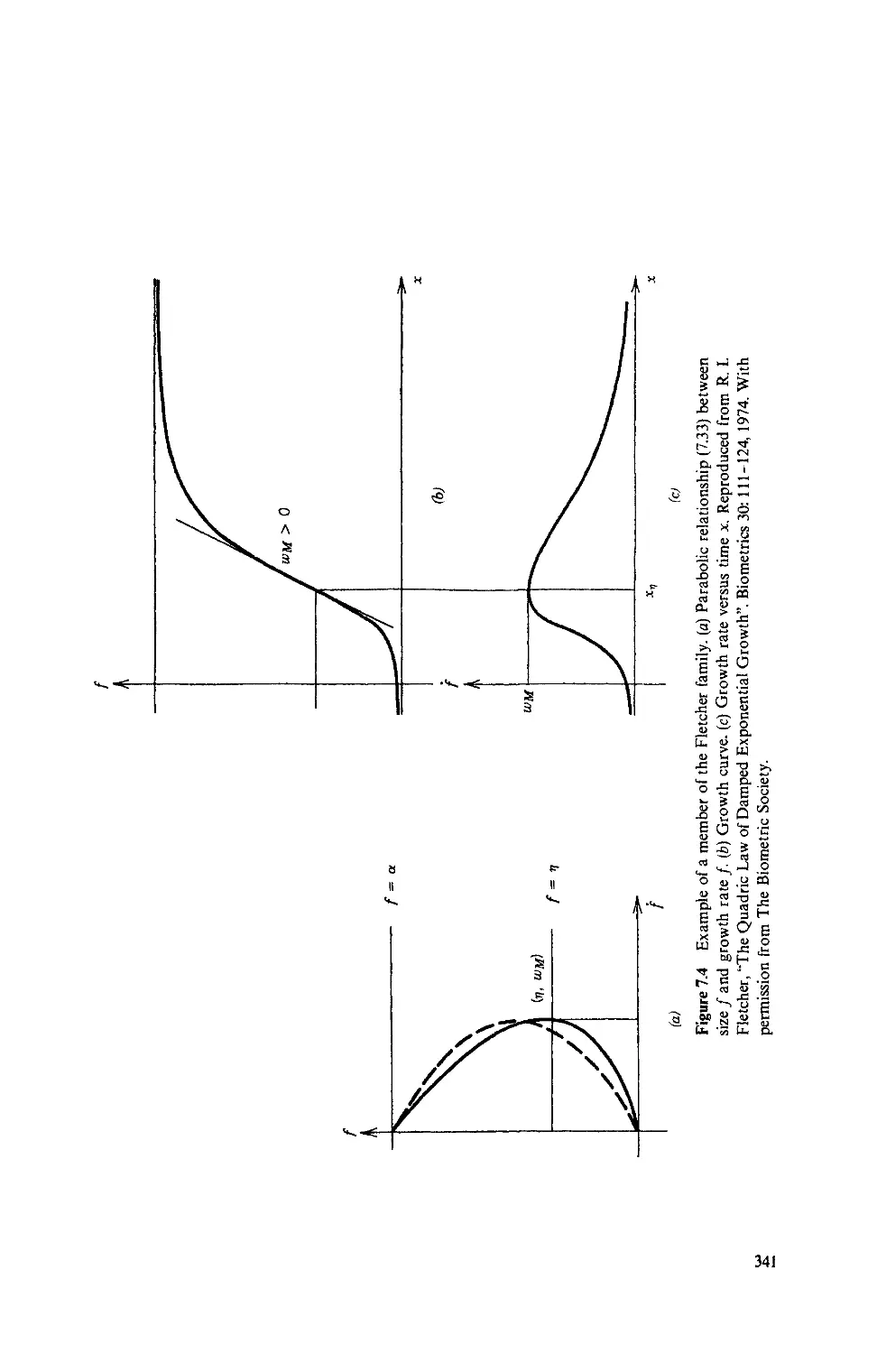
6.5, 7.1, 8.3, 8.4, Figs. 2.1, 6.4, 7.4, 7.5, 7.6, 9.6, 9.10, 9.11 (copyright by the
Biometric Society); Tables 2.2, 2.3, 4.1, 4.2, 9.4, Figs. 2.2, 2.3, 6.2, 9.1, 9.2, 9.4,
9.12, 9.16 (copyright by the Royal Statistical Society); Tables 2.5, 5.1, 5.3, 8.1,
9.1, 9.2, 9.5, 10.2, 10.3, 10.4, 10.5, 10.6, 11.1, 11.2, 11.4, 11.5, 11.6, Figs. 2.4, 2.5,
5.1, 5.2, 5.6, 5.7, 5.8, 5.9, 9.5, 9.7, 9.9., 9.17, 10.1, 11.1, 11.2, 11.6, 11.7 (copyright
by the American Statistical Association); Table 3.5 (copyright by Akademie-
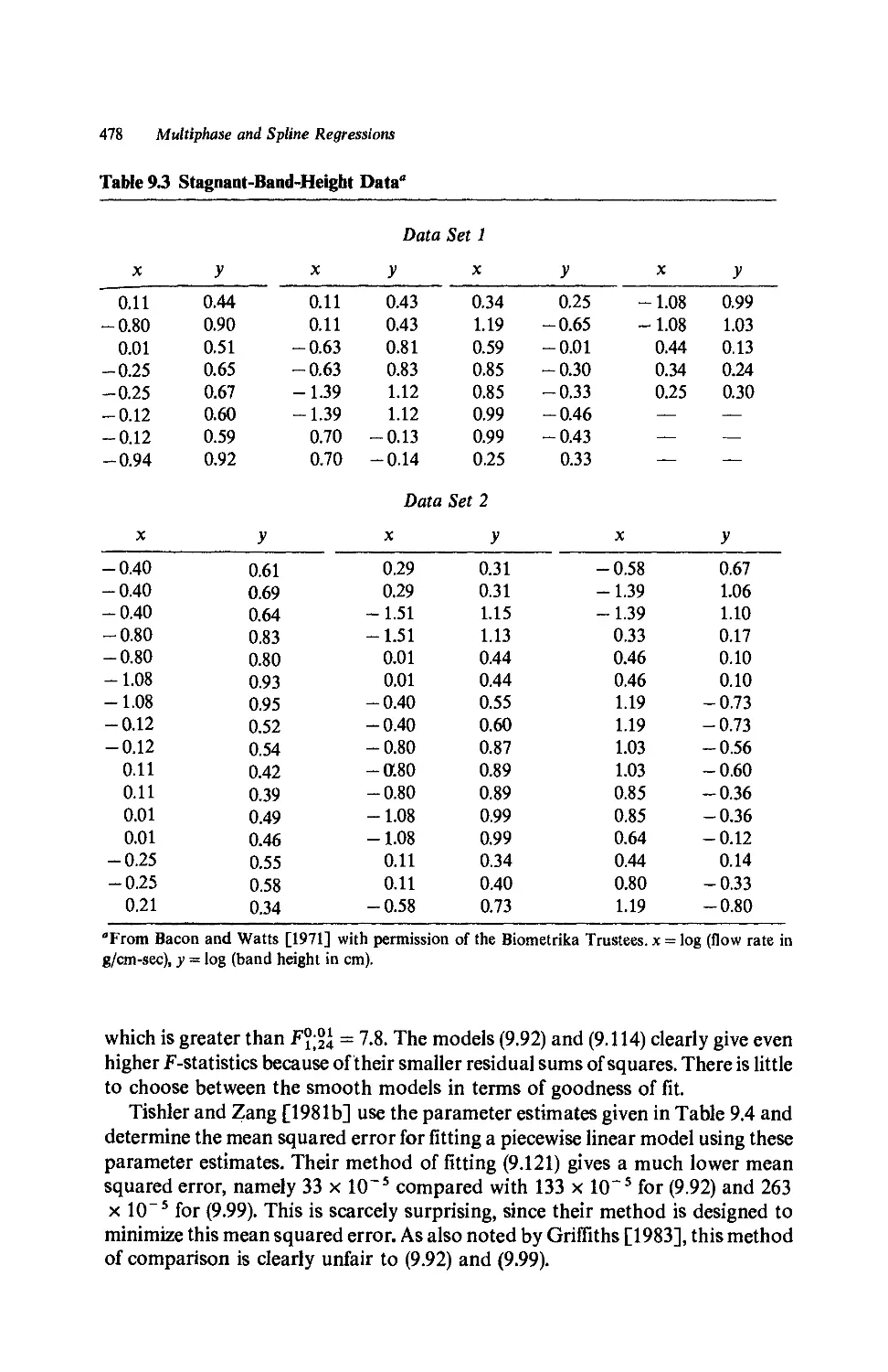
Verlag, Berlin, DDR); Tables 9.3, 11.3, Figs. 5.4, 9.8, 9.14, 11.3, 11.4 (copyright
by Biometrika Trust); Figs. 4.3, 5.3 (copyright by the Institute of Mathematical
Statistics); Table 2.4 (copyright by the American Chemical Society); Table 3.1,
Figs. 3.2, 3.3 (copyright by Plenum Press); Tables 8.2, 10.1, Figs. 8.12, 8.13, 8.14
(copyright by North-Holland Physics Publishing Company); Fig. 9.15 (copyright
by Marcel Dekker); Table 5.2 (copyright by Oxford University Press); Figs. 7.2,
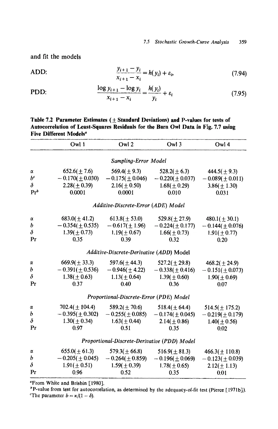
7.3 (copyright by Alan R. Liss); Table 7.2 and Fig. 7.7 (copyright by Growth
Publishing Company); and Table 6.3 and Fig. 6.3 (copyright by John Wiley
and Sons).
G. A. F. Seber
C. J. Wild
Auckland, New Zealand
May. 1988

Contents
1 Model Building 1
1.1 Notation, 1
1.2 Linear and Nonlinear Models, 4
1.3 Fixed-Regressor Model, 10
1.3.1 Regressors measured without error, 10
1.3.2 Conditional regressor models, 11
1.4 Random-Regressor (Errors-in-Variables) Models, 11
1.4.1 Functional relationships, 11
1.4.2 Structural relationships, 12
1.5 Controlled Regressors with Error, 13
1.6 Generalized Linear Model, 14
1.7 Transforming to Linearity, 15
1.8 Models with Autocorrelated Errors, 18
1.9 Further Econometric Models, 19
2 Estimation Methods 21
2.1 Least Squares Estimation, 21
2.1.1 Nonlinear least squares, 21
2.1.2 Linear approximation, 23
2.1.3 Numerical methods, 25
2.1.4 Generalized least squares, 27
*2.1.5 Replication and test of fit, 30
2.2 Maximum-Likelihood Estimation, 32
2.2.1 Normal errors, 32
"Starred topics can be omitted at first reading.

Contents
2.2.2 Nonnormal data, 34
2.2.3 Concentrated likelihood methods, 37
*2.3 Quasi-likelihood Estimation, 42
*2.4 LAM Estimator, 48
*2.5 L^norm Minimization, 50
2.6 Robust Estimation, 50
2.7 Bayesian Estimation, 52
2.7.1 Choice of prior distributions, 53
2.7.2 Posterior distributions, 55
2.7.3 Highest-posterior-density regions, 63
2.7.4 Normal approximation to posterior density, 64
2.7.5 Test for model adequacy using replication, 65
*2.7.6 Polynomial estimators, 66
2.8 Variance Heterogeneity, 68
2.8.1 Transformed models, 70
a. Box-Cox transformations, 71
b. John-Draper transformations, 72
2.8.2 Robust estimation for model A, 73
2.8.3 Inference using transformed data, 74
2.8.4 Transformations to linearity, 75
2.8.5 Further extensions of the Box-Cox method, 76
2.8.6 Weighted least squares: model B, 77
2.8.7 Prediction and transformation bias, 86
2.8.8 Generalized least-squares model, 88
Commonly Encountered Problems 91
3.1 Problem Areas, 91
3.2 Convergence of Iterative Procedures, 91
3.3 Validity of Asymptotic Inference, 97
3.3.1 Confidence regions, 97
3.3.2 Effects of curvature, 98
3.4 Identifiability and Ill-conditioning, 102
3.4.1 Identifiability problems, 102
3.4.2 Ill-conditioning, 103
a. Linear models, 103
b. Nonlinear models, 110
c. Stable parameters, 117
d. Parameter redundancy, 118
e. Some conclusions, 126

Contents xi
4 Measures of Curvature and Nonlinearity 127
4.1 Introduction, 127
4.2 Relative Curvature, 128
4.2.1 Curvature definitions, 129
4.2.2 Geometrical properties, 131
*4.2.3 Reduced formulae for curvatures, 138
*4.2.4 Summary of formulae, 145
4.2.5 Replication and curvature, 146
*4.2.6 Interpreting the parameter-effects array, 147
*4.2.7 Computing the curvatures, 150
*4.2.8 Secant approximation of second derivatives, 154
4.3 Beale's Measures, 157
*4.4 Connection Coefficients, 159
4.5 Subset Curvatures, 165
4.5.1 Definitions, 165
*4.5.2 Reduced formulae for subset curvatures, 168
*4.5.3 Computations, 170
4.6 Analysis of Residuals, 174
4.6.1 Quadratic approximation, 174
4.6.2 Approximate moments of residuals, 177
4.6.3 Effects of curvature on residuals, 178
4.6.4 Projected residuals, 179
a. Definition and properties, 179
b. Computation of projected residuals, 181
4.7 Nonlinearity and Least-Squares Estimation, 181
4.7.1 Bias, 182
4.7.2 Variance, 182
4.7.3 Simulated sampling distributions, 184
4.7.4 Asymmetry measures, 187
5 Statistical Inference 191
5.1 Asymptotic Confidence Intervals, 191
5.2 Confidence Regions and Simultaneous Intervals, 194
5.2.1 Simultaneous intervals, 194
5.2.2 Confidence regions, 194
5.2.3 Asymptotic likelihood methods, 196
5.3 Linear Hypotheses, 197
5.4 Confidence Regions for Parameter Subsets, 202
5.5 Lack of Fit, 203

xii Contents
*5.6 Replicated Models, 204
*5.7 Jackknife Methods, 206
*5.8 Effects of Curvature on Linearized Regions, 214
5.8.1 Intrinsic curvature, 214
5.8.2 Parameter-effects curvature, 218
5.8.3 Summary of confidence regions, 220
5.8.4 Reparametrization to reduce curvature effects, 222
5.8.5 Curvature and parameter subsets, 227
5.9 Nonlinear Hypotheses, 228
5.9.1 Three test statistics, 228
5.9.2 Normally distributed errors, 229
5.9.3 Freedom-equation specification, 232
5.9.4 Comparison of test statistics, 234
5.9.5 Confidence regions and intervals, 235
5.9.6 Multiple hypothesis testing, 235
5.10 Exact Inference, 236
5.10.1 Hartley's method, 236
5.10.2 Partially linear models, 240
5.11 Bayesian Inference, 245
*5.12 Inverse Prediction (Discrimination), 245
5.12.1 Single prediction, 245
5.12.2 Multiple predictions, 246
5.12.3 Empirical Bayes interval, 247
*5.13 Optimal Design, 250
5.13.1 Design criteria, 250
5.13.2 Prior estimates, 255
5.13.3 Sequential designs, 257
5.13.4 Multivariate models, 259
5.13.5 Competing models, 260
5.13.6 Designs allowing for curvature, 260
a. Volume approximation, 260
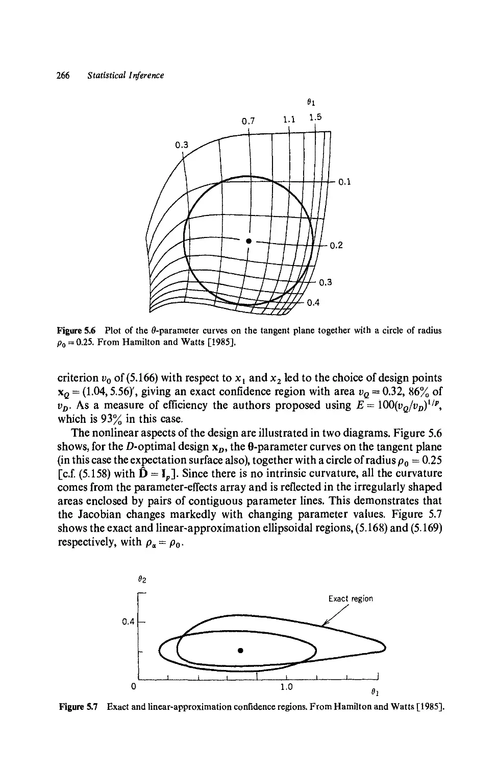
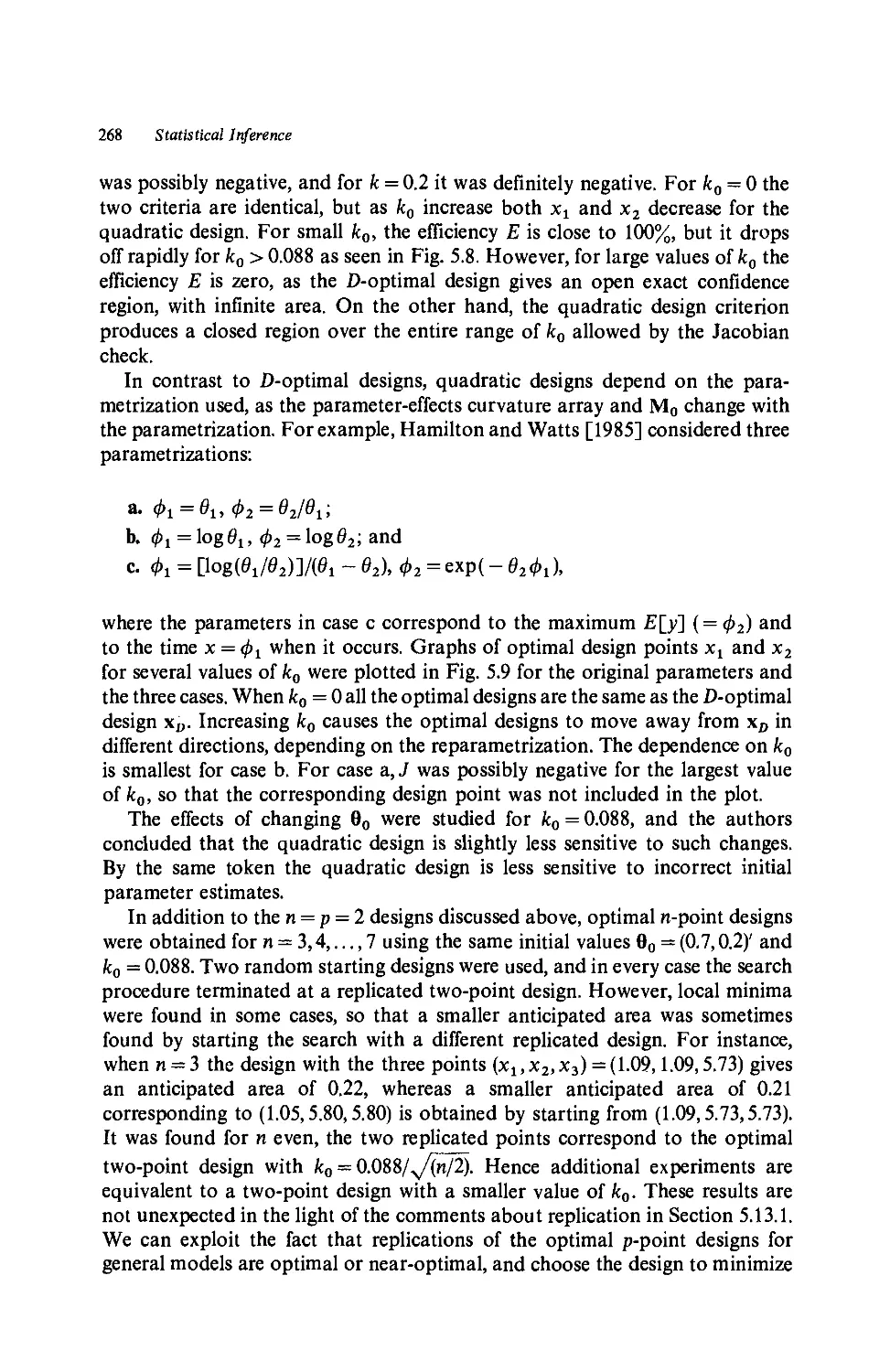
b. An example, 264
c. Conclusions, 269
6 Autocorrelated Errors 271
6.1 Introduction, 271
6.2 ARA) Errors, 275
6.2.1 Preliminaries, 275
6.2.2 Maximum-likelihood estimation, 277

Contents xiii
6.2.3 Two-stage estimation, 279
6.2.4 Iterated two-stage estimation, 280
6.2.5 Conditional least squares, 281
6.2.6 Choosing between the estimators, 282
6.2.7 Unequally spaced time intervals, 285
6.3 ARB) Errors, 286
6.4 AR(tfi) Errors, 289
6.4.1 Introduction, 289
6.4.2 Preliminary results, 290
6.4.3 Maximum-likelihood estimation and
approximations, 294
a. Ignore the determinant, 295
b. Approximate the derivative of the determinant, 295
c. Asymptotic variances, 296
6.4.4 Two-stage estimation, 301
6.4.5 Choosing a method, 303
6.4.6 Computational considerations, 304
6.5 MA(tf2) Errors, 305
6.5.1 Introduction, 305
6.5.2 Two-stage estimation, 306
6.5.3 Maximum-likelihood estimation, 306
6.6 ARMA^i,q2) Errors, 307
6.6.1 Introduction, 307
6.6.2 Conditional least-squares method, 310
6.6.3 Other estimation procedures, 314
6.7 Fitting and Diagnosis of Error Processes, 318
6.7.1 Choosing an error process, 318
6.7.2 Checking the error process, 321
a. Overfitting, 321
b. Use of noise residuals, 322
7 Growth Models 325
7.1 Introduction, 325
7.2 Exponential and Monomolecular Growth Curves, 327
7.3 Sigmoidal Growth Models, 328
7.3.1 General description, 328
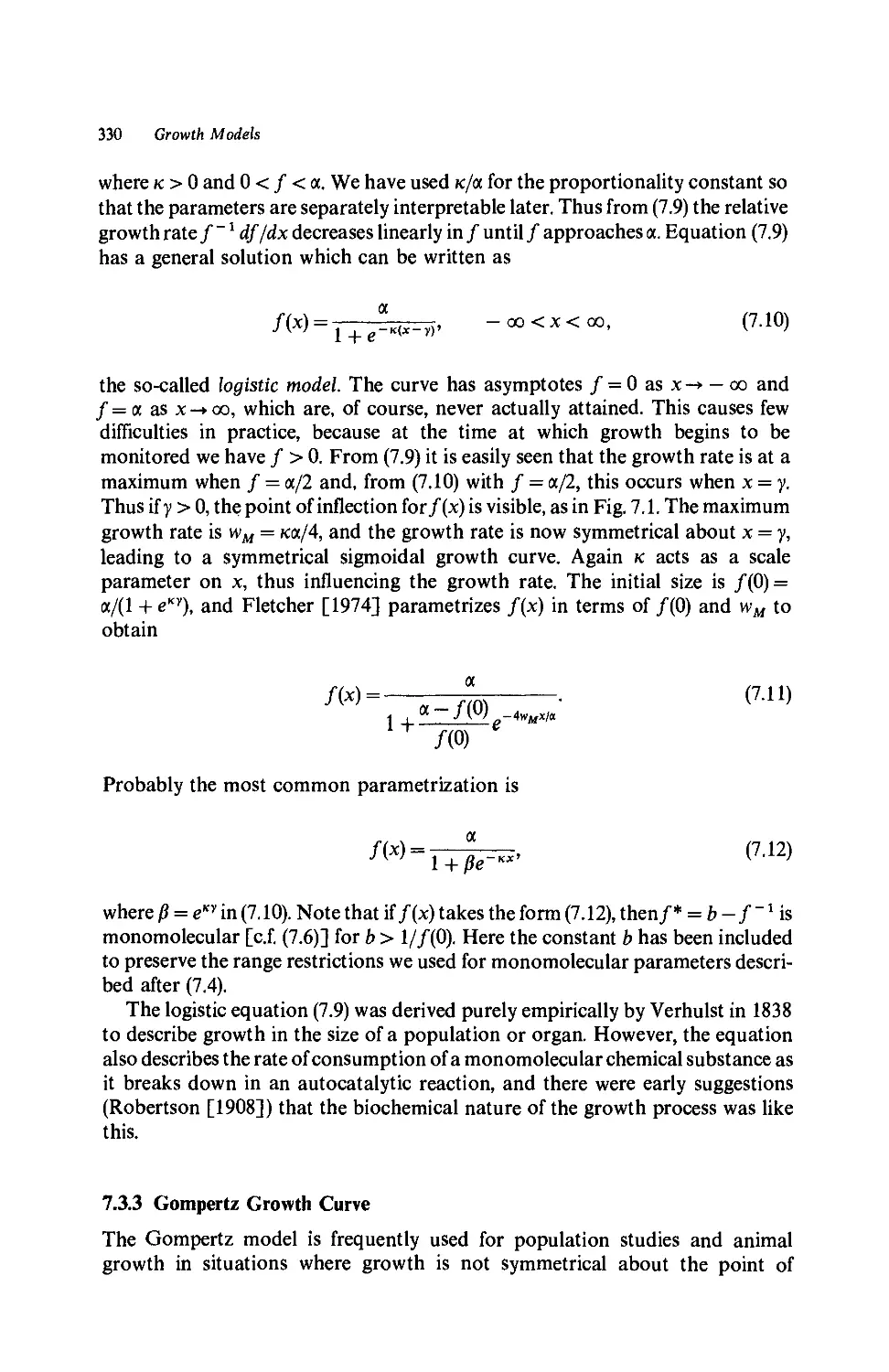
7.3.2 Logistic (autocatalytic) model, 329
7.3.3 Gompertz growth curve, 330
7.3.4 Von Bertalanffy model, 331

Contents
7.3.5 Richards curve, 332
7.3.6 Starting values for fitting Richards models, 335
7.3.7 General procedure for sigmoidal curves, 337
7.3.8 Weibull model, 338
7.3.9 Generalized logistic model, 339
7.3.10 Fletcher family, 339
7.3.11 Morgan-Mercer-Flodin (MMF) family, 340
7.4 Fitting Growth Models: Deterministic Approach, 342
7.5 Stochastic Growth-Curve Analysis, 344
7.5.1 Introduction, 344
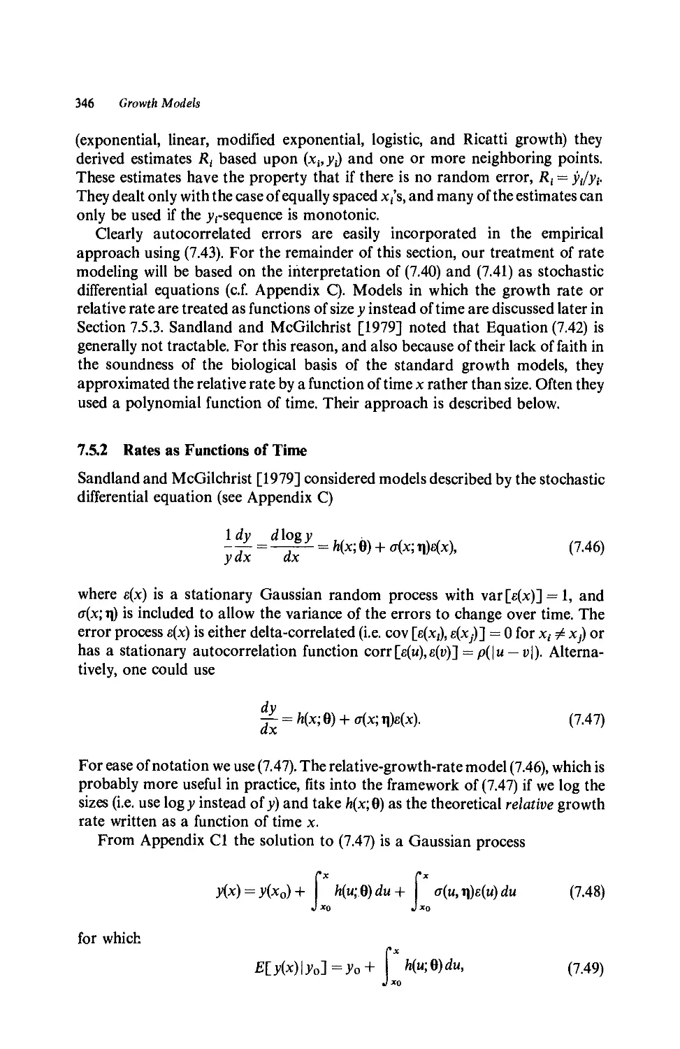
7.5.2 Rates as functions of time, 346
a. Uncorrelated error process, 347
b. Autocorrelated error processes, 348
7.5.3 Rates as functions of size, 353
a. A tractable differential equation, 354
b. Approximating the error process, 356
7.6 Yield-Density Curves, 360
7.6.1 Preliminaries, 360
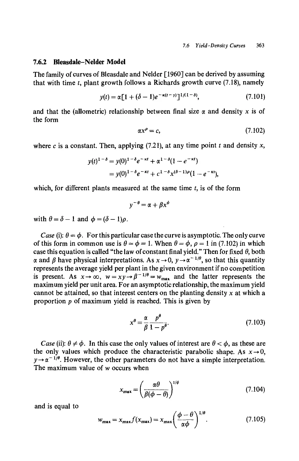
7.6.2 Bleasdale-Nelder model, 363
7.6.3 Holliday model, 364
7.6.4 Choice of model, 364
7.6.5 Starting values, 365
Compartmental Models 367
8.1 Introduction, 367
8.2 Deterministic Linear Models, 370
8.2.1 Linear and nonlinear models, 370
8.2.2 Tracer exchange in steady-state systems, 372
8.2.3 Tracers in nonsteady-state linear systems, 375
8.3 Solving the Linear Differential Equations, 376
8.3.1 The solution and its computation, 376
8.3.2 Some compartmental structures, 383
8.3.3 Properties of compartmental systems, 384
*8.4 Identifiability in Deterministic Linear Models, 386
8.5 Linear Compartmental Models with Random Error, 393
8.5.1 Introduction, 393
8.5.2 Use of the chain rule, 395
8.5.3 Computer-generated exact derivatives, 396
a. Method of Bates et al., 396

Contents xv
b. Method of Jennrich and Bright, 400
c. General algorithm, 401
8.5.4 The use of constraints, 402
8.5.5 Fitting compartmental models without using
derivatives, 404
8.5.6 Obtaining initial parameter estimates, 406
a. All compartments observed with zero or linear
inputs, 406
b. Some compartments unobserved, 407
c. Exponential peeling, 407
8.5.7 Brunhilda example revisited, 410
8.5.8 Miscellaneous topics, 412
8.6 More Complicated Error Structures, 413
*8.7 Markov-Process Models, 415
8.7.1 Background theory, 415
a. No environmental input, 416
b. Input from the environment, 420
8.7.2 Computational methods, 423
a. Unconditional generalized least squares, 423
b. Conditional generalized least squares, 424
8.7.3 Discussion, 429
8.8 Further Stochastic Approaches, 431
Multiphase and Spline Regressions 433
9.1 Introduction, 433
9.2 Noncontinuous Change of Phase for Linear Regimes, 438
9.2.1 Two linear regimes, 438
9.2.2 Testing for a two-phase linear regression, 440
9.2.3 Parameter inference, 445
9.2.4 Further extensions, 446
9.3 Continuous Case, 447
9.3.1 Models and inference, 447
9.3.2 Computation, 455
9.3.3 Segmented polynomials, 457
a. Inference, 460
b. Computation, 463
9.3.4 Exact tests for no change of phase in polynomials, 463
9.4 Smooth Transitions between Linear Regimes, 465
9.4.1 The sgn formulation, 465
9.4.2 The max-min formulation, 471

xvi Contents
a. Smoothing max @,z), 472
b. Limiting form for max {z,}, 474
c. Extending sgn to a vector of regressors, 476
9.4.3 Examples, 476
9.4.4 Discussion, 480
9.5 Spline Regression, 481
9.5.1 Fixed and variable knots, 481
a. Fixed knots, 484
b. Variable knots, 484
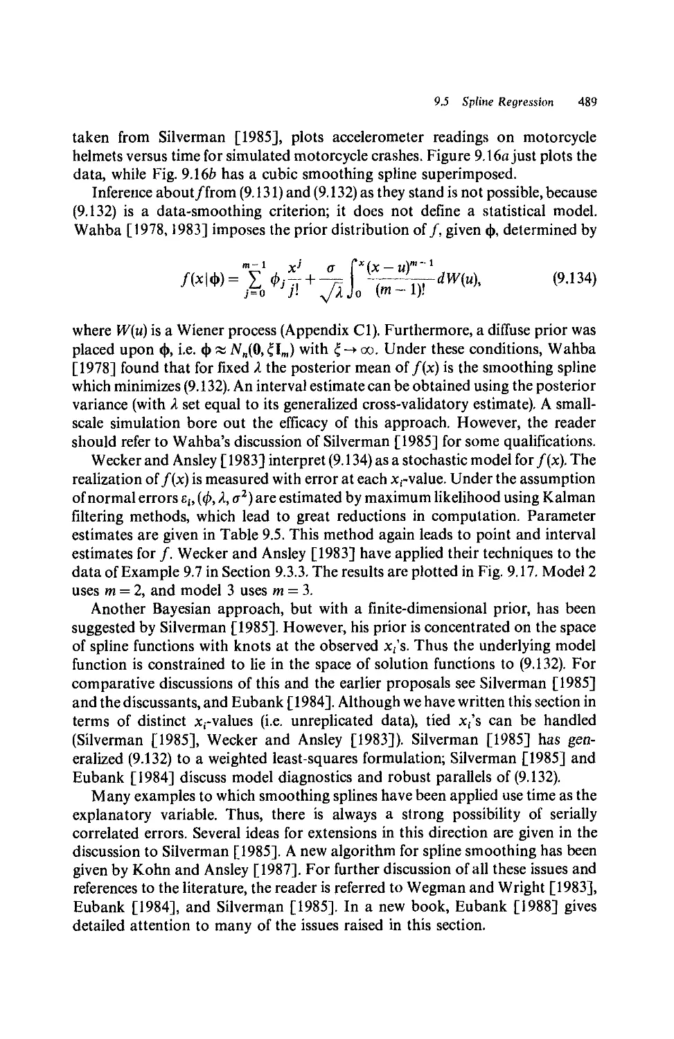
9.5.2 Smoothing splines, 486
*10 Errors-In-Variables Models 491
10.1 Introduction, 491
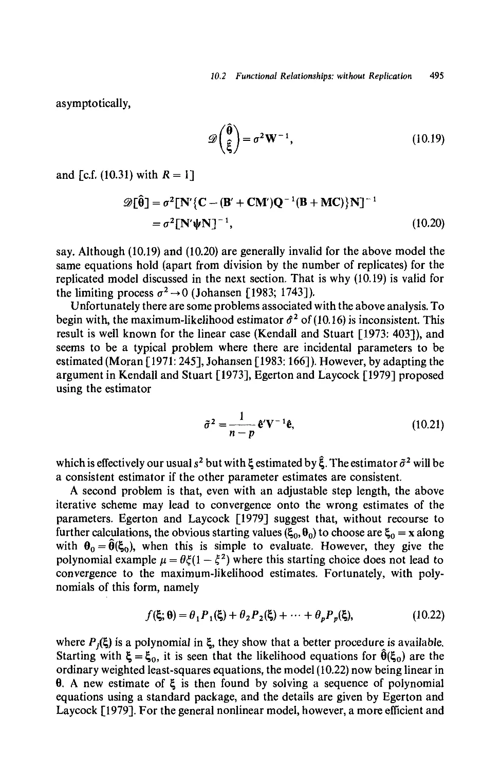
10.2 Functional Relationships: Without Replication, 492
10.3 Functional Relationships: With Replication, 496
10.4 Implicit Functional Relationships: Without Replication, 501
10.5 Implicit Functional Relationships: With Replication, 508
10.5.1 Maximum-likelihood estimation, 508
10.5.2 Bayesian estimation, 510
10.6 Implicit Relationships with Some Unobservable Responses, 516
10.6.1 Introduction, 516
10.6.2 Least-squares estimation, 516
10.6.3 The algorithm, 519
10.7 Structural and Ultrastructural Models, 523
10.8 Controlled Variables, 525
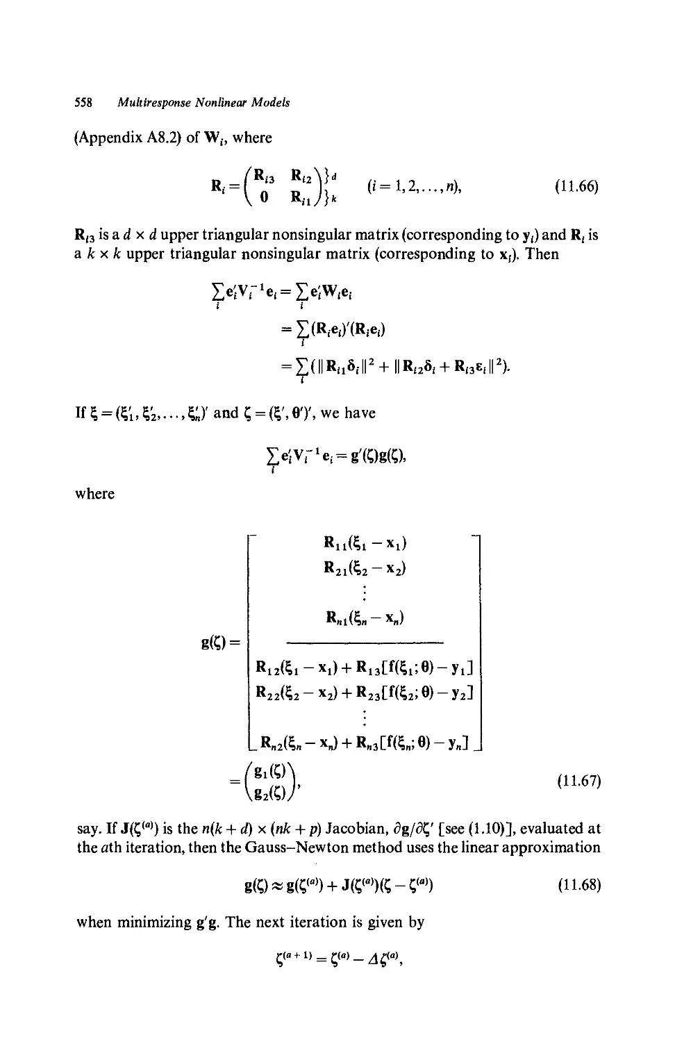
11 Multiresponse Nonlinear Models 529
11.1 General Model, 529
11.2 Generalized Least Squares, 531
11.3 Maximum-Likelihood Inference, 536
11.3.1 Estimation, 536
11.3.2 Hypothesis testing, 538
11.4 Bayesian Inference, 539
11.4.1 Estimates from posterior densities, 539
11.4.2 H.P.D. regions, 542
11.4.3 Missing observations, 544
*11.5 Linear Dependencies, 545
11.5.1 Dependencies in expected values, 545
11.5.2 Dependencies in the data, 546

Contents xvii
11.5.3 Eigenvalue analysis, 547
11.5.4 Estimation procedures, 549
* 11.6 Functional Relationships, 557
*12 Asymptotic Theory 563
12.1 Introduction, 563
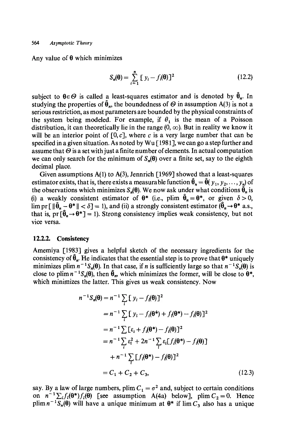
12.2 Least-Squares Estimation, 563
12.2.1 Existence of least-squares estimate, 563
12.2.2 Consistency, 564
12.2.3 Asymptotic normality, 568
12.2.4 Effects of misspecification, 572
12.2.5 Some extensions, 574
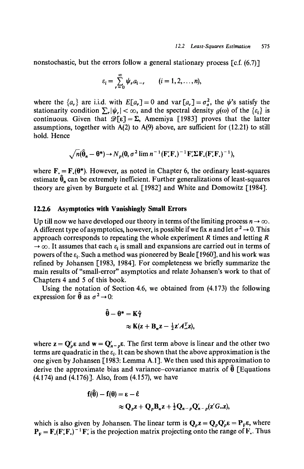
12.2.6 Asymptotics with vanishingty smalt errors, 575
12.3 Maximum-Likelihood Estimation, 576
12.4 Hypothesis Testing, 576
12.5 Multivariate Estimation, 581
13 Unconstrained Optimization 587
13.1 Introduction, 587
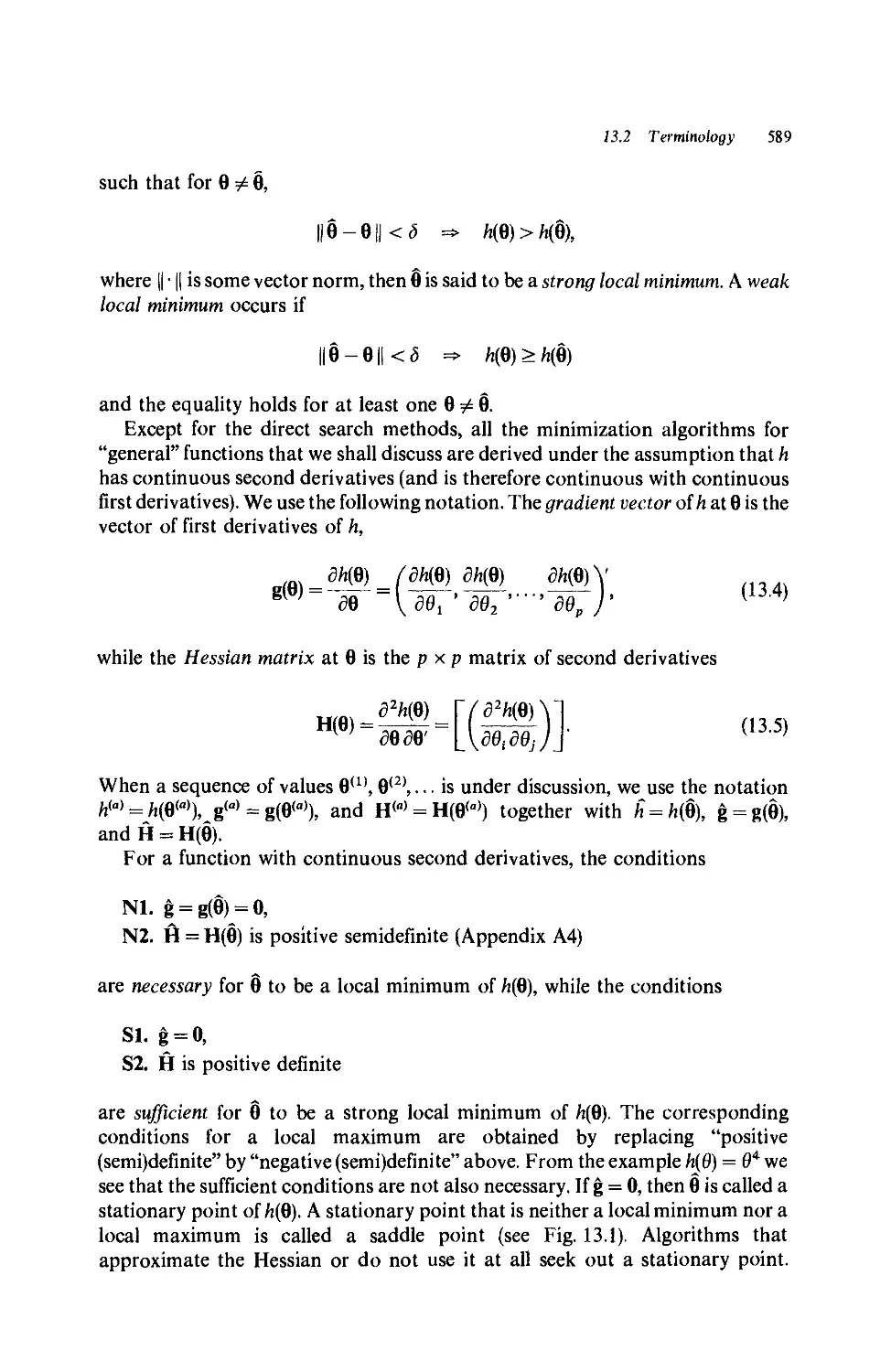
13.2 Terminology, 588
13.2.1 Local and global minimization, 588
13.2.2 Quadratic functions, 590
13.2.3 Iterative algorithms, 593
a. Convergence rates, 593
b. Descent methods, 594
c. Line searches, 597
13.3 Second-Derivative (Modified Newton) Methods, 599
13.3.1 Step-length methods, 599
a. Directional discrimination, 600
b. Adding to the Hessian, 602
13.3.2 Restricted step methods, 603
13.4 First-Derivative Methods, 605
13.4.1 Discrete Newton methods, 605
13.4.2 Quasi-Newton methods, 605
* 13.4.3 Conjugate-gradient methods, 609
13.5 Methods without Derivatives, 611
13.5.1 Nonderivative quasi-Newton methods, 611
♦ 13.5.2 Direction-set (conjugate-direction) methods, 612
13.5.3 Direct search methods, 615

xviii Contents
13.6 Methods for Nonsmooth Functions, 616
13.7 Summary, 616
14 Computational Methods for Nonlinear Least Squares 619
14.1 Gauss-Newton Algorithm, 619
14.2 Methods for Small-Residual Problems, 623
14.2.1 Hartley's method, 623
14.2.2 Levenberg-Marquardt methods, 624
14.2.3 Powell's hybrid method, 627
14.3 Large-Residual Problems, 627
14.3.1 Preliminaries, 627
14.3.2 Quasi-Newton approximation of A@), 628
14.3.3 The Gill-Murray method, 633
a. Explicit second derivatives, 636
b. Finite-difference approximation, 636
c. Quasi-Newton approximation, 637
14.3.4 Summary, 639
14.4 Stopping Rules, 640
14.4.1 Convergence criteria, 640
14.4.2 Relative offset, 641
14.4.3 Comparison of criteria, 644
14.5 Derivative-Free Methods, 646
14.6 Related Problems, 650
14.6.1 Robust loss functions, 650
14.6.2 Lj-minimization, 653
14.7 Separable Least-Squares Problems, 654
14.7.1 Introduction, 654
14.7.2 Gauss-Newton for the concentrated sum of squares, 655
14.7.3 Intermediate method, 657
14.7.4 The NIPALS method, 659
14.7.5 Discussion, 660
15 Software Considerations 661
15.1 Selecting Software, 661
15.1.1 Choosing a method, 661
15.1.2 Some sources of software, 663
a. Commercial libraries, 663
b. Noncommercial libraries, 663
c. ACM algorithms, 663

Contents xix
15.2 User-Supplied Constants, 664
15.2.1 Starting values, 665
a. Initial parameter value, 665
b. Initial approximation to the Hessian, 666
15.2.2 Control constants, 666
a. Step-length accuracy, 666
b. Maximum step length, 666
c. Maximum number of function evaluations, 667
15.2.3 Accuracy, 667
a. Precision of function values, 667
b. Magnitudes, 668
15.2.4 Termination criteria (stopping rules), 668
a. Convergence of function estimates, 669
b. Convergence of gradient estimates, 670
c. Convergence of parameter estimates, 670
d. Discussion, 671
e. Checking for a minimum, 672
15.3 Some Causes and Modes of Failure, 672
15.3.1 Programming error, 672
15.3.2 Overflow and underflow, 673
15.3.3 Difficulties caused by bad scaling (parametrization), 673
15.4 Checking the Solution, 675
APPENDIXES
A. Vectors and Matrices 677
Al Rank, 677
A2 Eigenvalues, 677
A3 Patterned matrices, 678
A4 Positive definite and semidefinite matrices, 678
A5 Generalized inverses, 679
A6 Ellipsoids, 679
A7 Optimization, 679
A8 Matrix factorizations, 680
A9 Multivariate f-distribution, 681
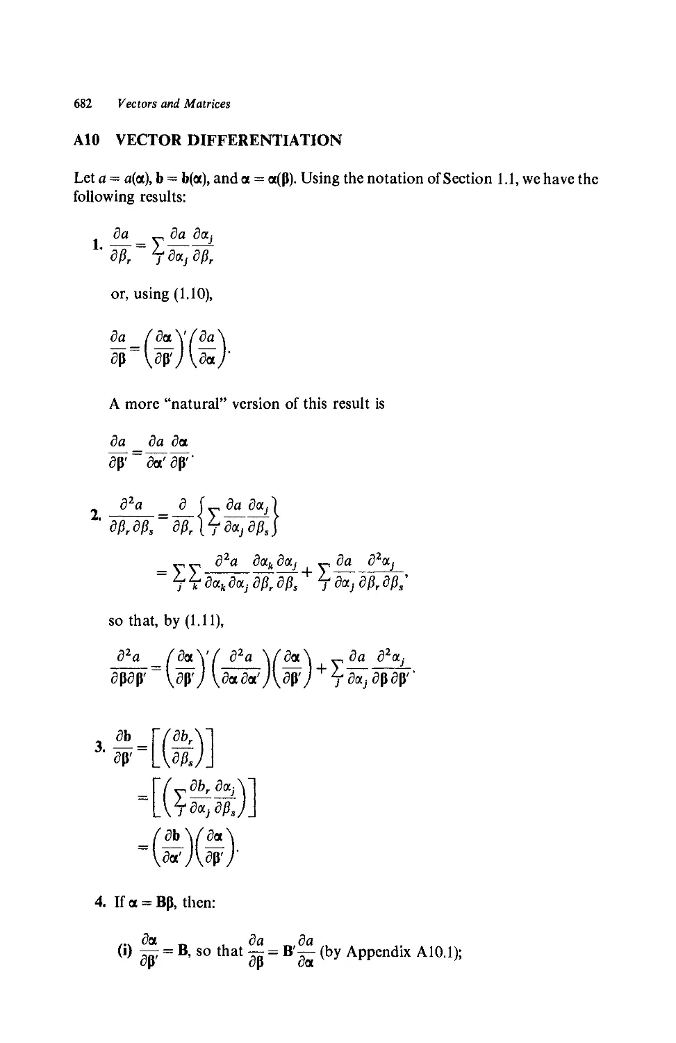
A10 Vector differentiation, 682
All Projection matrices, 683
A12 Quadratic forms, 684

xx Contents
A13 Matrix operators, 684
A14 Method of scoring, 685
B. Differential Geometry 687
Bl Derivatives for curves, 687
B2 Curvature, 688
B3 Tangent planes, 690
B4 Multiplication of 3-dimensional arrays, 691
B5 Invariance of intrinsic curvature, 692
C. Stochastic Differential Equations 695
Cl Rate equations, 695
C2 Proportional rate equations, 697
C3 First-order equations, 698
D. Multiple Linear Regression 701
Dl Estimation, 701
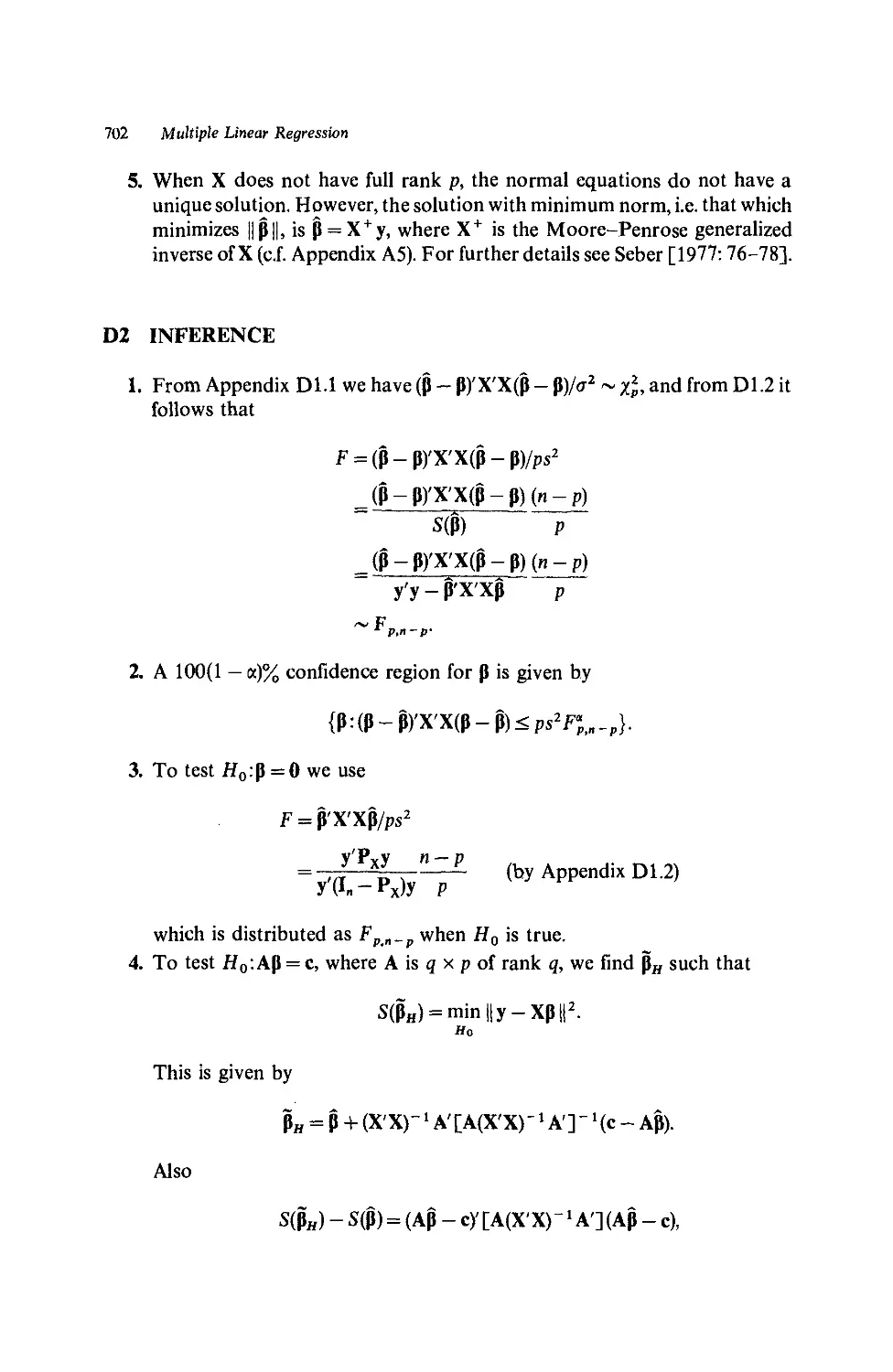
D2 Inference, 702
D3 Parameter subsets, 703
E. Minimization Subject to Linear Constraints 707
References 711
Author Index 745
Subject Index 753

Nonlinear Regression

Nonlinear Regression. G. A. F. Seber, C. J. Wild
Copyright © 1989 John Wiley & Sons, Inc.
ISBN: 0^71-61760-1
CHAPTER 1
Model Building
1.1 NOTATION
Matrices and vectors are denoted by boldface letters A and a, respectively, and
scalars by italics. If a is an n x 1 column vector with elements aua2,...,an, we
write a = [(a,)], and the length or norm of a is denoted by ||a||. Thus
The n x 1 vector with all its elements equal to unity is represented by ln.
If the m x n matrix A has elements atj, we write A = [(ay)], and the sum of the
diagonal elements, called the trace of A, is denoted by tr A (= a11 + a22 H 1- %t)>
where k is the smaller of m and ri). The transpose of A is represented by
A' = [(ay)], where 0^ = 0^. A matrix A~ that satisfies AA~A = A is called a
generalized inverse of A. If A is square, its determinant is written | A |, or det A
and if A is nonsingular (|A| / 0), its inverse is denoted by A" \ The n x n matrix
with diagonal elements dud2,...,dn and zero elsewhere is represented by
diag (di,d2,..., dn), and when all the dt's are unity, we have the identity matrix In.
For any m x n matrix A the space spanned by the columns of A, called the
range space or column space of A, is denoted by 5?[A]. The null space or kernel
of A ( = {x:Ax = 0}) is denoted by ./F[A]. If V is a vector space, then V1
represents the orthogonal complement of V, i.e.
F1 = {x:x'v = 0 for all v in V)
The symbol W1 will represent d-dimensional Euclidean space. An orthogonal
projection onto a vector subspace can be achieved using a symmetric idem potent
matrix (called a projection matrix). Properties of projection matrices are described
in Appendix All.
It is common practice to distinguish between random variables and their
values by using upper- and lowercase letters, for example Y and y. This is
particularly helpful in discussing errors-in-variables models. However, it causes

2 Model Building
difficulty with multivariate models, so that, on balance, we have decided not to
observe this convention. Instead we shall use boldface upper- and lowercase to
denote matrices and vectors respectively of both constants and random variables,
for example Y and y.
If x and y are random variables, then the symbols £[x], var[x], cov[x,y],
corr[x,y] and £[x|y] represent the expectation, variance, covariance, correla-
correlation, and conditional expectation, respectively. Multivariate analogues are &[x]
for the expected value of random x,
*[x,y] = [(covCx,,^])] = *[(x - fix)(y - fi,)'] A.1)
for the covariance of two random vectors x and y with expected values (means)
\ix and fij, respectively, and
the dispersion or variance-covariance matrix of x. The following will be used
frequently:
A.2)
from which we deduce
A.3)
We say that y ~ N(9, a2) if y is normally distributed with mean 0 and variance
a2. If y has a d-dimensional multivariate normal distribution with mean 0 and
dispersion matrix L, we write y ~ Nd@, L).The t- and chi-square distributions
with k degrees of freedom are denoted by tk and %L respectively, and the
/"-distribution with m and n degrees of freedom is denoted by Fmn. An important
distribution used in Bayesian methods is the inverted gamma distribution. This
has density function
a'b>0 and x>0> (L4)
and provides the useful integral
JW2)
f
Jo
If {zn} is a sequence of random vectors, we write
plimzn = z A.6)

1.1 Notation 3
if, for every d > 0,
Also, if g(-) is a positive function of n, we write
zn = op[<7(n)] A.7)
if plim zjg(n) = 0, and
zn = Op[0(n)] A.8)
if, for each e, there exists A(e) > 0 such that
for all n.
Differentiation with respect to vectors is used frequently in this book, and
as a variety of notations are used in practice, we now state our own. If a() and
b() are, respectively, a differentiable function and a differentiable nxl vector
function of the p-dimensional vector 0, we define
=(
=(^\ = (
30 \ 50! ' d62 '"■■' ddp ) \ 30' /'
'
do, V se, ' do, '•*"' de, )'
and
A.10)
\ vv /
If a() is twice differentiable, then we define
' = \ \ -2T ) ' (I'll)
where
In this book we will frequently use a dot to denote differentiation, e.g.
f(x) = df(x)/dx.
Finally we note that a number of resujts are included in the appendices, and
references to these are given, for example, as A4.2.

4 Model Building
1.2 LINEAR AND NONLINEAR MODELS
An important task in statistics is to find the relationships, if any, that exist in
a set of variables when at least one is random, bding subject to random
fluctuations and possibly measurement error. In regression problems typically
one of the variables, often called the response or dependent variable, is of
particular interest and is denoted by y. The other variables xux2,-..,xk, usually
called explanatory, regressor, or independent variables, are primarily used to
predict or explain the behavior of y. If plots of the data suggest some relationship
between y and the x/s, then we would hope to express this relationship via some
function /, namely
y*f(xux2,...,xk). A.12)
Using /, we might then predict y for a given set of x's. For example, y could
be the price of a used car of a certain make, xt the number of previous owners,
x2 the age of the car, and x3 the mileage. As in A.12), relationships can never
hold exactly, as data will invariably contain unexplained fluctuations or noise,
and some degree of measurement error is usually present.
Explanatory variables can be random or fixed (e.g. controlled). Consider an
experiment conducted to measure the yield (y) of wheat at several different
specified levels of density of planting (xx) and fertilizer application (x2). Then
both xt and x2 are fixed. If, at the time of planting, soil pH (x3) was also
measured on each plot, then x3 would be random.
Sometimes the appropriate mathematical form for the relationship A.12) is
known, except for some unknown constants or coefficients (called parameters),
the relationship being determined by a known underlying physical process or
governed by accepted scientific laws. Mathematically A.12) can be written as
ya/(x1,x2,...,xt;0), A.13)
where /is entirely known except for the parameter vector Q = @1,02,...,9p)',
which needs to be estimated. For example
and 0 = (<x,/?)'. Since these parameters often have physical interpretations, a
major aim of the investigation is to estimate the parameters as precisely as
possible. Frequently the relationship A.13) is tentatively suggested by theoretical
investigations and a further aim is to test the fit of the data to the model. With
two variables (x,y) an obvious first step is to graph the estimated functional
relationship and see how well it fits a scatterplot of the data points (x,-,^),
i = 1,2,..., n. Models with a known / are the main subject of this book.
However, in much of statistical practice, particularly in the biological as
opposed to the physical sciences, the underlying processes are generally complex

1.2 Linear and Nonlinear Models 5
and not well understood. This means that we have little or no idea about the
form of the relationship and our aim is to simply find some function/for which
A.13) holds as closely as possible. Again one usually assumes that the "true"
relationship belongs to a parametric family A.13), so that finding a model often
reduces to estimating 0. In this case, it is important to use a family that is
large and flexible enough to approximate a sufficiently wide variety of functional
forms. If several models fit the data equally well, we would usually choose the
simplest one. Even in this situation, where the unknown parameters do not
have special significance, a model which fits the data well will be useful. For
example it could be used for predicting y, or even controlling y, by adjusting
the x-variables. In some situations we may also use the model for calibration
(inverse prediction), in which we predict x for a new y-value. If we are interested
in simply fitting the best "black box" model to use, for example, in prediction,
or in finding the maximum and minimum values of the curve or the slope at
particular points, then splines (segmented polynomials) may be appropriate.
These are discussed in Section 9.5.
In linear regression analysis (see Seber [1977]) models of the form
yxPo + Pixi + ■ ■ ■ + Pp- i*p-1 with additive errors are used. We thus have
where £[e] = 0. Here § = (P0,pi,...,Pp^i)' and the x/s can include squares,
cross products, higher powers, and even transformations (e.g. logarithms) of
the original measurements. The important requirement is that the expression
should be linear in the parameters. For example
y « p0 + plXl + p2x2 + p3xj + pAx\
and
yxpo + pisinxi + p2sinx2
are both linear models, whereas
is a nonlinear model, being nonlinear in p2. We see from the above examples
that the family of linear models is very flexible, and so it is often used in the
absence of a theoretical model for /. As results from linear regression theory
are used throughout this book, the relevant theory is summarized briefly in
Appendix D.
Nonlinear models tend to be used either when they are suggested by
theoretical considerations or to build known nonlinear behavior into a model.
Even when a linear approximation works well, a nonlinear model may still be
used to retain a clear interpretation of the parameters. Nonlinear models have
been applied to a wide range of situations, even to finite populations (Valiant

6 Model Building
[1985]), and we now give a selection of examples. The approximate equality
sign of A.13) will be replaced by an equality, through it should be understood
that the given relationships are not expected to hold exactly in a set of data.
We postpone considerations of random error until Section 1.3. For a review of
some of the issues involved in nonlinear modeling see Cox [1977].
Example 1.1 Theoretical chemistry predicts that, for a given sample of gas
kept at a constant temperature, the volume i; and pressure p of the gas satisfy
the relationship pvy = c. Writing y = p and x = v~1, we have
y = cx'=f(x;c,y). A.14)
Here y is a constant for each gas, which is to be estimated from the data. This
particular model is said to be nonlinear, as/is nonlinear in one of the parameters,
y. In fact the model is nonlinear in y but linear in c: a number of models have
this property. We can, of course, take a log transformation so that setting
y = logp and x = logu, we have the re-expression
y = a. + Px,
where a. = log c and j8 = — y. This model is now linear in its unknown parameters
a. and /?. The decision whether or not to make linearizing transformation depends
very much on the nature of the errors or fluctuations in the variables. This point
is discussed later, in Section 1.7. ■
Example 1.2 In studying the relationships between migrant streams of people
and the size of urban areas, Olsson [1965] (see also King [1969: 126] for a
summary) proposed the following "gravity"-type model:
D" '
where k and b are constants, and / is the level of migration (interaction) between
two areas at distance D apart with respective population sizes Pt and P2. This
model can be constructed by arguing that migration will be inversely related
to distance but proportional to the size of each population. Olsson, in fact,
linearized the model using the transformation
log -^-r- = log k - b log D
or
and showed that the absolute values of b for different pairs of areas were

1.2 Linear and Nonlinear Models 7
consistent with the hypothesis that "migrants from small places move shorter
distances than migrants from large places." ■
Example 1.3 In an irreversible chemical reaction, substance A changes into
substance B, which in turn changes into substance C. Denote by A(t) the
quantity of substance A at time t. The differential equations governing the
changes are
dA(t)
dt
dB(t)
dt
dCjt)
dt
where 9i and 92 are unknown constants. Assuming A@) = 1, B(t) has the solution
9, ,
- —{exp(-02O-exp(-01O}. A.15)
= 9iA(t)-92B(t),
Here the relationship between B and t is nonlinear in 0X and 92. Since it is not
possible to linearize this model by means of a suitable transformation, this
model can be described as intrinsically nonlinear. This is an example of a
"compartmental" model. Such models are discussed in Chapter 8. ■
Example 1.4 The relative rate of growth of an organism or plant of size w(t)
at time t is often found to be well approximated by a function g of the size, i.e.,
d\ogw{t) Idw
-~H^=»-d7=0{w)- (L16)
Richards [1959], for example, proposed the function
Setting w — a.vs, A.16) becomes
5
This has solution
X + kt

8 Model Building
where A is a constant of integration. Thus
Again we have an intrinsically nonlinear model relating w and t, with unknown
parameters a,k, X and 5. The special case 5 = 1 gives the logistic curve
often seen in the form (with t = x)
1 1 1 _, _to
w a. a.
or
y = ao + Pe-kx A.20)
= «o + /?p*, 0<p<l, A.21)
where p-e'k. This model has also been used as a yield-fertilizer model in
agriculture, and as a learning curve in psychology. Models like A.18) and A.21)
are discussed in greater detail in Chapter 7. I.
Example 1.5 In the study of allometry, attention is focused on differences in
shape associated with size. For example, instead of relating two size measure-
measurements x and y (e.g. lengths of two bones) to time, we may be interested in relating
them to each other. Suppose the two relative growth rates are given by
\dx , , \dy .
—z- = kx and -— = «„.
xdt x ydt y
Defining /? = ky/kx we have, canceling out dt,
dy_dx
Making the strong assumption that /? is constant, we can integrate the above
equation and obtain
or
y = ax". A.22)

1.2 Linear and Nonlinear Models 9
This model has been studied for over 50 years and, as a first approximation,
seems to fit a number of growth processes quite well. An intrinsically nonlinear
extension of the above model is also used, namely
y = y + ax". A.23)
Griffiths and Sandland [1984] discuss allometric models with more than two
variables and provide references to the literature of allometry. ■
Example 1.6 The average yield y per plant for crop planting tends to decrease
as the density of planting increases, due to competition between plants for
resources. However, y is not only related to density, or equivalently the area
available to each plant, but also to the shape of the area available to each plant.
A square area tends to be more advantageous than an elongated rectangle.
Berry [1967] proposed a model for y as a function of the two explanatory
variables xx (the distance between plants within a row) and x2 (the distance
between rows), namely
A.24)
Yield-density models are discussed in Section 7.6.
Example 1.7 The forced expiratory volume y, a measure of how much air a
subject can breathe, is widely used in screening for chronic respiratory disease.
Cole [1975] discusses a nonlinear model relating y to height (xj) and age (x2)
of the form
y = xl(a + px2). A.25)
Example 1.8 The freezing point y of a solution of two substances is related to
the concentration x of component 1 by the equation
(L26)
where To is the freezing point of pure component 1. In this model we cannot
express y explicitly in terms of x, which would be the natural way of presenting
the relationship. One would vary x (the controlled explanatory variable) and
measure y (the response). ■
In the above discussion we have considered models of the form y = /(x;0),
or g(x, y; 0) = 0 as in Example 1.8, relating y and x, with 0 = (9it 92,. ■ ■, 9P)' being

10 Model Building
a vector of unknown parameters. This deterministic approach does not allow
for the fact that y is random and x may be random also. In addition, y and x
may be measured with error. The above relationships therefore need to be
modeled stochastically, and we now consider various types of model.
1.3 FIXED-REGRESSOR MODEL
1.3.1 Regressors Measured without Error
Suppose n is the expected size of an organism at time x, and it is assumed that
p = o.xe. However, due to random fluctuations and possibly errors of measure-
measurement, the actual size is y such that E[y~\ = p. Then the model becomes
y = axfi + e A.27)
or, in general,
y=f(x;d) + e, A.28)
where £[e] = E[y - fi] = 0. If the time is measured accurately so that its variance
is essentially zero, or negligible compared with var[_y], then one can treat x as
fixed rather than random.
Example 1.9 A model which has wide application in industrial, electrical, and
chemical engineering (Shah and Khatri [1965]) is
y = a + dx + Ppx + E, 0<p<l. A.29)
This model is a simple extension of A.21) and, in the context of demography,
is known as Makeham's second modification (Spergeon [1949]). It has also
been used in pharmacology, where, for example, y is the amount of unchanged
drug in the serum and x is the dose or time. ■
In the above examples we have seen that theoretical considerations often give
the form of the trend relationship between y and x but throw no light on an
appropriate form for an error structure to explain the scatter. Using the
deterministic approach, models are typically fitted by least squares. As in linear
regression, this is appropriate only when the random errors are uncorrelated
with constant variance, and such an assumption may be unreasonable. For
example, in the fitting of a growth curve such as A.21) it is often found that the
scatter about the growth curve increases with the size of the individual(s).
However, the variability of the scatter in a plot of the logarithm of y versus x
may appear fairly constant. Thus rather than using the model
y = <x0 + Ppx + e,

1.4 Random-Regressor (Errors-in-Variables) Model 11
it may be preferable to use
pPx) + e. A.30)
More generally, a relationship n = /(x; 0) may have to be transformed before
constructing a model of the form A.28). A more formal discussion of the effect
of transformations on the error structure follows in Section 1.7, and transforma-
transformations and weighting are discussed in Section 2.8.
1.3.2 Conditional Regressor Models
There are two variations on the above fixed-regressor approach in which x is
in fact random but can be treated as though it were fixed. The first occurs when
/ is a theoretical relationship and x is random but measured accurately, i.e.
x = x0, say. For example, y could be the length of a small animal and x its
weight. Although for an animal randomly selected from the population, x and
y are both random, x could be measured accurately but y would not have the
same accuracy. A suitable model would then be
Ely\x = xo-\=f(xo;% A.31)
and A.28) is to be interpreted as a conditional regression model, conditional on
the observed value of x.
The second variation occurs when / is chosen empirically to model the
relationship between y and the measured (rather than the true) value of x, even
when x is measured with error. In this case A.28) is used to model the conditional
distribution of y, given the measured value of x. We shall still call the above
two models with random x fixed-regressor models, as, once / is specified, they
are analyzed the same way, namely conditionally on x.
There is a third possible situation, namely,/is a theoretical model connecting
y to the true value of x, where x is measured with error. In this case the true
value of x is unknown and a new approach is needed, as described below.
1.4 RANDOM-REGRESSOR (ERRORS-IN-VARIABLES) MODEL
1.4.1 Functional Relationships
Suppose there is an exact functional relationship
/x=/(ftO) A.32)
between the realizations ^ and n of two variables. However, both variables are
measured with error, So that what is observed is
x = £ + 5 and y = n + e,

12 Model Building
where £[c5] = £[e].= 0. Then
y=/(£;e) + e
=/(x-<5;0) + e. A.33)
Using the mean-value theorem,
f(x - d;d) = /(x;0) - «5/(x;0), A.34)
where/ is the derivative of/, and x lies between x and x — d. Substituting A34)
in A.33) gives us
*, A.35)
say. This model is not the same as A.28), as x is now regarded as random and,
in general, £[e*] /0. If it is analyzed in the same manner as A.28) using least
squares, biases result (cf. Seber [1977: Section 6.4] for a discussion of the linear
case). For an example of this model see Example 1.1 [Equation A.14)]. The
theory of such models is discussed in Section 10.2.
Sometimes a functional relationship cannot be expressed explicitly but rather
is given implicitly in the form g(£,n;d) = 0 [or g(£;0) = 0] with
:)-CM:>
or
z = ; + v,
say. Here both variables are on the same footing, so that we do not distinguish
between response and explanatory variables.
1.4.2 Structural Relationships
A different type of model is obtained if the relationship A.32) is a relationship
between random variables (u and v, say) rather than their realizations. We then
have the so-called structural relationship
v = f(u;Q) A.36)
with y = v + e and x = u + d. Arguing as in A.34) leads to a model of the same
form as A.35) but with a different structure for e*. The linear case
A.37)

J.5 Controlled Regressors with Error 13
has been investigated in some detail (Moran [1971]), and it transpires that,
even for this simple case, there are identifiability problems when it comes to
the estimation of unknown parameters. For further details and references see
Section 10.7.
Example 1.10 In a sample of organisms, the allometric model A.22) of
Example 1.5 relating two size measurements is usually formulated as a structural
relationship
v = au", A.38)
or
log i; = j3o + 0 log u, A.39)
where /?0 = log a. Instead of assuming additive errors for v and u, another
approach (Kuhry and Marcus [1977]) is to assume additive errors for logu and
log u, namely y = log v + e and x = log u + <5, so that A.39) becomes
P6). A.40)
1.5 CONTROLLED REGRESSORS WITH ERROR
A third type of model, common to many laboratory experiments, is due to
Berkson [1950]. We begin with the structural relationship v = f(u;Q) and try
to set u at the target value x0. However, x0 is not attained exactly, but instead
we have u = xo + d, where £[<5] = 0 and u is unknown. For example, Ohm's
law states that v = ru, where u is the current in amperes through a resistor of
/•ohms, and v volts is the voltage across the resistor. We could then choose
various readings on the ammeter, say 1.1, 1.2, 1.3,... amperes, and measure the
corresponding voltages. In each case the true current will be different from the
ammeter reading. Thus, for a general model,
y = v + e
which can be expanded once again using the mean-value theorem to give
y = f(xo;Q) + Sf(x;9) + e
= /(xo;9) + e,

14 Model Building
say, where x lies between x0 and x0 + d. In general £[e] / 0, but if 5 is small
so that x«x0, then £[e]«0. In this case we can treat the model as a
fixed-regressor model of the form A.31). If/ is linear, so that
then e = 92d + e and £[e] = 0.
Although the fixed-regressor model is the main model considered in this
book, the other models are also considered briefly in Chapter 10.
1.6 GENERALIZED LINEAR MODEL
Example 1.11 In bioassay, the probability px of a response to a quantity x of
a drug can sometimes be modeled by the logistic curve [cf. A.19)]
_ exp(« + /?x) = 1
Px exp(a + Kx)+l 1 + exp [ - (a +/be)] ' V" '
If y is an indicator (binary) variable taking the values 1 for a cure and 0 otherwise,
then
= l-px + 0-qx = px (qx=l-px).
Hence
y = Px + e
where £[e] = 0. We note that
log (p*/g*) = « + #«,
where the left-hand side is called the logistic transform of px. This model is
therefore called a linear logistic model (Cox [1970]), and log(px/qx) is commonly
called the log odds. The model is a special case of the so-called generalized linear
model
E[y\x] = nx, fffa.) = « + P'x, A.42)
with the distribution of y belonging to the exponential family. This generalized
linear model includes as special cases the linear models [g(n) = n~], models which
can be transformed to linearity, and models which are useful for data with a
discrete or ordinal (ordered multistate) response variable y. For a full discussion
of this extremely useful class of models see McCullagh and Nelder [1983]. In
their Chapter 10 they show how such models can be adapted to allow for

1.7 Transforming to Linearity 15
additional nonlinear parameters. The statistical package glim (see Baker and
Nelder [1978]) was developed for fitting this class of models. ■
1.7 TRANSFORMING TO LINEARITY
A number of examples have been given in Section 1.2 (Examples 1.1, 1.2, and
1.5) in which a nonlinear trend relationship between y and x can be transformed
to give a linear relationship. Because of the relative simplicity of using linear
regression methods, working with the linearized model is very attractive.
Suppose we have the model
where the error in y is proportional to the expected magnitude of y but is
otherwise independent of x (in some fields this situation is termed "constant
relative error"). Then we can write
A.43)
where £[e0] = 0 and var[e0] = a% independently of x. However, the variance
of e( = Co{£[.y]}2) varies with x. If instead we take logarithms, then
+e0)
where £[e$] « £[e0] = 0 (for small e0), and var[e$] is independent of x. We
note that if e0 is normally distributed then eg is not, and vice versa.
On the other hand, if the error in y is additive and independent of x ("constant
absolute error"), we have
Then
= a + fix + v0,
say, where £[v0] « E{eo/E[y'}} = 0 for e0 small compared with E[y], and
var[v0] varies with E[y~]. Thus in the first case [the model A.43)], taking

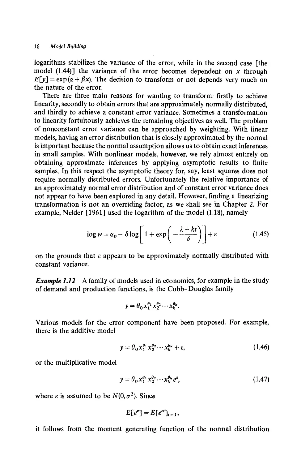
16 Model Building
logarithms stabilizes the variance of the error, while in the second case [the
model A.44)] the variance of the error becomes dependent on x through
E[y2 = exp (a + fix). The decision to transform or not depends very much on
the nature of the error.
There are three main reasons for wanting to transform: firstly to achieve
linearity, secondly to obtain errors that are approximately normally distributed,
and thirdly to achieve a constant error variance. Sometimes a transformation
to linearity fortuitously achieves the remaining objectives as well. The problem
of nonconstant error variance can be approached by weighting. With linear
models, having an error distribution that is closely approximated by the normal
is important because the normal assumption allows us to obtain exact inferences
in small samples. With nonlinear models, however, we rely almost entirely on
obtaining approximate inferences by applying asymptotic results to finite
samples. In this respect the asymptotic theory for, say, least squares does not
require normally distributed errors. Unfortunately the relative importance of
an approximately normal error distribution and of constant error variance does
not appear to have been explored in any detail. However, finding a linearizing
transformation is not an overriding factor, as we shall see in Chapter 2. For
example, Nelder [1961] used the logarithm of the model A.18), namely
Iogw=a0-c51og l + expf--yij +e A.45)
on the grounds that e appears to be approximately normally distributed with
constant variance.
Example 1.12 A family of models used in economics, for example in the study
of demand and production functions, is the Cobb-Douglas family
Various models for the error component have been proposed. For example,
there is the additive model
^-xek" + e, A.46)
or the multiplicative model
y = 60xellxe22-xekl'ec, A.47)
where e is assumed to be N@,a2). Since
it follows from the moment generating function of the normal distribution

1.7 Transforming to Linearity 17
that
£[e«] = e°2'2
and hence for A.47),
l,x2,...,xk-] = e0xelixe2^-xek-ea212. A.48)
Taking logarithms will transform A.47) into a linear model. A mixed model for
the error structure has also been proposed (Goldfeld and Quandt [1972:140ff.]),
namely
A.49)
Example 1.13 The Holliday model relating the average yield (y) per plant to
the density of crop planting (x) is given by
y»(a + Px + yx2)~l. A.50)
The linearizing transformation is clearly to use y~l. However, in practice it is
often found that the transformation that stabilizes the error variance is the
logarithmic transformation
log y = - log (a + Px + yx2) + e. A.51)
Models for yields versus densities are discussed further in Section 7.6. ■
We see from our three cases of additive, proportional, and multiplicative
error that the error structure must be considered before making linearizing
transformations. Although a residual plot is usually the most convenient method
of checking an error structure, occasionally physical considerations will point
towards the appropriate model (e.g. Just and Pope [1978]). The general
questions of transformations and weighting are discussed in Section 2.8, and
the dangers of ignoring variance heterogeneity are demonstrated there.
It should also be noted that the parameters of a linearized model are often
not as interesting or as important as the original parameters. In physical and
chemical models the original parameters usually have a physical meaning, e.g.
rate constants, so that estimates and confidence intervals for these parameters
are still required. Therefore, given the availability of efficient nonlinear algorithms,
the usefulness of linearization is somewhat diminished.
It is interesting to note that all of the models discussed in this section
(Section 1.7) fit into the generalized linear-model framework of A.42) when they

18 Model Building
are expressed in the form
y = /(x;0) + e
with normally distributed errors e having constant variance.
1.8 MODELS WITH AUTOCORRELATED ERRORS
In many examples in which nonlinear regression models have been fitted to
data collected sequentially over time, plots of the data reveal long runs of positive
residuals and long runs of negative residuals. This may be due to the inadequacy
of the model postulated for £[>|x], or it may be caused by a high degree of
correlation between successive error terms ef. A simple autocorrelation structure
which is sometimes applicable to data collected at equally spaced time intervals
is given by an autoregressive process of order 1 [ARA)], namely
e, = pe,-_i +ah A.52)
where the a, are uncorrelated, £[a,] = 0, var [a,] = a\, and \p\ < 1. Under such
a structure (see Section 6.2.1)
so that the correlation between ef and e,- decreases exponentially as the distance
increases between the times at which yt and y} were recorded.
Example 1.14 Consider the simple linear model
ei A-53)
for / = 1,2,..., n, in which the e.have an ARA) autocorrelation structure. From
A.52) a; = e( —pe,_i, so that for i = 2,3,...,n we have
p) + pyt- i + PiX,-Pi px,_, + a,. A.54)
This is of the form
y, = P% + pxfr + fii xf2 + Pi px% + at.
Thus a simple linear model with an autocorrelated error structure can be
converted into a nonlinear model with an uncorrelated constant-variance error
structure. The resulting nonlinear model can then be fitted by ordinary
least-squares methods. We should note that there can be problems with this
approach caused by the fact that it does not make full use of the first observation
pair (xi,yi). ■

1.9 Further Econometric Models 19
Methods for fitting linear and nonlinear models with autocorrelated (ARMA)
error structures are discussed in Chapter 6.
1.9 FURTHER ECONOMETRIC MODELS
There are two types of model which are widely used in econometrics. The first
is a model which includes "lagged" y-variables in with the x-variables, and the
second is the so-called simultaneous-equations model. These are illustrated by
the following examples.
Example 1.15 Suppose that the consumption yt at time i depends on income
variables x, and the consumption y,_i in the previous year through the model
x^ + e,. (i= 1,2,...,«), A.55)
where the e, are usually autocorrelated. This is called a lagged or dynamic model
because of its dependence on yt-1. It differs from previous models in that / and
e, in A.55) are usually correlated through yt-i. ■
Example 1.16 Consider the model (Amemiya [1983: p. 374])
>i2 + Mil + #3 + E(l»
where ea and ei2 are correlated. This model is called a simultaneous-equations
model and has general representation
ytj = fjk>n - yn. • ■ •. yim, x(; 0) + ey
(i=l,2,...,n, 7 = l,2,...,m)
or, in vector form,
y, = f(y,,x,;8) + E( (i = l,2,...,«). A.56)
This model is frequently expressed in the more general form
or

20 Model Building
If i refers to time, the above model can be generalized further by allowing x( to
include lagged values y,_i,y;_2, etc. ■
The above models are not considered further in this book, and the interested
reader is referred to Amemiya [1983] and Maddala [1977] for further details.
The asymptotic theory for the above models is developed in detail by Gallant
[1987: Chapters 6,7].

Nonlinear Regression. G. A. F. Seber, C. J. Wild
Copyright © 1989 John Wiley & Sons, Inc.
ISBN: 0^71-61760-1
CHAPTER 2
Estimation Methods
2.1 LEAST-SQUARES ESTIMATION
2.1.1 Nonlinear Least Squares
Suppose that we have n observations (x;,^), i = 1,2 n, from a fixed-regressor
nonlinear model with a known functional relationship /. Thus
(i=l,2,...,n), B.1)
where £[e,] = 0, x( is a k x 1 vector, and the true value 0* of 0 is known to
belong to 0, a subset of IRP. The least-squares estimate of 0*, denoted by 0,
minimizes the error sum of squares
B.2)
over 0e<9. It should be noted that, unlike the linear least-squares situation, S@)
may have several relative minima in addition to the absolute minimum 0.
Assuming the e; to be independently and identically distributed with variance
a2, it is shown in Chapter 12 that, under certain regularity assumptions, 0 and
s2 = S(Q)/(n - p) are consistent estimates of 0* and a1 respectively. With further
regularity conditions, 0 is also asymptotically normally distributed as n->oo.
These results are proved using a linear approximation discussed in the next
section. If, in addition, we assume that the ef are normally distributed, then 0
is also the maximum-likelihood estimator (see Section 2.2.1).
When each /(x,;0) is differentiable with respect to 0, and 0 is in the interior
of 0, 0 will satisfy
= 0 (r=l,2,...,p). B.3)
21

22 Estimation Methods
We shall use the notation /,@) = /(x,;e),
B.4)
\ /
and
F.@) = —— = I I ~z:— I j. B-5)
Also, for brevity, let
F. = F.@*) and F. = F.@). B.6)
Thus a dot subscript will denote first derivatives; two dots represent second
derivatives (see Chapter 4). Using the above notation we can write
= [y-f(e)]'[y-f(e)]
B.7)
Equation B.3) then leads to
= 0 (r = l,2,...,p), B.8)
or
0 = F:{y-f(§)}
= V'X B.9)
say. If Pf = F.(F;F.)F:, the idempotent matrix projecting W orthogonally
onto ^[F.] (see A11.4), then B.9) can also be written as
Pfe = 0. B.10)
The equations B.9) are called the normal equations for the nonlinear model. For
most nonlinear models they cannot be solved analytically, so that iterative
methods are necessary (see Section 2.1.3 and later chapters).
Example 2.1 Consider the allometric model
yi = axf + ei (i = 1,2,...,n). B.11)
The normal equations are

2.1 teast-Squares bstimation 23
and
EC,-«xf)«xflogxt = 0.
These equations do not admit analytic solutions for a. and p. ■
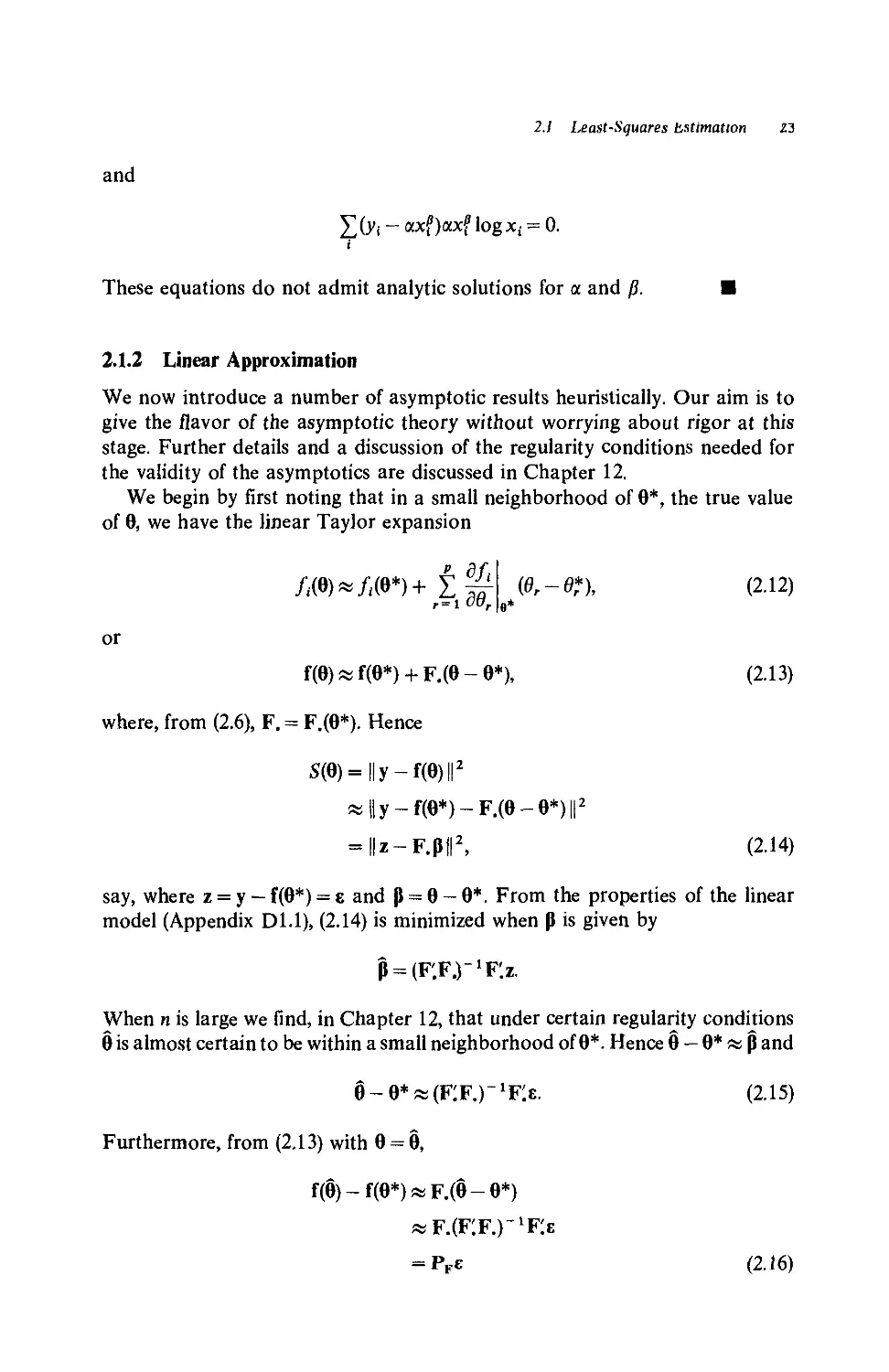
2.1.2 Linear Approximation
We now introduce a number of asymptotic results heuristically. Our aim is to
give the flavor of the asymptotic theory without worrying about rigor at this
stage. Further details and a discussion of the regularity conditions needed for
the validity of the asymptotics are discussed in Chapter 12.
We begin by first noting that in a small neighborhood of 0*, the true value
of 0, we have the linear Taylor expansion
or
where,
from
B.6),
J
Tf
(9,-9*),
9*
f@)«f@*) + F.@-0*),
F.@*). Hence
S@)=||y-f@)||2
B.12)
B.13)
«||y-f(e*)-F.@-0*)||2
= l|z-F.pf, B.14)
say, where z = y — f@*) = s and P = 0 — 0*. From the properties of the linear
model (Appendix Dl.l), B.14) is minimized when P is given by
When n is large we find, in Chapter 12, that under certain regularity conditions
0 is almost certain to be within a small neighborhood of 0*. Hence 0 — 0* « p and
§-0*«(F:F.r1F:£. B.15)
Furthermore, from B.13) with 0 = 0,
f@)-f@*)«F.@-0*)
B.16)

24 Estimation Methods
and
y-f@)«y-f@*)-F.@-0*)
= (Ib-Pf)e, B.17)
where PF = F.(F'.F.)~ l¥'. and In — PF are symmetric and idempotent (Appendix
All). Hence, from B.17) and B.16), we have
(n - p)s2 = S@)
= l|y-f(e)ll2
«||(In-PF)E||2
= E'(In-PF)E, B.18)
and
||f@)-f@*)||2«||F.@-0*)||2
=@-0*)'f:f.@-0*)
~ IIP E ||2
= e'Pfe. B.19)
Therefore, using B.18) and B.19), we get
S@*) - S@) a e'e - E'(In - Pf)e
= e'Pfs
a@-0*)'F:F.@-0*). B.20)
Within the order of the linear approximation used we can replace F. by F. = F.@)
in the above expressions, when necessary. Also B.15) and B.18) hold to op(n~ll2)
and op(l), respectively (e.g. Gallant [1987:259-260]). We now have the following
theorem.
Theorem 2.1 Given e~ JV(O, o2\n) and appropriate regularity conditions
(Section 12.2) then, for large n, we have approximately:
(i) 0 - 0* ~ Np@, a2C-1), where C = F:F. = F:@*)F.@*); B.21)
(ii) (n - p)s2lo2 « e'(Ib - PF)E/a2 ~ xl-P> B.22)
(iii) 0 is statistically independent of s2; and B.23)
(IV) [S@*) - S@)]/p ^ e'Pfe n - p
-p) ~ E'(In - Pf)e p
~F',„-„. B.24)

2.1 Least-Squares Estimation 25
The normality of 8 is not required for the proof of (i).
Proof: Parts (i) to (iii) follow from the exact linear theory of Appendix Dl
with X = F., while (iv) follows from Appendix A11.6. The normality of the e, is
not needed to prove (i), as B.15) implies that 0 — 0* is asymptotically a linear
combination of the i.i.d. et. An appropriate version of the central limit theorem
then gives us (i). ■
Finally, using (iv) and B.20) we have, approximately,
@-0*)'f:f.@-0*)
~2 ~FP,»-P> B-25)
pi
so that estimating F. by F., an approximate 100A - <x)% confidence region for
0* is given by
{0*: @* - 0)'F:F.@* - 0) < ps2F;^p}. B.26)
Thus F. (or F.) plays the same role as the X-matrix in linear regression. This
idea is taken further in Chapter 5, where we shall develop approximate
confidence intervals and hypothesis tests for 0* or subsets of 0*.
2.1.3 Numerical Methods
Suppose 0(a) is an approximation to the least-squares estimate 0 of a nonlinear
model. For 0 close to 0(a), we again use a linear Taylor expansion
f@) x f@(a)) + F.(a)@ - 0(a)), B.27)
where Fia) = F.@(a>). Applying this to the residual vector r@), we have
r@) = y-f@)
~ r@«->) - F<a)@ - 0(a)).
Substituting in S@) = r'@)r@) leads to
S@)« r'@«">)r@«">) - 2r'@(a))F.(H)@ - 0(a)) + @ - 0(a))'Fia)'F.(a)@ - 0(a)). B.28)
The right-hand side is minimized with respect to 0 when
0 - 0<") = (F<a)'Fia)r 1F<a)'r@(a))
= 8(a), say. B.29)
This suggests that, given a current approximation 0<a), the next approximation

26 Estimation Methods
should be
B30)
This provides an iterative scheme for obtaining 0. The approximation of S@)
by the quadratic B.28), and the resulting updating formulae B.29) and B.30),
are usually referred to as the Gauss-Newton method. It forms the basis of a
number of least-squares algorithms used throughout this book. The Gauss-
Newton algorithm is convergent, i.e. 0(a) ->0 as a-> oo, provided that 0A) is close
enough to 0* and n is large enough.
A more general approach, which applies to any function satisfying appropriate
regularity conditions, is the Newton method, in which S@) is expanded directly
using a quadratic Taylor expansion. Using the notation of A.9) and A.11), let
B.31)
and
B.32)
denote, respectively, the so-called gradient vector and Hessian matrix of S@).
Then we have the quadratic approximation
= S@(a)) + g'@(a))@ - 0(a)) + i@ - 0(a))'H@(a))@ - 0(a)), B.33)
which differs from B.28) only in that H@(a)) is approximated there by
2F'.@(a))F.@(a)). However, since
MM.
then
_ tdfm?jm _ fv _ fmdJM\ B 34)
(z35)
and H@(a)) is approximated by its expected value evaluated at 0(a) in B.28).
The minimum of the quadratic B.33) with respect to 0 occurs when
0-e<*>=-[H@(a))]-1g@(a))
— [H^gW- B36)
This is the so-called Newton method, and the "correction" 8(a) in B.30) now

2.1 Least-Squares Estimation 27
given by B.36) is called the Newton step. Various modifications to this method
have been developed, based on (for example) scaling g, modifying or approxi-
approximating H, and estimating the various first and second derivatives in g and H
using finite-difference techniques. Further details of these methods are given in
Chapters 13 and 14.
A feature of the quadratic approximation ^a)(B) of B.33) is that its contours
are concentric ellipsoids with center 0(a+1). To see this we write
qg")@) = 0'A0 - 20'b + c
where, for well-behaved functions, A = ^H@(a)) is positive definite (and therefore
nonsingular), c0 = A" 'b, and do = c- c'0Ac0. Then setting
= 2A0 - 2b) [cf. (Appendix A10.5)]
equal to zero gives us 0(a+1) = A~ lb = c0, where c0 is the center of the ellipsoidal
contours of @ - co)'A@ - co). This result also follows directly from A being
positive definite. We note that, for linear models,
S(p) = (y-Xp)'(y-Xp)
= y'y-2p'X'y + p'X'Xp,
a quadratic in p. Then both the Gauss-Newton and Newton approximations
are exact, and both find p in a single iteration.
Finally it should be noted that we do not advocate the unmodified
Gauss-Newton and Newton (Newton-Raphson) algorithms as practical
algorithms for computing least-squares estimates. Some of the problems that
can occur when using the basic unmodified algorithms are illustrated in Sections
3.2 and 14.1. A range of techniques for modifying the algorithms to make them
more reliable are described in Chapter 14. Nevertheless, throughout this book
we describe, for simplicity, just the bare Gauss-Newton scheme for a particular
application. Such iterative techniques should not be implemented without
employing some of the safeguards described in Chapter 14.
2.1.4 Generalized Least Squares
Before leaving numerical methods, we mention a generalization of the least-
squares procedure called weighted or generalized least squares (GLS). The
function to be minimized is now

28 Estimation Methods
where V is a known positive definite matrix. This minimization criterion usually
arises from the so-called generalized least-squares model y = f@) + 8, where
$[e] = 0 and S[e] = o2\. Thus the ordinary least squares (OLS) previously
discussed is a special case in which V = I,,. Denote by 90 the generalized least-
squares estimate which minimizes S@) above.
Let V = U'U be the Cholesky decomposition of V, where U is an upper
triangular matrix (Appendix A8.2). Multiplying the nonlinear model through
by R = (U')~1, we obtain
z = k@) + ii,
where z = Ry, k@) = Rf@) and t\ = Re. Then £[r\] = 0 and, from A.3), ®[tj] =
<t2RVR' = a2ln. Thus our original GLS model has now been transformed to an
OLS model. Furthermore,
= [y-f@)]'V[y-f@)]
= [y-f@)JR'R[y-f@)]
Hence the GLS sum of squares in the same as the OLS sum of squares for the
transformed model, and 0G is the OLS estimate from the transformed model.
Let K.@) = 5k@)/30' and K. = K.@). Then
Since 0G is the OLS estimate in the transformed model, it has for large n a
variance-covariance matrix given by [cf. B.21)]
= o-2[F:@*)R'RF.(e*)]
=o-2[
This matrix is estimated by
where
1
[>-k(eo)]'[z-k(eo)]
n-p
=^[y-f(So)]'V[y-f(So)].

2.1 Least-Squares Estimation 29
Repeatedly throughout this book we shall require the computation of a GLS
estimate. In each case the computational strategy is to transform the model to
an OLS model using the Cholesky decomposition V = U'U. The important
point of the above analysis is that treating the transformed problem as an
ordinary nonlinear least-squares problem produces the correct results for
the generalized least-squares problem. In particular, ordinary least-squares
programs produce the correct variance-covariance matrix estimates.
To illustrate, let us apply the linearization method to the original form of
S@). Using B.27) we have
S@) « [y - f@(a)) - F.(a)(e - 0(a))]'V- '[y - f@(a)) - F.(a)@ - 0(a))].
This approximation produces a linear generalized least-squares problem and is
thus minimized by
6 - 0<a> = (F<a>'V~1F<a)r 'Fi^'V '[y - f@(a))].
The above leads to the iterative scheme 0(a+1) = 0(a) + 8(a), where
g(<") _ (F<a>'V~ 'Fi"')" 'F.^'V" l[y — f@(a))]
= (Fia)'R'RFia)r 'Fi^'R'RCy - f@(a))]
= (K.(a)'K!a))~ 'K^'Cz - k@(a))]. B.37)
The last expression is the Gauss-Newton step for the transformed model and
minimizes the ordinary linear least-squares function
[z - k@«">) - K<a)8]'[z - k@(a)) - K<a)8]
with respect to 8. Thus 8<a) is obtained by an ordinary linear regression of
z — k@(a)) on K.(a). Linear least squares has, as virtual by-products, (X'X) ~ * and
the residual sum of squares. Therefore, at the final iteration where 0(a)a0G,
(X'X)-» = (fcK.) = (F'.V- lt.)~l,
and the residual sum of squares is
[z - k@o)]'[z - k@o)] = [y - f@o)]'V- J[y - f@c)]
If a linear least-squares program is used to perform the computations, then the
estimated variance-covariance matrix from the final least-squares regression is
£6
In practice we would not compute R = (U')~~l and multiply out Ry ( = z).
Instead it is better to solve the lower triangular system U'z = y for z directly

30 Estimation Methods
by forward substitution. We similarly solve U'k@(a)) = f@(a)) for k@(a)) and, in
the case of the Gauss-Newton method, U'Kfa) = F.(a) for K.(a).
Many applications of the above method arise from weighted least-squares
problems in which V is diagonal. Since U is then diagonal with diagonal elements
equal to the square roots of the corresponding elements of V, the computation
of z etc. becomes particularly simple.
It is now convenient, for easy reference, to summarize the main steps leading
to the computation of 0G, the value of 0 minimizing
S@)=[y-f@)]'V-1[y-f(9)],
and ®[0G] = (J2(F'.V~1F.)~1, an estimate of the asymptotic covariance matrix
of0o:
1. Perform a Cholesky decomposition V = U'U of V.
2. Solve U'z = y and U'k@) = f@) for z and k@).
3. Apply an ordinary nonlinear least-squares technique to
4. If a Gauss-Newton method is used for C), then 0(a+1) = 0(a) + 8<a), where
8(a) = (Kia)'K.(a)r 'Kl^O - k@(a))]
is obtained from a linear regression of z —k@(a)) on K.(a). The matrix
K<a) is found by solving U'K.@(a)) = F.@(a)).
5. ®[0G] = 62(K'.K.)~l is the estimated dispersion matrix obtained in C). If
the Gauss-Newton method is used, (K[K.)-1 and d2 can be obtained
from the linear regression in D) at the final iteration.
A more general version of generalized least squares in which V may depend
on 0 is described in Section 2.8.8. If V = V@), a known function of 0, then V
can, for example, be replaced by V@(a>) in B.37). A new Cholesky factorisation
of V is then required at each iteration.
♦2.1.5 Replication and Test of Fit
Suppose a design is replicated, say J, times for point x!( so that our nonlinear
model B.1) now becomes
=/(Xj:0*) + 8l7 (i = l,2,...,n ;=l,2,...,Jj) B.38)
where the fluctuations (or "errors") 8,^ are assumed to be i.i.d. N@, a2). As stressed

2.1 I^east-Squares Estimation 31
by Draper and Smith [1981:35], it is important to distinguish between a genuine
repeated point in which the response y is measured for two different experiments
with the same value of x,, and a "reconfirmed" point in which y is measured
twice for the same experiment. Although the latter method would supply
information on that part of a2 relating to the accuracy of the measuring method,
it is the former which forms the basis for B.38). This model includes the genuine
variation between different experiments with the same x observation as well as
error of measurements.
Ignoring the structure on ^,, we have the usual decomposition
EEoiSE
i j is
- M*J, B.39)
1 j
where SSCVy ~ h-J ls usually referred to as the "pure error" sum of squares.
Defining AT = X(</(, an unbiased estimate of a2 is
^-*.J, B-40)
and, under the normality assumptions of the eip
(N - n)s2 2
B.41)
To find the least-squares estimate 0 of 0 we minimize YEteu ~ MiJ with respect
to 0, which is equivalent to minimizing (cf. B.39)] Si^rCj'i. —/(x^G)]2, i.e. a
weighted least-squares analysis with weights J,. The normal equations for 0 are
therefore
. = 0 (r=l,2,...,p). B.42)
If Hi is replaced by /Jj=/(x,;0), the identity B.39) still applies, so that
II(yu - fid2 = II(y« - hJ + E^(y, - fif,
or
say. The left-hand side, called the residual sum of squares, is therefore split into
a pure-error sum of squares Q and a lack-of-fit sum of squares QH — Q. For the
case when ^j, is a linear function of 0 (i.e. \i = X0, say), a test for the validity of

32 Estimation Methods
this linear model is given by (Seber [1977: 181])
(Qn-Q)/(n-p)
-»)
~n'2 "~" B.43)
F =
where F~ Fn-.pN_n when the model is valid. Because of asymptotic linearity,
we find that the above F-test is approximately valid for large AT when the model
is nonlinear. Confidence intervals are discussed in Section 5.6.
2.2 MAXIMUM-LIKELIHOOD ESTIMATION
If the joint distribution of the e, in the model B.1) is assumed known, then the
maximum-likelihood estimate of 0 is obtaind by maximizing the likelihood
function. Suppose the e,'s are i.i.d. with density function a~lg(e/a), so that g is
the error distribution for errors standardized to have unit variance. Then the
likelihood function is
B.44)
We shall discuss both normally and nonnormally distributed errors below. In
both cases we find that the maximum-likelihood estimator of 0 can be found
using least-squares methods.
2.21 Normal Errors
If the e, are i.i.d N@, a2), then B.44) becomes
B.45)
Ignoring constants, we denote the logarithm of the above likelihood by L@,<r2)
and obtain
Given a2, B.46) is maximized with respect to 0 when S@) is minimized, that is,

2.2 Maximum-Likelihood Estimation 33
when 0 = 9 (the least-squares estimate). Furthermore, dL/da2 = 0 has solution
a2 = S(Q)/n, which gives a maximum (for given 0) as the second derivative is
negative. This suggests that 0 and &2 = S@)/« are the maximum-likelihood
estimates, and we now verify this directly. Since S@) > S@),
L$, 62) - L@, a2) = - ^log 62 - 5 - L@, <x2)
n, cf2 n 1S@)
■>Inn i; \
as log x < x — 1 for x >, 0. Hence 0 and 62 maximize L@, a2). The maximum
value of B.45) is
B.47)
Jennrich [1969: p. 640] notes that the least-squares estimate is now not only
the maximum-likelihood estimate but, under appropriate regularity conditions
(see Section 12.2), is also asymptotically efficient (i.e., a'0 is asymptotically
minimum-variance for every a). The usual asymptotic maximum-likelihood
theory does not apply directly, but needs modification, as theyt are not identically
distributed, having different means. Thus if 8 = @', i;)', where v = a1, then from
B.46) and B.35) the (expected) information matrix is given by
1-
J
1
2^1
dddv
0'
n
2?
B.48)
Hence, under appropriate regularity conditions, we have from A2.20) that
= o-2limn[F:@*)F.@*

34 Estimation Methods
As with the i.i.d. case, we see that the variance-covariance matrix of the
maximum-likelihood estimator 9 is given asymptotically by the inverse of the
(expected) information matrix in B.48).
Let 8 = (9',<r2)'. Then, since 3S(9)/39 = 0 at 9 = 9, we also have
3838'Jg
1 f d2S
Id2 13838' la
9'
0
d2s
{3939
0'
0
B.49)
2.2.2 Nonnormal Data
For completeness we shall now digress from our main theme of nonlinear
regression and consider the case where the log-likelihood function is a general
function of $ [y] = f(9), say L([f(9)]). Our discussion is drawn from the extensive
paper by Green [1984]. It is assumed that the model is sufficiently regular so
that the maximum-likelihood estimate 9 is the solution of the likelihood
equations
0 =
39
= '^If (by Appendix A 10.1).
B.50)
Let 9(a) be the ath approximation for 9 and consider the Taylor expansion
39
e
3L|
39
9""
d2L
3939'
(9-9*>).
Then
dL I
39 JB
B.51)
so that an updated estimate is 9(a + 1) = 9(a) + 8(a). This is Newton's method of
solving the equations, though in the above context statisticians often refer to it
as the Newton-Raphson method. In general, the negative second-derivative
matrix contains random variables, and it is often recommended that it be
replaced by its expected value, the so-called (expected) information matrix. This

2.2 Maximum-Likelihood Estimation 35
technique is known as Fisher's "scoring" algorithm, (cf. Appendix A14). We
now find the above expected matrix.
From Appendix A 10.2 we have
2 521
dQdQ' \dVjdtdT\dV
Assuming that the order of differentiation with respect to 0 and integration (or
summation) with respect to y can be interchanged, we have [with p() the density
function of y, and L = log p]
(t
p3f
= 3f r dy
= 0, B.53)
and, using a similar argument,
s\ ~ =0. B.54)
Hence
|_3f3f'J
^ [" 13p3p 132p]
L P2 dt dC p3f3f'J
3f 3f
= -G. B.55)
We note that G is positive definite, as
with equality only if a = 0 (under general conditions on L). Applying B.55) and
B.53) to B.52) gives us

36 Estimation Methods
which is positive definite (Appendix A4.5) for F. of full rank, and is therefore
nonsingular. Thus Fisher's scoring algorithm becomes
^) . B.57)
00 /()
The negative second-derivative matrix may not be positive definite at every 0(a),
and this can cause the Newton method of B.51) to fail (see Section 13.3.1). The
Fisher scoring method therefore uses an approximation of the negative second-
derivative matrix which is always positive definite, so that the step taken
at the ath iteration, 8(a) = e(a + 1)-0(a), leads off in an uphill direction (see
Section 13.2.3b with downhill replaced by uphill, as here we are referring to
maximization rather than minimization). It has a further advantage in that only
first derivatives of L are required, so that the approximation can often
be calculated more quickly than the second-derivative matrix. The scoring
algorithm pays for these advantages by converging more slowly than the Newton
method as 0(a) approaches 0. More widely applicable methods of protecting
against matrices which may not be positive definite are described in Section
13.3.1. With a number of well-known models such as the linear logistic regression
model (Section 1.6), the scoring algorithm and Newton's method coincide.
If we now set g = dL/df, we obtain from B.51) and B.57)
= [(F.V-'F.r'F.V-WV), B.58)
where \ = G~i and v = Vg. We note that the equation B.58) represents the
generalized least-squares estimate 8(a) of 8 for the model (evaluated at 0(a))
v = F[a)8 + v, B.59)
where ®[v] = V(a). Using the same idea as in Section 2.1.4, let V(a) = U'U be
the upper triangular Cholesky decomposition of V(a) (Appendix A8.2), and let
R^U')". Then multiplying B.59) by R, we obtain
z = X8+n, B.60)
where z = Rv, X = RFia), and 2>\r\\ = o2ln. Thus 8(a) can be computed by using
an ordinary linear least-squares program and regressing z on X. A standard
output from a linear-regression program is (X'X) [or s2 and s2(X'X)~1]: in
B.60)
(X'X)-1=(F'.V-1F.)ew1.

2.2 Maximum-Likelihood Estimation 37
Thus, by B.56), the regression output at the final iteration provides
which, under certain regularity conditions, is the asymptotic variance-covariance
matrix of 0.
The above method is a very general one and is commonly referred to as
iteratively reweighted least squares (IRLS). It can be applied to a wide range of
models, and one such application, quasi-likelihood models, is considered in
Section 2.3. The method enables a large range of models to be grafted onto
existing statistical packages with minimal additional programming by making
use of existing least-squares regression procedures. However, as IRLS is not
central to our main theme, we refer the interested reader to the paper of Green
[1984] and the ensuing discussion for further details and examples. In
commenting on Green's paper Ross claimed that it was preferable to use the
optimization facilities of good statistical packages rather than rely on the IRLS
method, especially when the problem is unfamiliar. He noted that IRLS needs
the correct algebraic specification and good initial estimates, and may still be
slow or divergent. However, the optimization applications require only the
model formulation and the distribution of errors. There is also protection from
divergence, and parameter transformations are easily incorporated.
The special case of a linear model /(x(;0) = x|0 is considered by Stirling
[1984]. An application to regression diagnostics is given by Moolgavkar et al.
[1984]. Green's method has been extended by J^rgensen [1984].
2.2.3 Concentrated Likelihood Methods
In finding maximum-likelihood estimates from general likelihoods it is some-
sometimes convenient to use the following stepwise method of maximization. Suppose
that we have a general log-likelihood function L@,t|z) to be maximized with
respect to 0 and t, where z represents the data and t is q x 1. It is assumed that
L is uniquely maximized with respect to 0 and t for every z. Then the first step
of the maximization is to find y@, z), the unique value of t which maximizes L
with respect to t, 0 being regarded as a constant. The second step consists of
finding 0 = 0(z), the value of 0 which maximizes
= L{0,y@,z)|z}. B.61)
Since
L{0(z),Y(e,z)|z} = M@|z)
>M@|z)
= L{0,y@,z)|z}
>L{0,t|z},

38 Estimation Methods
the maximum-likelihood estimates are 0 and £ = y@, z). If there are any relative
maxima, the above argument holds in a neighborhood of the absolute maximum
which does not contain any relative maxima. The key part of the argument is
that y@, z) must be unique for a given 0. The function M@|z) is called the
concentrated log-likelihood function (Hood and Koopmans [1953: pp. 156-157])
because it is concentrated on the set of parameters 0. In what follows we drop
the functional dependence on the data z for notational convenience.
We now consider some advantages of using M@) instead of L@, t). Firstly,
we shall see in Theorem 2.2 below that 0 can be obtained directly as the solution
of 3M@)/30 = 0, so that the nuisance parameter t is effectively eliminated.
Secondly, under certain conditions, an estimate of the asymptotic variance-
covariance matrix of 8 = (§',¥)' is given by
3838'
a (P + <?) * (P +1) matrix which can be partitioned to give an estimate of Q) [0].
However, if we are interested in just 0, then from Theorem 2.2 below we find
that ®[0] can be estimated by
Example 2.2 We now demonstrate the above methodology by rederiving the
maximum-likelihood estimates for the log-likelihood B.46) with t = a2. Dropping
the dependence on the data for notational convenience, we have
For fixed 0 the above expression is maximized when a2 = S@)/n, so that the
concentrated log-likelihood function is
B.62)
This is maximized when S@) is minimized, that is, at the least-squares estimate
0. Then S@)/n is the maximum-likelihood estimator a2 of a2. Furthermore, since

2.2 Maximum-Likelihood Estimation 39
[3S@)/30]e =
n dS(Q) dS(d) n d2S(d)
dddd' Jg { 2[S@)]2 30
1
f:f.
B.63)
2F'.(O)F.@) [by B.35)]
so that ^[0] is estimated by &2(F'.F.yx. This is our usual estimator but with
s2 replaced by a2 [cf. B.21)]. ■
We note that the inverse of B.63) is the upper diagonal block of B.49). This
result is generalized in the following theorem (Richards [1961], Kale [1963]).
Theorem 2.2 Let L@, t) be the log-likelihood function defined above, where 0
is the p x 1 vector parameter of interest and t is a q x 1 vector of "nuisance"
parameters. We assume that L is twice differentiate. Define 8 = @', t')', and let
8 = @',*')' solve 3L/38 = 0, that is, solve
3L@,t)
30
= 0 and
3t
= 0.
B.64)
Define
1(8) =-
d2L
3838'
d2L
dddW
d2L
3t30'
d2L
30 3t'
d2L
3t3t'
say, and assume that it is positive definite at 8 = 8. Also define
0 "8t
B.65)
B.66)

40 Estimation Methods
Suppose, for any fixed 0, that t = y@) solves
3L@,t) = q
and let M@) = L[0,y@)]. Then
(i) 3M@)/30|g = O, and
(ii) we have
= J«
B.67)
3030'
B.68)
[It should be noted that this theorem is true for any function L and not just
log-likelihoods.]
Proof: The assumption that 1(8) is positive definite means that 1(8) is positive
definite in a neighborhood Jf of 8, and both lee and Itt are nonsingular in Jf.
As pointed out by Kale [1963], the existence of S and the nonsingularity of Itt
in Jf imply that the implicit-function theorem can be applied to the set of
equations B.67). Hence in jV we have (a) y@) is uniquely defined, (b) t = y@)
and (c) y@) has continuous first-order derivatives. In the following we use the
differential notation of Section 1.1 and assume that expressions are valid for 8
(i): We note that, for t = y@),
that is,
r-t i/a-*^V) \>) \j\j t
,z) dxk
30, y S9j
dxk
3M@)_3L@,t) /3yV3L@,T)
30 " 30 "*" \ 5O7 / 3t
3L@,t)
30
B.69)
y(9)
since the second term is zero by B.67). Hence using t = y@), we have
dM(Q)
30
3L@,y)
i 50
3L@,t)
30
= 0,
by B.64). Thus (i) is proved.

2.2 Maximum-Likelihood Estimation 41
(ii): Now t = y@) is the solution of B.67), that is, of
5L@,t)
- =0 (s = 1,2,.. .,£[)■
In Jf, the above represents an identity in 0, so that differentiating with respect
to 9r, we get
j^feL^T) ")
32L@,t)
d9rdxs ? 3tu3ts 30rJt
that is
Now — 32L@,t)/3t3t' evaluated at t = y@) cannot be identified with Itt, as the
former is a function of 0 (y being a particular function of 0), whereas the latter
is a function of both 0 and t with t unconstrained. However, when 0 = 0 we
have y@) = t and the two matrices have the same value. The same argument
applies to the first matrix in B.70). Hence from B.70) we have
= (-Mtl%. B.71)
Using a similar argument leads to
3030' { dddd' \dd'J |_ 3t30'
Setting 0 = 0 and using B.71) gives us
Now if A and C are symmetric and all inverses exist,
'A BVW F- -F-G'
Cj VGF^1 C^+GF-'G'/ ( '
where F = A - BC" 'B' and G = C" 'B'. Applying this result to I" ^8) of B.66)

42 Estimation Methods
gives us
and (ii) is proved. ■
The methodology implied by the above lemma for finding the maximum-
likelihood estimates 0 and t, and their asymptotic variance-covariance matrices,
can be summarized as follows:
1. Differentiate the log-likelihood function with respect to t, and solve the
resulting equations for t = y@) as a function of 9.
2. Replace t by y@) in the log-likelihood, and obtain the concentrated log-
likelihood function M@).
3. Use M@) as though it were the true log-likelihood function for 0, and go
through the usual maximum-likelihood process, namely (a) differentiate
M@) with respect to 0 and solve for §, and (b) find the estimated
information matrix B.68). Under general regularity conditions the latter
matrix is an estimate of the asymptotic dispersion matrix of 0.
4. t is given by y@).
5. The remainder of I" 1(t>) can be obtained using B.72).
As already noted, a nice feature of the above method is that through using
the concentrated log-likelihood we can effectively eliminate the nuisance-
parameter vector t and deal with 0 directly. A second feature is that instead of
having to invert the (p + q) x (p + q) matrix 1E), we need only invert the q x q
matrix Itt in B.68). Finally, as mentioned in Section 5.9.1, various large-sample
tests for hypotheses about 0 can also be expressed in terms of the concentrated
log-likelihood rather than the log-likelihood.
*2.3 QUASI-LIKELIHOOD ESTIMATION
We now introduce an estimator of 0 which has properties akin to a maximum-
likelihood estimator but with the difference that the distribution of y does not
need to be known explicitly, only its first two moments. The following discussion
is based on McCullagh [1983], but with some notational changes.
Let <f[y] = f@) ( = fi, say) and ®[y] = o2V(\i). The log quasi-likelihood
function, considered as a function £(\i) of \i, is defined by the system of partial
differential equations
B.73)

2.3 Quasi-Likelihood Estimation 43
This definition is given by McCullagh [1983], and it extends Wedderburn's
[1974] definition. For notational convenience we shall write <^[f@)] and V[f@)]
as simply <f@) and V@), respectively. The maximum quasi-likelihood estimate
0 of 0 is obtained by solving the equations
30
)f{ [by Appendix A10.1]
F'.@)V~'@H - f@)] [by B.73)]. B.74)
To do this we can use a Gauss-Newton method based on the linear Taylor
expansion
f@)« f@(a)) + F.@(a))@ - 0(a)) B.75)
for 0 about an approximation 0(a). Substituting B.75) into B.74), and approxi-
approximating F.@) and V@) by F<a) = F.@(a)) and V(a) = V@(a)), we have
F(<.)<VW-1 [y _ f@«">) _ Fla)@ - 0(a))] « 0,
or
0 — 0(a)«(Fia)/ V(a) ~* Fia)) ~l F(.a)' V(H) ~l [y — f@(H))]
= 8(a), B.76)
say, where the superscript a denotes evaluation at 0(a). The next approximation
for 0 is then 0(a +1( = 0(a) + 8(a). As in the maximum-likelihood method [cf. B.58)]
we have, once again, a generalized least-squares technique in which 5(a) is
obtained by minimizing
[y _ f@<">) _ F<a>5]'V(a)-1 [y - f@(a>) - F<aM] B.77)
with respect to 5 (see Section 2.1.4 for computational details).
Given certain conditions, 0 has a number of useful properties. These
conditions are: (a) d3ft(d)/d9r d0s 09, is bounded (i = 1,2,..., n; r, s, t = 1,2,..., p),
(b) the third moments of y exist, and (c) n~xlH(Q*) has a positive definite limit
as n -> oo, where 0* is the true value of 0 and
A78)
= F'.@*)V~1@*)F.@*). B.79)
Assuming these conditions, McCullagh [1983] derived the following properties.

44 Estimation Methods
Firstly, using B.79) and B.76) (with 0(a) replaced by 0*), we have
>/«(S-e*)~iVp@,ff2[«-1I11@*)]-1) + Op(«-1'2) B.80)
[see A.8) for the notation Op]. Secondly, if the third moment is infinite then
the error term in B.80) is op(l). Thirdly, without altering the order of
approximation, B.78) can be replaced by — dV/5050'. Also a2 can be estimated
by
n-p
Fourthly, among all the estimators of 0* for which the influence function is
linear (i.e. estimators 0L satisfying
where L is a p x n matrix with elements which are functions of 0*), 0 has the
"minimum" dispersion matrix. Finally, suppose we wish to test H0:deco versus
Hi.Qefi, where co and Qhave respective dimensions q and p, and co <= Q(q < p).
If <^@O) and ^@ J are the maximum values of ^@) under HO and H i respectively,
then
B82)
when Ho is true. If /(9) is the log-likelihood function as opposed to an artificially
constructed log quasi-likelihood, and y has a continuous distribution, then the
error term in B.82) turns out to be Op(n~1). If V is singular, then V may be
replaced by an appropriate generalized inverse V" (Scott et al [1989]).
A nice feature of the above theory is that it does not require the existence
of a family of distributions for which /(ji) is the log-likelihood. Furthermore,
/(n) is not required explicitly for the computation of 0, though it is needed for
some forms of hypothesis testing. A solution for /(n) can sometimes be found
by constructing functions P(ji) and c(P) satisfying \i = dc/dfi and V(ji) = 32c/3P 3P',
and writing
where d(y, a) is arbitrary. To see that /(n) is a solution of B.73) we note that
82c y'v-ifa)
an'
An important special case of the above theory is when the yt are uncorrelated

2.3 Quasi-Likelihood Estimation 45
and
V(n) = diag [u(^i), v(n2)> • • ■ > v(nn)],
where v(nt) = y[/(x(;0)] = Ui@), say. Then B.73) reduces to
"*£t-- B-83)
Also, the quadratic described by B.81) now takes the form
y,-/(x,;0)]2, B.84)
the familiar weighted sum of squares. Because of some misleading statements
in the literature it should be noted that 0 is not the minimum of B.84): it is the
"minimum" obtained by treating vt(Q) as though it were functionally independent
of 0 (cf. Section 2.8.8).
We now consider a special family of density functions
p(y\n,o) = exp {o~2[a(n)y - b(n) + c(
= e\ B.85)
say, where n = Ely'], and a(n) and b(n) are at least twice differentiate. When
a = 1, B.85) reduces to the so-called (univariate) regular exponential family,
though expressed somewhat differently here in terms of n rather than a(n) = 4>,
say. Following Bradley [1973], we differentiate both sides of 1 = jeAdy with
respect to n and obtain
B.86)
so that
i(M) = Mfl(M)- B.87)
Using B.87) and differentiating B.86) again under the integral sign leads to
0 = a*
or
B.88)
Hence if y\,y2,-^,yn are independently distributed with Ely] = ^f =/(x,;0),

46 Estimation Methods
then the log-likelihood function is [cf. B.85)]
L = a~2^[o(//|)y, -bfjit) + c(yi,o-)],
and, using B.87),
dL _
B.89)
Apart from a2, which does not affect the estimation of 0, we see that B.89) is
of the same form as B.83). Hence the maximum-likelihood estimate 0 is the
same as the maximum quasi-likelihood estimate 0 and can be found using the
method of iteratively reweighted least squares. This result was proved by Charnes
et al. [1976] by a different route. They established that the maximum-likelihood
estimate was a solution of B.74) and gave sufficient conditions for a solution
of B.74) to maximize L{0) at a unique value of 0. The above theory can be
applied to members of the family B.85) and thus includes the Poisson, binomial,
exponential, multinomial, normal, inverse normal, and gamma distributions.
Applications are discussed by Jennrich and Moore [1975], McCullagh [1983],
and McCullagh and Nelder [1983].
The above method of computing maximum-likelihood estimates for regular
exponential families using iteratively reweighted least squares was originally
demonstrated by a number of authors for the linear model nt = x',0 (Bradley
[1973]) and the generalized linear models g(nt) = xJ0 (for some "link" function
g) introduced by Nelder and Wedderburn [1972] (see also McCullagh and
Nelder [1983], Fahrmeir and Kaufmann [1985]). Further extensions to more
general distributions are given by J^rgenson [1983], Cox [1984], and Stirling
[1984]. The reader is also referred to Nelder and Pregibon [1987], Firth [1987],
and Morton [1987a].
An attractive aspect of quasi-likelihood theory in this context is the following.
When a data analyst is fairly confident that the mean function and the
relationship between the mean and variance has been modeled fairly well, but
is unsure of other aspects of the parametric distribution used, quasi-likelihood
theory assures him or her of the asymptotic correctness of the resulting inferences.
In this way it is a generalization of the asymptotic applicability of least-squares
theory beyond the restrictive assumption of normally distributed errors.
However, there can be problems (Crowder [1987]).
Example 2.3 Suppose the yt are independent Poisson random variables with
means /i, = 0exp( — 0x,) = ^(8). Then the probability function of y is
= exp {y log n - n - log yl],

2.3 Quasi-Likelihood Estimation 47
which is of the form B.85) with a= 1. Hence the maximum-likelihood estimate
is obtained by IRLS using v(nt) = n-,. ■
The above quasi-likelihood approach is a special case of a general technique
usually referred to as the method of (unbiased) estimating equations (Durbin
[1960b], Godambe [I960]). This method consists of finding a suitable vector
function g(y, 0) such that
and choosing an estimate 0 such that
g(y,e)=o.
For example, if S(Q\y) is the likelihood function and
8(y,0) =
then <^[g(y,0)] = O and 0 is, under fairly general conditions, the maximum
likelihood estimate of 0. In the quasi-likelihood case we assume a specific form
for dt/dQ [cf. B.73) and B.74)] and set
g(y,0) = F:@)V-1(e)[y-f@)].
This has zero expectation, as <^[y] = f@), and 0 = 8, the maximum quasi-
likelihood estimator of 0.
If suitable conditions are imposed on the distribution of y and the function
g, then 0 will be consistent and close to the true value 0 for n sufficiently large.
Hence using a Taylor expansion,
o = g(y,0)
where G. = dg/30' evaluated at 0. If the rows of G. are linearly independent, then
>@ - 0)« ^(G.'G.) -» G;g(y, 0)
= Hng(y,0),
say. Given that plimHn exists and is nonsingular, and g(y,0) (suitably scaled)
tends to normality as n->oo, then 0 will be approximately normal.
The above estimating-equation method has been used in a wide range of
applications, e.g. distribution-free methods (Maritz [1981: 7]), nonlinear instru-
instrumental variables estimation (Hansen and Singleton [1982]), robust estimation

48 Estimation Methods
with i.i.d. random variables (Godambe and Thompson [1984]), and generalized
linear models with clustered data (Liang and Zeger [1986]). Hansen [1982]
discusses the theory under the title of generalized method of moment estimators.
How is g chosen? At present this seems to depend very much on the nature
of the problem considered. For the one-parameter i.i.d. case, Godambe and
Thompson [1978] suggest choosing g to minimize
(E[dg/dff]?'
*2.4 LAM ESTIMATOR
Byron and Bera [1983] introduced a new method of estimation called the linear
approximation method (LAM). Using a second-order Taylor expansion about
the fe-dimensional vector x0, we have
(x,-x0)+ ,, + ■>„ B.90)
where r, is the remainder. For illustrative purposes we assume k = 1, so that
the above model takes the form
where wj = [1, xf - xo,i(x, - x0J] and
Then combining the n equations we have
y = f@) + £
= Wp + r + e,
where W has ith row w',. For /c-dimensional x0, the above model still holds with
W an appropriate n x m matrix [m = 1 + k + jk(k + 1)], and P an m x 1 vector
function of 0. Depending on f,p, and k, the vector 0 will be uniquely under- or
overdetermined in terms of p. Byron and Bera [1983] introduced the following
four assumptions:

2.4 Lam Estimator 49
(i) There exists at least one way of determining 0 in terms of p, namely
0 = h(P), where h is differentiate.
(ii) W has rank m, so that W'W is positive definite.
(iii) W'W + W'Cr/3P') is positive definite in some neighborhood of p*, the
true value of p. [In other words, since W'W is positive definite, W'Cr/3P')
does not dominate W'W. A second interpretation of this assumption is
that f is not excessively nonlinear in terms of P, since dr/dP' = df/dP' — W.]
(iv) lim n' i W'W = Qi where Qt is a finite matrix, plim n' l W'[y - f@)] = 0,
plim[-n-'W'(dr/dP')] = P exists in a neighborhood of p*, and
1 — Q^"l P is nonsingular.
They then suggested the following method for estimating 0. Firstly, ignore
r and obtain the least-squares estimate PA) = (W'W)~1W'y. Secondly, estimate
0 by 0A) = h(PA)) and then estimate r by rA) = f@A)) - wpA). Thirdly, re-estimate
P using pB) = (W'W)~1W'(y — rA)). This process can be continued so that, in
general,
rW = f@«">) - Wp<a),
and
p("+1) = (W'W)-* W'(y - r«">)
= (W'W)-' W'[y - f@«">) + Wp(fl)]
= p«"> + (W'W)-'W'[y -f@(a))], B.91)
which is similar in form to the Gauss-Newton method B.29). The estimator
resulting from this iteration process is called the LAM estimator.
Byron and Bera [1983] showed that assumptions (i)-(iii) imply that the
iteration process B.91) converges. Furthermore, with the addition of assumption
(iv), the convergent solution of B.91) yields a consistent estimator of p*, provided
the process is started sufficiently close to p*. They also proved that the LAM
estimate is, asymptotically, not as efficient as the Gauss-Newton (least-squares)
estimate of P, the difference in their asymptotic variance-covariance matrices
being positive semidefinite. In applying the method, x0 must be chosen and
various starting estimates pA) can be used. Convergence can be improved by
using such standard devices as changing the step length of the correction
p(" + 1)_p(o) jn B.9i), The method seems to have more robust convergence
properties than the Gauss-Newton method, and, at the very least, the LAM
estimator is a source of consistent starting values for the Gauss-Newton method.
The reader is referred to Byron and Bera [1983] for further details and three
examples.

50 Estimation Methods
*2.5 1,,-NORM MINIMIZATION
We note that S@) of B.2) is based on a Euclidean norm. An alternative approach
is to use an Li-norm and minimize Lily; —/(xf;0)| with respect to 0. Sufficient
conditions for the weak consistency of the solution are given by Oberhofer
[1982]. This Lj-norm approach gives the maximum-likelihood estimate for the
case where the £; have a double exponential (Laplace) distribution
g(e) = j-e~m°, -oo<e<oo.
This has heavier tails than the normal distribution. As the Lj-criterion gives
lesser weight to large deviations than least squares, it is more resistant to the
effects of outliers and is often used as a technique for robust regression. For
further comments and references about Lp-norm estimation in general, see Gonin
and Money [1985a, b].
2.6 ROBUST ESTIMATION
For the nonlinear model B.1), the normal equations for the least-squares estimate
0 are, from B.8),
B.92)
However, if outliers are a problem, a more robust method of estimation is
needed. By analogy with robust linear regression, an M-estimate 0 of 0 is the
solution of (Huber [1972, 1977])
where ^ is a suitable function which downweights or omits extreme values, and
of is a robust estimate of dispersion (see Seber [1984: Section 4.4] for a brief
summary of robust estimation for simpler models). Further computational
details are given in Section 14.6.1.
Example 2.4 The choice of i// is a matter of taste; Tiede and Pagano [1979]
used the sine function
f«)» \z\<na,
\z\>na,

2.6 Robust Estimation 51
in fitting their calibration model
y, = a + fi(l+yxt)-l+e,. B.94)
They found that of the two recommended values 1.5 and 2.1 for a, the latter
seemed to perform better. Experimentation with various scale parameters led
them to choose a as the median of the largest n — p +1 absolute residuals
9
The authors applied their method to 124 data sets, and their algorithm failed
to converge in only 9 very poor-quality sets with large numbers of outliers. One
of their data sets is given in Table 2.1, and it has a very obvious outlier (see
Fig. 2.1) that one would normally omit before carrying out a standard
least-squares analysis. However, the advantage of using a robust method
which automatically rejects extreme observations is that it does not require a
subjective decision on the part of the experimenter. Tiede and Pagano [1979]
note that it is unlikely for a typical clinical laboratory to employ a full-time
statistician, so that automatic procedures for routine analyses seem appropriate
here.B
As bias can be a problem with least-squares estimates, the jackknife method
has been proposed as a possible alternative. In the examples considered by
several authors it seems that the jackknife is better in some cases and worse in
others, and generally cannot be relied on as a method of bias reduction in
nonlinear models (Simonoff and Tsai [1986: p. 106]). Its role in the construction
of confidence intervals and regions is discussed in Section 5.7. A number of
useful modifications of the jackknife are also presented there.
Table 2.1 Parameter Estimates for Data from the Model of Equation B.94)°
X
0
2
5
10
Robust
Least squares
y
7720
8113
6664
6801
4994
4948
3410
3208
oc
919.90
443.53
P
7022.29
7550.86
X
20
50
100
y
0.086
0.133
y
4478"
2396
1302
1377
1025
1096
5
1.330
0.958
"Reproduced from: J. J Tiede and M. Pagano, "The Application of Robust Calibration to
Radioimmunoassay", Biometrics 35, 567-574, 1979. With permission from the Biometric Society.
"Outlier.

52 Estimation Methods
o
o.
8.
o
8
o
I
8.
o
20.0
40.0 60.0
Concentration
80.0 100.0
Figure 2.1 Plot of the TSH data reproduced from: J. J. Tiede and M. Pagano, "The Application
of Robust Calibration to Radioimmunoassay". Biometrics 35,567-574,1979. With permission from
the Biometric Society. The observation B0,4478) is an outlier. The solid curve is a robust fit, and
the dashed curve is a standard least-squares fit.
2.7 BAYESIAN ESTIMATION
Consider the nonlinear model B.1) in vector form, namely
B.95)
where £~ Nn(Q,o2ln). If p@,a) is the prior distribution of the unknown
parameters, then the posterior density function is given by Bayes' theorem,
namely
p(y)
=
p(y)
ocp(y\9,a)p(Q,a).
B.96)

2.7 Bayesian Estimation 53
Here p(y|0,o-) is the likelihood function, which is frequently written as <f@, <r|y),
with any factor not involving 0 or a omitted, to emphasize that it is treated as
a function of 0 and o-2. The posterior distribution for 0 alone is then given by
p@|y)= |p@,ff|y)dff. B.97)
If the prior distributions of 0 and a are assumed to be independent, then we
can find p@|y) as follows. Firstly,
= \p(y\9,a)p(a)da, B.98)
since p@, a) = p@)p(<r). Secondly, from B.96) with a omitted,
B.99)
2.7.1 Choice of Prior Distributions
A number of prior distributions have been proposed. An important class of
priors is the so-called noninformative priors discussed by Box and Tiao [1973].
They are intended to approximate prior information or opinion about the model
parameters which is very vague in comparison with the information supplied
by the data; the information from the data being contained in the likelihood
function. According to Box and Tiao [1973: 58], noninformative priors should,
ideally, function as reference priors to be "employed as a point of reference
against which to judge the kind of unprejudiced inference that can be drawn
from the data." Their criteria led to a rule proposed by Jeffreys [1961] to
construct priors which are invariant under parameter transformations. This rule
is described below.
Let L(y) be the log-likelihood function for the parameters y of a model; then
Jeffreys' prior for y is
2, B.100)
where I(y) is the expected (Fisher) information matrix with (r, s)th element

54 Estimation Methods
When y = («', P')' and the components are taken to be a priori independent, i.e.
p(a,P) = Pi(a)p2(P), Jeffreys'rule is to obtain Pi (a) and p2(P) separately, treating
the other parameters as known. For example,
is treated as a function of a only, where
Applying the above ideas to B.95) we have, from B.46),
where S@) = || y - f@) ||2. Thus by B.35)
ocF;@)F.@). B.102)
Also
Here the noninformative prior for @, a), where 0 and a are a priori independent, is
-1, B.103)
as proposed by Eaves [1983], These priors are improper in that p@,<7) is not a
proper distribution. However, they give the same results as any proper prior
which is proportional to p@, a) over the support (domain) of the likelihood
function.
In the linear model case (see Appendix Dl.l) F'.@)F.@) = X'X, which is
independent of 0, so that Pi@) is proportional to a constant and
p@,o-)oco-~1. B.104)
By analogy with the linear case, Box and Tiao [1973: 431] argue that if there

2.1 Bayesian Estimation 55
is a parametrization of a nonlinear model for which the model acts in a close
to linear manner (i.e. a small parameter-effects curvature: see Chapter 4), B.104)
should be a reasonable approximation to the noninformative prior B.103). The
prior B.104) has been discussed, for example, by Zellner [1971]. It has often
been used indiscriminantly in that for problems with high intrinsic nonlinearity
or parametrizations with high parameter-effects nonlinearity (as discussed in
Chapter 4) it may be a bad approximation to the noninformative prior.
2.7.2 Posterior Distributions
Using the prior distribution B.104), we now obtain joint and marginal posterior
distributions for the parameters. Since the likelihood function for our normal
nonlinear model B.95) is
it follows from B.96) and B.105) that
r^\ B.106)
Integrating out a using the inverted gamma integral [cf. A.5)], we have
p(e|y)ocS(e)-"/2, B.107)
or
p(eiy)=:/c-is(er'i/2, ee©. B.108)
Usually 6>=R", and
\ B.109)
J
is found by numerical integration. The above theory also holds for discrete 0
but with the integral in B.109) replaced by a sum.
If B.104) is replaced by p@,o-)oco-~'p(O). then it follows from B.98) that
p(y|0)oc (V<" + 1)exp(--^S@)V
ocS@)~

56 Estimation Methods
by the argument leading to B.107). Hence, from B.99),
/2, B.110)
which, as expected, reduces to B.107) when p@) is constant.
The posterior distribution B.108) can be used for estimation (e.g., the posterior
mean <^[0|y] can be used as an estimate of 0), and for posterior intervals and
regions (Katz et al. [1981]). We note that the mode of B.108) is the value of 0
which minimizes S@), namely the least-squares (and maximum-likelihood)
estimate 0.
If the model is linear with f@) = X0 then, by Appendix D1.4,
S@) = (y-X0)'(y-X0)
= (y - X0)'(y - X0) + @ - 0)'X'X@ - 0)
I = vs2 + @ - 8)'X'X@ - 8), B.111)
where v = n -p and 0 = (X'X)~ 'X'y. From B.106) it follows that
^ 0)]Y B.112)
while B.107) leads to
B.113)
This distribution can be recognized as the multivariate f-distribution, namely
fp(v,0,s2(X'X)~1) (cf. Appendix A9), so that the constant of proportionality is
known. The marginal posterior distribution of 9r is a ^-distribution given by
s^J~r ~ """
where [(c")] = (X'X)~1. The highest posterior density (h.p.d.) interval (see
Section 2.7.3) for 6r is the same as the usual confidence interval based on 6r.
Furthermore, using the properties of the multivariate normal integral, 0 can be
integrated out of B.112) to give
p(o-|y)oco-~(v+1)e~vs2/o\ B.114)
the so-called inverted gamma distribution [see A.4)]. Since s2 and 0 are jointly
sufficient for a1 and 0, we can write p(a\s) instead of p(cr|y).

2.7 Bayesian Estimation 57
If a is known, it follows from B.112) that
p(e|y)ocexp[ -^i(e-8)'X'X(e-8)J, B.115)
so that the posterior distribution of 0 is now Np@,o-2(X'X)'). The case of a
mixture of linear and nonlinear parameters is considered by Katz et al. [1982],
The above discussion assumes that the model is linear. However, if the model
is nonlinear, but has a reasonable linear approximation [with X replaced by
F.@)], then the above analysis will be approximately true. Also, as n -> co the
multivariate (-distribution tends to the multivariate normal, so that the posterior
density will be asymptotically normal. Part of the value of the above analysis
is that it gives the results of the usual least-squares analysis a Bayesian posterior
probability interpretation in addition to the usual sampling-theory interpreta-
interpretation. However, there are difficulties associated with noninformative and
improper priors in multiparameter situations, and some controversy surrounds
their use (e.g. Stein [1962, 1965]; Stone [1976] and discussants).
When subjective opinion or further information about the parameters can
be expressed in the form of a suitable prior, then the posterior distribution can
be obtained using B.96). This distribution can also be used as a prior for any
new data set. A natural estimate of the parameter vector is the posterior mode,
as it is the most probable value of the parameter vector, given the data.
Furthermore, the mode can be found by simply maximizing B.96), without the
need for finding normalizing constants like k of B.109). However, most of the
usual Bayesian summary statistics such as the posterior moments £[0r|y] and
£[#r0sly] will require (p + l)-dimensional integrals. For the linear model we
find that if we use B.112) as our prior, then the posterior density has the same
functional form as the prior. Priors with this property are called conjugate priors
(cf. Maddala [1977: 412]). Usually integration can then be done analytically so
that marginal posterior distributions and posterior moments can be found using
analytic rather than numerical integration. However, in nonlinear models,
analytic integration is rarely feasible and numerical methods must be used. For
fairly straightforward likelihood functions like that arising from B.85) we can
evaluate the function at a large number of grid points and approximate integrals
by sums (Reilly [1976]). Assuming 0 to be approximated by a discrete random
variable over a p-dimensional rectangular grid of N points 0g (g = 1,2,..., N)
then, using a noninformative prior, we have from B.108)
B.116)
say, and
9=1

58 Estimation Methods
Once the p-dimensional array, P{Qg), associated with the grid is set up, marginal
posterior distributions can be obtained by summing out the unwanted elements
of 0r If only posterior modes are required, then the scale factor k is not needed.
Reilly [1976], in his examples, initially used a very coarse adjustable grid to
determine the appropriate range of 0 and to shift most of the posterior probability
to the central part of the array. He then used a much finer grid, 9 say, to find
the P(Qg). One advantage of this discrete method is that posterior densities for
functions of 0 can be readily found. For example, suppose p = 2, i.e. 0 = (9U 92)',
and we wish to find the posterior density of </> = 0i/02. We first determine a
range for <f> and then divide this range into cells as in constructing a histogram.
For each element of <& we then calculate a ratio <f>g. If <f>g lies in a particular
cell, we add P@g) into that cell and thus build up a histogram for </».
Other discrete priors can, of course, be used. If 0 and a have independent
priors, then we can use B.110). The grid method can also be applied to other
likelihood functions which do not involve the nuisance parameter a, as seen by
the following example. In such cases we use the general relationship p@|y)oc
Example 2.5 Reilly [1976] gave the set of data in Table 2.2 representing the
number of megacycles y to failure on a fatigue trial on eight specimens of a
joint between two pieces of rubber, all made under the same conditions. There
was good reason to believe that y had a Weibull distribution with probability
density function
B.118)
with 0 = (a, b, c)', where a, b, and c can be regarded as location, scale, and shape
parameters respectively. On mathematical grounds Reilly decided to work with
the logarithms of b and c, so that uniform priors were assumed for a, logb, and
log c. Using equally spaced values in the ranges of these transformed parameters
led to the following grid ofN = 21x51x51 points for the untransformed
parameters:
au = 0.005« - 0.005 («= 1,2,...,21),
bv = exp@.144i>- 2.644) (t>= 1,2,..., 51),
cw = exp@.072w-2.072) (w= 1,2,..., 51).
As mentioned above, the ranges of the parameters were initially determined by
a coarse grid (see Table 2.3). The likelihood function for n observations
y = CVi.yi>■ ■ ■.ynlf a"d 8rid Point 0g (g = 1,2,...,N) is given by
,), B.H9)

Table 2.2 Megacycles to Failure in a Fatigue Test"
0.12
1.28
1.72
2.36
2.80
3.16
3.84
4.68
"From Reilly [1976].
Table 2.3 Probability Distribution of Weibull Parameters"
c
0.14
0.33
0.82
2.01
4.95
0.14
0.33
0.82
2.01
4.95
0.14
0.33
0.82
2.01
4.95
0.14
0.33
0.82
2.01
4.95
0.14
0.33
0.82
2.01
4.95
"From
B = 0.08
0.0000001
0.0000002
0.0000000
0.0000000
0.0000000
0.0000001
0.0000003
0.0000000
0.0000000
0.0000000
0.0000002
0.0000004
0.0000000
0.0000000
0.0000000
0.0000003
0.0000007
0.0000000
0.0000000
0.0000000
0.0000007
0.0000016
0.0000000
0.0000000
0.0000000
Reilly [1976],
0.50
0.0000002
0.0000594
0.0000010
0.0000000
0.0000000
0.0000002
0.0000796
0.0000014
0.0000000
0.0000000
0.0000003
0.0001130
0.0000020
0.0000000
0.0000000
0.0000005
0.0001786
0.0000029
0.0000000
0.0000000
0.0000012
0.0003743
0.0000045
0.0000000
0.0000000
Probability
3.00
A = 0.000
0.0000002
0.0001652
0.0435437
0.2310455
0.0000007
A = 0.025
0.0000002
0.0002127
0.0489642
0.1889979
0.0000003
A = 0.050
0.0000004
0.0002890
0.0558285
0.1434556
0.0000001
A = 0.075
0.0000006
0.0004342
0.0653258
0.0946208
0.0000000
4=0.100
0.0000013
0.0008514
0.0818809
0.0428379
0.0000000
18.17
0.0000001
0.0000334
0.0000565
0.0000000
0.0000000
0.0000002
0.0000421
0.0000605
0.0000000
0.0000000
0.0000003
0.0000558
0.0000658
0.0000000
0.0000000
0.0000004
0.0000815
0.0000733
0.0000000
0.0000000
0.0000009
0.0001541
0.0000874
0.0000000
0.0000000
109.95
0.0000001
0.0000016
0.0000000
0.0000000
0.0000000
0.0000001
0.0000020
0.0000000
0.0000000
0.0000000
0.0000001
0.0000026
0.0000000
0.0000000
0.0000000
0.0000002
0.0000037
0.0000000
0.0000000
0.0000000
0.0000005
0.0000069
0.0000000
0.0000000
0.0000000
59

60 Estimation Methods
-1 0 1
Figure 2.2 Marginal distribution of c (from Reilly [1976]).
where p(yi\%) is obtained from B.118). By way of illustration, Reilly obtained
the marginal prior distribution of c and plotted the density function (Fig. 2.2).
He also considered the posterior distribution of the function of the parameter p
the pth fractile of y. The plot for p = 0.1, corresponding to the bottom decile
t0A, is given in Fig. 2.3. We note that the scale factor was not computed, as
only the shape of this distribution was of interest. ■
0 0.5 1.0 1.5
Lower Decile—Megacycles to failure
Figure 2.3 Distribution of lower-decile megacycles to failure (from Reilly [1976]).

2.7 Bayesian Estimation 61
The above method of Reilly is suitable only for straightforward and
well-behaved likelihoods. Naylor and Smith [1982] (see also Smith et al. [1985])
point out that there are important classes of problems for which large-scale
function evaluation of the above kind would be prohibitively expensive in
computer time. They give a more general method which is much faster for
Reilly's examples, in fact by a factor of 4 in one example and a factor of at least
25 in the other. Firstly they argue that, at least for moderate samples, it is
reasonable to assume p@1 y) [or equivalently p(y|0)p@)] to be adequately
approximated by the product of a p-dimensional multivariate normal probability
density and a polynomial in the elements of 0. Secondly, for a function g(t)
satisfying
where /i and a2 (> 0) are given and h(t) is a suitably regular function, they
develop the approximation
j:
g(t)dt*Y,mjg(Zj). B.120)
I J ~ *
Here N is the number of grid points,
2"-1JV< /^
z, = n + at} j^pj^^p
and tj is the yth zero of the Hermite polynomial HN(t) (see, for example, Davis
and Rabinowitz [1967]). Tables of tj, Wj, and w^exp(fj) are available for
N = 1AJ0 (Salzer et al. [1952]), and the relationship B.120) is exact if hit) is a
polynomial of degree at most 2iV— 1. For a multivariate function
3@) = h(d)Bny'2\i:\-ll2exp[- i@-
an "orthogonalizing" transformation of 0 can be used so that the multivariate
normal component splits into a product of univariate normal factors. The
following approximation can then be obtained:
B.122)
where the m^ and z£' are found using B.121) but with /u and a2 replaced by
estimates of the marginal posterior mean and variance of 0r> and dl,d2,...,Qq
are any q elements of the p-dimensional vector 0 (q < p).
There are three applications of the above numerical integration. Firstly, if

62 Estimation Methods
0@)ocp@|y), then B.122), with q = p, gives the scale factor which converts g(Q)
into p@|y). Secondly, if q < p and g@) = p@|y), then B.122) gives the posterior
density of a q-dimensional subset of 0. Finally, if gr(O) equals 9jp(Q\y) or 0,0;p@|y),
then we can use B.122) to find posterior moments. Further details of the method,
together with examples, are given by Naylor and Smith [1982], Smith et al.
[1985], and Smith and Naylor [1987]. The latter paper also discusses briefly
the computation of the marginal univariate and bivariate posterior densities
using splines.
A third, analytic method of approximating posterior moments and marginal
posterior densities from a unimodal joint posterior density is given by Tierney
and Kadane [1986]. The posterior mean of a smooth positive function r(d) is
given by [cf. B.99)]
EM = E|>(e)| y]
KO)p(y|0)p@)d0
, B.123)
|p(y|0)p@)d0
and, using Laplace's method, the above authors approximate this ratio by
Here 0^ and 0M respectively minimize
:n-1log[K0)p(y|0)p@)]
and B.124)
Also
3030'
and
3030'
Furthermore, if V[r~\ is the posterior variance of r@), and C[r, s] is the covariance
of two positive functions r@) and s@), then the following approximations can
be used:
B.125)

2.7 Bayesian Estimation 63
and
CO,s] = £[«] - £L>]£M- B.126)
These are found by replacing r by r2 and rs, respectively, in B.123) and B.124).
Tierney and Kadane [1986] show that when 0 is one-dimensional, some of
the error terms in the approximations for the numerator and denominator of
B.123) cancel out, so that
They note that when n is very large, B.125) should be used with caution, as it
involves computing a small number as the difference of two large numbers.
Obviously computations should be carried out with sufficient precision. When
n is very small, the variance approximation B.125) could possibly be negative,
and a covariance matrix computed from B.126) may not be positive semidefinite.
In computing QN, the posterior mode 0M can be used as a starting value. It
should be stressed that r@) must be a positive function, which can be a serious
limitation of the method. For example, if r(Q) = dp we require 6} ^ 0. However,
the authors show that Laplace's method can also be used to give a promising
approximation for the marginal density of any dj. They also give an example
which demonstrates that their methods compare very favorably with those of
Naylor and Smith [1982].
In conclusion we note that Smith et al. [1985] give a brief review of various
methods for handling posterior densities. They mention the above method of
Tierney and Kadane [1986] very briefly, as well as a method of successive
transformations to approximate normality due to Dagenais and Liem [1981].
2.7.3 Highest-Posterior-Density Regions
Once the posterior density p(y|y) has been found for a vector y of parameters,
we can make statements about the most likely values of y. For example, we
may wish to find a set Fa such that pr(ye.TJ= 1 — a for given a. In contrast
to confidence regions, y is now random rather than the set Fx. When constructing
a confidence interval with a given confidence level we would endeavor to choose
an interval with minimum length. Similarly, for confidence regions we would
try to choose a region with minimum volume. The same idea applies to Bayesian
regions: we choose Fx to be as small as possible. This will occur when Fx is
associated with those values which have the highest probability of occurrence.
Such a region is called a highest-posterior-density (h.p.d.) region. We now give
a formal definition (Box and Tiao [1973]). A region Fx in the parameter space

64 Estimation Methods
of y is called an h.p.d. region of content 1 — a. if
(i) pr[yerjy]=l-a, and
(ii) for Yiera and y2$ra, p(Yily) >p(y2|y).
A marginal h.p.d. interval for a single parameter yr is similarly derived from the
marginal posterior density p(yr| y). This marginal distribution is obtained, usually
numerically, by integrating out the other y's in p(y|y). The h.p.d. interval, say
[c,d] is that interval with minimum width d — c. Thus for a unimodal
distribution, c and d must satisfy
and p(c|y) = p(d|y). To see that this second condition is needed to minimise
d—c, suppose that p(c|y)<p(d|y). Then we can shift the interval to the right
and reduce its width, as the left-hand end will move further than the right-hand
end in order to encompass the same probability. Methods of solving for c and
d are described by Wright [1986].
2.7.4 Normal Approximation to Posterior Density
Suppose the y, are mutually independent with probability distribution given by
PiO>iIy)» where y is a q x 1 vector of unknown parameters with prior distribution
p(y). Then, from B.96), the posterior distribution of y is
where k does not depend on y. The posterior mode y is found by maximizing
n
A(f)= X 1°8P@;.lY) + logp(Y)
= L(y) + logp(y).
Since the sum of the logarithms is of order n, it is clear that the first term, the
log-likelihood, will dominate as n -> oo. Hence y will converge to the maximum-
likelihood estimate y as n -> oo provided p(y) is continuous and does not vanish
at y. Under general regularity conditions y will be a consistent estimator of y*,
the true value of y, so that for large enough n, y will be close to y*.
Now in a neighborhood of y we have the Taylor expansion (Bard [1974:
P-191])
logp(y|y)«logp(y|y)-i(y-y)'V-1(Y-Y), B.127)

2.7 Bayesian Estimation 65
where
^r^logMYlyjl. B.128)
Hence
p(Yly)« Pmax exp [ - i(y - y)'V - '(y - yI
where pma!( = p(y | y), so that close to y we see that y is approximately Nq(y, V).
We can therefore write
2[logp(y |y) -logp(y|y)] «(y-
~X2q, B.129)
approximately. If y = 0 then an h.p.d. region for 0 is given by (Box and Draper
[1972])
{0:p@|y)>p@|y)exp[-^(a)]}, B.130)
where pr[xl ^Z«(aK=:a- This region has a content of approximately 1—a.
Equivalently we can use
B.131)
2.7.5 Test for Model Adequacy Using Replication
Consider the replicated model
where the ey are i.i.d. N@, a2) and 4>i represents a possible departure from the
postulated nonlinear model. Let
where <j> = D>i, 4>2, ■ ■ ■, </>„)'• Using the prior distribution
p@,<t),o-)oco-,
Steece [1979] argued as in Section 2.7.2 and obtained the posterior distribution
[cf. B.108)]

66 Estimation Methods
This leads to
To test model adequacy, i.e. <t> = 0, Steece [1979] suggested constructing a
100A - <x)% h.p.d. region for <j> and seeing if it contained <|> = 0. Steece [1979]
also gave a linear approximation method similar in spirit to the argument
leading to B.115).
* 2.7.6 Polynomial Estimators
Consider, by way of illustration, the compartmental model A.15), namely
E[ytl = f(tr,% where
ft (e~tBl — e~'Bl)
^' (e^e2), B.132)
-V2
with parameter space 0 = {@j, 92)':0l > 02}. In addition to estimating the rates
#1 and 02, the parametric function
e2) B.133)
is also of interest, being the time t at which the maximum expected yield, E[y],
occurs. If 0 is the maximum-likelihood estimate of 0 (also least squares under
normality), then a natural estimator of 0 is $ = g@). This estimator will be
asymptotically normal if 0 is asymptotically normal. If we set 4>i =g(fy and
cp2 = O2, then 0i [ = <?@)] and $2 (= 02) are the maximum-likelihood estimates
of 0i and <t>2, as the transformation is one-to-one. For some functions it may
be preferable to transform from 0 to <j> right from the beginning, particularly if
the parameter-effects curvature for <j> is much smaller (see Chapter 4).
We now consider a general nonlinear model and a general function <f> = g(y)
of y = @', o-)', where yeF. Instead of using $ = g(y), where y is the maximum-
likelihood estimate of y, Gallant [1980] proposed a different method which is
particularly useful for the situation where 4> is to be estimated repetitively and
a premium is placed on the simplicity of the computations, e.g. the daily
calibration of an industrial process. He suggested selecting an "explicit" estimator
from a class of polynomial functions of the data according to the criterion of
best average mean squared error (AMSE). Such an estimator takes the form of
a'z, where the elements of z are polynomial functions of the yh for example
z = (l,yl,y2,---,yny B.134)
or
i-,yiY- B.135)

2.7 Bayesian Estimation 67
Since the estimation is repetitive, previous knowledge may be incorporated in
a prior density function p(y). Using the AMSE criterion, Gallant showed that
g(y) is estimated by $ = a'z, where
a = Ab. B.136)
Here A" is a generalized inverse of
= j
j B.137)
and
J B.138)
For example, suppose that ^[y|y] = o2ln. Then applying this to, say, B.134)
gives us
and
where
A
Gallant showed that, under fairly general conditions, 4> has good properties
relative to the Bayes estimator, which has the smallest AMSE attainable for
any estimator, polynomial or otherwise.
Various choices of the prior p(y) are available. For example, one could choose
a smooth approximation P(y) of the empirical distribution function of previous
maximum-likelihood estimates, so that p(y)dy is replaced by dP(y). In the case
of the above compartmental model B.132), Gallant used prior knowledge about
the sampling distributions of 0 and s2 to propose a uniform prior for 0 on the
ellipsoid
Q = {0:@ - cyC" '@ - c) < r2},
where C = [F:(c)F.(c)]~1 and F.@) = Udfi/d9J)'], and an independent inverted
gamma prior for a [see A.4)]. The values of c and r are chosen by the analyst—in
Gallant's case, from prior experiments. If v is the volume of 3) ( = 7tr2|C| for

68 Estimation Methods
p = 2, from Appendix A6), then
p(y) = p(9)p(<j), B.139)
where
and
for suitable v. In order to use B.136) we need to be able to evaluate integrals
of the form j/c@, o-)p(y) dy. Using the transformations w = (R')@-c) and
u = vs2/2a2, where C = R'R is the Cholesky decomposition of C, Gallant
obtained the expression
t^2 ^(R'w + cCvs2^]1
B.140)
and evaluated the above integral using suitable quadrature formulae with
specified c and r2 = 8s2. He found that the linear estimate 0 had smaller average
mean squared error than the maximum-likelihood estimate $, and that it
compared very favorably with the Bayes estimator.
2.8 VARIANCE HETEROGENEITY
In Section 1.7 we discussed the possibility of linearizing a nonlinear model using
an appropriate transformation. We saw that the errors in the original model
could be additive, proportional, or multiplicative, so that the appropriateness
of the transformation depends on this error structure. It was also noted in
Chapter 1 that theoretical considerations frequently provided a functional form
for the trend part of the model, so that y «/(x; 0) with / known. Although it
is then usually assumed that
y^fiXiify + Ei (i=l,2,...,n), B.141)
where the e; are i.i.d. N@, a2), there is often little understanding of the stochastic
nature of the model, particularly with regard to the distribution and variance
structure of the errors e,. If such a model is fitted by, for example, least squares,
the residuals
B.142)

2.8 Variance Heterogeneity 69
may provide some insight into the validity of the model and error assumptions.
However, such residuals can be misleading, particularly if the model is highly
nonlinear (as indicated by a high intrinsic curvature: see Chapter 4), and modified
residuals are discussed in Section 4.6.4. These so-called "projected" residuals
have similar properties to the ordinary residuals B.142) for linear models and
can be used to diagnose nonnormality and variance heterogeneity. When
assumptions are clearly violated, a new or more complex model must be built
and this in turn must be scrutinized. This process is continued until a model is
arrived at that appears adequate, and this final model is then used to make
inferences from the data.
The method of least squares does not require the assumption of normality.
However, we shall see later that this method may give completely misleading
estimates if there is variance heterogeneity. This heterogeneity can take two
important forms: (a) var [y] is proportional to some function of £[j>], and (b)
var [y] is proportional to some function of x (and possibly 0). If var [y] is a
known function of £[;>], then the quasi-likelihood method of Section 2.3 can
be used. Otherwise, two other methods of modeling (a) are available, and these
are described as models A and B below. Case (b) is considered in Section 2.8.8.
Box and Cox [1964] discussed the family of transformations
'/-I
/.?=u,
B.143)
for use when y > 0. Using a Taylor expansion, we have the first-order
approximations
and
r-JRM
"-2. B-144)
We can then choose X to make B.144) constant. This means we can either work
with yw and assume homogeneity, or else work with y and allow for
heterogeneity. The variance of y is then proportional to (£[j>]J~2A. Therefore,
when the variability in the appropriate residuals appears to increase or decrease
with the predicted value y, we have the following two approaches for extending
B.141). We adopt the terminology of Carroll and Ruppert [1984],
Model A The PTBS, or "power-transform both sides," model is (Leech
[1975])
^■)=/(x,.;ef' > + fij B.145)

70 Estimation Methods
for some Aj, where the et are i.i.d. N@, a2). This model is only approximate,
as, apart from the log-normal distribution (Aj = 0), y(Xi) cannot be normal
for positive y. In fact, from B.143) we must have yUl) > — Aj~ * when Aj > 0
and y(Al) < - Af * when Aj < 0. Some consequences of this normal approxi-
approximation are discussed by Hernandez and Johnson [1980] and Amemiya and
Powell [1981].
Model B The PTWLS, or "power-transformed weighted least squares,"
model is
fl=/(x,;e) + e,, B.146)
where the st are independent JV(O,o2f(xi;fyh). From B.144) we have
A2«2-2A,.
Here model B is a weighted least squares model in which the weights depend
on the parameters to be estimated; it has often been preferred to model A when
/(x;6) is a linear function of 6. In contrast, transformed models like A have been
preferred in nonlinear work. Models A and B differ mainly in that A transforms
so that yw has a different distribution from y as well as having a homogeneous
variance structure, while B models the variance heterogeneity but leaves
the distribution of y unchanged. However, the close similarity between the
approaches is emphasized by using the linear Taylor approximation
yx «/(x; 0)* + A/(x; 0)*- * [y - f(x; 0)].
Then the sum of squares for model A is
the weighted sum of squares for model B. In conclusion we note that
transformations other than the power transformation B.143) could be used in
the two models.
2.8.1 Transformed Models
Here we assume that a transformation function h exists under which the usual
model assumptions hold, i.e.
B.147)

2.8 Variance Heterogeneity 71
where the ef are i.i.d. N@,a2). In practice the transformation chosen may not
achieve the desired objective, and the fitted model should itself be subject to
scrutiny. We will now consider the families of transformations discussed by Box
and Cox [1964] and John and Draper [1980],
a Box-Cox Transformations
Suppose h(yi) = y\x\ where yw is defined by B.143); then B.147) becomes
model A. The joint distribution of the original yt is approximately
Bna2
so that, excluding constants, the log-likelihood is
-~ £ [#>-/(xi;ef>]2+ (A-1) £ logy,. B.148)
l la ;=i ;=i
For fixed k, maximizing L with respect to 0 and a2 is equivalent to minimizing
to obtain 0A, and then setting
*2=-£ W-/(**;e^]2- B.149)
Hence the maximum-likelihood (Box-Cox) estimate of k maximizes the concen-
concentrated log-likelihood function (Section 2.2.3)
M(A)= —log^+a-l) £ logy,. B.150)
In conjunction with a nonlinear least-squares program, the above can be
maximized using a one-dimensional maximization program, or by plotting M(A)
over a suitable range of A-values. From Section 5.2.3, an approximate 100A — <x)%
confidence interval for A is given by
kf(«)}, B.151)
where P[_x\ ^ Zi(«K = <*• Since a nonlinear least-squares problem must be solved
to obtain M(A) for each new value of A, maximization of the full function L@, a2, k)
using a quasi-Newton method (Section 13.4.2), for example, may be faster than
using M(k). However, very few iterations tend to be required to obtain SA from

72 Estimation Methods
its value at a neighboring A, and a plot of M(k) versus A is useful for several
reasons. Firstly, Xcan be read from it to an accuracy that will usually be sufficient
for practical purposes. For example, if X = 0.1 and the interval for A is wide,
one would probably use k — 0 and the corresponding log transformation.
Secondly, the asymptotic 100A -a)% confidence interval B.151) can be read
from the graph (see Fig. 8.12 of Section 8.5.7). Thirdly, the general shape of
M(A) gives an indication of how well the data support a particular A-value.
Finally we note that Bayesian estimation of k is also possible along the lines of
Box and Cox [1964], Pericchi [1981], and Sweeting [1984], An expression for
var[A] has recently been given by Lawrance [1987].
The family B.143) is clearly of no value if any of the y,'s are negative, so that
Box and Cox [1964] suggested the more general family
for y > — k2. Even for samples with positive yh this enlarged family gives a
more flexible range of transformations. The log-likelihood function is still
given by B.148), but with yiX) replaced by yw and (A— l)logy replaced by
(Aj — l)log(y + k2); and similarly with M(X). However, there are problems. The
maximum-likelihood estimate of k2 is — ymin, and the maximum value of M(X)
is 00. A satisfactory estimation procedure is needed. For further discussion, see
Carroll and Ruppert [1988].
Transformations such as those in the Box-Cox family affect the shape of the
distribution of yiX) as well as affecting the relationship between the variance of
yiX) and its expected value. Indeed, the family B.143) is often used to transform
a distribution to symmetry (see Hinkley [1975]). Values of A > 1 stretch out the
upper tail of the distribution of y, while values of A < 1 draw out the lower tail.
It should be stressed, once again, that the above theory is only approximate
in that, for A / 0, yw cannot be normal, as it is bounded either above or below.
Moreover, the model may be incorrect. The residuals from the fit of the
transformed data should therefore be checked for normality, as the transforma-
transformation may not be successful.
b John-Draper Transformations
John and Draper [1980] presented an example in which the "best" choice of A
in B.143) led to a model which was still unsatisfactory. The residuals for the
untransformed data were symmetric but heavy-tailed and had heterogeneity of
variance. However, they obtained a successful transformation using the modulus
family
j
y 1 B153)
U 1), A = 0. V' '

2.8 Variance Heterogeneity 73
When the y,-'s are distributed about zero, this transformation tends to influence
the tails of the distribution but has little effect on the skewness. If all the
observations are positive, the modulus and power transformations are equi-
equivalent. In conclusion it should be stressed that once the best choice from a
family of transformations is made, the transformed model should still be checked
for adequacy.
2.8.2 Robust Estimation for Model A
In the linear-model case, estimation of A by maximum likelihood, and likelihood-
ratio tests to assess the need for a transformation, can be heavily influenced by
the presence of outliers. Carroll [1980] noted that since the power transforma-
transformations are "intended to achieve only approximate normality, the methods
mentioned above are deficient in not considering the possibility that the errors
e might be only close to normality with perhaps heavier tail behaviour." Cook
and Wang [1983] further noted that an observation which is outlying or
influential in the untransformed data may not be noticed after transformation
because the transformation was largely determined to accommodate that
observation.
The method of Carroll [1980,1982a] is readily adapted to model A in B.145).
Consider a modification of the log-likelihood function B.148) in which
,.. B.154)
Here p is a robust loss function, for example Huber's function given by
\ \z\<k,
P(Z) \k(\z\-k/2), \z\>k,
for some k (e.g. k = 1.5 or 2.0). For fixed X and an initial estimate a0 of a, 0(A, <t0)
is chosen to maximize B.154). Then the estimate of a is updated (Carroll [1982a])
as the solution to
where /-, = [>lA)-/{xi;e(A,o-0)}<'l)]/o- and ip{z) = dp{z)/dz. These steps of
maximizing with respect to 0 and updating a are iterated until convergence to
give a robust concentrated log-likelihood for A, M(A). The transformation
parameter 1 is then chosen to maximize M(A).
The above approach does not prevent observations with extreme x-values
(or "outliers in x") having a large influence on the choice of A. The question of
influence has been discussed in the case of Box-Cox transformations to linearity
(see Section 2.8.4 below) by Cook and Wang [1983] and by Carroll and Ruppert

74 Estimation Methods
[1985]. Cook and Wang concentrate on diagnosing influential cases, while
Carroll and Ruppert seek to lessen the influence of "outliers in x" on A. An
excellent discussion of the very important problem of robust estimation and
influence diagnostics in the "transform both sides" model B.147) is given in the
recent paper by Carroll and Ruppert [1987].
2.8.3 Inference using Transformed Data
Having estimated A by A, the approach most often used in practice is to treat
X as if it were the true value and then fit the model to $\ namely
ei, B.155)
where the £j are i.i.d. AT(O, a2). This approach is attractive in that a standard
nonlinear regression program can be used. However, by ignoring the variability
of A, such an approach must lead to inferences that are too precise, for example,
a variance-covariance matrix for 0 that is too "small."
Carroll and Ruppert [1984] have investigated the seriousness of this problem
for fairly general transformations indexed by a parameter A. Suppose A is
obtained by maximum likelihood and we fit the model B.155) above by least
squares to obtain 0. Let E(A) be the asymptotic variance-covariance matrix for
0 obtained from least-squares theory on the assumption that A is not a random
variable but is the true value of A. Let £(A) be the true asymptotic variance-
covariance matrix for 0 obtained from maximum-likelihood theory for L@, a2, A)
(i.e., A is treated as another unknown parameter). Then Carroll and Ruppert
[1984] proved under fairly general conditions that as n->oo:
(i). E(l) <, E(A) < (n/2yL(X) (where A < B means that B - A is positive semi-
definite).
(ii). As a2 ->0, the limiting values of E(A) and E(A) are the same, but the
limiting distribution of d2 depends on whether or not A is known.
The first result tells us that the true asymptotic standard errors of the elements
of 0 could be at most y/n/2 (as 1.25) times larger than the values given in the
output of a nonlinear regression program. The second tells us that the standard
errors given by a nonlinear regression program will be essentially correct, in
large samples, if a2 is small enough. The above results were supported by a
small simulation study. For the model simulated, the bound of n/2 for the variance
ratios was too conservative, and the mean squared errors for the elements of
0 when A is unknown were always less than 1.2 times the mean squared errors
for A known. The errors incurred by treating 1 as known and using the "usual"
method of analysis are therefore, at worst, moderate. This is very different from
the situation where Box-Cox transformations are used to transform to linearity
(see Section 2.8.4 below).
In applications, rather than use A itself as above, A is frequently approximated

2.8 Variance Heterogeneity 75
by some "preferred" value (e.g. -1, -\, 0,j, 1) for Box-Cox transformations,
which also gives a good fit to the data. Such simple approximations often provide
an aid to interpretation; e.g., A = 0 corresponds to constant relative errors
[cf.A.43)]. Examples of the use of PTBS (model A) follow in Example 2.6 of
Section 2.8.6 and Example 8.8 of Section 8.5.7.
2.8.4 Transformations to Linearity
Box and Cox [1964] introduced their transformation methods in the context
of the model
^> = x;.0 + e., B.156)
where the e( are i.i.d. jV(O, a2). By using this model one hopes to find a power
transformation that simultaneously achieves linearity, constant variance, and
normality. This is in contrast to the situation we have described above (PTBS),
where the trend relationship y «/(x;0) is known and the transformation is then
undertaken only to produce constant variance and normality. Box and Cox's
method provides an estimate 1 of A using either a maximum-likelihood estimate
or a posterior mode. Applying the transformation y{\ a linear regression model
can then be fitted and inferences made using standard linear theory, on the
assumption that 2 is the correct value of A.
The above procedure, which we shall call the Box-Cox procedure, has recently
aroused some controversy. In particular, Bickel and Doksum [1981] showed
that when the model B.156) is true for some unknown triple @,<t2,A), the
estimates 0 and A are highly correlated and the standard errors for 0 produced
by the Box-Cox procedure are far too small. However, Box and Cox [1982]
questioned the scientific relevance of these results and introduced the following
illustrative example.
Consider two groups of observations modelled by
J#> = /i,+8y A=1,2).
The parameter 9 = fx2— fi^ measures the "difference" between the two groups.
Suppose one group of observations is concentrated around 995 and the other
around 1005. If A = 1, 9 represents the difference between groups for the
untransformed data and is estimated by 10 y-units. If A = — 1 we work with
units of z = y~l, so that 9 is estimated approximately by §55 — Too?' or about
10 z-units. Changing the value of A makes huge differences to the estimate.
Only with large data sets will the data be able to distinguish sharply between
these two values -1 and 1 of A. The effect will be that the estimates of A and
9 will be highly correlated, and the estimate of 9 in the true unknown
transformation scale ya) will have a much larger standard error than it would
have if A were known. They argue that 9, representing a difference in location
under an unknown transformation (and therefore in unknown units), has no

76 Estimation Methods
physical interepretation and is not, therefore, a useful parameter for estimation.
(Note that in contrast to this estimation problem, the hypothesis Ho: 9 = 0
always has meaning whether or not we know k.) According to Box and Cox
[1982], the goal of such transformations is to find a transformation for which
a linear model provides a reasonable approximation. For an elaboration on
the debate, see Hinkley and Runger [1984] and the discussants.
The debate about the Box-Cox procedure is important because it provides
a framework for discussing, to quote Hinkley and Runger [1984], "the general
issue of whether and how to adjust a 'model-given' analysis to allow for model
selection." Even in the above fairly simple situation, the question has not yet
been satisfactorily resolved. There remains the problem that inferences made
by treating k as known must still be overly precise. One area in which it is
possible to asses this effect is in prediction. Carroll and Ruppert [198 la] assumed
B.156) is true for some k and compared the mean squared error of prediction
(MSEP) for a predicted value j>BC of y at a new x0, obtained by the Box-Cox
procedure, with the MSEP of y obtained when the true value of k is known.
The estimate j)BC is given by
j>& = x'oea), B.157)
where 9B) is found by regressing y^ on x. Carroll and Ruppert [1981a] found
that MSEP(j)BC) is, on average, not much larger than MSEP(j)).
Doksum and Wong [1983] showed that using the Box-Cox procedure for
hypothesis testing gives tests with the correct asymptotic levels and good local
power in two-sample f-tests, linear-regression f-tests, and a number of important
analysis-of-variance tests. Carroll [1982b] produced similar results for linear-
regression f-tests that some of the regression coefficients may be zero. Doksum
and Wong [1983] also found that if the model B.156) is incorrect, transfor-
transformed f-tests can perform worse than untransformed ones. This emphasizes
the importance of model checking even after choosing the "best" transform-
transformation.
Even though the Box-Cox transformations to linearity were intended to
"massage" the data so that linear models could be used, we have discussed them
in some detail for the following reasons: (a) the model B.156) is strictly a nonlinear
model in y, (b) the controversies focus on important aspects of model building
and inference from models, and (c) the controversy surrounding the Box-Cox
procedure in linear models does not carry over to the "transform both sides"
method of B.155).
2.8.5 Further Extensions of the Box-Cox Method
In empirical model building, a single transformation does not always achieve
both linearity and homogeneity of variance. Wood [1974] allowed for one

2.8 Variance Heterogeneity 77
transformation to achieve linearity, g^y) say, and a separate transformation,
g2(y), to achieve constant variance. The resulting model is then
(hG^tofor'WIW + e., B.158)
where the e,. are i.i.d. JV@,o-2). When Box-Cox transformation are used,
yf = [A + x'pyI/)(p + e,. B.159)
When y/Owe can incorporate one of the y's in with p, giving the model
The model y «A + xfi)lly has been used in agriculture, under the name of
Bleasdale's simplified model, in which x is the crop density and y is the average
yield per plant (see Section 7.6.1).
Lahiri and Egy [1981] have proposed a further generalization which allows
for a transformation to linearity as in B.156) but also models possible
heterogeneity of variance using, for example, the PTWLS model of B.146).
2.8.6 Weighted Least Squares: Model B
Up till now we have dealt with variance heterogeneity using the model B.145),
whereby we transform both y and £[y] to stabilize the error variance. Another
way of tackling this is to leave the model unchanged, as in the PTWLS model
B.146), but allow for variance heterogeneity in the analysis by using a weighted
least-squares method. This approach is particularly relevant when the model
that we have to hand has already been linearized. As we saw in Section 1.7,
such linearization can lead to variance heterogeneity. To set the scene we
consider the following example.
Example 2.6 Carr [1960] studied the catalytic isometrization of n-pentane to
i-pentane in the presence of hydrone. One model proposed for the rate of this
reaction, based on a single-site mechanism, was
0103(x2-x3/1.632)
r ( '
03*2+ W
where r is the rate of disappearance of n-pentane [ing/(gcatalyst)-hr]; xlt x2,
and x3 are the partial pressures of hydrogen, n-pentane, and i-pentane,
respectively (in psia); 0j is a constant depending on the catalyst, and 02, 03, and
04 are equilibrium adsorption constants (in psia). Carr [1960] used the

78 Estimation Methods
following transformation to linearize the model:
x2 - Xj/1.632
B.161)
or
y«0o+0i*i +02*2+ 03*3' B.162)
If a standard linear least-squares procedure is carried out using the data of
Table 2.4, we obtain negative estimates of 02, 03, and 04, contrary to the usual
physical interpretation. Box and Hill [1974] studied this model and argued,
Table 2.4 Reaction Rate for Catalytic Isomerization of
zt-Pentane to Isopentane"
Run
No.
1
2
3
4
5
6
7
8
9
10
11
12
13
14
15
16
17
18
19
20
21
22
23
24
Partial
*i
205.8
404.8
209.7
401.6
224.9
402.6
212.7
406.2
133.3
470.9
300.0
301.6
297.3
314.0
305.7
300.1
305.4
305.2
300.1
106.6
417.2
251.0
250.3
145.1
Pressures
x2
90.9
92.9
174.9
187.2
92.7
102.2
186.9
192.6
140.8
144.2
68.3
214.6
142.2
146.7
142.0
143.7
141.1
141.5
83.0
209.6
83.9
294.4
148.0
291.0
(psia)
37.1
36.3
49.4
44.9
116.3
128.9
134.4
134.9
87.6
86.9
81.7
101.7
10.5
157.1
86.0
90.2
87.4
87.0
66.4
33.0
32.9
41.5
14.7
50.2
Rate
r
3.541
2.397
6.694
4.722
.593
.268
2.797
2.451
3.196
2.021
.896
5.084
5.686
1.193
2.648
3.303
3.054
3.302
1.271
11.648
2.002
9.604
7.754
11.590
"From Carr [1960] with permission of the American Chemical
Society.

2,8 Variance Heterogeneity 79
from the wedge-shaped plot of the residual y — P versus j> ( = P0 + --+j}3x3),
that an unweighted analysis is inappropriate, as the variance of y increases with
the mean. ■
Consider now the general nonlinear model
where the e, are independently distributed as N@,of). Box and Hill [1974]
assumed that there is a set of transformed responses yf] having constant
variance a2. Using the Box-Cox power transformation, with X = 0, we see that
B.144) leads to
or
afxa2/Wi, B.163)
where
Wi = U(Xi-,m2^2- B.164)
The likelihood function for the parameters 0,0, and a (or a2) is then given by
1/2
B.165)
say. Three methods of estimation are available. The first is the usual method
of maximum likelihood, in which we maximize the logarithm of B.165) with
respect to 0,0, and a2. The second method is to eliminate a by using the
concentrated log-likelihood function (cf. Section 2.2.3). Setting a2 = S@, <t>)/n,
and ignoring constants, we obtain
B.166)
which we maximize with respect to 0, and 0. This again leads to the
maximum-likelihood estimates 0, $, and 62 = S@, $)/n. The third method is to
use a Bayesian analysis and derive a joint posterior density for the parameters.

80 Estimation Methods
This approach was utilized by Box and Hill [1974] and Pritchard et al. [1977],
and we now discuss their methods.
Box and Hill used the prior distribution B.104), for 0 and a, and an
independent uniform prior for 0 so that
The joint posterior distribution is then given by (c.f. B.96)]
p@, (j>, a | y) oc p(y | 0, cj>, c)p@, (j>, o)
/ 1 \
B.167)
and a can be integrated out [see B.107)] to get
2s@,<rn/2- B.168)
We recall [see B.164)] that wt is a function of 0 and cp. Pritchard et al. [1977]
suggested using the modal parameter values of the above posterior distribution.
They proposed finding these values by a {p + l)-dimensional search on the
parameter space, which they call the direct procedure using derivative-free or
gradient methods. However, as B.166) is the logarithm of B.168), we see that
these modal estimates are, in fact, the maximum-likelihood estimates. Therefore
all three methods of estimation give identical point estimates. Also, if the normal
approximation for the posterior density of Section 2.7.4 is used, the approximate
Bayesian h.p.d. region for 0 coincides with the usual asymptotic confidence
region obtained from maximum-likelihood theory.
For a linear model with p replaced by 0, we have /(x,<0) = x-0, or f@) = X0.
This leads to
S@,<t>) = (y-X0)'W(y-X0), B.169)
where W = diag(H>i,H>2,...,H>n) and w,- = (x'i0J*. Suppose, then, that we have
a current estimate 0 of 0 and we estimate x'@ by xJ0 ( = j?,) in w{. With this
estimate of W we can use the theory of weighted least squares (Seber [1977:
61]) to obtain
S@, (j,) = (y - X0 + )'W(y - X0 + ) + @+ - 0)'X'WX@+ - 0)
= c + d,
where
0 + = (X' WX) -' X' Wy. B.170)

2.8 Variance Heterogeneity 81
Hence from B.167) we have, approximately,
Since W is now treated as a function of <f> only, we can integrate out 0 using
the properties of the multivariate normal integral, and then integrate out a using
A.5) to obtain
|W|l/2
=r^W^-xe+)'w(y-xe+)^("p)/2- A171)
|X WX| '
A suitable estimate of 4> is then the mode, 4>+, of the above distribution. We
then re-estimate wt and repeat the cycle, thus giving the following iterative
procedure of Box and Hill [1974]:
(i) Let*v,
(ii) Choose a starting value of <f> and calculate the w{.
(Hi) Compute 0+ from B.170), and evaluate p@|y) of B.171).
(iv) Return to step (ii) and continue until a <f>+ is found maximizing /?(</>|y).
(In h>; the same initial value of y, is used: only <f> changes.)
(v) With 4>+ as the value of 0, calculate h>; and then 0+. Using this value of
0+ as the new value of 6, return to step (i).
(vi) Start a new iteration to obtain a new value of <f> using the previous value
as a starting value. Continue the whole cycle until the iterations converge
on a common value of 0. Use 0+, the current estimate of 0.
The above procedure, called the staged procedure by Pritchard et al. [1977],
can be started by using yt instead of j7, initially in wf. Steps (ii)—(iv) may be
replaced by a standard algorithm for maximizing p{(p\y).
The staged procedure can also be used for fitting nonlinear models using an
approximate linearization with X = F.@) [cf. B.14)]. However, this requires
further iterations in finding 0+, this now being the value of 0 which minimizes
~Liwi{yi — /(x<;0)}2- The direct procedure (i.e. maximum likelihood) is therefore
preferred in this case.
The adequacy of the weights can be checked using residual plots. However,
for this purpose we use weighted observations ^/wji, the fitted values
^/wf/fr,;©) ( = vAv^j)(), and the weighted residuals ■s/\vi(yl-yi), where
w( = (j>,J*. If the model is highly nonlinear, then projected residuals may be
needed (cf. Section 4.6.4).

82 Estimation Methods
If the data are replicated so that
where the eU; ;' = 1,2,...,J,, are i.i.d. AT(O, o-2/w,), then a rough test of the
adequacy of the model can be made using [cf. B.43)]
Qa-QN-n
where AT = Xf J;,
and
Here 0e is 9 or 0+, depending on which procedure is used, and the weights
w, are appropriately estimated. If the model is linear, or there exists a
parametrization for which it can be adequately approximated by a linear model,
then F will be roughly distributed as Fn_pN_n when the model is valid. Pritchard
et al. [1977] suggested reducing the usual number of degrees of freedom, N -n,
by 1 to allow for the estimation of </>.
Example 2.6 (Continued) Pritchard et al. [1977] considered fitting three
models to the data of Table 2.4—the nonlinear model B.160), the linearized
model B.161), and the following linearized model:
Z = - = 0O«O + 01«l+/*2«2 + 03«3. B-173)
where m0 = (x2 — X3/I.632) and m, = m0Xj (i = 1,2,3). In the nonlinear model
both unweighted and weighted (direct search) methods were used for fitting 0,
while in the linearized models p was estimated using weighted and unweighted
methods and then transformed to give an estimate of 0. The results are given
in Table 2.5: the estimates of 02,03, and 04 have been multiplied by 14.7 to
convert the units from psia to atm. The original units, psia, were used in
Pritchard and Bacon [1977: p. 112] for the model B.173).
The first thing we notice from Table 2.5 is the inappropriateness of unweighted
least squares for the linearized models. The estimates of 02,03, and 04 not only
are negative, but they are also very different for the two linearized models
described by columns (i) and (ii). The difference is not unexpected, since
compared with B.173), B.161) is a weighted least-squares model with weights
(x2 - Xj/1.632J. As noted by Pritchard et al. [1977], this emphasizes the danger
of using a linearized model to find an initial approximation of 0 for the nonlinear

Table 23 Least-Sqnares Estimates of Parameters from Fitting Linearized and Nonlinear Models to Carr's Data
Parameter
c?2 (a. tin )
Pg (aim )
Q. (atm )
(h
F-testd
B.161)
Unweighted
(i)
193.0
-0.40
-0.03
-1.09
1.0
10.6
Linearized Models"
Unweighted
(ii)
16.3
-0.043
-0.014
-0.098
1.0
75.8
B.173)
Staged
(iii)
40.0
0.73
0.35
1.82
0.81
2.61
Direct
(iv)
39.5
0.76
0.36
1.86
-0.91
2.61
Nonlinear
Model"
B.160)
Unweighted
(v)
35.9(±16.1)c
1.04(±5.15)
0.55(±2.88)
2.46(± 11.99)
1.0
1.82
Direct
(vi)
38.6( ± 21.3)c
0.65(±2.43)
0.32( +1.33)
1.57(±5.73)
0.72(±0.38)
1.82
PTBS Model*
B.145)
(vii)
39.2
0.043
0.021
0.104
0.71 Uj)
"From Pritchard et al. [1977].
'From Caroll and Ruppert [1984].
'Approximate 95% h.p.d. intervals obtained from marginal posterior densities.
' 5% point of the reference F-distribution is 8.7.

84 Estimation Methods
(a)
.4 -r
-A -
b
?
i
SI °
8
o
o o
-
1 1
3 y
2 y
Figure 2.4 (a) Residual plot from unweighted fitting of the linearized model B.173). (b) Residual
plot from weighted fitting of the model B.173) by the direct procedure. From Pritchard et al. [1977].
model. However, a good minimization algorithm will often achieve convergence
with poor starting values. The lack of homogeneity for the linearized model
B.173) is demonstrated clearly by the unweighted residual plot in Fig. 2.4a. This
problem seems to be corrected by the weighted procedure (Fig. 2.4b).
The second feature of Table 2.5 is the wide h.p.d. intervals given in parentheses
in columns (v) and (vi). Those in column (vi) are based on the approximation
(cf. Section 2.7.4) y = (9', </>)' ~NP+1 (y, V), where
v =
-d2logp(y|y)~|
B.174)
and p(y\y), with mode y, is given by B.168). The matrix V can be estimated
numerically or else computed using analytic expressions given by Pritchard et
al. [1977] in their appendix. With the above normal approximation, the marginal
posterior distributions of the 9r and </» are univariate normal, and h.p.d. intervals
are then readily calculated. The intervals in column (v) were obtained in a similar
manner, but with <j> = 1 in B.168) and y = 8. Although it is comforting to see

2.8 Variance Heterogeneity 85
that the two sets of weighted estimates for the linearized model are close together
[column (iii) and (iv)], h.p.d. intervals for the original parameters may not be
readily calculated. This is a serious shortcoming of linearization.
We have seen that linearization leads to heterogeneity of variance. However,
we might ask whether there is any intrinsic heterogeneity in the nonlinear model
itself. According to Pritchard and Bacon [1977] the unweighted residual plot
does not suggest this, and the estimates from the unweighted and weighted
analyses [columns (v) and (vi)] do not appear to be very different. Yet the value
<t> = 1 is only just contained in the h.p.d. interval 0.72 + 0.38 for </», and the
h.p.d. intervals for 62,B3, and 04 are about half as wide for the weighted analysis.
This suggests the presence of some heterogeneity.
Of the 24 observations there is just one set of four approximate replicates
(runs 15 to 18 inclusive in Table 2.4), so that the approximate F-statistic of
B.172) can be calculated for each model. These F-ratios are given in Table 2.5
and (with N = 24, n = 21, and p = 4) are to be compared with F°tfl = 8.7 (or
F°-7°s = 94 if one degree of freedom is allowed for the estimation of </»). Although
this test is only approximate and the denominator has few degrees of freedom,
it is interesting to note that all the weighted analyses lead to low values of F,
thus suggesting adequate fits. This supports the evidence from the weighted-
residual plot given by Fig. 2.5.
So far our discussion has been in terms of the PTWLS model B.146) with
X2 = 2 - 2(f>. Since </» is estimated to be - 0.72 in column (vi) using a linearized
model based on the inverse transformation, we would expect Aj = -</»« 0.72
for the PTBS model B.145). Column (viii) from Carroll and Ruppert [1984]
gives the estimate At = .71. However, it should be noted that Carroll and Ruppert
[1984] could not reproduce column (v). Their estimates for unweighted nonlinear
least squares using several programs were very close to their results in column
(vii). They suspected that the differences in the estimates of 92,93, and 04
between columns (vi) and (vii) could be due to the presence of several local
maxima. ■
8
12 y
Figure 2.5 Residual plot from weighted fitting of the nonlinear model B.160) by the direct
procedure. From Pritchard et al. [1977].

86 Estimation Methods
The problem of heterogeneity in linear models has received considerable
attention in the literature. Various ways of modeling the heterogeneity as a
function of the mean, in addition to the method of Box and Hill [1974]
considered above, have been suggested (see Carroll and Ruppert [1982a] for
references and a robust estimation procedure). Various estimation procedures
have been proposed, such as ordinary, weighted, and generalized least squares,
as well as maximum likelihood (Jobson and Fuller [1980], Carroll and Ruppert
[1982b]). However, in the case of nonlinear models there seems little point in
using a linearizing transformation if it leads to heterogeneity. Also, as already
noted in the above example, the computational simplicity that comes with linear
models is often lost when one is faced with obtaining interval estimates for the
original rather than the transformed parameters. Currie [1982], for example,
studied the Michaelis-Menten model
and found that the best linearizing inverse transformation
\_y, J v v
produced unreliable estimates. He came to the conclusion that transformations
should not be used except in cases where they stabilize the variance.
We note that the above iterative procedure of Box and Hill [1974] is the
iteratively reweighted least squares (IRLS) method of Sections 2.2.2 and 2.3.
The latter technique can be applied to more general models with heterogeneity,
as described in Section 2.8.8. But first we discuss further the effect of linearizing
transformations on estimation.
2.8.7 Prediction and Transformation Bias
It was noted above that transforming to linearity is not appropriate if the
variance is not stabilized. Even then one is often more interested in the original
parameters, so that the point and interval estimators of the transformed
parameters need to be "detransformed." Where the emphasis is on estimating
E[y] for a given x, then simply detransforming the usual linear least-squares
prediction equation can lead to severe bias, as we shall see below.
Suppose that
z. = h{yt) = x;p + 8, (j = l,2,...,n),
where the £, are i.i.d. N{0, a1), holds for some known monotonic function h. We
can assume, without loss of generality, that h is monotonically increasing;
otherwise we can replace h(y) by — h(y). Writing z = Xp + £, then j) = (X'X)~ * X'z

2.8 Variance Heterogeneity 87
is the least-squares estimate of p. If y0 is a new and independent response at
x = x0 and z0 = h(y0), then z0 = x[,P is an unbiased estimator of £[z0]. However,
we shall now see that P0 = h~1{z0) is a biased estimator of £[j>0]. Since
zo~iV(x'op,cr2t>o), where v0 = Xo(X'X)~1xo, z0 has median XqP- Hence, from
it follows that JT^x'oP) is the median of y0, where the distribution of y0 is
generally skewed. Thus jH tends to estimate the median rather than the mean
of the distribution of y0. For example, if h(y) = logy, then
and
= exp(xoP + iff2tfo) B.175)
-»exp (x'o P) (as n -> oo)
= ^-1(x'0P), B.176)
= exp(x'op + i(T2). B.177)
From B.176) we see that jH consistently estimates the median of y0 but
underestimates jE[j>0] of B.177). In highlighting the above problem, Miller
[1984] recommended using
where s2 = || z - XJJ ||2/(n - p), as an estimator of £[j0]. Although this estimator
is still biased, the adjustment factor es2/2 substantially reduces the bias. Miller
produced similar results for h{y) = yk, where k- ±N~l and N is a positive
integer. He showed that E[yo'] = g(\'ofi,(j2), where g is a straightforward
function, and suggested the estimator £|>0] =0(x'op,s2). For the square-root,
cube-root, and logarithmic transformations, Miller found that his low-bias
estimators were numerically very similar to the very complex minimum-variance
unbiased estimators.
A nonparametric approach to the problem is given by Duan [1983]. He
proposed the "smearing" estimate
Z
i= 1

88 Estimation Methods
2.8.8 Generalized Least-Squares Model
Consider the general nonlinear model
where <^[e] = 0 and 3)\€\ = ct2V(8). It is assumed that the functional form of
V is known and that V(8) is positive definite for 8 sufficiently close to 8*, the
true value of 8. Define
S[8,V(8)] = [y-f(8)]'V-1(8)[y-f(8)]. B.178)
Then one method of estimating 8 is to use iteratively reweighted least squares.
If 8(a) is the current estimate of 8, then the next estimate 8(a+1) is obtained by
minimizing
Sa(8)-S[8,V(8(a))]. B.179)
This can be done several ways. Using the generalized least-squares method of
Section 2.1.4, we have the "nested" updating scheme
=::[F('..i')'V-1(8ta))F!a'i')]F!a'i')'V-1(8(a))[y-f(8(a>i'))], B.180)
where F.(8) = df(8)/58', Fi"-b) = F.(8(a'6)), and e*"'1'^"'. The converged value
of 9{a-b) as b -> oo becomes the new 8(a) namely 8(a+1), to be substituted into V(8).
An alternative algorithm is to use the updating formula
§(a) =Q(a+l) _Q(")
= [F!fl)'V- 1(8(a»)Fia)]- 'F^'V- W»)[y - f(8(a))]. B.181)
The difference between B.181) and B.180) is that B.181) takes a single
Gauss-Newton step towards the minimum of Sa(8) before updating V(8) and
going on to Sa+1(8), whereas B.180) actually minimizes Sa(8) (or, in practice,
gets closer to the minimum). We have seen no guidance in the literature about
whether it is better to update V^B) at every iteration or to go for several
iterations with the same value of \~1(Q).
If the algorithms converge, then 5->0 and 8(a>i>) and 8(a) converge to the
solution, 8 say, of [cf. B.181)]
F:(8)V-1(8)[y-f(8)]=0,
as in B.74). Under fairly general conditions (e.g. Fedorov [1974] for the case
when V(8) is diagonal) it can be shown that ^/^(B —8*) is asymptotically

2.8 Variance Heterogeneity 89
Np(9,cr2fi), where fi is consistently estimated by
1
A consistent estimate of a2 is then given by
1
<x2=-
S[9,V(9)]. B.182)
n-p
Writing
S[9, V(9)] = ££ [yt - f(x., 9)] ty - /(Xj; 9)] »",
we see that
a5[9gj(9)] = 2F!(9)V-! (9)[y - f(9)]
+ II {^ - /(x(; 9)] [yj - f(xy, 9)] -p B.183)
so that 9 does not minimize S[9, V(9)]. Only the first term of the above equation
vanishes at 9 = 9. Interestingly enough, 9, the value of 9 minimizing S[9, V(9)],
is generally not a consistent estimator of 9 (Fedorov [1972]: p. 45] with du = 0
and V(9) diagonal).
In conclusion we note that the use of a Cholesky decomposition of V(9(a))
to convert B.180) or B.181) to a usual linear-regression computation is discussed
in Section 2.1.4. A by-product of the linear regression is
an estimate of the asymptotic dispersion matrix of 9.

Nonlinear Regression. G. A. F. Seber, C. J. Wild
Copyright © 1989 John Wiley & Sons, Inc.
ISBN: 0^71-61760-1
CHAPTER 3
Commonly Encountered Problems
3.1 PROBLEM AREAS
At this point we briefly consider some problem areas commonly encountered
when fitting nonlinear regression models. We shall discuss problems associated
with (a) the convergence of the iterative methods of computation, (b) the finite
application of asymptotic inference theory, and (c) ill-conditioning in parameter
estimation. The difficulties arising in (c) are akin to multicollinearity in linear
regression and therefore may be due to the choice of the data points xf in the
model B.1). However, unlike the linear case, they may also be due to the nature
of the model. Each of these closely interconnected topics will be expanded on
as they arise in later chapters.
3.2 CONVERGENCE OF ITERATIVE PROCEDURES
Most of the methods of estimation discussed in the previous chapter, namely
least-squares and maximum-likelihood estimation, robust estimation, and
Bayesian estimation using posterior modes, require an estimate (8 say) obtained
by maximizing or minimizing an appropriate function of 8, say h{&). For
example, in least squares we minimize h{8) = || y — f(8) ||2. We shall refer only to
minimization, as maximizing h(8) is equivalent to minimizing — h{Q).
The function h{9) can rarely be minimized analytically, and an iterative
procedure for finding 8 is usually required. We start with an initial guess 8A)
and sequentially find 8B),8C),.• • in such a way that the sequence converges to
8. Obtaining 8(a+1) using 8(a) (and possibly previous iterations) is called the ath
iteration. In practice, at some finite value of a we decide that 8<a) is "close enough"
to 8 and use 8<a) as an approximation for 8. We discuss minimization algorithms
in Chapters 13 to 15.
Most of the algorithms we use can be considered as adaptations of, or
approximations to, the classical Newton method described in Section 2.1.3
91

92 Commonly Encountered Problems
[see B.33) with S(8) replaced by h(8)]. The essence of the method is to
approximate h(Q) by a quadratic gj,a)(8) in the neighborhood of the ath iterate
8(a) The next iterate 8(a+lf is found by minimizing q^\d) with respect to 8. Many
adaptations and protective strategies are used to transform this basic algorithm
into algorithms which are useful for general smooth functions of 8. Because of
the underlying Newton method, it is not surprising that the resulting algorithms
work best on functions that are close to quadratic. Since any smooth function
is approximately quadratic in a small enough neighborhood of 8 (e.g., take a
Taylor expansion about 8 rather than 8(a)), we find that in theory the Newton
method will converge provided the initial value 8A) is close enough to 8.
It is helpful to think of function minimization geometrically. For two-
dimensional 8 we can take the 0j and 62 axes as horizontal and the function
axis h as vertical, so that h(d) represents a three-dimensional surface. Then, if
the absolute minimum 8 is in the interior of the parameter space, the
function-minimization problem is equivalent to finding the bottom of the deepest
valley in the surface. However, as we see from the following example, our function
may have several valleys, so that we end up at a local rather than a global
minimum.
Example 3.1 Consider the function
h(d) = S(a, jS) = | (y, -ae-"*<J, C.1)
where the (xt,yt) are (-2,0), (-1,1), A,-0.9), B.0) (suggested by S. P.
Fitzpatrick). The surface contours for S, given in Fig. 3.1, indicate two valleys
representing two relative minima. ■
As function-minimization algorithms tend to head off in a downhill direction
from 8A), there is a tendency to end up at the bottom of the valley nearest to
8A). As noted above, the iteration process is based upon a quadratic approxi-
approximation ^a)(8) of S@). Therefore the rate of convergence will depend on how
well the contours through 8(a) of the two functions match up for each a. We
saw, in Section 2.1.3, that the contours of q%\Q) are concentric ellipsoids with
center 8(a+1).
Example 3.2 Watts [1981] fitted the Michaelis-Menten model
a v
-6 C.2)
to the data in Table 3.1 by least squares. This model relates the rate of formation
of product (y = enzyme velocity) in an enzyme-catalyzed chemical reaction to

3.2 Convergence of Iterative Procedures 93
0.30
0.17 ■
a o.o5
-0.08
-0.20
-1.20
-0.58
0.05
0.67
Figure 3.1 Surface contours for S(a, p) of Equation C.1) showing two relative minima, Ml (S = 1.69,
a = 0.087, p = 0.620) and M2 (S = 1.727, a = - 0.063, p = - 0.699).
Table 3.1 Enzyme Velocity (y) and Substrate
Concentration (x)a
X
2.0
2.0
0.667
0.667
0.400
0.400
"From
y
0.0615
.0527
.0334
.0258
.0138
.0258
Watts [1981]
X
0.286
.286
.222
.222
.200
.200
y
0.0129
.0183
.0083
.0169
.0129
.0087
the concentration of substrate, x. Figure 3.2 shows the contours of
C.3)
together with 0, the least-squares estimate minimizing S(9). A blown-up version
of these contours is given in Fig. 3.3 along with the approximating ellipsoids
for the first iterations 9A) and 0B) [denoted by A and B respectively] of a

94 Commonly Encountered Problems
10 -
O.I
e
0.2
0.3
1
Figure 3.2 Sum-of-squares contours for Equation C.3) using the enzyme data of Table 3.1. From
Watts [1981].
Gauss-Newton process [see B.29)]. The initial approximation 9A) = @.057,0.6)'
is well away from 9 = @.10579,1.7077)'. However, the approximating ellipse
through 9A) is close to the true contour of S(9), and its center 9B) = @.088,1.24)'
is much nearer to 0. The next approximating ellipse, through 9B), fits even
better, so that its center C is close to 9\ As expected from such a well-behaved
function S(9), convergence to § (point £>) is rapid.
Example 3.3 Consider fitting the model
C.4)
to the six data points (x,y) = @.1,0.095), @.5,0.393), A.0,0.632), A.4,1.0),
A.5,0.777), B.0,0.865). Figure 3.4a shows the contours of the sum of squares

3.2 Convergence of Iterative Procedures 95
0.5
0.06
0.08
e
0.10
0.12
1
Figure 3.3 Sum-of-squares contours and approximating ellipsoidal contours for data of Table 3.1:
A, first approximation 8A) = @.057,0.6)' (dashed curve); B, second approximation 8<2) = @.088,1.24)'
(dot-dash curve); C, third approximation 8C1; D, least squares estimate § = @.10579,1.7077)'. From
Watts [1981].
S(8), where 8 = (jS,y)'. This function has a long narrow curved valley with a
fairly flat valley floor. The Gauss-Newton algorithm diverges from the initial
approximation (J?A),yA)) = (8,0.5). (However, a trivial modification of the
Gauss-Newton algorithm, namely step halving if S(8(a+ 1J) > S(8<a)), will prevent
the divergence.)
Changing the parametrization can have a marked effect on the performance
of an algorithm. For example, Fig. 3.4b shows the contours of S using parameters
jSy and y: these contours are much closer to the elliptical shape. From the same
starting point, i.e. fiy = 4, y = 0.5, the Gauss-Newton algorithm converges in
four iterations to the point M.
In both Fig. 3.4a and b the contours of S(8) are elongated, and in 3.4a they
are also banana-shaped. We shall see in Section 3.3 that elongated contours
usually suggest some difficulty with parameter identification or "ill-conditioning"
of the data in that some function of the parameters (e.g. Qx + 82) can be estimated

9.00
6.75
0 4.50
2.25 -
0.00
5.00
3.75 -
2.50 -
1.25 -
0.00
0.00
3.00
3.00
Figure 3.4 Contours of the sum-of-squares function S(8) for two different parametrizations of the
model C.4): (a) p versus y, (b) py versus y. The position of the minimum is labeled by M.
96

33 Validity of Asymptotic Inference 97
precisely, but not the individual parameters. A bending of the contours as in
Fig. 3.4a sufficiently close to 9 indicates the inadequacy of any quadratic
approximation, particularly that obtained by the linearization method B.27). In
the next section we shall see that curvature of the contours can indicate problems
with asymptotic inference.
3.3 VALIDITY OF ASYMPTOTIC INFERENCE
3.3.1 Confidence Regions
Although asymptotic inference is discussed in detail in Chapter 5, we shall
introduce some results here. Let us consider the usual nonlinear regression model
where the e; are i.i.d. N@,a2). We noted earlier in Theorem 2.1 of
Section 2.1.2 that, as n->oo, the least-squares estimate § is asymptotically
iVp(9*,(T2(F'.F.)~1), where 9* is the true value of 9. Also, the matrix
F. = [E/(xf; 9)/d0y]9» plays the same role as X in the linear theory of
Appendix D. In particular, by analogy with the linear confidence region
(cf. Appendix D2.2)
^n_p> C.5)
we saw, from B.26), that
{9:(9 - 9)'F'.F.(9- 9) ^ ps2F"p,^p} C.6)
is an approximate 100A - a)% confidence region for 9. Here s2 — S(9)/(n - p),
F. = F.(9), and Fpn_p is the upper a critical value of the Fpn .p distribution. As
the linear approximation is valid asymptotically, C.6) will have the correct
confidence level of 1 - a asymptotically. For varying a the regions C.6) are
enclosed by ellipsoids which are also contours of the approximate multivariate
normal density function of 9 (with F. replaced by F.). Since S(9) measures the
"closeness" of the observations to the fitted equation for any 9, it would seem
appropriate to also base confidence regions for 9 on the contours of S(9). Such
a region could take the form
{9:S(9)<;cS(9)} C.7)
for some c, c> 1. Regions of this type are often called "exact" confidence regions,
as they are not based on any approximations. However, the confidence levels,
or coverage probabilities, of such regions are generally unknown, though
approximate levels can be obtained from asymptotic theory as follows.

98 Commonly Encountered Problems
For large enough n, the consistent estimator 9 will be sufficiently close to 9*
for the approximation B.20) to hold with F. replaced by F. Therefore,
substituting
S(9*) - S(9) a (9 - 9*)'F:F.(9 -9*) C.8)
from B.20) in C.6), or using B.24), we obtain the confidence region (Beale [I960])
C.9)
This will have the required asymptotic confidence level of 100A - a)%, as
asymptotically the regions C.6) and C.9) are the same (they are identical for
linear models). However, for finite n, these regions can be very different (see Fig.
3.13c in Section 3.4.2b), thus indicating inadequacy of the linear approximation
B.20). They are discussed further in Section 5.2.2. As we shall see in Chapter 5,
C.9) is more reliable, though it is more difficult to compute and to display.
Under the assumption of normal errors we see that the above clash between
the two confidence regions embodies a wider principle. We have a choice
between confidence regions based on the asymptotic normality of the maximum-
likelihood estimator 9 (which in this case is also the least-squares estimator)
and those based on the contours of the likelihood function via the likelihood-
ratio criterion.
3.3.2 Effects of Curvature
The set £2= {f(9):9e<9} gives a surface consisting of the set of all possible values
of <f[y] and is called the expectation surface (or solution locus). Then the essential
ingredient of the above asymptotics is the linear approximation (cf. Section 2.1.2)
f(9)»f(9) + F.(9-9) C.10)
to the expectation surface. We shall see in Chapter 4 that this approximation
states that the secant joining f(9) and f@), namely f(9) — f(9), lies in the tangent
plane to this surface at the point 9, the tangent plane being the space spanned
by the columns of F.. This local approximation of f(9) in a neighborhood of 9
by the tangent plane will be appropriate only if f(9) is fairly flat in that
neighborhood. If / and 6 are one-dimensional, then the first derivative of fF)
gives the slope of the curve, while the second derivative gives the rate of change
of slope, which is related to the curvature. More generally, the (local) curvature
of f (9) can be described in terms of two orthogonal components involving partial
second derivatives—one being normal to the expectation surface f(9), and the
other tangential. The first (normal) component is called the intrinsic curvature.
This simply measures how much the expectation surface is bending as 9 changes
near 9. The second (tangential) component is called the parameter-effects

300-
200-
100-
(b)
Figure 3.5 Plot ofthe expectation surface for x, = Iandx2 = 2:(a)fromthemodelC.12),£:[y] = eSx;
(b) from the model C.13), Ely] - <\>x. The points in (a) correspond to equally spaced 0-values,
0 = 0,0.5,1.0,...,3.0. The points in (b) correspond to 0 = 0,1,2,...,20.
99

100 Commonly Encountered Problems
curvature. Its role is more subtle, as it reflects how closely a local rectangular
grid of 8-values centered at 8 remains rectangular when translated into points
on f(8). Basically it measures the curvature of the projections on the tangent
plane of the lines of the expectation surface corresponding to a rectangular grid
of 8-values. Therefore a judicious change from 8 to some other parameter $
may reduce or even eliminate this component of curvature. For example, consider
the following simple model (inspired by Fig. 1.2 of Ratkowsky [1983]):
(i=l,2), C.11)
where xt = 1 and x2 = 2. Then the expectation surface
C.12)
represents a curve in two dimensions (Fig. 3.5a). If yt = 12 and y2 = 221.5, we
find that 0 = 2.7 and we see from Fig. 3.5a that f@) is fairly linear near @, i.e.,
the intrinsic curvature is small. However, for an equally spaced grid of 9-values,
we see that the corresponding points on the curve are not equally spaced but
rapidly get further apart as 6 increases, i.e., the parameter-effects curvature is
substantial. Since we want to linearize the 0-scale on f@) as much as possible,
an obvious transformation is </» = ee, so that out model now becomes
Then the expectation surface has representation
and this is graphed in Fig. 3.56. We obtain the same curve as before, but the
(/(-spacing is much more uniform, indicating a reduction in the parameter-effects
curvature. However, it should be noted that these curvatures depend very much
on the choice of the design points x,- as well as on the model. For example, if
Xj = — 0.1 and x2 = — 0.5, then Fig. 3.6 shows that the 0-parametrization now
has a more uniform spacing near 9 than the </>-parametrization near </> = es.
How important are these curvature effects? If the intrinsic curvature is high,
then the model is highly nonlinear and the linear tangent-plane approximation
will not be appropriate. Therefore, no matter what parametrization is used,
approximate inferences based on the asymptotic normality of 8 and the
confidence regions C.6) and C.9) will be misleading. However, in Chapter 5 we
shall see that it is possible to correct for intrinsic curvature to some extent.

1.0-
0.8
0.6-
0.4'
o.a
0.7
1.0-
o.a-
0.6
0.4
0.2
0.7
—I—'
o.a
o.a
—— ,
0.9
(a)
0.9
(b)
-T
1.0
1.0
Figure 3.6 Plot of the expectation surface for x, = - 0.1 and x2 = - 0.5: (a) model E[j>] = e"", (b)
model £[y] = 0". The points in (a) correspond to 0 = 0,0.5,1.0,..., 3.0, and in F) to 0 = 1,2,3 20.
101

102 Commonly Encountered Problems
Parameter-effects curvature can also invalidate inference procedures, and a
method of measuring its effect on C.6) [C.9) is unaffected] is given in Section
5.8.2. However, as we saw above, a careful choice of parameters can ameliorate
the problem.
The importance of carefully selecting the design points x,- has long been
recognized and is usually discussed under the heading of optimal designs. The
emphasis has been on choosing design points which minimize some aspect of
the design such as the volume of the confidence ellipsoid C.6) or the asymptotic
variance of a parameter, or which discriminate between competing models in
some optimal fashion. The effects of curvature also need to be allowed for in
any design criterion, and we need methods for finding design points which will
minimize these effects. Optimal designs are discussed in Section 5.13.
3.4 IDENTIFIABILITY AND ILL-CONDITIONING
3.4.1 ldentifiability Problems
The linear regression model (Appendix Dl.l) can be written in the form
y = H + e, where ne^[X] (the range space of X), i.e. H = Xp for some peRp. If
X is not of full rank, then P is not identifiable, because there are an infinite
number of p-values which satisfy Xp = n for a given \i (see Seber [1977:
Section 3.8]). Therefore, even if we knew the true value of ]i, we would not
know which of the p-values we wanted. In linear modeling, such rank-deficient
design matrices X arise in analysis-of-variance models such as
Here we usually impose ldentifiability constraints, e.g. £,<x, = "Ej^j = O, that
identify which solution to Xp = \i is required. Such constraints also define the
meaning of the parameters. Another approach to the problem of unidentifiability
is to look for a parametric function of the form a'P which is estimable. The
least-squares estimate a'P of such a function, where p is a solution of the (singular)
normal equations X'XJJ = X'y, then turns out to be invariant with respect to p.
Parameters can also be unidentifiable in nonlinear models. We define lack
of ldentifiability in the model E[y] =/(x;8) as occurring when there exist two
values Gj and 82 such that /(x;81) = /(x;82) for all x. For example, consider
the model (Bird and Milliken [1976])
^ C.14)
with 8 = (a,/?,T)'. Here /? and x only occur as the product fix, so that
8C = (ca, cjS, x/c) gives that same value of /(x; 8) for any nonzero c. A way out
of this problem would be to reparametrize using </»! = jSt and <j>2 = a/jS. Although
a careful inspection of the parameters will usually reveal any lack of ldentifiability

3.4 Identifiability and Ill-conditioning 103
in a simple model, a more formal approach using the above invariance property
of linear estimable functions is given by Bird and Milliken [1976]. If 8 is any
solution of the normal equations B.8), then ty = a(8) is said to be estimable if
$ = aF) is invariant for all solutions 8. Methods for checking identifiability for
compartmental models are discussed in Section 8.4.
The restrictions placed on the parameters by a hypothesis test can sometimes
induce a loss of identifiability. For example, we cannot readily test H0:y = 0 in
the model
C.15)
Under Ho,
/(x;8) = a1 + a2, C.16)
and »1 and a2 are not identifiable. There is, however, another type of problem
associated with nonlinear models, which might be described as approximate
nonidentifiability. Consider the model
/(x;8) = a1+a2x1/J. C.17)
When y is large, x1/y w x° = 1 and C.16) is approximately true. A similar situation
arises when y w 0 in C.15). Here it can be shown that as y->0, the least-squares
estimates of ax and a2 become infinite. However, this problem can be avoided
if we reparametrize the model (Stirling [1985]) and use
_ 1
As y-*0 the term in braces tends to x, and jSj and jS2 become the ordinary
linear-regression coefficients. However, problems still remain when jS2 x 0, as
the model is now insensitive to changes in y. A third, less obvious example is
given below (Example 3.5 in Section 3.4.2d).
3.4.2 Ill-conditioning
The above difficulties associated with identifiability stem from the structure of
the model and the method of parametrization rather than from inappropriate
design points x(. The problems encountered in the above nonlinear examples
remain no matter how well the xt- are placed. Algebraically, a lack of identifiability
is signaled by F'(8)F(8) from S(B) [or d2h(d)/dddd' for more general functions
K] being singular, or nearly so.
a Linear Models
In the case of linear models, the parameters are unidentifiable if the n x p matrix
X has rank less than p and X'X is singular. As we noted above, the most common

104 Commonly Encountered Problems
examples of this occur in analysis of variance. Otherwise, in the usual
multiple linear-regression model with continuous explanatory x-variables, it is
unlikely that X is rank deficient. However, a more important problem, usually
referred to as (approximate) multicollinearity, occurs when some of the columns
of X are highly correlated, rather than being exactly linearly related. Then X
has full rank p, but its columns are close to being linearly dependent and X'X
is nearly singular. When this happens, X'X is said to be ill-conditioned. An
example of this is given in Fig. 3.7, which represents a plot of the data in Table
3.2. This data consists of 50 observations on monozygote twins which were
analyzed by Lee and Scott [1986]. Here y is the birthweight of a baby, xt
(= AC) is the abdominal circumference, and x2 (= BPD) is the biparietal (head)
diameter. We shall now see what happens when we fit the centered model (c.f.
Seber[1977:p.330])
yt = fio + fii(xa-x1) + P2(xa-x2) + et. C.18)
Since /?0 (= y) is statistically independent of /^ and $2 under normality of the
Birth Weight
3000-
A
2000-
1000-
16.4
25.0
Abdominal Circumference
(AC)
29.3
Figure 3.7 Three-dimensional plot of the birthweight data from Table 3.2.

3,4 Identiflability and Ill-conditioning 105
Table 3.2 Birthweight Data for Monozygote Twins"
Observation
Number
1
2
3
4
5
6
7
8
9
10
11
12
13
14
15
16
17
18
19
20
21
22
23
24
25
26
27
28
29
30
31
32
33
34
35
36
37
38
39
40
41
42
43
44
Birth-
weight
BW(g)
1350
1500
2170
1780
1820
525
1300
1730
1580
1620
850
1915
1740
1640
1520
700
1040
640
900
580
1080
1480
1720
1180
1140
1020
1960
1160
1100
1175
1450
1480
1740
840
850
1080
1130
1100
1300
1540
2380
1980
1540
2280
Biparietal
Diameter
BPD (mm)
77
82
90
82
86
55
80
87
79
81
69
81
84
75
78
60
66
58
69
63
68
78
83
78
75
70
85
76
77
76
81
76
85
64
66
68
75
75
75
78
88
86
75
84
Abdominal
Circumference
AC (cm)
24.8
25.3
26.5
26.5
26.0
16.4
23.0
25.0
24.2
26.3
20.7
28.1
25.2
25.0
26.1
19.5
21.9
18.5
21.1
18.5
22.2
24.4
25.5
24.0
23.5
24.0
29.3
23.8
20.7
22.7
27.2
27.0
26.3
22.7
22.6
24.4
23.7
23.6
24.4
26.3
28.3
27.8
24.1
28.8

106 Commonly Encountered Problems
Table 3.2 (Continued).
Observation
Number
45
46
47
48
49
50
Birth-
weight
BW(g)
1700
1420
1750
1190
1530
480
Biparietal
Diameter
BPD (mm)
76
78
79
71
77
51
Abdominal
Circumference
AC (cm)
25.3
26.4
27.4
24.0
26.3
18.0
"Data courtesy of A. J. Lee and A. J. Scott.
£j, we can obtain a separate confidence region for p = (j8x, jS2)', namely the ellipse
with center 0 = (/?i, J?2)' and
X'X =
We note that
where r is the correlation coefficient of the pairs (xn,xi2), i= 1,2,...,n. From
the plot in Fig. 3.8 it is clear that the variables xt and x2 are approximately
linearly related; in fact r = 0.85. The model is therefore moderately ill-condi-
ill-conditioned. Furthermore, since ^[j$] = <t2(X'X)~i, we find that & and /?2 are highly
correlated with correlation - r.
Suppose, in the parameter space, we now shift the origin to j) and make a
rotation using an orthogonal matrix T which diagonalizes X'X. Then if
Z = T'(P-P),
(p - P)'X'X(p - p) = z'T'X'XTz
Here At and A2 are the (positive) eigenvalues of X'X with corresponding unit
eigenvectors tj and t2, the columns of T, representing the directions of the new
axes. In the new z-coordinate system the ellipse C.19) is given by the boundary
^z\ + k2z\ = c2 C.20)
with principal axes of lengths y/c*/Xi (i =1,2) (c.f. Appendix A6). In our example

3.4 Identifwbility and Ill-conditioning 107
Biparietal Diameter
(BPD)
90-
80-
70-
60-
50-
1
IS
20
T
25
I
30
Abdominal Circumference
(AC)
Figure 3.8 Scatterplot of abdominal circumference versus biparietal diameter for the birthweight
data of Table 3.2.
At = 3948.4, X2 = 101.5, and the 95% and 99% confidence ellipses are drawn in
Fig. 3.9: the z-coordinate axes are also indicated.
Having described the geometry of the confidence ellipse, we now consider
the statistical ramifications. Suppose we wish to find a confidence interval for
a'P, where a is any 2x1 vector. According to Scheffe's simultaneous confidence-
interval procedure (Scheffe [1959:68]), p lies in the confidence ellipse if and
only if it lies between every pair of parallel tangent planes. Statistically this
means that we can translate a confidence region into an equivalent set of
confidence intervals, one for each a'P where a is perpendicular to the pair of
tangent planes. The perpendicular distance between the tangent planes, namely
the projection of the ellipse in direction a, therefore describes how precisely a'P
is estimated. The greatest precision is thus obtained in the direction of the
shorter principal axis, and the least precision in the direction of the longer
principal axis. Other directions will have an intermediate precision. For example

108 Commonly Encountered Problems
99% Scheffe interval for 0ac
0ac
Figure 3.9 Plots of 95% and 99% confidence regions for p, given by Equation C.19), for the
birthweight data of Table 3.2.
the confidence interval for jS2 is simply the projection of the ellipse onto the
jS2-axis, and the 99% confidence interval for jS2 = ftvc ls shown in Fig. 3.9.
We can also discuss precision in terms of the original data and principal
components. The eigenvalues are an index of precision: the larger the eigenvalue,
the better the precision in the direction of the corresponding eigenvector
(principal component). If x = (jq, x2)' is the sample mean of the data points xf
in the (xl5x2) plane, then the first principal component of x,- is t'^X; — x), where
tt is the direction of the line through x for which the sum of squared distances
of the points from the line is minimized (Seber [1984:185]). It is therefore
not surprising that tt is the direction best estimated from the data and t2 is the
worst.
When XX is diagonal, ®\$\ [ = ^(X'X)] is also diagonal and & and $2
are uncorrelated (or independent with normal data). Then T = I2 and the axes
of the ellipse are parallel to the /?-axes. For example, in Fig. 3.10a & and j!?2
are uncorrelated, and jS2 is much more precisely estimated than jSl5 as the
projection of the ellipse onto the jS2-axis is much smaller than the projection

3.4 Identiflabilky and Ill-conditioning 109
\J
(b)
(c)
Figure 3.10 Various 95% confidence regions for p = (/?,, p2)' with different orientations of the major
axes: a, =/?, cos0 + /?2sin0 and <x2 =/?2 cos 0 —/?, sin 0. The intervals /, and /2 are the Scheffe
confidence intervals for /?, and p2 respectively.
onto the jSraxis. In Fig. 3.10ft ^ and /?2 are again uncorrelated, but fi1 is now
more precisely estimated. Finally, in Fig. 3.10c jSx and $2 are highly correlated.
As noted by Draper and Smith [1981:499], projecting in the directions of the
major axes of the ellipse, we see that <x2 = jS2 cos $ — j?i sin <j) is comparatively
precisely estimated, whereas al = jSx cos <f) + jS2 sin <j) is imprecisely estimated. A
consequence of this is that both P1 and jS2 are themselves imprecisely
estimated. However, such comparisons of precision are not appropriate unless
the explanatory variables x1 and x2 are measured on comparable scales.
Transforming xt -^IOxj transforms & -»0.1^! and has the effect of reducing
the projection onto the jSx axis to -fa of its original size.
Although the above discussion has been in terms of two dimensions, the
same problems arise in general. Ill-conditioning firstly leads to small eigenvalues
with the consequent stretching out of one or more axes of the confidence
ellipsoids. Precision is poor in these directions. Secondly, as the ellipsoid is
generally rotated (because of correlated x-variables), the precision of each
individual estimate /?, is affected, usually for the worse. Thirdly, the parameter

110 Commonly Encountered Problems
estimates can be highly correlated so that there is some "instability" in the
estimates. Finally, as the columns of X are almost linearly dependent, a range
of values of P will give almost equally good fits to the data.
b Nonlinear Models
From the above discussion we saw that multicoUinearity in linear models can
lead to highly correlated estimates and ill-conditioned matrices X'X (and X'X).
Unfortunately, all these problems are inherited by nonlinear-regression models
with the added complication that the contours of S(8), and therefore the
confidence contours of C.9), are often curved as in Fig. 3.11. Here the "projection"
of the contour onto g(Qx, 02) = c has substantial length, so that g(d1, Q2) will be
estimated with poor precision, The individual parameters 6^ and 62 do not fare
much better. Unfortunately, the problems of approximate nonidentifiability,
correlated estimates, and poor precision of estimation in certain directions are
not so clearly distinguished in nonlinear models. Nor do we have a good standard
terminology representing these phenomena at present. However, we shall use
the term "ill-conditioning" to describe all these problems in a nonlinear setting
01
Figure 3.11 Confidence contours for 8 = @,, 02)'.

3.4 Identiftability and Ill-conditioning 111
on the gounds that a major symptom of the problems is generally an
ill-conditioned matrix F;(8)F.(8).
Example 3.4 The three sets of data given in Table 3.3 were simulated from the
model
(i = 1,2, ...,10),
C.21)
where jS = 1, y = 1, and the e; are i.i.d. N@,0.052). The same set of random errors
{ef} was used for each data set. (This example was prompted by Ross [1970].)
In Fig. 3.12, yt is plotted against xt for data data set I, and superimposed are
graphs A-F of
C.22)
for different values of the parameter pair (jS, y) as specified in Table 3.4, The
curves B, C, D, and E appear to fit the data well, whereas A and F clearly do
1.5-1
1.0
0.5
0.00
A (p=2, Y=0.7)
B (C=2.4, y=0.325)
C (P=l,7, Y=0.5)
D (P=1.0, y=0.9)
E (P=0.8, T=l-4)
F (P=1.0, y=0.6)
Figure 3.12 Plot of the data set I from Table 3.3. Superimposed are the graphs of E[y] versus x,
given by Equation C.22), for various values of (/?,?).

112 Commonly Encountered Problems
Table 3.3 Three Sets of Simulated Data from the Model C.21) Using the Same
Errors et for Each Set
I
1
2
3
4
5
6
7
8
9
10
0.1
0.2
0.3
0.4
0.5
0.6
0.7
0.8
0.9
1.0
I
yt
0.0638
0.1870
0.2495
0.3207
0.3356
0.5040
0.5030
0.6421
0.6412
0.5678
X{
0.1
0.6
1.1
1.6
2.1
2.6
3.1
3.6
4.1
4.6
II
yt
0.0638
0.4569
0.6574
0.7891
0.8197
0.9786
0.9545
1.0461
1.0312
0.9256
xt
0.954
0.954
0.954
0.954
0.954
4.605
4.605
4.605
4.605
4.605
III
yt
0.5833
0.6203
0.6049
0.6056
0.5567
1.0428
0.9896
1.0634
1.0377
0.9257
-.03135
.00574
-.00969
- .00898
- .05787
.05285
- .00040
.07344
.04773
- .06432
Table 3.4 Curves A-F and Their Error Sum of Squares
£(p,y) from Equation C.23) for Data Set I in Table 3.3
Curve
A
B
C
D
E
F
2.0
2.4
1.7
1.0
0.8
1.0
7
0.7
0.325
0.5
0.9
1.4
0.6
S(fi,7)
0.560912
0.02624
0.02188
0.03136
0.022904
0.21908
not. For each of the curves A-F, the error sum of squares
C.23)
is given in Table 3.4. Using C.23) as the criterion, we see that curve C fits the
best. In Fig. 3.13a, using Set I, we have also plotted the contours of S(jS,y) at
levels corresponding, respectively, to the boundaries of the "exact" 99% and 95%
confidence regions for (jS,y) defined by C.9).
The curve /a versus x of C.22) is graphed in Fig. 3.14. As x -> oo, /a -> jS. Also
d±
dx
= Rve-yx
so that for small x, dfi/dx as jSy = X, say. If we consider /tasa proportion of its
limiting value jS, then y is a parameter governing the rate at which pi approaches
this limit. Looking at data set I plotted in Fig. 3.12, we see that the range of x

5.00
3.75 -
J3 2.50 -
1.25 -
0.00
0.00
3.00
5.00
3.75 -
J3 2.50 -
1.25
0.00
0.00
3.00
Figure 3.13 Plots of the 99% and 95% "exact" confidence regions (solid curves) and their linearized
approximations (dashed curves) for (p,y), based on Equations C.9) and C.6) respectively, for the
three data sets in Table 3.3: (a) set I, (b) set II, (c) set II (closer view), (d) set III.
113

p I*
(c)
Figure 3.13 (Continued)
1.50

3.4 ldentiflability and Ill-conditioning 115
M-1
X
Figure3.14 Plot of /i = Ely] versus x, where n = /?A - e">*).
is too small for the level of the asymptote /* = /? in Fig. 3.14 to be clearly
established. Thus much of the information about the parameters comes from
the early rate of increase where n « flyx, and we tend to have information about
the product jSy rather than the individual parameters. Furthermore, in estimating
P we are essentially "predicting" outside the range of our data.
Inferences made from the model C.22), albeit imprecise for data set I, depend
critically upon the assumed function for fi =/(x; 8). Even though this function
fits the data well over the observed range of x-values, predictions using the
fitted model could be grossly misleading. If we do not have complete confidence
in the model, it may be more realistic to look for a simpler model, such as a
quadratic in x, which is only intended to fit the data well over the observed
range of x-values and not explain asymptotic behavior. [For a discussion of
C.22) in the context of growth curves see Section 7.2. The parameter jS is of
particular interest there.]
The situation can be greatly improved from that of data set I if we have the
freedom to design the experiment so that the x-values can be placed further
along the curve. For example, for the model with jS = y = 1, we have /.i = 0.99jS
at x = 4.6. Thus in data set II in Table 3.3 the x-values are equally spaced
between 0.1 and 4.6. The random errors added in are the same as for data set
I, but the effect on the confidence regions for (fi,y) is dramatic (see Fig. 3.136).
The parameters are now much more precisely estimated, there is less ill-
conditioning, and the bending of the contours (banana shape) has lessened. For

116 Commonly Encountered Problems
comparison, the linearized confidence regions C.6) are also shown as dashed
curves on Fig. 3.13c.
The situation can be improved even further by using an optimal experimental
design [see Equation E.148)] in which we take half our observations at x = 0.954
(where/* = 0.6150) and the other half at 4.605 (/* = 0.990). This gives data set
III in Table 3.3. The corresponding 99% and 95% "exact" confidence regions
for (fi,y), together with the linearized regions, are plotted in Fig. 3.13d. We see
that there is a further improvement in precision and conditioning, and
again less bending of the contours. Clearly the linearized regions are a
better approximation to the exact regions for data set III than those for data
set II. ■
0.00-
0.00
0.75
1.50
Y
2.25
3.00
Figure 3.15 Plots of the 95% and 99% "exact" confidence regions for (py,y) for Example 3.4, data
set I (given in Table 3.3).

3.4 Identifiability and Ill-conditioning 117
c Stable Parameters
Ross [1970] discussed the idea of stable parameters using an example similar
to Example 3.4. These parameters constitute a parameter vector 8 for which
the elements of 0 are as close as possible to being uncorrelated. In particular,
the contours of S(8) should not be banana-shaped and in the two-dimensional
case should be oriented in the form of Fig. 3.10a or b. The parameters are called
stable because a change in the value of one parameter has little effect on the
estimates of the others (when the first parameter is assumed known and held
fixed while the rest are estimated). For example, using data set I of Table 3.3,
a contour plot of S(jS, y) using parameters fly and y gives approximately elliptical
contours (Fig. 3.15). To remove the correlation and preserve the physically
interpretable parameter jSy, we take
C.24)
2.0
1.5-
,.,.
0.5-
99%
0.00
1 I '
0.35
0.50
PY-o.35y
0.75
Figure 3.16 Plots of the 95% and 99% "exact" confidence regions for (py,py-O.35y) for
Example 3.4, data set I.

118 Commonly Encountered Problems
A contour plot for these parameters is given in Fig. 3.16, and we see that these
contours have approximately the correct form for stability. One advantage of
finding stable parameters lies in forcing us to think about those aspects of the
model for which the data provide good information and those aspects for which
there is little information.
Approximate ill-conditioning in linear regression (Fig. 3.7) is a problem with
the data and not the model. If the experimenter has freedom to place his or her
x-values (or design points) and does so in such a way that the variables are
uncorrelated (or nearly so), there will be no ill-conditioning. However, with
nonlinear models ill-conditioning can be a feature of the model itself. As we
have seen in the previous example, good experimental design can reduce the
problem, but it may not be able to eliminate it.
d Parameter Redundancy
Models of the form
y=
C.25)
arise frequently in many subject areas (see Chapter 8 on compartmental models).
We now discuss one such model below, which introduces a new problem relating
to ill-conditioning.
10
20
30
Figure 3.17 Ill-conditioned character of exponential functions. The points were calculated from
Equation C.26a) and the solid curve from C.26b).

3.4 ldentifiability and Ill-conditioning 119
Example 3.5 In Fig. 3.17, inspired by Cornish-Bowden [1976], we have
superimposed plots of
indicated by the dots, and
= 8.54e-*/2-J 4- 10.40e-*/l2-85,
C.26a)
C.26b)
indicated by a solid curve. Even though these functions are so different, the
curves are visually indistinguishable. This approximate lack of identifiability is
called parameter redundancy by Reich [1981]. Models such as this give rise to
bad ill-conditioning, no matter where the x's are placed—a common problem
with linear combinations of exponentials. Figure 3.18 displays plots of two
curves, each based on sums of two exponentials. Even though they have very
different parameter values, the curves almost coincide. ■
Example 3.6 Consider the modified Adair equation
n m i/ klx + 2klk2x2 + 3klk2k3x3 + 4klk2k3k4x4-
1 +
T*
T*
T*
f(x)
,—r
30
Figure 3.18 Ill-conditioned character of exponential functions- The solid curve is f(x) — le  +
He'. The dashed curve is
+ 6.06e-"9■*.

120 Commonly Encountered Problems
f(x)
5-
0 5 10
X
Figure 3.19 The modified Adair equation for three sets of parameter values given in Table 3.5.
where 8 = (/c1,/c2,/c3,/c4, Fmax)'. Using the values of the parameters given in
Table 3.5 (Reich [1974]), we again find that the three curves (Fig. 3.19) are very
similar in spite of the big differences in parameter values. ■
Example 3.7 The so-called Hill equation is given by the family of curves
where 8 = (Fmax,/c,n)'- In Fig. 3.20, adapted from Reich [1974], we have two
curves from the family corresponding to parameter values (a) 8 = A.108,0.3,0.8),'
the solid curve* and (b) 8 = A,1,3.1), the dashed curve. We see that the two
curves fit the observed data points equally well, as they are very similar over
the range of the observed x-values. Clearly observations at smaller values of x are
needed to discriminate between these competing curves. ■
For a single continuous x-variable on [0,xmax], Reich [1981] advocates
checking for parameter redundancy prior to data collection using methods based

3.4 ldentifiabiUty and lll-condilioning 121
1.5-
f(x)
0.5-
0.0-
Figure 3.20 The Hill equation for two sets of parameter values. A set of observed data points is
also shown.
on the matrix
C.27)
He motivates the choice of this matrix as follows. For a small change dQ in 8
we have the following change in the model structure:
For a "sensitive" model we would like the absolute value of this change to be
Table 3.5
Model
I
II
III
Parameter Values
logfe,
-1.01
-1.0
-1.4
for Three Curves
logfe2
-1.87
-2.33
-0.90
Satisfying the
logfe3
-4.0
-0.69
-2.18
Modified Adair
logfc*
2.87
0.0
0.30
Equation"
1.066
1.07
1.12
"From Reich [1974].

122 Commonly Encountered Problems
as large as possible, so that a measure of sensitivity is the average
where it = df(xt;Q)/dQ. If we take equally spaced x('s over the interval [0,xmax]
and set 8x = xmax/n, then
In v
rH' Amax
1 df(x;Q)df(x;d)
-*M,, C.28)
as n-> oo. Thus a sensitivity measure for change dQ can be defined as
Reich and Zinke [1974] and Reich [1981] proposed separating the diagonal
and off-diagonal elements my of M9 by using the correlation-like matrix
R, = [(ry)]-D-1M^-1, C.29)
where D = di-dg(y/mll,s/m22,...,y/mpp) and r^^m^imumjjI12. Let
A, ~£.X2> •••>AP be the eigenvalues of R9, and let T = [t1,t2,...,tp] be
the orthogonal matrix such that T'R9T = diag(A,,A2,...,Ap), i.e. R9tt = Attt
(/c = 1,2,...,p) (c.f. Appendix A2.2). Then we can describe those directions
ut = D~'tA for which lt«0 as redundant directions, since dQocuk implies
= tiR,tt [by C.29)]

3.4 Identifiability and Ill-conditioning 123
Reich [1981] describes the diagonal elements of D as giving the ".sensitivities"
of the individual parameters and R9 as representing the effect of redundancy.
Reich and Zinke [1974] proposed using |Re|~ * = (UkXk)~l as a measure of
redundancy, large values indicating severe redundancy. These will arise when
one or more of the Xk are small. We note that, in general, the Xk are positive
because R9 is positive definite, and p = trRB = HkXk. Hence some of the
eigenvalues will be greater than 1 and some will be less than 1, with an average
of 1. An "acceptable" threshold level for | Re| ~ * will depend on a2 and p: Reich
and Zinke [1974] suggest levels of 103 or 104.
From Theorem 2.1 in Section 2.1.2 with 8* replaced by 8 for notational
convenience, the variance-covariance matrix of ^/nB is approximately
-+o-2M9 as n->oo [by C.28)].
Now if vk = Dtk, then
var [v/nv't8] as a2v'kM^x \k
= ff2t'tDD-1R-1D-1Dtt [by C.29)]
= <r2At- C.31)
When kk is small, there is a direction \k which leads to a parametric function
\'kQ with large variance. Clearly the problems of large variances and redundancy
are related. If we worked with M9 instead of R9, we would get a different set
of eigenvalues and eigenvectors. Redefining Xk and tk to be these quantities and
setting D = ld above, we then have uk = \k = tk so that redundant directions
correspond directly to parametric functions with large variances. However, the
use of R9 here is often sensible, as we would want our measure of parameter
redundancy to be independent of the measurement scale used for the x-variable.
The criterion | RG | ~ * may therefore be a useful addition to the predicted
asymptotic variances of the ^fnd,, the diagonal elements of o2M^1.
One interpretation of the criterion |Rer1 is given by Reich [1981]. Suppose
the parameters are scaled for "equal sensitivity," so that Dwlp and R9wM9.
Then, for ||a|| = l,
var [,/na'8] w a1 a' R9""' a,
which has maximum and minimum values of a1 A",}, and a1 X^x respectively (by

124 Commonly Encountered Problems
Appendix A7.3). Hence the standard deviations of some parametric functions
will be of order <xA^,J/2, which is 1~{J2 times a. For example, if Amin = 0.01, then
the scale factor for converting the standard deviation of the error into the
standard deviation of yjn times the parametric estimate is A^,J/2 = 10. Reich
[1981] suggests that |R,
factor.
r1/2 =
= {Y\khYU2 is a "global" measure of this scale
Example 3.6 Reich [1981] considered the model
where 8 = (a,,0.2^1^2)- He assumed that xmax is large enough so that the
exponential terms have decayed virtually to zero by the time x = xmax. Then
integrals from 0 to xmax can be replaced by integrals from 0 to 00, and
20,
mu =
Hence, from Reich [1981],
1
b
-l/v/2
- 6A - c)
b
1
be
-l/v/2
-iA
be
1
b3
-b(l-ej
b3
1
Table 3.6 Variation of the Redundancy Measure with
the Ratio of Decay Rates"
Ratio r
1
0.9
0.8
0.7
0.6
0.5
0.4
0.3
0.2
0.1
0.01
0.001
0
00
6.8 x 1O10
1.7 x 108
4.3 x 106
2.6 x 105
2.6 x 104
3515
566
103
20
4.7
4.06
4
"Adapted from Reich [1981: Table 1].

3.4 Identiflability and Ill-conditioning 125
where
5./fl7flT B,
and c = —-.
We note that R9 depends only on the decay rates 0, and jS2 and not on the
amplitudes a, and a2. Then, defining r = P2IPi < 1> it transpires that
4\l+r
A table of | R9|~' for different values of r is given in Table 3.6. Using a threshold
value of |R9r' = 100, we see that parameters are redundant if r > 0.2, i.e. if the
decay rates differ by less than a factor of 5. ■
Example 3.7 Reich and Zinke [1974] investigated the Monod-Wyman-
Changeux kinetic equation
kxx k2x
+ L
with q = 4 and Q = (Vmax,kl,k2,L)'. They found that |Re|~* varied considerably,
depending on which of the parameters were known from other sources. Without
going into numerical details regarding the range of x etc., we summarize some
of their results briefly. When the full model is fitted, |Re| ~ * is 8300, whereas if
one of the parameters is known, the criterion is 1000 (Fmax known), 1.9 (kl
known), 1400 {k2 known), or 2.1 (L known). The authors proposed a threshold
level of 100 for |R91, so that there is strong evidence of redundancy. There
are too many parameters for the specification of the sigmoidal curve C.32).
However, a knowledge of Fmax or k2 does not help much, whereas knowledge
of /c, or L leads to a drastic improvement. ■
If we are interested in assessing the degree of redundancy in a model
for chosen experimental design points xl,x2>-..,xn> then we use n~xYd,iii'i =
n ~l F|(8)F.(8). If the columns of F.(8) are close to being linearly dependent, then
F;(8)F.(8)—and therefore R9—will be nearly singular, and IReT1 will be large.
Also the asymptotic variance-covariance matrix C.30) will be ill-conditioned.
Reich and Zinke [1974] allowed for unequal weighting in the model. The reader
is referred to their paper for details and further examples.
Reich's work is really part of experimental design. In Section 5.13 we discuss
the placing of the x-values to maximize the "precision" of 8. Typically we
minimize the determinant of ®[8], though experimental designing should
not stop here. We should investigate ®[8] [for example o-2{F.(8)'F.(8)}~1]

126 Commonly Encountered Problems
for the optimal design and intended sample size to ensure that the experiment
is worth doing. If ill-conditioning will prevent a satisfactory separate
estimation of physically important parameters, then another source of infor-
information may be required to separate them. It may not be worth while proceeding
without additional resources. As asymptotic theory forms the basis of design
considerations, it is probably a good idea to simulate the model and check the
applicability of the asymptotics. Unfortunately, a feature of nonlinear models
is that we usually need to have a fairly good idea about the value of 8 before
useful design work can be done. Sequential designs in which the estimate of 8
is sequentially updated are appropriate here.
e Some Conclusions
It is helpful to now give a brief summary of some of the problems described above:
1. Ill-conditioning problems of various kinds can be inherent in the model
itself.
2. Bad experimental designs with x-values in the wrong places can make
matters worse, but even with good designs and lots of data it may not be
possible to eliminate severe ill-conditioning.
3. Very accurate experimental data can still give rise to extremely imprecise
and highly correlated estimates.
4. Problem 3 may occur even though the model being used is the correct
one and fits the data well.
5. Scientists are sometimes reluctant to recognize the above problems.
Apart from a careful choice of design points, some of the above problems
can be overcome by using appropriate transformations. Ross [1980] lists five
types of transformations, each achieving a different purpose. They include
transformations of the parameters to achieve approximately zero correlations
among the estimates of the new parameters, transformations to improve the
computational processes either applied initially or throughout the optimization,
transformations to straighten curved valleys, and transformations to minimize
the curvature effects described in Chapter 4. This latter aspect is discussed in
Section 5.8.4.

Nonlinear Regression. G. A. F. Seber, C. J. Wild
Copyright © 1989 John Wiley & Sons, Inc.
ISBN: 0^71-61760-1
CHAPTER 4
Measures of Curvature and
Nonlinearity
4.1 INTRODUCTION
In Section 2.1.3 we indicated briefly how the least-squares estimate 8 for the non-
nonlinear model <^[y] = f(8) can be calculated iteratively using a linear approximation.
We found that F.(8) plays the same role as the matrix X in the approximating
linear model, and that asymptotically 8~ Np(8,o-2[F:(8)F.(8);r1). Further-
Furthermore, in Chapter 5 we shall see how this approximate linearization can be
exploited for making inferences about 8 and its elements. However, the linear
approximation is asymptotic, and we would like to know what happens when
n, the dimension of y, is moderate or small. We then find that 8 can have an
appreciable bias with a variance-covariance matrix ®[8] that exceeds
o-2[F;(8)F.(8)]~1 in the sense that the difference is generally positive definite.
Later, in Section 4.7, we shall show that, to a first order of approximation, the
bias and additional variance-covariance terms are simple functions of certain
arrays of projected second derivatives called curvature arrays. These arrays are
fundamental to the study of nonlinearity and come in two varieties: the first,
called the intrinsic array, measures the degree of bending and twisting of the
surface f(8); and the second, called the parameter-effects array, describes the
degree of curvature induced by the choice of parameters 8.
Based on intuitive ideas from differential geometry, the above arrays can be
used to develop the concepts of intrinsic and parameter-effects curvature at a
point 8. These curvatures are introduced in Section 4.2 along with their
interpretation and "reduced" formulae for their computation. They can be useful
in assessing the appropriateness of the linear approximation mentioned above.
Several other curvature measures have also been introduced, and these are
discussed briefly in Section 4.3; related quantities called statistical curvatures
and connection coefficients are introduced in Section 4.4. In Section 4.5 the
curvatures developed in Section 4.2 are generalized to deal with subsets of 8
rather than the full parameter set.
127

128 Measures of Curvature and Nonlinearity
As might be expected from the properties of §, the above intrinsic array also
plays a role in the interpretation of residual plots, as we see in Section 4.6. The
presence of moderate intrinsic-array values can invalidate residual plots, and
new residuals called projected residuals are introduced. Similar problems arise
in the construction of confidence regions and confidence intervals, but the
discussion of these is postponed to Chapter 5.
Finally, in Section 4.7, several theoretical and empirical methods based on
simulation are developed for assessing the effects of nonlinearity on the
distributional properties of 8.
4.2 RELATIVE CURVATURE
Using concepts from differential geometry (see Appendix B for some background),
Bates and Watts [1980, 1981a] and Goldberg et al. [1983] extended the
pioneering work of Beale [1960] and developed a number of useful measures
of nonlinearity based on the notion of curvature. These measures are independent
of scale changes in both the data and the parameters, so that they can be used
for comparing different data sets as well as different parametrizations of the
same data set. The discussion in much of this section is based on the papers of
Bates and Watts. We begin by distinguishing between the concepts of a model
and a model function. This distinction is akin to the difference between a linear
vector space and its matrix representation in the form of, say, the range space
or null space (kernel) of a matrix. The model takes the form
y = fi + e, D.1)
where \ieD, a subset of the sample space of y. Usually the sample space is K".
For the usual nonlinear regression model [c.f. B.1) and B.4)], Q can be described
in terms of a p-dimensional parameter 8e@ and a model function f(8); thus
D.2)
where
In this case Q is a p-dimensional surface in the n-dimensional sample space.
Since Q contains all possible values of $[y], it is called the expectation surface
(Goldberg et al. [1983]). Furthermore, as each \ie& satisfies \i = f(8) for some
8,/2is also known as the solution locus (Beale [I960]).
It is always possible to represent Q by a different parametrization and a
different model function. For example, for any bijective (one-to-one) function
defined by 8 = a((|>) we have
D.3)

4.2 Relative Curvature 129
say. We shall conveniently abuse the function notation and write |t@) = f(8)
and \i($) = g((|>).
For a linear model we have that
(i) Q is a linear subspace of the sample space; and
(ii) for any parametric description of Q in the form
, D.4)
equally spaced 8-values are mapped onto equally spaced ^-values in Q.
We shall be interested in the extent of departures from these properties in the
nonlinear model.
The least-squares estimate 0 of 8 for any linear or nonlinear model is obtained
by choosing 0 to minimize S(8) = ||y-n(8)||2, the squared distance between y
and a point |t@) in Q. For a linear model S(8) is minimized when y — |t@) is
perpendicular to Q. For a nonlinear model we shall see below that S(8) is
minimized when y — |t@) is perpendicular to the tangent plane to the expectation
surface at |t@).
4.2.1 Curvature Definitions
Before reading this section it may be helpful for the reader to look again at the
two-dimensional examples in Section 3.3.2, where we saw that there were two
aspects of curvature in studying nonlinear models. The first is related to the
bending of the expectation surface, and the second is related to the method of
parametrization.
Having discussed ideas of curvature informally, we now develop formal
definitions. Suppose 8 is close to 0; then we have the following quadratic Taylor
approximation:
n - A = f @) - f F)
« F.(8 - 6) + £@ - e)'F..(8 - 8)
= F.8 + i8'F..8, D.5)
where 8 = 8 — 8. The arrays of derivatives are
«xp LV

130 Measures of Curvature and Nonlinearity
and we have the symbolic representation in D.5) of
A = S'£.S. D.8)
Here it is convenient to represent the p x p array of n-dimensional vectors trs
(= ?sr) by a three-dimensional nx p x p array denoted by P.. with typical element
D9)
The first dimension can be regarded as being perpendicular to this page, and
the p x p array consisting of the ith slice or "face"—one for each observation—is
denoted by F,.. = [(/iM)]. Thus D.8) is a vector with ith element 8'F;..8, and we
use boldface italic for P.. to indicate we are using the form of mutliplication
described by D.8) [see Appendix B4].
If we ignore the quadratic term in D.5), we have the linear approximation
for 8 in the vicinity of 8
H-£«F.(8-8). D.10)
We shall see below from D.18) that the range (column space) of the matrix F.
is the tangent plane to the expectation surface at the point 8, and D.10) shows
that, under the approximation, \i lies in this tangent plane. Therefore the linear
approximation D.10) amounts to approximating the expectation surface in the
neighborhood of 8 by the tangent plane at 8. Using this linear approximation,
we see from B.26) that a 100A — a)% confidence region for 8 is the set of 8 in
the tangent plane such that
- 6) ||2 «Sps2F., D.11)
where Fa = Fpn_p, the upper a quantile value of the Fp>n-P distribution, and
■s2 = II y — AII 2/(« — P)- From D.11) we see that \i lies approximately on a sphere
with center ft and radius (ps2FaI12. It is convenient at this stage to introduce
the parameter
D.12)
called the standard radius, so that P-S/F~a is the radius of the above sphere. We
note that
(8 - §)' F: F.(8 - 6) < p2 F3 D.13)
is an ellipsoid with center 8.
The validity of the tangent-plane approximation D.10) will depend on the

4.2 Relative Curvature 131
magnitude of the quadratic term d'F..d in D.5) relative to the linear term F.8.
In making this comparison we find that it is helpful to split the quadratic term,
annxl vector, into two orthogonal components, the respective projections
onto the tangent plane and normal to the tangent plane. This decomposition
can be achieved using the projection matrix (Appendix A 11.4)
Pf = F.(F:F.)-1F;. D.14)
These two components are then given by
where ft = [(#)], Pi ~ [(?£)], Vn = PF?rs, and f» = (In - PF)?rs. Here T and
N stand for the tangential and normal components respectively. Bates and Watts
[1980] now define two measures for comparing each quadratic component with
the linear term, namely
K' = I*£*L D15)
6 IfTsii2 D-15)
and
K"=!^ D16)
K* J¥W ( 6)
For reasons described in the next section, the above ratios are called the
parameter-effects curvature and the intrinsic curvature, respectively, in direction
8. Since frs = f£ + f£, we have
||g'F..8||2 = \\VFTM2 + ll&TOll2,
and both of the curvatures need to be small if the tangent-plane approximation
is to be valid.
4.2.2 Geometrical Properties
To justify calling D.15) and D.16) curvatures, Bates and Watts [1980] used the
following ideas from differential geometry (see Appendix B). An arbitrary straight
line through 8 with direction h in the parameter set ©can be expressed in the form
9 + Z>h = e + 8, D.17)
where b is arbitrary. As b varies, this line generates in the expectation surface
Q the curve

132 Measures of Curvature and Nonlinearity
Expectation surface 0
Figure 4.1 The straight line AB in the parameter space 0 maps onto the curve (lifted line) CD in the
expectation surface Si. The tangent vector at C to the curve CD is given by (i.
called a lifted line (see Fig. 4.1). Since n(8) = f(8), the tangent to this curve at
6 = 0 is
M oer db
f th
i
r= 1
F.h.
D.18)
Since |ih, the tangent vector to the lifted line (Appendix (B1.3)), is a linear
combination of the columns of F. for every h, the range of the matrix F. is the
tangent plane at

4.2 Relative Curvature 133
The second directional derivative of m(8) at b — 0 is
= h'£.h, D.19)
as in D.8). We then have the orthogonal decomposition
where ji^ = PFjih. From the discussion at the end of Appendix B3.3 we see
that we can then interpret
IIMlFjiF ( ]
and
h IIM2 IIF.h||2
as "curvatures" at 8. Now Kl depends on the particular parametrization used,
so that the designation "parameter-effects curvature in direction h" at 8 seems
appropriate. However, K%, the intrinsic curvature in direction h, is an "intrinsic"
property of the expectation surface, as it does not depend on the parametric
system used. A proof of this invariance is given in Appendix B5.
To make the curvatures scale-free, Bates and Watts [1980] suggested
standardizing the model and associated quantities by the scale factor p of D.12):
p2 was also used by Beale [1960] as a normalizing factor. If we now divide
y,fi,|i,F., and F., by p and let jpa = FJin_p, then our two curvatures and the
curvature (inverse radius) of the sphere in D.11) are
yt( = KZp), y%( = K»p), and 1/^ D.22)
respectively. As a final step Bates and Watts suggested finding the maximum
curvatures y£ax and y^ax by respectively maximizing y[ and y" with respect
to h. An algorithm for doing this is described below in Section 4.2.7. A good
parameter choice would be one for which y£ax = 0, or approximately so, as the
smaller the curvature, the fewer problems there are likely to be with finding a
suitable confidence region for 8.

134 Measures of Curvature and Nonlinearity
Expectation surface
Figure 4.2 Deviation of the circular approximation from the tangent plane. Based on Bates and
Watts [1980: Fig. 1].
In using the tangent-plane approximation D.10) for inference we assume two
things about the local behavior of the expectation surface. Firstly there is the
planar assumption: the expectation surface is replaced locally by the tangent
plane. For example, in Fig. 4.2 we show the various "radii of curvature," namely
the reciprocals of D.22) (technically the Bates-Watts curvatures do not have
this interpretation, as emphasized by Hougaard [1985]). Using scaled units, one
measure of planarity in terms of confidence regions is the radius BC (= y/F~a)
of the sphere D.11) determined by \i, relative to the intrinsic "radius of curvature"
OD (=1/7?), namely
=y«
D.23)
We would like this ratio to be small. Another measure is the distance AB of
the expectation surface from the boundary of the sphere, relative to OD. If AB
is not too big, we have BD « OD, so that
AB OD - CD
OD OD
= 1 - CD/OD
(BD2-BC2y>2
OD
D.24)
and this will be large if y% is large. We conclude that the tangent-plane
approximation will be untenable if the maximum intrinsic curvature is too large
at§.

4.2 Relative Curvature 135
A second feature of the tangent-plane approximation is the uniform-coordinate
assumption: straight parallel equispaced lines in the parameter space 0 map
into straight parallel equispaced lines in the expectation surface (as they do in
the tangent plane). This approximation will not be tenable if the maximum
parameter-effects curvature is large at fi(9). Recalling from Appendix B2.3 that
the parameter-effects curvature for a given curve is of the form |s|/|s|2, where
s is the length of curve, then the uniform-coordinate assumption implies that s
(= ds/db) is constant, so that s = 0, or y^ax = 0- We note that the planar
assumption must be satisfied to a sufficient degree before it is sensible to discuss
whether the uniform-coordinate assumption is acceptable.
On the basis of D.23) and D.24) Bates and Watts [1980] suggested comparing
yJL and y£BX with l/JT^, where Fa = F%in^p. They did this for 24 published
data sets, of which the 16 unreplicated sets are used in Table 4.1. If
yliX<TL=, D.25)
then 2^
and the maximum departure described by D.24) is less than 14%. In this case
the planar assumption would seem acceptable, and in fact 13 out of the 16
Table 4.1 Relative Curvatures for 16 Published Unreplicated Data Sets"
Data
Set no.
1
6
7
10
11
13
14
15
16
18
19
20
21
22
23
24
n
1
4
6
4
6
11
15
5
10
16
12
57
57
20
24
54
P
2
2
2
2
2
2
2
3
3
3
3
4
4
4
4
9
/
/max
0.032
0.065
0.068
0.171
0.177
0.013
0.150
0.037
0.038
0.000
0.014
0.201
0.897
0.078
0.088
1.245
Vrms*
0.020
0.045
0.046
0.102
0.107
0.008
0.016
0.017
0.017
0.000
0.009
0.070
0.330
0.028
0.048
0.218
yT
/max
0.079
0.114
0.101
2.669
2.818
0.659
2.242
12.814
7.565
39.680
2.487
1.031
3.063
4.197
140.140
2.629
VT b
0.048
0.081
0.068
1.646
1.735
0.402
1.375
5.717
3.378
17.745
1.086
0.426
1.337
1.487
48.388
0.591
1/v^OS
0.416
0.229
0.379
0.229
0.379
0.485
0.513
0.228
0.480
0.541
0.509
0.627
0.627
0.577
0.591
0.691
"From Bates and Watts [1980].
'These curvatures are defined in Section 4.3.

136 Measures of Curvature and Nonlinearity
examples in Table 4.1 satisfy the bound D.25). By contrast, the parameter-effects
curvature y£ax is unacceptable in 13 of the 16 examples if the same criterion is
used. It is indeed fortunate that in most cases y^ax >s acceptably small, as little
can be done about intrinsic curvature, though some conservative modifications
can be made to confidence regions (see Section 5.8.3). However, a large y£8x can
be substantially reduced by an appropriate reparametrization. Care is needed
in choosing a suitable parameter transformation, as it will generally be
data-dependent. For example Bates and Watts found that using exp (xe") instead
of eBx reduced y£ax by a factor of 2.3 for one data set, and increased it by a
factor of 2.4 for another data set. This phenomenon was demonstrated
geometrically in Section 3.3.2. Bates and Watts also found that using additional
design points need not reduce nonlinearity, although the inferences may be
improved because the F-value will be decreased.
The usefulness of the rule D.25) will be discussed further in Section 5.8.3
when the construction of confidence regions has been considered. However, it
can be mentioned at this point that Ratkowsky (personal communication) has
found examples where y£ax seems spuriously high when the model appears
satisfactory in all other respects. This unreliability of Jma% has also been
demonstrated by Cook and Witmer [1985], who give examples of y£ax below
l/y/Fg but having an unsatisfactory tangent-plane approximation. Clearly
further research is needed here.
A major disadvantage of the above curvature measures is that they measure
the worst possible curvature in any given direction. If we are interested in
confidence regions for a subset of 8, then we may be interested in the curvatures
for certain directions only. This problem is discussed further in Section 4.5.
Example 4.1 We now demonstrate the above theory using the following
nonlinear model taken from Cook and Witmer [1985], namely
f(x,;9) = e1xl + e102(l-xl), i = l,2,...,n, D.26)
where n = 2m, x,= 1 for i= 1,2,...,m, and x( = 0 for i = m + l,m + 2,...,2m.
This model represents the usual two-sample problem in which the ratio, 02, of
the means is of interest. By reparametrizing using the one-to-one transformation
</»! = 0j and <t>2 = #102 tne model becomes linear. Since the intrinsic curvature
is invariant under one-to-one transformations of the parameters (Appendix B5),
it follows that y"= 0 for all h. To find the parameter-effects curvature we require
D.27)
and the ith face of P.. - [(?„)], namely
0 1-
1-x, 0

4.2 Relative Curvature 137
Thusfn=O, ?22=0, and
D.28)
Although not required in this example (as 7^=0), we can find PF of D.14)
readily by noting that the following range spaces are equal:
**>-*[• °J
As the columns of the right-hand matrix are orthogonal, the projection matrix
onto ^[F.], namely Pf = F.(F:F.)~1F: (c.f. Appendix A11.4), is
ri
m
0
m "_
where Jm is an m x m matrix of ones. Then, as expected, ?Js = PFfrs = ?rs and
f« = (I« - Pf)L = 0- Hence, from D.20) and D.21),
||F.h||2
2|M2
D.29)
By setting ^2 = cfti, and considering positive and negative c separately, we find
that y^ is maximized when
c = -
Substituting in D.29) leads to
T _ (
7max — P '
D.30)
For ease of exposition Cook and Witmer [1985] assume that a2 is known, so

138 Measures of Curvature and Nonlinearity
that the tangent-plane approximation D.13) is replaced by
=@! - 0{Jm(l + 61) + 2@! - 0i)(e2 -
where pr[jB > xp(a)] = «• The above expression then reduces to
Also, in D.29) and D.30) p is replaced by a. ■
The reader who wishes to avoid computational details can skip to Section
4.2.5.
*4.2.3 Reduced Formulae for Curvatures
In order to compute the scaled curvatures D.22) and, in particular, the maximum
curvatures
and yl^maxp!^-!, D.32)
it is convenient to reparametrize the model and then rotate the axes of the
sample space using an orthogonal matrix, 0' say. Here 0 's chosen so that the
first p coordinate vectors e1>e2,...,ep [with e\ = A,0,...,0) etc.] are parallel to,
and form the basis for, the tangent plane; and the last n — p (ep+1, ep+2,... ,en)
are orthogonal to the tangent plane. As we shall see below, this has the effect
of reducing the vectors (h'f'.. h)r and (h'F.. h)^ to simply the first p and last n — p
elements, respectively, of the new transformed h'F..h. Then, with reparametriza-
tion, we shall find that F. is replaced by a matrix with orthonormal columns,
and ||F.h||2 becomes equal to 1 when h is suitably scaled.
To find Q, we consider the QR decomposition (see Appendix A8.3) of the
nx p matrix F. (assumed to have rank p), namely
PP =QPRu, D.33)
Hn-p)xp
where &tl isa ndnsingular upper triangular matrix. Since R[ ^ R t j is the Cholesky
decomposition of F^F. (c.f. Appendix A8.2), Rn is unique if its diagonal 61ements
are all positive or all negative (Bates and Watts [1980] use the latter). If Rn
is unique, then so is Qp, as
1=F.ft, D.34)
say. However, Qn-P (and therefore 0) ls not unique, as, for example, any

4.2 Relative Curvature 139
permutation of the columns of Qn-P will do. It then follows from D.18) that
|ih = F.h = Opftiih = Qpd, D.35)
say, so that the columns of Qp form a basis for the tangent plane. As a bonus,
the columns of Qn_p form a basis for vectors perpendicular to the tangent plane.
If we then rotate all the vectors in the sample space by premultiplying by Q',
then the basis vectors, given by the columns of Q, rotate to ei, e2,...,en as
0'0 = In=(e1,e2,...,en).
Here e^ e2,...,ep now form a basis for the tangent plane.
We will now try to reparametrize the model so that Qp for the new coordinate
system plays the same role as the matrix of first derivatives F. for the original
system. Since d = Rub in D.35), we are led to consider the transformation
(|) = Rlie, or 9 = K(|), D.36)
where
1 O D.37)
(Bates and Watts [1980] actually use (J> = Ru(8-8), but we prefer D.36) for
ease of exposition later.) Then
D-38)
and (ji = Rn8 is the least-squares estimate for the model g(<|)).
Also a line in the 0-system with direction h now becomes
<|> = <p + (|) — <p
= $ + R11(8-8)
= $ + bRnh [by D.17)]
= $ + b&, D.39)
which is a line through $ with direction d. We can now proceed as in D.18)
but with the </>-parametrization and g instead of f. Thus
r p dgD>)d<t>rl
Lr=l d<t>r Ob J^
•J, [by D.39)]
r=l
= G.d, D.40)

140 Measures of Curvature and Nonlinearity
say, where G. = (g1;g2 gp). However, from D.38) and D.36),
,,, D-41)
u
say, where (?i,?2> • • • >?P) — F. • Hence, from D.34)
G. = F.K = 0P- D.42)
Also,
|id:=G.d = F.Kd = F.h = »ih. D.43)
We have now achieved our aim of making Qp the matrix of derivatives for the
new parametric system $. We now show that the curvatures are the same for
both systems.
Working with this new parametrization, we proceed as in D.19) and form
= d'G..d, D.44)
say, as in D.8), where G.. = [(&.,)]. We note that
= ~dd>
[by D.41)]
_3^
[by D.7)]
s- D.45)
u y
Comparing the ith elements of both sides, we have the following relationship
between the ith faces of the arrays G.. and F..:
Gi.. = K'F,,.K, D.46)

4.2 Relative Curvature 141
or, symbolically (see Appendix B4),
G.. = K'F..K D.47)
Furthermore, from D.46),
= d'K'Fj..Kd
= h'F...h
so that
fid = jih. D.48)
From D.43) the tangent plane for the (/(-parameters is the same as that for the
9-parameters, both being spanned by the columns of Qp [see also D.35) and
D.42)]. Since fijf is the projection of jih onto the tangent plane, we have
tf = tf and ti = tf. D.49)
If V] is the scaled parameter-effects curvature for the (/(-parameters, defined in
a similar fashion to yjf of D.22), then from D.43) and D.49) (or from the more
general result of Appendix B5),
l|G.d||2
llfCil
llh'Hhll
"WW
and, similarly, F" = y". Since the above ratios depend on the directions but
not the magnitudes of d and h, we can assume ||d || = 1. This leads to [c.f. D.40)]
||,id||=d'G:G.d
= d'd
= 1. D.50)

142 Measures of Curvature and Nonlinearity
If we now apply the rotation based on Q' [=(Qp, Qn _ p)'] to the above vectors,
we do not change their lengths, as, for all x,
| Q'x || = x'QQ'x = x'x = !! x ||2.
D.51)
The columns of Qp form a basis for the tangent plane, so that jij is a linear
combination of the columns of QD. However, we saw above that the rotation
using Q' rotates the columns of Qp to the vectors e1( e2 ep. Hence we have
the representation
D.52)
where %x is p x 1. A similar argument applies to the columns of Qn_p, so that
D.53)
where \2 is (n — p) x 1. Adding D.52) and D.53) gives us
Now
£)-•*-(&>
so that
D.54)
This leads us to consider the array
D.55)
say, where square-bracket multiplication represents summation over i=1,2 n

4.2 Relative Curvature 143
(see Appendix B4). Let
and
represent the first p and last n — p faces, respectively, of A.,, so that
Then if ||d|| = 1, we have
/7= HI Mill [by D.50)]
= P\\Q'HI\\ [by D.51)]
= p\\%i\\ [by D.52)]
D.56)
D.57)
= P
= P
[by D.54)]
= p £|d'A(..d|:
1/2
D.58)
and
1/2
D.59)
Since there is a one-to-one correspondence between d and h = Kd, K being
nonsingular, maximizing with respect to h is equivalent to maximizing with
respect to d. We therefore finally require
y =
= max Fj
II d || = 1
= max pi £ I
||d||-l \i=l
1/2
D.60)

144 Measures of Curvature and Nonlinearity
and
" V2
Z |d'Af..d|2 • D.61)
i=p+i /
An algorithm for doing this is described in the next section.
As p (=s*Jp) is a scale factor, Bates and Watts [1980] assume that
y,\i,i = y — (i,F., and F.. have all been divided by p right from the beginning.
Then the new K,G.., and A., become pK,pG.., and pA,, respectively, and p
disappears from D.60) and D.61).
In the above mathematical development we have been concerned with finding
curvatures and curvature arrays at 9 = 9. Such curvatures can, of course, be
evaluated at any other 9, and in Section 4.6 we are concerned with curvatures
at 9 = 9*, where 9* is the true value of 9. In this case we simply omit the caret
and write, for example,
with G.,QP,Rn,/*.., etc. being similarly defined.
Example 4.2 {continued) From D.27) we have
\V2lm 01l
where
-I1 '
"a\0 0JA+B'l)
and, with m = n/2,
Hence
■61I8,

4.2 Relative Curvature 145
say. From D.28) and the following equations, ln = f22 = 0, f12 = f2i = @', 1JJ',
and {uv = (uv (">" = 1>2). Then using D.56) and D.45), we have
2 2
iT — V V
2-, 2j
u = 1 n = 1
which, on simplification, leads to the following faces of Aj.\
A2r.. = Af../0'2, D.64)
a result quoted by Cook and Witmer [1985]. ■
• 4.2.4 Summary of Formulae
At this stage it is helpful to list some of the formulae derived thus far, with all
expressions evaluated at 9* the true value of 9 [c.f. D.62)]. To evaluate them
at 9 we simply add a caret to each symbol. These formulae are:
QJ,R11, K = R111, G. = QP, G.. = K'F..K,
e=K4>, ^..
rJ=p\\d'Ar.d\\, and r»=p\\d'A»il\\.
We also give some further results for future reference, though these may be
omitted at first reading. Firstly, from D.45),
Q'fuXs, D-65)
so that using the square-bracket multiplication of D.55) we have, from D.65),
K. D.66)
Hence
[Q'][K'F..K] = K'[Q'][F..]K. D.67)

146 Measures of Curvature and Nonlinearity
This relationship demonstrates that square-bracket and ordinary multiplication
commute (see Appendix B4.1).
Secondly, we note from D.56) that
= [K'F:][K'F..K] [by D.34)], D.68)
or
ar _ f
= 11 WWW^ihAs ii,r,s = \,2,...,p). D.69)
/ frl CW OtiOti
Similarly
or
0=1,2,. ..,n-p; r,s = l,2,...,p). D.70)
Here/fc = /(xfc;9), [(/cafr)] = K, and [(^)] = Qn~p. For later use we add one
further array, namely
<W= t t ^rJll\n kmikarkbska (UM=l,2,...,p). D.71)
All the above derivatives are evaluated at 8 = 8*, and D.69) and D.70) are
symmetric in (r, s), i.e., r and s can be interchanged without changing the value
of the array element.
4.2.5 Replication and Curvature
As noted by Bates and Watts [1980], completely replicating a design J times
[see B.38)] has the beneficial effect of reducing the curvature at any point in
any direction by a factor of J~1/2. This is seen by noting that, for the replicated
design, the corresponding derivative vectors rep |ih and rep jih are, respectively,
J copies of |ih and jih. Thus
||repjy=v/j|liy,

4.2 Relative Curvature 147
and the curvatures take the form
II rep M Th
repyh =
II rep (in ||2
In calculating the standard radius we now use p =sey/p, where si is given by
B.40). The reader who wishes to avoid some of the details should now skip to
Section 4.3.
* 4.2.6 Interpreting the Parameter-Effects Array
In the discussion following D.35) we noted that the orthogonal transformation
Q' [ = (Qp,Qn_p)'] made it easy to set up a coordinate system on the tangent
plane. Thus
tn-p
represents the new coordinates of |t@) relative to the origin £ [ = fi@)], and
0 , = T1e1+T2e2 +
is the component in the tangent plane. In terms of the (/(-coordinates we have
the transformation
t = o;rji(K4>)-A] = ♦(♦), D.72)
say, which takes a vector fy into a vector t in the tangent plane. Just as we can
trace parameter curves (called </>; parameter curves), on the expectation surface
by varying one coordinate of $ (</»,- say) while holding the others fixed, we can
also trace parameter curves on the tangent plane. If the function \|/ is in fact
linear, then the parameter curves on the tangent plane will be straight, equispaced
parallel lines, and by D.56) all the elements &Jrs in AT. will be zero, as grs = 0.
Nonzero entries in AT. then indicate a failure of the parameter curves to be
straight, or equidistant, or parallel. In this case Bates and Watts [1981a] give
the following geometrical interpretation of the elements ti[jk with respect to
parameter lines on the tangent plane:
(i) &Jit produces a change in length only. It is then called a compansion term,
since it causes a compression or expansion of scale along a (j>, parameter
line.
(ii) djjj (i # j) is called an arcing term, as it causes a change in the coordinate
T,- as we move along the <j>j parameter line, that is, produces a curved
<f>j parameter line.

148 Measures of Curvature and Nonlinearity
(iii) ti[is { = &Jji, J#y) is called a fanning term, since the </>; parameter lines
will appear to fan out from a common point on the x} axis.
(iv) dJJk (i, j, k all different) is called a torsion curve, since it causes a twisting
of the (</»j, </»t) parameter surface, this surface being obtained by varying
<t>j and <j>k but keeping the other </»'s fixed.
Example 4.3 Bates and Watts [1980] simulated the twelve observations given
in Table 4.2 for the Michaelis-Menten model
/(x;8) = ^^.
This was a replicated design with two replicates for each x-value. Bates and
Watts [1980,1981a] computed the following values (we use the scaled values of
Aj. from their 1981 paper):
9'= @.10579,1.7007), p = 2,
s2e = 1.998 x 10-4/6, [cf. B.40)]
= 0.008165,
and
»(- 0.00860 - 0.03099 \
~\ 0 -0.87016/
(Here Bates and Watts define the Cholesky decomposition in terms of an upper
triangular matrix with negative diagonal elements.) The two faces of AT. are
given by
It -( ° -0.292
1" V-0.292 -0.163
Table 4.2 Simulated Data from the Michaelis-Menten
Model"
X
2.000
2.000
0.667
0.667
0.400
0.400
y
0.0615
0.0527
0.0334
0.0258
0.0138
0.0258
X
0.286
0.286
0.222
0.222
0.200
0.200
y
0.0129
0.0183
0.0083
0.0169
0.0129
0.0087
"From Bates and Watts [1980],

4.2 Relative Curvature 149
and
/ 0 -0.08A
2" V-0.081 -0.716/
and the curvatures are
y2L = 0.0836
and
yTmax = 0.7710.
Bates and Watts compare these curvatures with l/y/'Fa = 1/V/F2°J = 0.441.
From D.23) we have
y«..
0<441 u-iy'
and from D.24)
i-{i-(ylxJ^}1/2=o.ois,
which give measures of the worst deviation (since we are using maxy$.
From the values 0.19 and 0.018 of the above two criteria it would seem that
we can ignore the intrinsic curvature. However,
which indicates an appreciable parameter-effects curvature.
Using the ^-coordinate system (but with a shift of origin to (j) so that <|) - (j)
becomes "(|>"), we obtain the (f)-, parameter curves on the tangent plane as shown
in Fig. 4.3. In interpreting this figure it should be noted that the lines labeled
</»! = 0, </»! = 1, and so on are actually <f>2 parameter curves, as 4>2 is the parameter
that is varying. An examination of Aj. reveals the following curvature effects.
The </>! compansion term at <3[u is zero, so that the </>2 parameter curves (i.e.
(j}1 =0, </»! = 1, etc.) are perfectly uniformly spaced (but curved in this case).
However, <3222 =0.716, which indicates that the <t>1 curves are markedly
compressed together as <f>2 increases. This lack of scale uniformity seems to be
the main reason for the large y^ax- The comparatively small arcing term
d\2i = — 0.163 will cause little bending of the <j>2 parameter curves, and the </»!
parameter curves will be straight, as <3ju=0. The small </»! fanning term
(^221 = ^212 = — 0,081) causes a slight convergence of the </»! parameter curves,
but the larger value for the <j>2 fanning term (<3[21 =<2[12= -0.292) causes
considerable convergence of the <t>2 parameter curves. These conclusions are
supported by Fig, 4,3.

150 Measures of Curvature and Nonlinearity
-3
-I-
0
I
Figure 4.3 (^-parameter curves on the tangent plane. From Bates and Watts [1981a], with
permission from the Institute of Mathematical Statistics.
* 4.2.7 Computing the Curvatures
The basic steps in calculating the curvature arrays can be summarized as follows
(Bates and Watts [1980], Bates et al. [1983]):
1. Calculate F. and P., = [(frs)], the derivative arrays evaluated at 8 = 9. The
array F.. is arranged in symmetric storage mode (ssm) using the n x q matrix,
with q = p(p + l)/2,
ssm — (f 11 > f 12 > • 2 2 > f 13' *2 3 > f3 3 > • • • > *pp)-
D.73)
(We note that fM = fsr.)
2. Form the nx(p + q) matrix D = (F.,Fssm), and rescale this matrix by
dividing each element by p = s^fp.
3. Use a QR decomposition with orthogonal matrix Ql5 and pivoting in
Fssm>t0 reduce D to an upper triangular form. Thus
o)'
D.74)

4.2 Relative Curvature 151
where
R
12
o r22;},
is an upper triangular matrix, and F^ is a q x q permutation matrix (and therefore
orthogonal). The matrix Ol5 which is introduced by pivoting, consists of a
product of matrices each representing a column interchange. Although F. is
assumed to have linearly independent columns, D need not have linearly
independent columns, so that some of the diagonal elements of R22 (and the
remaining elements in the corresponding rows) may be zero. Pivoting using a
permutation of the columns of Fs5m moves the zero rows to the bottom of R22
so that 0 is upper trapezoidal.
4. Find K = RJ1: Ru is the upper triangular matrix defined in D.33). This
follows from D.74), which gives
R
0
V o y
D.75)
and this implies that R'u
Also from D.74) we have
is the (unique) Cholesky decomposition of F|F..
D.76)
We noted after D.34) that Q is not unique, being any orthogonal matrix whose
first p columns are Qp. As Qj has this property [by D.75) and the uniqueness
of Rn], it can be used wherever Q occurs in the remaining steps.
5. Calculate the aH using D.65), namely
= Q'1Fssmmrs (say)
= Q'1Fssmn1n1mrs,
since IIj is orthogonal. Using symmetric storage model for the &„ and mrs, we

152 Measures of Curvature and Nonlinearity
have
= Q'iFssmn1(rr1M6Sm)
12
D.77)
by D.76), where Mssm is a q x q matrix composed of products of elements in K.
6. The two component arrays are then given by
and
Xn _
0
D.78)
D.79)
An advantage in using the symmetric storage mode is the presence of the zero
matrix in A^m. This implies a reduction in the dimension of the intrinsic-
curvature array, with a consequent saving in storage. Furthermore, once Mssm
has been computed we can obtain IliM,,,,, [ = (M'ssmIl1)'] by_ simply applying
the same column interchanges to M'ssm that were applied to Fssm.
The next stage is maximize D.58) and D.59), or their squares, with respect
to the unit vector d. To do this for FJ, say, we introduce a Lagrange multiplier
k and differentiate
£(d'A,...dJ
with respect to d. This leads to (Appendix A10.5)
or
where
r(d)=£(d'Ai..d)Ai..d.
D.80)

4.2 Relative Curvature 153
Multiplying on the left by d', we have
l = 2|(d'A,,dJ>fl,
so that a stationary value occurs at d = d0, say, when r0 [ = r(d0)] is in the same
direction as d0. The algorithm can be summarized as follows:
(i) Choose an initial direction d(a).
(ii) Using D.80), calculate r(a) = r(d(a)) and f(a) = r(a)/1| r(a) ||.
(iii) If f(a)'d(a) > 1 - 5 then set d(a + 1> = f(a) and repeat from step (ii); otherwise
set d0 = d(a) and calculate
r s
= IIAr
= IIAsrsmcd||d=do, D.81)
where
ai^{d\,2d1d2,d\,2didi,2d2di,dl...,dl)'. D.82)
In step (iii) the convergence criterion, 5, determines how close f(a) and d(a) are
to being in the same direction. As they are unit vectors, they will have an inner
product of unity if they are in the same direction. Bates and Watts [1980] note
that the algorithm tends to oscillate about the optimum as it gets close to
convergence, so they suggest modifying step (iii) and setting
-»?(") 4. AC)
They also noticed that in using a QR decomposition with pivoting, d0 tended
to lie close to ep = @,0,..., 1)', so that the initial value dA) = ep was used to start
the algorithm. Finally, the maximum intrinsic curvature y^ax is computed in
the same manner.
Bates and Watts [1980] found that with the above starting value and
convergence criterion, their modified algorithm using D.83) usually converged
in about four iterations and never required more than ten iterations in any of
their 24 examples. To check convergence to the global rather than a local
maximum, they also calculated bounds on the curvatures. Details of the bounds
are given in their paper. If the calculated maximum fell within the bounds, they
accepted that they had found the global maximum. Alternatively, one can find
the maximum using a standard program for optimization subject to constraints
(Section 13.1).

154 Measures of Curvature and Nonlinearity
As noted by Goldberg et al. [1983], the above method has several problems.
Firstly, the second derivatives in the array P.. can be very complex, especially for
multiparameter models. This makes their routine use difficult, particularly when
considering different methods of reparametrization. Secondly, analytic derivatives
represent only the local behavior of the expectation surface, and may not
represent the shape of the surface over the region of interest. Goldberg et al.
[1983] therefore propose an alternative formulation which effectively uses a
secant approximation to second derivatives. Their method is described below.
* 4.2.8 Secant Approximation of Second Derivatives
We now consider a method of estimating the second derivative vectors ?„ in
F.. evaluated at 6 using a number of secants emanating out from 6. Let tj(8) be
the secant joining the points fi(8) and |t@ + 8) on the expectation surface (see
Fig. 4.4). Then, from D.5),
= t8 + ia8) D.84)
say, where t8( = F,8) is in the tangent plane: a8( = 8'F..8) is usually called the
Tangent plane
i
cy- >
Curve in
expectation locns —>"'•-.
(below the tangenl plane) ""-
-Hp
Figure 4.4 Decomposition of the secant OP into tangential and orthogonal components OR and
RP respectively.

4.2 Relative Curvature 155
"acceleration" vector. From D.84) we have
a8«2{n(8)-t8}, D.85)
so that we ican compute the components of a8 using the approximations
aj«2{nr(8)-t8}
and
a8v = 2n».
Also, using the symmetric storage mode defined by D.73), we have
aJ = (8'F..8)r
J [by D.8)]
= Fsrsmc8, D.86)
where
We shall now show that by choosing several 8-directions, a system of equations
like D.86) can be set up and solved for Fs^m. A similar method will be used
below to find Ffsm.
To compute the components of a8 we need t)r(8) and 1)^(8), which can
be found by orthogonal projection. For example, i\T($) is the orthogonal
projection of n(8) onto the tangent plane, the range space ^[F.] of F.. Hence
(Appendix A 11.4)
= F.T
= tt, D.87)
say, where t = (F:F.)-1F:h(8). Also
V(8) = (IB-PF)n(8). D.88)
By analogy with the regression model y x F.p, with y replaced by tj(8), we see
that t is the "least-squares estimate" of P and that i\N (8) is the residual vector
for the fitted model (c.f. Appendix Dl).

156 Measures of Curvature and Nonlinearity
We now turn our attention to the estimation of F^m. As v\T(S) = t, [by D.87)],
Goldberg et al. [1983] suggest that t, rather than 8, is the appropriate direction
in which to consider the bending of the surface. This is because PR, the length
of t\N{8) in Fig. 4.4, is the orthogonal offset of P from the tangent plane in the
direction of t, (and not t8). The authors then approximate this offset by ^af,
so that
where [by D.86)]
= FsVt. D-89)
To estimate the arrays Fjm and F^m we use K directions 8t (and zk)
{k = \,2,...,K) and obtain, by transposing D.86), a set of equations of the form
Y x XB. Here the K rows of Y are estimated acceleration vectors, B is the
transpose of the relevant Fssm-matrix, and the rows of X are p(p + l)/2-
dimensional c-vectors. Therefore, provided K > p(p + l)/2, we can solve for B,
namely B = (X'X)-1X'Y. This means that any column of B can be found by
regressing the corresponding column of Y on X, and B can be regarded as the
least-squares estimate of B. We now summarize the above discussion in the
following algorithm.
1. Choose evaluation points 8 4- 8t (this is discussed below), and calculate
1FJ = 11F + 6*)-|iF), k = l,2,.-.,K. D.90)
2. Regress each ti(8J on F. to get
3. Form the following Z and C matrices:
ZT = [2nTFi )>•••> 2i,r(8K)]',
ZN = [2t|"Fi),...,2n>K)]', and Ct.
4. Since the rows of Zr and ZN estimate the acceleration vectors, we have
from D.86) and D.89) the equations (Zr)'wFsrsmQ or ZT w C8(Fsrsm)',
and ZN w C,(F^m)'. Obtain the "least-squares" solutions of these equations,

4,3 Beale's Measures 157
namely
and
using a regression package.
5. The closeness of the secant approximations can be measured by the
residuals from step 4, namely
Zr-C8(FLJ = Zr-Zr etc.
Various measures of fit are possible. One method is to convert the
multivariate model into the univariate regression model
vec 77 » diag (C,, C8,..., C.) vec (Fsrsm)'
i.e.
where vec denotes the columns of a matrix "rolled out" into a single
vector (Appendix A13.2). The least-squares estimate of P is vec (F^m)', and
we can, for example, use the coefficient of multiple correlation (k2) as a
measure of fit.
All that remains now is to choose the directions 8t. Goldberg et al. [1983]
work with the transformed parameters fy for which F. becomes Qp, and
H((|)) = fi((j) + 8). They choose a total of 2p + 4p(p - l)/2 [ = 2p2] directions ± e;
and (+ e( + *])/^j2 (i < j; i, j = 1,2,..., p), where e,- is the usual unit vector with
one in the ith dimension and zeros elsewhere, but in the (/(-parameter space.
The vectors 8t are obtained by multiplying each of the 2p2 unit vectors by
jO(jppB_pI/2, as this gives points on the boundary of the approximate linearized
confidence region [see D.13)].
4.3 BEALE'S MEASURES
Beale [1960] proposed four measures of nonlinearity. The first measure was
defined to be
£ ||ji(8J-T(8J||2

158 Measures of Curvature and Nonlinearity
where
and dk {k = 1,2,..., K) are K points near 8. Since the choice of the number and
location of the points is arbitrary, and the linear approximation T(8) to |t@)
depends on the particular parametrization chosen, Ne was called an empirical
measure of (total) nonlinearity for the parameter vector 8. Guttman and
Meeter [1965] tested Ng on two models, each with three experimental-design
combinations (involving 4,8, and 12 observations respectively) and found, by
looking at the contours of S(8), that Ng tended to underestimate severe
nonlinearity. Linssen [1975] also gave an example, based on 54 observations,
which showed that Ng could be small for a severely nonlinear model. He proposed
a modification
M* =
I llit(ek)-T@ft)ii2
£ IIT(8j-ji(e)n2
kl
1/2
in the hope of partly compensating for this defect in Ne. Similar shortcomings
in Ne were found by Gillis and Ratkowsky [1978] in their yield-density models,
and by Bates and Watts [1980] in several of their data sets.
Beale's second measure, N^, is the minimum value of Ng for any para-
parametrization and therefore measures the nonlinearity intrinsic to the model itself.
Thus Nq was called the empirical measure of intrinsic nonlinearity.
Beale's third measure, Ng, is the limit of Ne as K -* oo with the test points
6k having a particular configuration. His fourth measure is A^, the corresponding
limit of JV^. Bates and Watts [1980] give an elegant interpretation of N and
Ne in terms of mean square curvature. For example, they showed that
and
u
D.92)
where
\2 J mn
I dS
Jiidii=i
dS is an element of the surface area on a p-dimensional unit sphere, and
is the scaled normal curvature in direction d. Similarly

4.4 Connection Confidents 159
D.93)
Guttman and Meeter [1965] concluded from their small-sample experiment
that Ne and N^ seem to reflect fairly well the overall picture of nonlinearity for
their examples. Furthermore, Ne and N^ were reasonable estimates for Ne and
N^ provided the degree of nonlinearity was not too "high." Beale also gave an
estimate of N^ which effectively uses a secant-type approximation to the
second-derivative vector. This point is discussed further by Goldberg et al.
[1983].
The difference between the measures of Bates and Watts [1980] and those
of Beale [1960] is now clear. The former measure maximum curvature, while
the latter measure average curvature. It is therefore possible for a model with
a high degree of nonlinearity in just one direction on the expectation surface
to score high for the Bates-Watts intrinsic curvature but score low on Beale's
criterion because of the averaging effect. A comparison of the maximum curvatures
with the root-mean-square measures is given in Table 4.1 (Section 4.2.2). For
the parameter-effects curvatures, the maximum curvature is often more than
double the root-mean-square curvature.
*4.4 CONNECTION COEFFICIENTS
The measures of curvature described above focus on the geometrical properties
of the expectation surface (solution locus) <f [y] = |i(8). A different approach to
the problem was earlier suggested by Efron [1975: 1196], who considered
one-parameter (p = 1) models with a general (not necessarily normal) probability
density function p(y|0) belonging to a family J^ with appropriate regularity
properties. Let L@) = logp(y|0), and let UB) and UB) represent first and second
derivatives with respect to 6. It is assumed that the operations of differentiation
with respect to 6 and integration over the sample space can be interchanged.
For example
= \L(O)p(y\0)dy
dy
= 0. D.94)

160 Measures of Curvature and Nonlinearity
Then Efron defined the statistical curvature for ^ as
I !/2
D.95)
where
7@) = £[L@J] = -£[L@)]!
vO2@) = £[L@J] -72@) = var[L@)], D.96)
and
vt! (fl) = E[L@)E@)] = cov [L@), L@)]. D.97)
When the underlying distribution belongs to the one-parameter exponential
family
with 6 the so-called "natural parameter," then L@) is a constant and ye = 0.
Efron therefore regards ye as a measure of how close 3F is to being the exponential
family. It is zero for the exponential family and positive, for at least some
0-values, otherwise. He shows that families with small curvatures enjoy, nearly,
some of the good statistical properties of the exponential family, such as the
applicability of standard linear methods and the existence of locally most
powerful tests and efficient estimators.
How does Efron's statistical curvature yg compare with the intrinsic curvature
of Bates and Watts? It transpires that in this one-parameter case they are
essentially the same when the e( [ = yt — fii(d)'] are i.i.d. N@, a2) with known a2.
This fact was noted, without proof, by Reid and Hinkley in the discussion of
the paper by Bates and Watts [1980]. A proof follows.
Since
L@) = log pis 10) = constant - ~ || y - n(8) ||2,
we have (suppressing the dependence on 6 for notational convenience, and using
Appendix A 10.5)
cr2L = |i'(y-n) and cs2'L = ji'(y — I*) — l*'|i-
Taking expected values, we have from D.96) and D.97)
I2(B)
2'
D.98)

4.4 Connection Coefficients 161
D99)
(• }
where (by Appendix A 11.4) PA represents an orthogonal projection in the
direction of the tangent vector (i to the curve |t@). Substituting D.98) and D.99)
into D.95) leads to
a — O
= <T-
mr
\\M2
D.100)
since I — PA represents the projection perpendicular to the tangent, that is, in
the direction of the normal. Equation D.100) may be compared with D.21) when
p=\.
Efron [1975] also considered the so-called "curved exponential family" (i.e.
curved subsets of a larger multiparameter family indexed by a single parameter
d) with density function
where k = k{6), Be 0. He showed that the bias and asymptotic variance of the
maximum-likelihood estimate contain terms involving ye and a "naming
curvature." The latter is essentially the parameter-effects curvature of Bates and
Watts.
When we move away from the normal-distribution model, the approach of
Efron and that of Bates and Watts are quite different. Statistical curvature, takes
into account the change in the form of p(y\B), whereas the intrinsic curvature
apparently does not. Although the Bates-Watts curvatures are geometrical,
depending only on \iF), Bates and Watts in the discussion of their paper point
out that the normal-error assumption imposes a Euclidean metric to which
standard differential geometry can be applied. Changing the error distribution
should then lead to a different metric, thus changing the geometry and concepts
of curvature. Therefore the distribution of y can, in fact, be regarded as having
an indirect role in the Bates-Watts approach to curvature.
The next questions of interest are: (i) can Efron's statistical and naming

162 Measures of Curvature and Norilinearity
curvatures be extended to deal with multiparameter models, and (ii) can the
Bates-Watts curvatures be extended to nonnormal families such as, for example,
the generalized linear model? The answer to (i) is yes, and Reeds [1975] and
Madsen [1979] (see Amari [1982: 358]) give such extensions, though details
are not published. However, a more general geometrical framework which
endeavors to deal with these problems is provided by Dawid [1975], Amari
[1982, 1985], and Kass [1984]. This framework makes use of the so-called
information metric and a-connections, instead of the Euclidean inner product
and the ordinary derivative operators. As the theory is beyond the scope of this
book, we shall just highlight the main features.
The change in L(8) = logp(y|8) in going from 8 to 8 + dd is given by
= t ur(d)ddr. D.101)
As dQ changes, dL changes, but the coefficients ur(8) = dL(Q)/ddr remain the same
and can be regarded as basis elements (for a tangent space T9, say). To define
the inner product between two such dL increments we first define an inner
product for the basis elements. In a statistical context a natural inner product is
<ur,us> = E[ur(8)u5(8)]
say. The "length" of dQ can now be defined in terms of the "distributional
distance" using D.101), namely
Here {urs} is called the information metric, and it gives the appropriate
coefficients or "weights" in defining ||d8||2. By comparing the tangent spaces T9
and TB+M and establishing a relationship between their bases using the
information metric, one can establish a set of "connecting" coefficients called
affine connections. In particular one can define a one-parameter family of
connections called a-connections (Amari [1982]), namely
~^\, -l<a<l. D.102)
2
When we have a multivariate exponential family

4.4 Connection Coefficients 163
we find that d2L(d)/ddrdds is a constant, so that, by D.94), the first term of
D.102) is zero. The second term also vanishes when a = 1. We therefore call the
1-connection in D.102), namely
[M D103)
the exponential connection, as it vanishes for the exponential family.
For a similar reason we call the — 1-connection
D104)
the mixture connection, as it vanishes when p(y|8) is a certain mixture
distribution. We express D.102) in the form
r?lt(8)=^ ri,(9) + —^ r -,1 (9)
The above connections are akin to curvature coefficients and can be related
to the work of Efron [1975] and Bates and Watts [1980]. For example, suppose
the ef are i.i.d. N@,a2) with a2 known; then
Applying the theory following D.33), but with matrices evaluated at the true
value of 8 rather than 8, we define 8 = K(|) with K = [(/crs)]. Then
4t,£>^., D-105)
and
=ji S Ly ~fh{m KkkbrKs+g's'
where grs contains no random variables. Hence
d<t>J~a2hk&
ddbdocK°iKbrKcs
= a~2als [by D.69)],

164 Measures of Curvature and Nonlinearity
and
ri,D>) = <&(="£,)■ D.106)
We can therefore interpret the exponential connection as a parameter-effects
array. Furthermore, for any parametrization, we have from D.105)
since E[e;EjEt] =0, which is also true for any symmetric e, and not just normal
e, (Kass [1984]). Hence, from D.104),
and the family of a-connections reduces to just one connection, namely D.106).
To tidy up loose ends we now link up the above with a result due to Kass
[1984]. We first note that in the </»-system the metric matrix is now the identity
matrix. This follows from
dL dL
cbyD105)]'
which, by D.37) evaluated at 9 and the Cholesky decomposition F;(8)F,(8)
R'nRn, leads to
U = [(«,,)]
=kf:f.k
= K'R'11R11K
The related covariant derivatives Flrs are then given by
1 rs — Lj rsau
= * rsi
-als, D.107)
which is Kass's equation E) (see also Ross [1987: 93]).

4.5 Subset Curvatures 165
In conclusion, we see that a-connections can provide possible curvature
arrays for general nonnormal nonlinear models. When the data are normal
these arrays reduce to the Bates-Watts parameter-effects curvature array.
4.5 SUBSET CURVATURES
4.5.1 Definitions
A major disadvantage of the Bates-Watts curvatures is that they measure the
worst possible curvature in any direction from 9. If we are interested in particular
subsets of 9, then certain directions may not be relevant. Curvatures for subsets
are developed by Cook and Goldberg [1986] on the assumption of negligible
intrinsic curvature, and the following discussion is based on their work. A recent,
related reference is Clarke [1987b].
We begin, once again, with the nonlinear model
y = f(9) + e, D.108)
where e~ Nn@,a2ln) and 9e@. Consider the partition 9 = (9'1,9'2)', where 9( is
Pi x 1 A = 1,2) and Pi + p2 = P- Suppose that 92, our parameter subset of interest,
belongs to (92, so that (92 = {92".9e©}. We shall also use the notation
/(8) =/(91,92) for convenience. Let L(9i, 92) a2) be the log-likelihood for D.108),
and let Oj,^, and &2 be the maximum-likelihood (and least-squares) estimates
of the parameters. Then the standard likelihood confidence region for 92
[c.f. E.22)] can be written in the form
{92:S[91(92),92]<fea} = {92:||y-f[a1(92),92]||2<fea}
= {92:||y-b(92)||2<fea}, D.109)
say. Here ka is determined by the significance level, and aj(92) = §i(92) represents
the value of 9j which minimizes S(9i,92) for each value of 92. Now define
MTH::!::0!::
say. Then
f(9) = f(ai(92),92)
= f{a(92)}
= b(92), D.111)
as mentioned in D.109). As 92 varies over @2, a(92) will vary over a subset of
0 and b(92) will trace out a subset (submanifold) of the expectation surface,

166 Measures of Curvature and Nonlinearity
Q2 say. The form of b(82) will determine the behavior of the confidence region
D.109). If b is essentially linear over a sufficiently large neighborhood of 82, we
can then use a submanifold tangent-plane approximation. We also note that
Q2 is invariant under one-to-one transformations 82 = k((JJ), as maximum-
likelihood estimates remain maximum-likelihood under such transformations:
all we have is simply a reparametrization.
As a first step in developing subset curvatures we proceed in an analogous
fashion to D.5) and develop a quadratic Taylor expansion for b(82). In order
to do this we require subset analogues of F. and P.. for the function a(82) =
[fll(82We2),-.-,«P(e2)]'in D.110). If82 = @21,022)...,02p2)',let
and
Assuming that b(82) has continuous first and second derivatives, and noting
that a1(82) = 81 [i.e. b(82) = f(8)], we have for i = l,2,...,p,
= 1 uv2j
1
Now
l^1") = ( ? 5a 5^") =F-A' D.113)
and
32ft X]J(* y d2fj da' da> y
-i.-i 8ardas d92j d92k r=i dar d92jd92k
Hence substituting D.113) and D.114) into D.112), and setting 8 = 82-82, we
have
b(82) ss fF) + F.A.8 + i8'A:#..A.8 + |£.F'i..6). D.115)
Cook and Goldberg [1986] prove that the linear part of the above equation,

4.5 Subset Curvatures 167
namely
.A.8, D.116)
gives the appropriate tangent-plane approximation for b(82) at 82, leading to the
correct linearized confidence region for 82. They do this by showing that, with
negligible intrinsic curvature,
- - D.117
= (IB-PFi)F2)
where F, is n x p, (i=l,2) and PP( = F,(F',F,.)~1F",. If we use the linear
approximation for the expectation surface Q, then(F1,F2) behaves like (Xi,X2)
in the linear regression model of Appendix D3. The confidence region for p2 given
there (D3.3) is then interpreted as the following region for 82:
{82:HO. - PFl)F2(82-82)||2 <p2s2Fp2^p}. D.118)
The matrix part of this expression is the same as D.117), so that D.116) leads to the
correct linearized region.
In Section 4.2.2 we developed curvature definitions by comparing the
tangential and normal components of the quadratic term of the Taylor expansion
D.5) with the linear term. We now do the same thing for D.115), except that
we now find that three mutually orthogonal components are appropriate. If
^q is the quadratic part of D.115), then
.U.8 + F.8'i..8) D.119)
=qi + q2>
say. Here qt takes the form
which is normal to the tangent plane to Q, while q2 takes the form
q2 = u'F^u + F.w,
which is in the tangent plane, ^[F.]. Hence qt and q2 are the normal and
tangential components of q with respect to the expectation surface Q.
We now go a step further and split q2 into two orthogonal components,
both still in the tangent plane to ft ■" q2 in the tangent plane to the submanifold
Q2, and q£ normal to this tangent plane. If £ = F.A.8, the linear term, then by

168 Measures of Curvature and Nonlinearity
analogy with D.15) we, can define the parameter-effects and intrinsic "subset"
curvatures as ||q2 ||/||/||2 and ||q2 II/IKII2 respectively. In order to obtain
simple "reduced" forms for these curvatures as in Section 4.2.3, Cook and
Goldberg [1986] made the assumption that the intrinsic curvature array Ff!
has zero elements. From the examples given in the literature (e.g. Table 4.1 in
Section 4.2.2) this assumption seems a reasonable approximation for many
nonlinear models. Although q^ is not the intrinsic vector &'F"& [see D.119)],
qi = 6 when P., = 0, and q2=ql+ ^2- It may seem strange to the reader, as
it did at first to the authors, that we can have a zero intrinsic curvature and a
nonzero intrinsic subset curvature. However, these curvatures are measured in
two orthogonal directions. The intrinsic curvature measures the degree of
bending of the whole expectation surface, and not just b(82), in the direction
perpendicular to the tangent plane. On the other hand, the intrinsic subset
curvature measures the degree of bending of the "curve" b(82) in the direction
perpendicular to the tangent qj. If the intrinsic curvature is zero, then the
expectation surface and the tangent plane are the same, with b(82) a curve in
this plane. However, unless b(82) is a straight line, the intrinsic subset curvature
will not be zero.
Readers who are not interested in technical details may skip to Section 4.6.
Rules of thumb for subset curvatures are given in the paragraph following
Equation D.130).
• 4.5.2 Reduced Formulae for Subset Curvatures
The first step in obtaining reduced forms for the subset curvatures is to begin,
once again, with the QR decomposition of F., namely [cf. D.33)]
where the columns of Qp are orthonormal. We then make the transformation
(|> = Ri iB, or 8 = Rfi1 <|> = K<K and we define $ = R\ fi. Setting f(8) = f(K(|>) = g(§),
we obtain the ^-coordinate derivatives [cf. D.42) and D.47)] G. = Qp and
G.. = K'F..K. As with 8'= (81,82), consider the partition
QP = (QPl,QP2), D.120)
where QPi is n x pt with orthonormal columns A = 1,2). We also partition the
n x p x p array G.. in a similar fashion, namely
^ ) (g,. )

4.5 Subset Curvatures 169
say, where G.,(ij) is the nxp{x pj array [(gr,SJ)]- Then if fy is partitioned in the
same way as 8 and d = (JJ - <j>2, a Pi x 1 vector, Cook and Goldberg [1986]
show that the linear and quadratic terms of D.115) [see also D.119)] take the form
P22,]d D.122)
= iQP2d'[(QP2g,2S2)]d D.123)
and
= -QP1[d'][(Q'P2g,1S2)]d, D.124)
where the rules of square-bracket multiplication are described in Appendix B4.
We note that the columns of QP form a basis for the tangent plane, while the
columns of QP2 form a basis for the submanifold tangent plane.
The next stage of the reduction in Section 4.2.3 was to go from the array
G.. to the arrays A*, and Aj,. Here A" is assumed to be zero, while Aj, can
be partitioned in a similar fashion to G.. in D.121), namely,
^..A1) "..A2)
2t 2t
"..B1) ""B2)
say. Let the p2 x p2 x p2 subarray A ?$!) denote the last p2 faces of Ar.,B2), and let
the p2 x Pi x p2 subarray Aj$2) denote the last p2 faces of Aj.n2). Since
it follows that
and

170 Measures of Curvature and Nonlinearity
Now Q'P(QPi = IPi, so that || QP(x || = || x ||. Hence from D.122), D.123), and D.124)
:IIQP2d|| = ||d||, D.126)
D.127)
and
= 2
D.128)
where Aj12 is the ith face of Aj.n2y Since we can assume ||d|| = 1 in D.126),
we can now define the maximum parameter-effects and intrinsic subset curva-
curvatures for 82 at 82 as
|| D.129)
and
yLx.s = Pi max 2
D.130)
respectively, where p2 = ^JpiS [see D.118)] and s2 = \\y — f@)||2/(n — p).
Cook and Goldberg [1986] note that the intrinsic subset curvature y^ax.s
depends only on the fanning and torsion components of Aj, and not on the
compansion and arcing components (c.f. Section 4.2.6). As the last p2 columns
of Op are assumed to correspond to 82, it is, however, the fanning and torsion
with respect to this ordering which are relevant. If both subset curvatures are
small, the likelihood and tangent-plane confidence regions for 82 [c.f. D.109)
and D.118)] will be similar. A numerical example is given in Section 3.4.2,
Fig. 3.13. Although, following D.25), (FP2,„_,,)/2 can be used as a rough cutoff
value, Cook and Goldberg [1986] found from their experience that subset
curvatures must be much smaller than this to get close agreement between
tangent-plane and likelihood confidence regions. They also recommend combin-
combining the two subset curvatures into a total subset curvature
as it may be more relevant than the individual curvatures.
♦ 4.5.3 Computations
With regard to the computation of the subset curvatures it should be stressed
that the ordering of the parameters is important. As 82 denotes the last p2

4.5 Subset Curvatures 171
elements of 8, it is the last p2 columns of F. = [(dfjddj)^ that correspond to
82, and the subset arrays AT.B2) and AT.n2) follow directly from A].. If, however,
82 does not refer to the last p2 elements, then 8 must be reordered with a
corresponding reordering of the columns of F. and the calculation of a new
AJ. array. To avoid a lot of additional calculation Cook and Goldberg [1986]
suggest a more effective method for obtaining the new AT. array, AT.,, say, using
permutation matrices. Suppose II is the p x p permutation matrix which
permutes 8 so that 82 is now given by the last p2 elements of 8. Let the subscript
n denote evaluation in the permuted coordinate system. Thus
= QPRnrr D.132)
represents the same permutation applied to the columns of F,. Let Q^R, be
the QR decomposition of the p x p matrix ft nil', where Q+ is orthogonal and
Rn is upper triangular. Cook and Goldberg [1986] then give the following
useful relationship:
T.Q*] D.133)
relating the arrays in the old and permuted systems.
To prove D.133) we note first of all that
£.„ = 0,^11 it
= QPQ*ft,
= 0A, D-134)
say, where Qn is an n x p matrix with orthonormal columns as
OA=q;0;qpq*=q;ipq*=iP
Since the QR decomposition is unique (Appendix A8.3). QnRn is the QR
decomposition of P.n. Hence using the theory of Section 4.2.3 with the matrix
¥.„ instead of F. and Kn = ft instead of K = R^1, we have from D.66) and
D.67) [see also Appendix B4.1]
D.135)
Now Run^Q^R, so that Q;Ru = Rnn. Taking inverses, KQ1|t = H'Kn.

172 Measures of Curvature and Nonlinearity
Finally, substituting in D.135), we have
(by Appendix B4.1)
(byB4.2)
D.136)
Using the algorithm described in Section 4.2.7, Aj. will be in symmetric storage
mode, Ajsm [c.f. D.73)]. To obtain the corresponding matrix, A£m,„ say, for
the permuted coordinates, we note from D.136) that with Q+ = [(#„)],
~Q*(all>a12'- ■■>App)
— O' A
say. Thus
ssm, n = V# Ass
VVssm,
D.137)
where WS9m contains the vectors wM in symmetric storage mode.
Example 4.2 (continued) With a = [m(l + §1I 1/2, we have from D.64) the
faces
A[..=
a@2 @ 1
and
Then, using D.125), we have the subarrays
D.138)

4.5 Subset Curvatures 173
and
A t
To calculate curvatures we require the second face of these arrays, in this case
the second vector elements. Since 62 is one-dimensional we do not need to carry
out any minimization with respect to d, which is also one-dimensional, i.e.
d = + 1. Thus, from D.129) to D.131) we have the subset curvatures for 62, namely
2p2\62\a
yL*,~P2\A222\ = JT^fL- D-14°)
7lx,s = 2p2|d212|-^, D.141)
and
Tmax.S = ^V:' D-142)
as quoted by Cook and Goldberg [1986].
It is instructive to use the above permutation method to find the subset
. curvatures for d1. The first step is to find the permutation matrix which
interchanges 6^ and 92, namely
From D.63)
where Rn is upper triangular. We can find the 2 x 2 orthogonal matrix Q* by
noting that the B,1) element of Q'^RnIT (=RJ is zero and the diagonal
elements are positive. This gives us
*** A+022I'2
where c is the sign of @v To apply D.136) we note that the &JS in Aj. are all
multiples of the vector u = (#2,l)'. Hence each vector in the array Q^.^Q^,
being a linear combination of the &rs [c.f. D.45) and D.47)], is also a multiple
of u. Now Qlu is a 2-dimensional vector with second element zero. Therefore,

174 Measures of Curvature and Nonlinearity
from D.136), d222^ = &212:1, = 0 and the subset curvatures for Qx [c.f. D.140)
and D.141) with subscript n\ are zero. This is to be expected, as dx enters linearly
into the original model D.26) when 92 is regarded as a constant. ■
4.6 ANALYSIS OF RESIDUALS
4.6.1 Quadratic Approximation
Let § be the least-squares estimate for the model
3'i=/(xj;9L-ei) i=l,2 n,
where the e( are i.i.d. N{0,o2). Then the ith residual is defined to be &t =
yt — /(XjjS), and the vector of residuals is given by
e = y-y = y-f(9). D.143)
Cook and Tsai [1985] show that these residuals, which are so useful as a
diagnostic aid for linear regression models, can produce misleading results in
nonlinear models when there is intrinsic curvature.
In this section we discuss the effects of curvature on the usual residual plots
and recommend some transformed residuals which are sometimes more appro-
appropriate for diagnostics. The reader who wishes to skip the algebraic derivations
may proceed directly to Section 4.6.3, where the main results are summarized.
Before discussing the results of Cook and Tsai [1985], we note the relation-
relationship between their notation and our own. Firstly, their treatment follows that
of Section 4.1 except that all matrices and arrays are evaluated at 9 = 9*, the
true value of 9, rather than 9: we simply omit the caret from all our symbols.
Thus following D.62) we have the QR decomposition
F. = F.(9*)
= Q
Ru
9
= (Q,-QB
^QpK. D.144)
Secondly, they use the transformed parameters (J) = Rn9 [c.f. D.36)], so that
<p = Ri19, or 9 = K(ji, and
D.145)

4.6 Analysis of Residuals 175
Under this transformation we find, using the arguments that led to D.42), that
G. = Qp. We note from Q'pQp = Ip that
! QP(QPQP) Q^QpQ;,
D.146)
ib=qq=qpq;+qbpqbp,
and
iB-Pi = iB-QPQ'P = QB-PQ'B-P. D.147)
Here Pj and IB — P1 represent the orthogonal projections of W onto the tangent
plane Vx (=^[QP]) at 9*, and onto Kj(= <#[QB_p]) respectively. Finally,
they use 8 instead of <|) and fy instead of $ — fy*.
Assuming that ij) is sufficiently close to fy* (= Rn8*), we can use a quadratic
Taylor expansion for g of D.145) about <|)* and get [c.f.D.5)]
a« y -
= e-G.y-iy'G..y. D.148)
Here y = $ — (|)*, and the last term on the right of D.148) is a vector with ith
element iy'G,..y, where G,.. is the ith face of the n x p x p array G... We can
also use the expression
fC..t = ZIg,.U- D-149)
r s
In order to use D.148) for finding means and variances of the e( we need to
express y in terms of e. Such an expression can be found by expanding the
least-square normal equations for $ [c.f. B.9)], namely
about (|)*. Thus
Rewriting the above equation in vector form, and using D.148), we obtain
as G.'(e - G.y - £y'G..y) + £G,..£,y.
i

176 Measures of Curvature and Nonlinearity
Since G = Qp, we have GIG. = Ip and, from the above equation,
y » G:e + [(rgrs)]y-lG:(y'G..y), D.150)
as
By repeated substitution for y and £ in the right-hand side of D.150) we can obtain
an expression for e from D.148) that involves £ up to any desired power. We now
find a quadratic expression.
To begin with, linear approximations for y and & are [c.f. D.150)]
y«G:E = Q'pE = z, D.152)
say, and [using the linear part of D.148) with D.152)]
e«e-g.(g:e)
= (iB-QPQ>
= QBpQB_p£ [by D.147)]
= Qn-pW, D.153)
where
w = Q'b_pe. D.154)
Substituting D.152) and D.153) in the right-hand side of D.150) gives the
following quadratic approximation for y:
y » z + [(w'Q'B_pgJ]z - iQ'p(z'G..z). D.155)
To obtain a quadratic approximation for £ we replace y by the quadratic
approximation D.155) in the second term of D.148), and by the linear
approximation D.152) in the third term of D.148). Recalling D.57), we define
Bw = [(w'QB_pgrs)] = [(E'QB_pa?s)]. D.156)
We thus have from D.148) and D.147)
e » e - Qpz - Qp[(w'QB_pgK)]z -i(IB - QpQp)(z'G..z)
= (IB-QPQ'P)e-QPBwz-i(QB_pQ'B_p)(z'G..z) D.157)
= QB-Pw-QpBwz-iQB_pz'/<!!z, D.158)
as
D.159)

4.6 Analysis of Residuals 177
Cook and Tsai [1985] note that when 8* is replaced by 0, we have £->£,
aM-»^M' and B^-^B, where B is the special matrix introduced by Hamilton
et al. [1982] [c.f. E.62)].
4.6.2 Approximate Moments of Residuals
Referring to D.144), we note that, since Q is orthogonal,
■2IJ. D.160)
Hence using D.158), D.159), and the statistical independence of z and w,
n-p
i 2q y aAT
Pr-1
= ~WQn-P I *n- D-161)
r = P+l
Now if u and v are any random vectors, and at least one has mean zero, then
■^[u, v] = <f[uv'] [c.f. A.1)]. Applying this to the three terms in D.158), and using
E[zrzsztl = 0 and the statistical independence of z and w (or any functions of
them), we find that the three terms are uncorrelated. We use this result to find
an approximation for 3>[£\; but first a lemma.
Lemma: Let u = Bwz and v = "£A"jl. Then
^ Y(Af..J (= <t4L", say),
= 2<r4[(tr {Afl.Af..})] (= 2<t4Mjv, say).
Proof: Noting that A" represents the last n-p faces of A.., and letting A-!.
represent the jth face of A?, [also the (p + i)th face of A..'], we have from D.156)
and an analogous equation to D.151)
D.163a)

178 Measures of Curvature and Nonlinearity
Since w and z are statistically independent, and AJ[. is symmetric,
= <72<f[BwB'J, [by A.3)] D.163b)
[by D.163a)]
Y [by D.160)].
i= 1
Also, by Appendix A12.2,
cov [vh vj] = cov [z'A*.z, z'Af..z]
= 2<r4tr{A?U/Ar..}. ■
We can now use the above lemma and A.3) to get an approximation for <2>\z\
from D.158), namely
= «t2Qb_pQb_p + ^Q.L^Q; + VQB_PM"Q'B_P. D.164)
Also
pp D.165)
since £[ereser] = 0 for all r,s, t implies that the covariance of e with all but the
first term of D.158) is zero. Thus from D.164)
- KQ.-W-,, D.166)
which is negative semidefinite, as both terms are negative semidefinite.
4.6.3 Effects of Curvature on Residuals
For the linear model with X = F. (c.f. Appendix Dl) we have
<f[y] = X8* = QpR118* = Qp(|)* [by D.144)]
and & = (!„-?!)£, where Pj represents the orthogonal projection onto

4.6 Analysis of Residuals 179
. Furthermore, #[e] =0, ®[e] = 0-2(IB-P1) = 0-2QB_pQ'B_p [by
D.147)], and •<?[£,£] = 0, where y = X0 = Qp$. An important residual plot is
that of el = ii/{(l -rfiI/2s} versus Pit where s2 = ||y-y||2/(n-p) and ru is the
ith diagonal element of Q^Q'p = X(X'X)~ 1X'. Under the normality assumptions
for e, the £j may be treated, for plotting purposes, as though they were approxi-
approximately i.i.d. JV@,1). Also, e and y are approximately uncorrelated, so that there
is no linear trend in the plot. However, for nonlinear models we have additional
terms in the moment expressions which are functions of the intrinsic curvature
array A* and of §*. Hence residuals plots can be seriously affected by these
additional terms if there is substantial intrinsic curvature. In particular the e(
will have nonzero means [by D.161)] and different variances greater than one
[by D.164)], and the plot of «, versus j>< will tend to slope downwards [by
D.166)]. An ordinary residual may therefore appear to be unusually large simply
because it has a large positive expectation.
Various other types of residuals and diagnostic measures have been proposed
for linear models. However, Cook and Tsai [1985] suggest, by way of example,
that for nonlinear models these alternative types will suffer from the same
shortcomings as ordinary residuals. For example, the measures proposed by
Moolgavkar et al. [1984] will be affected by intrinsic curvature and need to be
modified in a similar fashion. The influence methods of Ross [1987], however,
look promising.
In conclusion we note that the parameter-effects array Aj. does not feature
in the above mathematics. This is to be expected, as & is invariant under
one-to-one transformations, i.e., f(8) = $
4.6.4 Projected Residuals
a Definition and Properties
The intrinsic curvature affects the residuals through the second and third terms
of D.158). The second term, QpBwz, belongs to ^[Qp] ( = flt); and the third
term, ZrZsQB-paJf,z,.zs, belongs to Q2, the space spanned by the vectors
QB-Pa* (r,s= l,2,...,p). We note that Q2 <=^[QB_P] =Q\. Then the contri-
contribution of these terms can be removed by projecting e onto the orthogonal
complement of Q12 = /21©/22, the direct sum of the two orthogonal spaces
Qx and Q2. This projection can be carried out using the projection matrix
IB~P12, where P12 represents the orthogonal projection onto Q12, and we
obtain the "projected" residuals (IB - P12)e of Cook and Tsai [1985]. To study
the properties of these residuals we note, from D.157) with the second and third
terms dropping out under projection, that
(Ib-P12)e«(Ib-P12)(Ib~QpQp)e
= (IB-Pi2)s. D-167)

180 Measures of Curvature and Nonlinearity
as /?! <=/212 (by considering Q^ +0), and this implies
(IB-P12)Qp = 0. D.168)
The vector (I,,-P12)e has similar moment properties to those of the ordi-
ordinary residual vector (IB-Pi)y [ = (IB-Pi)e] from the linear model (c.f.
Appendix D1.3), namely
Pi2)E]=(IB-Pi2)^2, D-169)
and, since IB —P12 is symmetric and idempotent,
- P12)S] « £[e'(Ib - P12)e] [by D.167)]
= cr2(n-trP12) [by Appendix A12.1]. D.170)
Equation D.169) can be used to standardize the projected residuals to
have approximately constant variance, while D.170) provides an estimate
E'(IB-P12)£/(n-trP12)of<r2.
A further property from the linear model which also holds is that the projected
residuals are uncorrelated with the fitted values, as
= 4(IB-P12M£,y]
= 4<T2(IB-P12)(QB_pQ'B_p-0rjO) [by D.165)]
= - 2^A,, - P12)QB_pMJVQ'B_p [by D.166) and D.168)]
= -(IB-P12H[QB_pz',4.V| [by D.162)]
= 0.
The last line follows from the fact that, by definition, QB_pz'/4^z belongs to
Q12, so that its projection (IB — P12)QB_pz'/4i!z onto/2f2 is zero.
We see then that many of the problems associated with the usual residuals
$ are largely overcome by the projected residuals. These latter residuals have
properties similar to those of the residuals from linear models and can be plotted
and interpreted in much the same manner. As, however, least-squares (and
maximum-likelihood) estimates have certain asymptotic properties, there will
be some loss of information in using the projected residuals. Although this loss
is difficult to quantify, being essentially the difference between D.164) and D.169),

4.7 Nonlinearity and Least-squares Estimation 181
Cook and Tsai [1985] suggest considering the loss in rank in going from IB — Pt
to IB — Pj 2. Let p2 be the dimension of Q2. Then Q12(= Q1®Q1) has dimension
p + p2, and the loss is (n — p) — (n — p — p2) = p2. If p2 is small relative to n — p,
then this rank loss will be negligible.
b Computation of Projected Residuals
In the formula D.167) for the projected residuals, the projection matrix P12 is
a function of 8*, the true value of 8, and can be estimated by replacing 8* by
8. Using a "hat" (caret) to represent this estimation process, we note from
f}2LQl that
,4,7,,
and the corresponding relationship between projection matrices is (Appendix
A11.7)
P2 = Pi2-Pi- D.172)
However, from the normal equations B.10), P^ = 8, so that P12e = P2£. Cook
and Tsai [1985] obtained the last equation and noted that P2e is found by
regressing § on the matrix with columns
O.-pAS = Qn-PQn-P&s = ft, - Pl)i,-
4.7 NONLINEARITY AND LEAST-SQUARES ESTIMATION
In Chapter 12 we see that, under fairly general conditions, the least-squares
estimate Br of Br is asymptotically unbiased, has asymptotic minimum variance,
and is asymptotically normal [c.f. B.21)]. The main basis for these properties
is, once again, the tangent-plane approximation D.10) for the expectation surface
in the neighborhood of 8. If this approximation is unsatisfactory, then Sr will not
have the three large-sample properties listed above. Although the measures of
curvature provide useful insights into the geometrical effects of nonlinearity,
they are apparently not always good indicators of the statistical properties of
the estimators (Lowry and Morton [1983]). Therefore, studying the sampling
distribution of @r for each r = 1,2,..., p will also shed some light on the effects
of nonlinearity. This approach, which we discuss below, has been hinted at by
various people, but it is Ratkowsky [1983] who successfully exploits this idea
in a practical manner. It should be stressed that the following methods depend
on normally distributed "errors" e;.

182 Measures of Curvature and Nonlinearity
4.7.1 Bias
If ^ = $ - (|)*, then we have from D.155) and D.156)
= (Ip + BJz-iz'^z. D.173)
Since the elements of z and w are all i.i.d. JV@,<r2), and 0 - 8* = K($ - $*), it
follows that
-8*]=K<f[y]
[We shall see below that this result also holds for a cubic expansion instead
ofthequadraticD.173).] M.J. Box [1971a] discussed bias in nonlinear estimation
and showed that the approximate bias can be related to Beale's measure of
nonlinearity (see also Beale's discussion of that paper). Bates and Watts [1980]
then showed that Box's expression for the bias was the same as D.174): their
term is scaled by p. This approximate bias can then be estimated by
V=-±s2k£*J,. D-175)
To the extent of the quadratic approximation D.173), the bias depends on the
parameter-effects array and can therefore be reduced or virtually eliminated
with an appropriate reparametrization. Since K and Aj. will already be available
from previous computations, 0 is readily calculated. It is convenient to express
the bias as a percentage, namely 100/?r/#r, and Ratkowsky [1983] suggests that
an absolute value in excess of 1 % is a good rule for indicating nonlinear behavior
in er.
How good is Box's approximation? For normal data, the empirical studies
of Box [1971a], Gillis and Ratkowsky [1978], and Ratkowsky [1983] indicate
that the approximation works very well, particularly when the bias is large.
The bias can be used for indicating which are the problem parameters in the
vector 8, For a further study of the properties and computation of the bias
approximation see Cook et al. [1986].
4.7.2 Variance
Using the same arguments that led to D.164), and applying D.162), we have

4.7 Nonlinearity and Least-squares Estimation 183
from the quadratic approximation D,173) and <^[BW] = 0
BJz]
{ p + BJ(IP + BJ']
= K{<t2(Ip + <f [BWB;]) + {3{
= K{<t2Ip + <r*LN + |<r4Mr}K' [by D.163b)]
= <t2KK' + ct^L" + |Mr)K', D.176)
where LN and Mr are defined analogously to D,162). We note from D.144) that
= <y2C'\ {AMI)
say. From B,21) we see that the first term of D.176), namely D.177), is the
variance-covariance matrix of Q when the linear approximation is valid. The
second and third terms give some indication as to the effect of the nonlinearity
on the variance and involve both the intrinsic and parameter-effects arrays.
These can be readily estimated.
Since z and w are linear functions of the £j, Equation D.173) represents the
approximation of y = $ — $* by a quadratic in the elements of e. However,
Clarke [1980] obtained a third-degree expansion for y. In his notation D = F.,
DK = Qp, H = Q'B_P, A, = Aj!., z and w are unchanged, and, using D.69) and
D.70), Airs = afrs and Blrs = afrs. Furthermore he used
a_7' jN7( - V V ,K77 |
8— Z/1..ZI — 2_, 2_,*rsZrZs I)
= z'Aj.z,
where the ith element of crs, is given by D,71). We recall, from D.163a), that
Thus from Clarke [1980: Equation B)] we have
y » z + Bwz - ib + {- iB.z + ^z'AT.b - £c + B2z}, D.178)
where the third-degree terms are given in braces. The first thing we note is that

184 Measures of Curvature and Nonlinearity
the expected value of the terms in braces is zero because z and w are independent
and £[zrzsz(] =0. Hence <?[?]'« -i^[b] and we have D.174) again. Next, if
we include fourth-order moments, then, in comparison with D.176), ^[y] now
has additional terms due to the covariance of the bracketed third order terms
in D.178) with the linear term z. Clarke, in fact, applied
and ignored fifth-degree terms and higher in the expansion of tjtj'. His final
result is
ct2KK' + aAK(\1 + V2 + V3)K', D.179)
where the matrices Vm (m = 1,2,3) have the following respective (r,s)th elements:
Y t WUL-flM™}, D-180)
1=1 11 = 1
1 1
u= 1 i>= 1
and [see D.71)]
1 p
*■ «=1
Unfortunately the crsuu involve third derivatives of f@) which are often messy
to find algebraically. Hence D.179) may have only a limited appeal in the routine
analysis of multiparameter problems. Perhaps V3 is not always necessary and
D.176) is adequate for some models. However, this point remains to be
investigated. We note that the first terms of D.180) and D.181) lead to LN and
iMT, respectively, in D.176).
In conclusion we note that the asymptotic third moments of 0 and related
parameters are given by Hougaard [1985].
4.7.3 Simulated Sampling Distributions
We recall that we have a sample of n observations yt satisfying
yi=f(xi;Q) + Bi (i=l,2,...,n), D.182)
where the e( are i.i.d N@,a2). Also 0 and s2 are the least-squares estimates of
0 and a1. Under certain regularity conditions (Section 12.2) we find that,

4.7 Nonlinearity and Least-squares Estimation 185
asymptotically, y/nfi - 0*) ~ Np@,a2V~1), where
V= limi(F;F.)
n-»oo W
has a strongly consistent estimator V = F'.F./n. This asymptotic theory follows
from the fact that, in the limit, the nonlinear model can be replaced by the
linear tangent-plane approximation. For moderate samples we would hope that
this linear approximation still holds, so that 6r is approximately normally
distributed and unbiased with a variance estimated by
vr = s2c", D.183)
where C = F;F. [c.f. D.177)]. However, if n is not large enough, then the bias
of 6r [approximately estimated by ji of D.175)] will be appreciable, and v, will
underestimate the variance [as indicated by D.176) and D.179)]. What we need
is tests for normality, bias, and variance excess. These are given by Ratkowsky
[1983], who proposes the following methods based on simulating the n-
observation experiment M times, say.
Suppose that 0 and s2 are treated as the "true" values of 0 and a2, and M
sets of size-n samples are simulated from
where 5t are i.i.d. N@,s2). For each set we can then obtain the least-squares
estimate 0m (m = 1,2,...,M) for the model
These M values of 0m will then provide information on the sampling distribution
of least-squares estimators.
Let us now consider just the rth element 0r of 0, and let urm (m = 1,2,...,M)
be the rth element of 0m. The simulation sample mean, variance, skewness, and
kurtosis are then computed as follows:
mean, = ur., D.184)
varr = i t ("™-«r-J' D.185)
iW 1
D.186)
D.187)

186 Measures of Curvature and Nonlinearity
Ratkowsky recommended that M be large and suggested M = 1000. Using Sr
and s2 as the true parameter values, we have
D.188)
\ °r /
and, using D.183),
'Var'-"''' D.189)
Approximate formal tests are also available. To test whether the bias is
significant we calculate
_ mean, - §r
and compare it with the usual N@,1) tables. In a similar manner we can carry
out a chi-square test for an increase in variance using the approximate Xm-i
variable
D.191)
Since M is large, the chi-square tables cannot be used. Instead we have the
normal approximation
Z=V/2M>-V/2(M-1)-1, D.192)
which is approximately N@,1) under the null hypothesis.
To test for normality we note that under the null hypothesis the urm are
normally distributed,
0lr~JV(O,6/M) and 02r~JV(O,24/M),
approximately. For M = 1000 the two-tailed critical values are therefore as
follows:
gu:± 0.152 E%), ±0.200 A%),
g2r:± 0.304 E%), ±0.399 A%).
Finally, we note that 0 and s2 are not the true parameter values, so that, as a
precaution, the above procedures could be carried out for a range of values
bracketing 0 and s2.

4.7 Nonlinearity and Least-squares Estimation 187
4.7.4 Asymmetry Measures
Lowry and Morton [1983] found in their examples that asymmetry (bias,
skewness, etc.) appeared to be the most important factor in assessing the effect
of non-linearity on the statistical properties of the estimators. A nearly symmetric
distribution always seemed to have a close fit to normality. R.K. Lowry (see
Ratkowsky [1983: 34]) introduced a new simulation method of estimating bias,
while Morton proposed a variance measure of nonlinearity. We now discuss
these methods. (A more detailed exposition is given by Morton [1987b].)
In the previous section we saw that we could get some idea of the properties
of the least-squares estimator 0 by simulating D.182) with 0 and a1 equal to 0
and s2, respectively. Since ef is symmetric, there are in fact two models we can
simulate at the same time with the above parameter values, namely
and
The least-squares estimates for these two models are denoted by 0+ and 0~.
These estimates will have the same distribution (as e, and — e-, have the same
distribution), and we can compare the simulated mean of ^@+ +0") with the
true value of 0 (= 0). Lowry and Morton therefore proposed the measure
-♦}. D.193)
We can now describe y (= (j> - ())*) of D.178) as y+ and, by changing the signs
of z and w, obtain y~. Adding these y's together, we find that the linear and
cubic terms disappear and
z}. D.194)
Thus, from D.174) and the independence of w and z,
I, D.195)
so that \(i has the same approximate bias as 5. Also, from D.176),
^[\ji] x oAK(LN + ^MT)K'. D.196)
With the notational correspondence ^/ncfmj = ajlm, R = x/nK and y/ncflM =

188 Measures of Curvature and Nonlinearity
Z(aU(%(» ^ is readily shown that D.196) is the same as the expression obtained
by Lowry and Morton [1983]. They proposed using the ratio
evaluated at 0 = 9 and a1 = s2, where d" is the rth diagonal element of KK' (c.f.
D.177)], as a measure of asymmetry. Using the quadratic approximation D.173),
it follows from D.176) that
[] <72KK'
which has diagonal elements
var [0r] « a2c" + var [$,].
Hence var [$r] also represents an "excess variance" due to the curvature arrays.
We note that Xr > 0, and we now show that Xr = 0 when the model is linear,
say y = X0 + e, where X is n x p of rank p. Then
0+=(X'X)'1X'y+
= (X'X)-1X'(X0
= 0 + (X'X)-1X'e
and
We find that ijf is now identically zero, so that var [i?r] = 0 and Xr = 0. Since
e;-8r= -(Sr -6r) + 2il/r, and 8?-8 and 6~-6 have the same distri-
distribution, it follows that 0r+ - 6r has a symmetric distribution when \f/r = 0:
otherwise the distribution of $r+ — 6r would be asymmetric. For this reason
Lowry and Morton refer to Xr as a measure of asymmetry.
D. Ratkowsky (personal communication, 1984), who has studied a wide range
of nonlinear models, found X, to be the most useful single tool available for
studying the behavior of nonlinear models. He suggested the rule of thumb that
if Ar<0.01, the behavior of 9r is close to linear, whereas if 0.01 <,Xr< 0.05,
the nonnormality of 9r is usually small enough to be ignored for most practical
purposes. If Ar>0.05, then perceptible skewness will be observed in the
simulation distribution associated with §r.
The computational procedure may be described as follows. We simulate M
sets of size-n samples from each of the models

Table 4.3 A Comparison of the Simultation Bias and Standard Deviation of ij/r, and the Simulated Xr, with the Corresponding Theoretical
Expressions*
Data*
Set
A)
B)
C)
D)
Curvature"
in = .053
pe = .571
n = 5
in = .246
pe = 6.99
n = 5
in = .032"
pe=39.7
n=16
IN = .151
pe = 23.5
n = 20
Parameter
Estimate
a = 539
0 = 308
p = .537
a = 41.7
0=15.8
y = .956
0,=.OO56
02 = 6181
03 = 345
a = .0019
0 = .O311
0 = 1.00
Theor.
Bias
.628
.641
.032
1.64
1.66
-.001
.0518
.0597
.0013
.0362
.0588
-.0013
.645
.657
.032
1.67
1.66
-.001
.0520
.0701
.0016
.0369
.0587
-.0017
Simulated
s.d. i>r
.990
.988
.001
26.5
26.5
.005
.0528
.0955
.0022
.0012
.0*13
.0122
Theor.
8.4 4>r
.927
.928
.001
2.38
2.39
.004
.0527
.0927
.0021
.0388
.0*13
.0119
Simulated
X
.0105
.0101
.0017
.494
.495
.051
.0329
.0*16
.0!70
.233
.073
.013
Theor.
K
.0097
.0091
.0016
.419
.465
.039
.0329
.0*16
.0570
.299
.079
.012
"From Lowry and Morton [1983].
'Sources of the data sets and parameter definitions are as follows: A) Pimentel-Gomes [1953]; B) Snedecor and Cochran [1967: Example 15.8.1, p. 471]; C) Meyer and
Roth [1972: Example 8]; D) Frappell [1973:1969/70 data set]. For each example 1000 simulations were used, except that in B) one simulation failed to get estimates to
converge.
cin = ?*,„, the intrinsic curvature, and pe = vL». 'he parameter-effects curvature.
''To be read as 0.0002

190 Measures of Curvature and Nonlinearity
and
where the E, are i.i.d. N@,s2), and calculate $£, S~, and ij/m = i(e+ +§")-§
(m = 1,2 M). If 0vm is the rth element of $„,, then £[i/?rm] and var[fcj
are estimated by the simulation mean and variance ^r. = Emi?m/M and
— «Ar.J/JVf, respectively; X, can then be estimated by
where i;r is given by D.183). In Table 4.3 from Lowry and Morton [1983] the
simulated mean and standard deviation of \j/r, and %„ are each compared with
the theoretical bias from D.195), the theoretical standard deviation from D.196),
and Xr from D.197), respectively (with a1 replaced by s2). Data set C) had a
large parameter-effects curvature (y£a)t), yet X was very small and the distri-
distributions close to normal. On the other hand, data set B) was exceptionally badly
behaved, but did not have such extreme curvatures. Judging by the closeness of
X and Ar, it would appear that Xr, based on the approximation D.194), is a
reasonable approximation to the true value of the variance ratio.

Nonlinear Regression. G. A. F. Seber, C. J. Wild
Copyright © 1989 John Wiley & Sons, Inc.
ISBN: 0^71-61760-1
CHAPTER 5
Statistical Inference
5.1 ASYMPTOTIC CONFIDENCE INTERVALS
Let
E.1)
where the e, are i.i.d. N@, a2). For notational convenience we now omit the star
from 0* and denote the true value of this parameter vector by 0. If we are
interested in constructing a confidence interval for a given linear combination
a'0, then we can apply Theorem 2.1 in Section 2.1.2. In particular we have the
asymptotic (linearization) result
S~JVp(9,«r2C-1), C = F:FO E.2)
which holds under appropriate regularity conditions. From E.2) we have,
asymptotically, a'0 ~ iV(a'0, c2a'C~ *a) independently of s2 = || y - f@) ||2/(n - p),
the latter being an unbiased estimate of a1 to order n~l. Hence for large n we
have, approximately,
a'0-a'0
* i i ^-« _ 1 i 1 it *j
n-p>
where tn_p is the t-distribution with n — p degrees of freedom. An approximate
100A - «)% confidence interval for a'0 is then
a'0±C2ps(a'CaI/2. E.4)
Here C can be estimated by C = F^F. (Donaldson and Schnabel [1987]). Setting
a' = @,0,..., 0,1,0,..., 0), where the rth element of a is one and the remaining
elements are zero, and defining [(c")] =C-1, a confidence interval for the rth
191

192 Statistical Inference
element of 0, 8r, is
E.5)
Gallant [1975b] simulated the true distribution of 0, - 6r)/(s2crrI12
(r = 1,2,3,4) for the model
yi = 0i*n + ^2^B + 04exp@3xi3) + e,, E.6)
i=l,2 30, where (xA,xi2) is A,1) for i = 1,2,..., 15 and @,1) for j = 16,
17,...,30, and the x3, are a random sample from [0,10]. He showed that, for
each r, the critical values of the distribution are reasonably well approximated
by the tn_p-distribution. (Note that our C-matrix is the inverse of Gallant's.)
From the above experiment and general experience he suggests that "the
asymptotic theory gives results which appear reasonable in applications."
However, we shall see later that the usefulness of E.5) depends on the curvature
properties of S\_y] = f@). Without adequate checks E.5) could be completely
misleading. For example, Donaldson and Schnabel [1987] give examples where
E.5) has poor coverage properties: in two cases, 44% and 10.8% for a nominally
95% confidence interval.
If we are interested in a set of intervals, one for each 8r (r = 1,2,... ,p), then
we can use, for example, the Bonferroni method and calculate
Gr i C-pP sy/£" (r= 1>2,.. .,p). E.7)
These p intervals will have an overall confidence level of at least 100A — a)%.
In the same way we can construct confidence intervals for m prechosen linear
combinations a}0 (/ = 1,2,...,m). We use E.4) but with a t-value of t"'!^'.
Tables for finding these t-values for a = .05 and a = .01 are given by Bailey
[1977]. Further methods of constructing confidence intervals are discussed
later as they are related to confidence regions and hypothesis tests.
Confidence intervals for nonlinear functions, a@) say, of 0 can be handled
in a similar fashion using the linear Taylor expansion
a@) as a@) + a'(§ - 0),
where a' = (da/39i,da/362,...,3a/d6p). Then
! S>[a'@ - 0)]
= a'<2>[0> [by A.3)]
and, from E.2), we have the asymptotic result
a(9)~JV(a(e),ff2a'C-1a).

5./ Asymptotic Confidence Intervals 193
Therefore an approximate 100A —<x)% confidence interval for a@) is
$tpps(*'C-l*$'2. E.8)
If several such intervals are required, then the Bonferroni method can be used
as above. However, such intervals will be affected by curvature in much the
same way as E.5).
Using the asymptotic linearization of E.1), we can apply existing linear
methods to finding a prediction interval for y at x = x0. Let
where e0 ~ N@, a2) and is independent of e. An obvious estimate of y0 is that
provided by the fitted model, namely the "prediction" $0 =/(xo;0). Since for
large n, 0 is close to the true value 0, we have the usual Taylor expansion
where
o;0) d/(xo;0)
f_
0
'■■" eep
Hence
y0 - h * y0 -/(x0;0) - f'o@ - 0) = e0 - fj>(9 - 0).
From E.2) and the statistical independence of 0 and e0,
Ely0 - y0] « £[e0] - ro/[S - 0] « 0,
var [y0 - j>0] x var [e0] + var [f'o@ - 0)]
= a2(l+v0),
say, and yo — yo is asymptotically N@,ct2[1 +u0])- Now s2 is independent of
y0 and is asymptotically independent of 0, so that s2 is asymptotically
independent of y0 — jH. Hence, asymptotically,
yo-yo .
and an approximate 100A — a)% confidence interval for y0 is therefore given by

194 Statistical Inference
Since f0 and F. are functions of 0, v0 is a function of 0 and can be estimated
by replacing 0 by 0.
The construction of simultaneous confidence bands for /(x; 0) is discussed
by Khorasani and Milliken [1982]. The problem of inverse prediction, which
arises for example in the use of calibration curves, is discussed in Section 5.12.
5.2 CONFIDENCE REGIONS AND SIMULTANEOUS INTERVALS
5.2.1 Simultaneous Intervals
As a first step in studying simultaneous confidence intervals for all linear
combinations b'0 (b ^ 0), we now consider the approximate 100A — a)%
confidence region for 0 given by B.26), namely
{0:@-0)'C@-0)<ps2Fp,n_p}, E.9)
sometimes called the linearization region. Following the usual linear theory for
Scheffe's S-method (e.g. Seber [1977: Chapter 5]), we have
* pr [(§ - 0)'C@ - 0) <; ps2F«,n_p = c]
= pr sup l .V,A " < c (by Appendix A7.2)
L b b'C-'b '
= pr[|b'@ - 0)| < (cb'CTlbI'2, all b # 0]. E.10)
Hence, with approximate probability 1 — a,
b'0±(pFp,n_pI'2s(b'C-1bI'2 E.11)
contains b'0, for all b. Included in this set are the intervals for individual 6r,
though these will be much wider than the Bonferroni intervals of E.7). Intervals
like those of E.11) are used for looking at linear combinations suggested by the
data, whereas the Bonferroni intervals are used for prechosen linear combin-
combinations. The latter situation, however, is usually the appropriate one in nonlinear
models. The intervals E.11) tend to be very wide so that they are of limited
usefulness.
5.2.2 Confidence Regions
Confidence regions were discussed in Section 3.3. Setting S@) = || e@) ||2 =
|| y- f@)||2, a competing region is [c.f. C.9)]
S@)-
S@)

5.2 Confidence Regions and Simultaneous Intervals 195
or, writing e = e(§),
||}, f l«P ()
Although E.12) and E.9) are asymptotically the same for nonlinear models and
exactly the same for linear models, they can be quite different for small samples:
E.12) seems to be superior, as it has better coverage (i.e. closer to the nominal
value) and is less affected by curvature (Donaldson and Schnabel [1987]). In
fact, as S@) is invariant to reparametrizations, we can assume that a transfor-
transformation has been found to remove the parameter-effects curvature. Thus E.13) is
only affected by intrinsic curvature, which is often negligible. Before discussing
the regions further, we mention an approximate version of E.12) proposed by
Box and Coutie [1956]. Expanding S@) about 0, as in B.33), we have
= S@) + £@-0)'H@-§), E.14)
say, since dS/dQ = 0 at 0. Then E.12) becomes, approximately,
-p}, E.15)
where s2 = S(Q)/(n — p). Also, from B.34) and the square-bracket multiplication of
Appendix B4 we have
. E.16)
If we replace H by (^[H])g = 2F;F. [c.f. B.35)], we see that we are back to E.9).
We can expect E.16) to approximate E.12) better than E.9), as it includes
second-order terms in the Taylor expansion, whereas E.9) has first-order terms
only. However, we note that regions like E.12) may be awkward to compute
and difficult to represent graphically, particularly if p, the dimension of 0, is
greater than 3 (or even 2). Usually we would be more interested in confidence
intervals for the individual elements Qr of 0 (see later).
We shall see in Section 5.8 that the validity of the above asymptotic theory
depends very much on both the degree of nonlinearity in the model and the
choice of parameters 0, as reflected in the intrinsic and parameter-effects
curvatures, respectively. If the linear approximation behind the theory is
satisfactory, then the wealth of results from linear theory can be applied with

196 Statistical Inference
X = F.. The linear methods for confidence regions and simultaneous confidence
intervals are discussed by Seber [1977], Miller [1981], and Savin [1984]. If the
curvature effects cannot be ignored, then some modifications to the above theory
are possible, as we shall see later.
As there is a close connection between confidence regions and hypothesis
tests, the latter are discussed below. This connection is exploited to give
confidence regions for subsets of 0 in Section 5.4. In particular, by using a subset
of just a single element we can obtain confidence intervals for the individual 9r.
5.2.3 Asymptotic Likelihood Methods
Before completing our discussion on confidence regions it is appropriate to
highlight a very general technique based on likelihood functions. Suppose L(y)
is the log-likelihood function for a general model with unknown r-dimensional
vector parameter y. Then, under certain regularity conditions, the hypothesis
H0:y = y0 can be tested using the statistic
LR= -21og<f
= 2[L(y)-L(y0)],
where ( is the likelihood-ratio test statistic and y, the maximum likelihood
estimate of y, maximizes L(y). The statistic LR is approximately distributed as
X, when Ho is true. An approximate 100A - a)% confidence region for y is
therefore given by "inverting" the test to obtain
{y.2[L(y)-L(y)]<;xr2(a)},
where pr[#2;>x2(a)] = a. Using a similar argument, if y = (y'i,y'2)' and y^yj
is the maximum-likelihood estimate of yt given the value of r2-dimensional y2,
then we have the confidence region
{Y2:2[L(y) - L(y1(y2),y2)] < ;£(«)}.
Under certain conditions (c.f. Amemiya [1983]), the above theory also holds
when L(y) is replaced by a concentrated log-likelihood function M@)
(c.f. Section 2.2.3). The corresponding confidence region for 0 is
{0:2[M@)-M@)]<x»}.
In the case of the nonlinear regression model with y = @', a2)' we find that
M@) = L@,<?2) and M@) = L@,ct2@)), where ff2(Q) is the maximum-likelihood
estimate of a1 for fixed 0. Under the assumption of normal errors, M@) is given

5.3 Linear Hypotheses 197
by B.62) and the confidence region becomes
{e:«[logS(e)-logS(9)]<x»}.
The above test procedures are discussed further in Section 5.9.1.
5.3 LINEAR HYPOTHESES
Suppose we wish to test the hypothesis f/o:0 = 0o versus f/^0^0,,. Two
asymptotically equivalent methods are available to us. The first method uses
E.9): we simply calculate
F^iQ-QJCiQ-Qoyps2, E.17)
which is approximately distributed as FPrU-p when Ho is true. We reject Ho
at the a level of significance if Ft > F"p n_p. The second method uses the likeli-
likelihood-ratio statistic, which, from B.47) and B.46) [leading to d\ = S@o)/«],
is given by
= [S(9)/S@o)r2. E.18)
We reject Ho if ( is too small or, equivalently, if
is too large. From B.24) we see that F2 is approximately Fpn.p when Ho is
true. We therefore reject Ho if 0O lies outside the region E.12). The power of
this test is discussed by Gallant [1975a, b].
Suppose that we now partition 0 = (9'i, 6'2)', where 02 is p2 x 1, and we wish
to test J/O2:02 = 0o2- Again both procedures can be used. Partitioning
0 = (O^g'J'and
r21 r22

198 Statistical Inference
we note from E.2) that 02 ~ JVP2@2,ct2C22), approximately. Partitioning F.=
(F^Fj), where F2 is n x p2, we have (cf. Appendix D3.1)
) = C22 — C21Cn C
22 — C21Cn C12
= F2F2-F2F1(F'1F1)-1F'1F2
= F'2(In-PFi)F2. E.20)
Then, analogously to E.17), we have the test statistic (cf. Appendix D3.2)
h = (§2 - eO2)'(c22)- \%2 - eo2)/p2s2. E.21)
This statistic is approximately distributed as FP2jU^p when Ho is true.
To apply the likelihood-ratio procedure we need to minimize S@) [ = S@!, 02),
say] subject to 02 = 0O2. Let S(S) = S[01@o2),0o2] be the minimum value of
S@) under H02, Then, arguing as in E.18), the likelihood-ratio statistic is
€ = [S@)/S@)]n/2. E.22)
Using E.19), we arrive at the test statistic
jmSmnj,
2 S@) Vi K '
which is also approximately distributed as FP2n_p when Ho is true.
A third method of constructing test statistics is also available, called the
Lagrange-multiplier method (cf. Section 5.9.1). It is available in two versions,
giving the test statistics
S(Q)/(n-p)
and
LM = —
SE)/n
e'e/n '
where e = y-f@). Here F3 is asymptotically equivalent to F2, so that F3 is
approximately distributed as FPun^p when Ho is true. The statistic LM is the
usual form of the Lagrange-multiplier test and is asymptotically xP2 wnen Ho
is true. It has the advantage that only the restricted estimate 0 is needed for its
computation. Using projection matrices (cf. Appendix All), it can be shown

5.3 Linear Hypotheses 199
(e.g. Gallant [1987: p. 87]) that
n~lLM n-p „
Pi
approximately when Ho is true. Thus we can use LM with a critical value of
F = F"
Although the statistic F3 requires both the restricted and unrestricted estimators
0 and 0, Gallant shows that it has a simpler distribution theory and slightly
better power than LM. He also notes that the numerator of F3 is quite a good
approximation for the numerator of F2, so that the two tests are very similar.
However, F2 is simpler to compute. Gallant [1987: Chapter 1, Section 5] derived
asymptotic expressions for the power functions of all four test statistics LM,
Fk (k = 1,2,3) and showed that F2 has better power than F3, though in many
cases there is little difference between F2, F3, and LM. The statistic F\ is a
special case of the so-called Wald test E.93), and Gallant [1987: p. 83]
demonstrated that its F-approximation can be seriously affected by severe
curvature, whether it be intrinsic or, more commonly, parameter-effects
curvature. However, the likelihood-ratio statistic F2 holds up well in this regard,
as we noted in Section 5.2.2 when discussing the full parameter set 0. This
statistic is only affected by intrinsic curvature.
Hamilton [1986] considered a further "efficient score" statistic
e'(PF-PFi)e/p2
e'(In-PF)e/(«-p)
where PF[ = [F^FiFJ^F'Jg and Ft consists of the first pt (-p-p2)
columns of F. (corresponding to df/dQ\). When Ho is true, it can be shown
that F4 -+R of E.24) as n -* oo. Hence the null distribution of F4 is approximately
Fp2,n-p- We note, in passing, that the numerator of F4 can be simplified. As
0"i@O2) satisfies the normal (subset) equations
= -2F'1{y-f@1,0O2)},
we have that PF e = 0, and the numerator of F4 reduces to 8'PFe/p2-
Which of the above five statistics should be used for testing H021 The statistic
F1 only requires the unconstrained least-squares estimate 9, and the inverses
of C and C22. Usually C" will be a by-product of the least-squares program,
and if p2 is small (say 1 or 2), then C22 will be trivial to invert. However,

200 Statistical Inference
although Ft has these desirable computational features, it can be seriously
affected by any parameter-effects curvature, and its indiscriminate use is not
recommended.
The other four statistics are fairly similar, though, as already observed, F2
is slightly more powerful. Since f@), S@), and PF are invariant under one-to-one
transformations of 0 [cf. Appendix B5, Equation A)], we can expect these
statistics to be unaffected by any parameter-effects curvature: only the effect of
intrinsic curvature needs to be considered. Recently Hamilton and Wiens [1987]
studied second-order approximations for the distributions of F2 and FA and
developed correction terms which are functions of the intrinsic-curvature arrays.
Assuming normality of the e,, they showed that as <t2-»0 (rather than n-»oo),
the limiting null distribution of Fk (k = 2,4) is, to order a3, ckFP2J1_p, where
ck = {\-yka2) (fc = 2,4).
They gave the following formula for yk (with the notational change that their
0! becomes our 02):
*-£-,-% E'26)
where
«*2
{trANOi..}\ E.27)
=-i Y' tr(AJLJ+i Y
( 1 ( = P+
Here the pxp matrix A£. (j= l,2,...,w —p) is the ith face of the intrinsic
curvature array A?, for the full model [cf. D.57)], and the pt x pt matrix Aq...
(i = 1,2,... ,n — Pi) is the ith face of the intrinsic curvature array for the restricted
model obtained by fixing 02 = 0O2 and working with 0t. To evaluate yk we use
02 = 0O2 and 0! =0i@O2), the restricted least-squares estimator of 0. In ck,a2
is estimated by s2 = S@)/(« — p). The computations can be simplified by an
appropriate choice of basis for the sample space (Hamilton and Wiens [1986]).
Hamilton and Wiens [1987] summarized the results of computing the
correction factors for 89 data sets corresponding to 37 different models with
up to 5 parameters. The likelihood-ratio factors c2 were all between 0.6499 and
1.0612, while the c/s were all between 0.6499 and 1.0021. This suggests that
for a2 small enough, the standard procedure of comparing F2 with Fx may
usually be conservative. The study also showed that c2 was typically further

5.3 Linear Hypotheses 201
from 1 than c4, which was generally less than 1. Furthermore, the smallest
subsets tended to have the most extreme factors for a given data set.
The authors noted that when the full parameter set is considered, i.e. 02 = 0
and p2 = p, then a41 and a42 disappear and
r2~p{n-p)'
a result obtained by Johansen [1983]. For the 89 data sets they found that c2
was usually closer to 1 for the full set of 0 than for subsets.
Unfortunately the above methods for testing H02 are not appropriate in
every case. In Section 3.4 we saw that some models cause problems because of
ill-conditioning. As pointed out by Gallant [1977b], similar problems can arise
in hypothesis testing. For example, consider testing H02:t = 0 for the model
E.1) with
f(\; 0) = gf(x; $) + xh(\; y) E.28)
and 0 = (((>', y', t)'. We note that the two test statistics Ft and F2 given above
for testing H02 require the computation of the unconstrained least-squares
estimates 0. Also certain regularity assumptions (see Chapter 12) are needed
for 0 to have appropriate asymptotic properties so that the asymptotic null
distributions of the test statistics described above are valid. However, if H02
is true or nearly so, y can vary without having much effect on the model E.28).
This will cause a convergence problem in using iterative procedures to find §.
Gallant [1977b] demonstrated this problem by simulating the model
with gi(x;<(>) = 9lx1+ 92x2, h(\;y) = exp@3x3), and r = 9A. Using simulated data
he showed that as 9A became smaller in absolute value, the sum-of-squares
surface H.b';—/(x,;0)]2 became very flat with respect to 93. He also noted
that two of the standard regularity assumptions needed for the convergence in
probability and the asymptotic normality of 0 were violated. Therefore, as Ft
and F2 are no longer appropriate test statistics, he proposed using an extension
of the "exact" methods of Section 5.10. This consists of testing Ho2:8 = 0 for
the model
where z, is a k x 1 vector of regressor variables which do not depend on any
unknown parameters. This model does not have the same problems as E.28),
so that, provided certain regularity conditions are satisfied (c.f. the Appendix of
Gallant [1977b]), F2 can be used for testing 5 = 0. Some methods for finding
a suitable number of additional regressors z are given by Gallant [1977b; 1987:

202 Statistical Inference
139], and the reader is referred to his work for further details and worked
examples. An application is described in Section 9.3.4.
In hypothesis testing or model building, one frequently wishes to fit submodels
of a general "umbrella" model. These submodels are often obtained by assigning
values to some of the elements of 0 (e.g. 02 = 902, as discussed above), equating
elements of 0 (e.g. several models with some common rate constants combined
into a single model), and imposing general linear equality constraints. To test
such a submodel we consider the general linear hypothesis H: A0 = c, where A
is q x p of rank q. In theory, the above test procedures are readily adapted to
handle Ho. We simply choose a (p — q) x p matrix K such that the p x p matrix
is nonsingular. If P = B0, then ^9) = ^"^) [=g(P), say], and testing HO is
equivalent to testing p2 = A9 = c. Thus, in theory, Ho can be tested by
reparametrizing the model so that £[y] = g(P) and testing f/02:p2 = c, where
p2 consists of the last q elements of p. However, in practice, more appropriate
computational methods are available particularly when several such hypotheses
(submodels) are to be considered. Although each submodel can be fitted
separately, this would require modifying the computer subroutines which
calculate function values and first and second derivatives every time a new
model is fitted. We describe in Appendix E a standard method for handling
linear equality constraints in which a single piece of code is written to calculate
function and derivative values for the umbrella model. Different submodels are
then fitted simply by specifying the relevant linear constraint matrix. Variance-
covariance matrices for constrained parameter estimates can also be obtained
this way.
5.4 CONFIDENCE REGIONS FOR PARAMETER SUBSETS
If 9 is partitioned in the form 9 = (Q\, 9'2)', where 92 is p2 x 1, then a number
of approximate confidence regions are available for 92. We can use the fact
that a 100A - a)% confidence region for 92 is the set of all 902 such that
J/0:92 = 902 is not rejected at the a level of significance. For example, from
E.20) and E.21) we have the approximate 100A -«)% region
{92:(92-92)'F2(In-PFi)F2(92-§2)<p2s2F«2,n_p}, E.29)
where s2 = S(9)/(n - p) and PFj = F1(F/1F1)~1F'1. This region is based on an
appropriate subset tangent-plane approximation [see Equations D.115) to
D.118)] and, as mentioned in the previous section, can be affected by the usual
intrinsic and parameter-effects curvatures (see also Section 5.8.5). However, as
noted by Hamilton [1986: 59] it has the advantage of having a simple shape

5.5 Lack of Fit 203
which can be readily conceptualized and displayed. Unfortunately, this is not
the case with the confidence region based on the corrected version of the
likelihood-ratio statistic E.23), namely
{e2:S[e1(e2),e2]-s(e)<p2s2(i-f2s2)F«2,n_p}, E.30)
where §i@2), which minimizes S@1,02) for specified 02, has to be computed
for each value of 02. The scale factor f2 is y2 of E.26) evaluated at the
unconstrained least-squares estimate 0 (Hamilton and Wiens [1987]). When
the intrinsic curvature is small, which is usually the case, then f 2 can be ignored.
Although it is straightforward to see if a particular 02 lies in the region E.30), it
can be expensive to compute the entire region, though the methods of Appendix E
can be used here. Also the region can be difficult to display if p2 > 2. Similar
comments apply to the LM method of E.24) or F4 when they are adapted to
constructing confidence regions along the lines of E.30).
If 02 is a single element, say 0,, then E.30) takes the form
This set of points can be unbounded or, if L has local minima, can consist of
several disjoint intervals. However, such occurrences are infrequent, though, as
Gallant [1987: 112] notes, they are more likely with LM regions. Gallant [1987:
107] describes a simple quadratic interpolation method for solving L{z) = Fa.
Here L is approximated by a quadratic q which has the same value as L at three
trial values of z. Solving q{z) = F,, gives a value of z, which can be used for locating
three more trial values if necessary, and so on.
If we are interested in confidence intervals for all the 9r, then we can use the
Bonferroni method [c.f. E.7)] and replace a by «/p in the above discussion.
In conclusion we note that there is another method for constructing a
confidence region for 0 which, given normal errors e,, has an exact confidence
level of 100A — a)%. This method is discussed later (Section 5.10). Unfortunately
it cannot be used for handling subsets of 0 except in one special case (Section
5.10.2).
5.5 LACK OF FIT
Once a nonlinear model has been chosen and the unknown parameters
estimated, the question of goodness of fit of the model to the data arises. Usually
one would look at the residuals yt — /(x;;S) and carry out various plots as
suggested in Section 4.6. If the intrinsic curvature is negligible, as is often the
case, then the usual residual plots carried out for linear models are also
appropriate here. However, if there is substantial intrinsic curvature, then the
projected residuals of Section 4.6.4 can be used.

204 Statistical Inference
When the model is replicated, the adequacy of the model can be tested
directly as in Section 2.1.5. If there are no replicates, then there are a number
of test procedures available, generally based on the idea of near-replicates. A
number of these, which are also suitable for nonlinear models, are given by
Neill and Johnson [1984].
A problem which sometimes arises is that of determining whether the absolute
error or the relative error is homogeneous. An approximate test, utilizing an
idea of Goldfeld and Quandt [1965], was proposed by Endrenyi and Kwong
[1981] in the context of kinetic models. They first fit the model by (unweighted)
least squares and order the residuals, say £A), £B),...,£(n), according to
the rank order of the corresponding fitted values j)t =/(x;;0), say
9a)>$w > ■■>$(„)■ Then they compute
the ratio of the last k squared residuals to the first k squared residuals. Under
the null hypothesis Ho of homogeneous absolute error, namely var[ef] = <72,
the ordering of the residuals will be random. Therefore, regarding the residuals
as being approximately i.i.d. with mean zero and a normal distribution, F(k) is
approximately distributed as Fkk where Ho is true. If however var[e,]oc
[/(X(;0)]~2, as under the alternative hypothesis of homogeneous relative error,
then the first k squared residuals will tend to be smaller than the last k, and
Fik) will be much greater than one. We therefore reject Ho if F(k) is too large.
Endrenyi and Kwong [1981] suggested choosing k equal to the integer part of
(n + 3)/4. Their examples seem to indicate that the method can be applied when
n is quite small, say n = 5. The test, however, will be unsatisfactory if the intrinsic
curvature is too large, as the residuals will be biased away from zero (Section
4.6.3).
♦ 5.6 REPLICATED MODELS
The replicated model of Section 2.1.5 in which there are J, replications for each
design point x( is just a special case of the usual model discussed above. The
only difference is that groups of observations have the same value of x, and
the general theory applies irrespective of whether some of the x,'s are equal or
not. However, with replication we can use the approximate goodness-of-fit test
B.43) to test the fit of the nonlinear model to the data. This test is based on
the "pure error" sum of squares B.40), which provides an estimate of a1 that
is valid irrespective of whether the model is true or not. We shall see below
that we can take advantage of the replication structure and compute estimators
and confidence intervals more efficiently.
As we have already noted, the equality of any x's does not affect the

5.6 Replicated Models 205
distribution theory for the least-squares estimate 0 obtained by minimizing
II^ - yt.J + %Jtly,. -/(x(; e)]2. E.31)
i j i
If
where N = 2^./, is the total number of observations, then from Theorem 2.1 in
Section 2.1.2 we have asymptotically
a. (N - p)s2R/a2 ~Xn-p, and
p,
2
b. § is statistically independent of s2R.
By differentiating E.31) we see that the normal equations for 0 [c.f. B.42)] can
be expressed in matrix form
F:A[y - f@)] = 0, E.32)
where y = (Pi.,p2 PJ~ NJWfl),°2&), and & = diag(Jl,J2,...,Jn).
Using a Taylor expression for 0 about 0, E.32) becomes
F:A[y - f@) - F.@ - 0)] « 0,
or
©-©^(FiAF.)-1^: A[y-f(9)].
This means that, asymptotically,
and the above minimization procedure is equivalent to weighted least squares
on the yi..
We note that with the replicated model formulation, we need only store the
mean response yt. and J^j(yij — pi.J (or equivalently the sample variance) for
the set of responses at each design point xf. The least-squares estimate 0 and
the matrix C of E.2) [the N x p matrix F.F) described there contains n blocks
with the (th block consisting of J, identical rows] can be obtained using a
weighted least-squares program on the vector y. Also S@) is obtained by simply
adding J^J^(ytj — yt.J to the weighted residual sum of squares produced by
this program [c.f. E.31)]. Thus instead of working with an iV-dimensional
response vector y and anJVxp derivative matrix F., computations are performed
using an n-dimensional response and an n x p matrix F..

206 Statistical Inference
We now proceed, as in Section 5.1 above, to construct confidence intervals.
For example, using sj as an estimate of a2, an approximate 100A - a)%
confidence interval for a'0 is
a'0 ± t$lpsR [a'(F:AF.)- Ja]1/2.
Alternatively, we can use the unbiased estimate
2 \
of B.40), which does not depend on the validity of the model 2i[,yy] =/(x,;0).
Under the normality assumptions, s2 is independent of y and therefore of 0,
as the solution 0 of E.32) is a function of y. Hence, from B.41), an approximate
100A - «)% confidence interval for a'0 is
Unfortunately, as the replicated data model is essentially a special case of the
unreplicated data model, we can expect the above region based on the asymptotic
distribution of 0 to be affected by both parameter-effects and intrinsic curvature.
However, these curvatures are smaller with replicated data (c.f. Section 4.2.5).
An alternative approach is to use likelihood-ratio methods, which are only
affected by intrinsic curvature. Thus, analogous to E.12), we have
If we are interested in just the subset 02, then we can readily extend the theory
in Section 5.4 to the case of replication. Corresponding to E.30) we have
{02:S@1@2),02) - S@) <p2s2eF°P2,N_n}.
Correction factors for the above two regions could no doubt be derived using
the method of Hamilton and Wiens [1986].
♦ 5.7 JACKKNIFE METHODS
Up till now we have focused our attention on the least-squares estimate 0 for
the nonlinear model E.1), and the theory has been heavily dependent on the
asymptotic normality of 0. We now ask whether a jackknife technique may be
more appropriate, as it is less dependent on underlying distribution theory.
Suppose that n — Gh, and let y' = (yi,y2,■■■,yn) be partitioned in the form
y' = (yi.y'2.---.yG). where each yg (g = 1,2,...,G) is a h x 1 vector. Let 0(g) be
the least-squares estimate of 0 for the model with the data group yg omitted.

5.7 Jackknife Methods 207
Usually 0(g) is computed iteratively using 0 as a starting value. We now define
G pseudovalues
SS = G0-(G-1H(S) @ = 1,2,...,G), E.33)
with sample mean
and sample variance-covariance (dispersion) matrix
E.34)
Then 0j is the jackknife estimate of 0, and Sj/G is an estimate of ^[0j]. Treating
the Qg(g= 1,2,..., G) as being approximately i.i.d. iVp@, £), we can construct a
100A - «)% confidence region for 0 using Hotelling's T2 distribution (e.g. Seber
[1984: 63]), namely
E.35)
Also, a 100A — a)% interval for a prechosen 6r is given by
Vjr±lG-p -fTt (J.JO)
where 6Jr is the rth element of 0j.
The properties of E.35) and E.36) were studied by Duncan [1978] for n = 24
(four replicates at six points) and different values of h using simulation. [There
is an omission of (G — 1)/G in his formula for E.35).] Although having h as
large as possible is computationally appealing, the evidence from his simulations
clearly favors one-at-a-time omissions (h = 1). He also included the "conven-
"conventional" region E.12) and the t-intervals E.5) in his study, which encompassed
three functions:
(I)
(II)

Table 5.1 Coverages of Nominal 95% Confidence Intervals and Regions for Data Simulated from Three Models Using Two Error Structures"
Distribution
Normal
Contaminated
normal
Normal
Normal
Parameters
0i1(' = O.2/
02( = O.5)
0i1('=O.2)
02 ( = 0.5)
@1,02)
0i ( = 0.2)
02( = O.5)
@1. 02)
0i (=1.4)
02( = O.4)
Errors:
Conventional
Model I
93.2
92.4
89.4
94.0
93.6
92.4
Model II
94.8
91.8
98.6
94.6
98.4
95.4
Additive
Jack-knifec
90.8
94.0
91.4
94.0
94.4
92.8
67.6
87.8
94.0
80.0
97.2
94.2
Errors:
Conventional
92.2
95.6
93.8
88.0
93.6
93.6
80.4
83.2
96.0
94.4
98.2
93.2
Multiplicative
Jack-knifec
93.6
94.8
93.8
93.6
94.2
91.8
60.6
81.4
86.0
76.8
97.0
93.0

Contaminated
normal
Double
exponential
Normal
Contaminated
normal
Double
exponential
@i,0a)
0, ( = 0.2)
02 ( = 0.5)
@1.02)
0i ( = 0.2)
02 ( = 0.5)
@1,02)
0i ( = 0.016)
02 ( = 0.85)
@1.0a)
0X( = 0.016)
02 ( = 0.85)
@i, 02)
0t( = 0.016)
02( = O.85)
96.2
94.4
98.8
96.2
94.2
98.4
Model III
95.2
94.0
93.0
96.4
96.0
94.4
95.4
95.2
95.4
72.4
88.2
93.6
722
90.8
94.8
93.4
95.8
94.2
95.4
97.2
95.2
95.2
96.8
952
83.4
84.6
96.2
83.4
83.0
96.8
68.8
88.4
65.6
95.4
95.2
95.4
67.0
90.8
66.2
65.6
84.2
87.8
66.2
85.0
89.4
892
94.2
88.8
95.2
96.8
95.2
91.6
942
93.0
"From Duncan [1978].
*The standard error of the coverages does not exceed 2.24%.
'One-at-a-time method (h = 1).
''These values, in brackets, are used for the simulations.

210 Statistical Inference
and
/(x;9)= 10006$. (Ill)
He also considered two models for the error structure, the additive form E.1) and
the multiplicative form
and simulated three distributions for e(—the normal, the scale-contaminated
normal, and the double exponential. The coverages for nominal 95% confidence
regions and intervals are summarized in Table 5.1, where the standard error of
any entry does not exceed 2.24%. For the additive case, the bivariate region
E.12) and the t-intervals gave adequate coverage for all three models and all
error distributions. The one-at-a-time jackknife performed in a similar fashion
for the confidence intervals but performed badly for the confidence region from
model II. For the multiplicative model the conventional procedures were often
inadequate, particularly in model III, where the jackknife showed some
superiority. Generally one would hope to distinguish between an additive or
multiplicative model by examining plots of residuals or pseudovalues (c.f. Hinkley
[1978: 19]) for the multiplicative model the variance of yt would vary with the
mean. From Duncan's small experiment it would appear that the conventional
methods are safer. However, the relative performance of the conventional and
jackknife methods is clearly model-dependent, and further research is needed
to provide adequate guidelines. One can at least conclude that, for moderate
sample sizes, the jackknife method cannot be trusted for establishing joint
confidence regions.
One problem with the above one-at-a-time jackknife procedure is that it
requires n + l nonlinear fits. Fox etal. [1980],-however, proposed a linear
jackknife which requires only one nonlinear fit and some subsidiary calculations
associated with a linear fit. Since h=l, we can now write 0(j) instead of 0(g),
and it is obtained by minimizing
Since 0(i) will be close to 0, we have, in the neighborhood of 0,
=/(Xj.;0) + fj@-0), E.38)
say. Hence setting t} = yt -f(\y, 0), P = 0 - §, and substituting E.38) into E.37),
gives us
e(i)«I(£;-fjPJ> E-39)

5.7 Jackknife Methods 211
which may be interpreted as the sum of squares for a regression model. Let F.(j)
and 8(f) be the (n — 1) x p matrix and the (n-l)xl vector with the ith row and
element, respectively, removed from F. and i. Then the above quadratic E.39)
is minimized at
= (F; F. - f< f;) -l(F'.e -?,■£,)
= -(FlF.-f,?;)-1?,^, E.40)
since F. = (?1,f2,...,?n)' and F; 8 = 0, these being the normal equations for 0
[see B.9)]. Using the identity
(A - yy')- ly = _^_!_, E.41)
we see that
= dA, E-42)
say, where ^,, = ?['(F!F.)~1fi is the ith diagonal element of the so-called "hat"
matrix PF = F^FIF.)^;. We can therefore use the approximation E.42), as
in E.33) but with G = n, to obtain the pseudovalue
= § + («- l)df£f
which is linear in £f. The sample mean and sample variance-covariance matrix
of these pseudovalues are defined to be
" i= 1
and
Slp=^jfZ (Si(LP) -eLP)(ei(LP) -eLPy. E.45)
Confidence regions and intervals can be obtained as before. For example, E.35)

212 Statistical Inference
becomes
e:(e - SLP)'sLV(e - eLP) <
n~p n
E.46)
Fox et al. [1980] used a chi-square rather than an F-approximation and obtained
the region
{0:@ - SLP)'SLV@ - SLP) < n
E.47)
A small simulation study of Fox etal. [1980] compared the conventional
methods and the two jackknife methods given above and came to similar
conclusions to those of Duncan [1978]. Although the linear jackknife appears
to be better than the standard jackknife, the region E.12) still seems to be the
most reliable of the three when it comes to confidence regions. For this reason
modifications of the linear jackknife were sought. Fox etal. [1980] suggested
multiplying the second term of E.43) by 1 — ha (i.e., high leverage points are
downweighted). This leads to the weighted pseudovalues
However, the mean of these values is simply 0, as the normal equations B.9)
imply that Sjf|£i = O. The above method is therefore useful for variance
estimation but not for bias reduction. SimonofTand Tsai [1986] proposed using
the weights A — fitiJ, giving the reweighted pseudovalues
The corresponding estimates 0RLQ and SRLQ are analogous to E.44) and E.45).
In a simulation study, however, w^Srlq consistently underestimated ^[SRLQ],
and the authors considered several alternatives, one of which is given below.
We recall that 0(f), which minimizes g(f) of E.39), will be close to 0. Hence
0 =
30
8A)
d2Q«
3030'§v @ '
"@ + H(f)@(f) — 0),
E.48)
where, from E.16),

5.7 Jackknife Methods 213
Here P(l),. is the (n — 1) x p x p array with the /th component (face) removed
from P.. = [C2f/30r30s)]§. Using the same approach which produced E.42) from
E.40), we see that E.48) leads to
§@ ~ 6 — 2H(f)
where f ( = §".'F.~jeJ0][F@..] and ^ = f,'Tf 1?(. The above equation leads to
the modified pseudovalues (with n instead of n — 1 in the second term)
E.49)
with corresponding estimates 0MLP and SMLP. SimonofT and Tsai [1986] found
that the best procedure (called RLQM) is to use 0RLQ and SMLP. Thus an
approximate 100A — «)% confidence region for 0 and a confidence interval for
9r are given by
e: @ - 0RLQ)'SML1p(e - SRLQ) < ^-—^- n,--p} E-50)
Q J_ *«/2 /Srr(MLP)
and
'r(RLQ)- .. ,w n
respectively, where [(sy(MLP))] = SMLP. In a study of real and simulated data sets,
Simonoff and Tsai [1986] came to the following conclusions:
1. For well-behaved data (no outliers or leverage points, and little curvature),
there is little difference among the various procedures.
2. Both least-squares and jackknife procedures can be heavily affected by
outliers, leverage points, and curvature effects. The RLQM procedure is
reasonably robust to these problems and is preferred over least squares,
the ordinary jackknife, and the linear jackknife @LP). The use of the latter
three procedures can lead to poor inferences in many cases. The RLQM
joint confidence region is also far more robust to the presence of outliers
and leverage points than is the likelihood region E.12).
3. The RLQM coverage properties are quite good, even for joint regions,
unless curvature effects are quite pronounced. In that case E.12) is
preferred, though its unusual shape would make interpretation difficult
(or impossible).

214 Statistical Inference
In concluding this section it should be noted that the leaving-one-out
estimates 0(f), obtained by minimizing E.37), are useful in their own right. They
can be used diagnostically for assessing the influence of individual observations
on the least squares estimates (see Cook [1986] for references).
♦ 5.8 EFFECTS OF CURVATURE ON LINEARIZED REGIONS
5.8.1 Intrinsic Curvature
In Section 5.2 we considered the confidence region E.12) and the linearized
region E.9). The latter was obtained from E.12) via C.8) using the linear
tangent-plane approximation
/@)-/@>F.@-0) E.51)
of the expectation surface (solution locus) in the neighborhood of 0. Drawing
heavily on the theory of Chapter 4, we shall now examine the effect of intrinsic
curvature on the validity of E.9). This will be done by using a quadratic rather
than a linear approximation around 0, with the second-order terms depending
on the intrinsic curvature array. Measures are derived which can be used to
check whether the usual linearized region E.9) differs appreciably from a region
developed using second-order corrections. We shall see that the second-order
corrected region involves a parameter transformation obtained by solving a
certain set of nonlinear equations E.54) described below. As much of what
follows is a theoretical digression, the reader who is not interested in technical
details may wish to skip to Section 5.9.
We first recall that ji = <^[y] and, for the model E.1), ji = f@) = ji@), say. In
order to compute curvatures we found it convenient in Section 4.2.3 to use an
orthogonal transformation Q' [ = (Qp,Qn-p)'] on the sample space, where the
columns of Qp form a basis for the tangent plane at 0 and, from D.34),
Qp = F.Rf/ = F.K. E.52)
The basis vectors et, e2,...,ep then provided a coordinate system for the tangent
plane at £ = ji@). For example, if
)p
E.53)
represents the new coordinates of the secant ji@) — ji@) relative to an origin at
H@), then
'x
0

5.8 Effects of Curvature on Linearized Regions 215
is the component in the tangent plane. Since intrinsic curvature is independent
of the method of parametrization (by Appendix B5), any suitable one-to-one
transformation of 0 will do. Hamilton et al. [1982] therefore proposed a
transformation based on E.53), namely
E.54)
This is one-to-one (bijective) in a neighborhood of 0, as
di
Bx dp.
= QPF.
(by Appendix A10.3)
[by E.52)]
E.55)
is nonsingular. It is a convenient transformation for studying intrinsic curvature
in that, as we show below, the parameter-effects curvature is zero. Therefore,
reparametrizing the underlying model in terms oft instead of 0, we have f [0(t)],
or ji(t) for short. A Taylor expansion of ji(t) at t = 0 (which corresponds to
0 = 0) using the same format as D.5) then gives us
i-A = i
xT.x + ^T't.x.
E.56)
Here
t=d±
dx'
|i50
9'dx'
(by Appendix A10.3).
= F.Rr'
[by E.55)]
= QP [by E.52)],
and, from the Appendix of Hamilton etal. [1982],
t..=
E.57)
Srrdxsjjl=a
E.58)

216 Statistical Inference
where A?, is defined by D.57), and square-bracket multiplication is described
in Appendix B4. We note that if t.. = [(?„)], then from the discussion following
D.14), and Equations E.57) and E.58), we see that
lrs —
=f.(f:f.)-if:trs
as QpQn_p = 0. Hence tT. = 0 and the parameter-effects curvature at 0 for the
t-system is zero.
Having established the properties of our transformation we now derive a
confidence region for 0 based on an approximation of e'e. Substituting E.57)
and E.58) into E.56), we can move Qn_p to the left (by Appendix B4.1) to get
J42TrT. E.59)
r s
and
J[t'^]. E.60)
where t = y - A- Recalling that Q;QP = Ip, 0i-p0.-p = h-p, and Ol-pQp = 0,
we have from E.60)
x + i(T'ii!T)'(T'^T) - 2e'QpT - \ [e'Qn_p] [t'^t]. E.61)
[This expansion of e'e does not contain all the third and fourth powers of t, as
third powers are ignored in E.60).] We define
, E.62)
and note from E.52) and the normal equations B.9) that
Qpt = (R^)'P:e = 0. E.63)
If we ignore fourth powers of t in E.61), we obtain the approximation
E.64)

5.8 Effects of Curvature on Linearized Regions 217
Now the confidence region E.13) is given by
l E.65)
n-p
where Fx = Fpn_p. Substituting the approximation E.64) into E.65) leads to
= F,p2, E.66)
where p = Sy/p = [pe'e/(n - p)]1/2 is the standard radius [c.f. D.12)].
The region E.66) will represent an ellipsoid in the t-coordinates if Ip — B is
positive definite. To show this, Hamilton etal. [1982] establish the following:
B = [(£„)]
= [(rQn_X)]
= [(8'Qn-PQ'n-pis)] [by D.57)]
= WUl E.67)
since E.63) implies that i is orthogonal to the tangent plane, thus giving
e =i Qw-pa for some a and
Therefore, using D.47) and the properties of three-dimensional arrays (see
Appendix B4.1), we have, from E.67),
= Q;Qp-[8'][K'jF..K] [by D.47)]
= K'FIF.K - K'[e-']r/..]K [by E.52)]
E.68)
where H = [d2S@)/dede']8, as shown in E.16). As 5@) is minimized at 9, H is
positive definite, and so is Ip - B. Hence the region E.66) is an ellipsoid with
center 0 (t = 0) in the tangent plane. This may be compared with the
corresponding region based on the linear approximation in the t-parameters
[c.f. E.59)]
p*. E-69)
obtained by setting A" (and therefore B) equal to zero in E.66), namely the

218 Statistical Inference
sphere
',x'x<Fxp2. E.70)
Since the t-parameters have a zero parameter-effects curvature, the effect of
intrinsic curvature on E.66) can be gauged by comparing the lengths of the axes
of E.66) with the radius of the sphere E.70). If Amax = Xl> X2> •■■ > Xp = Xmin
are the eigenvalues of B, then the ith smallest eigenvalue of Ip — B is 1 — Xh and
the length of the corresponding major axis is proportional to A —Af)~1/2
(by Appendix A6). To compare E.66) with E.70), Hamilton et al. [1982] suggested
comparingA - Amax) /2 and A - Amin)"l/2 with unity. A conservative allowance
for the intrinsic curvature embodied in B can be made by replacing each major
axis of t'(Ip - B)t = 1 by the longest axis A - AmaJ~1/2. The ellipsoid E.66) will
then be contained in the conservative spherical confidence region (Bates and
Watts [1981a])
T'T^-^f- = r2. E.71)
In deriving E,66), terms involving fourth powers of t were ignored in E.61).
A crude upper bound was given by the authors for the proportion of the ignored
term relative to the quadratic term. However, Hamilton (personal communication,
1986) does not currently favor the use of this bound, because, as already mentioned
after E.61), there are other ignored terms and these may be more important.
5.8.2 Parameter-Effects Curvature
We saw in the discussion following D.25) that the intrinsic curvature is often
negligible in nonlinear models and it is usually the parameter-effects curvature
that causes the problems. However, if the intrinsic curvature is not negligible,
then we can make a conservative adjustment to the linearized region E.70) by
extending the radius of this spherical region as in E.71). Unfortunately, this
region is defined in terms of the new parameters t which are related nonlinearly
to the original parameters 0 by E.54). In general it will not be possible to actually
solve E.54) for 0 in order to apply E.71) exactly. To assess the impact of the
parameter-effects curvature on this region it is therefore more convenient to
express E.71) in terms of the parameters <|>. These parameters form the basis of
our curvature calculations in Chapter 4 and have the same curvature effects as
those of 0 [c.f. the discussion following D.49)]. Since O^Rf/ck we have from
E.54)
i1 <!>)-£] E.72)
= t(«t>),
say, and E.71) becomes
r2. E.73)

5.8 Effects of Curvature on Linearized Regions 219
To obtain an approximation for this region we shall use a second order Taylor
expansion of t in terms of <|>. We will find that if a first-order expansion is in
fact adequate, then the region E.71) translates into the usual linearized region
for 0, namely E.9), but modified by an inflation factor. Otherwise the linearized
region will differ appreciably from E.71) and will therefore be inadequate. A
different parametrization from 0 should then be used, and some practical
guidelines are outlined in Section 5.8.4.
Now
dx 30
= R11R1
= !„.
[by E.55)]
and, using a similar argument (Bates and Watts [1981a]),
E.74)
E.75)
If we now carry out another Taylor expansion along the lines of E.56) and
incorporate the first- and second-derivative arrays given by E.74) and E.75),
we obtain
= tD»)-t($)
E.76)
where y = <|> — <j>. The confidence region E.73) based on the above quadratic
approximation E.76) may be compared with the corresponding linearized region
obtained by setting AT. equal to zero, namely
= @-0)'F:F.@-0), [by E.52)],
E.77)
which is our familiar linearized confidence region E.9) but with the conservative
inflation factor of A —An,,,). The above linear approximation will be
satisfactory if the quadratic term is small compared with the length of the linear

220 Statistical Inference
term, that is, if [c.f. E.76)]
<max{ip||d'/?:U||}max
|d||-l y P
= hLjrJp [by D.58), D.60), and E.71)]
= bL*K E-78)
is small (say less than \), where rx is given by E.71). To assess, therefore, the
effect of y£ax or particular terms of pAj. on the linearized confidence
region E.77), we simply compare them with %R~l =i[(l — ^maxV^a]1'2- Terms
exceeding ^R^1 in magnitude indicate that the linear approximation is
inadequate. If scaling by p is used, then p disappears from all the above
expressions.
When the intrinsic curvature is negligible, Amax x 0 and we now compare y£ax
with 1/B JFj [c.f. D.25)].
5.8.3 Summary of Confidence Regions
We now summarize the various confidence regions described above. Let t be
defined as in E.54). If third and fourth powers of t can be ignored in a Taylor
series expansion of e'e, then we can use the confidence region
E.79)
or the simpler but conservative region
{0:t't</-2,t = t@)}, E.80)
where p2 = ps2, Fa= Fp>n_p,
^ E.81)
and Amax is the maximum eigenvalue of B = [(£'£„)]. These regions are corrected,
at least partially, for the effects of intrinsic curvature. For use with the parameter
vector 0 they require the application of the inverse of t = t@) [c.f. E.54)] to the
ellipsoid E.79) or the sphere E.80). Alternatively, an explicit expression for 0
can be obtained using the quadratic approximation E.76), namely
{0: || R\!@ - 0) + ^@ - 0)'R\l AjA t@ - 0) ||2 < r2}. E.82)

5.8 Effects of Curvature on Linearized Regions 221
When E.78) is small, e.g. y£ax < 1/B^/^), then the parameter-effects curvature
can be ignored and E.82) reduces to
E.83)
If scaling by p is used, rx is replaced by Rx in the above.
100.0 r-
1.0
80.0
60.0
■a 4o.o
20.0
0.0
.95%
-90%
"85%
- • Data sets from Monte Carlo study
v Data set from Cook, Tsai, and Wei
i , i i i i i iMuii i
i.nl
io~3 io-2 io-1 io° io1 io2 ioJ
Scaled parameter-effects curvature
Figure 5.1 Coverage of the linearized confidence region versus scaled parameter-effects curvature
(c). From Donaldson and Schnabel [1987].
100.0
80.0
&
§> 60.0
S
~ 40.0
M
20.0
0.0
1.0
\
-t
95%
90%
85%
— • Data sets from Monte Carlo Study
v Data set from Cook, Tsai, and Wei
i i i null i i i mill i i nmil i ' i i""l i i i mill i i i miii] i i 11 iuJ
io-3 io-2 io-1 io° io1 io2 io3 io4
io1
Scaled intrinsic curvature
Figure 5.2 Coverage of likelihood confidence region versus scaled intrinsic curvature. From
Donaldson and Schnabel [1987].

222 Statistical Inference
Donaldson and Schnabel [1987] applied E.83), with rt = pJYx and « = 0.05,
to 20 data sets with negligible intrinsic curvature (Ama, x 0) but varying amounts
of parameter-effects curvature. They plotted the true (linearization) coverage of
E.83) (nominally 95%) versus the scaled version of the parameter-effects
curvature c = y^R^ = 7max\/^ of E.78) in Fig. 5.1. We see that when c increases
above unity (shown dotted), the true coverage begins to fall off dramatically. It
is clear, therefore, that the popular linearization region E.83) should not be
used unless the parameter-effects curvature is small enough. However, since the
20 data sets have negligible intrinsic curvature, the confidence region E.12) can
be used when E.83) is inappropriate, since, under normality, it is based on
contours of S@). As previously mentioned in Section 5.2 these are not affected
by the method of parametrization, so that the observed coverages are close to
the nominal 95% as seen in Fig. 5.2.
5,8.4 Reparametrization to Reduce Curvature Effects
If the parameter-effects curvature or some of the elements of AT. are too
large, so that the linear approximation of the confidence region E.83) is
unsatisfactory, then we would like to choose another parametrization. At present
little guidance is available, though occasionally certain transformations are
recommended from practical experience or are suggested by the model itself.
However, such transformations may not work for all data sets, as we saw in
Section 3.3.2, so that a certain amount of trial and error seems unavoidable. In
fact the book by Ratkowsky [1983] is largely a search for parametrizations that
are suitable for models and types of data often found in agricultural applications.
A similar search in the four-parameter logistic model is made by Ratkowsky
and Reedy [1986]. A useful class of transformations is the class of "expected
value" transformations (Ross [1970], Clarke [1987a]). Their use is demonstrated
in Example 5.2 below.
Suppose we choose another one-to-one parametrization
8 = 8@) E.84)
with corresponding first-derivative matrix
^ 38
and second-derivative array
38
D..=
Then, for the new parameter system 8, AT. now becomes (Bates and Watts

5.8 Effects of Curvature on Linearized Regions 223
[1981a: Equation C.14)])
Zls = Al-IK'l-][K'CT.Kl E.85)
where
#-[fir1 ][&.], E-86)
and K is defined by E.52). A similar expression for CT. was obtained by
Clarke [1980: Equation F)], but expressed less conveniently in terms of
derivatives with respect to 8 rather than with respect to 0. If the linear
approximation is now satisfactory, and the intrinsic curvature (which is
independent of the parametrization used) is zero, then the linearized confidence
region for 8 is
{8:(8-8)'A'A(8-8)<r.2}, E.87)
where 8 = 8F) and
38' 30'38' * '
The region E.87) can be inverted, using the inverse of E.84), to obtain a
confidence region for 0.
Ideally we would like to choose the transformation for which AT.t of
E.85) is zero, that is,
AZ = \K-l]lK'ClK~]. E.88)
Taking K to the left-hand side and comparing ith faces, we see that E.88)
has solution
which Bates and Watts [1981a] call the "target" transformation curvature array.
Using D.68),
= K' [Q'p] [£.] K (by Appendix B4.1)
and
= [K 0;] [£.] (by Appendix B4.2)
= [(F1F.)-1f:][F..] [by E.52)]
= [(F:F.)-1F'.ts)], E.89)
where the (r,s)th vector can be calculated by regressing frs on F..

224 Statistical Inference
Example 5.1 (Bates and Watts [1981a: p. 1161]) The model
y = r~
E.90)
was fitted to the data in Table 5.2 taken from Meyer and Roth [1972]. Here
§ = C.1320,15.160,0.77998)', y£M = 0.037, and ]£„ = 12.8. Although the intrinsic
curvature is small, the latter curvature is unacceptable by the criterion E.78),
as it exceeds R~o$ = 0.23. To try and improve the situation, an obvious
transformation is Et = 8lt 52~ 82, and 53 = 8183 as this reduces some of the
nonlinearity in E.90). Then
38
10 0
0 1 0
.03 0 0J
and
J(
88rd8
is zero except for <53i3 = E33i = 1. With the 8-parametrization, y^ax = 0.264,
which is a substantial improvement. We can also compare the two second-
derivative arrays. Their three symmetric "faces" are given below [c.f. E.85)]:
0.00
0.00
0.00
We see that the three elements with the largest absolute values are substantially
reduced. The linear approximation in the 8-parameters will provide a confidence
region much closer to the actual one than that given by a linear approximation
in the original parameters. Using the inverse of E.84), the region in 8 can then
be mapped into a region for 0. ■
pAl
-0.04
-0.05
•
-0.02
-0.03
•
0.00
-0.02
-0.33
0.69
12.77_
0.00~
0.10
-0.03_
-0.02"
-0.07
0.22
0.00
—
~0.00
•
.00
pAls
-0.04
-0.05
-0.02
-0.03
•
0.00
-0.02
0.11"
0.00
- 0.05
-0.00
0.10
-0.03
-0.02
-0.07
0.21

5.8 Effects of Curvature on Linearized Regions 225
Table S.2 Data'
Equation E.90)
y
0.126
0.219
0.076
0.126
0.186
' Fitted to the Model given
1.0
2.0
1.0
2.0
0.1
by
1.0
1.0
2.0
2.0
0.0
"From Meyer and Roth [1972].
Unfortunately the appropriate choice of 8 is not always as straightforward
as in the above example, and systematic methods for finding an appropriate
transformation are needed. Three methods for attempting to find a 8 which
satisfies Cj. = C* are given by Bates and Watts [1981a]. However, as noted by
the authors, two of the methods seem to be of limited practical use, as they
involve the solution of a complex system of differential equations. Their third
procedure consists of selecting a transformation from a restricted class and
"tuning" it to produce small curvatures for the particular data set at hand. They
demonstrated their method using the following example taken from Bates and
Watts [1980: Table 1] and used as Example 4.3 in Section 4.2.6.
Example 5.2 The data in Table 4.2 were fitted with the model
We saw in Example 4.3 that the intrinsic curvature could be ignored but
the parameter-effects curvature was substantial. A transformation is therefore
needed. Bates and Watts [1981a] chose the class of expected-value trans-
transformations suggested by Ross [1970,1980]. In this approach the expected values
of the model at particular design points are chosen as the parameters. For
example, consider the transformation
and
where u and v are appropriate values of x. Then the array E.86) with its two

226 Statistical Inference
faces is given by
€?.=
0
0
0
u){62
The target array E.89) is calculated from the data and this is given by
0
0
0
0
a
where (a, b)' = (F'.F.) ' F;f22 can be obtained from a linear regression program.
Equating Cj, = C* and solving for u and u gives
15.0-
10.0-
5.0-
0.0'
.Exact
Linear approximation
Quadratic approximation
o.o
0.5
Figure 5.3 Exact and approximate 95% confidence regions for the Michaelis-Menten example.
From Bates and Watts [1981a] with permission from the Institute of Mathematical Statistics.

5.8 Effects of Curvature on Linearized Regions 227
In order to compare the linearized region E.83) with that obtained by
inverting the linearized region E.87) for 8, an exact confidence region was
constructed using the method described later in Section 5.10.1 [see E.107) with
P = F.(9)[F:(9)F.(9)]~1F:(e)]. Figure 5.3 compares the three regions, and we
see that E.87) provides an accurate linearized region. ■
5.8.5 Curvature and Parameter Subsets
In Section 5.4 we considered a number of confidence regions for the parameter
subset 92 of 9 = (9\ ,9'2)'. The region based on the likelihood ratio was given by
[c.f. E.30) without the correction factor]
{92:S[91(92))92]-S(9)<p252F«2.n_p},
where 9t minimizes S(QltQ2) = ||y-f(9)||2 for specified 62. From E.54) and
E.64) we have the approximation
S(91592)-S(9>t'(Ip-B)t,
where B is given by E.62). Now 9t and 92 satisfy the first pt normal equations
Let t = (t'1,t'2)') where x{ is pE x 1, and define
a _rs11 B12i}Pl a a
"- a 6 i (B2i = »12).
LB21 B22j/P2
Then, using a Taylor expansion of the above normal equations and a suitable
choice of Qp in E.54), Hamilton [1986] showed that (in our notation)
so that
x'(Ip-B)x = t'1(IPi-Bu)t1-2t'1B'12x2
= t'2[IP2-B22-B21(I-B11)-1B12]t2.
Therefore

228 Statistical Inference
where f = B22 + B21(IPl - Bn)^, Since Ip-B is positive definite [by
E.68)], its inverse is also positive definite. Hence the lower diagonal block of
(Ip-B), namely (I^-T) [by Appendix A3.1], is positive definite, and
IPl — T is positive definite. Thus corresponding to the full parameter-set approxi-
approximation E.79) we have the subset approximation
where Amax is now the maximum eigenvalue of T. The reader is referred to
Hamilton [1986] for further details.
5.9 NONLINEAR HYPOTHESES
5.9.1 Three Test Statistics
We consider, once again, the nonlinear model E.1) but without the assumption
of normally distributed errors. Suppose we wish to test a nonlinear hypothesis
consisting of q (<p) independent nonlinear constraints, that is, J/o:a@) =
[a1@),a2@) a,@)]' = O. Three asymptotically equivalent test methods for
Ho have been developed, namely the likelihood-ratio (LR) test, Wald's [1943]
(W)test (extended further by Stroud [1971]), and the Lagrange multiplier (LM)
test due originally to Rao [1947] and developed further by Silvey [1959] (see
also Breusch and Pagan [1980]). If M@) is the concentrated log-likelihood
function for 0 [c.f. Section 2.2.3], or the log-likelihood function [ = L@)] from
a more general model for y not involving additional nuisance parameters like
a, then the three test statistics are defined as follows:
LR = 2[M@)-M@)], E.92)
W = a'@)(AD-1A')-1a@) E.93)
and
where
*-[(*§?)] - -^
Here D and D [implicit in E.94)] represent D evaluated at § and 0, the respective
unrestricted and restricted (by Ho) maximum-likelihood estimates of 0. Under
fairly general conditions (c.f. Amemiya [1983: 351], Engle [1984]), the above
three statistics are asymptotically equivalent and asymptotically distributed as

5.9 Nonlinear Hypotheses 229
xl when Ho is true. The statistic LR comes from -2log/, where ( is the
likelihood ratio, and this is asymptotically chi-square under Ho (Section 5.2.3).
The Wald statistic W is based on the asymptotic linearization (under Ho)
= A,,(e-e*),
where A^ is A evaluated at 0*, the true value of 0. Since 0 - 0* is asymptotically
Np@,D~*) it follows that AJ§ - 0*) is asymptotically JV,(O, A_D~' A'*). Hence
when Ho is true we have, from E.93),
which is asymptotically ^. In a similar fashion the asymptotic distribution of
LM follows from the fact that dM/dQ is asymptotically normal when Ho is true.
Furthermore, for an appropriate limiting sequence of alternatives [technically
9* _ e + = O(n ~l '2), where 0 -»0 + and 0 -» 0* as n ~* oo], the three statistics are
asymptotically distributed as noncentral chi-square when //„ is false. The
equivalence of the statistics follows from the fact that the model and hypothesis
are asymptotically equivalent to a linear model with known variance-covariance
matrix and a linear hypothesis. The three test statistics are asymptotically
equivalent to three corresponding statistics which are indentical for the linear
model. Further details are given in Section 12.4.
There is one subtle point about the use of the matrix D, defined by E.95),
that needs highlighting. When the three test statistics were first introduced, the
theory was derived for the case of i.i.d. random variables and no nuisance
parameters like a2. The extensions to the cases where the yt have different
expected values, as in our nonlinear model E.1), or where concentrated
likelihoods are used to avoid problems with nuisance parameters, are more
recent developments. Originally the matrix <^[D] was used instead of D, where
n~l$[D~] is the so-called information matrix, though it makes no difference
asymptotically whether we use D or (<?[D])8: they are asymptotically the same
as (f [D]. However, the situation is different with concentrated likelihoods. There
the matrix £> must be used, because the relationship B.68), which undergirds
the theory, holds for derivative matrices but not for their expected values.
5.9.2 Normally Distributed Errors
If the "errors" e, are normally distributed, then the concentrated likelihood
function is given by B.62), which, ignoring constants, is — (n/2) log S(G). The
maximum-likelihood estimates are now also the least-squares estimates. Using
B.63), and ignoring some smaller-order terms in E.94), the three statistics take

230 Statistical Inference
the form (Amemiya [1983:351])
= «DogS(8)-logSF)l E.96)
As special cases of the above general theory they are asymptotically x\ when
Ho is true. Since the asymptotic normality of the least-squares estimates provides
the normality part of the asymptotic linear model, we find that the assumption
of normal errors is not needed. The above three statistics are still asymptotically
Xq without the normality of the e, (Amemiya [1983]). We note that LR is also
mentioned briefly in Section 5.2.3.
Using the approximation log(l + x)« x for small x, we have
LR«(n-p)log|S
x{ap)J
V W S@)
= qF2, E.99)
where F2 is given by E.23). Milliken and DeBruin [1978] demonstrated that,
under general regularity conditions, qF2 is asymptotically x\ when Ho is true.
This is not surprising in view of E.99). They also presented some evidence, which
is supported by Gallant [1987], that the null distribution of F2 is generally well
approximated by the Fqn_p distribution. Milliken et al. [1977] carried out a
simulation study for the Michaelis-Menten model
^ == 1? 2,3, j=l,2,...,n,
and found that the F-approximation for F2 worked satisfactorily with smaller
sample sizes than the chi-squared approximation for qF2 (n = 6 as opposed to
n = 24).
Following Section 5.3, where we considered the special case of testing

5.9 Nonlinear Hypotheses 231
//o2:a@) = 02 —902 = 0> we can define a modified version of W, namely
1
nq
= a'@)[A(fi:F.)-1A']-1a@)/gs2. E.100)
This reduces to E.21) when Ho = H02. The statistics F3 and F4 in Section 5.3
also apply here and, along with F1? are approximately distributed as F,n_p
when Ho is true. Also LM can, once again, be related to Fq „ _ p via the relationship
E.24).
It is of interest to apply the above theory to the case of a linear model, as in
the following example.
Example 5.3 Suppose we wish to test Ho • P = Po f°r the linear model
y = Xp + e, where X is n x p of rank p and e ~ Nn@, a2ln). Then using p = 0,
A = Ip, F. = X, and p = (X'X)~ lX'y in the general theory, E.96) to E.98) become
LR = «log{S(p0)/S(P)},
W-«(P-po)'X'X(p-po)/S(P)
(by Appendix D1.4),
LM = «(y - Xpo)'X(X'X)- lX'(y - Xpo)/S(po)
= «(X'y - X'Xpo)'(X'X)- l(X'y - X'Xpo)/S(Po)
= «(X'Xp - X'Xpo)'(X'X)- ^X'Xp - X'Xpo)/S(Po)
= «(P-po)'X'X(p-po)/S(po)
If b = 5(P0)/S@), then LR = n log b, W = n(b - 1), and LM = n(l - b~1). Now
e*~l > 1 + (x— 1), so x —l>logx for x>0. Therefore, setting x = b and
x = b~l, we obtain b — 1 > logfc > 1 - b~l. Hence
W>LR>LM. E.101)
We note from Appendix D2.1 that the standard F-test for Ho is given by
F = (n — p)W/(np), so that W, LR, and LM are all monotonic functions of F.
Therefore exact tests based on these statistics are equivalent to the standard
F-test. We also find that F^FiJ^R [or LM with d, of E.25)] and F4 of
Section 5.3 are all the same as F. ■
Although LR, W, and LM are asymptotically equal in the general case, we

232 Statistical Inference
see that the ordering E.101) holds for the above linear model. This ordering
was established by Breusch [1979] for a general linear hypothesis and a more
general error covariance matrix. He used an elegant conditional-likelihood
argument, thereby extending previous cases considered by Savin [1976: auto-
regressive errors] and Berndt and Savin [1977: multivariate linear regression].
Hence, using E.101) and the chi-square distribution, we find that whenever the
LM test rejects the others also reject, and whenever W fails to reject the others
fail also. However, as noted by Engle [1984], the inequality has nothing to say
about the relative powers of the tests, because it applies under the null hypothesis
as well. If the W test has a size of 5%, then the LR and LM will have sizes less
than 5%. A reduction in size means a reduction in the power as well. Evidence
is given by Rothenberg [1980] and Evans and Savin [1982] that the powers
are approximately the same when the sizes are approximately corrected.
In the case of nonlinear models, the inequalities no longer hold, though
Mizon [1977] found that W;> LR most of the time in his examples. However,
this problem does not seem to arise with the modified statistics Fk (k = 1,2,3,4)
and LM (with dj.
5.9.3 Freedom-Equation Specification
A major problem in testing Ho using LR or LM with normal data is the
computation of the restricted least-squares estimate 0. This is obtained by
minimizing S@) subject to a@) = 0, and general methods are available for doing
this (e.g. Gill et al. [1981], Fletcher [1981]). However, as emphasized by Gallant
[1987], Ho can generally be rewritten in a "freedom equation" format 0 = 0(a),
where a has dimension r (= p — q).
Example 5.4 Suppose Q = (8l,62,63,64)',
and
Then r = 3 — 2 = 1 and we can, for example, choose a = 63. Since #t = l/#3 and
82 = log#3, we have
0(a) =
62 (a)
log a
Given the specification 0 = 0(a), then f@) = f[0(a)] = g(a), say. Thus,

5.9 Nonlinear Hypotheses 233
minimizing S@) subject to Ho is equivalent to the unconstrained minimization
of S(a) with respect to a. This can be done using a standard algorithm. All we
require is the Jacobian matrix {c.f. Appendix A 10.3)
lhlrlrF-[e(a)]0(a)' say- E-102>
In some situations it may not be possible to find the freedom-equation
specification analytically, as in the following example.
Example 5.5 Suppose we have the model
(81 + 82)e-*«>-e<) (82>81),
and we wish to test whether E[y] = \ when x=l, i.e. test Ho:(8{ + 82) =
exp [82 — #!). Then, setting 0t = a, we have
where a2{u) is the value of 82 satisfying 82 — a = log@2 + «)■ Unfortunately the
latter equation does not have an analytic solution. However, given a, this
equation can be solved iteratively for 82 using the iterative process 8Ba+l} =
log@<,a) + oc) + a. Also
da
so that
50/ 1
da ~ \(82 + a + l)/@2 + a - 1)
We see from the above example that it is not necessary to derive the freedom
specification analytically. All that is required are the values of 0 = 0(a) and
3g/3a' for a given a, and these can be found numerically. More generally, we
only need 0(a), as dQ/Ba' in E.102) can be approximated using first differences, e.g.
59(«) 0(a + hej) - 0(a)
da.) h
where e^ has 1 for the yth component and zeros elsewhere.

234 Statistical Inference
5.9.4 Comparison of Test Statistics
The modified statistics Fk (k = 1,2,3) and LM (with dj were compared
by Gallant [1987] for the general nonlinear hypothesis and not just for
J/O2:02 = 0O2. Hence the comments of Section 5.3 about the relative merits of
the statistics apply in general. The Wald statistic Ft of E.100) has the advantage
of not requiring the restricted estimator 0. This is particularly useful if several
hypotheses are to be checked. One simply evaluates a@) for the set of constraints
a@) imposed by each null hypothesis using the same value of 0. Also, given
0,^! can be readily calculated using a standard program for solving a linear
least-squares problem subject to linear constraints (Gallant [1987: 50]). The
linear model used is e = F.p + u, and the constraints are Ap = a@). This leads
to P = (F;F.)^1F;e = 0 [as F;e = 0, by the normal equations B.9)] and a test
statistic (by Appendix D2.4)
{AP - a@)}' [A(F;f.)- 'AT1 {AP - a@)}A?
= a'@) [A(F: F.) -l A'] -l a@)/<?s2
since s2 = £'£/(n — p). Unfortunately, Ft is not invariant to reparametrization,
so that a change in the parameters defining the model can lead to a different
value of Fi. It is perhaps not surprising, therefore, that Fy can be seriously
affected by any parameter-effects curvature. Another problem associated with
Ft is that it is not invariant to the method of expressing the nonlinear hypothesis
a@) = O. For example, 01-0-1 = O and 0^2-1 = 0 will lead to different
statistics (Gregory and Veall [1985]) which, although asymptotically equivalent,
can be appreciably different for small samples.
The likelihood-ratio statistic F2 tends to be the most powerful of the test
statistics. Along with R and F4, it is invariant under reparametrization, so that
it is not affected by any parameter-effects curvature. However, it can be affected
by intrinsic curvature, and the corrections for this obtained from E.26) still
apply to general Ho, but with @'i@O2)'6o2)' corresponding to H02 replaced by
the general restricted estimate 0 corresponding to Ho (Hamilton and Wiens
[1986]).
If one has a particular null hypothesis in mind and wishes to consider several
possible generalizations of the hypothesis, then an LM statistic has the advantage
that only one estimate of 0, 0, is required. Such generalizations are useful in
diagnostic testing: this role of the LM method is discussed by Engle [1984].
In conclusion we note that further extensions of the above test procedures
are given by a number of authors, including Gallant and Holly
[1980; implicit simultaneous-equations model], Gourieroux etal. [1980, 1982:
inequality constraints], Burguete etal. [1982: a general model encompassing
robust, multivariate, and simultaneous-equations models], Amemiya [1983: a

5.9 Nonlinear Hypotheses 235
general survey], Engle [1984: LM tests], Rogers [1986: one-sided alternatives],
and Gallant [1987: general theory].
5.9.5 Confidence Regions and Intervals
Confidence regions and intervals for a set of q nonlinear functions b@) can be
obtained, as in Section 5.4 for the special case b@) = 02, by "inverting" any of
the test procedures for testing J/o:a@) = b@) — b0 = 0. For example, using a
statistic Pk{b0), say, we have an approximate 100A - a)% confidence region
for b@). Thus if 8(b0) is the restricted estimate of 0 under Ho, the corrected
likelihood-ratio region corresponding to E.30) is
{b0: S[S(b0)] - S@) < qs2(l - f2s2)F«,n_p}.
Of special interest is the problem of finding a confidence interval for a single
function (q — 1). The above region then reduces to the form
{bo:L(bo)<F° ,„_„},
which can be found by standard interpolation methods. If k such intervals are
required, then we can use the Bonferroni method, i.e., a is replaced by a/k. In
the case of the Wald test the confidence interval for a single function a@) reduces
to E.8). However, as already noted, this interval can be affected by any
parameter-effects curvature. A recent method of Clarke [1987a] looks promising.
5.9.6 Multiple Hypothesis Testing
An important problem is that of choosing between alternative models. Some-
Sometimes one model is simply a special case of another and can be tested using a
nested scheme (c.f. Mizon [1977]). When nesting is not possible, the hypotheses
are sometimes called "separate" or non-nested. In the simplest situation we have
just two models and the problem is to test a specific null model against a
non-nested alternative, that is one not specified by the same set of parameters
as the null model. For example consider the non-nested competing models
H0-y = 0io + OuX + 6l2x2 + e
=/A)(x;0A)) + e E.103)
and
=/<2)(x;0B)) + e. E.104)

236 Statistical Inference
To date, the approach which has been most widely used is that of Cox
[1961,1962], who proposed comparing the value of the usual likelihood-ratio
statistic with its expected value under the null hypothesis (see also Fisher and
McAleer [1979] for useful comments on the issues involved). For nonlinear
models this approach has been extended in a number of directions, and the
reader is referred to the articles in the Journal of Econometrics, Volume 21
A983) and to Kent [1986] for further details and references. In particular,
Aguirre-Torres and Gallant [1983] considered the case of comparing multi-
variate nonlinear models and introduced a new nonparametric test based on
the bootstrap method.
A second method of testing alternative models is to embed both models in
a more general model and then test each alternative against the general model.
For example
y = 90 + 9lx + 62x2 + 03 exp @4x) + e E.105)
combines E.103) and E.104) into one model. However, it may happen that both
models are acceptable and we are still undecided. Another variation on the
same theme is to use the artificial model
y = (l - a)/<1((x;0A)) + a/<2)(x;0<2)) + e
and test H0:a = 0 versus Hl:a = 1. Unfortunately, by itself the above model is
not very useful, as a, 0A), and 0<2) will generally be unidentifiable. One possibility
is to replace 0<2) by its least-squares estimate: for further details see MacKinnon
etal. [1983]. The density functions for the two models rather than expected
values can also be combined in an appropriate manner (e.g. exponential
weighting in Atkinson [1970], Breusch and Pagan [1980]; linear weighting in
Quandt [1974]).
A third method, for handling either nested or non-nested hypotheses, based
on the concept of "pseudo-true" values, is given by Gourieroux etal. [1983].
In conclusion we note that the problem of competing models is considered
further in Section 5.13.5 under the general title of optimal designs. There we
discuss the question of choosing data points to facilitate model selection.
5.10 EXACT INFERENCE
5.10.1 Hartley's method
Hartley [1964] suggested the following method for providing exact tests and
confidence regions for 0 in the model y = f@) + e, where e ~ Nn@, <r2ln). Let P
be any nxn symmetric idempotent (projection) matrix of rank p. Since

5.10 Exact Inference 237
P(In - P) = 0, it follows from Appendix A11.6 that
F
9
[v-f@)]'P[y-f@)] n-p
[y-f(e)]'(in-P)[y-f@)] P
~Fp,n-P- E.106)
To test H0:Q = 0O we evaluate F9 and reject Ho at the a level of significance if
F9o>Fp,n_p.Also
or
0: e'@)Pe@) < e'@)e@) ~— 1 E.107)
is a 100A — a)% confidence region for 0, where e@) = y — f@) and
Given that the normality assumption for e is reasonable, the use of
E.106) not only has the advantage of providing exact tests and confidence
regions, but it also avoids the regularity conditions and the large samples needed
for the applicability of asymptotic least-squares theory. However, the power of
the exact test will depend very much on the choice of P. Gallant [1971] has
given examples where the test can have either very poor power or good power,
so that the choice of P is critical. An exact test with poor power is no substitute
for an approximate test with good power.
The choice of P is also important in "unraveling" the confidence region for
0. Even for p = 1 or 2, the presence of 0 in the denominator of F9 can make the
computation difficult, and may result in a confidence region made up of disjoint
subregions. By approximating f@), Hartley [1964] proposed choosing a P which
does not depend on 0 such that (In — P)f@)« 0. The denominator of F9 is now
approximately independent of 0 and we have, from E.106),
9 p y'(in-P)y
We now have the desirable feature that contours of F9 = a with respect to values
of 0 correspond to contours e'@)e@) = b of constant likelihood. Hartley [1964]
suggested several possibilities for P, including one based on Lagrangian
interpolation.

238 Statistical Inference
The test statistic F9 can also be derived in the following manner. Set
z = y - f@o). Then, under Ho, z = e and 8 = 0 in the linear model
z = D08 + e, E.109)
where Do is an arbitrary n x p matrix of rank p. Hence Ho can be tested by
testing 8 = 0, and from Appendix D2.3 the appropriate F-statistic is
p z'[In-D0(D'0D0)-l0Di,]z' E-U0)
namely, F9q of E.105) with P = Do(DoDo)~1D'o ( = PD<))say). This statistic can
be computed using a standard regression program. Since the rows of Do may
be regarded as observations on p regressors, the above method might be
described as the method of "redundant additional regressors."
A natural choice of Do can be obtained from linearization. For 0 close to 0O,
y - f @) « y - f@o) - F.@O)@ - 0O).
Thus we might hope to test 0 = 0O by fitting the linear model
y-f@o) = F.@o)8 + e, E.111)
where 8 = 0 — 0O, and testing 8 = 0. This corresponds to using Do = F.@O) in
E.109) and E.110). It should be noted that the precision of the approximation
used to get E.111) in no way affects the exactness of the statement E.106). The
Taylor expansion is simply used to find a D-matrix with good local power. In
this case P represents the projection onto the tangent plane to the expectation
surface at 0O, namely ^?[F.@O)]. If this linear tangent-plane approximation
works, it can be shown [e.g. by using E.108)] that the test based on Do = F.@O)
is approximately equal to the likelihood-ratio test E.19) and will therefore have
good power.
Halperin [1963] arrived at D = F.@) by requiring ^ = 0, or equivalently
D'[y - f@)] = 0 [c.f. Equation B.9)]. Sundararaj [1978] also arrived at the same
method by looking at the distribution of F;@)[y - f@)].
Example 5.6 Consider the model
y* =/(*<; 0) +e,-
= a+ /?0(x(; )>) + £,, E.112)
with 0' = (a, /?, y). To test 0 = 0O we carry out the test based on Do = F.@O),

5.10 Exact Inference 239
where
dy J
E.113)
However, Williams [1962] showed that it is possible to test }' = }'o by using a
Taylor expansion on just y. Assuming y is close to y0, we have the approximate
model
y,- = a
= a + j80(x,; )>„) + &9{Xi\ y0) + e,> E.114)
where 5 — fi(y — y0). To test y = y0 we simply test 5 = 0 in the linear model
E.114) using a standard linear regression package. If we wished to test
(a,P,y) = (ao^o.?o). then we could use the general method based on E.111).
However, this general approach is equivalent to testing (a,P,5) = (ao,po,0) in
E.114).
We note that E.114) is a special case of
y, = a + /fa(x,;yo) + M, + e,, E.115)
where d{ is the ith value of a redundant additional regressor—redundant in the
sense that if y0 is the true value of y then d — 0. A generalization of this procedure
for handling just the nonlinear parameters in a model, like y above, is given in
the next section. ■
Having discussed exact hypothesis tests, we now turn our attention to the
exact confidence region E.107). A natural question to ask is under what
conditions this region is similar to the asymptotic region E.13). Suppose that
n is large enough for the true parameter value 0 to be close to 0. Then using the
transformation E.54) from 0 to the t-parameters, and developing expressions
similar to those in Section 5.8.1, Hamilton et al. [1982] showed that when P
projects onto the tangent plane, i.e. P = F.@)[F;@)F.@)] "'F^G), then
E.107) is approximately equivalent to
^F,p2}. E.116)
This may be compared with the corresponding approximation to E.13), namely

240 Statistical Inference
[c.f. E.66)]
E.117)
where B is given by E.67), namely B = [(t'0n-p)][^]- We saw, from E.68),
that Ip —B is positive definite, so that E.116) will be an ellipsoid also if
Ip — A+/)B is also positive definite. The difference between E.116) and
E.117) depends on B, which is a function of the intrinsic curvature array
A^.. If these effects are sufficiently small, then the two regions will be
similar. Defining Amai = Xx > X2 > ■ ■ ■ > Xp = Xmin to be the eigenvalues of B, then
(Ip- B)[IP- A + /)B] has eigenvalues A - A,)[l - A + f)X{]. If these are all
positive, so that E.116) is an ellipsoid, then the lengths of the major axes are
{A - A;)[l -A + /)A,-]}/2, which can be used, as in Section 5.8.1, to assess
the effect of intrinsic curvature. Also, a conservative confidence region for t is
given by [c.f. E.71)]
t't<-
-. E.118)
This can be converted, as in Section 5.8.1, to give a conservative region for 0.
5.10.2 Partially Linear Models
For i= 1,2,...,n consider the following models:
y( = a
( - yJ
and
They are all special cases of
E.119)
E.120)
where the elements of Xy are functions of a g x 1 vector of unknown parameters
y, p is a b x 1 vector of unknown parameters, and Xy is an n x b matrix of rank
b for all y in a suitable region. For example, in the model E.119)
E.121)
1
1
1
xl
x2
xn
x\
xl
xl
~ a.
Pi
Now for fixed y, E.120) is a standard linear model with linear parameters P, so

5.10 Exact Inference 241
that such models are called partially linear or separable nonlinear models. Here
6= (P> Y')' is p x 1 with p = g + b: the elements of P are called the linear
parameters, and those of y the nonlinear parameters. We shall consider tests of
the following two hypotheses:
2. y = y0-
No exact methods have yet been developed for just P or proper subsets of y.
Generalizing E.120), we introduce an additional dummy regressor for each
nonlinear parameter, as in E.109), and consider (Halperin [1963])
= ZX + e, E.122)
say, where, for all 0 in a suitable region 0, D is any n x g matrix of rank g
whose elements depend on y and possibly p, and the n x p matrix Z has rank p.
If 0 takes its true value, then 8 = 0. With this format we can now use general
linear regression theory and establish F-statistics below for testing 0 = 0O and
y = y0, respectively.
Let X = (Z'Z)~lZ'y [ = (P',8')'] be the "least squares" estimate of X. Then,
from Appendix D2.1,
_n-p(%-XyZ'Z(l-X)
Fl»—p F7=7z'zT~ ( ]
is distributed as Fp n_p when 0 takes its true value. In E.123) 8 = 0 and F19 is
a function of p and y. A 100A - a)% confidence region for 0 is therefore given by
{0:F19<Fp>n_p}. E.124)
We can also test the hypothesis 0 = 0O by calculating F, 9 and rejecting Ho if
FU9o>F«,n_p. E.125)
The test statistic for 8 = 0 in E.122) takes the form [c.f. Appendix D3.4 with
(Xy,D) = (X1,X2)]
_ n-p 8DRD8
g y'y-X'Z'ZX
n-p 8DRD8
~~g~ y'Ry-l'fyRM'
E.126)

242 Statistical Inference
where
R = in-xr(x;xr)-1x;
and
8 = (D'RDID'Ry.
Since 8 == 0, F2 ~Fgn^p. If D does not depend on P then F2 is a function of
just y, say F2y. We can then construct a confidence region for y and a test for
y = y0 similar to E.124) and E.125), respectively. If D is also a function of p,
we can use the method of El-Shaarawi and Shah [1980] to generalize E.126).
They simply replace P by j} = (X^Xr)-1X^y in D to get D and then use the
latter in E.126). The test statistic becomes
f "-p S'D'RdS
^ (
where 8 = (D'RD)" 'D'Ry. Now from the model <f [y] = X?p we have that P is
statistically independent of y'Ry (by Appendix D1.2). If we condition on P, the
quadratic forms 8'D'RD8 and y'Ry in E.127) will have the same distributional
properties as the corresponding quadratics in E.126). Therefore with 8 = 0, the
conditional distribution of E.127) given J5 is the same as the distribution of F2,
namely Fgn^p. As this F-distribution does not depend on jj, it is also the
unconditional distribution, so that
F ~ F
We can use this statistic in the same way as F2 to construct a confidence region
for y and to test y = y0.
How do we find a suitable D-matrix? One way is to proceed as in Example
5.6 above and use a Taylor expansion of XrP about y = y0- This leads to
D = [(«*„)], where
d-^t^P, E.128)
Halperin [1963] obtained this D and noted that in one important instance it
is possible to define D free of p. Suppose that each ys of y occurs in one and
only one column of Xr (as in Example 5.7 below); then the pk's will appear
simply as multiplicative factors which can be removed by incorporating them
in 8 when defining D8 in E.122).
Example 5.7 Consider the model
yl = /J1e-'"" + /?2e-w" + el, E.129)

that is,
or
VVl" e-
5.10 Exact Inference 243
Then E.128) leads to Pjdxi}/dyj, and, ignoring Pj, we can choose
or
D=-diag(t1,t2)...,tJXr
Before concluding this section we mention three extensions. Firstly, if any of
the matrices are rank-deficient, e.g. Xy or (Xy,D) is less than full rank, then we
simply replace matrix inverses by generalized inverses, replace b by rank[Xr],
and replace g by rank[D'RD]. Secondly, El-Shaarawi and Shah [1980]
considered the model
yv = Xrp + e, E.130)
where the elements of yy now depend on y. Expanding yy — XrP about y0 leads to
dy= £ ~^Pk~~, E.131)
which now depends on y as well as p and y. Fortunately it transpires that we
can adapt the above method by simply replacing y in D by y = Xp\
Finally, Halperin [1964] gave a multivariate extension
where the e, are i.i.d. iVn@,E). We now have a random sample of size N from
a multivariate normal distribution with mean ft given by ji = Xrp. Halperin
[1964] once again used the augmented model E.122), namely
yf = ZX +

244 Statistical Inference
where D is given by E.128), and obtained multivariate analogues of E.123)
and E.126), which we now describe. If
= tt^ £(y,-y)(y.-y)'
and c-z'
then the maximum-likelihood estimate of X, when y is assumed known, is (Seber
[1984: 495])
(Note that N or N - 1 can be used in the definition of S, as the scale factor
cancels out of X.) Let
and
where X = (P', 8')' and 8 = 0. Then, with p = b + g, it can be shown that
F _N-nT»-T»-P
~FpJI-H, E.132)
and we can use F39 to construct hypothesis tests and confidence regions for
9 [ = (P',y')']. Furthermore, if U = @,1 ), where U is g x p, 8 = UX, and
then
9 1 + Tn-p
~Fg,N-n+b. E.133)
This can be used for making joint inferences about P and y. Halperin [1963]
noted that E.132) and E.133) follow from Rao [1959: 51-52]. They can also be

5.12 Inverse Prediction {Discrimination) 245
derived from the analysis-of-co variance method applied to a growth-curve model
(Seber [1984: 484-485, with the notational changes n -»N, K -> Z, D -> I or I/]).
When D does not depend on p, FA is a function of y only and can be used for
inferences about y.
In conclusion it should be noted that the various confidence regions discussed
above are difficult to compute and difficult to represent graphically for p > 3.
Also, a bad choice of D can lead to unrealistic regions which are disjoint.
5.11 BAYESIAN INFERENCE
Up till now we have discussed methods of inference based on the asymptotic
properties of the least-squares estimate 0 of 0, and on the contours of the
sum-of-squares function S@) = || y — f@) ||2. Under normality of the data, 0 is
also the maximum-likelihood estimate, and the sum-of-squares contours become
the contours of the likelihood function. However, as noted for example by Smith
et al. [1985], some likelihood and sum-of-squares functions have peculiar
properties which cause problems with both inference and computation. Also,
as discussed in Section 5.8, intrinsic and parameter-effects curvatures can have
serious effects on the asymptotic methods of inference proposed thus far.
Therefore, with the development of efficient methods for finding posterior density
functions and associated moments (c.f. Section 2.7.2), it is clear that Bayesian
methods of inference based on the joint posterior density of 0 and its marginal
densities can have considerable advantages. Parameters can be estimated by
the mode or the mean of the posterior density, and inferences can be based on
the h.p.d. (highest posterior density) intervals described in Section 2.7.3. The
hypothesis J/O:0 = 0O can be tested by seeing if 0O lies in the h.p.d. region for 0.
*5.12 INVERSE PREDICTION (DISCRIMINATION)
5.12.1 Single Prediction
Given the nonlinear model
where the e( are i.i.d. .JV@,<t2), we wish to predict the value of x0 given an
observation y0, say. A natural estimate of x0 is given by solving y0 = /(x;0) for
x, where / will generally be monotonic in the region of interest. As in the
straight-line case (Seber [1977: 187]), this estimate of x0 will usually be biased.
To obtain a confidence interval for x0 we assume that the linear approximation
for / is valid and argue as in Section 5.1. Thus if $x = /(x;0) then

246 Statistical Inference
where
r = P/(x;9) g/(*:9) g/(x;0)i
We therefore have, approximately,
where ?x and <)r denote evaluation at 0 = 0. Hence
and the set of all values of x satisfying the inequality
ps\\ +?;(F:F.)-1Tx] E.134)
will provide an approximate 100A — a)% confidence interval for x0. We note
that x occurs nonlinearly in j)x and ?x, so that the interval may be awkward to
compute. As with linear regression, we may get a finite interval, two semi-infinite
lines, or the entire real line (c.f. Seber [1977: 188]). If the linear approximation
underlying the above theory is not adequate and curvature effects need to be
taken into consideration, we could replace (FiF.)^2 by ^[0] of D.179).
5.12.2 Multiple Predictions
If we are interested in making k inverse predictions, then we can use the
Bonferroni method and replace a by a/fc in each of the intervals given by E.134).
These intervals will simultaneously contain their values of x0 with an overall
probability of at least 1 -a (c.f. Seber [1977: 126]).
If a large (unknown) number of inverse predictions are required, as is often
the case with nonlinear calibration curves, then a method of Lieberman et al.
[1967] can be generalized to nonlinear models (c.f. Tiede and Pagano [1979]).
Using the linear approximation again, we first note that a 100A — a/2)% band
for the calibration curve /(x;0) is given approximately by (Miller [1981: 111])
/(x; 0) e/(x; 0) ± (pF°£ _ „)l'2 (s2 0X)l'2. E.135)
Secondly, if a was known, P(Z > zy/2) = y/2 and £[y;t] = /(x;0), then each
interval
E-136)
would have probability 1 — y of containing /(x; 0). However, if a is unknown,

5/2 Inverse Prediction [Discrimination) 247
then it can be bounded above using the approximate inequality
where pr[^_p < c] = 1 — a/2. Hence all intervals E.136) must be contained in
Zs E.138)
with probability 1 — a/2. Finally, the inverse prediction interval for x0 is obtained
by intersecting E.138) with E.135) and projecting the intersection onto the x-axis
(Miller [1981: 126-127]). This is done by equating the lower end of E.135) with
the upper end of E.138), and vice versa. Hence the lower bound xL is the solution
x to
and the upper bound xy is the solution to
Then, for at least 100A - y)% of the inverse prediction intervals,
5.12.3 Empirical Bayes Interval
We now consider a Bayesian technique for finding a single inverse prediction
interval which accommodates known nonnormal distribution families for e.
The regressor x is assumed to be random but measured accurately, so that the
regression of y on x can be considered as conditional on the observed value of
x (see Section 1.3.2). Since x and y are both random, a prediction of x for given
y should clearly be based on the conditional distribution of x given y, if this
can be obtained or estimated. Following Lwin and Maritz [1980], we assume
that the density function p(y|x) of y given x comes from a location and scale
family so that
where h is the density function for a distribution with mean 0 and variance 1.

248 Statistical Inference
If ct and 0 are known, then it is readily shown that the prediction of x0, x*(y0)
say, with minimum mean squared error is given by
Now by Bayes' theorem
p(x\y) = P-{ylx)Mx)
p(y\x)Pi(x)
so that
E.139)
where P^x) is the distribution function of x. If the calibration observations
xt, x2 xn can be regarded as independent observations from the same random
process which generates the future samples to be measured (a somewhat
unrealistic assumption in many calibration experiments), then Pt(x) can be
estimated by the empirical distribution function
- number of xt < x
PW=
Using any reasonable estimates of 0 and a2 such as the least-squares estimates
0 and d2, x0 can now be estimated by
x(yo) = — = £ XiWi, E.140)
ihliyo-fix-M}/^ i=1
say. The performance of this nonlinear predictor can be measured by comparing
each Xj with its predicted value x(yt) calculated from the data with (xlt yt) omitted.
The predictor can also be used for straight lines and, under the rather restrictive
assumption above, has several advantages over the usual predictors based on
regressing x on y or y on x (Seber [1977:187]; Lwin and Maritz [1982]). Firstly,
if £[x2] < oo, then it can be shown from Stone [1977: Corollary 1, p. 598] that
x(y0) tends to x* (y0) in the mean square: this implies x(y0) is consistent. Secondly,

5.12 Inverse Prediction {Discrimination) 249
the estimator can be used for nonnormal distributions p(y\x). However, if
normality is assumed, then h(z) is simply the density function of the standard
normal distribution JV@,1). This assumption of normality can be checked using
a normal probability plot of the scaled residuals {yt — f(x,;Q)}/6. Thirdly, an
approximate confidence interval for x0 can be constructed as follows.
Lwin and Maritz [1980] regarded p(y\x) as a "data" density, Pi(x) as a
"prior" distribution function, and the optimal predictor x*(y0) as the posterior
mean with "posterior" distribution given by [c.f. B.99)]
dG(x\yo) =
E.141)
Then two-sided 100A — a)% "posterior" probability limits for x0 may be
obtained as
where q(k\y0) is the fcth quantile of the distribution function G(x\y0). Because
G may be a step function (which is certainly the case with its estimate), Lwin and
Maritz [1980] follow Stone [1977: 603] and define q(k\y0) as follows. Let
and
then we define
An empirical Bayes-type estimator of q(k\y0)can now be obtained by applying
these formulae to the empirical distribution used in E.140). Let
yo) = mi{x:G(x\yo)>k}
U(k\yo) = sup {x:G(x\yo)<k};
Uk\yo) = h
n
yo - /(*.
d
~y0 - f(xt
d
>k
and
x:-
y
n
,?,
h
yo
yo
-f(x,;
a
a
e)
6)"
<k

250 Statistical Inference
then q(k\y0) is estimated by
U+ U(k\y0)}. E.142)
Assuming £[x2] < oo and applying Corollary 6 of Stone [1977: 604], it
transpires that 4{k\yo)-*<l{k\yo) in tne mean square. Lwin and Maritz [1980]
stress that the nominal 100A — a)% confidence interval
[4(^^0X4A-ial^o)] E-143)
is asymptotic and may have a coverage probability very different from 1 — a
for small samples.
*5.13 OPTIMAL DESIGN
5.13.1 Design Criteria
If we are confident that a given nonlinear model E[yJ = /(xf;0) is appropriate
for a certain experimental situation, then there is the question of designing the
experiment, i.e. choosing the x, so that the unknown parameters are estimated
in an optimal fashion. The theory of optimal designs for linear models has been
extensively developed (see Atkinson [1982] and Steinberg and Hunter [1984]
for general reviews, and St. John and Draper [1975] for a review of D-optimality),
but the adaption to nonlinear models is more difficult, as the criteria involve
the unknown parameters 0 as well as the design points xf. References to the
design of nonlinear models are given by Cochran [1973] and Bates and Hunter
[1984], as well as by the above-mentioned reviews. The first real advance in
design methodology was made in the pioneering paper of Box and Lucas [1959].
They suggested the criterion of minimizing the determinant of the asymptotic
variance-covariance matrix of 0, namely maximizing [c.f. B.21)]
4 = |F:@)F.@)| E.144)
with respect to x1,x2,...,xn in the region of "operability", 9C, for values of 0
close to the true value 0*. This criterion is equivalent to using an approximate
linearization of the nonlinear model [with X = F.@)] and then, with 0*
appropriately estimated, looking for a D-optimal design for the linear model.
This criterion also has other attractive features (M. J. Box and Draper [1971:
732]). Firstly, it minimizes the volume of the asymptotic confidence region B.26)
for 0, the volume being proportional to A~1'2 (by Appendix A6). Secondly, it
maximizes the peak of the posterior density function of 0 for the linearized
model, given the noninformative prior for 0. Thirdly, it is invariant under changes
of scale of the 9r.
If var [jj] = <r2/wh where h>; = h>j(x;; 0), then weighted least-squares estimation

5.13 Optimal Design 251
is appropriate. The criterion E.144) now becomes
zV = |F:@)W@)F.@)|, E.145)
where W@) = diag(w1, w2,..., wn). For example, in pharmacokinetic models a
common method of weighting is (Endrenyi [1981b]) wt= [/(xf;0)]~2, which
corresponds to y( having a standard deviation proportional to its mean. This
arises if the model has a "constant relative error," namely a constant coefficient
of variation for the response y,. However, in this case an alternative approach
is to use a log transformation, i.e. kx = 0, in B.145). Then E.145) for the original
model is approximately equal to E.144) for the transformed model.
As the above designs depend on 0*, a sequential scheme which allows for
updating the current estimate of 0* is a sensible strategy: sequential designs are
discussed briefly below in Section 5.13.3. If a sequential approach is not possible,
then one strategy is to design the experiment with a prior guess for 0*. Another
strategy is maximin, in which the best design is sought for the "worst" value of
0* (Silvey [1980: 59]). Unfortunately, the worst value of 0* may lead to an
extreme design which is impractical. If prior information is available, then
Atkinson [1982] notes that the prior distribution of 0 can be discretized to
provide weights for the components of a so-called S-optimal design (Laiiter
[1976]). Alternatively, the design criterion can be integrated over the prior
distribution of 0* (Laiiter [1974]).
Box and Lucas [1959] restricted their investigation to the case where
the number of design points (ri) equals the number of parameters (p). The
experiment could then be replicated any number of times to achieve the
required precision. When n = p, F.@) is square and 4 = |F.@)|2, so that the
criterion reduces to maximizing the absolute value, mod|F.@)|, of |F.@)| over
X. Maximization is usually carried out numerically using a preliminary guess
at 0*, though analytical solutions are possible in simple cases, as demonstrated
by Box and Lucas [1959] and Endrenyi [1981b]—the latter author including
the case of constant relative error. Corresponding to an experimental point x
in 3C, there is a column vector a = d/(x;0*)/50 in W. As x varies in 3C, a will
range over a subset s# <= W. Given the p observations x1,x2,.. .,xp, |F.@*)| is
then proportional to the volume of the simplex formed by the origin and the
corresponding p values of a. It can then be shown that the values of a which
maximize mod|F.@)| must lie on the boundary of $#; this is also true for A of
E.144) when n >p (Atkinson and Hunter [1968: 288] with F.@*)-»X).
Example 5.8 Box and Lucas [1959] considered the model [see also C.21)]
y = P(l-e-*x) + e, y>0. E.146)
To find an optimal design with n — p = 2 we have to find two values of x,xx
and x2 say, which we can assume satisfy 0<xl<x2<b. Then Q' = (P,y)

252 Statistical Inference
and
where /,
dA dA
dp dy
Sf2 dfz
Up ~&f
x = xj. Hence
E.147)
,-y*i
since (ey - Y)jy is a monotonically increasing function for y > 0. We now wish
to maximize |F.@*)|. To do this we first observe that, as x2 increases, the first
term of E.147) increases and the second term decreases. Hence at the maximum
we have x2 = b, and differentiating the resulting equation with respect to xt
leads to the optimal solution
1
X, =
y l->
E.148)
Suppose we guess that P = y = 1 and we choose b so that (x = E[y] is close to
its asymptotic value of P [c.f. E.146)]. For example, when /j = 0.99/8 we have
x2 =■ b = 4.6 and
_ D.6H0.01)
Xl-1 0.99
For the case of constant relative error (Endrenyi [1981b]), the criterion of
E.145) is to maximize
IF.I
x2e
-yx2 \2
l-e~yXl l-e~yx
1
y2\eyx'-l
yx.2
E.149)

5.13 Optimal Design 253
As y/(ey — 1) is monotonically decreasing, the above expression is minimized by
making xx as small as possible and x2 as large as possible. If a < xi < x2 < b,
then our optimal design points are xt = a and x2 = b. Endrenyi [1981b] gives
graphs to show how the efficiency, as measured by the A or Aw criterion, falls
off as less than optimal designs are used. When the number of observations is
increased, the efficiencies can be quite low. ■
There is a further question relating to the case of n = p with replication, and
that is whether unequal replication is preferable. If r, replicates are made at x,
for i = 1,2,..., p B>( = N), M. J. Box [1968] showed that A of E.144) for the
N observations is maximized when the rt do not differ by more than unity.
Unfortunately, the design with r equal replicates of the optimal design with
n — p need not be the optimal design for a total of N = pr observations (see
Atkinson and Hunter [1968: 280] for a counterexample). However, the latter
authors and M J. Box [1968,1970a] give empirical and theoretical evidence
that, for many experimental situations, near-equal replication leads to the
optimal or a near-optimal design for all JV-observation designs. A sufficient
condition for optimal designs to have the replication property, namely that 9C
is contained in a certain ellipsoid, is given by Atkinson and Hunter [1968].
Box [1968] also discussed some methods for constructing designs with this
replication property. Such designs have a number of advantages, which Box
[1970a] lists. These include the nondependence of N on the number of design
points, and the reduction in the number of variables from kN to kp in optimizing
the design criterion.
If interest is focused on just a pt x 1 subset 0! of 0, then the criterion E.144)
can be modified accordingly. Let F.@*) = (Fi,F2), where Ft is wxpi, and
let F'.(9*)F.(9*) be partitioned as follows:
Then using arguments similar to those used for the full parameter set, i.e. looking
at the asymptotic variance-covariance matrix of 0\, the corresponding quantity
to be maximized with respect to the xf is
F12
(by Appendix A3.2). E.150)
F22
|F22|
As with A, this criterion (called Dj-optimality) is equivalent to maximizing the
peak of a linearized posterior density for 0t based on the noninformative prior
B.104) for 0 and a (Hunter et al. [1969], Hill and Hunter [1974]), or to
minimizing the volume of the linearized confidence region for 0t.

254 Statistical Inference
36.0 -
16.0 -
1.0
4.0
16.0
(square-root scale)
36.0
Figure 5.4 Contours of criterion ^JA for the model E.151) in the space of X[,x2 for 0<x, <x2.
From Box and Lucas [1959] with permission from the Biometrika Trustees.
Example 5.9 Box and Lucas [1959] considered the model
y =
0,-0.
-(e-62X-,
E.151)
If we are interested in the full parameter set 0 = @1,02)', then the n = p = 2
optimal design requires finding xt and x2 @<xt <x2) which maximize the
modulus of \(dfi/d6})\, where/, = E[y\x — xj. If preliminary guesses are 6* = 0.7
and 02 = 0.2, we find that (xl5x2) = A.23,6.86). It is interesting to note that
mod|F.@*)| ( = y/A) has two local maxima (see Fig. 5.4), and in cases such as
this, care is needed to ensure that the right maximum is chosen.
Hill and Hunter [1974] considered the above model further and found optimal
designs for just the single parameters 0t and 62 respectively. The criterion to
be maximized is denoted by 4S@,), where ^(flj) is given by E.150) with pt = 1,
and 4S@2) follows from E.150) by interchanging the subscripts 1 and 2. The
authors also considered a second case in which the values of 0J and 0* are
swapped around. The results for both cases and all three optimal designs are
given in Table 5.3 and indicate that the different criteria can lead to quite
different solutions. ■

5.13 Optimal Design 255
Table 5.3 Optimal Parameter-Estimation Designs Using the Model E.151)"
Criterion
Employed
A
4@2)
Optimal Settings for x,
Case 1
@T, 0J) = @.7,0.2) (9*,
1.23,6.86
1.17,7.44
3.52,5.64
,x2
Case 2
0J) = @.2,0.7)
1.59,5.89
1.27,9.11
6.66,6.87
-From Hill and Hunter [1974].
A major disadvantage of having n = p is that the adequacy of the model
cannot be investigated. If model adequacy is an important issue, then the design
should take this into account. Atkinson [1972] proposed checking a model by
embedding it in a more general model and testing whether the extra terms are
necessary. The experiment can then be designed to detect specific departures in
an optimal fashion. For linear models, Atkinson [1972] discussed various
optimality criteria and applied them to a number of examples. He also touched
briefly on nonlinear models and suggested three methods of extending these,
namely:
1. adding a low-order polynomial in the x-variables;
2. adding squared and cross-product terms in the partial derivatives
df(\;Q)/d6r; and
3. embedding the nonlinear model in a more general model which reduces
to the original form for particular values of some nonlinear parameters.
If the experimenter has reasonable faith in the model, then Atkinson recommends
method 2.
For linear models <^[y] = X0, E.144) reduces to |X'X|, which does not depend
on 0. In the case of partially linear models <f[y] = XYP, where 0 = (p',y')'
[c.f. Section 5.10.2], Hill [1980] showed that the D-optimal design for 0 depends
only on the values of the nonlinear parameters y. Conditions for extending this
property to Dj-optimality for subsets of 0 are given by Khuri [1984],
5.13.2 Prior Estimates
We have seen that an imporant feature of optimal-design theory for nonlinear
models is the need for a prior guess at 0*. In many situations this will not be
a problem if the right information is solicited from the experimenter. Pike [1984]
demonstrates this using the model
E152)

256 Statistical Inference
y
xmax
Figure 5.5 Graph of Equation E.151). From Pike [1984],
first discussed by Nelder [1966]. This model is graphed in Fig. 5.5 and the
challenge to the statistician is to ask the right questions so as to obtain
information about the four parameters a,/S0>^i> and 02. What is known about
the function is that
(i) y = 0 at x = - a, so that a is an "origin" parameter;
(ii) y is a maximum at x + a = y/pjf2 (= xmaj;
(iii) the rate of change of the response, dy/dx, at x = - a is l//?0; and
(iv) the optimum response is y = {(l1 + 2y/P0P2)~l ( = >'maJ-
For example, suppose that y is the response of a crop to the addition of x units
of fertilizer, so that a is the initial level of fertilizer and x + a the level after x
has been added. Pike [1984] notes that the prior information can be obtained
from the answers to the following four questions, which correspond to the above
four formulae:
(i) What is the basal level of fertilizer in the soil?
(ii) Where do you believe the maximum response might lie?
(iii) When small amounts of fertilizers are added, how much does the response
change?

5.13 Optimal Design 257
(iv) What is the likely value of the maximum response?
Answers to these questions will often be available to the accuracy required by
the design criterion. Clearly some imagination may be needed by the statistician
to come up with the right characteristics of the model, especially when there
are several x-variables instead of one as in E.152). Plots of the postulated model
will always be helpful, as in the above example. If the parameter-effects curvature
is a problem, then a parameter transformation like that suggested above, namely
may be appropriate.
5.13.3 Sequential Designs
A natural way of designing an experiment is to use a sequential method. After
observations have been made at n design points xt, x2,..., xn, we wish to choose
the next n0 points xn+1, xn+2,..., xn+no in some optimal fashion. Box and Hunter
[1965] proposed choosing the n0 points to maximize the peak of the posterior
distribution of 0 based on the n + n0 points. Using a uniform prior for 0 and
various approximations, they showed that this criterion leads once again to
maximizing E.144) constructed from the n + n0 points, but with respect to just
xn+!,..., xn+no. Their result was extended to the case of a multivariate normal
prior for 0 by Draper and Hunter [1967a]. Pritchard and Bacon [1977] discussed
further extensions for handling variance heterogeneity. We note that the
theory for nonsequential designs readily follows by setting n = 0. An optimal
nonsequential design can be used for the first part of a sequential experiment.
A case of particular interest is n0 = 1 when additional design points are
introduced one at a time. If fn + 1 = d/(xn+i;0)/d0 then, for n + 1 observations,
A of E.144) becomes
where
'F.@)Y/F.@)
= |C(n)|(l + rM+lC^tM+i) (by Appendix A3.3).
Since |C(n)| does not involve xn + 1, the above criterion of maximizing 4n+1 with
respect to xn+1 reduces to maximizing f'n+iC[nyfn + i with respect to xn + 1. This
criterion is given by Fedorov [1972: 188-189], who shows that it has certain

258 Statistical Inference
limiting optimal properties as «-»oo. The parameter vector 0* can be estimated
by the least-squares estimate 0(n) based on the n observations, and updated to
give 0(n+i) after a further observation is made. As C(~i1M the asymptotic
variance-covariance matrix of 0(n+ 1)f is needed for the next step, we can obtain
it using Appendix A3.4, namely
However, this expression requires evaluation jit 0(n+1) and is only useful if
0(n+1) «0(n), as Cf",1 is previously evaluated at 0(n).
We note that for 0(n) close to 0*,
/(xn+1;§(n))«/(xn+1;0*) + f^+1@(n)-0*),
so that
var[/(xn+1;0(n+1))]«f;+1^[0(n)]fn+1
~<r2f C-1f E 1541
Hence when the above approximate linearization is valid, the design criterion
is approximately equivalent to finding xn+1 which maximizes the asymptotic
variance of the "prediction" /(xn+ [;0(n+1)).
In concluding this discussion we emphasize that an appropriate stopping
rule for stopping the sequential experiment is needed. Some function of ®[0(n)]
would seem appropriate. For example, the process could stop when |C(n)|~'
becomes sufficiently small (Fedorov [1972: 196]).
Table 5.4 Least-Squares Estimates Using a Sequential Experiment"
Experiment x, x2 y Oj
1
2
3
4
5
6
7
9
10
11
12
13
"From Fedorov [1972].
1.0
2.0
1.0
2.0
0.1
3.0
0.2
3.0
0.3
3.0
3.0
0.2
3.0
1.0
1.0
2.0
2.0
0.0
0.0
0.0
0.0
0.0
0.8
0.0
0.0
0.8
0.126
0.129
0.076
0.126
0.186
0.606
0.268
0.614
0.318
0.298
0.509
0.247
0.319
10.39
3.11
3.96
3.61
3.56
3.32
3.33
3.74
3.58
3.57
48.83
15.19
15.32
14.00
13.96
13.04
13.48
13.71
13.15
12.77
0.74
0.79
0.66
0.66
0.67
0.67
0.67
0.63
0.63
0.63

5.13 Optimal Design 259
Example 5.10 Fedorov [1972: 193] simulated the model
y = f(x;Q) + e
=TT^Te^ + e' E155)
where X[ and x2 lie in [0,3], and e~iV@,0.01). He obtained the values of y
given in Table 5.4 for four values of x = (xt, x2)' and calculated the least-squares
estimate
0D) = A0.38,48.83,0.74)'.
Setting f, = 3/(xf; 0)/30 we have
cD,= Zifff|.
We next find x5 such that f'jC^'fj, evaluated at 0 = 0D), is maximized, and
perform the experiment at this value of x to get ys. Then 0E) = C.11,15.19,0.79)'
and
C—C 4-ff
E) — M4) + "S'S-
The sequence for a total of 13 observations is given in Table 5.4. At each stage
xn+1 was found by evaluating fn+1 over a grid of x-values. ■
5.13.4 Multivariate Models
The above sequential design theory for N = n + n0 observations was extended
to multiresponse (multivariate) models, with a known variance-covariance
matrix £ for the response vector, by Draper and Hunter [1966,1967b], using
uniform and multivariate normal priors, respectively, for 0. For a normal prior
with variance-covariance matrix V, the design criterion is maximize
|F:@)[£ ®IW]F.(9) + V" ' | E.156)
with respect toxn+,,xn+2,...,xJv. Here F.@) and £ ~ ' ® lN are defined by A1.6)
and Appendix A13.1. For a uniform prior, V is replaced by zero in E.156),
and for the univariate case £ reduces to a2. One likely use of a prior like the
multivariate normal is to indicate how the design is affected by variations in
the prior information, in this case changes in V.
Box [1970a] discussed the nonsequential case (w = 0) for the multivariate
model with uniform prior. He found that in a number of models, near-replication
led once again to designs which were optimum, or close to optimum. In a further
paper, Box [1971b] developed a similar criterion for the case when one is

260 Statistical Inference
interested in a subset of the parameters, the criterion being a multivariate
extension of E.150). Again L was regarded as known, but possibly nonconstant.
The cases when E is unknown, or nonconstant with some variance-covariance
matrices known and the remainder unknown, were investigated by Box and
Draper [1972].
5.13.5 Competing Models
Frequently there is more than one possible model for a given experimental
situation and the experiment needs to be designed to select the most appropriate
model. This problem has been studied by a number of authors, usually in a
linear-model framework (though their theory is applicable to nonlinear models
with an adequate linear approximation). References to this literature are given
by Atkinson and Cox [1974], Hill [1978], and Atkinson [1981]. If it is known
that one of the models is true, and the models are separate (i.e. not nested), then
the general methods of Atkinson and Fedorov [1975a, b] and Fedorov [1975]
can be used. These authors introduced a new class of designs, called T-optimal
designs, and discussed the construction of both sequential and nonsequential
designs. Unfortunately, even if the models are linear, the T-optimal designs
depend on the unknown parameter vector so that sequential designs are more
appropriate. The rationale behind the latter is to choose, at each stage, the next
observation x such that the least-squares predictions for the two best-fitting
models are furthest apart (Atkinson and Fedorov [1975b: 293]). The design
given by this intuitively attractive procedure converges to the T-optimal design
and, with its emphasis on squared prediction differences, is similar in spirit to
the Bayesian method of Box and Hill [1967] (see also Box [1969]). However,
it differs in that the variances of the predicted responses are ignored. The two
approaches are compared by Atkinson [1981], who found no difference in the
behavior of the two criteria for his examples. A criterion based on the sum of
the absolute prediction differences is proposed by Mannervik [1981].
5.13.6 Design Allowing for Curvature
a Volume Approximation
In Chapter 4 we saw that the asymptotic distributional theory for 0, the
least-squares estimate of 0*, needed to be modified for moderate samples to
allow for curvature effects. The linear approximation which led to the result
that G is approximately NP@*,[F;F.]), where F. = F.@*), was not always
adequate, and second-order terms were then needed. Box [1971a] obtained an
approximation for the bias of 0 [c.f. D.174)] in terms of the parameter-effects
curvature array and suggested designing experiments to minimize this bias.
Clarke [1980] calculated additional terms for ®[0], as given in D.179),
which involved both intrinsic and parameter-effects curvature arrays, and
recommended choosing the design to minimize the mean squared error of 0.

5.13 Optimal Design 261
Bates and Watts [1981a] suggested choosing the design points to minimize the
parameter-effects curvature in order to simplify inference procedures. We noted
in Section 5.13.1 that the criterion based on A of E.144) could be interpreted
in terms of the volume of the linearized region. This volume, being proportional
to |F;F.|~1/2 = A'1'2, can be regarded as a first-order approximation for the
volume of the exact confidence region. However, the approximation may be
inadequate because of curvature effects, and further terms should then be
considered. Hamilton and Watts [1985] introduced a quadratic design criterion
based on a second-order approximation for the volume in question, and the
following discussion is from their paper.
We begin with the one-to-one transformation E.54), namely
t = Qp[ji@)-£], E.157)
from 0 to a vector t in the tangent plane at fi@). In Section 5.8.1 we saw that
an approximate 100A - a)% confidence region for 0 is given by the second-order
approximation [Equation E.66) with B defined in E.62)]
{0:r'(Ip-B)T<Fap2 = p2},
or
{0:r'DT<p2}, E.158)
say, where
D = IP-B, E.159)
= K'[e'][£.]K [by E.67) and D.47)] E.160)
and p« = (ps2fjlll-pI/2. When a2 is known, pa = [cr2x2(a)]1/2. The volume of
E.158) can be obtained by integrating the absolute value of the Jacobian,
mod|50/dT'|, over the region t'Dt<p2. Hamilton and Watts [1985] showed
that a quadratic approximation to the Jacobian expanded about 0 = 0 (t = 0)
is given by
SB
■"■" *■ ■ ' ■" * E.161)
d%'
where
K = Rn' [by E.52)],
ih' = (trA(T1),trA(r2),...)trA(Ip))
E.162)

262 Statistical Inference
and Aj) is the 5th column slice of the three-dimensional parameter-effects
curvature array AT.. Thus A(s) is a p xp matrix with (i,r)th element &lrs, the
(r,s)th element in the ith face of AT.. As expected, when t = 0 E.161) reduces
to |K| [c.f. E.55)]. We note that
If the Cholesky decomposition of F|F. is carried out using positive diagonal
elements for Rn (see Appendix A8.2), then modjK| = |£|. Assuming that the
quadratic expression in E.161) is positive, so that there is no problem with
integrating its modulus, Hamilton and Watts showed that the volume of E.158)
based on the approximation E.161) is
= c\t:P.\- |6|A + k2 tr [D" lM]), E.164)
where
/ and k = pjy/2{p + 2) is called the "effective noise level" by
the authors. Hence this second-order approximation represents the first-
order approximation c|F;F.|~1/2 multiplied by a term involving the intrinsic-
curvature array through D and the parameter-effects curvature array through
M.
The expression E.164) cannot be used as a criterion for optimal design as it
stands, since k depends on s2, D depends on the residuals e, and the derivatives
in F.,D, and M are all evaluated at 0 = 0. To generate an anticipated volume
for a proposed experimental design, Hamilton and Watts [1985] suggested
choosing initial estimates 0O and o\; setting px = p0 = CT0[Xp(a)]1/2, k = ko =
Po/[2(P + 2)]1/2, and c = co = v?J2plir\_\{p + 2)]; and setting e = 0 in D, so that
D =IP. The latter choice for D was justified on the grounds that, in general,
<^fB] * 0 and for n = p designs we have B = 0 (see below). The remaining matrices
are evaluated at 0O to give Fo = F.@O) and Mo, so that E.164) becomes
^0 = c0|F'0F0|-1/2{l + fegtrM0}. E.166)
This is a function of the design points x, (i = 1,2 n) which can be chosen to
minimize E.166). When n = p, F.@) is square and therefore generally nonsingular
in a neighborhood of 0. Hence f"' exists, so that using the transformation

5.13 Optimal Design 263
0 = f ~' (P), we have the linear reparametrization
Thus the intrinsic curvature is zero and B = 0, as mentioned above.
For sequential designs with an initial w-observation experiment and n0 further
observations anticipated, we can use the current least-squares estimates 8n and
s2 to estimate 9,(T2, and the residuals £,■ (i= 1,2 n). The formula E.164) is
expressed in terms of n + n0 observations but with the residuals in 6 for
i = n + 1, n + 2 n + n0 set equal to zero. Since B = K' [(e'?,s)] K, where e and
f,s are (n + n0) x 1 vectors, we see that the last n0 elements in frs do not appear
in B, as they are multiplied by the last n0 zero elements in e. Hence B depends
on the new design points xn+ ,, xn+2,..., xn+/10 only through the elements of K.
A suitable design criterion would be to minimize v of E.164) with respect to the
new design points.
In the above theory it was assumed that 1 -m't + it'MT is positive
throughout the region of integration [see E.161)]. Hamilton and Watts
[1985: Appendix B] derived the following method for checking this assumption.
Writing t= ||t||(t/||t||) = ni, say, we have from E.161) and mod|K| = |K| that
J = mod|K| | 1 - mar +
where u'u = 1. In the direction u, J is positive for r less than the smaller positive
real root of the above quadratic, which is
m'u - [(m'uJ - 2u'Mu]1/2
r
if such a root exists. An approximation to the region of positive J is the sphere
with radius equal to the smallest value of ru for any direction u. By looking at
derivatives we see that ru is a decreasing function of rii'u and an increasing
function of u'Mu. Hence a lower bound of rmin for ru is obtained by taking the
maximum value of rii'u, namely ||rii||, since |rii'u| < ||m|| ||u|| = ||rii||, and the
minimum value of u'Mu, namely ylf the smallest eigenvalue of M. Thus
||ih||[||iii||2y1]
It can be shown that an upper bound, rmax, is given by the smaller of the values
obtained with u = m/||m|| and u = V[, where v, is the eigenvector associated
with y,.
The next stage is to see where the tangent-plane confidence ellipsoid [c.f.
E.158)] t'(Ip - B)t < pi lies with respect to the region of positive J. From E.71)

264 Statistical Inference
we see that the confidence ellipsoid is contained in a sphere || t || <; ra =
pj{\ - Amax), where Amax is the maximum eigenvalue of B. If rx < rmia, then J is
positive within the confidence region, while if rmln <r^<, rmax, J may be negative
and the volume approximation should be used with care. However, if ra > rmax,
then J is likely to be negative and the approximation should not be used. We
note that the above quantities are all evaluated at 6, the center of the ellipsoids
and spheres. However, in practice, various other estimates of 0, like the initial
guess 0O, will be used.
We mentioned above that for n = p designs the expectation surface is flat,
B = 0, and the confidence region E.158) becomes {0:||t|| <px}. As the tangent
plane is the same as the expectation surface, we have Qp = Ip. It then follows
from E.157) that t = ji@) - jl [ = f@) - f@)], and the confidence region is
{9: ||»i(9)-A||<;p.}. E.168)
The linear approximation to this region is
{0: @ - 0)'F:F.@ - 0) <; pl}. E.169)
b An Example
A numerical search routine is used to find the experimental design that minimizes
the anticipated volume. Initial estimates of the parameters and k, together with
starting values for the design points xf, are required. The volume criterion is
computed and the various quantities re-estimated. The process is repeated until
a minimum is obtained. Hamilton and Watts [1985] demonstrated the procedure
using the following example (with n = p = 2).
Example 5.11 Consider the model
0,
/(x;9) = -—l—(e~e2X-e-e>x) @,,02,x>O). E.170)
Box and Lucas [1959] used initial parameter values 0O = @.7,0.2)' and found,
by minimizing |F;,For1/2, that the D-optimal two-point design is [c.f. Table
5.3] xD = A.23,6.86)'. Hamilton and Watts [1985] used these values of x as
starting values for their search. They decided that <r0 = 0.1 was reasonable for
this situation, where the maximum expected response E[y~\ is about 0.6. Since
X2(.O5) = 6.0, we have p0 = 0.1 ^6 = 0.25, fe0 = 0.25^/8 = 0.0884, and c0 = np\.
For the above model E.170)
-0.4406 - 0.3408 \
-0.1174 -1.7485/'

5.13 Optimal Design 265
and a matrix Ko which satisfies Ko = (R[1'H and (R'nR,,), = F'0F0 is
-2.1930 0.1493 \
0 -0.5627/
[We note that the authors use a Cholesky decomposition in which the upper
triangular matrix Rn, and therefore K has negative diagonal elements (see
Appendix A8.2).] Then |K0| = |F^For1/2 = 1-23. The 2 x 2 x 2 array of second
derivatives {.{d2f(Q)/B6rB6s)\ is given by
-0.5780 - 0.3608 \
-0.3608 -0.2931/
0.1540 -0.2173\
-0.2173 9.7140/
Using D.69), the parameter-effects curvature array is
2.8765 0.1653\
0.1653 0.6665/
-0.0003 -0.3737\
- 0.3737 3.0464/
while the intrinsic curvature array has zero elements, as n = p implies that the
expectation surface is planar. From E.162), namely
we obtain
21.8768 6.5270\
6.5270 30.5770/
with trM0 = 52.45. Hence, from E.166),
v0 = ti@.25JA.23)[1 + @.0884J 52.45] = 0.34,
which is substantially different from the linear approximation 7i@.25JA.23) =
0.24, and much closer to the "volume" (actually area in this case) vD = 0.37 of
the exact region [c.f. E.168)]
{e:lln(e)-n(eo)ll<po}
found using Monte Carlo integration. An iterative minimization of the quadratic

266 Statistical Inference
0.7 1.1 15
0.3
0.3
0.4
Figure 5.6 Plot of the ^-parameter curves on the tangent plane together with a circle of radius
p0 = 0.25. From Hamilton and Watts [1985].
criterion v0 of E.166) with respect to X[ and x2 led to the choice of design points
xe = A.04,5.56)', giving an exact confidence region with area vQ = 0.32, 86% of
vD. As a measure of efficiency the authors proposed using E = i00(vQ/vDI1'',
which is 93% in this case.
The nonlinear aspects of the design are illustrated in two diagrams. Figure 5.6
shows, for the D-optimal design \D, the 0-parameter curves on the tangent plane
(in this case the expectation surface also), together with a circle of radius p0 = 0.25
[c.f. E.158) with D = Ip]. Since there is no intrinsic curvature, all the curvature
comes from the parameter-effects array and is reflected in the irregularly shaped
areas enclosed by pairs of contiguous parameter lines. This demonstrates that
the Jacobian changes markedly with changing parameter values. Figure 5.7
shows the exact and linear-approximation ellipsoidal regions, E.168) and E.169)
respectively, with px = p0.
0.4 -
Exact region
Figure 5.7 Exact and linear-approximation confidence regions. From Hamilton and Watts [1985].

5.13 Optimal Design 267
o
UJ
y
Ld
0,05
0.10
Figure 5.8 Efficiency of the D-optimal design relative to the quadratic optimal design. From
Hamilton and Watts [1985].
The effects of reparametrization and of changing ko,n, and the initial
parameter values 0O were investigated in detail by the authors. Changing k0
affects the quadratic design criterion by altering the design points and the area
of the exact region. To explore this, optimal designs were obtained using
0O = @.7,0.2)' and k0 in the range from 0 to 0.2. The appropriate Jacobian J
was checked in each case to see whether it remained positive over the region of
integration. For k0 < 0.15 there were no problems, but for k0 = 0.15 the Jacobian
4 -
'PEAK
D-OPTIMAL
A
•LOGARITHM
ORIGINAL
RATIO
AM.
Figure 5.9 Changes in design variables due to parametrization and noise level k0. From Hamilton
and Watts [1985].

268 Statistical Inference
was possibly negative, and for k = 0.2 it was definitely negative. For k0 = 0 the
two criteria are identical, but as k0 increase both xt and x2 decrease for the
quadratic design. For small k0, the efficiency E is close to 100%, but it drops
off rapidly for k0 > 0.088 as seen in Fig. 5.8. However, for large values of k0 the
efficiency E is zero, as the D-optimal design gives an open exact confidence
region, with infinite area. On the other hand, the quadratic design criterion
produces a closed region over the entire range of k0 allowed by the Jacobian
check.
In contrast to D-optimal designs, quadratic designs depend on the para-
metrization used, as the parameter-effects curvature array and Mo change with
the parametrization. For example, Hamilton and Watts [1985] considered three
parametrizations:
a. <t>1 = 61,<t>2 = 62/61;
b. cjI = log 0t, 02 = log 62; and
c. 0! = Pog@i/02)]/@i - 62), 02 = exp(-0201),
where the parameters in case c correspond to the maximum E\_y~\ ( = <f>2) and
to the time x = <jI when it occurs. Graphs of optimal design points xt and x2
for several values of k0 were plotted in Fig. 5.9 for the original parameters and
the three cases. When k0 = 0 all the optimal designs are the same as the D-optimal
design xD. Increasing k0 causes the optimal designs to move away from \D in
different directions, depending on the reparametrization. The dependence on k0
is smallest for case b. For case a, J was possibly negative for the largest value
of k0, so that the corresponding design point was not included in the plot.
The effects of changing 0O were studied for k0 = 0.088, and the authors
concluded that the quadratic design is slightly less sensitive to such changes.
By the same token the quadratic design is less sensitive to incorrect initial
parameter estimates.
In addition to the n = p = 2 designs discussed above, optimal n-point designs
were obtained for n = 3,4,..., 7 using the same initial values 0O = @.7,0.2)' and
k0 = 0.088. Two random starting designs were used, and in every case the search
procedure terminated at a replicated two-point design. However, local minima
were found in some cases, so that a smaller anticipated area was sometimes
found by starting the search with a different replicated design. For instance,
when n = 3 the design with the three points (x1,x2,x3) = A.09,1.09,5.73) gives
an anticipated area of 0.22, whereas a smaller anticipated area of 0.21
corresponding to A.05,5.80,5.80) is obtained by starting from A.09,5.73,5.73).
It was found for n even, the two replicated points correspond to the optimal
two-point design with k0 — 0.088/x/(n/2). Hence additional experiments are
equivalent to a two-point design with a smaller value of k0. These results are
not unexpected in the light of the comments about replication in Section 5.13.1.
We can exploit the fact that replications of the optimal p-point designs for
general models are optimal or near-optimal, and choose the design to minimize

5.13 Optimal Design 269
the anticipated volume for a replicated p-point design. The diagonal matrix W
has its ith diagonal element equal to the number of replicates to be run at the
ith point. ■
c Conclusions
Summarizing the results of several applications of their theory, Hamilton
and Watts [1985] came to the following conclusions. Firstly, the quadratic
design criterion is sensitive to the "effective noise level" (k), the method of
parametrization, and the results from previous experiments (when used), whereas
the D-optimal design is unaffected by any of these factors, as the linear
approximation fails to allow for curvature effects. Secondly, when k is small or
moderate, the gain in efficiency through using the quadratic rather than the
D-optimal design is slight but consistent. However, for large k the D-optimal
design can be disastrous, giving a confidence region of infinite size. Unfortunately
there does not seem to be a single way of determining whether a given k is too
large for the D-optimal criterion to be used safely. In similar situations the
quadratic criterion will produce reasonable results for a wide range of fe-values,
and it provides a warning when the nonlinearity is too great. Finally, the
quadratic criterion is less sensitive to changes in the initial parameter estimates.

Nonlinear Regression. G. A. F. Seber, C. J. Wild
Copyright © 1989 John Wiley & Sons, Inc.
ISBN: 0^71-61760-1
CHAPTER 6
Autocorrelated Errors
6.1 INTRODUCTION
Situations in which data are collected sequentially over time may give rise to
substantial serial correlation in the errors. This often happens with economic
data in which the response y and the explanatory variables x measure the state of
a market at a particular time. Both {yt} and {x;} are time series. Another well-
known example where serially correlated errors usually arise is in the fitting of
growth curves to data on a single animal as it ages.
Suppose we wish to fit a sigmoidal growth curve such as the Richards curve
[c.f. A.18)] to data collected on the size of an animal taken at various ages. Our
model is of the form
y = f{x;Q) + e, F.1)
in which y is the size at time x, /(x;0) is the theoretical trend curve, and e is some
form of random error. If we could monitor size continuously through time, we
would expect the resulting empirical curve of y versus x to be smooth and cross
the theoretical curve /(x; 0) a number of times as illustrated in Fig. 6.1. If the size
is measured at n equally spaced times x1; x2,...,xn, then
, F.2)
or
y = f@) + e. F.3)
If n is large, so that x, and xi+1 are sufficiently close together, models such as F.1)
but with uncorrelated errors become untenable because of long runs of residuals
with the same sign. Thus any reasonable model must allow for serial correlations
in the errors. However, if the time points are widely separated, the errors may be
approximately uncorrelated. The above types of behavior have been noted in
271

272 Autocorrelated Errors
y
TIME
Figure 6.1 Hypothetical growth of animal over time. Solid line is theoretical curve. Dashed line is
actual size continuously monitored.
growth data by researchers such as Grassia and De Boer [1980] and White and
Brisbin [1980]. This leads to the consideration of models in which the correlation
between errors e, and et+j decreases as the time between them increases. Almost
all the work in this area has been done with equally spaced x,'s, usually x( = /
(with a suitable time origin).
In addition to the above statistical effects, physical factors can also lead to the
consideration of serially correlated errors. Glasbey [1979] discussed factors
influencing growth curves for cows. He noted that contributions to the ei's such as
measurement error and how full the animal's stomach is at the time of weighing
may often be approximately uncorrelated. However, contributions from uncon-
uncontrolled environmental factors such as illness and variation in the nutritional
quality of the diet could be expected to have a lingering effect on size. Figure 6.1
illustrates another problem. In purely empirical model building, there is a conflict
between using more complicated models for the trend, and using a simple model
for the trend and a more complicated error structure.
Historically, nonlinear models such as growth curves have often been fitted by
ordinary least squares (OLS), i.e. by minimizing || y — f@) ||2, thus ignoring the
possibility of serial correlation. However, with fairly substantial autocorrelation
[e.g. pt = corr(ef, ei+l) = 0.9] OLS estimates can be extremely inefficient. Gallant
and Goebel [1976] reported a simulation in which the mean squared error (MSE)
for an OLS estimate was 6 times greater than the MSE of more appropriate
estimators. Ordinary least squares can also lead to estimated variances of the
parameter estimators that are too small, for instance up to a factor of 3 in the
example of Glasbey [1979].
In this chapter we assume that e = (e1;e2,...,en)' forms part of a weakly
stationary time series {e;:i = 0, ± 1,...}. Thus for all i, £[ef] =0, var[ef] = a2

6.1 Introduction 273
< oo, and the correlation between e, and ei±k depends only upon k, the "distance"
between them. For lag k we define the autocovariance function as
,,ei±j, fc = O,l,..., F.4)
and the autocorrelation function as
p)[ = corr[e!,ej±J = }')[/<T2, fc = O,l,.... F.5)
We note that
yo = a2 and pk = yk/y0- F.6)
For most of this chapter we shall go further and assume stationary autoregressive
moving-average models (ARMA) for the ef. Such models have representation
= £ iArflf_r, <Ao = 1, F.7)
r = 0
where the number of nonzero coefficients \pr may be finite or infinite, and the
«,• are i.i.d. with mean 0 and variance a\. It is assumed that
£|</M<°o, F.8)
r = 0
which is equivalent to the stationarity assumption and guarantees that all the
moments exist and are independent of i. Then
a1 = var[ef]
= var J>ra,--r
= 2>r var[af_r]
= aa2Z^2 F.9)
r
and
yk = E[elet + k]
= E\ X"Ar«[-rZ^ai+fc-s

274 Autocorrelated Errors
Then
for the general model F.7). Special cases of this model will be discussed in detail
throughout the chapter.
Let 2[z\ = £ = <t2V, so that V is the correlation matrix of the ef's. Hannan
[1971] (see also Amemiya [1983]) proved that if e comes from a stationary
process with continuous spectral density, then, under appropriate regularity
conditions, the OLS estimator 0OLS is a consistent estimator of 0* (the true value
of 0) and is asymptotically normally distributed with asymptotic variance-
covariance matrix
Gallant [1987: 137] gives an estimated asymptotic variance-covariance matrix
for the OLS estimate 0OLS that can be used even where the time series {e,} is not
stationary. This estimate, formed using the OLS residuals £,, is
If <n> is the integer nearest n1/5, then
and
r<o.
This asymptotic result is justified by Gallant [1987: Section 7.4].
However, if V were known, a more appropriate estimate of 0 would be the
generalized least-squares (GLS) estimate obtained by minimizing
Throughout this chapter we shall use the GLS method frequently and usually in
an iterative mode, with V being estimated from a previous iteration. The reader is
referred to Section 2.1.4 for computational details relating to GLS.
Finally we note note that F.2) can be quite general. Here xf need not refer just

6.2 ARA) Errors 275
to time: {xj may also be a time series. In this latter case x, could be replaced by a
vector of regressors.
6.2 ARA) ERRORS
6.2.1 Preliminaries
In many applications, the autocorrelation pk might reasonably be expected to
decrease steadily as the "distance" k between e, and e,+k increases. The simplest
correlation structure of this form is
so that from F.5),
ei] = pl{-'I = vy, F.11)
say, and 3>[z\ — £ = <t2V = ff2[(i>y)]. This is the correlation structure obtained if
we assume a first-order autoregressive model ARA) for the e,'s, namely
e, = 0e,_! + ab \<t>\<U F.12)
where {at:i = 0, ± 1, ± 2,...} are independent with E\_a{\ =0 and var[a,] = a\.
To see that F.12) leads to the appropriate structure F.7), we repeatedly substitute
into the right-hand side of F.12) to give
r=0
Alternatively, we can use the backward-shift operator B, where Bat = ai^.1. Then
F.12) becomes
and
where | ^» | < 1 is needed for convergence. This model is a special case of F.7) with
ij/r = <ff, and F.8) is satisfied. Hence from F.10) we have pk = <j>k and, also applying
F.9) to the model F.12), we identify
<t> = Pu al = {\-^)a\ F.13)

276 Autocorrelated Errors
Defining ®[e] = ff2V^, for the above model, we can verify directly by multiplic-
multiplication that
V--
1
0 0
-<j> o
0 0"
0 0
0 0
Lo o o o
F.14)
where
0
1
-A
0 ■•■
0 •••
1 ■••
0
0
0
0
0
0
L 0 0 0 •■■ -<t>
Hence
F.15)
F.16)
since the determinant of the triangular matrix R^ is the product of its diagonal
elements. Also
1
F.17)
Setting e, = yt - f(xt; 0) we have, from F.3),
where
and
S2{Q,<t>)
F.18)
F.19)
F.20)

6.2 ARA) Errors 277
We note in passing that, when <j> is known, the generalized least-squares criterion
requires the minimization with respect to 0 of F.18), that is, of S^G, <f>).
Under normality assumptions we have s~ Nn@, ct2V^), and—using F.16),
F.17), and F.13)~the joint probability density function of e is
j -
<j>2I'2 expj - ^A - <t>Je2 + £ (e, - <K- ,)
F.21)
Alternatively, this density can be obtained by noting that the elements of
a* = (e1,a2,...,«„)' are mutually independent with g! ~iV@,ct2/[1 - </>2])
and a, ~ N@,a2): the determinant of the transformation from a* to e is unity.
Finally, from F.21), the joint density function of y is
^J F.22)
We shall find below that Equations F.18) and F.22) suggest three approaches to
the estimation problem, namely maximum-likelihood, two-stage, and iterated
two-stage estimation. These methods and a conditional least-squares approach
are discussed in the next section.
6.2.2 Maximum-Likelihood Estimation
Taking logarithms of F.22), the log-likelihood function for y = @', <f>, a2)' under
the normality assumption is
L@, <t>, a2) = const - ^log a2 + ilog(l - <t>2) - ^S,(e, </»). F.23)
We obtain an asymptotically efficient estimator yMl °f Y by maximizing F.23).
Frydman [1980] established the strong consistency of yMi. under the following
conditions:
1. x, lies in a compact (i.e. closed and bounded) space SC for all i.
2. The admissible parameter space for y is compact, and iML always lies in this
space. Moreover, </>e[-1 + b,\—8] for some small <5 > 0 [c.f. F.12)].
3. /(x; 0) is continuous, one-to-one, and twice continuously differentiable in x
and0.
4. lim^n-1^©*)-^©)}'^1^*)-^)} exists and equals c(Q,<t>), say,
for all @, (j>) in the parameter space, where 0 < c@, <f>) < oo and 0* is the true
value of 0. Also 0 / 0* implies c@, <f>) > 0.

278 Autocorrelated Errors
With additional assumptions, the asymptotic normality and independence of
9ML, $ML, and <?£ML are established by Frydman [1978], namely (dropping the
star from the true values for notational convenience),
np@, a2 [«-! f: v;! f. r!),
F.24)
and
iV@,2<7*).
These results were established for linear models by Hildreth [1969]. The
estimated asymptotic dispersion matrix for 0ML can be computed either as
{^2(F;V^1F.)"l}ML or by using the inverse of the observed information matrix.
By comparing F.18) (c.f. Section 2.1.4) and F.24) we see that for unknown </>, 0ML
has the same asymptotic distribution as that obtained using the generalized least-
squares estimator with known <j>.
Example 6.1 Glasbey [1979] fitted the Richards growth model [c.f. A.18)]
10 20 30 40 50 60
Age (weeks)
Figure 6.2 Animal-4 growth data together with generalized logistic curve F.25) estimated after a log
transformation. From Glasbey [1979].

6.2 ARA) Errors 279
y = f(x; 0) + e, where x is time,
= «F1 + exp|
/(x;0) = «F1 + exp| - -~* 1T, F.25)
and e has an ARA) error structure, to growth data on Holstein cows. He calls the
Richards model the generalized logistic curve. Because of variance heterogeneity,
two transformations—logy [c.f. A.45)] and y/y—of the weight y were consi-
considered. Any improvement in the fit of the model to the data can be measured by the
increase in the maximum value of the log-likelihood function. Under this
criterion the square-root transformation is preferred. In Fig. 6.2,58 observations
on animal number 4 are plotted along with the fitted model based on log y. The
effect of serial correlation is very apparent from the graph, as the observed values
tend to linger either above or below the fitted curve. The reader is referred to
Glasbey's paper for further details. ■
6.2.3 Two-Stage Estimation
Instead of using maximum-likelihood estimators, the following two stage method
can be used.
1. (i) Fit the model by ordinary least squares to obtain §OLS.
(ii) Compute the residuals £j = .ft-/(*,•; ©ols)-
(iii) Obtain an estimate $ of <j> from {e(} and hence calculate V^1
from F.14).
2. Choose the two-stage estimator 0TS to minimize [c.f. F.18)]
Two-stage estimators of this type have been used extensively with linear
regression models since the work of Prais and Winsten [1954]. From simulation
studies Park and Mitchell [1980] recommend the following estimate of <j> ( = Pi):
$ = ^H^- F.26)
This estimate minimizes Si@OLS,<^>) of F.19) with respect to <f>. Other minor
variants which are asymptotically equivalent have been used. The usual'lag-1
sample autocorrelation
Pi = y, fi2 F-27)
is also widely used to estimate <j>.

280 Autocorrelated Errors
The two-stage estimator is a special case of an estimator proposed by Gallant
and Goebel [1976] for AR^J errors, which they actually call a one-stage
estimator. They showed that under suitable regularity conditions the two-stage
estimator 0^ has the same asymptotic distribution as that given for 0ML in F.24).
For further discussion see Section 6.4.
The two-stage estimator can be computed by fitting a new nonlinear
regression model with i.i.d. N@, <r2) errors using ordinary least squares. The new
model is
z. = g.(Q) + ai (i=l,2,...,n), F.28)
in which
Zl = A - $2I'2y1, 0(Xl; 0) = A - ^2I'2/(x1; 9)
and, for i = 2,3,..., n,
The error sum of squares for this model is S^O, <j>) [c.f. F.19)]. Also, the matrix of
first derivatives G. = l(Bgi(Q)/B6j)^satisfies G. = RF., where R = R^ [c.f. F.15)].
Thus
and this method of computation produces the correct estimated dispersion
matrix.
6.2.4 Iterated Two-Stage Estimation
The steps of the above two-stage algorithm can be repeated using the "improved"
estimator 0^ in place of 0OLS for the first stage. This produces a third-stage
estimator. Gallant and Goebel [1976] do this to obtain their "two-stage"
estimator. The process can be iterated further, or even to convergence. The
resulting estimators at any subsequent stage of the iterative process have the same
asymptotic distribution as the two-stage estimator (Gallant and Goebel [1976])
but may differ with respect to their performance in finite samples. The iterated
two-stage estimator differs from the maximum-likelihood estimator in finite
samples with respect to the calculation of $. The former chooses <j> to minimize
S^e, 4>), while the latter chooses <f> to minimize [c.f. F.23)]
1
The effect of the log(l — <j>2) term is to keep the estimate of <j> in the interval

6.2 ARA) Errors 281
(- 1,1) and bound it away from the end points. The two-stage and iterated
two-stage estimators can have problems caused by inadmissible estimates of <f>.
6.2.5 Conditional Least Squares
In Section 1.8 we noted that by considering the equations
and
we could form a more complicated nonlinear regression model with uncorrelated
errors. This model, namely
yt = <t>yi-i + f(Xi;Q)-<l>f(Xi-uQ) + at (i = 2,3,...,n), F.29)
could then be fitted by least squares. This leads to choosing values of 8 and <j> to
minimize S2@, <j>) of F.20). Alternatively, under normality assumptions the joint
density function of y is given by F.22), from which the conditional density of
yi>y3,•■-,}>!, given yl is found to be
F.30)
Taking logarithms, the conditional log-likelihood is thus
Lc@, <t>, al) = const - ^-log a2a - ^S2(Q, </>). F.31)
For any al, Lc is maximized with respect to 0 and <j> by once again minimizing
S2@, <t>)- Thus we will call the resulting estimator, 0CLS say, the conditional least-
squares estimator. When this method has been used with linear regression
models, the resulting estimator has sometimes been called the "nonlinear
estimator" because of F.29).
From F.23) we see that
L@,4>,a2a) = Lc@,<t>, al) - ^loga2a + ilog(l - <t>2)
-~2{l-<t>2){yi-f(xu0)}2-
2aa
F.32)
However, under reasonable asymptotic conditions to ensure consistency, S2@, <t>)
of F.20) dominates A -</>2){>', -/(xt;0)}2/2<r2, and \{n- l)log<r2 dominates
— \\ogal + \\og(\ — (f>2) as n-+oo. Thus maximizing Lc is, in the limit,

282 Autocotrelated Errors
equivalent to maximizing L, so that 0CLS has the same asymptotic behavior as the
maximum-likelihood estimator §ML. Since, however, 0CLS ignores to some extent
the first observation, we would expect 0ML to be more efficient in small samples.
Furthermore, the loss of the log(l - <j>2) term makes it possible for $ to lie outside
(-1,1).
We can also use the two-stage or iterated two-stage estimators with the
conditional least-squares approach. In the two-stage approach, <j> is estimated
from the ordinary least-squares residuals and then S2(9, $) is minimized with
respect to 0 alone. Park and Mitchell [1980] recommended the estimate
<t>=
HZttf '
which minimizes S2FOLS</>) with respect to <j>. The estimate and the correspond-
corresponding estimated dispersion matrix are computed as in Section 6.2.3, but omitting
the first pair [z^^x^G)].
With a linear regression model yt = P'x, + e-, and ARA) errors, the procedure
is particularly simple, since the two-stage estimator and its dispersion matrix
are obtained by using ordinary linear regression on the "pseudo-data" (z,,Wj),
i = 2,3,...,n, where Zi = yt — $yt-i and wi = \i — $\i^1. This procedure was
developed by Cochrane and Orcutt [1949], and the resulting estimator is
generally known as the Cochrane-Orcutt estimator. However, the procedure of
Prais and Winsten [1954] (see Section 6.2,3) is only slightly more complicated,
since it involves just adding the pair (z1; wt) with a slightly different definition,
namely zt = A - $2I'2y1 and wt = A - <^2I/2x1.
6.2.6 Choosing between the Estimators
The estimators we have described in Sections 6.2.2 to 6.2.5 are all asymptotically
equivalent. Of them, the two-stage estimators are probably the easiest to use with
the computer software that is widely available. In the special case of linear
models, the small-sample behavior of the various estimators has been inves-
investigated using simulation studies by Rao and Griliches [1969], Hong and
L'Esperance [1973], Spitzer [1979], and Park and Mitchell [1980]: further
studies are referenced by these authors. These studies have concentrated on the
relative efficiencies of the estimates of the regression coefficients. Kramer [1980]
looked at the finite-sample efficiency of ordinary least squares estimators using
second-order asymptotic approximations. Before discussing efficiencies we
outline some of the models simulated.
Spitzer [1979] repeated the simulation experiments of Rao and Griliches
[1969] using more replications and adding the true maximum-likelihood
estimator for comparative purposes. The model used was
yi = /?x, + tit ei = p1ei_1+ai> and x, = Ax,_! + v;. F.34)

6.2 ARA) Errors 283
The {a,-} are i.i.d. N@, al\ the v(. are i.i.d. iV(O, <rj), and a\ and al are chosen so that
the squared correlation of {x,} with {yj is 0.9. Varying k allows varying degrees
of autocorrelation in the xrsequence. A sample size of n = 20 was used
throughout. Some of the qualitative effects of Rao and Griliches [1969] could not
be reproduced by Spitzer.
Park and Mitchell [1980] simulated the model
+a, F.35)
using three xf sequences:
(i) x, = i;
(ii) a strongly trended x, sequence obtained from the U.S. gross national
product (GNP) from 1950-1970; and
(Hi) an untrended U.S. economic time series consisting of the manufacturing-
capacity utilization rate, 1950-1970.
They used samples of size 20 and 50. In simulations where |pt| is large,
inadmissable values of fa can occur, so that they restricted |pt| < .99999. The
method of handling such extreme cases can affect comparisons of the relative
efficiencies of the estimators. Such effects can be very serious at extreme px -values,
as we shall see below.
Several strong patterns emerge from this work. All of the methods discussed for
estimating p, produce negatively biased estimates. However, in the context of
nonlinear modeling, we regard <j> = pt as a nuisance parameter and are chiefly
interested in the beta regression parameters [c.f.F.34) and F.35)]. In this respect
none of the estimation techniques is uniformly better than any other for
estimating the betas, though it would appear that methods based upon
conditional least squares (CLS) should be avoided. For instance, no CLS method
discussed in Section 6.2.5 does substantially better than its counterpart in
Sections 6.2.2 to 6.2.4. Indeed, with a trended Xj-sequence, CLS methods can do
substantially worse. For example, with prvalues 0.4, 0.8, 0.9 and 0.99, CLS
methods tend to be much less efficient than ordinary least squares (OLS), whereas
the ML and two-stage methods of Sections 6.2.2 to 6.2.4 are more efficient. The
problem with conditional least-squares-based methods is not caused by poor
estimators of fa. In fact, even when the true value of <j> = pt is used in the two-
stage CLS estimator (truecls), we find that with a trended xrseries, truecls is
less efficient than the two-stage estimator itself in all cases tabulated. For
example, when p, = 0.98, n = 20, xf = i, and efficiency is measured in terms of the
ratio of the (theoretical) standard deviations of the estimators, truecls had a
relative efficiency of only 4% relative to OLS when estimating /?„, and 11% when
estimating fa. In contrast, the methods of Sections 6.2.2 to 6.2.4 were more
efficient than OLS. Kramer [1982] investigated this problem theoretically for the
linearly trended model x, = i of Park and Mitchell [1980] and showed that, for
finite samples, the efficiency of truecls relative to OLS tends to zero as pt -> 1.

284 Autocorrelated Errors
Park and Mitchell explained this behavior with a trended x, series as follows.
When X; is linear in i, say x; = a^i + a2 with known ap then for px « 1 we have
x, — pXj_! «X( —x,-! =al. Hence, from F.35)
- Pi) +/M*i-P*i-i)
F-36)
and j80 and /?! are almost unidentifiable. This results in large standard errors for
the parameter estimators. In such situations, the first observation supplies a
disproportionately large amount of information about the beta parameters. An
asymptotic analysis of this issue is given by Taylor [1981].
To put the above results in perspective we should note that an analysis based
on an ARA) error process really assumes that the process generating the errors
has been going on for some time and has settled down into some sort of
equilibrium before data collection begins. For data in which yt is measured
following some cataclysmic event such as the birth of an animal or a war, so that
initial errors do not behave in the same way as subsequent ones, the efficiency of
conditional least squares may not be so bad.
Spitzer [1979] measured the relative efficiency of two estimators as the ratio of
their mean squared errors. His estimators of ji in F.34) included the maximum-
likelihood (ML) and two-stage (TS) estimators, the latter being called PW for
Prais-Winsten. With his model, ML and TS are less efficient than OLS for an
interval of values about pt =0, although the relative efficiency is never worse
than 89% for ML and 93% for TS when pt = 0. OLS was very inefficient when {p11
was large (e.g. 16% compared to ML when pt =0.9). TS was slightly more
efficient than ML for —.5<p1<, .4, while ML was more efficient than TS outside
this range. The differences in efficiency were not serious except for very large pt-
values (pt > .9). Park and Mitchell [1980] included the iterated two-stage
method (itts), which was slightly more efficient than ML. However, when n = 20,
the efficiency gains over OLS for any of the methods were modest (less than 15%
reduction in standard deviation) except for the untrended xt series when pt > 0.8.
For n = 50, substantial gains in efficiency over OLS were also achievable in the
trended series for p!>0.9. Park and Mitchell [1980] advocated the use of
iterated two-stage estimators.
Hong and L'Esperance [1973] simulated a linear model with two correlated x-
variables and a model with distributed lags (i.e., yt depends on previous y-values).
From their results it appears that the interval about zero of pt-values in which
OLS beats the other estimators shrinks as the sample size increases. Also the size
of the interval depends on the model used.
In summary, all three methods—ML, TS, and iterated TS—p. _>vide good
estimators which guard against possibly serious losses in efficiency by OLS in the
presence of ARA) autocorrelated errors. In terms of efficiency they appear to be
comparable for pt < .8, but the iterative methods appear prefeiaoie for higher
degrees of autocorrelation.

6.2 AR(l) Errors 285
Unfortunately, little attention has been paid to the asymptotic standard errors
and their usefulness for approximate confidence intervals and hypothesis testing.
Park and Mitchell [1980] looked at error rates for asymptotic t-tests of
Ho:p0 = 0 and H0:pl = 0 in their model F.35) using the trended GNP xrseries
with n = 50 and using 1000 trials. For this series, OLS is reasonably efficient, but
the observed significance levels for a test nominally at the 5% significance level
gave a range of values of approximately 20% {pl = 0.4), 65% {p1 — 0.9), and 80%
(/>! = 0.98). The observed levels for the ML, TS, and iterated TS methods were
better, giving a range of values of approximately 9%(p1 = 0.4), 20% (p^ = 0.9),
and 35% {pl = 0.98). However, they are still much greater than the nominal value
of 5%. The differences between the estimators were relatively small for p1 < 0.9,
with the iterated TS method performing slightly better than ML, which was itself
slightly better than TS. More importantly, however, for Park and Mitchell's
simple linear regression model, samples of size n = 50 were still far too small for
the asymptotic theory to provide a good approximation to the true distribution
of the parameter estimators.
Recently Kobayashi [1985] investigated the comparative efficiencies of the
iterated two-stage, ML, and iterated CLS estimators using second-order
expansions for the asymptotic variances. His results are consistent with the
empirical results we have just discussed. To this order to approximation, the
iterated two-stage and ML methods are equivalent in asymptotic efficiency. Both
are more efficient than conditional least squares, the loss in efficiency being due to
the effect of the initial observation. He also investigated the downward bias in the
estimators of pl and found this to be the least severe with the iterated two-stage
method. However, the bias in ML and iterated CLS is substantially the same
when pl > 0, and the serial correlation in x is greater than that in e.
In conclusion we mention a two-stage estimator for linear models due to
Durbin [1960a]. Although it compares favorably with any of the other methods,
it does not generalize to nonlinear models.
6.2.7 Unequally Spaced Time Intervals
Frequently data are collected at irregular time intervals. Suppose that the ith data
point was obtained at time tt and ®[e] = £ = [(<x,;)]. By taking
<xy = cov [£,.,£,.] = <xV'-'jl, F.37)
Glasbey [1979] extended the ARA) model in a natural way. Let us write At-, =
(; — (,_! and consider
ai = E1.-04"Ei_1. F.38)
If we assume that e~Nn@,i;), then e;~JV@,<x2), a, ~ JV(O, <x2 [1 - <f>2A), and
a straightforward evaluation of the covariances shows that the elements of
a* = (£1,a2,...,an)' are uncorrelated and hence independent under normality.

286 Autocorrelated Errors
Since a* = Ke, where K is upper triangular with unit diagonal elements [by
F.38)], the Jacobian of this transformation | K | is unity. Hence e has joint density
function
F.39)
The joint density function for y, and hence the likelihood function, is obtained by
replacing e, by yt — /(xf; 6) in F.39). Maximum-likelihood estimates can then be
obtained in the usual way.
The two-step method could be generalized to this model using an estimate $ of
<t> from the least-squares residuals. The procedure again involves fitting an
artificial model to pseudo-data by ordinary least squares. The model is [c.f.
F.28)]
where zi.=yl, 0i(8) = /(xi;©), and for i = 2, 3,...,n,
'
and
JJ^p^l. (,40)
The main difficulty is to find a suitable estimate <f). One possibility would be to
choose $ so that ($,&2) maximized LFOLS,<£,<x2), where Lis the log-likelihood.
6.3 AR B) ERRORS
An autoregressive structure or order 2, denoted by ARB), is of the form
2 + ai, F.41)
where the a, are uncorrelated with £[aj = 0, var[a,] = a\, and var[£;] =<x2.
Multiplying F.41) by e^k and taking expected values gives us
or, using F.4),

6.3 ARB) Errors 287
Since e,-k depends only on a,-k, a,^k_!,...,
Hence
7 k = 7k) F-42)
and
Dividing by y0 (= ff2) gives us
Pk = <t>lPk~l+<t>2Pk-2, fc>0- F44)
Setting /c = 1 and noting that p0 = 1 leads to
and hence
p^T~r- F-45)
For k = 2,
- 02 = ~ 1" 02- F.46)
The remaining pk can be obtained recursively from F.44). From F.42),
yo(l — 4>\Pi — 4>2P2) = <Ji> and substituting for px and p2 gives us
n2_
a -
Properties of the ARB) model are discussed further by Box and Jenkins
[1976] and Abraham and Ledolter [1983: Chapter 5]. They note that F.41) takes
the form
or
ei = (I-(jIB-(lJB2y1ai, F.48)
where B is the usual backward-shift operator. The expression F.48) takes the

288 Autocorrelated Errors
general form [c.f. F.7)]
e, = ij/(B)at
which is stationary provided Zrl^rl < °°- Let Gj l and G2 * be the roots of the
characteristic equation
1 - <M - <£2B2 = A - GjB)(l - G2B) = 0.
Then the condition for stationarity is that both Gf' and G2 * lie outside the unit
circle in the complex plane (i.e. |G,| < 1, i = 1,2) or equivalently,
</>1 + 02<l, 02-0i<l» and -1<02<1. F.49)
If the roots are distinct, then
pk = A1G\ + A2Gk2, k = 0,1,2,..., F.50)
where Ax and A2 are determined by p0 = 1 and pj = p_j. If the roots are real,
then the autocorrelation function pk corresponds to a (possibly oscillating)
mixture of damped exponentials (Fig. 6.3a and c). If they are complex, the
autocorrelation function is a damped sine wave (Fig. 6.3fo and d). When the roots
are equal,
Using the same method as in Section 6.2.7, we can obtain the joint probability
density function of e under normality assumptions by considering the set of
(independent) transformed variables (ej, e2 — p^^, a3,..., an) where a; is related
to E, via F.41). The density is
F.51)
where
and px and <x2/<x2 are given by F.45) and F.47). The likelihood function for
(Q,<Pi,<p2,(Ta) is obtained by replacing e, by ^-/(XfjG). We postpone further
discussion of the above model until the following section, which deals with
general autoregressive error processes.

6.4 AR(qt) Errors 289
"* 1.0 r—
0.5 h
0.0
-0.5 r-
-1.0
, 1 ,
-
1 ,
1 ,
1 ,
III,
1 , 1 , 1 , 1
t>k 1.0 r-
0.5
0.0
-0.5
0 2 4 6 0 10 12 14
tag*
-1.0
TJV
, i , i , i
0 2 4 6 8 10 12 14
Lag*
t>k 1.0 r-
Pk 1.0 r-
0 2 4 6 8 10 12 14
-0.5 h
-1.0
. I I I . I . I . I ■ I . I
0 2 4 6 8 10 12 14
Lag*
id)
Figure 6.3 Autocorrelation functions for various stationary ARB) processes: (aL>l =0.5, (j>2 — 0-i;
(fc) 0 = 1.0, 02= -0.5; (e) 0, = -0.5, 02 = O.3; (d) 0, = -0.5, 02= -0.3. From Abraham and
Ledolter [1983] with permission from John Wiley and Sons.
6.4 AR(9l) ERRORS
6.4.1 Introduction
An auto regressive process of order ql is of the form
F.52)
where the a-, are uncorrelated with mean 0 and variance a\. Multiplying F.52) by

290 Autocorrelated Errors
£(_k for k = 0,1,... and taking expectations, we obtain, as in Section 6.3 for ql = 2,
<T2=T—7 T , F-53)
l<PP<P,,P«,
+ - + Ky*-«i (k>°)> F-54)
+ -- + (l>q1Pk-qi (k > 0). F.55)
Noting that p_} = p}, the first k of theequations F.55) are called the Yule-Walker
equations. If the roots of the characteristic equation
1-^B-^jB2 ^B^O
are distinct, it can be shown (Box and Jenkins [1976: Chapter 3]) that
where |G,| < 1, i = 1, 2,...,q1, for stationarity. This implies that the autocorrel-
autocorrelation function consists of mixtures of damped exponentials and sine waves.
Since with all autoregressive processes pk dies out as k -> oo, it is often difficult
to distinguish between models of different orders. This is to be expected, since it
can be hard to distinguish between one or two exponential decays and the sum of
several [see Fig. 3.17 for models C.26a) and C.26b)]. We would expect this to be
an advantage in nonlinear model fitting when the AR(qt) model is introduced
merely to produce a reasonable approximation to the correlation structure of the
£|. This existence of low-order models with very similar autocorrelation
structures to higher-order models means that low-order AR models for the e;'s
should often be adequate in practice. We now discuss maximum-likelihood and
two-stage estimation procedures.
6.4.2 Preliminary Results
As in Section 6.2, it is more convenient, for theoretical purposes, to work with the
parameter a\ = var[a,] than a2 = var [ej. We shall use the following notation.
For 1 < m < n let
Em = (£l»£2>--->£m)'
and
'■ F.56)
Since 3)\t\ = alM~(q\)t where e = en, we shall be particularly interested in Mn(,()
and M,l(9l): expressions for these are derived below using the method of Box and
Jenkins [1976: Appendix A7.5].

6.4 AR(q,) Errors 291
Under normality, the a, are i.i.d. N@, <x2) for i = 0, + 1,... and
»„+ = Kt + l.«,t +2. ■•-.««)'~^n-,,@. ffaln-«t)-
Since
fli = £1-01^-1 0«,£i-«, (» = 4i + 1 «).
we have
a?l + = »VE?1 + + K,
where e,1+=(e,1 + 1>e,1 + 2 £„)', K is a lower triangular matrix with unit
diagonal elements, and k is a function of e,, = (ei,e2,...,e,1)'. As |K| = 1, the
transformation has a unit Jacobian. The joint distribution of e,, + , conditional on
e,,, is therefore
,) |^J F.57)
where
S2(*)= t («i-
i = 9l + l
However, e,, ~N,1@,<7^M~A,l)) with density
|^| F.59)
Therefore multiplying F.57) and F.59) together gives us
J F.60)
where
s1D>) = e;1m,1(,1)e,1 + s2D>). F.61)
However, e ~Nn@,<j2Mn^1l)), so that from F.60)
IM««.)I = IM«.(«.)I
and
E'Mn(,l)E = tj^jt,, + S2ft). F-62)
In particular, taking n = q1 + \,we obtain
Ei, + lM,, + lH1)E?,H=E;,M,,(,l)E,,+(£,, + i-M, 0«,elJ F-63)

292 Autocorrelated Errors
for all e,, + v Since for symmetric matrices A and B the result x'Ax = x'Bx for all x
implies A = B, we have
M
91+1(91)"
^91(91)
0-0
0"
0
0
0_
+
0,2,
0109,
09,01
9.-1
-09,
-01
1
F.64)
Now for a stationary time series, Em = ^[em] not only is symmetric about the
main diagonal but also has transverse symmetry, i.e. symmetry about the
opposite diagonal. Matrices which are symmetric about both diagonals are called
doubly symmetric. This occurs in Em, as cov [£(,£^] depends only on \i — j\. It can
be shown that matrix inversion preserves double symmetry, so that from F.56)
MB(qi) is doubly symmetric for each m. In particular Mqi + 1(qi) and M,](in) are both
doubly symmetric. For given ql, these two facts together with Equation F.64) are
sufficient to obtain the elements of Mqi(qi) explicitly as follows.
If M,,,,,, = [(»!„)], then transverse symmetry gives mrs = mqi + 1 _,,„ +! _P. For
convenience we define
00= -1.
F.65)
Then applying the transverse symmetry of M,, + 1(9l) to the first row of the matrix
gives us
F.66)
We can then obtain each succeeding row as
Wrs + 0,, + i -r0,, + i _5 = m,( + 2 _5i,( +2-r
= mP_i,,_i + (riP_1(rV1 (r,s = 2,3,...,<71) F.67)
from the transverse symmetry of M,l(,0. For computational purposes we can
now apply Equation F.66) for s = 1, 2 q^ and Equation F.67) for r = 2,
3. • • •. L(ii + l)/2] and s = r, r + 1 q1 + 1 — r, where [a] is the integer part of a.
The rest of the matrix can be filled in using double symmetry. For theoretical,
rather than computational use, we now obtain explicit expressions for the elements
of M,,,,,,. It is natural to apply F.66) and F.67) sequentially, working down the
diagonal and minor diagonals, from which we obtain
(r=l,2
F.68)

6.4 AR(qJ Errors 293
and
rl
r,r+k= Z
0
Z
;=0
=l,2,...,^-l, /c=l,2,...,^-r). F.69)
We now turn our attention to Mniqi). Since e ~ JVn(O, fffM^,1,,), we have, from
F.62),
[M«(,,)],.= -<-
From this it can be established that (Verbyla [1985]; there are several misprints in
this paper)
0,
1 + .Z #>
r^~r+.Z
where the upper summation limits are
'r-l. 1<
\s-r\>qlt
r < s, \s~r
and
n — r, n —qij <
'r-l,
! <r<n —^t,
— ^! < r < M.
We can now write Mn(9l) compactly as
Mn(,0 = !- + Z ^2Ej- Z
F.70)
where E^ differs from the identity matrix In only in that the first and last; ones are
set to zero, F^ is zero except for ones on the upper and lower ;th minor diagonals,
and G|Ul+J is the same as F^ except that the first and last i ones on both minor
diagonals are set to zero.

294 Autocorrelated Errors
In order to consider various methods of estimation, we now wish to express
F.62) as a polynomial in the <pj. Let D be the (q1 + 1) x (q1 + 1) matrix with
elements
dij = eiej + ei+1ej+1 + ■■■ + En+1_;-£n + 1_j, F.71)
a sum of n — (i — 1) — (j — 1) terms. From F.70) it can be shown that
S1(<|)) = e'MB(,l)e
F.72)
wherebisai?! x 1 vector with elements foj = du+t and C is a ^ x (^ matrix with
elements cij — dt + 1j+1, and <|> = @i,02 0«i)'- This result is stated without
proof by Box and Jenkins [1976: 276].
For known <|>, the generalized least-squares criterion is to choose 6 to minimize
}, or equivalents to minimize
S(e,4>) = {y - f@)}'MB(,l){y -1(8)} F.73)
with respect to 6. If we substitute e-, = y-, — /(x;; 6) into the definition of F.71), and
hence into b and C, the preceding theory gives an explicit expression for SF, <|>),
namely
(=91 + 1
4>'C4>. F.74)
The computation of generalized least-squares estimates under autocorrelated
error processes is discussed in Section 6.4.6.
6.4.3 Maximum-Likelihood Estimation and Approximations
The joint density function of y, and hence the likelihood function, is obtained
from F.60) by substituting e, — yt — /(x,; 0) to form S(G, <|>) in place of St((|>). Thus
the log-likelihood is
Ufi,<K a.) = const - ^ log <ja2 + ilog |M,1(,,,| - 2^2 ^F, # F 75)
Maximization of Land the finding of asymptotic variance estimates require us to
be able to obtain first and second partial derivatives of this function. This is
straightforward except for the term in IM,,,,,,!, which is a function of <J> alone.
Unfortunately, as q1 increases the derivative of this determinant quickly becomes
very complicated, and it is desirable to use a simple approximation to maximum
likelihood. Box and Jenkins [1976: Appendix A7.5] describe three possibilities.

6.4 AR(qt) Errors 295
a Ignore the Determinant
If we ignore the determinant we have the approximation
L(8, <K a\) ~ const - ^ log aa2 - — S(8, <|>), F.76)
which can be justified heuristically. Asn->oo we would expect both terms in
F.76) to dominate |logM,l(lIl)|, since it does not increase with n. Given an
estimate 6, the (approximate) maximum-likelihood estimator of <|> from F.76)
satisfies 5S@, <|>)/5<J> = 0. From F.74), with 6 replaced by 6 in b and C, we have
(Appendix A10.5)
j| F.77)
so that
$ = C-1b. F.78)
The estimation of 6 is discussed later.
b Approximate the Derivative of the Determinant
Using the actual log-likelihood F.75), and F.77), we have [c.f. F.71)]
8L 1
(dMfd )
aa
F.79)
where mj = %dlog\Mqi{qi)\/d<j)j, ; = 1, 2,...tqv Each of the n-(i-1)-(;- 1)
terms in dtj has the same expectation, namely cov [e;, Ej'] — y^ _^, since {e,-} forms a
stationary series. Using this fact and £[3L/3^] = 0 [c.f. B.53)], we obtain
mpl + (n- jytj-(n-j- 1)^-1 (n -j-qi)^,,?;-,, = 0. F.80)
If we multiply F.54) by n, set k = j, and subtract F.80), we obtain
Given a G, we can follow Box and Jenkins [1976: 278] and use [c.f. F.71)]
dt + lj+l/(n — i —j) as a "sample" estimate of y(w( and substitute into F.81). This
estimate contains fewer terms than the usual estimate fk = £"= f^S; +Jn, but its
use results in a simple formula. Upon substitution we obtain

296 Autocorrelated Errors
as an estimate of <x2 rrij. By substituting this into F.79) and estimating each drj+1
we obtain
8L n h ^ i
With this approximation, dL/dty = 0 leads to C*<|> = b*, where, noting dtj = d-jU
we have
J* '7 „* _ J* nnrl L* _ J*
"'/"„(,- n(sn' cO-"' + U+i' ana °i — ..-+1-
We thus obtain
$ = C*-1b*. F,82)
a slight modification of the previous estimate F.78).
The third method for obtaining $ is described in Section 6.4.4.
c Asymptotic Variances
Before discussing methods of approximating 6, the maximum-likelihood es-
estimator of 6, we shall first consider its asymptotic dispersion matrix. From F.75),
the second derivatives of the log-likelihood d2L/dQdty and d2LldQdal both
consist of linear combinations of terms of the form
which has expectation zero. Thus both £[_82LI868§1'] =0 and S[_82LI868ol~]
= 0. Assuming the applicability of the usual asymptotic maximum-likelihood
theory, the asymptotic variance-covariance (dispersion) matrix for all the
estimates is given by the inverse of the expected information matrix. As this
matrix consists of two diagonal blocks, 0 is asymptotically independent of the
maximum-likelihood estimates of <|> and <x2, and has asymptotic dispersion
matrix {- g[_82L/8686'~]}-\ Now from F.75) and F.73)
~868& = 2o! 8686'

6.4 AR(qJ Errors 297
where /, = f(\t; 6) and Mn(,,, = [(ay)]. The first term is constant, and the second
has expectation zero. Therefore, since Mn(,,, is symmetric,
where F. = [(dfi/d0j)']. We thus find that the asymptotic dispersion matrix of
^/nO is the same as that of the generalized least squares estimate, namely the
inverse of F.83). Hence
^[■v/«8] fnal(n~lF'.MMqi)F.)~l- F.84)
The factor n '1 in F.83) is introduced here for later comparisons. This equivalence
to generalized least squares suggests the following algorithm for approximate
maximum-likelihood estimation.
We begin with the ordinary least-squares estimator 6A) = 6OLS and then iterate
to convergence the following two steps:
1. From 0(() calculate
(()_,C 1b, method (a),
~lb*, method (b).
Use <|><() in MnDl) to calculate M^,, using the method following F.67).
2. Obtain 6(( + 1) by minimizing
S(G, <|>(()) = {y — flOJJ'M^jly - f(G)}.
Using the converged estimates, we then compute tf* = S@, ej>)/n and estimate
^[6] by <?a(F!MA(,l)F.)~1. The above method is simply an iterated two-stage
method, and we discuss computational considerations in Section 6.4.6.
Glasbey [1980] used both methods of approximating the maximum likeli-
likelihood estimates using real data. He found method (a) unsatisfactory in moderate
to small samples, as it sometimes resulted in an estimated AR process which was
not stationary. He did not complete step 2 above, which itself involves a sequ-
sequence of iterations, but simply updated <j> and <xa after just the first step in
minimizing SF, tyv)). This method converged satisfactorily with his data.
We shall now continue the above analysis to obtain asymptotic variance
estimates for <j> and a\. Following experience with linear models, much larger
samples are likely to be needed for these estimates to be adequate than are needed
forO.

298 Autocorrelated Errors
We have from F.79)
32L
TTaX~ 4 v*ij+i vij+i v«i"iii +
o<xa cq>] <xa
and using the same arguments that led to F.81), we obtain
= 0(n~1). F.85)
This is negligible compared with F.83) for large n, so that ^/ncj) and *Jn&2a are
asymptotically independent. Furthermore, from F.79),
82L _dmj 1
so that
f" 1 3!Ll_ ldm, 1 n-i-j
= -Tcov[e,-,£,]
Hence, from F.56)
«M,I(,0. F.86)
Finally, £[- a2L/a(<x^2] = n/B<x*), so that
2<T*. F.87)
Example 6.2 Glasbey [1980] fitted the exponential-plus-linear trend model
F.88)

6.4 AR(q^) Errors 299
-20-
-30-
-40-
-50-
o -60-
-70-
-80-
-90-
10
15 20
Time (ms)
25
30
Figure 6.4 Exponential plus linear trend model F.88) fitted by ordinary least squares to observed
data. Reproduced from C. A. Glasbey, "Nonlinear Regression with Autoregressive Time Series
Errors". Biometrics 36:135-140, 1980. With permission from The Biometric Society.
to the data depicted in Fig. 6.4. Here xt is time and the responses yt are
measurements taken every 0.25 milliseconds on the relaxation in electrical
current (following a voltage jump) flowing through the end plate membrane of a
muscle fibre. The fitted curve is obtained from the ordinary least-squares fit. The
model clearly fits well apart from the tendency of runs of points to lie above or
below the fitted line, this tendency indicating positive autocorrelation in the
residuals. Parameter estimates and estimated standard errors from OLS are
given in Table 6.1, Glasbey decided to use an ARC) error structure using model
selection methods described later in Section 6.7.1 based on sample partial
autocorrelations of the least-squares residuals. Parameter estimates for an ARC)
fit and their standard errors are presented in Table 6.2. The changes in the
parameter estimates 6 are fairly small, but the increases in the standard errors of
these estimates are quite substantial, with a doubling for 04. ■
The argument used under method (a) [c.f. F.76)] can be extended: omitting a

300 Autocorrelated Errors
Table 6.1 Ordinary Least-Squares Estimates
(± Standard Errors)"
72.2 + 0.4
6.15+0.09
£3(nA): -81.3 + 0.6
04(nA/ms): -0.25 + 0.02
d2 0.161+0.020
"Reproduced from C. A. Glasbey,"Nonlinear Regression
with Autoregressive Time Series Errors". Biometrics 36:
135-140, 1980. With permission from The Biometric
Society.
finite number of terms from S(G, <|>) will have no effect asymptotically. Thus we
can use
- \{n ~ q,)log a\ - ~ S2F,())), F.89)
la.
where
as an approximation to the log-likelihood. From F.57), however, F.89) is also the
log-likelihood for F, <|), al) based upon the conditional distribution of y given y1,
y2>--->yqi- This approach results in conditional least-squares estimation, thus
generalizing Section 6.2.5. However, because of the inadequacies of conditional
least squares in the ARA) case we will not explore this method further.
A more accurate approximation to maximum likelihood than any considered
above would be to use analytic derivatives of L with respect to all terms except
|M,1(qi)|, whose derivatives could be approximated by finite differences, This
should be feasible if qx is not too large.
Table 6.2 Parameter Estimates (± Standard Errors) for
72.6 + 1.0
6.08 + 0.18
-81.2+1.2
-0.25 + 0.04
0.117 + 0.015
0.27 + 0.09
0.23 + 0.09
0.18 + 0.09
"Reproduced from C. A. Glasbey, "Nonlinear Regression with
Autoregressive Time Series Errors". Biometrics 36:135-140,
1980. With permission from The Biometric Society.

6.4 AR(qi) Errors
301
6.4.4 Two-Stage Estimation
The two-stage method described after F.84) is the same in essence as that given
in Section 6.2.3, and is recalled below.
1. (i) Obtain 60LS.
(ii) Compute an estimate <j> from the OLS residuals.
(iii) Use <j> and the method following F.67) to obtain an estimate Mn(9l)
of M*,,>. (Recall that #[e] = ^M^1,,.)
2. Choose §TS to minimize {y - f(e)}'Mn(,0{y - fF)}.
Either of methods (a) and (b) of the previous section can be used in 1 (ii). Method
(a) generalizes the estimator F.26) proposed by Park and Mitchell [1980]. The
method described below, which was introduced by Gallant and Goebel
[1975,1976], generalizes the use of $x = pu the usual lag-1 first-order sample
autocorrelation F.27).
Recalling that yk = y~k, where yk is the lag-k autocovariance F.4), the (Yule-
Walker) equations F.54) for k = 1,2 ql can be written in matrix form as
where y,, =(^,72 ?«.)'and
~ * (
To
F.90)
To
To
Gallant and Goebel [1976] suggested estimating yk by the sample
autocovariance
n-k
F.91)
They substitute these estimates into T{qi) and yqj to give
and corresponding estimators Mn(,,) and
n-p
F.92)
In a technical report (Gallant and Goebel [1975]) they prove that ,/n(GTS - 0*)

302 Autocorrelated Errors
is asymptotically normally distributed with mean zero and variance-covariance
matrix consistently estimated by
af2(n-1F'.MB(,l)F.)-1 =na2X F.93)
say, under appropriate regularity conditions. The proof only requires conditions
on the moments, and not normality of the errors. It involves showing that, with an
AR^j) error structure, the asymptotic distribution of the generalized least-
squares estimator of 6 is the same irrespective of whether ty is known or suitably
estimated. Their estimator is therefore asymptotically fully efficient for normally
distributed errors.
Gallant and Goebel [ 1976] also use a three-stage estimator (which they call
two-stage), which is simply one more iteration of the process. The residuals from
the two-stage fit are used to produce an updated estimate of e|) and hence of Mn(qi).
Then their estimator 63S is obtained by generalized least squares as before.
Iterating the process one or more times does not change the asymptotic behavior
of the estimate of 6, but intuitively we might expect it to be more efficient in small
samples. We recall that the approximate maximum likelihood methods discussed
in the previous section were iterated two-stage methods.
Example 6.3 Gallant and Goebel [1976] carried out simulations using the
model
y.^O^'+Ei F.94)
with 60 data points and 2000 simulations. They used normally distributed errors
with the a{ i.i.d. N@,0.25) and the following four correlation structures:
(i) i.i.d. errors: e; = a; (var [e,] = 0.25, Pl = 0);
(ii) MAD): e, = 1.5a, + 1.0a, _! + 0.85aj_2 + 0.33a;_3 +0.5a;_4 (var[ej =
1.08, Pl = 0.645), MAD) is defined in Section 6.5;
(iii) ARA): e, = 0.735e(_ l + a, (var [£j] = 0.54, Pl = 0.735);
(iv) ARB): e,= 1.048e,_1 - 0.1287^ _2 + at (var [a,] = 1.84, Pl =0.93).
For each error structure 6 was estimated using ordinary least squares, and two-
stage and three-stage estimators appropriate for ARB) errors. In terms of mean
squared error, the ARB) estimators were only slightly less efficient than ordinary
least squares with i.i.d. errors (96%), but showed substantial gains for any of the
other error structures, ranging from about 140% with MA D) errors to 500% or
600% when the errors were really ARB). The three-stage estimator was more
efficient than the two-stage estimator for ARB) errors A25% for both 0j and 92)
and essentially of equivalent efficiency for the other error structures.
The simulation also studied the behavior of the "t-statistics"

6,4 AR(qt) Errors 303
where krr is the rth diagonal element of K [c.f. F.93)]. For asymptotic inference,
for example setting confidence intervals for 0r, we would be relying on £r having
approximately a tn_p-distribution. With ARB) errors, an analysis based on OLS
led to 90% confidence intervals which were one-third the width that they should
have been, and significance tests nominally at the 5% level had a true size of about
50%. The results in other situations were less extreme. However, in all cases the
use of OLS when autocorrelated errors were present led to confidence intervals
for the 9r which were too narrow, and to tests whose nominal size was
considerably smaller than their true size. Under an i.i.d. error structure, the
empirical distribution of the Ts from OLS conformed very well to the t58-
distribution, as expected, while the t5 ^approximation was reasonable for both
the two-stage and three-stage estimators. With the other error structures the
asymptotic approximations were not as good. This is predictable to some extent,
because the variance of the £f's is much smaller for the i.i.d. simulation and we
would expect this to have an effect similar to a larger sample size.
Two features are particularly notable. Firstly, the distributions of the tr's for
the two- and three-stage estimators under the MAD) error structure were
surprisingly close to t58. We recall that these estimators are based on the
assumption of an ARB) error structure. Secondly, in general, the ?r's had
distributions closer to t58 for the three-stage estimator than they do for the two-
stage estimator. ■
6.4.5 Choosing a Method
Although the asymptotic theory has only been worked out in detail by Gallant
and Goebel [1975,1976] for their own procedure, it is clear that all the methods
discussed in Sections 6.4.3 and 6.4.4 are asymptotically equivalent. This can be
seen heuristically by noting that for each of the methods, the estimating
equations for <|> are asymptotically equivalent, so that the estimates of <J> are also
asymptotically equivalent. For example, using method (a) of Section 6.4.3 we
have $ = C~1b, whereas Gallant and Goebel use $ = f(~!1)y,1. For i<j, as
ciJ = di + 1J+1, we have from F.71)
and
[«f,„,]„ = " X+tMr+;-i- F.96)
r=l
Now ctj is obtained from F.96) by dropping i < q^ terms off both ends of F.96).
The expressions are therefore asymptotically equivalent, since qx is fixed as
n-* oo. The elements of b and nyqi bear a similar relationship.
Unfortunately there appear to have been no empirical comparisons of the
methods for finite samples. Experience from the AR A) case together with Gallant
and Goebel's simulation would tend to favor an iterative method. It also seems
that rather large samples will be required for asymptotic theory to provide a good

304 Autocorrelated Errors
approximation to the distribution of 6, even for models that are linear. Estimators
using the method of Section 6.4.3a or Equation F.92) from Gallant and Goebel
to obtain an estimate of <|> may lead to estimated error processes that are not
stationary. The good performance of the estimators based upon ARB) errors,
when the real error process was MA D), indicates that the estimators may have
desirable robustness properties. This question needs further investigation.
6.4.6 Computational Considerations
We now describe a computational method of Gallant and Goebel [1976] which
can be adapted to any of the other methods. It makes use of an ordinary nonlinear
least-squares program and requires minimal additional programming, provided
a routine is available for computing a Cholesky decomposition (Appendix A8.2).
We recall from F.62)
n
l ^qfir-qf- F-97)
Let L(9l) be the lower triangular Cholesky factor of M,l(,,, with positive diagonal
elements (c.f. Appendix A8.2), so that M,l(,l) = LJ,l)L(,1>. Adapting the method
of Gallant and Goebel [1976], define the nxn lower triangular matrix
L =
F.98)
Then the right-hand side of F.97) is (Le)'Le, and we have E'Mn(9l)E = e'L'Le for all
e. This establishes that M^,,, = L'L and L is the lower triangular Cholesky factor
of Mn(,,). For fixed <|>, the generalized least-squares criterion is to minimize with
respect to 6
S(e,«|>) = {y-f(O)}'MB(,l){y-f(e)}
F.99)
where z = Ly and gF) = Lf F). The latter expression can be minimized using an
ordinary least-squares program. The derivative matrix G.F) = 3gF)/36' required
by such a program is readily obtained as LF.F). The program also gives the

6.5 MA(q2) Errors 305
asymptotic estimated variance-covariance matrix of 6 as
^a2(G:G.)- > = <ta2(FX'LF.)- > = &2a(¥:Mniqi)F.r \
as required. The matrix multiplication by L does not require the storage of L, only
the lower triangle of L(qi) and the vector q>. To apply this method for generalized
least squares within a two-step or iterated method, current estimates of L^,, and
q> are required. Methods (a) and (b) give a current estimate q> using F.78) and
F.82) respectively, and M,l(9l) is computed from F.66) and F.67): L(9)) and L then
follow.
Gallant and Goebel's method begins with the estimates yk from F.91) for
k = 0, 1 ql which leads to an estimator ?,„,, of ^[e,J. The estimator <j> is
then computed from F.92), and from F.53) we have
As M,l(,)) = (cr~2r(,l))~1 [from F.56)], the lower Cholesky factor of &~2flqi) is
6.5 MA (q2) ERRORS
6.5.1 Introduction
Moving average models of order q2, denoted by MA(g2)> are of the form
£( = «(- <^l«i- 1 - <^2«i-2 £qial-q2' F.100)
where the a-, are i.i.d. with mean 0 and variance <x2. Then
yo = £[£,2] = (l+£2 + £2 + - + 07a2> F-101)
{k = \,X...,q2), F.102)
and
yk = 0 (fc
Thus there are no autocorrelations further apart than the order of the process.
Provided the roots of the characteristic equation
lie outside the unit circle, an MA(q2) process can be represented as an infinite AR
process, £,• = Er^i-r + «([cf- F.52)].

306 Autocorrelated Errors
6.5.2 Two-Stage Estimation
Two-stage estimation with MA(q2) errors is the same in principle as with an AR
error structure. The time-series parameters % and a\ are estimated from the OLS
residuals, and this gives an estimate of £ = ® [e] which can be used for estimating
6 by generalized least squares. Unfortunately, estimates of % cannot be obtained
explicitly. Algorithms for estimating the time-series parameters for general
ARMA(q1,q2) models, of which MA(q2) [ = ARMA@, q2)~] models are a special
case, are referenced in Section 6.6. In addition, specialized methods for MA
models are also available, but their use is probably unwarranted unless the two-
stage method is to be iterated repeatedly.
Methods for estimating % which are exactly maximum-likelihood have been
described by Pagan and Nicholls [1976] (in the context of linear models with MA
errors), Phadke and Kedem [1978], and Box and Jenkins [1976: Appendix A7.4].
The last two references describe methods for the evaluation of the log-likelihood
function L(%, al) for an MA(q2) time series. For fixed t, the maximum-likelihood
estimate of aj, &l(%), can be readily obtained analytically and the concentrated
log-likelihood function LR, #*(!;)] then computed using any of the above
methods. The concentrated log-likelihood then has to be maximized using an
algorithm which does not use derivatives (see Section 13.5). The method of Pagan
and Nicholls [1976] also produces most of the derivatives and is easily extended
to nonlinear models. We describe this method in Section 6.5.3. Pesaran [1973]
gave an explicit formula for L[%, &a(%)] and its first derivative in the special case of
q2 — \. Approximate maximum-likelihood methods are described by Box and
Jenkins [1976: Chapter 7]. Godolphin and cowriters used alternative approxim-
approximations which result in a very simple iterative scheme. A computer program
implementing the method is given by Angell and Godolphin [1978] (see also
Godolphin and de Gooijer [1982]).
Since £ = S>{z] is a band matrix, the lower Cholesky factor W of its estimate is
also a lower triangular matrix with the same bandwidth (i.e. q2 nonzero
subdiagonals). This results in savings in both the computation and the storage of
W. Using the methodology of Section 2.1.4, we can perform generalized least-
squares estimation using an OLS algorithm to minimize ||z — gF)||2, where z
= W~1y
6.5.3 Maximum-Likelihood Estimation
As in the autoregressive case, we find that iterated two-stage estimation again
gives maximum-likelihood or approximate maximum-likelihood estimates
under normality assumptions. However, the following method due to Pagan and
Nicholls [1976] allows for the calculation or the approximation of the first and
second derivatives of the likelihood function. Our model is
yi = f(\t;Q) + ei (i=l,2 n),
where et is given by F.100). Defining E = (e1,e2 £„)', a = (a!,a2 an)', and

6.6 ARMA(ql,q1) Errors 307
= (a_,2 + 1,...,a_1, a0)', we can express F.100) in the form
Na*.
Here M is an n x n lower diagonal band matrix with unit main diagonal elements
and q2 nonzero subdiagonals, with the jth subdiagonal away from the main
diagonal having all its elements — ^. The matrix N is zero apart from the first q2
rows, with row i of the form @ 0, — £q2,...,— £;). Then, since N'M = 0, we
have
= al(M'M + N'N)
say. Under normality, the log-likelihood function is
<6-103)
where e = y — fF). Pagan and Nicholls [1976] showed that the maximization of
F.103) is equivalent to the maximization of
F.104)
The proof involves showing that when a* is concentrated out of L, the resulting
function is L of F.103). Thus from Section 2.2.3 we can get the correct maximum-
likelihood estimates and elements of the inverse matrix of second derivatives by
maximizing L. The reader is referred to the original paper for details.
6.6 ARMA($!, q2) ERRORS
6.6.1 Introduction
Combining the autoregressive and the moving-average models leads us to the
autoregressive moving-average model of orders q1 and q2, denoted by
!, q2), of the form
8|- £ &«!-, = «<- I is,-, F-105)
r=1 s=1
Data which require many parameters using a pure AR or MA model can often be
modeled with only a few parameters using an ARMA model. To derive two-stage

308 Autocorrelated Errors
methods for such error processes it is again desirable to be able to form Si [e] from
the model parameters. Let
?«W =-ECe.-*^]- F-106)
Then yea(k) = 0 for k> 0, as et-k depends only on the previous and current a's.
From F.105),
yk = £[£,£;_ J
= Z <t>rJk-r + yjk) - £ Z.yjk- s) F.107)
r= 1 s=l
and
y*=X>r?*-, (^^ + i)- F.108)
This is of the same form as for an AR^j) process. It is not surprising, therefore,
that for ARMA(g1; q2) processes the pattern of the autocorrelation (or autocova-
riance) function is the same as for an AR^j) process except for the first q2 — q^
+ 1 values, which do not obey the pattern if q2 > qx (see Box and Jenkins [1976:
Chapter 3]). Once we have obtained y0, yl,...,yQ, where Q = max(qlf q2), all the
other autocovariances can be obtained recursively using F.108). To find these
initial autocovariances we require ym@), ym(- 1),.. .,?„(— Q), which are found
recursively by multiplying F.105) by a,, a,_ l,... in turn and taking expectations.
Thus
- 2) = 4>iU-1) + <t>2yJ0) -
(- fc + 1) + -. + 4>tM~ k + 1i) - KJff.2, F-109)
where yea(m) = 0 for m > 0 and
=<«*, k=\,2,...,q2, F.110)
0 otherwise.
If we now write out F.107) for k = 0,l,...,Q, using the fact that y~k = yk, we
obtain

6.6 ARMA(q,,q2) Errors 309
,-2
F.111)
<t>qjQ-qi
where
«2
-Z^T«(fc-sX l<k<q2,
k>q2.
This gives a set of g + 1 linear equations in Q + 1 unknowns which can be
written in the form By = c and hence solved for y = (y0, y1,..., yQ)'. A computer
algorithm implementing this scheme was given by McCleod [1975] (who used
slightly different notation) and is as follows:
1. Set <£0 = £0=~ 1,4 = 1.
For k = 1,2,..,,q2 set dk=-Zk
2. For k = 0,l,...,q2setbk= -Zqslk
For k>q2 set bk = 0,
3. U qi=0,yk = bkoi tor k = 0,l,...,q2.
U qi>0, solve the linear equations Ax = y, where
where
and
<^k, k=O,\,...,q1,
0 otherwise,
for i=l,2,...,
4.
[Note: A = — B above and y = — c; thus x = y.]
Setyk = xk + 1 for/c = 0, l,...,g.

310 Autocorrelated Errors
6.6.2 Conditional Least-Squares Method
White and Ratti [1977] and White and Brisbin [1980] apply to a nonlinear
growth model the methods developed by Pierce [1971a, b] for linear models with
an ARMA error structure. We will be discussing Pierce's work in some detail
below. But first, for later reference, we rewrite F.105) as
o,= S «.««-. + ««-S^i-,. F.H2)
S=l r=l
We now obtain the conditional distribution of E = (£1,£2,...,£n)' given a* =
(a_,2+1,...,a_1,a0)' and e* = (e_, 1 + i e-i»£(>)•
For i = 1,2,..., n, F.105) can be expressed in the form
L2a + h F.113)
or
a = L^L1e-Lr1h, F.114)
where L1 and L2 are nxn lower triangular matrices with unit diagonals, and h
has elements which are functions of a* and e*. Assuming that the a, are i.i.d.
N@,0^) then, conditional on a*, the elements of a = (alt a2,. ■ ■, «„)' are still i.i.d.
N@,0^). As the Jacobian of the transformation from a to e defined by F.114) is
|Lj| IL2I1 = 1) tne joint conditional density of e can be written as
where a is given by F.114). It is convenient to have a notation which distinguishes
between the a,- as i.i.d. N{Q,ol) random variables and the a, which have
representation F.114), i.e. are functions of e and the parameters 1; and <|>. We
denote the latter by a, and note that they are i.i.d. N@, a\) only when % and (j) take
their true values. Then substituting e; = yt — /(x,; G) and taking logarithms of
F.115) gives us the conditional log-likelihood function
Le(8,<|>, % al) = const —log<xa2 - ^ £ if. F.116)
1 la -i
This likelihood is based on the distribution of ylt y2,■■-,)>* conditional upon
a_,2 + 1,...,a_1,ao,3;_,1 + 1,...,3;-li3;o and x_,JL+1,...,x_1,x0. The conditional
maximum-likelihood estimators 6, $, and % are conditional least-squares
estimators in that they minimize £;«?• If &t = a,-(G, $, |), the maximum (con-
(conditional) likelihood estimator of a\ is simply E.^?/"-
To make the above theory the basis for a practical method, starting values for
the a_r, y_r, and x_r terms must be specified. Pierce [1971a] suggested that the

6.6 ARMA(qi,q2) Errors 311
simplest method is to set a* = 0 and e* = 0, but noted that more sophisticated
procedures such as backforecasting should have better small-sample properties.
Backforecasting means that starting values can be forecasted using the backward
process (see Box and Jenkins [1976: Section 6.4]) applied to the OLS residuals
£t, e2,■ ■ •,$„• If, instead, we minimized d*1 + l + —I- &l using starting values for
the q2 a,-terms up to a,,, and initial values for the parameters, we would not have
to specify starting values for the y;'s and x,'s, or alternatively the £,'s. These would
be supplied by the first ql observations (x(, y{), i=\,2,..,,ql. This modification
also emphasizes that Pierce's approach is a direct extension of the conditional
least-squares approaches discussed in Sections 6.4.3 and 6.2.5.
Pierce [1971a] showed that the effect of different starting values is asymptoti-
asymptotically negligible. Also, his asymptotic arguments, which he applied to linear
models, do not appear to be affected in any important way by moving from linear
to nonlinear models, The changes appear to be essentially confined to imposing
regularity conditions on the nonlinear model similar to those described in
Chapter 12, to achieve the desired convergence properties of sequences. How-
However, we have not worked this through in detail.
We can minimize £,a? using a nonlinear least-squares algorithm (see
Chapter 14). The derivatives required by such algorithms, namely d&Jd8r,
dajd(f)r, and dajdt,,, can be obtained recursively from the starting values and the
formulae derived below. To simplify notation we adopt the backward shift-
operator notation so that F.105) becomes
or
<t>(B)Ei = l;(B)a, F,117)
We also assume invertibility conditions on the ARMA(g1} q2) model to allow for
manipulations such as
e! = <f>-l(B)aB)ai. F.118)
Here the inverse is obtained by treating the inverse of a polynomial in B in the
usual manner, e.g. A ~4>B)~l = 1 + &B + <f>2B2 H—. If we define bir = dat/d6r,
then, from F.117) with af replaced by dh we have
where
Jo,

312 Autocorrelated Errors
With this definition, bir = 0 for i < 0 and the subsequent values can be obtained
recursively using F,119). Differentiating F,112) with respect to <f>n we obtain
r [by F,118)],
Hence
F,120)
as the operators commute, This equation allows recursive calculation
for x = 1, 2,,,,, n. Finally, differentiating F,112) with respect to £,, gives us
«B)|^ = *,_.. F.121)
As with the bir, d&t/d<l>r = 0 and dd{/d£s = 0 for i < 0, so that using Equations
F,120) and F.121) for i=l,2,.,,,n allows recursive calculation of these
derivatives,
Under certain regularity conditions, Pierce [1971a] found that the conditional
estimates 6, <j>, |, and 6\ were consistent and asymptotically normally distributed,
The normality assumption for the a;'s could also be relaxed. The conditions
involved are listed as follows:
(i) The a, are i.i.d, with mean zero, variance a2a, and finite kurtosis.
(ii) The roots of <p(B) = 0 and <^(B) = 0 all lie outside the unit circle, ensuring
stationarity of {e,} and invertibility, and they have no common roots,
(iii) limn_0On'~1FiF. is positive definite, and for all fixed h and k,
Pierce found the asymptotic dispersion matrix of ^/nO to be
where the (r,s)th element of D is lim,,-,^ £,&&.&„. For both linear and
nonlinear models

6.6 ARMA(q1,q2) Errors 313
where Lc is given by F.116). This is the same asymptotic dispersion matrix that
>/n6 would have if <|> and % were known, It should be noted that in Pierce's
notation 6 is p, /(x,; G) = xJO, and % is G.
The asymptotic dispersion matrix of ^/nt, — yjn(fy, %')' is of the form
2ru wi-
a'[w vj '
F.122)
where U and V are the autocovariance matrices of the respective autoregressive
processes <p(B)ut = a, and £(B)vt = a,. Also W = [(wr_s)], where wk = £[ujU,+k] is
the lag-/c "cross covariance" between the two processes. The matrix F.122) is the
same asymptotic dispersion matrix that ^fnt, would have had if there had been no
associated regression model.
Finally, ^/n&j has asymptotic variance la*A + |c2), where c2 is the (excess in)
kurtosis: for normal errors c2 = 0. If the skewness and kurtosis of the distribution
of the at's are both zero, Pierce [1971a] also showed that the three sets of
parameter estimates 6, £, and 6\ are asymptotically independent. Otherwise 6\
and 6 are correlated.
Pierce [1971a] carried out simulations with the model
yt = ol + Pxt + e, F.123)
with a = - 5, p = 2, and the xt i.i.d. N( 15,9). He used three error processes: AR A)
with <t> = 0.5, MAA) with £, = 0.5,and ARMAA,1) with <p = 0.5 and £ = - 0.5. In
each case o\ = \. Sample sizes of 15 (small), 50 (moderate), and 200 (large) were
taken, and each experiment was replicated 100 times. For small samples,
parameter estimates A, /?, and a\ showed little bias and the variances were
reasonable, giving for the worst case the empirical simulation variance of A as 2.6
compared with 1.9 from asymptotic theory. However, there were severe biases in
$ and <J, and their asymptotic variances were too small, possibly by a factor of 2 to
3. There was strong evidence that d\ and <f were not independent for error
processes involving MA terms. For moderate and large samples there were
negligible biases in A, fi, and &l, and there was excellent agreement between
empirical and theoretical variances. The $ and if estimates still showed some bias
for moderate samples, although the variance estimates were good. For large
samples with AR errors, $ had variances of 0.0027 (empirical) and 0.0037
(theoretical). Although this was the worst case, the empirical variances of both $
and if tended to be further away from the theoretical variances for large samples
(n = 200) than for moderate samples (n — 50), No indication of the sampling error
of the empirical variances was given, An overall impression remains that large-
sample theory begins to work faster for the parameters a, /?, and a\ than it does for
the time-series parameters, Pierce noted that increasing the number of time-series
parameters or allowing their values to approach the boundary of the stationary

314 Autocorrelated Errors
region would slow the rate at which large-sample theory gave reasonable
approximations to the true distributions of the parameter estimates.
Although the above discussion relates to the straight-line model F.123), it is
clear that similar considerations will apply to simple nonlinear models. Pierce
[1972] also extended the work of this section to allow for models with lagged
values of the y- and x-variables.
6.6.3 Other Estimation Procedures
Conditional least-squares procedures for ordinary time-series data are known to
be unreliable when the process is close to nonstationarity (Box and Jenkins [1976:
Chapter 7]). We have already seen situations in which conditional least squares
performs badly with an ARA) error process (Section 6,2,6), In time-series analysis
there is now much more emphasis upon exact maximum-likelihood estimation of
model parameters, particularly following the algorithm of Ansley [1979]. It
would clearly be desirable to generalize to the whole ARMA family of error
processes the methods which have proved successful for AR errors, namely two-
stage, iterated two-stage, and exact maximum-likelihood estimation. From
F.115) the full log-likelihood function can be written in the form
LF, (fc, %, a\) = LcF, fe %, al) + logp(a*, e*), F.124)
where p(a*, e*) is the joint density function of a* and e*. From the usual heuristic
arguments of Box and Jenkins [1976: Chapter 7] we would expect Lc to dominate
F,124) as n -* oo, as log p(a*, e*) involves only a finite number of terms, Therefore,
under suitable conditions we would expect the asymptotic theory of the previous
section for conditional estimation to apply to the exact maximum-likelihood
estimators as well.
Extension of the two-stage approach is conceptually simple, After fitting the
model by (ordinary) least squares, the time-series parameters <|>, %, and a\ can be
estimated from the OLS residuals. Equations F,109) and F.111) allow us to
calculate a corresponding estimate of ®[e] = £ = <x2V, and hence of the
correlation matrix V. The second-stage estimator of 6 may then be obtained by
generalized least squares, This procedure can then be iterated in the usual way,
When iterated to convergence, the method gives maximum-likelihood estimates
provided that a maximum-likelihood procedure is used to estimate <|> and % from
the residuals of the previous fit.
An obvious drawback of this two-stage approach is the need to store the n x n
symmetric matrix £ (or V, or its Cholesky factor). Galbraith and Galbraith
[1974] gave a clever factorization of Mn = o^E ~l that can be used if computer
storage is a problem, namely
Mn = C;Cn - (H'Cn)'(D + H'H)- 'H'Q. F.125)
Here Cn is an n x n lower triangular matrix with (r, s)th element cr_s given by the

6.6 ARMA(qx,q2) Errors 315
recursive relationship
cm = 0, m < 0,
cm = ^1cm_1 + - + ^,2cm_,a-(^m, m>0,
where the convention <f>0 = - 1 and <£m = 0 for m > qt is used. Thus Cn requires
only n storage positions. The matrix D is such that o^D is the (qx + q2) x
(q{ +q2) dispersion matrix of
Finally, H is n x (ql + q2) with hi} = ki+qi+qiJ, where
5=1
92
and
Computer programs for estimating the ARMA parameters <|>, %, and al from
time-series data are available in major statistical packages and as published
programs. A number of algorithms are available to calculate the exact value of the
log-likelihood function for a given set of parameter values by efficient methods
that do not involve the computation of E and E. For example Ansley [1978,
1979] gives a method and a program based on calculating the Cholesky
decomposition of the dispersion matrix of an artificial MA model. The Fortran
subroutines of Gardner et al. [1980] use Kalman filter recursions, and sugges-
suggestions for improvement are given by Kohn and Ansley [1984]. Extensions to time
series with missing observations are given by Jones [1980]. The fast algorithm of
Melard [1984] is basically a composite of several of the others; Fortran
subroutines implementing the method are given by him.
None of the above methods enables calculation of the derivatives of the log-
likelihood L, so that an optimization method which does not require derivatives
is required for maximum-likelihood estimation (Section 13.5). This can be a least-
squares method (Section 14.5) if Lis represented as a sum of squares as in Ansley
[1979] and Melard [1984]. Since the function evaluations are time-consuming,
maximum-likelihood calculations can be slow. The recursive methods of
McGilchrist et al. [1981] do provide derivatives of L, but we have seen no
comparisons of their method with the better-known algorithms.

316 Autocorrelated Errors
Box and Jenkins [1976: Chapter 7] describe methods for computing an
approximation to L and its derivatives for use in calculating approximate
maximum-likelihood estimates. The Fortran subroutines of McCleod and
Holanda Sales [1983] implement this method of calculating the value of L, but
with extensions to cover seasonal models and the use of an approximation to the
|S|~1/2 term in the likelihood introduced by McCleod [1977]. The approximate
calculations of McCleod and Holanda Sales [1983] are generally more efficient
computationally than exact likelihood calculations except when some para-
parameters are close to the admissibility (i.e. stationarity and invertibility) boundaries.
Their algorithm is designed to be used in conjunction with a least-squares
algorithm that does not require derivatives to calculate approximate maximum-
likelihood estimates.
More recently, Godolphin [1984] described an iterative method for calculat-
calculating estimates which maximize an alternative approximation to L. His method,
which uses the data through the sample autocorrelations, appears to be efficient
and easy to program. Godolphin claimed that it often gives results which agree
with maximum-likelihood estimates to several decimal places. The approach is
asymptotically equivalent to maximum likelihood, and Godolphin questions the
strength of the evidence in favor of maximum likelihood over the approximations
in small samples. The method may have problems if the parameters are close to
the admissibility boundaries.
As a method for calculating exact maximum-likelihood estimates in nonlinear
models, the iterated two-stage approach may be too slow to be practical. Of
course this situation could be improved by using an efficient approximate method
of estimating the time-series parameters, such as that of Godolphin [1984], until
the final few iterations. However, several specialist methods for exact maximum-
likelihood estimation have been suggested for linear models with ARMA errors,
and we now consider these briefly.
Consider the linear model
y = Xp + e F.126)
with ARMA errors and ^[E] = <x2Va, where Va = Va(<|>, %). Under normality
assumptions, the log-likelihood function is
„ 1
2 ff« 2 g a 2a2
For fixed <|> and %, the maximum-likelihood estimator (MLE) of p is the
generalized least-squares estimator
and the MLE of <xa is

6.6 ARMAfq^qz) Errors 317
Then inserting P and S\ into F.127), we obtain the concentrated negative log-
likelihood for <|> and % as
F.128)
The linear-model techniques of Harvey and Phillips [1979] and Kohn and
Ansley [1985] are clever methods of calculating F.128) without forming and
inverting Va. Both papers express F,128) as a sum of squares of the form
Hiri(^>, %J which can be minimized using a least-squares algorithm that does not
require derivatives. Harvey and Phillips [1979] employ Kalman filter recursions.
The method of Kohn and Ansley [1985] is apparently more efficient and has the
attractive feature that it combines an ARM A maximum-likelihood algorithm for
time series such as that of Ansley [1979] or Melard [1984], with an ordinary
least-squares regression subroutine. An alternative method due to McGilchrist
et al. [1981] also involves recursive calculations. Both the function values and
derivatives of the concentrated likelihood are calculated, and the likelihood is
maximized by a slight variant of Fisher's scoring technique.
The exploitation of the linear nature of the model is central to all of the three
methods above—in particular the closed-form expression for o\ and clever ways
of computing it. For nonlinear models y = f(G) + e and fixed (<|>, %), 6 has to be
obtained iteratively before o\ and the concentrated likelihood can be evaluated,
The linear ideas cannot therefore be simply adapted to give an efficient technique
for nonlinear models. Nevertheless, the standard linearization technique which
follows can always be used. At the /cth iteration, the model function is linearized
about the current approximation 6W to 6 to obtain the linear model
or equivalently
y»» = F.(e(k)H + e, F.129)
where
The next iterate 0(k+1) is obtained by applying the linear-model algorithm to
F,129). If starting values are sufficiently close to the maximum-likelihood
estimators so that the method converges, the method will also produce the correct
asymptotic variance-covariance matrices for 6, $, |, and a2a.

318 Autocorrelated Errors
6.7 FITTING AND DIAGNOSIS OF ERROR PROCESSES
6.7.1 Choosing an Error Process
In practice, the nature of the serially correlated error process is unknown. The
methods that have been suggested for modeling the process are, in general, ad hoc
and involve the fitting of stationary time-series models to the ordinary least-
squares (OLS) residuals. There are some partial theoretical justifications for this.
For instance, Hannan [1970: Chapter VII] showed that for linear models, with
some regularity conditions on the design matrix, the estimated autocorrelations
from the OLS residuals converge to the true autocorrelations as n -* oo.
As in linear modeling, serially correlated errors are often first detected from
plots of the OLS residuals (e.g. g, versus £,_!), or by formal tests such as the
Durbin-Watson test. The latter test was derived for linear regression models to
test the hypothesis that <f> = 0 in the ARA) error model et = <j>e;- j + a{. The test
statistic is
17-1*?
»2(l-fix\ F.130)
where /5a is the usual lag-1 sample autocorrelation F.27). As px takes values
between - 1 and + 1, the test statistic takes values approximately 0 to 2 for
positive correlation and 2 to 4 for negative correlation. The exact limits for a
significant test statistic D depend on the design matrix X. However, Durbin and
Watson [1951] calculated bounds dL and dv on the lower limit for D, and these
bounds only depend on the number of regressors. To test H0:<t> = Oversus Hx :<£
> Oat significance level a, the hypothesis is "accepted" if D > dv and rejected if D
< d'L, and the test is inconclusive if dL <, D < dv. To test Hj: $ < 0 we replace D by
4 - D, To test versus Hx:<t> ^ 0 at the 2a level, we "accept" Ho if D and 4 - D are
greater than dv, reject Ho if D or 4 - D is less than dL, and do neither otherwise.
Tables of dL and dv are given by Durbin and Watson [1951] and reproduced in
Abraham and Ledolter [1983: Table D, p. 433]. Durbin and Watson [1971]
described methods that used the data to calculate the exact limits numerically.
These can be employed if the test is inconclusive. An approximate procedure
which is sometimes used is to treat the inconclusive region as part of the rejection
region. The applicability of the Durbin-Watson test procedure to nonlinear
regression models does not seem to have been established rigorously although, as
Amemiya [1983: 355] noted, the asymptotic equivalence between the non-
nonlinear model /(x; 6) and its linear approximation

6.7 Fitting and Diagnosis of Error Processes 319
about 6*, the true value of 6, suggests that the test will be approximately valid.
Although the Durbin-Watson test was derived to detect ARA) departures from
an uncorrelated error sequence, King [1983] noted that it has good power
properties against MAA) departures and is, in fact, approximately a locally best
invariant test in this situation. Moreover, he stated that this type of behavior is
common in tests designed to detect ARA) disturbances. He also proposed a test
for linear models that can be more powerful than the Durbin-Watson test for
detecting ARA) departures from zero correlation, and a test procedure for
distinguishing between an ARA) and an MAA) error structure. However, we will
focus upon more general methods. Recently Robinson [1985] has developed
score tests for uncorrelated errors versus AR^j) alternatives which can be used
with missing observations in an equally spaced time series.
The construction of ARMA(q,, q2) models for observations from a stationary
time series is described in most books on time-series analysis that deal with the
time domain (Box-Jenkins) method—for example, Box and Jenkins [1976] and
Abraham and Ledolter [1983]. Only a brief overview is given here, bearing in
mind that the methods are applied to an estimated time series {£;}. We begin by
introducing the partial autocorrelation functions.
The partial autocorrelation between et and et^k, denoted by <j)kk, of an
autoregressive process can be thought of as the regression coefficient of e-, _k in the
representation
£, = (/>u£,_1 +</>fc2£;-2 + ••• + 0»fii-it + «i- F.131)
Sample estimates can be obtained by fitting autoregressive processes of orders 1,
2, 3,... by the methods described earlier and picking out the estimates ^ j,
<£22,..., <j>kk of the last coefficient fitted at each stage. A recursive formula is also
available, namely:
(ji) For/c = 2,3,...
<Pkj = <i>k-i,j-(i>kk<i>k-i,k~j (; = l,2,...,/c-1), (b)
where
Pk=- VH -Jl F132)
is the usual sample autocorrelation. This second method is rather sensitive to
roundoff errors in computation and is unreliable when the parameters are close to
the nonstationarity boundaries. Most computer packages use double precision
when computing the estimates.

320 Autocorrelated Errors
For an AR^) process, pk ^ 0 for all k, but for k k ql + 1, <pkk = 0 and the ^tt
are approximately i.i.d. JV(O, n'1). However, for an MA^) process the reverse
situation applies. We have <j>kk ^ 0 for all k, but for k > q2 + 1, pk = 0 and the pk
are approximately N@, vk), where
F.133)
We can estimate vk by replacing ps by ps. If all the e,'s are uncorrelated, then
var[/3k] an. These results are useful for providing a rough check on whether
the <j)kk or pk are approximately zero beyond some particular lag.
To choose the orders qx and q2 of an ARMAf^, q2) process to be tentatively
entertained, both Box and Jenkins [1976: Chapter 6] and Abraham and Ledolter
[1983: Section 5.5] recommend plotting the sample autocorrelation function or
SACF (pk versus k) and the sample partial autocorrelation function or SPACF
(<jikk versus k). The orders are then obtained by matching the patterns in these
plots to the patterns expected in theoretical ACF and PACF plots as described in
Table 6.3. The patterns can be obscured by the random error in the sample
estimates and the (sometimes strong) autocorrelation between them. Occasional
moderately large estimated autocorrelations can occur after the theoretical
function has damped out. At this stage it may be desirable to overfit the model
slightly so that qx and/or q2 are bigger than appears necessary. The model could
Table 6.3 Properties of the ACF and the PACF for Various ARMA Models0
Model
ARA)
ARB)
AR(<h)
MAA)
MA B)
MA(q2)
ARMAA,1)
ARMA(«?1><22)
ACF
Exponential or oscillatory
decay
Exponential or sine wave
decay
Exponential and/or
sine-wave decay
pk = 0 for k> 1
pk = 0 for k>2
pk = 0 for k > q2
Tails off. Exponential
decay from lag 1
Tails off after q2-qi lags
Exponential and/or sine wave
decay after q2 — ql lags
PACF
0t)! = 0 for k> 1
<t>kk = 0 for k>2
(j)kk = 0 for k> q1
Dominated by damped exponential
Dominated by damped exponential
or sine wave
Dominated by linear combination
of damped exponentials and/or
sine waves
Tails off. Dominated by
exponential decay from lag 1
Tails off after q1 — q2 lags
Dominated by damped exponentials
and/or sine waves after
<h - <Z2 lags
"From Abraham and Ledolter [1983] with permission from John Wiley and Sons.

6.7 Fitting and Diagnosis of Error Processes 321
Table 6.4 Partial Autocorrelations of the Ordinary
Least-Squares Residuals"
1 0.417
2 0.262
3 0.155
4 0.085
5 0.011
"Reproduced from C. A. Glasbey, "Nonlinear Regression
with Autoregressive Time Series Errors". Biometrics 36:
135-140,1980. With permission from The Biometric Society.
Table 6.5 Partial Autocorrelations for the Residuals
When AR C) is Fitted"
1 -0.015
2 - 0.029
3 0.024
4 0.066
5 0.008
"Reproduced from C. A. Glasbey, "Nonlinear Regression
with Autoregressive Time Series Errors". Biometrics 36:
135-140,1980. With permission from The Biometric Society.
then be simplified, if necessary, after the formal estimation of the parameters.
More recently a generalized PACF was introduced, but its use has been
questioned (Davies and Petruccelli [1984]).
Example 6.2 (continued) Table 6.4, adapted from Glasbey [1980], gives the
estimates of the partial autocorrelations for the ordinary least-squares residuals
in Example 6.2 following F.87). Using the approximate standard error of n~1/2
= 0.09, we see that only fyx 1 and $22 differ from zero by more than two standard
errors, although <fK3 is quite large. Glasbey [1980] then fitted an ARC) error
process to the data and calculated the partial autocorrelations for the new &
residuals (Table 6.5). These autocorrelations are small, thus indicating a satis-
satisfactory model for the correlation structure. Also, with an ARC) model, $3 = 0.18
with a standard error of 0.09 (see Table 6.2). This is just significant at the 5% level.
Glasbey therefore retained the AR C) process. ■
6.7.2 Checking the Error Process
a Overfitting
One simple way of checking the adequacy of the fitted model is to try fitting one
more ARMA parameter, with perhaps an additional AR parameter first, followed

322 Autocorrelated Errors
by a further MA parameter. A likelihood-ratio test can then be carried out to
formally test whether the additional parameter is zero.
b Use of Noise Residuals
Assuming the model to be true, the random variables {at} (commonly called a
"white noise" process) are uncorrelated, so that it is natural to check whether
there is still serial correlation present in the <VS- The methods we describe involve
treating {£,} as though it were the actual time series {et}. For an AR^j) process,
we have from F.52)
With an ARMA(gt, q2) process we can obtain the d/s recursively by using F.112),
namely
91 92 ^
<3, = £i- Z $A-r+ Z $A-»
r=l 5=1
and the starting values d} = 0 for j < 0. However, as the use of artificial starting
values could make the initial <VS unreliable, improvements can be made by
forecasting these values using the backward process (Box and Jenkins [1976:
Section 6.4]).
Let /3k(a) be the sample autocorrelation of the df residuals being used. For
ordinary time series, the usual variance estimate of 1/n for an autocorrelation can
be substantially larger than the true variance of fik(a) for small k. Its use, therefore,
can lead to the omission of important autocorrelations at small lags. Also, for
small lags, the fik(&) can be strongly correlated. For higher values of k the variance
estimate of 1/n works well. An improved estimate of the large-sample dispersion
matrix of [pl{ik),...,pk(k)']' is given by Abraham and Ledolter [1983: Sect-
Section 5.7.1] and McCleod [1978].
An overall test of model adequacy [i.e. pk(a) = 0 for all k], usually called the
Box-Pierce portmanteau test, uses the test statistic (with suitable K)
which has a large sample chi-square distribution with K — qi — q2 degrees of
freedom under the null hypothesis. Pierce [1971b] proved that this result still
holds when applied to a linear regression model with ARMA errors.
More recently Ljung and Box [1978] and Ansley and Newbold [1979]
advocated a slight modification to Q*, namely

6.7 Fitting and Diagnosis of Error Processes 323
which is asymptotically equivalent but more closely approximates the chi-square
distribution in smaller samples. It apparently works satisfactorily for K > 20.
Unfortunately the portmanteau test can have low power against important
alternatives (see Newbold [1981]), and a slightly less general test can be obtained
which has more power against ARMA alternatives. Godfrey [1979] derived
efficient score (Lagrange multiplier) tests (Section 12.4) for detecting ARMA
(qi + r,q2) or ARMA(q1,q2 + r) departures from an ARMA^,^) model.
Godfrey's test statistics can be calculated as follows. Define w, = z, = 0 for i < 0,
and recursively calculate
and
for i = l,2,...,n. To test Ho that the time series is ARMA(q1,q2) against the
alternative HA that it is ARMA(q, + r,q2), we fit the regression equation
<Si = «iWe_1 +«2w,_2+ ••• + a,1 + rw,_,1_r
+ Pizt- ! + ■•• + Puz,-U + error. F.135)
The Lagrange-multiplier statistic is n times the coefficient of determination R2 (c.f.
Seber [1977: 111]), and it is asymptotically x? when Ho is true. To test Ho against
the alternative HB that the series is ARMA^,^ + r), the regression equation
&i = «iw<-i + ••■ + «„»(-„ + 0iZj-i + ■■■ + 0,2+,Zj-,a-r + error
is used instead of F.135). Godfrey found that the asymptotic theory provided
better approximations to the finite-sample distributions of his statistics than for
the portmanteau test in the examples he simulated. He also found the Lagrange-
multiplier test has substantially greater power than the portmanteau test when
Ho was false, even with some ARMA series that differed from the specification
used in deriving the test [e.g. tfo:ARMA(l,0), tfB:ARMAB,0), actual series
ARMAB,1)]. Poskitt and Tremayne [1980] proved that the Lagrange-
multiplier tests for ARMA(<7! + r, q2), ARMA(g,, q2 + r), and ARMA(<ji + u, q2
+ v) with r = max(u, v) were asymptotically equivalent, thus showing a wider
applicability of Godfrey's test. Hosking [1980] gave a unified treatment of a
range of Lagrange-multiplier tests for departures from specified ARMA models.
He also included the portmanteau test which he derived as a Lagrange-multiplier
test against a specific alternative (which is not ARMA).
In conclusion it should be noted that the above theory refers to observed time
series. For nonlinear models we use {£J and assume that it is sufficiently close to
the unknown series {fij. Clearly the above comments will still hold asymptoti-
asymptotically for nonlinear models, though larger samples will be needed for finite-sample
validity.

Nonlinear Regression. G. A. F. Seber, C. J. Wild
Copyright © 1989 John Wiley & Sons, Inc.
ISBN: 0^71-61760-1
CHAPTER 7
Growth Models
7.1 INTRODUCTION
In this and the following chapters we make a fairly detailed study of several
classes of model that, historically, have provided a good deal of motivation for the
statistical development of nonlinear regression. This chapter deals primarily with
sigmoidal growth models, though there are sections on the closely related
agricultural yield-density models. The following chapter, Chapter 8, discusses
compartmental and sums-of-exponentials models, while Chapter 9 considers
change-of-phase models.
Models for growth data and compartmental models have developed over a
long period of time. As time progressed the main emphasis shifted from the
development of families of curves to describe trend or average behavior, to
"objective" ways of fitting these models, such as by nonlinear least squares.
Recently, there has been more emphasis on the problems involved in using
asymptotic results to make inferences from finite samples and on finding more
realistic ways to model the stochastic behavior of the data, as the assumptions
required for least squares are often untenable. By concentrating on only a few
areas of modeling in some detail, we hope to give some insight into the process of
statistical model building.
Frequently a dichotomy is made between empirical and mechanistic models
for modeling trends in data. An empirical model is one described by a (possibly
parametric) family of functions that is sufficiently flexible so that a member of
family fits the data well. A mechanistic model, on the other hand, is described by a
family of functions that is deduced from the mathematics of the mechanism
producing the data. In reality we find that the distinctions between the two types
of model are blurred. Models which were originally thought of as mechanistic are
often based upon such oversimplified assumptions that they are little more than
empirical and yet may be given undue credence because of their mechanistic
origins. The changepoint models of Chapter 9 are unashamedly empirical.
An empirical growth curve is a scatterplot of some measure of the size of an
325

326 Growth Models
object or individual against time x. It is generally assumed that, apart from some
form of random fluctuation, the underlying growth follows a smooth curve. This
curve, the theoretical growth curve, is usually assumed to belong to a known
parametric family of curves /(x;6) and the principal aim is to estimate the
parameters 6.
The analysis of growth data is important in many fields of study. Biologists are
interested in the description of growth and in trying to understand its underlying
mechanisms. Chemists are interested in the formulation of the product of a
chemical reaction over time. In agriculture there are obvious economic and
management advantages in knowing how large things grow, how fast they grow,
and how these factors respond to environmental conditions or treatments.
Normal infant growth is of interest in medicine, as is the growth of tumors and the
effect of treatments upon such growth. Social scientists are interested, for
example, in the growth of populations, new political parties, the food supply, and
energy demand. The same types of model occur when the explanatory variable x
is no longer time but increasing intensity of some other factor, such as the growth
of smog with increased solar radiation, weight gains with increased nutrients in
the diet, increase of nutrient in the blood with nutrient in the diet, changes in crop
yield with increased density of planting (Section 7.6), and dose-response curves
in bioassay (Finney [1978]) or radioligand assay (Finney [1976]). As most of the
mechanistic modeling has been done in a biological context, we shall use the same
context in this chapter.
While single growth curves may be of interest in their own right, very often
growth-curve data are collected to determine how growth responds to various
treatments or other covariate information. It is then essential to reduce each
individual growth curve to a small number of parameters so that changing
patterns of growth can be understood in terms of changes in these parameters.
Indeed, each growth curve may be summarized by its parameter estimates as a
single low-dimensional multivariate observation. These observations may then
by subject to an analysis of variance or to a regression analysis (Rodda [1981]).
There have been two main approaches to the analysis of growth-curve data,
namely statistical and biological. The so-called "statistical" approach is purely
empirical and involves fitting polynomial curves to the data using multivariate
models. The theory of such models is described by Seber [1984: Section 9.7].
These polynomial methods can provide useful predictive information and may be
the best approach if the growth information has been collected over a limited
range of the growth cycle. However, their parameters have no physical
interpretation, and they do not model subject-matter knowledge of the growth
process, for example the fact that the size of an animal tends to stabilize after a
certain age. Richards [1969] states that "the polynomial curves commonly
adopted in statistical work are usually quite inappropriate for growth studies."
For biological growth the mechanistic approach is often termed "biological."
This approach seeks a model with a biological basis and biologically interpret-
able parameters. We discuss several types of "biological" models. Unfortunately,
as Sandland and McGilchrist [1979] state, "At the current state of knowledge

1.2 Exponential and Monomolecular Growth Curves 327
about the vastly complex web of biology, biochemistry, nutrition and environ-
environment in which growth is embedded, such biological bases are at best a crude
approximation and at worst a chimera." This statement is supported by the
discussions of plant growth contained in Richards [1969] and Causton and
Venus [1981]. The models which follow are better thought of as empirical models
which have known nonlinear behavior built into them and which have physically
meaningful parameters. An interesting account of the historical development of
growth models is given by Sandland [1983],
7.2 EXPONENTIAL AND MONOMOLECULAR GROWTH CURVES
The simplest organisms begin to grow by the binary splitting of cells. With x
denoting time and / the size, this leads to exponential growth of the form
or
Thus the growth rate is proportional to the current size /, and for k > 0 growth is
unlimited. Exponential growth for small x is a feature of many growth models.
The time-power model
fix) = ax*, G.1)
which does not increase as fast as the exponential, is also sometimes useful.
However, both of these models lead to unlimited growth, whereas biological
growth almost invariably stabilizes over time, so that the final size
a = lim fix) G.2)
exists and is finite. As a result df/dx-*0 as x-* oo.
Perhaps the simplest assumption leading to limited growth is the assumption
that the growth rate is proportional to the size remaining, i.e.,
$ = «(«-/) G.3)
for some k > 0. The general solution to G.3) can be parametrized as
f(x) = a-(a-fr-™, G.4)
where x > 0 and k> 0. If the curve is to describe growth (i.e. increase), we require
a > P > 0. With this parametrization a is the final size, /? [ = /@)] is the initial size,
and k acts as a scale parameter on x, thus governing the rate of growth. A more

328 Growth Models
usual parametrization of G.4) is
f(x\ = a. — Be~ KX G 51
with p replacing a, — p. In line with Section 7.3 below, we can also write it in the
form
The model is usually called the monomolecular growth model. Gallucci and
Quinn [1979] call it the Von Bertalanffy model, but his name is more usually
attached to another model G.16) described below. The same curve arises in
other applications. If we reparametrize G.4) by replacing a - /? by - P and e~K
by p@<p< 1), we obtain
in which form it is known as the asymptotic regression model (Stevens [1951]).
The relationship is also Newton's law of cooling for a body cooling over time.
When used to model crop yield versus the rate of fertilizer, it has been known as
Mitcherlich's law. In conclusion we recall that the monomolecular model was
used in Chapter 3 as an example for discussing the effects of ill-conditioning,
experimental design, and choice of parametrization on parameter estimation.
7.3 SIGMOIDAL GROWTH MODELS
7.3.1 General Description
For many types of growth data, the growth rate does not steadily decline, but
rather increases to a maximum before steadily declining to zero. This is shown in
the growth curve by an S-shaped, or sigmoidal, pattern (Fig. 7.1a). Such a model
adds another recognizable feature to the curve, the position of the point of
inflection being the time when the growth rate is greatest (Fig. l.\b). In future
sections we shall use wM as in Fig. 7.1b for the maximum growth rate. The three
models described in the next three sections achieve this sigmoidal behavior by
modeling the current growth rate as the product of functions of the current size
and remaining growth, namely
df
-~ oc g{f)[h{a) - fe(/)], G.8)
dx
where g and h are increasing functions with gf(O) = /j@) = 0. Most of the growth
curves to follow are monomolecular for a simple transformation of either size /
(e.g. the Richards curve) or of time x (e.g. the Weibull model).

7.3 Sigmoidal Growth Models 329
TIME
(b)
Figure 7.1 Sigmoidal growth model, (a) Growth curve with a = final size and y = point of inflection.
{b) Growth-rate curve with wM = maximum growth rate.
7.3.2 Logistic (Autocataiytic) Model
The simplest form of G.8) is with g(f) = h{f) = /, so that
G.9)

330 Growth Models
where k > 0 and 0 < / < a. We have used k/« for the proportionality constant so
that the parameters are separately interpretable later. Thus from G.9) the relative
growth rate / ~l df/dx decreases linearly in / until / approaches a. Equation G.9)
has a general solution which can be written as
f(x) = JT^—j, -axx<oo, G.10)
the so-called logistic model. The curve has asymptotes / = 0asx->- oo and
/= a as x-xx>, which are, of course, never actually attained. This causes few
difficulties in practice, because at the time at which growth begins to be
monitored we have / > 0. From G.9) it is easily seen that the growth rate is at a
maximum when / = a/2 and, from G.10) with / = a/2, this occurs when x = y.
Thus if y > 0, the point of inflection for/(x) is visible, as in Fig. 7.1. The maximum
growth rate is wM = xa/4, and the growth rate is now symmetrical about x = y,
leading to a symmetrical sigmoidal growth curve. Again k acts as a scale
parameter on x, thus influencing the growth rate. The initial size is /@) =
«/(l + eKy), and Fletcher [1974] parametrizes f(x) in terms of /@) and wM to
obtain
/(*) = ——j™ ■ G-11)
Probably the most common parametrization is
where 0 = eKy in G.10). Note that if f(x) takes the form G.12), then/* = b -f~1 is
monomolecular [c.f. G.6)] for b > l//@). Here the constant b has been included
to preserve the range restrictions we used for monomolecular parameters descri-
described after G.4).
The logistic equation G.9) was derived purely empirically by Verhulst in 1838
to describe growth in the size of a population or organ. However, the equation
also describes the rate of consumption of a monomolecular chemical substance as
it breaks down in an autocatalytic reaction, and there were early suggestions
(Robertson [1908]) that the biochemical nature of the growth process was like
this.
7.3.3 Gompertz Growth Curve
The Gompertz model is frequently used for population studies and animal
growth in situations where growth is not symmetrical about the point of

7.3 Sigmoidal Growth Models 331
inflection. The growth rate is
J^ = K/(loga-log/) (K>0, «>0), G.13)
and the relative growth rate now declines with log (size). From G.13) we obtain
e-K<*~''»}. G.14)
The point of inflection for G.14) is at time x = y with / = «/e, at which point the
maximum growth rate, wM = K<x/e, occurs. For the Gompertz curve log/ is
monomolecular. Also, the Gompertz function has the property that any power of
/ is Gompertz. This means that several measures of size such as weight, surface
area, and length may all give rise to growth curves of the same shape. The growth
curve depicted in Fig. 7.1 is, in fact, a Gompertz curve.
The Gompertz model, based upon a model given by Gompertz in 1825 for the
hazard in a life table, was used as a growth model by Wright [1926]. Its initial
formulation was largely empirical, but later Medawar [1940] derived it as a
growth model for the heart of a chicken.
7.3.4 Von Bertalanffy Model
The model
j^=nfd~U G.15)
dx
was proposed as a mechanistic model for animal growth by von Bertalanffy in
1938. The growth rate of an animal with weight / is the difference between the
metabolic forces of anabolism and catabolism. Here anabolism is the synthesis of
new material, and catabolism is the "continuous loss of building material as it
takes place in any living organism" (von Bertalanffy [1957]). Catabolism is taken
to be proportional to weight, and anabolism is taken to have an allometric
relationship with weight (see Example 1.5 in Section 1.2). Von Bertalanffy [1957]
assumed that anabolism is proportional to the metabolic rate. He found
empirically that for a wide class of animals, the allometric power for the metabolic
rate is f, giving
and it is this relationship that is usually termed the von Bertalanffy model. It is
used extensively in fisheries research (see Seber [1986: p. 281] for some
references). All the models of Sections 7.3.2 to 7.3.4 above are special cases of the
Richards model to follow. We shall see that the von Bertalanffy model is similar in

332 Growth Models
shape to the Gompertz model, but with its point of inflection at a proportion
(fK « 0.296 of the final size a, compared with 1/e « 0.368 for the Gompertz.
Nelder et al. [1960] also derived G.15), but with different values of 3, from
assumptions about plant growth being proportional to the intensity of light
reaching the leaves. Von Bertalanffy found that, for a number of other animals,
the metabolic rate was proportional to weight, thus leading to exponential
growth. He allowed for values of d in the range § < 3 < 1.
Unfortunately, the "biological basis" of these models has been taken too
seriously and has led to the use of ill-fitting growth curves. For example,
Sandland [1983] states: "Despite the crudity with which the metabolic processes
above were modeled, equation D) [our Equation G.16)] has become ubiquitous
in the fisheries growth literature and has acquired, in some circles, a status far
beyond that accorded to purely empirical models." We recall also the quotation
from Sandland and McGilchrist [1979] that we used in Section 7.1.
Vieira and Hoffman [1977] discussed the relative merits of the logistic and
Gompertz curves. They argued that growth processes which are symmetrical
about their point of inflection are rare, and that the Gompertz model may be
better for asymmetrical curves. However, without a convincing mechanistic
model, a point of inflection at / = «/e is as arbitrarily imposed as a point of
inflection at / = a/2. What is needed is a fourth parameter to allow for this
uncertainty as to the position of the point of inflection, or equivalently, as to the
degree of asymmetry in the growth curve.
7.3.5 Richards Curve
Richards [1959] doubted the theoretical validity and usefulness of von
Bertalanffy's models as a description of the growth mechanism. However he
noted that Equation G.15) with d treated as a free parameter provided a flexible
family of curves with an arbitrarily placed point of inflection. It is easily seen that
for the growth rate to be positive but the ultimate size limited, rj and £, in G.15)
have to be negative when 5 > 1. Imposing df/dx = 0 at / = a, we can write G.15)
as
SM(9"'] ""•
where k = r\(\ — S)as~l. This model of Richards includes the monomolecular
model (d = 0), the von Bertalanffy model (d = §), the logistic model (d = 2), and (by
taking the limit as <5-> 1) the Gompertz equation G.13).
To solve G.17) we employ a substitution
In both cases G.17) reduces to dy/dx = —icy which has solution y = e~

7.3 Sigmoidal Growth Models 333
Thus we obtain
-'-e-"**-')]!/"-'), 3<\,
We adopt the single equivalent parametrization (c.f. Jorgensen [1981])
d\ 5*1, G.18)
which is valid for all 8 ^ 1. However, for 8 < 1 the further restriction A - 8)eKr < 1
is required to ensure that 0 < / < a. Using this parametrization G.18),/(x) and its
derivatives of all orders tend to the corresponding derivatives of the Gompertz
function G.14) as 8-* I.
Differentiating G.17),
d2f k [Jfy-1 Idf
i 2 — i JS 1 l / I "j— * v ' '
which is zero at/ = a./8ll{d~1! when 8 > 0. Thus the parameter E indirectly locates
the point of inflection of the curve on the /-axis at a proportion p = E1/A "*' of
final size and thus controls the shape of the curve. A parameter such as p would be
preferable, but there is no closed-form solution for S in terms of p. Again the
parameter y locates the point of inflection on the x-axis, and now the maximum
growth rate is
As 8-> oo, the curve G.18) tends to a truncated exponential. For 8 < 0 there is
no point of inflection. Again k acts as a scale factor on time x, so that for fixed 8 it
acts as a rate parameter. Unfortunately, with different-shaped curves there can be
no simple (single-parameter) concept of comparative growth rates. However,
Richards [1959] derived
as an average growth rate. Thus, adjusting for final size, k/[2(8 +-1)] (= X, say) is a
crude measure of "growth rate" for comparisons between growth curves with
different shapes. Figure 7.2 shows the shapes of the growth curves for different
values of 8, while Fig. 7.3 shows the corresponding growth rate curves / = df/dx
as a function of/ The curves are standardized to have the same final size a and
"growth rate" X. Clearly, from the figure, the maximum growth rates for curves
with the same value of X and 0.4 < 8 <, 4 are very similar. This confirms the
usefulness of the parameter X for a wide range of curves.

Time x
Figure 7.2 Richards family of growth curves for various 5. Here a = 1 and A is kept constant. The
parameter y is changed each time so that the curves do not sit on top of one another. From Richards
[1959].
0.0
0.0
1.0
0.5
Sizef
Figure 7.3 Relationship between growth rate and size for Richards family of curves having the S
values indicated. In all cases a = 1 and X is kept constant. The position of the maximum on each
curve is shown. From Richards [1959].
334

7.3 Sigmoidal Growth Models 335
We noted earlier that initial growth is often exponential, corresponding to the
binary splitting of cells. This feature is present in the Richards family when d > 1,
since from G.17)
,. 1 df k
urn —— =
<5-l'
which is constant, so that f{x)« /@) exp {kx/{5 — 1)} when x is small. From G.17)
we can write df/dx as
dx d-\J c5-la*'
so that the second term damps the first (exponential) growth term as / increases
until it overwhelms it and growth ceases. When d < 1, the initial relative growth
rate is infinite as / -* 0.
For any member of the Richards family f1'* is of the monomolecular
functional form G.6). However, for d < 1 we need to use b — fl~d, where b >
f@)l~d, to fulfill the range restrictions given for monomolecular parameters.
The Richards curves can also be parametrized in terms of/0 = f(x0) for some x0
as
7.3.6 Starting Values for Fitting Richards Models
The physical interpretability of many of the parameters means that crude initial
estimates can often be obtained from a scatterplot of the growth data, perhaps
with a freehand smooth curve added. For example, the final size a can often be
guessed this way. The coordinates of the point of inflection, x — y and / =
ocE1/A ""*', can then provide starting values for y and d. Finally, the intercept on
the /-axis is
which can be solved for k.
If convergence cannot be obtained from the above starting values, more
sophisticated refinements are available. Rearranging G.18), we obtain a trans-
transformation /* = g(f), namely
"A1".,
= Kx-Ky (8* 1), G.22)
8 — 1

336 Growth Models
or, from G.14),
/* = - log Dog(«//K = kx - kj (8 = 1). G.23)
Thus for given a and d, starting values for k and y can be obtained from a simple
linear regression of y* = g(y) on x, where y is the observation taken on /. This can
be improved upon, if necessary, by using a weighted regression with weights
inversely proportional to the variance of y*, using the result that
G.24)
*y I
When the asymptote is not clear on the scatterplot, a range of several a-values or a
grid of a and d values can be used with k and y obtained by linear regression as
above for each pair (a, d). This gives us a set of possible starting values (a, d, k, y).
The best of these can be chosen using the optimality criterion to be employed in
fitting the model. Using least squares, for example, we can choose the 4-tuple
(a, d, k, y) with the smallest value of
l)e~K(J"~v)}1/A~'')]2- G.25)
Richards [1969] described a simple method for estimating a for the
monomolecular model (S = 0) using three equally spaced time points xu x2, and
x3, which should be widely separated. Let Jt be the estimate of /(xf) obtained
visually from a freehand curve through the scatterplot of y versus x. Then from
G.6) it is easily verified that
so that
For any d i= 1 the same formula applied to the J\ ~s gives an estimate of a1 *. For
the Gompertz curve, the method applied to log 7; gives an estimate of log a.
Bad ill-conditioning and convergence problems have often been experienced in
fitting the Richards model to data. Both problems can occur when insufficient of
the curve is visible to provide a good initial estimate of the final size a (c.f.
Sections 3.2 and 3.4.2). Data which give rise to only moderate ill-conditioning
when logistic or Gompertz curves are fitted often give rise to pronounced ill-
conditioning when the full four-parameter Richards model is fitted. An important
reason for this is clear from Fig. 7.2. Curves with quite different ^-values look very
similar, and we would anticipate difficulty in distinguishing between them with
even a small amount of scatter. Indeterminancy in d or the location of the point of

7.3 Sigmoidal Growlh Models 337
inflection on the /-axis (at x = y) leads to indeterminacy in y. The parameters d
and k are also tied together through the fairly stable growth-rate parameter
Ratkowsky [1983: Chapter 8] gives a fuller discussion of methods for finding
starting values, including some more specialized techniques for the logistic and
Gompertz models.
7.3.7 General Procedure for Sigmoidal Curves
An obvious way of describing a sigmoidal shape is to use the distribution function
F(x;Q) of an absolutely continuous random variable with a unimodal distri-
distribution. Then
/(x) = «F0c(x-y);e) G.26)
gives us a sigmoidal growth curve for empirical use. The parametric family F(x; 6)
can be chosen to give as much flexibility as desired. For the Richards family,
F(x;3) = [1 + C - l)e-*]1/A ~".
This is a slightly different parametrization of the asymmetric family of
distributions described by Prentice [1976: Section 4] for binary-response data. It
includes the logistic distribution (d = 2) and the extreme-value distribution (d
-* 1). In Prentice [1976] this family is embedded in a two-parameter family of the
log F distribution which gives control over both skewness and kurtosis. This two-
parameter family also includes the normal, double-exponential, and exponential
distributions.
In the parametrization G.26) with given a and k, different values of /@) are
coped with by changing the time origin via y, i.e. by shifting the standard curve
horizontally. Another method is to shift the standard curve vertically using
f(x) = p + (<x-p)F(Kx;Q). G.27)
When this second method is applied to the logistic curve, the resulting curve is
called the Riccati model because it is the solution of the Ricatti differential
equation under certain restrictions on the range of the equation parameters. The
Riccati equation is of the form
For details, see Levenbach and Reuter [1976]. One of the features these authors
like about the Ricatti model is that it enables zero size to be attained at a finite
time (with /? < 0). This applies to any curve obtained by the second method above
[c.f. G.27)].

338 Growth Models
We can also combine G.26) and G.27) to obtain
When this is applied to the logistic distribution function
F(z) = (l+e~r\
we get
:
This is the four-parameter logistic curve widely used in radioligand assay (see
Finney [1976], Ratkowsky and Reedy [1986]), where x = log(dose).
7.3.8 Weibull Model
The Richards family can be obtained by assuming that a transformation of size,
namely Z1 ~ *, is monomolecular. The Weibull family can similarly be obtained by
assuming that size is monomolecular for a transformation xd of x. The one-
parameter Weibull distribution function is
F(x; d) = 1 - exp (- xd), x > 0. G.28)
This distribution function has a point of inflection at x = [(d — l)/S]us and
F = 1 - exp{- A - S~')}. In accordance with the previous section, a Weibull
growth curve can then be constructed either using the first method G.26), giving
f(x) = «A - exp{- [K(x - y)T}), G.29)
or using the second method G.27) to obtain
f(x) = a - (a - P)exp{ - (Kxf}. G.30)
The two families of curves given by G.29) and G.30) are different.
Equation G.30) seems to be more commonly used. For example, it is this model
that Ratkowsky [1983] calls the Weibull model. From G.30) we have
The general points made in the previous section about obtaining starting
values for G.30) are appropriate again here. From a scatterplot we would hope to
be able to estimate a and also /? [using /@) = j3]. Starting values for k and d can

7.3 Sigmoidal Growth Models 339
then be obtained by simple linear regression, since
/ a—A
log -log =Elog*+ Elogx.
V a-/?/
7.3.9 Generalized Logistic Model
This model, developed by Pearl and Reed [1925], incorporates skewed curves by
making f(x) logistic [c.f. G.10)] for a transformation g{x) of time x, namely
The transformation they employed in practice was a cubic polynomial g(x) =
+ P2x2 + P3x3. This model has seldom been used. Only for some combinations of
the /^-values is the time scale monotonically increasing over the time range of
interest. Also the parameters /?1; /?2, and f}3 are difficult to interpret.
Another possibility is to use a Box-Cox power transformation
This has been used in a generalized logistic quantal response curve by Miller et al.
A982). For this choice, g(x) is a monotonically increasing function of x.
7.3.10 Fletcher Family
As we have previously noted, the Richards family can be thought of in terms of
initial exponential growth which is increasingly damped as the size increases until
all growth ceases. However, this interpretation does not apply to curves below the
Gompertz (d < 1). Fletcher [1974] defined a family of skewed growth curves
which he called the "quadric law of damped exponential growth" with the aim of
producing a family of curves which all have the damped exponential form. He
also wanted to gain direct parametric control over the location of the point of
inflection, r\ say, on the /-axis. The other desired parameters were the maximum
rate of growth wM and the final size a. This was achieved by taking a quadratic
function in/, as used for the logistic of G.9), and rotating the axes but keeping the
curve fixed.
The general equation of a parabolic relationship between / and / = df/dx is
+ hff + c = 0, G.33)
where ag — h2/4 = 0 and
#0.

340 Growth Models
The parameters g and h are "rotation" terms (g = h = 0 for logistic growth).
Fletcher [1974] found that to preserve positive growth, in terms of the
parameters r\, wM, and a, we must have
aD« - a)' At]-a.'
» .: G-34)
a)' aDf7 - a)'
and that under these conditions G.33) has solution
Here g satisfies
to-u1rto-«2rBa = /»e*"fX, G-35)
where Uj = 4^ — a, and u2 = 3a — 4^. The parameter /? locates the curve on the x-
axis, but in a complex way involving the other parameters. Fletcher chooses /? so
that / passes through the initial-condition point (xo,/o). The family is only
defined for a/4 < t\ < ~ia./A. Figure 7.4 shows three representations of the curve for
a = 10, n = 7, wM = 2, and (xo,/o) = @,0.1).
Fletcher's curves still have the interpretation of damped exponential growth
throughout their range, 0.25 < rj/a, < 0.75, in contrast to the Richards model,
which only has this property for part of the range, namely t]/a. > e ~l x 0.37.
However, Fletcher has lost direct parametric control of the location of the curve
on the x-axis and, more importantly, there are no longer explicit formulae for /(x)
and its derivatives. This makes model fitting slower and more difficult, since /(x)
and its derivatives must be obtained by the numerical solution of nonlinear
equations.
7.3.11 Morgan-Mercer-FIodin (MMF) Family
In the context of growth response to nutritional intake, Morgan et al. [1975]
developed a family of sigmoidal growth curves based upon the hyperbolic
function
nx)
which we shall write in the form

/= a
f= V
/
/
;
/
J
X
/ wm > 0
X
(b)
(O
Figure 7.4 Example of a member of the Fletcher family, (a) Parabolic relationship G.33) between
size / and growth rate /. (b) Growth curve, (c) Growth rate versus time x. Reproduced from R. I.
Fletcher,'The Quadric Law of Damped Exponential Growth". Biometrics 30: 111-124, 1974. With
permission from The Biometric Society.

342 Growth Models
With this parametrization, a is the final size, /@) = fi, 3 determines the shape of
the sigmoid, and k is a scale parameter. In terms of Section 7.3.7, this family is
equivalent to taking the distribution function
G.37)
I -+" X
and using the method of G.27). This distribution has a point of inflection at x =
1C - l)/C + I)]1'* and F = C - l)/B<5) for 3 > 1. There is no point of inflection
for 3 < 1. All the MMF curves are "sublogistic" in the sense that the point of
inflection of F(x) is always below i- Now
c\F
dx
which may be compared with F(l — F) for the logistic distribution. Thus F(x)
tends to the logistic in shape as 3 -> oo. Starting values for the MMF curve G.36)
can be obtained as in Section 7.3.6 with a and /? obtained from a scatter plot, and 3
and k obtained using the linearization
r a
log = 3 log k + 3 log x
7.4 FITTING GROWTH MODELS: DETERMINISTIC APPROACH
Traditionally, growth curves with a trend relationship yi~f(xt;Q) have been
fitted by least squares, possibly after transforming the relationship to stabilize the
variance (Section 2.8). This is appropriate under the usual nonlinear regression
model
J>, = /(*,; 6)+ £, (i = l,2,...,n), G.38)
where the et are i.i.d with mean zero and variance a1. Simply adding a random or
measurement error to the trend relationship is often called the "deterministic"
approach. Such a model seems reasonable with cross-sectional data in which a
single size measurement is taken on each individual or experimental unit and the
"ages" of the individuals cover a range of x-values.
The use of G.38) for growth data has been investigated at length by
Ratkowsky [1983]. In Chapter 4 of his book he applied the Gompertz, logistic,
Richards, Morgan-Mercer-Flodin (MMF), and Weibull models to four different
sets of agricultural data using both the model G.38) and the same model after a
log transformation. Only the Richards model showed significant intrinsic

7.4 Fitting Growth Models: Deterministic Approach 343
curvature. This model had a significant intrinsic curvature for all four data sets
given under both the untransformed and the logged model. The data sets used by
Ratkowsky were too small to discriminate between the untransformed and
logged models. The other four-parameter curves—the MMF and Weibull
models—had a further advantage over the Richards curve in that their
parameter estimates were more stable on changing the transformation. Thus
Ratkowsky recommended the MMF and Weibull models in preference to the
Richards model for vegetative growth data when three-parameter curves such
as the logistic proved inadequate. Ratkowsky also searched for parametrizations
of these models with low parameter-effects curvature. However, the parametriz-
parametrizations described in this chapter were not among those that he tried. Good
parametrizations are sometimes data-dependent. Any confidence intervals for
the new parameters need to be "detransformed" to give intervals for the
parameters of interest.
Similar explorations of the monomolecular model are described in Chapter 5
of Ratkowsky [1983]. The model was applied to seven small data sets including
growth curves, data on crop yield versus fertilizer application rate, and data on
leaf production versus light irradiance. The intrinsic curvature was acceptably
low in only three of the data sets. The parametrization
/(x) = «-1-j8f G.39)
had the consistently lowest parameter-effects curvative among the six para-
parametrizations that he tried. Recently, Ratkowsky and Reedy A986) made a similar
study in which the four-parameter logistic model described at the end of
Section 7.3.7 was applied to five sets of radioligand data. Several parametriz-
parametrizations were acceptable for all five data sets.
Before leaving the model G.38), we note that there is a specialized literature on
obtaining direct (i.e. noniterative) estimators for the parameters of the asymptotic
or monomolecular model G.39) and extensions of that model such as
f(x) = en + dx + fixy
(see Shah and Khatri [1965,1973], Brooks [1974]). Similar estimators for fitting
k
yi =«+ Z PjPj + ei
have been given (Agha [1971], Delia Corte et al. [1974]).
We noted earlier that the standard least-squares approach is fairly natural for
cross-sectional data. However, growth data are often collected longitudinally.
Size measurements are taken on the same individual as it ages. In such cases,
unless the time spacing between xt and x,+ j is sufficiently large, it is usual to see
long runs of residuals with the same sign, thus making the assumption of
uncorrelated errors untenable. Glasbey [1979] noted that for animal growth,

344 Growth Models
factors such as measurement error and how full the animal's stomach is at the
time of weighing may often be approximately uncorrelated. However, contri-
contributions from uncontrollable environmental factors, illness, and variation of the
nutritional quality of the diet would be expected to have a lingering effect. These
problems can be partially accommodated in the deterministic approach by
allowing for an autocorrelated error structure for the errors in G.38) and using the
methods of Chapter 6. Examples of this approach using growth data are also
given there. We further noted in Chapter 6 that the use of ordinary least squares
can lead to inefficient estimates and grossly underestimated standard errors if the
error structure is autocorrelated.
Sometimes a mixture of cross-sectional and longitudinal data types are used.
For example, Vieira and Hoffman [1977] estimated an average growth curve
from monthly weight measurements on ten Holstein cows for the first 56 months
of life. Here plausible correlation structures are even more complex. Berkey
[1982] adopts an empirical Bayes approach for mixed data types.
7.5 STOCHASTIC GROWTH-CURVE ANALYSIS
7.5.1 Introduction
For longitudinal growth models, explaining scatter by simply tacking a random
error onto the deterministic growth equation seems particularly unsatisfactory.
Where variation is caused by an unpredictably varying environment, we would
expect setbacks caused by such factors as a period of bad nutrition, a bout of
sickness, and so on to affect growth patterns for some time into the future, and not
just perturb the current measurement. We can incorporate such lingering effects
by allowing autocorrelated errors, as in Section 7.4. However, even this is rather
clumsy.
An attractive alternative approach comes from thinking of growth as an
incremental process in which the current environmental conditions affect the
current increment in size. This leads to the consideration of models of the form
y = ~ = h(x,y;Q) + error. G.40)
We shall find that even when the errors in such models are independent, the y-
values are correlated. This is intuitively obvious, as (see below) for x2 > x1,y(x2)
is y(x1) plus further increments. Sandland and McGilchrist [1979] state that the
j>-process is also nonstationary. The discussion in this section will be largely
based on the work of Sandland and McGilchrist [1979], White and Brisbin
[1980], and Garcia [1983]. These authors found that, in practice, the errors in
relative growth rate are closer to having constant variance than the errors in the
rates themselves. Thus we also consider models of the form

7.5 Stochastic Growth-Curve Analysis 345
White and Brisbin [1980] and Sandland and McGilchrist [1979] found that for
their data sets, the usual determinstic models required complicated autocorrel-
autocorrelation structures for the errors. In contrast, growth-rate or relative-growth-rate
models like G.40) and G.41) with independent errors or a simple autocorrelation
structure usually fit well.
A natural simplification of G.41) is
^ e{x). G.42)
The difficulty with this equation is that, in practice, we measure size and not the
rate of change of size. The use of approximations to G.42) has a long history.
Suppose we have measurements (xt, yt), i = 1,2,..., n, on G.42) with x1<x2<--
< xn. People have tended to use least squares to fit models of the form
R^Hy^ + e,, G.43)
where Rt is some empirical estimate of the relative growth rate at time xt. For the
logistic curve, for example, the relative growth rate is of the form fi — yy
[c.f. G.9)]. As early as 1927, Hotelling estimated the relative rate yijyi by
_^m3^ = ^ (
J>i(X| + i-X|) yiAxt
say. He sought to estimate /? and y by minimizing
or more particularly its limiting form as Ax(->0, namely
using the calculus of variations (see Sandland [1983]).
A more commonly used estimate of relative growth rate is
Jx
dx_
+ ldx
the average value of yjy over the interval [x;,x(+ j), as noted by R. A. Fisher in
1920. More recently Levenbach and Reuter [1976] advocated estimating the
parameters of longitudinal growth curves using G.43). For a number of models

346 Growth Models
(exponential, linear, modified exponential, logistic, and Ricatti growth) they
derived estimates K, based upon (Xj,j>;) and one or more neighboring points.
These estimates have the property that if there is no random error, R-, = j>j/j>;.
They dealt only with the case of equally spaced x/s, and many of the estimates can
only be used if the .^-sequence is monotonic.
Clearly autocorrelated errors are easily incorporated in the empirical
approach using G.43). For the remainder of this section, our treatment of rate
modeling will be based on the interpretation of G.40) and G.41) as stochastic
differential equations (c.f. Appendix C). Models in which the growth rate or
relative rate are treated as functions of size y instead of time are discussed later in
Section 7.5.3. Sandland and McGilchrist [1979] noted that Equation G.42) is
generally not tractable. For this reason, and also because of their lack of faith in
the soundness of the biological basis of the standard growth models, they
approximated the relative rate by a function of time x rather than size. Often they
used a polynomial function of time. Their approach is described below.
7.5.2 Rates as Functions of Time
Sandland and McGilchrist [1979] considered models described by the stochastic
differential equation (see Appendix C)
- ~ = ^~- = h(x; 6) + a(x; vfox), G.46)
where e(x) is a stationary Gaussian random process with var[e(x)] = l, and
<x(x; t\) is included to allow the variance of the errors to change over time. The
error process e(x) is either delta-correlated (i.e. cov [£(X(), e(x;-)] = 0 for x, ^ xj) or
has a stationary autocorrelation function corr[e(u),e(u)] = p(|u — v\). Alterna-
Alternatively, one could use
£ = &(*; 6)+ <x(x;ti)E(x). G.47)
For ease of notation we use G.47). The relative-growth-rate model G.46), which is
probably more useful in practice, fits into the framework of G.47) if we log the
sizes (i.e. use log}' instead of y) and take h(x;Q) as the theoretical relative growth
rate written as a function of time x.
From Appendix Cl the solution to G.47) is a Gaussian process
= y(xo)+ h{u;<$)du + o{u,x\)e{u) du G.48)
J x0 Jx0
for which
Ely(?c)\yo]=yo+ h(u;Q)du, G.49)
Jxo

7.5 Stochastic Growth-Curve Analysis 347
where y0 = y(x0). (The differences in the mean of the solution process under
different stochastic integral representations discussed by Sandland and
McGilchrist [1979] are resolved in Appendix C.) We discuss other aspects of the
solution process under two headings: uncorrelated and autocorrelated errors.
a Uncorrelated Error Process
If e(x) is "white noise" (technically, the "derivative" of a Wiener process), then
y(x) has independent increments. In particular, setting Z; = j>,+1 — yt [where
y. = j>(xf)] for / = 1,2,..., n — 1, the z,'s are mutually independent. From G.48)
with xi +1 and xt instead of x and x0, and £[e(x)] = 0, we have
= I
'' h(u;Q)du. G.50)
Since var[e(x)] = 1, we also have
var[z,]=
z,]= <72(u;vi)du
Jxi
(i+ii) ^ <x(«;ii) = <x. G.51)
Hence, from G.48),
\'+l (i = l,2,...,n-1), G.52)
where the e, are independently distributed [since e(x) has independent incre-
increments], and G.52) can be fitted by weighted least squares using weights from
G.51).
It is also useful to have the variance-covariance matrix of the original
responses y(. Conditional on y0 = j>(x0), the size at some chosen time origin, we
have from Appendix Cl
rx,
\
0]=\ <T2(u;t\)du = <rf, G.53)
J
say. Since
3'r-3'o=Zo + Zl+"-+Zr-l.
it follows that for x, < x;,
co\[yi,yj\yo]=co\[yi-yo,yJ-yo\yo]
G.54)

348 Growth Models
The error structure considered in G.47) models variation in the size of the growth
increment due to stochastic variations in the environment. Garcia [1983]
considered an additional source of error, namely errors in the measurement of yt.
He assumes we measure yf given by
where xux2,...,xn are i.i.d. N@, of) independently of the yt. Thus E[yf~] = E\_y[\
and, fory* = (^,^f,...,^*)',
The model can then be fitted using maximum likelihood or generalized least
squares.
b Autocorrelated Error Processes
When e(x) has autocorrelation function corr [e(u), e(u)] = p{ | u — v |), we have from
Appendix Cl [Equations (9), A1) and A2) with x, < x;],
a{u;r[)a{v\x^p{\u-v\)dudv, G.55)
xt
Also, for any two nonoverlapping time intervals [x1;x2) and [x3,x4),
co\[y2-yl,y4.-y3]= o(u;vi)<T(v;vi)p(\u-v\)dudv. G.56)
J
Consider the special case in which a{u;vi} = a and p(\u - v\) = e"*1"' (or plu~vl for
0 < p < 1). This is the continuous analogue of a positively autocorrelated ARA)
process (see Section 6.2). Evaluating G.56) when x1<x2<x3< x4, we have
cov ly2 — ylt y4 — y3j =
JX) J
2
j2(eXx2-eXxi)(e~Xx3-e-XxA). G.57)
From G.55) and symmetry considerations,
van i>2 —i>i =■
G.58)

7.5 Stochastic Growth-Curve Analysis 349
say. In the case of time intervals of equal length 3 and distance rd apart, i.e. x2
— xx — x4 — x3 = 3 and x3 — xl = rd, then from G.57) and G.58) we have
cov [y2 -ylty4- y3] = a\exi - ]Je~
and
var[j>2 - yj = var[j>4 - j>3] = 2<x2(A<5 +
We now look at the correlation between y2 — j>i and j>4 — ^3 as E becomes small.
To maintain the spacing between xt and x3 as the interval lengths shrink, we let
E-»0 and r-* oo in such a way that Er = c for some positive constant c. Either
using L'Hospital's rule several times or expanding the exponentials we find that,
as 3 -* 0,
corr(y2-yuyA-y3)^e-Xc = e~x^~^. G.59)
Suppose xi+1 — *, = ($ (i= 1,2,...,n— 1), and let Zj = j>,+1 — ^ as before. Then
provided 3 is not too large, we would expect from G.59) that corr [z,, Zj\ x e~UI'~ii,
which is of the form p''~A Hence we would expect the error structure of the z, to be
approximately ARA).
Sandland and Gilchrist [1979] used the above analysis to motivate their
methods for fitting stochastic growth models to longitudinal data collected at
equally spaced time intervals. They worked with logged data, so that [c.f. G.45)]
Xi
G.60)
is the average relative growth rate, and they empirically fitted models of the form
1 f*<41
h(u;6)du + Ei G.61)
~ Xi J X,
Xt + 1
where the e/s are possibly autocorrelated [e.g. ARMA(qt, ^2K errors. The trend
relationship for Rt may be transformed to remove heteroscedasticity before fitting
a model with additive autocorrelated errors. As
implies
they advocated plotting Rt versus xf to help determine the form of h(x; 6) to use.
They constructed models in which fi(x;6) is either polynomial in x, or consists of
polynomial segments if the plots reveal a "change of phase" in the growth rate (see
Chapter 9). The following example describes one of their analyses.

350 Growth Models
Table 7.1 Growth of the Son of the Count de
Montbeillard"
Age (yr, mth
[day])
0
0,6
1,0
1,6
2,0
2,6
3,0
3,6
4,0
4,7
5,0
5,7
6,0
6,6[19]
7,0
7,3
7,6
8,0
8,6
Height
(cm)
51.4
65.0
73.1
81.2
90.0
92.8
98.8
100.4
105.2
109.5
111.7
115.5
117.8
122.9
124.3
127.0
128.9
130.8
134.3
Age (yr, mth
[day])
9,0
9,7[12]
10,0
11,6
12,0
12,8
13,0
13,6
14,0
14,6[10]
15,0[2]
15,6[8]
16,3[8]
16,6[6]
17,0[2]
17,1[9]
17,5[5]
17,7[4]
Height
(cm)
137.0
140.1
141.9
141.6
149.9
154.1
155.3
158.6
162.9
169.2
175.0
177.5
181.4
183.3
184.6
185.4
186.5
186.8
"Originally from Scammon [1927]. Reproduced from R. L. Sandland and C. A. McGilchrist,
"Stochastic Growth Curve Analysis". Biometrics 35: 255-271. With permission from The Biometric
Society.
Example 7.1 The data in Table 7.1 are a subset of the famous set of measurements
taken on the height of the son of the Count de Montbeillard between 1759 and
1777. Only the first ten years of data were used in this analysis, and the
observation at age 7 years 3 months was omitted to preserve approximately equal
spacing of the x's. A plot of R{ versus age is given in Fig. 7.5. Initially Sandland
and McGilchrist [1979] fitted cubic and quartic polynomials to the average
relative growth rates Rt, but these gave unsatisfactory patterns of residuals even
when an ARA) error process was used. Inspection of Fig. 7.5 (and a cusum plot)
suggested a log transform for the R/s [c.f. G.60)]. The reasons for this included the
apparent heteroscedasticity in the J?,-versus-age plot, and the initial steep falloff
in this plot during the first year of life, which they thought might be better fitted by
an exponential function. With the log transformation and ARA) errors, they
stated that "The model fitted reasonably well from quadratic upwards". There
was a fairly substantial gain in moving from a quadratic to a cubic model. The
usual chi-square statistic (= — 2 log likelihood) for model fitting dropped from
17.37 to 7.07, and the residual pattern looked better. We note that Sandland and

0.20
0.10
8 10
Age (years)
12
14
16
18
Figure 7.5 Plot of R, versus x, for data in Table 7.1. Reproduced from R. L. Sandland and
C. A. McGilchrist, "Stochastic Growth Curve Analysis". Biometrics 35: 255-271, 1979. With
permission from The Biometric Society.
5.0
4.6
4.2
3.8 I
6^-
10
Age (years)
Figure 7.6 Log height data from Table 7.1 with fitted growth curve superimposed. Reproduced
from R. L. Sandland and C. A. McGilchrist, "Stochastic Growth Curve Analysis". Biometrics 35:
255-271, 1979. With permission from The Biometric Society.
351

352 Growth Models
McGilchrist [1979] do not use the residuals that we have defined in Chapter 6.
Instead they use "recursive residuals" that are a byproduct of their method of
fitting. Finally, Fig. 7.6 is their plot "of expected values from the fitted model
correcting for the bias induced by the transformation." ■
There is a difficulty in obtaining predicted or expected values for y in rate
models that Sandland and McGilchrist do not mention. If we have a model for
dy/dx, where y may be log (size), and wish to integrate this to find y, an unknown
integration constant is introduced. More technically, from G.49),
r
J x
(u;Q)du. G.62)
By adjusting y0, the expected-value curve can be made to pass through any one of
the data points. In the paper referenced in Section 7.5.1, Levenbach and Reuter
[1976] used rate models to forecast time series. They described three possible
approaches. One, which they call a last-point fit, sets y0 [ = j>(x0)] so that the
curve passes through the last data point (xm yn). Another is to use a one-parameter
least-squares fit to the data to determine the integration constant or, equivalently,
y0. A third approach is to use a least-squares fit to find an integration constant for
each year of data and then use some sort of average of these constants across
years. They stated that in their time-series forecasting work, this third approach
has been found to work quite well. These ad hoc least-squares methods are less
attractive when we recall that the ^-sequence is autocorrelated. The "last-point
fit" method is well justified in the case of an uncorrelated error process for the
rates, because the forecast is then based upon the conditional distribution of the
future y given y = C'ir3;2>->3'n)'> as it ls easily shown that the conditional
distribution of y given y is normal with mean
Jxn
yn+ | h(u;Q)du G.63)
and variance
(*x
o2(u;t])du. G.64)
Yet another method for obtaining a forecast would be to take the uncon-
unconditional expectation of y at x, i.e. to take the expectation of G.49) with respect to
y0. However, we shall see that the distribution of y0 typically contains parameters
which are not contained in the rate model.
There is nothing to prevent the fitting of the usual nonlinear growth models
discussed previously using the method of Sandland and McGilchrist [1979]. For
notational simplicity we will express our models in terms of zt = yt + x — yt rather

7.5 Stochastic Growth-Curve Analysis 353
than converting to Rt. Thus we fit
z,= I 'fc(w;e)dw + E, G.65)
Jxt
for i = 1,2,..., n — 1. If y is size and the growth curve has equation /(x; 6), then
h(x;Q) = d/(x;6)/dx and G.65) becomes
However, we would usually be more interested in relative growth rates so that y is
log (size). Thus we require h(x;Q) = /(x; 6)//(x; 6) = d log /(x; 6)/dx. We illustrate
the approach using the Richards model G.18). For this model
/(x; 6) = a[ 1+(<5 - 1 )e ~ K(*"v)]'/('" ■"
and
h(u;Q)du =
= log /(x, +,; 8) - log /(x;; 6)
G-67)
which is independent of a. Thus there is no information in zlt z2, ■ ■ ■, zn _ x about
the limiting size a, which is often a parameter of primary importance. If f(x0; 6) is
known for some x0, we could express a, in terms of the other parameter estimates.
Otherwise all our information is contained in yt, z x, z2 zn _ t. Taking (x t, y t)
as our origin (xo,yo) and adopting the independent-error model, one approach
would be to set
20 = ^1 =/(xi;0) + eo G.68)
and use z0, zu..., zB_ t. However, for estimation purposes, care needs to be taken
in considering how e0 relates to eu £2, ...,£„_!■ For example, an assumption like
var[E0] = var[£,] for i > 1, which is implicit in a least-squares analysis, may be
unreasonable.
7.5.3 Rates as Functions of Size
In Section 7.5.1 we discussed the desirability of being able to work with models of
the form
Jr «jO+ «(*)> G-69)
ydx

354 Growth Models
where e(x) is some error stochastic process. In fact, models of the form
G.70)
are hardly ever tractable analytically. We describe two methods that have been
used to circumvent this difficulty.
a A Tractable Differential Equation
One of the few stochastic differential equations that are tractable is the linear
equation (Appendix Q. Garcia [1983] exploited this to construct a tractable
stochastic differential equation for fitting the Richards model. Rearranging G.18),
l)e-*(*-rt] G.71)
and
aK(^l)e
ax
= (c(a1"'5-/1"''). G.72)
This defines a linear differential equation for f1 ~d. Garcia [1983] used
^ G73)
subject to y(x0) = y0, where e(x) is "white noise". Writing v = yl ~i, G.73) becomes
which can be solved using Appendix C3 with /?(x)ss/?( = -k) and ^(x) =
^{=K<x}~d). If y0 = y(x0), it follows from Equations B2) and B3) of Appen-
Appendix C3 that
£[i>(x)|u0] = a1 -* -(a1"' -vo)e~K{x~xo) G.74)
and
Pminixi.xj)
cov[u(x,), u(x;)|u0] = e~Klx'+XJ~2u)a2(u)du, G.75)
where v0 = yo~d- Garcia further allowed for measurement error in determining y
and assumed that the error acted additively on yl ~d. Let y be the measured value
of y. Then the filial model with observations (Xi,yt), i= 1, 2,...,n, with xt <

7.5 Stochastic Growth-Curve Analysis 355
x2
<xn is
G.76)
where % = (£u £,2,■■■>£,„)' is multivariate normal with mean vector 0 and
dispersion matrix @{Q with (i,J)th element given by G.75). The measurement
errors t1; t2, ..., xn are assumed to be i.i.d. N@, of). If 5 were known and the terms
t, were ignored, the model parameters could be estimated by generalized least
squares using 3>\jQ. However, usually both d and of have to be estimated. Garcia
[1983] used maximum-likelihood estimation. To find the joint density function of
yuyi>--->yn> Garcia found it convenient to transform to zvz2,---,zn, where
and y0 ~ y0. He was able to show that z = (z1( z2,..., zn)' is multivariate normal
with £[z,] = 0 and
f
*1
{
*0
G.78)
M—7t = 1,
otherwise.
The likelihood function is thus the joint density
G.79)
where the variance-covariance matrix C has elements cy = cov O(,z;-] given by
G.78). Also
det
8zi
G.80)
where J is the Jacobian of the transformation. A very brief description of a
computer program which performs the maximum-likelihood estimation is given
by Garcia [1983], and details are available from him. The program uses a
modified Newton algorithm to maximize the log-likelihood, but exploits the
special structure of G.79) to make the computation efficient. We note that in

356 Growth Models
Garcia's model, where the rate is a function of size rather than time, we are now
able to estimate a [c.f. G.67) and the discussion].
Garcia's method shares a difficulty with the use of Box-Cox transformations
in the linear model (see Section 2.8.4). One transformation has to fulfill several
purposes simultaneously. Here S is the parameter value that characterizes the
point of inflection of the growth curve as a proportion of final size. The same
value must linearize the stochastic differential equation G.73) and define the
transformation scale on which measurement errors are additive [see G.76)].
Garcia [1983] reported difficulties with the separate estimation of the compo-
components of variance from measurement error and the stochastically varying
environment. However, in his experience, the estimates of the parameters of
interest seemed to be fairly insensitive to changes in variance. The reader is
referred to his paper for a further discussion of these issues.
b Approximating the Error Process
Rather than search for a tractable form of stochastic differential equation, White
and Brisbin [1980] made a discrete approximation of the error process. We now
describe their methods. They considered the additive and proportional error
models
dy
— = Ji(/,6) + e(x) (additive error) G.81)
and
-~ = h( y; 6) + ve(x) (proportional error) G.82)
ax
respectively. For size data yt collected at time x, (i = 0,1,..., n), White and Brisbin
approximate a Gaussian error structure by assuming that, for i = 1,2,...,n,
pCv\ — P v < v <- v G 8T>
G^Af — Gj, Afl _ j Z^ A *** Aj, ^ / .OJJ
where the e, are uncorrelated with mean zero and variance a2. They use nonlinear
least-squares estimation, so that 6 is found by minimizing Y.fih The calculation of
E( for given 6 involves finding e, such that the respective solutions of
and
^L = h(y) + yEi G.85)
ax
subject to ^(x,_1) = ^i_1 satisfy j>(x,) = j>,-. In general, the differential equations
must be solved numerically. A zero-finding algorithm is required to solve the

7.5 Stochastic Growth-Curve Analysis 357
following for £f:
-L
and
In the special case of a logistic growth model, White and Brisbin [1980] give an
analytic solution to G.84). They also give an analytic solution in the more useful
case of the Richards model under proportional errors G.85). Before deriving their
solution, we note that they call the combination of the two models above,
together with the above method of nonlinear least-squares estimation, ADE (for
additive discrete error) and PDE (proportional discrete error) respectively.
We can write the Richards model G.17) as
dx
When constrained to pass through (x,_i,j'j_1), this has solution, from G.21),
., //yl~^ (/>fl~& u* ~^\^~K(X ~xl- l)l 1/A ~&) (H QH\
y — \tx — \<x — /i-i y* j . y/.o/)
Let us write G.86) in the form
J- = ay<>- by, G.88)
so that
£ = al~', K=(l-c5)b. G.89)
b '
The solution to G.88) that passes through (xj_1; j^) is thus
y\b\b~y'-') '"" I G90)
Now under the PDE model, G.86) becomes
dx~\-8 y \-dJl"J
- ays -(b- e)y. G.91)

358 Growth Models
Thus comparing G.91) with G.88), we see that G.90) becomes
I— \
For fixed 6 = (a, k, 3)', we now solve
G.92)
1/A-«
G.93)
for £, and choose 6 to minimi
, using a least-squares algorithm that does not
require derivatives.
The ADE and PDE methods are clearly computationally intensive, particular-
particularly when there is no analytic solution for the differential equations. Instead of
solving the differential equations, White and Brisbin [1980], for comparative
purposes, use the empirical estimates of the derivatives
ldyjxt)
y dx
dx
dlogy
:~dx~''
xi + 1 ~ xi
80
100
120
140
Age (days)
Figure 7.7 Growth data of four sibling barn owls. Owls are numbered sequentially according to the
order of hatch. Although hatching occurred asynchronously, all birds are represented here
synchronously on a common age axis for comparison purposes. From White and Brisbin [1980].

7.5 Stochastic Growth-Curve Analysis 359
and fit the models
ADD:
PDD:
~ xi
= h(yt) + £,-,
h(yt)
xi
+ et
G.94)
G.95)
Table 7.2 Parameter Estimates (+ Standard Deviations) and P-values for tests of
Autocorrelation of Least-Squares Residuals for the Barn Owl Data in Fig. 7.7 using
Five Different Models"
a
bc
d
Pr"
a
b
d
Pr
a
b
d
Pr
a
b
d
Pr
a
b
d
Pr
Owll
652.6(+7.6)
-0.170(+0.030)
2.28(±0.39)
0.0001
Owl 2
Sampling-Error
569.4( + 9.3)
-O.175( +0.046)
2.16(±0.50)
0.0001
Additive-Discrete-Error
683.0(±41.2)
-0.354(+0.535)
1.39(+0.73)
0.35
613.8(±53.O)
-0.617(+1.96)
1.19(±0.67)
0.39
Owl 3
Model
528.2(±6.3)
-0.220( +0.037)
1.68(±0.29)
0.010
(ADE) Model
529.8(±27.9)
-0.224(± 0.177)
1.66(±0.73)
0.32
Additive-Discrete-Derivative (ADD) Model
669.9(+33.3)
-0.391 (+0.536)
1.38(±0.63)
0.37
597.6(±44.3)
-0.946(+4.22)
1.13(±0.64)
0.40
527.2(+29.8)
-O.338(± 0.416)
1.39(±0.60)
0.36
Proportional-Discrete-Error (PDF) Model
702.4(+ 104.4)
-O.395(+0.302)
1.30( + 0.34)
0.97
589.2(±70.6)
-O.255(± 0.085)
1.63(±0.44)
0.51
518.4(±64.4)
-0.174(+ 0.045)
2.14(±0.86)
0.35
Proportional-Discrete-Derivative (PDD) Model
655.0(±61.3)
-0.205( +0.045)
1.91(±0.51)
0.96
579.3(± 66.8)
-0.264(± 0.859)
1.59(±0.39)
0.52
516.9(±81.3)
-0.196(± 0.069)
1.78(±0.65)
0.35
Owl 4
444.5(±9.3)
-0.089( + 0.011)
3.86(± 1.30)
0.031
48O.l(±3O.l)
-0.144(+0.076)
1.91(±0.77)
0.20
468.2(±24.9)
-0.151(± 0.073)
1.90(+0.69)
0.07
514.5(± 175.2)
-0.219(± 0.179)
1.40(±0.56)
0.02
466.3(± 110.8)
-0.123(± 0.039)
2.12(± 1.13)
0.01
"From White and Brisbin [1980].
*P-value from test for autocorrelation, as determined by the adequacy-of-nt test (Pierce |1971b]).
■The parameter b = k/A - 8).

360 Growth Models
(i = 0,1,..., n - 1) by least squares. The reader will note that G.95) is simply G.43)
with Rt estimated using G.45).
Example 7.2 White and Brisbin [1980] fitted Richards curves using all four
models ADE, ADD, PDE, and PDD to the growth data for four sibling brown
owls shown in Fig. 7.7. They also fitted the "deterministic" Richards curve [c.f.
G.18) and G.38)] directly to y0, yt yn by ordinary least squares and called the
deterministic model the "sampling-error model." Using the residuals from the
least-squares fit of this model, they tested for autocorrelation and found
significant autocorrelations for all four birds (Table 7.2). When using the models
ADE, ADD, PDE, and PDD there were no significant autocorrelations in the
residuals for owls 1, 2, and 3. However, for owl 4 the autocorrelations were
significant for the PDE and PDD models, and close to being significant for the
ADD model. Parameter estimates are given for all the models in Table 7.2. There
are some fairly large differences in parameter estimates between the sampling-
error model and ADE. However, PDE and PDD are generally in reasonable
agreement, and ADE and ADD show particularly good agreement. In view of the
computational expense of the ADE method, White and Brisbin recommended
ADD for future work. However, further work is required, even for modeling the
owl data, as the residual plots for ADE and ADD show considerable hetero-
heterogeneity of variance. The PDE and PDD residual plots are not given, but White and
Brisbin [1980] say that they display an even larger heterogeneity of
variance. ■
7.6 YIELD-DENSITY CURVES
7.6.1 Preliminaries
Several models which are closely related to growth curves are found in
agriculture, where they are used for quantifying the relationship between the
density of crop planting and crop yield. Although some of them can be derived
from (usually oversimplified) mechanistic considerations, these models are again
best thought of simply as families of curves which have been found empirically to
fit data well.
Because of competition between plants for resources, the yield per plant tends
to decrease with increasing density of planting. However, the overall crop yield
may increase. The agronomist tends to be interested in yield-density curves for
prediction, for finding the density of planting giving rise to maximum yield, and
for the comparison of relationships under different conditions. Let w denote the
yield per unit area, and x the density of planting. Scatterplots of w versus x tend to
conform qualitatively to one of the two types of relationship depicated in Fig. 7.8.
A monotonically increasing curve which appears to be leveling off to an
asymptote is termed asymptotic, while a curve that rises and then falls again is said
to be parabolic. A particular type of crop tends to give rise consistently to one

7.6 Yield-Density Curves 361
form of curve or the other, although different parts of the same plant may give rise
to different forms of curve. Willey and Heath [1969] presented an example
showing an asymptotic curve for the yield of parsnips. However, when the
parsnips were subjected to size grading, the resulting curves were parabolic. If
observations are not taken at sufficiently large x-values it may be impossible to
distinguish between the two forms. Because of factors like these, it is desirable to
have families of curves capable of representing both shapes.
DENSITY
DENSITY
Figure 7.8 Yield-density curves: (a) asymptotic, (b) parabolic.

362 Growth Models
Let y = w/x, representing the average yield per plant if all plants survived. We
will consider the following models for y:
Shinozaki and Kira [1956]:
/(x) = (a + j8x), G.96)
Holliday [1960a]:
f(x) = (oi + Px + yxzy\ G.97)
Bleasdale and Nelder [I960]:
/(x) = (a + /jx*)-1/e, G.98)
Bleasdale's simplified equation:
/(x) = (a + j8x)-1'9, G.99)
Farazdaghi and Harris [1968]:
J\X) = yX + px ) . \/.lUU)
The most commonly used asymptotic curve is G.96), which is embedded in all the
remaining families; for example, that of Holliday when y = 0, and that of
Bleasdale and Nelder when 0 = <£ = 1. The last two models are special cases of
Bleasdale and Nelder (<j) = 1 and 9=1, respectively).
Before discussing the above models in more detail, we briefly describe one
further stage in modeling this process. Crop yield is not only affected by the
density of planting, or equivalently by the area available to each plant. The shape
of that area also affects yield, a square tending to be more favorable than an
elongated rectangle. A model was proposed by Berry [1967] which essentially
extends Bleasdale's simplified equation to take shape into account, namely
-1/8
where d t is the spacing between plants within a row and d2 is the distance between
rows.
One further feature we should note before proceeding is the following. For all
of our models, when x is small/(x) decreases as x increases. However, in reality, if
measurements are taken at densities low enough so that no competition between
plants is felt, this decrease will not occur. Consequently the models may not fit
well at low planting densities. For a more detailed discussion of planting densities
and crop yields, the reader is referred to Willey and Heath [1969], Mead [1979],
and Holliday [1960a, b].

7.6 Yield-Density Curves 363
7.6.2 Bleasdale-Nelder Model
The family of curves of Bleasdale and Nelder [1960] can be derived by assuming
that with time t, plant growth follows a Richards growth curve G.18), namely
y(t) = «[1 + (S- l)*-'*-'')]1*!-'), G.101)
and that the (allometric) relationship between final size a and density x is of
the form
ax" = c, G.102)
where c is a constant. Then, applying G.21), at any time point t and density x,
y(tI-' = y{0)l-*e-Kt + a1-''(I -e"Kt)
= yiOI ~VKI + c1 ~dx^- 1)p(l -e-"'),
which, for different plants measured at the same time t, is of the form
with 9 = 5 - 1 and <p = E - \)p.
Case (i): 9 = <f>. For this particular case the curve is asymptotic. The only curve
of this form in common use is 9 - <f> = 1. When 9 = <f>, p = 1 in G.102) in which
case this equation is called "the law of constant final yield." Then for fixed 9, both
a and /? have physical interpretations. As x->0, ^->a~1/e, so that this quantity
represents the average yield per plant in the given environment if no competition
is present. As x->oo, w = xj>-+j3~1/(l = wmilx and the latter represents the
maximum yield per unit area. For an asymptotic relationship, the maximum yield
cannot be attained, so that interest centers on the planting density x at which a
proportion p of maximum yield is reached. This is given by
*Si^ G103)
Case (ii): 9^4>. In this case the only values of interest are 9 < <f>, as these are
the only values which produce the characteristic parabolic shape. As x->0,
y-Kx~119. However, the other parameters do not have a simple interpretation.
The maximum value of w occurs when
a.9 \«*
G.104)
and is equal to
/At-n^ll\ G.i05)

364 Growth Models
The pivotal role of a//? in these equations suggests a parameterization
y-' = a(l + 0x*). G.106)
For a more detailed description of this family of curves, see Mead [1970],
7.6.3 Holliday Model
Under the Shinozaki-Kiro model G.96), a scatterplot of y~ * versus x should have
a linear trend. Holliday [1960] added a quadratic term [c.f. G.97)] to explain
curvature in such a plot. The curve is asymptotic for y = 0, where it reduces to
G.96). For y > 0 the maximum yield wmaj[ occurs at
where
wma« =
* 2a + fixma'
Nelder [1966] has generalized the Holliday model to the class of inverse
polynomials.
7t6.4 Choice of Model
With yield-density models there is no inherent difficulty in using the usual least-
squares approach (after transforming to stabilize the variance: see Section 2.8) as
there is with longitudinal growth data. Following Nelder [1963], there appears to
be a consensus that the log transformation generally stabilizes the variance.
The Bleasdale-Nelder model G.98) is seldom used in its complete form. Willey
and Heath [1969] and Mead [1970] both state that the value of the ratio Qj4> is
most important in determining the form of the yield-density curve. For a given
value of 0/<j) the individual parameters 0 and <j) tend to be badly determined;
hence the common use of either Bleadale's simplified equation (<p = 1) or the
Farazdaghi-Harris model (9 = 1). P. Gillis and D. A. Ratkowsky have, between
them, carried out fairly extensive comparisons of yield-density models (see Gillis
and Ratkowsky [1978], Ratkowsky [1983]) using simulations and fitting the
models to large numbers of published data sets. Broadly they conclude that in
terms of fit there is usually little difference between the models, but there are great
differences in the intrinsic curvature. The Holliday model performed consistently
well, but there were often intrinsic-curvature problems with Bleasdale's simplified
equation. In the smaller study described by Ratkowsky [1983: Chapter 3], the
Farazadaghi-Harris model G.100) also had consistently greater intrinsic curva-
curvature than the Holliday model. It had pronounced parameter-effects curvature as
well. However, no attempts to find a better parametrization were reported.
Mead [1970,1979], in contrast, advocated the Bleasdale model for unspecified

7.6 Yield-Density Curves 365
"biological advantages" and also because he found that in many practical
situations in which one is interested in comparing curves, a single value of 9 can be
used for the whole set of curves. This simplifies comparisons. Generally, when 9 is
treated as fixed, nonlinearity problems tend to disappear.
7.6.5 Starting Values
Starting values for the Holliday model Ely] = (a + fix + yx2)~l can be obtained
by regressing y~l on x and x2. However, better estimates can be obtained by
weighted least squares. Suppose the log transformation is the appropriate one to
stabilize the variance, so that we have
logJ>, = log/(x,;8) + E,., G.107)
where the et are i.i.d with mean 0 and variance a2. To a first-order approximation
var[j>]«var[logj>] [Ely']}2 = a2{Ely]}2. Thus for the Holliday model the
weighted least-squares estimators minimize
yj {Y 0
= -^ £ A - <xy, - px,y, - yxfy,J.
O i
These estimates can be readily obtained by a multiple regression of a vector of l's
on j>, xy, and x2y without a constant term.
With the Bleasdale model, similar methods apply for fixed 9 and <f>. Here a and
P can be simply estimated by regressing j;"9onx'. However, it is virtually as easy
to use weighted least squares again. If G.98) is appropriate and var [log y] = a2,
then var [log y\] = 9Z var [log yt] — 92o2. Hence
Ely?] *(« + fixfy1 and var[;>?] «<J292lE{yei)]2.
From G.108) the weighted least-squares criterion for y\ now reduces to
minimizing
which can be performed by regressing a vector of l's on ye and x^y8 without a
constant term. This method can be combined with a grid search on 9 and <j> if
necessary.

Nonlinear Regression. G. A. F. Seber, C. J. Wild
Copyright © 1989 John Wiley & Sons, Inc.
ISBN: 0^71-61760-1
CHAPTER 8
Compartmental Models
8.1 INTRODUCTION
The models of the previous chapter were, to a large extent, simply parametric
families of curves which have been found to fit data from various subject areas
very well. Any connections between the family of curves and underlying physical
processes were often tenuous. In this chapter we discuss a class of models in which
links with underlying physical processes can be much stronger.
Jacquez [1972] defined a compartmental system as "a system which is made
up of a finite number of macroscopic subsystems, called compartments or pools,
each of which is homogeneous and well mixed, and the compartments interact by
exchanging materials. There may be inputs from the environment into one or
more of the compartments, and there may be outputs (excretion) from one or
more compartments into the environment." We shall depict compartments by
boxes, and the exchange of material from one compartment to another by a
directed arrow as in Fig. 8.1 (the constants labeling the arrows are defined in the
10
F31
'21
12
Y
4/03
Figure B.1 Three-compartment model, showing exchanges between compartments and to and from
the environment.
367

368 Compartmental Models
next section). This diagram shows a system of three compartments in which there
is a flow of material from the environment into compartment 1, an exchange
between compartments 1 and 2, a flow of material from compartment 1 to
compartment 3, and an excretion to the environment from compartment 3. A
system with no interchange with the environment is said to be closed: otherwise
the system is open. The compartments need not be physically separated. For
example, in chemistry the compartments may refer to quantities of different
substances within the same container, and the "exchange of material" to the way
in which certain of the components are reacting to form others and vice versa.
Many chemical reactions, e.g. A*=>B + C, proceed in both directions but at
different rates.
Our attention will be mainly limited to linear compartmental models, in which
the rate of transfer of material from compartment j to any other compartment k is
proportional to the current amount of material in compartment j. These models
lead to linear systems of differential equations. However, many of the general
considerations carry over to nonlinear compartmental modeling as well. We
follow the historical development of the subject in that we begin with a
deterministic treatment and introduce stochastic considerations later, leading
finally to some stochastic process models.
The development and use of compartmental models began in the 1940s with
the use of tracer experiments in research into the physiology of animals and
humans. Measurements were made on the subsequent transport of the tracer
through other parts of the body. The early tracers were dyes; with the
introduction of radioactive tracers in the late 1940s, the subject began to expand
more rapidly. Important early works include the books by Sheppard [1962] and
Rescigno and Segre [1966] (Italian version, 1961). However, modern usage is
much wider. Compartmental models are now an important tool in many
branches of medicine, such as physiology (Jacquez [1972], Lambrecht and
Rescigno [1983]) and pharmacokinetics (the study of how drugs circulate
through the body over time—Wagner [1975]), and in many other branches of
biology (Atkins [1969]), including the study of ecosystems in ecology (O'Neill
[1979], Matis et al. [1979]). They are also useful in chemistry and biochemistry,
in specialized areas of agriculture such as fertilizer response, in the study of
population movements, and of the spread of epidemics. Kalbfleisch and Lawless
[1985] use a (Markov process) compartmental model in which healthy indiv-
individuals pass through a series of healthy and diseased states until they exit from the
system via death. Matis and Hartley [1971] reference models in sociology and
public health, and an anatomical model. Some idea of this diversity can be seen
from the following examples.
Example 8.1 Batschelet et al. [1979] used the model depicted in Fig. 8.2 to
describe the movement of lead in the human body. The input to the blood
compartment is the intake of lead from the air, water, and diet. Excretion from the
blood compartment was via urine, and excretion from the tissue compartment
was via hair, nails, and perspiration. Measurements on the system were made

8.1 Introduction 369
Skeleton
t
4
Blood
1
4
Tissue
Figure 8.2 Movement of lead in the human body described by a three-compartment model.
1
Site of
injection
Urine
Figure 8.3 Progress of an injected drug.
possible by adding a small amount of a stable lead isotope, e.g. 204Pb, to the diet
as a tracer. ■
Example 8.2 Metzler [1971] discussed a model for the kinetics of drug
movement when the drug is injected at an intramuscular site or given by oral dose
at time x = 0, and then allowed to disperse through the body. Noting the
comments of Haynes [1971], we use the representation of Allen [1983] for this
model, which is given in Fig. 8.3. Measurements were taken on the plasma
compartment over time via blood samples. ■
Example 8.3 Yet another variant of the three-compartment model is described
by White [1982]. The model, depicted in Fig. 8.4, was developed in a study of how
bees pick up radioactivity. The aim was to use honey bees to monitor radioactive
contaminants in the environment. The bees were put in a sealed cage, and their
water source was contaminated with radioactive tritium. ■
The previously referenced books contain many more examples. For instance,
Anderson [1983] includes among many other models a nine-compartment model
for the food chain in the Aleutian Islands.
Compartmental models typically involve "rate" constants like A in the growth
model dNJdx = XNX, where the growth rate is proportional to the population

370 Compartmental Models
Water
Source
Bees
Honey
Figure 8.4 Transfer of radioactive tritium.
size Nr at time x. Thus
dNJdx
(8.1)
or
(8.2)
This model has solution Nx = NoeXx, and compartmental models typically
involve linear combinations of exponential terms.
8.2 DETERMINISTIC LINEAR MODELS
8.2.1 Linear and Nonlinear Models
Let fj{x) denote the amount of material in compartment j at time x, and let r}0 be
the input rate to compartment j, that is, the rate at which material passes from the
environment to compartment j. We define the fractional transfer coefficient yjk as
the rate at which material is passing from compartment k into compartment;'
divided by the amount of material in k [c.f. (8.1)]: 7 = 0 corresponds to the
environment. Note that the subscript convention for yJk is the opposite to that
used in Markov chains. The parameters y}k and r10 are shown in Fig. 8.1.
Heuristically, in the infinitesimaltime interval [x, x + dx) an amount of material
Jjkfk dx passes from compartment k into j. Also an amount rJ0 dx passes into
compartment j from the environment. Thus in Fig. 8.1 the change in the quantity
of material in compartment 1 is
dfi =712/2 dx + rlodx — y3i/i dx — y2i/i ^x-
The rate of change is given by
/ rf/i
-(y
31

8.2 Deterministic Linear Models 371
Thus the whole system of Fig. 8.1 is described by the set of differential equations
A = - (y3i + V2i)/i + yu/2 + '•io.
A =721/1-7,2/2, (8-3)
A = 731/1-703/3-
In general the fractional rates ySk may depend on the time x, the state f of the
system, and some unknown parameters 8. Furthermore, we could have m such
compartments, with material being transferred between all compartments and
between the environment and any compartment. Such a general model can be
described by the system of differential equations
= Z j X
k=l k=O
kfj kfj
), (8.4)
called the mass-balance equations. For any particular system, for example those
in Figs. 8.1 to 8.4, certain of the yjk and rj0 are known to be zero.
In this chapter we focus almost entirely on linear systems, in which
yjk(f,x) = yjk, a constant. Frequently we shall also assume rJ0(x) = rj0 is constant.
Thus (8.4) becomes
m m
/;■ = Z yjkfk - Z ykjfj+no
k=l k=0
kfj kfj
m
= ^Jkfk + rJ0, (8.5)
where
and
m m
*jj=- Z Vkj = - Z aky (8.6)
k=0 k=0
kfj kfj
Writing (8.5) in matrix form gives us
f = Af+r(x), (8.7)
where A = [(a^)] ismxm. In general the nonzero yJks willform part of the vector
9 of unknown parameters. The initial state of the system f@) may be known or
may contain unknown parameters. Experimental data used to fit a compart-

372 Compartmental Models
mental model typically consist of measurements on //x) taken for one or more
compartments at a sequence of discrete time points. In many, if not most,
experimental situations it is impossible to take measurements from all of the
compartments. Indeed, at times the only measurement available is S,/;(x), the
total material in the system. The inability to take measurements in all the
compartments can cause identifiability problems with the parameters 6. Ident-
ifiability in compartmental models is discussed in Section 8.4, and identifiability
in general is discussed in Section 3.4. The purpose of a compartmental analysis is
usually to estimate 6 and/or test the fit of a postulated model to experimental
data, or to choose between competing models.
The matrix A in (8.7) satisfies the following conditions: (a) every off-diagonal
element is nonnegative, (b) every diagonal element is nonpositive, and (c) the
column sums are all nonpositive. Condition (c) holds because the /cth column sum
is — yok, by (8.6). Any square matrix A satisfying (a)-(c) is called a compartmental
matrix. Particular properties for the solution to (8.7) can be identified when A is a
compartmental matrix. Some of these will be summarized in Section 8.3.3.
We note that linear systems are useful in their own right for describing
transfers by diffusion, chemical reactions which follow first-order kinetics, and
radioactive decay. They have a large number of applications in various fields,
including pharmacology and ecosystems modeling. However, the most import-
important reason for their popularity is that they describe the kinetics of tracer
experiments.
8.2.2 Tracer Exchange in Steady-State Systems
Physical and biological systems are often in a so-called steady state, even if just for
a brief period of time. Material is being exchanged between compartments, but
the total amount of material, fj(x), in any particular compartment is constant, i.e.,
fj(x) = 0 for all x. Because the system is static, measurements of fj(x) reveal
nothing of its kinetics. A change in environmental conditions or in input rates
may cause the system to drift to a new steady state. Jacquez [1972: Section 5.2]
discussed the effects of perturbing steady-state systems. Tracer experiments
enable experimenters to investigate the kinetics of a steady-state system.
In a tracer experiment a small amount of labeled material is added to one or
more compartments. This may be done as an effectively instantaneous injection
(a bolus dose), as a series of bolus doses, or at a steady rate. The amounts of labeled
material in accessible compartments are then measured at a series of discrete time
points. We shall show that the tracer kinetics are approximately linear even when
the underlying system is nonlinear. In biological systems tracers may be dyes,
stable isotopes of elements which are identifiable by a different mass, or
radioactive isotopes detectable by an instrument such as a Geiger counter. If
stable or radioactive isotopes are used, they will be present in only very small
quantities. Atkins [1969] stated the following as the properties of a perfect tracer:
(i) The system is unable to distinguish between the material and its tracer.

8.2 Deterministic Linear Models 373
(ii) The amount of tracer is sufficiently small that it does not disturb the
steady state.
(iii) The tracer, when added, is not in equilibrium, so that the tracer itself is not
in a steady state.
(iv) If the tracer is an isotope, there should be no exchange of the isotope
between labeled compounds and the other compounds.
Implicit in property (i) and in the original definition of a compartment as "well
mixed" is that a bolus injection of tracer is instantaneously diffused throughout
the compartment. If the diffusion through the compartment is not very fast
compared with exchanges between compartments, the situation can often be
approximated by replacing this compartment by two or more compartments.
These and other practical considerations relating to the use of tracers are
discussed in most books on compartmental models in various subject areas, e.g.
Atkins [1969], Jacquez [1972], and Lambrecht and Rescigno [1983].
In this section we shall use v to represent the "mother" material in each
compartment of the system and reserve f just for the amounts of tracer. The
general compartmental system of differential equations (8.5) can be rewritten
> x)vk(x) + rJ0(x)
0(x), (8.8)
say, where
f (8.9)
and the a;1l are given by (8.6). Suppose that the input rate rJ0 is constant. Then as
the system is assumed to be in a steady state, we have Vj = 0, iV;(v, x) = Nj(\), and,
from (8.8),
0 = Nj(y) + rjO. (8.10)
Suppose now that a small amount of tracer /)@) is placed in compartment j at
time 0, and that the tracer is added at rate bs(x). Corresponding to (8.8) we have
the following equations for the combined tracer and mother material:
vj + fj = N,(y + f, x) + rj0 + bj(x). (8.11)
We can expand Nj as a first-order Taylor series about v to obtain

374 Compartmental Models
Using (8.10),
From (8.10), N/v) is independent of time x. Therefore a.% = 8Nj/8vk is independ-
independent of both f and x. Hence from (8.12)
fj *> 1 «** fk + bji*) G = 1.2 m),
or
f«A*f+b(x), (8.13)
and these are the equations of a linear system. If the original system was linear, i.e.
uJk(\, x) = Ujk, then from (8.8) a.% = 8Nj/3vk = <xjk and (8.13) holds exactly. As this is
an equation in terms of the tracer f only, we have the intuitively obvious result
that the tracer is exchanged according to the same rates as mother material. This
means that in considering the transfer of tracer we can ignore the mother material
entirely provided the latter is in a steady state. Unfortunately, real tracers are not
exchanged at exactly the same rate as mother substance. Jacquez [1972:
Section 5.3] notes that "radioactive isotopes differ in mass from their 'normal'
isotopes and both rates of diffusion and the rates of chemical reactions are
affected by mass." This effect is known as isotope fractionation. Frequently such
effects are negligible. For further discussion the reader is referred both to Jacquez
[1972] and Atkins [1969].
The tracer kinetics of (8.13) can be used to investigate the linearity of a system.
If it is possible to manipulate the inputs rJ0 to the system or change the
environment in such a way that other steady states are achieved, then we can test
for the constancy of the <xfks across experiments. In a nonlinear system the <xfks
provide information about the fractional transfer rates at the steady-state values.
Using (8.9),
(MO
The practical usefulness of these nonlinear equations will depend on the
complexity of the O/k(v).
We have noted that tracer experiments lead to ordinary linear compartmental
models of the form
f(x) = Af(x) + b(x), f(O) = S, (8-15)
where A is a compartmental matrix and f(x) is the amount of tracer present in the
compartments at time x. Frequently only the concentration of tracer in a sample,
the specific abundance, or (for radioactive tracers) the specific activity, can be

8.2 Deterministic Linear Models 375
measured. Apart from sampling and measurement errors, the concentration of
the tracer is /j(x)/vol;, where vol^ is the volume of the 7th compartment. The
specific abundance is defined as fj{x)/Vp the ratio of the amount of tracer to the
amount of mother substance, or equivalently the ratio of the concentrations of
the tracer and the mother substance. Anderson [1983] also defines specific
activity for radioactive tracers as ffx)/Vj. Atkins [1969] defines specific activity as
proportional to this ratio, where the constant of proportionality allows for
conversion from radioactive units to mass units and is the same for all
compartments. As the constant cancels out of the kinetic equations, we shall
follow Anderson [1983]. Jacquez [1972] allows for different conversion rates in
different compartments, but we shall ignore this complication.
Whether our measurements are concentrations, specific abundances, or
specific activities, we have measurements of the form c, = f}(x)/v}, where only the
interpretation of Vj alters. Thus from (8.13), with the star omitted from the
notation for convenience, we can write
or
4 = V-1AVc + V-1b(xX (8.16)
where V = diag(u1,u2,...,i'm)- This is again a linear system. The matrix C =
V~1AV need not be compartmental, but it is similar to A and thus has the same
eigenvalues: these are discussed in Section 8.3 below. When concentrations or
specific-abundance measurements are taken, any unknown u/s are included as
part of 6. Thus 0 consists of the unknown fractional transfer rates yjk, any
unknown components of the initial conditions, and any unknown steady-state
amounts Vj of mother substance (or compartment volumes).
8.2.3 Tracers in Nonsteady-State Linear Systems
Even for linear systems, tracer experiments can result in systems of differential
equations which do not have the simple linear form with constant coefficients.
Consider the linear system
If we have added tracer so that at time x we have a total amount fj(x) + v}(x) in the
7th compartment, then
h + fj = t M»* + /*) + '/*) + Hx) (8-!8)
k

376 Compartmental Models
and, subtracting (8.17),
as before. However, if we can only measure concentrations, specific abundances,
or specific activities, we have c/x) = /;{x)/u/x), or/) = CjVj. Thus (8.18) becomes
Vj + cfj + CjVj = £ a;-k(cki)k + uk) + r/x) + fc;(x).
Using (8.17) to remove the expression for Vj and to replace ij in CjVj, we obtain
r - V a Vk (
k Vj
(r, vk\ _ vk bt
(8.19)
CJrJ
or
i Z
J 4,
say. Unlike (8.17) with constant coefficients, Equation (8.19) has coefficients PJk
which are now functions of x through the u/x).
Example 8.4 Consider a single compartment system with
v = <xv + r.
This has solution
v(x) = \
L
Setting c = f/v, (8.19) becomes
8.3 SOLVING THE LINEAR DIFFERENTIAL EQUATIONS
8.3.1 The Solution and its Computation
Our compartmental models have produced linear systems of differential
equations of the form
f(x) = Af(x) + b(x) (8.20)

8.3 Solving the Linear Differential Equations 377
subject to
f@) = £. (8.21)
Here b(x) can refer either to an input vector r of material as in the compartmental
model of (8.7) or to the input of tracer as in the tracer experiment of (8.13). Such
equations are discussed in many books on differential equations and dynamical
systems: see, for example, Hirsch and Smale [1974]. They involve the use of the
matrix exponential eB for a square matrix B. This is defined as
B2 B3
eB = I + B + —+ — +••., (8.22)
and this series converges for any B. If A is any square matrix, the general solution
of the homogeneous equation f = Af is given by f = eAxc for any c. A particular
solution to (8.20) is given by
%A(^u)b(u)du.
That these are solutions is verifiable directly by differentiation and using the
expansion (8.22) in the case of eAxc. Thus the complete solution to (8.20) which
satisfies the initial conditions (8.21) is
Jo e
(8.23)
There are a number of methods for finding the form of eA*. We note that it is
virtually never useful to sum the series (8.22) (Moler and Van Loan [1978]). Once
eA* and eA[*"] have been formed, the integration in (8.23) can be performed
componentwise. A special case of interest is b(x) = b, a constant, with A
nonsingular. Then it can be shown that (8.23) reduces to
f=eAx£ + A-1b)-A-Ib. (8.24)
When the m xm matrix A has m linearly independent eigenvectors, it is
possible to form the spectral decomposition
A = SAS~l, (8.25)
where A = diag(l1; X2,..., lm) consists of the eigenvalues of A, and the ith column
of S is a right eigenvector of A corresponding to X, (see Hunter [1983: Chapter 4]
or Rao [1973: Chapter 1] for details). In particular, this is possible if all the
eigenvalues of A are distinct, as this implies that the eigenvectors are all linearly

378 Compartmental Models
independent. When there are multiple eigenvalues, a necessary and sufficient
condition for the existence of the spectral decomposition is that the dimension of
the subspace spanned by the eigenvectors of each eigenvalue must equal the
multiplicity of the eigenvalue. Since A" = SA"S "',we can apply (8.22) and obtain
eA* = SeA*S-\ (8.26)
where eA* = diag (ex '*, ekiX,..., eXmX). Writing the columns of S as Sj, s2,..., sm, and
the rows of S~' as s(l)/, sB)/ s(m)/, we have
A= Z AA* (8-27)
and
m
gA* = £ e^*S;So> (828)
The solution to the homogeneous equations f = Af and f @) = t, can then be
written
where fa = (sO)'!;)s/ the so-called sum-of-exponentials model. The nonhomog-
eneous equation with constant inputs has solution (8.24), which, using A =
SA^S, can be written as
f= £ pJV^-A^b, (8.30)
where Pj* = {sU)'(^ + b/Aj)}$j for j = 1,2,..., m. The eigenvalues Xj and eigenvec-
eigenvectors s; of A may be complex rather than real. Almost invariably, though, data
from actual compartmental models reveal a nonoscillatory exponential decay
form associated with the real and nonpositive eigenvalues Xs. In Section 8.3.3. we
shall discuss the eigenstructure of A and the nature of the solution when A is
compartmental rather than a general matrix.
The spectral decomposition of (8.25) can be used to find a theoretical solution
to the linear system of differential equations in the manner described by Hunter
[1983: Chapter 4]. Since SA = AS"\ the rows of S are left eigenvectors of
A. Eigenvalues and eigenvectors can be obtained by solving the equations
(A — llm)u = 0 and v'(A — llm) = 0' directly. However, it is often easier to find
the eigenvalues as the roots of the characteristic equation
|A-1IJ = O. (8.31)

8.3 Solving the Linear Differential Equations 379
For any square m x m matrix B it is known that
B(adjB) = (adjB)B = |
where adj B is the transposed matrix of cofactors. Furthermore, for any
eigenvalue Xj, | A — XjIJ = 0, so that
(A - XjIJ adj (A - XjIJ = [adj (A - 1;IJ] (A - A;IJ = 0. (8.32)
Thus any nonzero column of adj (A — X-LJ is a right eigenvector of A correspond-
corresponding to Xj, and any row is a left eigenvector. This gives us a method of obtaining
eigenvectors. We shall consider just the case when the eigenvalues are all different.
Then we need only one nonzero row (or column) of the adjoint matrix for each
eigenvalue, and we can take S as a set of right eigenvectors with s; corresponding
to Xj. If C is a set of left eigenvectors with row c0)' corresponding to Xj, then we
have
(8.33)
(asS-1S =
Example 8.5 Consider Example 8.2 in Section 8.1 with an initial quantity R of
drug in the injection compartment 1 and no drug elsewhere. The kinetic
equations are
= yAfi + y-1 f3 - (y i + yE)fi,
with initial conditions % = K(l,0,0)' = Rel and parameters
Hence
A =
A - II, =
-yA
yA -(
0
-VA-*
1a
0
0
Vi +
y,
yE)
0
yi
0
y-i
-v-i_
0
y-i
-y-1-4.

= 0
380 Compartmental Models
and the characteristic polynomial is
| A - 1I3| = - (yA + X){X2 + (y, + y_, + yE)X + y^
with eigenvalues
-yA and -\{y^ + y.l + yE± [fa + y_1 +yEJ -
We write the final two eigenvalues as a and b, where a + b=— (yl+y-1+yE)
and ab = y-1yE. Then
adj(A-H3)
4]
from which we read off right (column) eigenvectors corresponding to — yA, a, and
b respectively, giving (after some slight manipulation and canceling common
column factors)
S =
o o
The left (row) eigenvectors give us (using rows 1 and 3)
0 0
c =
(yA
Thus, normalizing the rows of C using (8.33), we obtain
1
(yA + a)
0
0
yA
a)(a-b) a-b
yA i
b)(b-a) b-a y^b-a)

8.3 Solving the Linear Differential Equations 381
Since % = Reu it follows from (8.29) that
f = R £
say, where
= e~yA\
b)(b)
(8.34)
We note that fx=R exp( — yAx) corresponds to simple exponential decay, as we
would expect from the physical situation. The expression f2 = Rw2 differs from
Allen [1983] and Metzler [1971] only in that we use a and b for the eigenvalues
where they use — a, and — p. We also note that methods for solving linear systems
based upon Laplace transforms or the differential-operator method (Atkins
[1969]) are often quicker and simpler than the spectral-decomposition method
for small problems. ■
Let us now consider the solution (8.23) for a general input function b(x). Using
the spectral decomposition, we have
I eA(*-u)b(u)du = S I eAt'-
Jo Jo
If k Jo
where
[ pl \ (8.35)
and S = [(s-)]. Thus the solution (8.23) can be expressed in terms of fairly
simple scalar integrals of the form (8.35). This fact is useful for both the analytic
and the numerical computation of f(x).
The spectral decomposition provides a mechanism for the numerical comput-
computation of eAx, where standard eigenvalue-eigenvector routines such as those in
eispack (Smith et al. [1976a]) can be used to perform the decomposition.
Theoretically, the method breaks down when A does not have a complete set of
linearly independent eigenvectors. Moler and Van Loan [1978] note that, in
practice, accuracy problems occur if several eigenvectors are nearly linearly
dependent so that the matrix S is ill conditioned. (Note that this problem does
not occur when A is symmetric, as we can then always choose an orthogonal S.)
Moler and Van Loan [1978] reviewed 19 algorithms for computing eA and eAx.

382 Compartmental Models
Those that are suited for calculating eAx for a large number of x-values appear to
be based upon decompositions similar to (8.25), namely A = SBS~1, so that eAx
= Se^S, where, ideally, e8* is easy to compute and S is well conditioned. As
with the spectral decomposition, other methods like the use of Schur comple-
complements can be inaccurate if some of the eigenvalues of A are very close together. We
should note at this point that this poses less of a problem to the compartmental
modeler than to the numerical analyst. If two or more eigenvalues are close
together, the modeler will often decide that the model is too complex and collapse
the model to one with fewer compartments, and thus fewer eigenvalues. However,
as we shall see in Section 8.3.2, features of compartmental systems called traps
can introduce repeated zero eigenvalues. Also, hypotheses that specify the
equality of some of the fractional transfer coefficients y}k can also induce repeated
eigenvalues.
A decomposition which is sometimes suggested when there are r repeated
eigenvalues is the Jordan canonical form (Kalbfleisch et al. [1983], Yang [1985]).
Here B is block-diagonal, namely B = diag (Jl, J2 Jr), where Jk corresponds
to the felh distinct eigenvalue Xk and is given by
K l 0 ■
0 Xk 1 0
0 •
0 0
0 Xk 1
• o xk
The dimension dk of Jk is equal to the multiplicity of Xk. Then eBx =
diag(eJ'* eh\ where
 x x2/2!
0 1 x
0 0 0
;-2)!
1
(8.36)
This method may be useful for obtaining theoretical results, but it is an extremely
unstable and inaccurate method for numerical computations (Moler and Van
Loan [1978]).
A stable decomposition algorithm has been developed by Bavely and Stewart
[1979] in which eigenvalues are grouped into clusters of "nearly equal"
eigenvalues. The matrix B is again block-diagonal, each block being an upper
triangular matrix with dimension equal to the number of eigenvalues in the
corresponding cluster.

8.3 Solving the Linear Differential Equations 383
8.3.2 Some Compartmental Structures
Another type of diagram used in the compartmental literature is the so-called
connectivity diagram. Formally, this is a directed graph in which the nodes are
the compartments and the directed edges are the nonzero flows connecting the
compartments. For example, the connectivity diagram for Fig. 8.4 in Section 8.1
is given by Fig. 8.5. We shall use these to describe some structure types that have
been isolated in the literature because specific results can be proved about their
behavior. A detailed description of connectivity diagrams and their uses is given
by Rescigno et al. [1983].
A fc-compartment catenary system is a system as shown in Fig. 8.6. A k-
compartment mammillary system is described by Fig. 8.7. The central compart-
compartment, labeled 1, is sometimes called the mother compartment and the remainder
are called daughters.
A subset T of compartments is called a trap if, once material has arrived at T, it
can never get out again. For example, in Fig. 8.8 7\ = {4} and T2 = {5,6,7} are
traps, but {1} is not, as material can escape to the environment. We can define a
trap as a subset T of the compartment set S = {1,2,..., m} for which ykj = 0 for all
j in T and k not in T. A system that does not excrete to the environment is itself a
trap. It is easily seen that T is a trap if and only if, by permuting the compartment
Figure 8.5 Connectivity diagram corresponding to Fig. 8.4.
Figure 8.6 A /[-compartment catenary system.
Figure 8.7 A /[-compartment mammillary system.

384 Compartmental Models
Figure 8.8 A seven-compartment model with two traps.
labels so that T consists of the last r components, A can be written in the form
'B 0 Vm""r
A =
C D
(8.37)
Here D is the compartmental matrix (see Section 8.2.1) for the compartmental
subsystem consisting only of the compartments in T. If there is more than one
trap, say Tx, T2 Tp, we can permute the compartment labels so that S =
S[ u Tj u ••• u Tp and A has the form
(8.38)
B
c,
C2
0
0
o ...
0 •••
D2
0
0
0
0 0
D,
If material can reach any compartment from any other compartment, then the
system is called strongly connected. Its matrix cannot then be written in the form
(8.37). Using terminology similar to that used in Markov chains, we call such a
matrix irreducible.
8.3.3 Properties of Compartmental Systems
In this subsection we list some properties of compartmental systems. Proofs or
references to proofs can be found in Anderson [1983: Section 12].
Let A be a compartmental matrix (see Section 8.2.1). Then the following apply:
1. The matrix A has no purely imaginary eigenvalues, and the real part (Re) of
any eigenvalue is nonpositive.

8.3 Solving the Linear Differential Equations 385
2. (a) The eigenvalue, 1A) say, of smallest magnitude is real and nonpositive.
(b) This eigenvalue has a nonnegative eigenvector v (i.e. vt >l 0, all i).
(c) For any other eigenvalue Xp Re A, < X(ly
3. (Strongly connected systems.) If A is irreducible, result 2 can be strength-
strengthened to the following:
(a) l(i) has a strictly positive eigenvector v (i.e. vt > 0, all i).
(b) 1A) is a simple (nonrepeated) eigenvalue,
(c)
Thus when the spectral decomposition exists, all the exponential terms in (8.29)
or (8.30) decay towards zero as x -* oo except possibly the term corresponding
to 1A). If 1A) is not zero, this term is the one that decays most slowly.
We now revert to the general case where A is no longer restricted to being
irreducible. The following bounds can be placed on 1A).
4. Let rmin and rmax be the respective minimum and maximum row sums of A.
Recalling from (8.6) that
then it can be shown that:
(a)
(b)
(c)
Anderson [1983] notes that for a system with a single exit in compartment;,
bound (c) reduces to 0 <* \ Xl \ < <x0j. Numerical problems arise if the excretion rate
<x0} is slow compared with other transfer rates. In this case A may appear singular.
We noted earlier that data from compartmental experiments almost always
showed the nonoscillatory "exponential decay" associated with real eigenvalues
in (8.29) or (8.30). A matrix A is said to be symmetrizable if there exists a positive
definite m x m matrix W such that WA is symmetric. It can be shown (Anderson
[1983]) that: (a) if A is symmetrizable, it has real eigenvalues; (b) for a catenary
system as in Fig. 8.6, A is symmetrizable provided a^j_ l ^ 0 for ; = 2,3,..., m; (c)
for a mammillary system, A is symmetrizable; (d) if the longest circuit that can be
taken from a compartment via other compartments and back again is of length 2,
then A has real eigenvalues. It is also of interest to know when the eigenvalues are
distinct.
5. (a) A mammillary system has distinct eigenvalues provided a^^a^ for
all y # k # 1, and a^a^ > 0 for all; = 1,2,..., m.
(b) A catenary compartmental matrix has distinct eigenvalues when
a}J+1*0, <xJ+1J*0 tor j = 1,2 m-1.

386 Compartmental Models
In Section 8.3.1 we noted that traps introduce zero eigenvalues. Fife [1972]
proved the following:
6. The system has (or is) a trap if and only if zero is an eigenvalue of A.
We note that a closed system has no exits and is therefore itself a trap. Hence a
closed system has at least one zero eigenvalue, and (8.29) is thus of the form
m
Using the partition of A in (8.38), it is readily shown that:
7. Each trap induces a zero eigenvalue.
This justifies our earlier statement (Section 8.3.1) that traps can induce zero as a
repeated eigenvalue of A.
We can rewrite result 6 as the following:
8. A is invertible if and only if the system contains no traps.
In particular, A is invertible for any strongly connected open system.
9. If A is invertible and b(x) = ba constant, then for any initial state f @), f (x) ->
— A~1b = fe, say, as x->oo.
This result is clear from (8.30), result 2, and the fact that zero is not an eigenvalue.
If f(x)-> const as x-> oo, then the system is said to be asymptotically stable. If we
choose f@) = fe, then from (8.24) with % = - A ~1 b we get f(x) = fe. Thus f (x) = 0,
and the system is in a steady state.
♦ 8.4 IDENTIFIABILITY IN DETERMINISTIC LINEAR MODELS
In Section 5.13 we discussed optimal experimental designs which involve
choosing the values of the explanatory x-variables to give maximum precision for
parameter estimates. In experimental design with a compartmental model this
appears, at first sight, to relate to the choice of time points xl,x2,..., xn, say, at
which to sample the system. However, there are other choices involved. There
may be a choice of compartments to sample, and in tracer experiments there may
be a choice of where tracer inputs are to be made, how they are made, and in what
quantities.
It is seldom possible to sample all compartments. The number of compart-
compartments to which tracers can be added may also be severely limited. Thus it may not
be possible to separately identify the fractional transfer coefficients (Section 8.2.1)

8.4 Identifiability in Deterministic Linear Models 387
or other relevant parameters even with complete "error-free" information from
the deterministic system. This lack of identifiability carries over to the stochastic
models we describe subsequently. If the lack of identifiability makes it impossible
to estimate parameters or test hypotheses of particular interest, it would be
desirable to know this fact before carrying out the experiment. Consequently, a
large literature has grown up on a priori identifiability in deterministic
differential-equation models, particularly in the linear and compartmental case.
Approximately half of Anderson [1983] is devoted to this topic. There are eight
papers, each partly review articles, in the Richard Bellman Memorial Volume of
Mathematical Biosciences, Vol. 77, 1985. The literature can also be approached
via Cobelli [1981]. We shall confine our attention to a few easily applied practical
methods for linear compartmental models. Of course, identifiability of relevant
parameters is only a first step. When measurements are taken with error, the
identifiable model may still be plagued with the extreme ill-conditioning
problems discussed in Section 3.4, which make the precise estimation of
parameters practically impossible.
In keeping with the literature on identifiability, let us rewrite the linear system
(8.20) as
f=A@)f + B@)u,
f@) = 0, (8.39)
where r\ is defined below. Nonzero initial amounts (called % in our previous
discussion) are coped with by treating them as part of the input process, i.e. as a
bolus dose at time x = 0 in u. The above representation (8.39) explicitly shows that
A depends on the/? x 1 vector of unknown parameters 0. The inputs b = B@)u are
represented in terms of q < m known inputs u = (uu u2,..-., ug)' and a matrix B@)
which allots inputs to compartments. Usually B consists of 0's and l's. For
example, with two inputs going to the first and third compartments respectively
of a three-compartment system we have
B =
However, B may contain unknown parameters, as when an injection dose is
modeled as going into two compartments in unknown proportions p and 1 — p
respectively.
Finally, it is possible to measure r\ of dimension d<m. Typically i\ is simply a
subset off, so that C is then a constant d x m matrix of 0's and l's. However, it too
may involve unknown parameters, as in the two-compartment model of Jennrich
1
0
0
0
0
1_

388 Compartmental Models
and Bright [1976], where
The a priori identifiability problem is whether 0 is uniquely determined by the
function i\(x). If it is, the system is called globally or structurally identifiable. In
contrast, the system is said to be locally identifiable if for almost any solution 0*
of (8.39) there is a neighborhood of 0* in which there are no other solutions.
This local condition is usually sufficient in practice (Jacquez and Greif [1985]).
From (8.23) with % = 0,
\Xr)Bu(r)dr, (8.40)
o
which has Laplace transform (or transfer function)
L,(s) = C(sIm-A)-1BL.(s)
(8.41)
where Lu(s) is the Laplace transform of u. As u is known Lu(s) is known. Jacquez
and Greif [1985] call <&(s) the transfer function of the experiment. In order to
identify 0 it is necessary and sufficient to be able to identify 0 from <&(s), i.e.,
different values of 0 cannot give the same function. Many useful approaches have
been based upon 4>(s), but before developing this further, we look at a simple
example.
Example 8.6 Consider the two-compartment model in Fig. 8.9 with input to
and measurement of compartment 1 only. This example was considered by
Bellman and Amstrom [1970]. The kinetic equations are (c.f. Section 8.2.1)
A = - (?O1 + ?2l)/l + 712/2 + «,
with r\ = fl and
Then C = B' = A, 0), au = -y2i-Ton <*22 = -?i2-?02.
A = |
a22

8.4 Identifiability in Deterministic Linear Models 389
u
'02
Figure 8.9 Two-compartment model with measurement on compartment 1.
and
s-a
22
s2 + c2s + c3'
with no common factors for y^^i 3*0. This gives us three equations in four
unknowns, namely
+ 701702).
c3 = ana22 - y12y21 =
so there is no unique solution. The system is neither globally nor locally
identifiable, as a continuum of different values of the yjk can give rise to the
same 4>(s). However, as Anderson [1983] notes, if we could clamp off the exit from
compartment 2 so that 7O2 = 0, we would have
It is easily seen that this system has a unique solution, so that the system is
globally identifiable. ■
The inverse Laplace transform of <D(s) = C(slm - A)!! is
R(x) = A

390 Compartmental Models
Thus identifying 0 from <i>(s) is equivalent to identifying 0 from R(x). As the
number of compartments increases, direct use of <D(s) or CeA*B for the
identifiability problem quickly involves the solution of very complicated
nonlinear equations with tedious error prone derivations. Direct approaches like
the above and other approaches in the literature can be facilitated by the use of
symbolic algebra programs (Raksanyi et al. [1985]).
Some approaches to identifiability are based on the so-called Markov
parameters
M^CA^B, /c = 0,1,.... (8.42)
Now by (8.22)
-^- (8-43)
and thus
(8.44)
Suppose the characteristic polynomial of A is written
g(X) = \Xlm-A\=fjdjk>. (8-45)
Then for integer r > 0,
dmAm+r + dm.1Am+'~1 + -~ + doAr = Arg(A) = 0, (8.46)
as gf(A) = 0 by the Cayley-Hamilton theorem (Appendix A2.1). Thus (8.46)
provides a recursive formula for evaluating Am+r in terms of lower powers of A, so
that, by induction, Am+r can be written in terms of Im, A Am. Thus
Mm+r = CAm+rB can be written in terms of Mo, Mu..., Mm.
We now consider the case where B@) = B and C@) = C are both known
constant matrices. A necessary and sufficient condition for local identifiability
based upon the Markov parameters is given by (8.50) below. Another approach is
based upon the expansion of the transfer function <i>(s) as a ratio of two
polynomials in s as we did in Example 8.6. It can be shown that (Anderson [1983:
Section 17])
6(s) ^; (84?)
|Slm — AI
where |slm- A| = am + am-1s + ••• + ajs +sm, E0 = M0 = CB, £,= [1^ +
OiMj-! + ••• + O/M0] (ad x q matrix), and at is (— 1)J times the sum of all the
j x j principal minors of A. Analogously to Example 8.6 (with Eo = Mo known, as

8.4 Jdentifiability in Deterministic Linear Models 391
B and C are known), we can pick out the coefficients of sk (k = 1,2,..., m - 1) in
the numerator and denominator of (8.47), thus giving a maximum of (m — \)dq
+ m nonlinear equations in p unknowns. The situation is complicated, since there
may be cancellation between polynomials in the numerator and denominator.
However, this formulation has been useful in constructing upper bounds on the
number of independent equations which <D(s) provides and thus finding necessary
conditions for identifiability.
We now present a number of necessary conditions for global or structural
identifiability for use when B and C are constant and A is a compartmental
matrix. These conditions can be readily verified using the connectivity diagram.
The two simplest necessary conditions for global identifiability are (Anderson
[1983: Section 17]):
1. Each compartment must be reachable from at least one compartment
receiving input. Otherwise we can never obtain information about transfers
from a compartment which receives no input.
2. Any compartment possessing at least one path leaving it, whether to
another compartment or an excretion, must be able to reach a sampled
compartment.
Anderson [1983: Section 18] makes use of v, the total number of independent
equations in (8.47) available to be solved for 0. If p = dim(Q)> v, then the v
nonlinear equations will not have a unique solution in any neighborhood.
Anderson gives upper bounds N on v. If p > N the model is deemed
unidentifiable.
Case 1: Each input goes to just one compartment, and n is a subset of f. Let
Ilf I2,...,lq denote the input compartments, and Ol5 O2,-.-,Od denote the
output compartments. Let p(O,, /,) denote the minimum number of edges (steps)
needed to traverse the connectivity diagram from li to O(. Then it can be shown
that
t t/,)] + m-t, (8.48)
where t is the number of traps in the system. Here [m - /?(O;, /,)] = 0 if O( cannot
be reached from Ijt and if I} = O( then p(OltIj) is redefined to be 1.
The bound can be tightened if we consider the diagrams connected with
subsystems, S-tJ say, of compartments that both are reachable from Is and can
reach 0,-. If the number of compartments in S(J- is n(OhIj\ Anderson shows that
v<N=£ £ iniOt,Ij)-p(O,,/j)] + m-t. (8.49)
Case 2: An input may go to several compartments and a sampled output

392 Compartmental Models
may come from several compartments. This case can be obtained from case 1 by
replacing p(Oit Is) in (8.48) and (8.49) by p(t]h Uj) taken from the shortest path from
a compartment receiving part of u} to a compartment contributing to r\t.
Analogously we redefine n(t\h us).
Anderson [1983] tightens the bounds still further in the special case
where
a so-called "washout" function.
Another useful condition which can be verified from the connectivity diagram
is given by Eisenfeld [1985]. His Proposition 2.1 is stated as follows: Let ajk and
ars be transfer coefficients such that (a) every sequence from an input compart-
compartment to an output compartment which contains either one of the edges k-*j or
s -> r contains the other, and (b) compartments j and s are excretory. Then <xjk,
ars, aOk, aOs are identifiable parameters.
There are other methods, which we will not discuss, based upon the ideas of
"controllability," "structural observability," and "exhaustive modeling" (Ander-
(Anderson [1983], Chapman and Godfrey [1985]), or "similarity transforms" (Jacquez
and Greif [1985]); see also Vajda [1984]. We conclude this section with some
verifiable criteria for local identifiability.
It may appear from (8.43) and the following discussion that R(jjc) is uniquely
determined by the Markov parameters Mo, M1,...,Mm. However, the coeffi-
coefficients dr of the characteristic equation and in (8.46) are functions of the elements
in A and thus of 0. In a 1979 paper Eisenfeld (see Eisenfeld [1986]) showed that
at most the first 2m Markov matrix parameters are independent. Cobelli
[1981] gave the following necessary and sufficient condition for local identifi-
identifiability of 0:
dM0
rank
ddn
30!
den
(8.50)
He also gave a similar condition derived from the transfer function <D(s)
(c.f. Cobelli et al. [1979]). Similar criteria are discussed by Delforge [1984]
and Eisenfeld [1986]. Anderson [1983: Section 22] also discussed this
problem.

8.5 Linear Compartmental Models with Random Error 393
8.5 LINEAR COMPARTMENTAL MODELS WITH RANDOM ERROR
8.5.1 Introduction
The first step towards modeling the stochastic features of data being analyzed
using compartmental models is to allow the measurement fj(x) on compartment j
at time x to be made with error. Thus our ith measurement on fj at time x(J is
f /.. . rt\ i ; 1 *} v. I 1 *> iu {Q 4T t \
yij — J j\Xn, XJ) ~r on, I — 1, Z,..., fti, J — 1, At..., m, ^o.Jlj
where the ey are uncorrelated with £[e(j] = 0 and var[ey] = er2. This model
justifies the long-established practice in compartmental analysis of estimating 0
by least squares. In line with Section 2.8.1, the relationship ytj x /,-(x,y; 0) may
have to be transformed before constructing a model such as (8.51). Methods for
selecting a transformation are described in Section 2.8.
From (8.29) and (8.30), /,(xy;0) can often be written as
m
f (x ' ft\ = /? 4- \"* R p^rX'J f 8 S"?^
r=l
where the P0J are only needed if there are constant-rate inputs to the system and
thejth element of A" xb is nonzero. In what follows we shall ignore the P0J. If there
is no exit from the system, then at least one eigenvalue, At say, is zero
(Section 8.3.3, result 6). We shall call the set of /?rj- and Xs parameters the
exponential parameters, and they are functions of the system parameters 0.
The exponential parameters can be estimated by least squares, that is, by
minimizing
(8.53)
where j ranges over the measured compartments. In compartmental modeling it
has been common to estimate the exponential parameters by least squares, or
even by crude methods such as exponential peeling described in Section 8.5.6
below, and then to solve for 0. Indeed, Anderson [1983: Section 23B] adopts this
approach (see also Matis et al. [1983: 12]).
Example 8.7 We recall Example 8.5 and Equation (8.34). In Metzler [1971]
measurements are taken from compartment 2, so that
(8.54)
(8-55)

394 Compartmental Models
Given estimates fS12, @22, J332, Xt, X2, and X3 from the data, we could then solve for
i
an estimate 0.
However, a problem with this approach is immediately obvious. In our
example there are more exponential parameters (six) than system parameters
(five). If we also measured compartment 3, there would be nine exponential
parameters and only five system parameters. It is thus extremely unlikely that the
resulting nine equations in five unknowns would be consistent. Even if we have
the same number of system parameters as exponential parameters and are able
to solve for 0, there is still the often difficult problem of finding its asymptotic
dispersion matrix. We will therefore concentrate on methods that use 0
directly. ■
Let us write the model (8.51) in vector form, namely yU) = (y1j,y2j,--.,ynj j)',
^\Q) = {fMiJ,Q),...Jj(xnjJ;Q)y, y = (ytl",yB",...,ytm)')', and f@) =
{fA)@)',...,ftm)@)'}'. If only d<m compartments are measured, y and f are
made up in the same way, but using only the y0) and f0' from measured
compartments. To avoid confusion between f@) as just defined and f defined by
f'to = (/i to, A to, • • •, /„(*))' = fte or
as used prior to Section 8.5, we shall use f@) and f(x) [or f(x;0)] to distinguish
between the two forms.
We can now write the model (8.51) as
y = f@) + e, (8.56)
where $[z] = 0,2 [e] = o2ln, and n is the total number of observations (= J^/ij if
all compartments are measured). The Gauss-Newton updating step for minimiz-
minimizing [y-f@)]'[y-f@)] is [cf. B.29)]
]  F:@(a))[y - f@(a))],
and an estimate of the asymptotic variance-covariance matrix of 0 is
where
Most of the other least-squares algorithms described in Chapter 14, for example
the modified Gauss-Newton and the Levenburg-Marquardt methods, also
make use of (8.57). We shall therefore devote much of our discussion, in particular
Sections 8.5.2 and 8.5.3, to the computation of (8.57).

8.5 Linear Compartmental Models with Random Error 395
An added complication that we have introduced [c.f. (8.39)] is that instead of
measuring samples from the compartments themselves, observations may be
taken at time x on
where C@) is a d x n matrix (d < m). Thus in place of (8.56) we have
E, (8.58)
where t|@) is defined analogously to f@) and we require <3t|@)/<30' in place of
<3f@)/<30'. This adds no real difficulties since, by the chain rule,
dr,j(x;Q)
—
We therefore concentrate on (8.56) and 5fF)/50'.
8.5.2 Use of the Chain Rule
Let the vector 8 contain the exponential parameters {Xj,PrJ}. When the
differential equations (8.20) have been solved to obtain f(x;0) in an explicit
analytical form as in Example 8.5 [see (8.34)], there are no theoretical difficulties
in deriving <3f@)/<30' by differentiation. However, the derivatives df}(xi};Q)ld5r
with respect to the exponential parameters are much easier to obtain [c.f. (8.29)
and (8.34)]. Using the chain rule (Appendix A10.3) gives us
(859)
8Q' 88' 00"
or
say. The calculation of F.@) by calculating G.(8) followed by computer
multiplication by 58/50' may be less open to human error. The situation would be
further improved if we could eliminate analytic differentiation altogether, as in
Section 8.5.3 below.
In some compartmental modeling, particularly in chemistry, the fractional
transfer rates yJk are themselves functions of the experimental conditions such as
temperature and pressure, as, for example, in the Arrhenius model (McLean
[1985]). These functions have unknown parameters <|), so that 0 = 0(<|>), where
dim(<|)) < dim@), and <|) contains the parameters of interest. If we have a method
of computing F.@), we can then convert this to the required df/dty using the same

396 Compartmental Models
method, namely
In compartmental modeling, rate constants are positive. Hence Bates and
Watts [1985a] and Bates et al. [1986] use the parameters $( = log 0; so that
0; = exp(<£() is forced to be positive. This can have the disadvantage that if a path
between two compartments is not necessary for modeling the data (i.e. 0, = 0 for
some 0, or if 0, is negative, the minimization algorithm tends to make ^ more
and more negative as the iteration proceeds until it stalls. Bates and Watts
[1985a: Response to Discussion] found this situation easy to recognize and found
the transformation to be generally useful. They pointed out problems with
another positivity transformation 0( = $?, which can take the value of <£,- = 0.
8.5.3 Computer-Generated Exact Derivatives
a Method of Bates et al.
We now present a method given by Bates et al. [1986] which generalizes Jennrich
and Bright [1976] and Kalbfleisch et al. [1983]. This method enables us to
compute F.@) = 5f@)/50' given only A = [(ars{0})], the initial state % = £@) of
the system, and the derivatives of these functions with respect to 0. Such functions
are typically trivial to compute. Usually 0 will include the nonzero ars, so that
these derivatives are either zero or one. Because the model can be expressed
simply in this way, the method is well suited to computer package implementation,
and a number of difficult and error-prone processes are avoided. For example,
it is no longer necessary to solve the linear system (8.20) explicitly. Also it is no
longer necessary to correctly differentiate complicated functions and to program
the results. Both steps frequently involve errors and waste a lot of time.
Recall that the linear system (8.20) is
(8.60)
with solution (8.23), namely
f(x) = eAx% + \ eMx'u)b(u)du. (8.61)
Jo
This can be written as
f(x) = eAx% + eAx*b(x), (8.62)
where * denotes the convolution operator. (We note that Bates et al. [1986]
include % in b(x) using a Dirac delta function at x = 0: our notation differs from
that used in the above papers.) When b(x)sb[= b@)], a constant input rate,

8.5 Linear Companmental Models with Random Error 397
then (8.61) reduces to [c.f. (8.24)]
f(x) = eA*% + (eA*-lJA~% (8.63)
which has the familiar form eAx% if there are no inputs (b — 0).
We now differentiate (8.60) with respect to 9k to obtain
, A ^ + [A^f(x;e) + b«(««)], (8.64)
where A1*' = dA/ddk and bw = db/ddk. We can also add %k) = d%/ddk. Then (8.64)
is a linear system of the form (8.60) with dffddk playing the role off, and with initial
condition
|_30* J.-o"
Thus it has solution
8dk
+ eAx * [A(k)f(x) + bw(jc)], (8.65)
where we suppress the dependence upon 0 for brevity. In the case of constant
inputs we have bw(x) = b"° and, by (8.63), (8.65) becomes
/* * [A(k> {cAx^ + (eAx - I)A " ^J
eAx* [A<VX](^ + A" Jb) + (eAx - I)A~ ^b'*' - AWA ~ l
(8.66)
since
Often % and b will be known constants, so that §w = 0 and b = 0 with resulting
simplifications. For zero inputs (b = 0), (8.66) becomes
ffi = eAx\™ + eAx * [A""cAx] \. (8.67)
Bates et al. [1986] showed that similar expressions can be obtained for second
derivatives if desired. For (8.66) and (8.67) to be useful we need to be able to
compute these expressions, particularly the convolutions. This is done using the
spectral decomposition A = SAS~1 of (8.25) again as follows.

398 Compartmental Models
We showed in (8.35) that a convolution of the form
► b(x)= I eMx-%(u)du
Jo
can be evaluated from scalar convolutions using the spectral decomposition. We
can use this method to find f(x) of (8.62) and then apply it to (8.65) to get df(x)/ddk.
Useful explicit results can be obtained in the special case of constant input rates
[b(x) = b]. Using the spectral decomposition,
ekx *
= S{eAx*[G(Vx]}S~1
. (8.68)
Here G^-S^A^S with (i,j)th element ffJJ' = [S^A^'S],,., and
= P
Jo
with (i, j)th element
Jo
,%*)> (8-69)
where
l-kj' X'*h' (8.70)
xeXiX, A, = Xj.
Bates et al. [1986] state that "in practice, the condition A( = X} is determined by
comparing |(A, — Aj)x] to machine precision." This is done to prevent the
subtraction exp(A;x) — exp(Ajx) from losing too many significant figures.
A disadvantage with the above procedure is that it uses the spectral
decomposition, which is relatively unstable for nonsymmetric matrices and need
not exist (see Section 8.3.1). However, Bates et al. [1986] state that it is possible to
compute cAx and cAx*(AwcAx) using the stable decomposition of Bavely and
Stewart [1979]. The equivalent decomposition of Bw is much more complicated.
Example 8.8 The Brunhilda data of Jennrich and Bright [1976] are given in
Table 8.1. It consists of measurements on the radioactivity of blood samples

8.5 Linear Companmental Models with Random Error 399
Table 8.1 Radioactive Counts of Blood Samples Taken at Specified Times after a Bolus
Injection of Radioactive Sulfate"
Time
(tnin)
2
4
6
8
10
15
20
Count
151117
113601
97652
90935
84820
76891
73342
Time
(tnin)
25
30
40
50
60
70
80
Count
70593
67041
64313
61554
59940
57698
56440
Time
(min)
90
110
130
150
160
170
180
Count
53915
50938
48717
45996
44968
43602
42668
"From Jennrich and Bright [1976].
taken from a baboon called Brunhilda at a number of specified times after a bolus
injection of radioactive sulfate. Jennrich and Bright analyzed these data using the
three-compartment catenary model depicted in Fig. 8.10. The measurements
were treated as coming from compartment 1, and the bolus injection was taken as
going into compartment 1. Bates et al. [1986] reanalyzed these data with a free
parameter 96 representing the initial radioactivity in compartment 1 immediately
following the injection. The linear system defining the model is
(8.71)
subject to £ = @6,O,O)'. Since there was no further input of tracer, the simple
version (8.67) of 8f(x)/d9k applies. The quantities required for applying the above
procedure are
s —% =••• = !; =0, q'
@!+02) 03
A= 02 -@3+04
0 04
1 0 0~|
0 0 0, AC)= 1 0 0 ,..., AF) = 0.
0 0 QJ
= 0,
0
05
-0
"-I
1
0
0,0)',
—
i.
,
0
0
0
0
0
0_
Suppose that we measure rj(x) = c'@)f(x) at various time points x. We consider

400 Compartmental Models
Figure 8.10 Three-compartment model for Brunhilda blood data.
here only the case of no input after time x = 0, so that f(x) = eK*%. Using the chain
rule,
(8.72)
8dk WT ddk '
where cw = 8c{Q}/d9k. We can evaluate (8.72) using (8.26) (8.67) and (8.68).
However, the approach of Jennrich and Bright [1976] described below involves
only one matrix of a similar form to SBS ~1 for computing drj/ddk (k - 1,2,..., p),
rather than the p matrices (8.68) required by the above approach. It may,
therefore, be possible to develop faster algorithms using Jennrich and Bright's
approach.
b Method of Jennrich and Bright
Using the chain rule with ij a function of c, %, and A = [(aui))], we have
% ddk
xuv 89k
dt\ dauv
(8.73)
'dauv ddk
We now show that the matrix drj/dA with (u, y)th element dt]/8auv is given by
dr,
(8.74)
where M has («, y)th element
with | = S~ % c = S'c, and kuu defined by (8.70). Firstly, since i(x) = 1^%, we have
daM daw

8.5 Linear Compartmental Models with Random Error 401
Then we find deAx/d<xuv, essentially by using dk = auv and just the second term in
(8.67), namely
= c'SB(u-")S-1^ [by (8.68)]
= c'B«u-1"I) (8.75)
where the superscripts («, v) denote differentiation with respect to am. Also A(u•"'
has all zero elements apart from unity in the (u,v)th position. Hence S^ 'A'" "'S
has (ij)th element g$-v) = siusvJ where siu = (S")iu, and from (8.69) and (8.75)
This is the (u,v)th element of (SMS)'.
We can readily generalize the method of Jennrich and Bright [1976] to
i\(x) = C@)f(x) for a q x m matrix C@) by applying (8.73) and (8.74) to each
element of t|. Thus
5A
where m{£ = L^cf, cU) = S'c(j), and ca)l is the jth row of C@). This requires q
matrices of the form SM0)S" K
c General Algorithm
The above methods of Bates et al. and Jennrich and Bright may be summarized as
follows:
(i) Use the current value of 0 to compute A@), £@) [and c@) if necessary].
(ii) Compute the spectral decomposition of A, i.e., find A and S.
(iii) For each time point x.
a. Compute f(x) using A and S (c.f. Section 8.3.1).
b. Compute df(x)/d0k (or dr\/ddk) for k = 1,2,..., p.
c. Use the results of substeps a and b in f@) and F,@) of Equations (8.56)
and (8.57).
(iv) Update 0 using an appropriate algorithm such as Gauss-Newton.
For step (ii), Bates et al. [1986] recommend using standard eigenvalue-
eigenvector routines such as those in eispack (Section 15.1.1, Smith et al.
[1976a]), but note that such routines usually return a decomposition even when
the spectral decomposition does not exist. The only warning of this, or of the

402 Compartmental Models
instability of the computation, is an S-matrix with a large condition number.
Advice on efficient implementation is given in Jennrich and Bright [1976].
Sometimes in kinetic modeling the measured time x does not correspond to
effective time in the system. The linear equations (8.60) apply more realistically to
x = max(x, t) for some unknown x > 0. The interval [0, t] is referred to as "dead
time" or "lag time." Bates and Watts [1985b] give simple adjustments to the
above analysis to accommodate dead time.
8.5.4 The Use of Constraints
Working with the sums-of-exponentials model (8.52) is attractive because
differentiation of /y(xy; P, k) is simple. In contrast, finding fj(x; 0) explicitly and
differentiating with respect to the 0-parameters can be a tedious, error-prone
process. This was an important motivation for the development of the methods of
the previous section. Allen [1983] uses an approach which can often be
implemented using available software. He advocates using a constrained
nonlinear least-squares program and imposing the relationship between (P, X) and
0 as constraints. If hypotheses are to be tested which impose further constraints
on 0, then the hypothesis constraints are simply added to the constraint list. This
approach also allows the estimation of implicit functions of the parameters. The
ideas used are completely general and can apply to any nonlinear model.
Example 8.9 We now return to the three-compartment model explored in
Examples 8.2, 8.5, and 8.7. Measurements of drug concentrations taken on
compartment 2 follow the model [c.f. (8.54)]
f,(x)=Ry
where
Ga + a)(a -b) + (yA + b)(b - a) (yA + a)(yA + b)
(8.76)
a + b=-(yi+y_i + yE), ab = y.tyE. (8.77)
We can solve (8.77) for a and b and substitute these values into (8.76) to obtain
/2(x;0) in terms of just the system parameters 0 = (R,y1,y_1,y£,yj4)'. An
algorithm such as Gauss-Newton then requires the derivatives df/dff. However,
differentiating/2(x;0) with respect to the elements of 0 is clearly more difficult
than differentiating f2(x) in (8.76) with respect to b = (a,b,QJ. Allen [1983]
advocates fitting the latter model, written as
>> = /(*; 8)+ 6, (8.78)
subject to the constraints
ab-y.iyE = O, (8.79a)
a + b + yl + y_l + yE = O (8.79b)

8.5 Linear Compartmental Models with Random Error 403
using a constrained nonlinear (generalized) least-squares program. This proce-
procedure is clearly less efficient in terms of computer time than fitting y = f(x; 6) + £
directly. However, it is a less error-prone procedure and is therefore more efficient
in terms of programming time—a factor which is assuming much more
importance as computing costs fall.
The constrained method also allows us to estimate functions of the parameters
and is particularly useful for those that can only be expressed implicitly. For
example, by differentiating (8.76) we see that p, the time at which maximum
concentration is achieved, is the solution of
o=a
(
c + b cc
a)(a-b) (yA + b)(b-a) (yA + a)(yA + b) (8.80)
The estimation ofp is achieved by simply adding (8.80) as a further constraint and
augmenting 8 to (a, b, 0', p)'.
In line with our earlier comments, we can take the restriction process a step
further and write f2(x) in terms of its exponential parameters [c.f. (8.55)]
subject to the constraints
+ a)(a-bY
and
together with (8.79). The above constraints can be simplified to
0-Pi + Pi + P3,
0 = Pt(yA + a)(y _, + b) + P2(y -1 + a)(yA + b\ (8.82)
0 = Pi(yA + a)(b-a) + RyA(y .,+a).
If the estimation of p is also required, we can rewrite (8.80) as
0 = ftae"' + P2b<?» - p3yAe-^, (8.83)
and 8 becomes (a,b,Pup2,P3,Q',p)'. ■

404 Compartmental Models
In general, suppose we want to fit a model of the form
y = f@) + e (8.84)
in which f@) can be rewritten in terms of the parameters P [ = P@)]. Suppose also
that the derivatives dfJdQk are complicated, whereas the derivatives dfj/df}k are
of simple form. We can write 8 = (P', 0')' (where redundancies in P and 0 are
omitted) and express the equations linking p and 0 in terms of the restriction
h(8) = 0. (8.85)
Writing f@) = g(8), the method is to fit (8.84) by (generalized) least squares by
solving the constrained problem
Minimize {y - ttf)}1*-x {y -
subject to h(8) = 0 (8.86)
using a constrained least-squares program, with 2 = IB for ordinary least squares.
Other functions of the parameters which are of interest, say p, may be estimated
by augmenting 8 to include p, and augmenting h(8) = 0 to include the restrictions
describing p.
To use the constraints method for inference we still need the asymptotic
distribution of 8. Allen [1983] quotes a 1981 University of Kentucky thesis in
which A. A. Lu proved the following: Consider the model y = g(8) + e, where
<f [e] = 0, 2\z] — 2 and 8 is subject to h(8) = 0. Then under essentially the same
conditions on g(8) and e as used by Jennrich [1969] (see Section 12.2), and
conditions on h(8) that allow the use of the implicit-function theorem, 8 [the
solution to (8.86)] is asymptotically normal with mean 8. Writing G.(8) =
dg(8)/58' and H.(8) = <3h(8)/38', the asymptotic variance-covariance matrix is
given by constrained linear model theory (c.f. Gerig and Gallant [1975]) with G
= G.(S) in place of the design matrix X, and H = H.(S) in place of the linear
restriction matrix. Thus, asymptotically,
®[S] = er2(GQ)+i:(GQ)+', (8.87)
where Q = I —H+H and the superscript " + " denotes the (unique) Moore-
Penrose generalized inverse of a matrix (Appendix A5). The number of degrees
of freedom associated with {y — g(S)}'£~i {y — g(S)}, which reduces to a1 times
the residual sum of squares when £ = a2\n, is n — rank [GQ]. The matrix (8.87)
can be calculated after finding 8 using a constrained least-squares program.
8.5.5 Fitting Compartmental Models without Using Derivatives
The nonlinear model (8.56) can be fitted in a straightforward fashion using a least-
squares algorithm that requires only function values f(x; 0) and not derivatives

8.3 Linear Compartmental Models with Random Error 405
with respect to 0. If f(x; 0) has not been obtained analytically, we can compute
f(x;0(a>) for all time points x using the spectral decomposition method or,
preferably, a more stable decomposition such as that of Bavely and Stewart
[1979]. The method of Berman et al. [1962] and the approach Berman and Weiss
used in their popular SAAM programs (Berman and Weiss [1978]) are of
interest. Rather than use decomposition methods to calculate eAx%, the original
system of differential equations is solved numerically (using a fourth-order
Runge-Kutta method) so that the program can be used for nonlinear as well as
linear systems of differential equations.
We have previously [c.f. (8.58)] discussed the situation where mixtures of
outputs from compartments, namely
t,(x;0) = C@)f(x;0) (8.88)
are measured at various time points x. Here the d x m matrix C@) typically
contains parameters of interest. Berman et al. [1962] treat a special case of this.
Expanding (8.88), we obtain
ri,(x;Q)= £ ctj(Q)fj(x;Q), (=1,2 d.
Suppose that the unknown parameters in C@) are the c,/s themselves and that
these do not appear in f(x;0). We thus write 0 = (c', <J>')' and f=f(x;<|)). Also,
measurements yit are taken on rj,(x;Q) at times xt for i= 1,2 q, so that
y»= E^Z/x,; <)>) + £,. (8.89)
Berman et al. [1962] treat (8.89) as a partially linear least squares problem
(Section 5.10.2) with the current estimates c(a) and <|)<a) being updated as follows.
We first fix c = c(a) in (8.89) and then obtain <|>(a +1! from (8.89) by nonlinear least
squares. Substituting <|)(a+1! into /_,(x,; <|>) gives us (8.89) in the form of the linear
model
y = Xc + e. (8.90)
We then find c(a+1) using (8.90) and linear least squares. This process is then
iterated until convergence.
If some of the coefficients ctJ are known, then we arrange (8.89) in the form
or
z = X1c1+e, (8.91)

406 Compartmental Models
where £+ and £* represent summation with respect to the known and unknown
ctj respectively. We now proceed with the iterations as before, except that given
^(«+i); we use (8.91) instead of (8.90) to compute cf + 1).
8.5.6 Obtaining Initial Parameter Estimates
a All Compartments Observed with Zero or Linear Inputs
We recall that for a linear compartmental model with zero inputs, the
deterministic system of linear differential equations is 'f(x) = Af(x), or [c.f. (8.4)]
//*)=£«;*/*(*)
(8-92)
In many modeling situations 0 consists of just the rate constants, the yJk's. We can
thus rewrite (8.92) in the form
fj(x) = z'j9, (8.93)
where Zj is a function of f(x). If estimates ff(x) of fj(x) and f*(x) of fj(x) can be
formed at a number of time points x, then we can put all these estimates at
different times and for different compartments into single vectors f * and f *
satisfying
f * a Z*0, (8.94)
where Z* is a function of f *. Here the rows of Z* are the estimated z/s of (8.93)
evaluated at the different time points. An initial estimate or starting value for 0
can then be obtained by regressing f* on Z*.
Suppose observations are taken on all of the compartments, with compart-
compartment j being observed at times xli; x2j,..., xnj}. Bates and Watts [1985a] use the
midpoint times xy = (xiS + xi+ ltj)/2 for i = 1,2,..., ns — 1 and estimate
—^ (8.95)
and
Thus we can set if = (fJ(xlj),...,ff(xnj_Uj))' and form f* =(ff,f?',...,f*7-
The row of Z* corresponding to ff(Xij) is i'} evaluated at f*(Xy).
The rate approximations above are based upon first differences and are fairly
crude. McLean [1985] classified the technique as a "differential" technique for

8.3 Linear Compartmental Models with Random Error 407
analyzing rate data as described in standard chemical-reaction engineering texts.
He noted that the reliability of such approximations is highly dependent on the
spacing of the x's and the scatter in the data. Bates and Watts [1985a]
suggested that it may be possible to improve the derivative estimates by
smoothing the data (x^-, yyj), (x2j, y2j),..., (xnjj, ynjj) for each compartment. The
estimates ff(x) and f*(x) may then be obtained from the smoothed relationship.
Bates and Watts suggested smoothing the response curve for each compartment
using smoothing splines (Section 9.5.2). In a similar context Jacquez [1972: 110-
111] suggested fitting a single exponential curve to successive groups of three or
five points and using this to smooth the central term. Alternatively, lower-order
polynomials can be used instead. The fitted curve can also provide the rate
estimate at the central value.
In conclusion we note that (8.93) can be generalized to allow for inputs into the
system which are linear in 0. The only change is in %-y Totally known inputs
should be subtracted from f*, analogously with (8.91).
b Some Compartments Unobserved
Bates and Watts [1985a] stated that when only a subset of the compartments are
observed it may still be possible to use the approximate-rates method above
provided other information is exploited, and they cite mass-balance relation-
relationships. Components from unobserved compartments in f* [c.f. (8.94)] should
clearly be dropped. However, since any derivative may involve any of the other
compartments, we still have the problem of estimating f}\x) terms from
unobserved compartments as required by Z* in (8.94).
McLean [1985] showed that the above technique of linear regression using
rate estimates can still sometimes be exploited in nonlinear systems. Otherwise
we are forced back to general methods for obtaining starting values as discussed
in Section 15.2.1. If the coefficients yJk are functions of the parameters 0 of interest,
then starting values yfk of the yjks obtained using the above method may still be
useful if we can solve the equations yfk = yJk(Q*) for 0* exactly or approximately
(e.g. a least-squares solution).
c Exponential Peeling
Starting values for sums-of-exponentials models
E[y\= E/?/AjX (A,-<0 for allj)
have traditionally been obtained using exponential curve peeling. Suppose the
A/s are negative and |Ax[ < \X2\ < ■■■ < |AJ. For large x the term Z^e*1* will
dominate, so that £[y] «)S1eAiX. We can plot log y versus x. If the plot is linear
there is only one exponential. Otherwise we look for a roughly linear portion at
the end of the curve, as illustrated in Fig. 8.11a. A straight line is fitted to the
points there, and estimates of ^ and At are obtained. The points used for

logy
8.75
log(y -j^
(a)
(b)
20
1 X
Figure 8.11 Exponential peeling, (a) logy versus x. Solid line is least-squares regression line for
points with x> 8.75. (b) log{ j> — Pievp(Xix)} versus x for points with x <8.75, where pt = e'**7,
X, = -0.104. Line is fitted least-squares regression line. Final estimates /?, =e'**7,X1 = -0.104,
f!2=e2i96,X2=-0.215.
408

8.5 Linear Compartmental Models with Random Error 409
73.5 -
A, 72.5 -
71.5 -
1 1 1 1
/ 95% c.i.
1 1
\
l
-2
-1 0
Box-Cox X
Figure 8.12 Concentrated log-likelihood function M(X) for Brunhilda data, showing approximate
95% confidence interval for X. From Bates et al. [1986].
estimating ^ and At are now discarded, and we plot log(y — /J^1*) versus x for
the remaining points. For large x, P2eXzx should now dominate, and the roughly
linear portion at the end of the curve corresponds to log fi2 + A2x The points on
the linear portion are used to estimate fi2 and X2 and are then discarded. We then
plot log(y - P^1" - P2e*2*) versus x, and the process continues. The first linear
plot we see tells us that this is the last pair of exponential parameters that can be
fitted. In Fig. 8.11 only two exponentials were fitted. Exponential curve peeling is
subjective and unreliable, but it can provide starting values for a least-squares
analysis. For a more detailed description see Jacquez [1972: 103].
We further note that the sums-of-exponentials model is a partially linear
model (Sections 5.10.2,14.7), so that given starting values for X., starting values for
P can be obtained by linear least squares.
Table 8.2 Parameter Estimates for Brunhilda Data"
Parameter
0,
0a
03
04
05
06"
Est.
0(
0.00941
0.2848
0.1923
0.0342
0.0627
2.434
Logged Analysis
95% Confidence
Interval
@.0085, 0.0104)
@.2324, 0.3491)
@.1642,0.2253)
@.0244, 0.0481)
@.0525,0.0749)
B.228 ,2.659 )
OLS
Est.
0,
0.00972
0.3011
0.2022
0.0384
0.0667
2.489
"From Bates et al. [1986] with permission of North-Holland Physics Publishing Co., Amsterdam.
*Scaledby 10.

410 Compartmental Models
"to
m
O
u
2.0
1.5
1.0
0.5
—
c
X
~ *x
X
I
-x x— x-_x_x<x ^
1 1 I
0 50 100 150 200
Time (min)
Figure 8.13 Brunhilda data with estimated curve superimposed (logged analysis). From Bates et al.
[1986].
8.5.7 Brunhilda Example Revisited
We consider Example 8.8 [c.f. (8.71)] once again and describe the analysis of the
data in Table 8.1 by Bates et al. [1986]. The linear system defining the model is
given by (8.71). Bates et al. allowed for heterogeneity by using a Box-Cox
transformation of both sides (Section 2.8.1), namely
where the ef are assumed to be i.i.d. ./V@, a2). The concentrated log-likelihood,
M(X) = logL{X,9(X),52(X)}, is plotted in Fig. 8.12. From this the maximum-
likelihood estimate of X is approximately — 0.1, with an approximate 95%
confidence interval for X of [- 2, 1.75]. These limits are very wide. Bates et al.
selected the log transformation (X = 0) and fitted
by least squares. The data with the fitted curve superimposed are shown in
Fig. 8.13. The parameter estimates together with a large-sample confidence
interval for each parameter are given in Table 8.2. The last column of Table 8.2
gives parameter estimates from an ordinary least-squares analysis. These are
close to the estimates obtained using the log transformation. This reflects the
width of the confidence interval for X and the fact that the log transformation is
only gently nonlinear over the range of the data (c.f. Bates et al. [1986, Fig. 4b]).
Bates et al. [1986] analyzed a second data set in which X is much more precisely
estimated (approximate confidence limits of -0.1 to 0.35). This time a logged
analysis and ordinary least squares gave very different results. Also the log
transformation was severely nonlinear over the range of the data.

8.5 Linear Compartmental Models with Random Error 411
8 0
2 ,
oo-l
-2
-x x
- I I I I I I
I
-0.B -0.4 0.0 0.4
Predicted log (activity)
(a)
-2 -„
-2-10 1 2
Normal(O.l) quantiles
Figure 8.14 Residual plots from the Brunhilda data: (a) residuals versus fitted values; (b) normal
probability plot. From Bates et al. [1986].
Residual plots for the logged analysis of the Brunhilda data are given in
Fig. 8.14. They show no disturbing patterns. In contrast, Bates et al. reported
fitting a two-compartment model to these data and obtained noticeable patterns
in the residuals. A formal F-test confirmed the need for the three-compartment
model.
Rather than treat d6 as a free parameter, Jennrich and Bright [1976] used an
estimated value of 96 ~ 2 x 105. This value is outside the confidence interval
given in Table 8.2. Moreover, Bates et al. [1986] state that the residuals from this
fit were poorly behaved. Jennrich and Bright [1976] originally obtained starting

412 Compartmental Models
values 61, 02> • ■ ■ > #s using a limited knowledge of the system. They obtained Qx as
minus the slope of the last part of the plot of log y versus time, and 62 as minus the
slope of the first part. All other rates were set equal to 62- They also used weighted
least squares with weights proportional to yf2, which, to a first order
approximation, is equivalent to using ordinary least squares with the log
transformation [c.f. B.146), A2 = 2]. They found that the starting values were not
crucial and that a variety of values led to the same minimum of the error sum of
squares.
8.5.8 Miscellaneous Topics
An impression may have arisen from the previous discussions that in compart-
compartmental analysis, subject-matter considerations suggest a compartmental model,
which is then fitted to data to obtain parameter estimates. However, the route
between subject-matter theory and the formulation of a suggested model is sel-
seldom this direct. Commonly the data themselves are used to determine how many
compartments are required to fit them, as discussed below. Subject-matter
considerations may suggest what these compartments could be thought of as
representing. This in turn suggests possibly competing compartmental models,
depending upon what pathways between compartments and to the environment
are postulated as being open. It is therefore necessary to use the data to
distinguish between possibly non-nested competing models and perhaps to
design experiments that will efficiently distinguish between competing models.
Determining the number of compartments to use is done by fitting sums-of-
exponentials models [c.f. (8.52)] to the data and determining how many
exponential terms can be fitted. This problem is closely analogous to the variable
selection problem in regression. Jacquez [1972:109] suggested adding exponent-
exponential terms until the reduction in the residual sum of squares with an additional
term becomes small. Another suggestion has been to add exponential terms until
the residuals first appear to have a reasonably random scatter. Smith et al.
[1976b] developed a transform method which "produces a spectrum whose
peaks correspond in amplitude and position to the various exponential
components present in the data." However, this method works well only when a,
the standard deviation of the errors, is very small compared with £[>>]. Values of
a of 1% and 0.1% of the maximum value of £[y] were used, and even at these
values spectral peaks can become very indistinct.
For the remainder of this section we deal briefly with identifiability problems
and experimental design. In Section 8.4 we discussed the question of whether the
system parameters 0 were identifiable from the entire function f(x). There is
another general approach which looks at whether the parameters are locally
identifiable from the function values {(xj, t(x2),...,l(xn) for a potential
experiment. This approach, which allows the investigation of ill-conditioning, has
already been described in Section 3.4. Several of the examples of experimental
designs given by Endrenyi [1981b] involve simple compartmental models.
Cobelli and Thomaseth [1985] reference further work on experimental design for

8.6 More Complicated Error Structures 413
compartmental models. This work deals with the optimal times x1,x2,...,xn at
which the systems should be observed, and specializes the ideas in Section 5.13.
However, they also extend the ideas of optimal design to include the optimal
choice of the inputs (e.g. tracer inputs) for a compartmental system.
8.6 MORE COMPLICATED ERROR STRUCTURES
In Section 8.5.1 we described models which essentially allowed for measurement
errors in the monitoring of a deterministic process. These random errors were
assumed to be uncorrelated. However, if we wish to allow for part of the
stochastic variability to be due to fluctuations in the flow of the material itself,
then it would seem appropriate to allow for correlated errors. For example, if
more material than expected leaves compartment j along one path, we might
expect less material to leave on another path. This would suggest that we should
allow for correlations between measurements taken on different compartments at
the same time x.
In this section we still imagine that the deterministic model describes the
expected amount of material present in any compartment at any time x, so that
we still consider models of the form
y = f(8) + E, (8.97)
where <f [e] = 0. However, we now allow for certain types of correlation between
elements of e. Thus we assume that ®[e] = V, where V is a positive definite matrix
which may or may not depend on unknown parameters. For known V, the
Gauss-Newton updating step is
v-1 [y - f(e(a))] (8.98)
and, asymptotically,
1. (8.99)
Thus the work that we have done in Section 8.5 on computing F.@) applies also
to this section. The computation of (8.98) and (8.99) using a Cholesky
decomposition for V was described in Section 2.1.4.
Before continuing we recall the notation of Section 8.5.1. However, we simplify
the situation there somewhat by assuming that all of the monitored compart-
compartments are observed at the same timesxux2,...,xn. Thus ytj is the measurement
on compartmentj at time xh yU) = {yx p y2j,..., ynj)' and y = (yA)/, yB)/,..., y(m)/).
Similarly V\Q) = (fj(xl;Q), fj(x2;Q),...,fj(xn;Q))', f@) = (fA>'(e),fB)m-.-,
f(m)'(G))', and y = f@) + e. Here fj(x;Q), the expected amount of material in
compartment; at time x, is defined by the system of linear differential equations
which specifies the compartmental model. If r < m compartments are observed,

414 Compartmental Models
only the y0> and f U)@) for the observed compartments are included in y and f@).
It was suggested above that we should allow for correlation between
measurements taken on different compartments at the same time x. Beauchamp
and Cornell [1966] do this by assuming that
This also assumes that measurements taken at different times are uncorrelated.
Since, in general, the covariances aJk are unknown, BeaUchamp and Cornell
estimate them using the strongly consistent estimators
. If..
Here e(J is the residual
where 0U) is the subset of elements of 0 appearing in f}(x; 6) and 0O) is the ordinary
least-squares estimate of 0(j) obtained only from the observations y1-" on the jth
compartment. Let V be obtained from V (= 3>\z]) by replacing ajk by ajk. As the
latter estimators are strongly consistent as n -+ oo, the generalized least-squares
estimator obtained using V has the same asymptotic distribution as that obtained
using V. The work of Beauchamp and Cornell [1966] is described in detail and in
a more general setting in Section 11.2, where we use multivariate notation.
Example 11.2 in Section 11.2 describes their analysis of the data in Table 11.1.
The passage of radioactive tracer was investigated using a two-compartment
model. Tracer was injected into one compartment, and the proportion of tracer in
each compartment was then monitored at various times after the injection. The
model
was fitted, where 0 = (du 02,03)\
f1(x;Q)=d1e-^x + (l-d1)e-e3X,
f2(x; 0) = 1 - F, + 6t)e-e*x + (d, + 04 -
and
0 =@3-W(l-0l)
@3-02H1+02 '
As the measurements were taken over time, we would suspect serial correlation

8.7 Markov-Process Models 415
between the errors as well as correlations between compartments. The fitted
curves of Beauchamp and Cornell are shown superimposed upon the data in
Figs. 11.1 and 11.2. They do indeed show a lack of fit that appears consistent with
serial correlations. This brings us back to a dilemma of empirical model building.
Do we improve the fit by increasing the complexity of the compartmental model,
or do we explain the lack of fit by using some form of serial-correlation structure?
In situations where we only have measurements on a single compartment, or
on a single linear combination of compartments, serial correlation can be
modeled using the methods of Chapter 6. To apply this approach to measure-
measurements on more than one compartment, some sort of joint time-series modeling of
the errors in different compartments would be required. However, instead of an
empirical approach along these lines, more truly stochastic models have been
developed which can provide a credible correlation structure.
*8.7 MARKOV-PROCESS MODELS
8.7.1 Background Theory
We begin consideration of stochastic modeling by describing Markov-process
models. These closely model the idealized compartmental system defined in
Section 8.1 in terms of homogeneous well-mixed compartments exchanging
material. We shall find that the mean behavior of the stochastic model is
described by the deterministic models we have already developed.
Suppose that the material is composed of particles and that the stochastic
nature of material transfer is caused by the independent random movement of
particles according to a continuous-time Markov process (see Cox and Miller
[1965: Chapter 4]). We shall find it convenient to treat the two processes
"excretion to the environment" and "input from the environment" as separate
processes. For the first process the environment is regarded as a "sink" for
particles excreted from the compartments and is labeled compartment 0.
However, particles arriving in the system from the outside are considered as a
second independent process and not as coming from compartment 0.
Let X(t) be the compartment occupied by any particular particle in the system
at time t. A Markov process can be specified in terms of the (m + 1) x (m + 1)
transition-probability matrix P(s, t) with (j, k)th element
P*fc t) = prtX(t) = j\X(s) = *] (8.101)
for j = 0,1,..., m and k = 0,1,..., m. We note that pJ0(s, t) = 0 for t > s and j ^ 0,
and we define poo(s, i)=l. The subscript convention for compartmental models is
used here for consistency within the chapter, and not that of the stochastic-
process literature, which is the reverse. Thus p^s, t) is the probability that a
particle resident in compartment k at time s is in compartment j at time t. The
particles move independently according to (8.101). Under these assumptions the
transfer probabilities do not depend on either the time the particle has been in the

416 Compartmental Models
compartment, or the number of other particles in the compartments, or the
previous history of the process.
Suppose we begin with n,@) particles in compartment j, and let
fl(O) = («o@), MO),..., nm@))' = (no@), n'@))',
with no@) = 0 (as the sink is empty at the start). We similarly define n(f) =
(no(f), n'(f))', which gives the number of particles in each compartment at time t.
Let z(f) be the vector whose jth element is the number of particles in the jth
compartment at time t that have come into the system from the environment after
t = 0. In keeping with our separation of the input and output processes for the
environment, we define z@) = 0. Let ur(f) be the vector whose jth element is the
number of particles in compartment) at time t (including j = 0) that originated
from compartment r at time 0. These ur(f) are independent. Also let
w(t) = t M'). (8-102)
This (m + 1) x 1 vector records the numbers of particles in each compartment,
including the sink, that were originally present in the system at t = 0. Then clearly
n(t) = w(t) + z(t) (8.103)
with z(f) independent of Uj(f), u2(t),...,um(t) [and thus of w(f)]. Also
ur(t) ~ Multinomial [nr@); pOr@, t), plr@, t),..., pmr@, t)]. (8.104)
a No Environmental Input
For ease of exposition we first of all restrict ourselves to the case of zero input
from the environment, i.e. z(f) = 0. Then
m
n(t)= £ ur(t),
so that, from (8.104),
W)] = t "r@)pjr@, t) (j = 0,1,..., m), (8.105)
l
t
or
<f[n(t)] = P@,t)n@), (8.106)
say. The Markov process can also be expressed in terms of the intensity matrix (or
instantaneous transfer-rate matrix), defined as A(f) with (j, k)th elements

8.7 Markov-Process Models 417
and
j=o itio °t
Jfk
as
m
£ pJk(t,t + St)=l.
;=o
Thus
aoo(t) = 0, aJO(t) = 0 (;=l,2,...,m, t>0). (8.107)
We are now in a position to show that the deterministic compartmental model
describes the mean behavior of the Markov-process model. Using the same sum-
of-multinomials argument as above in (8.105), we have, for j= 1,2,...,m,
m
Elnft + 6t)\n(tn = £ nr(t)pJr(t,t + St)
so that, unconditionally,
Etnj(t + St)-] = t Elnr(tnPjr(t, t + dt). (8.108)
In a similar fashion we have
m
= £ Elnr(t)]pOr(t, t + St),
r = O
since poo(f, f + St) = 1. Thus for ; = 0,1,..., m,
Elnj(t + St)] - £[»/*)] =
Dividing by St and taking limits, the definitions following (8.106) give us

418 Compartmental Models
or
^#[n(t)] = A(t)^[n(t)]. (8.109)
at
For (8.109) we have the constraint <^[n@)] = n@) = £.
We shall now compare (8.109) with the deterministic model (8.7) for the no-
input case [r(x) = 0]. To do this we remove the effect of the sink from (8.109).
Using (8.107), we see that A(f) has the form
where A(f) corresponds to the matrix A of (8.7), since it deals only with transfers
between the m actual compartments. Thus, omitting the first element (relating to
the. sink) from n(f), we see that (8.109) reduces to
so that the deterministic model (8.7) describes the behavior of <f [n(f)]. (We note
that this is not true for stochastic compartmental models in general: c.f.
Section 8.8.)
In what follows we shall restrict ourselves to mainly time-homogeneous
Markov-process models which are the natural analogues of linear deterministic
compartmental models. For these models
a.jk(t) = a.jk, A(t) = A, and P(s, t) = P(f - s).
Then, from standard Markov-process theory (see Cox and Miller [1965:
Section 4.5]), P(f) is the solution of the forward Kolmogorov equations
subject to P@) = Im+1,
namely
P(t)=
P(t)=
P(t)A
eh
/O u'cA'
Vo ,A'
/O u'cA'
\O P(t)
[by (8.110)]
(8.111)
say. Also, from (8.106),
<f[n(f)] = cXln@) (8.112)

8.7 Markov-Process Models 419
so that
(f[n(t)] = cA'n@). (8.113)
If a spectral decomposition of A is available, then from (8.29) we have
<W)]= Z &eXrl- (8.114)
Typically A = A@) and some or all of the initial counts n@) may be unknown
and thus contribute to 0. We consider data of the form n}(t) (j= 1,2,...,m)
observed at times tltt2,...,tn to produce yij = nJ(ti). We form yU) = (y1J,
y2j,...,ynj)' and y = (yA)', yB)',...,y(m)')' in the usual way, with the yij) from
unobserved compartments omitted. The vector f@) of expected responses is
obtained by stacking £[n/f()] analogously, and e is formed from Ei} = n,(f,-)
— E[ni(ti)'], thus giving us the model (8.97). Note also that we do not use the
count of particles that have gone to the environment. This can be recovered from
the original counts and the counts in the other compartments. Its use would
introduce an exact linear dependence in the data.
Referring to the model (8.97), we have that ®[e] = V@), which incorporates
correlations across compartments and over time. This matrix has elements of the
form cov [n,-(fa), nk(ffc)] where we may have j = k and/or ta = tb. From the
multinomial distributions (8.104) and fi(f) = £,ur(i) we have, for a time-
homogeneous process,
varCn/t)] = t nr@)pjr(t)U - P>@] (8.115)
and
cov [n/f)> nk(f)] = - £ nr@)pjr(t)pkr(t). (8.116)
It remains to find cov [n/fa), nk(f(,)] for ta ^ tb. We shall write jw/f) = E\nj(t)'] and
use (t, t + t) rather than (tm tb). The case when ta > tb can be obtained by
symmetry.
Given n(f), n(f + t) is the sum of independent multinomials uk(t + t), with
uk(t + T)|n(t)~ Multinomial[nk{t);pOk(rl...,pmk(t)l (8.117)
where uk(t + t) denotes the number of particles in each compartment originating
from the nk(t) particles in compartment k at time t. Hence, from (8.108) with x
instead of <5t, we have the unconditional expectations
E[nk(t + t)] = J itr(t)pUr).
r=l

420 Compartmental Models
Using the same conditional approach,
so that
nj(t)nk{t + r)] = E{n
+ £ {cov[n/tK
Hence for all j = 1,2,..., m and /c = 1,2,..., m,
COV [n/t), »*(' + *)] = EEM'KC + *)]
r
= pkJ{x) var [n/t)] + E cov [n/t). «r(f)] PJt), (8.118)
which can be expressed in terms of the nr@) and pjr(t) (r,j = 1,2,...,m) using
(8.115) and (8.116). Thus, summarizing, we have from (8.113)
and the terms of cov [n/f„).«*(*(>)] (x = tb-ta) are functions of n@) and [c.f.
(8.111K
Hence ®[e] = V@) can be expressed in terms of the elements of A and n@).
A similar result to (8.118) was given by El-Asfouri et al. [1979], though they
incorrectly omitted the second term. Our result (8.118) can be shown to agree
with the equations (8) of Kodell and Matis [1976] in the two-compartment case
that they discussed. Matis and Hartley [1971] give the covariance structure for
data of the form y, = £/i/ff). This model is generalized by Faddy [1976] to the
time-dependent case.
The above derivations apply equally to the time-dependent Markov process if
we replace pJk(t) by pJk@, i) and pjk(x) by pJk(t, t + t). The additional difficulties in
the time-dependent case come in the computation of P(s, t) and its derivatives
with respect to 0.
b Input from the Environment
Until now we have avoided discussion of the distribution of z(f), the number of
particles in each compartment at time t which have entered the system from the

8.7 Markov-Process Models 421
environment after f = 0. We shall assume that the input stream consists of
independent Poisson processes to some or all of the compartments with the input
process to compartment; having mean bj{t). Furthermore, we assume that once in
the system, the immigrant particles move independently according to the same
process as the original particles. Using simple probability arguments, Faddy
[1977] showed that zo(t), zl(t),...,zjt) are independent Poisson processes with
= £
k=l Jo
(8.119)
bk(u)Pjk(u,t)du (8.120)
and
0. (8.121)
Setting bo(t) = 0 and
b(t) = (bo(t), b'(t))' = (bo«A«> • • •, bJt)Y,
we have from (8.120) that
<f[z(t)] = \ P(u,t)b(u)du. (8.122)
Jo
For the time-homogeneous Markov process this reduces [using (8.111)] to
<f[z(t)] = fe~M'-uyb(u)du, (8.123)
Jo
the contribution of the input process to the deterministic model. Thus from
n(f) = w(f) + z(f), and applying (8.112) [with n replaced by w],
\ eM'~"%i)du,
Jo
= e A'n@)+ e^'~u%u)du, (8.124)
J
which may be compared with (8.23). To make the comparison more direct we can
remove the entry for compartment 0 in (8.124), using the same argument as that
following (8.109) and using bo(u) == 0. Thus
= cA'n@) + eM'u)b(u)du. (8.125)
Jo
In addition to the variance and covariance expressions (8.119) and (8.121), we
also need cov [z/f), zk(t + t)]. We use the fact that the particles z(f) are dispersed in

422 Compartmental Models
the usual multinomial way. Let vr(f; t + t) denote the number of particles in each
compartment at time t + x originating from the zr(t) particles in compartment r at
time t. Similarly let z(f; t + x) denote the numbers of particles in each compart-
compartment at time t + x that have entered the system subsequently to time t. Then
z(f +1) = £ vr(t; t + x) + z(t; t +1),
r=l
where, conditionally on z(f), all the variables on the right-hand side are
statistically independent with
v/f; t + x)\z(t) ~ Multinomial [z/f); Poj(t)>
Hence
r=l
so that
E[zk(t +1)] = S £[zr(t)]pkr(T) + £[z*(t; t +1)].
Using a similar argument,
Thus
cov[z/t),z*(f +1)] = Etzj(t)zk(t + t)] - £[z/t)]£[zk(t +1)]
= P*j(t)var[z/t)]. (8-126)
since the zft) (J= l,2,...,m) are independent Poisson processes and zo(t) = 0.
Finally, from n(f) = w(f) + z(f) and the fact that w(f) and z(f) are independent, we
have
cov [n/ta), B4(tj)] = cov [w/ta), w^t,,)] + cov [z/ta), zk(tfc)].
Thus from (8.115) and (8.116) [with n,<f) replaced by w/f)]. and from (8.119) and
(8.121), we have for;, k = 1,2,...,m
var in.it)-] = £ nr@)pJr(t) [1 - pJr(t)] + £[>#)] (8.127)

8.7 Markov-Process Models 423
with
m
cov[n,(t),nk(t)] = - £ nr(O)pjr(t)pkXtl (8-128)
Finally, from (8.118) [with n}{t) replaced by w}{t)~\, (8.126) and (8.127),
cov \n}(t), nk{t + t)] = pk}(%) var [^(t)] + f cov [n/t), nr(t)]pkrW, (8.129)
which can be expressed in terms of E[zj(t)'], n@), and P(t) using (8.127) and
(8.128).
As in the no-input case, our data take the form yi} = n}{t^ 0=1,2,..., m), the
number of counts in the)th compartment at time tt. These data are arranged in a
single vector y, and e = y - #[y]. The elements of #[y] are obtained from (8.125),
namely
f'
JV
These are functions of n@), the elements of A, and the parameters of the input
process b(f). We note that (8.111) still holds for a nonzero input, as it represents
the movements of particles between compartments, so that P(t) = eAl. Hence the
terms cov [n/fa), nk(tb)'] (x = tb- ta) making up V@) = ®[e] are functions of n@),
P(t) = eAt, and the Poisson rates in <f [z(f)]-
We find that the moments given above are valid for both time-dependent and
time-homogeneous Markov processes. If the internal process is time-dependent,
the notational changes from pJk(t) to pJk@, t) and from pjk (t) to pJk(t, t + t) are again
required. We note also that the formulation above involving z makes it easy to
allow a different Markov process for the transfer of immigrant particles from that
used for the original particles.
Instead of a continuous input, another possibility is to have an input of batches
at fixed times. In this case each batch is treated like a separate experiment and
contributes moments of the same form as (8.105), (8.115), (8.116), and (8.118) [but
with nj(t) replaced by Wj(f)]. We need only change n@) to the number in the batch
added and replace t in pJk(t) by the length of time the batch has been in the system.
8.7.2 Computational Methods
a Unconditional Generalized Least Squares
As in Chapter 6 and Section 2.8.8, we can take several approaches to estimating 0
for the model y = f@) + e where ®[e] = V@).
1. Two-Stage Estimation. Take a consistent estimator of 0 such as the

424 Compartmental Models
ordinary least-squares estimator 0OLS, and choose 0 to minimize
[y - f(e)]'v- HSoutfy - f@)]. (8.130)
2. Iterated Two-Stage Estimation. Use approach 1 iteratively, i.e., for a =
1,2,...obtain 0(a+1> by minimizing
Ey-f(e)]'v-1@(a))[y-f@)] (8.131)
with respect to 0, and iterate to convergence.
3. Minimize [y - WV^fj - f@)] with respect to 0 directly.
Approach 2 was used by Matis and Hartley [1971], though their data were of
the form yt = £/Jj(f () rather than counts for individual components. Approach 3
will seldom be computationally feasible, though it was used by Kodell and Matis
[1976] for the two-compartment model, in which they obtained analytic
expressions for V^).
b Conditional Generalized Least Squares
Suppose we again observe n(f) at times t1<t2< ••• <tn and we assume that there
is no external input (z(f) = 0), i.e., the total number of counts over all the
compartments including the sink is constant. Let yi = (ni(ti),n2(ti),.-.,nj^ti)y
= n(f(), and define vi = ti — ti_1 (i = 1,2,..., m) with f0 = 0. We recall that
m
= £ u,r, (8.132)
say, where conditional on y( _ 1 [or equivalently n(f (_ i), as the number of counts
to the environment (sink) can be obtained by subtraction], the uiir (r = 1,2,..., m)
are independent, and
Ui,rly£-i ~ Multinomial[>>,._ 1,r;pOl.(!;j),Pir(yf),---,Pmr(y()]- (8-133)
Thus the conditional probability distribution pr^t^lyf-i) is an m-fold
convolution of multinomials. Also pr(yf|y(_1) is the same except that the
(dependent) counts going to the environment at each stage are omitted in the
description of the distribution. Theoretically we could then build up the joint
distribution of y u y2,..., yn as
n
pr[yi,y2>---,yJfi@)]= FT pr(yilyi-i)
1=1
and use this distribution for full maximum-likelihood estimation. Kalbfleisch

8.7 Markov-Process Models 425
et al. [1983] note that the convolutions make this approach computationally
intractible and develop approximations.
Comparing (8.133) and (8.104), and noting that yf_ t = n(t^ t), we see that we
can replace n@) by y^ in (8.105), (8.115), and (8.116) to give
«-i] = P(»«)y«-i (8.134)
and
, (8.135)
where P(t>1) is the matrix of elements p ^(f;) (/ = 1,2,..., m, k = 1,2,..., m). If there
is no excretion to the environment, y, is singular given y,_ 1 as lj,,y( = l'My,_ i. We
must then drop the elements of yt and f£(G) corresponding to one of the
compartments, and drop the corresponding row and column of £,-@) to obtain a
nonsingular distribution for estimation.
It is possible to modify fj@) and £,-@) to allow for input processes by using
theory that is very similar to that of the previous section. There we incorporated
inputs using the unconditional moments. Kalbfleisch et al. [1983] discussed
incorporating input (or immigration) processes in their Section 5.
The conditional least-squares estimator of Kalbfleisch et al. [1983] minimizes
SiF) = t [ft - W[ft - W)l (8.136)
1=1
Conditional generalized least squares estimators are obtained from
S2F) = t [ft - WEf'@)[y, - f,@)]. (8.137)
i l
Kalbfleisch et al. also take a normal approximation to the multinomials in (8.133)
and thus to the conditional distribution of y; given y^. If the approximating
multivariate normal distribution of yi,y2)->yn is obtained via (8.134) and
(8.135), the resulting approximate - 2(log-likelihood function) is
S3@) = £ logdetL((e) + S2@). (8.138)
i=l
Kalbfleisch et al. consider four estimators Qk(k = l,2,3,4). Here 0\ minimizes
Si@) of (8.136), 03 minimizes S3@) of (8.138), and 04 minimizes S2@) of (8.137):
the authors prefer 03 to 04. Their 02 is an iterated two-stage estimator, and is
obtained iteratively by choosing 0<a+1> to minimize
=^ [y,-fi(e)]Tr1(e(a))[y1-f1<0)]. (8.139)

426 Compartmental Models
All the above estimates can obviously be obtained usinj* minimization
programs that do not use derivatives. However, for 0\ and 92, the authors
stress Gauss-Newton-based methods. If we write y = (y \, y'2)..., y'n)', f@) = (f i @),
f'2(Q),...,%(Q))', F[a> = 3f,(ew)/38', and F!a) = (FJf,F!a2" F!?% then
S|@) = [y - ne)]'£<a>- '[y - f@)], (8.140)
where £(a) ~* is a block diagonal with blocks Ef ^O'")). Minimizing (8.140) is then
a generalized least-squares problem, and the usual Gauss-Newton step is
(Section 2.1.4)
q(«+i) _ Q(a) + j-p(«)'2»a)"! Fia)] ~1 F<a)'L(a)~* [y - f@(a))]
j; EifEr^^Cy. - fi(e(a)])- (8.141)
The standard estimate of the asymptotic dispersion matrix for 02 is given by
(8-142)
We note that the Gauss-Newton method for Oj is identical to (8.141) but with
L(a) replaced by In. However, the asymptotic dispersion estimate then becomes
(8.143)
Kalbfleisch et al. [1983] used (8.142) to provide asymptotic dispersion estimates
for 03 and 04 also. Computational savings are possible if the times t( are equally
spaced (see Kalbfleisch et al. [1983: Section 4]).
As the y£s are not independent, further work is needed to justify the use of
3>\Q{\ and ^[02]. The authors identify two asymptotic limits as being of interest.
If N, the number of particles in the system, is large, whereas n, the number of time
points, is moderate, the limit as N -* 00 is of interest. With this limit the authors
state they can show that 02 and 04 are consistent and asymptotically normal.
They also state that if the system is ergodic and a moderate number of individuals
are followed over a large number of time points, the limit as n-»oo becomes
relevant. Work on the consistency of univariate conditional least-squares
estimators is referenced, as it may shed some light on this limit.

8.7 Markov-Process Models 427
For a homogeneous Markov process we have from (8.113), and (8.134)
= eA(9)l''yi_1, (8.144)
where the dependence on 0 is shown explicitly. As f,@) is of the form discussed in
Section 8.5.3, the methods of that section can be used to compute f,@) and its
derivatives Ff.@) = <3f;@)/58' without having to find an analytic expression for
P(t>,-).
There are some disadvantages in the conditional approach. For instance, it
can only be used in situations where all the compartments can be observed, and
observed at the same times. However, the unconditional methods work for any
subset of the compartments, and the formulae in the previous section can still be
used to calculate the covariance structure of the observations njtl}), even when
each compartment is observed at a different set of times.
The main advantage of the conditional approach is computational. From
(8.131), and the first equation of (8.141) with V@(a)) instead of £(a), we see that we
need to find the inverse of the nm x nm matrix V@(a)). However, the conditional
method only requires the inverses ofnraxm block matrices, £,@(a)) making up
E(a) in (8.141). Of course, we do not actually invert any matrices, but rather use the
Cholesky decomposition approach of Section 2.1.4. For example, in (8.141) we
find the Cholesky decomposition £;@(a)) = U';U( for each i, then solve Ufo = y,,
U;&@) = f(@), and UJGf.@) = F(.@) for xt> gj@), and G;.@) [ = dgl{0)/d0'] respec-
respectively. Then (8.139) becomes
s?@)= t IX
(8.145)
where z = K, z'2,..., z'J and g@) = (gi @), g'2 @),.... g'n(e))'. Applying the Gauss-
Newton method for ordinary least squares to (8.145) also requires
G.(8) =
As usual, the transformed problem results in the correct asymptotic dispersion
matrix for 0.
Example 8.10 Kodell and Matis [1976] simulated data from the so-called two-
compartment open model depicted in Fig. 8.15. The data are given in Table 8.3.
For this model

428 Compartmental Models
hi
'02
Figure 8.15
Table 8.3 Simnlated Data" from the Two-Compartment Model in Fig. 8.15
0
0.25
0.50
0.75
1.00
1.25
1.50
1.75
100
2.25
150
«iW
1000
772
606
477
386
317
278
217
183
159
142
n2(tt)
0
103
169
191
198
181
162
156
152
126
107
t,
2.75
3.00
3.25
3.50
3.75
4.00
4.25
4.50
4.75
5.00
»i(t|)
124
106
78
58
45
42
36
35
26
21
n2(tt)
98
79
80
76
70
58
49
39
27
24
'Reproduced from R. L. Kodell and J. H. Matis, "Estimating the Rate Constants in a Two-
compartment Stochastic Model". Biometrics 32:377-390,1976. With permission from The Biometric
Society.
and
A@) =
0 7oi
o -7oi-;
0 72i
7o2
-702-712
where the first row and column refer to transitions to and from the environment.
For this model the explicit form for P(f) = eA' is readily obtainable (though this
not necessary for the computational procedures we have outlined). The
eigenvalues of A are Ao = 0 and
Now
+ 7i2 ±
1 PoiW P02W
0 PnW P12W
0 P21W P22W
- 702 -

8.7 Markov-Process Models 429
Table 8.4 Parameter Estimates for Example 8.10" *
Procedure
True Values
K. M.a (Method 3)
K. M.a (OLS)
0/
e2
e3
yoi
0.50
0.484
0.502
0.506
0.492
0.495
0.501
0.50
0.550
0.565
0.568
0.555
0.561
0.589
0.75
0.727
0.691
0.683
0.731
0.730
0.732
In
0.25
0.397
0.482
0.498
0.409
0.425
0.485
'Reproduced from R. L. Kodell and J. H. Matis, "Estimating the Rate Constants in a Two-
compartment Stochastic Model". Biometrics 32:377-390,1976. With permission from The Biometric
Society.
'Reproduced from J. D. Kalbfleisch, J. F. Lawless and W. M. Vollmer, "Estimation in Markov
Models from Aggregate Data". Biometrics 39:907-919,1983. With permission from The Biometric
Society. Definitions of 8t (k = 1,2,3,4) follow Equation (8.138).
and using the method of Example 8.5 following Equation (8.33), we find that
A2 -Ay
and
(ee).
A2 — Al
The terms p22@ and p21 (t) are obtained by symmetry, and p01 (t) and po2(t) follow
from the fact that the column sums of P are unity.
The data in Table 8.3 were analyzed by both Kodell and Matis [1976] and
Kalbfleisch et al. [1983]. Kodell and Matis used the unconditional method 3
following Equation (8.131). They also produced estimates using ordinary least
squares (OLS). Table 8.4 gives the true parameter values together with estimates
from each method. All the estimators are fairly similar. Kalbfleisch et al. give
estimated standard errors for 02. ■
8.7.3 Discussion
From (8.114) and (8.124) we see that time-homogeneous Markov processes lead
to models which are linear combinations of decaying exponentials (eXx, X < 0).
Purdue [1979] references a series of papers by M. F. Wise and also work by A. H.
Marcus in which curves involving terms like x~" or x~"e~fix fit some of the data
much better (see also Wise [1979]). This type of behavior can be accommodated
by generalizing Markov processes to semi-Markov processes. This is done as
follows.
A Markov process can be defined in terms of the particles having exponentially

430 Compartmental Models
distributed residency times within compartments. At the end of its residence time
the particle is transferred to one of the other compartments (or excreted) with
probabilities according to a Markov-chain transition matrix. A semi-Markov
process is obtained by allowing for general distributions for residence times
instead of being limited to exponential distributions. Purdue [1979] discusses
these processes in addition to time-dependent Markov processes and gives
references to earlier work (see also Marcus [1979]). Matis et al. [1983] discuss the
use of gamma residence times. As particles still move independently in a semi-
Markov process, the previous analyses of Sections 8.7.1 and 8.7.2, and particular
the moments in terms of Pjk(t), still apply. However, it becomes much more
difficult to obtain or compute the pJk(t). More recent work on semi-Markov
compartmental models has been done by Agrafiotis [1982], Mehata and Selvam
[1981], and Parthasarathy and Mayilswami [1982, 1983].
In virtually all the examples we have seen, the material being transferred
between compartments is composed of particles. Application of the theory above
depends upon being able to count the particules in measured compartments.
However, in situations where there are huge numbers of particles this cannot be
done. There are no theoretical problems if the measurements taken, for example
radioactive counts, are proportional to the number of particles, i.e., we observe
y(f) = 02n(f). As # [y(f)] = <£2^[n(f)] and®[y(f)] = 04®[n(t)] our earlier theory
applies with, at worst, the introduction of an additional parameter 0.
Unfortunately, for the above Markov-process and semi-Markov-process
models, the coefficient of variation
cv ={var[n;(Q]}1/2
3 E\n0]
tends to zero as the number of particles involved becomes large (Matis and
Wehrly [1979b]). Suppose there are no inputs to the Markov-process system, so
that rij(t) = Wj(i). Setting n/0) = p}N, it follows from (8.105) and (8.115) that CV,
->0 at rate N~1/2. However, in many biological systems involving huge numbers
of particles the variability or scatter is still appreciable. This indicates that the
component of the observed variability arising just from the independent
movement of particles is often negligible compared with other stochastic
variability in the system. Rescigno and Matis [1981] noted that the coefficient of
variation due to particle movement in such a system can still be appreciable in
compartments with small numbers of particles, and that in pharmacokinetic and
cancer studies these "small' compartments are often of primary importance.
Particle-based models have also been very useful in population dynamics.
However, they do not always explain adequately the variability in many
applications, so that other stochastic approaches have been explored. We sketch
some of these in the following section.
We note, in conclusion, the real-data example of Matis and Hartley [1971],
which concerned the progress of plastic beads through the gastrointestinal tract
of a sheep. The collected data were of the form (yt> tt), where y; = Yj

8.8 Further Stochastic Approaches 431
analysis the authors allowed other sources of error in 2 [y] in addition to that due
to the Markov process, namely
Here EMP is the Markov process covariance matrix; LEP comes from "end-period
error"; and EM was due to "some unfortunate mastication of the beads by the
sheep." In a similar vein one could write (with MS referring to measurement)
Unfortunately, Matis and Hartley [1971] give no indication of how they
estimated these other components of variance.
8.8 FURTHER STOCHASTIC APPROACHES
In the models of the previous section the stochastic nature of the system is due to
the random movement of individual particles. Matis and Wehrly [1979a, b] call
this PI stochasticity. In addition they discuss allowing for the transfer rate
coefficients to vary from particle to particle. They call this P2 stochasticity.
There has been another strand to stochastic compartmental modeling,
developed by various researchers, which allows for random variation between
experiments of the same type, e.g. experiments on different subjects or a repeated
experiment on one subject. Matis and Wehrly [1979a, b] call the situation in
which the initial quantities of material in the compartments is random Rl
stochasticity, while R2 stochasticity allows the rate coefficients to vary randomly
from experiment to experiment. However, for any particular experiment a single
realization of the initial quantities is obtained and a single realization of the set of
rate constants. These features (Rl and R2) therefore add no within-experiment
variation. Matis and Wehrly [1979a, b] give references to the literature in R1/R2
modeling, most of which has centered on finding the unconditional distribution
of y. They use the standard expectation formulae to give the first and second
moments of the unconditional distribution of y for different combinations of PI,
P2, Rl, and R2 stochasticity for the one-compartment model. An interesting
feature of the results is that for models with P2 or R2 stochasticity, the behavior of
the mean is not described by the deterministic model. Indeed, there are models in
which the mean for the stochastic model always exceeds values obtained from the
deterministic model evaluated at the mean transfer rates. Matis et al. [1983:
Section 5] discuss the building of models that allow for clustering of particles.
Yet another approach to stochastic compartmental modeling has been
through stochastic differential equations, described, for example, by White and
Clark [1979] and Tiwari [1979]. These equations allow for random quantities of
material transferred over time, perhaps caused by randomly varying environ-
environmental conditions. Tiwari [1979] gives a fairly general framework for stochastic

432 Compartmental Models
differential-equation models and discusses an approach to estimation involving
information theory (the principle of maximum entropy).
White and Clark [1979] discuss two models. For the one-compartment case
the first is a discrete approximation to
like that discussed in Section 7.5.3b. For observations yt, y2,..., yn collected at
times jjq < x2 < ■ • • < xn, White and Clark assume that e(x) = at for x;_ j < x < xt
and that the at are i.i.d. N@,al). They then use maximum-likelihood estimation.
This is extended naturally to the multicompartment case as
with the a{ i.i.d. multivariate normal ATm@,Ea). If we do not make the discrete
approximation and allow ^(x) to be a Wiener process, we have a special case of the
growth model of Garcia [1983]. The solution process is given by Arnold [1974:
Section 8.5] and is simply a vector version of Appendix C3, Equation A9).
White and Clark's second model for the single compartment is
where k(x) is randomly distributed over time x about a mean level k. They use the
approximation k(x) = kt for xt-1 < x <, xt> where the kt are i.i.d. N(k, al).

Nonlinear Regression. G. A. F. Seber, C. J. Wild
Copyright © 1989 John Wiley & Sons, Inc.
ISBN: 0^71-61760-1
CHAPTER 9
Multiphase and Spline Regressions
9.1 INTRODUCTION
Consider a regression relationship between y and x in which the regression
function £[>>|:>c] = /(x;0) is obtained by piecing together different curves over
different intervals, i.e.
J2\ ,2), 1 2. (9 t)
./d(x;Od), aD_! <x.
Here /(x;0) is defined by different functions on different intervals, and typically
the end points of the intervals are unknown and must be estimated. The D
submodels will be referred to as phase models or regimes, and the end points as
changepoints or joinpoints. The problem is also called piecewise regression. The
models are intended for situations in which (a) the number of regimes is small, (b)
the behavior of £[y|x] within a regime can be well described by a simple
parametric function such as a straight line, and (c) there are fairly abrupt changes
between regimes. Such behavior is demonstrated in the examples to follow.
Models of the form (9.1) also arise in spline regression. Here the emphasis is on
modeling underlying smooth regression relationships rather than describing
abrupt or structural changes in the regression. In spline regression the individual
phase models /^(xjO,,) (d= l,2,...,D) are polynomials, and more stringent
conditions are imposed on /(x;0,a) at the changepoints ad—for example,
continuous second derivatives. The changepoints are called knots in the spline
literature. In the early parts of this chapter we confine our attention to change-of-
phase models, postponing the motivation of spline models until Section 9.5.
Example 9.1 Figure 9.1 plots pollen concentration at various depths of a lake
sediment core. Concentration measurements were taken at depth units x= 1,
433

434 Multiphase and Spline Regressions
21000-
17500-
g 14000-
10500-
7000-
3500-
10 15
30 35 40
Depth
Figure 9.1 The pollen-count example, Example 9.1. From Esterby and El-Shaarawi [1981].
2,...,46. There appears to be an abrupt change in the concentration-depth
relationship between x = 12 and x = 13. Esterby and El-Shaarawi [1981] model
this relationship as
yt = MxuQi) + £t> i= l,2,...,m,
yi = fiixi\ 02) + «i, i = m + 1, m + 2,..., n.
The observation number m after which the regime changes is unknown and must
be estimated from the data. They take fl and f2 as polynomials in x and make no
assumption about the continuity of the relationship. From the plot it is fairly
clear that m= 12. They wisely do not make the continuity assumption that
/1(a;01) = /2(a;02) for some a satisfying xm^a<xm+1. There is an apparent
discontinuity in the trend between the first 12 points and the remaining points.
This may represent a fairly abrupt shift in pollen concentrations because of the
abrupt change in the levels of airborne pollen. If the relationship between x and y
is continuous, or even smooth, there are insufficient data to model the transition
in trend between the first 12 and remaining points. If a continuity assumption
were to be imposed, either this would end up imposing an unwarrantedly severe
constraint on the ft(x; 0J and f2(x; 02) leading to a bad fit, or we would have to
use more complicated functional forms for fx and f2 than would otherwise be
necessary. In Fig. 9.1 the fitted curves fi and f2 are both cubic. ■

9.1 Introduction 435
Although it is not our main emphasis, in Section 9.2 below we discuss
change-of-phase models in which no continuity assumption is made.
Example 9.2 Figure 9.2 from Lerman [1980] plots loge(primordia number)
versus the number of days since wheat was sown. The number of primordia is a
measure of the development of the shoot apex. The pattern in the plot is clearly
well summarized by a pair of straight lines intersecting near x = 48 days. Lerman
[1980] notes that "there are good biological grounds for believing that the
transition occurs at an identifiable stage in the plant's development, namely at the
end of spikelet initiation." We might simplistically write the model
E[y\x] =
x<a,
021*. XXX.
(9.2)
However, to impose continuity at the join point, thus avoiding a situation as
shown in Fig. 9.3, we must further impose the constraint
(9.3)
Example 9.3 Figure 9.4, adapted from Smith and Cook [1980], plots the
reciprocal of serum-creatinine (corrected for body weight) versus time following a
I
I 2
1
I
I
I
I
I
10
20
50
60
30 40
Days since sowing, x
Figure 9.2 Example 9.2, wheat shoots. From Lerman [1980].
70

436 Multiphase and Spline Regressions
y
X
Figure 9.3 Two linear regimes which are not continuous.
80 -
70
60
S 50
7
I 40 -
20
10
Jill
I I
012345678
Days
Figure 9.4 Plot of (serum-creatinine)"' versus time (arbitrary origin). From Smith and Cook [1980:
patient A only].
renal transplant. This shows behavior similar to the previous example. The
transition from a positively to a negatively sloped line is interpreted as the time
when rejection of the kidney takes place. ■
An abrupt change, i.e. a change which appears continuous at the join but has
discontinuous first derivatives, tends to be visible in a scatterplot. Higher-order
continuity at the joins tends to arise in spline modeling (Section 9.5). In

9.1 Introduction 437
Section 9.3 we discuss inference from models which have various orders of
continuity at the changepoints.
In their discussion of Example 9.3, Smith and Cook [1980] note that "it might
be argued that rejection is not an instantaneous process, so that the sharp
intersection of the two lines is a fiction " They go on to state that, in their case,
any transition period is usually very short compared with the interval between
measurements, so that the intersecting lines provide a reasonable approximation.
However, in Example 9.4 to follow, there are more data points in the region of
change, and we see what appears to be two linear regimes with a smooth
transition.
Example 9.4 Watts and Bacon [1974: Example 2] give a data set from a study
of how fast sediment settles in a tank of fluid. The sediment was thoroughly mixed
through the liquid by agitation. At various times t after agitation ceased, the
experimenter measured the depth of clear liquid at the top of the tank. The data
are plotted in Fig. 9.5. ■
Example 9.5 Figure 9.6, adapted from Prunty [1983], plots yield of corn in
bushels per case versus quantity of fertilizer applied. The data were obtained in a
series of experiments in Ontario, Oregon. ■
The pattern in Fig. 9.6 is again two lines with a smooth transition, but the
transition is not so well characterized by the data points. In Section 9.4 we discuss
families of curves which summarize patterns consisting of two or more line
segments with smooth transitions between regimes. A feature of these curves is a
6.0
5.0
4.0
3.0
1.0
I I I I I I I I
0 20 40 60 80 100 120 140 160
Time t (min)
Figure9.5 Sediment settling data. From Watts and Bacon [1974].

438 Multiphase and Spline Regressions
150-
140-
130-
120-
110-
100-
90-
80-
70-
60?
50-
4.0-
30-
20-
10-
0-
40
80
120 160 200 240 280 320
Figure 9.6 Yield of corn (y) versus quantity of fertilizer applied (x). From Prunty [1983: data points
only].
parameter 7 which controls the sharpness of the transition. Also, as y-> 0 the
smooth curve tends to intersecting linear regimes.
Finally, Section 9.5 discusses the building of regression models using splines.
9.2 NONCONTINUOUS CHANGE OF PHASE FOR LINEAR
REGIMES
9.2.1 Two Linear Regimes
Consider fitting the model
x<a,
<xn.
020+021*.
to data in which Xi <x2 <
is not constrained to be continuous,
we cannot hope to estimate the changepoint a. At best we might estimate the
sequence number, 1 = k, say, in the ^-sequence after which the transition takes
place. The model then becomes
(9.4)

9.2 Noncontinuous Change of Phase for Linear Regimes 439
If k is known, (9.4) is an ordinary linear regression problem. We treat the case in
which k is unknown. Because the condition x^ < x2 < ■■■ < xn is of little value in
developing procedures for inference, most of the literature is written in terms of an
arbitrary, rather than a monotonic, x-sequence. Only the subscript order is
important. The model (9.4) was first studied by Quandt [1958].
Generalizing (9.4) to multiple linear regression, we consider the following
model. The sequence of data points (x.i,yi), (x2, y2),..., (xn,>>,,) is expressed
according to some natural ordering. This may be the time order of data collection
or according to the value of some other explanatory variable. It may be
reasonable to assume, or suspect, that after some unknown sequence number
i — k there has been a structural change in the relationship between y and x. Thus
y; = xiP2 + £2i, i = K+l,...,n, (9.5)
where p; is p x 1 (j = 1,2). Moreover, we assume independent errors % with sdi
~ N@,aj). Usually we make the further assumption a\ — a\, so that there is a
change in the regression but not in the residual variability. For Pj and p2 to be
estimable (i.e., the number of observations on each submodel is at least p), we
restrict k to the range K = p,p + l,...,n — p.
There are three important problems to address: (a) testing whether there is
indeed a change of phase, or whether a single regression can describe the data; (b)
making inferences about the changepoint k; and (c) making inferences about
regression parameters p^ p2, a\, and a\. Most of the attention in the literature
has been given to problems (a) and (b), particularly in the special case of a change
in location, i.e. £[>>,■] = ^ for i < k, £[yf] = fi2 f°r * > K-
For fixed k, (9.5) can be written in matrix form as independent regressions
where y'*' is k x 1 and yBK) is (n — K)x 1. The likelihood function is
m^2,alol,K) = Bn)-"i2(alYKi2(olr{tt-K)i2
x JJ exp | - ~ (y<"> - Xl«>fc,y(yl«» - X<r>Pd) J- (9.7)
Since for fixed k we have two independent linear models, the maximum-
likelihood estimators are
p>> = (X<,K>'X<,K>) -1 Xjf>'y «K> (d = 1,2), (9.8)
(9.9a)

440 Multiphase and Spline Regressions
SBK)
2 n — k'
where
$,K) = (yirK) - X<,K>p<?>)'(y<,K> - X<,K)P<,K>) (9.10)
is the residual sum of squares for the dth model (d = 1,2). If a\ = a\ = a2 then
Substituting these values in log/, we can concentrate the log-likelihood function
(see Section 2.2.3) with respect to k to obtain
- •v/6^-.v — — lOg —log yptrOi), l"-'^)
22 2 k 2 n—k
The maximum-likelihood estimate, k, of k is obtained by maximizing M(k) over
k = P)P + 1,...,n — p. In particular, under the assumption ffj ~a\,{= a2, say),
k minimizes S^' + SBK).
9.Z2 Testing for a Two-Phase Linear Regression
Consider testing for a single regression, i.e.
ffo:y = XP + e, e ~ Nn@, cr2ln). (9.14)
versus the two-phase alternative (9.6). The maximized log-likelihood for the
model (9.14) [c.f. Equation B.47)] is
(9.15)
where S is the residual sum of squares from (9.14). Thus the — 2(log-likelihood
ratio) for the test is, using (9.12) and (9.15).
[e c(k) c(k) -|
nlog Klog-^—(n-K)logr-^-r .
n k \n~K)JK=£
(9.16)
As Worsley [1983] notes, this tests for a change in variance as well as for a change
in regression. For the remainder of this discussion we follow the literature and

9.2 Noncontinuous Change of Phase for Linear Regimes 441
further assume a\ = a\ = a2. Then, from (9.13) and (9.15), the — 2(log-likelihood
ratio) is
L2 = n log
max l
p<K<n — p
Under standard asymptotic theory (see LR of Section 5.9.2) L2 would be
asymptotically Xp+i- However, standard theory does not apply here, because k
takes only discrete values and (9.14) is also true if the change is outside the range
of the data. The likelihood ratio does not have a limiting distribution, but tends to
infinity as n increases (Hawkins [1980], Quandt [I960]).
For known k the usual F-test statistic for fl^Pi = P2 m tne model (9.6) is, with
F =
K
n -2p)
which has an FPin_2p distribution when Ho is true. An intuitively appealing
procedure is to base a test upon
Fmax = max FK. (9.19)
p<K<n~p
Moreover, (9.19) is clearly equivalent to the likelihood-ratio procedure of (9.17).
Beckman and Cook [1979] and Worsley [1983] form approximations to the null
distribution of Fmax. Now Fmax is the maximum of n — 2p + 1 correlated F-
statistics FK which will be very highly correlated for adjacent values of k. It can be
shown that if Pi = P2 (= P, say), the F-statistic FK for testing fl^Pi = p2 in (9.6)
does not depend upon the parameters P and a2, although it clearly depends upon
the changepoint k used. Thus the null distribution of Fma!t is independent of P and
a2 and only depends upon the design matrix X of explanatory variables. For any
particular data set we can therefore simulate the distribution of Fmax using
arbitrary P and a2 values (e.g. P = 0, a2 = 1). The hypothesis of a single regression
can be rejected at the 100a% level if Fmax is in the upper 100a% of simulated
values.
Beckman and Cook [1979] simulated a simple linear regression (p — 2) with
four configurations of x-sequence on the interval 0 < x < 1 to estimate the 90%
percentile of the Fmax-distribution in each case. Configurations with larger
variances tended to give larger Fmax-values. For sample sizes over 10 the
estimated percentiles were based upon 10,000 simulations. For smaller sample

442 Multiphase and Spline Regressions
sizes 100,000 simulations were used. Since FmUL is the maximum of n — 2p + 1 F-
statistics, the usual Bonferroni modification is to compare FmM with Ff$Zl**1J
or, equivalently, multiply the P-value by n — 2p+l (see below). Thus the
Bonferroni approximation to the 90th percentile of the distribution of Fmax is
^p,'n-2p2p+1)- Becktnan and Cook also report these Bonferroni upper bounds.
However, the Bonferroni bounds are usually unduly conservative. For 10 <,n
<L 27 the Bonferroni 90th percentile is usually about one higher than the highest
90th percentile for the four configurations. It should also be noted that the F-
statistic does not tend to a limiting distribution as n increases, as Beckman and
Cook [1979] suggest. In fact it tends to infinity (Hawkins [1980]).
Worsley [1983] employs an improved Bonferroni inequality. Let AK be the
event that FK > u. The standard Bonferroni inequality is
(9.20)
L« J K
thus leading to
Pff 1
\_K=P K]~ " p'"~2p
However, Worsley [1982] gave an improved inequality
|~n~P ~j n — p n — p—i.
pr (J AK ^ J] Pr[-4K]~ 2 Pr[-^Kn/^K + i]- (9-21)
Lk=p J k~p k~p
Worsley [1983] found it convenient to work with
VK= ■ ^ ~ and Fmax= max VK (9.22)
in preference to FK and Fmax. For fixed k, Fb has a beta distribution, Beta (a, b),
with parameters a = \p and b = \{n — 2p). Worsley gave an improved Bonferroni
upper bound for prrVmax>t>] derived from (9.21). He also gave a simpler
approximation to this expression, namely
n-p-i
?
"ln-p-1 ~]
where Gpv(-) and gfpv() are, respectively, the distribution function and density
function of a Beta(^p,^v) random variable, v = n — 2p,
* =
(9.24)

9.2 Noncontinuous Change of Phase for Linear Regimes 443
and xK+1 is the (k + l)th row of the complete design matrix X. Worsley [1983]
checked the accuracy of the approximation (9.23) in two situations and found a
vast improvement over the simple Bonferroni bounds. The new bounds were
recommended as giving accurate conservative tests for significance levels a ^ 0.1
and sample sizes 10 < n < 50.
Farley et al. [1975] compared three competitive test methods for testing for a
two-phase regression. The first, "Chow's test," simply takes k = n/2 and uses the
usual F-test for pi = p2. The second was the likelihood-ratio test as above (i.e.
based on L2, Fmn, or Vmitx). The third method was that of Farley and Hinich
[1970], though Farley et al. [1975] gave a simpler interpretation, which we now
present. The equations (9.6) can be rewritten as
yS" = Xlr»(P + 8) + s?). ( '
and the test for #0:Pi = p2 is replaced by a test of Ho:8 = 0. Now from (9.25)
_ ]% (9.26)
where
«y otherwise.
We could write (9.26) in matrix form as
y = Xp + Z<K)8 + e. (9.28)
Thus for known k we could use (9.28) and test for a change by testing HQ:b = 0.
However, k is unknown. If we think of every value of k as being equally likely a
priori, then pr [k = i] = 1/n (or pr [k = i] = l/(n - 2p + 1) if p < k <, n - p) and
where
i
The Farley-Hinich test uses the linear model
y = Xp + Z8 + c, (9.29)
where Zij = (i- l)x,j/n. The test statistic is the usual F-test statistic for testing
Ho:8 = 0, which has an Fpn_lpdistribution when Ho is true. This F-test is thus

444 Multiphase and Spline Regressions
much easier to use than the likelihood-ratio test. The Farley-Hinich test is also
the likelihood-ratio test for a linear (in i) shift in the parameter values. However,
the Farley-Hinich procedure experiences difficulty when there may be a change
both in the intercept and in the coefficient of a trended x-variable. As an extreme
case, suppose xu = 1 for all i (corresponding to the intercept) and xti = i. Then
za = (i - l)/n, so that the ;th column of X and the first column of Z are linearly
dependent. Thus fij and 5^ are not separately estimable.
Farley et al. [1975] performed rather limited simulations to investigate the
comparative powers of the Chow, likelihood-ratio, and Farley-Hinich tests using
a model with one untrended and one trended continuous explanatory (x) variable
and a sample size of 60. They introduced a change in the coefficient of one
explanatory variable at a time. The change was of the order of six standard errors
of the estimated coefficient, and on different runs the change was introduced at a
different point k = i in the sequence. The Chow and the Farley-Hinich tests were
modified so that they were only trying to detect changes in coefficient for the
explanatory variables and not in the intercept. From comments in their paper
(p. 310) it does not seem that the likelihood-ratio test was similarly modified.
Several patterns emerged. As might be expected, the Chow test was most
powerful if the change occurred near the middle of the data sequence, but its
power dropped off much more quickly than for the other methods as k moved
away from that central region. The Farley-Hinich test was less powerful than the
Chow test for changes at central i-values, with a maximum power loss of 14%. The
likelihood-ratio test was less powerful than the Farley-Hinich test for a range of
central i-values, but more powerful toward the extremes of the data sequence.
Farley et al. [1975] included a cautionary note (p. 315) that only substantial
shifts in regression parameters can be detected with reasonable power.
A special case of the two-phase problem is one in which a change in intercept
only is conjectured. Worsley [1983] specializes his improved Bonferroni
approximation to the likelihood-ratio test to this case. Quantiles for the
likelihood-ratio test were calculated from simulations by Maronna and Yohai
[1978] in the case of a simple linear regression. These authors also investigated
the asymptotic behavior of the likelihood-ratio statistic. The Farley-Hinich
procedure is specialized by using only the first column of Z in (9.29), which
corresponds to the initial column of ones in X for the intercept term. However, as
we have already noted, there may be difficulties if some columns in X are strongly
trended, and the method cannot be used if there is an x-variable which is linear in i
(i=l,2,...,n).
Sequential control-chart approaches to detecting general (rather than simply
two-phase) changes in multiple-regression parameters, when data are collected
sequentially over time, are discussed by Brown et al. [1975]. These methods are
based upon the residuals for a one-step-ahead prediction, i.e. £(l) = yt — xjp(i),
where p(i) is the least-squares estimator of p from (x1,y1),...,(x,_1, jjj-J. Brown
et al. call these residuals recursive residuals and advocate the use of cusum plots
of the standardized residuals and their squares. Cusum methods for detecting
changes in the intercept only are discussed by Schweder [1976]. A nonparametric

9.2 Noncontinuous Change of Phase for Linear Regimes 445
approach to testing for a change of phase in regression is given by Sen [1980,
1983].
For a discussion of the very special problem of testing for a change of mean,
(i.e. £[yj = ^i for i < k, £[>>j] = n2 for i > k), see James et al. [1987], Siegmund
[1986: Section 3.4], Worsley [1979], Hawkins [1977], and the survey of Zacks
[1983]. For nonparametric approaches to testing for changes in location the
reader is referred to Wolfe and Schechtman [1984], Schechtman and Wolfe
[1985], Schechtman [1983], Sen [1983], and Pettitt [1979]. A Bayesian
approach to detecting a change is given by Broemeling and Chin Choy [1981].
9.2.3 Parameter Inference
The asymptotic distribution of the maximum-likelihood estimator k of the
changepoint has not been worked out at the time of writing. Hinkley [1970]
obtained the asymptotic distribution of k for the special case of a change in
normal mean, using the theory of random walks. In particular, k is not consistent,
as the numbers of observations both preceding and following yK tend to infinity.
As Hinkley states, this is to be expected, because observations distant from the
changepoint give negligible information about k. Hinkley [1970] advocated
inverting the likelihood-ratio test of H0:k = k0 to obtain a confidence set for k
rather than using the asymptotic distribution of k, because the use of k involves a
loss of information.
The — 2(log-likelihood ratio) statistic for testing H0:k = k0 in the model (9.6)
is, from (9.13) and E.92),
(9.30)
n max
p<K<n —
The asymptotic distribution of the likelihood-ratio statistic under Ho was
discussed by Hinkley [1970] for the change-of-means problem together with a
minor adjustment needed for the theory to apply to a change of intercept in a
simple linear regression. Another approach, based upon cusums, was used by
Hinkley [1971a] (see also Hinkley [1972]). Siegmund [1986: Section 3.5]
compared confidence sets for k obtained by inverting the likelihood-ratio test
with other approaches for the change-in-means problem (c.f. Cobb [1978] and
Hinkley and Schechtman [1987]).
For the regression model, work on inference about the changepoint k has been
primarily in the Bayesian framework, apart from Esterby and El-Shaarawi
[1981], who derived a marginal likelihood function for k in the sense of
Kalbfleisch and Sprott [1970]. Esterby and El-Shaarawi advocated direct use of
the likelihood function to obtain a range of plausible values for k. We now
describe some of the Bayesian work.

446 Multiphase and Spline Regressions
Ferreira [1975] gave marginal posterior distributions for all of the parameters
of the two-phase simple linear regression model including the changepoint. He
put independent uniform priors on the regression coefficients and log«r2. An
arbitrary independent discrete prior was placed upon k, including the special case
of a discrete uniform prior. Holbert and Broemeling [1977] also analyzed this
situation. Chin Choy and Broemeling [1980] gave posterior distributions for
Pi»P2>°'2» and K m (9-6). They placed a multivariate normal prior upon
P = (P'1,P'2)' and a dependent inverse gamma prior upon a2. An independent
discrete uniform prior was placed upon k. Posterior means and covariances are
also obtained for the parameters (Broemeling and Chin Choy [1981]) and Moen
et al. [1985] generalized this work to multivariate regressions. The priors above
were chosen largely for mathematical convenience. Considerations for choosing
priors for changepoint problems were discussed by Booth and Smith [1982], and
Pettitt [1981] combined nonparametric and Bayesian ideas to obtain a posterior
distribution for the changepoint. Hsu [1982] explored robust Bayesian inference
in the two-phase regression model using the (parametric) family of exponential
power distributions for the regression error £(. This family includes both
long- and short-tailed alternatives to the normal distribution. Guttman and
Menzefricke [1982] applied Bayesian decision theory to point estimation
of the changepoint. Earlier Bayesian work is referenced by the authors
above.
As we have seen, posterior distributions for the regression parameters P!,P2,
and a2 have been given for several sets of prior assumptions. Sampling-theory
inference about these parameters appears to be unexplored. The maximum-
likelihood estimators, $f> from (9.8) and d\k) = (S**1 + $f )/n, are available, but
the usual large-sample theory does not apply. Nevertheless, it seems likely that ad
hoc solutions such as separately applying ordinary linear regression theory to the
data points before and after the range of plausible values for k should give
reasonable answers.
9.2.4 Further Extensions
Efficient computation of maximum-likelihood estimates for multiphase
regression is difficult, particularly when the algorithm must also determine
the number of phases to be fitted. Algorithms have been proposed by
Hawkins [1976] and by Ertel and Fowlkes [1976], who also reference earlier
work.
A problem which is slightly related to two-phase regression involves so-called
"switching regressions" (Quandt and Ramsey [1978]). Here, for i= l,2,...,n,
iXj + £U with probability X,
'2\i + e2i with probability 1 - X,
where su~N@,o2), £2i~ N@,ol), and all errors are independent.

9.3 Continuous Case 447
9.3 CONTINUOUS CASE
9.3.1 Models and Inference
Let us return to our original change-of-phase model (9.1) with its single
explanatory variable x. We assume
y, = f(xt; 0, «) + £,. A=1,2,..., n), (9.32)
where £[£,]= 0, var[ej = a2, and the e,-'s are independent. We employ a
specialized version of (9.1) in (9.32), namely
, a<x<al5
. . 2 (9.33)
G'dSdM. a.D-i<x<b,
where 0j has dimension pd (d = 1,2,..., D) and 0' = @'1;02,..., 0'D). Moreover, we
impose continuity on /(x;0,a) at the changepoints ad, so that
for d = 1,2,..., D - 1. To allow for the possible imposition of greater degrees of
smoothness, let md be the order of the first derivative of/(x;0,ot) with respect to x
which is discontinuous at x = a.d. In other words, 8sf/dxs is continuous at ad for
s = 0, \,...,md^l but discontinuous for s = md.
An important special case of (9.34) is joining two or more line segments [c.f. the
model (9.2)], in which case f£,(x) = A, x) and md = 1 for all d. However, (9.33) also
allows for polynomial segments, and other functions can be useful. For example,
Lerman [1980] fits a segment of the form g(x) = x/(x — 1) as part of an
agricultural change-of-phase model. He also considers segments of the form
g()
For fixed a, the model (9.33) is a linear regression model subject to linear
constraints. Thus the exact methods of inference for partial linear models
discussed in Section 5.10 can be applied. One of these methods is specialized in
Section 9.3.4 to test for no change of phase. We now discuss asymptotic results.
If the errors % are normally distributed, maximum-likelihood estimation for
model (9.32) is the same as least-squares estimation (Section 2.2.1). The error sum
of squares is
s@,«)= t £ [y.—eig^,.)]2, (9.35)
d= 1 xteld
where
, (9.36)

448 Multiphase and Spline Regressions
<xo = a and a.D = b. The usual asymptotic theory of Section 2.1 does not apply,
because S@, a) may not even have continuous first derivatives with respect to the
otj's, and this makes the derivation of asymptotic results very difficult. Hinkley
[1969,1971b] derived asymptotic results for the special case of two line segments
and normally distributed errors.
Feder [1975a, b] gave a rigorous treatment for the full model (9.33). The only
further requirement on the error distribution, in addition to the e; being i.i.d. with
mean zero and variance a2, was £[|£j|2+<1] < oo for some <5>0. His most
important condition is that no two adjacent phase models are identical at the true
values 0* and a*, respectively, of 0 and a. In particular, this means that the
number of phases D must be known. Furthermore, the asymptotic sequence in
which (xux2,•••,*„) is embedded must be such that as n->ao the number of
observations falling into each interval Id of (9.36) also tends to infinity, and the
pattern of x('s must be such that each curve is identifiable. Under the above
conditions Feder [1975a] proved the consistency of the least-squares estimators
0 and & of 0* and a*, and also the consistency of
<?2=-S@,6c). (9.37)
n
Another consistent estimator is the usual nonlinear estimate
."-*« ,9.38,
where P is the number of "free parameters". Now in the model (9.33) we have
p + D — 1 parameters, D — 1 continuity constraints, and mT smoothing cons-
constraints, where
D D-l
and the mT "smoothing" constraints are given by
dx' = —dx' (s=l,2,...,md-l, d= 1,2,...,D- 1).
Thus P = p-mT.
The asymptotic distributions of 0 and a depend upon whether the m^'s are odd
or even. If all the mjs are odd, then asymptotically (see Feder [1975a:
Theorem 4.13])
@ - 0*) ~ NP(Q, o2G~ *), (9.39)

9.3 Continuous Case 449
where
(940)
[see (9.33) for /] and H(x) is the limiting distribution function for the asymptotic
behavior of the x-sequence. If any md is even, then 0,, and 0J + 1 are not
asymptotically normal in general (Feder [1975a: 76]). However, (9.39) covers the
important special case of intersecting lines (md = 1 for all d) and the case where
second-order continuity is imposed on polynomial segments (md — 3 for all d).
This latter case will be important in Section 9.5. However, (9.39) does not cover
first-order continuity (md = 2), which we discuss in more detail in Section 9.3.3.
We now consider the asymptotic distribution of a.
If all mds are odd, then asymptotically (Feder [1975a: Theorem 4.17])
(9.41)
where A,,, = A@*,a*) is a (D - 1) x p matrix which we now describe. Let us write
the rth row of A = A@, a) as (a'rl, Wt2,..., a'rD), where ard is a vector of dimension pd
given by
Kd=
0
), d = r,
(<*,.), d = r + 1,
otherwise,
(9.42)
Here
and gjm)(x) = dmg^x)/dxm. The results (9.39) and (9.41) require that the individual
phase functions Q*'gr(x) have mr continuous derivatives at ar and mr_ t continuous
derivatives at ar_ t. This is no real restriction, as most functions we wish to use for
our individual phase models, such as polynomials, are infinitely differentiable on
all of [a, &].
For sample data (xuy1),...,(xmyH), G can be estimated by
(9.43)
Using (9.33), it is easy to show that G is a diagonal block matrix with D blocks,

450 Multiphase and Spline Regressions
one for each 0,,. The dth block is the pd x pd matrix
G* = l E S/xd&xd. (9-44)
i:xfifd
where
Id = {xi:&d^1<xi<&d}.
Thus, asymptotically, if all the m/s are odd, we can treat the O/s as independent
multivariate normals with
%~NPd(<dd,6\xdxdr% (9.45)
where
The inverse of XjX,, can be obtained from a separate linear regression of y on gd(x)
for all the data points with <£,,_ t < xt < &d. However, following Lerman [1980], it
is reasonable to omit any data points lying within computational accuracy of
<£,,_! or &d in computing X^X,,.
If each md = l, A is asymptotically normal with mean a* and variance-
covariance matrix estimated by <r2A(nG)" lk\ where A = A@,a).
Example 9.6 Consider the case of two intersecting lines
with a continuity constraint /?10 + Pi i<x = P2o + Pi ia- Let us write the X;'s below
&asxlux12,...,xint and those after & as x2u x22,■■.,x2nr Then from (9.45) and
standard linear regression theory (e.g. Seber [1977: 179]) we have, asymptoti-
asymptotically, for d = 1, 2,
(9.47)
and
a2xd.
T.j(xdJ-xd.)

9.3 Continuous Case 451
Also, from the linear constraints we have
021-011
As g,,(x) = A, x)' for d=l,2, we find that
r(l,
P21 — P11
(9.50)
Hence from (9.41) with each md—lv/e have that 6t is asymptotically normal with
mean a* and variance
2a(covrj?lo,p5i1]
^^} (9.51)
This expression can also be obtained directly by applying the so-called ^-method
(i.e. a Taylor expansion) to & of (9.49) and recalling that p\0 and /?n are
asymptotically independent of /?20 and p2l. ■
In his empirical experience with the two-line-segment problem, Hinkley
[1969, 1971b] found that the asymptotic normal distributions for the 0r's were
good approximations in moderate-sized samples but that the asymptotic normal
approximation for & tended to be poor. Both Hinkley [1969] and Feder [1975a]
suggested refinements to the asymptotic distribution of & which give better small-
sample properties. However, Hinkley recommends use of the JiJcdihood-ratio
statistic for inferences about a or joint inferences about @, a).
In the discussion following (9.38) we saw that the dimension of the parameter
space was P = p — mT. Suppose, now, that we have a hypothesis Ho that restricts
the dimension of the parameter space to P — q, so that q independent restrictions
are imposed. Under normality assumptions the — 2(log-likelihood ratio) statistic
for testing Ho is, using B.62) and E.92),
«-.*§*$ ,9.52,
where @,5) are the maximum-likelihood (least-squares) estimators of @, a)
subject to the constraints imposed by Ho. Then Feder [1975b: Theorem 3.2]

452 Multiphase and Spline Regressions
proved that, under certain conditions,
asymptotically when Ho is true. The error distribution need not be normal, but
£(|e(|2 +<I) must be finite for some S > 0. The m^'s, defined following (9.34), must all
be odd. An important additional condition is that the parameters of the model
must remain identified under Ho. Feder [1975b: 90] noted that the distribution of
LR might be better approximated in finite samples by a multiple of the
asymptotically equivalent Fqn_p distribution. Thus (c.f. Section 5.3) we might use
(953)
qs
as a test statistic with an approximate Fqn^P null distribution.
We can use (9.53) to make inferences about a. Consider a two-phase regression
model with (m - l)th-order continuity. To test H0:u = u0 (i.e. q = 1) we require
S@, &) [ = S@(ao), a0), say]. For fixed ao we have two linear regressions
y2 = X202
,9.54,
where y t consists of the k0 observations, say, with xt < a0; y2 consists of n — k0
observations; Xt has rows g'i(Xj) [x( < a0]; and X2 has rows g'2(x,) [xf > a0]. Let
us write (9.54) as
Then S@(ao), ao) is the residual sum of squares for (9.55) subject to the linear
constraints O^'K) = GaSaW [s = 0,1,..., m - 1], or BO = 0, where
B =
g'i(a0)
(9.56)
gf(x) = d'gd(x)/dxs, and g{d0)(x) = gd(x). From Appendix D2.4 we can treat BO = 0
as a "hypothesis" constraint and obtain the relationship
S(§(ao),ao) = S(e(ao),ao)
(9.57)
where 6(a0) and S@(ao), ao) are, respectively, the "unconstrained" least-squares
estimator of 0 and the corresponding residual sum of squares obtained by fitting

9.3 Continuous Case 453
(9.55) without the constraints. We can now test a = a0 using (9.57) and (9.53) with
q = 1, namely
2 '
5
where s2 = S@, &)/(n - P) and P = p-m+l = Pi + P2-'" + l.
Following Hinkley [1971b], we can obtain a 100A - S)% confidence interval
for a by inverting the F-test for Ho, namely
{a: F(a) £**,,_,,}. (9.58)
Unfortunately, S(9(a), a) [and hence F(a)] is not necessarily monotonic in a for a
on either side of &, so that (9.58) may not be a single interval. Unless the likelihood
function for a is distinctly bimodal, Hinkley advocates using the interval (aL, av),
where at and av are the smallest and largest values of a satisfying (9.58).
Example 9.6 (continued) For the two-line-segment model (9.46), m=l,0 =
@io>0U,02(»02i)'> and B = (l,a0, - 1, -a0). Let
«(a0) = SE(a0), a0) - S(Q(u0), a0)
and
Then, from (9.57),
and the condition F(a) <F\ n_4 is equivalent to
«(a) < S(S, d) - S@(a), a) + s2F\ ,„ _ 4 (9.60)
= w,
say. Then a boundary point of (9.58) satisfies
«2[(#u -&iJ - ^i«i + c2n2)] + 2a[(/?10 - /?20)^u - 02l)
+ w(Wlx1>Cl + n2x2.c2)l + (P10 - i?20J - w££Cjx2,. = 0. (9.61)
d i
However, the J?rs and w depend on where the split of the form (9.54) occurs and

454 Multiphase and Spline Regressions
therefore depend on a. Hinkley's [1971b] procedure for finding at is to begin
with a split at x2 and then move on to x3, x4, etc. until a root of (9.61) is located in
[xfc xi+i). If no such root exists for i <1 k, where xk is the largest x{ not exceeding
&, then we technically would set aL = — oo. In a similar fashion a^ is obtained by
working down from xn_2. If no such root exists for i > & + 1, then av = + oo.
At this point it is convenient to summarize the results obtained thus far for
Example 9.6. In the next section we shall discuss methods of computing 0 =
@io>0ii>02o>02i)' and & Once & is available, we can find variance estimates as
follows. Using &, we can split the data in two and fit a separate (unconstrained)
regression line for each set of data. The standard variances for these estimates are
then asymptotically the same as the var [/?„], and var[<2] follows from (9.51).
Confidence intervals for a are then obtained from (9.61). To test hypotheses about
the elements of 0, e.g. Ho: ^ 1 = 0, we can use either (9.52) or (9.53), which requires
minimizing S@, a) subject to Ho. Another possibility is via (9.47), though, as
suggested by experience with other nonlinear models, methods such as (9.53)
based on the likelihood ratio are probably more reliable. ■
The restriction that the parameters remain identified under Ho, which was
used in Feder's [1975b] proof that the likelihood-ratio statistic is asymptotically
x\, rules out some very important hypotheses. For example, it rules out the
hypothesis Ho:0^gr(x) = 0^ + !&+ t(x) of no change of model from the rth segment
to the next. Under such a hypothesis ar, the intersection of the two regimes,
becomes unidentifiable. In particular, Feder's result does not cover testing for no
change in a two-phase linear regression model (9.46). Indeed, Feder [1975b]
investigated the special case of this model in which the first line is E[_y] = 0 (i.e.
0io = 0u=O and q = 2). He found the asymptotic null distribution of the
likelihood-ratio statistic (9.52) for testing no change "to be that of the maximum
of a number of correlated x\ and x\ random variables and to vary with the
configuration of the observation points of the independent variable" rather than
being asymptotically x\- Naive use of the x\ distribution was found to be
conservative.
For the general two-line problem (9.46) there are four independent parameters
for £[>>] (five parameters 0 and a, less one for the constraint), which is reduced to
two (the common intercept and slope) under the no-change hypothesis Ho. Thus
q = 2 once again. However, Hinkley [1971b] reported strong empirical evidence
that the null distribution of (9.52) was asymptotically xl- This suggests the use of
^o = [Si — S@, <8)]/3s2 [c.f. (9.53)], where St is the residual sum of squares from
fitting a single line, as an F3n_4-test for Ho. This is in strong contrast to the
noncontinuous case, where the F-statistic does not have a limiting distribution
[see the comments following (9.17)]. We consider "exact" tests for no change of
phase in Section 9.3.4.
Before concluding this section we reference some related work. Seber [1977:
Section 7.6] and Sprent [1961] consider the model (9.46) when it is known that a
lies between xd and xd+1. Smith and Cook [1980] give a Bayesian analysis of
(9.46) along with a method for handling the continuity constraint. A posterior

9.3 Continuous Case 455
probability for the validity of the constraint is also introduced. Gbur and Dahm
[1985] discuss (9.46) for the case when the x;'s are measured with error. A
multivariate version of (9.46) is considered by Heath and Anderson [1983].
Finally, Shaban [1980] gives an annotated bibliography on two-phase regression
and the changepoint problem.
9.3.2 Computation
There have been a variety of computational techniques suggested for change-of-
phase models. Suppose the individual phase models are straight lines. In
Section 9.4 we shall discuss algorithms [e.g. following (9.117)] in which the
change-of-phase model f(x; 0, a) of (9.33) is approximated by a smooth function
h(x; 0, a, y) which tends to f(x; 0, a) as y -> 0. The function h is chosen so that it has
continuous derivatives when y is fixed. Thus for fixed y, h can be fitted using an
ordinary nonlinear least-squares program. The least-squares estimates 0 and &
for / are obtained by progressively reducing y. We now discuss more direct
techniques.
We wish to find 0 and A to minimize S@, a) given by (9.35) subject to the
continuity constraints (9.34), which are linear in 0 at the phase boundaries.
Because (9.33) is a partially linear model (being linear when a is known), we have a
separable least-squares problem (Section 14.7) which can be solved by minimiz-
minimizing in two stages. Firstly we fix a, thus giving a partition of the x/s of the form
(9.36) and the regression model
Xi 0
0 X2
0 0
0D
(9.62)
where the rows of Xd are g^(x() for xteld of (9.36). Secondly, we find 0(ot), the
constrained least-squares estimate of 0, which minimizes S@(a), a) for (9.62)
subject to the linear constraints (9.34). This can be done as in (9.57), where the case
D = 2 is considered. Finally, we find & to minimize 5@@!), a) and thus obtain 0Fk)
= 0. Lerman [1980] advocates the use of a grid search (Section 13.2.3) to do this.
In special cases such as segmented polynomials with smooth joins, S@(a),a) can
be used much more efficiently (Section 9.3.3).
Hudson [1966] derived an algorithm for two-phase regression in which the
model function, but not its derivatives, is continuous at the changepoint. The
algorithm is not appropriate when we have a continuous first derivative at the
changepoint. A method for polynomial models with continuous first derivatives
is described in Section 9.3.3. Our description below of Hudson's method for
finding 6t to minimize S(Q(a), a) and calculating this minimum value draws heavily
on the paragraphs including Equations (9.54) to (9.57).
Suppose that the data are split so that we have k observations for the first

456 Multiphase and Spline Regressions
model and n — k for the second. We now allow for the situation where the split is
not necessarily in the interval containing the join at x = a, i.e., k is no longer
constrained to satisfy xK <> a < xK +1. In order for the p^-dimensional vector 0,, to
be identifiable (d = 1,2) we must have p^<.K^n-p2. Let ^^(G^'.O^'')',
where 9^K) is the unconstrained least-squares estimate of 0,,, and let St @(K)) be the
corresponding residual sum of squares after fitting the two segments. Suppose
that the two unconstrained fitted models intersect at a(K), so that
<KK)'gi(a(K)) = Of'gafc™)- (9.63)
For given a and k we further define 0(K)(a) to be the constrained least-squares
estimate of 0(i.e., the joinpoint is constrained to be a) with corresponding residual
sum of squares S@(lc)(a), a). For each k let dc(lc) be the value of a which minimizes
S(e(K)(a), a), and denote 0(K) = 0W(S(K)).
Having set up the notation, let us assume for the moment that k is correctly
known. Then Hudson [1966] showed that if a(K)e(xK,xK + 1) and (9.63) does not
hold for first derivatives of the g,,, then a(lc) = a(K) and 0(lc) = 0(K). Moreover, as the
constraint is obeyed at the unconstrained minimum, the constrained residual sum
of squares is the same as the unconstrained residual sum of squares, i.e.
S@(K),a(K)) = S(9"(K),a<K)) [=S1@(K))].
Following Hudson, we call a minimum located in (xK, xK +1) a type-I minimum. If
there is no solution to (9.63) in (xK, xK + 1), then Hudson showed that, for known k,
S(d(K)(u),u) is minimized for ae[xK,xK+1] at a~xK or xK+1. However, in this
situation we must perform the constrained minimization explicitly, i.e. compute
S@(K)(a), a) using (9.57) for each a. We shall call an endpoint minimum of this type
a type-II minimum.
In practice k is unknown and must be found using a systematic search. As &
solves
min min S@(lc)(a), a), (9.64)
we need to search through all the type-I and type-II minima to see which one
gives the smallest value of S@,a). We thus have the following algorithm of
Hudson:
1. Find the lowest type-I minimum.
Set S(M) = oo.
For K = pu Pi + l,...,n-p2:
a. Compute the unconstrained least squares estimate 0(lc) and find S^O'"').
b. Solve (9.63) for a'(K).
c. Suppose &Me(xK,xK+1) [type-I minimum], otherwise go to step d. Then
ifS1@(K))<S@,(«)set:

9.3 Continuous Case 457
@ e = ew,
(ii) <& = dt(K), and
(iii) S(M) = 5, (§<«>).
d. If aiK)i(xK,xK+l) [type-II minimum], then store St(QM) for future
reference.
Now that we have the lowest type-I minimum, we search through the intervals
that do not have a type-I minimum for a lower type-II minimum. We need to look
at the interval [xK,xK+1] only if the unconstrained residual sum of squares
S^G1*') is lower than the current value of S(G, <&), as the constrained sum of squares
is larger than the unconstrained. Thus we proceed as follows:
2. Find the lowest type-II minimum.
For k = Pi,Pi + 1,.- -,n — p2: If there is no type-I minimum and S(G(lc)) is
less than the current value of S(G, <&), then:
a. Compute S(G(K)(xK),xK) and S(G(K)(xK + 1),xK+1), and choose the smaller
(say, the former).
b. If SFM(xK),xK) < S(G,<«), then set
@ & = xK,
(ii) S(M) = SF»(xK),xK).
This algorithm has been refined for the case of two straight lines by Hinkley
[1969,1971b]. It has been extended in a straightforward manner to fitting three
phases by Williams [1970]. A difficulty with the algorithm, identified by Lerman
[1980], occurs when (9.63) cannot be solved analytically. Lerman went on the
propose the grid-search method described at the beginning of this subsection.
Equation (9.63) is readily solved for lines and quadratics in x. If the phase models
are cubic (respectively, quartic) polynomials, solution of (9.63) involves finding
the roots of a cubic (respectively, quartic). Explicit expressions for these roots can
be obtained from Van der Waerden [1953: Section 58].
In discussing type-I maxima we ruled out the case where the slopes of the two
segments are equal at <£(K). Such a situation would occur "by accident" and would
therefore have a low probability. It is certainly ruled out when the segments are
straight lines or constants, as the derivative constraint would imply that the
segments are identical. However, for general models, such a contingency (called a
type-Ill join) is discussed by Hudson, who suggests a procedure for finding a
type-Ill minimum.
9.3.3 Segmented Polynomials
Hartley's [1961] proof of the convergence of the modified Gauss-Newton
algorithm (also called Hartley's method: see Section 14.2.1) requires continuous
second derivatives of / with respect to all of the parameters. However, Gallant
and Fuller [1973] state a theorem proved by Gallant [1971] which proves

458 Multiphase and Spline Regressions
convergence of Hartley's method from an interior starting point to a stationary
point of the sum of squares. The proof requires only continuous first derivatives of
/ with respect to its parameters. Conditions imposed include: (a) the minimum
does not lie on the boundary of the parameter space, and (b) the first-derivative
matrix F.@,ot) of f with respect to the parameters retains full rank throughout the
iterations. In this section we take advantage of these results to determine a
subclass of segmented polynomial models which can be fitted using a standard
nonlinear least-squares program and for which the standard asymptotic
inference results of Chapter 5 can be used.
A segmented polynomial regression model is a special case of the model (9.33)
with continuity constraints of various orders in which the individual phase
models are polynomials in x, i.e.
Oifc(x) = 'l^y, (9.65)
J=o
or equivalently gi(x) = (\,x,x2,...,xVd~1)'. Again we assume md— 1 continuous
derivatives at the joinpoints ad, d — 1,..., D - 1, i.e.
ds oi'1 1 f ds f>"+i 1
dx J = 0 Jx-a, \_dX J = 0 Jx=*d
(9.66)
In certain cases segmented polynomial models can be written as a linear
combination of terms I,x,x2,...,x" \v = max,,(pd — 1)] and terms of the form
(x — ad)r+ (r=l,2,...,v) in such a way that all the continuity constraints are
taken care of implicitly. Here
For example, if we can write our model as
*-0H)r+ (9.68)
with no value of r appearing which is less than 2, then / has continuous
derivatives with respect to all of its parameters (and x) and can be fitted using a
standard nonlinear least-squares program. We qualify these remarks later in
Section 9.3.3b.
Instead of using terms (x — a.dJ+, it is sometimes more convenient to work with
terms of the form (ad — x)'+. Both these terms have continuous derivatives with
respect to either ad or x of orders 0,1, ...,/•- 1.
A spline function of degree q (see Section 9.5) is a segmented polynomial model
in which every polynomial phase model has degree q and there are q - 1

9.3 Continuous Case 459
continuous derivatives of x at the joins. It is well known (e.g. de Boor [1978],
Smith [1979]) that a q-spline can be written as [c.f. (9.130)]
f(x) = t <j>jx* + Y Ux ~ «„)*+ • (9.69)
Thus ^-splines for q > 2 fit into the above framework. In the important special
case of cubic splines (q = 3), f(x) has continuous second derivatives with respect
to all of its parameters. We now look at some simple models which were explored
by Gallant and Fuller [1973].
Consider grafting two quadratic segments (D = 2,p1 — p2 = 3) to preserve
continuous first derivatives of /. Using (9.65) and imposing continuity cons-
constraints (9.66) on / and its derivative, we obtain
010 + 011*1 + 012*1 = 020 + 021*1 + 022«1 (9-70)
and
= 021 + 2022a1. (9.71)
Using (9.70) and (9.71) to express 610 and d^m terms of the other parameters, it is
readily established that
fi(x) = h(x) + @12 - 022)(at - xf. (9.72)
Thus we can express f(x) in reparametrized form as
f(x) = 4>l + <j>2x + 4>3x2 + 4>M - x)\, (9.73)
where (j)^ = 62O, 4>2 = 921, 03 = 622, and <j>A = dl2 — d22. The initial polynomial
term thus expresses the second quadratic. If we replace (at - x)\ by (x — a,)+ in
(9.73), the polynomial term is the first quadratic. Two other models are
reparametrized by Gallant and Fuller [1973], The quadratic-linear model
(D = 2, Pi = 3, p2 = 2) subject to first-order continuity is
f(x) = 4> t + <t>2x + 03(ai - *)l, (9.74)
where 4>i = #20* 02 = 02i> an<i 03 = 0i2- The (pi + 4>2x part is thus the second
(linear) phase. This time we cannot write down the initial quadratic first and use
terms of the form (x — al)r+. To describe a quadratic going to a line we would have
to use
f(x) = 4)l + (lJx + 03x2 + 04(x - «iJ+
with a constraint </>4 = -03, and we do not want to use constraints. For the
quadratic-quadratic-linear model (D = 3,pt — p2 — 3,p3 — 2) with first-order

460 Multiphase and Spline Regressions
continuity, we again have to work from the right-hand segment and express f(x)
as
fix) = fa + <j>2x + 03(a2 - xJ+ + (K(«i - *)l, (9.75)
where 0i = 03O, 02 = 03i> 03 = 022> and (t>* = ^i2 — ^22- Similarly, we would
write a linear-quadratic-quadratic model working from the left-hand phase as
f(x) = fa + (t>2x + (t>3(x - aji + fa(x ~ «2)l ■ (9.76)
As Gallant and Fuller [1973] note, the functions l,x,x2,...,x",(ad — x)'+\v =
maxd(pd—l), d= 1,2,...,D— 1, r = 2,3,...,t>] form a basis for grafted poly-
polynomials with first-order continuity. If we wish to require higher-order continuity
at ad, e.g. md—\ continuous derivatives, only terms (a,, — xj+ with r>md are
included in the basis. However, it is not generally possible to use the basis without
imposing constraints on the parameters (j>s unless the orders of the polynomial
phase models are either nonincreasing (pt > p2 > ■■■ > pD) or nondecreasing (pt
< p2 ^ ■ • • < pD). If they are nondecreasing, we work from the left-hand side using
terms of the form (x — adf+. If they are nonincreasing, we work from the right-
hand side using terms of the form (a,, - x)r+.
The parameters </>; are sometimes simple linear functions of the parameters 9dj
expressing changes in polynomial coefficients as we pass from phase to phase, but
they may also be nonlinear functions of the parameters. Consider a cubic-cubic
model with continuous first derivatives. We might write such a model as
f(x) = 0o + fax + 4>2x2 + fax3 + 04(x - aJ+ + 05(x - aK+, (9.77)
where the polynomial represents the first cubic. It is clear that 05 = ^23~^i3J the
difference in the cubic terms, but the quadratic term of the second model is
022 = 02 + 04 — 305a. Thus 04 = 022 — #12 + 3@23 ~ ^13)a» a nonlinear function
of 0 and a.
Models that can be written in the form (9.68) with all the terms (x — <xd)r+
[or (a,, — xf+ ] having r > 2 will now be discussed under two headings: (a)
inference and (b) computation. Recall that models constructed in this way have
continuous derivatives with respect to x and all of their parameters.
a Inference
The consistency of the least-squares estimators of <j> and a follow from the results
of Feder [1975a] quoted in Section 9.3.1. However, the standard asymptotic
results for the least-squares estimators <j> and & do not follow from his general
treatment in cases where md is even (e.g. md = 2 with continuous first derivatives
only). However, Eubank [1984] states that Gallant [1974] has proved that for
continuously differentiable models of the form (9.68), and under certain regularity
conditions, the least-squares estimators (<j>, a) are asymptotically normal with

9.3 Continuous Case 461
dispersion matrix estimated by
i«)]" ' (9.78)
in the usual way. Gallant [1971] considered the quadratic-quadratic case in
detail and gave conditions upon the xrsequence under which these results hold.
Example 9.7 The data given in Table 9.1 and plotted in Fig. 9.7 consist of 72
measurements on the age in months (x) and the weight/height ratio (y) of
preschool boys. From the plot an obvious initial choice for f(x;ty,a) is the
quadratic-linear model (9.74) with join a,, say. In addition, Gallant and Fuller
[1973] fitted the quadratic-quadratic-linear model (9.75) with joins at and a2, by
least squares. For (9.74), their modified Gauss-Newton algorithm converged in 5
iterations. The authors do not detail how they arrived at their starting values, but
for fixed <xl (9.74) is an ordinary linear multiple regression model. Therefore one
need only specify a starting value for at obtained by eye (Gallant and Fuller used
<*! = 12), and then fiP, 020. an(J 030 are obtained by linear regression. Similarly,
Table 9.1 Weight/Height (WjH) versus Age for Preschool Boys"
W/H
0.46
0.47
0.56
0.61
0.61
0.67
0.68
0.78
0.69
0.74
0.77
0.78
0.75
0.80
0.78
0.82
0.77
0.80
0.81
0.78
0.87
0.80
0.83
0.81
Age
0.5
1.5
2.5
3.5
4.5
5.5
6.5
7.5
8.5
9.5
10.5
11.5
12.5
13.5
14.5
15.5
16.5
17.5
18.5
19.5
20.5
21.5
22.5
23.5
W/H
0.88
0.81
0.83
0.82
0.82
0.86
0.82
0.85
0.88
0.86
0.91
0.87
0.87
0.87
0.85
0.90
0.87
0.91
0.90
0.93
0.89
0.89
0.92
0.89
Age
24.5
25.5
26.5
27.5
28.5
29.5
30.5
31.5
32.5
33.5
34.5
35.5
36.5
37.5
38.5
39.5
40.5
41.5
42.5
43.5
44.5
45.5
46.5
47.5
W/H
0.92
0.96
0.92
0.91
0.95
0.93
0.93
0.98
0.95
0.97
0.97
0.96
0.97
0.94
0.96
1.03
0.99
1.01
0.99
0.99
0.97
1.01
0.99
1.04
Age
48.5
49.5
50.5
51.5
52.5
53.5
54.5
55.5
56.5
57.5
58.5
59.5
60.5
61.5
62.5
63.5
64.5
65.5
66.5
67.5
68.5
69.5
70.5
71.5
"From Eppright et al. [1972] and reproduced by Gallant [1977b],

462 Multiphase and Spline Regressions
POUNDS PER
INCH
I.I
1.0
0.9
0.8
0.7
0.6
0.5
0.4
0,3
-1 1 1 1 I I I I
J L
I I I I I I
0 4 8 12 i6 20 24 -28 32 36 40 44 48 52 56 60 64 68 72
MONTHS
Figure 9.7 Weight-height ratio versus age for preschool boys with fitted quadratic-linear model.
From Gallant [1977b].
to fit (9.75) the two joinpoints are obtained by eye (Gallant and Fuller used
a<11) = 4 and atp = 12), and the remaining parameters are obtained by linear
regression. It is clear by inspection of the plot that «t and a2 are not clearly
defined, as at was in (9.74). It is not surprising, therefore, that the optimization
problem is much more difficult. Gallant and Fuller's program took 64 iterations
to fit the quadratic-quadratic-linear model. All of the iterates are displayed in
their paper. The least-squares estimates and residual sums of squares for both
models are given in Table 9.2. We have already discussed the joinpoints. The
parameters 4>i and $2 are respectively the intercept and slope of the linear
segment, and these values are very similar for the two models. There is very little
difference in model fit in terms of the residual sum of squares, and Gallant and
Table 9.2 Models Fitted to the Data of Table 9.1"
$1
4>2
<t>3
&2
<t>*
*1
RSS*
Quadratic-
Linear Model
0.7292
0.003969
-0.002197
—
—
11.8313
0.03790
Quadratic-Quadratic-
Linear Model
0.7314
0.003927
- 0.0007999
14.7977
-0.002071
8.3188
0.03754
"From Gallant and Fuller [1973].
'Residual sum of squares.

9.3 Continuous Case 463
Fuller go on to test (9.74) against (9.75). We could regard this as a partial test of fit
of the quadratic-linear model. Thus we test
From Section 9.3.1 the standard asymptotic F-test results do not hold. Gallant
and Fuller appeal to the analogy with linear model theory and suggest the F-test
statistic
where S(<j>, a) is the residual sum of squares under (9.75), and S(<j>, a) is the residual
sum of squares for the reduced model under the hypothesis, i.e. (9.74). The
postulated approximate null distribution is F2,n_6 (n = 72). Here Fo = 0.31,
which provides no evidence at all against Ho. ■
We note that experimental design for segmented polynomial models has been
discussed by Park [1978].
b Computation
Jupp [1978] studied the special case of the model (9.68) where one fits cubic
splines by least squares. The changepoints (knots) are subject to an ordering
constraint a < a. t < a2 < • • • < aD _ t < b. The parameter space for a is thus j/, say,
the set of a-values satisfying the constraints. Jupp found that the sum-of-squares
surface typically had many local minima and that algorithms tend to become
trapped near the boundary of stf and often appear to converge there, quite far
from the stationary point on that boundary. Jupp [1978] used a separable
nonlinear least-squares algorithm of the type described, in Section 14.7.2. He
found performance to be vastly improved if a was replaced by the transformed
form w, where
" a, - a,
d=\,...,D-\, (9.80)
d-l
where a0 = a, aB = b. In the spline literature, the basis (x — adf+ for the space of
spline functions is known to lead to ill-conditioned design matrices for fitting the
model (9.69), which is an ordinary (i.e. unconstrained) linear regression for fixed a.
A more stable parametrization is in terms of so-called B-splines (see Jupp [1978]
for details).
9.3.4 Exact Tests for No Change of Phase in Polynomials
In this section we consider just polynomial phase models. Initially we discuss
testing for no change in the two-phase model using the method discussed

464 Multiphase and Spline Regressions
following Equation E.28). A two-phase polynomial model with polynomials of
degrees pd — 1 (d = 1,2) and a single continuity constraint at a can be written
(when pt > p2) as
/(x;e,a) = *£' 02Jx-» + P'f' 0/a - xy+, (9.81)
where the parameters </>j are functions of 0l5 G2, and a. Recall that higher-order
continuity is obtained by dropping the initial few (a - x)J+ terms. To modify (9.81)
if Pi < p2, see the discussion following (9.76).
We wish to test the fit of the single-phase model
f(x;Q) = "Y!d2jxJ = x'Q2. (9.82)
j=o
If a were known, we could fit the model
y = Xe2 + Z8 + e, (9.83)
where the ith row of X is x'(, 8 = (</>15..., </>pi _ j), and ztj = (a — x{)J+. The usual
linear-regression F-test of flr0:8 = 0 would then be applicable. However, a is
unknown. For any choice of Z, the F-test of 8 = 0 gives an "exact" test of fit for
model (9.82) in the sense that it has the correct significance level. The important
consideration is to choose Z so that the test has good power against the change-
of-phase alternative (9.81). Gallant [1977b] suggests choosing several values
aua2,...,a, covering a range of plausible values of a. One could then choose the
rows of Z to be [(«! - xt)+,...,(at - xt)+,... ,(a\ - ^,)+ ~\■ ■ ■ >(«, - *,•)+ ~']. As
this may result in a high-dimensional 8, Gallant uses Z* formed by taking the first
few principal components of the columns of Z. Gallant [1977b] gives an
application of this test for no change.
The idea also applies to testing the fit of the nonlinear model
y = f(x;Q) + z (9.84)
given that
y = f{x;Q) + \ 0,.(a-xy++£. (9.85)
In this case we form
) + z;8 + £() (9.86)
where zj is the ith row of Z, and use the asymptotic likelihood-ratio test or F-test
for Ho:8 = 0. The approach is justified provided the usual asymptotic theory
applies to the model (9.84).

9.4 Smooth Transitions between Linear Regimes 465
Example 9.7 (continued) Gallant [1977b] applied this method to Example 9.7
of Section 9.3.3 to test the fit of the quadratic-linear model (9.74)
versus the quadratic-quadratic-linear model (9.75) [with a,, a2 interchanged]
f(x;6) = (/>, + (t>2x + 03(<Xi - x)\ + 4>J^2 -X)l ■
Gallant [1977b] took a2 = 4,8,12 as plausible values of a2 (see Fig. 9.7). He used
a single z-variable which was the first principle component of D — xJ+, (8 — x)\,
and A2 — xJ+, namely
z = [2.08D-x)\ + 14.07(8-x)\ + 39.9A2-xJ+] x 10'4,
and fitted
>-■ = 0i + (M, + <M« - *fJ4 + tei + st, (9.87)
i = 1, 2,..., 72, by nonlinear least squares. He then performed a likelihood-ratio
test of H0:S = 0 using the F-statistic E.23), namely
~ = S($@), dc(O), 0) - S($, A, §) _ 0.03790 - 0.03769
2 SDdU)/("-5) 0.03769/G2-5)" ' '
which we compare with F167, This F-statistic is fairly similar to the previous one
[following (9.79)] and provides no evidence against the quadratic-linear
model. ■
9.4 SMOOTH TRANSITIONS BETWEEN LINEAR REGIMES
9.4.1 The sgn Formulation
Let us reconsider the simple continuous two-phase regression problem
020 + 021*. *>«,
where /?10 + Pn<x = /?20 + 02ia- Bacon and Watts [1971] note that this para-
metrization is not a sensitive one for detecting changes in slope and prefer the
reparametrization
= do + dl(x-a) + d2\x-<x\ (9.89)
= d0 + d i (x - a) + 62(x - a) sgn (x - a), (9.90)

466 Multiphase and Spline Regressions
where
pi, z<0,
sgn(z)= | 0, z = 0, (9.91)
(+ 1, z > 0.
Under this parametrization do = E[y\a], i.e., the changepoint is (<x,90). Also
Pn = d1-d2 and i?2i = ^i+^2. so that 0t = @U + J?2i)/2, the average slope,
while 02 = (/?2i ~ /?i i)/2» or half the difference in slopes.
In Examples 9.4 and 9.5 of Section 9.1 we saw smooth transitions between
approximately linear regimes. The transitions ranged from gradual to fairly
abrupt. It is clearly desirable to have a family of curves providing a smooth
transition between linear regimes—a family which gives parametric control of
the "sharpness" of the transition. Bacon and Watts [1971] approached the
problem by replacing sgn(-) in (9.90) by a member of a family of approximating
smooth functions trn(-) which obeyed certain conditions, to obtain
y(x - a) + 62(x - a)trn ( ^^ J. (9.92)
We use the modified and more concise version of these conditions due to Griffiths
and Miller [1973]:
(i) lim [ztrn(z)-|z|]=0, (9.93)
(ii) limtrn(z/y) = sgn(z), (9.94)
(iii) trn@) = sgn@) = 0. (9.95)
It is clear from (9.89) and (9.90) that to maintain asymptotic linearity as we move
away from the changepoint, z trn(z) should approach z sgn(z) (= |z|) arbitrarily
closely as z -* + oo, as ensured by the condition (9.93). The condition (9.94)
ensures that the piecewise linear model (9.90) is a limiting form of the smooth
transition model. Finally, the condition (9.95) ensures that the smooth model
passes through (a, 90), the intersection between the two lines (which are the
asymptotes to the curve).
One family that obeys the conditions (9.93) to (9.95) is
(9.96)
Figure 9.8 plots z trn(z/y) = z tanh(z/y) versus z for various values of y, showing
the convergence to z sgn(z) = \z\ as y -*0. Bacon and Watts [1971] reported that,

9.4 Smooth Transitions between Linear Regimes 467
in their experience, the fitted models were insensitive to the choice of transition
function among the functions they tried that obeyed the conditions (9.93)-(9.95).
These authors noted that for (9.92), with trn replaced by tanh, the radius of
curvature for the curve at the changepoint x = a is (c.f. Appendix B2)
(9.97)
thus giving a more explicit interpretation to y.
-10 -0-5
20
Figure 9.8 Plots of z tanh (z/y) versus z for several values of y. From Bacon and Watts [1971].
Figure 9.9 Comparison of the behavior of the tanh transition model (9.92), (9.96) with that of the
hyperbolic model (9.99). The parameters are a = 0; d0 = 0; y = 2 (tanh), y = 1 (hyperbolic), and y = 0
(asymptotes). The asymptotes (9.88), shown dashed, have zero intercepts and slopes + 1. From Watts
and Bacon [1974].

468 Multiphase and Spline Regressions
1.0
08
0.6
0.4
0.2
0
o.o4—-#r\s^Z--~~—!H^-——^^
' i i i i i
—
_—-—
i i
OX) 0.5 1.0 1.5 2.0 2.5 3.0 3.5 4.0
X
Figure 9.10 Plots of the hyperbolic curve (9.100) for various y. From Prunty [1983],
In Figs. 9.8 and 9.9 the transition model bulges on the outside of the corner
created by the intersection of the two lines. It is compelled to do so by the
condition (9.95), which forces the (smooth) transition model through the
intersection of the asymptotes (9.90). However, for data plotted in Figs. 9.5 and
9.6, the tendency is to cut the corner analogously to the curve labeled "hyperbola"
in Fig. 9.9. For this reason Griffiths and Miller [1973] decided to drop the
condition (9.95). They proposed replacing sgn(z) by
(9.98)
which satisfies only the first two conditions (9.93) and (9.94). This leads to the
model
E[y\x] =
- a)
(9.99)
This is the equation of a "bent," rather than rectangular, hyperbola. Like the tanh
model, it also has asymptotes (9.89) as y -* 0. If we set d0 = 0t = 0, 62 = 1. a = 0,
and y = 1, we obtain the simple hyperbola (£[y]J - x2 = 1. The model (9.99) was
proposed independently by Watts and Bacon [1974], though they replaced y in
(9.99) by y2/4. This was done so that the radius of curvature of (9.99) at x = a
would again be given by (9.97). For simplicity we will retain the parametrization

9.4 Smooth Transitions between Linear Regimes 469
in (9.99). The behavior of the hyperbolic model is shown in Fig. 9.10. The plotted
curves are of
y = f(x) = 1 + 17== [(x - a) - ^laf+yl (9.100)
1+/l
where a = ^/l — y, for various values of y. The parametrization was chosen to
keep /@) = 0,/@) = 1, and f(x) -* 1, f(x) -* 0 as x -* oo, where / is the derivative.
Because of the constraints, the joinpoint a = ^/F— y drifts. We note that as y -* 0,
/(x) tends to the pair of straight lines y = x and y = 1.
Prior to Equation (9.97) we stated that the transition model was insensitive to
choice of transition function. However, Griffiths and Miller [1973] explain that
the transition model and the hyperbolic model can give rather different results,
particularly for the parameter measuring the difference in slopes.
Prunty [1983] generalized (9.99) to
92{\x- *\s + y}lli. (9.101)
He notes that as S -* oo,
for x ^ 0. This is the same limit as for (9.100) as y -* 0, which can be seen by setting
y = 0, a = 1 and noting that ^/ix^Tf = 1 - x for x < 1 in (9.100). Hence the
curves for (9.101) show a very similar pattern to those in Fig. 9.10. However, the
formulation (9.101) is not differentiable, and we do not pursue this model further,
although a very similar idea is used in the next subsection.
The ideas we have presented generalize readily to more than two line segments.
The D-segment model
E[y\x] =
021*, aj<x<a2,
. 0DO + 0D1*> *D - 1 — •*,
(9.102)
can be written
f -aj_1), (9103)
J=2
D
Here
= 00 + 0!*+ £0;l*-«i-il- (9.104)
J=2
°J

470 Multiphase and Spline Regressions
1 1 1 I I I i i i i
■10 "B  '4  0 2 4 6 8 10
Figure 9.11 Plot of y = 8 + 0.5x - 0.75[(x + 6J+ l]-0.5[(x-2J + 0.1]. From Prunty
[1983].
so that dd = (Pil — pd_ul)/2. The line segments then intersect at the point
(a<i» #0 + 0iad + £j0jlad — aj-i I)- The hyperbolic approximation to (9.103) is
(9.105)
where a different degree of curvature ys- y can be estimated for each transition (see
Fig. 9.11).
Following Griffiths and Miller [1975] (see also Bunke and Schulze [1985]) we
can link up D nonlinear segments of the form f}(x; 0^) in a similar way. Such
submodels may be written in combined form as
t
0,_i)]sgn(x - a,_
(9.106)
Smooth transitions are accomplished by replacing sgn (x — ay_J by, for example,
hyp((x - a.j_ j); y) given by (9.98) or tanh [(x - Uj-J

9.4 Smooth Transitions between Linear Regimes 471
We note in passing that Bunke and Schulze [1985] smooth sgn(z) using
[-1, **-v
trn(z)=
5, -y<z<y,
1,
This method is similar in spirit to the method explored in detail in Section 9.4.2a.
However, it has the property that trn(O) = 0, thus forcing the smooth model to
bulge outside the corner as the model (9.96) does.
9.4.2 The max-min Formulation
From Fig. 9.12 it is clear that an alternative way of writing the continuous two-
phase regression problem (9.88) is either
p21x),
(9.107)
(a)
(b)
Figure 9.12 The two forms of the continuous two-phase regression model. From Tishler and Zang
[1981b].

472 Multiphase and Spline Regressions
or
Ety\x] = minO?10 + pnx, j?20 + p21x). (9.108)
Continuity of £[y|x] is implicit in this formulation and the location of the
changepoint, a, need not be represented. Since min(bi3 b2) = — max(- bu - b2),
methods need only be developed to cope with (9.107). Tishler and Zang
[1981a, b] smooth the max formulation (9.107) rather than the sgn formulation
(9.90). One advantage is the immediate generalization to changes of regime with a
multivariate explanatory variable x, for example
£[y|x] = max(P'1x,P'2x), (9.109)
where x has dimension k, say. When k = 3, i.e. we have two intersecting planes, we
find that the analogue of a changepoint is a change line of intersection. Again, the
continuous two-plane problem reduces to using the maximum or the minimum of
(P;x, P'2x). Obviously (9.109) can be further generalized to
E[y | x] = max (P'lX, P'2x,..., P'Dx), (9.110)
a formulation which can be useful for econometric models (see Tishler and Zang
[1981a]). However, in Section 9.4.2c below we shall use (9.109) to modify the sgn
formulation so that it, too, will handle multivariate x-variables.
Having motivated the change in formulation, we return to the problem of
smoothing (9.107). Tishler and Zang [1981a, b] use two different approaches. We
first describe the approach given in their [1981a] paper.
a Smoothing max @, z)
Let
u(z) = max@,z), zeU (9.111)
We may rewrite (9.109) as
= P'1x + «(P2x-Pix). (9.112)
Any lack of differentiability of (9.112) is due to a lack of differentiability of u(z\
which is continuously differentiable (of all orders) except for the kink at z = 0.
Tishler and Zang [1981a] replace «(•) in (9.112) by an approximation in which the
kink is smoothed out as in Fig. 9.13. They use
f0, z £ - y,
Mr(z)= j(z + yO4y, -y<z<Ly, (9.113)
[z, z>y,

9.4 Smooth Transitions between Linear Regimes 473
"Y Y
Figure 9.13 Plots of u(z) and uv{z) of (9.113). From Tishler and Zang [198 la].
for some positive y. Clearly limy_0«y(z) = u(z) and uy(z) has continuous first, but
not second, derivatives. Our two-phase regression model now becomes
(9.114)
We note that (9.114) is identical to the two-phase linear model for all x except for x
satisfying |P'2x — Pix| < y. This is in contrast to the tanh and hyperbolic models
of the previous subsection, for which the two lines were merely asymptotes.
Higher orders of continuity for uy(z) can be obtained by using higher-order
polynomials in (9.113). For example (Zang [1980])
, . -z4 3z2
- y < z < y,
(9.115)
has continuous second derivatives. Zang [ 1980] also gives expressions which will
enable uy{z) to have continuous third or fourth derivatives. However, Tishler and
Zang [1981a] only use (9.113). As with the models of Section 9.4.1, (9.114) can be
viewed as a model for two linear regimes with a smooth transition. We can treat y
as a free parameter of the model which is to be estimated. This parameter governs
the sharpness of the transition between linear regimes, and as y -* 0 the model
tends to intersecting straight lines. We note that the changepoint, or more
generally the hyperplane at which the change of regimes takes place, is no longer a
parameter that must be estimated. However, once Pj and p2 have been estimated,
the changepoint (hyperplane) can be estimated as the intersection of p'xx and p'2x.
The more general model for D linear segments, given by (9.110), can be
rewritten
E(y\x] =
«[P'2x - P'lX
_lX - P'D_ 2x
(9.116)

474 Multiphase and Spline Regressions
Each nested «(■) can be replaced by a smooth uyj(-\ where different ys parameters
allow varying degrees of abruptness of transition from regime to regime. Each ys is
to be estimated from the data.
However, Tishler and Zang [1981a] did not present the above method
primarily as a smooth-transition model. Their main objective was to approxi-
approximate two-phase or multiphase linear regression models so that the error sum of
squares
'■=1
= £(><;- max (ftx()Y (9.117)
■1\ 1JD /
could be minimized using standard iterative methods for smooth objective
functions, e.g. quasi-Newton methods (Section 13.4.2). Let Sy(P) = S.{>'i
- £[y.lxi]}2. where £[y|x] is given by (9.116) with «(•) replaced by «y(). Their
minimization strategy is broadly as follows:
1. Select a starting value yA) for y (e.g. 0.5H.
2. For a= 1,2,...:
(a) Obtain p(a) to minimize SV(P) with y = y(a), using P'"' as a starting
value.
(b) Choose y(a + 1)<y(a>.
Tishler and Zang used a quasi-Newton algorithm for step (a), although a specialist
least-squares algorithm (see Chapter 14) such as a modified Gauss-Newton
algorithm could also be used. The procedure stops when it is decided that, at
y = y(a>, S(P(a)) = Sy(P(a)). In the case of only two segments [see (9.112)] we can see
that this must occur except in the unlikely event of the fitted lines intersecting
exactly at a data point, as (9.112) and (9.114) are identical except for IP'jX — P'2x|
< y. For small enough y this region will contain no data points. However, it is
important that y not be allowed to become too small, as Sy(P)-» S(P) when y ->0
and does not have continuous derivatives. Methods for minimizing smooth
functions will then experience difficulties. For algorithmic details, such as the
method for reducing y at each step, the reader is referred to Tishler and Zang
[1981a] and Zang [1980].
b Limiting Form for max {zj
Let us recall the D-linear-segment problem (9.110), namely
max(PiX,...,P'Dx), and its specialization (9.109) when D = 2. The approach of
Tishler and Zang [1981b] is based upon the well-known result (e.g. Hardy et al.
[1952: 15]), that for positive real numbers zuz2,...,zD,
lim X z]\ = maxzj. (9.118)

9.4 Smooth Transitions between Linear Regimes 475
Because this result requires positive zit Tishler and Zang [1981b] modify the two-
phase regression model from
y = max(P'1x,p'2x) + e (9.119)
to
B + y = max(B + $\x,B + P'2x) + e, (9.120)
for which a smooth-transition approximation is
B + y = [(B + P'jx)* + (B + foxf]115 + e. (9.121)
From (9.118) with D = 2 we see that (9.120) is a limiting case of (9.121) as <5-» oo.
Tishler and Zang do not treat B as a free parameter, but simply as a number
which is used in an ad hoc way to keep everything positive. It is important that B
is not too large, otherwise the error-sum-of-squares surface becomes very flat and
is thus difficult to minimize. Tishler and Zang [1981b] suggest, as a rule of thumb,
that a value of B slightly larger than max | yd be used. Additionally, to avoid
overflow errors in the computation of £[£ + y,lxi] while fitting (9.121) when 3 is
large, Tishler and Zang [1981b] compute this value as
<9.,22,
where cf = max(|B +PiX(|, |B+P'2x(|).
The parameter 3 in (9.121), like y in the models (9.92), (9.99), and (9.114),
determines the abruptness of the transition between regimes. However, the two-
intersecting-line model is approached as 3 -> oo, in contrast to y -> 0. Analogously
with the earlier models, 3 could be estimated from the data by least squares, i.e.
(Pi>P2><5) chosen to minimize
S(P, S) = £ IB + yt - {(B + P'lXi)* + {B + P'.x;)*}1'*]2. (9.123)
In contrast, Tishler and Zang [1981b] again view (9.120) largely as a comput-
computational device for fitting (9.119) within an iterative process, such as the following:
1. Begin with starting values pA) and <5A) (moderately large and positive).
2. For a = 1,2,...:
(i) Starting from P(a), minimize the function Sg°(P) = S(P, <5(a)) with respect
to P to obtain p(a + 1).
(ii) Update 3{a+1) = <5(a) + 20, say.
The minimization step uses a method for smooth functions such as the quasi-

476 Multiphase and Spline Regressions
Newton method. Iterations cease, together with the increasing of <5(fl), when || P(fl)
_ p(«-D|| is sufficiently small. Extensions of the model and algorithm details are
discussed in Tishler and Zang [1981b]. These authors state (p. 119) that large odd
values of S create regions in which Sa(P) is very steep, a factor which can cause
numerical problems.
We reiterate that, although Tishler and Zang do not really present (9.121) as a
model for data with a smooth transition between linear regimes such as in
Examples 9.4 and 9.5 in Section 9.1, with S as a parameter, it is an obvious
candidate for that. In such circumstances a smaller value of S may provide the
best fit to the data.
c Extending sgn to a Vector of Regressors
In this section we have expressed the changepoint model in the form £[y|x] =
max(PiX, P'2x). Following (9.119) we tried a smooth approximation to the
maximum function resulting in (9.121). However,
max(P'lX, P'2x) = i(Px + p2)'x + i(Px - P2)'x sgn C^ - P2)'x], (9.124)
so that we can again approximate sgn(z) using a smooth transition function such
as tanh(z/y) or hyp(z) = (z2 + yI/2/z as in (9.98). Using the hyperbolic approxim-
approximation, (9.124) becomes
ElyW = i(Pi + p2)'x + H{(P! - P2)'*}2 + yJ1/2- (9.125)
We have thus obtained a model which behaves qualitatively the same way as
(9.121). However, it does not have the clumsy feature embodied in the unknown
constant B which had to be added to (9.121) to preserve positivity. Moreover,
in the special case of two lines, with x = (l,x)', it is straightforward to show
that where (9.89) and (9.90) define the maximum of two lines (rather than the
minimum), (9.124) is simply a reparametrization of (9.90). Equation (9.125) is
the equivalent reparametrization of (9.99). Thus in vector form, (9.125) is a
generalization of the usual hyperbolic model (9.99).
9.4.3 Examples
All four smooth-transition two-regime models, namely the tanh version of (9.92)
and the models (9.99), (9.114), and (9.121), have been applied to the two data sets
given by Bacon and Watts [1971]. The data sets, which come originally from the
Queen's University Ph.D. thesis of R. A. Cook, concern how the stagnant-surface-
layer height of a controlled flow of water behaves when flowing down an "inclined
channel using different surfactants." For both data sets x is the logarithm of the
flow rate in g/cm-sec and y is the logarithm of the height of the stagnant band in
centimeters. Both sets of data are given in Table 9.3. Data set 1 is plotted in
Fig. 9.14.

9.4 Smooth Transitions between Linear Regimes 411
y
1.0 --
0.8 ■-
I \ 0.6
t
0.2-■
-i.O
0.5
1.0
—1
-0.5 0
-0.2
-0.4--
-0.6 --
Figure 9.14 Stagnant-band-height data set 1 of Table 9.3. Plot of y = Iog«(band height in cm) versus
x = Ioge(ilow rate in g/cm-sec). From Bacon and Watts [1971],
The models above have all been fitted by least squares, and the least-squares
estimates and the residual sum of squares are presented in Table 9.4. Also results
have been converted to the 0-parametrization of (9.89) and (9.92). For models
(9.114) and (9.121), the joinpoints were obtained as the intersection of the two
lines, which are asymptotes in the case of (9.121). For all the models except (9.121),
the parameter estimates tabulated are least-squares estimates. The model (9.121)
was fitted by Tishler and Zang [1981b] using the strategy described following
(9.123), so it is really a piecewise linear fit and thus its residual sum of squares
should be approximately 0.009. However, for these data there is strong evidence
that the model should have a smooth transition. If we use the hyperbolic model
and test H0:y = 0 using the F-test [see Equation E.23)], we find
@.00938-0.00515)/!
0.00515/24

478 Multiphase and Spline Regressions
Table 93 Stagnant-Band-Height Data"
Data Set 1
0.11 0.44 0.11 0.43 0.34 0.25 -1.08 0.99
-0.80 0.90 0.11 0.43 1.19 -0.65 -1.08 1.03
0.01 0.51 -0.63 0.81 0.59 -0.01 0.44 0.13
-0.25 0.65 -0.63 0.83 0.85 -0.30 0.34 0.24
-0.25 0.67 -1.39 1.12 0.85 -0.33 0.25 0.30
-0.12 0.60 -1.39 1.12 0.99 -0.46 — —
-0.12 0.59 0.70 -0.13 0.99 -0.43 — —
-0.94 0.92 0.70 -0.14 0.25 0.33 — —
Data Set 2
-0.40
-0.40
-0.40
-0.80
-0.80
-1.08
-1.08
-0.12
-0.12
0.11
0.11
0.01
0.01
-0.25
-0.25
0.21
0.61
0.69
0.64
0.83
0.80
0.93
0.95
0.52
0.54
0.42
0.39
0.49
0.46
0.55
0.58
0.34
0.29
0.29
-1.51
-1.51
0.01
0.01
-0.40
-0.40
-0.80
-tt80
-0.80
-1.08
-1.08
0.11
0.11
-0.58
0.31
0.31
1.15
1.13
0.44
0.44
0.55
0.60
0.87
0.89
0.89
0.99
0.99
0.34
0.40
0.73
-0.58
-1.39
-1.39
0.33
0.46
0.46
1.19
1.19
1.03
1.03
0.85
0.85
0.64
0.44
0.80
1.19
0.67
1.06
1.10
0.17
0.10
0.10
-0.73
-0.73
-0.56
-0.60
-0.36
-0.36
-0.12
0.14
-0.33
-0.80
"From Bacon and Watts [1971] with permission of the Biometrika Trustees, x = log (flow rate in
g/cm-sec), y = log (band height in cm).
which is greater than Fj;^ = 7.8. The models (9.92) and (9.114) clearly give even
higher F-statistics because of their smaller residual sums of squares. There is little
to choose between the smooth models in terms of goodness of fit.
Tishler and Zang [1981b] use the parameter estimates given in Table 9.4 and
determine the mean squared error for fitting a piecewise linear model using these
parameter estimates. Their method of fitting (9.121) gives a much lower mean
squared error, namely 33 x 10~5 compared with 133 x 10" for (9.92) and 263
x 10 for (9.99). This is scarcely surprising, since their method is designed to
minimize this mean squared error. As also noted by Griffiths [1983], this method
of comparison is clearly unfair to (9.92) and (9.99).

9.4 Smooth Transitions between Linear Regimes 479
Table 9.4 Parameter Estimates and Residnal Snm of Sqnares for Least-Sqnares Fit of
Five Models with Two Regimes
s2
i
5
B
RSS'
*0
9*
&
f
5
B
RSS11
(9.92)°
tanh
0.484
- 0.728
-0.287
0.047
0.622
—
—
0.00490
—
—
—
—
—
—
—
Smooth-Transition Models
(9.99)° (9.114)*
Hyperbolic uy
Data Set 1
0.586 0.546
-0.735 -0.731
-0.359 -0.333
0.063 0.056
0.096 0.285
— —
— —
0.00515 0.00482
Data Set 2
— 0.333
— -0.816
— -0.348
— 0.251
— 0.01
— —
— —
— 0.0520
(9.121)c
0.531
-0.720
-0.300
0.037
--
200
2.0
—
0.335
- 0.817
-0.350
0.251
—
200
2.0
0.0520
(9.90)°
Piecewise
Linear
0.529
-0.719
- 0.297
0.036
—
—
—
0.00938
0.333
-0.816
- 0.348
0.252
—
—
—
0.0520
"From Griffiths and Miller [1973].
"Calculated from the results of Tishler and Zang [1981a].
'From Tishler and Zang [1981b].
'Residual sum of squares.
The smooth-transition models give very similar results except for the
parameter ff2 measuring the average difference in slopes. The difference is caused
by the fact that the tanh model (9.92) bulges outside the corner, while the
hyperbolic models (9.99) and (9.114) cut the corner, as is explained by Griffiths
and Miller [1973]. The smooth-transition models fit considerably better than the
piecewise linear model. For data set 2, every model gives essentially the same
answers. Griffiths and Miller [1973] reported only the piecewise linear fit. For the
models (9.92) and (9.99), the parameter y was so small in each case that they were
essentially piecewise linear anyway.
Before concluding, we note that Watts and Bacon [1974] analyze the data
in Fig. 9.5 on p. 437 using the hyperbolic model. This is a particularly interesting
analysis because they are forced to use an ARA) error structure (c.f. Section 6.2).

480 Multiphase and Spline Regressions
9.44 Discussion
We have seen no discussion about asymptotic inference for the smooth-transition
models of Section 9.4. However, all are smooth nonlinear regression models in
which -EOlx] = f(x; 0) has continuous second derivatives with respect to all of its
parameters. This is even true of the models of Section 9.4.2a provided we use
(9.115) to define uy(z). We rewrite this function as uz(y) to stress that we wish to
consider it as a function of y for fixed z. Thus
if z>0 then uz(y) = \Z' y;Z>
{A(y,z\ y>z,
(9.126)
if z<0 then uz(y) = \°'
where ^(y, z)is«y(z)of(9.115). Differentiating this function with respect toy, it is
easily seen that uz(y) has continuous second derivatives. The situation is a little
complicated with the model (9.121) because of the positivity constraints required
in raising arguments to the power d. Bacon and Watts [1971] develop Bayesian
methods of inference about the parameter y and the changepoint a.
On the problem of inferring whether there really has been a change of regime,
the smooth models are of no particular help, because we do not have a full set of
identifiable parameters if there is no change of regime.
There appears to be little to choose between the models. It may often be
possible, by looking at a scatterplot, to choose between the tanh model (9.92),
which bulges outside the corner, and the other models, which cut the corner.
Moreover, as Griffiths and Miller [1973] note, the tanh and hyperbolic models
can give quite different estimates of the difference-in-slopes parameter even when
both fit the data well, and this fact seems disturbing. However, it seems disturbing
only because of a too literal interpretation of these models as two line segments
with a smooth transition. If we want a very literal interpretation like this, we
should clearly use a model like (9.114). We would, however, recommend the
extended "hyperbolic" model (9.125) as replacement for (9.121). The model (9.125)
is a reparametrization of the usual hyperbolic model (9.99) which allows it to
be extended to a change of regression planes rather than regression lines.
Even when the underlying model has a smooth transition, the two-phase linear
regression model (y = 0) can be expected to fit well whenever there are very few
data points in the vicinity of the changepoint. A reparametrization of the form y
-^e^ (or y-> </>2) should be used to prevent the minimization algorithm stepping
to impossible nonpositive values. An indication that f (= e*) should be zero will
be signaled by </>(fl) -* — oo. In any situation where there are not many data points
estabilishing the nature of the transition, the parameter y (or S) can be expected to
be estimated with poor precision. When y is used as a free parameter, the sum-of-
squares surface tends to be badly conditioned, leading to problems with
minimization. Following Miller [1979:46], it is advisable initially to hold y fixed

9.5 Spline Regression 481
and first minimize with respect to the other parameters. We note further that the
models (9.90), (9.92), and (9.99) give rise to separable least-squares problems (see
Section 14.7), since for fixed (a,y) these are linear regression models in the other
parameters. This fact is useful both for finding starting values and for the
possibility of using specialist minimization software. From a guessed change-
point aA), starting values for the linear-regression parameters for the two line
segments of (9.90) can be obtained by ordinary linear least-squares regression.
These values can then be used as starting points for fitting (9.114), (9.121), or
(9.125).
9.5 SPLINE REGRESSION
9.5.1 Fixed and Variable Knots
A spline function (q-spline) is a piecewise or segmented polynomial of degree q
with q — 1 continuous derivatives at the changepoints. In the spline literature the
changepoints are called knots. We consider only functions of a single variable x.
Thus a spline function is a special case of the polynomial phase models discussed
in Section 9.3. For example, continuous-line-segment models are linear splines.
Cubic splines, or cubic polynomials with continuous second derivatives at the
joins, are commonly used in approximation theory.
In our previous discussion of multiphase models we were primarily concerned
with models to deal with trend relationships between y and x characterized by
abrupt changes between well-behaved (e.g. linear or low-order polynomial)
regimes. In this section the emphasis shifts to using such models to approximate
smooth regression functions. Our discussion draws heavily upon the review
paper of Eubank [1984].
Suppose y=f(x) + e, but f(x) is completely unknown. When faced with a
well-behaved curved trend in a scatterplot, most satisticians would fit a low-order
polynomial in x and go on to make inferences which are conditional upon the
truth of the polynomial model. This is done largely because the family of
polynomials is a family of simple curves which is flexible enough to approximate a
large variety of shapes. More technically, one could appeal to the Stone-
Weierstrass theorem (see Royden [1968: 174]), from which it follows that any
continuous function on [a, 6] can be approximated arbitrarily closely by a
polynomial. In practical terms, a better approximation can be obtained by
increasing the order of the polynomial. The cost incurred for doing this is the
introduction of additional parameters and some oscillation between data points.
Spline functions can be viewed as another way of improving a polynomial
approximation. Suppose we are prepared to assume that f(x) has q +1
continuous derivatives on [a, b]. Then by Taylor's theorem,
f(x)= £ <t>jX> + r(x), (9.127)

482 Multiphase and Spline Regressions
where
and the remainder is given by
bdq+1f(t)
dtq+\ (x-tf+dt, (9.128)
where z\ = zq if z > 0 and 0 otherwise. Use of an order-<j polynomial model
ignores the remainder term. Instead of improving the polynomial approximation
by increasing the order of the polynomial, let us approximate the remainder term.
To do this we consider a partition a = ao<a1< •■• <aD^1<aB = b and
approximate the (q-f l)th derivative of/by a step function to obtain
r(x)K-YUx-ad)\. (9.129)
q! d=i
The final term of the summation has been omitted as (x - b)q+ = 0 for x <, b. The
approximation to f{x) resulting from (9.129) is of the form
f(x)» f <j>jX> + °f Ux - a,)«+. (9.130)
j=0 <f=l
It should come as no surprise after Section 9.3.3 that the family of functions
(9.130) is precisely the family of <j-splines with knots at a1,...,aD_1. De Boor
[1978] gives a proof of this equivalence. Thus we have two parametrizations of q-
splines. The first is of the form (9.33) with the phase models all being polynomials
of order q and having md = q at every change. The second is (9.130). The spline
approximation can clearly be improved either by increasing the number of knots,
or by allowing the data to determine the position of the knots, thus improving the
approximation of the integral in (9.128). The advantage of using splines over
increasing the order of the polynomial, in some situations, is that the oscillatory
behavior of high-order polynomials can be avoided with splines.
Example 9.8 Figure 9.15a plots a property of titanium as it changes with
temperature. Superimposed are several polynomials and a cubic spline with five
knots fitted by least squares. The oscillatory nature of the polynomials limits their
usefulness as approximating functions. However, the comparision is a little
unfair. The seventh-order polynomial has 8 free parameters. The knots for the
spline have been placed optimally, so that the spline model has 14 free parameters

2
1.5
1
0.5
•••••a
mmm ■
"~ «■ «.
!■ • ■•
_
4th-order polynomial
5th-order polynomial
6th-order polynomial
7th-order polynomial
Cubic spline, 5 knots
_^ ^-r^x
i i
/ \
• 1
X •
/ \
* x
• \ \>
"" -x >
1
•
1
0 600
700
800 900
Temperature x
(a)
1000
1100
2.5
— • — Cubic spline,
- — — Cubic spline,
xxxxxxxxxx xxxx
1 1
uniform knots
optimal knots
knot selection
l
X
A
?\
/ .--4
? %■
1
^C*«*X X--5c'X X XV
\ / \
1
2
1.5 -
1 -
0.5 -
0 600
700 800 900
Temperature x
(b)
1000
1100
Figure 9.15 Titanium heat data (crosses): (a) least-squares fit by polynomials and a cubic spline;
(b) least-squares fit by cubic splines with uniform and free knots. From Eubank [1984].
483

484 Multiphase and Spline Regressions
including the knots (or changepoints). Figure 9.15b illustrates the improvement
to be obtained by letting the aD's be free parameters. The dotted line corresponds
to equally spaced a/s. ■
In the same spirit in which polynomial regression models are used, inferences
can be made which are conditional upon the truth of the spline model (9.130). A
primary purpose for fitting spline models is prediction within the range of the
data. Extrapolation is particularly dangerous in the unstructured situations in
which spline modeling is usually considered.
Following the literature, we consider the use of (9.130): (a) when the knots are
treated as fixed constants and (b) when the knots are treated as free parameters.
a Fixed Knots
When the positions of the knots ad are treated as fixed, the model (9.130) is clearly
a linear regression model. Placement of the knots is discussed by Wold [1974].
Equation (9.130) is an attractive parametrization of the spline model. The model
is easily fitted using an ordinary regression program. Testing whether a knot can
be removed and the same polynomial equation used to explain two adjacent
segments can be tested by testing H0:£i = 0, which is one of the t-test statistics
always printed by a regression program. However, this parametrization can lead
to ill-conditioned design matrices. The parametrization in terms of the model
(9.33), namely a linear model subject to linear constraints, has the advantage of
parameters which are easily interpretable in terms of the individual phase models.
However, a more sophisticated program is required to perform restricted least
squares, and if the number of knots is large, a large number of unnecessary
parameters are introduced. A useful alternative parametrization which leads to
easy evaluation and well-conditioned design matrices is via so-called B-splines
(see Eubank [1984: 441 ff.], Wold [1974], Jupp [1978]).
Fixed-spline regression models can clearly be checked using the standard
methods of regression diagnostics. The problems of particular interest with
splines are: (a) checking for the omission of knots (the recursive residuals of Brown
et al. [1975] can be useful here) and (b) checking whether the spline model is too
smooth. Figure 9.16 shows an example in which a smoothing spline model
smooths out an obvious sharp corner. A particular version of the linear-
regression variable selection problem involves the adding and subtracting of
knots. For further details and an introduction to the literature the reader is
referred to Eubank [1984], Wegman and Wright [1983], and Smith [1979].
b Variable Knots
Spline regression models with variable (or free) knots are a special case of
the models of Section 9.3, in particular those described in Section 9.3.1 and
Section 9.3.3. One problem that we did not mention there is the "estimation" of
D-l, the number of knots to be used in (9.130). Ertel and Fowlkes [1976] use a Cp-
like statistic which requires an estimate of a2 to be obtained by overfitting. Other

100 t-
100
20
40
Time (ms)
(a)
60
100 r-
-100
20
40
60
Time (ms)
(b)
Figure 9.16 Motorcycle-helment impact data: (a) raw data; (b) with a cubic smoothing spline
superimposed. From Silverman [1985].
485

486 Multiphase and Spline Regressions
approaches include Eubank [1984] (generalized cross validation) and Brannigan
[1981] (Akaike's information criterion). Agarwal and Studden [1978,1980] give
an analysis in which an asymptotic expression for the integrated mean squared
error is minimized with respect to the allocation of the x's, the placing of the
knots, and the number of knots. Eubank [1984: 473] quotes some asymptotic
results that suggest that variable-knot spline functions are more parsimonious
than the smoothing-spline models to follow.
9.5.2 Smoothing Splines
Let us assume we have data of the form (Xj, y{), i = 1,..., n, with a < xt < ■ ■ ■ < xn
< b, generated by a regression model
yt = f(xt) + *t (9-131)
with £[fij] = 0, var [e(] = a2, i = 1, 2,..., n. We wish to estimate /(x), but the only
structure we wish to impose upon the model comes from our belief that the
regression function has a certain degree of smoothness. This is a nonparametric
regression problem and, as such, is outside the scope of the book. However,
because of its relationship with the other spline models of this chapter, we give a
brief introduction to smoothing-spline approaches to the nonparametric re-
regression problem.
Silverman [1985] states that we would typically be interested in the estimation
of / and interesting features of / such as its maximum value. In applications to
growth data, the maximum value of the derivative of / representing the
maximum growth rate may be of interest. It would clearly be desirable to be able
to obtain interval estimates for the underlying function, and even more so to
obtain prediction intervals for y at values of x within the range of the data, as the
model itself is not particularly meaningful. Much early work concentrated simply
on the estimation of a smooth curve as a "data summary."
A smooth curve can be drawn that goes through all of the data points.
However, we wish to filter out very local variability, due to random error, from
grosser trends. One approach is to choose as / the function / with m derivatives
which minimizes
j [ x. (9.132)
The first term assures fidelity to the data in a least-squares sense. The second term
is a "roughness penalty" imposed so that, for example, the curve / does not have
too many bends. The parameter A adjusts the relative weighting given to the error
sum of squares and the roughness penalty. It thus controls the degree of
smoothing. The roughness penalty is proportional to the average size of the
squared mth derivative over the region of interest. The parameter m controls the
"order" of smoothing. The most commonly used value is m = 2, which penalizes

1.3
1.0
0.7
0.4
20
40
Months
(a)
60
80
I
Figure 9.17 Smoothing splines with 95% confidence limits fitted to data on weight/height versus
age: (a) m = 2 (cubic); (b) m = 3. (A square indicates observations; a solid line indicates the fitted spline;
broken lines indicate the 95% confidence limits.) From Wecker and Ansley [1983J.
487

488 Multiphase and Spline Regressions
any bending of the function. When m = 3, nonzero second derivatives attract no
penalty, but changes in the second derivative, or changes in curvature, are
penalized. Perhaps contrary to immediate intuition, choosing m = 3 often results
in smoother curves than m = 2 because the minimum is found within a smoother
class (see Fig. 9.17 above). The value m = 2 is the smallest giving visual
smoothness. If the data cannot be fitted exactly by a polynomial of degree less
than m, the unique minimizer of (9.132) is a spline of order q = 2m - 1 with
possible knots at each xf (Schoenberg [1964]). We call such a spline a smoothing
spline. Silverman [1984] showed that, asymptotically, minimizing (9.132)
behaves like a variable-bandwidth kernel smoothing method, thus establishing
relationships with other forms of nonparametric regression (c.f. the discussion of
Silverman [1985], Friedman [1984], Cleveland [1979], Velleman [1980], Cressie
[1986] and his discussion of Silverman [1985], Wegman and Wright [1983:
Section 5], and Eubank [1988].
An important ingredient of (9.132) is the specification of the smoothing
parameter A. The cross-validatory choice minimizes
t (9.133)
where /<f° is the estimator of/ obtained using the value X and omitting (*(,)>;)
from the data set. Thus /^~°(x() is the predicted value of y at xt obtained using all
the data except (Xi,yi). A popular choice of X minimizes a slight variant of (9.133).
This method, called generalized cross validation, was introduced by Craven and
Wahba [1979], who showed that it minimized the average squared error at the
design points. The IMSL package (see Section 15.1) has a cubic-spline smoothing
routine in which X is obtained by generalized cross validation. An approximation
which involves much less computation is given by Silverman [1985]. Cross-
validatory methods are particularly in tune with viewing a smoothing spline not
as estimating a model, but as producing a useful predictive equation. Figure 9.16,
Table 9.5 Maximum-Likelihood Estimates"
of Parameters
Applied to the
Section 9.3.3a
Parameter
$o
$i
$2
X
6
for the Model (9.134)
Data of Table 9.1. in
m = 2
0.4556
0.0383
0.0186
0.0250
Model
m = 3
0.4468
0.0466
-0.0017
2.1087 x 10~4
0.0249
"From Wecker and Ansley [1983].

9.5 Spline Regression 489
taken from Silverman [1985], plots accelerometer readings on motorcycle
helmets versus time for simulated motorcycle crashes. Figure 9.16a just plots the
data, while Fig. 9.16i> has a cubic smoothing spline superimposed.
Inference about/from (9.131) and (9.132) as they stand is not possible, because
(9.132) is a data-smoothing criterion; it does not define a statistical model.
Wahba [1978,1983] imposes the prior distribution of/, given <|), determined by
(9134)
where W(u) is a Wiener process (Appendix Cl). Furthermore, a diffuse prior was
placed upon <|>, i.e. <|)«iVn@, £Im) with <!;-> oo. Under these conditions, Wahba
[1978] found that for fixed X the posterior mean of f(x) is the smoothing spline
which minimizes (9.132). An interval estimate can be obtained using the posterior
variance (with X set equal to its generalized cross-validatory estimate). A small-
scale simulation bore out the efficacy of this approach. However, the reader
should refer to Wahba's discussion of Silverman [1985] for some qualifications.
Wecker and Ansley [1983] interpret (9.134) as a stochastic model for f(x). The
realization of f(x) is measured with error at each xrvalue. Under the assumption
of normal errors eh {<j>, X, a2) are estimated by maximum likelihood using Kalman
filtering methods, which lead to great reductions in computation. Parameter
estimates are given in Table 9.5. This method again leads to point and interval
estimates for /. Wecker and Ansley [1983] have applied their techniques to the
data of Example 9.7 in Section 9.3.3. The results are plotted in Fig. 9.17. Model 2
uses m = 2, and model 3 uses m = 3.
Another Bayesian approach, but with a finite-dimensional prior, has been
suggested by Silverman [1985]. However, his prior is concentrated on the space
of spline functions with knots at the observed x/s. Thus the underlying model
function is constrained to lie in the space of solution functions to (9.132). For
comparative discussions of this and the earlier proposals see Silverman [1985]
and the discussants, and Eubank [ 1984]. Although we have written this section in
terms of distinct xrvalues (i.e. unreplicated data), tied x,'s can be handled
(Silverman [1985], Wecker and Ansley [1983]). Silverman [1985] has gen-
generalized (9.132) to a weighted least-squares formulation; Silverman [1985] and
Eubank [1984] discuss model diagnostics and robust parallels of (9.132).
Many examples to which smoothing splines have been applied use time as the
explanatory variable. Thus, there is always a strong possibility of serially
correlated errors. Several ideas for extensions in this direction are given in the
discussion to Silverman [1985]. A new algorithm for spline smoothing has been
given by Kohn and Ansley [1987]. For further discussion of all these issues and
references to the literature, the reader is referred to Wegman and Wright [1983],
Eubank [1984], and Silverman [1985]. In a new book, Eubank [1988] gives
detailed attention to many of the issues raised in this section.

Nonlinear Regression. G. A. F. Seber, C. J. Wild
Copyright © 1989 John Wiley & Sons, Inc.
ISBN: 0^71-61760-1
CHAPTER 10*
Errors-in-Variables Models
10.1 INTRODUCTION
In Section 1.4 we discussed the effects that random x-variables (regressors) have
on nonlinear models. Two types of model were considered under the headings of
functional relationships and structural relationships respectively. In each case an
underlying relationship is assumed to exist either among mathematical or
random variables, but the variables are measured with error. Such models are
usually referred to as errors-in-variables models. A third variation was also
alluded to in Example 1.8 [see A26)], in which the response could not be
expressed explicitly in terms of the regressors. This type of model is called an
implicit model, and it will be discussed for the case of random regressors.
A major problem with the above models is that in addition to the main
parameter vector 6 of interest, there are also nuisance (incidental) parameters
relating to the distribution of the random regressors, for example the mean values
of the regressors. This creates complications with any asymptotic theory, because
the number of parameters tends to infinity as n, the number of observations, tends
to infinity. For example Neyman and Scott [1948] (see also Moran [1971])
showed that when the responses yt do not come from identical populations, the
maximum-likelihood estimates need not be consistent. Furthermore, even when
they are consistent, their asymptotic variance-covariance matrix is generally not
given by the inverse of the expected information matrix [c.f. B.48)] when
incidental parameters are present. The incidental parameters can also cause
identifiability problems. One way of overcoming these problems is to use
replication, and this extension is considered for the above models.
Associated with implicit models there is a problem which can arise when
modeling, for example, chemical reactions in which some of the measurements
are unobservable. This can be dealt with, theoretically, by using the implicit
equations to eliminate the unobserved variables, though this can lead to
extremely complex equations which are difficult to use. Alternatively, the
unobserved variables can be kept in to aid interpretation and maintain simplicity,
491

492 Errors-in-Variables Models
and these are estimated along with the parameters of interest. An algorithm for
doing this is discussed in detail in Section 10.6.
The chapter concludes with a brief discussion of a fourth type of model alluded
to in Section 1.5, which is usually referred to, in the linear case, as Berkson's
model or the controlled errors-in-variables model. Here the experimenter
endeavors to set the x-variables at certain targeted values but is unable to achieve
them exactly because of errors in the system.
10.2 FUNCTIONAL RELATIONSHIPS: WITHOUT REPLICATION
Suppose that the mathematical variables fi and 4 = (<^A), £B) Qk))' satisfy a
functional relationship
where / is single-valued with finite continuous first and second derivatives with
respect to t, and 6 in a closed bounded set. (This notation of using superscripts in
the <^w is to facilitate the extension of the theory to the replicated case later on.)
The parameters 6 are often called the structural parameters, and t, the incidental
parameters. It is assumed that /x and i; are measured with error, so that the
random variables y and xA),xB),...,x(A) are observed instead, where
y = n + e and xU) = £w + d<» (; = 1,2,..., k). A0.2)
Suppose that n sets of observations are made, so that y and xy) now become yt and
xY> (i= l,2,...,n). Equations A0.2) and A0.1) now become
and
AWfeO), where 4,- = (^1),^2) W
The first of these three equations has the vector representation y = ft + e.
However, the second equation, for the x's, can be expressed two ways, depending
on whether the elements of the matrix [(xj-0)] are listed by column or row:
= (x<1)» x<2)» • • •. x) (column representation),
(row representation),
where \U) = £0) + 5U) for; = 1,2,..., k. Using the column listing, as in Dolby and

10.2 Functional Relationships: without Replication 493
Freeman [1975], we define
and the augmented error vector
e = EA)',5B)')...,5('t)')e')' A0.4)
= (»',£')', A0.5)
with m-n{k + 1) components. This leads to the model
y = |i + e, x = £ + 5, and |i = f($;6). A0.6)
It is further assumed that e ~ Nm@, £), where £ = a2 V, V is a known mxm matrix,
and a2 is an unknown constant. In addition to the p structural parameters 6 we
now have nk incidental parameters tjw (; = 1,2,..., k) to be estimated. Without
replication, we find from related work on linear models that we have to assume V
is known to avoid inconsistencies and irregularities in the maximum-likelihood
equations (Lindley [1947], Dolby and Lipton [1972: 122], Dolby [1976b: 43]). If
V is diagonal, then this is equivalent to assuming that we know the ratios of the
variances, a somewhat unrealistic constraint often used for estimating linear
functional relationships.
To find the maximum-likelihood estimates of 6, £,, and a2 we begin with the
log-likelihood function
LF,4, a2) = const - ^ log a2 - a— e'Ve. A0.7)
For the case k=\, Dolby [1972, 1976a] derived the maximum-likelihood
equations and gave an iterative Fisher "scoring" method for their solution.
Egerton and Laycock [1979] discussed the straightforward extension to general
k, but with a row ordering applied to [(xP)] instead of the column ordering used
above. Since x, = ^ + bit they defined x = (x\, x'2,..., xj,)', with a similar ordering
applied to 5 [c.f. A0.5)]. However, since we discuss the replicated case in
Section 10.3 using the approach of Dolby and Freeman [1975], we shall use their
notation as described by A0.3) to A0.6). We first define the following matrices:
) w c)h'
= 1,2,...,/>), A0.9)

494 Errors-in-Variables Models
M =
M,
= diag
Q = A + MB' + BM' + MCM',
A0.10)
A0.11)
A0.12)
where A, B, and C can be obtained from V using Appendix A3.1. Then, from
A0.5),
e'V- ^ = (x - §)'A(x - « + 2(x - !j)'B[y - ffeO)]
A0.13)
The partial derivatives of LF, !j, a2) in A0.7) with respect to 6, %, and tr2 yield
the following likelihood equations respectively (c.f. Appendix A10.5):
A0.14)
A0.15)
(A + MB')(x - %) + (B + MC)(y - A) = 0,
and
A0.16)
where A =/(i^; 0) and & = (x' -1', y' - (I'). Using the method of scoring
(Appendix A14), the following iterative scheme for solving A0.14) and A0.15) can
be used (Dolby [1976a]):
Here W(a), the (expected) information matrix W for 0 and ^ evaluated at the ath
approximations 0(a) and £<„, of the maximum-likelihood estimates, is given by [c.f.
A0.29) below]
w-l _"-l.. "<* + <*"] (,o.18,
Also Dolby [1972] assumed (incorrectly, as we shall see below) that,
N'CN
> + MC)N

10.2 Functional Relationships: without Replication 495
asymptotically,
and [c.f. A0.31) with R = 1]
S>[§] = (T2[N'{C - (B' + CM )Q- HB + MC)}N]"'
= cr2[N'i|/N]~1, A0.20)
say. Although A0.19) and A0.20) are generally invalid for the above model the
same equations hold (apart from division by the number of replicates) for the
replicated model discussed in the next section. That is why A0.19) is valid for
the limiting process cr2->0 (Johansen [1983; 1743]).
Unfortunately there are some problems associated with the above analysis. To
begin with, the maximum-likelihood estimator <x2 of A0.16) is inconsistent. This
result is well known for the linear case (Kendall and Stuart [1973: 403]), and
seems to be a typical problem where there are incidental parameters to be
estimated (Moran [1971: 245], Johansen [1983:166]). However, by adapting the
argument in Kendall and Stuart [1973], Egerton and Laycock [1979] proposed
using the estimator
A0.21)
n-p
which is effectively our usual s2 but with Z, estimated by %. The estimator a2 will be
a consistent estimator if the other parameter estimates are consistent.
A second problem is that, even with an adjustable step length, the above
iterative scheme may lead to convergence onto the wrong estimates of the
parameters. Egerton and Laycock [1979] suggest that, without recourse to
further calculations, the obvious starting values {Z,o,%) to choose are !;0 = x along
with 0O = 0(!jo), when this is simple to evaluate. However, they give the
polynomial example n = 6^(\ — £2) where this starting choice does not lead to
convergence to the maximum-likelihood estimates. Fortunately, with poly-
polynomials of this form, namely
/&9) = fl1P1© + fl2P2(§) + - + 0pP,{Q, A0.22)
where Pjfe) is a polynomial in 4, they show that a better procedure is available.
Starting with % = i;0, it is seen that the likelihood equations for 6(i;0) are the
ordinary weighted least-squares equations, the model A0.22) now being linear in
6. A new estimate of t, is then found by solving a sequence of polynomial
equations using a standard package, and the details are given by Egerton and
Laycock [1979]. For the general nonlinear model, however, a more efficient and

496 Errors-in-Variables Models
stable algorithm for finding 6 and the %t is given by Schwetlick and Tiller [1985],
Although this algorithm, described in Section 11.6, was developed for multi-
response models, it can be applied to the above by simply setting d=\,d being the
dimension of the response vector. The basis of the algorithm is the Gauss-
Newton method, but with a Marquardt modification for just the 6 part of the
iteration.
A third difficulty arises over the use of maximum-likelihood estimators in the
presence of incidental parameters. We noted at the beginning of this chapter that
even if the maximum-likelihood estimators are consistent, their asymptotic
variance-covariance matrix is not generally given by the inverse of the expected
information matrix. Patefield [1977, 1978] showed this to be the case for a
straight-line functional relationship and gave an expression for the correct
asymptotic variance-covariance matrix of the slope and intercept estimates for
both uncorrelated and correlated errors. He also showed that a consistent
estimator of this matrix is not obtained by replacing parameters by their
maximum-likelihood estimators. The same problems will certainly arise with
nonlinear models, so that, as already noted above, A0.19) and A0.20) are no
longer true and will usually lead to underestimates of the var[6r]. However, the
above problems tend to disappear when the model is sufficiently replicated. This
is because in the usual asymptotic maximum-likelihood theory it is the number of
replicates that goes to infinity while the total number of unknown parameters
remains fixed.
Dolby [1972] also introduced a generalized least-squares technique similar in
spirit to the one proposed by Sprent [1969]. Under normality, Dolby showed
that his technique is approximately equivalent to maximizing the so-called
relative likelihood function of 6 (Kalbfleisch and Sprott [1970]), the latter being
proportional to the concentrated likelihood function (see Section 2.2.3). If z( =
yi - f(xi 8) aRd ty* is \|» of A0.20) with M evaluated at i; = x, then his procedure
is to minimize z'\|»*z with respect to 6. Dolby also gave two other methods for
estimating M. He finally showed that, for straight-line functional relationships,
his generalized least-squares method, the method of maximum relative likeli-
likelihood, and maximum likelihood are all exactly equivalent under normality, thus
extending similar results obtained by Sprent [1969]. The properties of Sprent's
generalized least-squares estimates for the straight line are discussed further by
Mak [1983].
10.3 FUNCTIONAL RELATIONSHIPS: WITH REPLICATION
The model considered above was y = ft + e and x = 4 + 8, where /j, = /(£(; 0), and
x = (xA)/, xB)/,..., x(A)')' represents n observations on each of k regressors. It was
assumed that e = E', e')' ~ ATm@,£), where m = n(fc+l), 2 = tr2V, and V is
known. The assumption of known V is often unrealistic, but it was required for a
satisfactory solution of the maximum-likelihood equations (c.f. Dolby and
Lipton [1972: Equation C)]) and the attainment of a genuine maximum.

10.3 Functional Relationships: with Replication 497
However, no assumption about 2 is needed if the model is replicated R times
{R > m), namely
y(r) = |i + e(r), x(r) = 4 + 5(r) (/■= 1,2,...,/?),
where x(r) = (x'1*', x<2)',..., x<k)')'. If er = E|r), e'(r))', then the log-likelihood function
is given by
A0.23)
1 r r i
= const+ £/? log |£ '|--tr L l V ere'r . A0.24)
2 L r=i J
Corresponding to the 5 and e parts of er, the matrices £ and L can be
partitioned in a conformable manner as in A0.8). For convenience we use the
same notation as before, but with V replaced by L. Differentiating A0.24) with
respect to 6,4, and L~1 leads to the maximum-likelihood equations [c.f. A0.9) to
A0.12) for definitions of matrices]
N'[B'(x-!) + £(!-A)] = 0, A0.25)
(A + MB')(x -1) + (B + MC)(y - A) = 0, A0.26)
and
B'
where x = ^r\ir)/R, and on. To use the scoring method for solving the above
equations (see Appendix A14) we require the (expected) information matrix
£)(£)'] (.0.28)
for <|) = [6', 4', (vech E)']', where vech L is a column vector of the distinct elements
of 2, defined in Appendix A 13.2. Differentiating A0.23) with respect to 6, we have

498 Errors-tn-Variables Models
[which leads to A0.25)]. Hence, from <^[I>,e;] = RE we have
= KN'CN.
We similarly find that
= KN'(B' + CM') [by A0.8) with V = S]
and
[by A0.12)].
Turning our attention to £ we find that £[d2L/doydv] = 0, where v is any
element of 6 or £. For example
which has zero expectation, as <^[er] = 0. Combining the above results, the
(expected) information matrix A0.28) takes the form
(B
V
N'CN
+ MC)N
0
N'(B'
+ CM')
Q
0
0
0
A
I(<|)) = fl (B + MC)N Q 0 A0.29)
A0.30)
say. For large R, the asymptotic variance-covariance matrix of the maximum-
likelihood estimates <j> is given by

10.3 Functional Relationships: with Replication 499
where
W.1 = /W11 WuN-^/Tn T12
W21 w22; VT21 t22
Hence using Appendix A3.1B),
=^(w11-w12w221w21)-1
= -[N'{C-(B'
R
= -[N'»|/N], A0.31)
R
say, where <|/ is expressed in terms of the block matrices making up L" [c.f.
A0.8)]. We now show that ty can be expressed in terms of 2, namely
= (H-M'G-G'M + M'FM)~1, A0.32)
where
F G
G H
To prove A0.32) we observe that
hn M\v_1/Ikn 0,_j >t - , ..-~ ( A0.33)
and
F
*n
-M' ij lo L / \G'-MT ©
A0.34)
Since the left-hand sides of A0.33) and A0.34) are inverses of each other, then so
are the right-hand sides. Equation A0.32) now follows from the inverse of A0.33)
using Appendix A3.1A).
With slight changes in notation, the above theory is based on Dolby and
Freeman [1975] who proposed an iterative method based on scoring, namely if

500 Errors-in-Variables Models
v' = @',5') then from the left-hand sides of A0.25) and A0.26) we have
<5v(fl) = v(a+1)-v(a)
N'B' N'C
RW '
say. The steps are as follows:
A0.35)
1. Use x ( = £@)) as an initial estimate of £,.
2. Choose an initial approximation 6@) of 6.
3. Using these initial estimates (v@), say), calculate the elements of fi@) from
rt=/(fee).
4. "Invert" the estimate of £ from A0.27) using £@) and |i@), thus giving
estimates of A, B, and C, the block matrices of £ ~*. (In practice one would
use a Cholesky decomposition method).
5. Obtain an estimate of M at v@) [c.f. A0.11)], and calculate u of A0.35).
6. Compute W of A0.30), and solve Wk = R ~* u to get k = dv@). Add dv@) to
the initial estimate to obtain the next approximation vA) ( = v@) + <5v@)).
Repeat from step 3.
The above method can also be used for the special case of the linear model
with k = p— 1. Dolby and Freeman [1975] showed that the maximum-likelihood
method is equivalent to a generalized least-squares procedure, thus linking up the
least-squares methods of Brown [1957] and Sprent [1966] with the maximum-
likelihood methods of Barnett [1970], Villegas [1961], and Dolby and Lipton
[1972]. The latter paper is a special case of the above general theory (k = 2), but
with a different ordering for the elements of e, namely [c.f. A0.4)]
When£ is completely unknown, the restriction R ^ n(k + 1) may lead to a large
number of replications. However, the number of replicates may be reduced if L is
partially known, the simplest case being when L is diagonal. The most common
situation is when the errors associated with a given experimental unit are
correlated but are independent of those from other units. Recalling that d\J) is the
ith element of 5(J), this means that the vectors E\u, $2),..., 5^\ e,)' are mutually
independent for i = l,2,...,n and have dispersion matrices Lf, say. Now if

10.4 Implicit Functional Relationships: without Replication 501
L* = 2*(j= 1,2,...,n),then (Appendix A 13.1)
In this case Dolby and Freeman [1975] showed that the maximum-likelihood
estimate of £ is £* ® In, where
1 R "
£* = — Yj Z ^ir^ir'
nK r=i i=i
w _(J1)_«A) B)_?B) (k) _ f(k) _ *y
"ir — \xlr hi < xir hi >■■•»•*&■ Si ) ^i A4^ )
and x^' is the ith element of x'^.
Finally we note there is a general formulation of the nonlinear problem given
by Wolter and Fuller [1982]. The main application of this formulation appears to
be the replicated model, and estimates are obtained with useful properties.
However, £ is assumed known.
10.4 IMPLICIT FUNCTIONAL RELATIONSHIPS: WITHOUT
REPLICATION
In Example 1.8 of Section 1.2 we saw that the response y could not be expressed
explicitly as a function of x, so that the relationship between y and x was
described by an implicit function. Usually the relationship is between the true
values of the variables, but the variables are measured with error. A very general
formulation of this model is given by Britt and Luecke [1973], and the following
discussion is based on their paper, with some changes in notation. Suppose the
m x 1 vector of expected ("true") values £ of all the variables satisfies the implicit
functional relationship
g&0) = O, A0.36)
where g is a q x 1 vector of functions, 6 is our usual p x 1 vector of unknown
parameters, and p <q<m. The measurements on £ contain random experi-
experimental errors, so that we actually observe
z = C + e. A0.37)
Here z includes both x and y variables, as the distinction between response and
regressor variables is unnecessary here. It is further assumed that e
~Nm@, tr2V0), where Vo is a known positive definite matrix and a2 is an
unknown constant. The matrix Vo needs to be known for much the same reasons
as given for the explicit model of Section 10.2. In fact, by taking g{^;&) =
H - /(£; 6) in A0.1) and z = (y, x')', the explicit model is clearly a special case of the
above implicit model.

502 Errors-in-Variables Models
Example 10.1 A common special case of A0.37) is when we have a single
nonlinear relationship g(£, n; 6) = 0 between the expected values £ and n of the
random variables x and y, respectively. For n pairs of observations we have
i.e. g(£0) = 0, where C = (£i>>/i, £2, >/2> ■■■,£,,>/«)'■ Also z' = (x1,3'1,x2,3;2,...,
xn< yX m = 2n, and q = n. Usually the pairs (xb yt) are mutually independent, so
that z ~ N2Jfc, tr2V0), where
V0 = diag(V,V,...,V) = In®V,
and V is a known 2x2 positive definite matrix. In some cases xt and y{ are also
independent, so that V is diagonal.
The above special case A0.38) can be extended by allowing more than one
function of g and more than two variables t, and n. For example we could replace
£; by \i and xt by xf. Alternatively, we could have the double response model
A0.39)
where for every { there are two responses ?y and v, each satisfying its own implicit
equation: yt is then replaced by a bivariate vector y; in z.
The model A0.38) can be more simply formulated by defining Zj = {xhy)',
5j = (§«.'/()' and writing
(i=l,2,...,n). A0.40)
The equations A0.38) now take the form g& 6) = #(£,■; 6) = 0, i =
Returning to the general formulation A0.36), we now require some assump-
assumptions to ensure that g is suitably behaved. We assume the following in a suitably
large neighborhood of the true values of £ and 6:
1. g is a continuous function from Um+P to R9.

10.4 Implicit Functional Relationships: without Replication 503
2. The partial derivative of each component of g(£; 6) with respect to each
argument in both £ and 6 exists and is continuous.
3. The second partial derivative of each component of g with respect to each
pair of arguments exists and is bounded.
4. Let
Then the q x m matrix S has rank q, and the q x p matrix T has rank p.
The matrices S and T are sometimes referred to as the Jacobians of g with
respect to £ and 6, respectively.
Armed with the above assumptions, we shall consider the problem of finding
the maximum-likelihood estimators of the unknown parameters. The density
function of z in A0.37) is given by
, A0.42)
where g(£; 6) = 0. To maximize the log-likelihood log p(-) subject to the restric-
restrictions (or equivalently minimize — log p, as in Britt and Luecke [ 1973]), we equate
to zero the derivatives of the function
iw log a2 + ~(z - Q'Vo Hz - 0 + *'g(fc 6) A0.43)
with respect to a2, £,6, and the Lagrange multiplier k. These equations are
(Appendix A 10.4)
», 1
l(z-Q = 0, A0.44)
■^VoHz-Q + S^ = 0, A0.45)
a
T'*. = 0, A0.46)
0. A0.47)
If <f2,£,8, and i are the solutions of the above equations, then A0.44) leads to
a2 = m~ Hz - Q'V^" Hz — £)• However, this estimator is inconsistent, and a more
appropriate estimator is [c.f. A0.21)]
_L_(z_^v-i(z_5). A0.48)
q-p

504 Errors-in-Variables Models
Here q — pis obtained from m — (m + p — q), where m + p — q is the number of
free parameters [q are lost because of the constraints A0.47)]. To solve A0.45) to
A0.47) we can use a linearization technique. We first expand g(£;§) [=0, by
A0.47)] about the ath approximation (C(a), 0(fl)) of (C,0), giving
g(C(a); e«") + sa(C - c(a)) + Ta(e - e(a))« o, A0.49)
where Sa is S evaluated at the approximation, and so on. The corresponding
approximations for A0.45) and A0.46) are
(z - C(a) + C(a) - Q ~ V0Sa*>2 « 0, A0.50)
Talx0. A0.51)
Multiplying A0.50) by Sa and substituting in A0.49) leads to
g(C(a); e(a)) + sa(z - c(a)) + Ta(e - e(a)) - sav0s;^2 * o. A0.52)
Since Vo is positive definite and the rows of Sa are linearly independent
(assumption 4), Aa = SaV0Sa is also positive definite (Appendix A4.5), and
therefore nonsingular. Premultiplying A0.52) by T^A, using A0.51), and
premultiplying by B^1 =(TaA~1Ta) gives us, approximately,
«5e<a> = e - e(a)
= - B.-1T.A.-1W(;(");e(")) + s.(z-(;("))]- A0.53)
From A0.52) we solve for W2 and substitute in A0.50) to get, approximately,
= z - C(a) - V0SaAa-l [g(C(a); 6(a)) + Sa(z - C(a)) + Ta56(a)]. A0.54)
The new iterations are given by
e(a) + <5e(o) and
and the process continues until || ^(a+1} - ^(a) || and || 6(a+ u - 6(a) || are sufficiently
small: &2 is given by A0.48) evaluated at the final value of £. The steps A0.53) and
A0.54) were also obtained independently by Bard [1974: 158],
The above procedure is equivalent to minimizing a linearized version of A0.43)
where g is replaced by
g(C(a); e<a)) + sa(c - c(a)) + Ta(e - e<a>).
A starting value for the algorithm may be obtained using an approximate version

10.4 Implicit Functional Relationships: without Replication 505
of the above algorithm due to Deming [1943]. He expanded g about (z, 6(a))
rather than (£(a), 6(a)) and obtained
A0.55)
and
sp) = z - ?•> - vos;(szvos;)- ^giz; e(a)) + Ta ae«]. (io.56)
Here Sz represents S evaluated at (z, 6(a)). We note that £(a) does not occur in <56(a),
so that the procedure is much quicker. The only reason for computing <5£(a) is to
help determine when convergence has been obtained. The method does not give a
true minimum, though it sometimes gives an answer which is close to the true
minimum. However, it has the same structure as the full algorithm, and it can
therefore be incorporated into the same computer program to find initial starting
values for the full algorithm. We note that A0.55) and A0.56) follow from A0.53)
and A0.54) on setting £(a) = z.
We now turn our attention to confidence intervals. Since (£, 6) will be close to
(£*,6*), the true values of the parameters, we have the Taylor expansion
o=g(C*;e*)
where S represents S evaluated at the maximum-likelihood estimates. Combining
the above equation with the maximum-likelihood equations, Britt and Luecke
[1973] showed, using similar algebra to the above, that (with A = SV0S' and
= -K(z-(;*), A0.57)
say. They then stated that if K is approximately constant and equal to K, say, in a
suitable neighborhood of (£*, 6*), then
= tr2KV0K'
= ff2T'
ff2T'(SV0S')-1T. A0.58)
However, we now show that A0.58) is generally invalid, so that an expression for
^[6] is still needed.

506 Errors-in-Variables Models
The problem with A0.58) is highlighted by first noting that an explicit
relationship fi = f(^; 6) can be written in the implicit form
g«;e) = |»-fE;0)-0. A0.59)
It then transpires that the linearization procedure used above and the scoring
method of Section 10.2 are equivalent (Dolby [1976a]). This extends the result of
Appendix A15 proved by Ratkowsky and Dolby [1975] for ordinary, as opposed
to errors-in-variables, nonlinear models. Also, equating T = — N and S =
(- M,I) for the model A0.59), Dolby [1976a] showed that SV0S' of A0.58) (called
0 in his notation) is the same as ty'1 of A0.20): thus A0.58) and A0.20) are the
same. However, it is known that A0.20) is incorrect for linear models as n -> oo, so
that A0.58) is also likely to be inappropriate for any implicit model in addition to
the special case of A0.59). This suggests that the argument following A0.57) is
suspect.
Unfortunately, the equivalence between the two iterative procedures indicates
that some of the problems encountered in Section 10.2 will be compounded with
implicit functions. For instance, the above linearization procedure may not
converge. If it does converge, then assumptions 1 to 3 above on g(£; 6) will
guarantee that the result is a stationary point of the likelihood function. However,
the stationary point (£, 0) may not be a maximum.
It should be noted that for many of the applications of the above theory, like
A0.38) and A0.39), the matrices S and T of A0.41) take a simple form. For example
S is diagonal for A0.38).
When tr2 is known, we simply omit Equation A0.44) from the analysis so that
the estimates of £ and 6 remain the same.
Example 10.2 (Britt and Luecke [1973]). The following model, describing the
compressibility of helium kept at a constant temperature of 273.15 K, was fitted
to the m = 12 measurements (z) in Table 10.1:
r=l
(i=l,2,...,q: 4=11).
Table 10.1
Expt.
1
2
3
4
Gas Pressnres for
Pressure
(atm)
683.599
391.213
233.607
143.091
Helinm at
Expt.
5
6
7
8
273.15K measnred
Pressure
(atm)
89.0521
55.9640
35.3851
22.4593
by the Bnrnett
Expt.
9
10
11
12
Method"
Pressure
(atm)
14.2908
9.1072
5.8095
3.7083
"From Blancett et al. [1970] with permission of North-Holland Physics Publishing Co., Amsterdam.

10.4 Implicit Functional Relationships: without Replication 507
Table 10.2 Estimated Parameters" for Helinm Data of
Table 10.1
Parameter
0, (cm3/g-mole)
62 (cm3/g-mole)
6i = volume ratio
Estimate
Approximate
Algorithm
11.9517521
113.9623863
1.5648810
General
Algorithm
11.9517622
113.9619475
1.5648810
"From Britt and Luecke [1973].
Here 6 = {8U 02,03)', where 6y and 02 are called virial coefficients and 93 is a
volume ratio. The experimental data were obtained by the Burnett method in
which the pressure of a contained gas at constant temperature is measured before
and after expansion into a larger volume. Successive gas expansions are
continued until the pressure is below a practical operating level. The matrix
Vo( = ^M/ff2) was assumed to be diagonal.
Starting values of 6X = 0,02 = 0, and 93 = 1.5, the latter being estimated from
the physical dimensions of the Burnett-cell volumes, were used for the general
algorithm. However, the algorithm failed to converge because the estimates of the
pressures £,- were totally unreasonable after the first iteration, so that the
subsequent linearization A0.49) about (£(a), 6(a)) was not valid. The Deming
approximate algorithm was not subject to this problem, since the linearization is
about (z,6(a)), and convergence was obtained in four interations. Using the
Deming estimates as starting values, the general algorithm was applied, and it
converged in two iterations, bringing only slight changes in the estimates (see
Table 10.2). ■
The above model and associated iterative procedures are very general and
encompass a wide range of models. A simpler format, however, for the more
common special case A0.40) is given below in Section 10.5.1. The model is derived
for Rj replicates of each z,-: we simply set each R, = 1. Another algorithm, giving
rise to the same estimates but using a Bayesian approach, is described in
Section 10.5.2. Once again we set R,= 1.
An interesting special case arises when some of the variables (labeled x, say) are
measured without error. For a single implicit relationship we then have
fc(Hf,xl;0) = Qp A0.60)
where x( is measured without error, and

508 Errors-in-Variables Models
To fit this into the general framework we set
gfc;Q) = h{tu,xl;Q) (i = l,2,...,n)
and
z = C + e, A0.61)
where £ = (i^, 1J, • • •, rfn)' aRd z = (y'i, y'2. • • ■, y'n)'- We can also go a step further in
generalization and replace h in A0.60) by a vector function h. This particular
model was considered by Bard [1974: 24, 68, 154-159] under the title of "exact
structural model," and he developed a general algorithm which can be shown to
reduce to the one given above by Britt and Luecke [1973].
Sometimes the equations g(£; 6) = 0 are such that part of z is not accessible to
the experimenter. If the model is well defined, then it will be possible, in theory at
least, to eliminate the corresponding part of £ from the equations and reduce the
problem to one which can be analyzed using the above methods. However, if the
equations are complicated, it may be more convenient to retain the original
equations and estimate the inaccessible part of £ as an intermediate step. Methods
for doing this are described by Sachs [1976], and we discuss his approach in
Section 10.6 below. This idea is akin to estimating missing observations in linear
models.
10.5 IMPLICIT FUNCTIONAL RELATIONSHIPS: WITH
REPLICATION
In the previous section we considered a very general implicit model without
replication. Such a formulation, however, is not so appropriate when considering
replication, and we now follow the notation of A0.40). Let
(i = l,2,...,n, r= 1,2,...,£,-), A0.62)
where the eir are i.i.d. Nd@, £). Also, suppose
g(Cf;e) = O (i = l,2,...,n), A0.63)
g being a q0 x 1 vector of functions {q0 < d). [In the notation of A0.36), q = nq0
and m = nd.~] We shall consider both maximum-likelihood and Bayesian methods
of estimation below.
10.5.1 Maximum-Likelihood Estimation
We now adapt the method of Britt and Luecke [1973] of Section 10.4 to fit in with
the new notation in A0.62) and A0.63). As the mathematics for the replicated case
is very similar to that of the unreplicated case already considered, we shall only

10.5 Implicit Functional Relationships: with Replication 509
sketch the details. We begin by assuming £ = o2Nl, where V, is known. Then
A0.43) becomes
! £ | £ XJgftjO), A0.64)
la (=lr=l
where N = £jR(, the total number of observations. We define the following
matrices by their (;, fc)th elements:
A0.65)
and
T»=T (fygg ; 1- A066)
The maximum-likelihood equations are now [c.f. A0.44) to A0.47)]
Nd 1
1 „_,*-,. „, "-. = 0 (i = l,2,...,n), A0.67)
, = 0, A0.68)
i
and A0.63). Expanding g(£,;6) about the ath approximation (^a),8(n)) of the
maximum-likelihood estimates (£,, 6) gives
where Sja is S; evaluated at the approximation, etc. Using the same arguments
that produced A0.50) to A0.54), and defining
n
rtia ~aia " laia> °ia~1iaAia 1ia' V'o — 2jKi"ia'
we obtain
ae(a) = e - e(a)
= - C."l J ««TtoAiJ [g(aa); 6<a)) + Su{i, - Cia))] A0.69)
and
= z, - Q-) - V^'toAi1 [g(aa); 6<a») + Sto(z, - C!a)) + Tia56<a>], A0.70)

510 Errors-in-Variables Models
where % = Zrz>r/-R/- The new iterations are given by
e«>+i) = e«o + 5eeo and g
The analogous expression to A0.57) is
= -C1 t RiWiV^-'SAii-Q), A0.71)
so that
^CCr^^Cr1, A0.72)
where C = E^TKSjViSj)" 1T, is evaluated at the true values of the parameters.
If we let each R, -> oo in such a way that R-JN is constant, we can apply the central
limit theorem to each z,, and hence to 6, so that
0 - 6* ~ Np{0, o2C~x) asymptotically. A0.73)
Also, the maximum-likelihood estimate of a2, which is again inconsistent, can be
adjusted to give the consistent estimator
A074)
Nd-(dn + p-nq0) '
The Deming approximate algorithm follows from A0.69) and A0.70) on setting
#> = *,.
If £ is unknown, it can be estimated by the unbiased estimate
^ t Z (xi, - *«)(xfr - *",)', dO.75)
fi i
i\ — n
which does not depend on the validity of the restrictions A0.63). Since a2 can be
incorporated with kt in A0.67), the iterative procedure does not depend on a2. We
can therefore set a2 = 1 and put Vt = £ in A0.69) and A0.70).
In conclusion we note that, apart from A0.72) and A0.73), the above theory
holds when there are no replicates and each Rt is unity. This special case
duplicates the theory of the previous section, but in a more convenient format.
10.5.2 Bayesian Estimation
Assuming a2 is known (i.e., we can set a2 = 1), we now reanalyze A0.62) using a
Bayesian method proposed by Reilly and Patino-Leal [1981]. The first step is to

10.5 Implicit Functional Relationships, with Replication 511
obtain an expression for the posterior density of 6 given the data, and this is done
iteratively. If £, is an approximation for £;, then we have a Taylor expansion for
A0.63), namely
^g^ty + S^-Q, A0.76)
or
S£i«sjt;r-g&;e) = bf, A0.77)
say, where [c.f. A0.65)]
The constraints on £( are now approximately linear, being of the form §;£,« b{.
However, these constraints can be more conveniently expressed in the "freedom
equation" form (c.f. Appendix E)
Cf=w,-«( + §;.(§,§;■)- %,
where Wf is a d x (d — q0) matrix of rank d — q0 satisfying Sj Wf = 0 {q0 being the
dimension of g) and a,- is unconstrained. It can then be shown that the likelihood
function is approximately proportional to
x exp | -1 £ R((«, - WWtYTiV/,)-'(a, - &,)J,
where a, = (WJVr * W()-" * WJVr ^ y( = z; - §;(§&)"" %, and z; = £fzfr/l
The authors then use Jeffrey's prior [c.f. B.100)] for each af, namely
— ——-r~r I
where L(a,) is the log-likelihood function expressed as a function of just af. Using
an independent uniform prior for 6, the joint posterior density of 6 and the a( is
obtained by multiplying the likelihood function by ILp(af)- We then find that the
a( can be integrated out using the properties of the multivariate normal
distribution. The matrices W, conveniently disappear, and we end up with the

512 Errors-in-Variables Models
following approximation for the posterior density of 6:
From A0.77)
sizi-bi = sizi-s& + g&;e), (io.79)
and an approximation for A0.78) is obtained by setting £, = zh namely
A0.80)
where S, is St evaluated at ^ = zt.
Reilly and Patino-Leal [1981] also give an iterative method for finding the
exact posterior density for any value of 6. They replace ^ by a sequence of
iterations $a) which converges to a root of A0.63), so that the linear constraint
A0.77) approaches A0.63). Their sequence is
tf+1) = z, - V^S^Sj"")- '[jg&H 6) + S|a)(z, - Q->)], A0.81)
where Sja) is S,- evaluated at Qa), with a starting value of Q1' = z,. If the process
converges so that t,f-*ti, say, then S|a) ->S(S,) [= S;, say] and A0.81) becomes
% -1, = v, SHSjV^;)-1 Ml; e) + s,(z, - £,)].
Premultiplying this equation by Sf leads to g(^;; 0) = 0, and we have checked that
the limit ^ satisfies the constraints. The exact posterior density is obtained by
taking the limit of A0.78) as lf+1,. Using A0.79) and g^O) = 0, we thus get
pF|data) = fcexpj - -^ R,[Sfo - fyy&Y&r '[S^, - $,)]}. A0.82)
Having established the posterior density of 6, we can use the mode 6, say, of
A0.82) as an estimate of 6. Again iteration is needed to find this mode, so that
using A0.81), the overall algorithm requires a double iteration, one for each of 6
and £;. For every iterated value of 6 it is necessary to iterate A0.81) to convergence
for each i.
When the dimension of g is greater than one, we can avoid finding the matrix
inverse in A0.81) and A0.82) by using the usual Cholesky factorization method.
Letting Sia)V1S|a)' = U;U{ be the Cholesky decomposition, where U, is upper
triangular, we solve the lower triangular systems of equations
U',w, -gfiM + Si'ta-m A0.83)

70.5 Implicit Functional Relationships: wild Replication 513
for the Wj and w, (/= 1,2,...,«). Equation A0.81) now becomes
since LI, is nonsingular. Let 0,, W,-, and w, denote the converged values of U,-, W;,
and w,, respectively. Then, using g(£,;6) = 0, we have from A0.83) that Sf(zf — Q
= Ofiv,-, and substituting in A0.82) leads to
- ^ £ Rffl, J.
pF|data) - fcexpj - ^ £ Rffl, J. A0.84)
The authors used the stability of w^W; as their criterion of convergence.
Although recognizing that starting with Q1' = i{ cannot guarantee convergence,
they found that it is almost always effective and that convergence is rapid. Usually
no more than ten iterations were required, and often no more than three or four
for relative tolerances as small as one part in 10'° on wjw,.
An interesting feature of the above Bayesian method is that for the particular
choice of the prior distributions, it leads to the same estimates as the maximum-
likelihood estimates of Section 10.5.1. That is why the same notation has been
used for 6 and £, in both cases. How do the two methods compare? The Britt
Luecke algorithm for the maximum-likelihood estimates appears to be more
straightforward in that there are just two iteration formulae A0.69) and A0.70). A
major drawback is the computation of Ca and its inverse in A0.69), where
However, given a good algorithm for the iterates of 6 leading to the maximization
of A0.78) as %t->£,-, the method of Reilly and Patino-Leal is efficient and stable.
The Bayesian method has other advantages over the maximum-likelihood
method. The latter relies on an asymptotic theory for &>[&] which does not apply
in the unreplicated case. However, the Bayesian method leads to a posterior
density which can be studied using, for example, the methods of Section 2.7.3.
The posterior density is valid for the unreplicated case also.
Example 10.3 (Reilly and Patino-Leal [1981]). A radiographic technique is
available for investigating prosthetic hip performance. To evaluate the relative
success of major surgical repair via implants, an analysis of the performance of
hip protheses in motion was undertaken. X-ray images of the prostheses were
made under conditions such that the beam of X-rays struck the photographic
plate an oblique angle, distorting the image of the spherical ball to an ellipse. To
estimate the distortion introduced, an ellipse of the form

514 Errors-in-Variables Models
Table 10.3 Digitized X-Ray Image Data"
i
1
2
3
4
5
6
7
8
9
10
z.-i
0.5
1.2
1.6
1.86
2.12
2.36
2.44
2.36
2.06
1.74
zn
-0.12
-0.60
-1.00
-1.4
-2.54
-3.36
-4.0
-4.75
-5.25
-5.64
i
11
12
13
14
15
16
17
18
19
20
Zil
1.34
0.9
-0.28
-0.78
-1.36
-1.90
-2.50
-2.88
-3.18
-3.44
-5.97
-6.32
-6.44
-6.44
-6.41
-6.25
-5.88
-5.50
-5.24
-4.86
"From Reilly and Patino-Leal [1981].
was fitted to data, an example (unreplicated) set of which is shown in Table 10.3.
The data are the measured zuz2 coordinates of points covering about half of the
circumference of the elliptical image of the ball. They may be expressed in the
(unreplicated) form
as in A0.40). It was known from past experience that all the e0- are independently
distributed with common variance equal to 0.0001, i.e. Vt =0.0001I2.
Point estimates of the 0r (r = 1,2,3,4) were obtained using both the
approximate and the exact posterior density functions. In each case the starting
values, given in Table 10.4, were obtained by guessing 0t and 02 by eye and then
substituting three of the measured sets of coordinates into A0.85) and solving for
63,04, and 0S. For the approximate method, the negative logarithm of A0.80) was
minimized using a variable-metric (quasi-Newton) method, and convergence was
Table 10.4 Point Estimates for Ellipse Parameters"
Parameter
0i
02
03
04
05
Starting
Value
-0.57
-3.4
0.1
5.7 xKT4
0.082
Final Value
Approximate
Method
- 1.00788
- 2.92395
0.08745
0.01646
0.07962
Exact
Method
- 0.99938
-2.93105
0.08757
0.01623
0.07975
"From Reilly and Patino-Leal [1981].

10.5 Implicit Functional Relationships: with Replication 515
reached in 26 iterations. The "exact" approach minimized the negative logarithm
of A0.82) using a variable-metric method for the 6-iterations along with A0.81).
Convergence required 24 iterations on 6. The two sets of estimates are given in
Table 10.4. ■
In concluding this section we now prove a lemma which may be skipped by
those readers not interested in the details.
Lemma The maximum-likelihood and Bayesian methods lead to the same
estimates.
Proof: Considering first the Bayesian method, we expand g($a); 6) about the
ath iterate 6(a), namely
gKI"'; e) ~ &&h e(a)) + Tja(e - e«"), A0.86)
where Tia is T, of A0.66) evaluated at (&a), 6ja)). Using A0.86) in A0.81), and
replacing 6 by 6(a) in S|a) to get Sia, we find that A0.81) becomes A0.70).
We now replace £, by $a) in A0.77) and A0.78) to get the approximation
pF| data)« k exp j - ~ £ Rt[S|'>ft - Q*) + tiWl 6)]'
} A0-87)
Using A0.86) once again and replacing S|a) [ = S;(Cia); 6)] by S,a [ = S^l"'; e(a))] in
A0.87) gives us
p@| data)» k exp ^ - - J) /?,.[K,.a + T,.aF - 6(a>)]'
(. /<=i
x (S^Si,)- '[K,, + T,.aF - 6<a»)] 1, A0.88)
where Kfa = SJz, - C(ia)) + g&\ e(a)). The negative logarithm of A0.88) is a
quadratic in 6 which is minimized when 6 — 6(a) is equal to (c.f. Appendix A10.4)
lTh
This equation is the same as A0.69). Hence the Bayesian estimators are obtained
by iterating on two equations which are the same as the two equations A0.69) and
A0.70) used for finding the maximum-likelihood estimates. We also note that the
Bayes approximate method is the same as the Deming approximate algorithm, as
they are both obtained by setting £ja) = zf. ■

516 Errors-in-Variables Models
10.6 IMPLICIT RELATIONSHIPS WITH SOME UNOBSERVABLE
RESPONSES
10.6.1 Introduction
Sachs [1976] considered the implicit model h = h(n, x;6) = 0 for a titration
experiment, where
a i,
-*i2-*l3-*l4 = °>
^2=(-T-+'/3+2J/4—-B—Hhr r1=0'
P J V 6 ' J A0.89)
— 1=0,
^4=^^-1=0.
Here t[ = (rj u r\2, J/3, J/4)', Q = {0u0lt 03)', x is measured with negligible error, and /?
is a complicated function of tj, x, and 0, being the solution of the two equations
and
The quantities kt (i — 4,5,6,7) are known, and only j/t is measured (with error), so
that r\2, j/3, and j/4 are inaccessible. It would be theoretically possible to use the
four equations h = 0 to eliminate j/2, >/3, and j/4 to get a single constraint
M'//i>xi;8) = 0 as m A0.60), and use the Britt-Luecke algorithm to estimate 6.
However, the resulting equation would be very complex, and it would be difficult
to derive analytically the partial derivatives needed for the algorithms of
Sections 10.4 and 10.5. Instead, it seems preferable to develop a method which
utilizes the original equations. Such methods are described by Sachs [1976], and
the following discussion is based on his paper.
10.6.2 Least-Squares Estimation
Suppose that we have the general implicit-function model
h(tl!,xj;e) = 0 (i=l,2,...,n), A0.90)
where h is q x 1, x; is the ith measurement on a vector of v variables measured
without error, and i\; = (j/u, r\i2,..., riiq)' is the unknown mean of the vector of q

10.6 Implicit Relationships with Some Vnobservable Responses 517
response variables y;. However, only the tth elements of the yf are observed, so
that
yn = 1u + e.-i (i = 1,2,...,m).
Let u, = (yu, y2l,..-,yj, v, =(j/u,j/2(,...,?/,„)', and e, = (eu,e2,,..,f.,,,)' = u, - v,. It
is assumed that <f [e,] = 0 and ^[e,] = cr2W, where W = diag(wt, w2,..., wn) is
known and a2 is unknown. The least-squares estimate 6 (and maximum-
likelihood estimate under normality) is obtained by minimizing
B = e;W-1e, A0.91)
subject to A0.90). In the course of finding 6, we also obtain estimates v, and e,. An
estimate of a2 is then given by
n-p
Methods for finding 6 are given by Sachs [1976], and we now outline his general
procedure.
Assuming that it is possible to express each n, uniquely as a function of 6, say
Hi = f(xf; 6), we can define the n x p matrix
as the Jacobian of v, with respect to 6. (In the algorithm that follows we do not
need to know /, only that it exists.) The least-squares estimate 6 of 6 is then given
by the following normal equations:
or
fyW-^O. A0.93)

518 Errors-in- Variables Models
If 6(a) is an approximation for 0, then we have the Taylor expansion
««,- v<a) - N£a)(8 - 6(a))
= e<a) - N<ea)(e - 6<a)), A0.94)
say. Substituting this approximation for e, into A0.93), and using the approxim-
approximation N(ea)« NB, we have
l [e<a) - N<a)(G - 6(a))] * 0,
or
0 - 6(a)»(Nf'W" 'N?)" 'NW'W lt?K A0.95)
Hence an iterative (Gauss-Newton) procedure for finding 6 is given by
#«+1) = e«) + (n«'w- 1n$*t ^'w- >, - v|a)). A0.96)
To carry out this iteration we need a method of finding v|a) and Nj*. Such a
method is described below.
Given 6(a), there is a unique ti(fa) (i = 1,2,..., n) such that ttf0 = f(x;; 6(a)). This
can be found by solving
h(t,<a>,x(;e<a>) = 0 A0.97)
iteratively for i\l"K We then select from the nJa) the elements
v(a) _ (M n{a) (a)y
Using a Taylor expansion in the neighborhood of i\\"-b), an approximation for x[\a),
we have
or
where H™ is ah/Sn' evaluated at (nJ.a'fr), 6(a)). This suggests the Newton iterative
procedure
j "\ Xi; 6(a)) A0.98)
for finding i\\a).

10.6 Implicit Relationships with Some Unobservable Responses 519
To find N(ea) [c.f. A0.92)] we note that
0 = h(n,x;6)
= h[f(x;e),x;e].
Applying the chain rule of partial differentiation gives us
or
so that Fe =
write
where
Fe + He = 0,
H~ 'He. If the above Jacobians are evaluated at (n|a), xf, 6(a)), we
1$= - [H?*] " 'Hji A0.99)
Hi L- fit -i w ^ '
dOi 80 2
d02
d0,
801 80 2 80 p _,
Comparing the above with Ne of A0.9), we see that the ith row of N{,a) is the same as
the ah row of Fj,?. Hence Njj* can be computed using A0.99).
10.6.3 The Algorithm
The three stages of the above method can now be put together. Given 6(a) and
n|a-°) (i = l,2,..., n), we proceed as follows. For i = 1,2,..., n carry out steps 1 to 4
below:
1. For b = 0,1,... until \\ri(ia-b+ ° - n\"-b)\\ is sufficiently small, compute
Take 4a) and H^J as n<a'fr +') and H§b), respectively, from the final iteration.
2. Compute z{ff = uit - >/{a), the ith element of e|a).
3. Compute Nia)|, = - [H^]" 'Hjjj1!,, where|u denotes the uth row.
4. Setn(fa+''°» = n|a).

520 Errors-in-Variables Models
We can now obtain a new estimate, 6<a+1), given by
#«+1) = om + [N<«)'\v- 1N^a)] ~ 'N^'W ltf>.
The whole of the above cycle is then repeated until 6(a) converges, to 8 say. To start
the process we require suitable initial approximations 6@) and n|°'0) (i =
1,2,..., n). The algorithm can be applied with a variable or fixed number of
iterations for the Newton procedure in step 1.
In order for the various stages of the above algorithm to be valid, at least the
following assumptions are required:
a. Over a suitably large range of values fl of (tj, x, 6):
(i) h(ti,x;6) = 0.
(ii) The Jacobian of h with respect to (ti,x,6) exists and is continuous.
(iii) The q x q matrix H,, is nonsingular. Then the implicit-function
theorem (e.g. Cooper and Steinberg [1970:108]) guarantees the
existence of a set of q functions f which are unique, continuous, and
differentiable in fl such that t[ = f(x; 6).
(iv) Ne has rank p.
b. If Q is defined by A0.91), then the Hessian [{d2Q/d0r 305)] is positive definite
in a neighborhood of 0. This assumption implies that if the process
converges to 6, then 6 is at least a local minimum.
This completes the list of assumptions.
To find confidence intervals for the elements of 6 we require an expression for
££[§]. For large n, 8 will be close to the true value of 6 and we have the Taylor
expansion
et = ut - v,
au,-»,-Ne(9-9).
= 6,-N,@-S).
Substituting for fe, in A0.93) gives us
or
8 - 6
say. Sachs [1976] effectively assumes that Ae« Ae, so that
A0.100)

Table 10.5 Potentiometric Titration of /V,/V-Dimethylaminoethylamine"
J
1
2
3
4
5
6
7
8
9
10
11
12
13
14
15
16
17
18
19
20
21
22
23
24
25
26
27
28
29
30
31
32
33
34
35
36
37
38
39
40
"From
un
10.002
9.820
9.739
9.643
9.559
9.457
9.339
9.276
9.145
8.994
8.830
8.731
8.660
8.497
8.230
7.991
7.735
7.430
7.194
7.026
6.889
6.777
6.675
6.578
6.474
6.378
6.280
6.184
6.078
5.959
5.837
5.686
5.489
5.249
5.045
4.852
4.656
4.552
4.453
4.220
0.0153
0.0229
0.0219
0.0249
0.0248
0.0246
0.0211
0.0213
0.0162
0.0032
-0.0017
-0.0081
-0.0086
-0.0234
- 0.0542
-0.0798
-0.0814
- 0.0566
- 0.0264
-0.0101
- 0.0078
-0.0019
0.0028
0.0055
0.0055
0.0085
0.0104
0.0145
0.0137
0.0091
0.0137
0.0147
0.0158
0.0161
0.0128
0.0064
0.0080
0.0068
0.0024
0.0017
Sachs [1976].
1.695
2.402
2.743
3.195
3.599
4.104
4.678
4.990
5.589
6.190
6.790
7.090
7.294
7.660
8.097
8.386
8.671
9.070
9.531
9.980
10.410
10.840
11.280
11.730
12.230
12.725
13.229
13.726
14.225
14.727
15.221
15.720
16.220
16.634
16.859
17.000
17.101
17.140
17.170
17.228
31.636
27.575
25.693
23.276
21.190
18.678
15.944
14.511
11.858
9.323
6.915
5.759
4.993
3.665
2.194
1.357
75.282 x 10'2
34.022 x 10'2
17.294 x 10'2
10.532 x 10'2
7.098 x 10'2
5.003 x 10'2
3.594 x 10~2
2.603 x 10*2
1.835 x 10~2
1.296 x 10~2
90.100 x 10~4
61.768 x 10~4
41.009 x 10~4
25.911 x 10'4
15.361 x 10""*
8.062 x 10~4
3.407 x 10'4
1.171 x 10~4
47.424 x 10'6
20.326 x 10
8.251 x 10~6
5.153 x 10~6
3.341 x 10~6
1.151 x 10'6
103/?,
8.050
10.856
12.161
13.838
15.286
17.030
18.927
19.921
21.757
23.504
25.148
25.927
26.437
27.295
28.150
28.478
28.387
27.434
25.772
24.023
22.338
20.676
19.009
17.344
15.542
13.808
12.094
10.451
8.849
7.282
5.783
4.311
2.877
1.721
1.107
72.908 x
46.650 x
36.925 x
29.764 x
17.499 x
3
10'2
10'2
10'2
10
10'2
103»?
1.701 x
3.550 x
4.781 x
6.834 x
9.161 x
12.901 x
18.669 x
22724 x
33.172 x
49.247 x
76.017 x
97.027 x
1.164 x
1.690 x
3.004 x
4.971 x
8.912 x
18.449 x
32.109 x
45.915 x
59.041 x
71.925 x
84.810 x
97.659 x
11.154
12.489
13.809
15.072
16.305
17.509
18.661
19.792
20.894
21.782
22.253
22.542
22.741
22.814
22.867
22.953
;4
10
10
10
10
10
10
10
10
10
10
10
10
10
10
10
10
10
10
10
10
10
10
10
10
-3
-3
-3
- 3
-3
-3
-3
-3
-3
-3
-3
- 3
- 1
- 1
''
-
-
-
-
-
521

522 Errors-in- Variables Models
Table 10.6 Parameter Estimates and Their Estimated
Standard Deviations for the Data of Table 10.5"
Parameter
02
03
Estimate
5.2592 x 10-'°
1.0665 x 10" 6
0.043051
Standard
Deviation
0.0848 x 10- Io
0.0169 x 10-6
0.000011
6e=0.027
° From Sachs [1976]. Known constants: kt = 20.000, ks -■
k6 = 0.09975, k7 = 0.09658.
■ 13.685,
In concluding the above theoretical development a word of caution is
appropriate. First, we do not know if the algorithm will converge or not.
Conditions for convergence have yet to be established. Sachs [1976] notes that
other algorithms can be used instead of the Gauss-Newton and Newton stages.
He also discusses extensions of the theory to the multivariate case when more
than one response is accessible. Second, the problem of finding the correct
asymptotic variance-covariance matrix for 6 in previous unreplicated models
[see the comments following A0.58)] suggests that A0.100) is suspect.
15
Figure 10.1 The (un,Xt) data are plotted as filled triangles. The solid line is the titration curve
computed with the parameter values of Table 10.6. From Sachs [1976].

70.7 Structural and Ultrastructural Models 523
Example 10.4 We now return to the model of Sachs [1976] introduced at the
beginning of Section 10.6.1 [see A0.89)]. In terms of the general theory, t = 1, and
40 observation pairs (xb un) are listed in Table 10.5. The known constants were k4
= 20.00, fc5 = 13.685, k6 = 0.09975, and fc7 = 0.09658. Reasonable initial estimates
were available (Table 10.6), and, using just one iteration in the Newton step,
convergence was achieved in 10 iterations. The final estimates are given in
Table 10.6. The parameter /? was also calculated iteratively throughout the
course of the computation.
By eliminating j/2, j/3, and j/4 from A0.89), it is possible to express j/t in terms of
x, namely r\v =/(x;6,/?). To evaluate how well the model fits the data, the data
pairs (x,-,w,i) were plotted as filled triangles in Fig. 10.1. The fitted model tjl =
f(x; 6, P) was plotted as the solid curve, and we see that this curve fits the data
well. ■
10.7 STRUCTURAL AND ULTRASTRUCTURAL MODELS
In Section 10.2 we investigated the model in which n observations were made on a
functional relationship, namely
Pi = /&;») (i=l,2,...,n) A0.101)
with y{ = n, + et and x( = ^ + 8,. Suppose that nt and £, are regarded as random
variables rather than mathematical variables, so that A0.101) becomes
fi = /(ui;e), A0.102)
where u; has some specified distribution with mean a. This model A0.102), in
which the u( have a common mean (usually the u, are a random sample), is called a
structural relationship. Dolby [1976b] proposed a generalization of this, which
he called an ultrastructural relationship, in which the u, have different means a,-.
This generalization represents a synthesis of the functional and structural models.
It is a functional relationship when ^[uj = 0, i.e. u( = a, ( = t,t in Section 10.2),
and a structural relationship when a, = a.
The case when / is linear with a single regressor variable, namely
», = »!+ 02U;, A0.103)
has received considerable attention in the literature (e.g. Moran [1971], Dolby
[1976b], Seber [1977:210], Bickel and Ritov [1987]). One helpful feature of the
linear model is that the joint unconditional distribution of (xi,y() can be found
and a likelihood function constructed. For example, if yt = vt + e,-, x( = u, + <5(, e;
~ Af(O, of), <5j ~ Af(O, oj), m,. ~ N{ah al), and the last three random variables are
mutually independent, then (xt,y^ have a bivariate normal distribution with

524 Errors-in-Variables Models
mean <|); and variance-covariance matrix £, where
r
Setting af = a leads to a linear structural model, and setting al = 0 leads to a
linear functional model. However, this linear ultrastructural model and its special
cases have problems associated with the solution of the maximum-likelihood
equations unless certain variance ratios are known. When al = 0, we find from
the theory of the straight-line functional model that we must know a^/aj;
otherwise the parameters are not identifiable.
When al/a] and al/aj are both known, Dolby [1976b] gives the maximum-
likelihood equations and estimates for the ultrastructural model. However, he
incorrectly used the information matrix to find the asymptotic variance-
covariance matrix of the parameter estimates. Patefield [1978] pointed out that
the maximum-likelihood estimates can be inconsistent in some cases, and gave
modifications. He also noted that the information matrix is not appropriate for
variance estimation and gave the correct asymptotic variance-covariance matrix.
When of/oj is known and a^/aj is unknown, Dolby [1976b] showed that the
maximum-likelihood equations have no solution. However, Gleser [1985]
proved that maximum-likelihood estimates still exist, but they occur at the part of
the boundary of the parameter space defined by requiring a\ = 0. Hence the
maximum-likelihood estimates are identical to those of the corresponding
parameters in the linear functional model with known ratio aj/aj. Multivariate
versions of these linear models are given by Morton [1981], Chan and Mak
[1983], and Amemiya and Fuller [1984].
The problem of having to know the variance ratios can be avoided by using
replication. One such ultrastructural model is considered by Cox [1976] and
Dolby [1976b]. It takes the form
vir = 9l+e2uir (r=l,2,...,K), A0.104)
together with ytr = vtr + eir, xir = uir + Sir, eir~ N{0,aj), Sir ~ N{0, a\\ and uir~
N(a.i,ol), where the eir, 5in and uir are mutually independent. However, when
a( = a, this model does not reduce to the usual replicated structural model and the
parameters become unidentifiable. Maximum-likelihood estimation of the usual
replicated model (with vir and uir replaced by vt and m,) is considered in detail by
Chan and Mak [1979].
When we generalize A0.104) to the nonlinear case
we run into difficulties, as the distribution of vir can no longer be readily expressed
in terms of the distribution of uir. The likelihood function therefore becomes
complicated, and approximate methods have to be sought (Brown [1978]).

10.8 Controlled Variables 525
Although we have not examined nonlinear models in this section, it is hoped
that the above discussion of the simplest linear case will highlight some of the
difficulties involved in developing a nonlinear theory.
10.8 CONTROLLED VARIABLES
We now consider a model which lies, in some sense, between the functional and
structural models. Let
y=f(x;Q) + e, A0.105)
where x is a vector of k random regressor variables, £[e] = 0, and var[e] = a2.
However, x, although set on a known target value of x0, is unknown because of an
unknown error b = [5u52,...,5$ given by
x = x0 + 8.
Here we assume that 8 is independent of e, &[8] = 0, and <^[8] = A2A(x0), where A
is a known positive definite matrix function of x0 (and possibly 6), and X1 is a
known constant. We note that if A ^ lk then X is not unique. Our model now
becomes
a nonlinear generalization of Berkson's [1950] model (c.f. Section 1.5). This
model may be compared with the functional-relationship model
and the structural-relationship model
x being known. To analyze A0.105) we follow the treatment of Fedorov [1972:
Section 1.6; 1974], who used a slightly more general format in his 1974 paper. To
begin with, we assume that for r, s, I = 1,2,..., k,
ElSrSsS,-] = Pcrsl, A0.106)
where crs, is bounded. We then find approximations for the mean and variance of
/(x; 6) by using a Taylor expansion about x0, namely
A0.107)

526 Errors-in- Variables Models
Now (f[5] =0, so that £[i>] =0 and, using tr[AB] =tr[BA] for conformable
matrices,
var [i>] = E[v2]
Using similar algebra,
£[dw] = 0(A3) and var [w] = 0(A4).
Hence
and
var [/(x; 6)] = var [i> + |w] + O(l3)
= var[i>]
Finally, we have from A0.105)
|^;J O(l3), A0.109)
and, since x is independent of e,
var[/(x;e)]
^J^J ^ A0.110)
'

10.8 Controlled Variables 527
Suppose that we have n independent pairs (x,, yt), with x, = xo, + 5, (i =
1,2,...,it), from the model A0.105), and a2 is also known. Then Fedorov
proposed the following weighted least-squares iterative procedure. If 6<a> is the
ath iteration, then 0(o + 1) is obtained by minimizing
t [&(xo,;e(a))r^.-atxo/e)]2
say, with respect to 6, using the approximations A0.109) and A0.110). Here aF)
has elements a,F), and BF) is the diagonal matrix with elements 6,(8). Given that
the approximations are valid, this procedure is an example of the iteratively
reweighted least-squares method described in Sections 2.2.2 and 2.8.8. The theory
of Section 2.8.8 applies here. In particular, if 6<o) converges to 0, then, under fairly
general conditions, y/n{Q — 6*) is asymptotically Np@, il), 6* being the true value
of 6. The matrix fi is consistently estimated by
n
where A.F) = l(dai{Q)/d9j)']. However, the usefulness of the above theory is
severely restricted by the requirement of knowing both a2 and X2.
If we can ignore w in A0.107), then the model A0.105) becomes, for n
observations,
, A0.111)
which is now a fixed-regressor model with £[ef] = 0 and
A0.112)
Although the ef will be mutually independent, the variance of ef will vary with i,
and this heterogeneity will need to be taken into account. However, if one
suspects that the errors in x are small compared with e, then it may be appropriate
to fit A0.111) by ordinary least squares and then carry out the usual residual plots
to detect heterogeneity.

Nonlinear Regression. G. A. F. Seber, C. J. Wild
Copyright © 1989 John Wiley & Sons, Inc.
ISBN: 0^71-61760-1
CHAPTER 11
Multiresponse Nonlinear Models
11.1 GENERAL MODEL
In the previous chapters we considered the single-response model
A natural extension of this is to replace the single response yt by a vector of
responses y,. The same regressor variables x, will usually apply to each element y(J
of yt, but the functional form of £[ yfJ-] will generally vary with j. We therefore
have the multiresponse nonlinear model
y,7 = //x,.;e) + ey (i=l,2,...,n, j=l,2,...,d), A1.1)
which represents d nonlinear models each observed at n values of x. This model
can also be expressed in vector form
yf = f(x(;e) + Ef, A1.2)
where the ti = (en,e,2,...,eu)' are usually assumed to be i.i.d. Afd@,L). The
formulation A1.1) also includes the compartmental models of Chapter 8, where
we have measurements ytj (j = 1,2,...,d) taken on d of m compartments at
n timepoints xu x2,...,xn. We now have two explanatory regressor variables, time
and the compartment measured, so we can write E[yiJ']=f(xi,j;d). This is a
special case of A1.1) with //*,.; 6) = f{xhj; 6).
If the model A1.2) were linear, it would take the form
y, = B'x, + B, (i = l,2,...,n), A1.3)
529

530 Multiresponse Nonlinear Models
which can be expressed as
vr
y*
y»
=
X'l"
X2
X«
B +
<_
or, in matrix form,
Y = XB + U.
We can also express A1.1) in much the same way, namely
Y = GF) + U,
A1.4)
A1.5)
where G{Q)tj=//{xj;0). However, it is also convenient to express this model in a
"rolled-out" form in which the responses are listed in a single vector y (= vec Y),
model by model. For the y'th model we have
or
U=U2,...,d),
A1.6)
say, and the normality assumptions now take the form z{1) ~ Nn@, <fjjln) and
S[E0Vk)'] = ajklm where [(trJk)] = L. Then using
y = vec Y = (yA)',yB)',... ,yW)')',
we have
say, where
A1.7)
A1.8)

21.2 Generalized Least Squares 531
The above system actually allows for a more general formulation. For
instance, the x-observations, 6, and the number of observations could vary from
model to model, so that instead of A1.1) we have
ytJ = fJLx,ji*j) + etj (i = 1,2,...,nj, j = l,2,...,d). A1.9)
Example 11.1 An example of A19) is the following pair of equations inves-
investigated by Gallant [1975c]:
and
By setting gpi-^Q) = fj{\i};Qj), where
we can still express A19) in the form of A1.7). If the 6/s are not all different, then 6
is the vector of all the distinct elements making up the 6/s. With this more general
formulation A1.2) becomes
*i- 01.11)
The model A1.6) also includes this generalization. ■
11.2 GENERALIZED LEAST SQUARES
We now drop the assumption that the e( are multivariate normal and assume they
are i.i.d. with mean 6 and variance-covariance matrix L. If £ were known, an
estimate of 6 could be obtained by minimizing
= [y-f(e)]'ft-1[y-f(e)] A1.12)
with respect to 6, when &l~l = TZ~l<8)ln> to get a generalized least-squares
estimate of 6. However, as £ is unknown, Beauchamp and Cornell [1966]
suggested using the method of Zellner [1962] whereby £ is replaced by a
consistent estimator as follows. Let 0O) be the least-squares estimate of 6 obtained
by fitting they'th single response model A1.6). Then e0) is estimated by
A1.13)

532 Multiresponse Nonlinear Models
and an can be estimated by
- _1 ,
" n ' '
A1.14)
We now minimize A1.12) using £ = [(#„)] as an estimate of £ to obtain an
estimate, 6 say, of 6. Define
where
F.@) =
A1.15)
F.2@)
A1.16)
and F./6) = l(dfU)/d0v)'] = ldfpi.u;d)/d0v)], the usual matrix of derivatives for
thejth model. Then, under appropriate regularity conditions (see Section 12.5),
y/n{$ — 6) is asymptotically normal with mean zero and variance-covariance
matrix for which W is a strongly consistent estimator.
For convenience the steps are summarized as follows:
1. Minimize ||y0) -f0^)!!2 with respect to 6 to obtain 60), for each j =
1,2,. ..,d.
2. Calculate e, from A1.13), and form t = [(<fM)] using A1.14).
3. Form the model A1.7), and minimize
A1.17)
with respect to 6 to get 6.
The minimization of TF) can be carried out in various ways. For example, we
can use the usual Taylor expansion of fF) for 6 close to an approximation 6(a),

11.2 Generalized Least Squares 533
namely
fF)« fF(a>) + F.(e(a>)F - 0(a>)
= f(a> + F<a>F - 6(a)),
say, where F.F) is given by A1.16). Substituting into f\6) gives
t * [y - f(a) - F.(a)@ - e(a>)]'f2- J[y - f(a> - F<a)F - 6(a))],
which can be readily minimized with respect to 6. The next approximation for 6 is
given by 6(a +1) = 6(a> + 8(a), where
5«o = [Fia);n-1F.(a)]~1F<a)'n^ '[y - f(a)]. A1.18)
Beauchamp and Cornell [1966] also considered the case where the/th model is
observed at only itj of the n values of x. We can still use the model A1.6), but some
of the elements of each yU) may be missing, so that yW) now has dimension n}. Then
an is estimated by
as in A1.14), but we have to make an adjustment for estimating ars {r ^ s). If the rth
and sth models have nrs values of x in common, then we can use these values to
find least-squares estimates, 6r(s) and 6s(r) respectively of 6, and compute the
corresponding residuals er(s) and e,(P). Then ars is estimated by
Ors = ~er(s)es(r) (r ^ Sh
and L is estimated by L = [(<!„)].
Example 11.2 Beauchamp and Cornell [1966] applied their theory to the
model
yu = Ux^) + eij (i = l,2,...,n, J = 1,2),
where 6' = {6U 62,63),
f2(Xi;Q) = l-@l + 04)exp(- 02xt) + @, + 04- l)exp(- 93xs).
This model, from Galambos and Cornell [1962], is based on a compartmental

534 Multiresponse Nonlinear Models
analysis in humans involving radioactive sulfate as a tracer. In Table 11.1 the
observation y(j refers to the proportion of injected radioactive tracer in
compartment j of the body; xt refers to the time in hours. Here d = 2, nl = 8,
n2 = 9, n = 9, and nl 2 = 8.
An initial estimate 6@) = @.381,0.021,0.197)' was found graphically. Using the
data yn (i = 2,3, ...,9) from the first model only, the least-squares estimate
§A) = @.555,0.031,0.171)' was found using Hartley's modified Gauss-Newton
procedure (c.f. Section 14.2.1 with 0(O) as a starting value). Similarly, using the
data yt2 {i = 1,2,...,9) from the second model, the estimate 0B) =
@.061,0.007,0.093)' was found. Since ylu the first element of yA), was not
observed, the latter calculation was repeated but with yl2, the first element of yB),
deleted to give 02A) = @.060,0.007,0.093)'. We note that 61B) = 6A>.
Table 11.1 Data on Proportions yn and yi2 of
Radioactive Tracer in Two Different Compartments at
Varions Times x,"
i
1
2
3
4
5
6
7
8
9
x, (hours)
0.33
2
3
5
8
12
24
48
72
yn
.84
.79
.64
.55
.44
.27
.12
.06
.03
.10
.14
.21
.30
.40
.54
.66
.71
"From Beauchamp and Cornell [1966].
Table 11.2 Estimated Error Vectors"
i
A)
1
2
3
4
5
6
7
8
9
B)
.0026
.0184
- .0237
.0049
.0020
.0014
-.0030
.0022
e2
C)
.0128
.0034
.0011
- .0034
- .0038
.0059
- .0048
.0044
-.0020
eH2)
D)
.0026
.0184
-.0237
.0049
.0020
.0014
- .0030
.0020
e2(l)
E)
.0036
.0014
-.0030
-.0034
.0061
.0050
.0042
-.0018
"From Beauchamp and Cornell [1966].

11.2 Generalized Least Squares 535
From these estimates the residuals were calculated (see Table 11.2) giving
<*n = £BJ/8 = 0.1189 x 1(T3,
*i2 =ZD)E)/8 =0.9753 x 10,
where S(a)(b) represents the sum of the products of corresponding elements in
columns (a) and (b) of Table 11.2. The estimate £ was then used in the iterative
process A1.18), using 6@) as a starting value. Eleven iterations were carried out to
give 6 = @.06751, 0.00706, 0.08393)' correct to four decimal places. Graphs
showing the original data and the fitted equation for each response variable are
given in Figs. 11.1 and 11.2. ■
In the case of Example 11.1 above, where 6y varies with the model, we find that
F.F) of A1.16) now takes the form
F.@) = diag[F.1@1),F.2@2),.
A1.19)
and steps 1-3 of the above algorithm still apply. As noted by Gallant [1975c], the
generalized least-squares problem associated with A1.17) can be reduced to an
(unweighted) least-squares problem using the standard reduction of Section 2.1.4
based on the Cholesky decomposition £ = UU, where U is upper triangular.
l.oo r
16
24 32 40 48
Hours after injection
56
64
72
Figure 11.1 Fitted curve and observed data for the proportion of radioactive tracer versus time after
injection for the first compartment. From Beauchamp and Cornell [1966].

536 Multiresponse Nonlinear Models
1.00 i-
16 24 32 40 48
Hours after injection
56
64
72
Figure 11.2 Fitted curve and observed data for the proportion of radioactive tracer versus time after
injection for the second compartment. From Beauchamp and Cornell [1966].
Defining R = (U')~1, z, = Ryi, and k,F) = Rf,F), we have, from A1.12),
Xi
A1.20)
say, where z' = (z't, z'2)..., zj,) and so on. Gallant [1975c: 40] also noted that 6, the
minimum of A1.20), is asymptotically more efficient than the model-by-model
estimate ($A\$B)\...,$(<0')' [obtained by minimizing ||yw-f'^(Oy)II2 for j =
1,2,...,d] in the sense that the difference between their asymptotic variance-
covariance matrices is positive definite.
11.3 MAXIMUM-LIKELIHOOD INFERENCE
11.3.1 Estimation
In the previous section we did not need to assume multivariate normality of the e;.
If we bring back this assumption, then the joint distribution of the "rolled-out"
vector y (= vec Y) of responses is
exp{ -

11.3 Maximum-Likelihood Inference 537
where
6F,E) - JT [y, - f,(O)JE- '[y, - f,@)]
= tr{£-1V(B)}, A1.21)
and
V(G)= t [y.-WOnCy.-f^O)]'
i=l
= [Y - G@)]'[Y - G@)]. A1.22)
Here Y = [(yy)] and G@) = [(/j{x,;0})]. Apart from a constant, the log-
likelihood function is given by
LF,E) = -^loglEI-itrfE-^O)}, A1.23)
so that maximizing the likelihood is equivalent to minimizing
L1(e,L) = log|E| + tr{£-1V(e)/n}. A1.24)
This minimizing can be done in two steps. We first fix 6 and then minimize
1^F, E) with respect to E. The resulting value of E, a function of 6, is then
substituted back into 1^F, E), and the resulting function of 6 is then minimized
with respect to 6. This technique of first eliminating E to obtain a function of 6 is
called concentrating the likelihood, and it is considered in detail in Section 2.2.3.
From Appendix A7.1 we see that L,F,E) is minimized for fixed 6 when E =
VF)/n, and the concentrated log-likelihood is MF)= - (n/2)M ^9), where
M1@) = L1{0,V@)/n}
= log|V@)/n|+d. A1.25)
Hence the maximum-likelihood estimate § of 0 is obtained by minimizing | FF)|:
a method for doing this, due to Bates and Watts [1987], is described in
Section 11.4.2. Also, from Section 2.2.3, the maximum-likelihood estimate of E is
E = VF)/n, Since § minimizes 1^F,E) when E = E, it follows that L,F,E) is
minimized by minimizing
tr{£" ^@)} = J [y, - «0) J£- '[y, - f,@)].
Hence from A1.12) we see that 6 can also regarded as a generalized least-squares
estimate.

538 Multiresponse Nonlinear Models
Under fairly general regularity conditions (c.f. Section 12.5) it can be shown
that, asymptotically, y/n(Q — 6) ~ N{Q,A~ 'F)), where
A(e)=lim{_iwm.
n-co I n \_ dOdH JJ
A method of estimating A~ 'F) is also described at the end of Section 12.5. These
asymptotic results can be used for hypothesis testing and constructing confidence
regions and intervals, along the lines described in Chapter 5.
At this point it is appropriate to discuss dimensions. We note that | VF) | > 0, as
the d x d matrix VF) is positive semidefinite. In order for the maximum-
likelihood method to work, we must have VF) nonsingular. From A1.22),
rank VF) = rank {Y - GF)} < min(n, d), so that we require n > d. We also need
n> p; otherwise we could fit one response perfectly with the corresponding
column of Y-GF) being 0. Then |VF)|=0 no matter how well the other
responses have been fitted.
In conclusion we stress that it is important to check the estimated model to see
if it fits the data adequately. This can be done by looking at appropriate plots of
the residuals yu) — ffl@) for each of the d single-response models. Provided
intrinsic curvature is not a problem, standard residual plots for linear regression
models can be used (e.g. Seber [1977: Section 6.6]). Some linear multivariate
techniques (c.f. Seber [1984: 408]) may also be appropriate.
11.3.2 Hypothesis Testing
The general theory for univariate models in Chapter 5 extends naturally to
multivariate models. To test a hypothesis Ho: aF) = 0 of q constraints, we can use
the likelihood-ratio statistic based on concentrated likelihoods [c.f. E.92)],
namely
LR = 2[MF) - M(§)]
= n[M1F)-M1(§)]
= n[log|V(8)|-log|V@)|] [by A1.25)].
Here 6 and 0 are the restricted (by Ho) and unrestricted maximum-likelihood
estimates of 6, obtained by minimizing | VF)| using, for example, the method of
Bates and Watts (Section 11.4.2). When Ho is true, LR is approximately %l- The
estimate 6 can be obtained by expressing Ho in the form of freedom equations as
in Section 5.9.3. However, if this is not possible analytically, then the method
could be computationally expensive.
Previously, in the absence of a good algorithm for minimizing a determinant,
several approximate methods were used. One possibility is to use a standard
likelihood-ratio statistic, but with 2 "pre-estimated" by a consistent estimator £c.

11.4 Bayesian Inference 539
This leads to [c.f. A1.23)]
LRc = 2[L(ec,Lc)-L(ec,Lc)]
which is approximately x% when Ho is true. Here 8C and 6C are the restricted and
unrestricted values of 6, respectively, which maximize LF, £c), that is, which
minimize BF, £c) [c.f. A1.21) and A1.23)]. This minimization is discussed in
Section 11.2 above. Various choices of £c are possible, for example 2 of A1.14).
Another possibility is to minimize <2F, ld) with respect to 6 and then use the
residuals as in A1.14). Gallant [1987:326] proposed an F-approximation for LRC.
In conclusion we note that confidence intervals can be constructed by
"inverting" test statistics as in Section 5.4.
11.4 BAYESIAN INFERENCE
11.4.1 Estimates from Posterior Densities
In Section 2.7.2 we derived the posterior distribution of 6 for a single-response
normal nonlinear model. The arguments there extend naturally to multiresponse
models. Following Jeffreys [1961], Box and Tiao [1973: 428] used independent
noninformative priors (see Section 2.7.1) for 6 and £, namely
oc|Lr(<i+1)/2. A1.26)
Assuming multivariate normality of the data, they showed that the posterior
distribution of 6 for the model A1.1) is given by
A1.27)
pF|y)oc|V(e)|
-n/2
where VF) is given by A1.22). An estimate of 6 can then be obtained by, for
example, maximizing A1.27), that is, by minimizing |VF)|. Therefore, with the
prior A1.26) we find that the posterior mode of A1.27) is the same as the
maximum-likelihood estimate. However, it is important to consider the whole
posterior distribution and not just the mode, as we see from the following
example.
Example 11.3 Box and Draper [1965J considered the following model:
yiJ = fJ{xi;0) + £ij (i = l,2,..., 10, ; = l,2), A1.28)
with 9 = \og4>,fl{x;9) = e~4'x,f2{x;B)=\-e-'l'x, and the pairs (sn,si2)' i.i.d.

540 Multiresponse Nonlinear Models
Table 11.3 Data Simulated from the Model A1.28)°
i
i
1
1
2
2
4
4
8
8
Data
tti
.907
.915
.801
.825
.649
.675
.446
.468
.233
.187
Set 1
y-a
.127
.064
.134
.200
.274
.375
.570
.535
.792
.803
Data
yn
.907
.915
.801
.825
.649
.675
.446
.468
.233
.187
Set 2
yn
.142
.079
.160
.188
.315
.416
.624
.589
.838
.849
"From Box and Draper [1965] with permission of the Biometrika
Trustees.
iV2@,£). The data are given in Table 11.3, data set 1, and the following discussion
is based on their paper.
Using A1.27), we have that
= P(O\yn\yw)
where vrs = E.-C^r - Mxtl 8I l)>is ~ /»(*<; 0I If only a single response vector yA)
or yB) is available, then p@\ ya>) ocvj}5, but if both yA) and yB) are available, then
2y5
p@\y)K{vnv22-v212
Box and Draper simulated the model A1.28) with a^= 0.0004, tr22 = 0.0016, and
<712 = 0.0004. When the posterior distributions from yA) and yB) taken separately
are plotted (see Fig. 11.3), they present consistent information about 0. As
expected, the precision of an estimate (e.g. the mode) from the first response,
which has smaller variance, is greater than that from the second. Also, although
the two responses are correlated to some extent (p = ol2/^/alla22 = 0-5), the two
responses together provide a posterior distribution which is sharper than either
of the two from individual responses.
The authors considered a second example, data set 2 in Table 11.3, in which
yA) is the same as for set 1 but ya) is generated using a different value of 0. The
three corresponding posterior distributions are again presented (Fig. 11.4), and
we see that they give conflicting information. The posterior density for yA) alone
gives evidence about 0 conflicting with that obtained from yB) alone. Fur-
Furthermore, yA) and yB) together provide less precise information about 0 than yA)

11.4 Bayesian Inference 541
25
20
15
10
and yd)
alone
-1.8
-1.7
-1.6
-1.5
-1.4
0 = In*
Figure 11.3 Posterior distributions for data set 1. From Box and Draper [1965] with permission
of the Biometrika Trustees.
201—
15
10
alone
alone
I
-1.8
-1.7
-1.6
-1.5
-1.4
-1.3
0 = In*
Figure 11.4 Posterior distributions for data set 2. From Box and Draper [1965] with permission
of the Biometrika Trustees.
alone. This conflicting evidence is due to a lack of fit of the model: in this case a
single value of 0 is not adequate for both responses. Box and Draper [1965]
concluded that, since the validity of a postulated model is always open to
question, the experimenter should:

542 Multiresponse Nonlinear Models
(i) check the individual fit of each response by analyzing residuals, and
(ii) consider the consistency of the information from the different responses by
comparing posterior densities.
Such care should be exercised even more with multiparameter models; Box and
Draper give an interesting example with three response variables and two
parameters. ■
11.4.2 H.P.D. Regions
We now turn our attention to the problem of finding h.p.d. regions for 6. The
following discussion is based on Bates and Watts [1985a]. Since 6 is found by
minimizing d{&) = | V(9)| with respect to 6, we have dd{Q)/dQ = 0 at 6 = §. Hence
for 6 close to 6 we have the Taylor expansion [c.f. A.9) and A.11)]
= 4C) + 4@ - 8)'HF - 8), A1.29)
where H = H(8) and HF) is the Hessian of d{9). Using the above in A1.27) and
setting v = n — p gives us
A1.30)
From Appendix A9 we see that A1.30) represents a p-dimensional {-distribu-
{-distribution, tptv.e^ejfirV1), and a 100A -a)% h.p.d. region for 6 is given
approximately by
Bates and Watts [1985a] noted that for uniresponse models, regions of the form
A1.31) are exact for linear models and approximate for nonlinear models,
whereas in the multiresponse case, A1.31) is always approximate and its validity
requires further investigation. If C = 2dF)(vH)~1, then we have from
Appendix A9 that
°0~tv, A1.32)
from which we can construct a marginal h.p.d. interval for 9r. Bates and Watts
gave an approximation for H = [(fcrs)], which we now briefly describe.

11.4 Bayesian Inference 543
Referring to A1.5), let Z = Y - GF), so that dF) = |Z'Z|. Define
Zr=l^= (iSOl aIld
Then Bates and Watts [1985a] proved that
kmdm
and
+Zrs], A1.33)
where Zrs = dZ/d9rd9s and Z+ is the Moore-Penrose generalized inverse
(Appendix A5) of Z. Hence the gradient gF) and Hessian HF) of dF) are given by
and
KM = ~-~ = 2d@)[/crs + 2krksl
Bates and Watts use an approximation for H obtained by setting Zrs = 0 in
A1.33).
The estimate 6 can now be found using a standard Newton algorithm: from
B.36) we have
§«■) = e(« +1) _ e«o = _ (h~ ' g)e(a).
Bates and Watts [1987] give the following compact scheme for computing kr and
the approximation to krS in terms of a matrix Jr which is found as follows. Let
be a QR decomposition of Z (c.f. Appendix A8.3), where Q is an n x n orthogonal
matrix and Ru is a d x d upper triangular matrix. Then

544 Multiresponse Nonlinear Models
is obtained by solving the triangular system JrRu = Q'Zr, from which we can
calculate
and
ue)=- i E{J,UU,«+ t Z
u-l v= 1 u = d+l t)= 1
If H(a) = HF(a)) is positive definite, then we can use the Cholesky decompo-
decomposition H(a) = U'U, where U is upper triangular. Bates and Watts suggest the
standard technique of finding 8(a) by solving
u'U8<a) = - g(e(a>)
for U8(a), and then solving for 8(a). They also propose stopping the iterations when
v||US<a>||2 2
2pd(Q) X '
where t, the tolerance, is set at 0.001. For further details and subroutines see Bates
and Watts [1984,1987].
An important application of multiresponse methods is in the kinetic modeling
of complex chemical reactions. Although in some situations only one of the
responses may be of any real interest, the use of other responses can improve the
precision of estimation and shed light on the modeling process (Ziegel and
Gorman [1980]). Frequently a kinetic network can be modeled by a linear system
of simultaneous differential equations of the form § = As, and Bates and Watts
[1985a, b] show how to apply the above methods to such systems. This work is
discussed in Chapter 8.
11.4.3 Missing Observations
If some of the observations in y = vecY are missing, then, with y suitably
rearranged, we can write f = (fo>fm) where y0 are the observations actually
observed and ym are the missing observations. Using a noninformative prior for
ym [namely, p(ym) a constant], M. J. Box et al. [1970] showed that under the
assumptions which led to A1.27),
p(e,ym)oc|V(e,ym)|-', A1.34)
which is the same as A1.27) but with V now regarded as a function of both 6 and
ym. Estimates of 6 and ym can be found by minimizing | V | with respect to 6 and ym.
However, as the estimate of ym will generally not be of interest in itself, we can
integrate out ym to obtain the marginal posterior density function of 6. This will

11.5 Linear Dependencies 545
usually require numerical integration, though the approximate methods of
Section 2.7.2 are applicable here.
The above method is a convenient one when there are only a few missing
values. However, with several missing values, the total number of parameters to
be estimated may be very large. An alternative procedure is to use the posterior
density pF,£|y0) in which only the observed responses appear. This density is
given by
p(e,L|yo)ocp(yo|e,L)p(e,L), A1.35)
and we can once again use the prior A1.26). The likelihood function for the
observed data, p(yo|6,£), is readily obtained from the "full" likelihood p(y|6,£),
as any subset of a multivariate normal is also multivariate normal. The above
approach is advocated by Stewart and S0rensen [1981], and the reader is referred
to their paper for details and examples.
♦ 11.5 LINEAR DEPENDENCIES
115.1 Dependencies in Expected Values
We now consider a rather specialized problem, that of handling possible linear
dependencies in the model. Our discussion is based on G. E. P. Box et al. [1973]
and McLean et al. [1979], and relates to stoichiometry, the branch of chemistry
concerned with the proportions of substances in compounds and reactions. In
chemical reactions it is not uncommon for linear relationships to exist among the
expected ("true") values of the responses because of the requirement of material
and energy balances or steady-state conditions. Using the model A1.1), we might
have the constraint
A1.36)
If there are m such linear constraints, they can be written as
(i=l,2,...,n), A1.37)
where A is a known mx d matrix of rank m and a0 is a known mxl vector. For
example, in a given chemical process it may follow that to maintain the carbon
balance, a certain linear relationship must exist among the amounts of the
substituents in all the experimental runs. A second relationship may exist to
maintain the nitrogen balance, and so on. Unfortunately the experimenter is not
usually given the full details of the process, but must learn about them by
interrogating the data. Careful experimental planning is also important.

546 Multiresponse Nonlinear Models
11.5.2 Dependencies in the Data
Linear dependencies may exist in the data as well as the expected values, for a
number of reasons. First, the experimenter, in realizing that formulae like A1.36)
do not hold for the actual observations because of experimental error, may force
his or her observations to fit the constraint by normalizing the data. For example,
if the original observations are ztJ and if yi} = aozVsf2Lrzir, then
yn + yn+-+yi4 = a0. A1.38)
In the case of m constraints like A1.37), the experimenter may measure the d
variables and then force ml of the constraints to hold for the data by normalizing
or otherwise adjusting the data. A second possibility is that the investigator may
measure only d — 1 of the response variables, say the first d — 1, and then calculate
the dth (yid) using a relationship like A1.38). In the case of ml constraints the
experimenter may measure only d — ml responses and then use the constraints to
calculate the remaining ml variables.
Suppose, then, that the first ml relationships of A1.37) are used for normalizing
or for calculating ml responses. Then
Aay, = a01 (i=l,2,...,n), A1.39)
where A' = (Ai,A'2), a'o = {»'ol,a'o2), and At is wt x d. Combining A1.39) with
A1.37) leads to
0, A1.40)
so that from A1.22)
A1.41)
and VF) has wt zero eigenvalues. McLean et al. [1979] mentioned two other
possible scenarios which are somewhat similar. First, the standardization may be
such that it varies with the response vectors, so that in contrast to A1.39) we have
Aiy, = b,. A1.42)
Taking expected values, we have Aj $[y{] = b,, so that both A1.40) and A1.41)
still hold. Second, A1.39) may hold, but in the process of standardizing the
responses we may find that <f[y(] #ffF), contrary to A1.11), so that
A1[y,--ff(e)]#0 A1.43)
and VF) is nonsingular.
Box et al. [1973] stress that normalizing or adjusting the data in the manner
described above should be avoided where possible. It is preferable for the

11.5 Linear Dependencies 547
experimenter to try and measure each response independently rather than forcing
responses to satisfy theoretical relationships that he or she believes to be true.
Furthermore, independent information on each of the m relationships will
provide better estimates of the parameters as well as allowing the model to be
checked. Unfortunately, in some situations, the analytical procedures or
equipment used necessarily makes use of such relationships. This is the case, for
example, with chemical-composition data obtained from gas chromatography,
where it is only possible to calculate relative percentages.
When it is impossible to determine all the responses independently or to avoid
normalized data, careful note should be made of which are actually measured,
which are obtained by calculation, and which of the expectation relationships
A1.37) are used in obtaining the data. Ignoring such dependencies can lead to
interpretation problems and to a poor fit of the model to the data.
Although a careful study of the system should, in principle, reveal all the
dependencies in the expected values, Box et al. [1973] have found that
dependencies are frequently overlooked and must be looked for empirically. They
proposed using the following eigenvalue analysis for the situation described by
A1.40).
11.5.3 Eigenvalue Analysis
As a0 in A1.37) is usually unknown, we can eliminate it by working with the
variables dl} = ytJ — y.}, d( = y, - y. Define the n x d matrix D = (d[, d2,..., dj'
(the transpose of the D-matrix used by Box et al.); then D'D is positive
semidefinite. Let 0 < At < A2 < ••• < Ad be the ordered eigenvalues of D'D, with
corresponding orthonormal eigenvectors zk. Hence
and premultiplying by z'k gives us
l|DzJ|2 = Ak. A1.44)
Now if there are ml exact linear relationships in the data, namely Alyi = a01
(i = 1,2,..., n), then A^ = 0 and
A1D' = A,(d1,d2,...,dn) = 0. A1.45)
Since AtD'D = 0, the first ml eigenvalues of D'D will be zero. Then, from A1.44),
Dzk = 0 (k = 1,2,..., wj, so that
Z!D' = 0, A1.46)
where Zt = (z,,z2,...,zm,)'. Comparing A1.45) and A1.46), we have
A^K^! A1.47)

548 Multiresponse Nonlinear Models
for some nonsingular d x d matrix K t, as the ro ws of A t and the rows of Z t form a
basis for the same vector space.
In addition to the wt exact linear relationships in the data, there may
be a further m1 = m — ml linear relationships in the expected values, namely
A2^[d,] = 0, or
A.d^u, (i=l,2,...,n), A1.48)
where <f[u(] = 0. Unless, however, A2 is given by the theory of the experiment, the
existence of an A2 can only be inferred from the data. Suppose that each row of A2
is split into two components, one in ^[A't] (=^[Z't]) and one perpendicular to
i]. This split gives us the matrix decomposition
where A2A)dj = 0 [by A1.45)]. Subtracting this last equation from A1.48), we
have A2A)d; = u(, i.e.
AiA)D' = (Ul,u2,...,un) = U', A1.49)
say. Subtracting off the expected value of the above expression gives us
so that the u; are linear combinations of the d( — $[dj, and therefore of the
"error" vectors e(. Hence, to the order of magnitude of the errors, A1.49) implies
A2(i)D'«0. As in A1.46), this will produce a corresponding set of constraints
Z2D'«0, where Z2 = (zmi + 1,zmi+2,...,zmj+m2)'. Since ||4D')J =lt [by A1.44)],
the existence of m2 {=m~ml) such constraints will be heralded by the
corresponding eigenvalues Xmi + u Xmi +2,..., lmi +m2 being sufficiently small. Also,
corresponding to A1.47) we have the approximate relationship
where K2 is nonsingular. Although Z2 comes from the random matrix D'D, it can
be treated as being approximately constant because of the above equation. Hence
from S[AiA)di] =0 we have K2Z2<f [d£] «0, or
Z2*[d,]«0. A1.50)
In order to determine m2 we need to look at the positive eigenvalues Amj + 1,
^ra, + 2»-- and draw a cutting line when they get too large. Box et al. [1973:
Appendix] showed that if A1.50) holds, then
«(n-

11.5 Linear Dependencies 549
Here £, the variance-covariance matrix of the z(, must be estimated from
previous experiments or replicates. However, only an order-of-magnitude value
is required, so that a fairly rough method of estimating £ will be sufficient. For
example, if high correlations among the responses are not expected, then we can
approximate £ by lda2, where a1 = ~Ziffu/d, and we have
= (n-l)<r2. A1.51)
One suggested estimate of <x2 is RSS/(nd — p), where RSS is the minimum value of
11.5.4 Estimation Procedures
Returning now to the original problem of estimating 6, we saw earlier in this
chapter that the maximum-likelihood estimate (or posterior mode) 6 is the value
of 6 which minimizes I VdF)| of A1.27). The subscript d, representing the number
of response variables, is now added for notational convenience. When there are
ml linear constraints among the responses, there will generally be problems in
using the above determinant criterion because, for example, of A1.41). To avoid
these, the set of responses should be reduced to just the d — mx responses that
have been independently determined (or, more generally, any d — m^ independent
linear combinations of them). We then minimize the corresponding determinant
|Vd-m,F)|. Any relationship, however, among the expected values of the
responses will not directly affect the fitting of the model and therefore will not be
detected at this stage. We see, therefore, that a preliminary eigenvalue-
eigenvector analysis is a useful tool for (i) uncovering exact relationships in the
data which must be allowed for in the subsequent analysis, and (ii) suggesting
linear relationships among the expected values which may throw some light on
the adequacy of the model being considered. Clearly any relationships found or
suggested by the analysis should be satisfactorily explained before any further
analysis of the data.
The above methodology of Box et al. [1973] refers specifically to the case
described by A1.39). Here, both D'D and VF) have ml zero eigenvalues, so that
the eigenvalues of D'D will tell us about the singularities of VF). However, for the
situation described by A1.42), we still have A1.40) and A1.41), but now
This will only be zero for alii if bl — b2 = ••• = bn.Iftheb;'s are not all equal, then
we have the situation where D'D is nonsingular, but VF) has ml zero eigenvalues.
On the other hand, we could have the situation described by A1.43), in which VF)
is nonsingular but D'D has ml zero eigenvalues. However, as McLean et al.
[1979] point out, the latter result may be acceptable or even preferable if the
linear relationships in the data have resulted from normalizing or adjusting

550 Multiresponse Nonlinear Models
procedures, and these procedures are not desired in the model. In this case we
would not reduce the number of responses, but simply go ahead with minimizing
I VdF)|. The elimination of linear dependencies would result in an unnecessary
loss of precision in the parameter estimates.
It is clear from the above discussion that the eigenvalues of D'D will shed light
on possible problems with minimizing | VF)|. However, D'D may be singular and
VF) nonsingular, and vice versa, so that it is important to look at the eigenvalues
of VF) as well. A scheme for looking at both sets of eigenvalues is described by
McLean et al. [1979]. If VF) is singular, there is the problem of how to remove
the singularities. Box et al. [1973] state that, apart from roundoff error, it makes
no difference which response variables involved in the underlying linear
relationships are deleted as long as the remaining response variables are linearly
independent. They noted that when the data do not satisfy a linear relationship
exactly, the location and precision of the parameter estimates will depend to some
extent on how the singularity is removed. In such cases McLean et al. [1979]
suggest that if the removal of a singularity could be achieved by deleting one of
two regressor variables whose variances are substantially different, then intui-
intuitively the precision of the estimated parameters and the fits of the individual
response models would be affected by which response variable is removed. They
then give an example which supports this view.
Example 11.4 Box et al. [1973] gave an interesting example of a complex
chemical reaction in which the proposed reaction model is pictured in Fig. 11.5.
The following detailed discussion is based closely on their article. The chemical
reaction is the isomerization of a-pinene (j^) to dipentene {y2) and allo-ocimen
{y3), the latter in turn yielding a- and /?-pyrone {y4) and a dimer (y5). The
unknown parameters 0, {r = 1,2,..., 5) are the rate constants of the reactions.
This process was studied by Fuguitt and Hawkins [1947], who reported the
concentrations of the reactant and the four products (Table 11.4). If the chemical
reaction orders are known, then mathematical models can be derived which give
Figure 11.5 Thermal isomerization of a-pinene (yi).

11.5 Linear Dependencies 551
Table 11.4 Data on Percentage Concentration versus Time for the Isomerization of
a-Pinene at 189.5°C
Time
Xj (min)
1230
3060
4920
7800
10680
15030
22620
36420
a-Pinene
88.35
76.4
65.1
50.4
37.5
25.9
14.0
4.5
yn
Dipentene
7.3
15.6
23.1
32.9
42.7
49.1
57.4
63.1
y,-3
allo-Ocimene
2.3
4.5
5.3
6.0
6.0
5.9
5.1
3.8
yu
Pyronene
0.4
0.7
1.1
1.5
1.9
2.2
2.6
2.9
Dimer
1.75
2.8
5.8
9.3
12.0
17.0
21.0
25.7
-From G.E.P. Box et al. [1973].
the concentrations of various substances as a function of time. In particular
Hunter and McGregor [1967] assumed first-order kinetics and derived the
following equations for the five responses:
>i3] = Cl exp{-<j>t,) + C2 expOStj) + C3 exp(yt,),
- exp(- (/>{,)] + -—[expOStj) - :
3U
= 02ylo{05
-cxp(j8t,) + ?5-f--rCxp(yt,)N
i i«5 + y>
5 ^[
, = 92yl0(85 -
- 7I and C3 = 02ylo@5
- /?)]. An
estimate of 6 = @l,92,■ ■ •, 65)' can be obtained by minimizing the determinant
criterion | V5(9)|. However, such an estimate leads to a model which provides an
unsatisfactory fit to the data (Fig. 11.6). This example shows how an analysis of
multiresponse data can lead to useless estimates if linear dependencies are
ignored.
It transpires that, because of experimental difficulties, y4 was not measured
independently but rather was assumed to constitute 3% of yv This leads to the
exact linear relationship
= 3.
A1.52)

552 Multiresponse Nonlinear Models
100
15 20 25 30
TIME (MINUTES X I0)
35
Figure 11.6 Data fit with parameter values which, ignoring dependencies, minimize |V5|. From Box
et al. [1973].
Further algebraic manipulations of the original first-order differential equations
produced two relationships among the expected responses, namely
and
A1.53)
A1.54)
where a! and a2 are constants. Equation A1.53) simply expresses an overall mass
balance for the system, while A1.54) results from the fact that the isomerizations
of a-pinene (y^) are assumed irreversible. The experimenters in this study also
chose to report their data in "normalized" weight form, thus perhaps using A1.53)
to force the following relationship among the observed responses:
+ yn + yi3 + y* + y^ = 100.
A1.55)
There are therefore three linear relationships in the system, A1.52) and A1.55) for
the data, and A1.54) for expected values. The first two are exact apart from
rounding error. In fact it was the presence of the rounding error which led to
| V5F)| not being exactly zero, and this made it technically possible to obtain a
spurious minimum for | V5F)|.

11.5 Linear Dependencies 553
Table 11.5 Eigenvalues and Eigenvectors of D'D"
0.0013
-.169
-.211
-.161
.931
-.185
0.0168
.476
.490
.435
.364
.459
Eigenvalues
1.21
Eigenvectors
-.296
-.611
.640
-.010
.360
K.
25.0
z4
.057
-.224
-.612
.004
.756
9660.
.809
-.540
-.013
-.024
-.231
-From Box et al. [1973].
Having found the linear relationships theoretically, we now see whether an
eigenvalue-eigenvector analysis will show them up. The eigenvalues Xk and the
corresponding eigenvectors zk of D'D are listed in Table 11.5. The mean variance,
a2, is estimated by
RSS 19.87
nd-p 40-5
-0.6.
To check for exact linear relationships among the responses, we look for zero
eigenvalues. Although there are none which are exactly zero, lt and 12 are both
very small and much smaller than [c.f. A1.51)]
(n - 1)<t2 « 4.2,
A1.56)
which we would expect from a linear expectation relationship. We therefore
suspect that zt and z2 provide linear relationships among the responses that are
exact except for rounding error. To obtain an estimate of £[Ak] when there is only
rounding error present, we can assume that the rounding error has a uniform
distribution with range - 0.5 to + 0.5 of the last digit reported. The variance of
the distribution, ofe say, is then given by the range squared divided by 12. In this
example all responses were rounded to the same number of significant figures, so
that
£[/U * (n - lKIztffr2e = (n - l)ff?e. A1.57)
The data in Table 11.4 were reported to the nearest 0.1%, so that the range is from

554 Multiresponse Nonlinear Models
-0.05 to +0.05, or 0.10. Hence
£[/U«7@.10J/12 = 0.006.
Both kl and A2 are of this order of magnitude, thus helping to confirm that zt and
z2 represents exact dependencies among the responses. Since we know the matrix
At from theoretical considerations, namely
we can also check to see if the plane determined by the two rows of A l is the same
as the plane determined by zl and z2. The respective cosines of the angles made by
each of the vectors a t and a2 with the latter plane are 0.9999 and 0.9993. The four
vectors may therefore be regarded as coplanar.
Box et al. [1973] noted that if the true underlying relationships are not known,
then it may be possible to use the kk to provide some idea as to what they might be.
For instance, if the smallest of the "zero" eigenvalues is much smaller than the
others, then its corresponding eigenvector may correspond fairly closely to the
most exact of the linear relationships (apart from a constant multiplier as || zt ||
= 1). However, this probably would not be the case if the "zero" eigenvalues were
of nearly equal magnitude. In the above example At = 0.0013 is much smaller
than A2 = 0.0168, zt =(-0.169, -0.211, -0.161, 0.931, -0.185)' has some
resemblance to at of A1.58), and z2 = @.476,0.490,0.435,0.364,0.459)' is similar
to that component of a2 which is orthogonal to zt, namely @.465, 0.468, 0.464,
0.363, 0.466)'.
Since 13 (= 1.21) is of similar order of magnitude to A1.56), it would seem that
z3 represents a linear relationship among the expected values. We can check this
as follows. From A1.54) we have the vector
A1.59)
which can be evaluated using the current estimates of 9l and 02. Taking the
component of A1.59) which is perpendicular to both zt and z2 (i.e. perpendicular
to ^[A'J) and normalizing, we have
a£A) = (- 0.308, - 0.665, 0.482, 0.008, 0.482)'.
This is very similar to
z3 = (- 0.296, - 0.611, 0.640, - 0.010, 0.360)'.
The confirmation of an expectation relationship such as A1.54) provides a useful
check on the hypothesized model structure. For example, if either of the

11.5 Linear Dependencies 555
isomerization reactions had been reversible, then A1.54) would not have been
true.
Having established the existence of two linear relationships among the
responses, we now consider the problem of estimating 6. The first step is to
remove these two "singularities" by dropping two of the responses so as to leave a
mathematically independent subset of the responses. Often the structure of the
problem and of the dependencies may suggest a natural way of dropping
responses. In the above example the first relationship A1.52) indicates that yt and
y4 are natural candidates, especially y4, as it is obtained from yt. The second
relationship A1.55) contains all five responses, so that one of the additional four
responses can be dropped. Another approach to the problem is to use three
linearly independent combinations of all five responses, where the linear
combinations adequately define the three-dimensional subspace orthogonal to
the two-dimensional "singular plane," $?[A'J.
Suppose that the theoretical relationships are unknown, so that we must rely
on the information provided by zt andz2.If Z = (z1,z2,...,z5)', we can make the
rotation Zy( to produce new coordinates gik = zjj,- (k = 1,2,..., 5). The first two
coordinates are (approximately) constant because of the linear relationships, and
the last three (k = 3, 4, 5) can be used to give three independent linear
combinations. Also the new variables have zero sample correlations. To see this,
define u = y, with probability n (i = 1,2,..., n). Then (?[u] = y, 0[u] =
zs [by A.2)]
= n'lz'rD'Dzs
= n~lz'rlszs
= n~lAsdrs. A1.60)
We now estimate 6 by minimizing the determinant of
v3(o)= j (&-^[g,])(g, -^[gjy, (ii.6i)
Table 11.6 Estimates of Rate Constants"
Rate Constants (KT'min)
Minimization of 0, §2 63 04 05
RSS 5.93 2.96 2.05 27.5 4.00
|V,|:
Empirical
eigenvectors 5.95 2.84 0.43 31.3 5.74
Theoretical
eigenvectors 5.95 2.85 0.50 31.5 5.89
"From Box et al. [1973].

556 Multiresponse Nonlinear Models
100
10 15 20 25 30
TIME (MINUTES X I0'3)
35
Figure 11.7 Data fit with parameter values which, allowing for three linear relationships, minimize
|V5|. From Box etal. [1973].
where gj = {gi3, gi4,0i5)-and E[gik] = zj^O). The estimates are given in row 2 of
Table 11.6. With the two dependencies removed, we now see from Fig. 11.7 that
the model fits the data very well, in contrast to Fig. 11.6.
When the theoretical relationships have been uncovered it is better, however,
to use three independent linear combinations of the five responses which are
orthogonal to the true singularity plane, ^[A'J, than the approximate one given
by Zi and z2 (although these will differ only slightly, as the roundoff error is
relatively small). For this purpose Box et al. [1973] used as the three linear
combinations the vector components a3,a4, and a5 of z3,z4, and z5 which are
orthogonal to a! and a2. We again minimize | V3F)| with gik = 3^,F) (k = 3,4,5),
and the estimates of the 0r are in row 3 in Table 11.6. As expected, these are close
to the values in row 2. The authors noted that the estimate of 03 is imprecise, as is
reflected by an extremely flat surface of | V3 F) | in the 03-direction. This was to be
expected, since most of the information on the 93 rate constant is contained in the
singularity plane and, in particular, in y4.
In practice, if any dependencies which are detected empirically can be justified
theoretically, then the theoretical relationships will be used as above. Otherwise
the empirical relationships are used. ■

11.6 Functional Relationships 557
* 11.6 FUNCTIONAL RELATIONSHIPS
So far in this chapter we have assumed that the vector of k explanatory variables x
is measured without error, or at least has a variance-covariance matrix which is
negligible compared with £, the variance-covariance matrix of the d x 1 response
vector y. However, in many situations this is not the case and an error or random
fluctuation in x must be allowed for in the analysis. One such model which
incorporates these so-called errors in variables is the functional-relationship
model, in which we have mathematical variables fi and i; satisfying a vector
functional relationship
|t=fD;O). A1.62)
Both fi and i; are measured with error, so that what are observed are y and x
respectively. If we have n observations on this model, then, in contrast to A1.2),
we have
A1.63)
and
(j=l,2,...,n). A1.64)
Setting ef = (z\ 8J)', we assume that the e, are independently distributed with
mean zero and positive definite variance-covariance matrix V,.
In order to estimate 6 we now have to estimate the nuisance parameters ijj
(i = 1,2,..., n) as well, and this cannot be done without some knowledge of the V,.
Assuming, therefore, that the V, are known, or at least estimates of the V; are
available, we can find estimates of the unknown parameters using the method of
generalized least squares. This consists of minimizing
<»«>
with respect to 6 and the £,. If the e, are also normally distributed then generalized
least squares is equivalent to maximum-likelihood estimation. Schwetlick and
Tiller [1985], in discussing the above model, gave a modified Gauss-Newton-
type method for carrying out the minimization of A1.65), called "a partially
regularized Marquardt-like method." This modification was introduced to
overcome stability and convergence problems that can occur with the Gauss-
Newton procedure. Their method is now discussed in detail.
The first step consists of transforming the model so that V, becomes ld+k, and
then rolling out the transformed responses into a single nd x 1 vector, as in A1.7).
Let W1 = V,~1, and let Wi = R;R( be the Cholesky decomposition

558 Multiresponse Nonlinear Models
(Appendix A8.2) of W,, where
Rf3 RB
R
U
(i-i,A.••,«),
A1.66)
R,3 is a d x d upper triangular nonsingular matrix (corresponding to y,) and R( is
a kxk upper triangular nonsingular matrix (corresponding to x(). Then
If 4 = (&, 4'2, • • ■, £)' and C = D', 6')', we have
where
A1.67)
say. If J(^(a)) is the n(k + d)x (nk + p) Jacobian, dg/dC,' [see A.10)], evaluated at
the ath iteration, then the Gauss-Newton method uses the linear approximation
A1.68)
when minimizing g'g. The next iteration is given by

11.6 Functional Relationships 559
where, suppressing the argument £(o) of the functions for notational convenience,
4^=(J'JIJ'g. A1.69)
This is the solution of the linear least-squares problem
Minimize || g-J4£||2. A1.70)
We note that J takes the form
Jn,0
A1.71)
A1.72)
0
D.
0
0
'^
0
0
6
HP
A1.73)
Here Jt! is a block-diagonal matrix with blocks Ra(= Ji i,( say) which are upper
triangular, J21 is a block-diagonal matrix with rectangular blocks
J -R +R ^';0)
A1.74)
and J22 has vertical blocks
tl22,i — Ki3~^^ ■•
We now proceed to solve A1.70) using appropriate transformations to
simplify the computations. Ignoring the zeros in Jt [see, A1.73) J, we can apply a
QR decomposition (Appendix A8.3) using, for example, Householder reflections

560 Multiresponse Nonlinear Models
(c.f. Lawson and Hanson [1974] or Dongarra et al. [1979]) to each triangle-
rectangle vertical pair, namely
Jll.i
•J2U
K,i,,
0
or
Kn.i
0
A1.75)
Here Qj is orthogonal, being a product of, say, Householder reflections, and Kt u
is upper triangular. By inserting diagonal ones and off-diagonal zeros into each
Qj, we obtain an augmented orthogonal matrix QJ(ALG) which now operates on all
the rows of the ith vertical block in A1.73) and not just on the triangle-rectangle
pair. For example,
an
an
operating on
□
becomes
DoDo
OIOO
DoDo
0 0 0 I
operating on
0
0
These augmented matrices can be multiplied together to give a single orthogonal
matrix Q' such that
£
-■■
A1.76a)
say, where K takes the form
K =
\l o
o N
0
•

11.6 Functional Relationships 561
Letting
we find that [c.f. A1.70)]
2. A1.76b)
To minimize A1.76b) we first calculate AQ as the solution of the linear least-
squares problem
Minimize || h2-K22 461|2. A1.77)
4ft
Then, using this value of 46, we choose A!; to make the first term of A1.76b) zero,
i.e., we solve the upper triangular system
K1144 = h1-K1246 A1.78)
for At,. This system decouples into n upper triangular systems of the form
where the index i refers to the corresponding blocks in ^^h^ and K12,
respectively. These are solved rapidly and accurately using back substitution. We
note that once J has been reduced to K, the orthogonal matrix Q does not need to
be recovered, as it does not appear in A1.76b).
If there is an (almost) rank deficiency in J at any stage of the iteration process
or the linear approximation A1.68) is unsatisfactory because of strong nonlinear-
ity in the model, then the Gauss-Newton method will experience convergence
problems. However, it is well known that these problems can be lessened using a
modification due to Marquardt [1963] (c.f. Section 14.2.2). We now replace
A1.69) by
= nk + p,
that is, A1.70) becomes
Minimize (!)( ,T
using a suitable X, Unfortunately, as J is large, this will be prohibitively expensive.
However, the % part of the iteration is not so critical, as we have good initial

562 Multiresponse Nonlinear Models
estimates x; of 4; (i'= 1,2, ...,n). Also, the 4 part of J contains the constant
nonsingular matrix Jn =diag(Rn,R2i,...,Rni), so that it is only necessary to
apply the Marquardt modification to the 6 part of J. Schwetlick and Tiller [1985]
show that such a modification is to find K as in A1.76a), but A1.77) and A1.78)
now become
and
K1144 = (l+A2)-1h1-K1249. A1.80)
Further details of the above algorithm, including starting values, choice of X, etc.,
are given in their paper.

Nonlinear Regression, G. A. F. Seber, C. J. Wild
Copyright © 1989 John Wiley & Sons, Inc.
ISBN: 0^71-61760-1
CHAPTER 12*
Asymptotic Theory
12.1 INTRODUCTION
Throughout this book we have made frequent use of large-sample Taylor
expansions for linearizing nonlinear theory. We have also assumed that various
estimators such as least-squares and maximum-likelihood estimators are as-
asymptotically normal. The validity of such results requires certain regularity
assumptions to hold, and in this chapter we collect together some of this
underlying theory. As most of the theory is very technical, we give just an
overview of the main principles involved, without worrying about proofs and
technical details,
Least-squares estimation is considered first, and we rely heavily on Jennrich
[1969], Malinvaud [1970a, b], and Wu [1981], and the helpful review papers of
Gallant [1975a] and Amemiya [1983], After a brief interlude with maximum-
likelihood estimation, nonlinear hypothesis tests are discussed. The likelihood-
ratio, Wald, and Lagrange-multiplier tests are shown to be asymptotically
equivalent. Finally, multivariate estimation is considered.
12.2 LEAST-SQUARES ESTIMATION
12.2.1 Existence of Least-Squares Estimate
Consider our usual nonlinear model
3>1=/(x,.;e*) + ei (i=l,2,...,n), A2.1)
where 6* is the true value of the p-dimensional vector parameter 6 and x, is a k x 1
vector in Rk. We shall assume the following:
A(l). The £( are i.i.d. with mean zero and variance a2 (a2 > 0).
AB). For each i, /(F) = /(x(;6) is a continuous function of 6 for 6e0.
AC). 0 is a closed, bounded (i.e. compact) subset of Rp.
563

564 Asymptotic Theory
Any value of 6 which minimizes
subject to 6e<9 is called a least-squares estimator and is denoted by 6n. In
studying the properties of 6n, the boutidedness of & in assumption AC) is not a
serious restriction, as most parameters are bounded by the physical constraints of
the system being modeled. For example, if Qv is the mean of a Poisson
distribution, it can theoretically lie in the range @, oo). But in reality we know it
will be an interior point of [0, c], where c is a very large number that can be
specified in a given situation. As noted by Wu [ 1981], we can go a step further and
assume that 0 is a set with just a finite number of elements. In actual computation
we can only search for the minimum of SnF) over a finite set, say to the eighth
decimal place.
Given assumptions A(l) to AC), Jennrich [1969] showed that a least-squares
estimator exists, that is, there exists a measurable function 6n = 6( y ls y2, ■ ■ ■, )>„) of
the observations which minimizes SnF). We now ask under what conditions 6n is
(i) a weakly consistent estimator of 6* (i.e., plim 6n = 6*, or given 5 > 0,
limpr[ || §„ — 6* || < <5] = 1), and (ii) a strongly consistent estimator @n->6* a.s.,
that is, pr[6n->6*] = 1). Strong consistency implies weak consistency, but not
vice versa.
12.2.2. Consistency
Amemiya [1983] gives a helpful sketch of the necessary ingredients for the
consistency of 6n. He indicates that the essential step is to prove that 6* uniquely
minimizes plim n~lSn(d). In that case, if n is sufficiently large so that n~ 1SJQ) is
close to plimn" 1SJQ), then §„, which minimizes the former, will be close to 6*,
which minimizes the latter. This gives us weak consistency. Now
C3, A2.3)
say. By a law of large numbers, plimC! = a2 and, subject to certain conditions
on n!^/;^*)/;^) [see assumption ADa) below], plimC2 = 0. Hence
^SnJfl) will have a unique minimum at 6* if limC3 also has a unique

12.2 Least-Squares Estimation 565
minimum at 6* [see assumption ADb) below]. Weak consistency would then be
proved. The strong consistency of §„ is obtained by using "almost sure" limits
rather than limits in probability in the above.
With these ideas in mind, we define
i)= Z [/.W-ZA)]2, A2.5)
and add the following assumption:
AD). (a) n~1BnF,e1) converges uniformly for all 9, 6! in 0 to a function
£F,6!) [which is continuous if (A2) and (A3) hold]. This implies,
by expanding A2.5), that n~lDn(Q,Ql) converges uniformly to
(b) It is now further assumed that £(8,8*) = 0 if and only if 6 = 6*
[i.e., DF,6*) is "positive definite"].
We shall also be interested in the two following related assumptions:
AD'). DJQ,Ql)-+oo as «->oo for all 6,6! in 0 such that e^.
AE')- £j is a continuous random variable with range (— oo, oo).
Given assumptions A(l) to AC), Jennrich [1969] (see also Johansen [1984])
proved that AD) is sufficient for §„ and a2 = Sn(9n)/n to be strongly consistent
estimators of 6* and a2 respectively. However, if we tighten up AC) so that 0 is
now a set with a finite number of elements, then (Wu [1981]) AD') is sufficient for
6n to be strongly consistent. If we add assumption AE') as well, then AD') is also
necessary, as strong consistency now implies AD'). This means that if we can find
a pair6 and &! in finite 0 such that lim DnF,6t) < oo, then 6,, is not consistent. For
example, Malinvaud [1970a] considered the decay model
yl = e-« + e, (i = l,2,...,n), A2.6)
which assumes that 0e0, a finite subset of @,2n), and e,e(- oo, oo). Since
for any 9(^0^)in @,2n), §„is not consistent. A further example is provided by

566 Asymptotic Theory
Jennrich [1969], namely
yi = -.+£i (i=l,2,...,n),
where 9e0, a finite subset of @, oo), and e(e( — oo, oo). Then since
A2.7)
converges for any 9 ^ 9l in @, oo), 9n is not consistent. It is perhaps not surprising
that these two examples cause problems, in that for large enough i, £[ y,] becomes
much smaller than e( and in the limit becomes indistinguishable from zero.
It should be noted that if, contrary to AE'), e( is bounded, then strong
consistency need not imply AD'). For example, suppose that et is uniformly
distributed on [- 1,1]. Adapting an example of Wu [1981: 505], let 0 = @,1}
and f(\t; 9) = xn + 9xi2, where xr2 > 2 for some r, xn > 0 for all i, and Zpc,^
converges. Given n > r, we can identify the true value 9* correctly by observing yr,
which will be less than xri + 1 when 0* = 0 and greater than xri + 1 when 9* — 1.
Then Sn(9) of A2.2) can only be evaluated at one of the two possible values of 9,
namely the true value of 9, so that §„ = 9*. Thus 9n is strongly consistent, but
Dn(9,9l) = Zi^?2 converges as n-> oo.
Wu [1981] proves a more general result about consistency which states that,
given a weaker version of A(l) to AC) (including 0 being any subset of IRP and not
just one with a finite number of elements), together with assumption AE') and the
assumption that the distribution of e( has so-called "finite Fisher information",
then D^O.O^-^oo is a necessary condition for the existence of any weakly
consistent estimator. Therefore, if his assumptions are satisfied and limDJQ,^^
< oo, then it is not possible to find a weakly consistent estimator by least squares,
or by any Other method. Hence if e( satisfies this finite-information property for
the examples A2.6) and A2.7), then a weakly consistent estimator does not exist in
either case.
In practice, however, the distribution of e,- is unknown and discrete (as
continuous variables are measured to the nearest unit), and the practical range of
£; is finite. This means that the normal distribution does not exactly describe real
measurements. But it can, of course, be a useful approximation to reality if the
probability in the tails of the distribution lying outside the true range is negligible.
For the same reason, if the observations suggest that the distribution of e, is
unimodal and "suitably" shaped, it will be reasonable to define e( to have the
range (— oo, oo) and thus satisfy AE'). An obvious exception to this is when e, has
a known distribution like the uniform distribution on [ — a, a] (a > 0). A typical
practical constraint is that y; > 0, especially when yt is some physical measure-
measurement, so that £,- > — /(x(; 6*).
Summing up, we see that assumptions A(l) to AD) are sufficient for strong
consistency. Assumptions A(l) to AC) can generally be justified on practical

12.2 Least-Squares Estimation 567
grounds, but AD) can cause problems. In models like A2.6) and A2.7) where
x, = i, the limit in AD) can be investigated directly. However, in most cases we
simply have n observations and it is difficult to see how to build up an appropriate
infinite sequence {x,}. It would be helpful if AD) could be split into two easily
verified assumptions, one concerning the form of / and the other relating to the
sequence {xj. Various possibilities have been proposed. Perhaps the simplest,
given by Jennrich [1969: 635], is to assume that /(x;6) is bounded and
continuous on i x 0, where 3C <= Rk, and that xt, x2, - -., x,, is a random sample
from some distribution with distribution function H(\). Then, for xe$C, we can
define the empirical distribution function Hn{\) — c/n, where c is the number of
x,'s less than or equal to x (a less than or equal to b means a( < b{ for all i). Since
Hn(x)-»H(x) with probability one, it follows from the Helly Bray theorem that,
with probability one,
!) A2.8)
uniformly for all 6, 6! in 0. Hence ADa) holds. If we also add the assumption
that/(x; 6) = /(x; 6*) with probability one implies 6 = 6*, then using the integral
representation in A2.8) we see that assumption ADb) also holds.
There are a number of variations on the above replacement for ADa):
Jennrich [1969] gives two. For example, the x( need not be a random sample, but
Wn(x) converges to a distribution function. Alternatively, if the \( are a random
sample, then it could be assumed that / is uniformly bounded in 6 by a function
which is square-integrable with respect to H. Malinvaud [1970a] generalizes the
first idea of Jennrich by introducing the concept of weak convergence of measure
and replaces the assumption that / is bounded by the assumption that 3C is
compact (since a continuous function on a compact set is bounded). Gallant
[1977a, 1987] generalizes the second idea of Jennrich by considering Cesaro
summability. In discussing these generalizations Amemiya [1983] concludes that
the best procedure is to leave AD) as it is and try to verify it directly. However,
there still remains the problem of defining the sequence{xj.
One other approach, suggested by Gallant [1975a], is to assume that the x; are
replicates of a fixed set of points. For example, given a fixed set of points
xf, xf,..., x$, we could choose xt = xf,..., xT = xf, xT +1 = xf, xf+2 = x2, etc.
Disproportionate allocation can be included by allowing some of the xf to be
equal. Then Hn(\) -> H(\), where H(\) = c*/T, c* being the number of xf less than
or equal to x.
As a summary, we can now list an alternative set of assumptions for the strong
consistency of 6n and 6%. These assumptions are a slightly stronger version of

568 Asymptotic Theory
those given by Malinvaud [1970a, Theorem 3; 1970b, Chapter 9] (see also
Gallant [1975a]):
B(l). The st are i.i.d. with mean zero and variance a2 (a2 > 0).
BB). The function /(x; 6) is continuous on f x 0.
BC). 9 and 0 are closed, bounded (compact) subsets of Uk and IRP
respectively.
BD). The observations x, are such that Hn(\)-*H(\) with probability one,
where Hn(\) is the empirical distribution function and H(\) is a
distribution function.
BE). If /(x; 6) = /(x; 6*) with probability one, then 6 = 6*.
If x is not a random variable, then the statement "with probability one" is omitted
in BD) and BE).
Other sets of assumptions can be used, and the reader is referred to Crowder
[1986] for a general discussion of consistency.
Example 12.1 Gallant [ 1975b, 1987] simulated the following one-way analysis-
of-covariance model:
Elyiil=Hi + ye'h!l' (i =1,2, ;=1,2,...,J), A2.9)
consisting of two treatments and a single concomitant variable, age (= z), which
affects the response exponentially. This model can be recast in the form
where
/(x; 6) = 0lXl + 02x2 + 04eX3. A2.10)
Here n = U, 6 = @U 02,03,04)' = (nl — n2, n2, P, y)', x3 = z, x = (xu x2, x3)', and
(xu x2) are indicator variables taking the values A,1) for the first treatment and
@,1) for the second. The observations on (xlt x2) therefore represent J replicates
at each of two points, while x3 can be regarded as a random observation from an
age distribution determined by the random allocation of experimental units to
the two treatments from a population of units. Although x is now a combination
of replicate data and random observations, it is clear that Hn(\)-*H(\) for
suitably defined H(\): thus BD) is satisfied. Under general conditions, the
remaining assumptions of B(l) to BE) will also hold, so that §„ will be strongly
consistent. ■
12.2.3 Asymptotic Normality
Assuming at least the weak consistency of the least-squares estimator, we now
find conditions under which 6n is asymptotically normal. This can be achieved by

12.2 Least-Squares Estimation 569
carrying out an expansion of dSnF)/d6 or a linear expansion of /,F) as in
Section 2.1.2. The latter approach is used by Jennrich [1969]. However, we shall
use the former expansion and follow Amemiya [1983].
Using the mean-value theorem and assuming that appropriate continuous
derivatives exist, we have (with high probability for large ri)
BQ
" BQ + BQB& ( ° )j
where BSJQ*)/BQ represents 8Sn(Q)/BQ evaluated at 6 = 6*, etc., and 6n lies
between 6n and 6*. Then, from A2.11),
and we need to prove that (i) n 1/2dSn(8*)/d8 is asymptotically normal, and (ii)
n~ld2SnFn)/dQdfi' converges in probability to a nonsingular matrix. Dealing
with (i) first, we have
so that
rn BQ Jn&r BQ
'.(e*)E) A2.14)
where F.F) = [(d/(F)/d0,.)] Since A2.14) represents a weighted average of the
i.i.d. e(, we can apply an appropriate central limit theorem and obtain
—-~ Afp@,4cr2ft) asymptotically, A2.15)
provided that
= iim1F:(e*)F.(e*) A2.16)
n
exists and is nonsingular.

570 Asymptotic Theory
To consider (ii) we differentiate A2.13) to get
n dQd& nY 50 30'
yJ
3030' nV ' 5030'
= 0,-0^0^, A2.17)
say. If 6n is strongly consistent, then 0n->0* with probability one. Hence, with
probability approaching one as n-> oo,0n will be in 0*, an open neighborhood.
Now, if hnF) is any sequence of continuous functions and hnF) converges almost
surely to a certain nonstochastic function h(Q) uniformly in 0, then
Therefore to prove (ii), we apply the above result to each element of the matrix
equation A2.17) and show that each of the three terms on the right-hand side of
A2.17) converges almost surely to a nonstochastic function uniformly in 0.
Sufficient conditions for this are
Z
and ~ Z =n aa converge uniformly
for 060* and r, s = 1,2,..., p. These conditions imply that plim Ga = 0 (a = 2,3),
and, using A2.16), we see that A2.17) leads to
Hence from A2.12), A2.14), and A2.18) we see that
^> A2.19)
1) [by A2.15)]. A2.20)
Thus (i) and (ii) imply A2.20). Also, from A2.14) and A2.16), A2.19) leads to
§„ - 0*
which is obtained by a different route in Section 2.1.2.
We now summarize the above discussion by listing the additional assumptions
needed for A2.20) to hold.

12.2 Least-Squares Estimation 571
AE). 6* is an interior point of 0. (Technically this means that 6* does not lie
on the boundary but belongs in an open subset of 0.) Let 0* be an open
neighborhood of 6* in 0.
AF). The first and second derivatives, d/i(O)/d0r and d2ft(Q)/d0rd0s (r,s =
1, 2, ...,p), exist and are continuous for all 6e0*.
AG).(l/n)Z?«1E/K0)/50)E/,@)/5e') [ = n-1F:(e)F.F)] converges to some
matrix ftF) uniformly in 6 for 6e0*.
A(8). (l/n)TUi[S2fi(9)/d0rd0s']2 converges uniformly in 6 for 6e0* (r,s =
1, 2,...,p).
A(9). ft = ftF*) is nonsingular.
If assumptions A(l) to A(9) hold, then
v/n@n-e*)~Afp@,ff2ft~1) asymptotically. A2.22)
Also n~1F.(QH)'F.(QJ is a strongly consistent estimator of ft. This follows from
AG) and the strong consistency of §„ [by A(l) to AD)]. Finally, using A2.16) we
have, for large n,
en-e*~Np@,ff2[F.'(e*)F.(e*)r1) approximately. A2.23)
Jennrich [1969] (see also Johansen [1984: Chapter 5]) proved asymptotic
normality using a similar set of assumptions: AG) and A(8) are replaced by the
stronger assumption:
A(8'). n~l"E.ig0)hj(Qi) converges uniformly for 6,6t in 0, where g{ and h{ are
each any one of /,(fl), 5/,(O)/50r, and d2fi(Q)/d6r d6s (r, s = 1,2,..., p).
(The limit is known as the tail product.)
He also noted that although §„ is asymptotically normal under the above
assumptions, it is not generally asymptotically efficient. However, asymptotic
efficiency is obtained if the e, are normally distributed.
If, instead, we use the approach basically due to Malinvaud [1970b] which led
to assumptions B(l) to BD) in Section 12.2.2, then we come up with the following
additional assumptions:
BF). 6* is an interior point of 0.
BG). The functions df(x;d)/d0r and d2f(x;Q)/d0rd0s (r, s= l,2,...,p) are
continuous on f x 0.
B(8). The matrix ft = [(«rJ@*))], where
d0r dtis
is nonsingular,

572 Asymptotic Theory
Gallant [1975a: see References 5 and 6 there] showed that assumptions B(l) to
B(8) are sufficient for A2.20) to hold. A further set of assumptions is given by
Gallant [1987: Chapter 4]. Another approach is to fix n and let a2 -+0 (Johansen
[1983: 174]; see also Section 12.2.6).
Some of the above results are reviewed by Bunke et al. [1977]. The work of
Jennrich and Malinvaud has been extended by Bunke and Schmidt [1980] and
Zwanzig [1980], respectively, to the cases of weighted least squares and
nonidentical distributions of the et. Their approach is via a partially linear
approximating function (see also Bunke [1980] and Chanda [1976]).
Example 12.2 Consider the model f(x;Q) = 6lexpF2x), and suppose that
assumptions B(l) to BG) hold. To prove B(8) we note that
+ a20*1xJexpBO$x)dH(x).
Then the above expression is zero if and only if at + a20*x = 0 with probability
one, that is, if at = a2 = 0. Hence ft is positive definite, and therefore nonsingular,
so that B(8) is true. ■
12.2.4 Effects of Misspecification
So far we^ have assumed that £[yf] = /(x,;6) is the correct model, and we
obtained §„ by minimizing
However, in many experimental situations, e.g. growth-curve analysis, the true
model is unknown and / is simply selected on empirical grounds from a range of
possible models. Suppose, then, that the true model is actually
y, = g(x,; 6) + e, (i = l,2,...,n), A2.25)
where Xjg^ and 6e®. Also define
where 6* is, once again, the true value of 6. We now consider the effects of this
misspecification on the asymptotic properties of 0n and d2 = n~1Sn(Qn), where §„
minimizes Sn(Q).

12.2 Least-Squares Estimation 573
Following White [1981], we first make some assumptions which are similar to
B(l) to BE) of Section 12.2.2:
C(l). The e,. are i.i.d. with mean zero and variance a2 (a2 > 0).
CB). g(\; 6) and /(x; 6) are continuous on f x 0.
CC). *X and & are closed, bounded (compact) subsets of IRk and IRP
respectively.
CD). The observations xl5 x2,. • •, xn are realizations of a random sample from
a distribution with distribution function H{\).
CE). q(\, 6) < w(x) in 3C x ©, where w(x) is integrable with respect to H, i.e.,
\m(\)dH(\)< oo,
CF). The prediction mean square error
has a unique minimum at 6 = 6t.
Then given assumptions C(l) to CF), White [1981] showed that §„ and df, are
strongly consistent estimates of 6f and TFf). Before giving further assumptions to
ensure asymptotic normality, we define
50,
89rd9s '
Hn™ d6rd6s ■
Similar equations are defined for g(\; 6). We also define the matrices AnF) and
BnF) with (r, s)th elements given respectively by
and

574 Asymptotic Theory
When they exist, define AF) and BF) with elements
and
We now add the following assumptions:
CG). Each qr(Q) and qrs(Q) is continuous on f x 0.
C(8). For all x and 6 in % x 0, \qr(O)q,(O)\ and \qrs(Q)\ are dominated by
integrable functions of x (r, s = 1,2,... ,p).
C(9). 6f is an interior point of 0.
CA0). AFf) and BFf) are nonsingular.
Then given assumptions C(l) to CA0), it can be shown that, asymptotically,
where C(Q) = A~1(Q)B(Q)A~1(Q). Also Cn = A ~ * Bn A~ * is a strongly consistent
estimator of CFf), where
and
White [1981] actually proved more general results using weaker assumptions.
For example, q(\, 6) can be a more general function. However, the above
assumptions are similar in spirit to B(l) to B(8). White [1981] also gave two tests
of the hypothesis that the chosen model is true up to an independent error.
Further extensions of the theory and general misspecification tests are given by
H. White [1982].
12.2.5 Some Extensions
White [1980] extended the above theory to the case where the regressor variables
x, are random and independent of e(, the {x,,e,} are independent but not
identically distributed, and estimation is by weighted least squares. The essential
details of the asymptotic theory are summarized briefly by Amemiya [1983:358],
who also considers autocorrelated errors. For example, suppose that the x( are

12.2 Least-Squares Estimation 575
nonstochastic, but the errors follow a general stationary process [c.f. F.7)]
e,=
where the {a,} are i.i.d. with £[ar] = 0 and var[ar] = tr^, the i/>'s satisfy the
stationarity condition ]£r | \j/r | < oo, and the spectral density gr(co) of the {e,} is
continuous. Given that ^[e] = L, Amemiya [1983] proves that the latter
assumptions, together with AB) to A(9) above, are sufficient for A2.21) to still
hold. Hence
v/n(9,1-0*)-»JVJ,@,ff2limn-1(P.F.)-1F.EF.(P.F.)-1),
where F. = F.F*). However, as noted in Chapter 6, the ordinary least-squares
estimate 6n can be extremely inefficient. Further generalizations of least-squares
theory are given by Burguete et al. [1982] and White and Domowitz [1984].
12.2.6 Asymptotics with Vanishingly Small Errors
Up till now we have developed our theory in terms of the limiting process n -» oo.
A different type of asymptotics, however, is possible if we fix n and let a2 -* 0. This
approach corresponds to repeating the whole experiment R times and letting R
-» oo. It assumes that each ef is small and expansions are carried out in terms of
powers of the e(. Such a method was pioneered by Beale [1960], and his work was
refined by Johansen [1983, 1984]. For completeness we briefly summarize the
main results of "small-error" asymptotics and relate Johansen's work to that of
Chapters 4 and 5 of this book.
Using the notation of Section 4.6, we obtained from D.173) the following
expression for 0 as a2 -»0:
e - e* = Ky
* K(z + Bwz - fr'Alx),
where z = Q'pe and w = Q'n-Pe. The first term above is linear and the other two
terms are quadratic in the e,. It can be shown that the above approximation is the
one given by Johansen [1983: Lemma A.I]. We then used this approximation to
derive the approximate bias and variance-covariance matrix of 6 [Equations
D.174) and D.176)]. Also, from D.157), we have
f F) - f F) = e - i
»Qpz+ QpBwz + iQnpQ^ p(zG..z),
which is also given by Johansen. The linear term is Qpz = QpQpe = PFe, where
PF = F.fFIF.J^F! is the projection matrix projecting onto the range of F.. Thus

576 Asymptotic Theory
we have the first-order approximations (to order a)
and
where e/tr ~ Afn(O, In). These results form Johansen's [1983] Theorem 5.3 and are
essentially the same as those given for the case of n-> oo [c.f. B.16) and B.17)].
By taking higher-order terms in the s(, Johansen used characteristic functions
to prove that, to order tr3, S(Q)/a2 = t'i/a2 and [SF) - S@)]/tr2 = (e'e - t'i)/a2
are independently distributed as [1 + a2y2/(n-p)~]Xn-P and A -o2y2/p)xl>
respectively, where y2 is given by E.27). This work has been extended by
Hamilton and Wiens [1987], and some of the extensions are discussed in
Section 5.3. The limiting process a2 -* 0 is also referred to in Section 2.8.3 and in
the paragraph following Equation A0.20).
12.3 MAXIMUM-LIKELIHOOD ESTIMATION
In Section 2.2 we discussed the method of maximum-likelihood estimation for
the nonlinear model yt = /(x,; 6) + ef when the errors e, are normal or nonnormal.
We found that with normal errors, the maximum-likelihood estimate 6 is the
same as the least-squares estimate and the theory of Section 12.1 applies. When
the errors are not normally distributed but the likelihood is a known function of
S[y], methods like IRLS of Section 2.2.2 can be used for finding 6. Unfortu-
Unfortunately, readily verifiable conditions for the uniqueness, consistency, asymptotic
normality, etc. are not easily available from the literature for the general
nonnormal case. The reason for this is that the y( are not identically distributed,
having different expected values. The general case of the yt being independently
but not identically distributed is considered by Bradley and Gart [1962] and
Hoadley [1971], but the assumptions postulated are complex and difficult to
verify. Questions of existence and uniqueness in some special cases are considered
by Wedderburn [1976], Pratt [1981], and Burridge [1981]. A helpful indication
of the assumptions required is given by Cox and Hinkley [1974].
12.4 HYPOTHESIS TESTING
Suppose that the response vector of observations y has probability density p(y |6)
and log-likelihood function LF) = logp(y|6). In Section 5.9.1 we considered the

12.4 Hypothesis Testing 577
problem of testing //0:aF)= [^F), a2F),...,«,F)]' = 0 determined by <j
independent constraints. Three test statistics for Ho were defined, namely E.92),
E.93), and E.94), with LF) replaced by the concentrated log-likelihood function
MF) (to get rid of the nuisance parameter a2). In this section we shall retain LF)
to indicate the full generality of what follows. The three statistics are then
(Likelihood ratio) LR = 2[LF) - LF)], A2.26)
(Wald's test) W = a'(e)(AD-1A')ea(e), A2.27)
where
(Lagrange multiplier) LM = (~D~1-^}, A2.28)
D=
aeae"
and
is a q xj> matrix of rank q (by the independence of the constraints). The estimates
6 and 6 represent the respective unrestricted and restricted (by Ho) maximum-
likelihood estimates of 6. These are also the least squares estimates under the
assumption of normality. (We have dropped the dependence on n used in
Section 12.1 for notational convenience; e.g. 0,, becomes 0.) Following the method
of Seber [1980: Chapter 11], we now demonstrate that the three statistics are
asymptotically equivalent and asymptotically distributed as x% when Ho is true.
This is done by showing that the model and hypothesis are asymptotically
equivalent to a linear normal model and a linear hypothesis.
The three statistics defined above are asymptotically equal to three statistics
which are identical for the linear model. Seber [1980] gives a rigorous derivation
for the case when the y( are independently and identically distributed. The
extension to the case when the yt have different means, as in the nonlinear
regression model, will follow in a similar fashion. For rigor one should use ,/nO,
^nS, y/nsi{Q), n^D, and n'l'28L/dQ in the asymptotics, as in Seber [1980].
However, to reduce technical detail and simplify the discussion, we shall generally
avoid the various multiplying factors involving n.
We shall assume that appropriate regularity conditions hold, so that 6 and 6
are asymptotically normal. Also, D is assumed to be positive definite in a
neighborhood of 6*, the true value of 6 (see Milliken and DeBruin [1978] for a
discussion of the assumptions needed). Now as n-» oo, 6 and 0 will be consistent
estimators of 6* and some vector 6f, respectively, where aFf) = 0. If Ho is true,
then 6* = 6*. It is convenient to consider a limitine seauence of alternative

578 Asymptotic Theory
hypotheses, since for a fixed alternative the power of a test will tend to unity as
n-> oo. Suppose then that 6* -> 0f in such a way that y/n(Q* — 0f) -> 5, where 5 is
fixed. Then, for large enough n, the vectors 0,6U6\ and 0f will all be close to
each other in a neighborhood, ®f say, of 0f. Let D, D, D,, and Dt represent the
positive definite matrix D evaluated at each of the four values of 6: similar
definitions apply to A. Using a Taylor expansion, and defining 5LF)/56 to be
dL(Q)/dQ evaluated at 6, we have
or
A2.29)
With an appropriate version of the multivariate central limit theorem, we find
that v = § - 6f ~ Afp(O, Dt~l) approximately. Thus
e-e*«et-e* + v, v~Arp(o,Dt~1)- A2.30)
Turning our attention to 6, we need to differentiate
LF) + l'a(G)
with respect to 6, where X is a vector of Lagrange multipliers. Thus 6 satisfies
~T + A'i = 0 A2.31)
and
aF) = 0. A2.32)
Since 0 is close to 0 (in 0f) and D is close to Dt, we have the Taylor expansions
dL(Q)
ae * .0 -D(e-e)
«-Dt@-0)
= - Dt@ - 0f) + Dt@ - 0f).
Also, since a@f) = 0,
0 = a@) - a@f)
*AJB-$).
A2.33)
A2.34)
A2.35)

12.4 Hypothesis Testing 579
Substituting A2.34) into A2.31) and approximating A by At gives us the equations
Dt@ - 6f) + Dt(§ - 6f) + A\l » 0 A2.36)
and
A^G-O^wO. A2.37)
Since Dt, and therefore Df, is positive definite, we have (Appendix A4.3)
Dt~* = VtV't, where Vt is nonsingular. Let
p = vf1(e*-et), A2.38)
^VfUO-O1).
Then multiplying A2.30) by V^1 we have, asymptotically,
z = p + E, E~Afp(O,Ip). A2.39)
Multiplying A2.36) by V't gives us the asymptotic equations
-p + z + (AtVt)'£ = 0 A2.40)
and
AtVtp = 0,
where At Vt is a q x p matrix of rank q, as Vt is nonsingolar. But these are precisely
the restricted least-squares equations for testing the linear hypothesis AfVtp = 0
for the linear model A2.39). This leads us to the following lemma.
Lemma Let z = p +je, where e ~ Afp(O, Ip), and consider //0:Cp = 0, where C is
q x p of rank q. Let i. and p be the restricted least-squares solutions of
0 A2.41)
and
Cp = 0. A2.42)
Then Ho can be tested using
G = (z-p)'(z-p) A2.43)
= z'C'(CC')Cz A2.44)
= l'CC'l, A2.45)

580 Asymptotic Theory
where G ~ Xq(A), the noncentral chi-square distribution with noncentrality
parameter A = p'C(CC)~ 'Cp.
Proof: To find the restricted least-squares estimate p, we differentiate
||z-p||2 + >/Cp. Since k'Cp = p'C'}*., we can use Appendix A10.4 and obtain
A2.41). Multiplying this equation by C and using A2.42), we obtain k =
- (CC)~'Cz. Substituting in A2.41) gives us p = (Ip - P)z, where P = C(CC)~lC
is symmetric and idempotent of rank q (by Appendix A 11.4). Hence
G = z'P2z
= z'Pz
= z'C'(CC')~1Cz
= I'CC'l.
By Appendix A 12.1 we have £[G] = trP + A = q + A, where A = p'Pp. Hence,
using Appendix Al 1.5, we finally have G ~ %l(A)- ■
To prove the asymptotic equality of our three large-sample tests we now apply
the above lemma with C = At Vt. Firstly, using a quadratic Taylor expansion and
dL(%)/dQ = 0, we have, from A2.26), with D approximated by Dt,
= L@) - L@)
*^~ (e-o)-i(e-e)'D(e-e)
= -K*-P)'(z-P) [by A2.38)]
= -iG,
say. We now turn our attention to W. Since aFf) = 0,
a@) x At@ - 6f)
= Atvtvt-1(e-et)
= Cz.
Approximating A and D by At and Dt respectively,
= AtVtV'tA't
= CC, A2.46)

12.5 Multivariate Estimation 581
so that from A2.27),
Finally, using A2.28) and A2.31) leads to
^1Al A2.47)
= l'CC'l [by A2.46)]
= G.
Thus by the lemma, LR, W, and LM are approximately equivalent to G, which is
xl(A). Here [c.f. A2.38) and A2.46)]
4=p'C'(CC')~1Cp
where ^F* - 6f) ->5. When Ho is true, 6* = 6f, 5 = 0, and A = 0. We note in
passing that, by A2.47), LM is a function of the Lagrange multiplier £, whence it
gets its name.
The above method can also be used when Ho has the freedom-
equation specification 6 = 6(a), where a is (p — q) x 1. In this case 6 = 6(a), where
a maximizes L[6(a)], and we assume 8-»e(at) = et. If the p x{p-q) matrix
T = \_{d9,/daj)']^ has rank p — q, then, under appropriate regularity conditions,
the corresponding asymptotic linear model and hypothesis take the form
(Seber [1964, 1967])
z = p + e, e~Afp@,Ip)
and
The same linearization can be extended to allow for identifiability constraints on
the parameters and to handle nested hypotheses (c.f. Seber [1967]). For further
details relating to the underlying assumptions in the normal case see Johansen
[1984: Section 5.3].
12.5 MULTIVARIATE ESTIMATION
The multivariate nonlinear model takes the form (Chapter 11)
, f = 1,2 n,

582 Asymptotic Theory
where the e, are i.i.d. with mean 0 and variance-covariance matrix L. Also
fjF) = f(xj;6) [c.f. A1.1) and A1.2)] or has the more general formulation given
by A1.9). Two methods of estimation for this model have been widely used,
maximum-likelihood estimation and generalized least-squares estimation. If the
Ej are assumed to be multivariate normal, then the maximum-likelihood estimate
6n is the value of 6 which maximizes the joint distribution of the y(. From
Section 11.3 this is obtained by minimizing |VF)|, where
V@) = £ [y, - f,F)] [y, - ft.F)]'. A2.48)
i=l
The maximum-likelihood estimator of £ is then
^ A2.49)
When normality is not assumed, we follow the econometric literature and call §„
the quasi-maximum-likelihood estimator (QMLE).
To describe the generalized least-squares method we begin with a matrix Sn
which is positive definite, with probability one if random. Then a generalized
least-squares (GLS) estimator, also called the minimum-distance estimator or
MDE in the econometric literature, is the value 6n(Sn) of 6 which minimizes
We now discuss the asymptotic properties of 6n(Sn) and §„ as estimators of the
true value 6*.
If Sn = S for all n, then the following conditions, which are multivariate
analogues of assumptions A(l) to AD) in Section 12.2.1 above, are sufficient for
the strong consistency of 6n(S):
a(l). The e, are i.i.d. with mean 0 and positive definite dispersion matrix L.
aB). For each i, the elements of f(F) are continuous functions of 6 for 6e 0, a
subset of W.
a C). 0 is a closed, bounded (compact) subset of Rp.
aD). Km n ~i £"_ t ^@)^@^' exists, and the convergence is uniform for all 6,6i
in 0;
lim n~! jt [f,.F) - f(F*)][f,@) - f,@*)]'
is positive definite for all 6 (^ 8*) in 0.

12.5 Multivariate Estimation 583
Ifa(l) to aD) hold, then Phillips [1976] showed that §,,(S) and the residual matrix
£.(S) = - Z [y; - f«(8I1(S))][yl - f,(en(S))]'
ttf=l
are strongly consistent estimators of 6* and L* respectively, where L* is the true
value of L.
For the more general situation in which Sn depends on n, we need to add just
one further assumption for 6n(Sn) and 2n(Sn) to be strongly consistent, namely:
I. Sn->S with probability one, where S is positive definite.
Malinvaud [1970b] proved the same result, but for weak consistency, using a
slightly different set of assumptions from a(l) to aD), namely the multivariate
analogues of B(l) to BE) in Section 12.2.3.
In practice we could choose Sn to be the inverse of the residual matrix and use
the following iteration process, called the iterated GLS procedure (Barnett
[1976]) or the Zellner iteration (Amemiya [1983]), after Zellner [1962]:
-1), A2.50)
where
t
i- 1
[y, - Wi-OHy* - f,(Of>)]'. A2.51)
Here the starting matrix Lj,1' is chosen to be an arbitrary positive definite matrix
independent of n, for example \d, and 9J,"+1} is obtained by minimizing
with respect to 6. Two questions come to mind. Firstly, does the iteration process
converge, and secondly, is the limit of Gj,"' as a -»oo independent of the starting
value Ej,1' (given that the process converges)? Phillips [1976] showed that under
certain conditions, and for large enough n, the answer to both questions is yes. He
also proved that as a -»oo, 6(a) converges to the QMLE 6n. These sufficient
conditions are assumptions a(l) to aD) above together with matrix analogues aE)
to a(9) of AE), AF), A(8'), and A(9). For example A(8') is replaced by a(8'), in
which n~ ^^(^^(Oi) becomes n~ ^g^OJh^Oi)'. Also, A(9) now takes the form:
a(9). For any positive definite p x p matrix R, the matrix MnF,R) with (r,s)th
element
has a positive definite limit as n -»oo.

584 Asymptotic Theory
Consider now just the ath iteration. We find that given a(l) to a(9), 6j,a + ° and
Li,"' are strongly consistent and 6S? +1} is asymptotically normal. To see this we set
Lj,1' = ld and use similar arguments to those given in Section 12.2.3 to show that
ej,1' is asymptotically normal. Then Lj,1' is strongly consistent, so that
assumption I holds and 6j,2) is asymptotically normal. This argument is repeated
until we reach 6i,a + 1). Unfortunately, we cannot assume that consistency and
asymptotic normality automatically apply to the limit 0n of 6j,a). Although this
route to the QMLE 6n gives us a computational method for finding 6n, it does not
lead to an asymptotic theory. Even if we express §„ directly as an MDE, namely
§„(£„"i) [see A2.50)], its strong consistency does not follow just from a(l) to aD):
assumption I is also needed with this approach. Unfortunately, we cannot
immediately assert that £„ converges with probability one to a positive definite
matrix, the requirement of assumption I. It is ji question of which you prove first,
the consistency of §„ or the consistency of £„. Interestingly enough, however,
assumption I is not required, and Phillips [1976] was able to show directly that
a(l) to aD) are sufficient for the strong consistency of 6n. It then follows that £„ is a
strongly consistent estimator of £*.
Barnett [1976] makes similar comments about the relative merits of the MDE
and the maximum-likelihood estimate, the QMLE under normality. He suggests
that the emphasis should shift from minimum-distance (generalized least-
squares) estimation to maximum-likelihood estimation, as good algorithms for
the latter are available. In making the comparison he notes that, apart from some
general lemas on consistency, Malinvaud's [1970b] results apply solely to the
MDE and are not appropriate for maximum-likelihood estimation. Assuming
multivariate normality of the Ej, Barnett then proceeds to give a general theory for
maximum-likelihood estimation based on the w-dimensional parameter vector
<|) = F', a')', where m = p + $d(d + 1) and <x = vech£, the vector of distinct
elements of 2 (in the upper triangle; c.f. Appendix A13.2). [In his notation
6 = (y', <t')'.] We now briefly summarize some of his results.
Barnett [1976] begins by effectively assuming some version of either a(l) to
aD) or Malinvaud's corresponding assumptions, so that the maximum-
likelihood estimator <()„ of <|>is weakly consistent. He then adds the following from
Malinvaud [1970b]:
c(l). For any positive definite px p matrix R, the matrix MnF*, R) of A2.52) is
nonsingular and converges to a nonsingular matrix MF*,R) as n-> oo.
cB). The first three derivatives of each element of f,F) are bounded uniformly
in iandO, 6e0.
is the likelihood function, being proportional to the joint distribution of
the y,, and

72.5 Multivariate Estimation 585
is the (expected) information matrix, then n~lJn($) converges to a nonsingular
matrix, J(<|)) say, as n -» oo. Barnett shows that if <j)n is a consistent solution of
the maximum-likelihood equations, then yfn{fyH — <|)*) is asymptotically
Afm(O, J^*)). Since Jn(<|)) and JD>) are known to be block-diagonal matrices
with the blocks corresponding to 6 and <r respectively, §„ and a,, are asymptoti-
asymptotically independent. Hence it follows that *Jn(Qn — 8*) is asymptotically
NMA'HQ*)), where
I. A2.54)
The subscript 6 is added to emphasize that the expected value is calculated using 6
and not 6* in the density function. A similar result holds for a,, — vech £„.
Barnett also proves that a weakly consistent estimator of J^^tj)*) is nH,
where
*"[
Unfortunately, H is not block-diagonal, and some method of computing the
diagonal blocks of H J is needed. Barnett shows that a concentrated-likelihood
method can be used for finding these blocks directly. For example, to find the
estimator of A ^(O) we use the concentrated log-likelihood function for 6,
namely MF) [==^ (n/2)M^Q); c.f. A1.25)]. Then the upper diagonal block
(HT1)!!, say, of H corresponding to 6 is given by
The above multivariate problem has also been studied extensively by Gallant
[1987: Chapter 5], who gives a different set of assumptions.

Nonlinear Regression. G. A. F. Seber, C. J. Wild
Copyright © 1989 John Wiley & Sons, Inc.
ISBN: 0^71-61760-1
CHAPTER 13
Unconstrained Optimization
13.1 INTRODUCTION
Estimation of the parameters of a nonlinear model typically involves the
optimization (maximization or minimization) of a function. We may require the
parameter values that minimize a weighted or unweighted sum of squares,
maximize a likelihood function, or maximize a posterior density function. For
nonlinear regression models with additive errors of the form
y, = ffeQ) + £it i=l,2,...,n,
a typical problem is to find the value of 6 which minimizes a function /iF) having
one of the following forms:
Z ly,-f{x£W2 = Z rt(Q)\ A3.1)
i=l f = 1
t Iy,-/to0I = I H*)\, A3.2)
(=1 i-l
h{&) = Z /»(r,@)) (robust loss function). A3.3)
In A3.1) 6 is chosen to be the least-squares estimator, while in A3.3) we minimize a
loss function /?(•), usually one of the so-called robust loss functions. Bayesian
methods also lead to optimization problems where the goal might be to minimize
the Bayes risk or else find the mode of the posterior distribution of 6.
The optimization problems arising in estimation for nonlinear models can
seldom be solved analytically. Almost invariably the optimal value of 6 must be
located by iterative techniques using a computer. Fortunately, good computer
programs for optimization are widely available in a number of the major
587

588 Unconstrained Optimization
numerical subroutine libraries, in some of the statistical packages, and as
published programs in journals and technical reports (see Chapter 15). Conseq-
Consequently statisticians need not, and in general probably should not, write their own
software. However, an understanding of how the major algorithms work is very
valuable when one wishes to choose an algorithm for a particular problem. We
need to be aware of the limitations of our chosen algorithms and have some idea
of what might go wrong. In this section we describe the major techniques for the
unconstrained optimization of a general function—unconstrained in the sense
that there are no restrictions placed on 6. Particular techniques for specialized
functions of the form A3.1) to A3.3) above are discussed in Chapter 14. In both
chapters attention is restricted to the important concepts, and major results are
given without proof. Readers interested in a more comprehensive coverage or in
the details of the algorithms will need to consult the general literature. Good
introductory references are the books by Nash and Walker-Smith [1987], Scales
[1985], Dennis and Schnabel [1983], Fletcher [1980], and Gill et al. [1981], and
Chapters 10 and 11 of Kennedy and Gentle [1980]. All contain algorithms laid
out step by step to some extent, though their descriptions are more detailed in
Dennis and Schnabel [1983], Scales [1985], and Kennedy and Gentle [1980].
Some older books and review articles such as Nash [1979], Brodlie [1977],
Dennis [1977], Powell [1976], Lill [1976], and Murray [1972a] are still valuable.
Constrained optimization problems in which h(Q) is optimized subject to 6
belonging to some defined subregion of Euclidean space occur less frequently in
statistical work and are not described here. For an introduction to constrained
optimization, also known as "mathematical programming," see Scales [1985],
Fletcher [1981], and Gill et al. [1981]. A method for optimization subject to
linear equality constraints is described in Appendix E.
The reader who is not interested in technical details can skip to the summary of
Section 13.7 and the decision tree in Fig. 13.5.
13.2 TERMINOLOGY
13.2.1 Local and Global Minimization
This chapter discusses the minimization of /iF), a real-valued function of p real
variables Q = (Ql,Q1,...,Qp)'. A separate discussion of maximization is un-
unnecessary, as 0 maximizes h(Q) if and only if it minimizes — h(Q). Initially we
restrict attention to unconstrained minimization, where we wish to minimize /iF)
over Rp. Most estimation methods require a global minimum of /iF), namely a
point 6 such that /iF) > /iF) for all 6 in W. Unfortunately, global minimization is
possible only for very restrictive classes of functions such as convex functions
(Dixon and Szego [1975,1978]). In most cases, the best we can hope for is a
numerical algorithm that will converge to a local (relative) minimum.
Intuitively, 6 is a local minimum if /iF) cannot be decreased in a small
neighborhood of 6. There are two types of local minimum. If there exists b > 0

13.2 Terminology 589
such that for 6^6,
where || • || is some vector norm, then 8 is said to be a strong local minimum. A weak
local minimum occurs if
and the equality holds for at least one 6^6.
Except for the direct search methods, all the minimization algorithms for
"general" functions that we shall discuss are derived under the assumption that h
has continuous second derivatives (and is therefore continuous with continuous
first derivatives). We use the following notation. The gradient vector of h at 6 is the
vector of first derivatives of h,
while the Hessian matrix at 6 is the p x p matrix of second derivatives
When a sequence of values 6A), 6B),... is under discussion, we use the notation
hM = /j(e(a)), g(a) = gF(a)), and H(a) = HF(a)) together with h = h@), g = g@),
and H = HF).
For a function with continuous second derivatives, the conditions
Nl. g = g(§) = 0,
N2. H = HF) is positive semidefinite (Appendix A4)
are necessary for Q to be a local minimum of /iF), while the conditions
51. g = 0,
52. H is positive definite
are sufficient for Q to be a strong local minimum of h(Q). The corresponding
conditions for a local maximum are obtained by replacing "positive
(semi)definite" by "negative (semi)definite" above. From the example h(Q) = 9* we
see that the sufficient conditions are not also necessary. If g = 0, then 6 is called a
stationary point of/iF). A stationary point that is neither a local minimum nor a
local maximum is called a saddle point (see Fig. 13.1). Algorithms that
approximate the Hessian or do not use it at all seek out a stationary point.

590 Unconstrained Optimization
h(ere2)
Figure 13.1 Saddle point.
Having converged to 0, the algorithm may incorporate a random search in the
vicinity of 0 to try and ensure that 0 is a local minimum and not just a saddle
point.
13.2.2 Quadratic Functions
Perhaps the simplest form of function that can possess a minimum is the
quadratic function
A3.6)
where a, b, and G are independent of 0. Differentiating, we see that q@) has a
gradient vector
and Hessian
H@) =
39 d&
= G.
A3.7)
A3.8)
Since any stationary point 0 must satisfy g@) = 0, q(Q) possesses a stationary point
if — b is contained in the space spanned by the columns of G. In particular, for
nonsingular G,
e=-G1b
A3.9)

13.2 Terminology 591
Suppose then that a stationary point 9 exists for q{9), and let A1; A2,..., Ap be the
eigenvalues of the symmetric matrix G with u^u^...,^ a corresponding
orthonormal set of eigenvectors (Appendix A2.2). Then
<?@ + au,-) = q@) + au;-(G0 + b) + ^uj-
= <?(§)+ §«24
A3.10)
since GO + b = 0 and Gu( = A(u,.. Hence the change in the value of q when we move
away from 0 in the direction + at depends on the sign of A;. If A; > 0, q increases; if
A, < 0, q decreases; and if A, = 0, q is constant along this line. The speed with which
q changes is directly proportional to the size of A,, so that if A, is small, q changes
very slowly along the line through 0 in the direction + u,. When all the
eigenvalues of G are positive, corresponding to G being positive definite, 0 is the
unique global minimum of q(Q). By substituting 0 from A3.9) we can verify that
g@) = ^@ - 0)'G@ - 0) + a - ib'G-1 b.
A3.11)
Thus the contours of q(Q) are ellipsoids centered at 0. Also the principal axes of
these ellipsoids lie along the directions of the eigenvectors of G, with the length of
-1.0
-0.5
0
1
(a)
Figure 13.2 Contours for a quadratic: (a) positive eigenvalues; (b) negative eigenvalues; (c) positive
and negative eigenvalues. The functions used are (a) h{9) = @, - IJ- 1.4@, - 1)@2 - 1) +F2 - lJ,(b)
MO) = 2O-@, - IJ + 1.4@, - 1)@2 - l)-@2 - IJ, (c) fc(8)- lOO + @, - IJ -0.6@, - 1)@2 - 1)
+ @2-IJ-

.2.0
ef
Figure 13.2 (Continued)
592

13.2 Terminology 593
the axis along u, being proportional to Af1/2 (Appendix A6). Analogous results
for a maximum hold if all the eigenvalues are negative. If G has eigenvalues of
both signs (G is indefinite), then 0 is a saddle point and q(d) is unbounded above
and below. Figure 13.2 depicts contours for three different quadratic functions
illustrating the situation when p = 2. These ideas are used to predict the local
behavior of a general function in a small neighborhood of a stationary point.
Quadratic functions are of particular importance in nonlinear optimization
for three main reasons. Firstly, any general minimization algorithm should work
well on such a simple function. Secondly, as a consequence of Taylor's theorem, a
general function can be well approximated by a quadratic function in a
neighborhood of the minimum. Thirdly, the best minimization algorithms use
quadratic approximations to the general function /i@) as part of the iterative
process.
13.2.3 Iterative Algorithms
Two noniterative algorithms for finding 0 to minimize h(Q) are the grid search and
the random search. The grid search consists simply of constructing a p-
dimensional rectangular block of points to cover the region where 0 is known to
be, evaluating h(Q) at each of the points, and taking the smallest value as h(Q). This
can give 0 to the precision of one "cell". Clearly the grid must be fine enough so
that h(Q) is "fairly constant" within each cell. Halving the cell edge length leads to
2P times as many function evaluations. A random search consists of randomly
generating a sequence of points lying within a specified region, evaluating h(Q) at
each point, and choosing the minimum. Both methods are extremely costly, since
they make a large number of unnecessary function evaluations and there is no
scope for learning from past values.
The algorithms which are of practical value are iterative. An initial guess 0A) is
provided, from which the algorithm generates a sequence of points 0B), 0<3),...
which are intended to converge to a local minimum 0. Practically useful
algorithms ensure that h{9) is reduced at each iteration so that /i@(a + u) < /i@(a)). A
method which always satisfies this condition is called a descent method. The
process is then terminated after a finite number of steps, using a stopping rule to
decide when it is close enough to the minimum (Section 15.2.4).
For brevity we shall not concern ourselves very much with mathematical
proofs of convergence. Most proofs assume conditions which are difficult to
verify in practical applications and ignore, for example, the effects of roundoff
error in computations. There are a number of direct search algorithms which
have been found to work extremely well in practice but for which no
mathematical convergence proofs have yet been produced.
a Convergence Rates
Although an algorithm may produce a convergent sequence {9<a)}, it may still be
of little value if it converges too slowly. The concept of speed of convergence has
been approached mathematically via the asymptotic convergence rate. This is the

594 Unconstrained Optimization
largest integer r such that
ne(a+1)-eii
0<lim " tl ^ " <oo, A3.12)
„->«, ne(a)-eir '
where || • || is any standard norm, usually the Euclidean norm, which we shall
denote by ||-||2. If the rate r is 1 and the limit above is strictly less than 1, the
sequence is said to have a linear rate of convergence. If the limit is zero when r—l,
the algorithm is said to exhibit superlinear convergence. The best that is achieved
in practice is quadratic convergence, when r = 2. In this case, after 0(a) gets close
enough to 0, the number of correct figures in 0(a) approximately doubles at each
iteration. Unfortunately the term "quadratically convergent" is sometimes also
applied to an algorithm which converges in a small finite number of steps to the
minimum of a quadratic function, though this concept is perhaps better known as
quadratic termination.
b Descent Methods
The iterative process can usually be thought of in terms of a point moving in W
from 0A) to 0B) to 0C) etc. along straight-line steps. The ath iteration consists of
the computation of the ath step 5(a), whereupon 0(a+l) becomes available as
The ath step 5(a) is usually computed in two stages: first computing the direction
for the step and then deciding how far to proceed in that direction. Thus
where the vector d(a) is called the direction of the step and p(a) is the step length.
Usually p(a) is chosen to approximately minimize h{6) along the line 0(a) + pd(fl), a
process known as a line search. If p(a) is the exact minimum at each iteration, the
algorithm is said to employ exact line searches; otherwise it employs approximate
(partial) line searches. When exact line searches are not employed, it is important
to ensure that h(Q) is sufficiently reduced at each iteration so that there is
convergence to a local minimum (Gill et al. [1981: 100]). Otherwise the process
might appear to converge simply by taking progressively smaller steps. As the
object is to minimize /i@), it is natural to move from 0(a) in a direction that, at least
initially, leads downhill. A descent direction d is one for which
Using a Taylor expansion, we have
■ pi)«fc(Ow) + pg(fl)'d + 0(p2), A3.16)

13.2 Terminology 595
so that when A3.15) holds, a small enough step p in direction d must decrease h(d).
As previously noted, the line search should ensure that the reduction obtained is
not too small.
The following important theorem suggests how descent directions might be
calculated.
Theorem 13.1 A direction d is a descent direction at 0 if and only if there exists a
positive definite matrix R such that
d = - Rg.
Proof: When d = - Rg, g'd = - g'Rg < 0 and A3.15) is satisfied. ■
Using the above theorem, A3.13) and A3.14) may be written as
q(« +1) = e«o _ p«">R«">g«">. A3.17)
One might use the direction for which the downhill gradient at 9<a) is steepest, i.e.
for which the decrease in h is a maximum for unit d. From A3.16) we wish to
maximize (g(a)'dJ/d'd, and this leads to (Appendix A7.2) d oc - g(a) [correspond-
[corresponding to R = Ip in A3.17)]. The choice of d = — g(a) coupled with an exact line search
at each iteration is called the method of steepest descent. However, the direction of
steepest descent depends entirely upon the scaling of the variables 0. Figure 13.3
shows the behavior of the steepest-descent algorithm with exact line searches on
the quadratic function ft@i,02) = #i + 4002- This pattern is known as hemstitch-
hemstitching. However, if we replace 02 by <jJ = *j40d2, then /@1,</>2) = ^i + 4>l- The
contours of this function are circles, and the steepest-descent direction finds the
minimum of @,0) in a single step from any starting point.
1
0
Figure 13.3
8'"' = F,
Progress of the steepest-descent algorithm minimizing h{9l,02) = 9*+4Q9\ from
l Contours of h are drawn at the levels h@'1'), h@m), MO'31), and h@'4').

596 Unconstrained Optimization
For a quadratic function of the form A3.6) with G positive definite, H(a) =
H = G, g(a) = b + G0(a), and, from A3.9),
S=-Gb
= -G(g(a)-Ge(a)),
or
e=e(a)-H-1g(a). A3.18)
For a general function h(Q), the step
g(a)=_H(a)-lg(a) A3 19)
is called the Newton step, and the direction of the step, the Newton direction. This
direction is one which, for a quadratic function, takes into account the "relative
scaling" of the parameters and leads straight to the minimum. We shall note in
Section 13.3 that the algorithm 0(a + 1) = 0(a) + 5(a) with 6(a) given by A3.19) for
general /i@) is called Newton's method. When applied to a twice continuously
differentiable function, Newton's method can be shown to be locally convergent,
i.e., it converges provided 0A) is sufficiently close to 0. The rate of convergence is
quadratic (Dennis and Schnabel [1983: Theorem 5.2.1]).
The fastest and most robust algorithms for the minimization of a general
smooth function employ the Newton direction d@) = - H(a)~ 1g(a), or an approx-
approximation to it, as the basic direction of search. In contrast to the direction of
steepest descent, the Newton direction is scale-invariant. To see this, suppose we
transform from parameters 0 to <|> = A0, where A is a nonsingular p x p matrix,
and let w(§) = h(A~1§) = /i@). In terms of the <|> parameters, with <|>(a) = A0(a),
1 (by Appendix A10.4)
so that
Hence the search direction in the 0 parameter space is the same whether we
calculate it directly or transform the Newton direction obtained under the <|>
parametrization. However, this is a theoretical result applying to exact arithme-
arithmetic. It is important, in practice, to watch out for the relative scaling of the
parameters, as bad scaling leads to ill-conditioned Hessians, and the Newton
direction may not be computed accurately enough; e.g., it may not even be a

13.2 Terminology 597
descent direction. Gill et al. [1981: Sections 7.5.1, 8.7] discuss the difficulties
caused by bad scaling in general optimization problems and suggest remedies.
Fletcher [1980: Theorem 2.4.1] proved a result that gives some guiding
principles for the construction of minimization algorithms using partial (approxi-
(approximate) line searches. Let g@) be uniformly continuous on {0:/i@) </i@)A)}.
Suppose the following two conditions hold:
(i) for some r\, 0 < r\ < \, we have
(ii) if £<a) is the angle between 5(a) and — g(a), i.e.,
CS <■> ii (n\ ii M s?(nr
where || • ||2 is the Euclidean norm, then £<a) < n/2 — /j. for some /j. > 0 and
alia.
Under these conditions we find that either g(a) = 0 for some a, g(a) -»0
(convergence to a stationary point), or h(a)~* — oo. Condition (ii) implies that the
search direction must be bounded away from an angle of 90° with the steepest-
descent direction — g(a) or, equivalently, be bounded away from becoming
tangential to the contour at 0(a). This can be achieved by choosing d(a) = - R(a)g(a),
where the eigenvalues of the positive definite matrix R(a) are bounded away from 0
and oo. The left-hand side of condition (i) ensures a "sufficient decrease" in h(Q),
while the right-hand side prevents the step lengths from becoming too large.
In conclusion we note that the result above is a global convergence result.
Whether or not the algorithm converges does not depend on the location of the
starting value 0A).
c Line Searches
The basic problem is to find the size p(a) of the step to be taken along the direction
d(a) by choosing p(a) (= f) say) to "minimize" the one-dimensional function
/i(p) = /i(e(fl) + pd(a)). A3.21)
Clearly an inefficient line-search method will slow down the entire minimization
algorithm, so that efficiency is important. The extent of minimization required is
also important. Many algorithms only require that h be sufficiently decreased and
not that an accurate approximation to the minimum be obtained.
Although accurate line searches usually lead to a decrease in the number of
iterations required by the minimization algorithm, the increased work involved
in minimizing h(p) may be inefficient. Therefore, in what follows it should be

598 Unconstrained Optimization
understood that as soon as a value of p is found that satisfies the conditions for a
sufficient decrease in h, e.g. A3.20), the search will stop. The best line-search
methods, sometimes called safeguarded polynomial interpolation methods,
combine two distinct elements, sectioning or bracketing, and polynomial
interpolation.
A sectioning algorithm will begin with an interval (pi,p2) known to contain,
or bracket, the minimum p, and steadily decrease the length of the bracketing
interval until the accuracy required for the estimate of p is obtained. When the
assumptions governing this algorithm are correct, the method tends to be reliable
but fairly slow. If first derivatives are available so that h(p) l = dh/dp~] can be
computed from
h(p) = g(e(fl) + pd(fl))'d(a), A3.22)
the sectioning can be based upon the well-known method of bisection for solving
h(p) = 0. The length of the bracketing interval is halved at each iteration. When
only function values are to be used, sectioning methods again begin with two
points (pi,p2) bracketing /3 but assume that h(p) is unimodal on this interval. By
placing two points c and d inside the interval i.e. p1<c<d<p2, (P\,d) must
bracket p if h(c) < h(d) and (c, p2) must bracket fi if h(c) > h(d), thus giving a new
bracketing interval of reduced length. The golden-section search locates c and d at
proportions 1 — x and x respectively along the interval (pi,p2)> where x =
2/A + y/5) x 0.62. This choice ensures that one of the intermediate points for
the current interval is in the correct position for the next interval, so that only
one new function evaluation is required at each iteration (Gill et al. [1981:
p. 90]). The length of the bracketing interval is reduced by approximately
one-third at each iteration.
Polynomial interpolation methods tend to be much faster than sectioning
(function-comparison) methods when they work. However, they are not as
reliable. Several, usually two or three, approximations to the minimum are
maintained at each iteration. A quadratic or cubic approximation to h(p) is
formed that agrees with h(p) at these points, and with the derivatives at one or
more of them if derivatives are being used. Then the minimum of the
approximating polynomial is taken as a new approximation to fi, and one of the
old points is discarded. Algorithms using only function evaluations usually use
quadratic interpolation, whereas if derivatives are employed, either quadratic or
cubic interpolation may be used. The choice of interpolation formula can depend
upon the relative expense of computing h(p) and h(p).
Safeguarded polynomial interpolation methods try to combine the speed of
polynomial interpolation with the safety of sectioning. There are many ways of
combining these algorithms, and there is no general agreement on the optimal
way to do it. One can ensure that the new point produced by the interpolation
method does not fall outside the bracketing interval, and then the new point can
be used to update the bracket. If this does not sufficiently reduce the length of the
bracket, a sectioning step can be taken instead. Care must also be taken so that

13.3 Second-Derivative (Modified Newton) Methods 599
successive approximations to p do not become too close together, or rounding
errors in the computation of differences between function values can cause
problems. More detailed comments and references are available from Fletcher
[1980] and Gill et al. [1981]. In his discussion of this topic, Scales [1985:
Chapter 2] includes detailed step-by-step algorithms.
13.3 SECOND-DERIVATIVE (MODIFIED NEWTON) METHODS
13.3.1 Step-Length Methods
Modified Newton methods make use of both the gradient vector and the Hessian
matrix. However, if one or both of these are unavailable, the same methods with
finite-difference approximations used for the derivatives can still perform well
(see Sections 13.4.1 and 13.5.1). It is generally accepted by specialists in
optimization that when second derivatives are available, a good modified
Newton algorithm is the most robust and reliable method for minimizing a
general smooth function. Usually it will take fewer iterations to reach minimum.
This is contrary to the perceptions of many statisticians whose ideas have been
influenced by accounts of the failings of the classical Newton (or Newton-
Raphson method). The step-length philosophy behind the modifications discus-
discussed in this section consists of modifying the Hessian, if necessary, to find a
descending search direction along which a step is taken. The length of the step is
determined by a line search.
The classical Newton method for a general function is based on taking a
second-order truncated Taylor series approximation
5) * h(Q(a)) + g(a)'S
A3.23)
say, and choosing the ath step to minimize qh(8). By A3.9) the minimum occurs at
g(")=_H(a)g(a) A3.24)
when H(a) is positive definite. This is the Newton step once again, and the
resulting method is called the Newton method. Statisticians tend to call it the
Newton-Raphson method, particularly when it is used to optimize the log-
likelihood function. As we have previously noted, if the starting value 0A) is
sufficiently close to a local minimum 0, the algorithm will converge at a quadratic
rate. Unmodified, however, the algorithm is not a good general-purpose
minimization algorithm, for the following two reasons. Firstly, even if H(a) is
positive definite, so that the step is taken in a descent direction, the quadratic
approximation may not be adequate at a distance ||5<a>|| from 9<a>. Thus the
Newton step may be too long and may even increase hF). This can be remedied by
simply including an adjustable step length p(a) in the algorithm rather than using

600 Unconstrained Optimization
the direct Newton step with p(a) = 1. A common strategy is to try p(a) = 1 and then
"backtrack" or progressively reduce the step until an acceptable step has been
formed [e.g. acceptable in the sense of [13.20)].
A second reason for failure with the classical Newton method is that although
the Hessian is positive definite at a local minimum in most applications, it need
not be positive definite at each iteration. Hence the method does not ensure
descent directions. If negative definite Hessians are encountered, the method may
converge to a local maximum. Indeed, H(a) may be indefinite (eigenvalues of both
signs) or even singular.
A modified Newton method performs the ath iteration as
0(a+ 1) = 0(a) _ pWfjM- !gW, A3.25)
where H(a) is a positive definite matrix which is H(a) itself or is formed by
modifying H(a) in some way. To prevent the algorithm crisscrossing a ridge in a
hemstitching pattern (as steepest descent did in Fig. 13.3) and thus making slow
progress, it is desirable that H(a) make use of the information contained in H(a) on
the relative scaling of the parameters. By using the unmodified Hessian whenever
it is positive definite, the modified algorithm reverts to finding Newton directions
as the minimum is approached, thus taking advantage of the Newton method's
quadratic convergence.
a Directional Discrimination
An early approach to modifying the Hessian, which illustrates a number of the
issues involved, is called directional discrimination by Bard [1974]. An example is
the method of Greenstadt [1967]. Directional discrimination methods involve
using a spectral decomposition of the Hessian, namely (Appendix A2.2)
H = TAT', A3.26)
where A = diag^, X2,..., Xp), the X{ are the eigenvalues, and T is an orthogonal
matrix with ith column tf an eigenvector corresponding to A,. We can also write
H = Xj^iM'i- Now the quadratic approximation to h(Q + 5) about 0 is
8. A3.27)
However, if we parametrize using <|> = T'5, we obtain
= h(Q) + £ [(g't
which can be minimized by minimizing with respect to each variable 4>i

13.3 Second-Derivative (Modified Newton) Methods 601
separately. The Newton step is
= -TA^T'g
= - t K'
il
and this minimizes qh(8) for positive definite H. For any <|>,
S = T<|> = f 0,t,,
(=1
so that the component of 5 along the direction tf has magnitude 14>i\. For general
H, t; is a direction of positive curvature if X{> 0 (see Fig. 13.4a) and qk(§) is
minimized by taking 0,= — Af1(g'ti)- If A;<0, t, is said to be a direction of
negative curvature, which is defined as tJHt; (= tj A(t; = Af) < 0; see Fig. 13.4ft. The
Newton step simply solves dqh(^)/d^>i = 0. However, for X-t < 0, qh is a negative
quadratic in 4>b so that 0; satisfying dqh/d(j>; = Q maximizes qhD>^. In other
words, instead of trying to minimize h, the component of 5New[on along the
direction t, attempts to find the maximum of h at the top of the ridge (Fig. 13.4b).
Greenstadt's suggestion was simply to reverse the direction of this component
and take 4>i= ~ I A£|~ 1g/ti. The length of the component has not been changed,
since even though qh(S) can be reduced indefinitely along t;, too long a step could
be dangerous. The quadratic approximation is unlikely to be close to h(Q + 5) as
we get too far from 0. Very small eigenvalues make the corresponding component
of the step very long, so that similar considerations apply. Finally, zero
eigenvalues have to be coped with. For example, Greenstadt [1967] proposed
using H = TBT', where B is diagonal with its ith diagonal element being the
maximum of |A,| and r\, for some small ?f>0. Bard [1974] refers to several
papers with similar approaches.
—t-
0
Newton direction
(a)
0
Newton Greenstadt
(b)
Figure 13.4 Direction of Newton step: (a) positive curvature {Xt > 0); (b) negative curvature (A, < 0).

602 Unconstrained Optimization
Unfortunately, the overheads involved in computing the spectral decompo-
decomposition make such algorithms inefficient. More efficient implementations of these
methods compute the Newton direction using an L4DL4 Cholesky factorization
of the Hessian, where Lt is lower triangular (Appendix A8.2). The spectral
decomposition is used only if a negative pivot is encountered during the
factorization. However, these methods are still not competitive with some of the
methods to follow.
b Adding to the Hessian
Another way of modifying the Hessian involves adding a positive definite matrix
A to H, namely
H = H + A, A3.28)
where A is large enough for H also to be positive definite. This idea was used by
Levenberg [1944] and Marquardt [1963] in least-squares problems. The first
application to the Newton method was by Goldfeld et al. [1966], who replaced
H(a) by
H(a) = H(a) + v<a)Ip, A3.29)
where v(a) > 0. Depending on the size of v(a), the method behaves more like the
Newton method (v(a) -»0) or steepest descent (v(a) -»00). It is desirable that v(a)
become zero as the minimum is approached to take advantage of the fast
convergence properties of the Newton method.
To choose v(a), Goldfeld et al. [1966] compute an eigenvalue decomposition of
H and choose v(a) a little larger than the magnitude of the most negative
eigenvalue. Modern methods use a matrix factorization such as an L^DLi
Cholesky decomposition (Appendix A8.2), which is useful for solving the linear
equations H5 = - g and which reveals, during computation, whether or not a
matrix is positive definite. However, this remark needs qualification. Because of
roundoff errors in computation, it is virtually impossible to know whether or not
a badly conditioned matrix with one or more very small eigenvalues is positive
definite. Consequently, ill-conditioned matrices are also modified. Since it is
desirable for v(a) to be kept as small as possible, several trial values may be needed
on any particular iteration.
The most commonly used modified Newton step-length method is that of
Murray [1972b], developed in several papers with P. E. Gill. This algorithm is
implemented in the NAG library (see Section 15.1.2) and is based upon a
modified Cholesky decomposition of H. Gill and Murray modify a standard
algorithm for Cholesky factorization to produce an L^DL/i decomposition of H
(if H is "sufficiently" positive definite), or of H = H + E, where E is diagonal with
positive diagonal elements (otherwise). The factorization is computed in a single
pass and thus avoids the additional overheads of needing several trial E-matrices.

13.3 Second-Derivative (Modified Newton) Methods 603
It is also arranged so that each element in L: is bounded by a positive number /?
chosen to reconcile three criteria: (i) the procedure should be numerically stable,
(ii) it should not modify sufficiently positive definite matrices, and (iii) when
modification is necessary, it should produce a correction matrix E which is as
small as possible. Fletcher [1980: 37] argues that Gill and Murray's approach
does not adequately handle situations in which 0(a) is close to a saddle point (i.e.
g(a) small, H(a) indefinite) and in his Chapter 5 produces numerical examples
where their method makes slow progress in the vicinity of a saddle point.
However, Gill et al. [1981: 107] overcome this by searching along a direction of
negative curvature in the vicinity of a saddle point. Such a direction can be
computed easily from the modified Cholesky decomposition.
A direction of negative curvature is a descent direction d in which d'Hd < 0, so
that the downhill gradient at 0(a) in the direction d is becoming steeper. Such a
direction is clearly an attractive search direction. Scales [1985: Sections 3.3.4,
3.3.5] gives fairly detailed algorithms for the Gill-Murray approaches. Fletcher
and Freeman [1977], however, found that it is not satisfactory to use directions of
negative curvative on successive iterations. For references to other algorithms for
computing directions of negative curvature see Gill et al. [1981: Section 4.4].
They describe or reference work in which other stable algorithms for factorizing a
symmetric indefinite matrix have been used as the basis for a modified Newton
algorithm.
13.3.2 Restricted Step Methods
Restricted step methods, also known as trust-region methods, approach the
modification of the Newton step from a very different viewpoint from that of step-
length methods. They are closer in spirit to the work of Levenberg [1944],
Marquardt [1963], and Goldfeld et al. [1966]. The quadratic approximation
qtfXd) to h(Qia)+6) [c.f. A3.27)] is regarded as being adequate for practical
purposes only in a neighborhood of 5 = 0 called a trust region. Therefore, instead
of minimizing q^S) globally as the Newton method does, a restricted step
method chooses the ath step 5(a) to minimize <?j,a)(8) over the trust region. This can
be done even when H(a) is indefinite or singular. In most practical applications a
trust region of the form
{5: || 61|2 <*«">}, A3.30)
for some k{a) > 0, is used. The trust region is expanded, maintained, or contracted
for the (a + l)th iteration depending on how well gS,a)E(a)) approximates
h{dia) + 5(a)). A typical modern implementation of a restricted step method
employs the following sequence of steps (adapted from Fletcher [1980: 78])
during the ath iteration:
1. Find 6(a) to minimize q^\8) subject to ||5||2 </c(a).

604 Unconstrained Optimization
2. Compute
h(dia)) - h{Qia) + 5(a))
r" = ~ /i@(a)) - 4a)E(a)) '
3. If ra < 0, reduce k(a) and return to step 1; otherwise
a. if ra is small (e.g. ra < 0.25), choose some k(a + i) < k(a);
b. if ra is moderate (e.g. 0.25 <, ra < 0.75), retain /c(a+u = k(a);
c. if ra is sufficiently large (e.g. ra>0.75), choose some k(a+1)>/c(a), thus
enlarging the trust region.
4. e(a+i) = e(a) + 8(a).
A number of rules of varying levels of sophistication are employed for
expanding or contracting the trust region. Eventually, as a local minimum with
positive definite Hessian is approached, the Newton step is always taken so that
quadratic convergence is retained.
Step 1 also needs further comment. If H(a) is positive definite, then the
unconstrained minimum of q^iS), which gives the Newton step, is also the
constrained minimum if || — H'^V'L ^^(a)- Otherwise, if there is no local
minimum of q^ in || 51| 2 < kia), the minimizer 5(a) is found on the boundary of
I! 81| 2 = k(a) regardless of H(a). It can be shown by introducing a Lagrange
multiplier (Fletcher [1980: Section 5.2]) that, in almost every situation, the
minimizer is of the form
8(v) = - (H(a) + vIB)- ya) A3.31)
for some v > max@, — A(n)), where Xin) is the smallest eigenvalue of H(a). As v varies
from — A(A) to oo, || 5(v) || 2 decreases monotonically from oo to zero. Therefore 5(a)
is obtained as 5(a) = 5(v(a)), where v(a) (approximately) solves ||5(v)|| =k{a). A
detailed and efficient algorithm for solving this nonlinear equation is given by
Dennis and Schnabel [1983]. The exceptional case occurs when g(a) is orthogonal
to the subspace generated by the eigenvectors of H(a) corresponding to X(n), and
kia) exceeds a certain threshold. A suggestion for dealing with this situation is
given by Fletcher [1980: 85], who goes on to state that this aspect of the problem
has not been adequately researched. Early restricted step algorithms tended to
control v(a) itself rather than the radius of the trust region k(a).
Largely because of their association with the classical Newton method, the
modified Newton methods have often been thought to perform well only close to
a local minimum. Consequently, "hybrid" algorithms have been written which
use steepest descent until the iterates approach the minimum. However, we find
that well-implemented modified Newton methods are the most reliable methods
for minimizing a general function possessing continuous second derivatives.
Examples exist where steepest descent fails to make progress at a point far from
the minimum whereas a modified Newton method converges quite satisfactorily

13.4 First-Derivative Methods 605
(see the Rosenbrock function in Gill et al. [1981]). Modified Newton methods
tend to have fewer iterations than their competitors and have very fast local
convergence. Also, by using the curvature information, they are able to detect and
move away from saddle points. However, the calculation of second derivations
may be expensive, making each iteration very time-consuming. With complicated
functions, both the differentiation and the programming of the resulting formulae
require considerable effort from the user, with the increased risk of making
mistakes. For the remainder of this chapter we consider methods that use only
function and gradient evaluations.
13.4 FIRST-DERIVATIVE METHODS
13.4.1 Discrete Newton Methods
Modified Newton methods can be successfully implemented using finite dif-
differences of the gradient to approximate the Hessian matrix. The resulting
methods are called discrete Newton methods. An increment b{ is taken along the
jth unit vector e, (with ith element unity and the remaining elements zero), and the
ith column of H(a) is estimated by
A3.32)
To approximate the derivative of the ith column, especially as g@(a)) -> 0, a small
value of b{ is necessary. However, if bt is too small, too many significant figures will
be lost in computing the difference in A3.32) using finite arithmetic. Fortunately,
a reasonable range of ^-values give good results in practice. Details of computing
the finite differences and strategies for choosing b-, are given by Gill et al. [1981:
Section 8.6]; see also Dennis and Schnabel [1983: Algorithm A5.6.1, p. 320].
Discrete Newton methods retain the advantages of modified Newton methods
to a large extent. However, they require p additional gradient vector evaluations
to approximate the Hessian, and still require a modification of the Hessian when
it is not positive definite, together with the solution of linear equations to obtain
5(a). Therefore, unless a known pattern of sparseness in the Hessian can be
exploited, discrete Newton methods tend to be inefficient compared with the
following quasi-Newton methods when p is larger than about 10.
13.4.2 Quasi-Newton Methods
Rather than calculate an approximation to the Hessian at the point 0(a), quasi-
Newton methods, otherwise known as variable-metric or secant methods, build up
an approximation to the Hessian gradually as the iterations proceed. A current
approximation B(a) of H(a) is maintained and used to define the direction d(a) of the

606 Unconstrained Optimization
ath step by solving
B<">d(a) = - g(a). A3.33)
The actual step 5(a) = p(a)d(a) is obtained after a line search along d(a) to find pia).
A Taylor expansion of g@(a) + 5(a)) about 0(a) yields
g@(a) + 5<<0) x g(Q(a)) + H<a>S<a>,
so that
where strict equality holds in A3.34) if /i@) is quadratic [by A3.7)]. Ideally we
would like to update the approximations so that A3.34) is satisfied with H(a)
replaced by B(a). However, this is not possible, since B(a) is used to determine 5(a).
Instead B(a+1) is chosen to satisfy
B(a+l)g(a)=g(a+l)_g(a)) A3.35)
which is called the quasi-Newton condition. Since an approximation to the
Hessian is being built up, it is desirable to preserve the good properties of B(a).
This is done by forming
B(a+l)=B(a)+E(a)) A3J6)
where E(a) is a "small" update matrix, usually of rank 1 or 2, such that A3.35)
holds. Iteration usually begins with BA) = Ip) so that the first step is the steepest-
descent step dA)= — gA).
The simplest systematic correction E(a) is a rank-one update of the form
E(a) = ,3rr', where, to satisfy A3.35),
(Y(«) _ B(aN(a)) (Y(a) - B(aN(a))'
E(a> n' B») A3 37)
E = —
(Y(a) - B(aM(a))'5(a)
with
For a quadratic function with nonsingular Hessian H, the exact Hessian is built
up after at most p steps provided B(a) does not become singular at any stage. The
rank-one update was briefly popular in the later 1960's. It gave the minimum of a
quadratic in at most p + 1 steps without the necessity for exact line searches,
which are required to ensure this result for existing rank-two methods. However,
B(a) may lose positive defmiteness and stop generating descent directions. As a

13.4 First-Derivative Methods 607
consequence of this, and because of the development of rank-two methods
without exact line searches, the rank-one update has been virtually abandoned.
Most of the better-known quasi-Newton algorithms use updates belonging to
the Broyden single-parameter rank-2 family (Broyden [1967]), for which
3 39)
E _
~ g<a>'B(a)S(a)
where
y(a) B(aN(a)
o)'g(a) g(a)'B(a)g(a^
Pla) is an arbitrary real parameter, and Y(n) is given by A3.38). The first quasi-
Newton algorithm, namely the Davidon-Fletcher-Powell (DFP) algorithm due
to Davidon [1959] and improved by Fletcher and Powell [1963], uses /?(a) = 1. If
exact line searches are used, B(a) remains positive definite as iterations proceed
provided
(i) 6(fl)/Y(a) > 0 and
(ii) /
F (g<<">'B<a>S<fl>)(Y(a)'B(a)'i Y(a)) - F(a)'Y(a)J
at each iteration (Brodlie [1977: 243]). Brodlie further states that condition (i) is
always satisfied in the case of an exact line search. Furthermore, using exact
arithmetic, quadratic termination is achieved, since a quadratic function is
minimized in at most p iterations with B(p+1) being equal to the Hessian.
For a general nonlinear function /i@), Dixon [1972] proved that when exact
line searches are used, all nondegenerate members of the Broyden family generate
the same search directions, and therefore the same sequence of steps, irrespective
of the choice of /?(a). However, some updates tend to achieve better reductions
than others with a "natural" step p(a) = 1. This makes line searches easier. Some
choices of Pla) lead to updates which are more stable numerically in finite
arithmetic. Another complicating factor is that for general functions, quasi-
Newton methods tend to be more efficient with less stringent line-search criteria,
even though the quadratic termination property above is thereby lost. The
update formula generally considered to be best uses /?(a) = 0. This is called the
BFGS formula, as it was introduced independently by Broyden [1970], Fletcher
[1970], Goldfarb [1970], and Shanno [1970]. An initial value of BA) = I, is
usually used, so that the first step is a steepest-descent step.
A rank-two modification of a positive definite matrix causes a rank-two
modification of its inverse. Let C(a) = B(a) ~1. Then, for any member of the
Broyden family, the update of C(<1) corresponding to the update of B(a) is obtained
from A3.39) and A3.40) as follows. We replace B(a) by C(a), interchange 6(a) and Y(a),

608 Unconstrained Optimization
and replace /?(a) by
r-1
where
,(fl)_
(y(a)'S(a>J
(Fletcher [1980:62]). In particular, the DFP formula corresponds to /i(a) = 0, and
the BGFS to fi(a) = 1. The above symmetry relating B(a) and C(a) is not surprising,
as the quasi-Newton condition A3.35) may be written either as
or as
C(a+1Vfl)= -6(a). A3.44)
In earlier work the approximation C(a) to H(a) ~1 was maintained rather than an
approximation to H(a), since the search direction A3.33) is then obtained by
matrix-vector multiplication, namely
d(a) = _ C(a,g(a)) A345)
instead of by the more expensive operation of solving a set of linear equations.
(We note that most books use the symbol H(a) to represent C(a), the approxim-
approximation to the inverse Hessian.)
When sufficiently accurate, though not necessarily exact, line searches are
employed with DFP or BFGS updates, the positive defmiteness of each B(a) is
preserved. However, this is a theoretical result assuming exact arithmetic. In
practice, because of roundoff error, the computed matrix may not be positive
definite, so that the resultant search direction is not a descent direction. Gill and
Murray [1972] introduced the idea of maintaining and updating LDL' Cholesky
factors of B(a). Gill and Murray [1977] review algorithms for updating factors
when a rank-one change is made and a rank-two change is just the sum of two
rank-one changes. Once the factorization has been updated, A3.33) can be solved
by one forward solution and one back substitution (Gill et al. [1981:
Section 2.2.4.4]), taking a comparable number of operations to the matrix
multiplication in A3.45). The advantages of this approach are increased
numerical stability and the ease of preserving the positive defmiteness of B(a+1J by
ensuring that the diagonal elements of D are positive. This method is described in
detail by Scales [1985: Section 3.5]. On most problems, earlier programs which
do not use factorization will cause no difficulties, and indeed, Grandinetti [1978]
found on practical advantage in using factorizations even on some ill-condition-
ill-conditioned problems.

13.4 First-Derivative Methods 609
We have seen how quasi-Newton methods attempt to build up an approxim-
approximation to the Hessian over a number of iterations (p + 1 for a quadratic function).
Clearly this approach cannot work in regions where the curvature, and hence the
Hessian, is changing rapidly. Although quasi-Newton methods produce descent
directions, progress through such a region is likely to be considerably slower than
for a modified Newton method. Similar problems can arise in regions where the
Hessian is indefinite. However, quasi-Newton methods are generally fast and
reliable. Superlinear convergence has been established under suitable conditions
on the function for the DFP and BFGS algorithms with exact line searches, and
for the BFGS algorithm with less stringent line searches (see Gill et al. [1981] for
references). Checks of whether 0 is indeed a minimum can be made by performing
a random search in the vicinity of 0 or by estimating the Hessian at the solution by
finite differences. Extraction of the approximate Hessian at the solution, for use in
statistical estimation, can be difficult using some of the commercial subroutine
libraries. It may be necessary for the user to calculate a finite-difference
approximation to H@). Algorithms A5.6.1 and A5.6.2 of Dennis and Schnabel
[1983] perform these calculations using gradient and function values
respectively.
Before continuing, we note that Dennis and Schnabel [1983] use the term
"quasi-Newton" in a more general sense than we do here. Our meaning agrees
with earlier literature. Dennis and Schnabel broaden the definition of quasi-
Newton to include the modified Newton methods of Section 13.3, and call
variable-metric methods "secant" methods. These authors also give a trust-
region (restricted-step) secant method.
* 13.4.3 Conjugate-Gradient Methods
For a very large problem, use of a quasi-Newton algorithm may be impractical or
expensive because of the necessity of storing an approximation to the Hessian
matrix. The conjugate-gradient methods described here are much less costly in
this regard and typically only require storage of three or four p-dimensional
vectors. They have been used successfully on problems with as many as 4000
parameters. However, they tend to be both less efficient and less robust than
quasi-Newton methods and are therefore recommended only for large problems,
p > 100 say. From a statistical viewpoint one should be suspicious of any
estimation procedure which uses large numbers of parameters and be doubtful of
the applicability of asymptotic theory without vast quantities of data. However,
large unconstrained optimization problems often arise as subproblems in solving
constrained optimization problems.
The methods we now consider are based upon the concept of conjugate
directions. We say that vectors r: and r2 are conjugate with respect to a positive
definite matrix G if r': Gr2 = 0. Any set of vectors r,, r2 rk for k < p which are
mutually conjugate with respect to G are linearly independent, since left-
multiplying £(Cjr,- = 0 by r^G implies that Cjt'jGtj = 0 or cj = 0.

610 Unconstrained Optimization
Consider the quadratic function
where G is positive definite. It can be shown (e.g. Scales [1985: Section 3.4.2]) that
q is minimized by minimizing with respect to each of a set of p mutually conjugate
directions rlt r2,..., xp using exact line searches. The search directions can be used
in any order. In their conjugate-gradient algorithm, Fletcher and Reeves [1964]
used the following directions for the r,'s:
rA)=-gA\ A3.46)
r(a+1)=_g(a+l) + ;g(a,r(a) A34?)
for a = 2, 3,..., p, where
P') = *'*ZmU- A3-48)
For q(Q), a step of length p(a) = - g«">'r<a)/r(a)'Gr(fl) minimizes q along r(a). Fletcher
and Reeves chose these directions to try and associate conjugacy properties
with the steepest-descent method in an attempt to improve steepest
descent's reliability and efficiency. In addition to conjugacy, Fletcher [1980:
Theorem 4.1.1] proved that this set of directions has further properties, namely (i)
they have orthogonal gradients, i.e. g(a)'£b) = 0 for a =£ b; (ii) they are descent
directions of search; and (iii) q is minimized in k < p steps, where k is the largest
integer for which g(a) # 0.
A method for minimizing a general nonlinear function is thus obtained as
e(a+l)=e(a) + p(a)r(a)> A3 A9)
where r(a) is defined as in A3.46) to A3.48), for 1 ^ a :S p, and p(a) is obtained using
an accurate line search. The method no longer terminates in p steps, but is
iterative. Traditionally r(a) is reset to the steepest-descent direction — g(a) after
every p iterations. This strategy is motivated by the idea that when iterates enter
the neighborhood of the solution in which h(Q) is closely approximated by a
quadratic, then the reset method can be expected to converge rapidly. However,
with continued application of A3.47) this may not occur.
Another formula for calculating /?(a) is the Polak-Ribiere formula (Polak
[1971])
r = (g(fl+1)-gg(fl+1)i A15Q)
which is identical to the Fletcher-Reeves formula A3.48) for a quadratic function

13.5 Methods Without Derivatives 611
but not in general. There are indications (Powell [1977]) that the Polak-Ribiere
formula should be used when p is very large. Scales [1985: Section 3.4.4] gives a
conjugate-gradient algorithm with resets in which either A3.48) or A3.50) can be
used.
The conjugate-gradient method as described above can be shown to be p-step
superlinearly convergent, i.e.
on a wide class of functions when implemented with restarts in exact arithmetic
and with exact line searches. However, this means little if p is large, and in practice
conjugate-gradient algorithms tend to exhibit only a linear convergence rate (Gill
et al. [1981: Section 4.8.3]).
Because of the difficulties in minimizing h{d) along r(a) to a high level of
accuracy, conjugate-gradient algorithms are often implemented with inexact
linear searches (Scales [1985: Section 3.4.9]), but care then has to be taken to
ensure each r(a) is a descent direction. It is possible to restart with r(a) = — g(a) each
time the descent criterion is violated, but if this occurs too frequently the
algorithm can be slowed drastically. Often it is found that little reduction in /i@)
tends to be made at the restarting iteration in comparison with other iterations.
Powell [1977] gives an efficient algorithm using restarts other than steepest
descent at the expense of increased storage requirements.
One research idea is preconditioning, in which an attempt is made to rescale the
problem so that the distinct eigenvalues of the Hessian tend to cluster close to
unity. If possible, this greatly speeds the algorithm. Another idea follows from
the fact that the "approximate inverse Hessian" formed by a single update of the
identity matrix using the BFGS formula [c.f. C(a) preceeding A3.41)] results in the
conjugate-gradient direction. Limited-memory quasi-Newton methods attempt to
store as many previous update vectors as possible and use them directly rather
than storing an approximate Hessian. For further discussion and references see
Fletcher [1980] and Gill et al. [1981].
13.5 METHODS WITHOUT DERIVATIVES
It is at present generally agreed that, unless storage problems make them
impractical, the fastest and most reliable methods for minimizing a smooth
function without the use of derivatives are quasi-Newton methods implemented
with finite-difference estimates of the derivatives. Nevertheless, we shall briefly
discuss several other methods that are widely available as well.
13.5.1 Nonderivative Quasi-Newton Methods
A natural and inexpensive estimate of gt(Q) = dh(d)/d6i is given by the forward-

612 Unconstrained Optimization
difference formula
for some small £, > 0. There are two major sources of error in the use of A3.51) as
an estimate oigt(Q). Firstly, there is the truncation error caused by truncating the
Taylor series expansion of h{d + ^e() after the linear term, an error of order &.
Secondly, there is the cancellation error caused by computing the subtraction in
A3.51) in finite arithmetic, an error of order l/£,. Consequently £, is chosen to
minimize an estimate of the sum of the two errors. Now an estimate o{d2h(Q)/d9f
is required to estimate the truncation error. Stewart [1967], for example,
re-estimates the {£,} at each iteration using the (i, i)th element of the current
approximation to the Hessian as an estimate of d2h(Q)/d0f. Gill and Murray
[1972] use a finite-difference approximation to the Hessian at the first iteration
and find that it is usually adequate to use the set of intervals obtained for the first
iteration thereafter. Both methods produce estimates of #j(9) which are adequate
for practical purposes provided #(@) is not too small. However, g$) -* 6 as 0 -»0,
and the approximate derivatives become inadequate when the difference in
function values becomes small relative to &. Large cancellation errors then begin
to invalidate the result. At this point a central-difference approximation to
may be used, namely
The truncation error in this approximation is of order £?, and it can therefore be
used with larger values of £,■ to avoid the cancellation errors. Forward differences
as in A3.51) are used initially, because g@) is estimated with half the number of
function evaluations that are necessary with central differences.
The use of finite-difference approximations to the gradient necessitates
changes in strategy in an implementation of a quasi-Newton algorithm. Gradient
evaluations become relatively expensive, and therefore the line search should not
require further gradient evaluations. Additionally, more accurate line searches
should be employed, since this typically reduces the number of iterations required
and hence the number of gradient evaluations. The resulting algorithms are
slightly more prone to failure in ill-conditioned problems or problems where the
parameters are badly scaled than their exact-derivative counterparts. However,
they are generally reliable and have the fast convergence property of exact
derivative quasi-Newton methods. Gillet al. [1981: Sections 4.6,8.6] contains an
excellent detailed discussion of the practical considerations.
* 13.5.2 Direction-Set (Conjugate-Direction) Methods
Conjugate directions for a quadratic function A3.6) can be obtained without the
use of derivatives. We recall from Section 13.4.3 that once such a set of directions

13.5 Methods Without Derivatives 613
has been obtained, a quadratic function can be minimized by minimizing along
each of the p directions in any order.One mechanism for obtaining conjugate
directions is through the parallel-subspace property, which is as follows (Fletcher
[1980: Theorem 4.2.1]).
Theorem 13.2 Let 0X and <92 be two linear subspaces generated by linearly
independent direction vectors dA \ dB),..., i{k) for some k < p about two points
vA) and vB). Thus, for u = 1, 2,
f k 1
0u = \ 0:0 = v(u) + £ aydU), each a; in R }.
If 0(u)
minimizes
over 0U (u = 1,2), then 0B) - 0A) is conjugate to each of the dU) with respect to G,
the Hessian of q(d).
Proof: Since 0(u) minimizes q(Q) for 9e(9u, it also minimizes q(Q) subject
to 0 = 6(u) + otjd01 for each ;. Furthermore,
^-^e(u) + ayd^) = 0 at aj = 0 (i.e. 0 = e(u))
implies g'(e(u))d(y) = 0 for each ;, where g@) = dq/dd = b + GO. Thus we have
) = 0. ■
We note that for 0B) — 0A) to be nonzero, vB) — vA) cannot be in the space
spanned by dA), dB),...,d((t).
The above theorem forms the basis for Powell's [1964] basic algorithm which
not only constructs p mutually conjugate directions for a quadratic function in p
steps, but also forms the basis for a general-purpose minimization algorithm. To
start the algorithm, p independent directions rA), rB),..., r(p) are required, and 0A)
is chosen to minimize h from an initial value 0@) along r(p). The algorithm then
proceeds as follows (paraphrasing Fletcher [1980: 72]). For a = 1,2,... perform
the following:
1. Find e = e(a) + £j'=1a/r(y) by minimizing /i@) from e(a) along the search
directions rA), rB),...,r(p) sequentially; i.e., starting from 0(a), minimize
along rA), then from this minimum minimize along r<2), etc. (Note that if h is
quadratic, then for a<p, the directions r(p~atl), r(p'a + 2),...,r(p) are
mutually conjugate, as shown below.)

614 Unconstrained Optimization
2. Relabel ra+ J) as r(y) for ; = 1,2,..., p - 1, and set r(p) = 0 - 0(a) as the new
conjugate direction.
3. Obtain 9<a+1> by minimizing h from 0 along r(p).
It is asserted in the algorithm that at the beginning of the ath iteration (a < p),
the a directions r(p~"a+1), r(p~"a+2) r(p) are mutually conjugate if h(d) is
quadratic. We show inductively that this is true. It is trivially true for a = 1, as we
have just one vector r(p), and we assume it is true for general a. Now 0(a) is
obtained from Of"' by minimizing from Of"' along the directions rj,jj,
rA),...,r(p) sequentially. Here rj,,] is the first direction, now discarded, from the
previous iteration, and rA) is r*,2] relabeled, etc. Thus 0(a) is obtained by
minimizing h from vA) along the directions rA), rB),..., r(p) sequentially, where vA)
is found by minimizing from 0(a ~J) along the direction r<,jj. Also, taking vB) = 0(a),
0 minimizes h from vB) along the directions rA),... ,r(p). Thus from Theorem 13.2
above,0-0(a) is conjugate to rA),...,r(p), so that {r(p-a+1),...,r(p),0-e(a)}—or,
relabeling, {r(p~a),r(p~a+1),...,r(p)}—are mutually conjugate. Hence the asser-
assertion is true for a + 1 iterations.
Unfortunately, the direction set can become linearly dependent, so that some
directions in Rp are no longer searched. Therefore, rather than dropping the
oldest direction, Powell [1964] discards a direction chosen so that the remaining
p direction vectors are, in a sense to be defined, most strongly conjugate.
Let R be any p x p matrix whose columns rA),rB),...,r(p) are scaled so that
r@'Gr@ = i for a positive definite matrix G. Theorem 4.2.2 of Fletcher [1980]
states that the determinant of R is maximized for all such matrices when
rA),... ,r(p) are mutually conjugate with respect to G. For a quadratic function,
the quantities r@'Gr(i) can be calculated during the line search along r(i) without
any knowledge of G being necessary. The vectors of the direction set can therefore
be scaled so that r@'Gr(i) = 1. Powell discards the member of the direction set for
which the determinant of the matrix formed by the remaining p directions,
suitably scaled, is largest. Besides preserving the "most conjugate" direction set,
this strategy preserves the linear independence of the direction set.
There have been a number of modifications of those basic ideas. For a
quadratic function, after p steps of Powell's basic algorithm the matrix R formed
as in the previous paragraph has the property R'GR = Ip, so that the Hessian can
be estimated by (RR'). Brent [1973] proceeds by finding the eigenvectors of
(RR') ~1 and uses these to define a new initial set of directions for a subsequent
cycle of p iterations, and so on. Other algorithms make use of another important
result due to Powell [1972]. If R is formed by making an orthogonal
transformation of_rA),...,r(p) and rescaling the resulting directions so that
fW'QjfW _ it then |R| > |R|. Hence orthogonal transformations of the direction
set can improve conjugacy. Nazareth [1977] abandons "exact" line searches
along search directions, but uses rotations which produce direction sets that
converge to conjugacy. Other algorithms which use orthogonal transformations
to improve conjugacy have been given by Rhead [1974], Brodlie [1975], and
Coope [1976]. These algorithms tend to be better than those of Powell [1964],

13.5 Methods Without Derivatives 615
but are still slower than quasi-Newton methods implemented with finite-
difference approximations to derivatives.
13.5.3 Direct Search Methods
Direct search methods do not attempt to either approximate derivatives
numerically or approximate h(Q) in the vicinity of 0(a) by a smooth function.
Instead they rely only upon the comparison of function values. A good survey of
such methods is given by Swann [1972]. In general, for smooth functions, no
direct search methods appear to be competitive with well- implemented discrete
quasi-Newton methods or conjugate-direction methods in terms of rate of
convergence, efficiency, or reliability. Gill et al. [1981] recommend such methods
only for nonsmooth functions. We shall describe the most successful of these
algorithms, the "simplex" algorithm of Nelder and Mead [1965]. This algorithm
has been popular with many statisticians, perhaps largely because it is simple and
easy to program. It is not to be confused with the more famous simplex algorithm
of linear programming and is sometimes called the polytope algorithm to make
this distinction clear.
The polytope algorithm requires p+l starting values 0A), 0B),...,0(p + 1)
which are mutually equidistant in p-dimensional space, thus forming the corners
of a regular polytope or simplex. For p = 2 the polytope is a triangle, and for p = 3
it is a tetrahedron. The polytope is moved through space toward the minimum by
progressively shifting the corner with the highest function value. The regularity or
equidistant property is not preserved as the polytope moves, since an adaptive
polytope is more efficient. Therefore at each stage (p + l) points 0A) 0(p+J) are
retained, together with their function values, and are ordered so that
hw< hB) <---<h(p+1),
where hir) = h(Qir)). The worst point 0(p + u is reflected through the centroid c of the
remaining points, namely
c=-ye<f). A3.53)
P(i
The new trial point is
A3.54)
where a > 0, called the reflection coefficient, is a parameter of the algorithm. The
action to be taken depends upon hT = h(QT) as follows:
1. If hA) <hT< hw, replace 0(p + J) by 0T and reorder.
2. If hT < h{1), the search direction is very promising, so try an expanded step.

616 Unconstrained Optimization
Compute
e£ = c + /?(eT-c), A3.55)
where /? > 1 is a parameter called the expansion coefficient. If h(QE) < hT,
then 0E replaces 0(p+1); otherwise 0T replaces 0(p+1).
3. If hT > h(p), so that 0T is still the worst point, take a (smaller) contracted step,
giving
+ y(e<*+1>-c) if hT
where y @<y < 1) is the contraction coefficient. Replace 9<*+1> by 0c if
h(Qc) < min {h(QT), h{d{p+1))}; otherwise contract still further.
Occasionally the polytope can be replaced by a regular polytope to prevent it
from becoming too distorted or from collapsing into a lower-dimensional
subspace. A possible stopping rule is to accept 0A) if p iterations have not
produced a lower point. O'Neill [1971] gives a computer program for the
algorithm; Parkinson and Hutchinson [1972] and Gill et al. [1981: 95] consider
modifications. A more recent discussion is given by Olsson and Nelson [1975].
Spendley [1969] adapts the algorithm for least-squares problems.
13.6 METHODS FOR NONSMOOTH FUNCTIONS
Methods for smooth functions, particularly quasi-Newton methods, still tend to
perform well on functions with a few isolated discontinuities provided these do
not occur in a close neighborhood of the minimum. When the discontinuities in
the gradient form a structured pattern, special methods can be developed, for
example for Lj (least absolute deviations) problems. Here h{d) has the form
m= t \hM A3-57)
i= 1
The Lt problem will be discussed in Section 14.6.2. Finally, the most generally
useful methods for nonsmooth problems are the direct search methods such as
the simplex (polytope) method of Section 13.5.3.
13.7 SUMMARY
Suppose /i@), a smooth function of p variables (parameters), is to be minimized.
Unless p is very large (say p > 250), the most effective algorithms for minimizing h

13.7 Summary 617
are iterative algorithms based upon the classical Newton method in which
A3.58)
where g@) = dh(Q)/dQ is the gradient vector, and H@) = d2h(d)/dd d& is called the
Hessian matrix. In practice this algorithm is modified to improve stability and
convergence. Line searches (Section 13.2.3c) may be incorporated using 8(a) =
— p(a)H(a) ~ 1g(a), where p(a) (> 0) is chosen so that 0(a + J) approximately minimizes
h from e(a) along the direction - H(a) ~ 1g(a). The Hessian H(a) is modified, if
necessary, to form H(a) which is positive definite. This ensures that the direction
-H(a)g(a) leads, initially, downhill. Alternatively, a restricted-step or trust-
region strategy may be used to modify A3.58). Such algorithms are called
Second d
avail
erivatives
able?
No
First derivatives
available?
No
Yes
Yes
Cost (H) s p Cost (g)
or robustness more
important than cost?
No
Robustness more
important than cost?
No
Cost (g) > 2 cost(W?
Yes
No
Yes
MN
-Hg
MN-gg
i
Yes
No
No
QN-gh
QN-gg
QN-hh
Figure 13.5 Decision tree for methods of minimizing a smooth function /i@) where p, the dimension
of 0, is not very large (e.g. p<250). Adapted from Scales [1985].

618 Unconstrained Optimization
modified Newton (MN) algorithms. When analytic expressions are used for both
H(a) and g(a) (Section 13.3) we will label the method MN-Hg.
However, analytic expressions for H@) may not be available or we may not
wish to go to the trouble of obtaining them. In this case H@(a)) can be
approximated in the MN algorithm by using finite differences in g@) (Sect-
(Section 13.4.1). We shall label these methods MN-gg, Finally, g may not be available
analytically but can be approximated using finite differences in h(d) (Sect-
(Section 13.5.1). These are labeled MN-hh.
Quasi-Newton (QN) methods employ a different strategy to approximate
H@(a)) when analytic expressions are unavailable (Section 13.4.2). They attempt
to gradually build up an approximation to the Hessian as iterations proceed
using changes in the gradient. Quasi-Newton methods can be implemented using
analytic gradient expressions (QN-gg) or using finite differences in /i@) to
approximate g@(a)) (Section 13.5.1). The latter is denoted by QN-hh. Scales
[1985] uses QN-gh to refer to the use of g@) in the basic iterations and just h{9) in
line searches.
Quality subroutine libraries such as NAG include advice leading to the "best"
algorithm for one's problem. Often this takes the form of a decision tree (e.g. Gill
et al. [1981; Fig. 8a]). Our Figure 13.5 is a much less detailed decision tree and is
adapted from Scales [1985: Fig. 3.2].
For problems involving very large numbers of parameters, conjugate-gradient
methods (Section 13.4.3) are often recommended, largely because they require
much less computer storage space. Finally, we note that in Section 13.6 we gave a
brief discussion of methods for nonsmooth problems.

Nonlinear Regression. G. A. F. Seber, C. J. Wild
Copyright © 1989 John Wiley & Sons, Inc.
ISBN: 0^71-61760-1
CHAPTER 14
Computational Methods for
Nonlinear Least Squares
14.1 GAUSS-NEWTON ALGORITHM
The computational problem most often encountered in this book is the nonlinear
least-squares problem: find 0 to minimize
S@)= tri(QJ A4-1)
Computational methods for adapting ordinary least-squares minimization
algorithms to solve weighted or generalized least-squares problems have already
been discussed (Section 2.1.4).
Although the least-squares problem A4.1) can be solved using any of the
methods of the previous chapter, with h(Q) = S(Q), algorithms have been
developed which exploit the special structure of A4.1) as a sum of squares. These
algorithms are based upon a modification to the Newton method introduced by
Gauss in 1809 and known as the Gauss-Newton algorithm (GN).
In Section 2.1.3 we derived the Gauss-Newton algorithm by taking a linear
Taylor series approximation to /;@) about 9(a) to obtain
+ i* e)- A4-2)
Using the approximation A4.2) in A4.1), the minimization problem was
619

620 Computational Methods for Nonlinear Least Squares
converted to a linear least-squares problem, namely [c.f. B.28)]
Minimize ||r<0) - F<fl)@- 0(a)) \\\ A4.3)
where r(a) = y - f@(a)) and F.(a) is df/d& evaluated at 0(a). Now A4.3) has solution
0 — 0(fl) = (Fia)'F.(a)) ~ 1Ffa)'r(a)
leading to the Gauss-Newton algorithm
Q(a+l) = 0(a) + S(a)!
where
8(") = (F(.a)'Fia)) ~1 Fia)'r(a). A4.4)
Functions of the form A4.1) also occur outside the context of nonlinear least-
squares regression, and numerical analysts prefer to discuss the problem in terms
of A4.1) instead of ||y — f ||2. In fact, most prefer to use S@)/2. Expressed in terms
of A4.1), the gradient and Hessian of S(8) are, respectively,
= 2J'r, A4.6)
and
H@) = |^
= 2 y, —'^-^ —1\^+2 Yi r>(®)
= 2(J'J + A). A4.7)
Here
J = J@)
Wj
dr
-F.@), A4.8)

14.1 Gauss-Newton Algorithm 621
the n x p matrix with yth column dr/d9j, and
|^ (R9)
Thus the Newton step is [c.f. B.36) and A3.19)]
N: 8(fl)=-H(fl)-yfl)=-(J(fl)'J(fl) + A(fl))~1J(<I)'i>('I)- A4.10)
Since J(o) = - F<a), we have F.(a)'F.(a) = J(a)'J(a) and A4.4) becomes
GN: 8(a)= -(J(a)'J(fl))-lj(a)'r(a)- A4-11)
Thus the Gauss-Newton algorithm is obtained from the Newton algorithm (N)
by ignoring part of the Hessian, namely A@) of A4.9). This dropping of A@) from
the Hessian matrix is responsible for both the strengths and the weaknesses of
Gauss-Newton-based algorithms.
Although we have written the Gauss-Newton step in the form A4.11), in good
implementations J'J is never formed. Instead 8(a) is obtained by solving the linear
least-squares problem A4.3), namely
Minimize || r(a) + J(a)81|2 A4.12)
using numerically stable methods based upon factorizations of J(a). These
factorizations may be orthogonal (QR) factorizations (Appendix A83) derived
from Householder or Givens transformations, or the singular-value decompo-
decomposition (Appendix A8.1). For descriptions of QR factorizations see Kennedy and
Gentle [1980], Golub and Van Loan [1983: Chapter 6], Lawson and Hanson
[1974], Maindonald [1984: Chapter 4], and the algorithms in Dennis and
Schnabel [1983].
The principal strengths of Gauss-Newton-based algorithms come from their
requiring only the first derivatives of the r;(9) stored in J. No separate
approximation to the Hessian need be stored. Thus each iteration is less
expensive than its Newton counterpart in terms of both time and storage. In
problems where A = A@) is small compared with J'J in A4.7), Gauss-Newton-
based algorithms often take a similar number of steps to a full modified Newton
algorithm and are thus much more efficient. They are also faster than the quasi-
Newton methods, which are the fastest first-derivative methods for general
functions.
We can begin to understand the potential weaknesses of Gauss-Newton-
based algorithms by looking at the local convergence properties of Gauss-
Newton itself. Recall that we derived the Gauss-Newton algorithm from the
Newton algorithm by assuming that A@) was small compared with J@)'J@) in
the Hessian A4.7) and could therefore be ignored.

622 Computational Methods for Nonlinear Least Squares
Example 14.1 Dennis [1977: Example 7.1] considered fitting the model
to the four points (xt, y,) = A,2), B,4), B, - 11), C,8). We note that for i = 1,2,4,
yi = 2Xi = e{lOi)xl, while the third point is a gross outlier. Dennis found that
0 = log,, 0.188, J'J = 4^58 x 10~2 and A = 18 x l(T2. Thus, rather than being
small compared with J'J, A is the dominant part of the Hessian. Dennis further
showed that, for the Gauss-Newton algorithm in a small enough neighborhood
off),
Thus the error in #<a) actually increases by a factor of four at each iteration, and
GN diverges. Dennis further stated that if the number of good points was
increased from three, this bad behavior of GN would be intensified. Readers
uninterested in technical details may omit the remainder of this section.
By comparing A4.10) and A4.11) we might expect GN to behave like the
Newton algorithm N in any iteration in which A(a) is small compared with
j(a)'j(a) we wouid expect ultimate Newton-like behavior if A = A(8) = 0. Indeed,
Dennis and Schnabel [1983: Corollary 10.2.2] proved local convergence of GN at
an asymptotically quadratic rate [c.f. A3.12) with r = 2] when A = 0. From A4.9),
A = 0 if (i) r(8) = 0, corresponding to a perfect fit of the nonlinear regression
model to the data, or if (ii) each d2 rf@)/30 58' = 0. The latter occurs if each r((8) [or
equivalently /((8)] is linear in 0 in the vicinity of 0. Thus A may be interpreted as a
composite measure of the size of the residuals and the nonlinearity of the
problem. Close-to-Newton behavior might be expected if either (i) or (ii) is
approximately true, thus producing a value of A which is small compared with
J'J.
Let X be the smallest eigenvalue of J'J, and let a be a parameter that is
interpreted as || A||2 (= N/A~7, where Aj is the maximum eigenvalue of A'A) by
Dennis and Schnabel [1983:224]. Under fairly weak conditions these authors, in
their Theorem 10.2.1, proved local convergence of GN if ajX < 1. Moreover, they
proved that for 0A) within a small enough neighborhood of 8,
W'-eu, A4.13)
thus proving a linear convergence rate for GN. If ajX > 1, GN may not be even
locally convergent. In fact, Osborne [1972: Theorem 2, Corollary 2] showed that
when 0 = 8 + ah (|| h || = 1), GN is divergent, regardless of the starting point 8A)
(c.f. Example 14.1 above), if
Minimum
h
for all directions h through 8.
A4.14)

14.2 Methods for Small-Residual Problems 623
The considerations of the previous paragraph lead us to discuss Gauss-
Newton-based algorithms under two headings: "small-residual problems" and
"large-residual problems." In doing this we follow the literature, although by
"small-residual problems" we really mean problems for which A is small. As we
have seen, A is small if r@) is small or the functions ^@) are nearly linear in the
vicinity of 0. However, there can be other causes. For example, if the second
derivatives of the r(@) are approximately equal at 0, then A [given by A4.9)
at 0 = 0] will tend to be small because of the cancellation of positive and
negative residuals.
Gauss-Newton-based algorithms for small-residual problems (Section 14.2)
are derived by taking the GN step as a search direction and modifying the basic
GN algorithm in the same ways that we modified the classical N algorithm in
Section 13.3. This gives such popular least-squares algorithms as Hartley's
[1961] method and the Marquardt [1963] method. In Section 14.3 we discuss
much more recent work on methods for large-residual problems. There, an
attempt is made to more closely approximate the full Newton direction of search
by approximating A(a) in A4.10).
By applying A4.6), the GN step A4.11) can be written as
«<■> = -ftjwjwj-y'. A4.15)
By Appendix A4.6, J(a)'J(a) is positive semidefinite and thus has nonnegative
eigenvalues. If it is nonsingular, it is also positive definite and, by Theorem 13.1 of
Section 13.2.3b, the direction of the GN step A4.15) is a descent direction.
However, J(a) may not be of full column rank, in which case A4.11) and A4.15) are
not defined. A GN step can still be obtained using the formulation A4.12), but the
solution to A4.12) is no longer unique. However, in statistical work a singular
J(a)'J(a), and particularly a singular J'J, tends to signal a lack of identifiability of
the parameters 0 in the nonlinear regression model.
If J(a) is ill conditioned, there are numerical problems in solving A4.12).
However^ ill-conditioning of J = J@) leads to more fundamental problems.
When J'J has some (comparatively speaking) very small eigenvalues, it follows
from A4.13) and the surrounding discussion that the GN algorithm may be
locally divergent. Even if it is convergent, the ultimate reduction in HBM - 0/| at
each step depends upon the ratio a IX, where X is the smallest eigenvalue of J'J
[see A4.13)]. Thus if A is small, the ultimate convergence of GN may be extremely
slow.
14.2 METHODS FOR SMALL-RESIDUAL PROBLEMS
14.Z1 Hartley's Method
To make practical use of the Gauss-Newton algorithm, modifications similar to
those applied to the Newton method in Section 13.3 must be made. The method,
variously known as the modified Gauss-Newton method, the damped Gauss-

624 Computational Methods for Nonlinear Least Squares
Newton method, or Hartley's method, introduced by Hartley [1961], merely uses
a line search along the Gauss-Newton direction, i.e.
where d(a) minimizes [c.f. A4.11), A4.12)]
||r(») + J(»)d||2 A4.17)
with respect to d. Further work has led to improved implementations, for
example the use of stable numerical methods that do not form J(a)' J(a) to minimize
A4.17), as discussed near A4.12). Dennis [1977] recommends solving A4.17)
using the singular-value decomposition method, which, although more expensive
than the Householder or Givens transformation methods, yields much more
useful information in the case of singular or near-singular J(a)' J(a). Of course when
j(a)/j(a) js sjngUiaj-5 A4.17) no longer has a unique solution. One possibility,
suggested by Ben-Israel, is to use the solution of A4.17) with minimum Euclidean
norm. In this case the solution does not have a component in the null space of J'J
and therefore belongs to the range space of J'J. A detailed exposition of this idea
follows equation A4.51). Care must be taken to avoid searching for a minimum
only in a subspace of W over a number of iterations. Catering for a rank-deficient
j(a)< j(a) js a complicated problem in practice because of difficulties inherent in
making decisions about the rank of a matrix in the presence of roundoff errors. In
general, implementations of Hartley's method are not as robust as good
implementations of the Levenberg-Marquardt technique to follow.
14.2.2 Levenberg-Marquardt Methods
Using ideas due to Levenberg [1944] and Marquardt [1963], Levenberg-
Marquardt algorithms allow for singular or ill-conditioned matrices J(a)'J(a) by
modifying the Gauss-Newton step A4.11) to
g<") = - (J<°)' J<"> + ^<")D(a)) ~J J(a)'r(a), A4.18)
where D(a) is a diagonal matrix with positive diagonal elements. Often, for
simplicity, D(a) = Ip. A popular choice is to set the diagonal elements of D(a) to be
the same as those of J(a)' J(a), so that the method is approximately invariant under
rescaling of the 0. Again, good modern implementations do not compute J(a)' J(a),
but instead calculate 5<a) as the solution of the linear least-squares problem
Minimize
'
A4.19)
using numerically stable methods. However, this issue is less critical with

14.2 Methods for Small-Residual Problems 625
Levenberg-Marquardt algorithms than it is with Hartley's method because
J'J + r\Ti is better conditioned than J'J.
When D(a> = Ip, the Levenberg-Marquardt direction [i.e. the direction of 5(a)
in A4.18K interpolates between the Gauss-Newton direction (^(a)-»0) and the
steepest-descent direction (rfa)-* <x>). Also, as the direction tends to steepest
descent, the step length || 5(a) || tends to zero. For rfa) > 0, J(a)'J(a) + tfa)D{a) is
positive definite, as D(a) is positive definite. Thus, from Theorem 13.1 of
Section 13.2.3b, 5(a) of A4.18) is a descent direction. As we have noted, as ^(a)-» oo
the length 5(a) tends to zero. Thus by choosing t\w large enough we can reduce
S@) = £,r?@). However, if rfa) is too large for too many iterations, the algorithm
will take too many small steps and thus make little progress.
Levenberg-Marquardt algorithms differ in how they choose and update ^<a).
Originally Levenberg [1944] chose rfa) to minimize S@) for 0 of the form 0(a)
+ 5<a), where 5<a) is given by A4.18). This has been abandoned because each trial
value of rfa) requires the (expensive) solution of another least-squares problem
A4.19). Marquardt [1963] adopted a much cheaper strategy. Initially a small
positive value was taken, e.g. >fA) = 0.01. If, at the ath iteration, the step 5(a) of
A4.18) reduces 5@), he sets 0(a+ J) = 0(a) + 6(a) and divides r\ by a factor, e.g. rfa+ u
= ?/a)/10, to push the algorithm closer to Gauss-Newton [and to bigger steps for
the next iteration, by A4.18)]. If within the ath iteration the step 5(a) does not
reduce S@), he progressively increases r\(a) by a factor, e.g. rfa)-* 10^(a), each time
recomputing 5(a) until a reduction in S@) is achieved. In contrast to Levenberg's
approach above, we see that A4.19) needs to be solved several times with different
r\ within some of the iterations only.
Some of the more modern Levenberg-Marquardt algorithms use a full trust-
region approach (c.f. Section 13.3.2) to update rfa) in place of the ad hoc method
used by Marquardt [1963] (see Fletcher [1971], More [1977]). Nash [1977]
incorporates a line search into a Levenberg-Marquardt algorithm. As a result of
some theoretical analysis, Dennis [1977: 281] recommends the use of "a cursory
line search" in such algorithms. Dennis and Schnabel [1983: 228] particularly
recommend the implementation of More [1977], which appears in minpack
(Section 15.1.2). There is general agreement that, in practice, Levenberg-
Marquardt algorithms have been proved to be good general-purpose algorithms
for least-squares problems. Generally they are robust and work well. However,
on large-residual problems their linear convergence can be very slow and they
may even fail. Readers uninterested in technical details may omit the remainder of
this section.
Nazareth [1980: Section 2.3] highlights a reason why Levenberg-Marquardt
algorithms may sometimes do poorly. If J(a) has rank q ( < p), so that J(a)' J(a) is
singular, then A4.17) does not have a unique solution. However, if the minimum-
norm solution is used, it will belong to the range space of J(a)'J(a), and the
modified Gauss-Newton algorithm may get "bogged down" in a subregion of W.
We now show that a Levenberg-Marquardt search direction has the same
property when D(a) = Ip in A4.18).
Suppose the parameters 0 are permuted so that the nonzero eigenvalues of J'J

626 Computational Methods for Nonlinear Least Squares
are the first q eigenvalues. Then the range space of J'J is of dimension q and the
null space has dimension p — q (by Appendix A 1.2). We take a singular-value
decomposition of J, namely (Appendix A8.1)
o)T' (R20)
where U and T are orthogonal n x n and p xp matrices respectively, and St
is diagonal with positive elements ^/I[, y/J^ sfkq (q<p). Partition
T = (Tls T2), where T1 consists of the first q columns of T. Then
A4.21)
where At = diag (X ls A2,..., A,) consists of the nonzero eigenvalues of J'J. This is
the spectral decomposition of J'J. As TiT2 = 0, we have from A4.21) and A4.20)
respectively
J'JT2 = 0 A4.22)
and
JT2 = 0. A4.23)
From A4.22), the p — q orthogonal columns of T2 are all in the null space of J'J
and thus form a basis. The q columns of Ti then form a basis of the range space of
J'J (by Appendix A1.3). Any vector direction d can be written d = d1 + d2, where
i1 and d2 lie in the range and null spaces respectively of J'J. Thus i1 = T^ for
some u, and d2 = T2v for some (p — g)-vector v. From A4.18), when D = Ip the
Levenberg-Marquardt step d satisfies
J'Jd + rii=- J'r. A4.24)
Thus writing d = T^ + T2v and using A4.22), Equation A4.24) becomes
J'JTiU + /fTiii + >?T2v = - J'r. A4.25)
Multiplying by T2, and using A4.23) and T2Tt = 0, we get
0 = ^T'2T2v = »jv. A4.26)
Thus for r\ > 0, we have v = 0 and d has no component in the null space of J'J.
Hence d belongs to the range space of J'J.
By contrast, consider the Newton step (! 4.! 0). For this step d satisfies
J'Jd + Ad = - J'r. A4.27)

14.3 Large-Residual Problems 627
If we write d = T^u + T2v as before and repeat the steps following A4.24), we
obtain
T'2AT2v = - T'jAT^. A4.28)
This imposes no requirement that v = 0, so that the Newton step need not be
confined to the range space of J'J.
14.2.3 Powell's Hybrid Method
Before concluding our discussion on small-residual problems we should
mention Powell's [1970] hybrid method, which is roughly competitive with, and
qualitatively similar to, the Levenberg-Marquardt method. The algorithm is
given by Scales [1985: Section 4.2.3]. At each iteration, the Gauss-Newton step
5^'n is calculated and used if it falls within a progressively updated trust region
||g(a)|| <^(«). Otherwise, let 5^= -p(a)g(a) be a step in the steepest-descent
direction with p(a) = \ || J(a)'r(a) || 2j || J(a) J(a)'r(a) ||2. The step size p(a) is readily shown
to minimize the quadratic approximation [c.f. A4.12)] of S@(a) + 5) along the
direction of steepest descent, i.e. with respect to p when 5 = — pg. If 5^ lies within
the trust region, i.e. || 5^ || < A{a), then 5(a) is obtained by searching the line joining
8gg and 5^N. This is the so-called dog-leg step. Finally, if || 6gg || > Aia) a steepest-
descent step is taken to the edge of the trust region.
14.3 LARGE-RESIDUAL PROBLEMS
14.3.1 Preliminaries
The central idea underlying Gauss-Newton-based algorithms for minimizing
S@) = r@)'r@) is the approximation of the Hessian 2(J'J + A) of A4.7) by 2J'J,
which involves assuming that A = A@) given by A4.9) is small in comparison with
J'J. In the previous section we found that the best Gauss -Newton-based
algorithms were based upon the Levenberg-Marquardt method and noted that
such algorithms are good general-purpose algorithms for least-squares probJems.
However, they sometimes run into difficulties when A = A@) is large, the so-
called "large-residual" problem. Levenberg-Marquardt algorithms generally
converge, but convergence can be unacceptably slow. Occasionally they will fail.
To build algorithms which are faster and more robust on problems with large
A it is necessary to incorporate information about A@) into the approximation to
the Hessian. Recall from A4.9) that
This involves the calculation of n p x p matrices of second derivatives. Explicit

628 Computational Methods for Nonlinear Least Squares
calculation of A@) from analytic expressions for the second derivatives leads us
back to the full Newton method. Gill and Murray [1978] point out that there has
been little attention given in the literature to nonlinear least-squares minimiz-
minimization in which second derivatives can be provided. Yet they note that in many
statistical problems in which rt takes the form
rr = yt — /(x£; 8),
the values of all of the r; and their first and second derivatives can be evaluated
using a single subroutine which accepts yb xt, and 0 as parameters. In many of the
models described in this book, obtaining second derivatives of /(x,; 0) with
respect to 0 is not particularly onerous. Gill and Murray [1978] give a hybrid
modified Newton/Gauss-Newton algorithm which can be useful when A is not
small. We describe this algorithm in Section 14.3.3. When analytic second
derivatives are not available, the approximation of the np2 second derivatives in
A@) by finite differences is generally considered unacceptably time-consuming.
A common strategy (Chambers [1973]) has been to switch from a Levenberg-
Marquardt algorithm to a quasi-Newton method for general functions if the
former proves inadequate. McKeown [1975], for example, demonstrates a range
of large-residual least-squares test problems in which each rf@) is quadratic in 0
and for which quasi-Newton algorithms for general functions are more efficient
than (specialized) Levenberg-Marquardt algorithms. Gauss-Newton-type in-
information about the Hessian can be incorporated to a very limited extent by
starting the quasi-Newton approximations to the Hessian with BA) = 2JA)'JA)
rather than BA) — lp. However, the quasi-Newton methods approximate all of the
Hessian H@) = 2C'5 + A). This ignores the fact that part of the Hessian, namely
J'J, is available analytically. The techniques below use quasi-Newton methods to
approximate just the unknown part of the Hessian, namely A@). To distinguish
quasi-Newton methods for general functions from the methods which follow, we
shall call the former full quasi-Newton methods.
The following two sections are rather technical. Readers interested only in the
central ideas may skip to the summary section 14.3.4.
14.3.2 Quasi-Newton Approximation of A@)
Let A(a) be the approximation to A at the ath iteration. Then the approximate
Hessian is
B(a) = 2[j<")'j(") + A(a)]. A4.29)
The step 5(a) = 0(a+ u — 0(a) is formed using one of the standard modifications of
the Newton method described in Section 13.3. For example, a step-length method
(Section 13.3.1) uses
d^-B^-V0- A4.30)

14.3 Large-Residual Problems 629
Here B(a) is obtained by modifying B(a) if necessary to make it sufficiently positive
definite, and p(a), the step length, is obtained using a line search along the
direction d(a). More often in the literature, a trust-region (or Levenberg-
Marquardt) method as described in Section 13.3.2 has been used. However, we
still have to decide how to initialize and update the approximation A(a).
Suppose we apply the quasi-Newton condition A3.35) to B(a + 1). This gives
B<a+ DfiW = y<«> = g«" + J> - gW, A4.31)
namely
2|J(a+ 1)'J(<"+ 1) _|_ £<a+ l)Jg(a) _ 2{ J<<" + l)'r<<" + D _ jW'i-W j.
Hence
A(a + 1N(a) = y(a), A4.32)
where
y(a) _ J(a+ l)'r(a+ 1) _ J(a)/r<a) _ J(a + l)'J(a + l)g(a) A4.33)
Equation A4.32) is identical in form to the quasi-Newton condition. However,
different methods define y(a) in A4.32) slightly differently. The form A4.33) was
used in Dennis's Broyden-Dennis method published in 1973. We originally
obtained the quasi-Newton condition from [c.f. A3.34)]
H(a)g(a) ~gi»t1)- g<a>( ,^'
which gives us
A(aM(a) « j(« + D'r(« +1) _ j<«)'r«» _ j(«)'j(«)8(«). A4.34)
However, A(a) is required to obtain the step 5<a), so, arguing as we did following
A3.34), we cannot impose the condition A4.34) upon A(a). If, instead, we impose
A4.34) on A(a+1), we obtain A(a+1M(a) = y(a) as before, but with
jia) = J(« + l)»r(« + 1) _ J(«)»r(«) _ J(«)'J(«)gO)g A4.35)
This form for y(a) was used by Betts [1976].
Finally, in their method, Dennis et al. [1981a, b] note that
= t »-i@)H|. A4.36)
say, where Hf is the Hessian of r,@). Suppose that H}"' is an approximation to H,.

630 Computational Methods for Nonlinear Least Squares
If we impose the quasi-Newton condition upon Hja), we obtain
ae ae
Defining
X(.+ i) = |rj.+i)flj.+i)i A437)
then
A(a+1M(a)= £ r((a+1)[(row i of J(a+1)) -(row i of J(a))]'
J(a))'r(a+1). A4.38)
Again we have A(a+1M(a) = y(a), but now
y<") = (J<"+1) _ J<"))'r<a+1). A4.39)
Setting u(t) = rt(Qia) + t5(a)), we can use
u(l) = u@)+ I u(i)dt,
Jo
to get
Thus
= r(fl) + J(aM(a), A4.40)
say. Using A4.40) to replace r(a+1) in the term J<a>'r(a+1) of A4.39), the latter
equation becomes
This result, noted by Nazareth [1980], shows that A4.39) is much more similar to
A4.33) and A4.35) than is first apparent.
To summarize, by comparing A4.32) with A4.31) we see that the latter is a
quasi-Newton condition which we would like to impose upon our updated
approximation to A@). Three very similar candidates, A4.33), A4.35), and A4.39),

14.3 Large-Residual Problems 631
have been proposed for y(a>. Dennis et al. [1981a: 351] stated that they tested all
three and that A4.39) came out "as the slight but clear winner."
Proposed algorithms have differed in terms of the quasi-Newton update
formulae imposed. Betts [1976] used the symmetric rank-one formula
A(a + 1) = A(a) + E(a), where the update E(a) is given by A3.37) with B(a) and Y(a)
replaced by A(a) and y(a) of A4.35), respectively. The Broyden-Dennis method
employs the Powell-symmetric-Broyden (PSB) update
w (y<«> _ A(aM(a)M(a)' + 6(a)(y(a) - A(aN(a))'
E " = glSvgW
However, Dennis et al. [1981a, b] use a slight variant of the Davidon-Fletcher-
Powell (DFP) update, namely
—
- A(flM(fl))y(fl)' + Y(fl)(Y(fl) ~
g(a)< (a)
where Y(a) = g(a + u - g(a) = 2(J(" + "'r^ " - J(fl)'r(a)). We note that the multiplica-
multiplicative factor 2 in the formulae for Y(a) can be omitted without affecting A4.42).
Quasi-Newton methods for approximating A@) are not as securely based as
the quasi-Newton methods for building up an approximation to the Hessian. The
matrix A@) need not be positive definite even at 0, and may in fact be singular.
However, A@) is always symmetric, so it is natural to require the updates to be
symmetric. Heuristically, if A(a> is a reasonable approximation to A(a> and if A@)
is not changing fast, then it is desirable that the update E(a> to form A(a + 1) =
A<"> + e@) be "small." Let us denote by ||C||f = (EE4I/2 the Frobenius norm
of a square matrix C. If R is a symmetric, positive definite square matrix,
then it has a symmetric positive definite square root R1/2. We define
IIC|lf,R= I|R~1/2CR-1/2||F. Dennis et al. [1981a] showed that this weighted
Frobenius norm is a natural analogue of the Frobenius norm for a matrix when
the standard inner product ||0|| = @'0I/2 is replaced by ||0||R = (G'R0I/2.
Theorem 3.1 of Dennis et al. [1981a] gives the following justification of the
update A4.42). Consider the class Q of symmetric update matrices E such that
(A(a) + EN(a) = y(a)
(the quasi-Newton condition for A(a + I))-Then it transpires thatE = E(a)ofA4.42)
has minimum weighted Frobenius norm ||E||f „ for any weighting matrix R for

632 Computational Methods for Nonlinear Least Squares
which
Rg(") = Y<">. A4.43)
We note that A4.43) is the quasi-Newton condition A4.31) satisfied by
approximations to the Hessian. Referring to the above choice of norm, Dennis
et al. [1981a] state, "Thus we hope the metric being used is not too different from
that induced by the natural scaling of the problem." A starting value of AA) = 0 is
used by these authors and others because Gauss-Newton-based algorithms
usually make good progress initially.
Dennis et al. [1981a: 351] observe that "It is well known by now that the
update methods do not generate approximations that become arbitrarily
accurate as the iteration proceeds." One of the groblems is that on a "zero-
residual" problem, A@) -> 0 as 0 -> 0 and therefore A(a) should tend to zero. As an
extreme example suppose r(a+ u - 0. Then applying A4.32) using y(a) of A4.39),
If we look at any of the update matrices E(a), A4.42)Jor example, then E("'v = 0 for
any vector v orthogonal to both 5(a) and Y(a). Thus A(a+1} is the same as A(a) on the
orthogonal complement of {5<a),Y<a)}- Dennis et al. obtained a substantial
improvement in performance by using so-called "sizing" of A(a) before updating
to obtain A(a+U. They use
A<a+1> = T(a)A(a) + E(a>, A4.44)
where E(a) is obtained from A4.42) but with T(a)A(a> replacing A(a). Here T(a) is a
deflating factor given by
gy
T(a) = min 1, t * . . A4.45)
V |6(a)'A(aM(a)|/
Nazareth [1980] tested a variety of methods for least-squares problems on a
set of eleven test functions. He compared a Levenberg-Marquardt algorithm
(LM) with Bett's method (B), the Broyden-Dennis method (BD), and an early
A977) version of the Dennis-Gay-Welsch method (DGW). To this list he added
a full quasi-Newton method for general functions (DQN) and a hybrid algorithm
of his own (H) in which the Hessian is approximated by
H<"> = 20(a)J(a)' J(a) + A - 0(a))B(a), A4.46)
a weighted average of the Gauss-Newton and quasi-Newton approximations.
Taking <j>{1) = 1, the initial step of H is (modified) Gauss-Newton. If 0(a)-»O as a
increases, then H tends to DQN and inherits its faster (superlinear) ultimate rate
of convergence. The strategy for choosing 4>{a) is based upon a comparison of the

14.3 Large-Residual Problems 633
actual reduction in S@) = r@)'r@) at the previous iteration with the reduction
predicted by the quadratic approximation employing H(a).
Recall that a Levenberg-Marquardt (LM) algorithm for least squares can.be
thought of as the Gauss-Newton method implemented with a trust-region
(restricted-step) strategy. Nazareth coded all the methods above with a trust-
region strategy, so that the differences between methods were confined to
differences between approximations to the Hessian. He measured the numbers of
function evaluations and the numbers of Jacobian evaluations as measures of
efficiency. Six zero-residual problems and five "large-residual" problems were
used. Before summarizing his conclusions, we note that these measures do not
take account of the fact that methods H, B, BD, and DGW in particular require
much more extensive "housekeeping" per iteration than LM.
Several lessons emerge from Nazareth's experiments. The specialized large-
residual least-squares algorithms B, BD, and DGW were clear winners on the
large-residual problems, with DGW being the best of the three. On the small-
residual problems LM tended to be most efficient except for one problem, in
which LM took twice as many function evaluations as DQN. On this occasion
the hybrid version H did better than both its constituents. We detect three broad
themes in Nazareth's results. A Gauss-Newton approximation to the Hessian
appears to be best for zero-residual problems. The DGW augmented Gauss-
Newton approximation appears to be best for large residual problems. Some
form of hybridization of the approximate Hessians can produce a general-
purpose algorithm which performs better overall than its components.
In their NL2SOL code, Dennis et al. [1981b] use a different approach to
hybridization. The quadratic approximation to S@) used by the Newton method
is
qf\d) = s(e(a)) + g(a)'(e - e(a))+i(o - e(a))'H(a)(e - e(a>) (uai)
[c.f. B.33), A3.23)]. Consider the two approximations to H(a), namely Hg'N =
2jW'jw (Gauss-Newton) and H&w = 2(J(a)'J(a) + A(a>). When substituted
into A4.47), either form gives a quadratic approximation to S@). Rather than
average the approximate Hessians as Nazareth [1980] does, DGW uses one or
the other, depending upon which quadratic approximation more accurately
predicted the change in S@) achieved at the previous iteration. We recall from
Section 13.3.2 that the updating of the trust-region radius also depends upon how
well the quadratic approximation predicts the change in S@). The interaction of
these two factors is quite complicated, and the reader is referred to Dennis et al.
[1981a] for further discussion.
14.3.3 The GiII-Murrs»y Method
The corrected Gauss-Newton method of Gill and Murray [1978] is another
augmented Gauss-Newton method but is qualitatively different from the Betts,
Broyden-Dennis, and Dennis-Gay-Welsch methods. It is derived using a

634 Computational Methods for Nonlinear Least Squares
singular-value decomposition of J(a), namely (Appendix A8.1)
S(a)
jT, A4.48)
in which U(a) and T(a) are orthogonal nxn and p x p matrices respectively, and
S(a) = diag(s1,...,sp)withs1 >s2 > •■• ^sp. The Newton step A4.10) is defined by
(je>)'j<«) + \W)&$ = - J<")'r(a). A4.49)
Substituting A4.48) in A4.49), we have
fT(a)gj(aJJ(a)' _j_ A(a)M(a) = _ "p (a)(S(a) 0)U<a)'r(a)
or
(S(aJ + T(a)'A(a)T«.))T(a)'gN = _ S«">r(a), A4.50)
where r(a) denotes the first p components of U(a)'r(a).
The Gauss-Newton step is obtained by assuming A(a) = 0. Thus
S^T^Sg}, = - S(a)r(a>. A4.51)
If J<a)'J(a>, and thus S(a), are of full rank p, A4.51) becomes
ag^-TW"^'. A4.52)
However, if rank(J(a)'J(a)) = q <p, then, theoretically, the last p — q singular
values are all zero, i.e. sq+ { = sq+1 = •■■ = sp = 0. Let us partition
o S°a
) f(a)=(';)'and
where St is q x q and r{ and t{ are q x 1. With S2 = 0, A4.51) imposes no
restrictions upon t2, but requires Sfti = — S1r1 or tt= — S^ 1r1. As T(a) is
orthogonal, || T(aM1| = || 51| and the solution to A4.51) with minimum Euclidean
norm is given by taking t2 = 0. Thus
A4.54)
This solution is in a subspace of Rp, the subspace spanned by the first q columns of
T(o). From the relationship between the singular-value decomposition of J(a) and
the spectral decomposition of J(a)'J(a) (c.f. Appendices A8.1 and A2.2), the first q
columns of T(a) consist of eigenvectors corresponding to nonzero eigenvalues of

14.3 Large-Residual Problems 635
j(a)'j(a) Thus the subspace above is the range space of J(a)'J(a) [c.f. the discussion
following A4.21)].
The result that S2 = 0 when rank(J(a)'J(a)) = q<p holds only if computations
are done exactly. When performed in finite (floating-point) arithmetic, roundoff
errors will ensure nonzero values for sq+l,...,sp. However, they will typically be
small. Thus any algorithm using the above method must use some cutoff point at
which it is decided that smaller singular values should be regarded as zero. The
number of "zero" singular values therefore gives an estimate of (p — q); then
A4.54) can be used. A cutoff value can be decided upon more sensibly if something
is known about the relative scaling of the variables in the problem. Still, badly ill-
conditioned full-rank matrices will be found to be rank-deficient also.
In the "corrected Gauss-Newton" method of Gill and Murray [1978] the
above analysis is modified. The value q above is no longer the rank of J(a), but a
parameter of the method called the grade. Although q is not the rank of J(a), the
method is partly motivated by the idea that the most important deficiency of the
Gauss-Newton direction as an approximation of the Newton direction is that it
contains no approximation to the component of the latter in the null space of
J(a)'J(a)
Let q be the "grade" of J(a): its choice will be discussed later. Let us retain the
partitioning of S(a) and r(a) in A4.53) and similarly write T(a) = (Ti,T2) where T{
consists of the first q columns of T(a). As the columns of T(a) form a basis for W, we
may write
= TlCl+T2c2, A4.55)
where ct is a g-vector and c2 a (p - ^-vector. Using partitions and T^Tj = 0, we
can rewrite A4.50) showing the first q and remaining p — q equations separately,
namely
(Sf + T'tAWTJc! + T'1A«1)T2c2 = -S^, A4.56)
T'2 AwTlCl + (Si + T'2A«">T2)c2 = - S2f2. A4.57)
Gill and Murray assume that terms involving A(a) are small compared with Sf,
which contains the largest q eigenvalues of J(a)' J(a). We cannot make such an
assumption about S2, however, as this contains the smaller eigenvalues of
J(a)' J(a), of which some may be computed estimates of zero eigenvalues. Therefore
we approximate A4.56) by S^ = —Si?! to obtain
c1=-Sr1r1. A4.58)
This estimate ct is substituted into A4.57), giving
(Si + T2A«">T2)c2 = - S2r2 - T'.A^T^, A4.59)

636 Computational Methods for Nonlinear Least Squares
which is then solved for c2. Finally, the "corrected" Gauss-Newton step is
Sg^T^+TjZa. A4.60)
Thus the step is made up of the Gauss-Newton step in the space spanned by the
eigenvectors in Tx (corresponding to the larger eigenvalues of J(a)'J(a)) and an
approximate Newton step in the space spanned by the columns of T2
(corresponding to the smaller eigenvalues of J(a)'J(a)). Of course if q = p, then
Si=S and 8c) = 5g«|. Gill and Murray present three approaches to solving
A4.59), corresponding to: (a) the use of explicit second derivatives for A(a),
(b) approximating T2A(a) using finite differences, and (c) approximating A(a)
by a quasi-Newton method.
a Explicit Second Derivatives
When explicit second derivatives are available, Gill and Murray's method has
several advantages over a full modified Newton method. For example, one
continues to take the cheaper Gauss-Newton steps while good progress is being
made. There are also advantages in terms of increased numerical stability
resulting from the separation of the larger singular values of J(a) into St and the
smaller singular values into S2 (see Gill and Murray [1978] for details).
b Finite-Difference Approximation
Using the method of Section 13.4.1, p finite differences in the Jacobian matrix J
would be required to approximate A(a), one along each coordinate direction of 0.
However, A(a) enters A4.59) only in the form T'2A(a). This enables Gill and
Murray [1978] to reduce the number of finite differences required top — q, which
is typically very small. Instead of taking differences along each coordinate
direction, i.e.
where es has 1 for the sth component and zeros elsewhere, Gill and Murray
[1978] take differences along the directions defined by the columns of T2. We
now derive their results. Recall that T(a) = (Ti,T2) = [(*„)], and denote the sth
column of T(a) by ts ( = T(a)es). Let % satisfy 0 = V% and let h be an arbitrary
continuously differentiable function of 0. Then for t small and k(%) = h(tM%) we
have
h(B + xt.)-h(B) k(%

14.3 Large-Residual Problems 637
dh 80,
=t:
ae
Applying A4.61) to each element of J = l(dri/80J)'], we get
where H( = d2rildbdQ'. Hence
and premultiplying A4.62) by r(a)' gives us
-r(a)'{J(e(a) + rts) - J(e(a))}» T t;(rj.a)H<-a))
T (=1
A4.61)
A4.62)
A4.63)
The rows of T'2A(a) are t^A* (s = q+ l,q + 2,...,p), thus proving our earlier
assertion that T2A{a) can be obtained using only p-q finite differences in J.
c Quasi-Newton Approximation
In a third algorithm, Gill and Murray [1978] maintain a quasi-Newton
approximation of A(a) as in Section 14.3.2. They use the form A4.33) of y(a) in
defining the quasi-Newton condition A4.32) together with a modification of the
BFGS update formula (Section 13.4.2)
E(fl)=--
1
A4.64)
where
and
W<a) = J(a+ ^'Jia+ D 4. A(a)
y(a) _ /J(a+ l)fr(a+ 1) _ J(«)'r<«)\

638 Computational Methods for Nonlinear Least Squares
In the context of their basic algorithm, Gill and Murray [1978] found the update
A4.64) to be the best of several they tried, including Betts' update.
We recall that the "corrected" Gauss-Newton step 6$ of A4.60) is the sum of
two components: a Gauss-Newton step in the ^-dimensional subspace spanned
by eigenvectors corresponding to the largest q eigenvalues of J(a)'J(a), and a
Newton step in the orthogonal complement of this subspace, namely the
subspace spanned by eigenvectors corresponding to the smallest p — q eigen-
eigenvalues. The way q is chosen for any particular iteration is clearly very important
in implementing the corrected method. However, the choice of q is not as critical,
as it is in the Gauss-Newton method, where it estimates the rank of J(a) and
determines a subspace in which the step must be taken. The "corrected" step 5^
can be interpreted as interpolating between the Gauss-Newton step (q = p) and
the Newton step (q = 0).
Gill and Murray begin iterations with q = p and maintain this value as long as
adequate progress is being made by the Gauss-Newton method. The value of q is
reduced by at least one at every iteration in which the proportional reduction in
S@) is less than 1%. The value of q is maintained when the reduction is between
1% and 10% and increased by at least one if the reduction achieved is better than
10%. Adjustments of "at least one" are made as the authors try to keep clusters of
singular values of similar size together, either in St or S2, and thus may move
several singular values at the same time. As q decreases, the subspace in which
Newton's method is used is enlarged.
Gill and Murray implement their method as a step-length method. The step
6^ of A4.60) becomes a direction of step, the length being determined by a line
search. Equation A4.59) is solved for c2 using a modified Cholesky decompo-
decomposition which may modify S| + T'2 A(a)T2 to ensure that it is positive definite (c.f.
Section 13.3.1b). A further test
llg(fl)ll II si? II ^
for some small </>, is applied to ensure that 5^ is a descent direction. Failing this, q
is set to zero and a full modified Newton step is taken. Readers are referred to Gill
and Murray [1978] for further discussion of implementation details, including a
method for moving off saddle points using directions of negative curvature.
Gill and Murray [1978] tested their three algorithms (second derivatives, finite
differences, and quasi-Newton) on 23 standard least-squares test problems, of
which about half were "zero-residual" problems. Almost all of Nazareth's [1980]
11 problems were contained in their list. They also tested a version of Betts'
algorithm (see Section 14.3.2). As measures of performance they used the number
of iterations to convergence and the number of function evaluations; Jacobian
evaluations were not counted. They found that second derivatives performed
better than finite differences, which performed better than the two quasi-Newton
algorithms. The latter were roughly comparable. For most problems, the
differences in performance were fairly small. In the experience of Gill and Murray

14.3 Large-Residual Problems 639
on large practical problems, the finite-difference and quasi-Newton algorithms
usually require similar numbers of iterations and function evaluations, but
occasionally the finite-difference algorithm will successfully find a solution to a
problem for which the quasi-Newton algorithms fail to make progress.
14.3.4 Summary
Most specialized algorithms for least-squares problems, like the popular
Levenberg-Marquardt algorithms, are based upon the Gauss-Newton modific-
modification to the Newton algorithm. Thus the Hessian matrix 2(J'J + A) of A4.7) is
approximated by 2J'J. This, in essence, is equivalent to assuming that A@) is
negligible in comparison with J'J. However, in many nonlinear least-squares
problems A is not negligible, and for these problems even well-implemented
Levenberg-Marquardt algorithms may converge painfully slowly or even fail. In
such situations most analysts then revert to using a minimization algorithm for
general functions, usually a quasi-Newton algorithm. However, Gill and Murray
[1978] note that the calculation of second derivatives and the use of a full
modified Newton algorithm is often a real possibility and should be considered.
Two alternative general methods have been proposed for improving on the
Gauss-Newton approximation to the Hessian and thus forging more robust
specialized least-squares algorithms. The first method (Section 14.3.2) is to
maintain a quasi-Newton approximation A(a) to just A(a). The best algorithm of
this type appears to be NL2SOL, written by Dennis et al. [1981a, b]. It is an
algorithm which approximates the Hessian by 2J(a)'J(a) or 2(J(a)'J(a) + A(a)),
depending upon which quadratic approximation A4.47) gives the best prediction
of the reduction in sum of squares achieved at the previous iteration. The second
method (Section 14.3.3) is due to Gill and Murray [1978]. It involves a dynamic
partitioning of the eigenvalues of J(a>' J(a) into a set of dominant eigenvalues and
the complementary set of lesser eigenvalues. The search direction used by the
method is composed of a Gauss-Newton step in the space spanned by the
eigenvectors corresponding to the dominant set of eigenvalues and an (approxi-
(approximate) Newton step in the space spanned by eigenvectors corresponding to the
lesser eigenvalues. Initially all the eigenvalues belong to the dominant set, so that
Gauss-Newton search directions are used. If at any stage poor progress is being
made, more and more eigenvalues are transferred to the lesser set, so that the
algorithm behaves more like a full modified Newton algorithm.
We have seen no comparative performance figures for NL2SOL and the Gill-
Murray method (GM). In particular, Nazareth [1980] did not include Gill and
Murray's method in his comparisons. He notes, though, that A(a> can be
significant when J(a>' J(a> is not close to being singular, and that in this case GM
makes no Newton-type correction to the Gauss-Newton direction, whereas the
methods of Section 14.3.2 (e.g. NL2SOL) do. However, this results from an
oversimplification of GM. It ignores the fact that the composition of the classes of
dominant and lesser eigenvalues (or singular values) depends on the reductions
being made in the sum of squares, and not on the condition number of J(fl)'J(a).

640 Computational Methods for Nonlinear Least Squares
Nazareth's remark also ignores the fact that the quasi-Newton approximations
A(a) to A(a) are not good element-by-element approximations. Thus any choice
between nusol and GM should be made on empirical grounds.
Algorithms such as NL2SOL and the GM method are motivated by a desire to
gain improved performance over Gauss-Newton-based algorithms on larger-
residual problems without sacrificing the efficiency of Gauss-Newton-based
algorithms on zero- or very small-residual problems. Both are hybrid algorithms
which revert to Gauss-Newton search directions while these directions are
working well. They both, therefore, achieve the above objective. There are costs
involved, however, in terms of increased storage and longer, more complicated
computer code. With all the features described by Dennis etal. [1981a, b],
NL2SOL occupies 2360 lines of Fortran code excluding comments. In integrated
statistical packages such as SAS, program size is an important consideration that
has to be traded off against other factors such as reliability. This may be the
reason that proc nun in SAS, and most other statistical packages, still use simple
Gauss-Newton-based algorithms.
14.4 STOPPING RULES
14.4.1 Convergence Criteria
Stopping rules, or convergence criteria, are discussed in general in Section 15.2.4.
There we recommend the concurrent use of several criteria. In this section we
look at some special criteria for least-squares problems, and their statistical
interpretation.
Least-squares minimization software is often used to solve nonlinear equ-
equations; e.g., r@) = 0 is solved by minimizing S(8) = r@)'r@). Thus some criterion of
the form
S{dia+i))<zA or S(e(a+1))<T4S(eA)) A4.65)
is required for these cases. Dennis et al. [1981a] only use additional criteria if
S@(a)) - S@(a+ ») < 2[S@(a)) - 4a)(e(a +1))], A4.66)
where <$°@) is the quadratic approximation A4.47) to S(9) at 0(a). They argue that
the other tests in use rely heavily upon the quadratic approximation and that this
approximation is bad if A4.66) fails to hold.
Two convergence criteria often used are to stop at the ath iteration if
sm ^<*s A4.67)

14.4 Stopping Rules 641
or
m<a)_ #<.a+1)|
max-m5)l <T<» A468)
where ts and t9 are small positive numbers. Similar, but slightly better, criteria are
described in Section 15.2.4. In discussing such "relative-change" rules, Bates and
Watts [1981b] note that many rules are just termination criteria rather than
convergence criteria, since they do not necessarily indicate whether or not a local
minimum has been reached. For example, Himmelblau [1972] recommended
that both A4.67) and A4.68) be used, as compliance with one criterion need not
necessarily imply compliance with the other. Bates and Watts [1981b], however,
emphasize that even compliance with both criteria does not guarantee conver-
convergence. These relative-change criteria only indicate how the algorithm is
progressing. Compliance with A4.67) could simply imply that S@) is very flat near
0(a), while A4.68) could be satisfied because the algorithm is taking small steps.
Both types of behavior can occur at the same time, e.g. the progress of a steepest-
descent algorithm along a flat ridge. For these reasons it is difficult to decide upon
ts and xg in A4.67) and A4.68).
14.4.2 Relative Offset
As Dennis [1977] noted, at the minimum [c.f. A4.6), A4.8)]
0 = g@)
= 2J@)'r@)
= -2F.(e)'[y-f@)],
so that the residual vector i = r(8) is orthogonal to the columns of J (or F.). He
therefore proposed a rule which declared convergence if the cosine of the angle
between the residual vector and the yth column of J(a) is smaller in absolute value
than some t for / = 1,2,..., p. Here the cosine of the angle between two vectors u
and v is
(R69)
As f is orthogonal to the columns of F., the orthogonal projection, f T, off onto
the range (column) space of F. is given by (Appendix A 11.4)
fT = F.(F:F.)F:f A4.70)
= e.
Let r^ be defined by A4.70) with 0 replaced by 0<a). A criterion similar in spirit to

642 Computational Methods for Nonlinear Least Squares
the criterion of Dennis [1977] is to declare convergence if r^ is "small." We note
that r^ is the orthogonal projection of the residual vector r(a) = y — f<a) onto the
tangent plane at 8(a). Bates and Watts [1981b] declare convergence if
where
p = (^—-j . A4.72)
They call P(a) the relative offset at 8(a).
Bates and Watts motivate the use of the scale factor p in the denominator by
referring to the confidence region based upon the^ tangent-plane approximation
for the solution locus in the neighborhood of 8. From D.11) and D.10), the
confidence region is given by
A4.73)
or
where
f(8)-f(8)«F.(8)(8-8), A4.75)
the right-hand side of the above equation being a vector in the range of F.(8), the
tangent plane at 0. The confidence region A4.74), expressed in terms of (i — £,
gives rise to a disk on the tangent plane with radius proportional to p. Suppose,
then, that convergence is declared at a value of 0(a) close to 8. This has two effects
on the resulting disk.
The first is that we use f(8) = f(8(a)) which means that the center is shifted by
d = f(8) - f(8(a)). Then, to the order of the approximation A4.75),
d = F.(8(a))(8-8(a)). A4.76)
Now [y - f(©)]£\ the projection of y - f(8) onto the tangent plane at 8(a), is
approximately the same as its projection f T onto the tangent plane at 8, namely
zero [by A4.70)]. Also, A4.76) implies that d belongs to the range of F!a), the
tangent plane at 8<a), so that
d = d(Ta)
~ [F<a)(8 - 8(a))]^
S F<a)(8 - 8(a))](Ta)

14.4 Stopping Rules 643
= [y-f(e(fl))](ra)
The second effect is that by B.19) and B.20)
Ilf(e)-f(e(a))ii2«s@)-s(e(a))
> S@) -
«llf(e)-f@)n2,
so that the radius of A4.73) is increased slightly. Therefore, to summarize, the use
of 9<a) instead of 0 shifts the center of the disk by approximately r^ and increases
the radius slightly. Comparing the length of the shift with the radius of the disk,
and removing the factor FJ „_ p to avoid dependencies on the confidence level [i.e.
using p of A4.72)], we arrive at the criterion A4.71). Bates and Watts [1981b]
suggest setting tp = 0.001; the disk will not be materially affected by a shift of the
order of 0.001 times the radius.
In the case of replicated data we now have
or
y = f @) +1,
where y = (y11,y12,...,y1Jl,...,3;,ll,yn2,...,ynJJ'and f@) = .f[y]. Then
l|r(fl)ll2 = Hy-f(e(fl))ll2
' j
= v'v + w'w,
say, and
y _ f(e(fl)) = V +
where v and w are orthogonal. In addition
so that v is perpendicular to the solution locus f@) and therefore to any tangent
plane. Hence v inflates the length of r(a) without contributing to r^'. On this basis,

644 Computational Methods for Nonlinear Least Squares
Bates and Watts [1981b] proposed modifying the denominator of P(a) in A4.71)
and defining the relative offset for replicated observations as
p«o = _ "*T " . A4.77)
[p{S@(a))-v'v}/(iV-p-v)]1/2
where JV = £,J, and where v = N — n, the number of degrees of freedom of
14.4.3 Comparison of Criteria
The relative-offset criterion has some clear advantages over the various relative-
change criteria. It provides an absolute measure of convergence in which the
convergence decision is linked to the accuracy required in the resulting statistical
inferences, in this case the radius of a confidence region. This prevents both
premature termination and unproductive computation. By contrast, the toler-
tolerances ts and t9 in the relative-change criteria A4.67) and A4.68) are generally
arbitrary. Bates and Watts [1981b] give two examples from the literature where
the least-squares estimates need to be quoted to several more decimal places to
obtain an acceptably low offset.
The ingredients for the relative offset, namely Ff (or J(a)) and r(a), are available
when using most specialized least-squares programs, particularly those
based upon the Gauss-Newton method. Suppose that instead of calculating
J(«)'J(«) = Fia)'F<a), the algorithm stores a QR factorization of F<a) (= - J(a))
of the form (Appendix A8.3)
p() _ O()R()
*• — Vp Kll>
where R{"\ is a p x p upper triangular matrix and Q(p"> is n x p with p orthonormal
columns. Then from A4.70), with 0(a) replacing 0,
l|r(Ta)ll = IIQP3)Ri1(R(i1'Qi,a)'Qpa)R(i1)R(itQpJ)''-(a)ll
= ||Q(a,Q(a,,r(a,||
HIO^'i^ll, A4.78)
thus providing for a calculation of A4.71).
The relative offset cannot be used in zero-residual problems, i.e. problems in
which r(§)'r(S) is theoretically zero. In this case the residual vector is due entirely
to roundoff error at the minimum, so that its direction is virtually random. It is
precisely to cope with such situations that an additional criterion such as A4.65)
must also be imposed.
Another case where orthogonality cannot be achieved is where the solution

14.4 Stopping Rules 645
locus is finite in extent but, with the current parametrization, y lies "off the edge"
(Bates and Watts [1981b: 182]). These cases are often discovered when one
parameter is forced to + oo or the derivative matrix becomes singular (e.g. Meyer
and Roth [1972: Example 5], where the minimum occurs at 0, = oo). In such
circumstances Bates and Watts note that the data analyst should realize that the
model does not fit the data well and that alternative models should be used.
Dennis et al. [1981a] and Dennis and Schnabel [1983: 234] have a criterion
which is similar to relative offset. As we have previously noted, at 0 the residual
vector f is orthogonal to the columns of £.. These columns span the tangent plane
to S@) at 0 = 0. Thus rT of A4.70), the orthogonal projection of r onto the tangent
plane at 0, is zero. Dennis et al. look at this from a different perspective. As 0(a)
-+ 0, the residual vector r(a) tends to become orthogonal to the tangent plane at
0(a). In particular r(a) and r^, its orthogonal projection onto the tangent plane at
0(a), tend to become orthogonal. Thus they terminate the iterative process when
the angle between r(a) and rf gets close enough to 90°, i.e. when [c.f. A4.69)]
A4.79)
However, we have reservations about this criterion. Firstly, tc is arbitrary and not
related to any resulting statistical inferences. Secondly, we are unsure of its
computational stability, since ||r^ II ->0 as Wa)-+d.
An assumption has been made in the previous discussion that xg in the relative-
change criterion A4.68) is merely arbitrary. This is not strictly true. The tolerance
t9 can indeed be chosen using statistical considerations. For example, we might
wish to stop when dff = 9f + i) — 6f] becomes much smaller than the current
approximation to the standard error (s.e.) of 9S, e.g. stop if
l<5(-a)l
max -l-J-Jr- < t9. A4.80)
i<;<ps.e.@;)
Dennis et al. [1981a: 357] quote a suggestion of J. W. Pratt. Let V(a) be the
current approximation to the asymptotic variance-covariance matrix of 0 [e.g.
o-(aJ{F<a)'F<a)}~1]. Pratt considers all possible linear combinations (f'5(a> and
suggests stopping if (Appendix A7.2)
^S = »(a)'V(fl)-18(ll)<t(,. A4.81)
These criteria are not sufficient by themselves, since 5(a) may be small simply
because the algorithm has taken a short step, and not because 0(a) is close to 0.
However, when coupled with A4.66) to ensure a reasonable quadratic approxim-
approximation, and when a natural rather than shortened Gauss -Newton or approximate
Newton step has been taken, A4.80) and A4.81) become attractive criteria. They
are also applicable outside the confines of the least-squares problem.

646 Computational Methods for Nonlinear Least Squares
14.5 DERIVATIVE-FREE METHODS
The most obvious way of constructing a derivative-free least-squares algorithm is
to take any of the previous first-derivative methods and use a forward-difference
approximation to the first derivatives, i.e., they'th column of J is approximated by
A4.82)
Scales [1985: 125] gives a simple rule for choosing £, based on earlier work by
Brown and Dennis [1972]. The rule is
where
JO-Ole1'2 if ^<10fi,
^@.001 |0j| if Bj7> 10ei/2,
and e is the machine relative precision. However, Dennis et al. [1981b] use a
much more elaborate strategy (see also Gill et al. [1981: Section 8.6]). Most of the
major subroutine libraries discussed in Section 15.1.2 have finite-difference
versions of their nonlinear least-squares routines available.
Finite-difference approximations to the np entries of J are costly unless
evaluations of the residual functions r,(9) are cheap. However, we have seen
several types of a problem where the evaluation of/(X;;0), and hence of r,@) =
yt - /(x;; 0), is very expensive. For example, for compartmental models described
by nonlinear systems of differential equations, function values are formed by the
numerical solution of those equations. Models with ARM A (qu q2) autocorre-
lated error structures (Section 6.6) also result in least-squares problems where
r,(9) is very expensive to compute. Consequently other methods have been
developed that essentially try to build up derivative information as the iterations
proceed.
As we have seen in Section 14.1, the Gauss-Newton algorithm for the model
y =s f@) + e approximates f@), for 0 close to 0(a), by the linear function
ft@) = f@(a)) + F.(e(fl))@ - 0(a)). A4.83)
This describes the tangent plane to the surface f@) at 0(a). The next iterate, 0(a+1),
is chosen to minimize || y — fL(9) ||2, i.e., 9<a+ i} is the point on the approximating
tangent hyperplane closest to y. For consistency with the rest of the chapter we
write this in terms of r(9) = y - f (9), so that corresponding to A4.83), r(9) is
approximated by
r<.°>(9) = r(9(fl)) + J(a)(9 - 9(a)). A4.84)

14.5 Derivative-Free Methods 647
Now A4.84) defines the approximating tangent hyperplane to r@) at 0 = 0(a), and
9<a + 1) is the point on this plane closest to the origin, i.e., 9<a+1) minimizes
Kfl)(e)li2.
In contrast, secant methods approximate r@) by a secant hyperplane r^a)@) in
W rather than the tangent hyperplane. One popular secant method is the DUD
(Doesn't Use Derivatives) algorithm of Ralston and Jennrich [1978], which
appears in several of the major statistical packages [e.g. in proc nlin in SAS, and
the BMDP program bmdpar]. DUD maintains a current set of p + 1 approxim-
approximations to 0, which we will denote by O^, 0^,..., ep"i j, at the ath iteration. This set
is maintained so as not to become coplanar [i.e. lie in a (p— l)-dimensional
hyperplane]. Now r^a)@) is chosen to agree with r@) at O^,..., 0(pa| j. The order of
the subscripts is from the oldest to the youngest, so that O^ has been in the
"current set" for the largest number of past iterations. In the basic algorithm a
Gauss-Newton-type step is taken: thus 0(a+1) minimizes !|r^||2. Then 0(a+1)
replaces one of the points in the "current set", if possible the oldest. A line search
can also be incorporated in the algorithm so that the (a + l)th step is now to
Opli +p(a)@(a+1)-e(pali), where p(a) is determined by the line search. Before
discussing strategies for initiating and updating the "current set," we look at the
computation of rjftO) and 0(a+1).
As O^,..., 0(pal j are not coplanar, it can be shown that the vectors fya) - 9<, j
(; = 1,2,... ,p) are linearly independent and thus form a basis for W. Any 9eRp
can be written as
=e(;i1 + p(a)o, A4.85)
say, where the matrix P(a) has ;th column 0jfl) —O^j (;= 1, 2,...,p) and is
nonsingular. Define
r<|"@) = r(e(pal!) + Q(a)o, A4.86)
where theyth column of Q(a) is r(e^) - r(e(pa| l)(j=\,2,..., p). It has the property
that r^Oj") = r(Qf) (e.g., for; # p + 1 take o = e;). Using A4.85), we can express
A4.86) as the secant hyperplane
r<f>@) = r(Qf+1) + (Q(a)P(a)-1)(e -e^!), A4.87)
which passes through the points {Qf\ r(Oja))},;= 1,2,... ,p + 1. This representation
emphasizes the similarity between the secant method and the Gauss-Newton
method [c.f. A4.84)]. In the secant method, Q<a>p<a>~1 is used to approximate the
Jacobian J(o) of Gauss-Newton. Rather than solve the least-squares problem
"minimize ||iia)(9)||2" using QR factorizations or a singular-value decom-

648 Computational Methods for Nonlinear Least Squares
position, Ralston and Jennrich [1978] recover 0(a + 1) by minimizing ||rka)(9)||2
in two stages. Firstly, they find at to minimize ||r(a)(o)||2 in A4.86), namely
d = - (Q<">'Q<a>)- iQW'rOji J. A4.88)
To compute the matrix inversion they use Gauss-Jordan pivoting with pivots
chosen using a stepwise regression method described by Jennrich and Sampson
[1968]. Secondly, 0(a+1) is obtained by evaluating A4.85) at o = d.
Ralston and Jennrich [1978] start the "current set" using a single user-
supplied starting value0A), which becomesO^lj. Then0(/',...,Oj,1'are obtained
fromO'pj! by displacing the ith element 6^1 i.jOfO*,1! j by a nonzero number ht, e.g.
ht = O.10*,1]u. The residual vector is evaluated at each fy^J = 1,2,..., p + 1, and
these vector's are relabeled so that S@A1)) ^ ••• ^ S@(p1] J, where S@) = r@)'r@).
We next consider the strategy used for updating the "current set" in DUD.
Ralston and Jennrich [1978] state that, "Theoretically, if the current set of
parameter vector differences spans the parameter space, the new set will span it
also, if and only if the component of o corresponding to the discarded parameter
vector is nonzero." They discard the oldest vector O^ if [a^^. 10~5. If |aj|
< 10 ~5, two members of the set are replaced as follows. Firstly 0ja), the oldest
component for which |a,|>10~5, is discarded. Secondly, 0'"' is replaced
by (O*!01 + 0(a+1))/2, where e(a + J> minimizes the norm of A4.87). The latter is done
to stop old vectors" remaining in the set indefinitely.
Earlier we mentioned using line searches with DUD. Because DUD was
primarily intended for problems in which evaluations of the residual vector, and
hence the sum of squares, are expensive, line searches are used sparingly: for
details see Ralston and Jennrich [1978: 8]. DUD can be thought of as an
approximate modified Gauss-Newton algorithm. It therefore experiences the
same types of difficulty with large residual problems. In their numerical-
performance comparisons, Ralston and Jennrich compared the behavior of DUD
with the published behavior of other least-squares algorithms. However, they did
not standardize stopping rules and implementation details, so that their results
have to be treated with caution. Still, DUD behaved very efficiently on some of
the standard test problems.
Fletcher [1980: Section 6.3] described a class of algorithms generalizing the
previous secant idea, which he called the generalized secant method. An
approximation J(a) to J is maintained using the change in residual vector r(a+1)
— r(a) to provide an approximation to the derivative along 5(a) = 0(a+u - 0(a) as
follows. Since, to a first-order approximation,
r(a + 1) _ r(a) _ J<<")@<<" + 1) _ 0<<">)
analogously to quasi-Newton updating of the Hessian [c.f. A3.35)], we require
J(a+1> to satisfy
J(«+ i)g(a) = r(«+ 1) _ r(«) = y(a)) A4.89)

14.5 Derivative-Free Methods 649
say. For a<p this is achieved using an update formula due to Barnes, namely
where
and w(a) is any vector orthogonal to 5A),..., 5(a ~ u. This update has the hereditary
property of preserving past derivative information, as EUN(k) = 0 for k <j and
thus
thus
[If r@) is linear, so that J(a) = J, then J(p+1' = J and the next Gauss-Newton step
solves the least-squares problem.] Since we can only retain derivative inform-
information along p linearly independent directions, for a > p an old direction has to be
dropped when the new direction 5<a) is added to the current set of p directions.
This is achieved by choosing w(a) in A4.90) orthogonal to the p — 1 5's one wishes
to retain. As with DUD, a strategy is required for discarding directions from the
current set of 5's in a way that prevents the set from coming close to being
dependent. Fletcher [1980] suggests a startup strategy in which the first p steps
are obtained from searches along the coordinate directions. The algorithm of
Powell [1965] is almost in the class above. However, instead of obtaining his
derivative information along S(a) from the full step as in A4.90), he obtains it from
the two lowest points found in the line search used to obtain 0(a+1). The
experiments of Ralston and Jennrich [1978] suggest that DUD is superior to
Powell's method in terms of numbers of function evaluations.
The method of Broyden [1965] is also similar to the generalized secant
method. Broyden uses 5(a) in place of w(a) in A4.90). By doing this the hereditary
property A4.91) is lost, as is finite termination on a linear least-squares problem.
Fletcher [1980: p. 109] notes that for linear least-squares problems Broyden's
formula has the property that
(J -J) -II, glaVgO) jtJ J)
-J)', A4.92)
where the symmetric idempotent matrix P, and therefore Ip — P, is a projection
matrix (Appendix A11.2). Since projecting a vector generally reduces its length,
we can expect from A4.92) that the error in 3 is usually reduced. Fletcher also
notes that the denominator of Broyden's update is 5(a)'5(a), which prevents the
update from becoming arbitrarily large, as can happen with A4.90).

650 Computational Methods for Nonlinear Least Squares
14.6 RELATED PROBLEMS
14.6.1 Robust Loss Functions
Rather than choose 0 to minimize the sum of squared residuals Y.iri(®J> we can
find a robust (M-) estimator (c.f. Section 2.6) to minimize an appropriate loss
function. Such functions are chosen to downweight the effects upon the fit of
observations with large residuals. Thus 0 is chosen to minimize a loss function of
the form
m =,?/(*)■
where a is some measure of dispersion. For least squares, PlsW = j2> PlsW = 2t,
and pLS{t) = 2. A well-known robust loss function is that of Huber [1973], which,
for some constant A > 0, has
fri.i-*. !l!*2 A4-94)
Then
2t, \t\<A, f2, \t\<A,
Another is that of Beaton and Tukey [1974], for which
\t\<A,
uj^ A495)
The Beaton-Tukey loss function has continuous second derivatives, whereas the
Huber loss function only has a continuous first derivative. Many others in
common use have discontinuities in both derivatives at \t\ - A for some A. The
point A is called a knot.
We shall deal only with methods for minimizing a function of the form A4.93)
which can be used when some of the r('s are nonlinear. More specialized methods
are possible when each r,@) is linear, for example r,@) = y — xJO. For a discussion
of these methods see Kennedy and Gentle [1980: Section 11.3].
For linear residual functions, the sum of squares is convex in 0 and has only a
single minimum provided the design matrix X = (x\,..., xj,)' is of full rank. This

14.6 Related Problems 651
does not apply to robust loss functions for linear models. The function /i(9) of
A4.93) may have several local minima in addition to the global minimum. This
increase in the number of local minima can be expected to carry over to the
nonlinear situation to some extent.
Another feature of the formulation A4.93) that requires discussion is the scale
factor a. In the usual least-squares problem, minimizing Xrf(9J and minimizing
Z![ri@)/<T]2 are equivalent. However, with robust loss functions a factor a is used
to scale the residuals, and this scaling affects the relative penalties (or
"downweighting") accorded to each residual. In rare problems a may be known.
However, it is usually unknown and is estimated for the (a + l)th iteration by
some robust measure of the spread of the residuals such as
V
jl
For a discussion of robust regression with particular reference to linear models
see Dutter [1977, 1978],
Let us now return to the problem of minimizing A4.93). The gradient vector
and Hessian of h(Q) are given by
1
g@) = -j(e)'v(e), A4.97)
a
and
H@) = -i[ J@)'D@)J(e)] + A@), A4.98)
a
where
A4.99)
A4.100)
A4.101)
[c.f. A4.6), A4.7), and A4.9)]. One can, of course minimize h{6) using general
minimization algorithms. For example, Welsch and Becker [1975] obtained
good results using a modified Newton algorithm. However, Dennis [1977] and
Dennis and Welsch [1978] explore special-purpose algorithms that parallel the
least-squares algorithms of Sections 14.1 to 14.3. For example, if we omit the term
A@) from the Hessian A4.98) in the Newton step [c.f. A4.10)], we obtain a Gauss-

652 Computational Methods for Nonlinear Least Squares
Newton step
8g{,= -ff(jW'DWj"'))-1Jl*v('", A4.102)
Dennis [1977: Theorem 9.2] considers the Levenberg-Marquardt modification
of A4.102) and proves local convergence at a rate which is at least linear under
conditions similar to those imposed on the Gauss-Newton algorithm in the
discussion surrounding Equation A4.13). Again the important factor is the
relative sizes of the minimum eigenvalue of J'DJ and the value of ||A@)||. The
robust loss functions have the effect of reducing the size of the large residuals, and
one might expect that this would increase the reliability of the Gauss-Newton
method. However, the results are equivocal because at the same time [since
generally p(t) < 2] the smallest eigenvalue of J'DJ tends to be smaller than the
smallest eigenvalue of J'J. There are other disadvantages, too. As it may happen
that p(t) < 0, J'DJ need not be positive (semi)definite and may not generate
descent directions. It is also more likely to be singular.
Some of the drawbacks above can be eliminated by replacing p'(t) in the
definition of D in A4.100) by w(t) = p(t)/t. Since we generally have p@) = 0,
A4.103)
may then be interpreted as a secant approximation of p(t). Dennis [1977] states
that for all the specific choices of p that he has seen, w{t) > max {0, p(t)}. Denote
by D the diagonal matrix obtained by making this change, that is, replacing p\rja)
by ff/j(rj/<r)/rj. Then A4.102) becomes
8<"> = _(j<«>l><«>j<<>>)-ij<<'>'D<a>r<a>. A4.104)
This is the solution of the weighted least squares problem
Minimize (r(a) + J(aN)'D(a)(r(a) + J(aM), A4.105)
with positive diagonal weight matrix D(a). Hence this modification of the Gauss-
Newton method results in an iteratively reweighted least-squares algorithm. As
£> has positive elements, J'DJ is positive semidefinite (Appendix A4.5). If J has
full rank, then J'DJ is positive definite and the method generates descent
directions.
However, Dennis and Welsch [1978] state that Gauss-Newton-type al-
algorithms for robust nonlinear regression "still lack reliability." This comment
includes methods based on A4.102), A4.105), or the use of J'J in place of J'DJ in
A4.102).
The approximate Newton method of Dennis et al. [1981a, b] (see Sec-
Section 14.3.2) generalizes to the robust problem fairly directly. This method was

14.6 Related Problems 653
based upon using quasi-Newton approximations to A@) given by A4.9) [c.f.
A4.101) in the robust case]. Using the argument following A4.36), the quasi-
Newton condition becomes
= I( j(- +1) _ jMjy + » = Y(a), A4.106)
say. In the update A4.42), Y(a) = g(a+1) - g(a) with g given in A4.97). Dennis and
Welsch [1978] give no discussion of how re-estimating the scale factor at each
iteration affects the algorithm, nor how it might be modified to accommodate
this. They state that their methods using this type of quasi-Newton algorithm
"have been competitive with full Newton methods and more reliable than Gauss-
Newton methods."
Dennis and Welsch note that stopping criteria based upon changes in 0 are not
greatly affected by the choice of scale factor a, but those based upon changes in
gradient are [by A4.97)]. They note that at the minimum, vF) is orthogonal to the
columns of J, and they use this to define a stopping rule (c.f. the orthogonality off
and the columns of J in Section 14.4). The criterion they propose is
max cos(uy,v) < t, A4.107)
where u, is theyth column of J and cos(u, v) is defined in A4.69). This is the direct
analogue of the stopping criterion for least squares proposed by Dennis [1977]
[see the paragraph preceding A4.69)]. In the least-squares case, Dennis has since
abandoned this criterion in favor of A4.79). A direct analogue to A4.79) is
v(a)'v(a)
WnWi^ A4J08)
where vf' = J«( JWJM)~' J(a)Va).
14.6.2 Li-Minimization
Another important loss function which is sometimes used as a robust loss
function is p(t) = |t|, so that
W=t\rffl)\> A4-109)
i = l
the sum of absolute residuals. When the residual functions are linear, the Lx
problem can be transformed to a linear-programming problem, and this is a basis
for many algorithms. For a survey in the linear-regression case see Kennedy and
Gentle [1980: Chapter 11] and Narula and Wellington [1982]. We describe only
the method proposed by Schlossmacher [1973] for the linear case, which applies
equally well to nonlinear regression.

654 Computational Methods for Nonlinear Least Squares
Schlossmacher's [1973] method uses iteratively reweighted least squares. At
the ath iteration, 0(a+1) is chosen to minimize
/i«">(e)= y w|av?(e), A4.110)
where usually w\a) = \r0a))\~\ The process terminates when e(a+1)«e(a). For
linear problems, the least-absolute-deviations surface passes through one or
more observations, and therefore zero residuals result. Also, during the iterations
some residuals may be zero or very close to zero. For observations where
r^O*"') w 0, Schlossmacher sets wia) = 0. He notes that this is justified in that the
effect of an almost zero residual on the total sum will be negligible. On the other
hand, including w\a) = | rj@(a)) | ~x leads to a very large weight, which can cause
numerical instability. If the residual becomes important on a subsequent
iteration, it is reinstated. Other approaches are to try a new starting point and/or
a new starting set of weights. It is possible that none of these approaches will solve
the problem, though Gill et al. [1981: 98] state that this is unlikely to occur in
practice.
Other approaches to the nonlinear L1 problem include Osborne and Watson
[1971] (which involves the solution of a sequence of linear Lj problems), El-Attar
et al. [1979], and Murray and Overton [1980].
14.7 SEPARABLE LEAST-SQUARES PROBLEMS
14.7.1 Introduction
A separable least-squares problem is one in which we can partition 0 = (P', y')' so
that for fixed y> S@) = S(p, y) is easily minimized with respect to p. The most
common problem of this type comes from partially linear models (Section 5.10.2)
A4.111)
in which the elements of y and the design matrix X may be functions of y. Here
A4.112)
and
)ll2- A4.113)
For y fixed, the minimization of S(P, y) with respect to p is a linear least-squares
problem which can be solved using any of the numerically stable techniques
mentioned in Section 14.1.
Let P and y have dimensions px and p2 ( = p~Pi) respectively. Denote by
O = (P',y')' the value of 0 which minimizes S@). Then suppose that for fixed y,

14.7 Separable Least-Squares Problems 655
P = b(Y) minimizes S, so that
~~ = 0. A4.114)
Define the concentrated sum of squares as
> = S(b(Y),Y). A4.115)
The idea underlying methods for separable functions is that we can obtain y by
minimizing M(y) and then recover j}, if necessary, as p = b(y). This can be justified
for the case when A4.114) has a unique solution for each y by using Theorem 2.2
of Section 2.2.3. The notation is different there because of a different emphasis,
i.e., the parameters are @',t')' rather than 0 = (P', y')'. However, Theorem 2.2 is
basically a general statement about a function and its derivatives, and the proof
makes no use of the special properties of a log-likelihood function. It also extends
to stationary values: a stationary value of M(y), as given by its derivative equated
to zero, leads to a stationary value of S@).
The above argument does not deal with multiple solutions to A4.114). Golub
and Pereyra [1973] give a rigorous treatment of the problem for a slight
simplification of the partially linear model A4.113), namely v(y) s y. To allow for
X(y) to be less than full rank, they take b(y) to be the solution of the normal
equations obtained using the Moore-Penrose generalized inverse
(Appendix D1.5). In their Theorem 2.1 these authors prove that if the rank of X(y)
is constant over the parameter space, a stationary point (respectively, the global
minimizer) of S can be obtained from a stationary point (respectively, the global
minimizer) of M as outlined above.
It has been recognized for some time that the construction of A4.115) for the
separable problem can be of value for partially linear models when using an
algorithm which does not employ derivatives (Lawton and Sylvestre [1971]).
Recognition that a least-squares problem is separable is useful for obtaining
starting values even if a general least-squares algorithm is to be used. A starting
value, yA) say, need only be supplied for y- If required, a corresponding starting
value for p is then pA) = b(YA))-
14.7.2 Gauss-Newton for the Concentrated Sum of Squares
In this subsection we consider just the partially linear model A4.112). Then, for
fixed y, P = b(Y) solves the linear least-squares problem A4.113). To allow for X(y)
possibly not having full rank we use Moore-Penrose generalized inverses
(Appendix D1.5). A solution to the linear least-squares problem
Minimize || y(Y)-X(Y)P ||2 A4.116)

656 Computational Methods for Nonlinear Least Squares
for fixed y is
b(Y) = X + (Y)y(Y). A4.117)
Writing rM(y) = r(b(Y), y), we have
= [In-P(Y)]y(Y), A4.118)
where
+ y) A4.119)
is the projection matrix onto the range space of X(y) (Appendix A 11.4).
Moreover,
M(Y)=l|rM(Y)ll2
= y(Y)'[IB-P(Y)]y(Y)- A4-120)
To set up Gauss-Newton-based algorithms for M(y) we need only the n xp2
Jacobian matrix
J-(Y)-^. A4-121)
This Jacobian has jth column
[Jm(y)L= -^y(Y) + [In-P(Y)]^. A4.122)
where it is shown below that
* (^*). ,,4.,25,
We now establish A4.123) using the clever proof of Golub and Pereyra [1973:
Lemma 4.1]. For convenience we drop the explicit dependence of matrices on y-
Recall, also, that P projects onto the range space of X, so that PX = X. Hence
dy} dyj

14.7 Separable Least-Squares Problems 657
which leads to
— X = (I.-P)—. A4.125)
AlsoP = XX+, so that
= (In_P)pX+. A4.126)
However, as P is symmetric,
dP V dP
Hence using the fact that P is idempotent, together with A4.126) and A4.127), we
have
yj dy}
dP dP
= —P + P--
d d
thus establishing A4.123). The proof given here also applies with other
generalized inverses. It is not limited to the Moore-Penrose inverse.
Golub and Pereyra [1973] describe in detail how to implement a Levenberg-
Marquardt modification of the Gauss-Newton algorithm using JM(y) in the case
y(y) = y. Refinements have been suggested by Krogh [1974] and Corradi and
Stefanini [1978] which allow for general y(y) (see also Ruhe and Wedin [1980]).
Kaufman and Pereyra [1978] have developed separable methods for problems
with equality constraints.
14.7.3 Intermediate Method
An obvious way of adapting the Gauss-Newton algorithm for the full problem
"minimize S@)" to the separable problem is as follows. The last p2 elements of the
Gauss-Newton step for the full problem, dy say, relate to y, so that we can use the
updates
7(«+i) = 7(«) + g(«) A4.129)

658 Computational Methods for Nonlinear Least Squares
and
p(a+l)=b(y(a+l))_ A4.130)
Separability is therefore used just to obtain an improved update of p.
Suppose we partition J@) = J(P, y) as (J^ J2), where Jf is n x p-r We may write
the Gauss-Newton step
6 = (J'J)-1J'r
as
so that by Appendix A3.1(l),
For the partially linear problem A4.113),
and if {Jz)} is the yth column of J2,
This is the method proposed by Barham and Drane [1972]. The method of
Kaufman [1975] is essentially a modern implementation of this idea (see Ruhe
and Wedin [1980]). However, QR factorizations are used to compute the
components of the Gauss-Newton step, and the J'J matrices are never formed.
Kaufman's method also incorporates a Levenberg-Marquardt modification.
Corradi and Stefanini [1978] use both a step-length modification and a
Levenberg-Marquardt modification.
Ruhe and Wedin [1980] reconcile the algorithm above and the algorithm of
Golub and Pereyra [1973] in the previous section, namely Gauss-Newton on
M(y), as follows. From B.69)
dM(i)
dy
A4.134)

14.7 Separable Least-Squares Problems 659
From B.68), with appropriate notational changes,
J^ H2lHrilHl2)l"-bw> (R135)
where H22 = d2S/dy dy', H12 = d2S/d$ dy', etc. Then the Newton step for M(y) is
8Y=-HM(Y)-1gM(Y)
= -2[{H22-H21H1-11H12}-1J'2r]|1=1)<Y, A4.136)
Now from A4.7) we have H = 2(J'J + A), where A = '£rid2ri/dBdQ', so that
H22 = 2(J'2J2 + A22), H21 = 2(J'2J1 + A21), etc. Clearly A4.131) corresponds
to neglecting all of the A-terms in A4.136). Consider now only the partially
linear model. From A4.132) and A4.133) we see that An = 0 and that A21
involves only first derivatives. The closest we can get to Hm(y) using only first
derivatives is to neglect A22 and use in A4.136)
iHM = J'2J2 - (J'2J, + A21)(J',J,r HJ'ih + A'21)
=j'2j2 - j2j,(Ji j,)~ ' J'i J2+a21(J'2 J1yl a'21
1)-1J'1J2 + J'2J1(J'1J1)-1A'21. A4.137)
Ruhe and Wedin [1980] prove that using Gauss-Newton on M(y) (c.f. Golub and
Pereyra [1973]) is equivalent to using the first three terms of A4.137), whereas
A4.131) uses only the first two.
14.7.4 The NIPALS Method
The nonlinear interactive partial least-squares (NIPALS) technique, due to Wold
and described by Wold and Lyttkens [1969] and Frisen [1979], alternately holds
one of p and y fixed and minimizes with respect to the other-—i.e., for a = 2,3,...,
find p(a+1) to minimize S(P,Y(a>); A4.138)
find Y(a + 1) to minimize S(P@+1),y)- A4.139)
This technique was designed for the subclass of separable problems in which both
A4.138) and A4.139) are linear least-squares problems, i.e., neither subproblem
requires an iterative solution. For example, the models
y = y + fix + yflx2 + e
and
fall into this class.

660 Computational Methods for Nonlinear Least Squares
Ruhe and Wedin [1980] investigated this method when A4.138) is a linear
least-squares problem but A4.139) is nonlinear. They compared the convergence
rate of NIPALS, both theoretically and empirically, with the methods of
Sections 14.7.2 and 14.7.3, and found NIPALS to be considerably slower.
14.7.5 Discussion
Ruhe and Wedin [1980] investigated the (asymptotic) convergence rates of the
separable algorithms, and found that the convergence rates of Gauss-Newton for
the full problem and the methods of Sections 14.7.2 and 14.7.3 are of the same
order. For example, if Gauss-Newton for the full problem is superlinearly
convergent, then both the other algorithms are superlinearly convergent as well.
The empirical evidence from, for instance, Barham and Drane [1972], Golub
and Pereyra [1973], Kaufman [1975], and Corradi and Stefanini [1978] shows
that the separable algorithms are often, but not always, faster than the
corresponding method for minimizing the original function. They may also
succeed on difficult problems, such as sums of exponentials, where other methods
fail.
We have noted that Golub and Pereyra's [1973] method, slightly improved by
Krogh [1974], applied Gauss-Newton to the reduced problem M(y). Kaufman's
[1975] algorithm, which is equivalent to using the y-component from the Gauss-
Newton step for the full problem, allows some reduction in computation. Her
algorithm is largely an adaptation of Golub and Pereyra [1973] with some steps
simplified. In the rather limited empirical comparisons carried out by Kaufman
[1975] and Ruhe and Wedin [1980], both Kaufman's method and Golub and
Pereyra's almost always took the same number of iterations, but Kaufman's
iterations are cheaper (about a 20% reduction in computer time in the two
examples of Kaufman [1975]). However, the search directions generated by
Golub and Pereyra's method are closer to the Newton direction in the sense of
using three terms of A4.137) instead of just two. It remains to be seen whether
there is some improvement in reliability.

Nonlinear Regression. G. A. F. Seber, C. J. Wild
Copyright © 1989 John Wiley & Sons, Inc.
ISBN: 0^71-61760-1
CHAPTER 15
Software Considerations
15.1 SELECTING SOFTWARE
There has long been a need for an extensive source of practical advice for
researchers and data analysts who have practical problems to solve using
optimization software. In particular, such people should be aware of the
difficulties that can be encountered and how to circumvent then. This need has
largely been fulfilled by Chapters 7 and 8 of Gill et al. [1981]. Chapter 7 of
Dennis and Schnabel [1983] is also useful. In this chapter we raise most of the
main issues. However, any reader who is having difficulties with a particular
problem, or who wants a deeper understanding, should consult Gill et al. [1981].
15.1.1 Choosing a Method
The method chosen for minimizing a given function will depend on the software
available to the data analyst. For example, the analyst might prefer a Gauss-
Newton-based algorithm for a least-squares problem, but the quasi-Newton
algorithm he or she already has will do the job. The additional efficiency of the
Gauss-Newton method must be weighed against the expense of acquiring it, or
the time required to type and test a published program. These costs will be too
great unless many similar problems are expected to be encountered. This type of
consideration should be born in mind during the following discussion.
Chambers [1973] suggested that the statistician should have access to, in
decreasing order of importance:
1. a recent quasi-Newton method with provision for finite-difference approx-
approximations to first derivatives;
2. a direct-search method such as a polytope (simplex) method;
3. a special routine for nonlinear least squares; and
4. a modified Newton method for problems with inexpensive second
derivatives.
661

662 Software Considerations
This still seems to be good advice. There have been improvements made in each of
these classes of algorithm over the intervening years, but no conceptually new
ones have displaced them in importance. One advance which is worthy of
mention, however, is in the development and availability of methods for problems
with bounds or linear inequality constraints of the form aJO < ct upon the
parameters. These programs can be used for unconstrained optimization by
making the bounds very large, with little additional cost in terms of efficiency,
though there is additional cost in terms of program size. Such programs can be
much more efficient, particularly when the analyst has sufficient idea of where the
minimum is, so that useful bounds can be placed upon the parameters.
Until now we have discussed minimal software requirements. At the other end
of the scale, many if not most statisticians working in universities, government
departments, and large industrial establishments now have access to high-quality
numerical subroutine libraries such as NAG or IMSL. These libraries have a
wide spectrum of optimization routines for different types of problem. Well-
documented libraries give advice on particular routines for particular problems.
For example, the NAG library uses decision trees to guide the user to a relevant
subroutine. They also have two user interfaces to some types of routine, one for
inexperienced users and another for experienced users which gives them more
control over the parameters of the algorithm.
One general rule is to choose an algorithm that makes as much use of the
structure of the particular problem as possible. Another is to choose a method
that uses as much derivative information as you can reasonably supply. We saw
in Chapter 13, as we progressed from second-derivative methods to derivative-
free methods for minimizing smooth functions, that the later methods attempt to
approximate the earlier methods and this leads to decreased reliability. The use of
second derivatives, for example, can enable the algorithm to check whether the
stationary point is a minimum, to steer around saddle points, and to check the
condition number of the Hessian at the computed minimum. (In Section 15.3.3
we discuss further the problems associated with ill-conditioning.) Quasi-Newton
algorithms do not always give good approximations to the Hessian, and in some
library programs it is not easy for the user to gain access to the approximate
Hessian for statistical purposes. These are all factors to be weighed against the
personal work involved in deriving and programming second derivatives and the
attendant risks of making mistakes. We recall the ordering given by Gill et al.
[1981] for optimization methods in terms of reliability:
1. modified Newton using second derivatives;
2. modified Newton without second derivatives;
3. quasi-Newton;
4. discrete quasi-Newton;
5. conjugate gradient;
6. conjugate directions (direction set); and
7. polytope (simplex).

15.1 Selecting Software 663
The reader is also referred to the decision tree of Fig. 13.5 in Section 13.7. Special
methods also exist for specialized applications such as least-squares problems
(Chapter 14) and large problems with sparse Hessians.
15.1.2 Some Sources of Software
To echo the advice of Chambers [1973], we do not recommend the writing of one's
own optimization software as a casual project. It is an undertaking which
requires a substantial investment because small implementation details can have
a large effect on both efficiency and reliability.
All of the major statistical packages [e.g. SAS, BMDP, SPSS, and some less
well-known packages such as NONLIN (American Statistician, 1986, p. 52)]
contain programs for fitting nonlinear models by least squares, usually a variant
of Marquardt's method (American Statistical Association [1982]). While the
implementations are possibly not as sophisticated as that of More [1977], they
have the advantage of easy use and easy data manipulation.
In this section we give other important sources of software for nonlinear
optimization, namely the major subroutine libraries and the Association of
Computing Machinery (ACM) algorithms. We divide the libraries into two
categories: commercial and noncommercial. The commercial libraries provide a
higher level of support. The noncommercial libraries are available for little more
than handling changes. Some libraries may not be available for certain machines.
a Commercial Libraries
NAG: The Numerical Algorithms Group Ltd, NAG Central Office, Mayfield
House, 265 Banbury Road, Oxford OX2 7DE, England.
IMSL: IMSL Incorporated, 2500 Park West One, 2500 City West Boulevard,
Houston, Texas 77042-3020, U.S.A.
MINOS: Systems Optimization Laboratory, Operations Research Dept.,
Stanford University, Stanford, CA 94305, U.S.A.
b Noncommercial Libraries
Harwell: Computer Science and Systems Division, AERE, Harwell, Oxford-
Oxfordshire, England.
MINPACK: Argonne National Laboratory, 9700 South Cass Avenue,
Argonne, Illinois 60439, U.S.A. [Complementary libraries: eispac (eigensystems),
linpac (linear algebra)]
NPL: National Physical Laboratory, Teddington, TW110LW, England.
c ACM Algorithms
The ACM algorithms are described in the journal ACM Transactions on
Mathematical Software (TOMS), which gives a brief description together with
calling sequences etc. The algorithms are available on payment of handling

664 Software Considerations
charges from: ACM Algorithms Distribution Service, IMSL Inc., 2500 Park West
One, 2500 CityWest Boulevard, Houston, Texas 77036, U.S.A. and are
distributed on tape or floppy disk. Order forms are in each issue of TOMS. The
ACM algorithms policy is described by Krogh [1986]. A feature of the ACM
software is that it is intended to be easily transportable between machines. A list
of algorithms March 1980-June 1986 is given in TOMS Vol. 12,1986, p. 181, and
for March 1975-December 1979 in TOMS Vol. 6,1980, p. 134. In particular, we
draw the reader's attention to algorithms 630,611, 573, 566, and 500. Algorithm
611 of Gay [1983a] is an unconstrained-minimization package implementing
modified Newton and quasi-Newton methods (including finite-difference approx-
approximations to derivatives) using a trust-region approach. Algorithm 573 is Dennis
et al.'s [1981b] NL2SOL nonlinear least-squares program mentioned at the end of
Section 14.3.2 (see also Gay [1983b]). Algorithm 500 is an earlier unconstrained-
minimization package of Shanno and Phua [1976]. Part of that program was
updated by Shanno and Phua [1980]. We note that Miller [1979: 42] found
Shanno and Phua's convergence criterion could be disastrous when fitting
mixtures of exponentials.
The software in major libraries, and even in TOMS to some extent, has the
advantage over homegrown products of extensive testing, heavy usage, and
updating as users have found problems. An excellent discussion of the testing of
unconstrained-optimization software is given by More et al. [1981]. Their paper
also contains a large number of test problems and describes ACM algorithm 566.
This is a collection of subroutines for testing such software, with special attention
paid to reliability and robustness. Hiebert [1981] tested the nonlinear least-
squares software of some of the major libraries (e.g. NAG, MINPACK, NPL,
and a version of NL2SOL), again with special regard to reliability and robustness.
At the time of publication, some of the results were already out of date. However,
Hiebert makes many valuable comments about both the routines and program
testing. He notes, for example, that the standard test problems tend to be well
scaled and have starting points close to the solution. To remedy this, three
starting values were used: 0A), 100A), and 1000A), where 0A) was the "usual"
starting value. The parameters were also transformed to different orders of
magnitude. These changes made the test problems much more difficult. Hoaglin
et al. [1982] advocated and demonstrated the use of exploratory data-analysis
techniques in analyzing the results of test data.
A very recent book, Nash and Walker-Smith [1987], comes with a floppy disk
of optimization software that runs on an IBM PC.
15.2 USER-SUPPLIED CONSTANTS
Optimization programs invariably require the values of a number of algorithm
parameters. Some may be built into the program while others have to be supplied
by the user. However some may have the option of being supplied by the user who
can thus taylor the algorithm to work efficiently on a particular type of problem.

15.2 User-Supplied Constants 665
Ideally, the users should be allowed a great deal of control if they want it.
However, default values for these constants should be built in which are designed
to work reasonably well on a wide spectrum of problems.
15.2.1 Starting Values
a Initial Parameter Value
The starting value 0A), which is an initial guess at the minimum 0, can sometimes
be suggested by prior information, e.g. similar problems in the past. Sometimes
there will be a starting value that tends to work well for a class of problems. An
example is the fitting of logistic regression models (Section 1.6), where the starting
value 0A) = 0 is almost always a good one. Indeed, the formulation of Fisher's
scoring algorithm for generalized linear models as an iteratively reweighted least-
squares method suggests a uniform starting mechanism for this whole class of
models (see McCullagh and Nelder [1983]). However, it is very difficult to say
anything about producing good starting values in general.
For the classical Newton or Gauss-Newton methods, a good starting value is
crucial to obtaining convergence. However, with good implementations of
modern methods which use line searches or trust regions and modify approxim-
approximations to the Hessian to ensure descent directions, convergence can often be
obtained from the first guess that comes to mind. Indeed, the optimization
methods themselves tend to be far better and more efficient at seeking out a
minimum than the various ad hoc procedures that are often suggested for finding
starting values. Exceptions to this rule can occur when there are no safeguards to
prevent the initial steps going into extreme regions of the 0-space from which
recovery is impossible. For example, overflow or underflow (Section 15.3.2) halts
execution or makes calculations meaningless. Difficulty may also occur with
highly ill-conditioned problems when the curvature is changing rapidly in some
directions but not others. In our experience, optimization methods used within
some statistical packages (e.g. for maximum likelihood) are often very unso-
unsophisticated and not robust against the choice of starting value.
Methods that are sometimes suggested include a grid search or a random
search over a defined rectangular region of the parameter space. If no sensible
bounds can be suggested for a parameter 6r, a transformed parameter can be
used. For example, 4> = ee/(l + ee) and <j> = arctan 9 both satisfy 0 < <j>< 1. These
procedures are expensive for high-dimensional problems; for instance, m levels
along each of the p dimensions requires m" function evaluations. They should
perhaps be used only after several failures from guessed starting values.
The dimension of a computation can be reduced if the problem is separable, i.e.
if we can partion 0 = (PY)' so that, for fixed y, h(Q) = /i(P, y) can be minimized
exactly or cheaply with respect to P to obtain j) = b(y) [c.f. Section 14.7]. Then a
starting value is required for just y, say yA). which leads to 0A) = [b^1')'.?'1'']'-
This can result in a substantial reduction in the dimension required for a grid

666 Software Considerations
search. For example, in the growth model
x + e,
we see that for fixed y, P can be recovered by linear least squares. The dimension 4
of 0 = (/?!,/?2>/?3>y)' is tnen reduced to the dimension 1 of y.
Sometimes the model to be fitted is an extension or a simplification of a
previously fitted model. Any relationships between the parameters of the two
models should be exploited to obtain starting values for the new model.
In Chapter 7 we discussed starting values for fitting growth and yield-density
models, and in Chapter 8 we considered starting values for compartmental
models. The methods suggested there came from a combination of the methods
discussed here and a knowledge of the form of the model. This dual approach is
needed for other models as well.
b Initial Approximation to the Hessian
Quasi-Newton algorithms may offer a choice of an initial approximation to the
Hessian. The usual default is BA) = Ip. However, in a least-squares problem, the
Gauss-Newton approximation to the Hessian at 0A), namely JA)'JA) (c.f.
Section 14.1), might be preferred. However, it is essential that BA) be positive
definite.
15.2.2 Control Constants
a Step-Length Accuracy
Many programs allow the user to control the accuracy of the line searches [c.f.
A3.21)]. Gill et al. [1981: 101] do this by requiring a sufficient reduction in the
directional derivative along direction d(a) at 0(a + 1) from the value at 0(a), namely
|g(e(a) + pd(a))'d(a)|<T|g(a)'d(a)|,
where 0 < t < 1. A value of t close to zero imposes a very accurate line search.
Some programs may allow control over the method actually used for the line
searches, e.g. whether first derivatives or only function values are used.
b Maximum Step Length
This could be the radius of the initial trust region or, in a step-length method,
simply a device to prevent the first few steps of the algorithm from getting into
extreme areas of the parameter space from which recovery is difficult. This is a
more direct approach than that used by Miller [1979], who suggested fairly
severe damping [r\ = 0.5 or 1 in A4.18)] during the initial stages of a Levenberg-
Marquardt algorithm. The maximum step length can also provide a check for the
divergence that occurs if /i@) is unbounded below or asymptotically tends to a
finite lower bound. Dennis and Schnabel [1983: 161] declare divergence if the
maximum step length has to be used for five consecutive steps.

15.2 User-Supplied Constants 667
c Maximum Number of Function Evaluations
A constant is always sought from the user to prevent too much computational
expense if little progress is being made. It may be a limit on the number of function
evaluations (nh) or the number of iterations (n,t). A limit on function evaluations is
better in that it also counts the work being done in line searches. Gill et al. [1981:
295] suggest that nh should have a lower bound of 5p for a quasi-Newton method
using exact gradient evaluations.
15.2.3 Accuracy
a Precision of Function Values
A program may ask for an upper bound on the absolute error eA and /or the
relative error eR in computations of h(Q). Gill et al. [1981: Section 8.5] list four
areas in which a sophisticated program will use eA, namely (i) the specification of
termination (stopping) criteria; (ii) determining the minimum separation between
points to be used in line searches; (iii) the computation of the length of interval to
be used in calculating finite-difference approximations to derivatives; and (iv) the
rescaling of the parameters to lessen ill-conditioning (see Section 15.3.3). They
note that use of a value for eA that is unrealistically small can cause unnecessary
further iterations which make no real progress, thus indicating that the algorithm
has failed. In contrast, too large a value may cause the algorithm to stop too soon.
Gill et al. [1981] make some very interesting observations. Using Taylor series
expansions, they show in their Section 8.2.2 that if
then
and
Ilg||2«2^~ljp A5.2)
where d = @ - 0)/1| 0 - 01|, a unit vector. Thus for well-conditioned problems
They note that the relationship eA = eR\h(Q)\ is useful only when eR is small
compared with \h(Q)\. Otherwise, in practice, eA is often much larger than this
relationship would suggest.
In some problems, the accuracy of computing /i@) depends largely on some

668 Software Considerations
particular intermediate calculation (the least accurate one) of roughly known
accuracy. For situations where this is not true, Gill et al. [1981: Section 5.2.2]
describe a number of methods for estimating eA, including the simple expedient of
recalculating /i(9A)) using higher precision (more significant figures). As eA may
change drastically over the path of the algorithm, these authors in their
Section 8.5.3 advocate internally updating eA using
A5.4)
where % (the machine relative precision) is essentially 10~m, m being the number
of significent digits used to represent 6r by the computer. It may be necessary to
recalculate eA near 0. We should stress here that eA and eR refer only to errors in
the calculation of /i@) and should be small even when fitting models to data
known only to two or three significant figures. Some people have the dangerous
misconception (see Section 15.3.3) that because the data are known only to a
small number of significant figures, little accuracy is required in computations. If
the data are inaccurate, we shall probably wish to solve several precise
optimization problems in which the data are perturbed slightly. We can then
inspect the effect of the perturbations on the solution and any resulting statistical
inferences (sensitivity analysis).
b Magnitudes
The program may ask for the typical magnitudes of h(Q) and each 6r to be
encountered during iterations. These magnitudes can be used in termination
criteria and in rescaling the parameters (Section 15.3.3).
15.2.4 Termination Criteria (Stopping Rules)
When minimizing a smooth function, we should observe convergence in three
sequences. As a-»oo we should have e(a)-»8, so that 0(a) -&a-U-+0, h{a)->h
(which implies h{a) — fc(fl~1)->0), and finally g(a)-»0. Let us consider the last
sequence. Even if the exact value of 0 were representable in the computer's
floating-point number system, it would be unlikely that the computed value of
g = g@) would be zero, because of roundoff errors in the computations. Also there
would probably be values of 0 # 0 at which the computed value of the gradient
was closer to zero than the computed g. The best we can do is to find a value of 0
for which the gradient is "small" and use that as an estimate of 8.
Different programs use different convergence criteria, and very often these
criteria are inadequate. It is clear (see Hiebert [1981]) that convergence criteria
for all of the sequences involved should be satisfied to help prevent the algorithm
from claiming to have found a solution when it has not done so. We base the
following discussion on the criteria suggested by Gill et al. [1981: Section 8.2.3],
Dennis et al. [1981a: Section 6], and Dennis and Schnabel [1983: Section 7.2].

15.2 User-Supplied Constants 669
Suppose we have an approximate Newton algorithm (e.g. modified Newton,
quasi-Newton, Gauss-Newton). Then the step 5(a) = 0(a + 2) - 0(a) is determined
using a quadratic function q(a)(Q) which is intended to approximate h(Q) in the
vicinity of 9{a). Dennis et al. [1981a] make a rough check upon the adequacy of
the quadratic approximation as a precursor to the more usual tests. They argue
that the analysis underlying the other tests relies heavily on the quadratic
approximation. The check performed is
0 < /i(e(fl"J)) - /i@(a)) < 2[/i(e("- u) - q(a~ ^(OM)]. A5.5)
i.e., the reduction in h achieved at the last iteration is no more than twice that
predicted by the quadratic approximation. We now turn our attention to the
convergence of the three sequences above, to answer the question "Do we stop
after the (a - l)th iteration and accept 0{a)?"
a Convergence of Function Estimates
Let t,, be the relative accuracy required in the computed value of h(Q)
(e.g. rh = 10 if we require six significant figures in h). Clearly we must have
rh > fij,, the relative error in computing h{a). The basic test is for a relative
change in h of no more than xh, i.e. 0< ft*""' —ft(<1) <xh\hia)\. However, this
criterion is inadequate in cases where /i(a)-»0. Gill et al. [1981: 307] state that, in
their experience, a small value of h is usually the result of cancellation and that
they therefore prefer to use similar measures of error when h{a) = 0 to those used
when /i(a) = 1. They therefore use
fc(--»)_fcW^Tfc(l + |fcw|). A5.6)
As Gill et al. note, there is an implicit scaling here. If we rescale h, e.g. h -»10~ loh,
Equation A5.6) may always be satisfied. In the spirit of Dennis and Schnabel
[1983], A5.6) would be replaced by
fc<--i) _ fc«o ^Thmax(|/i(fl)|,/lh), A5.7)
where Xh is a user-supplied constant giving a guess at the "usual" order of
magnitude of h. The default value is Xh = 1. Thus if h = 0, as in some problems,
then we should not stop until ht-a) < xhXh. Thus if a criterion like A5.6) is used, h
should be rescaled so that Xh = 1. We note that the right-hand sides of A5.6) and
A5.7) should be no smaller than ea, the absolute error in the computation of /i(a).
Instead of using a measure based upon (h^^ ~ hM)/\hia)\ as A5.6) and A5.7)
do, Dennis et al. [1981a] use a measure based on the predicted relative
change in h at the next iteration, namely [/i(a>-^(a)(e(a + 1))]/l'i(a)l, where
e<a + 1>_e(a)= -H*"""^"'. Thus the approximate Newton step, without line
search etc., is computed, but not used if all the convergence criteria are met.

670 Software Considerations
b Convergence of Gradient Estimates
We require g(a) -»0. However, the absolute size of g(a) depends both on the scaling
of h(d) and the scaling of 0. Now the ratio || g(a) || /| /i(a)| is independent of the scaling
of h. Using A5.3), we might impose a limit of the form ^JT,, on this ratio. However,
in the experience of Gill et al. [1981: 307] this is too stringent, and they use tj}/3
instead. Their termination criterion for g(a) is thus
llg^ll^T^l + l^l), A5.8)
where, as in A5.6), the  + " has been added to cope with those problems with h{a)
-»0. Thus again [c.f. A5.7)] there is the implicit assumption that kh x 1. The norm
these authors advocate for usual use is the infinity norm, i.e.
Under the transformation 0 -»10" 100, h{a) remains constant, but g(a), and thus
the ratio || g(a) \\j\h(a) \, becomes smaller by a factor of 10 °. Hence, with a "badly"
scaled 0 parametrization, A5.8) can be virtually automatically satisfied. For this
reason Dennis and Schnabel [1983] impose a limit on
„ . relative change in h
rel gradja) = —r- -—^—r--^
3 relative change in 9j
Their criterion is
max
max(| W% kh)
A5.9)
where Xej is a user-supplied constant giving the "usual" order of magnitude of 9j.
The numerator and denominator of A5.9) have been modified to allow for both
^a)->0 and /i(a)-»0 [c.f. A5.7)].
The criterion A5.9) is invariant under the rescaling of h and the independent
rescaling of individual 9/s. If a criterion like A5.8) is used, the 9/s should be scaled
so that each 9- typically has order of magnitude unity. Following A5.8), we could
set tb = TjJ/3 in A5.9). To trap occurrences in which 0A) is, by chance, close to 0,
Gill et al. [1981: 307] initially check if ||g(a)|| <eA.
c Convergence of Parameter Estimates
Gill etal. [1981] use
^ iie^ii). A5.10)

15.2 User-Supplied Constants 671
This is essentially a bound on relative changes in0. The factor ^fz~h is motivated
largely by A5.3). If 0(a)-»0, the absolute bound ||e(a)-e(a" ^H < J7h becomes
operative. As above, there is an implicit assumption that the elements of 0 are of
order of magnitude unity. Rather than expect users to rescale their parametriz-
ations to achieve this, Dennis and Schnabel [1983] ask the user for a value Xej
which is the rough magnitude of Oj in the problem and use
Following A5.10), we might take t9 = /
In optimization problems arising in statistics, the approximate inverse
Hessian is often an approximate variance-covariance matrix V for 0. Now if
s.e.(^) denotes the standard error of ffj, then (by Appendix A7.2)
l()i
max — x-^- = max
b'O
x = max ^
s.e.(b'O) M0 (b'VbI'2
= [(e-e(a))'V(e-e(a)K1/2.
Thus if we require
«> < i »i> (" -1!)] -1/2 < t9) A5.12)
the error in 0(a) as an estimate of 8 will make very little difference to the confidence
intervals for any linear combination of the 6/s. We have previously explored this
idea in the least-squares context following A4.80). The criterion A5.12) is
independent of any rescaling of 0 of the form 0 -»A0 for nonsingular A and has the
advantage of a statistical interpretation. A corresponding criterion for g(a)
suggested by D. A. Belsley is
|g<a)'V«">g«0|»/2<Tg, A5.13)
which is related to score or Lagrange-multiplier tests.
d Discussion
Many programs use one rather than all of the checks described above. As noted in
Section 14.4, small g and small relative changes in h may indicate that the
algorithm is traversing a region in which the surface is fairly flat. Small relative
changes in 0 may only indicate that, for some reason, the algorithm is taking short
steps. Even imposing the conditions of Sections 15.2.4a to c above simulta-
simultaneously may not be enough, because both types of behavior can occur
simultaneously far from the minimum—for example, the progress of the steepest-
descent algorithm through a fairly flat curving valley. The further check A5.5) on
the adequacy of the quadratic approximation provides an additional safeguard.

672 Software Considerations
If the problem has special structure, such as the least-squares problem in
Section 14.4, better stopping rules can be formulated.
We stress that the termination criteria in common usage make assumptions
about the scaling of h and 0. As the form of the criterion is not under user control,
the problem should be rescaled to make these assumptions reasonable, for
example so that the expected order of magnitude of h and each element of 0 is
unity. Termination criteria that are too exacting, e.g. requiring more accuracy
than the roundoff error in computations permit, will cause the program to report
failure.
e Checking for a Minimum
A number of the algorithms we have described have a tendency to steer around
saddle points or can be modified to do so. Nevertheless, if the Hessian (or a
suitable finite-difference approximation) is available, Gill et al. [1981: 307]
impose a further check on the solution, namely that H(a) be "sufficiently positive
definite." In the context of a modified Newton algorithm as described in
Section 13.3.1, H(a) is sufficiently positive definite if no modifications to the
ordinary LDL' Cholesky factorization have to be made when computing the
modified Cholesky decomposition. When second derivatives are not available
(e.g. in quasi-Newton algorithms), some programs have the option of performing
a local (e.g. random) search in the vicinity of the computed "minimum." The
solution will be accepted if no better point is found.
15.3 SOME CAUSES AND MODES OF FAILURE
There are two main types of failure. In this section we are concerned with the first
and most obvious type, that signaled by the program. A more insidious type of
failure occurs when the program mistakenly thinks it has found a solution. We
discuss some methods for checking a solution in Section 15.4. Some causes of
failure, such as overstringent convergence criteria, have already been discussed in
Sections 15.1 and 15.2.
15.3.1 Programming Error
Miller [1979: 41] described the incorporation of some "spying code" into a
frequently used nonlinear least-squares algorithm designed to report on user
problems. One of the most common causes of failure was incorrect differentiation
or the incorrect programming of derivatives. The algorithm now incorporates an
option for users to check their derivatives against finite-difference approxim-
approximations, and Miller notes that this feature has by now saved many hours of
computing time. Presumably there has been a similar saving in human time.
Some of the major libraries such as NAG now also have this feature.
The onus is still entirely upon the user to correctly define and program the

15.3 Some Causes and Modes of Failure 673
function /i@). Besides carefully checking the program code, the user can check
that the program gives the expected results at several points where the correct
value of h(Q) is known. These points should not be so special that parts of the
program code are not used. One cause of error is specifying a model containing
parameters which are not identifiable. Whereas this problem may be diagnosed
early with the classical Newton method because of singular Hessian matrices, the
problem can be masked by methods which modify the Hessian.
Most optimization techniques assume that h(Q) is smooth, yet the computed
version of h(Q) is necessarily discontinuous. This does not generally cause
problems except in cases of bad scaling (Section 15.3.3) provided that the function
and its derivatives are computed accurately. We noted earlier that in nonlinear
least squares with 'i(O) = SiC^,- — /(x,; OK2 there is a temptation to think that
because y and x are not measured accurately, /(x;0) need not be computed
accurately. Inaccurate calculations induce large discontinuities in h(Q) which are
particularly dangerous when finite-difference approximations to derivatives are
being used. Miller [1979: Section 2] gives an indication of the staggering amount
of accuracy that can be lost in least-squares calculations. Discontinuities in
gradient calculations can lead to convergence to a spurious local minimum. The
need to preserve smoothness has implications when the calculation involves
iterative subproblems such as integrals, where fixed rather than adaptive
quadrature should be used, or rational approximations. For further details see
Gilletal. [1981, Section 7.3].
15.3.2 Overflow and Underflow
Exponential overflow occurs when a calculated number is too large in absolute
value to be stored in the computer's floating-point number format. Computer
systems commonly treat this fault either by halting execution, or by setting the
answer to the largest representable number. Subsequent calculations are likely to
be meaningless. Underflow occurs when a calculated nonzero number is too
small to be represented. Again execution may halt or the result may be set to zero.
This too may invalidate subsequent calculations or cause other fatal errors such
as dividing by zero.
Under- and overflow problems are most likely to occur in calculating
functions involving exponentials, and they commonly occur after a large initial
step. One preventative measure is to decrease the maximum step size. The user
should also look for ways of programming the calculation which are less
susceptible to overflow. For example one can use
15.3.3 Difficulties Caused by Bad Scaling (Parametrization)
The optimization literature refers to choosing the parametrization of h(d) as
"scaling the variables." In Section 15.2.4 we discussed how the scaling of h and 0

674 Software Considerations
affects termination criteria. Changing the parametrization of h(Q) can affect the
practical rate of convergence of the algorithm, and indeed, whether or not the
program fails (see Example 3.3 of Section 3.2). Let 0 = A<|> for some nonsingular
matrix A. Then reparametrizing using <|>, we obtain
and
H2(«» = A'H@)A.
Thus the relative magnitudes of the elements of the gradient vector
have been changed, and so, as it turns out, has the condition number of the
Hessian.
The Newton direction solves H(a)d(a) = - g(a). If H(a) is very ill conditioned,
the Newton direction is almost orthogonal to the steepest-descent
direction or, equivalently, almost tangential to the contour line. For an ill-
conditioned matrix, the computed Newton direction will be particularly
inaccurate. In extreme cases the computed direction may lead uphill, even though
the actual direction is a descent direction. In less extreme cases, the angle between
the computed direction and the contour line may be so small that little reduction
in /i(9) is possible along this direction. Either way, failure results because a linear
search fails to reduce h(d) sufficiently. Similar effects occur in methods that
approximate the Hessian. This is why well-implemented versions require a matrix
defining a step direction to be "sufficiently positive definite." However,
in a badly parametrized problem where H(a) is badly ill-conditioned, H(a)
will often be substantially modified and this will slow convergence as 9<a)
approaches 0.
Ideally one would reparametrize so that the elements of g@) were of similar
magnitude and H@) was well conditioned. These goals may not be achievable
simultaneously. Bad scaling can cause some elements of a finite-difference
approximation to g to be formed mainly from "noise," particularly if g is small.
Gill et al. [1981: Section 8.7.1.3] discuss these issues and suggest some rescaling
strategies to improve finite-difference approximations. In Chapter 3 we saw how
nonlinear reparametrizations could improve conditioning. The only general
rescaling strategy in widespread use is rescaling so that the elements of 0 have the
same rough order of magnitude. Even this is difficult, as there may be large
changes in the order of magnitude of a single parameter over the course of
minimization. The algorithms of Dennis and Schnabel [1983] internally perform
a transformation 6j -»0,-/Aw, where Xej is a typical value of 9y If it is thought that
the order of magnitude of Oj may change substantially, these authors suggest
(p. 278) a midway value. For some more sophisticated ideas see Gill et al. [1981:
Section 8.7].

15.4 Checking the Solution 675
15.4 CHECKING THE SOLUTION
When presented with an apparent solution 8(a) for some a by an optimization
program, the user can check that the following apply:
(i) ||g(a)|| is much smaller than ||gA)||;
(ii) the final iterates show a fast rate of convergence to 0(a), and the function
values display a similar rate of convergence to h(a);
(iii) the Hessian is well conditioned; and
(iv) (to check for a minimum) either the Hessian is positive definite or a local
search cannot further reduce h(Q) by more than eA, the estimated error in
the computation of /i@).
If all of these apply, one can be fairly confident of the solution. A slowing down of
the rate of convergence in condition (ii) is likely as the limiting accuracy of the
computations is approached. Gill et al. [1981: Section 8.3] explore these ideas
in much more detail. To investigate condition (ii) they look at quantities
fc<6-i)_fc(w F = 2,3,....a).
They note that for superlinear convergence £ih+2) as £}b)r for some r > 1, and for
fast linear convergence £(ll + 1)«£(*)/Af, where M>2. If /i(a) is large, they
recommend looking at £}b)l\h{b)\. They further note that with Newton-type
methods, slow convergence can result from errors in calculating the Hessian
matrix.
If the user doubts the optimality of the solution, a number of approaches are
possible. The parameters can be rescaled to improve conditioning. The same
algorithm can be used with different starting points; for example, 9<a) + a@(a)
— 0A)) gives a point on the opposite side of 0(a) from the original starting point.
The parameters of the line search (if applicable) can be changed. A different
algorithm can be tried. In addition, Miller [1979: Section 2(f)] notes that with
least-squares problems, it is often obvious from a comparison of observed and
fitted values that a local minimum has been found. For a discussion of possible
approaches to finding a global optimum see Dixon and Szego [1975, 1978].

Nonlinear Regression. G. A. F. Seber, C. J. Wild
Copyright © 1989 John Wiley & Sons, Inc.
ISBN: 0^71-61760-1
APPENDIX A
Vectors and Matrices
Below we list a number of matrix results used in this book. Most of the omitted
proofs are given, for example, in Appendix A of Seber [1977,1984], The notation
is given in Section 1.1.
Al RANK
1. For any matrix A, rank [A'A] = rank [A],
2. If a matrix A has n columns, then
rank [A] + nullity [A] = n,
where nullity [A] is the dimension of the null space
3. If A is symmetric, ^?[A] = {./V[A]}\
A2 EIGENVALUES
1. Let A be any nx n symmetric matrix with eigenvalues Xu X2, ■ ■ ■, Xtt, and let
ff(A) = | AI« — A | = fl (X-Xd
t= i
be the characteristic polynomial. Then:
(i) trA= t k
677

678 Vectors and Matrices
(ii) |A|= [14
(iii) Cayley-Hamilton theorem. g(A) = 0.
2. Principal-Axis Theorem. If A is an n x n symmetric matrix, then there
exists an orthogonal matrix T = [tl512,..., tj such that T'AT = A, where
A = diag(/l!,A2 An). Here XUX2,...,Xn are the eigenvalues of A, and
At; = Aft,-. The eigenvectors t; form an orthonormal basis for W. The
factorization A = TAT' is known as the spectral decomposition of A.
A3 PATTERNED MATRICES
1. If All inverses exist, then
= i V+Bi2B22B21 -.
A2iA22
where B22
2.
A B
C D
= A22- A
^ A21, C,
|D||A-B
|A||D-C
J <
V=A»AS
D-'CI if
'A-'BI if
'ii
21QV
1, and
D1
A
r~1r \
Ml M2 |
Aw' + CnCiVcW'
AfilAi2, B21 = A2iAi1, Cn
C2i = A22 A2i.
exists,
exists.
3. IA + uu'| = IA |A + u'A-'u) (A nonsingular).
4. (A + uv')~' = A"' - -j ,k _. (A nonsingular).
1 + v A u
A4 POSITIVE DEFINITE AND SEMIDEFINITE MATRICES
Ann x n symmetric matrix A is said to be positive semidefinitef (p.s.d.) if and only
if x'Ax > 0 for all x. If x'Ax > 0 for all x, x # 0, then A is said to be positive definite
(p.d.).
1. A symmetric matrix A is p.s.d. if and only if its eigenvalues are nonnegative.
It is p.d. if and only if its eigenvalues are all positive.
2. A p.s.d. matrix A is p.d. if and only if it is nonsingular.
fSome authors use the term nonnegative definite.

A7 Optimization 679
3. A is p.d. if and only if there exists a nonsingular R such that A = R'R.
4. Given A is p.d., there exists a p.d. matrix A1/2 such that (A1/2J = A.
5. If A is p.d. then so is CAC, when C has linearly independent rows.
6. B'B is p.s.d. for any matrix B. If B is n x p of rank p, then B'B is p.d.
A5 GENERALIZED INVERSES
A generalized inverse of an m x n matrix A is defined to be any nxm matrix A~
that satisfies the condition (a) AA~ A = A. Such a matrix always exists. If A~ also
satisfies three more conditions, namely (b) A~ AA~ = A", (c) (AA~)' = AA~, (d)
(A~ A)' = A~A, then A~ is unique and it is called the Moore-Penrose inverse.
We denote this inverse by A + . (See also Appendices A8.1, All.4, and D1.5).
A6 ELLIPSOIDS
If A is an m x m positive definite matrix and 8 > 0, then x'Ax = <52 represents
an ellipsoid. This ellipsoid can be rotated so that its axes are parallel to the
coordinate axes. The rotation is accomplished by an orthogonal matrix T
where T'AT = diag(X1,A2,..-,km) and the A< are the (positive) eigenvalues
of A. If we put x = Ty, the ellipsoid becomes
y'T'ATy = A, y? + k?y\ + ■■■ + Amyi = <52.
Setting all the yf's equal to zero except yr gives us ar = 8/^/Tr as the length of the
rth semimajor axis. The volume of the ellipsoid is then given by
nml2
nnt28n
(by Appendix A2.1)
r(m/2+l)|A|1/2
oc|A|-1/2.
A7 OPTIMIZATION
1. Consider the matrix function / given by

680 Vectors and Matrices
where A is positive definite. Then, subject to £ being positive definite, /(£) is
minimized uniquely at £ = A.
2. Cauchy-Schwartz Inequality. If B is positive definite, then for any a
The supremum occurs when
3. If A is any symmetric matrix with minimum and maximum eigenvalues kmia
and Amax respectively, then
Aminx'x <S x'Ax < Amaxx'x
for all x, with the bounds being attained.
A8 MATRIX FACTORIZATIONS
1. Singular-Value Decomposition (SVD). Any mx n matrix A of rank r [r <
p = min(m, n)] can be expressed in the form
A = MAN',
where M is an m x m orthogonal matrix, N is an n x n orthogonal matrix,
and A = [(<5(y)] is an m x n matrix with <5n > 6l2> ■■■ ~Z.Srr>Sr + lr+1
= <5r+2,i-+2 = •• = bpp — Q and all off-diagonal elements zero. The Su are
called the singular values of A, and the positive <5i( are the positive square
roots of the nonzero eigenvalues of A'A (or AA'). Also, the first r columns
of N are the eigenvectors of A'A corresponding to the positive Stl. If A is
symmetric with ordered eigenvalues A(, then <5jj= |Aj|. If A is positive
definite, A{ = Su. The Moore-Penrose generalized inverse of A is given by
where A+ is A' with the first r diagonal elements 8U replaced by 8it 1.
2. Cholesky Decomposition, If A is an n x n positive definite matrix, then there
exists an n x n upper triangular matrix U = [(uy)] such that
A = U'U.
The matrix U is unique if its diagonal elements are all positive or all
negative. Let D2 =diag(uu,u22,...,unn), and let
■1 u12 u13 ••■ uln"
0 1 «23 •■• «2»
LO 0 1.

A9 Multivariate t-Distribution 681
Then
A = UiDfU1=U'1DU1,
where D is a diagonal matrix with positive elements. Some writers prefer to
use a lower triangular matrix L = U' (and L2 = Ui), so that A = LL'
= L^DLi. However, there is another factorization which is the "transpose"
of the above, namely A = L'L = UU', where L ( = U') is lower triangular
with positive diagonal elements.
3. QR decomposition. Any n x p matrix of rank p can be expressed in the form
A = QR
(Rn
= (QP,Qn-P
o
where Q is orthogonal, Qp has p columns, and Rn is a p xp upper
triangular matrix of rank p. Since
A'A = R'n
is positive definite, R'nRn is the Cholesky decomposition of A'A. If the
diagonal elements of R21 are all positive or all negative, then R2 2 is unique.
In this case Qp = ARf j1 is also unique and the decomposition A = QpRi i is
unique. However, the matrix Qn_p is not unique, as any permutation of its
columns will still give A = QR.
A9 MULTIVARIATE ^-DISTRIBUTION
An m x 1 vector of random variables y = (j>i, j>2>--->J'.n)' 's said to have a
multivariate t-distribution if its probability density function is given by
where £ is an m x m positive definite matrix. We shall write y ~ tm(v, fi, £). This
distribution has the following properties:
(i) If E = [(&„)] then (yr - //r)/V<^ ~ tv.
(ii) The distribution of (y - ^'E'^y - fi)/m is FniV.

682 Vectors and Matrices
A10 VECTOR DIFFERENTIATION
Let a = a(o), b = b(o), and o = o(P). Using the notation of Section 1.1, we have the
following results:
da _ ^ da da.}
or, using A.10),
da fda\fda
A more "natural" version of this result is
da da da.
d2a d J„ da dtXj
d2a dakdaj y da d2a.}
so that, by A.11),
d2a (d*\'( S2a \(da\ y da
) )) +
(
' \dj'
4. If o = Bp, then:
0) ^ = B, so that ~ = B'~ (by Appendix AlO.l);
Op up COL

All Projection Matrices 683
d2a (d*\'( d2a \da
(ii) =w) U*w(by Appendix Ala2)
5. If c and D are, respectively, a vector and symmetric matrix of constants,
then
All PROJECTION MATRICES
1. Given Q, a vector subspace of W (n-dimensional Euclidean space), every
n x 1 vector y can be expressed uniquely in the form
y = uy + vy,
where uye£2 and \yeQL, the orthogonal complement of Q.
2. There is a unique matrix P fisuch that for every y e R", uy = P ny. P n is called
the orthogonal projection of W onto Q. It has the following properties:
(i) fl = «CPj.
(ii) Pfi is symmetric and idempotent, i.e. Pn = P«.
(Hi) rank Pfi = trPfi = dimension [fl],
3. Vj, = (In — P«)y and IB — Pfi represents the orthogonal projection of W
onto QL.
4. If i3 = ^?[X], where X is n x p of rank r, then
Pfi= px = X(X'X)'X' = XX + ,
where (X'X)~ is a generalized inverse of X'X, and X + is the Moore Penrose
generalized inverse of X (see Appendices A5, A8.1). If r = p, then (X'X)"
becomes (X'X) and
PX = X(X'X)X'.
In this case rank Px = trPx = p [by Appendix Al 1.2(iii)].

684 Vectors and Matrices
5. If y ~ Nn(p, o2ln) and Q is p-dimensional, then C = y'Pfiy/o-2 has a
noncentral chi-square distribution with p degrees of freedom and noncentr-
ality parameter A=)i'Pn}i/o2 [denoted by XpD)]. We note from
Appendix A12.1 that £[g] = p + A.
6. If e ~ /V,,@, «r2ln) and Q is p-dimensional, then eT^e/o-2 and E'(In - P^e/c2
are independently distributed as %2 and xl-P respectively. Hence
n - p
— P
P-n"
7. If co <= n then
A12 QUADRATIC FORMS
1. If JE[y] = »i and D[y] = E, then
When E = o-2In, tr [AE] = a2 tr[A].
2. IfE~Nn(OVln)then
cov [e' Ae, e'Be] = 2<t4 tr [AB].
A13 MATRIX OPERATORS
1. Let A and B be m x m and n x n matrices, respectively; then
auB a12B
a21B a22B
A®B =
is called the Kronecker (direct or tensor) product of A and B.
2. Let A = (a1)a2,...,an) be an m x n matrix with columns a(. Then the
"rolled-out" vector a = (ai,a'2,...,aj' is denoted by a = vecA. If A is an
mxm symmetric matrix, then the rolled-out vector of distinct elements,
namely
b = (a11,a12,a22,a13,a23,a33,...,arara)
is denoted by b = vech A.

A14 Method of Scoring 685
A14 METHOD OF SCORING
Consider a model with log-likelihood function L(y). Then Fisher's method of
scoring for finding y, the maximum-likelihood estimate of y, is given by the
iterative process
1 A»lU) ==
0)
This algorithm can be regarded as a Newton method for maximizing L(y), but
with the Hessian replaced by its expected value. The expected Hessian is usually
simpler and more likely to be positive definite because of the relationship
which holds under fairly general conditions.
We can now apply this method to the nonlinear model
y = f@) + e,
where e ~ JVn(O, <r2V), V is known, and y - @', a1)'. Here
L@, a2) = const - £ log a2 - \ log | V | - -~ [y - 1@)]' V  [y - 1@)],
and we find that
0'
Also from A10.5, with F. = df/dW, we have
30 a2 ' l3
and
[by Equation A.1)].

686 Vectors and Matrices
Hence the first p elements of A) lead to
). B)
Now using a concentrated-likelihood approach [c.f. B.62)], it is readily shown
that maximizing L@, a2) is equivalent to minimizing
so that 0 is also the generalized least-squares estimate. Using the Taylor
expansion
f(e) * f (e(a>) + F.(e(a))(o - e(a)),
we find that the Gauss-Newton method of minimizing S@) leads once again to B)
[c.f. Equation B.37)]. This equivalence of the Gauss-Newton and the scoring
algorithms was demonstrated by Ratkowsky and Dolby [1975].

Nonlinear Regression. G. A. F. Seber, C. J. Wild
Copyright © 1989 John Wiley & Sons, Inc.
ISBN: 0^71-61760-1
APPENDIX B
Differential Geometry
Bl DERIVATIVES FOR CURVES
1. Let eue2, and e3 be an orthonormal basis in R3, and let
r(b) =r^bfa + r2(b)ez + r3(b)e3
represent a curve defined by the parameter b, be^c U. If
. _ dx _ drx(b) drz(b) dr^b)
exists and is continuous for be8%, then r(b) is said to be a regular
parametric representation. In this case the length of arc, s, measured from
some fixed point on the curve can also be used as a parameter. Setting
r = r(s), we define
j _ dx _ dr^s) drz(s) dr3(s)
ds ds ds ds
so that the "dot" and "one" represent differentiation with respect to b and s
respectively.
2. If || r(b) || is constant for all b e@, then, at any point on the curve, i(b) 1 r(b)
andr^sjlrfc).
Proof: Differentiating r'r = || r ||2 = c with respect to b gives us r'r + r'f
= 0, or r'r = 0, so that f ±r. Setting b = s, we have r1 ±r. [These results are
also geometrically obvious. Let P, Q, and R be neighboring points as
indicated in Fig. Bl; R is included for later discussion. Then constant ||r||
implies that OP = OQ, so that <5r becomes perpendicular to r as Q
687

688 Differential Geometry
t +5t
= r(s+5s)
P = r(s)
Figure Bl.
3. Let P in Fig. Bl also have representation r(b). Then r1(s) = t(s) and
i(b) = st[s(ft)], where t is the unit tangent vector at P in the direction of
increasing s. Also || r(b) ||2 = s2.
Proof: Let Ss > 0. Then
dsl Ss
chord PQ
arc PQ
•1,
so that || r11| = 1. Furthermore, the direction of <5r is that of the chord PQ, so
that, in the limit, r1 is a tangent at P pointing in the direction of increasing s,
i.e., r1 =t(s) with ||t(s)|| = 1. Finally
B2 CURVATURE
1. The plane PQR in Fig. Bl as Q and R tend to P is called the osculating plane
at P, and the plane perpendicular to t is called the normal plane. Then we
have the following;
(a) r11(s) = t'(s) = K(s)n(s), where r11 is called the curvature vector and | k(s) |,
its length, is called the (absolute) curvature at P. The vector n(s), called
the unit principal normal, is a unit vector in the normal plane parallel to
r11 but with orientation chosen in relation to t(s) so that the pair
[t(s),n(s)] forms the usual orientation of U2 as in Fig. B2.
(b) The osculating plane is the plane through t and n.

B2 Curvature 689
(a)
(b)
Figure B2.
Proof: (a): Since || t(s) || = 1, we have t1 It by Appendix B1.2, and t1 lies
in the normal plane, i.e., t1 ocn for some n. (b): <5t lies in the plane oft and
t + <5t. Also, the direction of QR tends to that of t + <5t as R tends to Q, and
the direction of PQ tends to that of t as Q tends to P. Thus in the limit, both
<5t (which tends to the direction of n) and t lie in the osculating
plane. ■
2. p(s) = 1/| k(s) I is called the radius of curvature, and it can be shown that it is
the limiting radius of the circle through P, Q, and R as Q and R tend to P. It
is clear that the radius of curvature of a circle is the radius of the circle.
>n\j**\ = l
II *[«(&)] II2 s2
3- (a) £
and is invariant with respect to the
(b)
parametric system used.
JS\

690 Differential Geometry
Proof: Using Appendix B1.3,
y — _
db
= st + st's
= st + s2kii,
so that |n'r| = s2|k| = ||r||2|K| (from Appendix B1.3). Whenfe = s, we have
||r1(s)||2= ||t(s)||2 = 1 and In'r111/||r11|2 = \k\ [by l(a) above]. Thus \k\ is a
property of the curve at P and does not depend on the parametric system
used. To prove (b) we note that t'r = s. This tangential component of
curvature does depend on the parametric system, since when s = b, S = 0
and (b) is zero. ■
4. From the expression for r above we can write
where, from the proof of statement 3 above, rT = St is the tangential
component of the curvature vector r, and r^ = s2fcn is the normal
component. We see that
s = |t'r|=||ifr|| =
and
where P, = tt' is the projection matrix projecting R3 orthogonally onto the
tangent vector t (Appendix A 11.4).
B3 TANGENT PLANES
Consider a three-dimensional surface r = r(at, a2) determined by two parameters
ax and a2- For each point in the (aua2) plane there is a point r (called P, say) on the
surface. If a curve with parametric representations ai = a^b) and a2 = a2(b) is
traced out in the {aua2) plane, then a corresponding curve r[ai(fe),a2(b)~\ will be
traced out on the surface.
1. At the point P we have
•-*
dr . dr .
da2

B4 Multiplication of 3-Dimensional Arrays 691
which is a linear combination of r, and r2. Hence for all curves through P it
follows from B1.3 that their tangents lie in a plane determined by r, and r2,
called the tangent plane.
2. The normal to the surface at P is defined to be a unit vector perpendicular to
the tangent plane with direction given by the usual right-hand rule for
vector products, i.e. n = r, x r2/|| rt x r2||. The intersection of any plane
containing the normal with the surface is called a normal section. Moreover,
the normal to the surface is also the normal to the curve of intersection, and
we can apply Appendix B2.3(a). The curvature \k\ is then called the normal
curvature for this particular curve of intersection.
3. The above theory can be generalized to surfaces in U". If r =
r(al,a2,■..,an_,) is an (n — l)-dimensional submanifold, then we have an
(n - l)-dimensional tangent plane spanned by the vectors dr/da, (i =
1,2,...,n— 1), and also a unique normal to this tangent plane. However,
if r = r(al,a2, ...,ap), where p < n — 1, then instead of a unique normal to
the tangent plane we have an (n — p)-dimensional normal subspace.
However, normal and tangential components of the curvature vector can
still be defined by projecting onto the tangent plane and perpendicular to
the tangent plane as in Appendix B2.4. Thus, given the curve r{b) =
rla^b),a2(b),...,ap(fc)], we can follow Bates and Watts [1980] and define
the two curvatures
and
where Pr is the symmetric idempotent matrix representing the projection of
U" onto the tangent plane at r(b). Because of the lack of a unique normal to
the tangent plane, the concept of radius of curvature does not carry over
directly. Furthermore, the reciprocal of a curvature is not, technically, a
radius of curvature in this case.
B4 MULTIPLICATION OF 3-DIMENSIONAL ARRAYS
Consider the nxpxp array W.. = {(wrs)} made up of a pxp array of
n-dimensional vectors wrs(r,s= l,2,...,p). If wirs is the ith element of wrs, then
the matrix of ith elements W,.. = [(wirs)] is called the ith face of W... We now
define two types of multiplication. Firstly, if B and C are pxp matrices, then

692 Differential Geometry
denotes the array with ith face V,.. = BWj..C, i.e.
Secondly, if D is a q x n matrix, then we define square-bracket multiplication by
the equation
where the right-hand side is a q x p x p array. The following properties can be
deduced.
1. [D]|W..C]=B[D][W..]C.
Proof:
= B{(Dwrs)}C
2. [DB] [W..-] = [D] [ {(Bwrj)}] = [D] [ [B] [fV.J ].
Proof:
= [D][{(Bwrs)}]
3. a'W..b =
4. [d'lE^..] is a matrix with (r,s)th element '£idi('wrs)i-
B5 INVARIANCE OF INTRINSIC CURVATURE
The curvature K% of D.16) is invariant under a bijective (one-to-one) transform-
transformation of the parameter space.

B5 Invariance of Intrinsic Curvature 693
Proof: Let 6 = u(<))) where u is bijective with inverse u. Then <j) =
u-1F) = v(e), say. Let <j) = vF) and f(Q) = f(u($)) = g(Q), say. The quadratic
Taylor expansion in the <|)-system corresponding to D.5) in the 8-system is
'G.D>-
say. Now
="E
= F.0.,
where 0. = [(dfy/d^y)],,,^ is nonsingular, as u is bijective. Hence the projection
matrix onto ^[G.] is given by (Appendix A11.4)
pg = g.(g:g.Ig:
=f.0.(©:f:f.0)-10:f:
=f.(f:f.)f:
=K (i)
Also
deadeb
djdi
Hence
where 6rs = [329/30f 30,]+_i. Since (I. - PF)F. = 0,
8^ = (I. - PF)is [by A) and Appendix Al 1.3]

694 Differential Geometry
From the ith element of the above vector equation we have
G,.. = 0.F?0.,
or, symbolically (Appendix B4),
For small 8 we can write 8 = 0A, so that
HAWAII J|A'0'./??0.A1|
| G. A ||2 ||F.0.A||
and invariance is proved.

Nonlinear Regression. G. A. F. Seber, C. J. Wild
Copyright © 1989 John Wiley & Sons, Inc.
ISBN: 0^71-61760-1
APPENDIX C
Stochastic Differential Equations
For an introduction to this subject see Arnold [1974].
Cl RATE EQUATIONS
Equations of the form
A)
where e(x) is so-called "white noise," are more properly written as
dy = f(x; 6) dx + <j(x; 6) dw(x), B)
where w(x) is a Wiener process. The latter process is a Gaussian process [i.e., w(x)
is normally distributed] with independent increments. Thus \(xl <x2<x3< x4,
then w(x2) — w(Xj) is statistically independent of w(x4) — w(x3). Moreover,
w(xl)-w(x,)~AT(Q,|xJ-.xy|). C)
Technically, a Wiener process is not differentiable, so that Equation B) is another
way of writing its formal solution
Ax) = y0 + fX /(«; 6) du + fX a{u; 0) dw(u),
D)
where y0 = y(x0). Conditionally on the value of y0, we find that y(x) is a Gaussian
process with independent increments. Also
f(u;Q)du, E)
J
695

696 Stochastic Differential Equations
and noting from C) that, effectively, var[dw(x)] = dx we have
var ly{x) | y0] = var [y{x) - y01 yQ]
= I o2{u;Q)du. F)
J xa
This reduces to (x — xo)c2 when <j2(u^8) = <r2. Furthermore, for xt < x;,
var [y{Xj) - y(x,)] = P' <t2(u; 6) du. G)
Instead of B) we now consider the model
dy = f(x; 6) dx + <j(x; 6)e(x) dx, (8)
where e(x) is an autocorrelated Gaussian process with mean zero, variance unity,
and autocorrelation function corr[e(x,), e(x,)] = p(\xt — Xj\). Such processes are
continuous, so that the solution and its moments can be obtained by ordinary
integration. Thus
iu + I * <
Jxo
\ /("; 6) du + a{u; 0)e(u) du (9)
with
Ely(x)\yo-]=yo+\ f(u-Q)du A0)
since
£ <j(u;e)e(u)du = <j(u;e)£[e(u)]du = 0.
LJ^o J J*o
Also
= var I <j(u; 6)e(u) du
= £ ff(«;6)ff(i;;e)e(«)e(t))d«du
LJjioJ^o J
<j(u;Q)<j(v;Q)p(\u-v\)dudv A1)
J JCo J Xo
and, for x, < x2 < x3 < x4,

C2 Proportional Rate Equations 697
co\[y(x2)-y(xl),y(x4)-y(x3n=\\ c(u;Q)c(v;Q)p(\u~v\)dudv. A2)
If we now allow p(\u — v\) to tend to the Dirac delta function, our process now
tends to a so-called "delta-correlated" Gaussian process or "white noise," i.e., the
solution for the autocorrelated error process (8) tends to the earlier solution
process for B). For example, A1) becomes
Jx0
= j c2(u;Q)du,
which is Equation F).
C2 PROPORTIONAL RATE EQUATIONS
We now consider equations of the form
A3)
If we want e(x) to represent "white noise," we can write Equation A3) in two
possible ways, namely
dlogy(x) = f(x;Q)dx + c(x;Q)dw(x) A4)
or
dy(x) = yf(x;Q)dx + c(x;Q)y dw(x). A5)
Equation A4) is of the form B) so that logy(x), rather than y(x) itself, is a
Gaussian process with independent increments and moments given by E) and F).
From ordinary differential-equation theory we would expect A4) and A5) to have
the same solution. However, the solution to A5) depends on the definition used
for a stochastic integral because of the nature of w(x). Ito's integral, for example,
depends upon the limits of sums of the form [with vv; = w(x,)] (Arnold [1974:
168])
\
g(x; w)dw(x)
as the time intervals (xi+, — xf) -»0. Using this integral, the solution to A4) differs
from the solution to A5) only in the mean term. For Ito's integral, A5) gives
E[}ogy(x)\y0l=logy0+ f* [/(u;e)-i<T2(u;e)]du, A6)

698 Stochastic Differential Equations
which differs from the corresponding mean of the solution to A4) by the
subtraction of the term \a2{u; 8). In contrast, Stratonovich's stochastic calculus
uses an integral which is the limit of sums of the form
as xi+l -xf-+0 (Arnold [1974: 168]). With this calculus A5) gives
E[logy(x)\y0] = logy0+\ f(u;Q)du,
as for A4). For a third approach we can consider
dy(x) =f(x;Q)y(x)dx + c(x;Q)y(x)e(x)dx,
where e(x) is an autocorrelated Gaussian process. In this case the above equation
can be manipulated as an ordinary differential equation to give
logy(x) = logy0+\ f(u;Q)du+\ <j{u; 0)e(u) du. A7)
Jxo Jx0
This is the solution process, whether we use A4) or A5). The moments of
J<j(u;8)e(u)du are given by A0) and A1). If we let the autocorrelation function of
e(x) tend to the delta function, the solution tends to the Stratonovich solution.
In this book we take the view that the (uncorrelated) white-noise solution
should be viewed as part of the continuum of solutions for autocorrelated error
processes. Many apparently uncorrelated error processes probably have low
levels of correlation, so that it is desirable to have very similar results with no
autocorrelation and with very low levels of autocorrelation. Consequently we
ignore the additional term in E[logy(xJ introduced by Ito's calculus.
C3 FIRST-ORDER EQUATIONS
Let e(x) again denote "white noise" or the "derivative" of a Wiener process. The
equation
jt = P(x)y + Z(x) + c(x)e{x) A8a)
subject to y{x0) = y0 is more properly written as
dy = [fi{x)y + f (x)] dx + <j(x) dw(x). A8b)

C3 First-Order Equations 699
This equation has solution (Arnold [1974: Section 8.2])
y(x) = 4>(x)(yo + \ &-\u)l;(u)du + \ 4>-l(u)c(u)dw(u)\ A9)
where
Conditionally upon y0, y(x) is a Gaussian process with independent increments.
It follows from A9) that
E[y(x)\yo] = $(x)(y0 + f <J>~»(«){(«)d«^ B0)
and
\ l]2du. B1)
Jx
Equations B0) and B1) readily generalize to the multivariate case of vector y(x),
as in compartmental modeling for example. The corresponding equations are
given by Arnold [1974].
For the homogeneous-coefficients case, i.e. j8(x) = /? and £(x) = £, the above
reduce to
E[y{x)\yo] = yoe«*-««> + l(e«*-*O>_ i) B2)
and
fmin(*,,*2)
cov[y(x,),y(x2)]= e^+Xl-lu)<J2{u)du. B3)
J *0

Nonlinear Regression. G. A. F. Seber, C. J. Wild
Copyright © 1989 John Wiley & Sons, Inc.
ISBN: 0^71-61760-1
APPENDIX D
Multiple Linear Regression
We summarize the following theory for convenient reference. Proofs are given in
Seber [1977].
Dl ESTIMATION
1. Let y = Xp + e, where e ~ iVn@, <x2ln), X is n x p of rank p, and p plays the
same role as 8 in nonlinear models. The least-squares estimate p, which
minimizes S(P) = ||y- Xp||2, is the solution of the normal equations
X'X|» = X'y, namely jUtX'XpX'y. Then
2. An unbiased estimate of a2 is s2 = S$)/(n - p). Since Xp = X(X'X)~'X'y =
Pxy, where Px is a projection matrix (Appendix Al 1), we have
S(P) = || y - Xp ||2 = y'(In - Px)y = y'Rxy,
say. Also j) is statistically independent of S(P), and S(P)/<r2 ~ xl~P-
3. The residual vector for the linear model is
as PXX = X. From the normal equations we have
X'e = 0.
Also <?[e] =0 and 2>[£] = <j2(In - Px). In Chapters 13 and 14 we use r
instead of e for notational convenience.
4. From the normal equations it can be shown that
S(P)=||y-Xp + X(p-p)||2
P)'X'X(P-P).
701

702 Multiple Linear Regression
5. When X does not have full rank p, the normal equations do not have a
unique solution. However, the solution with minimum norm, i.e. that which
minimizes ||f}||, is p = X+y, where X+ is the Moore-Penrose generalized
inverse of X (c.f. Appendix A5). For further details see Seber [1977:76-78].
D2 INFERENCE
1. From Appendix Dl.l we have (P - P)'X'X(j» - P)/<r2 ~ xl, and from D1.2 it
follows that
F = (P-p)'X'X(p-p)/ps2
_(P-P)'X'X(p-p)(n-p)
sl p
= (P-P)'X'X(P-p)(n-p)
y'y-P'X'Xp~ p
2. A 100A -k)% confidence region for p is given by
{P:(P-P)'X'X(p-P)<pS2F*p>n_p}.
3. To test tfo:p = 0 we use
F = P'X'Xp/ps2
which is distributed as Fpn_p when Ho is true.
4. To test Ho: Ap = c, where A is q x p of rank q, we find pH such that
S(PH) = min||y-Xp||2.
Ho
This is given by
pH = P-f(X'X)-1A'[A(X'X)-1A']-1(c-AP).
Also
S(Ph) - S(P) = (AP - c)'[A(X'X)-l A'](Ap - c),

D3 Parameter Subsets 703
and the test statistic for Ho is
S(fo)-S(j»)(n-p)
F =
S(P)
qs2
'X)-lA'yH*4-e)
qs2
which is distributed as Fq n_p when Ho is true. This test is also equivalent to
the likelihood-ratio test.
D3 PARAMETER SUBSETS
1. Suppose
where p( is p; x 1 (p, + p2 = p). We wish to find the distribution of JJ2. Now
'P.
P2;=ff
rl \r \rt v \ — 1
It Ai AiAi l
= ff'l v,v v'Y ■
WA1 A2A2/
Hence, from A) in Appendix A3.1,
y=a2B221
_2rv'v v v rv' v ^-1Y'Y T
— (J |_A2A2 ~ A2A1VA1 Al/ A1A2J
= <j2rX'(I — P )X I1 A)
where Px =X1(X'1X1)X'1 represents the orthogonal projection onto
(by Appendix All). Furthermore
iX, X'2X2; \X'2y)'

704 Multiple Linear Regression
so that from A) in Appendix A3.1
p2=-B2-21B21X'1y + Br21X'2y
= [X'2(In - PXi)X2]" lX'2(In - PXi)y. B)
We can, of course, obtain A) directly from p2. Thus
and
(P2-P2)'B22(P2-p2)/<x2~x22, C)
where
B22 = X'2(In — PXj)X2.
2. To test H0:p2 = p02, we use Appendix D2.4 with A = @,IP2) and c = p02 to
get
F = (P2-Po2)'B22(p2-po2)/p2s2,
which is distributed as FP2,n-p when Ho is true.
3. A 100A — <x)% confidence region for p2 is given by
or
{P2:(P2 -P2)'X'2[In -PXl]X2(p2 - p2) <P2s2FaP2,n-
{P2: II(I. -Px,)X2(P2 - P2)II2 ^ P2s2FaP2>n-p}.
This confidence region can also be obtained by applying Appendix Dl.l to
the linear model
This is verified by showing that p2 of B) is also given by
p2=(Z'2Z2)Z'2y.
4. Using Appendix D2.4, we can express the test statistic of D3.2 for testing
H0:p2 = 0 in the form
W) Pi
p2

D3 Parameter Subsets 705
where
S(PH) = min||y-Xip1||2
Pi
= y'(in-Px1)y
= y'Ry,
say, and (from Appendix D3.2)
Thus we have the following representation for F:
P2X'2RX2p2l n-
j^Ry-fcX'.RX^ p2

Nonlinear Regression. G. A. F. Seber, C. J. Wild
Copyright © 1989 John Wiley & Sons, Inc.
ISBN: 0^71-61760-1
APPENDIX E
Minimization Subject to Linear
Constraints
Suppose we wish to minimize /iF) subject to the linear constraints A6 = c. Then it
is readily established that
where 6,. is any particular solution of A6 = c. As we see later, we can always obtain
a p x q matrix S and a p x (p — q) matrix Z such that (S, Z) is nonsingular, AS = lq,
and AZ = 0. Now A(Sc) = c and, as AZ = 0 and Z has rank p-q, the columns of
Z span jV[\~]. Thus, using A),
{6: A6 = c} = {6:6 = 0(<|>) = Sc + Zfa <l>e Rp "«}.
By reparametrizing /iF) is in terms of <j>, the constrained problem is converted
into an unconstrained optimization problem of minimizing /c(<))), where
= h(Sc
Now, by Appendix A10.4,
and
where g and H are the gradient and Hessian of h. Let g,, and Hk be the gradient
and Hessian of fc(<j>). Then the unconstrained problem of minimizing fc(<j))can be
707

708 Minimization Subject to Linear Constraints
solved by supplying as much of the following information as necessary to an
ordinary program for unconstrained optimization:
For any <j) calculate 6 = Sc + Z<)). Then
2.
3.
If Newton's method (Section 13.3) is used for minimizing /c(<))), then the iterations
are given by
= <|)(a) - [z'H(e(a))Z] - i z'g(e(a)),
where
For the Gauss-Newton algorithm (Section 14.1) we have
^a+1) = ^ _ [z'j'(e(a))J(e(a))z] - 1 z' j'(e(a))[y - f(e(a))].
If/i(8) is a negative log-likelihood function, then the inverse of the Hessian or
expected Hessian of k($) at the minimum gives the asymptotic variance-
covariance matrix of the maximum-likelihood estimator <j> of <j>. Using
the estimated variance-covariance matrix of 8, the constrained maximum
likelihood estimator of 6, can be recovered, e.g.
In the case of least-squares estimation we can set /iF) = S(8)/2<r2 =
|| y - fF) ||2/2<r2. Then tf [H(9)] = F'.F'./a2, where F. = dt/dV, and we can use
The main advantage of the above approach is that it can be used for testing
whether certain submodels of an umbrella model <f[y] = fF), each specified by an
appropriate A and c, are true. Instead of having to provide a separate code for
each submodel, the same piece of code can be used in all cases. All that is required
is the specification of A and c from which Z is computed. If c = 0 then S is
unnecessary. For an unconstrained fit, q = 0 and we take Z = Ip.
If an unconstrained model or a model with fewer constraints has already been

Minimization Subject to Linear Constraints 709
fitted, and has minimum 6, a starting value of <]) can be obtained by "projecting" 8
onto {8: A8 = c}. The quadratic approximation B.33) to /i(8) in the vicinity of 8 is
qk(B) = q(B) + g'(8)(8 - 8) +±(8 - 8)'H(8)(8 - 8).
A natural choice of starting value for the constrained problem is the value which
minimizes qh subject to A8 = c, or equivalently, subject to 8 = Sc + Z<)). In the <j>-
parametrization we have
Z* - 8)'H(8)(Sc + Z* - 8),
which is minimized with respect to <j> by taking
* = [Z'H(8)Z] -»Z'[H(8)(8 - Sc) - g(8)].
The corresponding value of 8 is
8 = Sc + Z[Z'H(8)Z]- lZ'{H(B)$ - Sc) - g(8)].
We note that g(8) = 0 if 8 is an unconstrained minimum.
In conclusion we discuss the choice of S and Z. Clearly any (S, Z) of full rank
with AS = I, and AZ = 0 can be used. A particularly useful choice can be obtained
from a QR factorization of the p x q matrix (p > q) A' (see Appendix A8.3). Let
where Q = (Q,, Q2) is orthogonal, Q! has q columns, Q2 has p — q columns, and
R is a q x q upper triangular matrix. Then we can use
S = Q1(R-1)' and Z = Q2.
For further information about this and other choices of (S, Z), the reader is
referred to Fletcher [1981: Sections 10.1 and 11.1].

Nonlinear Regression. G. A. F. Seber, C. J. Wild
Copyright © 1989 John Wiley & Sons, Inc.
ISBN: 0^71-61760-1
References
Abraham, B. and Ledolter, J. A983). Statistical Methods for Forecasting. Wiley: New York.
Agarwal, G. G., and Studden, W. J. A978). Asymptotic design and estimation using linear
splines. Commun. Stat. Simul. Comput. B, 7, 309-319.
Agarwal, G. G., and Studden, W. J. A980). Asymptotic integrated mean square error using
least squares and bias as minimizing splines. Ann. Stat., 8, 1307-1325.
Agha, M. A971). A direct method for fitting linear combinations of exponentials.
Biometrics, 27, 399-413.
Agrafiotis, G. K. A982). On the stochastic theory of compartments: a semi-Markov
approach for the analysis of the fe-compartmental systems. Bull. Math. Bioi, 44,809-
817.
Aguirre-Torres, V., and Gallant, A. R. A983). The null and non-null asymptotic
distribution of the Cox test for multivariate nonlinear regression. Alternatives and a
new distribution-free Cox test. J. Econometrics, 21, 5-33.
Allen, D. M. A983). Parameter estimation for nonlinear models with emphasis on
compartmental models. Biometrics, 39, 629-637.
Amari, S. A982). Differential geometry of curved exponential families—curvatures and
information loss. Ann. Stat., 10, 357-385.
Amari, S. A985). Differential-Geometrical Methods in Statistics. Lecture Notes in Statistics
No. 28, 290 pp. Springer-Verlag: Berlin.
Amemiya, T. A983). Non-linear regression models. In Z. Griliches and M. D. Intriligator
(Eds.), Handbook of Econometrics, Vol. I, pp. 333-389. North-Holland: Amsterdam.
Amemiya, T., and Powell, J. L. A981). A comparison of the Box-Cox maximum likelihood
estimator and the non-linear two-stage least squares estimator. J. Econometrics, 17,
351-381.
Amemiya, Y., and Fuller, W. A. A984). Estimation for the multivariate errors-in-variables
model with estimated error covariance matrix. Ann. Stat., 12, 497-509.
American Statistical Assoc. A982). Software for Nonlinear models, Proceedings of the
Statistical Computing Section, pp. 1-20 (papers by D. M. Allen, J. Sail, and C. M.
Metzler).
Anderson, D. H. A983). Compartmental Modelling and Tracer Kinetics. Lecture Notes in
Biomathematics; Springer-Verlag: New York.
711

712 References
Angell, I. O., and Godolphin, E. J. A978). Implementation of the direct representation for
the maximum likelihood estimator of a Gaussian moving average process. J. Stat.
Comput. Simul., 8, 145-160.
Ansley, C. F. A978). Subroutine arma: Exact likelihood for univariate ARMA processes.
Technical Report, Graduate School of Business, University of Chicago.
Ansley, C. F. A979). An algorithm for the exact likelihood of a mixed autoregressive-
moving average process. Biometrika, 66, 59-65.
Ansley, C. F., and Newbold, P. A979). On the finite sample distribution of residual
autocorrelations in autoregressive-moving average models. Biometrika, 66,547-553.
Arnold, L. A974). Stochastic Differential Equations: Theory and Applications. Wiley. New
York.
Atkins, G. L. A969). Multicompartmental Models for Biological Systems. Methuen:
London.
Atkinson, A. C. A970). A method for discriminating between models. J. R. Stat. Soc. B, 32,
323-344.
Atkinson, A. C. A972). Planning experiments to detect inadequate regression models.
Biometrika, 59, 275-293.
Atkinson, A. C. A981). A comparison of two criteria for the design of experiments for
discriminating between models. Technometrics, 23, 301-305.
Atkinson, A. C. A982). Developments in the design of experiments. Internat. Stat. Rev., 50,
161-177.
Atkinson, A. C, and Cox, D. R. A974). Planning experiments for discriminating between
models. J. R. Stat. Soc. B, 36, 321-348.
Atkinson, A. C, and Fedorov, V. V. A975a). The design of experiments for discriminating
between two rival models. Biometrika, 62, 57-70.
Atkinson, A. C, and Fedorov, V. V. A975b). Optimal design: Experiments for discriminat-
discriminating between several models. Biometrika, 62, 289-303.
Atkinson, A. G, and Hunter, W. G. A968). The design of experiments for parameter
estimation. Technometrics, 10, 271-289.
Bacon, D. W., and Watts, D. G. A971). Estimating the transition between two intersecting
straight lines. Biometrika, 58, 525-534.
Bailey, B. J. R. A977). Tables of the Bonferroni t statistic. J. Am. Stat. Assoc, 72,469-478.
Baker, R. J., and Nelder, J. A. A978). The GLIM System, Release 3. Numerical Algorithms
Group: Oxford.
Bard, Y. A974). Nonlinear Parameter Estimation. Academic Press: New York.
Barham, R. H., and Drane, W. A972). An algorithm for least squares estimation of
nonlinear parameters when some of the parameters are linear. Technometrics, 14,
757-766.
Barnett, V. D. A970). Fitting straight lines—the linear functional relationship. Appl. Stat.,
19, 135-144.
Barnett, W. A. A976). Maximum likelihood and iterated Aitken estimation of nonlinear
systems of equations. J. Am. Stat. Assoc, 71, 354-360.
Bates, D. M, and Hunter, W. G. A984). Nonlinear models. In S. Kotz and N. L. Johnson
(Eds.), Encyclopedia of Statistical Sciences, Vol. 5. Wiley: New York.
Bates, D. M, and Watts, D. G. A980). Relative curvature measures of nonlinearity (with
Discussion). J. R. Stat. Soc. B, 42, 1-25.

References 713
Bates, D. M., and Watts, D. G. A981a). Parameter transformations for improved
approximate confidence regions in nonlinear least squares. Ann. Stat., 9,1152-1167.
Bates, D. M., and Watts, D. G. A981b). A relative offset orthogonality convergence
criterion for nonlinear least squares. Technometrics, 123, 179-183.
Bates, D. M., and Watts, D. G. A984). A multi-response Gauss-Newton algorithm.
Commun. Stat. Simul. Comput. B, 13, 705-715.
Bates, D. M., and Watts, D. G. A985a). Multiresponse estimation with special application
to linear systems of differential equations (with Discussion). Technometrics, 27, 329-
360.
Bates, D. M., and Watts, D. G. A985b). Fitting first order kinetic models quickly and
easily. J. Research Nat. Bureau Standards, 90, 433-439.
Bates, D. M., and Watts, D. G. A987). A generalized Gauss-Newton procedure for multi-
response parameter estimation. SIAM J. Sci. and Stat. Comput., 8, 49-55.
Bates, D. M., Hamilton, D. C, and Watts, D. G. A983). Calculation of intrinsic and
parameter-effects curvatures for nonlinear regression models. Commun. Stat. Simul.
Comput. B, 12, 469-477.
Bates, D. M., Wolf, D. A., and Watts, D. G. A986). Nonlinear least squares and first order
kinetics. In D. M. Allen (Ed.), Computer Science and Statistics: The Interface, pp. 71-
81. Elsevier: New York.
Batschelet, E., Brand, L. and Steiner, A. A979). On the kinetics of lead in the human body.
J. Math. Biol, 8, 15-23.
Bavely, C. A., and Stewart, G. W. A979). An algorithm for computing reducing subspaces
by block diagonalization. SIAM J. Numer. Anal, 16, 359-367.
Beal, S. L. A982). Bayesian analysis of nonlinear models. Biometrics, 38, 1089-1092.
Beale, E. M. L. A960). Confidence regions in non-linear estimation (with Discussion). J. R.
Stat. Soc. B, 22, 41-88.
Beaton, A. E., and Tukey, J. W. A974). The fitting of power series, meaning poly-
polynomials, illustrated on hand-spectroscopic data (with Discussion). Technometrics, 16,
147-192.
Beauchamp, J. J., and Cornell, R. G. A966). Simultaneous nonlinear estimation. Tech-
Technometrics, 8, 319-326.
Beckman, R. J., and Cook, R. D. A979). Testing for two-phase regressions. Technometrics,
21, 65-69.
Bellman, R., and Amstrom, K. J. A970). On structural identifiability. Math. Bioscl, 7,329-
339.
Berkey, C. S. A982). Bayesian approach for a nonlinear growth model. Biometrics, 38,
953-961.
Berkson, J. A950). Are there two regressions? J. Am. Stat. Assoc, 45, 164-180.
Berman, M, and Weiss, M. F. A978). SAAM Manual. U.S. Department of Health
Education and Welfare Publication No. (NIH) 78-180.
Berman, M, Shahn, E., and Weiss, M. F. A962). The routine fitting of kinetic data to
models. Biophys. J., 2, 275-287.
Berndt, E. R., and Savin, N. E. A977). Conflict among criteria for testing hypotheses in the
multivariate linear regression model. Econometrica, 45, 1263-1278.
Berry, G. A967). A mathematical model relating plant yield with arrangement for regularly
spaced crops. Biometrics, 23, 505-515.

714 References
Betts, J. T. A976). Solving the nonlinear least squares problem: Application of a general
method. J. Opt. Theor. AppL, 18, 469-484.
Bickel, P. J., and Doksum, K. A. A981). An analysis of transformations revisited. J. Am.
Stat. Assoc, 76, 296-311.
Bickel, P. J., and Ritov, Y. A987). Efficient estimation in the errors in variables model. Ann.
Stat., 15, 513-540.
Bird, H. A., and Milliken, G. A. A976). Estimable functions in the nonlinear model.
Commun. Stat. Theor. Methods A, 6, 999-1012.
Blancett, A. L., Hall, K. R., and Canfield, F. B. A970). Isotherms for the He-Ar system at
50, 0 and - 50°C up to 700 atm. Physica, 47, 75-91.
Bleasdale, J. K. A., and Nelder, J. A. A960). Plant population and crop yield. Nature, 188,
342.
Booth, N. B., and Smith, A. F. M. A982). A Bayesian approach to retrospective
identification of change-points. J. Econometrics, 19, 7-22.
Box, G. E. P., and Coutie, G. A. A956). Application of digital computers in the exploration
of functional relationships. Proc. I.E.E., 103, Part B, Suppl. 1, 100-107.
Box, G. E. P., and Cox, D. R. A964). The analysis of transformations (with Discussion).
J. R. Stat. Soc. B, 26, 211-252.
Box, G. E. P., and Cox, D. R. A982). An analysis of transformations revisited, rebutted. J.
Am. Stat. Assoc, 77, 209-210.
Box, G. E. P., and Draper, N. R. A965). The Bayesian estimation of common parameters
from several responses. Biometrika, 52, 355-365.
Box, G. E. P., and Hill, W. J. A967). Discrimination among mechanistic models.
Technometrics, 9, 57-71.
Box, G. E. P., and Hill, W. J. A974). Correcting inhomogeneity of variance with power
transformation weighting. Technometrics, 16, 385-389.
Box, G. E. P., and Hunter, W. G. A965). Sequential design of experiments for nonlinear
models. l.B.M. Scientific Computing Symposium in Statistics, pp. 113-137.
Box, G. E. P., and Jenkins, G. M. A976). Time Series Analysis: Forecasting and Control,
2nd ed. Holden-Day: San Francisco.
Box, G. E. P., and Lucas, H. L. A959). Design of experiments in non-linear situations.
Biometrika, 47, 77-99.
Box, G. E. P., and Tiao, G. C. A973). Bayesian Inference in Statistical Analysis. Addison-
Wesley: Reading, Mass.
Box, G. E. P., Hunter, W. G., MacGregor, J. F., and Erjavec, J. A973). Some problems
associated with the analysis of multiresponse data. Technometrics, 15, 33-51.
Box, M. J. A968). The occurrence of replications in optimal designs of experiments to
estimate parameters in non-linear models. J. R. Stat. Soc. B, 30, 290-302.
Box, M. J. A969). Planning experiments to test the adequacy of non-linear models. Appl.
Stat., 18, 241-248.
Box, M. J. A970a). Some experiences with a nonlinear experimental design criterion.
Technometrics, 12, 569-589.
Box, M. J. A970b). Improved parameter estimation. Technometrics, 12, 219-229.
Box, M. J. A971a). Bias in nonlinear estimation (with Discussion). J. R. Stat. Soc. B, 33,
171-201.

References 715
Box, M. J. A971b). An experimental design criterion for precise estimation of a subset of
the parameters in a nonlinear model. Biometrika, 58, 149-153.
Box, M. J., and Draper, N. R. A971). Factorial designs, the \X'X\ criterion, and some
related matters. Technometrics, 13, 731-742.
Box, M. J., and Draper, N. R. A972). Estimation and design criteria for multiresponse
non-linear models with non-homogeneous variance. Appl. Stat., 21, 13-24.
Box, M. J., Draper, N. R., and Hunter, W. G. A970). Missing values in multiresponse,
nonlinear model fitting. Technometrics, 12, 613-620.
Bradley, E. L. A973). The equivalence of maximum likelihood and weighted least squares
estimates in the exponential family. J. Am. Stat. Assoc, 68, 199-200.
Bradley, R. A., and Gart, J. J. A962). The asymptotic properties of ML estimators when
sampling from associated populations. Biometrika, 49, 205-214.
Brannigan, M. A981). An adaptive piecewise polynomial curve fitting procedure for data
analysis. Commun. Stat. Theor. Methods A, 10, 1823-1848.
Breiman, L., and Meisel, W. S. A976). General estimates of the intrinsic variability of data
in nonlinear regression models. J. Am. Stat. Assoc., 71, 301-307.
Brent, R. P. A973). Algorithms for Minimization without Derivatives. Prentice-Hall:
Englewood Cliffs, N.J.
Breusch, T. S. A979). Conflict among criteria for testing hypotheses: Extensions and
comments. Econometrica, 47, 203-207.
Breusch, T. S., and Pagan, A. R. A980). The Lagrange multiplier test and its applications
to model specification in econometrics. Rev. Econom. Stud., 47, 239-253.
Britt, H. I., and Luecke, R. H. A973). The estimation of parameters in nonlinear implicit
models. Technometrics, 15, 233-247.
Brodlie, K. W. A975). A new direction set method for unconstrained minimization
without evaluating derivatives. J. Inst. Math. Appl., 15, 385-396.
Brodlie, K. W. A977). Unconstrained minimization. In D. A. H. Jacobs (Ed.), The State of
the Art in Numerical Analysis, pp. 229-268. Academic Press: London.
Broemeling, L. D., and Chin Choy, J. H. A981). Detecting structural change in linear
models. Commun. Stat. Theor. Methods A, 10, 2551-2561.
Brooks, M. A. A974). Exponential regression with correlated observations. Biometrika, 61,
109-115.
Brown, G. H. A978). Calibration with an ultra-structural model. Appl. Stat., 27, 47-51.
Brown, K. M., and Dennis, J. E. A972). Derivative free analogues of the Levenberg-
Marquardt and Gauss algorithms for nonlinear least squares approximation. Numer.
Math., 18, 289-297.
Brown, R. L. A957). The bivariate structural relation. Biometrika, 44, 84-96.
Brown, R. L., Durbin, J., and Evans, J. M. A975). Techniques for testing the constancy of
regression relationships over time (with Discussion). J. R. Stat. Soc. B, 37,149-192.
Broyden, C. G. A965). A class of methods for solving nonlinear simultaneous equations.
Math. Comp., 19, 577-593.
Broyden, C. G. A967). Quasi-Newton methods and their application to function
minimization. Math. Comp., 21, 368-381.
Broyden, C. G. A970). The convergence of a class of double-rank minimization
algorithms. Parts I and II. J. Inst. Math. Appl., 6, 76-90 and 222-231.

716 References
Bunke, H. A980). Parameter estimation in nonlinear regression. In P. R. Krishnaiah (Ed.),
Handbook of Statistics, Vol. 1, pp. 593-615. North-Holland: Amsterdam.
Bunke, H., and Schmidt, W. H. A980). Asymptotic results on nonlinear approximation of
regression functions and weighted least squares. Math. Operationsforsch. Stat., Ser.
Stat., 11,3-22.
Bunke, H., and Schulze, U. A985). Approximation of change points in regression models.
In T. Pukkila and S. Puntanen (Eds.), Proceedings of the First International Tampere
Seminar on Linear Statistical Models and Their Applications, pp. 161-171. Dept. of
Math. Sci./Stat., University of Tampere, Finland.
Bunke, H., Henschke, K., Striiby, R., and Wisotzki, C. A977). Parameter estimation in
nonlinear regression models. Math. Operationsforsch. Stat., Ser. Stat., 8, 23-40.
Burguete, J. F., Gallant, A. R., and Souza, G. A982). On unification of the asymptotic
theory of nonlinear econometric models (with Discussion). Econometric Rev., 1,151—
190.
Burridge, J. A981). A note on maximum likelihood estimation for regression models using
grouped data. J. R. Stat. Soc, B, 43, 41-45.
Byron, R. P., and Bera, A. K. A983). Linearized estimation of nonlinear single equation
functions. Internat. Econom. Rev., 24, 237-248.
Carr, N. L. A960). Kinetics of catalytic isomerization of n-pentane. Indust. Eng. Chem., 52,
391-396.
Carroll, R. J. A980). A robust method for testing transformations to achieve approximate
normality. J. R. Stat. Soc. B, 42, 71-78.
Carroll, R. J. A982a). Two examples of transformations when there are possible outliers.
Appl. Stat., 31, 149-152.
Carroll, R. J. A982b). Test for regression parameters in power transformation models.
Scand. J. Stat., 9, 217-222.
Carroll, R. J. A982c). Prediction and power transformations when the choice of power is
restricted to a finite set. J. Am. Stat. Assoc, 77, 908-915.
Carroll, R. J,, and Ruppert, D. A981a). On prediction and the power transformation
family. Biometrika, 68, 609-615.
Carroll, R. J., and Ruppert, D. A981b). On robust tests for heteroscedasticity. Ann. Stat., 9,
206-210.
Carroll, R. J., and Ruppert, D. A982a). Robust estimation in heteroscedastic linear
models. Ann. Stat., 10, 429-441.
Carroll, R. J., and Ruppert, D. A982b). A comparison between maximum likelihood and
generalized least squares in a heteroscedastic linear model. J. Am. Stat. Assoc, 77,
878-882.
Carroll, R. J., and Ruppert, D. A984). Power transformations when fitting theoretical
models to data. J. Am. Stat. Assoc, 79, 321-328.
Carroll, R, J., and Ruppert, D. A985). Transformations in regression: A robust analysis.
Technometrics, 27, 1-12.
Carroll, R. J., and Ruppert, D. A987). Diagnostics and robust estimation when transform-
transforming the model and the response. Technometrics, 29, 287-299.
Carroll, R. J., and Ruppert, D. A988). Transformation and Weighting in Regression.
Chapman and Hall: London.

References 717
Causton, D. R., and Venus, J. C. A981). The Biometry of Plant Growth. Edward Arnold:
London.
Chambers, J. M. A973). Fitting nonlinear models: Numerical techniques. Biometrika, 60,
1-13.
Chan, L. K., and Mak, T. K. A979). Maximum likelihood estimation of a linear structural
relationship with replication. J. R. Stat. Soc. B, 41, 263-268.
Chan, N. N., and Mak, T. K. A983). Estimation of multivariate linear functional
relationships. Biometrika, 70, 263-267.
Chanda, K. C. A976). Efficiency and robustness of least squares estimators. Sankhya B, 38,
153-163.
Chapman, M. J., and Godfrey, K. R, A985). Some extensions to the exhaustive-modelling
approach to structural identifiability. Math. Biosci., 77, 305-323.
Charnes, A., Frome, E. L., and Yu, P. L. A976). The equivalence of generalized least
squares and maximum likelihood estimates in the exponential family. J. Am. Stat.
Assoc, 71, 169-171.
Chin Choy., J. H., and Broemeling, L. D. A980). Some Bayesian inferences for a changing
linear model. Technometrics, 22, 71-78.
Clarke, G. P. Y. A980). Moments of the least squares estimators in a non-linear regression
model. J. R. Stat. Soc. B, 42, 227-237.
Clarke, G. P. Y. A987a). Approximate confidence limits for a parameter function in
nonlinear regression. J. Am. Stat. Assoc, 82, 221-230.
Clarke, G. P. Y. A987b). Marginal curvatures and their usefulness in the analysis of
nonlinear regression models. J. Am. Stat. Assoc, 84, 844-850.
Cleveland, W. S. A979). Robust locally weighted regression and smoothing scatterplots. J.
Am. Stat. Assoc, 74, 829-836.
Cobb, G. W. A978). The problem of the Nile: Conditional solution to a change point
problem. Biometrika, 65, 243-251.
Cobelli, C. A981). A priori identifiability analysis in pharmacokinetic experiment design.
In L. Endrenyi (Ed.), Kinetic Data Analysis: Design and Analysis of Enzyme and
Pharmacokinetic Experiments, pp. 181-208. Plenum Press: New York.
Cobelli, C, and Thomaseth, K. A985). Optimal input design for identification of
compartmental models. Theory and applications to a model of glucose kinetics.
Math. Biosci., 77, 267-286.
Cobelli, C, Lepschy, A., and Romanin Jacur, G. A979). Identification experiments and
identifiability criteria for compartmental systems. In J. H. Matis, B. C. Patten, and
G. C. White (Eds.), Compartmental Analysis of Ecosystem Models, Statistical Ecology
Series Vol. 10, pp. 99-123. International Co-operative Publishing House: Fairland,
Md.
Cochran, W. G. A973). Experiments for nonlinear functions. J. Am. Stat. Assoc, 68, 771-
781.
Cochrane, D., and Orcutt, G. H. A949). Application of least squares regression to
relationships containing autocorrelated error terms. J. Am. Stat. Assoc, 44, 32-61.
Cole, T. J. A975). Linear and proportional regression models in the prediction of
ventilatory function. J. R. Stat. Soc. A, 138, 297-337.
Cook, R. D. A986). Assessment of local influence. J. R. Stat. Soc. B, 48, 133-155.

718 References
Cook, R. D., and Goldberg, M. L. A986). Curvatures for parameter subsets in nonlinear
regression. Ann. Stat., 14, 1399-1418.
Cook, R. D., and Tsai, C.-L. A985). Residuals in nonlinear regression. Biometrika, 72,23-
29.
Cook, R. D., and Wang, P. C. A983). Transformations and influential cases in regression.
Technometrics, 25, 337-343.
Cook, R. D., and Witmer, J. A. A985). A note on parameter-effects curvature. J. Am. Stat.
Assoc, 80, 872-878.
Cook, R. D., Tsai, C.-L., and Wei, B. C. A986). Bias in nonlinear regression. Biometrika, 73,
615-623.
Coope, I. D. A976). Conjugate direction algorithms for unconstrained optimization.
Ph.D. Thesis, Dept. of Mathematics, University of Leeds.
Cooper, L., and Steinberg, D. A970). Introduction to Methods of Optimization. W. B.
Saunders: Philadelphia.
Cornish-Bowden, A. J. A976). Principles of Enzyme Kinetics. Butterworths: London.
Corradi, C, and Stefanini, L. A978). Computational experience with algorithms for
separable nonlinear least squares problems. Calcolo, 15, 317-330,
Cox, C. A984). Generalized linear models—the missing link. Appl. Stat., 33, 18-24.
Cox, D. R. A961). Tests of separate families of hypotheses. Proc. 4th Berkeley Symp., 1,
105-123.
Cox, D. R. A962). Further results on tests of separate families of hypotheses. J. R. Stat. Soc.
B, 24, 406-424.
Cox, D. R. A970). Analysis of Binary Data. Chapman and Hall: London.
Cox, D. R. A977). Nonlinear models, residuals and transformations. Math. Operations-
forsch. Stat., Ser. Stat., 8, 3-22.
Cox, D. R., and Hinkley, D. V. A974). Theoretical Statistics. Chapman and Hall: London.
Cox, D. R., and Miller, H. D. A965). The Theory of Stochastic Processes. Methuen:
London.
Cox, N. R. A976). The linear structural relation for several groups of data. Biometrika, 63,
231-237.
Craven, P., and Wahba, G. A979). Smoothing noisy data with spline functions. Numer.
Math., 31, 377-403.
Cressie, N. A986). Kriging nonstationary data. J. Am. Stat. Assoc, 81, 625-634.
Crowder, M. A986). On consistency and inconsistency of estimating equations.
Econometric Theory, 2, 305-330.
Crowder, M. A987). On linear and quadratic estimating functions. Biometrika, 74, 591—
597.
Currie, D. J. A982). Estimating Michaelis-Menten parameters: Bias, variance and
experimental design. Biometrics, 38, 907-919.
Dagenais, M. G, and Liem, T. C. A981). Numerical approximation of marginals from
"well behaved" joint posteriors. J. Stat. Comput. Simul., 11, 273-279.
Davidon, W. C. A959). Variable metric method for minimization. A.E.C. Res. and Dev.
Report ANL-5990. Argonne National Laboratory, Argonne, Illinois.
Da vies, N., and Petruccelli, J. D. A984). On the use of the general partial autocorrelation

References 719
function for order determination in ARMA(p, q) processes. J. Am. Stat. Assoc, 79,
374-377.
Davis, A. W., and Veitch, L. G. A978). Approximate confidence intervals for nonlinear
functions, with applications to a cloud-seeding experiment. Technometrics, 20, 227-
230.
Davis, P. J., and Rabinowitz, P. A967). Numerical Integration. Blaisdell: Waltham, Mass.
Dawid, A. P. A975). Discussions on Efron's paper. J. R. Stat. Soc. B, 46, 1231-1234.
De Boor, C. A978). A Practical Guide to Splines. Springer-Verlag: New York.
Delforge, J. A984). On local identifiability of linear systems. Math. Bioscu, 70, 1-37.
Delia Corte, M, Buricchi, L., and Romano, S. A974). On the fitting of linear combinations
of exponentials. Biometrics, 30, 367-369.
Deming, W. E. A943). Statistical Adjustment of Data. Wiley: New York.
Dennis, J. E., Jr. A977). Non-linear least squares and equations. In D. A. H, Jacobs (Ed.),
The State of the Art in Numerical Analysis, pp. 269-312. Academic Press: London.
Dennis, J. E., Jr., and Schnabel, R. B. A983). Numerical Methods for Unconstrained
Optimization and Nonlinear Equations. Prentice-Hall: Englewood Cliffs, NJ.
Dennis, J. E., Jr., and Welsch, R. E. A978). Techniques for nonlinear least squares and
robust regression. Commun. Stat. Simul. Computat. B, 7, 345-359.
Dennis, J. E., Jr., Gay, D. M., and Welsch, R. E. A981a). An adaptive nonlinear least-
squares algorithm. ACM Trans. Math. Software, 7, 348-368.
Dennis, J. E,, Jr., Gay, D. M., and Welsch, R. E. A981b). Algorithm 573. NL2SOL~An
adaptive nonlinear least squares algorithm. ACM Trans. Math. Software, 7,369-383.
Dixon, L. C. W. A972). Quasi-Newton family generate identical points. Math. Prog., 2,
383-387.
Dixon, L. C. W., and Szego, G. P. (Eds.). A975). Towards Global Optimization, Vol. 1.
North Holland: Amsterdam.
Dixon, L. C. W., and Szego, G. P. (Eds.). A978). Towards Global Optimization, Vol. 2.
North Holland: Amsterdam.
Doksum, K. A., and Wong, C. W. A983). Statistical tests based on transformed data.
J. Am. Stat. Assoc, 78, 411-417.
Dolby, G. R. A972). Generalized least squares and maximum likelihood estimation of
non-linear functional relationships. J. R. Stat. Soc, B, 34, 393-400.
Dolby, G. R. A976a). The connection between methods of estimation in implicit and
explicit nonlinear models. Appl. Stat., 25, 157-162.
Dolby, G. R. A976b). The ultrastructural relation: A synthesis of the functional and
structural relations. Biometrika, 63, 39-50.
Dolby, G. R., and Freeman, T. G. A975). Functional relationships having many
independent variables and errors with multivariate normal distribution. J. Multivar.
Anal., 5, 466-479.
Dolby, G. R., and Lipton, S. A972). Maximum likelihood estimation of the general non-
nonlinear functional relationship with replicated observations and correlated errors.
Biometrika, 59, 121-129.
Donaldson, J. R., and Schnabel, R. B. A987). Computational experience with confidence
regions and confidence intervals for nonlinear least squares. Technometrics, 29, 67-
82.

720 References
Dongarra, J. J., Bunch, J. R., Moler, C. B., and Stewart, G. W. A979). LINPack Users'
Guide, Society for Industrial and Applied Mathematics.
Draper, N. R., and Hunter, W. G. A966). Design of experiments for parameter estimation
in multiresponse situations. Biometrika, 53, 525-533.
Draper, N. R., and Hunter, W. G. A967a). The use of prior distributions in the design of
experiments for parameter estimation in nonlinear situations. Biometrika, 54, 147—
153.
Draper, N. R., and Hunter, W. G. A967b). The use of prior distributions in the design of
experiments for parameter estimation in nonlinear situations: Multiresponse case.
Biometrika, 54, 662-665.
Draper, N. R., and Smith, H. A981). Applied Regression Analysis, 2nd ed. Wiley: New
York.
Duan, N. A983). Smearing estimate: A nonparametric retransformation method. J. Am.
Stat. Assoc, 78, 605-610.
Duncan, G. T. A978). An empirical study of jackknife constructed confidence regions in
nonlinear regression. Technometrics, 20, 123-129.
Durbin, J. A960a). The fitting of time-series models. Rev. Internat. Stat. Inst., 28,233-243,
Durbin, J. A960b). Estimation of parameters in time-series regression models. J. R. Stat.
Soc. B, 22, 139-153.
Durbin, J., and Watson, G. S. A951). Testing for serial correlation in least squares
regression II. Biometrika, 38, 159-178.
Durbin, J., and Watson, G. S. A971). Testing for serial correlation in least squares
regression III. Biometrika, 58, 1-19.
Dutter, R. A977). Numerical solution of robust regression problems: computational
aspects, a comparison. J. Stat. Comput. Simul., 5, 207-238.
Dutter, R. A978). Robust regression: LINWDR and NLWDR. In L. C. A. Corsten and J.
Hermans (Eds.), COMPSTAT1978, Proceedings in Computational Statistics, pp. 74-
80. Physica-Verlag: Vienna.
Eaves, D. M. A983). On Bayesian nonlinear regression with an enzyme example.
Biometrika, 70, 373-379.
Efron, B. A975). Defining the curvature of a statistical problem (with applications to
second order efficiency) (with Discussion), Ann. Stat., 3, 1189-1242.
Egerton, M. F., and Laycock, P. J. A979). Maximum likelihood estimation of multivariate
non-linear functional relationships. Math, Operationsforsch. Statist., Ser. Stat., 10,
273-280.
Eisenfeld, J. A985). Remarks on Bellman's structural identifiability. Math. Biosci., 77,
229-243.
Eisenfeld, J. A986). A simple solution to the compartmental structural identifiability
problem. Math. Biosci., 79, 209-220.
El-Asfouri, S., Mclnnis, B. C, and Kapadia, A. S. A979). Stochastic compartmental
modelling and parameter estimation with application to cancer treatment follow-up
studies. Bull. Math. Biol, 41, 203-215.
El-Attar, R. A., Vidyasagar, M., and Dutta, S. R. K. A979). An algorithm for Lrnorm
minimization with applications to nonlinear hx approximation. SIAM J. Numer.
Anal., 16, 70-86.

References 721
El-Shaarawi, A., and Shah, K. R. A980). Interval estimation in non-linear models. Sankhyd
B, 42, 229-232.
Endrenyi, L. (Ed.), A981a). Kinetic Data Analysis: Design and Analysis of Enzyme and
Pharmacokinetic Experiments. Plenum Press: New York.
Endrenyi, L, A981b). Design of experiments for estimating enzyme and pharmacokinetic
parameters. In L. Endrenyi (Ed.), Kinetic Data Analysis: Design and Analysis of
Enzyme and Pharmacokinetic Experiments, pp. 137-167. Plenum Press: New York.
Endrenyi, L., and Kwong, F. H. F. A981). Tests for the behaviour of experimental errors.
In L. Endrenyi (Ed.), Kinetic Data Analysis: Design and Analysis of Enzyme and
Pharmacokinetic Experiments, pp. 89-103. Plenum Press: New York.
Engle, R. F. A984). Wald, likelihood ratio and Lagrange multiplier tests in econometrics.
In Z. Griliches and M. D. Intriligator (Eds.), Handbook of Econometrics, Vol. II,
pp. 775-826. Elsevier Science Publishers.
Eppright, E. S., Fox, H. M., Fryer, B. A., Lamkin, G. H., Vivian, V. M., and Fuller, E. S.
A972). Nutrition of infants and preschool children in the North Central Region of the
United States of America, World Rev. Nutrition and Dietetics, 14, 269-332.
Ertel, J. E., and Fowlkes, E. B. A976). Some algorithms for linear spline and piecewise
multiple linear regression. J. Am. Stat. Assoc, 71, 640-648.
Esterby, S. R., and El-Shaarawi, A. A981). Interference about the point of change in a
regression model. Appl. Stat., 30, 277-285.
Eubank, R. L. A984). Approximate regression models and splines. Commun. Stat. Theory
Methods A, 13, 433-484.
Eubank, R. L. A988), Spline Smoothing and Nonparametric Regression. Marcel Dekker:
New York.
Evans, G. B. A., and Savin, N. E. A982). Conflict among the criteria revisited: The W, LR
and LM tests. Econometrica, 50, 737-748.
Faddy, M. J. A976). A note on the general time-dependent stochastic compartmental
model. Biometrics, 32, 443-448.
Faddy, M. J. A977). Stochastic compartmental models as approximations to more general
stochastic systems with the general stochastic epidemic as an example. Adv. Appl.
Prob., 9, 448-461.
Fahrmeir, L., and Kaufmann, H. A985). Consistency and asymptotic normality of the
maximum likelihood estimator in generalized linear models. Ann. Stat., 13, 342-368.
Farazdaghi, H., and Harris, P. M. A968). Plant competition and crop yield. Nature, 217,
289-290.
Farley, J. U., and Hinich, M. J. A970). A test for a shifting slope coefficient in a linear
model. J. Am. Stat. Assoc, 65, 1320-1329.
Farley, J. U., Hinich, M., and McGuire, T. W. A975). Some comparisons of tests for a shift
in the slopes of a multivariate linear time series model. J. Econometrics, 3, 297-318.
Feder, P. I. A975a). On asymptotic distribution theory in segmented regression
problems—identified case. Ann. Stat., 3, 49-83.
Feder, P. I. A975b). The log likelihood ratio in segmented regression. Ann. Stat., 3,84-97.
Fedorov, V. V. A972). Theory of Optimal Experiments. Academic Press: New York.
Fedorov, V. V. A974). Regression problems with controllable variables subject to error.
Biometrika, 67,49-56.

722 References
Fedorov, V. V. A975). Optimal experimental designs for discriminating two rival
regression models. In J. N. Srivastava (Ed.), A Survey of Statistical Design and Linear
Models, pp. 155-164. North Holland: Amsterdam.
Ferreira, P. E. A975). A Bayesian analysis of a switching regression model: Known
number of regimes. J. Am. Stat. Assoc, 70, 370-376.
Fife, D. A972). Which linear compartmental systems contain traps? Math. Biosci., 14,311-
315.
Finney, D. J. A976). Radioligand assay. Biometrics, 32, 721-740.
Finney, D. J. A978). Statistical Method in Biological Assay, 3rd ed. Griffin: London.
Firth, D. A987). On the efficiency of quasi-likelihood estimation. Biometrika, 74,233-245.
Fisher, G., and McAleer, M. A979). On the interpretation of the Cox test in econometrics.
Econom. Lett., 4, 145-150.
Fletcher, R. A970), A new approach to variable metric algorithms. Comput. J., 13, 317—
322. '
Fletcher, R. A971). A modified Marquardt subroutine for nonlinear least squares. Harwell
Report AERE-R6799.
Fletcher, R. A980). Practical Methods of Optimization: Vol. 1. Unconstrained Optimization.
Wiley: New York.
Fletcher, R. A981). Practical Methods of Optimization: Vol. 2. Constrained Optimization.
Wiley: New York.
Fletcher, R., and Freeman, T. L. A977). A modified Newton method for minimization. J.
Optim. Theory Appi, 23, 357-372.
Fletcher, R., and Powell, M. J. D. A963). A rapidly convergent descent method for
minimization. Comput. J., 6, 163-168.
Fletcher, R., and Reeves, C. M. A964). Function minimization by conjugate gradients.
Comput. J., 7, 149-154.
Fletcher, R. I. A974). The quadric law of damped exponential growth. Biometrics, 30,111-
124.
Fox, T., Hinkley, D., and Larntz, K. A980). Jackknifing in nonlinear regression.
Technometrics, 22, 29-33.
Frappell, B. D. A973). Plant spacing of onions. J. Hort. Sci., 48, 19-28.
Friedman, J. H. A984). A variable span smoother. LCS Technical Report No. 5, SLAC
PUB-3477, Stanford Linear Accelerator Center, Stanford, Calif.
Frisen, M. A979). A note on alternating estimation in non-linear regression. J. Stat.
Comput. Simul., 9, 19-23.
Frydman, R. A978). Nonlinear estimation problems. Ph.D. Dissertation, Dept. of
Economics, Columbia Univ.
Frydman, R. A980). A proof of the consistency of maximum likelihood estimators of
nonlinear regression models with autocorrelated errors. Econometrica, 48, 853-860.
Fuguitt, R. E., and Hawkins, J. E. A947). Rate of thermal isomerization of a-pinene in the
liquid phase. J. Am. Chem Soc, 69, 319-322.
Galamabos, J. T., and Cornell, R. G. A962). Mathematical models for the study of the
metabolic pattern of sulfate. J. Lab. and Clinical Med., 60, 53-63.
Galbraith, R. F., and Galbraith, J. I. A974). On the inverses of some patterned matrices
arising in the theory of stationary time series. J. Appl. Prob., 11, 63-71.

References 723
Gallant, A. R. A971). Statistical Inference for Non-linear Regression Models. Ph.D.
Thesis, Iowa State Univ.
Gallant, A. R. A974). The theory of nonlinear regression as it relates to segmented
polynomial regressions with estimated join points. Institute of Statistics Mimeo-
Mimeograph Series. No. 925, North Carolina State Univ.
Gallant, A. R. A975a). The power of the likelihood ratio test of location in nonlinear
regression models. J. Am. Stat. Assoc, 70, 198-203.
Gallant, A. R. A975b). Nonlinear regression. Am. Stat., 29B), 73-81.
Gallant, A. R. A975c). Seemingly unrelated nonlinear regressions. J. Econometrics, 3, 35-
50.
Gallant, A. R. A976). Confidence regions for the parameters of a nonlinear regression
model. Institute of Statistics Mimeograph Series No. 1077, North Carolina State
Univ., Raleigh, N. C.
Gallant, A. R. A977a). Three-stage least-squares estimation for a system of simultaneous,
nonlinear, implicit functions. J. Econometrics, 5, 71-88.
Gallant, A. R. A977b). Testing a nonlinear specification, a nonregular case. J. Am. Stat.
Assoc, 72, 523-530.
Gallant, A. R. A980). Explicit estimators of parametric functions in nonlinear regression.
J. Am. Stat. Assoc, 75, 182-193.
Gallant, A. R. A987). Nonlinear Statistical Models. Wiley: New York.
Gallant, A. R., and Fuller, W. A. A973). Fitting segmented polynomial regression models
whose join points have to be estimated. J. Am. Stat. Assoc, 68, 144-147.
Gallant, A. R., and Goebel, J. J. A975). Nonlinear regression with autoregressive errors.
Ser. No. 986. Inst. of Statistics, North Carolina State Univ., March 1975
(mimeographed).
Gallant, A. R., and Goebel, J. J. A976). Nonlinear regression with autocorrelated errors.
J. Am. Stat. Assoc, 71, 961-967.
Gallant, A. R., and Holly, A. A980). Statistical inference in an implicit, nonlinear,
simultaneous equation model in the context of maximum likelihood estimation.
Econometrica, 48, 697-720.
Gallucci, V. F. and Quinn, T. J. A979). Reparameterizing, fitting and testing a simple
growth model. Trans. Am Fish. Soc, 108, 14-25.
Garcia, O. A983). A stochastic differential equation model for the height growth of forest
stands. Biometrics, 39, 1059-1072.
Gardner, G., Harvey, A. C, and Phillips, G. D. A. A980). Algorithm AS154. An algorithm
for exact maximum likelihood estimation of autoregressive-moving average models
by means of Kalman filtering. Appl. Stat., 29, 311-317.
Gay, D. M. A983a). Algorithm 611. Subroutines for unconstrained minimization using a
model/trust-region approach. ACM Trans. Math. Software, 9, 503-524.
Gay, D. M. A983b). Remark on Algorithm 573. ACM Trans. Math. Software, 9, 139.
Gbur, E. E., and Dahm, P. F. A985). Estimation of the linear -linear segmented regression
model in the presence of measurement error. Commun. Stat. Theory Methods A, 14,
809-826.
Gerig, T. M., and Gallant, A. R. A975). Computing methods for linear models subject to
linear parametric constraints. J. Stat. Comput. Simul., 3, 283-296.

724 References
Gill, P. E., and Murray, W. A972). Quasi-Newton methods for unconstrained optimiz-
optimization. J. Inst. Math. Appi, 9, 91-108.
Gill, P. E., and Murray, W. A977). Modification of matrix factorizations after a rank-one
change. In D. A. H. Jacobs (Ed.), The State of the Art of Numerical Analysis, pp. 55-
83. Academic Press: London.
Gill, P. E., and Murray, W. A978). Algorithms for the solution of the nonlinear least-
squares problem. SIAM J. Numer. Anal, 15, 977-992.
Gill, P. E., Murray, W., and Wright, M. H. A981). Practical Optimization. Academic Press:
New York.
Gillis, P. R., and Ratkowsky, D. A. A978). The behaviour of estimators of the parameters
of various yield-density relationships. Biometrics, 34, 191-198.
Glasbey, C A. A979). Correlated residuals in non-linear regression applied to growth data.
Appl. Stat., 28, 251-259.
Glasbey, C. A. A980). Nonlinear regression with autoregressive time series errors.
Biometrics, 36, 135-140.
Gleser, L. J. A985). A note on G. R. Dolby's unreplicated ultrastructural model.
Biometrika, 72, 117-124.
Godambe, V. P. A960). An optimum property of regular maximum likelihood estimation.
Ann. Math. Stat., 31, 1208-1211.
Godambe, V. P., and Thompson, M. E. A978). Some aspects of estimating equations. J.
Stat. Plan. Infer., 2, 95-104.
Godambe, V. P., and Thompson, M. E. A984). Robust estimation through estimating
equations. Biometrika, 71, 115-125.
Godfrey, L. G. A979). Testing the adequacy of a time series model. Biometrika, 66,67-72.
Godolphin, E. J. A984). A direct representation for the large-sample maximum likelihood
estimator of a Gaussian autoregressive-moving average process. Biometrika, 71,281-
289.
Godolphin, E. J., and de Gooijer, J. G. A982). On the maximum likelihood estimation of
the parameters of a Gaussian moving average process. Biometrika, 69, 443-451.
Goldberg, M. L., Bates, D. M., and Watts, D. G. A983). Simplified methods of assessing
nonlinearity. Am. Stat. Assoc. Proc. Bus. Econ. Statistics Section, 67-74.
Goldfarb, D. A970). A family of variable metric methods derived by variational means.
Math. Comp., 26, 23-26.
Goldfeld, S. M., and Quandt, R. E. A965). Some tests for homoscedasticity. J. Am. Stat.
Assoc, 60, 539-547.
Goldfeld, S. M., and Quandt, R. E. A972). Nonlinear Methods in Econometrics. North-
Holland: Amsterdam.
Goldfeld, S. M., Quandt, R. E., and Trotter, H. F. A966). Maximization by quadratic hill
climbing. Econometrica, 34, 541-551.
Golub, G. H., and Pereyra, V. A973). The differentiation of pseudo-inverses and nonlinear
least squares problems whose variables separate. SIAM J. Numer. Anal., 10,413-432.
Golub, G. H., and Van Loan, C. F. A983). Matrix Computations. North Oxford Academic:
Oxford.
Gonin, R., and Money, A. H. A985a). Nonlinear Lp-norm estimation: Part 1. On the
choice of the exponent, p, where the errors are additive. Commun. Stat. Theory
Methods A, 14, 827-840.

References 725
Gonin, R., and Money, A. H. A985b). Nonlinear Lp-norm estimation: Part 2. The
asymptotic distribution of the exponent, p, a function of the sample kurtosis.
Commun. Stat. Theory Methods A, 14, 841-849.
Gourieroux, C, Holly, A., and Montfort, A. A980). Kuhn-Tucker, likelihood ratio and
Wald tests for nonlinear models, with inequality constraints on the parameters.
Discussion paper 770. Dept. of Economics, Harvard Univ., Cambridge, Mass.
Gourieroux, C, Holly, A., and Montfort, A. A982). Likelihood ratio test, Wald test and
Kunh-Tucker test in linear models with inequality constraints on the regression
parameters. Econometrica, 50, 63-80.
Gourieroux, C, Montfort, A., and Trognon, A. A983). Testing nested or non-nested
hypotheses. J. Econometrics, 21, 83-115.
Grandinetti, L. A978). Factorization versus nonfactorization in quasi-Newtonian al-
algorithms for differentiable optimization. Univ. della Calabria, Dipartimento di
Sistemi, Report N5.
Grassia, A., and de Boer, E. S. A980). Some methods of growth curve fitting. Math.
Scientist, 5, 91-103.
Green, P. J. A984). Iteratively reweighted least squares for maximum likelihood estim-
estimation, and some robust and resistant alternatives (with Discussion). J. R. Stat. Soc.
B, 46, 149-192.
Greenstadt, J. A967). On the relative efficiencies of gradient methods. Math. Comp., 21,
360-367.
Gregory, A. W., and Veall, M. R. A985). Formulating Wald tests of nonlinear restrictions.
Econometrica, 53, 1465-1468.
Griffiths, D. A983). Letter to the Editors on "Piecewise regression with smooth transition".
Appl. Stat., 32, 89-90.
Griffiths, D. A., and Miller, A. J. A973). Hyperbolic regression—a model based on two-
phase piecewise linear regression with a smooth transition between regimes. Commun.
Stat., 2, 561-569.
Griffiths, D., and Miller, A. A975). Letter to the Editor. Technometrics, 17, 281.
Griffiths, D., and Sandland, R. A984). Fitting generalized allometric models to multivari-
ate growth data. Biometrics, 40, 139-150.
Guttman, I., and Meeter, D. A. A965). On Beale's measures of non-linearity. Tech-
Technometrics, 7, 623-637.
Guttman, I., and Menzefricke, U. A982). On the use of loss functions in the change-point
problem. Ann. Inst. Stat. Math., 34, Part A, 319 326.
Halperin, M. A963). Confidence interval estimation in non-linear regression. J. R. Stat.
Soc. B, 25, 330-333.
Halperin, M. A964). Note on interval estimation in non-linear regression when responses
are correlated. J. R. Stat. Soc. B, 26, 267-269.
Hamilton, D. A986). Confidence regions for parameter subsets in nonlinear regression.
Biometrika, 73, 57-64.
Hamilton, D. C, and Watts, D. G. A985). A quadratic design criterion for precise
estimation in nonlinear regression models. Technometrics, 27, 241-250.
Hamilton, D., and Wiens, D. A986). Correction factors for F ratios in nonlinear regression.
Technical Report 86-1, Statistics Division, Dalhousie Univ. Halifax, N. S.

726 References
Hamilton, D., and Wiens, D. A987). Correction factors for F ratios in nonlinear regression
Biometrika, 74, 423-425.
Hamilton, D. C, Watts, D. G., and Bates, D. M. A982). Accounting for intrinsic
nonlinearity in nonlinear regression parameter inference regions. Ann. Stat., 10,386-
393.
Hannan, E. J. A970). Multiple Time Series. Wiley: New York.
Hannan, E. J. A971). Nonlinear time series regression. J. Appl. Prob., 8, 767-780.
Hansen, L. P. A982). Large sample properties of generalized method of moments
estimators. Econometrica, 50, 1029-1054.
Hansen, L. P., and Singleton, K. J. A982). Generalized instrumental variables estimation
of nonlinear rational expectations models. Econometrica, 50, 1269-1286.
Hardy, G. H., Littlewood, J. E., and Polya, G., A952). Inequalities. Cambridge Univ. Press:
Cambridge.
Hartley, H. O. A961). The modified Gauss-Newton method for the fitting of nonlinear
regression functions by least squares. Technometrics, 3, 269-280.
Hartley, H. O. A964). Exact confidence regions for the parameters in nonlinear regression
laws. Biometrika, 51, 347-353.
Harvey, A. C, and Phillips, G. D. A. A979). Maximum likelihood estimation of regression
models with autoregressive-moving average disturbances. Biometrika, 66, 49-58.
Hawkins, D. M.A976). Point estimation of the parameters of piecewise regression models.
Appl. Stat., 25, 51-57.
Hawkins, D. M. A977). Testing a sequence of observations for a shift in location. J. Am.
Stat. Assoc, 72, 180-186.
Hawkins, D. M. A980). A note on continuous and discontinuous segmented regressions.
Technometrics, 22, 443-444.
Haynes, J. D. A971). Comment on article on pharmacokinetics. J. Am. Stat. Assoc, 66,53-
54.
Heath, A. B., and Anderson, J. A. A983). Estimation in a multivariate two-phase
regression. Commun. Stat. Theory Methods A, 12, 809-828.
Hernandez, F., and Johnson, R. A. A980). The large-sample behaviour of transformations
to normality. J. Am. Stat. Assoc, 75, 855-861.
Hiebert, K. L. A981). An evaluation of mathematical software that solves nonlinear least
squares problems. ACM Trans. Math. Software, 7, 1-16.
Hildreth, C. A969). Asymptotic distribution of maximum likelihood estimators in a linear
model with autoregressive disturbances. Ann. Stat., 40, 583-594.
Hill, P. D. H. A978). A review of experimental design procedures for regression model
discrimination. Technometrics, 10, 145-160.
Hill, P. D. H. A980). D-optimal designs for partially nonlinear regression models.
Technometrics, 22, 275-276.
Hill, W. J., and Hunter, W. G. A974). Design of experiments for subsets of parameters.
Technometrics, 16, 425-434.
Himmelblau, D. M. A972). A uniform evaluation of unconstrained optimization techni-
techniques. In F. A. Lootsma (Ed.), Numerical Methods for Nonlinear Optimization, pp. 69-
97. Academic Press: London.
Hinkley, D. V. A969). Inference about the intersection in two-phase regression. Biometrika,
56, 495-504.

References 111
Hinkley, D. V. A970). Inference about the change-point in a sequence of random variables.
Biometrika, 57, 1-17.
Hinkley, D. V. A971a). Inference about the change-point from cumulative sum tests.
Biometrika, 58, 509-523.
Hinkley, D. V. A971b). Inference in two-phase regression. J. Am. Stat. Assoc, 66,736-743.
Hinkley, D. V. A972). Time ordered classification. Biometrika, 59, 509-523.
Hinkley, D. V. A975). On power transformations to symmetry. Biometrika, 62,101-112.
Hinkley, D. V. A978). Improving the jackknife with special reference to correlation
estimation. Biometrika, 65, 13-21.
Hinkley, D. V., and Runger, G. A984). The analysis of transformed data (with Discussion).
J. Am. Stat. Assoc, 79, 302-320.
Hinkley, D. V., and Schechtman, E. A987). Conditional bootstrap methods in the mean-
shift model. Biometrika, 74, 85-93.
Hirsch, M. W., and Smale, S. A974). Differential Equations, Dynamical Systems, and Linear
Algebra. Academic Press: New York.
Hoadley, B. A971). Asymptotic properties of maximum likelihood estimators for the
independent not identically distributed case. Ann. Math. Stat., 42, 1977-1991.
Hoaglin, D. C, Klema, V. C, and Peters, S. C. A982). Exploratory data analysis in a study
of the performance of nonlinear optimization routines. ACM Trans. Math. Software,
8, 145-162.
Holbert, D., and Broemeling, L. A977). Bayesian inferences related to shifting sequences
and two-phase regression. Commun. Stat. Theory Methods A, 6, 265 275.
Holliday, R. A960a). Plant population and crop yield: Part I. Field Crop Abstracts, 13,
159-167.
Holliday, R. A960b). Plant population and crop yield: Part II. Field Crop Abstracts, 13,
247-254.
Hong, D., and L'Esperance, W. L. A973). Effects of autocorrelated errors on various least
squares estimators: A Monte Carlo study. Commun. Stat., 6, 507-523.
Hood, W. C, and Koopmans, T. C. (Eds.) A953). Studies in Econometric Method. Wiley:
New York.
Hosking, J. R. M. A980). Lagrange-multiplier tests of time-series models. J. R. Stat. Soc. B,
42, 170-181.
Hougaard, P. A985). The appropriateness of the asymptotic distribution in a nonlinear
regression model in relation to curvature. J. R. Stat. Soc. B, 47, 103 114.
Hsu, D. A. A982). Robust inferences for structural shift in regression models. J.
Econometrics, 19, 89-107.
Huber, P. J. A972). Robust statistics: A review. Ann. Math. Stat., 43, 1041-1067.
Huber, P. J. A973). Robust regression: Asymptotics, conjectures, and Monte Carlo. Ann.
Stat., 1, 799-821.
Huber, P. J. A977). Robust methods of estimation of regression coefficients. Math.
Operationsforsch. Stat., Ser. Stat., 8, 141-153.
Hudson, D. J. A966). Fitting segmented curves whose join points have to be estimated. J.
Am. Stat. Assoc, 61, 1097-1129.
Hunter, J. J. A983). Mathematical Techniques of Applied Probability. Volume 1. Discrete
Time Models: Basic Theory. Academic Press: New York.

728 References
Hunter, W. G., and McGregor, J. F. A967). The estimation of common parameters from
several responses: Some actual examples. Unpublished Report, Dept. of Statistics,
Univ. of Wisconsin.
Hunter, W. G., Hill, W. J., and Henson, T. L. A969). Designing experiments for precise
estimation of all or some of the constants in a mechanistic model. Canad. J. Chem.
Eng., 47, 76-80.
Jacquez, J. A. A972). Compartmental Analysis in Biology and Medicine. Elsevier: New
York.
Jacquez, J. A., and Grief, P. A985). Numerical parameter identifiability and estimability:
Integrating identifiability, estimability and optimal sampling design. Math. Biosci.,
77, 201-227.
James, B., James, K. L., and Siegmund, D. A987). Tests for a change-point. Biometrika, 74,
71-83.
Jeffreys, H. A961). Theory of Probability, 3rd ed. Clarendon: Oxford.
Jennrich, R. I. A969). Asymptotic properties of nonlinear least squares estimators. Ann.
Math. Stat., 40, 633-643.
Jennrich, R. I., and Bright, P. B. A976). Fitting systems of linear differential equations
using computer generated exact derivatives. Technometrics, 18, 385-392.
Jennrich, R. I, and Moore, R. H. A975). Maximum likelihood estimation by means of
nonlinear least squares. Am. Stat. Assoc, Proc. Statist Comput. Section, 57-65.
Jennrich, R. I., and Sampson, P. F. A968). Application of stepwise regression to nonlinear
estimation. Technometrics, 10, 63-72.
Jobson, J. D., and Fuller, W. A. A980). Least squares estimation when the covariance
matrix and parameter vector are functionally related. J. Am. Stat. Assoc, 75,176-181.
Johansen, S. A983). Some topics in regression. Scand. J. Stat., 10, 161-194.
Johansen, S. A984), Functional Relations, Random Coefficients, and Nonlinear Regression
with Application to Kinetic Data. Lecture Notes in Statistics, No. 22,126 pp. Springer-
Verlag: Berlin.
John, J. A., and Draper, N. R. A980). An alternative family of transformations. Appl. Stat.,
29, 190-197.
Jones, R. H. A980). Maximum likelihood fitting of ARMA models to time series with
missing observations. Technometrics, 22, 389-397.
J^rgensen, B. A983). Maximum likelihood estimation and large-sample inference for
generalized linear and nonlinear regression models. Biometrika, 70, 19-28.
Jtfrgensen, B. A984). The delta algorithm and GLIM. Internat. Stat. Rev., 52, 283-300.
Jorgensen, M. A. A981). Fitting animal growth curves. New Zealand Statistician, 16,5-15.
Jupp, D. L. B. A978). Approximation to data by splines with free knots. SI AM J. Numer.
Anal., 15, 328-343.
Just, R. E., and Pope, R. D. A978). Stochastic specification of production functions and
economic implications. J. Econometrics, 7, 67-86.
Kalbfleisch, J. D., and Lawless, J. F. A985). The analysis of panel data under a Markov
assumption. J. Am. Stat. Assoc, 80, 863-871.
Kalbfleisch, J. D., and Sprott, D. A. A970). Applications of likelihood methods to models
involving large numbers of parameters (with Discussion). J. R. Stat. Soc B, 32,
175-208.

References 729
Kalbfleisch, J. D., Lawless, J. F., and Vallmer, W. M. A983). Estimation in Markov
models from aggregate data. Biometrics, 39, 907-919.
Kale, B. K. A963). Some remarks on a method of maximum-likelihood estimation
proposed by Richards. J. R. Stat. Soc. B, 25, 209-212.
Kass, R. E. A984). Canonical parameterizations and zero parameter-effects curvature.
J. R. Stat. Soc. B, 46, 86-92.
Katz, D., Azen, S. P., and Schumitzky, A. A981). Bayesian approach to the analysis of
nonlinear models: Implementation and evaluation. Biometrics, 37, 137-142.
Katz, D., Schumitzky, A., and Azen, S. P. A982). Reduction of dimensionality in Bayesian
nonlinear regression with a pharmacokinetic application. Math. Biosci., 59, 47-56.
Kaufman, L. A975). A variable projection method for solving separable nonlinear least
squares problems. BIT, 15, 49-57.
Kaufman, L., and Pereyra, V. A978). A method for separable nonlinear least squares
problems with separable nonlinear equality constraints. SI AM J. Numer. Anal., 15,
12-20.
Kendall, M. G., and Stuart, A. A973). The Advanced Theory of Statistics, Vol. 2, 3rd ed.
Griffin: London.
Kennedy, W. J., Jr., and Gentle, J. E. A980). Statistical Computing. Marcel Dekker. New
York.
Kent, J. T. A986). The underlying structure of nonnested hypothesis tests. Biometrika, 73,
333-343.
Khorasani, F., and Milliken, G. A. A982). Simultaneous confidence bands for nonlinear
regression models. Commun, Stat. Theory Methods A, 11, 1241-1253.
Khuri, A. I. A984). A note on D-optimal designs for partially nonlinear regression models.
Technometrics, 26, 59-61.
King, L. J. A969). Statistical Analysis in Geography. Prentice-Hall: Englewood Cliffs, N. J.
King, M. L. A983). Testing for autoregressive against moving average errors in the linear
regression model. J. Econometrics, 21, 35-51.
Kobayashi, M. A985). Comparison of efficiencies of several estimators for linear
regressions with autocorrelated errors. J. Am. Stat. Assoc, 80, 951-953.
Kodell, R. L., and Matis, J. H. A976). Estimating the rate constants in a two-compartment
stochastic model. Biometrics, 32, 377-390.
Kohn, R., and Ansley, C. F. A984). A note on Kalman filtering for the seasonal moving
average model. Biometrika, 71, 648-650.
Kohn, R., and Ansley, C. F. A985). Efficient estimation and prediction in time series
regression models. Biometrika, 72, 694-697.
Kohn, R., and Ansley, C. F. A987). A new algorithm for spline smoothing based on
smoothing a stochastic process. SI AM J. Sci. Stat. Comput., 8, 33-48.
Kramer, W. A980). Finite sample efficiency of ordinary least squares in the linear
regression model with autocorrelated errors. J. Am. Stat. Assoc, 75, 1005-1009.
Kramer, W. A982). Note on estimating linear trend when residuals are autocorrelated.
Econometrics, 50, 1065-1067.
Krogh, F. T. A974). Efficient implementation of a variable projection algorithm for
nonlinear least squares problems. Comm. ACM, 17, 167-169.

730 References
Krogh, F. T. A986). ACM algorithms policy. ACM Trans. Math. Software, 12, 171-174.
Kuhry, B., and Marcus, L. F. A977). Bivariate linear models in biometry. Syst. Zool., 26,
201-209.
Lahiri, K., and Egy, D. A981). Joint estimation and testing for functional form and
heteroskedasticity. J. Econometrics, 15, 299-307.
Lambrecht, R. M., and Rescigno, A. (Eds.) A983). Tracer Kinetics and Physiologic
Modeling. Lecture Notes in Biomathematics 48. Springer-Verlag: New York.
Laiiter, E. A974). Experimental designs in a class of models. Math. Operationsforsch. Stat.,
Ser. Stat., 5, 379-398.
Laiiter, E. A976). Optimal multipurpose designs for regression models. Math. Operations-
Operationsforsch. Stat., Ser. Stat., 7, 51-68.
Lawrance, A. J. A987). A note on the variance of the Box-Cox regression transformation
estimate. App. Stat., 36, 221-223.
Lawson, C. L., and Hanson, R. J. A974). Solving Least Squares Problems. Prentice-Hall:
Englewood Cliffs, N.J.
Lawton, W. H., and Sylvestre, E. A. A971). Estimation of linear parameters in nonlinear
regression. Technometrics, 13, 461-467.
Lee, A. J., and Scott, A. J. A986). Ultrasound in ante-natal diagnosis. In R. J. Brook, G. C.
Arnold, T. H. Hassard, and R. M. Pringle (Eds.), The Fascination of Statistics,
pp. 277-293. Marcel Dekker: New York.
Leech, D. A975). Testing the error specification in nonlinear regression. Econometrica, 43,
719-725.
Lerman, P. M. A980). Fitting segmented regression models by grid search. Appl. Stat., 29,
77-84.
Levenbach, H., and Reuter, B. E. A976). Forecasting trending time series with relative
growth rate models. Technometrics, 18, 261-272.
Levenberg, K. A944). A method for the solution of certain problems in least squares. Quart.
Appl. Math., 2, 164-168.
Liang, K.-Y., and Zeger, S. L. A986). Longitudinal data analysis using generalized linear
models. Biometrika, 73, 13-22.
Lieberman, G. J., Miller, R. G., Jr., and Hamilton, M. A. A967). Unlimited simultaneous
discrimination intervals in regression. Biometrika, 54, 133-145.
Lill, S. A. A976). A survey of methods for minimizing sums of squares of nonlinear
functions. In L. C. W. Dixon (Ed.), Optimization in Action, pp. 1-26. Academic Press:
London.
Lindley, D. V. A947). Regression lines and the linear functional relationship. Suppl. J. Roy.
Stat. Soc, 9, 218-244.
Linssen, H. N. A975). Nonlinearity measures: A case study. Statist. Neerland., 29,93-99.
Ljung, G. M., and Box, G. E. P. A979). The likelihood function of stationary
autoregressive-moving average models. Biometrika, 66, 265-270.
Lowry, R. K., and Morton, R. A983). An asymmetry measure for estimators in nonlinear
regression models, Proc. 44th Session International Statistical Institute, Madrid,
Contributed Papers 1983, Vol. 1, 351-354.
Lwin, T., and Maritz, J. S. A980). A note on the problem of statistical calibration. Appl.
Stat., 29, 135-141.

References 731
Lwin, T., and Maritz, J. S. A982). An analysis of the linear-calibration controversy from
the perspective of compound estimation. Technometrics, 24, 235-241.
McCleod, A. I. A977). Improved Box-Jenkins estimators. Biometrika, 64, 531-534.
McCleod, A. I. A978). On the distribution of residual autocorrelations in Box-Jenkins
models. J. R. Stat. Soc. B, 40, 296-302.
McCleod, A. I., and Holanda Sales, P. R. A983). Algorithm AS 191. An algorithm for
approximate likelihood calculation of ARMA and seasonal ARMA models. Appl.
Stat., 52,211-217.
McCleod, I. A975). Derivation of the theoretical autocovariance function of
autoregressive-moving average time series. Appl. Stat., 24, 255-256. (Correction:
Appl. Stat., 26, p. 194).
McCullagh, P. A983). Quasi-likelihood functions. Ann. Stat., 11, 59-67.
McCullagh, P., and Nelder, J. A. A983). Generalized Linear Models. Chapman and Hall:
London.
McGilchrist, C. A., Sandland, R. L., and Hill, L. J. A981). Estimation in regression models
with stationary dependent errors. Commun. Stat. Theory Methods A, 10, 2563-2580.
McKeown, J. J. A975). Specialised versus general-purpose algorithms for minimizing
functions that are sums of squared terms. Math. Prog., 9, 57-68.
MacKinnon, J. G., White, H., and Davidson, R. A983). Tests for model specification in the
presence of alternative hypotheses. J. Econometrics, 21, 53-70.
McLean, D. D. A985). Discussion of Bates and Watts. Technometrics, 27, 340-348.
McLean, D. D., Pritchard, D. J., Bacon, D. W., and Downie, J. A979). Singularities in
multiresponse modelling. Technometrics, 21, 291-298.
Maddala, G. S. A977). Econometrics. McGraw-Hill: New York.
Madsen, L. T. A979). The geometry of statistical models—a generalization of curvature.
Research Report 79-1, Statist. Res. Unit, Danish Medical Res. Council.
Maindonald, J. H. A984). Statistical Computation. Wiley: New York.
Mak, T. K. A983). On Sprent's generalized least-squares estimator. J. R. Stat. Soc. B, 45,
380-383.
Malinvaud, E. A970a). The consistency of nonlinear regressions. Ann. Math. Stat.,41,956-
969.
Malinvaud, E. A970b). Statistical Methods of Econometrics, translated by A. Silvey. North-
Holland: Amsterdam.
Mannervik, B. A981). Design and analysis of kinetic experiments for discrimination
between rival models. In L. Endrenyi (Ed.), Kinetic Data Analysis: Design and
Analysis of Enzyme and Pharmacokinetic Experiments, pp. 235-270. Plenum Press:
New York.
Marcus, A. H. A979). Semi-Markov compartmental models in ecology and environmental
health. In J. H. Matis, B. C. Patten, and G. C. White (Eds.), Compartmental Analysis
of Ecosystem Models, Statistical Ecology Series, Vol. 10, pp. 261-278. International
Co-operative Publishing House: Fairland, Md.
Maritz, J. S. A981). Distribution-Free Statistical Methods. Chapman and Hall: London.
Maronna, R., and Yohai, V. J. A978). A bivariate test for the detection of a systematic
change in mean. J. Am. Stat. Assoc, 73, 640-649.

732 References
Marquardt, D. W. A963). An algorithm for least-squares estimation of nonlinear para-
parameters. SI AM J. Appl. Math., 11, 431-441.
Matis, J. H., and Hartley, H. O. A971). Stochastic compartmental analysis: Model and
least squares estimation from time series data. Biometrics., 27, 77-102.
Matis, J. H., and Wehrly, T. E. A979a). Stochastic models of compartmental systems.
Biometrics, 35, 199-220.
Matis, J. H., and Wehrly, T. E. A979b). An approach to a compartmental model with
multiple sources of stochasticity for modelling ecological systems. In J. H. Matis,
B. C. Patten, and G. C. White, Compartmental Analysis of Ecosystem Models,
Statistical Ecology Series, Vol. 10, pp. 195-222. International Co-operative Publish-
Publishing House: Fairland, Md.
Matis, J. H., Patten, B. C, and White, G. C. (Eds.) A979). Compartmental Analysis of
Ecosystem Models, Statistical Ecology Series, Vol. 10. International Co-operative
Publishing House: Fairland, Md.
Matis, J. H., Wehrly, T. E., and Gerald, K. B. A983). The statistical analysis of
pharmacokinetic data. In R. M. Lambrecht and A. Rescigno (Eds.), Tracer Kinetics
and Physiologic Modeling, pp. 1-58. Lecture Notes in Biomathematics 48. Springer-
Verlag: New York.
Mead, R. A970). Plant density and crop yield. Appl. Stat., 19, 64-81.
Mead, R. A979). Competition experiments. Biometrics, 35, 41-54.
Medawar, P. B. A940). Growth, growth energy, and ageing of the chicken's heart. Proc.
Roy. Soc. London, 129, 332-355.
Mehata, K. M., and Selvam, D. P. A981). A stochastic model for the n-compartment
irreversible system. Bull. Math. Bioi, 43, 549-561.
Melard, G. A984). Algorithm AS197. A fast algorithm for the exact likelihood of
autoregressive-moving average models. Appl. Stat., 33, 104-110.
Metzler, C. M. A971). Usefulness of the two-compartment open model in pharmacokine-
tics. J. Am. Stat. Assoc, 66, 49-53.
Meyer, R. R., and Roth, P. M. A972). Modified damped least squares: An algorithm for
non-linear estimation. J. Inst. Math. Appl., 9, 218-233.
Miller, A. J. A979). Problems in nonlinear least squares estimation. In D. McNeil (Ed.),
Interactive Statistics, pp. 39-51. North-Holland: Amsterdam.
Miller, D. M. A984). Reducing transformation bias in curve fitting. Am. Stat., 38,124-126.
Miller, R. G., Jr. A981). Simultaneous Statistical Inference, 2nd ed. McGraw-Hill: New
York.
Miller, R. G., Jr., Halks-Miller, M., Egger, M. J., and Halpern, J. W. A982). Growth
kinetics of glioma cells. J. Am. Stat. Assoc, 77, 505-514.
Milliken, G. A., and De Bruin, R. L. A978). A procedure to test hypotheses for nonlinear
models. Commun. Stat. Theory Methods A, 7, 65-79.
Milliken, G. A., De Bruin, R. L., and Smith, J. E. A977). A simulation study of hypothesis
testing procedures for the Michaelis-Menten enzyme kinetic model. Tech. Report
No. 36, Dept. of Statistics, Kansas State Univ., Manhattan, Kansas 66506.
Mizon, G. E. A977). Inferential procedures in nonlinear models: An application in a UK
industrial cross section study of factor substitution and returns to scale.
Econometrica, 45, 1221-1242.

References 733
Moen, D. H., Salazar, D., and Broemeling, L. D. A985). Structural changes in multivariate
regression models. Commun. Stat. Theory Methods A, 14, 1757-1768.
Moler, C, and Van Loan, C. A978). Nineteen dubious ways to compute the exponential of
a matrix. SIAM Rev., 20, 801-836.
Moolgavkar, S. H., Lustbader, E. D., and Venzon, D. J. A984). A geometric approach to
nonlinear regression diagnostics with application to matched case-control studies.
Ann. Stat., 12, 816-826.
Moran, P. A. P. A971). Estimating structural and functional relationships. J. Multivariate
Anal., 1, 232-255.
More, J. J. A977). The Levenberg-Marquardt algorithm: Implementation and theory. In
G. A. Watson (Ed.), Numerical Analysis, Lecture Notes in Mathematics 630, pp. 105—
116. Springer-Verlag: Berlin.
More, J. J., Garbow, B. S., and Hillstrom, K. E. A981). Testing unconstrained optimiz-
optimization software. ACM Trans. Math. Software, 7, 17-41.
Morgan, P. H., Mercer, L. P., and Flodin, N. W. A975). General model for nutritional
responses of higher organisms. Proc. Nat. Acad, Sci. U.S.A., 72, 4327-4331.
Morton, R. A981). Estimating equations for an ultrastructural relationship. Biometrika,
68,735-737.
Morton, R. A987a). A generalized linear model with nested strata of extra-Poisson
variation. Biometrika, 74, 247-257.
Morton, R. A987b). Asymmetry of estimators in nonlinear regression. Biometrika, 74,
679-685.
Murray, W. (Ed.) A972a). Numerical Methods for Unconstrained Optimization. Academic
Press: London.
Murray, W. A972b). Second derivative methods. In W. Murray (Ed.), Numerical Methods
for Unconstrained Optimization, pp. 57-71. Academic Press: London.
Murray, W., and Overton, M. L. A980). A projected Lagrangian algorithm for nonlinear
L, optimization. Report SOL 80-4, Dept. of Operations Research, Stanford Univ.
Narula, S. C, and Wellington, J. F. A982). The minimum sum of absolute errors
regression: A state of the art survey. Internat. Stat. Rev., 50, 317-326.
Nash, J. C. A977). Minimizing a nonlinear sum of squares function on a small computer. J.
Inst. Math. Appl.,19, 231-237.
Nash, J. C. A979). Compact Numerical Methods for Computers: Linear Algebra and
Function Minimisation. Adam Hilger: Bristol.
Nash, J. C, and Walker-Smith, M. A987). Nonlinear Parameter Estimation: An Integrated
System in BASIC. Marcel Dekker: New York.
Naylor, J. C, and Smith, A. F. M. A982). Applications of a method for the efficient
computation of posterior distributions. Appl. Stat., 31, 214-225.
Nazareth, L. A977). A conjugate-direction algorithm without line searches. J. Optim.
Theory Appl., 23, 373-388.
Nazareth, L. A980), Some recent approaches to solving large residual nonlinear least
squares problems. SIAM Rev., 22, 1-11.
Neill, J. W., and Johnson, D. E. A984). Testing for lack of fit in regression—a review.
Commun. Stat. Theory Methods A, 13, 485-511.

734 References
Nelder, J. A. A961). The fitting of a generalization of the logistic curve. Biometrics, 17,89-
110.
Nelder, J. A. A963). Yield-density relations and Jarvis's lucerne data. J. Agric. Sci., 61,
427-429.
Nelder, J. A. A966). Inverse polynomials, a useful group of multifactor response functions.
Biometrics, 22, 128-141.
Nelder, J. A., and Mead, R. A965). A simplex method for function minimization. Comput.
J., 7, 308-313.
Nelder, J. A., and Pregibon, D. A987). An extended quasi-likelihood function. Biometrika,
74, 221-232.
Nelder, J. A., and Wedderburn, R. W. M. A972). Generalized linear models. J. R. Stat. Soc.
A, 135, 370-384.
Nelder, J. A., Austin, R. B., Bleasdale, J. K. A., and Salter, P. J. A960). An approach to the
study of yearly and other variation in crop yields. J. Horticultural Sci., 35, 73-82.
Newbold, P. A981). Some recent developments in time series analysis. Internat. Stat. Rev.,
49, 53-66.
Neyman, J., and Scott, E. A948). Consistent estimates based on partially consistent
observations. Econometrica, 16, 1-32.
Oberhofer, W. A982). The consistency of nonlinear regression minimizing the Lj-norm.
Ann. Stat., 10, 316-319.
Olsson, D. M., and Nelson, L. S. A975). The Nelder-Mead simplex procedure for function
minimization. Technometrics, 17, 45-51.
Olsson, G. A965). Distance and human interaction. A migration study. Geografiska
Annaler, 47, 3-43.
O'Neill, R. A971). Algorithm AS47: Function minimization using a simplex procedure.
Appl. Stat., 20, 338-345.
O'Neill, R. V. A979). A review of linear compartmental analysis in ecosystem science. In
J.H. Matis, B.C. Patten, and G. C. White (Eds.), Compartmental Analysis of
Ecosystem Models, Statistical Ecology Series, Vol. 10, pp. 3-27. International Co-
Cooperative Publishing House: Fairland, Md.
Osborne, M. R. A972). Some aspects of nonlinear least squares calculations. In F. A.
Lootsma (Ed.), Numerical Methodsfor Nonlinear Optimization, pp. 171-189. Academic
Press: London.
Osborne, M. R., and Watson, G. A. A971). An algorithm for discrete nonlinear L,
approximation. Comput. J., 14, 184-188.
Pagan, A. R., and Nicholls, D. F. A976). Exact maximum likelihood estimation of
regression models with finite order moving average errors. Rev. Econom. Stud., 43,
383-387.
Park, R. E., and Mitchell, B. M. A980). Estimating the autocorrelated error model with
trended data. J. Econometrics, 13, 185-201.
Park, S. H. A978). Experimental designs for fitting segmented polynomial regression
models. Technometrics, 20, 151-154.
Parkinson, J. M., and Hutchinson, D. A972). An investigation into the efficiency of
variants of the simplex method. In F. A. Lootsma (Ed.), Numerical Methodsfor Non-
Nonlinear Optimization, pp. 115-135. Academic Press: London.

References 735
Parthasarathy, P. R., and Mayilswami, P. A982). Stochastic compartmental models with
birth, death and immigration of particles, Commun. Stat. Theory Methods A, 11,
1625-1642.
Parthasarathy, P. R., and Mayilswami, P. A983). Sojourn time distribution in a stochastic
compartmental system. Commun. Stat. Theory Methods A, 12, 1619-1635.
Patefield, W. M. A977). On the information matrix in the linear functional relationship
problem. Appl. Stat., 26, 69-70.
Patefield, W. M. A978). The unreplicated ultrastructural relation: Large sample pro-
properties. Biometrika, 65, 535-540.
Pearl, R. and Reed, L. J. A925). Skew-growth curves. Proc. Nat. Acad. Sci. U.S.A. 11,16-
22.
Pericchi, L. R. A981). A Bayesian approach to transformations to normality. Biometrika,
68, 35-43.
Pesaran, M. H. A973). Exact maximum likelihood estimation of a regression equation
with a first-order moving-average error. Rev. Econom. Stud., 40, 529-535.
Pettitt, A. N. A979). A non-parametric approach to the change-point problem. Appl. Stat.,
28, 126-135.
Pettitt, A. N. A981). Posterior probabilities for a change-point using ranks. Biometrika, 68,
443-450.
Phadke, M. S., and Kedem, G. A978). Computation of the exact likelihood function of
multivariate moving-average models. Biometrika, 65, 511-519.
Phillips, P. C. B. A976). The iterated minimum distance estimator and the quasi-
maximum likelihood estimator. Econometrica, 44, 449-460.
Pierce, D. A. A971a). Least squares estimation in the regression model with
autoregressive-moving average errors. Biometrika, 58, 299-312.
Pierce, D. A. A971b). Distribution of residual autocorrelations in the regression model
with autoregressive-moving average errors. J. R. Stat. Soc. B, 33, 140-146.
Pierce, D. A. A972). Least squares estimation in dynamic-disturbance time series models.
Biometrika, 59, 73-78.
Pike, D. J. A984). Discussion on a paper by Steinberg and Hunter. Technometrics, 26,105-
109.
Pimentel-Gomes, F. A953). The use of Mitscherlich's regression law in the analysis of
experiments with fertilizers. Biometrics, 9, 498-516.
Polak, E. A971). Computational Methods in Optimization: A Unified Approach. Academic
Press: New York.
Poskitt, D. S., and Tremayne, A. R. A980). Testing the specification of a fitted
autoregressive-moving average model. Biometrika, 67, 359-363.
Powell, M. J. D. A964). An efficient method for finding the minimum of a function of
several variables without calculating derivatives. Comput. J., 7, 155-162.
Powell, M. J. D. A965). A method for minimizing a sum of squares of nonlinear functions
without calculating derivatives. Comput. J., 7, 303-307.
Powell, M. J. D. A970). A hybrid method for nonlinear equations. In P. Rabinowitz (Ed.),
Numerical Methods for Nonlinear Algebraic Equations, pp. 87-114. Gordon and
Breach: London.

736 References
Powell, M. J. D. A972). Unconstrained minimization algorithms without computation of
derivatives. AERE Harwell Report TP483.
Powell, M. J. D. A976). A view of unconstrained optimization. In L. C. W. Dixon (Ed.),
Optimization in Action, pp. 117-152. Academic Press: London.
Powell, M. J. D. A977). Restart procedures for the conjugate gradient method. Math,
Prog., 12, 241-254.
Prais, S. J., and Winsten, C. B. A954). Trend estimators and serial correlation.
Unpublished Cowles Commission discussion paper: Stat. No. 383, Chicago.
Pratt, J. W. A981). Concavity of the log likelihood. J. Am. Stat. Assoc, 76, 103-106.
Prentice, R. L. A976). A generalization of the probit and logit methods for dose-response
curves. Biometrics, 32, 761-768.
Pritchard, D. J., and Bacon, D. W. A977). Accounting for heteroscedasticity in experi-
experimental design. Technometrics, 19, 109-115.
Pritchard, D. J., Downie, J., and Bacon, D. W. A977). Further consideration of
heteroscedasticity in fitting kinetic models. Technometrics, 19, 227-236.
Prunty, L. A983). Curve fitting with smooth functions that are piecewise-linear in the limit.
Biometrics, 39, 857-866.
Purdue, P. A979). Stochastic compartmental models: A review of the mathematical theory
with ecological application. In J. H. Matis, B. C. Patten, and G. C. White (Eds.),
Compartmental Analysis of Ecosystem Models, Statistical Ecology Series, Vol. 10,
pp. 223-260. International Co-operative Publishing House: Fairland, Md.
Quandt, R. E. A958). The estimation of the parameters of a linear regression system
obeying two separate regimes. J. Am. Stat. Assoc, 53, 873-880.
Quandt, R. E. A960). Tests of the hypothesis that a linear regression system obeys two
separate regimes. J, Am. Stat. Assoc, 55, 324-330.
Quandt, R. E. A974). A comparison of methods for testing non-nested hypotheses. Rev. of
Econom. and Stat., 56, 92-99.
Quandt, R. E., and Ramsey, J. B. A978). Estimating mixtures of normal distributions and
switching regressions (with Discussion). J. Am. Stat. Assoc, 73, 730-752.
Raksanyi, A., Lecourtier, Y., and Walter, E. A985). Identifiability and distinguishability
testing via computer algebra. Math. Biosci,, 77, 245-266.
Ralston, M. L., and Jennrich, R. I. A978). Dud, a derivative-free algorithm for nonlinear
least squares. Technometrics, 20, 7-14.
Rao, C. R. A947). Large sample tests of statistical hypotheses concerning several
parameters with applications to problems of estimation. Proc Camb. Phil. Soc, 44,
50-57.
Rao, C. R. A959). Some problems involving linear hypotheses in multivariate analysis.
Biometrika, 46, 49-58.
Rao, C. R. A973). Linear Statistical Inference and Its Applications, 2nd ed. Wiley: New
York.
Rao, P., and Griliches, Z. A969). Small-sample properties of several two-stage regression
methods in the context of auto-correlated errors. J. Am. Stat. Assoc, 64, 253-272.
Ratkowsky, D. A. A983). Nonlinear Regression Modeling. Marcel Dekker: New York.
Ratkowsky, D. A. A988). Handbook of Nonlinear Regression Models, Marcel Dekker: New
York.

References 737
Ratkowsky, D. A., and Dolby, G. R. A975). Taylor series linearization and scoring for
parameters in nonlinear regression. Appl. Stat., 24, 109-111.
Ratkowsky, D. A., and Reedy, T. J. A986). Choosing near-linear parameters in the four-
parameter logistic model for radioligand and related assays. Biometrics, 42, 575-582.
Reeds, J. A975). Discussions on Efron's paper. Ann. Stat., 3, 1234-1238.
Reich, J. G. A974). Analysis of kinetic and binding measurements. I. Information content
of kinetic data. Studio Biophys., 42, 165-180.
Reich, J. G. A981). On parameter redundancy in curve fitting of kinetic data. In
L. Endrenyi (Ed.), Kinetic Data Analysis: Design and Analysis of Enzyme and
Pharmacokinetic Experiments, pp. 39-50. Plenum Press: New York.
Reich, J. G., and Zinke, I. A974). Analysis of kinetic and binding measurements IV.
Redundancy of model parameters. Studio Biophys., 43, 91-107.
Reilly, P. M. A976). The numerical computation of posterior distributions in Bayesian
statistical inference. Appl. Stat., 25, 201-209.
Reilly, P. M., and Patino-Leal, H. A981). A Bayesian study of theerror-in-variables model.
Technometrics, 23, 221-231.
Rescigno, A., and Matis, J. H. A981). On the relevance of stochastic compartmental
models to pharmacokinetic systems (Letter to the Editor). Bull. Math. Biol., 43, 245-
247.
Rescigno, A., and Segre, G. A966). Drug and Tracer Kinetics. Blaisdell: Waltham, Mass.
Rescigno, A., Lambrecht, R. M., and Duncan, C. C. A983). Mathematical methods in the
formulation of pharmacokinetic models. In R. M. Lambrecht and A. Rescigno (Eds.),
Tracer Kinetics and Physiologic Modeling, pp. 59-119. Lecture Notes in Biomath-
ematics 48; Springer-Verlag: New York.
Rhead, D. G. A974). On a new class of algorithms for function minimization without
evaluating derivatives, Dept. of Mathematics Report, Univ. of Nottingham.
Richards, F. J. A959). A flexible growth function for empirical use. J. Exp. Botany, 10,290-
300.
Richards, F. J. A969). The quantitative analysis of growth. In F. C. Stewart (Ed.), Plant
Physiology, Volume VA; Analysis of Growth: Behaviour of Plants and their Organs,
Chapter 1, pp. 3-76. Academic Press: New York.
Richards, F. S. G. A961). A method of maximum-likelihood estimation. J. R, Stat. Soc. B,
23, 469-476.
Robertson, T. B. A908). On the normal rate of growth of an individual and its biochemical
significance. Roux' Arch. Entwicklungsmech. Organismen, 25, 581-614.
Robinson, P. M. A985). Testing for serial correlation in regression with missing
observations. J. R. Stat. Soc. B, 47, 429-437.
Rodda, B. E. A981). Analysis of sets of estimates from pharmacokinetic studies. In L.
Endrenyi (Ed.), Kinetic Data Analysis: Design and Analysis of Enzyme and Pharmaco-
Pharmacokinetic Experiments, pp. 285-298. Plenum Press: New York.
Rogers, A. J. A986). Modified Lagrange multiplier tests for problems with one-sided
alternatives. J. Econometrics, 31, 341-361.
Ross, G. J. S. A970). The efficient use of function minimization in non-linear maximum
likelihood estimation. Appl. Stat., 19, 205-221.
Ross, G. J. S. A980). Uses of non-linear transformation in non-linear optimisation

738 References
problems. In M. M. Barritt and D. Wishart (Eds.), COMPSTAT1980, Proceedings in
Computational Statistics, pp. 382-388. Physica-Verlag: Vienna.
Ross, W. H. A987). The geometry of case deletion and the assessment of influence in
nonlinear regression. Canad. J. Stat., 15, 91-103.
Rothenberg, T. J. A980). Comparing alternative asymptotically equivalent tests. Invited
paper presented at World Congress of the Econometric Society, Aix-en-Provence.
Royden, H. L. A968). Real Analysis, 2nd ed. MacMillan: New York.
Ruhe, A., and Wedin, P. A. A980). Algorithms for separable nonlinear least squares
problems. SIAM Rev., 22, 318-337.
Sachs, W. H. A976). Implicit multifunctional nonlinear regression analysis. Tech-
nometrics, 18, 161-173.
St. John, R. C, and Draper, N. R. A975). D-optimality for regression designs: A review.
Technometrics, 17, 15-23.
Salzer, H. E, Zucker, R., and Capuano, R. A952). Table of the zeroes and weight factors
of the first twenty Hermite polynomials. J. Res. Nat. Bur. Standards, 48, 111-116.
Sandland, R. L. A983). Mathematics and the growth of organisms—some historical
impressions. Math. Scientist, 8, 11-30.
Sandland, R. L., and McGilchrist, C. A. A979). Stochastic growth curve analysis.
Biometrics, 35, 255-271.
Savin, N. E. A976). Conflict among testing procedures in a linear regression model with
autoregressive disturbances. Econometrica, 44, 1303-1315.
Savin, N. E. A984). Multiple hypothesis testing. In Z. Griliches and M. D. Intriligator
(Eds.), Handbook of Econometrics, Vol. II, pp. 827-879. Elsevier Science Publishers.
Scales, L. E. A985). Introduction to Nonlinear Optimization. Macmillan: London.
Scammon, R. E. A927). The first seriatim study of human growth. Am. J. Phys. Anthropol.,
10, 329-336.
Schechtman, E. A983). A conservative nonparametric distribution-free confidence bound
for the shift in the change-point problem. Commun, Stat, Theory Methods A, 12,245 5-
2464.
Schechtman, E., and Wolfe, D. A. A985). Multiple change-points problem—nonparametric
procedures for estimation of the points of change. Commun. Stat. Simul. Comput. B, 14,
615-631.
Scheffe, H. A959). The Analysis of Variance. Wiley: New York.
Schlossmacher, E. J. A973). An iterative technique for absolute deviations curve fitting. J.
Am. Stat. Assoc, 68, 857-859.
SchoenbergJ. J.( 1964). Spline functions and theproblem of graduation. Proc. Nat. Acad. Sci.
U.S.A., 52, 947-950.
Schweder, T. A976). Some "optimal" methods to detect structural shift or outliers in
regression. J. Am. Stat. Assoc, 71, 491-501.
Schwetlick, H., and Tiller, V. A985). Numerical methods for estimating parameters in
nonlinear models with errors in the variables. Technometrics, 27, 17-24.
Scott, A. J., Rao, J. N. K., and Thomas, D. R. A989). Weighted least squares and quasi-
likelihood estimation for categorical data under singular models. Report Series,
Dept. Math, and Stat., Auckland Univ., New Zealand

References 739
Seber, G. A. F. A964). The linear hypothesis and large sample theory. Ann. Math. Stat., 35,
773-779.
Seber, G. A. F. A967). Asymptotic linearisation of nonlinear hypotheses. Sankhya A, 29,
183-190.
Seber, G. A. F. A977). Linear Regression Analysis. Wiley: New York.
Seber, G. A. F. A980). The Linear Hypothesis: A General Theory. Griffin's Statistical
Monographs No. 19, 2nd ed. Griffin: London.
Seber, G. A. F. A984). Muttivariate Observations. Wiley: New York.
Seber, G. A. F. A986). A review of estimating animal abundance. Biometrics, 42,267-292.
Sen, P. K. A980). Asymptotic theory of some tests for a possible change in the regression
slope occurring at an unknown time point. Z. Wahrscheinlichkeitstheorie verw. Gebiete,
52, 203-218.
Sen, P. K. A983). On some recursive residual rank tests for change-points. In M. Haseeth
Rizvi, S. Jagdish, and D. S. Rustagi (Eds.), Recent Advances in Statistics: Papers in Honor
of Herman Chernoffon His Sixtieth Birthday, pp. 371-391. Academic Press: New York.
Serfling,R. J. A980). Approximation TheoremsofMathematicalStatistics. Wiley: New York.
Shaban, S. A. A980). Change-point problem and two-phase regression: An annotated
bibliography. Internat. Stat. Rev., 48, 83-93.
Shah, B. K., and Khatri, C. G. A965). A method of fitting the regression curve E(y) = a +
Sx + ftp*. Technometrics, 7, 59-65.
Shah, B. K., and Khatri, C. G. A973). An extension to a method of fitting regression curve
E(y) = a. + 5x+Pp*. Commun. Stat., 1, 365-370.
Shanno, D. F. A970). Conditioning of quasi-Newton methods for function minimization.
Math. Comp., 24, 647-657.
Shanno, D. F., and Phua, K. H. A976). Algorithm 500. Minimization of unconstrained
multivariate functions. ACM Trans. Math. Software, 2, 87-94.
Shanno, D. F., and Phua, K. H. A980). Remark on Algorithm 500. ACM Trans. Math.
Software, 6, 618-622.
Sheppard, C W. A962). Basic Principles of the Tracer Method. Wiley: New York.
Shinozaki, K., and Kira, T. A956). Intraspecific competition among higher plants. VII.
Logistic theory of the C-D effect. J. Inst. Polytech. Osaka City Univ. D7, 35-72.
Siegmund, D. A986). Boundary crossing probabilities and statistical applications. Ann.
Stat., 14, 361-404.
Silverman, B. W. A984). Spline smoothings: The equivalent variable kernel method. Ann.
Stat., 12, 898-916.
Silverman, B. W. A985). Some aspects of the spline smoothing approach to non-
parametric regression curve fitting (with Discussion). J. R. Stat. Soc. B, 47, 1-52.
Silvey, S. D. A959). The Lagrangian multiplier test. Ann. Math. Stat., 30, 389-407.
Silvey, S. D. A980). Optimal Design: An Introduction to the Theory for Parameter
Estimation. Chapman and Hall: London.
Simonoff, J. S., and Tsai, C.-L. A986). Jackknife-based estimators and confidence regions
in nonlinear regression. Technometrics, 28, 103-112.
Smith, A. F. M., and Cook, D. G. A980). Straight lines with a change-point: A Bayesian
analysis of some renal transplant data. Appl. Stat., 29, 180-189.

740 References
Smith, A. F. M., Skene, A. M., Shaw, J. E. H., Naylor, J. C, and Dransfield, M. A985). The
implementation of the Bayesian paradigm. Commun. Stat. Theory Methods A, 14,
1079-1102.
Smith, B. T., Boyle, J. M., Dongarra, J. J., Garbow, B. S., Ikebe, Y., Klema, V. C, and
Moler, C. B. A976a). Matrix Eigensystem Routines—EISPACK Guide. Springer-
Verlag: Berlin.
Smith, M. R., Cohn-Sfetcu, S., and Buckmaster, H. A. A976b). Decomposition of
multicomponent exponential decays by spectral analytic techniques. Technometrics,
18, 467-482.
Smith, P. L. A979). Splines as a useful and convenient statistical tool. Am. Stat., 33,57-62.
Smith, R. L, and Naylor, J. C. A987). A comparison of maximum likelihood and Bayesian
estimators for the three-parameter Weibull distribution. Appl. Stat., 36, 358-369.
Snedecor, G. W., and Cochran, W. G. A967). Statistical Methods, 6th ed. Iowa State Univ.
Press: Ames.
Spendley, W. A969). Nonlinear least squares fitting using a modified simplex minimization
method. In R. Fletcher (Ed.), Optimization, pp. 259-270. Academic Press: London
and New York.
Spergeon, E. F. A949). Life Contingencies. Cambridge Univ. Press.
Spitzer, J. J. A979). Small-sample properties of nonlinear least squares and maximum
likelihood estimators in the context of autocorrelated errors. J. Am. Stat. Assoc, 74,
41-47.
Sprent, P. A961). Some hypotheses concerning two phase regression lines. Biometrics, 17,
634-645.
Sprent, P. A969). Models in Regression and Related Topics. Methuen; London.
Steece, B. M. A979). A Bayesian approach to model adequacy. Commun. Stat. Theory
Methods A, 14, 1393-1402.
Stein, C. A962). Confidence sets for the mean of the multivariate normal distribution (with
Discussion). J. R. Stat. Soc. B, 24, 265-296.
Stein, C. A965). Approximation of improper prior measures by prior probability
measures. In J. Neyman and L. LeCam (Eds.), Bernoulli, Bayes, Laplace Volume,
pp. 217-240. Springer-Verlag OHG: Berlin.
Steinberg, D. M, and Hunter, W. G. A984). Experimental design: Review and comment.
Technometrics, 26, 71-97.
Stevens, W. L. A951). Asymptotic regression. Biometrics, 7, 247-267.
Stewart, G. W. A967). A modification of Davidon's method to accept difference
approximations of derivatives. J. Assoc. Comput. Mach, 14, 72-83.
Stewart, W. E., and S^rensen, J. P. A981). Bayesian estimation of common parameters
from multiresponse data with missing observations. Technometrics, 23, 131-141.
Stirling, W. D. A984). Iteratively reweighted least squares for models with a linear part.
Appl. Stat., 33, 7-17.
Stirling, W. D. A985). Algorithm AS212: Fitting the exponential curve by least squares.
Appl. Stat., 34, 183-192.
Stone, C. J. A977). Consistent non-parametric regression. Ann. Stat., 5, 595-645.
Stone, M. A976). Strong inconsistency from uniform priors. J. Am. Stat. Assoc, 71,114-
116.

References 741
Stroud. T. W. F. A971). On obtaining large-sample tests from asymptotically normal
estimators. Ann. Math, Stat., 42, 1412-1424.
Sundararaj, N. A978). A method for confidence regions for nonlinear models. Austral../.
Stat., 20, 270-274.
Swann, W. H. A972). Direct search methods. In W. Murray (Ed.), Numerical Methods for
Unconstrained Optimization, pp. 13-28. Academic Press: London.
Sweeting, T. J. A984). On the choice of prior distribution for the Box-Cox transformed
linear model. Biometrika, 71, 127-134.
Taylor, W. E. A981). On the efficiency of the Cochrane-Orcutt estimator. J. Econometrics,
17, 67-82.
Tiede, J. J., and Pagano, M. A979). The application of robust calibration to radioim-
munoassay. Biometrics, 35, 567-574.
Tierney, L., and Kadane, J. B. A986). Accurate approximations for posterior moments and
marginal densities. J. Am. Stat. Assoc, 81, 82-86.
Tishler, A., and Zang, I. A981a). A new maximum likelihood algorithm for piecewise
regression. J. Am. Stat. Assoc, 76, 980-987.
Tishler, A., and Zang, I. A981b). A maximum likelihood method for piecewise regression
models with a continuous dependent variable. Appl. Stat., 30, 116-124.
Tiwari, J. L. A979). A modelling approach based on stochastic differential equations, the
principle of maximum entropy, and Bayesian inference for parameters. In J. H. Matis,
B. C. Patten, and G. C. White (Eds.), Compartmental Analysis of Ecosystem Models,
Statistical Ecology Series, Vol. 10, pp. 167-194. International Co-operative Publish-
Publishing House: Fairland, Md.
Vajda, S. A984). Analysis of unique structural identifiability via submodels. Math. Biosci.,
71, 125-146.
Valiant, R. A985). Nonlinear prediction theory and the estimation of proportions in a
finite population. J. Am. Stat. Assoc, 80, 631-641.
Van der Waerden, B. L. A953). Modern Algebra. Frederick Ungar: New York.
Velleman, P. F. A980). Definition and comparison of robust nonlinear data smoothing
algorithms. J. Am, Stat. Assoc, 75, 609-615.
Verbyla, A. P. A985). A note on the inverse covariance matrix of the autoregressive
process. Austral. J. Stat., 27, 221-224.
Vieira, S., and Hoffman, R. A977). Comparison of the logistic and the Gompertz growth
functions considering additive and multiplicative error terms. Appl. Stat-, 26, 143—
148.
Villegas, C. A961). Maximum likelihood estimation of a linear functional relationship.
Ann. Math. Stat., 32, 1048-1062.
Von Bertalanffy, L. A957). Quantitative laws in metabolism and growth. Quart. Rev. Biol.,
32, 217-231.
Wagner, J. G. A975). Fundamentals of Clinical Pharmacokinetics. Drug Intelligence
Publications: Hamilton, Illinois.
Wahba, G. A978). Improper priors, spline smoothing and the problem of guarding against
model errors in regression. J. R, Stat. Soc B, 40, 364-372.
Wahba, G. A983). Bayesian "confidence intervals" for the cross-validated smoothing
spline. J. R. Stat. Soc. B, 45, 133-150.

742 References
Wald, A. A943). Test of statistical hypotheses concerning several parameters when the
number of observations is large. Trans. Am. Math. Soc, 54, 426-482.
Watts, D. G. A981). An introduction to nonlinear least squares. In L. Endrenyi (Ed.),
Kinetic Data Analysis: Design and Analysis of Enzyme and Pharmacokinetic Experi-
Experiments, pp. 1-24. Plenum Press: New York.
Watts, D. G., and Bacon, D. W. A974). Using an hyperbola as a transition model to fit
two-regime straight-line data. Technometrics, 16, 369-373.
Wecker, W. E., and Ansley, C. F. A983). The signal extraction approach to nonlinear
regression and spline smoothing. J. Am. Stat. Assoc, 78, 81-89.
Wedderburn, R. W. M. A974). Quasi-likelihood functions, generalized linear models and
the Gauss-Newton method. Biometrika, 61, 439-447.
Wedderburn, R. W. M. A976). On the existence and uniqueness of the maximum
likelihood estimates for certain generalized linear models. Biometrika, 63, 27-32.
Wegman, E. J., and Wright, I. W. A983). Splines in statistics. J. Am. Stat. Assoc, 78, 351-
365.
Welsch, R. E., and Becker, R. A. A975). Robust nonlinear regression using the dogleg
algorithm. In J. W. Frane (Ed.), Proc. Comp. Sci. and Stat. 8th Annual Symp. Interface,
pp. 272-279. Health Sciences Computing Facility: Univ. of California at Los Angeles.
White, G. C. A982). Nonlinear computer models for transuranic studies. Technical
Report, TRAN-STAT, Battelle Memorial Inst., Pacific Northwest Lab., Richland,
Wash.
White, G. C, and Brisbin, I. L., Jr. A980). Estimation and comparison of parameters in
stochastic growth models for barn owls. Growth, 44, 97-111.
White, G. C, and Clark, G. M. A979). Estimation of parameters for stochastic compart-
compartment models. In J. H. Matis, B. C. Patten, and G. C. White (Eds.), Compartmental
Analysis of Ecosystem Models, Statistical Ecology Series, Vol. 10, pp. 131-144.
International Co-operative Publishing House: Fairland, Md.
White, G. C, and Ratti, J. T. A977). Estimation and testing of parameters in Richards'
growth model for Western Grebes. Growth, 41, 315-323.
White, H. A980). Nonlinear regression on cross-section data. Econometrica, 48, 721-746.
White, H. A981). Consequences and detection of misspecified nonlinear regression models.
J. Am. Stat. Assoc, 76, 419-433.
White, H. A982). Maximum likelihood estimation of misspecified models. Econometrica,
50, 1-25.
White, H., and Domowitz, I. A984). Nonlinear regression with dependent observations.
Econometrica, 52, 143-161.
Willey, R. W., and Heath, S. B. A969). The quantitative relationships between plant
population and crop yield. Adv. Agronomy, 21, 281-321.
Williams, D. A. A970). Discrimination between regression models to determine the
pattern of enzyme synthesis in synchronous cell cultures. Biometrics, 26, 23-32.
Williams, E. J. A962). Exact fiducial limits in non-linear estimation. J. R. Stat. Soc. B, 24,
125-139.
Wise, M. F. A979). The need for rethinking on both compartments and modelling. In J. H.
Matis, B. C. Patten, and G. C. White (Eds.), Compartmental Analysis of Ecosystem
Models, Statistical Ecology Series, Vol. 10, pp. 279-293, International Co-operative
Publishing House: Fairland, Md.

References 743
Wold, H., and Lyttkens, E. A969). Nonlinear iterative partial least squares (NIPALS)
estimation procedures. Bull. Internat. Stat. Inst., 43, 29-51.
Wold, S. A974). Spline functions in data analysis. Technometrics, 16, 1-11.
Wolfe, D. A., and Schechtman, E. A984). Nonparametric statistical procedures for the
changepoint problem. J. Stat. Plan. Inf., 9, 389-396.
Wolter, K. M., and Fuller, W. A. A982). Estimation of nonlinear errors-in-variables
models. Ann. Stat., 10, 539-548.
Wood, J. T. A974). An extension of the analysis of transformations of Box and Cox. Appl.
Stat., 23, 278-283.
Worsley, K. J. A979). On the likelihood ratio test for a shift in location of normal
populations. J. Am. Stat. Assoc, 74, 365-367.
Worsley, K. J. A982). An improved Bonferroni inequality and applications. Biometrika,
69, 297-302.
Worsley, K. J. A983). Testing for a two-phase multiple regression, Technometrics, 25, 35-
42.
Wright, D. E. A986). A note on the construction of highest posterior density intervals.
Appl. Stat., 35, 49-53.
Wright, S. A926). Book review. J. Am. Stat. Assoc, 21, 493-497.
Wu, C. F. A981). Asymptotic theory of nonlinear least squares estimation. Ann. Stat., 9,
501-513.
Yang, S. A985). Discussion of Bates and Watts. Technometrics, 27, 349-351.
Zacks, S. A983). Survey of classical and Bayesian approaches to the change-point
problem: Fixed sample and sequential procedures of testing and estimation. In M.
Haseeth Rizvi, S. Jagdish, and D. S. Rustagi (Eds.), Recent Advances in Statistics:
Papers in Honor of Herman Chernoffon His Sixtieth Birthday. Academic Press: New
York.
Zang, I. A980). A smoothing-out technique for min-max optimization. Math. Prog., 19,
61-77.
Zellner, A. A962). An efficient method of estimating seemingly unrelated regressions and
tests for aggregation bias. J. Am. Stat. Assoc, 57, 348-368*.
Zellner, A. A971). An Introduction to Bayesian Inference in Econometrics. Wiley: New
York.
Ziegel, E. R., and Gorman, J. W. A980). Kinetic modelling with multiresponse data.
.Technometrics, 22, 139-151.
Zwanzig, S. A980). The choice of approximative models in nonlinear regression. Math.
Operationsforsch. Stat., Ser. Stat, 11, 23-47.

Author Index
Nonlinear Regression. G. A. F. Seber, C. J. Wild
Copyright © 1989 John Wiley & Sons, Inc.
ISBN: 0^71-61760-1
Abraham, B., 287, 289, 318-320, 322, 711
Agarwal, G.G., 486, 711
Agha, M., 343, 711
Agrafiotis, G.K., 430, 711
Aguirre-Torres, V., 236, 711
Allen, D.M., 369, 381, 402, 404, 711
Amari, S., 162, 711
Amemiya, T., 19, 20, 70, 196, 228, 230,
234-235, 274, 318, 563-564, 567, 569,
574-575, 583, 711
Amemiya, Y., 524, 711
Amstrdm, K.J., 388,713
Anderson, D.H., 369, 375, 384-385, 387,
389-393, 711
Anderson, J.A., 455, 726
Angell, I.O., 306, 712
Ansley, C.F., 314-315, 317, 322, 487-489,
712, 729, 742
Arnold, L., 432, 695, 697-699, 712
Atkins, G.L., 368, 372-375, 381, 712
Atkinson, A.C., 236, 250-251, 253, 255,
260, 712
Austin, R.B., 332, 734
Azen, S.P., 56-57, 729
Bacon, D.W., 80-85, 257, 437, 465-468,
476-480, 545-546, 549-550, 712, 731,
736, 742
Bailey, B.J.R., 192, 712
Baker, R.J., 15, 712
Bard, Y., 64, 504, 508, 600-601, 712
Barham, R.H., 658, 660, 712
Barnett, V.D., 500, 712
Barnett, W.A., 583-585, 712
Bates, D.M., 128, 131, 133-136, 138-139,
144, 146-150, 153-154, 156-161, 163,
177, 182, 215, 217-219, 222-226, 239,
250, 261, 396-399, 401-402, 406-407,
409-411, 537-538, 542-544, 641-645,
691, 712-713, 724, 726
Batschelet, E., 368, 713
Bavely, C.A., 382, 398, 405, 713
Beal, S.L., 713
Beale, E.M.L., 98, 128, 133, 157-159, 182,
575, 713
Beaton, A.E., 650, 713
Beauchamp, J.J., 414, 415, 531, 533-536,
713
Becker, R.A., 651, 742
Beckman, R.J., 441-442, 713
Bellman, R., 388, 713
Belsey, D.A., 671
Bera, A.K., 48-49, 716
Berkey, C.S., 344, 713
Berkson, J., 13, 525, 713
Berman, M., 405,713
Berndt, E.R., 232, 713
Berry, G., 9, 362,713
Betts, J.T.,629, 631, 714
Bickel, P.J., 75, 523, 714
Bird, H.A., 102-103, 714
Blancett, A.L., 506, 714
Bleasdale, J.K.A., 332, 362-363, 714, 734
Booth, N.B., 446, 714
Box, G.E.P., 53-54, 63, 69, 71-72, 75-76,
78-81, 86, 195, 250-251, 254, 257, 260,
264, 287, 290, 294-295, 306, 308, 311,
314, 316, 319, 320, 322, 539-542,
545-556, 714, 730
Box, M.J., 65, 182, 250, 253, 259, 260, 544,
714, 715
Boyle, J.M., 381,401,740
745

746 Author Index
Bradley, E.L., 45, 46,715
Bradley, R.A., 576, 715
Brand, L., 368, 713
Brannigan, M., 486, 715
Breiman, L., 715
Brent, R.P., 614, 715
Breusch, T.S., 228, 232, 236, 715
Bright, P.B., 387-388, 396, 398-402, 411,
728
Brisbin, I.L., Jr., 272, 310, 344-345,
356-360, 742
Britt, H.I., 501, 503, 505-508, 715
Brodlie, K.W., 588, 607, 614, 715
Broemeling, L.D., 445-446, 715, 717, 727,
733
Brooks, M.A., 343, 715
Brown, G.H., 524, 715
Brown, K.M., 646, 715
Brown, R.L., 444, 484, 500, 715
Broyden, C.G., 607, 649, 715
Buckmaster, H.A.,412, 740
Bunch, J.R.,560, 720
Bunke, H., 470-471, 572, 716
Burguete, J.F., 234, 575, 716
Buricchi, L., 343, 719
Burridge, J., 576, 716
Byron, R.P., 48-49, 716
Canfield, F.B., 506, 714
Capuano, R., 61, 738
Carr, N.L., 77-78, 716
Carroll, R.J., 69, 72-74, 76, 83, 85-86,
716
Causton, D.R., 327,717
Chambers, J.M., 628, 661, 663, 717
Chan, L.K., 524, 717
Chan, N.N., 524, 717
Chanda, K.C., 572, 717
Chapman, M.J., 392, 717
Charnes, A., 46, 717
Chin Choy, J.H., 445-446, 715, 717
Clark, G.M., 431-432, 742
Clarke, G.P.Y., 165, 183-184, 222-223, 235,
260, 717
Cleveland, W.S., 488, 717
Cobb, G.W., 445, 717
Cobelli, C, 387, 392, 412, 717
Cochran, W.G., 189, 250, 717, 740
Cochrane, D.,282, 717
Cohn-Sfetcu, S., 412, 740
Cole, T.J.,9, 717
Cook, D.G., 435-437, 454, 739
Cook R.A., 476
Cook, R.D., 73-74, 136-137, 145, 165-166,
168-171, 173-174, 177, 179, 181-182,
214, 221, 441-442, 713, 717-718
Coope, I.D., 614, 718
Cooper, L., 520, 718
Cornell, R.G., 414-415, 531, 533-536, 713,
722
Cornish-Bowden, A.J., 119, 718
Corradi, C, 657-658, 660, 718
Coutie, G.A., 195, 714
Cox, C, 46, 718
Cox, D.R., 6, 14, 69, 71, 72, 75-76, 236,
260, 415, 418, 576, 712, 714, 718
Cox, N.R., 524, 718
Craven, P., 488, 718
Cressie, N., 488, 718
Crowder, M., 46, 568, 718
Currie, D.J., 86, 718
Dagenais, M.G., 63, 718
Dahm, P.F., 455, 723
Davidon, W.C., 607, 718
Davidson, R., 236, 731
Davies, N., 321, 718
Davis, A.W., 719
Davis, P.J., 61, 719
Dawid, A.P., 162, 719
DeBoer, E.S.,272, 725
De Boor, C, 459, 482, 719
De Bruin, R.L., 230, 577, 732
De Gooijer, J.G., 306, 724
Delforge, J., 392, 719
Delia Corte, M., 343, 719
Deming, W.E.,505, 719
Dennis, J.E., Jr., 588, 596, 604-605, 609,
621-622, 624-625, 629, 631-633,
639-642, 645-646, 651-653, 661, 664,
666, 668-671, 674, 715, 719
Dixon, L.C.W., 588, 607, 675, 719
Doksum, K.A., 75-76, 714, 719
Dolby, G.R., 492-494, 496, 499-501, 506,
523-524, 686, 719, 737
Domowitz, I., 575, 742
Donaldson, J.R., 191-192, 195, 221-222,
719
Dongarra, J.J., 381, 401, 560, 720, 740
Downie, J., 80-85, 545-546, 549-550, 731,
736
Drane, W., 658, 660, 712
Dransfield, M., 61-63, 245, 740
Draper, N.R., 31, 65, 71-72, 109, 250, 257,
259-260, 539-542, 544, 714-715, 720,
728, 738

Author Index 747
Duan, N., 87, 720
Duncan, C.C., 383, 737
Duncan, G.T., 207, 209-210, 212, 720
Durbin, J., 47, 285, 318, 444, 484, 715, 720
Dutta, S.R.K., 654, 720
Dutter, R., 651, 720
Eaves, D.M., 54, 720
Efron, B., 159-161, 163, 720
Egerton, M.F., 493, 495, 720
Egger, M.J., 339, 732
Egy, D., 77, 730
Eisenfeld, J., 392,720
El-Asfouri, S., 420, 720
El-Attar, R.A., 654, 720
El-Shaarawi, A., 242-243, 434, 445, 721
Endrenyi, L., 204, 251-253, 412, 721
Engle, R.F., 228, 232, 234-235, 721
Eppright, E.S.,461, 721
Erjavec, J., 545-546, 714
Ertel, J.E., 446, 484, 721
Esterby, S.R., 434-435, 721
Eubank, R.L., 460, 481, 483-484, 486,
488-489, 721
Evans, G.B.A., 232, 721
Evans, J.M., 444, 484, 715
Faddy, M.J., 420-421, 721
Fahrmeir, L., 46, 721
Farazdaghi, H., 362, 721
Farley, J.U., 443-444, 721
Feder, P.I., 448-449, 451-452, 454, 460, 721
Fedorov, V.V., 88-89, 257-260, 525, 527,
712, 721-722
Ferreira, P.E., 446, 722
Fife, D., 386, 722
Finney, D.J., 326, 338, 722
Firth, D., 46, 722
Fisher, G., 236, 722
Fisher, R.A., 345
Fletcher, R., 232, 588, 597, 599, 603-604,
607-608, 610-611, 613-614, 625,
648-649, 709, 722
Fletcher, R.I., 330, 339-341, 722
Flodin, N.W., 340, 733
Fowlkes, E.B., 446, 484, 721
Fox, H.M., 461, 721
Fox, T., 210, 212, 722
Frappell, B.D., 189,722
Freeman, T.G., 492-493, 499-501, 719
Freeman, T.L., 603, 722
Friedman, J.H., 488, 722
Frisen, M., 659, 722
Frome, E.L., 46, 717
Frydman, R., 277-278, 722
Fryer, B.A., 461, 721
Fuguitt, R.E., 550, 722
Fuller, E.S., 461, 721
Fuller, W.A., 86, 457, 459-463, 501, 524,
711, 723, 728, 743
Galamabos, J.T., 533, 722
Galbraith, J.I., 314, 722
Galbraith, R.F., 314, 722
Gallant, A.R., 20, 24, 66-68, 192, 197, 199,
201, 203, 230, 232, 234-237, 272, 274,
280, 301-305, 404, 457, 459-465, 531,
535-536, 539, 563, 567-568, 572, 575,
585,711,716,723
Gallucci, V.F., 328, 723
Garbow, B.S., 381, 401, 664, 733, 740
Garcia, O., 344, 348, 354-356, 432, 723
Gardner, G., 315, 723
Gart, J.J., 576, 715
Gay, D.M., 629, 631-633, 639-640,
645-646, 652, 664, 668-669, 719, 723
Gbur, E.E., 455, 723
Gentle, J.E., 588, 621, 650, 653, 729
Gerald, K.B., 393, 430-431, 732
Gerig, T.M., 404,723
Gill, P.E., 232, 588, 594, 597-599, 602-603,
605, 608-609, 611-612, 615-616, 618,
628, 633-639, 646, 654, 661-662,
666-670, 672-675, 724
Gillis, P.R., 158, 182, 364, 724
Glasbey, C.A., 272, 278-279, 285, 297-300,
321, 343, 724
Gleser, L.J.,524, 724
Godambe, V.P., 47-48, 724
Godfrey, K.R., 392, 717
Godfrey, L.G., 323,724
Godolphin, E.J., 306, 316, 712, 724
Goebel, J.J., 272, 280, 301-305, 723
Goldberg, M.L., 128, 154, 156-157, 159,
165-166, 168-171, 173, 718, 724
Goldfarb, D., 607, 724
Goldfeld, S.M., 17, 204, 602-603, 724
Golub, G.H., 621, 655-660, 724
Gonin, R., 50, 724-725
Gorman, J.W., 544, 743
Gourieroux, C, 234, 236, 725
Grandinetti, L., 608, 725
Grassia, A., 272, 725
Green, P.J., 34, 37, 725
Greenstadt, J., 600-601, 725
Gregory, A.W., 234, 725

748 Author Index
Greif, P., 388, 392, 728
Griffiths, D.A., 9, 466, 468-470, 478-480,
725
Griliches, Z., 282-283, 736
Guttman, I., 158-159, 446, 725
Halks-Miller, M., 339, 732
Hall, K.R., 506, 714
Halperin, M., 238, 241-244, 725
Halpern, J.W., 339, 732
Hamilton, D.C., 150, 177, 199, 200,
202-203, 206, 215, 217-218, 227-228,
234, 239, 261-269, 576, 713, 725-726
Hamilton, M.A., 246, 730
Hannan, E.J., 274, 318, 726
Hansen, L.P., 47-48, 726
Hanson, R.J., 560, 621,730
Hardy, G.H., 474, 726
Harris, P.M., 362, 721
Hartley, H.O., 236-237, 368, 420, 424,
430-431, 457, 623-624, 726, 732
Harvey, A.C., 315, 317, 723, 726
Hawkins, D.M., 441-442, 445-446, 726
Hawkins, J.E., 550, 722
Haynes, J.D., 369, 726
Heath, A.B., 455,726
Heath, S.B., 361-362, 364, 742
Henschke, K., 572, 716
Henson, T.L., 253, 728
Hernandez, F., 70, 726
Hiebert, K.L., 664, 668, 726
Hildreth, C, 278, 726
Hill, L.J., 315, 317, 731
Hill, P.D.H., 255, 260, 726
Hill, W.J., 78-81, 86, 253-255, 260, 714,
726, 728
Hillstrom, K.E., 664, 733
Himmelblau, D.M., 641, 726
Hinich, M.J., 443-444, 721
Hinkley, D.V., 72, 76, 160, 210, 212, 445,
448, 451, 453-454, 457, 576, 718, 722,
726-727
Hirsch, M.W., 377, 727
Hoadley, B., 576, 727
Hoaglin, D.C.,664, 727
Hoffman, R., 332, 344, 741
Holanda Sales, P.R., 316, 731
Holbert, D., 446, 727
Holliday, R., 362, 364, 727
Holly, A., 234, 236, 723, 725
Hong, D., 282, 284, 727
Hood, W.C., 38, 727
Hosking, J.R.M., 323,727
Hougaard, P., 134, 184, 727
Hsu, D.A., 446, 727
Huber, P.J., 50, 650,727
Hudson, D.J., 455-457, 727
Hunter, J.J., 377-378, 727
Hunter, W.G., 250-251, 253-255, 257, 259,
544-556, 712, 714-715, 720, 726, 728,
740
Hutchinson, D., 616, 734
Ikebe, Y., 381, 401, 740
Jacquez, J.A., 367-368, 372-375, 388, 392,
407, 409, 412, 728
James, B., 445, 728
James, K.L., 445, 728
Jeffreys, H., 53-54, 539, 728
Jenkins, G.M., 287, 290, 294-295, 306, 308,
311, 314, 316, 319-320, 322, 714
Jennrich, R.I., 33, 46, 387-388, 3%,
398-402, 404, 411, 563-567, 569,
571-572, 647-649, 728, 736
Jobson, J.D., 86, 728
Johansen, S., 201, 495, 565, 571-572,
575-576, 581, 728
John, J.A., 71-72, 728
Johnson, D.E., 204,733
Johnson, R.A., 70, 726
Jones, R.H., 315, 728
J0rgensen, B., 37, 46, 728
Jorgensen, M.A., 333, 728
Jupp, D.L.B., 463, 484, 728
Just, R.E., 17, 728
Kadane, J.B., 62-63, 741
Kalbfleisch, J.D., 368, 382, 396, 424-426,
429, 445, 496, 728-729
Kale, B.K.,39, 40, 729
Kapadia, A.S., 420, 720
Kass, R.E., 162, 164, 729
Katz, D., 56, 57, 729
Kaufman, L., 657-658, 660, 729
Kaufmann, H., 46, 721
Kedem, G., 306,735
Kendall, M.G., 495, 729
Kennedy, W.J., Jr., 588, 621, 650, 653, 729
Kent, J.T., 236, 729
Khatri, C.G., 10, 343, 739
Khorasani, F., 194, 729
Khuri, A.I.,255,729
King, L.J., 6, 729
King, M.L., 319, 729
Kira, T., 362, 739
Klema, V.C., 381, 401, 664, 727, 740
Kobayashi, M., 285, 729

Author Index 749
Kodell, R.L., 420, 424, 427-429, 729
Kohn, R., 315, 317, 489, 729
Koopmans, T.C., 38, 727
Kramer, W., 282-283, 729
Krogh, F.T., 657, 660, 664, 729, 730
Kuhry, B., 13, 730
Kwong, F.H.F., 204, 721
Lahiri, K., 77, 730
Lambrecht, R.M., 368, 373, 383, 730, 737
Lamkin, G.H., 461, 721
Larntz, K., 210, 212, 722
Lauter, E., 251,730
Lawless, J.F., 368, 382, 396, 424-426, 429,
728, 729
Lawrance, A.J., 72, 730
Lawson, C.L., 560, 621, 730
Lawton, W.H., 655, 730
Laycock, P.J., 493, 495, 720
Lecourtier, Y., 390, 736
Ledolter, J., 287, 289, 318-320, 322, 711
Lee, A.J., 104, 106, 730
Leech, D., 69, 730
Lepschy, A., 392, 717
Lerman, P.M., 435, 447, 450, 455, 457, 730
L'Esperance, W.L., 282, 284, 727
Levenbach, H., 337, 345, 352, 730
Levenberg, K., 602-603, 624-625, 730
Liang, K.-Y., 48,730
Lieberman, G.J., 246, 730
Liem, T.C., 63,718
Lill, S.A., 588, 730
Lindley, D.V., 493, 730
Linssen, H.N., 158, 730
Lipton, S., 493, 496, 500, 719
Littlewood, J.E., 474, 726
Ljung, G.M., 322,730
Lowry, R.K., 181, 187-190, 730
Lu, A.A., 404
Lucas, H.L., 250-251, 254, 264, 714
Luecke, R.H., 501, 503, 505-508, 715
Lustbader, E.D., 37, 179, 733
Lwin, T., 247-250, 730-731
Lyttkens, E., 659, 743
McAleer, M., 236, 722
McCleod, A.I., 309, 316, 322, 731
McCullagh, P., 14, 42-43, 46, 665, 731
McGilchrist, C.A., 315, 317, 326, 332,
344-347, 349-352, 731, 738
MacGregor, J.F., 545-556, 714, 728
McGuire, T.W., 443-444, 721
Mclnnes, B.C., 420, 720
McKeown, J.J., 628, 731
MacKinnon, J.G., 236, 731
McLean, D.D., 395, 406-407, 545-546,
549-550, 731
Maddala, G.S., 20, 57, 731
Madsen, L.T., 162, 731
Maindonald, J.H.,621, 731
Mak, T.K., 496, 524, 717, 731
Malinvaud, E., 563, 565, 567-568, 571-572,
583-584, 731
Mannervik, B., 260, 731
Marcus, A.H., 429-430, 731
Marcus, L.F., 13, 730
Maritz, J.S., 47, 247-250, 730-731
Maronna, R., 444, 731
Marquardt, D.W., 561, 602-603, 623-625,
732
Matis, J.H., 368, 393, 420, 424, 427-431,
729, 732, 737
Mayilswami, P., 430, 735
Mead, R., 362, 364, 615, 732, 734
Medawar, P.B., 331, 732
Meeter, D.A., 158-159, 725
Mehata, K.M., 430, 732
Meisel, W.S., 715
M61ard, G., 315, 317, 732
Menzefricke, U., 446, 725
Mercer, L.P., 340, 733
Metzler, CM., 369, 381, 393, 711, 732
Meyer, R.R., 189, 224-225, 645, 732
Miller, A.J., 466, 468-470, 479-480, 664,
666, 672-673, 675, 725, 732
Miller, D.M., 87, 732
Miller, H.D., 415, 418, 718
Miller, R.G., Jr., 196, 246-247, 339, 730,
732
Milliken, G.A., 102-103, 194, 230, 577, 714,
729, 732
Mitchell, B.M., 279, 282-285, 301, 734
Miron, G.E., 232, 235, 732
Moen, D.H., 446, 733
Moler, C.B., 377, 381-382, 401, 560, 720,
733, 740
Money, A.H., 50, 724-725
Montfort, A., 234, 236, 725
Moolgavkar, S.H., 37, 179, 733
Moore, R.H., 46, 728
Moran, P.A.P., 13, 491, 495, 523, 733
Morfi, J.J., 625, 663-664, 733
Morgan, P.H., 340, 733
Morton, R., 46, 181, 187-190, 524, 730, 733
Murray, W., 232, 588, 594, 597-599,
602-603, 605, 608-609, 611-612,
615-616, 618, 628, 633-639, 646, 654,
661-662, 666-670, 672-675, 724, 733

750 Author Index
Narula, S.C.,653, 733
Nash, J.C., 588, 625, 664, 733
Naylor, J.C., 61-63, 245, 733, 740
Nazareth, L., 614, 625, 630, 632-633,
638-639, 733
Neill, J.W., 204, 733
Nelder, J.A., 14-16, 46, 256, 332, 362-364,
615,665,712,714,731,734
Nelson, L.S., 616, 734
Newbold, P., 322-323, 712, 734
Neyman, J.,491,734
Nicholls, D.F., 306-307, 734
Oberhofer, W., 50, 734
Olsson, D.M., 616, 734
Olsson, G., 6, 734
O'Neill, R., 616, 734
O'Neill, R.V., 368, 734
Orcutt, G.H., 282, 717
Osborne, M.R., 622, 654, 734
Overtoil, M.L., 654,733
Pagan, A.R., 228, 236, 306-307, 715, 734
Pagano, M., 50-52, 246, 741
Park, R.E., 279, 282-285, 301, 734
Park, S.H., 463, 734
Parkinson, J.M., 616, 734
Parthasarathy, P.R., 430, 735
Patefield, W.M., 496, 524, 735
Patino-Leal, H., 510, 512-514, 737
Patten, B.C., 368, 732
Pearl, R., 339, 735
Pereyra, V., 655-660, 724, 729
Pericchi, L.R., 72, 735
Pesaran, M.H., 306,735
Peters, S.C., 664, 727
Petruccelli, J.D., 321, 718
Pettitt, A.N., 445-446, 735
Phadke, M.S., 306, 735
Phillips, G.D.A., 315, 317, 723, 726
Phillips, P.C.B., 583-584, 735
Phua, K.H.,664,739
Pierce, D.A., 310-314, 322, 359, 735
Pike, D.J., 255-256, 735
Pimentel-Gomes, F., 189, 735
Polak, E., 610, 735
Polya, G., 474, 726
Pope, R.D., 17,728
Poskitt, D.S., 323, 735
Powell, J.L., 70, 711
Powell, M.J.D., 588, 607, 611, 613-614, 627,
649, 722, 735, 736
Prais, S.J., 279, 282,736
Pratt, J.W., 576, 645, 736
Pregibon, D., 46, 734
Prentice, R.L., 337, 736
Pritchard, D.J., 80-85, 257, 545-546,
549-550, 731, 736
Prunty, L., 437-438, 468-470, 736
Purdue, P., 429-430, 736
Quandt, R.E., 17, 204, 236, 439, 441, 446,
602-603, 724, 736
Quinn, T.J., 328, 723
Rabinowitz, P., 61, 719
Raksanyi, A., 390, 736
Ralston, M.L., 647-649, 736
Ramsey, J.B., 446, 736
Rao, C.R., 228, 244, 377, 736
Rao, J.N.K., 44, 738
Rao, P., 282-283, 736
Ratkowsky, D.A., 100, 136, 158, 181-182,
185-188, 222, 337-338, 342-343, 364,
506, 686, 724, 736, 737
Ratti, J.T., 310, 742
Reed, L.J., 339, 735
Reeds, J., 162, 737
Reedy, T.J., 222, 338, 343, 737
Reeves, CM., 610, 722
Reich, J.G., 119-125, 737
Reilly, P.M., 57-60, 510, 512-514, 737
Resigno, A., 368, 373, 383, 430, 730, 737
Reuter, B.E., 337, 345, 352, 730
Rhead, D.G., 614, 737
Richards, F.J., 7, 326-327, 332-334, 336,
737
Richards, F.S.G., 39, 737
Ritov, Y., 523, 714
Robertson, T.B., 330, 737
Robinson, P.M., 319, 737
Rodda, B.E., 326, 737
Rogers, A.J., 235,737
Romanin Jacur, G., 392, 717
Romano, S., 343, 719
Ross, G.J.S., 111, 117, 126, 222, 225, 737
Ross, W.H., 164, 179, 738
Roth, P.M., 189, 224-225, 645, 732
Rothenberg, T.J., 232, 738
Royden, H.L., 481, 738
Ruhe, A., 657-660, 738
Runger, G., 76, 727
Ruppert, D., 69, 72-74, 76, 83, 85-86, 716
Sachs, W.H., 508, 516-517, 520-523, 738
St. John, R.C., 250, 738
Salazar, D., 446, 733
Sail, J., 711

Author Index 751
Salter, P.J., 332, 734
Salzer, H.E.,61, 738
Sampson, P.F., 648, 728
Sandland, R.L., 9, 315, 317, 326-327, 332,
344-347, 349-352, 725, 731, 738
Savin, N.E., 196, 232, 713, 721, 738
Scales, L.E., 588, 599, 603, 608, 610-611,
617-618, 627, 646, 738
Scammon, R.E., 350, 738
Schechtman, E., 445, 727, 738, 743
Schefte, H., 107, 738
Schlossmacher, E.J., 653-654, 738
Schmidt, W.H., 572, 715
Schnabel, R.B., 191-192, 195, 221-222, 588,
596, 604-605, 609, 621-622, 625, 645,
661, 666, 668-671, 674, 719
Schoenberg, I.J., 488, 738
Schulze, U., 470-471, 716
Schumitzky, A., 56-57, 729
Schweder, T., 444, 738
Schwetlick, H., 496, 557, 562, 738
Scott, A.J., 44, 104, 106, 730, 738
Scott, E., 491, 734
Seber, G.A.F., 5, 12, 32, 50, 80, 102, 104,
108, 194, 196, 207, 244-246, 248, 323,
326, 331, 450, 454, 523, 538, 577, 581,
677, 701-702, 739
Segre, G., 368, 737
Selvam, D.P., 430, 732
Sen, P.K., 445, 739
Serfling, R.J., 739
Shaban, S.A., 455, 739
Shah, B.K., 10, 343, 739
Shah, K.R., 242-243, 721
Shahn, E.,405, 713
Shanno, D.F., 607, 664, 739
Shaw, J.E.H., 61-63, 245, 740
Sheppard, C.W., 368, 739
Shinozaki, K., 362, 739
Siegmund, D., 445, 728, 739
Silverman, B.W., 485-486, 488-489, 739
Silvey, S.D.,228, 251, 739
Simonoff, J.S., 51, 212-213, 739
Singleton, K.J., 47, 726
Skene, A.M., 61-63, 245, 740
Smale, S., 377, 727
Smith, A.F.M., 61-63, 245, 435-437, 446,
454, 714, 733, 739, 740
Smith, B.T., 381, 401, 740
Smith, H., 31, 109, 720
Smith, J.E., 230, 732
Smith, M.R., 412, 740
Smith, P.L., 459, 484, 740
Smith, R.L., 62, 740
Snedecor, G.W., 189, 740
S0rensen, J.P., 545, 740
Souza, G., 234, 575,716
Spendley, W., 616, 740
Spergeon, E.F., 10, 740
Spitzer, J.J., 282-284, 740
Sprent, P., 454, 496, 500, 740
Sprott, D.A., 445, 496, 728
Steece, B.M., 65-66, 740
Stefanini, L., 657-658, 660, 718
Stein, C, 57, 740
Steinberg, D.M., 250, 520, 718, 740
Steiner, A., 368, 713
Stevens, W.L., 328, 740
Stewart, G.W., 382, 398, 405, 560, 612, 713,
720, 740
Stewart, W.E., 545, 740
Stirling, W.D., 37, 46, 103, 740
Stone, C.J., 248-250, 740
Stone, M., 57, 740
Stroud, T.W.F., 228, 741
Striiby, R., 572, 716
Stuart, A., 495, 729
Studden, W.J.,486, 711
Sundararaj, N., 238, 741
Swann, W.H., 615, 741
Sweeting, T.J., 72, 741
Sylvestre, E.A., 655, 730
Szego, G.P.,588, 675, 719
Taylor, W.E., 284, 741
Thomas, D.R., 44, 738
Thomaseth, K., 412, 717
Thompson, M.E., 48, 724
Tiao, G.C., 53-54, 63, 539, 714
Tiede, J.J., 50-52, 246, 741
Tierney, L., 62-63, 740
Tiller, V., 496, 557, 562, 738
Tishler, A., 471-479, 741
Tiwari, J.L., 431,741
Tremayne, A.R., 323, 735
Trognon, A., 234, 236, 725
Trotter, H.F., 602-603, 724
Tsai, C.-L., 51, 174, 177, 179, 181-182,
212-213, 221, 718, 739
Tukey, J.W., 650, 713
Vajda, S., 392, 741
Valiant, R., 5, 6, 741
Vallmer, W.M., 382, 396, 424-426, 429, 729
Van der Waerden, B.L., 457, 741
Van Loan, C.F., 377, 381-382, 621, 724
Veall, M.R., 234, 725
Veitch, L.G., 719

752 Author Index
Velleman, P.F., 488, 741
Venus, J.C., 327, 717
Venzon, D.J., 37, 179, 733
Verbyla, A.P., 293, 741
Vidyasagar, M., 654, 720
Vieira, S., 332, 344, 741
Villegas, C, 500, 741
Vivian, V.M., 461, 721
Von Bertalanffy, L., 331-332, 741
Wagner, J.G., 368, 741
Wahba, G., 488-489, 718, 741
Wald, A., 228, 742
Walker-Smith, M., 588, 664, 733
Walter, E., 390, 736
Wang, P.C., 73-74, 718
Watson, G.A., 654, 734
Watson, G.S., 318, 720
Watts, D.G., 92-95, 128, 131, 133-136,
138-139, 144, 146-150, 153-154,
156-161, 163, 177, 182, 215, 217-219,
222-226, 239, 261-269, 396-399,
401-402, 406-407, 409-411, 437,
465-468, 476-480, 537-538, 542-544,
641-645, 691, 712-713, 724-726, 742
Wecker, W.E., 487-489, 742
Wedderburn, R.W.M., 43, 46, 576, 734, 742
Wedin, P.A., 657-660, 738
Wegman, E.J., 484, 488-489, 742
Wehrly, T.E., 393, 430-431, 732
Wei, B.C., 182, 221, 718
Weiss, M.F., 405, 713
Wellington, J.F., 653, 733
Welsch, R.E., 629, 631-633, 639-640,
645-646, 651-653, 664, 668-669, 719,
742
White, G.C., 272, 310, 344-345, 356-360,
368-369, 431-432, 732, 742
White, H., 236, 573-575, 731, 742
Wiens, D., 200, 203, 206, 234, 576, 725-726
Willey, R.W., 361-362, 364, 742
Williams, D.A., 457, 742
Williams, E.J., 239, 742
Winsten, C.B.,279, 282, 736
Wise, M.F., 429, 742
Wisotzki, C.,572, 716
Witmer, J.A., 136-137, 145, 718
Wold, H., 659, 743
Wold, S., 484, 743
Wolf, D.A, 396-399, 401, 409-411, 713
Wolfe, D.A., 445, 738, 743
Wolter, K.M., 501, 743
Wong, C.W., 76, 719
Wood, J.T., 76, 743
Worsley, K.J., 440-445, 743
Wright, D.E., 64, 743
Wright, I.W., 484, 488-489, 742
Wright, M.H., 232, 588, 594, 597-599, 603,
605, 608-609, 611-612, 615-616, 618,
646, 654, 661-662, 666-670, 672-675,
724
Wright, S., 331, 743
Wu, C.F., 563-566, 743
Yang, S., 382, 743
Yohai, V.J., 444, 731
Yu, P.L., 46, 717
Zacks, S., 445, 743
Zang, I., 471-479, 741, 743
Zeger, S.L., 48, 730
Zellner, A., 55, 531, 583, 743
Ziegel, E.R., 544, 743
Zinke, I., 122-123, 125, 737
Zucker, R., 61,738
Zwanzig, S., 572, 743

Nonlinear Regression. G. A. F. Seber, C. J. Wild
Copyright © 1989 John Wiley & Sons, Inc.
ISBN: 0^71-61760-1
Subject Index
Absolute residuals, 653
Acceleration vector, 155
Accuracy of computation, 667, 669, 675
ACF, see Autocorrelation function (ACF)
ACM algorithms, 663
Adding to the Hessian, see Hessian, mod-
modified
Additive errors, 5, 13, 16, 210, 356. See also
Constant absolute error
Adequacy of model, 225. See also Replicated
model
test for, 204
Adjoint matrix, see Matrix
Allometry, 8, 13, 22, 363
oc-connection, see Connection coefficients
Alternative models, 235, 260, 364
Analysis of variance, 102
Approximate nonidentifiability, 103
ARA) errors, 18, 275
change-of-phase model with, 479
choosing between estimators for, 282
Cochrane-Orcutt estimator, 282
conditional least squares estimator, 281
condition for stationarity, 275
iterated two-stage estimation, 280
maximum likelihood estimation, 277
two-stage estimation, 279
unequally spaced time intervals, 285
ARB) errors, 286
condition for stationarity, 288
Arcing, see Parameter-effects curvature
AVMA(qi,qi) errors, 307
backforecasting, 311
checking error process, 321
choosing error process, 318
conditional least squares estimation, 310,
314
expensive residuals, 646
invertibility, 312
iterated two-stage estimation, 314
linear-model techniques, 316-317
maximum likelihood estimation, 314
missing observations, 315
model fitting, 321
stationarity, 312
two-stage estimation, 307, 314
AR(<?i) errors, 289
approximate maximum likelihood estima-
estimation, 294
asymptotic variances, 296
computation, 304
conditional least squares estimation, 300
condition for stationarity, 290
iterated two-stage estimation, 297
three-stage estimator, 302
two-stage estimation, 301
Arrays, three-dimensional, 691. See also
Square-bracket multiplication; Sym-
Symmetric storage mode (SSM)
derivative, 129
multiplication of, 130, 691
Arrhenius model, 395
Association of Computing Machinery (ACM)
algorithms, 663
Asymmetry measure, 187
Asymptotic convergence rate, see Conver-
Convergence
Asymptotic likelihood methods, 196. See also
Lagrange multiplier (LM) test; Likeli-
Likelihood ratio test; Maximum likelihood es-
estimation; Maximum likelihood estimator;
Wald test
Asymptotic model, see Growth curve; Yield-
density curve
753

754 Subject Index
Asymptotic normality:
ARA) maximum likelihood estimators,
278
change-of-phase estimators, 448-450, 460
conditional estimators for AR(<ji,<j2)
model, 312
implicit functional relationships with repli-
replication and, 510
iteratively reweighted least-squares estima-
estimator, 88-89
least-squares estimator, 24, 127, 568
maximum-likelihood estimator, 33, 576
maximum quasi-likelihood estimator, 44
multi-response maximum-likelihood esti-
estimator, 538, 585
replicated least-squares estimator, 205
segmented polynomial estimators, 460-461
solution of unbiased estimating equations,
47
stochastic compartmental model and, 426
fl-th iteration, 91
Autocatalytic model, see Growth curve
Autocorrelated errors, 18, 271
checking error process, 321
choosing error process, 318
Gaussian process, 348, 696, 698
growth curves with, 343-345, 348
linear modes with, 18, 282, 316
unequal time intervals, 285
Autocorrelation function (ACF), 273, 290,
346
sample (SACF), 279, 319, 320
Autocovariance function, 273
sample, 301
Autoregressive moving-average (ARMA)
model, 273. See also ARMA(qi,?2)
errors
Autoregressive (AR) process, see ARA)
errors; AR(qi) errors
Average growth rate, see Growth curve
Average mean square error (AMSE), 66
Backforecasting, 311, 322
Backward-shift operator, 275, 287, 311
Badly conditioned sum of squares, 480
Banana-shaped contours, 115
Bayesian estimation, 52
Box-Cox transformation parameter, 72
Box-Hill method, 80
empirical, for inverse predictions, 247
implicit functional relationship, 510
multiresponse models, 539, 549
splines, 489
two-phase regression, 446, 480
Bayesian hypothesis testing, 245
model adequacy using replication, 65
Beale's measures of nonlinearity, 157
Beaton-Tukey loss function, 650
Bent hyperbola, 468
Berkson's model, 13, 525
Bett's method, 629, 632, 638
BFGS quasi-Newton update, 607-609, 637
Bisection method, 598
Bleasedale-Nelder model, see Yield-density
curve
Bleasedale's simplified model, see Yield-
density curve
BMDPAR, 647
BMDP (statistical package), 647, 663
Bolus dose, 372. See also Tracer
Bonferroni confidence intervals, 192, 194, 203
Bonferroni inequalities, 422
improved, 442
Box-Cox (power) transformation, 69, 71, 339
two-parameter, 72
Box-Cox procedure, see Transformation to
linearity
Box-Hill method, 79
Box-Perce portmanteau test, 322
Bracketing, 598
Britt-Luecke algorithm, 501, 516
Broyden-Dennis method, 629, 632
Broyden derivative-free update, 649
Broyden single-parameter rank-2 family, 607
Brunhilda experiment, see Data
B-splines, see Splines
% (covariance operator), 2
Calibration, see Inverse prediction
Calibration model, 51
Cancellation error, 612
Catenary system, see Compartmental models
Cauchy-Schwartz inequality, 680
Causes of failure, see Program failure
Cayley-Hamilton theorem, 390, 678
Central difference approximation, 612
Central limit theorem, 25, 569
Chain-rule of differentiation, 395, 400, 519
Change of mean, 445
Change of phase, test for, 439, 440-443, 454,
463
Change-of-phase models, 433. See also Lin-
Linear regimes; Segmented polynomial;
Smooth transition models; Splines; Two-
line-segment model; Two-phase (multi-
(multiple) linear regression
asymptotic theory, 448-450
Bayesian methods for, 446, 480

Subject Index 755
computation, 455, 463, 474-475, 480
continuity assumption, 434-435
continuous case, 447
hypothesis tests for parameters, 451
stochastic growth curve and, 349
testing for no change, 440, 454, 463
two-phase, 452
Changepoint, 433. See also Knot
inference for, 452
noncontinuous, 439-440
Changepoint observation number (k), 438,
445
Characteristic equation:
for eigenvalues, 378, 390, 677
for time series, 290, 305
Checking the solution, 675
Chi-square distribution, 2. See also Likeli-
Likelihood ratio test
idempotent matrix and, 684
noncentral, 229, 580, 684
quadratic form and, 684
Choice of design points, see Design points
Cholesky decomposition, 28, 36, 68, 89, 138,
262, 512, 535, 544, 557, 680
LDL\ 602, 608, 681
modified, 638, 672
using lower triangular matrix, 304, 681
with negative diagonal elements, 148, 265
Chow's test, 443
Closed system, see Compartmental models
Cobb-Douglas family, 16
Cochrane-Orcutt estimator, see ARA) errors
Coefficient of variation, 430
Commercial program libraries, 663
Compansion, see Parameter-effects curvature
Comparison of test statistics, 198-200, 232,
234
Compartmental matrix, 372, 384
eigenvalues, of, 385
Compartmental models, 367. See also Linear
compartmental model; Sum-of-exponen-
tials model
a priori identifiability, 387
catenary system for, 383, 385
closed system, 368
connectivity diagram for, 383
globally identifiable, 388-389, 391
locally identifiable, 388, 412
mammillary system, 383, 385
mixtures measured, 395, 405
mother compartment, 383
multiresponse, 413, 529, 533-534
number of compartments, 412
one-compartment, 376, 412
open system, 368
optimal design and, 254, 264, 412
properties of, 384
rate constant for, 369
some compartments unobserved, 386, 407
starting values, 406
steady state, 372
strongly connected, 384
structural identifiability, 391
three-compartment, 7, 66, 367, 369, 379,
393, 399, 402
trap, 383, 386
two-compartment, 387-389, 411, 427
Concentrated (log) likelihood, 37
autocorrelated linear regression and, 317
for Box-Cox transformation, 71, 410
for Box-Hill model, 79
for finding maximum likelihood estimator,
42
hypothesis testing and, 228-229
multiresponse model and, 537, 585
two linear regimes and, 440
Concentrated sum of squares, 655
Gauss-Newton method for, 655
Concentric ellipsoids, 27
Conditional (generalized) least squares, 281,
300, 310, 314, 424
Conditional regressor model, 11
Confidence band for model, 194, 246
Confidence ellipse, 106-109
Confidence interval, 191
affected by curvature, 192
inverse prediction, 245
jackknife, 207, 213
for linear function, 191
for nonlinear function, 192, 235
prediction, 193
simultaneous, 194
single parameter, 192, 203
Confidence region(s), see also Linearization
region
approximate, 25, 97, 130
effects of curvature on, 98, 214, 227
exact, 97, 112, 116, 194, 237
Hartley's method for, 237
jackknife, 207, 213
liner regression and, 97, 106, 167, 702,
704
for nonlinear functions, 235
for parameter subsets, 202, 227
related to stopping rules, 642, 644-645,
671
single elements, 203
summary of, 220

756 Subject Index
Conjugate directions, 609, 613
without derivatives, see Direction-set (con-
(conjugate directions) method
Conjugate-gradient method, 609, 618, 662
convergence rate, 611
Fletcher-Reeves formula, 610
Polak-Ribiere formula, 610
Connection coefficients, 159
alpha, 162
exponential, 163
mixture, 163
Constant absolute error, 15
Constant proportional error, see Multiplica-
Multiplicative model; Proportional error
Constant relative error, 15, 251-252
Constrained linear model, 404
Constrained optimization, 153, 588, 662
linear equality constraints, 202, 707
Constraint equation specification, see Non-
Nonlinear hypothesis
Continuity assumption for multiphase
models, 434
Contours, 92-97, 110, 112, 115-118, 254,
591-593, 595, 674
Control constants, 666
number of function evaluation, 667
step-length, 667
Controlled regressors, 13, 525. See also
Berkson's model
Convergence, 91
asymptotic convergence rate, 593-594
conjugate-gradient method, 611
criteria, see Stopping rules
of function estimates, 669
global, 597
of gradient estimates, 670
linear rate of, 611, 675
Newton's method and, 596
of parameter estimates, 670
p-step superlinear, 611
quadratic, 594, 596
quasi-Newton method and, 609
superlinear, 594, 609, 675
Convolution operator, 396
Cook-Witmer example, 136, 144, 172
Corrected Gauss-Newton method, 633
step, 636, 638
Correlation matrix, 274
Corr (correlation) notation, 2
Cosine angle between vectors, 641, 645
Cross-sectional data, see Growth curve
Cubic splines, see Splines
Curvature(s), 98, 131. See also Intrinsic cur-
curvature; Parameter-effects curvature; Sta-
Statistical curvature (of Efron); Subset
curvature(s)
computation of, 150
experimental design and, 100
for growth models, 343
mean square, 158
optimal designs and, 261
radius of, 133-134, 467, 689
reduced formulae for, 138
replication and, 146
scale-free, 133
subset, 165, 168
summary of formulae, 145
three-dimensional, 688
when negligible, 135, 149, 170
Curved exponential family, see Exponential
family
Cusum methods for intercept changes,
444-445
2fc (variance-covariance operator), 2
Damped exponential growth, 340
Damped Gauss-Newton method, see Mod-
Modified Gauss-Newton methods
Data:
for birthweights of monozygote twins, 105
for Brunhilda tracer experiment, 399, 410
for calibration model of Tiede and Pagano,
51
for catalytic isomerization of n-pentane,
78,82
for compressibility of helium, 506
for digitized X-ray image, 514
for heights of Count de Montbeillard's
son, 350
for isomerization of oc-pinene, 551
for megacycles to failure, 59
for Michaelis-Menten model, 93, 148
for potentiometric titration, 521
for radioactive tracer and two-compart-
two-compartment model, 534
for stagnant band heights, 478
for two-compartment model, 428
for weights and heights of preschool boys,
461
Data dependencies, 546
Davidon-Fletcher-Powell (DFP) quasi-New-
quasi-Newton algorithm, 607-609, 631
Dead time, 402
Delta-correlated Gaussian process, 346, 697
Deming's algorithm, 505, 510
Dennis-Gay-Welsch method, 629-633. See
also NL2SOL
Dependent variable, see Response variable

Subject Index 757
Derivative arrays, 129
Derivative-free methods, 611, 646. See also
Direct search methods
conjugate directions, 612
quasi-Newton, 611
Descent direction, 594, 599, 609, 638
Descent method, 593-594
Design matrix, 650, 654
Design points, 100, 125
choice of, 100, 102, 115, 118
Determinant, notation, 1
product of eigenvalues, 678
Deterministic compartmental models, 370
Detransformation, 86, 343
DFP, see Davidon-Fletcher-Powell (DFP)
quasi-Newton algorithm
Diagonal matrix, see Matrix
Differential geometry, 128, 131, 687
Differentiation with respect to vectors, see
Vector differentiation
Diffuse prior, see Prior distribution(s)
Directional discrimination, 600
Directiion of negative curvature, 601, 603,
638
Direction-set (conjugate directions) method,
612, 662
slower than finite quasi-Newton, 615
Direct procedure, 80
Direct product, see Kronecker product
Direct search methods, 615, 661
Discrete Newton method, see Modified New-
Newton methods
Discrete quasi-Newton method, 605, 618,
662
Discrimination, see Inverse prediction
Dispersion matrix, definition, 2
Dog-leg step, 627
£)-optimality, see Optimal experimental
design(s)
£)s-optimality, see Optimal experimental
design(s)
Dose-response curve, 326
Dot notation for differentiation, 3, 22
DUD (Doesn't Use Derivatives) algorithm,
647-649
Durbin-Watson test, 318
Dynamic model, see Lagged model
% (expectation), 2
Effective noise level, 262
Effects of curvatures on residuals,
see Residuals
Efficient-score statistic, 199
Eigenvalues and eigenvectors, 106, 108, 122,
218, 240, 263, 377, 547, 591, 600-602,
622-623, 626, 635, 639, 677-680. See
also Compartmental matrix; Spectral
decomposition
maximum and minimum eigenvalues, 680
E1SPACK library, 381, 400, 663, 740
Ellipse, 106
Ellipsoid(s), 27, 130, 217, 591, 679
approximating, 93, 130
concentric, 27
length of axes, 218, 679
volume of, 679
Empirical growth curve, 325
Empirical model, 325
Errors-in-variables model, 11, 491
Error sum of squares, 21
Estimable function, 102-103
Estimating equations, see Unbiased estimat-
estimating equations
Euclidean norm, see Norm
Euclidean space (R"), 1
Exact confidence region, see Confidence
region(s)
Exact line search, see Line search
Exact tests, 201, 236-244, 463
Excess variance, see Least squares estimator
Expectation surface, 98, 128
Expected information matrix, 33, 53, 498
inverse not asymptotic varjance-covariance
matrix, 496
Expected value of quadratic, see Quadratic
form(s)
Expected value transformation, 222-223,
225
Experimental design, see Opimal experimen-
experimental design(s)
Explanatory variables, 4
Exponential family, 14
curved, 161
one-parameter, 160
regular, 45
Exponential growth curve, see Growth curve
Exponential models, 5, 100, 103, 192, 201,
302, 568. See also Exponential-plus-
linear trend model; Growth curve,
monomolecular
negative, 8, 92, 94, 111, 233, 251, 327
sum of, see Sum-of-exponentials models
Exponential overflow, see Program failure
Exponential parameters, 393
Exponential peeling, 407
Exponential-plus-linear trend model, 298.
See also Compartmental models

758 Subject Index
Face of array, 130, 136, 224
Failure of algorithm, see Program failure
Fanning, see Parameter-effects curvature
Farazdaghi-Harris model, see Yield-density
curve
Farley-Hinich test, 443
F-distribution, notation, 2
Final size, 327
Finite differences, 27, 345, 349, 358, 605,
609, 612, 636, 639, 646, 661, 667, 673
Finite population, 5
Fisher's scoring algorithm, 35-36, 317,
493-494, 497, 685
when same as Newton's method, 36, 506,
686
Fixed knots, see Spline regression
Fixed-regressor model, 10
Fletcher-Reeves formula, see Conjugate-
gradient method
Forward Kolmogorov equations, 418
Forward substitution, 30
Fractional transfer coefficient, 370
Freedom equation specification, 511, 581.
See also Nonliner hypothesis
Freezing point model, 9
Frobenius norm, see Norm
F-test:
corrected for intrinsic curvature, 200
exact, 236-244
linear hypothesis, 197-202
model adequacy using replication, 32
nonlinear hypothesis, 231
Funtional relationships, 11. See also Implicit
functional relationships
expressed implicitly, 506
multivariate, 557
without replication, 492
with replication, 496
Garcia's model, see Growth curve
Gaussian process, 346, 695
Gauss-Jordan pivoting, 648
Gauss-Newton method, 26, 29, 43, 49, 88,
94-95, 394, 413, 426, 518, 561, 619, 634,
639, 660, 708. See also Modified
Gauss-Newton methods
compared with Newton method, 26, 621
for concentrated sum of squares, 655
convergence of, 622, 660
nonderivative, 646
for robust loss, 652
separable problem and, 657, 660
starting values and, 665
tangent-plane approximation and, 646
Gauss-Newton step, 29, 621, 634, 638
corrected, 636, 638
minimum Euclidean norm, 624, 534
Generalized cross-validation, 488
Generalized inverse, see Matrix
Generalized least squares, 27, 43, 88, 274,
294. See also Weighted least squares
constrained, 404
functional relationships and, 496
for Markov-process models, 423
multiresponse models and, 531
Generalized linear model, 14, 17, 46, 48
link function for, 46
Generalized logistic curve, see Growth curve
Generalized secant method, 648
Gill-Murray method for least squares prob-
problems, 633, 639
explicit second derivatives, 636
finite-difference approximation, 636
quasi-Newton approximation, 637
GLIM (statistical package), 15, 712
Globally identifiable, see Compartmental
models
Global minimum, see Minimum
GLS, see Generalized least squares
Golden section, 598
Gompertz curve, see Growth curve
Grade, 635
Gradient vector, 26, 589
finite difference approximation, 612
of least squares problem, 620
of quadratic, 590
of robust loss function, 651
Grid search, 455, 593, 665
Growth curve, see also Stochastic growth
curve; Yield-density curve
asymptotic, 328, 343
autocatalytic, 329
autocorrelated errors, 343-344
average growth rate, 333
biological and statistical approaches, 326
cross-sectional data, 342-344
curvature(s) and, 343
deterministic approach, 342
exponential, 327
final size, 327
Fletcher family, 339
Garcia's model for, 354
generalized logistic, 279, 339
Gompertz, 330, 332, 336-337, 342
growth rate, 333, 337
initial size, 330
logistic, 329, 332, 337-338, 342, 357
longitudinal data, 343-344, 349

Subject Index 759
maximum rate of growth, 329-331, 333,
339
monomolecular, 94, 111, 251, 328, 332,
336, 343
Morgan-Mercer-Flodin (MMF), 340, 342
Riccati, 337
Richards, 78, 271, 278, 332, 335, 337, 342,
353-354, 360, 363
sigmoidal, 328, 337
splines fitted to, 486
starting values, 335
time-power, 327
von Bertalanffy, 328, 331-332
Weibull, 338, 342
Hartley's method, see Modified
Gauss-Newton methods
Hartley's method of exact inference, 236
Harwell library, 663
Hat matrix, 211
Hemstitching, 595, 600
Hermite polynomials, 61
Hessian, 26, 589
expected, 685
finite difference approximation, 609, 612,
636
Gauss-Newton (GN) approximation, 621,
631,633
ill-conditioned, 596, 602, 674
improving GN approximation, 627-639,
653
initial approximation for, 666
of least squares problem, 620
modified, 600-603
of quadratic, 590
quasi-Newton approximation, 605, 618,
628, 637, 653
of robust loss, 651
sufficiently positive definite, 603, 674
update, see Update-matrix
well-conditioned, 675
Heterogeneity, see Variance heterogeneity
Highest posterior density (h.p.d.):
interval, 6, 64, 542
region, 63, 542
Hill equation, 120
Holliday model, see Yield-density curve
Hotelling's T2 distribution, 207
H.p.d., see Highest posterior density (h.p.d.)
Huber's loss function, 73, 650
Hudson's algorithm for two-phase regression,
455
Hyperbolic model, see Smooth transition
models
Hypothesis testing, see also Linear hypoth-
hypothesis; Nonlinear hypothesis
Bayesian, 245
exact test, 201, 236
general theory, 576
multiple, 235
nested, 235, 581
separate (non-nested), 235
Idempotent matrix, see Matrix
Identifiability, 102
for compartmental model, 387-391, 412
problems, 102
structural relationships and, 13
Identity matrix, 1
Ill-conditioning, 95, 110, 126. See also
Hessian; Scaling, bad
linear models and, 103, 106
nonlinear models and, 110, 201
Richards model and, 336
Implicit functional relationships, 12
normal equations for, 517
without replication, 501
with replication, 508
some unobservable responses, 516
some variables measured without error,
507
Implicit-function theorem, 40, 520
IMSL library, 488, 662, 663
Incidental parameters, 492
Inconsistent estimation, 491, 493, 495, 503
Independent variables, see Explanatory
variables
Influence methods, 74, 179
Influential observation(s), 73, 214
Information matrix, see Expected informa-
information matrix
Information metric, 162, 164
Initial estimates, see Starting values
Initial size, see Growth curve
Input rate, 370
Instantaneous transfer-rate matrix, see Inten-
Intensity matrix
Instrumental variables, 47
Intensity matrix, 416
Intrinsically nonlinear, 7
Intrinsic curvature, 98, 131, 133
effect on linearized confidence regions,
214
invariant under one-to-one transformation,
133, 136, 215, 692
negligible, 165
Invariant under one-to-one parametrizations,
133, 136, 179, 195, 200, 692

760 Subject Index
Inverse prediction, 245
empirical Bayes interval for, 247
multiple, 246
single, 245
Inverted gamma distribution, 2, 55-56
IRLS, see Iteratively reweighted least
squares (IRLS)
Isotope fractionation, see Tracer
Iterated two-stage least squares, see Two-
stage estimation
Iterative algorithms, 593
Iteratively reweighted least squares (IRLS),
37, 46, 86, 88, 652, 654
Ito's integral, 697
Jackknife, 51, 206. See also Confidence in-
interval; Confidence region(s)
linear, 210
one-at-a-time, 207, 210
Jacobian, 261, 355, 503, 517
quadratic approximation of, 261
unit, 291
Jacobian of residual vector (J), 620
finite difference approximation, 636, 646
ill-conditioned, 623
quasi-Newton approximation, 648-649
secant approximation, 647
Jeffrey's prior, see Prior distribution(s)
John-Draper transformations, 72
Joinpoint, see Changepoint; Knot
Jordan canonical form, 382
Kalman filter, 315, 317, 489
Kernel (null space) of matrix, see Matrix
Knot, 433, 481-482, 484. See aso Change-
point
Kronecker product, 684
Kurtosis, test for, 186
Lack of fit test, 203. See also Replicated
model
Lag, 273
Lagged model, 19
Lagrange multiplier, 152, 503, 509, 578, 604
Lagrange multiplier (LM) test, 198, 228-234,
323, 577, 671
Lag time, see Dead time
LAM, see Linear approximation method
(LAM)
Laplace's method, 62
Large-residual problems, 623, 627
Levenberg-Marquardt algorithm and, 627
quasi-Newton method and, 628
Last-point fit method, see Stochastic growth
curve
Latent roots and vectors, see Eigenvalues
and eigenvectors
Least absolute errors regression, see Norm,
Li-minimization
Least-squares computation, 25-26, 91-97,
587, 619
Least-squares estimation, 21, 619
with constraints, 402-404
GLS, see Generalized least squares
OLS (ordinary least squares), 28
with serial correlation, 272
replicated model, 31
Least-squares estimator, 21
asymptotic normality of, 24, 568
bias, 182
bias test, 186
consistency of, 21, 274, 564
dispersion matrix of, 183
effect of autocorrelated errors, 272, 299,
303
excess variance test for, 186
existence of, 563
misspecification and, 572
normal equations for, 22
residuals from, 174
same as maximum-likelihood estimator, 21
simulted sampling distribution of, 184
small error asymptotics, 575
tests for normality of, 186
Least-squares Jacobian (J), see Jacobian of
residual vector (J)
Length of vector, see Vector norm (length)
Levenberg-Marquardt methods, see also
Trust-region methods
general problems, 602-604
least squares problems, 624, 627, 629, 633,
639, 652, 657-658, 666
problem with, 625
Levenberg-Marquardt step, 624, 626
Lifted line, 132
Likelihood ratio test;
compared with Lagrange multiplier test,
231, 577
compared with Wald test, 231, 577
corrected for intrinsic curvature, 200
general, 196
linear hypothesis and, 197-198
for multiresponse model, 538
nonlinear hypothesis and, 228-234, 577
not asymptotically chi-square, 441-442,
454
for two-phase regression, 444-445, 451

Subject Index 761
Limited memory quasi-Newton method, see
Quasi-Newton methods
Limiting zero variance, see Vanishingly small
errors
Linear approximation, 23. See also Linear
Taylor expansion
Linear approximation method (LAM), 48
Linear compartmental model, 368
computer-generated exact derivatives, 396
deterministic, 376
identifiability, 386
with random errors, 393
some compartments unobserved, 407
Linear dependencies, 545
Linear differential equation, 376
Linear equality constraints, 707
Linear functional relationships, see Func-
Functional relationships
Linear hypothesis, 197, 202
comparison of test statistics for, 199, 231
computations for, 202
for parameter subset, 197
Linearization region, 25, 194, 214
intrinsic curvature and, 214
parameter-effects curvature and, 218
Linearized model, 78, 82
unweighted lease squares inappropriate, 82
Linearizing transformations, see Transforma-
Transformation to linearity
Linear jackknife, see Jackknife
Linear-plus-exponential trend model, see Ex-
Exponential-plus-linear trend model
Linear rate of convergence, see Convergence
Linear regimes, see also Two-line-segment
model
noncontinuous phase changes, 435, 438
with smooth transitions, 437, 465
Linear regression, 75, 97, 103-109, 231, 241,
701. See also Two-line-segment model;
Two-phase (multiple) linear regression
with autocorrelated errors, 282, 313, 316
Bayesian, 54, 56
definition, 5
Linear search, see Line search
Linear structural relationships, see Structural
relationships
Linear Taylor expansion, 23, 25, 43, 47, 70,
193, 258, 317, 504, 518, 619
Line search, 597, 666-667, 675. See also
Natural step
approximate (partial), 594, 597, 614
exact (accurate), 594, 606-607, 609-610,
612
Hartley's method and, 624
sufficiently accurate, 608
using finite differences, 612
Link function, see Generalized linear model
LINPACK library, 663
LM test, see Lagrange multiplier (LM) test
ii-norm minimization, see Norm
Locally identifiable, see Compartmental
models
Local minimum, see Minimum
Logistic curve, 14
Logistic growth model, see Growth curve
Log-likelihood ratio, 196
Log-normal distribution, 70
Log transformation, 10-11, 16-17, 72, 279,
365, 410
Longitudinal data, 343-344
Lower triangular system, 29
LR test, see Likelihood ratio test
Makeham's model, 10, 343
Mammillary system, see Compartmental
models
MA(<j2) errors, 305
characteristic equation, 305
maximum likelihood estimation, 306
two-stage estimation, 306
Marginal posterior distribution, see Posterior
distribution
Marginal prior distribution, see Prior distribu-
distribution (s)
Markov parameters, 390
Markov process compartmental models, 415
computational methods for, 423
discussion, 429
input from environment, 420
no environmental input, 416
time-dependent, 420
time-homogeneous, 418, 421
Marquardt's method, see Modified Gauss-
Newton methods
Mass-balance equation, 371
Mathematical programming, see Constrained
optimization
Matrix:
adjoint, 379
compartmental, 372
determinant of, 1
diagonal, 1
dbubly symmetric, 292
eigenvalues of, 677
eigenvectors of, 678
exponential, 377
generalized inverse, 1, 44, 243, 679
hat, 211

762 Subject Index
Matrix (Continued)
idempotent, 22, 24
ill-conditioned, 104
irreducible, 384
Moore-Penrose generalized inverse, 404,
543, 655, 657, 679, 680, 683, 703
nonnegative definite, 678
null space (kernel), 1, 626, 677
optimization, 679
orthogonal, 678
patterned, inverse of, 41, 197-198, 211,
499, 678
permutation, 151, 171
positive definite, 678
positive semidefinite, 678
projection, 1, 131, 137, 175-181, 239, 641,
649, 656, 683, 703
range (column) space, 1, 128, 626
rank, 677
square root, 679
symmetrizable, 385
trace, 1, 677
transpose, 1
triangular, 276
Maximin formulation, 251
Maximum, global, 153. See also Minimum
Maximum likelihood estimation, 32, 576
asymptotic normality, 278
autocorrelated normal errors, 277, 294,
306, 314
multiresponse model, 536, 549
nonnormal data, 34
normal errors, 32
Maximum likelihood estimator, 32
asymptotic variance-covariance matrix, 34,
42
from concentrated likelihood, 42
same as least squares, 21, 33
same as maximum quasi-likelihood estima-
estimator, 46
Maximum quasi-likelihood estimation, 42, 69
asymptotic normality, 44
Maximum rate of growth, see Growth curve
Maximum step-length, 666
Max-min formulation, see Smooth transition
models
Mean square curvature, see Curvature(s)
Measures of nonlinearity, see Asymmetry
measure; Beale's measures of non-
linearity; Curvature(s); Least-squares
estimator
Mechanistic model, 325
Median, 87
M-estimator, 50, 650
Michaelis-Men'ten model, 86, 92, 225, 230
Minimization subject to linear constraints,
709
Minimum:
checking for, 672, 675
global, 92, 588, 591,675
local, 92, 153, 588, 641
Minimum-distance estimator, 582
Minimum sum of absolute residuals, see
Norm, Li-minimization
MINOS library, 663
MINPACK library, 625, 663, 664
Missing observations in time series, 315
Misspecified models, 572
Mitcherlich's law, 328
Mixture connection, see Connection coeffi-
coefficients
Model A, see Power-transform-both-sides
(PTBS) model
Model B, see Power-transformed weighted
least squares (PTWLS) model
Modified Adair equation, 119
Modified Cholesky decomposition, see
Cholesky decomposition
Modified Gauss-Newton methods, 577, 623,
661. See also Gauss-Newton method;
Large residual problems; Levenberg-
Marquardt methods
derivative-free, 646
Hartley's method (damped method), 457,
534, 623
Marquardt's method, 561, 624-625
Modified Newton methods, 355, 599-605,
609, 617-618, 651, 661-662, 664, 672.
See also Fisher's scoring algorithm;
Gauss-Newton method; Modified
Gauss-Newton methods; Newton
method; Quasi-Newton methods
discrete (second derivative approximation),
605, 618, 662
for least-squares, 628
most reliable, 604
nonderivative, 618
restricted step methods, 603
for robust loss functions, 651, 653
step length methods, 599
Monod-Wyman-Changeux kinetic equation,
125
Monomolecular growth curve, see Growth
curve
Moore-Penrose generalized inverse, see
Matrix
Morgan-Mercer-Flodin curve, see Growth
curve

Subject Index 763
Mother compartment, see Compartmental
models
Mother material, 373
Moving average model, see MA(^) errors
Multiphse model, see Change-of-phase
models
Multiple hypothesis testing, 235
Multipe linear regression, see Linear regres-
regression
Multiplicative model, 16, 210
Multiresponse nonlinear model, 529
asymptotic theory for, 538
Bayesian inference for, 539
compartmental model, 413, 529, 533-534
functional relationships and, 557
generalized least squares for, 531
highest posterior density region for, 539,
542
hypothesis testing, 538
linear dependencies, 545
maximum likelihood estimation, 536, 582
missing observations, 533, 544
Multivariate estimation, 581
Multivariate normal distribution, notation, 2
approximation to posterior distribution, see
Posterior density function
Multivariate partially linear model, 243
Multivariate /-distribution, see (-distribution
NAG library, 602, 618, 662, 663, 664
Naming curvature, 161
Natural parameter of exponential family,
160
Natural step, 607, 645
Nested hypotheses, see Hypothesis testing
Newton direction, 596
Newton method, 26, 92, 518, 543, 599, 617,
708. See also Modified Newton methods
modifications for reliability, 600
reasons for failure, 599
starting values, 665
Newton-Raphson method, 27, 34, 599
Newton's law of cooling, 328
Newton step, 27, 596, 601, 621, 626, 634,
638, 669
compared with Gauss-Newton, 26, 621,
634
N1PALS, 659
NL2SOL, 633, 639, 664
No change, test for, 454
Noise residuals, 322
Noncentral chi-square distribution, see Chi-
square distribution
Noncommercial program libraries, 663
Nonconstant variance, see Variance hetero-
heterogeneity
Noncontinuous change of phase, 438
Noninformative prior, see Prior distribu-
distribution^)
Nonlinear hypothesis, 228, 576
comparison of test statistics for, 232, 234
constraint equation specification, 228
freedom equation specification, 232, 581
Nonlinearity, see Measures of nonlinearity
NONLIN (statistical package), 663
Nonnested hypotheses, see Hypothesis test-
testing
Nonparametric regression, 486, 488
Nonsmooth functions, 616
Norm:
Euclidean, 594, 634
Frobenius, 631
Li-minimization, 50, 616, 653
vector, 1
Normal equations:
implicit functional relationships and, 517
least squares, ordinary, 22, 50, 216, 234
linear models, 701
quasi-likelihood, 43, 88
replicated data and, 31, 205
subset, 227
NPL library, 663-664
Nuisance parameter(s), 39, 58, 491
Nullity, 677
Null space of matrix, see Matrix
OLS (ordinary least squares), see Least-
squares estimation
OP, op, 3, 24, 44
Open system, see Compartmental models
Optimal experimental design(s), 116, 250.
See also Parameter redundancy
allowing for curvature, 260
compartmental model and, 254, 264, 412
competing models and, 260
design criteria for, 250
D-optimality, 250
/Voptimality, 253
multivariate models, 259
for parameter subsets, 253
prior estimates for, 255
sequential, 257, 263
S-optimal, 251
r-optimal, 260
Optimization, 587
Optimization subject to constraints, see Con-
Constrained optimization
Orthogonal complement, 1, 179, 181

764 Subject Index
Orthogonal decomposition of vectors, 133,
683
Orthogonal matrix, see Matrix
Orthogonal offset, 156
Orthogonal projection, see Matrix,
projection
Outlier(s), 51, 73
Overflow, see Program failure
PACF, .see Partial autocorrelation function
(PACF)
Parallel subspace property, 613
Parameter-effects array, 147-149, 170
arcing, 147
compansion, 147
fanning, 148, 170
torsion, 148, 170
Parameter-effects curvature, 98-99, 131, 133,
218
noninformative prior and, 55
scaled, 133
transformation to reduce, 222
zero, 215
Parameter redundancy, 119
relationship to experimental design, 125
Parameters, 4
Parametric family, 5
Parametrization, see Reparametrization;
Scaling (parametrization)
Partial autocorrelation function (PACF), 319
sample, 319-320
Partially linear models, 240, 405, 409, 447,
455, 654. See also Separable least
squares
Patterned (partitioned) matrix, 678
Permutation matrix, see Matrix
Pharmacokinetic models, 251, 368
Phase model, see Regime
Piecewise regression, 433
Planar assumption, see Tangent-plane
approximation
Point of inflection, 328, 332-333, 335, 338,
342
Poisson distribution example, 46
Polak-Ribiere method, see Conjugate-gradi-
Conjugate-gradient method
Polynomial, segmented, see Splines
Polynomial estimator, 66
Polynomial interpolation, 598
Polytope algorithm, 615, 661-662
Portmanteau test, 322
Positive definite matrix, see Matrix
Positive semidefinite matrix, see Matrix
Posterior density function, 52
implicit functional relationships and, 512
moments of, 57, 62
normal approximation to, 64, 80, 84
Posterior distribution, 55
marginal, 57, 84
Posterior mode, 56, 64
direct procedure for, 80
equivalent to maximum likelihood estima-
estimator, 56, 80, 539
staged procedure for, 81
Posterior moments, see Posterior density
function
Powell's hybrid algorithm, 627
Powell-symmetric-Broyden update, 631
Power-transform-both-sides (PTBS) model,
69,410
inference from, 74
robust estimation, 73
Power-transformed weighted least squares
(PTWLS) model, 70, 77
Preconditioning, 611
Prediction bias after detransforming, 86
Prediction interval, see Confidence interval
Principal-axis theorem, 678
Principal components, 108, 461
Principle of maximum entropy, 432
Prior distribution(s), 52
based on Wiener process, 489
conjugate, 57
improper, 54, 57
Jeffrey's rule, 53-54, 511
marginal, 60
multiparameter controversy, 57
multivariate normal, 257, 259, 446
noninformative, 53-55, 57, 539, 544
reference, 53
for two-phase linear regression, 446
uniform, 58, 67, 80, 446
Prior estimates for optimal design, 255
PROC NLIN, 640, 647
Program failure, 672
bad scaling, 673
exponential overflow, 673
programming error, 396, 403, 605, 672
underflow, 673
Programming error, see Program failure
Projected residuals, 69, 81, 179
computation of, 181
properties, 179
Projection matrix, see Matrix
Proportional error, 356
Proportional rate equations, 346, 697
PTBS model, see Power-transform-both-sides
(PTBS) model
PTWLS model, see Power-transformed
weighted least squares (PTWLS) model

Subject Index 765
Pure error sum of squares, 31, 204
Pure error test of fit, see Replicated model
QR decomposition, 138, 150, 171, 174, 543,
559,621,644,681
Quadratic approximation, 26-27, 92, 600,
603, 633, 640, 669, 671. See also Quad-
Quadratic Taylor expansion
Quadratic convergence, see Convergence
Quadratic form(s):
chi-square distribution and, 684
covariance of two, 684
expected value, 684
Quadratic function, 590, 610, 613
minimum of, 591
Quadratic interpolation, 203
Quadratic Taylor expansion, 26, 129, 175,
215, 525, 599
Quadratic termination, 594, 607
Quadric law of damped exponential growth,
339
Quasi-likelihood estimation, see Maximum
quasi-likelihood estimation
Quasi-maximum-likelihood estimation
(QMLE), 582
Quasi-Newton condition, 606, 608, 629-630
Quasi-Newton methods, 71, 474, 605,
617-618, 628, 639, 661-662, 664, 666,
672
convergence rate, 609, 612
full, 628, 632
ill-conditioned Hessian approximation, 608
includes modified Newton, 609
limited memory, 611
nonderivative, 611, 615, 617-618
and nonsmooth function, 616
for part of Hessian, 628, 639-640, 653
Quasi-Newton update, see Update-matrix
p, see Standard radius
Radioligand assay, 326, 338, 343
Radius of curvature, 133-134, 467, 689
Random-regressor model, see Errors-in-vari-
Errors-in-variables model
Random search, 593, 609, 665, 672
Range space of matrix, see Matrix
Rank, see Matrix
Rate of convergence, iee Convergence
Rectangular grid for prior, 57
Recursive residuals, 444, 484
Reduced formulae for curvatures, see Curva-
Curvature^)
Redundant additional regressors, 238
Redundant directions, 122
Reference, prior, see Prior distribution(s)
Regime, 433
Regressor variables, see Explanatory vari-
variables
Relative change criterion, see Stopping rules
Relative curvature, 128
Relative growth rate, 7, 344-345
Relative offset, see Stopping rules
Relative scaling, see Scaling (parameteriza-
(parameterization)
Reliability of optimization methods, 662
Reparametrization, see also Expected value
transformation; Scaling (parametriza-
tion); Stable parameters
with constraints, 402
of growth models, 328, 330, 333, 335
to reduce curvature effects, 222, 342
to remove approximate nonidentifiability,
103
Replicated model, 30, 65, 82
Bayesian test for model adequacy, 65
confidence intervals, 204-206
curvature for, 146
least squares estimator for, 31
normal equations, 31, 205
relative offset stopping rule, 643
test for model adequacy, 30, 65, 82
weighted, 82
Residual plot, 17, 84, 203, 411
weighted, 81, 84
Residuals, 174. See also Projected residuals;
Recursive residuals
approximate moments of, 177
for Brunhilda example, 411
effects of curvature on, 178
lack of fit tested using ordered, 204
quadratic approximation for, 174
weighted, 81
Response variable, 4
Restricted step methods, 603. See also Trust-
region methods
Riccati model, see Growth curve
Richards curve, see Growth curve
Robust estimation, 47, 50
for linear models, 651
for model A, 73
Robust loss function, 50, 587, 650
Roughness penalty, 486
Saddle point, 589, 592, 603, 638, 672
Sample autocorrelation function (SACF), see
Autocorrelation function (ACF)
Sample partial autocorrelation function
(SPACF), .see Partial autocorrelation
function (PACF)

766 Subject Index
SAS (statistical package), 640, 647, 663
Scale factor, see Standard radius
Scaling (parametrization), 596, 632, 669-670,
672. See also Reparametrization
bad, 596, 612, 670, 673
effect on algorithm, 95, 674
relative, 596
well scaled, 664
Scheffe confidence intervals, 107
Score test, see Lagrange multiplier (LM) test
Scoring method, see Fisher's scoring algo-
algorithm
Secant approximation of second derivatives,
154
Secant hyperplane, 647
Secant methods, 605, 609, 652
for least squares, 647
Sectioning, 598
Segmented polynomial, 5, 447, 457. See also
Splines
computation, see Change-of-phase models
cubic-cubic, 434, 460
inference, 447, 460
linear-linear, see Two-line-segment model
linear-quadratic-quadratic, 460
no change of phase, 463
quadratic-linear, 459, 463
quadratic-quadratic, 459, 461
quadratic-quadratic-linear, 459, 462
Semi-Markov process, 429
Sensitivity analysis, 121-125, 668
Separable least squares, 455, 463, 654, 665.
See also Partially linear models
Separate hypotheses, see Hypothesis testing
Sequential design, see Optimal experimental
design(s)
Serially correlated errors, see Autocorrelated
errors
Sgn formulation, see Smooth transition
models
Sgn with vectors, see Smooth transition
models
Sigmoidal curve, see Growth curve
Simplex algorithm, 615. See also Polytope
algorithm
Simultaneous confidence band, 194, 246
Simultaneous confidence intervals, 194
Simultaneous equations model, 19
Single compartment model, 376
Singular value decomposition (SVD), 621,
624, 626, 634, 680
Sizing, 632
Skewness, 185
test for, 186
Slice, see Face of array
Small-error asymptotics, see Vanishingly
small errors
Small-residual problems, 623
Smearing estimate, 87
Smoothing splines, see Splines
Smooth transition models, 465
Bayesian methods, 480
hyperbolic model, 468, 476, 479-480
max-min formulation, 471, 479-480
sgn formulation, 465
sgn with vectors, 476
tanh model, 466, 479-480
trn formulation, 466
Solution locus, see Expectation surface
S-optimal design, 251
Sparse Hessians, 663
Specific abundance, see Tracer
Specific activity, see Tracer
Spectral decomposition, 377, 398, 600, 626,
634, 640, 678
Spline regression, 433, 481
Bayesian methods, 489
fixed knots, 484
number of knots, 482, 484
placing of knots, 482, 484
variable knots, 484
Splines, 5, 458, 481-482
B-, 463, 484
cubic, 459, 463, 481
linear, 481
segmented polynomial, 5, 458
smoothing, 486
SPSS (statistical package), 663
Square bracket multiplication, 130, 142, 146,
169, 195, 216, 692
Square root of matrix, see Matrix
SSM, see Symmetric storage mode (SSM)
Stable parameters, 117
Staged procedure, 81
Standard radius, 130, 144, 217, 220, 221, 642
Starting values:
general discussion, 665
linear compartmental models, 406, 412
Richards curves, 335
sum-of-exponentials models, 407
yield-density curves, 365
Stationarity assumption, 273, 288, 290, 312
Stationary point, 589
Stationary time series, 272, 275, 288, 290,
312
Statistical curvature (of Efron), 160
Steepest descent method, 595, 604, 641
conjugate directions and, 610

Subject Index 767
failure of, 604
step, 606-607, 627
Step-length method(s), 594, 599, 628, 638,
658, 666. See also Natural step
Stochastic compartmental models, 415, 429,
431. See also Markov process compart-
compartmental models
Stochastic differential equation(s), 346, 695
autocorrelated errors, 348
compartmental models, 431
uncorrelated errors, 347
Stochastic growth curve, 344
last-point fit method, 352
longitudinal data, 344, 349
rate as function of size, 353
rate as function of time, 346
Stochastic integral representation, 347
Stochastic process compartmental model,
415, 431
Stoichiometry, 545
Stopping rules, 667-668. See also Conver-
Convergence
for least squares, 640
relative change criteria, 641, 644, 671
relative offset, 641
statistical inference and, 641-645, 671
Stratonovich's stochastic calculus, 698
Strongly connected, see Compartmental
models
Structural parameters, 492
Structural relationships, 12, 523
identifiability of, 13
linear, 12
Subset confidence region, see Confidence
region (s)
Subset curvature (s), 165
computation of, 170
reduced formulae for, 168
total, 170
Sum-of-exponentials models, 66, 119, 242,
254, 264, 378, 381, 393, 402, 412, 664.
See also Compartmental models
partially linear, 409
using constraints, 402
Sum of squares, 21
ill-conditioned, 201, 480
invariant to one-to-one reparametrization,
195
Superlinear convergence, see Convergence
Switching regressions, 446
Symmetric matrix, 1
Symmetric storage mode (SSM), 150, 155,
172
Symmetrizable matrix, see Matrix
Tail product, 571
Tangent plane, 98, 690
basis for, 139
Tangent-plane approximation, 130, 238
criteria for validity, 135-136
planar assumption, 134
uniform coordinate assumption, 135
Tanh model, see Smooth transition models
Target transformation curvature array,
223
Taylor expansion, see Linear Taylor expan-
expansion; Quadratic Taylor expansion
(-distribution:
multivariate, 56-57, 542, 681
univariate, 2
Tensor product, see Kronecker product
Termination criteria, see Stopping rules
Three-dimensional arrays, see Arrays, three-
dimensional
Three-stage estimator, 302
Time power model, 327. See also Allometry
Torsion, see Parameter-effects curvature
Trace, see Matrix
Tracer, 368
bolus dose of, 372, 399
isotope fractionation, 374
multivariate two-compartment model, 414,
534
nonsteady-state system, 375
perfect, 372-373
specific abundance, 374
specific activity, 374
steady-state system, 372
Transfer function, 388
Transformation to linearity, 6, 9. See also
Detransformation; Linearized model
Box-Cox procedure, 73, 75
controversy about, 75
extensions of, 76
prediction and transformation bias, 86
Transformed model, 70. See also Power-
transform-both-sides (PTBS) model
inference from, 74
Transpose, see Matrix
Trap, see Compartmental models
Triangular matrix, see Matrix
Triangular system of equations, 29
Trn formulation, see Smooth transition
models
Truncation error, 612
Trust-region methods, 603, 609, 617, 625,
627, 629, 633, 664, 666. See also Leven-
berg-Marquardt methods
Gauss-Newton method using, 625, 633

768 Subject Index
Two-line-segment model, 435
asymptotic theory, 448
Bayesian inference, 446
computation, 457, 474-475, 480
continuous change, 450
estimate of changepoint, 440, 446, 450,
453
estimates of other parameters, 445, 450
hypothesis test for parameters, 453
noncontinuous change, 438
with smooth transition, 437, 465-469,
472-476, 480
test for, 440
Two-phase (multiple) linear regression, 452,
455-457, 472
with smooth transition, 472-476
test for single phase, 464
Two-stage estimation, 279, 301, 306-307,
314, 423
iterated, 280, 297, 424
Ultrastructural model, 523
Unbiased estimating equations, 47
Unequally spaced time intervals, see ARA)
errors
Uniform coordinate assumption, see Tangent-
plane approximation
Uniform prior distribution, see Prior distribu-
distributions)
Update-matrix, 606, 649
for least squares Jacobian, 648-649
for part of least squares Hessian, 631-632,
637
rank one, 606
rank two, 606-608
User-supplied constants, 664
Vanishingly small errors, 74, 200, 495, 575
Variable knots, see Spline regression
Variable-metric method, see Quasi-Newton
methods
Variance-covariance matrix, see Dispersion
matrix, definition
Variance heterogeneity, 15-17, 68, 84, 86,
257, 360
demonstrated, 84
Variance tending to zero, see Vanishingly
small errors
Vec, 157, 530, 536, 684
Vech, 497, 684
Vector differentiation, 3, 682
Vector norm (length), 1
Von Bertalanffy model, see Growth curve
Wald test, 228-234, 577
linear hypothesis, 199
Washout function, 392
Weibull distribution, 58, 338
Weibull model, see Growth curve
Weighted least squares, 27. See also Gener-
Generalized least squares; Power-transformed
weighted least squares (PTWLS) model
controlled variables and, 527
for model B, 77
optimal design and, 250-251
replicated data, 31,205
Richards curve and, 336
robust estimation and, 652
stochastic growth curve, 347
yield-density curve, 365
Weighted residuals, see Residuals
White noise, 347, 354, 695, 697
Wiener process, 347, 354, 489, 695
W test, see Wald test
Yield-density curve, 9, 360
asymptotic, 360
Bleasedale-Nelder, 362-363
Bleasedale's simplified, 77, 362, 365
choice of, 364
Farazdaghi-Harris, 362-363
Holliday, 17, 362, 364-365
inverse polynomial, 364
parabolic, 360
Shinozaki-Kira, 362
starting values, 365
Yield-fertilizer model, 8
Yule-Walker equations, 290, 301
Zellner iteration, 583
Zellner's method, 531
Zero residual problems (nonlinear equa-
equations), 622, 633, 638, 640

Nonlinear Regression. G. A. F. Seber, C. J. Wild
Copyright © 1989 John Wiley & Sons, Inc.
ISBN: 0^71-61760-1
WILEY SERIES IN PROBABILITY AND STATISTICS
ESTABLISHED BY WALTER A. SHEWHART AND SAMUEL S. WlLKS
Editors: David J. Balding, Noel A. C. Cressie, Nicholas I. Fisher,
Iain M. Johnstone, J. B. Kadane, Louise M. Ryan, David W. Scott,
Adrian F. M. Smith, JozefL. Teugels
Editors Emeriti: Vic Barnett, J. Stuart Hunter, David G. Kendall
The Wiley Series in Probability and Statistics is well established and authoritative. It covers
many topics of current research interest in both pure and applied statistics and probability
theory. Written by leading statisticians and institutions, the titles span both state-of-the-art
developments in the field and classical methods.
Reflecting the wide range of current research in statistics, the series encompasses applied,
methodological and theoretical statistics, ranging from applications and new techniques
made possible by advances in computerized practice to rigorous treatment of theoretical
approaches.
This series provides essential and invaluable reading for all statisticians, whether in aca-
demia, industry, government, or research.
ABRAHAM and LEDOLTER • Statistical Methods for Forecasting
AGRESTI ■ Analysis of Ordinal Categorical Data
AGRESTI ■ An Introduction to Categorical Data Analysis
AGRESTI ■ Categorical Data Analysis, Second Edition
ALTMAN, GILL, and McDONALD • Numerical Issues in Statistical Computing for the
Social Scientist
ANDEL • Mathematics of Chance
ANDERSON ■ An Introduction to Multivariate Statistical Analysis, Third Edition
"ANDERSON ■ The Statistical Analysis of Time Series
ANDERSON, AUQUIER, HAUCK, OAKES, VANDAELE, and WEISBERG •
Statistical Methods for Comparative Studies
ANDERSON and LOYNES • The Teaching of Practical Statistics
ARMITAGE and DAVID (editors) • Advances in Biometry
ARNOLD, BALAKRISHNAN, and NAGARAJA • Records
*ARTHANARI and DODGE ■ Mathematical Programming in Statistics
* BAILEY • The Elements of Stochastic Processes with Applications to the Natural
Sciences ;
BALAKRISHNAN and KOUTRAS • Runs and Scans with Applications
BARNETT • Comparative Statistical Inference, Third Edition
BARNETT and LEWIS • Outliers in Statistical Data, Third Edition
BARTOSZYNSKI and NIEWIADOMSKA-BUGAJ • Probability and Statistical Inference
BASILEVSKY • Statistical Factor Analysis and Related Methods: Theory and
Applications
BASU and RIGDON • Statistical Methods for the Reliability of Repairable Systems
BATES and WATTS • Nonlinear Regression Analysis and Its Applications
BECHHOFER, SANTNER, and GOLDSMAN • Design and Analysis of Experiments for
Statistical Selection, Screening, and Multiple Comparisons
BELSLEY • Conditioning Diagnostics: Collinearity and Weak Data in Regression
BELSLEY, KUH, and WELSCH • Regression Diagnostics: Identifying Influential
Data and Sources of Collinearity
*Now available in a lower priced paperback edition in the Wiley Classics Library.

BENDAT and PIERSOL • Random Data: Analysis and Measurement Procedures,
Third Edition
BERRY, CHALONER, and GEWEKE ■ Bayesian Analysis in Statistics and
Econometrics: Essays in Honor of Arnold Zellner
BERNARDO and SMITH • Bayesian Theory
BHAT and MILLER • Elements of Applied Stochastic Processes, Third Edition
BHATTACHARYA and JOHNSON • Statistical Concepts and Methods
BHATTACHARYA and WAYMIRE • Stochastic Processes with Applications
BILLINGSLEY • Convergence of Probability Measures, Second Edition
BILLINGSLEY • Probability and Measure, Third Edition
BIRKES and DODGE • Alternative Methods of Regression
BLISCHKE AND MURTHY (editors) • Case Studies in Reliability and Maintenance
BLISCHKE AND MURTHY • Reliability: Modeling, Prediction, and Optimization
BLOOMFIELD • Fourier Analysis of Time Series: An Introduction, Second Edition
BOLLEN • Structural Equations with Latent Variables
BOROVKOV ■ Ergodicity and Stability of Stochastic Processes
BOULEAU ■ Numerical Methods for Stochastic Processes
BOX • Bayesian Inference in Statistical Analysis
BOX • R. A. Fisher, the Life of a Scientist
BOX and DRAPER ■ Empirical Model-Building and Response Surfaces
*BOX and DRAPER • Evolutionary Operation: A Statistical Method for Process
Improvement
BOX, HUNTER, and HUNTER • Statistics for Experimenters: An Introduction to
Design, Data Analysis, and Model Building
BOX and LUCENO • Statistical Control by Monitoring and Feedback Adjustment
BRANDIMARTE • Numerical Methods in Finance: A MATLAB-Based Introduction
BROWN and HOLLANDER • Statistics: A Biomedical Introduction
BRUNNER, DOMHOF, and LANGER • Nonparametric Analysis of Longitudinal Data in
Factorial Experiments
BUCKLEW ■ Large Deviation Techniques in Decision, Simulation, and Estimation
CAIROLI and DALANG • Sequential Stochastic Optimization
CHAN • Time Series: Applications to Finance
CHATTERJEE and HADI • Sensitivity Analysis in Linear Regression
CHATTERJEE and PRICE • Regression Analysis by Example, Third Edition
CHERNICK ■ Bootstrap Methods: A Practitioner's Guide
CHERNICK and FRIIS • Introductory Biostatistics for the Health Sciences
CHILES and DELFINER • Geostatistics: Modeling Spatial Uncertainty
CHOW and LIU • Design and Analysis of Clinical Trials: Concepts and Methodologies
CLARKE and DISNEY • Probability and Random Processes: A First Course with
Applications, Second Edition
*COCHRAN and COX • Experimental Designs, Second Edition
CONGDON • Bayesian Statistical Modelling
CONOVER • Practical Nonparametric Statistics, Second Edition
COOK • Regression Graphics
COOK and WEISBERG • Applied Regression Including Computing and Graphics
COOK and WEISBERG • An Introduction to Regression Graphics
CORNELL • Experiments with Mixtures, Designs, Models, and the Analysis of Mixture
Data, Third Edition
COVER and THOMAS • Elements of Information Theory
COX ■ A Handbook of Introductory Statistical Methods
*COX • Planning of Experiments
CRESSIE ■ Statistics for Spatial Data, Revised Edition
CSORGO and HORVATH ■ Limit Theorems in Change Point Analysis
*Now available in a lower priced paperback edition in the Wiley Classics Library.

DANIEL • Applications of Statistics to Industrial Experimentation
DANIEL • Biostatistics: A Foundation for Analysis in the Health Sciences, Sixth Edition
*DANIEL • Fitting Equations to Data: Computer Analysis of Multifactor Data,
Second Edition
DASU and JOHNSON • Exploratory Data Mining and Data Cleaning
DAVID and NAGARAJA • Order Statistics, Third Edition
*DEGROOT, FIENBERG, and KADANE • Statistics and the Law
DEL CASTILLO • Statistical Process Adjustment for Quality Control
DETTE and STUDDEN • The Theory of Canonical Moments with Applications in
Statistics, Probability, and Analysis
DEY and MUKERJEE • Fractional Factorial Plans
DILLON and GOLDSTEIN • Multivariate Analysis: Methods and Applications
DODGE • Alternative Methods of Regression
*DODGE and ROMIG • Sampling Inspection Tables, Second Edition
*DOOB • Stochastic Processes
DOWDY and WEARDEN • Statistics for Research, Second Edition
DRAPER and SMITH • Applied Regression Analysis, Third Edition
DRYDEN and MARDIA • Statistical Shape Analysis
DUDEWICZ and MISHRA ■ Modern Mathematical Statistics
DUNN and CLARK • Applied Statistics: Analysis of Variance and Regression, Second
Edition
DUNN and CLARK • Basic Statistics: A Primer for the Biomedical Sciences,
Third Edition
DUPUIS and ELLIS • A Weak Convergence Approach to the Theory of Large Deviations
*ELANDT-JOHNSON and JOHNSON • Survival Models and Data Analysis
ENDERS • Applied Econometric Time Series
ETHIER and KURTZ • Markov Processes: Characterization and Convergence
EVANS, HASTINGS, and PEACOCK • Statistical Distributions, Third Edition
FELLER • An Introduction to Probability Theory and Its Applications, Volume I,
Third Edition, Revised, Volume II, Second Edition
FISHER and VAN BELLE • Biostatistics: A Methodology for the Health Sciences
*FLEISS ■ The Design and Analysis of Clinical Experiments
FLEISS • Statistical Methods for Rates and Proportions. Second Edition
FLEMING and HARRINGTON • Counting Processes and Survival Analysis
FULLER • Introduction to Statistical Time Series, Second Edition
FULLER • Measurement Error Models
GALLANT ■ Nonlinear Statistical Models
GHOSH, MUKHOPADHYAY, and SEN ■ Sequential Estimation
GIFI • Nonlinear Multivariate Analysis
GLASSERMAN and YAO • Monotone Structure in Discrete-Event Systems
GNANADESIKAN • Methods for Statistical Data Analysis of Multivariate Observations,
Second Edition
GOLDSTEIN and LEWIS • Assessment: Problems, Development, and Statistical Issues
GREENWOOD and NIKULIN • A Guide to Chi-Squared Testing
GROSS and HARRIS • Fundamentals of Queueing Theory, Third Edition
*HAHN and SHAPIRO ■ Statistical Models in Engineering
HAHN and MEEKER • Statistical Intervals: A Guide for Practitioners
HALD ■ A History of Probability and Statistics and their Applicalions Before 1750
HALD • A History of Mathematical Statistics from 1750 to 1930
HAMPEL • Robust Statistics: The Approach Based on Influence Functions
HANNAN and DEISTLER • The Statistical Theory of Linear Systems
HEIBERGER • Computation for the Analysis of Designed Experiments
HEDAYAT and SINHA • Design and Inference in Finite Population Sampling
HELLER ■ MACSYMA for Statisticians
*Now available in a lower priced paperback edition in the Wiley Classics Library.

HINKELMAN and KEMPTHORNE: • Design and Analysis of Experiments, Volume J:
Introduction to Experimental Design
HOAGLIN, MOSTELLER, and TUKEY • Exploratory Approach to Analysis
of Variance
HOAGLIN, MOSTELLER, and TUKEY • Exploring Data Tables, Trends and Shapes
*HOAGLIN, MOSTELLER, and TUKEY • Understanding Robust and Exploratory
Data Analysis
HOCHBERG and TAMHANE • Multiple Comparison Procedures
HOCKING • Methods and Applications of Linear Models: Regression and the Analysis
of Variance, Second Edition
HOEL • Introduction to Mathematical Statistics, Fifth Edition
HOGG and KLUGMAN • Loss Distributions
HOLLANDER and WOLFE • Nonparametric Statistical Methods, Second Edition
HOSMER and LEMESHOW • Applied Logistic Regression, Second Edition
HOSMER and LEMESHOW • Applied Survival Analysis: Regression Modeling of
Time to Event Data
H0YLAND and RAUSAND ■ System Reliability Theory: Models and Statistical Methods
HUBER • Robust Statistics
HUBERTY • Applied Discriminant Analysis
HUNT and KENNEDY • Financial Derivatives in Theory and Practice
HUSKOVA, BERAN, and DUPAC • Collected Works of Jaroslav Hajek—
with Commentary
IMAN and CONOVER • A Modern Approach to Statistics
JACKSON ■ A User's Guide to Principle Components
JOHN • Statistical Methods in Engineering and Quality Assurance
JOHNSON • Multivariate Statistical Simulation
JOHNSON and BALAKRISHNAN • Advances in the Theory and Practice of Statistics: A
Volume in Honor of Samuel Kotz
JUDGE, GRIFFITHS, HILL, LUTKEPOHL, and LEE • The Theory and Practice of
Econometrics, Second Edition
JOHNSON and KOTZ ■ Distributions in Statistics
JOHNSON and KOTZ (editors) ■ Leading Personalities in Statistical Sciences: From the
Seventeenth Century to the Present
JOHNSON, KOTZ, and BALAKRISHNAN • Continuous Univariate Distributions,
Volume 1, Second Edition
JOHNSON, KOTZ, and BALAKRISHNAN • Continuous Univariate Distributions,
Volume 2, Second Edition
JOHNSON, KOTZ, and BALAKRISHNAN • Discrete Multivariate Distributions
JOHNSON, KOTZ, and KEMP • Univariate Discrete Distributions, Second Edition
JURECKOVA and SEN • Robust Statistical Procedures: Aymptotics and Interrelations
JUREK and MASON • Operator-Limit Distributions in Probability Theory
KADANE • Bayesian Methods and Ethics in a Clinical Trial Design
KADANE AND SCHUM ■ A Probabilistic Analysis of the Sacco and Vanzetti Evidence
KALBFLEISCH and PRENTICE ■ The Statistical Analysis of Failure Time Data, Second
Edition
KASS and VOS ■ Geometrical Foundations of Asymptotic Inference
KAUFMAN and ROUSSEEUW ■ Finding Groups in Data: An Introduction to Cluster
Analysis
KEDEM and FOKIANOS • Regression Models for Time Series Analysis
KENDALL, BARDEN, CARNE, and LE • Shape and Shape Theory
KHURI ■ Advanced Calculus with Applications in Statistics, Second Edition
KHURI, MATHEW, and SINHA • Statistical Tests for Mixed Linear Models
KLEIBER and KOTZ ■ Statistical Size Distributions in Economics and Actuarial Sciences
KLUGMAN, PANJER, and WILLMOT ■ Loss Models: From Data to Decisions
*Now available in a lower priced paperback edition in the Wiley Classics Library.

KLUGMAN, PANJER, and WILLMOT • Solutions Manual to Accompany Loss Models:
From Data to Decisions
KOTZ, BALAKRISHNAN, and JOHNSON • Continuous Multivariale Distributions,
Volume 1, Second Edition
KOTZ and JOHNSON (editors) ■ Encyclopedia of Statistical Sciences: Volumes 1 to 9
with Index
KOTZ and JOHNSON (editors) • Encyclopedia of Statistical Sciences: Supplement
Volume
KOTZ, READ, and BANKS (editors) • Encyclopedia of Statistical Sciences: Update
Volume 1
KOTZ, READ, and BANKS (editors) • Encyclopedia of Statistical Sciences: Update
Volume 2
KOVALENKO, KUZNETZOV, and PEGG • Mathematical Theory of Reliability of
Time-Dependent Systems with Practical Applications
LACHIN • Biostatistical Methods: The Assessment of Relative Risks
LAD • Operational Subjective Statistical Methods: A Mathematical, Philosophical, and
Historical Introduction
LAMPERTI • Probability: A Survey of the Mathematical Theory, Second Edition
LANGE, RYAN, BILLARD, BRILLINGER, CONQUEST, and GREENHOUSE •
Case Studies in Biometry
LARSON • Introduction to Probability Theory and Statistical Inference, Third Edition
LAWLESS • Statistical Models and Methods for Lifetime Data, Second Edition
LAWSON • Statistical Methods in Spatial Epidemiology
LE • Applied Categorical Data Analysis
LE • Applied Survival Analysis
LEE and WANG • Statistical Methods for Survival Data Analysis, Third Edition
LePAGE and BILLARD • Exploring the Limits of Bootstrap
LEYLAND and GOLDSTEIN (editors) • Multilevel Modelling of Health Statistics
LIAO • Statistical Group Comparison
LINDVALL • Lectures on the Coupling Method
LINHART and ZUCCHINI • Model Selection
LITTLE and RUBIN • Statistical Analysis with Missing Data, Second Edition
LLOYD ■ The Statistical Analysis of Categorical Data
MAGNUS and NEUDECKER • Matrix Differential Calculus with Applications in
Statistics and Econometrics, Revised Edition
MALLER and ZHOU • Survival Analysis with Long Term Survivors
MALLOWS • Design, Data, and Analysis by Some Friends of Cuthbert Daniel
MANN, SCHAFER, and SINGPURWALLA • Methods for Statistical Analysis of
Reliability and Life Data
MANTON, WOODBURY, and TOLLEY • Statistical Applications Using Fuzzy Sets
MARDIA and JUPP • Directional Statistics
MASON, GUNST, and HESS • Statistical Design and Analysis of Experiments with
Applications to Engineering and Science, Second Edition
McCULLOCH and SEARLE • Generalized, Linear, and Mixed Models
McFADDEN • Management of Data in Clinical Trials
McLACHLAN • Discriminant Analysis and Statistical Pattern Recognition
McLACHLAN and KRISHNAN • The EM Algorithm and Extensions
McLACHLAN and PEEL • Finite Mixture Models
McNEIL • Epidemiological Research Methods
MEEKER and ESCOBAR • Statistical Methods for Reliability Data
MEERSCHAERT and SCHEFFLER • Limit Distributions for Sums of Independent
Random Vectors: Heavy Tails in Theory and Practice
*MILLER • Survival Analysis, Second Edition
MONTGOMERY, PECK, and VINING • Introduction to Linear Regression Analysis,
Third Edition
*Now available in a lower priced paperback edition in the Wiley Classics Library.

MORGENTHALER and TUKEY • Configural Polysampling: A Route to Practical
Robustness
MUIRHEAD • Aspects of Multivariate Statistical Theory
MURRAY • X-STAT 2.0 Statistical Experimentation, Design Data Analysis, and
Nonlinear Optimization
MURTHY, XIE, and JIANG • Weibull Models
MYERS and MONTGOMERY • Response Surface Methodology: Process and Product
Optimization Using Designed Experiments, Second Edition
MYERS, MONTGOMERY, and VINING • Generalized Linear Models. With
Applications in Engineering and the Sciences
NELSON • Accelerated Testing, Statistical Models, Test Plans, and Data Analyses
NELSON • Applied Life Data Analysis
NEWMAN • Biostatistical Methods in Epidemiology
OCHI • Applied Probability and Stochastic Processes in Engineering and Physical
Sciences
OKABE, BOOTS, SUGIHARA, and CHIU • Spatial Tesselations: Concepts and
Applications of Voronoi Diagrams, Second Edition
OLIVER and SMITH • Influence Diagrams, Belief Nets and Decision Analysis
PALTA • Quantitative Methods in Population Health: Extensions of Ordinary Regressions
PANKRATZ ■ Forecasting with Dynamic Regression Models
PANKRATZ • Forecasting with Univariate Box-Jenkins Models: Concepts and Cases
*PARZEN • Modern Probability Theory and Its Applications
PENA, TIAO, and TSAY ■ A Course in Time Series Analysis
PIANTADOSI • Clinical Trials: A Methodologic Perspective
PORT • Theoretical Probability for Applications
POURAHMADI • Foundations of Time Series Analysis and Prediction Theory
PRESS ■ Bayesian Statistics: Principles, Models, and Applications
PRESS • Subjective and Objective Bayesian Statistics, Second Edition
PRESS and TANUR • The Subjectivity of Scientists and the Bayesian Approach
PUKELSHEIM • Optimal Experimental Design
PURI, VILAPLANA, and WERTZ • New Perspectives in Theoretical and Applied
Statistics
PUTERMAN • Markov Decision Processes: Discrete Stochastic Dynamic Programming
♦RAO ■ Linear Statistical Inference and Its Applications, Second Edition
RENCHER • Linear Models in Statistics
RENCHER • Methods of Multivariate Analysis, Second Edition
RENCHER • Multivariate Statistical Inference with Applications
RIPLEY • Spatial Statistics
RIPLEY • Stochastic Simulation
ROBINSON • Practical Strategies for Experimenting
ROHATGI and SALEH • An Introduction to Probability and Statistics, Second Edition
ROLSKI, SCHMIDLI, SCHMIDT, and TEUGELS • Stochastic Processes for Insurance
and Finance
ROSENBERGER and LACHIN • Randomization in Clinical Trials: Theory and Practice
ROSS • Introduction to Probability and Statistics for Engineers and Scientists
ROUSSEEUW and LEROY • Robust Regression and Outlier Detection
RUBIN • Multiple Imputation for Nonresponse in Surveys
RUBINSTEIN • Simulation and the Monte Carlo Method
RUBINSTEIN and MELAMED • Modern Simulation and Modeling
RYAN • Modern Regression Methods
RYAN • Statistical Methods for Quality Improvement, Second Edition
SALTELLI, CHAN, and SCOTT (editors) • Sensitivity Analysis
*SCHEFFE • The Analysis of Variance
SCHIMEK • Smoothing and Regression: Approaches, Computation, and Application
SCHOTT • Matrix Analysis for Statistics
*Now available in a lower priced paperback edition in the Wiley Classics Library.

SCHUSS • Theory and Applications of Stochastic Differential Equations
SCOTT • Multivariate Density Estimation: Theory, Practice, and Visualization
*SEARLE • Linear Models
SEARLE • Linear Models for Unbalanced Data
SEARLE • Matrix Algebra Useful for Statistics
SEARLE, CASELLA, and McCULLOCH • Variance Components
SEARLE and WILLETT • Matrix Algebra for Applied Economics
SEBER and LEE • Linear Regression Analysis, Second Edition
SEBER • Multivariate Observations
SEBER and WILD • Nonlinear Regression
SENNOTT ■ Stochastic Dynamic Programming and the Control of Qucueing Systems
*SERFLING • Approximation Theorems of Mathematical Statistics
SHAFER and VOVK • Probability and Finance: It's Only a Game!
SMALL and McLEISH • Hilbert Space Methods in Probability and Statistical Inference
SRIVASTAVA • Methods of Multivariate Statistics
STAPLETON • Linear Statistical Models
STAUDTE and SHEATHER • Robust Estimation and Testing
STOYAN, KENDALL, and MECKE ■ Stochastic Geometry and Its Applications, Second
Edition
STOYAN and STOYAN • Fractals, Random Shapes and Point Fields: Methods of
Geometrical Statistics
STYAN • The Collected Papers of T. W. Anderson: 1943-1985
SUTTON, ABRAMS, JONES, SHELDON, and SONG ■ Methods for Meta-Analysis in
Medical Research
TANAKA • Time Series Analysis: Nonstationary and Noninvertible Distribution Theory
THOMPSON • Empirical Model Building
THOMPSON • Sampling, Second Edition
THOMPSON • Simulation: A Modeler's Approach
THOMPSON and SEBER • Adaptive Sampling
THOMPSON, WILLIAMS, and FINDLAY • Models for Investors in Real World Markets
TIAO, BISGAARD, HILL, PENA, and STIGLER (editors) • Box on Quality and
Discovery: with Design, Control, and Robustness
TIERNEY • LISP-STAT: An Object-Oriented Environment for Statistical Computing
and Dynamic Graphics
TSAY • Analysis of Financial Time Series
UPTON and FINGLETON • Spatial Data Analysis by Example, Volume II:
Categorical and Directional Data
VAN BELLE • Statistical Rules of Thumb
VIDAKOVIC ■ Statistical Modeling by Wavelets
WEISBERG ' Applied Linear Regression, Second Edition
WELSH ■ Aspects of Statistical Inference
WESTFALL and YOUNG • Resampling-Based Multiple Testing: Examples and
Methods for p-Value Adjustment
WH1TTAKER • Graphical Models in Applied Multivariate Statistics
WINKER • Optimization Heuristics in Economics: Applications of Threshold Accepting
WONNACOTT and WONNACOTT • Econometrics, Second Edition
WOODING • Planning Pharmaceutical Clinical Trials: Basic Statistical Principles
WOOLSON and CLARKE • Statistical Methods for the Analysis of Biomedical Data,
Second Edition
WU and HAMADA • Experiments: Planning, Analysis, and Parameter Design
Optimization
YANG • The Construction Theory of Denumerable Markov Processes
*ZELLNER • An Introduction to Bayesian Inference in Econometrics
ZHOU, OBUCHOWSKI, and McCLISH • Statistical Methods in Diagnostic Medicine
*Now available in a lower priced paperback edition in the Wiley Classics Library.