\
STUDIES IN NONLINEAUITY
»>
iVbNLINEAR
Dynamics
AND Chaos
* -I
With Applications to
Physics, Biology, Chemistry,
and Engineering
Steven H, Strogatz
. *
^

.*•." "^
« •
¥'
.'^
Oteven Strogatz is the best tf acher I know. From his own course he has
crystallized the perfect textbook for a first undergraduate course in
nonlinear dynamics, covering both continuous and discrete processes plus
fractals, with wonderfully seductive examples and problem sets. The book
would also serve well for higher level courses. I would love to teach out
of it." —Arthur T. Winfree, University of Arizona, and author of
Wlien Time Breaks Down and The Geometry of Biological Time
Oteven Strogatz's . is an exceptionally well
written introduction to tlie modern theoiy of dynamical systems and dif-
lerential equations, with many novel applications."
—Robert L. Devaney, Boston University and
author of A First Course in Chaotic Dynamical Systems
This textbook is aimed at newcomers to nonlinear dynamics and chaos,
especially students taking a first course in the subject. The presentation
stresses analytical methods, concrete examples, and geometric intuition.
The theory is developed systematically, starting with first-order differential
equations and their bifurcations, followed hy phase plane analysis, fimit
cycles and their bifurcations, and culminating with tlie Lorenz equations,
chaos, iterated maps, period doubling, renormalization, fractals, and
strange attractors.
A unique feature of the book is its emphasis on applications. Tliese
include mechanical vibrations, lasers, biological rhythms, superconducting
circuits, insect outbreaks, chemical oscillators, genetic control systems,
chaotic waterwheels, and even a technique for using chaos to send secret
messages. In each case, the scientific background is explained at an elemen-
tarjf level and closely integrated witli the mathematical theory.
Richly illustrated, and with many exercises and worked examples, this
book is ideal for an introductory course at the junior/senior or first-year
graduate level. It is also ideal for the scientist who has not had formal
instruction in nonlinear dynamics, but who now desires to begin informal
study. The prerequisites are multivariable calculus and introductory
physics.
is Associate Professor of Applied Mathematics at the
Massachusetts Institute of Technology, He received his Ph,D. from Harvard
University in 1986. Professor Strogatz has been honored with several a\vards
including MIT's highest teaching prize, the E. M. Baker Award for Excellence
in Undergraduate Teaching, as well as a Presidential Young Investigator
Award from the National Science Foundation. He has published over fifty
research articles, mainly on coupled oscillators in physics and biology. His
recent work on fireflies that flash in unison has been featured in the pages of
Scientific American, Nature, Science
News, and The New York Times.
trover design by Lynrie Rt<vti
Uackground art O W. U. Thoreau/Wostlight
Front cover insect art by Arthur T. Winfree and
Steven H. Strogatz
ISSN D-ED1-SM3MM-3
V
78020l43445
A ,

1\ ■ Z-"'"'^*: f^
NONLINEAR
DYNAMICS AND
CHAOS
With Applications to
Physics, Biology, Chemistry,
and Engineering
STEVEN H. STROGATZ
Advanced Book Program
PERSEUS BOOKS
Reading, Massachusetts

Many of the designations used by manufacturers and sellers to
distinguish their products are claimed as trademarks. Where those
designations appear in this book and Perseus Books was aware of a trademark
claim, the designations have been printed in initial capital letters.
Library of Congress Cataloging-in-Publication Data
Strogatz, Steven H. (Steven Henry)
NonUnear dynamics and chaos: with applications to physics,
biology, chemistry, and engineering / Steven H. Strogatz.
p. cm.
Includes bibliographical references and index.
ISBN 0-201-54344-3
1. Chaotic behavior in systems. 2. Dynamics. 3. Nonlinear
theories. I. Title.
Q172.5.C45S767 1994
50r.r85—dc20 93-6166
CIP
Copyright © 1994 by Perseus Books Publishing, L.L.C.
Perseus Books is a member of the Perseus Books Group.
All rights reserved. No part of this publication may be reproduced,
stored in a retrieval system, or transmitted, in any form or by any means,
electronic, mechanical, photocopying, recording, or otherwise, without
the prior written permission of the publisher. Printed in the United States
of America. Published simultaneously in Canada.
Cover design by Lynne Reed
Text design by Joyce C. Weston
Set in 10-point Times by Compset, Inc.
Cover art is a computer-generated picture of a scroll ring, from
Strogatz A985) with permission. Scroll rings are self-sustaining
sources of waves in diverse excitable media, including heart muscle,
neural tissue, and excitable chemical reactions (Winfree and Strogatz
1984,Winfree 1987b).
10 11 12 13 14 15—MA—03 02 01 00 99
Perseus Books are available for special discounts for bulk purchases in the
U.S. by corporations, institutions, and other organizations. For more
information, please contact the Special Markets Department at
HarperCollins Publishers, 10 East 53rd Street, New York, NY 10022, or call 1-
212-207-7528.

CONTENTS
Preface ix
1. Overview 1
1.0 Chaos, Fractals, and Dynamics 1
1.1 Capsule History of Dynamics 2
1.2 The Importance of Being Nonlinear 4
1.3 A Dynamical View of the World 9
Part I. One-Dimensional Flovs^s
2. Flows on the Line 15
2.0 Introduction 15
2.1 A Geometric Way of Thinking 16
2.2 Fixed Points and Stability 18
2.3 Population Growth 21
2.4 Linear Stability Analysis 24
2.5 Existence and Uniqueness 26
2.6 Impossibility of Oscillations 28
2.7 Potentials 30
2.8 Solving Equations on the Computer 32
Exercises 36
3. Bifurcations 44
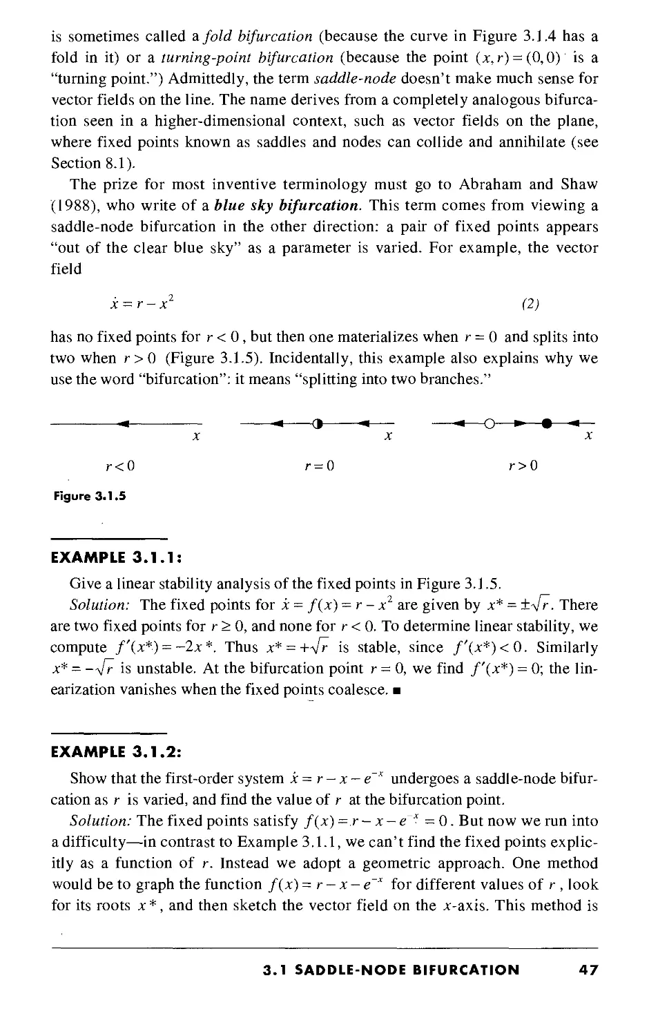
3.0 Introduction 44
3.1 Saddle-Node Bifurcation 45
3.2 Transcritical Bifurcation 50
3.3 Laser Threshold 53
3.4 Pitchfork Bifurcation 55
3.5 Overdamped Bead on a Rotating Hoop 61
CONTENTS

3.6 Imperfect Bifurcations and Catastrophes 69
3.7 Insect Outbreak 73
Exercises 79
4. Flows on the Circle 93
4.0 Introduction 93
4.1 Examples and Definitions 93
4.2 Uniform Oscillator 95
4.3 Nonuniform Oscillator 96
4.4 Overdamped Pendulum 101
4.5 Fireflies 103
4.6 Superconducting Josephson Junctions 106
Exercises 113
Part II. Two-Dimensional Flovs^s
5. Linear Systems 123
5.0 Introduction 123
5.1 Definitions and Examples 123
5.2 Classification of Linear Systems 129
5.3 Love Affairs 138
Exercises 140
6. Phase Plane 145
6.0 Introduction 145
6.1 Phase Portraits 145
6.2 Existence, Uniqueness, and Topological Consequences 148
6.3 Fixed Points and Linearization 150
6.4 Rabbits versus Sheep 155
6.5 Conservative Systems 159
6.6 Reversible Systems 163
6.7 Pendulum 168
6.8 Index Theory 174
Exercises 181
7. Limit Cycles 196
7.0 Introduction 196
7.1 Examples 197
7.2 Ruling Out Closed Orbits 199
7.3 Poincare-Bendixson Theorem 203
7.4 Lienard Systems 210
7.5 Relaxation Oscillators 211
7.6 Weakly Nonlinear Oscillators 215
Exercises 227
CONTENTS

8. Bifurcations Revisited 241
8.0 Introduction 241
8.1 Saddle-Node, Transcritical,
and Pitchfork Bifurcations 241
8.2 Hopf Bifurcations 248
8.3 Oscillating Chemical Reactions 254
8.4 Global Bifurcations of Cycles 260
8.5 Hysteresis in the Driven Pendulum and Josephson Junction 265
8.6 Coupled Oscillators and Quasiperiodicity 273
8.7 Poincare Maps 278
Exercises 284
Part III. Chaos
9. Lorenz Equations 301
9.0 Introduction 301
9.1 A Chaotic Waterwheel 302
9.2 Simple Properties of the Lorenz Equations 311
9.3 Chaos on a Strange Attractor 317
9.4 Lorenz Map 326
9.5 Exploring Parameter Space 330
9.6 Using Chaos to Send Secret Messages 335
Exercises 341
10. One-Dimensional Maps 348
10.0 Introduction 348
10.1 Fixed Points and Cobwebs 349
10.2 Logistic Map; Numerics 353
10.3 Logistic Map: Analysis 357
10.4 Periodic Windows 361
10.5 Liapunov Exponent 366
10.6 Universality and Experiments 369
10.7 Renormalization 379
Exercises 388
11. Fractals 398
.0 Introduction 398
. 1 Countable and Uncountable Sets 399
.2 Cantor Set 401
.3 Dimension of Self-Similar Fractals 404
.4 Box Dimension 409
.5 Pointwise and Correlation Dimensions 411
Exercises 416
CONTENTS

12. Strange Attractors 423
12.0 Introduction 423
12.1 The Simplest Examples 423
12.2 HenonMap 429
12.3 Rossler System 434
12.4 Chemical Chaos and Attractor Reconstruction 437
12.5 Forced Double-Well Oscillator 441
Exercises 448
Answers to Selected Exercises 455
References 465
Author Index 475
Subject Index 478
CONTENTS

PREFACE
This textbook is aimed at newcomers to nonlinear dynamics and chaos, especially
students taking a first course in the subject. It is based on a one-semester course
I've taught for the jjast several years at MIT and Cornell. My goal is to explain the
mathematics as clearly as possible, and to show how it can be used to understand
some of the wonders of the nonlinear world.
The mathematical treatment is friendly and informal, but still careful.
Analytical methods, concrete examples, and geometric intuition are stressed. The theory is
developed systematically, starting with first-order differential equations and their
bifurcations, followed by phase plane analysis, limit cycles and their bifurcations,
and culminating with the Lorenz equations, chaos, iterated maps, period doubling,
renormalization, fractals, and strange attractors.
A unique feature of the book is its emphasis on applications. These include
mechanical vibrations, lasers, biological rhythms, superconducting circuits, insect
outbreaks, chemical oscillators, genetic control systems, chaotic waterwheels, and
even a technique for using chaos to send secret messages. In each case, the
scientific background is explained at an elementary level and closely integrated with
the mathematical theory.
Prerequisites
The essential prerequisite is single-variable calculus, including
curve-sketching, Taylor series, and separable differential equations. In a few places, multivari-
able calculus (partial derivatives, Jacobian matrix, divergence theorem) and linear
algebra (eigenvalues and eigenvectors) are used. Fourier analysis is not assumed,
and is developed where needed. Introductory physics is used throughout. Other
scientific prerequisites would depend on the applications considered, but in all
cases, a first course should be adequate preparation.
PREFACE

Possible Courses
The book could be used for several types of courses:
• A broad introduction to nonlinear dynamics, for students with no prior
exposure to the subject. (This is the kind of course I have taught.) Here one goes
straight through the whole book, covering the core material at the beginning
of each chapter, selecting a few applications to discuss in depth and giving
light treatment to the more advanced theoretical topics or skipping them
altogether. A reasonable schedule is seven weeks on Chapters 1-8, and five or six
weeks on Chapters 9-12. Make sure there's enough time left in the semester
to get to chaos, maps, and fractals.
• A traditional course on nonlinear ordinary differential equations, but with
more emphasis on applications and less on perturbation theory than usual.
Such a course would focus on Chapters 1-8.
• A modern course on bifurcations, chaos, fractals, and their applications, for
students who have already been exposed to phase plane analysis. Topics
would be selected mainly from Chapters 3, 4, and 8-12.
For any of these courses, the students should be assigned homework from the
exercises at the end of each chapter. They could also do computer projects; build
chaotic circuits and mechanical systems; or look up some of the references to get a
taste of current research. This can be an exciting course to teach, as well as to take.
I hope you enjoy it.
Conventions
Equations are numbered consecutively within each section. For instance, when
we're working in Section 5.4, the third equation is called C) or Equation C), but
elsewhere it is called E.4.3) or Equation E.4.3). Figures, examples, and exercises
are always called by their full names, e.g.. Exercise 1.2.3. Examples and proofs
end with a loud thump, denoted by the symbol ■.
Ackno>vledgments
Thanks to the National Science Foundation for financial support. For help with
the book, thanks to Diana Dabby, Partha Saha, and Shinya Watanabe (students);
Jihad Touma and Rodney Worthing (teaching assistants); Andy Christian, Jim
Crutchfield, Kevin Cuomo, Frank DeSimone, Roger Eckhardt, Dana Hobson, and
Thanos Siapas (for providing figures); Bob Devaney, Irv Epstein, Danny Kaplan,
Willem Malkus, Charlie Marcus, Paul Matthews, Arthur Mattuck, Rennie Mirollo,
Peter Renz, Dan Rockmore, Gil Strang, Howard Stone, John Tyson, Kurt Wiesen-
PREFACE

feld, Art Winfree, and Mary Lou Zeeman (friends and colleagues who gave advice);
and to my editor Jack Repcheck, Lynne Reed, Production Supervisor, and all the
other helpful people at Perseus Books. Finally, thanks to my family and Elisabeth
for their love and encouragement.
Steven H. Strogatz
Cambridge, Massachusetts
PREFACE

OVERVIEW
1.0 chaos. Fractals, and Dynamics
There is a tremendous fascination today with chaos and fractals. James Gleick's
book Chaos (Gleick 1987) was a bestseller for months—an amazing
accomplishment for a book about mathematics and science. Picture books like The Beauty of
Fractals by Peitgen and Richter A986) can be found on coffee tables in living
rooms everywhere. It seems that even nonmathematical people are captivated by
the infinite patterns found in fractals (Figure 1.0.1). Perhaps most important of all,
chaos and fractals represent hands-on mathematics that is alive and changing. You
can turn on a home computer and create stunning mathematical images that no one
has ever seen before.
The aesthetic appeal of chaos
and fractals may explain why so
many people have become
intrigued by these ideas. But maybe
you feel the urge to go deeper—to
learn the mathematics behind the
pictures, and to see how the ideas
can be applied to problems in
science and engineering. If so, this is
a textbook for you.
The style of the book is
informal (as you can see), with an
emphasis on concrete examples and
geometric thinking, rather than
proofs and abstract arguments. It is
also an extremely "applied"
1.0 CHAOS, FRACTALS, AND DYNAMICS
•.'■.
^■* "^
■ -■■■,'-.:*
■■"■ " ■ ■■■• .
■ ■■rr- vj-f-'
^''
■ ^»
/ > ^ . ^%^•
Figure 1.0.1
.-■■
-
:
■■"■■ :r:^-
■*

book—virtually every idea is illustrated by some application to science or
engineering. In many cases, the applications are drawn from the recent research
literature. Of course, one problem with such an applied approach is that not everyone is
an expert in physics and biology and fluid mechanics... so the science as well as
the mathematics will need to be explained from scratch. But that should be fun,
and it can be instructive to see the connections among different fields.
Before we start, we should agree about something; chaos and fractals are part of
an even grander subject known as dynamics. This is the subject that deals with
change, with systems that evolve in time. Whether the system in question settles
down to equilibrium, keeps repeating in cycles, or does something more
complicated, it is dynamics that we use to analyze the behavior. You have probably been
exposed to dynamical ideas in various places—in courses in differential equations,
classical mechanics, chemical kinetics, population biology, and so on. Viewed
from the perspective of dynamics, all of these subjects can be placed in a common
framework, as we discuss at the end of this chapter.
Our study of dynamics begins in earnest in Chapter 2. But before digging in, we
present two overviews of the subject, one historical and one logical. Our treatment
is intuitive; careful definitions will come later. This chapter concludes with a
"dynamical view of the world," a framework that will guide our studies for the rest of
the book.
1.1 Capsule History of Dynomics
Although dynamics is an interdisciplinary subject today, it was originally a branch
of physics. The subject began in the mid-1600s, when Newton invented
differential equations, discovered his laws of motion and universal gravitation, and
combined them to explain Kepler's laws of planetary motion. Specifically, Newton
solved the two-body problem—the problem of calculating the motion of the earth
around the sun, given the inverse-square law of gravitational attraction between
them. Subsequent generations of mathematicians and physicists tried to extend
Newton's analytical methods to the three-body problem (e.g., sun, earth, and
moon) but curiously this problem turned out to be much more difficult to solve.
After decades of effort, it was eventually realized that the three-body problem was
essentially impossible to solve, in the sense of obtaining explicit formulas for the
motions of the three bodies. At this point the situation seemed hopeless.
The breakthrough came with the work of Poincare in the late 1800s. He
introduced a new point of view that emphasized qualitative rather than quantitative
questions. For example, instead of asking for the exact positions of the planets at
all times, he asked "Is the solar system stable forever, or will some planets
eventually fly off to infinity?" Poincare developed a powerful geometric approach to
analyzing such questions. That approach has flowered into the modern subject of
dynamics, with applications reaching far beyond celestial mechanics. Poincare
OVERVIEW

was also the first person to glimpse the possibility of chaos, in which a
deterministic system exhibits aperiodic behavior that depends sensitively on the initial
conditions, thereby rendering long-term prediction impossible.
But chaos remained in the background in the first half of this century; instead
dynamics was largely concerned with nonlinear oscillators and their applications
in physics and engineering. Nonlinear oscillators played a vital role in the
development of such technologies as radio, radar, phase-locked loops, and lasers. On the
theoretical side, nonlinear oscillators also stimulated the invention of new
mathematical techniques—pioneers in this area include van der Pol, Andronov, Little-
wood, Cartwright, Levinson, and Smale. Meanwhile, in a separate development,
Poincare's geometric methods were being extended to yield a much deeper
understanding of classical mechanics, thanks to the work of Birkhoff and later Kol-
mogorov, Arnol'd, and Moser.
The invention of the high-speed computer in the 1950s was a watershed in
the history of dynamics. The computer allowed one to experiment with
equations in a way that was impossible before, and thereby to develop some intuition
about nonlinear systems. Such experiments led to Lorenz's discovery in 1963 of
chaotic motion on a strange attractor. He studied a simplified model of
convection rolls in the atmosphere to gain insight into the notorious unpredictability of
the weather. Lorenz found that the solutions to his equations never settled down
to equilibrium or to a periodic state—instead they continued to oscillate in an
irregular, aperiodic fashion. Moreover, if he started his simulations from two
slightly different initial conditions, the resulting behaviors would soon become
totally different. The implication was that the system was inherently
unpredictable—tiny errors in measuring the current state of the atmosphere (or any
other chaotic system) would be amplified rapidly, eventually leading to
embarrassing forecasts. But Lorenz also showed that there was structure in the
chaos—when plotted in three dimensions, the solutions to his equations fell
onto a butterfly-shaped set of points (Figure 1.1.1). He argued that this set had
to be "an infinite complex of surfaces"—today we would regard it as an
example of a fractal.
Lorenz's work had little impact until the 1970s, the boom years for chaos. Here
are some of the main developments of that glorious decade. In 1971 Ruelle and Tak-
ens proposed a new theory for the onset of turbulence in fluids, based on abstract
considerations about strange attractors. A few years later. May found examples of
chaos in iterated mappings arising in population biology, and wrote an influential
review article that stressed the pedagogical importance of studying simple nonlinear
systems, to counterbalance the often misleading linear intuition fostered by
traditional education. Next came the most surprising discovery of all, due to the physicist
Feigenbaum. He discovered that there are certain universal laws governing the
transition from regular to chaotic behavior; roughly speaking, completely different
systems can go chaotic in the same way. His work established a link between chaos and
1.1 CAPSULE HISTORY OF DYNAMICS

Figure 1.1.1
phase transitions, and enticed a generation of physicists to the study of dynamics.
Finally, experimentalists such as Gollub, Libchaber, Swinney, Linsay, Moon, and
Westervelt tested the new ideas about chaos in experiments on fluids, chemical
reactions, electronic circuits, mechanical oscillators, and semiconductors.
Although chaos stole the spotlight, there were two other major developments in
dynamics in the 1970s. Mandelbrot codified and popularized fractals, produced
magnificent computer graphics of them, and showed how they could be applied in
a variety of subjects. And in the emerging area of mathematical biology, Winfree
applied the geometric methods of dynamics to biological oscillations, especially
circadian (roughly 24-hour) rhythms and heart rhythms.
By the 1980s many people were working on dynamics, with contributions too
numerous to list. Table 1.1.1 summarizes this history.
1.2 The Importance of Being Nonlinear
Now we turn from history to the logical structure of dynamics. First we need to
introduce some terminology and make some distinctions.
OVERVIEW

1666
1700s
1800s
1890s
1920-1950
1920-1960
1963
1970s
1980s
Dynamics
Newton
Poincarfi
Birkhoff
Kolmogorov
Amol'd
Moser
Lorenz
Ruelle &Takens
May
Feigenbaum
Winfree
Mandelbrot
- A Capsule History
Invention of calculus, explanation of planetary motion
Flowering of calculus and classical mechanics
Analytical studies of planetary motion
Geometric approach, nightmares of chaos
Nonlinear oscillators in physics and engineering,
invention of radio, radar, laser
Complex behavior in Hamiltonian mechanics
Strange attractor in simple model of convection
Turbulence and chaos
Chaos in logistic map
Universality and renormalization, connection between
chaos and phase transitions
Experimental studies of chaos
Nonlinear oscillators in biology
Fractals
Widespread interest in chaos, fractals, oscillators,
and their applications
Table 1.1.1
There are two main types of dynamical systems: differential equations and
iterated maps (also known as difference equations). Differential equations describe
the evolution of systems in continuous time, whereas iterated maps arise in
problems where time is discrete. Differential equations are used much more widely in
science and engineering, and we shall therefore concentrate on them. Later in the
book we will see that iterated maps can also be very useful, both for providing
simple examples of chaos, and also as tools for analyzing periodic or chaotic solutions
of differential equations.
Now confining our attention to differential equations, the main distinction is
between ordinary and partial differential equations. For instance, the equation for a
damped harmonic oscillator
' dt^
, dx , ^
dt
A)
1.2 THE IMPORTANCE OF BEING NONLINEAR

is an ordinary differential equation, because it involves only ordinary derivatives
dxidt and d^xldr . That is, there is only one independent variable, the time t. In
contrast, the heat equation
du _ d^u
is a partial differential equation—it has both time t and space x as independent
variables. Our concern in this book is with purely temporal behavior, and so we
deal with ordinary differential equations almost exclusively.
A very general framework for ordinary differential equations is provided by the
system
\ B)
i„=/,(X|, ...,x„).
Here the overdots denote differentiation with respect to t. Thus x- = dx/ jdt. The
variables x,, ... ,x„ mightrepresentconcentrationsof chemicals in a reactor,
populations of different species in an ecosystem, or the positions and velocities of the planets
in the solar system. The functions /j, ..., /, are determined by the problem at hand.
For example, the damped oscillator A) can be rewritten in the form of B),
thanks to the following trick: we introduce new variables x^= x and x, = i. Then
ii = ^2, from the definitions, and
from the definitions and the governing equation A). Hence the equivalent system
B) is
^2
h
Xo ,n X,
This system is said to be linear, because all the x, on the right-hand side appear
to the first power only. Otherwise the system would be nonlinear. Typical
nonlinear terms are products, powers, and functions of the x-, such as x^X2 , (x^f, or
cos x^ ■
For example, the swinging of a pendulum is governed by the equation
x + f sinx = 0,
where x is the angle of the pendulum from vertical, g is the acceleration due to
gravity, and L is the length of the pendulum. The equivalent system is nonlinear:
OVERVIEW

^2 =-xSinX|.
Nonlinearity makes the pendulum equation very difficult to solve analytically.
The usual way around this is to fudge, by invoking the small angle approximation
sinx » X for x «l. This converts the problem to a linear one, which can then be
solved easily. But by restricting to small x, we're throwing out some of the
physics, like motions where the pendulum whirls over the top. Is it really necessary
to make such drastic approximations?
It turns out that the pendulum equation can be solved analytically, in terms of
elliptic functions. But there ought to be an easier way. After all, the motion of the
pendulum is simple: at low energy, it swings back and forth, and at high energy it
whirls over the top. There should be some way of extracting this information from
the system directly. This is the sort of problem we'll learn how to solve, using
geometric methods.
Here's the rough idea. Suppose we happen to know a solution to the
pendulum system, for a particular initial condition. This solution would be a pair of
functions X|(f) and XjCf), representing the position and velocity of the
pendulum. If we construct an abstract space with coordinates (x^Xj), then the
solution (x,(f), x^it)) corresponds to a point moving along a curve in this space
(Figure 1.2.1).
Figure 1.2.1
This curve is called a trajectory, and the space is called the phase space for the
system. The phase space is completely filled with trajectories, since each point can
serve as an initial condition.
Our goal is to run this construction in reverse: given the system, we want to
1.2 THE IMPORTANCE OF BEING NONLINEAR

draw the trajectories, and thereby extract information about the solutions. In many
cases, geometric reasoning will allow us to draw the trajectories without actually
solving the systeml
Some terminology: the phase space for the general system B) is the space with
coordinates x,,..., x„. Because this space is n-dimensional, we will refer to B) as
an n-dimensional system or an nth-order system. Thus n represents the
dimension of the phase space.
Nonautonomous Systems
You might worry that B) is not general enough because it doesn't include any
explicit time dependence. How do we deal with time-dependent or nonautonomous
equations like the forced harmonic oscillator mx + bx + kx = Fcostl In this case too
there's an easy trick that allows us to rewrite the system in the form B). We let x, = x
and Xj = i as before but now we introduce x^=t. Then i, = 1 and so the equivalent
system is
X| X2
X2 =-j;;[-he, - bx2+ Fcosx^) C)
ij = 1
which is an example of a f/zree-dimensional system. Similarly, an nth-order time-
dependent equation is a special case of an (n-i-1 )-dimensional system. By this
trick, we can always remove any time dependence by adding an extra dimension to
the system.
The virtue of this change of variables is that it allows us to visualize a phase
space with trajectories/rozen in it. Otherwise, if we allowed explicit time
dependence, the vectors and the trajectories would always be wiggling—this would ruin
the geometric picture we're trying to build. A more physical motivation is that the
state of the forced harmonic oscillator is truly three-dimensional: we need to know
three numbers, x, x, and t, to predict the future, given the present. So a three-
dimensional phase space is natural.
The cost, however, is that some of our terminology is nontraditional. For
example, the forced harmonic oscillator would traditionally be regarded as a second-
order linear equation, whereas we will regard it as a third-order nonlinear system,
since C) is nonlinear, thanks to the cosine term. As we'll see later in the book,
forced oscillators have many of the properties associated with nonlinear systems,
and so there are genuine conceptual advantages to our choice of language.
Why Are Nonlinear Problems So Hard?
As we've mentioned earlier, most nonlinear systems are impossible to solve
analytically. Why are nonlinear systems so much harder to analyze than linear ones?
The essential difference is that linear systems can be broken down into parts. Then
OVERVIEW

each part can be solved separately and finally recombined to get the answer. This
idea allows a fantastic simplification of complex problems, and underlies such
methods as normal modes, Laplace transforms, superposition arguments, and Fourier
analysis. In this sense, a linear system is precisely equal to the sum of its parts.
But many things in nature don't act this way. Whenever parts of a system
interfere, or cooperate, or compete, there are nonlinear interactions going on. Most of
everyday life is nonlinear, and the principle of superposition fails spectacularly. If
you listen to your two favorite songs at the same time, you won't get double the
pleasure! Within the realm of physics, nonlinearity is vital to the operation of a laser, the
formation of turbulence in a fluid, and the superconductivity of Josephson junctions.
1.3 A Dynamical Vievs^ of the World
Now that we have established the ideas of nonlinearity and phase space, we can
present a framework for dynamics and its applications. Our goal is to show the
logical structure of the entire subject. The framework presented in Figure 1.3.1 will
guide our studies thoughout this book.
The framework has two axes. One axis tells us the number of variables needed
to characterize the state of the system. EquJ^valently, this number is the dimension
of the phase space. The other axis tells us whether the system is linear or
nonlinear.
For example, consider the exponential growth of a population of organisms.
This system is described by the first-order differential equation
x-rx
where x is the population at time t and r is the growth rate. We place this system
in the column labeled "n = 1" because one piece of information—the current value
of the population x—is sufficient to predict the population at any later time. The
system is also classified as linear because the differential equation x = rx is linear
in X.
As a second example, consider the swinging of a pendulum, governed by
x-hf sinx = 0.
In contrast to the previous example, the state of this system is given by two
variables: its current angle x and angular velocity x. (Think of it this way: we need
the initial values of both x and x to determine the solution uniquely. For example,
if we knew only x, we wouldn't know which way the pendulum was swinging.)
Because two variables are needed to specify the state, the pendulum belongs in the
n = 2 column of Figure 1.3.1. Moreover, the system is nonlinear, as discussed in
the previous section. Hence the pendulum is in the lower, nonlinear half of the
n = 2 column.
1.3 A DYNAMICAL VIEW OF THE WORLD

Number of variables
(Q
C
Linear
53
o
Nonlinear
n=l
Growth, decay, or
equilibrium
Exponential growth
RC circuit
Radioactive decay
Fixed points
Bifurcations
Overdamped systems,
relaxational dynamics
Logistic equation
for single species
n = 2
Oscillations
Linear oscillator
Mass and spring
RLC circuit
2-body problem
(Kepler, Newton)
Pendulum
Anharmonic oscillators
Limit cycles
Biological oscillators
(neurons, heart cells)
Predator-prey cycles
Nonlinear electronics
(van der Pol, Josephson)
n>3
Civil engineering.
structures
Electrical engineering
Thefr
Chaos
Strange attractors
(Lorenz)
3-body problem (PoincarS)
Chemical kinetics
Iterated maps (Feigenbaum)
Fractals
(Mandelbrot)
Forced nonlinear oscillators
(Levinson, Smale)
1 Practical uses of chaos
Quantum chaos ?
1
n» 1
Collective phenomena
Coupled harmonic oscillators
Solid-state physics
Molecular dynamics
Equilibrium statistical
mechanics
ontier
Coupled nonlinear oscillators
Lasers, nonlinear optics
Nonequilibrium statistical
mechanics
Nonlinear solid-state physics
(semiconductors)
Josephson arrays
Heart cell synchronization
Neiu"al networks
Immune system
Ecosystems
Economics
Continuum
Waves and patterns
Elasticity
Wave equations
Electromagnetism (Maxwell)
Quantum mechanics
(SchrBdinger, Heisenberg, Dirac)
Heat and diffusion
Acoustics
Viscous fluids
Spatio-temporal complexity
Nonlinear waves (shocks, solitons)
Plasmas
Earthquakes
General relativity (Einstein)
Quantum field theory
Reaction-diffusion,
biological and chemical waves
Fibrillation
Epilepsy
Turbulent fluids (Navier-Stokes)
Life

One can continue to classify systems in this way, and the result will be
something like the framework shown here. Admittedly, some aspects of the picture are
debatable. You might think that some topics should be added, or placed
differently, or even that more axes are needed—the point is to think about classifying
systems on the basis of their dynamics.
There are some striking patterns in Figure 1.3.1. All the simplest systems occur
in the upper left-hand corner. These are the small linear systems that we learn
about in the first few years of college. Roughly speaking, these linear systems
exhibit growth, decay, or equilibrium when n = 1, or oscillations when n = 2 . The
italicized phrases in Figure 1.3.1 indicate that these broad classes of phenomena
first arise in this part of the diagram. For example, an RC circuit has n = 1 and
cannot oscillate, whereas an RLC circuit has n = 2 and can oscillate.
The next most familiar part of the picture is the upper right-hand corner. This is
the domain of classical applied mathematics and mathematical physics where the
linear partial differential equations live. Here we find Maxwell's equations of
electricity and magnetism, the heat equation, Schrodinger's wave equation in quantum
mechanics, and so on. These partial differential equations involve an infinite
"continuum" of variables because each point in space contributes additional degrees of
freedom. Even though these systems are large, they are tractable, thanks to such
linear techniques as Fourier analysis and transform methods.
In contrast, the lower half of Figure 1.3.1—the nonlinear half—is often ignored
or deferred to later courses. But no more! In this book we start in the lower left
corner and systematically head to the right. As we increase the phase space dimension
from n = 1 to n = 3, we encounter new phenomena at every step, from fixed points
and bifurcations when n = 1, to nonlinear oscillations when n = 2 , and finally
chaos and fractals when n = 3 . In all cases, a geometric approach proves to be very
powerful, and gives us most of the information we want, even though we usually
can't solve the equations in the traditional sense of finding a formula for the
answer. Our journey will also take us to some of the most exciting parts of modern
science, such as mathematical biology and condensed-matter physics.
You'll notice that the framework also contains a region forbiddingly marked
"The frontier." It's like in those old maps of the world, where the mapmakers
wrote, "Here be dragons" on the unexplored parts of the globe. These topics are
not completely unexplored, of course, but it is fair to say that they lie at the limits
of current understanding. The problems are very hard, because they are both large
and nonlinear. The resulting behavior is typically complicated in both space and
time, as in the motion of a turbulent fluid or the patterns of electrical activity in a
fibrillating heart. Toward the end of the book we will touch on some of these
problems—they will certainly pose challenges for years to come.
1.3 A DYNAMICAL VIEW OF THE WORLD 1 1

ONE-DIMENSIONAL FLOWS

FLOWS ON THE LINE
2.0 Introduction
In Chapter 1, we introduced the general system
i, =/,U,, ...,xj
and mentioned that its solutions could be visualized as trajectories flowing through
an n-dimensional phase space with coordinates (x,, ... ,x^). At the moment, this
idea probably strikes you as a mind-bending abstraction. So let's start slowly,
beginning here on earth with the simple case n = 1. Then we get a single equation of
the form
x=fix).
Here x(f) is a real-valued function of time t, and f{x) is a smooth real-valued
function of x. We'll call such equations one-dimensional or first-order systems.
Before there's any chance of confusion, let's dispense with two fussy points of
terminology:
1. The word system is being used here in the sense of a dynamical system,
not in the classical sense of a collection of two or more equations. Thus
a single equation can be a "system."
2. We do not allow / to depend explicitly on time. Time-dependent or
"nonautonomous" equations of the form x = fix,t) are more
complicated, because one needs two pieces of information, x and f, to predict
the future state of the system. Thus x = fix,t) should really be
regarded as a two-dimensional or second-order system, and will
therefore be discussed later in the book.
2.0 INTRODUCTION 15

2.1 A Geometric Way of Thinking
Pictures are often more helpful than formulas for analyzing nonlinear systems.
Here we illustrate this point by a simple example. Along the way we will introduce
one of the most basic techniques of dynamics: interpreting a differential equation
as a vector field.
Consider the following nonlinear differential equation:
i = sinx. {1}
To emphasize our point about formulas versus pictures, we have chosen one of the
few nonlinear equations that can be solved in closed form. We separate the
variables and then integrate:
dx
dt = ,
smx
which implies
t = CSC X dx
■In cscx+cotx + C.
To evaluate the constant C, suppose that x= x^ at f = 0. Then C = In | esc x^^ + cot x^, |.
Hence the solution is
f = ln
cscx + cotx
B)
This result is exact, but a headache to interpret. For example, can you answer
the following questions?
1. Suppose Xfy = KJA-; describe the qualitative features of the solution x{t)
for all f > 0. In particular, what happens as f ^ °° ?
2. For an arbitrary initial condition x^,, what is the behavior of x{t) as
Think about these questions for a while, to see that formula B) is not transparent.
In contrast, a graphical analysis of A) is clear and simple, as shown in Figure
2.1.1. We think of t as time, x as the position of an imaginary particle moving
along the real line, and x as the velocity of that particle. Then the differential
equation i = sinx represents a vector field on the line: it dictates the velocity
vector X at each x. To sketch the vector field, it is convenient to plot x versus x, and
then draw arrows on the x-axis to indicate the corresponding velocity vector at
each X. The arrows point to the right when i > 0 and to the left when i < 0.
16 FLOWS ON THE LINE

In
Figure 2.1.1
Here's a more physical way to think about the vector field: imagine that fluid
is flowing steadily along the x-axis with a velocity that varies from place to
place, according to the rule i= sinx. As shown in Figure 2.1.1, theyZow is to the
right when i > 0 and to the left when i < 0. At points where i = 0, there is no
flow; such points are therefore called fixed points. You can see that there are two
kinds of fixed points in Figure 2.1.1: solid black dots represent stable fixed
points (often called attractors or sinks, because the flow is toward them) and
open circles represent unstable fixed points (also known as repellers or
sources).
Armed with this picture, we can now easily understand the solutions to the
differential equation x = sin x. We just start our imaginary particle at Xg and watch
how it is carried along by the flow.
This approach allows us to answer the questions above as follows:
1. Figure 2.1.1.shows that a particle starting at Xg = ;r/4 moves to the
right faster and faster until it crosses x = ;r/2 (where sinx reaches its
maximum). Then the particle starts slowing down and eventually
approaches the stable fixed point x = ;r from the left. Thus, the
qualitative form of the solution is as shown in Figure 2.1.2.
Note that the curve is concave up at first, and then concave down;
this corresponds to the initial acceleration for x < nil, followed by the
deceleration toward x = k.
2. The same reasoning applies to any initial condition x^. Figure 2.1.1
shows that if i > 0 initially, the particle heads to the right and
asymptotically approaches the nearest
stable fixed point. Similarly, if
i < 0 initially, the particle
approaches the nearest stable fixed
point to its left. If i = 0, then x
remains constant. The qualitative
form of the solution for any
initial condition is sketched in
Figure 2.1.3.
Figure 2.1.2
2.1 A GEOMETRIC WAY OF THINKING
17

2k
-In
Figure 2.1.3
In all honesty, we should admit that a picture can't tell us certain quantitative
things: for instance, we don't know the time at which the speed | i | is greatest. But in
many cases qualitative information is what we care about, and then pictures are fine.
2.2 Fixed Points and Stability
The ideas developed in the last section can be extended to any one-dimensional
system x = f(x). We just need to draw the graph of f{x) and then use it to sketch
the vector field on the real line (the x-axis in Figure 2.2.1).
Figure 2.2.1
18
FLOWS ON THE LINE

As before, we imagine that a fluid is flowing along the real line with a local
velocity f{x). This imaginary fluid is called the phase fluid, and the real line is the
phase space. The flow is to the right where f{x) > 0 and to the left where f(x) < 0.
To find the solution to i = f(x) starting from an arbitrary initial condition x^, we
place an imaginary particle (known as a phase point) at x^ and watch how it is
carried along by the flow. As time goes on, the phase point moves along the x-axis
according to some function x{t). This function is called the trajectory based at Xg,
and it represents the solution of the differential equation starting from the initial
condition x^. A picture like Figure 2.2.1, which shows all the qualitatively
different trajectories of the system, is called a phase portrait.
The appearance of the phase portrait is controlled by the fixed points x*,
defined by fix*) = 0 ; they correspond to stagnation points of the flow. In Figure
2.2.1, the solid black dot is a stable fixed point (the local flow is toward it) and the
open dot is an unstable fixed point (the flow is away from it).
In terms of the original differential equation, fixed points represent
equilibrium solutions (sometimes called steady, constant, or rest solutions, since if
x = X* initially, then x{t) = x* for all time). An equilibrium is defined to be
stable if all sufficiently small disturbances away from it damp out in time. Thus
stable equilibria are represented geometrically by stable fixed points. Conversely,
unstable equilibria, in which disturbances grow in time, are represented by
unstable fixed points.
EXAMPLE 2.2.1:
Find all fixed points for i = x^ -1, and classify their stability.
Solution: Here f{x) = x^ -\. To find the fixed points, we set f{x*) = 0 and
solve for X *. Thus x* = ±\. To determine stability, we plot x^ -1 and then sketch
the vector field (Figure 2.2.2). The flow is to the right where x^ -1 > 0 and to the
left where x^ -1 < 0. Thus x* = -\ is stable, and x* = \ is unstable. ■
Figure 2.2.2
2.2 FIXED POINTS AND STABILITY
19

Note that the definition of stable equilibrium is based on small disturbances;
certain large disturbances may fail to decay. In Example 2.2.1, all small
disturbances to X* = -l will decay, but a large disturbance that sends x to the right of
X = 1 will not decay—in fact, the phase point will be repelled out to +°° . To
emphasize this aspect of stability, we sometimes say that x* = -1 is locally stable, but
not globally stable.
R
C
Vn
EXAMPLE 2.2.2:
Consider the electrical circuit shown in Figure 2.2.3. A resistor R and a
capacitor C are in series with a battery of constant dc voltage VJ,. Suppose that the switch
is closed at r = 0, and that there is no charge on the capacitor initially. Let Q(t) de-
T note the charge on the capacitor at time
t>0. Sketch the graph of Q{t).
Solution: This type of circuit problem
is probably familiar to you. It is governed
by linear equations and can be solved
analytically, but we prefer to illustrate the
geometric approach.
First we write the circuit equations. As
we go around the circuit, the total voltage
"^^ drop must equal zero; hence -Vg +
Figure 2.2.3 RI + Q/C = 0, where / is the current
flowing through the resistor. This current causes charge to accumulate on the
capacitor at a rate Q = I. Hence
-V„+RQ + Q/C = 0 or
The graph of fiQ) is a straight line with a negative slope (Figure 2.2.4). The
corresponding vector field has a fixed point where fiQ) = 0, which occurs at
Q* = CVf,. The flow is to the right where
fiQ) > 0 and to the left where fiQ) < 0.
Thus the flow is always toward Q *—it is a
stable fixed point. In fact, it is globally
stable, in the sense that it is approached from
all initial conditions.
To sketch Qit), we start a phase point at
the origin of Figure 2.2.4 and imagine how
it would move. The flow carries the phase
point monotonically toward Q*. Its speed
Figure 2.2.4
20
FLOWS ON THE LINE

Q decreases linearly as it approaches the fixed point; therefore Q{t) is increasing
and concave down, as shown in Figure 2.2.5. ■
EXAMPLE 2.2.3:
Sketch the phase portrait
corresponding to X = X-cosX, and
determine the stability of all the fixed points.
Solution: One approach would be to
plot the function f(x) = x - cos x and
then sketch the associated vector field.
This method is valid, but it requires you
to figure out what the graph of
x-cosx looks like.
There's an easier solution, which exploits the fact that we know how to graph
y = x and y = cosx separately. We plot both graphs on the same axes and then
observe that they intersect in exactly one point (Figure 2.2.6).
Figure 2.2.5
y=x
y = cos X
Figure 2.2.6
This intersection corresponds to a fixed point, since x* = cos x * and therefore
/(x*) = 0. Moreover, when the line lies above the cosine curve, we have x > cos x
and so i > 0: the flow is to the right. Similarly, the flow is to the left where the line is
below the cosine curve. Hence x * is the only fixed point, and it is unstable. Note that
we can classify the stability of x *, even though we don't have a formula for x *
itself! ■
2.3 Population Grovs^th
The simplest model for the growth of a population of organisms is A^ = rN,
where N(t) is the population at time t, and r > 0 is the growth rate. This model
2.3 POPULATION GROWTH
21

Growth rate
Figure 2.3.1
predicts exponential growth:
A''@ = N^e", where A^^ is the
population at r = 0.
Of course such exponential
growth cannot go on forever.
To model the effects of
overcrowding and limited resources,
population biologists and
demographers often assume that
the per capita growth rate NJN
decreases when A^ becomes sufficiently large, as shown in Figure 2.3.1. For
small A^, the growth rate equals r, just as before. However, for populations larger
than a certain carrying capacity
Growth rate K, the growth rate actually
becomes negative; the death rate is
higher than the birth rate.
A mathematically convenient
way to incorporate these ideas is
to assume that the per capita
growth rate nIn decreases
linearly with N (Figure 2.3.2).
Figure 2.3.2
This leads to the logistic equation
A^'
A^ = rA^ 1-
K
first suggested to describe the growth of human populations by Verhulst in 1838.
This equation can be solved analytically (Exercise 2.3.1) but once again we prefer a
graphical approach. We plot A^ versus A^ to see what the vector field looks like.
Note that we plot only N>0, since it makes no sense to think about a negative
population (Figure 2.3.3). Fixed points occur at A^* = 0 and A^* = K, as found by
setting A^ = 0 and solving for A^. By looking at the flow in Figure 2.3.3, we see that
N* = 0 is an unstable fixed point and N* = K is a stable fixed point. In biological
terms, A^ = 0 is an unstable equilibrium: a small population will grow
exponentially fast and run away from A^ = 0 . On the other hand, if A^ is disturbed slightly
from K, the disturbance will decay monotonically and N(t) —> K as t —> o°.
In fact. Figure 2.3.3 shows that if we start a phase point at any Nf, > 0, it will
always flow toward N = K. Hence the population always approaches the carrying
capacity.
The only exception is if A^^ = 0; then there's nobody around to start reproducing,
and so N = 0 for all time. (The model does not allow for spontaneous generation!)
22
FLOWS ON THE LINE

N
Figure 2.3.3
Figure 2.3.3 also allows us to deduce the qualitative shape of the solutions. For
example, if A^^ < K/2, the phase point moves faster and faster until it crosses
A^ = K/2, where the parabola in Figure 2.3.3 reaches its maximum. Then the phase
point slows down and eventually creeps toward N = K. In biological terms, this
means that the population initially grows in an accelerating fashion, and the graph
of N{t) is concave up. But after A^ = K/2, the derivative A^ begins to decrease,
and so N(t) is concave down as it asymptotes to the horizontal line N = K (Figure
2.3.4). Thus the graph of A'^@ is S-shaped or sigmoid for A^^ < K/2.
N
K
K/2-
Figure 2.3.4
Something qualitatively different occurs if the initial condition A^^, lies between
K/2 and K; now the solutions are decelerating from the start. Hence these
solutions are concave down for all t. If the population initially exceeds the carrying
capacity (N„> K), then N(t) decreases toward N = K and is concave up. Finally, if
Ng=0 or Ng = K, then the population stays constant.
Critique of the Logistic Model
Before leaving this example, we should make a few comments about the biological
validity of the logistic equation. The algebraic form of the model is not to be taken
literally. The model should really be regarded as a metaphor for populations that have a
2.3 POPULATIOM GROWTH
23

tendency to grow from zero population up to some carrying capacity K.
Originally a much stricter interpretation was proposed; and the model was
argued to be a universal law of growth (Pearl 1927). The logistic equation was tested
in laboratory experiments in which colonies of bacteria, yeast, or other simple
organisms were grown in conditions of constant climate, food supply, and absence of
predators. For a good review of this literature, see Krebs A972, pp. 190-200).
These experiments often yielded sigmoid growth curves, in some cases with an
impressive match to the logistic predictions.
On the other hand, the agreement was much worse for fruit flies, flour beetles,
and other organisms that have complex life cycles, involving eggs, larvae, pupae,
and adults. In these organisms, the predicted asymptotic approach to a steady
carrying capacity was never observed—instead the populations exhibited large,
persistent fluctuations after an initial period of logistic growth. See Krebs A972) for a
discussion of the possible causes of these fluctuations, including age structure and
time-delayed effects of overcrowding in the population.
For further reading on population biology, see Pielou A969) or May A981).
Edelstein-Keshet A988) and Murray A989) are excellent textbooks on
mathematical biology in general.
2.4 Linear Stability Analysis
So far we have relied on graphical methods to determine the stability of fixed
points. Frequently one would like to have a more quantitative measure of stability,
such as the rate of decay to a stable fixed point. This sort of information may be
obtained by linearizing about a fixed point, as we now explain.
Let X* be a fixed point, and let r}{t) = x{t)-x* be a small perturbation away
from X *. To see whether the perturbation grows or decays, we derive a differential
equation for ry. Differentiation yields
since x * is constant. Thus rj = x = f{x) = f{x *+ rj). Now using Taylor's
expansion we obtain
fix * + ry) = fix*) + rif'ix*) + Oirj'),
where 0(r/^) denotes quadratically small terms in rj. Finally, note that fix*) = 0
since x * is a fixed point. Hence
rj = rif'ix*)+ OiT).
Now if fix*) ^ 0, the 0(r/^) terms are negligible and we may write the
approximation
24 FLOWS ON THE LINE

This is a linear equation in ry, and is called the linearization about x *. It shows
that the perturbation r\{t) grows exponentially if f'(x*) > 0 and decays if
f'(x*)<0. If f'(x*) = 0, the O(ri^) terms are not negligible and a nonlinear
analysis is needed to determine stability, as discussed in Example 2.4.3 below.
The upshot is that the slope f'{x*) at the fixed point determines its stability. If
you look back at the earlier examples, you'll see that the slope was always
negative at a stable fixed point. The importance of the sign of f'{x*) was clear from
our graphical approach; the new feature is that now we have a measure of how
stable a fixed point is—that's determined by the magnitude of f'{x*). This
magnitude plays the role of an exponential growth or decay rate. Its reciprocal 1/|/'(a:*)|
is a characteristic time scale; it determines the time required for x{t) to vary
significantly in the neighborhood of x*.
EXAMPLE 2.4.1:
Using linear stability analysis, determine the stability of the fixed points for
i = sinx.
Solution: The fixed points occur where f{x) = sin x = 0. Thus x* = kK , where
k is an integer. Then
r I, k even
f'(x*) = cos kTT = <
' [-1, k odd.
Hence x * is unstable if k is even and stable if k is odd. This agrees with the
results shown in Figure 2.1.1. ■
EXAMPLE 2.4.2:
Classify the fixed points of the logistic equation, using linear stability analysis,
and find the characteristic time scale in each case.
Solution: Here fiN) = rN{l-f), with fixed points A^* = 0 and A^* = K. Then
fXN) = r-^ and so /'(O) = r and f'(K) = -r . Hence A^* = 0 is unstable and
N* = K is stable, as found earlier by graphical arguments. In either case, the
characteristic time scale is l/|/'(A^*)| = I/r . ■
EXAMPLE 2.4.3:
What can be said about the stability of a fixed point when f'(x*) = 0?
Solution: Nothing can be said in general. The stability is best determined on a
case-by-case basis, using graphical methods. Consider the following examples:
(a) X = -x' (b) x = x^ (c) x = x^ (d) i: = 0
2.4 LINEAR STABILITY ANALYSIS 25

Each of these systems has a fixed point x* = 0 with f'{x*) = 0. However the
stability is different in each case. Figure 2.4.1 shows that (a) is stable and (b) is
unstable. Case (c) is a hybrid case we'll call half-stable, since the fixed point is
attracting from the left and repelling from the right. We therefore indicate this type
of fixed point by a half-filled circle. Case (d) is a whole line of fixed points;
perturbations neither grow nor decay.
Figure 2.4.1
These examples may seem artificial, but we will see that they arise naturally in the
context of bifurcations—more about that later. ■
2.5 Existence and Uniqueness
Our treatment of vector fields has been very informal. In particular, we have taken
a cavalier attitude toward questions of existence and uniqueness of solutions to
26
FLOWS ON THE LINE

the system x = f{x). That's in keeping with the "applied" spirit of this book.
Nevertheless, we should be aware of what can go wrong in pathological cases.
EXAMPLE 2.5.1:
Show that the solution to i = x"^ starting from Xg=0 is not unique.
Solution: The point x = 0 is a fixed point, so one obvious solution is x{t) = 0
for all t. The surprising fact is that there is another solution. To find it we separate
variables and integrate:
jx-"^d^ = j
dt
so
-x^'^=t + C. Imposing the initial condition x@) = 0 yields C = 0. Hence
•^@ = (fO is also a solution! ■
When uniqueness fails, our geometric approach collapses because the phase
point doesn't know how to move; if a phase point were started at the origin, would
it stay there or would it move according to x{t) = {-jt) ? (Or as my friends in
elementary school used to say when discussing the problem of the irresistible force
and the immovable object, perhaps the phase point would explode!)
Actually, the situation in Example 2.5.1 is even worse than we've let on—there
are infinitely many solutions starting from the same initial condition (Exercise
2.5.4).
What's the source of the non-uniqueness?
A hint comes from looking at the vector field
(Figure 2.5.1). We see that the fixed point
X* = Q is very unstable—the slope /'(O) is
infinite.
Chastened by this example, we state a
theorem that provides sufficient conditions for
existence and uniqueness of solutions to i = fix).
Figure 2.5.1
Existence and Uniqueness Theorem: Consider the initial value problem
X = fix), x@) = Xo .
Suppose that fix) and fix) are continuous on an open interval R of the x-axis,
and suppose that x^y is a point in R. Then the initial value problem has a solution
xit) on some time interval (-t,t) about ^ = 0, and the solution is unique.
For proofs of the existence and uniqueness theorem, see Borrelli and Coleman
A987), Lin and Segel A988), or virtually any text on ordinary differential equations.
This theorem says that if fix) is smooth enough, then solutions exist and are
unique. Even so, there's no guarantee that solutions exist forever, as shown by the
2.5 EXISTENCE AND UNIQUENESS
27

next example.
EXAMPLE 2.5.2:
Discuss the existence and uniqueness of solutions to the initial value problem
x = l + x^, x@) = X(,. Do solutions exist for all time?
Solution: Here f{x) = l + x^. This function is continuous and has a continuous
derivative for all X. Hence the theorem tells us that solutions exist and are unique for any
initial condition Xg. But the theorem does not say that the solutions exist for all time;
they are only guaranteed to exist in a (possibly very short) time interval around t = 0.
For example, consider the case where x@) = 0. Then the problem can be solved
analytically by separation of variables:
which yields
tan"' x = t + C
The initial condition x@) = 0 implies C = 0. Hence x(t) = ta.nt is the solution.
But notice that this solution exists only for - ;r/2 < / < ;r/2 , because x{t) -^ +oo as
t -^ ±nl2. Outside of that time interval, there is no solution to the initial value
problem for X(, = 0. ■
The amazing thing about Example 2.5.2 is that the system has solutions that
reach infinity infinite time. This phenomenon is called blow-up. As the name
suggests, it is of physical relevance in models of combustion and other runaway
processes.
There are various ways to extend the existence and uniqueness theorem. One
can allow / to depend on time /, or on several variables x,, ... ,x„. One of the
most useful generalizations will be discussed later in Section 6.2.
From now on, we will not worry about issues of existence and uniqueness—our
vector fields will typically be smooth enough to avoid trouble. If we happen to
come across a more dangerous example, we'll deal with it then.
2.6 Impossibility of Oscillotions
Fixed points dominate the dynamics of first-order systems. In all our examples so
far, all trajectories either approached a fixed point, or diverged to ±°°. In fact,
those are the only things that can happen for a vector field on the real line. The
reason is that trajectories are forced to increase or decrease monotonically, or remain
constant (Figure 2.6.1). To put it more geometrically, the phase point never
reverses direction.
28 FLOWS ON THE LINE

Figure 2.6.1
Thus, if a fixed point is regarded as an equilibrium solution, the approach to
equilibrium is always monotonic—overshoot and damped oscillations can never
occur in a first-order system. For the same reason, undamped oscillations are
impossible. Hence there are no periodic solutions to x = f{x).
These general results are fundamentally topological in origin. They reflect the
fact that x = f{x) corresponds to flow on a line. If you flow monotonically on a
line, you'll never come back to your starting place—that's why periodic solutions
are impossible. (Of course, if we were dealing with a circle rather than a line, we
could eventually return to our starting place. Thus vector fields on the circle can
exhibit periodic solutions, as we discuss in Chapter 4.)
Mechanical Analog: Overdamped Systems
It may seem surprising that solutions to i = f{x) can't oscillate. But this result
becomes obvious if we think in terms of a mechanical analog. We regard x = f{x) as a
limiting case of Newton's law, in the limit where the "inertia term" mx is negligible.
For example, suppose a mass m is attached to a nonlinear spring whose
restoring force is F{x), where x is the displacement from the origin. Furthermore,
suppose that the mass is immersed in a vat of very viscous fluid, like honey or motor
oil (Figure 2.6.2), so that it is subject to a damping force bx . Then Newton's law is
mx + bx = F{x).
, honey if the viscous damping is strong compared
a' Irsj to the inertia term {bx»mx), the system
should behave like bx = F{x), or equivalently
x = f{x), where f{x) = b~^F{x). In this over-
damped limit, the behavior of the mechanical
system is clear. The mass prefers to sit at a
stable equilibrium, where f{x) = 0 and fix) < 0.
If displaced a bit, the mass is slowly dragged
back to equilibrium by the restoring force. No overshoot can occur, because the
damping is enormous. And undamped oscillations are out of the question! These
conclusions agree with those obtained earlier by geometric reasoning.
F{x)
Figure 2.6.2
2.6 IMPOSSIBILITY OF OSCILLATIONS
29

Actually, we should confess that this argument contains a slight swindle. The
neglect of the inertia term mx is valid, but only after a rapid initial transient during
which the inertia and damping terms are of comparable size. An honest discussion
of this point requires more machinery than we have available. We'll return to this
matter in Section 3.5.
2.7 Potentials
There's another way to visualize the dynamics of the first-order system x = f{x),
based on the physical idea of potential energy. We picture a particle sliding down
the walls of a potential well, where the.potential V{x) is defined by
ax
As before, you should imagine that the particle is heavily damped—its inertia is
completely negligible compared to the damping force and the force due to the
potential. For example, suppose that the particle has to slog through a thick layer of
goo that covers the walls of the potential (Figure 2.7.1).
Figure 2.7.1
The negative sign in the definition of V follows the standard convention in
physics; it implies that the particle always moves "downhill" as the motion
proceeds. To see this, we think of x as a function of t, and then calculate the time-
derivative of V{x{t)). Using the chain rule, we obtain
dV _ dV dx
dt dx dt
Now for a first-order system.
30
FLOWS ON THE LINE

dx _ dV
dt dx
since x = f(x) = - dV/dx, by the definition of the potential. Hence,
<0.
dy___fdV\^
dt \dx J
Thus V(t) decreases along trajectories, and so the particle always moves toward
lower potential. Of course, if the particle happens to be at an equilibrium point
where dV/dx = 0, then V remains constant. This is to be expected, since
dV/dx = 0 implies x=0; equilibria occur at the fixed points of the vector field.
Note that local minima of V(x) correspond to stable fixed points, as we'd expect
intuitively, and local maxima correspond to unstable fixed points.
V{x)
EXAMPLE 2.7.1:
Graph the potential for the system x = -x, and identify all the equilibrium
points.
Solution: We need to find V{x) such that
-dV/dx = -x. The general solution is V{x) =
\x^ +C, where C is an arbitrary constant. (It always
happens that the potential is only defined up to an
additive constant. For convenience, we usually choose
C = 0.) The graph of V{x) is shown in Figure 2.7.2.
K The only equilibrium point occurs at x= 0, and it's
stable. ■
Figure 2.7.2
EXAMPLE 2.7.2:
Graph the potential for the system x= x-x^, and identify all equilibrium
points.
Solution: Solving -dV/dx = x- x' yields
V = -\x^ +\x^ +C. Once again we set C = 0.
Figure 2.7.3 shows the graph of Y. The local minima at
x = ±\ correspond to stable equilibria, and the local
maximum at x = 0 corresponds to an unstable
equilibrium. The potential shown in Figure 2.7.3 is often
called a double-well potential, and the system is said
to be bistable, since it has two stable equilibria. ■
Figure 2.7.3
2.7 POTENTIALS
31

2.8 Solving Equations on the Computer
Throughout this chapter we have used graphical and analytical methods to analyze
first-order systems. Every budding dynamicist should master a third tool:
numerical methods. In the old days, numerical methods were impractical because they
required enormous amounts of tedious hand-calculation. But all that has changed,
thanks to the computer. Computers enable us to approximate the solutions to
analytically intractable problems, and also to visualize those solutions. In this section
we take our first look at dynamics on the computer, in the context of numerical
integration of i = f{x).
Numerical integration is a vast subject. We will barely scratch the surface. See
Chapter 15 of Press et al. A986) for an excellent treatment.
Euler's Method
The problem can be posed this way: given the differential equation x = f{x),
subject to the condition x= Xg at t = tg, find a systematic way to approximate the
solution x(t).
Suppose we use the vector field interpretation of i = f{x). That is, we think of a
fluid flowing steadily on the x-axis, with velocity f{x) at the location x. Imagine
we're riding along with a phase point being carried downstream by the fluid.
Initially we're at Xg, and the local velocity is fixg). If we flow for a short time At,
we'll have moved a distance f{xg)At, because distance = rate x time . Of course,
that's not quite right, because our velocity was changing a little bit throughout the
step. But over a sufficiently small step, the velocity will be nearly constant and our
approximation should be reasonably good. Hence our new position x{tg + At) is
approximately Xg + f{Xg)At. Let's call this approximation x,. Thus
X{tg+At)'-X^=Xg+fiXg)At.
Now we iterate. Our approximation has taken us to a new location x,; our new
velocity is /(x,); we step forward to ^2 = x, + /(x, )Atr, and so on. In general, the
update rule is
x„^i=x„+f{x„)At.
This is the simplest possible numerical integration scheme. It is known as Euler's
method.
Euler's method can be visualized by plotting x versus t (Figure 2.8.1). The
curve shows the exact solution x{t), and the open dots show its values x(/„) at the
discrete times r„ = tg +nAt. The black dots show the approximate values given by
the Euler method. As you can see, the approximation gets bad in,a hurry unless A;
is extremely small. Hence Euler's method is not recommended in practice, but it
contains the conceptual essence of the more accurate methods to be discussed next.
32 FLOWS ON THE LINE

X(ti)
Euler
exact
Figure 2.8.1
Refinements
One problem with the Euler method is that it estimates the derivative only at
the left end of the time interval between r„ and /„^.,. A more sensible approach
would be to use the average derivative across this interval. This is the idea behind
the improved Euler method. We first take a trial step across the interval, using the
Euler method. This produces a trial value x,,^., = x„ + /(x„ )At; the tilde above the
X indicates that this is a tentative step, used only as a probe. Now that we've
estimated the derivative on both ends of the interval, we average /(x„) and /(x,,^.,),
and use that to take the real step across the interval. Thus the improved Euler
method is
x,.^i = x„ + fix„)At
x,„^ = x..+i[fix,.) + fCx,„,)]At.
(the trial step)
(the real step)
This method is more accurate than the Euler method, in the sense that it tends to
make a smaller error £ = |x(r„)-x,J for a given stepsize At. In both cases, the
error £ ^ 0 as A; ^ 0 , but the error decreases faster for the improved Euler
method. One can show that E °^ At for the Euler method, but E oc (At)^ for the
improved Euler method (Exercises 2.8.7 and 2.8.8). In the jargon of numerical
analysis, the Euler method is first order, whereas the improved Euler method is second
order.
Methods of third, fourth, and even higher orders have been concocted, but you
should realize that higher order methods are not necessarily superior. Higher order
methods require more calculations and function evaluations, so there's a
computational cost associated with them. In practice, a good balance is achieved by the
fourth-order Runge-Kutta method. To find x,,^, in terms of x„, this method first
requires us to calculate the following four numbers (cunningly chosen, as you'll
see in Exercise 2.8.9):
2.8 SOLVING EQUATIONS ON THE COMPUTER
33

k,=fix„+^k,)At
'^3=fix„+jk2)At
k, = f{x„+k,)At.
Then x^^., is given by
This method generally gives accurate results without requiring an excessively
small stepsize A;. Of course, some problems are nastier, and may require small
steps in certain time intervals, while permitting very large steps elsewhere. In such
cases, you may want to use a Runge-Kutta routine with an automatic stepsize
control; see Press et al. A986) for details.
Now that computers are so fast, you may wonder why we don't just pick a tiny
At once and for all. The trouble is that excessively many computations will occur,
and each one carries a penalty in the form of round-off error. Computers don't
have infinite accuracy—they don't distinguish between numbers that differ by
some small amount 5. For numbers of order 1, typically 5 ~10~^ for single
precision and 5 ~ 10~'* for double precision. Round-off error occurs during every
calculation, and will begin to accumulate in a serious way if At is too small. See
Hubbard and West A991) for a good discussion.
Practical Matters
You have several options if you want to solve differential equations on the
computer. If you like to do things yourself, you can write your own numerical
integration routines, and plot the results using whatever graphics facilities are available.
The information given above should be enough to get you started. For further
guidance, consult Press et al. A986); they provide sample routines written in Fortran,
C, and Pascal.
A second option is to use existing packages for numerical methods. The
software libraries by IMSL and NAG have a wide variety of state-of-the-art numerical
integrators. These libraries are well documented, reliable, and flexible, and can be
found at most university computing centers or networks. The packages Matlab,
Mathematica, and Maple are more interactive and also have programs for solving
ordinary differential equations.
The final option is for people who want to explore dynamics, not computing.
Dynamical systems software has recently become available for personal
computers. All you have to do is type in the equations and the parameters; the program
solves the equations numerically and plots the results. Some recommended
programs are Phaser (Kocak 1989) for the IBM PC or MacMath (Hubbard and West
34 FLOWS OM THE LIME

1992) for the Macintosh. MacMath was used to generate many of the plots in this
book.
These programs are easy to use, and they will help you build intuition about
dynamical systems.
EXAMPLE 2.8.1:
Use MacMath to solve the system x = x{\- x) numerically.
Solution: This is a logistic equation (Section 2.3) with parameters r = 1, K = \.
Previously we gave a rough sketch of the solutions, based on geometric arguments;
now we can draw a more quantitative picture.
As a first step, we plot the slope field for the system in the {t,x) plane (Figure
2.8.2). Here the equation x = x(l- x) is being interpreted in a new way. for each
point {t, x), the equation gives the slope dx/dt of the solution passing through that
point. The slopes are indicated by little line segments in Figure 2.8.2.
] \ \ \ \M \M \ \ i i \M
\ \ \ \ \ \ \ \ \ \ \ \ \ \
■\ \ \ \ \ \ \ \ \ \ \ \ \ \
■yyyyyyyyyyyyyy
yyyyyyyyyyyyyy
I I I
I I I
I I I I I I
-< t
10
Figure 2.8.2
Finding a solution now becomes a problem of drawing a curve that is always
tangent to the local slope. Figure 2.8.3 shows four solutions starting from various
points in the (r, x) plane.
0 5 10
Figure 2.8.3
These numerical solutions were computed using the Runge-Kutta method with a
2.8 SOLVING EQUATIONS ON THE COMPUTER
35

stepsize Ar = 0.1. The solutions have the shape expected from Section 2.3. ■
Computers are indispensable for studying dynamical systems. We will use them
liberally throughout this book, and you should do likewise.
EXERCISES FOR CHAPTER 2
2.1 A Geometric Way of Thinking
In the next three exercises, interpret i = sin x as a flow on the line.
2.1.1 Find all the fixed points of the flow.
2.1.2 At which points x does the flow have greatest velocity to the right?
2.1.3
a) Find the flow's acceleration ir as a function of x.
b) Find the points where the flow has maximum positive acceleration.
2.1.4 (Exact solution of i = sin x) As shown in the text, i = sin x has the
solution r = ln|(cscX(,+cotX(,)/(cscx + cotx)|, where X(, = x@) is the initial value
of X.
a) Given the specific initial condition x^ = njA, show that the solution above can
be inverted to obtain
x@=2tan
-I
1 + V2
Conclude that x{t) -^n as r ^ co ^ as claimed in Section 2.1. (You need to be good
with trigonometric identities to solve this problem.)
b) Try to find the analytical solution for x(t), given an arbitrary initial condition
x^.
2.1.5 (A mechanical analog)
a) Find a mechanical system that is approximately governed by i = sin x.
b) Using your physical intuition, explain why it now becomes obvious that x* = 0
is an unstable fixed point and x* = n is stable.
2.2 Fixed Points and Stability
Analyze the following equations graphically. In each case, sketch the vector field
on the real line, find all the fixed points, classify their stability, and sketch the
graph of x(t) for different initial conditions. Then try for a few minutes to obtain
the analytical solution for x(t); if you get stuck, don't try for too long since in
several cases it's impossible to solve the equation in closed form!
36 FLOWS ON THE LINE

2.2.1 i = 4x'-16
2.2.3 x = x-x^
2.2.5 i = l+4-cosx
2.2.2
2.2.4
2.2.6
i = l-x'^
X = e' sin x
i = 1 - 2 cos X
2.2.7 i = e"" - cos x (Hint: Sketch the graphs of e"" and cos x on the same
axes, and look for intersections. You won't be able to find the fixed points
explicitly, but you can still find the qualitative behavior.)
2.2.8 (Working backwards, from flows to equations) Given an equation x = f{x),
we know how to sketch the corresponding flow on the real line. Here you are asked
to solve the opposite problem: For the phase portrait shown in Figure 1, find an
equation that is consistent with it. (There are an infinite number of correct
answers—and wrong ones too.)
► €>-
-1
Figure 1
-o
2
2.2.9 (Backwards again, now from solutions to equations) Find an equation
X = f{x) whose solutions x{t) are consistent with those shown in Figure 2.
Figure 2
—^2.2.10 (Fixed points) For each of (a)-(e), find an equation x = f(x) with the
stated properties, or if there are no examples, explain why not. (In all cases,
assume that f{x) is a smooth function.)
a) Every real number is a fixed point.
b) Every integer is a fixed point, and there are no others.
c) There are precisely three fixed points, and all of them are stable.
d) There are no fixed points.
e) There are precisely 100 fixed points.
2.2.11 (Analytical solution for charging capacitor) Obtain the analytical solu-
V Q
tion of the initial value problem Q = -^ , with B@) = 0, which arose in
R RC
Example 2.2.2.
2.2.12 (A nonlinear resistor) Suppose the resistor in Example 2.2.2 is replaced
by a nonlinear resistor. In other words, this resistor does not have a linear
EXERCISES
37

8iV)
Figure 3
relation between voltage and current. Such non-
linearity arises in certain solid-state devices.
Instead of /^ = V/R, suppose we have /^ = g{V),
where g(V) has the shape shown in Figure 3.
Redo Example 2.2.2 in this case. Derive the
circuit equations, find all the fixed points, and
analyze their stability. What qualitative effects does
the nonlinearity introduce (if any)?
2.2.13 (Terminal velocity) The velocity v{t) of a skydiver falling to the ground
is governed by mv = mg~kv^, where m is the mass of the skydiver, g is the
acceleration due to gravity, and k>0 is a constant related to the amount of air
resistance.
a) Obtain the analytical solution for v(t), assuming that v@) = 0.
b) Find the limit of v{t) as t ^>°° . This limiting velocity is called the terminal
velocity. (Beware of bad jokes about the word terminal and parachutes that fail to open.)
c) Give a graphical analysis of this problem, and thereby re-derive a formula for
the terminal velocity.
d) An experimental study (Carlson et al. 1942) confirmed that the equation
mv = mg~kv^ gives a good quantitative fit to data on human skydivers. Six
men were dropped from altitudes varying from 10,600 feet to 31,400 feet to a
terminal altitude of 2,100 feet, at which they opened their parachutes. The long
free fall from 31,400 to 2,100 feet took 116 seconds. The average weight of the
men and their equipment was 261.2 pounds. In these units, g = 32.2 ft/sec^.
Compute the average velocity V .
e) Using the data given here, estimate the terminal velocity, and the value of the
drag constant k. (Hints: First you need to find an exact formula for s{t), the
distance fallen, where i'@) = 0, s-v, and v{t) is known from part (a). You
should get i'@ =-y-In fcosh ^), where V is the terminal velocity. Then solve
for y graphically or numerically, using i'= 29,300, r = 116, and g = 32.2.)
A slicker way to estimate V is to suppose V ~ V^^^, as a rough first
approximation. Then show that gt/V ~ 15 . Since gt/V » 1, we may use the
approximation In (cosh x)« X - In 2 for x»l. Derive this approximation and then
use it to obtain an analytical estimate of V. Then k follows from part (b). This
analysis is from Davis A962).
2.3 Population Grovs^th
2.3.1 (Exact solution of logistic equation) There are two ways to solve the
logistic equation A^ = rN(l - N/K) analytically for an arbitrary initial condition A^^,.
38
FLOWS ON THE LINE

a) Separate variables and integrate, using partial fractions.
b) Make the change of variables x = l/N. Then derive and solve the resulting
differential equation for x.
2.3.2 (Autocatalysis) Consider the model chemical reaction
in which one molecule of X combines with one molecule of A to form two
molecules of X. This means that the chemical X stimulates its own production, a process
called autocatalysis. This positive feedback process leads to a chain reaction, which
eventually is limited by a "back reaction" in which 2X returns to A + X.
According to the law of mass action of chemical kinetics, the rate of an
elementary reaction is proportional to the product of the concentrations of the reactants.
We denote the concentrations by lowercase letters x = [X] and a = [A]. Assume
that there's an enormous surplus of chemical A, so that its concentration a can be
regarded as constant. Then the equation for the kinetics of x is
X — KfClX fC_iX
where k^ and A: , are positive parameters called rate constants.
a) Find all the fixed points of this equation and classify their stability.
b) Sketch the graph of x{t) for various initial values Xg.
2.3.3 (Tumor growth) The growth of cancerous tumors can be modeled by the
Gompertz law A^ = ~aN \n{bN), where N{t) is proportional to the number of cells
in the tumor, and a,b> 0 are parameters.
a) Interpret a and b biologically.
b) Sketch the vector field and then graph N(t) for various initial values.
The predictions of this simple model agree surprisingly well with data on tumor
growth, as long as A^ is not too small; see Aroesty et al. A973) and Newton A980)
for examples.
>2.3.4 (The Allee effect) For certain species of organisms, the effective growth
rate n/n is highest at intermediate A^. This is the called the Allee effect (Edel-
stein-Keshet 1988). For example, imagine that it is too hard to find mates when A^
is very small, and there is too much competition for food and other resources when
A^ is large.
a) Show that n/n-r-a(N-b)^ provides an example of Allee effect, if r, a,
and b satisfy certain constraints, to be determined.
b) Find all the fixed points of the system and classify their stability.
c) Sketch the solutions N{t) for different initial conditions.
d) Compare the solutions N{t) to those found for the logistic equation. What are
the qualitative differences, if any?
EXERCISES 39

2.4 Linear Stability Analysis
Use linear stability analysis to classify the fixed points of the following systems. If
linear stability analysis fails because fix*) - 0, use a graphical argument to
decide the stability.
2.4.1 x = x{\-x) 2.4.2 x = x{\-x)(l-x)
2.4.3 i = tanx 2.4.-4 i = x^F-x)
2
2.4.5 x-\-e " 2.4.6 x-Vax
2.4.7 X- ax- x^, where a can be positive, negative, or zero. Discuss all three
cases.
2.4.8 Using linear stability analysis, classify the fixed points of the Gompertz
model of tumor growth A^ = ~aN\n{bN). (As in Exercise 2.3.3, N(t) is
proportional to the number of cells in the tumor and a,b>0 are parameters.)
2.4.9 (Critical slowing down) In statistical mechanics, the phenomenon of
"critical slowing down" is a signature of a second-order phase transition. At the
transition, the system relaxes to equilibrium much more slowly than usual. Here's
a mathematical version of the effect:
a) Obtain the analytical solution to i: = -x^ for an arbitrary initial condition.
Show that x{t) -^0 as t ^>o°, but that the decay is not exponential. (You
should find that the decay is a much slower algebraic function of t.)
b) To get some intuition about the slowness of the decay, make a numerically
accurate plot of the solution for the initial condition X(, = 10, for 0 < r < 10. Then,
on the same graph, plot the solution to i: = -x for the same initial condition.
2.5 Existence and Uniqueness
2.5.1 (Reaching a fixed point in a finite time) A particle travels on the half-line
x>0 with a velocity given by i = -x', where c is real and constant.
a) Find all values of c such that the origin x = 0 is a stable fixed point.
b) Now assume that c is chosen such that x = 0 is stable. Can the particle ever
reach the origin in a finite time? Specifically, how long does it take for the
particle to travel from x = 1 to x = 0, as a function of c ?
2.5.2 ("Blow-up": Reaching infinity in a finite time) Show that the solution to
x = l + x'° escapes to +o° in a finite time, starting from any initial condition.
(Hint: Don't try to find an exact solution; instead, compare the solutions to those of
x = l + x\)
2.5.3 Consider the equation x = rx + x^, where r > 0 is fixed. Show that
x{t) -^ +00 in finite time, starting from any initial condition x^, ^ 0.
2.5.4 (Infinitely many solutions with the same initial condition) Show that the
initial value problem x = x"', x@) = 0, has an infinite number of solutions. (Hint:
40 FLOWS ON THE LINE

Construct a solution that stays at x = 0 until some arbitrary time t^, after which it
takes off.)
2.5.5 (A general example of non-uniqueness) Consider the initial value
problem i = |x| '''"^ , x@) = 0, where p and q are positive integers with no common
factors.
a) Show that there are an infinite number of solutions if p<q.
b) Show that there is a unique solution if p> q.
2.5.6 (The leaky bucket) The following example (Hubbard and West 1991,
p. 159) shows that in some physical situations, non-uniqueness is natural and
obvious, not pathological.
Consider a water bucket with a hole in the bottom. If you see an empty bucket
with a puddle beneath it, can you figure out when the bucket was full? No, of
course not! It could have finished emptying a minute ago, ten minutes ago, or
whatever. The solution to the corresponding differential equation must be non-
unique when integrated backwards in time.
Here's a crude model of the situation. Let h{t) - height of the water remaining
in the bucket at time t; a = area of the hole; A = cross-sectional area of the bucket
(assumed constant); v(t) = velocity of the water passing through the hole.
a) Show that av{t) = Ah{t). What physical law are you invoking?
b) To derive an additional equation, use conservation of energy. First, find the
change in potential energy in the system, assuming that the height of the water
in the bucket decreases by an amount Ah and that the water has density p.
Then find the kinetic energy transported out of the bucket by the escaping
water. Finally, assuming all the potential energy is converted into kinetic energy,
derive the equation v^ = 2gh.
c) Combining (b) and (c), show h - -C4h, where C = ^/2g (f).
d) Given h{Q) = 0 (bucket empty at r = 0), show that the solution for h{t) is non-
unique in backwards time, i.e., for r < 0.
2.6 Impossibility of Oscillations
2.6.1 Explain this paradox: a simple harmonic oscillator mx - -kx is a system
that oscillates in one dimension (along the x-axis). But the text says
one-dimensional systems can't oscillate.
—^2.6.2 (No periodic solutions to i: = f{x)) Here's an analytic proof that periodic
solutions are impossible for a vector field on a line. Suppose on the contrary that
x(t) is a nontrivial periodic solution, i.e., x(t) = x(t + T) for some r>0, and
x{t) ^ x{t + s) for all 0<s<T. Derive a contradiction by considering
fix)iffdt.
EXERCISES 41

2.7 Potentials
For each of the following vector fields, plot the potential function V{x) and
identify all the equilibrium points and their stability.
2.7.1 x = x(\-x) 2.7.2 i = 3
2.7.3 i = sinx 2.7.4 i = 2 + sinx
2.7.5 i = -sinhx 2.7.6 i = r + x-x^,for various values of r.
2.7.7 (Another proof that solutions to i = f{x) can't oscillate) Let x - f{x) be
a vector field on the line. Use the existence of a potential function V{x) to show
that solutions x{t) cannot oscillate.
2.8 Solving Equations on the Computer
2.8.1 (Slope field) The slope is constant along horizontal lines in Figure 2.8.2.
Why should we have expected this?
2.8.2 Sketch the slope field for the following differential equations. Then
"integrate" the equation manually by drawing trajectories that are everywhere parallel
to the local slope.
a) x-x b) x = \-x^ c) x = \-Ax{\- x) d) i = sinx
—^ 2.8.3 (Calibrating the Euler method) The goal of this problem is to test the
Euler method on the initial value problem x =~x, x{Q) = 1.
a) Solve the problem analytically. What is the exact value of x{\)l
b) Using the Euler method with step size A; = 1, estimate x{\) numerically—call
the result x{\). Then repeat, using Ar = 10 ", for n = 1, 2, 3,4.
c) Plot the error £ = |x(l)-x(l)| as a function of Ar. Then plot In £ vs.
Inr.Explain the results.
' 2.8.4 Redo Exercise 2.8.3, using the improved Euler method.
1^2.8.5 Redo Exercise 2.8.3, using the Runge-Kutta method.
2.8.6 (Analytically intractable problem) Consider the initial value problem
x = x + e\ x{0) = 0. In contrast to Exercise 2.8.3, this problem can't be solved
analytically.
a) Sketch the solution x(t) for r > 0.
b) Using some analytical arguments, obtain rigorous bounds on the value of x at
t = 1. In other words, prove that a < x{l)<b , for a, b to be determined. By
being clever, try to make a and b as close together as possible. (Hint: Bound
the given vector field by approximate vector fields that can be integrated
analytically.)
c) Now for the numerical part: Using the Euler method, compute x at r = 1,
correct to three decimal places. How small does the stepsize need to be to obtain
the desired accuracy? (Give the order of magnitude, not the exact number.)
42 FLOWS ON THE LINE

d) Repeat part (b), now using the Runge-Kutta method. Compare the results for
stepsizes At-\, Ar = 0.1, and At = 0.01.
\2.8.7/ (Error estimate for Euler method) In this question you'll use Taylor series
expansions to estimate the error in taking one step by the Euler method. The exact
solution and the Euler approximation both start at x = x^ when t = 1^. We want to
compare the exact value x{tf) = x{tg + At) with the Euler approximation
X, = Xo + f{Xf^)At.
a) Expand x{t^)sx{tg + At) as a Taylor series in At, through terms of 0{At^).
Express your answer solely in terms of x^■,, At, and / and its derivatives at x^.
b) Show that the local error |x(r|)-X|| ~ C{At)^ and give an explicit expression
for the constant C. (Generally one is more interested in the global error
incurred after integrating over a time interval of fixed length T = nAt. Since each
step produces an 0{At)' error, and we take n = T/At = 0(Ar') steps, the
global error \x(tj- x„ | is 0{At), as claimed in the text.)
('2.8.8} (Error estimate for the improved Euler method) Use the Taylor series
arguments of Exercise 2.8.7 to show that the local error for the improved Euler
method is O(Ar').
2.8.9 (Error estimate for Runge-Kutta) Show that the Runge-Kutta method
produces a local error of size 0(At ).
(Warning: This calculation involves massive amounts of algebra, but if you do it
correctly, you'll be rewarded by seeing many wonderful cancellations. Teach
yonrseUMathematica, Maple, or some other symbolic manipulation language, and
do the problem on the computer.)
EXERCISES 43

3
BIFURCATIONS
3.0 Introduction
As we've seen in Chapter 2, the dynamics of vector fields on the line is very limited:
all solutions either settle down to equilibrium or head out to ±°°. Given the triviality
of the dynamics, what's interesting about one-dimensional systems? Answer:
Dependence on parameters. The qualitative structure of the flow can change as
parameters are varied. In particular, fixed points can be created or destroyed, or their
stability can change. These qualitative changes in the dynamics are called
bifurcations, and the parameter values at which they occur are called bifurcation points.
Bifurcations are important scientifically—they provide models of transitions
and instabilities as some control parameter is varied. For example, consider the
buckling of a beam. If a small weight is placed on top of the beam in Figure 3.0.1,
the beam can support the load and remain vertical. But if the load is too heavy, the
vertical position becomes unstable, and the beam may buckle.
weight
beam
beam "buckles"
/ / j' / y / / /
Figure 3.0.1
-TT-rrry-r?
Here the weight plays the role of the control parameter, and the deflection of the
beam from vertical plays the role of the dynamical variable x.
AA
BIFURCATIONS

One of the main goals of this book is to help you develop a solid and practical
understanding of bifurcations. This chapter introduces the simplest examples:
bifurcations of fixed points for flows on the line. We'll use these bifurcations to
model such dramatic phenomena as the onset of coherent radiation in a laser and
the outbreak of an insect population. (In later chapters, when we step up to two-
and three-dimensional phase spaces, we'll explore additional types of bifurcations
and their scientific applications.)
We begin with the most fundamental bifurcation of all.
3.1 Saddle-Node Bifurcation
The saddle-node bifurcation is the basic mechanism by which fixed points are
created and destroyed. As a parameter is varied, two fixed points move toward each
other, collide, and mutually annihilate.
The prototypical example of a saddle-node bifurcation is given by the first-
order system
X = r + X
(!)
where r is a parameter, which may be positive, negative, or zero. When r is
negative, there are two fixed points, one stable and one unstable (Figure 3.1.1a).
(a) r<0
(b) r = 0
(c) r>0
Figure 3.1.1
As r approaches 0 from below, the parabola moves up and the two fixed points move
toward each other. When r = 0, the fixed points coalesce into a half-stable fixed point
at X* = 0 (Figure 3.1.1b). This type of fixed point is extremely delicate—it vanishes
as soon as r > 0, and now there are no fixed points at all (Figure 3.1.1c).
In this example, we say that a bifurcation occurred at r = 0, since the vector
fields for r < 0 and r > 0 are qualitatively different.
Graphical Conventions
There are several other ways to depict a saddle-node bifurcation. We can show a
stack of vector fields for discrete values of r (Figure 3.1.2).
3.1 SADDLE-NODE BIFURCATION
45

^>
-o
->0
r=0
r<0
This representation emphasizes the
dependence of the fixed points on r. In
the limit of a continuous stack of vector
fields, we have a picture like Figure
3.1.3. The curve shown is r = -x^, i.e.,
i = 0, which gives the fixed points for
different r. To distinguish between
stable and unstable fixed points, we use
a solid line for stable points and a
broken line for unstable ones.
However, the most common way to
depict the bifurcation is to invert the axes of Figure 3.1.3. The rationale is that r
plays the role of an independent variable, and so should be plotted horizontally
-O
Figure 3.1.2
stable
unstable
Figure 3.1.3
(Figure 3.1.4). The drawback is that now the x-axis has to be plotted vertically,
which looks strange at first. Arrows are sometimes included in the picture, but not
always. This picture is called the
bifurcation diagram for the saddle-
unstable - - _ node bifurcation.
Terminology
Bifurcation theory is rife with
conflicting terminology. The
subject really hasn't settled down yet,
and different people use different
words for the same thing. For
example, the saddle-node bifurcation
stable '
Figure 3.1.4
46
BIFURCATIONS

is sometimes called a fold bifurcation (because the curve in Figure 3.1.4 has a
fold in it) or a turning-point bifurcation (because the point {x,r) = {0,0) is a
"turning point.") Admittedly, the term saddle-node doesn't make much sense for
vector fields on the line. The name derives from a completely analogous
bifurcation seen in a higher-dimensional context, such as vector fields on the plane,
where fixed points known as saddles and nodes can collide and annihilate (see
Section 8.1).
The prize for most inventive terminology must go to Abraham and Shaw
A988), who write of a blue sky bifurcation. This term comes from viewing a
saddle-node bifurcation in the other direction: a pair of fixed points appears
"out of the clear blue sky" as a parameter is varied. For example, the vector
field
x = r-x^ B)
has no fixed points for r < 0, but then one materializes when r = 0 and splits into
two when r>0 (Figure 3.1.5). Incidentally, this example also explains why we
use the word "bifurcation": it means "splitting into two branches."
-* d-
-O-
r<0
Figure 3.1.5
r=0
r>0
EXAMPLE 3.1.1:
Give a linear stability analysis of the fixed points in Figure 3.1.5.
Solution: The fixed points for x = f(x) = r - x^ are given by x* = ±^|r. There
are two fixed points for r > 0, and none for r < 0. To determine linear stability, we
compute f'{x*) = -2x*. Thus x* = -i-4r is stable, since f'{x*)<Q. Similarly
X* = -4r is unstable. At the bifurcation point r = 0, we find f'{x*) = 0; the
linearization vanishes when the fixed points coalesce. ■
EXAMPLE 3.1.2:
Show that the first-order system x = r - x - e'" undergoes a saddle-node
bifurcation as r is varied, and find the value of r at the bifurcation point.
Solution: The fixed points satisfy f{x) =.r — x — e" = 0. But now we run into
a difficulty—in contrast to Example 3.1.1, we can't find the fixed points
explicitly as a function of r. Instead we adopt a geometric approach. One method
would be to graph the function f{x) = r-x-e~^ for different values of r , look
for its roots x *, and then sketch the vector field on the x-axis. This method is
3.1 SADDLE-NODE BIFURCATION
47

fine, but there's an easier way. The point is that the two functions r~x and e^'
have much more familiar graphs than their difference r-x-e'". So we plot
r-x and e'" on the same picture (Figure 3.1.6a). Where the line r-x
intersects the curve e'", we have r- x = e~'' and so f{x) = 0. Thus,
intersections of the line and the curve correspond to fixed points for the system. This
picture also allows us to read off the direction of flow on the x-axis: the flow is
to the right where the line lies above the curve, since r-x> e'" and therefore
i > 0 . Hence, the fixed point on the right is stable, and the one on the left is
unstable.
Now imagine we start decreasing the parameter r. The line r-x slides down
and the fixed points approach each other. At some critical value r = r^, the line
becomes tangent to the curve and the fixed points coalesce in a saddle-node
bifurcation (Figure 3.1.6b). For r below this critical value, the line lies below the curve
and there are no fixed points (Figure 3.1.6c).
(b)
(c)
To find the bifurcation point r^, we impose the condition that the graphs of
r~ X and e'" intersect tangentially. Thus we demand equality of the functions and
their derivatives:
and
jL ff-'' - J.
= ±ir-x).
The second equation implies -e " = -1, so x = 0. Then the first equation yields
r = \. Hence the bifurcation point is r^ = 1 , and the bifurcation occurs at x = 0. ■
Normal Forms
In a certain sense, the examples x = r~ x or x = r + x^ are representative of
all saddle-node bifurcations; that's why we called them "prototypical." The idea is
that, close to a saddle-node bifurcation, the dynamics typically look like x = r- x^
or x = r + x^.
48
BIFURCATIONS

For instance, consider Example 3.1.2 near the bifurcation at x = 0 and r = 1.
Using the Taylor expansion for e~' about x = 0, we find
X = r — x — e
1-X+ — + ■
2!
to leading order in x. This has the same algebraic form as x = r-x^, and can be
made to agree exactly by appropriate rescalings of x and r.
It's easy to understand why saddle-node bifurcations typically have this
algebraic form. We just ask ourselves: how can two fixed points of i: = f{x) collide and
disappear as a parameter r is varied? Graphically, fixed points occur where the
graph of f{x) intersects the x-axis. For a saddle-node bifurcation to be possible, we
need two nearby roots of fix); this means f{x) must look locally "bowl-shaped" or
parabolic (Figure 3.1.7).
f(x) looks
parabolic in here
Figure 3.1.7
Now we use a microscope to zoom in on the behavior near the bifurcation. As r
varies, we see a parabola intersecting the x-axis, then becoming tangent to it, and
then failing to intersect. This is exactly the scenario in the prototypical Figure 3.1.1.
Here's a more algebraic version of the same argument. We regard / as a
function of both X and r , and examine the behavior of i = f{x, r) near the bifurcation
at x = X* and r = r^.. Taylor's expansion yields
x = fix,r)
= f{x*,rj + (x-x*)-:^
dx
U*.r,)
or
(.'C*,r,)
+ iix~x*f^
dx
(x*,r,)
3.1 SADDLE-NODE BIFURCATION
49

where we have neglected quadratic terms in (r - rj and cubic terms in (x - x*). Two
of the terms in this equation vanish: f{x*,r,.) = 0 since x* is a fixed point, and
df/dx\ ^, =0 by the tangency condition of a saddle-node bifurcation. Thus
X = a{r - r^) + b{x — x*)^ + ■
C)
where a = df/dr\^^dindb = \d^fldx^\ ^ . Equation C) agrees with the form of
our prototypical examples. (We are assuming that a,b^O, which is the typical case;
for instance, it would be a very special situation if the second derivative d^f/dx^
also happened to vanish at the fixed point.)
What we have been calling prototypical examples are more conventionally
known as normal forms for the saddle-node bifurcation. There is much, much
more to normal forms than we have indicated here. We will be seeing their
importance throughout this book. For a more detailed and precise discussion, see Guck-
enheimer and Holmes A983) or Wiggins A990).
3.2 Transcritical Bifurcation
There are certain scientific situations where a fixed point must exist for all values
of a parameter and can never be destroyed. For example, in the logistic equation
and other simple models for the growth of a single species, there is a fixed point at
zero population, regardless of the value of the growth rate. However, such a fixed
point may change its stability as the parameter is varied. The transcritical
bifurcation is the standard mechanism for such changes in stability.
The normal form for a transcritical bifurcation is
: rx -
A)
This looks like the logistic equation of Section 2.3, but now we allow x and r to
be either positive or negative.
Figure 3.2.1 shows the vector field as r varies. Note that there is a fixed point at
X* = Q for all values of r.
(a) r<0
Figure 3.2.1
(b) r = 0
(c) r>0
50
BIFURCATIONS

For r < 0, there is an unstable fixed point at x* = r and a stable fixed point at
X* = 0 . As r increases, the unstable fixed point approaches the origin, and
coalesces with it when r = 0 . Finally, when r > 0 , the origin has become unstable,
and x*= r is now stable. Some people say that an exchange of stabilities has
taken place between the two fixed points.
Please note the important difference between the saddle-node and transcritical
bifurcations: in the transcritical case, the two fixed points don't disappear after the
bifurcation—instead they just switch their stability.
Figure 3.2.2 shows the bifurcation diagram for the transcritical bifurcation. As
in Figure 3.1.4, the parameter r is regarded as the independent variable, and the
fixed points x* = 0 and x* = r are shown as dependent variables.
stable
stable ■
unstable
Figure 3.2.2
■ unstable
EXAMPLE 3.2.1:
Show that the first-order system x = x{l-x )-a(l-e *") undergoes a
transcritical bifurcation at x = 0 when the parameters a, b satisfy a certain equation, to
be determined. (This equation defines a bifurcation curve in the {a, b) parameter
space.) Then find an approximate formula for the fixed point that bifurcates from
X = 0, assuming that the parameters are close to the bifurcation curve.
Solution: Note that x = Q is a fixed point for all {a,b). This makes it plausible that
the fixed point will bifurcate transcritically, if it bifurcates at all. For small x, we find
X-e-'" =\-[\-bx + ^b^x^ +0{x'')\
= bx-^b^x^ +0{x')
and so
x = x-a(bx~^b'^x'^) + 0(x^)
= A - ab)x + D- ab^ )x^ +Oix^).
3.2 TRANSCRITICAL BIFURCATION
51

Hence a transcritical bifurcation occurs when ab = l; this is the equation for the
bifurcation curve. The nonzero fixed point is given by the solution of
l-ab + (j;ab^)x »0 , i.e.,
^ 2iab-l)
X*~ 7. .
ab^
This formula is approximately correct only if x * is small, since our series expansions
are based on the assumption of small x. Thus the formula holds only when ab is
close to 1, which means that the parameters must be close to the bifurcation curve. ■
EXAMPLE 3.2.2:
Analyze the dynamics of x = r\nx + x-\ near x = \, and show that the system
undergoes a transcritical bifurcation at a certain value of r. Then find new
variables X and R such that the system reduces to the approximate normal form
X ~ RX - X^ near the bifurcation.
Solution: First note that x = \ is a fixed point for all values of r. Since we are
interested in the dynamics near this fixed point, we introduce a new variable
u = x~\, where u is small. Then
u = X
= rln(l-l-M)-l-M
= r[u--^u^ + 0(u^)j + u
'='(r + l)u-^ru'^ +0(u^).
Hence a transcritical bifurcation occurs at r, = -1.
To put this equation into normal form, we first need to get rid of the coefficient
of u^. Let u = av, where a will be chosen later. Then the equation for v is
v = ir + l)v-i^ra)v^ +Oiv^).
So if we choose a = 2/r, the equation becomes
v = (r-l-l)v-v^-l-0(v').
Now if we let R = r + 1 and X = v, we have achieved the approximate normal
form X~ RX~X^, where cubic terms of order 0{X^) have been neglected. In
terms of the original variables, X = v = uja = \r{x~\).m
To be a bit more accurate, the theory of normal forms assures us that we can
find a change of variables such that the system becomes X = RX- X^, with strict,
rather than approximate, equality. Our solution above gives an approximation to
the necessary change of variables. If we wanted a better approximation, we would
52 BIFURCATIONS

retain the cubic terms in the series expansions (and perhaps even higher-order
terms if we're really feeling heroic) and we would have to do a more elaborate
calculation to eliminate these higher-order terms. See Exercises 3.2.6 and 3.2.7 for a
taste of such calculations, or see the books of Guckenheimer and Holmes A983),
Wiggins A990), or Manneville A990).
3.3 Laser Threshold
Now it's time to apply our mathematics to a scientific example. We analyze an
extremely simplified model for a laser, following the treatment given by Haken A983).
Physical Background
We are going to consider a particular type of laser known as a solid-state laser,
which consists of a collection of special "laser-active" atoms embedded in a solid-
state matrix, bounded by partially reflecting mirrors at either end. An external energy
source is used to excite or "pump" the atoms out of their ground states (Figure 3.3.1).
pump
u u
\
^ N laser light
s active material s^ ^"
mirror
Figure 3.3.1
Each atom can be thought of as a little antenna radiating energy. When the
pumping is relatively weak, the laser acts just like an ordinary lamp: the excited atoms
oscillate independently of one another and emit randomly phased light waves.
Now suppose we increase the strength of the pumping. At first nothing different
happens, but then suddenly, when the pump strength exceeds a certain threshold, the
atoms begin to oscillate in phase—the lamp has turned into a laser. Now the trillions
of little antennas act like one giant antenna and produce a beam of radiation that is
much more coherent and intense than that produced below the laser threshold.
This sudden onset of coherence is amazing, considering that the atoms are being
excited completely at random by the pump! Hence the process is self-organizing: the
coherence develops because of a cooperative interaction among the atoms themselves.
Model
A proper explanation of the laser phenomenon would require us to delve into
quantum mechanics. See Milonni and Eberly A988) for an intuitive discussion.
3.3 LASER THRESHOLD 53

Instead we consider a simplified model of the essential physics (Haken 1983, p.
127). The dynamical variable is the number of photons n{t) in the laser field. Its
rate of change is given by
h = gain - loss
= GnN-kn.
The gain term comes from the process of stimulated emission, in which photons
stimulate excited atoms to emit additional photons. Because this process occurs
via random encounters between photons and excited atoms, it occurs at a rate
proportional to n and to the number of excited atoms, denoted by A^(f). The
parameter G > 0 is known as the gain coefficient. The loss term models the escape
of photons through the endfaces of the laser. The parameter k>0 is a rate
constant; its reciprocal T = l/k represents the typical lifetime of a photon in the
laser.
Now comes the key physical idea: after an excited atom emits a photon, it drops
down to a lower energy level and is no longer excited. Thus A^ decreases by the
emission of photons. To capture this effect, we need to write an equation relating
N to n . Suppose that in the absence of laser action, the pump keeps the number of
excited atoms fixed at A^^. Then the actual number of excited atoms will be
reduced by the laser process. Specifically, we assume
N(t) = Ng -an,
where a > 0 is the rate at which atoms drop back to their ground states. Then
n = Gn(Ng -an)-kn
= (GNg~k)n~(aG)n'^ .
We're finally on familiar ground—this is a first-order system for n(t). Figure
3.3.2 shows the corresponding vector field for different values of the pump
strength Ng. Note that only positive values of n are physically meaningful.
Na<k/G
Figure 3.3.2
Na=k/G
Na > k/G
54
BIFURCATIONS

When Ng < k/G, the fixed point at n* = 0 is stable. This means that there is no
stimulated emission and the laser acts like a lamp. As the pump strength A^^, is
increased, the system undergoes a transcritical bifurcation when A^^ = k/G. For
Nq > k/G, the origin loses stability and a stable fixed point appears at
n* = {GNg - k)/aG > 0, corresponding to spontaneous laser action. Thus
Ng = k/G can be interpreted as the laser threshold in this model. Figure 3.3.3
summarizes our results.
laser
Figure 3.3.3
Although this model correctly predicts th^ existence of a threshold, it ignores
the dynamics of the excited atoms, the existence of spontaneous emission, and
several other complications. See Exercises 3.3.1 and 3.3.2 for improved models.
3.4 Pitchfork Bifurcation
We turn now to a third kind of bifurcation, the so-called pitchfork bifurcation.
This bifurcation is common in physical problems that have a symmetry. For
example, many problems have a spatial symmetry between left and right. In such
cases, fixed points tend to appear and disappear in symmetrical pairs. In the
buckling example of Figure 3.0.1, the beam is stable in the vertical position if the load
is small. In this case there is a stable fixed point corresponding to zero deflection.
But if the load exceeds the buckling threshold, the beam may buckle to either the
left or the right. The vertical position has gone unstable, and two new
symmetrical fixed points, corresponding to left- and right-buckled configurations, have
been born.
There are two very different types of pitchfork bifurcation. The simpler type is
called supercritical, and will be discussed first.
Supercritical Pitchfork Bifurcation
The normal form of the supercritical pitchfork bifurcation is
X = rx - X' ■ (I)
3.4 PITCHFORK BIFURCATIOM
55

Note that this equation is invariant under the change of variables x -^-x. That
is, if we replace x by -x and then cancel the resulting minus signs on both sides
of the equation, we get A) back again. This invariance is the mathematical
expression of the left-right symmetry mentioned earlier. (More technically, one
says that the vector field is equivariant, but we'll use the more familiar
language.)
Figure 3.4.1 shows the vector field for different values of r.
(a) r<0
Figure 3.4.1
(b) r = 0
(c) r>0
When r < 0 , the origin is the only fixed point, and it is stable. When r = 0 , the
origin is still stable, but much more weakly so, since the linearization vanishes. Now
solutions no longer decay exponentially fast—instead the decay is a much slower
algebraic function of time (recall Exercise 2.4.9). This lethargic decay is called
critical slowing down in the physics literature. Finally, when r > 0 , the origin has
become unstable. Two new stable fixed points appear on either side of the origin,
symmetrically located at x* = +4r-
The reason for the term "pitchfork" becomes clear when we plot the bifurcation
diagram (Figure 3.4.2). Actually, pitchfork trifurcation might be a better word!
stable
stable
unstable
stable
Figure 3.4.2
56
BIFURCATIONS

EXAMPLE 3.4.1:
Equations similar to i = -x + ;8 tanh x arise in statistical mechanical models of
magnets and neural networks (see Exercise 3.6.7 and Palmer 1989). Show that this
equation undergoes a supercritical pitchfork bifurcation as ^ is varied. Then give
a numerically accurate plot of the fixed points for each ^8.
Solution: We use the strategy of Example 3.1.2 to find the fixed points. The
graphs oi y-x and y = yStanhx are shown in Figure 3.4.3; their intersections
correspond to fixed points. The key thing to realize is that as ^ increases, the tanh
curve becomes steeper at the origin (its slope there is ;8). Hence for ;8 < 1 the
origin is the only fixed point. A pitchfork bifurcation occurs at ;8 = 1, x* = 0 , when
the tanh curve develops a slope of 1 at the origin. Finally, when ;8 > 1, two new
stable fixed points appear, and the origin becomes unstable.
^ tanh X
I3<1
Figure 3.4.3
P>\
Now we want to compute the fixed points x * for each p. Of course, one fixed
point always occurs at x* = 0; we are looking for the other, nontrivial fixed points.
One approach is to solve the
equation x* = ji tanh x *
numerically, using the Newton-
Raphson method or some other
root-finding scheme. (See Press
et al. A986) for a friendly and
informative discussion of
numerical methods.)
But there's an easier way,
which comes from changing
our point of view. Instead of
studying the dependence of
X* on ji, 'WQ think of x* as
the independent variable, and
then compute P = x */tanh x *. This gives us a table of pairs (x*,P). For each pair,
we plot P horizontally and x * vertically. This yields the bifurcation diagram
(Figure 3.4.4).
Figure 3.4.4
3.4 PITCHFORK BIFURCATION
57

The shortcut used here exploits the fact that f{x,P) = -x + ptanhx depends
more simply on P than on x . This is frequently the case in bifurcation problems—
the dependence on the control parameter is usually simpler than the dependence on
EXAMPLE 3.4.2:
Plot the potential V{x) for the system x = rx- x^, for the cases r < 0 , r = 0 ,
and r > 0.
Solution: Recall from Section 2.7 that the potential for x = f{x) is defined by
f{x) = ~dV/dx. Hence we need to solve -dV/dx = rx~ x^. Integration yields
V(x) = -jrx^ +ix'^, where we neglect the arbitrary constant of integration. The
corresponding graphs are shown in Figure 3.4.5.
r<0
Figure 3.4.5
r = 0
r>0
When r < 0 , there is a quadratic minimum at the origin. At the bifurcation value
r = 0 , the minimum becomes a much flatter quartic. For r > 0 , a local
maximum appears at the origin, and a symmetric pair of minima occur to either side
of it. ■
Subcritical Pitchfork Bifurcation
In the supercritical case x = rx-x^ discussed above, the cubic term is
stabilizing: it acts as a restoring force that pulls x{t) back toward x = 0. If instead the
cubic term were destabilizing, as in
_3
x= rx-i- X
B)
then we'd have a subcritical pitchfork bifurcation. Figure 3.4.6 shows the
bifurcation diagram.
58
BIFURCATIOMS

unstable
stable
unstable
unstable
Figure 3.4.6
Compared to Figure 3.4.2, the pitchfork is inverted. The nonzero fixed points
X* = +4--r are unstable, and exist only below the bifurcation (r < 0 ), which
motivates the term "subcritical." More importantly, the origin is stable for r < 0 and
unstable for r > 0 , as in the supercritical case, but now the instability for r > 0 is not
opposed by the cubic term—in fact the cubic term lends a helping hand in driving the
trajectories out to infinity! This effect leads to blow-up: one can show that
x{t) —> ±°° in finite time, starting from any initial condition x^ ^0 (Exercise 2.5.3).
In real physical systems, such an explosive instability is usually opposed by the
stabilizing influence of higher-order terms. Assuming that the system is still
symmetric under x —> -x , the first stabilizing term must be x^. Thus the canonical
example of a system with a subcritical pitchfork bifurcation is
x = rx-i-x^ -x^.
C)
There's no loss in generality in assuming that the coefficients of x^ and x^ are 1
(Exercise 3.5.8).
The detailed analysis of C) is left to you (Exercises 3.4.14 and 3.4.15). But we will
summarize the main results here. Figure 3.4.7 shows the bifurcation diagram for C).
For small x, the picture looks just like
Figure 3.4.6; the origin is locally
stable for r < 0, and two backward-
bending branches of unstable fixed
points bifurcate from the origin when
r = 0. The new feature, due to the x^
term, is that the unstable branches turn
around and become stable at r = r,,
where r^ < 0. These stable large-
amplitude branches exist for all r> r^.
Figure 3.4.7
3.4 PITCHFORK BIFURCATION
59

There are several things to note about Figure 3.4.7:
1. In the range r^ <r<0 , two qualitatively different stable states coexist,
namely the origin and the large-amplitude fixed points. The initial
condition Xg determines which fixed point is approached as t -^°° . One
consequence is that the origin is stable to small perturbations, but not to
large ones—in this sense the origin is locally stable, but not globally
stable.
2. The existence of different stable states allows for the possibility of
jumps and hysteresis as r is varied. Suppose we start the system in the
state X* = 0 , and then slowly increase the parameter r (indicated by an
arrow along the r-axis of Figure 3.4.8).
Figure 3.4.8
Then the state remains at the origin until r = 0 , when the origin loses
stability. Now the slightest nudge will cause the state to jump to one of
the large-amplitude branches. With further increases of r, the state
moves out along the large-amplitude branch. If r is now decreased, the
state remains on the large-amplitude branch, even when r is decreased
below 0! We have to lower r even further (down past r^) to get the
state to jump back to the origin. This lack of reversibility as a
parameter is varied is called hysteresis.
3. The bifurcation at r^ is a saddle-node bifurcation, in which stable and
unstable fixed points are born "out the clear blue sky" as r is increased
(see Section 3.1).
Terminology
As usual in bifurcation theory, there are several other names for the bifurcations
discussed here. The supercritical pitchfork is sometimes called a forward
bifurcation, and is closely related to a continuous or second-order phase transition in sta-
60
BIFURCATIONS

tistical mechanics. The subcritical bifurcation is sometimes called an inverted or
backward bifurcation, and is related to discontinuous or first-order phase
transitions. In the engineering literature, the supercritical bifurcation is sometimes
called soft or safe, because the nonzero fixed points are born at small amplitude; in
contrast, the subcritical bifurcation is hard or dangerous, because of the jump from
zero to large amplitude.
3.5 Overdomped Bead on a Rotating Hoop
In this section we analyze a classic problem from first-year physics, the bead on a
rotating hoop. This problem provides an example of a bifurcation in a mechanical
system. It also illustrates the subtleties involved in replacing Newton's law, which
is a second-order equation, by a simpler first-order equation.
The mechanical system is shown in Figure 3.5.1. A bead
of mass m slides along a wire hoop of radius r. The hoop is
constrained to rotate at a constant angular velocity a)
about its vertical axis. The problem is to analyze the
motion of the bead, given that it is acted on by both
gravitational and centrifugal forces. This is the usual statement of
the problem, but now we want to add a new twist: suppose
that there's also a frictional force on the bead that opposes
its motion. To be specific, imagine that the whole system is
immersed in a vat of molasses or some other very viscous
fluid, and that the friction is due to viscous damping.
Let ^ be the angle between the bead and the downward vertical direction. By
convention, we restrict ^ to the range -k<^<k, so there's only one angle for
each point on the hoop. Also, let p = r sin ^ denote the distance of the bead from
the vertical axis. Then the coordinates are as shown in Figure 3.5.2.
Now we write Newton's law for the bead. There's a
downward gravitational force mg, a sideways centrifugal force
mpd)^, and a tangential damping force b^. (The constants g
and b are taken to be positive; negative signs will be added
later as needed.) The hoop is assumed to be rigid, so we only
have to resolve the forces along the tangential direction, as
Figure3.5.2 shown in Figure 3.5.3. After substituting p = rsin(j) in the
centrifugal term, and recalling that the tangential acceleration is r(j), we obtain the
governing equation
Figure 3.5.1
mr(j) = -b(j) - mg sin (j) + mro) sin (j) cos (j).
(})
3.5 OVERDAMPED BEAD ON A ROTATING HOOP
61

mpco COS0
- mpco
This is a second-order differential
equation, since the second derivative <p is
the highest one that appears. We are not
yet equipped to analyze second-order
equations, so we would like to find some
conditions under which we can safely
neglect the mr(p term. Then A) reduces to a
first-order equation, and we can apply our
machinery to it.
Of course, this is a dicey business: we
can't just neglect terms because we feel
like it! But we will for now, and then at the end of this section we'll try to find a
regime where our approximation is valid.
Analysis of the First-Order System
Our concern now is with the first-order system
b^ = —mg sin ^ + mrco^ sin (j) cos (j)
■ mg sin <()
^rco'
cos ^ -1
B)
The fixed points of B) correspond to equilibrium positions for the bead. What's
your intuition about where such equilibria can occur? We would expect the bead to
remain at rest if placed at the top or the bottom of the hoop. Can other fixed points
occur? And what about stability? Is the bottom always stable?
Equation B) shows that there are always fixed points where sin(^ = 0, namely
(^* = 0 (the bottom of the hoop) and (j)* = 7i (the top). The more interesting result
is that there are two additional fixed points if
ro)
>1,
that is, if the hoop is spinning fast enough. These fixed points satisfy
(^* =r +cos~'(g/r(y^ j. To visualize them, we introduce a parameter
7-
ro)
and solve cos (j)* = I/7 graphically. We plot cos (j) vs. (j), and look for intersections
with the constant function I/7, shown as a horizontal line in Figure 3.5.4. For
7 < 1 there are no intersections, whereas for 7 > 1 there is a symmetrical pair of in-
62
BIFURCATIOMS

Figure 3.5.4
tersections to either side of <(>* = 0. As j —> co, these intersections approach ±;r/2.
Figure 3.5.5 plots the fixed points on the hoop for the cases 7 < 1 and 7 > 1.
bottom
bottom
y < 1
Figure 3.5.5
y > 1
To summarize our results so far, let's plot all the fixed points as a function of
the parameter 7 (Figure 3.5.6). As usual, solid lines denote stable fixed points and
broken lines denote unstable fixed points.
3.5 OVERDAMPED BEAD ON A ROTATING HOOP
63

We now see that a supercritical pitchfork bifurcation occurs at 7 = 1. It's left to
you to check the stability of the fixed points, using linear stability analysis or
graphical methods (Exercise 3.5.2).
Here's the physical interpretation of the results: When 7 < 1, the hoop is
rotating slowly and the centrifugal force is too weak to balance the force of gravity.
Thus the bead slides down to the bottom and stays there. But if 7 > 1, the hoop is
spinning fast enough that the bottom becomes unstable. Since the centrifugal force
grows as the bead moves farther from the bottom, any slight displacement of the
bead will be amplified. The bead is therefore pushed up the hoop until gravity
balances the centrifugal force; this balance occurs at <p* = ±cos~'(g/r(y^ j. Which of
these two fixed points is actually selected depends on the initial disturbance. Even
though the two fixed points are entirely symmetrical, an asymmetry in the initial
conditions will lead to one of them being chosen—physicists sometimes refer to
these as symmetry-broken solutions. In other words, the solution has less
symmetry than the governing equation.
What is the symmetry of the governing equation? Clearly the left and right
halves of the hoop are physically equivalent—this is reflected by the invariance of
A) and B) under the change of variables (j) —> -(j). As we mentioned in Section
3.4, pitchfork bifurcations are to be expected in situations where such a symmetry
exists.
Dimensional Analysis and Scaling
Now we need to address the question: When is it valid to neglect the inertia
term mrij) in A)? At first sight the limit m—>0 looks promising, but then we
notice that we're throwing out the baby with the bathwater: the centrifugal and
gravitational terms vanish in this limit too! So we have to be more careful.
In problems like this, it is helpful to express the equation in dimensionless form
(at present, all the terms in A) have the dimensions of force.) The advantage of a
dimensionless formulation is that we know how to define small—it means "much
less than 1." Furthermore, nondimensionalizing the equation reduces the number
of parameters by lumping them together into dimensionless groups. This
reduction always simplifies the analysis. For an excellent introduction to dimensional
analysis, see Lin and Segel A988).
There are often several ways to nondimensionalize an equation, and the best
choice might not be clear at first. Therefore we proceed in a flexible fashion. We
define a dimensionless time t by
t
T = —
T
where T is a characteristic time scale to be chosen later. When T is chosen
correctly, the new derivatives d(j)/dT and d^(j)/dT^ should be 0A), i.e., of order
64 BIFURCATIONS

unity. To express these new derivatives in terms of the old ones, we use the chain
rule:
■ _ dcj) _ dcj) dr _ 1 dcj)
" dt dT dt T dr
and similarly
■■ 1 d'(^
(The easy way to remember these formulas is to formally substitute Tt for t.)
Hence A) becomes
mr d d) b dd) . ^ 2 ■ ^
—^ ^ = --mgsmcp + mro) smcpcoscp.
T dt T dt
Now since this equation is a balance of forces, we nondimensionalize it by
dividing by a force mg. This yields the dimensionless equation
ST'
d^<p
dt'
mgT
dl
dT
-sin(b +
sin (j) cos (j).
C)
Each of the terms in parentheses is a dimensionless group. We recognize the group
ro)'/g in the last term—that's our old friend 7 from earlier in the section.
We are interested in the regime where the left-hand side of C) is negligible
compared to all the other terms, and where all the terms on the right-hand side
are of comparable size. Since the derivatives are 0A) by assumption, and
sincj) ~ 0A), we see that we need
0A), and
«1.
mgT gr
The first of these requirements sets the time scale T: a natural choice is
T =
mg
Then the condition r/gl' « 1 becomes
n2
mg\
«1,
D)
or equivalently.
b' » rn'gr.
3.5 OVERDAMPED BEAD ON A ROTATING HOOP
65

This can be interpreted as saying that the damping is very strong, or that the mass
is very small, now in a precise sense.
The condition D) motivates us to introduce a dimensionless group
e = ^. E)
Then C) becomes
, d^cj) _ d(j)
dx^ " dx
e—Y = sin (^-1-7 sin (^ cos (^ . F)
As advertised, the dimensionless Equation F) is simpler than A): the five
parameters m, g, r, CO, and b have been replaced by two dimensionless groups 7 and e.
In summary, our dimensidnal analysis suggests that in the overdamped limit
e —^ 0, F) should be well approximated by the first-order system
f = m) G)
dr
where
/((^) = - sin (^ -I- 7 sin (^ cos <(>
= sin (j)(Y cos (j)-1).
A Paradox
Unfortunately, there is something fundamentally wrong with our idea of
replacing a second-order equation by a first-order equation. The trouble is that a second-
order equation requires two initial conditions, whereas a first-order equation has
only one. In our case, the bead's motion is determined by its initial position and
velocity. These two quantities can be chosen completely independent of each other.
But that's not true for the first-order system: given the initial position, the initial
velocity is dictated by the equation d^jdt = f{^). Thus the solution to the first-
order system will not, in general, be able to satisfy both initial conditions.
We seem to have run into a paradox. Is G) valid in the overdamped limit or not?
If it is valid, how can we satisfy the two arbitrary initial conditions demanded by F)?
The resolution of the paradox requires us to analyze the second-order system
F). We haven't dealt with second-order systems before—that's the subject of
Chapter 5. But read on if you're curious; some simple ideas are all we need to
finish the problem.
Phase Plane Analysis
Throughout Chapters 2 and 3, we have exploited the idea that a first-order sys-
66 BIFURCATIONS

tem X = f{x) can be regarded as a vector field on a line. By analogy, the second-
order system F) can be regarded as a vector field on a plane, the so-called phase
plane.
The plane is spanned by two axes, one for the angle (j) and one for the angular
velocity d<pldT. To simplify the notation, let
Q. = 4>' = d(j)/dT
where prime denotes differentiation with respect to t. Then an initial condition for
F) corresponds to a point {(j)^^, Q.^) in the phase plane (Figure 3.5.7). As time
evolves, the phase point ((^(f). ^@) moves around in the phase plane along a
trajectory determined by the solution to F).
@@), a(o))
(T),a(T))
Figure 3.5.7
Our goal now is to see what those trajectories actually look like. As before, the
key idea is that the differential equation can be interpreted as a vector field on the
phase space. To convert F) into a vector field, we first rewrite it as
ea' = fi^)-a.
Along with the definition (j)' = £1, this yields the vector field
4>' = a (8a)
CL' = ^{fW-CL).
(8b)
We interpret the vector {(j)', Q.') at the point {(j), Q.) as the local velocity of a phase
fluid flowing steadily on the plane. Note that the velocity vector now has two
components, one in the (^-direction and one in the f^-direction. To visualize the
trajectories, we just imagine how the phase point would move as it is carried along by
the phase fluid.
In general, the pattern of trajectories would be difficult to picture, but the pre-
3.5 OVERDAMPED BEAD ON A ROTATING HOOP
67

sent case is simple because we are only interested in the limit e —^ 0. In this
limit, all trajectories slam straight up or down onto the curve C defined by
f((j)) = Q., and then slowly ooze along this curve until they reach a fixed point
(Figure 3.5.8).
C:fi(^)-Q=0
Figure 3.5.8
To arrive at this striking conclusion, let's do an order-of-magnitude calculation.
Suppose that the phase point lies off the curve C. For instance, suppose (cj), Q.) lies
an 0(V) distance below the curve C, i.e., Q. < f{<p) and /((^) -Q.'- 0{\). Then (8b)
shows that Q.' is enormously positive: Q.' ~ 0(l/e) » 1. Thus the phase point zaps
like lightning up to the region where f{<p) -Q.~ 0{e). In the limit e -^ 0, this
region is indistinguishable from C. Once the phase point is on C, it evolves
according to f^ ~ /((^); that is, it approximately satisfies the first-order equation
Our conclusion is that a typical trajectory is made of two parts: a rapid initial
transient, during which the phase point zaps onto the curve where <p' = f{<p),
followed by a much slower drift along this curve.
Now we see how the paradox is resolved; The second-order system F) does
behave like the first-order system G), but only after a rapid initial transient. During
this transient, it is not correct to neglect the term ed^(j)/dT^. The problem with our
earlier approach is that we used only a single time scale T = b/mg; this time scale
is characteristic of the slow drift process, but not of the rapid transient (Exercise
3.5.5).
A Singular Limit
The difficulty we have encountered here occurs throughout science and
engineering. In some limit of interest (here, the limit of strong damping), the term con-
68
BIFURCATIONS

taining the highest order derivative drops out of the governing equation. Then the
initial conditions or boundary conditions can't be satisfied. Such a limit is often
called singular. For example, in fluid mechanics, the limit of high Reynolds
number is a singular limit; it accounts for the presence of extremely thin "boundary
layers" in the flow over airplane wings. In our problem, the rapid transient played the
role of a boundary layer—it is a thin layer of time that occurs near the boundary
f = 0.
The branch of mathematics that deals with singular limits is called singular
perturbation theory. See Jordan and Smith A987) or Lin and Segel A988) for an
introduction. Another problem with a singular limit will be discussed briefly in
Section 7.5.
3.6 Imperfect Bifurcations and Catastrophes
As we mentioned earlier, pitchfork bifurcations are common in problems that have
a symmetry. For example, in the problem of the bead on a rotating hoop (Section
3.5), there was a perfect symmetry between the left and right sides of the hoop. But
in many real-world circumstances, the symmetry is only approximate—an
imperfection leads to a slight difference between left and right. We now want to see what
happens when such imperfections are present.
For example, consider the system
x = h + rx-x^. A)
If /z = 0 , we have the normal form for a supercritical pitchfork bifurcation, and
there's a perfect symmetry between x and -x. But this symmetry is broken when
h^O ; for this reason we refer to h as an imperfection parameter.
Equation A) is a bit harder to analyze than other bifurcation problems we've
considered previously, because we have two independent parameters to worry
about (/z and r). To keep things straight, we'll think of r as fixed, and then
examine the effects of varying h. The first step is to analyze the fixed points of A).
These can be found explicitly, but we'd have to invoke the messy formula for the
roots of a cubic equation. It's clearer to use a graphical approach, as in Example
3.1.2. We plot the graphs of y = rx- x^ and y = -h on the same axes, and look for
intersections (Figure 3.6.1). These intersections occur at the fixed points of A).
When r < 0 , the cubic is monotonically decreasing, and so it intersects the
horizontal line y = -h'm exactly one point (Figure 3.6.1a). The more interesting case is
r > 0; then one, two, or three intersections are possible, depending on the value of
h (Figure 3.6. lb).
3.6 IMPERFECT BIFURCATIONS AND CATASTROPHES 69

y = -h
(a) r<0
Figure 3.6.1
(b) r>0
The critical case occurs when the horizontal line is just tangent to either the
local minimum or maximum of the cubic; then we have a saddle-node bifurcation.
To find the values of h at which this bifurcation occurs, note that the cubic has a
local maximum when -^(rx- x^) = r-3x^ = 0. Hence
r
and the value of the cubic at the local maximum is
" (-^max^
2r r
3 ^3
Similarly, the value at the minimum is the negative of this quantity. Hence saddle-
node bifurcations occur when h = ±h^.(r), where
KXr) ■■
2r_ \r_
Equation A) has three fixed points for \t\ < h^(r) and one fixed point for \h\ > h^.{r).
To summarize the results so far, we plot the bifurcation curves h = ±\Xr) in
the (r,/z) plane (Figure 3.6.2). Note that the two bifurcation curves meet tangen-
tially at (r, h) = @,0); such a point is called a cusp point. We also label the regions
that correspond to different numbers of fixed points. Saddle-node bifurcations
occur all along the boundary of the regions, except at the cusp point, where we have a
codimension-2 bifurcation. (This fancy terminology essentially means that we
have had to tune two parameters, h and r, to achieve this type of bifurcation. Un-
<^il now, all our bifurcations could be achieved by tuning a single parameter, and
were therefore codimension-1 bifurcations.)
70
BIFURCATIONS

1 fixed point
Kir)
3 fixed points
-Kir)
Figure 3.6.2
Pictures like Figure 3.6.2 will prove very useful in our future work. We will
refer to such pictures as stability diagrams. They show the different types of
behavior that occur as we move around \n parameter space (here, the {r,h)
plane).
Now let's present our results in a more familiar way by showing the bifurcation
diagram of x* vs. r , for fixed h (Figure 3.6.3).
(a) ^1 = 0
(b) h^O
Figure 3.6.3
When /z = 0 we have the usual pitchfork diagram (Figure 3.6.3a) but when h^O ,
the pitchfork disconnects into two pieces (Figure 3.6.3b). The upper piece consists
entirely of stable fixed points, whereas the lower piece has both stable and unstable
branches. As we increase r from negative values, there's no longer a sharp
transition at r = 0 ; the fixed point simply glides smoothly along the upper branch.
Furthermore, the lower branch of stable points is not accessible unless we make a
fairly large disturbance.
Alternatively, we could plot x* vs. h, for fixed r (Figure 3.6.4).
3.6 IMPERFECT BIFURCATIONS AND CATASTROPHES
71

(a)r<0
Figure 3.6.4
(b)r>0
When r<0 there's one stable fixed point for each h (Figure 3.6.4a). However,
when r > 0 there are three fixed points when \h\ < h^(r), and one otherwise (Figure
3.6.4b). In the triple-valued region, the middle branch is unstable and the upper and
lower branches are stable. Note that these graphs look like Figure 3.6.1 rotated by
90°.
There is one last way to plot the results, which may appeal to you if you like
to picture things in three dimensions. This method of presentation contains all
of the others as cross sections or projections.
If we plot the fixed points x* above the
{r,h) plane, we get the cusp catastrophe
surface shown in Figure 3.6.5. The surface
folds over on itself in certain places. The
projection of these folds onto the (r,h) plane
yields the bifurcation curves shown in Figure
3.6.2. A cross section at fixed h yields
Figure 3.6.3, and a cross section at fixed r
yields Figure 3.6.4.
The term catastrophe is motivated by the
fact that as parameters change, the state of the system can be carried over the edge
of the upper surface, after which it drops discontinuously to the lower surface
(Figure 3.6.6). This jump could be truly
catastrophic for the equilibrium of a bridge or a
building. We will see scientific examples of
catastrophes in the context of insect
outbreaks (Section 3.7) and in the following
example from mechanics.
For more about catastrophe theory, see
Zeeman A977) or Poston and Stewart
A978). Incidentally, there was a violent
_ ^' controversy about this subject in the late
Figure 3.6.6 -^
Figure 3.6.5
72
BIFURCATIONS

1970s. If you like watching fights, have a look at Zahler and Sussman A977) and
KolataA977).
Bead on a Tilted Wire
As a simple example of imperfect bifurcation and catastrophe, consider the
following mechanical system (Figure 3.6.7).
Figure 3.6.7
A bead of mass m is constrained to slide along a straight wire inclined at an angle
9 with respect to the horizontal. The mass is attached to a spring of stiffness k and
relaxed length L^, and is also acted on by gravity. We choose coordinates along
the wire so that x = 0 occurs at the point closest to the support point of the spring;
let a be the distance between this support point and the wire.
In Exercises 3.5.4 and 3.6.5, you are asked to analyze the equilibrium positions
of the bead. But first let's get some physical intuition. When the wire is horizontal
F = 0), there is perfect symmetry between the left and right sides of the wire, and
X = 0 is always an equilibrium position. The stability of this equilibrium depends
on the relative sizes of Lg and a: if Lg <a , the spring is in tension and so the
equilibrium should be stable. But if Lg> a , the spring is compressed and so we
expect an unstable equilibrium at x = 0 and a pair of stable equilibria to either side
of it. Exercise 3.5.4 deals with this simple case.
The problem becomes more interesting when we tilt the wire F ^ 0). For small
tilting, we expect that there are still three equilibria if Lg> a . However if the tilt
becomes too steep, perhaps you can see intuitively that the uphill equilibrium
might suddenly disappear, causing the bead to jump catastrophically to the
downhill equilibrium. You might even want to build this mechanical system and try it.
Exercise 3.6.5 asks you to work through the mathematical details.
3.7 Insect Outbreak
For a biological example of bifurcation and catastrophe, we turn now to a model
for the sudden outbreak of an insect called the spruce budworm. This insect is a se-
3.7 INSECT OUTBREAK
73

rious pest in eastern Canada, where it attacks the leaves of the balsam fir tree.
When an outbreak occurs, the budworms can defoliate and kill most of the fir trees
in the forest in about four years.
Ludwig et al. A978) proposed and analyzed an elegant model of the interaction
between budworms and the forest. They simplified the problem by exploiting a
separation of time scales: the budworm population evolves on a fast time scale (they can
increase their density fivefold in a year, so they have a characteristic time scale of
months), whereas the trees grow and die on a slow time scale (they can completely
replace their foliage in about 7-10 years, and their life span in the absence of
budworms is 100-150 years.) Thus, as far as the budworm dynamics are concerned, the
forest variables may be treated as constants. At the end of the analysis, we will allow
the forest variables to drift very slowly—this drift ultimately triggers an outbreak.
Model
The proposed model for the budworm population dynamics is
N=RNi^l-j]-piN).
In the absence of predators, the budworm population N{t) is assumed to grow logis-
tically with growth rate R and carrying capacity K . The carrying capacity depends
on the amount of foliage left on the trees,
and so it is a slowly drifting parameter; at
^ i —■ " P^ ^ this stage we treat it as fixed. The term
p(N) represents the death rate due to
predation, chiefly by birds, and is assumed to
~ ^ have the shape shown in Figure 3.7.1. There
A is almost no predation when budworms are
,. _ _ , scarce; the birds seek food elsewhere. How-
Figure 3.7.1 '
ever, once the population exceeds a certain
critical level N = A , the predation turns on sharply and then saturates (the birds are
eating as fast as they can). Ludwig et al. A978) assumed the specific form
p{N) = / ,
where A,B>0 . Thus the full model is
N=RN\l -. (])
[. Kj A^ + N^
We now have several questions to answer. What do we mean by an "outbreak"
in the context of this model? The idea must be that, as parameters drift, the bud-
74 BIFURCATIONS

worm population suddenly jumps from a low to a high level. But what do we mean
by "low" and "high," and are there solutions with this character? To answer these
questions, it is convenient to recast the model into a dimensionless form, as in
Section 3.5.
Dimensionless Formulation
The model A) has four parameters: R, K, A, and B. As usual, there are various
ways to nondimensionalize the system. For example, both A and K have the same
dimension as N, and so either N/A or N/K could serve as a dimensionless
population level. It often takes some trial and error to find the best choice. In this case,
our heuristic will be to scale the equation so that all the dimensionless groups are
pushed into the logistic part of the dynamics, with none in the predation part. This
turns out to ease the graphical analysis of the fixed points.
To get rid of the parameters in the predation term, we divide A) by B and then let
x= N/A,
which yields
A dx R . (, Ax\ x"
B dt B y K ) \ + x^
Equation B) suggests that we should introduce a dimensionless time t and
dimensionless groups r and k , as follows:
Bt RA , K
T = — , r = , k = — .
ABA
Then B) becomes.
dx (, x\ x^
— = rx 1-- J, C)
dt [ k) l + x'
which is our final dimensionless form. Here r and k are the dimensionless growth
rate and carrying capacity, respectively.
Analysis of Fixed Points
Equation C) has a fixed point at x* = 0 ; it is always unstable (Exercise 3.7.1).
The intuitive explanation is that the predation is extremely weak for small x, and
so the budworm population grows exponentially for x near zero.
The other fixed points of C) are given by the solutions of
[ k l + x^
3.7 IMSECT OUTBREAK 75

Figure 3.7.2
This equation is easy to analyze
graphically—we simply graph the right- and
left-hand sides of D), and look for
intersections (Figure 3.7.2). The left-hand
side of D) represents a straight line with
x-intercept equal to k and a y-intercept
equal to r, and the right-hand side
represents a curve that is independent of
the parametersl Hence, as we vary the
parameters r and k, the line moves but
the curve doesn't—this convenient property is what motivated our choice of
nondimensionalization.
Figure 3.7.2 shows that if k is
sufficiently small, there is exactly one
intersection for any r > 0 . However,
for large A:, we can have one, two, or
three intersections, depending on the
value of r (Figure 3.7.3). Let's
suppose that there are three intersections
a, b, and c. As we decrease r with
k fixed, the line rotates
counterclockwise about k . Then the fixed
points b and c approach each other
and eventually coalesce in a saddle-node bifurcation when the line intersects the
curve tangentially (dashed line in Figure 3.7.3). After the bifurcation, the only
remaining fixed point is a (in addition to x* = 0 , of course). Similarly, a and b
can collide and annihilate as r is increased.
To determine the stability of the fixed points, we recall that x* = 0 is unstable,
and also observe that the stability type must alternate as we move along the x-axis.
Hence a is stable, b is unstable,
and c is stable. Thus, for r and
k in the range corresponding to
three positive fixed points, the
vector field is qualitatively like
that shown in Figure 3.7.4. The
smaller stable fixed point a is
called the refuge level of the
budworm population, while the
larger stable point c is the
outbreak level. From the point of
view of pest control, one would like to keep the population at a and away from c.
The fate of the system is determined by the initial condition x^; an outbreak occurs
Figure 3.7.3
Figure 3.7.4
76
BIFURCATIONS

if and only if Xg > b. In this sense the unstable equilibrium b plays the role of a
threshold.
An outbreak can also be triggered by a saddle-node bifurcation. If the
parameters r and k drift in such a way that the fixed point a disappears, then the
population will jump suddenly to the outbreak level c. The situation is made worse by the
hysteresis effect—even if the parameters are restored to their values before the
outbreak, the population will not drop back to the refuge level.
Calculating the Bifurcation Curves
Now we compute the curves in (k, r) space where the system undergoes saddle-
node bifurcations. The calculation is somewhat harder than that in Section 3.6: we
will not be able to write r explicitly as a function of k, for example. Instead, the
bifurcation curves will be written in the parametric form {k{x), r{x)), where x
runs through all positive values. (Please don't be confused by this traditional
terminology—one would call x the "parameter" in these parametric equations, even
though r and k are themselves parameters in a different sense.)
As discussed earlier, the condition for a saddle-node bifurcation is that the line
r(l - x/k) intersects the curve x/(l + x^) tangentially. Thus we require both
and
A
dx
'"-i
A
dx
A + x'
After differentiation, F) reduces to
F)
2
X
G)
k (l + x^f ■
We substitute this expression for r/k into E), which allows us to express r solely
in terms of .x. The result is
2x
r = :j~r. (8)
Then inserting (8) into G) yields
, 2x'
k = ^—- (9)
X -I
The condition k>0 implies that x must be restricted to the range x>l.
Together (8) and (9) define the bifurcation curves. For each x > 1, we plot the
3.7 IMSECT OUTBREAK 77

corresponding point {k{x),r{x)) in the {k,r] plane. The resulting curves are
shown in Figure 3.7.5. (Exercise 3.7.2 deals with some of the analytical properties
of these curves.)
0.8
0.7
0.6
0.5
0.4
0.3-1
0.2
0.1
0.0
outbreak
refuge
0
Figure 3.7.5
10
20 30
k
40
The different regions in Figure 3.7.5 are labeled according to the stable fixed
points that exist. The refuge level a is the only stable state for low r, and the
outbreak level c is the only stable state for large r. In the bistable region, both stable
states exist.
The stability diagram is very similar to Figure 3.6.2. It too can be regarded as
the projection of a cusp catastrophe surface, as schematically illustrated in Figure
3.7.6. You are hereby challenged to graph the surface accurately!
Figure 3.7.6
Comparison v^ith Observations
Now we need to decide on biologically plausible values of the dimensionless
groups r = RA/B and k = K/A . A complication is that these parameters may drift
78
BIFURCATIONS

slowly as the condition of the forest changes. According to Ludwig et al. A978), r
increases as the forest grows, while k remains fixed.
They reason as follows: let S denote the average size of the trees, interpreted as
the total surface area of the branches in a stand. Then the carrying capacity K
should be proportional to the available foliage, so K= K'S. Similarly, the half-
saturation parameter A in the predation term should be proportional to S;
predators such as birds search units of foliage, not acres of forest, and so the relevant
quantity A' must have the dimensions of budworms per unit of branch area. Hence
A = A'S and therefore
RA' , K'
r = S, k = —- . A0)
B A'
The experimental observations suggest that for a young forest, typically
k ~ 300 and r < 1/2 so the parameters lie in the bistable region. The budworm
population is kept down by the birds, which find it easy to search the small number
of branches per acre. However, as the forest grows, S increases and therefore the
point {k,r) drifts upward in parameter space toward the outbreak region of Figure
3.7.5. Ludwig et al. A978) estimate that r ~\ for a fully mature forest, which lies
dangerously in the outbreak region. After an outbreak occurs, the fir trees die and
the forest is taken over by birch trees. But they are less efficient at using nutrients
and eventually the fir trees come back—this recovery takes about 50-100 years
(Murray 1989).
We conclude by mentioning some of the approximations in the model presented
here. The tree dynamics have been neglected; see Ludwig et al. A978) for a
discussion of this longer time-scale behavior. We've also neglected the spatial
distribution of budworms and their possible dispersal—see Ludwig et al. A979) and
Murray A989) for treatments of this aspect of the problem.
EXERCISES FOR CHAPTER 3
3.1 Saddle-Node Bifurcation
For each of the following exercises, sketch all the qualitatively different vector
fields that occur as r is varied. Show that a saddle-node bifurcation occurs at a
critical value of r, to be determined. Finally, sketch the bifurcation diagram of
fixed points x * versus r.
3.1.1 x = \ + rx+ x^ 3.1.2 x-r-coshx
3.1.3 x = r + x-\n{l + x) 3.1.4 x= r+ \x- x l{\+x)
3.1.5 (Unusual bifurcations) In discussing the normal form of the saddle-node bi-
EXERCISES 79

furcation, we mentioned the assumption that a = df/dr\ ^ 0. To see what can
happen if df/drl^ ^ = 0, sketch the vector fields for the following examples, and then plot
the fixed points as a function of r.
a) X = r^ - x^
b) x=r^+x^
3.2 Transcritical Bifurcation
For each of the following exercises, sketch all the qualitatively different vector
fields that occur as r is varied. Show that a transcritical bifurcation occurs at a
critical value of r, to be determined. Finally, sketch the bifurcation diagram of fixed
points X* vs. r .
3.2.1 x = rx + x^ 3.2.2 x=rx-ln{l + x)
3.2.3 x = x-rx{l-x) 3.2.4 x^xir-e")
3.2.5 (Chemical kinetics) Consider the chemical reaction system
A + X^ZIl2X X + B *^ >C.
This is a generalization of Exercise 2.3.2; the new feature is that X is used up in
the production of C .
a) Assuming that both A and B are kept at constant concentrations a and b,
show that the law of mass action leads to an equation of the form x = c,x - c^x^,
where x is the concentration of X, and c, and c^ are constants to be
determined.
b) Show that x* = 0 is stable when k^b > k^a, and explain why this makes sense
chemically.
The next two exercises concern the normal form for the transcritical bifurcation. In
Example 3.2.2, we showed how to reduce the dynamics near a transcritical
bifurcation to the approximate form X = RX- X^ + O(X^). Our goal now is to show that
the O(X^) terms can always be eliminated by a suitable nonlinear change of
variables; in other words, the reduction to normal form can be made exact, not just
approximate.
3.2.6 (Eliminating the cubic term) Consider the system X = RX-X^+aX^
+ 0{X*), where R^O. We want to find a new variable x such that the system
transforms into x= Rx- x^ + 0(x'^). This would be a big improvement, since the cubic
term has been eliminated and the error term has been bumped up to fourth order.
Let X = X + bX^ +0{X*), where b will be chosen later to eliminate the cubic
term in the differential equation for x. This is called a near-identity
transformation, since x and X are practically equal; they differ by a tiny cubic term. (We
80 BIFURCATIONS

have skipped the quadratic term X^, because it is not needed—you should check
this later.) Now we need to rewrite the system in terms of x; this calculation
requires a few steps.
a) Show that the near-identity transformation can be inverted to yield
X= x + cx^ + 0{x^), and solve for c.
b) Write x = X + l>bX^X + OiX^), and substitute for X and X on the right-hand
side, so that everything depends only on x. Multiply the resulting series
expansions and collect terms, to obtain x-Rx-x^+kx^+ 0{x'^), where k depends
on a,b , and R.
c) Now the moment of triumph: Choose b so that k = Q .
d) Is is really necessary to make the assumption that R^07 Explain.
3.2.7 (Eliminating any higher-order term) Now we generalize the method of
the last exercise. Suppose we have managed to eliminate a number of higher-
order terms, so that the system has been transformed into X = RX - X^ +
a^X^+OiX"-"'), where n>3. Use the near-identity transformation x = X +
b^X" + OiX"^ ) and the previous strategy to show that the system can be rewritten
as x-Rx-x^ +0(x"'*'') for an appropriate choice of b^. Thus we can eliminate as
many higher-order terms as we like.
3.3 Laser Threshold
3.3.1 (An improved model of a laser) In the simple laser model considered in
Section 3.3, we wrote an algebraic equation relating N, the number of excited
atoms, to n, the number of laser photons. In more realistic models, this would be
replaced by a differential equation. For instance, Milonni and Eberly A988) show that
after certain reasonable approximations, quantum mechanics leads to the system
h = GnN - kn
N = -GnN-fN + p.
Here G is the gain coefficient for stimulated emission, k is the decay rate due to
loss of photons by mirror transmission, scattering, etc., / is the decay rate for
spontaneous emission, and p is the pump strength. All parameters are positive,
except p , which can have either sign.
This two-dimensional system will be analyzed in Exercise 8.1.13. For now,
let's convert it to a one-dimensional system, as follows.
a) Suppose that N relaxes much more rapidly than n . Then we may make the
quasi-static approximation N~0. Given this approximation, express N(t) in
terms of n(t) and derive a first-order system for n. (This procedure is often
called adiabatic elimination, and one says that the evolution of N{t) is slaved
to that of nit). See Haken A983).)
b) Show that n* = 0 becomes unstable for p> p^, where p^ is to be determined.
EXERCISES 81

c) what type of bifurcation occurs at the laser threshold p^ 7
d) (Hard question) For what range of parameters is it valid to make the
approximation used in (a)?
3.3.2 (Maxwell-Bloch equations) The Maxwell-Bloch equations provide an
even more sophisticated model for a laser. These equations describe the dynamics
of the electric field E, the mean polarization P of the atoms, and the population
inversion D:
E = K{P-E)
P = Y^{ED-P)
b = Y^{X + l-D-XEP)
where k is the decay rate in the laser cavity due to beam transmission, 7, and y^
are decay rates of the atomic polarization and population inversion, respectively,
and 1 is a pumping energy parameter. The parameter X may be positive, negative,
or zero; all the other parameters are positive.
These equations are similar to the Lorenz equations and can exhibit chaotic
behavior (Haken 1983, Weiss and Vilaseca 1991). However, many practical lasers do
not operate in the chaotic regime. In the simplest case 7,, 72 »k , then P and D
relax rapidly to steady values, and hence may be adiabatically eliminated, as follows.
a) Assuming P ~0, D~0, express P and D in terms of E, and thereby derive a
first-order equation for the evolution of E .
b) Find all the fixed points of the equation for E .
c) Draw the bifurcation diagram of E* vs. X. (Be sure to distinguish between
stable and unstable branches.)
3.4 Pitchfork Bifurcation
In the following exercises, sketch all the qualitatively different vector fields that
occur as r is varied. Show that a pitchfork bifurcation occurs at a critical value of
r (to be determined) and classify the bifurcation as supercritical or subcritical.
Finally, sketch the bifurcation diagram of x * vs. r.
3.4.1 x=rx + 4x^ 3.4.2 x-rx-sinhx
3.4.3 x=rx — 4x^ 3.4.4 x = x +
l + x'
The next exercises are designed to test your ability to distinguish among the
various types of bifurcations—it's easy to confuse them! In each case, find the values
of r at which bifurcations occur, and classify those as saddle-node, transcritical,
supercritical pitchfork, or subcritical pitchfork. Finally, sketch the bifurcation
diagram of fixed points x* vs. r .
82 BIFURCATIONS

3.4.6
3.4.8
3.4.10
X
1 + r
X
l + r"
x'
l+x^
3.4.5 x = r-3x^
3.4.7 X = 5- re
3.4.11 (An interesting bifurcation diagram) Consider the system x = rx - sin x.
a) For the case r = 0, find and classify all the fixed points, and sketch the vector
field.
b) Show that when r > 1, there is only one fixed point. What kind of fixed point is
it?
c) As r decreases from °o to 0, classify all the bifurcations that occur.
d) For 0 < r «1, find an approximate formula for values of r at which
bifurcations occur.
e) Now classify all the bifurcations that occur as r decreases 0 to -°o .
f) Plot the bifurcation diagram for -ao<r <°° , and indicate the stability of the
various branches of fixed points.
3.4.12 ("Quadfurcation") With tongue in cheek, we pointed out that the
pitchfork bifurcation could be called a "trifurcation," since three branches of fixed
points appear for r > 0. Can you construct an example of a "quadfurcation," in
which X = f{x, r) has no fixed points for r < 0 and four branches of fixed points
for r > 0 ? Extend your results to the case of an arbitrary number of branches, if
possible.
3.4.13 (Computer work on bifurcation diagrams) For the vector fields below,
use a computer to obtain a quantitatively accurate plot of the values of x * vs. r ,
where 0 < r < 3. In each case, there's an easy way to do this, and a harder way
using the Newton-Raphson method.
a) x= r- X-e^' b) x = l- x- e""
3.4.14 (Subcritical pitchfork) Consider the system x = rx + x'^-x^, which
exhibits a subcritical pitchfork bifurcation.
a) Find algebraic expressions for all the fixed points as r varies.
b) Sketch the vector fields as r varies. Be sure to indicate all the fixed points and
their stability.
c) Calculate r^, the parameter value at which the nonzero fixed points are born in a
saddle-node bifurcation.
3.4.15 (First-order phase transition) Consider the potential y(x) for the system
x= rx + x^ - x^. Calculate r^., where r^. is defined by the condition that V has three
equally deep wells, i.e., the values of V at the three local minima are equal.
EXERCISES 83

(Note: In equilibrium statistical mechanics, one says that a first-order phase
transition occurs at r = r^.. For this value of r, there is equal probability of finding
the system in the state corresponding to any of the three minima. The freezing of
water into ice is the most familiar example of a first-order phase transition.)
3.4.16 (Potentials) In parts (a)-(c), let V{x) be the potential, in the sense that
i = - dV/dx. Sketch the potential as a function of r . Be sure to show all the
qualitatively different cases, including bifurcation values of r .
a) (Saddle-node) x = r-x'
b) (Transcritical) x= rx- x^
c) (Subcritical pitchfork) x = rx + x^ - x^
3.5 Overdamped Bead on a Rotating Hoop
3.5.1 Consider the bead on the rotating hoop discussed in Section 3.5. Explain
in physical terms why the bead cannot have an equilibrium position with (j) > nil.
3.5.2 Do the linear stability analysis for all the fixed points for Equation C.5.7),
and confirm that Figure 3.5.6 is correct.
3.5.3 Show that Equation C.5.7) reduces to — = A(j)- B(j)^ +0{(j)') near
(^ = 0. Find A andB. ^'^
3.5.4 (Bead on a horizontal wire) A bead of mass m is constrained to slide along
a straight horizontal wire. A spring of relaxed length L^ and spring constant k is
attached to the mass and to a support point a distance h from the wire (Figure 1).
Figure 1
Finally, suppose that the motion of the bead is opposed by a viscous damping force
bx.
a) Write Newton's law for the motion of the bead.
b) Find all possible equilibria, i.e., fixed points, as functions of k, h, m, b, and L^.
c) Suppose m = 0 . Classify the stability of all the fixed points, and draw a
bifurcation diagram.
d) If m ^ 0, how small does m have to be to be considered negligible? In what
sense is it negligible?
84
BIFURCATIONS

3.5.5 (Time scale for the rapid transient) While considering the bead on the
rotating hoop, we used phase plane analysis to show that the equation
£-^ + -f^ = fi<t>)
dr dr
dcj)
has solutions that rapidly relax to the curve where — = f((j)).
dr
a) Estimate the time scale r^;„, for this rapid transient in terms of e, and then
express r^;„, in terms of the original dimensional quantities m, g, r, co, and
b.
b) Rescale the original differential equation, using r^;,„ as the characteristic time
scale, instead of 7|,,„,. = b/mg. Which terms in the equation are negligible on
this time scale?
c) Show that r^^,,, « 7;„„, if e « 1. (In this sense, the time scales T^;,,, and 7|,„„
are widely separated.)
3.5.6 (A model problem about singular limits) Consider the linear differential
equation
ex + x + x = Q,
subject to the initial conditions x@) = 1, i:@) = 0.
a) Solve the problem analytically for all e > 0.
b) Now suppose e « 1. Show that there are two widely separated time scales in
the problem, and estimate them in terms of e .
c) Graph the solution x{t) for e«l, and indicate the two time scales on the
graph.
d) What do you conclude about the validity of replacing ex + x + x=Q with its
singular limit x + x = Ql
e) Give two physical analogs of this problem, one involving a mechanical system,
and another involving an electrical circuit. In each case, find the dimensionless
combination of parameters corresponding to e, and state the physical meaning
of the limit e« 1.
3.5.7 (Nondimensionalizing the logistic equation) Consider the logistic
equation N = rN{\ - N/K), with initial condition A'(O) = N^.
a) This system has three dimensional parameters r, K , and N^y Find the
dimensions of each of these parameters.
b) Show that the system can be rewritten in the dimensionless form
dx
— = xi\-x), xiO)=x,
dr
EXERCISES 85

for appropriate choices of the dimensionless variables x, x^, and t .
c) Find a different nondimensionalization in terms of variables u and t, where u
is chosen such that the initial condition is always M(, = 1.
d) Can you think of any advantage of one nondimensionalization over the other?
3.5.8 (Nondimensionalizing the subcritical pitchfork) The first-order system
u = au + bu^ -cu", where b,c>Q, has a subcritical pitchfork bifurcation at a = 0.
Show that this equation can be rewritten as
dx _L 3 5
— = rx+x — X
dx
where x = u/U, t = t/T, and U, T, and r are to be determined in terms of a , b,
and c.
3.6 Imperfect Bifurcations and Catastrophes
3.6.1 (Warm-up question about imperfect bifurcation) Does Figure 3.6.3b
correspond to /z > 0 or to /z < 0 ?
3.6.2 (Imperfect transcritical bifurcation) Consider the system x = h + rx-x'.
When h = 0, this system undergoes a transcritical bifurcation at r = 0. Our goal is
to see how the bifurcation diagram of x * vs. r is affected by the imperfection
parameter h.
a) Plot the bifurcation diagram for x = h + rx- x', for h<0, h = 0 , and h>0.
b) Sketch the regions in the {r,h) plane that correspond to qualitatively different
vector fields, and identify the bifurcations that occur on the boundaries of those
regions.
c) Plot the potential V{x) corresponding to all the different regions in the ir,h)
plane.
3.6.3 (A perturbation to the supercritical pitchfork) Consider the system
X = rx + ax' - x^, where -oo <a <°° . When a = 0, we have the normal form for
the supercritical pitchfork. The goal of this exercise is to study the effects of the
new parameter a.
a) For each a, there is a bifurcation diagram of x * vs. r. As a varies, these
bifurcation diagrams can undergo qualitative changes. Sketch all the qualitatively
different bifurcation diagrams that can be obtained by varying a .
b) Summarize your results by plotting the regions in the (r,a) plane that
correspond to qualitatively different classes of vector fields. Bifurcations occur
on the boundaries of these regions; identify the types of bifurcations that
occur.
3.6.4 (Imperfect saddle-node) What happens if you add a small imperfection to
a system that has a saddle-node bifurcation?
86 BIFURCATIONS

3.6.5 (Mechanical example of imperfect bifurcation and catastrophe) Consider
the bead on a tilted wire discussed at the end of Section 3.6.
a) Show that the equilibrium positions of the bead satisfy
mg sin 0 = kx
1 ^«
V
4x^+a^
b) Show that this equilibrium equation can be written in dimensionless form as
. h R
U Vl + M^
for appropriate choices of R, h, and u .
c) Give a graphical analysis of the dimensionless equation for the cases R<1 and
R>1. How many equilibria can exist in each case?
d) Let r = R-l. Show that the equilibrium equation reduces to h + ru-\u^ =0
for small r , h , and u .
e) Find an approximate formula for the saddle-node bifurcation curves in the limit
of small r , h, and u .
f) Show that the exact equations for the bifurcation curves can be written in
parametric form as
h{u) = -u\ R{u) = {l + u^f'^,
where -°°<u<°° . (Hint: You may want to look at Section 3.7.) Check that
this result reduces to the approximate result in part (d).
g) Give a numerically accurate plot of the bifurcation curves in the (r, h) plane,
h) Interpret your results physically, in terms of the original dimensional variables.
3.6.6 (Patterns in fluids) Ahlers A989) gives a fascinating review of experiments
on one-dimensional patterns in fluid systems. In many cases, the patterns first emerge
via supercritical or subcritical pitchfork bifurcations from a spatially uniform state.
Near the bifurcation, the dynamics of the amplitude of the patterns are given
approximately hy tA = eA-gA^ m the supercritical case, or tA = eA-gA^ -kA^inihe sub-
critical case. Here A{t) is the amplitude, t is a typical time scale, and e is a small
dimensionless parameter that measures the distance from the bifurcation. The
parameter g > 0 in the supercritical case, whereas g < 0 and k>Q in the subcritical case.
(In this context, the equation tA = eA- gA^ \s often called the Landau equation.)
a) Dubois and Berge A978) studied the supercritical bifurcation that arises in
Rayleigh-Benard convection, and showed experimentally that the steady-state
amplitude depended on e according to the power law A* <^e^, where
ji = 0.50 + 0.01. What does the Landau equation predict?
b) The equation tA = eA-gA^ -kA^ is said to undergo a tricritical bifurcation
EXERCISES 87

when g = 0 ; this case is the borderline between supercritical and subcritical
bifurcations. Find the relation between A * and e when g-0.
c) In experiments on Taylor-Couette vortex flow, Aitta et al. A985) were able to
change the parameter g continuously from positive to negative by varying the
aspect ratio of their experimental set-up. Assuming that the equation is
modified to tA = h + eA- gA^ - M', where h>0 is a slight imperfection, sketch the
bifurcation diagram of A* vs. e in the three cases g >0 , g = 0, and g <0 .
Then look up the actual data in Aitta et al. A985, Figure 2) or see Ahlers
A989, Figure 15).
d) In the experiments of part (c), the amplitude A(t) was found to evolve toward a
steady state in the manner shown in Figure 2 (redrawn from Ahlers A989),
Figure 18). The results are for the imperfect subcritical case g <0 , h^O . In the
experiments, the parameter e was switched at f = 0 from a negative value to a
positive value e^ . In Figure 2, e^ increases from the bottom to the top.
large Cy
small e
•/
Figure 2
Explain intuitively why the curves have this strange shape. Why do the curves for
large e^ go almost straight up to their steady state, whereas the curves for small
Ef rise to a plateau before increasing sharply to their final level? (Hint: Graph A
vs. A for different e^.)
3.6.7 (Simple model of a magnet) A magnet can be modeled as an enormous
collection of electronic spins. In the simplest model, known as the Ising model, the
spins can point only up or down, and are assigned the values 5,=+l, for
i=l, ...,N»l. For quantum mechanical reasons, the spins like to point in the
same direction as their neighbors; on the other hand, the randomizing effects of
temperature tend to disrupt any such alignment.
An important macroscopic property of the magnet is its average spin or
magnetization
S^^
88
BIFURCATIONS

At high temperature the spins point in random directions and so m = 0; the
material is in the paramagnetic state. As the temperature is lowered, m remains near
zero until a critical temperature T^. is reached. Then aphase transition occurs and
the material spontaneously magnetizes. Now m > 0 ; we have aferromagnet.
But the symmetry between up and down spins means that there are two possible
ferromagnetic states. This symmetry can be broken by applying an external
magnetic field h, which favors either the up or down direction. Then, in an
approximation called mean-field theory, the equation governing the equilibrium value of m is
h = T tanh"' m - Jnm
where / and n are constants; / > 0 is the ferromagnetic coupling strength and n
is the number of neighbors of each spin (Ma 1985, p. 459).
a) Analyze the solutions m* of h = T tanh~'m ~ Jnm, using a graphical
approach.
b) For the special case h = 0, find the critical temperature T^ at which a phase
transition occurs.
3.7 Insect Outbreak
3.7.1 (Warm-up question about insect outbreak model) Show that the fixed
point X* = 0 is always unstable for Equation C.7.3).
3.7.2 (Bifurcation curves for insect outbreak model)
a) Using Equations C.7.8) and C.7.9), sketch r(x) and k(x) vs. x. Determine the
limiting behavior of r(x) and k{x) as x ^ 1 and x ^°° .
b) Find the exact values of r, k , and x at the cusp point shown in Figure 3.7.5.
3.7.3 (A model of a fishery) The equation N = rN{l -^)-H provides an
extremely simple model of a fishery. In the absence of fishing, the population is
assumed to grow logistically. The effects of fishing are modeled by the term -H,
which says that fish are caught or "harvested" at a constant rate H>0,
independent of their population N. (This assumes that the fishermen aren't worried about
fishing the population dry—they simply catch the same number offish every day.)
a) Show that the system can be rewritten in dimensionless form as
— ^xil-x)-h,
dt
for suitably defined dimensionless quantities x, t, and h .
b) Plot the vector field for different values of h .
c) Show that a bifurcation occurs at a certain value h^., and classify this
bifurcation.
d) Discuss the long-term behavior of the fish population for h < h^. and h>h^., and
give the biological interpretation in each case.
There's something silly about this model—the population can become nega-
EXERCISES 89

tive! A better model would have a fixed point at zero population for all values of
H. See the next exercise for such an improvement.
3.7.4 (Improved model of a fishery) A refinement of the model in the last
exercise is
KJ A + N
where H >0 and A>0. This model is more realistic in two respects: it has a fixed
point at Af = 0 for all values of the parameters, and the rate at which fish are
caught decreases with N. This is plausible—when fewer fish are available, it is
harder to find them and so the daily catch drops.
a) Give a biological interpretation of the parameter A; what does it measure?
b) Show that the system can be rewritten in dimensionless form as
; x{l- X)- h-
dr a + X
for suitably defined dimensionless quantities x, t , a, and h.
c) Show that the system can have one, two, or three fixed points, depending on the
values of a and h . Classify the stability of the fixed points in each case.
d) Analyze the dynamics near x = 0 and show that a bifurcation occurs when
h = a . What type of bifurcation is it?
e) Show that another bifurcation occurs when h = j{a + l)^, for a<a^., where a,
is to be determined. Classify this bifurcation.
f) Plot the stability diagram of the system in {a,h) parameter space. Can
hysteresis occur in any of the stability regions?
3.7.5 (A biochemical switch) Zebra stripes and butterfly wing patterns are two
of the most spectacular examples of biological pattern formation. Explaining the
development of these patterns is one of the outstanding problems of biology; see
Murray A989) for an excellent review of our current knowledge.
As one ingredient in a model of pattern formation, Lewis et al. A977) considered
a simple example of a biochemical switch, in which a gene G is activated by a
biochemical signal substance S. For example, the gene may normally be inactive but
can be "switched on" to produce a pigment or other gene product when the
concentration of S exceeds a certain threshold. Let g(t) denote the concentration of the
gene product, and assume that the concentration Sg of S is fixed. The model is
g = k,s„-k^g+ ,- ,
k^ +8
where the k's are positive constants. The production of gis stimulated by Sf, at a
90 BIFURCATIONS

rate k,, and by an autocatalytic or positive feedback process (the nonlinear term).
There is also a linear degradation of g at a rate k^.
a) Show that the system can be put in the dimensionless form
dx x^
= s-rx + -
dT \+x^
where r > 0 and i' > 0 are dimensionless groups.
b) Show that if i' = 0 , there are two positive fixed points x* if r < r., where r^. is
to be determined.
c) Assume that initially there is no gene product, i.e., g@) = 0, and suppose i' is
slowly increased from zero (the activating signal is turned on); what happens to
g{t) 1 What happens if i' then goes back to zero? Does the gene turn off again?
d) Find parametric equations for the bifurcation curves in (r, s) space, and classify
the bifurcations that occur.
e) Use the computer to give a quantitatively accurate plot of the stability diagram
in {r,s) space.
For further discussion of this model, see Lewis et al. A977); Edelstein-Keshet
A988), Section 7.5; or Murray A989), Chapter 15.
3.7.6 (Model of an epidemic) In pioneering work in epidemiology, Kermack
and McKendrick A927) proposed the following simple model for the evolution of
an epidemic. Suppose that the population can be divided into three classes: x{t) —
number of healthy people; y{t) = number of sick people; z{t) = number of dead
people. Assume that the total population remains constant in size, except for
deaths due to the epidemic. (That is, the epidemic evolves so rapidly that we can
ignore the slower changes in the populations due to births, emigration, or deaths by
other causes.)
Then the model is
X = -kxy
y - kxy - £y
z^iy
where k and i are positive constants. The equations are based on two
assumptions:
(i) Healthy people get sick at a rate proportional to the product of x and y. This
would be true if healthy and sick people encounter each other at a rate
proportional to their numbers, and if there were a constant probability that each such
encounter would lead to transmission of the disease,
(ii) Sick people die at a constant rate i.
The goal of this exercise is to reduce the model, which is a third-order system,
to a first-order system that can analyzed by our methods. (In Chapter 6 we will see
EXERCISES 91

a simpler analysis.)
a) Show that x+y + z = N, where N is constant.
b) Use the x and z equation to show that x{t) = Xg exp(- kz{t)/£), where
c) Show that z satisfies the first-order equation z== i[N - z- x^ exp(- kz/£)].
d) Show that this equation can be nondimensionalized to
du
— = a - bu - e
dT
by an appropriate rescaling.
e) Show that a>\ and fe > 0 .
f) Determine the number of fixed points u * and classify their stability.
g) Show that the maximum of u{t) occurs at the same time as the maximum of
both zit) and y(t). (This time is called the peak of the epidemic, denoted f^^^^.
At this time, there are more sick people and a higher daily death rate than at any
other time.)
h) Show that if b<\, then u{t) is increasing at f = 0 and reaches its maximum at
some time t^.^^^ > 0. Thus things get worse before they get better. (The term
epidemic is reserved for this case.) Show that u{t) eventually decreases to 0.
i) On the other hand, show that f^^^^ =0 if b>\. (Hence no epidemic occurs if
b>\.)
j) The condition b=\ is the threshold condition for an epidemic to occur. Can
you give a biological interpretation of this condition?
k) Kermack and McKendrick showed that their model gave a good fit to data from
the Bombay plague of 1906. How would you improve the model to make it
more appropriate for AIDS? Which assumptions need revising?
For an introduction to models of epidemics, see Murray A989), Chapter 19, or
Edelstein-Keshet A988). Models of AIDS are discussed by Murray A989) and
May and Anderson A987). An excellent review and commentary on the Ker-
mack-McKendrick papers is given by Anderson A991).
92 BIFURCATIONS

FLOWS ON THE CIRCLE
4.0 Introduction
So far we've concentrated on the equation x = f{x), which we visualized as a
vector field on the line. Now it's time to consider a new kind of differential equation
and its corresponding phase space. This equation,
o = fie),
corresponds to a vector field on the circle. Here 0 is a point on the circle and 6 is
the velocity vector at that point, determined by the rule 6 = fF). Like the line, the
circle is one-dimensional, but it has an important new property: by flowing in one
direction, a particle can eventually return to its starting place (Figure 4.0.1). Thus
periodic solutions become possible for the first time in this book!
To put it another way, vector fields on the circle provide the most
basic model of systems that can oscillate.
However, in all other respects, flows on the circle are similar to
flows on the line, so this will be a short chapter. We will discuss
the dynamics of some simple oscillators, and then show that these
Figure 4.0.1 equations arise in a wide variety of applications. For example, the
flashing of fireflies and the voltage oscillations of
superconducting Josephson junctions have been modeled by the same equation, even though
their oscillation frequencies differ by about ten orders of magnitude!
4.1 Examples and Definitions
Let's begin with some examples, and then give a more careful definition of vector
fields on the circle.
4.1 EXAMPLES AND DEFINITIONS 93

EXAMPLE 4.1.1:
Sketch the vector field on the circle corresponding to 0 = sin 0.
Solution: We assign coordinates to the circle in the usual way, with 0 = 0 in
the direction of "east," and with 0 increasing counterclockwise.
To sketch the vector field, we first find the fixed points, defined by 0 = 0.
These occur at 0* = 0 and 0* = 7t .To determine their stability, note that sin 0 > 0
on the upper semicircle. Hence 0 > 0 , so the flow is counterclockwise. Similarly,
the flow is clockwise on the lower semicircle,
where 0 <0 . Hence 0* = n is stable and 0* = 0
a* _ _ i ), o* _ n is unstable, as shown in Figure 4.1.1.
Actually, we've seen this example before—
it's given in Section 2.1. There we regarded
, , , i = sin X as a vector field on the line. Compare
Figure 4.1.1 ^
Figure 2.1.1 with Figure 4.1.1 and notice how
much clearer it is to think of this system as a vector field on the circle. ■
EXAMPLE 4.1.2:
Explain why 0 = 0 cannot be regarded as a vector field on the circle, for 0 in
the range -°° <0 <°°.
Solution: The velocity is not uniquely defined. For example, 0 = Q and 0 = 2n
are two labels for the same point on the circle, but the first label implies a velocity
of 0 at that point, while the second implies a velocity of 2;r. ■
If we try to avoid this non-uniqueness by restricting 0 to the range -n <0<k,
then the velocity vector jumps discontinuously at the point corresponding X.o 0 = n.
Try as we might, there's no way to consider 0 = 0 as a smooth vector field on the
entire circle.
Of course, there's no problem regarding 0 = 0 as a vector field on the line,
because then 0 = Q and 0 = 2k are different points, and so there's no conflict about
how to define the velocity at each of them.
Example 4.1.2 suggests how to define vector fields on the circle. Here's a
geometric definition: A vector field on the circle is a rule that assigns a unique
velocity vector to each point on the circle.
In practice, such vector fields arise when we have a first-order system 0 = /@),
where f{0) is a real-valued, In-periodic function. That is, f{0 + 2n) = f{0) for
all real 0. Moreover, we assume (as usual) that f@) is smooth enough to
guarantee existence and uniqueness of solutions. Although this system could be regarded
as a special case of a vector field on the line, it is usually clearer to think of it as a
vector field on the circle (as in Example 4.1.1). This means that we don't distin-
94 FLOWS ON THE CIRCLE

guish between 8 's that differ by an integer multiple of In. Here's where the
periodicity of f{6) becomes important—it ensures that the velocity 8 is uniquely
defined at each point 0 on the circle, in the sense that 8 is the same, whether we call
that point 8 or 8+2n ,ov 8 + Ink for any integer k .
4.2 Uniform Oscillator
A point on a circle is often called an angle or aphase. Then the simplest oscillator
of all is one in which the phase 8 changes uniformly:
8 = 0)
where co is a constant. The solution is
8{t) = 0}t + 8f,,
which corresponds to uniform motion around the circle at an angular frequency
0). This solution is periodic, in the sense that 8{t) changes by 2n, and therefore
returns to the same point on the circle, after a time T = Injo}. We call T the period
of the oscillation.
Notice that we have said nothing about the amplitude of the oscillation. There
really is no amplitude variable in our system. If we had an amplitude as well as a
phase variable, we'd be in a two-dimensional phase space; this situation is more
complicated and will be discussed later in the book. (Or if you prefer, you can
imagine that the oscillation occurs at some fixed amplitude, corresponding to the radius
of our circular phase space. In any case, amplitude plays no role in the dynamics.)
EXAMPLE 4.2.1:
Two joggers. Speedy and Pokey, are running at a steady pace around a circular
track. It takes Speedy 7j seconds to run once around the track, whereas it takes
Pokey Tj > 7] seconds. Of course. Speedy will periodically overtake Pokey; how
long does it take for Speedy to lap Pokey once, assuming that they start together?
Solution: Let 0,@ be Speedy's position on the track. Then 0, =@, where
CO, = 2n/T,. This equation says that Speedy runs at a steady pace and completes
a circuit every T, seconds. Similarly, suppose that
02 = «2 = 2;r/r2 for Pokey.
The condition for Speedy to lap Pokey is that the angle
between them has increased by 2;r. Thus if we define the phase
difference (j) = 8^-82,'we want to find how long it takes for
(j) to increase by 2n (Figure 4.2.1). By subtraction we find
4i = 8,-8^ =ci},-(Ot Thus (j) increases by 2n after a time
Figure 4.2.1 r i i i i r j
4.2 UNIFORM OSCILLATOR 95

T =
•"lap
2n
CO, -co
kT,
'2 J
Example 4.2.1 illustrates an effect called the beat phenomenon. Two noninter-
acting oscillators with different frequencies will periodically go in and out of
phase with each other. You may have heard this effect on a Sunday morning:
sometimes the bells of two different churches will ring simultaneously, then
slowly drift apart, and then eventually ring together again. If the oscillators
interact (for example, if the two joggers try to stay together or the bell ringers can hear
each other), then we can get more interesting effects, as we will see in Section 4.5
on the flashing rhythm of fireflies.
4.3 Nonuniform Oscillator
The equation
9 = co-asin6 A)
arises in many different branches of science and engineering. Here is a partial list:
Electronics (phase-locked loops)
Biology (oscillating neurons, firefly flashing rhythm, human sleep-wake
cycle)
Condensed-matter physics (Josephson junction, charge-density waves)
Mechanics (Overdamped pendulum driven by a constant torque)
Some of these applications will be discussed later in this chapter and in the exercises.
e
Figure 4.3.1
To analyze A), we assume that o)>0 and a > 0 for convenience; the results
for negative co and a are similar. A typical graph of fF) = co-asinO is shown in
Figure 4.3.1. Note that co is the mean and a is the amplitude.
Vector Fields
If a = 0, A) reduces to the uniform oscillator. The parameter a introduces a
96
FLOWS ON THE CIRCLE

nonuniformity in the flow around the circle: the flow is fastest at 0 = -njl and
slowest at 0 = njl (Figure 4.3.2a). This nonuniformity becomes more pronounced
as a increases. When a is slightly less than (O, the oscillation is very jerky: the
phase point 6{t) takes a long time to pass through a bottleneck near 9 = Kjl, after
which it zips around the rest of the circle on a much faster time scale. When a = co,
the system stops oscillating altogether: a half-stable fixed point has been born in a
saddle-node bifurcation at 0 = ;r/2 (Figure 4.3.2b). Finally, when a > CO , the half-
stable fixed point splits into a stable and unstable fixed point (Figure 4.3.2c). All
trajectories are attracted to the stable fixed point as f ^ °° .
slow passage
through here
(botfleneck)
{a) a<Q)
Figure 4.3.2
(b) a = 0)
(c) a> 0)
The same information can be shown by plotting the vector fields on the circle
(Figure 4.3.3).
slow
e = K/2
(b) a= a
(c) a> CO
EXAMPLE 4.3.1:
Use linear stability analysis to classify the fixed points of A) for a>co.
Solution: The fixed points 9 * satisfy
sm9* = Q}/a, cos9* = ±-{~l-iQ}/af.
4.3 NONUNIFORM OSCILLATOR
97

Their linear stability is determined by
f\e*) = -a COS e* = Ta-^l - («/a)^ .
Thus the fixed point with cos0*>O is the stable one, since f'{6*)<Q. This
agrees with Figure 4.3.2c. ■
Oscillation Period
For a<@ , the period of the oscillation can be found analytically, as follows:
the time required for 6 to change by 2n is given by
^ = Jc
dt
0 d6
de
de
Jo (o-asinO
where we have used A) to replace dtjdO. This integral can be evaluated by
complex variable methods, or by the substitution u = tanf. (See Exercise 4.3.2 for
details.) The result is
B)
4@"-a" '
Figure 4.3.4 shows the graph of T as a function of a .
T
2k 1@
CO
Figure 4.3.4
When a = 0 , Equation B) reduces to T = iTtjco, the familiar result for a uniform
oscillator. The period increases with a and diverges as a approaches co from
below (we denote this limit by a ^ (U~).
We can estimate the order of the divergence by noting that
^|o)^ -a^ = -Jco + a^CO-i
2@-1
(O-a
98
FLOWS ON THE CIRCLE

as a ^ (U . Hence
T»
K-42
-J CO-a '
C)
which shows that T blows up like (a^ -a) "^, where a^ =0). Now let's explain
the origin of this square-root scaling law.
Ghosts and Bottlenecks
The square-root scaling law found above is a very general feature of systems
that are close to a saddle-node bifurcation. Just after the fixed points collide, there
is a saddle-node remnant or ghost that leads to slow passage through a bottleneck.
For example, consider 6 - co -asmO for decreasing values of a , starting with
a>0). As a decreases, the two fixed points approach each other, collide, and
disappear (this sequence was shown earlier in Figure 4.3.3, except now you have to
read from right to left.) For a slightly less than o), the fixed points near ;r/2 no
longer exist, but they still make themselves felt through a saddle-node ghost
(Figure 4.3.5).
bottleneck
due to ghost
Figure 4.3.5
A graph of 6(t) would have the shape shown in Figure 4.3.6. Notice how the
trajectory spends practically all its time getting through the bottleneck.
e
bottleneck
Figure 4.3.6
Now we want to derive a general scaling law for the time required to pass
through a bottleneck. The only thing that matters is the behavior of 6 in the
immediate vicinity of the minimum, since the time spent there dominates all other time
4.3 MOMUMIFORM OSCILLATOR
99

scales in the problem. Generically, 0 looks parabolic near its minimum. Then the
problem simplifies tremendously: the dynamics can be reduced to the normal form
for a saddle-node bifurcation! By a local rescaling of space, we can rewrite the
vector field as
2
■ r + X
where r is proportional to the distance from the bifurcation, and 0 < r « 1. The
graph of X is shown in Figure 4.3.7.
Figure 4.3.7
To estimate the time spent in the bottleneck, we calculate the time taken for x to
go from -oo (all the way on one side of the bottleneck) to +00 (all the way on the
other side). The result is
_ r°° dx _ K
bottleneck I , 2 / '
D)
J-^ r + X ^Ir
which shows the generality of the square-root scaling law. (Exercise 4.3.1 reminds
you how to evaluate the integral in D).)
EXAMPLE 4.3.2:
Estimate the period of 9= 0)-asin9 in the limit a^>0), using the normal
form method instead of the exact result.
Solution: The period will be essentially the time required to get through the
bottleneck. To estimate this time, we use a Taylor expansion about 6 = ;r/2, where
the bottleneck occurs. Let (j) = 9- njl, where (j) is small. Then
^ = CO - asm((j) + f)
= CO-a cos (j)
== CO - a +-^a(j)^ + ■■■
which is close to the desired normal form. If we let
x = (a/2)'"(^, r = co-a
then B/a)"" x ~ r + x~ ,to leading order in x. Separating variables yields
100 FLOWS ON THE CIRCLE

J— r + x -sir
Now we substitute r = co- a. Furthermore, since a^ co , we may replace 2/a by
2/co. Hence
'tt^) 1
V ^« /
-J CO-a '
which agrees with C).
4.4 Overdamped Pendulum
We now consider a simple mechanical example of a nonuniform oscillator: an
overdamped pendulum driven by a constant torque. Let 9 denote the angle
between the pendulum and the downward vertical, and suppose that 9 increases
counterclockwise (Figure 4.4.1).
.«;"
Figure 4.4.1
Then Newton's law yields
f2
mL9 + b9 + mgLsin9 = r A)
where m is the mass and L is the length of the pendulum, b is a viscous damping
constant, g is the acceleration due to gravity, and F is a constant applied torque.
All of these parameters are positive. In particular, F > 0 implies that the applied
torque drives the pendulum counterclockwise, as shown in Figure 4.4.1.
Equation A) is a second-order system, but in the overdamped limit of extremely
large b, it may be approximated by a first-order system (see Section 3.5 and
Exercise 4.4.1). In this limit the inertia term ml}9 is negligible and so A) becomes
b9 + mgLsm9 = r. B)
To think about this problem physically, you should imagine that the pendulum is
immersed in molasses. The torque F enables the pendulum to plow through its vis-
4.4 OVERDAMPED PENDULUM 101

cous surroundings. Please realize that this is the opposite limit from the familiar
frictionless case in which energy is conserved, and the pendulum swings back and
forth forever. In the present case, energy is lost to damping and pumped in by the
applied torque.
To analyze B), we first nondimensionalize it. Dividing by mgL yields
-0 = sine.
mgL mgL
Hence, if we let
mgL r
then
0' = 7-sin0
where 0' = d0/dT .
mgL
C)
D)
The dimensionless group y is the ratio of the applied torque to the maximum
gravitational torque. If 7 > 1 then the applied torque can never be balanced by the
gravitational torque and the pendulum will overturn continually. The rotation rate
is nonuniform, since gravity helps the applied torque on one side and opposes it on
the other (Figure 4.4.2).
fast
slow
Figure 4.4.2
As 7^1^, the pendulum takes longer and longer to climb past 0 = ;r/2 on the
slow side. When 7 = 1 a fixed point appears at 0* = ;r/2, and then splits into two
when 7 < 1 (Figure 4.4.3). On physical grounds, it's clear that the lower of the two
equilibrium positions is the stable one.
102
FLOWS ON THE CIRCLE

Figure 4,4.3
As 7 decreases, the two fixed points move farther apart. Finally, when 7 = 0, the
applied torque vanishes and there is an unstable equilibrium at the top (inverted
pendulum) and a stable equilibrium at the bottom.
4.5 Fireflies
Fireflies provide one of the most spectacular examples of synchronization in
nature. In some parts of southeast Asia, thousands of male fireflies gather in trees at
night and flash on and off in unison. Meanwhile the female fireflies cruise
overhead, looking for males with a handsome light.
To really appreciate this amazing display, you have to see a movie or videotape
of it. A good example is shown in David Attenborough's A992) television series
The Trials of Life, in the episode called "Talking to Strangers." See Buck and
Buck A976) for a beautifully written introduction to synchronous fireflies, and
Buck A988) for a more recent review. For mathematical models of synchronous
fireflies, see MiroUo and Strogatz A990) and Ermentrout A991).
How does the synchrony occur? Certainly the fireflies don't start out
synchronized; they arrive in the trees at dusk, and the synchrony builds up gradually as the
night goes on. The key is that the fireflies influence each other: When one firefly
sees the flash of another, it slows down or speeds up so as to flash more nearly in
phase on the next cycle.
Hanson A978) studied this effect experimentally, by periodically flashing a
light at a firefly and watching it try to synchronize. For a range of periods close to
the firefly's natural period (about 0.9 sec), the firefly was able to match its
frequency to the periodic stimulus. In this case, one says that the firefly had been
entrained by the stimulus. However, if the stimulus was too fast or too slow, the
firefly could not keep up and entrainment was lost—then a kind of beat
phenomenon occurred. But in contrast to the simple beat phenomenon of Section 4.2, the
phase difference between stimulus and firefly did not increase uniformly. The
phase difference increased slowly during part of the beat cycle, as the firefly
struggled in vain to synchronize, and then it increased rapidly through 2n, after which
4.5 FIREFLIES 103

the firefly tried again on the next beat cycle. This process is called phase
walkthrough or phase drift.
Model
Ermentrout and Rinzel A984) proposed a simple model of the firefly's flashing
rhythm and its response to stimuli. Suppose that 9(t) is the phase of the firefly's
flashing rhythm, where 6 = 0 corresponds to the instant when a flash is emitted.
Assume that in the absence of stimuli, the firefly goes through its cycle at a
frequency CO, according to 9 = 0).
Now suppose there's a periodic stimulus whose phase 0 satisfies
e = Q., A)
where 0 = 0 corresponds to the flash of the stimulus. We model the firefly's
response to this stimulus as follows: If the stimulus is ahead in the cycle, then we
assume that the firefly speeds up in an attempt to synchronize, Conversely, the
firefly slows down if it's flashing too early. A simple model that incorporates
these assumptions is
9-0) +A sin@ - 9) B)
where A>0. For example, if 0 is ahead of 9 (i.e., O<0-0<;r) the firefly
speeds up (9 > CO ). The resetting strength A measures the firefly's ability to
modify its instantaneous frequency.
Analysis
To see whether entrainment can occur, we look at the dynamics of the phase
difference (j) = @-9 . Subtracting B) from A) yields
^ = Q-9 =Q.-@-Asm(l), C)
which is a nonuniform oscillator equation for (j)(t). Equation C) can be nondimen-
sionalized by introducing
Q.-CO
T = At, ii = . D)
A
Then
(j)'= ^-sincj) E)
where (j)' = d(j)/dT . The dimensionless group /i is a measure of the frequency
difference, relative to the resetting strength. When ^ is small, the frequencies are
relatively close together and we expect that entrainment should be possible. This is
104 FLOWS ON THE CIRCLE

confirmed by Figure 4.5.1, where we plot the vector fields for E), for different
values of /i > 0. (The case /i < 0 is similar.)
(a) /i = 0
(b) 0<fi<\
(c) /i > 1
Figure 4.5.1
When /i = 0, all trajectories flow toward a stable fixed point at (j)* = 0 (Figure
4.5.1a). Thus the firefly eventually entrains with zero phase difference in the case
Q. = CO .In other words, the firefly and the stimulus flash simultaneously if the
firefly is driven at its natural frequency.
Figure 4.5.1b shows that for 0 < /i < 1, the curve in Figure 4.5.1a lifts up and
the stable and unstable fixed points move closer together. All trajectories are still
attracted to a stable fixed point, but now (j)*>0. Since the phase difference
approaches a constant, one says that the firefly's rhythm is phase-locked to the
stimulus.
Phase-locking means that the firefly and the stimulus run with the same
instantaneous frequency, although they no longer flash in unison. The result (j)*>0
implies that the stimulus flashes ahead of the firefly in each cycle. This makes
sense—we assumed fi>0, which means that £!> O); the stimulus is inherently
faster than the firefly, and drives it faster than it wants to go. Thus the firefly falls
behind. But it never gets lapped—it always lags in phase by a constant amount (j) *.
If we continue to increase fi, the stable and unstable fixed points eventually
coalesce in a saddle-node bifurcation a.t fi= I. For ^ > 1 both fixed points have
disappeared and now phase-locking is lost; the phase difference (j) increases
indefinitely, corresponding to phase drift (Figure 4.5.1c). (Of course, once (j)
reaches Itt the oscillators are in phase again.) Notice that the phases don't
separate at a uniform rate, in qualitative agreement with the experiments of Hanson
A978): (j) increases most slowly when it passes under the minimum of the sine
wave in Figure 4.5. Ic, at (j) = njl, and most rapidly when it passes under the
maximum at (^ = -njl.
The model makes a number of specific and testable predictions. Entrainment is
predicted to be possible only within a symmetric interval of driving frequencies,
specifically (O- A<Q.<@ + A. This interval is called the range of entrainment
(Figure 4.5.2).
4.5 FIREFLIES
105

range of
entrainment
0 CD-A m m + A
Figure 4.5.2
Q
By measuring the range of entrainment experimentally, one can nail down the
value of the parameter A. Then the model makes a rigid prediction for the phase
difference during entrainment, namely
. ^^ Q.-@
sm d)* = F)
A
where -njl <<p*< nj2 corresponds to the stable fixed point of C).
Moreover, for /i > 1, the period of phase drift may be predicted as follows. The
time required for (^ to change by In is given by
drift
Jo
dt
-i
dcj)
Jo Q,- CO- Asincj)
To evaluate this integral, we invoke B) of Section 4.3, which yields
2;r
•'drift ~ I :; 7 • (^f
^j(Q.-Cl}f-A^
Since A and co are presumably fixed properties of the firefly, the predictions F)
and G) could be tested simply by varying the drive frequency Q.. Such
experiments have yet to be done.
Actually, the biological reality about synchronous fireflies is more complicated.
The model presented here is reasonable for certain species, such as Pteroptyx
cribellata, which behave as if A and @ were fixed. However, the species that is
best at synchronizing, Pteroptyx malaccae, is actually able to shift its frequency @
toward the drive frequency Q. (Hanson 1978). In this way it is able to achieve
nearly zero phase difference, even when driven at periods that differ from its
natural period by ±15 percent! A model of this remarkable effect has been presented
byErmentroutA991).
4.6 Superconducting Josephson Junctions
Josephson junctions are superconducting devices that are capable of generating
voltage oscillations of extraordinarily high frequency, typically lO'^-lO" cycles
106 FLOWS ON THE CIRCLE

per second. They have great technological promise as amplifiers, voltage
standards, detectors, mixers, and fast switching devices for digital circuits. Josephson
junctions can detect electric potentials as small as one quadrillionth of a volt, and
they have been used to detect far-infrared radiation from distant galaxies. For an
introduction to Josephson junctions, as well as superconductivity more generally,
see Van Duzer and Turner A981).
Although quantum mechanics is required to explain the origin of the Josephson
effect, we can nevertheless describe the dynamics of Josephson junctions in
classical terms. Josephson junctions have been particularly useful for experimental
studies of nonlinear dynamics, because the equation governing a single junction is the
same as that for a pendulum! In this section we will study the dynamics of a single
junction in the overdamped limit. In later sections we will discuss underdamped
junctions, as well as arrays of enormous numbers of junctions coupled together.
V/^.'>.
W,e^'^
Figure 4.6.1
superconductor #1
weak coupling
superconductor #2
Physical Background
A Josephson junction consists of two closely spaced superconductors separated
by a weak connection (Figure 4.6.1). This connection may be provided by an
insulator, a normal metal, a semiconductor, a weakened superconductor, or some other
material that weakly couples the
two superconductors. The two
superconducting regions may be
characterized by quantum
mechanical wave functions \l/,e*
and V''2^'*^ respectively. Normally
a much more complicated
description would be necessary because
there are ~ 10^^ electrons to deal
with, but in the superconducting ground state, these electrons form "Cooper pairs"
that can be described by a single macroscopic wave function. This implies an
astonishing degree of coherence among the electrons. The Cooper pairs act like a
miniature version of synchronous fireflies: they all adopt the same phase, because this
turns out to minimize the energy of the superconductor.
As a 22-year-old graduate student, Brian Josephson A962) suggested that it
should be possible for a current to pass between the two superconductors, even if
there were no voltage difference between them. Although this behavior would be
impossible classically, it could occur because of quantum mechanical tunneling of
Cooper pairs across the junction. An observation of this "Josephson effect" was
made by Anderson and Rowell in 1963.
Incidentally, Josephson won the Nobel Prize in 1973, after which he lost
interest in mainstream physics and was rarely heard from again. See Josephson A982)
for an interview in which he reminisces about his early work and discusses his
4.6 SUPERCONDUCTING JOSEPHSON JUNCTIONS
107

more recent interests in transcendental meditation, consciousness, language, and
even psychic spoon-bending and paranormal phenomena.
The Josephson Relations
We now give a more quantitative discussion of the Josephson effect. Suppose
that a Josephson junction is connected to a dc current source (Figure 4.6.2), so that
a constant current / > 0 is driven through
the junction. Using quantum mechanics,
one can show that if this current is less than
>( 4 sin0 a certain critical current I^, no voltage will
be developed across the junction; that is, the
junction acts as if it had zero resistance!
However, the phases of the two supercon-
'^""^^ ■ ■ ductors will be driven apart to a constant
phase difference (j) = (jJ - (j),, where (j)
satisfies the Josephson current-phase relation
7=4 sin(^. A)
Equation A) implies that the phase difference increases as the bias current I
increases.
When 7 exceeds 7^, a constant phase difference can no longer be maintained
and a voltage develops across the junction. The phases on the two sides of the
junction begin to slip with respect to each other, with the rate of slippage governed by
the Josephson voltage-phase relation
n ■
y = —^. B)
2e
Here V{t) is the instantaneous voltage across the junction, h is Planck's constant
divided by In, and e is the charge on the electron. For an elementary derivation of
the Josephson relations A) and B), see Feynman's argument (Feynman et al.
A965), Vol. Ill), also reproduced in Van Duzer and Turner A981).
Equivalent Circuit and Pendulum Analog
The relation A) applies only to the supercurrent carried by the electron pairs. In
general, the total current passing through the junction will also contain
contributions from a displacement current and an ordinary current. Representing the
displacement current by a capacitor, and the ordinary current by a resistor, we arrive
at the equivalent circuit shown in Figure 4.6.3, first analyzed by Stewart A968)
and McCumber A968).
108 FLOWS OM THE CIRCLE

X
R
J_
c
V
Figure 4.6.3
Now we apply Kirchhoff's voltage and current laws. For this parallel circuit,
the voltage drop across each branch must be equal, and hence all the voltages are
equal to V , the voltage across the junction. Hence the current through the
capacitor equals CV and the current through the resistor equals V/R . The sum of these
currents and the supercurrent I^ sin (j) must equal the bias current /; hence
Cy + —+/ sin(* = /.
R '
C)
Equation C) may be rewritten solely in terms of the phase difference ^, thanks to
B). The result is
hc ■■ h ■
—(b-i 41 + L sin0 = /,
2e^ 2eR ' ^
D)
which is precisely analogous to the equation governing a damped pendulum driven
by a constant torque! In the notation of Section 4.4, the pendulum equation is
ml}'e + be + mgL sin 0 = T .
Hence the analogies are as follows:
Pendulum
Angle 6
Angular velocity 6
Mass m
Applied torque T
Damping constant b
Josephson junction
Phase difference <p
h ■
Voltage —(j)
2e
Capacitance C
Bias current /
Conductance XjR
Maximum gravitational torque mgL Critical current I^
This mechanical analog has often proved useful in visualizing the dynamics of
Josephson junctions. Sullivan and Zimmerman A971) actually constructed such a
mechanical analog, and measured the average rotation rate of the pendulum as a
function of the applied torque; this is the analog of the physically important / - V
curve (current-voltage curve) for the Josephson junction.
4.6 SUPERCONDUCTING JOSEPHSON JUNCTIONS
109

Typical Parameter Values
Before analyzing D), we mention some typical parameter values for Josephson
junctions. The critical current is typically in the range I^ ~ 1 ^A- 1 mA, and a
typical voltage is I^R = 1 mV. Since 2e/h ~ 4.83 x lO''' Hz/V, a typical frequency is
on the order of lO" Hz. Finally, a typical length scale for Josephson junctions is
around 1 fim, but this depends on the geometry and the type of coupling used.
Dimensionless Formulation
If we divide D) by I^ and define a dimensionless time
2el R
T = —^t, E)
n
we obtain the dimensionless equation
li(j)"+ (!)' +sin (j) = — F)
where (j)' = d(j)/dT . The dimensionless group fi is defined by
„ 2eI,.R^C
and is called the McCumber parameter. It may be thought of as a dimensionless
capacitance. Depending on the size, the geometry,^and the type of coupling used in
the Josephson junction, the value of fi can range from fi ~ 10"' to much larger
values (^8 =10*").
We are not yet prepared to analyze F) in general. For now, let's restrict
ourselves to the overdamped limit fi «l. Then the term ficj)" may be neglected after
a rapid initial transient, as discussed in Section 3.5, and so F) reduces to a
nonuniform oscillator:
(j)' = sincj). G)
As we know from Section 4.3, the solutions of G) tend to a stable fixed point when
I < I,., and vary periodically when I > I^.
EXAMPLE 4.6.1:
Find the current-voltage curve analytically in the overdamped limit. In other
words, find the average value of the voltage (V) as a function of the constant
applied current /, assuming that all transients have decayed and the system has
110 FLOWS OM THE CIRCLE

reached steady-state operation. Then plot (V) vs. /.
Solution: It is sufficient to find {(j)'), since (V) = (h/2e)(^\ from the voltage-
phase relation B), and
\dtl~\dtdTl~ h ^^^'
from the definition of t in E); hence
(y) = /,i?(f). {8}
There are two cases to consider. When I <I^, all solutions of G) approach a fixed
point ^* = sin~'(///^.), where -njl <<()*< nil. Thus (^' = 0 in steady state, and so
(y) = 0 for/<4.
When I> I^., all solutions of G) are periodic with period
(9)
>//.)'-1
where the period is obtained from B) of Section 4.3, and time is measured in units
of T . We compute {(j)') by taking the average over one cycle:
^^' TJo dT TJo ^ T
Combining (8)-A0) yields
(W)
{V) = I,R^{I/I,) -1 for/>/,..
In summary, we have found
[0 for/<4
^^^ " I/,i?/(///, f-T for/>4
The I-V curve A1) is shown in Figure 4.6.4.
(")
4.6 SUPERCONDUCTING JOSEPHSON JUNCTIONS 1 1 1

viRic
V=IR
Figure 4.6.4
As / increases, the voltage remains zero until I > I^; then {V) rises sharply and
eventually asymptotes to the Ohmic behavior (V) ~ IR for I» I^. m
The analysis given in Example 4.6.1 applies only to the overdamped limit
P «l. The behavior of the system becomes much more interesting if p is not
negligible. In particular, the /-V curve can be hysteretic, as shown in Figure 4.6.5.
As the bias current is increased slowly from / = 0, the voltage remains at y = 0
until / > 4 . Then the voltage jumps up to a nonzero value, as shown by the upward
arrow in Figure 4.6.5. The voltage increases with further increases of /. However,
if we now slowly decrease I, the voltage doesn't drop back to zero at
I^ —we have to go below I^. before the voltage returns to zero.
V/RIc
Figure 4.6.5
The hysteresis comes about because the system has inertia when P^O. We can
make sense of this by thinking in terms of the pendulum analog. The critical
current I^. is analogous to the critical torque F^ needed to get the pendulum
overturning. Once the pendulum has started whirling, its inertia keeps it going so that even
if the torque is lowered below F^, the rotation continues. The torque has to be low-
1 12
FLOWS ON THE CIRCLE

ered even further before the pendulum will fail to make it over the top.
In more mathematical terms, we'll show in Section 8.5 that this hysteresis
occurs because a stable fixed point coexists with a stable periodic solution. We have
never seen anything like this before! For vector fields on the line, only fixed
points can exist; for vector fields on the circle, both fixed points and periodic
solutions can exist, but not simultaneously. Here we see just one example of the new
kinds of phenomena that can occur in two-dimensional systems. It's time to take
the plunge.
EXERCISES FOR CHAPTER 4
4.1 Examples and Definitions
4.1.1 For which real values of a does the equation 9 = sin(a9) give a well-
defined vector field on the circle?
For each of the following vector fields, find and classify all the fixed points, and
sketch the phase portrait on the circle.
4.1.2 0=l + 2cos0 4.1.3 6> = sin20
4.1.4 e = sm^e 4.1.5 0 = sin0 + cos0
4.1.6 0 = 3 +cos 20 4.1.7 0 = sin A:0 where A: is a positive integer.
4.1.8 (Potentials for vector fields on the circle)
a) Consider the vector field on the circle given by 0 = cos0. Show that this
system has a single-valued potential V{0), i.e., for each point on the circle, there is
a well-defined value of V such that d = -dV/dO. (As usual, 0 and 6 + 2nk
are to be regarded as the same point on the circle, for each integer k.)
b) Now consider 0=1. Show that there is no single-valued potential V{6) for this
vector field on the circle.
c) What's the general rule? When does 0 = /@) have a single-valued potential?
4.1.9 In Exercises 2.6.2 and 2.7.7, you were asked to give two analytical proofs
that periodic solutions are impossible for vector fields on the line. Review these
arguments and explain why they don't carry over to vector fields on the circle.
Specifically which parts of the argument fail?
4.2 Uniform Oscillator
4.2.1 (Church bells) The bells of two different churches are ringing. One bell
rings every 3 seconds, and the other rings every 4 seconds. Assume that the bells
have just rung at the same time. How long will it be until the next time they ring
together? Answer the question in two ways: using common sense, and using the
method of Example 4.2.1.
EXERCISES 113

4.2.2 (Beats arising from linear superpositions) Graph x{t) = sinSf + sin9f for
-20 < f < 20. You should find that the amplitude of the oscillations is
modulated—it grows and decays periodically.
a) What is the period of the amplitude modulations?
b) Solve this problem analytically, using a trigonometric identity that converts
sums of sines and cosines to products of sines and cosines.
(In the old days, this beat phenomenon was used to tune musical instruments.
You would strike a tuning fork at the same time as you played the desired note
on the instrument. The combined sound A, sina),? + Aj sintUjf would get louder
and softer as the two vibrations went in and out of phase. Each maximum of to-
tal amplitude is called a beat. When the time between beats is long, the
instrument is nearly in tune.)
4.2.3 (The clock problem) Here's an old chestnut from high school algebra: At
12:00, the hour hand and minute hand of a clock are perfectly aligned. When is the
next time they will be aligned? (Solve the problem by the methods of this section,
and also by some alternative approach of your choosing.)
4.3 Nonuniform Oscillator
4.3.1 As shown in the text, the time required to pass through a saddle-node
f°° dx
bottleneck is approximately r^o„iencck - T ■ ^^ evaluate this integral,
J— r + x
let X = ^Irt3.n0, use the identity 1 + tan^ 0 = sec^ 0, and change the limits of
integration appropriately. Thereby show that 7j^„ie„eck = tt /sir.
4.3.2 The oscillation period for the nonuniform oscillator is given by the inte-
f dO
gral T = I , where co> a>0. Evaluate this integral as follows.
J-t co-asinO
a) Let u = tanf . Solve for 9 and then express d6 in terms of u and du.
b) Show that sinO= 2u/(\ + u^). (Hint: Draw a right triangle with base 1 and
height u . Then f is the angle opposite the side of length u , since u = tanf by
definition. Finally, invoke the half-angle formula sin0 = 2sin-f cos-f .)
c) Show that u -^ ±°° as 9 ^> ±7r, and use that fact to rewrite the limits of
integration.
d) Express T as an integral with respect to u .
e) Finally, complete the square in the denominator of the integrand of (d), and
reduce the integral to the one studied in Exercise 4.3.1, for a suitable choice of x
and r.
For each of the following questions, draw the phase portrait as function of the
control parameter ^. Classify the bifurcations that occur as fi varies, and find all the
bifurcation values of fi.
114 FLOWS ON THE CIRCLE

4.3.3 0 = /isin0-sin20 4.3.4 0 =—^
IU +cos 6
4.3.5 e = li + cosO + cosie 4.3.6 0 =/i + sin0 + cos20
• sin0 • sin 20
4.3.7 e = 4.3.8 e-
U+sinO l + iisinO
4.3.9 (Alternative derivation of scaling law) For systems close to a saddle-node
bifurcation, the scaling law r^o„|(.„gc,j ~ 0{r~"^) can also be derived as follows.
a) Suppose that x has a characteristic scale 0(r"), where a is unknown for now.
Then x = r''u, where u ~ 0A). Similarly, suppose t = r^r, with t ~ 0A). Show
that X = r + x^ is thereby transformed to r"''' — = r + r^"u^.
dT
b) Assume that all terms in the equation have the same order with respect to r,
and thereby derive a= ■^, b = -j.
4.3.10 (Nongeneric scaling laws) In deriving the square-root scaling law for
the time spent passing through a bottleneck, we assumed that x had a quadratic
minimum. This is the generic case, but what if the minimum were of higher
order? Suppose that the bottleneck is governed by i = r + x^", where n > 1 is an
integer. Using the method of Exercise 4.3.9, show that r^o„ie„eck ~ '^'"''' ^^^
determine b and c .
(It's acceptable to leave c in the form of a definite integral. If you know
complex variables and residue theory, you should be able to evaluate c exactly by
integrating around the boundary of the pie-slice lz = re'^ ■.O<0< tt/h, 0<r < r\
and letting i? ^ °<d .)
4.4 Ovei-damped Pendulum
4.4.1 (Validity of overdamped limit) Find the conditions under which it is valid
to approximate the equation mllO + bO + mgL&inO = T by its overdamped limit
b6 + mgLsin6 = T.
4.4.2 (Understanding sin0(f)) By imagining the rotational motion of an over-
damped pendulum, sketch sin0(f) vs. f for a typical solution of 0'= 7-sin0.
How does the shape of the waveform depend on 7 ? Make a series of graphs for
different 7, including the limiting cases 7 = 1 and 7 » 1. For the pendulum, what
physical quantity is proportional to sin 0(f)?
4.4.3 (Understanding 0(f)) Redo Exercise 4.4.2, but now for 0(f) instead of
sin 0(f).
4.4.4 (Torsional spring) Suppose that our overdamped pendulum is connected
to a torsional spring. As the pendulum rotates, the spring winds up and generates
EXERCISES 115

an opposing torque —kO. Then the equation of motion becomes bO +
mgLsinO = r -k6.
a) Does this equation give a well-defined vector field on the circle?
b) Nondimensionalize the equation.
c) What does the pendulum do in the long run?
d) Show that many bifurcations occur as k is varied from 0 to °<d . What kind of
bifurcations are they?
4.5 Fireflies
4.5.1 (Triangle wave) In the firefly model, the sinusoidal form of the firefly's
response function was chosen somewhat arbitrarily. Consider the alternative
model @ = Q., 0 = 0) + Af(Q - 0), where / is given now by a triangle wave, not a
sine wave. Specifically, let
f((j)) = J ^ 2 V 2
on the interval -f<(j)<^ , and extend / periodically outside this intervaj.
a) Graph/(,^).
b) Find the range of entrainment.
c) Assuming that the firefly is phase-locked to the stimulus, find a formula for the
phase difference (j) *.
d) Find a formula for T^^-^,.
4.5.2 (General response function) Redo as much of the previous exercise as
possible, assuming only that f{<p) is a smooth, 2;r-periodic function with a single
maximum and minimum on the interval -n <(j)<7i.
4.5.3 (Excitable systems) Suppose you stimulate a neuron by injecting it with a
pulse of current. If the stimulus is small, nothing dramatic happens: the neuron
increases its membrane potential slightly, and then relaxes back to its resting
potential. However, if the stimulus exceeds a certain threshold, the neuron will "fire"
and produce a large voltage spike before returning to rest. Surprisingly, the size of
the spike doesn't depend much on the size of the stimulus—anything above
threshold will elicit essentially the same response.
Similar phenomena are found in other types of cells and even in some
chemical reactions (Winfree 1980, Rinzel and Ermentrout 1989, Murray 1989). These
systems are called excitable. The term is hard to define precisely, but roughly
speaking, an excitable system is characterized by two properties: A) it has a
unique, globally attracting rest state, and B) a large enough stimulus can send
the system on a long excursion through phase space before it returns to the
resting state.
116 FLOWS ON THE CIRCLE

This exercise deals with the simplest caricature of an excitable system. Let
0 = p. + sin0, where ^ is slightly less than 1.
a) Show that the system satisfies the two properties mentioned above. What object
plays the role of the "rest state"? And the "threshold"?
b) Let V(t)= cos 0(f)- Sketch V(t) for various initial conditions. (Here V is
analogous to the neuron's membrane potential, and the initial conditions
correspond to different perturbations from the rest state.)
4.6 Superconducting Josephson Junctions
4.6.1 (Current and voltage oscillations) Consider a Josephson junction in the
overdamped limit P = 0.
a) Sketch the supercurrent / sin(f)(t) as a function of t, assuming first that /// is
slightly greater than 1, and then assuming that ///,. » 1. (Hint: In each case,
visualize the flow on the circle, as given by Equation D.6.7).)
b) Sketch the instantaneous voltage V(t) for the two cases considered in (a).
4.6.2 (Computer work) Check your qualitative solution to Exercise 4.6.1 by
integrating Equation D.6.7) numerically, and plotting the graphs of I^.sin(f)(t) and
V{t).
4.6.3 (Washboard potential) Here's another way to visualize the dynamics of an
overdamped Josephson junction. As in Section 2.7, imagine a particle sliding
down a suitable potential.
a) Find the potential function corresponding to Equation D.6.7). Show that it is
not a single-valued function on the circle.
b) Graph the potential as a function of (j), for various values of ///^ . Here (j) is to
be regarded as a real number, not an angle.
c) What is the effect of increasing / ?
The potential in (b) is often called the "washboard potential" (Van Duzer and
Turner 1981, p. 179) because its shape is reminiscent of a tilted, corrugated
washboard.
4.6.4 (Resistively loaded array) Arrays of coupled Josephson junctions raise
many fascinating questions. Their dynamics are not yet understood in detail. The
questions are technologically important because arrays can produce much greater
power output than a single junction, and also because arrays provide a reasonable
model of the (still mysterious) high-temperature superconductors. For an
introduction to some of the dynamical questions of current interest, see Tsang et al. A991)
and Strogatz and Mirollo A993).
Figure 1 shows an array of two identical overdamped Josephson junctions.
The junctions are in series with each other, and in parallel with a resistive "load"
R.
EXERCISES 117

Hi
^,x
hX
1 h
Figure 1
The goal of this exercise is to derive the governing equations for this circuit. In
particular, we want to find differential equations for (j)^ and (j)^.
a) Write an equation relating the dc bias current /^ to the current /„ flowing
through the array and the current /^ flowing through the load resistor.
b) Let VJ and V^ denote the voltages across the first and second Josephson
junctions. Show that /,, = I^. sin (j), + V, /r and /^, = I^. sin (j)^ + V^ /r.
c) Let k=l,2 . Express V^ in terms of (^^.
d) Using the results above, along with Kirchhoffs voltage law, show that
/^ = /^,sin^
h ■ h ■ ■
+ :^'?* +:r-^(^i +"^2) for A: = 1,2.
2er 2eR
e) The equations in part (d) can be written in mgre standard form as equations for
^f., as follows. Add the equations for A: = 1,2 , and use the result to eliminate
the term {^^ +^2) ■ Show that the resulting equations take the form
^f. =Q. + asm(l)f. + Kysincj).,
j=t
and write down explicit expressions for the parameters Q.,a,K .
4.6.5 (N junctions, resistive load) Generalize Exercise 4.6.4 as follows.
Instead of the two Josephson junctions in Figure 1, consider an array of N junctions
in series. As before, assume the array is in parallel with a resistive load R, and that
the junctions are identical, overdamped, and driven by a constant bias current 4.
Show that the governing equations can be written in dimensionless form as
■■Q. + asin(l)i^+-j^2_,sm(l)j , for A: = l,...,Af,
J=i
118
FLOWS ON THE CIRCLE

and write down explicit expressions for the dimensionless groups Q. and a and the
dimensionless time t . (See Example 8.7.4 and Tsang et al. A991) for further
discussion.)
4.6.6 {N junctions, RLC load) Generalize Exercise 4.6.4 to the case where
there are N junctions in series, and where the load is a resistor R in series with a
capacitor C and an inductor L. Write differential equations for cj),, and for Q,
where Q is the charge on the load capacitor. (See Strogatz and MiroUo 1993.)
EXERCISES 119

TWO-DIMENSIONAL FLOWS

LINEAR SYSTEMS
5.0 Introduction
As we've seen, in one-dimensional phase spaces the flow is extremely confined—
all trajectories are forced to move monotonically or remain constant. In higher-
dimensional phase spaces, trajectories have much more room to maneuver, and so
a wider range of dynamical behavior becomes possible. Rather than attack all this
complexity at once, we begin with the simplest class of higher-dimensional
systems, namely linear systems in two dimensions. These systems are interesting in
their own right, and, as we'll see later, they also play an important role in the
classification of fixed points of nonlinear systems. We begin with some definitions
and examples.
5.1 Definitions and Examples
A two-dimensional linear system is a system of the form
x = ax + by
y = cx + dy
where a , b ,c , d are parameters. If we use boldface to denote vectors, this system
can be written more compactly in matrix form as
where
a b
c d
and X:
5.1 DEFINITIONS AND EXAMPLES
123

Such a system is linear in the sense that if x, and x^ are solutions, then so is any
linear combination c^x^ + c^x^ ■ Notice that x = 0 when x = 0, so x* = 0 is
always a fixed point for any choice of A .
The solutions of x = Ax can be visualized as trajectories moving on the {x,y)
plane, in this context called the phase plane. Our first example presents the phase
plane analysis of a familiar system.
EXAMPLE 5.1.1:
As discussed in elementary physics courses, the vibrations of a mass hanging
from a linear spring are governed by the linear differential equation
mx + kx = 0 {])
where m is the mass, k is the spring constant, and x is the displacement of the
mass from equilibrium (Figure 5.1.1). Give a phase plane analysis of this simple
harmonic oscillator.
^-^^. Solution: As you probably recall, it's easy to solve A) ana-
^ ^ lytically in terms of sines and cosines. But that's precisely what
makes linear equations so special! For the nonlinear equations
of ultimate interest to us, it's usually impossible to find an
analytical solution. We want to develop methods for deducing the
behavior of equations like A) without actually solving them.
The motion in the phase plane is determined by a vector
field that comes from the differential equation A). To find
this vector field, we note that the state of the system is char-
, . . acterized by its current position x and velocity v; if we know
Figure 5.1.1
the values of both x and v, then A) uniquely determines the
future states of the system. Therefore we rewrite A) in terms of x and v, as
follows:
i = V {2a}
v = -ix. {2b}
Equation Ba) is just the definition of velocity, and Bb) is the differential equation
A) rewritten in terms of v. To simplify the notation, let co^ = A:/m . Then B)
becomes
i = V {3a}
V = -CO^x. {3b}
The system C) assigns a vector (i, v) = {v,-0)^x) at each point (x, v), and
therefore represents a vector field on the phase plane. >*
124 LINEAR SYSTEMS

\ J
V
~" X
X
X
For example, let's see what the vector field looks like when we're on the x-axis.
Then v = 0 and so (i, v) = @, -uP'x). Hence the vectors point vertically downward
for positive x and vertically upward for negative x (Figure 5.1.2). As x gets
larger in magnitude, the vectors @,-(U^x) get longer. Similarly, on the v-axis, the
vector field is (i, v) = (v,0), which points to the right when v > 0 and to the left
when V < 0. As we move around in phase space, the vectors change direction as
shown in Figure 5.1.2.
Just as in Chapter 2, it is helpful to
visualize the vector field in terms of the
motion of an imaginary fluid. In the
present case, we imagine that a fluid is
flowing steadily on the phase plane
with a local velocity given by
(i, v) = (y,-m^x). Then, to find the
trajectory starting at {x^, V(,), we place an
imaginary particle or phase point at
{Xg, Vf,) and watch how it is carried
around by the flow.
The flow in Figure 5.1.2 swirls about
the origin. The origin is special, like the eye of a hurricane: a phase point placed
there would remain motionless, because (i,v) = @,0) when (x, v) = @,0); hence
the origin is a fixed point. But a phase point starting anywhere else would circulate
around the origin and eventually return
to its starting point. Such trajectories
form closed orbits, as shown in Figure
5.1.3. Figure 5.1.3 is called the phase
portrait of the system—it shows the
overall picture of trajectories in phase
space.
What do fixed points and closed
orbits have to do with the original
problem of a mass on a spring? The answers
are beautifully simple. The fixed point
(x, v) = @,0) corresponds to static
Figure 5.1.2
Figure 5.1.3
equilibrium of the system: the mass is at rest at its equilibrium position and will
remain there forever, since the spring is relaxed. The closed orbits have a more
interesting interpretation: they correspond to periodic motions, i.e., oscillations of
the mass. To see this, just look at some points on a closed orbit (Figure 5.1.4).
When the displacement x is most negative, the velocity v is zero; this
corresponds to one extreme of the oscillation, where the spring is most compressed
(Figure 5.1.4).
5.1 DEFINITIONS AND EXAMPLES
125

i^x::^
^^^
^^^ss::.:
x = 0
^:^^
(a)
(b)
(c)
(d)
Figure 5,1,4
In the next instant as the phase point flows along the orbit, it is carried to points
where x has increased and v is now positive; the mass is being pushed back
toward its equilibrium position. But by the time the mass has reached x = 0, it has a
large positive velocity (Figure 5.1.4b) and so it overshoots x = 0 . The mass
eventually comes to rest at the other end of its swing, where x is most positive and v is
zero again (Figure 5.1.4c). Then the mass gets pulled up again and eventually
completes the cycle (Figure 5.1.4d).
The shape of the closed orbits also has an interesting physical interpretation. The
orbits in Figures 5.1.3 and 5.1.4 are actually ellipses given by the equation
co^x^ + v^ = C, where C > 0 is a constant. In Exercise 5.1.1, you are asked to derive
this geometric result, and to show that it is equivalent to conservation of energy. ■
EXAMPLE 5.1.2:
fa 0 ,
Solve the linear system x = Ax, where A = \ \. Graph the phase portrait
126
LINEAR SYSTEMS

as a varies from -oo to +°° , showing the qualitatively different cases.
Solution: The system is
: -:
Matrix multiplication yields
X = ax
which shows that the two equations are uncoupled; there's no x in the y-equation
and vice versa. In this simple case, each equation may be solved separately. The
solution is
xit) = x,e"'
yit) = Joe'' ■
{la)
{lb}
The phase portraits for different values of a are shown in Figure 5.1.5. In each
case, y{t) decays exponentially. When a < 0, x{t) also decays exponentially and so
all trajectories approach the origin as f —^ co. However, the direction of approach
depends on the size of a compared to -1.
(?) a<-\
(b) a=-\
(c) -1 < a < 0
(d) a = 0
Figure 5.1.5
(e) a>0
5.1 DEFINITIONS AND EXAMPLES
127

In Figure 5.1.5a, we have a < -1, which implies that x(f) decays more rapidly
than y{t). The trajectories approach the origin tangent to the slower direction
(here, the y-direction). The intuitive explanation is that when a is very negative,
the trajectory slams horizontally onto the y-axis, because the decay of x{t) is
almost instantaneous. Then the trajectory dawdles along the y-axis toward the
origin, and so the approach is tangent to the y-axis. On the other hand, if we look
backwards along a trajectory (f —> -°°), then the trajectories all become parallel to
the faster decaying direction (here, the x-direction). These conclusions are easily
proved by looking at the slope dy/dx = y/x along the trajectories; see Exercise
5.1.2. In Figure 5.1.5a, the fixed point x* = 0 is called a stable node.
Figure 5.1.5b shows the case a = -l. Equation A) shows that y{t)/x{t) = }'o/a:(,=
constant, and so all trajectories are straight lines through the origin. This is a very
special case—it occurs because the decay rates in the two directions are precisely
equal. In this case, x * is called a symmetrical node or star.
When -1 < a < 0, we again have a node, but now the trajectories approach x *
along the x-direction, which is the more slowly decaying direction for this range of
a (Figure 5.1.5c).
Something dramatic happens when a = 0 (Figure 5.1.5d). Now (la) becomes
x{t) = Xg and so there's an entire line of fixed points along the x-axis. All
trajectories approach these fixed points along vertical lines.
Finally when a > 0 (Figure 5.1.5e), x * becomes unstable, due to the
exponential growth in the x-direction. Most trajectories veer away from x * and head out to
infinity. An exception occurs if the trajectory starts on the y-axis; then it walks a
tightrope to the origin. In forward time, the trajectories are asymptotic to the
praxis; in backward time, to the y-axis. Here x* = 0 is called a saddle point. The
y-axis is called the stable manifold of the saddle point x *, defined as the set of
initial conditions Xq such that x(f) —^ x * as f —^ °<d . Likewise, the unstable
manifold of X * is the set of initial conditions such that x(f) —^ x * as f —^ -oo. Here the
unstable manifold is the x-axis. Note that a typical trajectory asymptotically
approaches the unstable manifold as t —> o° , and approaches the stable manifold as
t —> -°°. This sounds backwards, but it's right! ■
Stability Language
It's useful to introduce some language that allows us to discuss the stability of
different types of fixed points. This language will be especially useful when we
analyze fixed points of nonlinear systems. For now we'll be informal; precise
definitions of the different types of stability will be given in Exercise 5.1.10.
We say that x* = 0 is an attracting fixed point in Figures 5.1.5a-c; all trajectories
that start near x* approach it as t —> oo , That is, x(f) —> x* as t —> o° . In fact x*
attracts all trajectories in the phase plane, so it could be called globally attracting.
There's a completely different notion of stability which relates to the behavior
128 LIMEAR SYSTEMS

of trajectories for all time, not just as f —^ °° . We say that a fixed point x * is Lia-
punov stable if all trajectories that start sufficiently close to x * remain close to it
for all time. In Figures 5.1.5a-d, the origin is Liapunov stable.
Figure 5.1.5d shows that a fixed point can be Liapunov stable but not attracting.
This situation comes up often enough that there is a special name for it. When a
fixed point is Liapunov stable but not attracting, it is called neutrally stable.
Nearby trajectories are neither attracted to nor repelled from a neutrally stable
point. As a second example, the equilibrium point of the simple harmonic
oscillator (Figure 5.1.3) is neutrally stable. Neutral stability is commonly encountered in
mechanical systems in the absence of friction. Conversely, it's possible for a fixed
point to be attracting but not Liapunov stable; thus, neither notion of stability
implies the other. An example is given by the following vector field on the circle:
6 = 1-COS0 (Figure 5.1.6). Here 0* = 0 attracts all trajectories as f —^ °<d , but it is
not Liapunov stable; there are trajectories that start infini-
tesimally close to 0 * but go on a very large excursion
before returning lo 6*.
However, in practice the two types of stability often
occur together. If a fixed point is both Liapunov stable and
attracting, we'll call it stable, or sometimes asymptotically
stable.
e- c 1 .«. Finally, x * is unstable in Figure 5.1.5e, because it is
Figure 5.1.6 •" °
neither attracting nor Liapunov stable.
A graphical convention: we'll use open dots to denote unstable fixed points, and
solid black dots to denote Liapunov stable fixed points. This convention is
consistent with that used in previous chapters.
5.2 Classification of Linear Systems
The examples in the last section had the special feature that two of the entries in
the matrix A were zero. Now we want to study the general case of an arbitrary
2x2 matrix, with the aim of classifying all the possible phase portraits that can
occur.
Example 5.1.2 provides a clue about how to proceed. Recall that the x and y
axes played a crucial geometric role. They determined the direction of the
trajectories as f —^ ±oo. They also contained special straight-line trajectories: a trajectory
starting on one of the coordinate axes stayed on that axis forever, and exhibited
simple exponential growth or decay along it.
For the general case, we would like to fmd the analog of these straight-line
trajectories. That is, we seek trajectories of the form
x@ = e^'v , B)
5.2 CLASSIFICATION OF LINEAR SYSTEMS 129

where v 9^ 0 is some fixed vector to be determined, and A is a growth rate, also to
be determined. If such solutions exist, they correspond to exponential motion
along the line spanned by the vector v .
To find the conditions on v and X, we substitute x(f) = e^y into x = Ax , and
obtain Xe^y = e^Ay . Canceling the nonzero scalar factor e^ yields
Av = Av, (ij
which says that the desired straight line solutions exist if v is an eigenvector of A
with corresponding eigenvalue X. In this case we call the solution B) an eigen-
solution.
Let's recall how to find eigenvalues and eigenvectors. (If your memory needs
more refreshing, see any text on linear algebra.) In general, the eigenvalues of a
matrix A are given by the characteristic equation det(A - A/) = 0, where / is the
identity matrix. For a 2 x 2 matrix
(a
the characteristic equation becomes
det
\
= 0.
c d — Xj
Expanding the determinant yields
A' - tA + A = 0 {4)
where
Then
T = trace(A) = a + d,
A = det(A) = ad-bc.
t + Vt^-4A t-Vt^-4A
^,- ^ > K- ^ EJ
are the solutions of the quadratic equation D). In other words, the eigenvalues
depend only on the trace and determinant of the matrix A .
The typical situation is for the eigenvalues to be distinct: X^^X^. In this case, a
theorem of linear algebra states that the corresponding eigenvectors v, and \^ are
linearly independent, and hence span the entire plane (Figure 5.2.1). In particular,
any initial condition X(, can be written as a linear combination of eigenvectors, say
130 LINEAR SYSTEMS

0=CiVi+C2V2
Figure 5.2.1
This observation allows us to write down the general solution for x(f) —it is simply
F)
x@ = C|e^''vi+C2e^''v2 .
Why is this the general solution? First of all, it is a linear combination of
solutions to X = Ax, and hence is itself a solution. Second, it satisfies the initial
condition x@) = Xf,, and so by the existence and uniqueness theorem, it is the only
solution. (See Section 6.2 for a general statement of the existence and uniqueness
theorem.)
EXAMPLE 5.2.1;
Solve the initial value problem x = x + y, y = Ax-ly, subject to the initial
condition {Xf^^y^^) = B,-3).
Solution: The corresponding matrix equation is
4 -l\y
First we find the eigenvalues of the matrix A . The matrix has t = -1 and A = -6 ,
so the characteristic equation is A^ + A - 6 = 0 . Hence
/i. = 2 , Aj — —3 .
Next we find the eigenvectors. Given an eigenvalue A, the corresponding
eigenvector v = (v,, Vj) satisfies
n-A 1
4 -2-A
^2
For A, = 2 , this yields
-1 1
4 -4 A V.
, which has a nontrivial solution
5.2 CLASSIFICATION OF LINEAR SYSTEMS
131

(V|, Vj) = A,1), or any scalar multiple thereof. (Of course, any multiple of an
eigenvector is always an eigenvector; we try to pick the simplest multiple, but any one will
D lYv,! fO\
do.) Similarly, for /t^ = -3, the eigenvector equation becomes ~ >
which has a nontrivial solution (v,, Vj) = A, -4). In summary,
1^ f \
Next we write the general solution as a linear combination of eigensolutions.
From F), the general solution is
x@ = c,f[V'+cj_Je-^'. G)
Finally, we compute c, and c^ to satisfy the initial condition ixg,yg) = B,-3). At
f = 0 , G) becomes
which is equivalent to the algebraic system
2 = C| + Cj ,
-3 = C| - 4c2.
The solution is c, = 1, c^ = 1. Substituting back into G) yields
x@ = e"+e"^',
for the solution to the initial value problem. ■
Whew! Fortunately we don't need to go through all this to draw the phase
portrait of a linear system. All we need to know are the eigenvectors and eigenvalues.
EXAMPLE 5.2.2:
Draw the phase portrait for the system of Example 5.2.1.
Solution: The system has eigenvalues A, = 2 , A^ = -3 . Hence the first
eigensolution grows exponentially, and the second eigensolution decays. This means the
origin is a saddle point. Its stable manifold is the line spanned by the eigenvector
Vj = A,-4), corresponding to the decaying eigensolution. Similarly, the unstable
132 LINEAR SYSTEMS

manifold is the line spanned by v, = A,1). As with all saddle points, a typical
trajectory approaches the unstable manifold as t -^0°, and the stable manifold as
t —^ -c«. Figure 5.2.2 shows the phase portrait. ■ ■
Figure 5.2.2
EXAMPLE 5.2.3:
Sketch a typical phase portrait for the case Aj < A, < 0 .
Solution: First suppose Aj < A, < 0 . Then both eigensolutions decay exponen-
sloweigendirection tiaHy- The fixed point is a stable
node, as in Figures 5.1.5a and 5.1.5c,
except now the eigenvectors are not
mutually perpendicular, in general.
Trajectories typically approach the
origin tangent to the slow eigendirec-
tion, defined as the direction spanned
by the eigenvector with the smaller
|A|. In backwards time (f —^ -oo), the
trajectories become parallel to the
fast eigendirection. Figure 5.2.3
shows the phase portrait. (If we reverse all the arrows in Figure 5.2.3, we obtain a
typical phase portrait for an unstable node.) ■
fast eigendirection
Figure 5.2.3
EXAMPLE 5.2.4:
What happens if the eigenvalues are complex numbers?
5.2 CLASSIFICATION OF LINEAR SYSTEMS
133

(a) center
Figure 5.2.4
(b) spiral
Solution: If the eigenvalues are complex, the fixed point is either a center
(Figure 5.2.4a) or a spiral (Figure 5.2.4b). We've already seen an example of a center
in the simple harmonic
oscillator of Section 5.1; the origin is
surrounded by a family of
closed orbits. Note that centers
are neutrally stable, since
nearby trajectories are neither
attracted to nor repelled from
the fixed point. A spiral would
occur if the harmonic oscillator
were lightly damped. Then the
trajectory would just fail to
close, because the oscillator loses a bit of energy on each cycle.
To justify these statements, recall that the eigenvalues are
Thus complex eigenvalues occur when
t'-4A<0.
To simplify the notation, let's write the eigenvalues as
A, 2 =a±ici}
where
a = T/2,
0)
4-V4A^
By assumption, 0)^0 . Then the eigenvalues are distinct and so the general
solution is still given by
x{t)--
Xit , kit
■■ c^e ' Vj +c^e - Vj
But now the c 's and v 's are complex, since the A's are. This means that x@
involves linear combinations of £<"*"">'. By Euler's formula, e"" =cos(Ot + ism(Ot.
Hence x(f) is a combination of terms involving e"cosft>f and e"sinft>f. Such
terms represent exponentially decaying oscillations if a = Re(A) < 0 and growing
oscillations if a > 0. The corresponding fixed points are stable and unstable
spirals, respectively. Figure 5.2.4b shows the stable case.
If the eigenvalues are pure imaginary (a = 0), then all the solutions are periodic
with period T = 2kja}. The oscillations have fixed amplitude and the fixed point is
a center.
For both centers and spirals, it's easy to determine whether the rotation is
clockwise or counterclockwise; just compute a few vectors in the vector field and the
sense of rotation should be obvious. ■
134
LINEAR SYSTEMS

EXAMPLE 5.2.5:
In our analysis of the general case, we have been assuming that the eigenvalues
are distinct. What happens if the eigenvalues are equall
Solution: Suppose A, = A^ = A. There are two possibilities: either there are two
independent eigenvectors corresponding to A, or there's only one.
If there are two independent eigenvectors, then they span the plane and so
every vector is an eigenvector with this same eigenvalue X. To see this, write
an arbitrary vector X(, as a linear combination of the two eigenvectors:
X(, = C|V| +C2V2. Then
Ax(, = ^(C| V| + CjVj) = C|AV| + CjAvj = AXfl
so X(, is also an eigenvector with eigenvalue X. Since multiplication by A
simply stretches every vector by a factor X, the matrix must be a multiple of the
identity:
(X 0\
A =
Then if A 9^ 0, all trajectories are straight lines through the origin (x@ = e'^Xo)
and the fixed point is a star node (Figure 5.2.5).
Figure 5.2.5
On the other hand, if A = 0, the whole plane is filled with fixed points! (No
surprise—the system is x = 0.)
The other possibility is that there's only one eigenvector (more accurately, the
eigenspace corresponding to X is one-dimensional.) For example, any matrix of
(X h\
with b^Q has only a one-dimensional eigenspace (Exer-
the form A ■
0 X
cise 5.2.11).
When there's only one eigendirection, the fixed point is a degenerate node. A
5.2 CLASSIFICATION OF LINEAR SYSTEMS
135

typical phase portrait is
shown in Figure 5.2.6. As
t —> +°° and also as t —> -°°,
eigendirection all trajectories become
parallel to the one available
eigendirection.
A good way to think about
the degenerate node is to
imagine that it has been cre-
Figure 5.2.6 ated by deforming an
ordinary node. The ordinary node
has two independent eigendirections; all trajectories are parallel to the slow
eigendirection as t —> °° , and to the fast eigendirection as t —^ -°° (Figure 5.2.7a).
(a) node
Figure 5.2.7
(b) degenerate node
Now suppose we start changing the parameters of the system in such a way that the
two eigendirections are scissored together. Then some of the trajectories will get
squashed in the collapsing region between the two eigendirections, while the
surviving trajectories get pulled around to form the degenerate node (Figure 5.2.7b).
Another way to get intuition about this case is to realize that the degenerate
node is on the borderline between a spiral and a node. The trajectories are trying
to wind around in a spiral, but they don't quite make it. ■
Classification of Fixed Points
By now you're probably tired of all the examples and ready for a simple
classification scheme. Happily, there is one. We can show the type and stability of all the
different fixed points on a single diagram (Figure 5.2.8).
136
LIMEAR SYSTEMS

saddle points
non-isolated
fixed points
Figure 5.2.8
4A =0
sl.lhk- spil.lls
■ sl.ihle iuhL-s .
stars, degenerate nodes
The axes are the trace t and the determinant A of the matrix A. All of the
information in the diagram is implied by the following formulas:
0 — 1
/L| 2 — 2
It +Vt
-4A
A — /ij/i2 ,
T = A| -I- ^2 .
The first equation is just E). The second and third can be obtained by writing the
characteristic equation in the form (A - A, )(A - A2) = A,^ - T/l -i- A = 0.
To arrive at Figure 5.2.8, we make the following observations:
If A < 0, the eigenvalues are real and have opposite signs; hence the fixed point
is a saddle point.
If A > 0, the eigenvalues are either real with the same sign (nodes), or complex
conjugate {spirals and centers). Nodes satisfy t^-4A>0 and spirals satisfy
T^ - 4A < 0. The parabola t^ - 4A = 0 is the borderline between nodes and
spirals; star nodes and degenerate nodes live on this parabola. The stability of the
nodes and spirals is determined by t . When t < 0, both eigenvalues have negative
real parts, so the fixed point is stable. Unstable spirals and nodes have t > 0.
Neutrally stable centers live on the borderline t = 0 , where the eigenvalues are purely
imaginary.
If A = 0, at least one of the eigenvalues is zero. Then the origin is not an
isolated fixed point. There is either a whole line of fixed points, as in Figure 5.1.5d, or
a plane of fixed points, if A = 0.
Figure 5.2.8 shows that saddle points, nodes, and spirals are the major types of
fixed points; they occur in large open regions of the (A, t) plane. Centers, stars,
degenerate nodes, and non-isolated fixed points are borderline cases that occur
along curves in the (A,t) plane. Of these borderline cases, centers are by far the
most important. They occur very commonly in frictionless mechanical systems
where energy is conserved.
5.2 CLASSIFICATION OF LINEAR SYSTEMS
137

EXAMPLE 5.2.6:
Classify the fixed point x* = 0 for the system k = Ax , where A
Solution: The matrix has A = -2 ; hence the fixed point is a
saddle point. ■
EXAMPLE 5.2.7:
B 1
Redo Example 5.2.6 for A =
Solution: Now A = 5 and t = 6 . Since A > 0 and t^ - 4A = 16 > 0 , the fixed
point is a node. It is unstable, since t > 0. ■
5.3 Love Affairs
To arouse your interest in the classification of linear systems, we now discuss a
simple model for the dynamics of love affairs (Strogatz 1988). The following story
illustrates the idea.
Romeo is in love with Juliet, but in our version of this story, Juliet is a fickle
lover. The more Romeo loves her, the more Juliet wants to run away and hide. But
when Romeo gets discouraged and backs off, Juliet begins to find him strangely
attractive. Romeo, on the other hand, tends to echo her: he warms up when she loves
him, and grows cold when she hates him.
Let
R{t) = Romeo's love/hate for Juliet at time t
J{t) = Juliet's love/hate for Romeo at time t.
Positive values of R, J signify love, negative values signify hate. Then a model
for their star-crossed romance is
R = aJ
J = -bR
where the parameters a and b are positive, to be consistent with the story.
The sad outcome of their affair is, of course, a neverending cycle of love and
hate; the governing system has a center at {R,J) = @,0). At least they manage to
achieve simultaneous love one-quarter of the time (Figure 5.3.1).
138 LINEAR SYSTEMS

Figure 5.3.1
Now consider the forecast for lovers governed by the general linear system
R = aR + bJ
J = cR + dJ
where the parameters a, b, c, d may have either sign. A choice of signs specifies
the romantic styles. As named by one of my students, the choice a>0, b>0
means that Romeo is an "eager beaver"—he gets excited by Juliet's love for him,
and is further spurred on by his own affectionate feelings for her. It's entertaining
to name the other three romantic styles, and to predict the outcomes for the various
pairings. For example, can a "cautious lover" (a < 0, b>0) find true love with an
eager beaver? These and other pressing questions will be considered in the
exercises.
EXAMPLE 5.3.1:
What happens when two identically cautious lovers get together?
Solution: The system is
R = aR + bJ
J = bR + aJ
with a < 0, b>0. Here a is a measure of cautiousness (they each try to avoid
throwing themselves at the other) and bis a measure of responsiveness (they both
get excited by the other's advances). We might suspect that the outcome depends
on the relative size of a and b. Let's see what happens.
The corresponding matrix is
A =
a b
b a
which has
T = 2a<0. ^ = a^-b'^.
T2-4A = 4fe' >0.
5.3 LOVE AFFAIRS
139

Hence the fixed point (R, J) = @,0) is a saddle point if a^ < b^ and a stable node
if a^ >b^. The eigenvalues and corresponding eigenvectors are
a + b.
A,1),
a-b .
A,-1).
Since a + b> a-b, the eigenvector A,1) spans the unstable manifold when the
origin is a saddle point, and it spans the slow eigendirection when the origin is a
stable node. Figure 5.3.2 shows the phase portrait for the two cases.
a > b
2 , i,2
a <b
Figure 5.3.2
If a^ > b^, the relationship always fizzles out to mutual indifference. The lesson
seems to be that excessive caution can lead to apathy.
If a^ < b^, the lovers are more daring, or perhaps more sensitive to each other.
Now the relationship is explosive. Depending on their feelings initially, their
relationship either becomes a love fest or a war. In either case, all trajectories approach
the line R = J,so their feelings are eventually mutual. ■
EXERCISES FOR CHAPTER 5
5.1 Definitions and Examples
5.1.1 (Ellipses and energy conservation for the harmonic oscillator) Consider
the harmonic oscillator i = v , v = -co^x .
a) Show that the orbits are given by ellipses co^x^ + v^ = C, where C is any non-
negative constant. (Hint: Divide the x equation by the v equation, separate the
V 's from the x 's, and integrate the resulting separable equation.)
b) Show that this condition is equivalent to conservation of energy.
140
LINEAR SYSTEMS

5.1.2 Consider the system x = ax , }' = -}', where a < -1. Show that all
trajectories become parallel to the y-direction as t —> °° , and parallel to the x-direction
as t -^ -°°.
(Hint: Examine the slope dy/dx = y/x.)
Write the following systems in matrix form.
5.1.3 x = -y,y = -x 5.1.4 i = 3x-2}', y = 2}'-x
5.1.5 i = 0, }' = x + }' 5.1.6 i = x, }' = 5x + }'
Sketch the vector field for the following systems. Indicate the length and direction
of the vectors with reasonable accuracy. Sketch some typical trajectories.
5.1.7 x = X, y = x + y 5.1.8 i:=-2}', }' = x
5.1.9 Consider the system x =-y, y = -x.
a) Sketch the vector field.
b) Show that the trajectories of the system are hyperbolas of the form x -y = C.
(Hint: Show that the governing equations imply xi - yy = 0 and then integrate
both sides.)
c) The origin is a saddle point; find equations for its stable and unstable
manifolds.
d) The system can be decoupled and solved as follows. Introduce new variables u
and V, where u = x + y, v-x-y. Then rewrite the system in terms of u and v.
Solve for u(t) and v(f), starting from an arbitrary initial condition (mq, Vq).
e) What are the equations for the stable and unstable manifolds in terms of u and
V?
f) Finally, using the answer to (d), write the general solution for x(t) and y{t),
starting from an initial condition {x^, y^).
5.1.10 (Attracting and Liapunov stable) Here are the official definitions of the
various types of stability. Consider a fixed point x * of a system x = f (x).
We say that x* is attracting if there is a 5 > 0 such that limx@ = x* when-
ever || x@) - x * || < 5. In other words, any trajectory that starts within a distance 5
of X * is guaranteed to converge to x * eventually. As shown schematically in
Figure 1, trajectories that start nearby are allowed to stray from x * in the short run,
but they must approach x * in the long run.
In contrast, Liapunov stability requires that nearby trajectories remain close for
all time. We say that x * is Liapunov stable if for each e > 0, there is a 5 > 0 such
that II x(f) - X * II < e whenever t > 0 and || x@) - x * || < 5. Thus, trajectories that
start within 5 of x * remain within e of x * for all positive time (Figure 1).
EXERCISES 141

radius -SI ( V radius =
Attracting Liapunov stable
Figure 1
Finally, x * is asymptotically stable if it is both attracting and Liapunov stable.
For each of the following systems, decide whether the origin is attracting,
Liapunov stable, asymptotically stable, or none of the above.
a) -i = y , y = -4x. b) X = 2y, y = X
c)i = 0,}' = x d)i = 0,}' = -}'
e) X = -x, y = -Sy f) i = x , y = y
5.1.11 (Stability proofs) Prove that your answers to 5.1.10 are correct, using the
definitions of the different types of stability. (You must produce a suitable 5 to
prove that the origin is attracting, or a suitable 5(e) to prove Liapunov stability.)
5.1.12 (Closed orbits from symmetry arguments) Give a simple proof that orbits
are closed for the simple harmonic oscillator i = v, v- -x, using only the
symmetry properties of the vector field. (Hint: Consider a trajectory that starts on the v-
axis at @,-V()), and suppose that the trajectory intersects the x-axis at (x,0). Then
use symmetry arguments to find the subsequent intersections with the v-axis and
X-axis.)
5.1.13 Why do you think a "saddle point" is called by that name? What's the
connection to real saddles (the kind used on horses)?
5.2 Classification of Linear Systems
^^2^ Consider the system i = 4x - y, y = 2x + y .
a) Write the system as ■k = Ax. Show that the characteristic polynomial is
A" - 5A -I- 6 , and find the eigenvalues and eigenvectors of A.
b) Find the general solution of the system.
c) Classify the fixed point at the origin.
d) Solve the system subject to the initial condition {x^^,y^-,) = C,4).
5.2.2 (Complex eigenvalues) This exercise leads you through the solution of a
142 LINEAR SYSTEMS

linear system where the eigenvalues are complex. The system is x = x -y,
}' = x + }'.
a) Find A and show that it has eigenvalues A, = 1 + i, A, = 1 - /, with eigenvectors
V, =(i, 1), Vj ={-i,\). (Note that the eigenvalues are complex conjugates, and
so are the eigenvectors—this is always the case for real A with complex
eigenvalues.)
b) The general solution is x(f) = c,e^''v, +C2e^-'v2. So in one sense we're done!
But this way of writing x(f) involves complex coefficients and looks
unfamiliar. Express x(f) purely in terms of real-valued functions. (Hint: Use
e'"" =cos(Uf-i-/sin(Uf to rewrite x(f) in terms of sines and cosines, and then
separate the terms that have a prefactor of ; from those that don't.)
Plot the phase portrait and classify the fixed point of the following linear systems.
If the eigenvectors are real, indicate them in your sketch.
5.2.3 i = y , y = -2x - 3y 5.2.4 i = 5x -I-1 Oy, y = -x - y
5.2.5 i = 3x-4}', }' = x-}' 5.2.6 x = -3x-I-2}', y = x-2}'
5.2.7 i = 5x-l-2}', }' = -17x-5}' 5.2.8 i =-3x-I-4}', y =-2x-I-Sy
5.2.9 i = 4x-3}', }' = 8x-6}' 5.2.10 i = y , }» =-x-2}'.
with b ^0, has only a one-
vO ^j
5.2.11 Show that any matrix of the form A ■
dimensional eigenspace corresponding to the eigenvalue A. Then solve the system
x = Ax and sketch the phase portrait.
5.2.12 (LRC circuit) Consider the circuit equation LI + RI + I/C = 0, where
L, C > 0 and i? > 0.
a) Rewrite the equation as a two-dimensional linear system.
b) Show that the origin is asymptotically stable if i? > 0 and neutrally stable if
R = 0.
c) Classify the fixed point at the origin, depending on whether R~C- AL is
positive, negative, or zero, and sketch the phase portrait in all three cases.
5.2.13 (Damped harmonic oscillator) The motion of a damped harmonic
oscillator is described by mx + bx + kjc = 0 , where b>0 is the damping constant.
a) Rewrite the equation as a two-dimensional linear system.
b) Classify the fixed point at the origin and sketch the phase portrait. Be sure to
show all the different cases that can occur, depending on the relative sizes of
the parameters.
c) How do your results relate to the standard notions of overdamped, critically
damped, and underdamped vibrations?
5.2.14 (A project about random systems) Suppose we pick a linear system at
EXERCISES 143

random; what's the probability that the origin will be, say, an unstable spiral? To
(a b\
be more specific, consider the system x = Ax, where A = \ . S'uppose we
{c d)
pick the entries a,b,c,d independently and at random from a uniform distribution
on the interval [-1,1]. Find the probabilities of all the different kinds of fixed
points.
To check your answers (or if you hit an analytical roadblock), try the Monte
Carlo method. Generate millions of random matrices on the computer and have the
machine count the relative frequency of saddles, unstable spirals, etc.
Are the answers the same if you use a normal distribution instead of a uniform
distribution?
5.3 Love Affairs
H 5.3.1 (Name-calling) Saggest names for the four romantic styles, determined
by the signs of a and b in R = aR + bJ.
5.3.2 Consider the affair described by R = J, J = -R+ J.
a) Characterize the romantic styles of Romeo and Juliet.
b) Classify the fixed point at the origin. What does this imply for the affair?
c) Sketch R{t) and J{t) as functions of t, assuming R{0) = 1, /(O) = 0.
In each of the following problems, predict the course of the love affair, depending
on the signs and relative sizes of a and b.
5.3.3 (Out of touch with their own feelings) Suppose Romeo and Juliet react to
each other, but not to themselves; R = aJ, J = bR. What happens?
y. 9S-3A (Fire and water) Do opposites attract? Analyze R = aR + bJ, J = -bR - aJ.
5.3.5 (Peas in a pod) If Romeo and Juliet are romantic clones {R = aR + bJ,
J = bR+ aJ), should they expect boredom or bliss?
"H^ *.5-3.6 (Romeo the robot) Nothingcouldever change the way Romeo feels about
Juliet: i? = 0, J = aR + bJ. Does Juliet end up loving him or hating him?
144 LINEAR SYSTEMS

PHASE PLANE
6.0 Introduction
This chapter begins our study of two-dimensional nonlinear systems. First we
consider some of their general properties. Then we classify the kinds of fixed points
that can arise, building on our knowledge of linear systems (Chapter 5). The theory
is further developed through a series of examples from biology (competition
between two species) and physics (conservative systems, reversible systems, and the
pendulum). The chapter concludes with a discussion of index theory, a topological
method that provides global information about the phase portrait.
This chapter is mainly about fixed points. The next two chapters will discuss
closed orbits and bifurcations in two-dimensional systems.
6.1 Phase Portraits
The general form of a vector field on the phase plane is
X^ — 72 (.^1 ,X2)
where /j and /^ are given functions. This system can be written more compactly
in vector notation as
x = f(x)
where x = (x^,X2) and f(x)=(/i(x), /2(x)). Here x represents a point in the
phase plane, and x is the velocity vector at that point. By flowing along the vector
field, a phase point traces out a solution x(f), corresponding to a trajectory
winding through the phase plane (Figure 6.1.1).
6.1 PHASE PORTRAITS 145

Figure 6.1.1
Furthermore, the entire phase plane is filled with
trajectories, since each point can play the role of an initial
condition.
For nonlinear systems, there's typically no hope of
finding the trajectories analytically. Even when explicit
formulas are available, they are often too complicated
to provide much insight. Instead we will try to determine the qualitative behavior
of the solutions. Our goal is to find the system's phase portrait directly from the
properties of f (x). An enormous variety of phase portraits is possible; one
example is shown in Figure 6.1.2.
Figure 6.1.2
Some of the most salient features of any phase portrait are:
1. IhQ fixed points, like A, B, and C in Figure 6.1.2. Fixed points satisfy
f(x*) = 0, and correspond to steady states or equilibria of the system.
2. The closed orbits, like D in Figure 6.1.2. These correspond to periodic
solutions, i.e., solutions for which x{t + T)=x{t) for all t, for some
r>o.
3. The arrangement of trajectories near the fixed points and closed orbits.
For example, the flow pattern near A and C is similar, and different
from that near B.
4. The stability or instability of the fixed points and closed orbits. Here,
the fixed points A, B, and C are unstable, because nearby trajectories
tend to move away from them, whereas the closed orbit D is stable.
Numerical Computation of Phase Portraits
Sometimes we are also interested in quantitative aspects of the phase portrait.
Fortunately, numerical integration of x = f(x) is not much harder than that of
X - f{x). The numerical methods of Section 2.8 still work, as long as we replace
the numbers x and f{x) by the vectors x and f(x). We will always use the
Runge-Kutta method, which in vector form is
146
PHASE PLAME

where
k, =f(x„)Af
k,=f(x„+ik,)Af
k,=f{x„+ik,)At
k,=f(x„+k3)Af.
A stepsize Af - 0.1 usually provides sufficient accuracy for our purposes.
When plotting the phase portrait, it often helps to see a grid of representative
vectors in the vector field. Unfortunately, the arrowheads and different lengths of
the vectors tend to clutter such pictures. A plot of the direction field is clearer:
short line segments are used to indicate the local direction of flow.
EXAMPLE 6.1.1:
Consider the system x = x + e~\ y = -y. First use qualitative arguments to
obtain information about the phase portrait. Then, using a computer, plot the
direction field. Finally, use the Runge-Kutta method to compute several trajectories,
and plot them on the phase plane.
Solution: First we find the fixed points by solving i = 0, y=Q simultaneously.
The only solution is {x*, y*) = (-1,0). To determine its stability, note that y{t) -^ 0
as f ^ cxD, since the solution to y = -y is y(t) == y^^e''. Hence e ' -^ 1 and so in the
long run, the equation for x becomes x~x + \\ this has exponentially growing
solutions, which suggests that the fixed point is unstable. In fact, if we restrict our
attention to initial conditions on the x-axis, then y^ = 0 and so y(t) = 0 for all time.
Hence the flow on the x-axis is governed strictly by i = x -i-1. Therefore the fixed
point is unstable.
To sketch the phase portrait, it is helpful to plot the nullclines, defined as the
curves where either x = 0 or }' = 0. The nullclines indicate where the flow is
purely horizontal or vertical (Figure 6.1.3). For example, the flow is horizontal
where j = 0, and since }' = -}', this occurs on the line y = 0 . Along this line, the
flow is to the right where i = x -i-1 > 0, that is, where x>-l.
Similarly, the flow is vertical where x = x + e~-' - 0, which occurs on the curve
shown in Figure 6.1.3. On the upper part of the curve where y >0, the flow is
downward, since y < 0.
6.1 PHASE PORTRAITS 147

x>0
j<0
j = 0
Figure 6.1.3
The nuUclines also partition the plane into regions where x and y have various
signs. Some of the typical vectors are sketched above in Figure 6.1.3. Even with
the limited information obtained so far. Figure 6.1.3 gives a good sense of the
overall flow pattern.
Now we use the computer to finish the problem. The direction field is indicated
by the line segments in Figure 6.1.4, and several trajectories are shown. Note how
the trajectories always follow the local slope.
Figure 6.1.4
The fixed point is now seen to be a nonlinear version of a saddle point.
6.2 Existence, Uniqueness, and
Topological Consequences
We have been a bit optimistic so far—at this stage, we have no guarantee that the
general nonlinear system x = f(x) even has solutions! Fortunately the existence
and uniqueness theorem given in Section 2.5 can be generalized to two-dimen-
148
PHASE PLANE

sional systems. We state the result for n-dimensional systems, since no extra effort
is involved:
Existence and Uniqueness Theorem: Consider the initial value problem
X =f(x), x@) = X(,. Suppose that f is continuous and that all its partial derivatives
dfjjdxj, i, j = 1,. .., n, are continuous for x in some open connected set D c R".
Then for Xg e D, the initial value problem has a solution x(f) on some time interval
(-t,t) about t = 0, and the solution is unique.
In other words, existence and uniqueness of solutions are guaranteed if f is
continuously differentiable. The proof of the theorem is similar to that for the case n = 1,
and can be found in most texts on differential equations. Stronger versions of the
theorem are available, but this one suffices for most applications.
From now on, we'll assume that all our vector fields are^smooth enough to
ensure the existence and uniqueness of solutions, starting from any point in phase
space.
The existence and uniqueness theorem has an important corollary: different
trajectories never intersect. If two trajectories did intersect, then there would be
two solutions starting from the same point (the
crossing point), and this would violate the
uniqueness part of the theorem. In more intuitive
language, a trajectory can't move in two
directions at once.
Because trajectories can't intersect, phase por-
,. 2 . traits always have a well-groomed look to them.
Otherwise they might degenerate into a snarl of
criss-crossed curves (Figure 6.2.1). The existence and uniqueness theorem
prevents this from happening.
In two-dimensional phase spaces (as opposed to higher-dimensional phase
spaces), these results have especially strong topological consequences. For
example, suppose there is a closed orbit C in the phase
C y^ ~~'~~"-\^ plane. Then any trajectory starting inside C is
trapped in there forever (Figure 6.2.2).
What is the fate of such a bounded trajectory? If
there are fixed points inside C, then of course the
trajectory might eventually approach one of them.
But what if there aren't any fixed points? Your
intuition may tell you that the trajectory can't
Figure 6.2.2 meander around forever—if so, you're right.
For vector fields on the plane, the Poincare-
Bendixson theorem states that if a trajectory is confined to a closed, bounded
region and there are no fixed points in the region, then the trajectory must
6.2 EXISTENCE, UNIQUENESS, AND CONSEQUENCES 149

eventually approach a closed orbit. We'll discuss this important theorem in
Section 7.3.
But that part of our story comes later. First we must become better acquainted
with fixed points.
6.3 Fixed Points and Linearization
In this section we extend the linearization technique developed earlier for one-
dimensional systems (Section 2.4). The hope is that we can approximate the phase
portrait near a fixed point by that of a corresponding linear system.
Linearized System
Consider the system
x = fix,y)
y = gix,y)
and suppose that (x*, y*) is a fixed point, i.e.,
f{x*,y*) = 0, g(x*,v*) = 0.
Let
u = X - X*, V = y-y*
denote the components of a small disturbance from the fixed point. To see whether
the disturbance grows or decays, we need to derive differential equations for u and
V. Let's do the M-equation first:
u = X (since x * is a constant)
= f(x *+u,y*+v) (by substitution)
= fix*,y*) + u^—+ V i-0(m', v",Mv) (Taylor series expansion)
dx dy
= u — + v^ + 0(u-,v-,uv) (since f(x*,y*)=0).
dx dy
To simplify the notation, we have written df'/dx and df'Idy, but please remember that
these partial derivatives are to be evaluated at the fixed point {x*,y*)\ thus they are
numbers, not functions. Also, the shorthand notation 0{u',v',uv) denotes quadratic
terms in u and v. Since u and v are small, these quadratic terms are extremely small.
Similarly we find
V = U h V —- -I- 0(u' ,V' ,UV).
dx oy
150 PHASE PLANE

Hence the disturbance (u, v) evolves according to
The matrix
A =
dx dy
V *■ ^ J
+ quadratic terms.
U)
is called the Jacobian matrix at the fixed point {x*,y*). It is the multivariable
analog of the derivative f'(x*) seen in Section 2.4.
Now since the quadratic terms in A) are tiny, it's tempting to neglect them
altogether. If we do that, we obtain the linearized system
a, 4-
B)
\ 3x 9y j\
whose dynamics can be analyzed by the methods of Section 5.2.
The Effect of Small Nonlinear Terms
Is it really safe to neglect the quadratic terms in A)? In other words, does the
linearized system give a qualitatively correct picture of the phase portrait near
{x*, y*) ? The answer is yes, as long as the fixed point for the linearized system
is not one of the borderline cases discussed in Section 5.2. In other words, if
the linearized system predicts a saddle, node, or a spiral, then the fixed point
really is a saddle, node, or spiral for the original nonlinear system. See An-
dronov et al. A973) for a proof of this result, and Example 6.3.1 for a concrete
illustration.
The borderline cases (centers, degenerate nodes, stars, or non-isolated fixed
points) are much more delicate. They can be altered by small nonlinear terms, as
we'll see in Example 6.3.2 and in Exercise 6.3.11.
EXAMPLE 6.3.1:
Find all the fixed points of the system x = -x + x\ y = -2}', and use
linearization to classify them. Then check your conclusions by deriving the phase portrait
for the full nonlinear system.
Solution: Fixed points occur where i = 0 and y = 0 simultaneously. Hence we
need x = 0 or x = ±l, and y = 0. Thus, there are three fixed points: @,0), A,0),
and (-1,0). The Jacobian matrix at a general point {x,y) is
6.3 FIXED POINTS AND LINEARIZATION
151

A =
(ax
dx
dy_
^ dx
ai'^
dy
Sy )
^-l + 3x^ 0^
0 -2
Next we evaluate A at the fixed points. At @,0) , we find A =
-1 0
0 -2
so
0
0
, so both A,0) and (-1,0) are sad-
@,0) isastablenode. At(+1,0), A =
die points.
Now because stable nodes and saddle points are not borderline cases, we can be
certain that the fixed points for the full nonlinear system have been predicted
correctly.
This conclusion can be checked explicitly for the nonlinear system, since the
X and y equations are uncoupled; the system is essentially two independent
first-order systems at right angles to each other. In the y-direction, all
trajectories decay exponentially to y = 0. In the x-direction, the trajectories are attracted
to X = 0 and repelled from x = ±\. The vertical lines x = 0 and x = ±\ are
invariant, because i = 0 on them; hence any trajectory that starts on these lines
stays on them forever. Similarly, y = 0 is an invariant horizontal line. As a final
observation, we note that the phase portrait must be symmetric in both the x and
y axes, since the equations are invariant under the transformations x —>-x and
y —> -y. Putting all this information together, we arrive at the phase portrait
shown in Figure 6.3.1.
Figure 6.3.1
This picture confirms that @,0) is a stable node, and (±1,0) are saddles, as
expected from the linearization. ■
The next example shows that small nonlinear terms can change a center into a spiral.
152
PHASE PLANE

EXAMPLE 6.3.2:
Consider the system
X = -y + ax{x^ +y^)
y = x + ay{x^ +y^)
where a is a parameter. Show that the linearized system incorrectly predicts that
the origin is a center for all values of a, whereas in fact the origin is a stable spiral
if a < 0 and an unstable spiral if a > 0.
Solution: To obtain the linearization about {x*,y*) = @,0), we can either
compute the Jacobian matrix directly from the definition, or we can take the following
shortcut. For any system with a fixed point at the origin, x and y represent
deviations from the fixed point, since u = x-x* = x and v = y - y* = y; hence we can
linearize by simply omitting nonlinear terms in x and y . Thus the linearized
system is i = -y, y = x. The Jacobian is
fO -1
A =
[\ 0
which has t = 0 , A = 1 > 0, so the origin is always a center, according to the
linearization.
To analyze the nonlinear system, we change variables to polar coordinates. Let
X = rcosO, y = r sin ft To derive a differential equation for r, we note x^ + y^ = r^,
so xt -I- yy = rr. Substituting for x and y yields
rr = x(-y + ax{x^ + y^))-!- ^(x -I- ay{x^ + y^fj
aix'+y'f
Hence r = ar^. In Exercise 6.3.12, you are asked to derive the following
differential equation for 9:
Q^xy-yx
r
After substituting for x and y we find 8 = \. Thus in polar coordinates the original
system becomes
3
r = ar
e = \.
The system is easy to analyze in this form, because the radial and angular mo-
6.3 FIXED POINTS AND LINEARIZATION 153

tions are independent. All trajectories rotate about the origin with constant angular
velocity 9 = 1.
The radial motion depends on a, as shown in Figure 6.3.2.
■^ / / / ^J,,— - •^ N I (J/ (
a<0
a = 0
a>0
Figure 6.3.2
If a < 0 , then r{t) -^ 0 monotonically as r ^ oo . In this case, the origin is a
stable spiral. (However, note that the decay is extremely slow, as suggested by the
computer-generated trajectories shown in Figure 6.3.2.) If a = 0, then r{t) = r^
for all t and the origin is a center. Finally, if a > 0 , then r{t) -^ °° monotonically
and the origin is an unstable spiral.
We can see now why centers are so delicate: all trajectories are required to close
perfectly after one cycle. The slightest miss converts the center into a spiral. ■
Similarly, stars and degenerate nodes can be altered by small nonlinearities, but
unlike centers, their stability doesn't change. For example, a stable star may be
changed into a stable spiral (Exercise 6.3.11) but not into an unstable spiral. This is
plausible, given the classification of linear systems in Figure 5.2.8: stars and
degenerate nodes live squarely in the stable or unstable region, whereas centers live
on the razor's edge between stability and instability.
If we're only interested in stability, and not in the detailed geometry of the
trajectories, then we can classify fixed points more coarsely as follows:
Robust cases:
Repellers (also called sources): both eigenvalues have positive real
part.
Attractors (also called sinks): both eigenvalues have negative real part.
Saddles: one eigenvalue is positive and one is negative.
Marginal cases:
Centers: both eigenvalues are pure imaginary.
Higher-order and non-isolated fixed points: at least one eigenvalue is
zero.
Thus, from the point of view of stability, the marginal cases are those where at
least one eigenvalue satisfies Re(A) = 0 .
154
PHASE PLANE

Hyperbolic Fixed Points, Topological Equivalence, and
Structural Stability
If Re(A) ^ 0 for both eigenvalues, the fixed point is often called hyperbolic.
(This is an unfortunate name—it sounds like it should mean "saddle point"—but it
has become standard.) Hyperbolic fixed points are sturdy; their stability type is
unaffected by small nonlinear terms. Nonhyperbolic fixed points are the fragile ones.
We've already seen a simple instance of hyperbolicity in the context of vector
fields on the line. In Section 2.4 we saw that the stability of a fixed point was
accurately predicted by the linearization, as long as f'{x*) ^ 0. This condition is the
exact analog of Re(A) ^ 0.
These ideas also generalize neatly to higher-order systems. A fixed point of an
nth-order system is hyperbolic if all the eigenvalues of the linearization lie off the
imaginary axis, i.e., Re(A, M^0 for ; = 1, . . . , n. The important Hartman-
Grobman theorem states that the local phase portrait near a hyperbolic fixed point
is "topologically equivalenf to the phase portrait of the linearization; in particular,
the stability type of the fixed point is faithfully captured by the linearization. Here
topologically equivalent means that there is a homeomorphism (a continuous
deformation with a continuous inverse) that maps one local phase portrait onto the
other, such that trajectories map onto trajectories and the sense of time (the
direction of the arrows) is preserved.
Intuitively, two phase portraits are topologically equivalent if one is a distorted
version of the other. Bending and warping are allowed, but not ripping, so closed
orbits must remain closed, trajectories connecting saddle points must not be broken, etc.
Hyperbolic fixed points also illustrate the important general notion of structural
stability. A phase portrait is structurally stable if its topology cannot be changed
by an arbitrarily small perturbation to the vector field. For instance, the phase
portrait of a saddle point is structurally stable, but that of a center is not: an arbitrarily
small amount of damping converts the center to a spiral.
6.4 Rabbits versus Sheep
In the next few sections we'll consider some simple examples of phase plane
analysis. We begin with the classic Lotka-Volterra model of competition between
two species, here imagined to be rabbits and sheep. Suppose that both species are
competing for the same food supply (grass) and the amount available is limited.
Furthermore, ignore all other complications, like predators, seasonal effects, and
other sources of food. Then there are two main effects we should consider:
1. Each species would grow to its carrying capacity in the absence of the
other. This can be modeled by assuming logistic growth for each
species (recall Section 2.3). Rabbits have a legendary ability to
reproduce, so perhaps we should assign them a higher intrinsic growth rate.
6.4 RABBITS VERSUS SHEEP 155

2. When rabbits and sheep encounter each other, trouble starts.
Sometimes the rabbit gets to eat, but more usually the sheep nudges the
rabbit aside and starts nibbling (on the grass, that is). We'll assume
that these conflicts occur at a rate proportional to the size of each
population. (If there were twice as many sheep, the odds of a rabbit
encountering a sheep would be twice as great.) Furthermore, we
assume that the conflicts reduce the growth rate for each species, but
the effect is more severe for the rabbits.
A specific model that incorporates these assumptions is
X = x{3- X -ly)
y = y(l-x-y)
( ai
dx
Sy
ai\
By
dy_
By y
where
x(r) = population of rabbits,
yif) = population of sheep
and X, y > 0. The coefficients have been chosen to reflect this scenario, but are
otherwise arbitrary. In the exercises, you'll be asked to study what happens if the
coefficients are changed.
To find the fixed points for the system, we solve i = 0 and y = 0
simultaneously. Four fixed points are obtained: @,0), @,2), C,0), and A,1). To classify
them, we compute the Jacobian:
(l-lx- 2y -Ix
. _ at oy _ J
'■■■ '■' I, -y l-X'-ly
Now consider the four fixed points in turn:
f3 Q\
@,0): Then A =
to 2j
The eigenvalues are A = 3, 2 so @,0) is an unstable node. Trajectories leave
the origin parallel to the eigenvector for A = 2, i.e. tangential to
V = @,1), which spans the y-axis. (Recall the general rule: at a
node, trajectories are tangential to the slow eigendirection,
which is the eigendirection with the smallest |A|.) Thus, the
phase portrait near @,0) looks like Figure 6.4.1.
X
f-\ 0
Figure 6.4.1 @,2): Then A =
This matrix has eigenvalues A = -1,-2, as can be seen from inspection, since
156 PHASE PLANE

the matrix is triangular. Hence the fixed point is a stable node. Trajectories
approach along the eigendirection associated with A = -1; you can check that this
direction is spanned by v = (l,-2). Figure 6.4.2 shows the phase portrait near the
fixed point @,2).
>
C,0): Then A =
-3 -6
0 -1
Figure 6.4.2
and A = -3,-1.
This is also a stable node. The trajectories approach along the slow
eigendirection spanned by v = C,-1), as shown in Figure 6.4.3.
A
A,1): Then A'-
-1 -2
-1 -1
Figure 6.4.3
, which has t = -2, A=-1, and /l = -l + V2.
Hence this is a saddle point. As you can check, the phase portrait near A,1) is as
shown in Figure 6.4.4.
X
Figure 6.4.4
Combining Figures 6.4.1-6.4.4, we get Figure 6.4.5, which already conveys a
good sense of the entire phase portrait. Furthermore, notice that the x and y axes
contain straight-line trajectories, since x =0 when x = 0, and y = 0 when y = 0.
6.4 RABBITS VERSUS SHEEP
157

^
X
^
Figure 6.4.5
Now we use common sense to fill in the rest of the phase portrait (Figure 6.4.6).
For example, some of the trajectories starting near the origin must go to the stable
node on the x-axis, while others must go to the stable node on the y-axis. In
between, there must be a special trajectory that can't decide which way to turn, and
so it dives into the saddle point. This trajectory is part of the stable manifold of the
saddle, drawn with a heavy line in Figure 6.4.6.
stable
manifold
Figure 6.4.6
The other branch of the stable mani fold consists of a trajectory coming in "from
infinity." A computer-generated phase portrait (Figure 6.4.7) confirms our sketch.
The phase portrait has an inter-
sheep / ^ esting biological interpretation. It
shows that one species generally
drives the other to extinction.
Trajectories starting below the stable
manifold lead to eventual
extinction of the sheep, while those
starting above lead to eventual
extinction of the rabbits. This
dichotomy occurs in other models of
competition and has led biologists
to formulate the principle of
competitive exclusion, which states that two species competing for the same limited
resource typically cannot coexist. See Pianka A981) for a biological discussion, and
rabbits
Figure 6.4.7
158
PHASE PLANE

Pielou A969), Edelstein-Keshet A988), or Murray A989) for additional
references and analysis.
Our example also illustrates some general mathematical concepts. Given an
attracting fixed point x *, we define its basin of attraction to be the set of initial
conditions Xq such that x(/) ^ x * as t —>°° . For instance, the basin of attraction for
the node at C,0) consists of all the points lying below the stable manifold of the
saddle. This basin is shown as the shaded region in Figure 6.4.8.
basin boundary =
stable manifold of saddle
sheep
rabbits
Figure 6.4.8
Because the stable manifold separates the basins for the two nodes, it is called the
basin boundary. For the same reason, the two trajectories that comprise the stable
manifold are traditionally called separatrices. Basins and their boundaries are
important because they partition the phase space into regions of different long-term
behavior.
6.5 Conservative Systems
Newton's law F = ma is the source of many important second-order systems. For
example, consider a particle of mass m moving along the x-axis, subject to a
nonlinear force F{x). Then the equation of motion is
mx = F(x).
Notice that we are assuming that F is independent of both x and t; hence there is
no damping or friction of any kind, and there is no time-dependent driving force.
Under these assumptions, we can show that energy is conserved, as follows. Let
V{x) denote the potential energy, defined by F{x) = -dV/dx. Then
mx H = 0 ,
dx
U)
6.5 CONSERVATIVE SYSTEMS
159

Now comes a trick worth remembering: multiply both sides by i and notice that
the left-hand side becomes an exact time-derivative!
mxx + i = 0 => —\i;mx^ + V(x)] = 0
dx dt^ J
where we've used the chain rule
d_ , ._dVdx
dt dx dt
in reverse. Hence, for a given solution x{t), the total energy
E = imx^ + Vix)
is constant as a function of time. The energy is often called a conserved quantity, a
constant of motion, or a first integral. Systems for which a conserved quantity
exists are called conservative systems.
Let's be a bit more general and precise. Given a system x = f(x), a conserved
quantity is a real-valued continuous function ^(x) that is constant on trajectories,
i.e. dE/dt = 0. To avoid trivial examples, we also require that ^(x) be nonconstant
on every open set. Otherwise a constant function like ^(x) = 0 would qualify as a
conserved quantity for every system, and so every system would be conservative!
Our caveat rules out this silliness.
The first example points out a basic fact about conservative systems.
EXAMPLE 6.5.1:
Show that a conservative system cannot have any attracting fixed points.
Solution: Suppose x * were an attracting fixed point. Then all points in its basin
of attraction would have to be at the same energy E{x*) (because energy is constant
on trajectories and all trajectories in the basin flow to x *). Hence ^(x) must be a
constant function for x in the basin. But this contradicts our definition of a
conservative system, in which we required that ^(x) be nonconstant on all open sets. ■
If attracting fixed points can't occur, then what kind of fixed points can occur?
One generally finds saddles and centers, as in the next example.
EXAMPLE 6.5.2:
Consider a particle of mass m = 1 moving in a double-well potential
V{x) = --jx^ +jx'^. Find and classify all the equilibrium points for the system.
Then plot the phase portrait and interpret the results physically.
Solution: The force is -dV/dx = x-x^ ,so the equation of motion is
160 PHASE PLANE

X = X — X' .
This can be rewritten as the vector field
x = y
y = X - x^
where y represents the particle's velocity. Equilibrium points occur where
ix,y) = iO,0). Hence the equilibria are ix*,y*) = @,0) and (+1,0). To classify
these fixed points we compute the Jacobian:
0
1
l-3x' 0
At @,0), we have A = -l, so the origin is a saddle point. But when {x*,y*) =
(±1,0), we find t = 0 , A = 2; hence these equilibria are predicted to be centers.
At this point you should be hearing warning bells—in Section 6.3 we saw that
small nonlinear terms can easily destroy a center predicted by the linear
approximation. But that's not the case here, because of energy conservation. The
trajectories are closed curves defined by the contours of constant energy, i.e..
tr
: X = constant.
Figure 6.5.1 shows the trajectories corresponding to different values of E. To
decide which way the arrows point along the trajectories, we simply compute the
vector {x,y) at a few convenient locations. For example, i > 0 and y = 0 on the
positive y-axis, so the motion is to the right. The orientation of neighboring
trajectories follows by continuity.
As expected, the system has a
saddle point at @,0) and centers at A,0)
and (-1,0). Each of the neutrally
stable centers is surrounded by a family
of small closed orbits. There are also
large closed orbits that encircle all
three fixed points.
Thus solutions of the system are
typically periodic, except for the
equilibrium solutions and two very
special trajectories: these are the
trajectories that appear to start and end at the origin. More precisely, these trajectories
approach the origin as t -^ ±°°. Trajectories that start and end at the same fixed
point are called homoclinic orbits. They are common in conservative systems, but
are rare otherwise. Notice that a homoclinic orbit does not conespond to a periodic
Figure 6.5.1
6.5 CONSERVATIVE SYSTEMS
161

solution, because the trajectory takes forever trying to reach the fixed point.
Finally, let's connect the phase portrait to the motion of an undamped particle in
a double-well potential (Figure 6.5.2).
Figure 6.5.2
The neutrally stable equilibria correspond to the particle at rest at the bottom of
one of the wells, and the small closed orbits represent small oscillations about
these equilibria. The large orbits represent more energetic oscillations that
repeatedly take the particle back and forth over the hump. Do you see what the saddle
point and the homoclinic orbits mean physically? ■
EXAMPLE 6.5.3:
Sketch the graph of the energy function E{x, y) for Example 6.5.2.
Solution: The graph of E{x,y) is shown in Figure 6.5.3. The energy E is
plotted above each point (x, y) of the phase plane. The resulting surface is often called
the energy surface for the system.
Figure 6.5.3
Figure 6.5.3 shows that the local minima of E project down to centers in the
phase plane. Contours of slightly higher energy correspond to the small orbits
surrounding the centers. The saddle point and its homoclinic orbits lie at even higher
energy, and the large orbits that encircle all three fixed points are the most energetic
of all.
It's sometimes helpful to think of the flow as occurring on the energy surface it-
162
PHASE PLANE

self, rather than in the phase plane. But notice—the trajectories must maintain a
constant height E, so they would run around the surface, not down it. ■
Nonlinear Centers
Centers are ordinarily very delicate but, as the examples above suggest, they are
much more robust when the system is conservative. We now present a theorem
about nonlinear centers in second-order conservative systems.
The theorem says that centers occur at the local minima of the energy function.
This is physically plausible—one expects neutrally stable equilibria and small
oscillations to occur at the bottom of any potential well, no matter what its shape.
Theorem 6.5.1: (Nonlinear centers for conservative systems) Consider
the system x = f(x), where x = {x,y)&'R^, and f is continuously differentiable.
Suppose there exists a conserved quantity E{x) and suppose that x * is an isolated
fixed point (i.e., there are no other fixed points in a small neighborhood
surrounding X *). If X * is a local minimum of E, then all trajectories sufficiently close to
X* are closed.
Ideas behind the proof: Since E is constant on trajectories, each
trajectory is contained in some contour of E. Near a local maximum or minimum, the
contours are closed. (We won't prove this, but Figure 6.5.3 should make it seem
obvious.) The only remaining question is whether the trajectory actually goes all
the way around the contour or whether it stops at a fixed point on the contour.
But because we're assuming that x* is an isolated fixed point, there cannot be
any fixed points on contours sufficiently close to x *. Hence all trajectories in a
sufficiently small neighborhood of x* are closed orbits, and therefore x* is a
center. ■
Two remarks about this result:
1. The theorem is valid for local maxima of E also. Just replace the
function E by -E, and maxima get converted to minima; then
Theorem 6.5.1 applies.
2. We need to assume that x * is isolated. Otherwise there are
counterexamples due to fixed points on the energy contour—see Exercise
6.5.12.
Another theorem about nonlinear centers will be presented in the next section.
6.6 Reversible Systems
Many mechanical systems have time-reversal symmetry. This means that their
dynamics look the same whether time runs forward or backward. For example, if you
were watching a movie of an undamped pendulum swinging back and forth, you
wouldn't see any physical absurdities if the movie were run backward.
6.6 REVERSIBLE SYSTEMS 163

In fact, any mechanical system of the form mx — F{x) is symmetric under time
reversal. If we make the change of variables t —> -t, the second derivative x stays
the same and so the equation is unchanged. Of course, the velocity x would be
reversed. Let's see what this means in the phase plane. The equivalent system is
x = y
y = iFix)
where y is the velocity. If we make the change of variables t -^ -t and y -^ -y,
both equations stay the same. Hence if (x(r), y{t)) is a solution, then so is {x{-t),
-y{-t)). Therefore every trajectory has a twin: they differ only by time-reversal
and a reflection in the x-axis (Figure 6.6.1).
Figure 6.6.1
The trajectory above the x-axis looks just like the one below the x-axis, except the
arrows are reversed.
More generally, let's define a reversible system to be any second-order system
that is invariant under t —> -t and y ^ -y. For example, any system of the form
x = f<,x,y)
y = Six, y),
where / is odd in y and g is even in y (i.e., fix,-y) =-f{x,y) and
g{x, -y) = g{x, y)) is reversible.
Reversible systems are different from conservative systems, but they have
many of the same properties. For instance, the next theorem shows that centers are
robust in reversible systems as well.
Theorem 6.6.1: (Nonlinear centers for reversible systems) Suppose the
origin x* = 0 is a linear center for the continuously differentiable system
x = f{x,y)
y = six, y),
and suppose that the system is reversible. Then sufficiently close to the origin, all
trajectories are closed curves.
164
PHASE PLANE

Ideas behind the proof: Consider a trajectory that starts on the positive
X-axis near the origin (Figure 6.6.2). Sufficiently near the origin, the flow swirls
around the origin, thanks to the dominant influence of the linear center, and so the
trajectory eventually intersects the negative x-axis. (This is the step where our
proof lacks rigor, but the claim should seem plausible.)
Figure 6.6.2
Now we use reversibility. By reflecting the trajectory across the x-axis, and
changing the sign of r, we obtain a twin trajectory with the same endpoints but
with its arrow reversed (Figure 6.6.3).
Figure 6.6.3
Together the two trajectories form a closed orbit, as desired. Hence all trajectories
sufficiently close to the origin are closed. ■
EXAMPLE 6.6.1:
Show that the system
has a nonlinear center at the origin, and plot the phase portrait.
Solution: We'll show that the hypotheses of the theorem are satisfied. The Ja-
cobian at the origin is
A =
0 1
-1 0
6.6 REVERSIBLE SYSTEMS
165

This has t = 0, A > 0, so the origin is a linear center. Furthermore, the system is
reversible, since the equations are invariant under the transformation t ^-t,
y ^ -y. By Theorem 6.6.1, the origin is a nonlinear center.
The other fixed points of the
system are (-1,1) and (-1,-1). They
are saddle points, as is easily
checked by computing the
linearization. A computer-generated
phase portrait is shown in Figure
6.6.4. It looks like some exotic sea
creature, perhaps a manta ray. The
reversibility symmetry is apparent.
The trajectories above the x-axis
have twins below the x-axis, with
arrows reversed.
Notice that the twin saddle
points are joined by a pair of
trajectories. They are called heteroclinic trajectories ox saddle connections. Like homo-
clinic orbits, heteroclinic trajectories are much more common in reversible or
conservative systems than in other types of systems. ■
Although we have relied on the computer to plot Figure 6.6.4, it can be sketched
on the basis of qualitative reasoning alone. For example, the existence of the
heteroclinic trajectories can be deduced rigorously using reversibility arguments
(Exercise 6.6.6). The next example illustrates the spirit of such arguments.
Figure 6.6.4
EXAMPLE 6.6.2:
Using reversibility arguments alone, show that the system
x = y
y= X- X'
has a homoclinic orbit in the half-plane x>Q.
Solution: Consider the unstable manifold of the saddle point at the origin. This
manifold leaves the origin along the vector A,1), since this is the unstable eigen-
direction for the linearization. Hence, close to the origin, part of the unstable
manifold lies in the first quadrant x,y>Q. Now imagine a phase point with coordinates
(x@, y{t)) moving along the unstable manifold, starting from x,y small and
positive. At first, x{t) must increase since x= y>Q. Also, y{t) increases initially,
since y= x-x' >0 for small x. Thus the phase point moves up and to the right.
Its horizontal velocity is continually increasing, so at some time it must cross the
166
PHASE PLANE

vertical line x = l. Then y < 0 so y{t) decreases, eventually reaching y = 0.
Figure 6.6.5 shows the situation.
Figure 6.6.5
Now, by reversibility, there must be a twin trajectory with the same endpoints
but with arrow reversed (Figure 6.6.6). Together the two trajectories form the
desired homoclinic orbit. ■
There is a more general definition of reversibility
which extends nicely to higher-order systems.
Consider any mapping R(x) of the phase space to itself
that satisfies /?^(x) = x. In other words, if the
mapping is applied twice, all points go back to where they
started. In our two-dimensional examples, a reflection
about the x-axis (or any axis through the origin) has
this property. Then the system x = f(x) is reversible
if it is invariant under the change of variables f —^ -f, x —^ /?(x).
Our next example illustrates this more general notion of reversibility, and also
highlights the main difference between reversible and conservative systems.
Figure 6.6.6
EXAMPLE 6.6.3:
Show that the system
X =-2 cos X - cos y
y = -1 cos y - cos x
is reversible, but not conservative. Then plot the phase portrait.
Solution: The system is invariant under the change of variables t -^-t, x -^ -x,
and y —^ -y. Hence the system is reversible, with Rix,y) = i-x,-y) in the
preceding notation.
To show that the system is not conservative, it suffices to show that it has an
attracting fixed point. (Recall that a conservative system can never have an attracting
fixed point—see Example 6.5.1.)
The fixed points satisfy 2 cos x = - cos y and 2 cos y = - cos x. Solving these
equations simultaneously yields cos x* = cos y* = 0. Hence there are four fixed points.
6.6 REVERSIBLE SYSTEMS
167

given by (x*,y*) = i±f, +f).
We claim that ix*,y*) = {-f, -f) is an attracting fixed point. The Jacobian
there is
2sinx* siny*
sinx* 2sin}'*
-2 -r
-1 -2/'
which has t = -4, A = 3 , t^ - 4A = 4. Therefore the fixed point is a stable node.
This shows that the system is not conservative.
The other three fixed points can be shown to be an unstable node and two
saddles. A computer-generated phase portrait is shown in Figure 6.6.7.
Figure 6.6.7
To see the reversibility symmetry, compare the dynamics at any two points (x, y) and
R{x,y) = {-x,-y). The trajectories look the same, but the arrows are reversed. In
particular, the stable node at (-f, -f)is the twin of the unstable node at (f, f). ■
The system in Example 6.6.3 is closely related to a model of two
superconducting Josephson junctions coupled through a resistive load (Tsang et al. 1991). For
further discussion, see Exercise 6.6.9 and Example 8.7.4. Reversible, nonconserv-
ative systems also arise in the context of lasers (Politi et al. 1986) and fluid flows
(Stone, Nadim, and Strogatz 1991 and Exercise 6.6.8).
6.7 Pendulum
Do you remember the first nonlinear system you ever studied in school? It was
probably the pendulum. But in elementary courses, the pendulum's essential non-
linearity is sidestepped by the small-angle approximation sin6~6. Enough of
that! In this section we use phase plane methods to analyze the pendulum, even in
the dreaded large-angle regime where the pendulum whirls over the top.
168
PHASE PLANE

In the absence of damping and external driving, the motion of a pendulum is
governed by
^ + ^sin0 = O {1}
where 6 is the angle from the downward vertical, g is the acceleration due to
gravity, and L is the length of the pendulum (Figure 6.7.1).
I
Figure 6.7.1
We nondimensionalize A) by introducing a frequency (O = ■^jg/L and a dimen-
sionless time t = cot. Then the equation becomes
0 + sin0 = O B)
where the overdot denotes differentiation with respect to t . The corresponding
system in the phase plane is
e = v {3a)
v = -sme {3b)
where v is the (dimensionless) angular velocity.
The fixed points are {6*, v*) = {kn, 0), where k is any integer. There's no
physical difference between angles that differ by 2;r, so we'll concentrate on the two
fixed points @,0) and (tt, 0). At @,0), the Jacobian is
fO 1
A =
so the origin is a linear center.
In fact, the origin is a nonlinear center, for two reasons. First, the system C) is
reversible: the equations are invariant under the transformation T —^ -T , v —^ -v .
Then Theorem 6.6.1 implies that the origin is a nonlinear center.
Second, the system is also conservative. Multiplying B) by 6 and integrating
yields
8@+sin0) = O =^ |0^-cos0 = constant.
6.7 PENDULUM 169

The energy function
Eie,v):
1 ,,2
COS 6
D)
has a local minimum at @,0), since E ~j{v + 0 ) -1 for small @, v). Hence
Theorem 6.5.1 provides a second proof that the origin is a nonlinear center. (This argument
also shows that the closed orbits are approximately circular, with 6 + v ~2{E+1).)
Now that we've beaten the origin to death, consider the fixed point at (;r,0).
The Jacobian is
A =
fO P
1 0
The characteristic equation is A -1 = 0. Therefore A, = -1, Aj = 1; the fixed
point is a saddle. The corresponding eigenvectors are v, = A,-1) and Vj = A,1).
The phase portrait near the fixed points can be sketched from the information
obtained so far (Figure 6.7.2).
Figure 6.7.2
To fill in the picture, we include the energy contours E ■
-COS0 for different
values of E. The resulting phase portrait is shown in Figure 6.7.3. The picture is
periodic in the 0-direction,
as we'd expect.
Now for the physical
interpretation. The center
corresponds to a state of neutrally
stable equilibrium, with the
pendulum at rest and hanging
straight down. This is the
lowest possible energy state
(£■=-1). The small orbits
surrounding the center
represent small oscillations about equilibrium, traditionally called librations. As £ increases,
the orbits grow. The critical case is i? = 1, corresponding to the heteroclinic trajectories
joining the saddles in Figure 6.7.3. The saddles represent an inverted pendulum at rest;
Figure 6.7.3
170
PHASE PLANE

E>1
E=l
E=-l
E=l
E>1
hence the heteroclinic trajectories represent delicate motions in which the pendulum
slows to a halt precisely as it approaches the inverted position. For £ > 1, the pendulum
whirls repeatedly over the top. These rotations should also be regarded as periodic
solutions, since 6 = -n and 6 = +n axQ the same physical position.
Cylindrical Phase Space
The phase portrait for the pendulum is more illuminating when wrapped onto
the surface of a cylinder (Figure 6.7.4). In fact, a cylinder is the natural phase
space for the pendulum, because it
incorporates the fundamental geometric
difference between v and 6: the angular
velocity v is a real number, whereas 6 is
an angle.
There are several advantages to the
cylindrical representation. Now the
periodic whirling motions look
periodic—they are the closed orbits that
encircle the cylinder for E>\. Also, it
becomes obvious that the saddle points
in Figure 6.7.3 are all the same physical
state (an inverted pendulum at rest).
The heteroclinic trajectories of Figure
6.7.3 become homoclinic orbits on the
cylinder.
There is an obvious symmetry
between the top and bottom half of Figure 6.7.4. For example, both homoclinic
orbits have the same energy and shape. To highlight this symmetry, it is
clockwise counterclockwise interesting (if a bit
whirling whirling mind-boggling at first)
to plot the energy
vertically instead of the
angular velocity v (Figure
6.7.5). Then the orbits
on the cylinder remain
at constant height,
while the cylinder gets
bent into a U-tube. The
two arms of the tube are
distinguished by the
sense of rotation of the
pendulum, either clock-
^ _ , wise or counterclock-
Figure 6.7.5
Figure 6.7.4
rotations
+ E=l
librations
E=-l
6.7 PENDULUM
171

wise. At low energies, this distinction no longer exists; the pendulum oscillates
to and fro. The homoclinic orbits lie at E=l, the borderline between rotations
and librations.
At first you might think that the trajectories are drawn incorrectly on one
of the arms of the U-tube. It might seem that the arrows for clockwise and
counterclockwise motions should go in opposite directions. But if you think about
the coordinate system shown in Figure 6.7.6, you'll see that the picture is
correct.
top
e=n:
V increasing
Figure 6.7.6
bottom
6 = 0
v=0
The point is that the direction of increasing 6 has reversed when the bottom of the
cylinder is bent around to form the U-tube. (Please understand that Figure 6.7.6
shows the coordinate system, not the actual trajectories; the trajectories were
shown in Figure 6.7.5.)
Damping
Now let's return to the phase plane, and suppose that we add a small amount of
linear damping to the pendulum. The governing equation becomes
e + be + sme = o
where b>0 is the damping strength. Then centers become stable spirals while
saddles remain saddles. A computer-generated phase portrait is shown in Figure
6.7.7.
172
PHASE PLANE

Figure 6.7.7
The picture on the U-tube is clearer. All trajectories continually lose altitude,
except for the fixed points (Figure 6.7.8).
clockwise
whirling
counterclockwise
whirling
rotations
E=l
Ubrations
£=-1
Figure 6.7.8
We can see this explicitly by computing the change in energy along a trajectory:
— = —(i6i' - cose) = 0@ + sine) = -b0^ < 0.
Hence E decreases monotonically along trajectories, except at fixed points where
61 = 0.
The trajectory shown in Figure 6.7.8 has the following physical interpretation:
the pendulum is initially whirling clockwise. As it loses energy, it has a harder
time rotating over the top. The corresponding trajectory spirals down the arm of
the U-tube until E<\; then the pendulum doesn't have enough energy to whirl,
and so it settles down into a small oscillation about the bottom. Eventually the mo-
6.7 PENDULUM
173

tion damps out and the pendulum comes to rest at its stable equilibrium.
This example shows how far we can go with pictures—without invoking any
difficult formulas, we were able to extract all the important features of the
pendulum's dynamics. It would be much more difficult to obtain these results
analytically, and much more confusing to interpret the formulas, even if we could find
them.
6.8 Index Theory
In Section 6.3 we learned how to linearize a system about a fixed point.
Linearization is a prime example of a local method: it gives us a detailed
microscopic view of the trajectories near a fixed point, but it can't tell us what happens
to the trajectories after they leave that tiny neighborhood. Furthermore, if the
vector field starts with quadratic or higher-order terms, the linearization tells us
nothing.
In this section we discuss index theory, a method that provides global
information about the phase portrait. It enables us to answer such questions as: Must a
closed trajectory always encircle a fixed point? If so, what types of fixed points are
permitted? What types of fixed points can coalesce in bifurcations? The method
also yields information about the trajectories near higher-order fixed points.
Finally, we can sometimes use index arguments to rule out the possibility of closed
orbits in certain parts of the phase plane.
The Index of a Closed Curve
The index of a closed curve C is an integer that measures the winding of the
vector field on C. The index also provides information about any fixed points that
might happen to lie inside the curve, as we'll see.
This idea may remind you of a concept in electrostatics. In that subject, one
often introduces a hypothetical closed surface (a "Gaussian surface") to probe a
configuration of electric charges. By studying the behavior of the electric field
on the surface, one can determine the total amount
of charge inside the surface. Amazingly, the
behavior on the surface tells us what's happening far away
inside the surface! In the present context, the electric
field is analogous to our vector field, the Gaussian
surface is analogous to the curve C, and the total
charge is analogous to the index.
Now let's make these notions precise. Suppose
Figure 6.8.1 that X = f (x) is a Smooth vector field on the phase
plane. Consider a closed curve C (Figure 6.8.1). This
curve is not necessarily a trajectory—it's simply a loop that we're putting in the
phase plane to probe the behavior of the vector field. We also assume that C is a
174 PHASE PLANE

"simple closed curve" (i.e., it doesn't intersect itself) and that it doesn't pass
through any fixed points of the system. Then at each point x on C, the vector field
x = {x,y) makes a well-defined angle
(j) = tan~'(>'/i)
with the positive x-axis (Figure 6.8.1).
As X moves counterclockwise around C, the angle (j) changes continuously
since the vector field is smooth. Also, when x returns to its starting place, (j)
returns to its original direction. Hence, over one circuit, (j) has changed by an integer
multiple of 2;r. Let [(j)]^ be the net change in (j) over one circuit. Then the index of
the closed curve C with respect to the vector field f is defined as
Thus, I^ is the net number of counterclockwise revolutions made by the vector
field as x moves once counterclockwise around C.
To compute the index, we do not need to know the vector field everywhere; we
only need to know it along C. The first two examples illustrate this point.
EXAMPLE 6.8.1:
Given that the vector field varies along C as shown in Figure 6.8.2, find /^.
Figure 6.8.2
Solution: As we traverse C once counterclockwise, the vectors rotate through
one full turn in the same sense. Hence I^ = +1.
If you have trouble visualizing this, here's a foolproof method. Number the
vectors in counterclockwise order, starting anywhere on C (Figure 6.8.3a). Then
transport these vectors (without rotation!) such that their tails lie at a common
origin (Figure 6.8.3b). The index equals the net number of counterclockwise
revolutions made by the numbered vectors.
6.8 INDEX THEORY 175

*-5
4
(b)
Figure 6.8.3
As Figure 6.8.3b shows, the vectors rotate once counterclockwise as we go in
increasing order from vector #1 to vector #8. Hence /^ = +1 . ■
EXAMPLE 6.8.2:
Given the vector field on the closed curve shown in Figure 6.8.4a, compute /<-.
3
2
7
5-
•1
(a)
(b)
Figure 6.8.4
Solution: We use the same construction as in Example 6.8.1. As we make one
circuit around C, the vectors rotate through one full turn, but now in the opposite
sense. In other words, the vectors on C rotate clockwise as we go around C
counterclockwise. This is clear from Figure 6.8.4b; the vectors rotate clockwise as we
go in increasing order from vector #1 to vector #8. Therefore Z^, = -1. ■
In many cases, we are given equations for the vector field, rather than a picture
of it. Then we have to draw the picture ourselves, and repeat the steps above.
Sometimes this can be confusing, as in the next example.
EXAMPLE 6.8.3:
Given the vector field i = x y, y = x - y^, find /^, where C is the unit circle
1.
x^+y'
176
PHASE PLANE

1,5,9
Solution: To get a clear picture of the vector field, it is sufficient to consider a few
conveniently chosen points on C. For instance, at {x,y) = A,0), the vector is ix,y) =
(x^y, x^ -y^) = @,l). This vector is labeled #1 in Figure 6.8.5a. Now we move
, counterclockwise around C,
computing vectors as we go.
At ix,y) = ^(l,l), we have
ix,y)= {x,y) = ^il,0\ la-
beled #2. The remaining
vectors are found similarly.
Notice that different points on
the circle may be associated
with the same vector; for
example, vector #3 and #7 are
both @,-1). /
6,8
— 2,4
(a)
3,7
(b)
Figure 6.8.5
Now we translate the vectors over to Figure 6.8.5b. As we move from #1' to #9
in order, the vectors rotate 180° clockwise between #1 and #3, then swing back
360° counterclockwise between #3 and #7, and finally rotate 180° clockwise again
between #7 and #9 as we complete the circuit of C. Thus [(^]^ = -n + ln-n = Q
and therefore Z^, = 0 . ■
We plotted nine vectors in this example, but you may want to plot more to see
the variation of the vector field in finer detail.
Properties of the Index
Now we list some of the most important properties of the index.
1. Suppose that C can be continuously deformed into C without passing
through a fixed point. Then Z^, = 7^ .
This property has an elegant proof: Our assumptions imply that as
we deform Cinto C, the index /<- varies continuously. But 7^ is an
integer—hence it can't change without jumping! (To put it more
formally, if an integer-valued function is continuous, it must be constant.)
As you think about this argument, try to see where we used the
assumption that the intermediate curves don't pass through any fixed
points.
2. If C doesn't enclose any fixed points, then /(,= 0.
Proof: By property A), we can shrink C to a tiny circle without
changing the index. But (j) is essentially constant on such a circle,
because all the vectors point in nearly the same direction, thanks to the as-
6.8 IMDEX THEORY
177

sumed smoothness of the vector field (Figure 6.8.6). Hence [(j)]^
and therefore I^ = 0.
Figure 6.8.6
3. If we reverse all the arrows in the vector field by changing t —> -t, the
index is unchanged.
Proof: All angles change from (^ to (^ + ;r. Hence [<f\^ stays the same.
4. Suppose that the closed curve C is actually a trajectory for the system,
i.e., C is a closed orbit. Then /^ = +1.
We won't prove this, but it should be clear from geometric intuition
(Figure 6.8.7).
Figure 6.8.7
Notice that the vector field is everywhere tangent to C , because C is a trajectory.
Hence, as x winds around C once, the tangent vector also rotates once in the same
sense.
Index of a Point
The properties above are useful in several ways. Perhaps most importantly, they
allow us to define the index of a fixed point, as follows.
Suppose X * is an isolated fixed point. Then the index / of x * is defined as /^,
where C is any closed curve that encloses x * and no other fixed points. By property
A) above, /^ is independent of C and is therefore a property of x * alone. Therefore
we may drop the subscript C and use the notation / for the index bf a point.
EXAMPLE 6.8.4:
Find the index of a stable node, an unstable node, and a saddle point.
Solution: The vector field near a stable node looks like the vector field of
Example 6.8.1. Hence / = +1. The index is also +1 for an unstable node, because the
only difference is that all the arrows are reversed; by property C), this doesn't
change the index! (This observation shows that the index is not related to stability.
178 PHASE PLANE

per se.) Finally, / = -1 for a saddle point, because the vector field resembles that
discussed in Example 6.8.2. ■
In Exercise 6.8.1, you are asked to show that spirals, centers, degenerate nodes
and stars all have / = +1. Thus, a saddle point is truly a different animal from all
the other familiar types of isolated fixed points.
The index of a curve is related in a beautifully simple way to the indices of the
fixed points inside it. This is the content of the following theorem.
Theorem 6.8.1: If a closed curve C surrounds n isolated fixed points
X,*, . . ., X,,*, then
/c=/,+/2+ ...+/„
where /^ is the index of x^*, for k=\,. . ., n .
Ideas behind the proof: The argument is a familiar one, and comes up
in multivariable calculus, complex variables, electrostatics, and various other
subjects. We think of C as a balloon and suck most of the air out it, being careful
not to hit any of the fixed points. The result of this deformation is a new closed
curve r, consisting of n small circles 7j,. . ., 7„ about the fixed points, and two-
way bridges connecting these circles (Figure 6.8.8). Note that /p = 7^, by
property A), since we didn't cross
any fixed points during the
deformation. Now let's
compute /p by considering [(j)]^.
There are contributions to
[p]^ from the small circles
and from the two-way bridges.
The key point is that the
contributions from the bridges
cancel out: as we move
around F, each bridge is traversed once in one direction, and later in the opposite
direction. Thus we only need to consider the contributions from the small circles.
On 7j , the angle <p changes by \<p\ = 2;r 7^, by definition of 7^,. Hence
Figure 6.8.8
/r = 2VWr = 2VXW,,=X^^
and since ly = I^^, we're done, i
6.8 INDEX THEORY
179

This theorem is reminiscent of Gauss's law in electrostatics, namely that the
electric flux through a surface is proportional to the total charge enclosed. See
Exercise 6.8.12 for a further exploration of this analogy between index and charge.
Theorem 6.8.2: Any closed orbit in the phase plane must enclose fixed
points whose indices sum to +1.
Proof: Let C denote the closed orbit. From property D) above, /^ = +1.
n
Then Theorem 6.8.1 implies 2_, ^t = +1 ■ ■
Theorem 6.8.2 has many practical consequences. For instance, it implies that
there is always at least one fixed point inside any closed orbit in the phase plane (as
you may have noticed on your own). If there is only one fixed point inside, it
cannot be a saddle point. Furthermore, Theorem 6.8.2 can sometimes be used to rule
out the possible occurrence of closed trajectories, as seen in the following
examples.
EXAMPLE 6.8.5:
Show that closed orbits are impossible for the "rabbit vs. sheep" system
X = x{3- x — 2y)
y = yi^-x-y)
studied in Section 6.4. Here x, y > 0.
Solution: As shown previously, the system has four fixed points: @,0) =
unstable node; @,2) and C,0) = stable nodes; and A,1) = saddle point. The index at
each of these points is shown in Figure
6.8.9. Now suppose that the system had a
~ ^ i'' ^. c closed trajectory. Where could it lie?
+1
There are three qualitatively different lo-
' ~ ~ -, cations, indicated by the dotted curves C,,
° ~^ iCo C2, Q . They can be ruled out as follows:
.__--' orbits like C, are impossible because they
^ . ^ don't enclose any fixed points, and orbits
+1 +1 ■*• like C2 violate the requirement that the
indices inside must sum to +1. But what is
Figure 6.8.9
wrong with orbits like C^, which satisfy
the index requirement? The trouble is that such orbits always cross the x-axis or
the y-axis, and these axes contain straight-line trajectories. Hence C3 violates the
rule that trajectories can't cross (recall Section 6.2). ■
180 PHASE PLANE

6.1.2
6.1.4
6.1.6
X= X- X, }' = -}'
x = y, y = a:A + y) -1
X = x^ - y , }' = a:-}'
EXAMPLE 6.8.6:
Show that the system x = xe'", y = 1 + x + y^ has no closed orbits.
Solution: This system has no fixed points: if i = 0, then x = 0 and so
y = 1 + y^ ^ 0. By Theorem 6.8.2, closed orbits cannot exist. ■
EXERCISES FOR CHAPTER 6
6.1 Phase Portraits
For each of the following systems, find the fixed points. Then sketch the nuUclines,
the vector field, and a plausible phase portrait.
6.1.1 x = x-y,y = l~e''
6.1.3 X = x{x -y), y = y{lx - y)
6.1.5 x = xil. —x — y), y = x-y
6.1.7 (NuUcline vs. stable manifold) There's a confusing aspect of Example
6.1.1. The nuUcline i = 0 in Figure 6.1.3 has a similar shape and location as the
stable manifold of the saddle, shown in Figure 6.1.4. But they're not the same
curve! To clarify the relation between the two curves, sketch both of them on the
same phase portrait.
(Computer work) Plot computer-generated phase portraits of the following
systems. As always, you may write your own computer programs or use any ready-
made software, e.g., MacMath (Hubbard and West 1992).
6.1.8 (van der Pol oscillator) x = y, y = -x + }'(l-x^)
6.1.9 (Dipole fixed point) x = 2xy, }i = y^ -x^
6.1.10 (Two-eyed monster) i: = }' + }'^, }» =-^-^r + '^y-xy+-|}'^ (from Borrelli
and Coleman 1987, p. 385.)
6.1.11 (Parrot) i = }' + }'^, }' = -x+-^}'-x}'+-|}'^ (from Borrelli and Coleman
1987, p. 384.)
6.1.12 (Saddle connections) A certain system is known to have exactly two fixed
points, both of which are saddles. Sketch phase portraits in which
a) there is a single trajectory that connects the saddles;
b) there is no trajectory that connects the saddles.
6.1.13 Draw a phase portrait that has exactly three closed orbits and one fixed point.
6.1.14 (Series approximation for the stable manifold of a saddle point) Recall
the system x = x + e''', }' = -}' from Example 6.1.1. We showed that this system
EXERCISES 181

has one fixed point, a saddle at (-1,0). Its unstable manifold is the x-axis, but its
stable manifold is a curve that is harder to find. The goal of this exercise is to
approximate this unknown curve.
a) Let {x,y) be a point on the stable manifold, and assume that {x,y) is close to
(-1,0). Introduce a new variable u = x+\, and write the stable manifold as
y = ajU + ajU' +0{u^). To determine the coefficients, derive two expressions
for dy/du and equate them.
b) Check that your analytical result produces a curve with the same shape as the
stable manifold shown in Figure 6.1.4.
6.2 Existence, Uniqueness, and Topological Consequences
6.2.1 We claimed that different trajectories can never intersect. But in many
phase portraits, different trajectories appear to intersect at a fixed point. Is there a
contradiction here?
6.2.2 Consider the system x = y, y = -x + {\- x~ - y~)y.
a) Let D be the open disk x^ +y~ < 4. Verify that the system satisfies the
hypotheses of the existence and uniqueness theorem throughout the domain D.
b) By substitution, show that x{t) = sint, y{t) = cost is an exact solution of the
system.
c) Now consider a different solution, in this case starting from the initial condition
x{0) = T, ^@) = 0. Without doing any calculations, explain why this solution
must satisfy x(t)' + y{t)~ < 1 for all f < °o .
6.3 Fixed Points and Linearization
For each of the following systems, find the fixed points, classify them, sketch the
neighboring trajectories, and try to fill in the rest of the phase portrait.
6.3.1
6.3.3
6.3.5
i = x-}',}' = x"-4
i = 1 + y - e'' , y = x^ -
i = sin y , 3) = cos x
-y
6.3.2
6.3.4
6.3.6
i = siny , y = x — x'
x = y + X- X', y = -y
i = xy - 1 , y = X - y^^
6.3.7 For each of the nonlinear systems above, plot a computer-generated phase
portrait and compare to your approximate sketch.
6.3.8 (Gravitational equilibrium) A particle moves along a line joining two
stationary masses, m, and m,, which are separated by a fixed distance a. Let x
denote the distance of the particle from m,.
a) Show that x = ^ ^, where G is the gravitational constant.
(x-a)' X'
b) Find the particle's equilibrium position. Is it stable or unstable?
182 PHASE PLANE

6.3.9 Consider the system x-y^- 4x, y = y^-y-l>x.
a) Find all the fixed points and classify them.
b) Show that the line x = y is invariant, i.e., any trajectory that starts on it stays on
it.
c) Show that |A:(f)-}'@| ~^ 0 as f —^ °<d for all other trajectories. (Hint: Form a
differential equation for x - y .)
d) Sketch the phase portrait.
e) If you have access to a computer, plot an accurate phase portrait on the square
domain -20<x,}'<20. (To avoid numerical instability, you'll need to use a
fairly small step size, because of the strong cubic nonlinearity.) Notice the
trajectories seem to approach a certain curve as t —^ -oo; can you explain this
behavior intuitively, and perhaps find an approximate equation for this curve?
6.3.10 (Dealing with a fixed point for which linearization is inconclusive) The
goal of this exercise is to sketch the phase portrait for x- xy, y = x" - y.
a) Show that the linearization predicts that the origin is a non-isolated fixed
point.
b) Show that the origin is in fact an isolated fixed point.
c) Is the origin repelling, attracting, a saddle, or what? Sketch the vector field
along the nuUclines and at other points in the phase plane. Use this information
to sketch the phase portrait.
d) Plot a computer-generated phase portrait to check your answer to (c).
(Note: This problem can also be solved by a method called center manifold
theory, as explained in Wiggins A990) and Guckenheimer and Holmes A983).)
6.3.11 (Nonlinear terms can change a star into a spiral) Here's another example
that shows that borderline fixed points are sensitive to nonlinear terms. Consider
the system in polar coordinates given by r = -r, 0 = 1/ln r.
a) Find r(t) and Q(t) explicitly, given an initial condition (r^j,Q^).
b) Show that r(f) —^ 0 and |0(f)| —^ co as f —^ °<d . Therefore the origin is a stable
spiral for the nonlinear system.
c) Write the system in x,y coordinates.
d) Show that the linearized system about the origin is x = -x, }' = -}'. Thus the
origin is a stable star for the linearized system.
6.3.12 (Polar coordinates) Using the identity 0 = tan '(y/x), show that
Q - {xy — yx)jr .
6.3.13 (Another linear center that's actually a nonlinear spiral) Consider the
system i = -y- x\ y = x. Show that the origin is a spiral, although the linearization
predicts a center.
6.3.14 Classify the fixed point at the origin for the system x = -y + ax^,
y = X + ay^, for all real values of the parameter a .
EXERCISES 183

6.3.15 Consider the system r = r(l-r^), 0 = l-cos0, where r,0 represent polar
coordinates. Sketch the phase portrait and thereby show that the fixed point r* = 1,
0* = 0 is attracting but not Liapunov stable.
6.3.16 (Saddle switching and structural stability) Consider the system
x = a + x^-xy,y = y — x -1, where a is a parameter.
a) Sketch the phase portrait for a = 0. Show that there is a trajectory connecting
two saddle points. (Such a trajectory is called a saddle connection.)
b) With the aid of a computer if necessary, sketch the phase portrait for a < 0 and
a>0.
Notice that for a ^ 0, the phase portrait has a different topological character: the
saddles are no longer connected by a trajectory. The point of this exercise is that
the phase portrait in (a) is not structurally stable, since its topology can be changed
by an arbitrarily small perturbation a .
6.3.17 (Nasty fixed point) The system x = xy-x^y+ y^ y = y^ +x'' - xy^ has a
nasty higher-order fixed point at the origin. Using polar coordinates or otherwise,
sketch the phase portrait.
6.4 Rabbits versus Sheep
Consider the following "rabbits vs. sheep" problems, where x,y>Q. Find the
fixed points, investigate their stability, draw the nuUclines, and sketch plausible
phase portraits. Indicate the basins of attraction of any stable fixed points.
6.4.1 X = x(i-x-y), y- yB-x-y)
6.4.2 i = xC - 2x - y), y = yB - x - y)
6.4.3 i = xC - 2x - 2y), y = yB - x - y)
The next three exercises deal with competition models of increasing complexity.
We assume N^,N^>^ in all cases.
6.4.4 The simplest model is A^, =r^N^- b^N^N^, N^ =r2N^- b^N^N^.
a) In what way is this model less realistic than the one considered in the text?
b) Show that by suitable rescalings of A^,, A'j, and t, the model can be nondimen-
sionalized to x' - x{\ - y), y' = y(p - x). Find a formula for the dimensionless
group p.
c) Sketch the nuUclines and vector field for the system in (b).
d) Draw the phase portrait, and comment on the biological implications.
e) Show that (almost) all trajectories are curves of the form p\nx-x =
In y - y + C (Hint: Derive a differential equation for dx/dy, and separate the
variables.) Which trajectories are not of the stated form?
6.4.5 Now suppose that species #l.has a finite carrying capacity AT,. Thus
184 PHASE PLANE

N,=r,N,il-NJK,)-b,N,N,
Nondimensionalize the model and analyze it. Show that there are two qualitatively
different kinds of phase portrait, depending on the size of AT,. (Hint: Draw the nuU-
clines.) Describe the long-term behavior in each case.
6.4.6 Finally, suppose that both species have finite carrying capacities:
N^=r^N^{\-N^IK^)- b^N, N^.
a) Nondimensionalize the model. How many dimensionless groups are needed?
b) Show that there are four qualitatively different phase portraits, as far as long-
term behavior is concerned.
c) Find conditions under which the two species can stably coexist. Explain the
biological meaning of these conditions. (Hint: The carrying capacities reflect the
competition within a species, whereas the b's reflect the competition between species.)
6.4.7 (Two-mode laser) According to Haken A983, p. 129), a two-mode laser
produces two different kinds of photons with numbers n, and Wj- By analogy with
the simple laser model discussed in Section 3.3, the rate equations are
n, = G^Nn^ -k^n^
^2 = G2A^«2 ~ ^2''2
where N(t) = Ng -a^n^ -a^n^ is the number of excited atoms. The parameters
G^,G2,k^,k2,a^,a2,Nf, are all positive.
a) Discuss the stability of the fixed point n, * = ^2 * = 0 ■
b) Find and classify any other fixed points that may exist.
c) Depending on the values of the various parameters, how many qualitatively
different phase portraits can occur? For each case, what does the model predict
about the long-term behavior of the laser?
6.5 Conservative Systems
6.5.1 Consider the system X = x''- X.
a) Find all the equilibrium points and classify them.
b) Find a conserved quantity.
c) Sketch the phase portrait.
6.5.2 Consider the system x = x- x^.
a) Find and classify the equilibrium points.
EXERCISES 185

b) Sketch the phase portrait.
c) Find an equation for the homoclinic orbit that separates closed and nonclosed
trajectories.
6.5.3 Find a conserved quantity for the system x = a-e'\ and sketch the phase
portrait for a < 0 , a = 0, and a > 0 .
6.5.4 Sketch the phase portrait for the system x = ax- x^ fora<0, a = 0, and
a>0.
6.5.5 Investigate the stability of the equilibrium points of the system
x = {x- a)(x^ - a) for all real values of the parameter a . (Hints: It might help to
graph the right-hand side. An alternative is to rewrite the equation as x = -V'(x)
for a suitable potential energy function V and then use your intuition about
particles moving in potentials.)
6.5.6 (Epidemic model revisited) In Exercise 3.7.6, you analyzed the Ker-
mack-McKendrick model of an epidemic by reducing it to a certain first-order
system. In this problem you'll see how much easier the analysis becomes in the phase
plane. As before, let x{t) > 0 denote the size of the healthy population and y{t) > 0
denote the size of the sick population. Then the model is
X = -kxy, y = kxy - iy
where k,(>0. (The equation for z(t), the number of deaths, plays no role in the
X, y dynamics so we omit it.)
a) Find and classify all the fixed points.
b) Sketch the nullclines and the vector field.
c) Find a conserved quantity for the system. (Hint: Form a differential equation
for dy/dx. Separate the variables and integrate both sides.)
d) Plot the phase portrait. What happens as t —> °°7
e) Let (Arip^o) be the initial condition. An epidemic is said to occur if y{t)
increases initially. Under what condition does an epidemic occur?
6.5.7 (General relativity and planetary orbits) The relativistic equation for the
orbit of a planet around the sun i.s
d^u 2
—:r + u = a + eu
de^
where u = l/r and r,6 are the polar coordinates of the planet in its plane of
motion. The parameter a is positive and can be found explicitly from classical
Newtonian mechanics; the term Eu is Einstein's correction. Here e is a very small
positive parameter,
a) Rewrite the equation as a system in the (m, v ) phase plane, where v = dujdO .
186 PHASE PLANE

b) Find all the equilibrium points of the system.
c) Show that one of the equilibria is a center in the (m,v) phase plane, according to
the linearization. Is it a nonlinear center?
d) Show that the equilibrium point found in (c) corresponds to a circular planetary
orbit.
Hamiltonian systems are fundamental to classical mechanics; they provide an
equivalent but more geometric version of Newton's laws. They are also central to
celestial mechanics and plasma physics, where dissipation can sometimes be
neglected on the time scales of interest. The theory of Hamiltonian systems is deep
and beautiful, but perhaps too specialized and subtle for a first course on nonlinear
dynamics. See Arnold A978), Lichtenberg and Lieberman A992), Tabor A989),
or Henon A983) for introductions.
Here's the simplest instance of a Hamiltonian system. Let H{p,q) be a smooth,
real-valued function of two variables. The variable q is the "generalized coordinate"
and p is the "conjugate momentum." (In some physical settings, H could also
depend explicitly on time t, but we' 11 ignore that possibility.) Then a system of the form
q = dH/dp, p = -dH/dq
is Called a Hamiltonian system and the function H is called the Hamiltonian.
The equations for q and p are called Hamilton's equations.
The next three exercises concern Hamiltonian systems.
6.5.8 (Harmonic oscillator) For a simple harmonic oscillator of mass m, spring
constant k, displacement x, and momentum p, the Hamiltonian is H = H .
2m 2
Write out Hamilton's equations explicitly. Show that one equation gives the usual
definition of momentum and the other is equivalent to F = ma. Verify that H is the
total energy.
6.5.9 Show that for any Hamiltonian system, H(x,p) is a conserved quantity.
(Hint: Show H = Oby applying the chain rule and invoking Hamilton's equations.)
Hence the trajectories lie on the contour curves H{x,p) = C.
6.5.10 (Inverse-square law) A particle moves in a plane under the influence of
an inverse-square force. It is governed by the Hamiltonian H{p, r) = — -I ^
2 2r >■
where r > 0 is the distance from the origin and p is the radial momentum. The
parameters h and k are the angular momentum and the force constant, respectively,
a) Suppose A: > 0, corresponding to an attractive force like gravity. Sketch the
EXERCISES 187

phase portrait in the ir,p) plane. (Hint: Graph the "effective potential"
V(r) = h^/2r^ -k/r and then look for intersections with horizontal lines of
height E . Use this information to sketch the contour curves H{p, r) = E for
various positive and negative values of E .)
b) Show that the trajectories are closed if - k^jlh^ < £ < 0 , in which case the
particle is "captured" by the force. What happens if £ > 0 ? What about £ = 0 ?
c) If A: < 0 (as in electric repulsion), show that there are no periodic orbits.
6.5.11 (Basins for damped double-well oscillator) Suppose we add a small
amount of damping to the double-well oscillator of Example 6.5.2. The new
system is i = y, >> = -by + x- x^, where Q<b«\. Sketch the basin of attraction for
the stable fixed point {x*,y*) = A,0). Make the picture large enough so that the
global structure of the basin is clearly indicated.
6.5.12 (Why we need to assume isolated minima in Theorem 6.5.1) Consider the
system x = xy, y - -x^.
a) Show that E= x^ +y'^ is conserved.
b) Show that the origin is a fixed point, but not an isolated fixed point.
c) Since E has a local minimum at the origin, one might have thought that the
origin has to be a center. But that would be a misuse of Theorem 6.5.1; the
theorem does not apply here because the origin is not an isolated fixed point. Show
that in fact the origin is not surrounded by closed orbits, and sketch the actual
phase portrait.
6.5.13 (Nonlinear centers)
a) Show that the Duffing equation x + x + ex^ = 0 has a nonlinear center at the
origin for all e > 0 .
b) If e < 0, show that all trajectories near the origin are closed. What about
trajectories that are far from the origin?
6.5.14 (Glider) Consider a glider flying at speed v at an angle 9 to the
horizontal. Its motion is governed approximately by the dimensionless equations
V = - sin 0 - Dv^
vd = -cose + v^
where the trigonometric terms represent the effects of gravity and the v^ terms
represent the effects of drag and lift.
a) Suppose there is no drag (Z)= 0). Show that v"* -3vcos0 is a conserved
quantity. Sketch the phase portrait in this case. Interpret your results physically—
what does the flight path of the glider look like?
b) Investigate the case of positive drag (D > 0).
In the next four exercises, we return to the problem of a bead on a rotating hoop.
188 PHASE PLANE

discussed in Section 3.5. Recall that the bead's motion is governed by
mr(j) =—b(j)~ mgsmcp + mrCO sin ^ cos ^.
Previously, we could only treat the overdamped limit. The next four exercises deal
with the dynamics more generally.
6.5.15 (Frictionless bead) Consider the undamped case b = 0 .
a) Show that the equation can be nondimensionalized to (j)" = sm(j){cos(j)-j~'),
where y = rCO^/g as before, and prime denotes differentiation with respect to
dimensionless time t = 0)t.
b) Draw all the qualitatively different phase portraits as 7 varies.
c) What do the phase portraits imply about the physical motion of the bead?
6.5.16 (Small oscillations of the bead) Return to the original dimensional
variables. Show that when b = 0 and O) is sufficiently large, the system has a
symmetric pair of stable equilibria. Find the approximate frequency of small oscillations
about these equilibria. (Please express your answer with respect to t, not t .)
6.5.17 (A puzzling constant of motion for the bead) Find a conserved quantity
when b = 0. You might think that it's essentially the bead's total energy, but it
isn't! Show explicitly that the bead's kinetic plus potential energy is not
conserved. Does this make sense physically? Can you find a physical interpretation
for the conserved quantity? (Hint: Think about reference frames and moving
constraints.)
6.5.18 (General case for the bead) Finally, allow the damping b to be arbitrary.
Define an appropriate dimensionless version of b, and plot all the qualitatively
different phase portraits that occur as b and 7 vary.
^5.19}(Rabbits vs. foxes) The model R = aR-bRF, F = -cF + dRF is the
Loti
otka-Volterra predator-prey model. Here R{t) is the number of rabbits, F{t) is
the number of foxes, and a,b,c,d>0 are parameters.
a) Discuss the biological meaning of each of the terms in the model. Comment on
any unrealistic assumptions.
b) Show that the model can be recast in dimensionless form as x' = x{l — y),
y' = liyix-\).
c) Find a conserved quantity in terms of the dimensionless variables.
d) Show that the model predicts cycles in the populations of both species, for
almost all initial conditions.
This model is popular with many textbook writers because it's simple, but some
are beguiled into taking it too seriously. Mathematical biologists dismiss the
Lotka-Volterra model because it is not structurally stable, and because real
predator-prey cycles typically have a characteristic amplitude. In other words, realistic
EXERCISES 189

models should predict a single closed orbit, or perhaps finitely many, but not a
continuous family of neutrally stable cycles. See the discussions in May A972), Edel-
stein-Keshet A988), or Murray A989).
6.6 Reversible Systems
Show that each of the following systems is reversible, and sketch the phase
portrait.
6.6.1 x = y(l-x-), >' = 1-}'^
6.6.2 x = y , y = x cos y
6.6.3 (Wallpaper) Consider the system i = sin y, y = sin x.
a) Show that the system is reversible.
b) Find and classify all the fixed points.
c) Show that the lines y = ±x are invariant (any trajectory that starts on them
stays on them forever).
d) Sketch the phase portrait.
6.6.4 (Computer explorations) For each of the following reversible systems,
try to sketch the phase portrait by hand. Then use a computer to check your sketch.
If the computer reveals patterns you hadn't anticipated, try to explain them.
a) x + {x)'+x = 3 b) i: = y-y'', }» = xcosy c) i = siny , y = y"-x
6.6.5 Consider equations of the form x + f{x) + g{x) = 0, where / is an even
function, and both / and g are smooth.
a) Show that the equation is invariant under the pure time-reversal symmetry
t -^-t.
b) Show that the equilibrium points cannot be stable nodes or spirals.
6.6.6 (Manta ray) Use qualitative arguments to deduce the "manta ray" phase
portrait of Example 6.6.1.
a) Plot the nuUclines i = 0 and y = 0 .
b) Find the sign of i, y in different regions of the plane.
c) Calculate the eigenvalues and eigenvectors of the saddle points at (-1,±1).
d) Consider the unstable manifold of (-1,-1). By making an argument about the
signs of i , y , prove that this unstable manifold intersects the negative x-axis.
Then use reversibility to prove the existence of a heteroclinic trajectory
connecting (-1,-1) to (-1,1).
e) Using similar arguments, prove that another heteroclinic trajectory exists, and
sketch several other trajectories to fill in the phase portrait.
6.6.7 (Oscillator with both positive and negative damping) Show that the
system X + XX + X = 0 is reversible and plot the phase portrait.
190 PHASE PLANE

6.6.8 (Reversible system on a cylinder) While studying chaotic streamlines inside
a drop immersed in a steady Stokes flow. Stone et al. A991) encountered the system
x = ^x{x-\)sm(j), ^ = -^W - ^cos(j) - -^ X cos (j)]
where 0< x<\ and -n < (jxn.
Since the system is 2;r-periodic in (j), it may be considered as a vector field on a
cylinder. (See Section 6.7 for another vector field on a cylinder.) The x-axis runs
along the cylinder, and the (^-axis wraps around it. Note that the cylindrical phase
space is finite, with edges given by the circles x = 0 and x = \.
a) Show that the system is reversible.
b) Verify that for -Aj > ;8 > j=, the system has three fixed points on the cylinder,
one of which is a saddle. Show that this saddle is connected to itself by a homo-
clinic orbit that winds around the waist of the cylinder. Using reversibility,
prove that there is a band of closed orbits sandwiched between the circle x = 0
and the homoclinic orbit. Sketch the phase portrait on the cylinder, and check
your results by numerical integration.
c) Show that as P -^ ^ from above, the saddle point moves toward the circle
X = 0, and the homoclinic orbit tightens like a noose. Show that all the closed
orbits disappear when ^8 = -fj .
d) For Q< ji<^, show that there are two saddle points on the edge x = 0. Plot
the phase portrait on the cylinder.
6.6.9 (Josephson junction array) As discussed in Exercises 4.6.4 and 4.6.5, the
equations
dT
= f^ + a sin (^j, + -j^ ^ sin (^., for A: = 1,2 ,
arise as the dimensionless circuit equations for a resistively loaded array of
Josephson junctions.
a) Let 0j = "^i - f ' ^nd show that the resulting system for Oj. is reversible.
b) Show that there are four fixed points (mod In) when \£i/(a +1)| < 1, and none
when|f^/(a + l)|>l.
c) Using the computer, explore the various phase portraits that occur for a = 1, as
Q, varies over the interval 0 < f^ < 3 .
For more about this system, see Tsang et al. A991).
6.6.10 Is the origin a nonlinear center for the system x = ~y-x^, y = x?
6.6.11 (Rotational dynamics and a phase portrait on a sphere) The rotational
dynamics of an object in a shear flow are governed by
EXERCISES 191

6 = cotcj) cos6, (^ = (cos^ (j) + Asm^ (j)) sin0,
where 9 and (j) are spherical coordinates that describe the orientation of the object.
Our convention here is that -K <8<K is the "longitude," i.e., the angle around
the z-axis, and -f <(^<-f is the "latitude," i.e., the angle measured northward
from the equator. The parameter A depends on the shape of the object.
a) Show that the equations are reversible in two ways: under t —> -t, 9-^ -9 and
under t -^ -t, (j)—> -(j).
b) Investigate the phase portraits when A is positive, zero, and negative. You may
sketch the phase portraits as Mercator projections (treating 9 and (j) as
rectangular coordinates), but it's better to visualize the motion on the sphere, if you can.
c) Relate your results to the tumbling motion of an object in a shear flow. What
happens to the orientation of the object as f —^ °° ?
6.7 Pendulum
6.7.1 (Damped pendulum) Find and classify the fixed points of 9 + b9 +
sin0 = 0 for all b>0, and plot the phase portraits for the qualitatively different
cases.
6.7.2 (Pendulum driven by constant torque) The equation 9 + sin9 = Y
describes the dynamics of an undamped pendulum driven by a constant torque, or an
undamped Josephson junction driven by a constant bias current.
a) Find all the equilibrium points and classify them as J varies.
b) Sketch the nuUclines and the vector field.
c) Is the system conservative? If so, find a conserved quantity. Is the system
reversible?
d) Sketch the phase portrait on the plane as j varies.
e) Find the approximate frequency of small oscillations about any centers in the
phase portrait.
6.7.3 (Nonlinear damping) Analyze 9 + {l + a cos 9) 9 + sin 9 = 0, for M a>0 .
6.7.4 (Period of the pendulum) Suppose a pendulum governed by 9+sm9 = 0
is swinging with an amplitude a . Using some tricky manipulations, we are going
to derive a formula for T{a), the period of the pendulum.
a) Using conservation of energy, show that 9^ = 2(cos0-cosa) and hence that
7 = 41 ""
Jo
Jo [2 (COS 0-COS a)]
f" d9
b) Using the half-angle formula, show that T = 4\ ^ .
■'0 [4(sinH a-single)]
c) The formulas in parts (a) and (b) have the disadvantage that a appears in both
the integrand and the upper limit of integration. To remove the a-dependence
192 PHASE PLANE

from the limits of integration, we introduce a new angle (j) that runs from 0 to
f when 0 runs fromO to a. Specifically, let (sin4-ci;)sin(^ = sin^-^. Using this
substitution, rewrite (b) as an integral with respect to <(>. Thereby derive the
exact result
T = 4 r'^ —^^ = 4A:(sin' ^ a),
Jo cos 7 0
where the complete elliptic integral of the first kind is defined as
A:(m)=r ^^5—rj^, forO<m<l.
Jo A-msin (j))
d) By expanding the elliptic integral using the binomial series and integrating
term-by-term, show that
T{a) = 27t[l + -^a'^+0{a*)] fora«l.
Note that larger swings take longer.
6.7.5 (Numerical solution for the period) Redo Exercise 6.7.4 using either
numerical integration of the differential equation, or numerical evaluation of the
elliptic integral. Specifically, compute the period T{a), where a runs from 0 to
180° in steps of 10°.
6.8 Index Theory
6.8.1 Show that each of the following fixed points has an index equal to -1-1.
a) stable spiral b) unstable spiral c) center d) star e) degenerate node
(Unusual fixed points) For each of the following systems, locate the fixed points
and calculate the index. (Hint: Draw a small closed curve C around the fixed point
and examine the variation of the vector field on C)
6.8.2 i = x\}' = }' 6.8.3 x=y-x,y = x^
6.8.4 x = y^, y — x 6.8.5 x= xy, >' = x-l-}'
6.8.6 A closed orbit in the phase plane encircles 5 saddles, A^ nodes, F spirals,
and C centers, all of the usual type. Show that 1^ + F + C = \ + S.
6.8.7 (Ruling out closed orbits) Use index theory to show that the system
X = x(A -y- y^), y = ^(x- 1) has no closed orbits.
6.8.8 A smooth vector field on the phase plane is known to have exactly three
closed orbits. Two of the cycles, say C, and C^, lie inside the third cycle Q.
However, C, does not lie inside C^, nor vice-versa.
a) Sketch the arrangement of the three cycles.
EXERCISES 193

b) Show that there must be at least one fixed point in the region bounded by C,,
6.8.9 A smooth vector field on the phase plane is known to have exactly two
closed trajectories, one of which lies inside the other. The inner cycle runs
clockwise, and the outer one runs counterclockwise. True or False: There must be at
least one fixed point in the region between the cycles. If true, prove it. If false,
provide a simple counterexample.
6.8.10 (Open-ended question for the topologically minded) Does Theorem 6.8.2
hold for surfaces other than the plane? Check its validity for various types of
closed orbits on a torus, cylinder, and sphere.
6.8.11 (Complex vector fields) Let z = x + iy. Explore the complex vector fields
z = z* and z = (zf, where A: > 0 is an integer and z = x-iy is the complex
conjugate of z.
a) Write the vector fields in both Cartesian and polar coordinates, for the cases
A: = 1,2,3.
b) Show that the origin is the only fixed point, and compute its index.
c) Generalize your results to arbitrary integer A: > 0.
6.8.12 ("Matter and antimatter") There's an intriguing analogy between
bifurcations of fixed points and collisions of particles and anti-particles. Let's explore this
in the context of index theory. For example, a two-dimensional version of the
saddle-node bifurcation is given by x = a + x^, >' = -}', where a is a parameter.
a) Find and classify all the fixed points as a varies from -oo to +°o .
b) Show that the sum of the indices of all the fixed points is conserved as a varies.
c) State and prove a generalization of this result, for systems of the form
X = f (x, a), where x g R^ and a is a parameter.
6.8.13 (Integral formula for the index of a curve) Consider a smooth vector field
X = f{x,y), y = gix,y) on the plane, and let C be a simple closed curve that does
not pass through any fixed points. As usual, let ^ = tan~'(}'/i) as in Figure 6.8.1.
a) Show that d(^ = ifdg-g df)/if +g').
b) Derive the integral formula
r - I ifdg-gdf
c
6.8.14 Consider the family of linear systems i = xcosa-ysina,
y = x^ir\a + y cos a, where a is a parameter that runs over the range 0 < a < ;r .
Let C be a simple closed curve that does not pass through the origin.
194 PHASE PLANE

a) Classify the fixed point at the origin as a function of a .
b) Using the integral derived in Exercise 6.8.13, show that 7^, is independent of
a .
c) Let C be a circle centered at the origin. Compute 7^- explicitly by evaluating
the integral for any convenient choice of a .
EXERCISES 195

7
LIMIT CYCLES
7.0 Introduction
A limit cycle is an isolated closed trajectory. Isolated means that neighboring
trajectories are not closed; they spiral either toward or away from the limit cycle
(Figure 7.0.1).
stable
limit cycle
unstable
limit cycle
half-stable
limit cycle
Figure 7.0.1
If all neighboring trajectories approach the limit cycle, we say the limit cycle is
stable or attracting. Otherwise the limit cycle is unstable, or in exceptional cases,
half-stable.
Stable limit cycles are very important scientifically—they model systems that
exhibit self-sustained oscillations. In other words, these systems oscillate even in
the absence of external periodic forcing. Of the countless examples that could be
given, we mention only a few: the beating of a heart; the periodic firing of a
pacemaker neuron; daily rhythms in human body temperature and hormone secretion;
chemical reactions that oscillate spontaneously; and dangerous self-excited
vibrations in bridges and airplane wings. In each case, there is a standard oscillation of
some preferred period, waveform, and amplitude. If the system is perturbed
slightly, it always returns to the standard cycle.
Limit cycles are inherently nonlinear phenomena; they can't occur in linear sys-
196
LIMIT CYCLES

tems. Of course, a linear system x = Ax can have closed orbits, but they won't be
isolated; if x{t) is a periodic solution, then so is cx(t) for any constant c ^ 0.
Hence x{t) is surrounded by a one-parameter family of closed orbits (Figure 7.0.2).
Consequently, the amplitude of a linear oscillation
is set entirely by its initial conditions; any slight
disturbance to the amplitude will persist forever. In
contrast, limit cycle oscillations are determined by
the structure of the system itself.
The next section presents two examples of
systems with limit cycles. In the first case, the limit
cycle is obvious by inspection, but normally it's
difficult to tell whether a given system has a limit
cycle, or indeed any closed orbits, from the
governing equations alone. Sections 7.2-7.4 present
some techniques for ruling out closed orbits or for
proving their existence. The remainder of the chapter discusses analytical
methods for approximating the shape and period of a closed orbit and for studying its
stability.
Figure 7.0.2
7.1 Examples
It's straightforward to construct examples of limit cycles if we use polar
coordinates.
EXAMPLE 7.1.1: A SIMPLE LIMIT CYCLE
Consider the system
r = r(l-r'),
8=1
0)
where r > 0. The radial and angular dynamics are uncoupled and so can be
analyzed separately. Treating r = r(l - r^) as a vector field on the line, we see that
r* = 0 is an unstable fixed point and r* = 1 is stable (Figure 7.1.1).
Figure 7.1.1
7.1 EXAMPLES
197

Hence, back in the phase plane, all
trajectories (except r* = 0) approach the
unit circle r* = l monotonically. Since
the motion in the 0-direction is simply
rotation at constant angular velocity, we
see that all trajectories spiral
asymptotically toward a limit cycle at r = 1
(Figure 7.1.2).
It is also instructive to plot solutions
as functions of t. For instance, in Figure
7.1.3 weplotx@ = r{t) cos 6{t) for a
trajectory starting outside the limit cycle.
As expected, the solution settles down to a sinusoidal oscillation of constant
amplitude, corresponding to the limit cycle solution x(t) = cos(f + ^q) of A). ■
Figure 7.1.2
Figure 7.1.3
EXAMPLE 7.1.2: VAN DER POL OSCILLATOR
A less transparent example, but one that played a central role in the
development of nonlinear dynamics, is given by the van der Pol equation
x + li{x -l)x + x = 0
B)
where /i > 0 is a parameter. Historically, this equation arose in connection with
the nonlinear electrical circuits used in the first radios (see Exercise 7.1.6 for the
circuit). Equation B) looks like a simple harmonic oscillator, but with a
nonlinear damping term p.{x^ -l)x . This term acts like ordinary positive damping for
|x|> 1, but like negative damping for |a:| < 1 . In other words, it causes large-
amplitude oscillations to decay, but it pumps them back up if they become too
small.
198
LIMIT CYCLES

As you might guess, the system eventually settles into a self-sustained
oscillation where the energy dissipated over one cycle balances the energy pumped in.
This idea can be made rigorous, and with quite a bit of work, one can prove that the
van der Pol equation has a unique, stable limit cycle for each fi>0 . This result
follows from a more general theorem discussed in Section 7.4.
To give a concrete illustration, suppose we numerically integrate B) for
/i = 1.5, starting from (x,x) = @.5, 0) at f = 0 . Figure 7.1.4 plots the solution in
the phase plane and Figure 7.1.5 shows the graph of x{t). Now, in contrast to
Example 7.1.1, the limit cycle is not a circle and the stable waveform is not a sine
wave. ■
Figure 7.1.4
7.2 Ruling Out Closed Orbits
Suppose we have a strong suspicion, based on numerical evidence or otherwise,
that a particular system has no periodic solutions. How could we prove this? In
the last chapter we mentioned one method, based on index theory (see Examples
6.8.5 and 6.8.6). Now we present three other ways of ruling out closed orbits.
They are of limited applicability, but they're worth knowing about, in case you
get lucky.
Gradient Systems
Suppose the system can be written in the form x = -W, for some continuously
differentiable, single-valued scalar function V(x). Such a system is called &
gradient system with potential function V.
Theorem 7.2.1: Closed orbits are impossible in gradient systems.
Proof: Suppose there were a closed orbit. We obtain a contradiction by
considering the change in V after one circuit. On the one hand, AV = 0 since V is
single-valued. But on the other hand.
7.2 RULIMG OUT CLOSED ORBITS
199

'■'' dV_
Jo dt
Jo
Jo
-I
^ -112 J
X dt
Jo
<0
(unless X = 0 , in which case the trajectory ;s a fixed point, not a closed orbit). This
contradiction shows that closed orbits can't exist in gradient systems. ■
The trouble with Theorem 7.2.1 is that most two-dimensional systems are not
gradient systems. (Although, curiously, all vector fields on the line are gradient
systems; this gives another explanation for the absence of oscillations noted in
Sections 2.6 and 2.7.)
EXAMPLE 7.2.1:
Show that there are no closed orbits for the system i: = sin y , y = x cos y .
Solution: The system is a gradient system with potential function V{x,y) =
-xsiny, since x = -dV/dx and y = -dV/dy. By Theorem 7.2.1, there are no
closed orbits. ■
How can you tell whether a system is a gradient system? And if it is, how do you
find its potential function V7 See Exercises 7.2.5 and 7.2.6.
Even if the system is not a gradient system, similar techniques may still work,
as in the following example. We examine the change in an energy-like function
after one circuit around the putative closed orbit, and derive a contradiction.
EXAMPLE 7.2.2:
Show that the nonlinearly damped oscillator x+(i)'' +x = 0 has no periodic
solutions.
Solution: Suppose that there were a periodic solution x{t) of period T.
Consider the energy function E(x,x) = j(x^ +x^). After one cycle, x and x return to
their starting values, and therefore AE = 0 around any closed orbit.
On the other hand, AE = \ Edt. If we can show this integral is nonzero, we've
Jn
reached a contradiction. Note that E = x{x + x) = x(-P) =-x'^<0. Therefore
AE =-\(x)'^dt<0, with equality only ifi^O.Buti^O would mean the trajectory
Jo
is a fixed point, contrary to the original assumption that it's a closed orbit. Thus AE is
strictly negative, which contradicts AE = 0. Hence there are no periodic solutions. ■
200 LIMIT CYCLES

Liapunov Functions
Even for systems that have nothing to do with mechanics, it is occasionally
possible to construct an energy-like function that decreases along trajectories. Such a
function is called a Liapunov function. If a Liapunov function exists, then closed
orbits are forbidden, by the same reasoning as in Example 7.2.2.
To be more precise, consider a system x = f(x) with a fixed point at x *.
Suppose that we can find a Liapunov function, i.e., a continuously differentiable, real-
valued function V{x) with the following properties:
1. y(x) > 0 for all X :i^ X * , and V{x*) = 0 . (We say that V is positive
definite.)
2. y < 0 for all X :i^ X * . (All trajectories flow "downhill" toward x *.)
Then x * is globally asymptotically stable: for all initial conditions, x(f) —^ x * as
t -^ °° . In particular the system has no closed orbits. (For a proof, see Jordan and
Smith 1987.)
The intuition is that all trajectories move monotonically down the graph of
y(x) toward X* (Figure 7.2.1).
y(x)
Figure 7.2.1
The solutions can't get stuck anywhere else because if they did, V would stop
changing, but by assumption, y < 0 everywhere except at x *.
Unfortunately, there is no systematic way to construct Liapunov functions.
Divine inspiration is usually required, although sometimes one can work backwards.
Sums of squares occasionally work, as in the following example.
EXAMPLE 7.2.3:
By constructing a Liapunov function, show that the system x = -x + Ay,
>> = -X - y"* has no closed orbits.
Solution: Consider 'V{x,y) = x^ +ay^ , where a is a parameter to be chosen
later. Then V = 2xx + 2ayy = 2x{-x + 4}') + 2ay{-x - y^) = -2x^ + (8 - 2a)xy -
2ay^. If we choose a = 4, the xy term disappears and V = -2x^ - 8}''*. By
inspection, y > 0 and y < 0 for all {x,y) ^ @,0). Hence V = x^ + 4y^ is a Liapunov
7.2 RULING OUT CLOSED ORBITS 201

function and so there are no closed orbits. In fact, all trajectories approach the
origin as t —^ °°.m
Dulac's Criterion
The third method for ruling out closed orbits is based on Green's theorem, and
is known as Dulac's criterion.
Dulac's Criterion: Let x = f (x) be a continuously differentiable vector
field defined on a simply connected subset R of the plane. If there exists a
continuously differentiable, real-valued function g(x) such that V(gx) has one sign
throughout R, then there are no closed orbits lying entirely in R.
Proof: Suppose there were a closed orbit C lying entirely in the region R.
Let A denote the region inside C (Figure 7.2.2). Then Green's theorem yields
^j V-{gx)dA = j gx-n
d£
where n is the outward normal and d£ is the element of arc length along C-
Look first at the double integral on the left: it must be nonzero, since V-(gx)
has one sign in R. On the other hand, the line integral on the right equals zero
since x -n = 0 everywhere, by the assumption that C is a trajectory (the tangent
vector X is orthogonal to n). This contradiction implies that no such C can
exist. ■
Figure 7.2.2
Dulac's criterion suffers from the same drawback as Liapunov's method: there
is no algorithm for finding g{\). Candidates that occasionally work are g = l,
l/x''y'', e"\ and e"'.
EXAMPLE 7.2.4:
Show that the system x = xB-x-y), y = y{4x-x^ -3) has no closed orbits
in the positive quadrant x, y > 0.
202 LIMIT CYCLES

Solution: A hunch tells us to pick g = l/xy . Then
V-igx) = —igx) + ~{gy)
dx ay
dx ^
<0.
2- x-y
dy
4x-x -3
Since the region x,y>Q is simply connected and g and f satisfy the required
smoothness conditions, Dulac's criterion implies there are no closed orbits in the
positive quadrant. ■
EXAMPLE 7.2.5:
Show that the system x ■
■ y , >> = -X - y + x^ + y^ has no closed orbits.
Solution: Let g = e'^' . Then V ■ (gx) = -le'^'y + e~^\-l + 2y) = -e'^' < 0. By
Dulac's criterion, there are no closed orbits. ■
7.3 Poincare-Bendixson Theorem
Now that we know how to rule out closed orbits, we turn to the opposite task:
finding methods to establish that closed orbits exist in particular systems. The
following theorem is one of the few results in this direction. It is also one of the key
theoretical results in nonlinear dynamics, because it implies that chaos can't occur
in the phase plane, as discussed briefly at the end of this section.
A)
B)
C)
D)
Poincare-Bendixson Theorem: Suppose that:
i? is a closed, bounded subset of the plane;
X = f (x) is a continuously differentiable vector field on an open set
containing R;
R does not contain any fixed points; and
There exists a trajectory C that is "confined" in i?, in the sense that it starts
in R and stays in R for all future time
(Figure 7.3.1).
Then either C is a closed orbit, or it spirals
toward a closed orbit as t ^>°°. In either
case, R contains a closed orbit (shown as a
heavy curve in Figure 7.3.1).
Figure 7.3.1
The proof of this theorem is subtle, and
requires some advanced ideas from topol-
7.3 POINCARE-BENDIXSON THEOREM
203

ogy. For details, see Perko A991), Coddington and Levinson A955), Hurewicz
A958), or Cesari A963).
In Figure 7.3.1, we have drawn i? as a ring-shaped region because any closed
orbit must encircle a fixed point (P in Figure 7.3.1) and no fixed points are allowed
inR.
When applying the Poincare-Ben-
dixson theorem, it's easy to satisfy
conditions (l)-C); condition D) is the
tough one. How can we be sure that a
confined trajectory C exists? The
standard trick is to construct a trapping
region R, i.e., a closed connected set
such that the vector field points
"inward" everywhere on the boundary of
R (Figure 7.3.2). Then all trajectories
Figure 7.3.2
in R are confined. If we can also arrange that there are no fixed points in R, then
the Poincare-Bendixson theorem ensures that R contains a closed orbit.
The Poincare-Bendixson theorem can be difficult to apply in practice. One
convenient case occurs when the system has a simple representation in polar
coordinates, as in the following example.
EXAMPLE 7.3.1:
Consider the system
e = i.
A)
When 11= 0, there's a stable limit cycle at r = 1, as discussed in Example 7.1.1.
Show that a closed orbit still exists for /i > 0, as long as ^i is sufficiently small.
Solution: We seek two concentric circles with radii r^i„ and r^^^, such that r < 0
on the outer circle and r > 0 on the inner circle. Then the annulus Q<r^,„<r< r^^^
will be our desired trapping region. Note that there are no fixed points in the
annulus since 0 > 0; hence if r^i„ and r^,^ can be found, the Poincare-Bendixson
theorem will imply the existence of a closed orbit.
To find r^i„, we require r = r(l-r^) + /ircos0 >0 for all 6- Since cos0>-l,
a sufficient condition for r^i„ is 1 - r^ - /i > 0. Hence any r^i„ < V'-/^ will work,
as long as /i < 1 so that the square root makes sense. We should choose r^;„ as
large as possible, to hem in the limit cycle as tightly as we can. For instance, we
could pick r^i„ = 0.999-/!^. (Even r^,„ = -/T^ works, but more careful rea-
204
LIMIT CYCLES

soning is required.) By a similar argument, the flow is inward on the outer circle if
r_=1.00l/TT7Z.
Therefore a closed orbit exists for all /i < 1, and it lies somewhere in the annu-
lus 0.999/W^ <r< I.OOI/TT7Z. ■
The estimates used in Example 7.3.1 are conservative. In fact, the closed orbit
can exist even if fi>l. Figure 7.3,3 shows a computer-generated phase portrait of
A) for fi = l.ln Exercise 7.3.8, you're asked to explore what happens for larger ^,
and in particular, whether there's a critical ^ beyond which the closed orbit
disappears. It's also possible to obtain some analytical insight about the closed orbit for
small ^ (Exercise 7.3.9).
Figure 7.3.3
When polar coordinates are inconvenient, we may still be able to find an
appropriate trapping region by examining the system's nullclines, as in the next example.
EXAMPLE 7.3.2:
In the fundamental biochemical process called glycolysis, living cells obtain
energy by breaking down sugar. In intact yeast cells as well as in yeast or muscle
extracts, glycolysis can proceed in an oscillatory fashion, with the concentrations of
various intermediates waxing and waning with a period of several minutes. For
reviews, see Chance et al. A973) or Goldbeter A980).
A simple model of these oscillations has been proposed by Sel'kov A968). In
dimensionless form, the equations are
X = -x + ay + x^y
y = b-ay-x^y
7.3 POINCARE-BENDIXSON THEOREM
205

where x and y are the concentrations of ADP (adenosine diphosphate) and F6P
(fructose-6-phosphate), and a,b>0 are kinetic parameters. Construct a trapping
region for this system.
Solution: First we find the nullclines. The first equation shows that i = 0 on the
curve y = x/(a + x^) and the second equation shows that y = 0 on the curve
y = b/(a + x^). These nullclines are sketched in Figure 7.3.4, along with some
representative vectors.
x/(a+x )
Figure 7.3.4
How did we know how to sketch these vectors? By definition, the arrows are
vertical on the i = 0 nullcline, and horizontal on the y = 0 nullcline. The direction of
flow is determined by the signs of x and y. For instance, in the region above both
nullclines, the governing equations imply i > 0 and y < 0, so the arrows point
down and to the right, as shown in Figure 7.3.4.
Now consider the region bounded by the dashed line shown in Figure 7.3.5. We
claim that it's a trapping region. To verify this, we have to show that all the
vectors on the boundary point into the box. On the horizontal and vertical sides,
there's no problem: the claim follows from Figure 7.3.4. The tricky part of the
construction is the diagonal line of slope -1 extending from the point {b, bja) to the
nullcline y = x/(a + x^). Where did this come from?
206
LIMIT CYCLES

(b, bla)
Figure 7.3.5
To get the right intuition, consider x and y in the limit of very large x . Then
X ~ x^y and y ~ -x^y, so y/x = dy/dx ~-l along trajectories. Hence the vector
field at large x is roughly parallel to the diagonal line. This suggests that in a more
precise calculation, we should compare the sizes of x and -y, for some
sufficiently large x.
In particular, consider x - {-y). We find
X -{-y) '=-x + ay + x^y + {b- ay- x y)
-=b-x.
Hence
-y> X if x> b .
This inequality implies that the vector field points inward on the diagonal line in
Figure 7.3.5, because dy/dx is more negative than -1, and therefore the vectors are
steeper than the diagonal line. Thus the region is a trapping region, as claimed. ■
Can we conclude that there is a closed orbit inside the trapping region? No!
There is a fixed point in the region (at the intersection of the nullclines), and so the
conditions of the Poincare-Bendixson theorem are not satisfied. But if this fixed
point is a repeller, then we can prove the existence of a closed orbit by considering
7.3 POINCARE-BENDIXSON THEOREM
207

the modified "punctured" region shown in Figure 7.3.6. (The hole is infinitesimal,
but drawn larger for clarity.)
Figure 7.3.6
The repeller drives all neighboring trajectories into the shaded region, and since
this region is free of fixed points, the Poincare-Bendixson theorem applies.
Now we find conditions under which the fixed point is a repeller.
EXAMPLE 7.3.3:
Once again, consider the glycolytic oscillator x = -x + ay + x y, y =
b-ay- x^y of Example 7.3.2. Prove that a closed orbit exists if a and b satisfy
an appropriate condition, to be determined. (As before, a,b>0.)
Solution: By the argument above, it suffices to find conditions under which the
fixed point is a repeller, i.e., an unstable node or spiral. In general, the Jacobian is
A =
-1 + 2xy a + x^
-2xy -(a + x^)
After some algebra, we find that at the fixed point
x^ = ,
y^
a + b'
the Jacobian has determinant A = a + fe^ > 0 and trace
208
LIMIT CYCLES

T = ■
b*+{2a-l)b^ +ia+a^)
a+b^
Hence the fixed point is unstable for t > 0, and stable for t < 0. The dividing line
T = 0 occurs when
b^ =4-(l-2a±^l-8a).
This defines a curve in {a,b) space, as shown in Figure 7.3.7.
1.2
1
T r
stable
fixed point
0 0.02 0.04 0.06 0.08 0.1 0.12 0.14
a
Figure 7.3.7
For parameters in the region corresponding to t > 0, we are guaranteed that the
system has a closed orbit—numerical integration shows that it is actually a stable
limit cycle. Figure 7.3.8 shows a computer-generated phase portrait for the typical
case a = 0.08, fe = 0.6. ■
Figure 7.3.8
7.3 POINCARE-BENDIXSON THEOREM
209

No Chaos in the Phase Plane
The Poincare-Bendixson theorem is one of the central results of nonlinear
dynamics. It says that the dynamical possibilities in the phase plane are very limited:
if a trajectory is confined to a closed, bounded region that contains no fixed points,
then the trajectory must eventually approach a closed orbit. Nothing more
complicated is possible.
This result depends crucially on the two-dimensionality of the plane. In higher-
dimensional systems (n > 3), the Poincare-Bendixson theorem no longer applies,
and something radically new can happen: trajectories may wander around forever
in a bounded region without settling down to a fixed point or a closed orbit. In
some cases, the trajectories are attracted to a complex geometric object called a
strange attractor, a fractal set on which the motion is aperiodic and sensitive to
tiny changes in the initial conditions. This sensitivity makes the motion
unpredictable in the long run. We are now face to face with chaos. We'll discuss this
fascinating topic soon enough, but for now you should appreciate that
the Poincare-Bendixson theorem implies that chaos can never occur in the phase
plane.
7.4 Lienard Systems
In the early days of nonlinear dynamics, say from about 1920 to 1950, there was a
great deal of research on nonlinear oscillations. The work was initially motivated
by the development of radio and vacuum tube technology, and later it took on a
mathematical life of its own. It was found that many oscillating circuits could be
modeled by second-order differential equations of the form
x + f{x)k+g{x) = Q, A)
now known as Lienard's equation. This equation is a generalization of the van der
Pol oscillator x+ ^{x^ -l)i: + x = 0 mentioned in Section 7.1. It can also be
interpreted mechanically as the equation of motion for a unit mass subject to a
nonlinear damping force -f{x)x and a nonlinear restoring force -g{x).
Lienard's equation is equivalent to the system
x = y
y = -gix)-fix)y. B)
The following theorem states that this system has a unique, stable limit cycle under
appropriate hypotheses on / and g. For a proof, see Jordan and Smith A987),
Grimshaw A990), or Perko A991).
Lienard's Theorem: Suppose that f{x) and g{x) satisfy the following
conditions:
210 LIMIT CYCLES

A) fi^) and g{x) are continuously differentiable for all x;
B) g{-x) - -g{x) for all x (i.e., g{x) is an orfj function);
C) g(x) > 0 for X > 0 ;
D) f{-x) = f{x) for all x (i.e., f{x) is an even function);
E) The odd function F(x) = I f(u)du has exactly one positive zero a.t x = a,
Jo
is negative for 0.<x<a, is positive and nondecreasing for x>a, and
F{x) ^ cxD as X ^ oo.
Then the system B) has a unique, stable limit cycle surrounding the origin in the
phase plane.
This result should seem plausible. The assumptions on g{x) mean that the
restoring force acts like an ordinary spring, and tends to reduce any displacement,
whereas the assumptions on f{x) imply that the damping is negative at small \x\
and positive at large \x\. Since small oscillations are pumped up and large
oscillations are damped down, it is not surprising that the system tends to settle into a
self-sustained oscillation of some intermediate amplitude.
EXAMPLE 7.4.1:
Show that the van der Pol equation has a unique, stable limit cycle.
Solution: The van der Pol equation x + ^{x^ - I) x + x = 0 has f{x) = lJ.{x^ -I)
and g{x) = X, so conditions (l)-D) of Lienard's theorem are clearly satisfied. To
check condition E), notice that
F(x) = ^i[-\;x' -x) = -^^ixix^ -3).
Hence condition E) is satisfied for a = -4^ ■ Thus the van der Pol equation has a
unique, stable limit cycle. ■
There are several other classical results about the existence of periodic solutions
for Lienard's equation and its relatives. See Stoker A950), Minorsky A962), An-
dronov et al. A973), and Jordan and Smith A987).
7.5 Relaxation Oscillations
It's time to change gears. So far in this chapter, we have focused on a qualitative
question: Given a particular two-dimensional system, does it have any periodic
solutions? Now we ask a quantitative question: Given that a closed orbit exists, what can
we say about its shape and period? In general, such problems can't be solved exactly,
but we can still obtain useful approximations if some parameter is large or small.
7.5 RELAXATION OSCILLATIONS 211

We begin by considering the van der Pol equation
,.2
x + ^ix -l)x + x = 0
for ii» I. In this strongly nonlinear limit, we'll see that the limit cycle consists
of an extremely slow buildup followed by a sudden discharge, followed by another
slow buildup, and so on. Oscillations of this type are often called relaxation
oscillations, because the "stress" accumulated during the slow buildup is "relaxed"
during the sudden discharge. Relaxation oscillations occur in many other scientific
contexts, from the stick-slip oscillations of a bowed violin string to the periodic
firing of nerve cells driven by a constant current (Edelstein-Keshet 1988, Murray
1989, Rinzel and Ermentrout 1989).
EXAMPLE 7.5.1:
Give a phase plane analysis of the van der Pol equation for ^»l.
Solution: It proves convenient to introduce different phase plane variables from
the usual "i = y, y = . . .". To motivate the new variables, notice that
x + ^x{x^ -l) = —(ir+^iUx^ -x] J.
So if we let
F{x)=-^x^ -X, w = x + nF{x), (!)
the van der Pol equation implies that
w = x + fix(x^ -l) = -x. B)
Hence the van der Pol equation is equivalent to A), B), which may be rewritten as
x= w- ^F{x)
w = -X. C)
One further change of variables is helpful. If we let
w
then C) becomes
x = n[y-Fix)]
y = -j;x. D)
212 LIMIT CYCLES

Now consider a typical trajectory in the {x,y) phase plane. The nullclines are
the key to understanding the motion. We claim that all trajectories behave like that
shown in Figure 7.5.1; starting from any point except the origin, the trajectory zaps
horizontally onto the cubic nullcline y = F{x). Then it crawls down the nullcline
until it comes to the knee (point B in Figure 7.5.1), after which it zaps over to the
other branch of the cubic at C. This is followed by another crawl along the cubic
slow /
cL__
D
fast
y
fast
\
• B
y=Fix)
—/a
//slow
Figure 7.5.1
until the trajectory reaches the next jumping-off point at D, and the motion
continues periodically after that.
To justify this picture, suppose that the initial condition is not too close to the
cubic nullcline, i.e., suppose y-F{x)~0{l). Then D) implies \x\~0(p.)»l
whereas \y\~ 0{fi~')« 1; hence the velocity is enormous in the horizontal
direction and tiny in the vertical direction, so trajectories move practically
horizontally. If the initial condition is above the nullcline, then y-F{x)>0 and
therefore i > 0 ; thus the trajectory moves sideways toward the nullcline.
However, once the trajectory gets so close that y- F{x)~ Oip."^), then x and y
become comparable, both being 0{fi~'). What happens then? The trajectory
crosses the nullcline vertically, as shown in Figure 7.5.1, and then moves
slowly along the backside of the branch, with a velocity of size 0{fi~'), until it
reaches the knee and can jump sideways again. ■
This analysis shows that the limit cycle has two widely separated time scales:
the crawls require At ~ 0{fi) and the jumps require At ~ 0{^'). Both time scales
are apparent in the waveform of x{t) shown in Figure 7.5.2, obtained by numerical
integration of the van der Pol equation for fi=lO and initial condition
ix„y,) = i2,0).
7.5 RELAXATION OSCILLATIONS
213

_4-J
Figure 7.5.2
-.^
L^
1
20
0(p
^
-')
40
^
EXAMPLE 7.5.2:
Estimate the period of the limit cycle for the van der Pol equation for ^»l.
Solution: The period T is essentially the time required to travel along the
two slow branches, since the time spent in the jumps is negligible for large fi.
dt. To
'a
derive an expression for dt, note that on the slow branches, y ~ F{x) and
thus
dt dt
1)
dx
Yt
But since dyjdt - -x/fJ. from D), we find dx/dt = -x/p.(x^ - 1). Therefore
/i(x -1) .
dt ==- ^-^ dx
E)
on a slow branch. As you can check (Exercise 7.5.1), the positive branch begins at
X.
A.^ - 2 and ends at Xg = 1. Hence
r = 2f' -^ix^-l)dx=2n
h X
\nx
2
fi[3-2\n2], F)
which is Oiji) as expected.
The formula F) can be refined. With much more work, one can show that
r = ^[3-21n2] + 2a^ '" + ..., where a = 2.338 is the smallest root of
Ai(-a) = 0. Here Ai(x) is a special function called the Airy function. This
correction term comes from an estimate of the time required to turn the corner between
214
LIMIT CYCLES

the jumps and the crawls. See Grimshaw A990, pp. 161-163) for a readable
derivation of this wonderful formula, discovered by Mary Cartwright A952). See
also Stoker A950) for more about relaxation oscillations.
One last remark: We have seen that a relaxation oscillation has two time scales
that operate sequentially—a slow buildup is followed by a fast discharge. In the
next section we will encounter problems where two time scales operate
concurrently, and that makes the problems a bit more subtle.
7.6 Weakly Nonlinear Oscillators
This section deals with equations of the form
x + x + Eh{x,x) = 0
A)
where 0 < e« 1 and h{x,x) is an arbitrary smooth function. Such equations
represent small perturbations of the linear oscillator x + x = 0 and are therefore called
weakly nonlinear oscillators. Two fundamental examples are the van der Pol
equation
x + x + E{x^-l)x = 0, B)
(now in the limit of small nonlinearity), and the Duffing equation
x + x + ex^ = 0. C)
To illustrate the kinds of phenomena that can arise. Figure 7.6.1 shows a
computer-generated solution of the van der Pol equation in the {x, x) phase plane, for
e = 0.1 and an initial condition close to the origin. The trajectory is a slowly
winding spiral; it takes many cycles for the amplitude to grow substantially. Eventually
Figure 7.6.1
7.6 WEAKLY NONLINEAR OSCILLATORS
215

the trajectory asymptotes to an approximately circular limit cycle whose radius is
close to 2.
We'd like to be able to predict the shape, period, and radius of this limit cycle.
Our analysis will exploit the fact that the oscillator is "close to" a simple harmonic
oscillator, which we understand completely.
Regular Perturbation Theory and Its Failure
As a first approach, we seek solutions of A) in the form of a power series in e .
Thus if x{t,e) is a solution, we expand it as
x{t,e) = Xg(t) + eXf(t) + e^x^(t) + . . . , D)
where the unknown functions x^ (f) are to be determined from the governing
equation and the initial conditions. The hope is that all the important information is
captured by the first few terms—ideally, the first two—and that the higher-order terms
represent only tiny corrections. This technique is called regular perturbation
theory. It works well on certain classes of problems (for instance. Exercise 7.3.9), but
as we'll see, it runs into trouble here.
To expose the source of the difficulties, we begin with a practice problem that
can be solved exactly. Consider the weakly damped linear oscillator
x + 2ex + x = 0, E)
with initial conditions
x@)=0, i@)=l. F)
Using the techniques of Chapter 5, we find the exact solution
x(t,E) = (l - e^)~"^ e~" sin (l - e^)"% . G)
Now let's solve the same problem using perturbation theory. Substitution of D)
into E) yields
.2 .
-^{xg +eX| +. . .) + 2e —(xo +eX| +.. .) + (xo +ex| +. . .) = 0. (8)
If we group the terms according to powers of e , we get
[xfl+Xo] + e[x|+2io+X|] + O(e^)=0. (9)
Since (9) is supposed to hold for all sufficiently small e , the coefficients of each
power of e must vanish separately. Thus we find
Oi\):x, + Xo=0 A0)
0(e): x,+2xg+x, =0. G7)
216 LIMIT CYCLES

(We're ignoring the O(e^) and higher equations, in the optimistic spirit mentioned
earlier.)
The appropriate initial conditions for these equations come from F). At f = 0 ,
D) implies that 0 = Xg{0) + ex,@) + . . . ; this holds for all e , so
x„iO) = 0, x,iO) = 0. A2)
By applying a similar argument to x{0) we obtain
io@)=l, i,@) = 0. A3)
Now we solve the initial-value problems one by one; they fall like dominoes.
The solution of A0), subject to the initial conditions Xg@) = 0, i(,@) = 1, is
Xoit)=smt. A4)
Plugging this solution into A1) gives
JC| +X| = -2cosf. G5)
Here's the first sign of trouble: the right-hand side of A5) is a resonant forcing.
The solution of A5) subject to X|@)=0, i,@) = 0 is
X|(f) = -fsinf, A6)
which is a secular term, i.e., a term that grows without bound as f ^ oo .
In summary, the solution of E), F) according to perturbation theory is
x(t,E)=smt-Etsmt + 0(E'^). A7)
How does this compare with the exact solution G)? In Exercise 7.6.1, you are
asked to show that the two formulas agree in the following sense: If G) is
expanded as power series in e , the first two terms are given by A7). In fact, A7) is
the beginning of a convergent series expansion for the true solution. For any fixed
f, A7) provides a good approximation as long as e is small enough—specifically,
we need et« 1 so that the correction term (which is actually O(e^f^)) is
negligible.
But normally we are interested in the behavior for fixed e, not fixed t. In that
case we can only expect the perturbation approximation to work for times
t« 0(l/e). To illustrate this limitation. Figure 7.6.2 plots the exact solution G)
and the perturbation series A7) for e = 0.1. As expected, the perturbation series
works reasonably well if f«| = 10, but it breaks down after that.
7.6 WEAKLY NONLINEAR OSCILLATORS 217

Figure 7.6-2
In many situations we'd like our approximation to capture the true solution's
qualitative behavior for all f, or at least for large t. By this criterion, A7) is a
failure, as Figure 7.6.2 makes obvious. There are two major problems:
1. The true solution G) exhibits two time scales: a fast time t ~ 0A) for
the sinusoidal oscillations and a slow time t ~ 1/e over which the
amplitude decays. Equation A7) completely misrepresents the slow time
scale behavior. In particular, because of the secular term fsinf, A7)
falsely suggests that the solution grows with time whereas we know
from G) that the amplitude A = (l-8^] e~'^' decays exponentially.
The discrepancy occurs because e"*^' = \-et + 0{e^t^), so to this
order in e, it appears (incorrectly) that the amplitude increases with t.
To get the correct result, we'd need to calculate an infinite number of
terms in the series. That's worthless; we want series approximations
that work well with just one or two terms.
2. The frequency of the oscillations in G) is (U = (l-e^) ~\--^e^,
which is shifted slightly from the frequency @=\ of A7). After a very
long time t ~ 0(l/e^), this frequency error will have a significant
cumulative effect. Note that this is a third, super-slow time scale!
Tv/o-Timlng
The elementary example above reveals a more general truth: There are going to
be (at least) two time scales in weakly nonlinear oscillators. We've already met
this phenomenon in Figure 7.6.1, where the amplitude of the spiral grew very
slowly compared to the cycle time. An analytical method called two-timing builds
in the fact of two time scales from the start, and produces better approximations
218
LIMIT CYCLES

than regular perturbation theory. In fact, more than two times can be used, but
we'll stick to the simplest case.
To apply two-timing to A), let t= f denote the fast 0A) time, and let T = et
denote the slow time. We'll treat these two times as if they were independent
variables. In particular, functions of the slow time T will be regarded as constants on
the fast time scale t . It's hard to justify this idea rigorously, but it works! (Here's
an analogy: it's like saying that your height is constant on the time scale of a day.
Of course, over many months or years your height can change dramatically,
especially if you're an infant or a pubescent teenager, but over one day your height
stays constant, to a good approximation.)
Now we turn to the mechanics of the method. We expand the solution of A) as a
series
x(f,e)=Xo(T,r) + ex,(T,r) + 0(e'). A8)
The time derivatives in A) are transformed using the chain rule:
dx dx dx dT dx dx
x = — = ^—+ = ^—+ e^—. A9)
dt dx dT dt dx dT "
A subscript notation for differentiation is more compact; thus we write A9) as
x = d^x + edjX. B0)
After substituting A8) into B0) and collecting powers of e, we find
x = d^Xg + e{dTXg + d^x,) + Oie^). B])
Similarly,
x = d„Xo+e{d„x,+2dj.,x„) + OiE^). B2)
To illustrate the method, let's apply it to our earlier test problem.
EXAMPLE 7.6.1:
Use two-timing to approximate the solution to the damped linear oscillator
X + 2ex + X = 0, with initial conditions x@) = 0, i@) = 1.
Solution: After substituting B1) and B2) for x and x, we get
d,,x, + e(d,,x^+2dr,x,) + 2ed^x, + x, + ex^+0{e^) = Q. B3)
Collecting powers of e yields a pair of differential equations:
Oil):d„x,+xo=0 B4)
7.6 WEAKLY NONLINEAR OSCILLATORS 219

0(e) ■. <9„X| + 2 dj^Xo + Id^x^ + X| = 0. B5)
Equation B4) is just a simple harmonic oscillator. Its general solution is
X(, = Asinr + BcosT, B6)
but now comes the interesting part: The "constants" A and B are actually
functions of the slow time T. Here we are invoking the above-mentioned ideas that t
and T should be regarded as independent variables, with functions of T behaving
like constants on the fast time scale t .
To determine A(T) and B(T), we need to go to the next order of e.
Substituting B6) into B5) gives
d,,x,+x,=-2C^^X0+ d,Xo)
= -2{A' + A)cost + 2{B' + B)smT B7)
where the prime denotes differentiation with respect to T.
Now we face the same predicament that ruined us after A5). As in that case, the
right-hand side of B7) is a resonant forcing that will produce secular terms like
Tsinr and tcost in the solution for x,. These terms would lead to a convergent
but useless series expansion for x. Since we want an approximation free from
secular terms, we set the coefficients of the resonant terms to zero—this manuever is
characteristic of all two-timing calculations. Here it yields
A' + A = 0 B8)
B' + B=0. B9)
The solutions of B8) and B9) are
AiT)=AiO)e~''
BiT)= B{0)e~''.
The last step is to find the initial values A@) and B@). They are determined by
A8), B6), and the given initial conditions x@) = 0, i@) = 1, as follows. Equation
A8) gives 0 = x@)= Xo@,0)-l-eX|@,0)-l-0(e^). To satisfy this equation for all
sufficiently small e , we must have
x,iO,0) = 0 C0)
and X|@,0) = 0. Similarly,
1 = x{0)= d^Xo{0,0) + e{drXo{0,0) + d,x,{0,0)) + 0{e^)
so
d,x„iO,0)=l C1)
220 LIMIT CYCLES

and <97-.^o@'0) + <?i-^i@'0) = 0- Combining B6) and C0) we find B@) = 0; hence
B{T)=0. Similarly, B6) and C1) imply A@)=1, so AiT)=e~''. Thus B6)
becomes
Hence
Xg{T,T)=e sinr.
C2)
x= e sin T + 0(e)
= e""' sinf+ 0(e)
is the approximate solution predicted by two-timing, i
C3)
Figure 7.6.3 compares the two-timing solution C3) to the exact solution G) for
e = 0.1. The two curves are almost indistinguishable, even though e is not terribly
small. This is a characteristic feature of the method—it often works better than it
has any right to.
1
0.5
-0.5 -
10
20
30
40
50
Figure 7.6.3
If we wanted to go further with Example 7.6.1, we could either solve for x, and
higher-order corrections, or introduce a super-slow time 3 = e^t to investigate the
long-term phase shift caused by the O(e^) error in frequency. But Figure 7.6.3
shows that we already have a good approximation.
OK, enough practice problems! Now that we have calibrated the method, let's
unleash it on a genuine nonlinear problem.
EXAMPLE 7.6.2:
Use two-timing to show that the van der Pol oscillator B) has a stable limit cycle
that is nearly circular, with a radius = 2 + 0{£) and a frequency 0}=\+ 0{e^).
7.6 WEAKLY NONLINEAR OSCILLATORS
221

Solution: The equation is x + x + e{x^ -l)i = 0. Using B1) and B2) and
collecting powers of e, we find the following equations:
0{\):d,,x^+x^ = Q C4)
Oie): d„x, + X, = -2d^rx, - (x^' -1) <9, x„. C5)
As always, the 0A) equation is a simple harmonic oscillator. Its general solution
can be written as B6), or alternatively, as
Xg = r(T)cos(T + <()iT)) C6)
where r{T) and (j){T) are the slowly-varying amplitude and phase of x^.
To find equations governing r and (j), we insert C6) into C5). This yields
<9„X| +x^ = -2[r'sm(T+ <()) +r(f)'cos(T + <()))
-rsin(T + (^)[r^cos^(T + (^)-l]. C7)
As before, we need to avoid resonant terms on the right-hand side. These are terms
proportional to cos(t + (j)) and sin(T + (j)). Some terms of this form already appear
explicitly in C7). But—and this is the important point—there is also a resonant
term lurking in sin(T + (j))cos^ (t + (j)), because of the trigonometric identity
sin(T + <()) cos^(t + <(>) = |[sin(T + (^) + sin 3(t + (j))]. C8)
(Exercise 7.6.10 reminds you how to derive such identities, but usually we won't need
them—shortcuts are available, as we'll see.) After substituting C8) into C7), we get
<9„x, +x, =[-2r' + r-|r^] sin{T + (j))
+ [-2r(j)'] cos(T + (j))-ir\m 3(t + (j)). ,^p,
To avoid secular terms, we require
-2r' + r-|r'=0 D0)
-2rf = 0 . D1)
First consider D0). It may be rewritten as a vector field
r' = irD-r') D2)
on the half-line r > 0 . Following the methods of Chapter 2 or Example 7.1.1, we
see that r* = 0 is an unstable fixed point and r* = 2 is a stable fixed point. Hence
r(T) -^2 as T ^ co . Secondly, D1) implies (^' = 0, so (j)(T) = (j)^ for some
constant (j)g. Hence Xg{T,T) —> 2cos{t + (j)g) and therefore
222 LIMIT CYCLES

x(f)^2c;os(f+ (^o) + 0(e) {43}
as f ^ cxD. Thus x{t) approaches a stable limit cycle of radius = 2 + 0(e).
To find the frequency implied by D3), let 6 = t + <p{T) denote the argument of
the cosine. Then the angular frequency m is given by
dO d(f) dT
@ = — =1 + —^— = \ + e<b=\, D4)
dt dT dt ^
through first order in e . Hence @=\ + 0{e^); if we want an explicit formula for
this 0{e^) correction term, we'd need to introduce a super-slow time 3 = e^f, or
we could use the Poincare-Lindstedt method, as discussed in the exercises. ■
Averaged Equations
The same steps occur again and again in problems about weakly nonlinear
oscillators. We can save time by deriving some general formulas.
Consider the equation for a general weakly nonlinear oscillator:
x + x + eh(x,x) = 0. D5)
The usual two-timing substitutions give
Oil):d,^x„+x„ = 0 D6)
Oie):d^x,+x,=-2d^j.x,-h D7)
where now h = h{Xg, d^x^). As in Example 7.6.2, the solution of the 0A)
equation is
x„ = r(T)cos(T+(l)(T)). D8)
Our goal is to derive differential equations for r' and (j)', analogous to D0) and
D1). We'll find these equations by insisting, as usual, that there be no terms
proportional to cos(T + (j)) and sin(T + (j)) on the right-hand side of D7). Substituting
D8) into D7), we see that this right-hand side is
2[r'sin(T+(^) + r(^'cos(T + (^)]-/2 D9)
where now h = h(rcos{T + (j)) , - rsin(T + (j))).
To extract the terms in h proportional to cos(t + (j)) and sin(T + (^), we borrow
some ideas from Fourier analysis. (If you're unfamiliar with Fourier analysis,
don't worry—we'll derive all that we need in Exercise 7.6.12.) Notice that h is a
In -periodic function of t + (^. Let
7.6 WEAKLY NONLINEAR OSCILLATORS 223

Fourier analysis tells us that hF) can be written as a Fourier series
h{e) = ^a^ coske + ^b^sinkO E0)
where the Fourier coefficients are given by
a„ = ^rhie)de
Jo
a^=|f h(e)coskede, k>l
Jo
b, = i\ hie)smkede, k>i. ^5^^
Hence D9) becomes
2[r'sin0 + r(^'cos0]-Va^ coskO-'S'bi^ sinkO . E2)
k=0 k=\
The only resonant terms in E2) are [2r' - b^ ] sin 0 and [2r(j)' - a, ] cos 0. Therefore,
to avoid secular terms we need r' = b^ /2 and rcj)' = aJ2. Using the expressions in
E1) for a, and b^, we obtain
r'=^{ hi0)sin0d0 = {hsin0)
Jo
r(l)' = ^\''hi0)cos0d0 = {hcos0) E3)
Jo
where the angled brackets (•) denote an average over one cycle of 0.
The equations in E3) are called the averaged or slow-time equations. To use
them, we write out h = h{rcos{T + <p), -rsin(T + (^))=/2(rcos0 ,-rsin0)
explicitly, and then compute the relevant averages over the fast variable 0, treating
the slow variable r as constant. Here are some averages that appear often;
(cos) = (sin) = 0, (sincos) = 0, (cos') = (sin') = 0, (cos'""" ) = (sin'""" ) = 0,
(cos') = (sin') = ^, (cos'*) = (sin'*) = 1, (cos'sin') = j,
(cos'") = (sin'") = J||a|iI, n>\. E4)
Other averages can either be derived from these, or found by direct integration. For
instance,
(cos' sin^) = (A - sin')sin^) = (sin^) - (sin^) = | - i| = ^
224 LIMIT CYCLES

and
(cos' sin) = -^lcos'e smede = --^ [cos"* ^j" = 0.
EXAMPLE 7.6.3:
Consider the van der Pol equation x + x + e{x^ - l)x = 0, subject to the initial
conditions x{0) = 1, i@) = 0. Find the averaged equations, and then solve them to
obtain an approximate formula for x{t,e). Compare your result to a numerical
solution of the full equation, for e = 0.1.
Solution: The van der Pol equation has h = {x^ - l)x = (r^ cos^ 9 - l)(-r sin0).
Hence E3) becomes
r' = {h sin e) = ((r^ cos^ 0 - l)(-r sin 0) sin O)
= r(sin' e) - r'/cos^ 0 sin^ O)
2 ' 8 '
and
r(j)' = {h cos e) = ((r^ cos^ 0 - l)(-r sin 9) cos o)
= r(sin 0 cos 0) - r Vcos'' 0 sin 0 i
= 0-0 = 0.
These equations match those found in Example 7.6.2, as they should.
The initial conditions x@) = 1 and i@) = 0 imply r@) » ^jx@f+i@f = 1
and (^@)«tan"'(i:@)/x@))-T = 0-0 = 0. Since f = 0, we find (^G)^0. To
find r{T), we solve r' = j;r-jr^ subject to r@) = 1. The differential equation
separates to
''' {dT.
f-^=f.
rD-r")
After integrating by partial fractions and using r@) = 1, we find
riT) = 2{l + 3e-'y"\ E5)
Hence
xit,E)~ x„iT,T) + Oie)
2
= , cosf+ 0(e).
^fu3^ E6)
7.6 WEAKLY NONLINEAR OSCILLATORS 225

Equation E6) describes the transient dynamics of the oscillator as it spirals out to
its limit cycle. Notice that r(T) -^2 as T ^ co , as in Example 7.6.2.
In Figure 7.6.4 we plot the "exact" solution of the van der Pol equation,
obtained by numerical integration for e = 0.1 and initial conditions x{0) = 1,
i@) = 0. For comparison, the slowly-varying amplitude r{T) predicted by E5) is
also shown. The agreement is striking. Alternatively, we could have plotted the
whole solution E6) instead of just its envelope; then the two curves would be
virtually indistinguishable, like those in Figure 7.6.3. ■
exact solution
10
20
30
40
50
Figure 7.6.4
Now we consider an example in which the frequency of an oscillator depends
on its amplitude. This is a common phenomenon, and one that is intrinsically
nonlinear—it cannot occur for linear oscillators.
EXAMPLE 7.6.4:
Find an approximate relation between the amplitude and frequency of the
Duffing oscillator x + x + sx^ = 0, where e can have either sign. Interpret the
results physically.
Solution: Here h = x^ = r^ cos' 6. Equation E3) becomes
r' = {h sin 0) = r'(cos'' e sin 0) = 0
and
r(^' = (/z cos 0) = r' (cos'* e) = I r'.
Hence r(T) = a, for some constant a, and <p' = lal As in Example 7.6.2, the
frequency (O is given by
226
LIMIT CYCLES

« = l + e(^' = l + |ea^+0(e^). {57}
Now for the physical interpretation. The Duffing equation describes the
undamped motion of a unit mass attached to a nonlinear spring with restoring force
F{x) = -x-ex^. We can use our intuition about ordinary linear springs if we
write F{x) = -kx , where the spring stiffness is now dependent on x:
k = k{x)= l + Ex^.
Suppose e > 0. Then the spring gets stijfer as the displacement x increases—this
is called a hardening spring. On physical grounds we'd expect it to increase the
frequency of the oscillations, consistent with E7). For e < 0 we have a softening
spring, exemplified by the pendulum (Exercise 7.6.15).
It also makes sense that r' = 0. The Duffing equation is a conservative system
and for all e sufficiently small, it has a nonlinear center at the origin (Exercise
6.5.13). Since all orbits close to the origin are periodic, there can be no long-term
change in amplitude, consistent with r' = 0 . ■
Validity of Tv/o-Timing
We conclude with a few comments about the validity of the two-timing method.
The rule of thumb is that the one-term approximation x^, will be within 0(e) of the
true solution x for all times up to and including t ~ 0(l/e), assuming that both x
and Xg start from the same initial condition. If x is a periodic solution, the
situation is even better: x^ remains within 0{e) of x for all t.
But for precise statements and rigorous results about these matters, and for
discussions of the subtleties that can occur, you should consult more advanced
treatments, such as Guckenheimer and Holmes A983) or Grimshaw A990). Those
authors use the method of averaging, an alternative approach that yields the same
results as two-timing. See Exercise 7.6.25 for an introduction to this powerful
technique.
Also, we have been very loose about the sense in which our formulas
approximate the true solutions. The relevant notion is that of asymptotic approximation.
For introductions to asymptotics, see Lin and Segel A988) or Bender and Orszag
A978).
EXERCISES FOR CHAPTER 7
7.1 Examples
Sketch the phase portrait for each of the following systems. (As usual, r,6 denote
polar coordinates.)
EXERCISES 227

7.1.1 r = r'-4r,0 = l 7.1.2 r = r(l-r^)(9 - r'), 0 = 1
7.1.3 r = r(l-r^)D-r^), 0 = 2-r^ 7.1.4 r = rsmr,0 = l
7.1.5 (From polar to Cartesian coordinates) Show that the system r = r(l - r^),
0 = 1 is equivalent to
x = x-y- x{x^ +y^), y = x + }'-}'(x^+}'^),
where x= rcos9 , y=^rsm9. (Hint: x = -^(rcos^) = rcos0-r0sin0.)
7.1.6 (Circuit for van der Pol oscillator) Figure 1 shows the "tetrode
multivibrator" circuit used in the earliest commercial radios and analyzed by van der Pol.
In van der Pol's day, the active element was a
vacuum tube; today it would be a semiconductor
device. It acts like an ordinary resistor when / is
high, but like a negative resistor (energy source)
when / is low. Its current-voltage characteristic
V = /(/) resembles a cubic function, as discussed
below.
Suppose a source of current is attached to the
circuit and then withdrawn. What equations
govern the subsequent evolution of the current and the
various voltages?
a) Let V =Vj^2 ~ ~^23 denote the voltage drop from point 3 to point 2 in the circuit.
Show that V=-I/C and V = LI + /(/).
b) Show that the equations in (a) are equivalent to
dw dx
-—=-x, --=w-fiF{x)
dr dr
where x = I^'^I, w= C'" V ,t = (LCy"^ t, and Fix) = /(L"'"x) .
In Section 7.5, we'll see that this system for (w,x) is equivalent to the van der
Pol equation, if F{x) = \x^ - x . Thus the circuit produces self-sustained
oscillations.
7.1.7 (Waveform) Consider the system r=rD-r^), 0=1, and let
x{t) = r(f)cos0(O- Given the initial condition x@) = 0.1, ^(O) = 0 , sketch the
approximate waveform of x{t), without obtaining an explicit expression for it.
7.1.8 (A circular limit cycle) Consider x + ax{x^ + x^-\) +x = Q , where
a>0.
a) Find and classify all the fixed points.
b) Show that the system has a circular limit cycle, and find its amplitude and period.
c) Determine the stability of the limit cycle.
228 LIMIT CYCLES

duck
d) Give an argument which shows that the limit cycle is unique, i.e., there are no
other periodic trajectories.
7.1.9 (Circular pursuit problem) A dog at the center of circular pond sees a
duck swimming along the edge. The dog chases the duck by always swimming
straight toward it. In other words, the dog's velocity vector always lies along the
line connecting it to the duck. Meanwhile, the duck takes evasive action by
swimming around the circumference as fast as it can, always moving counterclockwise,
a) Assuming the pond has unit radius and both animals swim at the same constant
speed, derive a pair of differential equations for the path of the dog. (Hint: Use the
coordinate system shown in Figure 2 and
find equations for dR/dO and d(l)/d6.)
Analyze the system. Can you solve it
explicitly? Does the dog ever catch the duck?
b) Now suppose the dog swims k times
faster than the duck. Derive the
differential equations for the dog's path.
c) If k = j;, what does the dog end up doing
in the long run?
Note: This problem has a long and
intriguing history, dating back to the mid-1800s at
least. It is much more difficult than similar
pursuit problems—there is no known
solution for the path of the dog in part (a), in
terms of elementary functions. See Davis
A962, pp. 113-125) for a nice analysis and a
guide to the literature.
Figure 2
7.2 Ruling Out Closed Orbits
Plot the phase portraits of the following gradient systems x = -W.
7.2.1 V=x^+y^ 7.2.2 V = x^ - y^ 7.2.3 y = e-'sin}'
7.2.4 Show that all vector fields on the line are gradient systems. Is the same
true of vector fields on the circle?
7.2.5 Let X = f{x, }'),}' = g{x, y) be a smooth vector field defined on the phase
plane.
a) Show that if this is a gradient system, then dfjdy = dgjdx .
b) Is the condition in (a) also sufficient?
7.2.6 Given that a system is a gradient system, here's how to find its potential
function V. Suppose that x = f{x,y), y = g{x,y). Then x = -Vy implies
EXERCISES
229

f{x,y) = -dVjdx and g{x,y) = -dVjdy. These two equations may be "partially
integrated" to find V. Use this procedure to find V for the following gradient
systems.
a) i= y^+}'cosx, y-lxy + ^vcix
h) X- 3x^ - 1 - e^-', y = -2xe^-
7.1 J Consider the system x=-y + Ixy ,y-x + x^-y^.
a) Show that dfjdy = dgjdx . (Then Exercise 7.2.5(a) implies this is a gradient
system.)
b) Find V.
c) Sketch the phase portrait.
7.2.8 Show that the trajectories of a gradient system always cross the equipo-
tentials at right angles (except at fixed points).
7.2.9 For each of the following systems, decide whether it is a gradient system.
If so, find V and sketch the phase portrait. On a separate graph, sketch the equipo-
tentials V - constant. (If the system is not a gradient system, go on to the next
question.)
a) i = }' + x^}', }' = -x + 2x}'
h) x = lx, }' = 8}'
c) i = -2xe' ^- , y = -2ye' *'
7.2.10 Show that the system x = y- x^, y = -x - y"" has no closed orbits, by
constructing a Liapunov function V = ax^ + by^ with suitable a, b.
7.2.11 Show that V = ax^ + 2bxy + cy^ is positive definite if and only if a > 0
and ac-b^ > 0. (This is a useful criterion that allows us to test for positive defi-
niteness when the quadratic form V includes a "cross term" 2bxy.)
7.2.12 Show that i = -x + 2}'''-2}''*, y = -x-y + xy has no periodic solutions.
(Hint: Choose a, m, and n such that V = x'" +ay" is a Liapunov function.)
7.2.13 Recall the competition model
TV, =r^N,i\-NjK^)-b,N^N^, N^=r^N^{\-N^IK^)-b^N^N^,
of Exercise 6.4.6. Using Dulac's criterion with the weighting function
g- {N^N^y , show that the system has no periodic orbits in the first quadrant
A^i,A^2 >0.
7.2.14 Consider x-x^-y-\-,y = }'(x-2).
a) Show that there are three fixed points and classify them.
230 LIMIT CYCLES

b) By considering the three straight lines through pairs of fixed points, show that
there are no closed orbits.
c) Sketch the phase portrait.
7.2.15 Consider the system x = x{2 - x-y), y = y{Ax- x^ - 3). We know from
Example 7.2.4 that this system has no closed orbits.
a) Find the three fixed points and classify them.
b) Sketch the phase portrait.
7.2.16 If R is not simply connected, then the conclusion of Dulac's criterion is
no longer valid. Find a counterexample.
7.2.17 Assume the hypotheses of Dulac's criterion, except now suppose that R
is topological^ equivalent to an annulus, i.e., it has exactly one hole in it. Using
Green's theorem, show that there exists at most one closed orbit in R. (This result
can be useful sometimes as a way of proving that a closed orbit is unique.)
7.3 Poincare-Bendixson Theorem
^■7.3.1 Consider x = x-y~ x{x^ + Sy^), y = x + y- y{x^ +y^)-
a) Classify the fixed point at the origin.
b) Rewrite the system in polar coordinates, using rr = xx + yy and
6 = (xy- yx)/r^.
c) Determine the circle of maximum radius, r,, centered on the origin such that all
trajectories have a radially outward component on it.
d) Determine the circle of minimum radius, r^, centered on the origin such that all
trajectories have a radially inward component on it.
e) Prove that the system has a limit cycle somewhere in the trapping region
r^ <r < r^.
1-7.3.2 Using numerical integration, compute the limit cycle of Exercise 7.3.1
and verify that it lies in the trapping region you constructed.
7.3.3 Show that the system x = x- y- x^, }'=x + }'-}''' has a periodic solution.
7.3.4 Consider the system
x = xil-4x^ -y^)~^yil + x), y = yil-4x^ ~ y^) + 2x{\ + x).
a) Show that the origin is an unstable fixed point.
b) By considering V, where V ={\-Ax^ -y^f', show that all trajectories
approach the ellipse Ax^ +y^ = \ as f ^ °<d .
7.3.5 Show that the system x = -x-y + x{x^ +2}'^), }'=x-}' + y{x^ +2y^)
has at least one periodic solution.
EXERCISES 231

7.3.6 Consider the oscillator equation x + F{x, i) i + x = 0, where F{x, i) < 0
if r < a and F{x,i) > 0 if r S fe , where r^ - x^ + x'.
a) Give a physical interpretation of the assumptions on F.
b) Show that there is at least one closed orbit in the region a<r<b.
7.3.7 Consider i = y + ax{\ -2b-r^), y = -x + ay(l -r^), where a and b are
parameters @<a<l,0<fe<4-) and P = x^ + y^.
a) Rewrite the system in polar coordinates.
b) Prove that there is at least one limit cycle, and that if there are several, they all
have the same period T{a,b).
c) Prove that for fe = 0 there is only one limit cycle.
7.3.8 Recall the system r= r(l-r^) + /ircos0, 0= 1 of Example 7.3.1. Using
the computer, plot the phase portrait for various values of fi>0 As there a critical
value fi^. at which the closed orbit ceases to exist? If so, estimate it. If not, prove
that a closed orbit exists for all fi>0.
7.3.9 (Series approximation for a closed orbit) In Example 7.3.1, we used the
Poincare-Bendixson Theorem to prove that the system r = r(l-r^) + fircos9,
6 = 1 has a closed orbit in the annulus -j^-Ji <r< -jV+Ji for all /i < 1.
a) To approximate the shape r{6) of the orbit for ^i« 1, assume a power series
solution of the form r{0) = 1 + /ir, {0) + 0(^^). Substitute the series into a
differential equation for drjdO. Neglect all 0{fi^) terms, and thereby derive a
simple differential equation for r^{9). Solve this equation explicitly for r^{9).
(The approximation technique used here is called regular perturbation theory;
see Section 7.6.)
b) Find the maximum and minimum r on your approximate orbit, and hence show
that it lies in the annulus -j^-Ji <r < -jV+Ji, as expected.
c) Use a computer to calculate r{0) numerically for various small ^i, and plot the
results on the same graph as your analytical approximation for r{6). How does
the maximum error depend on fil
7.3.10 Consider the two-dimensional system x- Ax-r^x, where ?" = ||x|| and
A is a 2 X 2 constant real matrix with complex eigenvalues a + ico . Prove that
there exists at least one limit cycle for a > 0 and that there are none for a < 0.
7.3.11 (Cycle graphs) Suppose x = f (x) is a smooth vector field on R^. An
improved version of the Poincare-Bendixson theorem states that if a trajectory is
trapped in a compact region, then it must approach a fixed point, a limit cycle, or
something exotic called a cycle graph (an invariant set containing a finite number
of fixed points connected by a finite number of trajectories, all oriented either
232 LIMIT CYCLES

clockwise or counterclockwise). Cycle graphs are rare in practice; here's a
contrived but simple example.
a) Plot the phase portrait for the system
r = r(I - r' )[r^ sin' 9 + (r^ cos' 9-if]
0 = r'sin'0 + (r'cos'0-l)'
where r,9 are polar coordinates. (Hint: Note the common factor in the two
equations; examine where it vanishes.)
b) Sketch x vs. t for a trajectory starting away from the unit circle. What happens
as f ^ cxD ?
7.4 Lienard Systems
f 7.4.1 Show that the equation x + fi{x^ -\)x + tanh x = 0,foT ii>0 , has exactly
one periodic solution, and classify its stability.
-f 7.4.2 Consider the equation x + ii{x'^ -\)x + x = Q.
a) Prove that the system has a unique stable limit cycle if /i > 0 .
b) Using a computer, plot the phase portrait for the case ii=\.
c) If /i < 0 , does the system still have a limit cycle? If so, is it stable or unstable?
7.5 Relaxation Oscillations
7.5.1 For the van der Pol oscillator with ^»\, show that the positive branch
of the cubic nuUcline begins at x^ = 2 and ends at x^ = I.
7.5.2 In Example 7.5.1, we used a tricky phase plane (often called the Lienard
plane) to analyze the van der Pol oscillator for ii»\ . Try to redo the analysis in
the standard phase plane where x = y, y = -x- p.(x^ - 1). What is the advantage
of the Lienard plane?
7.5.3 Estimate the period of the limit cycle of .t + k(x^ - 4)x + x=\ for A: » 1.
7.5.4 (Piecewise-linear nullclines) Consider the equation x + ^f(x)x + x = 0,
where/(x) = -I for|x|<l and/(x) = 1 for|x|>I.
a) Show that the system is equivalent to i = p.(y ~ F(x)), y = -x/ii, where F(x)
is the piecewise-linear function
Fix)-
x + 2, x<-\
-X, \x\<\
x-2, x>\ .
EXERCISES 233

b) Graph the nullclines.
c) Show that the system exhibits relaxation oscillations for fi»\, and plot the
limit cycle in the (x,y) plane.
d) Estimate the period of the limit cycle for fi»l.
7.5.5 Consider the equation x + ii(\x\- \] x + x = 0. Find the approximate
period of the limit cycle for fi»\ .
7.5.6 (Biased van der Pol) Suppose the van der Pol oscillator is biased by a
constant force: x + ii(x^ -I) x + x = a, where a can be positive, negative, or zero.
(Assume /: > 0 as usual.)
a) Find and classify all the fixed points.
b) Plot the nullclines in the Lienard plane. Show that if they intersect on the
middle branch of the cubic nullcline, the corresponding fixed point is
unstable.
c) For p.»\, show that the system has a stable limit cycle if and only if |a| < a^,
where a^. is to be determined. (Hint: Use the Lienard plane.)
d) Sketch the phase portrait for a slightly greater than a^.. Show that the system is
excitable (it has a globally attracting fixed point, but certain disturbances can
send the system on a long excursion through phase space before returning to the
fixed point; compare Exercise 4.5.3.)
This system is closely related to the Fitzhugh-Nagumo model of neural
activity; see Murray A989) or Edelstein-Keshet A988) for an introduction.
7.5.7 (Cell cycle) Tyson A991) proposed an elegant model of the cell division
cycle, based on interactions between the proteins cdc2 and cyclin. He showed that
the model's mathematical essence is contained in the following set of dimension-
less equations:
u = biv-u){a + u^)-u, v = c-u,
where u is proportional to the concentration of the active form of a cdc2-cyclin
complex, and V is proportional to the total cyclin concentration (monomers and dimers).
The parameters b » 1 and a « 1 are fixed and satisfy ^ab < 1 ,and c is adjustable.
a) Sketch the nullclines.
b) Show that the system exhibits relaxation oscillations for c, <c<C2, where c,
and c, are to be determined approximately. (It is too hard to find c, and c^
exactly, but a good approximation can be achieved if you assume 8afe « 1.)
c) Show that the system is excitable if c is slightly less than c,.
7.6 Weakly Nonlinear Oscillators
7.6.1 Show that if G.6.7) is expanded as a power series in e , we recover G.6.17).
234 LIMIT CYCLES

.^JjAi2J (Calibrating regular perturbation theory) Consider the initial value
problem x + x + ex = 0 , with x@) = 1, i@) = 0.
a) Obtain the exact solution to the problem.
b) Using regular perturbation theory, find Xg, x^, and Xj in the series expansion
x{t,e) = Xg (f) + ex^ (f) + e^Xj (f) + 0(e^).
c) Does the perturbation solution contain secular terms? Did you expect to see
any? Why?
—^7.6.3 (More calibration) Consider the initial value problem x + x = e , with
x@) = 1, i:@) = 0 .
a) Solve the problem exactly.
b) Using regular perturbation theory, find Xg, x^, and x^ in the series expansion
x{t,e) = Xf^{t) + Ex^{t) + E^ x^{t) + Oie'^).
c) Explain why the perturbation solution does or doesn't contain secular terms.
For each of the following systems x + x + eh{x, x) = 0, with 0 < e « 1, calculate
the averaged equations G.6.53) and analyze the long-term behavior of the system.
Find the amplitude and frequency of any limit cycles for the original system. If
possible, solve the averaged equations explicitly for x{t,e), given the initial
conditions x@) = a , x@) = 0 .
7.6.4 h{x,x) = x 7.6.5 h{x,x) = xx^
7.6.6 h{x,x) = xx 7.6.7 h{x,x) = {x'* -l)x
7.6.8 h(x,x) = {\x\-l)x 7.6.9 h(x,x) = (x'^ -l)x^
7.6.10 Derive the identity sin9 cos^ 9 = \[sin9 + sm39] as follows: Use the
complex representations
iS , -W W -iB
C -T B ^ — ^
COS 9 = , sin 0 =
/
2i
multiply everything out, and then collect terms. This is always the most
straightforward method of deriving such identities, and you don't have to remember any
others.
7.6.11 (Higher harmonics) Notice the third harmonic sin 3(t-F (^) in Equation
G.6.39). The generation of higher harmonics is a characteristic feature of
nonlinear systems. To find the effect of such terms, return to Example 7.6.2 and
solve for x^, assuming that the original system had initial conditions x@) = 2 ,
i@) = 0 .
7.6.12 (Deriving the Fourier coefficients) This exercise leads you through the
derivation of the formulas G.6.51) for the Fourier coefficients. For convenience.
EXERCISES 235

let brackets denote the average of a function: (/@)) = 2V f{d)dO for any 2n-
Jo
periodic function /. Let k and m be arbitrary integers.
a) Using integration by parts, complex exponentials, trig identities, or otherwise,
derive the orthogonality relations
(cos kO sin m0) = 0, for all k,m ;
(cos kO cos mO) = (sin kO sin mO) = 0, for all k =^m\
(cos' k6) = (sin' /te) = 4", for /t ^ 0 .
b) To find a^ for k^Q, multiply both sides of G.6.50) by cosmO and average
both sides term by term over the interval [0,2;r]. Now using the orthogonality
relations from part (a), show that all the terms on the right-hand side cancel
out, except the k = m terml Deduce that {hF)cosk0) = -^a^, which is
equivalent to the formula for flj in G.6.51).
c) Similarly, derive the formulas for b^ and a^.
7.6.13 (Exact period of a conservative oscillator) Consider the Duffing
oscillator x + x + ex^ = 0, where 0 < e« 1, x{0) = a, and i:@) = 0.
a) Using conservation of energy, express the oscillation period T{e) as a certain
integral.
b) Expand the integrand as a power series in e , and integrate term by term to
obtain an approximate formula T{8) = CQ+c^e + C2£^+0{e^). Find Cg, c,, Cj and
check that Cg, c, are consistent with G.6.57).
_7^6J4/ (Computer test of two-timing) Consider the equation x + ex' +x = 0.
a) Derive the averaged equations.
b) Given the initial conditions x@) = a, i@) = 0, solve the averaged equations
and thereby find an approximate formula for x{t,e).
c) Solve X + ei' +x = 0 numerically fora = l, e = 2, 0<f<50, and plot the
result on the same graph as your answer to part (b). Notice the impressive
agreement, even though e is not small!
7.6.15 (Pendulum) Consider the pendulum equation x + sin x = 0.
a) Using the method of Example 7.6.4, show that the frequency of small
oscillations of amplitude a«l is given by 0}~l--^a^. (Hint: sinx ~ x--^x'',
where \x^ is a "small" perturbation.)
b) Is this formula for o) consistent with the exact results obtained in Exercise 6.7.4?
7.6.16 (Amplitude of the van der Pol oscillator via Green's theorem) Here's
another way to determine the radius of the nearly circular limit cycle of the van der
236 LIMIT CYCLES

Pol oscillator x + ex{x^ -1) + x = 0 , in the limit e « 1. Assume that the limit
cycle is a circle of unknown radius a about the origin, and invoke the normal form of
Green's theorem (i.e., the 2-D divergence theorem):
i\-ndi=[[v-\dA
where C is the cycle and A is the region enclosed. By substituting v = x = (i, y)
and evaluating the integrals, show that a~2.
7.6.17 (Playing on a swing) A simple model for a child playing on a swing is
i:' + A+ £7+ ecos 2f)sinx = 0
where e and y are parameters, and 0 < e « 1. The variable x measures the angle
between the swing and the downward vertical. The term l + e7 + ecos2f models
the effects of gravity and the periodic pumping of the child's legs at approximately
twice the natural frequency of the swing. The question is: Starting near the fixed
point X = 0, i = 0 , can the child get the swing going by pumping her legs this
way, or does she need a push?
a) For small x, the equation may be replaced by x + (l + e7 + ecos2f)^ = 0.
Show that the averaged equations G.6.53) become
r' = |rsin2(^, (^'= ^G + 4-cos2(^),
where x = rcos0 = r(r)cos(f+ (^G)), i =-rsin0 =-r(r)sin(f+ (^G)), and
prime denotes differentiation with respect to slow time T = et. Hint: To
average terms like cos2t cos9 sin9 over one cycle of 9, recall that t =9-<p and
use trig identities:
(cos It COS 0 sin 0) = ^ (cosB0 - 2(^) sin 20)
= 4" ((cos 29 cos 2<p + sin 29 sin 2<p) sin 20)
= isin2(^.
b) Show that the fixed point r = 0 is unstable to exponentially growing
oscillations, i.e., r(T) = rQe''^ with A:> 0 , if |7| < 7^ where y^ is to be determined.
(Hint: For r near 0, (j)' » / so (j) equilibrates relatively rapidly.)
c) For l^l < 7,-' write a formula for the growth rate k in terms of y .
d) How do the solutions to the averaged equations behave if 17| > 7,; ?
e) Interpret the results physically.
7.6.18 (Mathieu equation and a super-slow time scale) Consider the Mathieu
equation x + {a + ecost)x = 0 with a~l. Using two-timing with a slow time
EXERCISES 237

T = E't, show that the solution becomes unbounded as
\--^e- + 0{e^)<a<\ + -^e- + 0{8*).
7.6.19 (Poincare-Lindstedt method) This exercise guides you through an
improved version of perturbation theory known as the Poincare-Lindstedt
method. Consider the Duffing equation x + x + ex^ =0, where 0<e«l,
x{0)=a, and i@)=0. We know from phase plane analysis that the true
solution x(t,8) is periodic; our goal is to find an approximate formula for
x(t,8) that is valid for all t. The key idea is to regard the frequency co as
unknown in advance, and to solve for it by demanding that x{t,e) contains no
secular terms.
a) Define a new time t = 0)t such that the solution has period Itt with respect to
T . Show that the equation transforms to co'x" + x + ex^ = 0.
b) Let x(T,e) = X(,(T) + eX|(T) + e-x,(T) + 0(e"'') and co= \ + eo}^+8^0J +0{e^).
(We know already that co^ = 1 since the solution has frequency co = 1 when
e = 0 .) Substitute these series into the differential equation and collect powers
of e . Show that
oi\):x;;+x, = o
Oie): x{'+x, =-2ci},x"-xl.
c) Show that the initial conditions become Xg{0) = a, i„@) = 0; Xf.{0) =
i,@) = 0 for all k>0.
d) Solve the 0A) equation for X(,.
e) Show that after substitution of X(, and the use of a trigonometric identity, the
0{e) equation becomes x"+x^ = {Icofi-ja^)cosT--^a^cos3t. Hence, to
avoid secular terms, we need (U, = f a".
f) Solve for x,.
Two comments: A) This exercise shows that the Duffing oscillator has a
frequency that depends on amplitude: «= 1+ f ea^+0(e^), in agreement with
G.6.57). B) The Poincare-Lindstedt method is good for approximating
periodic solutions, but that's all it can do; if you want to explore transients or non-
periodic solutions, you can't use this method. Use two-timing or averaging
theory instead.
7.6.20 Show that if we had used regular perturbation to solve Exercise 7.6.19, we
would have obtained x(f,e) = acosf +£«■'[-■|fsinf + -3^(cos3f-cosf)] + 0(e^).
Why is this solution inferior?
7.6.21 Using the Poincare-Lindstedt method, show that the frequency of the
limit cycle for the van der Pol oscillator x + e{x^-\)x +x = 0 is given by
238 LIMIT CYCLES

« = l--iVe' + 0(e').
7.6.22 (Asymmetric spring) Use the Poincare-Lindstedt method to find the first
few terms in the expansion for the solution of x + x + ex^ =0, with x{0) = a,
i@) = 0. Show that the center of oscillation is at x ~ ^ea^, approximately.
hjb^j Find the approximate relation between amplitude and frequency for the
periodic solutions of x- exx + x = 0 .
7.6.24 (Computer algebra) Using Mathematica, Maple, or some other computer
algebra package, apply the Poincare-Lindstedt method to the problem
x + X- ex^ = 0 , with x@) = a, and i:@) = 0. Find the frequency co of periodic
solutions, up to and including the 0{£^) term.
7.6.25 (The method of averaging) Consider the weakly nonlinear oscillator
x + x + £h{x,x,t) = 0. Let x{t)= r{t)cos{t + (j){t)), x = -r{t)sin(t + (j){t)). This
change of variables should be regarded as a definition of r(f) and (j){t).
a) Show that r = e/i sin(f + (^), r^ = eh cos{t + (j)). (Hence r and (j) are slowly
varying for 0 < e « 1, and thus x{t) is a sinusoidal oscillation modulated by a
slowly drifting amplitude and phase.)
J'l+TT
r{T)dT denote the running average of r over one cycle
of the sinusoidal oscillation. Show that d{r)/dt = (^dr/dt), i.e., it doesn't
matter whether we differentiate or time-average first.
c) Show that d{r)/dt= e{h[rcos{t + (j)), -rsin{t + (j)), t]sin(t + (j))).
d) The result of part (c) is exact, but not helpful because the left-hand side
involves (r) whereas the right-hand side involves r. Now comes the key
approximation: replace r and (j) by their averages over one cycle. Show that
r(t) = r{t) + 0(e) and ^{t) = ^(f) + 0(e), and therefore
drjdt = el^h[r cos(f + ^), - r sin(f + ^), f] sin(f + ^)) + 0{e^)
F d^jdt = e(^h[rcos{t + ^), -r sin(f + ^), f] cos(f + ^)) + 0{e^)
where the barred quantities are to be treated as constants inside the averages. These
equations are just the averaged equations G.6.53), derived by a different approach
in the text. It is customary to drop the overbars; one usually doesn't distinguish
between slowly varying quantities and their averages.
7.6.26 (Calibrating the method of averaging) Consider the equation x = -8xs'm^ t,
with 0 < e « 1 and X = X(, at f = 0.
EXERCISES 239

a) Find the exact solution to the equation.
x{T)dT . Show that x{t) = x{t) + 0{e). Use the method of aver-
!-7r
aging to find an approximate differential equation satisfied by x , and solve it.
c) Compare the results of parts (a) and (b); how large is the error incurred by
averaging?
240 LIMIT CYCLES

BIFURCATIONS REVISITED
8.0 Introduction
This chapter extends our earlier work on bifurcations (Chapter 3). As we move up
from one-dimensional to two-dimensional systems, we still find that fixed points
can be created or destroyed or destabilized as parameters are varied—but now the
same is true of closed orbits as well. Thus we can begin to describe the ways in
which oscillations can be turned on or off.
In this broader context, what exactly do we mean by a bifurcation? The usual
definition involves the concept of "topological equivalence" (Section 6.3): if the
phase portrait changes its topological structure as a parameter is varied, we say that
a. bifurcation has occurred. Examples include changes in the number or stability of
fixed points, closed orbits, or saddle connections as a parameter is varied.
This chapter is organized as follows: for each bifurcation, we start with a simple
prototypical example, and then graduate to more challenging examples, either
briefly or in separate sections. Models of genetic switches, chemical oscillators,
driven pendula and Josephson junctions are used to illustrate the theory.
8.1 Saddle-Node, Transcritical, and
Pitchfork Bifurcations
The bifurcations of fixed points discussed in Chapter 3 have analogs in two
dimensions (and indeed, in all dimensions). Yet it turns out that nothing really new
happens when more dimensions are added—all the action is confined to a
one-dimensional subspace along which the bifurcations occur, while in the extra
dimensions the flow is either simple attraction or repulsion from that subspace, as
we'll see below.
8.1 SADDLE-NODE, TRANSCRITICAL, AND PITCHFORK 241

Saddle-Node Bifurcation
The saddle-node bifurcation is the basic mechanism for the creation and
destruction of fixed points. Here's the prototypical example in two dimensions;
x = ji- X
(i)
In the x-direction we see the bifurcation behavior discussed in Section 3.1, while
in the y-direction the motion is exponentially damped.
Consider the phase portrait as ^i varies. For fi>0. Figure 8.1.1 shows that
there are two fixed points, a stable node at (x*,y*) = {^, 0) and a saddle at
(-aIJi, 0). As ^ decreases, the saddle and node approach each other, then collide
when fi = 0, and finally disappear when fi<0.
^>0
^ = 0
'ghost ,
^<o
Figure 8.1.1
Even after the fixed points have annihilated each other, they continue to influence
the flow—as in Section 4.3, they leave a ghost, a bottleneck region that sucks
trajectories in and delays them before allowing passage out the other side. For the same
reasons as in Section 4.3, the time spent in the bottleneck generically increases as
(/i-/ij~"", where p.^. is the value at which the saddle-node bifurcation occurs.
Some applications of this scaling law in
condensed-matter physics are discussed
by Strogatz and Westervelt A989).
Figure 8.1.1 is representative of the
following more general situation.
Consider a two-dimensional system
X = f{x, }'),}' = six, y) that depends on
a parameter fi. Suppose that for some
value of ^ the nuUclines intersect as
shown in Figure 8.1.2. Notice that each
intersection corresponds to a fixed point
Figure 8.1.2
242
BIFURCATIONS REVISITED

since x = 0 and y = 0 simultaneously. Thus, to see how the fixed points move as ^
changes, we just have to watch the intersections. Now suppose that the nuUclines
pull away from each other as fi varies, becoming tangent zX ^ = ji^. Then the fixed
points approach each other and collide when fJ. = p.^; after the nuUclines pull apart,
there are no intersections and the fixed points disappear with a bang. The point is
that all saddle-node bifurcations have this character locally.
EXAMPLE 8.1.1:
The following system has been discussed by Griffith A971) as a model for a
genetic control system. The activity of a certain gene is assumed to be directly
induced by two copies of the protein for which it codes. In other words, the gene is
stimulated by its own product, potentially leading to an autocatalytic feedback
process. In dimensionless form, the equations are
X = -ax + y
y = -—r - by
\ + x'
where x and y are proportional to the concentrations of the protein and the
messenger RNA from which it is translated, respectively, and a , b>0 are parameters
that govern the rate of degradation of x and y.
Show that the system has three fixed points when a<a^ , where a^ is to be
determined. Show that two of these fixed points coalesce in a saddle-node bifurcation
when a = a^. Then sketch the phase portrait for a < a^, and give a biological
interpretation.
Solution: The nuUclines are given by the line y = ax and the sigmoidal curve
b{l + x')
as sketched in Figure 8.1.3. Now suppose we vary a while holding b fixed. This is
simple to visualize, since a is the slope of the line. For small a there are three
intersections, as in Figure 8.1.3. As
a increases, the top two
intersections approach each other and
collide when the line intersects
the curve tangentially. For larger
values of a, those fixed points
disappear, leaving the origin as
the only fixed point.
Figure 8.1.3 To find fl,, we compute the
bil + x^)
8.1 SADDLE-NODE, TRANSCRITICAL, AND PITCHFORK
243

fixed points directly and find where they coalesce. The nullclines intersect when
bil + x')
One solution is x* = 0 , in which case y* = 0 . The other intersections satisfy the
quadratic equation
ab{l + x^) = X
which has two solutions
^ l + Vl-4aV
B)
lab
if 1 - 4a^b^ > 0, i.e., lab < 1. These solutions coalesce when lab = 1. Hence
a, = yib.
For future reference, note that the fixed point x* = 1 at the bifurcation.
The nullclines (Figure 8.1.4) provide a lot of information about the phase
portrait for a<a^.. The vector field is vertical on the line y = ax and horizontal on the
sigmoidal curve. Other arrows can be sketched by noting the signs of x and y. It
appears that the middle fixed point is a saddle and the other two are sinks. To
confirm this, we turn now to the classification of the fixed points.
y
\
t^—-■- ~ '
\
•■ \
.--r
► - —
\
Figure 8.1.4
The Jacobian matrix at {x,y) is
-a \
A has trace t = -{a + b)<Q so all the fixed points are either sinks or saddles,
depending on the value of the determinant A. At @,0), A = afe > 0 , so the origin is
always a stable fixed point. In fact, it is a stable node, since T^ - 4A = (a - bf' > 0
244
BIFURCATIONS REVISITED

(except in the degenerate case a = b, which we disregard). At the other two fixed
points, A looks messy but it can be simplified using B). We find
A = flfe-
2x'
{l + ix*f)
■ ab
1-
i+ix*y
■ ab
ix*y-i
l + ix*f
So A < 0 for the "middle" fixed point, which has 0 < x* < 1; this is a saddle point.
The fixed point with x*>l is always a stable node, since A<ab and therefore
T^~4A>{a-bf>0.
The phase portrait is plotted in Figure 8.1.5. By looking back at Figure 8.1.4, we
can see that the unstable manifold of the saddle is necessarily trapped in the narrow
channel between the two nullclines. More importantly, the stable manifold
separates the plane into two regions, each a basin of attraction for a sink.
Figure 8.1.5
The biological interpretation is that the system can act like a biochemical
switch, but only if the mRNA and protein degrade slowly enough—specifically,
their decay rates must satisfy ab< 1/2. In this case, there are two stable steady
states: one at the origin, meaning that the gene is silent and there is no protein
around to turn it on; and one where x and y are large, meaning that the gene is
active and sustained by the high level of protein. The stable manifold of the saddle
acts like a threshold; it determines whether the gene turns on or off, depending on
the initial values of x and y. m
As advertised, the flow in Figure 8.1.5 is qualitatively similar to that in the
idealized Figure 8.1.1. All trajectories relax rapidly onto the unstable manifold of the
saddle, which plays a completely analogous role to the x-axis in Figure 8.1.1.
Thus, in many respects, the bifurcation is a fundamentally one-dimensional
event, with the fixed points sliding toward each other along the unstable manifold
like beads on a string. This is why we spent so much time looking at bifurcations in
one-dimensional systems—they're the building blocks of analogous bifurcations in
higher dimensions. (The fundamental role of one-dimensional systems can be jus-
8.1 SADDLE-NODE, TRANSCRITICAL, AND PITCHFORK
245

tified rigorously by "center manifold theory''
duction.)
-see Wiggins A990) for an intro-
Transcritical and Pitchfork Bifurcations
Using the same idea as above, we can also construct prototypical examples of
transcritical and pitchfork bifurcations at a stable fixed point. In the x-direction
the dynamics are given by the normal forms discussed in Chapter 3, and in the
y-direction the motion is exponentially damped. This yields the following
examples:
(transcritical)
(supercritical pitchfork)
(subcritical pitchfork)
The analysis in each case follows the same pattern, so we'll discuss only the
supercritical pitchfork, and leave the other two cases as exercises.
X = jlX- X ,
X = fix- X^,
X = flX + X^,
y =
y =
y =
-y
-}
-}
EXAMPLE 8.1.2:
Plot the phase portraits for the supercritical pitchfork system x = fix-x\
y = -y,foTfi<0,fi = 0, and ii>0.
Solution: For fi<0, the only fixed point is a stable node at the origin. For
fi = 0 ,the origin is still stable, but now we have very slow (algebraic) decay along
the x-direction instead of exponential decay; this is the phenomenon of "critical
slowing down" discussed in Section 3.4 and Exercise 2.4.9. For fi>0, the origin
loses stability and gives birth to two new stable fixed points symmetrically located
at (x*,y*) = (+^ ,0). By computing the Jacobian at each point, you can check
that the origin is a saddle and the other two fixed points are stable nodes. The phase
portraits are shown in Figure 8.1.6. ■
/z = 0
/z>0
As mentioned in Chapter 3, pitchfork bifurcations are common in systems that
have a symmetry. Here's an example.
246
BIFURCATIOMS REVISITED

EXAMPLE 8.1.3:
Show that a supercritical pitchfork bifurcation occurs at the origin in the system
x = fix + y + sinx
and determine the bifurcation value fi^. Plot the phase portrait near the origin for
fi slightly greater than p.^.
Solution: The system is invariant under the change of variables x —> -x,
y ^ -y, so the phase portrait must be symmetric under reflection through the
origin. The origin is a fixed point for all ^, and its Jacobian is
^i + l 1
1 -1
which has T = ^ and A = -{fi + 2). Hence the origin is a stable fixed point if
fi<-2 and a saddle if fi>-2. This suggests that a pitchfork bifurcation occurs at
fJ.^ = -2. To confirm this, we seek a symmetric pair of fixed points close to the
origin for fi close to p.^. (Note that at this stage we don't know whether the
bifurcation is sub- or supercritical.) The fixed points satisfy y = x and hence
{fi+ l)x -F sin X = 0. One solution is x = 0, but we've found that already. Now
suppose X is small and nonzero, and expand the sine as a power series. Then
iH+l)x + x + Oix') = 0.
After dividing through by x and neglecting higher-order terms, we get
fi+2-x^/6~0 . Hence there is a pair of fixed points with x* ~ +^ 6(ii + 2) for
ji slightly greater than -2. Thus a supercritical pitchfork bifurcation occurs at
fi^. = -2. (If the bifurcation had been subcritical, the pair of fixed points would
exist when the origin was stable, not after it has become a saddle.) Because the
bifurcation is supercritical, we know the new fixed points are stable without even
checking.
To draw the phase portrait near @,0) for ii slightly greater than -2 , it's helpful
to find the eigenvectors of the Jacobian at the origin. This can be done exactly, but
a simple approximation is that the Jacobian is close to that at the bifurcation. Thus
-1 1
1 -1
which has eigenvectors A,1) and A,-1), with eigenvalues A = 0 and A = -2,
respectively. For ^ slightly greater than -2 , the origin becomes a saddle and so the
8.1 SADDLE-NODE, TRANSCRITICAL, AND PITCHFORK 247

zero eigenvalue becomes slightly positive. This information implies the phase
portrait shown in Figure 8.1.7.
Figure 8.1.7
Note that because of the approximations we've made, this picture is only valid
locally in both parameter and phase space—if we're not near the origin and if IJ. is
not close to i^^., all bets are off. ■
In all of the examples above, the bifurcation occurs when A = 0, or equiva-
lently, when one of the eigenvalues equals zero. More generally, the saddle-node,
transcritical, and pitchfork bifurcations are all examples of zero-eigenvalue
bifurcations. (There are other examples, but these are the most common.) Such
bifurcations always involve the collision of two or more fixed points.
In the next section we'll consider a fundamentally new kind of bifurcation, one
that has no counterpart in one-dimensional systems. It provides a way for a fixed
point to lose stability without colliding with any other fixed points.
8.2 Hopf Bifurcations
Suppose a two-dimensional system has a stable fixed point. What are all the
possible ways it could lose stability as a parameter /^ varies? The eigenvalues of the Ja-
cobian are the key. If the fixed point is stable, the eigenvalues A,, X2 must both lie
in the left half-plane Re A < 0. Since the A ' s satisfy a quadratic equation with real
coefficients, there are two possible pictures: either the eigenvalues are both real
and negative (Figure 8.2.1a) or they are complex conjugates (Figure 8.2.1b). To
248
BIFURCATIONS REVISITED

destabilize the fixed point, we need one or both of the eigenvalues to cross into the
right half-plane as /^ varies.
ImA
ImA
Re A
Re A
(a)
(b)
Figure 8.2.1
In Section 8.1 we explored the cases in which a real eigenvalue passes through
X = 0. These were just our old friends from Chapter 3, namely the saddle-node,
transcritical, and pitchfork bifurcations. Now we consider the other possible
scenario, in which two complex conjugate eigenvalues simultaneously cross the
imaginary axis into the right half-plane.
Supercritical Hopf Bifurcation
Suppose we have a physical system that settles down to equilibrium through
exponentially damped oscillations. In other words, small disturbances decay after
"ringing" for a while (Figure 8.2.2a). Now suppose that the decay rate depends on
a control parameter u. If the decay becomes slower and slower and finally
changes to growth at a critical value fi^, the equiUbrium state will lose stability. In
many cases the resulting motion is a small-amplitude, sinusoidal, limit cycle
oscillation about the former steady state (Figure 8.2.2b). Then we say that the system
has undergone a supercritical Hopf bifurcation.
In terms of the flow in phase
(a) /i < /i.
space, a supercritical Hopf
bifurcation occurs when a stable spiral
changes into an unstable spiral
surrounded by a small, nearly
elliptical limit cycle. Hopf
bifurcations can occur in phase spaces of
any dimension « > 2, but as in
the rest of this chapter, we'll restrict ourselves to two dimensions.
A simple example of a supercritical Hopf bifurcation is given by the following
system:
(b)M > ^ic
Figure 8.2.2
8.2 HOPF BIFURCATIONS
249

r = lir-r'
9 = C0 + br\
There are three parameters: IJ. controls the stability of the fixed point at the origin,
ft) gives the frequency of infinitesimal oscillations, and b determines the
dependence of frequency on amplitude for larger amplitude oscillations.
Figure 8.2.3 plots the phase portraits for IJ. above and below the bifurcation.
When iJ.<0 the origin r = 0 is a stable spiral whose sense of rotation depends on
the sign of (o . For ii = 0 the origin is still a stable spiral, though a very weak one:
the decay is only algebraically fast. (This case was shown in Figure 6.3.2. Recall
that the linearization wrongly predicts a center at the origin.) Finally, for ii>0
there is an unstable spiral at the origin and a stable circular limit cycle at r = ^/^ .
IX>0
To see how the eigenvalues behave during the bifurcation, we rewrite the
system in Cartesian coordinates; this makes it easier to find the Jacobian. We write
X = rcos9, y = rsm9. Then
i = rcosG-rOsinO
= (lir - r^)cos 9-r{co + br^)sin 6
= {l^-[x'+y'])x - {co + b[x'+y'])y
= l^x-(Oy + cubic terms
and similarly
y = cox + lJ.y + cubic terms.
So the Jacobian at the origin is
250 BIFURCATIONS REVISITED

which has eigenvalues
X = ii±ico.
As expected, the eigenvalues cross the imaginary axis from left to right as ii
increases from negative to positive values.
Rules of Thumb
Our idealized case illustrates two rules that hold generically for supercritical
Hopf bifurcations:
1. The size of the limit cycle grows continuously from zero, and increases
proportional to -Jfi-fJ^, for fi close to 1^^.
2. The frequency of the limit cycle is given approximately by @ = lmX,
evaluated ai fi = ^^. This formula is exact at the birth of the limit cycle,
and correct within 0{li - fi^) for fi close to fi^. The period is therefore
T = {2n/lmX)+ 0A1-11 J.
But our idealized example also has some artifactual properties. First, in Hopf
bifurcations encountered in practice, the limit cycle is elliptical, not circular, and
its shape becomes distorted as IJ. moves away from the bifurcation point. Our
example is only typical topologically, not geometrically. Second, in our idealized
case the eigenvalues move on horizontal lines as IJ. varies, i.e., Im X is strictly
independent of 1^. Normally, the eigenvalues would follow a curvy path and cross
the imaginary axis with nonzero slope (Figure 8.2.4).
ImA
A(/i)
A(/i)
Re A
Figure 8.2.4
Subcritical Hopf Bifurcation
Like pitchfork bifurcations, Hopf bifurcations come in both super- and subcritical
varieties. The subcritical case is always much more dramatic, and potentially
dangerous in engineering applications. After the bifurcation, the trajectories musi jump to a
distant attractor, which may be a fixed point, another limit cycle, infinity, or—in
8.2 HOPF BIFURCATIONS
251

three and higher dimensions—a chaotic attractor. We'll see a concrete example of
this last, most interesting case when we study the Lorenz equations (Chapter 9).
But for now, consider the two-dimensional example
r = jxr + r^ - r^
The important difference from the earlier supercritical case is that the cubic term
r' is now destabilizing; it helps to drive trajectories away from the origin.
The phase portraits are shown in Figure 8.2.5. For /i < 0 there are two attractors, a
stable limit cycle and a stable fixed point at the origin. Between them lies an unstable
cycle, shown as a dashed curve in Figure 8.2.5; it's the player to watch in this
scenario. As 1^ increases, the unstable cycle tightens like a noose around the fixed point.
A subcritical Hopf bifurcation occurs at /i = 0, where the unstable cycle shrinks to
zero amplitude and engulfs the origin, rendering it unstable. For ii>0, the large-
amplitude limit cycle is suddenly the only attractor in town. Solutions that used to
remain near the origin are now forced to grow into large-amplitude oscillations.
Ii<0
li>0
Figure 8.2.5
Note that the system exhibits hysteresis: once large-amplitude oscillations have
begun, they cannot be turned off by bringing /^ back to zero. In fact, the large
oscillations will persist until IJ. = -1/4 where the stable and unstable cycles collide
and annihilate. This destruction of the large-amplitude cycle occurs via another
type of bifurcation, to be discussed in Section 8.4.
Subcritical Hopf bifurcations occur in the dynamics of nerve cells (Rinzel and
Ermentrout 1989), in aeroelastic flutter and other vibrations of airplane wings
(Dowell and Ilgamova 1988, Thompson and Stewart 1986), and in instabilities of
fluid flows (Drazin and Reid 1981).
Subcritical, Supercritical, or Degenerate Bifurcation?
Given that a Hopf bifurcation occurs, how can we tell if it's sub- or
supercritical? The linearization doesn't provide a distinction: in both cases, a pair of eigen-
252
BIFURCATIONS REVISITED

values moves from the left to the right half-plane.
An analytical criterion exists, but it can be difficult to use (see Exercises
8.2.12-15 for some tractable cases). A quick and dirty approach is to use the
computer. If a small, attracting limit cycle appears immediately after the fixed point
goes unstable, and if its amplitude shrinks back to zero as the parameter is
reversed, the bifurcation is supercritical; otherwise, it's probably subcritical, in
which case the nearest attractor might be far from the fixed point, and the system
may exhibit hysteresis as the parameter is reversed. Of course, computer
experiments are not proofs and you should check the numerics carefully before making
any firm conclusions.
Finally, you should also be aware of a degenerate Hopf bifurcation. An
example is given by the damped pendulum 'x + iJ.x + %mx = Q. As we change the
damping ^ from positive to negative, the fixed point at the origin changes from
a stable to an unstable spiral. However at /i = 0 we do not have a true Hopf
bifurcation because there are no limit cycles on either side of the bifurcation.
Instead, ai n = 0 we have a continuous band of closed orbits surrounding the
origin. These are not limit cycles! (Recall that a limit cycle is an isolated closed
orbit.)
This degenerate case typically arises when a nonconservative system suddenly
becomes conservative at the bifurcation point. Then the fixed point becomes a
nonlinear center, rather than the weak spiral required by a Hopf bifurcation. See
Exercise 8.2.11 for another example.
EXAMPLE 8.2.1:
Consider the system x = ^x - y + xy^ ,y = x + ^y + y^. Show that a Hopf
bifurcation occurs at the origin as jX varies. Is the bifurcation subcritical, supercritical,
or degenerate?
,M -1
Solution: The Jacobian at the origin is A =
,1 M
which has T = 2/i,
A. = ^^ +\>Q, and X = ^ + i. Hence, as jX increases through zero, the origin
changes from a stable spiral to an unstable spiral. This suggests that some kind of
Hopf bifurcation takes place at /i = 0.
To decide whether the bifurcation is subcritical, supercritical, or degenerate, we
use simple reasoning and numerical integration. If we transform the system to
polar coordinates, we find that
r = jxr+ry^,
as you should check. Hence r> /xr . This implies that for li> 0, r(t) grows at least
8.2 HOPF BIFURCATIONS 253

as fast as r^e'". In other words, all trajectories are repelled out to infinity! So there
are certainly no closed orbits for ii> 0. In particular, the unstable spiral is not
surrounded by a stable limit cycle; hence the bifurcation cannot be supercritical.
Could the bifurcation be degenerate? That would require that the origin be a
nonlinear center when 1^ = 0. But r is strictly positive away from the x-axis, so
closed orbits are still impossible.
By process of elimination, we expect that the bifurcation is subcritical. This is
confirmed by Figure 8.2.6, which is a computer-generated phase portrait for
li = -0.2.
Figure 8.2.6
Note that an unstable limit cycle surrounds the stable fixed point, just as we expect
in a subcritical bifurcation. Furthermore, the cycle is nearly elliptical and
surrounds a gently winding spiral—these are typical features of either kind of Hopf
bifurcation. ■
8.3 Oscillating Chemical Reactions
For an application of Hopf bifurcations, we now consider a class of experimental
systems known as chemical oscillators. These systems are remarkable, both for
their spectacular behavior and for the story behind their discovery. After
presenting this background information, we analyze a simple model proposed recently for
oscillations in the chlorine dioxide-iodine-malonic acid reaction. The definitive
reference on chemical oscillations is the book edited by Field and Burger A985).
See also Epstein et al. A983), Winfree A987b) and Murray A989).
Belousov's "Supposedly Discovered Discovery"
In the early 1950s the Russian biochemist Boris Belousov was trying to create a
test tube caricature of the Krebs cycle, a metabolic process that occurs in living
254
BIFURCATIONS REVISITED

cells. When he mixed citric acid and bromate ions in a solution of sulfuric acid,
and in the presence of a cerium catalyst, he observed to his astonishment that the
mixture became yellow, then faded to colorless after about a minute, then returned
to yellow a minute later, then became colorless again, and continued to oscillate
dozens of times before finally reaching equilibrium after about an hour.
Today it comes as no surprise that chemical reactions can oscillate
spontaneously—such reactions have become a standard demonstration in chemistry
classes, and you may have seen one yourself. (For recipes, see Winfree A980).)
But in Belousov's day, his discovery was so radical that he couldn't get his work
published. It was thought that all solutions of chemical reagents must go monoton-
ically to equilibrium, because of the laws of thermodynamics. Belousov's paper
was rejected by one journal after another. According to Winfree A987b, p. 161),
one editor even added a snide remark about Belousov's "supposedly discovered
discovery" to the rejection letter.
Belousov finally managed to publish a brief abstract in the obscure
proceedings of a Russian medical meeting (Belousov 1959), although his colleagues
weren't aware of it until years later. Nevertheless, word of his amazing reaction
circulated among Moscow chemists in the late 1950s, and in 1961 a graduate
student named Zhabotinsky was assigned by his adviser to look into it. Zhabotinsky
confirmed that Belousov was right all along, and brought this work to light at an
international conference in Prague in 1968, one of the few times that Western and
Soviet scientists were allowed to meet. At that time there was a great deal of
interest in biological and biochemical oscillations (Chance et al. 1973) and the BZ
reaction, as it came to be called, was seen as a manageable model of those more
complex systems.
The analogy to biology turned out to be surprisingly close: Zaikin and Zhabotinsky
A970) and Winfree A972) observed beautiful propagating waves of oxidation in thin
unstirred layers of BZ reagent, and found that these waves annihilate upon collision,
just like waves of excitation in neural or cardiac tissue. The waves always take the
shape of expanding concentric rings or spirals (Color plate 1). Spiral waves are now
recognized to be a ubiquitous feature of chemical, biological, and physical excitable
media; in particular, spiral waves and their three-dimensional analogs, "scroll waves"
(Front cover illustration) appear to be implicated in certain cardiac arrhythmias, a
problem of great medical importance (Winfree 1987b).
Boris Belousov would be pleased to see what he started.
In 1980, he and Zhabotinsky were awarded the Lenin Prize, the Soviet Union's
highest medal, for their pioneering work on oscillating reactions. Unfortunately,
Belousov had passed away ten years earlier.
For more about the history of the BZ reaction, see Winfree A984, 1987b). An
English translation of Belousov's original paper from 1951 appears in Field and
Burger A985).
8.3 OSCILLATING CHEMICAL REACTIONS 255

CIO
chlorine Dioxide-lodine-Malonic Acid Reaction
The mechanisms of chemical oscillations can be very complex. The BZ reaction
is thought to involve more than twenty elementary reaction steps, but luckily many
of them equilibrate rapidly—this allows the kinetics to be reduced to as few as
three differential equations. See Tyson A985) for this reduced system and its
analysis.
In a similar spirit, Lengyel et al. A990) have proposed and analyzed a
particularly elegant model of another oscillating reaction, the chlorine dioxide-iodine-
malonic acid (ClOj-Ij-MA) reaction. Their experiments show that the following
three reactions and empirical rate laws capture the behavior of the system:
MA + I,-^IMA + r + H-"; -L^ = —'-^ -LLii (j)
dt k,,+[\,]
d\C\OA r nr 1
+ \-^c\Oi + \i,- -^-^ = -k,[c\o,][r] B)
CIO2" + 4r + 4H"' -»cr + 2I2 + 2H2O;
dt u + [r\
Typical values of the concentrations and kinetic parameters are given in Lengyel et
al. A990) and Lengyel and Epstein A991).
Numerical integrations of (l)-C) show that the model exhibits oscillations that
closely resemble those observed experimentally. However this model is still too
complicated to handle analytically. To simplify it, Lengyel et al. A990) use a
result found in their simulations: Three of the reactants (MA , I2, and ClOj) vary
much more slowly than the intermediates I and CIO2"' which change by several
orders of magnitude during an oscillation period. By approximating the
concentrations of the slow reactants as constants and making other reasonable
simplifications, they reduce the system to a two-variable model. (Of course, since this
approximation neglects the slow consumption of the reactants, the model will be
unable to account for the eventual approach to equilibrium.) After suitable nondi-
mensionalization, the model becomes
4xv
X = a-X :r D)
l + x^
^ = Hi-Y^I (V
256 BIFURCATIONS REVISITED

where x and y are the dimensionless concentrations of I~ and ClOj". The
parameters a,b>0 depend on the empirical rate constants and on the concentrations
assumed for the slow reactants.
We begin the analysis of D), E) by constructing a trapping region and applying
the Poincare-Bendixson theorem. Then we'll show that the chemical oscillations
arise from a supercritical Hopf bifurcation.
EXAMPLE 8.3.1:
Prove that the system D), E) has a closed orbit in the positive quadrant x,y >0
if a and b satisfy certain constraints, to be determined.
Solution: As in Example 7.3.2, the nullclines help us to construct a trapping
region. Equation D) shows that i: = 0 on the curve
y-
(a-x)(l + x'-)
4x
F)
and E) shows that j) = 0 on the >'-axis and on the parabola y=\ + x^. These
nullclines are sketched in Figure 8.3.1, along with some representative vectors.
i: = 0
Figure 8.3.1
(We've taken some pedagogical license with Figure 8.3.1; the curvature of the
nullcline F) has been exaggerated to highlight its shape, and to give us more room
to draw the vectors.)
Now consider the dashed box shown in Figure 8.3.2. It's a trapping region
because all the vectors on the boundary point into the box.
8.3 OSCILLATING CHEMICAL REACTIONS
257

x = 0
Figure 8.3.2
We can't apply the Poincare-Bendixson theorem yet, because there's a fixed
point
a/5.
y
*=l + (x*)' = l + (a/5)'
inside the box at the intersection of the nullclines. But now we argue as in Example
7.3.3: if the fixed point turns out to be a repeller, we can apply the
Poincare-Bendixson theorem to the "punctured" box obtained by removing the fixed point.
All that remains is to see under what conditions (if any) the fixed point is a
repeller. The Jacobian at {x*,y*) is
1
\ + {x*f
^3(x*)' - 5
2b{x*f
4x*
■ bx*
(We' ve used the relation y* = \ + {x*Y to simpHfy some of the entries in the
Jacobian.) The determinant and trace are given by
5bx'
\ + {x*y
>0,
Xx*f-5-bx*
\ + {x*f
We're in luck—since A > 0, the fixed point is never a saddle. Hence {x*,y*) is a
repeller if t > 0, i.e., if
b<b^.= 3a/5 - 25/a.
G)
When G) holds, the Poincare-Bendixson theorem implies the existence of a closed
orbit somewhere in the punctured box. ■
EXAMPLE 8.3.2:
Using numerical integration, show that a Hopf bifurcation occurs at ^ = b^. and
258
BIFURCATIONS REVISITED

decide whether the bifurcation is sub- or supercritical.
Solution: The analytical results above show that as b decreases through b^., the
fixed point changes from a stable spiral to an unstable spiral; this is the signature
of a Hopf bifurcation. Figure 8.3.3 plots two typical phase portraits. (Here we have
chosen a = 10 ; then G) implies b^. = 3.5 .) When b>b^., all trajectories spiral into
the stable fixed point (Figure 8.3.3a), while for b < b^ they are attracted to a stable
limit cycle (Figure 8.3.3b).
Hence the bifurcation is supercritical—after the fixed point loses stability, it is
surrounded by a stable limit cycle. Moreover, by plotting phase portraits as ^ —» b^.
from below, we could confirm that the hmit cycle shrinks continuously to a point,
as required. ■
Our results are summarized in the stability diagram in Figure 8.3.4. The boundary
between the two regions is given by the Hopf bifurcation locus b = 3a/5 - 25/a.
40
30
20
10
0
1 1 1
-
1 1 1 1 1 1 1 1 1 1
stable
fixed point
1
1 1 1 1 1 1 1 1
stable
limit cycle
1
1 1
-
^
-
-
10
20 30
a
40
50
Figure 8.3.4
8.3 OSCILLATING CHEMICAL REACTIONS
259

EXAMPLE 8.3.3:
Approximate the period of the limit cycle for b slightly less than b^..
Solution: The frequency is approximated by the imaginary part of the
eigenvalues at the bifurcation. As usual, the eigenvalues satisfy X^ - tA -I- A = 0. Since
T = 0 and A > 0 at ^ = ^,., we find
X=+HA.
But at b^,
5^* ts flJUJ 15fl'-625
l + (x*y l+(a/5y a +25
Hence (O » A'" = [A5a' - 625)/(a' + 25)]'" and therefore
T = 2n/(o
= 2n[{a- -h25)/A5a'-625)]'".
A graph of T{a) is shown in Figure 8.3.5. As a -» °°, r -» 2;r/Vl5 » 1.63. i
3.0
2.5
2.0
1.5
1.0
20
40
60
80
100
Figure 8.3.5
8.4 Global Bifurcations of Cycles
In two-dimensional systems, there are four common ways in which limit cycles are
created or destroyed. The Hopf bifurcation is the most famous, but the other three
deserve their day in the sun. They are harder to detect because they involve large
260
BIFURCATIONS REVISITED

regions of the phase plane rather than just the neighborhood of a single fixed point.
Hence they are called global bifurcations. In this section we offer some
prototypical examples of global bifurcations, and then compare them to one another and to
the Hopf bifurcation. A few of their scientific apphcations are discussed in
Sections 8.5 and 8.6 and in the exercises.
Saddle-node Bifurcation of Cycles
A bifurcation in which two limit cycles coalesce and annihilate is called a fold
or saddle-node bifurcation of cycles, by analogy with the related bifurcation of
fixed points. An example occurs in the system
r = flr+r^ - r'
studied in Section 8.2. There we were interested in the subcritical Hopf bifurcation
al 11 = 0; now we concentrate on the dynamics for jX<0.
It is helpful to regard the radial equation r= ^r + P -r^ as a one-dimensional
system. As you should check, this system undergoes a saddle-node bifurcation of
fixed points at /i^=-l/4. Now returning to the two-dimensional system, these
fixed points correspond to circular limit cycles. Figure 8.4.1 plots the "radial phase
portraits" and the corresponding behavior in the phase plane.
M<Mc
M = Mc
0> li> 11^
Figure 8.4.1
At 11^. a half-stable cycle is born out of the clear blue sky. As /i increases it splits
into a pair of limit cycles, one stable, one unstable. Viewed in the other direction, a
stable and unstable cycle collide and disappear as IJ. decreases through IJ.^. Notice
that the origin remains stable throughout; it does not participate in this bifurcation.
8.4 GLOBAL BIFURCATIONS OF CYCLES
261

For future reference, note that at birth the cycle has 0A) amplitude, in contrast
to the Hopf bifurcation, where the limit cycle has small amplitude proportional to
Infinite-period Bifurcation
Consider the system
9 = IJ.-sin 9
where i^>0. This system combines two one-dimensional systems that we have
studied previously in Chapters 3 and 4. In the radial direction, all trajectories
(except r* = 0) approach the unit circle monotonically as ? —» °o . In the angular
direction, the motion is everywhere counterclockwise if fJ.>l, whereas there are two
invariant rays defined by sin 0 = /i if /i < 1. Hence as ii decreases through /i^ = 1,
the phase portraits change as in Figure 8.4.2.
slow
/i <1
As IJ. decreases, the limit cycle r = 1 develops a bottleneck at 9 = n/2 that
becomes increasingly severe as /i —» 1"^. The oscillation period lengthens and finally
becomes infinite at /i^ = 1, when a fixed point appears on the circle; hence the term
infinite-period bifurcation. For /i < 1, the fixed point splits into a saddle and a
node.
As the bifurcation is approached, the amplitude of the oscillation stays 0A) but
the period increases like {^i- jj.^)'^'^, for the reasons discussed in Section 4.3.
Homoclinic Bifurcation
In this scenario, part of a limit cycle moves closer and closer to a saddle point.
At the bifurcation the cycle touches the saddle point and becomes a homoclinic or-
262 BIFURCATIONS REVISITED

bit. This is another kind of infinite-period bifurcation; to avoid confusion, we'll
call it a saddle-loop or homoclinic bifurcation.
It is hard to find an analytically transparent example, so we resort to the
computer. Consider the system
x = y
y = ^y + x-x^+xy.
Figure 8.4.3 plots a series of phase portraits before, during, and after the
bifurcation; only the important features are shown.
Numerically, the bifurcation is found to occur at ^^ ~ -0.8645. For /^< fi^, say
1^ = -0.92, a stable limit cycle passes close to a saddle point at the origin (Figure
8.4.3a). As fi increases to fi^, the limit cycle swells (Figure 8.4.3b) and bangs into
the saddle, creating a homoclinic orbit (Figure 8.4.3c). Once fJ.> fJ.^, the saddle
connection breaks and the loop is destroyed (Figure 8.4.3d).
Figure 8.4.3
The key to this bifurcation is the behavior of the unstable manifold of the
saddle. Look at the branch of the unstable manifold that leaves the origin to the
northeast: after it loops around, it either hits the origin (Figure 8.4.3c) or veers off to one
side or the other (Figures 8.4.3a, d).
8.4 GLOBAL BIFURCATIONS OF CYCLES
263

Scaling Lav^s
For each of the bifurcations given here, there are characteristic scaling laws that
govern the amplitude and period of the limit cycle as the bifurcation is approached.
Let fi denote some dimensionless measure of the distance from the bifurcation,
and assume that fi«l. The generic scaling laws for bifurcations of cycles in two-
dimensional systems are given in Table 7.4.1.
Supercritical Hopf
Saddle-node bifurcation
of cycles
Infinite-period
Homoclinic
Amplitude of
stable limit cycle Period of cycle
0{^i"^) 0A)
0A) 0A)
0A) 0{}i'"^)
0A) 0(ln/i)
Table 7.4.1
All of these laws have been explained previously, except those for the homo-
clinic bifurcation. The scahng of the period in that case is obtained by estimating
the time required for a trajectory to pass by a saddle point (see Exercise 8.4.12 and
Gaspard 1990).
Exceptions to these rules can occur, but only if there is some symmetry or
other special feature that renders the problem nongeneric, as in the following
example.
EXAMPLE 8.4.1:
The van der Pol oscillator x + ex{x^ -l) + x = 0 does not seem to fit anywhere
in Table 7.4.1. At e = 0 , the eigenvalues at the origin are pure imaginary (A = + /),
suggesting that a Hopf bifurcation occurs at £ = 0. But we know from Section 7.6
that for 0 < £ « 1, the system has a limit cycle of amphtude r ~ 2. Thus the cycle is
born "full grown," not with size 0(e"^) as predicted by the scaling law. What's the
explanation?
Solution: The bifurcation at £ = 0 is degenerate. The nonlinear term exx^
vanishes at precisely the same parameter value as the eigenvalues cross the imaginary
axis. That's a nongeneric coincidence if there ever was one!
We can rescale x to remove this degeneracy. Write the equation as 3c-I-x
-I- ex^x-ex = 0. Let u^ = ex^ to remove the £-dependence of the nonlinear term.
Then u = e^'^x and the equation becomes
264
BIFURCATIONS REVISITED

Now the nonlinear term is not destroyed when the eigenvalues become pure
imaginary. From Section 7.6 the limit cycle solutionis x{t,e) ~ 2cosr for 0 <e « 1. In
terms of u this becomes
u(t,e)~\2^[e\cost.
Hence the amplitude grows like e"^, just as expected for a Hopf bifurcation. ■
The scaling laws given here were derived by thinking about prototypical
examples in two-dimensional systems. In higher-dimensional phase spaces, the
corresponding bifurcations obey the same scaling laws, but with two caveats: A) Many
additional bifurcations of limit cycles become possible; thus our table is no longer
exhaustive. B) The homoclinic bifurcation becomes much more subtle to analyze.
It often creates chaotic dynamics in its aftermath (Guckenheimer and Holmes
1983, Wiggins 1990).
All of this begs the question: Why should you care about these scaling laws?
Suppose you're an experimental scientist and the system you're studying exhibits
a stable limit cycle oscillation. Now suppose you change a control parameter and
the oscillation stops. By examining the scaling of the period and amplitude near
this bifurcation, you can learn something about the system's dynamics (which are
usually not known precisely, if at all). In this way, possible models can be
eliminated or supported. For an example in physical chemistry, see Gaspard A990).
8.5 Hysteresis in the Driven Pendulum and
Josephson Junction
This section deals with a physical problem in which both homoclinic and infinite-
period bifurcations arise. The problem was introduced back in Sections 4.4 and
4.6. At that time we were studying the dynamics of a damped pendulum driven by
a constant torque, or equivalently, its high-tech analog, a superconducting Joseph-
son junction driven by a constant current. Because we weren't ready for two-
dimensional systems, we reduced both problems to vector fields on the circle by
looking at the heavily overdamped limit of negligible mass (for the pendulum) or
neghgible capacitance (for the Josephson junction).
Now we're ready to tackle the full two-dimensional problem. As we claimed at
the end of Section 4.6, for sufficiently weak damping the pendulum and the
Josephson junction can exhibit intriguing hysteresis effects, thanks to the
coexistence of a stable limit cycle and a stable fixed point. In physical terms, the
pendulum can settle into either a rotating solution where it whirls over the top, or a stable
rest state where gravity balances the applied torque. The final state depends on the
initial conditions. Our goal now is to understand how this bistability comes about.
8.5 HYSTERESIS IN THE DRIVEN PENDULUM 265

We will phrase our discussion in terms of the Josephson junction, but will
mention the pendulum analog whenever it seems helpful.
Governing Equations
As explained in Section 4.6, the governing equation for the Josephson junction is
hC ■■ h ■
2e 2eR
A)
where h is Planck's constant divided by 2;r, e is the charge on the electron, /g is
the constant bias current, C, R, and /^ are the junction's capacitance, resistance,
and critical current, and (p{t) is the phase difference across the junction.
To highlight the role of damping, we nondimensionalize A) differently from in
Section 4.6. Let
2el
t,
hC
Then A) becomes
0" + a0' + sin 0 = /
-f
a
ti
leLR'C
B)
C)
where a and / are the dimensionless damping and applied current, and the prime
denotes differentiation with respect to t. Here a > 0 on physical grounds, and we
may choose 7^0 without loss of generality (otherwise, redefine 0 —> -0).
Let y = (f)'. Then the system becomes
<P' = y
y' = I-sin<p-ay.
D)
As in Section 6.7 the phase space is a cylinder, since (p is an angular variable and
>; is a real number (best thought of as an angular velocity).
Fixed Points
The fixed points of D) satisfy >;* = 0 and sin <p* = I. Hence there are two fixed
points on the cylinder if / < 1, and none if / > 1. When the fixed points exist, one
is a saddle and the other is a sink, since the Jacobian
0
- cos 0'
1
-a
has T = -a < 0 and A = cos(p* = +^l- f . When A > 0, we have a stable node if
266
BIFURCATIONS REVISITED

T^ - 4A = a^ - 4^ 1 - /^ > 0, i.e., if the damping is strong enough or if / is close
to 1; otherwise the sink is a stable spiral. At /= 1 the stable node and the saddle
coalesce in a saddle-node bifurcation of fixed points.
Existence of a Closed Orbit
What happens when / > 1 ? There are no more fixed points available; something
new has to happen. We claim that all trajectories are attracted to a unique, stable
limit cycle.
The first step is to show that a periodic solution exists. The argument uses a
clever idea introduced by Poincare long ago. Watch carefully—this idea will come
up frequently in our later work.
Consider the nullcline >> = «"'(/-sin 0) where y' = 0. The flow is downward
above the nullcline and upward below it (Figure 8.5.1).
y = y2
y = yi
y=a (/-sin(/i)
Figure 8.5.1
In particular, all trajectories eventually enter the strip y^ <>'<>'2 (Figure 8.5.1),
and stay in there forever. (Here y^ and y^ are any fixed numbers such that
0 < >>, < (I—l)/a and y^ >(/+ l)/a .) Inside the strip, the flow is always to the
right, because y>0 implies 0' > 0.
Also, since 0 = 0 and <p = 2n are equivalent
on the cylinder, we may as well confine our
attention to the rectangular box 0 <(p<2n,
y^ < y <y2. This box contains all the information
about the long-term behavior of the flow (Figure
8.5.2).
Now consider a trajectory that starts at a
height y on the left side of the box, and follow it
until it intersects the right side of the box at some
new height P(y), as shown in Figure 8.5.2. The
mapping from y to P(y) is called the Poincare map. It tells us how the height of a
trajectory changes after one lap around the cylinder (Figure 8.5.3).
Figure 8.5.2
8.5 HYSTERESIS IN THE DRIVEN PENDULUM
267

Piy)
0=0
(mod 2n)
Figure 8.5.3
jectory that starts at y
The Poincare map is also called the first-return map, because
if a trajectory starts at a height y on the line <p = Q (mod 2n),
then P{y) is its height when it returns to that line for the first
time.
Now comes the key point: we can't compute P{y) explicitly,
but if we can show that there's a point y * such that P{y*) = y*,
then the corresponding trajectory will be a closed orbit (because
it returns to the same location on the cylinder after one lap).
To show that such a. y* must exist, we need to know what
the graph of P{y) looks like, at least roughly. Consider a tra-
>;,, 0 = 0. We claim that
P{y,)>y,-
This follows because the flow is strictly upward at first, and the trajectory can
never return to the line y = y^, since the flow is everywhere upward on that line
(recall Figures 8.5.1 and 8.5.2). By the same kind of argument,
^(>'2)<>'2-
Furthermore, P{y) is a continuous function. This follows from the theorem that
solutions of differential equations depend continuously on initial conditions, if the
vector field is smooth enough.
And finally, P{y) is a monotonic function. (By drawing pictures, you can
convince yourself that if P(y) were not monotonic, two trajectories would cross—and
that's forbidden.) Taken together, these results imply that P{y) has the shape
shown in Figure 8.5.4.
yBn)
Figure 8.5.4
By the intermediate value theorem (or common sense), the graph of P{y) must
cross the 45° diagonal somewhere; that intersection is our desired y *.
Uniqueness of the Limit Cycle
The argument above proves the existence of a closed orbit, and almost proves
its uniqueness. But we haven't excluded the possibility that P{y) = y on some in-
268
BIFURCATIONS REVISITED

terval, in which case there would be a band of infinitely many closed orbits.
To nail down the uniqueness part of our claim, we recall from Section 6.7 that
there are two topologically different kinds of periodic orbits on a cylinder:
Hbrations and rotations (Figure 8.5.5).
libration
rotation
c:>
Figure 8.5.5
For / > 1, Hbrations are impossible because any libration must encircle a fixed
point, by index theory—but there are no fixed points when / > 1. Hence we only
need to consider rotations.
Suppose there were two different rotations. The phase portrait on the cylinder
would have to look like Figure 8.5.6.
yu(<l>)
yii^)
Figure 8.5.6
One of the rotations would have to lie strictly above the other because trajectories
can't cross. Let y^i^) and >'^@) denote the "upper" and "lower" rotations, where
>'c/@)>>'l@) for all 0.
The existence of two such rotations leads to a contradiction, as shown by the
following energy argument. Let
E = \y -COS0.
E)
After one circuit around any rotation y{<p), the change in energy AE must vanish.
Hence
0 = AE--
Jo dd)
Jo d<l>
F)
8.5 HYSTERESIS IN THE DRIVEN PENDULUM
269

But E) implies
dE dy . ^
= >'^- + sin0 G)
d(p d<l>
and
dy _ y' _ I-sin<p-ay
(8)
d(p (p' y
from D). Substituting (8) into G) gives dEjd^ = I -ay. Thus F) implies
0= \{I-ay)d<l>
Jo
on any rotation y{(p). Equivalently, any rotation must satisfy
r^" 2kI
U@)# = . (9)
Jo a
But since yy{<l>)> y^(<l>),
yu(<t>)d(p> yL(<t>)d<t>,
0 Jo
and so (9) can't hold for both rotations.
This contradiction proves that the rotation for / > 1 is unique, as claimed.
Homoclinic Bifurcation
Suppose we slowly decrease /, starting from some value / > 1. What happens to
the rotating solution? Think about the pendulum: as the driving torque is reduced,
the pendulum struggles more and more to make it over the top. At some critical
value 4 < 1, the torque is insufficient to overcome gravity and damping, and the
pendulum can no longer whirl. Then the rotation disappears and all solutions damp
out to the rest state.
Our goal now is to visualize the corresponding bifurcation in phase space. In
Exercise 8.5.2, you're asked to show (by numerical computation of the phase
portrait) that if a is sufficiently small, the stable limit cycle is destroyed in a homo-
clinic bifurcation (Section 8.4). The following schematic drawings summarize the
results you should get.
First suppose I^< I <l. The system is bistable: a sink coexists with a stable
limit cycle (Figure 8.5.7).
270 BIFURCATIONS REVISITED

stable limit cycle
U
stable
manifold
of saddle
Figure 8.5.7
Keep your eye on the trajectory labeled U in Figure 8.5.7. It is a branch of the
unstable manifold of the saddle. As ? —> °°, U asymptotically approaches the stable
limit cycle.
As / decreases, the stable limit cycle moves down and squeezes U closer to the
stable manifold of the saddle. When 1 = 1,., the limit cycle merges with [/ in a
homoclinic bifurcation. Now [/ is a homoclinic orbit—it joins the saddle to itself
(Figure 8.5.8).
U = homoclinic orbit
Figure 8.5.8
Finally, when / < I,, the saddle connection breaks and U spirals into the sink
(Figure 8.5.9).
8.5 HYSTERESIS IN THE DRIVEN PENDULUM
271

The scenario described here is valid only if
the dimensionless damping a is sufficiently
small. We know that something different has
to happen for large a. After all, when a is
infinite we are in the overdamped limit studied
in Section 4.6. Our analysis there showed that
the periodic solution is destroyed by an infi-
nite-periocl bifurcation (a saddle and a node
are born on the former limit cycle). So it's
plausible that an infinite-period bifurcation
should also occur if a is large but finite.
These intuitive ideas are confirmed by
numerical integration (Exercise 8.5.2).
Putting it all together, we arrive at the stability diagram shown in Figure 8.5.10.
Three types of bifurcations occur: homoclinic and infinite-period bifurcations of
periodic orbits, and a saddle-node bifurcation of fixed points.
Figure 8.5.9
i
z.u
1.5
1.0
0.5
nn
' bistable
y^
1 1 1 . f 1 1 1 1 1 1 f I i 1
stable limit cycle '
^^^^'
stable fixed point
homoclinic
infinite-period
saddle-node
0.0
Figure 8.5.10
0.5
1.0
a
1.5
2.0
Our argument leading to Figure 8.5.10 has been heuristic. For rigorous proofs,
see Levi et al. A978). Also, Guckenheimer and Holmes A983, p. 202) derive an
analytical approximation for the homoclinic bifurcation curve for a « 1, using an
advanced technique known as Melnikov's method. They show that the bifurcation
curve is tangent to the line / = 4a/n as a —> 0. Even if a is not so small, this
approximation works nicely, thanks to the straightness of the homoclinic bifurcation
curve in Figure 8.5.10.
Hysteretic Current-Voltage Curve
Figure 8.5.10 explains why lightly damped Josephson junctions have hysteretic
I—V curves. Suppose a is small and / is initially below the homoclinic bifurca-
272
BIFURCATIONS REVISITED

tion (thick line in Figure 8.5.10). Then the junction will be operating at the stable
fixed point, corresponding to the zero-voltage state. As / is increased, nothing
changes until / exceeds 1. Then the stable fixed point disappears in a saddle-node
bifurcation, and the junction jumps into a nonzero voltage state (the limit cycle).
If / is brought back down, the limit cycle persists below 7=1 but its frequency
tends to zero continuously as I^ is approached. Specifically, the frequency tends to
zero like [ln(/ - 4)] , just as expected from the scaling law discussed in Section
8.4. Now recall from Section 4.6 that the junction's dc-voltage is proportional to
its oscillation frequency. Hence, the voltage also returns to zero continuously as
7-^7/ (Figure 8.5.11).
(y>
Figure 8.5.11
In practice, the voltage appears to jump discontinuously back to zero, but that is
to be expected because [lnG —7^)] has infinite derivatives of all orders at I^!
(See Exercise 8.5.1.) The steepness of the curve makes it impossible to resolve the
continuous return to zero. For instance, in experiments on pendula, Sullivan and
Zimmerman A971) measured the mechanical analog of the I-V curve—namely,
the curve relating the rotation rate to the applied torque. Their data show a jump
back to zero rotation rate at the bifurcation.
8.6 Coupled Oscillators and Quaslperlodlclty
Besides the plane and the cylinder, another important two-dimensional phase
space is the torus. It is the natural phase space for systems of the form
e,=f(e,,e,}
where f and f are periodic in both arguments.
8.6 COUPLED OSCILLATORS AND QUASIPERIODICITY
273

For instance, a simple model of coupled oscillators is given by
0, = ft), + Ki sin@2 - 0,)
4 = ©2 + ^2 sin@, - ©2),
r^;
where 0,, 02 ^re the phases of the oscillators, ft;,, ft;2 > 0 are their natural
frequencies, and ^,, ^2—0 ^re coupling constants. Equation A) has been used to
model the interaction between human circadian rhythms and the sleep-wake cycle
(Strogatz 1986, 1987).
An intuitive way to think about A) is to imagine two friends jogging on a
circular track. Here 0,@, 02@ represent their positions on the track, and ft;,, ft;2
are proportional to their preferred running speeds. If they were uncoupled, then
each would run at his or her preferred speed and the faster one would periodically
overtake the slower one (as in Example 4.2.1). But these aie friends—they want
to run around together] So they need to compromise, with each adjusting his or
her speed as necessary. If their preferred speeds are too
different, phase-locking will be impossible and they
may want to find new running partners.
Here we consider A) more abstractly, to illustrate
some general features of flows on the torus and also to
provide an example of a saddle-node bifurcation of
cycles (Section 8.4). To visualize the flow, imagine two
points running around a circle at instantaneous rates 0,,
02 (Figure 8.6.1). Alternatively, we could imagine a
single point tracing out a trajectory on a torus with coordinates 0,, 02 (Figure 8.6.2).
The coordinates are analogous to latitude and longitude.
Figure 8.6.1
82
coordinate system
Figure 8.6.2
But since the curved surface of a torus makes it hard to draw phase portraits, we
prefer to use an equivalent representation: a square with periodic boundary
conditions. Then if a trajectory runs off an edge, it magically reappears on the opposite
edge, as in some video games (Figure 8.6.3).
274
BIFURCATIONS REVISITED

Figure 8.6.3
Uncoupled System
Even the seemingly trivial case of uncoupled oscillators (^,, ^, =0) holds
some surprises. Then A) reduces to 0, = (W,, 02 = ®2 • "^^e corresponding
trajectories on the square are straight lines with constant slope dO^jdO^ = (W,/(W, . There
are two qualitatively different cases, depending on whether the slope is a rational
or an irrational number.
If the slope is rational, then (oJ@2 = p/q for some integers p, q with no
common factors. In this case all trajectories are closed orbits on the torus, because 0,
completes p revolutions in the same time that 02 completes q revolutions. For
example. Figure 8.6.4 shows a trajectory on the square with p = 3 , q = 2.
Figure 8.6.4
When plotted on the torus, the same trajectory gives... a trefoil knotl Figure 8.6.5
shows a trefoil, alongside a top view of a torus with a trefoil wound around it.
8.6 COUPLED OSCILLATORS AND QUASIPERIODICITY
275

trefoil knot
end here
two-thirds of
a revolution around the torus
start here,
on outer equator
Figure 8.6.5
Do you see why this knot corresponds to p=3, q = 21 Follow the knotted
trajectory in Figure 8.6.5, and count the number of revolutions made by 62 during the
time that 0, makes one revolution, where 0, is latitude and 0^ is longitude.
Starting on the outer equator, the trajectory moves onto the top surface, dives into the
hole, travels along the bottom surface, and then reappears on the outer equator,
two-thirds of the way around the torus. Thus 02 rnakes two-thirds of a revolution
while 0| makes one revolution; hence p = 3 , q = 2.
In fact the trajectories are always knotted if p, q'>2 have no common factors.
The resulting curves are called p:q torus knots.
The second possibility is that the slope is irrational (Figure 8.6.6).Then the
flow is said to be quasiperiodic. Every trajectory winds around endlessly on the
torus, never intersecting itself and yet never quite
closing.
How can we be sure the trajectories never close?
Any closed trajectory necessarily makes an integer
number of revolutions in both 0, and 62; hence the
slope would have to be rational, contrary to
assumption.
Furthermore, when the slope is irrational, each
trajectory is dense on the torus: in other words, each
trajectory comes arbitrarily close to any given point
on the torus. This is not to say that the trajectory
passes through each point; it just comes arbitrarily close (Exercise 8.6.3).
Quasiperiodicity is significant because it is a new type of long-term behavior.
Unlike the earlier entries (fixed point, closed orbit, homoclinic and heteroclinic
orbits and cycles), quasiperiodicity occurs only on the torus.
Figure 8.6.6
Coupled System
Now consider A) in the coupled case where K^, K2 >0. The dynamics can be
deciphered by looking at Ihe phase difference <p = 9^ - ^2 • Then A) yields
276
BIFURCATIONS REVISITED

It Spiral waves of cherfiicai activity i.n a shallow dish of the Belousov-
Zhabotinsky reaction (Section 8.3j. These snapshots read from left to right and
top to boitorri. The complicated initial condition shown in the upper ieft was
created by touching the liquid with a hot wire, thereby inducing an expanding cir-
culai' wave of oxidation, ond then disrupting this wave by gentiy rocking the
dish. As time evolves, the blue waves propagate by diffusion through the
moiionless reddish-orange liquid. Whenever two waves collide, they annihilate
each other, like grassfires rushing head on. Ultimately the system organizes itself
info a pair of counterrotoring spirols. Reproduced fi'oin Vv'infree (]974j.
Photographs by Fritz Goro,

20 ^
V
iO "--
■^T
u/
./
./
/
7i^y
40
,,\
.K* ...^
^;
\ \ '^■i?:M^
y^'
--i
0 /
y !
1
1
,i /
!o ---y
Ftef'e 1% Divergetice of r.earby trajectories oti the Lorenz attractor (Section
9,3j. The Lorenz attractor is shovs'n in blue. The red points show the evolution of
o small blob o? 10,000 nearby initio! conditions, of times i~2, 6, 9, arid 15.
As each point moves according to the Lorenz eqiiations, the blob is stretched
irito a brig thin filonient, which then wraps around the altractor. Ultimoteiy the
points spread over much of the attractor, showing that the final state could be
oimost an^'where, even though the initial conditions were almost identical. This
sensitive dependence on initial conditions is the signature of a chaotic system.
Piote in,spired by a sir?iiiar illustration in Crutchfield et al. A986). Numerica
integration and computer g.raphics by Thonos Siapas, using Equation (9.2.1
vvith pororrieters a=ilO, b-%/'Z, r = 28.

Fl«sfe 3s Fractal basin boundaries for the periodicaliy forced double-well
oscillator
.r' = ,v. y'r=x-x^- Sy-rF cos a)t,
with 5 = 0.25, F-0.25, iO~l (Section 12.5). For these parameter values, the sys-
teiT; has tv/o periodic aftractors, corresponding to forced osciilations confined to
the let; or riaht well.
(a) Color iTjop: The square regio.n ■2..5< .x-,_>-<2,5 is subdivided info 900x900
cells, and each cell is color-coded according to the x-position of its center point.
(b) Basins of attraction: Each cell is color-coded accordi.ng to its fate after
many drive cycles. Roughly speai<ing, it the trajectory ends up oscillating in the
right vv'ell, the original ceil is colored red; if it ends up i.n the left vv'ell, it is
colored blue. More precisely, given an initial point (x.^, vq) at the center of a cell,
the state (.x(f), y{t)) is computed at ,'=73x2;r/fo (that is, after 73 drive cycles),
and the original celi is color-coded by ihe value of .:c(/). The basins have a
complicated shape, and the boundary between them is fractal (Moon and Ll 1985).
Near the boundary, slight variations in initial conditions can lead to totally
different outcomes.
Con-iputotions by Thanos Siapas on a Thinking Machines CM-5 parallel
computer using a fifth-order Runge-Kutfa-Fehlberg method.

P^cste 4; Maps of the short-term behavior of tiie periodically forced double-weil
osciilalor. Eqc-ations, parameters, and color code as in Plate 3. hiowever,
instead of showing the system's asymptotic behavior, these plates show the
color-coded value of x{/) after only 1, 2, 3, and 4 drive cycles, respectively. The
red and blue regions correspond to initial conditions that converge rapidly to
one of the two attractors. A rainbow of colors is found near the basin boc-ndary,
because those initial conditions lead to trajectories that linger far from either
attraclor during tiie time shov/n.

0 = 0, - 02
:ft)i -@2-{K^ +^2)sin0
B)
which is just the nonuniform oscillator studied in Section 4.3. By drawing the
standard picture (Figure 8.6.7), we see that there are two fixed points for B) if
Iffl, - (Wj I < ^1 + ^2 ^nd none if I®, - (W^ | > ^i + ^2 ■ ^ saddle-node bifurcation
occurs when ft).
■ft;.
K,+K^.
Figure 8.6.7
Suppose for now that there are two fixed points, defined implicitly by
sin0*
ft)i -(O2
As Figure 8.6.7 shows, all trajectories of B) asymptotically approach the stable
fixed point. Therefore, back on the torus, the trajectories of A) approach a stable
phase-locked solution in which the oscillators are separated by a constant phase
difference 0 *. The phase-locked solution is periodic; in fact, both oscillators run
at a constant frequency given by (O* = 6, = 62 = (O2 + K^ sin 0 *. Substituting for
sin0* yields
CO
^ K.co^ + K^co,
K,+K2
This is called the compromise frequency because it lies between the natural
frequencies of the two oscillators (Figure 8.6.8).
Affl,
Ag>i
(O2 @*
Figure 8.6.8
Oh
The compromise is not generally halfway; instead the frequencies are shifted by an
amount proportional to the coupling strengths, as shown by the identity
8.6 COUPLED OSCILLATORS AND QUASIPERIODICITY
277

Aft),
=
ft)| -(W*
Oi^-Oi*
=
Now we're ready to plot the phase portrait on the torus (Figure 8.6.9). The
stable and unstable locked solutions appear as diagonal lines of slope 1, since
e^ = e^ = (o*.
Figure 8.6.9
If we pull the natural frequencies apart, say by detuning one of the oscillators,
then the locked solutions approach each other and coalesce when
I (Wi - (Wj I = ^1 + ^2 ■ Thus the locked solution is destroyed in a saddle-node
bifurcation of cycles (Section 8.4). After the bifurcation, the flow is like that in the
uncoupled case studied earlier: we have either quasiperiodic or rational flow,
depending on the parameters. The only difference is that now the trajectories on
the square are curvy, not straight.
8.7 Poincare Maps
In Section 8.5 we used a Poincare map to prove the existence of a periodic orbit for
the driven pendulum and Josephson junction. Now we discuss Poincare maps more
generally.
Poincare maps are useful for studying swirling flows, such as the flow near a
periodic orbit (or as we'll see later, the flow in some chaotic systems). Consider an
«-dimensional system x - f (x). Let S be
an « -1 dimensional surface of section
(Figure 8.7.1). S is required to be
transverse to the flow, i.e., all trajectories
starting on S flow through it, not parallel
to it.
The Poincare map P is a mapping
from S to itself, obtained by following
trajectories from one intersection with S
Figure 8.7.1
to the next. If x, g S denotes the ^h in-
278
BIFURCATIONS REVISITED

tersection, then the Poincare map is defined by
Xi-+i=-P(Xi,)-
Suppose that x* is a fixed point of P, i.e., P(x*) = x*. Then a trajectory starting
at X * returns to x * after some time T, and is therefore a closed orbit for the
original system x = f(x). Moreover, by looking at the behavior of P near this fixed
point, we can determine the stability of the closed orbit.
Thus the Poincare map converts problems about closed orbits (which are
difficult) into problems about fixed points of a mapping (which are easier in principle,
though not always in practice). The snag is that it's typically impossible to find a
formula for P. For the sake of illustration, we begin with two examples for which
P can be computed explicitly.
EXAMPLE 8.7.1:
Consider the vector field given in polar coordinates by r = r(l - r"), 6 = 1. Let
S be the positive x-axis, and compute the Poincare map. Show that the system has
a unique periodic orbit and classify its stability.
Solution: Let r^ be an initial condition on S. Since 9 = 1, the first return to S
occurs after a time of flight t = 2n. Then r^ = P(rg), where r, satisfies
dr
r' dr _ j-
27t
dt = 2n.
■''•„ r(l-r^)
Evaluation of the integral (Exercise 8.7.1) yields ''i = [l + e~^''{r^'' - 1)] ". Hence
P{r) = [l + e""'{r-^ - 1)]'"". The graph of P is plotted in Figure 8.7.2.
^2 = P(ri)
ri = P(ro)
Figure 8.7.2
A fixed point occurs at r* = 1 where the graph intersects the 45° line. The cobweb
construction in Figure 8.7.2 enables us to iterate the map graphically. Given an
input r^, draw a vertical line until it intersects the graph of P; that height is the out-
8.7 POINCARE MAPS
279

put r^^i. To iterate, we make r^,^, the new input by drawing a horizontal line until it
intersects the 45° diagonal line. Then repeat the process. Convince yourself that
this construction works; we'll be using it often.
The cobweb shows that the fixed point r* = 1 is stable and unique. No
surprise, since we knew from Example 7.1.1 that this system has a stable limit cycle
at r = 1. ■
EXAMPLE 8.7.2:
A sinusoidally forced 7?C-circuit can be written in dimensionless form as
X + X = Asincot, where @>0. Using a Poincare map, show that this system has a
unique, globally stable limit cycle.
Solution: This is one of the few time-dependent systems we've discussed in this
book. Such systems can always be made time-independent by adding a new
variable. Here we introduce 6 = cot and regard the system as a vector field on a
cylinder; 6 = @, x + x = AsinG. Any vertical line on the cylinder is an appropriate
section S; we choose S = {F,x): 6 = 0 mod2;r}. Consider an initial condition on
S given by 9@) = 0, x@) = Xg. Then the time of flight between successive
intersections is t = 2n/a). In physical terms, we strobe the system once per drive cycle
and look at the consecutive values of x.
To compute P, we need to solve the differential equation. Its general solution is
a sum of homogeneous and particular solutions: x(t) = 0,6 ' -I- c^ sin (Ot + c, cos (Ot.
The constants c^ and c, can be found explicitly, but the important point is that they
depend on A and co but not on the initial condition Xg; only c, depends on x„. To
make the dependence on Xq explicit, observe that at t = 0, x = Xg = c^+Cj^. Thus
x{t) = (Xq - c, ) e^' +c^sin(Ot + c, cos (Ot.
Then P is defined by x, = P(xg) = xBn/co). Substitution yields
P(Xo) = xBn/co) = (xo-c,)e''-''"''+ c^
0 4
where C4=C3(l-e-^''''").
The graph of P is a straight Une with a slope e'^"''" < 1 as shown in Figure
8.7.3.
280 BIFURCATIONS REVISITED

P{x)
Figure 8.7.3
Since P has slope less than 1, it intersects the diagonal at a unique point. Furthermore,
the cobweb shows that the deviation of x^ from the fixed point is reduced by a
constant factor with each iteration. Hence the fixed point is unique and globally stable.
In physical terms, the circuit always settles into the same forced oscillation,
regardless of the initial conditions. This is a familiar result from elementary physics,
looked at in a new way. ■
Linear Stability of Periodic Orbits
Now consider the general case: Given a system x = f(x) with a closed orbit,
how can we tell whether the orbit is stable is not? Equivalently, we ask whether
the corresponding fixed point x * of the Poincare map is stable. Let v^ be an
infinitesimal perturbation such that x * -I-Vq is in S. Then after the first return to S,
= P(x*) + [£)P(x*)]vo + o(||vof)
where DP(x*) is an (« -1) x (« -1) matrix called the linearized Poincare map at
X *. Since x* = P{x*), we get
V, =[£)P(x*)]v„
assuming that we can neglect the small <?j||v^|| J terms.
The desired stability criterion is expressed in terms of the eigenvalues Xj of
DP{x*): The closed orbit is linearly stable if and only if \X.\<1 for all j = 1,
. . . , « - 1.
8.7 POINCARE MAPS
281

To understand this criterion, consider the generic case where there are no
repeated eigenvalues. Then there is a basis of eigenvectors \e.] and so we can write
n-\ I- -'J
Vq = ^ VjCj for some scalars Vj. Hence
j=\
n—^ n—i
v,=(mx*))^v-e,.=;^v.A.e..
Iterating the linearized map k times gives
Hence, if all Ll^. < 1, then ||vj|| —» 0 geometrically fast. This proves that x * is
linearly stable. Conversely, if IX} > 1 for some j, then perturbations along e^. grow,
so X * is unstable. A borderline case occurs when the largest eigenvalue has
magnitude |/l,„| = 1; this occurs at bifurcations of periodic orbits, and then a nonlinear
stability analysis is required.
The Xj are called the characteristic or Floquet multipliers of the periodic
orbit. (Strictly speaking, these are the nontrivial multipliers; there is always an
additional trivial multiplier X = \ corresponding to perturbations along the periodic
orbit. We have ignored such perturbations since they just amount to
time-translation.)
In general, the characteristic multipliers can only be found by numerical
integration (see Exercise 8.7.10). The following examples are two of the rare
exceptions.
EXAMPLE 8.7.3:
Find the characteristic multiplier for the limit cycle of Example 8.7.1.
Solution: We linearize about the fixed point r* = 1 of the Poincare map. Let
r=\ + r], where T] is infinitesimal. Then r = 77= (l-l-77)(l-(l-l-77)^). After
neglecting 0G7^) terms, we get 77 = -277. Thus 77@ = 77oe"^'. After a time of flight
t = 2n, the new perturbation is 77, = e~'"'riQ. Hence e'^" is the characteristic
multiplier. Since \e~\ < 1, the limit cycle is linearly stable. ■
For this simple two-dimensional system, the linearized Poincare map
degenerates to a 1X1 matrix, i.e., a number. Exercise 8.7.1 asks you to show explicitly that
282 BIFURCATIONS REVISITED

P'{r*) = e^", as expected from the general theory above.
Our final example comes from a recent analysis of coupled Josephson
junctions.
EXAMPLE 8.7.4:
The Af-dimensional system
0, =Q + asin0;+^ V sin0^., A)
y=i
for £ = 1,..., Af, describes the dynamics of a series array of overdamped Josephson
junctions in parallel with a resistive load (Tsang et al. 1991). For technological
reasons, there is great interest in the solution where all the junctions oscillate in phase.
This in-phase solution is given by 0,@ = (p^(t)= . . . = <pN(t)= <p*(t), where (p*(t)
denotes the common waveform. Find conditions under which the in-phase solution is
periodic, and calculate the characteristic multipliers of this solution.
Solution: For the in-phase solution, all A'^ equations reduce to
d<b*
-^^— = Q. + (a + l)sin<l>* . B)
dt
This has a periodic solution (on the circle) if and only if |Q| > |a -I-1|. To determine
the stability of the in-phase solution, let 0, (t) = (p* (t) + rj. (t), where the 77, (t) are
infinitesimal perturbations. Then substituting <p- into A) and dropping quadratic
terms in 77 yields
fj. = [a COS <p*(t)] 77, + [cos (p*(t)]jrY,^J- (^>
j='
We don't have <p * (t) explicitly, but that doesn't matter, thanks to two tricks. First,
the linear system decouples if we change variables to
N
^i=V,^t-Vn i = l-..,N-l.
Then (^, = [a cos <p * (t)] ^.. Separation of variables yields
^ = [acos<p*(t)]dt = ±^^^^^^^^,
(^,. ^ ■■ Q. + (a + l)sm(p*
8.7 POINCARE MAPS 283

where we've used B) to eliminate dt. (That was the second trick.)
Now we compute the change in the perturbations after one circuit around the
closed orbit <p * :
r d^- _ C^" [acos(p*]d(p*
J~^' Jo Q + (a + l)sin0*
^ ln^^ = -^ln[Q + (fl+l)sin0*l'''=O.
4@) fl + 1 L ^ v' Jo
Hence ^,(T) = <?,@). Similarly, we can show that ii{T) = 1^@). Thus 77,G) = 77,@)
for all i; all perturbations are unchanged after one cycle! Therefore all the
characteristic multipliers A^ = 1. ■
This calculation shows that the in-phase state is (linearly) neutrally stable.
That's discouraging technologically—one would like the array to lock into
coherent oscillation, thereby greatly increasing the output power over that available
from a single junction.
Since the calculation above is based on linearization, you might wonder
whether the neglected nonlinear terms could stabilize the in-phase state. In fact
they don't: a reversibility argument shows that the in-phase state is not attracting,
even if the nonlinear terms are kept (Exercise 8.7.11).
EXERCISES FOR CHAPTER 8
8.1 Saddle-Node, Transcritical/ and Pitchfork Bifurcations
8.1.1 For the following prototypical examples, plot the phase portraits as ji
varies:
a) x = iix- x^, y = -y (transcritical bifurcation)
b) X = i^x + x^, y = -y (subcritical pitchfork bifurcation)
For each of the following systems, find the eigenvalues at the stable fixed point as
a function of /i, and show that one of the eigenvalues tends to zero as /i —» 0.
8.1.2
8.1.3
8.1.4
8.1.5
x = IJ.- x^,
X = IIX - X^ ,
X= jXX + X^ ,
Prove that at
y = -y
y = -y
y = -y
any zero-
Prove that at any zero-eigenvalue bifurcation in two dimensions, the null-
clines always intersect tangentially. (Hint: Consider the geometrical meaning of
the rows in the Jacobian matrix.)
284 BIFURCATIONS REVISITED

8.1.6 Consider the system x = y-2x , y = ii + x^-y.
a) Sketch the nullclines.
b) Find and classify the bifurcations that occur as ji varies.
c) Sketch the phase portrait as a function of /^.
8.1.7 Find and classify all bifurcations for the system x = y-cix,
y = -by + x/{l + x).
8.1.8 (Bead on rotating hoop, revisited) In Section 3.5, we derived the
following dimensionless equation for the motion of a bead on a rotating hoop:
d^<l> _ dip
~dx^~~'dx
e -j-y = - -^ - sin 0 + 7 sin 0 cos 0.
Here e > 0 is proportional to the mass of the bead, and 7 > 0 is related to the spin rate
of the hoop. Previously we restricted our attention to the overdamped limit e —» 0.
a) Now allow any e > 0. Find and classify all bifurcations that occur as e and 7
vary.
b) Plot the stability diagram in the positive quadrant of the e, 7 plane.
8.1.9 Plot the stability diagram for the system x + bx-kx+x^ =0, where b
and k can be positive, negative, or zero. Label the bifurcation curves in the {b,k)
plane.
8.1.10 (Budworms vs. the forest) Ludwig et al. A978) proposed a model for the
effects of spruce budworm on the balsam fir forest. In Section 3.7, we considered
the dynamics of the budworm population; now we turn to the dynamics of the
forest. The condition of the forest is assumed to be characterized by S{t), the average
size of the trees, and E{t), the "energy reserve" (a generalized measure of the
forest's health). In the presence of a constant budworm population B, the forest
dynamics are given by
where r^, r^, ^5, ^^, P > 0 are parameters.
a) Interpret the terms in the model biologically.
b) Nondimensionalize the system.
c) Sketch the nullclines. Show that there are two fixed points if B is small, and
none if B is large. What type of bifurcation occurs at the critical value of B ?
d) Sketch the phase portrait for both large and small values of B.
8.1.11 In a study of isothermal autocatalytic reactions, Gray and Scott A985)
considered a hypothetical reaction whose kinetics are given in dimensionless form by
u = a{l-u)-uv^, v= uv^-{a +k)v ,
EXERCISES 285
f
1-
V,
S K^^
Kg E J
E =
r^E
f
1-
'v
F ^
^E )
B
-P-
S

where a,k>0 are parameters. Show that saddle-node bifurcations occur at
k = —a± ■^'ja .
8.1.12 (Interacting bar magnets) Consider the system
where ^ > 0. For a rough physical interpretation, suppose that two bar magnets
are confined to a plane, but are free to rotate about a common pin joint, as shown in
Figure 1. Let 0,, 6^ denote the angular orientations of the north poles of the
magnets. Then the term KsinF^ - 0,) represents a repulsive force that tries to keep the
two north poles 180° apart. This repulsion is opposed by the sin0 terms, which
model external magnets that pull the north poles of both bar magnets to the east. If
the inertia of the magnets is negligible compared to viscous damping, then the
equations above are a decent approximation to the true dynamics.
Figure 1
a) Find and classify all the fixed points of the system.
b) Show that a bifurcation occurs at K = ^. What type of bifurcation is it? (Hint:
Recall that sin{a- b) = cos bsina-sinbcos a.)
c) Show that the system is a "gradient" system, in the sense that 6, = -dV/d6- for
some potential function V{6,,6^), to be determined.
d) Use part (c) to prove that the system has no periodic orbits.
e) Sketch the phase portrait for 0 < ^ < ^, and then for ^ > ^.
8.1.13 (Laser model) In Exercise 3.3.1 we introduced the laser model
h = GnN -kn
N=-GnN-fN+p
where N{t) is the number of excited atoms and n{t) is the number of photons in
the laser field. The parameter G is the gain coefficient for stimulated emission, k
is the decay rate due to loss of photons by mirror transmission, scattering, etc., /
is the decay rate for spontaneous emission, and p is the pump strength. All
parameters are positive, except p, which can have either sign. For more information,
see Milonni and Eberly A988).
286
BIFURCATIONS REVISITED

a) Nondimensionalize the system.
b) Find and classify all the fixed points.
c) Sketch all the qualitatively different phase portraits that occur as the dimen-
sionless parameters are varied.
d) Plot the stability diagram for the system. What types of bifurcation occur?
8.2 Hopf Bifurcations
8.2.1 Consider the biased van der Pol oscillator x + li{x' -I) x + x- a. Find
the curves in (/i, a) space at which Hopf bifurcations occur.
The next three exercises deal with the system x = -y+ iix + xy',
y = x + liy-x^.
8.2.2 By calculating the linearization at the origin, show that the system
X = -y + fix + xy^, y = x+liy-x- has pure imaginary eigenvalues when ii = 0.
8.2.3 (Computer work) By plotting phase portraits on the computer, show that
the system x = -y+ iix + xy-, y = x + liy-x^ undergoes a Hopf bifurcation at
11 = 0. Is. it subcritical, supercritical, or degenerate?
8.2.4 (A heuristic analysis) The system x = -y+ iix + xy', y = x+iiy-x' can
be analyzed in a rough, intuitive way as follows.
a) Rewrite the system in polar coordinates.
b) Show that if r « 1, then 9 ~ 1 and r~iir+}r^+ ■■■, where the terms omitted
are oscillatory and have essentially zero time-average around one cycle.
c) The formulas in part (b) suggest the presence of an unstable limit cycle of
radius r = -J-^fi for fi<0. Confirm that prediction numerically. (Since we
assumed that r « 1, the prediction is expected to hold only if |/i| « 1.)
The reasoning above is shaky. See Drazin A992, pp. 188-190) for a proper
analysis via the Poincare-Lindstedt method.
For each of the following systems, a Hopf bifurcation occurs at the origin when
11 = 0. Using a computer, plot the phase portrait and determine whether the
bifurcation is subcritical or supercritical.
8.2.5 x = y + iix, y=-x + jXy- x-y
8.2.6 x = ^ix+y-x^, y = -x + ^iy+2y^
8.2.7 x = ^ix + y- X-, y = -x + ^ly + lx'
8.2.8 (Predator-prey model) Odell A980) considered the system
i: = x[x(l-x)-y], y = y{x — a),
where x > 0 is the dimensionless population of the prey, y > 0 is the dimension-
EXERCISES 287

less population of the predator, and a > 0 is a control parameter.
a) Sketch the nullclines in the first quadrant x,y>0.
b) Show that the fixed points are @,0), A,0), and (a, a -a'), and classify them.
c) Sketch the phase portrait for a > 1, and show that the predators go extinct.
d) Show that a Hopf bifurcation occurs at a, = y . Is it subcritical or supercritical?
e) Estimate the frequency of limit cycle oscillations for a near the bifurcation.
f) Sketch all the topologically different phase portraits for 0 < a < 1.
The article by Odell A980) is worth looking up. It is an outstanding
pedagogical introduction to the Hopf bifurcation and phase plane analysis in general.
8.2.9 Consider the predator-prey model
y = y\ ay
l + xj \,l + x
where x,y>0 are the populations and a,b>0 are parameters.
a) Sketch the nullclines and discuss the bifurcations that occur as b varies.
b) Show that a positive fixed point x* > 0, y*>0 exists for all a,b>0. (Don't try
to find the fixed point explicitly; use a graphical argument instead.)
c) Show that a Hopf bifurcation occurs at the positive fixed point if
4(b-2)
b\b + 2)
and b>2. (Hint: A necessary condition for a Hopf bifurcation to occur is T = 0,
where t is the trace of the Jacobian matrix at the fixed point. Show that t = 0 if
and only if 2x* = b-2. Then use the fixed point conditions to express a^. in terms
of X*. Finally, substitute x* = {b-2)/2 into the expression for a^. and you're
done.)
d) Using a computer, check the validity of the expression in (c) and determine
whether the bifurcation is subcritical or supercritical. Plot typical phase
portraits above and below the Hopf bifurcation,
8.2.10 (Bacterial respiration) Fairen and Velarde A979) considered a model for
respiration in a bacterial culture. The equations are
xy . xy
x = B-x ^, y = A ^
l + qx \ + qx
where x and y are the levels of nutrient and oxygen, respectively, and A,B,q>Q
are parameters. Investigate the dynamics of this model. As a start, find all the fixed
points and classify them. Then consider the nullclines and try to construct a
trapping region. Can you find conditions on A, B, q under which the system has a stable
limit cycle? Use numerical integration, the Poincare-Bendixson theorem, results
about Hopf bifurcations, or whatever else seems useful. (This question is deliber-
288 BIFURCATIONS REVISITED

ately open-ended and could serve as a class project; see how far you can go.)
8.2.11 (Degenerate bifurcation, not Hopf) Consider the damped Duffing
oscillator 3c +/ii: + x - x' = 0.
a) Show that the origin changes from a stable to an unstable spiral as ^ decreases
though zero.
b) Plot the phase portraits for /i > 0, i^ = 0, and fi<0, and show that the
bifurcation at /i = 0 is a degenerate version of the Hopf bifurcation.
8.2.12 (Analytical criterion to decide if a Hopf bifurcation is subcritical or
supercritical) Any system at a Hopf bifurcation can be put into the following form by
suitable changes of variables:
x = -(oy + f{x,y), y = (Ox + g{x,y),
where / and g contain only higher-order nonlinear terms that vanish at the origin.
As shown by Guckenheimer and Holmes A983, pp. 152-156), one can decide
whether the bifurcation is subcritical or supercritical by calculating the sign of the
following quantity:
16a = /„,+4,+g„,+g,,,
yJxy^Jxx J yy ^ oxy^Oxx o_yv/ J xxo xx -J yy^ yy \
where the subscripts denote partial derivatives evaluated at @,0). The criterion is:
If a < 0, the bifurcation is supercritical; if a > 0, the bifurcation is subcritical.
a) Calculate a for the system x = -y + xy^, y = x-x^.
b) Use part (a) to decide which type of Hopf bifurcation occurs for
x = -y + i^x + xy^, y = X + i^y - x^ at /i = 0. (Compare the results of Exercises
8.2.2-8.2.4.)
(You might be wondering what a measures. Roughly speaking, a is the
coefficient of the cubic term in the equation r = ar' governing the radial dynamics at the
bifurcation. Here r is a slightly transformed version of the usual polar coordinate.
For details, see Guckenheimer and Holmes A983) or Grimshaw A990).)
For each of the following systems, a Hopf bifurcation occurs at the origin when
1^ = 0. Use the analytical criterion of Exercise 8.2.12 to decide if the bifurcation is
sub- or supercritical. Confirm your conclusions on the computer.
8.2.13 x = y + iix, y = -x + ^y-x^y
8.2.14 x = jxx + y- x^, y = -x + iiy + 2y^
8.2.15 x = iix + y-x^, y = -x + iiy + 2x^
8.2.16 In Example 8.2.1, we argued that the system x = fix-y + xy^,
EXERCISES 289

y = X + fiy + y^ undergoes a subcritical Hopf bifurcation at /i = 0. Use the
analytical criterion to confirm that the bifurcation is subcritical.
8.3 Oscillating Chemical Reactions
8.3.1 (Brusselator) The Brusselator is a simple model of a hypothetical
chemical oscillator, named after the home of the scientists who proposed it. (This is a
common joke played by the chemical oscillator community; there is also the
"Oregonator," "Palo Altonator," etc.) In dimensionless form, its kinetics are
x = l-(b + l)x + cix^y
y = bx- ax^y
where a,b>0 are parameters and x,y>0 are dimensionless concentrations.
a) Find all the fixed points, and use the Jacobian to classify them.
b) Sketch the nullclines, and thereby construct a trapping region for the flow.
c) Show that a Hopf bifurcation occurs at some parameter value b = b^, where b^
is to be determined.
d) Does the limit cycle exist for b> b^ or b < b^l Explain, using the
Poincare-Bendixson theorem.
e) Find the approximate period of the limit cycle for b~b^.
8.3.2 Schnackenberg A979) considered the following hypothetical model of a
chemical oscillator:
^A, B ^ ) y, 2X+Y ' >3X.
After using the Law of Mass Action and nondimensionalizing, Schnackenberg
reduced the system to
x = a- x+ x^y
y = b-x^y
where a,b>0 are parameters and x,y>0 are dimensionless concentrations.
a) Show that all trajectories eventually enter a certain trapping region, to be
determined. Make the trapping region as small as possible. (Hint; Examine the ratio
y/x for large x.)
b) Show that the system has a unique fixed point, and classify it.
c) Show that the system undergoes a Hopf bifurcation when b- a = {a + bf.
d) Is the Hopf bifurcation subcritical or supercritical? Use a computer to decide.
e) Plot the stability diagram in a,b space. (Hint: It is a bit confusing to plot the
curve b- a = {a+ bf, since this requires analyzing a cubic. As in Section 3.7,
Ihe parametric form of the bifurcation curve comes to the rescue. Show that the
bifurcation curve can be expressed as
290 BIFURCATIONS REVISITED

. = ix*[l-(x*f) , b=-^x*{l + (x*f)
where x* > 0 is the x-coordinate of the fixed point. Then plot the bifurcation curve
from these parametric equations. This trick is discussed in Murray A989).)
8.3.3 (Relaxation limit of a chemical oscillator) Analyze the model for the
chlorine dioxide-iodine-malonic acid oscillator, (8.3.4), (8.3.5), in the limit b«l.
Sketch the limit cycle in the phase plane and estimate its period.
8.4 Global Bifurcations of Cycles
8.4.1 Consider the system r = r(l-r^), 6 = i^-s'mO for /i slightly greater
than 1. Let x = rcos6 and y = rsin6. Sketch the waveforms of x(t) and y(t).
(These are typical of what one might see experimentally for a system on the verge
of an infinite-period bifurcation.)
8.4.2 Discuss the bifurcations of the system r = r{/^ - sin r), 0 = 1 as /i varies.
8.4.3 (Homoclinic bifurcation) Using numerical integration, find the value of
fi at which the system x = fix + y-x''', y = -x + fiy + 2x^ undergoes a
homoclinic bifurcation. Sketch the phase portrait just above and below the bifurcation.
8.4.4 (Second-order phase-locked loop) Using a computer, explore the phase
portrait of 6+ (l-ficos6H + s'm9 = 0 for fi>0. For some values of fi, you
should find that the system has a stable limit cycle. Classify the bifurcations that
create and destroy the cycle as ii increases from 0.
Exercises 8.4.5-8.4.11 deal with Ihe forced Duffing oscillator in the limit
where the forcing, detuning, damping, and nonlinearity are all weak:
X + x + e{bx' + kx-ax - Fcost)=0,
where 0 < e « 1, ^ > 0 is the nonlinearity, k>0 is the damping, a is the
detuning, and F > 0 is the forcing strength. This system is a small perturbation of a
harmonic oscillator, and can therefore be handled with the methods of Section 7.6.
We have postponed the problem until now because saddle-node bifurcations of
cycles arise in its analysis.
8.4.5 (Averaged equations) Show that the averaged equations G.6.53) for the
system are
r' = -^(kr+FcoS(p), (p' = -iDa - 3br^ + ^cos(p),
where x = r cos{t + <l>), x = -r sin{t + <p), and prime denotes differentiation with
respect to slow time T = e?, as usual. (If you skipped Section 7.6, accept these
equations on faith.)
EXERCISES 291

8.4.6 (Correspondence between averaged and original systems) Show that fixed
points for the averaged system correspond to phase-locked periodic solutions for
the original forced oscillator. Show further that saddle-node bifurcations of fixed
points for the averaged system correspond to saddle-node bifurcations of cycles
for the oscillator.
8.4.7 (No periodic solutions for averaged system) Regard (r,0) as polar
coordinates in the phase plane. Show that the averaged system has no closed orbits.
(Hint; Use Dulac's criterion with g(r,<p)=r. Let x' = (r',r<p'). Compute
y-(rx') = -^(rr') + -l:-^{r^<p') and show that it has one sign.)
8.4.8 (No sources for averaged system) The result of the previous exercise
shows that we only need to study the fixed points of the averaged system to
determine its long-term behavior. By calculating Vx'=-^(r')-i--i:-^(r0'), show that
the fixed points cannot be sources; only sinks and saddles are possible.
8.4.9 (Resonance curves and cusp catastrophe) In this exercise you are asked to
determine how the equilibrium amplitude of the driven oscillations depends on the
other parameters.
a) Show that the fixed points satisfy r^[k^ +(ibr^ - af ] = Fl
b) From now on, assume that k and F are fixed. Graph r vs. a for the linear
oscillator (^ = 0 ). This is the familiar resonance curve.
c) Graph r vs. a for the nonlinear oscillator (^ ^ 0). Show that the curve is
single-valued for small nonlinearity, say b<b^, but triple-valued for large nonlin-
earity (b>b^.), and find an explicit formula for b^. (Thus we obtain the
intriguing conclusion that the driven oscillator can have three limit cycles for
some values of a and b !)
d) Show that if r is plotted as a surface above the (a,b) plane, the result is a cusp
catastrophe surface (recall Section 3.6).
8.4.10 Now for the hard part: analyze the bifurcations of the averaged system.
a) Plot the nullclines r' = 0 and <p' = 0 in the phase plane, and study how their
intersections change as the detuning a is increased from negative values to large
positive values.
b) Assuming that b> b^, show that as a increases, the number of stable fixed
points changes from one to two and then back to one again.
8.4.11 (Numerical exploration) Fix the parameters k = \, b = y, F=2.
a) Using numerical integration, plot the phase portrait for the averaged system
with a increasing from negative to positive values.
b) Show that for a = 2.8, there are two stable fixed points.
c) Go back to the original forced Duffing equation. Numerically integrate it and
plot x(t) as a increases slowly from a = -\ to a=5, and then decreases
292 BIFURCATIONS REVISITED

slowly back to a = -1. You should see a dramatic hysteresis effect with the
limit cycle oscillation suddenly jumping up in amplitude at one value of a, and
then back down at another.
8.4.12 (Scaling near a homoclinic bifurcation) To fmd how the period of a closed
orbit scales as a homoclinic bifurcation is approached, we estimate the time it takes
for a trajectory to pass by a saddle point (this time is much longer than all others in
the problem). Suppose the system is given locally by x ~ X^^x , y ~-X,y- Let a
trajectory pass through the point (/i, 1), where /^«l is the distance from the stable
manifold. How long does it take until the trajectory has escaped from the saddle,
say out to x(t) ~ 1? (See Gaspard A990) for a detailed discussion.)
8.5 Hysteresis in the Driven Pendulum and
Josephson Junction
8.5.1 Show that [ln(/- 4)] has infinite derivatives of all orders at /^. (Hint:
Consider /(/)=(ln/) ' and try to derive a formula for /*"^"(/) in terms of
/*"'(/), where /*"'(/) denotes the «th derivative of /(/).)
8.5.2 Consider the driven pendulum <p" + a<p' + sin0 = /. By numerical
computation of the phase portrait, verify that if a is fixed and sufficiently small, the
system's stable limit cycle is destroyed in a homoclinic bifurcation as / decreases.
Show that if a is too large, the bifurcation is an infinite-period bifurcation instead.
8.5.3 (Logistic equation with periodically varying carrying capacity) Consider
the logistic equation N = rN{\ - N/K(t)), where the carrying capacity is positive,
smooth, and T-periodic in t.
a) Using a Poincare map argument like that in the text, show that the system has at
least one stable limit cycle of period T, contained in the strip K^^^ < N < K^^^.
b) Is the cycle necessarily unique?
8.6 Coupled Oscillators and Quasiperiodicity
-f'8.6.1 ("Oscillator death" and bifurcations on a torus) In a paper on systems of
neural oscillators, Ermentrout and Kopell A990) illustrated the notion of
"oscillator death" with the following model:
0i = ft;, -I- sin 0| cos ©2, 02 = ®2 + ^i" ^2 cos 0,,
where (o,, (O^ ^0.
a) Sketch all the qualitatively different phase portraits that arise as ft;,, ft;2 vary.
b) Find the curves in ft;,, ft;2 parameter space along which bifurcations occur, and
classify the various bifurcations.
c) Plot the stability diagram in ft;,, ft;2 parameter space.
EXERCISES 293

^ 8.6.2 Reconsider the system (8.6.1):
^^ =ft)| +/s:|Sin@2 -0|), ^2 = ®2 +-fi^2Sin@| -02)-
a) Show that the system has no fixed points, given that (W,, co^yO and K^,
b) Find a conserved quantity for the system. (Hint: Solve for sin@2 - ^i) in two
ways. The existence of a conserved quantity shows that this system is a non-
generic flow on the torus; normally there would not be any conserved
quantities.)
c) Suppose that K^ = K^. Show that the system can be nondimensionalized to
dOJdT = 1 + a^m{6^- 9^), dO-^ldx = ft)-l-asin@, -6-{).
d) Find the winding number lim0.(T)/02 (t) analytically. (Hint: Evaluate the
long-time averages {d{^^ + 9^ )/dT) and (^@, - ©2 )/^'Z^) > where the brackets
are defined by (/) = lim ^ f{z)dz. For another approach, see Guckenheimer
and Holmes A983, p. 299).)
8.6.3 (Irrational flow yields dense orbits) Consider the flow on the torus given
by 0| = (W|, 02 = ®2' where (O, /(W, is irrational. Show each trajectory is dense; i.e.,
given any point p on the torus, any initial condition q , and any £ > 0, there is
some t < °° such that the trajectory starting at q passes within a distance e of p.
-f- 8.6.4 Consider the system
0, =E-sme,+Ksin{92-e,), 9^ = E + sme2 +KsiniG^-e^]
where E,K>0.
a) Find and classify all the fixed points.
b) Show that if E is large enough, the system has periodic solutions on the torus.
What type of bifurcation creates the periodic solutions?
c) Find the bifurcation curve in (E, K) space at which these periodic solutions are
created.
A generalization of this system to A^» 1 phases has been proposed as a model
of switching in charge-density waves (Strogatz et al. 1988, 1989).
8.6.5 (Plotting Lissajous figures) Using a computer, plot the curve whose
parametric equations are x{t) = s.int, y{t) = s.incot, for the following rational and
irrational values of the parameter (o:
(a) ffl = 3 (b) (w = I (c) ffl = I
(d)ffl = V2 (e) co = n (f) ffl = i(l-hV5).
294 BIFURCATIONS REVISITED

The resulting curves are called Lissajous figures. In the old days they were
displayed on oscilloscopes by using two ac signals of different frequencies as inputs.
8.6.6 (Explaining Lissajous figures) Lissajous figures are one way to visualize
the knots and quasiperiodicity discussed in the text. To see this, consider a pair of
uncoupled harmonic oscillators described by the four-dimensional system
x+ x = 0, y + co^y = 0.
a) Show that if x = A(t)s\n0(t), y = B(t)sm<p(t), then A = B-0 (so A,B are
constants) and 0 = 1, 0 = (W.
b) Explain why (a) implies that trajectories are typically confined to
two-dimensional tori in a four-dimensional phase space.
c) How are the Lissajous figures related to the trajectories of this system?
8.6.7 (Mechanical example of quasiperiodicity) The equations
mr = —J -k , 6= ^
mr' mr
govern the motion of a mass m subject to a central force of constant strength k>0.
Here r,d are polar coordinates and h> 0 is a constant (the angular momentum of
the particle).
a) Show that the system has a solution r= r^, 6 = (Og, corresponding to uniform
circular motion at a radius r^ and frequency (Og. Find formulas for r^ and (Og.
b) Find the frequency @^ of small radial oscillations about the circular orbit.
c) Show that these small radial oscillations correspond to quasiperiodic motion by
calculating the winding number (Oj(Og .
d) Show by a geometric argument that the motion is either periodic or
quasiperiodic for any amplitude of radial oscillation. (To say it in a more interesting
way, the motion is never chaotic.)
e) Can you think of a mechanical realization of this system?
8.6.8 Solve the equations of Exercise 8.6.7 on a computer, and plot the
particle's path in the plane with polar coordinates r,9.
8.7 Poincare Maps
J'l dr
5- that arises in Ex-
t, r{l-r )
ample 8.7.1, and show that r^=[l+e""'{rg'-^ -l)]~' . Then confirm that
P'(r*) = e~'"', as expected from Example 8.7.3.
"f" 8.7.2 Consider the vector field on the cylinder given by 0-1, y = ay. Define
an appropriate Poincare map and find a formula for it. Show that the system has a
periodic orbit. Classify its stability for all real values of a.
EXERCISES 295

-^8.7.3 (Overdamped system forced by a square wave) Consider an overdamped
linear oscillator (or an ^C-circuit) forced by a square wave. The system can be
nondimensionalized to x + x = F(t), where F(t) is a square wave of period T. To
be more specific, suppose
r+A, 0<t<T/2
Fit) = 1
[-A, T/2<t<T
for t G @, T), and then F(t) is periodically repeated for all other t. The goal is to
show that all trajectories of the system approach a unique periodic solution. We
could try to solve for x(t) but that gets a little messy. Here's an approach based on
the Poincare map—the idea is to "strobe" the system once per cycle.
a) Let x@) = x^. Show that x(T) = x^e''' - A (l - e''"'^ f.
b) Show that the system has a unique periodic solution, and that it satisfies
Xo = -Atanh(r/4).
c) Interpret the limits of x{T) as T —> 0 and T —> °°. Explain why they're
plausible.
d) Let X| = x(T), and define the Poincare map P by x, = P(Xg). More generally,
x„+\ = P(x„)- Plot the graph of P.
e) Using a cobweb picture, show that P has a globally stable fixed point. (Hence
the original system eventually settles into a periodic response to the forcing.)
8.7.4 A Poincare map for the system x + x = Asincot was shown Figure 8.7.3,
for a particular choice of parameters. Given that ft) > 0, can you deduce the sign of
A? If not, explain why not.
8.7.5 (Another driven overdamped system) By considering an appropriate
Poincare map, prove that the system 6 + sin6 = sint has at least two periodic
solutions. Can you say anything about their stability? (Hint: Regard the system as a
vector field on a cylinder: i=l, 9 = sint-sin9. Sketch the nullclines and
thereby infer the shape of certain key trajectories that can be used to bound the
periodic solutions. For instance, sketch the trajectory that passes through
(t,e) = (f,f).)
8.7.6 Give a mechanical interpretation of the system 0-l-sin0 = sinr
considered in the previous exercise.
8.7.7 (Computer work) Plot a computer-generated phase portrait of the system
i= 1, 0 = sinr - sin0. Check that your results agree with your answer to Exercise
8.7.5.
8.7.8 Consider the system x + x = F{t), where F{t) is a smooth, T-periodic
function. Is it true that the system necessarily has a stable T-periodic solution x{t) ?
If so, prove it; if not, find an F that provides a counterexample.
296 BIFURCATIONS REVISITED

"T 8.7.9 Consider the vector field given in polar coordinates by r = r-r^, d=\.
a) Compute the Poincare map from S to itself, where S is the positive x-axis.
b) Show that the system has a unique periodic orbit and classify its stability.
c) Find the characteristic multiplier for the periodic orbit.
8.7.10 Explain how to find Floquet multipliers numerically, starting from
perturbations along the coordinate directions.
8.7.11 (Reversibility and the in-phase periodic state of a Josephson array) Use a
reversibility argument to prove that the in-phase periodic state of (8.7.1) is not
attracting, even if the nonlinear terms are kept.
-f^8.7.12 (Globally coupled oscillators) Consider the following system of A^
identical oscillators:
where ^ > 0 and f{6) is smooth and 2;r-periodic. Assume that f{d) > 0 for all 9
so that the in-phase solution is periodic. By calculating the linearized Poincare
map as in Example 8.7.4, show that all the characteristic multipliers equal -1-1.
Thus the neutral stability found in Example 8.7.4 holds for a broader class of
oscillator arrays. In particular, the reversibility of the system is not essential. This
example is from Tsang et al. A991).
EXERCISES 297

PART THREE
CHAOS

LORENZ EQUATIONS
9.0 Introduction
We begin our study of chaos with the Lorenz equations
x= (J{y- x)
y=rx-y-xz
Z = xy-bz-
Here a, r, b>0 are parameters. Ed Lorenz A963) derived this three-dimensional
system from a drastically simplified model of convection rolls in the atmosphere.
The same equations also arise in models of lasers and dynamos, and as we'll see in
Section 9.1, they exactly describe the motion of a certain waterwheel (you might
like to build one yourself).
Lorenz discovered that this simple-looking deterministic system could have
extremely erratic dynamics: over a wide range of parameters, the solutions oscillate
irregularly, never exactly repeating but always remaining in a bounded region of
phase space. When he plotted the trajectories in three dimensions, he discovered
that they settled onto a complicated set, now called a strange attractor. Unlike
stable fixed points and limit cycles, the strange attractor is not a point or a curve or
even a surface—it's a fractal, with a fractional dimension between 2 and 3.
In this chapter we'll follow the beautiful chain of reasoning that led Lorenz to
his discoveries. Our goal is to get a feel for his strange attractor and the chaotic
motion that occurs on it.
Lorenz's paper (Lorenz 1963) is deep, prescient, and surprisingly readable—
look it up! It is also reprinted in Cvitanovic A989a) and Hao A990). For a
captivating history of Lorenz's work and that of other chaotic heroes, see Gleick
A987).
9.0 INTRODUCTION 301

9.1 A Chaotic Waterwheel
A neat mechanical model of the Lorenz equations was invented by Willem Malkus
and Lou Howard at MIT in the 1970s. The simplest version is a toy waterwheel
with leaky paper cups suspended from its rim (Figure 9.1.1).
i
i
i
(a)
(b)
(c)
Figure 9.1.1
Water is poured in steadily from the top. If the flow rate is too slow, the top cups
never fill up enough to overcome friction, so the wheel remains motionless. For
faster inflow, the top cup gets heavy enough to start the wheel turning (Figure
9.1.1a). Eventually the wheel settles into a steady rotation in one direction or the
other (Figure 9.1.1b). By symmetry, rotation in either direction is equally possible;
the outcome depends on the initial conditions.
By increasing the flow rate still further, we can destabilize the steady rotation.
Then the motion becomes chaotic: the wheel rotates one way for a few turns, then
some of the cups get too full and the wheel doesn't have enough inertia to carry
them over the top, so the wheel slows down and may even reverse its direction
(Figure 9.1.1c). Then it spins the other way for a while. The wUeel keeps changing
direction erratically. Spectators have been known to place bets (small ones, of
course) on which way it will be turning after a minute.
Figure 9.1.2 shows Malkus's more sophisticated set-up that we use nowadays at
MIT.
302
LORENZ EQUATIONS

(top view)
hole at bottom
of chamber
water pumped
into manifold
manifold
(perforated hose)
waterwheel
chamber
water
column
(side view)
screw to
adjust tilt
it stand
Figure 9.1.2
The wheel sits on a table top. It rotates in a plane that is tilted slightly from the
horizontal (unlike an ordinary waterwheel, which rotates in a vertical plane). Water is
pumped up into an overhanging manifold and then sprayed out through dozens of
small nozzles. The nozzles direct the water into separate chambers around the rim
of the wheel. The chambers are transparent, and the water has food coloring in it,
so the distribution of water around the rim is easy to see. The water leaks out
9.1 A CHAOTIC WATERWHEEL
303

through a small hole at the bottom of each chamber, and then collects underneath
the wheel, where it is pumped back up through the nozzles. This system provides a
steady input of water.
The parameters can be changed in two ways. A brake on the wheel can be
adjusted to add more or less friction. The tilt of the wheel can be varied by turning a
screw that props the wheel up; this alters the effective strength of gravity.
A sensor measures the wheel's angular velocity @(t), and sends the data to a
strip chart recorder which then plots @(t) in real time. Figure 9.1.3 shows a record
of @(t) when the wheel is rotating chaotically. Notice once again the irregular
sequence of reversals.
0)
Figure 9.1.3
We want to explain where this chaos comes from, and to understand the
bifurcations that cause the wheel to go from static equilibrium to steady rotation to
irregular reversals.
Notation
Here are the coordinates, variables and parameters that describe the wheel's
motion (Figure 9.1.4):
(top view)
Figure 9.1.4
6 = angle in the lab frame (not the frame attached to the wheel)
6 = 0 ^ 12:00 in the lab frame
304
LORENZ EQUATIONS

&)(?) = angular velocity of the wheel (increases counterclockwise, as does 9)
m{9,t) = mass distribution of water around the rim of the wheel, defined
such that the mass between 6. and 62 is M(t) = m(9, t) dO
Je,
Q{9) = inflow (rate at which water is pumped in by the nozzles above
position G)
r = radius of the wheel
K = leakage rate
V = rotational damping rate
/ = moment of inertia of the wheel
The unknowns are m{d,t)a.nd @(t). Our first task is to derive equations
governing their evolution.
Conservation of Mass
To find the equation for conservation of mass, we use a standard argument. You
may have encountered it if you've studied fluids, electrostatics, or chemical
engineering. Consider any sector [0,, 62 ] fixed in space (Figure 9.1.5).
coAt
}coAt
Figure 9.1.5
The mass in that sector is M(t) - m(9,t)d6. After an infinitesimal time At, what
Je,
is the change in mass AM? There are four contributions:
,02
1. The mass pumped in by the nozzles is Qd9
At.
2. The mass that leaks out is
K
Km dOlAt. Notice the factor of m in the
integral; it implies that leakage occurs at a rate proportional to the mass
of water in the chamber—more water implies a larger pressure head and
therefore faster leakage. Although this is plausible physically, the fluid
mechanics of leakage is complicated, and other rules are conceivable as
9.1 A CHAOTIC WATERWHEEL
305

well. The real justification for the rule above is that it agrees with direct
measurements on the waterwheel itself, to a good approximation. (For
experts on fluids: to achieve this linear relation between outflow and
pressure head, Malkus attached thin tubes to the holes at the bottom of
each chamber. Then the outflow is essentially Poiseuille flow in a pipe.)
3. As the wheel rotates, it carries a new block of water into our
observation sector. That block has mass mF^)(oAt, because it has angular
width (oAt (Figure 9.1.5), and m@,) is its mass per unit angle.
4. Similarly, the mass carried out of the sector is -m(92)@At.
Hence,
Qd9-\ K
AM=At\ Ode- Kmde
+ m(9^)@At-m(e2)@At. A)
To convert A) to a differential equation, we put the transport terms inside the inte-
gral, using m@,)- m@2)= - "t— d9. Then we divide by At and let At —> 0.
Je, do
The result is
"^^ = f\Q-Km-(o^)d0.
Je,
dt
But by definition of M,
dM r»2 d
= r^d0.
Je, dt
dt Je, dt
Hence
^de=\ (Q~Km~co^)d0.
Je, dt Je,
Since this holds for all 0, and 62, we must have
dm - ,^ dm
—- = Q-Km-@'-- . B)
dt de
Equation B) is often called the continuity equation. Notice that it is a.partial
differential equation, unlike all the others considered so far in this book. We'll worry
about how to analyze it later; we still need an equation that tells us how a){t) evolves.
Torque Balance
The rotation of the wheel is governed by Newton's law F = ma, expressed as a
balance between the applied torques and the rate of change of angular momentum.
Let / denote the moment of inertia of the wheel. Note that in general / depends on
306 LORENZ EQUATIONS

t, because the distribution of water does. But this complication disappears if we
wait long enough: as r —> °° , one can show that I{t) —> constant (Exercise 9.1.1).
Hence, after the transients decay, the equation of motion is
/ft) = damping torque + gravitational torque.
There are two sources of damping: viscous damping due to the heavy oil in the
brake, and a more subtle "inertial" damping caused by a spin-up effect—the water
enters the wheel at zero angular velocity but is spun up to angular velocity (o before
it leaks out. Both of these effects produce torques proportional to ft;, so we have
damping torque = ~v@ ,
where v > 0. The negative sign means that the damping opposes the motion.
The gravitational torque is like that of an inverted pendulum, since water is
pumped in at the top of wheel (Figure 9.1.6).
(top view)
Figure 9.1.6
In an infinitesimal sector dd, the mass dM = mdd. This mass element produces a
torque
dx = {dM)grsmd = mgrsinOdO.
To check that the sign is correct, observe that when sin 0 > 0 the torque tends to
increase @, just as in an inverted pendulum. Here g is the effective gravitational
constant, given by g = gg sin a where gg is the usual gravitational constant and a is the
tilt of the wheel from horizontal (Figure 9.1.7).
So
wheel
(side view)
a
Figure 9.1.7
Integration over all mass elements yields
J'27t
mF,t)sin6d6.
0
9.1 A CHAOTIC WATERWHEEL 307

Putting it all together, we obtain the torque balance equation
Id) = -vco + gr
J ax
m(e,t)
0
sinede.
C)
This is called an integro-dijferential equation because it involves both derivatives
and integrals.
Amplitude Equations
Equations B) and C) completely specify the evolution of the system. Given the
current values of mF,t) and (o(t), B) tells us how to update m and C) tells us
how to update o). So no further equations are needed.
If B) and C) truly describe the waterwheel's behavior, there must be some
pretty complicated motions hidden in there. How can we extract them? The
equations appear much more intimidating than anything we've studied so far.
A miracle occurs if we use Fourier analysis to rewrite the system. Watch!
Since m(9, t) is periodic in d, we can write it as a Fourier series
m@,t)= V [a„(Osin«0 + ^„(r)cos«0
D)
By substituting this expression into B) and C), we'll obtain a set of amplitude
equations, ordinary differential equations for the amplitudes a„, ^„ of the
different harmonics or modes. But first we must also write the inflow as a Fourier
series:
Q(e) = ^q„cosne.
E)
There are no sin n9 terms in the series because water is added symmetrically at the
top of the wheel; the same inflow occurs at 6 and -6. (In this respect, the
waterwheel is unlike an ordinary, real-world waterwheel where asymmetry is used to
drive the wheel in the same direction at all times.)
Substituting the series for m and Q into B), we get
d_
dt
2^ a„COsin«0 + ^„(Ocos«0
de
2^ a„(Osin«0 + ^„(Ocos«0
V a„(Osin«0 + ^„(Ocos«0
-K
308
LORENZ EQUATIONS

Now carry out the differentiations on both sides, and collect terms. By
orthogonality of the functions sinnO, cosnO, we can equate the coefficients of each harmonic
separately. For instance, the coefficient of s'mn9 on the left-hand side is a„, and on
the right it is ncob,^ - Ka,,. Hence
a„ = ncob,, - Ka,^. F)
Similarly, matching coefficients of cos n9 yields
b, = -n(Oa„ - Kb,, + q„ . G)
Both F) and G) hold for all « = 0 , 1,
Next we rewrite C) in terms of Fourier series. Get ready for the miracle.
When we substitute D) into C), only one term survives in the integral, by
orthogonality:
J'2;r
0
Id) =-V@ + gr V a„{t)sinn9 + b„{t)cosn9
L 11=0
sm9d9
«1
^
d)
= cob^ -
= -@a^
Ka^
-Kb,-^
= (-VCO + ngra^
<i\
)//
J'IK
a, sin^ 9d9
0
= -va) + ngray (8)
Hence, only a, enters the differential equation for d). But then F) and G) imply
that a,, Z?, , and CO form a closed system—these three variables are decoupled from
all the other a„, b„, n^l \ The resulting equations are
(9)
(If you're curious about the higher modes a„, b„, n^l, see Exercise 9.1.2.)
We've simplified our problem tremendously: the original pair of integro-partial
differential equations B), C) has boiled down to the three-dimensional system (9).
It turns out that (9) is equivalent to the Lorenz equations! (See Exercise 9.1.3.)
Before we turn to that more famous system, let's try to understand a little about (9).
No one has ever fully understood it—its behavior is fantastically complex—but we
can say something.
Fixed Points
We begin by finding the fixed points of (9). For notational convenience, the
usual asterisks will be omitted in the intermediate steps.
9.1 A CHAOTIC WATERWHEEL 309

Setting all the derivatives equal to zero yields
a^=(obJK A0)
COa^=qj- Kb^ A1)
a, =vco/ngr. A2)
Now solve for b^ by eliminating a, from A0) and A1):
--- Kg,
• co'+K'
A3)
Equating A0) and A2) yields CObJK = vcolngr. Hence (W = 0 or
b,=Kv/ngr. A4)
Thus, there are two kinds of fixed point to consider:
1. If (W = 0 , then a, = 0 and b, = q, /K. This fixed point
(a, *, b, *, CO*) = @, q, IK, 0) A5)
corresponds to a state of no rotation; the wheel is at rest, with inflow
balanced by leakage. We're not saying that this state is stable, just that
it exists; stability calculations will come later.
2. If (O^O, then A3) and A4) imply b, = KqJ{co^ + K^) = Kv/ngr.
Since K ^0,wegel qj{@^ +K^) = v/ngr. Hence
V
If the right-hand side of A6) is positive, there are two solutions, ±co*,
corresponding to steady rotation in either direction. These solutions
exist if and only if
^>1. A7)
K V
The dimensionless group in A7) is called the Rayleigh number. It measures
how hard we're driving the system, relative to the dissipation. More precisely, the
ratio in A7) expresses a competition between g and q, (gravity and inflow, which
tend to spin the wheel), and K and v (leakage and damping, which tend to stop
the wheel). So it makes sense that steady rotation is possible only if the Rayleigh
number is large enough.
The Rayleigh number appears in other parts of fluid mechanics, notably
convection, in which a layer of fluid is heated from below. There it is proportional to
the difference in temperature from bottom to top. For small temperature gradients,
310 LORENZ EQUATIONS

heat is conducted vertically but the fluid remains motionless. When the Rayleigh
number increases past a critical value, an instability occurs—the hot fluid is less
dense and begins to rise, while the cold fluid on top begins to sink. This sets up a
pattern of convection rolls, completely analogous to the steady rotation of our wa-
terwheel. With further increases of the Rayleigh number, the rolls become wavy
and eventually chaotic.
The analogy to the waterwheel breaks down at still higher Rayleigh numbers,
when turbulence develops and the convective motion becomes complex in
space as well as time (Drazin and Reid 1981, Berge et al. 1984, Manneville
1990). In contrast, the waterwheel settles into a pendulum-like pattern of
reversals, turning once to the left, then back to the right, and so on indefinitely (see
Example 9.5.2).
9.2 Simple Properties of the Lorenz Equations
In this section we'll follow in Lorenz's footsteps. He took the analysis as far as
possible using standard techniques, but at a certain stage he found himself
confronted with what seemed like a paradox. One by one he had eliminated all the
known possibilities for the long-term behavior of his system; he showed that in a
certain range of parameters, there could be no stable fixed points and no stable
limit cycles, yet he also proved that all trajectories remain confined to a bounded
region and are eventually attracted to a set of zero volume. What could that set be?
And how do the trajectories move on it? As we'll see in the next section, that set is
the strange attractor, and the motion on it is chaotic.
But first we want to see how Lorenz ruled out the more traditional possibilities.
As Sherlock Holmes said in The Sign of Four, "When you have eliminated the
impossible, whatever remains, however improbable, must be the truth."
The Lorenz equations are
x = a{y- x)
y = rx-y-xz
z=xy-bz. A)
Here a, r, b>0 are parameters, a is the Prandtl number, r is the Rayleigh
number, and b has no name. (In the convection problem it is related to the aspect
ratio of the rolls.)
Nonlinearity
The system A) has only two nonlinearities, the quadratic terms xy and xz . This
should remind you of the waterwheel equations (9.1.9), which had two
nonlinearities, (Wa, and (ob^. See Exercise 9.1.3 for the change of variables that transforms
the waterwheel equations into the Lorenz equations.
9.2 SIMPLE PROPERTIES OF THE LORENZ EQUATIONS 311

Symmetry
There is an important symmetry in the Lorenz equations. If we replace
{x,y) —> {-x,-y) in A), the equations stay the same. Hence, if {x{t), y{t), z{t)) is
a solution, so is [-x{t),- y{t), z@) ■ In other words, all solutions are either
symmetric themselves, or have a symmetric partner.
Volume Contraction
The Lorenz system is dissipative: volumes in phase space contract under the
flow. To see this, we must first ask: how do volumes evolve?
Let's answer the question in general, for any three-dimensional system x = f(x).
Pick an arbitrary closed surface S{t) of volume Vit) in phase space. Think of the
points on S as initial conditions for trajectories, and let them evolve for an
infinitesimal time dt. Then S evolves into a new surface S(t + dt); what is its volume
V(t + dt) ?
Figure 9.2.1 shows a side view of the volume.
Sit+dt)
Figure 9.2.1
Let n denote the outward normal on S. Since f is the instantaneous velocity of the
points, f ■ n is the outward normal component of velocity. Therefore in time dt a
patch of area dA sweeps out a volume (f • ndt)dA , as shown in Figure 9.2.2.
f-n dt {
Figure 9.2.2
312
LORENZ EQUATIONS

Hence
V(t + dt) = V(t) + (volume swept out by tiny patches of surface,
integrated over all patches),
so we obtain
V(t + dt) = V(t) + \ (f-ndt)dA.
Hence
dt Js
Finally, we rewrite the integral above by the divergence theorem, and get
V={vfdV. B)
Jv
For the Lorenz system,
y.f= [(y(y-x)] + --[rx-y-xz] + ~[xy-bz]
ox dy dz
= -0-\-b<Q.
Since the divergence is constant, B) reduces to V = -{a +1 + b)V, which has
solution V{t) = V@) e^'''^*''^''^'. Thus volumes in phase space shrink exponentially fast.
Hence, if we start with a enormous solid blob of initial conditions, it eventually
shrinks to a limiting set of zero volume, like a balloon with the air being sucked out
of it. All trajectories starting in the blob end up somewhere in this limiting set;
later we'll see it consists of fixed points, hmit cycles, or for some parameter
values, a strange attractor.
Volume contraction imposes strong constraints on the possible solutions of the
Lorenz equations, as illustrated by the next two examples.
EXAMPLE 9.2.1:
Show that there are no quasiperiodic solutions of the Lorenz equations.
Solution: We give a proof by contradiction. If there were a quasiperiodic
solution, it would have to lie on the surface of a torus, as discussed in Section 8.6, and
this torus would be invariant under the flow. Hence the volume inside the torus
would be constant in time. But this contradicts the fact that all volumes shrink
exponentially fast. ■
9.2 SIMPLE PROPERTIES OF THE LORENZ EQUATIONS 313

EXAMPLE 9.2.2:
Show that it is impossible for the Lorenz system to have either repelling fixed
points or repelling closed orbits. (By repelling, we mean that all trajectories
starting near the fixed point or closed orbit are driven away from it.)
Solution: Repellers are incompatible with volume contraction because they are
sources of volume, in the following sense. Suppose we encase a repeller with a
closed surface of initial conditions nearby in phase space. (Specifically, pick a
small sphere around a fixed point, or a thin tube around a closed orbit.) A short
time later, the surface will have expanded as the corresponding trajectories are
driven away. Thus the volume inside the surface would increase. This contradicts the
fact that all volumes contract. ■
By process of elimination, we conclude that all fixed points must be sinks or
saddles, and closed orbits (if they exist) must be stable or saddle-like. For the case
of fixed points, we now verify these general conclusions explicitly.
Fixed Points
Like the waterwheel, the Lorenz system A) has two types of fixed points. The
origin (x*,y*,z*) = @,0,0) is a fixed point for all values of the parameters. It is
like the motionless state of the waterwheel. For r > 1, there is also a symmetric
pair of fixed points x*= y* = ±^b{r- 1) , z* = r- 1. Lorenz called them C* and
C^ . They represent left- or right-turning convection rolls (analogous to the steady
rotations of the waterwheel). As r —> 1*, C* and C^ coalesce with the origin in a
pitchfork bifurcation.
Linear Stability of the Origin
The linearization at the origin is x = <7(y- x), y = rx- y, z = -bz , obtained by
omitting the xy and xz nonlinearities in A). The equation for z is decoupled and
shows that z(t) —> 0 exponentially fast. The other two directions are governed by
the system
yj
-a a
r -1
with trace T = -CT - 1 < 0 and determinant A = ctA - r). If r > 1, the origin is a
saddle point because A < 0. Note that this is a new type of saddle for us, since the
full system is three-dimensional. Including the decaying z-direction, the saddle
has one outgoing and two incoming directions. If r < 1, all directions are incoming
and the origin is a sink. Specifically, since T^-4A = (CT +1)^-4cT(l-r) =
(a - \f + 4ar > 0, the origin is a stable node for r < 1.
314 LORENZ EQUATIONS

Global Stability of the Origin
Actually, for r < 1, we can show that every trajectory approaches the origin as
? —> °o ; the origin is globally stable. Hence there can be no limit cycles or chaos
for r < 1.
The proof involves the construction of a Liapunov function, a smooth, positive
definite function that decreases along trajectories. As discussed in Section 7.2, a
Liapunov function is a generalization of an energy function for a classical
mechanical system—in the presence of friction or other dissipation, the energy decreases
monotonically. There is no systematic way to concoct Liapunov functions, but
often it is wise to try expressions involving sums of squares.
Here, consider V(x,y,z) = -^x^ + y^ + z^ ■ The surfaces of constant V are
concentric ellipsoids about the origin (Figure 9.2.3).
y= const
Figure 9.2.3
The idea is to show that if r < 1 and (x, y, z) ^ @,0,0), then V <0 along
trajectories. This would imply that the trajectory keeps moving to lower V, and hence
penetrates smaller and smaller ellipsoids as ? —> °° . But V is bounded below by 0, so
y(x@) —> 0 and hence x{t) —> 0, as desired.
Now calculate:
-jV = -^xx + yy + zz
= (yx-x^) + (ryx-y'^ -xzy) + {zxy-hz})
= {r+\)xy-x'-y'- -hz^.
Completing the square in the first two terms gives
■y=-\^-^yX-\\-m'y-bz\
We claim that the right-hand side is strictly negative if r < 1 and (x, y, z) ^ @,0,0). It
is certainly not positive, since it is a negative sum of squares. But could 7 = 0? That
would require each of the terms on the right to vanish separately. Hence >> = 0, z = 0,
9.2 SIMPLE PROPERTIES OF THE LORENZ EQUATIONS 315

from the second two terms on the right-hand side. (Because of the assumption r < 1,
the coefficient of y^ is nonzero.) Thus the first term reduces to -x^, which vanishes
only if x = 0.
The upshot is that V = 0 implies (x, y, z) = @,0,0). Otherwise 7 < 0. Hence the
claim is established, and therefore the origin is globally stable for r < 1.
Stability of C and C
Now suppose r > 1, so that C* and C^ exist. The calculation of their stability is
left as Exercise 9.2.1. It turns out that they are linearly stable for
1 < r < r„
(T((T + ^ + 3)
(assuming also that ct-'^-1>0). We use a subscript H because C* and C^ lose
stability in a Hopf bifurcation at r = r^ .
What happens immediately after the bifurcation, for r slightly greater than r^?
You might suppose that C* and C^ would each be surrounded by a small stable
limit cycle. That would occur if the Hopf bifurcation were supercritical. But
actually it's subcritical—the limit cycles are unstable and exist only for r < Kfj . This
requires a difficult calculation; see Marsden and McCracken A976) or Drazin
A992, Q8.2onp. 277).
Here's the intuitive picture. For r<r^ the phase portrait near C^ is shown
schematically in Figure 9.2.4.
unstable manifold
of saddle cycle
Figure 9.2.4
The fixed point is stable. It is encircled by a saddle cycle, a new type of unstable limit
cycle that is possible only in phase spaces of three or more dimensions. The cycle has
316
LORENZ EQUATIONS

a two-dimensional unstable manifold (the sheet in Figure 9.2.4), and a
two-dimensional stable manifold (not shown). As r-^ r^ from below, the cycle shrinks down
around the fixed point. At the Hopf bifurcation, the fixed point absorbs the saddle
cycle and changes into a saddle point. For r > r„ there are no attractors in the
neighborhood.
So for r> r„ trajectories must fly away to a distant attractor. But what can it
be? A partial bifurcation diagram for the system, based on the results so far, shows
no hint of any stable objects for r > r„ (Figure 9.2.5).
unstable
Could it be that all trajectories are repelled out to infinity? No; we can prove that
all trajectories eventually enter and remain in a certain large ellipsoid (Exercise
9.2.2). Could there be some stable limit cycles that we're unaware of? Possibly,
but Lorenz gave a persuasive argument that for r slightly greater than r„ , any limit
cycles would have to be unstable (see Section 9.4).
So the trajectories must have a bizarre kind of long-term behavior. Like balls
in a pinball machine, they are repelled from one unstable object after another.
At the same time, they are confined to a bounded set of zero volume, yet
they manage to move on this set forever without intersecting themselves or
others.
In the next section we'll see how the trajectories get out of this conundrum.
9.3 Chaos on a Strange Attractor
Lorenz used numerical integration to see what the trajectories would do in the
long run. He studied the particular case G = 10, ^=f, r = 28. This value of r is
9.3 CHAOS ON A STRANGE ATTRACTOR
317

just past the Hopf bifurcation value r„ =o-(o- + ^ +3)/(ct-^-1) = 24.74, so he
knew that something strange had to occur. Of course, strange things could occur
for another reason—the electromechanical computers of those days were
unreliable and difficult to use, so Lorenz had to interpret his numerical results with
caution.
He began integrating from the initial condition @, 1, 0), close to the saddle
point at the origin. Figure 9.3.1 plots y(t) for the resulting solution.
y
Figure 9.3.1
After an initial transient, the solution settles into an irregular oscillation that
persists as ? —> °° , but never repeats exactly. The motion is aperiodic.
Lorenz discovered that a wonderful structure emerges if the solution is
visualized as a trajectory in phase space. For instance, when x(t) is plotted against z{t),
a butterfly pattern appears (Figure 9.3.2).
318
LORENZ EQUATIONS

Figure 9.3.2
The trajectory appears to cross itself repeatedly, but that's just an artifact of
projecting the three-dimensional trajectory onto a two-dimensional plane. In three
dimensions no self-intersections occur.
Let's try to understand Figure 9.3.2 in detail. The trajectory starts near the
origin, then swings to the right, and then dives into the center of a spiral on the left.
After a very slow spiral outward, the trajectory shoots back over to the right side,
spirals around a few times, shoots over to the left, spirals around, and so on
indefinitely. The number of circuits made on either side varies unpredictably from one
cycle to the next. In fact, the sequence of the number of circuits has many, of the
characteristics of a random sequence. Physically, the switches between left and
right correspond to the irregular reversals of the waterwheel that we observed in
Section 9.1.
When the trajectory is viewed in all three dimensions, rather than in a two-
dimensional projection, it appears to settle onto an exquisitely thin set that looks
like a pair of butterfly wings. Figure 9.3.3 shows a schematic of this strange at-
tractor (a term coined by Ruelle and Takens A971)). This limiting set is the
attracting set of zero volume whose existence was deduced in Section 9.2.
9.3 CHAOS ON A STRANGE ATTRACTOR
319

Figure 9.3.3 Abraham and Shaw A983), p. 88
What is the geometrical structure of the strange attractor? Figure 9.3.3 suggests
that it is a pair of surfaces that merge into one in the lower portion of Figure 9.3.3.
But how can this be, when the uniqueness theorem (Section 6.2) tells us that
trajectories can't cross or merge? Lorenz A963) gives a lovely explanation—the two
surfaces only appear to merge. The illusion is caused by the strong volume
contraction of the flow, and insufficient numerical resolution. But watch where that
idea leads him:
It would seem, then, that the two surfaces merely appear to merge, and remain
distinct surfaces. Following these surfaces along a path parallel to a
trajectory, and circling C* and C , we see that each surface is really a pair of
surfaces, so that, where they appear to merge, there are really four surfaces.
Continuing this process for another circuit, we see that there are really eight
surfaces, etc., and we finally conclude that there is an infinite complex of
surfaces, each extremely close to one or the other of two merging surfaces.
Today this "infinite complex of surfaces" would be called a fractal. It is a set of
points with zero volume but infinite surface area. In fact, numerical experiments
suggest that it has a dimension of about 2.05! (See Example 11.5.1.) The amazing
geometric properties of fractals and strange attractors will be discussed in detail in
Chapters 11 and 12. But first we want to examine chaos a bit more closely.
Exponential Divergence of Nearby Trajectories
The motion on the attractor exhibits sensitive dependence on initial conditions.
This means that two trajectories starting very close together will rapidly diverge
from each other, and thereafter have totally different futures. Color Plate 2 vividly
illustrates this divergence by plotting the evolution of a small red blob of 10,000
nearby initial conditions. The blob eventually spreads over the whole attractor.
Hence nearby trajectories can end up anywhere on the attractor! The practical
implication is that long-term prediction becomes impossible in a system like this,
where small uncertainties are amplified enormously fast.
320
LORENZ EQUATIONS

Let's make these ideas more precise. Suppose that we let transients decay, so that
a trajectory is "on" the attractor. Suppose x(t) is a point on the attractor at time t,
and consider a nearby point, say x@ + E(f), where 5 is a tiny separation vector of
initial length ||E(, || = 10"", say (Figure 9.3.4).
x(t)
Figure 9.3.4
Now watch how 5(t) grows. In numerical studies of the Lorenz attractor, one finds
that
\So e'
where A = 0.9 . Hence neighboring trajectories separate exponentially fast. Equiv-
alently, if we plot ln||E(f)|| versus t, we find a curve that is close to a straight line
with a positive slope of X (Figure 9.3.5).
In lis
Figure 9.3.5
We need to add some qualifications:
1. The curve is never exactly straight. It has wiggles because the strength
of the exponential divergence varies somewhat along the attractor.
2. The exponential divergence must stop when the separation is
comparable to the "diameter" of the attractor—the trajectories obviously can't
9.3 CHAOS ON A STRANGE ATTRACTOR
321

get any farther apart than that. This explains the leveling off or
saturation of the curve in Figure 9.3.5.
3. The number X is often called the Liapunov exponent, although this is a
sloppy use of the term, for two reasons:
First, there are actually n different Liapunov exponents for an n-
dimensional system, defined as follows. Consider the evolution of an
infinitesimal sphere of perturbed initial conditions. During its
evolution, the sphere will become distorted into an infinitesimal ellipsoid.
Let Ej(f), k = 1,...,«, denote the length of the A:thprincipal axis of the
ellipsoid. Then E^@ ~ 5^@)e^'-', where the A^ are the Liapunov
exponents. For large t, the diameter of the ellipsoid is controlled by the most
positive /Ij. Thus our X is actually the largest Liapunov exponent.
Second, X depends (slightly) on which trajectory we study. We
should average over many different points on the same trajectory to get
the true value of X.
When a system has a positive Liapunov exponent, there is a time horizon
beyond which prediction breaks down, as shown schematically in Figure 9.3.6. (See
Lighthill 1986 for a nice discussion.) Suppose we measure the initial conditions of
an experimental system very accurately. Of course, no measurement is perfect—
there is always some error \\5J\ between our estimate and the true initial state.
t = 0
2 initial conditions,
almost indistinguishable
t = t,
horizon
prediction
fails out here
Figure 9.3.6
After a time t, the discrepancy grows to ||<5@|| ~ ||<5o||e'^'. Let a be a measure of
our tolerance, i.e., if a prediction is within a of the true state, we consider it
acceptable. Then our prediction becomes intolerable when ||<5@|| ^ a, and this occurs
after a time
^horizon ~ ^
1 a
— In-ji—
V^ ll<5o||;
The logarithmic dependence on \\5g\\ is what hurts us. No matter how hard we
work to reduce the initial measurement error, we can't predict longer than a few
322
LORENZ EQUATIONS

multiples of l/A. The next example is intended to give you a quantitative feel for
this effect.
EXAMPLE 9.3.1:
Suppose we're trying to predict the future state of a chaotic system to within a
tolerance of a = 10"'. Given that our estimate of the initial state is uncertain to
within ||E(,|| = 10"', for about how long can we predict the state of the system, while
remaining within the tolerance? Now suppose we buy the finest instrumentation,
recruit the best graduate students, etc., and somehow manage to measure the initial
state a million times better, i.e., we improve our initial error to \\5g\\ = 10~". How
much longer can we predict?
Solution: The original prediction has
1 , 10"' 1 , ..n4. 4 In 10
The improved prediction has
A 10-" X X
Thus, after a millionfold improvement in our initial uncertainty, we can predict
only 10/4 = 2.5 times longer! ■
Such calculations demonstrate the futility of trying to predict the detailed long-
term behavior of a chaotic system. Lorenz suggested that this is what makes long-
term weather prediction so difficult.
Defining Chaos
No definition of the term chaos is universally accepted yet, but almost everyone
would agree on the three ingredients used in the following working definition:
Chaos is aperiodic long-term behavior in a deterministic system
that exhibits sensitive dependence on initial conditions.
1. "Aperiodic long-term behavior" means that there are trajectories which
do not settle down to fixed points, periodic orbits, or quasiperiodic
orbits as ? —> °° . For practical reasons, we should require that such
trajectories are not too rare. For instance, we could insist that there be an
open set of initial conditions leading to aperiodic trajectories, or
perhaps that such trajectories should occur with nonzero probability, given
a random initial condition.
9.3 CHAOS ON A STRANGE ATTRACTOR 323

"Deterministic" means that the system has no random or noisy inputs or
parameters. The irregular behavior arises from the system's nonlinear-
ity, rather than from noisy driving forces.
. "Sensitive dependence on initial conditions" means that nearby
trajectories separate exponentially fast, i.e., the system has a positive Lia-
punov exponent.
EXAMPLE 9.3.2:
Some people think that chaos is just a fancy word for instability. For instance,
the system i = x is deterministic and shows exponential separation of nearby
trajectories. Should we call this system chaotic?
Solution: No. Trajectories are repelled to infinity, and never return. So infinity
acts like an allracling fixed point. Chaotic behavior should be aperiodic, and that
excludes fixed points as well as periodic behavior. ■
Defining Attractor and Strange Attractor
The term attractor is also difficult to define in a rigorous way. We want a
definition that is broad enough to include all the natural candidates, but restrictive
enough to exclude the imposters. There is still disagreement about what the
exact definition should be. See Guckenheimer and Holmes A983, p. 256), Eck-
mann and Ruelle A985), and Milnor A985) for discussions of the subtleties
involved.
Loosely speaking, an attractor is a set to which all neighboring trajectories
converge. Stable fixed points and stable limit cycles are examples. More precisely, we
define an attractor to be a closed set A with the following properties:
1. A is an invariant set: any trajectory x(t) that starts in A stays in A for
all time.
2. A attracts an open set of initial conditions: there is an open set U
containing A such that if x@) € U, then the distance from x(t) to A tends
to zero as f —> °° . This means that A attracts all trajectories that start
sufficiently close to it. The largest such U is called the basin of
attraction of A.
3. A is minimal: there is no proper subset of A that satisfies conditions
1 and 2.
EXAMPLE 9.3.3:
Consider the system x = x-x^, y = -y. Let / denote the interval -l<x<l.
324 LORENZ EQUATIONS

>; ^ 0. Is / an invariant set? Does it attract an open set of initial conditions? Is it an
attractor?
Solution: The phase portrait is shown in Figure 9.3.7. There are stable fixed
points at the endpoints (±1,0) of / and a saddle point at the origin. Figure 9.3.7
shows that / is an invariant set; any trajectory that starts in / stays in / forever.
(In fact the whole x-axis is an invariant set, since if y@) = 0, then y(t) = 0 for all
t.) So condition 1 is satisfied.
y
Figure 9.3.7
Moreover, / certainly attracts an open set of initial conditions—it attracts all
trajectories in the xy plane. So condition 2 is also satisfied.
But / is not an attractor because it is not minimal. The stable fixed points
(±1,0) are proper subsets of / that also satisfy properties 1 and 2. These points are
the only attractors for the system. •
There is an important moral to Example 9.3.3. Even if a certain set attracts all
trajectories, it may fail to be an attractor because it may not be minimal—it may
contain one or more smaller attractors.
The same could be true for the Lorenz equations. Although all trajectories are
attracted to a bounded set of zero volume, that set is not necessarily an attractor,
since it might not be minimal. To this day, no one has managed to prove that the
Lorenz attractor seen in computer experiments is truly an attractor in this technical
sense. But everyone believes it is, except for a few purists.
Finally, we define a strange attractor to be an attractor that exhibits sensitive
dependence on initial conditions. Strange attractors were originally called strange
because they are often fractal sets. Nowadays this geometric property is regarded
as less important than the dynamical property of sensitive dependence on initial
conditions. The terms chaotic attractor and fractal attractor are used when one
wishes to emphasize one or the other of those aspects.
9.3 CHAOS ON A STRANGE ATTRACTOR
325

9.4 Lorenz Map
Lorenz A963) found a beautiful way to analyze the dynamics on his strange attrac-
tor.'He directs our attention to a particular view of the attractor (Figure 9.4.1),
Figure 9.4.1
and then he writes:
the trajectory apparently leaves one spiral only after exceeding some critical
distance from the center. Moreover, the extent to which this distance is
exceeded appears to determine the point at which the next spiral is entered; this
in turn seems to determine the number of circuits to be executed before
changing spirals again. It therefore seems that some single feature of a given
circuit should predict the same feature of the following circuit.
The "single feature" that he focuses on is z„, the «th local maximum of z{t)
(Figure 9.4.2).
326
LORENZ EQUATIONS

2/1+1
Figure 9.4.2
Lorenz's idea is that z„ should predict z„+, • To check this, he numerically integrated
the equations for a long time, then measured the local maxima of z@, and finally
plotted z„+i vs. z„. As shown in Figure 9.4.3, the data from the chaotic time series
appear to fall neatly on a curve—there is almost no "thickness" to the graph!
^n+1
25
30
35
40
45
50
Figure 9.4.3
By this ingenious trick, Lorenz was able to extract order from chaos. The
function z„+, = /(z„) shown in Figure 9.4.3 is now called the Lorenz map. It tells us a
lot about the dynamics on the attractor: given Zq, we can predict Zi by z, = /(Zo) <
and then use that information to predict z.2 = /(z,), and so on, bootstrapping our
way forward in time by iteration. The analysis of this iterated map is going to lead
us to a striking conclusion, but first we should make a few clarifications.
First, the graph in Figure 9.4.3 is not actually a curve. It does have some
thickness. So strictly speaking, /(z) is not a well-defined function, because there can be
9.4 LORENZ MAP
327

more than one output z„^, for a given input z„. On the other hand, the thickness is
so small, and there is so much to be gained by treating the graph as a curve, that we
will simply make this approximation, keeping in mind that the subsequent analysis
is plausible but not rigorous.
Second, the Lorenz map may remind you of a Poincare map (Section 8.7). In
both cases we're trying to simplify the analysis of a differential equation by
reducing it to an iterated map of some kind. But there's an important distinction: To
construct a Poincare map for a three-dimensional flow, we compute a trajectory's
successive intersections with a two-dimensional surface. The Poincare map takes a
point on that surface, specified by two coordinates, and then tells us how those two
coordinates change after the first return to the surface. The Lorenz map is different
because it characterizes the trajectory by only one number, not two. This simpler
approach works only if the attractor is very "flat," i.e., close to two-dimensional, as
the Lorenz attractor is.
Ruling Out Stable Limit Cycles
How do we know that the Lorenz attractor is not just a stable limit cycle in
disguise? Playing devil's advocate, a skeptic might say, "Sure, the trajectories don't
ever seem to repeat, but maybe you haven't integrated long enough. Eventually the
trajectories will settle down into a periodic behavior—it just happens that the period
is incredibly long, much longer than you've tried in your computer. Prove me
wrong."
So far, no one has been able to refute this argument in a rigorous sense. But by
using his map, Lorenz was able to give a plausible counterargument that stable
limit cycles do not, in fact, occur for the parameter values he studied.
His argument goes like this: The key observation is that the graph in Figure
9.4.3 satisfies
|/'(z)|>l A)
everywhere. This property ultimately implies that if any limit cycles exist, they are
necessarily unstable.
To see why, we start by analyzing the fixed points of the map /. These are
points z * such that f{z*) = z *, in which case z„ = z„^, = z„+2 = • • • ■ Figure 9.4.3
shows that there is one fixed point, where the 45° diagonal intersects the graph. It
represents a closed orbit that looks like that shown in Figure 9.4.4.
328 LORENZ EQUATIONS

Figure 9.4.4
To show that this closed orbit is unstable, consider a slightly perturbed trajectory
that has z„ =z*+ 7?,,, where 77,, is small. After linearization as usual, we find
n„+i "/'(z*)^,,-Since |/'(z*)| > 1, by the key property A), we get
h,u\>h,\-
Hence the deviation 77,, grows with each iteration, and so the original closed orbit
is unstable.
Now we generalize the argument slightly to show that all closed orbits are unstable.
EXAMPLE 9.4.1:
Given the Lorenz map approximation z„+, =f{z„), with |/'(z)|>l for all z,
show that all closed orbits are unstable.
Solution: Think about the sequence {z„} corresponding to an arbitrary closed
orbit. It might be a complicated sequence, but since we know that the orbit
eventually closes, the sequence must eventually repeat. Hence z„+,, = z„, for some integer
p>l. (Here p is the period of the sequence, and z„ is a period-p point.)
Now to prove that the corresponding closed orbit is unstable, consider the fate
of a small deviation 77,,, and look at it after p iterations, when the cycle is
complete. We'll show that ??„+,, >|n„|' which implies that the deviation has grown and
the closed orbit is unstable.
To estimate 77,,^,, go one step at a time. After one iteration, 77,,^! = /'(z„) 77,,, by
linearization about z„ • Similarly, after two iterations,
n,M =/'(z„+i)n„+i
= /'(z„.,)[/'(z„)n„]
= [/'(z„..)/'(zj]n„.
9.4 LORENZ MAP
329

Hence after p iterations.
n..^„ "
n/'(--*)
V,.
B)
In B), each of the factors in the product has absolute value greater than 1, because
|/'(z)| > 1 for all z . Hence |t7„+,,I >ll,,]' which proves that the closed orbit is
unstable. ■
9.5 Exploring Parameter Space
So far we have concentrated on the particular parameter values ct = 10 , b = j,
r = 28 , as in Lorenz A963). What happens if we change the parameters? It's like a
walk through the jungle—one can find exotic limit cycles tied in knots, pairs of
limit cycles linked through each other, intermittent chaos, noisy periodicity, as
well as strange attractors (Sparrow 1982, Jackson 1990). You should do some
exploring on your own, perhaps starting with some of the exercises.
There is a vast three-dimensional parameter space to be explored, and much
remains to be discovered. To simplify matters, many investigators have kept ct = 10
and b = j while varying r. In this section we give a glimpse of some of the
phenomena observed in numerical experiments. See Sparrow A982) for the definitive
treatment.
The behavior for small values of ris summarized in Figure 9.5.1,
stable
origin
stable fixed points C^, C
transient chaos
strange attractor
Figure 9.5.1
Much of this picture is familiar. The origin is globally stable for r < 1. At r = 1 the
origin loses stability by a supercritical pitchfork bifurcation, and a symmetric pair
330
LORENZ EQUATIONS

of attracting fixed points is born (in our schematic, only one of the pair is shown).
At r^ = 24.74 the fixed points lose stability by absorbing an unstable limit cycle in
a subcritical Hopf bifurcation.
Now for the new results. As we decrease r from r^ , the unstable limit cycles
expand and pass precariously close to the saddle point at the origin. At
r = 13.926 the cycles touch the saddle point and become homoclinic orbits;
hence we have a homoclinic bifurcation. (See Section 8.4 for the much simpler
homoclinic bifurcations that occur in two-dimensional systems.) Below
r= 13.926 there are no limit cycles. Viewed in the other direction, we could
say that a pair of unstable limit cycles are created as r increases through
r = 13.926.
This homoclinic bifurcation has many ramifications for the dynamics, but its
analysis is too advanced for us—see Sparrow's A982) discussion of "homoclinic
explosions." The main conclusion is that an amazingly complicated invariant set
is born at r = 13.926, along with the unstable limit cycles. This set is a thicket of
infinitely many saddle-cycles and aperiodic orbits. It is not an attractor and is not
observable directly, but it generates sensitive dependence on initial conditions in
its neighborhood. Trajectories can get hung up near this set, somewhat like
wandering in a maze. Then they rattle around chaotically for a while, but eventually
escape and settle down to C* or C~. The time spent wandering near the set gets
longer and longer as r increases. Finally, at r = 24.06 the time spent wandering
becomes infinite and the set becomes a strange attractor (Yorke and Yorke
1979).
EXAMPLE 9.5.1:
Show numerically that the Lorenz equations can exhibit transient chaos when
r = 21 (with CT = 10 and ^ = f as usual).
Solution: After experimenting with a few different initial conditions, it is easy
to find solutions like that shown in Figure 9.5.2.
9.5 EXPLORING PARAMETER SPACE 331

Figure 9.5.2
At first the trajectory seems to be tracing out a strange attractor, but eventually it stays
on the right and spirals down toward the stable fixed point C^ (Recall that both C*
and C~ are still stable at r = 21.) The time series of y vs. t shows the same result: an
initially erratic solution ultimately damps down to equilibrium (Figure 9.5.3).
Figure 9.5.3
332
LORENZ EQUATIONS

Other names used for transient chaos are metastable chaos (Kaplan and Yorke
1979) orpre-turbulence (Yorke and Yorke 1979, Sparrow 1982). ■
By our definition, the dynamics in Example 9.5.1 are not "chaotic," because
the long-term behavior is not aperiodic. On the other hand, the dynamics do
exhibit sensitive dependence on initial conditions—if we had chosen a slightly
different initial condition, the trajectory could easily have ended up at C~ instead
of C*. Thus the system's behavior is unpredictable, at least for certain initial
conditions.
Transient chaos shows that a deterministic system can be unpredictable, even
if its final states are very simple. In particular, you don't need strange attractors
to generate effectively random behavior. Of course, this is familiar from
everyday experience—many games of "chance" used in gambling are essentially
demonstrations of transient chaos. For instance, think about rolling dice. A
crazily-rolling die always stops in one of six stable equilibrium positions. The
problem with predicting the ojutcome is that the final position depends
sensitively on the initial orientation and velocity (assuming the initial velocity is large
enough).
Before we leave the regime of small r, we note one other interesting
implication of Figure 9.5.1: for 24.06 <r < 24.74 , there are two types of attractors: fixed
points and a strange attractor. This coexistence means that we can have
hysteresis between chaos and equilibrium by varying r slowly back and forth past these
two endpoints (Exercise 9.5.4). It also means that a large enough perturbation
can knock a steadily rotating waterwheel into permanent chaos; this is
reminiscent (in spirit, though not detail) of fluid flows that mysteriously become
turbulent even though the basic laminar flow is still linearly stable (Drazin and Reid
1981).
The next example shows that the dynamics become simple again when r is
sufficiently large.
EXAMPLE 9.5.2:
Describe the long-term dynamics for large values of r, for (T = 10, i> = |.
Interpret the results in terms of the motion of the waterwheel of Section 9.1.
Solution: Numerical simulations indicate that the system has a globally
attracting limit cycle for all r > 313 (Sparrow 1982). In Figures 9.5.4 and 9.5.5 we plot a
typical solution for r = 350; note the approach to the limit cycle.
9.5 EXPLORING PARAMETER SPACE 333

Figure 9.5.4
Figure 9.5.5
This solution predicts that the waterwheel should ultimately rock back and forth
like a pendulum, turning once to the right, then back to the left, and so on. This is
observed experimentally. ■
334
LORENZ EQUATIONS

In the limit r —> °o one can obtain many analytical results about the Lorenz
equations. For instance, Robbins A979) used perturbation methods to characterize
the limit cycle at large r. For the first steps in her calculation, see Exercise 9.5.5.
For more details, see Chapter 7 in Sparrow A982).
The story is much more complicated for r between 28 and 313. For most
values of r one finds chaos, but there are also small windows of periodic behavior
interspersed. The three largest windows are 99.524. ..< r<100.795. ..;
145<r<166; and r> 214.4. The alternating pattern of chaotic and periodic
regimes resembles that seen in the logistic map (Chapter 10), and so we will defer
further discussion until then.
9.6 Using Chaos to Send Secret Messages
One of the most exciting recent developments in nonlinear dynamics is the
realization that chaos can be useful. Normally one thinks of chaos as a fascinating
curiosity at best, and a nuisance at worst, something to be avoided or engineered away.
But since about 1990, people have found ways to exploit chaos to do some
marvelous and practical things. For an introduction to this new subject, see Vohra et al.
A992).
One application involves "private communications." Suppose you want to send
a secret message to a friend or business partner. Naturally you should use a code,
so that even if an enemy is eavesdropping, he will have trouble making sense of the
message. This is an old problem—people have been making (and breaking) codes
for as long as there have been secrets worth keeping.
Kevin Cuomo and Alan Oppenheim A992, 1993) have implemented a
new approach to this problem, building on Pecora and Carroll's A990)
discovery of synchronized chaos. Here's the strategy: When you transmit the
message to your friend, you also "mask" it with much louder chaos. An
outside listener only hears the chaos, which sounds like meaningless noise.
But now suppose that your friend has a magic receiver that perfectly
reproduces the chaos—then he can subtract off the chaotic mask and listen to the
message!
Cuomo's Demonstration
Kevin Cuomo was a student in my course on nonlinear dynamics, and at the end
of the semester he treated our class to a live demonstration of his approach. First he
showed us how to make the chaotic mask, using an electronic implementation of
the Lorenz equations (Figure 9.6.1). The circuit involves resistors, capacitors,
operational amplifiers, and analog multiplier chips.
9.6 USING CHAOS TO SEND SECRET MESSAGES 335

R4
^wv-l
R2S
R5 \
R3 =
CI
II
2^
=
Figure 9.6.1 Cuomo and Oppenheim A993), p. 66
The voltages u,v,w at three different points in the circuit are proportional to
Lorenz's x,y,z. Thus the circuit acts like an analog computer for the Lorenz
equations. Oscilloscope traces of u(t) vs. w(t), for example, confirmed that the circuit
was following the familiar Lorenz attractor. Then, by hooking up the circuit to a
loudspeaker, Cuomo enabled us to hear the chaos—it sounds like static on the radio.
The hard part is to make a receiver that can synchronize perfectly to the chaotic
transmitter. In Cuomo's set-up, the receiver is an identical Lorenz circuit, driven in
a certain clever way by the transmitter. We'll get into the details later, but for now
let's content ourselves with the experimental fact that synchronized chaos does
occur. Figure 9.6.2 plots the receiver variables u^(t) and v^(t) against their transmitter
counterparts u(t) and v(t).
Ur(t)o
Vr(tH
Figure 9.6.2 Courtesy of Kevin Cuomo
336
LORENZ EQUATIONS

The 45° trace on the oscilloscope indicates that the synchronization is nearly
perfect, despite the fact that both circuits are running chaotically. The synchronization
is also quite stable: the data in Figure 9.6.2 reflect a time span of several minutes,
whereas without the drive the circuits would decorrelate in about 1 millisecond.
Cuomo brought the house down when he showed us how to use the circuits to
mask a message, which he chose to be a recording of the hit song "Emotions" by
Mariah Carey. (One student, apparently with different taste in music, asked "Is that
the signal or the noise?") After playing the original version of the song, Cuomo
played the masked version. Listening to the hiss, one had absolutely no sense that
there was a song buried underneath. Yet when this masked message was sent to the
receiver, its output synchronized almost perfectly to the original chaos, and after
instant electronic subtraction, we heard Mariah Carey again! The song sounded
fuzzy, but easily understandable.
Figures 9.6.3 and 9.6.4 illustrate the system's performance more quantitatively.
Figure 9.6.3a is a segment of speech from the sentence "He has the bluest eyes,"
obtained by sampling the speech waveform at a 48 kHz rate and with 16-bit resolution.
This signal was then masked by much louder chaos. The power spectra in Figure
9.6.4 show that the chaos is about 20 decibels louder than the message, with
coverage over its whole frequency range. Finally, the unmasked message at the receiver
is shown in Figure 9.6.3b. The original speech is recovered with only a tiny amount
of distortion (most visible as the increased noise on the flat parts of the record).
-0.5
-0.5
Figure 9.6.3 Cuomo and Oppenheim A993), p. 67
9.6 USING CHAOS TO SEND SECRET MESSAGES
337

20
0
-20
-40
Chaotic Masking
Spectrum
Frequency (kHz)
Figure 9.6.4 Cuomo and Oppenheim A993), p. 68
Proof of Synchronization
The signal-masking method discussed above was made possible by the
conceptual breakthrough of Pecora and Carroll A990). Before their work, many people
would have doubted that two chaotic systems could be made to synchronize. After
all, chaotic systems are sensitive to slight changes in initial condition, so one might
expect any errors between the transmitter and receiver to grow exponentially. But
Pecora and Carroll A990) found a way around these concerns. Cuomo and
Oppenheim A992, 1993) have simplified and clarified the argument; we discuss their
approach now.
The receiver circuit is shown in Figure 9.6.5.
Ri r
R4
=
CI
^p' '
B
:>>
\y
u
drive signal
Figure 9.6.5 Courtesy of Kevin Cuomo
It is identical to the transmitter, except that the drive signal u(t) replaces the
receiver signal M,@ at a crucial place in the circuit (compare Figure 9.6.1). To see
338
LORENZ EQUATIONS

what effect this has on the dynamics, we write down the governing equations for
both the transmitter and the receiver. Using Kirchhoff s laws and appropriate
nondimensionalizations (Cuomo and Oppenheim 1992), we get
u = (y(v-u)
v = ru — v —20 uw A)
w = 5uv — bw
as the dynamics of the transmitter. These are just the Lorenz equations, written in
terms of scaled variables
(This scaling is irrelevant mathematically, but it keeps the variables in a more
favorable range for electronic implementation, if one unit is supposed to correspond
to one volt. Otherwise the wide dynamic range of the solutions exceeds typical
power supply limits.)
The receiver variables evolve according to
". =<7(v,-",)
v^ = m{t) - V, - 20 u{t)w^ B)
w,. = 5u(t) V, - bw^
where we have written u(t) to emphasize that the receiver is driven by the chaotic
signal u(t) coming from the transmitter.
The astonishing result is that the receiver asymptotically approaches perfect
synchrony with the transmitter, starting from any initial conditionsl To be precise, let
d = (u, V, w) = state of the transmitter or "driver"
r = (m, , v^, w J = state of the receiver
e = d - r = error signal
The claim is that e(t) —> 0 as ? —> °° , for all initial conditions.
Why is this astonishing? Because at each instant the receiver has only partial
information about the state of the transmitter—it is driven solely by u(t), yet
somehow it manages to reconstruct the other two transmitter variables v{t) and w{t) as
well.
The proof is given in the following example.
EXAMPLE 9.6.1;
By defining an appropriate Liapunov function, show that e(t) —> 0 as r —> °° .
Solution: First we write the equations governing the error dynamics.
Subtracting B) from A) yields
9.6 USING CHAOS TO SEND SECRET MESSAGES 339

e, = (y{e^ - e,)
gj = -^2 - 20u(t)e-^
63 = 5u(t)e2 - be^
This is a linear system for e(r), but it has a chaotic time-dependent coefficient u{t)
in two terms. The idea is to construct a Liapunov function in such a way that the
chaos cancels out. Here's how: Multiply the second equation by e^ and the third
by 463 and add. Then
62^2 -I- 46363 = -62^ - 20^@6263 -I- 20^@6263 - Abe^^ C)
= -e^ - Abe^
and so the chaotic term disappears!
The left-hand side of C) is \-^{e^ -i-4e3^). This suggests the form of a
Liapunov function. As in Cuomo and Oppenheim A992), we define the function
£(e,0 = ^(^e,'+e2'+V)-
E is certainly positive definite, since it is a sum of squares (as always, we assume
c > 0). To show £■ is a Liapunov function, we must show it decreases along
trajectories. We've already computed the time-derivative of the second two terms, so
concentrate on the first term, shown in brackets below:
= -{e^-e,e^-e^-Abe^.
Now complete the square for the term in brackets:
E^-\e,-\e^ -r{\e^ -e^ -Abe^
= -[ei-^e,f-^e,^-4be,\
Hence E<0, with equality only if e = 0. Therefore £ is a Liapunov function, and
so e = 0 is globally asymptotically stable. ■
A stronger result is possible: one can show that e(r) decays exponentially fast
(Cuomo, Oppenheim, and Strogatz 1993; see Exercise 9.6.1). This is important,
because rapid synchronization is necessary for the desired application.
We should be clear about what we have and haven't proven. Example 9.6.1
shows only that the receiver will synchronize to the transmitter if the drive signal
is u(t). This does not prove that the signal-masking approach will work. For that
application, the drive is a mixture u(t) + m(t) where m(t) is the message and
340 LORENZ EQUATIONS

u(t)» m{t) is the mask. We have no proof that the receiver will regenerate u{t)
precisely. In fact, it doesn't—that's why Mariah Carey sounded a little fuzzy. So
it's still something of a mathematical mystery as to why the approach works as
well as it does. But the proof is in the listening!
EXERCISES FOR CHAPTER 9
9.1 A Chaotic Waterwheel
9.1.1 (Waterwheel's moment of inertia approaches a constant) For the
waterwheel of Section 9.1, show that I{t) —> constant as ? —> °° , as follows:
a) The total moment of inertia is a sum / = 7^^^^, + /^^t^,, where Z^^^^, depends only
on the apparatus itself, and not on the distribution of water around the rim. Ex-
press 4;,,^^ in terms of M = m{d, t) dO.
Jo
b) Show that M satisfies M = Q^^^. - KM, where Q^^^ = Q{e)de.
Jo
c) Show that I(t) —> constant as ? —> °°, and find the value of the constant.
9.1.2 (Behavior of higher modes) In the text, we showed that three of the
waterwheel equations decoupled from all the rest. How do the remaining modes behave?
a) If QF) = q^ cos 6, the answer is simple: show that for n^l, all modes
a„, ^„ —> 0 as r —> °° .
b) What do you think happens for a more general Q@) = y q^cosn91
Part (b) is challenging; see how far you can get. For the state of current
knowledge, see Kolar and Gumbs A992).
9.1.3 (Deriving the Lorenz equations from the waterwheel) Find a change of
variables that converts the waterwheel equations
a, = ft)i>, - Ka^
b^ = -ffla, -I- ^, - Kb^
I I
into the Lorenz equations
X = <j{y- x)
y=rx-xz-y
z = xy-bz
EXERCISES 341

where a,b,r>0 are parameters. (This can turn into a messy calculation—it helps
to be thoughtful and systematic. You should find that x is like (o , y is like a,, and
z is like ^,.) Also, show that when the waterwheel equations are translated into the
Lorenz equations, the Lorenz parameter b turns out to be b=\. (So the water-
wheel equations are not quite as general as the Lorenz equations.) Express the
Prandtl and Rayleigh numbers a and r in terms of the waterwheel parameters.
9.1.4 (Laser model) As mentioned in Exercise 3.3.2, the Maxwell-Bloch
equations for a laser are
E = K(P- E)
P = y,{ED-P)
b = y^{X + \-D-XEP).
a) Show that the non-lasing state (the fixed point with E* = 0) loses stability
above a threshold value of X, to be determined. Classify the bifurcation at this
laser threshold.
b) Find a change of variables that transforms the system into the Lorenz system.
The Lorenz equations also arise in models of geomagnetic dynamos (Robbins
1977) and thermoconvection in a circular tube (Malkus 1972). See Jackson A990,
vol. 2, Sections 7.5 and 7.6) for an introduction to these systems.
9.1.5 (Research project on asymmetric waterwheel) Our derivation of the
waterwheel equations assumed that the water is pumped in symmetrically at the top.
Investigate the asymmetric case. Modify Q{6) in (9.1.5) appropriately. Show that
a closed set of three equations is still obtained, but that (9.1.9) includes a new term.
Redo as much of the analysis in this chapter as possible. You should be able to
solve for the fixed points and show that the pitchfork bifurcation is replaced by an
imperfect bifurcation (Section 3.6). After that, you're on your own! This problem
has not yet been addressed in the literature.
9.2 Simple Properties of the Lorenz Equations
-|-9.2.1 (Parameter where Hopf bifurcation occurs)
a) For the Lorenz equations, show that the characteristic equation for the
eigenvalues of the Jacobian matrix at C*, C~ is
X^ +{a + b + \)X- +{r + a)bX + 2ba{r-\) = 0.
b) By seeking solutions of the form X = i(o, where (o is real, show that there is a
pair of pure imaginary eigenvalues when r = r„ = CT . Explain why
\a-b-\)
we need to assume a >b + \.
c) Find the third eigenvalue.
342 LORENZ EQUATIONS

-4-9.2.2 (An ellipsoidal trapping region for the Lorenz equations) Show that there
is a certain ellipsoidal region E of the form rx^ + (Jy^ + G(z - 2rf' < C such that
all trajectories of the Lorenz equations eventually enter E and stay in there
forever. For a much stiffer challenge, try to obtain the smallest possible value of C
with this property.
9.2.3 (A spherical trapping region) Show that all trajectories eventually enter
and remain inside a large sphere S of the form x^ + y^ + (z -r-af' = C, for C
sufficiently large. (Hint: Show that x^ +y^ +{z- r-<j)^ decreases along
trajectories for all {x,y,z) outside a certain fixed ellipsoid. Then pick C large enough so
that the sphere S encloses this ellipsoid.)
9.2.4 (z-axis is invariant) Show that the z-axis is an invariant line for the
Lorenz equations. In other words, a trajectory that starts on the z-axis stays on it
forever.
9.2.5 (Stability diagram) Using the analytical results obtained about
bifurcations in the Lorenz equations, give a partial sketch of the stability diagram.
Specifically, assume b = \ as in the waterwheel, and then plot the pitchfork and Hopf
bifurcation curves in the (CT, r) parameter plane. As always, assume CT, r > 0 . (For
a numerical computation of the stability diagram, including chaotic regions, see
Kolar and Gumbs A992).)
9.2.6 (Rikitake model of geomagnetic reversals) Consider the system
X = -vx + zy
y = -vy + {z-a)x
z = l-xy
where a, v > 0 are parameters.
a) Show that the system is dissipative.
b) Show that the fixed points may be written in parametric form as x* = ±k,
y*-±k~\ z* = VA:^, where v{k^ -k'^)- a.
c) Classify the fixed points.
These equations were proposed by Rikitake A958) as a model for the self-
generation of the Earth's magnetic field by large current-carrying eddies in the
core. Computer experiments show that the model exhibits chaotic solutions for
some parameter values. These solutions are loosely analogous to the irregular
reversals of the Earth's magnetic field inferred from geological data. See Cox A982)
for the geophysical background.
9.3 Chaos on a Strange Attractor
V9.3.1 (Quasiperiodicity ;it chaos) The trajectories of the quasiperiodic system
0, = ft),, 02 = ®2' (®i /®2 irrational) are not periodic.
EXERCISES 343

a) Why isn't this system considered chaotic?
b) Without using a computer, find the largest Liapunov exponent for the system.
(Numerical experiments) For each of the values of r given below, use a computer
to explore the dynamics of the Lorenz system, assuming cr = 10 and b = 8/3 as
usual. In each case, plot x(t), y(t), and x vs. z- You should investigate the
consequences of choosing different initial conditions and lengths of integration. Also, in
some cases you may want to ignore the transient behavior, and plot only the
sustained long-term behavior.
9.3.2 r = 10 9.3.3 r = 22 (transient chaos)
9.3.4 r = 24.5 9.3.5 r = 100 (surprise)
(chaos and stable point co-exist)
9.3.6 r = 126.52 9.3.7 r = 400
9.3.8 (Practice with the definition of an attractor) Consider the following fa-
mihar system in polar coordinates: r=r(l-r^), 6=1. Let D be the disk
x^+y^<l.
a) Is £) an invariant set?
b) Does D attract an open set of initial conditions?
c) Is D an attractor? If not, why not? If so, find its basin of attraction.
d) Repeat part (c) for the circle x^ +y^ =1.
9.3.9 (Exponential divergence) Using numerical integration of two nearby
trajectories, estimate the largest Liapunov exponent for the Lorenz system, assuming
that the parameters have their standard values r = 28, c = 10, ^ = 8/3.
9.3.10 (Time horizon) To illustrate the "time horizon" after which prediction
becomes impossible, numerically integrate the Lorenz equations for r = 28, (J = 10,
^ = 8/3 . Start two trajectories from nearby initial conditions, and plot x(t) for both
of them on the same graph.
9.4 Lorenz Map
9.4.1 (Computer work) Using numerical integration, compute the Lorenz map
for r = 28, CT = 10, ^ = 8/3.
9.4.2 (Tent map, as model of Lorenz map) Consider the map
■^n+l
2x„, 0<x„<i
2-2x„, i<x„<l
as a simple analytical model of the Lorenz map.
a) Why is it called the "tent map"?
b) Find all the fixed points, and classify their stability.
c) Show that the map has a period-2 orbit. Is it stable or unstable?
344 LORENZ EQUATIONS

d) Can you find any period-3 points? How about period-4? If so, are the
corresponding periodic orbits stable or unstable?
9.5 Exploring Parameter Space
(Numerical experiments) For each of the values of r given below, use a computer
to explore the dynamics of the Lorenz system, assuming CT = 10 and b = 8/3 as
usual. In each case, plot x(r), y{t), and x vs. z.
9.5.1 r = 166.3 (intermittent chaos)
9.5.2 r= 212 (noisy periodicity)
9.5.3 the interval 145 < r < 166 (period-doubling)
9.5.4 (Hysteresis between a fixed point and a strange attractor) Consider the
Lorenz equations with CT = 10 and ^ = 8/3 . Suppose that we slowly "turn the r
knob" up and down. Specifically, let r = 24.4 -I- sinojr, where (O is small compared
to typical orbital frequencies on the attractor. Numerically integrate the equations,
and plot the solutions in whatever way seems most revealing. You should see a
striking hysteresis effect between an equilibrium and a chaotic state.
9.5.5 (Lorenz equations for large r) Consider the Lorenz equations in the limit
r —> °° . By taking the limit in a certain way, all the dissipative terms in the
equations can be removed (Robbins 1979, Sparrow 1982).
a) Let £ = r "^, so that r —> °° corresponds to £ —> 0. Find a change of variables
involving £ such that as £ —> 0, the equations become
Y' = -XZ
Z'^XY.
b) Find two conserved quantities (i.e., constants of the motion) for the new system.
c) Show that the new system is volume-preserving (i.e., the volume of an arbitrary
blob of "phase fluid" is conserved by the time-evolution of the system, even
though the shape of the blob may change dramatically.)
d) Explain physically why the Lorenz equations might be expected to show some
conservative features in the limit r —> °° .
e) Solve the system in part (a) numerically. What is the long-term behavior? Does
it agree with the behavior seen in the Lorenz equations for large r?
9.5.6 (Transient chaos) Example 9.5.1 shows that the Lorenz system can exhibit
transient chaos for r = 21, G = 10, b = f. However, not all trajectories behave this
way. Using numerical integration, find three different initial conditions for which
there is transient chaos, and three others for which there isn't. Give a rule of thumb
which predicts whether an initial condition will lead to transient chaos or not.
EXERCISES 345

9.6 Using Chaos to Send Secret Messages
9.6.1 (Exponentially fast synchronization) The Liapunov function of Example
9.6.1 shows that the synchronization error e@ tends to zero as r —> =» , but it does
not provide information about the rate of convergence. Sharpen the argument to
show that the synchronization error e(t) decays exponentially fast.
a) Prove that V = ^e^^ + 2^3^ decays exponentially fast, by showing V < -kV, for
some constant k>0 to be determined.
b) Show that part (a) implies that e^it), e^(t) —> 0 exponentially fast.
c) Finally show that e^(t) —> 0 exponentially fast.
-f" 9.6.2 (Pecora and Carroll's approach) In the pioneering work of Pecora and
Carroll A990), one of the receiver variables is simply set equal to the
corresponding transmitter variable. For instance, if x(t) is used as the transmitter drive signal,
then the receiver equations are
x,(t)=x(t)
y^ = rx{t)-y^~x{t)z^
where the first equation is not a differential equation. Their numerical simulations
and a heuristic argument suggested that y^(t) —> y(t) and z,(t) —> z(t) as ? —> =» ,
even if there were differences in the initial conditions.
Here is asimpleproof of that result, due to Heand VaidyaA992).
a) Show that the error dynamics are
ei=0
^2 = -^2 - x{t)e^
gj = x{t)e2 - be^
where e^ -x-x^, e^ =y-y,, and e^ = z-z^.
b) Show that V -e^ + el is a Liapunov function.
c) What do you conclude?
9.6.3 (Computer experiments on synchronized chaos) Letx, >>, z be governed by
the Lorenz equations with r = 60, CT = 10, ^ = 8/3. Let x^, y^, z, be governed by the
system in Exercise 9.6.2. Choose different initial conditions for y and y^, and
similarly for z and z,, and then start integrating numerically.
a) Plot y{t) and y^{t) on the same graph. With any luck, the two time series
should eventually merge, even though both are chaotic.
b) Plot the (>',z) projectionof both trajectories.
-|" 9.6.4 (Some drives don't work) Suppose z{t) were the drive signal in Exercise
9.6.2, instead of x{t). In other words, we replace z^ by z{t) everywhere in the re-
346 LORENZ EQUATIONS

ceiver equations, and watch how x^ and y^ evolve.
a) Show numerically that the receiver does not synchronize in this case.
b) What if y{t) were the drive?
9.6.5 (Masking) In their signal-masking approach, Cuomo and Oppenheim
A992, 1993) use the following receiver dynamics:
x=cr{y^-x^)
%=rs{t)-y^~s{t)z^
z, = s(t)y^-bz^
where s(t) = x(t) + m(t), and m(t) is the low-power message added to the much
stronger chaotic mask x(t). If the receiver has synchronized with the drive, then
x^(t)''x(t) and so m(t) may be recovered as m(t) = s(t)-x^(t). Test this
approach numerically, using a sine wave for m(t). How close is the estimate m(t) to
the actual message m(t)l How does the error depend on the frequency of the sine
wave?
9.6.6 (Lorenz circuit) Derive the circuit equations for the transmitter circuit
shown in Figures 9.6.1.
EXERCISES 347

10
ONE-DIMENSIONAL MAPS
10.0 Introduction
This chapter deals with a new class of dynamical systems in which time is discrete,
rather than continuous. These systems are known variously as difference
equations, recursion relations, iterated maps, or simply maps.
For instance, suppose you repeatedly press the cosine button on your calculator,
starting from some number Xq . Then the successive readouts are x, = cos Xq ,
Xj = cos X|, and so on. Set your calculator to radian mode and try it. Can you
explain the surprising result that emerges after many iterations?
The rule x,,^, = cos x^ is an example of a one-dimensional map, so-called
because the points x„ belong to the one-dimensional space of real numbers. The
sequence Xq , X,, Xj, ... is called the orbit starting from Xq .
Maps arise in various ways:
1. As tools for analyzing differential equations. We have already
encountered maps in this role. For instance, Poincare maps allowed us to prove
the existence of a periodic solution for the driven pendulum and
Josephson junction (Section 8.5), and to analyze the stability of
periodic solutions in general (Section 8.7). The Lorenz map (Section 9.4)
provided strong evidence that the Lorenz attractor is truly strange, and
is not just along-period limit cycle.
2. As models of natural phenomena. In some scientific contexts it is
natural to regard time as discrete. This is the case in digital electronics, in
parts of economics and finance theory, in impulsively driven
mechanical systems, and in the study of certain animal populations where
successive generations do not overlap.
3. As simple examples of chaos. Maps are interesting to study in their own
right, as mathematical laboratories for chaos. Indeed, maps are capable
348 ONE-DIMENSIONAL MAPS

of much wilder behavior than differential equations because the points
x„ hop along their orbits rather than flow continuously (Figure 10.0.1).
Figure 10.0.1
The study of maps is still in its infancy, but exciting progress has been made in
the last twenty years, thanks to the growing availability of calculators, then
computers, and now computer graphics. Maps are easy and fast to simulate on digital
computers where time is inherently discrete. Such computer experiments have
revealed a number of unexpected and beautiful patterns, which in turn have
stimulated new theoretical developments. Most surprisingly, maps have generated a
number of successful predictions about the routes to chaos in semiconductors, con-
vecting fluids, heart cells, lasers, and chemical oscillators.
We discuss some of the properties of maps and the techniques for analyzing
them in Sections 10.1-10.5. The emphasis is on period-doubling and chaos in the
logistic map. Section 10.6 introduces the amazing idea of universality, and
summarizes experimental tests of the theory. Section 10.7 is an attempt to convey the
basic ideas of Feigenbaum's renormalization technique.
As usual, our approach will be intuitive. For rigorous treatments of
one-dimensional maps, see Devaney A989) and Collet and Eckmann A980).
10.1 Fixed Points and Cobvsrebs
In this section we develop some tools for analyzing one-dimensional maps of the
form x„^| = /(x„), where / is a smooth function from the real line to itself.
A Pedantic Point
When we say "map," do we mean the function / or the difference equation
^n+i ~ /(^n)? Following common usage, we'll call both of them maps. If you're
disturbed by this, you must be a pure mathematician ... or should consider
becoming one!
Fixed Points and Linear Stability
Suppose X * satisfies f(x*) = x *. Then x * is a fixed point, for if x^ = x * then
^n+\ - f(Xn) = f(x*) = X*; hence the orbit remains at x* for all future iterations.
To determine the stability of x *, we consider a nearby orbit x„ = x * +7]^ and
ask whether the orbit is attracted to or repelled from x *. That is, does the devia-
10.1 FIXED POINTS AND COBWEBS 349

tion 77,, grow or decay as n increases? Substitution yields
X * + 7] „, = x„,, =f{x* + 77,,) = /(x*) + fix*) 77,, + 0G7„^).
But since /(x*) = x*, this equation reduces to
?7„.,-/'(^*)n„+0G7,/).
Suppose we can safely neglect the 0G7,,^) terms. Then we obtain the linearized
map 77,,^! = /'(x*O7„ with eigenvalue or multiplier X = f'(x*). The solution of
this linear map can be found explicitly by writing a few terms: 77, = Xri^,
772 = /l77| = /l^77o, and so in general 77,, = X"T]g. If \X\ = \f'(x*)\< 1, then 77,, -^ 0
as « —> 00 and the fixed point x * is linearly stable. Conversely, if |/'(x*)| > 1 the
fixed point is unstable. Although these conclusions about local stability are based
on linearization, they can be proven to hold for the original nonlinear map. But the
linearization tells us nothing about the marginal case |/'(x*)| = l; then the
neglected 0G7,/) terms determine the local stability. (All of these results have
parallels for differential equations—recall Section 2.4.)
EXAMPLE 10.1.1:
Find the fixed points for the map x,,^, = x/ and determine their stability.
Solution: The fixed points satisfy x* = (x*)". Hence x* = 0 or x* = 1 . The
multiplier is X =/'(x*)= 2x *. The fixed point x* = 0 is stable since | /l| = 0 < 1,
and X* = 1 is unstable since |/l| = 2 > 1. ■
Try Example 10.1.1 on a hand calculator by pressing the x" button over and
over. You'll see that for sufficiently small x^,, the convergence to x* = 0 is
extremely rapid. Fixed points with multiplier A = 0 are called superstable because
perturbations decay like 77,, ~ rjg' ', which is much faster than the usual 77,, ~ X"t]q
at an ordinary stable point.
Cob>vebs
In Section 8.7 we introduced the cobweb construction for iterating a map
(Figure 10.1.1).
350 ONE-DIMENSIONAL MAPS

^n+l = /(^n)
Figure 10.1.1
Given x„^[ = /(x„) and an initial condition Xg, draw a vertical line until it
intersects the graph of / ; that height is the output x,. At this stage we could return to the
horizontal axis and repeat the procedure to get Xj from Xj, but it is more convenient
simply to trace a horizontal line till it intersects the diagonal line x,,^, = x„, and then
move vertically to the curve again. Repeat the process n times to generate the first
n points in the orbit.
Cobwebs are useful because they allow us to see global behavior at a glance,
thereby supplementing the local information available from the linearization.
Cobwebs become even more valuable when linear analysis fails, as in the next
example.
EXAMPLE 10.1.2:
Consider the map x„^, = sinx„. Show that the stability of the fixed point x* ■
0
is not determined by the linearization. Then use a cobweb to show that x* = 0 is
stable—in fact, globally stable.
Solution: The multiplier at x* = 0 is f'@) = cos(O) = 1, which is a marginal
case where linear analysis is inconclusive. However, the cobweb of Figure 10.1.2
shows that x* = 0 is locally stable; the orbit slowly rattles down the narrow
channel, and heads monotonically for the fixed point. (A similar picture is obtained for
Xo < 0 .)
To see that the stability is global, we have to show that all orbits satisfy x„ —> 0.
But for any Xg, the first iterate is sent immediately to the interval -1 < x, < 1 since
|sinx|<l. The cobweb in that interval looks qualitatively like Figure 10.1.2, so
convergence is assured. ■
10.1 FIXED POINTS AND COBWEBS
351

x„+i — sinx„
Figure 10.1.2
Finally, let's answer the riddle posed in Section 10.0.
EXAMPLE 10.1.3:
Given x„+i = cos x^, how does x^ behave as « —> °° ?
Solution: If you tried this on your calculator, you found that x^ —> 0.739. . .,
no matter where you started. What is this bizarre number? It's the unique solution
of the transcendental equation x = cos x , and it corresponds to a fixed point of the
map. Figure 10.1.3 shows that a typical orbit spirals into the fixed point
X* = 0.739. . . as « -^ °° . ■
Figure 10.1.3
The spiraling motion implies that x^ converges to x * through damped
oscillations. That is characteristic of fixed points with /I < 0. In contrast, at stable fixed
points with /I > 0 the convergence is monotonia.
352
ONE-DIMENSIONAL MAPS

10.2 Logistic Map: Numerics
In a fascinating and influential review article, Robert May A976) emphasized that
even simple nonlinear maps could have very complicated dynamics. The article
ends memorably with "an evangelical plea for the introduction of these difference
equations into elementary mathematics courses, so that students' intuition may be
enriched by seeing the wild things that simple nonlinear equations can do."
May illustrated his point with the logistic map
x„^t='-x„{l-xj.
(I)
a discrete-time analog of the logistic equation for population growth (Section 2.3).
Here x„ >0 is a dimensionless measure of the population in the «th generation
and r>0 is the intrinsic growth rate. As shown in Figure 10.2.1, the graph of A) is
a parabola with a maximum value of r/4 at x = 4-. We restrict the control
parameter r to the range 0 < r < 4 so that A) maps the interval 0 < x < 1 into itself. (The
behavior is much less interesting for other values of x and r—see Exercise
10.2.1.)
Figure 10.2.1
Period-Doubling
Suppose we fix r, choose some initial population Xg, and then use A) to
generate the subsequent x„. What happens?
For small growth rate r <l, the population always goes extinct: x„ —> 0 as
« —> °° . This gloomy result can be proven by cobwebbing (Exercise 10.2.2).
For 1 < r < 3 the population grows and eventually reaches a nonzero steady
state (Figure 10.2.2). The results are plotted here as a time series of x„ vs. n.
To make the sequence clearer, we have connected the discrete points («, x„) by
line segments, but remember that only the corners of the jagged curves are
meaningful.
10.2 LOGISTIC MAP: NUMERICS
353

1.0 +
^
0.5
10
r=2.!
20
30
40
50
Figure 10.2.2
For larger r, say r = 3.3, the population builds up again but now oscillates
about the former steady state, alternating between a large population in one
generation and a smaller population in the next (Figure 10.2.3). This type of oscillation,
in which x„ repeats every two iterations, is called aperiod-2 cycle.
1.0
^
0.5
r = 3.3
Figure 10.2.3
At still larger r, say r = 3.5, the population approaches a cycle that now repeats
every/owr generations; the previous cycle has doubled its period io period-4
(Figure 10.2.4).
1.0--
0.5
Figure 10.2.4
354
ONE-DIMENSIONAL MAPS

Fmlher period-doublings to cycles of period 8, 16, 32, ... , occur as r
increases. Specifically, let r„ denote the value of r where a 2"-cycle first appears.
Then computer experiments reveal that
r,=3
r^ = 3.449...
r^ = 3.54409...
r^ = 3.5644...
r, =3.568759...
(period 2 is born)
4
8
16
32
r„ =3.569946...
Note that the successive bifurcations come faster and faster. Ultimately the r„
converge to a limiting value r^. The convergence is essentially geometric: in the limit
of large n , the distance between successive transitions shrinks by a constant factor
5 = lim ''" "''"-' = 4.669
We'll have a lot more to say about this number in Section 10.6.
Chaos and Periodic Windo>vs
According to Gleick A987, p. 69), May wrote the logistic map on a corridor
blackboard as a problem for his graduate students and asked, "What the Christ
happens for r > rjl" The answer turns out to be complicated: For many values of
r, the sequence {x„} never settles down to a fixed point or a periodic orbit—
instead the long-term behavior is aperiodic, as in Figure 10.2.5. This is a discrete-
time version of the chaos we encountered earlier in our study of the Lorenz
equations (Chapter 9).
r=3.9
Figure 10.2.5
The corresponding cobweb diagram is impressively complex (Figure 10.2.6).
10.2 LOGISTIC MAP: NUMERICS
355

X
n+l
An
Figure 10.2.6
You might guess that the system would become more and more chaotic as r
increases, but in fact the dynamics are more subtle than that. To see the long-
term behavior for all values of r at once, we plot the orbit diagram, a
magnificent picture that has become an icon of nonlinear dynamics (Figure 10.2.7).
Figure 10.2.7 plots the system's attractor as a function of r. To generate the
orbit diagram for yourself, you'll need to write a computer program with
two "loops." First, choose a value of r. Then generate an orbit starting
from some random initial condition Xg. Iterate for 300 cycles or so, to allow
the system to settle down to its eventual behavior. Once the transients have
decayed, plot many points, say x^g^, . . . , x^gg above that r. Then move to
an adjacent value of r and repeat, eventually sweeping across the whole
picture.
Figure 10.2.7 shows the most interesting part of the diagram, in the region
3.4 < r < 4. At r = 3.4, the attractor is a period-2 cycle, as indicated by the two
branches. As r increases, both branches split simultaneously, yielding a period-4
cycle. This splitting is the period-doubling bifurcation mentioned earlier. A
cascade of further period-doublings occurs as r increases, yielding period-8, period-
16, and so on, until at r = r„ =3.57, the map becomes chaotic and the attractor
changes from a finite to an infinite set of points.
For r> r^ the orbit diagram reveals an unexpected mixture of order and chaos,
with periodic windows interspersed between chaotic clouds of dots. The large
window beginning near r ~ 3.83 contains a stable period-3 cycle. A blow-up of part of
the period-3 window is shown in the lower panel of Figure 10.2.7. Fantastically, a
copy of the orbit diagram reappears in miniature!
356
ONE-DIMENSIONAL MAPS

k'jV
^i'
:■> ^ •*
5:^
3.7
'oi
Z'
iv
x: 4.^.,<
1
is i'
It i
Figure 10.2.7 Campbell A979), p. 35, courtesy of Roger Eckhardt
10.3 Logistic Map: Analysis
The numerical results of the last section raise many tantalizing questions. Let's try
to answer a few of the more straightforward ones.
EXAMPLE 10.3.1:
Consider the logistic map x„+| = rx„ A - x„) for 0 < x„ < 1 and 0 < r < 4 . Find
all the fixed points and determine their stability.
Solution: The fixed points satisfy x* = f(x*) = rx * A - x'*). Hence x* = 0 or
l = r(l-x*), i.e., x*=\-~. The origin is a fixed point for all r, whereas
X* = 1 - 7 is in the range of allowable x only if r > 1.
Stability depends on the multiplier f'(x'*) = r-2rx ''". Since /'(O) = r, the
origin is stable for r<\ and unstable for r>\. At the other fixed point,
10.3 LOGISTIC MAP: ANALYSIS
357

f'(x*) = r-2r(\-j:)= 2-r. Hence x* ^
for 1 < r < 3. It is unstable for r > 3. ■
1-7 is Stable for -1 < B - r) < 1, i.e.,
The results of Example 10.3.1 are clarified by a graphical analysis (Figure
10.3.1). For r < 1 the parabola lies below the diagonal, and the origin is the only
fixed point. As r increases, the parabola gets taller, becoming tangent to the
diagonal at r = \. For r > 1 the parabola intersects the diagonal in a second fixed point
X* = 1 - 7, while the origin loses stability. Thus we see that x * bifurcates from the
origin in a transcritical bifurcation at r = 1 (borrowing a term used earlier for
differential equations).
^n+\
Figure 10.3.1
Figure 10.3.1 also suggests how x* itself loses stability. As r increases beyond
1, the slope at x* gets increasingly steep. Example 10.3.1 shows that the critical
slope f'{x*) = -1 is attained when r = 3. The resulting bifurcation is called a. flip
bifurcation.
Flip bifurcations are often associated with period-doubling. In the logistic map,
the flip bifurcation at r = 3 does indeed spawn a 2-cycle, as shown in the next
example.
EXAMPLE 10.3.2:
Show that the logistic map has a 2-cycle for all r > 3.
Solution: A 2-cycle exists if and only if there are two points p and q such that
f(p) = 1 and f(q) = p. Equivalently, such a p must satisfy f(f(p)) = p, where
f{x) = rx{\-x). Hence p is a fixed point of the second-iterate map
358
ONE-DIMENSIONAL MAPS

f^{x) = f(f(x)). Since f(x) is a quadratic polynomial, f^(x) is a quartic
polynomial. Its graph for r > 3 is shown in Figure 10.3.2.
Figure 10.3.2
To find p and q, we need to solve for the points where the graph intersects the
diagonal, i.e., we need to solve the fourth-degree equation f^{x) = x. That sounds
hard until you realize that the fixed points x* = 0 and x* = l-~ are trivial
solutions of this equation. (They satisfy f(x*) = x*, so f^(x*) = x* automatically.)
After factoring out the fixed points, the problem reduces to solving a quadratic
equation.
We outline the algebra involved in the rest of the solution. Expansion of the
equation f^(x)- x=0 gives r^x(l-x)[l- rx([-x)]~x = 0. After factoring out
X and X - A - -Jr) by long division, and solving the resulting quadratic equation, we
obtain a pair of roots
A ^
r + l+VG^^3)GTT)
2r
which are real for r > 3. Thus a 2-cycle exists for all r > 3, as claimed. At r = 3, the
roots coincide and equal x* = 1 - 7 = f, which shows that the 2-cycle bifurcates
continuously from x *. For r < 3 the roots are complex, which means that a
2-cycle doesn't exist. ■
A cobweb diagram reveals how flip bifurcations can give rise to period-
doubling. Consider any map /, and look at the local picture near a fixed point
where f'{x*) » -1 (Figure 10.3.3).
10.3 LOGISTIC MAP: ANALYSIS
359

^n+l
Figure 10.3.3
If the graph of / is concave down near x *, the cobweb tends to produce a small,
stable 2-cycle close to the fixed point. But like pitchfork bifurcations, flip
bifurcations can also be subcritical, in which case the 2-cycle exists below the bifurcation
and is unstable—see Exercise 10.3.11.
The next example shows how to determine the stability of a 2-cycle.
EXAMPLE 10.3.3:
Show that the 2-cycle of Example 10.3.2 is stable for 3 < r < 1 -i- V6 = 3.449. . . .
(This explains the values of r, and r^ found numerically in Section 10.2.)
Solution: Our analysis follows a strategy that is worth remembering: To
analyze the stability of a cycle, reduce the problem to a question about the stability of
a fixed point, as follows. Both p and q are solutions of f^(x) = x, as pointed out
in Example 10.3.2; hence p and q aie fixed points of the second-iterate map
f^(x). The original 2-cycle is stable precisely if p and q are stable fixed points
for /^
Now we're on familiar ground. To determine whether p is a stable fixed point
of /^ we compute the multiplier
^ = f (/(/(^))),=, = f'ifip)) f'ip) = nq)f'{p) ■
(Note that the same X is obtained at x = q, by the symmetry of the final term
above. Hence, when the p and q branches bifurcate, they must do so
simultaneously. We noticed such a simultaneous splitting in our numerical observations of
Section 10.2.)
360
ONE-DIMENSIONAL MAPS

After carrying out the differentiations and substituting for p and q, we obtain
X = r{\-2q)r{\-2p)
= r-[\-2{p + q) + Apq]
= r'[l-2(r + l)/r + 4(r+l)/r ] n
= 4 + 2r-r'.
Therefore the 2-cycle is linearly stable for 14 + 2r - r" I < 1, i.e., for 3 < r < 1 + V6 . ■
Figure 10.3.4 shows a partial bifurcation diagram for the logistic map, based
on our results so far. Bifurcation diagrams are different from orbit diagrams in that
unstable objects are shown as well; orbit diagrams show only the attractors.
Figure 10.3.4
Our analytical methods are becoming unwieldy. A few more exact results can
be obtained (see the exercises), but such results are hard to come by. To elucidate
the behavior in the interesting region where r > r^ , we are going to rely mainly on
graphical and numerical arguments.
10.4 Periodic Windovs^s
One of the most intriguing features of the orbit diagram (Figure 10.2.7) is the
occurrence of periodic windows for r> r^. The period-3 window that occurs near
3.8284. . . < r < 3.8415. .. is the most conspicuous. Suddenly, against a backdrop
of chaos, a stable 3-cycle appears out of the blue. Our first goal in this section is to
understand how this 3-cycle is created. (The same mechanism accounts for the
creation of all the other windows, so it suffices to consider this simplest case.)
First, some notation. Let f{x) = rx{\- x) so that the logistic map is x„+| = /(x„).
Then x,,^, = /(/(x„)) or more simply, x„^, = /' (x„). Similarly, x,,^, = f (x„).
10.4 PERIODIC WINDOWS
361

The third-iterate map /'(x) is the key to understanding the birth of the period-
3 cycle. Any point /? in a period-3 cycle repeats every three iterates, by definition,
so such points satisfy p = f^(p) and are therefore fixed points of the third-iterate
map. Unfortunately, since /" (x) is an eighth-degree polynomial, we cannot solve
for the fixed points explicitly. But a graph provides sufficient insight. Figure
10.4.1 plots fix) for r = 3.835.
f\x)
X
Figure 10.4.1
Intersections between the graph and the diagonal line correspond to solutions
of /" (x) = X. There are eight solutions, six of interest to us and marked with
dots, and two imposters that are not genuine period-3; they are actually fixed
points, or period-1 points for which f(x*) = x*. The black dots in Figure 10.4.1
correspond to a stable period-3 cycle; note that the slope of /'(x) is shallow at
these points, consistent with the stability of the cycle. In contrast, the slope
exceeds 1 at the cycle marked by the open dots; this 3-cycle is therefore
unstable.
Now suppose we decrease r toward the chaotic regime. Then the graph in
Figure 10.4.1 changes shape—the hills move down and the valleys rise up. The curve
therefore pulls away from the diagonal. Figure 10.4.2 shows that when r = 3.8, the
six marked intersections have vanished. Hence, for some intermediate value
between r = 3.8 and r = 3.835, the graph of /'(x) must have become tangent to the
diagonal. At this critical value of r, the stable and unstable period-3 cycles
coalesce and annihilate in a tangent bifurcation. This transition defines the beginning
of the periodic window.
362
ONE-DIMENSIONAL MAPS

fix)
Figure 10.4.2
One can show analytically that the value of r at the tangent bifurcation is
l + Vs =3.8284. . . (Myrberg 1958). This beautiful result is often mentioned in
textbooks and articles—but always without proof. Given the resemblance of this
result to the 1 + V6 encountered in Example 10.3.3, I'd always assumed it should
be comparably easy to derive, and once assigned it as a routine homework
problem. Oops! It turns out to be a bear. See Exercise 10.4.10 for hints, and Saha and
Strogatz A994) for Partha Saha's solution, the most elementary one my class
could find. Maybe you can do better; if so, let me know!
Intermittency
For r just below the period-3 window, the system exhibits an interesting kind
of chaos. Figure 10.4.3 shows a typical orbit for r = 3.8282.
nearly
period-3
chaos
r=3.8282
Figure 10.4.3
Part of the orbit looks like a stable 3-cycle, as indicated by the black dots. But this
is spooky since the 3-cycle no longer exists! We're seeing theg/iosf of the 3-cycle.
10.4 PERIODIC WINDOWS
363

We should not be surprised to see ghosts—they always occur near saddle-node
bifurcations (Sections 4.3 and 8.1) and indeed, a tangent bifurcation is just a saddle-
node bifurcation by another name. But the new wrinkle is that the orbit returns to
the ghostly 3-cycle repeatedly, with intermittent bouts of chaos between visits.
Accordingly, this phenomenon is known as intermittency (Pomeau and Manneville
1980).
Figure 10.4.4 shows the geometry underlying intermittency.
Figure 10.4.4
In Figure 10.4.4a, notice the three narrow channels between the diagonal and the
graph of /'(x). These channels were formed in the aftermath of the tangent
bifurcation, as the hills and valleys of /'(x) pulled away from the diagonal. Now focus
on the channel in the small box of Figure 10.4.4a, enlarged in Figure 10.4.4b. The
orbit takes many iterations to squeeze through the channel. Hence /' (x„) ~ x„
during the passage, and so the orbit looks like a 3-cycle; this explains why we see a
ghost.
Eventually, the orbit escapes from the channel. Then it bounces around
chaotically until fate sends it back into a channel at some unpredictable later time and
place.
Intermittency is not just a curiosity of the logistic map. It arises commonly in
systems where the transition from periodic to chaotic behavior takes place by a
saddle-node bifurcation of cycles. For instance. Exercise 10.4.8 shows that
intermittency can occur in the Lorenz equations. (In fact, it was discovered there; see
Pomeau and Manneville 1980).
In experimental systems, intermittency appears as nearly periodic motion
interrupted by occasional irregular bursts. The time between bursts is statistically
distributed, much like a random variable, even though the system is completely
deterministic. As the control parameter is moved farther away from the periodic
window, the bursts become more frequent until the system is fully chaotic. This
progression is known as the intermittency route to chaos.
364
ONE-DIMENSIONAL MAPS

Figure 10.4.5 shows an experimental example of the intermittency route to
chaos in a laser.
\dw^
mmmmmm
0 5 10
Time (ps)
Figure 10.4.5 Harrison and Biswas A986), p. 396
The intensity of the emitted laser light is plotted as a function of time. In the lowest
panel of Figure 10.4.5, the laser is pulsing periodically. A bifurcation to
intermittency occurs as the system's control parameter (the tilt of the mirror in the laser
cavity) is varied. Moving from bottom to top of Figure 10.4.5, we see that the
chaotic bursts occur increasingly often.
For a nice review of intermittency in fluids and chemical reactions, see Berge et
al. A984). Those authors also review two other types of intermittency (the kind
considered here is Type I intermittency) and give a much more detailed treatment
of intermittency in general.
Period-Doubling in the Windo>v
We commented at the end of Section 10.2 that a copy of the orbit diagram
appears in miniature in the period-3 window. The explanation has to do with hills and
valleys again. Just after the stable 3-cycle is created in the tangent bifurcation, the
slope at the black dots in Figure 10.4.1 is close to +1. As we increase r, the hills
rise and the valleys sink. The slope of f^(x) at the black dots decreases steadily
from +1 and eventually reaches -1. When this occurs, a flip bifurcation causes
10.4 PERIODIC WINDOWS
365

each of the black dots to split in two; the 3-cycle doubles its period and becomes a
6-cycle. The same mechanism operates here as in the original period-doubling
cascade, but now produces orbits of period 3-2". A similar period-doubling cascade
can be found in all of the periodic windows.
10.5 Liapunov Exponent
We have seen that the logistic map can exhibit aperiodic orbits for certain
parameter values, but how do we know that this is really chaos? To be called "chaotic," a
system should also show sensitive dependence on initial conditions, in the sense
that neighboring orbits separate exponentially fast, on average. In Section 9.3 we
quantified sensitive dependence by defining the Liapunov exponent for a chaotic
differental equation. Now we extend the definition to one-dimensional maps.
Here's the intuition. Given some initial condition Xq, consider a nearby point
Xg + E(„ where the initial separation 5^^ is extremely small. Let E„ be the separation
after n iterates. If |<5„ | = |<5(, | e"^, then X is called the Liapunov exponent. A positive
Liapunov exponent is a signature of chaos.
A more precise and computationally useful formula for X can be derived. By
taking logarithms and noting that E„ = /" (Xq + <5(,) - /" (X(,), we obtain
A = -ln
n
= -ln
n
So
/"(x„+<5o)-/"(x„)
1
ln(/")'(Xo)
where we've taken the limit 5g-^0 in the last step. The term inside the logarithm
can be expanded by the chain rule;
//—I
{f"y(x,)=]jf'(x,)
(We've already seen this formula in Example 9.4.1, where it was derived by heuristic
reasoning about multipliers, and in Example 10.3.3, for the special case n = 2.) Hence
A = -ln
n
^Sininx,.)!
366
ONE-DIMENSIONAL MAPS

If this expression has a limit as « —> °° , we define that limit to be the Liapunov
exponent for the orbit starting at Xg:
A = lim Uyin|/'(x,.)|
Note that X depends on Xg. However, it is the same for all Xg in the basin of
attraction of a given attractor. For stable fixed points and cycles, X is negative; for
chaotic attractors, X is positive.
The next two examples deal with special cases where X can be found analytically.
EXAMPLE 10.5.1:
Suppose that / has a stable p-cycle containing the point Xg. Show that the
Liapunov exponent A < 0. If the cycle is superstable, show that X = -°° .
Solution: As usual, we convert questions about /7-cycles of / into questions
about fixed points of /''. Since Xg is an element of a p-cycle, Xg is a fixed point of
/''. By assumption, the cycle is stable; hence the multiplier |(/'')'(JCo)| < 1 •
Therefore In (/'')'(X(,) < ln(l) = 0, a result that we'll use in a moment.
Next observe that for a p-cyc\e.
A = lim -yin|/'(x,)|
=0
= l|;in|/'(x,.)|
since the same p terms keep appearing in the infinite sum. Finally, using the chain
rule in reverse, we obtain
-yin|/'(x,.)| = -ln|(rmo)|<0,
Pt^ P
as desired. If the cycle is superstable, then |(/'')'(X(,) = 0 by definition, and thus
A = - In @) = -oo. ■
P
The second example concerns the tent map, defined by
f(x) = \
[r- rx, -J < X < 1
for0<r<2 andO<x<l (Figure 10.5.1).
10.5 LIAPUNOV EXPONENT 367

■*n+l
Figure 10.5.1
Because it is piecewise linear, the tent map is far easier to analyze than the logistic
map.
EXAMPLE 10.5.2:
Show that X=lnr for the tent map, independent of the initial condition Xg.
fl "' 1
Solution: Since f'{x) = ±r for all x, we find /l= lim ^—V^ ln|/'(x,)|^
= lnr. ■ "^ '=» J
Example 10.5.2 suggests that the tent map has chaotic solutions for all r > 1, since
/I = In r > 0. In fact, the dynamics of the tent map can be understood in detail, even
in the chaotic regime; see Devaney A989).
In general, one needs to use a computer to calculate Liapunov exponents. The
next example outlines such a calculation for the logistic map.
EXAMPLE 10.5.3:
Describe a numerical scheme to compute X for the logistic map
f{x) = rx{\-x). Graph the results as a function of the control parameter r, for
3<r<4.
Solution: Fix some value of r. Then, starting from a random initial condition,
iterate the map long enough to allow transients to decay, say 300 iterates or so.
Next compute a large number of additional iterates, say 10,000. You only need to
store the current value of x„, not all the previous iterates. Compute
ln| /'(x„) I = ln| r - 2rx„ | and add it to the sum of the previous logarithms. The
Liapunov exponent is then obtained by dividing the grand total by 10,000. Repeat this
procedure for the next r, and so on. The end result should look like Figure 10.5.2.
368
ONE-DIMENSIONAL MAPS

X 0
-0-5
Figure 10.5.2 Olsen and Degn A 985), p. 175
Comparing this graph to the orbit diagram (Figure 10.2.7), we notice that X
remains negative for r <r^ ~ 3.57, and approaches zero at the period-doubling
bifurcations. The negative spikes correspond to the 2"-cycles. The onset of chaos is
visible near r ~ 3.57, where X first becomes positive. For r > 3.57 the Liapunov
exponent generally increases, except for the dips caused by the windows of
periodic behavior. Note the large dip due to the period-3 window near r = 3.83. ■
Actually, all the dips in Figure 10.5.2 should drop down to A = -°° , because a
superstable cycle is guaranteed to occur somewhere near the middle of each dip,
and such cycles have X = -°° , by Example 10.5.1. This part of the spike is too
narrow to be resolved in Figure 10.5.2.
10.6 Universality and Experiments
This section deals with some of the most astonishing results in all of nonlinear
dynamics. The ideas are best introduced by way of an example.
EXAMPLE 10.6.1:
Plot the graph of the sine map .x,,^, = rsinnx^^ for 0 < r < 1 and 0 < .x < 1, and
compare it to the logistic map. Then plot the orbit diagrams for both maps, and list
some similarities and differences.
Solution: The graph of the sine map is shown in Figure 10.6.1.
10.6 UNIVERSALITY AND EXPERIMENTS
369

Figure 10.6.1
It has the same shape as the graph of the logistic map. Both curves are smooth,
concave down, and have a single maximum. Such maps are called unimodal.
Figure 10.6.2 shows the orbit diagrams for the sine map (top panel) and the
logistic map (bottom panel). The resemblance is incredible. Note that both diagrams
have the same vertical scale, but that the horizontal axis of the sine map diagram is
scaled by a factor of 4. This normalization is appropriate because the maximum of
rsin;rx is r, whereas that of rx(l-x) is \r.
Figure 10.6.2 shows that the ^wa/ifaftve dynamics of the two maps are identical.
They both undergo period-doubling routes to chaos, followed by periodic windows
interwoven with chaotic bands. Even more remarkably, the periodic windows
occur in the same order, and with the same relative sizes. For instance, the period-3
window is the largest in both cases, and the next largest windows preceding it are
period-5 and period-6.
But there are quantitative differences. For instance, the period-doubling
bifurcations occur later in the logistic map, and the periodic windows are thinner. ■
Qualitative Universality: The U-sequence
Example 10.6.1 illustrates a powerful theorem due to Metropolis et al. A973).
They considered all unimodal maps of the form x,,,,^, = r/(x„), where f{x) also
satisfies /(O) = /(I) = 0. (For the precise conditions, see their original paper.)
Metropolis et al. proved that as r is varied, the order in which stable periodic
solutions appear is independent of the unimodal map being iterated. That is, the
periodic attractors always occur in the same sequence, now called the universal or
U-sequence. This amazing result implies that the algebraic form of f{x) is
irrelevant; only its overall shape matters.
Up to period 6, the U-sequence is
1, 2, 2 X 2 , 6, 5, 3, 2 X 3, 5, 6, 4, 6, 5, 6.
370
ONE-DIMENSIONAL MAPS

O.7SOOO0
0.250000.
0.880000
1,000000
O.7SOOO0.
0.2S0000
O.12SOO0.
S^-'ifl*':.'!
r-.K?j-. .tM*J
Figure 10.6.2 Courtesy of Andy Christian
The beginning of this sequence is familiar: periods 1, 2, and 2x2 are the first
stages in the period-doubling scenario. (The later period-doublings give periods
greater than 6, so they are omitted here.) Next, periods 6, 5, 3 correspond to the
large windows mentioned in the discussion of Figure 10.6.2. Period 2x3 is the
10.6 UNIVERSALITY AND EXPERIMENTS
371

first period-doubling of the period-3 cycle. The later cycles 5, 6, 4, 6, 5, 6 are less
familiar; they occur in tiny windows and easy to miss (see Exercise 10.6.5 for their
locations in the logistic map).
The U-sequence has been found in experiments on the Belousov-Zhabotinsky
chemical reaction. Simoyi et al. A982) studied the reaction in a continuously
stirred flow reactor and found a regime in which periodic and chaotic states
alternate as the flow rate is increased. Within the experimental resolution, the periodic
states occurred in the exact order predicted by the U-sequence. See Section 12.4
for more details of these experiments.
The U-sequence is qualitative; it dictates the order, but not the precise
parameter values, at which periodic attractors occur. We turn now to Mitchell Feigen-
baum's celebrated discovery of quantitative universality in one-dimensional maps.
Quantitative Universality
You should read the dramatic story behind this work in Gleick A987), and also
see Feigenbaum A980; reprinted in Cvitanovic 1989a) for his own reminiscences.
The original technical papers are Feigenbaum A978, 1979)—published only after
being rejected by other journals. These papers are fairly heavy reading; see
Feigenbaum A980), Schuster A989) and Cvitanovic A989b) for more accessible
expositions.
Here's a capsule history. Around 1975, Feigenbaum began to study period-
doubling in the logistic map. First he developed a complicated (and now forgotten)
"generating function theory" to predict r„, the value of r where a 2"-cycle first
appears. To check his theory numerically, and not being fluent with large computers,
he programmed his handheld calculator to compute the first several r„. As the
calculator chugged along, Feigenbaum had time to guess where the next bifurcation
would occur. He noticed a simple rule: the r„ converged geometrically, with the
distance between successive transitions shrinking by a constant factor of about 4.669.
Feigenbaum A980) recounts what happened next:
I spent part of a day trying to fit the convergence rate value, 4.669, to the
mathematical constants I knew. The task was fruitless, save for the fact that it
made the number memorable.
At this point I was reminded by Paul Stein that period-doubling isn't a
unique property of the quadratic map but also occurs, for example, in
^n+i ~ rsinnx^. However my generating function theory rested heavily on the
fact that the nonlinearity was simply quadratic and not transcendental.
Accordingly, my interest in the problem waned.
Perhaps a month later I decided to compute the ^„ 's in the transcendental
case numerically. This problem was even slower to compute than the
quadratic one. Again, it became apparent that the r„ 's converged geometrically,
and altogether amazingly, the convergence rate was the same 4.669 that I
remembered by virtue of my efforts to fit it.
372 ONE-DIMENSIONAL MAPS

In fact, the same convergence rate appears no matter what uniinodal map is
iterated] In this sense, the number
5=lim '^—^ = 4.669. .
is universal. It is a new mathematical constant, as basic to period-doubling as n is
to circles.
Figure 10.6.3 schematically illustrates the meaning of 5. Let A„ = r^, - r^,_^
denote the distance between consecutive bifurcation values. Then A,,/A,,^, -^ 5 as
« —> °° .
There is also universal scaling in the x-direction. It is harder to state precisely
because the pitchforks have varying widths, even at the same value of r. (Look
back at the orbit diagrams in Figure 10.6.2 to confirm this.) To take account of this
nonuniformity, we define a standard .Jc-scale as follows: Let x,„ denote the
maximum of /, and let c?„ denote the distance from x,„ to the nearest point in a 2"-cycle
(Figure 10.6.3).
*n+l
Figure 10.6.3
Then the ratio d„jd^^^^ tends to a universal limit as « ^ °° :
-^ ^ a = -2,5029. , ,,
10.6 UNIVERSALITY AND EXPERIMENTS
373

independent of the precise form of /. Here the negative sign indicates that the
nearest point in the 2"-cycle is alternately above and below .)c,„, as shown in Figure
10.6.3. Thus the d,, are alternately positive and negative.
Feigenbaum went on to develop a beautiful theory that explained why a and 5
are universal (Feigenbaum 1979). He borrowed the idea of renormalization from
statistical physics, and thereby found an analogy between a, 5 and the universal
exponents observed in experiments on second-order phase transitions in magnets,
fluids, and other physical systems (Ma 1976). In Section 10.7, we give a brief look
at this renormalization theory.
Experimental Tests
Since Feigenbaum's work, sequences of period-doubling bifurcations have
been measured in a variety of experimental systems. For instance, in the
convection experiment of Libchaber et al. A982), a box containing liquid mercury is
heated from below. The control parameter is the Rayleigh number R, a dimension-
less measure of the externally imposed temperature gradient from bottom to top.
For R less than a critical value R^ , heat is conducted upward while the fluid
remains motionless. But for R> R^, the motionless state becomes unstable and
convection occurs—hot fluid rises on one side, loses its heat at the top, and descends
on the other side, setting up a pattern of counterrotating cylindrical rolls (Figure
10.6.4).
cold
Figure 10.6.4
For R just slightly above R^, the rolls are straight and the motion is steady.
Furthermore, at any fixed location in space, the temperature is constant. With more
heating, another instability sets in. A wave propagates back and forth along each
roll, causing the temperature to oscillate at each point.
In traditional experiments of this sort, one keeps turning up the heat, causing
further instabilities to occur until eventually the roll structure is destroyed and the
system becomes turbulent. Libchaber et al. A982) wanted to be able to increase the
heat without destabilizing the spatial structure. That's why they chose mercury—
374
ONE-DIMENSIONAL MAPS

then the roll structure could be stabilized by applying a dc magnetic field to the
whole system. Mercury has a high electrical conductivity, so there is a strong
tendency for the rolls to align with the field, thereby retaining their spatial
organization. There are further niceties in the experimental design, but they need not
concern us; see Libchaber et al. A982) or Bergeet al. A984).
Now for the experimental results. Figure 10.6.5 shows that this system
undergoes a sequence of period-doublings as the Rayleigh number is increased.
Figure 10.6.5 Libchaber et al. A982), p. 213
Each time series shows the temperature variations at one point in the fluid. For
RjR^. = liAl, the temperature varies periodically. This may be regarded as the basic
period-1 state. When R is increased to RjR^ =3.52, the successive temperature
maxima are no longer equal; the odd peaks are a little higher than before, and the
even peaks are a little lower. This is the period-2 state. Further increases in R
generate additional period-doublings, as shown in the lower two time series in Figure
10.6.5.
By carefully measuring the values of R at the period-doubling bifurcations,
Libchaber et al. A982) arrived at a value of 5 = A A + 0.1, in reasonable agreement
with the theoretical result 5 ~ 4.699.
10.6 UNIVERSALITY AND EXPERIMENTS
375

Table 10.6.1, adapted from Cvitanovic A989b), summarizes the results from a
few experiments on fluid convection and nonlinear electronic circuits. The
experimental estimates of 5 are shown along with the errors quoted by the
experimentalists; thus 4.3 (8) means 4.3 + 0.8 .
Experiment
Hydrodynamic
water
mercury
Electronic
diode
diode
transistor
Josephson simul.
Number of period
doublings
4
4
4
5
4
3
5
4.3 (8)
4.4A)
4.5 F)
4.3 (I)
4.7 C)
4.5 C)
Authors
Giglioetal. (I98I)
Libchaber et al. A982)
Linsay(I98I)
Testa et al. A982)
Arecchi and Lisi A982)
Yeh and Kao A982)
Table 10.6.1
It is important to understand that these measurements are difficult. Since 5-5,
each successive bifurcation requires about a fivefold improvement in the
experimenter's ability to measure the external control parameter. Also, experimental
noise tends to blur the structure of high-period orbits, so it is hard to tell precisely
when a bifurcation has occurred. In practice, one cannot measure more than about
five period-doublings. Given these difficulties, the agreement between theory and
experiment is impressive.
Period-doubling has also been measured in laser, chemical, and acoustic
systems, in addition to those listed here. See Cvitanovic A989b) for references.
What Do 1 -D Maps Have to Do with Science?
The predictive power of Feigenbaum's theory may strike you as mysterious.
How can the theory work, given that it includes none of the physics of real systems
like convecting fluids or electronic circuits? And real systems often have
tremendously many degrees of freedom—how can all that complexity be captured by a
one-dimensional map? Finally, real systems evolve in continuous time, so how can
a theory based on discrete-time maps work so well?
To work toward the answer, let's begin with a system that is simpler than a
convecting fluid, yet (seemingly) more complicated than a one-dimensional map. The
system is a set of three differential equations concocted by Rossler A976) to
exhibit the simplest possible strange attractor. The Rossler system is
376
ONE-DIMENSIONAL MAPS

can occur only in three or higher dimensions, since the limit cycle needs room to
avoid crossing itself.) Another period-doubling bifurcation creates the four-loop
cycle shown at c = 4. After an infinite cascade of further period-doubhngs, one
obtains the strange attractor shown at c = 5.
To compare these results to those obtained for one-dimensional maps, we use
Lorenz's trick for obtaining a map from a flow (Section 9.4). For a given value
of c, we record the successive local maxima of x(t) for a trajectory on the
strange attractor. Then we plot x,,^, vs. x„, where x„ denotes the «th local
maximum. This Lorenz map for c = 5 is shown in Figure 10.6.7. The data points fall
very nearly on a one-dimensional curve. Note the uncanny resemblance to the
logistic map!
^m« (N)
Figure 10.6.7 Olsen and Degn A9851, p. 186
14
We can even compute an orbit diagram for the Rossler system. Now we allow all
values of c, not just those where the system is chaotic. Above each c, we plot all the
local maxima x„ on the attractor for that value of c. The number of different
maxima tells us the "period" of the attractor. For instance, at c = 3.5 the attractor is
period-2 (Figure 10.6.6), and hence there are two local maxima of x(t). Both of
these points are graphed above c = 3.5 in Figure 10.6.8. We proceed in this way for
all values of c, thereby sweeping out the orbit diagram.
378
ONE-DIMENSIONAL MAPS

14
^,.,.-v
60
Figure 10.6.8 Olsen and Degn A985), p. 186
This orbit diagram allows us to keep track of the bifurcations in the Rossler
system. We see the period-doubling route to chaos and the large period-3 window—
all our old friends are here.
Now we can see why certain physical systems are governed by Feigenbaum's
universality theory—if the system's Lorenz map is nearly one-dimensional and
unimodal, then the theory applies. This is certainly the case for the Rossler system,
and probably for Libchaber's convecting mercury. But not all systems have one-
dimensional Lorenz maps. For the Lorenz map to be almost one-dimensional, the
strange attractor has to be very flat, i.e., only slightly more than two-dimensional.
This requires that the system be highly dissipative; only two or three degrees of
freedom are truly active, and the rest follow along slavishly. (Incidentally, that's
another reason why Libchaber et al. A982) applied a magnetic field; it increases
the damping in the system, and thereby favors a low-dimensional brand of chaos.)
So while the theory works for some mildly chaotic systems, it does not apply to
fully turbulent fluids or flbrillating hearts, where there are many active degrees of
freedom corresponding to complicated behavior in space as well as time. We are
still a long way from understanding such systems.
10.7 Renormalization
In this section we give an intuitive introduction to Feigenbaum's A979)
renormalization theory for period-doubling. For nice expositions at a higher mathematical
level than that presented here, see Feigenbaum A980), Collet and Eckmann
A980), Schuster A989), Drazin A992), and Cvitanovic A989b).
10.7 RENORMALIZATION
379

First we introduce some notation. Let /(x, r) denote a unimodal map that
undergoes a period-doubling route to chaos as r increases, and suppose that x„ is the
maximum of /. Let r„ denote the value of r at which a 2''-cycle is born, and let R^
denote the value of r at which the 2''-cycle is superstable.
Feigenbaum phrased his analysis in terms of the superstable cycles, so let's get
some practice with them.
EXAMPLE 10.7.1:
Find Rg and 7?, for the map f(x, r)= r- x^.
Solution: At R^ the map has a superstable fixed point, by definition. The fixed
point condition is x* = 7?(, - (x*)^ and the superstability condition is
X = {dfldx)^^^t = 0. Since dfjdx = -2x, we must have x* = 0, i.e., the fixed
point is the maximum of /. Substituting x* = 0 into the fixed point condition yields
7^=0.
At 7?| the map has a superstable 2-cycle. Let p and q denote the points of the
cycle. Superstability requires that the multiplier X - (-2p)(-2q) = 0, so the point
X = 0 must be one of the points in the 2-cycle. Then the period-2 condition
/^@,7?|) = 0 implies R, -(Rff =0. Hence R, =1 (since the other root gives a
fixed point, not a 2-cycle). ■
Example 10.7.1 illustrates a general rule: A superstable cycle of a unimodal
map always contains x„ as one of its points. Consequently, there is a simple
graphical way to locate R^ (Figure 10.7.1). We draw a horizontal line at height x„ ; then
R^ occurs where this line intersects the figtree portion of the orbit diagram
(Feigenbaum = figtree in German). Note that R^ lies between r^ and r^^y
Numerical experiments show that the spacing between successive R^ also shrinks by the
universal factor 5 ~ 4.669.
The renormalization theory is based on the self-similarity of the figtree—the
twigs look like the earlier branches, except they are scaled down in both the x and
r directions. This structure reflects the endless repetition of the same dynamical
processes; a 2''-cycle is born, then becomes superstable, and then loses stability in
a period-doubling bifurcation.
To express the self-similarity mathematically, we compare / with its second
iterate /^ at corresponding values of r, and then "renormalize" one map into the
other. Specifically, look at the graphs of f(x,Rg) and f^{x,R^) (Figure 10.7.2, a
andb).
380 ONE-DIMENSIONAL MAPS

Ffgure 10.7.1
f(x,Ro)
f (X.RO
(a)
Figure 10.7.2
This is a fair comparison because the maps have the same stability properties: x,„
is a superstable fixed point for both of them. Please notice that to obtain Figure
10.7.2b, we took the second iterate of / and increased r from R^ to 7?,. This
r-shifting is a basic part of the renormahzation procedure.
The small box of Figure 10.7.2b is reproduced in Figure 10.7.2c. The key point
is that Figure 10.7.2c looks practically identical to Figure 10.7.2a, except for a
change of scale and a reversal of both axes. From the point of view of dynamics,
the two maps are very similar—cobweb diagrams starting from corresponding
points would look almost the same.
Now we need to convert these qualitative observations into formulas. A helpful
first step is to translate the origin of x to x„,, by redefining x as x - x„,. This rede-
10.7 RENORMAHZATION
381

finition of x dictates that we also subtract x,„ from /, since f{x^^,r) = x,,^,. The
translated graphs are shown in Figure 10.7.3a and 10.7.3b.
f(x,Ro)
f\x,R,) ,^_,._^ a/' f .«l||
i rescale by
} I «=-"-.
(a)
Figure 10.7.3
(b)
@
Next, to make Figure 10.7.3b look hke Figure 10.7.3a, we blow it up by a factor
|a| > 1 in both directions, and also invert it by replacing (x,y) by (-x,-y). Both
operations can be accomplished in one step if we define the scale factor a to be
negative. As you are asked to show in Exercise 10.7.2, rescaling by a is
equivalent to replacing f^{x,R^) by af^{xja, 7?,). Finally, the resemblance between
Figure 10.7.3a and Figure 10.7.3c shows that
f{x,R,)^af\-,R,
a
In summary, / has been renormalized by taking its second iterate, rescaling
X —> xja, and shifting r to the next superstable value.
There is no reason to stop at /^. For instance, we can renormalize /^ to
generate f^ ; it too has a superstable fixed point if we shift r \.o R^. The same reasoning
as above yields
A%-']-<^-''^-
When expressed in terms of the original map /(x, R^), this equation becomes
f{x,R,)^a'f\^,R,
After renormalizing n times we get
a rB"}
f(x,R,)^a"f
R..
a
382
ONE-DIMENSIONAL MAPS

Feigenbaum found numerically that
X
lima-r'[—,^„J = goW. A)
where ga{x) is a universal function with a superstable fixed point. The limiting
function exists only if a is chosen correctly, specifically, a = -2.5029. . . .
Here "universal" means that the limiting function goix) is independent of the
original / (almost). This seems incredible at first, but the form of A) suggests the
explanation: go(x) depends on / only through its behavior near x = 0, since that's
all that survives in the argument x /a" as « —> °° . With each renormalization,
we're blowing up a smaller and smaller neighborhood of the maximum of /, so
practically all information about the global shape of / is lost.
One caveat: The order of the maximum is never forgotten. Hence a more
precise statement is that g^ix) is universal for all / with a quadratic maximum (the
generic case). A different gg(x) is found for / 's with a fourth-degree maximum,
etc.
To obtain other universal functions g,(x), start with f{x,R) instead of
f(x,R,):
g,(x) = \ima"r>\—,R,
Here g,(x) is a universal function with superstable 2'-cycle. The case where we
start with R. = R^ (at the onset of chaos) is the most interesting and important,
since then
f{x,RJ^af{-,R^
For once, we don't have to shift r when we renormalize! The limiting function
g^(x), usually called g(x), satisfies
g(x) = ag^i^]. B)
This is a functional equation for g(x) and the universal scale factor a. It is self-
referential: g(x) is defined in terms of itself.
The functional equation is not complete until we specify boundary conditions
on g(x). After the shift of origin, all our unimodal / 's have a maximum at x = 0,
so we require g'@) = 0. Also, we can set g@) = 1 without loss of generality. (This
10.7 RENORMALIZATION 383

just defines the scale for x; if g{x) is a solution of B), so is ixgi^xjn), with the
same a. See Exercise 10.7.3.)
Now we solve for g{x) and a. At x = 0 the functional equation gives
g{0) = ag{gm . But g{0) = 1, so 1 = agi\). Hence,
« = 1/^A),
which shows that a is determined by g{x). No one has ever found a closed form
solution for g{x), so we resort to a power series solution
g(x) = 1 + C2X^ + C^x'^ + . . .
(which assumes that the maximum is quadratic). The coefficients are determined
by substituting the power series into B) and matching hke powers of x. Feigen-
baum A979) used a seven-term expansion, and found Cj ~ -1.5276, c^ ~ 0.1048,
along with a ~ -2.5029. Thus the renormalization theory has succeeded in
explaining the value of a observed numerically.
The theory also explains the value of 5. Unfortunately, that part of the story
requires more sophisticated apparatus than we are prepared to discuss (operators in
function space, Frechet derivatives, etc.). Instead we turn now to a concrete
example of renormalization. The calculations are only approximate, but they can be
done explicitly, using algebra instead of functional equations.
Renormalization for Pedestrians
The following pedagogical calculation is intended to clarify the renormalization
process. As a bonus, it gives closed form approximations for a and 5. Our
treatment is modified from May and Oster A980) and Helleman A980).
Let f(x,fi) be any unimodal map that undergoes a period-doubling route to
chaos. Suppose that the variables are defined such that the period-2 cycle is born at
X = 0 when jj. = 0. Then for both x and jj. close to 0, the map is approximated by
^.+; =-{l + ^i)x„+axl+...,
since the eigenvalue is -1 at the bifurcation. (We are going to neglect all higher
order terms in x and ^ ; that's why our results will be only approximate.) Without
loss of generality we can set a = 1 by rescaling x —> xja. So locally our map has
the normal form
Here's the idea: for ^>0, there exist period-2 points, say p and q. As ii
increases, p and q themselves will eventually period-double. When this happens.
384 ONE-DIMENSIONAL MAPS

the dynamics of /' near p will necessarily be approximated by a map with the
same algebraic form as C), since all maps have this form near a period-doubling
bifurcation. Our strategy is to calculate the map governing the dynamics of f' near
p, and renormalize it to look like C). This defines a renormalization iteration,
which in turn leads to a prediction of a and 5.
First, we find p and q. By definition of period-2, p is mapped to q and q to p.
Hence C) yields
p = -(l + fl)q + q-, q = -(l + fl)p + p-.
By subtracting one of these equations from the other, and factoring out p- q ,'we
find that p + q = fi. Then multiplying the equations together and simplifying
yields pq = -^. Hence
II+^ II-+ All ii-^ii-+Aii
P- ^ , . = ^ ■
Now shift the origin to p and look at the local dynamics. Let
f{x) = -{\^H)x + x-.
Then /? is a fixed point of /'. Expand p + 77„^^| = f'ip + TjJ in powers of the small
deviation 77,,. After some algebra (Exercise 10.7.10) and neglecting higher order
terms as usual, we get
77„_^i =(l-4/i-^'O7„+C77,^ + ... D)
where
C=4^ + ^--3^^-+4^. E)
As promised, the 77-map D) has the same algebraic form as the original map
C)! We can renormalize D) into C) by rescaling rj and by defining a new 11.
(Note: The need for both of these steps was anticipated in the abstract version of
renormalization discussed earlier. We have to rescale the state variable 77 and shift
the bifurcation parameter /^.)
To rescale 77, let x„ = C77,,. Then D) becomes
^«+. =(l-4M-i"')^„+^'+■••• W
This matches C) almost perfectly. All that remains is to define a new parameter fl
hy -(I + fl) = (\ - 4fi - fi'). Then F) achieves the desired form
10.7 RENORMALIZATION 385

x„^,=-(\+fl)x„+xl+... G)
where the renormalized parameter fl is given by
fl = l^^ +4/^-2. (8)
When fl = 0 the renormalized map G) undergoes a flip bifurcation. Equiva-
lently, the 2-cycle for the original map loses stability and creates a 4-cycle. This
brings us to the end of the first period-doubling.
EXAMPLE 10.7.2:
Using (8), calculate the value of fi at which the original map C) gives birth to a
period-4 cycle. Compare your result to the value r2 = 1 + V6 found for the logistic
map in Example 10.3.3.
Solution: The period-4 solution is born when JJ. = ^i^ +4^-2 = 0. Solving this
quadratic equation yields ^ = -2 + a/6 . (The other solution is negative and is not
relevant.) Now recall that the origin of ii was defined such that /i = 0 at the birth of pe-
riod-2, which occurs at r = 3 for the logistic map. Hence rj = 3 + (-2 + a/6) = 1 + a/6 ,
which recovers the result obtained in Example 10.3.3. ■
Because G) has the same form as the original map, we can do the same analysis
all over again, now regarding G) as the fundamental map. In other words, we can
renormalize ad infinitum] This allows us to bootstrap our way to the onset of
chaos, using only the renormalization transformation (8).
Let jXf. denote the parameter value at which the original map C) gives birth to a
2*-cycle. By definition of ^, we have /i|=0; by Example 10.7.2,
li2=-2 + -j6 ~ 0.449. In general, the IJ.^ satisfy
^,_,=^,'+4^,-2. (9)
At first it looks like we have the subscripts backwards, but think about it, using
Example 10.7.2 as a guide. To obtain ^2, we set /i = 0 (= fi,) in (8) and then solved
for 1^ . Similarly, to obtain /^^, we set fl = fi^_i in (8) and then solve for /i.
To convert (9) into a forward iteration, solve for /^f. in terms of fi^_^:
Mt=-2 + V6+7^- A0)
386 ONE-DIMENSIONAL MAPS

Exercise 10.7.11 asks you to give a cobweb analysis of A0), starting from the
initial condition fi^ = 0. You'll find that /^^ -^ /^*, where fi*>0 is a stable fixed
point corresponding to the onset of chaos.
EXAMPLE 10.7.3:
Find fi * .
Solution: It is slightly easier to work with (9). The fixed point satisfies
fx* = (fj,*y +4fi*-2, and is given by
/i* = i-(-3 + VT7)»0.56. A1)
Incidentally, this gives a remarkably accurate prediction of r„ for the logistic map.
Recall that /i = 0 corresponds to the birth of period-2, which occurs at r = 3 for
the logistic map. Thus fi * corresponds to r„ = 3.56 whereas the actual numerical
result is r„ = 3.57 ! ■
Finally we get to see how 5 and a make their entry. For k»l, the fi^ should
converge geometrically to /i * at a rate given by the universal constant 5. Hence
5 ~ (fii^_i - fi*)/(fi^ - fi*). As A: —> °° , this ratio tends to 0/0 and therefore may be
evaluated by L'Hopital's rule. The result is
= 2n*+ A
where we have used (9) in calculating the derivative. Finally, we substitute for jx *
using A1) and obtain
<5»1+VT7=5.12.
This estimate is about 10 percent larger than the true 5 ~ 4.67, which is not bad
considering our approximations.
To find the approximate a, note that we used C as a rescaling parameter when
we defined x„ = Cr]^. Hence C plays the role of a. Substitution of fi* into E)
yields
C='-±^-3
1+Vl7
= -2.24,
which is also within 10 percent of the actual value a = -2.50.
10.7 RENORMALIZATION 387

■Ti11iiintiriil1iMiil1i
Note: Many of these exercises ask you to use a computer. Feel free to write your
own programs, or to use commercially available software. The programs in Mac-
Math (Hubbard and West 1992) are particularly easy to use.
10.1 Fixed Points and Cobwebs
(Calculator experiments) Use a pocket calculator to explore the following maps.
Start with some number and then keep pressing the appropriate function key; what
happens? Then try a different number—is the eventual pattern the same? If
possible, explain your results mathematically, using a cobweb or some other argument.
10.1.1 x„_,, = ^x„ 10.1.2 x„_,, =x„
10.1.3 x„_^, =expx„ 10.1.4 x„_^|=lnx„
10.1.5 x„_|^|=cotx„ 10.1.6 x„_|^|=tanx„
10.1.7 x„_^|=sinhx„ 10.1.8 x„_^|=tanhx„
10.1.9 Analyze the map x„_^i =2x„/(l + x„) for both positive and negative x„.
10.1.10 Show that the map x^^, = 1 +ysinx„ has a unique fixed point. Is it stable?
10.1.11 (Cubic map) Consider the map x„^| = 3x„ - x„.
a) Find all the fixed points and classify their stability.
b) Draw a cobweb starting at Xg = 1.9.
c) Draw a cobweb starting at Xg = 2.1.
d) Try to explain the dramatic difference between the orbits found in parts (b) and
(c). For instance, can you prove that the orbit in (b) will remain bounded for all
«? Or that |xJ-^°° in (c)?
10.1.12 (Newton's method) Suppose you want to find the roots of an equation
g(x) = 0. Then Newton's method says you should consider the map x^_^, = f(x^),
where
a) To calibrate the method, write down the "Newton map" x^^, = /(x„) for the
equation g(x) = x^ - 4 = 0.
b) Show that the Newton map has fixed points at x* = + 2.
c) Show that these fixed points are superstable.
d) Iterate the map numerically, starting from x^ = 1. Notice the extremely rapid
convergence to the right answer!
10.1.13 (Newton's method and superstability) Generalize Exercise 10.1.12 as fol-
388 ONE-DIMENSIONAL MAPS

lows. Show that (under appropriate circumstances, to be stated) the roots of an
equation g(x) = 0 always correspond to superstable fixed points of the Newton
map x„_^| = fix J, where /(xj = x„ - g(xj/g'(xj. (This explains why Newton's
method converges so fast—if it converges at all.)
10.1.14 Prove that x* = 0 is a globally stable fixed point for the map
x„^i = -sinx^. (Hint: Draw the line x^^, = -x„ on your cobweb diagram, in
addition to the usual line x^^, = x^.)
10.2 Logistic Map: Numerics
10.2.1 Consider the logistic map for all real x and for any r>\.
a) Show that if x„ > 1 for some n, then subsequent iterations diverge toward -°° .
(For the application to population biology, this means the population goes
extinct.)
b) Given the result of part (a), explain why it is sensible to restrict r and x to the
intervals r g [0,4] and x g [0,1].
10.2.2 Use a cobweb to show that x* = 0 is globally stable for 0 < r < 1 in the
logistic map.
10.2.3 Compute the orbit diagram for the logistic map.
Plot the orbit diagram for each of the following maps. Be sure to use a large
enough range for both r and x to include the main features of interest. Also, try
different initial conditions, just in case it matters.
10.2.4 x„^| = x„e '^"~''"' (Standard period-doubling route to chaos)
10.2.5 x„^| = e~"' (One period-doubling bifurcation and the show is over)
10.2.6 x„^|=rcosx„ (Period-doubling and chaos galore)
10.2.7 x„^| = r tan x„ (Nasty mess)
10.2.8 x„^| = rx„ - x^ (Attractors sometimes come in symmetric pairs)
10.3 Logistic Map: Analysis
10.3.1 (Superstable fixed point) Find the value of r at which the logistic map
has a superstable fixed point.
10.3.2 (Superstable 2-cycle) Let p and q be points in a 2-cycle for the logistic
map.
a) Show that if the cycle is superstable, then either p = j or (?=^. (In other
words, the point where the map takes on its maximum must be one of the points
in the 2-cycle.)
b) Find the value of r at which the logistic map has a superstable 2-cycle.
EXERCISES 389

10.3.3 Analyze the long-term behavior of the map x,,,,^, = rx„/(l+x,^), where
r > 0. Find and classify all fixed points as a function of r. Can there be periodic
solutions? Chaos?
10.3.4 (Quadratic map) Consider the quadratic map x,,^, = xl +c.
a) Find and classify all the fixed points as a function of c.
b) Find the values of c at which the fixed points bifurcate, and classify those
bifurcations.
c) For which values of c is there a stable 2-cycle? When is it superstable?
d) Plot a partial bifurcation diagram for the map. Indicate the fixed points, the 2-
cycles, and their stability.
10.3.5 (Conjugacy) Show that the logistic map x,,^, = rx„(l -x,J can be
transformed into the quadratic map >'„^, =yl +c by a linear change of variables,
x,j = ay^^ + b, where a, b are to be determined.
(One says that the logistic and quadratic maps are "conjugate." More generally,
a conjugacy is a change of variables that transforms one map into another. If two
maps are conjugate, they are equivalent as far as their dynamics are concerned;
you just have to translate from one set of variables to the other. Strictly speaking,
the transformation should be a homeomorphism, so that all topological features are
preserved.)
10.3.6 (Cubic map) Consider the cubic map x„_|^| = /(x,,), where /(x,,) = rx„ -x'.
a) Find the fixed points. For which values of r do they exist? For which values
are they stable?
b) To find the 2-cycles of the map, suppose that f{p) = q and f{q) = p. Show that
p,q are roots of the equation x(x^ - r + l)(x^ - r-l)(x'*-rx^+1) = 0 and use
this to find all the 2-cycles.
c) Determine the stability of the 2-cycles as a function of r.
d) Plot a partial bifurcation diagram, based on the information obtained.
10.3.7 (A chaotic map that can be analyzed completely) Consider the decimal
shift map on the unit interval given by
^,,+1 = 10^„ (modi).
As usual, "mod 1" means that we look only at the noninteger part of x. For
example, 2.63 (modi) = 0.63.
a) Draw the graph of the map.
b) Find all the fixed points. (Hint: Write x„ in decimal form.)
c) Show that the map has periodic points of all periods, but that all of them are
unstable. (For the first part, it suffices to give an explicit example of a period-/?
point, for each integer p>\.)
d) Show that the map has infinitely many aperiodic orbits.
390 ONE-DIMENSIONAL MAPS

e) By considering the rate of separation between two nearby orbits, show that the
map has sensitive dependence on initial conditions.
10.3.8 (Dense orbit for the decimal shift map) Consider a map of the unit
interval into itself. An orbit {x„} is said to be "dense" if it eventually gets arbitrarily
close to every point in the interval. Such an orbit has to hop around rather crazily!
More precisely, given any £ > 0 and any point p g [0,1], the orbit {x,J is dense if
there is some finite n such that |x„ — p\<e.
Explicitly construct a dense orbit for the decimal shift map x^^, = lOx,, (modi) .
10.3.9 (Binary shift map) Show that the binary shift map x^^, = 2x^ (mod 1) has
sensitive dependence on initial conditions, infinitely many periodic and aperiodic
orbits, and a dense orbit. (Hint: Redo Exercises 10.3.7 and 10.3.8, but write x„ as a
binary number, not a decimal.)
10.3.10 (Exact solutions for the logistic map with r = 4 ) The previous exercise
shows that the orbits of the binary shift map can be wild. Now we are going to see
that this same wildness occurs in the logistic map when r = 4.
a) Let {0„} be an orbit of the binary shift map 6^^, = 20„ (mod 1), and define a new
sequence {x„} by x„ = sin^(;r0„). Show that x^^, =4x„(l-x„), no matter what
6g we started with. Hence any such orbit is an exact solution of the logistic map
with r = 4 !
b) Graph the time series x„ vs. n , for various choices of 9^.
10.3.11 (Subcritical flip) Let x„_^| =/(xj, where/(x) =-A + r)x-x^-2x'.
a) Classify the linear stability of the fixed point x* = 0.
b) Show that a flip bifurcation occurs at x* = 0 when r = 0.
c) By considering the first few terms in the Taylor series for /^(x) or otherwise,
show that there is an unstable 2-cycle for r < 0 , and that this cycle coalesces
with X* = 0 as r —> 0 from below.
d) What is the long-term behavior of orbits that start near x* = 0, both for r < 0
and r > 0 ?
10.3.12 (Numerics of superstable cycles) Let R^ denote the value of r at which
the logistic map has a superstable cycle of period 2".
a) Write an implicit but exact formula for ^„ in terms of the point x = -^ and the
function /(x, r) = rx(l - x).
b) Using a computer and the result of part (a), find ^j' ^3'- • • > ^v ^o five
significant figures.
c) Evaluate —^ 5_
10.3.13 (Tantalizing patterns) The orbit diagram of the logistic map (Figure
10.2.7) exhibits some striking features that are rarely discussed in books.
EXERCISES 391

a) There are several smooth, dark tracks of points running through the chaotic part
of the diagram. What are these curves? (Hint: Think about f{x^,r), where
x^= J is the point at which / is maximized.)
b) Can you find the exact value of r at the corner of the "big wedge"? (Hint:
Several of the dark tracks in part (b) intersect at this corner.)
10.4 Periodic Windows
10.4.1 (Exponential map) Consider the map x^^, = rexpx„ for r > 0.
a) Analyze the map by drawing a cobweb.
b) Show that a tangent bifurcation occurs at r = 1/e.
c) Sketch the time series x„ vs. n for r just above and just below r = 1/e.
10.4.2 Analyze the map x^^, = rx^/(l + xl). Find and classify all the bifurcations
and draw the bifurcation diagram. Can this system exhibit intermittency?
10.4.3 (A superstable 3-cycle) The map x„^| = 1 - rxl has a superstable 3-cycle
at a certain value of r. Find a cubic equation for this r.
10.4.4 Approximate the value of r at which the logistic map has a superstable 3-
cycle. Please give a numerical approximation that is accurate to at least four places
after the decimal point.
10.4.5 (Band merging and crisis) Show numerically that the period-doubling
bifurcations of the 3-cycle for the logistic map accumulate near r = 3.8495..., to
form three small chaotic bands. Show that these chaotic bands merge near
r = 3.857... to form a much larger attractor that nearly fills an interval.
This discontinuous jump in the size of an attractor is an example of a crisis
(Grebogi, Ott, and Yorke 1983a).
10.4.6 (A superstable cycle) Consider the logistic map with r = 3.7389149. Plot
the cobweb diagram, starting from Xg=-j (the maximum of the map). You should
find a superstable cycle. What is its period?
10.4.7 (Iteration patterns) Superstable cycles for the logistic map can be
characterized by a string of R's and L 's, as follows. By convention, we start the cycle
at Xg = j;. Then if the «th iterate x„ lies to the right of Xg = ■^, the «th let);er in the
string is an R; otherwise it's an L. (No letter is used if x„ = j, since the super-
stable cycle is then complete.) The string is called the symbol sequence or
iteration pattern for the superstable cycle (Metropolis et al. 1973).
a) Show that for the logistic map with r > 2, the first two letters are always RL.
b) What is the iteration pattern for the orbit you found in Exercise 10.4.6?
10.4.8 (Intermittency in the Lorenz equations) Solve the Lorenz equations
numerically for G = 10, ^ = f , and r near 166.
a) Show that if r = 166, all trajectories are attracted to a stable limit cycle. Plot
392 ONE-DIMENSIONAL MAPS

both the xz projection of the cycle, and the time series x{t).
b) Show that if r = 166.2 , the trajectory looks like the old limit cycle for much of
the time, but occasionally it is interrupted by chaotic bursts. This is the
signature of intermittency.
c) Show that as r increases, the bursts become more frequent and last longer.
10.4.9 (Period-doubling in the Lorenz equations) Solve the Lorenz equations
numerically for G = 10, b = \ , and r = 148.5. You should find a stable limit cycle.
Then repeat the experiment for r = 147.5 to see a period-doubled version of this
cycle. (When'plotting your results, discard the initial transient, and use the xy
projections of the attractors.)
10.4.10 (The birth of period 3) This is a hard exercise. The goal is to show that
the period-3 cycle of the logistic map is born in a tangent bifurcation at
.8284.... Here are a few vague hints. There are four unknowns: the
three period-3 points a, b, c and the bifurcation value r. There are also four
equations: f{a) = b , f{b) = c, /(c) = a , and the tangent bifurcation condition. Try to
eliminate a,b,c (which we don't care about anyway) and get an equation for r
alone. It may help to shift coordinates so that the map has its maximum &\. x = Q
rather than x = -k ■ Also, you may want to change variables again to symmetric
polynomials involving sums of products of a,b,c. See Saha and Strogatz A994)
for one solution, probably not the most elegant one!
10.5 Liapunov Exponent
10.5.1 Calculate the Liapunov exponent for the linear map jc,,^, = rx,^.
10.5.2 Calculate the Liapunov exponent for the decimal shift map
■^,,+1 =10.)c„(modl).
10.5.3 Analyze the dynamics of the tent map for r < 1.
10.5.4 (No windows for the tent map) Prove that, in contrast to the logistic map,
the tent map does not have periodic windows interspersed with chaos.
10.5.5 Plot the orbit diagram for the tent map.
10.5.6 Using a computer, compute and plot the Liapunov exponent as a function
of r for the sine map .x,,^, = r sin nx,,, for 0 < x,, < 1 and 0 < r < 1.
10.5.7 The graph in Figure 10.5.2 suggests that A = 0 at each period-doubling
bifurcation value /;,. Show analytically that this is correct.
10.6 Universality and Experiments
The first two exercises deal with the sine map ;c„^| = rsin;r;c„, where 0 < r < 1 and
X G [0,1]. The goal is to learn about some of the practical problems that come up
when one tries to estimate 5 numerically.
EXERCISES 393

10.6.1 (Naive approach)
a) At each of 200 equally spaced r values, plot x-i„^ through Xk^q vertically above
r, starting from some random initial condition x„. Check your orbit diagram
against Figure 10.6.2 to be sure your program is working.
b) Now go to finer resolution near ,the period-doubling bifurcations, and estimate
?;,, for « = 1, 2, .. . , 6. Try to achieve five significant figures of accuracy.
r — f
c) Use the numbers from (b) to estimate the Feigenbaum ratio — ^^.
(Note; To get accurate estimates in part (b), you need to be clever, or careful, or
both. As you probably found, a straightforward approach is hampered by "critical
slowing down"—the convergence to a cycle becomes unbearably slow when that
cycle is on the verge of period-doubling. This makes it hard to decide precisely
where the bifurcation occurs. To achieve the desired accuracy, you may have to
use double precision arithmetic, and about lO'* iterates. But maybe you can find a
shortcut by reformulating the problem.)
10.6.2 (Superstable cycles to the rescue) The "critical slowing down"
encountered in the previous problem is avoided if we compute R,^ instead of r„. Here 7?„
denotes the value of r at which the sine map has a superstable cycle of period 2".
a) Explain why it should be possible to compute 7?„ more easily and accurately
than r„.
b) Compute the first six 7?„ 's and use them to estimate 5.
If you're interested in knowing the best way to compute 5, see Briggs A991)
for the state of the art.
10.6.3 (Qualitative universality of patterns) The U-sequence dictates the
ordering of the windows, but it actually says more: it dictates the iteration pattern
within each window. (See Exercise 10.4.7 for the definition of iteration patterns.)
For instance, consider the large period-6 window for the logistic and sine maps,
visible in Figure 10.6.2.
a) For both maps, plot the cobweb for the corresponding superstable 6-cycle,
given that it occurs at r = 3.6275575 for the logistic map and r = 0.8811406
for the sine map. (This cycle acts as a representative for the whole window.)
b) Find the iteration pattern for both cycles, and confirm that they match.
10.6.4 (Period 4) Consider the iteration patterns of all possible period-4 orbits
for the logistic map, or any other unimodal map governed by the U-sequence.
a) Show that only two patterns are possible for period-4 orbits: RLL and RLR.
b) Show that the period-4 orbit with pattern RLL always occurs after RLR, i.e., at
a larger value of r.
10.6.5 (Unfamiliar later cycles) The final superstable cycles of periods 5, 6, 4, 6,
5, 6 in the logistic map occur at approximately the following values of r:
394 ONE-DIMENSIONAL MAPS

3.9057065, 3.9375364, 3.9602701, 3.9777664, 3.9902670, 3.9975831
(Metropolis et al. 1973). Notice that they're all near the end of the orbit diagram. They
have tiny windows around them and tend to be overlooked.
a) Plot the cobwebs for these cycles.
b) Did you find it hard to obtain the cycles of periods 5 and 6? If so, can you
explain why this trouble occurred?
10.6.6 (A trick for locating superstable cycles) Hao and Zheng A989) give an
amusing algorithm for finding a superstable cycle with a specified iteration
pattern. The idea works for any unimodal map, but for convenience, consider the map
x„^i = r - x^^, for 0 < r < 2 . Define two functions R(y) = -Jr-y , L(y) = -■%]r-y .
These are the right and left branches of the inverse map.
a) For instance, suppose we want to find the r corresponding to the superstable 5-
cycle with pattern RLLR. Then Hao and Zheng show that this amounts to
solving the equation r = RLLR@). Show that when this equation is written out
explicitly, it becomes
■ = ^r + ^r + ^>
b) Solve this equation numerically by the iterating the map
starting from any reasonable guess, e.g., r^ =2 . Show numerically that r^
converges rapidly to 1.860782522
c) Verify that the answer to (b) yields a cycle with the desired pattern.
10.7 Renormalization
10.7.1 (Hands on the functional equation) The functional equation
g(x) = ag^(x/a) arose in our renormalization analysis of period-doubling. Let's
approximate its solution by brute force, assuming that g(x) is even and has a
quadratic maximum at x = 0.
a) Suppose g(x) ~1+C2X^ for small x. Solve for Cj and a. (Neglect 0(x*)
terms.)
b) Now assume g(x)~l+C2X^ +c^x*, and use Mathematica, Maple, Macsyma
(or hand calculation) to solve for a, C2, c^. Compare your approximate results
to the "exact" values a » -2.5029..., Cj » -1.527..., 04= 0.1048 ....
10.7.2 Given a map y^^^ = f(y^), rewrite the map in terms of a rescaled variable
x„ = ay,^. Use this to show that rescaling and inversion converts /^ (x, 7?,) into
af^[x/a, 7?|), as claimed in the text.
EXERCISES 395

10.7.3 Show that if g is a solution of the functional equation, so is jxg^xljj.),
with the same a.
10.7.4 (Wildness of the universal function g{x)) Near the origin g{x) is roughly
parabolic, but elsewhere it must be rather wild. In fact, the function g{x) has
infinitely many wiggles as x ranges over the real line. Verify these statements by
demonstrating that g{x) crosses the lines y = ±x infinitely many times. (Hint:
Show that if X * is a fixed point of g{x), then so is ax *.)
10.7.5 (Crudest possible estimate of a ) Let f{x,r) = r-x^.
a) Write down explicit expressions for f{x,RQ) and af^ixja , R,)-
b) The two functions in (a) are supposed to resemble each other near the origin, if
a is chosen correctly. (That's the idea behind Figure 10.7.3.) Show the O(x^)
coefficients of the two functions agree if a = -2.
10.7.6 (Improved estimate of a ) Redo Exercise 10.7.5 to one higher order: Let
f(x,r) = r-x^ again, but now compare af^[x/a, 7?,) to a^f*{^x/a^ , R2) and
match the coefficients of the lowest powers of x. What value of a is obtained in
this way?
10.7.7 (Quartic maxima) Develop the renormalization theory for functions with
a fourth-degree maximum, e.g., f(x, r) = r-x'^. What approximate value of a is
predicted by the methods of Exercises 10.7.1 and 10.7.5? Estimate the first few
terms in the power series for the universal function g{x). By numerical
experimentation, estimate the new value of S for the quartic case.
See Briggs A991) for precise values of a and 5 for this fourth-degree case, as
well as for all other integer degrees between 2 and 12.
10.7.8 (Renormalization approach to intermittency: algebraic version) Consider
the map x,,^, = f(x^,r), where f(x^,r) = —r + x — x^. This is the normal form for
any map close to a tangent bifurcation.
a) Show that the map undergoes a tangent bifurcation at the origin when r = 0.
b) Suppose r is small and positive. By drawing a cobweb, show that a typical
orbit takes many iterations to pass through the bottleneck at the origin.
c) Let N{r) denote the typical number of iterations of / required for an orbit to get
through the bottleneck. Our goal is to see how N{r) scales with r as r —> 0. We
use a renormalization idea: Near the origin, /^ looks like a rescaled version of
/, and hence it too has a bottleneck there. Show that it takes approximately
j:N(r) iterations for orbits of/^ to pass through the bottleneck.
d) Expand f^(x,r) and keep only the terms through O(x^). Rescale x and r to
put this new map into the desired normal form F{X,R) ~ -R + X - X^. Show
that this renormalization implies the recursive relation
396 ONE-DIMENSIONAL MAPS

^N{r)^N{Ar).
e) Show that the equation in (d) has solutions N{r) = ar* and solve for b.
10.7.9 (Renormalization approach to intermittency: functional version) Show
that if the renormalization procedure in Exercise 10.7.8 is done exactly, we are led
to the functional equation
g{x) = ag\xla)
(just as in the case of period-doubling!) but with new boundary conditions
appropriate to the tangent bifurcation:
g{0) = 0, g'{0) = \.
Unlike the period-doubling case, this functional equation can be solved explicitly
(Hirsch et al. 1982).
a) Verify that a solution is a = 2, g{x) = x/(\ + ax), with a arbitrary.
b) Explain why a = 2 is almost obvious, in retrospect. (Hint: Draw cobwebs for
both g and g^ for an orbit passing through the bottleneck. Both cobwebs look
like staircases; compare the lengths of their steps.)
10.7.10 Fill in the missing algebraic steps in the concrete renormalization
calculation for period-doubling. Let f(x) = -A + /i)x + x^. Expand _? + ??„+) = f^(P+ ''!„)
in powers of the small deviation rj^, using the fact that p is a fixed point of /I
Thereby confirm that A0.7.4) and A0.7.5) are correct.
10.7.11 Give a cobweb analysis of A0.7.10), starting from the initial condition
1^1 =0. Show that /^f. —> /i*, where fi*>0 is a stable fixed point corresponding
to the onset of chaos.
EXERCISES 397

11
FRACTALS
11.0 Introduction
Back in Chapter 9, we found that the solutions of the Lorenz equations settle down
to a complicated set in phase space. This set is the strange attractor. As Lorenz
A963) realized, the geometry of this set must be very peculiar, something like an
"infinite complex of surfaces." In this chapter we develop the ideas needed to
describe such strange sets more precisely. The tools come from fractal geometry.
Roughly speaking,/racta/s are complex geometric shapes with fine structure
at arbitrarily small scales. Usually they have some degree of self-similarity. In
other words, if we magnify a tiny part of a fractal, we will see features
reminiscent of the whole. Sometimes the similarity is exact; more often it is only
approximate or statistical.
Fractals are of great interest because of their exquisite combination of beauty,
complexity, and endless structure. They are reminiscent of natural objects like
mountains, clouds, coastlines, blood vessel networks, and even broccoli, in a way
that classical shapes like cones and squares can't match. They have also turned out
to be useful in scientific applications ranging from computer graphics and image
compression to the structural mechanics of cracks and the fluid mechanics of
viscous fingering.
Our goals in this chapter are modest. We want to become familiar with the
simplest fractals and to understand the various notions of fractal dimension. These ideas
will be used in Chapter 12 to clarify the geometric structure of strange attractors.
Unfortunately, we will not be able to delve into the scientific applications of
fractals, nor the lovely mathematical theory behind them. For the clearest introduction to
the theory and applications of fractals, see Falconer A990). The books of Mandelbrot
A982), Peitgen and Richter A986), Bamsley A988), Feder A988), and Schroeder
A991) are also recommended for their many fascinating pictures and examples.
398 FRACTALS

11.1 Countable and Uncountable Sets
This section reviews the parts of set theory that we'll need in later discussions of
fractals. You may be familiar with this material already; if not, read on.
Are some infinities larger than others? Surprisingly, the answer is yes. In the
late 1800s, Georg Cantor invented a clever way to compare different infinite sets.
Two sets X and Y are said to have the same cardinality (or number of elements) if
there is an invertible mapping that pairs each element xg X with precisely one
ysY. Such a mapping is called a one-to-one correspondence; it's like a buddy
system, where every x has a buddy y, and no one in either set is left out or
counted twice.
A familiar infinite set is the set of natural numbers N = {1,2,3,4,...}. This set
provides a basis for comparison—if another set X can be put into one-to-one
correspondence with the natural numbers, then X is said to be countable. Otherwise
X is uncountable.
These definitions lead to some surprising conclusions, as the following
examples show.
EXAMPLE 11.1.1;
Show that the set of even natural numbers E = {2,4,6,...} is countable.
Solution: We need to find a one-to-one correspondence between E and N.
Such a correspondence is given by the invertible mapping that pairs each natural
number n with the even number 2«; thus l<-42, 2<r^ 4 ,3 <r^6 , and so on.
Hence there are exactly as many even numbers as natural numbers. You might
have thought that there would be only half as many, since all the odd numbers are
missing.' ■
There is an equivalent characterization of countable sets which is frequently
useful. A set X is countable if it can be written as a list {x, ,X2,X3,...}, with every
XG X appearing somewhere in the list. In other words, given any x, there is some
finite n such that x„ = x.
A convenient way to exhibit such a list is to give an algorithm that
systematically counts the elements of X. This strategy is used in the next two examples.
EXAMPLE 1 1.1.2:
Show that the integers are countable.
Solution: Here's an algorithm for listing all the integers: We start with 0 and
then work in order of increasing absolute value. Thus the list is
{0,1,-1,2,-2,3,-3,...}. Any particular integer appears eventually, so the integers
are countable. ■
11.1 COUNTABLE AND UNCOUNTABLE SETS 399

EXAMPLE 1 1.1.3:
Show that the positive rational numbers are countable.
Solution: Here's a wrong way: we start listing the numbers j, t, i , t ... in
order. Unfortunately we never finish the |'s and so numbers like f are never counted.'
The right way is to make a table where the pq-th entry is p/q. Then the
rational can be counted by the weaving procedure shown in Figure 11.1.1. Any given
p/q is reached after a finite number of steps, so the rationals are countable. ■
1-^1 1 . 1 ,,,
1 2 3 4 '"
/ / /
2 2 2 2 ^_
1 2 3 4 '"
I /
3 3 3 3 ^^^
1 2 3 4 '"
Figure 11.1.1
Now we consider our first example of an uncountable set.
EXAMPLE 1 1.1.4:
Let X denote the set of all real numbers between 0 and 1. Show that X is
uncountable.
Solution: The proof is by contradiction. If X were countable, we could list all
the real numbers between 0 and 1 as a set { jc,, X2,x^,...}. Rewrite these numbers in
decimal form:
-A' n ^~ V_/. ^ n I ^'X'} ^ '\'\ '14.
where x,^ denotes the jth digit of the real number x-.
To obtain a contradiction, we'll show that there's a number r between 0 and 1
that is not on the list. Hence any list is necessarily incomplete, and so the reals are
uncountable.
We construct r as follows: its first digit is anything other than x,,, the first digit
400 FRACTALS

of X|. Similarly, its second digit is anything other than the second digit of x^. In
general, the «th digit of r is x„„, defined as any digit other than x„„. Then we claim
that the number r = x, 1X22X33 • • • is not on the list. Why not? It can't be equal to x,,
because it differs from x, in the first decimal place. Similarly, r differs from X2 in
the second decimal place, from X3 in the third decimal place, and so on. Hence r is
not on the list, and thus X is uncountable. ■
This argument (devised by Cantor) is called the diagonal argument, because r
is constructed by changing the diagonal entries x„„ in the matrix of digits x,j .
11.2 Cantor Set
Now we turn to another of Cantor's creations, a fractal known as the Cantor set. It
is simple and therefore pedagogically useful, but it is also much more than that—
as we'll see in Chapter 12, the Cantor set is intimately related to the geometry of
strange attractors.
Figure 11.2.1 shows how to construct the Cantor set.
1
h \ 1
5,
S2
\ '*
Cantor Set C ■^oo
Figure 11.2.1
We start with the closed interval Sq = [0,1] and remove its open middle third, i.e.,
we delete the interval (|, f) and leave the endpoints behind. This produces the pair
of closed intervals shown as S,. Then we remove the open middle thirds of those
two intervals to produce S^, and so on. The limiting set C = S^ is the Cantor set. It
is difficult to visualize, but Figure 11.2.1 suggests that it consists of an infinite
number of infinitesimal pieces, separated by gaps of various sizes.
Fractal Properties of the Cantor Set
The Cantor set C has several properties that are typical of fractals more generally:
1 1.2 CANTOR SET 401

1. C has structure at arbitrarily small scales. If we enlarge part of C
repeatedly, we continue to see a complex pattern of points separated by
gaps of various sizes. This structure is neverending, like worlds within
worlds. In contrast, when we look at a smooth curve or surface under
repeated magnification, the picture becomes more and more featureless.
2. C is self-similar. It contains smaller copies of itself at all scales. For
instance, if we take the left part of C (the part contained in the interval
[O,^]) and enlarge it by a factor of three, we get C back again.
Similarly, the parts of C in each of the four intervals of S^ are geometrically
similar to C, except scaled down by a factor of nine.
If you're having trouble seeing the self-similarity, it may help to
think about the sets S„ rather than the mind-boggling set S„. Focus on
the left half of S^—it looks just like S,, except three times smaller.
Similarly, the left half of S, is S^, reduced by a factor of three. In
general, the left half of S,,^, looks like all of S„, scaled down by three. Now
set « = °°. The conclusion is that the left half of S^ looks like S„,
scaled down by three, just as we claimed earlier.
Warning: The strict self-similarity of the Cantor set is found only in
the simplest fractals. More general fractals are only approximately self-
similar.
3. The dimension of C is not an integer. As we'll show in Section 11.3, its
dimension is actually In2/ln3 = 0.63! The idea of a noninteger
dimension is bewildering at first, but it turns out to be a natural generalization
of our intuitive ideas about dimension, and provides a very useful tool for
quantifying the structure of fractals.
Two other properties of the Cantor set are worth noting, although they are not
fractal properties as such: C has measure zero and it consists ofuncountably many
points. These properties are clarified in the examples below.
EXAMPLE 1 1.2.1:
Show that the measure of the Cantor set is zero, in the sense that it can be
covered by intervals whose total length is arbitrarily small.
Solution: Figure 11.2.1 shows that each set S„ completely covers all the sets
that come after it in the construction. Hence the Cantor set C = S^ is covered by
each of the sets S„. So the total length of the Cantor set must be less than the total
length of S„, for any n. Let L, denote the length of S„. Then from Figure 11.2.1
we see that L^ = 1, L, = f, L2 = (f)(f) = (f) , and in general, L„ = (f)". Since
L^, —> 0 as « —> °°, the Cantor set has a total length of zero. ■
402 FRACTALS

Example 11.2.1 suggests that the Cantor set is "small" in some sense. On the
other hand, it contains tremendously many points—uncountably many, in fact. To
see this, we first develop an elegant characterization of the Cantor set.
EXAMPLE 11.2.2:
Show that the Cantor set C consists of all points c g [0,1] that have no I's in
their base-3 expansion.
Solution: The idea of expanding numbers in different bases may be unfamiliar,
unless you were one of those children who was taught "New Math" in elementary
school. Now you finally get to see why base-3 is useful!
First let's remember how to write an arbitrary number x g [0,1] in base-3. We
expand in powers of 1/3 : thus if x = —^+~+^-\— , then x = .a^a^a^ ... in
base-3, where the digits a^^ are 0, 1, or 2. This expansion has a nice geometric
interpretation (Figure 11.2.2).
.0... .1... .2...
I lii^i I I t ■ u .1 I
.00... .01... .02... .20... .21... .22...
Figure 11.2.2
If we imagine that [0,1] is divided into three equal pieces, then the first digit a,
tells us whether x is in the left, middle, or right piece. For instance, all numbers
with a, = 0 are in the left piece. (Ordinary base-10 works the same way, except
that we divide [0,1] into ten pieces instead of three.) The second digit 02 provides
more refined information: it tells us whether x is in the left, middle, or right third
of a given piece. For instance, points of the form x = .01... are in the middle part
of the left third of [0,1], as shown in Figure 11.2.2.
Now think about the base-3 expansion of points in the Cantor set C. We deleted
the middle third of [0,1] at the first stage of constructing C; this removed all points
whose first digit is 1. So those points can't be in C. The points left over (the only
ones with a chance of ultimately being in C ) must have 0 or 2 as their first digit.
Similarly, points whose second digit is 1 were deleted at the next stage in the
construction. By repeating this argument, we see that C consists of all points
1 1.2 CANTOR SET 403

whose base-3 expansion contains no I's, as claimed. ■
There's still a fussy point to be addressed. What about end points like
j =. 1000... ? It's in the Cantor set, yet it has a 1 in its base-3 expansion. Does
this contradict what we said above? No, because this point can also be written
solely in terms of O's and 2's, as follows; | = .1000. . . = .02222. ... By this trick,
each point in the Cantor set can be written such that no 1 's appear in its base-3
expansion, as claimed.
Now for the payoff
EXAMPLE 11.2.3:
Show that the Cantor set is uncountable.
Solution: This is just a rewrite of the Cantor diagonal argument of Example
11.1.4, so we'll be brief. Suppose there were a list {c,,C2,c^, . ..} of all points in
C. To show that C is uncountable, we produce a point c that is in C but not on
the list. Let c,^ denote the 7th digit in the base-3 expansion of c,. Define
c = C||C,2 ..., where the overbar means we switch O's and 2's: thus c„„ = 0 if
c„„ = 2 and c,„, = 2 if c„„ = 0. Then c is in C , since it's written solely with O's
and 2's, but c is not on the list, since it differs from c„ in the «th digit. This
contradicts the original assumption that the list is complete. Hence C is
uncountable. ■
11.3 Dimension of Self-Similar Fractals
What is the "dimension" of a set of points? For familiar geometric objects, the
answer is clear—lines and smooth curves are one-dimensional, planes and smooth
surfaces are two-dimensional, solids are three-dimensional, and so on. If forced to
give a definition, we could say that the dimension is the minimum number of
coordinates needed to describe every point in the set. For instance, a smooth curve is
one-dimensional because-every point on it is determined by one number, the arc
length from some fixed reference point on the curve.
But when we try to apply this definition to fractals, we quickly run into
paradoxes. Consider the von Koch curve, defined recursively in Figure 11.3.1.
404 FRACTALS

Si
S3
von Koch curve K
Figure 11.3.1
We start with a line segment Sg. To generate S,, we delete the middle third of Sg
and replace it with the other two sides of an equilateral triangle. Subsequent stages
are generated recursively by the same rule: S„ is obtained by replacing the middle
third of each line segment in S„_| by the other two sides of an equilateral triangle.
The limiting set K = S^ is the von Koch curve.
A Paradox
What is the dimension of the von Koch curve? Since it's a curve, you might be
tempted to say it's one-dimensional. But the trouble is that K has infinite arc length]
To see this, observe that if the length of Sq is L^, then the length of S, is Lj = j L^,
because S, contains four segments, each of length ^■^o- "'"he length increases by a
factor of f at each stage of the construction, so L^ = (f )" L^ —> °° as « —> °°.
Moreover, the arc length between any two points on K is infinite, by similar
reasoning. Hence points on K aren't determined by their arc length from a
particular point, because every point is infinitely far from every other!
11.3 DIMENSION OF SELF-SIMILAR FRACTALS
405

This suggests that K is more than one-dimensional. But would we really want
to say that K is two-dimensional? It certainly doesn't seem to have any "area." So
the dimension should be between 1 and 2, whatever that means.
With this paradox as motivation, we now consider some improved notions of
dimension that can cope with fractals.
Similarity Dimension
The simplest fractals are self-similar, i.e., they are made of scaled-down copies
of themselves, all the way down to arbitrarily small scales. The dimension of such
fractals can be defined by extending an elementary observation about classical
self-similar sets like line segments, squares, or cubes. For instance, consider the
square region shown in Figure 11.3.2.
m = number of copies
r = scale factor
m -
r-
Figure ^^,i
= 4
= 2
.2
ra = 9
r=3
If we shrink the square by a factor of 2 in each direction, it takes four of the small
squares to equal the whole. Or if we scale the original square down by a factor of 3,
then nine small squares are required. In general, if we reduce the linear dimensions
of the square region by a factor of r, it takes r^ of the smaller squares to equal the
original.
Now suppose we play the same game with a solid cube. The results are
different: if we scale the cube down by a factor of 2, it takes eight of the smaller cubes to
make up the original. In general, if the cube is scaled down by r, we need r' of the
smaller cubes to make up the larger one.
The exponents 2 and 3 are no accident; they reflect the two-dimensionality of
the square and the three-dimensionality of the cube. This connection between
dimensions and exponents suggests the following definition. Suppose that a
self-similar set is composed of m copies of itself scaled down by a factor of r.
Then the similarity dimension d is the exponent defined by m = r'', or equiva-
lently,
d =
\nm
Inr
406
FRACTALS

This formula is easy to use, since m and r are usually clear from inspection.
EXAMPLE 1 1.3.1:
Find the similarity dimension of the Cantor set C.
Solution: As shown in Figure 11.3.3, C is composed of two copies of itself,
each scaled down by a factor of 3.
I ^ ^ 1 [0, 1]
The left half of the Cantor set
is the original Cantor set,
scaled down by a factor of 3
Figure 11.3.3
So m = 2 when r = 3 . Therefore J = In 2 / In 3 = 0.63 . ■
In the next example we confirm our earlier intuition that the von Koch curve
should have a dimension between 1 and 2.
EXAMPLE 1 1.3.2:
Show that the von Koch curve has a similarity dimension of In4/ln3 = 1.26.
Solution: The curve is made up of four equal pieces, each of which is similar to
the original curve but is scaled down by a factor of 3 in both directions. One of
these pieces is indicated by the arrows in Figure 11.3.4.
Figure 11.3.4
Hence m = 4 when r = 3, and therefore J = In 4/ln 3. ■
More General Cantor Sets
Other self-similar fractals can be generated by changing the recursive
procedure. For instance, to obtain a new kind of Cantor set, divide an interval into five
equal pieces, delete the second and fourth subintervals, and then repeat this
process indefinitely (Figure 11.3.5).
1 1.3 DIMENSION OF SELF-SIMILAR FRACTALS 407

Figure 11.3.5
We call the limiting set the even-fifths Cantor set, since the even fifths are
removed at each stage. (Similarly, the standard Cantor set of Section 11.2 is often
called the middle-thirds Cantor set.)
EXAMPLE 11.3.3:
Find the similarity dimension of the even-fifths Cantor set.
Solution: Let the original interval be denoted Sg, and let S„ denote the «th
stage of the construction. If we scale S„ down by a factor of five, we get one third
of the set S„^|. Now setting « = °°, we see that the even-fifths Cantor set S^ is
made of three copies of itself, shrunken by a factor of 5. Hence m = 3 when r = 5,
and so J = In 3 / In 5. ■
There are so many different Cantor-like sets that mathematicians have
abstracted their essence in the following definition. A closed set S is called a
topological Cantor set if it satisfies the following properties:
1. S is "totally disconnected." This means that S contains no connected
subsets (other than single points). In this sense, all points in S are
separated from each other. For the middle-thirds Cantor set and other
subsets of the real line, this condition simply says that S contains no
intervals.
2. On the other hand, S contains no "isolated points." This means that
every point in S has a neighbor arbitrarily close by—given any point
pG S and any small distance e > 0, there is some other point qs S
within a distance e of p.
The paradoxical aspects of Cantor sets arise because the first property says that
points in S are spread apart, whereas the second property says they're packed
together! In Exercise 11.3.6, you're asked to check that the middle-thirds Cantor set
satisfies both properties.
Notice that the definition says nothing about self-similarity or dimension. These
notions are geometric rather than topological; they depend on concepts of distance,
volume, and so on, which are too rigid for some purposes. Topological features are
more robust than geometric ones. For instance, if we continuously deform a self-
similar Cantor set, we can easily destroy its self-similarity but properties 1 and 2
will persist. When we study strange attractors in Chapter 12, we'll see that the
cross sections of strange attractors are often topological Cantor sets, although they
are not necessarily self-similar.
408 FRACTALS

11.4 Box Dimension
To deal with fractals that are not self-similar, we need to generalize our notion of
dimension still further. Various definitions have been proposed; see Falconer
A990) for a lucid discussion. All the definitions share the idea of "measurement at
a scale e "—roughly speaking, we measure the set in a way that ignores
irregularities of size less than e, and then study how the measurements vary as e —» 0.
Definition of Box Dimension
One kind of measurement involves covering the set with boxes of size e
(Figure 11.4.1).
el
L
A^(e)oc —
e
iV(e)o=4
Figure 11.4.1
Let S be a subset of £)-dimensional Euclidean space, and let A^(e) be the
minimum number of £)-dimensional cubes of side e needed to cover S. How does A^(e)
depend on £? To get some intuition, consider the classical sets shown in Figure
11.4.1. For a smooth curve of length L, N(e) o^ L/e; for a planar region of area A
bounded by a smooth curve, A^(e) oc A/e^. The key observation is that the
dimension of the set equals the exponent d in the power law N(e) =<: l/e''.
This power law also holds for most fractal sets S, except that d is no longer an
integer. By analogy with the classical case, we interpret J as a dimension, usually
called the capacity or box dimension of S. An equivalent definition is
J ,. \nN{e) .^ ^ ,. . .
d = hm , if the limit exists.
£^0 ln(l/£)
EXAMPLE 1 1.4.1:
Find the box dimension of the Cantor set.
Solution: Recall that the Cantor set is covered by each of the sets S„ used in its
construction (Figure 11.2.1). Each 5„ consists of 2" intervals of length A/3)", so if
we pick e = A/3)", we need all 2" of these intervals to cover the Cantor set. Hence
1 1.4 BOX DIMENSION
409

A^ = 2" when e = A/3)". Since e -» 0 as « -» °° , we find
,. In Me)
hm
«^o ln(l/e)
lnB") _ «ln2
lnC") ~ «ln3
In 2
In 3
in agreement with the similarity dimension found in Example 11.3.1. ■
This solution illustrates a helpful trick. We used a discrete sequence e = A/3)" that
tends to zero as « —» °o, even though the definition of box dimension says that we
should let £ —» 0 continuously. If £ ^^t A/3)", the covering will be slightly wasteful—
some boxes hang over the edge of the set—but the limiting value of d is the same.
EXAMPLE 11.4.2:
A fractal that is not self-similar is constructed as follows. A square region is
divided into nine equal squares, and then one of the small squares is selected at
random and discarded. Then the process is repeated on each of the eight remaining
small squares, and so on. What is the box dimension of the limiting set?
Solution: Figure 11.4.2 shows the first two stages in a typical realization of this
random construction.
5,
Figure 11.4.2
Pick the unit of length to equal the side of the original square. Then S, is covered
(with no wastage) by A^ = 8 squares of side £ = j. Similarly, S2 is covered by
A^ = 8^ squares of side £ = (j)l In general, A^ = 8" when £ = (j)". Hence
d = lim
e^o ln(l/£)
InNje) _ln(8") _«ln8 _ln8
~ lnC") " «ln3 ~ In3
Critique of Box Dimension
When computing the box dimension, it is not always easy to find a minimal
cover. There's an equivalent way to compute the box dimension that avoids this
problem. We cover the set with a square mesh of boxes of side £, count the number
of occupied boxes A^(£), and then compute d as before.
Even with this improvement, the box dimension is rarely used in practice. Its
computation requires too much storage space and computer time, compared to other
410
FRACTALS

types of fractal dimension (see below). The box dimension also suffers from some
mathematical drawbacks. For example, its value is not always what it should be: the
set of rational numbers between 0 and 1 can be proven to have a box dimension of 1
(Falconer 1990, p. 44), even though the set has only countably many points.
Falconer A990) discusses other fractal dimensions, the most important of which
is the Hausdorff dimension. It is more subtle than the box dimension. The main
conceptual difference is that the Hausdorff dimension uses coverings by small sets of
varying sizes, not just boxes of fixed size £. It has nicer mathematical properties
than the box dimension, but unfortunately it is even harder to compute numerically.
11.5 Point>vise and Correlation Dimensions
Now it's time to return to dynamics. Suppose that we're studying a chaotic system
that settles down to a strange attractor in phase space. Given that strange attractors
typically have fractal microstructure (as we'll see in Chapter 12), how could we
estimate the fractal dimension?
First we generate a set of very many points jx,., / = 1,...,«} on the attractor by
letting the system evolve for a long time (after taking care to discard the initial
transient, as usual). To get better statistics, we could repeat this procedure for
several different trajectories. In practice, however, almost all trajectories on a strange
attractor have the same long-term statistics so it's sufficient to run one trajectory
for an extremely long time. Now that we have many points on the attractor, we
could try computing the box dimension, but that approach is impractical, as
mentioned earlier.
Grassberger and Procaccia A983) proposed a more efficient approach that has
become standard. Fix a point x on the attractor A. Let N^{e) denote the number of
points on A inside a ball of radius e about x (Figure 11.5.1).
. . . .'•....
y ^
. • ■■■:■:■■
i^€T) Ball of radius
A" iirl centered at x
"■':.■' .■
Figure 11.5.1
1 1.5 POINTWISE AND CORRELATION DIMENSIONS
41 1

Most of the points in the ball are unrelated to the immediate portion of the
trajectory through X; instead they come from later parts that just happen to pass close to
X. Thus N^(e) measures how frequently a typical trajectory visits an e-neighbor-
hood of X.
Now vary e. As e increases, the number of points in the ball typically grows as
a power law:
where d is called ihepointwise dimension at x. The pointwise dimension can
depend significantly on x ; it will be smaller in rarefied regions of the attractor. To
get an overall dimension of A, one averages N^{e) over many x. The resulting
quantity C(e) is found empirically to scale as
C(£) oc e'',
where d is called the correlation dimension.
The correlation dimension takes account of the density of points on the
attractor, and thus differs from the box dimension, which weights all occupied boxes
equally, no matter how many points they contain. (Mathematically speaking, the
correlation dimension involves an invariant measure supported on a fractal, not
just the fractal itself.) In general, ^correlation - '^box' although they are usually very
close (Grassberger and Procaccia 1983).
To estimate d, one plots logC(e) vs. loge. If the relation C(e) °= e"^ were valid
for all e, we'd find a straight line of slope d. In practice, the power law holds only
over an intermediate range of e (Figure 11.5.2).
InC
slope = d.
Ine
Figure 11.5.2
The curve saturates at large e because the e-balls engulf the whole attractor and so
N^ (e) can grow no further. On the other hand, at extremely small e, the only
point in each e-ball is x itself. So the power law is expected to hold only in the
scaling region where
(minimum separation of points on A ) « £ « (diameter of A ).
412
FRACTALS

EXAMPLE 1 1.5.1:
Estimate the correlation dimension of the Lorenz attractor, for the standard
parameter values r = 28, CT = 10, ^ = f .
Solution: Figure 11.5.3 shows the results of Grassberger and Procaccia A983).
(Note that in their notation, the radius of the balls is (. and the correlation
dimension is V.) A line of slope J^„„ = 2.05 + 0.01 gives an excellent fit to the data,
except for large e, where the expected saturation occurs.
0
-5
-10
-15
20
25
-
-
-
1
1
Lorenj eqs f
l/ = 2.05±.01 /
y
1 1
I
•
*
1
-
-
-
-
-
-
loqgd/lo)
10 15
do arbitrary)
Figure 11.5.3 Grassberger and Procaccia A983), p. 196
These results were obtained by numerically integrating the system with a
Runge-Kutta method. The time step was 0.25, and 15,000 points were computed.
Grassberger and Procaccia also report that the convergence was rapid; the
correlation dimension could be estimated to within +5 percent using only a few thousand
points. ■
EXAMPLE 1 1.5.2:
Consider the logistic map x,,^, ='"^„(l-^„) at the parameter value
r ~r^= 3.5699456..., corresponding to the onset of chaos. Show that the attractor
1 1.5 POINTWISE AND CORRELATION DIMENSIONS
413

is a Cantor-like set, although it is not strictly self-similar. Then compute its
correlation dimension numerically.
Solution: We visualize the attractor by building it up recursively. Roughly
speaking, the attractor looks like a 2"-cycle, for « »1. Figure 11.5.4
schematically shows some typical 2"-cycles for small values of n.
Figure 11.5.4
The dots in the left panel of Figure 11.5.4 represent the superstable 2"-cycles. The
right panel shows the corresponding values of x. As « —» °° , the resulting set
approaches a topological Cantor set, with points separated by gaps of various sizes.
But the set is not strictly self-similar—the gaps scale by different factors
depending on their location. In other words, some of the "wishbones" in the orbit diagram
are wider than others at the same r. (We commented on this nonuniformity in
Section 10.6, after viewing the computer-generated orbit diagrams of Figure 10.6,2.)
The correlation dimension of the limiting set has been estimated by Grassberger
and Procaccia A983). They generated a single trajectory of 30,000 points, starting
from Xq-\. Their plot of logC(£) vs. log£ is well fit by a straight line of slope
J,„„ = 0.500 ± 0.005 (Figure 11.5.5).
0-
-10
-20-
-
-
-
I
1
•
1
1 1 1
Logistic mop
o=Oco= 3.56994 ^^-^^
^^ 1'=0.500±.005
1 1 1
-
-
-
10 20 30 40
Loq2 (l/lo> do orbitrary)
Figure 11.5.5 Grassberger and Procaccia A983), p. 193
414
FRACTALS

This is smaller than the box dimension d^^^ =0.538 (Grassberger 1981), as
expected. ■
For very small £, the data in Figure 11.5.5 deviate from a straight line.
Grassberger and Procaccia A983) attribute this deviation to residual correlations among
the x^'s on their single trajectory. These correlations would be negligible if the
map were strongly chaotic, but for a system at the onset of chaos (like this one), the
correlations are visible at small scales. To extend the scaling region, one could use
a larger number of points or more than one trajectory.
Multifractals
We conclude by mentioning a recent development, although we cannot go into
details. In the logistic attractor of Example 11.5.2, the scaling varies from place to
place, unlike in the middle-thirds Cantor set, where there is a uniform scaling by ^
everywhere. Thus we cannot completely characterize the logistic attractor by its
dimension, or any other single number—we need some kind of distribution
function that tells us how the dimension varies across the attractor. Sets of this type are
called multifractals.
The notion of pointwise dimension allows us to quantify the local variations in
scaling. Given a multifractal A, let S„ be the subset of A consisting of all points
with pointwise dimension a. If a is a typical scaling factor on A , then it will be
represented often, so S„ will be a relatively large set; if a is unusual, then S„ will
be a small set. To be more quantitative, we note that each S„ is itself a fractal, so it
makes sense to measure its "size" by its fractal dimension. Thus, let f(a) denote
the dimension of S^ . Then f{a) is called the multifractal spectrum of A or the
spectrum of scaling indices (Halsey et al. 1986).
Roughly speaking, you can think of the multifractal as an interwoven set of
fractals of different dimensions a, where f{a) measures their relative weights.
Since very large and very small a are unlikely, the shape of f{a) typically looks
like Figure 11.5.6. The maximum value of f(a) turns out to be the box dimension
(Halsey et al. 1986).
'^box
Figure 11.5.6
For systems at the onset of chaos, multifractals lead to a more powerful version
of the universality theory mentioned in Section 10.6. The universal quantity is now
1 1.5 POINTWISE AND CORRELATION DIMENSIONS 415

a function f(cc), rather than a single number; it therefore offers much more
information, and the possibility of more stringent tests. The theory's predictions have
been checked for a variety of experimental systems at the onset of chaos, with
striking success. See Glazier and Libchaber A988) for a review. On the other
hand, we still lack a rigorous mathematical theory of multifractals; see Falconer
A990) for a discussion of the issues.
EXERCISES FOR CHAPTER 1 1
11.1 Countable and Uncountable Sets
n. 1.1 Why doesn' t the diagonal argument used in Example 11.1.4 show that the
rationals are also uncountable? (After all, rationals can be represented as
decimals.)
n. 1.2 Show that the set of odd integers is countable.
n .1.3 Are the irrational numbers countable or uncountable? Prove your answer.
n.1.4 Consider the set of all real numbers whose decimal expansion contains
only 2's and 7's. Using Cantor's diagonal argument, show that this set is
uncountable.
11.1.5 Consider the set of integer lattice points in three-dimensional space, i.e.,
points of the form (p,q,ry, where p, q, and r are integers. Show that this set is
countable.
11.1.6 (lOx mod 1) Consider the decimal shift map x^^, = 10x„ (modi).
a) Show that the map has countably many periodic orbits, all of which are
unstable.
b) Show that the map has uncountably many aperiodic orbits.
c) An "eventually-fixed point" of a map is a point that iterates to a fixed point
after a finite number of steps. Thus x^^, = x„ for all n> N, where A^ is some
positive integer. Is the number of eventually-fixed points for the decimal shift map
countable or uncountable?
11.1.7 Show that the binary shift map x„^| = 2x„ (mod 1) has countably many
periodic orbits and uncountably many aperiodic orbits.
11.2 , Cantor Set
11.2.1 (Cantor set has measure zero) Here's another way to show that the Cantor
set has zero total length. In the first stage of construction of the Cantor set, we
removed an interval of length ^ from the unit interval [0,1]. At the next stage we re-
416 FRACTALS

moved two intervals, each of length ^ . By summing an appropriate infinite series,
show that the total length of all the intervals removed is 1, and hence the leftovers
(the Cantor set) must have length zero.
11.2.2 Show that the rational numbers have zero measure. (Hint: Make a list of
the rationals. Cover the first number with an interval of length e, cover the second
with an interval of length ^ e. Now take it from there.)
11.2.3 Show that any countable subset of the real line has zero measure. (This
generalizes the result of the previous question.)
11.2.4 Consider the set of irrational numbers between 0 and 1.
a) What is the measure of the set?
b) Is it countable or uncountable?
c) Is it totally disconnected?
d) Does it contain any isolated points?
11.2.5 (Base-3 and the Cantor set)
a) Find the base-3 expansion of 1/2 .
b) Find a one-to-one correspondence between the Cantor set C and the interval
[0,1]. In other words, find an invertible mapping that pairs each point cg C
with precisely one x g [0,1].
c) Some of my students have thought that the Cantor set is "all endpoints"—they
claimed that any point in the set is the endpoint of some sub-interval involved
in the construction of the set. Show that this is false by explicitly identifying a
point in C that is not an endpoint.
11.2.6 (Devil's staircase) Suppose that we pick a point at random from the
Cantor set. What's the probability that this point lies to the left of x, where 0 < x < 1 is
some fixed number? The answer is given by a function P(x) called the devil's
staircase.
a) It is easiest to visualize P{x) by building it up in stages. First consider the set
Sq in Figure 11.2.1. Let Pq{x) denote the probability that a randomly chosen
point in Sq lies to the left of x. Show that Pq{x) = x.
b) Now consider S, and define P^ix) analogously. Draw the graph of P^ix). (Hint:
It should have a plateau in the middle.)
c) Draw the graphs of P„(x), for « = 2,3,4. Be careful about the widths and
heights of the plateaus.
d) The limiting function P^{x) is the devil's staircase. Is it continuous? What
would a graph of its derivative look like?
Like other fractal concepts, the devil's staircase was long regarded as a
mathematical curiosity. But recently it has arisen in physics, in connection with mode-
locking of nonlinear oscillators. See Bak A986) for an entertaining introduction.
EXERCISES 417

11.3 Dimension of Self-Similar Fractals
n .3.1 (Middle-halves Cantor set) Construct a new kind of Cantor set by
removing the middle half of each sub-interval, rather than the middle third.
a) Find the similarity dimension of the set.
b) Find the measure of the set.
11.3.2 (Generalized Cantor set) Consider a generalized Cantor set in which we
begin by removing an open interval of length 0 < a < 1 from the middle of [0,1].
At subsequent stages, we remove an open middle interval (whose length is the
same fraction a) from each of the remaining intervals, and so on. Find the
similarity dimension of the limiting set.
n.3.3 (Generalization of even-fifths Cantor set) The "even-sevenths Cantor
set" is constructed as follows: divide [0,1] into seven equal pieces; delete pieces 2,
4, and 6; and repeat on sub-intervals.
a) Find the similarity dimension of the set.
b) Generalize the construction to any odd number of pieces, with the even ones
deleted. Find the similarity dimension of this generalized Cantor set.
11.3.4 (No odd digits) Find the similarity dimension of the subset of [0,1]
consisting of real numbers with only even digits in their decimal expansion.
n.3.5 (No8's) Find the similarity dimension of the subset of [0,1] consisting of
real numbers that can be written without the digit 8 appearing anywhere in their
decimal expansion.
11.3.6 Show that the middle-thirds Cantor set contains no intervals. But also
show that no point in the set is isolated.
n.3.7 (Snowflake) To construct the famous fractal known as the von Koch
snowflake curve, use an equilateral triangle for S^. Then do the von Koch
procedure of Figure 11.3.1 on each of the three sides.
a) Show that S, looks like a star of David.
b) Draw S^ and Sj.
c) The snowflake is the limiting curve S = S^. Show that it has infinite arc length.
d) Find the area of the region enclosed by S.
e) Find the similarity dimension of S.
The snowflake curve is continuous but nowhere differentiable—loosely
speaking, it is "all corners"!
11.3.8 (Sierpinski carpet) Consider the process shown in Figure 1. The closed
unit box is divided into nine equal boxes, and the open central box is deleted. Then
this process is repeated for each of the eight remaining sub-boxes, and so on.
Figure 1 shows the first two stages,
a) Sketch the next stage S,.
418 FRACTALS

b) Find the similarity dimension of the limiting fractal, known as the Sierpinski
carpet.
c) Show that the Sierpinski carpet has zero area.
Figure 1
11.3.9 (Sponges) Generalize the previous exercise to three dimensions—start
with a solid cube, and divide it into 27 equal sub-cubes. Delete the central cube on
each face, along with the central cube. (If you prefer, you could imagine drilling
three mutually orthogonal square holes through the centers of the faces.) Infinite
iteration of this process yields a fractal called the Menger sponge. Find its
similarity dimension. Repeat for the Menger hypersponge in A^ dimensions, if you dare.
11.3.10 (Fat fractal) A. fat fractal is a fractal with a nonzero measure. Here's a
simple example: start with the unit interval [0,1] and delete the open middle 1/2,
1/4, 1/8, etc., of each remaining sub-interval. (Thus a smaller and smaller fraction
is removed at each stage, in contrast to the middle-thirds Cantor set, where we
always remove 1/3 of what's left.)
a) Show that the limiting set is a topological Cantor set.
b) Show that the measure of the limiting set is greater than zero. Find its exact
value if you can, or else just find a lower bound for it.
Fat fractals answer a fascinating question about the logistic map. Farmer A985)
has shown numerically that the set of parameter values for which chaos occurs is a
fat fractal. In particular, if r is chosen at random between r„ and r = 4 , there is
about an 89% chance that the map will be chaotic. Farmer's analysis also suggests
that the odds of making a mistake (calling an orbit chaotic when it's actually
periodic) are about one in a million, if we use double precision arithmetic!
11.4 Box Dimension
Find the box dimension of the following sets.
11.4.1 von Koch snowflake (see Exercise 11.3.7)
11.4.2 Sierpinski carpet (see Exercise 11.3.8)
11.4.3 Menger sponge (see Exercise 11.3.9)
11.4.4 The Cartesian product of the middle-thirds Cantor set with itself.
EXERCISES
419

11.4.5 Menger hypersponge (see Exercise 11.3.9)
11.4.6 (A strange repeller for the tent map) The tent map on the interval [0,1] is
defined by x^^, = f(x„), where
rx, 0 < X < i
fix) = i
r(l-x), i<x<l
and r > 0. In this exercise we assume r>2. Then some points get mapped outside
the interval [0,1]. If f{Xg) > 1 then we say that Xg has "escaped" after one
iteration. Similarly, if f"(Xg) > 1 for some finite n , but /*(Xg) g [0,1] for all k<n,
then we say that x^ has escaped after n iterations.
a) Find the set of initial conditions Xg that escape after one or two iterations.
b) Describe the set of Xg that never escape.
c) Find the box dimension of the set of Xg that never escape. (This set is called the
invariant set.)
d) Show that the Liapunov exponent is positive at each point in the invariant set.
The invariant set is called a strange repeller, for several reasons: it has a fractal
structure; it repels all nearby points that are not in the set; and points in the set hop
around chaotically under iteration of the tent map.
11.4.7 (A lopsided fractal) Divide the closed unit interval [0,1] into four
quarters. Delete the open second quarter from the left. This produces a set S,. Repeat
this construction indefinitely; i.e., generate S^^., from S„ by deleting the second
quarter of each of the intervals in S„.
a) Sketch the sets S|,...,S4.
b) Compute the box dimension of the limiting set S„.
c) Is S„ self-similar?
11.4.8 (A thought question about random fractals) Redo the previous question,
except add an element of randomness to the process: to generate S^^, from S„, flip
a coin; if the result is heads, delete the second quarter of every interval in S„; if
tails, delete the third quarter. The limiting set is an example of a random fractal.
a) Can you find the box dimension of this set? Does this question even make
sense? In other words, might the answer depend on the particular sequence of
heads and tails that happen to come up?
b) Now suppose if tails comes up, we delete the first quarter. Could this make a
difference? For instance, what if we had a long string of tails?
See Falconer A990, Chapter 15) for a discussion of random fractals.
11.4.9 (Fractal cheese) A fractal slice of swiss cheese is constructed as follows:
The unit square is divided into p^ squares, and m^ squares are chosen at random
and discarded. (Here p> m + l, and p, m are positive integers.) The process is re-
420 FRACTALS

peated for each remaining square (side = l/p). Assuming that this process is
repeated indefinitely, find the box dimension of the resulting fractal. (Notice that the
resulting fractal may or may not be self-similar, depending on which squares are
removed at each stage. Nevertheless, we are still able to calculate the box
dimension.)
11.4.10 (Fat fractal) Show that the fat fractal constructed in Exercise 11.3.10 has
box dimension equal to 1.
11.5 Pointv^ise and Correlation Dimensions
11.5.1 (Project) Write a program to compute the correlation dimension of the
Lorenz attractor. Reproduce the results in Figure 11.5.3. Then try other values of r.
How does the dimension depend on r?
EXERCISES 421

STRANGE ATTRACTORS
12.0 Introduction
Our work in the previous three chapters has revealed quite a bit about chaotic
systems, but something important is missing: intuition. We know what happens but
not why it happens. For instance, we don't know what causes sensitive dependence
on initial conditions, nor how a differential equation can generate a fractal attrac-
tor. Our first goal is to understand such things in a simple, geometric way.
These same issues confronted scientists in the mid-1970s. At the time, the only
known examples of strange attractors were the Lorenz attractor A963) and some
mathematical constructions of Smale A967). Thus there was a need for other
concrete examples, preferably as transparent as possible. These were supplied by
Henon A976) and Rossler A976), using the intuitive concepts of stretching and
folding. These topics are discussed in Sections 12.1-12.3. The chapter concludes
with experimental examples of strange attractors from chemistry and mechanics.
In addition to their inherent interest, these examples illustrate the techniques of
attractor reconstruction and Poincare sections, two standard methods for analyzing
experimental data from chaotic systems.
12.1 The Simplest Examples
Strange attractors have two properties that seem hard to reconcile. Trajectories on
the attractor remain confined to a bounded region of phase space, yet they separate
from their neighbors exponentially fast (at least initially). How can trajectories
diverge endlessly and yet stay bounded?
The basic mechanism involves repeated stretching and folding. Consider a
small blob of initial conditions in phase space (Figure 12.1.1).
12.1 THE SIMPLEST EXAMPLES 423

V
Figure 12.1.1
A strange attractor typically arises when the flow contracts the blob in some
directions (reflecting the dissipation in the system) and stretches it in others (leading to
sensitive dependence on initial conditions). The stretching cannot go on forever—
the distorted blob must be folded back on itself to remain in the bounded region.
To illustrate the effects of stretching and folding, we consider a domestic
example.
Making Pastry
Figure 12.1.2 shows a process used to make filo pastry or croissant.
isiii
flatten and stretch
»-
i
re-inject
c
Figure 12.1.2
The dough is rolled out and flattened, then folded over, then rolled out again, and
so on. After many repetitions, the end product is a flaky, layered structure—the
culinary analog of a fractal attractor.
Furthermore, the process shown in Figure 12.1.2 automatically generates
sensitive dependence on initial conditions. Suppose that a small drop of food coloring is
put in the dough, representing nearby initial conditions. After many iterations of
stretching, folding, and re-injection, the coloring will be spread throughout the
dough.
Figure 12.1.3 presents a more detailed view of this pastry map, here modeled as
a continuous mapping of a rectangle into itself.
424
STRANGE ATTRACTORS

1
a
c'
d'
b'
^1  
Figure 12.1.3
The rectangle abed is flattened, stretched, and folded into the horseshoe djj'c'd,
also shown as S,. In the same way, S, is itself flattened, stretched, and folded into
Sj, and so on. As we go from one stage to the next, the layers become thinner and
there are twice as many of them.
Now try to picture the limiting set S^. It consists of infinitely many smooth
layers, separated by gaps of various sizes. In fact, a vertical cross section through the
middle of S„ would resemble a Cantor set\ Thus S„ is (locally) the product of a
smooth curve with a Cantor set. The fractal structure of the attractor is a
consequence of the stretching and folding that created S„ in the first place.
Terminology
The transformation shown in Figure 12.1.3 is normally called a horseshoe
map, but we have avoided that name because it encourages confusion with
another horseshoe map (the Smale horseshoe), which has very different properties.
In particular, Smale's horseshoe map does not have a strange attractor; its
invariant set is more like a strange saddle. The Smale horseshoe is fundamental to
rigorous discussions of chaos, but its analysis and significance are best deferred to a
more advanced course. See Exercise 12.1.7 for an introduction, and Gucken-
heimer and Holmes A983) or Arrowsmith and Place A990) for detailed
treatments. ,
Because we want to reserve the word horseshoe for Smale's mapping, we
have used the name, pastry map for the mapping above. A better name would be
"the baker's map" but that name is already taken by the map in the following
example.
12.1 THE SIMPLEST EXAMPLES
425

EXAMPLE 12.1.1:
The baker's map B of the square 0<x<l, 0<y<\ to itself is given by
(^.+i'>'„+i) =
for 0 < x„ < 4-
Bx„-l,fl>;„+i) fori<x„<l
where a is a parameter in the range 0 < a < -^ . Illustrate the geometric action of B
by showing its effect on a face drawn in the unit square.
Solution: The reluctant experimental subject is shown in Figure 12.1.4a.
<r^=^3>.
cut and
stack
(b)
Figure 12.1.4
As we'll see momentarily, the transformation may be regarded as a product of two
simpler transformations. First the square is stretched and flattened into a 2 x a
rectangle (Figure 12.1.4b). Then the rectangle is cut in half, yielding two 1 x a
rectangles, and the right half is stacked on top of the left half such that its base is at the
level y=T: (Figure 12.1.4c).
Why is this procedure equivalent to the formulas for B ? First consider the left
half of the square, where 0 < x„ < 4- • Here (x„^,, >'„^.,) = Bx„., ay^), so the
horizontal direction is stretched by 2 and the vertical direction is contracted by a, as
claimed. The same is true for the right half of the rectangle, except that the image
is shifted left by 1 and up by \, since (x„^,,>'„^,) = Bx„, ayj^) + {-\,\). This shift is
equivalent to the stacking just claimed. ■
The baker's map exhibits sensitive dependence on initial conditions, thanks to
the stretching in the x-direction. It has many chaotic orbits—uncountably many, in
fact. These and other dynamical properties of the baker's map are discussed in the
exercises.
426
STRANGE ATTRACTORS

The next example shows that, like the pastry map, the baker's map has a strange
attractor with a Cantor-like cross section.
EXAMPLE 12.1.2:
Show that for a < 4^, the baker's map has a fractal attractor A that attracts all
orbits. More precisely, show that there is a set A such that for any initial condition
(Xg,yg), the distance from B"(Xg,yg) to A converges to zero as « —» °° .
Solution: First we construct the attractor. Let S denote the square 0 < x < 1,
0 < >; < 1; this includes all possible initial conditions. The first three images of S
under the map B are shown as shaded regions in Figure 12.1.5.
1. . 1
■
5^E)
.
„
B^(S)
B(S)
Figure 12.1.5
The first image B(S) consists of two strips of height a, as we know from Example
12.1.1. Then B{S) is flattened, stretched, cut, and stacked to yield B^{S). Now we
have four strips of height a^. Continuing in this way, we see that B"(S) consists of
2" horizontal strips of height a". The limiting set A - B"(S) is a fractal. Topolog-
ically, it is a Cantor set of line segments.
A technical point: How we can be sure that there actually is a "limiting set"?
We invoke a standard theorem from point-set topology. Observe that the
successive images of the square are nested inside each other like Chinese boxes:
B"*'{S) c B"{S) for all n . Moreover each B"{S) is a compact set. The theorem
(Munkres 1975) assures us that the countable intersection of a nested family of
compact sets is a non-empty compact set—this set is our A. Furthermore,
AczB"(S) for all «.
The nesting property also helps us to show that A attracts all orbits. The point
B"(Xg,yQ) lies somewhere in one of the strips of B"(S), and all points in these
strips are within a distance a" of A, because A is contained in B"(S). Since
a" —» 0 as « —» °° , the distance from B"(xo,>'o) to A tends to zero as « —» °°, as
required. ■
12.1 THE SIMPLEST EXAMPLES
427

EXAMPLE 12.1.3:
Find the box dimension of the attractor for the baker's map with a <j;.
Solution: The attractor A is approximated by B"(S), which consists of 2"
strips of height a" and length 1. Now cover A with square boxes of side e = a"
(Figure 12.1.6).
a'
Figure 12.1.6
Since the strips have length 1, it takes about a~" boxes to cover each of them.
There are 2" strips altogether, so A^ = a " x 2" = (a/2)"". Thus
InN ,. ln[(fl/2rl in^
-—— = lim — i = 1 + —-
^0 ln(|) "^~ ln(a"")
In a
As a check, note that d—^2 as a —» y ; this makes sense because the attractor fills
an increasingly large portion of square S as a —» ^ . ■
The Importance of Dissipation
For a<j, the baker's map shrinks areas in phase space. Given any region R in
the square,
area(BG?))<areaG?).
This result follows from elementary geometry. The baker's map elongates R by a
factor of 2 and flattens it by a factor of a, so area(BG?)) = 2a xareaG?). Since
a < 4" by assumption, area(B(R)) < areaG?) as required. (Note that the cutting
operation does not change the region's area.)
Area contraction is the analog of the volume contraction that we found for the
Lorenz equations in Section 9.2. As in that case, it yields several conclusions. For
instance, the attractor A for the baker's map must have zero area. Also, the baker's
map cannot have any repelling fixed points, since such points would expand area
elements in their neighborhood.
In contrast, when a = j the baker's map is area-preserving:
area(BG?)) = areaG?). Now the square S is mapped onto itself, with no gaps be-
428
STRANGE ATTRACTORS

tween the strips. The map has qualitatively different dynamics in this case.
Transients never decay—the orbits shuffle around endlessly in the square but never
settle down to a lower-dimensional attractor. This is a kind of chaos that we have not
seen before!
This distinction between a < ^ and a = j; exemplifies a broader theme in
nonlinear dynamics. In general, if a map or flow contracts volumes in phase space, it is
called dissipative. Dissipative systems commonly arise as models of physical
situations involving friction, viscosity, or some other process that dissipates energy. In
contrast, area-preserving maps are associated with conservative systems,
particularly with the Hamiltonian systems of classical mechanics.
The distinction is crucial because area-preserving maps cannot have attractors
(strange or otherwise). As defined in Section 9.3, an "attractor" should attract all
orbits starting in a sufficiently small open set containing it; that requirement is
incompatible with area-preservation.
Several of the exercises give a taste of the new phenomena that arise in area-
preserving maps. To learn more about the fascinating world of Hamiltonian chaos,
see the review articles by Jensen A987) or Henon A983), or the books by Tabor
A989) or Lichtenberg and Lieberman A992).
12.2 Henon Map
In this section we discuss another two-dimensional map with a strange attractor. It
was devised by the theoretical astronomer Michel Henon A976) to illuminate the
microstructure of strange attractors.
According to Gleick A987, p. 149), Henon became interested in the problem
after hearing a lecture by the physicist Yves Pomeau, in which Pomeau described the
numerical difficulties he had encountered in trying to resolve the tightly packed
sheets of the Lorenz attractor. The difficulties stem from the rapid volume
contraction in the Lorenz system: after one circuit around the attractor, a volume in phase
space is typically squashed by a factor of about 14,000 (Lorenz 1963).
Henon had a clever idea. Instead of tackling the Lorenz system directly, he
sought a mapping that captured its essential features but which also had an
adjustable amount of dissipation. Henon chose to study mappings rather than
differential equations because maps are faster to simulate and their solutions can be
followed more accurately and for a longer time.
The Henon map is given by
where a and b are adjustable parameters. H6non A976) arrived at this map by an
elegant line of reasoning. To simulate the stretching and folding that occurs in the
Lorenz system, he considered the following chain of transformations (Figure 12.2.1).
12.2 HENON MAP 429

(a)
(b)
(c)
(d)
Figure 12.2.1
Start with a rectangular region elongated along the x-axis (Figure 12.2.1a). Stretch
and fold the rectangle by applying the transformation
T': x' = x, y'=l + y-ax^.
(The primes denote iteration, not differentiation.) The bottom and top of the
rectangle get mapped to parabolas (Figure 12.2.1b). The parameter a controls the
folding. Now fold the region even more by contracting Figure 12.2.1b along the
X-axis:
: X =bx , y = y
where -1 < ^ < 1. This produces Figure 12.2.1c. Finally, come back to the
orientation along the x-axis by reflecting across the line y = x (Figure 12.2. Id):
:X =y , y =x .
Then the composite transformation T = T'" T" T' yields the Henon mapping A),
where we use the notation (x„,>'„) for {x,y) and (x„^,,>'„^,) for {x"',y"').
Elementary Properties of the Henon Map
As desired, the Henon map captures several essential properties of the Lorenz
system. (These properties will be verified in the examples below and in the
exercises.)
1. The Henon map is invertible. This property is the counterpart of the fact
that in the Lorenz system, there is a unique trajectory through each
point in phase space. In particular, each point has a unique past. In this
respect the Henon map is superior to the logistic map, its
one-dimensional analog. The logistic map stretches and folds the unit interval, but
it is not invertible since all points (except the maximum) come from
two pre-images.
2. The Henon map is dissipative. It contracts areas, and does so at the
same rate everywhere in phase space. This property is the analog of
constant negative divergence in the Lorenz system.
430
STRANGE ATTRACTORS

3. For certain parameter values, the Henon map has a trapping region. In
other words, there is a region R that gets mapped inside itself (Figure
12.2.2). As in the Lorenz system, the strange attractor is enclosed in the
trapping region.
Figure 12.2.2
The next property highlights an important difference between the
Henon map and the Lorenz system.
4. Some trajectories of the Henon map escape to infinity. In contrast, all
trajectories of the Lorenz system are bounded; they all eventually
enter and stay inside a certain large ellipsoid (Exercise 9.2.2). But it is
not surprising that the Henon map has some unbounded trajectories;
far from the origin, the quadratic term in A) dominates and repels
orbits to infinity. Similar behavior occurs in the logistic map—recall
that orbits starting outside the unit interval eventually become
unbounded.
Now we verify properties 1 and 2. For 3 and 4, see Exercises 12.2.9 and 12.2.10.
EXAMPLE 12.2.1:
Show that the Henon map T is invertible if ^ ^ 0, and find the inverse T~\
Solution: We solve A) for x„ and >>„, given x^^, and >'„^|. Algebra yields
^'n+l ' Xi -^ii+l
-1 + ab (x.+i) . Thus T"' exists for all ^ ^ 0. i
EXAMPLE 12.2.2:
Show that the Henon map contracts areas if -1 < ^ < 1.
12.2 HENON MAP
431

fat-
ax
3g
\3x
3f\
dv
5g
By,
Solution: To decide whether an arbitrary two-dimensional map x„^., = /(x^,}?,,),
Xi+i = g(x„ ,y„) is area-contracting, we compute the determinant of its Jacobian
matrix
J =
If |det J(x,>')|< 1 for all (x,y), the map is area-contracting.
This rule follows from a fact of multivariable calculus: if J is the Jacobian of a
two-dimensional map T, then T maps an infinitesimal rectangle at (x, y) with area
dxdy into an infinitesimal parallelogram with area |det J(x,>')|cfcc^>'. Thus if
|det J(x,>')|< 1 everywhere, the map is area-contracting.
For the Henon map, we have f(x,y) = 1 - ax^ + y and g(x,y) = bx. Therefore
-2ax V
b 0^
and det i{x,y)= -b for all {x,y). Hence the map is area-contracting for -1 < ^ < 1,
as claimed. In particular, the area of any region is reduced by a constant factor of
\b\ with each iteration. ■
Choosing Parameters
The next step is to choose suitable values of the parameters. As Henon A976)
explains, b should not be too close to zero, or else the area contraction will be
excessive and the fine structure of the attractor will be invisible. But if b is too large,
the folding won't be strong enough. (Recall that b plays two roles: it controls the
dissipation and produces extra folding in going from Figure 12.2.1b to Figure
12.2.1c.) A good choice is ^ = 0.3 .
To find a good value of a , Henon had to do some exploring. If a is too small or
too large, all trajectories escape to infinity; there is no attractor in these cases.
(This is reminiscent of the logistic map, where almost all trajectories escape to
infinity unless 0 < r < 4.) For intermediate values of a, the trajectories either
escape to infinity or approach an attractor, depending on the initial conditions. As a
increases through this range, the attractor changes from a stable fixed point to a
stable 2-cycle. The system then undergoes a period-doubling route to chaos,
followed by chaos intermingled with periodic windows. Henon picked a = 1.4, well
into the chaotic region.
Zooming In on a Strange Attractor
In a striking series of plots, Henon provided the first direct visualization of the
fractal structure of a strange attractor. He set a = 1.4, b = 0.3 and generated the at-
432 STRANGE ATTRACTORS

tractor by computing ten thousand successive iterates of A), starting from the
origin. You really must try this for yourself on a computer. The effect is eerie—the
points (x„, >>„) hop around erratically, but soon the attractor begins to take form,
"like a ghost out of the mist" (Gleick 1987, p.l50).
The attractor is bent like a boomerang and is made of many parallel curves
(Figure 12.2.3a).
-1.S -1.0 -O.S 0 O.S 1.0 1.S
:>^.
~^^-^""N.
•;-.. --^i;-
•■^"^■^
:-^
'■^■..
>><
"^-. '""'^^.^ '"""
^~^ ~~->
\
<s
^
"■--
(c)
V.
'"■^'•i-.''";
Figure 12.2.3 Henon A9761, PP 74-76
Figure 12.2.3b is an enlargement of the small square of Figure 12.2.3a. The
characteristic fine structure of the attractor begins to emerge. There seem to be six
parallel curves: a lone curve near the middle of the frame, then two closely spaced
curves above it, and then three more. If we zoom in on those three curves (Figure
12.2.3c), it becomes clear that they are actually six curves, grouped one, two,
three, exactly as before! And those curves are themselves made of thinner curves
in the same pattern, and so on. The self-similarity continues to arbitrarily small
scales.
12.2 HENON MAP
433

The Unstable Manifold of the Saddle Point
Figure 12.2.3 suggests that the Henon attractor is Cantor-like in the transverse
direction, but smooth in the longitudinal direction. There's a reason for this. The
attractor is closely related to a locally smooth object—the unstable manifold of a
saddle point that sits on the edge of the attractor. To be more precise. Benedicks
and Carleson A991) have proven that the attractor is the closure of a branch of the
unstable manifold; see also Simd A979).
Hobson A993) has recently developed a method for computing this unstable
manifold to very high accuracy. As expected, it is indistinguishable from the
strange attractor. Hobson also presents some enlargements of less familiar parts of
the Henon attractor, one of which looks like Saturn's rings (Figure 12.2.4).
0.382
0.381
0.38
-1.285 -1.28 -1.275
Figure 12.2.4 Courtesy of Dana Hobson
12.3 Rossler System
So far we have used two-dimensional maps to help us understand how stretching
and folding can generate strange attractors. Now we return to differential equations.
In the culinary spirit of the pastry map and the baker's map. Otto Rossler A976)
found inspiration in a taffy-pulling machine. By pondering its action, he was led to
a system of three differential equations with a simpler strange attractor than
Lorenz's. The Rossler system has only one quadratic nonhnearity xz :
x = -y-z
y = x + ay
Z = b + z{x-c).
A)
434
STRANGE ATTRACTORS

Figure 12.3.1
We first met this system in Section 10.6, where we saw that it undergoes a period-
doubling route to chaos as c is increased.
Numerical integration shows that
y I this system has a strange attractor for
a = ^ = 0.2, c = 5.7 (Figure 12.3.1).
A schematic version of the attractor
is shown in Figure 12.3.2.
Neighboring trajectories separate by spiraling
out ("stretching"), then cross
without intersecting by going into the
third dimension ("folding") and then
circulate back near their starting
places ("re-injection"). We can now
see why three dimensions are needed
for a flow to be chaotic.
Let's consider the schematic
picture in more detail, following the
visual approach of Abraham and Shaw
A983). Our goal is to construct a
geometric model of the Rossler
attractor, guided by the stretching, folding, and re-injection seen in numerical
integrations of the system.
Figure 12.3.3a shows the flow near a typical trajectory. In one
direction there's compression
toward the attractor, and in the
other direction there's
divergence along the attractor.
Figure 12.3.3b highlights the sheet
on which there's sensitive
dependence on initial conditions.
These are the expanding
directions along which
stretching takes place. Next the flow
folds the wide part of the sheet
in two and then bends it around
so that it nearly joins the
narrow part (Figure 12.3.4a).
Overall, the flow has taken the
single sheet and produced two
sheets after one circuit. Repeating the process, those two sheets produce
four (Figure 12.3.4b) and then those produce eight (Figure 12.3.4c), and
so on.
Figure 12.3.2 Abraham and Shaw A983], p. 1 21
12.3 ROSSLER SYSTEM
435

compression
toward attractor
Figure 12.3.3
trajectory
divergence
along attractor
(a)
(b)
(c)
Figure 12.3.4 Abraham and Shaw A983], pp 122-123
In effect, the flow is acting like the pastry transformation, and the phase space is
acting like the dough! Ultimately the flow generates an infinite complex of tightly
packed surfaces; the strange attractor.
Figure 12.3.5 shows a Poincare section of the attractor. We slice the attractor
with a plane, thereby exposing its cross section,
(In the same way, biologists examine complex
three-dimensional structures by slicing them and
preparing slides.) If we take a further
one-dimensional slice or Lorenz section through the
Poincare section, we find an infinite set of points
separated by gaps of various sizes.
This pattern of dots and gaps is a topological
Cantor set. Since each dot corresponds to one
layer of the complex, our model of the Rossler
attractor is a Cantor set of surfaces. More
precisely, the attractor is locally topologically
equivalent to the Cartesian product of a ribbon
and a Cantor set. This is precisely the structure
we would expect, based on our earlier work with
Figure 12.3.5 Abraham and Shaw jUg pastrv mao
A9831, p. 123 F y F-
436
STRANGE ATTRACTORS

12.4 Chemical Chaos and Attractor Reconstruction
In this section we describe some beautiful experiments on the Belousov-Zhabotin-
sky chemical reaction. The results show that strange attractors really do occur in
nature, not just in mathematics. For more about chemical chaos, see Argoul et al.
A987).
In the BZ reaction, malonic acid is oxidized in an acidic medium by bromate
ions, with or without a catalyst (usually cerous or ferrous ions). It has been known
since the 1950s that this reaction can exhibit limit-cycle oscillations, as discussed
in Section 8,3. By the 1970s, it became natural to inquire whether the BZ reaction
could also become chaotic under appropriate conditions. Chemical chaos was first
reported by Schmitz, Graziani, and Hudson A977), but their results left room for
skepticism—some chemists suspected that the observed complex dynamics might
be due instead to uncontrolled fluctuations in experimental control parameters.
What was needed was some demonstration that the dynamics obeyed the newly
emerging laws of chaos.
The elegant work of Roux, Simoyi, Wolf, and Swinney estabhshed the reahty
of chemical chaos (Simoyi et al. 1982, Roux et al, 1983). They conducted an
experiment on the BZ reaction in a "continuous flow stirred tank reactor." In this
standard set-up, fresh chemicals are pumped through the reactor at a constant rate
to replenish the reactants and to keep the system far from equilibrium. The flow
rate acts as a control parameter. The reaction is also stirred continuously to mix the
chemicals. This enforces spatial homogeneity, thereby reducing the effective
number of degrees of freedom. The behavior of the reaction is monitored by measuring
B{t), the concentration of bromide ions.
Figure 12.4.1 shows a time series measured by Roux et al, A983). At first
glance the behavior looks periodic, but it really isn't—the amplitude is erratic.
Roux et al. A983) argued that this aperiodicity corresponds to chaotic motion on a
strange attractor, and is not merely random behavior caused by imperfect
experimental control.
185
Lo 170
B (a 24
TIME (MINUTES)
Figure 12.4.1 Rouxet al. A 983], p. 258
12.4 CHEMICAL CHAOS AND ATTRACTOR RECONSTRUCTION
437

The first step in their argument is almost magical. Put yourself in their
shoes—how could you demonstrate the presence of an underlying strange
attractor, given that you only measure a single time series B(t) ? It seems that there
isn't enough information. Ideally, to characterize the motion in phase space, you
would like to simultaneously measure the varying concentrations of all the other
chemical species involved in the reaction. But that's virtually impossible, since
there are at least twenty other chemical species, not to mention the ones that are
unknown.
Roux et al. A983) exploited a surprising data-analysis technique, now known as
attractor reconstruction (Packard et al. 1980, Takens 1981). The claim is that for
systems governed by an attractor, the dynamics in the full phase space can be
reconstructed from measurements of just a single time series! Somehow that single
variable carries sufficient information about all the others.
The method is based on time delays. For instance, define a two-dimensional
vector x@ = {B{t), B{t + t)) for some delay t > 0. Then the time series B(t)
generates a trajectory x(t) in a two-dimensional phase space. Figure 12.4.2 shows the
result of this procedure when applied to the data of Figure 12.4.1, using z = 8.8
seconds. The experimental data trace out a strange attractor that looks remarkably
like the Rossler attractor!
Roux et al, A983) also considered
the attractor in three dimensions, by
defining the three-dimensional
vector x{t) = {B{t),B{t + T),B{t + 2T)).
To obtain a Poincare section of the
attractor, they computed the
intersections of the orbits x(t) with a fixed
plane approximately normal to the
orbits (shown in projection as a
dashed line in Figure 12.4.2). Within
the experimental resolution, the data
fall on a one-dimensional curve.
Hence the chaotic trajectories are
confined to an approximately two-
dimensional sheet,
Roux et al. then constructed an
approximate one-dimensional map that governs the dynamics on the attractor. Let
X|, X2, ... , X„, X„^, , ... denote successive values of B(t + t) at points where the
orbit x@ crosses the dashed line shown in Figure 12,4.2. A plot of X,,^, vs. X„
yields the result shown in Figure 12.4.3, The data fall on a smooth one-dimensional
map, within experimental resolution. This confirms that the observed aperiodic
behavior is governed by deterministic laws: Given X„ , the map determines X^^^.
Figure 1 2.4.2 Roux et al. A983], p. 262
438
STRANGE ATTRACTORS

'n+1
1 • • • • •
2 •
(a)
Figure 12.4.3 Rouxetal. A983], p. 262
Furthermore, the map is unimodal, like the logistic map. This suggests that the
chaotic state shown in Figure 12.4.1 may be reached by a period-doubling
scenario. Indeed such period-doublings were found experimentally (Coffman et al.
1987), as shown in Figure 12,4.4.
The final nail in the coffin was
the demonstration that the
chemical system obeys the U-sequence
expected for unimodal maps
(Section 10.6). In the regime past the
onset of chaos, Roux et al. A983)
observed many distinct periodic
windows. As the flow rate was
varied, the periodic states
occurred in precisely the order
predicted by universality theory.
Taken together, these results
demonstrate that deterministic
chaos can occur in a nonequilib-
rium chemical system. The most
remarkable thing is that the
results can be understood (to a large extent) in terms of one-dimensional maps, even
though the chemical kinetics are at least twenty-dimensional. Such is the power of
universality theory.
But let's not get carried away. The universality theory works only because the
attractor is nearly a two-dimensional surface. This low dimensionality results from
the continuous stirring of the reaction, along with strong dissipation in the kinetics
20 minutes
Figure 12.4.4 Coffmon et al. A987], p. 123
12.4 CHEMICAL CHAOS AND ATTRACTOR RECONSTRUCTION
439

themselves. Higher-dimensional phenomena like chemical turbulence remain
beyond the limits of the theory.
Comments on Attractor Reconstruction
The key to the analysis of Roux et al. A983) is the attractor reconstruction.
There are at least two issues to worry about when implementing the method.
First, how does one choose the embedding dimension, i.e., the number of
delays? Should the time series be converted to a vector with two components, or
three, or more? Roughly speaking, one needs enough delays so that the
underlying attractor can disentangle itself in phase space. The usual approach is
to increase the embedding dimension and then compute the correlation
dimensions of the resulting attractors. The computed values will keep increasing until
the embedding dimension is large enough; then there's enough room for the
attractor and the estimated correlation dimension will level off at the "true"
value.
Unfortunately, the method breaks down once the embedding dimension is too
large; the sparsity of data in phase space causes statistical sampling problems. This
limits our ability to estimate the dimension of high-dimensional attractors. For
further discussion, see Grassberger and Procaccia A983), Eckmann and Ruelle
A985), and Moon A992).
A second issue concerns the optimal value of the delay t. For real data (which
are always contaminated by noise), the optimum is typically around one-tenth to
one-half the mean orbital period around the attractor. See Eraser and Swinney
A986) for details.
The following simple example suggests why some delays are better than
others.
EXAMPLE 12.4.1:
Suppose that an experimental system has a limit-cycle attractor. Given that one
of its variables has a time series x{t) = sint, plot the time-delayed trajectory
x@ = (x(t),x(t + t)) for different values of t. Which value of t would be best if
the data were noisy?
Solution: Figure 12.4.5 shows x(t) for three values of t. For 0 < T < f , the
trajectory is an ellipse with its long axis on the diagonal (Figure 12.4.5a). When
T = f , x@ traces out a circle (Figure 12.4.5b). This makes sense since x(t) = s'mt
and y(t) = sm(t + ^) = cost; these are the parametric equations of a circle. For
larger t we find ellipses again, but now with their long axes along the line y = -x
(Figure 12.4.5c).
440 STRANGE ATTRACTORS

X(t + X)
Figure 12.4.5
Note that in each case the method gives a closed curve, which is a topologically
faithful reconstruction of the system's underlying attractor (a limit cycle).
For this system the optimum delay is t = f , i.e., one-quarter of the natural
orbital period, since the reconstructed attractor is then as "open" as possible.
Narrower cigar-shaped attractors would be more easily blurred by noise. ■
In the exercises, you're asked to do similar calibrations of the method using quasi-
periodic data as well as time series from the Lorenz and Rossler attractors.
Many people find it mysterious that information about the attractor can be
extracted from a single time series. Even Ed Lorenz is impressed by the method.
When my dynamics class asked him to name the development in nonlinear
dynamics that surprised him the most, he cited attractor reconstruction.
In principle, attractor reconstruction can distinguish low-dimensional chaos
from noise: as we increase the embedding dimension, the computed correlation
dimension levels off for chaos, but keeps increasing for noise (see Eckmann and
Ruelle A985) for examples). Armed with this technique, many optimists have
asked questions like. Is there any evidence for deterministic chaos in stock market
prices, brain waves, heart rhythms, or sunspots? If so, there may be simple laws
waiting to be discovered (and in the case of the stock market, fortunes to be made).
Beware: Much of this research is dubious. For a sensible discussion, along with a
state-of-the-art method for distinguishing chaos from noise, see Kaplan and Glass
A993).
12.5 Forced Double-Well Oscillator
So far, all of our examples of strange attractors have come from autonomous
systems, in which the governing equations have no explicit time-dependence. As soon
as we consider forced oscillators and other nonautonomous systems, strange
attractors start turning up everywhere. That is why we have ignored driven systems
until now—we simply didn't have the tools to deal with them.
This section provides a glimpse of some of the phenomena that arise in a
particular forced oscillator, the driven double-well oscillator studied by Francis Moon
12.5 FORCED DOUBLE-WELL OSCILLATOR
441

and his colleagues at Cornell. For more information about this system, see Moon
and Holmes A979), Holmes A979), Guckenheimer and Holmes A983), Moon and
Li A985), and Moon A992). For introductions to the vast subject of forced
nonlinear oscillations, see Jordan and Smith A987), Moon A992), Thompson and
Stewart A986), and Guckenheimer and Holmes A983).
Magneto-Elastic Mechanical System
Moon and Holmes A979) studied the mechanical system shown in Figure
12.5.1.
periodic
forcing
:
magnet
U rigid frame
Figure 12.5.1
A slender steel beam is clamped in a rigid framework. Two permanent magnets at
the base pull the beam in opposite directions. The magnets are so strong that the
beam buckles to one side or the other; either configuration is locally stable. These
buckled states are separated by an energy barrier, corresponding to the unstable
equilibrium in which the beam is straight and poised halfway between the
magnets.
To drive the system out of its stable equilibrium, the whole apparatus is shaken
from side to side with an electromagnetic vibration generator. The goal is to
understand the forced vibrations of the beam as measured by x(t), the displacement of
the tip from the midline of the magnets.
For weak forcing, the beam is observed to vibrate slightly while staying near
one or the other magnet, but as the forcing is slowly increased, there is a sudden
point at which the beam begins whipping back and forth erratically. The irregular
motion is sustained and can be observed for hours—tens of thousands of drive
cycles.
Double-Well Analog
The magneto-elastic system is representative of a wide class of driven bistable
systems. An easier system to visualize is a damped particle in a double-well
potential (Figure 12.5.2), Here the two wells correspond to the two buckled states of the
beam, separated by the hump at x = 0.
442
STRANGE ATTRACTORS

periodic
forcing
:.1
Figure 12.5.2
Suppose the well is shaken periodically from side to side. On physical grounds, what
might we expect? If the shaking is weak, the particle should stay near the bottom of a
well, jiggling slightly. For stronger shaking, the particle's excursions become larger. We
can imagine that there are (at least) two types of stable oscillation: a small-amplitude,
low-energy oscillation about the bottom of a well; and a large-amplitude, high-energy
oscillation in which the particle goes back and forth over the hump, sampling one well
and then the other. The choice between these oscillations probably depends on the initial
conditions. Finally, when the shaking is extremely strong, the particle is always flung
back and forth across the hump, for any initial conditions.
We can also anticipate an intermediate case that seems complicated. If the particle has
barely enough energy to climb to the top of the hump, and if the forcing and damping are
balanced in a way that keeps the system in this precarious state, then the particle may
sometimes fall one way, sometimes the other, depending on the precise timing of the
forcing. This case seems potentially chaotic.
Model and Simulations
Moon and Holmes A979) modeled their system with the dimensionless equation
X + dx- X +.
Fcosmt
A)
where 5 > 0 is the damping constant, F is the forcing strength, and (O is the forcing
frequency. Equation A) can also be viewed as Newton's law for a particle in a double-well
potential of the form V{x) ■
-X . In both cases, the force Fcosmt is an inertial
force that arises from the oscillation of the coordinate system; recall that x is defined as
the displacement relative to the moving frame, not the lab frame.
The mathematical analysis of A) requires some advanced techniques from global
bifurcation theory; see Holmes A979)or Section 2.2 of Guckenheimer and Holmes A983).
Our more modest goal is to gain some insight into A) through numerical simulations.
12.5 FORCED DOUBLE-WELL OSCILLATOR
443

In all the simulations below, we fix
5 = 0.25, ffl = 1,
while varying the forcing strength F.
EXAMPLE 12.5.1:
By plotting x(t), show that A) has several stable limit cycles for F = 0.18.
Solution: Using MacMath (Hubbard and West 1992), we obtain the time series
shown in Figure 12.5.3.
Figure 12.5.3
The solutions converge straightforwardly to periodic solutions. There are two
other limit cycles in addition to the two shown here. There might be others, but
they are harder to detect. Physically, all these solutions correspond to oscillations
confined to a single well. ■
The next example shows that at much larger forcing, the dynamics become
complicated.
EXAMPLE 12.5.2:
Compute x{t) and the velocity y{t) = x{t), for F = 0.40 and initial conditions
(■^o'>'o) = (O'O). Then plot x{t) vs. y{t).
Solution: The aperiodic appearance of x{t) and y{t) (Figure 12.5.4) suggests
that the system is chaotic, at least for these initial conditions. Note that x changes
sign repeatedly; the particle crosses the hump repeatedly, as expected for strong
forcing.
444
STRANGE ATTRACTORS

Figure 12.5.4
The plot of x{t) vs. y(t) is messy and hard to interpret (Figure 12.5.5). i
y
Figure 12.5.5
Note that Figure 12.5.5 is not a true phase portrait, because the system is nonau-
tonomous. As we mentioned in Section 1.2, the state of the system is given by
(x,y,t), not (x,y) alone, since all three variables are needed to compute the
system's subsequent evolution. Figure 12.5.5 should be regarded as a
two-dimensional projection of a three-dimensional trajectory. The tangled appearance of the
projection is typical for nonautonomous systems.
Much more insight Can be gained from a Poincare section, obtained by plotting
(x(t),y(t)) whenever t is an integer multiple of 2k . In physical terms, we "strobe"
the system at the same phase in each drive cycle. Figure 12.5.6 shows the Poincare
section for the system of Example 12.5.1.
12.5 FORCED DOUBLE-WELL OSCILLATOR
445

2.0
-1.0
Figure 12.5.6 Guckenheimer and Holmes A983], p. 90
Now the tangle resolves itself—the points fall on a fractal set, which we interpret
as a cross section of a strange attractor for A). The successive points (x(t),y(t))
are found to hop erratically over the attractor, and the system exhibits sensitive
dependence on initial conditions, just as we'd expect.
These results suggest that the model is capable of reproducing the sustained
chaos observed in the beam experiments. Figure 12.5.7 shows that there is good
qualitative agreement between the experimental data (Figure 12.5.7a) and
numerical simulations (Figure 12.5.7b).
(a)
^
y Time
(b)
ftftMAJWinTU
Figure 12.5.7 Guckenheimer and Holmes A983), p. 84
Transient Chaos
Even when A) has no strange attractors, it can still exhibit complicated
dynamics (Moon and Li 1985). For instance, consider a regime in which two or more
stable hmit cycles coexist. Then, as shown in the next example, there can be transient
chaos before the system settles down. Furthermore the choice of final state
depends sensitively on initial conditions (Grebogi et al. 1983b).
EXAMPLE 12.5.3:
For F = 0.25, find two nearby trajectories that both exhibit transient chaos
before finally converging to different periodic attractors.
Solution: To find suitable initial conditions, we could use trial and error, or we
could guess that transient chaos might occur near the ghost of the strange attractor
of Figure 12.5.6. For instance, the point {x^,y^) = @.2,0.1) leads to the time series
shown in Figure 12.5.8a.
446
STRANGE ATTRACTORS

Figure 12.5.8
After a chaotic transient, the solution approaches a periodic state with x > 0.
Physically, this solution describes a particle that goes back and forth over the hump a
few times before settling into small oscillations at the bottom of the well on the
right. But if we change x^ shghtly to Xg = 0.195, the particle eventually oscillates
in the left well (Figure 12.5.8b). ■
Fractal Basin Boundaries
Example 12.5.3 shows that it can be hard to predict the final state of the system,
even when that state is simple. This sensitivity to initial conditions is conveyed
more vividly by the following graphical method. Each initial condition in a
900 X 900 grid is color-coded according to its fate. If the trajectory starting at
(Xg,yg) ends up in the left well, we place a blue dot at (Xg,yg); if the trajectory
ends up in the right well, we place a red dot.
Color plate 3 shows the computer-generated result for A). The blue and red
regions are essentially cross sections of the basins of attraction for the two attractors,
to the accuracy of the grid. Color plate 3 shows large patches in which all the
points are colored red, and others in which all the points are colored blue. In
between, however, the slightest change in initial conditions leads to alternations in
the final state reached. In fact, if we magnify these regions, we see further
intermingling of red and blue, down to arbitrarily small scales. Thus the boundary
between the basins is a fractal. Near the basin boundary, long-term prediction
becomes essentially impossible, because the final state of the system is exquisitely
sensitive to tiny changes in initial condition (Color plate 4).
12.5 FORCED DOUBLE-WELL OSCILLATOR
447

12.1 The Simplest Examples
12.1.1 (Uncoupled linear map) Consider the linear map x,,^, = ax„, y,,^, = by^^,
where a,b are real parameters. Draw all the possible patterns of orbits near the
origin, depending on the signs and sizes of a and b.
12.1.2 (Stability criterion) Consider the linear map x,,^, = ox,,-i-^y,,, y,,^, =
cx„ +^}'„, where a,b,c,d are real parameters. Find conditions on the parameters
which ensure that the origin is globally asymptotically stable, i.e., (x,,,)?,^)—» @,0)
as « —» °° , for all initial conditions.
12.1.3 Sketch the face of Figure 12.1.4 after one more iteration of the baker's
map.
12.1.4 (Vertical gaps) Let B be the baker's map with a < ^. Figure 12.1.5 shows
that the set B^(S) consists of horizontal strips separated by vertical gaps of
different sizes.
a) Find the size of the largest and smallest gaps in the set B^(S).
b) Redo part (a) for B'(S).
c) Finally, answer the question in general for B" (S).
12.1.5 (Area-preserving baker's map) Consider the dynamics of the baker's map
in the area-preserving case a = y.
a) Given that (x, y) = {.a^a^a^... , .b^b^b^...) is the binary representation of an
arbitrary point in the square, write down the binary representation of B(x,y).
(Hint: The answer should look nice.)
b) Using part (a) or otherwise, show that B has a period-2 orbit, and sketch its
location in the unit square.
c) Show that B has countably many periodic orbits.
d) Show that B has uncountably many aperiodic orbits.
e) Are there any dense orbits? If so, write one down explicitly. If not, explain why
not.
12.1.6 Study the baker's map on a computer for the case a = -j. Starting from a
random initial condition, plot the first ten iterates and label them.
12.1.7 (Smale horseshoe) Figure 1 illustrates the mapping known as the Sntale
horseshoe (Smale 1967).
448 STRANGE ATTRACTORS

re-inject
flatten and
stretch c
a'
fold
slice off the
overhanging parts
(c
'b'
1^'
Figure 1
Notice the crucial difference between this map and that shown in Figure 12.1.3:
here the horseshoe hangs over the edge of the original square. The overhanging
parts are lopped off before the next iteration proceeds.
a) The square at the lower left of Figure 1 contains two shaded horizontal strips.
Find the points in the original square that map to these strips. (These are the
points that survive one iteration, in the sense that they still remain in the
square.)
b) Show that after the next round of the mapping, the square on the lower left
contains/owr horizontal strips. Find where they came from in the original square.
(These are the points that survive two iterations.)
c) Describe the set of points in the original square that survive forever.
The horseshoe arises naturally in the analysis of transient chaos in differential
equations. Roughly speaking, the Poincare map of such systems can often be
approximated by the horseshoe. During the time the orbit remains in a certain region
corresponding to the square above, the stretching and folding of the map causes
chaos. However, almost all orbits get mapped out of this region eventually (into
the "overhang"), and then they escape to some distant part of phase space; this is
why the chaos is only transient. See Guckenheimer and Holmes A983) or Arrow-
smith and Place A990) for introductions to the mathematics of horseshoes.
12.1.8 (Henon's area-preserving quadratic map) The map
■^«+i - ^n '^os o; - (y,, - xl) sin a
ynM = x„ sin a -F (y,, - x]) cos a
EXERCISES
449

illustrates many of the remarkable properties of area-preserving maps (Henon
1969, 1983). Here 0 < a < :7r is a parameter.
a) Verify that the map is area-preserving.
b) Find the inverse mapping.
c) Explore the map on the computer for various a. For instance, try cos a = 0.24,
and use initial conditions in the square -l<x,y<l. You should be able to find
a lovely chain of five islands surrounding the five points of a period-5 cycle.
Then zoom in on the neighborhood of the point x = 0.57, y = 0.l6. You'll see
smaller islands, and maybe even smaller islands around them! The complexity
extends all the way down to finer and finer scales. If you modify the parameter
to cosa = 0.22 , you'll still see a prominent chain of five islands, but it's now
surrounded by a noticeable chaotic sea.
This mixture of regularity and chaos is typical for area-preserving maps (and
for Hamiltonian systems, their continuous-time counterpart),
12.1.9 (The standard map) The map
^„+i =x„+y„^i, yn+i =y„+ksmx^
is called the standard map because it arises in many different physical contexts,
ranging from the dynamics of periodically kicked oscillators to the motion of
charged particles perturbed by a broad spectrum of oscillating fields (Jensen 1987,
Lichtenberg and Lieberman 1992). The variables x, y, and the governing
equations are all to be evaluated modulo 2k . The nonlinearity parameter k>0 is a
measure of how hard the system is being driven.
a) Show that the map is area-preserving for all k.
b) Plot various orbits for k = 0. (This corresponds to the integrable limit of the
system.)
c) Using a computer, plot the phase portrait for k = 0.5. Most orbits should still
look regular.
d) Show that for k = l, the phase portrait contains both islands and chaos.
e) Show that at A: = 2, the chaotic sea has engulfed almost all the islands.
12.2 Henon Map
12.2.1 Show that the product mapping T'" T" T' is equivalent to the formulas in
A2.2.1), as claimed in the text.
12.2.2 Show that the transformations T' and T'" are area-preserving, but T" is
not.
12.2.3 Redraw Figure 12.2.1, using an ellipse instead of a rectangle as the test
shape.
a) Sketch the successive images of the ellipse under the maps T', T", T'".
b) Represent the ellipse parametrically and draw accurate plots on a computer.
450 STRANGE ATTRACTORS

The next three exercises deal with the fixed points of the Henon map.
12.2.4 Find all the fixed points of the Henon map and show that they exist only if
a > Aq, where a„ is to be determined.
12.2.5 Calculate the Jacobian matrix of the Henon map and find its eigenvalues.
12.2.6 A fixed point of a map is linearly stable if and only if all eigenvalues of
the Jacobian satisfy |'1|<1. Determine the stability of the fixed points of the
Henon map, as a function of a and b. Show that one fixed point is always unstable,
while the other is stable for a slightly larger than a„. Show that this fixed point
loses stability in a flip bifurcation (A = -1) at a, = i(i-b)'.
12.2.7 B-cycle) Consider the Henon map with -\< b< 1. Show that the map
has a 2-cycle for a > a, =^(\- b)'. For which values of a is the 2-cycle stable?
12.2.8 (Numerical experiments) Explore numerically what happens in the
H6non map for other values of a, still keeping ^ = 0.3.
a) Show that period-doubling can occur, leading to the onset of chaos at a = 1.06 .
b) Describe the attractor for a = 1.3 .
12.2.9 (Invariant set for the Henon map) Consider the H6non map T with the
standard parameter values a = \A, b = 03. Let Q denote the quadrilateral with
vertices (-1.33,0.42), A.32,0.133), A.245,-0.14), (-1.06,-0.5).
a) Plot Q and its image T(Q). (Hint: Represent the edges of Q using the parametric
equations for a line segment. These segments are mapped to arcs of parabolas.)
b) Prove T(Q) is contained in Q .
12.2.10 Some orbits of the Henon map escape to infinity. Find one that you can
prove diverges.
12.2.11 Show that for a certain choice of parameters, the Henon map reduces to an
effectively one-dimensional map.
12.2.12 Suppose we change the sign of b. Is there any difference in the dynamics?
12.2.13 (Computer project) Explore the area-preserving Henon map (^ = 1).
The following exercises deal with the Lozi map
where a,b are real parameters, with -1 < ^ < 1 (Lozi 1978). Note its similarity to
the Henon map. The Lozi map is notable for being one of the first systems proven
to have a strange attractor (Misiurewicz 1980). This has only recently been
achieved for the Henon map (Benedicks and Carleson 1991) and is still an
unsolved problem for the Lorenz equations.
EXERCISES 451

12.2.14 In the style of Figure 12.2.1, plot the image of a rectangle under the Lozi
map.
12.2.15 Show that the Lozi map contracts areas if -1 < ^ < 1.
12.2.16 Find and classify the fixed points of the Lozi map.
12.2.17 Find and classify the 2-cycles of the Lozi map.
12.2.18 Show numerically that the Lozi map has a strange attractor when a = 1.7,
^ = 0.5.
12.3 Rossler System
12.3.1 (Numerical experiments) Explore the Rossler system numerically. Fix
b = 2, c = 4, and increase a in small steps from 0 to 0.4.
a) Find the approximate value of a at the Hopf bifurcation and at the first period-
doubling bifurcation.
b) For each a, plot the attractor, using whatever projection looks best. Also plot
the.time series z(t).
12.3.2 (Analysis) Find the fixed points of the Rossler system, and state when
they exist. Try to classify them. Plot a partial bifurcation diagram of x * vs. c, for
fixed a, b. Can you find a trapping region for the system?
12.3.3 The Rossler system has only one nonlinear term, yet it is much harder to
analyze than the Lorenz system, which has two. What makes the Rossler system
less tractable?
12.4 Chemical Chaos and Attractor Reconstruction
12.4.1 Prove that the time-delayed trajectory in Figure 12.4.5 traces an ellipse
for 0<T<f.
12.4.2 (Quasiperiodic data) Plot the time-delayed trajectory (x(f), x(t + z)) for
the signal x(f) = 3sinf-i-sin(V2f), for various values of t. Does the reconstructed
attractor appear to be a torus as expected? Which t seems optimal? Try repeating the
process with three-dimensional embeddings; i.e., use (x(t), x(t + z), x(t + 2t)).
12.4.3 Numerically integrate the Rossler system for a = 0.4, b = 2, c = 4, and
obtain a long time series for x(t). Then use the attractor-reconstruction method for
various values of the delay and plot (x(t), x(t + t)). Find a value of t for which
the reconstructed attractor looks similar to the actual Rossler attractor. How does
that T compare to typical orbital periods of the system?
12.4.4 Redo the previous exercise for the Lorenz equations with the standard
parameters r = 2% ,b = 8/3, G = 10.
452 STRANGE ATTRACTORS

12.5 Forced Double-Well Oscillator
12.5.1 (Basins for the unforced oscillator) Sketch the basins for the weakly
damped double-well oscillator A2.5.1) in the unforced case when F=0. How
does their shape depend on the size of the damping? What happens to the basins as
the damping tends to zero? What implications does this have for the predictability
of the unforced system?
12.5.2 (Coexisting chaos and limit cycle) Consider the double-well oscillator
A2.5.1) with parameters 5 = 0.15, F = 0.3, and @ = l. Show numerically that the
system has at least two coexisting attractors: a large limit cycle and a smaller
strange attractor. Plot both in a Poincare section.
12.5.3 (Ueda attractor) Consider the system x-i-fci-I-x'= Bcosf, with A: = 0.1,
B=12. Show numerically that the system has a strange attractor, and plot its
Poincare section.
12.5.4 (Chaos in the damped driven pendulum) Consider the forced pendulum
e + be + sine = Fcost, wilhb = 0.22, F=2.1 (Grebogi et al. 1987).
a) Starting from any reasonable initial condition, use numerical integration to
compute e(t). Show that the time series has an erratic appearance, and interpret
it in terms of the pendulum's motion.
b) Plot the Poincare section by strobing the system whenever t = 2nk, where k is
an integer.
c) Zoom in on part of the strange attractor found in part (b). Enlarge a region that
reveals the Cantor-like cross section of the attractor.
12.5.5 (Fractal basin boundaries in the damped driven pendulum) Consider the
pendulum of the previous exercise, but now let ^ = 0.2, F=2 (Grebogi et al.
1987).
a) Show that there are two stable fixed points in the Poincare section. Describe the
corresponding motion of the pendulum in each case.
b) Compute the basins for each fixed point. Use a reasonably fine grid of initial
conditions, and then integrate from each one until the trajectory has settled
down to one of the fixed points. (You'll need to establish a criterion to decide
whether convergence has occurred.) Show that the boundary between the
basins looks hke a fractal.
EXERCISES 453

ANSWERS TO
SELECTED EXERCISES
Chapter 2
2.1.1 sin X = 0 at X* = nn, for integer n
2.1.3 (a) x = -^(x) = -^(sinx) = (cosx)x = cosx sinx = -5-sin2x
2.2.1 X* = 2, unstable; X* =-2, stable
2.2.10 (a) X = 0 (b) X = sin nx (c) impossible: between any two stable fixed
points, there must be an unstable one (assuming that the vector field is smooth),
(d) X = 1
rml e"— e~
2.2.13 (a) v= —(^^^^^ 1, where r = ^gk/m. (b) ^mg/k (d) V,,,=
29,300/116 = 253 ft/s = 172 mph (e) V = 265 ft/s
2.3.2 X* = 0, unstable; x* = k^a/k_^, stable
2.4.5 X* = 0, /'(x*) = 0, half-stable by graphical analysis
2.4.6 X* = 1, /'(x*) = 1, unstable
2.5.1 A-c)"'
2.5.6 (a) Conservation of mass—the volume of water flowing through the hole
equals the volume of water lost from the bucket. Equating the time derivatives
of these two volumes yields av{t) = Ah(t). (b) Change in P.E. = [Am]g/z =
[pA(Ah)]gh = change in K.E. = ^ (Am)v^ = {(pAAh)v^. Hence v^ = 2gh.
J't+T rx(t+T)
f(x)^dt = f(x)dx = 0. The first equality fol-
t Jx{t)
fx(r+r)
2.6.2
'x{t)
lows from the chain rule, and the second from the assumption that x(f) = x(f + T).
ANSWERS TO SELECTED EXERCISES 455

On the other hand, J f(x)%dt=\ {^) dt>0 by assumption that T>0 and
■^ does not vanish identically.
2.7.5 V{x) = cosh X ; equilibrium x* = 0 , stable
2.8.1 The equation is time-independent so the slope is determined solely by x.
2.8.6 (b) From Taylor's series, we find x + e'" =l + -fX^-}x^ + 0(x'^).
Graphical analysis shows that 1 < x = x + e'" <l + ^x^ for all x. Integration then
yields t < x(t) < 42 ian(t/42). Hence 1 < x(l) < a/2 tan([/42) = 1.208.
(c> A step size of order 10^ is needed, and yields x^^^^(l) = 1.15361.
(d) A step size Af = 1 gives three-decimal accuracy: Af = 1 => Xjjg(l) = 1.1536059;
At = 0.1 => XrkA) = 1.1536389 ; Af = 0.01 => x^^(l) = 1.1536390.
2.8.7 (a) x(ti) - x(tg + At) = x(tg) + Atx(tg) + ^(Atf x(tg) + 0(Atf =
Xg + At f(Xg) -I-1 (Af )^ f\xg)f(Xg) -i- C>(Af)', where we' ve made use of i = f(x)
and X = f\x)x = fix) fix).
(b) I x(f,) - X, I = i (Af )^ fix, )f(x, ) + 0(Atf. Hence C = j /'(x„ )f(x,).
Chapter 3
3.1.1 r, =+2
3.2.3 r, = 1
3.2.6 (a) c = -^ (c) Choose ^ =-a/27?.
Gnp
3.3.1 (a)n=-——--kn (c) transcritical
f+ Gn
3.4.4 r^ = -1, subcritical pitchfork
3.4.11 (b) x*-Q, unstable (c) r^=l, subcritical pitchfork; infinitely many
saddle-node bifurcations occur as r decreases from 1 to 0 (use graphical analysis),
(d) r, = [D« -I- l)f]"' for integer n»\.
3.4.15 r^=-3/16
3.5.4 (a) mx + bx + kxiX-L^lQi^ +x'^f''^)-Q (d) m«b^/k
3.5.5 (a) 4,, = mr/b
3.5.7 (b)x = N/K, Xg=NJK,T = rt
3.6.5 (b) u = x/a, R = I^/a, h = mgsm6/ka. (c)R<l, unique fixed point;
R>1, one, two, or three fixed points, depending on h .
3.7.2 (b) Cusp at X = V3
456 ANSWERS TO SELECTED EXERCISES

3.7.4 (d) transcritical (e) saddle-node
3.7.5 (b) r^.=j (d) saddle-node curves at r^. =2x/(l + x^)^, s^. =
x\l-x'-)/(l + x^f
Chapter 4
4.1.1 a = integer. For a well-defined vector field on the circle, we need
sin(a@ -I- Ink)) = sin(a0) for all integer k . Hence 2Kka = 2Kn , for some integer
n . Thus ka = integer, for all integer k . This is possible only if a is itself an
integer.
4.1.3 Unstable fixed points: 0* = O,n. Stable fixed points: 6* = + k/2 .
4.2.1 12 seconds
4.2.3 12/11 hours later, i.e., at approximately 1:05 and 27 seconds. This
problem can be solved in many ways. One method is based on Example 4.2.1. It takes
the minute hand 7^ = 1 hr and the hour hand T^ =12 hrs to complete one revolution
around the clockface. Hence the time required for the minute hand to lap the hour
hand is T = (l-^)-' =-jf hrs.
du
4.3.2 (a) de = 2du/(l + u^) (d) T = 2\ -. (e) x = u-a/a).
J— cou -2au + co
2, 2 rr '2 r dx 2n
r = l-a /co\T = -\ j = p=-7=
CO J" r + x (O^r ^c
jCO^-a'^
4.3.10 h = 4T:-\,c=\ ^ = .
J-l-FM^" «sin(;r/2«)
4.4.1 h^ » m^glJ, approximation valid after an initial transient
4.5.1 (h)\co-Q\<fA
4.6.4 (aL = /„+/, (c)y,=A^^
2e
4.6.5 Let R^ = R/N. Then Q. = Ii,RJIj, a = -(R^+r)/r, T = [2eiy/n(Rg +
r)]t.
4.6.6 Kirchhoff's current law gives — +1,, sind), H = I,, k = l, . . . ,
^ 2er dt ' ^* dt "
N, and Kirchhoff's voltage law gives
dt^ dt C 2e^ dt
ANSWERS TO SELECTED EXERCISES 457

chapter 5
5.1.9 (c) x = y , stable manifold; x = -y , unstable manifold
5.1.10 (d) Liapunov stable (e) asymptotically stable
5.2.1 (a) Ai = 2 , ^2 = 3 , Vi = A,2), v^ = A,1). (b) x(f) = q
(c) unstable node (d) x = e^' + 2e", y = 2e^' + 2e"
v2y
Kh
e".
ySmtj
+ Qe'
\^ cos t J
5.2.2 x(f) = Qe'
5.2.3 stable node
5.2.5 degenerate node
5.2.7 center
5.2.9 non-isolated fixed point
5.3.1 a > 0, ^ < 0 : Narcissistic Nerd, Better Latent than Never, Flirting Fink,
Likes to Tease but not to Please, a < 0, ^ > 0 : Bashful Budder, Lackluster Libido
Lover, a,^ < 0 : Hermit, Malevolent Misanthrope (Answers suggested by my
students and also by students in Peter Christopher's class at Worcester Polytechnic
Institute.)
Chapter 6
6.1.1 saddle point at @,0)
6.1.5 stable fixed point at A,1), saddle point at @,0), y-axis is invariant.
6.3.3 @,0), saddle point
6.3.6 (-1,-1), stable node; A,1), saddle point
6.3.8 (b) unstable
6.3.9 (a) stable node at @,0), saddle points at +B,2).
6.4.1 Unstable node at @,0), stable node at C,0), saddle point at @,2). Null-
clines are parallel diagonal lines. All trajectories end up at C,0), except those
starting on the y-axis.
6.4.2 All trajectories approach A,1), except those starting on the axes.
6.4.4 (a) Each species grows exponentially in the absence of the other, (b)
x = h^N^jr^, y — h^l^^jr^, z = r^t, p = r^/rj. (d) saddle point at (p,l). Almost all
trajectories approach the axes. Hence one or the other species dies out.
458 ANSWERS TO SELECTED EXERCISES

6.5.1 (a)centerat @,0), saddles at (±1,0) Qa) \x'^ +\x'^-\x^ =C
6.5.2 (c)/ = x^-|x'
6.5.6 (e) Epidemic occurs if x^ > Ijk .
6.6.1 Reversible, since equations invariant under t -^-t, y -^ ~y.
6.6.10 Yes. The linearization predicts a center and the system is reversible:
f —» -f, X —» -X. A variant of Theorem 6.6.1 shows the system has a nonlinear
center.
6.7.2 (e) Small oscillations have angular frequency A- 7^)"'' for -1 < 7 < 1.
6.8.2 fixed point at @,0), index 7 = 0.
6.8.7 B,0) and @,0), saddles; A,3), stable spiral; (-2,0), stable node.
Coordinate axes are invariant. A closed orbit would have to encircle the node or the
spiral. But such a cycle can't encircle the node (cycle would cross the x-axis:
forbidden). Similarly, cycle can't encircle the spiral, since spiral is joined to saddle
at B,0) by a branch of saddle's unstable manifold, and cycle can't cross this
trajectory.
6.8.9 False. Counterexample: use polar coordinates and consider
r - r{r^ - l)(r^ - 9), 0 = r^ - 4 . This has all the required properties but there are
no fixed points between the cycles r = 1 and r = 3, since r :;it 0 in that region.
6.8.11 (c) For z = z , the origin has index k . To see this, let z = re'^. Then
z = r*e'*^. Hence (p = k6 and the result follows. Similarly, the origin has index
-k for z = (z)*.
Chapter 7
7.1.8 (b) Period T = 2k (c) stable
7.1.9 (b) R(p'= cos(p- R, R' -sin(p-k, where prime denotes differentiation
with respect to the central angle 9 . (c) The dog asymptotically approaches a circle
for which R = 4\^ = 4i-
7.2.5 (b) Yes, as long as the vector field is smooth everywhere, i.e., there are no
singularities.
7.2.9 (c) V = 6" *^ , equipotentials are circles x'^ +y'^ = C.
7.2.10 Any a,b>0 with a = i> suffices.
7.2.12 a-\,m = 2,n = A
7.3.1 (a) unstable spiral (b) r = r(l-r^-r^ sin^ 20) (c) r^=^^.lOl
ANSWERS TO SELECTED EXERCISES 459

(d) r, = 1 (e) No fixed points inside the trapping region, so Poincare-Bendixson
implies the existence of limit cycle.
7.3.7 (a) r = ar(\-r- -2bcos-0), 0 =-\+absin2e. (b) There is at least
one limit cycle in the annular trapping region ■\j\-2b < r<\, by the
Poincare-Bendixson theorem. Period of any such cycle is T = ix>dt = ix>(-^)d0 =
r^u^^^ = T(a,b].
Jo
7.3.9 (a) r@) = l + /i(fcos0 + ^sin0) + O(/i-). (b) r„,„, = 1 + JL+ 0(/i'),
7.4.1 Use Lienard's theorem.
7.5.2 In the Lienard plane, the limit cycle converges to a fixed shape as /J —» °°;
that's not true in the usual phase plane.
7.5.4 (d) r = B In 3)/i.
7.5.5 r = 2[V2-ln(l+V2)]/i
7.6.7 r' = ^r(\-i/), stable limit cycle at r = 8"* = 2"\ frequency
@ = \ + O(e-).
7.6.8 r' = 4-r(l-3^r), stable limit cycle at r = in , @ = \ + O(e-)
7.6.9 r' = -^r^F-r'), stable limit cycle at r = V6 , ft) = 1 + 0(e-)
7.6.14 (b) x(f,£)~(a'-+|ef) 'cosf
7.6.17 (bO,,=j (c)yt = |^l-47- (d) If 7 > i, then <^'> 0 for all <^, and
r(T) is periodic. In fact, r((l)) °^ [y + jcos2(p) , so if r is small initially, r((^)
remains close to 0 for all time.
7.6.19 (d) x„ = acosz (f) x, = ^ya'^cosST-cosT)
7.6.22 x = acosft;?+|ea'C-2cosft;f-cos2ft;f) + 0(£"), ft; = 1 - ile'a"+
7.6.24 ft; = 1 - f £fl- - ^ e'fl* - ^ g'fl'' + 0(e')
Chapter 8
8.1.3 /l| = -|/i|, /I, =-1
8.1.6 (b) //^. = 1; saddle-node bifurcation
460 ANSWERS TO SELECTED EXERCISES

8.1.13 (a) One nondimensionalization is dxIdT = x{y-\), dy/dt = -xy-ay + b,
where T = kt, x = Gn/k, y - GN/k, a = f/k, b = pG/k} (d) Transcritical
bifurcation when a = b .
8.2.3 subcritical
8.2.5 supercritical
8.2.8 (d) supercritical
8.2.12 (a) a = I (b) subcritical
8.3.1 (a) x* = l, y* = b/a, T = b-(l + a), A= a>0. Fixed point is stable if
b<l + a, unstable if b>l + a, and linear center if b = l + a. (c) b^.=l + a
(d) b > b^. (e) T = 2n/4a
8.4.3 fi = 0.066 + 0.001
8.4.4 Cycle created by supercritical Hopf bifurcation at /j = 1, destroyed by ho-
moclinic bifurcation at /i = 3.72 + 0.01.
, , 32V3 yt'
8.4.9 (c) b^. = — r-
V ; . 27 F^
8.4.12 f ~0(A,"'ln(V/^))•
8.6.2 (d) If |l-ffl|>|2a|, then lim0,(T)/02 (t) = A + ffl+ ffl^)/(l + ffl-ffl^),
where co^ = (^(l-cof -4a^] . On the other hand, if |l - (w|< |2a|, phase-locking
occurs and lim 0,(t)/02 ('^) = ^-
8.6.6 (c) Lissajous figures are planar projections of the motion. The motion in
the four-dimensional space (x,x,y,y) is projected onto the plane (x,y). The
parameter ft) is a winding number, since it is a ratio of two frequencies. For rational
winding numbers, the trajectories on the torus are knotted. When projected onto
the xy plane they appear as closed curves with self-crossings (like a shadow of a
knot).
8.6.7 (a) rg = (h^/mk)"^, cOg = hjinrl (c) (OjCOg = V3 , which is irrational, (e)
Two masses are connected by a string of fixed length. The first mass plays the role
of the particle; it moves on a frictionless, horizontal "air table." It is connected to
the second mass by a string that passes through a hole in the center of the table.
This second mass hangs below the table, bobbing up and down and supplying the
constant force of its weight. This mechanical system obeys the equations given in
the text, after some rescaling.
8.7.2 a < 0 , stable; a = 0, neutral; a > 0 , unstable
8.7.4 A < 0
ANSWERS TO SELECTED EXERCISES 461

8.7.9 (b) stable (c) e"
Chapter 9
9.1.2 i{al +bl) = 2(fl„a„ + bA) = -2K{al +bl). Thus {al +bl)^ e'"" ^ 0
as f —» °° .
9.1.3 Let a^ =ay , b^ = Pz + qJK, a> = yx, and t = Tt , and solve for the
coefficients by matching the Lorenz and waterwheel equations. Find T = l/K,
y = ±K. Picking y = K yields a = Kv/ngr, P =-Kv/ngr. Also a = v/KI,
Rayleigh r = ngrq^ /K^ v.
9.1.4 (a) degenerate pitchfork (b) Let a = [b(r-l)Y^
flaser=(<7/'C-)fL,
Then
E = ax, P = ay, D = r- z, 7,= K/a , y.^ = Kb/a, /I = r-1.
9.2.1 (h)lf a<b + l, then C* and C" are stable for all r > 0 . (c) If r = r,,,
then /I3 = -(a + ^ +1).
x^ y2 (z-r)^
9.2.2 Pick C so large that — h ^ H ~- > 1 everywhere on the boundary
of£. ^^ ^'
9.3.8 (a) yes (b) yes
9.4.2 (b) X* = -f ; unstable (c) x, = ■§■, Xj = f; 2-cycle is unstable.
9.5.5 (a)X=ex, Y = e^(yy, Z = a{e^z-\), T = t/e
9.5.6 Transient chaos does not occur if the trajectory starts close enough to C*
or C~.
9.6.1 (a) V<-kV for any A: < minB,2^). Integration then yields
o<y(f)< Vo^"*'-
(b) ^e/ < y < Vge'" , so e^it) < BVo)"^e''"'\ Similarly, e,(t) < Oie''"'^).
(c) Integration of e, = CT(e2-e,), combined with e2(f)< 0(e~*"^), implies
e,(f)< max|0(e '^'), 0(e *"^)}. So all components of e(f) decay exponentially fast.
oC
^3
9.6.6 According to Cuomo and Oppenheim A992, 1993),
1
u = ■
R,C,
R.
-V —-
R, R^ + R,
1 +
^
K
■3 V
—^ V — UW
R^ Rg
1+^
R
u
I J
1
V = •
^isQ
^n
7?,, 7?,
^10 +^11
1 + -
- + ■
*12
W = ■
^^20^3
R:.
R:,
■ uv —
^17 + ^It
^8 ^<
9 J
1 + -
V
^,
w
16 y
Chapter 10
10.1.1 x„ -» 1 as « -» °° , for all x^ > 0
462
ANSWERS TO SELECTED EXERCISES

lO.l.lOYes
10.1.13 Differentiation yields I = f'(x*) = g(x*)g"(x*)/g'(x*f. Hence g(x*) = 0
implies X = 0 (unless g'(x*) = 0 too; this nongeneric case requires separate
treatment).
10.3.2 (b)l + V5
10.3.7 (d) Any orbit starting at an irrational number x^ will be aperiodic, since
the decimal expansion of an irrational number never repeats.
10.3.12 (a) The maximum of the map occurs at x = y. A superstable cycle of
period 2" occurs when this point is an element of a 2"-cycle, or equivalently, a fixed
point of/'^"'(x,r). Hence the desired formula for R^ is f''^"\j,R„) = j ■
10.3.13(a) The curves are f''(j,r) vs. r,for k = l,2,... Intuitively, points near
^in ~ J g^t mapped to almost the same value, since the slope equals zero at x,„. So
there is a high density of points near the iterates f''(j) of the maximum, (b) The
corner of the big wedge occurs when f^(j) = /''(i), as is clear from the graphs of
part (a). Hence f(u) = u, where u = f^(j). So u must equal the fixed point
I-7. The solution of/"'(y,r) = I-7 can be obtained exactly as r=^ + ^ll9 +
1/3 / ; \l/3
V297)" "+tA9 + V297) "=3.67857...
10.4.4 3.8318741. . .
10.4.7 (b) RLRR
10.5.3 The origin is globally stable for r < 1, by cobwebbing. There is an
interval of marginally stable fixed points for r = 1.
10.5.4 The Liapunov exponent is necessarily negative in aperiodic window. But
since X = lnr>0 for all r > 1, there can be r\0 periodic windows after the onset of
chaos.
10.6.1 (b) r, =0.71994, r^ =0.83326, r, =0.85861, r^ =0.86408, r^ =0.86526,
r^ = 0.86551.
10.7.1 (a) a = -1-^3" = -2.732. .., C2 = a/2 =-1.366. .. (b) Solvea = (l-F
C2 +C4) '^ Cj = 2a^' -jU-l, C4 = l + jU-a'' simultaneously. Relevant root is
a = -2.53403. .., C2=-1.52224. . ., c^ =0.12761. . .
10.7.8 (e)^ = -l/2
10.7.9 (b) The steps in the cobweb staircase for g^ are twice as long, so a = 2.
ANSWERS TO SELECTED EXERCISES 463

Chapter 11
n.1.3 uncountable
n.1.6 (a) Xq is rational <=> the corresponding orbit is periodic
12 4 ("n 1 ,
n.2.1 - + - + — + •••=- = 1
3 9 27 UJl-l
11.2.4 Measure = 1; uncountable.
11.2.5 (b) Hint: Write x g [0,1] in binary, i.e., base-2.
11.3.1 (a) ^ = In 2/ln 4 = 4-
11.3.4 In5/lnl0
11.4.1 In4/ln3
11.4.2 In8/ln3
11.4.9 \r\{p' -m')l\np
Chapter 12
12.1.5 (a) B{x,y) = {.a^a^a^...,.a^b^b2b^...). To describe the dynamics more
transparently, associate the symbol ...b^b^b^.a^a^a^... with (x,y) by simply
placing X and y back-to-back. Then in this notation, B(x,y) = ...b^b^b^a^.a^Oj^... . In
other words, B just shifts the binary point one place to the right, (b) In the
notation above, ...1010.1010... and ...0101.0101... are the only period-2 points. They
correspond to (f ,y) and G,^). (d) Pick x = irrational, y = anything.
12.1.8 (b) x„ = x„^| cosa-i-}'„^i sina, y,^ =-x,,^, sina-i-}',^^, cosa-i-(x„^i cosa-i-
12.2.4 x* = Bay' b-\±^|(h^l^f~+4a , y* = bx* , a,^ =-i(\-bf
12.2.5 X = -ax*±4(ax*)^^
12.2.15 detj = -^
12.3.3 The Rossler system lacks the symmetry of the Lorenz system.
12.5.1 The basins become thinner as the damping decreases.
464 ANSWERS TO SELECTED EXERCISES

REFERENCES
Abraham, R. H., and Shaw, C. D. A983) Dynamics: The Geometry of Behavior. Part 2:
Chaotic Behavior (Aerial Press, Santa Cruz, CA).
Abraham, R. H., and Shaw, C. D. A988) Dynamics: The Geometry of Behavior. Part 4:
Bifurcation Behavior (Aerial Press, Santa Cruz, CA).
Ahlers, G. A989) Experiments on bifurcations and one-dimensional patterns in
nonlinear systems far from equilibrium. In D. L. Stein, ed. Lectures in the Sciences
of Complexity (Addison-Wesley, Reading, MA).
Aitta, A., Ahlers, G., and Cannell, D. S. A985) Tricritical phenomena in rotating Tay-
lor-Couette flow. Phys. Rev- Lett. 54, 673.
Anderson, P. W., and Rowell, J. M. A963) Probable observation of the Josephson
superconducting tunneling effect. Phys. Rev. Lett. 10, 230.
Anderson, R. M. A991) The Kermack-McKendrick epidemic threshold theorem. Bull.
Math. Biol. 53, 3.
Andronov, A. A., Leontovich, E. A., Gordon, 1.1., and Maier, A. G. A973) Qualitative
Theory of Second-Order Dynamic Systems (Wiley, New York).
Arecchi, F. T., and Lisi, F. A982) Hopping mechanism generating 1/f noise in
nonlinear systems. Phys. Rev- Lett. 49, 94.
Argoul, F., Arneodo, A., Richetti, P., Roux, J. C, and Swinney, H. L. A987) Chemical
chaos: From hints to confirmation. Ace. Chem. Res. 20, 436.
Arnold, V. I. A978) Mathematical Methods of Classical Mechanics (Springer, New
York).
Aroesty, J., Lincoln, T., Shapiro, N., and Boccia, G. A973) Tumor growth and
chemotherapy: mathematical methods, computer simulations, and
experimental foundations. Math. Biosci. 17, 243.
Arrowsmith, D. K., and Place, C. M. A990) An Introduction to Dynamical Systems
(Cambridge University Press, Cambridge, England).
Attenborough, D. A992) The Trials of Life. For synchronous fireflies, see the episode
entitled "Talking to Strangers," available on videotape from Ambrose Video
Publishing, 1290 Avenue of the Americas, Suite 2245, New York, NY 10104.
Bak, P. A986) The devil's staircase. Phys. Today, Dec. 1986, 38.
REFERENCES 465

Bamsley, M. F. A988) Fractals Everywhere (Academic Press, Orlando, FL).
Belousov, B. P. A959) Oscillation reaction and its mechanism (in Russian). Sbornik
Referatov po Radiacioni Medicine, p. 145. 1958 Meeting.
Bender, C. M., and Orszag, S. A. A978) Advanced Mathematical Methods for
Scientists and Engineers (McGraw-Hill, New York).
Benedicks, M., and Carleson, L. A991) The dynamics of the Henon map. Annals of
Math. 133, 73.
Berge, P., Pomeau, Y., and Vidal, C. A984) Order Within Chaos: Towards a
Deterministic Approach to Turbulence (Wiley, New York).
Borrelli, R. L., and Coleman, C. S. A987) Differential Equations: A Modeling
Approach (Prentice-Hall, Englewood Cliffs, NJ).
Briggs, K. A991) A precise calculation of the Feigenbaum constants. Mathematics of
Computation 57, 435.
Buck, J. A988) Synchronous rhythmic flashing of fireflies. II. Quart. Rev. Biol. 63,
265.
Buck, J., and Buck, E. A976) Synchronous fireflies. Sci. Am. 234, May, 74.
Campbell, D. A979) An introduction to nonlinear dynamics. In D. L. Stein, ed.
Lectures in the Sciences of Complexity (Addison-Wesley, Reading, MA).
Carlson, A. J., Ivy, A. C, Krasno, L. R., and Andrews, A. H. A942) The physiology of
free fall through the air: delayed parachute jumps. Quart. Bull. Northwestern
Univ. Med School 16, 254 (cited in Davis 1962).
Cartwright, M. L. A952) Van der Pol's equation for relaxation oscillations.
Contributions to Nonlinear Oscillations, Mo\. 2, Pnnceion, 3.
Cesari, L. A963) Asymptotic Behavior and Stability Problems in Ordinary Differential
Equations (Academic, New York).
Chance, B., Pye, E. K., Ghosh, A. K., and Hess, B., eds. A973) Biological and
Biochemical Oscillators (Academic Press, New York).
Coddington, E. A., and Levinson, N. A955) Theory of Ordinary Differential
Equations (McGraw-Hill, New York).
Coffman, K. G., McCormick, W. D., Simoyi, R. H., and Swinney, H. L. A987)
Universality, multiplicity, and the effect of iron impurities in the
Belousov-Zhabotinskii reaction. J. Chem. Phys. 86, 119.
Collet, P., and Eckmann, J.-P. A980) Iterated Maps of the Interval as Dynamical
Systems (Birkhauser, Boston).
Cox, A. A982) Magnetostratigraphic time scale. In W. B. Harland et al., eds. Geologic
Time Scale (Cambridge University Press, Cambridge, England).
Crutchfield, J. P,, Farmer, J. D., Packard, N. H., and Shaw, R. S. A986) Chaos. Sci.
Am. 254, December, 46.
Cuomo, K. M., and Oppenheim, A. V. A992) Synchronized chaotic circuits and
systems for communications. MIT Research Laboratory of Electronics
Technical Report No. 575.
Cuomo, K. M., and Oppenheim, A. V. A993) Circuit implementation of synchronized
chaos, with applications to communications. Phys. Rev. Lett. 71, 65.
Cuomo, K. M., Oppenheim, A. V., and Strogatz, S. H. A993) Synchronization of
Lorenz-based chaotic circuits, with applications to communications. IEEE
Trans. Circuits and Systems (in press).
466 REFERENCES

Cvitanovic, P., ed. A989a) Universality in Chaos, 2nd ed. (Adam Hilger, Bristol and
New York)
Cvitanovic, P. A989b) Universality in chaos. In P. Cvitanovic, ed. Universality in
Chaos, 2nd ed. (Adam Hilger, Bristol and New York).
Davis, H. T. A962) Introduction to Nonlinear Dijferential and Integral Equations
(Dover, New York).
Devaney, R. L. A989) An Introduction to Chaotic Dynamical Systems, 2nd ed. (Addi-
son-Wesley, Redwood City, CA)
Dowell, E. H., and Ilgamova, M. A988) Studies in Nonlinear Aeroelasticity (Springer,
New York).
Drazin, P. G. A992) Nonlinear Systems (Cambridge University Press, Cambridge,
England).
Drazin, P. G., and Reid, W. H. A981) Hydrodynamic Stability (Cambridge University
Press, Cambridge, England).
Dubois, M., and Berge, P. A978) Experimental study of the velocity field in
Rayleigh-Benard convection. J. Fluid Mech. 85, 641.
Eckmann, J.-P., and Ruelle, D. A985) Ergodic theory of chaos and strange attractors.
Rev. Mod. Phys. 51,6\1.
Edelstein-Keshet, L. A988) Mathematical Models in Biology (Random House, New
York).
Epstein, I. R., Kustin, K., De Kepper, P. and Orban, M. A983) Oscillating chemical
reactions. Sci. Am. 248C), 112.
Ermentrout, G. B. A991) An adaptive model for synchrony in the firefly Pteroptyx
malaccae. J. Math. Biol. 29, 571.
Ermentrout, G. B., and Kopell, N. A990) Oscillator death in systems of coupled neural
oscillators. SI AM J. Appl. Math. 50, 125.
Ermentrout, G. B., and Rinzel, J. A984) Beyond a pacemaker's entrainment limit;
phase walk-through. Am. J. Physiol. 246, R102.
Fairen, V., and Velarde, M. G. A979) Time-periodic oscillations in a model for the
respiratory process of abacterial culture. J. Math. Biol. 9, 147.
Falconer, K. A990) Fractal Geometry: Mathematical Foundations and Applications
(Wiley, Chichester, England).
Farmer, J. D. A985) Sensitive dependence on parameters in nonlinear dynamics. Phys.
Rev. Lett. 55,35].
Feder, J. A988) Fractals (Plenum, New York).
Feigenbaum, M. J. A978) Quantitative universality for a class of nonlinear
transformations. J. Stat. Phys. 19, 25.
Feigenbaum, M. J. A979) The universal metric properties of nonlinear
transformations. J. Stat. Phys. 21, 69.
Feigenbaum, M. J. A980) Universal behavior in nonlinear systems. Los Alamos Sci. 1, 4.
Feynman, R. P., Leighton, R. B., and Sands, M. A965) The Feynman Lectures on
Physics (Addison-Wesley, Reading, MA).
Field, R., and Burger, M., eds. A985) Oscillations and Traveling Waves in Chemical
Systems (Wiley, New York).
Firth, W. J. A986) Instabilities and chaos in lasers and optical resonators. In A. V.
Holden, ed. Chaos (Princeton University Press, Princeton, NJ).
REFERENCES 467

Fraser, A. M., and Swinney, H. L. A986) Independent coordinates for strange attrac-
tors from mutual information. Phys. Rev. A 33, 1134.
Gaspard, P. A990) Measurement of the instability rate of a far-from-equilibrium
steady state at an infinite period bifurcation. J. Phys. Chem. 94, 1.
Giglio, M., Musazzi, S., and Perini, V. A981) Transition to chaotic behavior via a
reproducible sequence of period-doubling bifurcations. Phys. Rev. Lett. 47,
243.
Glass, L. A977) Patterns of supernumerary limb regeneration. Science 198, 321.
Glazier, J. A., and Libchaber, A. A988) Quasiperiodicity and dynamical systems: an
experimentalist's view. IEEE Trans, on Circuits and Systems 35, 790.
Gleick, J. A987) Chaos: Making a New Science (Viking, New York).
Goldbeter, A. A980) Models for oscillations and excitability in biochemical systems.
In L. A. Segel, ed.. Mathematical Models in Molecular and Cellular Biology
(Cambridge University Press, Cambridge, England).
Grassberger, P. A981) On the Hausdorff dimension of fractal attractors. J. Stat. Phys.
26, 173.
Grassberger, P., and Procaccia, I. A983) Measuring the strangeness of strange
attractors. Physica D 9, 189.
Gray, P., and Scott, S. K. A985) Sustained oscillations and other exotic patterns of
behavior in isothermal reactions. J. Phys. Chem. 89, 22.
Grebogi, C, Ott, E., and Yorke, J. A. A983a) Crises, sudden changes in chaotic
attractors and transient chaos. Physica Dl, 181.
Grebogi, C, Ott, E., and Yorke, J. A. A983b) Fractal basin boundaries, long-lived chaotic
transients, and unstable-unstable pair bifurcation. Phys. Rev. Lett 50, 935.
Grebogi, C, Ott, E., and Yorke, J. A. A987) Chaos, strange attractors, and fractal
basin boundaries in nonlinear dynamics. Science 238, 632.
Griffith, J. S. A971) Mathematical Neurobiology (Academic Press, New York).
Grimshaw, R. A990) Nonlinear Ordinary Differential Equations (Blackwell, Oxford,
England).
Guckenheimer, J., and Holmes, P. A983) Nonlinear Oscillations, Dynamical Systems,
and Bifurcations of Vector Fields (Springer, New York).
Haken, H. A983) Synergetics, 3rd ed. (Springer, Berlin).
Halsey, T., Jensen, M. H., Kadanoff, L. P., Procaccia, I. and Shraiman, B. I. A986)
Fractal measures and their singularities: the characterization of strange sets.
Phys. Rev. A 22, 1141.
Hanson, F. E. A978) Comparative studies of firefly pacemakers. Federation Proc. 37,
2158.
Hao, Bai-Lin, ed. A990) Chaos II (World Scientific, Singapore).
Hao, Bai-Lin, and Zheng, W.-M. A989) Symbolic dynamics of unimodal maps
revisited. Int. J. Mod. Phys. B 3, 235.
Harrison, R. G., and Biswas, D. J. A986) Chaos in light. Nature 321, 504.
He, R., and Vaidya, P. G. A992) Analysis and synthesis of synchronous periodic and
chaotic systems. Phys. Rev. A 46, 7387.
Helleman, R. H. G. A980) Self-generated chaotic behavior in nonlinear mechanics. In
E. G. D. Cohen, ed. Fundamental Problems in Statistical Mechanics 5, 165.
468 REFERENCES

Henon, M. A969) Numerical study of quadratic area-preserving mappings. Quart.
Appl. Math. 27,291.
Henon, M. A976) A two-dimensional mapping with a strange attractor. Commun.
Math. Phys. 50, 69.
Henon, M. A983) Numerical exploration of Hamiltonian systems. In G. looss, R. H.
G. Helleman, and R. Stora, eds. Chaotic Behavior of Deterministic Systems
(North-Holland, Amsterdam).
Hirsch, J. E., Nauenberg, M., and Scalapino, D. J. A982) Intermittency in the presence
of noise: a renormalization group formulation. Phys. Lett. A 87, 391.
Hobson, D. A993) An efficient method for computing invariant manifolds of planar
maps. J. Camp. Phys. 104, 14.
Holmes, P. A979) A nonlinear oscillator with a strange attractor. Phil. Trans. Roy.
Sac. A 292, 419.
Hubbard, J. H., and West, B. H. A991) Differential Equations: A Dynamical Systems
Approach, Part I (Springer, New York).
Hubbard, J. H., and West, B. H. A992) MacMath: A Dynamical Systems Software
Package for the Macintosh (Springer, New York).
Hurewicz, W. A958) Lectures on Ordinary Differential Equations (MIT Press,
Cambridge, MA).
Jackson, E. A. A990) Perspectives of Nonlinear Dynamics, Vols. 1 and 2 (Cambridge
University Press, Cambridge, England).
Jensen, R. V. A987) Classical chaos. Am. Scientist 75, 168.
Jordan, D. W., and Smith, P. A987) Nonlinear Ordinary Differential Equations, 2nd ed.
(Oxford University Press, Oxford, England).
Josephson, B. D. A962) Possible new effects in superconductive tunneling. Phys. Lett.
1,251.
Josephson, B. D. A982) Interview. Omni, July 1982, p. 87.
Kaplan, D. T., and Glass, L. A993) Coarse-grained embeddings of time series; random
walks, Gaussian random processes, and deterministic chaos. Physica D 64,431.
Kaplan, J. L., and Yorke, J. A. A979) Preturbulence: A regime observed in a fluid flow
model of Lorenz. Commun. Math. Phys. 67, 93.
Kermack, W. O., and McKendrick, A. G. A927) Contributions to the mathematical
theory of epidemics—I. Proc. Roy. Soc. 115A, 700.
Kocak, H. A989) Differential and Difference Equations Through Computer
Experiments, 2nd ed. (Springer, New York).
Kolar, M., and Gumbs, G. A992) Theory for the experimental observation of chaos in
a rotating waterwheel. Phys. Rev. A 45, 626.
Kolata, G. B. A977) Catastrophe theory: the emperor has no clothes. Science 196, 287.
Krebs, C. J. A972) Ecology: The Experimental Analysis of Distribution and
Abundance (Harper and Row, New York).
Lengyel, I., and Epstein, I. R. A991) Modeling of Turing structures in the chlorite-
iodide-malonic acid-starch reaction. Science 251, 650.
Lengyel, I., Rabai, G., and Epstein, I. R. A990) Experimental and modeling study of
oscillations in the chlorine dioxide-iodine-malonic acid reaction. J. Am.
Chem.Soc. 112,9104.
REFERENCES 469

Levi, M., Hoppensteadt, R, and Miranker, W. A978) Dynamics of the Josephson
junction. Quart. Appl. Math. 35, 167.
Lewis, J., Slack, J. M. W., and Wolpert, L. A977) Thresholds in development. J.
Theor. Biol. 65, 579
Libchaber, A., Laroche, C, and Fauve, S. A982) Period doubling cascade in mercury,
a quantitative measurement. J. Physique Lett. 43, L211.
Lichtenberg, A. J., and Lieberman, M. A. A992) Regular and Chaotic Dynamics, 2nd
ed. (Springer, New York).
Lighthill, J. A986) The recently recognized failure of predictability in Newtonian
dynamics. Proc. Roy. Soc. Lond. A 407, 35.
Lin, C. C, and Segel, L. A988) Mathematics Applied to Deterministic Problems in the
Natural Sciences (SIAM, Philadelphia).
Linsay, P. A981) Period doubling and chaotic behavior in a driven anharmonic
oscillator. Phys. Rev. Lett. 47, 1349.
Lorenz, E. N. A963) Deterministic nonperiodic flow. J. Atmos. Sci. 20, 130.
Lozi, R. A978) Un attracteur etrange du type attracteur de Henon. J. Phys. (Paris) 39
(C5), 9.
Ludwig, D., Jones, D. D., and Rolling, C. S. A978) Qualitative analysis of insect
outbreak systems: the spruce budworm and forest. J. Anim. Ecol. 47, 315.
Ludwig, D., Aronson, D. G., and Weinberger, H. F. A979) Spatial patterning of the
spruce budworm. J. Math. Biol. 8, 217.
Ma, S.-K. A976) Modern Theory of Critical Phenomena (Benjamin/Cummings,
Reading, MA).
Ma, S.-K. A985) Statistical Mechanics (World Scientific, Singapore).
Malkus, W. V. R. A972) Non-periodic convection at high and low Prandtl number.
Memoires Societe Royale des Sciences de Liege, Series 6, Vol. 4, 125.
Mandelbrot, B. B. A982) The Fractal Geometry of Nature (Freeman, San Francisco).
Manneville, P. A990) Dissipative Structures and Weak Turbulence (Academic,
Boston).
Marsden, J. E., and McCracken, M. A976) The Hopf Bifurcation and Its Applications
(Springer, New York).
May, R. M. A972) Limit cycles in predator-prey communities. Science 111, 900.
May, R. M. A976) Simple mathematical models with very complicated dynamics.
Nature 261,459.
May, R. M. A981) Theoretical Ecology: Principles and Applications, 2nd ed. (Black-
well, Oxford, England).
May, R. M., and Anderson, R. M. A987) Transmission dynamics of HIV infection.
Nature 2,16, 137.
May, R. M., and Oster, G. F. A980) Period-doubling and the onset of turbulence: an
analytic estimate of the Feigenbaum ratio. Phys. Lett A 78, 1.
McCumber, D. E. A968) Effect of ac impedance on dc voltage-current characteristics
of superconductor weak-link junctions. J. Appl. Phys. 39, 3113.
Metropolis, N., Stein, M. L., and Stein, P. R. A973) On finite limit sets for
transformations on the unit interval. J. Combin. Theor. 15, 25.
Milnor, J. A985) On the concept of attractor. Commun. Math. Phys. 99, 177.
470 REFERENCES

Milonni, P. W., and Eberly, J. H. A988) Lasers (Wiley, New York).
Minorsky, N. A962) Nonlinear Oscillations (Van Nostrand, Princeton, NJ).
Mirollo, R. E., and Strogatz, S. H. A990) Synchronization of pulse-coupled biological
oscillators. SIAMJ. Appl. Math. 50, 1645.
Misiurewicz, M. A980) Strange attractors for the Lozi mappings. Ann. N. Y. Acad. Sci.
357, 348.
Moon, F. C. A992) Chaotic and Fractal Dynamics: An Introduction for Applied
Scientists and Engineers (Wiley, New York).
Moon, F. C, and Holmes, P. J. A979) A magnetoelastic strange attractor. J. Sound.
Vib. 65, 275.
Moon, F. C, and Li, G.-X. A985) Fractal basin boundaries and homoclinic orbits for
periodic motion in a two-well potential. Phys. Rev. Lett. 55, 1439.
Moore-Ede, M. C, Sulzman, F. M., and Fuller, C. A. A982) The Clocks That Time Us.
(Harvard University Press, Cambridge, MA)
Munkres, J. R. A975) Topology: A First Course (Prentice-Hall, Englewood Cliffs,
NJ).
Murray, J. A989) Mathematical Biology (Springer, New York).
Myrberg, P. J. A958) Iteration von Quadratwurzeloperationen. Annals Acad. Sci. Fen-
nicae A I Math. 259, 1.
Nayfeh, A. A973) Perturbation Methods (Wiley, New York).
Newton, C. M. A980) Biomathematics in oncology; modelling of cellular systems.
Ann. Rev. Biophys. Bioeng. 9, 541.
Odell, G. M. A980) Qualitative theory of systems of ordinary differential equations,
including phase plane analysis and the use of the Hopf bifurcation theorem.
Appendix A.3. In L. A. Segel, ed., Mathematical Models in Molecular and
Cellular Biology (Cambridge University Press, Cambridge, England).
Olsen, L. F., and Degn, H. A985) Chaos in biological systems. Quart. Rev. Biophys.
18, 165.
Packard, N. H., Crutchfield, J. P., Farmer, J. D., and Shaw, R. S. A980) Geometry
from a time series. Phys. Rev. Lett. 45, 712.
Palmer, R. A989) Broken ergodicity. In D. L. Stein, ed. Lectures in the Sciences of
Complexity (Addison-Wesley, Reading, MA).
Pearl, R. A927) The growth of populations. Quart. Rev. Biol. 2, 532.
Pecora, L. M., and Carroll, T. L. A990) Synchronization in chaotic systems. Phys. Rev.
Lett. 64,821.
Peitgen, H.-O., and Richter, P. H. A986) The Beauty of Fractals (Springer, New York).
Perko, L. A991) Differential Equations and Dynamical Systems (Springer, New York).
Pianka, E. R. A981) Competition and niche theory. In R. M. May, ed. Theoretical
Ecology: Principles and Applications (Blackwell, Oxford, England).
Pielou, E. C. A969) An Introduction to Mathematical Ecology (Wiley-Interscience,
New York).
Politi, A., Oppo, G. L., and Badii, R. A986) Coexistence of conservative and dissipa-
tive behavior in reversible dynamical systems. Phys. Rev. A 33, 4055.
Pomeau, Y., and Manneville, P. A980) Intermittent transition to turbulence in dissipa-
tive dynamical systems. Commun. Math. Phys. 74, 189.
REFERENCES 471

Poston, T., and Stewart, I. A978) Catastrophe Theory and Its Applications (Pitman,
London).
Press, W. H., Flannery, B. P., Teukolsky, S. A., and Vetterling, W. T. A986)
Numerical Recipes: The Art of Scientific Computing (Cambridge University Press,
Cambridge, England).
Rikitake, T. A958) Oscillations of a system of disk dynamos. Proc. Camb. Phil. Soc.
54, 89.
Rinzel, J., and Ermentrout, G.B. A989) Analysis of neural excitability and oscillations.
In C. Koch and I. Segev, eds. Methods in Neuronal Modeling: From Synapses
to Networks (MIT Press, Cambridge, MA).
Robbins, K. A. A977) A new approach to subcritical instability and turbulent
transitions in a simple dynamo. Math. Proc. Camb. Phil. Soc. 82, 309.
Robbins, K. A. A979) Periodic solutions and bifurcation structure at high r in the
Lorenz system. SIAM J. Appl. Math. 36, 457.
Rossler, O. E. A976) An equation for continuous chaos. Phys. Lett. A 57, 397.
Roux, J. C, Simoyi, R. H., and Swinney, H. L. A983) Observation of astrange attrac-
tor. Physica D 8, 257.
Ruelle, D., and Takens, F. A971) On the nature of turbulence. Commun. Math. Phys.
20, 167.
Saha, P., and Strogatz, S. H. A994) The birth of period three. Math. Mag. (in press)
Schmitz, R. A., Graziani, K. R., and Hudson, J. L. A977) Experimental evidence of
chaotic states in the Belousov-Zhabotinskii reaction. J. Chem. Phys. 67, 3040.
Schnackenberg, J. A979) Simple chemical reaction systems with limit cycle behavior.
J. Theor. Biol. 81, 389.
Schroeder, M. A991) Fractals, Chaos, Power Laws (Freeman, New York).
Schuster, H. G. A989) Deterministic Chaos, 2nd ed. (VCH, Weinheim, Germany).
Sel'kov, E. E. A968) Self-oscillations in glycolysis. A simple kinetic model. Eur. J.
Biochem. 4, 79.
Simo, C. A979) On the Henon-Pomeau attractor. J. Stat. Phys. 21, 465.
Simoyi, R. H., Wolf, A., and Swinney, H. L. A982) One-dimensional dynamics in a
multicomponent chemical reaction. Phys. Rev. Lett. 49, 245.
Smale, S. A967) Differentiable dynamical systems. Bull. Am. Math. Soc. 73, 747.
Sparrow, C. A982) The Lorenz Equations: Bifurcations, Chaos, and Strange Attrac-
tors (Springer, New York) Appl. Math. Sci. 41.
Stewart, W. C. A968) Current-voltage characteristics of Josephson junctions. Appl.
Phys. Lett. 12, 277.
Stoker, J. J. A950) Nonlinear Vibrations (Wiley, New York).
Stone, H. A., Nadim, A., and Strogatz, S.H. A991) Chaotic streamlines inside drops
immersed in steady Stokes flows. J. Fluid Mech. 232, 629.
Strogatz, S. H. A985) Yeast oscillations, Belousov-Zhabotinsky waves, and the non-
retraction theorem. Math. Intelligencer 1 B), 9.
Strogatz, S. H. A986) The Mathematical Structure of the Human Sleep-Wake Cycle.
Lecture Notes in Biomathematics, Vol. 69. (Springer, New York).
Strogatz, S. H. A987) Human sleep and circadian rhythms: a simple model based on
two coupled oscillators. J. Math. Biol. 25, 327.
472 REFERENCES

Strogatz, S. H. A988) Love affairs and differential equations. Math. Magazine 61, 35.
Strogatz, S. H., Marcus, C. M., Westervelt, R. M., and Mirollo, R. E. A988) Simple
model of collective transport with phase slippage. Phys. Rev. Lett. 61, 2380.
Strogatz, S. H., Marcus, C. M., Westervelt, R. M., and Mirollo, R. E. A989)
Collective dynamics of coupled oscillators with random pinning. Physica D 36, 23.
Strogatz, S. H., and Mirollo, R. E. A993) Splay states in globally coupled Josephson
arrays: analytical prediction of Floquet multipliers. Phys. Rev. EAl, 220.
Strogatz, S. H., and Westervelt, R. M. A989) Predicted power laws for delayed
switching of charge-density waves. Phys. Rev. B 40, 10501.
Sullivan, D. B., and Zimmerman, J. E. A971) Mechanical analogs of time dependent
Josephson phenomena. Am. J. Phys. 39, 1504.
Tabor, M. A989) Chaos and Integrability in Nonlinear Dynamics: An Introduction
(Wiley-Interscience, New York).
Takens, F. A981) Detecting strange attractors in turbulence. Lect. Notes in Math. 898,
366.
Testa, J. S., Perez, J., and Jeffries, C. A982) Evidence for universal chaotic behavior
of a driven nonlinear oscillator. Phys. Rev. Lett. 48, 714.
Thompson, J. M. T., and Stewart, H. B. A986) Nonlinear Dynamics and Chaos
(Wiley, Chichester, England).
Tsang, K. Y., Mirollo, R. E., Strogatz, S. H., and Wiesenfeld, K. A991) Dynamics of a
globally coupled oscillator array. Physica D 48, 102.
Tyson, J. J. A985) A quantitative account of oscillations, bistability, and travelling
waves in the Belousov-Zhabotinskii reaction. In R. J. Field and M. Burger,
eds. Oscillations and Traveling Waves in Chemical Systems (Wiley, New
York).
Tyson, J. J. A991) Modeling the cell division cycle: cdc2 and cyclin interactions.
Proc. Natl. Acad. Sci. USA 88, 7328.
Van Duzer, T., and Turner, C. W. A981) Principles of Superconductive Devices and
Circuits (Elsevier, New York).
Vohra, S., Spano, M., Shlesinger, M., Pecora, L., and Ditto, W. A992) Proceedings of
the First Experimental Chaos Conference (World Scientific, Singapore).
Weiss, C. O., and Vilaseca, R. A991) Dynamics of Lasers (VCH, Weinheim,
Germany).
Wiggins, S. A990) Introduction to Applied Nonlinear Dynamical Systems and Chaos
(Springer, New York).
Winfree, A. T. A972) Spiral waves of chemical activity. Science 175, 634.
Winfree, A. T. A974) Rotating chemical reactions. Sci. Amer 230 F), 82.
Winfree, A. T. A980) The Geometry of Biological Time (Springer, New York).
Winfree, A. T. A984) The prehistory of the Belousov-Zhabotinsky reaction. J. Chem.
Educ. 61,66].
Winfree, A. T. A987a) The Timing of Biological Clocks (Scientific American Library).
Winfree, A. T. A987b) When Time Breaks Down (Princeton University Press,
Princeton, NJ).
Winfree, A. T., and Strogatz, S. H. A984) Organizing centers for three-dimensional
chemical waves. Nature 311, 611.
REFERENCES 473

Yeh, W. J., and Kao, Y. H. A982) Universal scaling and chaotic behavior of a Joseph-
son junction analog. Phys. Rev. Lett. 49, 1888.
Yorke, E. D., and Yorke, J. A. A979)Metastable chaos: Transition to sustained chaotic
behavior in the Lorenz model. J. Stat. Phys. 21, 263.
Zahler, R. S., and Sussman, H. J. A977) Claims and accomplishments of applied
catastrophe theory. Nature 269, 759.
Zaikin, A. N., and Zhabotinsky, A. M. A970) Concentration wave propagation in two-
dimensional liquid-phase self-organizing system. Nature 225, 535.
Zeeman, E. C. A977) Catastrophe Theory: Selected Papers 1972-1977 (Addison-
Wesley, Reading, MA).
474 REFERENCES

AUTHOR INDEX
Abraham and Shaw A983), 320, 435, 436
Abraham and Shaw A988), 47
AhlersA989), 87, 88
Aittaetal. A985), 88
Anderson and Rowell A963), 107
Anderson A991), 92
Andronovetal. A973), 151,211
Arecchi and Lisi A982), 376
Argouletal. A987), 437
Arnold A978), 187
Aroestyetal. A973), 39
Arrowsmith and Place A990), 425, 449
AttenboroughA992), 103
Bak( 1986), 417
Barnsley A988), 398
Belousov( 1959), 255
Bender and Orszag A978), 227
Benedicks and Carleson A991), 434, 451
Bergeetal. A984), 311,365, 375
Borrelli and Coleman A987), 27, 181
BriggsA991), 394, 396
Buck A988), 103
Buck and Buck A976), 103
Campbell A979), 357
Carlson etal. A942), 38
Cartwrlght A952), 215
Cesari A963), 204
Chance et al. A973), 205, 255
Coddington and Levinson A955), 204
Coffmanetal. A987), 439
Collet and Eckmann A980), 349, 379
Cox A982), 343
Crutchfield et al. A986), Plate 2
Cuomo and Oppenheim A992), 335, 338-340,
347,462
Cuomo and Oppenheim A993), 335-338, 347,
462
Cuomoetal. A993), 340
Cvitanovic A989a). 301,372
Cvitanovic A989b), 372, 376, 379
DavisA962), 38, 229
Devaney A989), 349, 368
Dowell and llgamova A988), 252
DrazinA992), 287, 316, 379
Drazin and Reid A981), 252, 311,333
Dubois and Berge A978), 87
Eckmann and Ruelle A985), 324, 440, 441
Edelstein-Keshet A988), 24, 39, 91, 92, 159,
190,212,234
Epsteinetal. A983), 254
ErmentroutA991), 103, 106
Ermentrout and Kopell A990), 293
Ermentrout and Rinzel A984), 104
Fairen and Velarde A979), 288
Falconer A990), 398, 409, 411, 420
Farmer A985), 419
Feder A988), 398
AUTHOR INDEX
475

Feigenbaum A978), 372
Feigenbaum A979), 372, 374, 379, 384
Feigenbaum A980), 372, 379
Feynmanetal. A965), 108
Field and Burger A985), 254
Fraser and Swinney A986), 440
Gaspard A990), 264, 265, 293
Giglioetal. A981), 376
Glazier and Libchaber A988), 416
GleickA987), 1,301, 355,372,429,433
Goldbeter( 1980), 205
Grassberger A981), 415
Grassberger and Procaccia A983), 411-415,
440
Gray and Scott A985), 285
Grebogietal. A983a), 392
Grebogietal. A983b), 446
Grebogietal. A987), 453
Griffith A971), 243
Grimshaw A990), 210, 215, 227, 289
Guckenheimer and Holmes A983), 50, 53,
183, 227, 265, 272, 289, 294, 324, 425,
442, 443, 446, 449
HakenA983), 53, 54, 81,82, 185
Halseyetal. A986), 415
Hanson A978), 103, 105, 106
Hao( 1990), 301
Hao and Zheng A989), 395
Harrison and Biswas A986), 365
HeandVaidya( 1992), 346
Helleman A980), 384
Henon A969), 450
Henon A976), 423, 429, 432, 433
Henon A983), 187,429,450
Hirschetal. A982), 397
Hobson A993), 434
HolmesA979), 442, 443
Hubbard and West A991), 34, 41
Hubbard and West A992), 34, 181, 388, 444
Hurewicz A958), 204
JacksonA990), 330, 342
JensenA987), 429, 450
Jordan and Smith A987), 69, 201, 210, 211,
442
JosephsonA962), 107
JosephsonA982), 107
Kaplan and Glass A993), 441
Kaplan and Yorke A979), 333
Kermack and McKendrick A927), 91
KocakA989), 34
Kolar and Gumbs A992), 341, 343
KolataA977), 73
KrebsA972), 24
Lengyel and Epstein A991), 256
Lengyeletal. A990), 256
Levietal. A978), 272
Lewis etal. A977), 90, 91
Libchaber et al. A982), 374-376, 379
Lichtenberg and Lieberman A992), 187, 429,
450
LighthillA986). 322
Lin and Segel A988), 27, 64, 69, 227
Linsay A981), 376
Lorenz A963), 301, 320, 326, 330, 398, 423,
429
Lozi( 1978), 451
Ludwig et al. A978), 74, 79, 285
Ludwig etal. A979), 79
Ma A976), 374
Ma A985), 89
Malkus A972), 342
Mandelbrot A982), 398
MannevilleA990), 53, 311
Marsden and McCracken A976), 316
May A972), 190
May A976), 353
May A981), 24
May and Anderson A987), 92
May and Oster( 1980), 384
McCumberA968), 108
Metropolis et al. A973), 370, 392, 395
Milnor A985), 324
Minorsky A962), 211
Milonni and Eberly A988), 53, 81, 286
Mirollo and Strogatz A990), 103
Misiurewicz A980), 451
MoonA992), 440, 442
Moon and Holmes A979), 442, 443
Moon and Li A985), 442, 446, Plate 3
Munkres( 1975), 427
Murray A989), 24, 79, 90-92, 116, 159, 190,
212,234,254,291
Myrberg A958), 363
476
AUTHOR INDEX

Newton A980), 39
OdellA980), 287, 288
Olsen and Degn A985), 369, 311-319
Packardetal. A980), 438
Palmer A989), 57
Pearl A927), 24
Pecora and Carroll A990), 335, 338, 346
Peitgen and Richter A986), 1, 398
PerkoA991), 204, 210
PiankaA981), 158
PielouA969), 24, 159
Politietal. A986), 168
Pomeau and Manneville A980), 364
Poston and Stewart A978), 72
Pressetal. A986), 32, 34, 57
Rikitake A958), 343
Rinzel and Ermentrout A989), 116, 212, 252
Robbins A977), 342
Robbins(l979), 335, 345
R6ssler(l976), 376,423, 434
Rouxetal. A983), 437^40
Ruelle and Takens A971), 319
Sahaand Strogatz A994), 363, 393
Schmitzetal. A977), 437
Schnackenberg A979), 290
Schroeder( 199 0,398
Schuster A989), 372, 379
Sel'kov A968), 205
Simd( 1979), 434
Simoyietal. A982), 372, 437
Smale A967), 423, 448
Sparrow A982), 330-335, 345
Stewart A968), 108
Stoker A950), 211,215
Stone etal. A991), 168, 191
Strogatz A985), front cover
Strogatz A986), 274
Strogatz A987), 274
Strogatz A988), 38
Strogatzetal. A988), 294
Strogatzetal. A989), 294
Strogatz and Mirollo A993), 117, 119
Strogatz and Westervelt A989), 242
Sullivan and Zimmerman A971), 109, 273
Tabor A989), 187,429
Takens A981), 438
Testaetal. A982), 376
Thompson and Stewart A986), 252, 442
Tsang et al. A991), 117, 119, 168, 191, 283,
297
Tyson A985), 256
Tyson A991), 234
Van Duzer and Turner (H
Vohraetal. A992), 335
!1), 107, 108, 117
Weiss and Vilaseca(l991), 82
Wiggins A990), 50, 53, 183, 246, 265
Winfree A972), 255
Winfree( 1974), Plate 1
Winfree A980), 116,255
Winfree A984), 255
Winfree A987b), 254, 255, front cover
Winfree and Strogatz A984), front cover
Yeh and Kao A982), 376
Yorke and Yorke A979), 331, 333
Zahler and Sussman A977), 73
Zaikin and Zhabotinsky A970), 255
Zeeman(l977), 72
AUTHOR INDEX
477

SUBJECT INDEX
acceleration, 36
adiabatic elimination, 81
ADP, 206
aeroelastic flutter, 252
age structure, 24
AIDS, 92
air resistance, 38
airplane wings
boundary layers, 69
vibrations of, 252
Airy function, 214
algebraic decay
and critical slowing down, 40, 56
and Hopf bifurcation, 250
and pitchfork bifurcation, 246
algebraic renormalization, 384, 397
Allee effect, 39
amplitude
of fluid pattern, 87
of oscillation, 95
slowly varying, 222
amplitude equations, 308
amplitude-dependent frequency
for Duffing oscillator, 226, 229, 238
for Hopf bifurcation, 250
for pendulum, 193,236,238
angle, 95
angular frequency, 95
angular momentum, 187, 295, 306
angular velocity, 169
aperiodic, 3, 318, 323, 355
area-preserving map, 428, 450
baker's map, 448
H6non, 449, 450
standard map, 450
array of Josephson junctions, 117, 191, 283,
297
arrhythmia, 255
aspect ratio, 88
asymmetric spring, 239
asymptotic approximation, 227
asymptotic stability, 129, 142
and Liapunov functions, 201
precise definition of, 142
atmosphere, 3, 301
attracting
but not Liapunov stable, 129, 184
precise definition of, 141
attracting fixed point, 128
impossible for conservative system, 160,
167
robustness of, 154
attracting limit cycle, 196
attractor
definition of, 324, 344
impossible for area-preserving map, 429
in one-dimensional system, 17
attractor basin, 159
attractor reconstruction, 438
comments on, 440
for BZ chemical reaction, 438
for Lorenz system, 452
478
SUBJECT INDEX

for Rossler system, 452
Lorenz impressed by, 441
autocatalysis, 39, 91, 243, 285
average spin, 88
averaged equations, 224, 235
derivation by averaging, 239
derivation by two-timing, 224
for forced Duffing oscillator, 291
for van der Pol oscillator, 225
for weakly nonlinear oscillators, 224
averages, table of, 224
averaging, method of, 227, 239
averaging theory, 239
back reaction, 39
backward bifurcation, 61
backwards time, 128
bacteria, growth of, 24
bacterial respiration, 288
baker's map, 426, 448
balsam fir tree, 285
band merging, 392
band of closed orbits, 191
bar magnets, 286
base-3 numbers, 403
basin of attraction, 159, 188, 245, 324
basin boundary, fractal, 447, 453, Plate 3
bead on a horizontal wire, 84
bead on a rotating hoop, 61, 84, 189
bifurcations for, 285
frictionless, 189
general case, 189
puzzling constant of motion, 189
small oscillations of, 189
bead on a tilted wire, 73, 87
beam, forced vibrations of, 442
beat phenomenon, 96, 103, 114
beaver, eager, 139
bells, 96, 113
Belousov-Zhabotinsky reaction, 255, 437
attractor reconstruction for, 438
chaos in, 437
period-doubling in, 439
reduction to 1-D map, 438
scroll waves, front cover
spiral waves, Plate 1
U-sequence, 372, 439
bias current, 108, 192
bifurcation, 44, 241
backward, 61
blue sky, 47
codimension-1, 70
codimension-2, 70
dangerous, 61
definition of, 44, 241
degenerate Hopf, 253, 289
flip, 358
fold, 47
forward, 60
global, 260, 291
homoclinic (saddle-loop), 262, 270, 291, 293
Hopf, 248, 287
imperfect, 69
in 2-D systems, 241
infinite-period, 262, 291
inverted, 61
of periodic orbits, 260
period-doubling, 353
pitchfork, 55, 246, 284
saddle-node, 45, 79, 242, 284
saddle-node, of cycles, 261, 291
safe, 61
soft, 61
subcritical Hopf, 287
subcritical pitchfork, 284
supercritical Hopf, 287
supercritical pitchfork, 284
tangent, 362
transcritical, 50, 80, 246, 284
transcritical (for a map), 358
turning-point, 47
unusual, 79
zero-eigenvalue, 248
bifurcation curves, 51, 76, 290
for driven pendulum and Josephson
junction, 272
for imperfect bifurcation, 70
for insect outbreak model, 89
bifurcation diagram, 46
Lorenz system, 317, 331
vs. orbit diagram, 361
bifurcation point, 44
binary shift map, 391, 416
biochemical oscillations, 205, 255
biochemical switch, 90, 245
biological oscillations, 4, 255
birch trees, 79
SUBJECT INDEX
479

birds, as predators of budworms, 74
bistability, 31,78, 272, 442
blow-up, 28, 40, 59
blue sky bifurcation, 47
boldface as vector notation, 123, 145
Bombay plague, 92
borderline fixed point, 137
sensitive to nonlinear terms, 151, 183
bottleneck, 97, 99, 114, 242, 262
at tangent bifurcation, 364
time spent in, 99
boundary layers, and singular limits, 69
box dimension, 409, 419
critique of, 410
of fractal that is not self-similar, 410
brain waves, 441
brake, for waterwheel, 304
bridges, for calculating index, 179
bromate, 255
bromide ions, 437
Brusselator, 290
buckling, 44, 55,442
buddy system, 399
budworm, 73, 285
bursts, intermittent, 364
butterfly wing patterns, 90
butterfly wings and Lorenz attractor, 319
BZ reaction
see Belousov-Zhabotinsky reaction
cancer, 39
Cantor set, 401
base-3 representation, 403, 417
box dimension, 409
devil's staircase, 417
even-fifths, 408
even-sevenths, 418
fine structure, 402
fractal properties, 401
measure zero, 402, 416
middle-halves, 418
no I's in base-3 expansion, 403
not all endpoints, 417
self-similarity, 402
similarity dimension, 407
topological, 408
uncountable, 404, 417
capacitor, charging process, 20, 37
capacity, see box dimension
cardiac arrhythmia, 255
cardinality, 399
carrying capacity, 22, 293
Cartesian coordinates vs. polar, 228
catastrophe, 72, 86
and bead on tilted wire, 73, 87
and forced Duffing oscillator, 292
and imperfect bifurcation, 72
and insect outbreak, 73, 78
catastrophe theory, 72
cdc2 protein, 234
celestial mechanics, 187
cell division cycle, 234
cells, Krebs cycle in, 255
center, 134, 161
altered by nonlinearity, 153, 183
and Hopf bifurcation, 250
marginality of, 154
center manifold theory, 183, 246
centrifugal force, 61
cerium, 255
chain of islands, 450
chambers, for waterwheel, 303
chaos, 3, 323, Plate 2
aesthetic appeal of, 1
and private communications, 335
definition of, 3, 323
difficulty of long-term prediction, 320
impossible in 2-D systems, 210
in area-preserving maps, 429, 450
in forced vibrations, 442
in Hamiltonian systems, 429
in lasers, 82
in logistic map, 355
in Lorenz system, 317
in waterwheel, 304
intermittency route to, 364
metastable, 333
period-doubling route, to 355
sound of, 336
synchronization of, 335
transient, 331,344, 446
usefulness of, 335
vs. instability, 324
vs. noise, 441
chaotic attractor, 325
chaotic sea, 450
chaotic streamlines, 191
chaotic waterwheel, 302
480
SUBJECT INDEX

characteristic equation, 130, 342
characteristic multipliers, 282, 297
characteristic time scale, 65
charge, analogous to index, 174, 180, 194
charge-density waves, 96, 294
chase problem, 229
cheese, fractal, 420
chemical chaos, 437
chemical kinetics, 39, 79, 256, 285, 290
chemical oscillator, 254, 290
Belousov-Zhabotinsky reaction, 255
Brusselator, 290
CIMA reaction, 256, 290
stability diagram, 259, 290
chemical turbulence, 440
chemical waves, 255, Plate 1, front cover
church bells, 96, 113
CIMA reaction, 256, 290
circadian rhythms, 196, 274
circle, as phase space, 93
circuit
experiments on period-doubling, 376
forced RC, 280
Josephson array, 117
Josephson junction, 108
oscillating, 210
RC, 20
van der Pol, 228
circular tube, convection in, 342
citric acid, 255
classification of fixed points, 136
clock problem, 114
closed orbits, 125, 146
isolated, 196,253
perturbation series for, 232
saddle cycle, 316
continuous band of, 191
existence of, 203,211,233
linear oscillations vs. limit cycles, 197
ruled out by Dulac's criterion, 202, 230
ruled out by gradient system, 199
ruled out by index theory, 180, 193
ruled out by Liapunov function, 201, 230
stability via Poincare map, 281, 297
uniqueness of, 211, 233
cobweb diagram, 279, 296, 350, 388
codes, secret, 335
codimension-1 bifurcation, 70
codimension-2 bifurcation, 70
coherence, 107
coherent solution, for Josephson array, 283,
297
communications, private, 335
compact sets, 427
competition model, 155, 158, 184
competitive exclusion, principle of, 158
complete elliptic integral, 193
complex conjugate, 194
complex eigenvalues, 232, 249
complex exponentials, 235
complex variables, 98, 115, 179
complex vector field, 194
compromise frequency, 277
computer, solving differential equations with,
32, 147
computer algebra
and numerical integrators, 34
and order of numerical integration schemes,
43
and Poincare-Lindstedt method, 239
conjugacy, of maps, 390
conjugate momentum, 187
consciousness, 108
conservation of energy, 126, 140, 159
and period of Duffing oscillator, 236
conservation of mass, 305, 306
conservative system, 160, 185
and degenerate Hopf bifurcation, 253
no attracting fixed points for, 160, 167
vs. reversible system, 167
conserved quantity, 160, 185, 294, 345
constant of motion, 160,345
constant solution, 19
continuity equation, for waterwheel, 306
continuous flow stirred tank reactor, 437
continuous transition, 60
contour, of constant energy, 161
contour integral, 115
control parameter, 44
convection, 87, 310
experiments on period-doubling, 376
in a circular tube, 342
in mercury, 374
convection rolls, 3, 301, 311
Cooper pairs, 107
correlation dimension, 412
and attractor reconstruction, 441
for logistic attractor at onset of chaos, 413
SUBJECT INDEX
481

correlation dimension (Cont.)
forLorenz attractor, 413, 421
scaling region, 412
vs. box dimension, 412
cosine map, 348, 352
countableset, 399, 416
coupled oscillators, 274, 293
cover, of a set, 409
crisis, 392
critical current, 108
critical slowing down, 40, 246
at period-doubling, 394
at pitchfork bifurcation, 56
critical temperature, 88
croissant, 424
cubic map, 388, 390
cubic nullcline, 213, 234
cubic term
destabilizing in subcritical bifurcation, 58,
252
stabilizing in supercritical bifurcation, 58
current bias, 108
current-vcSltage curve, 110, 272
cusp catastrophe, 72
for forced Duffing oscillator, 292
for insect outbreak model, 78
cusp point, 70
cycle graph, 232
cyclin, 234
cylinder, 171, 191,266
cylindrical phase space, 171, 191,266,280
daily rhythms, 196
damped harmonic oscillator, 216, 219
damped oscillations, in a map, 352
damped pendulum, 172, 192,253
damping
inertial, 307
negative, 198
nonlinear, 192,210
viscous, 307
damping force, 61
dangerous bifurcation, 61, 251
data analysis, 438
decay rate, 25
decimal shift map, 390, 416
degenerate Hopf bifurcation, 253, 289
degenerate node, 135, 136
delay, for attractor reconstruction, 438, 440
dense, 276, 294
dense orbit, 391,449
determinant, 130, 137
deterministic, 324
detuning, 291
developmental biology, 90
devil's staircase, 417
diagonal argument, 401, 416
dice, and transient chaos, 333
difference equation, 5, 348
differential equation, 5
as a vector field, 16, 67
digital circuits, 107
dimension
box, 409
classical definition, 404
correlation, 412
embedding, 440
fractal, 406, 409, 412
Hausdorff, 411
of phase space, 8, 9
pointwise, 412
similarity, 406
dimensional analysis, 64, 75, 85
dimensionless group, 64, 75, 102, 110
direction field, 147
disconnected, totally, 408
discontinuous transition, 61
discrete time, 348
displacement current, 108
dissipative, 312, 344
dissipative map, 429
distribution of water, for waterwheel, 303
divergence theorem, 237, 313
dog vs. duck, 229
double-well o.scillator
basins for, 453
damped, 188
forced, 441
double-well potential, 31, 160, 442
dough, as analog of phase space, 424
drag and lift, 188
dragons, as symbol of the unknown, 11
driven double-well oscillator, 441, 453,
Plates 3, 4
driven Duffing oscillator, 291, 441
driven Josephson junction, 265
driven pendulum (constant torque), 265
existence of closed orbit, 267
482
SUBJECT INDEX

homoclinic bifurcation in, 270, 293
hysteresis in, 273
infinite-period bifurcation in, 272
saddle-node bifurcation in, 267
stability diagram, 272
uniqueness of closed orbit, 268
driven pendulum (oscillating torque), 453
drop, flow in a, 191
duck vs. dog, 229
Duffing equation, 215
Duffing oscillator
amplitude-dependent frequency, 226
and Poincare-Lindstedt method, 238
by regular perturbation theory, 238
exact period, 236
periodically forced, 291, 441
Dulac's criterion 202, 230
and forced Duffing oscillator, 292
dynamical view of the world, 9
dynamics, 2, 9
dynamos, and Lorenz equations, 301, 342
eager beaver, 139
eddies, 343
effective potential, 188
eigendirection, slow and fast, 133
eigensolution, 130
eigenvalues
and bifurcations, 248
and hyperbolicity, 155
complex, 134, 142,232
definition of, 130
equal, 135
imaginary at Hopf bifurcation, 25)
of linearized Poincare map, 281, 297
of 1-Dmap, 350
eigenvector, definition of, 130
Einstein's correction, 186
electric field, 82
electric flux, 180
electric repulsion, 188
electronic spins, 88
electrostatics, 174, 179, 305
ellipses, 126, 140
elliptic functions, 7
elliptic integral, 193
embedding dimension, 440
empirical rate laws, 256
energy, 160
as coordinate on U-tube, 171
energy contour, 161, 170
energy surface, 162
entrainment, 103, 105
epidemic, 91, 92, 186
equilibrium, 19,31, 125, 146
equivariant, 56
error
global, 43
local, 43
of numerical scheme, 33
round-off, 34
error dynamics, for synchronized chaos, 339
error signal, 339
ESP, 108
Euler method, 32
calibration of, 42
improved, 33
Euler's formula, 134
evangelical plea, 353
even function, 211
even-fifths Cantor set, 408
eventually-fixed point, 416
exact derivative, 160
exchange of stabilities, 51
excitable system, 116, 234, Plate 1
existence and uniqueness theorem
for n-dimensional systems, 148. 182
for 1-Dsystems, 26, 27
existence of closed orbit. 203, 211, 233
by Poincare-Bendixson theorem, 203
by Poincare map, 267, 296
for driven pendulum, 267
existence of solutions, for only finite time,
28
experiments
chemical oscillators, 254, 372, 437
convection in mercury, 374
driven pendulum. 273
fireflies, 103
fluid patterns, 87
forced double-well oscillator, 441, 446
lasers, 365
period-doubling, 374
private communications, 335
synchronized chaos, 335
exponential divergence, 320, 344, Plate 2
exponential growth of populations, 9, 22
exponential map, 392
SUBJECT INDEX
483

F6P, in glycolysis, 206
face, to visualize a map, 426, 448
failure, of perturbation theory, 218
far-infrared, 107
fast eigendirection, 133
fast time scale, 218
fatfractal, 419, 421
Feigenbaum constants
experimental measurement of, 374
from algebraic renormalization (crude), 387
from functional renormalization (exact), 384
numerical computation of, 355, 372, 394
ferromagnet, 88
fibrillation, 11,379
figtree, 380
filo pastry, analog of strange attractor, 424
fir tree, 74, 285
fireflies, 93, 103, 106, 116
first integral, 160
first-order phase transition, 61, 83
first-order system, 15, 62
first-return map, 268
see Poincare map
fishery, 89
Fitzhugh-Nagumo model, 234
fixed points, 17, 19, 125, 146
attracting, 128
classification of, 136
half stable, 26
higher-order, 174, 193
hyperbolic, 155
line of 128, 137
linear stability of 24, 150
marginal, 154
non-isolated, 137
ofamap, 328, 349, 388
plane filled with, 135, 137
repelling, 314
robust, 154
stable, 17, 19, 129
superstable, 350
unstable, 17, 19, 129
flashing rhythm, of fireflies, 103
flight path, of glider, 188
flip bifurcation, 358
in Henon map, 451
in logistic map, 358
subcritical, 360, 391
Floquet multipliers, 282, 297
flour beetles, 24
flow, 17,93
fluid flow
chaotic waterwheel, 302
convection, 87, 310, 342, 374
in a spherical drop, 168, 191
patterns in, 87
tumbling object in shear flow, 192
subcritical Hopf bifurcation, 252
flutter, 252
flux, 180
fold bifurcation, 47
fold bifurcation of cycles, 261
forced double-well oscillator, 441, 453,
Plates 3, 4
forced Duffing oscillator, 291, 441
forced oscillators, 441, 450, 453
forest, 74, 285
forward bifurcation, 60
Fourier series, 224, 235, 236, 308
foxes vs. rabbits, 189
fractal, 398,401
characteristic properties, 401, 402
cross-section of strange attractor, 433, 446
example that is not self similar, 410
Lorenz attractor as, 301, 320,413,421
fractal attractor, 325
fractal basin boundary, 447, Plate 3
forced double-well oscillator, 447
forced pendulum, 453
fractal dimensions
box, 409
correlation, 412
Hausdorff 411
pointwise, 412
similarity, 406
framework for dynamics, 9
freezing of ice, 84
frequency, dependence on amplitude
see amplitude-dependent frequency
frequency difference, 104
frontier, 11
fruitflies, 24
functional equation, 383, 395
for intermittency, 397
for period-doubling, 383, 395
gain coefficient, for a laser, 54,81, 286
galaxies, 107
484
SUBJECT INDEX

games of chance, and transient chaos, 333
Gauss's law, 180
Gaussian surface, 174
gene, 90, 243
general relativity, 186
generalized Cantor set, 407
see topological Cantor set
generalized coordinate, 187
genetic control system, 243
geology, 343
geomagnetic dynamo, and Lorenz equations,
342
geomagnetic reversals, 343
geometric approach, development of, 3
ghost, of saddle-node, 99, 242, 262, 363
glider, 188
global bifurcations of cycles, 260, 291
homoclinic (saddle-loop), 262
infinite-period, 262
period-doubling, 379
saddle-node, 261
scaling laws, 264
global error, 43
global stability, 20
and Lorenz equations, 315
from cobweb diagram, 351
globally attracting, 129
globally coupled oscillators, 297
glycolysis, model of, 205
Gompertz law of tumor growth, 39
goo, 30
gradient system, 199, 229, 286
graphic (cycle graph), 232
Grassberger-Procaccia dimension
see correlation dimension
gravitation, 2, 182, 187
gravitational force, 61
Green's theorem, 202, 231, 237
growth rate, 25
half-stable, 26
fixed point, 45, 97
limit cycle, 196, 261
Hamilton's equations, 187
Hamiltonian chaos, 429
Hamiltonian system, 187, 450
hand calculator, Feigenbaum's, 372
hardening spring, 227
harmonic oscillator, 124, 143, 187
perturbation of, 215, 291
weakly damped, 216
harmonics, 308
Hartman-Grobman theorem, 155
Hausdorff dimension, 411
heart rhythms, 196, 255, 441
heat equation, 6
Henon area-preserving map, 449
Henon map, 429, 450
heteroclinic trajectory, 166, 171, 190
high-temperature superconductors, 117
higher harmonics, from nonlinearity, 235
higher modes, 341
higher-order equations, rewriting, 6
higher-order fixed point, 154, 174, 177,
183
higher-order term, elimination of, 80
homeomorphism, 155
homoclinic bifurcation, 262, 291
in Lorenz equations, 331
in driven pendulum, 265, 270, 293
scaling law, 293
subtle in higher dimensions, 265
homoclinic orbit, 161, 171, 186, 191
Hopfbifurcation, 248, 287
analytical criterion, 253, 289
degenerate, 253,289
in chemical oscillator, 259, 290
in Lorenz equations, 342
subcritical vs. supercritical, 253, 289
horizon, for prediction, 322, 344
hormone secretion, 196
horseshoe, 425,448
human circadian rhythms, 274
human populations, 22
hyperbolas, 141
hyperbolic fixed point, 155
hysteresis, 60
between equilibrium and chaos, 333,
345
in driven pendulum, 265, 273
in forced Duffing oscillator, 293
in hydrodynamic stability, 333
in insect outbreak model, 76
in Josephson junction, 112, 272
in Lorenz equations, 333, 345
in subcritical Hopfbifurcation, 252
in subcritical pitchfork bifurcation, 60
SUBJECT INDEX
485

imperfect bifurcation, 69, 86
and cusp catastrophe, 72
bifurcation diagram for, 71
in a mechanical system, 73, 87
in asymmetric waterwheel, 342
imperfection parameter, 69
impossibility of oscillations, 28, 41
false for flows on the circle, 113
improved Euler method, 33, 42
in-phase solution, 283, 297
index, 174, 193
analogous to charge, 180, 194
integral formula, 194
of a closed curve, 174
of a point, 178
properties of, 177
unrelated to stability, 178
inertia, and hysteresis, 112
inertia term
negligible in overdamped limit, 29
validity of neglecting, 64
inertial damping, in waterwheel, 307
infinite complex of surfaces, 320
infinite-period bifurcation, 262, 291
in driven pendulum, 265, 272, 293
infinity, different types, 399
inflow, 305
initial conditions
and singular limits, 66
sensitive dependence on, 320
initial transient, 68, 85
initial value problem, 27, 149
insect outbreak, 73, 89, 285
insulator, 107
integer lattice points, 416
integral, first, 160
integral formula, for index, 194
integration step size, 32
integro-differential equation, 308
intermediate value theorem, 268
intermittency, 364, 392
experimental signature, of 364
in lasers, 365
in logistic map, 364
in Lorenz equations, 392, 393
renormalization theory for, 396
Type I, 364
intermittent chaos, 330, 345
invariance, under change of variables, 56
invariant line, 152, 183,343
invariant measure, 412
invariant ray, 262
invariant set, 324, 33 1
inverse-square law, 2, 187
inversion, 82
inverted bifurcation, 61
inverted pendulum, 170, 307
irrational frequency ratio, 275, 294
Ising model, 88
island chain, 450
isolated closed trajectory, 196, 253
isolated point, 408, 417
isothermal autocatalytic reaction, 285
iterated map, see map
iteration pattern
for superstable cycle, 392
and U-sequence, 394
I-V (current-voltage) curve, 110, 228, 272
Jacobian matrix, 151
joggers, 95,274
Josephson arrays, 1 17, 191, 283, 297
Josephson effect, observation of, 107
Josephson junction, 93, 106, 117
driven by constant current, 265
example of reversible system, 168
pendulum analog, 109, 273
typical parameter values, 110
undamped, 192
Josephson relations, 108
Juliet and Romeo, 138, 144
jump phenomenon, 60
and forced Duffing oscillator, 293
and relaxation oscillation, 213
at subcritical Hopf bifurcation, 251
for subcritical pitchfork bifurcation, 60
Kermack-McKendrick model, 91, 186
Kirchhoff s laws, 109, 118, 339
knot, 275, 295
knotted limit cycles, 330
knotted trajectory, 276, 295
Koch curve, see von Koch curve
Krebs cycle, 254
lag, for attractor reconstruction, 438
laminar flow, 333
Landau equation, 87
486
SUBJECT INDEX

language, 108
Laplace transforms, 9
large-amplitude branches, 59
large-angle regime, 168
laser, 53, 81, 185,286,301,342,365
improved model of, 81, 286
intermittent chaos in, 365
Lorenz equations, 82, 301, 342
Maxwell-Bloch equations, 82, 342
reversible system, 168
simplest model of, 53
threshold,53, 81,286, 342
two-mode, 185
vs. lamp, 53
latitude, 192,274
law of mass action, 39, 80, 290
leakage rate, 305
leaky bucket, and non-uniqueness, 41
Lenin Prize, 255
Liapunov exponent, 322, 344, 366, 393
Liapunov function, 201
definition of, 201
for Lorenz equations, 315
for synchronized chaos, 339, 346
ruling out closed orbits, 201, 230
Liapunov stable, 129, 141
libration, 170,269
Lienard plane, 233
Lienard system, 210, 233
lifetime, of photon in a laser, 54
lift and drag, 188
limit cycles, 196,216,251
examples, 197
existence of, 203,210
global bifurcations of, 260
Hopf bifurcation, 248
in weakly nonlinear oscillators, 215
ruling out, 199
vanderPol, 198,212
limited resources, 22, 155, 158
line of fixed points, 137
linear, 6, 124
linear map, 448
linear partial differential equations, 11
linear stability analy.sis
of fixed point of a map, 349
for 1-D systems, 24
for 2-D systems, 150
linear system, 6, 123
linearization
fails for borderline cases, 151, 153, 183,
351
fails for higher-order fixed points, 174, 183
for 1-D maps, 349
for 1-D systems, 25
for 2-D systems, 150
ofPoincare map, 281,297
predicts center at Hopf bifurcation, 250
reliable for hyperbolic fixed points, 155
linearized map, 350
linearized Poincare map, 281, 297
linearized system, 151
linked limit cycles, 330
Lissajous figures, 295
load, 117
local, 174
local error, 43
locally stable, 20
locking, of a driven oscillator, 105
logistic attractor, at onset of chaos, 413
logistic differential equation, 22
experimental tests of, 24
with periodic carrying capacity, 293
logistic growth, 22, 24
logistic map, 353, 357, 389
bifurcation diagram (partial), 361
chaos in, 355
exact solution for r=4, 391
fat fractal, 419
fixed points, 357
fiip bifurcation, 358
intermittency, 364
Liapunov exponent, 368
numerical experiments, 353
Orbit diagram, 356
period-doubling, 353
periodic windows, 361
probability of chaos in, 419
superstable fixed point, 389
superstable two-cycle, 389
time series, 353
transcritical bifurcation, 358
two-cycle, 358
longitude, 192, 274
lopsided fractal, 420
Lorenz attractor, 3, 317, Plate 2
asafractal, 301,320, 413, 421
as infinite complex of surfaces, 320
SUBJECT INDEX
487

Lorenz attractor (Cont.)
fractal dimension, 320, 413
not proven to be an attractor, 325
schematic, 320
Lorenz equations, 301
and dynamos, 342
and lasers, 82, 342
and private communications, 335
and subcritical Hopf bifurcation, 252
argument against stable limit cycles, 328
attracting set of zero volume, 313
bifurcation diagram (partial), 317, 331
boundedness of solutions, 317, 343
chaos in, 318
circuit for, 335
dissipative, 312
exploring parameter space, 330
fixed points, 314
global stability of origin, 315
homoclinic explosion, 331
inlimitofhighr, 335, 345
intermittency, 364, 392
largest Liapunov exponent, 322
linear stability of origin, 314
no quasiperiodicity, 313
no repellers, 314
numerical experiments. 344
period-doubling in, 393
periodic windows, 335
pitchfork bifurcation, 314
sensitive dependence, 320
strange attractor, 319
subcritical Hopf bifurcation, 316, 342
symmetry, 312
synchronized chaos in, 335
trapping region, 343
volume contraction, 312
waterwheel as mechanical analog, 309, 311,
341
Lorenz map, 326, 344, 348
for Rossler system, 378
vs. Poincare map, 328
Lorenz section, 436
Lorenz system, see Lorenz equations
Lotka-Volterra competition model, 155, 184
Lotka-Volterra predator-prey model, 189, 190
love affairs, 138, 144
low Reynolds number, 191
Lozi map, 451
magnets, 57, 88, 286, 442
magnetic field
in convection experiments, 375,
379
reversal of the Earth's, 343
magnetization, 88
magneto-elastic oscillator
see forced double-well oscillator
manifold, for waterwheel, 303
manta ray, 166, 190
map
area-preserving, 428, 450
baker's, 426, 448
binary shift, 391
cosine, 348, 352
cubic, 388, 390
decimal shift, 390
exponential, 392
fixed point of, 349
Henon, 429, 450
linear, 448
logistic, 353
Lorenz, 326, 344, 348
Lozi, 451
one-dimensional, 348
pastry, 424
Poincare, 267, 278, 295, 348
quadratic, 390
second-iterate, 358
sine, 369
Smale horseshoe, 425, 448
standard, 450
tent, 344, 367
unimodal, 370
mapmakers, 11
marginal fixed point, 154, 350
mask, 335, 341
mass action, law of, 39, 290
mass distribution, for waterwheel, 305
Mathieu equation, 237
matrix form, 123
matter and antimatter, 194
Maxwell's equations. 11
Maxwell-Bloch equations, 82, 342
McCumber parameter, 110
mean polarization, 82
mean-field theory, 89
measure, of a subset of the line, 402
mechanical analog, 29, 109, 302
488
SUBJECT INDEX

mechanical system
bead on a rotating hoop, 61
bead on a tilted wire, 73, 87
chaotic waterwheel, 302
driven pendulum, 265
magneto-elastic, 441
overdamped pendulum, 101
undamped pendulum, 168
medicine, 255
Melnikov method, 272
membrane potential, 116
Menger hypersponge, 420
Menger sponge, 419
Mercator projection, 192
mercury, convection in, 374
message, secret, 335, 340
messenger RNA (mRNA), 243
metabolism, 205, 254
method of averaging, 227, 239
middle-thirds Cantor set, see Cantor set
minimal, 324
minimal cover, 409
miracle, 308, 309
mode-locking, and devil's staircase, 417
modes, 308
modulated, 114
moment of inertia, waterwheel, 305, 307,
341
momentum, 187
monster, two-eyed, 181
Monte Carlo method, 144
multifractals, 415, 416
multiple time scales, 218
multiplier, 282, 297, 350
importance of sign of, 352
of 1-D map, 350
characteristic, 282, 297
Floquet, 282, 297
multivariable calculus, 179,432
muscle extracts, 205
musical instruments, tuned by beats, 114
n-dimensional system, 8, 15, 149, 278
natural numbers, 399
near-identity transformation, 80
negative damping, 198
negative resistor, 228
nested sets, 427
neural networks, 57
neural oscillators, 293
neural tissue, 255
neurons, 116
and subcritical Hopf bifurcation, 252
Fitzhugh-Nagumo model of, 234
oscillating, 96, 212, 293
pacemaker, 196
neutrally stable, 129, 161
neutrally stable cycles
different from limit cycles, 197, 253
in predator-prey model, 190
Newton's method, 388"
Newton-Raphson method, 57, 83
Nobel Prize, 107
node
degenerate, 135
stable, 128, 133
star, 128, 135
symmetrical, 128
unstable, 133
noise vs. chaos, 441
noisy periodicity, 330, 345
non-isolated fixed point, marginality of,
154
non-uniqueness of solutions, 27, 40
nonautonomous system, 8
as higher-order system, 15, 280
forced double-well oscillator, 441
forced RC-circuit, 280
nondimensionalization, 64, 75, 85, 102, 169
noninteracting oscillators, 95
nonlinear center, 187, 188, 227
and degenerate Hopf bifurcation, 253
for conservative system, 161, 163
for pendulum, 169
for reversible system, 164
nonlinear damping, 198, 210
nonlinear problems, intractability of, 8
nonlinear resistor, 37
nonlinear restoring force, 210, 227
nonlinear terms, 6
nonuniform oscillator, 96, 114, 277
biological example, 104
electronic example, 107
mechanical example, 101
noose, 191,252
normal form, 48
obtained by changing variables, 52, 80
pitchfork bifurcation, 55
SUBJECT INDEX
489

normal form (Cont.)
saddle-node bifurcation, 45, 100
transcritical bifurcation, 80
normal modes, 9
nozzles, for waterwheel, 303
nth-order system, 8
nullclines, 147,284, 288
and trapping regions, 206, 257, 290
cubic, 213,234
for chemical oscillator, 257, 290
intersect at fixed point, 242
piecewise-linear, 233
vs. stable manifold, 181
numerical integration, 32, 33, 146, 147
numerical method, 33, 146, 147
order of, 33
software for, 34
O (big "oh") notation, 24, 150
odd function, 211
one-dimensional A-D) map, 348
forBZ attractor, 438
linear stability analysis, 349
relation to real chaotic system, 376
one-dimensional A-D) system, 15
one-to-one correspondence, 399
orbit, for a map, 348
orbit diagram, 389
construction of, 369
for logistic map, 356
sine map vs. logistic map, 371
vs. bifurcation diagram, 361
order
of maximum of a map, 383
of numerical method, 33, 43
ordinary differential equation, 6
Oregonator, 290
orientational dynamics, 192
orthogonality, 309
orthogonality relations, 236
oscillating chemical reaction, 290
see chemical oscillator
oscillator
damped harmonic, 143
double-well, 188
Duffing, 215
forced double-well, 441
forced pendulum, 265, 453
limit cycle, 196
magneto-elastic, 441
nonuniform, 96
pendulum, 101, 168
piecewise-linear, 233
relaxation, 212, 233
self-sustained, 196
simple harmonic, 124
uniform, 95
vanderPol, l8l, 198
weakly nonlinear, 215, 235
oscillator death, 293
oscillators, coupled, 274
oscillators, globally coupled, 297
oscilloscope, 295, 336
outbreak, insect, 73, 76, 285
overdamped bead on a rotating hoop, 6l,
84
see bead on a rotating hoop
overdamped limit, 29, 66, 101
for Josephson junction, 110
validity of, 30
overdamped pendulum, lOl, 115
overdot, as time derivative, 6
pacemaker neuron, 196
Palo Altonator, 290
parachute, 38
paramagnet, 89
parameter, control, 44
parameter shifting, in renormalization, 381,
385, 395
parameter space, 51, 71
parametric equations, 77
parametric form of bifurcation curves, 77, 91,
290
paranormal phenomena, 108
parrot, 181
partial differential equation, 6
conservation of mass for waterwheel, 306
linear, 11
partial fractions, 295
particle, 16
pastry map, analog of strange attractor, 424
pattern formation, biological, 90
patterns in fluids, 87
peak, of an epidemic, 92
pendulum, 96, 168, 192
and Lorenz equations, 334
as analog of Josephson junction, 109
490
SUBJECT INDEX

as conservative system, 169
as reversible system, 169
chaos in, 453
damped, 172, 192
driven by constant torque, 192, 265
elliptic integral for period, 193
fractal basin boundaries in, 453
frequency obtained by two-timing, 236
inverted, 103
overdamped, 96, 101, 115
period of, 192
periodically forced, 453
solution by elliptic functions, 7
undamped, 168
per capita growth rate, 22
period, 95
chemical oscillator, 260, 290
Duffing oscillator, 227, 236
nonuniform oscillator, 98
pendulum, 192
periodic point for a map, 329
piecewise-linear oscillator, 234
van der Pol oscillator, 214, 223, 238
period-doubling, 353, 355
experimental tests, 374
in BZ chemical reaction, 439
in logistic map (analysis), 358
in logistic map (numerics), 353
in Lorenz equations, 345, 393
in Rossler system, 378
renormalization theory, 379, 395
period-doubling bifurcation of cycles, 377
period-four cycle, 354, 386
period-p point, 329
period-three window, 361
and intermittency, 364
birth of, 361,393
in Rossler system, 379
orbit diagram, 356
period-doubling at end of, 365
period-two cycle, 354
periodic boundary conditions, 274
periodic motion, 125
periodic point. 329
periodic solutions, 95, 146
existenceof, 203, 211,233
stability viaPoincare map, 281, 297
uniqueness of, 211, 233
uniqueness via Dulac, 231
periodic windows, 356, 361, 392
for logistic map, 356, 361
in Lorenz equations, 335
perturbation series, 217
perturbation theory, regular, 216, 235
perturbation theory, singular, 69
phase, 95, 274
slowly varying, 222
phase difference, 95, 105, 276
phase drift, 104, 106
phase fluid, 19
phase plane, 67, 124, 145
phase point, 19,28,67, 125
phase portrait, 19, 125, 145
phase space, 7, 19
circle, 93
cylinder, 171, 191,266
line, 19
plane, 124
sphere, 192
torus, 273
phase space dimension, 9
phase space reconstruction
see attractor reconstruction
phase walk-through, 104
phase-locked, 105, 116,277
phase-locked loop, 3, 96, 291
phase-locking
in forced Duffing oscillator, 292
of joggers, 274
photons, 54, 81,286
pictures vs. formulas, 16, 174
pie-slice contour, 115
piecewise-linear oscillator, 233
pigment, 90
pinball machine, 317
pipe flow, 306
pitchfork bifurcation, 55, 82, 246
plague, 92
Planck's constant, 108
plane of fixed points, 137
planetary orbits. 186, 187
plasma physics, 187
plea, evangelical, 353
Poincare map, 267, 278, 295, 348
and stability of closed orbits, 281, 297
definition of, 278
fixed points yield closed orbits, 279
for forced logistic equation, 293
SUBJECT INDEX
491

Poincare map (Cont.)
in driven pendulum, 267
linearized, 281,297
simple examples, 279
strobe analogy, 280, 296
time of flight, 279
Poincare section, 278, 436
BZ chemical reaction, 438
forced double-well oscillator, 445
Poincare-Bendixson theorem, 149, 203, 231
and chemical oscillator, 257, 290
and glycolytic oscillator, 208
implies no chaos in phase plane, 210
statement of, 203
Poincar6-Lindstedt method, 223, 238, 287
pointwise dimension, 412
Poiseuille flow in a pipe, 306
Pokey, 95
polar coordinates, 153, 183
and limit cycles, 197
and trapping regions, 204, 231
vs. Cartesian, 228
polarization, 82
population growth, 21
population inversion, 82
positive definite, 201, 230
positive feedback, 91
potential, 30, 84, 113
double-well, 31,442
effective, 188
for gradient system, 199, 229
for subcritical pitchfork, 83, 84
for supercritical pitchfork, 58
sign convention for, 30
potential energy, 159, 186
potential well, 30
power law, and fractal dimension, 409
power spectrum, 337
Prandtl number, 311, 342
pre-turbulence, 333
predation, 74
predator-prey model, 189
and Hopf bifurcation, 287, 288
pressure head, 305
prey, 189
principle of competitive exclusion, 158
private communications, 335
probability
of different fixed points, 144
of chaos in logistic map, 419
protein, 243
psychic spoon-bending, 108
pump, for a laser, 53, 81, 286
punctured region, 208, 258, 290
pursuit problem, 229
quadfurcation, 83
quadratic map, 390
quadratic maximum, 383
quadratically small terms, 150
qualitative universality, 370
quantitative universality, 372
quantum mechanics, 11, 107
quartic maximum, 396
quasi-static approximation, 81
quasiperiodic, 276
quasiperiodicity, 293
and attractor reconstruction, 452
different from chaos, 343
impossible for Lorenz system, 313
largest Liapunov exponent, 344
mechanical example, 295
r-shifting, in renormalization, 381, 385
rabbits vs. foxes, 189
rabbits vs. sheep, 155, 184
no closed orbits, 180
radial dynamics, 197, 261, 289
radial momentum, 187
radio, 3,210, 228
random behavior as transient chaos, 333
random fractal, 420
random sequence, 302, 319
range of entrainment, 106, 116
rate constants, 39, 257
rate laws, empirical, 256
rational frequency ratio, 275
Rayleigh number
as temperature gradient, 374
for Lorenz equations, 3 11
for waterwheel, 310, 342
Rayleigh-Benard convection, 87
RC circuit, 20
driven by sine wave, 280
driven by square wave, 296
reaching a fixed point in a finite time, 40
receiver circuit, 338
recursion relation, 348
492
SUBJECT INDEX

refuge, 76
regular perturbation theory, 216, 235
can't handle two time scales, 218
for Duffing oscillator, 238
to approximate closed orbit, 232
relativity, 186
relaxation limit, 291
relaxation oscillator, 212, 233
cell cycle, 234
chemical example, 291
period of van der Pol, 214
piecewise-linear, 233
renormalization, 379, 395
algebraic, 384, 397
for pedestrians, 384, 397
functional, 382
in statistical physics, 374
renormalization transformation, 382
repeller
impossible for Lorenz system, 314
in one-dimensional system, 17
robustness of, 154
rescaling, 381,385, 395
resetting strength, 104
residue theory, 115
resistor, negative, 228
resistor, nonlinear, 37
resonance curves, for forced Duffing, 292
resonant forcing, 217
resonant term, elimination of, 220
respiration, 288
rest solution, 19
resting potential, 116
restoring force, nonlinear, 210
return map, see Poincare map
reversals
of Earth's magnetic field, 343
of waterwheel, 302, 311
reversibility, for Josephson array, 297
reversible system, 164, 190, 191
coupled Josephson junctions, 168, 191
fluid flow in a spherical drop, 168, 191
general definition of, 167
Josephson array, 297
laser, 168
undamped pendulum, 169
vs. conservative system, 167
Rikitake model of geomagnetic reversals, 343
ringing, 249
RNA, 243
robust fixed points, 154
rolls, convection, 374
romance, star-crossed, 138
romantic styles, 139, 144
Romeo and Juliet, 138, 144
root-finding scheme, 57
Rossler attractor, 435, 438
Rossler system, 376, 434, 452
Lorenz map, 378
period-doubling, 377
strange attractor (schematic), 435
rotation, 171,269
rotational damping rate, 305
rotational dynamics, 191
round-off error, 34
routes to chaos
intermittency, 364
period-doubling, 355, 374
ruling out closed orbits, 199, 230
by Dulac's criterion, 202, 230
by gradient system, 199
by index theory, 180, 194
by Liapunov function, 201, 230
Runge-Kutta method, 33, 146
calibration of, 42
for higher-dimensional systems, 146
for 1-D systems, 33
running average, 239
saddle connection, 166, 181, 184
saddle connection bifurcation, 184, 263, 271
saddle cycle, 316
saddle point, 128, 132
saddle switching, 184
saddle-node bifurcation, 45, 79
bifurcation diagram for, 46
ghosts and bottlenecks, 99, 242
graphical representation of, 45
in autocatalytic reaction, 286
in driven pendulum, 267
in fireflies, 105
in genetic control system, 243
in imperfect bifurcation, 70
in insect outbreak model, 76
in overdamped pendulum, 102
in nonuniform oscillator, 97
in 2-D systems, 242, 284
normal form, 48, 100, 242
SUBJECT INDEX
493

saddle-node bifurcation (Cont.)
ofcycles, 261,274, 278
remnant of, 99
tangential intersection at, 48, 76
saddle-node bifurcation ofcycles, 261, 274
in coupled oscillators, 278
in forced Duffing oscillator, 291
intermittency, 364
safe bifurcation, 61
saturation, 322
Saturn's rings, and Henon attractor, 434
scale factor, universal, 381, 396
scaling, 64, 75, 85
scaling law, 115
and fractal dimension, 409
for global bifurcations ofcycles, 264
near saddle-node, 99, 242
nongeneric, 115
square-root, 99, 242
scaling region, 412
Schrodinger equation, 11
scroll wave, 255, front cover
sea, chaotic, 450
sea creature, 166
second-iterate map, 358
and renormalization, 380, 396
second-order differential equation, 62
second-order phase transition, 40
and supercritical pitchfork, 60
and universality, 374
second-Order system, 15
replaced by first-order system, 29, 62, 101
secret messages, 335
secular term, 217
eliminated by Poincare-Lindstedt, 238
eliminated by two-timing, 220
secure communications, 335
self-excited vibration, 196
self-similarity, 398
as basis for renormalization, 380
of Cantor set, 402
offigtree, 380
of fractals, 398
self-sustained oscillation, 196, 228
semiconductor, 107, 228
semistable fixed point, 26
sensitive dependence, 3, 320, Plate 2
as positive Liapunov exponent, 324
due to fractal basin boundaries, 447
due to stretching and folding, 424
in binary shift map, 391
in decimal shift map, 390, 391
in Lorenz system, 320
in Rbssler system, 435
separation of time scales, 85
separation of variables, 16
separation vector, 321
separatrices, 159
sets, 399
shear flow, 191
sheep vs. rabbits, 155
Sherlock Holmes, 311
Sierpinski carpet, 418, 419
sigmoid growth curve, 23
signal masking, 335, 347
similarity dimension, 406
simple closed curve, 175
simple harmonic oscillator, 124, 187
sine map, 369, 393
singular limit, 68, 212
singular perturbation theory, 69
sink, 17, 154
sinusoidal oscillation, 198
and Hopf bifurcation, 249
SIRepidemic model 91, 186
skydiving, experimental data, 38
slaving, 81
sleep-wake cycle, 274
slope field, 35
slow branch, 214
slow eigendirection, 133, 156
slow time scale, 218
slow-time equations, 224
slowing down, critical, 40
slowly-varying amplitude and phase, 222, 239
Smale horseshoe, 425, 448
and transient chaos, 449
definition of, 448
invariant set is strange saddle, 425
vs. pastry map, 425
small nonlinear terms, effect of, 151, 183
small-angle approximation, 7, 168
snide remark, by editor to Belousov, 255
snowflake curve, 418
soft bifurcation, 61
softening spring, 227
software for dynamical systems, 34
solar system, 2
494
SUBJECT INDEX

solid-state device, 38
solid-state laser, 53
source, 17, 154
speech, masking with chaos, 337
Speedy, 95
sphere, as phase space, 192
spherical coordinates, 192
spherical drop, Stokes flow in a, 191
spike, 116
spins, 89
spiral, 134
and Hopf bifurcation, 249
as perturbation of a center, 153, 183
as perturbation of a star, 183
spiral waves, 255, Plate 1
sponge, Menger, 419
spontaneous emission
decay rate for, 81, 286
ignored in simple laser model, 55
spontaneous generation, 22
spontaneous magnetization, 89
spoon-bending, psychic, 108
spring
asymmetric, 239
hardening, 227
softening, 227
spring constant, 124
spruce budworm, 73, 285
square wave, 296
square-root scaling law, 99, 115, 242
applications in physics, 242
derivation of, 100
for infinite-period bifurcation, 262
stability, 129, 141, 142
asymptotic, 129
cases where linearization fails, 25, 351
different types of, 128
global, 20
graphical conventions, 129
Liapunov, 129
linear, 24, 154,281
linear, for a 2-D map, 451
local, 20
neutral, 129
ofclosed orbits, 196, 281
of cycles in 1-D maps, 360
offixedpointof aflow, 129, 141, 142
of fixed point of a map, 349
structural, 155
stability diagram, 71
stable, see stability
stable manifold, 128, 133, 158
as basin boundary, 159, 245
as threshold, 245
series approximation for, 181
vs. nullcline, 181
stagnation point, 19
standard map, 450
stal-node, 128, 135
altered by small nonlinearity, 183
state, 8, 124
steady solution, 19
steady states, 146
step, 32
stepsize, 33, 147
stepsize control, automatic, 34
stick-slip oscillation, 212
stimulated emission, 54, 81, 286
stock market, dubious link to chaos, 441
Stokes flow, 191
straight-line trajectories, 129
strange attractor, 301, 324, 325
and uniqueness of solutions, 320
chemical example, 438
definition of, 325
discovery of, 3
for baker's map, 427
for Lorenz equations, 319
for pastry map, 425
forced double-well oscillator, 446
fractal structure, 424, 429
impossible in 2-D flow, 210, 435
proven for Lozi and Henon maps, 451
Rossler system, 435
strange repeller, for tent map, 420
streamlines, chaotic, 191
stretching and folding, 423, 424
in Henon map, 429
in Rossler attractor, 435
in Smale horseshoe, 449
strongly nonlinear, 212, 233
structural stability, 155, 184^^
subcritical flip bifurcation, 391
subcritical Hopf bifurcation, 251, 252, 287
in Lorenz equations, 252, 316, 342
subcritical pitchfork bifurcation, 58, 82, 246
bifurcation diagram for, 58
in fluid patterns, 87
SUBJECT INDEX
495

subcritical pitchfork bifurcation (Cont.)
in 2-D systems, 246, 284
prototypical example of, 59
superconducting devices, 106
superconductors, 106
supercritical Hopf bifurcation, 249, 287
frequency of limit cycle, 25 1, 260, 290
in chemical oscillator, 259, 290
scaling of limit cycle amplitude, 251
simple example, 250
supercritical pitchfork bifurcation, 55, 82,
246
bifurcation diagram for, 56
for bead on rotating hoop, 64
in fluid patterns, 87
in Lorenz system, 314
in 2-D systems, 246, 284
supercurrent, 108
superposition, 9
superslow time scale, 218
superstable cycles, 367, 380
and logistic attractor at onset of chaos, 414
and renormalization, 380, 396
contain critical point of the map, 380
numerical virtues of, 394
numerics, 391
with specified iteration pattern, 395
superstable fixed point, 350, 389
and Newton's method, 388
supertrackf, 392
supposedly discovered discovery, 255
surface of section, 278
swing, playing on a, 237
switch, 90
biochemical, 245
genetic, 241
switching devices, 107
symbol sequence, 392, 394
symbolic manipulation programs, 34, 43, 239
symmetric pair of fixed points, 56
symmetry, 171
and pitchfork bifurcation, 55, 246
in Lorenz equations, 312
time-reversal, 163
symmetry-breaking, 64
synchronization, 103
of chaos, 337
of coupled oscillators, 277
of fireflies, 103
synchronized chaos, 335
circuit for, 337
experimental demonstration, 336
Liapunov function, 339, 346
numerical experiments, 346
some drives fail, 346
system, 15
tangent bifurcation, 362, 364, 392, 393
Taylor series, 43, 49, 100
Taylor-Couette vortex flow, 88
temperature, 89, 196
temperature gradient, 310, 374
tent map
as model of Lorenz map, 344
Liapunov exponent, 367
no windows, 393
orbit diagram, 393
strange repel ler, 420
terminal velocity, 38
tetrode multivibrator, 228
three-body problem, 2
three-cycle, birth of, 361
threshold, 77, 90, 117,245
time
continuous for flows, 5
discrete for maps, 5, 348
time horizon, 322, 344
time of flight, for aPoincare map, 279
time scale, 25, 64, 85
dominant, 99
super-slow, 237
fast and slow, 218
separation of, 68, 74, 213
time series, for a 1-D map, 353
time-dependent system
see nonautonomous system
time-reversal symmetry, 163
topological Cantor set, 408
cross-section of Henon attractor, 433
cross-section of pastry attractor, 425
cross-section of Rossler attractor, 436
cross-section of strange attractor, 408
logistic attractor at onset of chaos, 414
topological consequences
of uniqueness of solutions, 149, 182
topological equivalence, 155
torque, 103, 192
torque balance, 306
496
SUBJECT INDEX

torsional spring, 115
torus, 273
torus knot, 276
total energy, 160
totally disconnected, 408, 417
trace, 130, 137,274
tracks, in orbit diagram of logistic map, 392
trajectories never intersect, 149, 182
trajectory, 1, 19, 67
as contour for conservative system, 161,
170
straight-line, 129
tangent to slope field, 35
transcendental meditation, 108
transcritical bifurcation, 50, 79, 246
as exchange of stabilities, 5 1
bifurcation diagram for, 51
imperfect, 86
in logistic map, 358
in 2-D systems, 246, 284
laser threshold as example of, 55
transient, 68, 85
transient chaos, 331,' 333, 446
in forced double-well oscillator, 446
in games of chance, 333
in Lorenz equations, 331, 345
in Smale horseshoe, 449
transmitter circuit, 336, 347
trapping region, 204, 231, 288, 290
and nullclines, 206, 257, 290
and Poincare-Bendixson theorem, 204
for chemical oscillator, 257, 290
for glycolytic oscillator, 206
for Henon map, 451
for Lorenz equations, 343
tree dynamics, 74, 79, 285
trefoilknot, 275, 295
triangle wave, 116
tricritical bifurcation, in fluid patterns, 87
trifurcation, 56, 83
trigonometric identities, 222, 235
tumbling in a shear flow, 191, 192
tumor growth, 39
tuning fork, 114
tunneling, 107
turbulence, 11
at high Rayleigh number, 311, 374
delayed in convecting mercury, 374
not predicted by waterwheel equations, 311
Ruelle-Takens theory, 3
spatio-temporal complexity of, 379
turning-point bifurcation, 47
twin trajectory, 164
two-body problem, 2
two-cycle, 358
two-dimensional system, 15, 123, 145
impossibility of chaos, 210
two-eyed monster, 181
two-mode laser, 185
two-timing, 218, 236
derivation of averaged equations, 223
examples, 219
validity of, 227
U-sequence, 370
and iteration patterns, 394
in BZ chemical reaction, 372, 439
in 1-D maps, 370
U-tube, pendulum dynamics on, 171
Ueda attractor, 453
uncountable set, 399, 400, 416
Cantor set, 404
diagonal argument, 401
real numbers, 400
uncoupled equations, 127
uniform oscillator, 95, 113
unimodal map, 370, 438
uniqueness of closed orbit, 211, 233
in driven pendulum, 268
viaDulac, 231
uniqueness of solutions, 26, 27, 149
and Lorenz attractor, 320
theorem, 27, 149
universal, definition of, 383
universal constants, see Feigenbaum constants
universal function, 383, 395
wildness of, 396
universal routes to chaos, 3
universality, 369
discovery of, 372
intuitive explanation for, 383
qualitative, 370
quantitative, 372
unstable, 129
unstable fixed point, 17, 350
unstable limit cycle, 196
in Lorenz equations, 316, 329
in subcritical Hopf bifurcation, 252
SUBJECT INDEX
497

unstable manifold, 128, 133
and homoclinic bifurcation, 263, 271
unusual bifurcations, 79
unusual fixed point, 193
vacuum tube, 210, 228
van der Pol equation, 198
van der Pol oscillator, 181, 198
amplitude via Green's theorem, 237
as relaxation oscillator, 212, 234
averaged equations, 225
biased, 234, 287
circuit for, 228
degenerate bifurcation in, 264
limit cycle for weakly nonlinear, 223
period in relaxation limit, 214
shape of limit cycle, 199
solved by two-timing, 222
unique stable limit cycle, 199, 211
waveform, 199
vector, 123
vector field, 16, 124, 125
on the circle, 93, 113
on the complex plane, 194
on the cylinder, 171, 191, 266
on the line, 16
on the plane, 124, 125, 145
vector notation, boldface, 123, 145
velocity vector, 16, 125, 145
vibration, forced, 442
video games, 274
violin string, 212
viscous damping, 307
voltage oscillations, 106
voltage standard, 107
volume contraction
formula for contraction rate, 313
in Lorenz equations, 312
in Rikitake model, 343
volume preserving, 345
von Koch curve, 404
infinite arc length, 405
similarity dimension, 407
von Koch snowflake, 418
walk-through, phase, 104
wallpaper, 190
washboard potential, 117
waterwheel, chaotic, 302
amplitude equations, 308
asymmetrically driven, 342
moment of inertia, 307, 341
dynamics of higher modes, 341
equations of motion, 306, 307
equivalent to Lorenz, 309, 341
notation for, 304
schematic diagram of, 303
stability diagram (partial), 343
unlike normal waterwheel, 308
wave functions, 107
waves, chemical, 255, Plate 1
weakly nonlinear oscillator, 215, 234
weather, unpredictability of, 3, 323
wedge, in logistic orbit diagram, 392
whirling pendulum, 168
widely separated time scales, 85, 213
winding number, 294, 295
windows, periodic, 356, 361
yeast, 24, 205
zebra stripes, 90
zero resistance, 108
zero-eigenvalue bifurcation, 248, 284
Zhabotinsky reaction, 255
498
SUBJECT INDEX