Advances and Applications in Chaotic Systems. Volume 636 - Vaidyanathan S., Volos C.

Preface
About the Subject
About the Book
Objectives of the Book
Organization of the Book
Book Features
Audience
Acknowledgements
Synchronization Phenomena in Coupled Hyperchaotic Oscillators with Hidden Attractors Using a Nonlinear Open Loop Controller
2 The Four-Dimensional Modified Lorenz System
4 Circuit's Implementation of the Proposed Scheme
A Chaotic Hyperjerk System Based on Memristive Device
3 A 4-D Novel Memristive Hyperjerk System
4 Analysis of the 4-D Novel Memristive Hyperjerk System
4.1 Equilibrium Points
4.2 Lyapunov Exponents and Kaplan--Yorke Dimension
5 Adaptive Synchronization for the Hyperjerk Memristive System
6 SPICE Implementation of the Memristive Hyperjerk System
A Novel Hyperjerk System with Two Quadratic Nonlinearities and Its Adaptive Control
1 Introduction
3 Analysis of the Novel Hyperjerk System
3.3 Lyapunov Exponents and Kaplan--Yorke Dimension
4 Adaptive Control of the Novel Hyperjerk System
5 Adaptive Synchronization of the Identical Novel Hyperjerk Systems
A Novel Conservative Jerk Chaotic System With Two Cubic Nonlinearities and Its Adaptive Backstepping Control
2 A 3-D Novel Conservative Jerk Chaotic System
3 Analysis of the 3-D Conservative Jerk Chaotic System
3.1 Volume Conservation of the Flow
3.4 Lyapunov Exponents and Kaplan--Yorke Dimension
4 Adaptive Control of the 3-D Conservative Jerk Chaotic System
5 Adaptive Synchronization of the Identical 3-D Conservative Jerk Chaotic Systems
Adaptive Backstepping Control, Synchronization and Circuit Simulation of a Novel Jerk Chaotic System with a Quartic Nonlinearity
3 Analysis of the 3-D Jerk Chaotic System
3.1 Dissipativity
3.3 Lyapunov Exponents and Kaplan--Yorke Dimension
4 Adaptive Control of the 3-D Novel Jerk Chaotic System
5 Adaptive Synchronization of the Identical 3-D Jerk Chaotic Systems
6 Circuit Realization of the Novel Jerk System
A Seven-Term Novel Jerk Chaotic System and Its Adaptive Control
1 Introduction
3 Analysis of the 3-D Novel Jerk Chaotic System
3.1 Dissipativity
Adaptive Control and Circuit Simulation of a Novel 4-D Hyperchaotic System with Two Quadratic Nonlinearities
3 Analysis of the Novel Hyperchaotic System
3.1 Dissipativity
3.3 Rotation Symmetry About the x3-axis
3.4 Invariance
3.5 Lyapunov Exponents and Kaplan--Yorke Dimension
4 Adaptive Control of the Novel Hyperchaotic System
5 Adaptive Synchronization of the Identical Novel Hyperchaotic Systems
6 Circuit Realization of the Novel 4-D Hyperchaotic System
Analysis, Adaptive Control and Synchronization of a Novel 3-D Highly Chaotic System
3 Analysis of the Novel 3-D Highly Chaotic System
3.1 Dissipativity
3.3 Symmetry and Invariance
3.4 Lyapunov Exponents and Kaplan--Yorke Dimension
4 Adaptive Control of the Novel Highly Chaotic System
5 Adaptive Synchronization of the Identical Novel Highly Chaotic Systems
Qualitative Analysis and Adaptive Control of a Novel 4-D Hyperchaotic System
1 Introduction
2 A Novel 4-D Hyperchaotic System
3 Analysis of the Novel 4-D Hyperchaotic System
3.1 Dissipativity
Global Chaos Control and Synchronization of a Novel Two-Scroll Chaotic System with Three Quadratic Nonlinearities
1 Introduction
3 Analysis of the Novel 3-D Two-Scroll Chaotic System
3.1 Dissipativity
4 Adaptive Control of the Novel 3-D Two-Scroll Chaotic System
5 Adaptive Synchronization of the Identical Novel Two-Scroll Chaotic Systems
A Novel 3-D Circulant Chaotic System with Labyrinth Chaos and Its Adaptive Control
2 A Novel 3-D Circulant System with Labyrinth Chaos
3 Analysis of the Novel 3-D Circulant Chaotic System
3.1 Dissipativity
3.3 Lyapunov Exponents and Kaplan--Yorke Dimension
4 Adaptive Control of the Novel Circulant Chaotic System
5 Adaptive Synchronization of the Identical Novel Circulant Chaotic Systems
A 3-D Novel Jerk Chaotic System and Its Application in Secure Communication System and Mobile Robot Navigation
2 3-D Novel Vaidyanathan Jerk Chaotic System
2.2 Numerical Simulation Using MATLAB
2.3 Lyapunov Exponents and Lyapunov Dimension
2.4 FFT Analysis
2.5 Poincaré Map Analysis
3 Circuitry Design of the Vaidyanathan Jerk Chaotic System
4 Bidirectional Chaotic Synchronization
4.1 Mathematical Model of Bidirectional Synchronization
4.2 Analog Circuit Simulation in MultiSIM
5 Application in Secure Communication System
5.1 Mathematical Model of Secure Communication Systems
5.2 Numerical Simulation of Secure Communication Systems
5.3 Analog Circuit Simulation of Secure Communication System
6 Application in Mobile Robot Navigation
6.1 Mathematical Models of Mobile Robot Navigation
6.2 Numerical Simulation of Mobile Robot Navigation
6.3 Experimental Results of Mobile Robot Navigation
On the Verification for Realizing Multi-scroll Chaotic Attractors with High Maximum Lyapunov Exponent and Entropy
3 Computing Lyapunov Exponents and Entropy
3.1 Lyapunov Exponents
3.2 Evaluation of Entropy
4 Circuit Realization with Commercially Available Operational Amplifiers
Chaotic Synchronization of CNNs in Small-World Topology Applied to Data Encryption
1 Introduction
3.1 Watts--Strogatz Small-World Algorithm
3.2 Newman--Watts Small-World Algorithm
4 CNNs as Chaos Generators
4.1 Cellular Neural Network
5 Synchronization of N Chaotic CNNs Arranged in Small-World Topology
5.1 Conditions for Synchronization by Using the Coupling Matrix
6 Chaotic Encryption
6.1 Chaotic Signals Evaluation
Fuzzy Adaptive Synchronization of Incommensurate Fractional-Order Chaotic Systems
1 Introduction
2 Basic Definitions and Preliminaries for Fractional-Order Systems
3 Problem Statement and Fuzzy Logic Systems
3.1 Problem Statement
Implementation of a Laboratory-Based Educational Tool for Teaching Nonlinear Circuits and Chaos
2 The Circuit of Chua's Oscillator
2.1 History
2.2 The Description of Chua's Oscillator
2.3 Implementation of Chua's Diode
3 The Proposed Educational Tool Based on Chua's Oscillator Circuit
4.1 Experimental Characteristic of the Nonlinear Resistor of Chua's Oscillator Circuit
4.2 Experimental Study of Circuit's Dynamics
Control of Shimizu--Morioka Chaotic System with Passive Control, Sliding Mode Control and Backstepping Design Methods
1 Introduction
3 Control of Shimizu--Morioka Chaotic System
3.1 Passive Control
Generalized Projective Synchronization of a Novel Chaotic System with a Quartic Nonlinearity via Adaptive Control
3 Qualitative Properties of the 3-D Novel Chaotic System
3.1 Dissipativity
3.3 Lyapunov Exponents and Kaplan--Yorke Dimension
4 Adaptive Controller Design for the GPS of Novel Chaotic Systems
A Novel 4-D Hyperchaotic Chemical Reactor System and Its Adaptive Control
2 A Novel 4-D Hyperchaotic Chemical Reactor System
3 Analysis of the Novel 4-D Hyperchaotic Chemical Reactor System
3.1 Equilibrium Points
3.2 Invariance
3.3 Lyapunov Exponents and Kaplan--Yorke Dimension
4 Adaptive Control of the Novel 4-D Hyperchaotic Chemical Reactor System
5 Adaptive Synchronization of the Identical Novel Hyperchaotic Chemical Reactor Systems
A Novel 5-D Hyperchaotic System with a Line of Equilibrium Points and Its Adaptive Control
3 Analysis of the Novel 5-D Hyperchaotic System
3.1 Dissipativity
3.3 Lyapunov Exponents and Kaplan--Yorke Dimension
4 Adaptive Control of the Novel 5-D Hyperchaotic System
Analysis, Control and Circuit Simulation of a Novel 3-D Finance Chaotic System
3 Analysis of the Novel 3-D Finance Chaotic System
3.1 Equilibrium Points
3.2 Rotation Symmetry About the x2-axis
3.3 Invariance
3.4 Lyapunov Exponents and Kaplan--Yorke Dimension
4 Adaptive Control of the Novel 3-D Finance Chaotic System
5 Circuit Simulation of the Novel Finance Chaotic System
A Novel Highly Hyperchaotic System and Its Adaptive Control
1 Introduction
3 Analysis of the Novel 4-D Hyperchaotic System
3.3 Rotation Symmetry About the x3-Axis
3.4 Invariance
3.5 Lyapunov Exponents and Kaplan--Yorke Dimension
4 Adaptive Control of the Novel Highly Hyperchaotic System
Sliding Mode Controller Design for the Global Stabilization of Chaotic Systems and Its Application to Vaidyanathan Jerk System
3 A Novel Sliding Mode Control Method for Global Stabilization of Chaotic Systems
4 Vaidyanathan Jerk Chaotic System and Its Properties
5 Sliding Mode Controller Design for the Global Stabilization of Vaidyanathan Jerk System
Adaptive Control and Synchronization of a Rod-Type Plasma Torch Chaotic System via Backstepping Control Method
3 Analysis of the 3-D Rod-Type Plasma Torch Chaotic System
3.1 Dissipativity
3.3 Invariance
3.4 Lyapunov Exponents and Kaplan--Yorke Dimension
4 Adaptive Control of the Rod-Type Plasma Torch Chaotic System
5 Adaptive Synchronization of the Identical Rod-Type Plasma Torch Chaotic Systems
Analysis, Adaptive Control and Synchronization of a Novel 3-D Chaotic System with a Quartic Nonlinearity
3.4 Lyapunov Exponents and Kaplan--Yorke Dimension
4 Adaptive Control of the Novel 3-D Chaotic System
5 Adaptive Synchronization of the Identical Novel Chaotic Systems
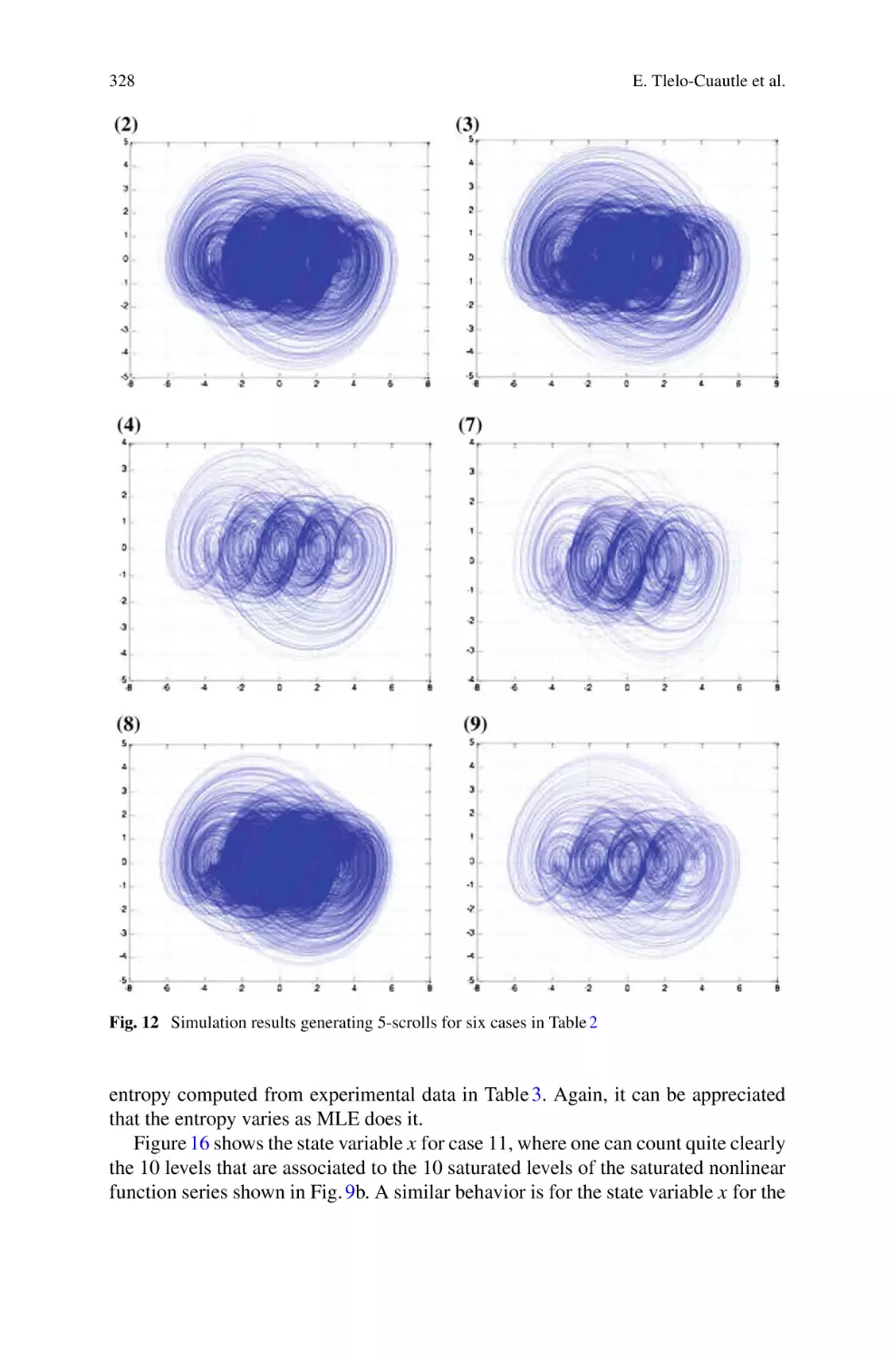
Author: Vaidyanathan S. Volos C.
Tags: informatics computer engineering
ISBN: 978-3-319-30278-2
Year: 2016
Similar
Advances in Memristors, Memristive Devices and Systems. Volume 701
Advances on Intelligent Informatics and Computing
Computer Systems: Theory, Technology, and Applications
Nonlinear systems. Analysis, stability and control
Text
                    Studies in Computational Intelligence 636

Sundarapandian Vaidyanathan
Christos Volos Editors

Advances and
Applications
in Chaotic
Systems

Studies in Computational Intelligence
Volume 636

Series editor
Janusz Kacprzyk, Polish Academy of Sciences, Warsaw, Poland
e-mail: kacprzyk@ibspan.waw.pl

About this Series
The series “Studies in Computational Intelligence” (SCI) publishes new developments and advances in the various areas of computational intelligence—quickly and
with a high quality. The intent is to cover the theory, applications, and design
methods of computational intelligence, as embedded in the ﬁelds of engineering,
computer science, physics and life sciences, as well as the methodologies behind
them. The series contains monographs, lecture notes and edited volumes in
computational intelligence spanning the areas of neural networks, connectionist
systems, genetic algorithms, evolutionary computation, artiﬁcial intelligence,
cellular automata, self-organizing systems, soft computing, fuzzy systems, and
hybrid intelligent systems. Of particular value to both the contributors and the
readership are the short publication timeframe and the worldwide distribution,
which enable both wide and rapid dissemination of research output.

More information about this series at http://www.springer.com/series/7092

Sundarapandian Vaidyanathan
Christos Volos
Editors

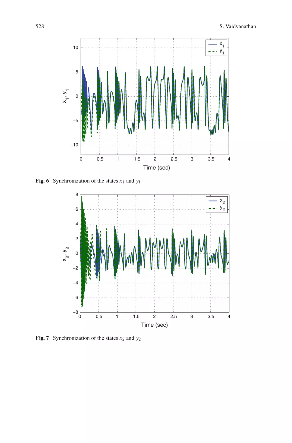
Advances and Applications
in Chaotic Systems

123

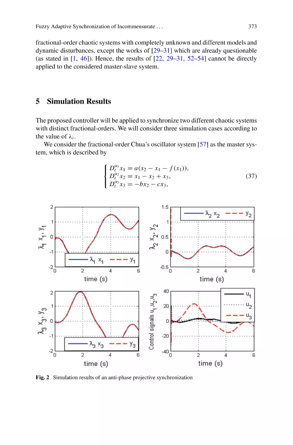
Editors
Sundarapandian Vaidyanathan
Research and Development Centre
Vel Tech University
Chennai
India

Christos Volos
Department of Physics
Aristotle University of Thessaloniki
Thessaloniki
Greece

ISSN 1860-949X
ISSN 1860-9503 (electronic)
Studies in Computational Intelligence
ISBN 978-3-319-30278-2
ISBN 978-3-319-30279-9 (eBook)
DOI 10.1007/978-3-319-30279-9
Library of Congress Control Number: 2016932742
© Springer International Publishing Switzerland 2016
This work is subject to copyright. All rights are reserved by the Publisher, whether the whole or part
of the material is concerned, speciﬁcally the rights of translation, reprinting, reuse of illustrations,
recitation, broadcasting, reproduction on microﬁlms or in any other physical way, and transmission
or information storage and retrieval, electronic adaptation, computer software, or by similar or dissimilar
methodology now known or hereafter developed.
The use of general descriptive names, registered names, trademarks, service marks, etc. in this
publication does not imply, even in the absence of a speciﬁc statement, that such names are exempt from
the relevant protective laws and regulations and therefore free for general use.
The publisher, the authors and the editors are safe to assume that the advice and information in this
book are believed to be true and accurate at the date of publication. Neither the publisher nor the
authors or the editors give a warranty, express or implied, with respect to the material contained herein or
for any errors or omissions that may have been made.
Printed on acid-free paper
This Springer imprint is published by Springer Nature
The registered company is Springer International Publishing AG Switzerland

Preface

About the Subject
Chaos theory is a ﬁeld of study in mathematics with several applications in science
and engineering. Chaotic systems are nonlinear dynamical systems and maps that
are highly sensitive to initial conditions. The sensitivity to initial conditions is
usually called the butterfly effect for dynamical systems and maps.
Chaotic systems can be observed in many natural systems such as weather and
climate. Chaos theory has applications in several areas such as vibration control,
electric circuits, chemical reactions, lasers, combustion engines, computers, cryptosystems, encryption, secure communications, biology, medicine, management,
ﬁnance, etc. Chaotic behaviour of systems can be modelled by discrete-time or
continuous-time mathematical models.

About the Book
The new Springer book, Advances and Applications in Chaotic Systems, consists of
25 contributed chapters by subject experts who are specialized in the various topics
addressed in this book. The special chapters have been brought out in this book
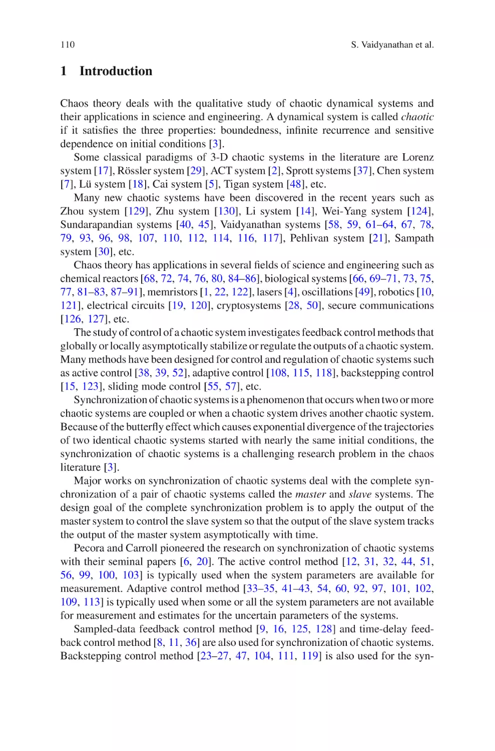
after a rigorous review process in the broad areas of modelling and application of
chaotic systems. Special importance was given to chapters offering practical solutions and novel methods for the recent research problems in the modelling and
application of chaotic systems.
This book discusses trends and applications of chaos modeling and chaotic
systems in science and engineering.

Objectives of the Book
The objective of this book takes a modest attempt to cover the framework of
advances and applications of chaotic systems in a single volume. The book is not
only a valuable title on the publishing market, it is also a successful synthesis
v

vi

Preface

of control techniques applied to chaotic systems. Several multidisciplinary
applications of chaotic systems in control, engineering and information technology
are discussed in this book.

Organization of the Book
This well-structured book consists of 25 full chapters.

Book Features
• The chapters deal with the recent research problems in the areas of chaos theory,
chaos modelling and applications.
• The chapters contain a good literature survey with a long list of references.
• The chapters are well written with a good exposition of the research problem,
methodology and block diagrams.
• The chapters are lucidly illustrated with numerical examples and simulations.
• The chapters discuss details of engineering applications and future research
areas.

Audience
The book is primarily meant for researchers from academia and industry, who are
working in the research areas—chaos theory, control engineering, computer science
and information technology. The book can also be used at the graduate or advanced
undergraduate level as a textbook or major reference for courses such as nonlinear
dynamical systems, control systems, mathematical modelling, computational science, numerical simulation and many others.

Acknowledgements
As the editors, we hope that the chapters in this well-structured book will stimulate
further research in chaos theory, computational intelligence and control systems and
utilize them in real-world applications.
We hope sincerely that this book, covering so many different topics, will be very
useful for all readers.
We would like to thank all the reviewers for their diligence in reviewing the
chapters.
Special thanks go to Springer, especially the book editorial team.
Sundarapandian Vaidyanathan
Christos Volos

Contents

Synchronization Phenomena in Coupled Hyperchaotic Oscillators
with Hidden Attractors Using a Nonlinear Open Loop Controller . . . . .
Ch.K. Volos, V.-T. Pham, S. Vaidyanathan,
I.M. Kyprianidis and I.N. Stouboulos
A Chaotic Hyperjerk System Based on Memristive Device . . . . . . . . . .
Viet-Thanh Pham, Sundarapandian Vaidyanathan, Christos K. Volos,
Sajad Jafari and Xiong Wang

1

39

A Novel Hyperjerk System with Two Quadratic Nonlinearities
and Its Adaptive Control. . . . . . . . . . . . . . . . . . . . . . . . . . . . . . . . . . .
Sundarapandian Vaidyanathan

59

A Novel Conservative Jerk Chaotic System With Two Cubic
Nonlinearities and Its Adaptive Backstepping Control . . . . . . . . . . . . .
Sundarapandian Vaidyanathan and Christos K. Volos

85

Adaptive Backstepping Control, Synchronization and Circuit
Simulation of a Novel Jerk Chaotic System with a Quartic
Nonlinearity . . . . . . . . . . . . . . . . . . . . . . . . . . . . . . . . . . . . . . . . . . . . 109
Sundarapandian Vaidyanathan, Viet-Thanh Pham and Christos K. Volos
A Seven-Term Novel Jerk Chaotic System and Its Adaptive
Control. . . . . . . . . . . . . . . . . . . . . . . . . . . . . . . . . . . . . . . . . . . . . . . . 137
Sundarapandian Vaidyanathan
Adaptive Control and Circuit Simulation of a Novel 4-D Hyperchaotic
System with Two Quadratic Nonlinearities . . . . . . . . . . . . . . . . . . . . . . 163
Sundarapandian Vaidyanathan, Christos K. Volos and Viet-Thanh Pham
Analysis, Adaptive Control and Synchronization of a Novel
3-D Highly Chaotic System . . . . . . . . . . . . . . . . . . . . . . . . . . . . . . . . . 189
Sundarapandian Vaidyanathan

vii

viii

Contents

Qualitative Analysis and Adaptive Control of a Novel 4-D
Hyperchaotic System . . . . . . . . . . . . . . . . . . . . . . . . . . . . . . . . . . . . . . 211
Sundarapandian Vaidyanathan
Global Chaos Control and Synchronization of a Novel Two-Scroll
Chaotic System with Three Quadratic Nonlinearities . . . . . . . . . . . . . . 235
Sundarapandian Vaidyanathan
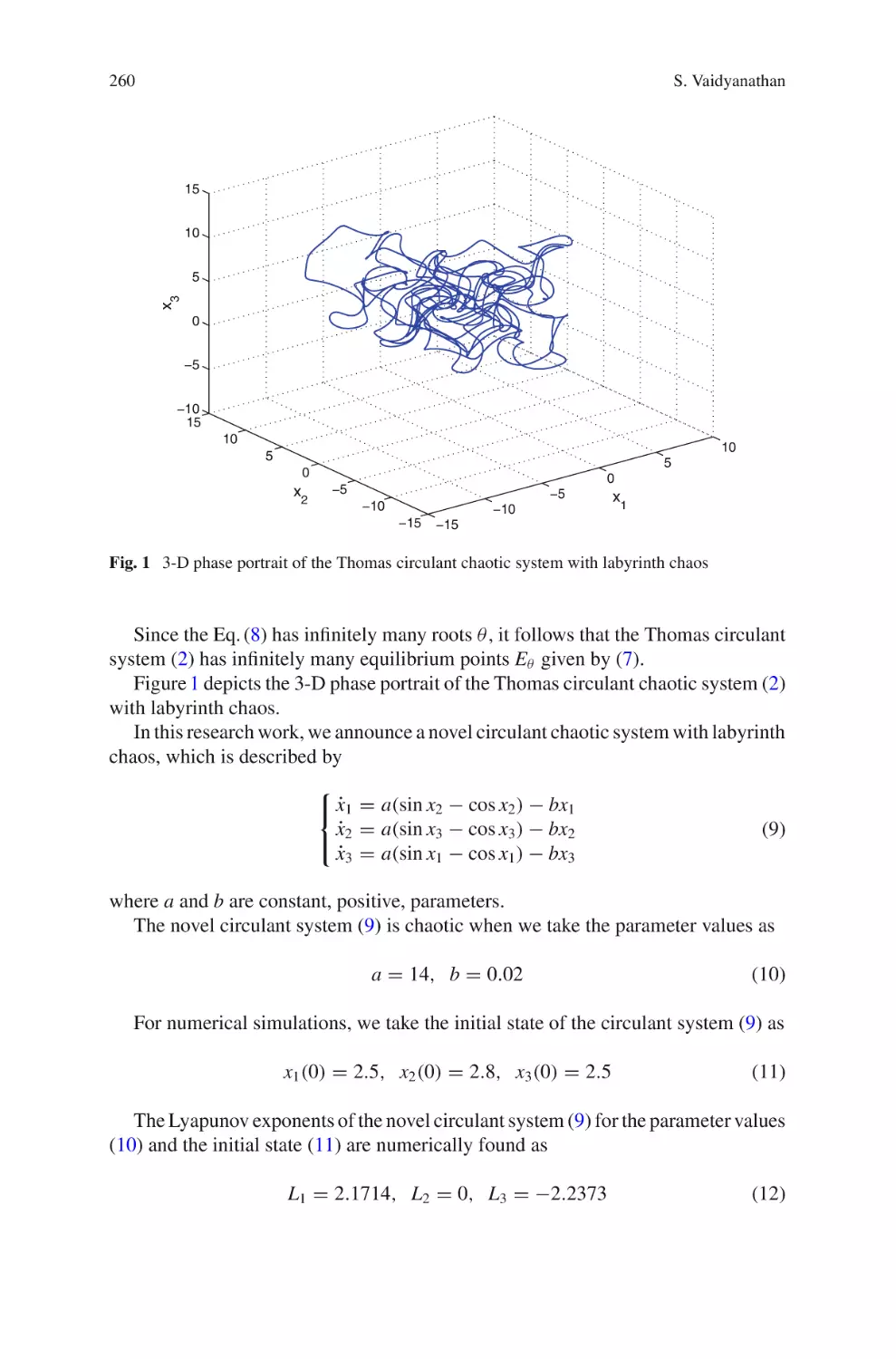
A Novel 3-D Circulant Chaotic System with Labyrinth Chaos
and Its Adaptive Control. . . . . . . . . . . . . . . . . . . . . . . . . . . . . . . . . . . 257
Sundarapandian Vaidyanathan
A 3-D Novel Jerk Chaotic System and Its Application in Secure
Communication System and Mobile Robot Navigation . . . . . . . . . . . . . 283
Aceng Sambas, Sundarapandian Vaidyanathan, Mustafa Mamat,
W.S. Mada Sanjaya and Darmawan Setia Rahayu
On the Veriﬁcation for Realizing Multi-scroll Chaotic Attractors
with High Maximum Lyapunov Exponent and Entropy . . . . . . . . . . . . 311
E. Tlelo-Cuautle, M. Sánchez-Sánchez, V.H. Carbajal-Gómez,
A.D. Pano-Azucena, L.G. de la Fraga and G. Rodriguez-Gómez
Chaotic Synchronization of CNNs in Small-World Topology
Applied to Data Encryption. . . . . . . . . . . . . . . . . . . . . . . . . . . . . . . . . 337
A.G. Soriano-Sánchez, C. Posadas-Castillo, M.A. Platas-Garza
and C. Elizondo-González
Fuzzy Adaptive Synchronization of Incommensurate
Fractional-Order Chaotic Systems . . . . . . . . . . . . . . . . . . . . . . . . . . . . 363
A. Bouzeriba, A. Boulkroune, T. Bouden and S. Vaidyanathan
Implementation of a Laboratory-Based Educational Tool for
Teaching Nonlinear Circuits and Chaos . . . . . . . . . . . . . . . . . . . . . . . . 379
A.E. Giakoumis, Ch.K. Volos, I.N. Stouboulos, I.M. Kyprianidis,
H.E. Nistazakis and G.S. Tombras
Control of Shimizu–Morioka Chaotic System with Passive Control,
Sliding Mode Control and Backstepping Design Methods:
A Comparative Analysis . . . . . . . . . . . . . . . . . . . . . . . . . . . . . . . . . . . 409
Uğur Erkin Kocamaz, Yilmaz Uyaroğlu
and Sundarapandian Vaidyanathan
Generalized Projective Synchronization of a Novel Chaotic System
with a Quartic Nonlinearity via Adaptive Control . . . . . . . . . . . . . . . . 427
Sundarapandian Vaidyanathan and Sarasu Pakiriswamy
A Novel 4-D Hyperchaotic Chemical Reactor System and Its
Adaptive Control . . . . . . . . . . . . . . . . . . . . . . . . . . . . . . . . . . . . . . . . 447
Sundarapandian Vaidyanathan and Abdesselem Boulkroune

Contents

ix

A Novel 5-D Hyperchaotic System with a Line of Equilibrium Points
and Its Adaptive Control. . . . . . . . . . . . . . . . . . . . . . . . . . . . . . . . . . . 471
Sundarapandian Vaidyanathan
Analysis, Control and Circuit Simulation of a Novel 3-D Finance
Chaotic System . . . . . . . . . . . . . . . . . . . . . . . . . . . . . . . . . . . . . . . . . . 495
S. Vaidyanathan, Ch.K. Volos, O.I. Tacha, I.M. Kyprianidis,
I.N. Stouboulos and V.-T. Pham
A Novel Highly Hyperchaotic System and Its Adaptive Control . . . . . . 513
Sundarapandian Vaidyanathan
Sliding Mode Controller Design for the Global Stabilization of Chaotic
Systems and Its Application to Vaidyanathan Jerk System . . . . . . . . . . 537
Sundarapandian Vaidyanathan
Adaptive Control and Synchronization of a Rod-Type Plasma Torch
Chaotic System via Backstepping Control Method . . . . . . . . . . . . . . . . 553
Sundarapandian Vaidyanathan
Analysis, Adaptive Control and Synchronization of a Novel 3-D
Chaotic System with a Quartic Nonlinearity . . . . . . . . . . . . . . . . . . . . . 579
Sundarapandian Vaidyanathan

Synchronization Phenomena in Coupled
Hyperchaotic Oscillators with Hidden
Attractors Using a Nonlinear Open
Loop Controller
Ch.K. Volos, V.-T. Pham, S. Vaidyanathan, I.M. Kyprianidis
and I.N. Stouboulos
Abstract In recent years the study of dynamical systems with hidden attractors,
namely systems in which their basins of attraction do not intersect with small neighborhoods of equilibria, is a great challenge due to their application in many research
fields such as in mechanics, secure communication and electronics. Especially, the
investigation of hyperchaotic systems with hidden attractors plays a crucial role in
this research approach. Motivated by the very complex dynamical behavior of hyperchaotic systems and the unusual features of hidden attractors, a bidirectionally and
unidirectionally coupling scheme of systems of this family, by using a nonlinear open
loop controller, is studied in this chapter. For this reason, a recently new proposed
hyperchaotic system with hidden attractors, the four-dimensional modified Lorenz
system, which is structurally the simplest hyperchaotic system with hidden attractors,
is used. The simulation results show that the proposed scheme drives the coupled
system either to complete synchronization or anti-synchronization depending on the
choice of the signs of the error function’s parameters. In addition, an electronic circuit emulating the control scheme of the coupled hyperchaotic systems with hidden
attractors is also presented to verify the feasibility of the proposed model.

Ch.K. Volos (B) · I.M. Kyprianidis · I.N. Stouboulos
Physics Department, Aristotle University of Thessaloniki, GR-54124 Thessaloniki, Greece
e-mail: volos@physics.auth.gr
I.M. Kyprianidis
e-mail: imkypr@auth.gr
I.N. Stouboulos
e-mail: stouboulos@physics.auth.gr
V.-T. Pham
School of Electronics and Telecommunications, Hanoi University of Science
and Technology, 01 Dai Co Viet, Hanoi, Vietnam
e-mail: pvt3010@gmail.com
S. Vaidyanathan
Research and Development Centre, Vel Tech University,
Avadi, Chennai 600062, Tamil Nadu, India
e-mail: sundarvtu@gmail.com
© Springer International Publishing Switzerland 2016
S. Vaidyanathan and C. Volos (eds.), Advances and Applications
in Chaotic Systems, Studies in Computational Intelligence 636,
DOI 10.1007/978-3-319-30279-9_1

1

2

Ch.K. Volos et al.

Keywords Chaos · Hidden oscillation · Complete synchronization · Antisynchronization · Bidirectional coupling · Unidirectional coupling · Nonlinear open
loop controller

1 Introduction
In the last three decades the phenomenon of synchronization between coupled chaotic
systems has attracted the interest of the scientific community because it is a rich and
multi-disciplinary phenomenon with broad range applications, such as in secure communications [19] and cryptography [14, 60], in broadband communications systems
[7] and in a variety of complex physical, chemical, and biological systems [17, 37,
41, 51, 54, 57, 62]. In general, synchronization of chaos is a process, where two or
more chaotic systems adjust a given property of their motion to a common behavior, such as equal trajectories or phase locking, due to coupling or forcing. Because
of the exponential divergence of the nearby trajectories of a chaotic system, having two chaotic systems being synchronized, might be a surprise. However, today
the synchronization of coupled chaotic oscillators is a phenomenon well established
experimentally and reasonably well understood theoretically.
The history of chaotic synchronization’s theory began with the study of the interaction between coupled chaotic systems in the 1980s and early 1990s by Fujisaka
and Yamada [11], Pikovsky [49], Pecora and Carroll [48]. Since then, a wide range of
research activity based on synchronization of nonlinear systems has risen and a variety of synchronization’s forms depending on the nature of the interacting systems and
of the coupling schemes has been presented. Complete or full chaotic synchronization [9, 24–26, 28, 39, 55, 63], phase synchronization [8, 45], lag synchronization
[52, 56], generalized synchronization [53], anti-synchronization [22, 36], anti-phase
synchronization [1, 5, 6, 27, 58, 64], projective synchronization [38], anticipating
[61] and inverse lag synchronization [34] are the most interesting types of synchronization, that have been investigated numerically and experimentally by many
research groups.
This work is referred to complete synchronization and to anti-synchronization.
In the first case, which is the most studied type of synchronization, two identical
coupled chaotic systems leads to a perfect coincidence of their chaotic trajectories
i.e., x1 (t) = x2 (t) as t → ∞. In the anti-synchronization, on the other hand, which
is also a very interesting type of synchronization, two systems x1 and x2 , can be
synchronized in amplitude, but with opposite sign, for initial conditions chosen from
large regions in the phase space, that is x1 (t) = −x2 (t) as t → ∞.
As it is known, nonlinear systems and especially chaotic systems exhibit high
sensitivity on initial conditions or system’s parameters and thus, if they are identical
and, possibly, starting from almost the same initial conditions, following trajectories
which rapidly become uncorrelated. For this reason, many techniques have been
set up to obtain the aim of chaotic synchronization. So, many of these techniques
to couple two or more nonlinear chaotic systems can be mainly divided into two

Synchronization Phenomena in Coupled Hyperchaotic Oscillators …

3

classes: bidirectional or mutual coupling and unidirectional coupling [13]. In the
mutual coupling both the systems are connected and each system’s dynamic behavior
influences the dynamics of the other, while on the contrary in unidirectional coupling,
only the first system drives the second one.
Recently, a great interest for dynamical systems with hidden attractors has been
raised. The term “hidden attractor” is referred to the fact that in this class of systems
the attractor is not associated with an unstable equilibrium and thus often remains
undiscovered because it may occur in a small region of parameter space and with
a small basin of attraction in the space of initial conditions [23, 31–33, 46, 47]. In
2010, for the first time, a chaotic hidden attractor was discovered in the most wellknown nonlinear circuit, in Chua’s circuit, which is described by a three-dimensional
dynamical system [23, 31].
The problem of analyzing hidden oscillations arose for the first time in the second
part of Hilbert’s 16th problem (1900) for two-dimensional polynomial systems [16].
The first nontrivial results were obtained in Bautin’s works [2, 3], which were devoted
to constructing nested limit cycles in quadratic systems and showed the necessity of
studying hidden oscillations for solving this problem.
Later, in the middle of the 20th century, Kapranov studied [21] the qualitative
behavior of Phase-Locked Loop (PLL) systems, which are used in telecommunications and computer architectures, and estimated stability domains. In that work,
Kapranov assumed that in PLL systems there were self-excited oscillations only.
However, in 1961, Gubar’ [15] revealed a gap in Kapranov’s work and showed analytically the possibility of the existence of hidden oscillations in two-dimensional
system of PLL, thus, from a computational point of view, the system considered was
globally stable, but, in fact, there was only a bounded domain of attraction.
Also, in the same period, the investigations of widely known Markus–Yamabe [40]
and Kalman [20] conjectures on absolute stability have led to the finding of hidden
oscillations in automatic control systems with a unique stable stationary point and
with a nonlinearity, which belongs to the sector of linear stability [4, 10, 30].
Furthermore, systems with hidden attractors have received attention due to their
practical and theoretical importance in other scientific branches, such as in mechanics
(unexpected responses to perturbations in a structure like a bridge or in an airplane
wing) [18, 29]. So, the study of these systems is an interesting topic of a significant
importance.
In this work a hyperchaotic four-dimensional modified Lorenz system with hidden
attractors, is used for studying the bidirectional or unidirectional coupling by using
the nonlinear open loop controller. The simulation results from system’s numerical
integration as well as the circuital implementation of the proposed system in SPICE,
confirm the appearance of complete synchronization and anti-synchronization phenomena depending on the signs of the parameters of the error functions.
The chapter is organized as follows. In Sect. 2 the four-dimensional modified
Lorenz system, which is used in this work, is presented. The scheme, by using the
nonlinear open loop controller, in both coupling ways (bidirectional and unidirectional) as well as the simulation results are discussed in Sect. 3. Section 4 presents
the circuital implementation of the unidirectional coupling system and the simula-

4

Ch.K. Volos et al.

tion results which are obtained by using SPICE. Finally, the conclusive remarks are
drawn in the last section.

2 The Four-Dimensional Modified Lorenz System
In this work the simplest four-dimensional hyperchaotic Lorenz-type system, which
has been proposed by Gao and Zhang [12], is used. This system is an extension of
a modified Lorenz system, which was studied by Schrier and Maas as well as by
Munmuangsaen and Srisuchinwong [42, 59]. The proposed system is described by
the following set of differential equations.
⎧
ẋ = y − x
⎪
⎪
⎨
ẏ = −x z + u
ż
= xy − c
⎪
⎪
⎩
u̇ = −dy

(1)

It is structurally a very simple four-dimensional dynamical system having only
two independent parameters (c, d). Also, as it is mentioned in [35], it has many
interesting properties not found in other proposed systems, such as:
(i) It has very few terms, only seven with two quadratic nonlinearities, and two
parameters.
(ii) All its attractors are hidden.
(iii) It exhibits hyperchaos over a large region of parameter space.
(iv) Its Jacobian matrix has rank less than four everywhere in the space of the
parameters.
(v) It exhibits a quasi-periodic route to chaos with an attracting torus for some
choice of parameter values.
(vi) It has regions in which the torus coexists with either a symmetric pair of strange
attractors or a symmetric pair of limit cycles and other regions where three
limit cycles coexist.
(vii) The basins of attraction have an intricate fractal structure.
(viii) There is a series of Arnold tongues [43] within the quasi-periodic region where
the two fundamental oscillations mode-lock and form limit cycles of various
periodicities.
All the afore-mentioned reasons make the dynamical system (1) an ideal candidate
for the coupling scheme which is used in this work. Especially, the existence of hidden
attractors and the hyperchaotic nature of a system like this have played a crucial role
in our decision.
In this section the system’s dynamic behavior is investigated numerically by
employing a fourth order Runge–Kutta algorithm. For this reason, the bifurcation
diagram, which is a very useful tool from nonlinear theory, is used. In Figs. 1, 2, 3,
4, 5, 6 and 7 the bifurcation diagrams of the variable y versus the parameter d, for

Synchronization Phenomena in Coupled Hyperchaotic Oscillators …
Fig. 1 Bifurcation diagram
of y versus d for c = 5, with
initial conditions (x0 , y0 , z 0 ,
u 0 ) = (0.55, −0.49, −0.08,
0.50)

Fig. 2 Bifurcation diagram
of y versus d for c = 4, with
initial conditions (x0 , y0 , z 0 ,
u 0 ) = (0.55, −0.49, −0.08,
0.50)

Fig. 3 Bifurcation diagram
of y versus d for c = 3.5,
with initial conditions (x0 ,
y0 , z 0 , u 0 ) = (0.55, −0.49,
−0.08, 0.50)

5

6
Fig. 4 Bifurcation diagram
of y versus d for c = 2.97,
with initial conditions (x0 ,
y0 , z 0 , u 0 ) = (0.55, −0.49,
−0.08, 0.50)

Fig. 5 Bifurcation diagram
of y versus d for c = 2.9,
with initial conditions (x0 ,
y0 , z 0 , u 0 ) = (0.55, −0.49,
−0.08, 0.50)

Fig. 6 Bifurcation diagram
of y versus d, for c = 2.7,
with initial conditions (x0 ,
y0 , z 0 , u 0 ) = (0.55, −0.49,
−0.08, 0.50)

Ch.K. Volos et al.

Synchronization Phenomena in Coupled Hyperchaotic Oscillators …

7

Fig. 7 Bifurcation diagram
of y versus d, for c = 1, with
initial conditions (x0 , y0 , z 0 ,
u 0 ) = (0.55, −0.49, −0.08,
0.50)

various values of the parameter c, reveal the richness of system’s dynamical behavior. Besides limit cycles, system (1) has quasi-periodicity, chaos, and hyperchaos,
which can make the control of the system a difficult case in practical applications
where a particular dynamic is desired. In more, details, as the value of d is decreased
from d = 0.9 the system goes from a period-1 steady state (Fig. 8), through a quasiperiodic route (Figs. 9, 10, 11, 12 and 13), to a chaotic state, which is confirmed by
the chaotic attractor in x–z plane, that is shown in Fig. 14. However, a very interesting
feature of the specific system is the existence of hyperchaos for a range of parameters
as it is shown in the phase portraits of Figs. 15, 16, 17, 18 and 19. Figure 20 shows

Fig. 8 Phase portrait of z
versus x for c = 2.7 and
d = 0.9 (period-1 state),
with initial conditions (x0 ,
y0 , z 0 , u 0 ) = (0.55, −0.49,
−0.08, 0.50)

8
Fig. 9 Quasi-periodic
attractor for c = 2.7 and
d = 0.75, in x–y plane, with
initial conditions (x0 , y0 , z 0 ,
u 0 ) = (0.55, −0.49, −0.08,
0.50)

Fig. 10 Quasi-periodic
attractor for c = 2.7 and
d = 0.75, in x–z plane, with
initial conditions (x0 , y0 , z 0 ,
u 0 ) = (0.55, −0.49, −0.08,
0.50)

Fig. 11 Quasi-periodic
attractor for c = 2.7 and
d = 0.75, in x–u plane, with
initial conditions (x0 , y0 , z 0 ,
u 0 ) = (0.55, −0.49, −0.08,
0.50)

Ch.K. Volos et al.

Synchronization Phenomena in Coupled Hyperchaotic Oscillators …
Fig. 12 Quasi-periodic
attractor for c = 2.7 and
d = 0.75, in y–z plane, with
initial conditions (x0 , y0 , z 0 ,
u 0 ) = (0.55, −0.49, −0.08,
0.50)

Fig. 13 Quasi-periodic
attractor for c = 2.7 and
d = 0.75, in y–u plane, with
initial conditions (x0 , y0 , z 0 ,
u 0 ) = (0.55, −0.49, −0.08,
0.50)

Fig. 14 Phase portrait of z
versus x for c = 2.7 and
d = 0.2 (chaotic state), with
initial conditions (x0 , y0 , z 0 ,
u 0 ) = (0.55, −0.49, −0.08,
0.50)

9

10
Fig. 15 Hyperchaotic
attractor for c = 2.7 and
d = 0.44, in x–y plane, with
initial conditions (x0 , y0 , z 0 ,
u 0 ) = (0.55, −0.49, −0.08,
0.50)

Fig. 16 Hyperchaotic
attractor for c = 2.7 and
d = 0.44, in x–z plane, with
initial conditions (x0 , y0 , z 0 ,
u 0 ) = (0.55, −0.49, −0.08,
0.50)

Fig. 17 Hyperchaotic
attractor for c = 2.7 and
d = 0.44, in x–u plane, with
initial conditions (x0 , y0 , z 0 ,
u 0 ) = (0.55, −0.49, −0.08,
0.50)

Ch.K. Volos et al.

Synchronization Phenomena in Coupled Hyperchaotic Oscillators …

11

Fig. 18 Hyperchaotic
attractor for c = 2.7 and
d = 0.44, in y–z plane, with
initial conditions (x0 , y0 , z 0 ,
u 0 ) = (0.55, −0.49, −0.08,
0.50)

Fig. 19 Hyperchaotic
attractor for c = 2.7 and
d = 0.44, in y–u plane, with
initial conditions (x0 , y0 , z 0 ,
u 0 ) = (0.55, −0.49, −0.08,
0.50)

the Lyapunov exponents’ spectra for chosen value of the parameter c (c = 2.7). The
system’s hyperchaotic behavior is found for c = 2.7 in the range of d ∈ [0.388, 0.49]
(Figs. 15, 16, 17, 18 and 19), where the system has two positive Lyapunov exponents,
as it is shown in the embedded diagram in Fig. 20.

12

Ch.K. Volos et al.

Fig. 20 The diagrams of Lyapunov exponents (λi ) versus the parameter d, for c = 2.7

3 The Coupling Scheme
Two identical coupled chaotic systems can be described by the following system of
differential equations:

ẋ = f (x) + U X
(2)
ẏ = f (y) + UY
where ( f (x), f (y)) ∈ R n are the flows of the systems. The coupling of the systems
is defined by the Nonlinear Open Loop Controllers (NOLCs), U X and UY [44]. The
error function is given by e = βy − αx, where α and β are constants. If one applies
the Lyapunov Function Stability (LFS) technique, a stable synchronization state will
be realized when the error function of the coupled system follows the limit
lim ||e(t)|| → 0

t→∞

(3)

so that αx = βy.
As it is mentioned, the design process of the coupling scheme, is based on the
Lyapunov function
1
V (e) = e T e
(4)
2
where T denotes transpose of a matrix and V (e) is a positive definite function. For
known system’s parameters and with the appropriate choice of the controllers U X and
UY , the coupled system has V̇ (e) < 0. This ensures the asymptotic global stability
of synchronization and thereby realizes any desired synchronization state.

Synchronization Phenomena in Coupled Hyperchaotic Oscillators …

13

By using the appropriate NOLCs functions U X , UY and error function’s
parameters α, β, a unidirectional or bidirectional (mutual) coupling scheme can
be implemented. In more details, for (U X = 0, β = 1) or (UY = 0, α = 1), a unidirectional coupling scheme is realized, while for U X,Y = 0 and α, β = 0, a bidirectional
coupling scheme is realized, respectively. The signs of α, β play a crucial role to the
type of synchronization (complete synchronization or anti-synchronization), which
is observed in this work. On the other hand, the ratio of α over β decides the amplification or attenuation of one oscillator relative to another one.
Next, the results of the simulation process in the two coupling (bidirectional and
unidirectional) schemes and for various values of parameters α and β are presented.

3.1 Bidirectional Coupling
Systems of chaotic oscillators bidirectionally (mutually) coupled are frequently
found not only in the simulation environment or the laboratory but also in the natural world [41, 50]. This way of coupling, which is the simplest, is very interesting
because it displays much of the phenomenology that is observed in more complex
networks. Asymptotically stable synchronization between the coupled oscillators
happens to be one of the basic phenomena that is observed.
As it is mentioned, the synchronization of coupled chaotic systems is a process
where two or more systems adjust a given property of their motion to a common
behavior, such as identical trajectories, due to coupling.
So, in the first case, the bidirectional coupling scheme of two coupled systems of
Eq. (1), which is described by the following systems (5) and (6), is studied.
Coupled System-1:
⎧
ẋ1 = x2 − x1 + U X 1
⎪
⎪
⎨
ẋ2 = −x1 x3 + x4 + U X 2
(5)
ẋ3 = x1 x2 − c + U X 3
⎪
⎪
⎩
ẋ4 = −d x2 + U X 4
Coupled System-2:

⎧
ẏ1
⎪
⎪
⎨
ẏ2
ẏ3
⎪
⎪
⎩
ẏ4

= y2 − y1 + UY 1
= −y1 y3 + y4 + UY 2
= y1 y2 − c + UY 3
= −dy2 + UY 4

(6)

where U X = [U X 1 , U X 2 , U X 3 , U X 4 ]T and UY = [UY 1 , UY 2 , UY 3 , UY 4 ]T are the
NOLCs functions. The error function is defined by e = β y − αx, with e = [e1 , e2 ,
e3 , e4 ]T , x = [x1 , x2 , x3 , x4 ]T and y = [y1 , y2 , y3 , y4 ]T . So, the errors dynamics, by
taking the difference of Eqs. (5) and (6), are written as:

14

Ch.K. Volos et al.

⎧
⎪
⎪ ė1
⎨
ė2
ė3
⎪
⎪
⎩
ė4

= e2 − e1 + βUY 1 − αU X 1
= αx1 x3 − βy1 y3 + e4 + βUY 2 − αU X 2
= −αx1 x2 + βy1 y2 − c(β − α) + βUY 3 − αU X 3
= −de2 + βUY 4 − αU X 4

(7)

For stable synchronization e → 0 as t → ∞. By substituting the conditions in
Eq. (7) and taking the time derivative of Lyapunov function
V̇ (e) = e1 ė1 + e2 ė2 + e3 ė3 + e4 ė4
= e1 (e2 − e1 + βUY 1 − αU X 1 )
+ e2 (αx1 x3 − βy1 y3 + e4 + βUY 2 − αU X 2 )
+ e3 [−αx1 x2 + βy1 y2 − c (β − α) + βUY 1 − αU X 1 ]
+ e4 (−de2 + βUY 1 − αU X 1 )

(8)

we consider the following NOLC controllers:
⎧
UX1
⎪
⎪
⎪
⎪
⎨ UX2
⎪
UX3
⎪
⎪
⎪
⎩
UX4
⎧
UY 1
⎪
⎪
⎪
⎨U
Y2
⎪ UY 3
⎪
⎪
⎩U
Y4

and

=
=

1
e
2α 2
1
x + e2 + e4 )
α (αx 1 3
1
x + e3 )
α (−αx 1 2

=

1
α

=



− d2 e2 + e4

(9)



1
= − 2β
e2
1
= β (βy1 y3 )
= β1 [−βy1 y2 + c(β − α)]
1
= 2β
(de2 )

(10)

V̇ (e) = −e12 − e22 − e32 − e42 < 0

(11)

such that

So, Eq. (11) ensures the asymptotic global stability of synchronization.
Next, the simulation results, in this coupling scheme, for three different cases of
system’s parameters (α, β), are presented.
3.1.1

The symmetric case (α = β)

Firstly, the parameters α, β are chosen to be equal (α = β = 1). This is the most
studied type of mutual coupling and also the most interesting due to its applications in
a variety of scientific fields. Also, by choosing, in this case, the systems’ parameters
as c = 2.7 and d = 0.44, each one of the coupled systems is in a hyperchaotic state.
In this case of coupled identical systems with the proposed coupling scheme, only
the complete synchronization is observed. This type of synchronization is confirmed

Synchronization Phenomena in Coupled Hyperchaotic Oscillators …

15

Fig. 21 The phase portrait
of y1 versus x1 , for
α = β = 1, c = 2.7 and
d = 0.44

Fig. 22 The time-series of
x2 , y2 , for α = β = 1,
c = 2.7 and d = 0.44

by the y1 versus x1 plot of Fig. 21. Furthermore, the time-series of the variables
x2 , y2 as well as the errors ei (i = 1, 2, 3, 4) show the exponential convergence to zero which confirms the expected system’s complete synchronization
(Figs. 22 and 23).

3.1.2

The case α = 2, β = 1

In this case, the parameters of the error functions are chosen to be α = 2 and β = 1.
By choosing again the systems’ parameters as c = 2.7, d = 0.44 and for α = 2 the
hyperchaotic attractor of the second system is enlarged by two times, as it is shown
with red color in Fig. 24, as well as by the time-series of signals y1 and y2 in regard to
the signals x1 and x2 respectively (Figs. 26 and 27). The y1 versus x1 plot in Fig. 25
confirms that the coupled system is in complete synchronization state independently

16
Fig. 23 The plot of errors
ei (=βyi − αxi ), for
α = β = 1, c = 2.7 and
d = 0.44

Fig. 24 The phase portraits
of x2 versus x1 and y2 versus
y1 , for α = 2, β = 1,
c = 2.7 and d = 0.44

Fig. 25 The phase portrait
of y1 versus x1 , for α = 2,
β = 1, c = 2.7 and d = 0.44

Ch.K. Volos et al.

Synchronization Phenomena in Coupled Hyperchaotic Oscillators …

17

Fig. 26 The time-series of
x1 , y1 , for α = 2, β = 1,
c = 2.7 and d = 0.44

Fig. 27 The time-series of
x2 , y2 , for α = 2, β = 1,
c = 2.7 and d = 0.44

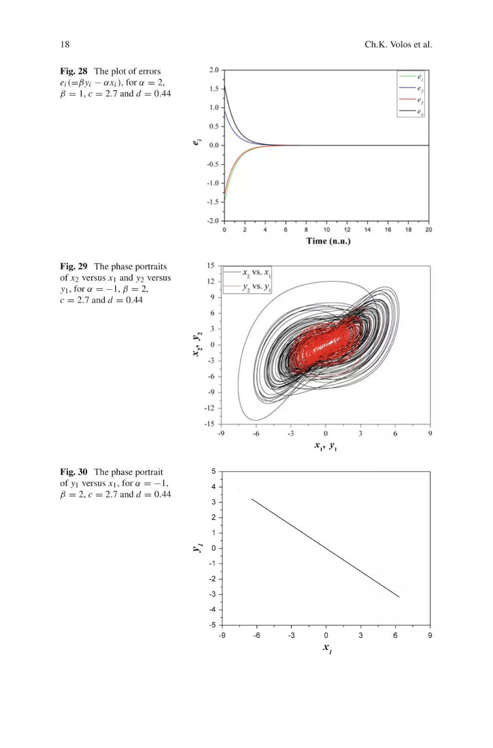
of the values of the error’s parameters α, β. The error plot ei = yi − 2xi (i = 1, 2,
3, 4) in Fig. 28 shows the exponential convergence to zero that confirms the realization
of system’s complete synchronization state.

3.1.3

The Case α = −1, β = 2

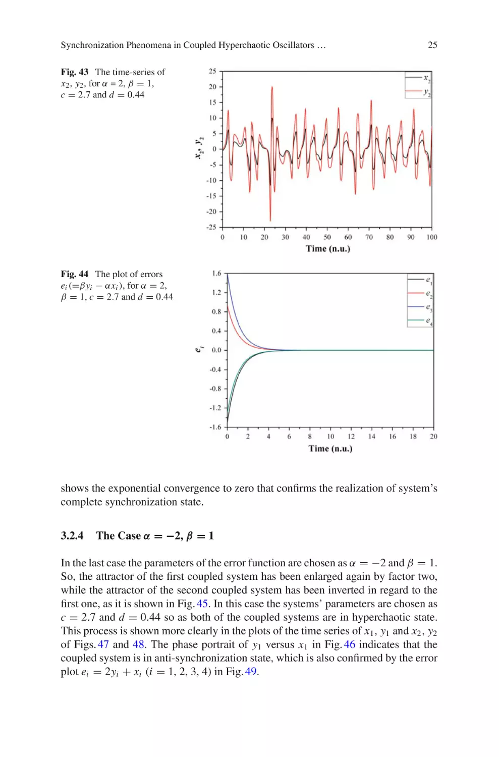
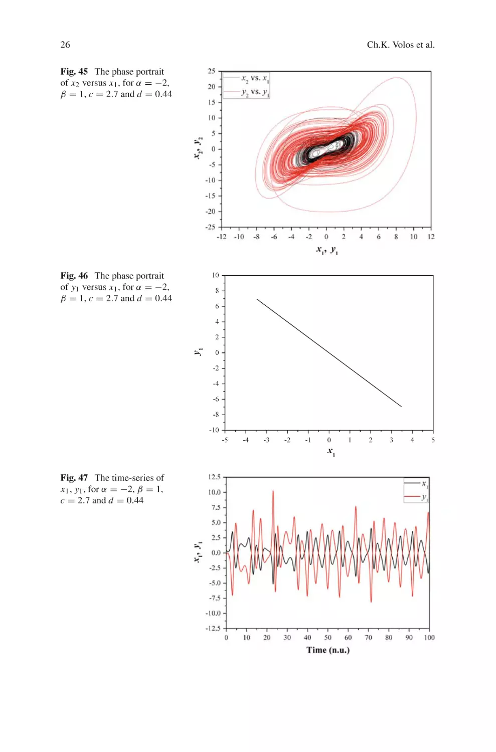
By choosing the parameters of the error functions as α = −1 and β = 2, the attractor
of the first coupled system has been enlarged by factor two, while the attractor
of the second coupled system has been inverted in regard to the first one, as it is
shown in Fig. 29. In this case the systems’ parameters are chosen again as c = 2.7
and d = 0.44 so as both of the coupled systems are in hyperchaotic state. This
process is shown more clearly in the plots of the time-series of x1 , y1 and x2 , y2
(Figs. 31 and 32). The phase portrait of y1 versus x1 in Fig. 30 indicates that the

18
Fig. 28 The plot of errors
ei (=βyi − αxi ), for α = 2,
β = 1, c = 2.7 and d = 0.44

Fig. 29 The phase portraits
of x2 versus x1 and y2 versus
y1 , for α = −1, β = 2,
c = 2.7 and d = 0.44

Fig. 30 The phase portrait
of y1 versus x1 , for α = −1,
β = 2, c = 2.7 and d = 0.44

Ch.K. Volos et al.

Synchronization Phenomena in Coupled Hyperchaotic Oscillators …

19

Fig. 31 The time-series of
x1 , y1 , for α = −1, β = 2,
c = 2.7 and d = 0.44

Fig. 32 The time-series of
x2 , y2 , for α = −1, β = 2,
c = 2.7 and d = 0.44

coupled system is in anti-synchronization state, which is also confirmed by the error
plot ei = 2y1 + x1 (i = 1, 2, 3, 4) in Fig. 33.

3.2 Unidirectional Coupling
In this section, the unidirectional coupling scheme, U X = 0, for β = 1, given by
Eq. (1), is presented.
Master System:
⎧
ẋ1 = x2 − x1
⎪
⎪
⎨
ẋ2 = −x1 x3 + x4
(12)
ẋ3 = x1 x2 − c
⎪
⎪
⎩
ẋ4 = −d x2

20

Ch.K. Volos et al.

Fig. 33 The plot of errors
ei (=βyi − αxi ), for
α = −1, β = 2, c = 2.7 and
d = 0.44

Slave System:

⎧
ẏ1
⎪
⎪
⎨
ẏ2
⎪ ẏ3
⎪
⎩
ẏ4

= y2 − y1 + UY 1
= −y1 y3 + y4 + UY 2
= y1 y2 − c + UY 3
= −dy2 + UY 4

(13)

where U Y = [UY 1 , UY 2 , UY 3 , UY 4 ]T are the Nonlinear Open Loop Controller
(NOLC). The error function is defined by e = β y − αx, with e = [e1 , e2 , e3 , e4 ]T ,
x = [x1 , x2 , x3 , x4 ]T and y = [y1 , y2 , y3 , y4 ]T . So, the error dynamics, by taking the
difference of Eqs. (12) and (13), are written as:
⎧
ė1
⎪
⎪
⎨
ė2
⎪ ė3
⎪
⎩
ė4

= e2 − e1 + βUY 1
= αx1 x3 − βy1 y3 + e4 + βUY 2
= −αx1 x2 + βy1 y2 + c(α − β) + βUY 3
= −de2 + βUY 4

(14)

For stable synchronization e → 0 with t → ∞. By substituting the conditions in
Eq. (14) and taking the time derivative of Lyapunov function
V̇ (e) = e1 ė1 + e2 ė2 + e3 ė3 + e4 ė4
= e1 (e2 − e1 + βUY 1 ) + e2 (αx1 x3 − βy1 y3 + e4 + βUY 2 )
+ e3 [−αx1 x2 + βy1 y2 + c (α − β) + βUY 3 ] + e4 (−de2 + βUY 4 )
(15)

Synchronization Phenomena in Coupled Hyperchaotic Oscillators …

we consider the following NOLC controllers
⎧
UY 1 = − β1 e2
⎪
⎪
⎪
⎨ U = − 1 (e + αx x − βy y + e )
Y2
2
1 3
1 3
4
β
1
=
−
−
αx
x
+
βy
y
+
c(α
− β)]
U
[e
⎪
Y3
3
1 2
1 2
⎪
β
⎪
⎩ U = − 1 (e − de )
Y4
4
2
β
such that

V̇ (e) = −e12 − e22 − e32 − e42 < 0

21

(16)

(17)

Equation (17) ensures the asymptotic global stability of synchronization.
3.2.1

The Case α = β = 1

In this case, as it occurs in the mutual coupling, the phenomenon of complete synchronization is achieved for every value of α = β. Especially, for α = β = 1, the
two coupled systems are in the same hyperchaotic state, due to the chosen values of
system’s parameters (c = 2.7 and d = 0.44). The goal of complete synchronization
is achieved as it is shown from the plots of y1 versus x1 , the time-series of x2 , y2 and
the errors ei in Figs. 34, 35 and 36.
3.2.2

The Case for α = −β = −1

By using opposing values for the parameters α = −β = −1 the phenomenon of antisynchronization is achieved, as it is shown in Fig. 37. Initially, the coupled systems are
in different hyperchaotic states but the unidirectional coupling leads the slave system
to an opposite hyperchaotic attractor in regard to the master system. This conclusion
is derived from the phase portrait of y1 versus x1 (Fig. 37), as well as from the

Fig. 34 The phase portrait
of y1 versus x1 , for
α = β = 1, c = 2.7 and
d = 0.44

22
Fig. 35 The time-series of
y2 , x2 , for α = β = 1,
c = 2.7 and d = 0.44

Fig. 36 The plot of errors
ei (=βyi − αxi ), for
α = β = 1, c = 2.7 and
d = 0.44

Fig. 37 The phase portrait
of y1 versus x1 , for
α = −β = −1, c = 2.7 and
d = 0.44

Ch.K. Volos et al.

Synchronization Phenomena in Coupled Hyperchaotic Oscillators …

23

Fig. 38 The time-series of
y2 , x2 , for α = −β = −1,
c = 2.7 and d = 0.44

Fig. 39 The plot of errors
ei (=βyi – αxi ), for
α = −β = −1, c = 2.7 and
d = 0.44

time-series of x2 , y2 (Fig. 38). Also, the plot of errors ei = yi + xi in Fig. 39 confirms
the anti-synchronization of the coupled system.

3.2.3

The Case α = 2, β = 1

In this case, the parameters of the error functions are chosen as α = 2 and β = 1.
By choosing the systems’ parameters as c = 2.7, d = 0.44 and for α = 2 the chaotic
attractor of the second system is enlarged by two times, as it is shown with red color
in Fig. 40, as well as by the time-series of signals y1 and y2 in regard to the signals x1
and x2 respectively (Figs. 42 and 43). The y1 versus x1 plot in Fig. 41 confirms that
the coupled system is in complete synchronization state independently of the values
of the error’s parameters α, β. The error plot ei = y1 − 2x1 (i = 1, 2, 3, 4) in Fig. 44

24
Fig. 40 The phase portraits
of x2 versus x1 and y2 versus
y1 , for α = 2, β = 1,
c = 2.7 and d = 0.44

Fig. 41 The phase portrait
of y1 versus x1 , for α = 2,
β = 1, c = 2.7 and d = 0.44

Fig. 42 The time-series of
x1 , y1 , for α = 2, β = 1,
c = 2.7 and d = 0.44

Ch.K. Volos et al.

Synchronization Phenomena in Coupled Hyperchaotic Oscillators …

25

Fig. 43 The time-series of
x2 , y2 , for α = 2, β = 1,
c = 2.7 and d = 0.44

Fig. 44 The plot of errors
ei (=βyi − αxi ), for α = 2,
β = 1, c = 2.7 and d = 0.44

shows the exponential convergence to zero that confirms the realization of system’s
complete synchronization state.
3.2.4

The Case α = −2, β = 1

In the last case the parameters of the error function are chosen as α = −2 and β = 1.
So, the attractor of the first coupled system has been enlarged again by factor two,
while the attractor of the second coupled system has been inverted in regard to the
first one, as it is shown in Fig. 45. In this case the systems’ parameters are chosen as
c = 2.7 and d = 0.44 so as both of the coupled systems are in hyperchaotic state.
This process is shown more clearly in the plots of the time series of x1 , y1 and x2 , y2
of Figs. 47 and 48. The phase portrait of y1 versus x1 in Fig. 46 indicates that the
coupled system is in anti-synchronization state, which is also confirmed by the error
plot ei = 2yi + xi (i = 1, 2, 3, 4) in Fig. 49.

26
Fig. 45 The phase portrait
of x2 versus x1 , for α = −2,
β = 1, c = 2.7 and d = 0.44

Fig. 46 The phase portrait
of y1 versus x1 , for α = −2,
β = 1, c = 2.7 and d = 0.44

Fig. 47 The time-series of
x1 , y1 , for α = −2, β = 1,
c = 2.7 and d = 0.44

Ch.K. Volos et al.

Synchronization Phenomena in Coupled Hyperchaotic Oscillators …

27

Fig. 48 The time-series of
x2 , y2 , for α = −2, β = 1,
c = 2.7 and d = 0.44

Fig. 49 The plot of errors
ei (=βyi − αxi ), for
α = −2, β = 1, c = 2.7 and
d = 0.44

4 Circuit’s Implementation of the Proposed Scheme
In this section the circuit implementation of the proposed scheme, with the electronic
simulation package Cadence OrCAD, in the case of unidirectional coupling systems
with a = β is presented, in order to prove the feasibility of this method. The coupling
system is realized by common electronic components. The system’s circuit consists
of three sub-circuits, which are the master circuit, the slave circuit and the coupling
circuit.
Figure 50 depicts the schematic of the master circuit. It has four integrators (U1 ,
U2 , U3 and U4 ) and two differential amplifiers (U7 , U8 ), which are implemented
with the TL084, as well as two signals multipliers (U5 , U6 ) by using the AD633. By
applying Kirchhoff’s circuit laws, the corresponding circuital equations of designed
master circuit can be written as:

28

Ch.K. Volos et al.

Fig. 50 The schematic of the master circuit

⎧
⎪
⎪ ẋ1 =
⎪
⎪
⎪
⎪
⎨ ẋ2 =
⎪
ẋ3 =
⎪
⎪
⎪
⎪
⎪
⎩
ẋ4 =

1
RC

(x2 − x1 )

1
RC

R
− R1 10V
x1 x3 + x4

1
RC

R
R1 10V

1
RC

− RRd x2

x1 x2 − c

(18)

where xi (i = 1, . . . , 4) are the voltages in the outputs of the operational amplifiers
U1 , U2 , U3 and U4 . Normalizing the differential equations of system (18) by using
τ = t/RC we could see that this system is equivalent to the system (12). The circuit
components have been selected as: R = 10 k, R1 = 1 k, Rd = 22.727 k, C =
10 nF, VC = 2.7 V, while the power supplies of all active devices are ±15 VDC . For the
chosen set of components the master system’s parameters are: c = 2.7 and d = 0.44.
In Figs. 51, 52, 53, 54 and 55 the hyperchaotic attractors, which are obtained from
Cadence OrCAD in various phase planes, are proved to be in a very good agreement
with the respective phase portraits from system’s simulation process (Figs. 15, 16,
17, 18 and 19). So, the proposed circuit emulates well the master system.
In Fig. 56 the schematic of the slave circuit, which is similar to the master circuit,
is shown. The difference of this circuit in comparison to the previous one are the
signals mu2 , mu3 and mu4 , which are the opposites of the signals UY 2 , UY 3 and UY 4 ,
produced by the controllers of Eq. (16). Also, e2 is the difference signal (βy2 − αx2 ).

Synchronization Phenomena in Coupled Hyperchaotic Oscillators …

29

Fig. 51 Hyperchaotic attractor of the designed master circuit obtained from Cadence OrCAD in
the (x1 , x2 ) phase plane

Fig. 52 Hyperchaotic attractor of the designed master circuit obtained from Cadence OrCAD in
the (x1 , x3 ) phase plane

30

Ch.K. Volos et al.

Fig. 53 Hyperchaotic attractor of the designed master circuit obtained from Cadence OrCAD in
the (x1 , x4 ) phase plane

Fig. 54 Hyperchaotic attractor of the designed master circuit obtained from Cadence OrCAD in
the (x2 , x3 ) phase plane

Synchronization Phenomena in Coupled Hyperchaotic Oscillators …

31

Fig. 55 Hyperchaotic attractor of the designed master circuit obtained from Cadence OrCAD in
the (x2 , x4 ) phase plane

Fig. 56 The schematic of the slave circuit

32

Ch.K. Volos et al.

Next, the design of the coupling circuit as well as the simulation results obtained
from SPICE in the case of α = β is discussed in details.
In the case of α = β = 1 and by considering the achievement of synchronization
between the coupled systems (12) and (13), the NOLCs take the following forms.
⎧
UY 1
⎪
⎪
⎨
UY 2
UY 3
⎪
⎪
⎩
UY 4

= −e2
= − (e2 + e4 )
= −e3
= − (e4 − de2 )

(19)

The units from which the coupling circuit is consisted, are shown in the schematic
of Fig. 57. In this schematic u 2 and u 4 are the control signals UY 2 and UY 4 of Eq. (19)

Fig. 57 The schematic of the coupling circuit

Synchronization Phenomena in Coupled Hyperchaotic Oscillators …

33

Fig. 58 The phase portrait in the (x1 , y1 ) phase plane, for α = β = 1, c = 2.7 and d = 0.44,
obtained from Cadence OrCAD

Fig. 59 The phase portrait in the (x2 , y2 ) phase plane, for α = β = 1, c = 2.7 and d = 0.44,
obtained from Cadence OrCAD

34

Ch.K. Volos et al.

Fig. 60 The phase portrait in the (x3 , y3 ) phase plane, for α = β = 1, c = 2.7 and d = 0.44,
obtained from Cadence OrCAD

Fig. 61 The phase portrait in the (x4 , y4 ) phase plane, for α = β = 1, c = 2.7 and d = 0.44,
obtained from Cadence OrCAD

Synchronization Phenomena in Coupled Hyperchaotic Oscillators …

35

respectively, while mu 2 and mu4 are the opposite of these signals. Also, ei , (i = 2,
3, 4) are the difference signals (βyi − αxi , i = 2, 3, 4) and me2 is the opposite of e2 .
Figures 58, 59, 60 and 61 depict the phase portraits in (xi , yi ) phase plane, with
i = 1, . . . , 4, for α = β = 1, c = 2.7 and d = 0.44, obtained from Cadence OrCAD.
These figures confirm the achievement of complete synchronization in the case of
unidirectionally coupled circuits with the proposed method.

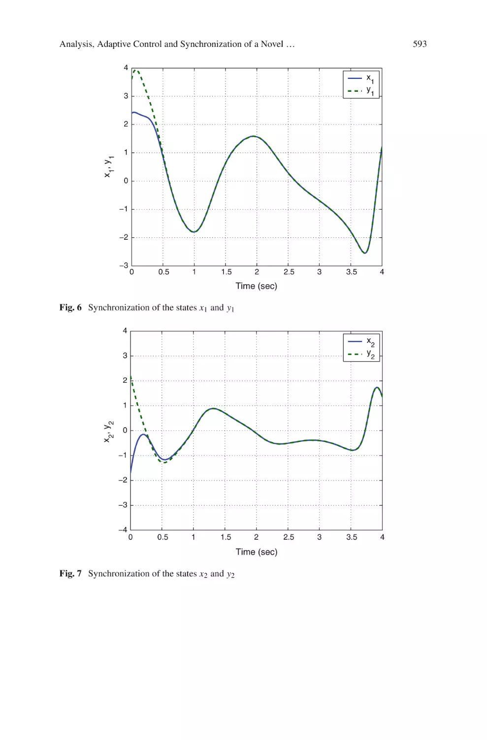
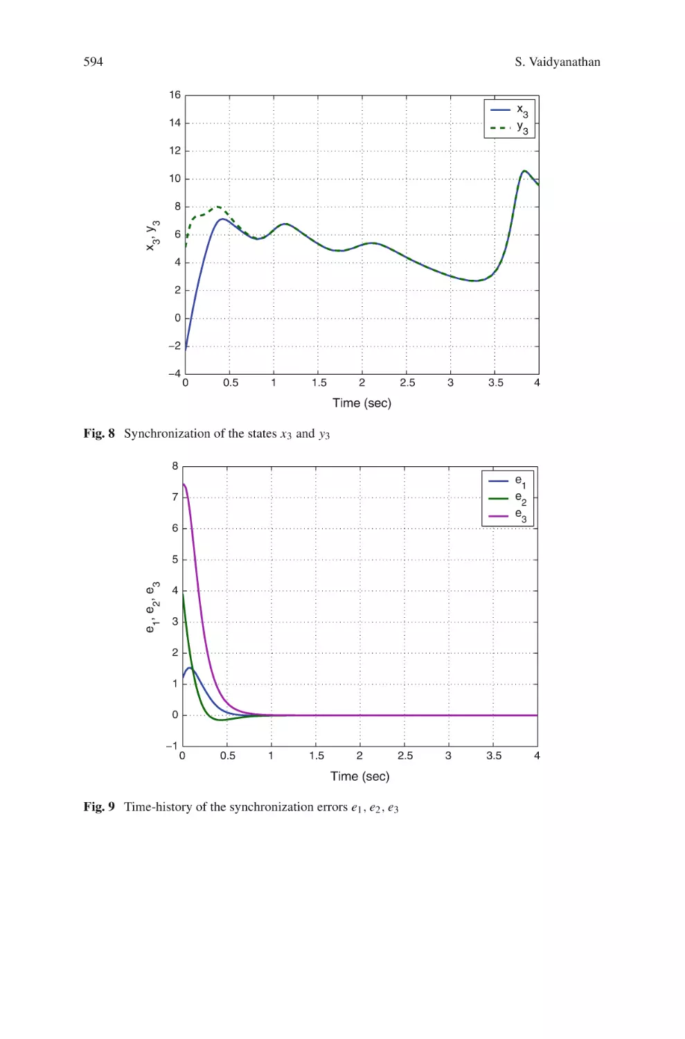
5 Conclusion
In this chapter, the case of bidirectional and unidirectional coupling scheme of hyperchaotic dynamical systems with hidden attractors was studied. The proposed system
is a four-dimensional modified Lorenz system, which is the simplest hyperchaotic
system of this family. Furthermore, the coupling method was based on a recently
new proposed scheme based on the nonlinear open loop controller.
According to the simulation results from system’s numerical integration as well
as the circuital implementation of the proposed system in SPICE, in the case
of unidirectional coupling, the appearance of complete synchronization and antisynchronization, depending on the signs of the parameters of the error functions,
was investigated in various cases. So, by choosing an appropriate sign for the error
functions one could drive the coupling system either in complete synchronization or
anti-synchronization behavior.
As it is known, the complex behavior of hyperchaotic systems, like the aforementioned, makes the control difficult in practical applications where a particular
dynamic is desired. So, this chapter presents an interesting research result for the
family of hyperchaotic systems with hidden attractors, because this method could
be very useful in many potential applications of these systems. As a next step in this
direction is the application of the proposed method in non-identical coupling systems in order to satisfy the goal of control of systems, which are in totally different
dynamical behaviors.

References
1. Astakhov V, Shabunin A, Anishchenko V (2000) Antiphase synchronization in symmetrically
coupled self-oscillators. Int J Bifurc Chaos 10:849–857
2. Bautin NN (1939) On the number of limit cycles generated on varying the coefficients from a
focus or centre type equilibrium state. Doklady Akademii Nauk SSSR 24:668–671
3. Bautin NN (1952) On the number of limit cycles appearing on varying the coefficients from a
focus or centre type of equilibrium state. Mat Sb (N.S.) 30:181–196
4. Bernat J, Llibre J (1996) Counterexample to Kalman and Markus-Yamabe conjectures in dimension larger than 3. Dyn Contin Discret Impul Syst 2:337–379
5. Blazejczuk-Okolewska B, Brindley J, Czolczynski K, Kapitaniak T (2001) Antiphase synchronization of chaos by noncontinuous coupling: two impacting oscillators. Chaos Solitons Fract
12:1823–1826

36

Ch.K. Volos et al.

6. Cao LY, Lai YC (1998) Antiphase synchronism in chaotic system. Phys Rev 58:382–386
7. Dimitriev AS, Kletsovi AV, Laktushkin AM, Panas AI, Starkov SO (2006) Ultrawideband wireless communications based on dynamic chaos. J Commun Technol Electron 51:
1126–1140
8. Dykman GI, Landa PS, Neymark YI (1991) Synchronizing the chaotic oscillations by external
force. Chaos Solitons Fract 1:339–353
9. Enjieu Kadji HG, Chabi Orou JB, Woafo P (2008) Synchronization dynamics in a ring of four
mutually coupled biological systems. Commun Nonlinear Sci Numer Simul 13:1361–1372
10. Fitts RE (1966) Two counterexamples to Aizerman’s conjecture. Trans IEEE AC-11:553–556
11. Fujisaka H, Yamada T (1983) Stability theory of synchronized motion in coupled-oscillator
systems. Prog Theor Phys 69:32–47
12. Gao Z, Zhang C (2011) A novel hyperchaotic system. J Jishou Univ (Natural Science Edition)
32:65–68
13. Gonzalez-Miranda JM (2004) Synchronization and control of chaos. Imperial College Press,
London
14. Grassi G, Mascolo S (1999) Synchronization of high-order oscillators by observer design with
application to hyperchaos-based cryptography. Int J Circ Theor Appl 27:543–553
15. Gubar’ NA (1961) Investigation of a piecewise linear dynamical system with three parameters.
J Appl Math Mech 25:1011–1023
16. Hilbert D (1901) Mathematical problems. Bull Am Math Soc 8:437–479
17. Holstein-Rathlou NH, Yip KP, Sosnovtseva OV, Mosekilde E (2001) Synchronization phenomena in nephron-nephron interaction. Chaos 11:417–426
18. Jafari S, Sprott J (2013) Simple chaotic flows with a line equilibrium. Chaos Solit Fract
57:79–84
19. Jafari S, Haeri M, Tavazoei MS (2010) Experimental study of a chaos-based communication
system in the presence of unknown transmission delay. Int J Circ Theor Appl 38:1013–1025
20. Kalman RE (1957) Physical and mathematical mechanisms of instability in nonlinear automatic
control systems. Trans ASME 79:553–566
21. Kapranov M (1956) Locking band for phase-locked loop. Radiofizika 2:37–52
22. Kim CM, Rim S, Kye WH, Rye JW, Park YJ (2003) Anti-synchronization of chaotic oscillators.
Phys Lett A 320:39–46
23. Kuznetsov NV, Leonov GA, Vagaitsev VI (2010) Analytical-numerical method for attractor
localization of generalized Chua’s system. IFAC Proc Vol (IFAC-PapersOnline) 4(1):29–33
24. Kyprianidis IM, Stouboulos IN (2003) Synchronization of two resistively coupled nonautonomous and hyperchaotic oscillators. Chaos Solitons Fract 17:317–325
25. Kyprianidis IM, Stouboulos IN (2003) Chaotic synchronization of three coupled oscillators
with ring connection. Chaos Solitons Fract 17:327–336
26. Kyprianidis IM, Volos ChK, Stouboulos IN, Hadjidemetriou J (2006) Dynamics of two resistively coupled Duffing-type electrical oscillators. Int J Bifurc Chaos 16:1765–1775
27. Kyprianidis IM, Bogiatzi AN, Papadopoulou M, Stouboulos IN, Bogiatzis GN, Bountis T
(2006) Synchronizing chaotic attractors of Chua’s canonical circuit. The case of uncertainty in
chaos synchronization. Int J Bifurc Chaos 16:1961–1976
28. Kyprianidis IM, Volos ChK, Stouboulos IN (2008) Experimental synchronization of two resistively coupled Duffing-type circuits. Nonlinear Phenom Complex Syst 11:187–192
29. Lauvdal T, Murray R, Fossen T (1997) Stabilization of integrator chains in the presence of
magnitude and rate saturations: a gain scheduling approach. IEEE Control Decision Conf, pp
4004–4005
30. Leonov G, Kuznetsov NV (2013) Analytical-numerical methods for hidden attractors’ localization: the 16th Hilbert problem, Aizerman and Kalman conjectures, and Chua circuits. Numerical
methods for differential equations, optimization, and technological problems, computational
methods in applied sciences. Springer 27:41–64
31. Leonov G, Kuznetsov N, Vagaitsev V (2011) Localization of hidden Chua’s attractors. Phys
Lett A 375:2230–2233

Synchronization Phenomena in Coupled Hyperchaotic Oscillators …

37

32. Leonov G, Kuznetsov N, Kuznetsova O, Seldedzhi S, Vagaitsev V (2011) Hidden oscillations
in dynamical systems. Trans Syst Contr 6:54–67
33. Leonov G, Kuznetsov N, Vagaitsev V (2012) Hidden attractor in smooth Chua system. Physica
D 241:1482–1486
34. Li GH (2009) Inverse lag synchronization in chaotic systems. Chaos Solitons Fract 40:
1076–1080
35. Li C, Sprott JC (2014) Coexisting hidden attractors in a 4-D simplified Lorenz system. Int J
Bifurc Chaos 24(3):1450034
36. Liu W, Qian X, Yang J, Xiao J (2006) Antisynchronization in coupled chaotic oscillators. Phys
Lett A 354:119–125
37. Liu X, Chen T (2010) Synchronization of identical neural networks and other systems with an
adaptive coupling strength. Int J Circ Theor Appl 38:631–648
38. Mainieri R, Rehacek J (1999) Projective synchronization in three-dimensional chaotic system.
Phys Rev Lett 82:3042–3045
39. Maritan A, Banavar J (1994) Chaos noise and synchronization. Phys Rev Lett 72:1451–1454
40. Markus L, Yamabe H (1960) Global stability criteria for differential systems. Osaka Math J
12:305–317
41. Mosekilde E, Maistrenko Y, Postnov D (2002) Chaotic synchronization: applications to living
systems. World Scientific, Singapore
42. Munmuangsaen B, Srisuchinwong B (2009) A new five-term simple chaotic attractor. Phys
Lett A 373:4038–4043
43. Paar V, Pavin N (1998) Intermingled fractal Arnold tongues. Phys Rev E 57:1544–1549
44. Padmanaban E, Hens C, Dana K (2011) Engineering synchronization of chaotic oscillator using
controller based coupling design. Chaos 21:013110
45. Parlitz U, Junge L, Lauterborn W, Kocarev L (1996) Experimental observation of phase synchronization. Phys Rev E 54:2115–2217
46. Pham V-T, Volos ChK, Jafari S, Wang X, Vaidyanathan S (2014) Hidden hyperchaotic attractor in a novel simple memristive neural network. J Optoelectron Adv Mater Rapid Commun
8(11–12):1157–1163
47. Pham V-T, Jafari S, Volos ChK, Wang X, Golpayegani Mohammad Reza Hashemi S (2014) Is
that really hidden? The presence of complex fixed-points in chaotic flows with no equilibria.
Int J Bifurc Chaos 24(11):1450146
48. Pecora LM, Carroll TL (1990) Synchronization in chaotic systems. Phys Rev Lett 64:821–824
49. Pikovsky AS (1984) On the interaction of strange attractors. Z Phys B—Condensed Matter
55:149–154
50. Pikovsky AS, Maistrenko YL (2003) Synchronization: theory and application. Springer,
Netherlands
51. Pikovsky AS, Rosenblum M, Kurths J (2003) Synchronization: a universal concept in nonlinear
sciences. Cambridge University Press, Cambridge
52. Rosenblum MG, Pikovsky AS, Kurths J (1997) From phase to lag synchronization in coupled
chaotic oscillators. Phys Rev Lett 78:4193–4196
53. Rulkov NF, Sushchik MM, Tsimring LS, Abarbanel HDI (1995) Generalized synchronization
of chaos in directionally coupled chaotic systems. Phys Rev E 51:980–994
54. Szatmári I, Chua LO (2008) Awakening dynamics via passive coupling and synchronization
mechanism in oscillatory cellular neural/nonlinear networks. Int J Circ Theor Appl 36:525–553
55. Tafo Wembe E, Yamapi R (2009) Chaos synchronization of resistively coupled Duffing systems: numerical and experimental investigations. Commun Nonlinear Sci Numer Simul 14:
1439–1453
56. Taherion S, Lai YC (1999) Observability of lag synchronization of coupled chaotic oscillators.
Phys Rev E 59:R6247–R6250
57. Tognoli E, Kelso JAS (2009) Brain coordination dynamics: true and false faces of phase synchrony and metastability. Prog Neurobiol 87:31–40
58. Tsuji S, Ueta T, Kawakami H (2007) Bifurcation analysis of current coupled BVP oscillators.
Int J Bifurc Chaos 17:837–850

38

Ch.K. Volos et al.

59. Van der Schrier G, Maas LRM (2000) The diffusionless Lorenz equations: Shil’nikov bifurcations and reduction to an explicit map. Phys Nonlinear Phenom 141:19–36
60. Volos ChK, Kyprianidis IM, Stouboulos IN (2006) Experimental demonstration of a chaotic
cryptographic scheme. WSEAS Trans Circ Syst 5:1654–1661
61. Voss HU (2000) Anticipating chaotic synchronization. Phys Rev E 61:5115–5119
62. Wang J, Che YQ, Zhou SS, Deng B (2009) Unidirectional synchronization of Hodgkin-Huxley
neurons exposed to ELF electric field. Chaos Solitons Fract 39:1335–1345
63. Woafo P, Enjieu Kadji HG (2004) Synchronized states in a ring of mutually coupled selfsustained electrical oscillators. Phys Rev E 69:046206
64. Zhong GQ, Man KF, Ko KT (2001) Uncertainty in chaos synchronization. Int J Bifurc Chaos
11:1723–1735

A Chaotic Hyperjerk System Based
on Memristive Device
Viet-Thanh Pham, Sundarapandian Vaidyanathan, Christos K. Volos,
Sajad Jafari and Xiong Wang

Abstract From the mechanical system point of view, third-order derivatives of
displacement or the time rate of change of acceleration is the jerk, while the fourth
derivative has been known as a snap. As a result, a dynamical system which is presented by an nth order ordinary differential equation with n > 3 describing the time
evolution of a single scalar variable is considered as a hyperjerk system. Hyperjerk
system has received significant attention because of its elegant form. Motivated by
reported attractive hyperjerk systems, a 4-D novel chaotic hyperjerk system has been
introduced and studied in this work. Interestingly, this hyperjerk system displays an
infinite number of equilibrium points because of the presence of a memristive device.
In addition, an adaptive controller is proposed to achieve synchronization of such
novel hyperjerk systems with two unknown parameters. In order to confirm the feasibility of the mathematical hyperjerk model, its electronic circuit is designed and
implemented by using SPICE.

V.-T. Pham (B)
School of Electronics and Telecommunications, Hanoi University
of Science and Technology, Hanoi, Vietnam
e-mail: pvt3010@gmail.com
S. Vaidyanathan
Research and Development Centre, Vel Tech University, Tamil Nadu, India
e-mail: sundar@veltechuniv.edu.in
C.K. Volos
Physics Department, Aristotle University of Thessaloniki, Thessaloniki, Greece
e-mail: volos@physics.auth.gr
S. Jafari
Biomedical Engineering Faculty, Amirkabir University of Technology, Tehran, Iran
e-mail: sajadjafari@aut.ac.ir
X. Wang
Institute for Advanced Study, Shenzhen University, Guangdong, Shenzhen 518060,
People’s Republic of China
e-mail: wangxiong8686@szu.edu.cn
© Springer International Publishing Switzerland 2016
S. Vaidyanathan and C. Volos (eds.), Advances and Applications
in Chaotic Systems, Studies in Computational Intelligence 636,
DOI 10.1007/978-3-319-30279-9_2

39

40

Keywords Chaos
Circuit · OrCAD

V.-T. Pham et al.

· Hidden attractor · Hyperjerk · Equilibrium · Memristive ·

1 Introduction
Chaotic systems have applied in several fields of science and engineering [2, 3, 7, 9,
46, 50, 66] after the vital discovery of Lorenz’s model for atmospheric convection
[31]. There are well-known chaotic systems such as Rössler system [42], Arneodo
system [1], Chen system [7], Lü system [32] etc. In addition, various new chaotic
systems have been introduced recently [16, 20, 34, 37, 40, 57, 63].
There is significant interest in investigating novel jerk chaotic systems [47]. From
the view point of mathematics, a jerk system is presented by an explicit third-order
ordinary differential equation which describes the time evolution of a single scale
variable, for example x. Therefore, a jerk system is given as
d3x
= f
dt 3



d2x d x
,
,x
dt 2 dt


(1)

From the view point of mechanics, system (1) is called jerk system because when the
scalar x represents the position of a moving object at the time t, the third derivative
indicates the jerk [44]. Interestingly, well-known chaotic systems, i.e. Lorenz and
Rössler systems, can be represented in jerk forms [21, 28].
Different examples of jerk systems were reported in the literature. A piecewise
exponential jerk system was investigated by Sun and Sprott [52]. Another simple
chaotic jerk system with exponential nonlinearity was presented in Munmuangsaen
et al. [35] while its elegant electronic circuital implementation, including six resistors,
three capacitors, four operational amplifiers and a silicon diode only, was introduced
in Sprott [48]. A six-term 3-D novel jerk chaotic system with two hyperbolic sinusoidal nonlinearities was proposed by Vaidyanathan et al. [59]. Multi-scroll chaotic
attractors could be generated in the jerk mode [30] or jerk circuits [33, 67] while
multi-scroll and hypercube attractors were also achieved from a general jerk circuit
using Josephson junctions [65].
By generalizing the definition of a jerk system [45], a hyperjerk system can be
considered as

 (n−1)
x
d
dx
d (n) x
,
x
,
(2)
=
f
,
.
.
.
,
dt n
dt n−1
dt
with n ≥ 4 [47]. Hyperjerk form can described all periodically forced oscillators and
many of the coupled oscillators [29] while transformation of 4-D dynamical systems
to hyperjerk form was reported in Elhadj and Sprott [12]. Chaotic hyperjerk system
including fourth and fifth derivatives was introduced [8]. In addition, Chlouverakis and Sprott found hyperchaotic hyperjerk flows. More recently, Sundarapandian

A Chaotic Hyperjerk System Based on Memristive Device

41

proposed a 4-D novel hyperchaotic hyperjerk system by adding a quadratic nonlinearity to the Chlouverakis–Sprott hyperjerk system [60].
It is easy to see that reported jerk/hyperjerk systems have a finite number of equilibrium points. It is very interesting to ask naturally whether there exists a chaotic
jerk/hyperjerk system without equilibria or with an unlimited equilibrium set. Some
authors have recently answered this attractive question. Wang and Chen [64] constructed a jerk system with no equilibrium point, but still generated a chaotic attractor.
A chaotic memory system with infinitely many equilibria was designed by using the
concept of memory element [4]. Studying such jerk/hyperjerk systems with special
features is still an open research direction.
In this chapter, our work has concentrated on a hyperjerk system based on a
memristive device which can exhibit chaotic attractors. Moreover, such hyperjerk
system has an infinite number of equilibrium points. This research work is organized as follows. Section 2 gives a brief introduction to the memristive device. The
memristive hyperjerk system is presented in Sect. 3 while its qualitative properties
are analyzed in Sect. 4. In Sect. 5, we describe the adaptive synchronization design
for achieving global chaos synchronization of the identical novel hyperjerk systems
with two unknown parameters. Section 6 shows the circuital implementation of our
memristive hyperjerk system. Finally, conclusions are drawn in the last section.

2 Model of Memristive Device
Memristor was proposed by L.O. Chua as the fourth basic circuit element beside the
three conventional ones (the resistor, the inductor and the capacitor) [10]. Memristor presents the relationship between two fundamental circuit variables, the charge
(q) and the flux (ϕ). Hence, there are two kinds of memristor: charge-controlled
memristor and flux-controlled memristor [10, 54]. A charge-controlled memristor is
described by
v M = M (q) i M ,

(3)

where v M is the voltage across the memristor and i M is the current through the
memristor. Here the memristance (M) is defined by
M (q) =

dϕ (q)
,
dq

(4)

while the flux-controlled memristor is given by
i M = W (ϕ) v M ,

(5)

where W (ϕ) is the memductance, which is defined by
W (ϕ) =

dq (ϕ)
.
dϕ

(6)

42

V.-T. Pham et al.

Moreover, by generalizing the original definition of a memristor [11, 54], a memristive system is given as:

ẋ = F (x, u, t)
(7)
y = G (x, u, t) u,
where u, y, and x denote the input, output and state of the memristive system,
respectively. The function F is a continuously differentiable, n-dimensional vector
field and G is a continuous scalar function.
Based on the definition of memristive system [4, 11, 38, 54], a memristive device
is introduced in this section and used in our whole chapter. The memristive device
is described by the following form:

ẋ1 = x2
(8)
y = (1 − x1 ) x2 .
Here x2 , y, and x1 are the input, output and state of the memristive device, respectively.
An external bipolar periodic signal is applied across terminals of memristive
device (8) to investigate its fingerprint [51, 54, 55]. The external sinusoidal stimulus
is given by
(9)
x2 = X 2 sin (2π f t) ,
where X 2 is the amplitude and f is the frequency. From the first equation of (8), the
state variable of the memristive device is obtained as
t
x1 (t) =

t
X 2 sin (2π f τ ) dτ

x2 (τ ) dτ = x1 (0) +
−∞

0

= x1 (0) +

X2
(1 − cos (2π f t)) ,
2π f

(10)

with x1 (0) is the initial condition of the internal state in the memristive device. Thus,
the initial condition of the internal state variable is given by
0
x1 (0) =

x2 (τ ) dτ .

(11)

−∞

Substituting (9) and (10) into (8), it is easy to derive the output of the memristive
device


X2
y (t) = 1 − x1 (0) −
(1 − cos (2π f t)) X 2 sin (2π f t)
2π f


X 22
X2
= 1 − x1 (0) −
sin (4π f t) .
X 2 sin (2π f t) +
2π f
4π f t

(12)

A Chaotic Hyperjerk System Based on Memristive Device
Fig. 1 Hysteresis loops of
the proposed memristive
device (8) driven by a
sinusoidal stimulus (9) when
changing the frequency f

43

1.5

f = 0.1
f = 0.2
f=5

1

y(t)

0.5
0
−0.5
−1
−1.5
−1

−0.5

0

0.5

1

x2(t)

From Eq. (12), it is easily seen that the output y depends on the frequency of the
applied input stimulus. Hysteresis loop of the memristive device (8) when driven
by a periodic signal (9) with different frequencies are shown in Fig. 1. Exhibited
“pinched hysteresis loop” in the input–output plane indicates the vital fingerprint of
memristive device (8).

3 A 4-D Novel Memristive Hyperjerk System
In this chapter, a novel 4-D memristive system is proposed by using the memristive
device (8) and the reported approach in Bao et al. [4]. The novel memristive system
is given in system form as
⎧
ẋ1 = x2
⎪
⎪
⎨
ẋ2 = x3
(13)
ẋ3 = x4
⎪
⎪
⎩
ẋ4 = −x3 − ax4 − bx3 x4 − y,
where a, b are positive parameters and y = (1 − x1 ) x2 is the output of memristive
device (8).
The novel memristive system (13) can be rewritten by
d 4 x1
= f
dt 4




d 3 x1 d 2 x1 d x1
, x1 ,
,
,
dt 3 dt 2 dt

(14)

where
f =−

d 2 x1
d 3 x1
d 2 x1 d 3 x1
d x1
.
−
a
−
b
− (1 − x1 )
2
3
2
3
dt
dt
dt dt
dt

(15)

44

V.-T. Pham et al.

Therefore, memristive system (13) is called a hyperjerk system because it involves
time derivatives of a jerk function [45, 47]. In this chapter, the memristive system
(13) is chaotic when the parameters a, and b take the values
a = 0.5, b = 0.4.

(16)

For the selected parameter values in (16), the Lyapunov exponents of the novel
memristive system (13) are obtained as
L 1 = 0.0730, L 2 = 0.0018, L 3 = 0, L 4 = −0.5755.

(17)

2

2

0

0

x3

Fig. 2 2-D projections of
the novel chaotic hyperjerk
system (13) in
(x1 , x2 )-plane,
(x1 , x3 )-plane,
(x2 , x3 )-plane, and
(x1 , x4 )-plane

x2

For numerical simulations, we take the initial conditions of the novel memristive
system (13) as x1 (0) = 0.06, x2 (0) = 10−6 , x3 (0) = 0, and x4 (0) = 0. Here the
initial condition of the input of the memristive device x2 (0) should be tiny to guarantee
an appropriate value of the internal state variable of the memristive device. Figures 2,
3 and 4 illustrate the 2-D projections and 3-D projections of the new memristive
system (13).

−2

−2
−2

0

2

−2

0

x1
2

x4

x3

2
0

0
−2

−2
−2

0

−2

2

0

2

x1

x2
2

3

1

x

Fig. 3 Strange attractor of
the novel chaotic hyperjerk
system (13) in
(x1 , x2 , x3 )-space

2

x1

0
−1
−2
2
4
0

x2

2
0
−2 −2

x1

A Chaotic Hyperjerk System Based on Memristive Device
Fig. 4 Strange attractor of
the novel chaotic hyperjerk
system (13) in
(x1 , x2 , x4 )-space

45

2

x

4

0
−2
−4
2
4
0

x2

2
0
−2 −2

x1

4 Analysis of the 4-D Novel Memristive Hyperjerk System
4.1 Equilibrium Points
The equilibrium points of the 4-D novel memristive hyperjerk system (13) are
obtained by solving the equations
⎧
f 1 (x1 , x2 , x3 , x4 ) =
⎪
⎪
⎨
f 2 (x1 , x2 , x3 , x4 ) =
f 3 (x1 , x2 , x3 , x4 ) =
⎪
⎪
⎩
f 4 (x1 , x2 , x3 , x4 ) =

x2
x3
x4
−x3 − ax4 − bx3 x4 − y

=
=
=
=

0
0
.
0
0

(18)

Thus, the equilibrium points of the system (13) are characterized by the equations
y = (1 − x1 )x2 = 0, x2 = 0, x3 = 0, x4 = 0

(19)

Solving the system (19), we get the equilibrium points of the hyperjerk system (13) as
⎡ ⎤
c
⎢0⎥
⎥
Ec = ⎢
⎣0⎦,
0

(20)

where c is a real constant. Interestingly, the novel hyperjerk system (13) displays
an infinite number of equilibrium points because of the presence of a memristive
device (8). According to a new classification of chaotic dynamics [24–27], there are
two kinds of attractors: self-excited attractors and hidden attractors. A self-excited
attractor has a basin of attraction that is excited from unstable equilibria. In contrast,
a hidden attractor cannot be discovered by using a numerical approach where a
trajectory started from a point on the unstable manifold in the neighbourhood of an
unstable equilibrium [15, 22, 23]. Therefore, hyperjerk system (13) can be considered
as a chaotic memristive system with hidden attractor.

46

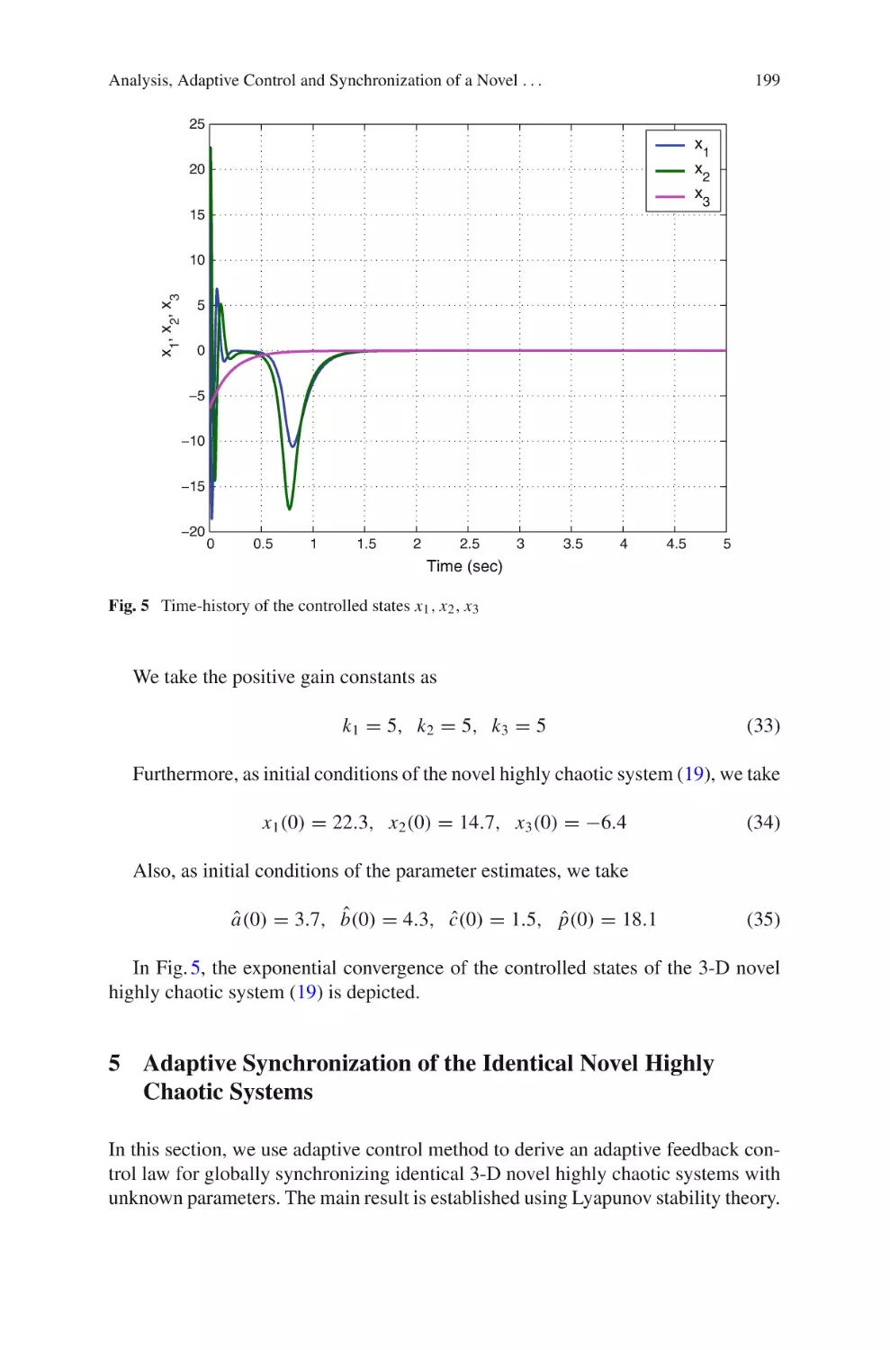
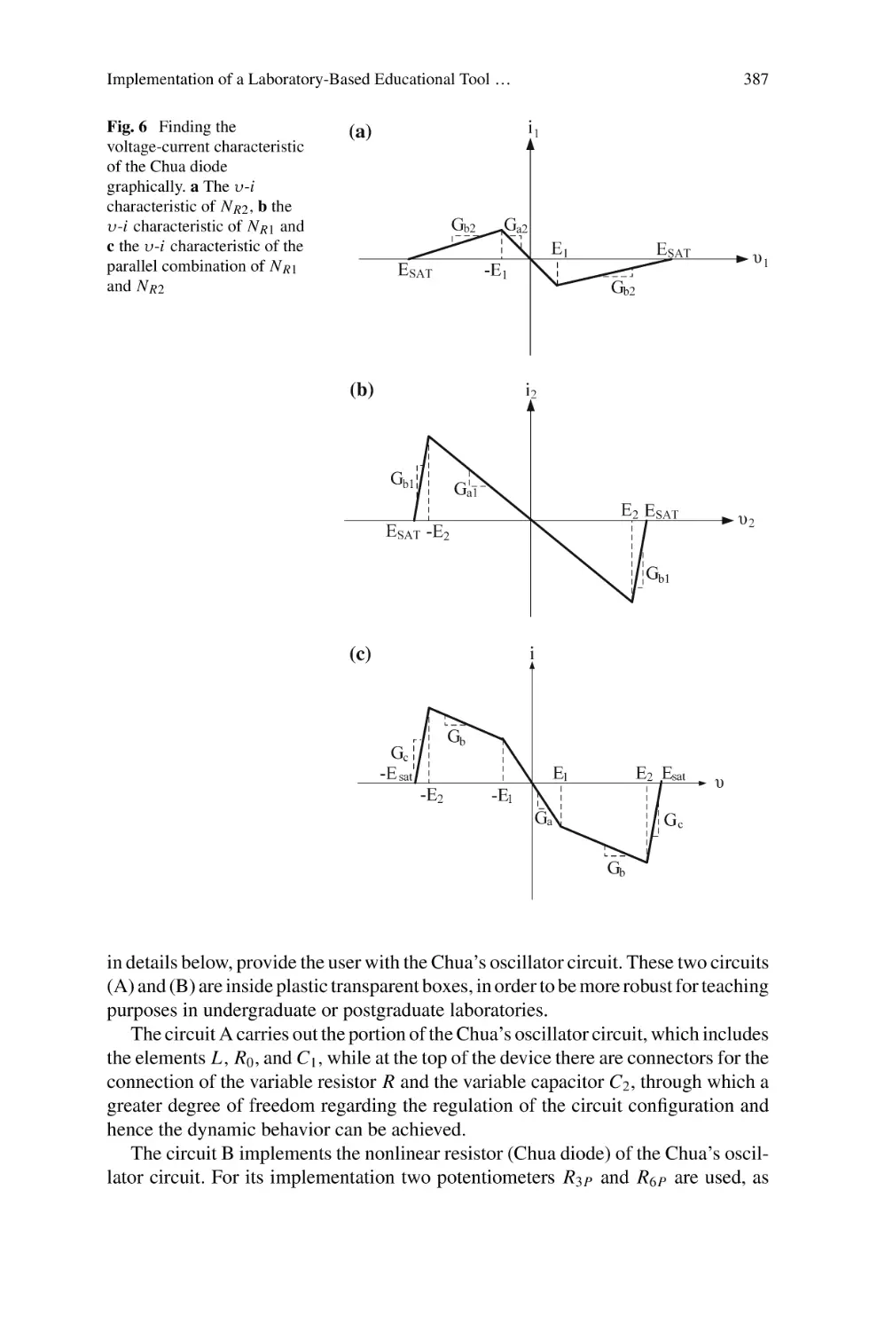
V.-T. Pham et al.

In order to discover the stability type of the equilibrium points E c the Jacobian
matrix of the novel memristive hyperjerk system (13) is calculated at any point x as
⎤
0
1
0
0
⎥
⎢0
0
1
0
⎥,
J (x) = ⎢
⎦
⎣0
0
0
1
x2 x1 − 1 −1 − bx4 −a − bx3
⎡

It is noting that

⎡

0 1
⎢0 0
Δ
J0 = J (E c ) = ⎢
⎣0 0
0 c−1

⎤
0 0
1 0 ⎥
⎥,
0 1 ⎦
−1 −0.5

(21)

(22)

which has the characteristic equation is


λ λ3 + 0.5λ2 + λ + 1 − c = 0.

(23)

When c = 0.06 the characteristic Eq. (23) has a zero eigenvalue and three nonzero
eigenvalues
λ1 = 0, λ2 = −0.7749, λ3,4 = 0.1375 ± 1.0928i

(24)

This shows that the equilibrium point E c is an unstable saddle-focus point.

4.2 Lyapunov Exponents and Kaplan–Yorke Dimension
For the parameter values a = 0.5, b = 0.4 and c = 0.06, the Lyapunov exponents
of the novel memristive hyperjerk system (13) are obtained using MATLAB as
L 1 = 0.0730, L 2 = 0.0018, L 3 = 0 and L 4 = −0.5755

(25)

There is one positive Lyapunov exponents in the LE spectrum (25), thus the novel
memristive hyperjerk system (13) exhibits chaotic behavior.
In addition, since L 1 + L 2 + L 3 + L 4 = −0.5007 < 0, it indicates that the novel
memristive system (13) is dissipative.
The Kaplan–Yorke fractional dimension, that presents the complexity of attractor
[46, 50], is defined by
j
1 

DK Y = j + 
Li
(26)
 L j+1 
i=1

A Chaotic Hyperjerk System Based on Memristive Device

where j is the largest interger satisfying

j

i=1

L i ≥ 0 and

47
j+1


L i < 0. Therefore, the

i=1

Kaplan–Yorke dimension of the novel memristive hyperjerk system (13) is calculated as
DK Y = 3 +

L1 + L2 + L3
= 3.130,
|L 4 |

(27)

which is fractional.

5 Adaptive Synchronization for the Hyperjerk Memristive
System
One of the most important characteristics relating to chaotic systems and their applications is the possibility of synchronization of two chaotic ones [5, 13, 17, 36].
A wide range of research activities based on synchronization of nonlinear systems
has been studied [6, 14, 18, 39, 49, 58]. For example, various synchronization phenomena in bidirectionally coupled double scroll circuits were reported in Volos et
al. [61] or image encryption process based on chaotic synchronization phenomena
was presented in [62]. Different synchronization schemes have proposed such as
anti-synchronization [56], adaptive sycnchronization [59], or hybrid chaos synchronization [18], etc. Here we consider the adaptive synchronization of identical 4-D
memristiive hyperjerk systems with two unknown parameters.
The master system is considered as the 4-D novel memristive hyperjerk system
given by
⎧
⎪ ẋ1 = x2
⎪
⎨
ẋ2 = x3
(28)
⎪ ẋ3 = x4
⎪
⎩
ẋ4 = −x3 − ax4 − bx3 x4 − x2 + x1 x2
where x1 , x2 , x3 , x4 are the states of the system, and a, b are unknown constant
parameters.
The slave system is considered as the 4-D novel memristive hyperjerk system
given by
⎧
ẏ1 = y2
⎪
⎪
⎨
ẏ2 = y3
(29)
ẏ3 = y4
⎪
⎪
⎩
ẏ4 = −y3 − ay4 − by3 y4 − y2 + y1 y2 + u
where y1 , y2 , y3 , y4 are the states of the system, and u is a backstepping control to
be determined using estimates â(t) and b̂(t) for a and b, respectively.

48

V.-T. Pham et al.

The synchronization errors between the states of the master system (28) and the
slave system (29) are defined as
⎧
e1 = y1 − x1
⎪
⎪
⎨
e2 = y2 − x2
(30)
e3 = y3 − x3
⎪
⎪
⎩
e4 = y4 − x4
Thus, the error dynamics is easily obtained as follows
⎧
ė1
⎪
⎪
⎨
ė2
ė3
⎪
⎪
⎩
ė4

= e2
= e3
= e4
= −e3 − ae4 − e2 − b(y3 y4 − x3 x4 ) + y1 y2 − x1 x2 + u

(31)

The parameter estimation errors are defined as:


ea (t) = a − â(t)
eb (t) = b − b̂(t)

(32)

Differentiating (32) with respect to t, we obtain the following equations:


˙
ėa (t) = −â(t)
˙
ė (t) = −b̂(t)

(33)

b

Next, the main result of this section will be presented and proved.
Theorem 5.1 The identical 4-D novel memristive hyperjerk systems (28) and (29)
with unknown parameters a and b are globally and exponentially synchronized by
the adaptive control law


u(t) = −5e1 − 9e2 − 8e3 − [4 − â(t)]e4 + b̂(t) (y3 y4 − x3 x4 )
− (y1 y2 − x1 x2 ) − kz 4

(34)

where k > 0 is a gain constant,
z 4 = 3e1 + 5e2 + 3e3 + e4 ,

(35)

and the update law for the parameter estimates â(t), b̂(t), ĉ(t) is given by


˙
â(t)
= −e4 z 4
˙b̂(t) = −
(y3 y4 − x3 x4 ) z 4

(36)

Proof We prove this result via backstepping control method and Lyapunov stability
theory.

A Chaotic Hyperjerk System Based on Memristive Device

49

First, we define a quadratic Lyapunov function
V1 (z 1 ) =

1 2
z
2 1

(37)

where
z 1 = e1

(38)

Differentiating V1 along the error dynamics (31), we get
V̇1 = z 1 ż 1 = e1 e2 = −z 12 + z 1 (e1 + e2 )

(39)

z 2 = e1 + e2

(40)

Here, we define

Using (40), we can simplify the Eq. (39) as
V̇1 = −z 12 + z 1 z 2

(41)

Secondly, we define a quadratic Lyapunov function
V2 (z 1 , z 2 ) = V1 (z 1 ) +


1 2
1 2
z =
z + z 22
2 2
2 1

(42)

Differentiating V2 along the error dynamics (31), we get
V̇2 = −z 12 − z 22 + z 2 (2e1 + 2e2 + e3 )

(43)

z 3 = 2e1 + 2e2 + e3

(44)

Now, we define

Using (44), we can simplify the Eq. (43) as
V̇2 = −z 12 − z 22 + z 2 z 3

(45)

Thirdly, we define a quadratic Lyapunov function
V3 (z 1 , z 2 , x3 ) = V2 (z 1 , z 2 ) +


1 2
1 2
z 1 + z 22 + z 32
z3 =
2
2

(46)

Differentiating V3 along the error dynamics (31), we get
V̇3 = −z 12 − z 22 − z 32 + z 3 (3e1 + 5e2 + 3e3 + e4 )

(47)

50

V.-T. Pham et al.

Now, we define
z 4 = 3e1 + 5e2 + 3e3 + e4

(48)

Using (48), we can simplify the Eq. (47) as
V̇3 = −z 12 − z 22 − z 32 + z 3 z 4

(49)

Finally, we define a quadratic Lyapunov function
1
1
1
V (z 1 , z 2 , z 3 , z 4 , ea , eb ) = V3 (z 1 , z 2 , z 3 ) + z 42 + ea2 + eb2
2
2
2

(50)

which is a positive definite function on R 6 .
Differentiating V along the error dynamics (31), we get
V̇ = −z 12 − z 22 − z 32 − z 42 + z 4 (z 4 + z 3 + ż 4 ) − ea â˙ − eb b̂˙

(51)

Equation (51) can be written compactly as
V̇ = −z 12 − z 22 − z 32 − z 42 + z 4 S − ea â˙ − eb b̂˙

(52)

S = z 4 + z 3 + ż 4 = z 4 + z 3 + 3ė1 + 5ė2 + 3ė3 + ė4

(53)

where

A simple calculation gives
S = 5e1 + 9e2 + 8e3 + (4 − a)e4 − b (y3 y4 − x3 x4 ) + (y1 y2 − x1 x2 ) + u

(54)

Substituting the adaptive control law (34) into (54), we obtain




S = − a − â(t) e4 − b − b̂(t) (y3 y4 − x3 x4 ) − kz 4

(55)

Using the definitions (33), we can simplify (55) as
S = −ea e4 − eb (y3 y4 − x3 x4 ) − kz 4

(56)

Substituting the value of S from (56) into (52), we obtain
⎧
˙
⎨ V̇ = −z 12 − z 22 − z 32 − (1 + k)z 42 + ea (−e4 z 4 − â)


⎩
+ eb − (y3 y4 − x3 x4 ) z 4 − b̂˙

(57)

A Chaotic Hyperjerk System Based on Memristive Device

51

Substituting the update law (36) into (57), we get
V̇ = −z 12 − z 22 − z 32 − (1 + k)z 42 ,

(58)

which is a negative semi-definite function on R 6 . Therefore, according to the Lyapunov stability theory [19, 43] we obtain e1 (t) → 0, e2 (t) → 0, e3 (t) → 0,
e4 (t) → 0, ea (t) → 0, eb (t) → 0 exponentially when t → 0 that is, synchronization between master and slave system.
In order to confirm and demonstrate the effectiveness of the proposed synchronization scheme, we consider a numerical example. In the numerical simulations, the
fourth-order Runge–Kutta method is used to solve the systems. The parameters of
the memristive hyperjerk systems are selected as a = 0.5, b = 0.4 and the positive
gain constant as k = 6. The initial conditions of the master system (28) and the
slave system (29) have been chosen as x1 (0) = 0.06, x2 (0) = 10−6 , x3 (0) = 0,
x4 (0) = 0 and y1 (0) = 0.02, y2 (0) = 10−4 , y3 (0) = 0, y4 (0) = 0, respectively.
We assumed that the initial values of the parameter estimates are â(0) = 0.46 and
b̂(0) = 0.01.
When adaptive control law (34) and the update law for the parameter estimates
(36) are applied, the master (28) and slave system (29) are synchronized completely

Fig. 5 Synchronization of
the states x1 (t) and y1 (t)

0.6
0.4

1

x ,y1

0.2
0

−0.2
−0.4

0

20

40

60

80

100

60

80

100

Time

Fig. 6 Synchronization of
the states x2 (t) and y2 (t)

0.6
0.4

2

x ,y2

0.2
0
−0.2
−0.4

0

20

40

Time

52

V.-T. Pham et al.

Fig. 7 Synchronization of
the states x3 (t) and y3 (t)

0.4
0.2

x3,y3

0
−0.2
−0.4
−0.6

0

20

40

60

80

100

60

80

100

Time

Fig. 8 Synchronization of
the states x4 (t) and y4 (t)

0.4
0.2

4

x ,y

4

0
−0.2
−0.4
−0.6

0

20

40

Time

Fig. 9 Time series of the
synchronization errors e1 , e2 ,
e3 , and e4

0.06
e1
e2

0.04

e2
e4

ei

0.02
0
−0.02
−0.04

0

2

4

6

8

10

Time

as shown in Figs. 5, 6, 7 and 8. In such figures, time series of master states are denoted
as blue solid lines while corresponding slave states are plotted as red dash-dot lines.
In addition, the time-history of the complete synchronization errors e1 , e2 , e3 , and e4
are reported in Fig. 9. The obtained results illustrate the correctness of used approach.

A Chaotic Hyperjerk System Based on Memristive Device

53

6 SPICE Implementation of the Memristive Hyperjerk
System
In this section, an electronic circuit is proposed to implement memristive hyperjerk
system (13). The circuit in Fig. 10 has been designed by applying the general approach
with operational amplifiers [41, 53]. Thus, the variables x1 , x2 , x3 , x4 of memristive
system (13) are the voltages across the capacitor C1, C2, C3, and C4, respectively.
As shown in Fig. 10 the memristive system is realized by common electronic components. Indeed the sub-circuit of memristive device in Fig. 10 only emulates the
memristive device because there are not any commercial off-the-shelf memristive
devices in the market yet. By applying Kirchhoff’s circuit laws, the corresponding
circuital equations of designed circuit can be written as:
⎧ dvC
1
= R11C1 vC2
⎪
⎪
dt
⎪
⎪
dv
⎨ C2 = 1 v
dt
R2 C 2 C 3
dvC3
⎪
= R31C3 vC4
⎪
dt
⎪
⎪
⎩ dvC4
= − R41C4 vC3 −
dt

(59)
1
v
R5 C 4 C 4

−

1
v v
R6 C 4 C 3 C 4

−

1
R7 C 4

y,

Fig. 10 Schematic of the circuit which emulating novel hyperjerk system (8) with the presence of
the memristive device

54

V.-T. Pham et al.

Fig. 11 Chaotic attractor of
the designed circuit obtained
from Cadence OrCAD in the
(vC1 , vC2 ) phase plane

Fig. 12 Chaotic attractor of
the designed circuit obtained
from Cadence OrCAD in the
(vC1 , vC3 ) phase plane

where vC1 , vC2 , vC3 , and vC4 are the voltages across the capacitors C1 , C2 , C3 , and
C4 , respectively. Here the memristive device is described by the following circuital
equations:

dvC1
dt

= R11C1 vC2
y = vC2 − vC1 vC2 .

(60)

A Chaotic Hyperjerk System Based on Memristive Device

55

Fig. 13 Chaotic attractor of
the designed circuit obtained
from Cadence OrCAD in the
(vC2 , vC3 ) phase plane

Fig. 14 Chaotic attractor of
the designed circuit obtained
from Cadence OrCAD in the
(vC1 , vC4 ) phase plane

The power supplies of all active devices are ±15VDC and the operational amplifiers
TL084 are used in this work. The values of components are selected as follows:
R1 = R2 = R3 = R4 = R7 = R = 100 k, R5 = 200 k, R6 = 250 k, and
C1 = C2 = C3 = C4 = 1 nF.
The designed circuit is implemented in the electronic simulation package Cadence
OrCAD and the obtained results are reported in Figs. 11, 12, 13 and 14. Theoretical
attractors (see Fig. 2) are similar with the circuital ones (see Figs. 11, 12, 13 and 14).

56

V.-T. Pham et al.

7 Conclusion
A 4-D hyperjerk system is introduced in this work. The hyperjerk system is constructed by using a memristive device which creates the special feature of such
hyperjerk system, possessing an infinite number of equilibrium points. This special
feature is rarely observed in other chaotic hyperjerk systems. Dynamical behaviors
of the memristive hyperjerk system are investigated through equilibrium points, projections of chaotic attractors, Lyapunov exponents and Kaplan–Yorke dimension. In
addition, the capacity of synchronization scheme of memristive hyperjerk systems
is shown via backstepping control approach. To verify the feasibility of such hyperjerk system, we present its circuital implementation. Because the designed circuit
modeling the hyperjerk system can generate chaos, it can applied into potential applications in various fields of chaos-based engineering, such as secure communications,
random bit generation, liquid mixing or path planning for mobile robot, etc.
Acknowledgments This research is funded by Vietnam National Foundation for Science and Technology Development (NAFOSTED) under grant number 102.99–2013.06.

References
1. Arneodo A, Coullet P, Tresser C (1981) Possible new strange attractors with spiral structure.
Comm Math Phys 79:573–579
2. Azar AT, Vaidyanathan S (2015) Chaos modeling and control systems design. Springer, New
York
3. Azar AT, Vaidyanathan S (2015) Computational intelligence applications in modeling and
control. Springer, New York
4. Bao B, Zou X, Liu Z, Hu F (2013) Generalized memory element and chaotic memory system.
Int J Bif Chaos 23:1350135
5. Boccaletti S, Kurths J, Osipov G, Valladares DL, Zhou CS (2002) The synchronization of
chaotic systems. Phys Rep 366:1–101
6. Buscarino A, Fortuna L, Frasca M (2009) Experimental robust synchronization of hyperchaotic
circuits. Physica D 238:1917–1922
7. Chen GR (1999) Controlling chaos and bifurcations in engineering systems. CRC Press, Boca
Raton
8. Chen G, Yu X (2003) Chaos control: theory and applications. Springer, Berlin
9. Chlouverakis KE, Sprott JC (2006) Chaotic hyperjerk systems. Chaos, Solitons Fractals
28:739–746
10. Chua LO (1971) Memristor–the missing circuit element. IEEE Trans Circuit Theory 18:
507–519
11. Chua LO, Kang SM (1976) Memristive devices and system. Proc IEEE 64:209–223
12. Elhadj Z, Sprott JC (2013) Transformation of 4-D dynamical systems to hyperjerk form. Palest
J Maths 2:38–45
13. Fortuna L, Frasca M (2007) Experimental synchronization of single-transistor-based chaotic
circuits. Chaos 17:043118-1–5
14. Gamez-Guzman L, Cruz-Hernandez C, Lopez-Gutierrez R, Garcia-Guerrero EE (2009) Synchronization of chua’s circuits with multi-scroll attractors: application to communication. Commun Nonlinear Sci Numer Simul 14:2765–2775

A Chaotic Hyperjerk System Based on Memristive Device

57

15. Jafari S, Sprott JC (2013) Simple chaotic flows with a line equilibrium. Chaos, Solitons Fractals
57:79–84
16. Jafari S, Sprott JC, Golpayegani SMRH (2013) Elementary quadratic chaotic flows with no
equilibria. Phys Lett A 377:699–702
17. Kapitaniak T (1994) Synchronization of chaos using continuous control. Phys Rev E 50:
1642–1644
18. Karthikeyan R, Vaidyanathan S (2014) Hybrid chaos synchronization of four-scroll systems
via active control. J Electr Eng 65:97–103
19. Khalil H (2002) Nonlinear systems. Prentice Hall, New Jersey
20. Kingni ST, Jafari S, Simo H, Woafo P (2014) Three-dimensional chaotic autonomous system with only one stable equilibrium: analysis, circuit design, parameter estimation, control,
synchronization and its fractional-order form. Eur Phys J Plus 129:76
21. Lainscsek C, Lettellier C, Gorodnitsky I (2003) Global modeling of the rössler system from
the z-variable. Phys Lett A 314:409–427
22. Leonov GA, Kuznetsov NV (2011) Algorithms for searching for hidden oscillations in the
Aizerman and Kalman problems. Dokl Math 84:475–481
23. Leonov GA, Kuznetsov NV (2013) Hidden attractors in dynamical systems: from hidden
oscillation in Hilbert-Kolmogorov, Aizerman and Kalman problems to hidden chaotic attractor
in Chua circuits. Int J Bifurc Chaos 23:1330002
24. Leonov GA, Kuznetsov NV, Kuznetsova OA, Seldedzhi SM, Vagaitsev VI (2011) Hidden
oscillations in dynamical systems. Trans Syst Contr 6:54–67
25. Leonov GA, Kuznetsov NV, Vagaitsev VI (2011) Localization of hidden Chua’s attractors.
Phys Lett A 375:2230–2233
26. Leonov GA, Kuznetsov NV, Vagaitsev VI (2012) Hidden attractor in smooth Chua system.
Physica D 241:1482–1486
27. Leonov GA, Kuznetsov NV, Kiseleva MA, Solovyeva EP, Zaretskiy AM (2014) Hidden oscillations in mathematical model of drilling system actuated by induction motor with a wound
rotor. Nonlinear Dyn 77:277–288
28. Linz SJ (1997) Nonlinear dynamical models and jerky motion. Am J Phys 65:523–526
29. Linz SJ (2008) On hyperjerky systems. Chaos, Solitons Fractals 37:741–747
30. Liu C, Yi J, Xi X, An L, Fu Y (2012) Research on the multi-scroll chaos generation based on
Jerk mode. Procedia Eng 29:957–961
31. Lorenz EN (1963) Deterministic non-periodic flow. J Atmos Sci 20:130–141
32. Lü J, Chen G (2002) A new chaotic attractor coined. Int J Bifurc Chaos 12:659–661
33. Ma J, Wu X, Chu R, Zhang L (2014) Selection of multi-scroll attractors in Jerk circuits and
their verification using Pspice. Nonlinear Dyn 76:1951–1962
34. Molaei M, Jafari S, Sprott JC, Golpayegani S (2013) Simple chaotic flows with one stable
equilibrium. Int J Bifurc Chaos 23:1350188
35. Munmuangsaen B, Srisuchinwong B, Sprott JC (2011) Generalization of the simplest
autonomous chaotic system. Phys Lett A 375:1445–1450
36. Pecora LM, Carroll TL (1990) Synchronization in chaotic signals. Phys Rev A 64:821–824
37. Pehlivan I, Moroz I, Vaidyanathan S (2014) Analysis, synchronization and circuit design of a
novel butterfly attractor. J Sound Vibr 333:5077–5096
38. Pershin YV, Fontaine SL, Ventra MD (2009) Memristive model of amoeba learning. Phys Rev
E 80:021926
39. Pham VT, Rahma F, Frasca M, Fortuna L (2014) Dynamics and synchronization of a novel
hyperchaotic system without equilibrium. Int J Bifurc Chaos 24:1450087
40. Pham V-T, Volos C, Jafari S, Wang X, Vaidyanathan S (2014) Hidden hyperchaotic attractor in a
novel simple memristive neural network. Optoelectron. Adv Mater Rapid Comm 8:1157–1163
41. Pham VT, Volos CK, Jafari S, Wei Z, Wang X (2014) Constructing a novel no-equilibrium
chaotic system. Int J Bifurc Chaos 24:1450073
42. Rössler OE (1976) An equation for continuous chaos. Phys Lett A 57:397–398
43. Sastry S (1999) Nonlinear systems: analysis, stability, and control. Springer, USA
44. Schot S (1978) Jerk: the time rate of change of acceleration. Am J Phys 46:1090–1094

58

V.-T. Pham et al.

45. Sprott JC (1997) Some simple chaotic jerk functions. Am J Phys 65:537–543
46. Sprott JC (2003) Chaos and times-series analysis. Oxford University Press, Oxford
47. Sprott JC (2010) Elegant chaos: algebraically simple chaotic flows. World Scientific,
Singapore
48. Sprott JC (2011) A new chaotic jerk circuit. IEEE Trans Circuits Syst-II: Exp Briefs 58:240–243
49. Srinivasan K, Senthilkumar DV, Murali K, Lakshmanan M, Kurths J (2011) Synchronization transitions in coupled time-delay electronic circuits with a threshold nonlinearity. Chaos
21:023119
50. Strogatz SH (1994) Nonlinear dynamics and chaos: with applications to physics, biology,
chemistry, and engineering. Perseus Books, Massachusetts
51. Strukov DB, Snider GS, Stewart DR, Williams RS (2008) The missing memristor found. Nature
453:80–83
52. Sun KH, Sprott JC (2009) A simple jerk system with piecewise exponential nonlinearity. Int J
Nonlinear Sci Num Simu 10:1443–1450
53. Sundarapandian V, Pehlivan I (2012) Analysis, control, synchronization, and circuit design of
a novel chaotic system. Math Comp Model 55:1904–1915
54. Tetzlaff R (2014) Memristor and memristive systems. Springer, New York
55. Tour JM, He T (2008) The fourth element. Nature 453:42–43
56. Vaidyanathan S (2012) Anti-synchronization of four-wing chaotic systems via sliding mode
control. Int J Auto Compt 9:274–279
57. Vaidyanathan S (2013) A new six-term 3-D chaotic system with an exponential nonlineariry.
Far East J Math Sci 79:135–143
58. Vaidyanathan S (2014) Analysis and adaptive synchronization of eight-term novel 3-D chaotic
system with three quadratic nonlinearities. Eur Phys J Spec Topics 223:1519–1529
59. Vaidyanathan S, Volos C, Pham VT, Madhavan K, Idowo BA (2014) Adaptive backstepping
control, synchronization and circuit simualtion of a 3-D novel jerk chaotic system with two
hyperbolic sinusoidal nonlinearities. Arch Cont Sci 33:257–285
60. Vaidyanathan S, Volos C, Pham VT (2015) Analysis, adaptive control and synchronization
of a novel 4-D hyperchaotic hyperjerk system and its SPICE implementation. Arch Cont Sci
25:257–285
61. Volos CK, Kyprianidis IM, Stouboulos IN (2011) Various synchronization phenomena in bidirectionally coupled double scroll circuits. Commun Nonlinear Sci Numer Simul 71:3356–3366
62. Volos CK, Kyprianidis IM, Stouboulos IN (2013) Image encryption process based on chaotic
synchronization phenomena. Signal Process 93:1328–1340
63. Wang X, Chen G (2012) A chaotic system with only one stable equilibrium. Commun Nonlinear
Sci Numer Simul 17:1264–1272
64. Wang X, Chen G (2013) Constructing a chaotic system with any number of equilibria. Nonlinear
Dyn 71:429–436
65. Yalcin M (2007) Multi-scroll and hypercube attractors from a general Jerk circuit using Josephson junctions. Chaos, Solitons Fractals 34:1659–1666
66. Yalcin ME, Suykens JAK, Vandewalle J (2005) Cellular Neural Networks Multi-Scroll Chaos
and Synchronization. World Scientific, Singapore
67. Yu S, Lü J, Leung H, Chen G (2005) Design and implementation of n-scroll chaotic attractors
from a general Jerk circuit. IEEE Trans Circ Syst I 52:1459–1476

A Novel Hyperjerk System with Two
Quadratic Nonlinearities and Its Adaptive
Control
Sundarapandian Vaidyanathan

Abstract This work announces a novel 4-D hyperjerk system with two cubic nonlinearities. The proposed chaotic system is an eight-term polynomial system with
two cubic nonlinearities. The phase portraits of the novel hyperjerk system are displayed and the qualitative properties of the system are discussed. The novel hyperjerk
system has a unique equilibrium, which is unstable. The Lyapunov exponents of the
novel hyperjerk system are obtained as L 1 = 0.0622, L 2 = 0, L 3 = −0.4639 and
L 4 = −0.5945, which shows that the novel hyperjerk system is chaotic. The Kaplan–
Yorke dimension of the novel hyperjerk system is obtained as D K Y = 2.1341. Next,
an adaptive backstepping controller is designed to globally stabilize the novel hyperjerk system with unknown parameters. Moreover, an adaptive backstepping controller is also designed to achieve global chaos synchronization of the identical novel
hyperjerk systems with unknown parameters. The main control results in this work
are established using Lyapunov stability theory. MATLAB simulations have been
shown to illustrate the phase portraits of the novel hyperjerk system and also the
adaptive backstepping control results.
Keywords Chaos · Chaotic systems
Synchronization · Hyperjerk systems

· Backstepping control · Adaptive control ·

1 Introduction
Chaos theory deals with the qualitative study of chaotic dynamical systems and
their applications in science and engineering. A dynamical system is called chaotic
if it satisfies the three properties: boundedness, infinite recurrence and sensitive
dependence on initial conditions [3].

S. Vaidyanathan (B)
Research and Development Centre, Vel Tech University,
Avadi, Chennai 600062, India
e-mail: sundarvtu@gmail.com
© Springer International Publishing Switzerland 2016
S. Vaidyanathan and C. Volos (eds.), Advances and Applications
in Chaotic Systems, Studies in Computational Intelligence 636,
DOI 10.1007/978-3-319-30279-9_3

59

60

S. Vaidyanathan

Some classical paradigms of 3-D chaotic systems in the literature are Lorenz
system [15], Rössler system [25], ACT system [2], Sprott systems [32], Chen system
[6], Lü system [16], Cai system [4], Tigan system [43], etc.
Many new chaotic systems have been discovered in the recent years such as
Zhou system [117], Zhu system [118], Li system [13], Wei-Yang system [115],
Sundarapandian systems [35, 40], Vaidyanathan systems [51, 52, 54–57, 60, 71,
72, 86, 89, 91, 100, 103, 105, 107, 109, 110], Pehlivan system [18], Sampath
system [26], etc.
Chaos theory has many applications in science and engineering such as chemical
systems [61, 65, 67, 69, 73, 77–79], biological systems [59, 62–64, 66, 68, 70,
74–76, 80–84], memristors [1, 19, 113], etc.
The study of control of a chaotic system investigates feedback control methods that
globally or locally asymptotically stabilize or regulate the outputs of a chaotic system.
Many methods have been designed for control and regulation of chaotic systems such
as active control [33, 34, 45], adaptive control [101, 108, 111], backstepping control
[14, 114], sliding mode control [48, 50], etc.
Synchronization of chaotic systems is a phenomenon that occurs when two or more
chaotic systems are coupled or when a chaotic system drives another chaotic system.
Because of the butterfly effect which causes exponential divergence of the trajectories
of two identical chaotic systems started with nearly the same initial conditions, the
synchronization of chaotic systems is a challenging research problem in the chaos
literature [3].
Pecora and Carroll pioneered the research on synchronization of chaotic systems
with their seminal papers [5, 17]. The active control method [11, 27, 28, 39, 44,
49, 92, 93, 96] is typically used when the system parameters are available for measurement. Adaptive control method [29–31, 36–38, 47, 53, 85, 90, 94, 95, 102,
106] is typically used when some or all the system parameters are not available for
measurement and estimates for the uncertain parameters of the systems.
Sampled-data feedback control method [9, 116] and time-delay feedback control
method [7, 10] are also used for synchronization of chaotic systems. Backstepping
control method [20–24, 42, 97, 104, 112] is also used for the synchronization of
chaotic systems. Backstepping control is a recursive method for stabilizing the origin
of a control system in strict-feedback form [12]. In this research work, we apply
backstepping control method for the adaptive control and synchronization of the
novel hyperjerk system.
Sliding mode control method [41, 46, 58, 87, 88, 98, 99] is also a popular method
for the synchronization of chaotic systems.
In the recent decades, there is some good interest in finding novel chaotic and
hyperchaotic systems, which can be expressed by an explicit fourth order differential
equation describing the time evolution of the single scalar variable x given by


d x d2x d3x
d4x
= j x,
, 2, 3
dt
dt dt dt

(1)

A Novel Hyperjerk System with Two Quadratic Nonlinearities …

61

The differential equation (1) is called “hyperjerk system” because the fourth order
time derivative in mechanical systems is called hyperjerk [8].
By defining phase variables
x1 = x, x2 =

dx
d2x
d3x
, x3 = 2 , x4 = 3 ,
dt
dt
dt

(2)

the hyperjerk differential equation (1) can be expressed as a 4-D system given by
⎧
ẋ1
⎪
⎪
⎨
ẋ2
ẋ3
⎪
⎪
⎩
ẋ4

=
=
=
=

x2
x3
x4
j (x1 , x2 , x3 , x4 )

(3)

In this research work, we announce a 4-D novel hyperjerk system and discuss
the qualitative properties of the novel hyperjerk system. We have designed adaptive backstepping controllers for stabilization and synchronization of the 4-D novel
hyperjerk system.
This work is organized as follows. Section 2 describes the dynamic equations and
phase portraits of the 4-D novel hyperjerk system. Section 3 details the qualitative
properties of the novel hyperjerk system.
The Lyapunov exponents of the hyperjerk system are obtained as L 1 = 0.0622,
L 2 = 0, L 3 = −0.4639 and L 4 = −0.5945. The Kaplan–Yorke dimension of the
hyperjerk system is obtained as D K Y = 2.1341.
In Sect. 4, we design an adaptive backstepping controller to globally stabilize the
novel hyperjerk system with unknown parameters. In Sect. 5, an adaptive backstepping controller is designed to achieve global chaos synchronization of the identical
novel hyperjerk systems with unknown parameters. Section 6 contains a summary of
the main results derived in this work.

2 A 4-D Novel Hyperjerk System
In this section, we describe a 4-D novel hyperjerk system with two quadratic nonlinearities, which is modeled by the 4-D dynamics
⎧
⎪
⎪ ẋ1
⎨
ẋ2
ẋ3
⎪
⎪
⎩
ẋ4

=
=
=
=

x2
x3
x4
1 − ax1 − x22 − x32 − bx3 − cx4

where x1 , x2 , x3 , x4 are the states and a, b, c are constant positive parameters.

(4)

62

S. Vaidyanathan

The system (4) is a nine-term polynomial system having two quadratic nonlinearities.
The equilibrium points of (4) are obtained by solving the system
x2 = 0, x3 = 0, x4 = 0, 1 − ax1 − x22 − x32 − bx3 − cx4 = 0

(5)

By solving the Eq. (5), we see that the system (4) has a unique equilibrium point
given by
⎡
⎤
1/a
⎢ 0 ⎥
⎥
E1 = ⎢
(6)
⎣ 0 ⎦
0
The system (4) exhibits a strange chaotic attractor for the parameter values
a = 1, b = 4, c = 1

(7)

For numerical simulations, we take the initial conditions as
x1 (0) = 0.5, x2 (0) = 0.4, x3 (0) = 0.3, x4 (0) = 0.9

(8)

Figures 1, 2, 3 and 4 show the 3-D projection of the novel hyperjerk system (4)
on the (x1 , x2 , x3 ), (x1 , x2 , x4 ), (x1 , x3 , x4 ) and (x2 , x3 , x4 ) spaces, respectively.

x3

5

0

−5
5

0

x2
−5 −30

−25

−20

−15

−10

−5

x1

Fig. 1 3-D projection of the novel hyperjerk system on the (x1 , x2 , x3 ) space

0

5

A Novel Hyperjerk System with Two Quadratic Nonlinearities …

63

6
4

x4

2
0
−2
−4
−6
5
0

x2
−5 −30

−25

−20

−10

−15

−5

0

5

x1

Fig. 2 3-D projection of the novel hyperjerk system on the (x1 , x2 , x4 ) space

6
4

x4

2
0
−2
−4
−6
5
0

x3
−5 −30 −25

−20

−15

−10

−5

0

5

x1

Fig. 3 3-D projection of the novel hyperjerk system on the (x1 , x3 , x4 ) space

3 Analysis of the Novel Hyperjerk System
In this section, we give a dynamic analysis of the novel hyperjerk system (4).

64

S. Vaidyanathan

6
4

x4

2
0
−2
−4
−6
5
5
0

0

x3
−5 −5

x2

Fig. 4 3-D projection of the novel hyperjerk system on the (x2 , x3 , x4 ) space

3.1 Dissipativity
In vector notation, the novel hyperjerk system (4) can be expressed as
⎤
f 1 (x1 , x2 , x3 , x4 )
⎢ f 2 (x1 , x2 , x3 , x4 ) ⎥
⎥
ẋ = f (x) = ⎢
⎣ f 3 (x1 , x2 , x3 , x4 ) ⎦ ,
f 4 (x1 , x2 , x3 , x4 )

(9)

⎧
f 1 (x1 , x2 , x3 , x4 ) = x2
⎪
⎪
⎨
f 2 (x1 , x2 , x3 , x4 ) = x3
⎪ f 3 (x1 , x2 , x3 , x4 ) = x4
⎪
⎩
f 4 (x1 , x2 , x3 , x4 ) = 1 − ax1 − x22 − x32 − bx3 − cx4

(10)

⎡

where

Let Ω be any region in R4 with a smooth boundary and also, Ω(t) = Φt (Ω),
where Φt is the flow of f . Furthermore, let V (t) denote the hypervolume of Ω(t).
By Liouville’s theorem, we know that

(∇ · f ) d x1 d x2 d x3 d x4

V̇ (t) =
Ω(t)

(11)

A Novel Hyperjerk System with Two Quadratic Nonlinearities …

65

The divergence of the novel hyperjerk system (9) is found as:
∇· f =

∂ f2
∂ f3
∂ f4
∂ f1
+
+
+
= −c < 0
∂ x1
∂ x2
∂ x3
∂ x4

(12)

since c is a positive constant.
Inserting the value of ∇ · f from (12) into (11), we get

V̇ (t) =

(−1) d x1 d x2 d x3 d x4 = −cV (t)

(13)

Ω(t)

Integrating the first order linear differential equation (13), we get
V (t) = exp(−ct)V (0)

(14)

From Eq. (14), it follows that V (t) → 0 exponentially as t → ∞. This shows that
the hyperjerk system (4) is dissipative. Hence, the system limit sets are ultimately
confined into a specific limit set of zero hypervolume, and the asymptotic motion of
the hyperjerk system (4) settles onto a strange attractor of the system.

3.2 Equilibrium Points
We take the parameter values as in the chaotic case (7), i.e.
a = 1, b = 4, c = 1

(15)

In Sect. 2, we showed that the novel hyperjerk system (4) has a unique equilibrium
point given by
⎡
⎤ ⎡ ⎤
1/a
1
⎢ 0 ⎥ ⎢0⎥
⎢
⎥
⎢
⎥
E1 = ⎣
=
(16)
0 ⎦ ⎣0⎦
0
0
To test the stability type of the equilibrium point E 1 , we calculate the Jacobian
matrix of the novel hyperjerk system (4) at any point x:
⎤ ⎡
⎤
0
1
0
0
0
1
0
0
⎢
⎢ 0
0
1
0 ⎥
0
1
0 ⎥
⎥=⎢ 0
⎥
J (x) = ⎢
⎣ 0
0
0
1 ⎦
0
0
1 ⎦ ⎣ 0
−1 −2x2 −2x3 − 4 −1
−a −2x2 −2x3 − b −c
⎡

(17)

66

S. Vaidyanathan

⎡

We find that

0
⎢ 0
Δ
⎢
J1 = J (E 1 ) = ⎣
0
−1

⎤
1 0
0
0 1
0 ⎥
⎥
0 0
1 ⎦
0 −4 −1

(18)

The matrix J1 has the eigenvalues
λ1,2 = −0.5368 ± 1.8785i, λ3,4 = 0.0368 ± 0.5105i

(19)

This shows that the equilibrium point E 1 is a saddle-focus, which is unstable.

3.3 Lyapunov Exponents and Kaplan–Yorke Dimension
We take the parameter values of the novel hyperjerk system (4) as a = 1, b = 4 and
c = 1. We take the initial state of the novel hyperjerk system (4) as given in (8).
Then the Lyapunov exponents of the novel hyperjerk system (4) are numerically
obtained using MATLAB as
L 1 = 0.0622, L 2 = 0, L 3 = −0.4639, L 4 = −0.5945

(20)

Thus, the maximal Lyapunov exponent (MLE) of the novel hyperjerk system (4)
is positive, which means that the system has a chaotic behavior.
Since L 1 + L 2 + L 3 + L 4 = −0.9962 < 0, it follows that the novel hyperjerk
system (4) is dissipative.
Also, the Kaplan–Yorke dimension of the hyperjerk system (4) is obtained as
DK Y = 2 +

L1 + L2
= 2.1341
|L 3 |

(21)

which is fractional.

4 Adaptive Control of the Novel Hyperjerk System
In this section, we use backstepping control method to derive an adaptive feedback
control law for globally stabilizing the 4-D novel hyperjerk system with unknown
parameters.

A Novel Hyperjerk System with Two Quadratic Nonlinearities …

67

Thus, we consider the 4-D novel hyperjerk system given by
⎧
ẋ1
⎪
⎪
⎨
ẋ2
ẋ3
⎪
⎪
⎩
ẋ4

= x2
= x3
= x4
= 1 − ax1 − x22 − x32 − bx3 − cx4 + u

(22)

where x1 , x2 , x3 , x4 are the states, a, b, c are unknown constant parameters, and u is
a backstepping control law to be determined using estimates â(t), b̂(t) and ĉ(t) for
a, b and c, respectively.
The parameter estimation errors are defined as:
⎧
⎨ ea (t) = a − â(t)
e (t) = b − b̂(t)
⎩ b
ec (t) = c − ĉ(t)

(23)

Differentiating (23) with respect to t, we obtain the following equations:
⎧
˙
⎪
⎨ ėa (t) = −â(t)
˙
ėb (t) = −b̂(t)
⎪
⎩
˙
ėc (t) = −ĉ(t)

(24)

Next, we shall state and prove the main result of this section.
Theorem 1 The 4-D novel hyperjerk system (22), with unknown parameters a, b
and c, is globally and exponentially stabilized by the adaptive feedback control law,




u(t) = −1 − 5 − â(t) x1 − 10x2 − 9 − b̂(t) x3 + ĉ(t)x4 + x22 + x32 − kz 4

(25)

where k > 0 is a gain constant,
z 4 = 3x1 + 5x2 + 3x3 + x4

(26)

and the update law for the parameter estimates â(t), b̂(t), ĉ(t) is given by
⎧
˙
⎪
⎨ â(t) = −x1 z 4
˙ = −x z
b̂(t)
3 4
⎪
⎩˙
ĉ(t) = −x4 z 4

(27)

Proof We prove this result via Lyapunov stability theory [12].
First, we define a quadratic Lyapunov function
V1 (z 1 ) =

1 2
z
2 1

(28)

68

S. Vaidyanathan

where
z 1 = x1

(29)

Differentiating V1 along the dynamics (22), we get
V̇1 = z 1 ż 1 = x1 x2 = −z 12 + z 1 (x1 + x2 )

(30)

z 2 = x1 + x2

(31)

Now, we define

Using (31), we can simplify the Eq. (30) as
V̇1 = −z 12 + z 1 z 2

(32)

Secondly, we define a quadratic Lyapunov function
V2 (z 1 , z 2 ) = V1 (z 1 ) +


1 2
1 2
z2 =
z 1 + z 22
2
2

(33)

Differentiating V2 along the dynamics (22), we get
V̇2 = −z 12 − z 22 + z 2 (2x1 + 2x2 + x3 )

(34)

z 3 = 2x1 + 2x2 + x3

(35)

Now, we define

Using (35), we can simplify the Eq. (34) as
V̇2 = −z 12 − z 22 + z 2 z 3

(36)

Thirdly, we define a quadratic Lyapunov function
V3 (z 1 , z 2 , x3 ) = V2 (z 1 , z 2 ) +


1 2
1 2
z3 =
z 1 + z 22 + z 32
2
2

(37)

Differentiating V3 along the dynamics (22), we get
V̇3 = −z 12 − z 22 − z 32 + z 3 (3x1 + 5x2 + 3x3 + x4 )

(38)

Now, we define
z 4 = 3x1 + 5x2 + 3x3 + x4

(39)

Using (39), we can simplify the Eq. (38) as
V̇2 = −z 12 − z 22 − z 32 + z 3 z 4

(40)

A Novel Hyperjerk System with Two Quadratic Nonlinearities …

69

Finally, we define a quadratic Lyapunov function
1
1
1
1
V (z 1 , z 2 , z 3 , z 4 , ea , eb , ec ) = V3 (z 1 , z 2 , z 3 ) + z 42 + ea2 + eb2 + ec2
2
2
2
2

(41)

which is a positive definite function on R7 .
Differentiating V along the dynamics (22), we get
V̇ = −z 12 − z 22 − z 32 − z 42 + z 4 (z 4 + z 3 + ż 4 ) − ea â˙ − eb b̂˙ − ec ĉ˙

(42)

Equation (42) can be written compactly as
V̇ = −z 12 − z 22 − z 32 − z 42 + z 4 S − ea â˙ − eb b̂˙ − ec ĉ˙

(43)

S = z 4 + z 3 + ż 4 = z 4 + z 3 + 3ẋ1 + 5ẋ2 + 3ẋ3 + ẋ4

(44)

where

A simple calculation gives
S = 1 + (5 − a)x1 + 10x2 + (9 − b)x3 − cx4 − x22 − x32 + u

(45)

Substituting the adaptive control law (25) into (45), we obtain






S = − a − â(t) x1 − b − b̂(t) x3 − c − ĉ(t) x4 − kz 4

(46)

Using the definitions (24), we can simplify (46) as
S = −ea x1 − eb x3 − ec x4 − kz 4

(47)

Substituting the value of S from (47) into (43), we obtain


V̇ = −z 12 − z 22 − z 32 − (1 + k)z 42 + ea −x1 z 4 − â˙




+ eb −x3 z 4 − b̂˙ + ec −x4 z 4 − ĉ˙

(48)

Substituting the update law (27) into (48), we get
V̇ = −z 12 − z 22 − z 32 − (1 + k)z 42 ,

(49)

which is a negative semi-definite function on R7 .
From (49), it follows that the vector z(t) = (z 1 (t), z 2 (t), z 3 (t), z 4 (t)) and the
parameter estimation error (ea (t), eb (t), ec (t)) are globally bounded, i.e.



z 1 (t) z 2 (t) z 3 (t) z 4 (t) ea (t) eb (t) ec (t) ∈ L∞

(50)

70

S. Vaidyanathan

Also, it follows from (49) that
V̇ ≤ −z 12 − z 22 − z 32 − z 42 = −z2

(51)

z2 ≤ −V̇

(52)

That is,

Integrating the inequality (52) from 0 to t, we get
t
|z(τ )|2 dτ ≤ V (0) − V (t)

(53)

0

From (53), it follows that z(t) ∈ L2 .
From Eq. (22), it can be deduced that ż(t) ∈ L∞ .
Thus, using Barbalat’s lemma [12], we conclude that z(t) → 0 exponentially as
t → ∞ for all initial conditions z(0) ∈ R4 .
Hence, it is immediate that x(t) → 0 exponentially as t → ∞ for all initial
conditions x(0) ∈ R4 .
This completes the proof.

For the numerical simulations, the classical fourth-order Runge–Kutta method
with step size h = 10−8 is used to solve the system of differential equations (22)
and (27), when the adaptive control law (25) and the parameter update law (27) are
applied.
The parameter values of the novel hyperjerk system (22) are taken as in the chaotic
case (7), i.e.
a = 1, b = 4, c = 1
(54)
We take the positive gain constant as
k=8

(55)

As initial conditions of the hyperjerk system (22), we take
x1 (0) = −2.3, x2 (0) = 3.4, x3 (0) = 4.7, x4 (0) = −1.9

(56)

Also, as initial conditions of the parameter estimates â(t) and b̂(t), we take
â(0) = 5.2, b̂(0) = 1.4, ĉ(0) = 8.5

(57)

In Fig. 5, the exponential convergence of the controlled states x1 (t), x2 (t), x3 (t),
x4 (t) is depicted, when the adaptive control law (25) and the parameter update law
(27) are implemented.

A Novel Hyperjerk System with Two Quadratic Nonlinearities …
Fig. 5 Time-history of the
controlled states
x1 , x2 , x3 , x4

71

20
x1
x2
x3
x4

x1, x2, x3, x4

10

0
−10

−20
−30

−40

0

1

2

3

4

5

6

7

8

9

10

Time (sec)

5 Adaptive Synchronization of the Identical Novel
Hyperjerk Systems
In this section, we use backstepping control to derive an adaptive control law for
globally and exponentially synchronizing the identical novel hyperjerk systems with
unknown parameters.
As the master system, we consider the 4-D novel hyperjerk system given by
⎧
ẋ1
⎪
⎪
⎨
ẋ2
ẋ3
⎪
⎪
⎩
ẋ4

=
=
=
=

x2
x3
x4
1 − ax1 − x22 − x32 − bx3 − cx4

(58)

where x1 , x2 , x3 , x4 are the states of the system, and a, b, c are unknown constant
parameters.
As the slave system, we consider the 4-D novel hyperjerk system given by
⎧
ẏ1
⎪
⎪
⎨
ẏ2
ẏ3
⎪
⎪
⎩
ẏ4

= y2
= y3
= y4
= 1 − ay1 − y22 − y32 − by3 − cy4 + u

(59)

where y1 , y2 , y3 , y4 are the states of the system, and u is a backstepping control to
be determined using estimates â(t), b̂(t) and ĉ(t) for a, b and c, respectively.
We define the synchronization errors between the states of the master system (58)
and the slave system (59) as
ei = yi − xi , (i = 1, 2, 3, 4)

(60)

72

S. Vaidyanathan

Then the error dynamics is easily obtained as
⎧
ė1
⎪
⎪
⎨
ė2
ė3
⎪
⎪
⎩
ė4

=
=
=
=

e2
e3
e4
−ae1 − be3 − ce4 − y22 + x22 − y32 + x32 + u

(61)

The parameter estimation errors are defined as:
⎧
⎨ ea (t) = a − â(t)
e (t) = b − b̂(t)
⎩ b
ec (t) = c − ĉ(t)

(62)

Differentiating (62) with respect to t, we obtain the following equations:
⎧
˙
⎪
⎨ ėa (t) = −â(t)
˙
ėb (t) = −b̂(t)
⎪
⎩
˙
ėc (t) = −ĉ(t)

(63)

Next, we shall state and prove the main result of this section.
Theorem 2 The identical 4-D hyperjerk systems (58) and (59) with unknown parameters a, b and c are globally and exponentially synchronized by the adaptive control
law






u = − 5 − â(t) e1 − 10e2 − 9 − b̂(t) e3 − 4 − ĉ(t) e4
+ y22 − x22 + y32 − x32 − kz 4

(64)

where k > 0 is a gain constant,
z 4 = 3e1 + 5e2 + 3e3 + e4 ,

(65)

and the update law for the parameter estimates â(t), b̂(t), ĉ(t) is given by
⎧
˙
⎪
⎨ â(t) = −e1 z 4
˙ = −e z
b̂(t)
3 4
⎪
⎩˙
ĉ(t) = −e4 z 4

(66)

Proof We prove this result via backstepping control method and Lyapunov stability
theory.
First, we define a quadratic Lyapunov function
V1 (z 1 ) =

1 2
z
2 1

(67)

A Novel Hyperjerk System with Two Quadratic Nonlinearities …

73

where
z 1 = e1

(68)

Differentiating V1 along the error dynamics (61), we get
V̇1 = z 1 ż 1 = e1 e2 = −z 12 + z 1 (e1 + e2 )

(69)

z 2 = e1 + e2

(70)

Now, we define

Using (70), we can simplify the Eq. (69) as
V̇1 = −z 12 + z 1 z 2

(71)

Secondly, we define a quadratic Lyapunov function
V2 (z 1 , z 2 ) = V1 (z 1 ) +


1 2
1 2
z2 =
z 1 + z 22
2
2

(72)

Differentiating V2 along the error dynamics (61), we get
V̇2 = −z 12 − z 22 + z 2 (2e1 + 2e2 + e3 )

(73)

z 3 = 2e1 + 2e2 + e3

(74)

Now, we define

Using (74), we can simplify the Eq. (73) as
V̇2 = −z 12 − z 22 + z 2 z 3

(75)

Thirdly, we define a quadratic Lyapunov function
V3 (z 1 , z 2 , x3 ) = V2 (z 1 , z 2 ) +


1 2
1 2
z3 =
z 1 + z 22 + z 32
2
2

(76)

Differentiating V3 along the error dynamics (61), we get
V̇3 = −z 12 − z 22 − z 32 + z 3 (3e1 + 5e2 + 3e3 + e4 )

(77)

Now, we define
z 4 = 3e1 + 5e2 + 3e3 + e4

(78)

Using (78), we can simplify the Eq. (77) as
V̇2 = −z 12 − z 22 − z 32 + z 3 z 4

(79)

74

S. Vaidyanathan

Finally, we define a quadratic Lyapunov function
1
1
1
1
V (z 1 , z 2 , z 3 , z 4 , ea , eb , ec ) = V3 (z 1 , z 2 , z 3 ) + z 42 + ea2 + eb2 + ec2
2
2
2
2

(80)

Differentiating V along the error dynamics (61), we get
V̇ = −z 12 − z 22 − z 32 − z 42 + z 4 (z 4 + z 3 + ż 4 ) − ea â˙ − eb b̂˙ − ec ĉ˙

(81)

Equation (81) can be written compactly as
V̇ = −z 12 − z 22 − z 32 − z 42 + z 4 S − ea â˙ − eb b̂˙ − ec ĉ˙

(82)

S = z 4 + z 3 + ż 4 = z 4 + z 3 + 3ė1 + 5ė2 + 3ė3 + ė4

(83)

where

A simple calculation gives
S = (5 − a)e1 + 10e2 + (9 − b)e3 + (4 − c)e4 − y22 + x22 − y32 + x32 + u

(84)

Substituting the adaptive control law (64) into (84), we obtain






S = − a − â(t) e1 − b − b̂(t) e3 − c − ĉ(t) e4 − kz 4

(85)

Using the definitions (63), we can simplify (85) as
S = −ea e1 − eb e3 − ec e4 − kz 4

(86)

Substituting the value of S from (86) into (82), we obtain
⎧


⎨ V̇ = −z 2 − z 2 − z 2 − (1 + k)z 2 + ea −e1 z 4 − â˙
1
3
 2
 4


˙
⎩
+eb −e3 z 4 − b̂ + ec −e4 z 4 − ĉ˙

(87)

Substituting the update law (66) into (87), we get
V̇ = −z 12 − z 22 − z 32 − (1 + k)z 42 ,

(88)

which is a negative semi-definite function on R7 .
From (88), it follows that the vector z(t) = (z 1 (t), z 2 (t), z 3 (t), z 4 (t)) and the
parameter estimation error (ea (t), eb (t), ec (t)) are globally bounded, i.e.



z 1 (t) z 2 (t) z 3 (t) z 4 (t) ea (t) eb (t) ec (t) ∈ L∞

(89)

A Novel Hyperjerk System with Two Quadratic Nonlinearities …

75

Also, it follows from (88) that
V̇ ≤ −z 12 − z 22 − z 32 − z 42 = −z2

(90)

z2 ≤ −V̇

(91)

That is,

Integrating the inequality (91) from 0 to t, we get
t
|z(τ )|2 dτ ≤ V (0) − V (t)

(92)

0

From (92), it follows that z(t) ∈ L2 .
From Eq. (61), it can be deduced that ż(t) ∈ L∞ .
Thus, using Barbalat’s lemma [12], we conclude that z(t) → 0 exponentially as
t → ∞ for all initial conditions z(0) ∈ R4 .
Hence, it is immediate that e(t) → 0 exponentially as t → ∞ for all initial

conditions e(0) ∈ R4 . This completes the proof.
For the numerical simulations, the classical fourth-order Runge–Kutta method
with step size h = 10−8 is used to solve the system of differential equations (58)
and (59).
The parameter values of the novel hyperjerk system are taken as in the chaotic
case, viz. a = 1, b = 4 and c = 1. The gain constant is taken as k = 8.
Also, as initial conditions of the master system (58), we take
x1 (0) = 1.8, x2 (0) = −0.5, x3 (0) = −2.7, x4 (0) = 4.9

Fig. 6 Synchronization of
the states x1 and y1

(93)

6
x1
y1

4

x1, y1

2

0

−2

−4

−6

0

1

2

3

4

5

6

Time (sec)

7

8

9

10

76

S. Vaidyanathan

Fig. 7 Synchronization of
the states x2 and y2

4
x2
y2

3

x2, y2

2

1

0

−1

−2

0

1

2

3

4

5

6

7

8

9

10

Time (sec)

Fig. 8 Synchronization of
the states x3 and y3

6
x3
y3

5
4

x 3, y3

3
2
1
0
−1
−2
−3
−4

0

1

2

3

4

5

6

7

8

9

10

Time (sec)

As initial conditions of the slave system (59), we take
y1 (0) = −4.7, y2 (0) = 2.6, y3 (0) = 5.1, y4 (0) = −3.2

(94)

Furthermore, as initial conditions of the parameter estimates â(t), b̂(t) and ĉ(t),
we take
â(0) = 2.3, b̂(0) = 6.8, ĉ(0) = 7.6
(95)
In Figs. 6, 7, 8 and 9, the complete synchronization of the identical 4-D hyperjerk
systems (58) and (59) is shown, when the adaptive control law and the parameter
update law are implemented.
Also, in Fig. 10, the time-history of the complete synchronization errors is shown.

A Novel Hyperjerk System with Two Quadratic Nonlinearities …
Fig. 9 Synchronization of
the states x4 and y4

77

10
x4
y4

5

x4, y4

0
−5
−10
−15
−20
−25

0

1

2

3

4

5

6

7

8

9

10

Time (sec)

Fig. 10 Time-history of the
synchronization errors
e1 , e2 , e3 , e4

10
x4
y4

5

x4, y4

0
−5
−10
−15
−20
−25

0

1

2

3

4

5

6

7

8

9

10

Time (sec)

6 Conclusions
This work announced a novel 4-D hyperjerk system with two cubic nonlinearities.
The proposed chaotic system is an eight-term polynomial system with two cubic
nonlinearities. The phase portraits of the novel hyperjerk system are displayed and
the qualitative properties of the system are discussed. The novel hyperjerk system
has a unique equilibrium, which is unstable. The Lyapunov exponents of the novel
hyperjerk system have been obtained as L 1 = 0.0622, L 2 = 0, L 3 = −0.4639 and
L 4 = −0.5945, while the Kaplan–Yorke dimension of the novel hyperjerk system
has been found as D K Y = 2.1341. Next, an adaptive backstepping controller has been
designed to globally stabilize the novel hyperjerk system with unknown parameters.
Moreover, an adaptive backstepping controller has also been designed to achieve
global chaos synchronization of the identical novel hyperjerk systems with unknown

78

S. Vaidyanathan

parameters. The backstepping control method is a recursive procedure that links the
choice of a Lyapunov function with the design of a controller and guarantees global
asymptotic stability of strict feedback systems. MATLAB simulations were shown
to illustrate the phase portraits of the novel hyperjerk system and also the adaptive
backstepping control results.

References
1. Abdurrahman A, Jiang H, Teng Z (2015) Finite-time synchronization for memristor-based
neural networks with time-varying delays. Neural Netw 69:20–28
2. Arneodo A, Coullet P, Tresser C (1981) Possible new strange attractors with spiral structure.
Commun Math Phys 79(4):573–576
3. Azar AT, Vaidyanathan S (2015) Chaos modeling and control systems design, vol 581.
Springer, Germany
4. Cai G, Tan Z (2007) Chaos synchronization of a new chaotic system via nonlinear control. J
Uncertain Syst. 1(3):235–240
5. Carroll TL, Pecora LM (1991) Synchronizing chaotic circuits. IEEE Trans Circuits Syst
38(4):453–456
6. Chen G, Ueta T (1999) Yet another chaotic attractor. Int J Bifurc Chaos 9(7):1465–1466
7. Chen WH, Wei D, Lu X (2014) Global exponential synchronization of nonlinear timedelay Lur’e systems via delayed impulsive control. Commun Nonlinear Sci Numer Simul
19(9):3298–3312
8. Chlouverakis KE, Sprott JC (2006) Chaotic hyperjerk systems. Chaos Solitons Fractals
28(3):739–746
9. Gan Q, Liang Y (2012) Synchronization of chaotic neural networks with time delay in
the leakage term and parametric uncertainties based on sampled-data control. J Frankl Inst
349(6):1955–1971
10. Jiang GP, Zheng WX, Chen G (2004) Global chaos synchronization with channel time-delay.
Chaos Solitons Fractals 20(2):267–275
11. Karthikeyan R, Sundarapandian V (2014) Hybrid chaos synchronization of four-scroll systems
via active control. J Electr Eng 65(2):97–103
12. Khalil HK (2001) Nonlinear systems, 3rd edn. Prentice Hall, New Jersey
13. Li D (2008) A three-scroll chaotic attractor. Phys Lett A 372(4):387–393
14. Li GH, Zhou SP, Yang K (2007) Controlling chaos in Colpitts oscillator. Chaos Solitons
Fractals 33:582–587
15. Lorenz EN (1963) Deterministic periodic flow. J Atmos Sci 20(2):130–141
16. Lü J, Chen G (2002) A new chaotic attractor coined. Int J Bifurc Chaos 12(3):659–661
17. Pecora LM, Carroll TL (1990) Synchronization in chaotic systems. Phys Rev Lett 64(8):
821–824
18. Pehlivan I, Moroz IM, Vaidyanathan S (2014) Analysis, synchronization and circuit design
of a novel butterfly attractor. J Sound Vib 333(20):5077–5096
19. Pham VT, Volos CK, Vaidyanathan S, Le TP, Vu VY (2015) A memristor-based hyperchaotic
system with hidden attractors: dynamics, synchronization and circuital emulating. J Eng Sci
Technol Rev 8(2):205–214
20. Rasappan S, Vaidyanathan S (2012) Global chaos synchronization of WINDMI and Coullet
chaotic systems by backstepping control. Far East J Math Sci 67(2):265–287
21. Rasappan S, Vaidyanathan S (2012) Hybrid synchronization of n-scroll Chua and Lur’e chaotic
systems via backstepping control with novel feedback. Arch Control Sci 22(3):343–365
22. Rasappan S, Vaidyanathan S (2012) Synchronization of hyperchaotic Liu system via backstepping control with recursive feedback. Commun Comput Inf Sci 305:212–221

A Novel Hyperjerk System with Two Quadratic Nonlinearities …

79

23. Rasappan S, Vaidyanathan S (2013) Hybrid synchronization of n-scroll chaotic Chua circuits using adaptive backstepping control design with recursive feedback. Malays J Math Sci
7(2):219–246
24. Rasappan S, Vaidyanathan S (2014) Global chaos synchronization of WINDMI and Coullet chaotic systems using adaptive backstepping control design. Kyungpook Math J 54(1):
293–320
25. Rössler OE (1976) An equation for continuous chaos. Phys Lett A 57(5):397–398
26. Sampath S, Vaidyanathan S, Volos CK, Pham VT (2015) An eight-term novel four-scroll
chaotic system with cubic nonlinearity and its circuit simulation. J Eng Sci Technol Rev
8(2):1–6
27. Sarasu P, Sundarapandian V (2011) Active controller design for the generalized projective
synchronization of four-scroll chaotic systems. Int J Syst Signal Control Eng Appl 4(2):26–33
28. Sarasu P, Sundarapandian V (2011) The generalized projective synchronization of hyperchaotic Lorenz and hyperchaotic Qi systems via active control. Int J Soft Comput 6(5):
216–223
29. Sarasu P, Sundarapandian V (2012) Adaptive controller design for the generalized projective
synchronization of 4-scroll systems. Int J Syst Signal Control Eng Appl 5(2):21–30
30. Sarasu P, Sundarapandian V (2012) Generalized projective synchronization of three-scroll
chaotic systems via adaptive control. Eur J Sci Res 72(4):504–522
31. Sarasu P, Sundarapandian V (2012) Generalized projective synchronization of two-scroll
systems via adaptive control. Int J Soft Comput 7(4):146–156
32. Sprott JC (1994) Some simple chaotic flows. Phys Rev E 50(2):647–650
33. Sundarapandian V (2010) Output regulation of the Lorenz attractor. Far East J Math Sci
42(2):289–299
34. Sundarapandian V (2011) Output regulation of the Arneodo-Coullet chaotic system. Commun
Comput Inf Sci 133:98–107
35. Sundarapandian V (2013) Analysis and anti-synchronization of a novel chaotic system via
active and adaptive controllers. J Eng Sci Technol Rev 6(4):45–52
36. Sundarapandian V, Karthikeyan R (2011) Anti-synchronization of hyperchaotic Lorenz and
hyperchaotic Chen systems by adaptive control. Int J Syst Signal Control Eng Appl 4(2):18–25
37. Sundarapandian V, Karthikeyan R (2011) Anti-synchronization of Lü and Pan chaotic systems
by adaptive nonlinear control. Eur J Sci Res 64(1):94–106
38. Sundarapandian V, Karthikeyan R (2012) Adaptive anti-synchronization of uncertain Tigan
and Li systems. J Eng Appl Sci 7(1):45–52
39. Sundarapandian V, Karthikeyan R (2012) Hybrid synchronization of hyperchaotic Lorenz and
hyperchaotic Chen systems via active control. J Eng Appl Sci 7(3):254–264
40. Sundarapandian V, Pehlivan I (2012) Analysis, control, synchronization, and circuit design
of a novel chaotic system. Math Comput Model 55(7–8):1904–1915
41. Sundarapandian V, Sivaperumal S (2011) Sliding controller design of hybrid synchronization
of four-wing chaotic systems. Int J Soft Comput 6(5):224–231
42. Suresh R, Sundarapandian V (2013) Global chaos synchronization of a family of n-scroll
hyperchaotic Chua circuits using backstepping control with recursive feedback. Far East J
Math Sci 73(1):73–95
43. Tigan G, Opris D (2008) Analysis of a 3D chaotic system. Chaos Solitons Fractals 36:
1315–1319
44. Vaidyanathan S (2011) Hybrid chaos synchronization of Liu and Lü systems by active nonlinear control. Commun Comput Inf Sci 204:1–10
45. Vaidyanathan S (2011) Output regulation of the unified chaotic system. Commun Comput Inf
Sci 204:84–93
46. Vaidyanathan S (2012) Analysis and synchronization of the hyperchaotic Yujun systems via
sliding mode control. Adv Intell Syst Comput 176:329–337
47. Vaidyanathan S (2012) Anti-synchronization of Sprott-L and Sprott-M chaotic systems via
adaptive control. Int J Control Theory Appl 5(1):41–59

80

S. Vaidyanathan

48. Vaidyanathan S (2012) Global chaos control of hyperchaotic Liu system via sliding control
method. Int J Control Theory Appl 5(2):117–123
49. Vaidyanathan S (2012) Output regulation of the Liu chaotic system. Appl Mech Mater 110–
116:3982–3989
50. Vaidyanathan S (2012) Sliding mode control based global chaos control of Liu-Liu-Liu-Su
chaotic system. Int J Control Theory Appl 5(1):15–20
51. Vaidyanathan S (2013) A new six-term 3-D chaotic system with an exponential nonlinearity.
Far East J Math Sci 79(1):135–143
52. Vaidyanathan S (2013) Analysis and adaptive synchronization of two novel chaotic systems
with hyperbolic sinusoidal and cosinusoidal nonlinearity and unknown parameters. J Eng Sci
Technol Rev 6(4):53–65
53. Vaidyanathan S (2013) Analysis, control and synchronization of hyperchaotic Zhou system
via adaptive control. Adv Intell Syst Comput 177:1–10
54. Vaidyanathan S (2014) A new eight-term 3-D polynomial chaotic system with three quadratic
nonlinearities. Far East J Math Sci 84(2):219–226
55. Vaidyanathan S (2014) Analysis and adaptive synchronization of eight-term 3-D polynomial
chaotic systems with three quadratic nonlinearities. Eur Phys J: Spec Top 223(8):1519–1529
56. Vaidyanathan S (2014) Analysis, control and synchronisation of a six-term novel chaotic
system with three quadratic nonlinearities. Int J Model Identif Control 22(1):41–53
57. Vaidyanathan S (2014) Generalized projective synchronisation of novel 3-D chaotic systems
with an exponential non-linearity via active and adaptive control. Int J Model Identif Control
22(3):207–217
58. Vaidyanathan S (2014) Global chaos synchronization of identical Li-Wu chaotic systems via
sliding mode control. Int J Model Identif Control 22(2):170–177
59. Vaidyanathan S (2015) 3-cells Cellular Neural Network (CNN) attractor and its adaptive
biological control. Int J PharmTech Res 8(4):632–640
60. Vaidyanathan S (2015) A 3-D novel highly chaotic system with four quadratic nonlinearities,
its adaptive control and anti-synchronization with unknown parameters. J Eng Sci Technol
Rev 8(2):106–115
61. Vaidyanathan S (2015) A novel chemical chaotic reactor system and its adaptive control. Int
J ChemTech Res 8(7):146–158
62. Vaidyanathan S (2015) Adaptive backstepping control of enzymes-substrates system with
ferroelectric behaviour in brain waves. Int J PharmTech Res 8(2):256–261
63. Vaidyanathan S (2015) Adaptive biological control of generalized Lotka-Volterra threespecies biological system. Int J PharmTech Res 8(4):622–631
64. Vaidyanathan S (2015) Adaptive chaotic synchronization of enzymes-substrates system with
ferroelectric behaviour in brain waves. Int J PharmTech Res 8(5):964–973
65. Vaidyanathan S (2015) Adaptive control of a chemical chaotic reactor. Int J PharmTech Res
8(3):377–382
66. Vaidyanathan S (2015) Adaptive control of the FitzHugh-Nagumo chaotic neuron model. Int
J PharmTech Res 8(6):117–127
67. Vaidyanathan S (2015) Adaptive synchronization of chemical chaotic reactors. Int J ChemTech
Res 8(2):612–621
68. Vaidyanathan S (2015) Adaptive synchronization of generalized Lotka-Volterra three-species
biological systems. Int J PharmTech Res 8(5):928–937
69. Vaidyanathan S (2015) Adaptive synchronization of novel 3-D chemical chaotic reactor systems. Int J ChemTech Res 8(7):159–171
70. Vaidyanathan S (2015) Adaptive synchronization of the identical FitzHugh-Nagumo chaotic
neuron models. Int J PharmTech Res 8(6):167–177
71. Vaidyanathan S (2015) Analysis, control and synchronization of a 3-D novel jerk chaotic
system with two quadratic nonlinearities. Kyungpook Math J 55:563–586
72. Vaidyanathan S (2015) Analysis, properties and control of an eight-term 3-D chaotic system
with an exponential nonlinearity. Int J Model Identif Control 23(2):164–172

A Novel Hyperjerk System with Two Quadratic Nonlinearities …

81

73. Vaidyanathan S (2015) Anti-synchronization of brusselator chemical reaction systems via
adaptive control. Int J ChemTech Res 8(6):759–768
74. Vaidyanathan S (2015) Chaos in neurons and adaptive control of Birkhoff-Shaw strange
chaotic attractor. Int J PharmTech Res 8(5):956–963
75. Vaidyanathan S (2015) Chaos in neurons and synchronization of Birkhoff-Shaw strange
chaotic attractors via adaptive control. Int J PharmTech Res 8(6):1–11
76. Vaidyanathan S (2015) Coleman-Gomatam logarithmic competitive biology models and their
ecological monitoring. Int J PharmTech Res 8(6):94–105
77. Vaidyanathan S (2015) Dynamics and control of brusselator chemical reaction. Int J ChemTech
Res 8(6):740–749
78. Vaidyanathan S (2015) Dynamics and control of tokamak system with symmetric and magnetically confined plasma. Int J ChemTech Res 8(6):795–803
79. Vaidyanathan S (2015) Global chaos synchronization of chemical chaotic reactors via novel
sliding mode control method. Int J ChemTech Res 8(7):209–221
80. Vaidyanathan S (2015) Global chaos synchronization of the forced Van der Pol chaotic oscillators via adaptive control method. Int J PharmTech Res 8(6):156–166
81. Vaidyanathan S (2015) Global chaos synchronization of the Lotka-Volterra biological systems
with four competitive species via active control. Int J PharmTech Res 8(6):206–217
82. Vaidyanathan S (2015) Lotka-Volterra population biology models with negative feedback and
their ecological monitoring. Int J PharmTech Res 8(5):974–981
83. Vaidyanathan S (2015) Lotka-Volterra two species competitive biology models and their
ecological monitoring. Int J PharmTech Res 8(6):32–44
84. Vaidyanathan S (2015) Output regulation of the forced Van der Pol chaotic oscillator via
adaptive control method. Int J PharmTech Res 8(6):106–116
85. Vaidyanathan S, Azar AT (2015) Analysis and control of a 4-D novel hyperchaotic system.
In: Azar AT, Vaidyanathan S (eds) Chaos modeling and control systems design, studies in
computational intelligence, vol 581. Springer, Germany, pp 19–38
86. Vaidyanathan S, Azar AT (2015) Analysis, control and synchronization of a nine-term 3-D
novel chaotic system. In: Azar AT, Vaidyanathan S (eds) Chaos modelling and control systems
design, studies in computational intelligence, vol 581. Springer, Germany, pp 19–38
87. Vaidyanathan S, Azar AT (2015) Anti-synchronization of identical chaotic systems using
sliding mode control and an application to Vaidhyanathan-Madhavan chaotic systems. Stud
Comput Intell 576:527–547
88. Vaidyanathan S, Azar AT (2015) Hybrid synchronization of identical chaotic systems using
sliding mode control and an application to Vaidhyanathan chaotic systems. Stud Comput Intell
576:549–569
89. Vaidyanathan S, Madhavan K (2013) Analysis, adaptive control and synchronization of a
seven-term novel 3-D chaotic system. Int J Control Theory Appl 6(2):121–137
90. Vaidyanathan S, Pakiriswamy S (2013) Generalized projective synchronization of six-term
Sundarapandian chaotic systems by adaptive control. Int J Control Theory Appl 6(2):153–163
91. Vaidyanathan S, Pakiriswamy S (2015) A 3-D novel conservative chaotic system and
its generalized projective synchronization via adaptive control. J Eng Sci Technol Rev
8(2):52–60
92. Vaidyanathan S, Rajagopal K (2011) Anti-synchronization of Li and T chaotic systems by
active nonlinear control. Commun Comput Inf Sci 198:175–184
93. Vaidyanathan S, Rajagopal K (2011) Global chaos synchronization of hyperchaotic Pang and
Wang systems by active nonlinear control. Commun Comput Inf Sci 204:84–93
94. Vaidyanathan S, Rajagopal K (2011) Global chaos synchronization of Lü and Pan systems by
adaptive nonlinear control. Commun Comput Inf Sci 205:193–202
95. Vaidyanathan S, Rajagopal K (2012) Global chaos synchronization of hyperchaotic Pang and
hyperchaotic Wang systems via adaptive control. Int J Soft Comput 7(1):28–37
96. Vaidyanathan S, Rasappan S (2011) Global chaos synchronization of hyperchaotic Bao and
Xu systems by active nonlinear control. Commun Comput Inf Sci 198:10–17

82

S. Vaidyanathan

97. Vaidyanathan S, Rasappan S (2014) Global chaos synchronization of n-scroll Chua circuit
and Lur’e system using backstepping control design with recursive feedback. Arab J Sci Eng
39(4):3351–3364
98. Vaidyanathan S, Sampath S (2011) Global chaos synchronization of hyperchaotic Lorenz
systems by sliding mode control. Commun Comput Inf Sci 205:156–164
99. Vaidyanathan S, Sampath S (2012) Anti-synchronization of four-wing chaotic systems via
sliding mode control. Int J Autom Comput 9(3):274–279
100. Vaidyanathan S, Volos C (2015) Analysis and adaptive control of a novel 3-D conservative
no-equilibrium chaotic system. Arch Control Sci 25(3):333–353
101. Vaidyanathan S, Volos C, Pham VT (2014) Hyperchaos, adaptive control and synchronization
of a novel 5-D hyperchaotic system with three positive Lyapunov exponents and its SPICE
implementation. Arch Control Sci 24(4):409–446
102. Vaidyanathan S, Volos C, Pham VT (2014) Hyperchaos, adaptive control and synchronization
of a novel 5-D hyperchaotic system with three positive Lyapunov exponents and its SPICE
implementation. Arch Control Sci 24(4):409–446
103. Vaidyanathan S, Volos C, Pham VT, Madhavan K, Idowu BA (2014) Adaptive backstepping
control, synchronization and circuit simulation of a 3-D novel jerk chaotic system with two
hyperbolic sinusoidal nonlinearities. Arch Control Sci 24(3):375–403
104. Vaidyanathan S, Idowu BA, Azar AT (2015) Backstepping controller design for the global
chaos synchronization of Sprott’s jerk systems. Stud Comput Intell 581:39–58
105. Vaidyanathan S, Rajagopal K, Volos CK, Kyprianidis IM, Stouboulos IN (2015) Analysis,
adaptive control and synchronization of a seven-term novel 3-D chaotic system with three
quadratic nonlinearities and its digital implementation in LabVIEW. J Eng Sci Technol Rev
8(2):130–141
106. Vaidyanathan S, Volos C, Pham VT, Madhavan K (2015) Analysis, adaptive control and
synchronization of a novel 4-D hyperchaotic hyperjerk system and its SPICE implementation.
Arch Control Sci 25(1):5–28
107. Vaidyanathan S, Volos CK, Kyprianidis IM, Stouboulos IN, Pham VT (2015) Analysis, adaptive control and anti-synchronization of a six-term novel jerk chaotic system with two exponential nonlinearities and its circuit simulation. J Eng Sci Technol Rev 8(2):24–36
108. Vaidyanathan S, Volos CK, Madhavan K (2015) Analysis, control, synchronization and SPICE
implementation of a novel 4-D hyperchaotic Rikitake dynamo System without equilibrium. J
Eng Sci Technol Rev 8(2):232–244
109. Vaidyanathan S, Volos CK, Pham VT (2015) Analysis, adaptive control and adaptive synchronization of a nine-term novel 3-D chaotic system with four quadratic nonlinearities and
its circuit simulation. J Eng Sci Technol Rev 8(2):181–191
110. Vaidyanathan S, Volos CK, Pham VT (2015) Global chaos control of a novel nine-term chaotic
system via sliding mode control. In: Azar AT, Zhu Q (eds) Advances and applications in sliding
mode control systems, studies in computational intelligence, vol 576. Springer, Germany, pp
571–590
111. Vaidyanathan S, Volos CK, Pham VT, Madhavan K (2015) Analysis, adaptive control and
synchronization of a novel 4-D hyperchaotic hyperjerk system and its SPICE implementation.
Arch Control Sci 25(1):135–158
112. Vaidyanathan S, Volos CK, Rajagopal K, Kyprianidis IM, Stouboulos IN (2015) Adaptive
backstepping controller design for the anti-synchronization of identical WINDMI chaotic
systems with unknown parameters and its SPICE implementation. J Eng Sci Technol Rev
8(2):74–82
113. Volos CK, Kyprianidis IM, Stouboulos IN, Tlelo-Cuautle E, Vaidyanathan S (2015) Memristor: a new concept in synchronization of coupled neuromorphic circuits. J Eng Sci Technol
Rev 8(2):157–173
114. Wang X, Ge C (2008) Controlling and tracking of Newton-Leipnik system via backstepping
design. Int J Nonlinear Sci 5(2):133–139
115. Wei Z, Yang Q (2010) Anti-control of Hopf bifurcation in the new chaotic system with two
stable node-foci. Appl Math Comput 217(1):422–429

A Novel Hyperjerk System with Two Quadratic Nonlinearities …

83

116. Xiao X, Zhou L, Zhang Z (2014) Synchronization of chaotic Lur’e systems with quantized
sampled-data controller. Commun Nonlinear Sci Numer Simul 19(6):2039–2047
117. Zhou W, Xu Y, Lu H, Pan L (2008) On dynamics analysis of a new chaotic attractor. Phys
Lett A 372(36):5773–5777
118. Zhu C, Liu Y, Guo Y (2010) Theoretic and numerical study of a new chaotic system. Intell
Inf Manag 2:104–109

A Novel Conservative Jerk Chaotic
System With Two Cubic Nonlinearities
and Its Adaptive Backstepping Control
Sundarapandian Vaidyanathan and Christos K. Volos

Abstract First, this work announces a six-term novel 3-D conservative jerk chaotic
system with two cubic nonlinearities. The conservative chaotic systems are characterized by the property that they are volume conserving. The phase portraits of the novel
conservative jerk chaotic system are displayed and the qualitative properties of the
novel system are discussed. The novel jerk chaotic system has three unstable equilibrium points. The Lyapunov exponents of the novel jerk chaotic system are obtained
as L 1 = 0.01562, L 2 = 0 and L 3 = −0.01562. The Kaplan–Yorke dimension of the
novel jerk chaotic system is obtained as D K Y = 3. Next, an adaptive backstepping
controller is designed to globally stabilize the novel conservative chaotic system
with unknown parameters. Moreover, an adaptive backstepping controller is also
designed to achieve global chaos synchronization of the identical conservative jerk
chaotic systems with unknown parameters. The backstepping control method is a
recursive procedure that links the choice of a Lyapunov function with the design of
a controller and guarantees global asymptotic stability of strict feedback systems.
MATLAB simulations have been shown to illustrate the phase portraits of the novel
conservative jerk chaotic system and also the adaptive backstepping control results.
Keywords Chaos · Chaotic systems · Conservative chaotic systems · Backstepping
control · Adaptive control · Synchronization

S. Vaidyanathan (B)
Research and Development Centre, Vel Tech University,
Avadi, Chennai 600062, Tamil Nadu, India
e-mail: sundarvtu@gmail.com
C.K. Volos
Physics Department, Aristotle University of Thessaloniki,
54124 Thessaloniki, Greece
e-mail: chvolos@gmail.com
© Springer International Publishing Switzerland 2016
S. Vaidyanathan and C. Volos (eds.), Advances and Applications
in Chaotic Systems, Studies in Computational Intelligence 636,
DOI 10.1007/978-3-319-30279-9_4

85

86

S. Vaidyanathan and C.K. Volos

1 Introduction
Chaos theory deals with the qualitative study of chaotic dynamical systems and
their applications in science and engineering. A dynamical system is called chaotic
if it satisfies the three properties: boundedness, infinite recurrence and sensitive
dependence on initial conditions [3].
The Lyapunov exponent is a measure of the divergence of phase points that are
initially very close and can be used to quantify chaotic systems. It is common to refer
to the largest Lyapunov exponent as the Maximal Lyapunov Exponent (MLE).
Some classical paradigms of 3-D chaotic systems in the literature are Lorenz system [19], Rössler system [32], ACT system [2], Sprott systems [40], Chen system [7],
Lü system [20], Cai system [5], Tigan system [53], etc.
Many new chaotic systems have been discovered in the recent years such as
Zhou system [134], Zhu system [135], Li system [16], Wei-Yang system [129],
Sundarapandian systems [45, 50], Vaidyanathan systems [63, 64, 66–69, 72, 83,
84, 98, 101, 103, 112, 115, 117, 119, 121, 122], Pehlivan system [23], Sampath
system [33], etc.
Chaos theory has applications in several fields of science and engineering such as
chemical reactors [73, 77, 79, 81, 85, 89–91], biological systems [71, 74–76, 78,
80, 82, 86–88, 92–96], memristors [1, 24, 127], lasers [4], oscillations [54], neural
networks [11, 42], robotics [12, 126], electrical circuits [21, 125], cryptosystems
[31, 55], secure communications [131, 132], etc.
The study of control of a chaotic system investigates feedback control methods that
globally or locally asymptotically stabilize or regulate the outputs of a chaotic system.
Many methods have been designed for control and regulation of chaotic systems such
as active control [43, 44, 57], adaptive control [113, 120, 123], backstepping control
[17, 128], sliding mode control [60, 62], etc.
Synchronization of chaotic systems is a phenomenon that occurs when two or more
chaotic systems are coupled or when a chaotic system drives another chaotic system.
Because of the butterfly effect which causes exponential divergence of the trajectories
of two identical chaotic systems started with nearly the same initial conditions, the
synchronization of chaotic systems is a challenging research problem in the chaos
literature [3].
Major works on synchronization of chaotic systems deal with the complete synchronization of a pair of chaotic systems called the master and slave systems. The
design goal of the complete synchronization problem is to apply the output of the
master system to control the slave system so that the output of the slave system tracks
the output of the master system asymptotically with time.
Pecora and Carroll pioneered the research on synchronization of chaotic systems
with their seminal papers [6, 22]. The active control method [14, 34, 35, 49, 56,
61, 104, 105, 108] is typically used when the system parameters are available for
measurement. Adaptive control method [36–38, 46–48, 59, 65, 97, 102, 106, 107,

A Novel Conservative Jerk Chaotic System With Two Cubic Nonlinearities …

87

114, 118] is typically used when some or all the system parameters are not available
for measurement and estimates for the uncertain parameters of the systems.
Sampled-data feedback control method [9, 18, 130, 133] and time-delay feedback control method [8, 13, 39] are also used for synchronization of chaotic systems.
Backstepping control method [26–30, 52, 109, 116, 124] is also used for the synchronization of chaotic systems. Backstepping control is a recursive method for
stabilizing the origin of a control system in strict-feedback form [15]. Another popular method for the synchronization of chaotic systems is the sliding mode control
method [51, 58, 70, 99, 100, 110, 111], which is a nonlinear control method that
alters the dynamics of a nonlinear system by application of a discontinuous control
signal that forces the system to “slide” along a cross-section of the system’s normal
behavior.
In the chaos literature, there is an active interest in the discovery of conservative
chaotic systems [41], which have the special property that the volume of the flow is
conserved. If the sum of the Lyapunov exponents of a chaotic system is zero, then
the system is conservative. On the other hand, if the sum of the Lyapunov exponents
of a chaotic system is negative, then the system is dissipative.
Classical examples of conservative chaotic systems are Nosé-Hoover system [25],
Hénon-Heiles system [10], etc. Classical example of dissipative chaotic systems are
Lorenz system [19], Rössler system [32], Chen system [7], etc.
In the chaos literature, numerous dissipative chaotic systems have been discovered, but only a very few conservative chaotic systems have been found.
In this research work, we announce a six-term novel 3-D conservative jerk chaotic
system with two cubic nonlinearities. We have also designed adaptive backstepping
controllers for stabilization and synchronization of the six-term novel 3-D conservative jerk chaotic system.
This work is organized as follows. Section 2 describes the dynamic equations
and phase portraits of the novel 3-D conservative jerk chaotic system. Section 3
details the qualitative properties of the novel conservative jerk chaotic system. The
novel jerk chaotic system has three unstable equilibrium points. Also, the Lyapunov
exponents of the novel jerk chaotic system are obtained as L 1 = 0.01562, L 2 = 0
and L 3 = −0.01562, while the Kaplan–Yorke dimension of the novel jerk chaotic
system is obtained as D K Y = 3.
In Sect. 4, we design an adaptive backstepping controller to globally stabilize the
novel conservative chaotic system with unknown parameters. In Sect. 5, an adaptive backstepping controller is designed to achieve global chaos synchronization of
the identical conservative jerk chaotic systems with unknown parameters. Section 6
provides a summary of the main results obtained in this work.

88

S. Vaidyanathan and C.K. Volos

2 A 3-D Novel Conservative Jerk Chaotic System
In this section, we describe a six-term novel conservative chaotic system with two
cubic nonlinearities.
Our novel 3-D conservative jerk chaotic system is modeled by the 3-D dynamics
⎧
⎨ ẋ1 = x2
ẋ2 = x3


⎩
ẋ3 = −ax2 + x1 x12 + x22 − b

(1)

where x1 , x2 , x3 are the states and a, b are constant positive parameters.
The system (1) exhibits conservative chaotic behaviour for the parameter values
a = 4, b = 1

(2)

For numerical simulations, we take the initial conditions as
x1 (0) = −0.5, x2 (0) = 0.1, x3 (0) = 0.4

(3)

Figure 1 shows the 3-D phase portrait of the novel conservative jerk chaotic system
(1). Figures 2, 3 and 4 show the 2-D projection of the novel conservative jerk chaotic
system (1) on the (x1 , x2 ), (x2 , x3 ) and (x1 , x3 ) planes, respectively.

Fig. 1 3-D phase portrait of
the novel conservative jerk
chaotic system

3
2

x3

1
0
−1
−2
−3
2
1
0

x2

−1
−2 −1.5

−1

−0.5

x1

0

0.5

1

A Novel Conservative Jerk Chaotic System With Two Cubic Nonlinearities …
Fig. 2 2-D projection of the
conservative jerk chaotic
system on the (x1 , x2 ) plane

89

1.5
1
0.5

x2

0
−0.5
−1
−1.5
−2
−1.5

−1

0

−0.5

0.5

1

x1

Fig. 3 2-D projection of the
conservative jerk chaotic
system on the (x2 , x3 ) plane

3

2

x3

1

0

−1

−2

−3
−2

−1.5

−1

−0.5

x2

0

0.5

1

1.5

3 Analysis of the 3-D Conservative Jerk Chaotic System
In this section, we give a dynamic analysis of the 3-D novel conservative jerk chaotic
system (1).

3.1 Volume Conservation of the Flow
In vector notation, we may express the system (1) as
⎡

⎤
f 1 (x1 , x2 , x3 )
ẋ = f (x) = ⎣ f 2 (x1 , x2 , x3 ) ⎦
f 3 (x1 , x2 , x3 )

(4)

90

S. Vaidyanathan and C.K. Volos

Fig. 4 2-D projection of the
conservative jerk chaotic
system on the (x1 , x3 ) plane

3

2

x3

1

0

−1

−2

−3
−1.5

−1

−0.5

0

0.5

1

x1

where

⎧
⎨ f 1 (x1 , x2 , x3 ) = x2
f 2 (x1 , x2 , x3 ) = x3


⎩
f 3 (x1 , x2 , x3 ) = −ax2 + x1 x12 + x22 − b

(5)

We take the parameter values as in the chaotic case, viz. a = 4 and b = 1.
Let Ω be any region in R3 with smooth boundary and also Ω(t) = Φt (Ω), where
Φt is the flow of f .
Furthermore, let V (t) denote the volume of Ω(t).
By Liouville’s theorem, we have
(∇ · f ) d x1 d x2 d x3

V̇ =

(6)

Ω(t)

The divergence of the novel chaotic system (1) is easily calculated as
∇· f =

∂ f2
∂ f3
∂ f1
+
+
=0+0+0=0
∂ x1
∂ x2
∂ x3

(7)

Substituting (7) into (6), we get
V̇ = 0

(8)

Integrating (8), we obtain the unique solution as
V (t) = V (0) for all t ≥ 0
This shows that the 3-D novel chaotic system (1) is volume-conserving.
Hence, the system (1) is a conservative chaotic system.

(9)

A Novel Conservative Jerk Chaotic System With Two Cubic Nonlinearities …

91

3.2 Symmetry
It is easy to see that the system (1) is invariant under the coordinates transformation
(x1 , x2 , x3 ) → (−x1 , −x2 , −x3 )

(10)

Thus, the novel conservative jerk chaotic system (1) has point reflection symmetry about the origin. Hence, it follows that any non-trivial trajectory of the novel
conservative jerk chaotic system (1) must have a twin trajectory.

3.3 Equilibrium Points
The equilibrium points of the conservative jerk chaotic system (1) are obtained by
solving the equations
⎧
=0
⎨ f 1 (x1 , x2 , x3 ) = x2
f 2 (x1 , x2 , x3 ) = x3

=0
⎩
f 3 (x1 , x2 , x3 ) = −ax2 + x1 x12 + x22 − b = 0

(11)

We take the parameter values as in the chaotic case, viz. a = 4 and b = 1.
Solving the Eq. (11), we get the equilibrium points of the jerk chaotic system (1)
as
⎡ ⎤
⎡ ⎤
⎡
⎤
0
1
−1
E 0 = ⎣ 0 ⎦ , E 1 = ⎣ 0 ⎦ and E 2 = ⎣ 0 ⎦
(12)
0
0
0
To test the stability type of the equilibrium points E 0 , E 1 and E 2 , we calculate
the Jacobian matrix of the novel conservative jerk chaotic system (1) at any point x:
⎡

⎤
0
1
0
0
0
1⎦
J (x) = ⎣
2
2
3x1 + x2 − 1 −4 + 2x1 x2 0
We find that

(13)

⎡

⎤
0 1 0
J0 = J (E 0 ) = ⎣ 0 0 1 ⎦
−1 −4 0
Δ

(14)

The matrix J0 has the eigenvalues
λ1 = −0.2463, λ2,3 = 0.1231 ± 2.0113i
This shows that the equilibrium point E 0 is a saddle-focus.

(15)

92

S. Vaidyanathan and C.K. Volos

Next, we find that

⎡

⎤
0 1 0
J1 = J (E 1 ) = ⎣ 0 0 1 ⎦
2 −4 0
Δ

(16)

The matrix J1 has the eigenvalues
λ1 = 0.4735, λ2,3 = −0.2367 ± 2.0416i
This shows that the equilibrium point E 1 is a saddle-focus.
Next, we find that
⎡
⎤
0 1 0
Δ
J2 = J (E 2 ) = ⎣ 0 0 1 ⎦
2 −4 0

(17)

(18)

The matrix J2 has the eigenvalues
λ1 = 0.4735, λ2,3 = −0.2367 ± 2.0416i

(19)

This shows that the equilibrium point E 2 is a saddle-focus.
Thus, the conservative jerk chaotic system (1) has three saddle-foci equilibria,
which are all unstable.

3.4 Lyapunov Exponents and Kaplan–Yorke Dimension
We take the parameter values of the conservative jerk system (1) as a = 4 and b = 1.
We take the initial state of the jerk system (1) as given in (3).
Then the Lyapunov exponents of the jerk system (1) are numerically obtained
using MATLAB as
L 1 = 0.01562, L 2 = 0, L 3 = −0.01562

(20)

It is noted that the sum of the Lyapunov exponents of the jerk system (1) is zero,
which confirms the fact that the jerk system (1) is conservative.
Also, the Kaplan–Yorke dimension of the jerk system (1) is calculated as
DK L = 2 +

L1 + L2
=2+1=3
|L 3 |

(21)

A Novel Conservative Jerk Chaotic System With Two Cubic Nonlinearities …

93

4 Adaptive Control of the 3-D Conservative Jerk Chaotic
System
In this section, we use backstepping control method to derive an adaptive feedback
control law for globally stabilizing the 3-D novel conservative jerk chaotic system
with unknown parameters.
Thus, we consider the 3-D novel conservative jerk chaotic system given by
⎧
⎨ ẋ1 = x2
ẋ2 = x3
(22)


⎩
ẋ3 = −ax2 + x1 x12 + x22 − b + u
where a and b are unknown constant parameters, and u is a backstepping control law
to be determined using estimates â(t) and b̂(t) for a and b, respectively.
The parameter estimation errors are defined as:
ea (t) = a − â(t)
eb (t) = b − b̂(t)

(23)

Differentiating (23) with respect to t, we obtain the following equations:
˙
ėa (t) = −â(t)
˙
ė (t) = −b̂(t)

(24)

b

Next, we shall state and prove the main result of this section.
This theorem gives a backstepping-based adaptive control for globally stabilizing
the 3-D novel conservative jerk chaotic system (22) with unknown parameters, and
we establish theorem using Lyapunov stability theory [15].
Theorem 1 The 3-D novel conservative jerk chaotic system (22), with unknown
parameters a and b, is globally and exponentially stabilized by the adaptive feedback
control law,


u(t) = −(3 − b̂(t))x1 − (5 − â(t))x2 − 3x3 − x1 x12 + x22 − kz 3

(25)

where k > 0 is a gain constant,
z 3 = 2x1 + 2x2 + x3 ,

(26)

and the update law for the parameter estimates â(t), b̂(t) is given by
˙
â(t)
= −x2 z 3
˙b̂(t) = −x z
1 3

(27)

94

S. Vaidyanathan and C.K. Volos

Proof We prove this result via Lyapunov stability theory [15].
First, we define a quadratic Lyapunov function
V1 (z 1 ) =

1 2
z
2 1

(28)

where
z 1 = x1

(29)

Differentiating V1 along the dynamics (22), we get
V̇1 = z 1 ż 1 = x1 x2 = −z 12 + z 1 (x1 + x2 )

(30)

z 2 = x1 + x2

(31)

Now, we define

Using (31), we can simplify the Eq. (30) as
V̇1 = −z 12 + z 1 z 2

(32)

Secondly, we define a quadratic Lyapunov function
V2 (z 1 , z 2 ) = V1 (z 1 ) +


1 2
1 2
z 1 + z 22
z2 =
2
2

(33)

Differentiating V2 along the dynamics (22), we get
V̇2 = −z 12 − z 22 + z 2 (2x1 + 2x2 + x3 )

(34)

z 3 = 2x1 + 2x2 + x3

(35)

Now, we define

Using (35), we can simplify the Eq. (34) as
V̇2 = −z 12 − z 22 + z 2 z 3

(36)

Finally, we define a quadratic Lyapunov function
1
1
1
V (z 1 , z 2 , z 3 , ea , eb ) = V2 (z 1 , z 2 ) + z 32 + ea2 + eb2
2
2
2

(37)

which is a positive definite function on R5 .
Differentiating V along the dynamics (22), we get
V̇ = −z 12 − z 22 − z 32 + z 3 (z 3 + z 2 + ż 3 ) − ea â˙ − eb b̂˙

(38)

A Novel Conservative Jerk Chaotic System With Two Cubic Nonlinearities …

95

Equation (38) can be written compactly as
V̇ = −z 12 − z 22 − z 32 + z 3 S − ea â˙ − eb b̂˙

(39)

S = z 3 + z 2 + ż 3 = z 3 + z 2 + 2 ẋ1 + 2 ẋ2 + ẋ3

(40)

where

A simple calculation gives


S = (3 − b)x1 + (5 − a)x2 + 3x3 + x1 x12 + x22 + u

(41)

Substituting the adaptive control law (25) into (41), we obtain




S = − b − b̂(t) x1 − a − â(t) x2 − kz 3

(42)

Using the definitions (24), we can simplify (42) as
S = −eb x1 − ea x2 − kz 3

(43)

Substituting the value of S from (43) into (39), we obtain




V̇ = −z 12 − z 22 − (1 + k)z 32 + ea −x2 z 3 − â˙ + eb −x1 z 3 − b̂˙

(44)

Substituting the update law (27) into (44), we get
V̇ = −z 12 − z 22 − (1 + k)z 32 ,

(45)

which is a negative semi-definite function on R5 .
From (45), it follows that the vector z(t) = (z 1 (t), z 2 (t), z 3 (t)) and the parameter
estimation error (ea (t), eb (t)) are globally bounded, i.e.



z 1 (t) z 2 (t) z 3 (t) ea (t) eb (t) ∈ L∞

(46)

Also, it follows from (45) that
V̇ ≤ −z 12 − z 22 − z 32 = − z

2

(47)

That is,
z

2

≤ −V̇

(48)

96

S. Vaidyanathan and C.K. Volos

Integrating the inequality (48) from 0 to t, we get
t

|z(τ )|2 dτ ≤ V (0) − V (t)

(49)

0

From (49), it follows that z(t) ∈ L2 .
From Eq. (22), it can be deduced that ż(t) ∈ L∞ .
Thus, using Barbalat’s lemma [15], we conclude that z(t) → 0 exponentially as
t → ∞ for all initial conditions z(0) ∈ R3 .
Hence, it is immediate that x(t) → 0 exponentially as t → ∞ for all initial conditions x(0) ∈ R3 .
This completes the proof.

For the numerical simulations, the classical fourth-order Runge–Kutta method
with step size h = 10−8 is used to solve the system of differential equations (22) and
(27), when the adaptive control law (25) is applied.
The parameter values of the novel conservative jerk chaotic system (22) are taken
as
a = 4, b = 1
(50)
We take the positive gain constant as
k = 10

(51)

Furthermore, as initial conditions of the novel conservative jerk chaotic system
(22), we take
(52)
x1 (0) = 6.2, x2 (0) = −8.3, x3 (0) = 4.7
Also, as initial conditions of the parameter estimates â(t) and b̂(t), we take
â(0) = 8.2, b̂(0) = 9.5

(53)

In Fig. 5, the exponential convergence of the controlled states x1 (t), x2 (t), x3 (t)
is depicted, when the adaptive control law (25) and (27) are implemented.

5 Adaptive Synchronization of the Identical 3-D
Conservative Jerk Chaotic Systems
In this section, we use backstepping control method to derive an adaptive control law
for globally and exponentially synchronizing the identical 3-D novel conservative
jerk chaotic systems with unknown parameters.

A Novel Conservative Jerk Chaotic System With Two Cubic Nonlinearities …
Fig. 5 Time-history of the
controlled states x1 , x2 , x3

97

8
x1
x2
x3

6
4

x1, x2, x3

2
0
−2
−4
−6
−8
−10

0

1

2

3

4

5

6

7

8

9

10

Time (sec)

As the master system, we consider the 3-D novel jerk chaotic system given by
⎧
⎨ ẋ1 = x2
ẋ2 = x3


⎩
ẋ3 = −ax2 + x1 x12 + x22 − b

(54)

where x1 , x2 , x3 are the states of the system, and a and b are unknown constant
parameters.
As the slave system, we consider the 3-D novel jerk chaotic system given by
⎧
⎨ ẏ1 = y2
ẏ2 = y3


⎩
ẏ3 = −ay2 + y1 y12 + y22 − b + u

(55)

where y1 , y2 , y3 are the states of the system, and u is a backstepping control to be
determined using estimates â(t) and b̂(t) for a and b, respectively.
We define the synchronization errors between the states of the master system (54)
and the slave system (55) as
⎧
⎨ e1 = y1 − x1
e2 = y2 − x2
(56)
⎩
e3 = y3 − x3
Then the error dynamics is easily obtained as
⎧
⎨ ė1 = e2
ė2 = e3
⎩
ė3 = −be1 − ae2 + y13 − x13 + y1 y22 − x1 x22 + u

(57)

98

S. Vaidyanathan and C.K. Volos

The parameter estimation errors are defined as:
ea (t) = a − â(t)
eb (t) = b − b̂(t)

(58)

Differentiating (58) with respect to t, we obtain the following equations:
˙
ėa (t) = −â(t)
˙
ė (t) = −b̂(t)

(59)

b

Theorem 2 The identical 3-D novel jerk chaotic systems (54) and (55) with unknown
parameters a and b are globally and exponentially synchronized by the adaptive
control law




u(t) = − 3 − b̂(t) e1 − 5 − â(t) e2 − 3e3 − y13 + x13 − y1 y22 + x1 x22 − kz 3
(60)
where k > 0 is a gain constant,
z 3 = 2e1 + 2e2 + e3 ,

(61)

and the update law for the parameter estimates â(t), b̂(t) is given by
˙
â(t)
= −e2 z 3
˙b̂(t) = −e z

(62)

1 3

Proof First, we define a quadratic Lyapunov function
V1 (z 1 ) =

1 2
z
2 1

(63)

where
z 1 = e1

(64)

Differentiating V1 along the error dynamics (57), we get
V̇1 = z 1 ż 1 = e1 e2 = −z 12 + z 1 (e1 + e2 )

(65)

z 2 = e1 + e2

(66)

Now, we define

Using (66), we can simplify the Eq. (65) as
V̇1 = −z 12 + z 1 z 2

(67)

A Novel Conservative Jerk Chaotic System With Two Cubic Nonlinearities …

99

Secondly, we define a quadratic Lyapunov function
V2 (z 1 , z 2 ) = V1 (z 1 ) +


1 2
1 2
z 1 + z 22
z2 =
2
2

(68)

Differentiating V2 along the error dynamics (57), we get
V̇2 = −z 12 − z 22 + z 2 (2e1 + 2e2 + e3 )

(69)

z 3 = 2e1 + 2e2 + e3

(70)

Now, we define

Using (70), we can simplify the Eq. (69) as
V̇2 = −z 12 − z 22 + z 2 z 3

(71)

Finally, we define a quadratic Lyapunov function
1
1
1
V (z 1 , z 2 , z 3 , ea , eb ) = V2 (z 1 , z 2 ) + z 32 + ea2 + eb2
2
2
2

(72)

which is a positive definite function on R5 .
Differentiating V along the error dynamics (57), we get
V̇ = −z 12 − z 22 − z 32 + z 3 (z 3 + z 2 + ż 3 ) − ea â˙ − eb b̂˙

(73)

Equation (73) can be written compactly as
V̇ = −z 12 − z 22 − z 32 + z 3 S − ea â˙ − eb b̂˙

(74)

S = z 3 + z 2 + ż 3 = z 3 + z 2 + 2ė1 + 2ė2 + ė3

(75)

where

A simple calculation gives
S = (3 − b)e1 + (5 − a)e2 + 3e3 + y13 − x13 + y1 y22 − x1 x22 + u

(76)

Substituting the adaptive control law (60) into (41), we obtain




S = − b − b̂(t) e1 − a − â(t) e2 − kz 3

(77)

Using the definitions (59), we can simplify (77) as
S = −eb e1 − ea e2 − kz 3

(78)

100

S. Vaidyanathan and C.K. Volos

Substituting the value of S from (78) into (74), we obtain




V̇ = −z 12 − z 22 − (1 + k)z 32 + ea −e2 z 3 − â˙ + eb −e1 z 3 − b̂˙

(79)

Substituting the update law (62) into (79), we get
V̇ = −z 12 − z 22 − (1 + k)z 32 ,

(80)

which is a negative semi-definite function on R5 .
From (80), it follows that the vector z(t) = (z 1 (t), z 2 (t), z 3 (t)) and the parameter
estimation error (ea (t), eb (t)) are globally bounded, i.e.



z 1 (t) z 2 (t) z 3 (t) ea (t) eb (t) ∈ L∞

(81)

Also, it follows from (80) that
V̇ ≤ −z 12 − z 22 − z 32 = − z

2

(82)

That is,
z

2

≤ −V̇

(83)

Integrating the inequality (83) from 0 to t, we get
t

|z(τ )|2 dτ ≤ V (0) − V (t)

(84)

0

From (84), it follows that z(t) ∈ L2 .
From Eq. (57), it can be deduced that ż(t) ∈ L∞ .
Thus, using Barbalat’s lemma [15], we conclude that z(t) → 0 exponentially as
t → ∞ for all initial conditions z(0) ∈ R3 .
Hence, it is immediate that e(t) → 0 exponentially as t → ∞ for all initial conditions e(0) ∈ R3 .
This completes the proof.

For the numerical simulations, the classical fourth-order Runge–Kutta method
with step size h = 10−8 is used to solve the system of differential equations (54)
and (55), when the adaptive control law (60) and the parameter update law (62) are
applied.
The parameter values of the novel conservative jerk chaotic systems are taken as
in the chaotic case, i.e. a = 4 and b = 1.
The positive gain constant k is taken as k = 10.
Furthermore, as initial conditions of the master chaotic system (54), we take
x1 (0) = 0.1, x2 (0) = −1.2, x3 (0) = −1.6

(85)

A Novel Conservative Jerk Chaotic System With Two Cubic Nonlinearities …
Fig. 6 Synchronization of
the states x1 and y1

101

4
x1
y1

3

x1, y1

2

1

0

−1

−2

0

1

2

3

4

5

6

7

8

9

10

Time (sec)

Fig. 7 Synchronization of
the states x2 and y2

3
x2
y2

2

x 2, y2

1
0
−1
−2
−3
−4

0

1

2

3

4

5

6

7

8

9

10

Time (sec)

As initial conditions of the slave chaotic system (55), we take
y1 (0) = 3.6, y2 (0) = 2.3, y3 (0) = 1.2

(86)

Also, as initial conditions of the parameter estimates â(t) and b̂(t), we take
â(0) = 2.6, b̂(0) = 3.4

(87)

In Figs. 6, 7 and 8, the complete synchronization of the identical 3-D conservative
jerk chaotic systems (54) and (55) is shown.
Also, in Fig. 9, the time-history of the synchronization errors e1 (t), e2 (t), e3 (t),
is shown.

102

S. Vaidyanathan and C.K. Volos

Fig. 8 Synchronization of
the states x3 and y3

8
x3
y3

6
4
2

x 3, y3

0
−2
−4
−6
−8
−10
−12
−14

0

1

2

3

4

5

6

7

8

9

10

Time (sec)

Fig. 9 Time-history of the
synchronization errors
e1 , e2 , e3

6
e1
e2
e3

4
2

e1, e2, e3

0
−2
−4
−6
−8
−10
−12
−14

0

1

2

3

4

5

6

7

8

9

10

Time (sec)

6 Conclusions
In the chaos literature, numerous dissipative chaotic systems have been discovered,
but only a very few conservative chaotic systems have been found. In this research
work, we announced a six-term novel 3-D conservative jerk chaotic system with two
cubic nonlinearities. The qualitative properties of the conservative jerk chaotic system
were discussed in detail. We have also designed adaptive backstepping controllers for
stabilization and synchronization of the six-term novel 3-D conservative jerk chaotic
system.

A Novel Conservative Jerk Chaotic System With Two Cubic Nonlinearities …

103

References
1. Abdurrahman A, Jiang H, Teng Z (2015) Finite-time synchronization for memristor-based
neural networks with time-varying delays. Neural Netw 69:20–28
2. Arneodo A, Coullet P, Tresser C (1981) Possible new strange attractors with spiral structure.
Commun Math Phys 79(4):573–576
3. Azar AT, Vaidyanathan S (2015) Chaos modeling and control systems design, vol 581.
Springer, Germany
4. Behnia S, Afrang S, Akhshani A, Mabhouti K (2013) A novel method for controlling chaos
in external cavity semiconductor laser. Optik 124(8):757–764
5. Cai G, Tan Z (2007) Chaos synchronization of a new chaotic system via nonlinear control. J
Uncertain Syst 1(3):235–240
6. Carroll TL, Pecora LM (1991) Synchronizing chaotic circuits. IEEE Trans Circuits Syst
38(4):453–456
7. Chen G, Ueta T (1999) Yet another chaotic attractor. Int J Bifurc Chaos 9(7):1465–1466
8. Chen WH, Wei D, Lu X (2014) Global exponential synchronization of nonlinear timedelay Lur’e systems via delayed impulsive control. Commun Nonlinear Sci Numer Simul
19(9):3298–3312
9. Gan Q, Liang Y (2012) Synchronization of chaotic neural networks with time delay in
the leakage term and parametric uncertainties based on sampled-data control. J Frankl Inst
349(6):1955–1971
10. Hénon M, Heiles C (1964) The applicability of third integral of motion: some numerical
experiments. Astron J 69(1):73–79
11. Huang WZ, Huang Y (2008) Chaos of a new class of Hopfield neural networks. Appl Math
Comput 206(1):1–11
12. Islam MM, Murase K (2005) Chaotic dynamics of a behaviour-based miniature mobile robot:
effects of environment and control structure. Neural Netw 18(2):123–144
13. Jiang GP, Zheng WX, Chen G (2004) Global chaos synchronization with channel time-delay.
Chaos Solitons Fractals 20(2):267–275
14. Karthikeyan R, Sundarapandian V (2014) Hybrid chaos synchronization of four-scroll systems
via active control. J Electr Eng 65(2):97–103
15. Khalil HK (2001) Nonlinear systems, 3rd edn. Prentice Hall, New Jersey
16. Li D (2008) A three-scroll chaotic attractor. Phys Lett A 372(4):387–393
17. Li GH, Zhou SP, Yang K (2007) Controlling chaos in Colpitts oscillator. Chaos Solitons
Fractals 33:582–587
18. Li N, Zhang Y, Nie Z (2011) Synchronization for general complex dynamical networks with
sampled-data. Neurocomputing 74(5):805–811
19. Lorenz EN (1963) Deterministic periodic flow. J Atmos Sci 20(2):130–141
20. Lü J, Chen G (2002) A new chaotic attractor coined. Int J Bifurc Chaos 12(3):659–661
21. Matouk AE (2011) Chaos, feedback control and synchronization of a fractional-order
modified autonomous Van der Pol-Duffing circuit. Commun Nonlinear Sci Numer Simul
16(2):975–986
22. Pecora LM, Carroll TL (1990) Synchronization in chaotic systems. Phys Rev Lett
64(8):821–824
23. Pehlivan I, Moroz IM, Vaidyanathan S (2014) Analysis, synchronization and circuit design
of a novel butterfly attractor. J Sound Vib 333(20):5077–5096
24. Pham VT, Volos CK, Vaidyanathan S, Le TP, Vu VY (2015) A memristor-based hyperchaotic
system with hidden attractors: dynamics, synchronization and circuital emulating. J Eng Sci
Technol Rev 8(2):205–214
25. Posch HA, Hoover WG, Vesely FJ (1986) Canonical dynamics of the Nosé oscillator: stability,
order, and chaos. Phys Rev A 33(6):4253–4265
26. Rasappan S, Vaidyanathan S (2012) Global chaos synchronization of WINDMI and Coullet
chaotic systems by backstepping control. Far East J Math Sci 67(2):265–287

104

S. Vaidyanathan and C.K. Volos

27. Rasappan S, Vaidyanathan S (2012) Hybrid synchronization of n-scroll Chua and Lur’e chaotic
systems via backstepping control with novel feedback. Arch Control Sci 22(3):343–365
28. Rasappan S, Vaidyanathan S (2012) Synchronization of hyperchaotic Liu system via backstepping control with recursive feedback. Commun Comput Inf Sci 305:212–221
29. Rasappan S, Vaidyanathan S (2013) Hybrid synchronization of n-scroll chaotic Chua circuits using adaptive backstepping control design with recursive feedback. Malays J Math Sci
7(2):219–246
30. Rasappan S, Vaidyanathan S (2014) Global chaos synchronization of WINDMI and Coullet chaotic systems using adaptive backstepping control design. Kyungpook Math J 54(1):
293–320
31. Rhouma R, Belghith S (2011) Cryptanalysis of a chaos-based cryptosystem. Commun Nonlinear Sci Numer Simul 16(2):876–884
32. Rössler OE (1976) An equation for continuous chaos. Phys Lett A 57(5):397–398
33. Sampath S, Vaidyanathan S, Volos CK, Pham VT (2015) An eight-term novel four-scroll
chaotic system with cubic nonlinearity and its circuit simulation. J Eng Sci Technol Rev
8(2):1–6
34. Sarasu P, Sundarapandian V (2011) Active controller design for the generalized projective
synchronization of four-scroll chaotic systems. Int J Syst Signal Control Eng Appl 4(2):26–33
35. Sarasu P, Sundarapandian V (2011) The generalized projective synchronization of hyperchaotic Lorenz and hyperchaotic Qi systems via active control. Int J Soft Comput 6(5):
216–223
36. Sarasu P, Sundarapandian V (2012) Adaptive controller design for the generalized projective
synchronization of 4-scroll systems. Int J Syst Signal Control Eng Appl 5(2):21–30
37. Sarasu P, Sundarapandian V (2012) Generalized projective synchronization of three-scroll
chaotic systems via adaptive control. Eur J Sci Res 72(4):504–522
38. Sarasu P, Sundarapandian V (2012) Generalized projective synchronization of two-scroll
systems via adaptive control. Int J Soft Comput 7(4):146–156
39. Shahverdiev EM, Shore KA (2009) Impact of modulated multiple optical feedback time delays
on laser diode chaos synchronization. Opt Commun 282(17):3568–3572
40. Sprott JC (1994) Some simple chaotic flows. Phys Rev E 50(2):647–650
41. Sprott JC (2010) Elegant chaos. World Scientific, Singapore
42. Sun Y, Babovic V, Chan ES (2010) Multi-step-ahead model error prediction using time-delay
neural networks combined with chaos theory. J Hydrol 395:109–116
43. Sundarapandian V (2010) Output regulation of the Lorenz attractor. Far East J Math Sci
42(2):289–299
44. Sundarapandian V (2011) Output regulation of the Arneodo-Coullet chaotic system. Commun
Comput Inf Sci 133:98–107
45. Sundarapandian V (2013) Analysis and anti-synchronization of a novel chaotic system via
active and adaptive controllers. J Eng Sci Technol Rev 6(4):45–52
46. Sundarapandian V, Karthikeyan R (2011) Anti-synchronization of hyperchaotic Lorenz and
hyperchaotic Chen systems by adaptive control. Int J Syst Signal Control Eng Appl 4(2):18–25
47. Sundarapandian V, Karthikeyan R (2011) Anti-synchronization of Lü and Pan chaotic systems
by adaptive nonlinear control. Eur J Sci Res 64(1):94–106
48. Sundarapandian V, Karthikeyan R (2012) Adaptive anti-synchronization of uncertain Tigan
and Li systems. J Eng Appl Sci 7(1):45–52
49. Sundarapandian V, Karthikeyan R (2012) Hybrid synchronization of hyperchaotic Lorenz and
hyperchaotic Chen systems via active control. J Eng Appl Sci 7(3):254–264
50. Sundarapandian V, Pehlivan I (2012) Analysis, control, synchronization, and circuit design
of a novel chaotic system. Math Comput Model 55(7–8):1904–1915
51. Sundarapandian V, Sivaperumal S (2011) Sliding controller design of hybrid synchronization
of Four-Wing Chaotic systems. Int J Soft Comput 6(5):224–231
52. Suresh R, Sundarapandian V (2013) Global chaos synchronization of a family of n-scroll
hyperchaotic Chua circuits using backstepping control with recursive feedback. Far East J
Math Sci 73(1):73–95

A Novel Conservative Jerk Chaotic System With Two Cubic Nonlinearities …

105

53. Tigan G, Opris D (2008) Analysis of a 3D chaotic system. Chaos Solitons Fractals
36:1315–1319
54. Tuwankotta JM (2006) Chaos in a coupled oscillators system with widely spaced frequencies
and energy-preserving non-linearity. Int J Nonlinear Mech 41(2):180–191
55. Usama M, Khan MK, Alghathbar K, Lee C (2010) Chaos-based secure satellite imagery
cryptosystem. Comput Math Appl 60(2):326–337
56. Vaidyanathan S (2011) Hybrid chaos synchronization of Liu and Lü systems by active nonlinear control. Commun Comput Inf Sci 204:1–10
57. Vaidyanathan S (2011) Output regulation of the unified chaotic system. Commun Comput Inf
Sci 204:84–93
58. Vaidyanathan S (2012) Analysis and synchronization of the hyperchaotic Yujun systems via
sliding mode control. Adv Intell Syst Comput 176:329–337
59. Vaidyanathan S (2012) Anti-synchronization of Sprott-L and Sprott-M chaotic systems via
adaptive control. Int J Control Theory Appl 5(1):41–59
60. Vaidyanathan S (2012) Global chaos control of hyperchaotic Liu system via sliding control
method. Int J Control Theory Appl 5(2):117–123
61. Vaidyanathan S (2012) Output regulation of the Liu chaotic system. Appl Mech Mater
110–116:3982–3989
62. Vaidyanathan S (2012) Sliding mode control based global chaos control of Liu-Liu-Liu-Su
chaotic system. Int J Control Theory Appl 5(1):15–20
63. Vaidyanathan S (2013) A new six-term 3-D chaotic system with an exponential nonlinearity.
Far East J Math Sci 79(1):135–143
64. Vaidyanathan S (2013) Analysis and adaptive synchronization of two novel chaotic systems
with hyperbolic sinusoidal and cosinusoidal nonlinearity and unknown parameters. J Eng Sci
Technol Rev 6(4):53–65
65. Vaidyanathan S (2013) Analysis, control and synchronization of hyperchaotic Zhou system
via adaptive control. Adv Intell Syst Comput 177:1–10
66. Vaidyanathan S (2014) A new eight-term 3-D polynomial chaotic system with three quadratic
nonlinearities. Far East J Math Sci 84(2):219–226
67. Vaidyanathan S (2014) Analysis and adaptive synchronization of eight-term 3-D polynomial
chaotic systems with three quadratic nonlinearities. Eur Phys J: Spec Top 223(8):1519–1529
68. Vaidyanathan S (2014) Analysis, control and synchronisation of a six-term novel chaotic
system with three quadratic nonlinearities. Int J Model Identif Control 22(1):41–53
69. Vaidyanathan S (2014) Generalized projective synchronisation of novel 3-D chaotic systems
with an exponential non-linearity via active and adaptive control. Int J Model Identif Control
22(3):207–217
70. Vaidyanathan S (2014) Global chaos synchronization of identical Li-Wu chaotic systems via
sliding mode control. Int J Model Identif Control 22(2):170–177
71. Vaidyanathan S (2015) 3-cells Cellular Neural Network (CNN) attractor and its adaptive
biological control. Int J PharmTech Res 8(4):632–640
72. Vaidyanathan S (2015) A 3-D novel highly chaotic system with four quadratic nonlinearities,
its adaptive control and anti-synchronization with unknown parameters. J Eng Sci Technol
Rev 8(2):106–115
73. Vaidyanathan S (2015) A novel chemical chaotic reactor system and its adaptive control. Int
J ChemTech Res 8(7):146–158
74. Vaidyanathan S (2015) Adaptive backstepping control of enzymes-substrates system with
ferroelectric behaviour in brain waves. Int J PharmTech Res 8(2):256–261
75. Vaidyanathan S (2015) Adaptive biological control of generalized Lotka-Volterra threespecies biological system. Int J PharmTech Res 8(4):622–631
76. Vaidyanathan S (2015) Adaptive chaotic synchronization of enzymes-substrates system with
ferroelectric behaviour in brain waves. Int J PharmTech Res 8(5):964–973
77. Vaidyanathan S (2015) Adaptive control of a chemical chaotic reactor. Int J PharmTech Res
8(3):377–382

106

S. Vaidyanathan and C.K. Volos

78. Vaidyanathan S (2015) Adaptive control of the FitzHugh-Nagumo chaotic neuron model. Int
J PharmTech Res 8(6):117–127
79. Vaidyanathan S (2015) Adaptive synchronization of chemical chaotic reactors. Int J ChemTech
Res 8(2):612–621
80. Vaidyanathan S (2015) Adaptive synchronization of generalized Lotka-Volterra three-species
biological systems. Int J PharmTech Res 8(5):928–937
81. Vaidyanathan S (2015) Adaptive synchronization of novel 3-D chemical chaotic reactor systems. Int J ChemTech Res 8(7):159–171
82. Vaidyanathan S (2015) Adaptive synchronization of the identical FitzHugh-Nagumo chaotic
neuron models. Int J PharmTech Res 8(6):167–177
83. Vaidyanathan S (2015) Analysis, control and synchronization of a 3-D novel jerk chaotic
system with two quadratic nonlinearities. Kyungpook Math J 55:563–586
84. Vaidyanathan S (2015) Analysis, properties and control of an eight-term 3-D chaotic system
with an exponential nonlinearity. Int J Model Identif Control 23(2):164–172
85. Vaidyanathan S (2015) Anti-synchronization of brusselator chemical reaction systems via
adaptive control. Int J ChemTech Res 8(6):759–768
86. Vaidyanathan S (2015) Chaos in neurons and adaptive control of Birkhoff-Shaw strange
chaotic attractor. Int J PharmTech Res 8(5):956–963
87. Vaidyanathan S (2015) Chaos in neurons and synchronization of Birkhoff-Shaw strange
chaotic attractors via adaptive control. Int J PharmTech Res 8(6):1–11
88. Vaidyanathan S (2015) Coleman-Gomatam logarithmic competitive biology models and their
ecological monitoring. Int J PharmTech Res 8(6):94–105
89. Vaidyanathan S (2015) Dynamics and control of brusselator chemical reaction. Int J ChemTech
Res 8(6):740–749
90. Vaidyanathan S (2015) Dynamics and control of tokamak system with symmetric and magnetically confined plasma. Int J ChemTech Res 8(6):795–803
91. Vaidyanathan S (2015) Global chaos synchronization of chemical chaotic reactors via novel
sliding mode control method. Int J ChemTech Res 8(7):209–221
92. Vaidyanathan S (2015) Global chaos synchronization of the forced Van der Pol chaotic oscillators via adaptive control method. Int J PharmTech Res 8(6):156–166
93. Vaidyanathan S (2015) Global chaos synchronization of the Lotka-Volterra biological systems
with four competitive species via active control. Int J PharmTech Res 8(6):206–217
94. Vaidyanathan S (2015) Lotka-Volterra population biology models with negative feedback and
their ecological monitoring. Int J PharmTech Res 8(5):974–981
95. Vaidyanathan S (2015) Lotka-Volterra two species competitive biology models and their
ecological monitoring. Int J PharmTech Res 8(6):32–44
96. Vaidyanathan S (2015) Output regulation of the forced Van der Pol chaotic oscillator via
adaptive control method. Int J PharmTech Res 8(6):106–116
97. Vaidyanathan S, Azar AT (2015) Analysis and control of a 4-D novel hyperchaotic system.
In: Azar AT, Vaidyanathan S (eds) Chaos modeling and control systems design, studies in
computational intelligence, vol 581. Springer, Germany, pp 19–38
98. Vaidyanathan S, Azar AT (2015) Analysis, control and synchronization of a nine-term 3-D
novel chaotic system. In: Azar AT, Vaidyanathan S (eds) Chaos modelling and control systems
design, studies in computational intelligence, vol 581. Springer, Germany, pp 19–38
99. Vaidyanathan S, Azar AT (2015) Anti-synchronization of identical chaotic systems using
sliding mode control and an application to Vaidhyanathan-Madhavan chaotic systems. Stud
Comput Intell 576:527–547
100. Vaidyanathan S, Azar AT (2015) Hybrid synchronization of identical chaotic systems using
sliding mode control and an application to Vaidhyanathan chaotic systems. Stud Comput Intell
576:549–569
101. Vaidyanathan S, Madhavan K (2013) Analysis, adaptive control and synchronization of a
seven-term novel 3-D chaotic system. Int J Control Theory Appl 6(2):121–137
102. Vaidyanathan S, Pakiriswamy S (2013) Generalized projective synchronization of six-term
Sundarapandian chaotic systems by adaptive control. Int J Control Theory Appl 6(2):153–163

A Novel Conservative Jerk Chaotic System With Two Cubic Nonlinearities …

107

103. Vaidyanathan S, Pakiriswamy S (2015) A 3-D novel conservative chaotic system and
its generalized projective synchronization via adaptive control. J Eng Sci Technol Rev
8(2):52–60
104. Vaidyanathan S, Rajagopal K (2011) Anti-synchronization of Li and T chaotic systems by
active nonlinear control. Commun Comput Inf Sci 198:175–184
105. Vaidyanathan S, Rajagopal K (2011) Global chaos synchronization of hyperchaotic Pang and
Wang systems by active nonlinear control. Commun Comput Inf Science 204:84–93
106. Vaidyanathan S, Rajagopal K (2011) Global chaos synchronization of Lü and Pan systems by
adaptive nonlinear control. Commun Comput Inf Sci 205:193–202
107. Vaidyanathan S, Rajagopal K (2012) Global chaos synchronization of hyperchaotic Pang and
hyperchaotic Wang systems via adaptive control. Int J Soft Comput 7(1):28–37
108. Vaidyanathan S, Rasappan S (2011) Global chaos synchronization of hyperchaotic Bao and
Xu systems by active nonlinear control. Commun Comput Inf Sci 198:10–17
109. Vaidyanathan S, Rasappan S (2014) Global chaos synchronization of n-scroll Chua circuit
and Lur’e system using backstepping control design with recursive feedback. Arab J Sci Eng
39(4):3351–3364
110. Vaidyanathan S, Sampath S (2011) Global chaos synchronization of hyperchaotic Lorenz
systems by sliding mode control. Commun Comput Inf Sci 205:156–164
111. Vaidyanathan S, Sampath S (2012) Anti-synchronization of four-wing chaotic systems via
sliding mode control. Int J Autom Comput 9(3):274–279
112. Vaidyanathan S, Volos C (2015) Analysis and adaptive control of a novel 3-D conservative
no-equilibrium chaotic system. Arch Control Sci 25(3):333–353
113. Vaidyanathan S, Volos C, Pham VT (2014) Hyperchaos, adaptive control and synchronization
of a novel 5-D hyperchaotic system with three positive Lyapunov exponents and its SPICE
implementation. Arch Control Sci 24(4):409–446
114. Vaidyanathan S, Volos C, Pham VT (2014) Hyperchaos, adaptive control and synchronization
of a novel 5-D hyperchaotic system with three positive Lyapunov exponents and its SPICE
implementation. Arch Control Sci 24(4):409–446
115. Vaidyanathan S, Volos C, Pham VT, Madhavan K, Idowu BA (2014) Adaptive backstepping
control, synchronization and circuit simulation of a 3-D novel jerk chaotic system with two
hyperbolic sinusoidal nonlinearities. Arch Control Sci 24(3):375–403
116. Vaidyanathan S, Idowu BA, Azar AT (2015) Backstepping controller design for the global
chaos synchronization of Sprott’s jerk systems. Stud Comput Intell 581:39–58
117. Vaidyanathan S, Rajagopal K, Volos CK, Kyprianidis IM, Stouboulos IN (2015) Analysis,
adaptive control and synchronization of a seven-term novel 3-D chaotic system with three
quadratic nonlinearities and its digital implementation in LabVIEW. J Eng Sci Technol Rev
8(2):130–141
118. Vaidyanathan S, Volos C, Pham VT, Madhavan K (2015) Analysis, adaptive control and
synchronization of a novel 4-D hyperchaotic hyperjerk system and its SPICE implementation.
Arch Control Sci 25(1):5–28
119. Vaidyanathan S, Volos CK, Kyprianidis IM, Stouboulos IN, Pham VT (2015) Analysis, adaptive control and anti-synchronization of a six-term novel jerk chaotic system with two exponential nonlinearities and its circuit simulation. J Eng Sci Technol Rev 8(2):24–36
120. Vaidyanathan S, Volos CK, Madhavan K (2015) Analysis, control, synchronization and SPICE
implementation of a novel 4-D hyperchaotic Rikitake dynamo System without equilibrium. J
Eng Sci Technol Rev 8(2):232–244
121. Vaidyanathan S, Volos CK, Pham VT (2015) Analysis, adaptive control and adaptive synchronization of a nine-term novel 3-D chaotic system with four quadratic nonlinearities and
its circuit simulation. J Eng Sci Technol Rev 8(2):181–191
122. Vaidyanathan S, Volos CK, Pham VT (2015) Global chaos control of a novel nine-term chaotic
system via sliding mode control. In: Azar AT, Zhu Q (eds) Advances and applications in sliding
mode control systems, studies in computational intelligence, vol 576. Springer, Germany, pp
571–590

108

S. Vaidyanathan and C.K. Volos

123. Vaidyanathan S, Volos CK, Pham VT, Madhavan K (2015) Analysis, adaptive control and
synchronization of a novel 4-D hyperchaotic hyperjerk system and its SPICE implementation.
Arch Control Sci 25(1):135–158
124. Vaidyanathan S, Volos CK, Rajagopal K, Kyprianidis IM, Stouboulos IN (2015) Adaptive
backstepping controller design for the anti-synchronization of identical WINDMI chaotic
systems with unknown parameters and its SPICE implementation. J Eng Sci Technol Rev
8(2):74–82
125. Volos CK, Kyprianidis IM, Stouboulos IN, Anagnostopoulos AN (2009) Experimental study
of the dynamic behavior of a double scroll circuit. J Appl Funct Anal 4:703–711
126. Volos CK, Kyprianidis IM, Stouboulos IN (2013) Experimental investigation on coverage
performance of a chaotic autonomous mobile robot. Robot Auton Syst 61(12):1314–1322
127. Volos CK, Kyprianidis IM, Stouboulos IN, Tlelo-Cuautle E, Vaidyanathan S (2015) Memristor: a new concept in synchronization of coupled neuromorphic circuits. J Eng Sci Technol
Rev 8(2):157–173
128. Wang X, Ge C (2008) Controlling and tracking of Newton-Leipnik system via backstepping
design. Int Jo Nonlinear Sci 5(2):133–139
129. Wei Z, Yang Q (2010) Anti-control of Hopf bifurcation in the new chaotic system with two
stable node-foci. Appl Math Comput 217(1):422–429
130. Xiao X, Zhou L, Zhang Z (2014) Synchronization of chaotic Lur’e systems with quantized
sampled-data controller. Commun Nonlinear Sci Numer Simul 19(6):2039–2047
131. Yang J, Zhu F (2013) Synchronization for chaotic systems and chaos-based secure communications via both reduced-order and step-by-step sliding mode observers. Commun Nonlinear
Sci Numer Simul 18(4):926–937
132. Yang J, Chen Y, Zhu F (2014) Singular reduced-order observer-based synchronization for
uncertain chaotic systems subject to channel disturbance and chaos-based secure communication. Appl Math Comput 229:227–238
133. Zhang H, Zhou J (2012) Synchronization of sampled-data coupled harmonic oscillators with
control inputs missing. Syst Control Lett 61(12):1277–1285
134. Zhou W, Xu Y, Lu H, Pan L (2008) On dynamics analysis of a new chaotic attractor. Phys
Lett A 372(36):5773–5777
135. Zhu C, Liu Y, Guo Y (2010) Theoretic and numerical study of a new chaotic system. Intell
Inf Manag 2:104–109

Adaptive Backstepping Control,
Synchronization and Circuit Simulation
of a Novel Jerk Chaotic System
with a Quartic Nonlinearity
Sundarapandian Vaidyanathan, Viet-Thanh Pham
and Christos K. Volos
Abstract This work describes a six-term novel 3-D jerk chaotic system with a
quartic nonlinearity. The phase portraits of the novel jerk chaotic system are displayed and the qualitative properties of the novel jerk system are discussed. The
novel jerk chaotic system has exactly one equilibrium point, which is saddlefocus. The Lyapunov exponents of the novel jerk chaotic system are obtained as
L 1 = 0.1443, L 2 = 0 and L 3 = −2.8439. The Kaplan–Yorke dimension of the novel
jerk chaotic system is obtained as D K Y = 2.0507. Next, an adaptive backstepping
controller is designed to globally stabilize the novel jerk chaotic system with unknown
parameters. Moreover, an adaptive backstepping controller is also designed to achieve
global chaos synchronization of the identical jerk chaotic systems with unknown
parameters. The backstepping control method is a recursive procedure that links the
choice of a Lyapunov function with the design of a controller and guarantees global
asymptotic stability of strict feedback systems. MATLAB simulations have been
shown to illustrate the phase portraits of the novel jerk chaotic system and also the
adaptive backstepping control results. Finally, an electronic circuit realization of the
novel jerk chaotic system using Spice is presented in detail to confirm the feasibility
of the theoretical model.
Keywords Chaos · Chaotic systems
Synchronization · Circuit simulation

· Backstepping control · Adaptive control ·

S. Vaidyanathan (B)
Research and Development Centre, Vel Tech University, Avadi, Chennai 600062,
Tamil Nadu, India
e-mail: sundarvtu@gmail.com
V.-T. Pham
School of Electronics and Telecommunications, Hanoi University of Science
and Technology, 01 Dai Co Viet, Hanoi, Vietnam
e-mail: pvt3010@gmail.com
C.K. Volos
Physics Department, Aristotle University of Thessaloniki, 54124 Thessaloniki, Greece
e-mail: chvolos@gmail.com
© Springer International Publishing Switzerland 2016
S. Vaidyanathan and C. Volos (eds.), Advances and Applications
in Chaotic Systems, Studies in Computational Intelligence 636,
DOI 10.1007/978-3-319-30279-9_5

109

110

S. Vaidyanathan et al.

1 Introduction
Chaos theory deals with the qualitative study of chaotic dynamical systems and
their applications in science and engineering. A dynamical system is called chaotic
if it satisfies the three properties: boundedness, infinite recurrence and sensitive
dependence on initial conditions [3].
Some classical paradigms of 3-D chaotic systems in the literature are Lorenz
system [17], Rössler system [29], ACT system [2], Sprott systems [37], Chen system
[7], Lü system [18], Cai system [5], Tigan system [48], etc.
Many new chaotic systems have been discovered in the recent years such as
Zhou system [129], Zhu system [130], Li system [14], Wei-Yang system [124],
Sundarapandian systems [40, 45], Vaidyanathan systems [58, 59, 61–64, 67, 78,
79, 93, 96, 98, 107, 110, 112, 114, 116, 117], Pehlivan system [21], Sampath
system [30], etc.
Chaos theory has applications in several fields of science and engineering such as
chemical reactors [68, 72, 74, 76, 80, 84–86], biological systems [66, 69–71, 73, 75,
77, 81–83, 87–91], memristors [1, 22, 122], lasers [4], oscillations [49], robotics [10,
121], electrical circuits [19, 120], cryptosystems [28, 50], secure communications
[126, 127], etc.
The study of control of a chaotic system investigates feedback control methods that
globally or locally asymptotically stabilize or regulate the outputs of a chaotic system.
Many methods have been designed for control and regulation of chaotic systems such
as active control [38, 39, 52], adaptive control [108, 115, 118], backstepping control
[15, 123], sliding mode control [55, 57], etc.
Synchronization of chaotic systems is a phenomenon that occurs when two or more
chaotic systems are coupled or when a chaotic system drives another chaotic system.
Because of the butterfly effect which causes exponential divergence of the trajectories
of two identical chaotic systems started with nearly the same initial conditions, the
synchronization of chaotic systems is a challenging research problem in the chaos
literature [3].
Major works on synchronization of chaotic systems deal with the complete synchronization of a pair of chaotic systems called the master and slave systems. The
design goal of the complete synchronization problem is to apply the output of the
master system to control the slave system so that the output of the slave system tracks
the output of the master system asymptotically with time.
Pecora and Carroll pioneered the research on synchronization of chaotic systems
with their seminal papers [6, 20]. The active control method [12, 31, 32, 44, 51,
56, 99, 100, 103] is typically used when the system parameters are available for
measurement. Adaptive control method [33–35, 41–43, 54, 60, 92, 97, 101, 102,
109, 113] is typically used when some or all the system parameters are not available
for measurement and estimates for the uncertain parameters of the systems.
Sampled-data feedback control method [9, 16, 125, 128] and time-delay feedback control method [8, 11, 36] are also used for synchronization of chaotic systems.
Backstepping control method [23–27, 47, 104, 111, 119] is also used for the syn-

Adaptive Backstepping Control, Synchronization and Circuit Simulation …

111

chronization of chaotic systems. Backstepping control is a recursive method for
stabilizing the origin of a control system in strict-feedback form [13]. Another popular method for the synchronization of chaotic systems is the sliding mode control
method [46, 53, 65, 94, 95, 105, 106], which is a nonlinear control method that
alters the dynamics of a nonlinear system by application of a discontinuous control
signal that forces the system to “slide” along a cross-section of the system’s normal
behavior.
In the recent decades, there is some good interest in finding novel chaotic systems,
which can be expressed by an explicit third order differential equation describing the
time evolution of the single scalar variable x given by
...
x = j (x, ẋ, ẍ)

(1)

The differential equation (1) is called “jerk system” because the third order time
derivative in mechanical systems is called jerk.
By defining phase variables x1 = x, x2 = ẋ and x3 = ẍ, the jerk differential equation (1) can be expressed as a 3-D system given by
⎧
⎨ ẋ1 = x2
ẋ2 = x3
⎩
ẋ3 = j (x1 , x2 , x3 )

(2)

In this research work, we announce a six-term novel 3-D jerk chaotic system with
a quartic nonlinearity. We have also designed adaptive backstepping controllers for
stabilization and synchronization of the six-term novel 3-D jerk chaotic system.
This work is organized as follows. Section 2 describes the dynamic equations and
phase portraits of the novel 3-D jerk chaotic system. Section 3 details the qualitative
properties of the novel jerk chaotic system. The novel jerk chaotic system has exactly
one equilibrium point, which is a saddle-focus. Thus, the system has an unstable
equilibrium point. The Lyapunov exponents of the novel jerk chaotic system are
obtained as L 1 = 0.1443, L 2 = 0 and L 3 = −2.8439. Since the sum of the Lyapunov
exponents is negative, the novel jerk chaotic system is dissipative. Thus, the system
limit sets are ultimately confined into a specific limit set of zero volume, and the
asymptotic motion of the novel jerk chaotic system settles onto a strange attractor of
the system. The Kaplan–Yorke dimension of the novel jerk chaotic system is obtained
as D K Y = 2.0507.
In Sect. 4, we design an adaptive backstepping controller to globally stabilize the
novel jerk chaotic system with unknown parameters. In Sect. 5, an adaptive backstepping controller is designed to achieve global chaos synchronization of the identical
novel jerk chaotic systems with unknown parameters. In Sect. 6, an electronic circuit
realization of the novel jerk chaotic system using Spice is presented to confirm the
feasibility of the theoretical model. Section 7 contains the conclusions of this work.

112

S. Vaidyanathan et al.

2 A 3-D Novel Jerk Chaotic System
In this section, we describe a six-term novel jerk chaotic system with a quartic
nonlinearity.
Our novel 3-D jerk chaotic system is modeled by the 3-D dynamics
⎧
⎨ ẋ1 = x2
ẋ2 = x3
⎩
ẋ3 = −ax1 − bx3 + cx13 x2 − 1

(3)

where x1 , x2 , x3 are the states and a, b, c are constant positive parameters.
The system (3) exhibits a strange chaotic attractor for the parameter values
a = 4, b = 2.7, c = 0.6

(4)

For numerical simulations, we take the initial conditions as
x1 (0) = 0.6, x2 (0) = 0.2, x3 (0) = 0.4

(5)

Figure 1 shows the 3-D phase portrait of the novel system (3). Figures 2, 3 and 4
show the 2-D projection of the novel jerk chaotic system (3) on the (x1 , x2 ), (x2 , x3 )
and (x1 , x3 ) planes, respectively.

40
30

x3

20
10
0
−10
−20
5
4

0

2

x2

0

−5

−2
−4
−10 −6

Fig. 1 3-D phase portrait of the novel jerk chaotic system

x1

Adaptive Backstepping Control, Synchronization and Circuit Simulation …

113

5

x2

0

−5

−10
−5

−4

−3

−2

−1

0

1

2

3

4

x1
Fig. 2 2-D projection of the jerk chaotic system on the (x1 , x2 ) plane
40

30

x3

20

10

0

−10

−20
−10

−5

0

x2
Fig. 3 2-D projection of the jerk chaotic system on the (x2 , x3 ) plane

5

114

S. Vaidyanathan et al.
40

30

x3

20

10

0

−10

−20
−5

−4

−3

−2

−1

0

1

2

3

4

x1
Fig. 4 2-D projection of the jerk chaotic system on the (x1 , x3 ) plane

3 Analysis of the 3-D Jerk Chaotic System
In this section, we give a dynamic analysis of the 3-D novel jerk chaotic system (3).

3.1 Dissipativity
In vector notation, the new jerk system (3) can be expressed as
⎡

where

⎤
f 1 (x1 , x2 , x3 )
ẋ = f (x) = ⎣ f 2 (x1 , x2 , x3 ) ⎦ ,
f 3 (x1 , x2 , x3 )

(6)

⎧
⎨ f 1 (x1 , x2 , x3 ) = x2
f 2 (x1 , x2 , x3 ) = x3
⎩
f 3 (x1 , x2 , x3 ) = −ax1 − bx3 + cx13 x2 − 1

(7)

Let Ω be any region in R3 with a smooth boundary and also, Ω(t) = Φt (Ω),
where Φt is the flow of f . Furthermore, let V (t) denote the volume of Ω(t).

Adaptive Backstepping Control, Synchronization and Circuit Simulation …

115

By Liouville’s theorem, we know that
(∇ · f ) d x1 d x2 d x3

V̇ (t) =

(8)

Ω(t)

The divergence of the novel jerk system (6) is found as:
∇· f =

∂ f2
∂ f3
∂ f1
+
+
= −b < 0
∂ x1
∂ x2
∂ x3

(9)

since b is a positive parameter.
Inserting the value of ∇ · f from (9) into (8), we get
(−b) d x1 d x2 d x3 = −bV (t)

V̇ (t) =

(10)

Ω(t)

Integrating the first order linear differential equation (10), we get
V (t) = exp(−bt)V (0)

(11)

Since b > 0, it follows from Eq. (11) that V (t) → 0 exponentially as t → ∞.
This shows that the novel 3-D jerk chaotic system (3) is dissipative. Hence, the
system limit sets are ultimately confined into a specific limit set of zero volume,
and the asymptotic motion of the novel jerk chaotic system (3) settles onto a strange
attractor of the system.

3.2 Equilibrium Points
The equilibrium points of the jerk chaotic system (3) are obtained by solving the
equations
⎧
=0
⎨ f 1 (x1 , x2 , x3 ) = x2
=0
f 2 (x1 , x2 , x3 ) = x3
(12)
⎩
f 3 (x1 , x2 , x3 ) = −ax1 − bx3 + cx13 x2 − 1 = 0
We take the parameter values as in the chaotic case, viz. a = 4, b = 2.7 and
c = 0.6.
Solving the Eq. (12), we get a unique equilibrium point of the jerk chaotic system
(3) as
⎡
⎤ ⎡
⎤
−1/a
−0.25
0⎦
(13)
E1 = ⎣ 0 ⎦ = ⎣
0
0

116

S. Vaidyanathan et al.

To test the stability type of the equilibrium point E 1 , we calculate the Jacobian
matrix of the novel jerk chaotic system (3) at any point x:
⎡

⎤
0
1
0
0
0
1 ⎦
J (x) = ⎣
−a + 3cx12 x2 cx13 −b
We find that

(14)

⎡

⎤
0
1
0
Δ
0
1 ⎦
J1 = J (E 1 ) = ⎣ 0
−4 −0.0094 −2.7

(15)

The matrix J1 has the eigenvalues
λ1 = −3.1104, λ2,3 = 0.2052 ± 1.1153i

(16)

This shows that the equilibrium point E 1 is a saddle-focus, which is unstable.

3.3 Lyapunov Exponents and Kaplan–Yorke Dimension
We take the parameter values of the novel jerk system (3) as a = 4, b = 2.7 and
c = 0.6. We take the initial state of the jerk system (3) as given in (5).
Then the Lyapunov exponents of the jerk system (3) are numerically obtained
using MATLAB as
L 1 = 0.1443, L 2 = 0, L 3 = −2.8439

(17)

Thus, the maximal Lyapunov exponent (MLE) of the novel jerk system (3) is
positive, which means that the system has a chaotic behavior.
Since L 1 + L 2 + L 3 = −0.082 < 0, it follows that the novel jerk chaotic system
(3) is dissipative.
Also, the Kaplan–Yorke dimension of the novel jerk chaotic system (3) is obtained
as
L1 + L2
= 2.0507
(18)
DK Y = 2 +
|L 3 |
which is fractional.

4 Adaptive Control of the 3-D Novel Jerk Chaotic System
In this section, we use backstepping control method to derive an adaptive feedback
control law for globally stabilizing the 3-D novel novel jerk chaotic system with
unknown parameters.

Adaptive Backstepping Control, Synchronization and Circuit Simulation …

117

Thus, we consider the 3-D novel jerk chaotic system given by
⎧
⎨ ẋ1 = x2
ẋ2 = x3
⎩
ẋ3 = −ax1 − bx3 + cx13 x2 − 1 + u

(19)

where a, b and c are unknown constant parameters, and u is a backstepping control
law to be determined using estimates â(t), b̂(t) and ĉ(t) for a, b and c, respectively.
The parameter estimation errors are defined as:
⎧
⎨ ea (t) = a − â(t)
e (t) = b − b̂(t)
⎩ b
ec (t) = c − ĉ(t)

(20)

Differentiating (20) with respect to t, we obtain the following equations:
⎧
˙
⎪
⎨ ėa (t) = −â(t)
˙
ėb (t) = −b̂(t)
⎪
⎩
˙
ėc (t) = −ĉ(t)

(21)

Next, we shall state and prove the main result of this section.
This theorem gives a backstepping-based adaptive control for globally stabilizing
the 3-D novel jerk chaotic system (19) with unknown parameters, and we establish
theorem using Lyapunov stability theory [13].
Theorem 1 The 3-D novel jerk chaotic system (19), with unknown parameters a, b
and c, is globally and exponentially stabilized by the adaptive feedback control law,
u(t) = −(3 − â(t))x1 − 5x2 − (3 − b̂(t))x3 − ĉ(t)x13 x2 + 1 − kz 3

(22)

where k > 0 is a gain constant,
z 3 = 2x1 + 2x2 + x3 ,

(23)

and the update law for the parameter estimates â(t), b̂(t), ĉ(t) is given by
⎧
˙
⎪
⎨ â(t) = −x1 z 3
˙ = −x z
b̂(t)
3 3
⎪
⎩˙
ĉ(t) = x13 x2 z 3

(24)

Proof We prove this result via Lyapunov stability theory [13].
First, we define a quadratic Lyapunov function
V1 (z 1 ) =

1 2
z
2 1

(25)

118

S. Vaidyanathan et al.

where
z 1 = x1

(26)

Differentiating V1 along the dynamics (19), we get
V̇1 = z 1 ż 1 = x1 x2 = −z 12 + z 1 (x1 + x2 )

(27)

z 2 = x1 + x2

(28)

Now, we define

Using (28), we can simplify the Eq. (27) as
V̇1 = −z 12 + z 1 z 2

(29)

Secondly, we define a quadratic Lyapunov function
V2 (z 1 , z 2 ) = V1 (z 1 ) +

1 2
1 2
z2 =
z + z 22
2
2 1

(30)

Differentiating V2 along the dynamics (19), we get
V̇2 = −z 12 − z 22 + z 2 (2x1 + 2x2 + x3 )

(31)

z 3 = 2x1 + 2x2 + x3

(32)

Now, we define

Using (32), we can simplify the Eq. (31) as
V̇2 = −z 12 − z 22 + z 2 z 3

(33)

Finally, we define a quadratic Lyapunov function
1
1
1
1
V (z 1 , z 2 , z 3 , ea , eb , ec ) = V2 (z 1 , z 2 ) + z 32 + ea2 + eb2 + ec2
2
2
2
2

(34)

which is a positive definite function on R6 .
Differentiating V along the dynamics (19), we get
V̇ = −z 12 − z 22 − z 32 + z 3 (z 3 + z 2 + ż 3 ) − ea â˙ − eb b̂˙ − ec ĉ˙

(35)

Equation (35) can be written compactly as
V̇ = −z 12 − z 22 − z 32 + z 3 S − ea â˙ − eb b̂˙ − eb b̂˙ − ec ĉ˙

(36)

Adaptive Backstepping Control, Synchronization and Circuit Simulation …

119

where
S = z 3 + z 2 + ż 3 = z 3 + z 2 + 2 ẋ1 + 2 ẋ2 + ẋ3

(37)

A simple calculation gives
S = (3 − a)x1 + 5x2 + (3 − b)x3 + cx13 x2 − 1 + u

(38)

Substituting the adaptive control law (22) into (38), we obtain




S = − a − â(t) x1 − b − b̂(t) x3 + c − ĉ(t) x13 x2 − kz 3

(39)

Using the definitions (21), we can simplify (39) as
S = −ea x1 − eb x3 + ec x13 x2 − kz 3

(40)

Substituting the value of S from (40) into (36), we obtain






V̇ = −z 12 − z 22 − (1 + k)z 32 + ea −x1 z 3 − â˙ + eb −x3 z 3 − b̂˙ + ec x13 x2 z 3 − ĉ˙

(41)
Substituting the update law (24) into (41), we get
V̇ = −z 12 − z 22 − (1 + k)z 32 ,

(42)

which is a negative semi-definite function on R6 .
From (42), it follows that the vector z(t) = (z 1 (t), z 2 (t), z 3 (t)) and the parameter
estimation error (ea (t), eb (t), ec (t)) are globally bounded, i.e.

z 1 (t) z 2 (t) z 3 (t) ea (t) eb (t) ec (t) ∈ L∞

(43)

Also, it follows from (42) that
V̇ ≤ −z 12 − z 22 − z 32 = −z2

(44)

z2 ≤ −V̇

(45)

That is,

Integrating the inequality (45) from 0 to t, we get
t

|z(τ )|2 dτ ≤ V (0) − V (t)
0

From (46), it follows that z(t) ∈ L2 .

(46)

120

S. Vaidyanathan et al.

From Eq. (19), it can be deduced that ż(t) ∈ L∞ .
Thus, using Barbalat’s lemma [13], we conclude that z(t) → 0 exponentially as
t → ∞ for all initial conditions z(0) ∈ R3 .
Hence, it is immediate that x(t) → 0 exponentially as t → ∞ for all initial conditions x(0) ∈ R3 .
This completes the proof.

For the numerical simulations, the classical fourth-order Runge–Kutta method
with step size h = 10−8 is used to solve the system of differential equations (19) and
(24), when the adaptive control law (22) is applied.
The parameter values of the novel jerk chaotic system (19) are taken as
a = 4, b = 2.7, c = 0.6

(47)

We take the positive gain constant as
k=8

(48)

Furthermore, as initial conditions of the novel jerk chaotic system (19), we take
x1 (0) = 5.4, x2 (0) = 3.2, x3 (0) = 2.7

(49)

Also, as initial conditions of the parameter estimates â(t), b̂(t) and ĉ(t), we take
â(0) = 3.2, b̂(0) = 5.4, ĉ(0) = 10.4

(50)

In Fig. 5, the exponential convergence of the controlled states x1 (t), x2 (t), x3 (t)
is depicted, when the adaptive control law (22) and (24) are implemented.

5 Adaptive Synchronization of the Identical 3-D Jerk
Chaotic Systems
In this section, we use backstepping control method to derive an adaptive control
law for globally and exponentially synchronizing the identical 3-D novel jerk chaotic
systems with unknown parameters.
As the master system, we consider the 3-D novel jerk chaotic system given by
⎧
⎨ ẋ1 = x2
ẋ2 = x3
⎩
ẋ3 = −ax1 − bx3 + cx13 x2 − 1

(51)

where x1 , x2 , x3 are the states of the system, and a, b and c are unknown constant
parameters.

Adaptive Backstepping Control, Synchronization and Circuit Simulation …

121

30

x1
x2
x3

20

x1, x2, x3

10

0

−10

−20

−30

−40
0

2

4

6

8

10

12

Time (sec)

Fig. 5 Time-history of the controlled states x1 , x2 , x3

As the slave system, we consider the 3-D novel jerk chaotic system given by
⎧
⎨ ẏ1 = y2
ẏ2 = y3
⎩
ẏ3 = −ay1 − by3 + cy13 y2 − 1 + u

(52)

where y1 , y2 , y3 are the states of the system, and u is a backstepping control to be
determined using estimates â(t), b̂(t) and ĉ(t) for a, b and c, respectively.
We define the synchronization error between the states of the master system (51)
and the slave system (52) as
⎧
⎨ e1 = y1 − x1
e2 = y2 − x2
(53)
⎩
e3 = y3 − x3
Then the error dynamics is easily obtained as
⎧
⎨ ė1 = e2
ė2 = e3
⎩
ė3 = −ae1 − be3 + c y13 y2 − x13 x2 + u

(54)

The parameter estimation errors are defined as:
⎧
⎨ ea (t) = a − â(t)
e (t) = b − b̂(t)
⎩ b
ec (t) = c − ĉ(t)

(55)

122

S. Vaidyanathan et al.

Differentiating (55) with respect to t, we obtain the following equations:
⎧
˙
⎪
⎨ ėa (t) = −â(t)
˙
ėb (t) = −b̂(t)
⎪
⎩
˙
ėc (t) = −ĉ(t)

(56)

Theorem 2 The identical 3-D novel jerk chaotic systems (51) and (52) with unknown
parameters a, b and c are globally and exponentially synchronized by the adaptive
control law




u(t) = − 3 − â(t) e1 − 5e2 − 3 − b̂(t) e3 − ĉ(t) y13 y2 − x13 x2 − kz 3 (57)
where k > 0 is a gain constant,
z 3 = 2e1 + 2e2 + e3 ,

(58)

and the update law for the parameter estimates â(t), b̂(t), ĉ(t) is given by
⎧
˙
⎪
⎨ â(t) = −e1 z 3
˙ = −e z
b̂(t)
3 3
⎪
⎩˙
ĉ(t) = z 3 y13 y2 − x13 x2

(59)

Proof First, we define a quadratic Lyapunov function
V1 (z 1 ) =

1 2
z
2 1

(60)

where
z 1 = e1

(61)

Differentiating V1 along the error dynamics (54), we get
V̇1 = z 1 ż 1 = e1 e2 = −z 12 + z 1 (e1 + e2 )

(62)

z 2 = e1 + e2

(63)

Now, we define

Using (63), we can simplify the Eq. (62) as
V̇1 = −z 12 + z 1 z 2

(64)

Adaptive Backstepping Control, Synchronization and Circuit Simulation …

123

Secondly, we define a quadratic Lyapunov function
V2 (z 1 , z 2 ) = V1 (z 1 ) +

1 2
1 2
z + z 22
z =
2 2
2 1

(65)

Differentiating V2 along the error dynamics (54), we get
V̇2 = −z 12 − z 22 + z 2 (2e1 + 2e2 + e3 )

(66)

z 3 = 2e1 + 2e2 + e3

(67)

Now, we define

Using (67), we can simplify the Eq. (66) as
V̇2 = −z 12 − z 22 + z 2 z 3

(68)

Finally, we define a quadratic Lyapunov function
1
1
1
1
V (z 1 , z 2 , z 3 , ea , eb , ec ) = V2 (z 1 , z 2 ) + z 32 + ea2 + eb2 + ec2
2
2
2
2

(69)

Differentiating V along the error dynamics (54), we get
V̇ = −z 12 − z 22 − z 32 + z 3 (z 3 + z 2 + ż 3 ) − ea â˙ − eb b̂˙

(70)

Equation (70) can be written compactly as
V̇ = −z 12 − z 22 − z 32 + z 3 S − ea â˙ − eb b̂˙

(71)

S = z 3 + z 2 + ż 3 = z 3 + z 2 + 2ė1 + 2ė2 + ė3

(72)

where

A simple calculation gives
S = (3 − a)e1 + 5e2 + (3 − b)e3 + c y13 y2 − x13 x2 + u

(73)

Substituting the adaptive control law (57) into (73), we obtain




S = − a − â(t) e1 − b − b̂(t) e3 + c − ĉ(t) y13 y2 − x13 x2 − kz 3

(74)

Using the definitions (56), we can simplify (74) as
S = −ea e1 − eb e3 + ec y13 y2 − x13 x2 − kz 3

(75)

124

S. Vaidyanathan et al.

Substituting the value of S from (75) into (71), we obtain




V̇ = −z 12 − z 22 − (1 + k)z 32 + ea −e1 z 3 − â˙ + eb −e3 z 3 − b̂˙


+ ec z 3 y13 y2 − x13 x2 − ĉ˙

(76)

Substituting the update law (59) into (76), we get
V̇ = −z 12 − z 22 − (1 + k)z 32 ,

(77)

which is a negative semi-definite function on R6 .
From (77), it follows that the vector z(t) = (z 1 (t), z 2 (t), z 3 (t)) and the parameter
estimation error (ea (t), eb (t), ec (t)) are globally bounded, i.e.

z 1 (t) z 2 (t) z 3 (t) ea (t) eb (t) ec (t) ∈ L∞

(78)

Also, it follows from (77) that
V̇ ≤ −z 12 − z 22 − z 32 = −z2

(79)

z2 ≤ −V̇

(80)

That is,

Integrating the inequality (80) from 0 to t, we get
t

|z(τ )|2 dτ ≤ V (0) − V (t)

(81)

0

From (81), it follows that z(t) ∈ L2 .
From Eq. (54), it can be deduced that ż(t) ∈ L∞ .
Thus, using Barbalat’s lemma [13], we conclude that z(t) → 0 exponentially as
t → ∞ for all initial conditions z(0) ∈ R3 .
Hence, it is immediate that e(t) → 0 exponentially as t → ∞ for all initial conditions e(0) ∈ R3 .
This completes the proof.

For the numerical simulations, the classical fourth-order Runge–Kutta method
with step size h = 10−8 is used to solve the system of novel jerk chaotic systems,
which are taken as the master and slave systems.

Adaptive Backstepping Control, Synchronization and Circuit Simulation …

125

The parameter values of the novel jerk chaotic systems are taken as in the chaotic
case, i.e. a = 4, b = 2.7 and c = 0.6.
We take the positive gain constant as k = 10.
Furthermore, as initial conditions of the master system (51), we take
x1 (0) = 0.5, x2 (0) = 0.3, x3 (0) = 0.6

(82)

As initial conditions of the slave system (52), we take
y1 (0) = −0.4, y2 (0) = −0.2, y3 (0) = 0.2

(83)

Also, as initial conditions of the parameter estimates â(t), b̂(t) and ĉ(t), we take
â(0) = 0.6, b̂(0) = 1.4, ĉ(0) = 0.5

(84)

In Figs. 6, 7, and 8, the complete synchronization of the identical 3-D jerk chaotic
systems (51) and (52) is depicted.
Also, in Fig. 9, the time-history of the synchronization errors e1 (t), e2 (t), e3 (t),
is depicted.
4

x1
y1

3
2

x1, y1

1
0
−1
−2
−3
−4
0

2

4

6

8

10

12

Time (sec)

Fig. 6 Synchronization of the states x1 and y1

14

16

18

20

126

S. Vaidyanathan et al.
6

x2
y2
4

x2, y2

2

0

−2

−4

−6

0

2

4

6

8

10

12

14

16

18

20

Time (sec)
Fig. 7 Synchronization of the states x2 and y2
25

x3
y3

20

15

x3, y3

10

5

0

−5

−10

0

2

4

6

8

10

12

Time (sec)

Fig. 8 Synchronization of the states x3 and y3

14

16

18

20

Adaptive Backstepping Control, Synchronization and Circuit Simulation …

127

2.5

e1
e2
e3

2

e1, e2, e3

1.5
1
0.5
0
−0.5
−1
−1.5

0

2

4

6

8

10

12

14

16

18

20

Time (sec)
Fig. 9 Time-history of the synchronization errors e1 , e2 , e3

6 Circuit Realization of the Novel Jerk System
In this section, circuit realization of the novel jerk system is reported. The state
variable x3 of jerk system (3) is scaled down. As a result, the novel jerk system (3)
has been changed to
⎧
⎨ Ẋ 1 = X 2
Ẋ = 4X 3
⎩ 2
Ẋ 3 = − a4 X 1 − bX 3 + 4c X 13 X 2 − 41 ,

(85)

where X 1 = x1 , X 2 = x2 , and X 3 = 41 x3 .
The electronic circuit realizing the system (85) is designed by using off-theshelf components and shown in Fig. 10. It is easy to obtained the following circuital
equations
⎧ dvC
1
1
⎪
⎨ dt = R1 C1 vC2
dvC2
= R21C2 vC3
dt
⎪
⎩ dvC3
= − R31C3 vC1 −
dt

(86)
1
v
R4 C 3 C 3

+

1
v3 v
1000R5 C3 C1 C2

−

1
V
R6 C 3 e

where vC1 , vC2 , and vC3 are the voltages across the capacitors C1 , C2 , and C3 , respectively. Here the design approach based on the operational amplifiers [98, 110] is
applied. Therefore, each state variable of system (85), i.e. X 1 , X 2 , X 3 is implemented
as the voltage across the corresponding capacitors C1 , C2 , and C3 , respectively.

128

S. Vaidyanathan et al.

Fig. 10 The designed electronic circuit schematic of the novel jerk chaotic system

The power supplies of all active devices are ±15VDC and the TL084 operational amplifiers are used in this work. The values of components in Fig. 10
are chosen to match the parameters of system (85) as follows: R1 = R3 = R7 =
R8 = R9 = R10 = 400 k, R2 = 100 k, R4 = 148.148 k, R5 = 2.666 k, R6 =
1.6 M, Ve = 1VDC , and C1 = C2 = C3 =1 nF.

Fig. 11 Phase portrait result
of the designed electronic
circuit obtained from
OrCAD in vC1 –vC2 plane

Adaptive Backstepping Control, Synchronization and Circuit Simulation …

129

The designed circuit is implemented in the electronic simulation package Cadence
OrCAD. The obtained results are displayed in Figs. 11, 12 and 13, which show the
chaotic attractors in vC1 –vC2 , vC2 –vC3 , and vC1 –vC3 planes. Thus the feasibility of the
proposed chaotic jerk system is confirmed.
Fig. 12 Phase portrait result
of the designed electronic
circuit obtained from
OrCAD in vC2 –vC3 plane

Fig. 13 Phase portrait result
of the designed electronic
circuit obtained from
OrCAD in vC1 –vC3 plane

130

S. Vaidyanathan et al.

7 Conclusions
In this paper, we proposed a novel six-term jerk chaotic system with a quartic nonlinearity. Dynamic characteristics of new system has been discovered. It is worth noting
that the possibilities of control and synchronization of such system with unknown
parameters are verified by constructing an adaptive backstepping controller. The
main results were established using adaptive control theory and Lyapunov stability
theory. Moreover, the correction and feasibility of novel theoretical system are confirmed through Spice results which are obtained from the designed electronic circuit.
It is possible to use the new jerk system in potential chaos-based applications such
as secure communications, random generation, or path planning for autonomous
mobile robots. It is believed that the unknown dynamical behaviors of such strange
chaotic jerk systems should be further investigated in the future research on chaos
theory.

References
1. Abdurrahman A, Jiang H, Teng Z (2015) Finite-time synchronization for memristor-based
neural networks with time-varying delays. Neural Netw 69:20–28
2. Arneodo A, Coullet P, Tresser C (1981) Possible new strange attractors with spiral structure.
Commun Math Phys 79(4):573–576
3. Azar AT, Vaidyanathan S (2015) Chaos modeling and control systems design, vol 581.
Springer, Germany
4. Behnia S, Afrang S, Akhshani A, Mabhouti K (2013) A novel method for controlling chaos
in external cavity semiconductor laser. Optik 124(8):757–764
5. Cai G, Tan Z (2007) Chaos synchronization of a new chaotic system via nonlinear control. J
Uncertain Syst 1(3):235–240
6. Carroll TL, Pecora LM (1991) Synchronizing chaotic circuits. IEEE Trans Circuits Syst
38(4):453–456
7. Chen G, Ueta T (1999) Yet another chaotic attractor. Int J Bifurc Chaos 9(7):1465–1466
8. Chen WH, Wei D, Lu X (2014) Global exponential synchronization of nonlinear timedelay Lur’e systems via delayed impulsive control. Commun Nonlinear Sci Numer Simul
19(9):3298–3312
9. Gan Q, Liang Y (2012) Synchronization of chaotic neural networks with time delay in
the leakage term and parametric uncertainties based on sampled-data control. J Frankl Inst
349(6):1955–1971
10. Islam MM, Murase K (2005) Chaotic dynamics of a behaviour-based miniature mobile robot:
effects of environment and control structure. Neural Netw 18(2):123–144
11. Jiang GP, Zheng WX, Chen G (2004) Global chaos synchronization with channel time-delay.
Chaos Solitons Fractals 20(2):267–275
12. Karthikeyan R, Sundarapandian V (2014) Hybrid chaos synchronization of four-scroll systems
via active control. J Electr Eng 65(2):97–103
13. Khalil HK (2001) Nonlinear systems, 3rd edn. Prentice Hall, New Jersey
14. Li D (2008) A three-scroll chaotic attractor. Phys Lett A 372(4):387–393
15. Li GH, Zhou SP, Yang K (2007) Controlling chaos in Colpitts oscillator. Chaos Solitons
Fractals 33:582–587
16. Li N, Zhang Y, Nie Z (2011) Synchronization for general complex dynamical networks with
sampled-data. Neurocomputing 74(5):805–811

Adaptive Backstepping Control, Synchronization and Circuit Simulation …

131

17. Lorenz EN (1963) Deterministic periodic flow. J Atmos Sci 20(2):130–141
18. Lü J, Chen G (2002) A new chaotic attractor coined. Int J Bifurc Chaos 12(3):659–661
19. Matouk AE (2011) Chaos, feedback control and synchronization of a fractional-order
modified autonomous Van der Pol-Duffing circuit. Commun Nonlinear Sci Numer Simul
16(2):975–986
20. Pecora LM, Carroll TL (1990) Synchronization in chaotic systems. Phys Rev Lett
64(8):821–824
21. Pehlivan I, Moroz IM, Vaidyanathan S (2014) Analysis, synchronization and circuit design
of a novel butterfly attractor. J Sound Vib 333(20):5077–5096
22. Pham VT, Volos CK, Vaidyanathan S, Le TP, Vu VY (2015) A memristor-based hyperchaotic
system with hidden attractors: dynamics, synchronization and circuital emulating. J Eng Sci
Technol Rev 8(2):205–214
23. Rasappan S, Vaidyanathan S (2012) Global chaos synchronization of WINDMI and Coullet
chaotic systems by backstepping control. Far East J Math Sci 67(2):265–287
24. Rasappan S, Vaidyanathan S (2012) Hybrid synchronization of n-scroll Chua and Lur’e chaotic
systems via backstepping control with novel feedback. Arch Control Sci 22(3):343–365
25. Rasappan S, Vaidyanathan S (2012) Synchronization of hyperchaotic Liu system via backstepping control with recursive feedback. Commun Comput Inf Sci 305:212–221
26. Rasappan S, Vaidyanathan S (2013) Hybrid synchronization of n-scroll chaotic Chua circuits using adaptive backstepping control design with recursive feedback. Malays J Math Sci
7(2):219–246
27. Rasappan S, Vaidyanathan S (2014) Global chaos synchronization of WINDMI and Coullet chaotic systems using adaptive backstepping control design. Kyungpook Math J 54(1):
293–320
28. Rhouma R, Belghith S (2011) Cryptanalysis of a chaos-based cryptosystem. Commun Nonlinear Sci Numer Simul 16(2):876–884
29. Rössler OE (1976) An equation for continuous chaos. Phys Lett A 57(5):397–398
30. Sampath S, Vaidyanathan S, Volos CK, Pham VT (2015) An eight-term novel four-scroll
chaotic system with cubic nonlinearity and its circuit simulation. J Eng Sci Technol Rev
8(2):1–6
31. Sarasu P, Sundarapandian V (2011) Active controller design for the generalized projective
synchronization of four-scroll chaotic systems. Int J Syst Signal Control Eng Appl 4(2):26–33
32. Sarasu P, Sundarapandian V (2011) The generalized projective synchronization of hyperchaotic Lorenz and hyperchaotic Qi systems via active control. Int J Soft Comput 6(5):
216–223
33. Sarasu P, Sundarapandian V (2012) Adaptive controller design for the generalized projective
synchronization of 4-scroll systems. Int J Syst Signal Control Eng Appl 5(2):21–30
34. Sarasu P, Sundarapandian V (2012) Generalized projective synchronization of three-scroll
chaotic systems via adaptive control. Eur J Sci Res 72(4):504–522
35. Sarasu P, Sundarapandian V (2012) Generalized projective synchronization of two-scroll
systems via adaptive control. Int J Soft Comput 7(4):146–156
36. Shahverdiev EM, Shore KA (2009) Impact of modulated multiple optical feedback time delays
on laser diode chaos synchronization. Opt Commun 282(17):3568–3572
37. Sprott JC (1994) Some simple chaotic flows. Phys Rev E 50(2):647–650
38. Sundarapandian V (2010) Output regulation of the Lorenz attractor. Far East J Math Sci
42(2):289–299
39. Sundarapandian V (2011) Output regulation of the Arneodo-Coullet chaotic system. Commun
Comput Inf Sci 133:98–107
40. Sundarapandian V (2013) Analysis and anti-synchronization of a novel chaotic system via
active and adaptive controllers. J Eng Sci Technol Rev 6(4):45–52
41. Sundarapandian V, Karthikeyan R (2011) Anti-synchronization of hyperchaotic Lorenz and
hyperchaotic Chen systems by adaptive control. Int J Syst Signal Control Eng Appl 4(2):18–25
42. Sundarapandian V, Karthikeyan R (2011) Anti-synchronization of Lü and Pan chaotic systems
by adaptive nonlinear control. Eur J Sci Res 64(1):94–106

132

S. Vaidyanathan et al.

43. Sundarapandian V, Karthikeyan R (2012) Adaptive anti-synchronization of uncertain Tigan
and Li systems. J Eng Appl Sci 7(1):45–52
44. Sundarapandian V, Karthikeyan R (2012) Hybrid synchronization of hyperchaotic Lorenz and
hyperchaotic Chen systems via active control. J Eng Appl Sci 7(3):254–264
45. Sundarapandian V, Pehlivan I (2012) Analysis, control, synchronization, and circuit design
of a novel chaotic system. Math Comput Model 55(7–8):1904–1915
46. Sundarapandian V, Sivaperumal S (2011) Sliding controller design of hybrid synchronization
of four-wing chaotic systems. Int J Soft Comput 6(5):224–231
47. Suresh R, Sundarapandian V (2013) Global chaos synchronization of a family of n-scroll
hyperchaotic Chua circuits using backstepping control with recursive feedback. Far East J
Math Sci 73(1):73–95
48. Tigan G, Opris D (2008) Analysis of a 3D chaotic system. Chaos Solitons Fractals 36:
1315–1319
49. Tuwankotta JM (2006) Chaos in a coupled oscillators system with widely spaced frequencies
and energy-preserving non-linearity. Int J Non-Linear Mech 41(2):180–191
50. Usama M, Khan MK, Alghathbar K, Lee C (2010) Chaos-based secure satellite imagery
cryptosystem. Comput Math Appl 60(2):326–337
51. Vaidyanathan S (2011) Hybrid chaos synchronization of Liu and Lü systems by active nonlinear control. Commun Comput Inf Sci 204:1–10
52. Vaidyanathan S (2011) Output regulation of the unified chaotic system. Commun Comput Inf
Sci 204:84–93
53. Vaidyanathan S (2012) Analysis and synchronization of the hyperchaotic Yujun systems via
sliding mode control. Adv Intell Syst Comput 176:329–337
54. Vaidyanathan S (2012) Anti-synchronization of Sprott-L and Sprott-M chaotic systems via
adaptive control. Int J Control Theory Appl 5(1):41–59
55. Vaidyanathan S (2012) Global chaos control of hyperchaotic Liu system via sliding control
method. Int J Control Theory Appl 5(2):117–123
56. Vaidyanathan S (2012) Output regulation of the Liu chaotic system. Appl Mech Mater
110–116:3982–3989
57. Vaidyanathan S (2012) Sliding mode control based global chaos control of Liu-Liu-Liu-Su
chaotic system. Int J Control Theory Appl 5(1):15–20
58. Vaidyanathan S (2013) A new six-term 3-D chaotic system with an exponential nonlinearity.
Far East J Math Sci 79(1):135–143
59. Vaidyanathan S (2013) Analysis and adaptive synchronization of two novel chaotic systems
with hyperbolic sinusoidal and cosinusoidal nonlinearity and unknown parameters. J Eng Sci
Technol Rev 6(4):53–65
60. Vaidyanathan S (2013) Analysis, control and synchronization of hyperchaotic Zhou system
via adaptive control. Adv Intell Syst Comput 177:1–10
61. Vaidyanathan S (2014) A new eight-term 3-D polynomial chaotic system with three quadratic
nonlinearities. Far East J Math Sci 84(2):219–226
62. Vaidyanathan S (2014) Analysis and adaptive synchronization of eight-term 3-D polynomial
chaotic systems with three quadratic nonlinearities. Eur Phys J Spec Top 223(8):1519–1529
63. Vaidyanathan S (2014) Analysis, control and synchronisation of a six-term novel chaotic
system with three quadratic nonlinearities. Int J Model Identif Control 22(1):41–53
64. Vaidyanathan S (2014) Generalized projective synchronisation of novel 3-D chaotic systems
with an exponential non-linearity via active and adaptive control. Int J Model Identif Control
22(3):207–217
65. Vaidyanathan S (2014) Global chaos synchronization of identical Li-Wu chaotic systems via
sliding mode control. Int J Model Identif Control 22(2):170–177
66. Vaidyanathan S (2015) 3-cells cellular neural network (CNN) attractor and its adaptive biological control. Int J PharmTech Res 8(4):632–640
67. Vaidyanathan S (2015) A 3-D novel highly chaotic system with four quadratic nonlinearities,
its adaptive control and anti-synchronization with unknown parameters. J Eng Sci Technol
Rev 8(2):106–115

Adaptive Backstepping Control, Synchronization and Circuit Simulation …

133

68. Vaidyanathan S (2015) A novel chemical chaotic reactor system and its adaptive control. Int
J ChemTech Res 8(7):146–158
69. Vaidyanathan S (2015) Adaptive backstepping control of enzymes-substrates system with
ferroelectric behaviour in brain waves. Int J PharmTech Res 8(2):256–261
70. Vaidyanathan S (2015) Adaptive biological control of generalized Lotka-Volterra threespecies biological system. Int J PharmTech Res 8(4):622–631
71. Vaidyanathan S (2015) Adaptive chaotic synchronization of enzymes-substrates system with
ferroelectric behaviour in brain waves. Int J PharmTech Res 8(5):964–973
72. Vaidyanathan S (2015) Adaptive control of a chemical chaotic reactor. Int J PharmTech Res
8(3):377–382
73. Vaidyanathan S (2015) Adaptive control of the FitzHugh-Nagumo chaotic neuron model. Int
J PharmTech Res 8(6):117–127
74. Vaidyanathan S (2015) Adaptive synchronization of chemical chaotic reactors. Int J ChemTech
Res 8(2):612–621
75. Vaidyanathan S (2015) Adaptive synchronization of generalized Lotka-Volterra three-species
biological systems. Int J PharmTech Res 8(5):928–937
76. Vaidyanathan S (2015) Adaptive synchronization of novel 3-D chemical chaotic reactor systems. Int J ChemTech Res 8(7):159–171
77. Vaidyanathan S (2015) Adaptive synchronization of the identical FitzHugh-Nagumo chaotic
neuron models. Int J PharmTech Res 8(6):167–177
78. Vaidyanathan S (2015) Analysis, control and synchronization of a 3-D novel jerk chaotic
system with two quadratic nonlinearities. Kyungpook Math J 55:563–586
79. Vaidyanathan S (2015) Analysis, properties and control of an eight-term 3-D chaotic system
with an exponential nonlinearity. Int J Model Identif Control 23(2):164–172
80. Vaidyanathan S (2015) Anti-synchronization of Brusselator chemical reaction systems via
adaptive control. Int J ChemTech Res 8(6):759–768
81. Vaidyanathan S (2015) Chaos in neurons and adaptive control of Birkhoff-Shaw strange
chaotic attractor. Int J PharmTech Res 8(5):956–963
82. Vaidyanathan S (2015) Chaos in neurons and synchronization of Birkhoff-Shaw strange
chaotic attractors via adaptive control. Int J PharmTech Res 8(6):1–11
83. Vaidyanathan S (2015) Coleman-Gomatam logarithmic competitive biology models and their
ecological monitoring. Int J PharmTech Res 8(6):94–105
84. Vaidyanathan S (2015) Dynamics and control of Brusselator chemical reaction. Int J
ChemTech Res 8(6):740–749
85. Vaidyanathan S (2015) Dynamics and control of tokamak system with symmetric and magnetically confined plasma. Int J ChemTech Res 8(6):795–803
86. Vaidyanathan S (2015) Global chaos synchronization of chemical chaotic reactors via novel
sliding mode control method. Int J ChemTech Res 8(7):209–221
87. Vaidyanathan S (2015) Global chaos synchronization of the forced Van der Pol chaotic oscillators via adaptive control method. Int J PharmTech Res 8(6):156–166
88. Vaidyanathan S (2015) Global chaos synchronization of the Lotka-Volterra biological systems
with four competitive species via active control. Int J PharmTech Res 8(6):206–217
89. Vaidyanathan S (2015) Lotka-Volterra population biology models with negative feedback and
their ecological monitoring. Int J PharmTech Res 8(5):974–981
90. Vaidyanathan S (2015) Lotka-Volterra two species competitive biology models and their
ecological monitoring. Int J PharmTech Res 8(6):32–44
91. Vaidyanathan S (2015) Output regulation of the forced Van der Pol chaotic oscillator via
adaptive control method. Int J PharmTech Res 8(6):106–116
92. Vaidyanathan S, Azar AT (2015) Analysis and control of a 4-D novel hyperchaotic system.
In: Azar AT, Vaidyanathan S (eds) Chaos modeling and control systems design, Studies in
computational intelligence, vol 581. Springer, Germany, pp 19–38
93. Vaidyanathan S, Azar AT (2015) Analysis, control and synchronization of a nine-term 3-D
novel chaotic system. In: Azar AT, Vaidyanathan S (eds) Chaos modelling and control systems
design, Studies in computational intelligence, vol 581. Springer, Germany, pp 19–38

134

S. Vaidyanathan et al.

94. Vaidyanathan S, Azar AT (2015) Anti-synchronization of identical chaotic systems using
sliding mode control and an application to Vaidhyanathan-Madhavan chaotic systems. Stud
Comput Intell 576:527–547
95. Vaidyanathan S, Azar AT (2015) Hybrid synchronization of identical chaotic systems using
sliding mode control and an application to Vaidhyanathan chaotic systems. Stud Comput Intell
576:549–569
96. Vaidyanathan S, Madhavan K (2013) Analysis, adaptive control and synchronization of a
seven-term novel 3-D chaotic system. Int J Control Theory Appl 6(2):121–137
97. Vaidyanathan S, Pakiriswamy S (2013) Generalized projective synchronization of six-term
Sundarapandian chaotic systems by adaptive control. Int J Control Theory Appl 6(2):153–163
98. Vaidyanathan S, Pakiriswamy S (2015) A 3-D novel conservative chaotic system and
its generalized projective synchronization via adaptive control. J Eng Sci Technol Rev
8(2):52–60
99. Vaidyanathan S, Rajagopal K (2011) Anti-synchronization of Li and T chaotic systems by
active nonlinear control. Commun Comput Inf Sci 198:175–184
100. Vaidyanathan S, Rajagopal K (2011) Global chaos synchronization of hyperchaotic Pang and
Wang systems by active nonlinear control. Commun Comput Inf Sci 204:84–93
101. Vaidyanathan S, Rajagopal K (2011) Global chaos synchronization of Lü and Pan systems by
adaptive nonlinear control. Commun Comput Inf Sci 205:193–202
102. Vaidyanathan S, Rajagopal K (2012) Global chaos synchronization of hyperchaotic Pang and
hyperchaotic Wang systems via adaptive control. Int J Soft Comput 7(1):28–37
103. Vaidyanathan S, Rasappan S (2011) Global chaos synchronization of hyperchaotic Bao and
Xu systems by active nonlinear control. Commun Comput Inf Sci 198:10–17
104. Vaidyanathan S, Rasappan S (2014) Global chaos synchronization of n-scroll Chua circuit
and Lur’e system using backstepping control design with recursive feedback. Arab J Sci Eng
39(4):3351–3364
105. Vaidyanathan S, Sampath S (2011) Global chaos synchronization of hyperchaotic Lorenz
systems by sliding mode control. Commun Comput Inf Sci 205:156–164
106. Vaidyanathan S, Sampath S (2012) Anti-synchronization of four-wing chaotic systems via
sliding mode control. Int J Autom Comput 9(3):274–279
107. Vaidyanathan S, Volos C (2015) Analysis and adaptive control of a novel 3-D conservative
no-equilibrium chaotic system. Arch Control Sci 25(3):333–353
108. Vaidyanathan S, Volos C, Pham VT (2014) Hyperchaos, adaptive control and synchronization
of a novel 5-D hyperchaotic system with three positive Lyapunov exponents and its SPICE
implementation. Arch Control Sci 24(4):409–446
109. Vaidyanathan S, Volos C, Pham VT (2014) Hyperchaos, adaptive control and synchronization
of a novel 5-D hyperchaotic system with three positive Lyapunov exponents and its SPICE
implementation. Arch Control Sci 24(4):409–446
110. Vaidyanathan S, Volos C, Pham VT, Madhavan K, Idowu BA (2014) Adaptive backstepping
control, synchronization and circuit simulation of a 3-D novel jerk chaotic system with two
hyperbolic sinusoidal nonlinearities. Arch Control Sci 24(3):375–403
111. Vaidyanathan S, Idowu BA, Azar AT (2015) Backstepping controller design for the global
chaos synchronization of Sprott’s jerk systems. Stud Comput Intell 581:39–58
112. Vaidyanathan S, Rajagopal K, Volos CK, Kyprianidis IM, Stouboulos IN (2015) Analysis,
adaptive control and synchronization of a seven-term novel 3-D chaotic system with three
quadratic nonlinearities and its digital implementation in LabVIEW. J Eng Sci Technol Rev
8(2):130–141
113. Vaidyanathan S, Volos C, Pham VT, Madhavan K (2015) Analysis, adaptive control and
synchronization of a novel 4-D hyperchaotic hyperjerk system and its SPICE implementation.
Arch Control Sci 25(1):5–28
114. Vaidyanathan S, Volos CK, Kyprianidis IM, Stouboulos IN, Pham VT (2015) Analysis, adaptive control and anti-synchronization of a six-term novel jerk chaotic system with two exponential nonlinearities and its circuit simulation. J Eng Sci Technol Rev 8(2):24–36

Adaptive Backstepping Control, Synchronization and Circuit Simulation …

135

115. Vaidyanathan S, Volos CK, Madhavan K (2015) Analysis, control, synchronization and SPICE
implementation of a novel 4-D hyperchaotic Rikitake dynamo system without equilibrium. J
Eng Sci Technol Rev 8(2):232–244
116. Vaidyanathan S, Volos CK, Pham VT (2015) Analysis, adaptive control and adaptive synchronization of a nine-term novel 3-D chaotic system with four quadratic nonlinearities and
its circuit simulation. J Eng Sci Technol Rev 8(2):181–191
117. Vaidyanathan S, Volos CK, Pham VT (2015) Global chaos control of a novel nine-term chaotic
system via sliding mode control. In: Azar AT, Zhu Q (eds) Advances and applications in sliding
mode control systems, Studies in computational intelligence, vol 576. Springer, Germany, pp
571–590
118. Vaidyanathan S, Volos CK, Pham VT, Madhavan K (2015) Analysis, adaptive control and
synchronization of a novel 4-D hyperchaotic hyperjerk system and its SPICE implementation.
Arch Control Sci 25(1):135–158
119. Vaidyanathan S, Volos CK, Rajagopal K, Kyprianidis IM, Stouboulos IN (2015) Adaptive
backstepping controller design for the anti-synchronization of identical WINDMI chaotic
systems with unknown parameters and its SPICE implementation. J Eng Sci Technol Rev
8(2):74–82
120. Volos CK, Kyprianidis IM, Stouboulos IN, Anagnostopoulos AN (2009) Experimental study
of the dynamic behavior of a double scroll circuit. J Appl Funct Anal 4:703–711
121. Volos CK, Kyprianidis IM, Stouboulos IN (2013) Experimental investigation on coverage
performance of a chaotic autonomous mobile robot. Robot Auton Syst 61(12):1314–1322
122. Volos CK, Kyprianidis IM, Stouboulos IN, Tlelo-Cuautle E, Vaidyanathan S (2015) Memristor: a new concept in synchronization of coupled neuromorphic circuits. J Eng Sci Technol
Rev 8(2):157–173
123. Wang X, Ge C (2008) Controlling and tracking of Newton-Leipnik system via backstepping
design. Int J Nonlinear Sci 5(2):133–139
124. Wei Z, Yang Q (2010) Anti-control of Hopf bifurcation in the new chaotic system with two
stable node-foci. Appl Math Comput 217(1):422–429
125. Xiao X, Zhou L, Zhang Z (2014) Synchronization of chaotic Lur’e systems with quantized
sampled-data controller. Commun Nonlinear Sci Numer Simul 19(6):2039–2047
126. Yang J, Zhu F (2013) Synchronization for chaotic systems and chaos-based secure communications via both reduced-order and step-by-step sliding mode observers. Commun Nonlinear
Sci Numer Simul 18(4):926–937
127. Yang J, Chen Y, Zhu F (2014) Singular reduced-order observer-based synchronization for
uncertain chaotic systems subject to channel disturbance and chaos-based secure communication. Appl Math Comput 229:227–238
128. Zhang H, Zhou J (2012) Synchronization of sampled-data coupled harmonic oscillators with
control inputs missing. Syst Control Lett 61(12):1277–1285
129. Zhou W, Xu Y, Lu H, Pan L (2008) On dynamics analysis of a new chaotic attractor. Phys
Lett A 372(36):5773–5777
130. Zhu C, Liu Y, Guo Y (2010) Theoretic and numerical study of a new chaotic system. Intell
Inf Manag 2:104–109

A Seven-Term Novel Jerk Chaotic System
and Its Adaptive Control
Sundarapandian Vaidyanathan

Abstract In this work, we describe a seven-term novel 3-D jerk chaotic system
with two nonlinearities (quadratic and cubic). The phase portraits of the novel jerk
chaotic system are displayed and the dynamic properties of the novel jerk chaotic
system are discussed. The novel jerk chaotic system has three saddle-foci equilibrium
points, which are unstable. The Lyapunov exponents of the novel jerk chaotic system are obtained as L 1 = 0.5565, L 2 = 0 and L 3 = −1.5566. The Kaplan–Yorke
dimension of the novel jerk chaotic system is obtained as D K Y = 2.3575. Next,
an adaptive backstepping controller is designed to globally stabilize the novel jerk
chaotic system with unknown parameters. Moreover, an adaptive backstepping controller is also designed to achieve global chaos synchronization of the identical jerk
chaotic systems with unknown parameters. The backstepping control method is a
recursive procedure that links the choice of a Lyapunov function with the design of
a controller and guarantees global asymptotic stability of strict feedback systems.
MATLAB simulations have been shown to illustrate all the main results derived in
this work.
Keywords Chaos · Chaotic systems · Jerk systems · Backstepping control · Adaptive control · Synchronization

1 Introduction
Chaos theory deals with the qualitative study of chaotic dynamical systems and
their applications in science and engineering. A dynamical system is called chaotic
if it satisfies the three properties: boundedness, infinite recurrence and sensitive
dependence on initial conditions [3].

S. Vaidyanathan (B)
Research and Development Centre, Vel Tech University,
Avadi, Chennai 600062, Tamil Nadu, India
e-mail: sundarvtu@gmail.com
© Springer International Publishing Switzerland 2016
S. Vaidyanathan and C. Volos (eds.), Advances and Applications
in Chaotic Systems, Studies in Computational Intelligence 636,
DOI 10.1007/978-3-319-30279-9_6

137

138

S. Vaidyanathan

Some classical paradigms of 3-D chaotic systems in the literature are Lorenz system [17], Rössler system [29], ACT system [2], Sprott systems [37], Chen system [7],
Lü system [18], Cai system [5], Tigan system [48], etc.
Many new chaotic systems have been discovered in the recent years such as
Zhou system [128], Zhu system [129], Li system [14], Wei-Yang system [123],
Sundarapandian systems [40, 45], Vaidyanathan systems [58, 59, 61–64, 67, 78,
79, 93, 96, 98, 107, 109, 111, 113, 115, 116], Pehlivan system [21], Sampath
system [30], etc.
Chaos theory has applications in several fields of science and engineering such as
chemical reactors [68, 72, 74, 76, 80, 84–86], biological systems [66, 69–71, 73, 75,
77, 81–83, 87–91], memristors [1, 22, 121], lasers [4], oscillations [49], robotics
[10, 120], electrical circuits [19, 119], cryptosystems [28, 50], secure communications [125, 126], etc.
Many methods have been designed for control and regulation of chaotic systems
such as active control [38, 39, 52], adaptive control [108, 114, 117], backstepping
control [15, 122], sliding mode control [55, 57], etc.
Synchronization of chaotic systems is a phenomenon that occurs when two or more
chaotic systems are coupled or when a chaotic system drives another chaotic system.
Because of the butterfly effect which causes exponential divergence of the trajectories
of two identical chaotic systems started with nearly the same initial conditions, the
synchronization of chaotic systems is a challenging research problem in the chaos
literature [3].
Pecora and Carroll pioneered the research on synchronization of chaotic systems
with their seminal papers [6, 20]. The active control method [12, 31, 32, 44, 51,
56, 99, 100, 103] is typically used when the system parameters are available for
measurement. Adaptive control method [33–35, 41–43, 54, 60, 92, 97, 101, 102,
108, 112] is typically used when some or all the system parameters are not available
for measurement and estimates for the uncertain parameters of the systems.
Sampled-data feedback control method [9, 16, 124, 127] and time-delay feedback control method [8, 11, 36] are also used for synchronization of chaotic systems.
Backstepping control method [23–27, 47, 104, 110, 118] is also used for the synchronization of chaotic systems. Backstepping control is a recursive method for
stabilizing the origin of a control system in strict-feedback form [13]. Another popular method for the synchronization of chaotic systems is the sliding mode control
method [46, 53, 65, 94, 95, 105, 106], which is a nonlinear control method that
alters the dynamics of a nonlinear system by application of a discontinuous control
signal that forces the system to “slide” along a cross-section of the system’s normal
behavior.
In the recent decades, there is some good interest in finding jerk chaotic systems,
which are described by the third-order ODE
...
x = j (x, ẋ, ẍ)

(1)

The differential equation (1) is called “jerk system” because the third order time
derivative in mechanical systems is called jerk.

A Seven-Term Novel Jerk Chaotic System and Its Adaptive Control

139

By defining phase variables x1 = x, x2 = ẋ and x3 = ẍ, the jerk differential
equation (1) can be expressed as a 3-D system given by
⎧
⎨ ẋ1 = x2
ẋ2 = x3
⎩
ẋ3 = j (x1 , x2 , x3 )

(2)

In this research work, we announce a six-term novel 3-D jerk chaotic system with
a quartic nonlinearity. We have also designed adaptive backstepping controllers for
stabilization and synchronization of the six-term novel 3-D jerk chaotic system.
This work is organized as follows. Section 2 describes the dynamic equations and
phase portraits of the novel 3-D jerk chaotic system. Section 3 details the qualitative
properties of the novel jerk chaotic system. The novel jerk chaotic system has three
unstable equilibrium points. The Lyapunov exponents of the novel jerk chaotic system
are obtained as L 1 = 0.5565, L 2 = 0 and L 3 = −1.5566, while the Kaplan–Yorke
dimension of the novel jerk chaotic system is obtained as D K Y = 2.3575.
In Sect. 4, we design an adaptive backstepping controller to globally stabilize the
novel jerk chaotic system with unknown parameters. In Sect. 5, an adaptive backstepping controller is designed to achieve global chaos synchronization of the identical
novel jerk chaotic systems with unknown parameters. Section 6 contains the conclusions of this work.

2 A 3-D Novel Jerk Chaotic System
In this section, we describe a seven-term novel 3-D jerk chaotic system with two
nonlinearities (quadratic and cubic) described by
⎧
⎨ ẋ1 = x2
ẋ2 = x3
⎩
ẋ3 = ax1 − x12 − x13 − bx2 − x3

(3)

where x1 , x2 , x3 are the states and a, b are constant, positive parameters.
The system (3) exhibits a strange chaotic attractor for the parameter values
a = 134, b = 50

(4)

For numerical simulations, we take the initial conditions as
x1 (0) = 0.2, x2 (0) = 0, x3 (0) = 0.4

(5)

Figure 1 shows the 3-D phase portrait of the novel system (3). Figures 2, 3 and 4
show the 2-D projection of the novel jerk chaotic system (3) on the (x1 , x2 ), (x2 , x3 )
and (x1 , x3 ) planes, respectively.

140

S. Vaidyanathan

600
400
200

x3

0
−200
−400
−600
−800
100
50
0

x2

−50
−100

−15

−10

−5

5

0

10

15

20

x1

Fig. 1 3-D phase portrait of the novel jerk chaotic system
60

40

20

x2

0

−20

−40

−60

−80

−100
−15

−10

−5

0

5

10

x1

Fig. 2 2-D projection of the jerk chaotic system on the (x1 , x2 ) plane

15

20

A Seven-Term Novel Jerk Chaotic System and Its Adaptive Control

141

600

400

200

x3

0

−200

−400

−600

−800
−100

−80

−60

−40

−20

0

20

40

60

x2

Fig. 3 2-D projection of the jerk chaotic system on the (x2 , x3 ) plane
600

400

200

x3

0

−200

−400

−600

−800
−15

−10

−5

0

5

10

x1

Fig. 4 2-D projection of the jerk chaotic system on the (x1 , x3 ) plane

15

20

142

S. Vaidyanathan

3 Analysis of the 3-D Novel Jerk Chaotic System
3.1 Dissipativity
In vector notation, the new jerk system (3) can be expressed as
⎡

where

⎤
f 1 (x1 , x2 , x3 )
ẋ = f (x) = ⎣ f 2 (x1 , x2 , x3 ) ⎦ ,
f 3 (x1 , x2 , x3 )

(6)

⎧
⎨ f 1 (x1 , x2 , x3 ) = x2
f 2 (x1 , x2 , x3 ) = x3
⎩
f 3 (x1 , x2 , x3 ) = ax1 − x12 − x13 − bx2 − x3

(7)

Let Ω be any region in R3 with a smooth boundary and also, Ω(t) = Φt (Ω),
where Φt is the flow of f . Furthermore, let V (t) denote the volume of Ω(t).
By Liouville’s theorem, we know that
(∇ · f ) d x1 d x2 d x3

V̇ (t) =

(8)

Ω(t)

The divergence of the novel jerk system (6) is found as:
∇· f =

∂ f2
∂ f3
∂ f1
+
+
= −1 < 0
∂ x1
∂ x2
∂ x3

(9)

since b is a positive parameter.
Inserting the value of ∇ · f from (9) into (8), we get
(−b) d x1 d x2 d x3 = −V (t)

V̇ (t) =

(10)

Ω(t)

Integrating the first order linear differential equation (10), we get
V (t) = exp(−t)V (0)

(11)

Since b > 0, it follows from Eq. (11) that V (t) → 0 exponentially as t → ∞.
This shows that the novel 3-D jerk chaotic system (3) is dissipative. Hence, the
system limit sets are ultimately confined into a specific limit set of zero volume,
and the asymptotic motion of the novel jerk chaotic system (3) settles onto a strange
attractor of the system.

A Seven-Term Novel Jerk Chaotic System and Its Adaptive Control

143

3.2 Equilibrium Points
The equilibrium points of the novel jerk chaotic system (3) are obtained by solving
the equations
⎧
=0
⎨ f 1 (x1 , x2 , x3 ) = x2
=0
f 2 (x1 , x2 , x3 ) = x3
(12)
⎩
f 3 (x1 , x2 , x3 ) = ax1 − x12 − x13 − bx2 − x3 = 0
We take the parameter values as in the chaotic case, viz. a = 134 and b = 50.
Solving the Eq. (12), we get three equilibrium points of the novel jerk chaotic
system (3) as
⎡ ⎤
⎡
⎡
⎤
⎤
0
11.0866
−12.0866
⎦ , E2 = ⎣
⎦
0
0
E0 = ⎣ 0 ⎦ , E1 = ⎣
0
0
0

(13)

To test the stability type of the equilibrium points, we calculate the Jacobian matrix
of the novel jerk chaotic system (3) at any point x:
⎡

⎤
0
1
0
0
0
1 ⎦
J (x) = ⎣
2
a − 2x1 − 3x1 −b −1
We find that

(14)

⎡

⎤
0
1
0
Δ
0
1 ⎦
J0 = J (E 0 ) = ⎣ 0
134 −50 −1

(15)

The matrix J0 has the eigenvalues
λ1 = 2.3218, λ2,3 = −1.6609 ± 7.4131 i

(16)

This shows that the equilibrium point E 0 is a saddle-focus, which is unstable.
Next, we find that
⎡
⎤
0
1
0
Δ
0
0
1 ⎦
J1 = J (E 0 ) = ⎣
(17)
−256.9113 −50 −1
The matrix J1 has the eigenvalues
λ1 = −4.0978, λ2,3 = 1.5489 ± 7.7650 i

(18)

This shows that the equilibrium point E 1 is a saddle-focus, which is unstable.

144

S. Vaidyanathan

We also find that
⎡

⎤
0
1
0
0
0
1 ⎦
J2 = J (E 0 ) = ⎣
−280.0845 −50 −1
Δ

(19)

The matrix J1 has the eigenvalues
λ1 = −4.3418, λ2,3 = 1.6709 ± 7.8560 i

(20)

This shows that the equilibrium point E 2 is a saddle-focus, which is unstable.
Thus, the novel jerk chaotic system (3) has three unstable equilibrium points.

3.3 Lyapunov Exponents and Kaplan–Yorke Dimension
We take the parameter values of the novel jerk system (3) as a = 134 and b = 50.
We take the initial state of the jerk system (3) as given in (5).
Then the Lyapunov exponents of the novel jerk system (3) are numerically
obtained using MATLAB as
L 1 = 0.5565, L 2 = 0, L 3 = −1.5566

(21)

Thus, the maximal Lyapunov exponent (MLE) of the novel jerk system (3) is
positive, which means that the system has a chaotic behavior.
Since L 1 + L 2 + L 3 = −1.001 < 0, it follows that the novel jerk chaotic system
(3) is dissipative.
Also, the Kaplan–Yorke dimension of the novel jerk chaotic system (3) is
obtained as
L1 + L2
= 2.3575
(22)
DK Y = 2 +
|L 3 |
which is fractional.

4 Adaptive Control of the 3-D Novel Jerk Chaotic System
In this section, we use backstepping control method to derive an adaptive feedback
control law for globally stabilizing the 3-D novel jerk chaotic system with unknown
parameters.

A Seven-Term Novel Jerk Chaotic System and Its Adaptive Control

145

Thus, we consider the 3-D novel jerk chaotic system given by
⎧
⎨ ẋ1 = x2
ẋ2 = x3
⎩
ẋ3 = ax1 − x12 − x13 − bx2 − x3 + u

(23)

In (23), x1 , x2 , x3 are the states, a, b are unknown constant parameters, and u is
a backstepping control law to be determined using estimates â(t) and b̂(t) for the
unknown parameters a and b, respectively.
The parameter estimation errors are defined as:
ea (t) = a − â(t)
eb (t) = b − b̂(t)

(24)

Differentiating (24) with respect to t, we obtain the following equations:
˙
ėa (t) = −â(t)
˙
ė (t) = −b̂(t)

(25)

b

Next, we shall state and prove the main result of this section.
Theorem 1 The 3-D novel jerk chaotic system (23), with unknown parameters a
and b, is globally and exponentially stabilized by the adaptive feedback control law,


u(t) = − 3 + â(t) x1 − 5 − b̂(t) x2 − 2x3 + x12 + x13 − kz 3

(26)

where k > 0 is a gain constant,
z 3 = 2x1 + 2x2 + x3 ,

(27)

and the update law for the parameter estimates â(t), b̂(t) is given by
˙
â(t)
= x1 z 3
˙ = −x z
b̂(t)

(28)

2 3

Proof We prove this result via Lyapunov stability theory [13].
First, we define a quadratic Lyapunov function
V1 (z 1 ) =

1 2
z
2 1

(29)

where
z 1 = x1

(30)

146

S. Vaidyanathan

Differentiating V1 along the dynamics (23), we get
V̇1 = z 1 ż 1 = x1 x2 = −z 12 + z 1 (x1 + x2 )

(31)

z 2 = x1 + x2

(32)

Now, we define

Using (32), we can simplify the Eq. (31) as
V̇1 = −z 12 + z 1 z 2

(33)

Secondly, we define a quadratic Lyapunov function
V2 (z 1 , z 2 ) = V1 (z 1 ) +


1 2
1 2
z2 =
z 1 + z 22
2
2

(34)

Differentiating V2 along the dynamics (23), we get
V̇2 = −z 12 − z 22 + z 2 (2x1 + 2x2 + x3 )

(35)

z 3 = 2x1 + 2x2 + x3

(36)

Now, we define

Using (36), we can simplify the Eq. (35) as
V̇2 = −z 12 − z 22 + z 2 z 3

(37)

Finally, we define a quadratic Lyapunov function
1
1
1
V (z 1 , z 2 , z 3 , ea , eb ) = V2 (z 1 , z 2 ) + z 32 + ea2 + eb2
2
2
2

(38)

Differentiating V along the dynamics (23), we get
V̇ = −z 12 − z 22 − z 32 + z 3 (z 3 + z 2 + ż 3 ) − ea â˙ − eb b̂˙

(39)

Equation (39) can be written compactly as
V̇ = −z 12 − z 22 − z 32 + z 3 S − ea â˙ − eb b̂˙

(40)

S = z 3 + z 2 + ż 3 = z 3 + z 2 + 2 ẋ1 + 2 ẋ2 + ẋ3

(41)

where

A Seven-Term Novel Jerk Chaotic System and Its Adaptive Control

147

A simple calculation gives
S = (3 + a)x1 + (5 − b)x2 + 2x3 − x12 − x13 + u

(42)

Substituting the adaptive control law (26) into (42), we obtain


S = a − â(t) x1 − b − b̂(t) x2 − kz 3

(43)

Using the definitions (25), we can simplify (43) as
S = ea x1 − eb x2 − kz 3

(44)

Substituting the value of S from (44) into (40), we obtain




V̇ = −z 12 − z 22 − (1 + k)z 32 + ea x1 z 3 − â˙ + eb −x2 z 3 − b̂˙

(45)

Substituting the update law (28) into (45), we get
V̇ = −z 12 − z 22 − (1 + k)z 32 ,

(46)

which is a negative semi-definite function on R5 .
From (46), it follows that the vector z(t) = (z 1 (t), z 2 (t), z 3 (t)) and the parameter
estimation error (ea (t), eb (t)) are globally bounded, i.e.
z 1 (t) z 2 (t) z 3 (t) ea (t) eb (t) ∈ L∞

(47)

Also, it follows from (46) that
V̇ ≤ −z 12 − z 22 − z 32 = −z2

(48)

z2 ≤ −V̇

(49)

That is,

Integrating the inequality (49) from 0 to t, we get
t

|z(τ )|2 dτ ≤ V (0) − V (t)
0

From (50), it follows that z(t) ∈ L2 .
From Eq. (23), it can be deduced that ż(t) ∈ L∞ .

(50)

148

S. Vaidyanathan

Thus, using Barbalat’s lemma [13], we conclude that z(t) → 0 exponentially as
t → ∞ for all initial conditions z(0) ∈ R3 .
Hence, it is immediate that x(t) → 0 exponentially as t → ∞ for all initial
conditions x(0) ∈ R3 .
This completes the proof.

For the numerical simulations, the classical fourth-order Runge–Kutta method
with step size h = 10−8 is used to solve the system of differential equations (23) and
(28), when the adaptive control law (26) is applied.
The parameter values of the novel jerk chaotic system (23) are taken as
a = 134, b = 50

(51)

We take the positive gain constant as
k=8

(52)

Furthermore, as initial conditions of the novel jerk chaotic system (23), we take
x1 (0) = −5.4, x2 (0) = 6.2, x3 (0) = 4.7

(53)

30

x1
x2

20

x3
10

x1, x2, x3

0

−10

−20

−30

−40

−50

0

1

2

3

4

5

Time (sec)

Fig. 5 Time-history of the controlled states x1 , x2 , x3

6

7

8

9

10

A Seven-Term Novel Jerk Chaotic System and Its Adaptive Control

149

Also, as initial conditions of the parameter estimates â(t) and b̂(t), we take
â(0) = 10.2, b̂(0) = 12.4

(54)

In Fig. 5, the exponential convergence of the controlled states x1 (t), x2 (t), x3 (t)
is depicted, when the adaptive control law (26) and (28) are implemented.

5 Adaptive Synchronization of the Identical 3-D Jerk
Chaotic Systems
In this section, we use backstepping control method to derive an adaptive control
law for globally and exponentially synchronizing the identical 3-D novel jerk chaotic
systems with unknown parameters.
As the master system, we consider the 3-D novel jerk chaotic system given by
⎧
⎨ ẋ1 = x2
ẋ2 = x3
⎩
ẋ3 = ax1 − x12 − x13 − bx2 − x3

(55)

where x1 , x2 , x3 are the states of the system, and a, b are unknown, constant parameters.
As the slave system, we consider the 3-D novel jerk chaotic system given by
⎧
⎨ ẏ1 = y2
ẏ2 = y3
⎩
ẏ3 = ay1 − y12 − y13 − by2 − y3 + u

(56)

where y1 , y2 , y3 are the states of the system, and u is a backstepping control to
be determined using estimates â(t) and b̂(t) for the unknown parameters a and b,
respectively.
We define the synchronization error between the states of the master system (55)
and the slave system (56) as
⎧
⎨ e1 = y1 − x1
e2 = y2 − x2
(57)
⎩
e3 = y3 − x3
Then the error dynamics is easily obtained as
⎧
⎨ ė1 = e2
ė2 = e3
⎩
ė3 = ae1 − be2 − e3 − y12 + x12 − y13 + x13 + u

(58)

150

S. Vaidyanathan

The parameter estimation errors are defined as:
ea (t) = a − â(t)
eb (t) = b − b̂(t)

(59)

Differentiating (59) with respect to t, we obtain
˙
ėa (t) = −â(t)
˙
ė (t) = −b̂(t)

(60)

b

Theorem 2 The identical 3-D novel jerk chaotic systems (55) and (56) with unknown
parameters a and b are globally and exponentially synchronized by the adaptive
control law


(61)
u = − 3 + â(t) e1 − 5 − b̂(t) e2 − 2e3 + y12 − x12 + y13 − x13 − kz 3
where k > 0 is a gain constant,
z 3 = 2e1 + 2e2 + e3 ,

(62)

and the update law for the parameter estimates â(t), b̂(t) is given by
˙
â(t)
= e1 z 3
˙b̂(t) = −e z

(63)

2 3

Proof First, we define a quadratic Lyapunov function
V1 (z 1 ) =

1 2
z
2 1

(64)

where
z 1 = e1

(65)

Differentiating V1 along the error dynamics (58), we get
V̇1 = z 1 ż 1 = e1 e2 = −z 12 + z 1 (e1 + e2 )

(66)

z 2 = e1 + e2

(67)

Now, we define

Using (67), we can simplify the Eq. (66) as
V̇1 = −z 12 + z 1 z 2

(68)

A Seven-Term Novel Jerk Chaotic System and Its Adaptive Control

151

Secondly, we define a quadratic Lyapunov function
V2 (z 1 , z 2 ) = V1 (z 1 ) +


1 2
1 2
z 1 + z 22
z2 =
2
2

(69)

Differentiating V2 along the error dynamics (58), we get
V̇2 = −z 12 − z 22 + z 2 (2e1 + 2e2 + e3 )

(70)

z 3 = 2e1 + 2e2 + e3

(71)

Now, we define

Using (71), we can simplify the Eq. (70) as
V̇2 = −z 12 − z 22 + z 2 z 3

(72)

Finally, we define a quadratic Lyapunov function
1
1
1
V (z 1 , z 2 , z 3 , ea , eb ) = V2 (z 1 , z 2 ) + z 32 + ea2 + eb2
2
2
2

(73)

Differentiating V along the error dynamics (58), we get
V̇ = −z 12 − z 22 − z 32 + z 3 (z 3 + z 2 + ż 3 ) − ea â˙ − eb b̂˙

(74)

Equation (74) can be written compactly as
V̇ = −z 12 − z 22 − z 32 + z 3 S − ea â˙ − eb b̂˙

(75)

S = z 3 + z 2 + ż 3 = z 3 + z 2 + 2ė1 + 2ė2 + ė3

(76)

where

A simple calculation gives
S = (3 + a)e1 + (5 − b)e2 + 2e3 − y12 + x12 − y13 + x13 + u

(77)

Substituting the adaptive control law (61) into (77), we obtain


S = a − â(t) e1 − b − b̂(t) e2 − kz 3

(78)

Using the definitions (60), we can simplify (78) as
S = ea e1 − eb e2 − kz 3

(79)

152

S. Vaidyanathan

Substituting the value of S from (79) into (75), we obtain




V̇ = −z 12 − z 22 − (1 + k)z 32 + ea e1 z 3 − â˙ + eb −e2 z 3 − b̂˙

(80)

Substituting the update law (63) into (80), we get
V̇ = −z 12 − z 22 − (1 + k)z 32 ,

(81)

which is a negative semi-definite function on R5 .
From (81), it follows that the vector z(t) = (z 1 (t), z 2 (t), z 3 (t)) and the parameter
estimation error (ea (t), eb (t)) are globally bounded, i.e.
z 1 (t) z 2 (t) z 3 (t) ea (t) eb (t) ∈ L∞

(82)

Also, it follows from (81) that
V̇ ≤ −z 12 − z 22 − z 32 = −z2

(83)

z2 ≤ −V̇

(84)

That is,

Integrating the inequality (84) from 0 to t, we get
t

|z(τ )|2 dτ ≤ V (0) − V (t)

(85)

0

From (85), it follows that z(t) ∈ L2 .
From Eq. (58), it can be deduced that ż(t) ∈ L∞ .
Thus, using Barbalat’s lemma [13], we conclude that z(t) → 0 exponentially as
t → ∞ for all initial conditions z(0) ∈ R3 .
Hence, it is immediate that e(t) → 0 exponentially as t → ∞ for all initial
conditions e(0) ∈ R3 .
This completes the proof.

For the numerical simulations, the classical fourth-order Runge–Kutta method
with step size h = 10−8 is used to solve the system of novel jerk chaotic systems,
which are taken as the master and slave systems.
The parameter values of the novel jerk chaotic systems are taken as in the chaotic
case, i.e. a = 134 and b = 50.
We take the positive gain constant as k = 8.
Furthermore, as initial conditions of the master system (55), we take
x1 (0) = 2.5, x2 (0) = 1.8, x3 (0) = −1.7

(86)

A Seven-Term Novel Jerk Chaotic System and Its Adaptive Control

153

20

x1
y1
15

x1, y1

10

5

0

−5

−10

0

1

2

3

4

5

6

7

8

9

10

Time (sec)

Fig. 6 Synchronization of the states x1 and y1
80

x2
y2

60
40

x2, y2

20
0
−20
−40
−60
−80
−100

0

1

2

3

4

5

Time (sec)

Fig. 7 Synchronization of the states x2 and y2

6

7

8

9

10

154

S. Vaidyanathan
600

x3
y3
400

x3, y3

200

0

−200

−400

−600

0

1

2

3

4

5

6

7

8

9

10

Time (sec)

Fig. 8 Synchronization of the states x3 and y3
25

e1
e2

20

e3
15

e1, e2, e3

10

5

0

−5

−10

−15

0

1

2

3

4

5

6

Time (sec)

Fig. 9 Time-history of the synchronization errors e1 , e2 , e3

7

8

9

10

A Seven-Term Novel Jerk Chaotic System and Its Adaptive Control

155

As initial conditions of the slave system (56), we take
y1 (0) = −4.8, y2 (0) = −6.2, y3 (0) = 5.4

(87)

Also, as initial conditions of the parameter estimates â(t) and b̂(t), we take
â(0) = 16.3, b̂(0) = 8.5

(88)

In Figs. 6, 7 and 8, the complete synchronization of the identical 3-D jerk chaotic
systems (55) and (56) is depicted.
Also, in Fig. 9, the time-history of the synchronization errors e1 (t), e2 (t), e3 (t),
is depicted.

6 Conclusions
This work announced a seven-term novel 3-D jerk chaotic system with two nonlinearities (quadratic and cubic). The novel jerk chaotic system has three saddle-foci
equilibrium points, which are unstable. The Lyapunov exponents of the novel jerk
chaotic system have been obtained as L 1 = 0.5565, L 2 = 0 and L 3 = −1.5566,
while the Kaplan–Yorke dimension of the novel jerk chaotic system is obtained as
D K Y = 2.3575. In this work, adaptive backstepping controllers have been designed
for the global stabilization and global chaos synchronization for the identical novel
jerk chaotic systems. The main results were proved using Lyapunov stability theory.
Numerical simulations using MATLAB have been depicted to illustrate all the main
results derived in this work.

References
1. Abdurrahman A, Jiang H, Teng Z (2015) Finite-time synchronization for memristor-based
neural networks with time-varying delays. Neural Netw 69:20–28
2. Arneodo A, Coullet P, Tresser C (1981) Possible new strange attractors with spiral structure.
Commun Math Phys 79(4):573–576
3. Azar AT, Vaidyanathan S (2015) Chaos modeling and control systems design, vol 581.
Springer, Germany
4. Behnia S, Afrang S, Akhshani A, Mabhouti K (2013) A novel method for controlling chaos
in external cavity semiconductor laser. Optik 124(8):757–764
5. Cai G, Tan Z (2007) Chaos synchronization of a new chaotic system via nonlinear control. J
Uncertain Syst 1(3):235–240
6. Carroll TL, Pecora LM (1991) Synchronizing chaotic circuits. IEEE Trans Circuits Syst
38(4):453–456
7. Chen G, Ueta T (1999) Yet another chaotic attractor. Int J Bifurc Chaos 9(7):1465–1466

156

S. Vaidyanathan

8. Chen WH, Wei D, Lu X (2014) Global exponential synchronization of nonlinear timedelay Lur’e systems via delayed impulsive control. Commun Nonlinear Sci Numer Simul
19(9):3298–3312
9. Gan Q, Liang Y (2012) Synchronization of chaotic neural networks with time delay in
the leakage term and parametric uncertainties based on sampled-data control. J Frankl Inst
349(6):1955–1971
10. Islam MM, Murase K (2005) Chaotic dynamics of a behaviour-based miniature mobile robot:
effects of environment and control structure. Neural Netw 18(2):123–144
11. Jiang GP, Zheng WX, Chen G (2004) Global chaos synchronization with channel time-delay.
Chaos, Solitons and Fractals 20(2):267–275
12. Karthikeyan R, Sundarapandian V (2014) Hybrid chaos synchronization of four-scroll systems
via active control. J Electr Eng 65(2):97–103
13. Khalil HK (2001) Nonlinear Syst, 3rd edn. Prentice Hall, New Jersey
14. Li D (2008) A three-scroll chaotic attractor. Phys Lett A 372(4):387–393
15. Li GH, Zhou SP, Yang K (2007) Controlling chaos in Colpitts oscillator. Chaos, Solitons and
Fractals 33:582–587
16. Li N, Zhang Y, Nie Z (2011) Synchronization for general complex dynamical networks with
sampled-data. Neurocomputing 74(5):805–811
17. Lorenz EN (1963) Deterministic periodic flow. J Atmos Sci 20(2):130–141
18. Lü J, Chen G (2002) A new chaotic attractor coined. Int J Bifurc Chaos 12(3):659–661
19. Matouk AE (2011) Chaos, feedback control and synchronization of a fractional-order modified autonomous Van der Pol-Duffing circuit. Commun Nonlinear Sci Numer Simul 16(2):
975–986
20. Pecora LM, Carroll TL (1990) Synchronization in chaotic systems. Phys Rev Lett
64(8):821–824
21. Pehlivan I, Moroz IM, Vaidyanathan S (2014) Analysis, synchronization and circuit design
of a novel butterfly attractor. J Sound Vib 333(20):5077–5096
22. Pham VT, Volos CK, Vaidyanathan S, Le TP, Vu VY (2015) A memristor-based hyperchaotic
system with hidden attractors: dynamics, synchronization and circuital emulating. J Eng Sci
Technol Rev 8(2):205–214
23. Rasappan S, Vaidyanathan S (2012) Global chaos synchronization of WINDMI and Coullet
chaotic systems by backstepping control. Far East J Math Sci 67(2):265–287
24. Rasappan S, Vaidyanathan S (2012) Hybrid synchronization of n-scroll Chua and Lur’e chaotic
systems via backstepping control with novel feedback. Arch Control Sci 22(3):343–365
25. Rasappan S, Vaidyanathan S (2012) Synchronization of hyperchaotic Liu system via backstepping control with recursive feedback. Commun Comput Inf Sci 305:212–221
26. Rasappan S, Vaidyanathan S (2013) Hybrid synchronization of n-scroll chaotic Chua circuits
using adaptive backstepping control design with recursive feedback. Malaysian J Math Sci
7(2):219–246
27. Rasappan S, Vaidyanathan S (2014) Global chaos synchronization of WINDMI and
Coullet chaotic systems using adaptive backstepping control design. Kyungpook Math J
54(1):293–320
28. Rhouma R, Belghith S (2011) Cryptanalysis of a chaos-based cryptosystem. Commun Nonlinear Sci Numer Simul 16(2):876–884
29. Rössler OE (1976) An equation for continuous chaos. Phys Lett A 57(5):397–398
30. Sampath S, Vaidyanathan S, Volos CK, Pham VT (2015) An eight-term novel four-scroll
chaotic system with cubic nonlinearity and its circuit simulation. J Eng Sci Technol Rev
8(2):1–6
31. Sarasu P, Sundarapandian V (2011) Active controller design for the generalized projective
synchronization of four-scroll chaotic systems. Int J Syst Signal Control Eng Appl 4(2):26–33
32. Sarasu P, Sundarapandian V (2011) The generalized projective synchronization of hyperchaotic Lorenz and hyperchaotic Qi systems via active control. Int J Soft Comput
6(5):216–223
33. Sarasu P, Sundarapandian V (2012) Adaptive controller design for the generalized projective
synchronization of 4-scroll systems. Int J Syst Signal Control Eng Appl 5(2):21–30

A Seven-Term Novel Jerk Chaotic System and Its Adaptive Control

157

34. Sarasu P, Sundarapandian V (2012) Generalized projective synchronization of three-scroll
chaotic systems via adaptive control. Eur J Sci Res 72(4):504–522
35. Sarasu P, Sundarapandian V (2012) Generalized projective synchronization of two-scroll
systems via adaptive control. Int J Soft Comput 7(4):146–156
36. Shahverdiev EM, Shore KA (2009) Impact of modulated multiple optical feedback time delays
on laser diode chaos synchronization. Opt Commun 282(17):2572–3568
37. Sprott JC (1994) Some simple chaotic flows. Phys Rev E 50(2):647–650
38. Sundarapandian V (2010) Output regulation of the Lorenz attractor. Far East J Math Sci
42(2):289–299
39. Sundarapandian V (2011) Output regulation of the Arneodo-Coullet chaotic system. Commun
Comput Inf Sci 133:98–107
40. Sundarapandian V (2013) Analysis and anti-synchronization of a novel chaotic system via
active and adaptive controllers. J Eng Sci Technol Rev 6(4):45–52
41. Sundarapandian V, Karthikeyan R (2011) Anti-synchronization of hyperchaotic Lorenz and
hyperchaotic Chen systems by adaptive control. Int J Syst Signal Control Eng Appl 4(2):18–25
42. Sundarapandian V, Karthikeyan R (2011) Anti-synchronization of Lü and Pan chaotic systems
by adaptive nonlinear control. Eur J Sci Res 64(1):94–106
43. Sundarapandian V, Karthikeyan R (2012) Adaptive anti-synchronization of uncertain Tigan
and Li systems. J Eng Appl Sci 7(1):45–52
44. Sundarapandian V, Karthikeyan R (2012) Hybrid synchronization of hyperchaotic Lorenz and
hyperchaotic Chen systems via active control. J Eng Appl Sci 7(3):254–264
45. Sundarapandian V, Pehlivan I (2012) Analysis, control, synchronization, and circuit design
of a novel chaotic system. Math Comput Model 55(7–8):1904–1915
46. Sundarapandian V, Sivaperumal S (2011) Sliding controller design of hybrid synchronization
of four-wing chaotic systems. Int J Soft Comput 6(5):224–231
47. Suresh R, Sundarapandian V (2013) Global chaos synchronization of a family of n-scroll
hyperchaotic Chua circuits using backstepping control with recursive feedback. Far East J
Math Sci 73(1):73–95
48. Tigan G, Opris D (2008) Analysis of a 3D chaotic system. Chaos, Solitons and Fractals
36:1315–1319
49. Tuwankotta JM (2006) Chaos in a coupled oscillators system with widely spaced frequencies
and energy-preserving non-linearity. Int J Non-Linear Mech 41(2):180–191
50. Usama M, Khan MK, Alghathbar K, Lee C (2010) Chaos-based secure satellite imagery
cryptosystem. Comput Math Appl 60(2):326–337
51. Vaidyanathan S (2011) Hybrid chaos synchronization of Liu and Lü systems by active nonlinear control. Communications in computer and information science 204
52. Vaidyanathan S (2011) Output regulation of the unified chaotic system. Commun Comput Inf
Sci 204:84–93
53. Vaidyanathan S (2012) Analysis and synchronization of the hyperchaotic Yujun systems via
sliding mode control. Adv Intell Syst Comput 176:329–337
54. Vaidyanathan S (2012) Anti-synchronization of Sprott-L and Sprott-M chaotic systems via
adaptive control. Int J Control Theory Appl 5(1):41–59
55. Vaidyanathan S (2012) Global chaos control of hyperchaotic Liu system via sliding control
method. Int J Control Theory Appl 5(2):117–123
56. Vaidyanathan S (2012) Output regulation of the Liu chaotic system. Appl Mech Mat
110–116:3982–3989
57. Vaidyanathan S (2012) Sliding mode control based global chaos control of Liu-Liu-Liu-Su
chaotic system. Int J Control Theory Appl 5(1):15–20
58. Vaidyanathan S (2013) A new six-term 3-D chaotic system with an exponential nonlinearity.
Far East J Math Sci 79(1):135–143
59. Vaidyanathan S (2013) Analysis and adaptive synchronization of two novel chaotic systems
with hyperbolic sinusoidal and cosinusoidal nonlinearity and unknown parameters. J Eng Sci
Technol Rev 6(4):53–65

158

S. Vaidyanathan

60. Vaidyanathan S (2013) Analysis, control and synchronization of hyperchaotic Zhou system
via adaptive control. Adv Intell Syst Comput 177:1–10
61. Vaidyanathan S (2014) A new eight-term 3-D polynomial chaotic system with three quadratic
nonlinearities. Far East J Math Sci 84(2):219–226
62. Vaidyanathan S (2014) Analysis and adaptive synchronization of eight-term 3-D polynomial
chaotic systems with three quadratic nonlinearities. Eur Phys J Spec Top 223(8):1519–1529
63. Vaidyanathan S (2014) Analysis, control and synchronisation of a six-term novel chaotic
system with three quadratic nonlinearities. Int J Model Identif Control 22(1):41–53
64. Vaidyanathan S (2014) Generalized projective synchronisation of novel 3-D chaotic systems
with an exponential non-linearity via active and adaptive control. Int J Model Identif Control
22(3):207–217
65. Vaidyanathan S (2014) Global chaos synchronization of identical Li-Wu chaotic systems via
sliding mode control. Int J Model Identif Control 22(2):170–177
66. Vaidyanathan S (2015) 3-cells cellular neural network (CNN) attractor and its adaptive biological control. Int J Pharmtech Res 8(4):632–640
67. Vaidyanathan S (2015) A 3-D novel highly chaotic system with four quadratic nonlinearities,
its adaptive control and anti-synchronization with unknown parameters. J Eng Sci Technol
Rev 8(2):106–115
68. Vaidyanathan S (2015) A novel chemical chaotic reactor system and its adaptive control. Int
J ChemTech Res 8(7):146–158
69. Vaidyanathan S (2015) Adaptive backstepping control of enzymes-substrates system with
ferroelectric behaviour in brain waves. Int J PharmTech Res 8(2):256–261
70. Vaidyanathan S (2015) Adaptive biological control of generalized Lotka-Volterra threespecies biological system. Int J PharmTech Res 8(4):622–631
71. Vaidyanathan S (2015) Adaptive chaotic synchronization of enzymes-substrates system with
ferroelectric behaviour in brain waves. Int J PharmTech Res 8(5):964–973
72. Vaidyanathan S (2015) Adaptive control of a chemical chaotic reactor. Int J PharmTech Res
8(3):377–382
73. Vaidyanathan S (2015) Adaptive control of the FitzHugh-Nagumo chaotic neuron model. Int
J PharmTech Res 8(6):117–127
74. Vaidyanathan S (2015) Adaptive synchronization of chemical chaotic reactors. Int J ChemTech
Res 8(2):612–621
75. Vaidyanathan S (2015) Adaptive synchronization of generalized Lotka-Volterra three-species
biological systems. Int J PharmTech Res 8(5):928–937
76. Vaidyanathan S (2015) Adaptive synchronization of novel 3-D chemical chaotic reactor systems. Int J ChemTech Res 8(7):159–171
77. Vaidyanathan S (2015) Adaptive synchronization of the identical FitzHugh-Nagumo chaotic
neuron models. Int J PharmTech Res 8(6):167–177
78. Vaidyanathan S (2015) Analysis, control and synchronization of a 3-D novel jerk chaotic
system with two quadratic nonlinearities. Kyungpook Math J 55:563–586
79. Vaidyanathan S (2015) Analysis, properties and control of an eight-term 3-D chaotic system
with an exponential nonlinearity. Int J Model Identif Control 23(2):164–172
80. Vaidyanathan S (2015) Anti-synchronization of brusselator chemical reaction systems via
adaptive control. Int J ChemTech Res 8(6):759–768
81. Vaidyanathan S (2015) Chaos in neurons and adaptive control of Birkhoff-Shaw strange
chaotic attractor. Int J PharmTech Res 8(5):956–963
82. Vaidyanathan S (2015) Chaos in neurons and synchronization of Birkhoff-Shaw strange
chaotic attractors via adaptive control. Int J PharmTech Res 8(6):1–11
83. Vaidyanathan S (2015) Coleman–Gomatam logarithmic competitive biology models and their
ecological monitoring. Int J PharmTech Res 8(6):94–105
84. Vaidyanathan S (2015) Dynamics and control of brusselator chemical reaction. Int J ChemTech
Res 8(6):740–749
85. Vaidyanathan S (2015) Dynamics and control of tokamak system with symmetric and magnetically confined plasma. Int J ChemTech Res 8(6):795–803

A Seven-Term Novel Jerk Chaotic System and Its Adaptive Control

159

86. Vaidyanathan S (2015) Global chaos synchronization of chemical chaotic reactors via novel
sliding mode control method. Int J ChemTech Res 8(7):209–221
87. Vaidyanathan S (2015) Global chaos synchronization of the forced Van der Pol chaotic oscillators via adaptive control method. Int J PharmTech Res 8(6):156–166
88. Vaidyanathan S (2015) Global chaos synchronization of the Lotka-Volterra biological systems
with four competitive species via active control. Int J PharmTech Res 8(6):206–217
89. Vaidyanathan S (2015) Lotka-Volterra population biology models with negative feedback and
their ecological monitoring. Int J PharmTech Res 8(5):974–981
90. Vaidyanathan S (2015) Lotka-Volterra two species competitive biology models and their
ecological monitoring. Int J PharmTech Res 8(6):32–44
91. Vaidyanathan S (2015) Output regulation of the forced Van der Pol chaotic oscillator via
adaptive control method. Int J PharmTech Res 8(6):106–116
92. Vaidyanathan S, Azar AT (2015) Analysis and control of a 4-D novel hyperchaotic system.
In: Azar AT, Vaidyanathan S (eds) Chaos modeling and control systems design, studies in
computational intelligence, vol 581. Springer, Germany, pp 19–38
93. Vaidyanathan S, Azar AT (2015) Analysis, control and synchronization of a nine-term 3-D
novel chaotic system. In: Azar AT, Vaidyanathan S (eds) Chaos modelling and control systems
design, studies in computational intelligence, vol 581. Springer, Germany, pp 19–38
94. Vaidyanathan S, Azar AT (2015) Anti-synchronization of identical chaotic systems using
sliding mode control and an application to Vaidhyanathan-Madhavan chaotic systems. Stud
Comput Intell 576:527–547
95. Vaidyanathan S, Azar AT (2015) Hybrid synchronization of identical chaotic systems using
sliding mode control and an application to Vaidhyanathan chaotic systems. Stud Comput Intell
576:549–569
96. Vaidyanathan S, Madhavan K (2013) Analysis, adaptive control and synchronization of a
seven-term novel 3-D chaotic system. Int J Control Theory Appl 6(2):121–137
97. Vaidyanathan S, Pakiriswamy S (2013) Generalized projective synchronization of six-term
Sundarapandian chaotic systems by adaptive control. Int J Control Theory Appl 6(2):153–163
98. Vaidyanathan S, Pakiriswamy S (2015) A 3-D novel conservative chaotic system and
its generalized projective synchronization via adaptive control. J Eng Sci Technol Rev
8(2):52–60
99. Vaidyanathan S, Rajagopal K (2011) Anti-synchronization of Li and T chaotic systems by
active nonlinear control. Commun Comput Inf Sci 198:175–184
100. Vaidyanathan S, Rajagopal K (2011) Global chaos synchronization of hyperchaotic Pang and
Wang systems by active nonlinear control. Commun Comput Inf Sci 204:84–93
101. Vaidyanathan S, Rajagopal K (2011) Global chaos synchronization of Lü and Pan systems by
adaptive nonlinear control. Commun Comput Inf Sci 205:193–202
102. Vaidyanathan S, Rajagopal K (2012) Global chaos synchronization of hyperchaotic Pang and
hyperchaotic Wang systems via adaptive control. Int J Soft Comput 7(1):28–37
103. Vaidyanathan S, Rasappan S (2011) Global chaos synchronization of hyperchaotic Bao and
Xu systems by active nonlinear control. Commun Comput Inf Sci 198:10–17
104. Vaidyanathan S, Rasappan S (2014) Global chaos synchronization of n-scroll Chua circuit
and Lur’e system using backstepping control design with recursive feedback. Arabian J Sci
Eng 39(4):3351–3364
105. Vaidyanathan S, Sampath S (2011) Global chaos synchronization of hyperchaotic Lorenz
systems by sliding mode control. Commun Comput Inf Sci 205:156–164
106. Vaidyanathan S, Sampath S (2012) Anti-synchronization of four-wing chaotic systems via
sliding mode control. Int J Autom Comput 9(3):274–279
107. Vaidyanathan S, Volos C (2015) Analysis and adaptive control of a novel 3-D conservative
no-equilibrium chaotic system. Arch Control Sci 25(3):333–353
108. Vaidyanathan S, Volos C, Pham VT (2014) Hyperchaos, adaptive control and synchronization
of a novel 5-D hyperchaotic system with three positive Lyapunov exponents and its SPICE
implementation. Arch Control Sci 24(4):409–446

160

S. Vaidyanathan

109. Vaidyanathan S, Volos C, Pham VT, Madhavan K, Idowu BA (2014) Adaptive backstepping
control, synchronization and circuit simulation of a 3-D novel jerk chaotic system with two
hyperbolic sinusoidal nonlinearities. Arch Control Sci 24(3):375–403
110. Vaidyanathan S, Idowu BA, Azar AT (2015) Backstepping controller design for the global
chaos synchronization of Sprott’s jerk systems. Stud Comput Intell 581:39–58
111. Vaidyanathan S, Rajagopal K, Volos CK, Kyprianidis IM, Stouboulos IN (2015) Analysis,
adaptive control and synchronization of a seven-term novel 3-D chaotic system with three
quadratic nonlinearities and its digital implementation in LabVIEW. J Eng Sci Technol Rev
8(2):130–141
112. Vaidyanathan S, Volos C, Pham VT, Madhavan K (2015) Analysis, adaptive control and
synchronization of a novel 4-D hyperchaotic hyperjerk system and its SPICE implementation.
Arch Control Sci 25(1):5–28
113. Vaidyanathan S, Volos CK, Kyprianidis IM, Stouboulos IN, Pham VT (2015) Analysis, adaptive control and anti-synchronization of a six-term novel jerk chaotic system with two exponential nonlinearities and its circuit simulation. J Eng Sci Technol Rev 8(2):24–36
114. Vaidyanathan S, Volos CK, Madhavan K (2015) Analysis, control, synchronization and SPICE
implementation of a novel 4-D hyperchaotic Rikitake dynamo System without equilibrium. J
Eng Sci Technol Rev 8(2):232–244
115. Vaidyanathan S, Volos CK, Pham VT (2015) Analysis, adaptive control and adaptive synchronization of a nine-term novel 3-D chaotic system with four quadratic nonlinearities and
its circuit simulation. J Eng Sci Technol Rev 8(2):181–191
116. Vaidyanathan S, Volos CK, Pham VT (2015) Global chaos control of a novel nine-term chaotic
system via sliding mode control. In: Azar AT, Zhu Q (eds) Advances and applications in sliding
mode control systems, studies in computational intelligence, vol 576. Springer, Germany, pp
571–590
117. Vaidyanathan S, Volos CK, Pham VT, Madhavan K (2015) Analysis, adaptive control and
synchronization of a novel 4-D hyperchaotic hyperjerk system and its SPICE implementation.
Arch Control Sci 25(1):135–158
118. Vaidyanathan S, Volos CK, Rajagopal K, Kyprianidis IM, Stouboulos IN (2015) Adaptive
backstepping controller design for the anti-synchronization of identical WINDMI chaotic
systems with unknown parameters and its SPICE implementation. J Eng Sci Technol Rev
8(2):74–82
119. Volos CK, Kyprianidis IM, Stouboulos IN, Anagnostopoulos AN (2009) Experimental study
of the dynamic behavior of a double scroll circuit. J Appl Funct Anal 4:703–711
120. Volos CK, Kyprianidis IM, Stouboulos IN (2013) Experimental investigation on coverage
performance of a chaotic autonomous mobile robot. Robot Auton Syst 61(12):1314–1322
121. Volos CK, Kyprianidis IM, Stouboulos IN, Tlelo-Cuautle E, Vaidyanathan S (2015) Memristor: a new concept in synchronization of coupled neuromorphic circuits. J Eng Sci Technol
Rev 8(2):157–173
122. Wang X, Ge C (2008) Controlling and tracking of Newton-Leipnik system via backstepping
design. Int J Nonlinear Sci 5(2):133–139
123. Wei Z, Yang Q (2010) Anti-control of Hopf bifurcation in the new chaotic system with two
stable node-foci. Appl Math Comput 217(1):422–429
124. Xiao X, Zhou L, Zhang Z (2014) Synchronization of chaotic Lur’e systems with quantized
sampled-data controller. Commun Nonlinear Sci Numer Simul 19(6):2039–2047
125. Yang J, Zhu F (2013) Synchronization for chaotic systems and chaos-based secure communications via both reduced-order and step-by-step sliding mode observers. Commun Nonlinear
Sci Numer Simul 18(4):926–937
126. Yang J, Chen Y, Zhu F (2014) Singular reduced-order observer-based synchronization for
uncertain chaotic systems subject to channel disturbance and chaos-based secure communication. Appl Math Comput 229:227–238
127. Zhang H, Zhou J (2012) Synchronization of sampled-data coupled harmonic oscillators with
control inputs missing. Syst Control Lett 61(12):1277–1285

A Seven-Term Novel Jerk Chaotic System and Its Adaptive Control

161

128. Zhou W, Xu Y, Lu H, Pan L (2008) On dynamics analysis of a new chaotic attractor. Phys
Lett A 372(36):5773–5777
129. Zhu C, Liu Y, Guo Y (2010) Theoretic and numerical study of a new chaotic system. Intell
Inf Manag 2:104–109

Adaptive Control and Circuit Simulation
of a Novel 4-D Hyperchaotic System
with Two Quadratic Nonlinearities
Sundarapandian Vaidyanathan, Christos K. Volos and Viet-Thanh Pham

Abstract This work describes a ten-term novel 4-D hyperchaotic system with two
quadratic nonlinearities. The phase portraits of the novel hyperchaotic system are
depicted and the qualitative properties of the novel hyperchaotic system are discussed.
The novel hyperchaotic system has a unique equilibrium at the origin, which is a
saddle point. The Lyapunov exponents of the novel hyperchaotic system are obtained
as L 1 = 1.0784, L 2 = 0.1114, L 3 = 0 and L 4 = −18.1714, while the Kaplan–
Yorke dimension of the novel hyperchaotic system is obtained as D K Y = 3.0655.
Since the sum of the Lyapunov exponents is negative, the novel hyperchaotic system
is dissipative. Next, an adaptive controller is designed to globally stabilize the novel
hyperchaotic system with unknown parameters. Moreover, an adaptive controller is
also designed to achieve global chaos synchronization of the identical hyperchaotic
systems with unknown parameters. MATLAB simulations are depicted to illustrate
all the main results derived in this work. Finally, an electronic circuit realization
of the novel hyperchaotic system using Spice is presented in detail to confirm the
feasibility of the theoretical model.
Keywords Chaos · Chaotic systems · Hyperchaos · Hyperchaotic systems
Adaptive control · Synchronization · Circuit simulation

·

S. Vaidyanathan (B)
Research and Development Centre, Vel Tech University,
Avadi, Chennai 600062, Tamil Nadu, India
e-mail: sundarvtu@gmail.com
C.K. Volos
Physics Department, Aristotle University of Thessaloniki,
54124 Thessaloniki, Greece
e-mail: chvolos@gmail.com
V.-T. Pham
School of Electronics and Telecommunications, Hanoi University of Science
and Technology, 01 Dai Co Viet, Hanoi, Vietnam
e-mail: pvt3010@gmail.com
© Springer International Publishing Switzerland 2016
S. Vaidyanathan and C. Volos (eds.), Advances and Applications
in Chaotic Systems, Studies in Computational Intelligence 636,
DOI 10.1007/978-3-319-30279-9_7

163

164

S. Vaidyanathan et al.

1 Introduction
Chaos theory deals with the qualitative study of chaotic dynamical systems and
their applications in science and engineering. A dynamical system is called chaotic
if it satisfies the three properties: boundedness, infinite recurrence and sensitive
dependence on initial conditions [3].
Some classical paradigms of 3-D chaotic systems in the literature are Lorenz
system [14], Rössler system [22], ACT system [2], Sprott systems [27], Chen system
[7], Lü system [15], Cai system [5], Tigan system [31], etc.
Many new chaotic systems have been discovered in the recent years such as Zhou
system [93], Zhu system [94], Li system [12], Wei-Yang system [88], Sundarapandian
systems [29, 30], Vaidyanathan systems [35, 37–41, 44, 55, 56, 70, 71, 73, 74, 76,
77, 79, 80, 82], Pehlivan system [17], Sampath system [24], etc.
Chaos theory has applications in several fields of science and engineering such as
chemical reactors [45, 49, 51, 53, 57, 61–63], biological systems [43, 46–48, 50,
52, 54, 58–60, 64–68], memristors [1, 19, 85], lasers [4], oscillations [32], robotics
[9, 84], electrical circuits [16, 83], cryptosystems [21, 33], secure communications
[89, 90], etc.
A hyperchaotic system is defined as a chaotic system with at least two positive
Lyapunov exponents [3]. Thus, the dynamics of a hyperchaotic system can expand
in several different directions simultaneously. Thus, the hyperchaotic systems have
more complex dynamical behaviour and they have miscellaneous applications in
engineering such as secure communications [89, 90], cryptosystems [8, 20], fuzzy
logic [26, 92], electrical circuits [87, 91], etc.
The minimum dimension of an autonomous, continuous-time, hyperchaotic system is four. The first 4-D hyperchaotic system was found by Rössler [23]. Many
hyperchaotic systems have been reported in the chaos literature such as hyperchaotic
Lorenz system [10], hyperchaotic Lü system [6], hyperchaotic Chen system [13],
hyperchaotic Wang system [86], hyperchaotic Vaidyanathan systems [36, 42, 69,
75, 78, 81], hyperchaotic Pham system [18], etc.
In this research work, we announce a ten-term novel 4-D hyperchaotic system
with two quadratic nonlinearities. We have also designed adaptive controllers for
stabilization and synchronization of the novel hyperchaotic systems. Adaptive control
method [25, 28, 34, 72] is a popular method used in the control literature for the
synchronization of nonlinear systems when the system parameters are unknown.
This work is organized as follows. Section 2 describes the dynamic equations and
phase portraits of the novel 4-D hyperchaotic system. Section 3 details the qualitative
properties of the novel hyperchaotic chaotic system. The novel hyperchaotic system
has a unique equilibrium point at the origin, which is a saddle point. Thus, the system
has an unstable equilibrium point. The Lyapunov exponents of the novel hyperchaotic
system are obtained as L 1 = 1.0784, L 2 = 0.1114, L 3 = 0 and L 4 = −18.1714,
while the Kaplan–Yorke dimension of the novel hyperchaotic system is obtained as
D K Y = 3.0655. Since the sum of the Lyapunov exponents is negative, the novel
hyperchaotic system is dissipative.

Adaptive Control and Circuit Simulation …

165

In Sect. 4, we design an adaptive controller to globally stabilize the novel hyperchaotic system with unknown parameters. In Sect. 5, an adaptive controller is
designed to achieve global chaos synchronization of the identical novel hyperchaotic
systems with unknown parameters. In Sect. 6, an electronic circuit realization of the
novel hyperchaotic system using Spice is presented to confirm the feasibility of the
theoretical model. Section 7 contains the conclusions of this work.

2 A Novel 4-D Hyperchaotic System
In this section, we describe a ten-term novel hyperchaotic system, which is given by
the 4-D dynamics
⎧
ẋ1 = a(x2 − x1 ) + x4
⎪
⎪
⎨
ẋ2 = bx1 − px1 x3 + x4
(1)
ẋ3 = x1 x2 − cx3
⎪
⎪
⎩
ẋ4 = −x1 − x2
where x1 , x2 , x3 , x4 are the states and a, b, c, p are constant positive parameters.
The novel 4-D system (1) is a ten-term polynomial system with two quadratic
nonlinearities.
The system (1) exhibits a strange chaotic attractor for the parameter values
a = 12, b = 36, c = 5, p = 12

(2)

6
5

x3

4
3
2
1
0
15
10

10

5

5

0

x2

0

−5
−5

−10
−15

x1

−10

Fig. 1 3-D projection of the novel hyperchaotic system on the (x1 , x2 , x3 ) space

166

S. Vaidyanathan et al.

10

x4

5

0

−5

−10
15
10

10

5

5

0

x2

0

−5

x1

−5

−10
−15

−10

Fig. 2 3-D projection of the novel hyperchaotic system on the (x1 , x2 , x4 ) space

10

x4

5

0

−5

−10

6
5

10

4

5

3

x3

0

2
−5

1
0

x1

−10

Fig. 3 3-D projection of the novel hyperchaotic system on the (x1 , x3 , x4 ) space

Adaptive Control and Circuit Simulation …

167

10

x4

5

0

−5

−10
6
5

15

4

10
3

x3

5
0

2

−5

1
0

−10

x2

−15

Fig. 4 3-D projection of the novel hyperchaotic system on the (x2 , x3 , x4 ) space

For numerical simulations, we take the initial conditions as
x1 (0) = 1.8, x2 (0) = 1.6, x3 (0) = 1.2, x4 (0) = 1.4

(3)

Figures 1, 2, 3 and 4 the 3-D projection of the novel hyperchaotic system (1) on
the (x1 , x2 , x3 ), (x1 , x2 , x4 ), (x1 , x3 , x4 ) and (x2 , x3 , x4 ) spaces, respectively.

3 Analysis of the Novel Hyperchaotic System
In this section, we give a dynamic analysis of the 4-D novel hyperchaotic system (1).
We take the parameter values as in the hyperchaotic case (2).

3.1 Dissipativity
In vector notation, the novel hyperchaotic system (1) can be expressed as
⎤
f 1 (x1 , x2 , x3 , x4 )
⎢ f 2 (x1 , x2 , x3 , x4 ) ⎥
⎥
ẋ = f (x) = ⎢
⎣ f 3 (x1 , x2 , x3 , x4 ) ⎦ ,
f 4 (x1 , x2 , x3 , x4 )
⎡

(4)

168

S. Vaidyanathan et al.

⎧
f 1 (x1 , x2 , x3 , x4 ) = a(x2 − x1 ) + x4
⎪
⎪
⎨
f 2 (x1 , x2 , x3 , x4 ) = bx1 − px1 x3 + x4
⎪ f 3 (x1 , x2 , x3 , x4 ) = x1 x2 − cx3
⎪
⎩
f 4 (x1 , x2 , x3 , x4 ) = −x1 − x2

where

(5)

Let  be any region in R4 with a smooth boundary and also, (t) = Φt (),
where Φt is the flow of f . Furthermore, let V (t) denote the hypervolume of (t).
By Liouville’s theorem, we know that
(∇ · f ) d x1 d x2 d x3 d x4

V̇ (t) =

(6)

(t)

The divergence of the novel hyperchaotic system (4) is found as:
∇· f =

∂ f2
∂ f3
∂ f4
∂ f1
+
+
+
= −(a + c) = −μ < 0
∂ x1
∂ x2
∂ x3
∂ x4

(7)

Inserting the value of ∇ · f from (7) into (6), we get
(−μ) d x1 d x2 d x3 d x4 = −μV (t)

V̇ (t) =

(8)

(t)

Integrating the first order linear differential equation (8), we get
V (t) = exp(−μt)V (0)

(9)

Since μ > 0, it follows from Eq. (9) that V (t) → 0 exponentially as t → ∞.
This shows that the novel hyperchaotic system (1) is dissipative.
Hence, the system limit sets are ultimately confined into a specific limit set of
zero hypervolume, and the asymptotic motion of the novel jerk chaotic system (1)
settles onto a strange attractor of the system.

3.2 Equilibrium Points
We take the parameter values as in the hyperchaotic case (2).
It is easy to see that the system (1) has a unique equilibrium at the origin.
To test the stability type of the equilibrium point E 0 = 0, we calculate the Jacobian
matrix of the novel hyperchaotic system (1) at x = 0:

Adaptive Control and Circuit Simulation …

169

⎡

⎤
−12 12 0 1
⎢ 36 0 0 1 ⎥
Δ
⎥
J = J (E 0 ) = ⎢
⎣ 0 0 −5 0 ⎦
−1 −1 0 0

(10)

The matrix J has the eigenvalues
λ1 = −5, λ2 = −27.6373, λ3 = 0.1401, λ4 = 15.4972

(11)

This shows that the equilibrium point E 0 = 0 is a saddle-point, which is unstable.

3.3 Rotation Symmetry About the x3 -axis
We find that the novel 4-D hyperchaotic system (1) is invariant under the change of
coordinates
(12)
(x1 , x2 , x3 , x4 ) → (−x1 , −x2 , x3 , −x4 )
Since the transformation (12) persists for all values of the system parameters, it
follows that the novel 4-D hyperchaotic system (1) has rotation symmetry about the
x3 -axis and that any non-trivial trajectory must have a twin trajectory.

3.4 Invariance
We find that the x3 -axis is invariant under the flow of the novel 4-D hyperchaotic
system (1). The invariant motion along the x3 -axis is characterized by the scalar
dynamics
(13)
ẋ3 = −cx3 , (c > 0)
which is globally exponentially stable.

3.5 Lyapunov Exponents and Kaplan–Yorke Dimension
We take the parameter values of the novel system (1) as in the hyperchaotic case (2),
i.e. a = 12, b = 36, c = 5 and p = 12.
We take the initial state of the novel system (1) as given in (3).
Then the Lyapunov exponents of the system (1) are numerically obtained using
MATLAB as
L 1 = 1.0784, L 2 = 0.1114, L 3 = 0, L 4 = −18.1714

(14)

170

S. Vaidyanathan et al.

Since there are two positive Lyapunov exponents in (14), the novel system (1)
exhibits hyperchaotic behavior.
Since L 1 + L 2 + L 3 + L 4 = −16.9816 < 0, it follows that the novel hyperchaotic system (1) is dissipative.
Also, the Kaplan–Yorke dimension of the novel hyperchaotic system (1) is calculated as
L1 + L2 + L3
= 3.0655,
(15)
DK Y = 3 +
|L 4 |
which is fractional.

4 Adaptive Control of the Novel Hyperchaotic System
In this section, we use adaptive control method to derive an adaptive feedback control law for globally stabilizing the novel 4-D hyperchaotic system with unknown
parameters.
Thus, we consider the novel 4-D hyperchaotic system given by
⎧
ẋ1
⎪
⎪
⎨
ẋ2
ẋ3
⎪
⎪
⎩
ẋ4

= a(x2 − x1 ) + x4 + u 1
= bx1 − px1 x3 + x4 + u 2
= x1 x2 − cx3 + u 3
= −x1 − x2 + u 4

(16)

In (16), x1 , x2 , x3 , x4 are the states and u 1 , u 2 , u 3 , u 4 are the adaptive controls to
be determined using estimates of the unknown parameters.
We consider the adaptive feedback control law
⎧
u1
⎪
⎪
⎨
u2
⎪ u3
⎪
⎩
u4

=
=
=
=

−â(t)(x2 − x1 ) − x4 − k1 x1
−b̂(t)x1 + p̂(t)x1 x3 − x4 − k2 x2
−x1 x2 + ĉ(t)x3 − k3 x3
x 1 + x 2 − k4 x 4

(17)

where k1 , k2 , k3 , k4 are positive gain constants.
Substituting (17) into (16), we get the closed-loop plant dynamics as
⎧
ẋ1
⎪
⎪
⎨
ẋ2
⎪
ẋ
⎪
⎩ 3
ẋ4

=
=
=
=

[a − â(t)](x2 − x1 ) − k1 x1
[b − b̂(t)]x1 − [ p − p̂(t)]x1 x3 − k2 x2
−[c − ĉ(t)]x3 − k3 x3
−k4 x4

(18)

Adaptive Control and Circuit Simulation …

The parameter estimation errors are defined as
⎧
ea (t) = a − â(t)
⎪
⎪
⎨
eb (t) = b − b̂(t)
e (t) = c − ĉ(t)
⎪
⎪
⎩ c
e p (t) = p − p̂(t)
In view of (19), we can simplify the plant dynamics (18) as
⎧
ẋ1 = ea (x2 − x1 ) − k1 x1
⎪
⎪
⎨
ẋ2 = eb x1 − e p x1 x3 − k2 x2
ẋ3 = −ec x3 − k3 x3
⎪
⎪
⎩
ẋ4 = −k4 x4

171

(19)

(20)

Differentiating (19) with respect to t, we obtain
⎧
˙
⎪
ėa (t) = −â(t)
⎪
⎪
⎨
˙
ėb (t) = −b̂(t)
˙
⎪
ėc (t) = −ĉ(t)
⎪
⎪
⎩
˙
ė p (t) = − p̂(t)

(21)

We consider the quadratic candidate Lyapunov function defined by
V (x, ea , eb , ec , e p ) =

 1 2

1 2
x + x22 + x32 + x42 +
e + eb2 + ec2 + e2p
2 1
2 a

(22)

Differentiating V along the trajectories of (20) and (21), we obtain


V̇ = −k1 x12 − k2 x22 − k3 x32 − k4 x42 + ea x1 (x2 − x1 ) − â˙






+ eb x1 x2 − b̂˙ + ec −x32 − ĉ˙ + e p −x1 x2 x3 − p̂˙

(23)

In view of (23), we take the parameter update law as
⎧
˙
⎪
â(t)
= x1 (x2 − x1 )
⎪
⎪
⎨˙
b̂(t) = x1 x2
˙
⎪
ĉ(t)
= −x32
⎪
⎪
⎩˙
p̂(t) = −x1 x2 x3

(24)

Next, we state and prove the main result of this section.
Theorem 1 The novel 4-D hyperchaotic system (16) with unknown system parameters is globally and exponentially stabilized for all initial conditions by the adaptive
control law (17) and the parameter update law (24), where k1 , k2 , k3 , k4 are positive
gain constants.

172

S. Vaidyanathan et al.

Proof We prove this result by applying Lyapunov stability theory [11].
We consider the quadratic Lyapunov function defined by (22), which is clearly a
positive definite function on R8 .
By substituting the parameter update law (24) into (23), we obtain the timederivative of V as
(25)
V̇ = −k1 x12 − k2 x22 − k3 x32 − k4 x42
From (25), it is clear that V̇ is a negative semi-definite function on R8 .
Thus, we can conclude that the state vector x(t) and the parameter estimation
error are globally bounded, i.e.


T
x1 (t) x2 (t) x3 (t) x4 (t) ea (t) eb (t) ec (t) e p (t) ∈ L∞ .

We define k = min{k1 , k2 , k3 , k4 }.
Then it follows from (25) that
V̇ ≤ −kx(t)2

(26)

kx(t)2 ≤ −V̇

(27)

Thus, we have

Integrating the inequality (27) from 0 to t, we get
t

x(τ )2 dτ ≤ V (0) − V (t)

k

(28)

0

From (28), it follows that x ∈ L2 .
Using (20), we can conclude that ẋ ∈ L∞ .
Using Barbalat’s lemma [11], we conclude that x(t) → 0 exponentially as t → ∞
for all initial conditions x(0) ∈ R4 .
This completes the proof.

For the numerical simulations, the classical fourth-order Runge–Kutta method
with step size h = 10−8 is used to solve the systems (16) and (24), when the adaptive
control law (17) is applied.
The parameter values of the novel 4-D hyperchaotic system (16) are taken as in
the hyperchaotic case (2), i.e.
a = 12, b = 36, c = 5, p = 12

(29)

We take the positive gain constants as ki = 6 for i = 1, . . . , 4.
Furthermore, as initial conditions of the novel 4-D hyperchaotic system (16), we
take
(30)
x1 (0) = 6.2, x2 (0) = 3.8, x3 (0) = −7.2, x4 (0) = −5.6

Adaptive Control and Circuit Simulation …

173

12

x1
10

x2
x3

8

x4

x1, x2, x3, x4

6
4
2
0
−2
−4
−6
−8

0

1

2

3

4

5

6

7

8

Time (sec)

Fig. 5 Time-history of the controlled states x1 , x2 , x3 , x4

Also, as initial conditions of the parameter estimates, we take
â(0) = 5.1, b̂(0) = 9.3, ĉ(0) = 1.9, p̂(0) = 3.4

(31)

In Fig. 5, the exponential convergence of the controlled states of the novel 4-D
hyperchaotic system (16) is depicted.

5 Adaptive Synchronization of the Identical Novel
Hyperchaotic Systems
In this section, we use adaptive control method to derive an adaptive feedback control law for globally synchronizing identical novel 4-D hyperchaotic systems with
unknown parameters.
As the master system, we consider the novel 4-D hyperchaotic system given by
⎧
ẋ1
⎪
⎪
⎨
ẋ2
ẋ3
⎪
⎪
⎩
ẋ4

= a(x2 − x1 ) + x4
= bx1 − px1 x3 + x4
= x1 x2 − cx3
= −x1 − x2

(32)

174

S. Vaidyanathan et al.

In (32), x1 , x2 , x3 , x4 are the states and a, b, c, p are unknown system parameters.
As the slave system, we consider the novel 4-D hyperchaotic system given by
⎧
ẏ1
⎪
⎪
⎨
ẏ2
ẏ3
⎪
⎪
⎩
ẏ4

= a(y2 − y1 ) + y4 + u 1
= by1 − py1 y3 + y4 + u 2
= y1 y2 − cy3 + u 3
= −y1 − y2 + u 4

(33)

In (33), y1 , y2 , y3 , y4 are the states and u 1 , u 2 , u 3 , u 4 are the adaptive controls
to be determined using estimates â(t), b̂(t), ĉ(t), p̂(t) for the unknown parameters
a, b, c, p, respectively.
The synchronization error between the novel hyperchaotic systems (32) and (33)
is defined by
⎧
e1 = y1 − x1
⎪
⎪
⎨
e2 = y2 − x2
(34)
e3 = y3 − x3
⎪
⎪
⎩
e4 = y4 − x4
Then the synchronization error dynamics is obtained as
⎧
ė1
⎪
⎪
⎨
ė2
ė3
⎪
⎪
⎩
ė4

= a(e2 − e1 ) + e4 + u 1
= be1 + e4 − p(y1 y3 − x1 x3 ) + u 2
= −ce3 + y1 y2 − x1 x2 + u 3
= −e1 − e2 + u 4

(35)

We consider the adaptive feedback control law
⎧
u1
⎪
⎪
⎨
u2
⎪
u
⎪
⎩ 3
u4

=
=
=
=

−â(t)(e2 − e1 ) − e4 − k1 e1
−b̂(t)e1 − e4 + p̂(t)(y1 y3 − x1 x3 ) − k2 e2
ĉ(t)e3 − y1 y2 + x1 x2 − k3 e3
e1 + e2 − k4 e4

(36)

where k1 , k2 , k3 , k4 are positive gain constants.
Substituting (36) into (35), we get the closed-loop error dynamics as
⎧
ė1
⎪
⎪
⎪
⎪
⎨
ė2
⎪
⎪
ė
⎪
⎪
⎩ 3
ė4



= a − â(t) (e2 − e1 ) − k1 e1




= b − b̂(t) e1 − p − p̂(t) (y1 y3 − x1 x3 ) − k2 e2


= − c − ĉ(t) e3 − k3 e3
= −k4 e4

(37)

Adaptive Control and Circuit Simulation …

175

The parameter estimation errors are defined as
⎧
ea (t) = a − â(t)
⎪
⎪
⎨
eb (t) = b − b̂(t)
⎪
e (t) = c − ĉ(t)
⎪
⎩ c
e p (t) = p − p̂(t)

(38)

In view of (38), we can simplify the error dynamics (37) as
⎧
ė1
⎪
⎪
⎨
ė2
ė3
⎪
⎪
⎩
ė4

=
=
=
=

ea (e2 − e1 ) − k1 e1
eb e1 − e p (y1 y3 − x1 x3 ) − k2 e2
−ec e3 − k3 e3
−k4 e4

(39)

Differentiating (38) with respect to t, we obtain
⎧
˙
⎪
⎪ ėa (t) = −â(t)
⎪
⎨
˙
ėb (t) = −b̂(t)
˙
⎪
ėc (t) = −ĉ(t)
⎪
⎪
⎩
˙
ė p (t) = − p̂(t)

(40)

We use adaptive control theory to find an update law for the parameter estimates.
We consider the quadratic candidate Lyapunov function defined by
V (e, ea , eb , ec , e p ) =

 1 2

1 2
e1 + e22 + e32 + e42 +
ea + eb2 + ec2 + e2p
2
2

(41)

Differentiating V along the trajectories of (39) and (40), we obtain


V̇ = −k1 e12 − k2 e22 − k3 e32 − k4 e42 + ea e1 (e2 − e1 ) − â˙






+ eb e1 e2 − b̂˙ + ec −e32 − ĉ˙ + e p −e2 (y1 y3 − x1 x3 ) − p̂˙

(42)

In view of (42), we take the parameter update law as
⎧
˙
⎪
â(t)
= e1 (e2 − e1 )
⎪
⎪
⎨˙
b̂(t) = e1 e2
˙
⎪
ĉ(t)
= −e32
⎪
⎪
⎩˙
p̂(t) = −e2 (y1 y3 − x1 x3 )

(43)

Next, we state and prove the main result of this section.
Theorem 2 The novel hyperchaotic systems (32) and (33) with unknown system
parameters are globally and exponentially synchronized for all initial conditions by

176

S. Vaidyanathan et al.

the adaptive control law (36) and the parameter update law (43), where k1 , k2 , k3 , k4
are positive gain constants.
Proof We prove this result by applying Lyapunov stability theory [11].
We consider the quadratic Lyapunov function defined by (41), which is clearly a
positive definite function on R8 .
By substituting the parameter update law (43) into (42), we obtain
V̇ = −k1 e12 − k2 e22 − k3 e32 − k4 e42

(44)

From (44), it is clear that V̇ is a negative semi-definite function on R8 .
Thus, we can conclude that the error vector e(t) and the parameter estimation
error are globally bounded, i.e.


e1 (t) e2 (t) e3 (t) e4 (t) ea (t) eb (t) ec (t) e p (t)

T

∈ L∞ .

(45)

We define k = min{k1 , k2 , k3 , k4 }.
Then it follows from (44) that
V̇ ≤ −ke(t)2

(46)

ke(t)2 ≤ −V̇

(47)

Thus, we have

Integrating the inequality (47) from 0 to t, we get
t

e(τ )2 dτ ≤ V (0) − V (t)

k

(48)

0

From (48), it follows that e ∈ L2 .
Using (39), we can conclude that ė ∈ L∞ .
Using Barbalat’s lemma [11], we conclude that e(t) → 0 exponentially as t → ∞
for all initial conditions e(0) ∈ R4 .
This completes the proof.

For the numerical simulations, the classical fourth-order Runge–Kutta method
with step size h = 10−8 is used to solve the systems (32), (33) and (43), when the
adaptive control law (36) is applied.
The parameter values of the novel hyperchaotic systems are taken as in the hyperchaotic case (2), i.e. a = 12, b = 36, c = 5 and p = 12.
We take the positive gain constants as ki = 6 for i = 1, . . . , 4.
Furthermore, as initial conditions of the master system (32), we take
x1 (0) = 4.2, x2 (0) = −5.8, x3 (0) = 7.3, x4 (0) = 9.1

(49)

Adaptive Control and Circuit Simulation …

177
x1

10

y1

x1, y1

5

0

−5

−10
0

1

2

3

4

5

6

Time (sec)

Fig. 6 Synchronization of the states x1 and y1
20

x2
y2

15

10

x2, y2

5

0

−5

−10

−15

−20
0

1

2

3

Time (sec)

Fig. 7 Synchronization of the states x2 and y2

4

5

6

178

S. Vaidyanathan et al.
8

x3
y3
6

x3, y3

4

2

0

−2

−4

0

1

2

3

4

5

6

Time (sec)

Fig. 8 Synchronization of the states x3 and y3
12

x4
10

y4

8
6

x4, y4

4
2
0
−2
−4
−6
−8

0

1

2

3

Time (sec)

Fig. 9 Synchronization of the states x4 and y4

4

5

6

Adaptive Control and Circuit Simulation …

179

10

e1
e2
5

e3
e4

e1, e2, e3, e4

0

−5

−10

−15

−20

0

1

2

3

4

5

6

Time (sec)

Fig. 10 Time-history of the synchronization errors e1 , e2 , e3 , e4

As initial conditions of the slave system (33), we take
y1 (0) = −8.4, y2 (0) = 3.5, y3 (0) = −2.1, y4 (0) = −6.4

(50)

Also, as initial conditions of the parameter estimates, we take
â(0) = 3.1, b̂(0) = 12.4, ĉ(0) = 4.7, p̂(0) = −5.8

(51)

Figures 6, 7, 8 and 9 describe the complete synchronization of the novel hyperchaotic systems (32) and (33), while Fig. 10 describes the time-history of the synchronization errors e1 , e2 , e3 , e4 .

6 Circuit Realization of the Novel 4-D Hyperchaotic System
The electronic circuit modelling the hyperchaotic system (1) is realized by using
off-the-shelf components such as resistors, capacitors, operational amplifiers and
multipliers. Using the design approach based on the operational amplifiers [17, 73,
76], we have the circuit as shown in Fig. 11 where each state variable of system (1),
i.e. x1 , x2 , x3 , x4 is implemented as the voltage across the corresponding capacitors
C1 , C2 , C3 , and C4 , respectively.

180

S. Vaidyanathan et al.

Fig. 11 The designed electronic circuit schematic of the ten-term novel 4-D hyperchaotic system
with two quadratic nonlinearities

The circuital equations of the circuit in Fig. 11 are obtained as
⎧
dvC1
⎪
⎪
⎪
⎪
⎪
dt
⎪
⎪
⎪ dvC2
⎪
⎪
⎨
dt
dv
⎪
C3
⎪
⎪
⎪
⎪
dt
⎪
⎪
⎪
dvC4
⎪
⎪
⎩
dt

1
1
1
vC −
vC +
vC
R1 C 1 2
R2 C 1 1
R3 C 1 4
1
1
1
=
vC −
vC vC +
vC
R4 C2 1 10R5 C2 1 3
R6 C 2 4
1
1
=
vC vC −
vC
10R7 C3 1 2
R8 C 3 3
1
1
=−
vC −
vC
R9 C 4 1
R10 C4 3
=

(52)

where vC1 , vC2 , vC3 , and vC4 are the voltages across the capacitors C1 , C2 , C3 , and
C4 , respectively.
The power supplies of all active devices are ±15VDC . The TL084 operational
amplifiers are used in this work. The values of components in Fig. 11 are seleceted
to match the parameters of system (1) as follows: R1 = R2 = 30 k, R3 = R6 =
R9 = R10 = R = 360 k, R4 = 10 k, R5 = 3 k, R7 = 36 k, R8 = 72 k, and
C1 = C2 = C3 = C4 = 1n F.
The designed circuit is implemented in the electronic simulation package Cadence
OrCAD. The obtained results are summarized in Figs. 12, 13, 14 and 15, which
indicate the hyperchaotic attractors in vC1 − vC2 , vC1 − vC3 , vC1 − vC4 and vC2 − vC3
planes.

Adaptive Control and Circuit Simulation …
Fig. 12 Phase portrait result
of the designed electronic
circuit obtained from
OrCAD in vC1 − vC2 plane

Fig. 13 Phase portrait result
of the designed electronic
circuit obtained from
OrCAD in vC1 − vC3 plane

181

182
Fig. 14 Phase portrait result
of the designed electronic
circuit obtained from
OrCAD in vC1 − vC4 plane

Fig. 15 Phase portrait result
of the designed electronic
circuit obtained from
OrCAD in vC2 − vC3 plane

S. Vaidyanathan et al.

Adaptive Control and Circuit Simulation …

183

7 Conclusions
In this work, a ten-term novel 4-D hyperchaotic system with two quadratic nonlinearities was presented. Fundamental dynamics of the new system were investigated through dissipativity, equilibria, rotation symmetry, Lyapunov exponents and
Kaplan–Yorke dimension. In addition, an adaptive controller was designed not only to
stabilize the novel hyperchaotic system with unknown parameters but also to achieve
global chaos synchronization of two identical such systems with unknown system
parameters. MATLAB simulations were depicted to illustrate all the main results
derived in this work. Furthermore, an electronic circuit realization of the novel hyperchaotic system using the electronic simulation package Cadence OrCAD confirmed
the feasibility of the theoretical model. Hence, it is believed that the new system due
to its hyperchaotic nature, can be used in diverse chaos-based applications, such as
in secure communication schemes. So, the complex dynamical behavior of this system and its applications in various scientific fields will be further explored in future
research.

References
1. Abdurrahman A, Jiang H, Teng Z (2015) Finite-time synchronization for memristor-based
neural networks with time-varying delays. Neural Netw 69:20–28
2. Arneodo A, Coullet P, Tresser C (1981) Possible new strange attractors with spiral structure.
Commun Math Phys 79(4):573–576
3. Azar AT, Vaidyanathan S (2015) Chaos modeling and control systems design, vol 581. Springer,
Germany
4. Behnia S, Afrang S, Akhshani A, Mabhouti K (2013) A novel method for controlling chaos in
external cavity semiconductor laser. Optik 124(8):757–764
5. Cai G, Tan Z (2007) Chaos synchronization of a new chaotic system via nonlinear control. J
Uncertain Syst 1(3):235–240
6. Chen A, Lu J, Lü J, Yu S (2006) Generating hyperchaotic Lü attractor via state feedback control.
Physica A 364:103–110
7. Chen G, Ueta T (1999) Yet another chaotic attractor. Int J Bifurc Chaos 9(7):1465–1466
8. Hammami S (2015) State feedback-based secure image cryptosystem using hyperchaotic synchronization. ISA Trans 54:52–59
9. Islam MM, Murase K (2005) Chaotic dynamics of a behaviour-based miniature mobile robot:
effects of environment and control structure. Neural Netw 18(2):123–144
10. Jia Q (2007) Hyperchaos generated from the Lorenz chaotic system and its control. Phys Lett
A 366:217–222
11. Khalil HK (2001) Nonlinear Syst, 3rd edn. Prentice Hall, New Jersey
12. Li D (2008) A three-scroll chaotic attractor. Phys Lett A 372(4):387–393
13. Li X (2009) Modified projective synchronization of a new hyperchaotic system via nonlinear
control. Commun Theor Phys 52:274–278
14. Lorenz EN (1963) Deterministic periodic flow. J Atmos Sci 20(2):130–141
15. Lü J, Chen G (2002) A new chaotic attractor coined. Int Bifurc Chaos 12(3):659–661
16. Matouk AE (2011) Chaos, feedback control and synchronization of a fractional-order modified
autonomous Van der Pol-Duffing circuit. Commun Nonlinear Sci Numer Simul 16(2):975–986
17. Pehlivan I, Moroz IM, Vaidyanathan S (2014) Analysis, synchronization and circuit design of
a novel butterfly attractor. J Sound Vib 333(20):5077–5096

184

S. Vaidyanathan et al.

18. Pham VT, Volos C, Jafari S, Wang X, Vaidyanathan S (2014) Hidden hyperchaotic attractor in a novel simple memristive neural network. Optoelectron Adv Mat Rapid Commun
8(11–12):1157–1163
19. Pham VT, Volos CK, Vaidyanathan S, Le TP, Vu VY (2015) A memristor-based hyperchaotic
system with hidden attractors: dynamics, synchronization and circuital emulating. J Eng Sci
Technol Rev 8(2):205–214
20. Rhouma R, Belghith S (2008) Cryptanalysis of a new image encryption algorithm based on
hyper-chaos. Phys Lett A 372(38):5973–5978
21. Rhouma R, Belghith S (2011) Cryptanalysis of a chaos-based cryptosystem. Commun Nonlinear Sci Numer Simul 16(2):876–884
22. Rössler OE (1976) An equation for continuous chaos. Phys Lett A 57(5):397–398
23. Rössler OE (1979) An equation for hyperchaos. Phys Lett A 71:155–157
24. Sampath S, Vaidyanathan S, Volos CK, Pham VT (2015) An eight-term novel four-scroll chaotic
System with cubic nonlinearity and its circuit simulation. J Eng Sci Technol Rev 8(2):1–6
25. Sarasu P, Sundarapandian V (2012) Generalized projective synchronization of two-scroll systems via adaptive control. Int J Soft Comput 7(4):146–156
26. Senouci A, Boukabou A (2014) Predictive control and synchronization of chaotic and hyperchaotic systems based on a T − S fuzzy model. Math Comput Simul 105:62–78
27. Sprott JC (1994) Some simple chaotic flows. Phys Rev E 50(2):647–650
28. Sundarapandian V (2013) Adaptive control and synchronization design for the Lu-Xiao chaotic
system. Lect Notes Electr Eng 131:319–327
29. Sundarapandian V (2013) Analysis and anti-synchronization of a novel chaotic system via
active and adaptive controllers. J Eng Sci Technol Rev 6(4):45–52
30. Sundarapandian V, Pehlivan I (2012) Analysis, control, synchronization, and circuit design of
a novel chaotic system. Math Comput Model 55(7–8):1904–1915
31. Tigan G, Opris D (2008) Analysis of a 3D chaotic system. Chaos, Solitons and Fractals
36:1315–1319
32. Tuwankotta JM (2006) Chaos in a coupled oscillators system with widely spaced frequencies
and energy-preserving non-linearity. Int J Non-Linear Mech 41(2):180–191
33. Usama M, Khan MK, Alghathbar K, Lee C (2010) Chaos-based secure satellite imagery cryptosystem. Comput Math Appl 60(2):326–337
34. Vaidyanathan S (2012) Anti-synchronization of Sprott-L and Sprott-M chaotic systems via
adaptive control. Int J Control Theory Appl 5(1):41–59
35. Vaidyanathan S (2013) A new six-term 3-D chaotic system with an exponential nonlinearity.
Far East J Math Sci 79(1):135–143
36. Vaidyanathan S (2013) A ten-term novel 4-D hyperchaotic system with three quadratic nonlinearities and its control. Int J Control Theory Appl 6(2):97–109
37. Vaidyanathan S (2013) Analysis and adaptive synchronization of two novel chaotic systems
with hyperbolic sinusoidal and cosinusoidal nonlinearity and unknown parameters. J Eng Sci
Technol Rev 6(4):53–65
38. Vaidyanathan S (2014) A new eight-term 3-D polynomial chaotic system with three quadratic
nonlinearities. Far East J Math Sci 84(2):219–226
39. Vaidyanathan S (2014) Analysis and adaptive synchronization of eight-term 3-D polynomial
chaotic systems with three quadratic nonlinearities. Eur Phys J Spec Top 223(8):1519–1529
40. Vaidyanathan S (2014) Analysis, control and synchronisation of a six-term novel chaotic system
with three quadratic nonlinearities. Int J Model Identif Control 22(1):41–53
41. Vaidyanathan S (2014) Generalized projective synchronisation of novel 3-D chaotic systems
with an exponential non-linearity via active and adaptive control. Int J Model Identif Control
22(3):207–217
42. Vaidyanathan S (2014) Qualitative analysis and control of an eleven-term novel 4-D hyperchaotic system with two quadratic nonlinearities. Int J Control Theory Appl 7:35–47
43. Vaidyanathan S (2015) 3-cells cellular neural network (CNN) attractor and its adaptive biological control. Int J PharmTech Res 8(4):632–640

Adaptive Control and Circuit Simulation …

185

44. Vaidyanathan S (2015) A 3-D novel highly chaotic system with four quadratic nonlinearities,
its adaptive control and anti-synchronization with unknown parameters. J Eng Sci Technol Rev
8(2):106–115
45. Vaidyanathan S (2015) A novel chemical chaotic reactor system and its adaptive control. Int J
ChemTech Res 8(7):146–158
46. Vaidyanathan S (2015) Adaptive backstepping control of enzymes-substrates system with ferroelectric behaviour in brain waves. Int J PharmTech Res 8(2):256–261
47. Vaidyanathan S (2015) Adaptive biological control of generalized Lotka-Volterra three-species
biological system. Int J PharmTech Res 8(4):622–631
48. Vaidyanathan S (2015) Adaptive chaotic synchronization of enzymes-substrates system with
ferroelectric behaviour in brain waves. Int J PharmTech Res 8(5):964–973
49. Vaidyanathan S (2015) Adaptive control of a chemical chaotic reactor. Int J PharmTech Res
8(3):377–382
50. Vaidyanathan S (2015) Adaptive control of the FitzHugh-Nagumo chaotic neuron model. Int J
PharmTech Res 8(6):117–127
51. Vaidyanathan S (2015) Adaptive synchronization of chemical chaotic reactors. Int J ChemTech
Res 8(2):612–621
52. Vaidyanathan S (2015) Adaptive synchronization of generalized Lotka-Volterra three-species
biological systems. Int J PharmTech Res 8(5):928–937
53. Vaidyanathan S (2015) Adaptive synchronization of novel 3-D chemical chaotic reactor systems. Int J ChemTech Res 8(7):159–171
54. Vaidyanathan S (2015) Adaptive synchronization of the identical FitzHugh-Nagumo chaotic
neuron models. Int J PharmTech Res 8(6):167–177
55. Vaidyanathan S (2015) Analysis, control and synchronization of a 3-D novel jerk chaotic system
with two quadratic nonlinearities. Kyungpook Math J 55:563–586
56. Vaidyanathan S (2015) Analysis, properties and control of an eight-term 3-D chaotic system
with an exponential nonlinearity. Int J Model Identif Control 23(2):164–172
57. Vaidyanathan S (2015) Anti-synchronization of brusselator chemical reaction systems via adaptive control. Int J ChemTech Res 8(6):759–768
58. Vaidyanathan S (2015) Chaos in neurons and adaptive control of Birkhoff-Shaw strange chaotic
attractor. Int J PharmTech Res 8(5):956–963
59. Vaidyanathan S (2015) Chaos in neurons and synchronization of Birkhoff-Shaw strange chaotic
attractors via adaptive control. Int J PharmTech Res 8(6):1–11
60. Vaidyanathan S (2015) Coleman-Gomatam logarithmic competitive biology models and their
ecological monitoring. Int J PharmTech Res 8(6):94–105
61. Vaidyanathan S (2015) Dynamics and control of brusselator chemical reaction. Int J ChemTech
Res 8(6):740–749
62. Vaidyanathan S (2015) Dynamics and control of tokamak system with symmetric and magnetically confined plasma. Int J ChemTech Res 8(6):795–803
63. Vaidyanathan S (2015) Global chaos synchronization of chemical chaotic reactors via novel
sliding mode control method. Int J ChemTech Res 8(7):209–221
64. Vaidyanathan S (2015) Global chaos synchronization of the forced Van der Pol chaotic oscillators via adaptive control method. Int J PharmTech Res 8(6):156–166
65. Vaidyanathan S (2015) Global chaos synchronization of the Lotka-Volterra biological systems
with four competitive species via active control. Int J PharmTech Res 8(6):206–217
66. Vaidyanathan S (2015) Lotka–Volterra population biology models with negative feedback and
their ecological monitoring. Int J PharmTech Res 8(5):974–981
67. Vaidyanathan S (2015) Lotka-Volterra two species competitive biology models and their ecological monitoring. Int J PharmTech Res 8(6):32–44
68. Vaidyanathan S (2015) Output regulation of the forced Van der Pol chaotic oscillator via
adaptive control method. Int J PharmTech Res 8(6):106–116
69. Vaidyanathan S, Azar AT (2015) Analysis and control of a 4-D novel hyperchaotic system.
Stud Comput Intell 581:3–17

186

S. Vaidyanathan et al.

70. Vaidyanathan S, Azar AT (2015) Analysis, control and synchronization of a nine-term 3-D
novel chaotic system. In: Azar AT, Vaidyanathan S (eds) Chaos modelling and control systems
design, studies in computational intelligence, vol 581. Springer, Germany, pp 19–38
71. Vaidyanathan S, Madhavan K (2013) Analysis, adaptive control and synchronization of a
seven-term novel 3-D chaotic system. Int J Control Theory Appl 6(2):121–137
72. Vaidyanathan S, Pakiriswamy S (2013) Generalized projective synchronization of six-term
Sundarapandian chaotic systems by adaptive control. Int J Control Theory Appl 6(2):153–163
73. Vaidyanathan S, Pakiriswamy S (2015) A 3-D novel conservative chaotic system and its generalized projective synchronization via adaptive control. J Eng Sci Technol Rev 8(2):52–60
74. Vaidyanathan S, Volos C (2015) Analysis and adaptive control of a novel 3-D conservative
no-equilibrium chaotic system. Arch Control Sci 25(3):333–353
75. Vaidyanathan S, Volos C, Pham VT (2014) Hyperchaos, adaptive control and synchronization
of a novel 5-D hyperchaotic system with three positive Lyapunov exponents and its SPICE
implementation. Arch Control Sci 24(4):409–446
76. Vaidyanathan S, Volos C, Pham VT, Madhavan K, Idowu BA (2014) Adaptive backstepping
control, synchronization and circuit simulation of a 3-D novel jerk chaotic system with two
hyperbolic sinusoidal nonlinearities. Arch Control Sci 24(3):375–403
77. Vaidyanathan S, Rajagopal K, Volos CK, Kyprianidis IM, Stouboulos IN (2015) Analysis,
adaptive control and synchronization of a seven-term novel 3-D chaotic system with three
quadratic nonlinearities and its digital implementation in LabVIEW. J Eng Sci Technol Rev
8(2):130–141
78. Vaidyanathan S, Volos C, Pham VT, Madhavan K (2015) Analysis, adaptive control and synchronization of a novel 4-D hyperchaotic hyperjerk system and its SPICE implementation.
Nonlinear Dyn 25(1):135–158
79. Vaidyanathan S, Volos CK, Kyprianidis IM, Stouboulos IN, Pham VT (2015) Analysis, adaptive
control and anti-synchronization of a six-term novel jerk chaotic system with two exponential
nonlinearities and its circuit simulation. J Eng Sci Technol Rev 8(2):24–36
80. Vaidyanathan S, Volos CK, Pham VT (2015) Analysis, adaptive control and adaptive synchronization of a nine-term novel 3-D chaotic system with four quadratic nonlinearities and its
circuit simulation. J Eng Sci Technol Rev 8(2):181–191
81. Vaidyanathan S, Volos CK, Pham VT (2015) Analysis, control, synchronization and SPICE
implementation of a novel 4-D hyperchaotic Rikitake dynamo system without equilibrium. J
Eng Sci Technol Rev 8(2):232–244
82. Vaidyanathan S, Volos CK, Pham VT (2015) Global chaos control of a novel nine-term chaotic
system via sliding mode control. In: Azar AT, Zhu Q (eds) Advances and applications in sliding
mode control systems, studies in computational intelligence, vol 576. Springer, Germany, pp
571–590
83. Volos CK, Kyprianidis IM, Stouboulos IN, Anagnostopoulos AN (2009) Experimental study
of the dynamic behavior of a double scroll circuit. J Appl Funct Anal 4:703–711
84. Volos CK, Kyprianidis IM, Stouboulos IN (2013) Experimental investigation on coverage
performance of a chaotic autonomous mobile robot. Robot Autonom Syst 61(12):1314–1322
85. Volos CK, Kyprianidis IM, Stouboulos IN, Tlelo-Cuautle E, Vaidyanathan S (2015) Memristor:
a new concept in synchronization of coupled neuromorphic circuits. J Eng Sci Technol Rev
8(2):157–173
86. Wang J, Chen Z (2008) A novel hyperchaotic system and its complex dynamics. Int J Bifurc
Chaos 18:3309–3324
87. Wei X, Yunfei F, Qiang L (2012) A novel four-wing hyper-chaotic system and its circuit
implementation. Procedia Eng 29:1264–1269
88. Wei Z, Yang Q (2010) Anti-control of Hopf bifurcation in the new chaotic system with two
stable node-foci. Appl Math Comput 217(1):422–429
89. Yang J, Zhu F (2013) Synchronization for chaotic systems and chaos-based secure communications via both reduced-order and step-by-step sliding mode observers. Commun Nonlinear
Sci Numer Simul 18(4):926–937

Adaptive Control and Circuit Simulation …

187

90. Yang J, Chen Y, Zhu F (2014) Singular reduced-order observer-based synchronization for uncertain chaotic systems subject to channel disturbance and chaos-based secure communication.
Appl Math Comput 229:227–238
91. Yujun N, Xingyuan W, Mingjun W, Huaguang Z (2010) A new hyperchaotic system and its
circuit implementation. Commun Nonlinear Sci Numer Simul 15(11):3518–3524
92. Zhang H, Liao X, Yu J (2005) Fuzzy modeling and synchronization of hyperchaotic systems.
Chaos, Solitons and Fractals 26(3):835–843
93. Zhou W, Xu Y, Lu H, Pan L (2008) On dynamics analysis of a new chaotic attractor. Phys Lett
A 372(36):5773–5777
94. Zhu C, Liu Y, Guo Y (2010) Theoretic and numerical study of a new chaotic system. Intell Inf
Manag 2:104–109

Analysis, Adaptive Control
and Synchronization of a Novel 3-D
Highly Chaotic System
Sundarapandian Vaidyanathan

Abstract In this work, we describe an eight-term novel highly chaotic system with
three quadratic nonlinearities. The phase portraits of the novel highly chaotic system
are illustrated and the dynamic properties of the highly chaotic system are discussed.
The novel highly chaotic system has three unstable equilibrium points. We show that
the equilibrium point at the origin is a saddle point, while the other two equilibrium
points are a saddle-focus and a critical point. The novel highly chaotic system has
rotation symmetry about the x3 axis. The Lyapunov exponents of the novel highly
chaotic system are obtained as L 1 = 7.6557, L 2 = 0 and L 3 = −24.6796, while the
Kaplan–Yorke dimension of the novel chaotic system is obtained as D K Y = 2.3102.
Since the maximal Lyapunov exponent of the novel chaotic system has a high value,
viz. L 1 = 7.6557, the novel chaotic system is highly chaotic. Since the sum of the
Lyapunov exponents is negative, the novel chaotic system is dissipative. Next, we
derive new results for the global chaos control of the novel highly chaotic system with
unknown parameters using adaptive control method. We also derive new results for
the global chaos synchronization of the identical novel highly chaotic systems with
unknown parameters using adaptive control method. The main control results are
established using Lyapunov stability theory. MATLAB simulations are depicted to
illustrate the phase portraits of the novel highly chaotic system and also the adaptive
control results derived in this work.
Keywords Chaos · Chaotic systems
Adaptive control · Synchronization

· Highly chaotic system · Chaos control ·

S. Vaidyanathan (B)
Research and Development Centre, Vel Tech University,
Avadi, Chennai 600062, Tamil Nadu, India
e-mail: sundarvtu@gmail.com
© Springer International Publishing Switzerland 2016
S. Vaidyanathan and C. Volos (eds.), Advances and Applications
in Chaotic Systems, Studies in Computational Intelligence 636,
DOI 10.1007/978-3-319-30279-9_8

189

190

S. Vaidyanathan

1 Introduction
In the last few decades, Chaos theory has become a very important and active research
field, employing many applications in different disciplines like physics, chemistry,
biology, ecology, engineering and economics, among others [3].
Some classical paradigms of 3-D chaotic systems in the literature are Lorenz
system [11], Rössler system [20], ACT system [2], Sprott systems [25], Chen system
[6], Lü system [12], Cai system [5], Tigan system [35], etc.
Many new chaotic systems have been discovered in the recent years such as Zhou
system [108], Zhu system [109], Li system [10], Sundarapandian systems [28, 32],
Vaidyanathan systems [44, 46, 48–51, 55, 66, 67, 81, 82, 84, 90, 92, 95, 98, 99,
101], Pehlivan system [15], Sampath system [21], etc.
Chaos theory has applications in several fields of science and engineering such as
chemical reactors [56, 60, 62, 64, 68, 72–74], biological systems [54, 57–59, 61, 63,
65, 69–71, 75–79], memristors [1, 16, 105], lasers [4], oscillations [36], robotics [7,
104], electrical circuits [13, 103], cryptosystems [19, 37], secure communications
[106, 107], etc.
The control of a chaotic system aims to stabilize or regulate the system with
the help of a feedback control. There are many methods available for controlling a
chaotic system such as active control [26, 38, 39], adaptive control [27, 40, 45, 47,
53, 80, 91, 97, 100], sliding mode control [42, 43], backstepping control [14, 94,
102], etc.
There are many methods available for chaos synchronization such as active control
[8, 22, 23, 85, 87, 93], adaptive control [24, 29–31, 41, 83, 86], sliding mode control
[33, 52, 89, 96], backstepping control [17, 18, 34, 88], etc.
In this research work, we announce an eight-term novel highly chaotic system
with three quadratic nonlinearities. Using adaptive control method, we have also
derived new results for the global chaos control of the novel highly chaotic system
and global chaos synchronization of the identical novel highly chaotic systems when
the system parameters are unknown.
This work is organized as follows. Section 2 describes the dynamic equations and
phase portraits of the eight-term novel highly chaotic system. Section 3 details the
dynamic analysis and properties of the novel highly chaotic system. The Lyapunov
exponents of the novel chaotic system are obtained as L 1 = 7.6557, L 2 = 0 and
L 3 = −24.6796, while the Kaplan–Yorke dimension of the novel chaotic system
is obtained as D K Y = 2.3102. Since the maximal Lyapunov exponent of the novel
chaotic system has a high value, viz. L 1 = 7.6557, the novel chaotic system is highly
chaotic.
In Sect. 4, we derive new results for the global chaos control of the novel highly
chaotic system with unknown parameters. In Sect. 5, we derive new results for the
global chaos synchronization of the identical novel highly chaotic systems with
unknown parameters. Section 6 contains a summary of the main results derived in
this work.

Analysis, Adaptive Control and Synchronization of a Novel . . .

191

2 A Novel 3-D Highly Chaotic System
In this section, we describe an eight-term novel chaotic system, which is given by
the 3-D dynamics
⎧
⎪
⎨ ẋ1 = a(x2 − x1 ) + cx2 x3
ẋ2 = px1 − bx2 − x1 x3
(1)
⎪
⎩ ẋ = x 2 − x
3
3
1
where x1 , x2 , x3 are the states and a, b, c, p are constant, positive parameters.
The novel 3-D system (1) is an eight-term polynomial system with three quadratic
nonlinearities.
The system (1) exhibits a highly chaotic attractor for the parameter values
a = 15, b = 1.1, c = 12, p = 90

(2)

For numerical simulations, we take the initial conditions as
x1 (0) = 0.2, x2 (0) = 0, x3 (0) = 0.4

(3)

Figure 1 depicts the 3-D phase portrait of the novel highly chaotic system (1),
while Figs. 2, 3 and 4 depict the 2-D projection of the novel highly chaotic system
(1) on the (x1 , x2 ), (x2 , x3 ) and (x1 , x3 ) planes, respectively.

4500
4000
3500
3000

x3

2500
2000
1500
1000
500
0
150
100

500

50
0

x2

0

−50

x1

−100
−150

−500

Fig. 1 3-D phase portrait of the novel highly chaotic system

192

S. Vaidyanathan
150

100

x2

50

0

−50

−100

−150
−500

−400

−300

−200

−100

0

100

200

300

400

500

x1

Fig. 2 2-D projection of the novel highly chaotic system on the (x1 , x2 ) plane

4500
4000
3500
3000

x3

2500
2000
1500
1000
500
0
−150

−100

−50

0

50

100

x2

Fig. 3 2-D projection of the novel highly chaotic system on the (x2 , x3 ) plane

150

Analysis, Adaptive Control and Synchronization of a Novel . . .

193

4500
4000
3500
3000

x3

2500
2000
1500
1000
500
0
−500

−400

−300

−200

−100

0

100

200

300

400

500

x1

Fig. 4 2-D projection of the novel highly chaotic system on the (x1 , x3 ) plane

3 Analysis of the Novel 3-D Highly Chaotic System
In this section, we give a dynamic analysis of the 3-D novel highly chaotic system
(1). We take the parameter values as in the chaotic case (2), viz. a = 15, b = 1.1,
c = 12 and p = 90.

3.1 Dissipativity
In vector notation, the novel chaotic system (1) can be expressed as
⎡

⎤
f 1 (x1 , x2 , x3 )
ẋ = f (x) = ⎣ f 2 (x1 , x2 , x3 ) ⎦,
f 3 (x1 , x2 , x3 )

(4)

where
⎧
⎪
⎨ f 1 (x1 , x2 , x3 ) = a(x2 − x1 ) + cx2 x3
f 2 (x1 , x2 , x3 ) = px1 − bx2 − x1 x3
⎪
⎩ f (x , x , x ) = x 2 − x
3 1 2
3
3
1

(5)

194

S. Vaidyanathan

Let Ω be any region in R3 with a smooth boundary and also, Ω(t) = Φt (Ω),
where Φt is the flow of f . Furthermore, let V (t) denote the volume of Ω(t).
By Liouville’s theorem, we know that
(∇ · f ) d x1 d x2 d x3

V̇ (t) =

(6)

Ω(t)

The divergence of the novel chaotic system (4) is found as
∇· f =

∂ f1
∂ f2
∂ f3
+
+
= −(a + b + 1) = −μ < 0
∂ x1
∂ x2
∂ x3

(7)

since μ = a − b + c = 21 > 0.
Inserting the value of ∇ · f from (7) into (6), we get
(−μ) d x1 d x2 d x3 = −μV (t)

V̇ (t) =

(8)

Ω(t)

Integrating the first order linear differential equation (8), we get
V (t) = exp(−μt)V (0)

(9)

Since μ > 0, it follows from Eq. (9) that V (t) → 0 exponentially as t → ∞.
This shows that the novel chaotic system (1) is dissipative.
Hence, the system limit sets are ultimately confined into a specific limit set of
zero volume, and the asymptotic motion of the novel chaotic system (1) settles onto
a strange attractor of the system.

3.2 Equilibrium Points
We take the parameter values as in the chaotic case (2), viz. a = 15, b = 1.1, c = 12
and p = 90.
It is easy to see that the system (1) has three equilibrium points, viz.
⎡ ⎤
⎡
⎡
⎤
⎤
0
9.4860
−9.4860
E 0 = ⎣ 0 ⎦, E 1 = ⎣ 0.1300 ⎦, E 2 = ⎣ 0.1300 ⎦
0
89.9849
−89.9849
The Jacobian of the system (1) at any point x ∈ R3 is calculated as

(10)

Analysis, Adaptive Control and Synchronization of a Novel . . .

⎤ ⎡
⎤
−15
15 + 12x3 12x2
−a
a + cx3 cx2
⎢
⎢
−b
−x1 ⎥
−1.1
−x1 ⎥
J (x) = ⎣ p − x3
⎦ = ⎣ 90 − x3
⎦
2x2
0
−1
2x2
0
−1

195

⎡

(11)

We find that the matrix J0 = J (E 0 ) has the eigenvalues
λ1 = −1, λ2 = −45.4439, λ3 = 29.3439

(12)

This shows that the equilibrium point E 0 is a saddle-point, which is unstable.
We find that the matrix J1 = J (E 1 ) has the eigenvalues
λ1 = −21.9770, λ2,3 = 2.4385 ± 10.8119i

(13)

This shows that the equilibrium point E 1 is a saddle-focus, which is unstable.
We find that the matrix J2 = J (E 2 ) has the eigenvalues
λ1 = 0, λ2,3 = −8.55 ± 437.77i

(14)

Thus, E 2 is a critical point, which can be easily seen as unstable.

3.3 Symmetry and Invariance
It is easy to see that the system (1) is invariant under the change of coordinates
(x1 , x2 , x3 ) → (−x1 , −x2 , x3 )

(15)

Thus, it follows that the 3-D novel chaotic system (1) has rotation symmetry about
the x3 -axis and that any non-trivial trajectory must have a twin trajectory.
Next, it is easy to see that the x3 -axis is invariant under the flow of the 3-D novel
chaotic system (1). The invariant motion along the x3 -axis is characterized by
ẋ3 = −x3 ,

(16)

which is globally exponentially stable.

3.4 Lyapunov Exponents and Kaplan–Yorke Dimension
We take the parameter values of the novel system (1) as in the chaotic case (2). We
take the initial state of the novel system (1) as given in (3).

196

S. Vaidyanathan

Then the Lyapunov exponents of the system (1) are numerically obtained as
L 1 = 7.6557, L 2 = 0, L 3 = −24.6796

(17)

Also, the Kaplan–Yorke dimension of the novel chaotic system (1) is found as
DK Y = 2 +

L1 + L2
= 2.3102
|L 3 |

(18)

4 Adaptive Control of the Novel Highly Chaotic System
In this section, we use adaptive control method to derive an adaptive feedback control law for globally stabilizing the novel 3-D highly chaotic system with unknown
parameters.
Thus, we consider the novel highly chaotic system given by
⎧
⎪
⎨ ẋ1 = a(x2 − x1 ) + cx2 x3 + u 1
ẋ2 = px1 − bx2 − x1 x3 + u 2
⎪
⎩ ẋ = x 2 − x + u
3
3
3
1

(19)

In (19), x1 , x2 , x3 are the states and u 1 , u 2 , u 3 are the adaptive controls to be determined using estimates â(t), b̂(t), ĉ(t), p̂(t) for the unknown parameters a, b, c, p,
respectively.
We consider the adaptive feedback control law
⎧
u = −â(t)(x2 − x1 ) − ĉ(t)x2 x3 − k1 x1
⎪
⎨ 1
u 2 = − p̂(t)x1 + b̂(t)x2 + x1 x3 − k2 x2
⎪
⎩ u = −x 2 + x − k x
3
3
3 3
1

(20)

where k1 , k2 , k3 are positive gain constants.
Substituting (20) into (19), we get the closed-loop plant dynamics as
⎧


ẋ1 = a − â(t) (x2 − x1 ) + c − ĉ(t) x2 x3 − k1 x1
⎪
⎪
⎨



ẋ2 = p − p̂(t) x1 − b − b̂(t) x2 − k2 x2
⎪
⎪
⎩ ẋ3 = −k3 x3
The parameter estimation errors are defined as

(21)

Analysis, Adaptive Control and Synchronization of a Novel . . .

⎧
ea (t) = a − â(t)
⎪
⎪
⎪
⎪
⎨ eb (t) = b − b̂(t)
ec (t) = c − ĉ(t)
⎪
⎪
⎪
⎪
⎩ e p (t) = p − p̂(t)

197

(22)

In view of (22), we can simplify the plant dynamics (21) as
⎧
⎪
⎨ ẋ1 = ea (x2 − x1 ) + ec x2 x3 − k1 x1
ẋ2 = e p x1 − eb x2 − k2 x2
⎪
⎩ ẋ = −k x
3
3 3

(23)

Differentiating (22) with respect to t, we obtain
⎧
˙
⎪
ėa (t) = −â(t)
⎪
⎪
⎪
⎪
˙
⎨ ė (t) = −b̂(t)
b
˙
⎪
ėc (t) = −ĉ(t)
⎪
⎪
⎪
⎪
˙
⎩ ė p (t) = − p̂(t)

(24)

We consider the quadratic candidate Lyapunov function defined by
V (x, ea , eb , ec , e p ) =

 1 2

1 2
x1 + x22 + x32 +
ea + eb2 + ec2 + e2p
2
2

(25)

Differentiating V along the trajectories of (23) and (24), we obtain


V̇ = −k1 x12 − k2 x22 − k3 x32 + ea x1 (x2 − x1 ) − â˙






+eb −x22 − b̂˙ + ec x1 x2 x3 − ĉ˙ + e p x1 x2 − p̂˙

(26)

In view of (26), we take the parameter update law as
⎧
˙
⎪
â(t)
= x1 (x2 − x1 )
⎪
⎪
⎪
⎪
˙
⎨ b̂(t)
= −x22
˙
⎪
ĉ(t)
= x1 x2 x3
⎪
⎪
⎪
⎪
˙ = x1 x2
⎩ p̂(t)

(27)

Next, we state and prove the main result of this section.
Theorem 1 The novel 3-D highly chaotic system (19) with unknown system parameters is globally and exponentially stabilized for all initial conditions by the adaptive
control law (20) and the parameter update law (27), where k1 , k2 , k3 are positive
gain constants.

198

S. Vaidyanathan

Proof We prove this result by applying Lyapunov stability theory [9].
We consider the quadratic Lyapunov function defined by (25), which is clearly a
positive definite function on R7 .
By substituting the parameter update law (27) into (26), we obtain the timederivative of V as
V̇ = −k1 x12 − k2 x22 − k3 x32

(28)

From (28), it is clear that V̇ is a negative semi-definite function on R7 .
Thus, we can conclude that the state vector x(t) and the parameter estimation
error are globally bounded i.e.
x1 (t) x2 (t) x3 (t) ea (t) eb (t) ec (t) e p (t)

T

∈ L∞ .

We define k = min{k1 , k2 , k3 }.
Then it follows from (28) that
V̇ ≤ −kx(t)2

(29)

kx(t)2 ≤ −V̇

(30)

Thus, we have

Integrating the inequality (30) from 0 to t, we get
t

x(τ )2 dτ ≤ V (0) − V (t)

k

(31)

0

From (31), it follows that x ∈ L2 .
Using (23), we can conclude that ẋ ∈ L∞ .
Using Barbalat’s lemma [9], we conclude that x(t) → 0 exponentially as t → ∞
for all initial conditions x(0) ∈ R3 .
Hence, the novel highly chaotic system (19) with unknown system parameters is
globally and exponentially stabilized for all initial conditions by the adaptive control
law (20) and the parameter update law (27).
This completes the proof.

For the numerical simulations, the classical fourth-order Runge–Kutta method
with step size h = 10−8 is used to solve the systems (19) and (27), when the adaptive
control law (20) is applied.
The parameter values of the novel 3-D highly chaotic system (19) are taken as in
the chaotic case (2), i.e.
a = 15, b = 1.1, c = 12, p = 90

(32)

Analysis, Adaptive Control and Synchronization of a Novel . . .

199

25

x1
x2
x3

20
15

x1, x2, x3

10
5
0
−5
−10
−15
−20

0

0.5

1

1.5

2

2.5

3

3.5

4

4.5

5

Time (sec)

Fig. 5 Time-history of the controlled states x1 , x2 , x3

We take the positive gain constants as
k1 = 5, k2 = 5, k3 = 5

(33)

Furthermore, as initial conditions of the novel highly chaotic system (19), we take
x1 (0) = 22.3, x2 (0) = 14.7, x3 (0) = −6.4

(34)

Also, as initial conditions of the parameter estimates, we take
â(0) = 3.7, b̂(0) = 4.3, ĉ(0) = 1.5, p̂(0) = 18.1

(35)

In Fig. 5, the exponential convergence of the controlled states of the 3-D novel
highly chaotic system (19) is depicted.

5 Adaptive Synchronization of the Identical Novel Highly
Chaotic Systems
In this section, we use adaptive control method to derive an adaptive feedback control law for globally synchronizing identical 3-D novel highly chaotic systems with
unknown parameters. The main result is established using Lyapunov stability theory.

200

S. Vaidyanathan

As the master system, we consider the novel 3-D chaotic system given by
⎧
⎪
⎨ ẋ1 = a(x2 − x1 ) + cx2 x3
ẋ2 = px1 − bx2 − x1 x3
⎪
⎩ ẋ = x 2 − x
3
3
1

(36)

In (36), x1 , x2 , x3 are the states and a, b, c, p are unknown system parameters.
As the slave system, we consider the novel 3-D chaotic system given by
⎧
⎪
⎨ ẏ1 = a(y2 − y1 ) + cy2 y3 + u 1
ẏ2 = py1 − by2 − y1 y3 + u 2
⎪
⎩ ẏ = y 2 − y + u
3
3
3
1

(37)

In (37), y1 , y2 , y3 are the states and u 1 , u 2 , u 3 are the adaptive controls to be determined using estimates â(t), b̂(t), ĉ(t), p̂(t) for the unknown parameters a, b, c, p,
respectively.
The synchronization error between the novel chaotic systems is defined by
⎧
⎨ e1 = y1 − x1
e2 = y2 − x2
⎩
e3 = y3 − x3

(38)

Then the error dynamics is obtained as
⎧
⎪
⎨ ė1 = a(e2 − e1 ) + c(y2 y3 − x2 x3 ) + u 1
ė2 = pe1 − be2 − y1 y3 + x1 x3 + u 2
⎪
⎩ ė = −e + y 2 − x 2 + u
3
3
3
1
1

(39)

We consider the adaptive feedback control law
⎧
u = −â(t)(e2 − e1 ) − ĉ(t)(y2 y3 − x2 x3 ) − k1 e1
⎪
⎨ 1
u 2 = − p̂(t)e1 + b̂(t)e2 + y1 y3 − x1 x3 − k2 e2
⎪
⎩ u = e − y2 + x 2 − k e
3
3
3 3
1
1

(40)

where k1 , k2 , k3 are positive gain constants.
Substituting (40) into (39), we get the closed-loop error dynamics as
⎧


ė1 = a − â(t) (e2 − e1 ) + c − ĉ(t) (y2 y3 − x2 x3 ) − k1 e1
⎪
⎪
⎨



ė2 = p − p̂(t) e1 − b − b̂(t) e2 − k2 e2
⎪
⎪
⎩ ė3 = −k3 e3

(41)

Analysis, Adaptive Control and Synchronization of a Novel . . .

201

The parameter estimation errors are defined as
⎧
ea (t) = a − â(t)
⎪
⎪
⎪
⎪
⎨ eb (t) = b − b̂(t)
⎪
ec (t) = c − ĉ(t)
⎪
⎪
⎪
⎩ e p (t) = p − p̂(t)

(42)

In view of (42), we can simplify the error dynamics (41) as
⎧
⎪
⎨ ė1 = ea (e2 − e1 ) + ec (y2 y3 − x2 x3 ) − k1 e1
ė2 = e p e1 − eb e2 − k2 e2
⎪
⎩ ė = −k e
3
3 3

(43)

Differentiating (42) with respect to t, we obtain
⎧
˙
⎪
ėa (t) = −â(t)
⎪
⎪
⎪
⎪
˙
⎨ ė (t) = −b̂(t)
b
˙
⎪
⎪ ėc (t) = −ĉ(t)
⎪
⎪
⎪
˙
⎩ ė p (t) = − p̂(t)

(44)

We consider the quadratic candidate Lyapunov function defined by
V (e, ea , eb , ec , e p ) =

 1 2

1 2
e1 + e22 + e32 +
ea + eb2 + ec2 + e2p
2
2

(45)

Differentiating V along the trajectories of (43) and (44), we obtain




V̇ = −k1 e12 − k2 e22 − k3 e32 + ea e1 (e2 − e1 ) − â˙ + eb −e22 − b̂˙




+ec e1 (y2 y3 − x2 x3 ) − ĉ˙ + e p e1 e2 − p̂˙

(46)

In view of (46), we take the parameter update law as
⎧
˙
⎪
â(t)
= e1 (e2 − e1 )
⎪
⎪
⎪
⎪
˙
⎨ b̂(t)
= −e22
˙
⎪ ĉ(t)
= e1 (y2 y3 − x2 x3 )
⎪
⎪
⎪
⎪
˙ = e1 e2
⎩ p̂(t)
Next, we state and prove the main result of this section.

(47)

202

S. Vaidyanathan

Theorem 2 The novel highly chaotic systems (36) and (37) with unknown system
parameters are globally and exponentially synchronized for all initial conditions by
the adaptive control law (40) and the parameter update law (47), where k1 , k2 , k3
are positive gain constants.
Proof We prove this result by applying Lyapunov stability theory [9].
We consider the quadratic Lyapunov function defined by (45), which is clearly a
positive definite function on R7 .
By substituting the parameter update law (47) into (46), we obtain
V̇ = −k1 e12 − k2 e22 − k3 e32

(48)

From (48), it is clear that V̇ is a negative semi-definite function on R7 .
Thus, we can conclude that the error vector e(t) and the parameter estimation
error are globally bounded, i.e.
e1 (t) e2 (t) e3 (t) ea (t) eb (t) ec (t) e p (t)

T

∈ L∞ .

(49)

We define k = min{k1 , k2 , k3 }.
Then it follows from (48) that
V̇ ≤ −ke(t)2

(50)

ke(t)2 ≤ −V̇

(51)

Thus, we have

Integrating the inequality (51) from 0 to t, we get
t

e(τ )2 dτ ≤ V (0) − V (t)

k

(52)

0

From (52), it follows that e ∈ L2 .
Using (43), we can conclude that ė ∈ L∞ .
Using Barbalat’s lemma [9], we conclude that e(t) → 0 exponentially as t → ∞
for all initial conditions e(0) ∈ R3 .
Hence, we have proved that novel highly chaotic systems (36) and (37) with
unknown system parameters are globally and exponentially synchronized for all
initial conditions.
This completes the proof.

For the numerical simulations, the classical fourth-order Runge–Kutta method
with step size h = 10−8 is used to solve the systems (36), (37) and (47), when the
adaptive control law (40) is applied.

Analysis, Adaptive Control and Synchronization of a Novel . . .

203

The parameter values of the novel chaotic systems are taken as in the chaotic case
(2), i.e.
a = 15, b = 1.1, c = 12, p = 90

(53)

We take the positive gain constants as ki = 5 for i = 1, 2, 3.
Furthermore, as initial conditions of the master system (36), we take
x1 (0) = 2.4, x2 (0) = 3.7, x3 (0) = 6.3

(54)

As initial conditions of the slave system (37), we take
y1 (0) = 3.6, y2 (0) = 1.5, y3 (0) = 9.2

(55)

Also, as initial conditions of the parameter estimates, we take
â(0) = 12.1, b̂(0) = 10.3, ĉ(0) = 15.4, p̂(0) = 20.9

(56)

Figures 6, 7 and 8 describe the complete synchronization of the novel highly
chaotic systems (36) and (37), while Fig. 9 describes the time-history of the synchronization errors e1 , e2 , e3 .
400

x1
y1

300

200

1

x ,y

1

100

0

−100

−200

−300

−400
0

0.5

1

1.5

2

2.5

Time (sec)

Fig. 6 Synchronization of the states x1 and y1

3

3.5

4

4.5

5

204

S. Vaidyanathan
100

x2
y2
50

2

x ,y

2

0

−50

−100

−150

0

0.5

1

1.5

2

2.5

3

3.5

4

4.5

5

Time (sec)

Fig. 7 Synchronization of the states x2 and y2

3500

x3
y3

3000

2500

3

x ,y

3

2000

1500

1000

500

0

0

0.5

1

1.5

2

2.5

Time (sec)

Fig. 8 Synchronization of the states x3 and y3

3

3.5

4

4.5

5

Analysis, Adaptive Control and Synchronization of a Novel . . .

205

4

e1
e2
e3

3
2

1

e , e2, e3

1
0
−1
−2
−3
−4
−5

0

0.5

1

1.5

2

2.5

3

3.5

4

4.5

5

Time (sec)

Fig. 9 Time-history of the synchronization errors e1 , e2 , e3

6 Conclusions
This work announced an eight-term novel highly chaotic system with three quadratic
nonlinearities. First, the qualitative properties of the highly chaotic system are discussed. We showed that the novel highly chaotic system has three unstable equilibrium points. The novel highly chaotic system has rotation symmetry about the x3
axis. The Lyapunov exponents of the novel highly chaotic system have been obtained
as L 1 = 7.6557, L 2 = 0 and L 3 = −24.6796, while the Kaplan–Yorke dimension
of the novel chaotic system has been derived as D K Y = 2.3102. Since the maximal
Lyapunov exponent of the novel chaotic system has a high value, viz. L 1 = 7.6557,
the novel chaotic system is highly chaotic. Since the sum of the Lyapunov exponents
is negative, the novel chaotic system is dissipative. Then we derived new results for
the global chaos control of the novel highly chaotic system with unknown parameters using adaptive control method. We also derived new results for the global chaos
synchronization of the identical novel highly chaotic systems with unknown parameters using adaptive control method. The main control results have been proved
using Lyapunov stability theory. MATLAB simulations were shown to illustrate all
the results derived in this work.

206

S. Vaidyanathan

References
1. Abdurrahman A, Jiang H, Teng Z (2015) Finite-time synchronization for memristor-based
neural networks with time-varying delays. Neural Netw 69:20–28
2. Arneodo A, Coullet P, Tresser C (1981) Possible new strange attractors with spiral structure.
Commun Math Phys 79(4):573–576
3. Azar AT, Vaidyanathan S (2015) Chaos modeling and control systems design, vol 581.
Springer, Cham
4. Behnia S, Afrang S, Akhshani A, Mabhouti K (2013) A novel method for controlling chaos
in external cavity semiconductor laser. Optik 124(8):757–764
5. Cai G, Tan Z (2007) Chaos synchronization of a new chaotic system via nonlinear control. J
Uncertain Syst 1(3):235–240
6. Chen G, Ueta T (1999) Yet another chaotic attractor. Int J Bifur Chaos 9(7):1465–1466
7. Islam MM, Murase K (2005) Chaotic dynamics of a behaviour-based miniature mobile robot:
effects of environment and control structure. Neural Netw 18(2):123–144
8. Karthikeyan R, Sundarapandian V (2014) Hybrid chaos synchronization of four-scroll systems
via active control. J Electr Eng 65(2):97–103
9. Khalil HK (2001) Nonlinear Syst, 3rd edn. Prentice Hall, New Jersey
10. Li D (2008) A three-scroll chaotic attractor. Phys Lett A 372(4):387–393
11. Lorenz EN (1963) Deterministic periodic flow. J Atmos Sci 20(2):130–141
12. Lü J, Chen G (2002) A new chaotic attractor coined. Int J Bifur Chaos 12(3):659–661
13. Matouk AE (2011) Chaos, feedback control and synchronization of a fractional-order modified autonomous Van der Pol-Duffing circuit. Commun Nonlinear Sci Numer Simul 16(2):
975–986
14. Njah AN, Sunday OD (2009) Generalization on the chaos control of 4-D chaotic systems
using recursive backstepping nonlinear controller. Chaos, Solitons Fractals 41(5):2371–2376
15. Pehlivan I, Moroz IM, Vaidyanathan S (2014) Analysis, synchronization and circuit design
of a novel butterfly attractor. J Sound Vib 333(20):5077–5096
16. Pham VT, Volos CK, Vaidyanathan S, Le TP, Vu VY (2015) A memristor-based hyperchaotic
system with hidden attractors: dynamics, synchronization and circuital emulating. J Eng Sci
Technol Rev 8(2):205–214
17. Rasappan S, Vaidyanathan S (2013) Hybrid synchronization of n-scroll Chua circuits using
adaptive backstepping control design with recursive feedback. Malays J Math Sci 73(1):73–95
18. Rasappan S, Vaidyanathan S (2014) Global chaos synchronization of WINDMI and Coullet chaotic systems using adaptive backstepping control design. Kyungpook Math J 54(1):
293–320
19. Rhouma R, Belghith S (2011) Cryptanalysis of a chaos-based cryptosystem. Commun Nonlinear Sci Numer Simul 16(2):876–884
20. Rössler OE (1976) An equation for continuous chaos. Phys Lett A 57(5):397–398
21. Sampath S, Vaidyanathan S, Volos CK, Pham VT (2015) An eight-term novel four-scroll
chaotic system with cubic nonlinearity and its circuit simulation. J Eng Sci Technol Rev
8(2):1–6
22. Sarasu P, Sundarapandian V (2011) Active controller design for generalized projective synchronization of four-scroll chaotic systems. Int J Syst Signal Control Eng Appl 4(2):26–33
23. Sarasu P, Sundarapandian V (2011) The generalized projective synchronization of hyperchaotic Lorenz and hyperchaotic Qi systems via active control. Int J Soft Comput
6(5):216–223
24. Sarasu P, Sundarapandian V (2012) Generalized projective synchronization of two-scroll
systems via adaptive control. Int J Soft Comput 7(4):146–156
25. Sprott JC (1994) Some simple chaotic flows. Phys Rev E 50(2):647–650
26. Sundarapandian V (2010) Output regulation of the Lorenz attractor. Far East J Math Sci
42(2):289–299
27. Sundarapandian V (2013) Adaptive control and synchronization design for the Lu-Xiao
chaotic system. Lect Notes Electr Eng 131:319–327

Analysis, Adaptive Control and Synchronization of a Novel . . .

207

28. Sundarapandian V (2013) Analysis and anti-synchronization of a novel chaotic system via
active and adaptive controllers. J Eng Sci Technol Rev 6(4):45–52
29. Sundarapandian V, Karthikeyan R (2011) Anti-synchronization of hyperchaotic Lorenz and
hyperchaotic Chen systems by adaptive control. Int J Syst Signal Control Eng Appl 4(2):18–25
30. Sundarapandian V, Karthikeyan R (2011) Anti-synchronization of Lü and Pan chaotic systems
by adaptive nonlinear control. Eur J Sci Res 64(1):94–106
31. Sundarapandian V, Karthikeyan R (2012) Adaptive anti-synchronization of uncertain Tigan
and Li systems. J Eng Appl Sci 7(1):45–52
32. Sundarapandian V, Pehlivan I (2012) Analysis, control, synchronization, and circuit design
of a novel chaotic system. Math Comput Model 55(7–8):1904–1915
33. Sundarapandian V, Sivaperumal S (2011) Sliding controller design of hybrid synchronization
of four-wing chaotic systems. Int J Soft Comput 6(5):224–231
34. Suresh R, Sundarapandian V (2013) Global chaos synchronization of a family of n-scroll
hyperchaotic Chua circuits using backstepping control with recursive feedback. Far East J
Math Sci 7(2):219–246
35. Tigan G, Opris D (2008) Analysis of a 3D chaotic system. Chaos, Solitons Fractals 36:
1315–1319
36. Tuwankotta JM (2006) Chaos in a coupled oscillators system with widely spaced frequencies
and energy-preserving non-linearity. Int J Non-Linear Mech 41(2):180–191
37. Usama M, Khan MK, Alghathbar K, Lee C (2010) Chaos-based secure satellite imagery
cryptosystem. Comput Math Appl 60(2):326–337
38. Vaidyanathan S (2011) Output regulation of Arneodo-Coullet chaotic system. Commun Comput Inf Sci 133:98–107
39. Vaidyanathan S (2011) Output regulation of the unified chaotic system. Commun Comput Inf
Sci 198:1–9
40. Vaidyanathan S (2012) Adaptive controller and syncrhonizer design for the Qi-Chen chaotic
system. Advances in computer science and information technology. Computer science and
engineering, vol 84, Lecture notes of the institute for computer sciences, social-informatics
and telecommunications engineeringSpringer, Berlin, pp 73–82
41. Vaidyanathan S (2012) Anti-synchronization of Sprott-L and Sprott-M chaotic systems via
adaptive control. Int J Control Theory Appl 5(1):41–59
42. Vaidyanathan S (2012) Global chaos control of hyperchaotic Liu system via sliding control
method. Int J Control Theory Appl 5(2):117–123
43. Vaidyanathan S (2012) Sliding mode control based global chaos control of Liu-Liu-Liu-Su
chaotic system. Int J Control Theory Appl 5(1):15–20
44. Vaidyanathan S (2013) A new six-term 3-D chaotic system with an exponential nonlinearity.
Far East J Math Sci 79(1):135–143
45. Vaidyanathan S (2013) A ten-term novel 4-D hyperchaotic system with three quadratic nonlinearities and its control. Int J Control Theory Appl 6(2):97–109
46. Vaidyanathan S (2013) Analysis and adaptive synchronization of two novel chaotic systems
with hyperbolic sinusoidal and cosinusoidal nonlinearity and unknown parameters. J Eng Sci
Technol Rev 6(4):53–65
47. Vaidyanathan S (2013) Analysis, control and synchronization of hyperchaotic Zhou system
via adaptive control. Adv Intell Syst Comput 177:1–10
48. Vaidyanathan S (2014) A new eight-term 3-D polynomial chaotic system with three quadratic
nonlinearities. Far East J Math Sci 84(2):219–226
49. Vaidyanathan S (2014) Analysis and adaptive synchronization of eight-term 3-D polynomial chaotic systems with three quadratic nonlinearities. Eur Phys J: Special Top 223(8):
1519–1529
50. Vaidyanathan S (2014) Analysis, control and synchronisation of a six-term novel chaotic
system with three quadratic nonlinearities. Int J Model, Ident Control 22(1):41–53
51. Vaidyanathan S (2014) Generalised projective synchronisation of novel 3-D chaotic systems
with an exponential non-linearity via active and adaptive control. Int J Model, Identif Control
22(3):207–217

208

S. Vaidyanathan

52. Vaidyanathan S (2014) Global chaos synchronisation of identical Li-Wu chaotic systems via
sliding mode control. Int J Model, Identif Control 22(2):170–177
53. Vaidyanathan S (2014) Qualitative analysis and control of an eleven-term novel 4-D hyperchaotic system with two quadratic nonlinearities. Int J Control Theory Appl 7:35–47
54. Vaidyanathan S (2015) 3-cells cellular neural network (CNN) attractor and its adaptive biological control. Int J PharmTech Res 8(4):632–640
55. Vaidyanathan S (2015) A 3-D novel highly chaotic system with four quadratic nonlinearities,
its adaptive control and anti-synchronization with unknown parameters. J Eng Sci Technol
Rev 8(2):106–115
56. Vaidyanathan S (2015) A novel chemical chaotic reactor system and its adaptive control. Int
J ChemTech Res 8(7):146–158
57. Vaidyanathan S (2015) Adaptive backstepping control of enzymes-substrates system with
ferroelectric behaviour in brain waves. Int J PharmTech Res 8(2):256–261
58. Vaidyanathan S (2015) Adaptive biological control of generalized Lotka-Volterra threespecies biological system. Int J PharmTech Res 8(4):622–631
59. Vaidyanathan S (2015) Adaptive chaotic synchronization of enzymes-substrates system with
ferroelectric behaviour in brain waves. Int J PharmTech Res 8(5):964–973
60. Vaidyanathan S (2015) Adaptive control of a chemical chaotic reactor. Int J PharmTech Res
8(3):377–382
61. Vaidyanathan S (2015) Adaptive control of the FitzHugh-Nagumo chaotic neuron model. Int
PharmTech Res 8(6):117–127
62. Vaidyanathan S (2015) Adaptive synchronization of chemical chaotic reactors. Int J ChemTech
Res 8(2):612–621
63. Vaidyanathan S (2015) Adaptive synchronization of generalized Lotka-Volterra three-species
biological systems. Int J PharmTech Res 8(5):928–937
64. Vaidyanathan S (2015) Adaptive synchronization of novel 3-D chemical chaotic reactor systems. Int J ChemTech Res 8(7):159–171
65. Vaidyanathan S (2015) Adaptive synchronization of the identical FitzHugh-Nagumo chaotic
neuron models. Int J PharmTech Res 8(6):167–177
66. Vaidyanathan S (2015) Analysis, control and synchronization of a 3-D novel jerk chaotic
system with two quadratic nonlinearities. Kyungpook Math J 55:563–586
67. Vaidyanathan S (2015) Analysis, properties and control of an eight-term 3-D chaotic system
with an exponential nonlinearity. Int J Model, Identif Control 23(2):164–172
68. Vaidyanathan S (2015) Anti-synchronization of brusselator chemical reaction systems via
adaptive control. Int J ChemTech Res 8(6):759–768
69. Vaidyanathan S (2015) Chaos in neurons and adaptive control of Birkhoff-Shaw strange
chaotic attractor. Int J PharmTech Res 8(5):956–963
70. Vaidyanathan S (2015) Chaos in neurons and synchronization of Birkhoff-Shaw strange
chaotic attractors via adaptive control. Int J PharmTech Res 8(6):1–11
71. Vaidyanathan S (2015) Coleman-Gomatam logarithmic competitive biology models and their
ecological monitoring. Int J PharmTech Res 8(6):94–105
72. Vaidyanathan S (2015) Dynamics and control of brusselator chemical reaction. Int J ChemTech
Res 8(6):740–749
73. Vaidyanathan S (2015) Dynamics and control of tokamak system with symmetric and magnetically confined plasma. Int J ChemTech Res 8(6):795–803
74. Vaidyanathan S (2015) Global chaos synchronization of chemical chaotic reactors via novel
sliding mode control method. Int J ChemTech Res 8(7):209–221
75. Vaidyanathan S (2015) Global chaos synchronization of the forced Van der Pol chaotic oscillators via adaptive control method. Inte J PharmTech Res 8(6):156–166
76. Vaidyanathan S (2015) Global chaos synchronization of the Lotka-Volterra biological systems
with four competitive species via active control. Int J PharmTech Res 8(6):206–217
77. Vaidyanathan S (2015) Lotka-Volterra population biology models with negative feedback and
their ecological monitoring. Int J PharmTech Res 8(5):974–981

Analysis, Adaptive Control and Synchronization of a Novel . . .

209

78. Vaidyanathan S (2015) Lotka-Volterra two species competitive biology models and their
ecological monitoring. Int J PharmTech Res 8(6):32–44
79. Vaidyanathan S (2015) Output regulation of the forced Van der Pol chaotic oscillator via
adaptive control method. Int J PharmTech Res 8(6):106–116
80. Vaidyanathan S, Azar AT (2015) Analysis and control of a 4-D novel hyperchaotic system.
Stud Comput Intell 581:3–17
81. Vaidyanathan S, Azar AT (2015) Analysis, control and synchronization of a nine-term 3D novel chaotic system. In: Azar AT, Vaidyanathan S (eds) Chaos Modelling and Control
Systems Design, Studies in Computational Intelligence, vol 581. Springer, Cham, pp 19–38
82. Vaidyanathan S, Madhavan K (2013) Analysis, adaptive control and synchronization of a
seven-term novel 3-D chaotic system. Int J Control Theory Appl 6(2):121–137
83. Vaidyanathan S, Pakiriswamy S (2013) Generalized projective synchronization of six-term
Sundarapandian chaotic systems by adaptive control. Int J Control Theory Appl 6(2):153–163
84. Vaidyanathan S, Pakiriswamy S (2015) A 3-D novel conservative chaotic system and
its generalized projective synchronization via adaptive control. J Eng Sci Technol Rev
8(2):52–60
85. Vaidyanathan S, Rajagopal K (2011) Hybrid synchronization of hyperchaotic Wang-Chen
and hyperchaotic Lorenz systems by active non-linear control. Int J Syst Signal Control Eng
Appl 4(3):55–61
86. Vaidyanathan S, Rajagopal K (2012) Global chaos synchronization of hyperchaotic Pang and
hyperchaotic Wang systems via adaptive control. Int J Soft Comput 7(1):28–37
87. Vaidyanathan S, Rasappan S (2011) Global chaos synchronization of hyperchaotic Bao and
Xu systems by active nonlinear control. Commun Comput Inf Sci 198:10–17
88. Vaidyanathan S, Rasappan S (2014) Global chaos synchronization of n-scroll Chua circuit
and Lur’e system using backstepping control design with recursive feedback. Arabian J Sci
Eng 39(4):3351–3364
89. Vaidyanathan S, Sampath S (2012) Anti-synchronization of four-wing chaotic systems via
sliding mode control. Int J Autom Comput 9(3):274–279
90. Vaidyanathan S, Volos C (2015) Analysis and adaptive control of a novel 3-D conservative
no-equilibrium chaotic system. Arch Control Sci 25(3):333–353
91. Vaidyanathan S, Volos C, Pham VT (2014) Hyperchaos, adaptive control and synchronization
of a novel 5-D hyperchaotic system with three positive Lyapunov exponents and its SPICE
implementation. Arch Control Sci 24(4):409–446
92. Vaidyanathan S, Volos C, Pham VT, Madhavan K, Idowu BA (2014) Adaptive backstepping
control, synchronization and circuit simulation of a 3-D novel jerk chaotic system with two
hyperbolic sinusoidal nonlinearities. Arch Control Sci 24(3):375–403
93. Vaidyanathan S, Azar AT, Rajagopal K, Alexander P (2015) Design and SPICE implementation of a 12-term novel hyperchaotic system and its synchronisation via active control. Int J
Model, Identif Control 23(3):267–277
94. Vaidyanathan S, Idowu BA, Azar AT (2015) Backstepping controller design for the global
chaos synchronization of Sprott’s jerk systems. Stud Comput Intell 581:39–58
95. Vaidyanathan S, Rajagopal K, Volos CK, Kyprianidis IM, Stouboulos IN (2015) Analysis,
adaptive control and synchronization of a seven-term novel 3-D chaotic system with three
quadratic nonlinearities and its digital implementation in LabVIEW. J Eng Sci Technol Rev
8(2):130–141
96. Vaidyanathan S, Sampath S, Azar AT (2015) Global chaos synchronisation of identical chaotic
systems via novel sliding mode control method and its application to Zhu system. Int J Model,
Identif Control 23(1):92–100
97. Vaidyanathan S, Volos C, Pham VT, Madhavan K (2015) Analysis, adaptive control and
synchronization of a novel 4-D hyperchaotic hyperjerk system and its SPICE implementation.
Nonlinear Dyn 25(1):135–158
98. Vaidyanathan S, Volos CK, Kyprianidis IM, Stouboulos IN, Pham VT (2015) Analysis, adaptive control and anti-synchronization of a six-term novel jerk chaotic system with two exponential nonlinearities and its circuit simulation. J Eng Sci Technol Rev 8(2):24–36

210

S. Vaidyanathan

99. Vaidyanathan S, Volos CK, Pham VT (2015) Analysis, adaptive control and adaptive synchronization of a nine-term novel 3-D chaotic system with four quadratic nonlinearities and
its circuit simulation. J Eng Sci Technol Rev 8(2):181–191
100. Vaidyanathan S, Volos CK, Pham VT (2015) Analysis, control, synchronization and SPICE
implementation of a novel 4-D hyperchaotic Rikitake dynamo system without equilibrium. J
Eng Sci Technol Rev 8(2):232–244
101. Vaidyanathan S, Volos CK, Pham VT (2015) Global chaos control of a novel nine-term chaotic
system via sliding mode control. In: Azar AT, Zhu Q (eds) Advances and Applications in
Sliding Mode Control Systems, Studies in Computational Intelligence, vol 576. Springer,
Cham, pp 571–590
102. Vincent UE, Njah AN, Laoye JA (2007) Controlling chaos and deterministic directed transport
in inertia ratchets using backstepping control. Phys D 231(2):130–136
103. Volos CK, Kyprianidis IM, Stouboulos IN, Anagnostopoulos AN (2009) Experimental study
of the dynamic behavior of a double scroll circuit. J Appl Funct Anal 4:703–711
104. Volos CK, Kyprianidis IM, Stouboulos IN (2013) Experimental investigation on coverage
performance of a chaotic autonomous mobile robot. Robot Autonom Syst 61(12):1314–1322
105. Volos CK, Kyprianidis IM, Stouboulos IN, Tlelo-Cuautle E, Vaidyanathan S (2015) Memristor: a new concept in synchronization of coupled neuromorphic circuits. J Eng Sci Technol
Rev 8(2):157–173
106. Yang J, Zhu F (2013) Synchronization for chaotic systems and chaos-based secure communications via both reduced-order and step-by-step sliding mode observers. Commun Nonlinear
Sci Numer Simul 18(4):926–937
107. Yang J, Chen Y, Zhu F (2014) Singular reduced-order observer-based synchronization for
uncertain chaotic systems subject to channel disturbance and chaos-based secure communication. Appl Math Comput 229:227–238
108. Zhou W, Xu Y, Lu H, Pan L (2008) On dynamics analysis of a new chaotic attractor. Phys
Lett A 372(36):5773–5777
109. Zhu C, Liu Y, Guo Y (2010) Theoretic and numerical study of a new chaotic system. Intell
Inf Manage 2:104–109

Qualitative Analysis and Adaptive Control
of a Novel 4-D Hyperchaotic System
Sundarapandian Vaidyanathan

Abstract In this work, we announce a nine-term novel 4-D hyperchaotic system with
two quadratic nonlinearities. The phase portraits of the nine-term novel hyperchaotic
system are depicted and the qualitative properties of the novel hyperchaotic system
are discussed. The novel hyperchaotic system has a unique equilibrium at the origin,
which is a saddle point. The Lyapunov exponents of the novel hyperchaotic system
are obtained as L1 = 5.3131, L2 = 0.1122, L3 = 0 and L4 = −38.3607. Since the
maximal Lyapunov exponent of the novel hyperchaotic system has a high value, viz.
L1 = 5.3131, the system shows highly hyperchaotic behavior. Also, the Kaplan–
Yorke dimension of the novel hyperchaotic system is obtained as DKY = 3.1414.
Since the sum of the Lyapunov exponents is negative, the novel hyperchaotic system
is dissipative. Next, an adaptive controller is designed to globally stabilize the novel
hyperchaotic system with unknown parameters. Finally, an adaptive controller is
also designed to achieve global chaos synchronization of the identical hyperchaotic
systems with unknown parameters. MATLAB simulations are depicted to illustrate
all the main results derived in this work.
Keywords Chaos · Chaotic systems
Adaptive control · Synchronization

·

Hyperchaos

·

Hyperchaotic systems

·

1 Introduction
In the last few decades, Chaos theory has become a very important and active research
field, employing many applications in different disciplines like physics, chemistry,
biology, ecology, engineering and economics, among others [3].

S. Vaidyanathan (B)
Research and Development Centre, Vel Tech University,
Avadi, Chennai 600062, Tamil Nadu, India
e-mail: sundarvtu@gmail.com
© Springer International Publishing Switzerland 2016
S. Vaidyanathan and C. Volos (eds.), Advances and Applications
in Chaotic Systems, Studies in Computational Intelligence 636,
DOI 10.1007/978-3-319-30279-9_9

211

212

S. Vaidyanathan

Some classical paradigms of 3-D chaotic systems in the literature are Lorenz
system [15], Rössler system [23], ACT system [2], Sprott systems [30], Chen system
[5], Lü system [16], Cai system [4], Tigan system [40], etc.
Many new chaotic systems have been discovered in the recent years such as
Zhou system [111], Zhu system [113], Li system [12], Wei-Yang system [106],
Sundarapandian systems [33, 37], Vaidyanathan systems [47, 49, 51–54, 58, 69,
70, 84, 85, 87, 93, 95, 97, 100, 101, 103], Pehlivan system [17], Sampath system
[25], etc.
Chaos theory has applications in several fields of science and engineering such as
chemical reactors [59, 63, 65, 67, 71, 75–77], biological systems [57, 60–62, 64,
66, 68, 72–74, 78–82], memristors [1, 19, 104], etc.
A hyperchaotic system is defined as a chaotic system with at least two positive
Lyapunov exponents [3]. Thus, the dynamics of a hyperchaotic system can expand
in several different directions simultaneously. Thus, the hyperchaotic systems have
miscellaneous applications in engineering such as secure communications [7, 14,
108], cryptosystems [8, 22, 112], fuzzy logic [29, 110], electrical circuits [107,
109], etc.
The first 4-D hyperchaotic system was found by Rössler [24]. Many hyperchaotic
systems have been reported in the chaos literature such as hyperchaotic Lorenz
system [9], hyperchaotic Lü system [6], hyperchaotic Chen system [13], hyperchaotic
Wang system [105], hyperchaotic Vaidyanathan systems [48, 56, 83, 94, 99, 102],
hyperchaotic Pham system [18], etc.
The control of a chaotic or hyperchaotic system aims to stabilize or regulate the
system with the help of a feedback control. There are many methods available for
controlling a chaotic system such as active control [31, 41, 42], adaptive control [32,
43, 50], sliding mode control [45, 46], backstepping control [96], etc.
The synchronization of chaotic systems aims to synchronize the states of master
and slave systems asymptotically with time. There are many methods available for
chaos synchronization such as active control [10, 26, 27, 88, 90], adaptive control
[28, 34–36, 44, 86, 89], sliding mode control [38, 55, 92, 98], backstepping control
[20, 21, 39, 91], etc.
In this research work, we announce a nine-term novel 4-D hyperchaotic system
with two quadratic nonlinearities. We have also designed adaptive controllers for
stabilization and synchronization of the novel hyperchaotic systems when the system
parameters are unknown.
This work is organized as follows. Section 2 describes the dynamics of the novel
4-D hyperchaotic system. Section 3 details the qualitative properties of the novel
hyperchaotic system. The Lyapunov exponents of the novel hyperchaotic system
are obtained as L1 = 5.3131, L2 = 0.1122, L3 = 0 and L4 = −38.3607, while the
Kaplan–Yorke dimension of the novel hyperchaotic system is obtained as DKY =
3.1414.

Qualitative Analysis and Adaptive Control …

213

In Sect. 4, we design an adaptive controller to globally stabilize the novel hyperchaotic system with unknown parameters. In Sect. 5, an adaptive controller is
designed to achieve global chaos synchronization of the identical novel hyperchaotic
systems with unknown parameters. Section 6 summarizes the main results derived
in this work.

2 A Novel 4-D Hyperchaotic System
In this section, we describe a nine-term novel hyperchaotic system, which is given
by the 4-D dynamics
⎧
ẋ1 = a(x2 − x1 ) + x4
⎪
⎪
⎪
⎪
⎨ ẋ2 = bx1 − x1 x3
(1)
ẋ3 = x1 x2 − cx3
⎪
⎪
⎪
⎪
⎩ ẋ4 = −p(x1 + x2 )
where x1 , x2 , x3 , x4 are the states and a, b, c, p are constant positive parameters.
The novel 4-D system (1) is a nine-term polynomial system with two quadratic
nonlinearities.
The system (1) exhibits a strange hyperchaotic attractor for the parameter values
a = 30, b = 340, c = 3, p = 6

(2)

For numerical simulations, we take the initial conditions as
x1 (0) = 2.8, x2 (0) = 2.4, x3 (0) = 2.5, x4 (0) = 2.6

(3)

Figures 1, 2, 3 and 4 show the 3-D projection of the novel hyperchaotic system
(1) on the (x1 , x2 , x3 ), (x1 , x2 , x4 ), (x1 , x3 , x4 ) and (x2 , x3 , x4 ) spaces, respectively.

3 Analysis of the Novel 4-D Hyperchaotic System
In this section, we give a dynamic analysis of the 4-D novel hyperchaotic system (1).
We take the parameter values as in the hyperchaotic case (2).

3.1 Dissipativity
In vector notation, the novel hyperchaotic system (1) can be expressed as

214

S. Vaidyanathan

700
600
500

x3

400
300
200
100
0
400
200

200
0

x2

100

150

50

−200

0
−400

−50
−100

x1

Fig. 1 3-D projection of the novel hyperchaotic system on the (x1 , x2 , x3 ) space

300
200

x4

100
0
−100
−200
−300
400
200

200

x2

150

0

100
50

−200

0
−400

−50
−100

x1

Fig. 2 3-D projection of the novel hyperchaotic system on the (x1 , x2 , x4 ) space

⎤
f1 (x1 , x2 , x3 , x4 )
⎢ f2 (x1 , x2 , x3 , x4 ) ⎥
⎥
ẋ = f (x) = ⎢
⎣ f3 (x1 , x2 , x3 , x4 ) ⎦ ,
f4 (x1 , x2 , x3 , x4 )
⎡

(4)

Qualitative Analysis and Adaptive Control …

215

300
200
100

x4

0
−100
−200
−300
800
600
400

x3

200
0

−100

−50

0

50

100

150

200

x1

Fig. 3 3-D projection of the novel hyperchaotic system on the (x1 , x3 , x4 ) space

300
200

x4

100
0
−100
−200
−300
800
400

600
200

400

x3

0

200

−200
0

x2

−400

Fig. 4 3-D projection of the novel hyperchaotic system on the (x2 , x3 , x4 ) space

where

⎧
f1 (x1 , x2 , x3 , x4 ) = a(x2 − x1 ) + x4
⎪
⎪
⎪
⎪
⎨ f2 (x1 , x2 , x3 , x4 ) = bx1 − x1 x3
f3 (x1 , x2 , x3 , x4 ) = x1 x2 − cx3
⎪
⎪
⎪
⎪
⎩ f4 (x1 , x2 , x3 , x4 ) = −p(x1 + x2 )

(5)

216

S. Vaidyanathan

Let Ω be any region in R4 with a smooth boundary and also, Ω(t) = Φt (Ω),
where Φt is the flow of f . Furthermore, let V (t) denote the hypervolume of Ω(t).
By Liouville’s theorem, we know that
(∇ · f ) dx1 dx2 dx3 dx4

V̇ (t) =

(6)

Ω(t)

The divergence of the novel hyperchaotic system (4) is found as:
∇ ·f =

∂f2
∂f3
∂f4
∂f1
+
+
+
= −(a + c) = −μ < 0
∂x1
∂x2
∂x3
∂x4

(7)

Inserting the value of ∇ · f from (7) into (6), we get
(−μ) dx1 dx2 dx3 dx4 = −μV (t)

V̇ (t) =

(8)

Ω(t)

Integrating the first order linear differential equation (8), we get
V (t) = exp(−μt)V (0)

(9)

Since μ > 0, it follows from Eq. (9) that V (t) → 0 exponentially as t → ∞.
This shows that the novel hyperchaotic system (1) is dissipative. Hence, the system
limit sets are ultimately confined into a specific limit set of zero hypervolume, and
the asymptotic motion of the novel hyperchaotic system (1) settles onto a strange
attractor of the system.

3.2 Equilibrium Points
We take the parameter values as in the hyperchaotic case (2).
It is easy to see that the system (1) has a unique equilibrium at the origin.
To test the stability type of the equilibrium point E0 = 0, we calculate the Jacobian
matrix of the novel hyperchaotic system (1) at x = 0:
We find that
⎤
⎡
−30 30 0 1
⎥
⎢
⎢ 340 0 0 0 ⎥
Δ
⎥
(10)
J = J(E0 ) = ⎢
⎢ 0 0 −3 0 ⎥
⎦
⎣
−6 −6 0 0

Qualitative Analysis and Adaptive Control …

217

The matrix J has the eigenvalues
λ1 = −117.1588, λ2 = −3, λ3 = 0.2002, λ4 = 86.9585

(11)

This shows that the equilibrium point E0 = 0 is a saddle-point, which is unstable.

3.3 Rotation Symmetry About the x3 -Axis
It is easy to see that the novel 4-D hyperchaotic system (1) is invariant under the
change of coordinates
(x1 , x2 , x3 , x4 ) → (−x1 , −x2 , x3 , −x4 )

(12)

Since the transformation (12) persists for all values of the system parameters, it
follows that the novel 4-D hyperchaotic system (1) has rotation symmetry about the
x3 -axis and that any non-trivial trajectory must have a twin trajectory.

3.4 Invariance
It is easy to see that the x3 -axis is invariant under the flow of the 4-D novel hyperchaotic system (1). The invariant motion along the x3 -axis is characterized by the
scalar dynamics
(13)
ẋ3 = −cx3 , (c > 0)
which is globally exponentially stable.

3.5 Lyapunov Exponents and Kaplan–Yorke Dimension
We take the parameter values of the novel system (1) as in the hyperchaotic case (2),
i.e. a = 30, b = 340, c = 3 and p = 6.
We take the initial state of the novel system (1) as given in (3).
Then the Lyapunov exponents of the system (1) are numerically obtained using
MATLAB as
L1 = 5.3131, L2 = 0.1122, L3 = 0, L4 = −38.3607

(14)

Since there are two positive Lyapunov exponents in (14), the novel system (1)
exhibits hyperchaotic behavior.

218

S. Vaidyanathan

Since the maximal Lyapunov exponent of the system (1) has a high value, viz.
L1 = 5.3131, the system is highly hyperchaotic.
Since L1 + L2 + L3 + L4 = −32.9354 < 0, it follows that the novel hyperchaotic
system (1) is dissipative.
Also, the Kaplan–Yorke dimension of the novel hyperchaotic system (1) is calculated as
L1 + L2 + L3
= 3.1414,
(15)
DKY = 3 +
|L4 |
which is fractional.

4 Adaptive Control of the Novel Hyperchaotic System
In this section, we use adaptive control method to derive an adaptive feedback control law for globally stabilizing the novel 4-D hyperchaotic system with unknown
parameters.
Thus, we consider the novel 4-D hyperchaotic system given by
⎧
⎪
⎪ ẋ1
⎪
⎪
⎨ ẋ2
ẋ3
⎪
⎪
⎪
⎪
⎩ ẋ4

=
=
=
=

a(x2 − x1 ) + x4 + u1
bx1 − x1 x3 + u2
x1 x2 − cx3 + u3
−p(x1 + x2 ) + u4

(16)

In (16), x1 , x2 , x3 , x4 are the states and u1 , u2 , u3 , u4 are the adaptive controls
to be determined using estimates â(t), b̂(t), ĉ(t), p̂(t) for the unknown parameters
a, b, c, p, respectively.
We consider the adaptive feedback control law
⎧
u1
⎪
⎪
⎪
⎪
⎨ u2
⎪
u3
⎪
⎪
⎪
⎩ u4

= −â(t)(x2 − x1 ) − x4 − k1 x1
= −b̂(t)x1 + x1 x3 − k2 x2
= −x1 x2 + ĉ(t)x3 − k3 x3
= p̂(t)(x1 + x2 ) − k4 x4

(17)

where k1 , k2 , k3 , k4 are positive gain constants.
Substituting (17) into (16), we get the closed-loop plant dynamics as
⎧
ẋ1
⎪
⎪
⎪
⎪
⎨ ẋ2
⎪
ẋ3
⎪
⎪
⎪
⎩ ẋ4

= [a − â(t)](x2 − x1 ) − k1 x1
= [b − b̂(t)]x1 − k2 x2
= −[c − ĉ(t)]x3 − k3 x3
= −[p − p̂(t)](x1 + x2 ) − k4 x4

(18)

Qualitative Analysis and Adaptive Control …

219

The parameter estimation errors are defined as
⎧
ea (t) =
⎪
⎪
⎪
⎪
⎨ eb (t) =
⎪
ec (t) =
⎪
⎪
⎪
⎩ ep (t) =

a − â(t)
b − b̂(t)
c − ĉ(t)
p − p̂(t)

(19)

In view of (19), we can simplify the plant dynamics (18) as
⎧
ẋ
⎪
⎪
⎪ 1
⎪
⎨ ẋ2
ẋ3
⎪
⎪
⎪
⎪
⎩ ẋ4

=
=
=
=

ea (x2 − x1 ) − k1 x1
eb x1 − k2 x2
−ec x3 − k3 x3
−ep (x1 + x2 ) − k4 x4

(20)

Differentiating (19) with respect to t, we obtain
⎧
⎪
ėa (t) =
⎪
⎪
⎪
⎪
⎨ ė (t) =
b
⎪
ė
⎪ c (t) =
⎪
⎪
⎪
⎩ ėp (t) =

˙
−â(t)
˙
−b̂(t)
˙
−ĉ(t)

(21)

˙
−p̂(t)

We consider the quadratic candidate Lyapunov function defined by
V (x, ea , eb , ec , ep ) =

 1 2

1 2
x1 + x22 + x32 + x42 +
ea + e2b + e2c + e2p
2
2

(22)

Differentiating V along the trajectories of (20) and (21), we obtain


V̇ = −k1 x12 − k2 x22 − k3 x32 − k4 x42 + ea x1 (x2 − x1 ) − â˙






˙
+ eb x1 x2 − b̂ + ec −x32 − ĉ˙ + ep −x4 (x1 + x2 ) − p̂˙

(23)

In view of (23), we take the parameter update law as
⎧
˙ =
⎪
â(t)
⎪
⎪
⎪
⎪
˙
⎨ b̂(t)
=
˙
⎪
ĉ(t) =
⎪
⎪
⎪
⎪
˙ =
⎩ p̂(t)

x1 (x2 − x1 )
x1 x2
−x32
−x4 (x1 + x2 )

Next, we state and prove the main result of this section.

(24)

220

S. Vaidyanathan

Theorem 1 The novel 4-D hyperchaotic system (16) with unknown system parameters is globally and exponentially stabilized for all initial conditions by the adaptive
control law (17) and the parameter update law (24), where k1 , k2 , k3 , k4 are positive
gain constants.
Proof We prove this result by applying Lyapunov stability theory [11].
We consider the quadratic Lyapunov function defined by (22), which is clearly a
positive definite function on R8 .
By substituting the parameter update law (24) into (23), we obtain the timederivative of V as
(25)
V̇ = −k1 x12 − k2 x22 − k3 x32 − k4 x42
From (25), it is clear that V̇ is a negative semi-definite function on R8 .
Thus, we can conclude that the state vector x(t) and the parameter estimation
error are globally bounded, i.e.
T

x1 (t) x2 (t) x3 (t) x4 (t) ea (t) eb (t) ec (t) ep (t) ∈ L∞ .
We define k = min{k1 , k2 , k3 , k4 }.
Then it follows from (25) that
V̇ ≤ −kx(t)2

(26)

kx(t)2 ≤ −V̇

(27)

Thus, we have

Integrating the inequality (27) from 0 to t, we get
t

x(τ )2 dτ ≤ V (0) − V (t)

k

(28)

0

From (28), it follows that x ∈ L2 .
Using (20), we can conclude that ẋ ∈ L∞ .
Using Barbalat’s lemma [11], we conclude that x(t) → 0 exponentially as t → ∞
for all initial conditions x(0) ∈ R4 .
This completes the proof.

For the numerical simulations, the classical fourth-order Runge–Kutta method
with step size h = 10−8 is used to solve the systems (16) and (24), when the adaptive
control law (17) is applied.
The parameter values of the novel 4-D hyperchaotic system (16) are taken as in
the hyperchaotic case (2), i.e.
a = 30, b = 340, c = 3, p = 6

(29)

Qualitative Analysis and Adaptive Control …

221

200

x1
x2
x3
x4

150

x1, x2, x3, x4

100

50

0

−50

−100

0

0.5

1

1.5

2

2.5

3

3.5

4

4.5

5

Time (sec)

Fig. 5 Time-history of the controlled states x1 , x2 , x3 , x4

We take the positive gain constants as ki = 6 for i = 1, . . . , 4.
Furthermore, as initial conditions of the novel 4-D hyperchaotic system (16), we
take
(30)
x1 (0) = 7.5, x2 (0) = −6.2, x3 (0) = 9.3, x4 (0) = −10.8
Also, as initial conditions of the parameter estimates, we take
â(0) = 1.4, b̂(0) = 20.3, ĉ(0) = 10.5, p̂(0) = 15.7

(31)

In Fig. 5, the exponential convergence of the controlled states of the novel 4-D
hyperchaotic system (16) is shown.

5 Adaptive Synchronization of the Identical Novel
Hyperchaotic Systems
In this section, we use adaptive control method to derive an adaptive feedback control law for globally synchronizing identical novel 4-D hyperchaotic systems with
unknown parameters.

222

S. Vaidyanathan

As the master system, we consider the novel 4-D hyperchaotic system given by
⎧
ẋ1
⎪
⎪
⎪
⎪
⎨ ẋ2
ẋ3
⎪
⎪
⎪
⎪
⎩ ẋ4

=
=
=
=

a(x2 − x1 ) + x4
bx1 − x1 x3
x1 x2 − cx3
−p(x1 + x2 )

(32)

In (32), x1 , x2 , x3 , x4 are the states and a, b, c, p are unknown system parameters.
As the slave system, we consider the 4-D novel hyperchaotic system given by
⎧
ẏ1
⎪
⎪
⎪
⎪
⎨ ẏ2
ẏ3
⎪
⎪
⎪
⎪
⎩ ẏ4

=
=
=
=

a(y2 − y1 ) + y4 + u1
by1 − y1 y3 + u2
y1 y2 − cy3 + u3
−p(y1 + y2 ) + u4

(33)

In (33), y1 , y2 , y3 , y4 are the states and u1 , u2 , u3 , u4 are the adaptive controls
to be determined using estimates â(t), b̂(t), ĉ(t), p̂(t) for the unknown parameters
a, b, c, p, respectively.
The synchronization error between the novel hyperchaotic systems (32) and (33)
is defined by
⎧
e1 = y1 − x1
⎪
⎪
⎨
e2 = y2 − x2
(34)
e3 = y3 − x3
⎪
⎪
⎩
e4 = y4 − x4
Then the synchronization error dynamics is obtained as
⎧
ė1
⎪
⎪
⎪
⎪
⎨ ė2
ė3
⎪
⎪
⎪
⎪
⎩ ė4

=
=
=
=

a(e2 − e1 ) + e4 + u1
be1 − y1 y3 + x1 x3 + u2
−ce3 + y1 y2 − x1 x2 + u3
−p(e1 + e2 ) + u4

(35)

We consider the adaptive feedback control law
⎧
⎪
⎪ u1
⎪
⎪
⎨ u2
⎪
u3
⎪
⎪
⎪
⎩ u4

= −â(t)(e2 − e1 ) − e4 − k1 e1
= −b̂(t)e1 + y1 y3 − x1 x3 − k2 e2
= ĉ(t)e3 − y1 y2 + x1 x2 − k3 e3
= p̂(t)(e1 + e2 ) − k4 e4

where k1 , k2 , k3 , k4 are positive gain constants.

(36)

Qualitative Analysis and Adaptive Control …

223

Substituting (36) into (35), we get the closed-loop error dynamics as
⎧


ė1 = a − â(t) (e2 − e1 ) − k1 e1
⎪
⎪
⎪


⎪
⎪
⎨ ė2 = b − b̂(t) e1 − k2 e2


⎪
ė3 = − c − ĉ(t) e3 − k3 e3
⎪
⎪
⎪


⎪
⎩ ė4 = − p − p̂(t) (e1 + e2 ) − k4 e4

(37)

The parameter estimation errors are defined as
⎧
ea (t) =
⎪
⎪
⎪
⎪
⎨ eb (t) =
⎪
ec (t) =
⎪
⎪
⎪
⎩ ep (t) =

a − â(t)
b − b̂(t)
c − ĉ(t)
p − p̂(t)

(38)

In view of (38), we can simplify the error dynamics (37) as
⎧
ė
⎪
⎪
⎪ 1
⎪
⎨ ė2
ė3
⎪
⎪
⎪
⎪
⎩ ė4

=
=
=
=

ea (e2 − e1 ) − k1 e1
eb e1 − k2 e2
−ec e3 − k3 e3
−ep (e1 + e2 ) − k4 e4

(39)

Differentiating (38) with respect to t, we obtain
⎧
⎪
ėa (t) =
⎪
⎪
⎪
⎪
⎨ ė (t) =
b
⎪
ė
⎪ c (t) =
⎪
⎪
⎪
⎩ ėp (t) =

˙
−â(t)
˙
−b̂(t)
˙
−ĉ(t)

(40)

˙
−p̂(t)

We use adaptive control theory to find an update law for the parameter estimates.
We consider the quadratic candidate Lyapunov function defined by
V (e, ea , eb , ec , ep ) =

 1 2

1 2
e1 + e22 + e23 + e24 +
ea + e2b + e2c + e2p
2
2

(41)

Differentiating V along the trajectories of (39) and (40), we obtain


V̇ = −k1 e21 − k2 e22 − k3 e23 − k4 e24 + ea e1 (e2 − e1 ) − â˙






˙
+ eb e1 e2 − b̂ + ec −e23 − ĉ˙ + ep −e4 (e1 + e2 ) − p̂˙

(42)

224

S. Vaidyanathan

In view of (42), we take the parameter update law as
⎧
˙ =
⎪
â(t)
⎪
⎪
⎪
⎪
˙
⎨ b̂(t)
=
˙
⎪
ĉ(t) =
⎪
⎪
⎪
⎪
˙ =
⎩ p̂(t)

e1 (e2 − e1 )
e1 e2
−e23

(43)

−e4 (e1 + e2 )

Next, we state and prove the main result of this section.
Theorem 2 The novel hyperchaotic systems (32) and (33) with unknown system
parameters are globally and exponentially synchronized for all initial conditions by
the adaptive control law (36) and the parameter update law (43), where k1 , k2 , k3 , k4
are positive gain constants.
Proof We prove this result by applying Lyapunov stability theory [11].
We consider the quadratic Lyapunov function defined by (41), which is clearly a
positive definite function on R8 .
By substituting the parameter update law (43) into (42), we obtain
V̇ = −k1 e21 − k2 e22 − k3 e23 − k4 e24

(44)

From (44), it is clear that V̇ is a negative semi-definite function on R8 .
Thus, we can conclude that the error vector e(t) and the parameter estimation
error are globally bounded, i.e.
T

e1 (t) e2 (t) e3 (t) e4 (t) ea (t) eb (t) ec (t) ep (t) ∈ L∞ .

(45)

We define k = min{k1 , k2 , k3 , k4 }.
Then it follows from (44) that
V̇ ≤ −ke(t)2

(46)

ke(t)2 ≤ −V̇

(47)

Thus, we have

Integrating the inequality (47) from 0 to t, we get
t

e(τ )2 dτ ≤ V (0) − V (t)

k
0

From (48), it follows that e ∈ L2 .
Using (39), we can conclude that ė ∈ L∞ .

(48)

Qualitative Analysis and Adaptive Control …

225

Using Barbalat’s lemma [11], we conclude that e(t) → 0 exponentially as t → ∞
for all initial conditions e(0) ∈ R4 .
This completes the proof.

For the numerical simulations, the classical fourth-order Runge–Kutta method
with step size h = 10−8 is used to solve the systems (32), (33) and (43), when the
adaptive control law (36) is applied.
The parameter values of the novel hyperchaotic systems are taken as in the hyperchaotic case (2), i.e. a = 30, b = 340, c = 3 and p = 6.
We take the positive gain constants as ki = 6 for i = 1, . . . , 4.
Furthermore, as initial conditions of the master system (32), we take
x1 (0) = −15.3, x2 (0) = 2.8, x3 (0) = −6.7, x4 (0) = 12.9

(49)

As initial conditions of the slave system (33), we take
y1 (0) = 25.4, y2 (0) = −3.5, y3 (0) = 4.2, y4 (0) = −9.4

(50)

Also, as initial conditions of the parameter estimates, we take
â(0) = 12.1, b̂(0) = 10.4, ĉ(0) = 14.7, p̂(0) = 25.8

(51)

200

x1
y1

150

100

x1, y1

50

0

−50

−100

−150

−200
0

0.5

1

1.5

2

2.5

Time (sec)

Fig. 6 Synchronization of the states x1 and y1

3

3.5

4

4.5

5

226

S. Vaidyanathan
500

x2
y2

400
300
200

x2, y2

100
0

−100
−200
−300
−400
0

0.5

1

1.5

2

2.5

3

3.5

4

4.5

5

Time (sec)

Fig. 7 Synchronization of the states x2 and y2
700

x3
y3

600

500

x3, y3

400

300

200

100

0

−100

0

0.5

1

1.5

2

2.5

Time (sec)

Fig. 8 Synchronization of the states x3 and y3

3

3.5

4

4.5

5

Qualitative Analysis and Adaptive Control …

227

400

x4
y4
300

200

x4, y4

100

0

−100

−200

0

0.5

1

1.5

2

2.5

3

3.5

4

4.5

5

Time (sec)

Fig. 9 Synchronization of the states x4 and y4
200

e1
e2
e3
e4

150

e1, e2, e3, e4

100

50

0

−50

−100

0

0.5

1

1.5

2

2.5

3

Time (sec)

Fig. 10 Time-history of the synchronization errors e1 , e2 , e3 , e4

3.5

4

4.5

5

228

S. Vaidyanathan

Figures 6, 7, 8 and 9 describe the complete synchronization of the novel hyperchaotic systems (32) and (33), while Fig. 10 describes the time-history of the synchronization errors e1 , e2 , e3 , e4 .

6 Conclusions
In this work, we described a nine-term novel 4-D hyperchaotic system with two
quadratic nonlinearities. We discussed the qualitative properties of the novel hyperchaotic system in detail. The novel hyperchaotic system has a unique equilibrium at
the origin, which is a saddle-point and unstable. The novel hyperchaotic system has a
rotation symmetry about the x3 -axis. The x3 axis is an invariant manifold for the novel
hyperchaotic system. The Lyapunov exponents of the novel hyperchaotic system have
been obtained as L1 = 5.3131, L2 = 0.1122, L3 = 0 and L4 = −38.3607. Since the
maximal Lyapunov exponent of the novel hyperchaotic system has a high value, viz.
L1 = 5.3131, the system shows highly hyperchaotic behavior. Also, the Kaplan–
Yorke dimension of the novel hyperchaotic system is obtained as DKY = 3.1414.
Since the sum of the Lyapunov exponents is negative, the novel hyperchaotic system
is dissipative. Next, an adaptive controller was designed to globally stabilize the novel
hyperchaotic system with unknown parameters. Finally, an adaptive controller was
also designed to achieve global chaos synchronization of the identical hyperchaotic
systems with unknown parameters. MATLAB simulations were shown to depict all
the main results derived in this work.

References
1. Abdurrahman A, Jiang H, Teng Z (2015) Finite-time synchronization for memristor-based
neural networks with time-varying delays. Neural Netw 69:20–28
2. Arneodo A, Coullet P, Tresser C (1981) Possible new strange attractors with spiral structure.
Commun Math Phys 79(4):573–576
3. Azar AT, Vaidyanathan S (2015) Chaos Modeling and Control Systems Design, vol 581.
Springer, Germany
4. Cai G, Tan Z (2007) Chaos synchronization of a new chaotic system via nonlinear control. J
Uncertain Syst 1(3):235–240
5. Chen G, Ueta T (1999) Yet another chaotic attractor. Int J Bifurc Chaos 9(7):1465–1466
6. Chen A, Lu J, Lü J, Yu S (2006) Generating hyperchaotic Lü attractor via state feedback
control. Phys A 364:103–110
7. Filali RL, Benrejeb M, Borne P (2014) On observer-based secure communication design using
discrete-time hyperchaotic systems. Commun Nonlinear Sci Numer Simul 19(5):1424–1432
8. Hammami S (2015) State feedback-based secure image cryptosystem using hyperchaotic
synchronization. ISA Trans 54:52–59
9. Jia Q (2007) Hyperchaos generated from the Lorenz chaotic system and its control. Phys Lett
A 366:217–222
10. Karthikeyan R, Sundarapandian V (2014) Hybrid chaos synchronization of four-scroll systems
via active control. J Electr Eng 65(2):97–103

Qualitative Analysis and Adaptive Control …

229

11. Khalil HK (2001) Nonlinear Syst, 3rd edn. Prentice Hall, New Jersey
12. Li D (2008) A three-scroll chaotic attractor. Phys Lett A 372(4):387–393
13. Li X (2009) Modified projective synchronization of a new hyperchaotic system via nonlinear
control. Commun Theor Phys 52:274–278
14. Li C, Liao X, Wong KW (2005) Lag synchronization of hyperchaos with application to secure
communications. Chaos, Solitons Fractals 23(1):183–193
15. Lorenz EN (1963) Deterministic periodic flow. J Atmos Sci 20(2):130–141
16. Lü J, Chen G (2002) A new chaotic attractor coined. Int J Bifurc and Chaos 12(3):659–661
17. Pehlivan I, Moroz IM, Vaidyanathan S (2014) Analysis, synchronization and circuit design
of a novel butterfly attractor. J Sound Vib 333(20):5077–5096
18. Pham VT, Volos C, Jafari S, Wang X, Vaidyanathan S (2014) Hidden hyperchaotic attractor in a novel simple memristive neural network. Optoelectron Adv Mater Rapid Commun
8(11–12):1157–1163
19. Pham VT, Volos CK, Vaidyanathan S, Le TP, Vu VY (2015) A memristor-based hyperchaotic
system with hidden attractors: dynamics, synchronization and circuital emulating. J Eng Sci
Technol Rev 8(2):205–214
20. Rasappan S, Vaidyanathan S (2013) Hybrid synchronization of n-scroll Chua circuits using
adaptive backstepping control design with recursive feedback. Malays J Math Sci 73(1):73–95
21. Rasappan S, Vaidyanathan S (2014) Global chaos synchronization of WINDMI and
Coullet chaotic systems using adaptive backstepping control design. Kyungpook Math J
54(1):293–320
22. Rhouma R, Belghith S (2008) Cryptanalysis of a new image encryption algorithm based on
hyper-chaos. Phys Lett A 372(38):5973–5978
23. Rössler OE (1976) An equation for continuous chaos. Phys Lett A 57(5):397–398
24. Rössler OE (1979) An equation for hyperchaos. Phys Lett A 71:155–157
25. Sampath S, Vaidyanathan S, Volos CK, Pham VT (2015) An eight-term novel four-scroll
chaotic System with cubic nonlinearity and its circuit simulation. J Eng Sci Technol Rev
8(2):1–6
26. Sarasu P, Sundarapandian V (2011) Active controller design for generalized projective synchronization of four-scroll chaotic systems. Int J Syst Signal Control Eng Appl 4(2):26–33
27. Sarasu P, Sundarapandian V (2011) The generalized projective synchronization of hyperchaotic Lorenz and hyperchaotic Qi systems via active control. Int J Soft Comput
6(5):216–223
28. Sarasu P, Sundarapandian V (2012) Generalized projective synchronization of two-scroll
systems via adaptive control. Int J Soft Comput 7(4):146–156
29. Senouci A, Boukabou A (2014) Predictive control and synchronization of chaotic and hyperchaotic systems based on a T − S fuzzy model. Math Comput Simul 105:62–78
30. Sprott JC (1994) Some simple chaotic flows. Phys Rev E 50(2):647–650
31. Sundarapandian V (2010) Output regulation of the Lorenz attractor. Far East J Math Sci
42(2):289–299
32. Sundarapandian V (2013) Adaptive control and synchronization design for the Lu-Xiao
chaotic system. Lect Notes Electr Eng 131:319–327
33. Sundarapandian V (2013) Analysis and anti-synchronization of a novel chaotic system via
active and adaptive controllers. J Eng Sci Technol Rev 6(4):45–52
34. Sundarapandian V, Karthikeyan R (2011) Anti-synchronization of hyperchaotic Lorenz and
hyperchaotic Chen systems by adaptive control. Int J Syst Signal Control Eng Appl 4(2):18–25
35. Sundarapandian V, Karthikeyan R (2011) Anti-synchronization of Lü and Pan chaotic systems
by adaptive nonlinear control. Eur J Sci Res 64(1):94–106
36. Sundarapandian V, Karthikeyan R (2012) Adaptive anti-synchronization of uncertain Tigan
and Li systems. J Eng Appl Sci 7(1):45–52
37. Sundarapandian V, Pehlivan I (2012) Analysis, control, synchronization, and circuit design
of a novel chaotic system. Math Comput Model 55(7–8):1904–1915
38. Sundarapandian V, Sivaperumal S (2011) Sliding controller design of hybrid synchronization
of four-wing chaotic systems. Int J Soft Comput 6(5):224–231

230

S. Vaidyanathan

39. Suresh R, Sundarapandian V (2013) Global chaos synchronization of a family of n-scroll
hyperchaotic Chua circuits using backstepping control with recursive feedback. Far East J
Math Sci 7(2):219–246
40. Tigan G, Opris D (2008) Analysis of a 3D chaotic system. Chaos, Solitons Fractals
36:1315–1319
41. Vaidyanathan S (2011) Output regulation of Arneodo-Coullet chaotic system. Commun Comput Inform Sci 133:98–107
42. Vaidyanathan S (2011) Output regulation of the unified chaotic system. Commun Comput
Inform Sci 198:1–9
43. Vaidyanathan S (2012) Adaptive controller and syncrhonizer design for the Qi-Chen chaotic
system. Lect Notes Inst Comput Sci Social-Inform Telecommun Eng 84:73–82
44. Vaidyanathan S (2012) Anti-synchronization of Sprott-L and Sprott-M chaotic systems via
adaptive control. Int J Control Theory Appl 5(1):41–59
45. Vaidyanathan S (2012) Global chaos control of hyperchaotic Liu system via sliding control
method. Int J Control Theory Appl 5(2):117–123
46. Vaidyanathan S (2012) Sliding mode control based global chaos control of Liu-Liu-Liu-Su
chaotic system. Int J Control Theory Appl 5(1):15–20
47. Vaidyanathan S (2013) A new six-term 3-D chaotic system with an exponential nonlinearity.
Far East J Math Sci 79(1):135–143
48. Vaidyanathan S (2013) A ten-term novel 4-D hyperchaotic system with three quadratic nonlinearities and its control. Int J Control Theory Appl 6(2):97–109
49. Vaidyanathan S (2013) Analysis and adaptive synchronization of two novel chaotic systems
with hyperbolic sinusoidal and cosinusoidal nonlinearity and unknown parameters. J Eng Sci
Technol Rev 6(4):53–65
50. Vaidyanathan S (2013) Analysis, control and synchronization of hyperchaotic Zhou system
via adaptive control. Adv Intell Syst Comput 177:1–10
51. Vaidyanathan S (2014) A new eight-term 3-D polynomial chaotic system with three quadratic
nonlinearities. Far East J Math Sci 84(2):219–226
52. Vaidyanathan S (2014) Analysis and adaptive synchronization of eight-term 3-D polynomial
chaotic systems with three quadratic nonlinearities. Eur Phys J: Spec Top 223(8):1519–1529
53. Vaidyanathan S (2014) Analysis, control and synchronisation of a six-term novel chaotic
system with three quadratic nonlinearities. Int J Model Identif Control 22(1):41–53
54. Vaidyanathan S (2014) Generalized projective synchronisation of novel 3-D chaotic systems
with an exponential non-linearity via active and adaptive control. Int J Model Identif Control
22(3):207–217
55. Vaidyanathan S (2014) Global chaos synchronisation of identical Li-Wu chaotic systems via
sliding mode control. Int J Model Identif Control 22(2):170–177
56. Vaidyanathan S (2014) Qualitative analysis and control of an eleven-term novel 4-D hyperchaotic system with two quadratic nonlinearities. Int J Control Theory Appl 7:35–47
57. Vaidyanathan S (2015) 3-cells Cellular Neural Network (CNN) attractor and its adaptive
biological control. Int J PharmTech Res 8(4):632–640
58. Vaidyanathan S (2015) A 3-D novel highly chaotic system with four quadratic nonlinearities,
its adaptive control and anti-synchronization with unknown parameters. J Eng Sci Technol
Rev 8(2):106–115
59. Vaidyanathan S (2015) A novel chemical chaotic reactor system and its adaptive control. Int
J ChemTech Res 8(7):146–158
60. Vaidyanathan S (2015) Adaptive backstepping control of enzymes-substrates system with
ferroelectric behaviour in brain waves. Int J PharmTech Res 8(2):256–261
61. Vaidyanathan S (2015) Adaptive biological control of generalized Lotka-Volterra threespecies biological system. Int J PharmTech Res 8(4):622–631
62. Vaidyanathan S (2015) Adaptive chaotic synchronization of enzymes-substrates system with
ferroelectric behaviour in brain waves. Int J PharmTech Res 8(5):964–973
63. Vaidyanathan S (2015) Adaptive control of a chemical chaotic reactor. Int J PharmTech Res
8(3):377–382

Qualitative Analysis and Adaptive Control …

231

64. Vaidyanathan S (2015) Adaptive control of the FitzHugh–Nagumo chaotic neuron model. Int
J PharmTech Res 8(6):117–127
65. Vaidyanathan S (2015) Adaptive synchronization of chemical chaotic reactors. Int J ChemTech
Res 8(2):612–621
66. Vaidyanathan S (2015) Adaptive synchronization of generalized Lotka–Volterra three-species
biological systems. Int J PharmTech Res 8(5):928–937
67. Vaidyanathan S (2015) Adaptive synchronization of novel 3-D chemical chaotic reactor systems. Int J ChemTech Res 8(7):159–171
68. Vaidyanathan S (2015) Adaptive synchronization of the identical FitzHugh–Nagumo chaotic
neuron models. Int J PharmTech Res 8(6):167–177
69. Vaidyanathan S (2015) Analysis, control and synchronization of a 3-D novel jerk chaotic
system with two quadratic nonlinearities. Kyungpook Math J 55:563–586
70. Vaidyanathan S (2015) Analysis, properties and control of an eight-term 3-D chaotic system
with an exponential nonlinearity. Int J Model Identif Control 23(2):164–172
71. Vaidyanathan S (2015) Anti-synchronization of brusselator chemical reaction systems via
adaptive control. Int J ChemTech Res 8(6):759–768
72. Vaidyanathan S (2015) Chaos in neurons and adaptive control of Birkhoff-Shaw strange
chaotic attractor. Int J PharmTech Res 8(5):956–963
73. Vaidyanathan S (2015) Chaos in neurons and synchronization of Birkhoff-Shaw strange
chaotic attractors via adaptive control. Int J PharmTech Res 8(6):1–11
74. Vaidyanathan S (2015) Coleman-Gomatam logarithmic competitive biology models and their
ecological monitoring. Int J PharmTech Res 8(6):94–105
75. Vaidyanathan S (2015) Dynamics and control of brusselator chemical reaction. Int J ChemTech
Res 8(6):740–749
76. Vaidyanathan S (2015) Dynamics and control of tokamak system with symmetric and magnetically confined plasma. Int J ChemTech Res 8(6):795–803
77. Vaidyanathan S (2015) Global chaos synchronization of chemical chaotic reactors via novel
sliding mode control method. Int J ChemTech Res 8(7):209–221
78. Vaidyanathan S (2015) Global chaos synchronization of the forced Van der Pol chaotic oscillators via adaptive control method. Int J PharmTech Res 8(6):156–166
79. Vaidyanathan S (2015) Global chaos synchronization of the Lotka-Volterra biological systems
with four competitive species via active control. Int J PharmTech Res 8(6):206–217
80. Vaidyanathan S (2015) Lotka-Volterra population biology models with negative feedback and
their ecological monitoring. Int J PharmTech Res 8(5):974–981
81. Vaidyanathan S (2015) Lotka-Volterra two species competitive biology models and their
ecological monitoring. Int J PharmTech Res 8(6):32–44
82. Vaidyanathan S (2015) Output regulation of the forced Van der Pol chaotic oscillator via
adaptive control method. Int J PharmTech Res 8(6):106–116
83. Vaidyanathan S, Azar AT (2015) Analysis and control of a 4-D novel hyperchaotic system.
Stud Comput Intell 581:3–17
84. Vaidyanathan S, Azar AT (2015) Analysis, control and synchronization of a nine-term 3D novel chaotic system. In: Azar AT, Vaidyanathan S (eds) Chaos Modelling and Control Systems Design, Studies in Computational Intelligence, vol 581. Springer, Germany,
pp 19–38
85. Vaidyanathan S, Madhavan K (2013) Analysis, adaptive control and synchronization of a
seven-term novel 3-D chaotic system. Int J Control Theory Appl 6(2):121–137
86. Vaidyanathan S, Pakiriswamy S (2013) Generalized projective synchronization of six-term
Sundarapandian chaotic systems by adaptive control. Int J Control Theory Appl 6(2):153–163
87. Vaidyanathan S, Pakiriswamy S (2015) A 3-D novel conservative chaotic System and
its generalized projective synchronization via adaptive control. J Eng Sci Technol Rev
8(2):52–60
88. Vaidyanathan S, Rajagopal K (2011) Hybrid synchronization of hyperchaotic Wang-Chen
and hyperchaotic Lorenz systems by active non-linear control. Int J Syst Signal Control Eng
Appl 4(3):55–61

232

S. Vaidyanathan

89. Vaidyanathan S, Rajagopal K (2012) Global chaos synchronization of hyperchaotic Pang and
hyperchaotic Wang systems via adaptive control. Int J Soft Comput 7(1):28–37
90. Vaidyanathan S, Rasappan S (2011) Global chaos synchronization of hyperchaotic Bao and
Xu systems by active nonlinear control. Commun Comput Inform Sci 198:10–17
91. Vaidyanathan S, Rasappan S (2014) Global chaos synchronization of n-scroll Chua circuit
and Lur’e system using backstepping control design with recursive feedback. Arab J Sci Eng
39(4):3351–3364
92. Vaidyanathan S, Sampath S (2012) Anti-synchronization of four-wing chaotic systems via
sliding mode control. Int J Autom Comput 9(3):274–279
93. Vaidyanathan S, Volos C (2015) Analysis and adaptive control of a novel 3-D conservative
no-equilibrium chaotic system. Arch Control Sci 25(3):333–353
94. Vaidyanathan S, Volos C, Pham VT (2014) Hyperchaos, adaptive control and synchronization
of a novel 5-D hyperchaotic system with three positive Lyapunov exponents and its SPICE
implementation. Arch Control Sci 24(4):409–446
95. Vaidyanathan S, Volos C, Pham VT, Madhavan K, Idowu BA (2014) Adaptive backstepping
control, synchronization and circuit simulation of a 3-D novel jerk chaotic system with two
hyperbolic sinusoidal nonlinearities. Arch Control Sci 24(3):375–403
96. Vaidyanathan S, Idowu BA, Azar AT (2015) Backstepping controller design for the global
chaos synchronization of Sprott’s jerk systems. Stud Comput Intell 581:39–58
97. Vaidyanathan S, Rajagopal K, Volos CK, Kyprianidis IM, Stouboulos IN (2015) Analysis,
adaptive control and synchronization of a seven-term novel 3-D chaotic system with three
quadratic nonlinearities and its digital implementation in LabVIEW. J Eng Sci Technol Rev
8(2):130–141
98. Vaidyanathan S, Sampath S, Azar AT (2015) Global chaos synchronisation of identical chaotic
systems via novel sliding mode control method and its application to Zhu system. Int J Model
Identif Control 23(1):92–100
99. Vaidyanathan S, Volos C, Pham VT, Madhavan K (2015) Analysis, adaptive control and
synchronization of a novel 4-D hyperchaotic hyperjerk system and its SPICE implementation.
Nonlinear Dyn 25(1):135–158
100. Vaidyanathan S, Volos CK, Kyprianidis IM, Stouboulos IN, Pham VT (2015) Analysis, adaptive control and anti-synchronization of a six-term novel jerk chaotic system with two exponential nonlinearities and its circuit simulation. J Eng Sci Technol Rev 8(2):24–36
101. Vaidyanathan S, Volos CK, Pham VT (2015) Analysis, adaptive control and adaptive synchronization of a nine-term novel 3-D chaotic system with four quadratic nonlinearities and
its circuit simulation. J Eng Sci Technol Rev 8(2):181–191
102. Vaidyanathan S, Volos CK, Pham VT (2015) Analysis, control, synchronization and SPICE
implementation of a novel 4-D hyperchaotic Rikitake dynamo system without equilibrium. J
Eng Sci Technol Rev 8(2):232–244
103. Vaidyanathan S, Volos CK, Pham VT (2015) Global chaos control of a novel nine-term chaotic
system via sliding mode control. In: Azar AT, Zhu Q (eds) Advances and Applications in
Sliding Mode Control Systems, Studies in Computational Intelligence, vol 576. Springer,
Germany, pp 571–590
104. Volos CK, Kyprianidis IM, Stouboulos IN, Tlelo-Cuautle E, Vaidyanathan S (2015) Memristor: a new concept in synchronization of coupled neuromorphic circuits. J Eng Sci Technol
Rev 8(2):157–173
105. Wang J, Chen Z (2008) A novel hyperchaotic system and its complex dynamics. Int J Bifurc
Chaos 18:3309–3324
106. Wei Z, Yang Q (2010) Anti-control of Hopf bifurcation in the new chaotic system with two
stable node-foci. Appl Math Comput 217(1):422–429
107. Wei X, Yunfei F, Qiang L (2012) A novel four-wing hyper-chaotic system and its circuit
implementation. Proced Eng 29:1264–1269
108. Wu X, Zhu C, Kan H (2015) An improved secure communication scheme based passive synchronization of hyperchaotic complex nonlinear system. Appl Math Comput
252:201–214

Qualitative Analysis and Adaptive Control …

233

109. Yujun N, Xingyuan W, Mingjun W, Huaguang Z (2010) A new hyperchaotic system and its
circuit implementation. Commun Nonlinear Sci Numer Simul 15(11):3518–3524
110. Zhang H, Liao X, Yu J (2005) Fuzzy modeling and synchronization of hyperchaotic systems.
Chaos, Solitons Fractals 26(3):835–843
111. Zhou W, Xu Y, Lu H, Pan L (2008) On dynamics analysis of a new chaotic attractor. Phys
Lett A 372(36):5773–5777
112. Zhu C (2012) A novel image encryption scheme based on improved hyperchaotic sequences.
Opt Commun 285(1):29–37
113. Zhu C, Liu Y, Guo Y (2010) Theoretic and numerical study of a new chaotic system. Intell
Inform Manag 2:104–109

Global Chaos Control and Synchronization
of a Novel Two-Scroll Chaotic System
with Three Quadratic Nonlinearities
Sundarapandian Vaidyanathan

Abstract In this work, we describe a seven-term two-scroll novel chaotic system
with three quadratic nonlinearities. The phase portraits of the two-scroll novel chaotic
system are illustrated and the dynamic properties of the novel chaotic system are discussed. The novel chaotic system has two unstable equilibrium points. We show that
the equilibrium point at the origin is a saddle point, while the other equilibrium point
is a saddle-focus. The novel chaotic system has rotation symmetry about the x3 axis.
The Lyapunov exponents of the novel chaotic system are obtained as L 1 = 3.1464,
L 2 = 0 and L 3 = −24.0635, while the Kaplan–Yorke dimension of the novel chaotic
system is obtained as D K Y = 2.1308. Since the sum of the Lyapunov exponents is
negative, the novel chaotic system is dissipative. Next, we derive new results for the
global chaos control of the novel two-scroll chaotic system with unknown parameters using adaptive control method. We also derive new results for the global chaos
synchronization of the identical novel two-scroll chaotic systems using adaptive
control method. The main control results are established using Lyapunov stability
theory. MATLAB simulations are shown to illustrate the phase portraits of the novel
two-scroll chaotic system and also the adaptive control results derived in this work.
Keywords Chaos · Chaotic systems · Chaos control · Adaptive control · Synchronization

1 Introduction
In the last few decades, Chaos theory has become a very important and active research
field, employing many applications in different disciplines like physics, chemistry,
biology, ecology, engineering and economics, among others [2].

S. Vaidyanathan (B)
Research and Development Centre, Vel Tech University, Avadi, Chennai 600062,
Tamil Nadu, India
e-mail: sundarvtu@gmail.com
© Springer International Publishing Switzerland 2016
S. Vaidyanathan and C. Volos (eds.), Advances and Applications
in Chaotic Systems, Studies in Computational Intelligence 636,
DOI 10.1007/978-3-319-30279-9_10

235

236

S. Vaidyanathan

Some classical paradigms of 3-D chaotic systems in the literature are Lorenz
system [9], Rössler system [18], ACT system [1], Sprott systems [23], Chen system
[4], Lü system [10], Cai system [3], Tigan system [33], etc.
Many new chaotic systems have been discovered in the recent years such as Zhou
system [105], Zhu system [106], Li system [8], Sundarapandian systems [26, 30],
Vaidyanathan systems [41, 43, 45–48, 52, 63, 64, 78, 79, 81, 87, 89, 92, 95, 96,
98], Pehlivan system [13], Sampath system [19], etc.
Chaos theory has applications in several fields of science and engineering such as
chemical reactors [53, 57, 59, 61, 65, 69–71], biological systems [51, 54–56, 58,
60, 62, 66–68, 72–76], memristors [14, 102], robotics [5, 101], electrical circuits
[11, 100], cryptosystems [17, 34], secure communications [103, 104], etc.
The control of a chaotic system aims to stabilize or regulate the system with
the help of a feedback control. There are many methods available for controlling a
chaotic system such as active control [24, 35, 36], adaptive control [25, 37, 42, 44,
50, 77, 88, 94, 97], sliding mode control [39, 40], backstepping control [12, 91, 99],
etc.
Major works on synchronization of chaotic systems deal with the complete synchronization (CS) which has the design goal of using the output of the master system
to control the slave system so that the output of the slave system tracks the output of
the master system asymptotically with time. Thus, if x(t) and y(t) denote the state
of the master and slave systems, then the design goal of complete synchronization
(CS) is to satisfy the condition
lim x(t) − y(t) = 0 for all x(0), y(0) ∈ Rn

t→∞

(1)

There are many methods available for chaos synchronization such as active control
[6, 20, 21, 82, 84, 90], adaptive control [22, 27–29, 38, 80, 83], sliding mode control
[31, 49, 86, 93], backstepping control [15, 16, 32, 85], etc.
In this research work, we announce a seven-term novel two-scroll chaotic system
with three quadratic nonlinearities. Using adaptive control method, we have also
derived new results for the global chaos control of the novel two-scroll chaotic
system and global chaos synchronization of the identical novel two-scroll chaotic
systems when the system parameters are unknown.
This work is organized as follows. Section 2 describes the dynamic equations
and phase portraits of the seven-term novel two-scroll chaotic system. Section 3
details the dynamic analysis and properties of the novel two-scroll chaotic system.
The Lyapunov exponents of the novel chaotic system are obtained as L 1 = 3.1464,
L 2 = 0 and L 3 = −24.0635, while the Kaplan–Yorke dimension of the novel chaotic
system is obtained as D K Y = 2.1308.
In Sect. 4, we derive new results for the global chaos control of the novel twoscroll chaotic system with unknown parameters. In Sect. 5, we derive new results for
the global chaos synchronization of the identical novel two-scroll chaotic systems
with unknown parameters. Section 6 contains a summary of the main results derived
in this work.

Global Chaos Control and Synchronization of a Novel …

237

2 A Novel 3-D Two-Scroll Chaotic System
In this section, we describe a seven-term novel chaotic system, which is given by the
3-D dynamics
⎧
⎨ ẋ1 = a(x2 − x1 ) + x2 x3
ẋ2 = bx2 − x1 x3
(2)
⎩
ẋ3 = x1 x2 − cx3
where x1 , x2 , x3 are the states and a, b, c are constant positive parameters.
The novel 3-D system (2) is a seven-term polynomial system with three quadratic
nonlinearities.
The system (2) exhibits a two-scroll chaotic attractor for the parameter values
a = 36, b = 20, c = 5

(3)

For numerical simulations, we take the initial conditions as
x1 (0) = 0.2, x2 (0) = 0, x3 (0) = 0.4

(4)

Figure 1 depicts the 3-D phase portrait of the novel two-scroll chaotic system (2),
while Figs. 2, 3 and 4 depict the 2-D projection of the novel two-scroll chaotic system
(2) on the (x1 , x2 ), (x2 , x3 ) and (x1 , x3 ) planes, respectively.

40
35
30

x3

25
20
15
10
5
0
30
20
10
0

x2

−10
−20
−30

−40

−30

−20

Fig. 1 3-D phase portrait of the novel two-scroll chaotic system

−10

0

x1

10

20

30

238

S. Vaidyanathan
30

20

x2

10

0

−10

−20

−30
−40

−30

−20

−10

0

10

20

30

40

x1

Fig. 2 2-D projection of the novel two-scroll chaotic system on the (x1 , x2 ) plane

40
35
30
25

x3

20
15
10
5
0
−5
−30

−20

−10

0

10

20

x2

Fig. 3 2-D projection of the novel two-scroll chaotic system on the (x2 , x3 ) plane

30

Global Chaos Control and Synchronization of a Novel …

239

40

35

30

x3

25

20

15

10

5

0
−40

−30

−20

−10

0

10

20

30

x1

Fig. 4 2-D projection of the novel two-scroll chaotic system on the (x1 , x3 ) plane

3 Analysis of the Novel 3-D Two-Scroll Chaotic System
In this section, we give a dynamic analysis of the 3-D novel chaotic system (2). We
take the parameter values as in the chaotic case (3), viz. a = 36, b = 20 and c = 5.

3.1 Dissipativity
In vector notation, the novel chaotic system (2) can be expressed as
⎡

where

⎤
f 1 (x1 , x2 , x3 )
ẋ = f (x) = ⎣ f 2 (x1 , x2 , x3 ) ⎦ ,
f 3 (x1 , x2 , x3 )

(5)

⎧
⎨ f 1 (x1 , x2 , x3 ) = a(x2 − x1 ) + x2 x3
f 2 (x1 , x2 , x3 ) = bx2 − x1 x3
⎩
f 3 (x1 , x2 , x3 ) = x1 x2 − cx3

(6)

Let Ω be any region in R3 with a smooth boundary and also, Ω(t) = Φt (Ω),
where Φt is the flow of f . Furthermore, let V (t) denote the volume of Ω(t).

240

S. Vaidyanathan

By Liouville’s theorem, we know that
(∇ · f ) d x1 d x2 d x3

V̇ (t) =

(7)

Ω(t)

The divergence of the novel chaotic system (5) is found as
∇· f =

∂ f2
∂ f3
∂ f1
+
+
= −(a − b + c) = −μ < 0
∂ x1
∂ x2
∂ x3

(8)

since μ = a − b + c = 21 > 0.
Inserting the value of ∇ · f from (8) into (7), we get
(−μ) d x1 d x2 d x3 = −μV (t)

V̇ (t) =

(9)

Ω(t)

Integrating the first order linear differential equation (9), we get
V (t) = exp(−μt)V (0)

(10)

Since μ > 0, it follows from Eq. (10) that V (t) → 0 exponentially as t → ∞.
This shows that the novel chaotic system (2) is dissipative.
Hence, the system limit sets are ultimately confined into a specific limit set of
zero volume, and the asymptotic motion of the novel chaotic system (2) settles onto
a strange attractor of the system.

3.2 Equilibrium Points
We take the parameter values as in the chaotic case (3).
It is easy to see that the system (2) has two equilibrium points, viz.
⎡ ⎤
⎡
⎤
0
10.0000
E 0 = ⎣ 0 ⎦ and E 1 = ⎣ 7.1555 ⎦
0
14.3110

(11)

The Jacobian of the system (2) at any point x ∈ R3 is calculated as
⎡

⎤ ⎡
⎤
−a a + x3 x2
−36 36 + x3 x2
b
−x1 ⎦ = ⎣ −x3
20
−x1 ⎦
J (x) = ⎣ −x3
x2
x1
−c
x2
x1
−5

(12)

Global Chaos Control and Synchronization of a Novel …

241

We find that the matrix J0 = J (E 0 ) has the eigenvalues
λ1 = −5, λ2 = −36, λ3 = 20

(13)

This shows that the equilibrium point E 0 is a saddle-point, which is unstable.
We also find that the matrix J1 = J (E 1 ) has the eigenvalues
λ1 = −28.1171, λ2,3 = 3.5586 ± 17.7834i

(14)

This shows that the equilibrium point E 1 is a saddle-focus, which is unstable.

3.3 Rotation Symmetry About the x3 -Axis
It is easy to see that the system (2) is invariant under the change of coordinates
(x1 , x2 , x3 ) → (−x1 , −x2 , x3 )

(15)

Thus, the 3-D novel chaotic system (2) has rotation symmetry about the x3 -axis
and that any non-trivial trajectory must have a twin trajectory.

3.4 Invariance
It is easy to see that the x3 -axis is invariant under the flow of the 3-D novel chaotic
system (2). The invariant motion along the x3 -axis is characterized by
ẋ3 = −cx3 , (c > 0)

(16)

which is globally exponentially stable.

3.5 Lyapunov Exponents and Kaplan–Yorke Dimension
We take the parameter values of the novel system (2) as in the chaotic case (3). We
take the initial state of the novel system (2) as given in (4).
Then the Lyapunov exponents of the system (2) are numerically obtained as
L 1 = 3.1464, L 2 = 0, L 3 = −24.0635

(17)

242

S. Vaidyanathan

From (17), we note that the Maximal Lyapunov Exponent (MLE) of the novel
chaotic system (2) is given by L 1 = 3.1464. Since the sum of the Lyapunov exponents
in (17) is negative, we conclude that the novel chaotic system (2) is dissipative.
Also, the Kaplan–Yorke dimension of the novel chaotic system (2) is found as
DK Y = 2 +

L1 + L2
= 2.1308
|L 3 |

(18)

4 Adaptive Control of the Novel 3-D Two-Scroll Chaotic
System
In this section, we use adaptive control method to derive an adaptive feedback control
law for globally stabilizing the novel 3-D two-scroll chaotic system with unknown
parameters.
Thus, we consider the novel 3-D chaotic system given by
⎧
⎨ ẋ1 = a(x2 − x1 ) + x2 x3 + u 1
ẋ2 = bx2 − x1 x3 + u 2
⎩
ẋ3 = x1 x2 − cx3 + u 3

(19)

In (19), x1 , x2 , x3 are the states and u 1 , u 2 , u 3 are the adaptive controls to be determined using estimates â(t), b̂(t), ĉ(t) for the unknown parameters a, b, c, respectively.
We consider the adaptive feedback control law
⎧
⎨ u 1 = −â(t)(x2 − x1 ) − x2 x3 − k1 x1
u = −b̂(t)x2 + x1 x3 − k2 x2
⎩ 2
u 3 = −x1 x2 + ĉ(t)x3 − k3 x3

(20)

where k1 , k2 , k3 are positive gain constants.
Substituting (20) into (19), we get the closed-loop plant dynamics as
⎧
⎨ ẋ1 = [a − â(t)](x2 − x1 ) − k1 x1
ẋ = [b − b̂(t)]x2 − k2 x2
⎩ 2
ẋ3 = −[c − ĉ(t)]x3 − k3 x3

(21)

The parameter estimation errors are defined as
⎧
⎨ ea (t) = a − â(t)
e (t) = b − b̂(t)
⎩ b
ec (t) = c − ĉ(t)

(22)

Global Chaos Control and Synchronization of a Novel …

243

In view of (22), we can simplify the plant dynamics (21) as
⎧
⎨ ẋ1 = ea (x2 − x1 ) − k1 x1
ẋ2 = eb x2 − k2 x2
⎩
ẋ3 = −ec x3 − k3 x3

(23)

Differentiating (22) with respect to t, we obtain
⎧
˙
⎪
⎨ ėa (t) = −â(t)
˙
ėb (t) = −b̂(t)
⎪
⎩
˙
ėc (t) = −ĉ(t)

(24)

We consider the quadratic candidate Lyapunov function defined by
V (x, ea , eb , ec ) =

1 2
1 2
x1 + x22 + x32 +
e + eb2 + ec2
2
2 a

(25)

Differentiating V along the trajectories of (23) and (24), we obtain
V̇ = −k1 x12 − k2 x22 − k3 x32 + ea x1 (x2 − x1 ) − â˙


+eb x 2 − b̂˙ + ec −x 2 − ĉ˙
2


(26)

3

In view of (26), we take the parameter update law as
⎧
˙
⎪
⎨ â(t) = x1 (x2 − x1 )
˙ = x2
b̂(t)
2
⎪
⎩˙
ĉ(t) = −x32

(27)

Next, we state and prove the main result of this section.
Theorem 1 The novel 3-D two-scroll chaotic system (19) with unknown system
parameters is globally and exponentially stabilized for all initial conditions by the
adaptive control law (20) and the parameter update law (27), where k1 , k2 , k3 are
positive gain constants.
Proof We prove this result by applying Lyapunov stability theory [7].
We consider the quadratic Lyapunov function defined by (25), which is clearly a
positive definite function on R6 .
By substituting the parameter update law (27) into (26), we obtain the timederivative of V as
(28)
V̇ = −k1 x12 − k2 x22 − k3 x32
From (28), it is clear that V̇ is a negative semi-definite function on R6 .

244

S. Vaidyanathan

Thus, we can conclude that the state vector x(t) and the parameter estimation
error are globally bounded, i.e.


x1 (t) x2 (t) x3 (t) ea (t) eb (t) ec (t)

T

∈ L∞ .

We define k = min{k1 , k2 , k3 }.
Then it follows from (28) that
V̇ ≤ −kx(t)2

(29)

kx(t)2 ≤ −V̇

(30)

Thus, we have

Integrating the inequality (30) from 0 to t, we get
t

x(τ )2 dτ ≤ V (0) − V (t)

k

(31)

0

From (31), it follows that x ∈ L2 .
Using (23), we can conclude that ẋ ∈ L∞ .
Using Barbalat’s lemma [7], we conclude that x(t) → 0 exponentially as t → ∞
for all initial conditions x(0) ∈ R3 .
This completes the proof.

For the numerical simulations, the classical fourth-order Runge–Kutta method
with step size h = 10−8 is used to solve the systems (19) and (27), when the adaptive
control law (20) is applied.
The parameter values of the novel 3-D two-scroll chaotic system (19) are taken
as in the chaotic case (3), i.e.
a = 36, b = 20, c = 5

(32)

We take the positive gain constants as
k1 = 5, k2 = 5, k3 = 5

(33)

Furthermore, as initial conditions of the novel 3-D chaotic system (19), we take
x1 (0) = 12.5, x2 (0) = 32.7, x3 (0) = −15.4

(34)

Also, as initial conditions of the parameter estimates, we take
â(0) = 2.7, b̂(0) = 10.3, ĉ(0) = 7.4

(35)

Global Chaos Control and Synchronization of a Novel …

245

40

x1
x2
x3

30

x1, x2, x3

20

10

0

−10

−20

0

0.5

1

1.5

2

2.5

3

Time (sec)

Fig. 5 Time-history of the controlled states x1 , x2 , x3

In Fig. 5, the exponential convergence of the controlled states of the 3-D novel
two-scroll chaotic system (19) is depicted.

5 Adaptive Synchronization of the Identical Novel
Two-Scroll Chaotic Systems
In this section, we use adaptive control method to derive an adaptive feedback control
law for globally synchronizing identical 3-D novel two-scroll chaotic systems with
unknown parameters.
As the master system, we consider the novel 3-D chaotic system given by
⎧
⎨ ẋ1 = a(x2 − x1 ) + x2 x3
ẋ2 = bx2 − x1 x3
⎩
ẋ3 = x1 x2 − cx3

(36)

In (36), x1 , x2 , x3 are the states and a, b, c are unknown system parameters.
As the slave system, we consider the novel 3-D chaotic system given by
⎧
⎨ ẏ1 = a(y2 − y1 ) + y2 y3 + u 1
ẏ2 = by2 − y1 y3 + u 2
⎩
ẏ3 = y1 y2 − cy3 + u 3

(37)

246

S. Vaidyanathan

In (37), y1 , y2 , y3 are the states and u 1 , u 2 , u 3 are the adaptive controls to be determined using estimates â(t), b̂(t), ĉ(t) for the unknown parameters a, b, c, respectively.
The synchronization error between the novel chaotic systems is defined by
⎧
⎨ e1 = y1 − x1
e2 = y2 − x2
⎩
e3 = y3 − x3

(38)

Then the error dynamics is obtained as
⎧
⎨ ė1 = a(e2 − e1 ) + y2 y3 − x2 x3 + u 1
ė2 = be2 − y1 y3 + x1 x3 + u 2
⎩
ė3 = −ce3 + y1 y2 − x1 x2 + u 3

(39)

We consider the adaptive feedback control law
⎧
⎨ u 1 = −â(t)(e2 − e1 ) − y2 y3 + x2 x3 − k1 e1
u = −b̂(t)e2 + y1 y3 − x1 x3 − k2 e2
⎩ 2
u 3 = ĉ(t)e3 − y1 y2 + x1 x2 − k3 e3

(40)

where k1 , k2 , k3 are positive gain constants.
Substituting (40) into (39), we get the closed-loop error dynamics as
⎧


⎪
⎨ ė1 = a − â(t) (e2 − e1 ) − k1 e1
ė2 = b − b̂(t) e2 − k2 e2
⎪


⎩
ė3 = − c − ĉ(t) e3 − k3 e3

(41)

The parameter estimation errors are defined as
⎧
⎨ ea (t) = a − â(t)
e (t) = b − b̂(t)
⎩ b
ec (t) = c − ĉ(t)

(42)

In view of (42), we can simplify the error dynamics (41) as
⎧
⎨ ė1 = ea (e2 − e1 ) − k1 e1
ė2 = eb e2 − k2 e2
⎩
ė3 = −ec e3 − k3 e3
Differentiating (42) with respect to t, we obtain

(43)

Global Chaos Control and Synchronization of a Novel …

247

⎧
˙
⎪
⎨ ėa (t) = −â(t)
˙
ėb (t) = −b̂(t)
⎪
⎩
˙
ėc (t) = −ĉ(t)

(44)

We consider the quadratic candidate Lyapunov function defined by
V (e, ea , eb , ec ) =

1 2
1 2
e1 + e22 + e32 +
e + eb2 + ec2
2
2 a

(45)

Differentiating V along the trajectories of (43) and (44), we obtain
V̇ = −k1 e12 − k2 e22 − k3 e32 + ea e1 (e2 − e1 ) − â˙


+eb e2 − b̂˙ + ec −e2 − ĉ˙
2


(46)

3

In view of (46), we take the parameter update law as
⎧
˙
⎪
⎨ â(t) = e1 (e2 − e1 )
˙ = e2
b̂(t)
2
⎪
⎩˙
ĉ(t) = −e32

(47)

Next, we state and prove the main result of this section.
Theorem 2 The novel two-scroll chaotic systems (36) and (37) with unknown system
parameters are globally and exponentially synchronized for all initial conditions by
the adaptive control law (40) and the parameter update law (47), where k1 , k2 , k3
are positive gain constants.
Proof We prove this result by applying Lyapunov stability theory [7].
We consider the quadratic Lyapunov function defined by (45), which is clearly a
positive definite function on R6 .
By substituting the parameter update law (47) into (46), we obtain
V̇ = −k1 e12 − k2 e22 − k3 e32

(48)

From (48), it is clear that V̇ is a negative semi-definite function on R6 .
Thus, we can conclude that the error vector e(t) and the parameter estimation
error are globally bounded, i.e.


e1 (t) e2 (t) e3 (t) ea (t) eb (t) ec (t)

T

∈ L∞ .

(49)

We define k = min{k1 , k2 , k3 }.
Then it follows from (48) that
V̇ ≤ −ke(t)2

(50)

248

S. Vaidyanathan

Thus, we have
ke(t)2 ≤ −V̇

(51)

Integrating the inequality (51) from 0 to t, we get
t

e(τ )2 dτ ≤ V (0) − V (t)

k

(52)

0

From (52), it follows that e ∈ L2 .
Using (43), we can conclude that ė ∈ L∞ .
Using Barbalat’s lemma [7], we conclude that e(t) → 0 exponentially as t → ∞
for all initial conditions e(0) ∈ R3 .
Hence, we have proved that novel two-scroll chaotic systems (36) and (37) with
unknown system parameters are globally and exponentially synchronized for all
initial conditions.
This completes the proof.

For the numerical simulations, the classical fourth-order Runge–Kutta method
with step size h = 10−8 is used to solve the systems (36), (37) and (47), when the
adaptive control law (40) is applied.
The parameter values of the novel chaotic systems are taken as in the chaotic case
(3), i.e.
a = 36, b = 20, c = 5
(53)
We take the positive gain constants as ki = 5 for i = 1, 2, 3.
Furthermore, as initial conditions of the master system (36), we take
x1 (0) = 32.4, x2 (0) = −15.8, x3 (0) = −26.7

(54)

As initial conditions of the slave system (37), we take
y1 (0) = 12.7, y2 (0) = 3.5, y3 (0) = 14.2

(55)

Also, as initial conditions of the parameter estimates, we take
â(0) = 2.1, b̂(0) = 20.4, ĉ(0) = 25.3

(56)

Figures 6, 7 and 8 describe the complete synchronization of the novel chaotic
systems (36) and (37), while Fig. 9 describes the time-history of the synchronization
errors e1 , e2 , e3 .

Global Chaos Control and Synchronization of a Novel …

249

60

x1
y1

40

20

x1, y1

0

−20

−40

−60

−80

0

0.5

1

1.5

2

2.5

3

Time (sec)

Fig. 6 Synchronization of the states x1 and y1
60

x2
y2
40

x2, y2

20

0

−20

−40

−60

0

0.5

1

1.5

Time (sec)

Fig. 7 Synchronization of the states x2 and y2

2

2.5

3

250

S. Vaidyanathan
70

x3
60

y3

50
40

x3, y3

30
20
10
0
−10
−20
−30

0

0.5

1

1.5

2

2.5

3

Time (sec)

Fig. 8 Synchronization of the states x3 and y3
50

e1
e2

40

e3

e1, e2, e3

30

20

10

0

−10

−20
0

0.5

1

1.5

Time (sec)

Fig. 9 Time-history of the synchronization errors e1 , e2 , e3

2

2.5

3

Global Chaos Control and Synchronization of a Novel …

251

6 Conclusions
In this work, we described a seven-term two-scroll novel chaotic system with three
quadratic nonlinearities and discussed the qualitative properties of the system. We
derived new results for the global chaos control of the novel two-scroll chaotic system
with unknown parameters using adaptive control method. We also derived new results
for the global chaos synchronization of the identical two-scroll chaotic systems using
adaptive control method. MATLAB simulations were shown to illustrate all the main
results derived in this work.

References
1. Arneodo A, Coullet P, Tresser C (1981) Possible new strange attractors with spiral structure.
Commun Math Phys 79(4):573–576
2. Azar AT, Vaidyanathan S (2015) Chaos modeling and control systems design, vol 581.
Springer, Germany
3. Cai G, Tan Z (2007) Chaos synchronization of a new chaotic system via nonlinear control. J
Uncertain Syst 1(3):235–240
4. Chen G, Ueta T (1999) Yet another chaotic attractor. Intern J Bifurc Chaos 9(7):1465–1466
5. Islam MM, Murase K (2005) Chaotic dynamics of a behaviour-based miniature mobile robot:
effects of environment and control structure. Neural Netw 18(2):123–144
6. Karthikeyan R, Sundarapandian V (2014) Hybrid chaos synchronization of four-scroll systems
via active control. J Electr Eng 65(2):97–103
7. Khalil HK (2001) Nonlinear systems, 3rd edn. Prentice Hall, New Jersey
8. Li D (2008) A three-scroll chaotic attractor. Phys Lett A 372(4):387–393
9. Lorenz EN (1963) Deterministic periodic flow. J Atmos Sci 20(2):130–141
10. Lü J, Chen G (2002) A new chaotic attractor coined. Int J Bifurc Chaos 12(3):659–661
11. Matouk AE (2011) Chaos, feedback control and synchronization of a fractional-order modified autonomous Van der Pol-Duffing circuit. Commun Nonlinear Sci Numer Simul 16(2):
975–986
12. Njah AN, Sunday OD (2009) Generalization on the chaos control of 4-D chaotic systems
using recursive backstepping nonlinear controller. Chaos, Solitons Fractals 41(5):2371–2376
13. Pehlivan I, Moroz IM, Vaidyanathan S (2014) Analysis, synchronization and circuit design
of a novel butterfly attractor. J Sound Vib 333(20):5077–5096
14. Pham VT, Volos CK, Vaidyanathan S, Le TP, Vu VY (2015) A memristor-based hyperchaotic
system with hidden attractors: dynamics, synchronization and circuital emulating. J Eng Sci
Technol Rev 8(2):205–214
15. Rasappan S, Vaidyanathan S (2013) Hybrid synchronization of n-scroll Chua circuits using
adaptive backstepping control design with recursive feedback. Malaysian J Math Sci 73(1):
73–95
16. Rasappan S, Vaidyanathan S (2014) Global chaos synchronization of WINDMI and Coullet chaotic systems using adaptive backstepping control design. Kyungpook Math J 54(1):
293–320
17. Rhouma R, Belghith S (2011) Cryptanalysis of a chaos-based cryptosystem. Commun Nonlinear Sci Numer Simul 16(2):876–884
18. Rössler OE (1976) An equation for continuous chaos. Phys Lett A 57(5):397–398
19. Sampath S, Vaidyanathan S, Volos CK, Pham VT (2015) An eight-term novel four-scroll
chaotic system with cubic nonlinearity and its circuit simulation. J Eng Sci Technol Rev
8(2):1–6

252

S. Vaidyanathan

20. Sarasu P, Sundarapandian V (2011) Active controller design for generalized projective synchronization of four-scroll chaotic systems. Int J Syst Signal Control Eng Appl 4(2):26–33
21. Sarasu P, Sundarapandian V (2011) The generalized projective synchronization of hyperchaotic Lorenz and hyperchaotic Qi systems via active control. Int J Soft Comput
6(5):216–223
22. Sarasu P, Sundarapandian V (2012) Generalized projective synchronization of two-scroll
systems via adaptive control. Int J Soft Comput 7(4):146–156
23. Sprott JC (1994) Some simple chaotic flows. Phys Rev E 50(2):647–650
24. Sundarapandian V (2010) Output regulation of the Lorenz attractor. Far East J Math Sci
42(2):289–299
25. Sundarapandian V (2013) Adaptive control and synchronization design for the Lu-Xiao
chaotic system. Lect Notes Electr Eng 131:319–327
26. Sundarapandian V (2013) Analysis and anti-synchronization of a novel chaotic system via
active and adaptive controllers. J Eng Sci Technol Rev 6(4):45–52
27. Sundarapandian V, Karthikeyan R (2011) Anti-synchronization of hyperchaotic Lorenz and
hyperchaotic Chen systems by adaptive control. Int J Syst Signal Control Eng Appl 4(2):18–25
28. Sundarapandian V, Karthikeyan R (2011) Anti-synchronization of Lü and Pan chaotic systems
by adaptive nonlinear control. Eur J Sci Res 64(1):94–106
29. Sundarapandian V, Karthikeyan R (2012) Adaptive anti-synchronization of uncertain Tigan
and Li systems. J Eng Appl Sci 7(1):45–52
30. Sundarapandian V, Pehlivan I (2012) Analysis, control, synchronization, and circuit design
of a novel chaotic system. Math Comput Model 55(7–8):1904–1915
31. Sundarapandian V, Sivaperumal S (2011) Sliding controller design of hybrid synchronization
of four-wing chaotic systems. Int J Soft Comput 6(5):224–231
32. Suresh R, Sundarapandian V (2013) Global chaos synchronization of a family of n-scroll
hyperchaotic Chua circuits using backstepping control with recursive feedback. Far East J
Math Sci 7(2):219–246
33. Tigan G, Opris D (2008) Analysis of a 3D chaotic system. Chaos Solitons Fractals
36:1315–1319
34. Usama M, Khan MK, Alghathbar K, Lee C (2010) Chaos-based secure satellite imagery
cryptosystem. Comput Math Appl 60(2):326–337
35. Vaidyanathan S (2011) Output regulation of Arneodo-Coullet chaotic system. Commun Comput Inf Sci 133:98–107
36. Vaidyanathan S (2011) Output regulation of the unified chaotic system. Commun Comput Inf
Sci 198:1–9
37. Vaidyanathan S (2012) Adaptive controller and syncrhonizer design for the Qi-Chen chaotic
system. Lect Notes Inst Comput Sci Soc-Inf Telecommun Eng 84:73–82
38. Vaidyanathan S (2012) Anti-synchronization of Sprott-L and Sprott-M chaotic systems via
adaptive control. Int J Control Theory Appl 5(1):41–59
39. Vaidyanathan S (2012) Global chaos control of hyperchaotic Liu system via sliding control
method. Int J Control Theory Appl 5(2):117–123
40. Vaidyanathan S (2012) Sliding mode control based global chaos control of Liu-Liu-Liu-Su
chaotic system. Int J Control Theory Appl 5(1):15–20
41. Vaidyanathan S (2013) A new six-term 3-D chaotic system with an exponential nonlinearity.
Far East J Math Sci 79(1):135–143
42. Vaidyanathan S (2013) A ten-term novel 4-D hyperchaotic system with three quadratic nonlinearities and its control. Int J Control Theory Appl 6(2):97–109
43. Vaidyanathan S (2013) Analysis and adaptive synchronization of two novel chaotic systems
with hyperbolic sinusoidal and cosinusoidal nonlinearity and unknown parameters. J Eng Sci
Technol Rev 6(4):53–65
44. Vaidyanathan S (2013) Analysis, control and synchronization of hyperchaotic Zhou system
via adaptive control. Adv Intell Syst Comput 177:1–10
45. Vaidyanathan S (2014) A new eight-term 3-D polynomial chaotic system with three quadratic
nonlinearities. Far East J Math Sci 84(2):219–226

Global Chaos Control and Synchronization of a Novel …

253

46. Vaidyanathan S (2014) Analysis and adaptive synchronization of eight-term 3-D polynomial
chaotic systems with three quadratic nonlinearities. Eur Phys J: Spec Top 223(8):1519–1529
47. Vaidyanathan S (2014) Analysis, control and synchronisation of a six-term novel chaotic
system with three quadratic nonlinearities. Int J Model Identif Control 22(1):41–53
48. Vaidyanathan S (2014) Generalised projective synchronisation of novel 3-D chaotic systems
with an exponential non-linearity via active and adaptive control. Int J Model Identif Control
22(3):207–217
49. Vaidyanathan S (2014) Global chaos synchronisation of identical Li-Wu chaotic systems via
sliding mode control. Int J Model Identif Control 22(2):170–177
50. Vaidyanathan S (2014) Qualitative analysis and control of an eleven-term novel 4-D hyperchaotic system with two quadratic nonlinearities. Int J Control Theory Appl 7:35–47
51. Vaidyanathan S (2015) 3-cells Cellular Neural Network (CNN) attractor and its adaptive
biological control. Int J PharmTech Res 8(4):632–640
52. Vaidyanathan S (2015) A 3-D novel highly chaotic system with four quadratic nonlinearities,
its adaptive control and anti-synchronization with unknown parameters. J Eng Sci Technol
Rev 8(2):106–115
53. Vaidyanathan S (2015) A novel chemical chaotic reactor system and its adaptive control. Int
J ChemTech Res 8(7):146–158
54. Vaidyanathan S (2015) Adaptive backstepping control of enzymes-substrates system with
ferroelectric behaviour in brain waves. Int J PharmTech Res 8(2):256–261
55. Vaidyanathan S (2015) Adaptive biological control of generalized Lotka-Volterra threespecies biological system. Int J PharmTech Res 8(4):622–631
56. Vaidyanathan S (2015) Adaptive chaotic synchronization of enzymes-substrates system with
ferroelectric behaviour in brain waves. Int J PharmTech Res 8(5):964–973
57. Vaidyanathan S (2015) Adaptive control of a chemical chaotic reactor. Int J PharmTech Res
8(3):377–382
58. Vaidyanathan S (2015) Adaptive control of the FitzHugh-Nagumo chaotic neuron model. Int
J PharmTech Res 8(6):117–127
59. Vaidyanathan S (2015) Adaptive synchronization of chemical chaotic reactors. Int J ChemTech
Res 8(2):612–621
60. Vaidyanathan S (2015) Adaptive synchronization of generalized Lotka-Volterra three-species
biological systems. Int J PharmTech Res 8(5):928–937
61. Vaidyanathan S (2015) Adaptive synchronization of novel 3-D chemical chaotic reactor systems. Int J ChemTech Res 8(7):159–171
62. Vaidyanathan S (2015) Adaptive synchronization of the identical FitzHugh-Nagumo chaotic
neuron models. Int J PharmTech Res 8(6):167–177
63. Vaidyanathan S (2015) Analysis, control and synchronization of a 3-D novel jerk chaotic
system with two quadratic nonlinearities. Kyungpook Math J 55:563–586
64. Vaidyanathan S (2015) Analysis, properties and control of an eight-term 3-D chaotic system
with an exponential nonlinearity. Int J Model Identif Control 23(2):164–172
65. Vaidyanathan S (2015) Anti-synchronization of brusselator chemical reaction systems via
adaptive control. Int J ChemTech Res 8(6):759–768
66. Vaidyanathan S (2015) Chaos in neurons and adaptive control of Birkhoff-Shaw strange
chaotic attractor. Int J PharmTech Res 8(5):956–963
67. Vaidyanathan S (2015) Chaos in neurons and synchronization of Birkhoff-Shaw strange
chaotic attractors via adaptive control. Int J PharmTech Res 8(6):1–11
68. Vaidyanathan S (2015) Coleman-Gomatam logarithmic competitive biology models and their
ecological monitoring. Int J PharmTech Res 8(6):94–105
69. Vaidyanathan S (2015) Dynamics and control of brusselator chemical reaction. Int J ChemTech
Res 8(6):740–749
70. Vaidyanathan S (2015) Dynamics and control of tokamak system with symmetric and magnetically confined plasma. Int J ChemTech Res 8(6):795–803
71. Vaidyanathan S (2015) Global chaos synchronization of chemical chaotic reactors via novel
sliding mode control method. Int J ChemTech Res 8(7):209–221

254

S. Vaidyanathan

72. Vaidyanathan S (2015) Global chaos synchronization of the forced Van der Pol chaotic oscillators via adaptive control method. Int J PharmTech Res 8(6):156–166
73. Vaidyanathan S (2015) Global chaos synchronization of the Lotka-Volterra biological systems
with four competitive species via active control. Int J PharmTech Res 8(6):206–217
74. Vaidyanathan S (2015) Lotka-Volterra population biology models with negative feedback and
their ecological monitoring. Int J PharmTech Res 8(5):974–981
75. Vaidyanathan S (2015) Lotka-Volterra two species competitive biology models and their
ecological monitoring. Int J PharmTech Res 8(6):32–44
76. Vaidyanathan S (2015) Output regulation of the forced Van der Pol chaotic oscillator via
adaptive control method. Int J PharmTech Res 8(6):106–116
77. Vaidyanathan S, Azar AT (2015) Analysis and control of a 4-D novel hyperchaotic system.
Stud Comput Intell 581:3–17
78. Vaidyanathan S, Azar AT (2015) Analysis, control and synchronization of a nine-term 3-d
novel chaotic system. In: Azar AT, Vaidyanathan S (eds) Chaos modelling and control systems
design, studies in computational intelligence, vol 581. Springer, cham, pp 19–38
79. Vaidyanathan S, Madhavan K (2013) Analysis, adaptive control and synchronization of a
seven-term novel 3-D chaotic system. Int J Control Theory Appl 6(2):121–137
80. Vaidyanathan S, Pakiriswamy S (2013) Generalized projective synchronization of six-term
Sundarapandian chaotic systems by adaptive control. Int J Control Theory Appl 6(2):153–163
81. Vaidyanathan S, Pakiriswamy S (2015) A 3-D novel conservative chaotic system and
its generalized projective synchronization via adaptive control. J Eng Sci Technol Rev
8(2):52–60
82. Vaidyanathan S, Rajagopal K (2011) Hybrid synchronization of hyperchaotic Wang-Chen
and hyperchaotic Lorenz systems by active non-linear control. Int J Syst Signal Control Eng
Appl 4(3):55–61
83. Vaidyanathan S, Rajagopal K (2012) Global chaos synchronization of hyperchaotic Pang and
hyperchaotic Wang systems via adaptive control. Int J Soft Comput 7(1):28–37
84. Vaidyanathan S, Rasappan S (2011) Global chaos synchronization of hyperchaotic Bao and
Xu systems by active nonlinear control. Commun Comput Inf Sci 198:10–17
85. Vaidyanathan S, Rasappan S (2014) Global chaos synchronization of n-scroll Chua circuit
and Lur’e system using backstepping control design with recursive feedback. Arab J Sci Eng
39(4):3351–3364
86. Vaidyanathan S, Sampath S (2012) Anti-synchronization of four-wing chaotic systems via
sliding mode control. Int J Autom Comput 9(3):274–279
87. Vaidyanathan S, Volos C (2015) Analysis and adaptive control of a novel 3-D conservative
no-equilibrium chaotic system. Arch Control Sci 25(3):333–353
88. Vaidyanathan S, Volos C, Pham VT (2014) Hyperchaos, adaptive control and synchronization
of a novel 5-D hyperchaotic system with three positive Lyapunov exponents and its SPICE
implementation. Arch Control Sci 24(4):409–446
89. Vaidyanathan S, Volos C, Pham VT, Madhavan K, Idowu BA (2014) Adaptive backstepping
control, synchronization and circuit simulation of a 3-D novel jerk chaotic system with two
hyperbolic sinusoidal nonlinearities. Arch Control Sci 24(3):375–403
90. Vaidyanathan S, Azar AT, Rajagopal K, Alexander P (2015) Design and SPICE implementation of a 12-term novel hyperchaotic system and its synchronisation via active control. Int J
Model Identif Control 23(3):267–277
91. Vaidyanathan S, Idowu BA, Azar AT (2015) Backstepping controller design for the global
chaos synchronization of Sprott’s jerk systems. Stud Comput Intell 581:39–58
92. Vaidyanathan S, Rajagopal K, Volos CK, Kyprianidis IM, Stouboulos IN (2015) Analysis,
adaptive control and synchronization of a seven-term novel 3-D chaotic system with three
quadratic nonlinearities and its digital implementation in LabVIEW. J Eng Sci Technol Rev
8(2):130–141
93. Vaidyanathan S, Sampath S, Azar AT (2015) Global chaos synchronisation of identical chaotic
systems via novel sliding mode control method and its application to Zhu system. Int J Model
Identif Control 23(1):92–100

Global Chaos Control and Synchronization of a Novel …

255

94. Vaidyanathan S, Volos C, Pham VT, Madhavan K (2015) Analysis, adaptive control and
synchronization of a novel 4-D hyperchaotic hyperjerk system and its SPICE implementation.
Nonlinear Dyn 25(1):135–158
95. Vaidyanathan S, Volos CK, Kyprianidis IM, Stouboulos IN, Pham VT (2015) Analysis, adaptive control and anti-synchronization of a six-term novel jerk chaotic system with two exponential nonlinearities and its circuit simulation. J Eng Sci Technol Rev 8(2):24–36
96. Vaidyanathan S, Volos CK, Pham VT (2015) Analysis, adaptive control and adaptive synchronization of a nine-term novel 3-D chaotic system with four quadratic nonlinearities and
its circuit simulation. J Eng Sci Technol Rev 8(2):181–191
97. Vaidyanathan S, Volos CK, Pham VT (2015) Analysis, control, synchronization and SPICE
implementation of a novel 4-D hyperchaotic Rikitake dynamo system without equilibrium. J
Eng Sci Technol Rev 8(2):232–244
98. Vaidyanathan S, Volos CK, Pham VT (2015) Global chaos control of a novel nine-term chaotic
system via sliding mode control. In: Azar AT, Zhu Q (eds) Advances and applications in sliding
mode control systems, studies in computational intelligence, vol 576. Springer, Germany, pp
571–590
99. Vincent UE, Njah AN, Laoye JA (2007) Controlling chaos and deterministic directed transport
in inertia ratchets using backstepping control. Phys D 231(2):130–136
100. Volos CK, Kyprianidis IM, Stouboulos IN, Anagnostopoulos AN (2009) Experimental study
of the dynamic behavior of a double scroll circuit. J Appl Funct Anal 4:703–711
101. Volos CK, Kyprianidis IM, Stouboulos IN (2013) Experimental investigation on coverage
performance of a chaotic autonomous mobile robot. Robot Auton Syst 61(12):1314–1322
102. Volos CK, Kyprianidis IM, Stouboulos IN, Tlelo-Cuautle E, Vaidyanathan S (2015) Memristor: A new concept in synchronization of coupled neuromorphic circuits. J Eng Sci Technol
Rev 8(2):157–173
103. Yang J, Zhu F (2013) Synchronization for chaotic systems and chaos-based secure communications via both reduced-order and step-by-step sliding mode observers. Commun Nonlinear
Sci Numer Simul 18(4):926–937
104. Yang J, Chen Y, Zhu F (2014) Singular reduced-order observer-based synchronization for
uncertain chaotic systems subject to channel disturbance and chaos-based secure communication. Appl Math Comput 229:227–238
105. Zhou W, Xu Y, Lu H, Pan L (2008) On dynamics analysis of a new chaotic attractor. Phys
Lett A 372(36):5773–5777
106. Zhu C, Liu Y, Guo Y (2010) Theoretic and numerical study of a new chaotic system. Intell
Inf Manag 2:104–109

A Novel 3-D Circulant Chaotic System
with Labyrinth Chaos and Its Adaptive
Control
Sundarapandian Vaidyanathan

Abstract In this work, we describe a novel 3-D dissipative circulant chaotic system
with labyrinth chaos. The novel chaotic system is a nine-term polynomial system with
six sinusoidal nonlinearities. The phase portraits of the novel circulant chaotic system
are illustrated and the dynamic properties of the novel circulant chaotic system are
discussed. The novel circulant chaotic system has infinitely many equilibrium points
and it exhibits labyrinth chaos. We show that all the equilibrium points of the novel
circulant chaotic system are saddle-foci and hence they are unstable. The Lyapunov
exponents of the novel circulant chaotic system are obtained as L1 = 2.1714, L2 = 0
and L3 = −2.2373, while the Kaplan–Yorke dimension of the novel circulant chaotic
system is obtained as DKY = 2.9705. Since the Kaplan–Yorke dimension of the the
novel circulant chaotic system has a very large value and close to three, the novel
circulant chaotic system with labyrinth chaos exhibits highly complex behaviour.
Since the sum of the Lyapunov exponents is negative, the novel chaotic system is
dissipative. Next, we derive new results for the global chaos control of the novel
circulant chaotic system with unknown parameters using adaptive control method.
We also derive new results for the global chaos synchronization of the identical novel
circulant chaotic systems with unknown parameters using adaptive control method.
The main control results are established using Lyapunov stability theory. MATLAB
simulations are depicted to illustrate the phase portraits of the novel circulant chaotic
system and also the adaptive control results derived in this work.
Keywords Chaos · Chaotic systems · Circulant chaotic system · Chaos control ·
Adaptive control · Synchronization

S. Vaidyanathan (B)
Research and Development Centre, Vel Tech University, Avadi, Chennai 600062,
Tamil Nadu, India
e-mail: sundarvtu@gmail.com
© Springer International Publishing Switzerland 2016
S. Vaidyanathan and C. Volos (eds.), Advances and Applications
in Chaotic Systems, Studies in Computational Intelligence 636,
DOI 10.1007/978-3-319-30279-9_11

257

258

S. Vaidyanathan

1 Introduction
In the last few decades, chaos theory has become a very important and active research
field, employing many applications in different disciplines like physics, chemistry,
biology, ecology, engineering and economics, among others [3].
Some classical paradigms of 3-D chaotic systems in the literature are Lorenz
system [11], Rössler system [20], ACT system [2], Sprott systems [25], Chen system
[6], Lü system [12], Cai system [5], Tigan system [37], etc.
Many new chaotic systems have been discovered in the recent years such as Zhou
system [110], Zhu system [111], Li system [10], Sundarapandian systems [29, 33],
Vaidyanathan systems [46, 48, 50–53, 57, 68, 69, 83, 84, 86, 92, 94, 97, 100, 101,
103], Pehlivan system [15], Sampath system [21], etc.
Chaos theory has applications in several fields of science and engineering such as
chemical reactors [58, 62, 64, 66, 70, 74–76], biological systems [56, 59–61, 63, 65,
67, 71–73, 77–81], memristors [1, 16, 107], lasers [4], oscillations [38], robotics [7,
106], electrical circuits [13, 105], cryptosystems [19, 39], secure communications
[108, 109], etc.
The control of a chaotic system aims to stabilize or regulate the system with
the help of a feedback control. There are many methods available for controlling a
chaotic system such as active control [27, 40, 41], adaptive control [28, 42, 47, 49,
55, 82, 93, 99, 102], sliding mode control [44, 45], backstepping control [14, 96,
104], etc.
There are many methods available for chaos synchronization such as active control
[8, 22, 23, 87, 89, 95], adaptive control [24, 30–32, 43, 85, 88], sliding mode control
[34, 54, 91, 98], backstepping control [17, 18, 35, 90], etc.
In this research work, we announce a novel circulant chaotic system with
Labyrinth chaos. Using adaptive control method, we have also derived new results
for the global chaos control of the novel circulant chaotic system and global chaos
synchronization of the identical novel highly chaotic systems when the system parameters are unknown.
This work is organized as follows. Section 2 describes the dynamic equations and
phase portraits of the novel circulant chaotic system. Section 3 details the qualitative
properties of the novel highly chaotic system. The novel circulant chaotic system
has infinitely many equilibrium points and it exhibits labyrinth chaos. The Lyapunov
exponents of the novel chaotic system are obtained as L1 = 2.1714, L2 = 0 and
L3 = −2.2373, while the Kaplan–Yorke dimension of the novel chaotic system is
obtained as DKY = 2.9705. The large value of DKY indicates the high complexity of
the novel circulant chaotic system.
In Sect. 4, we derive new results for the global chaos control of the novel circulant
chaotic system with unknown parameters. In Sect. 5, we derive new results for the
global chaos synchronization of the identical novel circulant chaotic systems with
unknown parameters. Section 6 contains the conclusions of this work.

A Novel 3-D Circulant Chaotic System …

259

2 A Novel 3-D Circulant System with Labyrinth Chaos
A particularly elegant chaos system is one in which the variables are cyclically
symmetric [26]. Thus, a 3-D circulant system has the form
⎧
⎨ ẋ1 = ϕ(x1 , x2 , x3 )
ẋ2 = ϕ(x2 , x3 , x1 )
⎩
ẋ3 = ϕ(x3 , x1 , x2 )

(1)

where all the functions are the same except the state variables which are rotated.
A famous circulant chaotic system is the Thomas system [36], which can be
expressed as
⎧
⎨ ẋ1 = sin x2 − bx1
ẋ2 = sin x3 − bx2
(2)
⎩
ẋ3 = sin x1 − bx3
where b is a constant that corresponds to how dissipative the system is, and acts as
a bifurcation parameter. The Thomas system (2) is found chaotic when
b = 0.2082

(3)

For numerical simulations, we take the initial state of the Thomas system (2) as
x1 (0) = 0.4, x2 (0) = 0, x3 (0) = 0

(4)

The Lyapunov exponents of the Thomas circulant system (2) for the initial state
(4) and the parameter value (3) are numerically found as
L1 = 0.0179, L2 = 0, L3 = −0.6376

(5)

Thus, the Kaplan–Yorke dimension of the Thomas circulant system (2) is derived
as
DKY = 2 +

L1 + L2
= 2.0281
|L3 |

(6)

It is also easy to see that the Thomas circulant system (2) has infinitely many
equilibrium points given by
⎡ ⎤
θ
Eθ = ⎣ θ ⎦ ,
(7)
θ
where θ is a root of the transcendental equation
sin θ = bθ,

(b = 0.2082)

(8)

260

S. Vaidyanathan

15
10

x3

5
0
−5
−10
15
10

10

5

5

0

x2

0

−5

−5
−10

−10
−15

x1

−15

Fig. 1 3-D phase portrait of the Thomas circulant chaotic system with labyrinth chaos

Since the Eq. (8) has infinitely many roots θ , it follows that the Thomas circulant
system (2) has infinitely many equilibrium points Eθ given by (7).
Figure 1 depicts the 3-D phase portrait of the Thomas circulant chaotic system (2)
with labyrinth chaos.
In this research work, we announce a novel circulant chaotic system with labyrinth
chaos, which is described by
⎧
⎨ ẋ1 = a(sin x2 − cos x2 ) − bx1
ẋ2 = a(sin x3 − cos x3 ) − bx2
⎩
ẋ3 = a(sin x1 − cos x1 ) − bx3

(9)

where a and b are constant, positive, parameters.
The novel circulant system (9) is chaotic when we take the parameter values as
a = 14, b = 0.02

(10)

For numerical simulations, we take the initial state of the circulant system (9) as
x1 (0) = 2.5, x2 (0) = 2.8, x3 (0) = 2.5

(11)

The Lyapunov exponents of the novel circulant system (9) for the parameter values
(10) and the initial state (11) are numerically found as
L1 = 2.1714, L2 = 0, L3 = −2.2373

(12)

A Novel 3-D Circulant Chaotic System …

261

Thus, the Kaplan–Yorke dimension of the novel circulant system (9) is derived as
DKY = 2 +

L1 + L2
= 2.9705
|L3 |

(13)

The maximal Lyapunov exponent of the novel circulant chaotic system (9) is
L1 = 2.1714, which is much higher than the maximal Lyapunov exponent of the
Thomas circulant chaotic system (2), viz. L1 = 0.0179.
Also, the Kaplan–Yorke dimension of the novel circulant chaotic system (9)
is DKY = 2.9705, which is much higher than the Kaplan–Yorke dimension of the
Thomas circulant chaotic system (2), viz. DKY = 2.0281.
This shows that the novel circulant chaotic system (9) exhibits more chaotic
behaviour than the Thomas circulant system (2). Also, the large value of DKY , which
is close to three, indicates that it exhibits high complexity.
It is also easy to see that the novel circulant circulant system (9) has infinitely
many equilibrium points given by
⎡ ⎤
θ
Eθ = ⎣ θ ⎦ ,
θ

(14)

where θ is a root of the transcendental equation
sin θ − cos θ =

b
θ,
a

If we define
μ=

(a = 14, b = 0.02)

(15)

b
,
a

(16)

then we can express (15) equivalently as
sin θ − cos θ = μ θ,

(μ = 0.0014)

(17)

Since the Eq. (17) has infinitely many roots θ , it follows that the novel chaotic
circulant system (9) has infinitely many equilibrium points Eθ given by (14).
In this work, we shall show that all the equilibrium points Eθ , (θ ∈ R) are saddlefocus points, which are unstable.
Figure 2 depicts the 3-D phase portrait of the novel circulant chaotic system (9)
with labyrinth chaos.
Figures 3, 4 and 5 depict the 2-D projection of the novel circulant chaotic system
(9) on the (x1 , x2 ), (x2 , x3 ) and (x1 , x3 ) planes, respectively.

262

S. Vaidyanathan

100

x3

50

0

−50
100
50

50
0

0

x

2

−50

−50

−100
−100

x

1

−150

Fig. 2 3-D phase portrait of the novel circulant chaotic system with labyrinth chaos
100
80
60
40

x2

20
0
−20
−40
−60
−80
−120

−100

−80

−60

−40

−20

0

20

x1

Fig. 3 2-D projection of the novel circulant chaotic system on the (x1 , x2 ) plane

40

A Novel 3-D Circulant Chaotic System …

263

100

x

3

50

0

−50
−80

−60

−40

−20

0

20

x

40

60

80

100

2

Fig. 4 2-D projection of the novel circulant chaotic system on the (x2 , x3 ) plane
100

x3

50

0

−50
−120

−100

−80

−60

−40

x

−20

0

20

1

Fig. 5 2-D projection of the novel circulant chaotic system on the (x1 , x3 ) plane

40

264

S. Vaidyanathan

3 Analysis of the Novel 3-D Circulant Chaotic System
In this section, we study the qualitative properties of the 3-D novel circulant chaotic
system (9). We take the parameter values as in (10), viz. a = 14 and b = 0.02.

3.1 Dissipativity
In vector notation, the novel chaotic system (9) can be expressed as
⎡

where

⎤
f1 (x1 , x2 , x3 )
ẋ = f (x) = ⎣ f2 (x1 , x2 , x3 ) ⎦ ,
f3 (x1 , x2 , x3 )

(18)

⎧
⎨ f1 (x1 , x2 , x3 ) = a(sin x2 − cos x2 ) − bx1
f2 (x1 , x2 , x3 ) = a(sin x3 − cos x3 ) − bx2
⎩
f3 (x1 , x2 , x3 ) = a(sin x1 − cos x1 ) − bx3

(19)

Let Ω be any region in R3 with a smooth boundary and also, Ω(t) = Φt (Ω),
where Φt is the flow of f . Furthermore, let V (t) denote the volume of Ω(t).
By Liouville’s theorem, we know that
(∇ · f ) dx1 dx2 dx3

V̇ (t) =

(20)

Ω(t)

The divergence of the novel chaotic system (18) is found as
∇ ·f =

∂f2
∂f3
∂f1
+
+
= −3b = −ε < 0
∂x1
∂x2
∂x3

(21)

where ε = 3b = 0.06 > 0.
Inserting the value of ∇ · f from (21) into (20), we get
(−ε) dx1 dx2 dx3 = −εV (t)

V̇ (t) =

(22)

Ω(t)

Integrating the first order linear differential equation (22), we get
V (t) = exp(−εt)V (0)

(23)

Since ε > 0, it follows from Eq. (23) that V (t) → 0 exponentially as t → ∞.
This shows that the novel chaotic system (9) is dissipative.

A Novel 3-D Circulant Chaotic System …

265

Hence, the system limit sets are ultimately confined into a specific limit set of
zero volume, and the asymptotic motion of the novel chaotic system (9) settles onto
a strange attractor of the system.

3.2 Equilibrium Points
We take the parameter values as in the chaotic case (10), viz. a = 14 and b = 0.02.
It is easy to see that the novel circulant circulant system (9) has infinitely many
equilibrium points given by
⎡ ⎤
θ
Eθ = ⎣ θ ⎦ ,
(24)
θ
where θ is a root of the transcendental equation
sin θ − cos θ =

b
θ,
a

If we define
μ=

(a = 14, b = 0.02)

(25)

b
,
a

(26)

then we can express (25) equivalently as
sin θ − cos θ = μ θ,

(μ = 0.0014)

(27)

Since the Eq. (27) has infinitely many roots θ , the novel chaotic circulant system
(9) has infinitely many equilibrium points Eθ given by (24).
Using MATLAB, some equilibrium points of the novel chaotic circulant system
(9) can be listed as follows:
⎡

⎤ ⎡
⎤ ⎡
⎤ ⎡
⎤
−2.3538
0.7862
3.9230
7.0757
. . . , ⎣ −2.3538 ⎦ , ⎣ 0.7862 ⎦ , ⎣ 3.9230 ⎦ , ⎣ 7.0757 ⎦ , . . .
−2.3538
0.7862
3.9230
7.0757

(28)

The Jacobian matrix of the novel circulant chaotic system (9) at any point x ∈ R3
is obtained as
⎡
⎤
−b
a(cos x2 + sin x2 )
0
0
−b
a(cos x3 + sin x3 ) ⎦
J(x) = ⎣
(29)
0
−b
a(cos x1 + sin x1 )

266

S. Vaidyanathan

For all equilibrium points Eθ , the matrix J(Eθ ) has the same eigenvalues viz.
λ1 = −19.8188, λ2,3 = 9.8794 ± 17.1463 i

(30)

Thus, all the equilibrium points Eθ of the novel circulant chaotic system (9) are
saddle-focus points, which are unstable.

3.3 Lyapunov Exponents and Kaplan–Yorke Dimension
We take the parameter values of the novel system (9) as in the chaotic case (10), viz.
a = 14 and b = 0.02. We take the initial state of the novel system (9) as given in
(11).
Then the Lyapunov exponents of the system (9) are numerically obtained as
L1 = 2.1714, L2 = 0, L3 = −2.2373

(31)

Thus, the maximal Lyapunov exponent of the novel circulant chaotic system (9)
is L1 = 2.1714 > 0.
Since the sum of the Lyapunov exponents of the novel circulant chaotic system
(9) is negative, the system is dissipative.
Also, the Kaplan–Yorke dimension of the novel circulant chaotic system (9) is
found as
L1 + L2
= 2.9705
(32)
DKY = 2 +
|L3 |
which is a very high value as it is close to three. This shows the high complexity
of the novel circulant chaotic system (9). Hence, it is suitable for many engineering
applications such as cryptosystems, secure communications, etc.

4 Adaptive Control of the Novel Circulant Chaotic System
In this section, we use adaptive control method to derive an adaptive feedback control
law for globally stabilizing the novel 3-D circulant chaotic system with unknown
parameters.
Thus, we consider the novel circulant chaotic system given by
⎧
⎨ ẋ1 = a(sin x2 − cos x2 ) − bx1 + u1
ẋ2 = a(sin x3 − cos x3 ) − bx2 + u2
⎩
ẋ3 = a(sin x1 − cos x1 ) − bx3 + u3

(33)

A Novel 3-D Circulant Chaotic System …

267

In (33), x1 , x2 , x3 are the states and u1 , u2 , u3 are the adaptive controls to be
determined using estimates â(t), b̂(t) for the unknown parameters a, b, respectively.
To simplify the notation, we define
F(α) = sin α − cos α

(34)

Using (34), we can represent (33) in a simple form as
⎧
⎨ ẋ1 = aF(x2 ) − bx1 + u1
ẋ2 = aF(x3 ) − bx2 + u2
⎩
ẋ3 = aF(x1 ) − bx3 + u3

(35)

We consider the adaptive feedback control law
⎧
⎪
⎨ u1 = −â(t)F(x2 ) + b̂(t)x1 − k1 x1
u2 = −â(t)F(x3 ) + b̂(t)x2 − k2 x2
⎪
⎩ u = −â(t)F(x ) + b̂(t)x − k x
3
1
3
3 3

(36)

where k1 , k2 , k3 are positive gain constants.
Substituting (36) into (35), we get the closed-loop plant dynamics as
⎧

⎪
ẋ1 = a − â(t) F(x2 ) − b − b̂(t) x1 − k1 x1
⎪
⎪
⎪
⎨

ẋ2 = a − â(t) F(x3 ) − b − b̂(t) x2 − k2 x2
⎪
⎪

⎪
⎪
⎩ ẋ3 = a − â(t) F(x1 ) − b − b̂(t) x3 − k2 x3

(37)

The parameter estimation errors are defined as


ea (t) = a − â(t)
eb (t) = b − b̂(t)

(38)

In view of (38), we can simplify the plant dynamics (37) as
⎧
⎨ ẋ1 = ea F(x2 ) − eb x1 − k1 x1
ẋ2 = ea F(x3 ) − eb x2 − k2 x2
⎩
ẋ3 = ea F(x1 ) − eb x3 − k2 x3

(39)

Differentiating (38) with respect to t, we obtain


˙
ėa (t) = −â(t)
˙
ėb (t) = −b̂(t)

(40)

268

S. Vaidyanathan

We consider the quadratic candidate Lyapunov function defined by
V (x, ea , eb ) =

 1 2

1 2
x1 + x22 + x32 +
ea + e2b
2
2

(41)

Differentiating V along the trajectories of (39) and (40), we obtain
V̇ = −k1 x12 − k2 x22 − k3 x32 + ea x1 F(x2 ) + x2 F(x3 ) + x3 F(x1 ) − â˙

˙
+ eb −x12 − x22 − x32 − b̂


(42)

In view of (42), we take the parameter update law as


˙ = x1 F(x2 ) + x2 F(x3 ) + x3 F(x1 )
â(t)
˙
b̂(t) = −x12 − x22 − x32

(43)

Next, we state and prove the main result of this section.
Theorem 1 The novel 3-D circulant chaotic system (35) with unknown system parameters is globally and exponentially stabilized for all initial conditions by the adaptive control law (36) and the parameter update law (43), where k1 , k2 , k3 are positive
gain constants and F(α) is defined by (34).
Proof We prove this result by applying Lyapunov stability theory [9].
We consider the quadratic Lyapunov function defined by (41), which is clearly a
positive definite function on R5 .
By substituting the parameter update law (43) into (42), we obtain the timederivative of V as
(44)
V̇ = −k1 x12 − k2 x22 − k3 x32
From (44), it is clear that V̇ is a negative semi-definite function on R5 .
Thus, we can conclude that the state vector x(t) and the parameter estimation
error are globally bounded i.e.
x1 (t) x2 (t) x3 (t) ea (t) eb (t)

T

∈ L∞ .

We define k = min{k1 , k2 , k3 }.
Then it follows from (44) that
V̇ ≤ −kx(t)2

(45)

kx(t)2 ≤ −V̇

(46)

Thus, we have

A Novel 3-D Circulant Chaotic System …

269

Integrating the inequality (46) from 0 to t, we get
t

x(τ )2 dτ ≤ V (0) − V (t)

k

(47)

0

From (47), it follows that x ∈ L2 .
Using (39), we can conclude that ẋ ∈ L∞ .
Using Barbalat’s lemma [9], we conclude that x(t) → 0 exponentially as t → ∞
for all initial conditions x(0) ∈ R3 .
This completes the proof.

For the numerical simulations, the classical fourth-order Runge–Kutta method
with step size h = 10−8 is used to solve the systems (35) and (43), when the adaptive
control law (36) is applied.
The parameter values of the novel 3-D circulant chaotic system (35) are taken as
in the chaotic case (10), i.e. a = 14 and b = 0.02.
We take the positive gain constants as ki = 5 for i = 1, 2, 3.
Furthermore, as initial conditions of the novel highly chaotic system (35), we take
x1 (0) = 15.3, x2 (0) = 12.7, x3 (0) = −16.9

(48)

Also, as initial conditions of the parameter estimates, we take
â(0) = 25.3, b̂(0) = 14.8

(49)

In Fig. 6, the exponential convergence of the controlled states of the 3-D novel
highly chaotic system (35) is depicted.

5 Adaptive Synchronization of the Identical Novel
Circulant Chaotic Systems
In this section, we apply adaptive control method to derive an adaptive feedback
control law for globally synchronizing identical 3-D novel circulant chaotic systems
with unknown parameters.
To simplify the notation, we define
F(α) = sin α − cos α

(50)

As the master system, we consider the novel circulant chaotic system given by
⎧
⎨ ẋ1 = aF(x2 ) − bx1
ẋ2 = aF(x3 ) − bx2
⎩
ẋ3 = aF(x1 ) − bx3

(51)

270

S. Vaidyanathan
20

x1
x2

15

x3
10

x1, x2, x3

5

0

−5

−10

−15

−20

0

0.5

1

1.5

2

2.5

3

Time (sec)

Fig. 6 Time-history of the controlled states x1 , x2 , x3

In (51), x1 , x2 , x3 are the states and a, b are unknown system parameters.
As the slave system, we consider the novel circulant chaotic system given by
⎧
⎨ ẏ1 = aF(y2 ) − by1 + u1
ẏ2 = aF(y3 ) − by2 + u2
⎩
ẏ3 = aF(y1 ) − by3 + u3

(52)

In (52), y1 , y2 , y3 are the states and u1 , u2 , u3 are the adaptive controls to be
determined using estimates of the unknown system parameters.
The synchronization error between the novel chaotic systems is defined by
⎧
⎨ e1 = y1 − x1
e2 = y2 − x2
⎩
e3 = y3 − x3

(53)

Then the error dynamics is obtained as
⎧
⎨ ė1 = a[F(y2 ) − F(x2 )] − be1 + u1
ė2 = a[F(y3 ) − F(x3 )] − be2 + u2
⎩
ė3 = a[F(y1 ) − F(x1 )] − be3 + u3

(54)

To simplify the notation, we define
G(α, β) = F(β) − F(α)

(55)

A Novel 3-D Circulant Chaotic System …

271

Then the error dynamics (54) can be simplified as
⎧
⎨ ė1 = a G(x2 , y2 ) − be1 + u1
ė2 = a G(x3 , y3 ) − be2 + u2
⎩
ė3 = a G(x1 , y1 ) − be3 + u3

(56)

We consider the adaptive feedback control law
⎧
⎪
⎨ u1 = −â(t) G(x2 , y2 ) + b̂(t)e1 − k1 e1
u2 = −â(t) G(x3 , y3 ) + b̂(t)e2 − k2 e2
⎪
⎩ u = −â(t) G(x , y ) + b̂(t)e − k e
3
1 1
3
3 3

(57)

where k1 , k2 , k3 are positive gain constants.
Substituting (57) into (56), we get the closed-loop error dynamics as
⎧

⎪
ė
=
a
−
â(t)
G(x
,
y
)
−
b
−
b̂(t)
e1 − k1 e1
⎪
1
2
2
⎪
⎪
⎨

ė2 = a − â(t) G(x3 , y3 ) − b − b̂(t) e2 − k2 e2
⎪
⎪

⎪
⎪
⎩ ė3 = a − â(t) G(x1 , y1 ) − b − b̂(t) e3 − k3 e3

(58)

The parameter estimation errors are defined as


ea (t) = a − â(t)
eb (t) = b − b̂(t)

(59)

In view of (59), we can simplify the error dynamics (58) as
⎧
⎨ ė1 = ea G(x2 , y2 ) − eb e1 − k1 e1
ė2 = ea G(x3 , y3 ) − eb e2 − k2 e2
⎩
ė3 = ea G(x1 , y1 ) − eb e3 − k3 e3

(60)

Differentiating (59) with respect to t, we obtain


˙
ėa (t) = −â(t)
˙
ėb (t) = −b̂(t)

(61)

We consider the quadratic candidate Lyapunov function defined by
V (e, ea , eb , ec ) =

 1 2

1 2
e + e22 + e23 +
e + e2b
2 1
2 a

(62)

272

S. Vaidyanathan

Differentiating V along the trajectories of (60) and (61), we obtain
V̇ = −k1 e21 − k2 e22 − k3 e23
+ea e1 G(x2 , y2 ) + e2 G(x3 , y3 ) + e3 G(x1 , y1 ) − â˙

˙
+eb −e21 − e22 − e23 − b̂


(63)

In view of (63), we take the parameter update law as


˙ = e1 G(x2 , y2 ) + e2 G(x3 , y3 ) + e3 G(x1 , y1 )
â(t)
˙
b̂(t) = −e21 − e22 − e23

(64)

Next, we state and prove the main result of this section.
This result is proved by applying adaptive control theory and Lyapunov stability
theory.
Theorem 2 The novel circulant chaotic systems (51) and (52) with unknown system
parameters are globally and exponentially synchronized for all initial conditions by
the adaptive control law (57) and the parameter update law (64), where k1 , k2 , k3 are
positive gain constants and F, G are defined by the Eqs. (50) and (55), respectively.
Proof We prove this result by applying Lyapunov stability theory [9].
We consider the quadratic Lyapunov function defined by (62), which is clearly a
positive definite function on R5 .
By substituting the parameter update law (64) into (63), we obtain
V̇ = −k1 e21 − k2 e22 − k3 e23

(65)

From (65), it is clear that V̇ is a negative semi-definite function on R5 .
Thus, we can conclude that the error vector e(t) and the parameter estimation
error are globally bounded, i.e.
e1 (t) e2 (t) e3 (t) ea (t) eb (t)

T

∈ L∞ .

(66)

We define k = min{k1 , k2 , k3 }.
Then it follows from (65) that
V̇ ≤ −ke(t)2

(67)

ke(t)2 ≤ −V̇

(68)

Thus, we have

A Novel 3-D Circulant Chaotic System …

273

Integrating the inequality (68) from 0 to t, we get
t

e(τ )2 dτ ≤ V (0) − V (t)

k

(69)

0

From (69), it follows that e ∈ L2 .
Using (60), we can conclude that ė ∈ L∞ .
Using Barbalat’s lemma [9], we conclude that e(t) → 0 exponentially as t → ∞
for all initial conditions e(0) ∈ R3 .
Hence, we have proved that novel circulant chaotic systems (51) and (52) with
unknown system parameters are globally and exponentially synchronized for all
initial conditions.
This completes the proof.

For the numerical simulations, the classical fourth-order Runge–Kutta method
with step size h = 10−8 is used to solve the systems (51), (52) and (64), when the
adaptive control law (57) is applied.
The parameter values of the novel chaotic systems are taken as in the chaotic case
(10), i.e.
a = 14, b = 0.02
(70)
We take the positive gain constants as
k1 = 5, k2 = 5, k3 = 5

(71)

Furthermore, as initial conditions of the master system (51), we take
x1 (0) = 5.4, x2 (0) = 12.7, x3 (0) = 4.9

(72)

As initial conditions of the slave system (52), we take
y1 (0) = 14.5, y2 (0) = 3.5, y3 (0) = 10.2

(73)

Also, as initial conditions of the parameter estimates, we take
â(0) = 6.1, b̂(0) = 24.8

(74)

Figures 7, 8 and 9 describe the complete synchronization of the novel circulant
chaotic systems (51) and (52), while Fig. 10 describes the time-history of the synchronization errors e1 , e2 , e3 .

274

S. Vaidyanathan
25

x1
y1
20

x1, y1

15

10

5

0

−5

0

0.5

1

1.5

2

2.5

3

Time (sec)

Fig. 7 Synchronization of the states x1 and y1
20

x2
y2
15

x2, y2

10

5

0

0

0.5

1

1.5

Time (sec)

Fig. 8 Synchronization of the states x2 and y2

2

2.5

3

A Novel 3-D Circulant Chaotic System …

275

15

x3
y3
10

3

x ,y

3

5

0

−5

−10

0

0.5

1

1.5

2

2.5

3

Time (sec)

Fig. 9 Synchronization of the states x3 and y3
20

e1
e2

15

e3
10

e1, e , e
2 3

5

0

−5

−10

−15

−20

0

0.5

1

1.5

Time (sec)

Fig. 10 Time-history of the synchronization errors e1 , e2 , e3

2

2.5

3

276

S. Vaidyanathan

6 Conclusions
In this work, we announced a novel 3-D dissipative circulant chaotic system with
Labyrinth chaos. The novel chaotic system is a nine-term polynomial system with six
sinusoidal nonlinearities. The phase portraits of the novel circulant chaotic system
were illustrated and the qualitative properties of the novel circulant chaotic system
were discussed. The novel circulant chaotic system has infinitely many equilibrium
points and it exhibits labyrinth chaos. We showed that all the equilibrium points
of the novel circulant chaotic system are saddle-foci and hence they are unstable.
The Lyapunov exponents of the novel circulant chaotic system were obtained as
L1 = 2.1714, L2 = 0 and L3 = −2.2373, while the Kaplan–Yorke dimension of the
novel circulant chaotic system was derived as DKY = 2.9705. Since the Kaplan–
Yorke dimension of the the novel circulant chaotic system has a very high value
and close to three, the novel circulant chaotic system with labyrinth chaos exhibits
highly complex behaviour. Hence, it is suitable for engineering applications such as
cryptosystems, secure communications, etc. In this work, we also derived new results
for the global chaos control of the novel circulant chaotic system with unknown
parameters using adaptive control method. Finally, we also derived new results for
the global chaos synchronization of the identical novel circulant chaotic systems with
unknown parameters using adaptive control method. The main control results were
established using Lyapunov stability theory. MATLAB simulations were depicted to
illustrate all the main results of this work.

References
1. Abdurrahman A, Jiang H, Teng Z (2015) Finite-time synchronization for memristor-based
neural networks with time-varying delays. Neural Netw 69:20–28
2. Arneodo A, Coullet P, Tresser C (1981) Possible new strange attractors with spiral structure.
Commun Math Phys 79(4):573–576
3. Azar AT, Vaidyanathan S (2015) Chaos Modeling and Control Systems Design, vol 581.
Springer, Germany
4. Behnia S, Afrang S, Akhshani A, Mabhouti K (2013) A novel method for controlling chaos
in external cavity semiconductor laser. Optik 124(8):757–764
5. Cai G, Tan Z (2007) Chaos synchronization of a new chaotic system via nonlinear control. J
Uncertain Syst 1(3):235–240
6. Chen G, Ueta T (1999) Yet another chaotic attractor. Int J Bifurc Chaos 9(7):1465–1466
7. Islam MM, Murase K (2005) Chaotic dynamics of a behaviour-based miniature mobile robot:
effects of environment and control structure. Neural Netw 18(2):123–144
8. Karthikeyan R, Sundarapandian V (2014) Hybrid chaos synchronization of four-scroll systems
via active control. J Electr Eng 65(2):97–103
9. Khalil HK (2001) Nonlinear Systems, 3rd edn. Prentice Hall, New Jersey
10. Li D (2008) A three-scroll chaotic attractor. Phys Lett A 372(4):387–393
11. Lorenz EN (1963) Deterministic periodic flow. J Atmos Sci 20(2):130–141
12. Lü J, Chen G (2002) A new chaotic attractor coined. Int J Bifurc Chaos 12(3):659–661
13. Matouk AE (2011) Chaos, feedback control and synchronization of a fractional-order
modified autonomous Van der Pol-Duffing circuit. Commun Nonlinear Sci Numer Simul
16(2):975–986

A Novel 3-D Circulant Chaotic System …

277

14. Njah AN, Sunday OD (2009) Generalization on the chaos control of 4-D chaotic systems
using recursive backstepping nonlinear controller. Chaos, Solitons Fractals 41(5):2371–2376
15. Pehlivan I, Moroz IM, Vaidyanathan S (2014) Analysis, synchronization and circuit design
of a novel butterfly attractor. J Sound Vib 333(20):5077–5096
16. Pham VT, Volos CK, Vaidyanathan S, Le TP, Vu VY (2015) A memristor-based hyperchaotic
system with hidden attractors: dynamics, synchronization and circuital emulating. J Eng Sci
Technol Rev 8(2):205–214
17. Rasappan S, Vaidyanathan S (2013) Hybrid synchronization of n-scroll Chua circuits using
adaptive backstepping control design with recursive feedback. Malays J Math Sci 73(1):73–95
18. Rasappan S, Vaidyanathan S (2014) Global chaos synchronization of WINDMI and
Coullet chaotic systems using adaptive backstepping control design. Kyungpook Math J
54(1):293–320
19. Rhouma R, Belghith S (2011) Cryptanalysis of a chaos-based cryptosystem. Commun Nonlinear Sci Numer Simul 16(2):876–884
20. Rössler OE (1976) An equation for continuous chaos. Phys Lett A 57(5):397–398
21. Sampath S, Vaidyanathan S, Volos CK, Pham VT (2015) An eight-term novel four-scroll
chaotic system with cubic nonlinearity and its circuit simulation. J Eng Sci Technol Rev
8(2):1–6
22. Sarasu P, Sundarapandian V (2011a) Active controller design for generalized projective synchronization of four-scroll chaotic systems. Int J Syst Signal Control Eng Appl 4(2):26–33
23. Sarasu P, Sundarapandian V (2011b) The generalized projective synchronization of hyperchaotic Lorenz and hyperchaotic Qi systems via active control. Int J Soft Comput 6(5):216–223
24. Sarasu P, Sundarapandian V (2012) Generalized projective synchronization of two-scroll
systems via adaptive control. Int J Soft Comput 7(4):146–156
25. Sprott JC (1994) Some simple chaotic flows. Phys Rev E 50(2):647–650
26. Sprott JC (2010) Elegant Chaos. World Scientific, Singapore
27. Sundarapandian V (2010) Output regulation of the Lorenz attractor. Far East J Math Sci
42(2):289–299
28. Sundarapandian V (2013a) Adaptive control and synchronization design for the Lu-Xiao
chaotic system. Lect Notes Electr Eng 131:319–327
29. Sundarapandian V (2013b) Analysis and anti-synchronization of a novel chaotic system via
active and adaptive controllers. J Eng Sci Technol Rev 6(4):45–52
30. Sundarapandian V, Karthikeyan R (2011a) Anti-synchronization of hyperchaotic Lorenz and
hyperchaotic Chen systems by adaptive control. Int J Syst Signal Control Eng Appl 4(2):18–25
31. Sundarapandian V, Karthikeyan R (2011b) Anti-synchronization of Lü and Pan chaotic systems by adaptive nonlinear control. Eur J Sci Res 64(1):94–106
32. Sundarapandian V, Karthikeyan R (2012) Adaptive anti-synchronization of uncertain Tigan
and Li systems. J Eng Appl Sci 7(1):45–52
33. Sundarapandian V, Pehlivan I (2012) Analysis, control, synchronization, and circuit design
of a novel chaotic system. Math Comput Model 55(7–8):1904–1915
34. Sundarapandian V, Sivaperumal S (2011) Sliding controller design of hybrid synchronization
of four-wing chaotic systems. Int J Soft Comput 6(5):224–231
35. Suresh R, Sundarapandian V (2013) Global chaos synchronization of a family of n-scroll
hyperchaotic Chua circuits using backstepping control with recursive feedback. Far East J
Math Sci 7(2):219–246
36. Thomas R (1999) Deterministic chaos seen in terms of feedback circuits: analysis, synthesis,
‘labyrnth chaos’. Int J Bifurc Chaos 9:1889–1905
37. Tigan G, Opris D (2008) Analysis of a 3D chaotic system. Chaos, Solitons Fractals 36:
1315–1319
38. Tuwankotta JM (2006) Chaos in a coupled oscillators system with widely spaced frequencies
and energy-preserving non-linearity. Int J Non-Linear Mech 41(2):180–191
39. Usama M, Khan MK, Alghathbar K, Lee C (2010) Chaos-based secure satellite imagery
cryptosystem. Comput Math Appl 60(2):326–337

278

S. Vaidyanathan

40. Vaidyanathan S (2011a) Output regulation of Arneodo-Coullet chaotic system. Commun
Comput Inf Sci 133:98–107
41. Vaidyanathan S (2011b) Output regulation of the unified chaotic system. Commun Comput
Inf Sci 198:1–9
42. Vaidyanathan S (2012a) Adaptive controller and syncrhonizer design for the Qi-Chen chaotic
system. Lect Notes Inst Comput Sci Social-Inform Telecommun Eng 84:73–82
43. Vaidyanathan S (2012b) Anti-synchronization of Sprott-L and Sprott-M chaotic systems via
adaptive control. Int J Control Theory Appl 5(1):41–59
44. Vaidyanathan S (2012c) Global chaos control of hyperchaotic Liu system via sliding control
method. Int J Control Theory Appl 5(2):117–123
45. Vaidyanathan S (2012d) Sliding mode control based global chaos control of Liu-Liu-Liu-Su
chaotic system. Int J Control Theory and Appl 5(1):15–20
46. Vaidyanathan S (2013a) A new six-term 3-D chaotic system with an exponential nonlinearity.
Far East J Math Sci 79(1):135–143
47. Vaidyanathan S (2013b) A ten-term novel 4-D hyperchaotic system with three quadratic
nonlinearities and its control. Int J Control Theory Appl 6(2):97–109
48. Vaidyanathan S (2013c) Analysis and adaptive synchronization of two novel chaotic systems
with hyperbolic sinusoidal and cosinusoidal nonlinearity and unknown parameters. J Eng Sci
Technol Rev 6(4):53–65
49. Vaidyanathan S (2013d) Analysis, control and synchronization of hyperchaotic Zhou system
via adaptive control. Adv Intell Syst Comput 177:1–10
50. Vaidyanathan S (2014a) A new eight-term 3-D polynomial chaotic system with three quadratic
nonlinearities. Far East J Math Sci 84(2):219–226
51. Vaidyanathan S (2014b) Analysis and adaptive synchronization of eight-term 3-D polynomial
chaotic systems with three quadratic nonlinearities. Eur Phys J: Spec Top 223(8):1519–1529
52. Vaidyanathan S (2014c) Analysis, control and synchronisation of a six-term novel chaotic
system with three quadratic nonlinearities. Int J Model Identif Control 22(1):41–53
53. Vaidyanathan S (2014d) Generalised projective synchronisation of novel 3-D chaotic systems
with an exponential non-linearity via active and adaptive control. Int J Model Identif Control
22(3):207–217
54. Vaidyanathan S (2014e) Global chaos synchronisation of identical Li-Wu chaotic systems via
sliding mode control. Int J Model Identif Control 22(2):170–177
55. Vaidyanathan S (2014f) Qualitative analysis and control of an eleven-term novel 4-D hyperchaotic system with two quadratic nonlinearities. Int J Control Theory Appl 7:35–47
56. Vaidyanathan S (2015a) 3-cells Cellular Neural Network (CNN) attractor and its adaptive
biological control. Int J PharmTech Res 8(4):632–640
57. Vaidyanathan S (2015b) A 3-D novel highly chaotic system with four quadratic nonlinearities,
its adaptive control and anti-synchronization with unknown parameters. J Eng Sci Technol
Rev 8(2):106–115
58. Vaidyanathan S (2015c) A novel chemical chaotic reactor system and its adaptive control. Int
J ChemTech Res 8(7):146–158
59. Vaidyanathan S (2015d) Adaptive backstepping control of enzymes-substrates system with
ferroelectric behaviour in brain waves. Int J PharmTech Res 8(2):256–261
60. Vaidyanathan S (2015e) Adaptive biological control of generalized Lotka-Volterra threespecies biological system. Int J PharmTech Res 8(4):622–631
61. Vaidyanathan S (2015f) Adaptive chaotic synchronization of enzymes-substrates system with
ferroelectric behaviour in brain waves. Int J PharmTech Res 8(5):964–973
62. Vaidyanathan S (2015g) Adaptive control of a chemical chaotic reactor. Int J PharmTech Res
8(3):377–382
63. Vaidyanathan S (2015h) Adaptive control of the FitzHugh-Nagumo chaotic neuron model.
Int J PharmTech Res 8(6):117–127
64. Vaidyanathan S (2015i) Adaptive synchronization of chemical chaotic reactors. Int J
ChemTech Res 8(2):612–621

A Novel 3-D Circulant Chaotic System …

279

65. Vaidyanathan S (2015j) Adaptive synchronization of generalized Lotka-Volterra three-species
biological systems. Int J PharmTech Res 8(5):928–937
66. Vaidyanathan S (2015k) Adaptive synchronization of novel 3-D chemical chaotic reactor
systems. Int J ChemTech Res 8(7):159–171
67. Vaidyanathan S (2015l) Adaptive synchronization of the identical FitzHugh-Nagumo chaotic
neuron models. Int J PharmTech Res 8(6):167–177
68. Vaidyanathan S (2015m) Analysis, control and synchronization of a 3-D novel jerk chaotic
system with two quadratic nonlinearities. Kyungpook Math J 55:563–586
69. Vaidyanathan S (2015n) Analysis, properties and control of an eight-term 3-D chaotic system
with an exponential nonlinearity. Int J Model Identif and Control 23(2):164–172
70. Vaidyanathan S (2015o) Anti-synchronization of brusselator chemical reaction systems via
adaptive control. Int J ChemTech Res 8(6):759–768
71. Vaidyanathan S (2015p) Chaos in neurons and adaptive control of Birkhoff-Shaw strange
chaotic attractor. Int J PharmTech Res 8(5):956–963
72. Vaidyanathan S (2015q) Chaos in neurons and synchronization of Birkhoff-Shaw strange
chaotic attractors via adaptive control. Int J PharmTech Res 8(6):1–11
73. Vaidyanathan S (2015r) Coleman-Gomatam logarithmic competitive biology models and their
ecological monitoring. Int J PharmTech Res 8(6):94–105
74. Vaidyanathan S (2015s) Dynamics and control of brusselator chemical reaction. Int J
ChemTech Res 8(6):740–749
75. Vaidyanathan S (2015t) Dynamics and control of tokamak system with symmetric and magnetically confined plasma. Int J ChemTech Res 8(6):795–803
76. Vaidyanathan S (2015u) Global chaos synchronization of chemical chaotic reactors via novel
sliding mode control method. Int J ChemTech Res 8(7):209–221
77. Vaidyanathan S (2015v) Global chaos synchronization of the forced Van der Pol chaotic
oscillators via adaptive control method. Int J PharmTech Res 8(6):156–166
78. Vaidyanathan S (2015w) Global chaos synchronization of the Lotka-Volterra biological systems with four competitive species via active control. Int J PharmTech Res 8(6):206–217
79. Vaidyanathan S (2015x) Lotka-Volterra population biology models with negative feedback
and their ecological monitoring. Int J PharmTech Res 8(5):974–981
80. Vaidyanathan S (2015y) Lotka-Volterra two species competitive biology models and their
ecological monitoring. Int J PharmTech Res 8(6):32–44
81. Vaidyanathan S (2015z) Output regulation of the forced Van der Pol chaotic oscillator via
adaptive control method. Int J PharmTech Res 8(6):106–116
82. Vaidyanathan S, Azar AT (2015a) Analysis and control of a 4-D novel hyperchaotic system.
Stud Comput Intell 581:3–17
83. Vaidyanathan S, Azar AT (2015b) Analysis, control and synchronization of a nine-term
3-D novel chaotic system. In: Azar AT, Vaidyanathan S (eds) Chaos Modelling and Control Systems Design, Studies in Computational Intelligence, vol 581. Springer, Germany,
pp 19–38
84. Vaidyanathan S, Madhavan K (2013) Analysis, adaptive control and synchronization of a
seven-term novel 3-D chaotic system. Int J Control Theory Appl 6(2):121–137
85. Vaidyanathan S, Pakiriswamy S (2013) Generalized projective synchronization of six-term
Sundarapandian chaotic systems by adaptive control. Int J Control Theory Appl 6(2):153–163
86. Vaidyanathan S, Pakiriswamy S (2015) A 3-D novel conservative chaotic system and
its generalized projective synchronization via adaptive control. J Eng Sci Technol Rev
8(2):52–60
87. Vaidyanathan S, Rajagopal K (2011) Hybrid synchronization of hyperchaotic Wang-Chen
and hyperchaotic Lorenz systems by active non-linear control. Int J Syst Signal Control Eng
Appl 4(3):55–61
88. Vaidyanathan S, Rajagopal K (2012) Global chaos synchronization of hyperchaotic Pang and
hyperchaotic Wang systems via adaptive control. Int J Soft Comput 7(1):28–37
89. Vaidyanathan S, Rasappan S (2011) Global chaos synchronization of hyperchaotic Bao and
Xu systems by active nonlinear control. Commun Comput Inform Sci 198:10–17

280

S. Vaidyanathan

90. Vaidyanathan S, Rasappan S (2014) Global chaos synchronization of n-scroll Chua circuit
and Lur’e system using backstepping control design with recursive feedback. Arab J Sci Eng
39(4):3351–3364
91. Vaidyanathan S, Sampath S (2012) Anti-synchronization of four-wing chaotic systems via
sliding mode control. Int J Autom Comput 9(3):274–279
92. Vaidyanathan S, Volos C (2015) Analysis and adaptive control of a novel 3-D conservative
no-equilibrium chaotic system. Archiv Control Sci 25(3):333–353
93. Vaidyanathan S, Volos C, Pham VT (2014a) Hyperchaos, adaptive control and synchronization
of a novel 5-D hyperchaotic system with three positive Lyapunov exponents and its SPICE
implementation. Archiv Control Sci 24(4):409–446
94. Vaidyanathan S, Volos C, Pham VT, Madhavan K, Idowu BA (2014b) Adaptive backstepping
control, synchronization and circuit simulation of a 3-D novel jerk chaotic system with two
hyperbolic sinusoidal nonlinearities. Arch Control Sci 24(3):375–403
95. Vaidyanathan S, Azar AT, Rajagopal K, Alexander P (2015a) Design and SPICE implementation of a 12-term novel hyperchaotic system and its synchronisation via active control. Int
J Model Identif Control 23(3):267–277
96. Vaidyanathan S, Idowu BA, Azar AT (2015b) Backstepping controller design for the global
chaos synchronization of Sprott’s jerk systems. Stud Comput Intell 581:39–58
97. Vaidyanathan S, Rajagopal K, Volos CK, Kyprianidis IM, Stouboulos IN (2015c) Analysis,
adaptive control and synchronization of a seven-term novel 3-D chaotic system with three
quadratic nonlinearities and its digital implementation in LabVIEW. J Eng Sci Technol Rev
8(2):130–141
98. Vaidyanathan S, Sampath S, Azar AT (2015d) Global chaos synchronisation of identical
chaotic systems via novel sliding mode control method and its application to Zhu system. Int
J Model Identif Control 23(1):92–100
99. Vaidyanathan S, Volos C, Pham VT, Madhavan K (2015e) Analysis, adaptive control and
synchronization of a novel 4-D hyperchaotic hyperjerk system and its SPICE implementation.
Nonlinear Dyn 25(1):135–158
100. Vaidyanathan S, Volos CK, Kyprianidis IM, Stouboulos IN, Pham VT (2015f) Analysis,
adaptive control and anti-synchronization of a six-term novel jerk chaotic system with two
exponential nonlinearities and its circuit simulation. J Eng Sci Technol Rev 8(2):24–36
101. Vaidyanathan S, Volos CK, Pham VT (2015g) Analysis, adaptive control and adaptive synchronization of a nine-term novel 3-D chaotic system with four quadratic nonlinearities and
its circuit simulation. J Eng Sci Technol Rev 8(2):181–191
102. Vaidyanathan S, Volos CK, Pham VT (2015h) Analysis, control, synchronization and SPICE
implementation of a novel 4-D hyperchaotic Rikitake dynamo system without equilibrium. J
Eng Sci Technol Rev 8(2):232–244
103. Vaidyanathan S, Volos CK, Pham VT (2015i) Global chaos control of a novel nine-term
chaotic system via sliding mode control. In: Azar AT, Zhu Q (eds) Advances and Applications
in Sliding Mode Control Systems, Studies in Computational Intelligence, vol 576. Springer,
Germany, pp 571–590
104. Vincent UE, Njah AN, Laoye JA (2007) Controlling chaos and deterministic directed transport
in inertia ratchets using backstepping control. Phys D 231(2):130–136
105. Volos CK, Kyprianidis IM, Stouboulos IN, Anagnostopoulos AN (2009) Experimental study
of the dynamic behavior of a double scroll circuit. J Appl Funct Anal 4:703–711
106. Volos CK, Kyprianidis IM, Stouboulos IN (2013) Experimental investigation on coverage
performance of a chaotic autonomous mobile robot. Robot Auton Syst 61(12):1314–1322
107. Volos CK, Kyprianidis IM, Stouboulos IN, Tlelo-Cuautle E, Vaidyanathan S (2015) Memristor: a new concept in synchronization of coupled neuromorphic circuits. J Eng Sci Technol
Rev 8(2):157–173
108. Yang J, Zhu F (2013) Synchronization for chaotic systems and chaos-based secure communications via both reduced-order and step-by-step sliding mode observers. Commun Nonlinear
Sci Numer Simul 18(4):926–937

A Novel 3-D Circulant Chaotic System …

281

109. Yang J, Chen Y, Zhu F (2014) Singular reduced-order observer-based synchronization for
uncertain chaotic systems subject to channel disturbance and chaos-based secure communication. Appl Math Comput 229:227–238
110. Zhou W, Xu Y, Lu H, Pan L (2008) On dynamics analysis of a new chaotic attractor. Phys
Lett A 372(36):5773–5777
111. Zhu C, Liu Y, Guo Y (2010) Theoretic and numerical study of a new chaotic system. Intell
Inform Manag 2:104–109

A 3-D Novel Jerk Chaotic System
and Its Application in Secure Communication
System and Mobile Robot Navigation
Aceng Sambas, Sundarapandian Vaidyanathan, Mustafa Mamat,
W.S. Mada Sanjaya and Darmawan Setia Rahayu

Abstract In this work, we study the complex dynamics of a six-term 3-D novel
jerk chaotic system with two hyperbolic sinusoidal nonlinearities, which was proposed by Vaidyanathan et al. Arch Control Sci 24(3):375–403, 2014, [98]. The initial
study in this chapter is to analyze the eigenvalue structures, various attractors, Lyapunov exponent analysis, Kaplan Yorke dimension, FFT analysis and Poincaré map
analysis. We have studied the dynamic behavior of the system in the case of the bidirectional coupling via a linear resistor. Both experimental and simulation results have
shown that chaotic synchronization is possible. Furthermore, the effectiveness of the
bidirectional coupling method scheme between two identical 3-D novel jerk chaotic
systems in a secure communication system is presented in detail. Also, the driving
strategy of a mobile robot is studied, in order to generate the most unpredictable trajectory. Kinematics model of the robot’s movement has been created and combined
with the networking system of a 3-D novel jerk circuit so that the movement of the
robot is very difficult to predict. Finally, numerical simulations by using MATLAB
A. Sambas (B)
Department of Mechanical Engineering, Universitas Muhammadiyah Tasikmalaya,
Tasikmalaya, Indonesia
e-mail: acenx.bts@gmail.com
M. Mamat
Faculty of Informatics and Computing, Universiti Sultan Zainal Abidin,
Kuala Terengganu, Malaysia
e-mail: must@unisza.edu.my
S. Vaidyanathan
Research and Development Centre, Vel Tech University, Chennai,
Tamil Nadu, India
e-mail: sundarvtu@gmail.com
W.S.M. Sanjaya
Department of Physics, Universitas Islam Negeri Sunan
Gunung Djati Bandung, Bandung, Indonesia
e-mail: madasws@gmail.com
D.S. Rahayu
Bolabot Techno Robotic School, CV Sanjaya Star Group, Bandung, Indonesia
e-mail: darmawan.sr@gmail.com
© Springer International Publishing Switzerland 2016
S. Vaidyanathan and C. Volos (eds.), Advances and Applications
in Chaotic Systems, Studies in Computational Intelligence 636,
DOI 10.1007/978-3-319-30279-9_12

283

284

A. Sambas et al.

2010, experimental results, as well as the implementation of circuit simulations by
using Proteus has been performed in this study.
Keywords Chaos · Jerk systems · Bidirectional coupling · Chaos synchronization ·
Secure communication · Mobile robot

1 Introduction
Chaotic systems are defined as nonlinear dynamical systems which are sensitive to
initial conditions, topologically mixing and with dense periodic orbits [5]. Sensitivity
to initial conditions of chaotic systems is popularly known as the butterfly effect.
Small changes in an initial state will make a very large difference in the behavior of
the system at future states.
Some classical paradigms of 3-D chaotic systems in the literature are Lorenz
system [16], Moore–Spiegel system [20], Rössler system [33], ACT system [4],
Sprott systems [52], Chen system [7], Lü system [10], Cai system [6], Tigan system
[64], Malasoma system [18], etc.
Many new chaotic systems have been discovered in the recent years such as Zhou
system [118], Zhu system [119], Li system [12], Wei–Yang system [114], Han system
[11], Sundarapandian systems [57, 61], Vaidyanathan systems [68, 70, 72–76, 80,
81, 84, 85, 98, 100, 102, 103, 105], Pehlivan system [28], Sampath–Vaidyanathan
system [42], Pandey system [25], Pham system [31], etc.
The synchronization of chaotic systems is a phenomenon that occurs when two or
more chaotic systems are coupled or when a chaotic system drives another chaotic
system [110, 113]. Because of the butterfly effect which causes exponential divergence of the trajectories of two identical chaotic systems started with nearly the same
initial conditions, the synchronization of chaotic systems is a challenging research
problem in the chaos literature [5].
Major works on synchronization of chaotic systems deal with the complete synchronization (CS) of a pair of chaotic systems called the master and slave systems.
The design goal of the complete synchronization is to apply the output of the master
system to control the slave system so that the output of the slave system tracks the
output of the master system asymptotically with time.
Chaos theory has important applications in several branches of science and engineering like physics [51, 104], economics [106], biology [43, 77], ecology [44],
psychology [54], chemical reactions [21, 78, 79], robotics [19, 24, 108], random
bits generator [107], encryption [1, 2, 14, 109], communication devices [3, 8], secure
communication system [39–41, 117], circuits [13, 112], memristors [30, 32, 111],
neural networks [15], fuzzy systems [23], etc.
Synchronization of chaotic systems deals with the problem of synchronizing the
respective states of two chaotic systems called as master and slave systems asymptotically with time. Because of the butterfly effect, which causes the exponential
divergence of the trajectories of two identical chaotic systems started with nearly

A 3-D Novel Jerk Chaotic System and Its Application in Secure …

285

the same initial conditions, synchronizing two chaotic systems is seemingly a very
challenging problem in the chaos literature. Pecora and Carroll pioneered research
on the chaos synchronization problem with a seminal work [27].
Over the last three decades, various types of chaos synchronization problems
have been proposed in the chaos literature, which include complete synchronization
[26, 34, 36, 56, 63, 66, 69, 71, 88, 89, 91–93, 95, 97, 99, 101], anti-synchronization
[58, 59, 67, 82, 86, 87, 96], hybrid synchronization [9, 35, 37, 60, 62, 65, 83, 90,
94], generalized synchronization [38], impulsive synchronization [110], unidirectional synchronization [40], bidirectional synchronization [41], projective synchronization [17], generalized projective synchronization [45–49], etc.
Synchronization of chaotic systems is a key issue in symmetric chaos based secure
communication schemes. Many researchers demonstrated, using simulation, that
chaos can be synchronized and applied to secure communication schemes such as
secure fiber optical communication scheme using chaos [3], secure communication
based on chaotic stream cipher [117], secure communication with chaotic lasers [50],
chaotic communication on a satellite formation flying [8] and satellite communications using transiently chaotic neural networks [15].
In mobile robot navigation, recent efforts to apply the theory of dynamical systems to robotic include the study of chaos in patrol mobile robot [19], floor-cleaning
operation robot [24], motion control of robots using a chaotic truly random bits generator [107], chaotic mobile robot using fuzzy logic [23] and chaotic robot prediction
by neuro-fuzzy control [22].
In this work, we investigate the novel Vaidyanathan jerk chaotic system with two
hyperbolic sinusoidal nonlinearities [98]. Basic dynamical properties of the novel
Vaidyanathan novel jerk chaotic system are analyzed by means of equilibrium points,
eigenvalue structures, Lyapunov exponents. Kaplan Yorke dimension, Poincaré map
and FFT analysis. To confirm the validity of the theoretical model, we also discuss the
implementation of the novel Vaidyanathan jerk chaotic system by circuit design and
simulation in MultiSIM. Furthermore, simulation results are used to visualize and
illustrate the effectiveness of Vaidyanathan jerk chaotic system in synchronization
and secure communication. In mobile robot navigation, kinematic model, numerical
simulation and experimental results have been performed in this study.
In Sect. 2, a 3-D novel Vaidyanathan jerk chaotic system [98] is introduced and
its qualitative properties are discussed in detail. In Sect. 3, the circuital realization
of the Vaidyanathan jerk chaotic system is described. In Sect. 4, the bidirectional
method is applied to synchronize identical novel Vaidyanathan jerk chaotic systems.
In Sect. 5, the chaotic masking communication method of the 3-D novel Vaidyanathan
jerk chaotic system is realized using MATLAB and MultiSIM programs. In Sect. 6,
chaotic navigation mobile robot using 3-D novel Vaidyanathan jerk chaotic system
is presented in detail. Section 7 summarizes the main results derived in this work.

286

A. Sambas et al.

2 3-D Novel Vaidyanathan Jerk Chaotic System
Moore and Spiegel found a model for the irregular variability in the luminosity of
stars [20]. Moore–Spiegel chaotic system is given by the third order differential
equation
...
x = −ẍ + 9ẋ − x 2 ẋ − 5x
(1)
In mechanics, if x represents the displacement of a body, then ẋ and ẍ represent
...
the velocity and acceleration of the body, respectively. The third order derivative x
is called the jerk of the body. Thus, the Moore–Spiegel system (1) represents a jerk
dynamics.
By defining state variables x1 = x, x2 = ẋ and x3 = ẍ, we can also represent the
Moore–Spiegel jerk dynamics (1) in system form as
ẋ1 = x2
ẋ2 = x3
ẋ3 = −5x1 + (9 − x12 )x2 − x3

(2)

In system form, the Moore–Spiegel chaotic system (2) is a six-term polynomial
chaotic system with a cubic nonlinearity.
The simplest cubic case of a jerk chaotic dynamics was proposed by Malasoma
[18]. Malasoma cubic jerk dynamics is given by
...
x = −aẍ + x ẋ 2 − x,

(3)

which is chaotic for a = 2.03.
In system form, Malasoma chaotic dynamics (3) can be represented as
ẋ1 = x2
ẋ2 = x3
ẋ3 = −x1 + x1 x22 − ax3

(4)

In 2000, Sprott found a new class of chaotic circuits using piecewise linear functions [53]. In 2009, Sun and Sprott found a simple jerk system with piecewise
exponential nonlinearity [55]. There is also some interest in the literature in finding
hyperjerk hyperchaotic systems and a recent work [101] discusses the properties of
the Vaidyanathan hyperjerk system. In this work, we investigate the properties of the
3-D novel Vaidyanathan jerk chaotic system [98].
The 3-D novel Vaidyanathan jerk chaotic system is described by
⎧
⎨ ẋ = y
ẏ = z


⎩
ż = x − a sinh(x) + sinh(y) − bz
where a and b are positive parameters.

(5)

A 3-D Novel Jerk Chaotic System and Its Application in Secure …

287

In [101], it was shown that the Vaidyanathan jerk system (5) is chaotic when
a = 0.4 and b = 0.8.
In this work, we take the parameters of the Vaidyanathan jerk system (5) as
a = 0.4 and b = 0.67. For numerical simulations, we take the initial condition as
(x0 , y0 , z0 ) = (0.8, 1.2, 0.5).

2.1 Equilibrium Points
The equilibrium points of the 3-D novel Vaidyanathan jerk system (5) for the chaotic
case a = 0.4 and b = 0.67 are obtained by solving the system of equations
⎧
⎨y = 0
z = 0

⎩
x − a sinh(x) + sinh(y) − bz = 0

(6)

Solving the system (6), we obtain
x − 0.4 sinh(x) = 0, y = 0, z = 0

(7)

Thus, we find that the Vaidyanathan jerk system (5) has three equilibrium points
given by
⎡ ⎤
⎡
⎡
⎤
⎤
0
2.5527
−2.5527
⎦
0
E0 = ⎣ 0 ⎦ , E+ = ⎣ 0 ⎦ , E− = ⎣
(8)
0
0
0
To test the stability type of the equilibrium points E0 , E+ , E− , we calculate the
Jacobian matrix of the novel Vaidyanathan jerk chaotic system (5) at any point x
(with a = 0.4 and b = 0.67):
⎡

⎤
0
1
0
0
0
1 ⎦
J(x) = ⎣
1 − 0.4 cosh(x) −0.4 cosh(y) −0.67
We find that

(9)

⎡

⎤
0 1
0
1 ⎦
J0 = J(E0 ) = ⎣ 0 0
0.6 −0.4 −0.67

(10)

which has the eigenvalues
λ1 = 0.5553, λ2,3 = −0.6127 ± 0.8397i

(11)

288

A. Sambas et al.

This shows that the equilibrium point E0 is a saddle-focus, which is unstable.
Next, we find that
⎡
⎤
0
1
0
0
0
1 ⎦
J+ = J(E+ ) = ⎣
(12)
−1.5839 −0.4 −0.67
which has the eigenvalues
λ1 = −1.2998, λ2,3 = 0.3149 ± 1.0580i

(13)

This shows that the equilibrium point E+ is a saddle-focus, which is unstable.
Since J(E− ) = J(E+ ), the matrices J(E− ) and J(E+ ) have the same eigenvalues.
This shows that the equilibrium point E− is also a saddle-focus, which is unstable.

2.2 Numerical Simulation Using MATLAB
Numerical simulations of the Vaidyanathan jerk chaotic system (5) are carried out
by using MATLAB 2010. The fourth-order Runge–Kutta method is used to solve the
system of differential equations (5).
We consider the parameter values as a = 0.4 and b = 0.67. We take the initial
condition as (x0 , y0 , z0 ) = (0.8, 1.2, 0.5).
Figure 1a–c show the 2-D projections of the strange attractor of the Vaidyanathan
jerk system (5) on to the x−y plane, the y−z plane and the x−z plane, respectively.
The time series of the Vaidyanathan jerk circuit’s variables are shown in Fig. 1d.

2.3 Lyapunov Exponents and Lyapunov Dimension
Lyapunov exponent of a dynamical system is a measure of exponential divergence
of orbits, which characterizes the rate of separation of very close trajectories [5]. In a
three dimensional system, like the Vaidyanathan jerk system (5), there are three Lyapunov exponents (LE1 , LE2 , LE3 ). In more details, for a 3-D continuous dissipative
system, the values of the Lyapunov exponents are useful for distinguishing among
the various types of phase orbits. So, the possible spectra of attractors, of this class
of dynamical systems, can be classified into four groups, based on the Lyapunov
exponents [115].
•
•
•
•

(λ1 , λ2 , λ3 )−→(−, −, −): a fixed point
(λ1 , λ2 , λ3 )−→(0, −, −): a limit point.
(λ1 , λ2 , λ3 )−→(0, 0, −): a 2-torus.
(λ1 , λ2 , λ3 )−→(+, 0, −): a strange attractor.

A 3-D Novel Jerk Chaotic System and Its Application in Secure …

289

Fig. 1 Numerical simulation results using MATLAB 2010, for a = 0.4, b = 0.67, in a x−y plane,
b x−z plane, c y−z plane, d time series of x, y, z signals

Lyapunov dimension of a chaotic system is also called Kaplan–Yorke dimension,
which gives an estimate of the rate of entropy production and of the fractal dimension
of the chaotic dynamical system [5].
We take the parameter values as a = 0.4 and b = 0.67. We take the initial condition as (x0 , y0 , z0 ) = (0.8, 1.2.0.5). Then the values of the Lyapunov exponents of
the Vaidyanathan jerk system (5) are numerically obtained as
L1 = 0.0905, L2 = 0, L3 = −0.7576

(14)

The dynamics of the Lyapunov exponents of the Vaidyanathan jerk system (5) is
shown in Fig. 2.
Thus, the maximal Lyapunov exponent (MLE) of the 3-D novel Vaidyanathan
jerk system (5) is L1 = 0.0905 > 0, which means that the Vaidyanathan jerk system
(5) has a chaotic behavior for the parameter values a = 0.4, b = 0.67.

290

A. Sambas et al.

Fig. 2 The dynamics of
Lyapunov exponents of the
Vaidyanathan jerk system for
a = 0.4, b = 0.67

Since the sum of the Lyapunov exponents is negative, the 3-D novel Vaidyanathan
jerk system (5) is dissipative.
Also, the Kaplan–Yorke dimension of the Vaidyanathan jerk system (5) is
obtained as
DKY = 2 +
which is fractional.
Fig. 3 The frequency
spectrum generated
numerically from chaotic
system, Spectrum z versus
frequency, for
a = 0.4, b = 0.67

L1 + L2
= 2.1195,
|L3 |

(15)

A 3-D Novel Jerk Chaotic System and Its Application in Secure …

291

Fig. 4 A gallery of Poincaré maps for the Vaidyanathan jerk chaotic system for a = 0.4, b = 0.67.
The plots give the maxima of a y(n + 1) versus those of y(n); b z(n + 1) versus those of z(n)

292

A. Sambas et al.

2.4 FFT Analysis
Fourier transform can be used to convert a signal in the time domain to the frequency
domain (spectrum). In this study, differential equations in the time domain become
algebraic operations in the frequency domain.
The frequency spectra of signal z is generated numerically from the 3-D novel
Vaidyanathan jerk chaotic system (5), is shown in Fig. 3. One can note that the
bandwidth of signal z is in about 0–1.5 kHz.

2.5 Poincaré Map Analysis
The Poincaré map is a useful tool for analysing the dynamical characteristics of
chaotic system. It is used to discuss the dynamical behaviour of the 3-D novel
Vaidyanathan jerk chaotic system (5). In the chaotic case, the phase portrait of the
Vaidyanathan jerk chaotic system (5) is very dense in the sense that the trajectories
of the motion are very close to each other. It can be only indicative of the minima
and maxima of the motion. Any other characterization of the motion is difficult to
be interpreted. So, one way to capture the qualitative features of the strange attractor
is to obtain the Poincaré map [11]. Figure 4a, b show the Poincaré section map by
using MATLAB for a = 0.4, b = 0.67.

3 Circuitry Design of the Vaidyanathan Jerk Chaotic
System
Chaotic phenomena in electric circuits have been studied with great interest. The
circuit employs simple electronic elements, such as resistors, capacitors, multiplier
and operational amplifiers. In this circuit (Fig. 5), the voltages of C1 , C2 , C3 are used
as x, y and z, respectively.
The corresponding circuit equation can be described as
dVC1
1
=
VC2
dt
C1 R1
1
dVC2
=
VC3
dt
C2 R2
1
dVC3
1
1
1
=
VC1 −
sinh(VC1 ) −
sinh(VC2 ) −
VC3
dt
C3 R3
C3 R4
C3 R5
C3 R6

(16)

We
choose
R1 = R2 = R3 = R7 = R8 = R9 = R10 = R11 = R12 = R17 =
10 K, R4 = R5 = 250 , R6 = 15 K, R16 = R20 = 1 M, R15 = R19 = 60 K.

A 3-D Novel Jerk Chaotic System and Its Application in Secure …

293

Fig. 5 Schematic of the Vaidyanathan jerk chaotic system by using MultiSIM 10.0

Fig. 6 Various projections of the Vaidyanathan chaotic attractor using MultiSIM 10.0, for a =
0.4, b = 0.67, a x−y plane, b x−z plane, c y−z plane

294

A. Sambas et al.

R14 = R18 = 120 K, C1 = C2 = C3 = C4 = 10 nF. The circuit has three integrators (by using Op-amp TL082CD) in a feedback loop and six multipliers (IC AD633).
The supplies of all active devices are ±9 V. With MultiSIM 10.0, we obtain the
experimental observations of system (16) as shown in Fig. 6. As compared with
Fig. 1, a good qualitative agreement between the numerical simulations and the MultiSIM 10.0 results of the 3-D novel Vaidyanathan jerk chaotic system is confirmed.

Fig. 7 Phase portrait of x2 vs x1 and error x2 − x1 in the case of bidirectionally coupled 3-D novel
Jerk circuits, for a Bidirectional synchronization for gc = 0.5, b error x2 − x1 numerical results for
gc = 0.5, c Bidirectional synchronization for gc = 0.4 (full synchronization) and d error x2 − x1
numerical results for gc = 0.4

A 3-D Novel Jerk Chaotic System and Its Application in Secure …

295

4 Bidirectional Chaotic Synchronization
4.1 Mathematical Model of Bidirectional Synchronization
Synchronization between coupled chaotic systems has received considerable
attention and led to communication applications. With coupling method and
synchronizing identical chaotic systems, a message signal sent by a transmitter system can be reproduced at a receiver under the influence of a single chaotic signal
through synchronization. This work presents the study of numerical simulation of

Fig. 8 Bidirectional chaotic synchronization 3-D novel Jerk circuit by using MultiSIM 10.0

296

A. Sambas et al.

chaos synchronization of coupled chaotic 3-D novel Jerk chaotic circuits. The following (bidirectional coupling) configuration is described below:
x˙1
y˙1
z˙1
x˙2
y˙2
z˙2

=
=
=
=
=
=

y1
z1 + gc (y2 − y1 )
x1 − a[sinh(x1 ) + sinh(y1 )] − bz1
y2
z2 + gc (y1 − y2 )
x2 − a[sinh(x2 ) + sinh(y2 )] − bz2

(17)

The coupling coefficient gc is present in the equations of both systems, since
the coupling between them is mutual. Numerical simulations of system (17), by
using the fourth-order Runge–Kutta method, are used to describe the dynamics of
chaotic synchronization of bidirectionally coupled 3-D novel Jerk chaotic systems.
In bidirectional (mutual) coupling, both coupled systems are connected in such a
way that they mutually influence each other’s behavior. Synchronization numerically
appears for a coupling factor gc ≥ 0.5 as shown in Fig. 7a, with error ex = x1 −
x2 −→ 0, which implies the complete synchronization.

4.2 Analog Circuit Simulation in MultiSIM
Simulation results show that the two systems are synchronized well. Figure 8 shows
the circuit schematic for implementing the bidirectional synchronization of coupled
Jerk systems. Chaotic synchronization appears for a coupling strength R21 ≤ 100 m,
as shown in Fig. 9a. For different initial conditions or resistance coupling strength
R21 > 100 m, the synchronization cannot occur as shown in Fig. 9b.

Fig. 9 Synchronization phase portrait of x2 versus x1 , for a R21 = 100 m and b R21 = 1 
MultiSIM 10.0, for a = 0.4, b = 0.67

A 3-D Novel Jerk Chaotic System and Its Application in Secure …

297

5 Application in Secure Communication System
5.1 Mathematical Model of Secure Communication Systems
To study the effectiveness of signal masking approach in the 3-D novel Jerk circuit,
we first set the information-bearing signal ms (t) in the form of square wave:
4
ms (t) =
π

∞
n=1

1
sin[(2n − 1)2π ft]
2n − 1

(18)

The sum of the signal ms (t) and the chaotic signal m3−DnovelJerkcircuit (t), produced
by the 3-D novel Jerk circuit, is the new encryption signal mencryption (t), which is
given by Eq. (19).
mencryption (t) = ms (t) + m3−DnovelJerkcircuit (t)

(19)

The signal m3−DnovelJerkcircuit (t) is one of the parameters of Eq. 5. After finishing the
encryption process the original signal can be recovered with the following procedure.
mdecryption (t) = mencryption (t) − m3−DnovelJerkcircuit (t)

(20)

So, mdecryption (t)is the original signal and must be the same with ms (t). Due to the
fact that the input signal can be recovered from the output signal, it turns out that it
is possible to implement a secure communication system using the proposed chaotic
system.

5.2 Numerical Simulation of Secure Communication Systems
In chaos-based secure communication scheme, chaos synchronization is the critical
issue, because the two identical chaos generators in the transmitter and the receiver
end need to be synchronized. Information signal is added to the chaotic signal at
transmitter and at receiver the masking signal is regenerated and subtracted from the
receiver signal [116]. Figure 10a–c show the MATLAB 2010 numerical simulation
results for the proposed chaotic masking communication scheme.

5.3 Analog Circuit Simulation of Secure Communication
System
Information is masked by chaotic signals at the transmitter, and then sent to the
receiver by the public channel. Finally the encrypted signals are decrypted at the
receiver. In this system, the key issue is that the two identical chaos generators

298

A. Sambas et al.

Fig. 10 MATLAB 2010 simulation of 3-D novel Jerk circuit masking communication system when
amplitude is 1 V and frequency 1 kHz: a Information signal. b Chaotic masking transmitted signal.
c Retrieved signal
Fig. 11 The principle
diagram of chaos-based
secure communication

in the transmitter end and the receiver end need to be synchronized. Thus, chaos
synchronization is the key technique throughout this whole process [116]. The principle diagram of symmetric chaos-based secure communication schemes is shown
in Fig. 11.

A 3-D Novel Jerk Chaotic System and Its Application in Secure …

299

Fig. 12 MultiSIM 10.0 outputs of Jerk circuit masking communication systems, when amplitude
is 1 V and frequency 1 kHz: a Information signal. b Chaotic masking transmitted signal. c Retrieved
signal

The information signal is a sinusoidal pulse signal of frequency f = 1 kHz and
amplitude A = 1 V (Fig. 12a), provided by an external source. In Fig. 12c we can see
that the recovered signal is exactly the same with the information signal, while the
transmitted signal (Fig. 12b), where the chaotic masking transmitted signal. Simulation results with MultiSIM 10.0 have shown that the performance of chaotic 3-D
novel Jerk circuits in chaotic masking and message recovery is very satisfactory.

6 Application in Mobile Robot Navigation
6.1 Mathematical Models of Mobile Robot Navigation
In a chaos-based navigation system, chaos is used to control the movement of the
system. Most of the chaos is used to control the movement of the system Arduino.

300

A. Sambas et al.

The main purpose of the research in combining chaotic systems with robots is that
a chaotic system is very sensitive to initial conditions and hence it is very hard to
predict the trajectory of the system.
There are three conditions in a dynamic system to produce chaos-based robot
trajectory [108].
• It must be very sensitive on initial conditions. This feature contributes to the
desired robot unexpected path planning and making long-term chaotic trajectory
prediction
• Its chaotic orbits must be dense. The trajectory of a dynamical system is dense, if
it comes arbitrarily close to any point in the domain.
• It must be topologically mixing. That is, the chaotic system will move over time
so that each designated area of the trajectory will eventually cover part of any
particular region.
An advantage of using chaos is that the behavior of the robot can be predicted in
advance by the system designer. So, an autonomous mobile robot with such characteristics may be used successfully as mobile robot navigation.
Kinematics is the study of the mathematics of motion without considering the
forces that develop a relationship between control parameters and the behavior of a
system in space. The model of the robot is as shown in Fig. 13.
For a differential drive the kinematics equations in the world frame are as follows
vr (t) = linear velocity of right wheel
vl (t) = linear velocity of left wheel
wr (t) = angular velocity of right wheel
wl (t) = angular velocity of left wheel
r = nominal radius of each wheel
L = distance between the two wheels
R = Instantaneous curvature radius of the robot trajectory, relative to the mid-point
axis
• ICC = Instantaneous Center of Curvature
• R − L2 = Curvature radius of trajectory described by left wheel
• R + L2 = Curvature radius of trajectory described by right wheel
•
•
•
•
•
•
•

Fig. 13 Kinematic model of
mobile robot

A 3-D Novel Jerk Chaotic System and Its Application in Secure …

301

With respect to ICC the angular velocity of the robot is given as follows:
vr (t)
R + L2
vl (t)
w(t) =
R + L2
vr (t) − vl (t)
w(t) =
L

w(t) =

(21)

The instantaneous curvature radius of the robot trajectory relative to the mid-point
axis is given as:
L(vl (t) + vr (t))
(22)
R=
2(vl (t) + vr (t))
Therefore the linear velocity of the robot is given as:
v(t) = w(t)R =

1
(vr (t) + vl (t))
2

(23)

The kinematics equations in the world frame can be represented as follows [29]:
Ẋ = v(t) cos θ (t)
Ẏ = v(t) sin θ (t)
θ̇ = w(t)

(24)

These are the equations that are used to build a model of the robot. These equations
were used to simulate the robot in MATLAB. The 3-D novel Vaidyanathan jerk
system controller was tested and fine-tuned on this model as well as compared with
other controllers for optimum results.

6.2 Numerical Simulation of Mobile Robot Navigation
In this work, the three proposed dynamical systems were solved numerically by using
the fourth order Runge–Kutta algorithm. Searching for sets of optimal parameters
for the 3D novel jerk system for generating the best possible patterns is very timeconsuming task. Therefore, for convenience we retain their original parameters of
these systems as used in the literature. Here is the equation of linear velocity and
angular velocity, where in the linear velocity of right wheel and linear velocity of
left wheel are replaced by a chaotic signal x and y:
1
(ẋ(t) + ẏ(t))
2
ẋ(t) − ẏ(t)
w(t) =
L
v(t) =

(25)

302

A. Sambas et al.

By combining Eqs. (5) and (24), the following dynamics is obtained.
ẋ
ẏ
ż
Ẋ
Ẏ
θ̇

=
=
=
=
=
=

y
z
x − a[sinh(x) + sinh(y)] − bz
v(t) cos θ (t)
v(t) sin θ (t)z
w(t)

(26)

The system (26) describes the mobile robot navigation based on the novel
Vaidyanathan jerk system. The behavior of the 3D novel Vaidyanathan jerk system is chaotic. The chaotic mobile robot trajectory shown in Fig. 14 may be obtained
by solving the system dynamics (26) by taking the parameter values and initial conditions as
a = 0.4, b = 0.67, L = 0.05, (x0 , y0 , z0 ) = (0.8, 1, 2, 0.5), (X0 , Y0 , θ0 ) = (0, 0, 0)
The duration for run-time for simulation was taken as T = 10,000 s.
Figure 14 shows the motion of the mobile robot with the proposed controller. It
is observed that the motion of the robot is unpredictable and with sensitive dependence on the initial condition. The trajectories generated by (26) scanned the whole
workspace regardless of the shape of workspace.
In Fig. 14, the mobile robot motion path with equation x and y for PWM shows
significantly higher value of coverage rate in regard to the other systems, where
the 72 % of the terrain shows to be covered by the robot. The results show that the
mobile robot navigation systems with combining the equation x − y have a better
level of coverage rate. The robot’s workplace is supposed to be a square terrain
with dimensions M = 5 m × 5 m = 25 m2 in normalized unit cells. Furthermore, a
Fig. 14 Trajectory mobile
robot navigation of 3D novel
Jerk system using MATLAB

A 3-D Novel Jerk Chaotic System and Its Application in Secure …

303

second interesting evaluation criterion is the coverage time of the system, which is
the total time for the system to cover the entire terrain.

6.3 Experimental Results of Mobile Robot Navigation
Embedded controller realizations are generally subject to stronger constraints than
their PC-based counterparts regarding speed, memory, and the environment in which
the embedded system operates. In this work, the hardware used in building the robot
along with the software implementation are given. The basic hardware components
used are, motor driver type L293D and Arduino Uno ATMEGA 328P.
In this work the experimental results concerning the coverage performance of
an autonomous mobile robot, by using equation 3-D novel Jerk system the chaotic
motion controller, are presented. Chaos signal from the computer via serial communication is sent to the Arduino. Furthermore, the Arduino sends a command in the
form of PWM to drive the linear velocity of right wheel and linear velocity of left
wheel. Figure 15 shows the circuit schematic of principle mobile robot navigation.
The autonomous mobile robot of this work is a four wheels platform, in which only
the two wheels are independently controlled on velocity and rotation sense by using
two gear motors Fig. 16.
The 3-D novel Vaidyanathan jerk system shows significantly higher value of
coverage rate in regard to the other systems. The 3-D novel Vaidyanathan jerk system
has the better performance which is obvious in Fig. 17, where the terrain shows to be
covered by the robot. This happens because the 3-D novel Vaidyanathan jerk system
produces a mobile robot’s orbit which is constituted by spiral curves that abstain
longer distances concerning the other two systems.

Fig. 15 Schematic of principle mobile robot navigation using Proteus

304

A. Sambas et al.

Fig. 16 The chaotic autonomous mobile robot

Fig. 17 Experimental results of the mobile robot motion path

7 Conclusion
In this work, we studied the complex dynamics of a six-term 3-D novel jerk
chaotic system with two hyperbolic sinusoidal nonlinearities, which was proposed
by Vaidyanathan et al. [98]. The complex dynamics of the novel jerk chaotic system
has also been explored in detail including eigenvalue structures, various attractors,
Lyapunov exponent analysis, Kaplan–Yorke dimension, FFT analysis and Poincaré

A 3-D Novel Jerk Chaotic System and Its Application in Secure …

305

map analysis. Moreover, it is implemented via a designed circuit and tested experimentally with MultiSIM. The MultiSIM results of the 3D novel Vaidyanathan jerk
system were well agreed with the simulation results.
The chaotic synchronization of two identical 3-D novel Vaidyanathan jerk system
has been investigated by implementing bidirectional method technique. The proposed method of synchronization between chaotic circuits can be applied successfully to a secure communication scheme. Chaos synchronization and chaos masking
were realized by using MATLAB 2010 and MultiSIM 10.0 programs. The comparison between MATLAB 2010 and MultiSIM 10.0 simulation results demonstrate
the effectiveness of the proposed secure communication scheme. Finally, the effectiveness of the bidirectional scheme between two identical 3-D novel Vaidyanathan
jerk circuits in a secure communication system is presented in details. Integration of
theoretical physics, the numerical simulation by using MATLAB 2010, as well as the
implementation of circuit simulations by using MultiSIM 10.0 have been performed
in this study.
In mobile robot navigation, the driving strategy of a mobile robot is presented, in
order to generate the most unpredictable trajectory, as well as the trajectory with the
higher coverage rate of a specific terrain. 3D novel Jerk system shows significantly
higher value of coverage rate in regard to the other systems, which is the criterion of
success of such robot’s mission, among the proposed dynamical systems. This is due
to the nature of the jerk chaotic attractors produced by the 3-D novel Vaidyanathan
jerk chaotic system. This study has some flaws, especially in the delivery of data
from the computer to the Arduino still using USB. It is possible to use the wireless
mobile robot navigation system in future research.

References
1. Abdulkareem A, Abduljaleel IQ (2013) Speech encryption using chaotic map and blowfish
algorithms. J Basrah Res—Sci 39(2):68–76
2. Andreatos AS, Leros AP (2013) Secure image encryption based on a Chua chaotic noise
generator. J Eng Sci Technol Rev 6(4):90–103
3. Argyris A, Syvridis D, Larger L, Annovazzi-Lodi V, Colet P, Fischer I, Garcia-Ojalvo J,
Mirasso CR, Pesquera L, Shore KA (2005) Chaos-based communications at high bit rates
using commercial fibre-optic links. Nature 438:343–346
4. Arneodo A, Coullet P, Tresser C (1981) Possible new strange attractors with spiral structure.
Commun Math Phys 79(4):573–576
5. Azar AT, Vaidyanathan S (2015) Chaos modeling and control systems design, vol 581.
Springer, Germany
6. Cai G, Tan Z (2007) Chaos synchronization of a new chaotic system via nonlinear control. J
Uncertain Syst 1(3):235–240
7. Chen G, Ueta T (1999) Yet another chaotic attractor. Int J Bifurc Chaos 9(7):1465–1466
8. Grzybowski JMV, Rafikov M, Macau EEN (2010) Chaotic communication on a satellite
formation flying—the synchronization issue in a scenario with transmission delays. Acta
Astronaut 66(7–8):1160–1168
9. Karthikeyan R, Sundarapandian V (2014) Hybrid synchronization of four-scroll systems via
active control. J Electr Eng 65(2):97–103

306

A. Sambas et al.

10. Lü J, Chen G (2002) A new chaotic attractor coined. Int J Bifurc Chaos 12(3):659–661
11. Lü J, Han F, Yu X, Chen G (2004) Generating 3-D multi-scroll chaotic attractors: a hysteresis
series switching method. Automatica 40(10):1677–1687
12. Li D (2008) A three-scroll chaotic attractor. Phys Lett A 372(4):387–393
13. Li XF, Chlouverakis KE, Xu DL (2009) Nonlinear dynamics and circuit realization of a
new chaotic flow: a variant of Lorenz, Chen and Lü. Nonlinear Anal-Real World Appl
10(4):2357–2368
14. Lian S, Sun J, Liu G, Wang Z (2008) Efficient video encryption scheme based on advanced
video coding. Multimed Tools Appl 38(1):75–89
15. Liu W, Wang L (2009) Minimizing interference in satellite communications using transiently
chaotic neural networks. Comput Math Appl 57(6):1024–1029
16. Lorenz EN (1963) Deterministic periodic flow. J Atmos Sci 20(2):130–141
17. Mainieri R, Rehacek J (1999) Projective synchronization in three-dimensional chaotic systems. Phys Rev Lett 82:3042–3045
18. Malasoma JM (2000) What is the simplest dissipative chaotic jerk equation which is parity
invariant? Phys Lett A 264:383–389
19. Martins-Filho LS, Macau EEN (2007) Patrol mobile robots and chaotic trajectories. Math
Probl Eng 2007:1–10
20. Moore DW, Spiegel EA (1966) A thermally excited nonlinear oscillator. Astrophys J 143:
871–887
21. Nakajima K, Sawada Y (1980) Experimental studies on the weak coupling of oscillatory
chemical reaction systems. Astrophys J 72(4):2231–2234
22. Ng KC, Trivedi MM (1998) A neuro-fuzzy controller for mobile robot navigation and multirobot convoying. IEEE Trans Syst Man Cybern—Part B: Cybern 28(6):829–840
23. Ni J, Yang SX (2012) A fuzzy-logic based chaos GA for cooperative foraging of multi-robots
in unknown environments. Int J Robot Autom 27(1):15–30
24. Palacin J, Salde JA, Valganon I, Clua X (2004) Building a mobile robot for a floor-cleaning
operation in domestic environments. IEEE Trans Instrum Meas 53(5):1418–1424
25. Pandey A, Baghel RK, Singh RP (2013) An autonomous chaotic circuit for wideband secure
communication. Int J Eng Bus Enterp Appl 4(1):44–47
26. Park JH (2006) Chaos synchronization between two different chaotic dynamical systems.
Chaos Solitons Fractals 27:549–554
27. Pecora LM, Carroll TL (1990) Synchronization in chaotic systems. Phys Rev Lett 64:821–825
28. Pehlivan I, Moroz IM, Vaidyanathan S (2014) Analysis, synchronization and circuit design
of a novel butterfly attractor. J Sound Vib 333(20):5077–5096
29. Peri VM (2005) Fuzzy Logic Controller for an Autonomous Mobile Robot. In: PhD Thesis,
Jawaharlal Nehru Technological University
30. Pham V-T, Volos C, Jafari S, Wang X, Vaidyanathan S (2014) Hidden hyperchaotic attractor in a novel simple memristive neural network. Optoelectr Adv Mater Rapid Commun
8(11–12):1157–1163
31. Pham V-T, Vaidyanathan S, Volos CK, Jafari S (2015) Hidden attractors in a chaotic system
with an exponential nonlinear term. Eur Phys J: Spec Top 224(8):1507–1517
32. Pham V-T, Volos CK, Vaidyanathan S, Le TP, Vu VY (2015) A memristor-based hyperchaotic
system with hidden attractors: dynamics, synchronization and circuital emulating. J Eng Sci
Technol Rev 8(2):205–214
33. Rössler OE (1976) An equation for continuous chaos. Phys Lett A 57(5):397–398
34. Rasappan S, Vaidyanathan S (2012) Global chaos synchronization of WINDMI and Coullet
chaotic systems by backstepping control. Far East J Math Sci 67(2):265–287
35. Rasappan S, Vaidyanathan S (2012) Hybrid synchronization of n-scroll Chua and Lur’e chaotic
systems via backstepping control with novel feedback. Arch Control Sci 22(3):343–365
36. Rasappan S, Vaidyanathan S (2012) Synchronization of hyperchaotic Liu system via backstepping control with recursive feedback. Commun Comput Inf Sci 305:212–221
37. Rasappan S, Vaidyanathan S (2013) Hybrid synchronization of n-scroll Chua circuits
using adaptive backstepping control design with recursive feedback. Malays J Math Sci
7(2):219–246

A 3-D Novel Jerk Chaotic System and Its Application in Secure …

307

38. Rulkov NF, Sushchik MM, Tsimring LS, Abarbanel HDI (1995) Generalized synchronization
of chaos in directionally coupled chaotic systems. Phys Rev E 51(2):980–994
39. Sambas A, Sanjaya WSM, Halimatussadiyah (2012) Unidirectional chaotic synchronization of Rossler circuit and its application for secure sommunication. WSEAS Trans Syst
11(9):506–515
40. Sambas A, Sanjaya WSM, Mamat M (2013) Design and numerical simulation of unidirectional chaotic synchronization and its application in secure communication system. J Eng Sci
Technol Rev 6(4):66–73
41. Sambas A, Sanjaya WSM, Mamat M, Halimatussadiyah (2013) Design and analysis bidirectional chaotic synchronization of Rossler circuit and its application for secure communication.
Appl Math Sci 7(1):11–21
42. Sampath S, Vaidyanathan S, Volos CK, Pham V-T (2015) An eight-term novel four-scroll
chaotic system with cubic nonlinearity and its circuit simulation. J Eng Sci Technol Rev
8(2):1–6
43. Sanjaya WSM, Mamat M, Salleh Z, Mohd I (2011) Bidirectional chaotic synchronization of
Hindmarsh-Rose neuron model. Appl Math Sci 5:2685–2695
44. Sanjaya WSM, Mohd I, Mamat M, Salleh Z (2012) Mathematical model of three species food
chain interaction with mixed functional response. Int J Mod Phys 9:334–340
45. Sarasu P, Sundarapandian V (2011) Active controller design for generalized projective synchronization of four-scroll chaotic systems. Int J Syst Signal Control Eng Appl 4(2):26–33
46. Sarasu P, Sundarapandian V (2011) The generalized projective synchronization of hyperchaotic Lorenz and hyperchaotic Qi systems via active control. Int J Soft Comput
6(5):216–223
47. Sarasu P, Sundarapandian V (2012) Adaptive controller design for the generalized projective
synchronization of 4-scroll systems. Int J Syst Signal Control Eng Appl 5(2):21–30
48. Sarasu P, Sundarapandian V (2012) Generalized projective synchronization of three-scroll
chaotic systems via adaptive control. Eur J Sci Res 72(4):504–522
49. Sarasu P, Sundarapandian V (2012) Generalized projective synchronization of two-scroll
systems via adaptive control. Int J Soft Comput 7(4):146–156
50. Sciamanna M, Shore KA (2015) Chaos synchronization and chaos communication using laser
diodes. Nat Photon 9:151–162
51. Shinbrot T, Grebogi C, Wisdom J, Yorke JA (1992) Chaos in a double pendulum. Am J Phys
60:491–499
52. Sprott JC (1994) Some simple chaotic flows. Phys Rev E 50(2):647–650
53. Sprott JC (2000) Simple chaotic systems and circuits. Am J Phys 68:758–763
54. Sprott JC (2004) Dynamical models of love. Nonlinear Dyn Psychol Life Sci 8:303–314
55. Sun KH, Sprott JC (2009) A simple jerk system with piecewise exponential nonlinearity. Int
J Nonlinear Sci Numer Simul 10(11–12):1443–1450
56. Sundarapandian V (2013) Adaptive control and synchronization design for the Lu-Xiao
chaotic system. Lect Notes Electr Eng 131:319–327
57. Sundarapandian V (2013) Analysis and anti-synchronization of a novel chaotic system via
active and adaptive controllers. J Eng Sci Technol Rev 6(4):45–52
58. Sundarapandian V, Karthikeyan R (2011) Anti-synchronization of hyperchaotic Lorenz and
hyperchaotic Chen systems by adaptive control. Int J Syst Signal Control Eng Appl 4(2):18–25
59. Sundarapandian V, Karthikeyan R (2012) Adaptive anti-synchronization of uncertain Tigan
and Li systems. J Eng Appl Sci 7(1):45–52
60. Sundarapandian V, Karthikeyan R (2012) Hybrid synchronization of hyperchaotic Lorenz and
hyperchaotic Chen systems via active control. J Eng Appl Sci 7(3):254–264
61. Sundarapandian V, Pehlivan I (2012) Analysis, control, synchronization, and circuit design
of a novel chaotic system. Math Comput Modell 55(7–8):1904–1915
62. Sundarapandian V, Sivaperumal S (2011) Sliding controller design of hybrid synchronization
of four-wing chaotic systems. Int J Soft Comput 6(5):224–231
63. Suresh R, Sundarapandian V (2013) Global chaos synchronization of a family of n-scroll
hyperchaotic Chua circuits using backstepping control with recursive feedback. Far East J
Math Sci 73(1):73–95

308

A. Sambas et al.

64. Tigan G, Opris D (2008) Analysis of a 3D chaotic system. Chaos Solitons Fractals
36:1315–1319
65. Vaidyanathan S (2011) Hybrid chaos synchronization of Liu and Lü systems by active nonlinear control. Commun Comput Inf Sci 204:1–10
66. Vaidyanathan S (2012) Analysis and synchronization of the hyperchaotic Yujun systems via
sliding mode control. Adv Intell Syst Comput 176:329–337
67. Vaidyanathan S (2012) Anti-synchronization of Sprott-L and Sprott-M chaotic systems via
adaptive control. Int J Control Theory Appl 5(1):41–59
68. Vaidyanathan S (2013) A new six-term 3-D chaotic system with an exponential nonlinearity.
Far East J Math Sci 79(1):135–143
69. Vaidyanathan S (2013) A ten-term novel 4-D hyperchaotic system with three quadratic nonlinearities and its control. Int J Control Theory Appl 6(2):97–109
70. Vaidyanathan S (2013) Analysis and adaptive synchronization of two novel chaotic systems
with hyperbolic sinusoidal and cosinusoidal nonlinearity and unknown parameters. J Eng Sci
Technol Rev 6(4):53–65
71. Vaidyanathan S (2013) Analysis, control and synchronization of hyperchaotic Zhou system
via adaptive control. Adv Intell Syst Comput 177:1–10
72. Vaidyanathan S (2014) A new eight-term 3-D polynomial chaotic system with three quadratic
nonlinearities. Far East J Math Sci 84(2):219–226
73. Vaidyanathan S (2014) Analysis and adaptive synchronization of eight-term 3-D polynomial
chaotic systems with three quadratic nonlinearities. Eur Phys J: Spec Top 223(8):1519–1529
74. Vaidyanathan S (2014) Analysis, control and synchronisation of a six-term novel chaotic
system with three quadratic nonlinearities. Int J Modell Identif Control 22(1):41–53
75. Vaidyanathan S (2014) Generalized projective synchronisation of novel 3-D chaotic systems
with an exponential non-linearity via active and adaptive control. Int J Modell Identif Control
22(3):207–217
76. Vaidyanathan S (2015) A 3-D novel highly chaotic system with four quadratic nonlinearities,
its adaptive control and anti-synchronization with unknown parameters. J Eng Sci Technol
Rev 8(2):106–115
77. Vaidyanathan S (2015) Adaptive backstepping control of enzymes-substrates system with
ferroelectric behaviour in brain waves. Int J PharmTech Res 8(2):256–261
78. Vaidyanathan S (2015) Adaptive control of a chemical chaotic reactor. Int J PharmTech Res
8(3):377–382
79. Vaidyanathan S (2015) Adaptive synchronization of chemical chaotic reactors. Int J ChemTech
Res 8(2):612–621
80. Vaidyanathan S (2015) Analysis, properties and control of an eight-term 3-D chaotic system
with an exponential nonlinearity. Int J Modell Identif Control 23(2):164–172
81. Vaidyanathan S, Azar AT (2015) Analysis, control and synchronization of a nine-term
3-D novel chaotic system. In: Azar AT, Vaidyanathan S (eds) Chaos Modelling and Control Systems Design, Studies in Computational Intelligence, vol 581. Springer, Germany, pp
19–38
82. Vaidyanathan S, Azar AT (2015) Anti-synchronization of identical chaotic systems using
sliding mode control and an application to Vaidyanathan-Madhavan chaotic systems. Stud
Comput Intell 576:527–547
83. Vaidyanathan S, Azar AT (2015) Hybrid synchronization of identical chaotic systems using
sliding mode control and an application to Vaidyanathan chaotic systems. Stud Comput Intell
576:549–569
84. Vaidyanathan S, Madhavan K (2013) Analysis, adaptive control and synchronization of a
seven-term novel 3-D chaotic system. Int J Control Theory Appl 6(2):121–137
85. Vaidyanathan S, Pakiriswamy S (2015) A 3-D novel conservative chaotic System and
its generalized projective synchronization via adaptive control. J Eng Sci Technol Rev
8(2):52–60
86. Vaidyanathan S, Rajagopal K (2011) Anti-synchronization of Lü and Pan chaotic systems by
adaptive nonlinear control. Eur J Sci Res 64(1):94–106

A 3-D Novel Jerk Chaotic System and Its Application in Secure …

309

87. Vaidyanathan S, Rajagopal K (2011) Anti-synchronization of Li and T chaotic systems by
active nonlinear control. Commun Comput Inf Sci 198:175–184
88. Vaidyanathan S, Rajagopal K (2011) Global chaos synchronization of hyperchaotic Pang and
Wang systems by active nonlinear control. Commun Comput Inf Sci 204:84–93
89. Vaidyanathan S, Rajagopal K (2011) Global chaos synchronization of Lü and Pan systems by
adaptive nonlinear control. Commun Comput Inf Sci 205:193–202
90. Vaidyanathan S, Rajagopal K (2011) Hybrid synchronization of hyperchaotic Wang-Chen
and hyperchaotic Lorenz systems by active non-linear control. Int J Syst Signal Control Eng
Appl 4(3):55–61
91. Vaidyanathan S, Rajagopal K (2012) Global chaos synchronization of hyperchaotic Pang and
hyperchaotic Wang systems via adaptive control. Int J Soft Comput 7(1):28–37
92. Vaidyanathan S, Rasappan S (2010) New results on the global chaos synchronization for
Liu-Chen-Liu and Lü chaotic systems. Commun Comput Inf Sci 102:20–27
93. Vaidyanathan S, Rasappan S (2011) Global chaos synchronization of hyperchaotic Bao and
Xu systems by active nonlinear control. Commun Comput Inf Sci 198:10–17
94. Vaidyanathan S, Rasappan S (2011) Hybrid synchronization of hyperchaotic Qi and Lü systems by nonlinear control. Commun Comput Inf Sci 131:585–593
95. Vaidyanathan S, Sampath S (2011) Global chaos synchronization of hyperchaotic Lorenz
systems by sliding mode control. Commun Comput Inf Sci 205:156–164
96. Vaidyanathan S, Sampath S (2012) Anti-synchronization of four-wing chaotic systems via
sliding mode control. Int J Autom Comput 9(3):274–279
97. Vaidyanathan S, Volos C, Pham V-T (2014) Hyperchaos, adaptive control and synchronization
of a novel 5-D hyperchaotic system with three positive Lyapunov exponents and its SPICE
implementation. Arch Control Sci 24(4):409–446
98. Vaidyanathan S, Volos C, Pham V-T, Madhavan K, Idowu BA (2014) Adaptive backstepping
control, synchronization and circuit simulation of a 3-D novel jerk chaotic system with two
hyperbolic sinusoidal nonlinearities. Arch Control Sci 24(3):375–403
99. Vaidyanathan S, Pham V-T, Volos CK (2015) A 5-D hyperchaotic Rikitake dynamo system
with hidden attractors. Eur Phys J: Spec Top 224(8):1575–1592
100. Vaidyanathan S, Rajagopal K, Volos CK, Kyprianidis IM, Stouboulos IN (2015) Analysis,
adaptive control and synchronization of a seven-term novel 3-D chaotic system with three
quadratic nonlinearities and its digital implementation in LabVIEW. J Eng Sci Technol Rev
8(2):130–141
101. Vaidyanathan S, Volos C, Pham V-T, Madhavan K (2015) Analysis, adaptive control and
synchronization of a novel 4-D hyperchaotic hyperjerk system and its SPICE implementation.
Arch Control Sci 25(1):135–158
102. Vaidyanathan S, Volos CK, Kyprianidis IM, Stouboulos IN, Pham V-T (2015) Analysis,
adaptive control and anti-synchronization of a six-term novel jerk chaotic system with two
exponential nonlinearities and its circuit simulation. J Eng Sci Technol Rev 8(2):24–36
103. Vaidyanathan S, Volos CK, Pham V-T (2015) Analysis, adaptive control and adaptive synchronization of a nine-term novel 3-D chaotic system with four quadratic nonlinearities and
its circuit simulation. J Eng Sci Technol Rev 8(2):181–191
104. Vaidyanathan S, Volos CK, Pham V-T (2015) Analysis, control, synchronization and SPICE
implementation of a novel 4-D hyperchaotic Rikitake dynamo system without equilibrium. J
Eng Sci Technol Rev 8(2):232–244
105. Vaidyanathan S, Volos CK, Pham V-T (2015) Global chaos control of a novel nine-term
chaotic system via sliding mode control. In: Azar AT, Zhu Q (eds) Advances and Applications
in Sliding Mode Control Systems, Studies in Computational Intelligence, vol 576. Springer,
Germany, pp 571–590
106. Volos CK, Kyprianidis IM, Stavrinides SG, Stouboulos IN, Magafas I, Anagnostopoulos AN
(2011) Nonlinear financial dynamics from an engineer’s point of view. J Eng Sci Technol Rev
4(3):281–285
107. Volos CK, Kyprianidis IM, Stouboulos IN (2012) Motion control of robots using a chaotic
truly random bits generator. J Eng Sci Technol Rev 5(2):6–11

310

A. Sambas et al.

108. Volos CK, Kyprianidis IM, Stouboulos IN (2013) Experimental investigation on coverage
performance of a chaotic autonomous mobile robot. Robot Auton Syst 61:1314–1322
109. Volos CK, Kyprianidis IM, Stouboulos IN (2013) Text encryption scheme realized with a
chaotic pseudo-random bit generator. J Eng Sci Technol Rev 6:9–14
110. Volos CK, Stavrinides SG, Kyprianidis IM, Stouboulos IN, Ozer M, Anagnostopoulos AN
(2013) Impulsive synchronization between double-scroll circuits. In: Stavrinides SG, Banerjee
S, Caglar SH, Ozer M (eds) Chaos and Complex Systems. Springer, New York, pp 469–474
111. Volos CK, Kyprianidis IM, Stouboulos IN, Tlelo-Cuautle E, Vaidyanathan S (2015) Memristor: A new concept in synchronization of coupled neuromorphic circuits. J Eng Sci Technol
Rev 8(2):157–173
112. Volos CK, Pham V-T, Vaidyanathan S, Kyprianidis IM, Stouboulos IN (2015) Synchronization
phenomena in coupled Colpitts circuits. J Eng Sci Technol Rev 8(2):142–151
113. Voss HU (2000) Anticipating chaotic synchronization. Phys Rev E 61:5115–5119
114. Wei Z, Yang Q (2010) Anti-control of Hopf bifurcation in the new chaotic system with two
stable node-foci. Appl Math Comput 217(1):422–429
115. Wolf A, Swift JB, Swinney HL, Vastano JA (1985) Determining Lyapunov exponents from a
time series. Phys D 16:285–317
116. Zhang H (2010) Chaos Synchronization and Its Application to Secure Communication. In:
PhD thesis, University of Waterloo, Canada
117. Zhang W, Tang S, Zhang L, Ma Z, Song J (2015) Chaotic stream cipher-based secure d ata
communications over intelligent transportation network. Int J Antennas Propag 2015:1–13
118. Zhou W, Xu Y, Lu H, Pan L (2008) On dynamics analysis of a new chaotic attractor. Phys
Lett A 372(36):5773–5777
119. Zhu C, Liu Y, Guo Y (2010) Theoretic and numerical study of a new chaotic system. Intell
Inf Manag 2:104–109

On the Verification for Realizing Multi-scroll
Chaotic Attractors with High Maximum
Lyapunov Exponent and Entropy
E. Tlelo-Cuautle, M. Sánchez-Sánchez, V.H. Carbajal-Gómez,
A.D. Pano-Azucena, L.G. de la Fraga and G. Rodriguez-Gómez

Abstract Nowadays, many works have been presented regarding the modeling,
simulation and circuit realization of different kinds of continuous-time multi-scroll
chaotic attractors. However, very few works describe the experimental realization of
attractors having high maximum Lyapunov exponent (MLE) and high entropy, which
are desirable characteristics to guarantee better chaotic unpredictability. For instance,
two chaotic oscillators having the same MLE values can behave in a very different
way, e.g. showing different entropy values. That way, we describe the experimental
realization of an optimized multi-scroll chaotic oscillator with both high MLE and
entropy. First, the MLE is optimized by applying an evolutionary algorithm, which
provides a set of feasible solutions. Second, the associated entropy is evaluated
for each feasible solution. In this chapter, experimental results are shown for the
electronic implementation of a chaotic oscillator generating 2-, 5- and 10-scrolls.
Finally, the experimental results show that by increasing the number of scrolls both
the MLE and its associated entropy increase in a similar proportion, thus guaranteeing
better unpredictability.

E. Tlelo-Cuautle (B) · V.H. Carbajal-Gómez · A.D. Pano-Azucena · G. Rodriguez-Gómez
INAOE, Luis Enrique Erro No. 1, Tonantzintla, Puebla, Mexico
e-mail: etlelo@inaoep.mx
V.H. Carbajal-Gómez
e-mail: victhug26@gmail.com
A.D. Pano-Azucena
e-mail: ana.dalia.p.a@gmail.com
G. Rodriguez-Gómez
e-mail: grodrig@inaoep.mx
M. Sánchez-Sánchez
Institute of Agricultural Engineering, Universidad del Papaloapan, Loma Bonita,
Oaxaca, Mexico
e-mail: masanchez@unpa.edu.mx
L.G. de la Fraga
CINVESTAV, Mexico City, Mexico
e-mail: fraga@cs.cinvestav.mx
© Springer International Publishing Switzerland 2016
S. Vaidyanathan and C. Volos (eds.), Advances and Applications
in Chaotic Systems, Studies in Computational Intelligence 636,
DOI 10.1007/978-3-319-30279-9_13

311

312

E. Tlelo-Cuautle et al.

Keywords Multi-scroll chaotic oscillator · Maximum Lyapunov exponent
Entropy · Evolutionary algorithm · Operational amplifier

·

1 Introduction
In Electronics, a great variety of chaotic oscillators has been implemented with
different kinds of electronic devices [7, 15, 19], using integrated circuits technology
[20], and more recently by using field programmable gate arrays [17]. In addition,
recent works show a relationship between the number of scrolls and the value of the
maximum Lyapunov exponent (MLE) [2, 18], and also a relationship between the
number of scrolls and the associated entropy [23]. Both characteristics associated to
MLE and entropy are quite desirable to improve for the development of enhanced
applications in nonlinear systems, like for example: the implementation of random
number generators [1, 4, 10, 23] that are quite useful in robotics [16, 21].
In this chapter we show the experimental realization of multi-scroll chaotic attractors that are optimized to provide a high value of the MLE, and for each attractor it
is also guaranteed to have a good distribution of the trajectories that is visualized in
the phase-space portraits. As concluded in [23], the next sections show that the MLE
increases by increasing the number of scrolls, indicating a better unpredictability
of the dynamical system due to the increment of its associated entropy. In addition,
we also show the experimental realization of multi-scroll chaotic attractors having a
uniform distribution of its trajectories in the phase-space portrait, because when the
phases are not well distributed among all the scrolls, some scrolls cannot be formed,
thus leading to a pretty difficult problem for the electronic implementation.
The optimization algorithm proposed in [2], is applied herein. It is based on the
evolutionary algorithm known as non-dominated sorting genetic algorithm (NSGAII) [3], and it optimizes two characteristics, namely: (a) Maximizing the positive
Lyapunov exponent, and (b) minimizing the dispersions of the phase transitions
among all scrolls in an attractor. The results of the optimization algorithm show that
both characteristics are in conflict, so that a feasible set of solutions is provided to
select the best one according to the problem at hand.
From the set of feasible solutions provided by applying [2], we select some multiscroll chaotic attractors having high MLE, and then we realize experiments by implementing the chaotic oscillators with commercially available operational amplifiers.
The purpose of the experiments are oriented to verify the relationship on the number
of scrolls, their MLE value and the associated entropy.
The case of study is the multi-scroll chaotic oscillator based on saturated nonlinear function series, already described in [7]. It is a third order continuous-time
dynamical system, and then it has three Lyapunov exponents, one being positive,
which is known as MLE and its value indicates the degree of chaotic behavior. It
is optimized by applying the evolutionary algorithm given in [2], and its associated entropy is evaluated from both numerical simulations and experimental data
for generating 2-, 5- and 10-scrolls. The goal of performing the experiments is to

On the Verification for Realizing Multi-scroll Chaotic Attractors …

313

verify that the higher the number of scrolls the higher the MLE and its associated
entropy [9]. Further, optimized chaotic oscillators should improve applications like
random number generators [1, 4, 10, 16, 21, 23], synchronization [6], and secure
communication systems [5], for instance.

2 Multi-scroll Chaotic Oscillators
The study of chaotic dynamical systems traces its origin to the findings of E.N. Lorenz
in the early 1960s. His interest in weather forecasting led him to the discovery of a
nonlinear dynamical system that displayed high sensitivity to the initial conditions,
an essential property of chaotic systems. Ever since then, decades of research have
expanded the understanding of this ubiquitous phenomena and produced several
applications in different areas of engineering.
Dynamical systems describe motion in nature that can be modeled by equations
of the following forms:
ẋ(t) = f (a, x(t)) t > 0
(1)
and
x(n + 1) = f (a, x(n)) n ∈ N

(2)

In these equations, the state variables of the dynamical system are represented by
x(t) and x(n). The possible values of the state variables imply that (1) is a differential
equation while (2) is a difference equation or map. In both cases, x represents a qdimensional state vector, i.e. x ∈ Rq . The control parameter a (also called bifurcation
parameter) has m components such that a ∈ Rm . The control parameter affects the
evolution of the state variables, and the relationship between the parameters and the
state variables is defined by a function f . The range of f is in the same space of the
state vector x. Chaos, defined colloquially as irregular an unpredictable behavior, can
stem from dynamical systems as long as f has the suitable properties. Likewise, a
must be set to the appropriate values in order to precipitate a transition to chaos. The
chaotic behavior product of dynamical systems is known as deterministic chaos.
In electronics, chaotic oscillators have been implemented to generate double or
multi-scroll chaotic attractors. In the last case, multi-scrolls have been generated
by using different kinds of electronic devices [7, 15, 19], as well as by designing
integrated circuits [20] or by using configurable digital architectures [17]. However,
analog realizations suffer the limitations of the electronic devices [11], or suffer
the variations problems from integrated circuit fabrication technologies as shown in
[20], where a variation in process, voltage or temperature (PVT) may degrade or even
eliminate the normal behavior of a chaotic oscillator, rendering it useless. That way,
still more research is done regarding the design of chaotic oscillators using analog
devices. In this chapter, the chaotic oscillator is realized by using commercially
available operational amplifiers.

314

E. Tlelo-Cuautle et al.

The case of study is the multi-scroll chaotic oscillator based on saturated nonlinear
function series [7], which can be described by the system of differential equations
given by (3), where a, b, c, and d1 are positive constants that can have values in the
interval [0, 1]. In (3), the dynamical system is controlled by a saturated nonlinear
function series f that is approximated by piecewise-linear functions.
ẋ = y
ẏ = z

(3)

ż = −ax − by − cz + d1 f (x; m)
In the following, we describe in detail how the saturated function f in (3) is
obtained. Let f0 be the saturated function:
⎧
⎪
⎨1,
f0 (x; m) = mx ,
⎪
⎩
−1,

if x > m
if |x| ≤ m
if x < −m,

(4)

where 1/m is the slope of the middle segment and m > 0; the upper radial {f0 (x; m) =
1 |x > m}, and the lower radial {f0 (x; m) = −1 |x < −m} are called saturated
plateaus, and the segment {f0 (x; m) = x/m | |x| ≤ m} between the two saturated
plateaus is called saturated slope.
Lets us consider now the saturated functions fh and f−h defined as:

fh (x; m, h) =

⎧
⎪
⎨2,

x−k
⎪ m

⎩

and
f−h (x; m, −h) =

+ 1,

0,

⎧
⎪
⎨0,

x−k
⎪ m

⎩
−2,

− 1,

if x > h + m
if |x − h| ≤ m
if x < h − m,
if x > h + m
if |x − h| ≤ m
if x < h − m,

(5)

(6)

where h is called the saturated delay time and h > m. Therefore, a saturated function
series for a chaotic oscillator with s scrolls is defined as the function:
f (x; m) =

s−2


f2i−s+2 (x; m, 2i − s + 2)

(7)

i=0

where s > 2.
For example, using f = f0 in (3), a 2-scrolls chaotic oscillator can be generated. Therefore, the saturated function series to generate 3-scrolls is f (x; m) =
f−1 (x; m, −1) + f1 (x; m, 1). To generate a 4-scrolls attractor it will be f (x; m) =
f−2 (x; m, −2) + f0 (x; m) + f2 (x; m, 2), and so on.

On the Verification for Realizing Multi-scroll Chaotic Attractors …

315

In [2], the optimization of the MLE requires as input data, the number of scrolls to
be generated. Then, a bi-objective optimization problem is encoded: (i) to maximize
MLE, and (ii) to minimize the variability in the oscillator’s phase-space transitions
or the trajectories. From (3), the optimization problem is devoted to find the values
of the four coefficient variables a, b, c and d1 that solve both objectives (i) and (ii).
Those four coefficients can take values within the range [0.0, 1.0], and one decides
how many decimal numbers to use.

3 Computing Lyapunov Exponents and Entropy
Lyapunov exponents are asymptotic measures that characterize the average rate of
growth (or shrinking) of small perturbations to the solutions of a dynamical system. Lyapunov exponents provide quantitative measures of response sensitivity of a
dynamical system to small changes in initial conditions. The number of Lyapunov
exponents is equal to the number of states variables in the dynamical system, and at
least three state variables are required to generate chaotic behavior. In this chapter,
the case of study is a multi scroll chaotic oscillator having three state variables,
described by (3). The experimental results presented in the next sections will verify
what is already known that by increasing the number of scrolls both the MLE and
its associated entropy increase in a similar proportion [23].

3.1 Lyapunov Exponents
Lets us consider an n-dimensional dynamical system:
ẋ = f (x),

t > 0,

x(0) = x0 ∈ Rn

(8)

where x and f are n-dimensional vector fields. To determine the n-Lyapunov exponents of the system one have to find the long term evolution of small perturbations
to a trajectory, which are determined by the variational equation of (8),
ẏ =




∂f 
x(t) y = J x(t) y
∂x

(9)

where J is the n × n Jacobian matrix of f . A solution to (9) with a given initial
perturbation y(0) can be written as
y(t) = Y (t)y(0)

(10)

316

E. Tlelo-Cuautle et al.

with Y (t) as the fundamental solution satisfying


Ẏ = J x(t) Y ,

Y (0) = In

(11)

Here In denotes the n × n identity matrix. If we consider the evolution of an
infinitesimal n-parallelepiped [p1 (t), . . . , pn (t)] with the axis pi (t) = Y (t)pi (0) for
i = 1, . . . , n, where pi (0) denotes an orthogonal basis of Rn . The ith Lyapunov exponent, which measures the long-time sensitivity of the flow x(t) with respect to the
initial data x(0) at the direction pi (t), is defined by the expansion rate of the length
of the ith axis pi (t) and is given by
λi = lim

t→∞

1
ln pi (t)
t

(12)

In summary, the Lyapunov exponents can be computed as follows [2, 13, 18, 22]:
1. Initial conditions of the system and the variational system are set to X0 and In×n ,
respectively.
2. The systems are integrated by several steps until an orthonormalization period
TO is reached. The integration of the variational system Y = [y1 , y2 , y3 ] depends
on the specific Jacobian that the original system X is using in the current step.
3. The variational system is orthonormalized by using the standard Gram-Schmidt
method [12], and the logarithm of the norm of each Lyapunov vector contained
in Y is obtained and accumulated in time.
4. The next integration is carried out by using the new orthonormalized vectors as
initial conditions. This process is repeated until the full integration period T is
reached.
5. The Lyapunov exponents are obtained by
T
1 
ln yi
λi ≈
T j = TO

The time-step selection was set as in [18], by using the minimum absolute value
of all the eigenvalues of the system λmin , and ψ was chosen well above the sample
theorem as 50.
tstep =

1
λmin ψ

The orthogonalization period TO was chosen about 50 tstep . This procedure is used
herein as in [2] to optimize the MLE.

On the Verification for Realizing Multi-scroll Chaotic Attractors …

317

3.2 Evaluation of Entropy
For chaotic oscillators, the entropy is an alternative choice to Lyapunov exponents
because it reveals aspects of the underlying dynamical system (i.e., it quantifies the
stretching and the folding aspects at the same time). In this manner, in this chapter
the entropy is evaluated because its rate of growth is an interesting parameter to
quantify disorder in chaotic oscillators. In the same direction, as chaotic attractors
can be recognized by visual inspection in their phase-space portraits, we perform a
numerical quantification of chaos by optimizing the MLE of the chaotic oscillator
described by (3). The entropy has also some relationships of interest as for the sum of
Lyapunov exponents [13, 14], which measure the instability of nearby trajectories.
The entropy is computed herein by applying the algorithm presented by Moddemeijer, which is online available at http://www.cs.rug.nl/~rudy/matlab/. That way,
in Sect. 5, we list 10 values of the MLE and their associated entropy that is evaluated from both numerical simulation and experimental data for generating 2-, 5- and
10-scrolls attractors.

4 Circuit Realization with Commercially Available
Operational Amplifiers
The multi-scroll chaotic oscillator based on saturated nonlinear function series f is
described by (3). For the circuit realization, one should approximate function f by
piecewise-linear (PWL) segments as follows:
⎧
(2q + 1)k,
⎪
⎪
⎨
k(x − ih) + 2ik,
f (x; k, h, p, q) =
(2i + 1)k,
⎪
⎪
⎩
−(2p + 1)k.
with

(13)

x > qh + 1
|x − ih| ≤ 1, −p ≤ i ≤ q
ih + 1 < x < (i + 1)h − 1, −p ≤ i ≤ q − 1
x < −ph − 1.

For instance, Fig. 1 shows two kinds of saturated functions. The one with 5 linear
segments is used to generate odd number of scrolls, and the one with 7 segments
is used to generate even number of scrolls. The difference is that the one on the
right has an slope crossing the origin of the plane. Thus, by increasing the number
of segments from the three near the origin in Fig. 1b, one generates as many even
number of scrolls as the number of saturated levels, which are the linear segments
with slope = 0. In a similar way, starting from five segments, as the PWL description

318
Fig. 1 PWL descriptions of
a saturated nonlinear
function series to generate a
3-scrolls, and b 4-scrolls

E. Tlelo-Cuautle et al.

(a)
2k
k

h1
h1-

x

h1+

(b)
3k
2k
k
h1
h1-

h1+

x

in Fig. 1a, one can generate as many odd number of scrolls as the number of saturated
levels.
In simulating multi-scroll chaotic oscillators, one should scale the values to be
realized with electronic devices. For example, by simulating 6-scrolls one needs a
PWL description like the one in Fig. 1b but with 11 segments (6 saturated levels
plus 5 slopes). Therefore, by setting a, b, c, d1 = 0.7, k = 10, h = 20, p = q = 2,
the simulation result is shown in Fig. 2. As one sees, the ranges for the vertical
and horizontal axes are around ±12 and ±60, respectively. It is pretty clear that
the horizontal range cannot be realized using commercially available operational
amplifiers because they can be biased only up to ±18 V.
To cope with this problem one can scale the PWL description by modifying (13) by
α. Now, the saturated nonlinear function series is redefined by (14), where α allows
that k < 1, because the chaos condition now applies on s = αk , the new slope. In this
manner, k and α can be selected to allow k < 1, so that the ranges in (13) can be scaled.
As a result, now the generation of a 6-scrolls attractor with a = b = c = d1 = 0.7,
k = 1, α = 0.1, s = 10, h = 2, and p = q = 2, is shown in Fig. 3. As one sees, the
ranges of the attractor are within the ranges that can be processed by commercially
available operational amplifiers. Besides, it is possible to compute small ranges for

On the Verification for Realizing Multi-scroll Chaotic Attractors …
Fig. 2 Generating a
6-scrolls attractor without
scaling

319

15

10

5

0

−5

−10

−15
−80

Fig. 3 Generating 6-scrolls
with ranges that can be
processed by commercially
available operational
amplifiers

−60

−40

−20

0

20

40

60

80

−6

−4

−2

0

2

4

6

8

1.5

1

0.5

0

−0.5

−1

−1.5
−8

Fig. 4 Block diagram
description of (3)

320

E. Tlelo-Cuautle et al.

realizing attractors with integrated circuit technology [20], it just depends on setting
the values of k and α.

f (x1 ; k, h, p, q) =

⎧
(2q + 1)k
⎪
⎪k
⎪
⎪
(x − ih) + 2ik
⎪
⎨α 1
(2i + 1)k
⎪
⎪
⎪
⎪
⎪
⎩
−(2p + 1)k

x1 > qh + α
| x1 − ih |≤ α
−p ≤ i ≤ q
ih + α < x1 < (i + 1)h − α
−p ≤ i ≤ q − 1
x1 < −ph − α

(14)

By applying flow diagrams from linear systems, the dynamical system in (3) can
be described by the block diagram shown in Fig. 4. An analogy to electronics, the
diagram consists of 3 integrators, 1 adder, one current-to-voltage (I/V) converter, one
block for the saturated nonlinear function series (f (x1 )) and amplifiers. In this manner,
each block can be realized with commercially available operational amplifiers. One
of the realizations is shown in Fig. 5, where the block for (f (x1 )) is labeled SNLF.
For realizing the nonlinear saturated function series, one can take advantage of the
saturation properties of the operational amplifiers. In this manner, two saturated levels
can be implemented in voltage mode by using the finite-gain model of the operational
amplifier, as shown in Fig. 6. It is clear that by simulation, several limitations can
be included, for example: gain, bandwidth, slew rate and saturation [11]. Therefore,
if a shift-voltage (±E) is added, one gets the shifted-voltage saturated functions
described by (15) for positive and negative shifts, respectively, these effects are
shown in Fig. 7.
Av
2
Av
Vo =
2

Vo =

Vsat
− E| − |Vi −
Av
Vsat
|Vi +
+ E| − |Vi −
Av
|Vi +

Vsat
− E|
Av
Vsat
+ E|
Av

(15)

The saturated nonlinear function series can now be implemented as shown in
Fig. 8, where the number of operational amplifiers equals the number of scrolls to
be generated, minus one. The reason is that one operational amplifier can generate
2-scrolls, then one needs three amplifiers to generate 3-scrolls, and so on. In the same
manner, to generate a saturated nonlinear function with different voltage-shifts, then
E takes different values in (15). On the other hand, the values of the plateaus k, in
voltage and current, the breakpoints α, the slope s and the saturated delays h are
evaluated by (16) [15, 19].
k = Rix Isat , Isat =

Vsat
Riz |Vsat |
Ei
, α=
, h=
Rc
Rfz
(1 + RRizfz )

(16)

On the Verification for Realizing Multi-scroll Chaotic Attractors …

Fig. 5 Circuit realization of (3) by using commercial operational amplifiers

321

322

E. Tlelo-Cuautle et al.

Fig. 6 Finite gain model of
the operational amplifier

Fig. 7 Shift of the voltage
when E takes a Negative and
b Positive values

(a)

E

(b)

E

5 Experimental Verification Results
To have control on varying the coefficients a, b, c and d1 in (3), the multi-scroll
chaotic oscillator was implemented as shown in Fig. 5, where the block sketching
the saturated nonlinear function (SNLF) is shown in Fig. 8. The values of the circuit
elements are: C = 1 nF, R = 1 M, Ria = Rib = Ric = Rid = 10 k, Ri = Rf , with
Vsat = ±16 to ±18 V. Besides, to set the corresponding values of the coefficients a,

On the Verification for Realizing Multi-scroll Chaotic Attractors …

323

Fig. 8 Realization of the saturated nonlinear function series using operational amplifiers
Table 1 Optimized MLE and its associated entropy for generating 2-scrolls
Case a
b
c
d1
MLE
1
2
3
4
5
6
7
8
9
10
11

1.0000
1.0000
0.8661
0.7746
1.0000
1.0000
0.7743
0.9248
0.7178
0.7060
0.7060

1.0000
0.7884
1.0000
0.6588
0.7000
0.7000
0.6716
0.7491
0.6593
0.6451
0.7000

0.4997
0.6435
0.3934
0.5846
0.6780
0.7000
0.5892
0.6686
0.5546
0.5523
0.7000

1.0000
0.6665
0.9903
0.4931
0.1069
0.2542
1.8469
0.6814
0.2247
0.2181
0.7000

0.3761
0.3713
0.3607
0.3460
0.3437
0.3425
0.3391
0.3385
0.3376
0.3320
0.2658

Simulated
entropy
1.4742
1.0709
1.15806
1.1133
0.7281
1.16843
1.5712
1.1628
0.2925
0.2765
1.3312

b, c and d1 , associated to the optimized values for MLE listed in Tables 1, 2 and 3,
linear precision potentiometers were used to tune the four decimals. In Fig. 5, the
resistances associated to the four coefficients are labeled as: Rfa , Rfb , Rfc , Rfd .

324

E. Tlelo-Cuautle et al.

Table 2 Optimized MLE and its associated entropy for generating 5-scrolls
Case
a
b
c
d
MLE
Entropy
simulated
1
2
3
4
5
6
7
8
9
10
11

1.0000
0.9880
0.9890
0.9910
0.9880
0.9840
0.9890
1.0000
0.9800
1.0000
0.7000

0.7250
0.7140
0.7300
0.6810
0.7480
0.6810
0.6810
0.7840
0.7960
0.7330
0.7000

0.2250
0.2050
0.2070
0.2300
0.1890
0.2270
0.2040
0.2000
0.1570
0.2050
0.7000

1.0000
1.0000
1.0000
0.9810
1.0000
0.9830
0.9790
1.0000
1.0000
1.0000
0.7000

0.6919
0.6914
0.6908
0.6814
0.6663
0.6651
0.6645
0.6533
0.6523
0.6471
0.2840

2.2481
2.2962
2.2708
2.2906
1.3800
2.3365
2.1736
2.2628
1.3214
2.2560
2.2352

Table 3 Optimized MLE and its associated entropy for generating 10-scrolls
Case
a
b
c
d
MLE
Entropy
simulated
1
2
3
4
5
6
7
8
9
10
11

1.0000
1.0000
1.0000
1.0000
1.0000
1.0000
1.0000
1.0000
1.0000
1.0000
0.7000

0.5160
0.5054
0.5130
0.5410
0.5930
0.5160
0.6430
0.7000
0.7995
0.7200
0.7000

0.1190
0.1140
0.1180
0.1060
0.0840
0.1580
0.0975
0.1160
0.2127
0.4195
0.7000

1.0000
1.0000
1.0000
1.0000
1.0000
1.0000
1.0000
1.0000
0.9831
1.0000
0.7000

0.8853
0.8826
0.8792
0.8712
0.8545
0.8438
0.8314
0.7825
0.7249
0.6177
0.3026

2.8882
2.9032
2.8863
2.8874
2.8664
2.9273
2.8957
2.8788
2.6036
2.8748
2.8956

Entropy
experiment
2.0131
2.1472
2.0779
2.1175
1.9619
2.0757
2.3032
2.3024
2.1260
2.0287
1.9403

Entropy
experiment
2.6302
2.6152
2.6193
2.5166
2.4594
2.6874
2.4891
2.6890
1.8740
2.6213
2.6157

The measurements were performed using a 200 MHz oscilloscope with a sampling
frequency of 1 G/s. This equipment introduces errors in saving the samples, so that
it is reflected in the differences when computing the entropy from simulated and
experimental results, as shown in Tables 2 and 3.
The experimental results for the realization of the saturated nonlinear function
series with 3 and 19 segments, to generate 2- and 10-scrolls, respectively, are shown
in Fig. 9. Other saturated nonlinear function series can be generated as already shown
in [8, 11].

On the Verification for Realizing Multi-scroll Chaotic Attractors …

325

Fig. 9 Experimental results
for the saturated nonlinear
function series with a 3, and
b 19 segments

Figure 10 shows the simulation results for six cases from Table 1. As one sees,
case 11 has the lowest MLE, where all coefficients are set to traditional values of 0.7,
as used in [8]. Furthermore, when applying [2], the other 10 cases provide higher
MLEs, because the coefficients a, b, c and d1 were varied (optimized). The simulated
entropy also shown in Table 1, shows slight variations when the MLE increases, but
it can be appreciated that in general it increases as MLE does it.
Figure 11 shows experimental results for generating two-scrolls for six cases in
Table 1. As one sees, the more complex behavior appears for the highest MLE.
This is better appreciated when incrementing the number of scrolls, as shown in the
following cases for generating 5- and 10-scrolls.
Figure 12 shows six cases from Table 2. In these cases it is better appreciated that
the higher the value of the MLE, the better the complex behavior of the 5-scrolls
attractor, i.e. the scrolls are less defined in the phase-space portraits, as already
shown in [2]. This is indeed confirmed in Fig. 13 for generating a 5-scrolls attractor,
for which we list the entropy computed from experimental data. It can be appreciated
that the entropy increases as MLE does it.
Figure 14 shows six simulation results for generating 10-scrolls from Table 3. As
one sees, case 11 is generated when the four coefficients have the same value of 0.7,

326

E. Tlelo-Cuautle et al.

Fig. 10 Simulation results generating 2-scrolls for six cases in Table 1

for which the 10-scrolls are pretty good appreciated. However, the scrolls become
more complex as the MLE increases, so that case 2 in Fig. 14 shows a more complex
attractor.
The simulated entropy in Table 3 shows a little bit difference for the 11 cases,
where cases 2 and 6 have the higher simulated entropy value.

On the Verification for Realizing Multi-scroll Chaotic Attractors …

327

Fig. 11 Experimental results generating 2-scrolls for six cases in Table 1

Figure 15 shows six experimental cases from Table 3. The 10-scrolls attractors
for those cases were generated using the saturated nonlinear function series shown
in Fig. 9b, with 19 segments. As supposed, case 1 has the more complex chaotic
behavior because it has the highest MLE. The other 5 cases shown in Fig. 15 are also
complex because MLE is higher than when using traditional coefficient values of
0.7 [8]. In that case, the scrolls are more defined in the phase space diagram, as for
the simulated case 11 in Fig. 14. As it was done for the 5-scrolls attractor, we list the

328

E. Tlelo-Cuautle et al.

Fig. 12 Simulation results generating 5-scrolls for six cases in Table 2

entropy computed from experimental data in Table 3. Again, it can be appreciated
that the entropy varies as MLE does it.
Figure 16 shows the state variable x for case 11, where one can count quite clearly
the 10 levels that are associated to the 10 saturated levels of the saturated nonlinear
function series shown in Fig. 9b. A similar behavior is for the state variable x for the

On the Verification for Realizing Multi-scroll Chaotic Attractors …

329

Fig. 13 Experimental results generating 5-scrolls for six cases in Table 2

other cases, but the phase space portraits are more complex as MLE being increased,
as shown in Figs. 14 and 15.
From the simulated and experimental data, it can be concluded that the more
scrolls are generated the higher the values for the entropy and MLE.
It is worth mentioning that because we used a 200 MHz oscilloscope with a sampling frequency of 1 G/s, the saved experimental data is contaminated with undesired

330

E. Tlelo-Cuautle et al.

Fig. 14 Simulation results generating 10-scrolls for six cases in Table 3

frequencies, as shown in Fig. 17. It means that one should filter the experimental
signal to avoid aliasing and then recover the chaotic signal. Figure 18 shows the
comparison of the signals in the phase space portraits, when they are plotted directly
from the experimental data, and after the signal is filtered.

On the Verification for Realizing Multi-scroll Chaotic Attractors …

Fig. 15 Experimental results generating 10-scrolls for six cases in Table 3

Fig. 16 Counting 10 levels when generating a 10-scrolls attractor

331

332

E. Tlelo-Cuautle et al.
10
Original signal
Filtered signal

8

X

6

4

2

0
2000

2050

2100

2150

2200

2250

2300

2350

2400

T

Fig. 17 Signal from experimental data and after it is filtered in MATLABTM

(a) 3
2

Y

1

0

−1

−2

−10

−8

−6

−4

−2

0

2

4

6

8

10

2

4

6

8

10

X

(b) 3
2

Y

1

0

−1

−2

−10

−8

−6

−4

−2

0

X

Fig. 18 Phase space portraits for the 10-scrolls attractor from: a experimental data and, b after it
is filtered

On the Verification for Realizing Multi-scroll Chaotic Attractors …

333

(a) 5
4
3
2

Y

1
0
−1
−2
−3
−4
−5

−6

−4

−2

0

2

4

6

2

4

6

X

(b) 5
4
3
2

Y

1
0
−1
−2
−3
−4
−5

−6

−4

−2

0

X

Fig. 19 Phase space portraits from experimental data showing 5-scrolls with the highest a MLE
and, b entropy

The signals were filtered in MATLAB using y = sgolayfilt(x, k, f ) (a Savitzky–
Golay Finite Impulse Response smoothing filter). If x is a matrix, sgolayfilt operates
on each column. The polynomial order k must be less than the frame size f , which
must be odd. In our experiments, we used k = 9 and f = 31, to approximate the
experimental data to the observed signals in the oscilloscope.
Finally, from the filtered data and from Tables 2 and 3, we selected the cases
with the highest values for the MLE and their associated entropy computed from
experimental data, so that they are shown in Figs. 19 and 20 for generating 5- and
10-scrolls, respectively.

334

E. Tlelo-Cuautle et al.

(a) 8
6
4

Y

2
0
−2
−4
−6
−8
−12

−10

−8

−6

−4

−2

0

2

4

6

2

4

6

8

10

12

X

(b) 8
6
4

Y

2
0
−2
−4
−6
−12

−10

−8

−6

−4

−2

0

8

10

12

X

Fig. 20 Phase space portraits from experimental data showing 10-scrolls with the highest a MLE
and, b entropy

6 Conclusion
This article showed the experimental verification on optimizing the MLE in a multiscroll chaotic oscillator based on saturated function series, and its associated entropy.
The optimization of MLE was performed by applying an evolutionary algorithm for
generating 2-, 5- and 10-scrolls.
The laboratory experiments confirmed that the chaotic behavior becomes more
complex as MLE is maximized. Furthermore, to better confirm the chaotic complexity
associated to the value of MLE, we listed the associated entropy from simulated and
experimental data for generating 2-, 5- and 10-scrolls attractors.
It was also discussed that to eliminate the undesired frequencies introduced by the
poor sampling of the oscilloscope, the experimental data (signal) should be filtered.
As a final conclusion, the experiments showed that multi-scroll chaotic oscillators
have a more complex chaotic behavior when the number of scrolls increases. For

On the Verification for Realizing Multi-scroll Chaotic Attractors …

335

instance, Tables 1, 2 and 3 clearly show that by increasing the number of scrolls,
when the chaotic oscillator is optimized, both MLE and the entropy increases.
Acknowledgments This work has been partially supported by CONACyT-Mexico under grants
168357 and 237991.

References
1. Cicek I, Pusane AE, Dundar G (2014) A novel design method for discrete time chaos based
true random number generators. Integr VLSI J 47(1):38–47
2. de la Fraga LG, Tlelo-Cuautle E (2014) Optimizing the maximum lyapunov exponent and
phase space portraits in multi-scroll chaotic oscillators. Nonlinear Dyn 76(2):1503–1515
3. Deb K, Pratap A, Agarwal S, Meyarivan T (2002) A fast and elitist multiobjective genetic
algorithm: NSGA-II. IEEE Trans Evol Comput 6(2):182–197
4. Ergün S, Özogez S (2010) Truly random number generators based on non-autonomous
continuous-time chaos. Int J Circuit Theory Appl 38(1):1–24
5. Gamez-Guzman L, Cruz-Hernandez C, Lopez-Gutierrez R, Garcia-Guerrero E (2009) Synchronization of chua’s circuits with multi-scroll attractors: Application to communication. Commun
Nonlinear Sci Numer Simul 14(6):2765–2775. doi:10.1016/j.cnsns.2008.10.009, http://www.
sciencedirect.com/science/article/pii/S1007570408003298
6. Karthikeyan R, Sundarapandian V (2014) Hybrid chaos synchronization of four-scroll systems
via active control. J Electr Eng 65(2):97–103
7. Lü J, Chen G (2006) Generating multiscroll chaotic attractors: theories, methods and applications. Int J Bifurc Chaos 16(4):775–858
8. Lu J, Chen G, Yu X, Leung H (2004) Design and analysis of multiscroll chaotic attractors from
saturated function series. IEEE Trans Circuits Syst 51:2476–2490
9. Moddemeijer R (1989) On estimation of entropy and mutual information of continuous distributions. Signal Process 16(3):233–248
10. Nejati H, Beirami A, Ali WH (2012) Discrete-time chaotic-map truly random number generators: design, implementation, and variability analysis of the zigzag map. Analog Integr Circuits
Signal Process 73(1):363–374. doi:10.1007/s10470-012-9893-9
11. Ortega-Torres E, Sanchez-Lopez C, Mendoza-Lopez J (2013) Frequency behavior of saturated
nonlinear function series based on opamps. Revista Mexicana De Fiscia 59(6):504–510
12. Parker T, Chua L (1989) Practical numerical algorithms for chaotic systems. Springer, New
York
13. Pesis YB (1977) Characteristic Lyapunov exponents and smooth ergodic theory. Russ Math
Surv 32(4):55–112
14. Ruelle D (1979) Bifurcation theory and its application in scientific disciplines. New York
Academy of Science, New York
15. Sánchez-López C, Trejo-Guerra R, Munoz-Pacheco JM, Tlelo-Cuautle E (2010) Nscroll chaotic attractors from saturated function series employing CCII+s. Nonlinear Dyn
61(1–2):331–341
16. Tlelo-Cuautle E, Ramos-López HC, Sánchez-Sánchez M, Pano-Azucena AD, SánchezGaspariano LA, Nunez-Perez JC, Camas-Anzueto JL (2014) Application of a chaotic oscillator
in an autonomous mobile robot. J Electr Eng 65(3):157–162
17. Tlelo-Cuautle E, Rangel-Magdaleno J, Pano-Azucena A, Obeso-Rodelo P, Nunez-Perez
J (2015) FPGA realization of multi-scroll chaotic oscillators. Commun Nonlinear Sci
Numer Simul 27(1–3):66–80. doi:10.1016/j.cnsns.2015.03.003, http://www.sciencedirect.
com/science/article/pii/S1007570415000878

336

E. Tlelo-Cuautle et al.

18. Trejo-Guerra R, Tlelo-Cuautle E, Munoz-Pacheco JM, Sánchez-López C, Cruz-Hernández C
(2010) On the relation between the number of scrolls and the lyapunov exponents in PWLfunctions-based η-scroll chaotic oscillators. Int J Nonlinear Sci Numer Simul 11(11):903–910.
doi:10.1515/IJNSNS.2010.11.11.903
19. Trejo-Guerra R, Tlelo-Cuautle E, Sánchez-López C, Muñoz-Pacheco J, Cruz-Hernández C
(2010) Realization of multiscroll chaotic attractors by using current-feedback operational
amplifiers. Revista Mexicana de Fisica 54(4):268–274
20. Trejo-Guerra R, Tlelo-Cuautle E, Jiménez-Fuentes JM, Sánchez-López C, Muñoz-Pacheco
JM, Espinosa-Flores-Verdad G, Rocha-Pérez JM (2012) Integrated circuit generating 3-and
5-scroll attractors. Commun Nonlinear Sci Numer Simul 17(11):4328–4335
21. Volos CK, Kyprianidis IM, Stouboulos I (2013) Experimental investigation on coverage performance of a chaotic autonomous mobile robot. Robot Auton Syst 61(12):1314–1322
22. Wolf A, Swift JB, Swinney HL, Vastano JA (1985) Determining lyapunov exponents from a
time series. Phys D: Nonlinear Phenom 16(3):285–317. doi:10.1016/0167-2789(85)90011-9,
http://www.sciencedirect.com/science/article/pii/0167278985900119
23. Yalcin ME (2007) Increasing the entropy of a random number generator using n-scroll chaotic
attractors. Int J Bifurc Chaos 17(12):4471–4479. doi:10.1142/S0218127407020130

Chaotic Synchronization of CNNs
in Small-World Topology Applied
to Data Encryption
A.G. Soriano-Sánchez, C. Posadas-Castillo, M.A. Platas-Garza
and C. Elizondo-González

Abstract This work addresses the synchronization of chaos and its main application.
Three different models of CNN are considered as generators of chaotic behavior. The
Watts–Strogatz and Newman–Watts algorithms are used to arrange the chaotic CNN
models in small-world topology. The resulting complex network is carried synchrony
with the Complex Systems Theory. Prior to encryption, recently established selection criteria, which consider energy and frequency characteristics, are used to choose
the chaotic signal that best hides the message. After selecting the signal, encryption,
transmission and retrieval of a confidential message are performed. When considering the message requirements by using the selection criteria, the security level of
encryption is improved in the time and frequency domain.
Keywords Chaotic CNNs · Chaos synchronization · Small-world networks · Secret
communications

1 Introduction
In this work, chaos synchronization and chaotic encryption are discussed. Both fields
have been extensively studied due to their importance for engineering. As a result, a
big part of their body of knowledge has been established in the last two decades.
A.G. Soriano-Sánchez · C. Posadas-Castillo (B) · M.A. Platas-Garza
C. Elizondo-González
Facultad de Ingeniería Mecánica y Eléctrica, Universidad Autónoma
de Nuevo León, San Nicolas de los Garza, Mexico
e-mail: cornelio.posadascs@uanl.edu.mx
A.G. Soriano-Sánchez
e-mail: allansori@gmail.com
M.A. Platas-Garza
e-mail: miguel.platasg@uanl.mx
C. Elizondo-González
e-mail: celizond@yahoo.com
© Springer International Publishing Switzerland 2016
S. Vaidyanathan and C. Volos (eds.), Advances and Applications
in Chaotic Systems, Studies in Computational Intelligence 636,
DOI 10.1007/978-3-319-30279-9_14

337

338

A.G. Soriano-Sánchez et al.

Chaos as we know it today has its beginning in the early 1960s. With the appearance of computers, it was possible to visualize the behavior of some systems from the
solution of their differential equations. That was when Edward N. Lorenz published
his historical article on deterministic nonperiodic flow [27]. By using numerical methods, Lorenz obtained the trajectories of equations describing the forced dissipative
hydrodynamic flow to be identified in phase space. As a result, a lot of information on
chaos subsequently emerged. Chaos turned out to be such an interesting phenomenon
that many systems have been created solely to generate it and deepen its study.
Among the best known chaos generators can be found conventional chaotic oscillators like Chua, Lorenz and Rössler models [10, 27, 31, 41], multi-scroll attractor
chaotic oscillators [29, 30, 55, 64], fractional-order chaotic oscillators [19, 38, 54]
and Cellular Neural Networks [4, 39, 67, 68], for instance.
The so-called Cellular Neural Networks (CNNs) have been extensively studied
since their beginning three decades ago. The acronym CNN for Cellular Neural Network was first introduced by L.O. Chua and L. Yang in 1988 [11]. The best features
of these systems are: on one hand, their ability of real-time signal processing; on
the other hand, their local interconnection makes them tailor-made for monolithic
implementation [11, 65]. We are interested in the application that interpreted CNN
as Cellular Nonlinear Networks. In this way, CNNs are considered for generating
chaotic signals. We are interested in three different CNNs that exhibit chaotic behavior: the standard CNN model (Chua–Yang) [11], the chaotic 3D CNN [18] and the
Lu–He CNN model [28]. In addition to the complexity generated by locally coupled
nonlinear dynamical systems to generate a specific behavior, we will arrange the
CNNs in small-world topology to generate a network to be synchronized.
Chaos synchronization has its beginning in the early 1990s when L.M. Pecora
and T.L. Carroll synchronized, for the first time, two identical chaotic oscillators
with different initial conditions [35]. The basic concepts and applications of chaos
synchronization were established some years later.
In 1994, C.W. Wu and L.O. Chua defined concepts such as asymptotic and partial
synchronization. They established the relation between asymptotic synchronization
and asymptotic stability [62]. The role of unstable periodic orbits in synchronous
chaotic behavior was investigated by J.F. Heagy et al. in 1995 [17]. They proved how
desynchronized bursting behavior is initiated, and suggested taking this phenomenon
into account to yield high quality chaotic synchronization.
In 1996, N.F. Rulkov discussed the cooperative behavior related to the regimes of
synchronized chaos and outlined some examples that illustrate different types of identical chaotic oscillations [42]. One year later, L.M. Pecora et al. reviewed the basics
of chaotic synchronization and examined coupling configurations as well as secure
communication schemes [36]. G. Kulumbán et al. provided a unified approach for
the analysis and comparison of conventional and chaotic communications systems,
clarifying the role of synchronization for chaotic communications and describing
chaotic synchronization schemes [21].
Since then, chaotic encryption has attracted the interest of researchers. As a
result, chaotic communications have been implemented extensively, this because

Chaotic Synchronization of CNNs in Small-World …

339

non-periodicity and apparent randomness of chaotic signals seem to be their main
benefits [22].
Three major encryption schemes have been proposed for private communications
[13]: chaotic masking scheme [3, 37, 56], chaos shift keying scheme [20, 63, 66]
and chaotic modulation scheme [5, 8, 58]. Recently, new encryption techniques and
communication schemes have been formulated. Some of them consider generating
pseudo-random sequences by iterating chaotic maps to encrypt image blocks [25].
The aim was to generate pseudo-random sequences with high initial-value sensitivity
and good randomness. Some others focus on the robustness and security [7]. In order
to increase the security of the algorithm, the size of the key space and the complexity
of the coupling parameters are increased.
On the other hand, several methods have been proposed to achieve chaotic synchronization, which is a key step in the private communication process. The most
important results that have been derived from this research are: firstly, the discovery
that the behavior of many biological and non-biological systems can be modeled
by the dynamics of complex networks: modeling of the human brain [49, 52], the
spread of epidemics in a population [44] and modeling of economic systems [23].
Secondly, the effect of topology on the realization of system processes: synchronization of networked nonlinear systems [2, 50], synchronization of pyloric central
pattern generator of the lobster [12], the presence of Alzheimer in a human brain
[53] and stable growth of a neurons population [14], for instance.
The above quoted papers are some results of the investigation of complex networks
arranged in a particular way, small-world topology. The small-world networks have
their beginning in the 1960s when Stanley Milgram performed an experiment that
led to the well-known concept of six degrees of separation [15]. According to [61]
and [32], Milgram’s experiment consisted of randomly distributed letters to people
in Nebraska to be sent to Boston by people who might know the consignee. Milgram
found that it had only taken an average of six steps for a letter to get from Nebraska to
Boston. He concluded that six was the average number of acquaintances separating
people in the entire world.
Such networks became popular after D.J. Watts and S.H. Strogatz published the
algorithm to introduce the small-world property into a regular network. They showed
that the resulting network fulfilled two main characteristics: high clustering coefficient and short average path length [61]. After this pioneering work, many researcher
turned their attention to those types of networks during the next years.
This work carries out a process of secret communication by using chaos. The
chaotic signal, which encrypts the message, is chosen based on its energy and frequency characteristics to ensure good encryption. Three models of CNNs are used
as chaos generators arranged in small-world topology. The resulting network is synchronized by the Complex System Theory.
The remainder of the chapter is organized as follows: a brief review on complex
dynamical networks and their synchronization is given in Sect. 2. Section 3 provides
the explanation of the small-world algorithms and the description of some basic
network characteristics. Section 4 provides the definition and necessary concepts of
CNNs as well as the model descriptions and the corresponding chaotic attractors.

340

A.G. Soriano-Sánchez et al.

Section 5 provides the necessary conditions to achieve synchronization and examples
of small-world network synchronization. Section 6 provides two selection criteria to
evaluate the masking signal as well as the chaotic encryption, transmission and
retrieval of a confidential message. Section 7 provides the results interpretation and
some remarks on the chaotic encryption and small-world algorithms. Some conclusions and the possible direction of the research are given in Sect. 8.

2 Complex Networks
In the present section we will address the topic of complex networks and their synchronization. We will provide the definition of a complex network and the coupling
matrix technique, which is used to achieve synchrony.
Among the possible definitions of a complex network, we will use the one suggested by Wang [59].
Definition 1 A complex network is defined as an interconnected set of oscillators
(two or more), where each oscillator is a fundamental unit, with its dynamic depending of the nature of the network.
Each oscillator is defined as follows
ẋi = f (xi ) + ui ,

xi (0),

i = 1, 2, . . . , N,

(1)

where N is the network’s size, xi = [xi1 , xi2 , . . . , xin ] ∈ Rn represents the state
variables of the oscillator i. xi (0) ∈ Rn are the initial conditions for oscillator i.
ui ∈ Rn establishes the synchronization between two or more oscillators and is
defined as follows [60]
ui = c

N


aij xj ,

i = 1, 2, . . . , N.

(2)

j=1

The constant c > 0 represents the coupling strength.  ∈ Rn×n is a constant
matrix to determine the coupled state variable of each oscillator. Assume that  =
diag(r1 , r2 , . . . , rn ) is a diagonal matrix. If two oscillators are linked through their
kth state variables, then, the diagonal element rk = 1 for a particular k and rj = 0
for j = k.
Synchronization is achieve through (2), where aij are the elements of A ∈ RN×N
which is the coupling matrix. The matrix A shows the connections between oscillators; if the oscillator ith is connected to the oscillator jth, then aij = 1, otherwise
aij = 0 for i = j. The diagonal elements of A matrix are defined as

Chaotic Synchronization of CNNs in Small-World …

aii = −

N


N


aij = −

j=1,j=i

341

i = 1, 2, . . . , N.

aji

(3)

j=1,j=i

The dynamical complex network (1) and (2) is said to achieve synchronization if
x1 (t) = x2 (t) = · · · = xN (t) as t → ∞.

(4)

In this chapter we will synchronize N-coupled CNNs arranged in small-world
topology.

3 Small-World Networks
Even though the small-world property was derived from a research social in nature,
numerous applications have been found in different fields ranging from engineering
to biology [1, 16, 26, 40], therefore it has become a topic widely studied.
The small-world property consists in the existence of long-range links connecting
pairs of nodes distant from each other. The concept of the six degrees of separation
is implied due to it is needed a small number of steps (acquaintances) to reach any
node in this type of networks.
Two of the most important features of complex networks that will be affected by
the small-world property are the following: on one hand the clustering coefficient C,
which is defined as the average fraction of pairs of neighbors of an oscillator that are
also neighbors of each other, the clustering coefficient Ci of the oscillator i is defined
as the ratio between the actual number Ei of edges that exist between ki oscillators
and the total number ki (ki − 1)/2, so
Ci =

2Ei
.
ki (ki − 1)

(5)

The clustering coefficient C of the whole network is the averaged of Ci over all
i. On the other hand the average path length L, which is defined as the distance
between two oscillators averaged over all pairs of oscillators [6, 59]
L=


1
dij ,
N(N − 1) i=j

1 ≤ i, j ≤ N

(6)

where dij is the distance between node i and node j. Due to the existence of longrange links, the small-world network has high clustering coefficient C(N, p) and
short average path length L(N, p).
In the following, the algorithms to introduce the small-world property will be
described.

342

A.G. Soriano-Sánchez et al.

Fig. 1 Evolution of the Watts–Strogatz small-world algorithm. The solid lines are the links in their
original positions. The dash–dot line is the rewired link to a randomly chosen position

3.1 Watts–Strogatz Small-World Algorithm
In 1998 D.J. Watts and S.H. Strogatz proposed an algorithm to introduce the smallworld property into a regular network. Such network is arranged in the nearest neighbor topology, which is a ring lattice with periodic boundary conditions [34].
The Watts–Strogatz model is created by rewiring a certain amount of the existing
links to new randomly chosen positions. Restrictions are:
1.
2.
3.
4.
5.

The size of the networks remains unchanged.
The amount of links remains unchanged.
No CNN is allowed to have multiple links with other CNN.
No CNN is allowed to have links with itself.
The relation N  k must hold,

where N is the size of the network, k is the periodic boundary condition, i.e., CNN i
is connected with i ± 1, i ± 2, . . . , i ± k neighboring CNNs; p is the probability to
rewire a link, thus Nkp are the long-range links that can be created. Figure 1 shows
the evolution of the Watts–Strogatz small-world algorithm.
When p = 0 the topology remains unchanged and the network is considered
regular. When 0 < p < 1 one obtains a small-world network. At the point where
p = 1 all the links have been rewired and the network topology has become random.
An important issue to be taken under consideration is the fact that this algorithm can
lead us to generate isolated cluster since it breaks the existing links.

3.2 Newman–Watts Small-World Algorithm
After Watts and Strogatz published their pioneering algorithm to generate smallworld networks, a revised version emerged one year later. In 1999, M.E.J. Newman and D.J. Watts proposed a modified version of the original small-world model
[33, 34].

Chaotic Synchronization of CNNs in Small-World …

343

Fig. 2 Evolution of the Newman–Watts small-world algorithm. The solid lines are the original
links. The dash–dot lines are the links randomly added

Newman–Watts algorithm also starts from the nearest neighbor topology, but
unlike the previous case, the algorithm introduces the small-world property by adding
links to pairs of CNN randomly chosen. Restrictions remain almost the same except
for the second one which has been removed.
To determine the amount of links to be added we consider the following: a CNN
i is already connected with its 2k neighboring CNNs. The fourth restriction does not
allow the CNN i to have links with itself, thus, it can connect N − (2k + 1) CNNs
more; therefore, for the whole network we have N(N − (2k + 1)) links. However,
since the considered network is undirected and the third restriction does not allow
multiple links between pairs of CNNs, the connection from CNN i to CNN j is the
same as the connection from CNN j to CNN i; therefore we have N(N − (2k + 1))/2
possible links. As the Newman–Watts algorithm is applied, N(N − (2k + 1))p/2
links are introduced.
Figure 2 shows the evolution of the Newman–Watts small-world algorithm. When
p = 0, as in the previous case, the topology remains unchanged and the network is
considered regular. When 0 < p < 1 one obtains a small-world network by adding
links to randomly pairs of CNNs. At the point where p = 1 all the possible links
have been added and the network has become globally coupled.
Figure 3 depicts the evolution of the clustering coefficient for a network with
different values of k when applying the small-world algorithms. As above mentioned,
both algorithms have led us to a different type of network. When p = 1, Watts–
Strogatz algorithm generates a random network whose clustering coefficient is small
(Fig. 3a), i.e. the network has a low connectivity. On the other hand, Newman–Watts
algorithm generates a globally coupled network whose clustering coefficient is the
highest possible (Fig. 3b), i.e., every pair of CNN has a link.
In this chapter we will use both small-world algorithms in order to determine the
advantages that these could bring to achieve synchronization.

344

A.G. Soriano-Sánchez et al.

(a)

(b)

0.7

1

0.6

0.9
0.8

0.5

0.7

0.4

0.6
0.3

0.5

0.2

0.4

0.1
0
10−2

0.3
10−1

100

0.2
10−2

10−1

100

Fig. 3 Evolution of the clustering coefficient of a network where N = 100 and k = 2, 4, 6, 8, 10
when applying small-world algorithms: a Clustering coefficient when links are rewired (Watts–
Strogatz algorithm). b Clustering coefficient when links are added (Newman–Watts algorithm)

4 CNNs as Chaos Generators
The present section focuses on the definition and description of a CNN. Authors
will first provide the definition of a CNN and its general characteristics. Then, the
mathematical models to be used will be described and examples of their chaotic
attractors will be shown.

4.1 Cellular Neural Network
Among the existing definitions of CNNs, authors resort to the following one given
in [11]:
Definition 2 A Cellular Neural Network is an spatial arrangement consisting of
locally-coupled cells. Each cell is a dynamical system which has an input, an output
and a state evolving according to some prescribed dynamical laws. The cell in row i
and column j is denoted as C(i, j) and it is said to be isolated if it is not coupled to
any other cell.
The variables for an isolated cell are [11]: input u(t) ∈ Ru , threshold z(t) ∈ Rz
which is usually assumed to be scalar, state x(t) ∈ Rx and output y(t) ∈ Ry . An
example of an isolated cell is given in Fig. 4.
Each cell is coupled only among the neighboring cells lying within some prescribed sphere of influence with radius r, i.e., the r-neighborhood of the cell, which
is defined as follows [11]
Sr (i, j) = {C(k, l)| max {|k − i|, |l − j|} ≤ r, 1 ≤ k ≤ M, 1 ≤ l ≤ N} .

(7)

Chaotic Synchronization of CNNs in Small-World …

345

Fig. 4 A two-dimensional
isolated cell: input
uij (t) ∈ Ru , threshold
zij (t) ∈ Rz , state xij (t) ∈ Rx
and output yij (t) ∈ Ry

Fig. 5 M × N arrays of the
cell C(i, j): 3 × 3 array
obtained with r = 1
(dash–dot line) and 5 × 5
array by using r = 2 (dash
line)

Depending on the magnitude of the r-neighborhood, one can build M × N rectangular arrays of cells. Figure 5 shows two possible arrangements formed by the
sphere of influence of cell C(i, j): a 3 × 3 array obtained by using r = 1 and a 5 × 5
array obtained by using r = 2. The resulting network, which can be 1-D as shown in
Fig. 6a or 2-D as shown in Fig. 6b, is governed mathematically by four specifications
[9]:

(a)

(b)

Fig. 6 Cells (represented by octagons) forming CNNs of different dimensions: a 1-D CNN. b 2-D
CNN

346

•
•
•
•

A.G. Soriano-Sánchez et al.

Cell dynamics,
Synaptic law,
Boundary conditions,
Initial conditions.

The cell dynamics are defined by the state equations. The synaptic law defines
the coupling between the considered cell Ci and the cells included within the sphere
of influence Si . The boundary conditions define the neighborhood of those cells that
are located on an edge of the array. The most common boundary conditions for 2-D
CNNs are [65]:
1. Fixed (Dirichlet) boundary conditions:
xi,0 = E1 , i ∈ {1, 2, . . . , M},

(8a)

xi,N+1 = E2 , i ∈ {1, 2, . . . , M},
x0,i = E3 , j ∈ {1, 2, . . . , N},

(8b)
(8c)

xM+1,j = E4 , j ∈ {1, 2, . . . , N},

(8d)

where E1 , E2 , E3 and E4 ∈ R.
2. Zero-Flux (Neumann) boundary conditions:
xi,0 = xi,1 , i ∈ {1, 2, . . . , M},

(9a)

xi,N+1 = xi,M , i ∈ {1, 2, . . . , M},
x0,i = x1,j , j ∈ {1, 2, . . . , N},

(9b)
(9c)

xM+1,j = xN,j , j ∈ {1, 2, . . . , N}.

(9d)

3. Periodic (Toroidal) boundary conditions:
xi,0 = xi,M , i ∈ {1, 2, . . . , M},

(10a)

xi,N+1 = xi,1 , i ∈ {1, 2, . . . , M},
x0,i = xN,j , j ∈ {1, 2, . . . , N},

(10b)
(10c)

xM+1,j = x1,j , j ∈ {1, 2, . . . , N}.

(10d)

4.2 Models of CNNs
Below, the mathematical models of the CNNs are provided. Examples of their states
and chaotic attractors are given as well. These models will be used as chaos generators
and will be arranged in small-world topology to be synchronized.

Chaotic Synchronization of CNNs in Small-World …

4.2.1

347

The Standard CNN

We will describe first the Chua–Yang model which is widely known as the standard
model because it has been extensively studied. The standard CNN is described as
follows [11]
ẋij = −xij + zij +



akl ykl +

kl∈Sr (i,j)



bkl vkl , i = 1, . . . , M ; j = 1, . . . , N, (11)

kl∈Sr (i,j)

yij = f (xij ),

(12)

Sr (i, j) is the sphere
where zij is a scalar for simplicity,
 of influence with radius r, i.e.,
akl ykl and
bkl vkl are the local couplings,
the r-neighborhood of the cell.
kl∈Sr (i,j)

kl∈Sr (i,j)

and
f (xij ) =


1
|xij + 1| − |xij − 1| .
2

(13)

For the particular case where M = 1 and N = 2, (11) and (12) assume the simpler
form of a 1 × 2 array [71]
⎧
ẋ1
⎪
⎪
⎨
ẋ2
y1
⎪
⎪
⎩
y2

= −x1 + a00 f (x1 ) + a01 f (x2 ) + b00 v1 (t),
= −x2 + a0,−1 f (x1 ) + a00 f (x2 ) + b00 v2 (t),
= f (x1 ),
= f (x2 ),

(14)

where by using a00 = 2, a0,−1 = 1.2, a01 = −1.2, b00 = 1, v1 (t) = 4.04sin (πt/2)
and v2 (t) = 0, we simplify (14) to
ẋ1 = −x1 + 2f (x1 ) − 1.2f (x2 ) + 4.04 sin
ẋ2 = −x2 + 1.2f (x1 ) + 2f (x2 ),

π 
t ,
2

(15)

with the nonlinear function
f (x1,2 ) =


1
|x1,2 + 1| − |x1,2 − 1| .
2

(16)

It was first shown in [71] that (15) and (16) exhibited chaotic behavior for the
parameters given. Figure 7a, b shows an example of the chaotic attractor and the state
variables respectively generated from (15) and (16).

348

A.G. Soriano-Sánchez et al.

(a)

(b)

3

5

2

0

1

−5
0

10

20

30

40

50

60

70

80

90 100

0

10

20

30

40

50

60

70

80

90 100

0
2
1
0
−1
−2

−1
−2
−3
−6

−4

−2

0

2

4

6

Fig. 7 a View (x1 , x2 )-plane for the chaotic attractor of the standard CNN (15) and (16). b x1 (t)
and x2 (t) state variables obtained with x(0) = [−0.2, 0.1]T

4.2.2

Chaotic 3D CNN

The second model taken under consideration is the so-called chaotic 3D CNN. This
model is a simpler form of the biological one proposed by J. J. Hopfield which was
described as follows [18]
Ci

dui
dt

=−

ui 
+
Tij Vj + Ii ,
Ri
j

Vi = gi (ui ),

(17)

(18)

to model the graded response and the effect of the action potentials. Tij was biologically viewed as a description of the synaptic interconnection strength from neuron
j to neuron i. Vi is the output of the neuron j and it is bounded above and below
Vi0 ≤ Vi ≤ Vi1 . The simplified model of the Hopfield system is described as follows
[69]
ẋ = −x + T tanh(x),
(19)
where the state vector x ∈ R3 , tanh(x) = [tanh(x1 ) tanh(x2 ) tanh(x3 )]T and
⎤ ⎡
⎤
⎡
1.49 2 1
T11 T12 T13
T = ⎣T21 T22 T23 ⎦ = ⎣ −2 1.7 0⎦ .
4 −4 2
T31 T32 T33

(20)

The chaotic 3D CNN described by (19) exhibits chaotic behavior for parameters
given in (20) [69]. References [24, 70] give alternative parameters for (19) to exhibit
chaotic or hyperchaotic behavior. An example of the chaotic attractor and state variables are shown in Fig. 8a, b respectively. They were obtained by using the initial
conditions x(0) = [−0.2, 0.1, 0.1]T .

Chaotic Synchronization of CNNs in Small-World …

349

(b)
1
0
−1

(a)
6

0

20

40

60

80

100

120

140

160

180

0

20

40

60

80

100

120

140

160

180

0

20

40

60

80

100

120

140

160

180

4
2
0
−2

2
0
−2
−4
−6
−3

−2

−1

0

1

2

3

1

0.5

0

−1
−0.5

−1.5

5
0
−5

Fig. 8 a View (x, y, z)-plane for the chaotic attractor of the 3D CNN in (19). b x1 (t), x2 (t) and
x3 (t) states variables obtained with x(0) = [0.1, −0.2, −0.2]T

4.2.3

Lu–He CNN

The third model under consideration is the one-dimensional Lu–He system with timedelay. The importance of the model is due to it is well-know that chaotic behavior
cannot be found in continuous systems with less than two dimensions. It does not
seem to be true for systems with delay. That is what H. Lu et al. claimed and proved
when first proposed a simple equation with only one variable as chaos generator
[28]. This model has been widely studied and different modalities have emerged [39,
45–48, 57]. The time-delay Lu–He system is described as follows [28]


ẋ(t) = 0.001x(t) − 3.8 (|xτ + 1| − |xτ − 1|) + 2.85 xτ +

 
4  
− xτ −
3 


4 
,
3
(21)

where xτ = x(t − τ). Equation (21) has an infinite-dimensional solution space, with
initial condition as any continuous function defined on the closed interval [−τ, 0]

(a)

(b)

1.5

1.5

1

1

0.5

0.5

0

0

−0.5

−0.5

−1

−1

−1.5
−1.5

τ

−1.5
−1

−0.5

0

0.5

1

1.5

0

5

10

15

20

25

30

35

40

45

50

Fig. 9 a View (x(t), x(t − τ))-plane for the chaotic attractor of the Lu–He system in (21). b x(t)
(solid line) and x(t − τ) (dash line) states variables obtained with x(0) = −1

350

A.G. Soriano-Sánchez et al.

[28]. By considering τ = 1, we choose the arbitrary function φ0 = 0.5 ∈ [−τ, 0] for
t ∈ [0, τ]. By using the initial condition x(0) = −1 we obtain the chaotic attractor
and the x(t) state shown in Fig. 9a, b respectively.
These CNN models will be used as the chaotic oscillators to be arranged in smallworld topology. The resulting arrangement, which is a small-world network, will be
synchronized via the coupling matrix as explained in Sect. 2.

5 Synchronization of N Chaotic CNNs Arranged
in Small-World Topology
Section 5 will be devoted to achieve synchronization between chaotic CNNs arranged
in a specific topology. The CNN models described in Sect. 4 will be used to compose
the small-world networks. The small-world property will be introduced by the algorithms described in Sect. 3. In the following, conditions to achieve synchronization
are provided.

5.1 Conditions for Synchronization by Using
the Coupling Matrix
Suppose there are no isolated clusters in the complex network, then the coupling
matrix A is a symmetric irreducible matrix, so one eigenvalue of A is zero and all the
other eigenvalues are strictly negative, this means, λ2,...,N (A) < 0.
Theorem 1 [59] Consider the dynamical network (1). Let
0 = λ1 > λ2 ≥ λ3 · · · ≥ λN ,

(22)

be the eigenvalues of its coupling matrix A. Suppose that there exist an n×n diagonal
matrix H > 0 and two constants d̄ < 0 and τ > 0, such that



T
Df (s (t)) + d H + H Df (s (t)) + d ≤ −τIn ,

(23)

for all d ≤ d̄, where In ∈ Rn×n is an unit matrix. If moreover,
cλ2 ≤ d̄,
then the synchronization state (4) is exponentially stable.

(24)

Chaotic Synchronization of CNNs in Small-World …

351

The coupling strength is computed as follows
 
 d̄ 
 
c ≥  ,
 λ2 

(25)

which will affect the stability of the synchronization state (4) through the control
law (2).

5.2 Synchronization Results
In the following, complex networks of identical chaotic CNNs will be synchronized.
The CNNs considered can be either the standard CNN (Chua–Yang model) described
by (15) and (16), the chaotic 3D CNN described by (19) and (20) or the Lu–He CNN
model described by (21).
Considering a synchronization scheme of N-coupled chaotic CNN, the coupling
matrix of the original topology (nearest neighbor) is obtained as explained in Sect. 2.
All its eigenvalues are 0 = λ1 > λ2 ≥ λ3 · · · ≥ λN . As the small-world property is
introduced, the largest nonzero eigenvalue λ2 (p) will vary, thus, the coupling strength
given by (25) becomes


 d̄ 


(26)
c(p) ≥ 
.
 λ2 (p) 
The coupling strength c(p) is computed for each λ2 (p), which varies depending on
the small-world algorithm. The obtained ratio is the lowest boundary necessary for
each type of CNN to reach synchrony and it decreases as the probability increases.
The following characteristics apply to Case 1, Case 2 and Case 3: initial conditions
were randomly generated for each chaotic CNN within the range [−16, 10] without
repeating them. The Gamma matrix is defined such that synchronization is achieved
by the first state variable, i.e., for the standard CNN (Case 1)  = diag(1, 0), for
the chaotic 3D CNN (Case 2)  = diag(1, 0, 0) and finally, for the Lu–He CNN
(Case 3)  = 1. The size of the complex network is N = 300 for all cases. The
periodic boundary conditions are k = 3 (Case 1 and Case 3) and k = 10 (Case 2).
The small-world property is introduced by Newman–Watts algorithm (Case 1 and
Case 3) and Watts–Strogatz algorithm (Case 2). The long-range connections will be
either added or created as p grows.
The coupling strength is computed according to (26) and the resulting values are
depicted in Fig. 10, where d̄ = −10 and d̄ = −1 were used for the standard CNN
and the Lu–He CNN models respectively when using Newman–Watts algorithm.
According to (2), the control laws ui1 for i = 1, . . . , N are given by the A matrix
nonzero elements for all cases.

352

A.G. Soriano-Sánchez et al.

Fig. 10 Evolution of the
coupling strength lower
boundary for two types of
CNN as function of the
probability when using the
Newman–Watts small-world
algorithm. The size of the
network N = 300 with a
periodic boundary condition
k=3

15
10
5
0
−5
−10
−15
−20
−25
−30

λ

−35
−40
0.02

5.2.1

0.04

0.06

0.08

0.1

0.12

0.14

0.16

0.18

0.2

Case 1: Synchronization of N Standard CNNs

By using d̄ = −10, the chaotic state variables x1 (t) and x2 (t) of a single standard
CNN described by (15)–(16) are stabilized. The coupling strength c is computed
from (26), thus, c(p) ≥ | − 10/λ2 (p)| which lower boundary is given in Fig. 10 with
“+”-mark.
The set of equations that describes the complex network is given as follows
⎧
N
⎨ ẋ = −x + 2f (x ) − 1.2f (x ) + 4.04 sin  π t  + c 
aij xj1 ,
i1
i1
i1
i2
2
j=1
⎩
ẋi2 = −xi2 + 1.2f (xi1 ) + 2f (xi2 ),

(27)

with the nonlinear function
f (xi1,2 ) =


1
|xi1,2 + 1| − |xi1,2 − 1| ,
2

(28)

where 1 ≤ i ≤ 300. By using p = 0.2, the coupling strength was set in c = 1
and the following synchronization results were obtained. Figure 11a shows the time
evolution of some chaotic state variables xj1 and xj2 for j = 26, 53, 249, 130.
Figure 11b shows the phase portraits between some arbitrary chosen states and the
chaotic attractor. Synchronization is confirmed by the phase portraits, therefore,
condition x1 (t) = x2 (t) = · · · = xN (t) as t → ∞ holds.

5.2.2

Case 2: Synchronization of N Chaotic 3D CNN

By using d̄ = −1 the chaotic state variables x1 (t), x2 (t) and x3 (t) of a single chaotic
3D CNN described by (19) and (20) are stabilized. The coupling strength is obtained
by using (26) as follows c(p) ≥ |−1/λ2 (p)|. Note that we only have to determine

Chaotic Synchronization of CNNs in Small-World …

353

(b)
(a)

3
2
1
0
−1
−2
−3

10
5

0

0

−10
−10

−5
−10
−15
0

0.5

1

1.5

2

2.5

3

3.5

4

4.5

5

10
10

0

0

−10
−10

0

0

10

0

10

−10
−10

−5

10

10

−10

0

0

−15

−10
−10
0

1

2

3

4

5

6

7

8

0

10

−10
−10

0

−5

0

5

10
10
0

0

10

−10

−10

0

10

9

Fig. 11 a Time evolution of state variables xj1 and xj2 for j = 26, 53, 249, 130. b Phase portraits
to corroborate synchronization between xi1 versus xj1 for i = 1, 61, 121; j = 121, 181, 241 and
view (x14,1 , x14,2 )-plane of the chaotic attractor

λ2 (p) which will vary as the network varies through the probability p. For this case,
the small-world property will be introduced by the Watts–Strogatz algorithm.
The equations that describe the complex network are given as follows
ẋi = −xi + T tanh(xi ) + c

N


aij xj ,

1 ≤ i ≤ 300,

(29)

j=1

where
⎡
⎤ ⎡
⎤
T11 T12 T13
1.49 2 1
T = ⎣T21 T22 T23 ⎦ = ⎣ −2 1.7 0⎦ .
4 −4 2
T31 T32 T33

(30)

For this case by using p = 0.4, the corresponding coupling strength is c = 0.5.
Synchronization results are the following. Figure 12a shows the time evolution of
some state variables xj1 , xj2 and xj3 for j = 55, 242, 72, 174. Figure 12b provides the
phase portraits between some arbitrary chosen states and the corresponding chaotic
attractor for the network (29) and (30). Synchronization is verified by the phase
portraits, thus, the condition x1 (t) = x2 (t) = · · · = xN (t) as t → ∞ holds as well.
5.2.3

Case 3: Synchronization of N Lu–He CNN

Similarly as in the previous cases, we proceeded to meet the conditions of Theorem 1.
By using d̄ = −1 the chaotic state variables x(t) and x(t − τ) of a single Lu–He CNN
described by (21) are stabilized. The coupling strength is obtained by using (26) as
follows c(p) ≥ |−1/λ2 (p)| which lower boundary is given in Fig. 10 with “×”-mark.
The small-world property will be introduced by the Newman–Watts algorithm as in
Case 1.

354

A.G. Soriano-Sánchez et al.

(b)2

(a)
6
4
2
0
−2

4
2
0
−2
−4
2

0
−2
−2
0

1

2

3

4

5

0

2

6

2
6
4
2
0
−2

0

0

1

2

3

4

5

6

7

8

5
0
−5
0

2

4

6

8

10

12

0

2

0

−1 −2

0

−2
−2

t (sec)

1

2

0

2

−2
−2

0

2

2

2

0

0

0

−2
−2

−2
−2

−2
−2

0

2

2

0

2

0

2

Fig. 12 a Time evolution of state variables xj1 , xj2 and xj3 for j = 55, 242, 72, 174. b
Phase portraits to corroborate synchronization between xi1 versus xj1 for i = 100, 120, 200;
j = 200, 250, 300 and view (x1,1 , x1,2 , x1,3 )-plane of the chaotic attractor

(a)

(b)
1

1.5

2

1

0
−2
−2

0.5

0.5

0

0

2

−0.5
−1

0
−0.5

2

2

0

0

−2
−2

0

2

−2
−2

−1.5
−1.5 −1 −0.5

0

0

0.5

1

1.5

2

−1
−1.5

2

2

0

0

−2
−2

−2

0

0.5

1

1.5

2

2.5

3

3.5

0

2

−2
−2

2
0
0

2

−2
−2

0

2

4

Fig. 13 a Time evolution of state variables xj1 for j = 69, 98, 21, 95. b Phase portraits to
corroborate synchronization between xi1 versus xj1 for i = 29, 30, 205; j = 205, 244, 283 and
view (x1 (t), x1 (t − τ))-plane of the chaotic attractor

Equations describing the complex network are given as follows
 


ẋi (t) = 0.001xi (t) − 3.8 xi,τ + 1 − xi,τ − 1

 

N


4  
4 

+2.85 xi,τ +  − xi,τ −  + c
aij xj ,
3
3
j=1

(31)

where xi,τ = xi (t − τ) and 1 ≤ i ≤ 300. By using p = 0.3, the coupling strength was
set in c = 1. The following synchronization results were obtained. Figure 13a shows
the time evolution of some state variables arbitrary chosen xj1 for j = 69, 98, 21, 95.
Figure 13b depicts the phase portraits between some arbitrary chosen states and the
corresponding chaotic attractor. Synchronization is confirmed by the phase portraits,
therefore, condition x1 (t) = x2 (t) = · · · = xN (t) as t → ∞ holds.

Chaotic Synchronization of CNNs in Small-World …

355

In the remainder of this work, one of the most important application of chaotic
signals will be described. A process of secret communication will be performed by
using the presented chaotic signals.

6 Chaotic Encryption
One of the most important application of chaos in engineering is secret communications. Chaotic encryption has become one of the most feasible alternatives to hide
a confidential message; as a result, it has been deeply studied for the last decade or
two which resulted in the appearance of several ways to encrypt [3, 8, 37, 58, 63,
66]. However, chaotic encryption seems to be vulnerable when omitting the energy
and spectral characteristics of signals involved. For this reason, the chaotic signals
considered will be evaluated to determine a suitable one to be used when encrypting
the confidential message.

6.1 Chaotic Signals Evaluation
In the following, the criteria for assessing the quality of the candidate signals to
encrypt will be briefly described. The resulting indices, which were applied to the
signals showed in the synchronization process, will be given as well. These data will
be used to select the best chaotic signal to encrypt a confidential message.
The first selection criterion considers the energy level of the chaotic signal, which
suggests the bigger the energy level, the better the signal to encrypt. The criterion is
described as follows [51]
N−1

n=0

|xc (n)|2 

N−1


|xm (n)|2 ,

(32)

n=0

where xc (n) is the samples set of the chaotic signal and xm (n) is the samples set of
the message (digital audio). The criterion, J1 is defined as the ratio between the right
and the left parts of (32), i.e., J1 yields the times the chaotic signal energy exceeds
the message energy, therefore, J1  1 results in a good encryption.
The second criterion considers the chaotic signal energy in a frequency range
which result to be the range where the most energy of the message is located. This is
done to ensure good encryption from the frequency domain. The criterion is described
as follows [51]
N−1
N−1


α(k)|Xc (k)|2 
α(k)|Xm (k)|2 ,
(33)
k=0

k=0

356

A.G. Soriano-Sánchez et al.

where Xc (k) are the chaotic signal spectrum samples, Xm (k) are the message spectrum
samples and α(k) is a frequency weighting function that selects the range where the
message is located. J2 is defined as the ratio between right and left parts of (33),
which gives the relation between chaotic signal energy and message energy in a
specific frequency band if α(k) = 1 in K ∈ [k1 , k2 ]. Criterion J2 will yield how
many times the weighted chaotic signal energy exceeds the weighted energy of the
message, thus, J2  1 results in a good encryption.
As an additional tool, the index of correlation between the message and its encryption will allow us to support the choice of the chaotic signal. The correlation index
is defined as follows [43]
cov(X, Y )
rxy =
,
(34)
σX σY
where σ is the standard deviation. In terms of mean and
 expectation, the covariance
cov(X, Y ) can be expressed as E (X − μX )(Y − μY ) , where μ is the mean of X or
Y and E is the expectation. The resulting index is within [−1, 1]. It is said that x and
y are weakly (strongly) correlated if rxy ≈ 0 (rxy ≈ ±1). When rxy = −1 there is a
total negative correlation while rxy = 0 means there is no correlation.
The indices corresponding to each type of CNN are given in Table 1. These data
were obtained from the complex networks previously synchronized. The weighting
function α(k) has a unity gain in the message’s frequency range 0.01–5 kHz and null
elsewhere. The total energy of the message is 3.6085 ×103 .
Two things are worth mentioning from Table 1: in the first place, the fact that the
chaotic states generated by the CNN standard model seem to be better candidates
since all their values resulted to be J1 > 1 and J2 > 1. In the second place, we
highlight the resulting values of J1 and J2 corresponding to the x1,2 state of the
standard CNN model. It may be noticed that, according to J2 , almost all the chaotic

Table 1 Data obtained from the state vector of the CNN1 of each complex network in Sect. 5:
resulting indices J1 , J2 after applying selection criteria (32) and (33) and the correlation between
the message m(t) and its encryption s(t) in time and frequency domain rm,s and Rm,s respectively
CNN model State
Ea
J1
J2
rm,s
Rm,s
CNN
standard
Chaotic 3D
CNN

Lu–He
CNN
a Chaotic
b ×104

c ×10−6

d ×10−3

x1,1

3.6447b

10.1004

1.4491

0.0046

0.0118

x1,2
x1,1

0.7651b
0.2159b

2.1204
0.5984

2.2055
1.7435

0.0067
0.0023

−0.0021
0.0049

x1,2
x1,3
x1

0.5816b
6.6921b
0.022

1.6118
18.5455
6.1022c

0.4302
0.6181
0.0025

0.0012
0.0041
0.1716d

−0.0138
0.025
0.1148d

signal energy

Chaotic Synchronization of CNNs in Small-World …

357

signal energy is located in the message’s frequency range. The reader has to notice
that even when the x1,3 state corresponding to the chaotic 3D CNN model has a big
J1 , the corresponding J2 < 1 which means that almost all the chaotic signal energy
is outside the range of interest.
Columns rm,s and Rm,s give us the correlation between the message and its encryption, rm,s is the correlation index in time domain while Rm,s was obtained from their
frequency spectrum when using all available signals. The lower the index, the weaker
the correlation between the message and its encryption. With these data we can confirm the election of the chaotic signal to encrypt the message.

6.2 Encryption Results
The end result of this research is to apply the apparent randomness of chaotic systems to hide information, and use their ability to be synchronized to retrieve it. For
this purpose, the chaotic systems are CNNs arranged in small-world topology. The
chaotic signal to mask the message is selected according to its encryption capability
determined by (32) and (33). It is highly recommended to choose the chaotic signal
based on both criteria J1 and J2 to prevent a bad encryption.
In the following, the encryption, transmission and retrieval of a confidential message will be carried out. Figure 14 shows the two-channel communication diagram
with multi-user modality that will be used. The additive chaotic encryption will be
utilized to hide the confidential message. It consist on the application of autonomous
chaotic oscillators whose output signal is added to the information signal. This sum
is sent over a communication channel. Another chaotic signal of the encoder is also
transmitted and used by the decoder to synchronize an equivalent chaotic oscillator

Fig. 14 Two-channel communication diagram with multi-user modality

358

A.G. Soriano-Sánchez et al.
0.1
0.05
0
−0.05
−0.1
0

1

2

3

4

5

2
0
−2
0

1

2

3

4

5

6

7

8

0.1
0.05
0
−0.05
−0.1
3.5

4

4.5

5

5.5

6

6.5

7

7.5

8

8.5

Fig. 15 Resulting signals of the communication process. At the top, the message m(t) to be
encrypted. In the middle the transmitted signal s(t) which is the sum of the x1,2 chaotic state
and the confidential message m(t). At the bottom, the retrieved message m (t)

with the encoder system. The reconstructed chaotic signal is then subtracted from
the sum transmitted which finally restores the information [13].
We will consider as a confidential message to be transmitted a short part of the classical song Le nozze di Figaro (The Marriage of Figaro) by W. A. Mozart. Figure 15
shows the resulting signals of the communication process. At the top, the message to
be encrypted m(t); in the middle, the encrypted message s(t) = x1,2 (t) + m(t) which
is transmitted by the second channel; finally at the bottom, the retrieved message
m (t) = s(t) − x1,2 (t) for every user.
The encryption was made by using the x1,2 state of the standard CNN model,
since as explained, almost all its energy is located in the message’s frequency band.
Without hesitation, selecting the chaotic signal based on its energy and bandwidth
characteristics improves the security level of the encrypted message, since it is prevented from retrieval by conventional filtering techniques.

7 Discussion
In this section the strengths and weaknesses of the three main results of this work
are discussed.
Firstly, we highlight the synchronization of complex networks composed of
chaotic CNN models arranged in small world topology.
For purposes of encryption, the use of such systems allows us to generate a
wide variety of chaotic signals, since due to its structure, the number of chaotic
signals generated by a CNN varies according to its dimension, which makes the

Chaotic Synchronization of CNNs in Small-World …

359

selection process more effective, since the greater the number of signals evaluated,
more extensive is the field of requirements that can be met.
Secondly, we highlight the use of criteria, which consider energy and frequency
characteristics, to select the chaotic signal to hide the message. This brings an
improvement in the security level of the encrypted message, since knowing its bandwidth allows us to choose a suitable chaotic signal to cover those frequencies. As
a result, the encrypted message is prevented from being retrieved by using filtering
techniques. However, the proposed criteria do not provide local information of the
chaotic signal, i.e., the criteria do not allow us to know if its magnitude is insufficient
to mask the message in a given time interval.
Correlation indices (Table 1 columns rm,s and Rm,s ) supported the choice of the
chaotic signal since they are very close to zero. This ensures that the encrypted
message is weakly correlated with the original one, therefore, the chosen chaotic
signal properly encrypts the confidential information.
As the third and final result, we have the encryption, transmission and retrieval
of a confidential message. This was possible by making use of the ability of chaotic
systems to be synchronized. The chaotic system, shown in the communication diagram (Fig. 14), is a complex network with small-world topology. This turns out to
be novel, since usually the system that generates the chaotic signal is a single oscillator, so emerging dynamics, present in complex systems, can be exploited. Because
it was possible to achieve identical synchronization, the confidential message was
fully retrieved.

8 Conclusion
In this work the synchronization of complex networks with small-world topology
composed of chaotic CNNs models was performed. Synchronization was accomplished by using the technique of coupling matrix. The simulations showed the
importance of the probability when computing the coupling strength. We concluded
that the bigger the probability, the smaller the coupling strength.
Another important aspect that involves the probability is the clustering coefficient,
which varies considerably as a function of probability p (Fig. 3a, b). For purposes
of synchronization, both algorithms could be merged into a combination to keep the
network clustering coefficient as big as possible, i.e., by choosing Watts–Strogatz
algorithm for small values of p and Newman–Watts algorithm for large values of p
and thus promote the status of synchrony.
The encryption results allow us to determine that selecting the chaotic signal
according to indices delivered by the criteria (Table 1), the message will be encrypted
properly and there will be no need to attenuate the message intensity. Once again,
we emphasize the importance of considering the message requirements, especially
its frequency location, when selecting the chaotic signal to hide it.
Private communications using chaos have still issues to be addressed to improve
the security of the encrypted message. Adding a third selection criterion that con-

360

A.G. Soriano-Sánchez et al.

siders the modulation of chaotic signal energy to the frequency band of interest, or
perform multiple encryption using different frequency bands surely will impact on
the effectiveness of the encryption.
Acknowledgments This work was supported by CONACYT México under Research Grant No.
166654, PAICYT under Research Grant IT956-11 and Facultad de Ingeniería Mecánica y Eléctrica
(FIME-UANL).

References
1. Anishchenko A, Treves A (2006) Autoassociative memory retrieval and spontaneous activity
bumps in small-world networks of integrate-and-fire neurons. J Physiol 100:225–236
2. Arellano-Delgado A, Cruz-Hernández C, López-Gutiérrez RM, Posadas-Castillo C (2015)
Outer synchronization of simple firefly discrete models in coupled networks. Math Probl Eng
2015:1–14
3. Arellano-Delgado A, López-Gutiérrez R, Cruz-Hernández C, Posadas-Castillo C, CardozaAvendano L, Serrano-Guerrero H (2013) Experimental network synchronization via plastic
optical fiber. Opt Fiber Technol 19(2):93–108
4. Arena P, Fortuna L, Porto D (2000) Chaotic behavior in noninteger-order cellular neural networks. Phys Rev E 61(1):776–781
5. Banerjee S (2009) Synchronization of time-delayed systems with chaotic modulation and cryptography. Chaos Soliton Fractals 42(3):745–750
6. Barrat A, Weigt M (2000) On the properties of small-world network models. Eur Phys J B
13:547–560
7. Behnia S, Akhshani A, Akhavan A, Mahmodi H (2009) Applications of tripled chaotic maps
in cryptography. Chaos Solitons Fractals 40:505–519
8. Bhat L, Sudha KL (2012) Performance analysis of chaotic DS-CDMA with CSK modulation.
Int J Adv Eng Res Stud 1(3):133–136
9. Chua LO, Hasler M, Moschytz GS, Neirynck J (1995) Autonomous cellular neural networks: a
unified paradigm for pattern formation and active wave propagation. IEEE Trans Circuits Sys
I Fundam Theory Appl 42(10):559–577
10. Chua LO, Komuro M, Matsumoto T (1986) The double scroll family. IEEE Trans Circuits Syst
11:1072–1118
11. Chua LO, Yang L (1998) Cellular neural networks: theory and applications. IEEE Trans Circuits
Syst 35:1257–1290
12. Cornejo-Pérez O, Solís-Perales GC, Arenas-Prado JA (2012) Synchronization dynamics in a
small pacemaker neuronal ensemble via a robust adaptive controller. Chaos Solitons Fractal
45:861–868
13. Dachselt F, Schwarz W (2001) Chaos and cryptography. IEEE Trans Circuits Syst I Fundam
Theory Appl 48:1498–1509
14. Gray RT, Fung CKC, Robinson PA (2009) Stability of small-world networks of neural populations. Neurocomputing 72:1565–1574
15. Guare J (ed) (1990) Six degrees of separation: a play. Vintage, New York
16. Guzmán-Vargas L, Hernández-Pérez R (2006) Small-world topology and memory effects on
decision time in opinion dynamics. Physica A 372:326–332
17. Heagy JF, Carroll TL, Pecora LM (1995) Desynchronization by periodic orbits. Phys Rev E
52:R1253–R1256
18. Hopfield JJ (1984) Neurons with graded response have collective computational properties like
those of two-state neurons. Proc Natl Acad Sci USA 81:3088–3092
19. Huang X, Zhao Z, Wang Z, Li Y (2012) Chaos and hyperchaos in fractional-order cellular
neural networks. Neurocomputing 94:13–21

Chaotic Synchronization of CNNs in Small-World …

361

20. Kaddoum G, Gagnon F (2012) Design of a high-data-rate differential chaos-shift keying system.
IEEE Trans Circuits Syst II Express Briefs 59(7):448–452
21. Kolumbán G, Kennedy MP, Chua LO (1997) The role of synchronization in digital communication. IEEE Trans Circuits Syst I Fundam Theory Appl 44:927–935
22. Larson LE, Liu JM, Tsimring LS (eds) (2006) Digital communications using chaos and nonlinear dynamics. Springer, New York
23. Latora V, Marchiori M (2003) Economic small-world behavior in weighted networks. Eur Phys
J B 32:249–263
24. Li Q, Yang XS (eds) (2007) Horseshoe dynamics in a small hyperchaotic neural network.
Springer, Berlin
25. Lian S (2009) Efficient image or video encryption based on spatiotemporal chaos system.
Chaos Solitons Fractals 40:2509–2519
26. Liu Y, Liang M, Zhou Y, He Y, Hao Y, Song M, Yu C, Liu H, Liu Z, Jiang T (2008) Disrupted
small-world networks in schizophrenia. Brain 131:945–961
27. Lorenz EN (1963) Deterministic nonperiodic flow. J Atmos Sci 20:130–141
28. Lu H, He Y, He X (1998) A chaos-generator: analyses of complex dynamics of a cell equation in delayed cellular neural networks. IEEE Trans Circuits Syst I Fundam Theory Appl
45(2):178–181
29. Lu J, Chen G (2006) Generating multiscroll chaotic attractors: theories, methods and applications. Int J Bifurc Chaos 16(4):775–858
30. Lu J, Yu S, Leung H, Chen G (2006) Experimental verification of multidirectional multiscroll
chaotic attractors. IEEE Trans Circuits Syst I Regul Pap 53(1):149–165
31. Matsumoto T (1984) A chaotic attractor from chua’s circuit. IEEE Trans Circuits Syst
12:1055–1058
32. Milgram S (1967) The small-world problem. Psychol Today 1(1):61–67
33. Newman MEJ, Watts DJ (1999) Renormalization group analysis of the small-world network
model. Phys Lett A 263:341–346
34. Newman MEJ, Watts DJ (1999) Scaling and percolation in the small-world network model.
Phys Rev E 60:7332–7342
35. Pecora LM, Carroll TL (1990) Synchronization in chaotic systems. Phys Rev Lett 64:821–824
36. Pecora LM, Carroll TL, Johnson GA, Mar DJ, Heagy JF (1997) Fundamentals of synchronization in chaotic systems, concepts, and applications. Chaos 7:520–543
37. Pehlivan I, Uyaroğlu Y, Yoğun M (2010) Chaotic oscillator design and realizations of
the Rucklidge attractor and its synchronization and masking simulations. Sci Res Essays
5(16):2210–2219
38. Petráš I (2008) A note on the fractional-order Chua’s system. Chaos Soliton Fractals
38:140–147
39. Posadas-Castillo C, Cruz-Hernández C, López-Gutiérrez R (2008) Synchronization of chaotic
neural networks with delay in irregular networks. Appl Math Comput 205:487–496
40. Ramani A, Grammaticos B, Satsuma J (2009) Modelling the dynamics of nonendemic epidemics. Chaos Soliton Fractals 40:491–496
41. Rossler OE (1976) An equation for continuous chaos. Phys Lett A 57(5):397–398
42. Rulkov NF (1996) Images of synchronized chaos: experiments with circuits. Chaos 6:262–279
43. Salkind N (ed) (2007) Pearson product-moment correlation coefficient. Sage Publications,
Thousand Oaks
44. Santos FC, Rodrigues JF, Pacheco JM (2005) Epidemic spreading and cooperation dynamics
on homogeneous small-world networks. Phys Rev E 72:056–128
45. Senthilkumar DV, Kurths J (2010) Characteristics and synchronization of time-delay systems
driven by a common noise. Eur Phys J Special Topics 187:87–93
46. Senthilkumar DV, Lakshmanan M (2007) Delay time modulation induced oscillating synchronization and intermittent anticipatory/lag and complete synchronizations in time-delay
nonlinear dynamical systems. 17(013112)
47. Senthilkumar DV, Lakshmanan M (2007) Intermittency transition to generalized synchronization in coupled time-delay systems. Phys Rev E 76(066210)

362

A.G. Soriano-Sánchez et al.

48. Senthilkumar DV, Lakshmanan M, Kurths J (2008) Transition from phase to generalized synchronization in time-delay systems. Chaos 18(023118)
49. Shibata S, Komaki Y, Seki F, Inouye MO, Nagai T, Okano H (2015) Connectomics: comprehensive approaches for whole-brain mapping. Microscopy (Tokyo) 64(1):57–67
50. Soriano-Sánchez AG, Posadas-Castillo C, Platas-Garza MA (2015) Synchronization of generalized chua’s chaotic oscillators in small-world topology. J Eng Sci Technol Rev 8(2):185–191
51. Soriano-Sánchez AG, Posadas-Castillo C, Platas-Garza MA, Diaz-Romero DA (2015) Performance improvement of chaotic encryption via energy and frequency location criteria. Math
Comput Simul 112:14–27
52. Sporns O (2011) The human connectome: a complex network. Ann N Y Acad Sci 1224:
109–125
53. Stam CJ, Jones BF, Nolte G, Breakspear M, Scheltens P (2007) Small-world networks and
functional connectivity in Alzheimer’s disease. Cereb Cortex 17:92–99
54. Tavazoei MS, Haeri M (2008) Chaotic attractors in incommensurate fractional order systems.
Physica D 237:2628–2637
55. Tlelo-Cuautle E, Rangel-Magdaleno JJ, Pano-Azucena AD, Obeso-Rodelo PJ, Nunez-Perez
JC (2015) FPGA realization of multi-scroll chaotic oscillators. Commun Nonlinear Sci Numer
Simul 27(1):66–80
56. Uyaroğlu Y, Pehlivan I (2010) Nonlinear Sprott94 Case A chaotic equation: synchronization
and masking communication applications. Comput Electr Eng 36(6):1093–1100
57. Vasegh N, Sedigh AK (2009) Chaos control in delayed chaotic systems via sliding mode based
delayed feedback. Chaos Soliton Fractals 40:159–165
58. Wang MJ, Wang XY, Pei BN (2012) A new digital communication scheme based on chaotic
modulation. Nonlinear Dyn 67(2):1097–1104
59. Wang XF (2002) Complex networks: topology, dynamics and synchronization. Int J Bifurc
Chaos 12(5):885–916
60. Wang XF, Chen G (2002) Synchronization in small-world dynamical networks. Int J Bifurc
Chaos 12(1):187–192
61. Watts DJ, Strogatz SH (1998) Collective dynamics of small-world networks. Nature
393:440–442
62. Wu CW, Chua LO (1994) A unified framework for synchronization and control of dynamical
systems. Int J Bifurc Chaos 4:979–998
63. Xu WK, Wang L, Kolumbán G (2011) A novel differential chaos shift keying modulation
scheme. Int J Bifurc Chaos 21(3):799–814
64. Yalçin ME (2007) Multi-scroll and hypercube attractors from a general jerk circuit using
Josephson junctions. Chaos Soliton Fractals 34:1659–1666
65. Yalçin ME, Suykens JAK, Vandewalle JPL (eds) (2004) Cellular neural networks, multi-scroll
chaos and synchronization, serie A, vol 50. World Scientific, Singapore
66. Yang H, Jiang GP (2012) High-efficiency differential-chaos-shift-keying scheme for chaosbased noncoherent communication. IEEE Trans Circuits Syst II Express Briefs 59(5):312–316
67. Yang W, Sun J (2010) Function projective synchronization of two-cell quantum-CNN chaotic
oscillators by nonlinear adaptive controller. Phys Lett A 374(4):557–561
68. Yang XS, Huang Y (2006) A new class of chaotic simple three-neuron cellular neural networks.
Int J Bifurc Chaos 16:1019–1021
69. Yang XS, Li Q (2006) Horseshoe chaos in cellular neural networks. Int J Bifurc Chaos
16:157–161
70. Yuan Q, Li Q, Yang XS (2009) Horseshoe chaos in a class of simple Hopfield neural networks.
Chaos Soliton Fractals 39:1522–1529
71. Zou F, Nossek JA (1991) A chaotic attractor with cellular neural networks. IEEE Trans Circuits
Syst 38(7):811–812

Fuzzy Adaptive Synchronization
of Incommensurate Fractional-Order
Chaotic Systems
A. Bouzeriba, A. Boulkroune, T. Bouden and S. Vaidyanathan

Abstract This chapter presents a fuzzy adaptive control scheme for achieving a
generalized projective synchronization (GPS) of two incommensurate fractionalorder chaotic systems. The master system and the slave system are assumed to be
with non-identical structure, external dynamical disturbances, uncertain models and
distinct fractional-orders. The adaptive fuzzy systems are employed for approximating some unknown nonlinear functions. Lyapunov method is adopted for deriving
the adaptation laws and proving the stability of the closed-loop system. Under mild
assumptions, the proposed control scheme can guarantee all the signals in the closedloop system remain bounded and the synchronization errors converge asymptotically
towards a small of neighbourhood of the origin. Finally, numerical experiment results
are presented to show the effectiveness of the proposed synchronization scheme.
Keywords Fuzzy adaptive control · Incommensurate fractional-order systems
Chaotic systems · Chaos synchronization

·

1 Introduction
Fractional calculus is an area of mathematics that deals with differentiation and
integration of arbitrary orders. Recently, the fractional calculus has been studied
with increasing interest from chemists, physicians and engineers. In fact, it was
A. Bouzeriba · A. Boulkroune (B)
LAJ, University of Jijel, BP. 98, Ouled-Aissa, 18000 Jijel, Algeria
e-mail: boulkroune2002@yahoo.fr
A. Bouzeriba
e-mail: bouzeriba.amel@yahoo.fr
T. Bouden
NDT, University of Jijel, BP. 98, Ouled-Aissa, 18000 Jijel, Algeria
e-mail: bouden_toufik@yahoo.com
S. Vaidyanathan
R & D Centre, Vel Tech University, Avadi, Chennai, India
e-mail: sundarvtu@gmail.com
© Springer International Publishing Switzerland 2016
S. Vaidyanathan and C. Volos (eds.), Advances and Applications
in Chaotic Systems, Studies in Computational Intelligence 636,
DOI 10.1007/978-3-319-30279-9_15

363

364

A. Bouzeriba et al.

found that various systems in interdisciplinary fields can be precisely modelled
by fractional-order differential equations such as [5, 39]: dielectric polarization,
electrode-electrolyte polarization, viscoelastic systems, electromagnetic waves, heat
diffusion systems, finance systems, batteries, neurons, and so on. That is to say, fractional derivatives give a superb instrument for a precise description of memory and
heredity features of several material and processes.
Chaotic systems are nonlinear and deterministic rather than probabilistic. They
are characterized by the self similarity of the strange attractor and unusual sensitivity
to initial conditions quantified by fractal dimension and the existence of a positive
Lyapunov exponent, respectively, [2]. Recently, many works have shown that some
fractional-order systems can behave chaotically, namely fractional-order Rössler
system [23], fractional-order Lorenz system [20], fractional-order Arneodo system
[32], fractional-order Lü system [16].
Synchronization problem consists in designing a slave system whose behavior
mimics another system (i.e. master system). The latter drives the slave system via
the transmitted signals. In the literature, various types of the chaos synchronization
have been revealed, such as complete synchronization (CS) [11, 14, 45], phase synchronization (PHS) [33, 37], lag synchronization (LS) [12, 24], generalized synchronization (GS) [51], generalized projective synchronization (GPS) [25, 27, 40–44, 47,
55]. However, all these synchronization methods focus on integer-order chaotic systems, which is a very special case of the non-integer-order (i.e. fractional-order)
chaotic systems. In addition, it has been assumed in [11, 12, 14, 24, 25, 27, 33, 37,
45, 51, 55] that models of the chaotic systems are almost known. Therefore, it is very
interesting to extend these fundamental results to uncertain fractional-order chaotic
systems and to incorporate an online function approximator (such as adaptive fuzzy
system) to deal with model uncertainties.
Based on the universal approximation feature of the fuzzy systems [50], fuzzy
adaptive control schemes [3, 4, 6, 15, 21, 35, 36, 48, 49] have been developed for
a class of uncertain chaotic systems with integer-order. In these schemes, the fuzzy
logic systems are employed to online estimate the uncertain nonlinear functions. The
stability of the closed-loop system has been analyzed in Lyapunov sense. In order to
deal with the bounded external disturbances and fuzzy approximation errors, a robust
control term has been added to the dominate fuzzy adaptive control term. This robust
control term can be designed by a sliding mode control (SMC) approach [6, 15,
35, 36] and an H∞ control approach [21, 48, 49]. However, these synchronization
schemes [6, 15, 21, 35, 36, 48, 49] are limited to uncertain chaotic integer-order
systems.
Synchronization of fractional-order chaotic systems is yet considered as a challenging research topic [22, 28–31, 52–54]. In [54], chaos synchronization of variableorder fractional financial system based on active control method has been studied. In
[52], a local stability criterion for synchronization of incommensurate fractionalorder chaotic systems has been derived based on the stability theory of linear
incommensurate fractional-order differential equations. A modified projective synchronization via active SMC of two different fractional-order systems has been
proposed in [53]. The author of [22] has designed an impulsive synchronization

Fuzzy Adaptive Synchronization of Incommensurate . . .

365

system for fractional order chaotic systems. Chaos synchronization between two
different uncertain fractional order chaotic systems has been studied based on adaptive fuzzy sliding mode control in [31]. A generalized projective synchronization of
fractional order chaotic system has been developed in [28] using an adaptive fuzzy
sliding mode control strategy. In [30], an adaptive fuzzy control based synchronization of uncertain fractional-order chaotic systems with time delay has been proposed.
In [29]. An adaptive fuzzy logic controller has been designed for achieving an H∞
synchronizing for a class of uncertain fractional-order chaotic systems. However,
the fundamental results of [29–31] are already questionable, because the stability
analysis has not been derived rigorously in mathematics, as stated in [1, 46].
In the current chapter, a direct adaptive fuzzy control is designed to achieve a GPS
of two different incommensurate fractional-order chaotic systems with uncertain
dynamics and external disturbances. Lyapunov method is adopted to carry out the
design of the adaptation laws and the stability analysis of the corresponding closedloop system. To show the effectiveness of the proposed synchronization scheme, an
illustrative example will be presented. Compared to the previous works [22, 28–31,
52–54], the main contributions of this chapter are:
(1) The master and slave systems are assumed to be with non-identical structure,
external dynamical disturbances, uncertain models and distinct fractional-orders.
To the best of our knowledge, the design of a direct adaptive fuzzy control for
such a class of fractional-order chaotic systems has not been formerly considered
in the control literature.
(2) The conditions imposed in the previous literature [22, 52–54] on full or partial
knowledge of the models of the master and slave systems are neglected here. In
fact, the adaptive fuzzy systems incorporated in the proposed controller permits
to online approximate the uncertain functions.
(3) Unlike the closely related works [29–31], the stability analysis of the underlying
closed-loop system is rigorously established in this paper, through the use of
some properties of the Caputo fractional-order derivative [13, 19, 26, 34, 38,
56].
(4) Compared to [28], the proposed control law is very simple, continuous and free of
singularity problem. Moreover, one does not use the fractional-order derivatives
of the master state vector as input for the designed fuzzy systems.

2 Basic Definitions and Preliminaries
for Fractional-Order Systems
The most frequently used definitions for fractional derivatives are: Riemann–
Liouville, Grünwald–Letnikov, and Caputo definitions [34]. As the Caputo fractional operator is more consistent than another ones [13, 19, 26, 34, 38, 56], then
this operator will be employed in the rest of this paper. Also, a modification of

366

A. Bouzeriba et al.

Adams–Bashforth–Moulton algorithm proposed in [17, 18] will be used for computer
numerical simulation of the Caputo fractional-order differential equations.
The Caputo fractional derivative of a function x(t) with respect to time is defined
as follows [34]:
Dtα x(t)

1
=
(m − α)

t

(t − τ )−α+m−1 x (m) (τ )dτ,

(1)

0

where m = [α] + 1, [α] is the integer part of α, Dtα is called the α-or der Caputo
differential operator, and (.) is the well-known Euler’s gamma function:
∞
(P) =

t p−1 e−t dt; with (P + 1) = P(P)

(2)

0

This function can be seen as an extension of the factorial to real number arguments.
The following properties of the Caputo fractional-order derivative will be
employed in the sequent sections [13, 26, 34]:
Property 1 Let 0 < q < 1, then
1−q

Dx(t) = Dt

q

Dt x(t), where D =

d
.
dt

(3)

Property 2 The Caputo fractional derivative operator is a linear operator:
q

q

q

Dt (νx(t) + μy(t)) = ν Dt x(t) + μDt y(t),

(4)

where ν and μ are real constants.
q
q
q
q
q
Especially, Dt x(t) = Dt (x(t) + 0) = Dt x(t) + Dt 0, then, we have Dt 0 = 0.
Property 3 Consider a Caputo fractional nonlinear system [19, 38, 56]:
q

Dt x(t) = f (x(t)), with 0 < q < 1

(5)

If one assumes that f (x(t))satisfies the Lipchitz condition with respect to x, i.e.,
 f (x(t)) − f (x1 (t)) ≤  x(t) − x1 (t) ,

(6)

where  is a positive constant. Without loss of generality, one also assumes that
f (x)satisfies f (x) = 0 at x = 0.
It follows that:
 f (x(t)) ≤  x(t) ,
(7)

Fuzzy Adaptive Synchronization of Incommensurate . . .

367

3 Problem Statement and Fuzzy Logic Systems
3.1 Problem Statement
Our main motivation consists in designing a fuzzy adaptive control system achieving
a GPS between two different fractional-order chaotic systems. Figure 1 presents this
proposed synchronization scheme.
The uncertain fractional-order chaotic master system can be given in the following
form:
(8)
Dtαi xi = f mi (x), for i = 1, . . . , n
where Dtαi = dtd αi , 0 < αi < 1is the fractional-order, x = [x1 , . . . , xn ]T ∈ R n is the
state vector that is measurable, and f mi (x) is an unknown continuous nonlinear
function.
The slave system is described by
αi

β

Dt i yi = f si (y) + u i + di (t, y), for i = 1, . . . , n

(9)

where 0 < βi < 1 is the fractional-order of the states of the slave system, f si (y) is an
unknown continuous nonlinear function, y = [y1 , . . . , yn ]T ∈ R n is its state vector
which is also assumed to be measurable. uis the control input to be determined,
and di (t, y)denotes the lumped disturbances that can include unmodeled dynamics,
parametric variations, and external and noise disturbances.
Remark 1 Compared to [22, 28–31, 52–54], the systems (8) and (9) considered
in this paper represent a relatively large class of uncertain fractional-order chaotic
systems, for the following reasons:

λ

Mx (t )

Fuzzy adaptive

−

controller

+
u

y (t )
Master system

Slave system

Dtα1 x 1 = f m 1 (x )

Dtβ 1 y 1 = f S 1 ( y ) + u1 + d 1 (t , y )

Dtα n x n = f mn (x )

Dtβ n y n = f sn ( y ) + u n + d n (t , y )

Fig. 1 The proposed chaos synchronization scheme

368

A. Bouzeriba et al.

(a) Many chaotic systems can be described in this considered form, such as
fractional-order Chen system, fractional-order Lorenz system, fractional-order
Lü system, fractional-order unified chaotic system, and so on.
(b) The master system and slave system are assumed to be completely different, with
incommensurate (or inhomogeneous) fractional-orders (i.e. α1 = α2 = · · · =
αn , and β
1  = β2  = · · ·  = βn )and with different orders (i.e. αi  = βi , and

n
n
α

=
i
1
1 βi ).
(c) Both systems are assumed to be with uncertain dynamics (i.e. f mi (x) and f si (y)
are unknown). The slave system is affected by external dynamic disturbances.
Remark 2 If (α1 = α2 = · · · = αn ) and (β1 = β2 = · · · = βn ), the GPS of different
incommensurate fractional-order chaotic systems will be reduced to a GPS of different commensurate fractional-order chaotic systems. Especially, if α1 = α2 = · · · =
αn = 1 and β1 = β2 = · · · = βn = 1, the GPS of different commensurate fractionalorder chaotic systems will become a GPS of integer-order chaotic systems.
Our objective is to design an appropriate fuzzy adaptive control law u i (for all
i = 1, . . . , n)such that a GPS between the master system (8) and the slave system
(9) is practically realized, while ensuring the boundedness of all closed-loop system
signals.
The synchronization error variables between the two systems are defined as
follows:
(10)
ei = yi − λi xi , for i = 1, . . . , n
where λi is the scaling factor that defines a proportional relation between the synchronized systems.
Remark 3 If λ1 = λ2 · · · = λn = λ, the GPS problem becomes a projective synchronization (PS) problem. In particular, if λ = 1 and −1, this problem is further
reduced to CS and anti-phase synchronization (AS), respectively. If the scaling factors λ1 = λ2 · · · = λn = 0, the synchronization problem is turned into a chaos control
problem.
Remark 4 As the GPS is a more general definition that the PS, it is obvious that
the unpredictability of the scaling matrix M = diag(λ1 , λ2 , . . . , λn ), in GPS can
additionally enhance the security in communication applications.
Now, as in [38], one defines a new error variable Si such that:
1−βi

Dt

Si = ei ,

for i = 1, 2, . . . , n

(11)

According to Property 1, one can rewrite (11) as follows:
β

1−βi

Dt i Dt

β

β

Si = Ṡi = Dt i ei = f si (y) + u i − λi Dt i xi + di (t, y).

(12)

or
Ṡi = φi (x, y, di ) + u i ,

(13)

Fuzzy Adaptive Synchronization of Incommensurate . . .

with



β
φi (x, y, di ) = f si (y) − λi Dt i xi + di (t, y)

369

(14)

Remark 5 By dynamics (13), we know that the GPS between the master system
(8) and the slave system (9) is transformed into the following problem: designing a
control law u i such that the dynamics (13) is practically stabilized. In short, this GPS
problem becomes stabilization one.
Remark 6 Since the nonlinear function φi (x, y, di ) is uncertain, the design of a
control law to stabilize the dynamics (13) is not easy. To overcome such a problem,
one will use later an adaptive fuzzy system to estimate the functional upper-bound
of φi (x, y, di ).
Remark 7 From (11) and according to Properties 1–3 of the Caputo fractional derivative operator [13, 19, 26, 34, 38, 56], one can easily show the existence of a positive
real number li , such that |ei | ≤ li |Si |. Hence, Si = 0 implies that ei = 0 and the
boundedness of Si implies that of ei .

3.2 Fuzzy Approximator
The basic components of a fuzzy logic system include a fuzzifier, a fuzzy knowledgebase, an inference engine and a defuzzifier [7–10, 50]. The fuzzy inference engine
uses a set of fuzzy If–Then rules to perform a mapping from an input x T =
[x1 , . . . , xn ] ∈ R n to an output fˆ ∈ R. The ith fuzzy rule is written as:
R (i) : i f x1 is Ai1 and . . . and xn is Ain then fˆ is f i ,

(15)

where Ai1 , Ai2 , . . . , and Ain are fuzzy sets and f i is a fuzzy singleton for the output
in the ith rule.
If one uses a singleton fuzzifier, product inference, and center-average defuzzifier,
the output of this fuzzy logic system can be simply formulated as


n
fi
j=1 μ Aij (x j )
 = θ T ψ(x),
fˆ(x) =  
m
n
i
i=1
j=1 μ A j (x j )
m

i=1

(16)

where μ Aij (x j ) is the membership function of the fuzzy set Aij , m is the number of
fuzzy rules, θ T = f 1 , . . . , f m is the adaptive parameter (consequent parameters)
vector, and ψ T = ψ 1 , ψ 2 , . . . , ψ m where
n

j=1 μ Aij (x j )

ψ i (x) =  
m
n
i=1
j=1 μ Aij (x j )

(17)

370

A. Bouzeriba et al.

is the fuzzy basis function (FBF).
The fuzzy logic system (16) is able to uniformly approximate any real continuous
function f (x) defined on a compact set to any arbitrary accuracy [7–10, 50]. Of
particular importance, one assumes that the FBFs, i.e. ψ(x), are properly specified
in advance by designer. However, the vector θ is determined by some adequate
adaptive laws that will be designed later.

4 Design of Fuzzy Adaptive Controller
In the sequel, the following mild assumptions are required:
Assumption 1 The unknown external disturbance satisfies:
|di (t, y)| ≤ d̄i (y),

(18)

where d̄i (y) is an unknown continuous positive function.
Assumption 2 There exists an unknown continuous positive function φ̄i (y) such
that:
|φi (x, y, di )| ≤ φ̄i (y), for i = 1, . . . , n
(19)
The unknown function φ̄i (y) can be approximated, on a compact set
linearly parameterized fuzzy systems (16) as follows:
φ̄ˆ i (y, θi ) = θiT ψi (y), with i = 1, . . . , n

y,

by the

(20)

where ψi (y) is the FBF vector, which is determined a priori by the designer, and θi
is the vector of the adjustable parameters of this fuzzy system.
Without loss of generality, we assume that there exists an optimal fuzzy approximator with m ∗ fuzzy rules that can identify the nonlinear function φ̄i (y) with a
minimal approximation error, i.e.
φ̄i (y) = φ̄ˆ i (y, θi∗ ) + δi (y) = θi∗T ψi (y) + δi (y)

(21)

where δi (y) is the minimal approximation error and usually assumed to be bounded
for all y ∈ y , i.e. |δi (y)| ≤ δ̄i , with δ̄i is an unknown constant [7–10, 50], and

θi∗ = arg minθi sup y∈

y

φ̄i (y) − φ̄ˆ i (y, θi )


(22)

Notice that θi∗ is the optimal value of θi [7–10, 50] and mainly introduced for analysis
purposes. Its value is not needed when implementing the controller.

Fuzzy Adaptive Synchronization of Incommensurate . . .

371

From the previous analysis, one can get the following expressions:
φ̄ˆ i (y, θi ) − φ̄i (y) = φ̄ˆ i (y, θi ) − φ̄ˆ i (y, θi∗ ) + φ̄ˆ i (y, θi∗ ) − φ̄ˆ i (y),
= θiT ψi (y) − θi∗T ψi (y) − δi (y),
= θ̃iT ψi (y) − δi (y).

(23)

with θ̃i = θi − θi∗ , for i = 1, . . . , n.
For the master-slave system (8) and (9), the control law can be designed as:
ui =

−ρi2 (t)Si
(ρi |Si | + εi )

for i = 1, . . . , n

(24)

with ρi (t) = θiT ψi (y) + k0i + k1i |Si |, where k0i is an adaptive parameter which will
be designed later, and k1i > 0 is a positive design parameter. εi > 0 is a positive and
small design parameter.
From (13), we have
Si Ṡi = Si φi (x, y, di ) + Si u i ≤ |Si | φ̄i (y) + Si u i

(25)

Using (23) and substituting the control law (24) into (25) yields
Si Ṡi ≤ |Si | φ̄i (y) − ρi2 (t)Si2 /(ρi |Si | + εi ) + ρi |Si | − ρi |Si |
≤ − |Si | θ̃iT ψi (y) + |Si | |δi (y)| − k0i |Si | − k1i Si2 + εi .

(26)

Adaptation laws are designed as follows:
θ̇i = γθi (|Si | ψi (y) − σθi θi ), with θi j (0) > 0

(27)

k̇0i = γki (|Si | − σki k0i ), with k0i (0) > 0

(28)

where γθi , σθi , σki and γki are strictly positive design parameters.
Now, we are in a position to present our main result.
Theorem 1 For the master-slave system (8) and (9), if Assumptions 1 and 2 are valid,
the control law (24) together with its adaptation laws (27) and (28) can guarantee
the following properties:
• All the signals in the closed-loop system are bounded.
• Signals Si and ei asymptotically converge to a residual set that can be made small
by properly adjusting the design parameters.
Proof Consider the following Lyapunov function candidate:
Vi =

1 2
1
θ̃i
S +
2 i
2γθi

2

+

1 2
k̃ ,
2γki 0i

(29)

372

A. Bouzeriba et al.

∗
∗
with k̃0i = k0i − k0i
, where k0i
= δ̄i .

Differentiating Vi with respect to time yields
V̇i = Si Ṡi +

1 T
1
k̇0i k̃0i
θ̃i θ̇i +
γθi
γki

(30)

Using (26)–(28), V̇i becomes
V̇i ≤ −k1i Si2 + εi − σθi θ̃iT θi − σki k0i k̃0i .

(31)

σθi
θ̃i
2

(32)

It is clear that
− σθi θ̃iT θi ≤ −

− σki k0i k̃0i ≤ −

2

+

σθi ∗
θi
2

2

σki 2
σki ∗2
k̃0i +
k
2
2 0i

(33)

Substituting (32) and (33) into (31), we get
σθi
θ̃i
2
≤ −ηi Vi + μi

V̇i ≤ −k1i Si2 −

∗2
with μi = σ2ki k0i
+ σ2θi θi∗
Therefore, we get

2

2

−

σki 2
σki ∗2 σθi ∗
θi
k +
k̃ +
2 0i
2 0i
2

2

+ εi
(34)


+ εi and ηi = min 2k1i , σθi γθi , σki γki .



μi
μi
e−ηi t
+ Vi (0) −
0 ≤ Vi (t) ≤
ηi
ηi

(35)

which means that all the signals of the closed-loop system are bounded. Especially,
we have

2μi
|Si | ≤
, when t → ∞
(36)
ηi
Therefore, Si converges to an adjustable residual set (defined by (36)). Since μi
can be selected arbitrary and ηi only depends on the design parameters (that can be
selected sufficiently large), the ultimate bounds of the error Si can be made arbitrary
small.
Based on Remark 7 and Properties 1–3, the synchronization errors are stable and
also converge to an adjustable residual set.

Remark 8 It is worth noting that the synchronization of the fractional-order chaotic
systems with known or partially known dynamics has been comprehensively studied
in many works [22, 29–31, 52–54]. But, to the best of our knowledge, there are no theoretical or applied works in the literature on the synchronization of incommensurate

Fuzzy Adaptive Synchronization of Incommensurate . . .

373

fractional-order chaotic systems with completely unknown and different models and
dynamic disturbances, except the works of [29–31] which are already questionable
(as stated in [1, 46]). Hence, the results of [22, 29–31, 52–54] cannot be directly
applied to the considered master-slave system.

5 Simulation Results
The proposed controller will be applied to synchronize two different chaotic systems
with distinct fractional-orders. We will consider three simulation cases according to
the value of λi .
We consider the fractional-order Chua’s oscillator system [57] as the master system, which is described by
⎧ α1
⎨ Dt x1 = a(x2 − x1 − f (x1 )),
D α2 x2 = x1 − x2 + x3 ,
⎩ tα3
Dt x3 = −bx2 − cx3 ,

Fig. 2 Simulation results of an anti-phase projective synchronization

(37)

374

A. Bouzeriba et al.

where f (x1 ) = m 1 x1 + 21 (m 0 − m 1 ) (|x1 + 1| − |x1 − 1|) , m 0 = −1.1726, m 1 =
−0.7872, a = 10, 725, b = 10.593, c = 0.268. The system (37) is a chaotic attractor
for α1 = 0.93, α2 = 0.99 and α3 = 0.92, [57].
The controlled fractional-order Rössler system in [23] is considered as the slave
system, which is described by:
⎧ β1
⎨ Dt y1 = −(y2 + y3 ) + u 1 + d1 (t),
β
D 2 y = y1 + ay2 + u 2 + d2 (t),
⎩ tβ3 2
Dt y3 = b + y3 (y1 − c) + u 3 + d3 (t),

(38)

where a = 0.5, b = 0.2 and c = 10. For u i = 0 and di (.) = 0, the system (38) has a
chaotic behavior for β1 = 0.9, β2 = 0.85 and β3 = 0.95.
The external dynamic disturbances are selected as follows: d1 (t) = d2 (t) =
d3 (t) = 0.2 sin(3t) + 0.2 cos(3t).
The initial conditions are: x(0) = [x1 (0), x2 (0), x3 (0)]T = [0.2, −0.1, 0.1]T and
y(0) = [y1 (0), y2 (0), y3 (0)]T = [0.5, 1.5, 0.1]T .
The adaptive fuzzy systems, θiT ψi (y), with i = 1, 2, 3, have the vector y =
[y1 , y2 , y3 ]T as input. For each input variable of these fuzzy systems, as in [8], we
define three (one triangular and two trapezoidal) membership functions uniformly
distributed on the intervals [−2, 2]. The design parameters are chosen as follows:

Fig. 3 Simulation results of a complete projective synchronization

Fuzzy Adaptive Synchronization of Incommensurate . . .

375

k11 = k12 = k13 = 10, γθ1 = γθ2 = γθ3 = 50, σθ1 = σθ2 = σθ3 = 0.001, σk1 = σk2 =

σk3 = 0.05.

The initial conditions for the adaptive parameters are selected as: θ1 j (0) =
θ2 j (0) = θ3 j (0) = 0.001and k0i (0) = 0.001.
Three simulation cases will be considered.

Case 1: Anti-phase projective synchronization (λi = −0.5).
The obtained results are given in Fig. 2. It is clear that the trajectories of slave
system (y1 , y2 , y3 ) practically and quickly converge to that of the master system
(λ1 x1 , λ2 x2 , λ3 x3 ). Hence, the projective anti-phase synchronization between the
master and slave systems is effectively realized.
Case 2: Complete projective synchronization (λi = 0.2).
The obtained simulation results for this complete projective synchronization are given
in Fig. 3. From this figure, it is clear that the trajectories of slave system (y1 , y2 , y3 )
effectively track to that of the master system (λ1 x1 , λ2 x2 , λ3 x3 ). The corresponding
control signals are also bounded, continuous and admissible.
Case 3: Generalized projective synchronization (λ1 = 1, λ2 = −1, λ3 = 0.5).
Figure 4 depicts the generalized projective synchronization between the master system (37) and the slave system (38).

Fig. 4 Simulation results of a generalized projective synchronization

376

A. Bouzeriba et al.

6 Conclusion
This chapter has been conducted to investigate the problem of GPS of two incommensurate fractional-order chaotic systems with uncertain dynamics and external disturbances. The master and slave system are assumed to be with different fractionalorders and different structure. This GPS has been practically achieved by using a
smooth fuzzy adaptive control law. The adaptive fuzzy systems, incorporated in the
controller, are employed for approximating unknown nonlinear functions. Furthermore, a Lyapunov based analysis has been carried out to conclude about the practical
stability as well as the asymptotic convergence of the underlying synchronization
errors towards a small of neighborhood of the origin. Finally, numerical simulations
have been given to verify the effectiveness of our synchronization scheme.

References
1. Aghababa MP (2012) Comments on H∞ synchronization of uncertain fractional order chaotic
systems: adaptive fuzzy approach. ISA Trans 51(1):11–12
2. Azar AT, Vaidyanathan S (2015) Chaos modeling and control systems design, Studies in computational intelligence, vol 581. Springer, Germany
3. Azar AT, Vaidyanathan S (2015) Computational intelligence applications in modeling and
control, Studies in computational intelligence, vol 575. Springer, Germany
4. Azar AT, Vaidyanathan S (2015) Handbook of research on advanced intelligent control engineering and automation. IGI-Global, USA
5. Baleanu D, Güvenç ZB, Tenreiro Machado JA (2010) New trends in nanotechnology and
fractional calculus applications. Springer, New York
6. Boulkroune A, Msaad M (2012) Fuzzy adaptive observer-based projective synchronization for
nonlinear systems with input nonlinearity. J Vib Control 18:437–450
7. Boulkroune A, M’saad M (2012) On the design of observer-based fuzzy adaptive controller
for nonlinear systems with unknown control gain sign. Fuzzy Sets Syst 201:71–85
8. Boulkroune A, Tadjine M, M’saad M, Farza M (2008) How to design a fuzzy adaptive control
based on observers for uncertain affine nonlinear systems. Fuzzy Sets Syst 159:926–948
9. Boulkroune A, M’Saad M, Farza M (2011) Adaptive fuzzy controller for multivariable
nonlinear state time-varying delay systems subject to input nonlinearities. Fuzzy Sets Syst
164(1):45–65
10. Boulkroune A, Bouzeriba A, Hamel S, Bouden T (2014) A projective synchronization scheme
based on fuzzy adaptive control for unknown multivariable chaotic systems. Nonlinear Dyn
78:433–447
11. Bowonga S, Kakmenib M, Koinac R (2006) Chaos synchronization and duration time of a class
of uncertain systems. Math Comput Simul 71:212–228
12. Cailian C, Gang F, Xinping G (2005) An adaptive lag-synchronization method for time-delay
chaotic systems. Proc Am Control Conf 6:4277–4282
13. Carpinteri A, Mainardi F (1997) Fractals and fractional calculus. Springer, New York
14. Carroll TL, Heagy JF, Pecora LM (1996) Transforming signals with chaotic synchronization.
Phys Rev E 54:4676–4680
15. Chen CS, Chen HH (2009) Robust adaptive neural-fuzzy-network control for the synchronization of uncertain chaotic systems. Nonlinear Anal Real World Appl 10(3):1466–1479
16. Deng W, Li C (2005) Chaos synchronization of the fractional Lü system. Phys A 353:61–72
17. Diethelm K, Ford NJ (2002) Analysis of fractional differential equations. J Math Anal Appl
265:229–248

Fuzzy Adaptive Synchronization of Incommensurate . . .

377

18. Diethelm K, Ford NJ, Freed AD (2002) A predictor-corrector approach for the numerical
solution of fractional differential equations. Nonlinear Dyn 29:3–22
19. Dong-Feng W, Jin-Ying Z, Xiao-Yan W (2011) Synchronization of uncertain fractional-order
chaotic systems with disturbance based on a fractional terminal sliding mode controller. Chin
Phys B 20(11):110506
20. Grigorenko I, Grigorenko E (2003) Chaotic dynamics of the fractional Lorenz system. Phys
Rev Lett 91:034101
21. Hwang EJ, Hyun CH, Kim E, Park M (2009) Fuzzy model based adaptive synchronization of
uncertain chaotic systems: robust tracking control approach. Phys Lett A 373(22):1935–1939
22. Jin-Gui L (2013) A novel study on the impulsive synchronization of fractional-order chaotic
systems. Chin Phys B 22:060510
23. Li C, Chen G (2004) Chaos and hyperchaos in the fractional-order Rössler equations. Phys A
341:55–61
24. Li C, Liao X, Wong KW (2005) Lag synchronization of hyperchaos with application to secure
communications. Chaos Solitons Fractals 23(1):183–193
25. Li GH (2006) Projective synchronization of chaotic system using backstepping control. Chaos
Solitons Fractals 29(2):490–494
26. Li Y, Chen YQ, Podlubny I (2010) Stability of fractional-order nonlinear dynamic systems: Lyapunov direct method and generalized Mittag-Leffler stability. Comput Math Appl
59(5):1810–1821
27. Li Z, Xu D (2004) A secure communication scheme using projective chaos synchronization.
Chaos Solitons Fractals 22(2):477–481
28. Li-Ming W, Yong-Guang T, Yong-Quan C, Feng W (2014) Generalized projective synchronization of the fractional-order chaotic system using adaptive fuzzy sliding mode control. Chin
Phys B 23:100501
29. Lin TC, Kuo CH (2011) synchronization of uncertain fractional order chaotic systems: adaptive
fuzzy approach. ISA Trans 50:548–556
30. Lin TC, Lee TY (2011) Chaos synchronization of uncertain fractional-order chaotic systems
with time delay based on adaptive fuzzy sliding mode control. IEEE Trans Fuzzy Syst 19:
623–635
31. Lin TC, Lee TY, Balas VE (2011) Adaptive fuzzy sliding mode control for synchronization of
uncertain fractional order chaotic systems. Chaos Solitons Fractals 44:791–801
32. Lu J (2005) Chaotic dynamics and synchronization of fractional order Arneodo’s systems.
Chaos Solitons Fractals 26(4):1125–1133
33. Pikovsky AS, Rosenblum MG, Osipov GV, Kurths J (1997) Phase synchronization of chaotic
oscillators by external driving. Phys D Nonlinear Phenom 104:219–238
34. Podlubny I (1999) Fractional differential equations. Academic Press, New York
35. Poursamad A, Davaie-Markazi AH (2009) Robust adaptive fuzzy control of unknown chaotic
systems. Appl Soft Comput 9(3):970–976
36. Roopaei M, Jahromi MZ (2008) Synchronization of two different chaotic systems using novel
adaptive fuzzy sliding mode control. Chaos 18:033133
37. Rosenblum MG, Pikovsky AS, Kurths J (1996) Phase synchronization of chaotic oscillators.
Phys Rev Lett 76:1804–1807
38. Ruo-Xun Z, Shi-Ping Y (2011) Adaptive stabilization of an incommensurate fractional order
chaotic system via a single state controller. Chin Phys B 20(11):110506
39. Sabatier J, Agrawal OP, Machado JAT (2007) Advances in fractional calculus. Springer, London
40. Sarasu P, Sundarapandian V (2011) Active controller design for generalized projective synchronization of four-scroll chaotic systems. Int J Syst Signal Control Eng Appl 4(2):26–33
41. Sarasu P, Sundarapandian V (2011) The generalized projective synchronization of hyperchaotic
Lorenz and hyperchaotic Qi systems via active control. Int J Soft Comput 6(5):216–223
42. Sarasu P, Sundarapandian V (2012) Adaptive controller design for the generalized projective
synchronization of 4-scroll systems. Int J Syst Signal Control Eng Appl 5(2):21–30
43. Sarasu P, Sundarapandian V (2012) Generalized projective synchronization of three-scroll
chaotic systems via adaptive control. Eur J Sci Res 72(4):504–522

378

A. Bouzeriba et al.

44. Sarasu P, Sundarapandian V (2012) Generalized projective synchronization of two-scroll systems via adaptive control. Int J Soft Comput 7(4):146–156
45. Sun J, Zhang Y (2004) Impulsive control and synchronization of Chua’s oscillators. Math
Comput Simul 66:499–508
46. Tavazoei MS (2012) Comments on chaos synchronization of uncertain fractional-order chaotic
systems with time delay based on adaptive fuzzy sliding mode control. IEEE Trans Fuzzy Syst
20(5):993–995
47. Vaidyanathan S, Pakiriswamy S (2013) Generalized projective synchronization of six-term
Sundarapandian chaotic systems by adaptive control. Int J Control Theory Appl 6(2):153–163
48. Wang J, Zhang Z, Li H (2008) Synchronization of FitzHugh-Nagumo systems in EES via H8
variable universe adaptive fuzzy control. Chaos Solitons Fractals 36:1332–1339
49. Wang J, Chen L, Deng B (2009) Synchronization of Ghostburster neuron in external electrical stimulation via H8 variable universe fuzzy adaptive control. Chaos Solitons Fractals
39(5):2076–2085
50. Wang LX (1994) Adaptive fuzzy systems and control: design and stability analysis. PrenticeHall, Englewood Cliffs, New Jersey
51. Wang YW, Guan ZH (2006) Generalized synchronization of continuous chaotic systems. Chaos
Solitons Fractals 27:97–101
52. Wang JW, Zhang YB (2009) Synchronization in coupled nonidentical incommensurate
fractional-order systems. Phys Lett A 374:202–207
53. Wang X, Zhang X, Ma C (2012) Modified projective synchronization of fractional order chaotic
systems via active sliding mode control. Nonlinear Dyn 69:511–517
54. Xu Y, He Z (2013) Synchronization of variable-order fractional financial system via active
control method. Cent Eur J Phys 11:824–835
55. Yan J, Li C (2005) Generalized projective synchronization of a unified chaotic system. Chaos
Solitons Fractals 26(4):1119–1124
56. Zhang R, Yang S (2012) Robust chaos synchronization of fractional-order chaotic systems with
unknown parameters and uncertain perturbations. Nonlinear Dyn 69(3):983–992
57. Zhu H, Zhou S, Zhang J (2009) Chaos and synchronization of the fractional order Chua’s
system. Chaos Solitons Fractals 39:1595–1603

Implementation of a Laboratory-Based
Educational Tool for Teaching Nonlinear
Circuits and Chaos
A.E. Giakoumis, Ch.K. Volos, I.N. Stouboulos, I.M. Kyprianidis,
H.E. Nistazakis and G.S. Tombras

Abstract The last three decades the subject of nonlinear circuits has become an
interesting topic not only due to its applications in various fields but also for educational aims. In this direction, Chua’s circuit is considered a cornerstone because it is
a unique platform both for the understanding of nonlinear phenomena and the study
of experimental chaos as well. So, in this chapter, a new laboratory setup of Chua’s
oscillator circuit is presented. The proposed realization is suitable for studying, in
the laboratory, the design of a nonlinear circuit step by step. It is also a very useful
tool for illustrating in the oscilloscope well-known phenomena related with chaos
theory, such as period doubling route to chaos, crisis phenomena, intermittency, and
attractors’ coexistence. The proposed platform could be a useful laboratory-based
educational tool for teaching nonlinear circuits in courses related with nonlinear
dynamics and chaos for undergraduate, postgraduate and Ph.D. students.
Keywords Nonlinear circuit · Chaos · Chua’s oscillator · Chua’s diode · Period
doubling route to chaos · Crisis phenomena · Intermittency · Attractor’s coexistence

A.E. Giakoumis · Ch.K. Volos (B) · I.N. Stouboulos · I.M. Kyprianidis
Physics Department, Aristotle University of Thessaloniki, GR-54124 Thessaloniki, Greece
e-mail: volos@physics.auth.com
A.E. Giakoumis
e-mail: ang1960@el.teithe.gr
I.N. Stouboulos
e-mail: stouboulos@physics.auth.com
I.M. Kyprianidis
e-mail: imkypr@auth.gr
H.E. Nistazakis · G.S. Tombras
Faculty of Physics, Department of Electronics, Computers, Telecommunications
and Control, National and Kapodistrian University of Athens, GR-15784 Athens, Greece
e-mail: enistaz@phys.uoa.gr
G.S. Tombras
e-mail: gtombras@phys.uoa.gr
© Springer International Publishing Switzerland 2016
S. Vaidyanathan and C. Volos (eds.), Advances and Applications
in Chaotic Systems, Studies in Computational Intelligence 636,
DOI 10.1007/978-3-319-30279-9_16

379

380

A.E. Giakoumis et al.

1 Introduction
For decades, the engineering undergraduate education in the area of circuit and
design has been mainly focused in linear models. The reason is that linear system
theory has been thoroughly developed and mathematical tools are available to analyze such systems. This philosophy has led many scientists and experimentalists to
disregard many observed phenomena because linear system theory cannot explain
them. Furthermore, in the last decades, there is a strong interest in exploring systems
that display unusual complicated waveforms, commonly known as strange attractors.
These attractors have been increasingly observed in several nonlinear deterministic
systems.
Therefore, it is important for today’s students to be exposed to these complex
chaos phenomena. As a consequence, electronic oscillators generating chaotic waveforms are the most convenient tools for practical training of students taking courses
on nonlinear dynamics and chaos [1, 4, 34–36, 40]. From a didactical point of
view, the oscillator should not be higher than a third-order system and preferably
autonomous. In more details, the system should have at least three state variables in
order to be chaotic, according to Poincaré–Bendixson theorem, while the choice of
an autonomous system is done because this will eliminate the need for an external
driving input such as a sinusoidal source. Also, it should contain a single, simply
defined and common nonlinear unit. Smooth, monotonous and unambiguous nonlinear functions are preferred to piecewise linear, non-monotonous and ambiguous
ones. From a technical point of view the circuit should contain as few elements as
possible. All the devices should be commercially available and cheap. The circuit
should be easy to build and tune up. Also, the oscillator should operate at kilohertz
frequencies to simplify the measuring procedures.
For this reason a number of chaotic oscillators have been described in literature
[7]. However, the first nonlinear circuit, the Chua’s oscillator, which is designed for
exploring chaos in the laboratory, is the most suitable from all, because it shows
a very rich dynamical behavior [17, 23]. Until now, a great variety of nonlinear
phenomena, such as routes to chaos, stochastic resonance, signal amplification via
chaos, 1/f noise generation, antimonotonicity, period adding, crisis phenomena etc.,
have been discovered in Chua’s oscillator circuit.
In this chapter, a new laboratory setup of Chua’s oscillator circuit is presented.
The proposed realization is suitable for studying, in the laboratory, the design of a
nonlinear circuit step by step. It is also very useful for illustrating in the oscilloscope
the aforementioned phenomena that a nonlinear circuit can produce. So, this work
presents a laboratory-based educational tool for teaching nonlinear circuits in courses
related with nonlinear dynamics and chaos for undergraduate, postgraduate and Ph.D.
students.

Implementation of a Laboratory-Based Educational Tool …

381

This chapter is organized as follows. In Sect. 2 the history of Chua’s oscillator
circuit as well as its detailed description are reported in details. The design procedure
of the proposed laboratory setup of this circuit is presented step by step in Sect. 3. In
Sect. 4 the experiments, which could be done with this laboratory-based educational
tool are described and the obtained results are illustrated. Finally, Sect. 5 includes
the conclusion remarks of this chapter and some thoughts for future work.

2 The Circuit of Chua’s Oscillator
2.1 History
Chaos has preoccupied scientists since the late of 19th century. In more details,
the study began in 1889 by Henry Poincaré [38], who was the first that observed
this kind of dynamical behavior. However, chaos theory begins to take form in the
second half of the 20th century after observations of the evolution of different physical
systems [29, 30], while many scientists confirmed that chaos finds application in all
disciplines, including biology, chemistry, mechanics, economics, etc. [15, 18, 27, 33,
34]. Chaos results from the exceptional sensitivity of a system to initial conditions,
an effect which is popularly referred to as the “Butterfly Effect” [21].
From 1983 onwards there is a surge in the study of chaos in electronic circuits.
It started with the design of the first autonomous chaotic electronic circuit by Chua
in 1983 [8, 10, 11, 17]. In order to reach, however, the implementation of chaotic
circuits, the design of nonlinear and negative resistors, including dynatron vacuum
tubes [22], kallirotron, transitron, etc. preceded [6, 41]. The discovery of the transistor
in 1947 led to the investigation of solid state negative resistors [3]. In 1958 Esaki
discovered the tunnel diode and eight years later the Gunn diode [14, 42]. However,
the discovery of operational amplifiers gave scientists the possibility to easily and
quickly build nonlinear elements with piecewise-linear functions of current versus
voltage.
The Chua circuit is the first nonlinear circuit designed to confirm experimentally
the appearance of chaos. This circuit is considered a paradigm because it is a fact
that Chua’s circuit is the first chaotic system in which chaos was systematically
derived, physically confirmed and rigorously analyzed. In more details, Chua’s circuit
constituted for three decades the simplest chaotic circuit and it consists of only five
components: two capacitors, an inductor, a resistance and a nonlinear element, known
as a Chua diode (Fig. 1). Although the capacitors, the inductor and the resistor are
conventional parts, the nonlinear element can be designed and implemented in many
ways, depending on the use that it is intended for.
Historically, the birth of the Chua circuit emerged in 1983 during the visit of
Leon Chua at the lab of Takashi Matsumoto at the University of Waseda in Tokyo
[10, 11]. At that time there was a strong desire to implement circuits, which would
provide experimental confirmation of chaos, a phenomenon that until then had been

382

A.E. Giakoumis et al.

Fig. 1 The Chua circuit

observed and studied in simulation level only. This desire was for Chua the motivation
to explore the possibility of drawing an autonomous chaotic circuit. However, the
starting point of this effort was different from that which has been followed in previous
years by various researchers, and rather than starting from known chaotic dynamical
systems, such as the Lorenz or the Rössler system [29, 39], he attempted to design
an autonomous nonlinear circuit that exhibits chaotic behavior.
For this reason, Chua decided that the circuit should have three equilibria, as few
passive components as possible and a single nonlinear resistor with a split linear
voltage-current characteristic. So, the characteristic of the nonlinear resistor had to
consist of three sections, each with a negative slope. Also, because all the other
components of the circuit were passive, the nonlinear resistor N R had to be an active
element, in order to ensure the instability of the equilibrium points.
This observation combined with the fact that the characteristic of the nonlinear
resistor N R should be a function controlled by voltage, as it was easier to be designed,
led Chua to the design of the voltage-current characteristic of Fig. 2. However, as
all physical resistors are ultimately passive elements, which means that for large
values of voltage and current the power consumed, P= iυ, is positive, Chua settled
on the characteristic of Fig. 3, where the two additional outer sections do not affect
the circuit equilibria but ensure the above requirements.
After the design of the circuit, Chua cooperated with Matsumoto and Komuro [9]
and chose the values of each element via simulations while taking into consideration
the fact that the line load should intersect with the characteristic of the nonlinear
resistor N R at three points. After this procedure they eventually discovered that the
circuit can produce double-scroll chaotic attractors, thus achieving the mission for
which it was designed.

Implementation of a Laboratory-Based Educational Tool …

383

Fig. 2 The current-voltage
characteristic of the
non-linear resistor N R of the
circuit, as originally
designed by Chua

Fig. 3 The current-voltage
characteristic of the
non-linear resistor N R of the
circuit, as the final result

2.2 The Description of Chua’s Oscillator
The Chua circuit of Fig. 1 is described mathematically by the following set of differential equations:
⎧ dυ1
⎪
⎨ C1 dt = G (υ2 − υ1 ) − f (υ1 )
⎪
⎩

2
C2 dυ
= G (υ1 − υ2 ) + i L
dt

L didtL

(1)

= −υ2

where G = 1/R and f (.) = i R is the voltage-current function of the nonlinear element.
However, given the small parasitic ohmic resistance R0 of the inductor, the
so-called Chua’s oscillator circuit arises (Fig. 4).
The Chua’s oscillator circuit is described respectively by the following system of
differential equations:

384

A.E. Giakoumis et al.

Fig. 4 The Chua’s oscillator
circuit

⎧ dυ1
⎪
⎨ C1 dt = G (υ2 − υ1 ) − f (υ1 )
2
C2 dυ
= G (υ1 − υ2 ) + i L
dt
⎪
⎩ di L
L dt = −υ2 − R0 i L

(2)

or, alternatively, by the following normalized system:
⎧ dx
= α [y − x − f (x)]
⎪
dτ
⎪
⎪
⎪
⎨
dy
=x−y+z
dτ
⎪
⎪
⎪
⎪
⎩ dz
= −βy − γ z
dτ

(3)

where constitutive variables x = υ1 /E 1 and y = υ2 /E 1 represent the voltages across
the capacitors C1 and C2 , while the variable z = (i L R)/E 1 represents the current
flowing through the inductor L. The dimensionless time τ is defined as τ = t/RC2
and the normalized parameters α, β and γ as: α = C2 /C1 , β = R 2 C2 /L and γ =
RR0 C2 /L, respectively.
In addition, the dimensionless form of the nonlinear function f (x) of the N R
Chua diode is given by the following equation:
f (x) = m c x + 0.5 (m a − m b ) (|x + 1| − |x − 1|)
+ 0.5 (m b − m c ) (|x + E 2 /E 1 | − |x − E 2 /E 1 |)

(4)

where m a = RGa , m b = RGb and m c = RGc .
As it is mentioned, the circuit of Chua’s oscillator can produce double-scroll
attractors (Fig. 5), which are an indication of the generated chaotic behavior of the
circuit.

Implementation of a Laboratory-Based Educational Tool …

385

Fig. 5 The double-scroll
chaotic attractor generated
by the Chua’s oscillator
circuit

More specifically, the Chua oscillator circuit has three equilibria. The first of these
is at the origin, (x, y, z) = (0, 0, 0), while the other two are at the points:

P (x, y, z) = −
+

G
1
(G a − G b ) E 1 , 0,
(G a − G b ) E 1
G + Gb
G + Gb



and
−

P (x, y, z) =




G
1
(G a − G b ) E 1 , 0, −
(G a − G b ) E 1 ,
G + Gb
G + Gb

1
where G = R+R
.
0
The equilibrium points P + and P − are located at the centers of the holes of the
created scrolls (Fig. 5). A typical orbit that produces double-scroll chaotic attractors
rotates around one of the two equilibrium points in a random way and when the orbit
moves away from it, it is attracted by the other equilibrium point and repeats the
same procedure producing the double-scroll chaotic attractor of Fig. 5.
The Chua oscillator circuit is the most typical representative of a larger class
of nonlinear circuits, known as Chua’s Circuit Family. A circuit, described by the
constitutive equation ẋ = f (x) belongs to this class if and only if [17]:

1. The function f (·) is continuous,
2. The function f (·) is characterized by odd symmetry, i.e. f (−x) = −f (x) and
3. The state space can be divided by two parallel planes U1 and U−1 into three
sections, D1 , D0 and D−1 .
According to Chua:
“The Chua oscillator circuit is structurally the simplest and dynamically the most
complex member of Chua’s circuit family.” [8]

386

A.E. Giakoumis et al.

To date, a large number of nonlinear phenomena associated with chaos theory, has
been recorded in literature, produced by members of Chua’s circuit family, such as:
•
•
•
•
•

Routes to chaos (e.g. by period doubling) [16].
The phenomenon of antimonotonicity [13, 24].
The phenomenon of period addition [37].
Resonance phenomena [2].
Signal amplification through chaos, when the circuit operates in area of the simple
scroll attractor [20].

2.3 Implementation of Chua’s Diode
The Chua’s oscillator circuit can be circuitally implemented in many ways. As all
linear elements (resistors, capacitors, inductor), that comprise the circuit are ready
to find in commerce, the interest focuses on how to implement the nonlinear element
N R . Today various realizations based on the use of operational amplifiers [23, 43]
diode [31], transistor [32] and transconductance amplifiers [12] have been proposed.
In this work, the typical voltage-current nonlinear element (Chua diode) of the
circuit of Chua’s oscillator derived from the parallel connection of two negative resistance converters N R1 and N R2 . The first N R1 consists of three sections with slopes
G a1 and G b1 , while the breakpoints are ±E 2 , as shown in Fig. 6b. Correspondingly,
the second negative resistance N R2 converter consists of three sections with slopes
G a2 and G b2 , and the breakpoints are ±E 1 , as illustrated in Fig. 6a. The final characteristic of the diode Chua, resulting from the parallel connection of the two negative
resistance converters N R1 and N R2 , consists of five sections with slopes G a , G b and
G c , while the two breakpoints are ±E 1 and ±E 2 (Fig. 6c).
Figure 7 shows the complete Chua’s oscillator circuit, where the nonlinear element N R has been implemented using two parallel-connected negative resistance
converters N R1 and N R2 , implemented with op-amps. Assuming that R1 = R2 , the
slopes of the characteristic of N R1 are G b1 = 1/R1 and G a1 = −1/R3 , while the
3
E sat . Respectively, assuming R4 = R5 the slopes
breakpoints are E 2 = ± R2R+R
3
of characteristic of N R2 is G b2 = 1/R4 and G a2 = −1/R6 , while the break6
E sat . Therefore, as shown graphically in Fig. 12, we get:
points are E 1 = ± R5R+R
6
G a = G a1 + G a2 and G b = G a1 + G b2 .

3 The Proposed Educational Tool Based on Chua’s
Oscillator Circuit
In this section the proposed laboratory setup of Chua’s oscillator circuit for studying,
in the laboratory, is presented. This laboratory setup consists of two independent
circuits (A) and (B) (Fig. 8), which when they are connected, as it will be described

Implementation of a Laboratory-Based Educational Tool …

387

Fig. 6 Finding the
voltage-current characteristic
of the Chua diode
graphically. a The υ-i
characteristic of N R2 , b the
υ-i characteristic of N R1 and
c the υ-i characteristic of the
parallel combination of N R1
and N R2

in details below, provide the user with the Chua’s oscillator circuit. These two circuits
(A) and (B) are inside plastic transparent boxes, in order to be more robust for teaching
purposes in undergraduate or postgraduate laboratories.
The circuit A carries out the portion of the Chua’s oscillator circuit, which includes
the elements L, R0 , and C1 , while at the top of the device there are connectors for the
connection of the variable resistor R and the variable capacitor C2 , through which a
greater degree of freedom regarding the regulation of the circuit configuration and
hence the dynamic behavior can be achieved.
The circuit B implements the nonlinear resistor (Chua diode) of the Chua’s oscillator circuit. For its implementation two potentiometers R3P and R6P are used, as

388

A.E. Giakoumis et al.

Fig. 7 Chua’s oscillator circuit as implemented using operational amplifiers

Fig. 8 The circuits (A) and (B) as parts of the Chua’s oscillator circuit

Implementation of a Laboratory-Based Educational Tool …
Table 1 Values of the
components of circuit A

Table 2 Values of the
components of circuit B

389

Components

Values

L
R0
R
C1
C2

18 mH
10 
Variable resistor
8.2 nF
Variable capacitor

Components

Values

R1
R2
R3

1.5 k
1.5 k
2 k (+R3P = 1 k →
potentiometer)
22 k
22 k
3 k (+R6P = 1 k →
potentiometer)
OP07

R4
R5
R6
Operational amplifier

shown in Fig. 8, for adjusting the resistance values of R3 = 2 k (+R3P = 1 k →
potentiometer) and R6 = 3 k (+R6P = 1 k → potentiometer). At the top there is
a switch, which when is in position off (right) isolates the two potentiometers from
the circuit, in order to be adjusted to the chosen values. Therefore, through the setting
of these two potentiometers a greater degree of freedom in terms of configuration
of the i-υ characteristic of the Chua’s diode and therefore the dynamic behavior of
the Chua’s oscillator circuit, is achieved. Moreover, in the right part of the device
there are connector terminals for the positive (V +), the negative (V − ) supply and
the ground. Finally, the two LEDs, when lit, confirm that the operating voltage of
the device is in the permissible operating limits of the circuit.
In Tables 1 and 2 the values of the elements of the two circuits (A) and (B) are
displayed.

4 Experimental Procedure
In this section the experimental results of the use of Chua’s oscillator circuit are presented. In more details, the experimental characteristic of the nonlinear resistor with
two different methods as well as the experimental observation of circuit’s dynamic
behavior are studied by using the proposed laboratory setup of the Chua’s oscillator
circuit.

390

A.E. Giakoumis et al.

Table 3 Values of
potentiometers of the
non-linear resistor circuit

Potentiometer

Value ()

R3P
R6P

200
300

4.1 Experimental Characteristic of the Nonlinear Resistor
of Chua’s Oscillator Circuit
In order to find the experimental characteristic of the nonlinear resistor of the Chua
oscillator circuit, circuit (B) is used. For this purpose we followed two different methods. The first method allows the supervisory observation of the desired characteristic
by using the oscilloscope, while the second method is the analytical finding of the
experimental characteristic through measurement of voltages and currents (υ R , i R )
of the nonlinear resistor with the help of the multimeter. For the aim of this work,
the potentiometers are adjusted to the values as shown in Table 3.

4.1.1

Supervisory Observation of Circuit’s Characteristic

For the supervisory observation of the experimental characteristic of the nonlinear
resistor of Chua oscillator circuit, we used the circuit of Fig. 9, in which the resistor
values are determined in the previous measurement.
The voltage υ S is a triangular low-frequency voltage signal (200 Hz) with amplitude VS = 10 V, which is applied via the resistor R S to the nonlinear resistor N R ,
which is part of the circuit B. Also, the supplied voltages of op-amps are ±10 V.
The resistor R S is used for measuring the current i R flowing through the nonlinear
resistor when a voltage υ R is applied at its ends. A suitable for this purpose resistance
value of R S is 100 . Then the voltage across the resistor R S is:
υ Rs = − i R Rs = −100 i R

(5)

Therefore, with the setup of Fig. 9 the voltage υ Rs can be displayed on an oscilloscope, and indirectly the current i R versus the voltage υ R (Fig. 10). For this purpose,
the channel Y of the oscilloscope is connected to the ends of the resistor R S and
the signal is inverted, while the channel X is connected to the ends of the nonlinear
resistor, by setting the oscilloscope at XY mode.

4.1.2

Analytical Measurement of Circuit’s Characteristic

At this section the analytical finding of the experimental characteristic of the nonlinear resistor through the measurement of voltages and currents (υ R , i R ) using the
multimeter, is presented. For this purpose, the circuit of Fig. 11 is implemented,

Implementation of a Laboratory-Based Educational Tool …

391

Fig. 9 The circuit for the supervisory observation of the experimental characteristic of the nonlinear
resistor of the Chua’s oscillator circuit
Fig. 10 The experimental
i-υ characteristic of the
nonlinear resistor N R
(horizontal axes 2 V/div,
vertical axes 2 V/div)

where the nonlinear resistor N R is supplied by a DC voltage source υ R = υ DC ,
producing a current i R . In Fig. 12 the i-υ characteristic of the nonlinear resistor N R ,
which is obtained with this method, is shown. With this procedure, the exact values
of the experimental breakpoints, saturation voltages and slopes of the five-segments
of the i-υ characteristic are measured as they are presented in Table 4.

392

A.E. Giakoumis et al.

Fig. 11 The circuit for finding in analytical way the i-υ characteristic of the nonlinear resistor of
the Chua’s oscillator circuit
Fig. 12 The i-υ
characteristic of the
nonlinear resistor N R ,
through the measurement of
voltages and currents using
the multimeter

4.2 Experimental Study of Circuit’s Dynamics
In order to study the dynamics of the Chua’s oscillator circuit, the two circuits A and
B are connected, while a resistor box, for adjusting the resistor R and a capacitor
box, for adjusting the capacitor C2 , are used, as shown in Fig. 13. Also the channels
X and Y of the oscilloscope are connected to the ends of the capacitors C2 and C1 ,
respectively, so that the voltages υ2 and υ1 could be displayed on the oscilloscope.
Next, the two possible way of studying the circuit’s dynamics is presented in
details. Keeping each time the value of the element R (or C2 ) constant and varying
the value of the other C2 (or R), the phenomena related to the dynamic behavior
of the circuit (e.g., path to the chaos through period doubling, attractors crisis, antimonotonicity, coexistence of attractors) are observed at the oscilloscope.

Implementation of a Laboratory-Based Educational Tool …

393

Table 4 Experimental breakpoints, saturation voltages and slopes of the five-segments of the i-υ
characteristic
Parameters
Values
–E1
E1
–E2
E2
– Esat
Esat
Ga
G+
b
G−
b
G−
c
G+
c

–1.2116 V
1.2011 V
–4.84 V
4.84 V
–6.43 V
6.43 V
–0.7849 mS
–0.1650 mS
–0.1659 mS
1.3694 mS
1.3729 mS

Fig. 13 Setup for the experimental study of the dynamic behavior of the Chua’s oscillator circuit

4.2.1

Chua’s Oscillator Dynamics by Varying the Capacitor C2

In the first case, the resistor R is kept constant (R = 1.5 k), while the capacitor
C2 play the role of the bifurcation parameter. Starting from low values of C2 (C2 =
20 nF) the system is in the stable equilibrium point P + or P − (Fig. 14). However,
by increasing the value of C2 the first bifurcation that can be observed is the loss of

394

A.E. Giakoumis et al.

Fig. 14 Experimental phase
portrait of υ2 versus υ1 , for
R = 1.5 k and C2 = 20 nF.
(Stable equilibrium point
P + ) Horizontal axes
0.5 V/div, vertical axes
0.2 V/div

stability of the equilibrium point through a Hopf bifurcation and, thus, the birth of
two symmetric stable limit cycles of period-1. One of these symmetric limit cycles
can be shown in Fig. 15 for C2 = 40 nF.
Increasing further the value of C2 , a sequence of period-doubling bifurcations
can be observed. Period-2 and period-4 limit cycles are displayed in Figs. 16 and 17,
respectively. This sequence of period-doubling bifurcations leads to chaos through
the well-known period-doubling route to chaos. The chaotic attractor that can be
observed is shown in Figs. 18 and 21, for C2 = 66 nF and C2 = 71 nF. This attractor
is confined to the two regions D1 and D0 and is referred to either as single-scroll
chaotic attractor or Rössler screw-type attractor for its resemblance to the structure of
the Rössler attractor. Since the circuit is symmetric, a mirrored single-scroll attractor
lies in the regions D−1 and D0 (Fig. 19), which is produced for different set of circuit’s
initial conditions. This is the phenomenon of attractors’ coexistence, which is very
usual in chaotic systems. The region of values of the capacitor C2 , in which the circuit
is in a single-scroll chaotic state, interrupted by a small window, in which the circuit
is in a period-3 steady state (Fig. 20). This phenomenon is very common in chaotic
systems [28].
For further increasing the values of the capacitor C2 , the two distinct single attractors grow in size until they collide giving birth to the double-scroll chaotic attractor,
which spans all the three regions D1 , D0 and D−1 , as shown in Figs. 22 and 23 for
C2 = 100 nF and C2 = 200 nF, respectively.

Implementation of a Laboratory-Based Educational Tool …
Fig. 15 Experimental phase
portrait of υ2 versus υ1 , for
R = 1.5 k and C2 = 40 nF.
(Period-1 steady state)
Horizontal axes 0.5 V/div,
vertical axes 0.2 V/div

Fig. 16 Experimental phase
portrait of υ2 versus υ1 , for
R = 1.5 k and C2 = 60 nF.
(Period-2 steady state)
Horizontal axes 0.5 V/div,
vertical axes 0.2 V/div

Fig. 17 Experimental phase
portrait of υ2 versus υ1 , for
R = 1.5 k and C2 = 64 nF.
(Period-4 steady state)
Horizontal axes 0.5 V/div,
vertical axes 0.2 V/div

395

396
Fig. 18 Experimental phase
portrait of υ2 versus υ1 , for
R = 1.5 k and C2 = 66 nF.
(Single-scroll chaotic
attractor) Horizontal axes
0.5 V/div, vertical axes
0.2 V/div

Fig. 19 Experimental phase
portrait of υ2 versus υ1 , for
R = 1.5 k and C2 = 66 nF.
(Single-scroll chaotic
attractor) Horizontal axes
0.5 V/div, vertical axes
0.2 V/div

Fig. 20 Experimental phase
portrait of υ2 versus υ1 , for
R = 1.5 k and C2 = 70 nF.
(Period-3 steady state)
Horizontal axes 0.5 V/div,
vertical axes 0.2 V/div

A.E. Giakoumis et al.

Implementation of a Laboratory-Based Educational Tool …
Fig. 21 Experimental phase
portrait of υ2 versus υ1 , for
R = 1.5 k and C2 = 71 nF.
(Single-scroll chaotic
attractor) Horizontal axes
0.5 V/div, vertical axes
0.2 V/div

Fig. 22 Experimental phase
portrait of υ2 versus υ1 , for
R = 1.5 k and C2 =
100 nF. (Double-scroll
chaotic attractor) Horizontal
axes 0.5 V/div, vertical axes
0.2 V/div

Fig. 23 Experimental phase
portrait of υ2 versus υ1 , for
R = 1.5 k and C2 =
200 nF. (Double-scroll
chaotic attractor) Horizontal
axes 0.5 V/div, vertical axes
0.2 V/div

397

398
Fig. 24 Experimental phase
portrait of υ2 versus υ1 , for
R = 1.5 k and C2 =
210 nF. (Single-scroll chaotic
attractor) Horizontal axes
0.5 V/div, vertical axes
0.2 V/div

Fig. 25 Experimental phase
portrait of υ2 versus υ1 , for
R = 1.5 k and C2 =
230 nF. (Period-3 steady
state) Horizontal axes
0.5 V/div, vertical axes
0.2 V/div

Fig. 26 Experimental phase
portrait of υ2 versus υ1 , for
R = 1.5 k and C2 =
232 nF. (Single-scroll chaotic
attractor) Horizontal axes
0.5 V/div, vertical axes
0.2 V/div

A.E. Giakoumis et al.

Implementation of a Laboratory-Based Educational Tool …
Fig. 27 Experimental phase
portrait of υ2 versus υ1 , for
R = 1.5 k and C2 =
238 nF. (Period-4 steady
state) Horizontal axes
0.5 V/div, vertical axes
0.2 V/div

Fig. 28 Experimental phase
portrait of υ2 versus υ1 , for
R = 1.5 k and C2 =
250 nF. (Period-2 steady
state) Horizontal axes
0.5 V/div, vertical axes
0.2 V/div

Fig. 29 Experimental phase
portrait of υ2 versus υ1 , for
R = 1.5 k and C2 =
260 nF. (Period-1 steady
state) Horizontal axes
0.5 V/div, vertical axes
0.2 V/div

399

400

A.E. Giakoumis et al.

Fig. 30 Experimental phase
portrait of υ2 versus υ1 , for
R = 1.5 k and C2 =
270 nF. (Stable equilibrium
point P + ) Horizontal axes
0.5 V/div, vertical axes
0.2 V/div

Fig. 31 Experimental phase
portrait of υ2 versus υ1 , for
C2 = 80 nF and R =
1.65 k. (Stable equilibrium
point P + ) Horizontal axes
0.5 V/div, vertical axes
0.2 V/div

For values of C2 greater than 200 nF a reverse route from a double-scroll chaotic
attractor to a single-scroll chaotic attractor (Figs. 24 and 26), which is interrupted
again by a period-3 steady state (Fig. 25) and finally to a period-1 steady state (Fig. 29)
through a reverse sequence of period-doubling (Figs. 27 and 28) is observed. In
Fig. 30, for C2 = 270 nF the circuit results to a stable equilibrium point.
All this route of system’s dynamic behavior, by following the forward and reverse
period doubling sequences, e.g. period-1 → period-2 → period-4 → · · · → singlescroll attractor → double-scroll attractor → single-scroll attractor → · · · → period-4
→ period-2 → period-1, is the well-known phenomenon of antimonotonicity [5, 25,
26].

Implementation of a Laboratory-Based Educational Tool …

401

Fig. 32 Experimental phase
portrait of υ2 versus υ1 , for
C2 = 80 nF and R =
1.65 k. (Stable equilibrium
point P − ) Horizontal axes
0.5 V/div, vertical axes
0.2 V/div

Fig. 33 Experimental phase
portrait of υ2 versus υ1 , for
C2 = 80 nF and R = 1.6 k.
(Period-1 steady state)
Horizontal axes 0.5 V/div,
vertical axes
0.2 V/div

4.2.2

Chua’s Oscillator Dynamics by Varying the Resistor R

In the second case, the capacitor C2 is kept constant (C2 = 80 nF), while the resistor
plays the role of the bifurcation parameter. For large values of R (R = 1.65 k)
whether the system is in the stable equilibrium point P + or P − , depends on circuit’s
initial conditions (Figs. 31 and 32). However, by decreasing the value of R the first
bifurcation that can be observed is the loss of stability of the equilibrium point through
a Hopf bifurcation, as in the previous case, and thus, the birth of a symmetric stable
limit cycles of period-1 is produced (Fig. 33).
Decreasing further the value of R, a sequence of period-doubling bifurcations
can be observed. Period-2 and period-4 limit cycles are displayed in Figs. 34 and 35,
respectively. This sequence of period-doubling bifurcations leads to a single-scroll

402

A.E. Giakoumis et al.

Fig. 34 Experimental phase
portrait of υ2 versus υ1 , for
C2 = 80 nF and R =
1.54 k. (Period-2 steady
state) Horizontal axes
0.5 V/div, vertical axes
0.2 V/div

Fig. 35 Experimental phase
portrait of υ2 versus υ1 , for
C2 = 80 nF and R =
1.526 k. (Period-4 steady
state) Horizontal axes
0.5 V/div, vertical axes
0.2 V/div

chaotic attractor through the well-known period-doubling route to chaos (Fig. 36).
For further decreasing of the value of R, a double-scroll chaotic attractor is observed,
as shown in Figs. 37, 39 and 41 for R = 1.49 k, R = 1.42 k and R = 1.35 k,
respectively. This region of values of R, in which the circuit is in a double-scroll
chaotic attractor’s behavior, interrupted by windows, in which the circuit is in symmetric periodic behavior (Fig. 38) or in asymmetric periodic behavior (Fig. 40).
Finally, the circuit, for further decreasing the value of R, results to a stable external
limit cycle of period-1 (Fig. 42). This behavior coexists with the double-scroll chaotic
attractor and is a consequence of the form of i-υ characteristic of the nonlinear resistor
N R . In fact, when the three segment nonlinearity of Fig. 2 is considered, for large
initial conditions the behavior of the circuit may be unstable, which is clearly not
the case of a real circuit. However, when the five segment nonlinearity of Fig. 3 is
taken into account, it can be demonstrated that the double-scroll attractor coexists

Implementation of a Laboratory-Based Educational Tool …

403

Fig. 36 Experimental phase
portrait of υ2 versus υ1 , for
C2 = 80 nF and R =
1.51 k. (Single-scroll
chaotic attractor) Horizontal
axes 0.5 V/div, vertical axes
0.2 V/div

Fig. 37 Experimental phase
portrait of υ2 versus υ1 , for
C2 = 80 nF and R =
1.49 k. (Double-scroll
chaotic attractor) Horizontal
axes 0.5 V/div, vertical axes
0.2 V/div

with a stable external limit cycle and that an unstable saddle-type periodic orbit
separates the basins of attraction of the two attractors. This phenomenon is known
as a boundary crisis [19].

5 Conclusion
In this chapter, a new laboratory setup of Chua’s oscillator circuit was presented. The
proposed realization is suitable for teaching, in the laboratory, courses related with
nonlinear circuits and chaos for undergraduate, postgraduate and Ph.D. students. It
constituted of two independent circuits, which the first one is the nonlinear resistor
while the second is the rest of the Chua’s oscillator circuit. In this way, experiments

404

A.E. Giakoumis et al.

Fig. 38 Experimental phase
portrait of υ2 versus υ1 , for
C2 = 80 nF and R =
1.43 k. (Periodic steady
state) Horizontal axes
0.5 V/div, vertical axes
0.2 V/div

Fig. 39 Experimental phase
portrait of υ2 versus υ1 , for
C2 = 80 nF and R =
1.42 k. (Double-scroll
chaotic attractor) Horizontal
axes 0.5 V/div, vertical axes
0.2 V/div

related with the finding of the i-υ characteristic curve, for different values of the
resistors R3 and R6 , could be done in the laboratory. Also, the dynamic behavior of
Chua’s oscillator circuit could be studied by changing either the value of the resistor
R or the value of the capacitor C2 .
So, the proposed laboratory setup of Chua’s oscillator circuit offers to the student
a great variety of exercises through which well-known phenomena related with chaos
theory, such as period-doubling route to chaos, crisis phenomena, intermittency, and
attractors’ coexistence, can be experimentally observed. As a future thought, the
realization of other interesting nonlinear circuits and memristor emulators, in such
way, could be done.

Implementation of a Laboratory-Based Educational Tool …
Fig. 40 Experimental phase
portrait of υ2 versus υ1 , for
C2 = 80 nF and R =
1.36 k. (Periodic
asymmetric attractor)
Horizontal axes
0.5 V/div, vertical axes 0.2
V/div

Fig. 41 Experimental phase
portrait of υ2 versus υ1 , for
C2 = 80 nF and R =
1.35 k. (Double-scroll
chaotic attractor) Horizontal
axes 0.5 V/div, vertical axes
0.2 V/div

Fig. 42 Experimental phase
portrait of υ2 versus υ1 , for
C2 = 80 nF and R =
1.32 k. (Period-1 steady
state) Horizontal axes 1
V/div, vertical axes 0.5 V/div

405

406

A.E. Giakoumis et al.

References
1. Alligood KT, Sauer TD, Yorke JA (2000) Chaos: an introduction to dynamical systems.
Springer, New York
2. Anishchenko V, Safonova M, Chua LO (1992) Stochastic resonance in Chua’s circuit. Int J
Bifurc Chaos 2:397–401
3. Arns RG (1998) The other transistor: early history of the metal-oxide semiconductor field-effect
transistor. Eng Sci Educ J 7(5):233–240
4. Baker GL, Gollub JP (1990) Chaotic dynamics: an introduction. Cambridge University Press,
Cambridge
5. Bier M, Bountis TC (1984) Remerging Feigenbaum trees in dynamical systems. Phys Lett A
104:239–244
6. Brunetti C (1939) The transitron oscillator. Proc IRE 27(2):88–94
7. Chen G, Ueta T (2002) Chaos in circuits and systems. World Scientific, Singapore
8. Chua LO (1994) Chua’s circuit 10 year later. Int J Bifurc Chaos 22:279–305
9. Chua LO, Yu J, Yu Y (1983) Negative resistance devices. Int J Circuit Theory Appl 11:161–186
10. Chua LO, Wu CW, Huang A, Zhong GQ (1993) A universal circuit for studying and generating
chaos—part I: routes to chaos. IEEE Trans Circuits Syst I 40(10):732–744
11. Chua LO, Wu CW, Huang A, Zhong GQ (1993) A universal circuit for studying and generating
chaos—part II: strange attractors. IEEE Trans Circuits Syst I 40(10):745–761
12. Cruz JM, Chua LO (1992) A CMOS IC nonlinear resistor for Chua’s circuit. ERL Memorandum, Electronics Research Laboratory, University of California, Berkeley
13. Dawson P, Grebogi C, Yorke J, Kan I (1992) Antimonotonicity-inevitable reversal of period
doubling cascades. Phys Lett A 162:249–252
14. Esaki L (1958) New phenomenon in narrow germanium p-n junctions. Phys Rev 109(2):603
15. Field RJ, Györgyi L (1993) Chaos in chemistry and biochemistry. World Scientific Publishing,
Singapore
16. Feigenbaum MJ (1979) The universal metric properties of nonlinear transformations. J Stat
Phys 21:669–706
17. Fortuna L, Frasca M, Xibilia MG (2009) Chua’s circuit implementations: yesterday, today and
tomorrow. World Scientific, Singapore
18. Grebogi C, Yorke J (1997) The impact of chaos on science and society. United Nations University Press, Tokyo
19. Grebogi C, Ott E, Yorke JA (1983) Crises: sudden changes in chaotic attractors and chaotic
transients. Phys D 7:181–200
20. Halle K, Chua LO, Anishchenko V, Safonova M (1992) Signal amplification via chaos: experimental evidence. Int J Bifurc Chaos 2:1011–1020
21. Hasselblatt B, Katok A (2003) A first course in dynamics: with a panorama of recent developments. Cambridge University Press, Cambridge
22. Hull AW (1918) The dynatron: a vacuum tube possessing negative electric resistance. Proc Inst
Radio Eng 6(1):5–35
23. Kennedy MP (1992) Robust op amp realization of Chua’s circuit. Frequenz 46(3–4):66–80
24. Kocarev L, Halle K, Eckert K, Chua LO (1993) Experimental observations of antimonotonicity
in Chua’s circuit. Int J Bifurc Chaos 3:1051–1055
25. Kyprianidis IM, Fotiadou ME (2006) Complex dynamics in Chua’s canonical circuit with a
cubic nonlinearity. WSEAS Trans Circuits Syst 5:1036–1043
26. Kyprianidis IM, Haralabidis P, Stouboulos IN, Bountis T (2000) Antimonotonicity and
chaotic dynamics in a fourth order autonomous nonlinear electric circuit. Int J Bifurc Chaos
10:1903–1915
27. Kyrtsou C, Vorlow C (2005) Complex dynamics in macroeconomics: a novel approach. In:
Diebolt C, Kyrtsou C (eds) New trends in macroeconomics. Springer, Berlin, pp 223–245.
ISBN-13: 978-3-540-21448-9
28. Li TY, Yorke JA (1975) Period three implies chaos. Am Math Mon 82(10):985–992

Implementation of a Laboratory-Based Educational Tool …

407

29. Lorenz EN (1963) Deterministic non-periodic flow. J Atmos Sci 20:130–141
30. Mandelbrot B (1977) The fractal geometry of nature. W.H. Freeman Company, New York
31. Matsumoto T (1984) A chaotic attractor from Chua’s circuit. IEEE Trans Circuits Syst CAS–
31(12):1055–1058
32. Matsumoto T, Chua LO, Tokumasu K (1986) Double scroll via a two-transistor circuit. IEEE
Trans Circuits Syst 33(8):828–835
33. May RM (1976) Theoretical ecology: principles and applications. W.B. Saunders Company,
Philadelphia
34. Moon FC (1987) Chaotic vibrations: an introduction for applied scientists and engineers. Wiley,
New York
35. Nicolis G (1995) Introduction to nonlinear science. Cambridge University Press, Cambridge
36. Ott E (1993) Chaos in dynamical systems. Cambridge University Press, Cambridge
37. Pivka L, Spany V (1993) Boundary surfaces and basin bifurcations in Chua’s circuit. J Circuits
Syst Comput 3:441–470
38. Poincaré JH (1890) Sur le probleme des trois corps et les equations de la dynamique. Divergence
des series de M. Lindstedt. Acta Math 13:1–270
39. Rössler OE (1976) An equation for continuous chaos. Phys Lett 57A(5):397–398
40. Strogatz SH (1994) Nonlinear dynamics and chaos. Addison-Wesley, New York
41. Turner LB (1920) The Kallirotron. An aperiodic negative-resitance triode combination. Radio
Rev 1:317–329
42. Voelcker J (1989) The Gunn effect. IEEE Spectr 26(7). doi:10.1109/6.29344
43. Zhong GQ, Ayron F (1985) Experimental confirmation of chaos from Chua’s circuit. Int J
Circuit Theory Appl 13(11):93–98

Control of Shimizu–Morioka Chaotic System
with Passive Control, Sliding Mode Control
and Backstepping Design Methods:
A Comparative Analysis
Uğur Erkin Kocamaz, Yilmaz Uyaroğlu and Sundarapandian Vaidyanathan

Abstract This chapter investigates the control of continuous time Shimizu–Morioka
chaotic system with unknown system parameters by means of three different control
approaches, namely passive control, sliding mode control and backstepping design.
Based on the properties of sliding mode control theory, the appropriate surfaces are
designed. Lyapunov functions are used to realize that the passive controller and backstepping controllers ensure the global asymptotic stability of the system. Owing to
the controllers, the Shimizu–Morioka chaotic system stabilizes towards its equilibrium points in the state space. Numerical simulations are performed to show and
compare the efficiency of the proposed control methods.
Keywords Shimizu–Morioka chaotic system · Passive control · Sliding mode control · Backstepping design · Chaos control

1 Introduction
Since Lorenz found the first chaotic attractor [21], plenty of new chaotic attractors
have been discovered. Henon map [10], Rössler attractor [33], Chua’s double scroll
[24], Chen [5] and Lü [22] chaotic systems are the well-known and most studied
ones. Shimizu and Morioka [35] introduced a continuous time chaotic system and
Shimizu–Morioka chaotic system has become one of the important chaotic systems.
U.E. Kocamaz (B)
Bahcelievler, Guvercin, Serdivan, Sakarya, Turkey
e-mail: ugurkocamaz@gmail.com
Y. Uyaroğlu
Faculty of Engineering, Department of Electrical & Electronics Engineering,
Sakarya University, Serdivan, 54187 Sakarya, Turkey
e-mail: uyaroglu@sakarya.edu.tr
S. Vaidyanathan
Research and Development Centre,Vel Tech Dr. RR and Dr. SR Technical University,
Avadi, Chennai 600 062, Tamil Nadu, India
e-mail: sundarvtu@gmail.com
© Springer International Publishing Switzerland 2016
S. Vaidyanathan and C. Volos (eds.), Advances and Applications
in Chaotic Systems, Studies in Computational Intelligence 636,
DOI 10.1007/978-3-319-30279-9_17

409

410

U.E. Kocamaz et al.

This system shows similar bifurcation as in the Lorenz chaotic attractor, but it is
not equivalent to the Lorenz chaotic system in the topological structure. All of the
chaotic systems have different characteristics and the investigations on the dynamic
behaviours of them such as Lyapunov exponents, Hopf bifurcation analysis, topological structure, stability, control and synchronization are realized separately in many
papers. Recently, several novel chaotic attractors have also been presented [18, 32],
and many more will be revealed due to their potential applications especially in data
encryption and secure communication [1, 30].
A nonlinear system under chaotic behaviour might have undesired trajectories,
so the control of chaotic systems has become one of the major research areas for
the nonlinear systems. When the control of a chaotic system is achieved, the system
stabilizes towards its equilibrium points. At first, Hubler [11] introduced an adaptive
control for chaotic systems. Then, Ott, Grebogi and Yorke [29] proposed a method
called OGY for controlling chaotic systems. After these pioneering studies, various
effective methods have been applied for the control of chaotic systems such as linear
feedback [17], nonlinear feedback [51], adaptive [16], sliding mode [2, 13, 26, 47,
48], passive [4, 8, 23, 31, 49], backstepping design [26, 27, 46, 50] and impulsive
[44] controls. Among them, the passive control method has been gaining importance
in the control of chaotic systems on account of using only one state controller which
provides considerable significance in reducing the cost and complexity. The passivity
theory keeps the system internally stable with implementing a controller which renders the closed loop system passive upon the properties of the system. Recently, the
passive control method has been implemented for the control of Lorenz [49], Chen
[31], unified [4], Rabinovich [8], n-dimensional [23] chaotic systems. The sliding
mode control is one of the well-known control methods, and its dynamic performance
is determined by the prescribed manifold or sliding surface where a switching structure gets the control. It maintains discontinuous control by enforcing the system states
to stay on the sliding surface [36]. In recent years, the sliding mode control has been
successfully applied in the control of Lorenz [48], Chua [13], Rössler [2], Duffing–
Holmes [47], Arneodo [26] chaotic systems. Backstepping design is a systematic
control method that combines the choice of a Lyapunov function with the design of a
feedback controller. First, a small subsystem is only considered, for which a virtual
control law is constructed. Then, the design is extended in several steps until the
control laws for the full system have been constructed [9]. It has been successfully
used to control chaotic Lorenz [46], Chen [46], Lü [46], Arneodo [26], hyperchaotic
Rössler [50], hyperchaotic Liu [27] systems. The methodology of passive control,
sliding mode control and backstepping design methods can be reached in number
of papers [8, 27, 40, 46, 47, 49]. In some papers, the control of chaotic systems is
investigated by using more than one method with giving comparative analyses [6,
26, 28, 43, 45].
Since the continuous time Shimizu–Morioka chaotic system was introduced [30],
its dynamical behaviours and properties have been extensively investigated in some
papers [7, 15, 19, 20, 25, 34, 37]. The synchronization of Shimizu–Morioka chaotic
system is implemented with active control [14, 38, 40], feedback control [17],
adaptive control [41], sliding mode control [40] and linear-nonlinear decomposition

Control of Shimizu–Morioka Chaotic System with Passive Control …

411

[3] methods. Feedback controllers [17], adaptive controllers [41], delayed feedback
controllers [7] and linearized feedback controllers [12] are employed for the control
of continuous time Shimizu–Morioka chaotic system. According to the literature
review, the control of Shimizu–Morioka chaotic system was not investigated with
the passive control, sliding mode control and backstepping design approaches.
This chapter concerns on the further investigations on the control of Shimizu–
Morioka chaotic system. First, a brief description of continuous time nonlinear
Shimizu–Morioka system is given in Sect. 2. Then, three different control methods,
namely passive control, sliding mode control and backstepping design, are applied
for achieving the control of this nonlinear system to its equilibrium points in Sect. 3.
Afterwards, numerical simulations are demonstrated to verify and compare the effectiveness of the control results for the Shimizu–Morioka chaotic system in Sect. 4.
Finally, Sect. 5 concludes the chapter.

2 Shimizu–Morioka Chaotic System
The continuous time Shimizu–Morioka chaotic system is defined by a set of three
first-order differential equations as
⎧
⎨ ẋ = y,
ẏ = (1 − z)x − ay,
⎩
ż = −bz + x 2 ,

(1)

where x, y, z are state variables and a, b are positive constant parameters [35]. It
exhibits chaotic behaviour when the parameter values are selected as a = 0.75 and
b = 0.45 [41]. According to these parameters and the initial conditions x(0) = 0,
y(0) = 0.25 and z(0) = 1, the time series of Shimizu–Morioka system are illustrated
in Fig. 1, the 2D phase plots are illustrated in Fig. 2, and the 3D phase plane is
illustrated in Fig. 3.
The equilibria of Shimizu–Morioka chaotic system (1) can be found with getting
ẋ = 0, ẏ = 0 and ż = 0 as follows:
⎧
⎨ y = 0,
(1 − z)x − ay = 0,
⎩
−bz + x 2 = 0.

(2)

Hence,√
the Shimizu–Morioka
√ chaotic system has three equilibrium points; E 0 (0,
0, 0), E 1 ( b, 0, 1) and E 2 (– b, 0, 1). When the b parameter is equal to 0.45, the
equilibrium points become E 1 (0.67082, 0, 1) and E 2 (–0.67082, 0, 1).

412

U.E. Kocamaz et al.

Fig. 1 Time series of Shimizu–Morioka chaotic system for a x signals, b y signals, c z signals

Fig. 2 Phase plots of Shimizu–Morioka chaotic system in a x–y phase plot, b x–z phase plot,
c y–z phase plot

Control of Shimizu–Morioka Chaotic System with Passive Control …

413

Fig. 3 3D phase plane of
Shimizu–Morioka chaotic
system

3 Control of Shimizu–Morioka Chaotic System
3.1 Passive Control
In this section, passive control method is applied to system (1) in order to control the
Shimizu–Morioka chaotic system to equilibrium points. When the passive controller
u is added to system (1), it changes into the following form:
⎧
⎨ ẋ1 = x2 + u,
ẋ2 = (1 − x3 )x1 − ax2 ,
⎩
ẋ3 = −bx3 + x1 2 .

(3)

The state variable x1 is considered as the output of the system and assuming that
y = x1 , z 1 = x2 , z 2 = x3 , z = [z 1 z 2 ]T , then system (3) becomes
⎧
⎨ ż 1 = (1 − z 2 )y − az 1 ,
ż 2 = −bz 2 + y 2 ,
⎩
ẏ = z 1 + u.

(4)

The passivity theory has the following generalized form


ż = f 0 (z) + p(z, y)y,
ẏ = b(z, y) + a(z, y)u,

(5)

where system (4) can be expressed in the normal form of system (5) as follows:

f 0 (z) =


−az 1
,
−bz 2

(6)

414

U.E. Kocamaz et al.


p(z, y) =


1 − z2
,
2y

(7)

b(z, y) = z 1 ,

(8)

a(z, y) = 1.

(9)

Let, the storage function is selected as V (z, y) = W (z) + 0.5(y 2 ) where W (z) =
0.5(z 1 2 + z 2 2 ) is the Lyapunov function of f 0 (z) with W (0) = 0. Then, by taking
the derivative of W (z) with Eq. (6),
∂ W (z)
f 0 (z) = [ z 1 z 2 ]
Ẇ (z) =
∂z



−az 1
−bz 2



= −az 1 2 − bz 2 2 .

(10)

Because W (z) ≥ 0 and Ẇ (z) ≤ 0, it can be concluded that W (z) is the Lyapunov
function of f 0 (z) and the f 0 (z) is globally asymptotically stable [8]. So, the controlled Shimizu–Morioka chaotic system (3) is a minimum phase system based on
the Lyapunov stability. According to the passivity theory, the controlled system can
be equivalent to a passive system and globally asymptotically stabilized at its zero
equilibrium point by the following state controller [49]:


∂ W (z)
p(z, y) − αy + v
u = a(z, y)−1 −b T (z, y) −
∂z





1 − z2
− αy + v
= 1−1 −z 1 − z 1 z 2
2y
= −2z 1 + z 1 z 2 − 2z 2 y − αy + v

(11)

where α > 0 is a real constant and v is an external input signal. Providing that the
conversions y = x1 , z 1 = x2 and z 2 = x3 are taken back, the controller u can be
denoted by the following form:
u = −2x2 + x2 x3 − 2x1 x3 − αx1 + v.

(12)

The control of Shimizu–Morioka chaotic system (3) by using the passive control
method is completed with Eq. (12). Hence, the control of Shimizu–Morioka chaotic
system with uncertain parameters by means of passive control is achieved.
Substituting Eq. (12) into system (3) yields
⎧
⎨ ẋ1 = −x2 + x2 x3 − 2x1 x3 − αx1 + v,
ẋ2 = (1 − x3 )x1 − ax2 ,
⎩
ẋ3 = −bx3 + x1 2 .

(13)

Control of Shimizu–Morioka Chaotic System with Passive Control …

415

Although the passive controlled Shimizu–Morioka chaotic system changes the
equilibria of the system, the controller stabilizes the chaotic system at any equilibrium
point with adjusting the v parameter. Let ẋ = 0 and then the controlled system (13)
becomes
⎧
⎨ 0 = −x2 + x2 x3 − 2x1 x3 − αx1 + v,
0 = (1 − x3 )x1 − ax2 ,
(14)
⎩
0 = −bx3 + x1 2 .
Thus,

⎧
⎨ x3 = x12 /b,
x2 = (x1 − x1 3 /b)/a,
⎩
v = −(x12 x2 − 2x1 3 )/b + x2 + αx1 .

(15)

The conditions in Eq. (15) maintain the global asymptotical
stability of √
Shimizu–
√
Morioka chaotic system towards its E 0 (0, 0, 0), E 1 ( b, 0, 1) and E 2 (– b, 0, 1)
equilibrium points.

3.2 Sliding Mode Control
In this section, sliding mode control method is applied to system (1) in order to control
the Shimizu–Morioka chaotic system to equilibrium points. When the sliding mode
controllers u 1 , u 2 and u 3 are added to system (1), it changes into the following form:
⎧
⎨ ẋ1 = x2 + u 1 ,
ẋ2 = (1 − x3 )x1 − ax2 + u 2 ,
⎩
ẋ3 = −bx3 + x12 + u 3 .

(16)

A fixed point of system (16) can be denoted as (xd , yd , z d ). After that, the trajectory
error states are determined as e1 = x1 – xd , e2 = x2 – yd and e3 = x3 – z d . Then the
state variables are obtained as x1 = e1 + xd , x2 = e2 + yd and x3 = e3 + z d , the
error state dynamic equations of system (16) become
⎧
⎨ ė1 = e2 + yd + u 1 ,
ė2 = (1 − (e3 + z d ))(e1 + xd ) − a(e2 + yd ) + u 2 ,
⎩
ė3 = −b(e3 + z d ) + (e1 + xd )2 + u 3 .

(17)

The error dynamic equations of system (17) can be rewritten as follows:
⎧
⎨ ė1 = e2 + yd + u 1 ,
ė2 = (1 − z d )e1 − ae2 − xd e3 − e1 e3 + xd − ayd − xd z d + u 2 ,
⎩
ė3 = e1 2 + 2xd e1 − be3 + xd 2 − bz d + u 3 .

(18)

The yd , xd – ayd – xd z d and xd2 – bzd equations in system (18) are stable values and
do not affect the system dynamics when controlling to the zero equilibrium point.
Therefore, the error state dynamic equations of system (18) can be simplified as

416

U.E. Kocamaz et al.

⎧
⎨ ė1 = e2 + u 1 ,
ė2 = (1 − z d )e1 − ae2 − xd e3 − e1 e3 + u 2 ,
⎩
ė3 = 2xd e1 − be3 + e12 + u 3 .

(19)

The error dynamics (19) are regularized in the matrix notation as

where

ė = Ae + η(x, y) + u

(20)

⎤
⎡ ⎤
⎤
⎡
u1
0
1 0
0
A = ⎣ 1 − z d −a −xd ⎦ , η(x, y) = ⎣ −e1 e3 ⎦ , u = ⎣ u 2 ⎦ .
2xd 0 −b
e12
u3

(21)

⎡

Based on the sliding mode theory, the control signal u is defined as [40]:
u(t) = −η(x, y) + Bv(t)

(22)

where B is selected so that (A, B) is controllable. So, B is chosen as
T
B = [ 0 1 1] .

(23)

According to the Hurwitz criterion, the vector C must be selected such that the
system matrix of the controlled dynamics [I − B(C B)−1 C]A has all eigenvalues
with negative real parts. The sliding mode variable C is taken as [9.5 2.5 –1.5] for
the E 0 and E 2 equilibrium points. Then, the sliding surface is constructed as
s = Ce = [ 9.5 2.5 −1.5 ]e = 9.5e1 + 2.5e2 − 1.5e3

(24)

which makes the sliding mode state equation asymptotically stable. The selected C
vector does not maintain the Hurwitz criterion for the E 1 equilibrium point, so it is
selected differently as [–1.25 –2.5 3.5]. Then, the surface for E 1 equilibrium point
becomes
s = Ce = [ −1.25 −2.5 3.5 ]e = −1.25e1 − 2.5e2 + 3.5e3 .

(25)

From the property of the sliding mode control methodology [40]:

v(t) = −(C B)−1 C(k I + A)e + qsign(s)

(26)

where I is the identity matrix and k, q are positive real constants. A large value of k
may cause chattering and an appropriate value of q reduces the chattering and also
speeds up the reaching time to the sliding surface.
After that, the required sliding mode control signal is determined by Eq. (22)
where η(e) and B are obtained from Eqs. (21) and (23), respectively:

Control of Shimizu–Morioka Chaotic System with Passive Control …

⎧
⎨ u 1 = 0,
u 2 = (x − xd )(z − z d ) + v(t),
⎩
u 3 = −(x − xd )2 + v(t).

417

(27)

The control of Shimizu–Morioka chaotic system (16) by using the sliding mode
control method is completed with Eq. (27). Hence, the control of Shimizu–Morioka
chaotic system with uncertain parameters by means of sliding mode control is
achieved.

3.3 Backstepping Design
In this section, backstepping control method is applied to system (1) in order to control
the Shimizu–Morioka chaotic system to equilibrium points. When the backstepping
controllers u 1 , u 2 and u 3 are added to system (1), it changes into the following form:
⎧
⎨ ẋ1 = x2 + u 1 ,
ẋ2 = (1 − x3 )x1 − ax2 + u 2 ,
⎩
ẋ3 = −bx3 + x12 + u 3 .

(28)

A fixed point of system (28) can be denoted as (xd , yd , z d ). After that, the trajectory
error states are determined as e1 = x1 – xd , e2 = x2 – yd and e3 = x3 – z d . Then the
state variables are obtained as x1 = e1 + xd , x2 = e2 + yd and x3 = e3 + z d , the
error state dynamic equations of system (28) become
⎧
⎨ ė1 = e2 + yd + u 1 ,
ė2 = (1 − (e3 + z d ))(e1 + xd ) − a(e2 + yd ) + u 2 ,
⎩
ė3 = −b(e3 + z d ) + (e1 + xd )2 + u 3 .

(29)

System (29) can be considered as a control problem with control inputs u 1 , u 2
and u 3 , which are the functions of the error vectors e1 , e2 and e3 .
There are three steps in the following backstepping design procedure. At the
ith step, an intermediate control function αi will be obtained by constructing an
appropriate Lyapunov function Vi .
Step 1: Define w1 = e1 . Then its derivative is
ẇ1 = e2 + yd + u 1 ,

(30)

where e2 = α1 (w1 ) is regarded as a virtual controller.
For the design of α1 (w1 ) to stabilize the w1 —subsystem (30), a Lyapunov function
V1 is chosen as
1
V1 = w12 .
(31)
2

418

U.E. Kocamaz et al.

The derivative of V1 is
V̇1 = w1 ẇ1 = w1 (α1 (w1 ) + yd + u 1 ).

(32)

If u 1 = –yd and α1 (w1 ) = −w1 , then V̇1 is obtained as
V̇1 = −w12 ,

(33)

which is negative definite. This implies that the w1 —subsystem (30) is globally
asymptotically stable.
Since the virtual control function α1 (w1 ) is estimative, the error variable can be
defined as
(34)
w2 = e2 − α1 (w1 ) = e2 + w1 .
Then, the following (w1 , w2 )—subsystem is obtained


ẇ1 = w2 − w1 ,
ẇ2 = (1 − e3 − z d )(w1 + xd ) + (1 − a)(w2 − w1 ) − ayd + u 2 ,

(35)

where e3 = α2 (w1 , w2 ) is regarded as a virtual controller.
Step 2: In this step, the following Lyapunov function V2 is constructed to stabilize
the (w1 , w2 )—subsystem (35)
V2 =

1 2
(w + w22 ).
2 1

(36)

Its derivative is
V̇2 = − w12 + w2 (w1 + (1 − α2 − z d )(w1 + xd ) + (1 − a)(w2 − w1 )
− ayd + u 2 ).

(37)

If α2 (w1 , w2 ) = 0, then
u 2 = −2w1 − xd + z d (w1 + xd ) − (1 − a)(w2 − w1 ) + ayd − k1 w2 ,

(38)

where k1 > 0 is a gain constant.
Substituting Eq. (38) into Eq. (37) yields
V̇2 = −w12 − k1 w22 ,

(39)

which is negative definite. This implies that the (w1 , w2 )—subsystem (35) is globally
asymptotically stable.
Since the virtual control function α2 (w1 , w2 ) is estimative, the error variable can
be defined as
(40)
w3 = e3 − α2 (w1 , w2 ) = e3 .

Control of Shimizu–Morioka Chaotic System with Passive Control …

419

Then, the following (w1 , w2 , w3 )—subsystem is obtained
⎧
⎨ ẇ1 = w2 − w1 ,
ẇ2 = −w1 − w3 (w1 + xd ) − k1 w2 ,
⎩
ẇ3 = −b(w3 + z d ) + (w1 + xd )2 + u 3 .

(41)

Step 3: In order to stabilize the (w1 , w2 , w3 )—subsystem (41), the following Lyapunov
function is constructed
1
(42)
V3 = (w12 + w22 + w32 ).
2
The derivative of V3 is
V̇3 = −w12 − k1 w22 + w3 (−w2 (w1 + xd ) − b(w3 + z d ) + (w1 + xd )2 + u 3 ). (43)
Then, the controller u 3 can be taken as
u 3 = w2 (w1 + xd ) + b(w3 + z d ) − (w1 + xd )2 − k2 w3 ,

(44)

where k2 > 0 is a gain constant.
Substituting Eq. (44) into Eq. (43) yields
V̇3 = −w12 − k1 w22 − k2 w32 ,

(45)

which is negative definite. This implies that the (w1 , w2 , w3 )—subsystem (41) is
globally asymptotically stable.
Since w1 = e1 , w2 = e2 – α1 (w1 ) and w3 = e3 – α2 (w1 , w2 ), this implies that (e1 ,
e2 , e3 ) → (0, 0, 0) as t → ∞. Hence, the control of Shimizu–Morioka chaotic system
with uncertain parameters by means of backstepping design is achieved.
In summary, the backstepping control that achieves global asymptotic stability of
the error dynamics (29) is
⎧
⎨ u 1 = −yd ,
u 2 = −2w1 − xd + z d (w1 + xd ) − (1 − a)(w2 − w1 ) + ayd − k1 w2 ,
⎩
u 3 = w2 (w1 + xd ) + b(w3 + z d ) − (w1 + xd )2 − k2 w3 ,

(46)

where k1 , k2 are positive gain constants and w1 , w2 , w3 are defined by
⎧
⎨ w1 = e1 ,
w2 = e1 + e2 ,
⎩
w3 = e3 .

(47)

420

U.E. Kocamaz et al.

4 Numerical Simulations
In this section, numerical simulations are performed to demonstrate the control of
Shimizu–Morioka chaotic system in Eqs. (3), (16) and (28). The fourth-order Runge–
Kutta method is used in all numerical simulations with variable time step. The parameter values of Shimizu–Morioka system are considered as a = 0.75 and b = 0.45
with the initial conditions x(0) = 0, y(0) = 0.25 and z(0) = 1 to ensure the chaotic
behaviour. The passive control parameter is chosen as α = 10, the sliding mode con-

Fig. 4 The controlled Shimizu–Morioka chaotic system towards E 0 (0, 0, 0) equilibrium point
when the controllers are activated at t = 20 for a x signals, b y signals, c z signals

Control of Shimizu–Morioka Chaotic System with Passive Control …

421

trol parameters are selected as k = 10, q = 0.1 and the backstepping control gains are
taken as k1 = 5, k2 = 5. The controllers are activated at t = 20 in the simulations.
A chaotic system stabilizes towards a desired equilibrium point with sliding mode
and backstepping
controllers by adjusting its
√
√xd , yd and z d parameters. For instance,
xd = b, yd = 0 and z d = 1 for the E 1 ( b, 0, 1) equilibrium point. A passive
controller slightly changes the controlled system but it still preserves to stabilize
towards the equilibrium points with adjusting the v parameter. According to the
conditions in Eq. (15) with the parameter values b = 0.45 and α = 10, the v passive
√
control parameter
√ is calculated as 0, 8.0498 and –8.0498 for the E 0 (0, 0, 0), E 1 ( b,
0, 1) and E 2 (– b, 0, 1) equilibrium points, respectively.

√
Fig. 5 The controlled Shimizu–Morioka chaotic system towards E 1 ( b, 0, 1) equilibrium point
when the controllers are activated at t = 20 for a x signals, b y signals, c z signals

422

U.E. Kocamaz et al.

The simulation results of controlled Shimizu–Morioka chaotic system with
the passive control,
sliding mode√control and backstepping design methods to
√
E 0 (0, 0, 0),E 1 ( b, 0, 1) and E 2 (– b, 0, 1) equilibrium points are shown in Figs. 4,
5 and 6, respectively.
As expected, the related figures show that the outputs of Shimizu–Morioka chaotic
system converge to its equilibrium points in an appropriate time period, after the
passive controller, the sliding mode controllers and backstepping controllers are
activated. Thus, computer simulations have confirmed all the theoretical analyses
of proposed passive control, sliding mode control and backstepping design meth-

√
Fig. 6 The controlled Shimizu–Morioka chaotic system towards E 2 (– b, 0, 1) equilibrium point
when the controllers are activated at t = 20 for a x signals, b y signals, c z signals

Control of Shimizu–Morioka Chaotic System with Passive Control …

423

ods. Figures 4, 5 and 6 include comparative results for the control of Shimizu–
Morioka chaotic system. While the control is provided at t ≥ 24 by using the sliding
mode controllers, it is observed when t ≥ 25 with the backstepping controllers and
t ≥ 29 with the passive controller for the E 0 (0, 0, 0) equilibrium point. Furthermore,
√
the control is√firstly observed owing to the sliding mode controllers for the E 1 ( b, 0,
1) and E 2 (– b, 0, 1) equilibrium points. By comparison of the passive control, sliding mode control and backstepping design methods at the same specified values of
Shimizu–Morioka chaotic system, it can be concluded that the sliding mode control
method is more successfully on achieving the control of Shimizu–Morioka chaotic
system.

5 Conclusion
In this chapter, a single passive controller, two sliding mode controllers and three
backstepping controllers have been designed to realize the global asymptotical stability of continuous time Shimizu–Morioka chaotic system towards its equilibrium
points with parameter uncertainties. Simulation results are demonstrated to verify all
the theoretical analyses. In addition, the performances of the proposed control methods are compared with the numerical simulations. They have shown that the sliding
mode controllers regulate the control of Shimizu–Morioka chaotic system in a better
time period than the passive controller and backstepping controllers, which exposes
the effectiveness of sliding mode control method. Backstepping design method also
gives good control results. On the other hand, the advantage of passive control method
is to achieve the control of Shimizu–Morioka chaotic system with only one state controller which provides easiness in implementation and low-cost production.

References
1. Banerjee S, Kurths J (2014) Chaos and cryptography: a new dimension in secure communications. Eur Phys J-Spec Topics 223(8):1441–1445
2. Chang JF, Hung ML, Yang YS, Liao TL, Yan JJ (2008) Controlling chaos of the family of
Rössler systems using sliding mode control. Chaos, Solitons Fractals 37(2):609–622
3. Chantov D (2009) Chaotic synchronization methods based on stability analysis of linear systems. Trak Univ J Sci 10(2):165–171
4. Chen X, Liu C (2010) Passive control on a unified chaotic system. Nonlinear Anal: Real World
Appl 11:683–687
5. Chen G, Ueta T (1999) Yet another chaotic attractor. Int J Bifurc Chaos 9(7):1465–1466
6. de Paula AS, Savi MA (2011) Comparative analysis of chaos control methods: a mechanical
system case study. Int J Non-Linear Mech 46(8):1076–1089
7. El-Dessoky MM, Yassen MT, Aly ES (2014) Bifurcation analysis and chaos control in ShimizuMorioka chaotic system with delayed feedback. Appl Math Comput 243:283–297
8. Emiroglu S, Uyaroglu Y (2010) Control of Rabinovich chaotic system based on passive control.
Sci Res Essays 5(21):3298–3305

424

U.E. Kocamaz et al.

9. Guessas L, Benmahammed K (2011) Adaptive backstepping and PID optimized by genetic
algorithm in control of chaotic. Int J In-novative Comput Inf Control 7(9):5299–5312
10. Henon M (1976) A two-dimensional mapping with a strange attractor. Commun Math Phys
50(1):69–77
11. Hubler A (1989) Adaptive control of chaotic systems. Helv Phys Acta 62:343–346
12. Islam N, Mazumdar HP, Das A (2009) On the stability and control of the Schimizu-Morioka
system of dynamical equations. Differ Geom-Dyn Syst 11:135–143
13. Jang MJ, Chen CL, Chen CK (2002) Sliding mode control of chaos in the cubic Chua’s circuit
system. Int J Bifurc Chaos 12(6):1437–1449
14. Kareem SO, Ojo KS, Njah AN (2012) Function projective synchronization of identical and
non-identical modified finance and Shimizu-Morioka systems. Pramana—J Phys 79(1):71–79
15. Leonov GA (2012) General existence conditions of homoclinic trajectories in dissipative systems. Lorenz, Shimizu-Morioka, Lu and Chen systems. Phys Lett A 376:3045–3050
16. Li CL, Tong YN (2013) Adaptive control and synchronization of a fractional-order chaotic
system. Pramana—J Phys 80(4):583–592
17. Liao X, Xu F, Wang P, Yu P (2009) Chaos control and synchronization for a special generalized
Lorenz canonical system–the SM system. Chaos, Solitons Fractals 39(5):2491–2508
18. Lin Y, Wang CH (2015) A novel grid multi-scroll chaotic oscillator. Electron World
121(1946):35–39
19. Liu L, Gao B (2011) Conditions for appearance and disappearance of limit cycles in the
Shimizu-Morioka system. Int J Bifurc Chaos 21(9):2489–2503
20. Llibre J, Pessoa C (2015) The Hopf bifurcation in the Shimizu-Morioka system. Nonlinear
Dyn 79(3):2197–2205
21. Lorenz EN (1963) Deterministic nonperiodic flow. J Atmos Sci 20:130–141
22. Lü J, Chen G, Zhang S (2002) The compound structure of a new chaotic attractor. Chaos,
Solitons & Fractals 14(5):669–672
23. Mahmoud GM, Mahmoud EE, Arafa AA (2013) Passive control of n-dimensional chaotic
complex nonlinear systems. J Vib Control 19(7):1061–1071
24. Matsumoto T (1984) A chaotic attractor from Chua’s circuit. IEEE Trans Circuits Syst CAS
31(12):1055–1058
25. Messias M, Gouveia MRA, Pessoa C (2012) Dynamics at infinity and other global dynamical
aspects of Shimizu-Morioka equations. Nonlinear Dyn 69(1–2):577–587
26. Motallebzadeh F, Dadras S, Motallebzadeh F, Ozgoli S (2009) Controlling chaos in Arneodo
system. 17th Mediterranean Conference on Control & Automation, Thessaloniki, Greece,
IEEE, vols 1–3, pp 314–319
27. Njah AN (2010) Tracking control and synchronization of the new hyperchaotic Liu system via
backstepping techniques. Nonlinear Dyn 61(1–2):1–9
28. Ojo KS, Njah AN, Ogunjo ST (2013) Comparison of backstepping and modified active control in projective synchronization of chaos in an extended Bonhöffer-van der Pol oscillator.
Pramana—J Phys 80(5):825–835
29. Ott E, Grebogi C, Yorke JA (1990) Controlling chaos. Phys Rev Lett 64(11):1196–1199
30. Peng ZP, Wang CH, Lin Y, Luo XW (2014) A novel four-dimensional multi-wing hyper-chaotic
attractor and its application in image encryption. Acta Phys Sinica 63(24):240506
31. Qi D, Zhao G, Song Y (2004) Passive control of Chen chaotic system. Proceedings of the 5th
World Congress on Intelligent Control and Automation, Hangzhou, China, pp 1284–1286
32. Qiao ZQ, Li XY (2014) Dynamical analysis and numerical simulation of a new Lorenz-type
chaotic system. Math Comput Model Dyn Syst 20(3):264–283
33. Rössler OE (1976) An equation for continuous chaos. Phys Lett A 57(5):397–398
34. Shilnikov AL (1993) On bifurcations of the Lorenz attractor in the Shimizu-Morioka model.
Physica D 62:338–346
35. Shimizu T, Morioka N (1980) On the bifurcation of a symmetric limit cycle to an asymmetric
one in a simple model. Phys Lett A 76(3–4):201–204
36. Slotine JJ (1984) Sliding controller design for nonlinear systems. Int J Control 40(2):421–434

Control of Shimizu–Morioka Chaotic System with Passive Control …

425

37. Tigan G, Turaev D (2011) Analytical search for homoclinic bifurcations in the ShimizuMorioka model. Physica D 240:985–989
38. Vaidyanathan S (2011) Global chaos synchronization of Shimizu-Morioka and Liu-Chen
chaotic systems by active nonlinear control. Int J Adv Sci Technol 2(4):11–20
39. Vaidyanathan S (2011) Global chaos synchronization of Arneodo and Shimizu-Morioka chaotic
systems by active nonlinear control. Int J Adv Sci Technol 2(6):32–42
40. Vaidyanathan S (2011) Sliding mode controller design for synchronization of Shimizu-Morioka
chaotic systems. Int J Inf Sci Tech 1(1):20–29
41. Vaidyanathan S (2012) Adaptive control and synchronization of Shimizu-Morioka chaotic
system. Int J Found Comput Sci Technol 2(4):29–42
42. Wang X, Li X (2010) Feedback control of the Liu chaotic dynamical system. Int J Modern
Phys B 24(3):397–404
43. Wang MJ, Wang XY (2009) Controlling Liu system with different methods. Modern Phys Lett
B 23(14):1805–1818
44. Wu X, Lu J, Tse CK, Wang J, Liu J (2007) Impulsive control and synchronization of the Lorenz
systems family. Chaos, Solitons Fractals 31(3):631–638
45. Yang C, Tao CH, Wang P (2010) Comparison of feedback control methods for a hyperchaotic
Lorenz system. Phys Lett A 374(5):729–732
46. Yassen MT (2006) Chaos control of chaotic dynamical systems using backstepping design.
Chaos, Solitons Fractals 27(2):537–548
47. Yau HT, Chen CK, Chen CL (2000) Sliding mode control of chaotic systems with uncertainties.
Int J Bifurc Chaos 10(5):1139–1147
48. Yau HT, Yan JJ (2004) Design of sliding mode controller for Lorenz chaotic system with
nonlinear input. Chaos, Solitons Fractals 19(4):891–898
49. Yu W (1999) Passive equivalence of chaos in Lorenz system. IEEE Trans Circuits Syst-I:
Fundam Theory Appl 46(7):876–878
50. Zhang H, Ma XK, Li M, Zou JL (2005) Controlling and tracking hyperchaotic Rössler system
via active backstepping design. Chaos, Solitons Fractals 26(2):353–361
51. Zhou WN, Pan L, Li Z, Halang WA (2009) Non-linear feedback control of a novel chaotic
system. Int J Control, Autom Syst 7(6):939–944

Generalized Projective Synchronization
of a Novel Chaotic System with a Quartic
Nonlinearity via Adaptive Control
Sundarapandian Vaidyanathan and Sarasu Pakiriswamy

Abstract In this work, we announce a 3-D six-term novel chaotic system with a
quartic nonlinearity. Next, the qualitative properties of the novel chaotic system are
discussed in detail. We show that the novel chaotic system has three unstable equilibrium points. The Lyapunov exponents of the novel chaotic system are obtained
as L 1 = 0.1507, L 2 = 0 and L 3 = −0.9521, while the Kaplan–Yorke dimension
of the novel chaotic system is obtained as D K Y = 2.1583. The maximal Lyapunov
exponent (MLE) of the novel chaotic system is obtained as L 1 = 0.1507. Using
Lyapunov stability theory, this work also derives an adaptive controller for the generalized projective synchronization (GPS) of identical novel chaotic systems with
unknown parameters. In the chaos literature, many types of synchronization such
as complete synchronization (CS), anti-synchronization (AS), hybrid synchronization (HS), projective synchronization (PS) and generalized synchronization (GS) are
considered for the synchronization of a pair of chaotic systems called master and
slave systems. All these types of synchronization are special cases of the generalized projective synchronization (GPS) of chaotic systems. MATLAB plots have been
depicted to illustrate the phase portraits of the novel chaotic system and also the GPS
results for the novel chaotic systems using adaptive controllers.
Keywords Chaos · Chaotic systems · Synchronization · Active control · Adaptive
control

S. Vaidyanathan (B)
Research and Development Centre, Vel Tech University, Avadi,
Chennai 600062, Tamil Nadu, India
e-mail: sundarvtu@gmail.com
S. Pakiriswamy
School of Electrical and Computing, Vel Tech University, Avadi,
Chennai 600062, Tamil Nadu, India
e-mail: sarasujivat@gmail.com
© Springer International Publishing Switzerland 2016
S. Vaidyanathan and C. Volos (eds.), Advances and Applications
in Chaotic Systems, Studies in Computational Intelligence 636,
DOI 10.1007/978-3-319-30279-9_18

427

428

S. Vaidyanathan and S. Pakiriswamy

1 Introduction
Chaotic systems are defined as nonlinear dynamical systems which are sensitive to
initial conditions, topologically mixing and with dense periodic orbits. Sensitivity to
initial conditions of chaotic systems is popularly known as the butterfly effect. Small
changes in an initial state will make a very large difference in the behavior of the
system at future states.
Some classical paradigms of 3-D chaotic systems in the literature are Lorenz
system [15], Rössler system [29], ACT system [2], Sprott systems [37], Chen system
[9], Lü system [16], Cai system [7], Tigan system [48], etc.
Many new chaotic systems have been discovered in the recent years such as
Zhou system [132], Zhu system [133], Li system [14], Wei–Yang system [126],
Sundarapandian systems [40, 45], Vaidyanathan systems [59, 60, 62–65, 68, 79,
80, 94, 97, 101, 112, 114, 116, 118, 119, 121], Pehlivan system [21], Sampath–
Vaidyanathan system [30], etc.
The synchronization of chaotic systems is a phenomenon that occurs when two or
more chaotic systems are coupled or when a chaotic system drives another chaotic
system. Because of the butterfly effect which causes exponential divergence of the
trajectories of two identical chaotic systems started with nearly the same initial
conditions, the synchronization of chaotic systems is a challenging research problem
in the chaos literature [3, 4].
Chaos theory has applications in several fields of science and engineering such as
chemical reactors [69, 73, 75, 77, 81, 85–87], biological systems [67, 70–72, 74,
76, 78, 82–84, 88–92], memristors [1, 22, 125], lasers [6], oscillations [49], robotics
[11, 124], electrical circuits [17, 123], cryptosystems [28, 50], secure communications [127, 128], etc.
Major works on synchronization of chaotic systems deal with the complete synchronization (CS) of a pair of chaotic systems called the master and slave systems.
The design goal of the complete synchronization is to apply the output of the master
system to control the slave system so that the output of the slave system tracks the
output of the master system asymptotically with time.
Pecora and Carroll pioneered the research on synchronization of chaotic systems
with their seminal papers [8, 20]. The active control method [38, 52, 57, 103, 107] is
commonly used when the system parameters are available for measurement. Adaptive
control method [39, 53, 61, 93, 104, 106, 113, 117, 120] is commonly used when
some or all the system parameters are not available for measurement and estimates
for the uncertain parameters of the systems.
Backstepping control method [23–27, 47, 109, 115, 122] is also used for the
synchronization of chaotic systems, which is a recursive method for stabilizing the
origin of a control system in strict-feedback form. Sliding mode control method
[46, 54, 56, 58, 66, 95, 96, 110, 111] is also a popular method for the synchronization
of chaotic systems.
In the chaos literature, many types of synchronization schemes have been proposed such as complete synchronization [38, 52, 57, 103, 107], anti-synchronization

Generalized Projective Synchronization of a Novel Chaotic System …

429

[41–43, 55, 102], hybrid synchronization [12, 44, 51, 105, 108], generalized synchronization [5, 10, 130], projective synchronization [36, 129, 131], generalized
projective synchronization [18, 19, 31–35, 98–100], etc.
In generalized projective synchronization (GPS), the responses of the synchronized dynamical states synchronize up to a constant scaling matrix α. The complete
synchronization (CS) and anti-synchronization (AS) are special cases of the generalized projective synchronization where the scaling matrix α = I and α = −I ,
respectively. Hybrid, projective and generalized synchronization are special cases of
the generalized projective synchronization of chaotic systems.
In this work, we first announce a 3-D six-term novel chaotic system with a quartic
nonlinearity. Next, the qualitative properties of the novel chaotic system are discussed in detail. This work derives new results for adaptive controller design for the
generalized projective synchronization (GPS) of the identical novel chaotic systems.
This work is organized as follows. Section 2 discusses the dynamic equations of
the novel chaotic system. Section 3 discusses the qualitative properties of the novel
chaotic system. In this section, we show that the novel chaotic system has three
unstable equilibrium points. The Lyapunov exponents of the novel chaotic system
are obtained as L 1 = 0.1507, L 2 = 0 and L 3 = −0.9521, while the Kaplan–Yorke
dimension of the novel chaotic system is obtained as D K Y = 2.1583. The maximal
Lyapunov exponent (MLE) of the novel chaotic system is obtained as L 1 = 0.1507.
In Sect. 4, we derive new GPS results for the adaptive controller design for identical
novel chaotic systems, when the system parameters are unknown. In Sect. 5, we
summarize the main results obtained in this work.

2 A Six-Term 3-D Novel Chaotic System
In this work, we announce a six-term novel chaotic system described by the 3-D
dynamics
ẋ1 = x2
ẋ2 = x1 − ax2 − x1 x3
(1)
ẋ3 = −bx3 + x14
where x1 , x2 , x3 are the states and a, b are constant, positive, parameters.
The system (1) exhibits a strange chaotic attractor when the parameter values
are taken as
a = 0.5, b = 0.3
(2)
For numerical simulations, we take the initial values of the Vaidyanathan chaotic
system (1) as
x1 (0) = 0.1, x2 (0) = 0.2, x3 (0) = 0.1

(3)

430

S. Vaidyanathan and S. Pakiriswamy

Figure 1 shows the 3-D phase portrait of the novel chaotic system (1). Figures 2, 3
and 4 show the 2-D projections of the novel chaotic system (1) on the (x1 , x2 ), (x2 , x3 )
and (x1 , x3 ) coordinate planes respectively.

4.5
4
3.5
3

x3

2.5
2
1.5
1
0.5
0
2
1
0

x2

−1
−2
−3 −1.5

−1

−0.5

0.5

0

1.5

1

2

x1

Fig. 1 3-D phase portrait of the Vaidyanathan chaotic system

2.5
2
1.5
1

x2

0.5
0
−0.5
−1
−1.5
−2
−2.5
−2

−1.5

−1

−0.5

0

0.5

1.5

x1
Fig. 2 2-D projection of the Vaidyanathan chaotic system on the (x1 , x2 ) plane

2

Generalized Projective Synchronization of a Novel Chaotic System …

431

4.5
4
3.5
3

x3

2.5
2
1.5
1
0.5
0
−2.5

−2

−1.5

−1

−0.5

0

0.5

1

1.5

2

x2
Fig. 3 2-D projection of the Vaidyanathan chaotic system on the (x2 , x3 ) plane

5
4.5
4
3.5

x3

3
2.5
2
1.5
1
0.5
0
−2

−1.5

−1

−0.5

0

0.5

1

1.5

x1
Fig. 4 2-D projection of the Vaidyanathan chaotic system on the (x1 , x3 ) plane

2

432

S. Vaidyanathan and S. Pakiriswamy

3 Qualitative Properties of the 3-D Novel Chaotic System
In this section, we give a dynamic analysis of the 3-D novel jerk chaotic system (1).

3.1 Dissipativity
In vector notation, the novel system (1) can be expressed as
⎡

where

⎤
f 1 (x1 , x2 , x3 )
ẋ = f (x) = ⎣ f 2 (x1 , x2 , x3 ) ⎦ ,
f 3 (x1 , x2 , x3 )

(4)

⎧
⎨ f 1 (x1 , x2 , x3 ) = x2
f 2 (x1 , x2 , x3 ) = x1 − ax2 − x1 x3
⎩
f 3 (x1 , x2 , x3 ) = −bx3 + x14

(5)

Let Ω be any region in R3 with a smooth boundary and also, Ω(t) = Φt (Ω),
where Φt is the flow of f . Furthermore, let V (t) denote the volume of Ω(t).
By Liouville’s theorem, we know that
(∇ · f ) d x1 d x2 d x3

V̇ (t) =

(6)

Ω(t)

The divergence of the novel jerk system (4) is found as:
∇· f =

∂ f1
∂ f2
∂ f3
+
+
= −a − b = −μ < 0
∂ x1
∂ x2
∂ x3

(7)

where μ = a + b > 0.
Inserting the value of ∇ · f from (7) into (6), we get
(−μ) d x1 d x2 d x3 = −μV (t)

V̇ (t) =

(8)

Ω(t)

Integrating the first order linear differential equation (8), we get
V (t) = exp(−μt)V (0)

(9)

Since μ > 0, it follows from Eq. (9) that V (t) → 0 exponentially as t → ∞.
This shows that the novel 3-D chaotic system (1) is dissipative. Hence, the system

Generalized Projective Synchronization of a Novel Chaotic System …

433

limit sets are ultimately confined into a specific limit set of zero volume, and the
asymptotic motion of the novel chaotic system (1) settles onto a strange attractor of
the system.

3.2 Equilibrium Points
The equilibrium points of the novel chaotic system (1) are obtained by solving the
equations
⎧
=0
⎨ f 1 (x1 , x2 , x3 ) = x2
f 2 (x1 , x2 , x3 ) = x1 − ax2 − x1 x3 = 0
(10)
⎩
=0
f 3 (x1 , x2 , x3 ) = −bx3 + x14
We take the parameter values as in the chaotic case, viz. a = 0.5 and b = 0.3.
Solving the Eq. (10), we get three equilibrium points of the novel chaotic system
(1), viz.
⎡ ⎤
⎡
⎡
⎤
⎤
0
0.7401
−0.7401
⎦
0
(11)
E 0 = ⎣ 0 ⎦ , E 1 = ⎣ 0 ⎦ and E 2 = ⎣
0
1
1
To test the stability type of the equilibrium point E 1 , we calculate the Jacobian
matrix of the novel chaotic system (1) at any point x:
⎡

⎤ ⎡
⎤
0
1
0
0
1
0
J (x) = ⎣ 1 − x3 −a −x1 ⎦ = ⎣ 1 − x3 −0.5 −x1 ⎦
4x13
0
−b
4x13
0
−0.3
We find that

(12)

⎡

⎤
0
1
0

0 ⎦
J0 = J (E 0 ) = ⎣ 1 −0.5
0
0
−0.3

(13)

The matrix J0 has the eigenvalues
λ1 = 0.7808, λ2 = −0.3, λ3 = −1.2808

(14)

This shows that the equilibrium point E 0 is a saddle-point, which is unstable.
Next, we find that
⎡
⎤
0
1
0

−0.5 −0.7401 ⎦
J1 = J (E 1 ) = ⎣ 0
(15)
1.6216
0
−0.3

434

S. Vaidyanathan and S. Pakiriswamy

The matrix J1 has the eigenvalues
λ1 = −1.3486, λ2,3 = 0.2743 ± 0.9026i

(16)

This shows that the equilibrium point E 1 is a saddle-focus, which is unstable.
A simple calculation shows that J2 = J (E 2 ) has the same eigenvalues as J1 .
Thus, the equilibrium point E 2 is also a saddle-focus, which is unstable.
Hence, the novel chaotic system (1) has three unstable equilibrium points, viz.
E 0 , E 1 and E 2 .

3.3 Lyapunov Exponents and Kaplan–Yorke Dimension
We take the parameter values of the novel system as (1) a = 0.5 and b = 0.3. We
take the initial state of the system (1) as given in (3).
Then the Lyapunov exponents of the novel system (1) are numerically obtained
using MATLAB as
L 1 = 0.1507, L 2 = 0, L 3 = −0.9521

(17)

Thus, the maximal Lyapunov exponent (MLE) of the novel system (1) is positive,
which means that the system has a chaotic behavior.
Since L 1 + L 2 + L 3 = −0.8014 < 0, it follows that the novel chaotic system (1)
is dissipative.
Also, the Kaplan–Yorke dimension of the novel chaotic system (1) is obtained as
DK Y = 2 +

L1 + L2
= 2.1583
|L 3 |

(18)

which is fractional.

4 Adaptive Controller Design for the GPS
of Novel Chaotic Systems
In this section, we design an adaptive controller for the generalized projective synchronization (GPS) of the identical novel chaotic systems, when the system parameters are unknown.
As the master system, we consider the novel chaotic system
ẋ1 = x2
ẋ2 = x1 − ax2 − x1 x3
ẋ3 = −bx3 + x14
where x1 , x2 , x3 are the states and a, b are unknown parameters.

(19)

Generalized Projective Synchronization of a Novel Chaotic System …

435

As the slave system, we consider the controlled novel chaotic system
ẏ1 = y2 + u 1
ẏ2 = y1 − ay2 − y1 y3 + u 2
ẏ3 = −by3 + y14 + u 3

(20)

where y1 , y2 , y3 are the states and u 1 , u 2 , u 3 are adaptive controls to be designed
using estimates for unknown parameters.
For the GPS of the identical novel chaotic systems (19) and (20), we define the
GPS synchronization error as
e1 = y1 − m 1 x1
e2 = y2 − m 2 x2
e3 = y3 − m 3 x3

(21)

where m 1 , m 2 , m 3 are real scaling constants.
The error dynamics is obtained by differentiating (21) as
ė1 = y2 − m 1 x2 + u 1
ė2 = y1 − m 2 x1 − ae2 − y1 y3 + m 2 x1 x3 + u 2
ė3 = −be3 + y14 − m 3 x14 + u 3

(22)

We consider the adaptive controller defined by
u 1 = −y2 + m 1 x2 − k1 e1
u 2 = −y1 + m 2 x1 + â(t)e2 + y1 y3 − m 2 x1 x3 − k2 e2

(23)

u 3 = b̂(t)e3 − y14 + m 3 x14 − k3 e3
where k1 , k2 , k3 are positive gain constants and â(t), b̂(t) are estimates of the
unknown parameters a, b, respectively.
Substituting (23) into (22), we get the closed-loop control system
ė1 = −k1 e1
ė2 = − a − â(t) e2 − k2 e2

(24)

ė3 = − b − b̂(t) e3 − k3 e3
We define the parameter estimation errors as
ea (t) = a − â(t)
eb (t) = b − b̂(t)

(25)

436

S. Vaidyanathan and S. Pakiriswamy

Using (25), we can simplify the error dynamics as
ė1 = −k1 e1
ė2 = −ea e2 − k2 e2
ė3 = −eb e3 − k3 e3

(26)

Differentiating (25) with respect to t, we obtain
˙
ėa = −â(t)
˙
ė = −b̂(t)

(27)

b

We use adaptive control theory to find an update law for the parameter estimates.
We consider the quadratic candidate Lyapunov function defined by
V (e1 , e2 , e3 , ea , eb ) =


1 2
e1 + e22 + e32 + ea2 + eb2
2

(28)

Differentiating V along the trajectories of (26) and (27), we obtain
V̇ = −k1 e12 − k2 e22 − k3 e32 + ea −e22 − â˙ + eb −e32 − b̂˙

(29)

In view of Eq. (29), we take the parameter update law as
â˙ = −e22
b̂˙ = −e32

(30)

Next, we state and prove the main result of this section.
Theorem 1 The adaptive control law defined by (23) and the parameter update law
(30) achieve global and exponential generalized projective synchronization (GPS)
between the identical Vaidyanathan systems (19) and (20) with unknown parameters,
where k1 , k2 , k3 are positive gain constants.
Proof We consider the quadratic Lyapunov function defined by (28), which is clearly
a positive definite function on R7 .
By substituting the parameter update law (30) into (29), we obtain the timederivative of V as
(31)
V̇ = −k1 e12 − k2 e22 − k3 e32
From (31), it is clear that V̇ is a negative semi-definite function on R7 .
Thus, we conclude that the GPS error vector e(t) and the parameter estimation
error are globally bounded, i.e.
e1 (t) e2 (t) e3 (t) ea (t) eb (t)

T

∈ L∞ .

Generalized Projective Synchronization of a Novel Chaotic System …

437

We define k = min{k1 , k2 , k3 }.
Then it follows from (31) that
V̇ ≤ −ke(t)2

(32)

ke(t)2 ≤ −V̇

(33)

Thus, we have

Integrating the inequality (33) from 0 to t, we get
t

e(τ )2 dτ ≤ V (0) − V (t)

k

(34)

0

From (34), it follows that e ∈ L2 .
Using (26), we conclude that ė ∈ L∞ .
Using Barbalat’s lemma [13], we conclude that e(t) → 0 exponentially as t → ∞
for all initial conditions e(0) ∈ R3 .
This completes the proof.

For numerical simulations using MATLAB, we use the classical fourth order
Runge–Kutta method with h = 10−8 for solving systems of differential equations.
The parameter values of the Vaidyanathan chaotic systems are taken as in the
chaotic case (2), i.e.
a = 0.5, b = 0.3

(35)

k1 = 8, k2 = 8, k3 = 8

(36)

m 1 = 2.3, m 2 = 1.4, m 3 = 1.7

(37)

We take the gains as

We the GPS scales as

As initial values of the master system (19), we take
x1 (0) = 3.2, x2 (0) = −2.9, x3 (0) = 1.5

(38)

As initial values of the slave system (20), we take
y1 (0) = 1.7, y2 (0) = 1.2, y3 (0) = 4.3

(39)

438

S. Vaidyanathan and S. Pakiriswamy
8

y1
m1 x1

6

y1, m1 x1

4

2

0

−2

−4

−6
0

0.5

1

1.5

2

2.5

3

3.5

4

4.5

5

Time (sec)
Fig. 5 Synchronization of the states y1 and m 1 x1

15

y2
m2 x2
10

y2, m2 x2

5

0

−5

−10

−15

0

0.5

1

1.5

2

2.5

3

Time (sec)
Fig. 6 Synchronization of the states y2 and m 2 x2

3.5

4

4.5

5

Generalized Projective Synchronization of a Novel Chaotic System …

439

40

y3
m3 x3

35
30

y3, m3 x3

25
20
15
10
5
0
0

0.5

1

1.5

2

2.5

3

3.5

4

4.5

5

Time (sec)
Fig. 7 Synchronization of the states y3 and m 3 x3

6

e1
e2
e3

4

e1, e2, e3

2

0

−2

−4

−6
0

0.5

1

1.5

2

2.5

3

Time (sec)
Fig. 8 Time-history of the GPS synchronization errors

3.5

4

4.5

5

440

S. Vaidyanathan and S. Pakiriswamy

As initial values of the parameter estimates, we take
â(0) = 5.2, b̂(0) = 9.4

(40)

Figures 5, 6 and 7 depict the GPS of the identical novel chaotic systems (19)
and (20). Figure 8 depicts the time-history of the GPS synchronization errors
e1 , e2 , e3 .

5 Conclusions
In this work, we described a 3-D six-term novel chaotic system with a quartic nonlinearity. We discussed the qualitative properties of the novel chaotic system are
discussed in detail. We showed that the novel chaotic system has three unstable
equilibrium points. The Lyapunov exponents of the novel chaotic system have been
obtained as L 1 = 0.1507, L 2 = 0 and L 3 = −0.9521, while the Kaplan–Yorke
dimension of the novel chaotic system has been obtained as D K Y = 2.1583. Using
Lyapunov stability theory, we also derived an adaptive controller for the generalized projective synchronization (GPS) of the identical novel chaotic systems with
unknown parameters. MATLAB plots have been depicted to illustrate the phase portraits of the novel chaotic system and also the GPS results for the novel chaotic
systems using adaptive control.

References
1. Abdurrahman A, Jiang H, Teng Z (2015) Finite-time synchronization for memristor-based
neural networks with time-varying delays. Neural Netw 69:20–28
2. Arneodo A, Coullet P, Tresser C (1981) Possible new strange attractors with spiral structure.
Commun Math Phys 79(4):573–576
3. Azar AT, Vaidyanathan S (2015a) Chaos modeling and control systems design, Studies in
computational intelligence, vol 581. Springer, Germany
4. Azar AT, Vaidyanathan S (2015b) Computational intelligence applications in modeling and
control. Studies in computational intelligence, vol 575. Springer, Germany
5. Basnarkov L, Duane GS, Kocarev L (2014) Generalized synchronization and coherent structures in spatially extended systems. Chaos Solitons Fractals 59:35–41
6. Behnia S, Afrang S, Akhshani A, Mabhouti K (2013) A novel method for controlling chaos
in external cavity semiconductor laser. Optik 124(8):757–764
7. Cai G, Tan Z (2007) Chaos synchronization of a new chaotic system via nonlinear control. J
Uncertain Syst 1(3):235–240
8. Carroll TL, Pecora LM (1991) Synchronizing chaotic circuits. IEEE Trans Circuits Syst
38(4):453–456
9. Chen G, Ueta T (1999) Yet another chaotic attractor. Int J Bifurc Chaos 9(7):1465–1466
10. Hu A, Xu Z (2011) Multi-stable chaotic attractors in generalized synchronization. Commun
Nonlinear Sci Numer Simul 16(8):3237–3244
11. Islam MM, Murase K (2005) Chaotic dynamics of a behaviour-based miniature mobile robot:
effects of environment and control structure. Neural Netw 18(2):123–144

Generalized Projective Synchronization of a Novel Chaotic System …

441

12. Karthikeyan R, Sundarapandian V (2014) Hybrid synchronization of four-scroll systems via
active control. J Electr Eng 65(2):97–103
13. Khalil HK (2001) Nonlinear Syst, 3rd edn. Prentice Hall, New Jersey
14. Li D (2008) A three-scroll chaotic attractor. Phys Lett A 372(4):387–393
15. Lorenz EN (1963) Deterministic periodic flow. J Atmosph Sci 20(2):130–141
16. Lü J, Chen G (2002) A new chaotic attractor coined. Int J Bifurc Chaos 12(3):659–661
17. Matouk AE (2011) Chaos, feedback control and synchronization of a fractional-order modified autonomous Van der Pol-Duffing circuit. Commun Nonlinear Sci Numer Simul 16(2):
975–986
18. Pakiriswamy S, Vaidyanathan S (2012a) Generalized projective synchronization of hyperchaotic Lü and hyperchaotic Cai systems via active control. Lect Notes Inst Comput Sci,
Soc-Inf Telecommun Eng 84:53–62
19. Pakiriswamy S, Vaidyanathan S (2012b) Generalized projective synchronization of threescroll chaotic systems via active control. Lect Notes Inst Comput Sci, Soc-Inf Telecommun
Eng 85:146–155
20. Pecora LM, Carroll TL (1990) Synchronization in chaotic systems. Phys Rev Lett
64(8):821–824
21. Pehlivan I, Moroz IM, Vaidyanathan S (2014) Analysis, synchronization and circuit design
of a novel butterfly attractor. J Sound Vib 333(20):5077–5096
22. Pham VT, Volos CK, Vaidyanathan S, Le TP, Vu VY (2015) A memristor-based hyperchaotic
system with hidden attractors: Dynamics, synchronization and circuital emulating. J Eng Sci
Technol Rev 8(2):205–214
23. Rasappan S, Vaidyanathan S (2012a) Global chaos synchronization of WINDMI and Coullet
chaotic systems by backstepping control. Far East J Math Sci 67(2):265–287
24. Rasappan S, Vaidyanathan S (2012b) Hybrid synchronization of n-scroll Chua and Lur’e
chaotic systems via backstepping control with novel feedback. Arch Control Sci 22(3):
343–365
25. Rasappan S, Vaidyanathan S (2012c) Synchronization of hyperchaotic Liu system via backstepping control with recursive feedback. Commun Comput Inf Sci 305:212–221
26. Rasappan S, Vaidyanathan S (2013) Hybrid synchronization of n-scroll chaotic Chua circuits using adaptive backstepping control design with recursive feedback. Malays J Math Sci
7(2):219–246
27. Rasappan S, Vaidyanathan S (2014) Global chaos synchronization of WINDMI and Coullet
chaotic systems using adaptive backstepping control design. Kyungpook Math J 54(1):293–
320
28. Rhouma R, Belghith S (2011) Cryptanalysis of a chaos-based cryptosystem. Commun Nonlinear Sci Numer Simul 16(2):876–884
29. Rössler OE (1976) An equation for continuous chaos. Phys Lett A 57(5):397–398
30. Sampath S, Vaidyanathan S, Volos CK, Pham VT (2015) An eight-term novel four-scroll
chaotic System with cubic nonlinearity and its circuit simulation. J Eng Sci Technol Rev
8(2):1–6
31. Sarasu P, Sundarapandian V (2011a) Active controller design for generalized projective synchronization of four-scroll chaotic systems. Int J Syst Signal Control Eng Appl 4(2):26–33
32. Sarasu P, Sundarapandian V (2011b) The generalized projective synchronization of hyperchaotic Lorenz and hyperchaotic Qi systems via active control. Int J Soft Comput 6(5):216–223
33. Sarasu P, Sundarapandian V (2012a) Adaptive controller design for the generalized projective
synchronization of 4-scroll systems. Int J Syst Signal Control Eng Appl 5(2):21–30
34. Sarasu P, Sundarapandian V (2012b) Generalized projective synchronization of three-scroll
chaotic systems via adaptive control. Eur J Sci Res 72(4):504–522
35. Sarasu P, Sundarapandian V (2012c) Generalized projective synchronization of two-scroll
systems via adaptive control. Int J Soft Comput 7(4):146–156
36. Shi Y, Zhu P, Qin K (2014) Projective synchronization of different chaotic neural networks with
mixed time delays based on an integral sliding mode controller. Neurocomputing 123:443–449
37. Sprott JC (1994) Some simple chaotic flows. Phys Rev E 50(2):647–650

442

S. Vaidyanathan and S. Pakiriswamy

38. Sundarapandian V (2010) Output regulation of the Lorenz attractor. Far East J Math Sci
42(2):289–299
39. Sundarapandian V (2013a) Adaptive control and synchronization design for the Lu-Xiao
chaotic system. Lect Notes Electr Eng 131:319–327
40. Sundarapandian V (2013b) Analysis and anti-synchronization of a novel chaotic system via
active and adaptive controllers. J Eng Sci Technol Rev 6(4):45–52
41. Sundarapandian V, Karthikeyan R (2011a) Anti-synchronization of hyperchaotic Lorenz and
hyperchaotic Chen systems by adaptive control. Int J Syst Signal Control Eng Appl 4(2):18–25
42. Sundarapandian V, Karthikeyan R (2011b) Anti-synchronization of Lü and Pan chaotic systems by adaptive nonlinear control. Eur J Sci Res 64(1):94–106
43. Sundarapandian V, Karthikeyan R (2012a) Adaptive anti-synchronization of uncertain Tigan
and Li systems. J Eng Appl Sci 7(1):45–52
44. Sundarapandian V, Karthikeyan R (2012b) Hybrid synchronization of hyperchaotic Lorenz
and hyperchaotic Chen systems via active control. J Eng Appl Sci 7(3):254–264
45. Sundarapandian V, Pehlivan I (2012) Analysis, control, synchronization, and circuit design
of a novel chaotic system. Math Comput Model 55(7–8):1904–1915
46. Sundarapandian V, Sivaperumal S (2011) Sliding controller design of hybrid synchronization
of four-wing chaotic systems. Int J Soft Comput 6(5):224–231
47. Suresh R, Sundarapandian V (2013) Global chaos synchronization of a family of n-scroll
hyperchaotic chua circuits using backstepping control with recursive feedback. Far East J
Math Sci 73(1):73–95
48. Tigan G, Opris D (2008) Analysis of a 3D chaotic system. Chaos Solitons Fractals 36:
1315–1319
49. Tuwankotta JM (2006) Chaos in a coupled oscillators system with widely spaced frequencies
and energy-preserving non-linearity. Int J Non-Linear Mech 41(2):180–191
50. Usama M, Khan MK, Alghathbar K, Lee C (2010) Chaos-based secure satellite imagery
cryptosystem. Comput Math Appl 60(2):326–337
51. Vaidyanathan S (2011a) Hybrid chaos synchronization of Liu and Lü systems by active nonlinear control. Commun Comput Inf Sci 204:1–10
52. Vaidyanathan S (2011b) Output regulatoin of Arneodo-Coullet chaotic system. Commun
Comput Inf Sci 133:98–107
53. Vaidyanathan S (2012a) Adaptive controller and synchronizer design for the Qi-Chen chaotic
system. Lect Notes Inst Comput Sci, Soc-Inf Telecommun Eng 85:124–133
54. Vaidyanathan S (2012b) Analysis and synchronization of the hyperchaotic Yujun systems via
sliding mode control. Adv Intell Syst Comput 176:329–337
55. Vaidyanathan S (2012c) Anti-synchronization of Sprott-L and Sprott-M chaotic systems via
adaptive control. Int J Control Theory Appl 5(1):41–59
56. Vaidyanathan S (2012d) Global chaos control of hyperchaotic Liu system via sliding control
method. Int J Control Theory Appl 5(2):117–123
57. Vaidyanathan S (2012e) Output regulatoin of the Liu chaotic system. Appl Mech Mater
110–116:3982–3989
58. Vaidyanathan S (2012f) Sliding mode control based global chaos control of Liu-Liu-Liu-Su
chaotic system. Int J Control Theory Appl 5(1):15–20
59. Vaidyanathan S (2013a) A new six-term 3-D chaotic system with an exponential nonlinearity.
Far East J Math Sci 79(1):135–143
60. Vaidyanathan S (2013b) Analysis and adaptive synchronization of two novel chaotic systems
with hyperbolic sinusoidal and cosinusoidal nonlinearity and unknown parameters. J Eng Sci
Technol Rev 6(4):53–65
61. Vaidyanathan S (2013c) Analysis, control and synchronization of hyperchaotic Zhou system
via adaptive control. Adv Intell Syst Comput 177:1–10
62. Vaidyanathan S (2014a) A new eight-term 3-D polynomial chaotic system with three quadratic
nonlinearities. Far East J Math Sci 84(2):219–226
63. Vaidyanathan S (2014b) Analysis and adaptive synchronization of eight-term 3-D polynomial
chaotic systems with three quadratic nonlinearities. Eur Phys J: Spec Top 223(8):1519–1529

Generalized Projective Synchronization of a Novel Chaotic System …

443

64. Vaidyanathan S (2014c) Analysis, control and synchronisation of a six-term novel chaotic
system with three quadratic nonlinearities. Int J Model Identif Control 22(1):41–53
65. Vaidyanathan S (2014d) Generalized projective synchronisation of novel 3-D chaotic systems
with an exponential non-linearity via active and adaptive control. Int J Model Identif Control
22(3):207–217
66. Vaidyanathan S (2014e) Global chaos synchronization of identical Li-Wu chaotic systems via
sliding mode control. Int J Model Identif Control 22(2):170–177
67. Vaidyanathan S (2015a) 3-cells cellular neural network (CNN) attractor and its adaptive
biological control. Int J PharmTech Res 8(4):632–640
68. Vaidyanathan S (2015b) A 3-D novel highly chaotic system with four quadratic nonlinearities,
its adaptive control and anti-synchronization with unknown parameters. J Eng Sci Technol
Rev 8(2):106–115
69. Vaidyanathan S (2015c) A novel chemical chaotic reactor system and its adaptive control. Int
J ChemTech Res 8(7):146–158
70. Vaidyanathan S (2015d) Adaptive backstepping control of enzymes-substrates system with
ferroelectric behaviour in brain waves. Int J PharmTech Res 8(2):256–261
71. Vaidyanathan S (2015e) Adaptive biological control of generalized Lotka-Volterra threespecies biological system. Int J PharmTech Res 8(4):622–631
72. Vaidyanathan S (2015f) Adaptive chaotic synchronization of enzymes-substrates system with
ferroelectric behaviour in brain waves. Int J PharmTech Res 8(5):964–973
73. Vaidyanathan S (2015g) Adaptive control of a chemical chaotic reactor. Int J PharmTech Res
8(3):377–382
74. Vaidyanathan S (2015h) Adaptive control of the FitzHugh-Nagumo chaotic neuron model.
Int J PharmTech Res 8(6):117–127
75. Vaidyanathan S (2015i) Adaptive synchronization of chemical chaotic reactors. Int J
ChemTech Res 8(2):612–621
76. Vaidyanathan S (2015j) Adaptive synchronization of generalized Lotka-Volterra three-species
biological systems. Int J PharmTech Res 8(5):928–937
77. Vaidyanathan S (2015k) Adaptive synchronization of novel 3-D chemical chaotic reactor
systems. Int J ChemTech Res 8(7):159–171
78. Vaidyanathan S (2015l) Adaptive synchronization of the identical FitzHugh-Nagumo chaotic
neuron models. Int J PharmTech Res 8(6):167–177
79. Vaidyanathan S (2015m) Analysis, control and synchronization of a 3-D novel jerk chaotic
system with two quadratic nonlinearities. Kyungpook Math J 55:563–586
80. Vaidyanathan S (2015n) Analysis, properties and control of an eight-term 3-D chaotic system
with an exponential nonlinearity. Int J Model Identifn Control 23(2):164–172
81. Vaidyanathan S (2015o) Anti-synchronization of brusselator chemical reaction systems via
adaptive control. Int J ChemTech Res 8(6):759–768
82. Vaidyanathan S (2015p) Chaos in neurons and adaptive control of Birkhoff-Shaw strange
chaotic attractor. Int J PharmTech Res 8(5):956–963
83. Vaidyanathan S (2015q) Chaos in neurons and synchronization of Birkhoff-Shaw strange
chaotic attractors via adaptive control. Int J PharmTech Res 8(6):1–11
84. Vaidyanathan S (2015r) Coleman-Gomatam logarithmic competitive biology models and their
ecological monitoring. Int J PharmTech Res 8(6):94–105
85. Vaidyanathan S (2015s) Dynamics and control of brusselator chemical reaction. Int J
ChemTech Res 8(6):740–749
86. Vaidyanathan S (2015t) Dynamics and control of tokamak system with symmetric and magnetically confined plasma. Int J ChemTech Res 8(6):795–803
87. Vaidyanathan S (2015u) Global chaos synchronization of chemical chaotic reactors via novel
sliding mode control method. Int J ChemTech Res 8(7):209–221
88. Vaidyanathan S (2015v) Global chaos synchronization of the forced Van der Pol chaotic
oscillators via adaptive control method. Int J PharmTech Res 8(6):156–166
89. Vaidyanathan S (2015w) Global chaos synchronization of the Lotka-Volterra biological systems with four competitive species via active control. Int J PharmTech Res 8(6):206–217

444

S. Vaidyanathan and S. Pakiriswamy

90. Vaidyanathan S (2015x) Lotka-Volterra population biology models with negative feedback
and their ecological monitoring. Int J PharmTech Res 8(5):974–981
91. Vaidyanathan S (2015y) Lotka-Volterra two species competitive biology models and their
ecological monitoring. Int J PharmTech Res 8(6):32–44
92. Vaidyanathan S (2015z) Output regulation of the forced Van der Pol chaotic oscillator via
adaptive control method. Int J PharmTech Res 8(6):106–116
93. Vaidyanathan S, Azar AT (2015a) Analysis and control of a 4-D novel hyperchaotic system,
vol. 581, pp. 3–17
94. Vaidyanathan S, Azar AT (2015b) Analysis, control and synchronization of a nine-term 3-D
novel chaotic system. In: Azar AT, Vaidyanathan S (eds) Chaos modelling and control systems
design. Studies in computational intelligence, vol 581. Springer, Germany, pp 19–38
95. Vaidyanathan S, Azar AT (2015c) Anti-synchronization of identical chaotic systems using
sliding mode control and an application to Vaidhyanathan-Madhavan chaotic systems. Stud
Comput Intell 576:527–547
96. Vaidyanathan S, Azar AT (2015d) Hybrid synchronization of identical chaotic systems using
sliding mode control and an application to Vaidhyanathan chaotic systems. Stud Comput Intell
576:549–569
97. Vaidyanathan S, Madhavan K (2013) Analysis, adaptive control and synchronization of a
seven-term novel 3-D chaotic system. Int J Control Theory Appl 6(2):121–137
98. Vaidyanathan S, Pakiriswamy S (2011) The design of active feedback controllers for the
generalized projective synchronization of hyperchaotic Qi and hyperchaotic Lorenz systems.
Commun Comput Inf Sci 245:231–238
99. Vaidyanathan S, Pakiriswamy S (2012) Generalized projective synchronization of doublescroll chaotic systems using active feedback control. Lect Notes Inst Comput Sci Soc-Inf
Telecommun Eng 84:111–118
100. Vaidyanathan S, Pakiriswamy S (2013) Generalized projective synchronization of six-term
Sundarapandian chaotic systems by adaptive control. Int J Control Theory Appl 6(2):153–163
101. Vaidyanathan S, Pakiriswamy S (2015) A 3-D novel conservative chaotic System and
its generalized projective synchronization via adaptive control. J Eng Sci Technol Rev
8(2):52–60
102. Vaidyanathan S, Rajagopal K (2011a) Anti-synchronization of Li and T chaotic systems by
active nonlinear control. Commun Comput Inf Sci 198:175–184
103. Vaidyanathan S, Rajagopal K (2011b) Global chaos synchronization of hyperchaotic Pang
and Wang systems by active nonlinear control. Commun Comput Inf Sci 204:84–93
104. Vaidyanathan S, Rajagopal K (2011c) Global chaos synchronization of Lü and Pan systems
by adaptive nonlinear control. Commun Comput Inf Sci 205:193–202
105. Vaidyanathan S, Rajagopal K (2011d) Hybrid synchronization of hyperchaotic Wang-Chen
and hyperchaotic Lorenz systems by active non-linear control. Int J Syst Signal Control Eng
Appl 4(3):55–61
106. Vaidyanathan S, Rajagopal K (2012) Global chaos synchronization of hyperchaotic Pang and
hyperchaotic Wang systems via adaptive control. Int J Soft Comput 7(1):28–37
107. Vaidyanathan S, Rasappan S (2011a) Global chaos synchronization of hyperchaotic Bao and
Xu systems by active nonlinear control. Commun Comput Inf Sci 198:10–17
108. Vaidyanathan S, Rasappan S (2011b) Hybrid synchronization of hyperchaotic Qi and Lü
systems by nonlinear control. Commun Comput Inf Sci 131:585–593
109. Vaidyanathan S, Rasappan S (2014) Global chaos synchronization of n-scroll Chua circuit
and Lur’e system using backstepping control design with recursive feedback. Arab J Sci Eng
39(4):3351–3364
110. Vaidyanathan S, Sampath S (2011) Global chaos synchronization of hyperchaotic Lorenz
systems by sliding mode control. Commun Comput Inf Sci 205:156–164
111. Vaidyanathan S, Sampath S (2012) Anti-synchronization of four-wing chaotic systems via
sliding mode control. Int J Autom Comput 9(3):274–279
112. Vaidyanathan S, Volos C (2015) Analysis and adaptive control of a novel 3-D conservative
no-equilibrium chaotic system. Arch Control Sci 25(3):333–353

Generalized Projective Synchronization of a Novel Chaotic System …

445

113. Vaidyanathan S, Volos C, Pham VT (2014a) Hyperchaos, adaptive control and synchronization
of a novel 5-D hyperchaotic system with three positive Lyapunov exponents and its SPICE
implementation. Arch Control Sci 24(4):409–446
114. Vaidyanathan S, Volos C, Pham VT, Madhavan K, Idowu BA (2014b) Adaptive backstepping
control, synchronization and circuit simulation of a 3-D novel jerk chaotic system with two
hyperbolic sinusoidal nonlinearities. Arch Control Sci 24(3):375–403
115. Vaidyanathan S, Idowu BA, Azar AT (2015a) Backstepping controller design for the global
chaos synchronization of Sprott’s jerk systems. Stud Comput Intell 581:39–58
116. Vaidyanathan S, Rajagopal K, Volos CK, Kyprianidis IM, Stouboulos IN (2015b) Analysis,
adaptive control and synchronization of a seven-term novel 3-D chaotic system with three
quadratic nonlinearities and its digital implementation in LabVIEW. J Eng Sci Technol Rev
8(2):130–141
117. Vaidyanathan S, Volos C, Pham VT, Madhavan K (2015c) Analysis, adaptive control and
synchronization of a novel 4-D hyperchaotic hyperjerk system and its SPICE implementation.
Arch Control Sci 25(1):135–158
118. Vaidyanathan S, Volos CK, Kyprianidis IM, Stouboulos IN, Pham VT (2015d) Analysis,
adaptive control and anti-synchronization of a six-term novel jerk chaotic system with two
exponential nonlinearities and its circuit simulation. J Eng Sci Technol Rev 8(2):24–36
119. Vaidyanathan S, Volos CK, Pham VT (2015e) Analysis, adaptive control and adaptive synchronization of a nine-term novel 3-D chaotic system with four quadratic nonlinearities and
its circuit simulation. J Eng Sci Technol Rev 8(2):181–191
120. Vaidyanathan S, Volos CK, Pham VT (2015f) Analysis, control, synchronization and SPICE
implementation of a novel 4-D hyperchaotic Rikitake dynamo system without equilibrium. J
Eng Sci Technol Rev 8(2):232–244
121. Vaidyanathan S, Volos CK, Pham VT (2015g) Global chaos control of a novel nine-term
chaotic system via sliding mode control. In: Azar AT, Zhu Q (eds) Advances and applications
in sliding mode control systems, studies in computational intelligence, vol 576. Springer,
Germany, pp 571–590
122. Vaidyanathan S, Volos CK, Rajagopal K, Kyprianidis IM, Stouboulos IN (2015h) Adaptive
backstepping controller design for the anti-synchronization of identical WINDMI chaotic
systems with unknown parameters and its SPICE implementation. J Eng Sci Technol Rev
8(2):74–82
123. Volos CK, Kyprianidis IM, Stouboulos IN, Anagnostopoulos AN (2009) Experimental study
of the dynamic behavior of a double scroll circuit. J Appl Funct Anal 4:703–711
124. Volos CK, Kyprianidis IM, Stouboulos IN (2013) Experimental investigation on coverage
performance of a chaotic autonomous mobile robot. Robot Auton Syst 61(12):1314–1322
125. Volos CK, Kyprianidis IM, Stouboulos IN, Tlelo-Cuautle E, Vaidyanathan S (2015) Memristor: A new concept in synchronization of coupled neuromorphic circuits. J Eng Sci Technol
Rev 8(2):157–173
126. Wei Z, Yang Q (2010) Anti-control of Hopf bifurcation in the new chaotic system with two
stable node-foci. Appl Math Comput 217(1):422–429
127. Yang J, Zhu F (2013) Synchronization for chaotic systems and chaos-based secure communications via both reduced-order and step-by-step sliding mode observers. Commun Nonlinear
Sci Numer Simul 18(4):926–937
128. Yang J, Chen Y, Zhu F (2014) Singular reduced-order observer-based synchronization for
uncertain chaotic systems subject to channel disturbance and chaos-based secure communication. Appl Math Comput 229:227–238
129. Yu J, Hu C, Jiang H, Fan X (2014) Projective synchronization for fractional neural networks.
Neural Netw 49:87–95
130. Yuan Z, Xu Z, Guo L (2012) Generalized synchronization of two bidirectionally coupled
discrete dynamical systems. Commun Nonlinear Sci Numer Simul 17(2):992–1002
131. Zhang D, Xu J (2010) Projective synchronization of different chaotic time-delayed neural
networks based on integral sliding mode controller. Appl Math Comput 217(1):164–174

446

S. Vaidyanathan and S. Pakiriswamy

132. Zhou W, Xu Y, Lu H, Pan L (2008) On dynamics analysis of a new chaotic attractor. Phys
Lett A 372(36):5773–5777
133. Zhu C, Liu Y, Guo Y (2010) Theoretic and numerical study of a new chaotic system. Intell
Inf Manag 2:104–109

A Novel 4-D Hyperchaotic Chemical Reactor
System and Its Adaptive Control
Sundarapandian Vaidyanathan and Abdesselem Boulkroune

Abstract Chaos in nonlinear dynamics occurs widely in physics, chemistry, biology, ecology, secure communications, cryptosystems and many scientific branches.
Chaotic systems have important applications in science and engineering. In this
work, we derive a twelve-term novel 4-D hyperchaotic system by introducing a state
feedback control to the 3-D chemical chaotic reactor obtained by Huang, Yang, J
Math Chem 38(1):107–117, 2015, [11]. The phase portraits of the twelve-term novel
hyperchaotic chemical reactor system are depicted and the qualitative properties of
the novel hyperchaotic system are discussed. The Lyapunov exponents of the novel
hyperchaotic chemical reactor system are obtained as L 1 = 0.2263, L 2 = 0.0365,
L 3 = 0 and L 4 = −10.8396. Also, the Kaplan–Yorke dimension of the novel hyperchaotic chemical reactor system is obtained as D K Y = 3.0240. Since the sum of
the Lyapunov exponents is negative, the novel hyperchaotic system is dissipative.
Next, an adaptive controller is designed to globally stabilize the novel hyperchaotic
system with unknown parameters. Finally, an adaptive controller is also designed
to achieve global chaos synchronization of the identical hyperchaotic systems with
unknown parameters. MATLAB simulations are depicted to illustrate all the main
results derived in this work.
Keywords Chaos · Chaotic systems · Chemical reactor
chaotic systems · Adaptive control · Synchronization

· Hyperchaos · Hyper-

S. Vaidyanathan (B)
Research and Development Centre, Vel Tech University, Avadi, Chennai 600062,
Tamil Nadu, India
e-mail: sundarvtu@gmail.com
A. Boulkroune
LAJ, University of Jijel, BP. 98, 18000 Ouled-aissa, Jijel, Algeria
e-mail: boulkroune2002@yahoo.fr
© Springer International Publishing Switzerland 2016
S. Vaidyanathan and C. Volos (eds.), Advances and Applications
in Chaotic Systems, Studies in Computational Intelligence 636,
DOI 10.1007/978-3-319-30279-9_19

447

448

S. Vaidyanathan and A. Boulkroune

1 Introduction
Chaos theory describes the quantitative study of unstable aperiodic dynamic behaviour in deterministic nonlinear dynamical systems. For the motion of a dynamical
system to be chaotic, the system variables should contain some nonlinear terms
and the system must satisfy three properties: boundedness, infinite recurrence and
sensitive dependence on initial conditions [3].
Some classical paradigms of 3-D chaotic systems in the literature are Lorenz
system [18], Rössler system [26], ACT system [2], Sprott systems [33], Chen system
[6], Lü system [19], Cai system [4], Tigan system [43], etc.
Many new chaotic systems have been discovered in the recent years such as
Zhou system [114], Zhu system [116], Li system [16], Wei–Yang system [110],
Sundarapandian systems [36, 40], Vaidyanathan systems [50, 52, 54–57, 61, 72,
73, 87, 88, 90, 96, 98, 100, 103, 104, 106], Pehlivan system [20], Sampath system
[28], etc.
Chaos theory has applications in several fields of science and engineering such as
chemical reactors [62, 66, 68, 70, 74, 78–80], biological systems [60, 63–65, 67,
69, 71, 75–77, 81–85], memristors [1, 22, 107], etc.
A hyperchaotic system is defined as a chaotic system with at least two positive
Lyapunov exponents [3]. Thus, the dynamics of a hyperchaotic system can expand
in several different directions simultaneously. Thus, the hyperchaotic systems have
more complex dynamical behaviour and they have miscellaneous applications in
engineering such as secure communications [7, 15, 111], cryptosystems [10, 25,
115], fuzzy logic [32, 113], electrical circuits [109, 112], etc.
The first 4-D hyperchaotic system was found by Rössler [27]. Many hyperchaotic
systems have been reported in the chaos literature such as hyperchaotic Lorenz system [12], hyperchaotic Lü system [5], hyperchaotic Chen system [17], hyperchaotic
Wang system [108], hyperchaotic Vaidyanathan systems [51, 59, 86, 97, 102, 105],
hyperchaotic Pham system [21], etc.
The control of a chaotic or hyperchaotic system aims to stabilize or regulate the
system with the help of a feedback control. There are many methods available for
controlling a chaotic system such as active control [34, 44, 45], adaptive control [35,
46, 53], sliding mode control [48, 49], backstepping control [99], etc.
The synchronization of chaotic systems aims to synchronize the states of master
and slave systems asymptotically with time. There are many methods available for
chaos synchronization such as active control [13, 29, 30, 91, 93], adaptive control
[31, 37–39, 47, 89, 92], sliding mode control [41, 58, 95, 101], backstepping control
[23, 24, 42, 94], etc.
Recently, Huang and Yang derived a chemical reactor model by considering reactor dynamics with five steps [11]. For the non-dimensionalized dynamical evolutions of the Huang–Yang chaotic reactor, the Lyapunov exponents were obtained as
L 1 = 0.4001, L 2 = 0 and L 3 = −11.8762.
In this research work, we derive a novel 4-D hyperchaotic chemical reactor system
by adding a state feedback control to the 3-D Huang–Yang chemical reactor.

A Novel 4-D Hyperchaotic Chemical Reactor System and Its Adaptive Control

449

This work is organized as follows. Section 2 describes the dynamics of the twelveterm novel 4-D hyperchaotic chemical reactor system. Section 3 details the qualitative
properties of the novel hyperchaotic chemical system. The Lyapunov exponents of
the novel hyperchaotic chemical system are obtained as L 1 = 0.4119, L 2 = 0.0434,
L 3 = 0 and L 4 = −11.9003, while the Kaplan–Yorke dimension of the novel hyperchaotic system is obtained as D K Y = 3.0383.
In Sect. 4, we design an adaptive controller to globally stabilize the novel hyperchaotic chemical reactor system with unknown parameters. In Sect. 5, an adaptive
controller is designed to achieve global chaos synchronization of the identical novel
hyperchaotic chemical reactor systems with unknown parameters. Section 6 contains
the conclusions of this work.

2 A Novel 4-D Hyperchaotic Chemical Reactor System
The well-stirred chemical reactor dynamics model of Huang–Yang [11] consist of
the following five steps given below.
k−1


A1 + X −

− 2X

(1a)

k1

k2

X +Y −
→ 2Y
k3

A5 + Y −
→ A2
k4

X+Z−
→ A3
k−5


A5 + Z −

− 2Z

(1b)
(1c)
(1d)
(1e)

k5

Equations (1a) and (1e) indicate reversible steps, while Eqs. (1c)–(1e) indicate
non-reversible steps of the Huang–Yang chemical reactor [11].
In (1), A1 , A4 , A5 are initiators and A2 , A3 are products. The intermediates whose
dynamics are followed are X , Y and Z .
Assuming an ideal mixture and a well-stirred reactor, the macroscopic rate equations for the Huang–Yang chemical reactor can be written in non-dimensionalized
form as
⎧
⎨ ẋ = a1 x − k−1 x 2 − x y − x z
ẏ = x y − a5 y
(2)
⎩
ż = a4 z − x z − k−5 z 2

450

S. Vaidyanathan and A. Boulkroune

In (2), x, y and z are the mole fractions of X , Y and Z . Also, the rate constants
k1 , k3 and k5 are incorporated in the parameters a1 , a5 and a4 .
To simplify the notations, we rename the constants and express the chemical
reactor system (2) as
⎧
⎨ ẋ = ax − px 2 − x y − x z
ẏ = x y − cy
(3)
⎩
ż = bz − x z − qz 2
Huang and Yang [11] showed that the chemical reactor system (3) is chaotic,
when the system parameters are chosen as
a = 30, b = 16.5, c = 10, p = 0.415, q = 0.5

(4)

The Lyapunov exponents of the Huang–Yang chemical reactor system (3) for the
parameter values (4) are numerically obtained as
L 1 = 0.2138, L 2 = 0, L 3 = −10.8292

(5)

In this section, we derive a twelve-term novel hyperchaotic system by introducing
a state feedback control to the Huang–Yang chemical reactor system (3).
Our novel hyperchaotic chemical chaotic reactor system is described by the 4-D
dynamics
⎧
⎪ ẋ = ax − px 2 − x y − x z
⎪
⎨
ẏ = x y − cy + sw
(6)
⎪ ż = bz − x z − qz 2
⎪
⎩
ẇ = −r (x + z)
where x, y, z, w are the states and a, b, c, p, q, r, s are constant positive parameters.
The 4-D system (6) consists of twelve terms on the right hand side with six
quadratic nonlinearities.
The system (6) exhibits a strange hyperchaotic attractor for the parameter values
a = 30, b = 16.5, c = 10, p = 0.415, q = 0.5, r = 0.07, s = 0.0001 (7)
For numerical simulations, we take the initial conditions as
x(0) = 3, y(0) = 0, z(0) = 0.1, w(0) = 0.1

(8)

Figures 1, 2, 3 and 4 the 3-D projection of the novel hyperchaotic system (6) on
the (x, y, z), (x, y, w), (x, z, w) and (y, z, w) spaces, respectively.

A Novel 4-D Hyperchaotic Chemical Reactor System and Its Adaptive Control

451

25
20

z

15
10
5
0
80
80

60
60

40

y

40

20

20

x

0 0

Fig. 1 3-D projection of the novel hyperchaotic system on the (x, y, z) space

50
0

w

−50
−100
−150
−200
−250
80
80

60
60

40

y

40

20

20
0 0

x

Fig. 2 3-D projection of the novel hyperchaotic system on the (x, y, w) space

452

S. Vaidyanathan and A. Boulkroune

50
0

w

−50
−100
−150
−200
−250
25
20

80
15

z

60
10

40
5

20

x

0 0

Fig. 3 3-D projection of the novel hyperchaotic system on the (x, z, w) space

50
0

w

−50
−100
−150
−200
−250
25
20
15

z

10
5
0 0

10

20

30

40

50

60

70

y

Fig. 4 3-D projection of the novel hyperchaotic system on the (y, z, w) space

3 Analysis of the Novel 4-D Hyperchaotic Chemical
Reactor System
In this section, we give a dynamic analysis of the novel 4-D hyperchaotic chemical
reactor system (6). We take the parameter values as in the hyperchaotic case (7).

A Novel 4-D Hyperchaotic Chemical Reactor System and Its Adaptive Control

453

3.1 Equilibrium Points
It is easy to see that the hyperchaotic chemical reactor system (6) has an equilibrium
at the origin.
We take the parameter values as in the hyperchaotic case (7).
To test the stability type of the equilibrium point E 0 = 0, we calculate the Jacobian
matrix of the novel hyperchaotic system (6) at E 0 = 0:
We find that
⎡
⎤ ⎡
⎤
a 0 0 0
30
0
0
0
⎢ 0 −c 0 s ⎥ ⎢
0 −10
0 0.0001 ⎥
Δ
⎥ ⎢
⎥ (9)
J = J (E 0 ) = ⎢
⎣ 0 0 b 0⎦ = ⎣
0
0 16.5
0 ⎦
−r 0 −r 0
−0.07
0 −0.07
0
The matrix J has the eigenvalues
λ1 = −10, λ2 = 0, λ3 = 16.5, λ4 = 30

(10)

This shows that the equilibrium point E 0 = 0 is a saddle-point, which is unstable.

3.2 Invariance
It is easy to see that the (z, w) plane is invariant under the flow of the novel 4-D
hyperchaotic system (6). The invariant motion along the (z, w)-plane is characterized
by the planar dynamics
ż = bz − qz 2
(11)
ẇ = −r z
which is unstable because b is a positive constant.

3.3 Lyapunov Exponents and Kaplan–Yorke Dimension
We take the parameter values of the 4-D chemical reactor system (6) as in the hyperchaotic case (7).
We take the initial state of the novel system (6) as given in (8).
Then the Lyapunov exponents of the system (6) are numerically obtained using
MATLAB as
L 1 = 0.2263, L 2 = 0.0365, L 3 = 0, L 4 = −10.8396

(12)

Since there are two positive Lyapunov exponents in (12), the novel system (6)
exhibits hyperchaotic behavior.

454

S. Vaidyanathan and A. Boulkroune

Since L 1 + L 2 + L 3 + L 4 = −10.6768 < 0, it follows that the novel hyperchaotic system (6) is dissipative.
The Kaplan–Yorke dimension [8, 9] of a chaotic system of order n is defined as
DK Y = j +

L1 + · · · + L j
|L j+1 |

(13)

where L 1 ≥ L 2 ≥ · · · ≥ L n are the Lyapunov exponents of the chaotic system and j
is the largest integer for which L 1 + L 2 + · · · + L j ≥ 0. (Kaplan–Yorke conjecture
states that for typical chaotic systems, D K Y ≈ D L , the information dimension of the
system.)
Thus, the Kaplan–Yorke dimension of the novel hyperchaotic chemical reactor
system (6) is calculated as
DK Y = 3 +

L1 + L2 + L3
= 3.0240,
|L 4 |

(14)

which is fractional.

4 Adaptive Control of the Novel 4-D Hyperchaotic
Chemical Reactor System
In this section, we use adaptive control method to derive an adaptive feedback control
law for globally stabilizing the novel 4-D hyperchaotic chemical reactor system with
unknown parameters.
Thus, we consider the novel 4-D hyperchaotic system given by
⎧
ẋ
⎪
⎪
⎨
ẏ
ż
⎪
⎪
⎩
ẇ

= ax − px 2 − x y − x z + u x
= x y − cy + sw + u y
= bz − x z − qz 2 + u z
= −r (x + z) + u w

(15)

In (15), x, y, z, w are the states and u x , u y , u z , u w are the adaptive controls to be
determined using estimates of the unknown system parameters.
We consider the adaptive feedback control law
⎧
u x = −â(t)x + p̂(t)x 2 + x y + x z − k x x
⎪
⎪
⎨ u = −x y + ĉ(t)y − ŝ(t)w − k y
y
y
2
u
=
−
b̂(t)z
+
x
z
+
q̂(t)z
−
k
⎪
zz
⎪
⎩ z
u w = r̂ (t)(x + z) − kw w
where k x , k y , k z , kw are positive gain constants.

(16)

A Novel 4-D Hyperchaotic Chemical Reactor System and Its Adaptive Control

455

Substituting (16) into (15), we get the closed-loop plant dynamics as
⎧
ẋ
⎪
⎪
⎨ ẏ
⎪
ż
⎪
⎩
ẇ

= [a − â(t)]x − [ p − p̂(t)]x 2 − k x x
= −[c − ĉ(t)]y + [s − ŝ(t)]w − k y y
= [b − b̂(t)]z − [q − q̂(t)]z 2 − k z z
= −[r − r̂ (t)](x + z) − kw w

(17)

The parameter estimation errors are defined as
⎧
ea (t) = a − â(t)
⎪
⎪
⎪
⎪
eb (t) = b − b̂(t)
⎪
⎪
⎪
⎪ ec (t) = c − ĉ(t)
⎨
e p (t) = p − p̂(t)
⎪
⎪
⎪
eq (t) = q − q̂(t)
⎪
⎪
⎪
e (t) = r − r̂ (t)
⎪
⎪
⎩ r
es (t) = s − ŝ(t)

(18)

In view of (18), we can simplify the plant dynamics (17) as
⎧
ẋ
⎪
⎪
⎨
ẏ
ż
⎪
⎪
⎩
ẇ

=
=
=
=

ea x − e p x 2 − k x x
−ec y + es w − k y y
eb z − eq z 2 − k z z
−er (x + z) − kw w

(19)

Differentiating (18) with respect to t, we obtain
⎧
ėa
⎪
⎪
⎪
⎪
⎪
ėb
⎪
⎪
⎪
⎪
⎨ ėc
ė p
⎪
⎪
⎪
ėq
⎪
⎪
⎪
⎪
⎪
ė
⎪
⎩ r
ės

= −â˙
= −b̂˙

= −ĉ˙
= − p̂˙
= −q̂˙
= −r̂˙
= −ŝ˙

(20)

We consider the quadratic candidate Lyapunov function defined by
V =

 1 2

1 2
x + y 2 + z 2 + w2 +
ea + eb2 + ec2 + e2p + eq2 + er2 + es2
2
2

(21)

Differentiating V along the trajectories of (19) and (20), we obtain






V̇ = −k x x 2 − k y y 2 − k z z 2 − kw w 2 + ea x 2 − â˙ + eb z 2 − b̂˙ + ec −y 2 − ĉ˙








+e p −x 3 − p̂˙ + eq −z 3 − q̂˙ + er −(x + z)w − r̂˙ + es yw − ŝ˙
(22)
In view of (22), we take the parameter update law as

456

S. Vaidyanathan and A. Boulkroune

⎧˙
â(t) =
⎪
⎪
⎪
˙
⎪ b̂(t)
⎪
=
⎪
⎪
⎪
˙
⎪
=
⎨ ĉ(t)
˙ =
p̂(t)
⎪
⎪
˙
⎪
q̂(t) =
⎪
⎪
⎪
⎪
⎪
r̂˙ (t) =
⎪
⎩˙
ŝ(t) =

x2
z2
−y 2
−x 3
−z 3
−(x + z)w
yw

(23)

Next, we state and prove the main result of this section.
Theorem 1 The novel 4-D hyperchaotic chemical reactor system (15) with unknown
system parameters is globally and exponentially stabilized for all initial conditions by
the adaptive control law (16) and the parameter update law (23), where k x , k y , k z , kw
are positive gain constants.
Proof We prove this result by applying Lyapunov stability theory [14].
We consider the quadratic Lyapunov function defined by (21), which is clearly a
positive definite function on R11 .
By substituting the parameter update law (23) into (22), we obtain the timederivative of V as
(24)
V̇ = −k x x 2 − k y y 2 − k z z 2 − kw w 2
From (24), it is clear that V̇ is a negative semi-definite function on R11 .
Thus, we can conclude that the state vector X (t) = (x(t), y(t), z(t), w(t)) and
the parameter estimation error are globally bounded.
We define k = min{k x , k y , k z , kw }.
Then it follows from (24) that

Thus, we have

V̇ ≤ −kX (t)2

(25)

kX (t)2 ≤ −V̇

(26)

Integrating the inequality (26) from 0 to t, we get
t
X (τ )2 dτ ≤ V (0) − V (t)

k
0

From (27), it follows that X ∈ L2 .
Using (19), we can conclude that Ẋ ∈ L∞ .

(27)

A Novel 4-D Hyperchaotic Chemical Reactor System and Its Adaptive Control

457

Using Barbalat’s lemma [14], we conclude that X (t) → 0 exponentially as
t → ∞ for all initial conditions X (0) ∈ R4 .
This completes the proof.

For the numerical simulations, the classical fourth-order Runge–Kutta method
with step size h = 10−8 is used to solve the systems (15) and (23), when the adaptive
control law (16) is applied.
The parameter values of the novel 4-D hyperchaotic system (15) are taken as in
the hyperchaotic case (7), i.e.
a = 30, b = 16.5, c = 10, p = 0.415, q = 0.5, r = 0.07, s = 0.0001 (28)
We take the positive gain constants as k x = 20, k y = 10, k z = 10 and kw = 10.
Furthermore, as initial conditions of the novel 4-D hyperchaotic chemical reactor
system (15), we take
x(0) = 5.1, y(0) = 2.3, z(0) = 1.8, w(0) = 2.7

(29)

Also, as initial conditions of the parameter estimates, we take
â(0) = 2, b̂(0) = 5, ĉ(0) = 3, p̂(0) = 12, q̂(0) = 24, r̂ (0) = 8, ŝ(0) = 10
(30)
In Fig. 5, the exponential convergence of the controlled states of the novel 4-D
hyperchaotic chemical reactor system (15) is depicted.
25

x
y
z
w

20

x, y, z, w

15

10

5

0

−5
0

0.5

1

1.5

2

2.5

3

Time (sec)
Fig. 5 Time-history of the controlled states x, y, z, w

3.5

4

4.5

5

458

S. Vaidyanathan and A. Boulkroune

5 Adaptive Synchronization of the Identical Novel
Hyperchaotic Chemical Reactor Systems
In this section, we use adaptive control method to derive an adaptive feedback control
law for globally synchronizing identical novel 4-D hyperchaotic chemical chaotic
reactor systems with unknown parameters.
As the master system, we consider the novel 4-D hyperchaotic system given by
⎧
ẋ1
⎪
⎪
⎨
ẏ1
ż
⎪
1
⎪
⎩
ẇ1

= ax1 − px12 − x1 y1 − x1 z 1
= x1 y1 − cy1 + sw1
= bz 1 − x1 z 1 − qz 12
= −r (x1 + z 1 )

(31)

In (31), x1 , y1 , z 1 , w1 are the states and a, b, c, p, q, r, s are unknown parameters.
As the slave system, we consider the novel 4-D hyperchaotic system given by
⎧
ẋ2
⎪
⎪
⎨
ẏ2
ż
⎪
2
⎪
⎩
ẇ2

= ax2 − px22 − x2 y2 − x2 z 2 + u x
= x2 y2 − cy2 + sw2 + u y
= bz 2 − x2 z 2 − qz 22 + u z
= −r (x2 + z 2 ) + u w

(32)

In (32), y1 , y2 , y3 , y4 are the states and u x , u y , u z , u w are the adaptive controls.
The synchronization error is defined by
⎧
⎪
⎪ ex
⎨
ey
ez
⎪
⎪
⎩
ew

=
=
=
=

x2 − x1
y2 − y1
z2 − z1
w 2 − w1

(33)

Then the synchronization error dynamics is obtained as
⎧
ėx
⎪
⎪
⎨
ė y
ėz
⎪
⎪
⎩
ėw

= aex − p(x22 − x12 ) − x2 y2 + x1 y1 − x2 z 2 + x1 z 1 + u x
= −ce y + x2 y2 − x1 y1 + sew + u y
= bez − x2 z 2 + x1 z 1 − q(z 22 − z 12 ) + u z
= −r (ex + ez ) + u w

(34)

We consider the adaptive feedback control law
⎧
ux
⎪
⎪
⎨u
y
⎪
u
⎪
⎩ z
uw

= −â(t)ex + p̂(t)(x22 − x12 ) + x2 y2 − x1 y1 + x2 z 2 − x1 z 1 − k x ex
= ĉ(t)e y − x2 y2 + x1 y1 − ŝ(t)ew − k y e y
= −b̂(t)ez + x2 z 2 − x1 z 1 + q̂(t)(z 22 − z 12 ) − k z ez
= r̂ (t)(ex + ez ) − kw ew

(35)

A Novel 4-D Hyperchaotic Chemical Reactor System and Its Adaptive Control

459

In (35), k x , k y , k z , kw are positive gain constants.
Substituting (35) into (34), we get the closed-loop error dynamics as
⎧
ėx = [a − â(t)]ex − [ p − p̂(t)](x 2 − x 2 ) − k x ex
⎪
⎪
⎨ ė = −[c − ĉ(t)]e + [s − ŝ(t)]e 2 − k 1e
y
y
w
y y
2
2
ė
=
[b
−
b̂(t)]e
−
[q
−
q̂(t)](z
−
z
⎪
z
z
2
1 ) − k z ez
⎪
⎩
ėw = −[r − r̂ (t)](ex + ez ) − kw ew

(36)

The parameter estimation errors are defined as
⎧
⎪
⎪ ea (t) = a − â(t)
⎪
⎪
eb (t) = b − b̂(t)
⎪
⎪
⎪
⎪
⎨ ec (t) = c − ĉ(t)
e p (t) = p − p̂(t)
⎪
⎪
⎪ eq (t) = q − q̂(t)
⎪
⎪
⎪
⎪ er (t) = r − r̂ (t)
⎪
⎩
es (t) = s − ŝ(t)

(37)

In view of (37), we can simplify the error dynamics (36) as
⎧
ėx
⎪
⎪
⎨
ė y
ėz
⎪
⎪
⎩
ėw

=
=
=
=

ea ex − e p (x22 − x12 ) − k x ex
−ec e y + es ew − k y e y
eb ez − eq (z 22 − z 12 ) − k z ez
−er (ex + ez ) − kw ew

(38)

Differentiating (37) with respect to t, we obtain
⎧
ėa
⎪
⎪
⎪
⎪
⎪
ėb
⎪
⎪
⎪
⎪
⎨ ėc
ė p
⎪
⎪
⎪
ėq
⎪
⎪
⎪
⎪
⎪
ė
⎪
⎩ r
ės

= −â˙
= −b̂˙

= −ĉ˙
= − p̂˙
= −q̂˙
= −r̂˙
= −ŝ˙

(39)

We consider the quadratic candidate Lyapunov function defined by
V =

 1 2

1 2
ex + e2y + ez2 + ew2 +
ea + eb2 + ec2 + e2p + eq2 + er2 + es2
2
2

Differentiating V along the trajectories of (38) and (39), we obtain

(40)

460

S. Vaidyanathan and A. Boulkroune





V̇ = −k x ex2 − k y e2y − k z ez2 − kw ew2 + ea ex2 − â˙ + eb ez2 − b̂˙






+ec −e2y − ĉ˙ + e p −ex (x22 − x12 ) − p̂˙ + eq −ez (z 22 − z 12 ) − q̂˙




+er −(ex + ez )ew − r̂˙ + es e y ew − ŝ˙

(41)

In view of (41), we take the parameter update law as
⎧˙
â(t) =
⎪
⎪
⎪
˙
⎪
⎪
⎪
⎪ b̂(t) =
⎪
˙
⎪
=
⎨ ĉ(t)
˙ =
p̂(t)
⎪
⎪
˙
⎪
q̂(t)
=
⎪
⎪
⎪
⎪
˙
⎪ r̂ (t) =
⎪
⎩˙
ŝ(t) =

ex2
ez2
−e2y
−ex (x22 − x12 )
−ez (z 22 − z 12 )
−(ex + ez )ew
e y ew

(42)

Theorem 2 The novel hyperchaotic chemical reactor systems (31) and (32) with
unknown system parameters are globally and exponentially synchronized for all
initial conditions by the adaptive control law (35) and the parameter update law
(42), where k x , k y , k z , kw are positive gain constants.
Proof We consider the quadratic Lyapunov function defined by (40), which is clearly
a positive definite function on R11 .
By substituting the parameter update law (42) into (41), we obtain
V̇ = −k x ex2 − k y e2y − k z ez2 − kw ew2

(43)

From (43), it is clear that V̇ is a negative semi-definite function on R11 .
Thus, we can conclude that the error vector e(t) = (ex (t), e y (t), ez (t), ew (t)) and
the parameter estimation error are globally bounded.
We define k = min{k1 , k2 , k3 , k4 }.
Then it follows from (43) that
V̇ ≤ −ke(t)2

(44)

ke(t)2 ≤ −V̇

(45)

Thus, we have

Integrating the inequality (45) from 0 to t, we get
t
e(τ )2 dτ ≤ V (0) − V (t)

k
0

From (46), it follows that e ∈ L2 . Using (38), we can conclude that ė ∈ L∞ .

(46)

A Novel 4-D Hyperchaotic Chemical Reactor System and Its Adaptive Control

461

Using Barbalat’s lemma [14], we conclude that e(t) → 0 exponentially as t → ∞

for all initial conditions e(0) ∈ R4 .
For the numerical simulations, the classical fourth-order Runge–Kutta method
with step size h = 10−8 is used to solve the systems (31), (32) and (42), when the
adaptive control law (35) is applied.
The parameter values of the novel hyperchaotic systems are taken as in the hyperchaotic case (7).
We take the positive gain constants as k x = 20, k y = 10, k z = 10 and kw = 10.
Furthermore, as initial conditions of the master system (31), we take
x1 (0) = 5.2, x2 (0) = 2.8, x3 (0) = 4.3, x4 (0) = 7.6

(47)

As initial conditions of the slave system (32), we take
y1 (0) = 6.4, y2 (0) = 3.5, y3 (0) = 7.2, y4 (0) = 5.4

(48)

Also, as initial conditions of the parameter estimates, we take
â(0) = 12, b̂(0) = 4, ĉ(0) = 1, p̂(0) = 8, q̂(0) = 6, r̂ (0) = 5, ŝ(0) = 7 (49)
Figures 6, 7, 8 and 9 describe the complete synchronization of the novel hyperchaotic systems (31) and (32), while Fig. 10 describes the time-history of the synchronization errors ex , e y , ez , ew .
45

x1
x2

40
35

x1, x2

30
25
20
15
10
5
0
0

0.5

1

1.5

Time (sec)
Fig. 6 Synchronization of the states x1 and x2

2

2.5

3

462

S. Vaidyanathan and A. Boulkroune
60

y1
y2
50

y1, y2

40

30

20

10

0

0

0.5

1

1.5

2

2.5

3

Time (sec)
Fig. 7 Synchronization of the states y1 and y2

30

z1
z2
25

z1, z2

20

15

10

5

0

0

0.5

1

1.5

Time (sec)
Fig. 8 Synchronization of the states z 1 and z 2

2

2.5

3

A Novel 4-D Hyperchaotic Chemical Reactor System and Its Adaptive Control

463

8

w1
w2

7.5
7
6.5

w1, w2

6
5.5
5
4.5
4
3.5
3

0

0.5

1

1.5

2

2.5

3

Time (sec)
Fig. 9 Synchronization of the states w1 and w2
8

ex
ey
ez
ew

6

ex, ey, ez, ew

4

2

0

−2

−4
0

0.5

1

1.5

2

Time (sec)
Fig. 10 Time-history of the synchronization errors ex , e y , ez , ew

2.5

3

464

S. Vaidyanathan and A. Boulkroune

6 Conclusions
Chaos and hyperchaos have important applications in science and engineering. Since
a hyperchaotic system has at least two positive Lyapunov exponents, the dynamics
of a hyperchaotic system can expand in several different directions simultaneously.
Thus, hyperchaotic systems have more complex behaviour than chaotic systems and
they have miscellaneous applications in areas like secure communications, cryptosystems, etc. In this work, we derived a twelve-term novel 4-D hyperchaotic system by
introducing a state feedback control to the 3-D chemical chaotic reactor obtained
by Huang and Yang [11]. The qualitative properties of the novel hyperchaotic system were discussed in detail. The Lyapunov exponents of the novel hyperchaotic
chemical reactor system were obtained as L 1 = 0.2263, L 2 = 0.0365, L 3 = 0 and
L 4 = −10.8396, while the Kaplan–Yorke dimension of the novel hyperchaotic chemical reactor system was derived as DKY = 3.0240. Since the sum of the Lyapunov
exponents is negative, the novel hyperchaotic system is dissipative. Next, an adaptive controller was designed to globally stabilize the novel hyperchaotic system with
unknown parameters. Finally, an adaptive controller was also designed to achieve
global chaos synchronization of the identical hyperchaotic systems with unknown
parameters. MATLAB simulations were shown to validate and illustrate the main
results derived in this work.

References
1. Abdurrahman A, Jiang H, Teng Z (2015) Finite-time synchronization for memristor-based
neural networks with time-varying delays. Neural Netw 69:20–28
2. Arneodo A, Coullet P, Tresser C (1981) Possible new strange attractors with spiral structure.
Commun Math Phys 79(4):573–576
3. Azar AT, Vaidyanathan S (2015) Chaos modeling and control systems design, vol 581.
Springer, Germany
4. Cai G, Tan Z (2007) Chaos synchronization of a new chaotic system via nonlinear control. J
Uncertain Syst 1(3):235–240
5. Chen A, Lu J, Lü J, Yu S (2006) Generating hyperchaotic Lü attractor via state feedback
control. Phys A 364:103–110
6. Chen G, Ueta T (1999) Yet another chaotic attractor. Int J Bifurc Chaos 9(7):1465–1466
7. Filali RL, Benrejeb M, Borne P (2014) On observer-based secure communication design using
discrete-time hyperchaotic systems. Commun Nonlinear Sci Numer Simul 19(5):1424–1432
8. Grassberger P, Procaccia I (1983) Characterization of strange attractors. Phys Rev Lett
50:346–349
9. Grassberger P, Procaccia I (1983) Measuring the strangeness of strange attractors. Phys D
9:189–208
10. Hammami S (2015) State feedback-based secure image cryptosystem using hyperchaotic
synchronization. ISA Trans 54:52–59
11. Huang Y, Yang XS (2005) Chaoticity of some chemical attractors: a computer assisted proof.
J Math Chem 38(1):107–117
12. Jia Q (2007) Hyperchaos generated from the Lorenz chaotic system and its control. Phys Lett
A 366:217–222

A Novel 4-D Hyperchaotic Chemical Reactor System and Its Adaptive Control

465

13. Karthikeyan R, Sundarapandian V (2014) Hybrid chaos synchronization of four-scroll systems
via active control. J Electr Eng 65(2):97–103
14. Khalil HK (2001) Nonlinear systems, 3rd edn. Prentice Hall, New Jersey
15. Li C, Liao X, Wong KW (2005) Lag synchronization of hyperchaos with application to secure
communications. Chaos Solitons Fractals 23(1):183–193
16. Li D (2008) A three-scroll chaotic attractor. Phys Lett A 372(4):387–393
17. Li X (2009) Modified projective synchronization of a new hyperchaotic system via nonlinear
control. Commun Theor Phys 52:274–278
18. Lorenz EN (1963) Deterministic periodic flow. J Atmos Sci 20(2):130–141
19. Lü J, Chen G (2002) A new chaotic attractor coined. Int J Bifurc Chaos 12(3):659–661
20. Pehlivan I, Moroz IM, Vaidyanathan S (2014) Analysis, synchronization and circuit design
of a novel butterfly attractor. J Sound Vib 333(20):5077–5096
21. Pham VT, Volos C, Jafari S, Wang X, Vaidyanathan S (2014) Hidden hyperchaotic attractor in a novel simple memristive neural network. Optoelectron Adv Mater Rapid Commun
8(11–12):1157–1163
22. Pham VT, Volos CK, Vaidyanathan S, Le TP, Vu VY (2015) A memristor-based hyperchaotic
system with hidden attractors: Dynamics, synchronization and circuital emulating. J Eng Sci
Technol Rev 8(2):205–214
23. Rasappan S, Vaidyanathan S (2013) Hybrid synchronization of n-scroll Chua circuits using
adaptive backstepping control design with recursive feedback. Malays J Math Sci 73(1):73–95
24. Rasappan S, Vaidyanathan S (2014) Global chaos synchronization of WINDMI and
Coullet chaotic systems using adaptive backstepping control design. Kyungpook Math J
54(1):293–320
25. Rhouma R, Belghith S (2008) Cryptanalysis of a new image encryption algorithm based on
hyper-chaos. Phys Lett A 372(38):5973–5978
26. Rössler OE (1976) An equation for continuous chaos. Phys Lett A 57(5):397–398
27. Rössler OE (1979) An equation for hyperchaos. Phys Lett A 71:155–157
28. Sampath S, Vaidyanathan S, Volos CK, Pham VT (2015) An eight-term novel four-scroll
chaotic System with cubic nonlinearity and its circuit simulation. J Eng Sci Technol Rev
8(2):1–6
29. Sarasu P, Sundarapandian V (2011) Active controller design for generalized projective synchronization of four-scroll chaotic systems. Int J Syst Signal Control Eng Appl 4(2):26–33
30. Sarasu P, Sundarapandian V (2011) The generalized projective synchronization of hyperchaotic Lorenz and hyperchaotic Qi systems via active control. Int J Soft Comput
6(5):216–223
31. Sarasu P, Sundarapandian V (2012) Generalized projective synchronization of two-scroll
systems via adaptive control. Int J Soft Comput 7(4):146–156
32. Senouci A, Boukabou A (2014) Predictive control and synchronization of chaotic and hyperchaotic systems based on a T −S fuzzy model. Math Comput Simul 105:62–78
33. Sprott JC (1994) Some simple chaotic flows. Phys Rev E 50(2):647–650
34. Sundarapandian V (2010) Output regulation of the Lorenz attractor. Far East J Math Sci
42(2):289–299
35. Sundarapandian V (2013) Adaptive control and synchronization design for the Lu-Xiao
chaotic system. Lect Notes Electr Eng 131:319–327
36. Sundarapandian V (2013) Analysis and anti-synchronization of a novel chaotic system via
active and adaptive controllers. J Eng Sci Technol Rev 6(4):45–52
37. Sundarapandian V, Karthikeyan R (2011) Anti-synchronization of hyperchaotic Lorenz and
hyperchaotic Chen systems by adaptive control. Int J Syst Signal Control Eng Appl 4(2):18–25
38. Sundarapandian V, Karthikeyan R (2011) Anti-synchronization of Lü and Pan chaotic systems
by adaptive nonlinear control. Eur J Sci Res 64(1):94–106
39. Sundarapandian V, Karthikeyan R (2012) Adaptive anti-synchronization of uncertain Tigan
and Li systems. J Eng Appl Sci 7(1):45–52
40. Sundarapandian V, Pehlivan I (2012) Analysis, control, synchronization, and circuit design
of a novel chaotic system. Math Comput Model 55(7–8):1904–1915

466

S. Vaidyanathan and A. Boulkroune

41. Sundarapandian V, Sivaperumal S (2011) Sliding controller design of hybrid synchronization
of four-wing chaotic systems. Int J Soft Comput 6(5):224–231
42. Suresh R, Sundarapandian V (2013) Global chaos synchronization of a family of n-scroll
hyperchaotic Chua circuits using backstepping control with recursive feedback. Far East J
Math Sci 7(2):219–246
43. Tigan G, Opris D (2008) Analysis of a 3D chaotic system. Chaos Solitons Fractals 36:
1315–1319
44. Vaidyanathan S (2011) Output regulation of Arneodo-Coullet chaotic system. Commun Comput Inf Sci 133:98–107
45. Vaidyanathan S (2011) Output regulation of the unified chaotic system. Commun Comput Inf
Sci 198:1–9
46. Vaidyanathan S (2012) Adaptive controller and syncrhonizer design for the Qi-Chen chaotic
system. Lect Notes Inst Comput Sci Soc-Inf Telecommun Eng 84:73–82
47. Vaidyanathan S (2012) Anti-synchronization of Sprott-L and Sprott-M chaotic systems via
adaptive control. Int J Control Theory Appl 5(1):41–59
48. Vaidyanathan S (2012) Global chaos control of hyperchaotic Liu system via sliding control
method. Int J Control Theory Appl 5(2):117–123
49. Vaidyanathan S (2012) Sliding mode control based global chaos control of Liu-Liu-Liu-Su
chaotic system. Int J Control Theory Appl 5(1):15–20
50. Vaidyanathan S (2013) A new six-term 3-D chaotic system with an exponential nonlinearity.
Far East J Math Sci 79(1):135–143
51. Vaidyanathan S (2013) A ten-term novel 4-D hyperchaotic system with three quadratic nonlinearities and its control. Int J Control Theory Appl 6(2):97–109
52. Vaidyanathan S (2013) Analysis and adaptive synchronization of two novel chaotic systems
with hyperbolic sinusoidal and cosinusoidal nonlinearity and unknown parameters. J Eng Sci
Technol Rev 6(4):53–65
53. Vaidyanathan S (2013) Analysis, control and synchronization of hyperchaotic Zhou system
via adaptive control. Adv Intell Syst Comput 177:1–10
54. Vaidyanathan S (2014) A new eight-term 3-D polynomial chaotic system with three quadratic
nonlinearities. Far East J Math Sci 84(2):219–226
55. Vaidyanathan S (2014) Analysis and adaptive synchronization of eight-term 3-D polynomial
chaotic systems with three quadratic nonlinearities. Eur Phys J: Spec Top 223(8):1519–1529
56. Vaidyanathan S (2014) Analysis, control and synchronisation of a six-term novel chaotic
system with three quadratic nonlinearities. Int J Model Ident Control 22(1):41–53
57. Vaidyanathan S (2014) Generalized projective synchronisation of novel 3-D chaotic systems
with an exponential non-linearity via active and adaptive control. Int J Model Ident Control
22(3):207–217
58. Vaidyanathan S (2014) Global chaos synchronisation of identical Li-Wu chaotic systems via
sliding mode control. Int J Model Ident Control 22(2):170–177
59. Vaidyanathan S (2014) Qualitative analysis and control of an eleven-term novel 4-D hyperchaotic system with two quadratic nonlinearities. Int J Control Theory Appl 7:35–47
60. Vaidyanathan S (2015) 3-cells Cellular Neural Network (CNN) attractor and its adaptive
biological control. Int J PharmTech Res 8(4):632–640
61. Vaidyanathan S (2015) A 3-D novel highly chaotic system with four quadratic nonlinearities,
its adaptive control and anti-synchronization with unknown parameters. J Eng Sci Technol
Rev 8(2):106–115
62. Vaidyanathan S (2015) A novel chemical chaotic reactor system and its adaptive control. Int
J ChemTech Res 8(7):146–158
63. Vaidyanathan S (2015) Adaptive backstepping control of enzymes-substrates system with
ferroelectric behaviour in brain waves. Int J PharmTech Res 8(2):256–261
64. Vaidyanathan S (2015) Adaptive biological control of generalized Lotka-Volterra threespecies biological system. Int J PharmTech Res 8(4):622–631
65. Vaidyanathan S (2015) Adaptive chaotic synchronization of enzymes-substrates system with
ferroelectric behaviour in brain waves. Int J PharmTech Res 8(5):964–973

A Novel 4-D Hyperchaotic Chemical Reactor System and Its Adaptive Control

467

66. Vaidyanathan S (2015) Adaptive control of a chemical chaotic reactor. Int J PharmTech Res
8(3):377–382
67. Vaidyanathan S (2015) Adaptive control of the FitzHugh-Nagumo chaotic neuron model. Int
J PharmTech Res 8(6):117–127
68. Vaidyanathan S (2015) Adaptive synchronization of chemical chaotic reactors. Int J ChemTech
Res 8(2):612–621
69. Vaidyanathan S (2015) Adaptive synchronization of generalized Lotka-Volterra three-species
biological systems. Int J PharmTech Res 8(5):928–937
70. Vaidyanathan S (2015) Adaptive synchronization of novel 3-D chemical chaotic reactor systems. Int J ChemTech Res 8(7):159–171
71. Vaidyanathan S (2015) Adaptive synchronization of the identical FitzHugh-Nagumo chaotic
neuron models. Int J PharmTech Res 8(6):167–177
72. Vaidyanathan S (2015) Analysis, control and synchronization of a 3-D novel jerk chaotic
system with two quadratic nonlinearities. Kyungpook Math J 55:563–586
73. Vaidyanathan S (2015) Analysis, properties and control of an eight-term 3-D chaotic system
with an exponential nonlinearity. Int J Model Ident Control 23(2):164–172
74. Vaidyanathan S (2015) Anti-synchronization of brusselator chemical reaction systems via
adaptive control. Int J ChemTech Res 8(6):759–768
75. Vaidyanathan S (2015) Chaos in neurons and adaptive control of Birkhoff-Shaw strange
chaotic attractor. Int J PharmTech Res 8(5):956–963
76. Vaidyanathan S (2015) Chaos in neurons and synchronization of Birkhoff-Shaw strange
chaotic attractors via adaptive control. Int J PharmTech Res 8(6):1–11
77. Vaidyanathan S (2015) Coleman-Gomatam logarithmic competitive biology models and their
ecological monitoring. Int J PharmTech Res 8(6):94–105
78. Vaidyanathan S (2015) Dynamics and control of brusselator chemical reaction. Int J ChemTech
Res 8(6):740–749
79. Vaidyanathan S (2015) Dynamics and control of tokamak system with symmetric and magnetically confined plasma. Int J ChemTech Res 8(6):795–803
80. Vaidyanathan S (2015) Global chaos synchronization of chemical chaotic reactors via novel
sliding mode control method. Int J ChemTech Res 8(7):209–221
81. Vaidyanathan S (2015) Global chaos synchronization of the forced Van der Pol chaotic oscillators via adaptive control method. Int J PharmTech Res 8(6):156–166
82. Vaidyanathan S (2015) Global chaos synchronization of the Lotka-Volterra biological systems
with four competitive species via active control. Int J PharmTech Res 8(6):206–217
83. Vaidyanathan S (2015) Lotka-Volterra population biology models with negative feedback and
their ecological monitoring. Int J PharmTech Res 8(5):974–981
84. Vaidyanathan S (2015) Lotka-Volterra two species competitive biology models and their
ecological monitoring. Int J PharmTech Res 8(6):32–44
85. Vaidyanathan S (2015) Output regulation of the forced Van der Pol chaotic oscillator via
adaptive control method. Int J PharmTech Res 8(6):106–116
86. Vaidyanathan S, Azar AT (2015) Analysis and control of a 4-D novel hyperchaotic system.
Stud Comput Intell 581:3–17
87. Vaidyanathan S, Azar AT (2015) Analysis, control and synchronization of a nine-term 3-D
novel chaotic system. In: Azar AT, Vaidyanathan S (eds) Chaos modelling and control systems
design. Studies in computational intelligence, vol 581. Springer, Germany, pp 19–38
88. Vaidyanathan S, Madhavan K (2013) Analysis, adaptive control and synchronization of a
seven-term novel 3-D chaotic system. Int J Control Theory Appl 6(2):121–137
89. Vaidyanathan S, Pakiriswamy S (2013) Generalized projective synchronization of six-term
Sundarapandian chaotic systems by adaptive control. Int J Control Theory Appl 6(2):153–163
90. Vaidyanathan S, Pakiriswamy S (2015) A 3-D novel conservative chaotic system and
its generalized projective synchronization via adaptive control. J Eng Sci Technol Rev
8(2):52–60
91. Vaidyanathan S, Rajagopal K (2011) Hybrid synchronization of hyperchaotic Wang-Chen
and hyperchaotic Lorenz systems by active non-linear control. Int J Syst Signal Control Eng
Appl 4(3):55–61

468

S. Vaidyanathan and A. Boulkroune

92. Vaidyanathan S, Rajagopal K (2012) Global chaos synchronization of hyperchaotic Pang and
hyperchaotic Wang systems via adaptive control. Int J Soft Comput 7(1):28–37
93. Vaidyanathan S, Rasappan S (2011) Global chaos synchronization of hyperchaotic Bao and
Xu systems by active nonlinear control. Commun Comput Inf Sci 198:10–17
94. Vaidyanathan S, Rasappan S (2014) Global chaos synchronization of n-scroll Chua circuit
and Lur’e system using backstepping control design with recursive feedback. Arab J Sci Eng
39(4):3351–3364
95. Vaidyanathan S, Sampath S (2012) Anti-synchronization of four-wing chaotic systems via
sliding mode control. Int J Autom Comput 9(3):274–279
96. Vaidyanathan S, Volos C (2015) Analysis and adaptive control of a novel 3-D conservative
no-equilibrium chaotic system. Arch Control Sci 25(3):333–353
97. Vaidyanathan S, Volos C, Pham VT (2014) Hyperchaos, adaptive control and synchronization
of a novel 5-D hyperchaotic system with three positive Lyapunov exponents and its SPICE
implementation. Arch Control Sci 24(4):409–446
98. Vaidyanathan S, Volos C, Pham VT, Madhavan K, Idowu BA (2014) Adaptive backstepping
control, synchronization and circuit simulation of a 3-D novel jerk chaotic system with two
hyperbolic sinusoidal nonlinearities. Arch Control Sci 24(3):375–403
99. Vaidyanathan S, Idowu BA, Azar AT (2015) Backstepping controller design for the global
chaos synchronization of Sprott’s jerk systems. Stud Comput Intell 581:39–58
100. Vaidyanathan S, Rajagopal K, Volos CK, Kyprianidis IM, Stouboulos IN (2015) Analysis,
adaptive control and synchronization of a seven-term novel 3-D chaotic system with three
quadratic nonlinearities and its digital implementation in LabVIEW. J Eng Sci Technol Rev
8(2):130–141
101. Vaidyanathan S, Sampath S, Azar AT (2015) Global chaos synchronisation of identical chaotic
systems via novel sliding mode control method and its application to Zhu system. Int J Model
Ident Control 23(1):92–100
102. Vaidyanathan S, Volos C, Pham VT, Madhavan K (2015) Analysis, adaptive control and
synchronization of a novel 4-D hyperchaotic hyperjerk system and its SPICE implementation.
Nonlinear Dyn 25(1):135–158
103. Vaidyanathan S, Volos CK, Kyprianidis IM, Stouboulos IN, Pham VT (2015) Analysis, adaptive control and anti-synchronization of a six-term novel jerk chaotic system with two exponential nonlinearities and its circuit simulation. J Eng Sci Technol Rev 8(2):24–36
104. Vaidyanathan S, Volos CK, Pham VT (2015) Analysis, adaptive control and adaptive synchronization of a nine-term novel 3-D chaotic system with four quadratic nonlinearities and
its circuit simulation. J Eng Sci Technol Rev 8(2):181–191
105. Vaidyanathan S, Volos CK, Pham VT (2015) Analysis, control, synchronization and SPICE
implementation of a novel 4-D hyperchaotic Rikitake dynamo system without equilibrium. J
Eng Sci Technol Rev 8(2):232–244
106. Vaidyanathan S, Volos CK, Pham VT (2015) Global chaos control of a novel nine-term chaotic
system via sliding mode control. In: Azar AT, Zhu Q (eds) Advances and applications in sliding
mode control systems. Studies in computational intelligence, vol 576. Springer, Germany, pp
571–590
107. Volos CK, Kyprianidis IM, Stouboulos IN, Tlelo-Cuautle E, Vaidyanathan S (2015) Memristor: A new concept in synchronization of coupled neuromorphic circuits. J Eng Sci Technol
Rev 8(2):157–173
108. Wang J, Chen Z (2008) A novel hyperchaotic system and its complex dynamics. Int J Bifurc
Chaos 18:3309–3324
109. Wei X, Yunfei F, Qiang L (2012) A novel four-wing hyper-chaotic system and its circuit
implementation. Procedia Eng 29:1264–1269
110. Wei Z, Yang Q (2010) Anti-control of Hopf bifurcation in the new chaotic system with two
stable node-foci. Appl Math Comput 217(1):422–429
111. Wu X, Zhu C, Kan H (2015) An improved secure communication scheme based passive synchronization of hyperchaotic complex nonlinear system. Appl Math Comput 252:
201–214

A Novel 4-D Hyperchaotic Chemical Reactor System and Its Adaptive Control

469

112. Yujun N, Xingyuan W, Mingjun W, Huaguang Z (2010) A new hyperchaotic system and its
circuit implementation. Commun Nonlinear Sci Numer Simul 15(11):3518–3524
113. Zhang H, Liao X, Yu J (2005) Fuzzy modeling and synchronization of hyperchaotic systems.
Chaos Solitons Fractals 26(3):835–843
114. Zhou W, Xu Y, Lu H, Pan L (2008) On dynamics analysis of a new chaotic attractor. Phys
Lett A 372(36):5773–5777
115. Zhu C (2012) A novel image encryption scheme based on improved hyperchaotic sequences.
Optics Commun 285(1):29–37
116. Zhu C, Liu Y, Guo Y (2010) Theoretic and numerical study of a new chaotic system. Intell
Inf Manag 2:104–109

A Novel 5-D Hyperchaotic System
with a Line of Equilibrium Points
and Its Adaptive Control
Sundarapandian Vaidyanathan

Abstract Chaos theory describes the qualitative study of unstable aperiodic
behavior in deterministic nonlinear dynamical systems. Chaos theory has applications in several fields of science and engineering. A hyperchaotic system is generally defined as a chaotic system with at least two positive Lyapunov exponents.
In this research work, we announce a novel 5-D hyperchaotic system with an infinite line of equilibrium points. The novel 5-D hyperchaotic system has fifteen terms
on the right hand side with two quadratic nonlinearities. The phase portraits of the
5-D novel hyperchaotic system are depicted and the qualitative properties of the
novel hyperchaotic system are discussed. All the equilibrium points of the novel 5-D
hyperchaotic system are unstable. The Lyapunov exponents of the 5-D novel hyperchaotic system are obtained as L1 = 1.2995, L2 = 0.2505, L3 = 0.0615, L4 = 0 and
L5 = −17.5932. The maximal Lyapunov exponent of the novel hyperchaotic system
is L1 = 1.2995. Also, the Kaplan–Yorke dimension of the 5-D novel hyperchaotic
system is obtained as DKY = 4.0916. Since the sum of the Lyapunov exponents is
negative, the 5-D novel hyperchaotic system is dissipative. Next, an adaptive controller is designed to globally stabilize the novel hyperchaotic system with unknown
parameters. Finally, an adaptive controller is also designed to achieve global chaos
synchronization of the identical hyperchaotic systems with unknown parameters.
MATLAB simulations are depicted to illustrate all the main results derived in this
work for the 5-D novel hyperchaotic system.
Keywords Chaos · Chaotic systems · Hyperchaos
Line equilibrium · Adaptive control · Synchronization

·

Hyperchaotic systems

·

S. Vaidyanathan (B)
Research and Development Centre, Vel Tech University,
Avadi, Chennai 600062, Tamil Nadu, India
e-mail: sundarvtu@gmail.com
© Springer International Publishing Switzerland 2016
S. Vaidyanathan and C. Volos (eds.), Advances and Applications
in Chaotic Systems, Studies in Computational Intelligence 636,
DOI 10.1007/978-3-319-30279-9_20

471

472

S. Vaidyanathan

1 Introduction
In the last few decades, Chaos theory has become a very important and active research
field, employing many applications in different disciplines like physics, chemistry,
biology, ecology, engineering and economics, among others [3]. Some classical paradigms of 3-D chaotic systems in the literature are Lorenz system [17], Rössler system
[25], ACT system [2], Sprott systems [32], Chen system [6], Lü system [18], Cai
system [4], Tigan system [42], etc.
Many new chaotic systems have been discovered in the recent years such as
Zhou system [113], Zhu system [115], Li system [15], Wei-Yang system [109],
Sundarapandian systems [35, 39], Vaidyanathan systems [49, 51, 53–56, 60, 71,
72, 86, 87, 89, 95, 97, 99, 102, 103, 105], Pehlivan system [19], Sampath system
[27], etc.
Chaos theory has applications in several fields of science and engineering such as
chemical reactors [61, 65, 67, 69, 73, 77–79], biological systems [59, 62–64, 66,
68, 70, 74–76, 80–84], memristors [1, 21, 106], etc.
A hyperchaotic system is defined as a chaotic system with at least two positive
Lyapunov exponents [3]. Thus, the dynamics of a hyperchaotic system can expand in
several different directions simultaneously. Hyperchaotic systems possess complex
behaviour and they have miscellaneous applications in engineering such as secure
communications [7, 13, 110], cryptosystems [8, 24, 114], fuzzy logic [31, 112],
electrical circuits [108, 111], etc.
The minimal dimension of an autonomous hyperchaotic system is four. The first 4D hyperchaotic system was found by Rössler [26]. Many hyperchaotic systems have
been reported in the chaos literature such as hyperchaotic Lorenz system [10], hyperchaotic Lü system [5], hyperchaotic Chen system [16], hyperchaotic Wang system
[107], hyperchaotic Vaidyanathan systems [50, 58, 85, 96, 101, 104], hyperchaotic
Pham system [20], etc.
The control of a chaotic or hyperchaotic system aims to stabilize or regulate the
system with the help of a feedback control. There are many methods available for
controlling a chaotic system such as active control [33, 43, 44], adaptive control [34,
45, 52], sliding mode control [47, 48], backstepping control [98], etc.
The synchronization of chaotic systems aims to synchronize the states of master
and slave systems asymptotically with time. There are many methods available for
chaos synchronization such as active control [11, 28, 29, 90, 92], adaptive control
[30, 36–38, 46, 88, 91], sliding mode control [40, 57, 94, 100], backstepping control
[22, 23, 41, 93], etc.
Recently, there is good interest in the chaos literature in the finding of chaotic or
hyperchaotic systems with line equilibrium [9, 14].
In this research work, we announce a novel 5-D hyperchaotic system with a line
of equilibrium points given by

T
Ek = 0, 0, 0, k, −k , (k ∈ R)

(1)

A Novel 5-D Hyperchaotic System with a Line of Equilibrium Points …

473

All the equilibrium points (1) of the novel 5-D hyperchaotic system are unstable.
The novel 5-D hyperchaotic system has fifteen terms on the right hand side with two
quadratic nonlinearities. We have also designed adaptive controllers for stabilization
and synchronization of the novel hyperchaotic systems when the system parameters
are unknown.
This work is organized as follows. Section 2 describes the dynamic equations and
phase portraits of the fifteen-term novel 5-D hyperchaotic system. Section 3 details
the qualitative properties of the novel hyperchaotic system. The Lyapunov exponents
of the 5-D novel hyperchaotic system are obtained as L1 = 1.2995, L2 = 0.2505,
L3 = 0.0615, L4 = 0 and L5 = −17.5932. The maximal Lyapunov exponent of the
novel hyperchaotic system is L1 = 1.2995. Also, the Kaplan–Yorke dimension of the
5-D novel hyperchaotic system is obtained as DKY = 4.0916. Since the sum of the
Lyapunov exponents is negative, the 5-D novel hyperchaotic system is dissipative.
In Sect. 4, we design an adaptive controller to globally stabilize the novel 5-D
hyperchaotic system with unknown parameters. In Sect. 5, an adaptive controller is
designed to achieve global chaos synchronization of the identical novel 5-D hyperchaotic systems with unknown parameters. Section 6 summarizes the main results
derived in this work.

2 A Novel 5-D Hyperchaotic System
In [58], Vaidyanathan derived an eleven-term novel 4-D hyperchaotic system with
only two quadratic nonlinearities, which is described by the dynamics
⎧
ẋ1
⎪
⎪
⎨
ẋ2
ẋ3
⎪
⎪
⎩
ẋ4

=
=
=
=

a(x2 − x1 ) + x3 + x4
cx1 − x1 x3 + x4
−bx3 + x1 x2
−d(x1 + x2 )

(2)

where x1 , x2 , x3 , x4 are the states and a, b, c, d are constant positive parameters.
In [58], Vaidyanathan showed that the system (2) exhibits a strange hyperchaotic
attractor, when the parameters take the values
a = 12, b = 4, c = 100, d = 5

(3)

In [58], Vaidyanathan showed that the system (2) has a unique equilibrium at
the origin, which is a saddle-point. Hence, x = 0 is an unstable equilibrium of the
hyperchaotic system.
In [58], the Lyapunov exponents of the Vaidyanathan hyperchaotic system (2) for
the parameter values (3) have been numerically obtained using MATLAB as
L1 = 1.3981, L2 = 0.2393, L3 = 0, L4 = −17.6509

(4)

474

S. Vaidyanathan

Also, the Kaplan–Yorke dimension of the Vaidyanathan hyperchaotic system (2)
has been calculated as
DKY = 3 +

L1 + L2 + L3
= 3.0928
|L4 |

(5)

In this research work, we obtain a novel 5-D hyperchaotic system by adding a
state feedback control to the 4-D Vaidyanathan hyperchaotic system as follows:
⎧
ẋ1
⎪
⎪
⎪
⎪
⎨ ẋ2
ẋ3
⎪
⎪
ẋ
⎪
4
⎪
⎩
ẋ5

=
=
=
=
=

a(x2 − x1 ) + x3 + x4 + x5
cx1 − x1 x3 + x4 + x5
−bx3 + x1 x2
−d(x1 + x2 )
−p(x1 + x2 )

(6)

where x1 , x2 , x3 , x4 , x5 are the states and a, b, c, d, p are constant positive parameters.
The 5-D system (6) has fifteen terms on the right hand side with only two quadratic
nonlinearities.
The 5-D system (6) exhibits a strange hyperchaotic attractor when the parameter
values are taken as
a = 12, b = 4, c = 100, d = 5, p = 1

(7)

For numerical simulations, we take the initial conditions of the 5-D system (6) as
x1 (0) = 0.5, x2 (0) = 1.1, x3 (0) = 0.8, x4 (0) = 0.1, x5 (0) = 1.2

(8)

The Lyapunov exponents of the 5-D system (6) for the parameter values (7) and
for the initial conditions (8) are numerically determined using MATLAB as
⎧
L1
⎪
⎪
⎪
⎪
L
⎨ 2
L3
⎪
⎪
L
⎪
4
⎪
⎩
L5

=
=
=
=
=

1.2995
0.2505
0.0615
0
−17.5932

(9)

Thus, the 5-D system (6) is hyperchaotic with three positive Lyapunov exponents.
Figures 1, 2, 3 and 4 the 3-D projection of the 5-D hyperchaotic system (6) on the
(x1 , x2 , x3 ), (x1 , x3 , x5 ), (x2 , x3 , x4 ) and (x3 , x4 , x5 ) spaces, respectively.

A Novel 5-D Hyperchaotic System with a Line of Equilibrium Points …

475

200

x3

150
100
50
0
150
100
50
0

x2

−50
−100 −60

−40

−20

0

20

40

60

x1

Fig. 1 3-D projection of the novel hyperchaotic system on the (x1 , x2 , x3 ) space

10
0

x5

−10
−20
−30
−40
−50
200
150
100

x3

50
0

−60

−40

−20

0

20

40

x1

Fig. 2 3-D projection of the novel hyperchaotic system on the (x1 , x3 , x5 ) space

60

476

S. Vaidyanathan

50
0

x4

−50
−100
−150
−200
−250
200
150
100

x3

50
0 −100

−50

0

50

100

150

x2

Fig. 3 3-D projection of the novel hyperchaotic system on the (x2 , x3 , x4 ) space

10
0

x5

−10
−20
−30
−40
−50
50
0

200

−50
−100
−150
x4
−200
−250 0

150
100
50

x3

Fig. 4 3-D projection of the novel hyperchaotic system on the (x3 , x4 , x5 ) space

A Novel 5-D Hyperchaotic System with a Line of Equilibrium Points …

477

3 Analysis of the Novel 5-D Hyperchaotic System
3.1 Dissipativity
In vector notation, the novel 5-D hyperchaotic system (6) can be expressed as
⎡

where

⎤
f1 (x1 , x2 , x3 , x4 , x5 )
⎢ f2 (x1 , x2 , x3 , x4 , x5 ) ⎥
⎢
⎥
⎥
ẋ = f (x) = ⎢
⎢ f3 (x1 , x2 , x3 , x4 , x5 ) ⎥ ,
⎣ f4 (x1 , x2 , x3 , x4 , x5 ) ⎦
f5 (x1 , x2 , x3 , x4 , x5 )

(10)

⎧
f1 (x1 , x2 , x3 , x4 , x5 ) = a(x2 − x1 ) + x3 + x4 + x5
⎪
⎪
⎪
⎪
⎨ f2 (x1 , x2 , x3 , x4 , x5 ) = cx1 − x1 x3 + x4 + x5
f3 (x1 , x2 , x3 , x4 , x5 ) = −bx3 + x1 x2
⎪
⎪
⎪ f4 (x1 , x2 , x3 , x4 , x5 ) = −d(x1 + x2 )
⎪
⎩
f5 (x1 , x2 , x3 , x4 , x5 ) = −p(x1 + x2 )

(11)

Let Ω be any region in R5 with a smooth boundary and also, Ω(t) = Φt (Ω),
where Φt is the flow of f . Furthermore, let V (t) denote the volume of Ω(t).
By Liouville’s theorem, we know that

(∇ · f ) dx1 dx2 dx3 dx4 dx5

V̇ (t) =

(12)

Ω(t)

The divergence of the novel 5-D system (6) is found as:
∇ ·f =

∂f2
∂f3
∂f1
∂f1
∂f1
+
+
+
+
= −a − b = −μ
∂x1
∂x2
∂x3
∂x4
∂x5

(13)

where μ = a + b.
For the choice of parameter values given in (7), we find that μ = 16 > 0.
Inserting the value of ∇ · f from (13) into (12), we get

(−μ) dx1 dx2 dx3 dx4 dx5 = −μV (t)

V̇ (t) =

(14)

Ω(t)

Integrating the first order linear differential equation (14), we get
V (t) = exp(−μt)V (0)

(15)

478

S. Vaidyanathan

Since μ > 0, it follows from (15) that V (t) → 0 exponentially as t → ∞. This
shows that the novel 5-D hyperchaotic system (6) is dissipative. Hence, the system
limit sets are ultimately confined into a specific limit set of zero volume, and the
asymptotic motion of the novel 5-D hyperchaotic system (6) settles onto a strange
attractor of the system.

3.2 Equilibrium Points
The equilibrium points of the 5-D novel hyperchaotic system (6) are obtained by
solving the equations
a(x2 − x1 ) + x3 + x4 + x5 = 0
cx1 − x1 x3 + x4 + x5 = 0

(16a)
(16b)

−bx3 + x1 x2 = 0
−d(x1 + x2 ) = 0

(16c)
(16d)

−p(x1 + x2 ) = 0

(16e)

We take the parameter values as in the Eq. (7).
It is easy to see that the 5-D novel hyperchaotic system (6) has a line of equilibrium
points given by
⎡
⎤
0
⎢ 0⎥
⎢
⎥
⎥
(17)
Ek = ⎢
⎢ 0 ⎥ , (k ∈ R)
⎣ k⎦
−k
The Jacobian matrix of the 5-D hyperchaotic system (6) at any equilibrium point
Ek is obtained as the constant matrix
⎤ ⎡
−12
−a a 1 1 1
⎢ c 0 0 1 1 ⎥ ⎢ 100
⎢
⎥ ⎢
⎥ ⎢
J = J (Ek ) = ⎢
⎢ 0 0 −b 0 0 ⎥ = ⎢ 0
⎣ −d −d 0 0 0 ⎦ ⎣ −5
−1
−p −p 0 0 0
⎡

12
0
0
−5
−1

1
0
−4
0
0

1
1
0
0
0

⎤
1
1⎥
⎥
0⎥
⎥
0⎦
0

(18)

The eigenvalues of the matrix J (x ) are numerically obtained as
λ1 = −41.2426, λ2 = −4, λ3 = 0, λ4 = 0.6305, λ5 = 28.6121
Thus, all the line equilibrium points Ek are unstable.

(19)

A Novel 5-D Hyperchaotic System with a Line of Equilibrium Points …

479

3.3 Lyapunov Exponents and Kaplan–Yorke Dimension
For the parameter values given in the Eq. (7) and for the initial conditions (8), the
Lyapunov exponents of the 5-D novel hyperchaotic system (6) are numerically calculated using MATLAB as
L1 = 1.2995, L2 = 0.2505, L3 = 0.0615, L4 = 0, L5 = −17.5932

(20)

Thus, the 5-D novel hyperchaotic Lorenz system (6) has three positive Lyapunov exponents. Also, the maximal Lyapunov exponent (MLE) of the system (6)
is obtained as L1 = 1.2995.
Since the sum of the Lyapunov exponents is negative, the novel hyperchaotic
system (6) is dissipative.
Also, the Kaplan–Yorke dimension of the novel hyperchaotic system (6) is
obtained as
L1 + L2 + L3 + L4
= 4.0916
(21)
DKY = 4 +
|L5 |
which is fractional.
Since the 5-D hyperchaotic Lorenz system (6) has three positive Lyapunov exponents, it has a very complex dynamics and the system trajectories can be expended
in three different directions.

4 Adaptive Control of the Novel 5-D Hyperchaotic System
In this section, we use adaptive control method to derive an adaptive feedback control law for globally stabilizing the novel 5-D hyperchaotic system with unknown
parameters.
Thus, we consider the novel 5-D hyperchaotic system given by
⎧
ẋ1
⎪
⎪
⎪
⎪
⎨ ẋ2
ẋ3
⎪
⎪
⎪ ẋ4
⎪
⎩
ẋ5

= a(x2 − x1 ) + x3 + x4 + x5 + u1
= cx1 − x1 x3 + x4 + x5 + u2
= −bx3 + x1 x2 + u3
= −d(x1 + x2 ) + u4
= −p(x1 + x2 ) + u5

(22)

In (22), x1 , x2 , x3 , x4 , x5 are the states and u1 , u2 , u3 , u4 , u5 are the adaptive
controls to be determined using estimates â(t), b̂(t), ĉ(t), d̂(t), p̂(t) for the unknown
parameters a, b, c, d, p, respectively.

480

S. Vaidyanathan

We consider the adaptive feedback control law
⎧
u1
⎪
⎪
⎪
⎪
u
⎨ 2
u3
⎪
⎪
⎪ u4
⎪
⎩
u5

=
=
=
=
=

−â(t)(x2 − x1 ) − x3 − x4 − x5 − k1 x1
−ĉ(t)x1 + x1 x3 − x4 − x5 − k2 x2
b̂(t)x3 − x1 x2 − k3 x3
d̂(t)(x1 + x2 ) − k4 x4
p̂(t)(x1 + x2 ) − k5 x5

(23)

where k1 , k2 , k3 , k4 , k5 are positive gain constants.
Substituting (23) into (22), we get the closed-loop plant dynamics as
⎧
ẋ1
⎪
⎪
⎪
⎪
ẋ
⎨ 2
ẋ3
⎪
⎪
⎪
ẋ
⎪
⎩ 4
ẋ5

=
=
=
=
=

[a − â(t)](x2 − x1 ) − k1 x1
[c − ĉ(t)]x1 − k2 x2
−[b − b̂(t)]x3 − k3 x3
−[d − d̂(t)](x1 + x2 ) − k4 x4
−[p − p̂(t)](x1 + x2 ) − k5 x5

(24)

The parameter estimation errors are defined as
⎧
ea (t) =
⎪
⎪
⎪
⎪
⎨ eb (t) =
ec (t) =
⎪
⎪
⎪
e
(t) =
⎪
⎩ d
ep (t) =

a − â(t)
b − b̂(t)
c − ĉ(t)
d − d̂(t)
p − p̂(t)

(25)

In view of (25), we can simplify the plant dynamics (24) as
⎧
ẋ1
⎪
⎪
⎪
⎪
⎨ ẋ2
ẋ3
⎪
⎪
ẋ
⎪
4
⎪
⎩
ẋ5

=
=
=
=
=

ea (x2 − x1 ) − k1 x1
ec x1 − k2 x2
−eb x3 − k3 x3
−ed (x1 + x2 ) − k4 x4
−ep (x1 + x2 ) − k5 x5

(26)

Differentiating (25) with respect to t, we obtain
⎧
˙
ėa (t) = −â(t)
⎪
⎪
⎪
˙
⎪
⎪
⎨ ėb (t) = −b̂(t)
˙
ėc (t) = −ĉ(t)
⎪
⎪
˙
⎪
⎪
ė (t) = −d̂(t)
⎪
⎩ d
˙
ėp (t) = −p̂(t)

(27)

A Novel 5-D Hyperchaotic System with a Line of Equilibrium Points …

481

We consider the quadratic candidate Lyapunov function defined by
5

1 2 1 2
e + e2b + e2c + e2d + e2p
x +
V (x, ea , eb , ec , ed , ep ) =
2 i=1 i
2 a

(28)

Differentiating V along the trajectories of (26) and (27), we obtain
V̇ = −k1 x12 − k2 x22 − k3 x32 − k4 x42 − k5 x52






˙
+ ea x1 (x2 − x1 ) − â˙ + eb −x32 − b̂ + ec −x32 − ĉ˙




˙
+ ed −x4 (x1 + x2 ) − d̂ + ep −x5 (x1 + x2 ) − p̂˙

(29)

In view of (29), we take the parameter update law as
⎧˙
â(t)
⎪
⎪
⎪˙
⎪
⎪
⎨ b̂(t)
˙
ĉ(t)
⎪
⎪
˙
⎪
⎪ d̂(t)
⎪
⎩˙
p̂(t)

= x1 (x2 − x1 )
= −x32
= x1 x2

(30)

= −x4 (x1 + x2 )
= −x5 (x1 + x2 )

Next, we state and prove the main result of this section.
Theorem 1 The novel 5-D hyperchaotic system with unknown system (22) parameters is globally and exponentially stabilized for all initial conditions by the adaptive
control law (23) and the parameter update law (30), where ki , (i = 1, . . . , 5) are
positive gain constants.
Proof We prove this result by applying Lyapunov stability theory [12].
We consider the quadratic Lyapunov function defined by (28), which is clearly a
positive definite function on R10 .
By substituting the parameter update law (30) into (29), we obtain the timederivative of V as
V̇ = −k1 x12 − k2 x22 − k3 x32 − k4 x42 − k5 x52

(31)

From (31), it is clear that V̇ is a negative semi-definite function on R10 .
Thus, we can conclude that the state vector x(t) and the parameter estimation
error are globally bounded, i.e.
T

x1 (t) x2 (t) x3 (t) x4 (t) x5 (t) ea (t) eb (t) ec (t) ed (t) ep (t) ∈ L∞ .
We define k = min{k1 , k2 , k3 , k4 , k5 }.

482

S. Vaidyanathan

Then it follows from (31) that
V̇ ≤ −kx(t)2

(32)

kx(t)2 ≤ −V̇

(33)

Thus, we have

Integrating the inequality (33) from 0 to t, we get
t
x(τ )2 dτ ≤ V (0) − V (t)

k

(34)

0

From (34), it follows that x ∈ L2 .
Using (26), we can conclude that ẋ ∈ L∞ .
Using Barbalat’s lemma [12], we conclude that x(t) → 0 exponentially as t → ∞
for all initial conditions x(0) ∈ R5 .
This completes the proof.

For the numerical simulations, the classical fourth-order Runge–Kutta method
with step size h = 10−8 is used to solve the systems (22) and (30), when the adaptive
control law (23) is applied.
The parameter values of the novel 4-D hyperchaotic system (22) are taken as in
the hyperchaotic case (7), i.e.
a = 12, b = 4, c = 100, d = 5, p = 1

(35)

We take the positive gain constants as
k1 = 5, k2 = 5, k3 = 5, k4 = 5, k5 = 5

(36)

Furthermore, as initial conditions of the novel 5-D hyperchaotic system (22), we
take
x1 (0) = 12.5, x2 (0) = −16.2, x3 (0) = 19.4, x4 (0) = 20.8, x5 (0) = 14.3
(37)
Also, as initial conditions of the parameter estimates, we take
â(0) = 1.4, b̂(0) = 20.3, ĉ(0) = 10.5, d̂(0) = 15.7, p̂(0) = 22.1

(38)

In Fig. 5, the exponential convergence of the controlled states of the novel 5-D
hyperchaotic system (22) is shown.

A Novel 5-D Hyperchaotic System with a Line of Equilibrium Points …
Fig. 5 Time-history of the
controlled states
x1 , x2 , x3 , x4 , x5

483

70
x1
x2
x3
x4
x5

60
50

x1, x2, x3, x4, x5

40
30
20
10
0
−10
−20
−30
0

0.5

1

1.5

2

2.5

3

3.5

4

4.5

5

Time (sec)

5 Adaptive Synchronization of the Identical Novel
Hyperchaotic Systems
In this section, we use adaptive control method to derive an adaptive feedback control law for globally synchronizing identical novel 5-D hyperchaotic systems with
unknown parameters. We use Lyapunov stability theory to prove the main adaptive
control result.
As the master system, we consider the novel 5-D hyperchaotic system given by
⎧
ẋ1
⎪
⎪
⎪
⎪
⎨ ẋ2
ẋ3
⎪
⎪
ẋ
⎪
4
⎪
⎩
ẋ5

=
=
=
=
=

a(x2 − x1 ) + x3 + x4 + x5
cx1 − x1 x3 + x4 + x5
−bx3 + x1 x2
−d(x1 + x2 )
−p(x1 + x2 )

(39)

In (39), x1 , x2 , x3 , x4 , x5 are the states and a, b, c, d, p are unknown system parameters.
As the slave system, we consider the novel 5-D hyperchaotic system given by
⎧
ẏ1
⎪
⎪
⎪
⎪
⎨ ẏ2
ẏ3
⎪
⎪
ẏ
⎪
4
⎪
⎩
ẏ5

= a(y2 − y1 ) + y3 + y4 + y5 + u1
= cy1 − y1 y3 + y4 + y5 + u2
= −by3 + y1 y2 + u3
= −d(y1 + y2 ) + u4
= −p(y1 + y2 ) + u5

(40)

The synchronization error between the novel hyperchaotic systems (39) and (40)
is defined by
ei = yi − xi , (i = 1, 2, . . . , 5)
(41)

484

S. Vaidyanathan

Then the synchronization error dynamics is obtained as
⎧
ė1
⎪
⎪
⎪
⎪
⎨ ė2
ė3
⎪
⎪
ė
⎪
4
⎪
⎩
ė5

=
=
=
=
=

a(e2 − e1 ) + e3 + e4 + e5 + u1
ce1 + e4 + e5 − y1 y3 + x1 x3 + u2
−be3 + y1 y2 − x1 x2 + u3
−d(e1 + e2 ) + u4
−p(e1 + e2 ) + u5

(42)

We consider the adaptive feedback control law
⎧
u1
⎪
⎪
⎪
⎪
⎨ u2
u3
⎪
⎪
⎪
u
⎪
⎩ 4
u5

=
=
=
=
=

−â(t)(e2 − e1 ) − e3 − e4 − e5 − k1 e1
−ĉ(t)e1 − e4 − e5 + y1 y3 − x1 x3 − k2 e2
b̂(t)e3 − y1 y2 + x1 x2 − k3 e3
d̂(t)(e1 + e2 ) − k4 e4
p̂(t)(e1 + e2 ) − k5 e5

(43)

where k1 , k2 , k3 , k4 , k5 are positive gain constants.
Substituting (43) into (42), we get the closed-loop error dynamics as
⎧
ė1
⎪
⎪
⎪
⎪
⎪
ė2
⎪
⎪
⎨
ė3
⎪
⎪
⎪
⎪
ė4
⎪
⎪
⎪
⎩
ė5



= a − â(t) (e2 − e1 ) − k1 e1


= c − ĉ(t) e1 − k2 e2
= − b − b̂(t) e3 − k3 e3


= − d − d̂(t) (e1 + e2 ) − k4 e4


= − p − p̂(t) (e1 + e2 ) − k5 e5

(44)

The parameter estimation errors are defined as
⎧
ea (t) =
⎪
⎪
⎪
⎪
⎨ eb (t) =
ec (t) =
⎪
⎪
⎪
e (t) =
⎪
⎩ d
ep (t) =

a − â(t)
b − b̂(t)
c − ĉ(t)
d − d̂(t)
p − p̂(t)

(45)

In view of (45), we can simplify the error dynamics (44) as
⎧
ė1
⎪
⎪
⎪
⎪
⎨ ė2
ė3
⎪
⎪
ė
⎪
4
⎪
⎩
ė5

=
=
=
=
=

ea (e2 − e1 ) − k1 e1
ec e1 − k2 e2
−eb e3 − k3 e3
−ed (e1 + e2 ) − k4 e4
−ep (e1 + e2 ) − k5 e5

(46)

A Novel 5-D Hyperchaotic System with a Line of Equilibrium Points …

485

Differentiating (45) with respect to t, we obtain
⎧
˙
⎪
⎪ ėa (t) = −â(t)
⎪
˙
⎪
⎪
⎨ ėb (t) = −b̂(t)
˙
ėc (t) = −ĉ(t)
⎪
⎪
˙
⎪
⎪
ė (t) = −d̂(t)
⎪
⎩ d
˙
ėp (t) = −p̂(t)

(47)

We use adaptive control theory to find an update law for the parameter estimates.
We consider the quadratic candidate Lyapunov function defined by
V (e, ea , eb , ec , ed , ep ) =

5

1 2 1 2
ea + e2b + e2c + e2d + e2p
ei +
2 i=1
2

(48)

Differentiating V along the trajectories of (46) and (47), we obtain
V̇ = −k1 e21 − k2 e22 − k3 e23 − k4 e24 − k5 e25






˙
+ ea e1 (e2 − e1 ) − â˙ + eb −e23 − b̂ + ec e1 e2 − ĉ˙




˙
+ ed −e4 (e1 + e2 ) − d̂ + ep −e5 (e1 + e2 ) − p̂˙

(49)

In view of (49), we take the parameter update law as
⎧˙
â(t)
⎪
⎪
⎪
˙
⎪
⎪
⎨ b̂(t)
˙
ĉ(t)
⎪
⎪
˙
⎪
⎪
d̂(t)
⎪
⎩˙
p̂(t)

= e1 (e2 − e1 )
= −e23
= e1 e2

(50)

= −e4 (e1 + e2 )
= −e5 (e1 + e2 )

Next, we state and prove the main result of this section.
Theorem 2 The novel 5-D hyperchaotic systems (39) and (40) with unknown system
parameters are globally and exponentially synchronized for all initial conditions by
the adaptive control law (43) and the parameter update law (50), where ki , (i =
1, . . . , 5) are positive gain constants.
Proof We prove this result by applying Lyapunov stability theory [12].
We consider the quadratic Lyapunov function defined by (48), which is clearly a
positive definite function on R10 .
By substituting the parameter update law (50) into (49), we obtain
V̇ = −k1 e21 − k2 e22 − k3 e23 − k4 e24 − k5 e25

(51)

486

S. Vaidyanathan

From (51), it is clear that V̇ is a negative semi-definite function on R10 .
Thus, we can conclude that the error vector e(t) and the parameter estimation
error are globally bounded, i.e.
T

e1 (t) e2 (t) e3 (t) e4 (t) e5 (t) ea (t) eb (t) ec (t) ed (t) ep (t) ∈ L∞ .

(52)

We define k = min{k1 , k2 , k3 , k4 , k5 }.
Then it follows from (51) that
V̇ ≤ −ke(t)2

(53)

ke(t)2 ≤ −V̇

(54)

Thus, we have

Integrating the inequality (54) from 0 to t, we get
t
e(τ )2 dτ ≤ V (0) − V (t)

k

(55)

0

From (55), it follows that e ∈ L2 .
Using (46), we can conclude that ė ∈ L∞ .
Using Barbalat’s lemma [12], we conclude that e(t) → 0 exponentially as t → ∞
for all initial conditions e(0) ∈ R5 .
This completes the proof.

For the numerical simulations, the classical fourth-order Runge–Kutta method
with step size h = 10−8 is used to solve the 5-D systems (39), (40) and (50), when
the adaptive control law (43) is applied.
The parameter values of the novel hyperchaotic systems are taken as in the hyperchaotic case (7), i.e.
a = 12, b = 4, c = 100, d = 5, p = 1

(56)

We take the positive gain constants as ki = 5 for i = 1, 2, . . . , 5.
Furthermore, as initial conditions of the master system (39), we take
x1 (0) = 6.3, x2 (0) = 5.8, x3 (0) = −2.7, x4 (0) = 14.5, x5 (0) = −16.7
(57)
As initial conditions of the slave system (40), we take
y1 (0) = 15.4, y2 (0) = −13.5, y3 (0) = 14.2, y4 (0) = −29.4, y5 (0) = 22.8
(58)

A Novel 5-D Hyperchaotic System with a Line of Equilibrium Points …

487

Also, as initial conditions of the parameter estimates, we take
â(0) = 2.1, b̂(0) = 4.7, ĉ(0) = 3.2, d̂(0) = 12.4, p̂(0) = 25.8

(59)

Figures 6, 7, 8, 9 and 10 describe the complete synchronization of the novel 5-D
hyperchaotic systems (39) and (40), while Fig. 11 describes the time-history of the
synchronization errors e1 , e2 , e3 , e4 , e5 .
Fig. 6 Synchronization of
the states x1 and y1

200
x1
y1

150
100

x1, y1

50
0
−50
−100
−150
−200

0

0.5

1

1.5

2

2.5

3

3.5

4

4.5

5

Time (sec)

Fig. 7 Synchronization of
the states x2 and y2

500
x2
y2

400
300

x2, y2

200
100
0
−100
−200
−300
−400

0

0.5

1

1.5

2

2.5

3

Time (sec)

3.5

4

4.5

5

488

S. Vaidyanathan

Fig. 8 Synchronization of
the states x3 and y3

700
x3
y3

600
500

x3, y3

400
300
200
100
0
−100
0

0.5

1

1.5

2

2.5

3

3.5

4

4.5

5

Time (sec)

Fig. 9 Synchronization of
the states x4 and y4

400
x4
y4

300

x4, y4

200

100

0

−100

−200

0

0.5

1

1.5

2

2.5

3

Time (sec)

3.5

4

4.5

5

A Novel 5-D Hyperchaotic System with a Line of Equilibrium Points …
Fig. 10 Synchronization of
the states x5 and y5

489

200
e1
e2
e3
e4

150

e1, e2, e3, e4

100

50

0

−50

−100

0

0.5

1

1.5

2

2.5

3

3.5

4

4.5

5

Time (sec)

Fig. 11 Time-history of the
synchronization errors
e1 , e2 , e3 , e4 , e5

200
e1
e2
e3
e4

150

e1, e2, e3, e4

100

50

0

−50

−100

0

0.5

1

1.5

2

2.5

3

3.5

4

4.5

5

Time (sec)

6 Conclusions
In this research work, we described a novel 5-D hyperchaotic system with an infinite
line of equilibrium points. All the equilibrium points of the novel 5-D hyperchaotic
system are unstable. The novel 5-D hyperchaotic system has fifteen terms on the right
hand side with two quadratic nonlinearities. The phase portraits of the 5-D novel
hyperchaotic system are depicted and the qualitative properties of the novel hyperchaotic system are discussed. The Lyapunov exponents of the 5-D novel hyperchaotic

490

S. Vaidyanathan

system have been obtained as L1 = 1.2995, L2 = 0.2505, L3 = 0.0615, L4 = 0 and
L5 = −17.5932, The maximal Lyapunov exponent of the novel hyperchaotic system
is L1 = 1.2995. while the Kaplan–Yorke dimension of the 5-D novel hyperchaotic
system is obtained as DKY = 4.0916. Next, an adaptive controller was designed to
globally stabilize the novel hyperchaotic system with unknown parameters. Finally,
an adaptive controller was also designed to achieve global chaos synchronization of
the identical hyperchaotic systems with unknown parameters. MATLAB simulations
were shown to illustrate all the main results derived in this work.

References
1. Abdurrahman A, Jiang H, Teng Z (2015) Finite-time synchronization for memristor-based
neural networks with time-varying delays. Neural Netw 69:20–28
2. Arneodo A, Coullet P, Tresser C (1981) Possible new strange attractors with spiral structure.
Commun Math Phys 79(4):573–576
3. Azar AT, Vaidyanathan S (2015) Chaos modeling and control systems design, vol 581.
Springer, Germany
4. Cai G, Tan Z (2007) Chaos synchronization of a new chaotic system via nonlinear control. J.
Uncertain Syst 1(3):235–240
5. Chen A, Lu J, Lü J, Yu S (2006) Generating hyperchaotic Lü attractor via state feedback
control. Physica A 364:103–110
6. Chen G, Ueta T (1999) Yet another chaotic attractor. Int J Bifurc Chaos 9(7):1465–1466
7. Filali RL, Benrejeb M, Borne P (2014) On observer-based secure communication design using
discrete-time hyperchaotic systems. Commun Nonlinear Sci Numer Simul 19(5):1424–1432
8. Hammami S (2015) State feedback-based secure image cryptosystem using hyperchaotic
synchronization. ISA Trans 54:52–59
9. Jafari S, Sprott JC (2013) Simple chaotic flows with a line equilibrium. Chaos Solitons Fractals
57:79–84
10. Jia Q (2007) Hyperchaos generated from the Lorenz chaotic system and its control. Phys Lett
A 366:217–222
11. Karthikeyan R, Sundarapandian V (2014) Hybrid chaos synchronization of four-scroll systems
via active control. J Electr Eng 65(2):97–103
12. Khalil HK (2001) Nonlinear systems, 3rd edn. Prentice Hall, New Jersey
13. Li C, Liao X, Wong KW (2005) Lag synchronization of hyperchaos with application to secure
communications. Chaos Solitons Fractals 23(1):183–193
14. Li C, Sprott JC, Thio W (2014) Bistability in a hyperchaotic system with a line equilibrium.
J Exp Theor Phys 118(3):494–500
15. Li D (2008) A three-scroll chaotic attractor. Phys Lett A 372(4):387–393
16. Li X (2009) Modified projective synchronization of a new hyperchaotic system via nonlinear
control. Commun Theor Phys 52:274–278
17. Lorenz EN (1963) Deterministic periodic flow. J Atmos Sci 20(2):130–141
18. Lü J, Chen G (2002) A new chaotic attractor coined. Int J Bifurc Chaos 12(3):659–661
19. Pehlivan I, Moroz IM, Vaidyanathan S (2014) Analysis, synchronization and circuit design
of a novel butterfly attractor. J Sound Vib 333(20):5077–5096
20. Pham VT, Volos C, Jafari S, Wang X, Vaidyanathan S (2014) Hidden hyperchaotic attractor in a novel simple memristive neural network. Optoelectron Adv Mater Rapid Commun
8(11–12):1157–1163
21. Pham VT, Volos CK, Vaidyanathan S, Le TP, Vu VY (2015) A memristor-based hyperchaotic
system with hidden attractors: dynamics, synchronization and circuital emulating. J Eng Sci
Technol Rev 8(2):205–214

A Novel 5-D Hyperchaotic System with a Line of Equilibrium Points …

491

22. Rasappan S, Vaidyanathan S (2013) Hybrid synchronization of n-scroll Chua circuits using
adaptive backstepping control design with recursive feedback. Malays J Math Sci 73(1):73–95
23. Rasappan S, Vaidyanathan S (2014) Global chaos synchronization of WINDMI and
Coullet chaotic systems using adaptive backstepping control design. Kyungpook Math J
54(1):293–320
24. Rhouma R, Belghith S (2008) Cryptanalysis of a new image encryption algorithm based on
hyper-chaos. Phys Lett A 372(38):5973–5978
25. Rössler OE (1976) An equation for continuous chaos. Phys Lett A 57(5):397–398
26. Rössler OE (1979) An equation for hyperchaos. Phys Lett A 71:155–157
27. Sampath S, Vaidyanathan S, Volos CK, Pham VT (2015) An eight-term novel four-scroll
chaotic system with cubic nonlinearity and its circuit simulation. J Eng Sci Technol Rev
8(2):1–6
28. Sarasu P, Sundarapandian V (2011) Active controller design for generalized projective synchronization of four-scroll chaotic systems. Int J Syst Signal Control Eng Appl 4(2):26–33
29. Sarasu P, Sundarapandian V (2011) The generalized projective synchronization of hyperchaotic Lorenz and hyperchaotic Qi systems via active control. Int J Soft Comput
6(5):216–223
30. Sarasu P, Sundarapandian V (2012) Generalized projective synchronization of two-scroll
systems via adaptive control. Int J Soft Comput 7(4):146–156
31. Senouci A, Boukabou A (2014) Predictive control and synchronization of chaotic and hyperchaotic systems based on a T –S fuzzy model. Math Comput Simul 105:62–78
32. Sprott JC (1994) Some simple chaotic flows. Phys Rev E 50(2):647–650
33. Sundarapandian V (2010) Output regulation of the Lorenz attractor. Far East J Math Sci
42(2):289–299
34. Sundarapandian V (2013) Adaptive control and synchronization design for the Lu-Xiao
chaotic system. Lect Notes Electr Eng 131:319–327
35. Sundarapandian V (2013) Analysis and anti-synchronization of a novel chaotic system via
active and adaptive controllers. J Eng Sci Technol Rev 6(4):45–52
36. Sundarapandian V, Karthikeyan R (2011) Anti-synchronization of hyperchaotic Lorenz and
hyperchaotic Chen systems by adaptive control. Int J Syst Signal Control Eng Appl 4(2):18–25
37. Sundarapandian V, Karthikeyan R (2011) Anti-synchronization of Lü and Pan chaotic systems
by adaptive nonlinear control. Eur J Sci Res 64(1):94–106
38. Sundarapandian V, Karthikeyan R (2012) Adaptive anti-synchronization of uncertain Tigan
and Li systems. J Eng Appl Sci 7(1):45–52
39. Sundarapandian V, Pehlivan I (2012) Analysis, control, synchronization, and circuit design
of a novel chaotic system. Math Comput Model 55(7–8):1904–1915
40. Sundarapandian V, Sivaperumal S (2011) Sliding controller design of hybrid synchronization
of four-wing chaotic systems. Int J Soft Comput 6(5):224–231
41. Suresh R, Sundarapandian V (2013) Global chaos synchronization of a family of n-scroll
hyperchaotic Chua circuits using backstepping control with recursive feedback. Far East J
Math Sci 7(2):219–246
42. Tigan G, Opris D (2008) Analysis of a 3D chaotic system. Chaos Solitons Fractals 36:
1315–1319
43. Vaidyanathan S (2011) Output regulation of Arneodo-Coullet chaotic system. Commun Comput Inf Sci 133:98–107
44. Vaidyanathan S (2011) Output regulation of the unified chaotic system. Commun Comput Inf
Sci 198:1–9
45. Vaidyanathan S (2012) Adaptive controller and syncrhonizer design for the Qi-Chen chaotic
system. Lect Notes Inst Comput Sci Soc-Inf Telecommun Eng 84:73–82
46. Vaidyanathan S (2012) Anti-synchronization of Sprott-L and Sprott-M chaotic systems via
adaptive control. Int J Control Theory Appl 5(1):41–59
47. Vaidyanathan S (2012) Global chaos control of hyperchaotic Liu system via sliding control
method. Int J Control Theory Appl 5(2):117–123

492

S. Vaidyanathan

48. Vaidyanathan S (2012) Sliding mode control based global chaos control of Liu-Liu-Liu-Su
chaotic system. Int J Control Theory Appl 5(1):15–20
49. Vaidyanathan S (2013) A new six-term 3-D chaotic system with an exponential nonlinearity.
Far East J Math Sci 79(1):135–143
50. Vaidyanathan S (2013) A ten-term novel 4-D hyperchaotic system with three quadratic nonlinearities and its control. Int J Control Theory Appl 6(2):97–109
51. Vaidyanathan S (2013) Analysis and adaptive synchronization of two novel chaotic systems
with hyperbolic sinusoidal and cosinusoidal nonlinearity and unknown parameters. J Eng Sci
Technol Rev 6(4):53–65
52. Vaidyanathan S (2013) Analysis, control and synchronization of hyperchaotic Zhou system
via adaptive control. Adv Intell Syst Comput 177:1–10
53. Vaidyanathan S (2014) A new eight-term 3-D polynomial chaotic system with three quadratic
nonlinearities. Far East J Math Sci 84(2):219–226
54. Vaidyanathan S (2014) Analysis and adaptive synchronization of eight-term 3-D polynomial
chaotic systems with three quadratic nonlinearities. Eur Phys J Spec Top 223(8):1519–1529
55. Vaidyanathan S (2014) Analysis, control and synchronisation of a six-term novel chaotic
system with three quadratic nonlinearities. Int J Model Identif Control 22(1):41–53
56. Vaidyanathan S (2014) Generalized projective synchronisation of novel 3-D chaotic systems
with an exponential non-linearity via active and adaptive control. Int J Model Identif Control
22(3):207–217
57. Vaidyanathan S (2014) Global chaos synchronisation of identical Li-Wu chaotic systems via
sliding mode control. Int J Model Identif Control 22(2):170–177
58. Vaidyanathan S (2014) Qualitative analysis and control of an eleven-term novel 4-D hyperchaotic system with two quadratic nonlinearities. Int J Control Theory Appl 7:35–47
59. Vaidyanathan S (2015) 3-cells Cellular Neural Network (CNN) attractor and its adaptive
biological control. Int J PharmTech Res 8(4):632–640
60. Vaidyanathan S (2015) A 3-D novel highly chaotic system with four quadratic nonlinearities,
its adaptive control and anti-synchronization with unknown parameters. J Eng Sci Technol
Rev 8(2):106–115
61. Vaidyanathan S (2015) A novel chemical chaotic reactor system and its adaptive control. Int
J ChemTech Res 8(7):146–158
62. Vaidyanathan S (2015) Adaptive backstepping control of enzymes-substrates system with
ferroelectric behaviour in brain waves. Int J PharmTech Res 8(2):256–261
63. Vaidyanathan S (2015) Adaptive biological control of generalized Lotka-Volterra threespecies biological system. Int J PharmTech Res 8(4):622–631
64. Vaidyanathan S (2015) Adaptive chaotic synchronization of enzymes-substrates system with
ferroelectric behaviour in brain waves. Int J PharmTech Res 8(5):964–973
65. Vaidyanathan S (2015) Adaptive control of a chemical chaotic reactor. Int J PharmTech Res
8(3):377–382
66. Vaidyanathan S (2015) Adaptive control of the FitzHugh-Nagumo chaotic neuron model. Int
J PharmTech Res 8(6):117–127
67. Vaidyanathan S (2015) Adaptive synchronization of chemical chaotic reactors. Int J ChemTech
Res 8(2):612–621
68. Vaidyanathan S (2015) Adaptive synchronization of generalized Lotka-Volterra three-species
biological systems. Int J PharmTech Res 8(5):928–937
69. Vaidyanathan S (2015) Adaptive synchronization of novel 3-D chemical chaotic reactor systems. Int J ChemTech Res 8(7):159–171
70. Vaidyanathan S (2015) Adaptive synchronization of the identical FitzHugh-Nagumo chaotic
neuron models. Int J PharmTech Res 8(6):167–177
71. Vaidyanathan S (2015) Analysis, control and synchronization of a 3-D novel jerk chaotic
system with two quadratic nonlinearities. Kyungpook Math J 55:563–586
72. Vaidyanathan S (2015) Analysis, properties and control of an eight-term 3-D chaotic system
with an exponential nonlinearity. Int J Model Identif Control 23(2):164–172

A Novel 5-D Hyperchaotic System with a Line of Equilibrium Points …

493

73. Vaidyanathan S (2015) Anti-synchronization of brusselator chemical reaction systems via
adaptive control. Int J ChemTech Res 8(6):759–768
74. Vaidyanathan S (2015) Chaos in neurons and adaptive control of Birkhoff-Shaw strange
chaotic attractor. Int J PharmTech Res 8(5):956–963
75. Vaidyanathan S (2015) Chaos in neurons and synchronization of Birkhoff-Shaw strange
chaotic attractors via adaptive control. Int J PharmTech Res 8(6):1–11
76. Vaidyanathan S (2015) Coleman-Gomatam logarithmic competitive biology models and their
ecological monitoring. Int J PharmTech Res 8(6):94–105
77. Vaidyanathan S (2015) Dynamics and control of brusselator chemical reaction. Int J ChemTech
Res 8(6):740–749
78. Vaidyanathan S (2015) Dynamics and control of tokamak system with symmetric and magnetically confined plasma. Int J ChemTech Res 8(6):795–803
79. Vaidyanathan S (2015) Global chaos synchronization of chemical chaotic reactors via novel
sliding mode control method. Int J ChemTech Res 8(7):209–221
80. Vaidyanathan S (2015) Global chaos synchronization of the forced Van der Pol chaotic oscillators via adaptive control method. Int J PharmTech Res 8(6):156–166
81. Vaidyanathan S (2015) Global chaos synchronization of the Lotka-Volterra biological systems
with four competitive species via active control. Int J PharmTech Res 8(6):206–217
82. Vaidyanathan S (2015) Lotka-Volterra population biology models with negative feedback and
their ecological monitoring. Int J PharmTech Res 8(5):974–981
83. Vaidyanathan S (2015) Lotka-Volterra two species competitive biology models and their
ecological monitoring. Int J PharmTech Res 8(6):32–44
84. Vaidyanathan S (2015) Output regulation of the forced Van der Pol chaotic oscillator via
adaptive control method. Int J PharmTech Res 8(6):106–116
85. Vaidyanathan S, Azar AT (2015) Analysis and control of a 4-D novel hyperchaotic system.
Stud Comput Intell 581:3–17
86. Vaidyanathan S, Azar AT (2015) Analysis, control and synchronization of a nine-term 3-D
novel chaotic system. In: Azar AT, Vaidyanathan S (eds) Chaos modelling and control systems
design, studies in computational intelligence, vol 581. Springer, Germany, pp 19–38
87. Vaidyanathan S, Madhavan K (2013) Analysis, adaptive control and synchronization of a
seven-term novel 3-D chaotic system. Int J Control Theory Appl 6(2):121–137
88. Vaidyanathan S, Pakiriswamy S (2013) Generalized projective synchronization of six-term
Sundarapandian chaotic systems by adaptive control. Int J Control Theory Appl 6(2):153–163
89. Vaidyanathan S, Pakiriswamy S (2015) A 3-D novel conservative chaotic System and
its generalized projective synchronization via adaptive control. J Eng Sci Technol Rev
8(2):52–60
90. Vaidyanathan S, Rajagopal K (2011) Hybrid synchronization of hyperchaotic Wang-Chen
and hyperchaotic Lorenz systems by active non-linear control. Int J Syst Signal Control Eng
Appl 4(3):55–61
91. Vaidyanathan S, Rajagopal K (2012) Global chaos synchronization of hyperchaotic Pang and
hyperchaotic Wang systems via adaptive control. Int J Soft Comput 7(1):28–37
92. Vaidyanathan S, Rasappan S (2011) Global chaos synchronization of hyperchaotic Bao and
Xu systems by active nonlinear control. Commun Comput Inf Sci 198:10–17
93. Vaidyanathan S, Rasappan S (2014) Global chaos synchronization of n-scroll Chua circuit
and Lur’e system using backstepping control design with recursive feedback. Arab J Sci Eng
39(4):3351–3364
94. Vaidyanathan S, Sampath S (2012) Anti-synchronization of four-wing chaotic systems via
sliding mode control. Int J Autom Comput 9(3):274–279
95. Vaidyanathan S, Volos C (2015) Analysis and adaptive control of a novel 3-D conservative
no-equilibrium chaotic system. Arch Control Sci 25(3):333–353
96. Vaidyanathan S, Volos C, Pham VT (2014) Hyperchaos, adaptive control and synchronization
of a novel 5-D hyperchaotic system with three positive Lyapunov exponents and its SPICE
implementation. Arch Control Sci 24(4):409–446

494

S. Vaidyanathan

97. Vaidyanathan S, Volos C, Pham VT, Madhavan K, Idowu BA (2014) Adaptive backstepping
control, synchronization and circuit simulation of a 3-D novel jerk chaotic system with two
hyperbolic sinusoidal nonlinearities. Arch Control Sci 24(3):375–403
98. Vaidyanathan S, Idowu BA, Azar AT (2015) Backstepping controller design for the global
chaos synchronization of Sprott’s jerk systems. Stud Comput Intell 581:39–58
99. Vaidyanathan S, Rajagopal K, Volos CK, Kyprianidis IM, Stouboulos IN (2015) Analysis,
adaptive control and synchronization of a seven-term novel 3-D chaotic system with three
quadratic nonlinearities and its digital implementation in LabVIEW. J Eng Sci Technol Rev
8(2):130–141
100. Vaidyanathan S, Sampath S, Azar AT (2015) Global chaos synchronisation of identical chaotic
systems via novel sliding mode control method and its application to Zhu system. Int J Model
Identif Control 23(1):92–100
101. Vaidyanathan S, Volos C, Pham VT, Madhavan K (2015) Analysis, adaptive control and
synchronization of a novel 4-D hyperchaotic hyperjerk system and its SPICE implementation.
Nonlinear Dyn 25(1):135–158
102. Vaidyanathan S, Volos CK, Kyprianidis IM, Stouboulos IN, Pham VT (2015) Analysis, adaptive control and anti-synchronization of a six-term novel jerk chaotic system with two exponential nonlinearities and its circuit simulation. J Eng Sci Technol Rev 8(2):24–36
103. Vaidyanathan S, Volos CK, Pham VT (2015) Analysis, adaptive control and adaptive synchronization of a nine-term novel 3-D chaotic system with four quadratic nonlinearities and
its circuit simulation. J Eng Sci Technol Rev 8(2):181–191
104. Vaidyanathan S, Volos CK, Pham VT (2015) Analysis, control, synchronization and SPICE
implementation of a novel 4-D hyperchaotic Rikitake dynamo system without equilibrium. J
Eng Sci Technol Rev 8(2):232–244
105. Vaidyanathan S, Volos CK, Pham VT (2015) Global chaos control of a novel nine-term chaotic
system via sliding mode control. In: Azar AT, Zhu Q (eds) Advances and applications in sliding
mode control systems, studies in computational intelligence, vol 576. Springer, Germany, pp
571–590
106. Volos CK, Kyprianidis IM, Stouboulos IN, Tlelo-Cuautle E, Vaidyanathan S (2015) Memristor: A new concept in synchronization of coupled neuromorphic circuits. J Eng Sci Technol
Rev 8(2):157–173
107. Wang J, Chen Z (2008) A novel hyperchaotic system and its complex dynamics. Int J Bifurc
Chaos 18:3309–3324
108. Wei X, Yunfei F, Qiang L (2012) A novel four-wing hyper-chaotic system and its circuit
implementation. Procedia Eng 29:1264–1269
109. Wei Z, Yang Q (2010) Anti-control of Hopf bifurcation in the new chaotic system with two
stable node-foci. Appl Math Comput 217(1):422–429
110. Wu X, Zhu C, Kan H (2015) An improved secure communication scheme based passive synchronization of hyperchaotic complex nonlinear system. Appl Math Comput
252:201–214
111. Yujun N, Xingyuan W, Mingjun W, Huaguang Z (2010) A new hyperchaotic system and its
circuit implementation. Commun Nonlinear Sci Numer Simul 15(11):3518–3524
112. Zhang H, Liao X, Yu J (2005) Fuzzy modeling and synchronization of hyperchaotic systems.
Chaos Solitons Fractals 26(3):835–843
113. Zhou W, Xu Y, Lu H, Pan L (2008) On dynamics analysis of a new chaotic attractor. Phys
Lett A 372(36):5773–5777
114. Zhu C (2012) A novel image encryption scheme based on improved hyperchaotic sequences.
Opt Commun 285(1):29–37
115. Zhu C, Liu Y, Guo Y (2010) Theoretic and numerical study of a new chaotic system. Intell
Inf Manag 2:104–109

Analysis, Control and Circuit Simulation
of a Novel 3-D Finance Chaotic System
S. Vaidyanathan, Ch.K. Volos, O.I. Tacha, I.M. Kyprianidis,
I.N. Stouboulos and V.-T. Pham

Abstract There is a growing interest in developing nonlinear dynamical systems
for economic models displaying chaotic behaviour. In this work, we describe an
eight-term novel 3-D finance chaotic system consisting of two nonlinearities (one
quadratic and one quartic). The phase portraits of the novel 3-D finance chaotic
system are depicted using MATLAB. We give a dynamic analysis of the novel 3-D
finance chaotic system. The novel chaotic system has three equilibrium points of
which one equilibrium point on the x2 axis is a saddle point, while the other two
equilibrium points are saddle-foci. The novel finance chaotic system has rotation
symmetry about the x2 axis. The Lyapunov exponents of the novel finance chaotic
system are obtained as L1 = 0.1209, L2 = 0 and L3 = −0.4321, while the Kaplan–
Yorke dimension of the novel finance chaotic system is obtained as DKY = 2.2798.
Since the sum of the Lyapunov exponents is negative, the novel chaotic system
is dissipative. Next, we derive new results for the global chaos control of the novel
finance chaotic system with unknown parameters using adaptive control method. The
chaos control problem aims to regulate the states of the novel finance chaotic system
to desired constant values. The main adaptive control result for the novel finance
chaotic system is established using Lyapunov stability theory. Finally, an electronic
circuit realization of the novel finance chaotic system using Spice is presented in
detail to confirm the feasibility of the theoretical model.
Keywords Chaos · Chaotic systems · Finance system · Chaos control · Adaptive
control
S. Vaidyanathan (B)
Research and Development Centre, Vel Tech University,
Avadi, Chennai 600062, Tamil Nadu, India
e-mail: sundarvtu@gmail.com
Ch.K. Volos · O.I. Tacha · I.M. Kyprianidis · I.N. Stouboulos
Department of Physics, Aristotle University of Thessaloniki,
54124 Thessaloniki, Greece
V.-T. Pham
School of Electronics and Telecommunications,
Hanoi University of Science and Technology, Hanoi, Vietnam
email: pvt3010@gmail.com
© Springer International Publishing Switzerland 2016
S. Vaidyanathan and C. Volos (eds.), Advances and Applications
in Chaotic Systems, Studies in Computational Intelligence 636,
DOI 10.1007/978-3-319-30279-9_21

495

496

S. Vaidyanathan et al.

1 Introduction
In the last few decades, Chaos theory has become a very important and active research
field, employing many applications in different disciplines like physics, chemistry,
biology, ecology, engineering and economics, among others [3, 13, 15, 25]. Some
classical paradigms of 3-D chaotic systems in literature are the Lorenz system [17],
Rössler system [22], ACT system [2], Sprott systems [24], Chen system [6], Lü
system [18], Cai system [5], Tigan system [30], etc.
Many new chaotic systems have been discovered in the recent years such as Zhou
system [90], Zhu system [91], Li system [16], Sundarapandian systems [28, 29],
Vaidyanathan systems [36, 38, 40–43, 46, 57, 58, 72–75, 77, 79, 81, 82, 84],
Pehlivan system [20], Sampath system [23], etc.
Chaos theory has applications in several fields of science and engineering such as
chemical reactors [47, 51, 53, 55, 59, 63–65], biological systems [45, 48–50, 52,
54, 56, 60–62, 66–70], memristors [1, 21, 89], etc.
The control of a chaotic system aims to stabilize or regulate the system with
the help of a feedback control. There are many methods available for controlling a
chaotic system such as active control [26, 31, 32], adaptive control [27, 33, 37, 39,
44, 71, 76, 80, 83], sliding mode control [34, 35], backstepping control [19, 78, 85],
etc.
In recent years, there is significant interest in applying nonlinear dynamical systems to model finance systems displaying chaotic behaviour [4, 7–10, 86–88]. The
study of complexity of economy and finance systems has important theoretical and
practical meaning and it is the developmental direction of complex nonlinear economic systems.
In this work, we describe an eight-term novel 3-D finance chaotic system consisting of two nonlinearities (one quadratic and one quartic). Our novel 3-D finance
chaotic system is obtained by modifying the dynamics of the finance chaotic system
described in [10].
This work is organized as follows. Section 2 describes the dynamic equations
and phase portraits of the novel 3-D finance chaotic system. Section 3 details the
qualitative analysis and properties of the novel finance chaotic system.
In Sect. 3, the Lyapunov exponents of the novel finance chaotic system are obtained
as L1 = 0.1209, L2 = 0 and L3 = −0.4321, while the Kaplan–Yorke dimension of
the novel chaotic system is obtained as DKY = 2.2798. The maximal Lyapunov novel
exponent of the novel finance chaotic system is L1 = 0.1209. Since the sum of the
Lyapunov exponents is negative, the novel finance chaotic system is dissipative.
In Sect. 4, we derive new results for the global chaos control of the novel finance
chaotic system with unknown parameters.
In Sect. 5, an electronic circuit realization of the novel finance chaotic system
using Spice is presented to confirm the feasibility of the theoretical model. Section 6
contains the conclusions of this work.

Analysis, Control and Circuit Simulation of a Novel …

497

2 A Novel 3-D Finance Chaotic System
In [10], Gao and Ma studied the finance chaotic system described by the dynamics
⎧
⎨ ẋ1 = x3 + (x2 − a)x1
ẋ2 = 1 − bx2 − x12
⎩
ẋ3 = −x1 − cx3

(1)

where x1 , x2 , x3 are the states and a, b, c are constant, positive, parameters.
In the finance model (1), x1 denotes the interest rate, x2 denotes the investment
demand and x3 denotes the price index. The parameter a denotes the savings, b
denotes the investment cost and c denotes the commodities demand elasticity.
In [10], it was shown that the system (1) exhibits a strange chaotic attractor for
the parameter values
a = 6, b = 0.1, c = 1
(2)
For the initial values
x1 (0) = 0.6, x2 (0) = 0.2, x3 (0) = 0.8

(3)

and for the parameter values (2), the Lyapunov exponents of the finance chaotic
system (1) can be numerically obtained as
L1 = 0.0833, L2 = 0, L3 = −0.4101

(4)

The Kaplan–Yorke dimension [11, 12] of a chaotic system of order n is defined
as
DKY = j +

L1 + · · · + Lj
|Lj+1 |

(5)

where L1 ≥ L2 ≥ · · · ≥ Ln are the Lyapunov exponents of the chaotic system and j
is the largest integer for which L1 + L2 + · · · + Lj ≥ 0. (Kaplan–Yorke conjecture
states that for typical chaotic systems, DKY ≈ DL , the information dimension of the
system.)
Thus, the Kaplan–Yorke dimension of the finance chaotic system (1) can be numerically obtained as
L1 + L2
= 2.2031
(6)
DKY = 2 +
|L3 |
In this section, we describe an eight-term novel finance chaotic system, which is
obtained by modifying the second equation in the dynamics of (1) as
⎧
⎨ ẋ1 = x3 + (x2 − a)x1
ẋ2 = 1 − bx2 − x14
⎩
ẋ3 = −x1 − cx3

(7)

498

S. Vaidyanathan et al.

The novel finance system (7) is an eight-term polynomial system with two nonlinearities (one quadratic and one quartic).
The novel finance system (7) exhibits a strange chaotic attractor for the parameter
values
a = 7.5, b = 0.1, c = 1
(8)
For numerical simulations, we take the initial conditions as
x1 (0) = 0.6, x2 (0) = 0.2, x3 (0) = 0.8

(9)

In this paper, we shall show that for the parameter values (8) and for the initial
conditions (9), the Lyapunov exponents of the novel finance chaotic system (7) are
given by
(10)
L1 = 0.1209, L2 = 0, L3 = −0.4321
Thus, the Kaplan–Yorke dimension of the novel finance chaotic system (7) can
be numerically obtained as
DKY = 2 +

L1 + L2
= 2.2798
|L3 |

(11)

From Eqs. (4) and (10), we note that the maximal Lyapunov exponent of the
Gao–Ma finance chaotic system (1) is L1 = 0.0833, while the maximal Lyapunov
exponent of the novel finance chaotic system (7) is L1 = 0.1209.

1

x3

0.5
0

−0.5
−1
10
8
6

x2

4
2
0 −2

−1.5

−1

Fig. 1 3-D phase portrait of the novel finance chaotic system

−0.5

x1

0

0.5

1

1.5

Analysis, Control and Circuit Simulation of a Novel …

499

From Eqs. (6) and (11), we note that the Kaplan–Yorke dimension of the Gao–Ma
finance chaotic system (1) is DKY = 2.2031, while the Kaplan–Yorke dimension of
the novel finance chaotic system (7) is DKY = 2.2798.
The above observations show that the novel finance chaotic system (7) displays
more complexity than the Gao–Ma finance chaotic system (1).
Figure 1 depicts the 3-D phase portrait of the novel finance chaotic system (7),
while Figs. 2, 3 and 4 depict the 2-D projection of the novel finance chaotic system
(7) on the (x1 , x2 ), (x2 , x3 ) and (x1 , x3 ) planes, respectively.
From Figs. 1, 2, 3 and 4, we deduce that the strange chaotic attractor of the novel
finance chaotic system (7) can be classified as a two-scroll chaotic attractor.
Fig. 2 2-D projection of the
novel finance chaotic system
on the (x1 , x2 ) plane

12
10
8

x2

6
4
2
0
−2
−2

−1.5

−1

−0.5

0

0.5

1

1.5

2

9

10

x1

Fig. 3 2-D projection of the
novel finance chaotic system
on the (x2 , x3 ) plane

1
0.8
0.6
0.4

x3

0.2
0
−0.2
−0.4
−0.6
−0.8
−1

0

1

2

3

4

5

x2

6

7

8

500

S. Vaidyanathan et al.

Fig. 4 2-D projection of the
novel finance chaotic system
on the (x1 , x3 ) plane

1
0.8
0.6
0.4

x3

0.2
0

−0.2
−0.4
−0.6
−0.8
−1
−2

−1.5

−1

−0.5

0

0.5

1

1.5

x1

3 Analysis of the Novel 3-D Finance Chaotic System
In this section, we give a dynamic analysis of the 3-D novel chaotic system (7). We
take the parameter values as in the chaotic case (8), viz. a = 7.5, b = 0.1 and c = 1.

3.1 Equilibrium Points
It is easy to see that the system (7) has three equilibrium points, viz.
⎡

⎡
⎡
⎤
⎤
⎤
0
0.6223
−0.6223
E1 = ⎣ 10 ⎦ , E2 = ⎣ 8.5000 ⎦ and E3 = ⎣ 8.5000 ⎦
0
−0.6223
0.6223

(12)

The Jacobian of the system (7) at any point x ∈ R3 is calculated as
⎡

⎤ ⎡
⎤
x2 − a x1
x2 − 7.5
1
x1
1
−0.1 0 ⎦
J(x) = ⎣ −4x13 −b 0 ⎦ = ⎣ −4x13
−1
0 −c
−1
0
−1

(13)

We find that the matrix J1 = J(E1 ) has the eigenvalues
λ1 = −0.6861, λ2 = −0.1, λ3 = 2.1861

(14)

This shows that the equilibrium point E1 is a saddle-point, which is unstable.

Analysis, Control and Circuit Simulation of a Novel …

501

Next, we find that the matrix J2 = J(E2 ) has the eigenvalues
λ1 = −0.6369, λ2,3 = 0.2685 ± 0.9326i

(15)

This shows that the equilibrium point E2 is a saddle-focus, which is unstable.
We also find that the matrix J3 = J(E3 ) has the eigenvalues
λ1 = −0.6369, λ2,3 = 0.2685 ± 0.9326i

(16)

This shows that the equilibrium point E3 is also a saddle-focus, which is unstable.

3.2 Rotation Symmetry About the x2 -axis
It is easy to see that the system (7) is invariant under the change of coordinates
(x1 , x2 , x3 ) → (−x1 , x2 , −x3 )

(17)

Thus, it follows that the 3-D novel finance chaotic system (7) has rotation symmetry about the x2 -axis and that any non-trivial trajectory must have a twin trajectory.

3.3 Invariance
It is easy to see that the x2 -axis is invariant under the flow of the 3-D novel finance
chaotic system (7). The invariant motion along the x2 -axis is characterized by
ẋ2 = 1 − bx2 , (b > 0)

(18)

which is stable, but not asymptotically stable.

3.4 Lyapunov Exponents and Kaplan–Yorke Dimension
We take the parameter values of the novel system (7) as in the chaotic case (8). We
take the initial state of the novel system (7) as given in (9).
Then the Lyapunov exponents of the system (7) are numerically obtained as
L1 = 0.1209, L2 = 0, L3 = −0.4321

(19)

Thus, the maximal Lyapunov exponent of the novel finance chaotic system (7) is
found as L1 = 0.1209.

502

S. Vaidyanathan et al.

Also, the Kaplan–Yorke dimension of the novel chaotic system (7) is found as
DKY = 2 +

L1 + L2
= 2.2798
|L3 |

(20)

4 Adaptive Control of the Novel 3-D Finance Chaotic
System
In this section, we consider the controlled novel 3-D finance chaotic system given
by
⎧
⎨ ẋ1 = x3 + (x2 − a)x1 + u1
ẋ2 = 1 − bx2 − x14 + u2
(21)
⎩
ẋ3 = −x1 − cx3 + u3
where x1 , x2 , x3 are the states and a, b, c are unknown system parameters.
We consider the research problem of finding adaptive controls u1 , u2 , u3 so as to
regulate the states x1 , x2 , and x3 of the system (21) to desired constant values α, β
and γ respectively.
Thus, we define the control error as
⎧
⎨ e1 (t) = x1 (t) − α
e2 (t) = x2 (t) − β
(22)
⎩
e3 (t) = x3 (t) − γ
Then the error dynamics is determined as
⎧
⎨ ė1 = (e3 + γ ) + (e2 + β)(e1 + α) − a(e1 + α) + u1
ė2 = 1 − b(e2 + β) − (e1 + α)4 + u2
⎩
ė3 = −(e1 + α) − c(e3 + γ ) + u3

(23)

We consider the adaptive feedback control law
⎧
⎨ u1 = −(e3 + γ ) − (e2 + β)(e1 + α) + â(t)(e1 + α) − k1 e1
u = −1 + b̂(t)(e2 + β) + (e1 + α)4 − k2 e2
⎩ 2
u3 = (e1 + α) + ĉ(t)(e3 + γ ) − k3 e3

(24)

where k1 , k2 , k3 are positive gain constants.
Substituting (24) into (23), we get the closed-loop plant dynamics as
⎧
⎨ ė1 = −[a − â(t)](e1 + α) − k1 e1
ė = −[b − b̂(t)](e2 + β) − k2 e2
⎩ 2
ė3 = −[c − ĉ(t)](e3 + γ ) − k3 e3

(25)

Analysis, Control and Circuit Simulation of a Novel …

503

The parameter estimation errors are defined as
⎧
⎨ ea (t) = a − â(t)
e (t) = b − b̂(t)
⎩ b
ec (t) = c − ĉ(t)

(26)

In view of (26), we can simplify the plant dynamics (25) as
⎧
⎨ ė1 = −ea (e1 + α) − k1 e1
ė2 = −eb (e2 + β) − k2 e2
⎩
ė3 = −ec (e3 + γ ) − k3 e3

(27)

Differentiating (26) with respect to t, we obtain
⎧
˙
⎪
⎨ ėa (t) = −â(t)
˙
ėb (t) = −b̂(t)
⎪
⎩
˙
ėc (t) = −ĉ(t)

(28)

We consider the quadratic candidate Lyapunov function defined by
V (e, ea , eb , ec ) =

1 2
1 2
e1 + e22 + e23 +
e + e2b + e2c
2
2 a

(29)

Differentiating V along the trajectories of (27) and (28), we obtain
⎧
⎨ V̇ = −k1 e2 − k2 e2 − k3 e2 + ea −e1 (e1 + α) − â˙
1
2
3
˙
⎩
+ eb −e2 (e2 + β) − b̂ + ec −e3 (e3 + γ ) − ĉ˙

(30)

In view of (30), we take the parameter update law as
⎧
˙
⎪
⎨ â(t) = −e1 (e1 + α)
˙
b̂(t) = −e2 (e2 + β)
⎪
⎩˙
ĉ(t) = −e3 (e3 + γ )

(31)

Next, we state and prove the main result of this section.
Theorem 1 The states x1 , x2 and x3 of the novel 3-D finance chaotic system (21) with
unknown system parameters are globally and exponentially regulated for all initial
conditions to the desired constant values α, β and γ , respectively, by the adaptive
control law (24) and the parameter update law (31), where k1 , k2 , k3 are positive
gain constants.
Proof We prove this result by applying Lyapunov stability theory [14].
We consider the quadratic Lyapunov function defined by (29), which is clearly a
positive definite function on R6 .

504

S. Vaidyanathan et al.

By substituting the parameter update law (31) into (30), we obtain the timederivative of V as
(32)
V̇ = −k1 e21 − k2 e22 − k3 e23
From (32), it is clear that V̇ is a negative semi-definite function on R6 .
Thus, we can conclude that the state vector x(t) and the parameter estimation
error are globally bounded, i.e.


e1 (t) e2 (t) e3 (t) ea (t) eb (t) ec (t)

T

∈ L∞ .

We define k = min{k1 , k2 , k3 }.
Then it follows from (32) that
V̇ ≤ −k e(t)

2

(33)

≤ −V̇

(34)

Thus, we have
k e(t)

2

Integrating the inequality (34) from 0 to t, we get
t
e(τ )

k

2

dτ ≤ V (0) − V (t)

(35)

0

From (35), it follows that e ∈ L2 .
Using (27), we can conclude that ė ∈ L∞ .
Using Barbalat’s lemma [14], we conclude that e(t) → 0 exponentially as t → ∞
for all initial conditions e(0) ∈ R3 .
Hence, it follows that the states x1 , x2 and x3 of the novel 3-D finance chaotic
system (21) with unknown system parameters a, b and c are globally and exponentially regulated for all initial conditions to the desired constant values α, β and γ ,
respectively, by the adaptive control law (24) and the parameter update law (31).
This completes the proof.

For the numerical simulations, the classical fourth-order Runge–Kutta method
with step size h = 10−8 is used to solve the systems (21) and (31), when the adaptive
control law (24) is applied.
The parameter values of the novel 3-D finance chaotic system (21) are taken as
in the chaotic case (8), i.e.
a = 7.5, b = 0.1, c = 1

(36)

Analysis, Control and Circuit Simulation of a Novel …
Fig. 5 Time-history of the
regulated states x1 , x2 , x3

505

6
x1
x2
x3

5

x1, x2, x3

4
α=3

3

β=2

2

γ=1

1

0

0

5

10

15

20

25

30

35

40

Time (sec)

We take the positive gain constants as
k1 = 10, k2 = 10, k3 = 10

(37)

Furthermore, as initial conditions of the novel 3-D finance chaotic system (21),
we take
(38)
x1 (0) = 3.1, x2 (0) = 5.7, x3 (0) = 2.4
As initial conditions of the parameter estimates, we take
â(0) = 3.4, b̂(0) = 2.8, ĉ(0) = 4.7

(39)

As the desired values of the states, we take
α = 3, β = 2, γ = 1

(40)

In Fig. 5, the exponential convergence of the regulated states of the 3-D novel
finance chaotic system (21) is depicted.
It is seen that the states x1 , x2 , x3 of the novel finance chaotic system (21) converge
to the desired steady-state values in 30 s.

5 Circuit Simulation of the Novel Finance Chaotic System
In this section, circuit implementation of the novel finance chaotic system is studied.
The electronic circuit realizing the new system (7) is designed using operational
amplifier approach [74, 77, 83] and shown in Fig. 6. Each state variable of system

506

S. Vaidyanathan et al.

Fig. 6 The designed electronic circuit schematic of the novel finance chaotic system

(7), i.e. x1 , x2 , x3 is implemented as the voltage across the corresponding capacitors
C1 , C2 , and C3 , respectively. The circuital equations of the designed circuit are
⎧ dvC
1
= R11C1 vC3 + 10R12 C1 vC1 vC2 − R31C1 vC1
⎪
⎪
⎨ dt
dvC2
1
= − R41C2 Ve − R51C2 vC2 − 1000R
v4
dt
6 C2 C1
⎪
⎪
⎩ dvC3
= − R71C3 vC1 − R81C3 vC3
dt

(41)

where vC1 , vC2 , and vC3 denote the voltages across the capacitors C1 , C2 , and C3 ,
respectively.
The TL084 operational amplifiers are used in this work. The power supplies of the
operational amplifiers are ±15VDC . The values of components in Fig. 6 are chosen to
match the parameters of system (7) as follows: R1 = R4 = R7 = R8 = R9 = R10 =
400 k, R2 = 40 k, R3 = 53.333 k, R5 = 4 M, R6 = 0.4 k, Ve = −1VDC , and
C1 = C2 = C3 = 1 nF.
The designed circuit is implemented by using the electronic simulation package
Cadence OrCAD. The obtained results are presented in Figs. 7, 8 and 9, which show
the chaotic attractors in vC1 − vC2 , vC2 − vC3 , and vC1 − vC3 planes, respectively. It is
easy to see a good agreement between the circuital attractors and theoretical ones.

Analysis, Control and Circuit Simulation of a Novel …
Fig. 7 Chaotic attractor of
the designed electronic
circuit in vC1 − vC2 plane

Fig. 8 Chaotic attractor of
the designed electronic
circuit in vC2 − vC3 plane

507

508

S. Vaidyanathan et al.

Fig. 9 Chaotic attractor of
the designed electronic
circuit in vC1 − vC3 plane

6 Conclusions
In this chapter, the dynamics of a eight-term novel 3-D finance chaotic system consisting of two nonlinearities (one quadratic and one quartic), were investigated. The
model describes the time variation of three state variables: the interest rate (x1 ), the
investment demand (x2 ) and the price index (x3 ). From the economical point of view,
the factors that influence changes in the variable x1 mainly come from the investment market and the structural adjustment from the prices. The changing rate of x2
is in proportion to the rate of investment, and in proportion to an inversion with the
cost of investment and interest rates. Furthermore, changes in x3 are controlled by a
contradiction between supply and demand in commercial markets and are also influenced by inflation rates. So, as parameters in the proposed system the saving amount,
cost per investment and the elasticity of demand of commercial markets, have been
chosen. Interesting features of this novel finance system, such as a chaotic behavior and a rotation symmetry about the x2 axis were investigated. Also, new results
for the global chaos control of the proposed finance chaotic system with unknown
parameters using adaptive control method was presented. This, approach is a very
interesting research subject due to the fact that the chaos control problem aims to
regulate the states of the novel finance chaotic system to desired constant values. In
economy, this result has a significant interest, especially in cases in which finance
systems need to be regulated. Finally, an electronic circuit realization of the novel
finance chaotic system using Spice was presented in detail to confirm the feasibility
of the theoretical model.

Analysis, Control and Circuit Simulation of a Novel …

509

References
1. Abdurrahman A, Jiang H, Teng Z (2015) Finite-time synchronization for memristor-based
neural networks with time-varying delays. Neural Netw 69:20–28
2. Arneodo A, Coullet P, Tresser C (1981) Possible new strange attractors with spiral structure.
Commun Math Phys 79(4):573–576
3. Azar AT, Vaidyanathan S (2015) Chaos modeling and control systems design, vol 581. Springer,
Berlin
4. Bouali S, Buscarino A, Fortuna L, Frasca M, Gambuzza LV (2012) Emulating complex business
cycles by using an electronic analogue. Nonlinear Anal: Real World Appl 13(6):2459–2465
5. Cai G, Tan Z (2007) Chaos synchronization of a new chaotic system via nonlinear control. J
Uncertain Syst 1(3):235–240
6. Chen G, Ueta T (1999) Yet another chaotic attractor. Int J Bifur Chaos 9(7):1465–1466
7. Chen WC (2008) Dynamics and control of a financial system with time-delayed feedbacks.
Chaos, Solitons Fractals 37(4):1198–1207
8. Chen WC (2008) Nonlinear dynamics and chaos in a fractional-order financial system. Chaos,
Solitons Fractals 36(5):1305–1314
9. Fanti L, Manfredi P (2007) Chaotic business cycles and fiscal policy: an IS-LM model with
distributed tax collection lags. Chaos, Solitons Fractals 32(2):736–744
10. Gao Q, Ma J (2009) Chaos and Hopf bifurcation of a finance system. Nonlinear Dyn
58(1–2):209–216
11. Grassberger P, Procaccia I (1983) Characterization of strange attractors. Phys Rev Lett
50:346–349
12. Grassberger P, Procaccia I (1983) Measuring the strangeness of strange attractors. Phys D:
Nonlinear Phenom 9:189–208
13. Hilborn RC (2001) Chaos and nonlinear dynamics: an introduction for scientists and engineers,
2nd edn. Oxford University Press, Oxford, UK
14. Khalil HK (2001) Nonlinear Systems, 3rd edn. Prentice Hall, New Jersey
15. Lakshmanan M, Rajasekhar S (2003) Nonlinear dynamics: integrability, chaos, and patterns.
Springer, Berlin
16. Li D (2008) A three-scroll chaotic attractor. Phys Lett A 372(4):387–393
17. Lorenz EN (1963) Deterministic periodic flow. J Atmos Sci 20(2):130–141
18. Lü J, Chen G (2002) A new chaotic attractor coined. Int J Bifurc Chaos 12(3):659–661
19. Njah AN, Sunday OD (2009) Generalization on the chaos control of 4-D chaotic systems using
recursive backstepping nonlinear controller. Chaos, Solitons Fractals 41(5):2371–2376
20. Pehlivan I, Moroz IM, Vaidyanathan S (2014) Analysis, synchronization and circuit design of
a novel butterfly attractor. J Sound Vib 333(20):5077–5096
21. Pham VT, Volos CK, Vaidyanathan S, Le TP, Vu VY (2015) A memristor-based hyperchaotic
system with hidden attractors: dynamics, synchronization and circuital emulating. J Eng Sci
Technol Rev 8(2):205–214
22. Rössler OE (1976) An equation for continuous chaos. Phys Lett A 57(5):397–398
23. Sampath S, Vaidyanathan S, Volos CK, Pham VT (2015) An eight-term novel four-scroll chaotic
system with cubic nonlinearity and its circuit simulation. J Eng Sci Technol Rev 8(2):1–6
24. Sprott JC (1994) Some simple chaotic flows. Phys Rev E 50(2):647–650
25. Strogatz SH (1994) Nonlinear dynamics and chaos: with applications to physics, biology,
chemistry, and engineering. Perseus Books, Massachussetts
26. Sundarapandian V (2010) Output regulation of the Lorenz attractor. Far East J Math Sci
42(2):289–299
27. Sundarapandian V (2013) Adaptive control and synchronization design for the Lu-Xiao chaotic
system. Lect Notes Electr Eng 131:319–327
28. Sundarapandian V (2013) Analysis and anti-synchronization of a novel chaotic system via
active and adaptive controllers. J Eng Sci Technol Rev 6(4):45–52
29. Sundarapandian V, Pehlivan I (2012) Analysis, control, synchronization, and circuit design of
a novel chaotic system. Mathe Comput Modell 55(7–8):1904–1915

510

S. Vaidyanathan et al.

30. Tigan G, Opris D (2008) Analysis of a 3D chaotic system. Chaos, Solitons Fractals
36:1315–1319
31. Vaidyanathan S (2011) Output regulation of Arneodo-Coullet chaotic system. Commun Comput Inf Sci 133:98–107
32. Vaidyanathan S (2011) Output regulation of the unified chaotic system. Commun Compute Inf
Sci 198:1–9
33. Vaidyanathan S (2012) Adaptive controller and syncrhonizer design for the Qi-Chen chaotic
system. Advances in computer science and information technology. Computer science and
engineering, vol 84., Lecture notes of the institute for computer sciences, social-informatics
and telecommunications engineeringSpringer, Berlin, pp 73–82
34. Vaidyanathan S (2012) Global chaos control of hyperchaotic Liu system via sliding control
method. Int J Control Theory Appl 5(2):117–123
35. Vaidyanathan S (2012) Sliding mode control based global chaos control of Liu-Liu-Liu-Su
chaotic system. Int J Control Theory Appl 5(1):15–20
36. Vaidyanathan S (2013) A new six-term 3-D chaotic system with an exponential nonlinearity.
Far East J Math Sci 79(1):135–143
37. Vaidyanathan S (2013) A ten-term novel 4-D hyperchaotic system with three quadratic nonlinearities and its control. Int J Control Theory Appl 6(2):97–109
38. Vaidyanathan S (2013) Analysis and adaptive synchronization of two novel chaotic systems
with hyperbolic sinusoidal and cosinusoidal nonlinearity and unknown parameters. J Eng Sci
Technol Rev 6(4):53–65
39. Vaidyanathan S (2013) Analysis, control and synchronization of hyperchaotic Zhou system via
adaptive control. Adv Intell Syst Comput 177:1–10
40. Vaidyanathan S (2014) A new eight-term 3-D polynomial chaotic system with three quadratic
nonlinearities. Far East J Math Sci 84(2):219–226
41. Vaidyanathan S (2014) Analysis and adaptive synchronization of eight-term 3-D polynomial
chaotic systems with three quadratic nonlinearities. Eur Phys J: Special Top 223(8):1519–1529
42. Vaidyanathan S (2014) Analysis, control and synchronisation of a six-term novel chaotic system
with three quadratic nonlinearities. Int J Model, Identif Control 22(1):41–53
43. Vaidyanathan S (2014) Generalized projective synchronisation of novel 3-D chaotic systems
with an exponential non-linearity via active and adaptive control. Int J Model, Identif Control
22(3):207–217
44. Vaidyanathan S (2014) Qualitative analysis and control of an eleven-term novel 4-D hyperchaotic system with two quadratic nonlinearities. Int J Control Theory Appl 7:35–47
45. Vaidyanathan S (2015) 3-cells cellular neural network (CNN) attractor and its adaptive biological control. Int J PharmTech Res 8(4):632–640
46. Vaidyanathan S (2015) A 3-D novel highly chaotic system with four quadratic nonlinearities,
its adaptive control and anti-synchronization with unknown parameters. J Eng Sci Technol Rev
8(2):106–115
47. Vaidyanathan S (2015) A novel chemical chaotic reactor system and its adaptive control. Int J
ChemTech Res 8(7):146–158
48. Vaidyanathan S (2015) Adaptive backstepping control of enzymes-substrates system with ferroelectric behaviour in brain waves. Int J PharmTech Res 8(2):256–261
49. Vaidyanathan S (2015) Adaptive biological control of generalized Lotka-Volterra three-species
biological system. Int J PharmTech Res 8(4):622–631
50. Vaidyanathan S (2015) Adaptive chaotic synchronization of enzymes-substrates system with
ferroelectric behaviour in brain waves. Int Jo PharmTech Res 8(5):964–973
51. Vaidyanathan S (2015) Adaptive control of a chemical chaotic reactor. Int J PharmTech Res
8(3):377–382
52. Vaidyanathan S (2015) Adaptive control of the FitzHugh-Nagumo chaotic neuron model. Int J
PharmTech Res 8(6):117–127
53. Vaidyanathan S (2015) Adaptive synchronization of chemical chaotic reactors. Int J ChemTech
Res 8(2):612–621

Analysis, Control and Circuit Simulation of a Novel …

511

54. Vaidyanathan S (2015) Adaptive synchronization of generalized Lotka-Volterra three-species
biological systems. Int J PharmTech Res 8(5):928–937
55. Vaidyanathan S (2015) Adaptive synchronization of novel 3-D chemical chaotic reactor systems. Int J ChemTech Res 8(7):159–171
56. Vaidyanathan S (2015) Adaptive synchronization of the identical FitzHugh-Nagumo chaotic
neuron models. Int J PharmTech Res 8(6):167–177
57. Vaidyanathan S (2015) Analysis, control and synchronization of a 3-D novel jerk chaotic system
with two quadratic nonlinearities. Kyungpook Math J 55:563–586
58. Vaidyanathan S (2015) Analysis, properties and control of an eight-term 3-D chaotic system
with an exponential nonlinearity. Int J Model, Identif Control 23(2):164–172
59. Vaidyanathan S (2015) Anti-synchronization of brusselator chemical reaction systems via adaptive control. Int J ChemTech Res 8(6):759–768
60. Vaidyanathan S (2015) Chaos in neurons and adaptive control of Birkhoff-Shaw strange chaotic
attractor. Int J PharmTech Res 8(5):956–963
61. Vaidyanathan S (2015) Chaos in neurons and synchronization of Birkhoff-Shaw strange chaotic
attractors via adaptive control. Int J PharmTech Res 8(6):1–11
62. Vaidyanathan S (2015) Coleman-Gomatam logarithmic competitive biology models and their
ecological monitoring. Int J PharmTech Res 8(6):94–105
63. Vaidyanathan S (2015) Dynamics and control of brusselator chemical reaction. Int J PharmTech
Res 8(6):740–749
64. Vaidyanathan S (2015) Dynamics and control of tokamak system with symmetric and magnetically confined plasma. Int J PharmTech Res 8(6):795–803
65. Vaidyanathan S (2015) Global chaos synchronization of chemical chaotic reactors via novel
sliding mode control method. Int J PharmTech Res 8(7):209–221
66. Vaidyanathan S (2015) Global chaos synchronization of the forced Van der Pol chaotic oscillators via adaptive control method. Int J PharmTech Res 8(6):156–166
67. Vaidyanathan S (2015) Global chaos synchronization of the Lotka-Volterra biological systems
with four competitive species via active control. Int J PharmTech Res 8(6):206–217
68. Vaidyanathan S (2015) Lotka-Volterra population biology models with negative feedback and
their ecological monitoring. Int J PharmTech Res 8(5):974–981
69. Vaidyanathan S (2015) Lotka-Volterra two species competitive biology models and their ecological monitoring. Int J PharmTech Res 8(6):32–44
70. Vaidyanathan S (2015) Output regulation of the forced Van der Pol chaotic oscillator via
adaptive control method. Int J PharmTech Res 8(6):106–116
71. Vaidyanathan S, Azar AT (2015) Analysis and control of a 4-D novel hyperchaotic system.
Stud Comput Intell 581:3–17
72. Vaidyanathan S, Azar AT (2015) Analysis, control and synchronization of a nine-term 3-D
novel chaotic system. In: Azar AT, Vaidyanathan S (eds) Chaos modelling and control systems
design, studies in computational intelligence, vol 581. Springer, Berlin, pp 19–38
73. Vaidyanathan S, Madhavan K (2013) Analysis, adaptive control and synchronization of a
seven-term novel 3-D chaotic system. Int J Control Theory Appl 6(2):121–137
74. Vaidyanathan S, Pakiriswamy S (2015) A 3-D novel conservative chaotic System and its generalized projective synchronization via adaptive control. J Eng Sci Techn Rev 8(2):52–60
75. Vaidyanathan S, Volos C (2015) Analysis and adaptive control of a novel 3-D conservative
no-equilibrium chaotic system. Arch Control Sci 25(3):333–353
76. Vaidyanathan S, Volos C, Pham VT (2014) Hyperchaos, adaptive control and synchronization
of a novel 5-D hyperchaotic system with three positive Lyapunov exponents and its SPICE
implementation. Arch Control Sci 24(4):409–446
77. Vaidyanathan S, Volos C, Pham VT, Madhavan K, Idowu BA (2014) Adaptive backstepping
control, synchronization and circuit simulation of a 3-D novel jerk chaotic system with two
hyperbolic sinusoidal nonlinearities. Arch Control Sci 24(3):375–403
78. Vaidyanathan S, Idowu BA, Azar AT (2015) Backstepping controller design for the global
chaos synchronization of Sprott’s jerk systems. Stud Comput Intell 581:39–58

512

S. Vaidyanathan et al.

79. Vaidyanathan S, Rajagopal K, Volos CK, Kyprianidis IM, Stouboulos IN (2015) Analysis,
adaptive control and synchronization of a seven-term novel 3-D chaotic system with three
quadratic nonlinearities and its digital implementation in LabVIEW. J Eng Sci Technol Rev
8(2):130–141
80. Vaidyanathan S, Volos C, Pham VT, Madhavan K (2015) Analysis, adaptive control and synchronization of a novel 4-D hyperchaotic hyperjerk system and its SPICE implementation.
Arch Control Sci 25(1):135–158
81. Vaidyanathan S, Volos CK, Kyprianidis IM, Stouboulos IN, Pham VT (2015) Analysis, adaptive
control and anti-synchronization of a six-term novel jerk chaotic system with two exponential
nonlinearities and its circuit simulation. J Eng Sci Technol Rev 8(2):24–36
82. Vaidyanathan S, Volos CK, Pham VT (2015) Analysis, adaptive control and adaptive synchronization of a nine-term novel 3-D chaotic system with four quadratic nonlinearities and its
circuit simulation. J Eng Sci Technol Rev 8(2):181–191
83. Vaidyanathan S, Volos CK, Pham VT (2015) Analysis, control, synchronization and SPICE
implementation of a novel 4-D hyperchaotic Rikitake dynamo system without equilibrium. J
Eng Sci Technol Rev 8(2):232–244
84. Vaidyanathan S, Volos CK, Pham VT (2015) Global chaos control of a novel nine-term chaotic
system via sliding mode control. In: Azar AT, Zhu Q (eds) Advances and applications in
sliding mode control systems, studies in computational intelligence, vol 576. Springer, Berlin,
pp 571–590
85. Vincent UE, Njah AN, Laoye JA (2007) Controlling chaos and deterministic directed transport
in inertia ratchets using backstepping control. Phys D 231(2):130–136
86. Volos CK, Stavrinides SG, Kyprianidis IM, Stouboulos IN, Magafas I, Anagnostopoulos AN
(2011) Nonlinear financial dynamics from an engineer’s point of view. J Eng Sci Technol Rev
4(3):281–285
87. Volos CK, Kyprianidis IM, Stouboulos IN (2012) Synchronization phenomena in coupled
nonlinear systems applied in economic cycles. WSEAS Trans Syst 11(12):681–690
88. Volos CK, Kyprianidis IM, Stouboulos IN (2015) The effect of foreign direct investment in
economic growth from the perspective of nonlinear dynamics. J Eng Sci Technol Rev 8(1):1–7
89. Volos CK, Kyprianidis IM, Stouboulos IN, Tlelo-Cuautle E, Vaidyanathan S (2015) Memristor:
a new concept in synchronization of coupled neuromorphic circuits. J Eng Sci Technol Rev
8(2):157–173
90. Zhou W, Xu Y, Lu H, Pan L (2008) On dynamics analysis of a new chaotic attractor. Phys Lett
A 372(36):5773–5777
91. Zhu C, Liu Y, Guo Y (2010) Theoretic and numerical study of a new chaotic system. Intell Inf
Manage 2:104–109

A Novel Highly Hyperchaotic System
and Its Adaptive Control
Sundarapandian Vaidyanathan

Abstract In this work, we describe a twelve-term novel highly hyperchaotic system
with four quadratic nonlinearities and an exponential nonlinearity. The phase portraits of the twelve-term novel hyperchaotic system are depicted and the qualitative
properties of the novel hyperchaotic system are discussed. The novel hyperchaotic
system has two unstable equilibrium points. The Lyapunov exponents of the novel
hyperchaotic system are obtained as L 1 = 14.5577, L 2 = 0.1225, L 3 = 0 and
L 4 = −36.3884. The maximal Lyapunov exponent of the novel hyperchaotic system has a high value, viz. L 1 = 14.5577. Thus, the novel 4-D system shows highly
hyperchaotic behavior. Also, the Kaplan–Yorke dimension of the novel hyperchaotic
system is obtained as D K Y = 3.4045, which is a high value for a 4-D hyperchaotic
system. Since the sum of the Lyapunov exponents is negative, the novel hyperchaotic
system is dissipative. Next, an adaptive controller is designed to globally stabilize the
highly hyperchaotic system with unknown parameters. Finally, an adaptive controller
is also designed to achieve global chaos synchronization of the identical highly hyperchaotic systems with unknown parameters. MATLAB simulations are presented to
depict the phase portraits of the novel highly hyperchaotic system and illustrate all
the main adaptive control results derived in this work.
Keywords Chaos · Chaotic systems
Adaptive control · Synchronization

·

Hyperchaos

·

Hyperchaotic systems

·

1 Introduction
In the last few decades, Chaos theory has become a very important and active research
field, employing many applications in different disciplines like physics, chemistry,
biology, ecology, engineering and economics, among others [3].
S. Vaidyanathan (B)
Research and Development Centre, Vel Tech University, Avadi, Chennai 600062,
Tamil Nadu, India
e-mail: sundarvtu@gmail.com
© Springer International Publishing Switzerland 2016
S. Vaidyanathan and C. Volos (eds.), Advances and Applications
in Chaotic Systems, Studies in Computational Intelligence 636,
DOI 10.1007/978-3-319-30279-9_22

513

514

S. Vaidyanathan

Some classical paradigms of 3-D chaotic systems in the literature are Lorenz
system [15], Rössler system [23], ACT system [2], Sprott systems [30], Chen system
[6], Lü system [16], Cai system [4], Tigan system [40], etc.
Many new chaotic systems have been discovered in the recent years such as
Zhou system [112], Zhu system [114], Li system [13], Wei-Yang system [108],
Sundarapandian systems [33, 37], Vaidyanathan systems [47, 49, 51–54, 58, 69,
70, 84, 85, 87, 93, 95, 98, 101, 102, 104], Pehlivan system [17], Sampath system
[25], etc.
Chaos theory has applications in several fields of science and engineering such as
chemical reactors [59, 63, 65, 67, 71, 75–77], biological systems [57, 60–62, 64,
66, 68, 72–74, 78–82], memristors [1, 19, 105], etc.
A hyperchaotic system is defined as a chaotic system with at least two positive
Lyapunov exponents [3]. Thus, the dynamics of a hyperchaotic system can expand
in several different directions simultaneously. Thus, the hyperchaotic systems have
more complex dynamical behaviour and they have miscellaneous applications in
engineering such as secure communications [7, 12, 109], cryptosystems [8, 22,
113], fuzzy logic [29, 111], electrical circuits [107, 110], etc.
The minimum dimension of an autonomous, continuous-time, hyperchaotic system is four. The first 4-D hyperchaotic system was found by Rössler [24]. Many
hyperchaotic systems have been reported in the chaos literature such as hyperchaotic
Lorenz system [9], hyperchaotic Lü system [5], hyperchaotic Chen system [14],
hyperchaotic Wang system [106], hyperchaotic Vaidyanathan systems [48, 56, 83,
94, 96, 100, 103], hyperchaotic Pham system [18], etc.
The control of a chaotic or hyperchaotic system aims to stabilize or regulate the
system with the help of a feedback control. There are many control methods such as
active control [31, 41, 42], adaptive control [32, 43, 50], sliding mode control [45,
46], backstepping control [97], etc.
The synchronization of chaotic systems aims to synchronize the states of master
and slave systems asymptotically with time. There are many control methods for
synchronization such as active control [10, 26, 27, 88, 90], adaptive control [28,
34–36, 44, 86, 89], sliding mode control [38, 55, 92, 99], backstepping control [20,
21, 39, 91], etc.
In this research work, we announce a twelve-term novel 4-D hyperchaotic system
with four quadratic nonlinearities and an exponential nonlinearity. Section 2 describes
the dynamic equations and phase portraits of the twelve-term novel 4-D hyperchaotic
system. Section 3 details the qualitative properties of the novel highly hyperchaotic
system. The Lyapunov exponents of the novel hyperchaotic system are obtained
as L 1 = 14.5577, L 2 = 0.1225, L 3 = 0 and L 4 = −36.2884. Since the maximal
Lyapunov exponent of the novel hyperchaotic system is very high, viz. L 1 = 14.5577,
it follows that the novel hyperchaotic system is highly hyperchaotic.

A Novel Highly Hyperchaotic System and Its Adaptive Control

515

2 A Novel 4-D Hyperchaotic System
In this section, we describe a twelve-term novel hyperchaotic system described by
⎧
ẋ1
⎪
⎪
⎨
ẋ2
ẋ3
⎪
⎪
⎩
ẋ4

= a(x2 − x1 ) + x2 x3 + q x4
= bx1 − cx1 x3 + q x4
= exp(x1 x2 ) − px3 + x12 + x22
= −r x2

(1)

where x1 , x2 , x3 , x4 are the states and a, b, c, p, q, r are constant positive parameters.
The system (1) exhibits a strange hyperchaotic attractor for the parameter values
a = 13.8, b = 41, c = 0.4, p = 10.6, q = 2.8, r = 3.5

(2)

For numerical simulations, we take the initial conditions as
x1 (0) = 0.4, x2 (0) = 0.2, x3 (0) = 0.2, x4 (0) = 0.4

(3)

Figures 1, 2, 3 and 4 show the 3-D projection of the novel hyperchaotic system
(1) on the (x1 , x2 , x3 ), (x1 , x2 , x4 ), (x1 , x3 , x4 ) and (x2 , x3 , x4 ) spaces, respectively.

x 10

4

3
2.5

x

3

2
1.5
1
0.5
0
5
10
5

0

x

0

2

−5
−5 −10

x1

Fig. 1 3-D projection of the novel hyperchaotic system on the (x1 , x2 , x3 ) space

516

S. Vaidyanathan

6
5

x4

4
3
2
1
0
−1
5
10
5

0

0

x2

−5
−5 −10

x1

Fig. 2 3-D projection of the novel hyperchaotic system on the (x1 , x2 , x4 ) space

6
5
4

x4

3
2
1
0
−1
3
2.5
x 10

4

10

2

5

1.5

x3

0

1

−5

0.5
0 −10

x

1

Fig. 3 3-D projection of the novel hyperchaotic system on the (x1 , x3 , x4 ) space

A Novel Highly Hyperchaotic System and Its Adaptive Control

517

6
5
4

x

4

3
2
1
0
−1
3
2.5

x 10

4

5

2
1.5

x3

0

1
0.5
0 −5

x2

Fig. 4 3-D projection of the novel hyperchaotic system on the (x2 , x3 , x4 ) space

3 Analysis of the Novel 4-D Hyperchaotic System
In this section, we give a dynamic analysis of the 4-D novel hyperchaotic system (1).
We take the parameter values as in the hyperchaotic case (2).

3.1 Dissipativity
In vector notation, the novel hyperchaotic system (1) can be expressed as
⎤
f 1 (x1 , x2 , x3 , x4 )
⎢ f 2 (x1 , x2 , x3 , x4 ) ⎥
⎥
ẋ = f (x) = ⎢
⎣ f 3 (x1 , x2 , x3 , x4 ) ⎦ ,
f 4 (x1 , x2 , x3 , x4 )

(4)

⎧
f 1 (x1 , x2 , x3 , x4 ) = a(x2 − x1 ) + x2 x3 + q x4
⎪
⎪
⎨
f 2 (x1 , x2 , x3 , x4 ) = bx1 − cx1 x3 + q x4
⎪ f 3 (x1 , x2 , x3 , x4 ) = exp(x1 x2 ) − px3 + x12 + x22
⎪
⎩
f 4 (x1 , x2 , x3 , x4 ) = −r x2

(5)

⎡

where

Let Ω be any region in R4 with a smooth boundary and also, Ω(t) = Φt (Ω),
where Φt is the flow of f . Furthermore, let V (t) denote the hypervolume of Ω(t).

518

S. Vaidyanathan

By Liouville’s theorem, we know that
(∇ · f ) d x1 d x2 d x3 d x4

V̇ (t) =

(6)

Ω(t)

The divergence of the novel hyperchaotic system (4) is found as:
∇· f =

∂ f2
∂ f3
∂ f4
∂ f1
+
+
+
= −(a + p) = −μ < 0
∂ x1
∂ x2
∂ x3
∂ x4

(7)

Inserting the value of ∇ · f from (7) into (6), we get
(−μ) d x1 d x2 d x3 d x4 = −μV (t)

V̇ (t) =

(8)

Ω(t)

Integrating the first order linear differential equation (8), we get
V (t) = exp(−μt)V (0)

(9)

Since μ > 0, it follows from Eq. (9) that V (t) → 0 exponentially as t → ∞.
This shows that the novel hyperchaotic system (1) is dissipative. Hence, the system
limit sets are ultimately confined into a specific limit set of zero hypervolume, and
the asymptotic motion of the novel hyperchaotic system (1) settles onto a strange
attractor of the system.

3.2 Equilibrium Points
We take the parameter values as in the hyperchaotic case (2).
It is easy to see that the system (1) has two equilibrium points given by
⎡

⎡
⎤
⎤
0
−38.0946
⎢ 0 ⎥
⎢
⎥
0
⎢
⎥
⎥
E1 = ⎢
⎣ 0.0943 ⎦ and E 2 = ⎣ −137 ⎦
0
−187.7521

(10)

The Jacobian matrix of the system (1) at any point x ∈ R4 is given by
⎡

x2
−a
a + x3
⎢
0
−cx
b
−
cx
1
1
J (x) = ⎢
⎣ x2 exp(x1 x2 ) + 2x1 x1 exp(x1 x2 ) + 2x2 − p
0
−r
0

⎤
q
q⎥
⎥
0⎦
0

(11)

A Novel Highly Hyperchaotic System and Its Adaptive Control

Thus, the Jacobian matrix at E 1 is obtained as
⎡
⎤
−13.8 13.8943
0
2.8
⎢ 41
0
0
2.8 ⎥
⎥
J1 = J (E 1 ) = ⎢
⎣ 0
0
−10.6 0 ⎦
0
−3.5
0
0

519

(12)

which has the eigenvalues
λ1 = −31.8864, λ2 = −10.6, λ3 = 0.9848, λ4 = 17.1015
This shows that E 1 is a saddle-point, which is unstable.
Next, the Jacobian matrix at E 1 is obtained as
⎤
⎡
−13.8
−123.2
0
2.8
⎢ 56.2378
0
15.2378 2.8 ⎥
⎥
J2 = J (E 2 ) = ⎢
⎣ −76.1892 −38.0946 −10.6
0 ⎦
0
−3.5
0
0

(13)

(14)

which has the eigenvalues
λ1 = −0.0669, λ2 = 7.7477, λ3,4 = −16.0404 ± 87.4911 i

(15)

This shows that E 2 is a saddle-focus, which is unstable.

3.3 Rotation Symmetry About the x3 -Axis
It is easy to see that the novel 4-D hyperchaotic system (1) is invariant under the
change of coordinates
(x1 , x2 , x3 , x4 ) → (−x1 , −x2 , x3 , −x4 )

(16)

Since the transformation (16) persists for all values of the system parameters, it
follows that the novel 4-D hyperchaotic system (1) has rotation symmetry about the
x3 -axis and that any non-trivial trajectory must have a twin trajectory.

3.4 Invariance
It is easy to see that the x3 -axis is invariant under the flow of the 4-D novel hyperchaotic system (1).

520

S. Vaidyanathan

The invariant motion along the x3 -axis is characterized by the scalar dynamics
ẋ3 = 1 − px3 , (c > 0)

(17)

which is stable, but not asymptotically stable.

3.5 Lyapunov Exponents and Kaplan–Yorke Dimension
We take the parameter values of the novel system (1) as in the hyperchaotic case (2),
i.e.
a = 13.8, b = 41, c = 0.4, p = 10.6, q = 2.8, r = 3.5
(18)
We take the initial state of the novel system (1) as given in (3).
Then the Lyapunov exponents of the system (1) are numerically obtained using
MATLAB as
L 1 = 14.5577, L 2 = 0.1225, L 3 = 0, L 4 = −36.3884

(19)

Since there are two positive Lyapunov exponents in (19), the novel system (1)
exhibits hyperchaotic behavior.
Since the maximal Lyapunov exponent of the system (1) has a high value, viz.
L 1 = 14.5577, the system is highly hyperchaotic.
Since L 1 + L 2 + L 3 + L 4 = −21.6082 < 0, it follows that the novel hyperchaotic
system (1) is dissipative.
Also, the Kaplan–Yorke dimension of the novel hyperchaotic system (1) is calculated as
L1 + L2 + L3
= 3.4045
(20)
DK Y = 3 +
|L 4 |
The high value of D K Y shows the complex behaviour of the novel hyperchaotic
system (1).

4 Adaptive Control of the Novel Highly Hyperchaotic
System
In this section, we apply adaptive control method to derive an adaptive feedback
control law for globally stabilizing the novel 4-D highly hyperchaotic system with
unknown parameters.

A Novel Highly Hyperchaotic System and Its Adaptive Control

521

Thus, we consider the controlled novel 4-D hyperchaotic system given by
⎧
ẋ1
⎪
⎪
⎨
ẋ2
ẋ3
⎪
⎪
⎩
ẋ4

= a(x2 − x1 ) + x2 x3 + q x4 + u 1
= bx1 − cx1 x3 + q x4 + u 2
= exp(x1 x2 ) − px3 + x12 + x22 + u 3
= −r x2 + u 4

(21)

In (21), x1 , x2 , x3 , x4 are the states and u 1 , u 2 , u 3 , u 4 are the adaptive controls to
be determined using estimates of the unknown system parameters.
We consider the adaptive feedback control law
⎧
u1
⎪
⎪
⎨
u2
⎪
u
⎪
⎩ 3
u4

= −â(t)(x2 − x1 ) − x2 x3 − q̂(t)x4 − k1 x1
= −b̂(t)x1 + ĉ(t)x1 x3 − q̂(t)x4 − k2 x2
= −exp(x1 x2 ) + p̂(t)x3 − x12 − x22 − k3 x3
= r̂ (t)x2 − k4 x4

(22)

where k1 , k2 , k3 , k4 are positive gain constants.
Substituting (22) into (21), we get the closed-loop plant dynamics as
⎧
ẋ1
⎪
⎪
⎨
ẋ2
ẋ
⎪
⎪
⎩ 3
ẋ4

=
=
=
=

[a − â(t)](x2 − x1 ) + [q − q̂(t)]x4 − k1 x1
[b − b̂(t)]x1 − [c − ĉ(t)]x1 x3 + [q − q̂(t)]x4 − k2 x2
−[ p − p̂(t)]x3 − k3 x3
−[r − r̂ (t)]x2 − k4 x4

(23)

The parameter estimation errors are defined as
⎧
⎪
⎪ ea (t) = a − â(t)
⎪
⎪
e (t) = b − b̂(t)
⎪
⎪
⎨ b
ec (t) = c − ĉ(t)
e
⎪
p (t) = p − p̂(t)
⎪
⎪
⎪
(t) = q − q̂(t)
e
⎪
q
⎪
⎩
er (t) = r − r̂ (t)

(24)

In view of (24), we can simplify the plant dynamics (23) as
⎧
ẋ1
⎪
⎪
⎨
ẋ2
ẋ3
⎪
⎪
⎩
ẋ4

= ea (x2 − x1 ) + eq x4 − k1 x1
= eb x1 − ec x1 x3 + eq x4 − k2 x2
= −e p x3 − k3 x3
= −er x2 − k4 x4

Differentiating (24) with respect to t, we obtain

(25)

522

S. Vaidyanathan

⎧
˙
ėa (t) = −â(t)
⎪
⎪
⎪
⎪
˙
⎪
ėb (t) = −b̂(t)
⎪
⎪
⎨
˙
ėc (t) = −ĉ(t)
˙
⎪
ė
⎪
p (t) = − p̂(t)
⎪
⎪
˙
⎪
ė (t) = −q̂(t)
⎪
⎪
⎩ q
ėr (t) = −r̂˙ (t)

(26)

We consider the quadratic candidate Lyapunov function defined by
V (x, ea , eb , ec , e p , eq , er ) =

1
2

4

xi2 +
i=1


1 2
ea + eb2 + ec2 + e2p + eq2 + er2 (27)
2

Differentiating V along the trajectories of (25) and (26), we obtain
⎧


2
2
2
2
˙
⎪
V̇
=
−
k
x
x
−
k
x
−
k
x
−
k
x
+
e
(x
−
x
)
−
â
⎪
1
2
3
4
a
1
2
1
1
2
3
4
⎪
⎪
⎨






˙
+ eb x1 x2 − b̂ + ec −x1 x2 x3 − ĉ˙ + e p −x32 − p̂˙
⎪
⎪




⎪
⎪
⎩
+ eq x1 x4 + x2 x4 − q̂˙ + er −x2 x4 − r̂˙

(28)

In view of (28), we take the parameter update law as
⎧
˙
â(t)
= x1 (x2 − x1 )
⎪
⎪
⎪
⎪˙
⎪
b̂(t) = x1 x2
⎪
⎪
⎨˙
ĉ(t) = −x1 x2 x3
˙ = −x 2
⎪
p̂(t)
⎪
3
⎪
⎪
˙
⎪
+ x2 )x4
q̂(t)
=
(x
⎪
1
⎪
⎩˙
r̂ (t) = −x2 x4

(29)

Next, we state and prove the main result of this section.
Theorem 1 The novel 4-D hyperchaotic system (21) with unknown system parameters is globally and exponentially stabilized for all initial conditions by the adaptive
control law (22) and the parameter update law (29), where k1 , k2 , k3 , k4 are positive
gain constants.
Proof We prove this result by applying Lyapunov stability theory [11].
We consider the quadratic Lyapunov function defined by (27), which is clearly a
positive definite function on R10 .
By substituting the parameter update law (29) into (28), we obtain the timederivative of V as
(30)
V̇ = −k1 x12 − k2 x22 − k3 x32 − k4 x42
From (30), it is clear that V̇ is a negative semi-definite function on R10 .

A Novel Highly Hyperchaotic System and Its Adaptive Control

523

Thus, we can conclude that the state vector x(t) and the parameter estimation
error are globally bounded, i.e.


x1 (t) x2 (t) x3 (t) x4 (t) ea (t) eb (t) ec (t) e p (t) eq (t) er (t)

T

∈ L∞ .

We define k = min{k1 , k2 , k3 , k4 }.
Then it follows from (30) that
V̇ ≤ −kx(t)2

(31)

kx(t)2 ≤ −V̇

(32)

Thus, we have

Integrating the inequality (32) from 0 to t, we get
t

x(τ )2 dτ ≤ V (0) − V (t)

k

(33)

0

From (33), it follows that x ∈ L2 .
Using (25), we can conclude that ẋ ∈ L∞ .
Using Barbalat’s lemma [11], we conclude that x(t) → 0 exponentially as t → ∞
for all initial conditions x(0) ∈ R4 .
Thus, the novel 4-D hyperchaotic system (21) with unknown system parameters is
globally and exponentially stabilized for all initial conditions by the adaptive control
law (22) and the parameter update law (29).
This completes the proof.

For the numerical simulations, the classical fourth-order Runge–Kutta method
with step size h = 10−8 is used to solve the systems (21) and (29), when the adaptive
control law (22) is applied.
The parameter values of the novel highly hyperchaotic system (21) are taken as
in the hyperchaotic case (2), i.e.
a = 13.8, b = 41, c = 0.4, p = 10.6, q = 2.8, r = 3.5

(34)

We take the positive gain constants as ki = 6 for i = 1, 2, 3, 4.
Furthermore, as initial conditions of the novel 4-D hyperchaotic system (21), we
take
(35)
x1 (0) = 3.2, x2 (0) = 6.8, x3 (0) = 4.7, x4 (0) = 10.3
Also, as initial conditions of the parameter estimates, we take
â(0) = 3, b̂(0) = 11, ĉ(0) = 14, p̂(0) = 6, q̂(0) = 1, r̂ (0) = 7

(36)

524

S. Vaidyanathan
20

x1
x2
x3
x4

x1, x2, x3, x4

15

10

5

0

−5

0

0.5

1

1.5

2

2.5

3

3.5

4

4.5

5

Time (sec)
Fig. 5 Time-history of the controlled states x1 , x2 , x3 , x4

In Fig. 5, the exponential convergence of the controlled states of the novel 4-D
hyperchaotic system (21) is shown.

5 Adaptive Synchronization of the Identical Novel
Hyperchaotic Systems
In this section, we apply adaptive control method to derive an adaptive feedback control law for globally synchronizing identical novel 4-D highly hyperchaotic systems
with unknown parameters.
As the master system, we consider the novel 4-D hyperchaotic system given by
⎧
ẋ1
⎪
⎪
⎨
ẋ2
ẋ3
⎪
⎪
⎩
ẋ4

= a(x2 − x1 ) + x2 x3 + q x4
= bx1 − cx1 x3 + q x4
= exp(x1 x2 ) − px3 + x12 + x22
= −r x2

(37)

In (37), x1 , x2 , x3 , x4 are the states and a, b, c, p are unknown system parameters.
As the slave system, we consider the 4-D novel hyperchaotic system given by
⎧
ẏ1
⎪
⎪
⎨
ẏ2
ẏ3
⎪
⎪
⎩
ẏ4

= a(y2 − y1 ) + y2 y3 + qy4 + u 1
= by1 − cy1 y3 + qy4 + u 2
= exp(y1 y2 ) − py3 + y12 + y22 + u 3
= −r y2 + u 4

(38)

A Novel Highly Hyperchaotic System and Its Adaptive Control

525

The synchronization error between the novel hyperchaotic systems (37) and (38)
is defined by
⎧
e1 = y1 − x1
⎪
⎪
⎨
e2 = y2 − x2
(39)
e3 = y3 − x3
⎪
⎪
⎩
e4 = y4 − x4
Then the synchronization error dynamics is obtained as
⎧
ė1
⎪
⎪
⎨
ė2
ė3
⎪
⎪
⎩
ė4

= a(e2 − e1 ) + qe4 + y2 y3 − x2 x3 + u 1
= be1 + qe4 − c(y1 y3 − x1 x3 ) + u 2
= − pe3 + exp(y1 y2 ) − exp(x1 x2 ) + y12 + y22 − x12 − x22 + u 3
= −r e2 + u 4

(40)

We consider the adaptive feedback control law
⎧
u1
⎪
⎪
⎨
u2
⎪ u3
⎪
⎩
u4

= −â(t)(e2 − e1 ) − q̂(t)e4 − y2 y3 + x2 x3 − k1 e1
= −b̂(t)e1 − q̂(t)e4 + ĉ(t)(y1 y3 − x1 x3 ) − k2 e2
= p̂(t)e3 − exp(y1 y2 ) + exp(x1 x2 ) − y12 − y22 + x12 + x22 − k3 e3
= r̂ (t)e2 − k4 e4

(41)

where k1 , k2 , k3 , k4 are positive gain constants.
Substituting (41) into (40), we get the closed-loop error dynamics as
⎧
ė1
⎪
⎪
⎪
⎪
⎨ ė
2
⎪
⎪
ė3
⎪
⎪
⎩
ė4





= a − â(t) (e2 − e1 ) + q − q̂(t) e4 − k1 e1






= b − b̂(t) e1 + q − q̂(t) e4 − c − ĉ(t) (y1 y3 − x1 x3 ) − k2 e2


= − p − p̂(t) e3 − k3 e3


= − r − r̂ (t) e2 − k4 e4

(42)

The parameter estimation errors are defined as
⎧
ea (t) = a − â(t)
⎪
⎪
⎪
⎪
e (t) = b − b̂(t)
⎪
⎪
⎨ b
ec (t) = c − ĉ(t)
⎪
e
p (t) = p − p̂(t)
⎪
⎪
⎪
(t) = q − q̂(t)
e
⎪
q
⎪
⎩
er (t) = r − r̂ (t)

(43)

In view of (43), we can simplify the error dynamics (42) as
⎧
ė1
⎪
⎪
⎨
ė2
⎪ ė3
⎪
⎩
ė4

= ea (e2 − e1 ) + eq e4 − k1 e1
= eb e1 + eq e4 − ec (y1 y3 − x1 x3 ) − k2 e2
= −e p e3 − k3 e3
= −er e2 − k4 e4

(44)

526

S. Vaidyanathan

Differentiating (43) with respect to t, we obtain
⎧
˙
ėa (t) = −â(t)
⎪
⎪
⎪
⎪
˙
⎪
ėb (t) = −b̂(t)
⎪
⎪
⎨
˙
ėc (t) = −ĉ(t)
˙
⎪
ė p (t) = − p̂(t)
⎪
⎪
⎪
˙
⎪
ė (t) = −q̂(t)
⎪
⎪
⎩ q
ėr (t) = −r̂˙ (t)

(45)

We use adaptive control theory to find an update law for the parameter estimates.
We consider the quadratic candidate Lyapunov function defined by
V (e, ea , eb , ec , e p , eq , er ) =

1
2

4

ei2 +
i=1


1 2
ea + eb2 + ec2 + e2p + eq2 + er2
2

(46)

Differentiating V along the trajectories of (44) and (45), we obtain


V̇ = − k1 e12 − k2 e22 − k3 e32 − k4 e42 + ea e1 (e2 − e1 ) − â˙






+ eb e1 e2 − b̂˙ + ec −e2 (y1 y3 − x1 x3 ) − ĉ˙ + e p −e32 − p̂˙




+ eq e1 e4 + e2 e4 − q̂˙ + er −e2 e4 − r̂˙

(47)

In view of (47), we take the parameter update law as
⎧
˙
â(t)
= e1 (e2 − e1 )
⎪
⎪
⎪˙
⎪
⎪
⎪
⎪ b̂(t) = e1 e2
⎨
˙
ĉ(t)
= −e2 (y1 y3 − x1 x3 )
˙
⎪
p̂(t)
=
−e32
⎪
⎪
⎪
˙
⎪
= (e1 + e2 )e4
⎪ q̂(t)
⎪
⎩˙
r̂ (t) = −e2 e4

(48)

Theorem 2 The novel highly hyperchaotic systems (37) and (38) with unknown
system parameters are globally and exponentially synchronized for all initial conditions by the adaptive control law (41) and the parameter update law (48), where
k1 , k2 , k3 , k4 are positive gain constants.
Proof We prove this result by applying Lyapunov stability theory [11].
We consider the quadratic Lyapunov function defined by (46), which is clearly a
positive definite function on R10 .

A Novel Highly Hyperchaotic System and Its Adaptive Control

527

By substituting the parameter update law (48) into (47), we obtain
V̇ = −k1 e12 − k2 e22 − k3 e32 − k4 e42

(49)

From (49), it is clear that V̇ is a negative semi-definite function on R10 .
Thus, we can conclude that the error vector e(t) and the parameter estimation
error are globally bounded. We define k = min{k1 , k2 , k3 , k4 }.
Then it follows from (49) that
V̇ ≤ −ke(t)2

(50)

ke(t)2 ≤ −V̇

(51)

Thus, we have

Integrating the inequality (51) from 0 to t, we get
t

e(τ )2 dτ ≤ V (0) − V (t)

k

(52)

0

From (52), it follows that e ∈ L2 . Using (44), we can conclude that ė ∈ L∞ .
Using Barbalat’s lemma [11], we conclude that e(t) → 0 exponentially as t → ∞

for all initial conditions e(0) ∈ R4 .
For the numerical simulations, the classical fourth-order Runge–Kutta method
with step size h = 10−8 is used to solve the systems (37), (38) and (48), when the
adaptive control law (41) is applied.
The parameter values of the novel hyperchaotic systems are taken as in the hyperchaotic case (2).
We take the positive gain constants as ki = 6 for i = 1, . . . , 4.
Furthermore, as initial conditions of the master system (37), we take
x1 (0) = −3.9, x2 (0) = 2.8, x3 (0) = 1.7, x4 (0) = −8.3

(53)

As initial conditions of the slave system (38), we take
y1 (0) = 2.4, y2 (0) = 3.5, y3 (0) = −4.2, y4 (0) = 9.2

(54)

Also, as initial conditions of the parameter estimates, we take
â(0) = 2, b̂(0) = 6, ĉ(0) = 4, p̂(0) = 7, q̂(0) = 12, r̂ (0) = 5

(55)

Figures 6, 7, 8 and 9 describe the complete synchronization of the novel hyperchaotic systems (37) and (38), while Fig. 10 describes the time-history of the synchronization errors e1 , e2 , e3 , e4 .

528

S. Vaidyanathan
x1
y1

10

x1, y1

5

0

−5

−10
0

0.5

1

1.5

2

2.5

3

3.5

4

Time (sec)
Fig. 6 Synchronization of the states x1 and y1
8

x2
y2

6
4

x2, y2

2
0
−2
−4
−6
−8
0

0.5

1

1.5

2

Time (sec)
Fig. 7 Synchronization of the states x2 and y2

2.5

3

3.5

4

A Novel Highly Hyperchaotic System and Its Adaptive Control

529

900

x3
y3

800
700
600

x3, y3

500
400
300
200
100
0
−100

0

0.5

1

1.5

2

2.5

3

3.5

4

Time (sec)
Fig. 8 Synchronization of the states x3 and y3
10

x4
y4

8
6
4

x4, y4

2
0
−2
−4
−6
−8
−10
0

0.5

1

1.5

2

Time (sec)
Fig. 9 Synchronization of the states x4 and y4

2.5

3

3.5

4

530

S. Vaidyanathan
20

e1
e2
e3
e4

15

e1, e2, e3, e4

10

5

0

−5

−10

−15
0

0.5

1

1.5

2

2.5

3

3.5

4

Time (sec)

Fig. 10 Time-history of the synchronization errors e1 , e2 , e3 , e4

6 Conclusions
In this research work, we announced a twelve-term novel 4-D highly hyperchaotic
system with four quadratic nonlinearities and an exponential nonlinearity. We discussed the qualitative properties of the novel hyperchaotic system in detail. The
novel hyperchaotic system has two unstable equilibrium points. The Lyapunov exponents of the novel hyperchaotic system have been found as L 1 = 14.5577, L 2 =
0.1225, L 3 = 0 and L 4 = −36.3884. Since the maximal Lyapunov exponent of
the novel hyperchaotic system has a high value, viz. L 1 = 14.5577, the novel 4-D
system shows highly hyperchaotic behavior. Also, the Kaplan–Yorke dimension of
the novel hyperchaotic system has been calculated as D K Y = 3.4045, which is a high
value for a 4-D hyperchaotic system. Since the sum of the Lyapunov exponents is
negative, the novel hyperchaotic system is dissipative. Next, we designed an adaptive
controller to globally stabilize the novel highly hyperchaotic system with unknown
parameters. We also designed an adaptive controller to achieve global chaos synchronization of the identical highly hyperchaotic systems with unknown parameters.
MATLAB simulations were shown to depict the phase portraits of the novel highly
hyperchaotic system and illustrate all the main control results derived in this work.

A Novel Highly Hyperchaotic System and Its Adaptive Control

531

References
1. Abdurrahman A, Jiang H, Teng Z (2015) Finite-time synchronization for memristor-based
neural networks with time-varying delays. Neural Netw 69:20–28
2. Arneodo A, Coullet P, Tresser C (1981) Possible new strange attractors with spiral structure.
Commun Math Phys 79(4):573–576
3. Azar AT, Vaidyanathan S (2015) Chaos modeling and control systems design, vol 581.
Springer, Germany
4. Cai G, Tan Z (2007) Chaos synchronization of a new chaotic system via nonlinear control. J
Uncertain Syst 1(3):235–240
5. Chen A, Lu J, Lü J, Yu S (2006) Generating hyperchaotic Lü attractor via state feedback
control. Phys A 364:103–110
6. Chen G, Ueta T (1999) Yet another chaotic attractor. Int J Bifurc Chaos 9(7):1465–1466
7. Filali RL, Benrejeb M, Borne P (2014) On observer-based secure communication design using
discrete-time hyperchaotic systems. Commun Nonlinear Sci Numer Simul 19(5):1424–1432
8. Hammami S (2015) State feedback-based secure image cryptosystem using hyperchaotic
synchronization. ISA Trans 54:52–59
9. Jia Q (2007) Hyperchaos generated from the Lorenz chaotic system and its control. Phys Lett
A 366:217–222
10. Karthikeyan R, Sundarapandian V (2014) Hybrid chaos synchronization of four-scroll systems
via active control. J Electr Eng 65(2):97–103
11. Khalil HK (2001) Nonlinear systems, 3rd edn. Prentice Hall, New Jersey
12. Li C, Liao X, Wong KW (2005) Lag synchronization of hyperchaos with application to secure
communications. Chaos Solitons Fractals 23(1):183–193
13. Li D (2008) A three-scroll chaotic attractor. Phys Lett A 372(4):387–393
14. Li X (2009) Modified projective synchronization of a new hyperchaotic system via nonlinear
control. Commun Theor Phys 52:274–278
15. Lorenz EN (1963) Deterministic periodic flow. J Atmos Sci 20(2):130–141
16. Lü J, Chen G (2002) A new chaotic attractor coined. Int J Bifurc Chaos 12(3):659–661
17. Pehlivan I, Moroz IM, Vaidyanathan S (2014) Analysis, synchronization and circuit design
of a novel butterfly attractor. J Sound Vib 333(20):5077–5096
18. Pham VT, Volos C, Jafari S, Wang X, Vaidyanathan S (2014) Hidden hyperchaotic attractor in a novel simple memristive neural network. Optoelectron Adv Mater Rapid Commun
8(11–12):1157–1163
19. Pham VT, Volos CK, Vaidyanathan S, Le TP, Vu VY (2015) A memristor-based hyperchaotic
system with hidden attractors: dynamics, synchronization and circuital emulating. J Eng Sci
Technol Rev 8(2):205–214
20. Rasappan S, Vaidyanathan S (2013) Hybrid synchronization of n-scroll Chua circuits using
adaptive backstepping control design with recursive feedback. Malays J Math Sci 73(1):73–95
21. Rasappan S, Vaidyanathan S (2014) Global chaos synchronization of WINDMI and Coullet chaotic systems using adaptive backstepping control design. Kyungpook Math J 54(1):
293–320
22. Rhouma R, Belghith S (2008) Cryptanalysis of a new image encryption algorithm based on
hyper-chaos. Phys Lett A 372(38):5973–5978
23. Rössler OE (1976) An equation for continuous chaos. Phys Lett A 57(5):397–398
24. Rössler OE (1979) An equation for hyperchaos. Phys Lett A 71:155–157
25. Sampath S, Vaidyanathan S, Volos CK, Pham VT (2015) An eight-term novel four-scroll
chaotic system with cubic nonlinearity and its circuit simulation. J Eng Sci Technol Rev
8(2):1–6
26. Sarasu P, Sundarapandian V (2011) Active controller design for generalized projective synchronization of four-scroll chaotic systems. Int J Syst Signal Control Eng Appl 4(2):26–33
27. Sarasu P, Sundarapandian V (2011) The generalized projective synchronization of hyperchaotic Lorenz and hyperchaotic Qi systems via active control. Int J Soft Comput
6(5):216–223

532

S. Vaidyanathan

28. Sarasu P, Sundarapandian V (2012) Generalized projective synchronization of two-scroll
systems via adaptive control. Int J Soft Comput 7(4):146–156
29. Senouci A, Boukabou A (2014) Predictive control and synchronization of chaotic and hyperchaotic systems based on a T − S fuzzy model. Math Comput Simul 105:62–78
30. Sprott JC (1994) Some simple chaotic flows. Phys Rev E 50(2):647–650
31. Sundarapandian V (2010) Output regulation of the Lorenz attractor. Far East J Math Sci
42(2):289–299
32. Sundarapandian V (2013) Adaptive control and synchronization design for the Lu-Xiao
chaotic system. Lect Notes Electr Eng 131:319–327
33. Sundarapandian V (2013) Analysis and anti-synchronization of a novel chaotic system via
active and adaptive controllers. J Eng Sci Technol Rev 6(4):45–52
34. Sundarapandian V, Karthikeyan R (2011) Anti-synchronization of hyperchaotic Lorenz and
hyperchaotic Chen systems by adaptive control. Int J Syst Signal Control Eng Appl 4(2):18–25
35. Sundarapandian V, Karthikeyan R (2011) Anti-synchronization of Lü and Pan chaotic systems
by adaptive nonlinear control. Eur J Sci Res 64(1):94–106
36. Sundarapandian V, Karthikeyan R (2012) Adaptive anti-synchronization of uncertain Tigan
and Li systems. J Eng Appl Sci 7(1):45–52
37. Sundarapandian V, Pehlivan I (2012) Analysis, control, synchronization, and circuit design
of a novel chaotic system. Math Comput Model 55(7–8):1904–1915
38. Sundarapandian V, Sivaperumal S (2011) Sliding controller design of hybrid synchronization
of four-wing chaotic systems. Int J Soft Comput 6(5):224–231
39. Suresh R, Sundarapandian V (2013) Global chaos synchronization of a family of n-scroll
hyperchaotic Chua circuits using backstepping control with recursive feedback. Far East J
Math Sci 7(2):219–246
40. Tigan G, Opris D (2008) Analysis of a 3D chaotic system. Chaos Solitons Fractals 36:
1315–1319
41. Vaidyanathan S (2011) Output regulation of Arneodo-Coullet chaotic system. Commun Comput Inf Sci 133:98–107
42. Vaidyanathan S (2011) Output regulation of the unified chaotic system. Commun Comput Inf
Sci 198:1–9
43. Vaidyanathan S (2012) Adaptive controller and syncrhonizer design for the Qi-Chen chaotic
system. Lect Notes Inst Comput Sci Soc-Inf Telecommun Eng 84:73–82
44. Vaidyanathan S (2012) Anti-synchronization of Sprott-L and Sprott-M chaotic systems via
adaptive control. Int J Control Theory Appl 5(1):41–59
45. Vaidyanathan S (2012) Global chaos control of hyperchaotic Liu system via sliding control
method. Int J Control Theory Appl 5(2):117–123
46. Vaidyanathan S (2012) Sliding mode control based global chaos control of Liu-Liu-Liu-Su
chaotic system. Int J Control Theory Appl 5(1):15–20
47. Vaidyanathan S (2013) A new six-term 3-D chaotic system with an exponential nonlinearity.
Far East J Math Sci 79(1):135–143
48. Vaidyanathan S (2013) A ten-term novel 4-D hyperchaotic system with three quadratic nonlinearities and its control. Int J Control Theory Appl 6(2):97–109
49. Vaidyanathan S (2013) Analysis and adaptive synchronization of two novel chaotic systems
with hyperbolic sinusoidal and cosinusoidal nonlinearity and unknown parameters. J Eng Sci
Technol Rev 6(4):53–65
50. Vaidyanathan S (2013) Analysis, control and synchronization of hyperchaotic Zhou system
via adaptive control. Adv Intell Syst Comput 177:1–10
51. Vaidyanathan S (2014) A new eight-term 3-D polynomial chaotic system with three quadratic
nonlinearities. Far East J Math Sci 84(2):219–226
52. Vaidyanathan S (2014) Analysis and adaptive synchronization of eight-term 3-D polynomial
chaotic systems with three quadratic nonlinearities. Eur Phys J: Spec Top 223(8):1519–1529
53. Vaidyanathan S (2014) Analysis, control and synchronisation of a six-term novel chaotic
system with three quadratic nonlinearities. Int J Modell Identif Control 22(1):41–53

A Novel Highly Hyperchaotic System and Its Adaptive Control

533

54. Vaidyanathan S (2014) Generalized projective synchronisation of novel 3-D chaotic systems
with an exponential non-linearity via active and adaptive control. Int J Modell Identif Control
22(3):207–217
55. Vaidyanathan S (2014) Global chaos synchronisation of identical Li-Wu chaotic systems via
sliding mode control. Int J Modell Identif Control 22(2):170–177
56. Vaidyanathan S (2014) Qualitative analysis and control of an eleven-term novel 4-D hyperchaotic system with two quadratic nonlinearities. Int J Control Theory Appl 7:35–47
57. Vaidyanathan S (2015) 3-cells cellular neural network (CNN) attractor and its adaptive biological control. Int J Pharm Tech Res 8(4):632–640
58. Vaidyanathan S (2015) A 3-D novel highly chaotic system with four quadratic nonlinearities,
its adaptive control and anti-synchronization with unknown parameters. J Eng Sci Technol
Rev 8(2):106–115
59. Vaidyanathan S (2015) A novel chemical chaotic reactor system and its adaptive control. Int
J Chem Tech Res 8(7):146–158
60. Vaidyanathan S (2015) Adaptive backstepping control of enzymes-substrates system with
ferroelectric behaviour in brain waves. Int J Pharm Tech Res 8(2):256–261
61. Vaidyanathan S (2015) Adaptive biological control of generalized Lotka-Volterra threespecies biological system. Int J Pharm Tech Res 8(4):622–631
62. Vaidyanathan S (2015) Adaptive chaotic synchronization of enzymes-substrates system with
ferroelectric behaviour in brain waves. Int J Pharm Tech Res 8(5):964–973
63. Vaidyanathan S (2015) Adaptive control of a chemical chaotic reactor. Int J Pharm Tech Res
8(3):377–382
64. Vaidyanathan S (2015) Adaptive control of the FitzHugh-Nagumo chaotic neuron model. Int
J Pharm Tech Res 8(6):117–127
65. Vaidyanathan S (2015) Adaptive synchronization of chemical chaotic reactors. Int J Chem
Tech Res 8(2):612–621
66. Vaidyanathan S (2015) Adaptive synchronization of generalized Lotka-Volterra three-species
biological systems. Int J Pharm Tech Res 8(5):928–937
67. Vaidyanathan S (2015) Adaptive synchronization of novel 3-D chemical chaotic reactor systems. Int J Chem Tech Res 8(7):159–171
68. Vaidyanathan S (2015) Adaptive synchronization of the identical FitzHugh-Nagumo chaotic
neuron models. Int J Pharm Tech Res 8(6):167–177
69. Vaidyanathan S (2015) Analysis, control and synchronization of a 3-D novel jerk chaotic
system with two quadratic nonlinearities. Kyungpook Math J 55:563–586
70. Vaidyanathan S (2015) Analysis, properties and control of an eight-term 3-D chaotic system
with an exponential nonlinearity. Int J Modell Identif Control 23(2):164–172
71. Vaidyanathan S (2015) Anti-synchronization of Brusselator chemical reaction systems via
adaptive control. Int J Chem Tech Res 8(6):759–768
72. Vaidyanathan S (2015) Chaos in neurons and adaptive control of Birkhoff-Shaw strange
chaotic attractor. Int J Pharm Tech Res 8(5):956–963
73. Vaidyanathan S (2015) Chaos in neurons and synchronization of Birkhoff-Shaw strange
chaotic attractors via adaptive control. Int J Pharm Tech Res 8(6):1–11
74. Vaidyanathan S (2015) Coleman-Gomatam logarithmic competitive biology models and their
ecological monitoring. Int J Pharm Tech Res 8(6):94–105
75. Vaidyanathan S (2015) Dynamics and control of Brusselator chemical reaction. Int J Chem
Tech Res 8(6):740–749
76. Vaidyanathan S (2015) Dynamics and control of Tokamak system with symmetric and magnetically confined plasma. Int J Chem Tech Res 8(6):795–803
77. Vaidyanathan S (2015) Global chaos synchronization of chemical chaotic reactors via novel
sliding mode control method. Int J Chem Tech Res 8(7):209–221
78. Vaidyanathan S (2015) Global chaos synchronization of the forced Van der Pol chaotic oscillators via adaptive control method. Int J Pharm Tech Res 8(6):156–166
79. Vaidyanathan S (2015) Global chaos synchronization of the Lotka-Volterra biological systems
with four competitive species via active control. Int J Pharm Tech Res 8(6):206–217

534

S. Vaidyanathan

80. Vaidyanathan S (2015) Lotka-Volterra population biology models with negative feedback and
their ecological monitoring. Int J Pharm Tech Res 8(5):974–981
81. Vaidyanathan S (2015) Lotka-Volterra two species competitive biology models and their
ecological monitoring. Int J Pharm Tech Res 8(6):32–44
82. Vaidyanathan S (2015) Output regulation of the forced Van der Pol chaotic oscillator via
adaptive control method. Int J Pharm Tech Res 8(6):106–116
83. Vaidyanathan S, Azar AT (2015) Analysis and control of a 4-D novel hyperchaotic system.
Stud Comput Intell 581:3–17
84. Vaidyanathan S, Azar AT (2015) Analysis, control and synchronization of a nine-term 3-D
novel chaotic system. In: Azar AT, Vaidyanathan S (eds) Chaos modelling and control systems
design, vol 581. Studies in computational intelligence. Springer, Germany, pp 19–38
85. Vaidyanathan S, Madhavan K (2013) Analysis, adaptive control and synchronization of a
seven-term novel 3-D chaotic system. Int J Control Theory Appl 6(2):121–137
86. Vaidyanathan S, Pakiriswamy S (2013) Generalized projective synchronization of six-term
Sundarapandian chaotic systems by adaptive control. Int J Control Theory Appl 6(2):153–163
87. Vaidyanathan S, Pakiriswamy S (2015) A 3-D novel conservative chaotic system and its
generalized projective synchronization via adaptive control. J Eng Sci Technol Rev 8(2):
52–60
88. Vaidyanathan S, Rajagopal K (2011) Hybrid synchronization of hyperchaotic Wang-Chen
and hyperchaotic Lorenz systems by active non-linear control. Int J Syst Signal Control Eng
Appl 4(3):55–61
89. Vaidyanathan S, Rajagopal K (2012) Global chaos synchronization of hyperchaotic Pang and
hyperchaotic Wang systems via adaptive control. Int J Soft Comput 7(1):28–37
90. Vaidyanathan S, Rasappan S (2011) Global chaos synchronization of hyperchaotic Bao and
Xu systems by active nonlinear control. Commun Comput Inf Sci 198:10–17
91. Vaidyanathan S, Rasappan S (2014) Global chaos synchronization of n-scroll Chua circuit
and Lur’e system using backstepping control design with recursive feedback. Arab J Sci Eng
39(4):3351–3364
92. Vaidyanathan S, Sampath S (2012) Anti-synchronization of four-wing chaotic systems via
sliding mode control. Int J Autom Comput 9(3):274–279
93. Vaidyanathan S, Volos C (2015) Analysis and adaptive control of a novel 3-D conservative
no-equilibrium chaotic system. Arch Control Sci 25(3):333–353
94. Vaidyanathan S, Volos C, Pham VT (2014) Hyperchaos, adaptive control and synchronization
of a novel 5-D hyperchaotic system with three positive Lyapunov exponents and its SPICE
implementation. Arch Control Sci 24(4):409–446
95. Vaidyanathan S, Volos C, Pham VT, Madhavan K, Idowu BA (2014) Adaptive backstepping
control, synchronization and circuit simulation of a 3-D novel jerk chaotic system with two
hyperbolic sinusoidal nonlinearities. Arch Control Sci 24(3):375–403
96. Vaidyanathan S, Azar AT, Rajagopal K, Alexander P (2015) Design and SPICE implementation of a 12-term novel hyperchaotic system and its synchronisation via active control. Int J
Modell Identif Control 23(3):267–277
97. Vaidyanathan S, Idowu BA, Azar AT (2015) Backstepping controller design for the global
chaos synchronization of Sprott’s jerk systems. Stud Comput Intell 581:39–58
98. Vaidyanathan S, Rajagopal K, Volos CK, Kyprianidis IM, Stouboulos IN (2015) Analysis,
adaptive control and synchronization of a seven-term novel 3-D chaotic system with three
quadratic nonlinearities and its digital implementation in LabVIEW. J Eng Sci Technol Rev
8(2):130–141
99. Vaidyanathan S, Sampath S, Azar AT (2015) Global chaos synchronisation of identical chaotic
systems via novel sliding mode control method and its application to Zhu system. Int J Modell
Identif Control 23(1):92–100
100. Vaidyanathan S, Volos C, Pham VT, Madhavan K (2015) Analysis, adaptive control and
synchronization of a novel 4-D hyperchaotic hyperjerk system and its SPICE implementation.
Nonlinear Dyn 25(1):135–158

A Novel Highly Hyperchaotic System and Its Adaptive Control

535

101. Vaidyanathan S, Volos CK, Kyprianidis IM, Stouboulos IN, Pham VT (2015) Analysis, adaptive control and anti-synchronization of a six-term novel jerk chaotic system with two exponential nonlinearities and its circuit simulation. J Eng Sci Technol Rev 8(2):24–36
102. Vaidyanathan S, Volos CK, Pham VT (2015) Analysis, adaptive control and adaptive synchronization of a nine-term novel 3-D chaotic system with four quadratic nonlinearities and
its circuit simulation. J Eng Sci Technol Rev 8(2):181–191
103. Vaidyanathan S, Volos CK, Pham VT (2015) Analysis, control, synchronization and SPICE
implementation of a novel 4-D hyperchaotic Rikitake dynamo system without equilibrium. J
Eng Sci Technol Rev 8(2):232–244
104. Vaidyanathan S, Volos CK, Pham VT (2015) Global chaos control of a novel nine-term chaotic
system via sliding mode control. In: Azar AT, Zhu Q (eds) Advances and applications in sliding
mode control systems, vol 576. Studies in computational intelligence. Springer, Germany, pp
571–590
105. Volos CK, Kyprianidis IM, Stouboulos IN, Tlelo-Cuautle E, Vaidyanathan S (2015) Memristor: a new concept in synchronization of coupled neuromorphic circuits. J Eng Sci Technol
Rev 8(2):157–173
106. Wang J, Chen Z (2008) A novel hyperchaotic system and its complex dynamics. Int J Bifurc
Chaos 18:3309–3324
107. Wei X, Yunfei F, Qiang L (2012) A novel four-wing hyper-chaotic system and its circuit
implementation. Procedia Eng 29:1264–1269
108. Wei Z, Yang Q (2010) Anti-control of Hopf bifurcation in the new chaotic system with two
stable node-foci. Appl Math Comput 217(1):422–429
109. Wu X, Zhu C, Kan H (2015) An improved secure communication scheme based passive synchronization of hyperchaotic complex nonlinear system. Appl Math Comput 252:
201–214
110. Yujun N, Xingyuan W, Mingjun W, Huaguang Z (2010) A new hyperchaotic system and its
circuit implementation. Commun Nonlinear Sci Numer Simul 15(11):3518–3524
111. Zhang H, Liao X, Yu J (2005) Fuzzy modeling and synchronization of hyperchaotic systems.
Chaos Solitons Fractals 26(3):835–843
112. Zhou W, Xu Y, Lu H, Pan L (2008) On dynamics analysis of a new chaotic attractor. Phys
Lett A 372(36):5773–5777
113. Zhu C (2012) A novel image encryption scheme based on improved hyperchaotic sequences.
Opt Commun 285(1):29–37
114. Zhu C, Liu Y, Guo Y (2010) Theoretic and numerical study of a new chaotic system. Intell
Inf Manag 2:104–109

Sliding Mode Controller Design
for the Global Stabilization of Chaotic
Systems and Its Application to Vaidyanathan
Jerk System
Sundarapandian Vaidyanathan

Abstract Chaos in nonlinear dynamics occurs widely in physics, chemistry, biology, ecology, secure communications, cryptosystems and many scientific branches.
Control of chaotic systems is an important research problem in chaos theory. Sliding
mode control is an important method used to solve various problems in control systems engineering. In robust control systems, the sliding mode control is often adopted
due to its inherent advantages of easy realization, fast response and good transient
performance as well as insensitivity to parameter uncertainties and disturbance. In
this work, we derive a novel sliding mode control method for the global stabilization of chaotic systems. The general control result derived using novel sliding mode
control method is proved using Lyapunov stability theory. As an application of the
general result, the problem of global stabilization of the Vaidyanathan jerk chaotic
system (2015) is studied and a new sliding mode controller is derived. The Lyapunov
exponents of the Vaidyanathan jerk system are obtained as L1 = 0.12476, L2 = 0 and
L3 = −1.12451. Since the Vaidyanathan jerk system has a positive Lyapunov exponent, it is chaotic. The Maximal Lyapunov Exponent (MLE) of the Vaidyanathan
jerk system is given by L1 = 0.12476. Also, the Kaplan–Yorke dimension of the
Vaidyanathan jerk system is obtained as DKY = 2.11095. Numerical simulations
using MATLAB have been shown to depict the phase portraits of the Vaidyanathan
jerk system and the sliding mode controller design for the global stabilization of the
Vaidyanathan jerk system.
Keywords Chaos
Stabilization

·

Chaotic systems

·

Jerk systems

·

Sliding mode control

·

S. Vaidyanathan (B)
Research and Development Centre, Vel Tech University, Avadi 600062, Tamil Nadu, India
e-mail: sundarvtu@gmail.com
© Springer International Publishing Switzerland 2016
S. Vaidyanathan and C. Volos (eds.), Advances and Applications
in Chaotic Systems, Studies in Computational Intelligence 636,
DOI 10.1007/978-3-319-30279-9_23

537

538

S. Vaidyanathan

1 Introduction
Chaos theory describes the quantitative study of unstable aperiodic dynamic behaviour in deterministic nonlinear dynamical systems. For the motion of a dynamical
system to be chaotic, the system variables should contain some nonlinear terms
and the system must satisfy three properties: boundedness, infinite recurrence and
sensitive dependence on initial conditions [9].
The Lyapunov exponent is a measure of the divergence of phase points that are
initially very close and can be used to quantify chaotic systems. It is common to
refer to the largest Lyapunov exponent as the Maximal Lyapunov Exponent (MLE).
A positive maximal Lyapunov exponent and phase space compactness are usually
taken as defining conditions for a chaotic system.
Some classical paradigms of 3-D chaotic systems in the literature are Lorenz
system [30], Rössler system [40], ACT system [1], Sprott systems [43], Chen system
[15], Lü system [31], Liu system [29], Cai system [14], Chen–Lee system [16], Tigan
system [51], etc.
Many new chaotic systems have been discovered in the recent years such as
Zhou system [116], Zhu system [117], Li system [25], Wei–Yang system [111],
Sundarapandian systems [48, 49], Vaidyanathan systems [60, 63, 65–68, 70, 81,
95–97, 99, 101, 104, 106–108], Pehlivan system [35], Sampath system [41], Pham
system [36],etc.
Chaos theory and control systems have many important applications in science
and engineering [2, 10–13, 118]. Some commonly known applications are oscillators
[22, 42], lasers [26, 113], chemical reactors [71, 75, 77, 79, 82, 86–88], biological
systems [69, 72–74, 76, 78, 83–85, 89, 91–93], ecology [18, 45], encryption [24,
115], cryptosystems [39, 52], mechanical systems [4–8], secure communications
[17, 33, 114], robotics [32, 34, 109], cardiology [38, 112], intelligent control [3,
27], neural networks [20, 21, 28], finance [19, 44], memristors [37, 110], etc.
Control or regulation of a chaotic system deals with the design of a state feedback
control law so as to stabilize or regulate the trajectories of the chaotic system. Many
techniques have been devised for the global control of chaotic systems such as the
active control method [46, 47, 55, 56, 102], adaptive control method [61, 62, 64,
90, 94, 100, 103, 105], sliding mode control method [50, 57–59, 98], etc.
In the sliding mode control theory, the control dynamics will have two sequential
modes, viz. the reaching mode and the sliding mode. Basically, a sliding mode
controller (SMC) design consists of two parts: hyperplane design and controller
design. A hyperplane is first designed via the pole-placement approach in the modern
control theory and a controller is then designed based on the sliding condition. The
stability of the overall system is guaranteed by the sliding condition and by a stable
hyperplane.
The sliding mode control method is an effective control tool which has the advantages of low sensitivity to parameter variations in the plant and disturbances affecting
the plant.

Sliding Mode Controller Design for the Global Stabilization …

539

In this work, we use a novel sliding mode control method for deriving a general
result for the global stabilization of chaotic systems using sliding mode control
(SMC) theory.
The general control result derived using novel sliding mode control method is
proved using Lyapunov stability theory. As an application of the general result, the
problem of global stabilization of the Vaidyanathan jerk chaotic system [80] is studied
and a new sliding mode controller is derived.
This work is organized as follows. Section 2 contains the problem statement of
global chaos control of chaotic systems. Section 3 describes the novel sliding mode
controller design for globally stabilizing chaotic systems. The general control result
derived using novel sliding mode control method is proved using Lyapunov stability
theory.
Section 4 describes the Vaidyanathan jerk chaotic system [80] and its properties.
The Lyapunov exponents of the Vaidyanathan jerk system are obtained as L1 =
0.12476, L2 = 0 and L3 = −1.12451. Since the Vaidyanathan jerk system has a
positive Lyapunov exponent, it is chaotic. The Maximal Lyapunov Exponent (MLE)
of the Vaidyanathan jerk system is given by L1 = 0.12476. Also, the Kaplan–Yorke
dimension of the Vaidyanathan jerk system is obtained as DKY = 2.11095.
Section 5 describes the application of the general result derived in Sect. 3 for
the global chaos control of the Vaidyanathan jerk chaotic system [80]. Numerical
simulations using MATLAB have been shown to depict the phase portraits of the
Vaidyanathan jerk system and the sliding mode controller design for the global
stabilization of the Vaidyanathan jerk system. Section 6 contains the conclusions
of this work.

2 Problem Statement
This section gives a problem statement for the global chaos control of a given chaotic
system.
To start with, we consider a chaotic system given by
ẋ = Ax + f (x) + u

(1)

where x ∈ Rn denotes the state of the system, A ∈ Rn×n denotes the matrix of system
parameters, f (x) ∈ Rn contains the nonlinear parts of the system and u is the control.
Thus, the global chaos control for the given chaotic system (1) can be stated
as follows: Find a feedback controller u(x) so as to render the state x(t) of the
corresponding closed-loop system to be globally asymptotically stable for all values
of x(0) ∈ Rn , i.e.
(2)
lim x(t) = 0 for all x(0) ∈ Rn
t→∞

540

S. Vaidyanathan

3 A Novel Sliding Mode Control Method for Global
Stabilization of Chaotic Systems
This section details the main results of this work, viz. novel sliding mode controller
design for achieving global asymptotic stabilization of a given chaotic system.
First, we start the design by setting the control as
u(t) = −f (x) + Bv(t)

(3)

In Eq. (3), B ∈ Rn is chosen such that (A, B) is completely controllable.
By substituting (3) into (1), we get the closed-loop plant dynamics
ẋ = Ax + Bv

(4)

The system (4) is a linear time-invariant control system with single input v.
Next, we start the sliding controller design by defining the sliding variable as
s(x) = Cx = c1 x1 + c2 x2 + · · · + cn xn ,

(5)

where C ∈ R1×n is a constant vector to be determined.
The sliding manifold S is defined as the hyperplane
S = {x ∈ Rn : s(x) = Cx = 0}

(6)

We shall assume that a sliding motion occurs on the hyperplane S.
In sliding mode, the following equations must be satisfied:
s=0
ṡ = CAx + CBv = 0

(7a)
(7b)

CB = 0

(8)

We assume that

The sliding motion is influenced by the equivalent control derived from (7b) as
veq (t) = −(CB)−1 CAx(t)

(9)

By substituting (9) into (4), we obtain the equivalent system dynamics in the
sliding phase as
(10)
ẋ = Ax − (CB)−1 CAx = Ex,
where



E = I − B(CB)−1 C A

(11)

Sliding Mode Controller Design for the Global Stabilization …

541

We note that E is independent of the control and has at most (n − 1) non-zero
eigenvalues, depending on the chosen switching surface, while the associated eigenvectors belong to ker(C).
Since (A, B) is controllable, we can use sliding control theory [53, 54] to choose
B and C so that E has any desired (n − 1) stable eigenvalues.
This shows that the dynamics (10) is globally asympotically stable.
Finally, for the sliding controller design, we apply a novel sliding control law, viz.
ṡ = −ks − qs2 sgn(s)

(12)

In (12), sgn(·) denotes the sign function and the SMC constants k > 0, q > 0 are
found in such a way that the sliding condition is satisfied and that the sliding motion
will occur.
By combining Eqs. (7b), (9) and (12), we finally obtain the sliding mode controller
v(t) as


(13)
v(t) = −(CB)−1 C(kI + A)x + qs2 sgn(s)
Next, we establish the main result of this section.
Theorem 1 The chaotic system (1) is globally asymptotically stabilized for all initial
conditions x(0) in Rn , where v is defined by the novel sliding mode control law (13),
B ∈ Rn×1 is such that (A, B) is controllable, C ∈ R1×n is such that CB = 0 and the
matrix E defined by (11) has (n − 1) stable eigenvalues.
Proof Upon substitution of the control laws (3) and (13) into the system dynamics
(1), we obtain the closed-loop system as


ẋ = Ax − B(CB)−1 C(kI + A)x + qs2 sgn(s)

(14)

We shall show that the error dynamics (14) is globally asymptotically stable by
considering the quadratic Lyapunov function
V (x) =

1 2
s (x)
2

(15)

The sliding mode motion is characterized by the equations
s(x) = 0 and ṡ(x) = 0

(16)

By the choice of E, the dynamics in the sliding mode given by Eq. (10) is globally
asymptotically stable.
When s(x) = 0, V (x) > 0.
Also, when s(x) = 0, differentiating V along the error dynamics (14) or the equivalent dynamics (12), we get
V̇ (x) = sṡ = −ks2 − qs3 sgn(s) < 0

(17)

542

S. Vaidyanathan

Hence, by Lyapunov stability theory [23], the error dynamics (14) is globally
asymptotically stable for all x(0) ∈ Rn .
This completes the proof.


4 Vaidyanathan Jerk Chaotic System and Its Properties
In this section, we describe the Vaidyanathan jerk chaotic system [80] and discuss
its dynamic properties.
The Vaidyanathan jerk chaotic system [80] is described by the 3-D dynamics
ẋ1 = x2
ẋ2 = x3
ẋ3 = ax1 − bx2 − x3 − x12 − x22

(18)

where x1 , x2 , x3 are the states and a, b are constant, positive, parameters.
In [80], it was shown that the system (18) exhibits a strange chaotic attractor,
when the parameters take the values
a = 7.5 b = 4

(19)

For numerical simulations, we take the initial values of the Vaidyanathan jerk
chaotic system (18) as
x1 (0) = 0.2, x2 (0) = 0.6, x3 (0) = 0.4

(20)

For the parameter values in (19) and the initial values in (20), the Lyapunov
exponents of the Vaidyanathan jerk system (18) are numerically obtained as
L1 = 0.12476, L2 = 0, L3 = −1.12451

(21)

Since the sum of the Lyapunov exponents in (21) is negative, the Vaidyanathan
jerk system (18) is dissipative.
The Kaplan–Yorke dimension of the Vaidyanathan jerk system (18) is calculated
as
L1 + L2
= 2.11095,
(22)
DKY = 2 +
|L3 |
which is fractional.
It is easy to show that the Vaidyanathan hyperjerk system (18) has two equilibrium
points given by
⎡ ⎤
⎡
⎤
0
7.5
E0 = ⎣ 0 ⎦ and E1 = ⎣ 0 ⎦
(23)
0
0

Sliding Mode Controller Design for the Global Stabilization …

543

In [80], it was shown that both E0 and E1 are saddle-focus points, and hence they
are unstable.
For the initial conditions given in (20), phase portraits of the Vaidyanathan jerk
system (18) are plotted using MATLAB.
Figures 1 shows the strange chaotic attractor of the Vaidyanathan jerk system (18).
Figures 2, 3 and 4 show the 2-D projection of the Vaidyanathan jerk system (18) on
the (x1 , x2 ), (x2 , x3 ) and (x1 , x3 ) planes, respectively.

10

5

x3

0

−5

−10
5
10
8

0

6
4

x2

2
−5

0

x1

Fig. 1 Strange chaotic attractor of the Vaidyanathan jerk system
5
4
3
2

x

2

1
0

−1
−2
−3
−4
−5

0

1

2

3

4

5

x

6

7

1

Fig. 2 2-D projection of the Vaidyanathan jerk system on the (x1 , x2 ) plane

8

9

544

S. Vaidyanathan
10
8
6
4

x

3

2
0

−2
−4
−6
−8
−10
−5

−4

−3

−2

−1

0

1

2

3

4

5

x

2

Fig. 3 2-D projection of the Vaidyanathan jerk system on the (x2 , x3 ) plane
10
8
6
4

x

3

2
0

−2
−4
−6
−8
−10

0

1

2

3

4

5

x

6

7

1

Fig. 4 2-D projection of the Vaidyanathan jerk system on the (x1 , x3 ) plane

8

9

Sliding Mode Controller Design for the Global Stabilization …

545

5 Sliding Mode Controller Design for the Global
Stabilization of Vaidyanathan Jerk System
In this section, we describe the sliding mode controller design for the global stabilization of Vaidyanathan jerk system [80] by applying the novel method described
by Theorem 1 in Sect. 3.
Thus, we consider the controlled Vaidyanathan jerk system given by
ẋ1 = x2 + u1
ẋ2 = x3 + u2
ẋ3 = ax1 − bx2 − x3 − x12 − x22 + u3

(24)

In matrix form, we can write the error dynamics (24) as
ẋ = Ax + ψ(x) + u

(25)

The matrices A and ψ in (25) are given by
⎡

⎡
⎤
⎤
0 1 0
0
⎦
0
A = ⎣ 0 0 1 ⎦ , ψ(x) = ⎣
a −b −1
−x12 − x22

(26)

We follow the procedure given in Sect. 3 for the construction of the novel sliding
controller to achieve global stabilization of the Vaidyanathan jerk system (24).
We take the parameter values of a and b as in the chaotic case, i.e.
a = 7.5, b = 4

(27)

u(t) = −ψ(x) + Bv(t)

(28)

First, we set u as
where B is selected such that (A, B) is completely controllable.
A simple choice of B is
⎡ ⎤
1
B = ⎣1⎦
1

(29)

It can be easily checked that (A, B) is completely controllable.
Next, we take the sliding variable as


s(x) = Cx = 1 −1 −20 e = x1 − x2 − 20x3

(30)

546

S. Vaidyanathan

If we define E = [I − B(CB)−1 C]A, then the matrix E has the eigenvalues
eig(E) = {0, −1.7500 ± 2.1243i}

(31)

which shows that the motion along the sliding manifold is globally asymptotically
stable.
Next, we take the sliding mode gains as
k = 5, q = 0.2

(32)

From Eq. (13) in Sect. 3, we obtain the novel sliding control v as
v(t) = −7.25x1 + 3.8x2 − 4.05x3 + 0.01s2 sgn(s)

(33)

As an application of Theorem 1 to the identical Vaidyanathan jerk chaotic system,
we obtain the following main result of this section.
Theorem 2 Vaidyanathan jerk chaotic system (24) is globally and asymptotically stabilized for all initial conditions x(0) ∈ R3 with the sliding controller u
defined by (28), where ψ(x) is defined by (26), B is defined by (29) and v is
defined by (33).

For numerical simulations, we use MATLAB for solving the systems of differential equations using the classical fourth-order Runge–Kutta method with step size
h = 10−8 .
15

x1
x2
x3

5

1

2

x ,x ,x

3

10

0

−5

0

1

2

3

4

Time (sec)
Fig. 5 Time-history of the controlled states x1 , x2 , x3

5

6

7

8

Sliding Mode Controller Design for the Global Stabilization …

547

The parameter values of the Vaidyanathan jerk system are taken as in the chaotic
case, viz. a = 7.5 and b = 4.
The sliding mode gains are taken as k = 5 and q = 0.2.
As an initial condition for the Vaidyanathan jerk system (24), we take
x1 (0) = 5.7, x2 (0) = 8.2, x3 (0) = 14.3

(34)

Figure 5 shows the time-history of the controlled states x1 , x2 , x3 .

6 Conclusions
In this work, we derived a novel sliding mode control method for the global stabilization of chaotic systems. The general control result derived using novel sliding mode
control method was proved using Lyapunov stability theory. As an application of the
general result, the problem of global stabilization of the Vaidyanathan jerk chaotic
system (2015) was studied and a new sliding mode controller has been derived.
The Lyapunov exponents of the Vaidyanathan jerk system have been obtained as
L1 = 0.12476, L2 = 0 and L3 = −1.12451. Since the Vaidyanathan jerk system has
a positive Lyapunov exponent, it is chaotic. The Maximal Lyapunov Exponent (MLE)
of the Vaidyanathan jerk system is seen as L1 = 0.12476. Also, the Kaplan–Yorke
dimension of the Vaidyanathan jerk system has been derived as DKY = 2.11095.
Numerical simulations using MATLAB were shown to depict the phase portraits of
the Vaidyanathan jerk system and the sliding mode controller design for the global
stabilization of the Vaidyanathan jerk system.

References
1. Arneodo A, Coullet P, Tresser C (1981) Possible new strange attractors with spiral structure.
Commun Math Phys 79(4):573–576
2. Azar AT (2010) Fuzzy systems. IN-TECH, Vienna
3. Azar AT (2012) Overview of type-2 fuzzy logic systems. Int J Fuzzy Syst Appl 2(4):1–28
4. Azar AT, Serrano FE (2014) Robust IMC-PID tuning for cascade control systems with gain
and phase margin specifications. Neural Comput Appl 25(5):983–995
5. Azar AT, Serrano FE (2015) Adaptive sliding mode control of the Furuta pendulum. In:
Azar AT, Zhu Q (eds) Advances and applications in sliding mode control systems, studies in
computational intelligence, vol 576. Springer, Berlin, pp 1–42
6. Azar AT, Serrano FE (2015) Deadbeat control for multivariable systems with time varying
delays. In: Azar AT, Vaidyanathan S (eds) Chaos modeling and control systems design, studies
in computational intelligence, vol 581. Springer, Berlin, pp 97–132
7. Azar AT, Serrano FE (2015) Design and modeling of anti wind up PID controllers. In: Zhu Q,
Azar AT (eds) Complex system modelling and control through intelligent soft computations,
studies in fuzziness and soft computing, vol 319. Springer, Cham, pp 1–44
8. Azar AT, Serrano FE (2015) Stabilizatoin and control of mechanical systems with backlash.
In: Vaidyanathan S, Azar AT (eds) Handbook of research on advanced intelligent control

548

9.
10.
11.
12.

13.
14.
15.
16.
17.
18.
19.
20.
21.
22.

23.
24.

25.
26.

27.
28.
29.
30.
31.
32.
33.
34.
35.

S. Vaidyanathan
engineering and automation, Advances in Computational Intelligence and Robotics (ACIR).
IGI-Global, Hershey, pp 1–60
Azar AT, Vaidyanathan S (2015) Chaos modeling and control systems design, vol 581.
Springer, Berlin
Azar AT, Vaidyanathan S (2015) Chaos modeling and control systems design, studies in
computational intelligence, vol 581. Springer, Berlin
Azar AT, Vaidyanathan S (2015) Computational intelligence applications in modeling and
control, studies in computational intelligence, vol 575. Springer, Cham
Azar AT, Vaidyanathan S (2015) Handbook of research on advanced intelligent control engineering and automation., Advances in computational intelligence and robotics (ACIR)IGIGlobal, Pennsylvania
Azar AT, Zhu Q (2015) Advances and applications in sliding mode control systems, studies
in computational intelligence, vol 576. Springer, Cham
Cai G, Tan Z (2007) Chaos synchronization of a new chaotic system via nonlinear control. J
Uncertain Syst 1(3):235–240
Chen G, Ueta T (1999) Yet another chaotic attractor. Int J Bifurc Chaos 9(7):1465–1466
Chen HK, Lee CI (2004) Anti-control of chaos in rigid body motion. Chaos Solitons Fractals
21(4):957–965
Feki M (2003) An adaptive chaos synchronization scheme applied to secure communication.
Chaos Solitons Fractals 18(1):141–148
Gibson WT, Wilson WG (2013) Individual-based chaos: Extensions of the discrete logistic
model. J Theor Biol 339:84–92
Guégan D (2009) Chaos in economics and finance. Annu Rev Control 33(1):89–93
Huang X, Zhao Z, Wang Z, Li Y (2012) Chaos and hyperchaos in fractional-order cellular
neural networks. Neurocomputing 94:13–21
Kaslik E, Sivasundaram S (2012) Nonlinear dynamics and chaos in fractional-order neural
networks. Neural Netw 32:245–256
Kengne J, Chedjou JC, Kenne G, Kyamakya K (2012) Dynamical properties and chaos
synchronization of improved Colpitts oscillators. Commun Nonlinear Sci Numer Simul
17(7):2914–2923
Khalil HK (2001) Nonlinear systems, 3rd edn. Prentice Hall, Upper Saddle River
Lang J (2015) Color image encryption based on color blend and chaos permutation in the
reality-preserving multiple-parameter fractional Fourier transform domain. Opt Commun
338:181–192
Li D (2008) A three-scroll chaotic attractor. Phys Lett A 372(4):387–393
Li N, Pan W, Yan L, Luo B, Zou X (2014) Enhanced chaos synchronization and communication in cascade-coupled semiconductor ring lasers. Commun Nonlinear Sci Numer Simul
19(6):1874–1883
Li Z, Chen G (2006) Integration of fuzzy logic and chaos theory, studies in fuzziness and soft
computing, vol 187. Springer, Berlin
Lian S, Chen X (2011) Traceable content protection based on chaos and neural networks.
Appl Soft Comput 11(7):4293–4301
Liu C, Liu T, Liu L, Liu K (2004) A new chaotic attractor. Chaos Solitions Fractals
22(5):1031–1038
Lorenz EN (1963) Deterministic periodic flow. J Atmos Sci 20(2):130–141
Lü J, Chen G (2002) A new chaotic attractor coined. Int J Bifurc Chaos 12(3):659–661
Mondal S, Mahanta C (2014) Adaptive second order terminal sliding mode controller for
robotic manipulators. J Frankl Inst 351(4):2356–2377
Murali K, Lakshmanan M (1998) Secure communication using a compound signal from
generalized chaotic systems. Phys Lett A 241(6):303–310
Nehmzow U, Walker K (2005) Quantitative description of robot-environment interaction
using chaos theory. Robot Auton Syst 53(3–4):177–193
Pehlivan I, Moroz IM, Vaidyanathan S (2014) Analysis, synchronization and circuit design
of a novel butterfly attractor. J Sound Vib 333(20):5077–5096

Sliding Mode Controller Design for the Global Stabilization …

549

36. Pham VT, Vaidyanathan S, Volos CK, Jafari S (2015a) Hidden attractors in a chaotic system
with an exponential nonlinear term. Eur Phys J Spec Top 224(8):1507–1517
37. Pham VT, Volos CK, Vaidyanathan S, Le TP, Vu VY (2015b) A memristor-based hyperchaotic
system with hidden attractors: dynamics, synchronization and circuital emulating. J Eng Sci
Technol Rev 8(2):205–214
38. Qu Z (2011) Chaos in the genesis and maintenance of cardiac arrhythmias. Prog Biophysi
Mol Biol 105(3):247–257
39. Rhouma R, Belghith S (2011) Cryptoanalysis of a chaos based cryptosystem on DSP. Commun
Nonlinear Sci Numer Simul 16(2):876–884
40. Rössler OE (1976) An equation for continuous chaos. Phys Lett A 57(5):397–398
41. Sampath S, Vaidyanathan S, Volos CK, Pham VT (2015) An eight-term novel four-scroll
chaotic system with cubic nonlinearity and its circuit simulation. J Eng Sci Technol Rev
8(2):1–6
42. Sharma A, Patidar V, Purohit G, Sud KK (2012) Effects on the bifurcation and chaos in
forced Duffing oscillator due to nonlinear damping. Commun Nonlinear Sci Numer Simul
17(6):2254–2269
43. Sprott JC (1994) Some simple chaotic flows. Phys Rev E 50(2):647–650
44. Sprott JC (2004) Competition with evolution in ecology and finance. Phys Lett A
325(5–6):329–333
45. Suérez I (1999) Mastering chaos in ecology. Ecol Model 117(2–3):305–314
46. Sundarapandian V (2003) A relation between the output regulation and the observer design
for nonlinear systems. Appl Math Lett 16:235–242
47. Sundarapandian V (2010) Output regulation of the Lorenz attractor. Far East J Math Sci
42:289–299
48. Sundarapandian V (2013) Analysis and anti-synchronization of a novel chaotic system via
active and adaptive controllers. J Eng Sci Technol Rev 6(4):45–52
49. Sundarapandian V, Pehlivan I (2012) Analysis, control, synchronization, and circuit design
of a novel chaotic system. Math Comput Model 55(7–8):1904–1915
50. Sundarapandian V, Sivaperumal S (2012) Sliding controller design of hybrid synchronization
of four-wing chaotic systems. Int J Soft Comput 6(5):224–231
51. Tigan G, Opris D (2008) Analysis of a 3D chaotic system. Chaos Solitons Fractals 36:
1315–1319
52. Usama M, Khan MK, Alghatbar K, Lee C (2010) Chaos-based secure satellite imagery cryptosystem. Comput Math Appl 60(2):326–337
53. Utkin VI (1977) Variable structure systems with sliding modes. IEEE Trans Autom Control
22(2):212–222
54. Utkin VI (1993) Sliding mode control design principles and applications to electric drives.
IEEE Trans Ind Electron 40(1):23–36
55. Vaidyanathan S (2011) Output regulation of Arneodo–Coullet chaotic system. Commun Comput Inf Sci 133:98–107
56. Vaidyanathan S (2011) Output regulation of the unified chaotic system. Commun Comput Inf
Sci 198:1–9
57. Vaidyanathan S (2012) Analysis and synchronization of the hyperchaotic Yujun systems via
sliding mode control. Adv Intell Syst Comput 176:329–337
58. Vaidyanathan S (2012) Global chaos control of hyperchaotic Liu system via sliding control
method. Int J Control Theory Appl 5(2):117–123
59. Vaidyanathan S (2012) Sliding control based global chaos control of Liu-Liu-Liu-Su chaotic
system. Int J Control Theory Appl 5(1):15–20
60. Vaidyanathan S (2013) A new six-term 3-D chaotic system with an exponential nonlinearity.
Far East J Math Sci 79(1):135–143
61. Vaidyanathan S (2013) A ten-term novel 4-D hyperchaotic system with three quadratic nonlinearities and its control. Int J Control Theory Appl 6:97–109
62. Vaidyanathan S (2013) Adaptive control and synchronization design for the Lu-Xiao chaotic
system. Lect Notes Electr Eng 131:319–327

550

S. Vaidyanathan

63. Vaidyanathan S (2013) Analysis and adaptive synchronization of two novel chaotic systems
with hyperbolic sinusoidal and cosinusoidal nonlinearity and unknown parameters. J Eng Sci
Technol Rev 6(4):53–65
64. Vaidyanathan S (2013) Analysis, control and synchronization of hyperchaotic Zhou system
via adaptive control. Adv Intell Syst Comput 177:1–10
65. Vaidyanathan S (2014) A new eight-term 3-D polynomial chaotic system with three quadratic
nonlinearities. Far East J Math Sci 84(2):219–226
66. Vaidyanathan S (2014) Analysis and adaptive synchronization of eight-term 3-D polynomial
chaotic systems with three quadratic nonlinearities. Eur Phys J Spec Top 223(8):1519–1529
67. Vaidyanathan S (2014) Analysis, control and synchronisation of a six-term novel chaotic
system with three quadratic nonlinearities. Int J Model Identif Control 22(1):41–53
68. Vaidyanathan S (2014) Generalized projective synchronisation of novel 3-D chaotic systems
with an exponential non-linearity via active and adaptive control. Int J Model Identif Control
22(3):207–217
69. Vaidyanathan S (2015) 3-cells Cellular Neural Network (CNN) attractor and its adaptive
biological control. Int J PharmTech Res 8(4):632–640
70. Vaidyanathan S (2015) A 3-D novel highly chaotic system with four quadratic nonlinearities,
its adaptive control and anti-synchronization with unknown parameters. J Eng Sci Technol
Rev 8(2):106–115
71. Vaidyanathan S (2015) A novel chemical chaotic reactor system and its adaptive control. Int
J ChemTech Res 8(7):146–158
72. Vaidyanathan S (2015) Adaptive backstepping control of enzymes-substrates system with
ferroelectric behaviour in brain waves. Int J PharmTech Res 8(2):256–261
73. Vaidyanathan S (2015) Adaptive biological control of generalized Lotka–Volterra threespecies biological system. Int J PharmTech Res 8(4):622–631
74. Vaidyanathan S (2015) Adaptive chaotic synchronization of enzymes-substrates system with
ferroelectric behaviour in brain waves. Int J PharmTech Res 8(5):964–973
75. Vaidyanathan S (2015) Adaptive control of a chemical chaotic reactor. Int J PharmTech Res
8(3):377–382
76. Vaidyanathan S (2015) Adaptive control of the FitzHugh–Nagumo chaotic neuron model. Int
J PharmTech Res 8(6):117–127
77. Vaidyanathan S (2015) Adaptive synchronization of chemical chaotic reactors. Int J ChemTech
Res 8(2):612–621
78. Vaidyanathan S (2015) Adaptive synchronization of generalized Lotka–Volterra three-species
biological systems. Int J PharmTech Res 8(5):928–937
79. Vaidyanathan S (2015) Adaptive synchronization of novel 3-D chemical chaotic reactor systems. Int J ChemTech Res 8(7):159–171
80. Vaidyanathan S (2015) Analysis, control, and synchronization of a 3-D novel jerk chaotic
system with two quadratic nonlinearities. Kyungpook Math J 55:563–586
81. Vaidyanathan S (2015) Analysis, properties and control of an eight-term 3-D chaotic system
with an exponential nonlinearity. Int J Model Identif Control 23(2):164–172
82. Vaidyanathan S (2015) Anti-synchronization of brusselator chemical reaction systems via
adaptive control. Int J ChemTech Res 8(6):759–768
83. Vaidyanathan S (2015) Chaos in neurons and adaptive control of Birkhoff–Shaw strange
chaotic attractor. Int J PharmTech Res 8(5):956–963
84. Vaidyanathan S (2015) Chaos in neurons and synchronization of Birkhoff–Shaw strange
chaotic attractors via adaptive control. Int J PharmTech Res 8(6):1–11
85. Vaidyanathan S (2015) Coleman–Gomatam logarithmic competitive biology models and their
ecological monitoring. Int J PharmTech Res 8(6):94–105
86. Vaidyanathan S (2015) Dynamics and control of brusselator chemical reaction. Int J ChemTech
Res 8(6):740–749
87. Vaidyanathan S (2015) Dynamics and control of tokamak system with symmetric and magnetically confined plasma. Int J ChemTech Res 8(6):795–803

Sliding Mode Controller Design for the Global Stabilization …

551

88. Vaidyanathan S (2015) Global chaos synchronization of chemical chaotic reactors via novel
sliding mode control method. Int J ChemTech Res 8(7):209–221
89. Vaidyanathan S (2015) Global chaos synchronization of the forced Van der Pol chaotic oscillators via adaptive control method. Int J PharmTech Res 8(6):156–166
90. Vaidyanathan S (2015) Hyperchaos, qualitative analysis, control and synchronisation of a
ten-term 4-D hyperchaotic system with an exponential nonlinearity and three quadratic nonlinearities. Int J Model Identif Control 23:380–392
91. Vaidyanathan S (2015) Lotka–Volterra population biology models with negative feedback
and their ecological monitoring. Int J PharmTech Res 8(5):974–981
92. Vaidyanathan S (2015) Lotka–Volterra two species competitive biology models and their
ecological monitoring. Int J PharmTech Res 8(6):32–44
93. Vaidyanathan S (2015) Output regulation of the forced Van der Pol chaotic oscillator via
adaptive control method. Int J PharmTech Res 8(6):106–116
94. Vaidyanathan S, Azar AT (2015) Analysis and control of a 4-D novel hyperchaotic system.
Stud Comput Intell 581:3–17
95. Vaidyanathan S, Azar AT (2015) Analysis, control and synchronization of a nine-term 3-D
novel chaotic system. In: Azar AT, Vaidyanathan S (eds) Chaos Model Control Syst Des, Stud
Comput Intell, vol 581. Springer, Cham, pp 19–38
96. Vaidyanathan S, Madhavan K (2013) Analysis, adaptive control and synchronization of a
seven-term novel 3-D chaotic system. Int J Control Theory Appl 6(2):121–137
97. Vaidyanathan S, Pakiriswamy S (2015) A 3-D novel conservative chaotic system and its
generalized projective synchronization via adaptive control. J Eng Sci Technol Rev 8(2):
52–60
98. Vaidyanathan S, Sampath S (2012) Anti-synchronization of four-wing chaotic systems via
sliding mode control. Int J Autom Comput 9(3):274–279
99. Vaidyanathan S, Volos C (2015) Analysis and adaptive control of a novel 3-D conservative
no-equilibrium chaotic system. Arch Control Sci 25(3):333–353
100. Vaidyanathan S, Volos C, Pham VT (2014a) Hyperchaos, adaptive control and synchronization
of a novel 5-D hyperchaotic system with three positive Lyapunov exponents and its SPICE
implementation. Arch Control Sci 24:409–446
101. Vaidyanathan S, Volos C, Pham VT, Madhavan K, Idowu BA (2014b) Adaptive backstepping
control, synchronization and circuit simulation of a 3-D novel jerk chaotic system with two
hyperbolic sinusoidal nonlinearities. Arch Control Sci 24(3):375–403
102. Vaidyanathan S, Azar AT, Rajagopal K, Alexander P (2015) Design and SPICE implementation of a 12-term novel hyperchaotic system and its synchronisation via active control. Int J
Model Identif Control 23:267–277
103. Vaidyanathan S, Pham VT, Volos CK (2015) A 5-D hyperchaotic Rikitake dynamo system
with hidden attractors. Eur Phys J Spec Top 224:1575–1592
104. Vaidyanathan S, Rajagopal K, Volos CK, Kyprianidis IM, Stouboulos IN (2015) Analysis,
adaptive control and synchronization of a seven-term novel 3-D chaotic system with three
quadratic nonlinearities and its digital implementation in LabVIEW. J Eng Sci Technol Rev
8(2):130–141
105. Vaidyanathan S, Volos C, Pham VT (2015d) Analysis, control, synchronization and SPICE
implementation of a novel 4-D hyperchaotic Rikitake dynamo system without equilibrium. J
Eng Sci Technol Rev 8:232–244
106. Vaidyanathan S, Volos CK, Kyprianidis IM, Stouboulos IN, Pham VT (2015e) Analysis,
adaptive control and anti-synchronization of a six-term novel jerk chaotic system with two
exponential nonlinearities and its circuit simulation. J Eng Sci Technol Rev 8(2):24–36
107. Vaidyanathan S, Volos CK, Pham VT (2015f) Analysis, adaptive control and adaptive synchronization of a nine-term novel 3-D chaotic system with four quadratic nonlinearities and
its circuit simulation. J Eng Sci Technol Rev 8(2):174–184
108. Vaidyanathan S, Volos CK, Pham VT (2015g) Global chaos control of a novel nine-term
chaotic system via sliding mode control. In: Azar AT, Zhu Q (eds) Advances and Applications
in Sliding Mode Control Systems, Studies in Computational Intelligence, vol 576. Springer,
Cham, pp 571–590

552

S. Vaidyanathan

109. Volos CK, Kyprianidis IM, Stouboulos IN (2013) Experimental investigation on coverage
performance of a chaotic autonomous mobile robot. Robot Auton Syst 61(12):1314–1322
110. Volos CK, Kyprianidis IM, Stouboulos IN, Tlelo-Cuautle E, Vaidyanathan S (2015) Memristor: a new concept in synchronization of coupled neuromorphic circuits. J Eng Sci Technol
Rev 8(2):157–173
111. Wei Z, Yang Q (2010) Anti-control of Hopf bifurcation in the new chaotic system with two
stable node-foci. Appl Math Comput 217(1):422–429
112. Witte CL, Witte MH (1991) Chaos and predicting varix hemorrhage. Med Hypotheses
36(4):312–317
113. Yuan G, Zhang X, Wang Z (2014) Generation and synchronization of feedback-induced
chaos in semiconductor ring lasers by injection-locking. Optik- Int J Light Electron Opt
125(8):1950–1953
114. Zaher AA, Abu-Rezq A (2011) On the design of chaos-based secure communication systems.
Commun Nonlinear Syst Numer Simul 16(9):3721–3727
115. Zhang X, Zhao Z, Wang J (2014) Chaotic image encryption based on circular substitution
box and key stream buffer. Signal Process: Image Commun 29(8):902–913
116. Zhou W, Xu Y, Lu H, Pan L (2008) On dynamics analysis of a new chaotic attractor. Phys
Lett A 372(36):5773–5777
117. Zhu C, Liu Y, Guo Y (2010) Theoretic and numerical study of a new chaotic system. Intell
Inf Manag 2:104–109
118. Zhu Q, Azar AT (2015) Complex system modelling and control through intelligent soft computations, studies in fuzzines and soft computing, vol 319. Springer, Berlin

Adaptive Control and Synchronization
of a Rod-Type Plasma Torch Chaotic
System via Backstepping Control Method
Sundarapandian Vaidyanathan

Abstract In this work, we first describe the Ghorui jerk chaotic system (2000)
describing a strange attractor of a thermal arc plasma system based on triple convection theory. The phase portraits of the rod-type plasma torch chaotic system are
displayed and the dynamic properties of the rod-type plasma torch chaotic system are discussed. We show that the rod-type plasma torch chaotic system has
three unstable equilibrium points on the x1 -axis. The Lyapunov exponents of the
rod-type plasma torch chaotic system are obtained as L 1 = 0.3451, L 2 = 0 and
L 3 = −1.3509. Clearly, the Maximal Lyapunov Exponent (MLE) of the rod-type
plasma torch chaotic system is given by L 1 = 0.3451. Since the sum of the Lyapunov exponents of the rod-type plasma torch chaotic system is negative, the chaotic
system is dissipative. Also, the Kaplan–Yorke dimension of the rod-type plasma
torch chaotic system is obtained as D K Y = 2.2555. Next, an adaptive backstepping
controller is designed to globally stabilize the rod-type plasma torch chaotic system
with unknown parameters. Moreover, an adaptive backstepping controller is also
designed to achieve global chaos synchronization of the identical rod-type plasma
torch chaotic systems with unknown parameters. The backstepping control method
is a recursive procedure that links the choice of a Lyapunov function with the design
of a controller and guarantees global asymptotic stability of strict feedback systems.
MATLAB simulations have been shown to illustrate all the main results derived in
this work.
Keywords Chaos · Chaotic systems · Jerk systems · Triple convection · Plasma
torch system · Backstepping control · Adaptive control · Synchronization

S. Vaidyanathan (B)
Research and Development Centre, Vel Tech University, Avadi, Chennai 600062,
Tamil Nadu, India
e-mail: sundarvtu@gmail.com
© Springer International Publishing Switzerland 2016
S. Vaidyanathan and C. Volos (eds.), Advances and Applications
in Chaotic Systems, Studies in Computational Intelligence 636,
DOI 10.1007/978-3-319-30279-9_24

553

554

S. Vaidyanathan

1 Introduction
Chaos theory deals with the qualitative study of chaotic dynamical systems and
their applications in science and engineering. A dynamical system is called chaotic
if it satisfies the three properties: boundedness, infinite recurrence and sensitive
dependence on initial conditions [3].
Some classical paradigms of 3-D chaotic systems in the literature are Lorenz
system [18], Rössler system [30], ACT system [2], Sprott systems [38], Chen system
[7], Lü system [19], Cai system [5], Tigan system [49], etc.
Many new chaotic systems have been discovered in the recent years such as
Zhou system [130], Zhu system [131], Li system [15], Wei-Yang system [125],
Sundarapandian systems [41, 46], Vaidyanathan systems [59, 60, 62–65, 68, 79,
80, 94, 97, 99, 108, 111, 113, 115, 117, 118], Pehlivan system [22], Sampath
system [31], etc.
Chaos theory has applications in several fields of science and engineering such as
chemical reactors [69, 73, 75, 77, 81, 85–87], biological systems [67, 70–72, 74, 76,
78, 82–84, 88–92], memristors [1, 23, 123], lasers [4], oscillations [50], robotics [11,
122], electrical circuits [20, 121], cryptosystems [29, 51], secure communications
[127, 128], etc.
Many methods have been designed for control and regulation of chaotic systems
such as active control [39, 40, 53], adaptive control [109, 116, 119], backstepping
control [16, 124], sliding mode control [56, 58], etc.
Synchronization of chaotic systems is a phenomenon that occurs when two or more
chaotic systems are coupled or when a chaotic system drives another chaotic system.
Because of the butterfly effect which causes exponential divergence of the trajectories
of two identical chaotic systems started with nearly the same initial conditions, the
synchronization of chaotic systems is a challenging research problem in the chaos
literature [3].
Pecora and Carroll pioneered the research on synchronization of chaotic systems
with their seminal papers [6, 21]. The active control method [13, 32, 33, 45, 52,
57, 100, 101, 104] is typically used when the system parameters are available for
measurement. Adaptive control method [34–36, 42–44, 55, 61, 93, 98, 102, 103,
110, 114] is typically used when some or all the system parameters are not available
for measurement and estimates for the uncertain parameters of the systems.
Sampled-data feedback control method [9, 17, 126, 129] and time-delay feedback control method [8, 12, 37] are also used for synchronization of chaotic systems.
Backstepping control method [24–28, 48, 105, 112, 120] is also used for the synchronization of chaotic systems. Backstepping control is a recursive method for
stabilizing the origin of a control system in strict-feedback form [14]. Another popular method for the synchronization of chaotic systems is the sliding mode control
method [47, 54, 66, 95, 96, 106, 107], which is a nonlinear control method that
alters the dynamics of a nonlinear system by application of a discontinuous control
signal that forces the system to “slide” along a cross-section of the system’s normal
behavior.

Adaptive Control and Synchronization of a Rod-Type Plasma …

555

In the recent decades, there is some good interest in finding jerk chaotic systems,
which are described by the third-order ODE
...
x = j (x, ẋ, ẍ)

(1)

The differential equation (1) is called “jerk system” because the third order time
derivative in mechanical systems is called jerk.
By defining phase variables x1 = x, x2 = ẋ and x3 = ẍ, the jerk differential equation (1) can be expressed as a 3-D system given by
⎧
⎨ ẋ1 = x2
ẋ2 = x3
⎩
ẋ3 = j (x1 , x2 , x3 )

(2)

Thermal plasma technology is of great importance in industry where it is applied
in the manufacture of novel materials, eliminating poisonous waste, and in enabling
secure and effective production. The efficiency of plasma technology in modern
industry is affected mainly by the instruments used to produce plasma such as plasma
fluctuations. In the recent decades, a diagrammatic plasma torch has been proposed
for studying fluctuations in practical tests. Especially, it was shown that the inherent
variations in plasma instruments can exhibit chaotic dynamical behaviour [10].
In this research work, we study an important jerk 3-D system, viz. Ghorui’s rodtype plasma torch chaotic system [10] which is based on triple convection theory.
Also, we use backstepping control method for the global stabilization and synchronization of the Ghorui’s rod-type plasma torch chaotic system.
In control theory, backstepping is a control technique used to derive control laws
associated with an appropriate Lyapunov function, which guarantees the stability
of nonlinear systems. The idea of backstepping control method is to recursively
select some appropriate functions of state variables in pseudo-control inputs for
lower dimension subsystems of the overall system. Each backstepping stage yields
a new pseudo-control design, which is expressed in terms of the pseudo-control
designs obtained from the previous design stages. Finally, a backstepping feedback
controller is obtained when the backstepping design procedure is terminated. This
backstepping feedback controller achieves the original design objective due to the
final Lyapunov function and it is produced by summing up the Lyapunov functions
associated with each individual design stage.
This research work is organized as follows. Section 2 describes the dynamic
equations and phase portraits of the Ghorui’s rod-type plasma torch chaotic system. Section 3 details the qualitative properties of the rod-type plasma torch chaotic
system. We show that the rod-type plasma torch chaotic system has three unstable
equilibrium points on the x1 -axis. The Lyapunov exponents of the rod-type plasma
torch chaotic system are obtained as L 1 = 0.3451, L 2 = 0 and L 3 = −1.3509, while
the Kaplan–Yorke dimension of the rod-type plasma torch chaotic system is obtained
as D K Y = 2.2555.

556

S. Vaidyanathan

In Sect. 4, we design an adaptive backstepping controller to globally stabilize
the rod-type plasma torch chaotic system with unknown parameters. In Sect. 5, an
adaptive backstepping controller is designed to achieve global chaos synchronization
of the identical rod-type plasma torch chaotic systems with unknown parameters.
Section 6 contains the conclusions of this work.

2 Rod-Plasma Torch 3-D Chaotic System
The following differential equation is considered for the modelling of a thermal arc
plasma based on triple convection theory [10]:
...
F + Ω2 F̈ + Ω1 Ḟ + Ω0 F = ±F 3

(3)

Thermo-physical parameters such as the plasma torch tool, flow speed of plasma
gas, and arc current determine the parameters of Eq. (3). To study the dynamical
behaviour of the plasma torch, the coefficients in Eq. (3) are considered as in [10].
Thus, we rewrite the Ghorui’s thermal arc plasma equation (3) as
...
F + F̈ + b Ḟ − a F = −F 3

(4)

where a and b are constant, positive, parameters.
The state-space model of the rod-plasma torch equation (4) can be described as
follows.
⎧
⎨ ẋ1 = x2
ẋ2 = x3
(5)
⎩
ẋ3 = ax1 − bx2 − x3 − x13
where x1 , x2 , x3 are the states and a, b are constant, positive parameters.
In [10], it was shown that the system (5) exhibits a strange chaotic attractor for
the parameter values
a = 130, b = 50
(6)
For numerical simulations, we take the initial conditions as
x1 (0) = 0.1, x2 (0) = 0.1, x3 (0) = 0.1

(7)

Figure 1 shows the 3-D phase portrait of the rod-type plasma torch chaotic system
(5). Figures 2, 3 and 4 show the 2-D projection of the rod-type plasma torch chaotic
system (5) on the (x1 , x2 ), (x2 , x3 ) and (x1 , x3 ) planes, respectively.

Adaptive Control and Synchronization of a Rod-Type Plasma …

557

600
400
200

x3

0
−200
−400
−600
−800
100
50
0
−50

x2

−100

−10

−15

−5

5

0

15

10

x1

Fig. 1 3-D phase portrait of the rod-type plasma torch chaotic system
80
60
40
20

x2

0
−20
−40
−60
−80
−100
−120
−15

−10

−5

0

5

10

15

20

x1

Fig. 2 2-D projection of the rod-type plasma torch chaotic system on the (x1 , x2 ) plane

20

558

S. Vaidyanathan
800
600
400

x

3

200
0
−200
−400
−600
−800
−120 −100

−80

−60

−40

−20

0

20

40

60

80

x2

Fig. 3 2-D projection of the rod-type plasma torch chaotic system on the (x2 , x3 ) plane
600

400

200

x3

0

−200

−400

−600

−800
−15

−10

−5

0

5

10

15

20

x1

Fig. 4 2-D projection of the rod-type plasma torch chaotic system on the (x1 , x3 ) plane

Adaptive Control and Synchronization of a Rod-Type Plasma …

559

3 Analysis of the 3-D Rod-Type Plasma Torch
Chaotic System
3.1 Dissipativity
In vector notation, the rod-type plasma torch system (5) can be expressed as
⎡

where

⎤
f 1 (x1 , x2 , x3 )
ẋ = f (x) = ⎣ f 2 (x1 , x2 , x3 ) ⎦ ,
f 3 (x1 , x2 , x3 )

(8)

⎧
⎨ f 1 (x1 , x2 , x3 ) = x2
f 2 (x1 , x2 , x3 ) = x3
⎩
f 3 (x1 , x2 , x3 ) = ax1 − bx2 − x3 − x13

(9)

Let Ω be any region in R3 with a smooth boundary and also, Ω(t) = Φt (Ω),
where Φt is the flow of f . Furthermore, let V (t) denote the volume of Ω(t).
By Liouville’s theorem, we know that
(∇ · f ) d x1 d x2 d x3

V̇ (t) =

(10)

Ω(t)

The divergence of the novel jerk system (8) is found as:
∇· f =

∂ f2
∂ f3
∂ f1
+
+
= −1 < 0
∂ x1
∂ x2
∂ x3

(11)

since b is a positive parameter.
Inserting the value of ∇ · f from (11) into (10), we get
(−b) d x1 d x2 d x3 = −V (t)

V̇ (t) =

(12)

Ω(t)

Integrating the first order linear differential equation (12), we get
V (t) = exp(−t)V (0)

(13)

Since b > 0, it follows from Eq. (13) that V (t) → 0 exponentially as t → ∞.
This shows that the rod-type plasma torch chaotic system (5) is dissipative. Hence,
the system limit sets are ultimately confined into a specific limit set of zero volume,
and the asymptotic motion of the rod-type plasma torch chaotic system (5) settles
onto a strange attractor of the system.

560

S. Vaidyanathan

3.2 Equilibrium Points
The equilibrium points of the rod-type plasma torch chaotic system (5) are obtained
by solving the equations
⎧
=0
⎨ f 1 (x1 , x2 , x3 ) = x2
=0
f 2 (x1 , x2 , x3 ) = x3
⎩
f 3 (x1 , x2 , x3 ) = ax1 − bx2 − x3 − x13 = 0

(14)

We take the parameter values as in the chaotic case, viz. a = 130 and b = 50.
Solving the Eq. (14), we get three equilibrium points of the rod-type plasma torch
chaotic system (5) as
⎡ ⎤
⎡√
⎡ √
⎤
⎤
0
− 130
130
E0 = ⎣ 0 ⎦ , E1 = ⎣ 0 ⎦ , E2 = ⎣ 0 ⎦
0
0
0

(15)

To test the stability type of the equilibrium points, we calculate the Jacobian matrix
of the rod-type plasma torch chaotic system (5) at any point x:
⎡

⎤
0
1
0
0
0
1 ⎦
J (x) = ⎣
2
130 − 3x1 −50 −1
We find that

(16)

⎡

⎤
0
1
0
0
1 ⎦
J0 = J (E 0 ) = ⎣ 0
130 −50 −1


(17)

The matrix J0 has the eigenvalues
λ1 = 2.2650, λ2,3 = −1.6325 ± 7.3980 i

(18)

This shows that the equilibrium point E 0 is a saddle-focus, which is unstable.
Next, we find that
⎡
⎤
0
1
0

0
1 ⎦
J1 = J (E 0 ) = ⎣ 0
(19)
−260 −50 −1
The matrix J1 has the eigenvalues
λ1 = −4.1312, λ2,3 = 1.5656 ± 7.7772 i

(20)

This shows that the equilibrium point E 1 is a saddle-focus, which is unstable.

Adaptive Control and Synchronization of a Rod-Type Plasma …

561

We also find that
⎡

⎤
0
1
0
0
1 ⎦
J2 = J (E 0 ) = ⎣ 0
−260 −50 −1


(21)

The matrix J2 has the eigenvalues
λ1 = −4.1312, λ2,3 = 1.5656 ± 7.7772 i

(22)

This shows that the equilibrium point E 2 is a saddle-focus, which is unstable.
Thus, the rod-type plasma torch chaotic system (5) has three unstable equilibrium
points on the x1 -axis.

3.3 Invariance
The rod-type plasma torch chaotic system (5) is invariant under the coordinates
transformation
(23)
(x1 , x2 , x3 ) → (−x1 , −x2 , −x3 )
This shows that the rod-type plasma torch chaotic system (5) has point-reflection
symmetry about the origin and every non-trivial trajectory of the system (5) must
have a twin trajectory.

3.4 Lyapunov Exponents and Kaplan–Yorke Dimension
We take the parameter values of the rod-type plasma torch system (5) as a = 130
and b = 50. We take the initial state of the rod-type plasma torch system (5) as given
in (7).
Then the Lyapunov exponents of the rod-type plasma torch system (5) are numerically obtained using MATLAB as
L 1 = 0.3451, L 2 = 0, L 3 = −1.3509

(24)

Thus, the maximal Lyapunov exponent (MLE) of the rod-type plasma torch system
(5) is positive, which means that the system has a chaotic behavior.
Since L 1 + L 2 + L 3 = −1.0058 < 0, it follows that the rod-type plasma torch
chaotic system (5) is dissipative.

562

S. Vaidyanathan

Also, the Kaplan–Yorke dimension of the rod-type plasma torch chaotic system
(5) is obtained as
L1 + L2
= 2.2555
(25)
DK Y = 2 +
|L 3 |

4 Adaptive Control of the Rod-Type Plasma Torch Chaotic
System
In this section, we use backstepping control method to derive an adaptive feedback
control law for globally stabilizing the rod-type plasma torch chaotic system with
unknown parameters.
Thus, we consider the rod-type plasma torch chaotic system given by
⎧
⎨ ẋ1 = x2
ẋ2 = x3
⎩
ẋ3 = ax1 − bx2 − x3 − x13 + u

(26)

In (26), x1 , x2 , x3 are the states, a, b are unknown constant parameters, and u is
a backstepping control law to be determined using estimates â(t) and b̂(t) for the
unknown parameters a and b, respectively.
The parameter estimation errors are defined as:
ea (t) = a − â(t)
eb (t) = b − b̂(t)

(27)

Differentiating (27) with respect to t, we obtain the following equations:
˙
ėa (t) = −â(t)
˙
ė (t) = −b̂(t)

(28)

b

Next, we shall state and prove the main result of this section.
Theorem 1 The 3-D rod-type plasma torch chaotic system (26), with unknown parameters a and b, is globally and exponentially stabilized by the adaptive feedback
control law,


u(t) = − 3 + â(t) x1 − 5 − b̂(t) x2 − 2x3 + x13 − kz 3
(29)
where k > 0 is a gain constant,
z 3 = 2x1 + 2x2 + x3 ,

(30)

Adaptive Control and Synchronization of a Rod-Type Plasma …

563

and the update law for the parameter estimates â(t), b̂(t)) is given by
˙
â(t)
= x1 z 3
˙ = −x z
b̂(t)

(31)

2 3

Proof We prove this result via Lyapunov stability theory [14].
First, we define a quadratic Lyapunov function
V1 (z 1 ) =

1 2
z
2 1

(32)

where
z 1 = x1

(33)

Differentiating V1 along the dynamics (26), we get
V̇1 = z 1 ż 1 = x1 x2 = −z 12 + z 1 (x1 + x2 )

(34)

z 2 = x1 + x2

(35)

Now, we define

Using (35), we can simplify the Eq. (34) as
V̇1 = −z 12 + z 1 z 2

(36)

Secondly, we define a quadratic Lyapunov function
V2 (z 1 , z 2 ) = V1 (z 1 ) +


1 2
1 2
z2 =
z 1 + z 22
2
2

(37)

Differentiating V2 along the dynamics (26), we get
V̇2 = −z 12 − z 22 + z 2 (2x1 + 2x2 + x3 )

(38)

z 3 = 2x1 + 2x2 + x3

(39)

Now, we define

Using (39), we can simplify the Eq. (38) as
V̇2 = −z 12 − z 22 + z 2 z 3

(40)

Finally, we define a quadratic Lyapunov function
1
1
1
V (z 1 , z 2 , z 3 , ea , eb ) = V2 (z 1 , z 2 ) + z 32 + ea2 + eb2
2
2
2

(41)

564

S. Vaidyanathan

Differentiating V along the dynamics (26), we get
V̇ = −z 12 − z 22 − z 32 + z 3 (z 3 + z 2 + ż 3 ) − ea â˙ − eb b̂˙

(42)

Equation (42) can be written compactly as
V̇ = −z 12 − z 22 − z 32 + z 3 S − ea â˙ − eb b̂˙

(43)

S = z 3 + z 2 + ż 3 = z 3 + z 2 + 2 ẋ1 + 2 ẋ2 + ẋ3

(44)

where

A simple calculation gives
S = (3 + a)x1 + (5 − b)x2 + 2x3 − x13 + u

(45)

Substituting the adaptive control law (29) into (45), we obtain


S = a − â(t) x1 − b − b̂(t) x2 − kz 3

(46)

Using the definitions (28), we can simplify (46) as
S = ea x1 − eb x2 − kz 3

(47)

Substituting the value of S from (47) into (43), we obtain




V̇ = −z 12 − z 22 − (1 + k)z 32 + ea x1 z 3 − â˙ + eb −x2 z 3 − b̂˙

(48)

Substituting the update law (31) into (48), we get
V̇ = −z 12 − z 22 − (1 + k)z 32 ,

(49)

which is a negative semi-definite function on R5 .
From (49), it follows that the vector z(t) = (z 1 (t), z 2 (t), z 3 (t)) and the parameter
estimation error (ea (t), eb (t)) are globally bounded, i.e.
z 1 (t) z 2 (t) z 3 (t) ea (t) eb (t) ∈ L∞

(50)

Also, it follows from (49) that
V̇ ≤ −z 12 − z 22 − z 32 = − z

2

(51)

That is,
z

2

≤ −V̇

(52)

Adaptive Control and Synchronization of a Rod-Type Plasma …

565

Integrating the inequality (52) from 0 to t, we get
t

|z(τ )|2 dτ ≤ V (0) − V (t)

(53)

0

From (53), it follows that z(t) ∈ L2 .
From Eq. (26), it can be deduced that ż(t) ∈ L∞ .
Thus, using Barbalat’s lemma [14], we conclude that z(t) → 0 exponentially as
t → ∞ for all initial conditions z(0) ∈ R3 .
Hence, it is immediate that x(t) → 0 exponentially as t → ∞ for all initial conditions x(0) ∈ R3 .
This completes the proof.

For the numerical simulations, the classical fourth-order Runge–Kutta method
with step size h = 10−8 is used to solve the system of differential equations (26) and
(31), when the adaptive control law (29) is applied.
The parameter values of the novel jerk chaotic system (26) are taken as
a = 130, b = 50

(54)

We take the positive gain constant as k = 10.
Furthermore, as initial conditions of the novel rod-type plasma torch chaotic
system (26), we take
x1 (0) = 12.6, x2 (0) = 8.2, x3 (0) = 6.3

(55)

Also, as initial conditions of the parameter estimates â(t) and b̂(t), we take
â(0) = 15.9, b̂(0) = 26.7

(56)

In Fig. 5, the exponential convergence of the controlled states x1 (t), x2 (t), x3 (t)
is depicted, when the adaptive control law (29) and (31) are implemented.

5 Adaptive Synchronization of the Identical Rod-Type
Plasma Torch Chaotic Systems
In this section, we use backstepping control method to derive an adaptive control
law for globally and exponentially synchronizing the identical 3-D novel rod-type
plasma torch chaotic systems with unknown parameters.

566

S. Vaidyanathan
40

x1
x2
x3

30
20

x1, x2, x3

10
0
−10
−20
−30
−40
−50
0

1

2

3

4

5

6

7

8

9

10

Time (sec)

Fig. 5 Time-history of the controlled states x1 , x2 , x3

As the master system, we consider the rod-type plasma torch chaotic system given
by

⎧
⎨ ẋ1 = x2
ẋ2 = x3
⎩
ẋ3 = ax1 − bx2 − x3 − x13

(57)

where x1 , x2 , x3 are the states of the system, and a, b are unknown, constant parameters.
As the slave system, we consider the rod-type plasma torch chaotic system given
by
⎧
⎨ ẏ1 = y2
ẏ2 = y3
(58)
⎩
ẏ3 = ay1 − by2 − y3 − y13 + u
where y1 , y2 , y3 are the states of the system, and u is a backstepping control to
be determined using estimates â(t) and b̂(t) for the unknown parameters a and b,
respectively.
We define the synchronization error between the states of the master system (57)
and the slave system (58) as
⎧
⎨ e1 = y1 − x1
e2 = y2 − x2
(59)
⎩
e3 = y3 − x3

Adaptive Control and Synchronization of a Rod-Type Plasma …

567

Then the error dynamics is easily obtained as
⎧
⎨ ė1 = e2
ė2 = e3
⎩
ė3 = ae1 − be2 − e3 − y13 + x13 + u

(60)

The parameter estimation errors are defined as:
ea (t) = a − â(t)
eb (t) = b − b̂(t)

(61)

Differentiating (61) with respect to t, we obtain
˙
ėa (t) = −â(t)
˙
ė (t) = −b̂(t)

(62)

b

Theorem 2 The identical 3-D novel rod-type plasma torch chaotic systems (57) and
(58) with unknown parameters a and b are globally and exponentially synchronized
by the adaptive control law


u = − 3 + â(t) e1 − 5 − b̂(t) e2 − 2e3 + y13 − x13 − kz 3

(63)

where k > 0 is a gain constant,
z 3 = 2e1 + 2e2 + e3 ,

(64)

and the update law for the parameter estimates â(t), b̂(t) is given by
˙
â(t)
= e1 z 3
˙b̂(t) = −e z

(65)

2 3

Proof First, we define a quadratic Lyapunov function
V1 (z 1 ) =

1 2
z
2 1

(66)

where
z 1 = e1

(67)

Differentiating V1 along the error dynamics (60), we get
V̇1 = z 1 ż 1 = e1 e2 = −z 12 + z 1 (e1 + e2 )

(68)

568

S. Vaidyanathan

Now, we define
z 2 = e1 + e2

(69)

Using (69), we can simplify the Eq. (68) as
V̇1 = −z 12 + z 1 z 2

(70)

Secondly, we define a quadratic Lyapunov function
V2 (z 1 , z 2 ) = V1 (z 1 ) +


1 2
1 2
z2 =
z 1 + z 22
2
2

(71)

Differentiating V2 along the error dynamics (60), we get
V̇2 = −z 12 − z 22 + z 2 (2e1 + 2e2 + e3 )

(72)

z 3 = 2e1 + 2e2 + e3

(73)

Now, we define

Using (73), we can simplify the Eq. (72) as
V̇2 = −z 12 − z 22 + z 2 z 3

(74)

Finally, we define a quadratic Lyapunov function
1
1
1
V (z 1 , z 2 , z 3 , ea , eb ) = V2 (z 1 , z 2 ) + z 32 + ea2 + eb2
2
2
2

(75)

Differentiating V along the error dynamics (60), we get
V̇ = −z 12 − z 22 − z 32 + z 3 (z 3 + z 2 + ż 3 ) − ea â˙ − eb b̂˙

(76)

Equation (76) can be written compactly as
V̇ = −z 12 − z 22 − z 32 + z 3 S − ea â˙ − eb b̂˙

(77)

S = z 3 + z 2 + ż 3 = z 3 + z 2 + 2ė1 + 2ė2 + ė3

(78)

where

A simple calculation gives
S = (3 + a)e1 + (5 − b)e2 + 2e3 − y13 + x13 + u

(79)

Adaptive Control and Synchronization of a Rod-Type Plasma …

569

Substituting the adaptive control law (63) into (79), we obtain


S = a − â(t) e1 − b − b̂(t) e2 − kz 3

(80)

Using the definitions (62), we can simplify (80) as
S = ea e1 − eb e2 − kz 3

(81)

Substituting the value of S from (81) into (77), we obtain




V̇ = −z 12 − z 22 − (1 + k)z 32 + ea e1 z 3 − â˙ + eb −e2 z 3 − b̂˙

(82)

Substituting the update law (65) into (82), we get
V̇ = −z 12 − z 22 − (1 + k)z 32 ,

(83)

which is a negative semi-definite function on R5 .
From (83), it follows that the vector z(t) = (z 1 (t), z 2 (t), z 3 (t)) and the parameter
estimation error (ea (t), eb (t)) are globally bounded, i.e.
z 1 (t) z 2 (t) z 3 (t) ea (t) eb (t) ∈ L∞

(84)

Also, it follows from (83) that
V̇ ≤ −z 12 − z 22 − z 32 = − z

2

(85)

That is,
z

2

≤ −V̇

(86)

Integrating the inequality (86) from 0 to t, we get
t

|z(τ )|2 dτ ≤ V (0) − V (t)

(87)

0

From (87), it follows that z(t) ∈ L2 .
From Eq. (60), it can be deduced that ż(t) ∈ L∞ .
Thus, using Barbalat’s lemma [14], we conclude that z(t) → 0 exponentially as
t → ∞ for all initial conditions z(0) ∈ R3 .
Hence, it is immediate that e(t) → 0 exponentially as t → ∞ for all initial conditions e(0) ∈ R3 .
This completes the proof.


570

S. Vaidyanathan

For the numerical simulations, the classical fourth-order Runge–Kutta method
with step size h = 10−8 is used to solve the system of rod-type plasma torch chaotic
systems, which are taken as the master and slave systems.
The parameter values of the rod-type plasma torch chaotic systems are taken as
in the chaotic case, i.e. a = 130 and b = 50.
We take the positive gain constant as k = 10.
Furthermore, as initial conditions of the master system (57), we take
x1 (0) = 7.2, x2 (0) = 4.9, x3 (0) = −10.1

(88)

As initial conditions of the slave system (58), we take
y1 (0) = −14.8, y2 (0) = −16.5, y3 (0) = 8.3

(89)

Also, as initial conditions of the parameter estimates â(t) and b̂(t), we take
â(0) = 12.7, b̂(0) = 28.5

(90)

In Figs. 6, 7 and 8, the complete synchronization of the identical 3-D rod-type
plasma torch chaotic systems (57) and (58) is depicted.
Also, in Fig. 9, the time-history of the synchronization errors e1 (t), e2 (t), e3 (t),
is depicted.

30

x1
y1

25
20
15

x1, y1

10
5
0
−5
−10
−15
−20
0

1

2

3

4

5

Time (sec)

Fig. 6 Synchronization of the states x1 and y1

6

7

8

9

10

Adaptive Control and Synchronization of a Rod-Type Plasma …

571
x2
y2

80
60
40

0

2

x ,y

2

20

−20
−40
−60
−80
0

1

2

3

4

5

6

7

8

9

10

Time (sec)

Fig. 7 Synchronization of the states x2 and y2
600

x3
y3
400

x3, y3

200

0

−200

−400

−600
0

1

2

3

4

5

Time (sec)

Fig. 8 Synchronization of the states x3 and y3

6

7

8

9

10

572

S. Vaidyanathan
120

e1
e2
e3

100
80

e1, e2, e3

60
40
20
0
−20
−40
0

1

2

3

4

5

6

7

8

9

10

Time (sec)

Fig. 9 Time-history of the synchronization errors e1 , e2 , e3

6 Conclusions
In this work, we first described the Ghorui jerk chaotic system (2000) describing a
strange attractor of a thermal arc plasma system based on triple convection theory.
The phase portraits of the rod-type plasma torch chaotic system were displayed and
the dynamic properties of the rod-type plasma torch chaotic system were discussed.
We established that the rod-type plasma torch chaotic system has three unstable
equilibrium points on the x1 -axis. The Lyapunov exponents of the rod-type plasma
torch chaotic system have been obtained as L 1 = 0.3451, L 2 = 0 and L 3 = −1.3509.
Since the sum of the Lyapunov exponents of the rod-type plasma torch chaotic system
is negative, the chaotic system is dissipative. Also, the Kaplan–Yorke dimension
of the rod-type plasma torch chaotic system has been derived as D K Y = 2.2555.
Next, an adaptive backstepping controller was designed to globally stabilize the rodtype plasma torch chaotic system with unknown parameters. Moreover, an adaptive
backstepping controller was also designed to achieve global chaos synchronization
of the identical rod-type plasma torch chaotic systems with unknown parameters.
MATLAB simulations were shown to illustrate all the main results derived in this
work.

Adaptive Control and Synchronization of a Rod-Type Plasma …

573

References
1. Abdurrahman A, Jiang H, Teng Z (2015) Finite-time synchronization for memristor-based
neural networks with time-varying delays. Neural Netw 69:20–28
2. Arneodo A, Coullet P, Tresser C (1981) Possible new strange attractors with spiral structure.
Commun Math Phys 79(4):573–576
3. Azar AT, Vaidyanathan S (2015) Chaos modeling and control systems design, vol 581.
Springer, Germany
4. Behnia S, Afrang S, Akhshani A, Mabhouti K (2013) A novel method for controlling chaos
in external cavity semiconductor laser. Optik 124(8):757–764
5. Cai G, Tan Z (2007) Chaos synchronization of a new chaotic system via nonlinear control. J
Uncertain Syst 1(3):235–240
6. Carroll TL, Pecora LM (1991) Synchronizing chaotic circuits. IEEE Trans Circuits Syst
38(4):453–456
7. Chen G, Ueta T (1999) Yet another chaotic attractor. Int J Bifurc Chaos 9(7):1465–1466
8. Chen WH, Wei D, Lu X (2014) Global exponential synchronization of nonlinear timedelay Lur’e systems via delayed impulsive control. Commun Nonlinear Sci Numer Simul
19(9):3298–3312
9. Gan Q, Liang Y (2012) Synchronization of chaotic neural networks with time delay in
the leakage term and parametric uncertainties based on sampled-data control. J Frankl Inst
349(6):1955–1971
10. Ghorui S, Sahasrabudhe SN, Muryt PSS, Das AK, Venkatramani N (2000) Experimental
evidence of chaotic behavior in atmosphere pressure arc discharge. IEEE Trans Plasma Sci
28(1):253–260
11. Islam MM, Murase K (2005) Chaotic dynamics of a behaviour-based miniature mobile robot:
effects of environment and control structure. Neural Netw 18(2):123–144
12. Jiang GP, Zheng WX, Chen G (2004) Global chaos synchronization with channel time-delay.
Chaos Solitons Fractals 20(2):267–275
13. Karthikeyan R, Sundarapandian V (2014) Hybrid chaos synchronization of four-scroll systems
via active control. J Electr Eng 65(2):97–103
14. Khalil HK (2001) Nonlinear systems, 3rd edn. Prentice Hall, New Jersey
15. Li D (2008) A three-scroll chaotic attractor. Phys Lett A 372(4):387–393
16. Li GH, Zhou SP, Yang K (2007) Controlling chaos in Colpitts oscillator. Chaos Solitons
Fractals 33:582–587
17. Li N, Zhang Y, Nie Z (2011) Synchronization for general complex dynamical networks with
sampled-data. Neurocomputing 74(5):805–811
18. Lorenz EN (1963) Deterministic periodic flow. J Atmos Sci 20(2):130–141
19. Lü J, Chen G (2002) A new chaotic attractor coined. Int J Bifurc Chaos 12(3):659–661
20. Matouk AE (2011) Chaos, feedback control and synchronization of a fractional-order modified autonomous Van der Pol-Duffing circuit. Commun Nonlinear Sci Numer Simul 16(2):
975–986
21. Pecora LM, Carroll TL (1990) Synchronization in chaotic systems. Phys Rev Lett 64(8):
821–824
22. Pehlivan I, Moroz IM, Vaidyanathan S (2014) Analysis, synchronization and circuit design
of a novel butterfly attractor. J Sound Vib 333(20):5077–5096
23. Pham VT, Volos CK, Vaidyanathan S, Le TP, Vu VY (2015) A memristor-based hyperchaotic
system with hidden attractors: dynamics, synchronization and circuital emulating. J Eng Sci
Technol Rev 8(2):205–214
24. Rasappan S, Vaidyanathan S (2012) Global chaos synchronization of WINDMI and Coullet
chaotic systems by backstepping control. Far East J Math Sci 67(2):265–287
25. Rasappan S, Vaidyanathan S (2012) Hybrid synchronization of n-scroll Chua and Lur’e chaotic
systems via backstepping control with novel feedback. Arch Control Sci 22(3):343–365
26. Rasappan S, Vaidyanathan S (2012) Synchronization of hyperchaotic Liu system via backstepping control with recursive feedback. Commun Comput Inf Sci 305:212–221

574

S. Vaidyanathan

27. Rasappan S, Vaidyanathan S (2013) Hybrid synchronization of n-scroll chaotic Chua circuits using adaptive backstepping control design with recursive feedback. Malays J Math Sci
7(2):219–246
28. Rasappan S, Vaidyanathan S (2014) Global chaos synchronization of WINDMI and
Coullet chaotic systems using adaptive backstepping control design. Kyungpook Math J
54(1):293–320
29. Rhouma R, Belghith S (2011) Cryptanalysis of a chaos-based cryptosystem. Commun Nonlinear Sci Numer Simul 16(2):876–884
30. Rössler OE (1976) An equation for continuous chaos. Phys Lett A 57(5):397–398
31. Sampath S, Vaidyanathan S, Volos CK, Pham VT (2015) An eight-term novel four-scroll
chaotic system with cubic nonlinearity and its circuit simulation. J Eng Sci Technol Rev
8(2):1–6
32. Sarasu P, Sundarapandian V (2011) Active controller design for the generalized projective
synchronization of four-scroll chaotic systems. Int J Syst Signal Control Eng Appl 4(2):26–33
33. Sarasu P, Sundarapandian V (2011) The generalized projective synchronization of hyperchaotic Lorenz and hyperchaotic Qi systems via active control. Int J Soft Comput
6(5):216–223
34. Sarasu P, Sundarapandian V (2012) Adaptive controller design for the generalized projective
synchronization of 4-scroll systems. Int J Syst Signal Control Eng Appl 5(2):21–30
35. Sarasu P, Sundarapandian V (2012) Generalized projective synchronization of three-scroll
chaotic systems via adaptive control. Eur J Sci Res 72(4):504–522
36. Sarasu P, Sundarapandian V (2012) Generalized projective synchronization of two-scroll
systems via adaptive control. Int J Soft Comput 7(4):146–156
37. Shahverdiev EM, Shore KA (2009) Impact of modulated multiple optical feedback time delays
on laser diode chaos synchronization. Opt Commun 282(17):3568–3572
38. Sprott JC (1994) Some simple chaotic flows. Phys Rev E 50(2):647–650
39. Sundarapandian V (2010) Output regulation of the Lorenz attractor. Far East J Math Sci
42(2):289–299
40. Sundarapandian V (2011) Output regulation of the Arneodo-Coullet chaotic system. Commun
Comput Inf Sci 133:98–107
41. Sundarapandian V (2013) Analysis and anti-synchronization of a novel chaotic system via
active and adaptive controllers. J Eng Sci Technol Rev 6(4):45–52
42. Sundarapandian V, Karthikeyan R (2011) Anti-synchronization of hyperchaotic Lorenz and
hyperchaotic Chen systems by adaptive control. Int J Syst Signal Control Eng Appl 4(2):18–25
43. Sundarapandian V, Karthikeyan R (2011) Anti-synchronization of Lü and Pan chaotic systems
by adaptive nonlinear control. Eur J Sci Res 64(1):94–106
44. Sundarapandian V, Karthikeyan R (2012) Adaptive anti-synchronization of uncertain Tigan
and Li systems. J Eng Appl Sci 7(1):45–52
45. Sundarapandian V, Karthikeyan R (2012) Hybrid synchronization of hyperchaotic Lorenz and
hyperchaotic Chen systems via active control. J Eng Appl Sci 7(3):254–264
46. Sundarapandian V, Pehlivan I (2012) Analysis, control, synchronization, and circuit design
of a novel chaotic system. Math Comput Modell 55(7–8):1904–1915
47. Sundarapandian V, Sivaperumal S (2011) Sliding controller design of hybrid synchronization
of four-wing chaotic systems. Int J Soft Comput 6(5):224–231
48. Suresh R, Sundarapandian V (2013) Global chaos synchronization of a family of n-scroll
hyperchaotic Chua circuits using backstepping control with recursive feedback. Far East J
Math Sci 73(1):73–95
49. Tigan G, Opris D (2008) Analysis of a 3D chaotic system. Chaos Solitons Fractals
36:1315–1319
50. Tuwankotta JM (2006) Chaos in a coupled oscillators system with widely spaced frequencies
and energy-preserving non-linearity. Int J Non-Linear Mech 41(2):180–191
51. Usama M, Khan MK, Alghathbar K, Lee C (2010) Chaos-based secure satellite imagery
cryptosystem. Comput Math Appl 60(2):326–337

Adaptive Control and Synchronization of a Rod-Type Plasma …

575

52. Vaidyanathan S (2011) Hybrid chaos synchronization of Liu and Lü systems by active nonlinear control. Commun Comput Inf Sci 204:1–10
53. Vaidyanathan S (2011) Output regulation of the unified chaotic system. Commun Comput Inf
Sci 204:84–93
54. Vaidyanathan S (2012) Analysis and synchronization of the hyperchaotic Yujun systems via
sliding mode control. Adv Intell Syst Comput 176:329–337
55. Vaidyanathan S (2012) Anti-synchronization of Sprott-L and Sprott-M chaotic systems via
adaptive control. Int J Control Theory Appl 5(1):41–59
56. Vaidyanathan S (2012) Global chaos control of hyperchaotic Liu system via sliding control
method. Int J Control Theory Appl 5(2):117–123
57. Vaidyanathan S (2012) Output regulation of the Liu chaotic system. Appl Mech Mater
110–116:3982–3989
58. Vaidyanathan S (2012) Sliding mode control based global chaos control of Liu-Liu-Liu-Su
chaotic system. Int J Control Theory Appl 5(1):15–20
59. Vaidyanathan S (2013) A new six-term 3-D chaotic system with an exponential nonlinearity.
Far East J Math Sci 79(1):135–143
60. Vaidyanathan S (2013) Analysis and adaptive synchronization of two novel chaotic systems
with hyperbolic sinusoidal and cosinusoidal nonlinearity and unknown parameters. J Eng Sci
Technol Rev 6(4):53–65
61. Vaidyanathan S (2013) Analysis, control and synchronization of hyperchaotic Zhou system
via adaptive control. Adv Intell Syst Comput 177:1–10
62. Vaidyanathan S (2014) A new eight-term 3-D polynomial chaotic system with three quadratic
nonlinearities. Far East J Math Sci 84(2):219–226
63. Vaidyanathan S (2014) Analysis and adaptive synchronization of eight-term 3-D polynomial
chaotic systems with three quadratic nonlinearities. Eur Phys J: Spec Top 223(8):1519–1529
64. Vaidyanathan S (2014) Analysis, control and synchronisation of a six-term novel chaotic
system with three quadratic nonlinearities. Int J Modell Identif Control 22(1):41–53
65. Vaidyanathan S (2014) Generalized projective synchronisation of novel 3-D chaotic systems
with an exponential non-linearity via active and adaptive control. Int J Modell Identif Control
22(3):207–217
66. Vaidyanathan S (2014) Global chaos synchronization of identical Li-Wu chaotic systems via
sliding mode control. Int J Modell Identif Control 22(2):170–177
67. Vaidyanathan S (2015) 3-cells cellular neural network (CNN) attractor and its adaptive biological control. Int J Pharm Tech Res 8(4):632–640
68. Vaidyanathan S (2015) A 3-D novel highly chaotic system with four quadratic nonlinearities,
its adaptive control and anti-synchronization with unknown parameters. J Eng Sci Technol
Rev 8(2):106–115
69. Vaidyanathan S (2015) A novel chemical chaotic reactor system and its adaptive control. Int
J Chem Tech Res 8(7):146–158
70. Vaidyanathan S (2015) Adaptive backstepping control of enzymes-substrates system with
ferroelectric behaviour in brain waves. Int J Pharm Tech Res 8(2):256–261
71. Vaidyanathan S (2015) Adaptive biological control of generalized Lotka-Volterra threespecies biological system. Int J Pharm Tech Res 8(4):622–631
72. Vaidyanathan S (2015) Adaptive chaotic synchronization of enzymes-substrates system with
ferroelectric behaviour in brain waves. Int J Pharm Tech Res 8(5):964–973
73. Vaidyanathan S (2015) Adaptive control of a chemical chaotic reactor. Int J Pharm Tech Res
8(3):377–382
74. Vaidyanathan S (2015) Adaptive control of the FitzHugh-Nagumo chaotic neuron model. Int
J Pharm Tech Res 8(6):117–127
75. Vaidyanathan S (2015) Adaptive synchronization of chemical chaotic reactors. Int J Chem
Tech Res 8(2):612–621
76. Vaidyanathan S (2015) Adaptive synchronization of generalized Lotka-Volterra three-species
biological systems. Int J Pharm Tech Res 8(5):928–937

576

S. Vaidyanathan

77. Vaidyanathan S (2015) Adaptive synchronization of novel 3-D chemical chaotic reactor systems. Int J Chem Tech Res 8(7):159–171
78. Vaidyanathan S (2015) Adaptive synchronization of the identical FitzHugh-Nagumo chaotic
neuron models. Int J Pharm Tech Res 8(6):167–177
79. Vaidyanathan S (2015) Analysis, control, and synchronization of a 3-D novel jerk chaotic
system with two quadratic nonlinearities. Kyungpook Math J 55:563–586
80. Vaidyanathan S (2015) Analysis, properties and control of an eight-term 3-D chaotic system
with an exponential nonlinearity. Int J Modell Identif Control 23(2):164–172
81. Vaidyanathan S (2015) Anti-synchronization of Brusselator chemical reaction systems via
adaptive control. Int J Chem Tech Res 8(6):759–768
82. Vaidyanathan S (2015) Chaos in neurons and adaptive control of Birkhoff-Shaw strange
chaotic attractor. Int J Pharm Tech Res 8(5):956–963
83. Vaidyanathan S (2015) Chaos in neurons and synchronization of Birkhoff-Shaw strange
chaotic attractors via adaptive control. Int J Pharm Tech Res 8(6):1–11
84. Vaidyanathan S (2015) Coleman-Gomatam logarithmic competitive biology models and their
ecological monitoring. Int J Pharm Tech Res 8(6):94–105
85. Vaidyanathan S (2015) Dynamics and control of Brusselator chemical reaction. Int J Chem
Tech Res 8(6):740–749
86. Vaidyanathan S (2015) Dynamics and control of Tokamak system with symmetric and magnetically confined plasma. Int J Chem Tech Res 8(6):795–803
87. Vaidyanathan S (2015) Global chaos synchronization of chemical chaotic reactors via novel
sliding mode control method. Int J Chem Tech Res 8(7):209–221
88. Vaidyanathan S (2015) Global chaos synchronization of the forced Van der Pol chaotic oscillators via adaptive control method. Int J Pharm Tech Res 8(6):156–166
89. Vaidyanathan S (2015) Global chaos synchronization of the Lotka-Volterra biological systems
with four competitive species via active control. Int J Pharm Tech Res 8(6):206–217
90. Vaidyanathan S (2015) Lotka-Volterra population biology models with negative feedback and
their ecological monitoring. Int J Pharm Tech Res 8(5):974–981
91. Vaidyanathan S (2015) Lotka-Volterra two species competitive biology models and their
ecological monitoring. Int J Pharm Tech Res 8(6):32–44
92. Vaidyanathan S (2015) Output regulation of the forced Van der Pol chaotic oscillator via
adaptive control method. Int J Pharm Tech Res 8(6):106–116
93. Vaidyanathan S, Azar AT (2015) Analysis and control of a 4-D novel hyperchaotic system. In:
Azar AT, Vaidyanathan S (eds) Chaos modeling and control systems design, vol 581. Studies
in computational intelligence. Springer, Germany, pp 19–38
94. Vaidyanathan S, Azar AT (2015) Analysis, control and synchronization of a nine-term 3-D
novel chaotic system. In: Azar AT, Vaidyanathan S (eds) Chaos modelling and control systems
design. Studies in computational intelligence, vol 581. Springer, Germany, pp 19–38
95. Vaidyanathan S, Azar AT (2015) Anti-synchronization of identical chaotic systems using
sliding mode control and an application to Vaidhyanathan-Madhavan chaotic systems. Stud
Comput Intell 576:527–547
96. Vaidyanathan S, Azar AT (2015) Hybrid synchronization of identical chaotic systems using
sliding mode control and an application to Vaidhyanathan chaotic systems. Stud Comput Intell
576:549–569
97. Vaidyanathan S, Madhavan K (2013) Analysis, adaptive control and synchronization of a
seven-term novel 3-D chaotic system. Int J Control Theory Appl 6(2):121–137
98. Vaidyanathan S, Pakiriswamy S (2013) Generalized projective synchronization of six-term
Sundarapandian chaotic systems by adaptive control. Int J Control Theory Appl 6(2):153–163
99. Vaidyanathan S, Pakiriswamy S (2015) A 3-D novel conservative chaotic system and
its generalized projective synchronization via adaptive control. J Eng Sci Technol Rev
8(2):52–60
100. Vaidyanathan S, Rajagopal K (2011) Anti-synchronization of Li and T chaotic systems by
active nonlinear control. Commun Comput Inf Sci 198:175–184

Adaptive Control and Synchronization of a Rod-Type Plasma …

577

101. Vaidyanathan S, Rajagopal K (2011) Global chaos synchronization of hyperchaotic Pang and
Wang systems by active nonlinear control. Commun Comput Inf Sci 204:84–93
102. Vaidyanathan S, Rajagopal K (2011) Global chaos synchronization of Lü and Pan systems by
adaptive nonlinear control. Commun Comput Inf Sci 205:193–202
103. Vaidyanathan S, Rajagopal K (2012) Global chaos synchronization of hyperchaotic Pang and
hyperchaotic Wang systems via adaptive control. Int J Soft Comput 7(1):28–37
104. Vaidyanathan S, Rasappan S (2011) Global chaos synchronization of hyperchaotic Bao and
Xu systems by active nonlinear control. Commun Comput Inf Sci 198:10–17
105. Vaidyanathan S, Rasappan S (2014) Global chaos synchronization of n-scroll Chua circuit
and Lur’e system using backstepping control design with recursive feedback. Arab J Sci Eng
39(4):3351–3364
106. Vaidyanathan S, Sampath S (2011) Global chaos synchronization of hyperchaotic Lorenz
systems by sliding mode control. Commun Comput Inf Sci 205:156–164
107. Vaidyanathan S, Sampath S (2012) Anti-synchronization of four-wing chaotic systems via
sliding mode control. Int J Autom Comput 9(3):274–279
108. Vaidyanathan S, Volos C (2015) Analysis and adaptive control of a novel 3-D conservative
no-equilibrium chaotic system. Arch Control Sci 25(3):333–353
109. Vaidyanathan S, Volos C, Pham VT (2014) Hyperchaos, adaptive control and synchronization
of a novel 5-D hyperchaotic system with three positive Lyapunov exponents and its SPICE
implementation. Arch Control Sci 24(4):409–446
110. Vaidyanathan S, Volos C, Pham VT (2014) Hyperchaos, adaptive control and synchronization
of a novel 5-D hyperchaotic system with three positive Lyapunov exponents and its SPICE
implementation. Arch Control Sci 24(4):409–446
111. Vaidyanathan S, Volos C, Pham VT, Madhavan K, Idowu BA (2014) Adaptive backstepping
control, synchronization and circuit simulation of a 3-D novel jerk chaotic system with two
hyperbolic sinusoidal nonlinearities. Arch Control Sci 24(3):375–403
112. Vaidyanathan S, Idowu BA, Azar AT (2015) Backstepping controller design for the global
chaos synchronization of Sprott’s jerk systems. Stud Comput Intell 581:39–58
113. Vaidyanathan S, Rajagopal K, Volos CK, Kyprianidis IM, Stouboulos IN (2015) Analysis,
adaptive control and synchronization of a seven-term novel 3-D chaotic system with three
quadratic nonlinearities and its digital implementation in LabVIEW. J Eng Sci Technol Rev
8(2):130–141
114. Vaidyanathan S, Volos C, Pham VT, Madhavan K (2015) Analysis, adaptive control and
synchronization of a novel 4-D hyperchaotic hyperjerk system and its SPICE implementation.
Arch Control Sci 25(1):5–28
115. Vaidyanathan S, Volos CK, Kyprianidis IM, Stouboulos IN, Pham VT (2015) Analysis, adaptive control and anti-synchronization of a six-term novel jerk chaotic system with two exponential nonlinearities and its circuit simulation. J Eng Sci Technol Rev 8(2):24–36
116. Vaidyanathan S, Volos CK, Madhavan K (2015) Analysis, control, synchronization and SPICE
implementation of a novel 4-D hyperchaotic Rikitake dynamo system without equilibrium. J
Eng Sci Technol Rev 8(2):232–244
117. Vaidyanathan S, Volos CK, Pham VT (2015) Analysis, adaptive control and adaptive synchronization of a nine-term novel 3-D chaotic system with four quadratic nonlinearities and
its circuit simulation. J Eng Sci Technol Rev 8(2):181–191
118. Vaidyanathan S, Volos CK, Pham VT (2015) Global chaos control of a novel nine-term chaotic
system via sliding mode control. In: Azar AT, Zhu Q (eds) Advances and applications in sliding
mode control systems, vol 576. Studies in computational intelligence. Springer, Germany, pp
571–590
119. Vaidyanathan S, Volos CK, Pham VT, Madhavan K (2015) Analysis, adaptive control and
synchronization of a novel 4-D hyperchaotic hyperjerk system and its SPICE implementation.
Arch Control Sci 25(1):135–158
120. Vaidyanathan S, Volos CK, Rajagopal K, Kyprianidis IM, Stouboulos IN (2015) Adaptive
backstepping controller design for the anti-synchronization of identical WINDMI chaotic
systems with unknown parameters and its SPICE implementation. J Eng Sci Technol Rev
8(2):74–82

578

S. Vaidyanathan

121. Volos CK, Kyprianidis IM, Stouboulos IN, Anagnostopoulos AN (2009) Experimental study
of the dynamic behavior of a double scroll circuit. J Appl Funct Anal 4:703–711
122. Volos CK, Kyprianidis IM, Stouboulos IN (2013) Experimental investigation on coverage
performance of a chaotic autonomous mobile robot. Robot Auton Syst 61(12):1314–1322
123. Volos CK, Kyprianidis IM, Stouboulos IN, Tlelo-Cuautle E, Vaidyanathan S (2015) Memristor: a new concept in synchronization of coupled neuromorphic circuits. J Eng Sci Technol
Rev 8(2):157–173
124. Wang X, Ge C (2008) Controlling and tracking of Newton-Leipnik system via backstepping
design. Int J Nonlinear Sci 5(2):133–139
125. Wei Z, Yang Q (2010) Anti-control of Hopf bifurcation in the new chaotic system with two
stable node-foci. Appl Math Comput 217(1):422–429
126. Xiao X, Zhou L, Zhang Z (2014) Synchronization of chaotic Lur’e systems with quantized
sampled-data controller. Commun Nonlinear Sci Numer Simul 19(6):2039–2047
127. Yang J, Zhu F (2013) Synchronization for chaotic systems and chaos-based secure communications via both reduced-order and step-by-step sliding mode observers. Commun Nonlinear
Sci Numer Simul 18(4):926–937
128. Yang J, Chen Y, Zhu F (2014) Singular reduced-order observer-based synchronization for
uncertain chaotic systems subject to channel disturbance and chaos-based secure communication. Appl Math Comput 229:227–238
129. Zhang H, Zhou J (2012) Synchronization of sampled-data coupled harmonic oscillators with
control inputs missing. Syst Control Lett 61(12):1277–1285
130. Zhou W, Xu Y, Lu H, Pan L (2008) On dynamics analysis of a new chaotic attractor. Phys
Lett A 372(36):5773–5777
131. Zhu C, Liu Y, Guo Y (2010) Theoretic and numerical study of a new chaotic system. Intell
Inf Manag 2:104–109

Analysis, Adaptive Control
and Synchronization of a Novel 3-D Chaotic
System with a Quartic Nonlinearity
Sundarapandian Vaidyanathan

Abstract In this work, we describe a seven-term novel chaotic system with a quartic
nonlinearity and two quadratic nonlinearities. The phase portraits of the novel chaotic
system are illustrated and the dynamic properties of the chaotic system are discussed.
The novel 3-D chaotic system has three unstable equilibrium points. We show that
the equilibrium point at the origin is a saddle point, while the other two equilibrium
points are saddle-foci. We show that novel 3-D chaotic system has rotation symmetry
about the x3 -axis. We also show that the x3 -axis is invariant under the flow of the 3-D
novel chaotic system. The Lyapunov exponents of the novel 3-D chaotic system are
obtained as L 1 = 0.75364, L 2 = 0 and L 3 = −2.50392, while the Kaplan–Yorke
dimension of the novel chaotic system is obtained as D K Y = 2.3010. Since the sum
of the Lyapunov exponents is negative, the novel chaotic system is dissipative. Next,
we derive new results for the global chaos control of the novel 3-D chaotic system
with unknown parameters using adaptive control method. We also derive new results
for the global chaos synchronization of the identical novel 3-D chaotic systems with
unknown parameters using adaptive control method. The main control results are
established using Lyapunov stability theory. MATLAB simulations are depicted to
illustrate the phase portraits of the novel 3-D chaotic system and also the adaptive
control results derived in this work.
Keywords Chaos · Chaotic systems · Chaos control · Adaptive control · Synchronization

S. Vaidyanathan (B)
Research and Development Centre, Vel Tech University, Avadi,
Chennai 600062, Tamil Nadu, India
e-mail: sundarvtu@gmail.com
© Springer International Publishing Switzerland 2016
S. Vaidyanathan and C. Volos (eds.), Advances and Applications
in Chaotic Systems, Studies in Computational Intelligence 636,
DOI 10.1007/978-3-319-30279-9_25

579

580

S. Vaidyanathan

1 Introduction
In the last few decades, Chaos theory has become a very important and active research
field, employing many applications in different disciplines like physics, chemistry,
biology, ecology, engineering and economics, among others [3].
Some classical paradigms of 3-D chaotic systems in the literature are Lorenz
system [11], Rössler system [20], ACT system [2], Sprott systems [25], Chen system
[6], Lü system [12], Cai system [5], Tigan system [35], etc.
Many new chaotic systems have been discovered in the recent years such as Zhou
system [108], Zhu system [109], Li system [10], Sundarapandian systems [28, 32],
Vaidyanathan systems [44, 46, 48–51, 55, 66, 67, 81, 82, 84, 90, 92, 95, 98, 99,
101], Pehlivan system [15], Sampath system [21], etc.
Chaos theory has applications in several fields of science and engineering such as
chemical reactors [56, 60, 62, 64, 68, 72–74], biological systems [54, 57–59, 61,
63, 65, 69–71, 75–79], memristors [1, 16, 105], lasers [4], oscillations [36], robotics
[7, 104], electrical circuits [13, 103], cryptosystems [19, 37], secure communications
[106, 107], etc.
The control of a chaotic system aims to stabilize or regulate the system with
the help of a feedback control. There are many methods available for controlling a
chaotic system such as active control [26, 38, 39], adaptive control [27, 40, 45, 47,
53, 80, 91, 97, 100], sliding mode control [42, 43], backstepping control [14, 94,
102], etc.
There are many methods available for chaos synchronization such as active control
[8, 22, 23, 85, 87, 93], adaptive control [24, 29–31, 41, 83, 86], sliding mode control
[33, 52, 89, 96], backstepping control [17, 18, 34, 88], etc.
In this research work, we announce a seven-term novel 3-D chaotic system with a
quartic nonlinearity and two quadratic nonlinearities. Using adaptive control method,
we have also derived new results for the global chaos control of the novel 3-D chaotic
system and global chaos synchronization of the identical novel 3-D chaotic systems
when the system parameters are unknown.
This work is organized as follows. Section 2 describes the dynamic equations and
phase portraits of the seven-term novel 3-D chaotic system. Section 3 details the
dynamic analysis and properties of the novel 3-D chaotic system. The Lyapunov
exponents of the novel chaotic system are obtained as L 1 = 0.75364, L 2 = 0 and
L 3 = −2.50392, while the Kaplan–Yorke dimension of the novel chaotic system is
obtained as D K Y = 2.3010. We show that novel 3-D chaotic system has rotation
symmetry about the x3 -axis. We also that the x3 -axis is invariant under the flow of
the 3-D novel chaotic system.
In Sect. 4, we derive new results for the global chaos control of the novel
3-D chaotic system with unknown parameters. In Sect. 5, we derive new results
for the global chaos synchronization of the identical novel 3-D chaotic systems with
unknown parameters. Section 6 contains a summary of the main results derived in
this work.

Analysis, Adaptive Control and Synchronization of a Novel …

581

2 A Novel 3-D Chaotic System
In this section, we describe a seven-term novel chaotic system, which is given by the
3-D dynamics
⎧
⎨ ẋ1 = x2 + x2 x3
ẋ2 = ax1 − x2 − x1 x3
(1)
⎩
ẋ3 = − bx3 + x14
where x1 , x2 , x3 are the states and a, b are constant, positive parameters.
The novel 3-D system (1) is a seven-term polynomial system with a quartic nonlinearity and two quadratic nonlinearities.
The system (1) exhibits a strange chaotic attractor for the parameter values
a = 4, b = 0.75

(2)

For numerical simulations, we take the initial conditions as
x1 (0) = 1, x2 (0) = 1, x3 (0) = 1

(3)

Figure 1 depicts the 3-D phase portrait of the novel chaotic system (1), while
Figs. 2, 3 and 4 depict the 2-D projection of the novel chaotic system (1) on the
(x1 , x2 ), (x2 , x3 ) and (x1 , x3 ) planes, respectively.

30
25

15

x

3

20

10
5
0
4
4

2
2

0

x2

0

−2

−2
−4 −4

Fig. 1 3-D phase portrait of the novel highly chaotic system

x1

582

S. Vaidyanathan
3

2

1

x2

0

−1

−2

−3

−4
−4

−3

−2

−1

0

1

2

3

4

x1
Fig. 2 2-D projection of the novel highly chaotic system on the (x1 , x2 ) plane
30

25

x

3

20

15

10

5

0
−4

−3

−2

−1

0

1

2

3

x2

Fig. 3 2-D projection of the novel highly chaotic system on the (x2 , x3 ) plane

4

Analysis, Adaptive Control and Synchronization of a Novel …

583

30

25

x3

20

15

10

5

0
−4

−3

−2

−1

0

1

2

3

4

x1

Fig. 4 2-D projection of the novel highly chaotic system on the (x1 , x3 ) plane

3 Analysis of the Novel 3-D Highly Chaotic System
In this section, we give a dynamic analysis of the 3-D novel highly chaotic system
(1). We take the parameter values as in the chaotic case (2), viz. a = 4 and b = 0.75.

3.1 Dissipativity
In vector notation, the novel chaotic system (1) can be expressed as
⎡

where

⎤
f 1 (x1 , x2 , x3 )
ẋ = f (x) = ⎣ f 2 (x1 , x2 , x3 ) ⎦ ,
f 3 (x1 , x2 , x3 )

(4)

⎧
⎨ f 1 (x1 , x2 , x3 ) = x2 + x2 x3
f 2 (x1 , x2 , x3 ) = ax1 − x2 − x1 x3
⎩
f 3 (x1 , x2 , x3 ) = −bx3 + x14

(5)

Let Ω be any region in R3 with a smooth boundary and also, Ω(t) = Φt (Ω),
where Φt is the flow of f . Furthermore, let V (t) denote the volume of Ω(t).

584

S. Vaidyanathan

By Liouville’s theorem, we know that
(∇ · f ) d x1 d x2 d x3

V̇ (t) =

(6)

Ω(t)

The divergence of the novel chaotic system (4) is found as
∇· f =

∂ f2
∂ f3
∂ f1
+
+
= −1 − b = −μ < 0
∂ x1
∂ x2
∂ x3

(7)

since μ = 1 + b = 1.75 > 0.
Inserting the value of ∇ · f from (7) into (6), we get
(−μ) d x1 d x2 d x3 = −μV (t)

V̇ (t) =

(8)

Ω(t)

Integrating the first order linear differential equation (8), we get
V (t) = exp(−μt)V (0)

(9)

Since μ > 0, it follows from Eq. (9) that V (t) → 0 exponentially as t → ∞.
This shows that the novel chaotic system (1) is dissipative.
Hence, the system limit sets are ultimately confined into a specific limit set of
zero volume, and the asymptotic motion of the novel chaotic system (1) settles onto
a strange attractor of the system.

3.2 Equilibrium Points
We take the parameter values as in the chaotic case (2), viz. a = 4 and b = 0.75.
It is easy to see that the system (1) has three equilibrium points, viz.
⎡ ⎤
⎡ 1⎤
⎡
1 ⎤
0
34
−3 4
E0 = ⎣ 0 ⎦ , E1 = ⎣ 0 ⎦ , E2 = ⎣ 0 ⎦
0
4
4

(10)

The Jacobian of the system (1) at any point x ∈ R3 is calculated as
⎡

⎤
0
1 + x3
x2
−1
−x1 ⎦
J (x) = ⎣ 4 − x3
4x13
0
−0.75

(11)

Analysis, Adaptive Control and Synchronization of a Novel …

585

The Jacobian of the system (1) at E 0 is obtained as
⎡

⎤
0 1
0
0 ⎦
J0 = J (E 0 ) = ⎣ 4 −1
0 0 −0.75

(12)

We find that the matrix J0 has the eigenvalues
λ1 = −0.75, λ2 = −2.5616, λ3 = 1.5616

(13)

This shows that the equilibrium point E 0 is a saddle-point, which is unstable.
The Jacobian of the system (1) at E 1 is obtained as
⎡

⎤
0
5
0
0 −1 −1.3161 ⎦
J1 = J (E 1 ) = ⎣
9.1180
0
−0.75

(14)

We find that the matrix J1 has the eigenvalues
λ1 = −4.5204, λ2,3 = 1.3852 ± 3.3696i

(15)

This shows that the equilibrium point E 1 is a saddle-focus, which is unstable.
The Jacobian of the system (1) at E 2 is obtained as
⎡

⎤
0
5
0
0 −1 −1.3161 ⎦
J2 = J (E 2 ) = ⎣
9.1180
0
−0.75

(16)

We find that the matrix J2 has the eigenvalues
λ1 = −4.5204, λ2,3 = 1.3852 ± 3.3696i

(17)

This shows that the equilibrium point E 2 is a saddle-focus, which is unstable.

3.3 Symmetry and Invariance
It is easy to see that the system (1) is invariant under the change of coordinates
(x1 , x2 , x3 ) → (−x1 , −x2 , x3 )

(18)

Thus, it follows that the 3-D novel chaotic system (1) has rotation symmetry about
the x3 -axis and that any non-trivial trajectory must have a twin trajectory.

586

S. Vaidyanathan

Next, it is easy to see that the x3 -axis is invariant under the flow of the 3-D novel
chaotic system (1). The invariant motion along the x3 -axis is characterized by
ẋ3 = −bx3 ,

(b > 0)

(19)

which is globally exponentially stable.

3.4 Lyapunov Exponents and Kaplan–Yorke Dimension
We take the parameter values of the novel system (1) as in the chaotic case (2), i.e.
a = 4, b = 0.75

(20)

We take the initial state of the novel system (1) as given in (3), i.e.
x1 (0) = 1, x2 (0) = 1, x3 (0) = 1

(21)

Then the Lyapunov exponents of the system (1) are numerically obtained as
L 1 = 0.75364, L 2 = 0, L 3 = −2.50392

(22)

Since the sum of the Lyapunov exponents is negative, we conclude that the novel
chaotic system (1) is dissipative.
Also, the Kaplan–Yorke dimension of the novel chaotic system (1) is found as
DK Y = 2 +

L1 + L2
= 2.3010
|L 3 |

(23)

4 Adaptive Control of the Novel 3-D Chaotic System
In this section, we use adaptive control method to derive an adaptive feedback control
law for globally stabilizing the novel 3-D chaotic system with unknown system
parameters.
Thus, we consider the novel 3-D chaotic system with controls given by
⎧
⎨ ẋ1 = x2 + x2 x3 + u 1
ẋ2 = ax1 − x2 − x1 x3 + u 2
⎩
ẋ3 = −bx3 + x14 + u 3

(24)

In (24), x1 , x2 , x3 are the states and u 1 , u 2 , u 3 are the adaptive controls to be
determined using estimates â(t), b̂(t) for the unknown parameters a, b, respectively.

Analysis, Adaptive Control and Synchronization of a Novel …

587

We consider the adaptive feedback control law
⎧
⎨ u 1 = −x2 − x2 x3 − k1 x1
u 2 = −â(t)x1 + x2 + x1 x3 − k2 x2
⎩
u 3 = b̂(t)x3 − x14 − k3 x3

(25)

where k1 , k2 , k3 are positive gain constants.
Substituting (25) into (24), we get the closed-loop plant dynamics as
⎧
⎨ ẋ1 = −k1 x1
ẋ2 = [a − â(t)]x1 − k2 x2
⎩
ẋ3 = −[b − b̂(t)]x3 − k3 x3

(26)

The parameter estimation errors are defined as
ea (t) = a − â(t)
eb (t) = b − b̂(t)

(27)

In view of (27), we can simplify the plant dynamics (26) as
⎧
⎨ ẋ1 = −k1 x1
ẋ2 = ea x1 − k2 x2
⎩
ẋ3 = −eb x3 − k3 x3

(28)

Differentiating (27) with respect to t, we obtain
˙
ėa (t) = −â(t)
˙
ė (t) = −b̂(t)

(29)

b

We consider the quadratic candidate Lyapunov function defined by
V (x, ea , eb ) =

1 2
1 2
x1 + x22 + x32 +
e + eb2
2
2 a

(30)

Differentiating V along the trajectories of (28) and (29), we obtain




V̇ = −k1 x12 − k2 x22 − k3 x32 + ea x1 x2 − â˙ + eb −x32 − b̂˙

(31)

In view of (31), we take the parameter update law as
˙
â(t)
= x1 x2
˙b̂(t) = −x 2
3
Next, we state and prove the main result of this section.

(32)

588

S. Vaidyanathan

Theorem 1 The novel 3-D chaotic system (24) with unknown system parameters
is globally and exponentially stabilized for all initial conditions by the adaptive
control law (25) and the parameter update law (32), where k1 , k2 , k3 are positive
gain constants.
Proof We prove this result by applying Lyapunov stability theory [9].
We consider the quadratic Lyapunov function defined by (30), which is clearly a
positive definite function on R5 .
By substituting the parameter update law (32) into (31), we obtain the timederivative of V as
(33)
V̇ = −k1 x12 − k2 x22 − k3 x32
From (33), it is clear that V̇ is a negative semi-definite function on R5 .
Thus, we can conclude that the state vector x(t) and the parameter estimation
error are globally bounded i.e.


x1 (t) x2 (t) x3 (t) ea (t) eb (t)

T

∈ L∞ .

We define k = min{k1 , k2 , k3 }.
Then it follows from (33) that
V̇ ≤ −kx(t)2

(34)

kx(t)2 ≤ −V̇

(35)

Thus, we have

Integrating the inequality (35) from 0 to t, we get
t

x(τ )2 dτ ≤ V (0) − V (t)

k

(36)

0

From (36), it follows that x ∈ L2 .
Using (28), we can conclude that ẋ ∈ L∞ .
Using Barbalat’s lemma [9], we conclude that x(t) → 0 exponentially as t → ∞
for all initial conditions x(0) ∈ R3 .
Hence, the novel highly chaotic system (24) with unknown system parameters is
globally and exponentially stabilized for all initial conditions by the adaptive control
law (25) and the parameter update law (32).
This completes the proof.


Analysis, Adaptive Control and Synchronization of a Novel …

589

For the numerical simulations, the classical fourth-order Runge–Kutta method
with step size h = 10−8 is used to solve the systems (24) and (32), when the adaptive
control law (25) is applied.
The parameter values of the novel 3-D chaotic system (24) are taken as in the
chaotic case (2), i.e.
a = 4, b = 0.75
(37)
We take the positive gain constants as
k1 = 6, k2 = 6, k3 = 6

(38)

Furthermore, as initial conditions of the novel highly chaotic system (24), we take
x1 (0) = 12.7, x2 (0) = 24.8, x3 (0) = −16.9

(39)

Also, as initial conditions of the parameter estimates, we take
â(0) = 15.7, b̂(0) = 14.3

(40)

In Fig. 5, the exponential convergence of the controlled states of the 3-D novel
chaotic system (24) is depicted.
25

x1
x2
x3

20
15

x1, x2, x3

10
5
0
−5
−10
−15
−20

0

1

2

3

Time (sec)

Fig. 5 Time-history of the controlled states x1 , x2 , x3

4

5

6

590

S. Vaidyanathan

5 Adaptive Synchronization of the Identical Novel
Chaotic Systems
In this section, we use adaptive control method to derive an adaptive feedback control
law for globally synchronizing identical novel 3-D chaotic systems with unknown
parameters. The main result is established using Lyapunov stability theory.
As the master system, we consider the novel 3-D chaotic system given by
⎧
⎨ ẋ1 = x2 + x2 x3
ẋ2 = ax1 − x2 − x1 x3
⎩
ẋ3 = −bx3 + x14

(41)

In (41), x1 , x2 , x3 are the states and a, b, c, p are unknown system parameters.
As the slave system, we consider the novel 3-D chaotic system given by
⎧
⎨ ẏ1 = y2 + y2 y3 + u 1
ẏ2 = ay1 − y2 − y1 y3 + u 2
⎩
ẏ3 = −by3 + y14 + u 3

(42)

In (42), y1 , y2 , y3 are the states and u 1 , u 2 , u 3 are the adaptive controls to be
determined using estimates â(t), b̂(t) for the unknown parameters a, b, respectively.
The synchronization error between the novel chaotic systems is defined by
⎧
⎨ e1 = y1 − x1
e2 = y2 − x2
⎩
e3 = y3 − x3

(43)

Then the error dynamics is obtained as
⎧
⎨ ė1 = e2 + y2 y3 − x2 x3 + u 1
ė2 = ae1 − e2 − y1 y3 + x1 x3 + u 2
⎩
ė3 = −be3 + y14 − x14 + u 3

(44)

We consider the adaptive feedback control law
⎧
⎨ u 1 = −e2 − y2 y3 + x2 x3 − k1 e1
u 2 = −â(t)e1 + e2 + y1 y3 − x1 x3 − k2 e2
⎩
u 3 = b̂(t)e3 − y14 + x14 − k3 e3

(45)

where k1 , k2 , k3 are positive gain constants.
Substituting (45) into (44), we get the closed-loop error dynamics as
⎧
⎨ ė1 = −k1 e1
ė2 = [a − â(t)]e1 − k2 e2
⎩
ė3 = −[b − b̂(t)]e3 − k3 e3

(46)

Analysis, Adaptive Control and Synchronization of a Novel …

591

The parameter estimation errors are defined as
ea (t) = a − â(t)
eb (t) = b − b̂(t)

(47)

In view of (47), we can simplify the error dynamics (46) as
⎧
⎨ ė1 = −k1 e1
ė2 = ea e1 − k2 e2
⎩
ė3 = −eb e3 − k3 e3

(48)

Differentiating (47) with respect to t, we obtain
˙
ėa (t) = −â(t)
˙
ė (t) = −b̂(t)

(49)

b

We consider the quadratic candidate Lyapunov function defined by
V (e, ea , eb ) =

1 2
1 2
e1 + e22 + e32 +
e + eb2
2
2 a

(50)

Differentiating V along the trajectories of (48) and (49), we obtain




V̇ = −k1 e12 − k2 e22 − k3 e32 + ea e1 e2 − â˙ + eb −e32 − b̂˙

(51)

In view of (51), we take the parameter update law as
˙
â(t)
= e1 e2
˙b̂(t) = −e2

(52)

3

Next, we state and prove the main result of this section.
Theorem 2 The novel 3-D chaotic systems (41) and (42) with unknown system
parameters are globally and exponentially synchronized for all initial conditions by
the adaptive control law (45) and the parameter update law (52), where k1 , k2 , k3
are positive gain constants.
Proof We prove this result by applying Lyapunov stability theory [9].
We consider the quadratic Lyapunov function defined by (50), which is clearly a
positive definite function on R5 .
By substituting the parameter update law (52) into (51), we obtain
V̇ = −k1 e12 − k2 e22 − k3 e32
From (53), it is clear that V̇ is a negative semi-definite function on R5 .

(53)

592

S. Vaidyanathan

Thus, we can conclude that the error vector e(t) and the parameter estimation
error are globally bounded, i.e.


e1 (t) e2 (t) e3 (t) ea (t) eb (t)

T

∈ L∞ .

(54)

We define k = min{k1 , k2 , k3 }.
Then it follows from (53) that
V̇ ≤ −ke(t)2

(55)

ke(t)2 ≤ −V̇

(56)

Thus, we have

Integrating the inequality (56) from 0 to t, we get
t

e(τ )2 dτ ≤ V (0) − V (t)

k

(57)

0

From (57), it follows that e ∈ L2 .
Using (48), we can conclude that ė ∈ L∞ .
Using Barbalat’s lemma [9], we conclude that e(t) → 0 exponentially as t → ∞
for all initial conditions e(0) ∈ R3 .
This completes the proof.

For the numerical simulations, the classical fourth-order Runge–Kutta method
with step size h = 10−8 is used to solve the systems (41), (42) and (52), when the
adaptive control law (45) is applied.
The parameter values of the novel chaotic systems are taken as in the chaotic
case (2), i.e. a = 4 and b = 0.75. We take the positive gain constants as ki = 6 for
i = 1, 2, 3.
As initial conditions of the master system (41), we take x1 (0) = 2.4, x2 (0) = −1.7
and x3 (0) = −2.3.
As initial conditions of the slave system (42), we take y1 (0) = 3.6, y2 (0) = 2.2
and y3 (0) = 5.1.
Also, as initial conditions of the parameter estimates, we take â(0) = 8.1 and
b̂(0) = 7.4.
Figures 6, 7 and 8 describe the complete synchronization of the novel highly
chaotic systems (41) and (42), while Fig. 9 describes the time-history of the synchronization errors e1 , e2 , e3 .

Analysis, Adaptive Control and Synchronization of a Novel …

593

4

x1
y1

3

1

1

x ,y

1

2

0

−1

−2

−3

0

0.5

1

1.5

2

2.5

3

3.5

4

Time (sec)

Fig. 6 Synchronization of the states x1 and y1
4

x2
y2

3
2

x2, y2

1
0
−1
−2
−3
−4
0

0.5

1

1.5

2

Time (sec)

Fig. 7 Synchronization of the states x2 and y2

2.5

3

3.5

4

594

S. Vaidyanathan
16

x3
y3

14
12
10

x3, y3

8
6
4
2
0
−2
−4

0

0.5

1

1.5

2

2.5

3

3.5

4

Time (sec)

Fig. 8 Synchronization of the states x3 and y3
8

e1
e2
e3

7
6

e1, e2, e3

5
4
3
2
1
0
−1

0

0.5

1

1.5

2

2.5

Time (sec)

Fig. 9 Time-history of the synchronization errors e1 , e2 , e3

3

3.5

4

Analysis, Adaptive Control and Synchronization of a Novel …

595

6 Conclusions
In this work, we announced a seven-term novel chaotic system with a quartic nonlinearity and two quadratic nonlinearities. The phase portraits of the novel chaotic
system were illustrated and the dynamic properties of the chaotic system were discussed. We showed that the novel 3-D chaotic system has three unstable equilibrium points. Explicitly, we established that the equilibrium point at the origin is a
saddle point, while the other two equilibrium points are saddle-foci. We showed
that novel 3-D chaotic system has rotation symmetry about the x3 -axis. We also
showed that the x3 -axis is invariant under the flow of the 3-D novel chaotic system.
The Lyapunov exponents of the novel 3-D chaotic system have been obtained as
L 1 = 0.75364, L 2 = 0 and L 3 = −2.50392, while the Kaplan–Yorke dimension of
the novel chaotic system has been derived as D K Y = 2.3010. Since the sum of the
Lyapunov exponents is negative, the novel chaotic system is dissipative. Next, we
established new results for the global chaos control of the novel 3-D chaotic system with unknown parameters using adaptive control method. We also established
new results for the global chaos synchronization of the identical novel 3-D chaotic
systems with unknown parameters using adaptive control method. The main control
results were proved using Lyapunov stability theory. MATLAB simulations have
been shown to illustrate the phase portraits of the novel 3-D chaotic system and also
the adaptive control results derived in this work.

References
1. Abdurrahman A, Jiang H, Teng Z (2015) Finite-time synchronization for memristor-based
neural networks with time-varying delays. Neural Netw 69:20–28
2. Arneodo A, Coullet P, Tresser C (1981) Possible new strange attractors with spiral structure.
Commun Math Phys 79(4):573–576
3. Azar AT, Vaidyanathan S (2015) Chaos modeling and control systems design, vol 581.
Springer, Cham
4. Behnia S, Afrang S, Akhshani A, Mabhouti K (2013) A novel method for controlling chaos
in external cavity semiconductor laser. Opt 124(8):757–764
5. Cai G, Tan Z (2007) Chaos synchronization of a new chaotic system via nonlinear control. J
Uncertain Syst 1(3):235–240
6. Chen G, Ueta T (1999) Yet another chaotic attractor. Int J Bifurc Chaos 9(7):1465–1466
7. Islam MM, Murase K (2005) Chaotic dynamics of a behaviour-based miniature mobile robot:
effects of environment and control structure. Neural Netw 18(2):123–144
8. Karthikeyan R, Sundarapandian V (2014) Hybrid chaos synchronization of four-scroll systems
via active control. J Electr Eng 65(2):97–103
9. Khalil HK (2001) Nonlinear systems, 3rd edn. Prentice Hall, New Jersey
10. Li D (2008) A three-scroll chaotic attractor. Phys Lett A 372(4):387–393
11. Lorenz EN (1963) Deterministic periodic flow. J Atmos Sci 20(2):130–141
12. Lü J, Chen G (2002) A new chaotic attractor coined. Int J Bifurc Chaos 12(3):659–661
13. Matouk AE (2011) Chaos, feedback control and synchronization of a fractional-order modified autonomous Van der Pol-Duffing circuit. Commun Nonlinear Sci Numer Simul 16(2)
:975–986

596

S. Vaidyanathan

14. Njah AN, Sunday OD (2009) Generalization on the chaos control of 4-D chaotic systems
using recursive backstepping nonlinear controller. Chaos Solitons Fractals 41(5):2371–2376
15. Pehlivan I, Moroz IM, Vaidyanathan S (2014) Analysis, synchronization and circuit design
of a novel butterfly attractor. J Sound Vib 333(20):5077–5096
16. Pham VT, Volos CK, Vaidyanathan S, Le TP, Vu VY (2015) A memristor-based hyperchaotic
system with hidden attractors: Dynamics, synchronization and circuital emulating. J Eng Sci
Technol Rev 8(2):205–214
17. Rasappan S, Vaidyanathan S (2013) Hybrid synchronization of n-scroll Chua circuits using
adaptive backstepping control design with recursive feedback. Malays J Math Sci 73(1):73–95
18. Rasappan S, Vaidyanathan S (2014) Global chaos synchronization of WINDMI and coullet chaotic systems using adaptive backstepping control design. Kyungpook Math J 54(1):
293–320
19. Rhouma R, Belghith S (2011) Cryptanalysis of a chaos-based cryptosystem. Commun Nonlinear Sci Numer Simul 16(2):876–884
20. Rössler OE (1976) An equation for continuous chaos. Phys Lett A 57(5):397–398
21. Sampath S, Vaidyanathan S, Volos CK, Pham VT (2015) An eight-term novel four-scroll
chaotic system with cubic nonlinearity and its circuit simulation. J Eng Sci Technol Rev
8(2):1–6
22. Sarasu P, Sundarapandian V (2011) Active controller design for generalized projective synchronization of four-scroll chaotic systems. Int J Syst Signal Control Eng Appl 4(2):26–33
23. Sarasu P, Sundarapandian V (2011) The generalized projective synchronization of hyperchaotic Lorenz and hyperchaotic Qi systems via active control. Int J Soft Comput 6(5):
216–223
24. Sarasu P, Sundarapandian V (2012) Generalized projective synchronization of two-scroll
systems via adaptive control. Int J Soft Comput 7(4):146–156
25. Sprott JC (1994) Some simple chaotic flows. Phys Rev E 50(2):647–650
26. Sundarapandian V (2010) Output regulation of the Lorenz attractor. Far East J Math Sci
42(2):289–299
27. Sundarapandian V (2013) Adaptive control and synchronization design for the Lu-Xiao
chaotic system. Lect Notes Electr Eng 131:319–327
28. Sundarapandian V (2013) Analysis and anti-synchronization of a novel chaotic system via
active and adaptive controllers. J Eng Sci Technol Rev 6(4):45–52
29. Sundarapandian V, Karthikeyan R (2011) Anti-synchronization of hyperchaotic Lorenz and
hyperchaotic Chen systems by adaptive control. Int J Syst Signal Control Eng Appl 4(2):18–25
30. Sundarapandian V, Karthikeyan R (2011) Anti-synchronization of Lü and Pan chaotic systems
by adaptive nonlinear control. Eur J Sci Res 64(1):94–106
31. Sundarapandian V, Karthikeyan R (2012) Adaptive anti-synchronization of uncertain Tigan
and Li systems. J Eng Appl Sci 7(1):45–52
32. Sundarapandian V, Pehlivan I (2012) Analysis, control, synchronization, and circuit design
of a novel chaotic system. Math Comput Model 55(7–8):1904–1915
33. Sundarapandian V, Sivaperumal S (2011) Sliding controller design of hybrid synchronization
of four-wing chaotic systems. Int J Soft Comput 6(5):224–231
34. Suresh R, Sundarapandian V (2013) Global chaos synchronization of a family of n-scroll
hyperchaotic Chua circuits using backstepping control with recursive feedback. Far East J
Math Sci 7(2):219–246
35. Tigan G, Opris D (2008) Analysis of a 3D chaotic system. Chaos, Solitons Fractals 36:
1315–1319
36. Tuwankotta JM (2006) Chaos in a coupled oscillators system with widely spaced frequencies
and energy-preserving non-linearity. Int J Non-Linear Mech 41(2):180–191
37. Usama M, Khan MK, Alghathbar K, Lee C (2010) Chaos-based secure satellite imagery
cryptosystem. Comput Math Appl 60(2):326–337
38. Vaidyanathan S (2011) Output regulation of Arneodo-Coullet chaotic system. Commun Comput Inf Sci 133:98–107

Analysis, Adaptive Control and Synchronization of a Novel …

597

39. Vaidyanathan S (2011) Output regulation of the unified chaotic system. Commun Comput Inf
Sci 198:1–9
40. Vaidyanathan S (2012) Adaptive controller and syncrhonizer design for the Qi-Chen chaotic
system. Lect Notes Insti Compu Sci, Soc-Inf Telecommun Eng 84:73–82
41. Vaidyanathan S (2012) Anti-synchronization of Sprott-L and Sprott-M chaotic systems via
adaptive control. Int J Control Theory Appl 5(1):41–59
42. Vaidyanathan S (2012) Global chaos control of hyperchaotic Liu system via sliding control
method. Int J Control Theory Appl 5(2):117–123
43. Vaidyanathan S (2012) Sliding mode control based global chaos control of Liu-Liu-Liu-Su
chaotic system. Int J Control Theory Appl 5(1):15–20
44. Vaidyanathan S (2013) A new six-term 3-D chaotic system with an exponential nonlinearity.
Far East J Math Sci 79(1):135–143
45. Vaidyanathan S (2013) A ten-term novel 4-D hyperchaotic system with three quadratic nonlinearities and its control. Int J Control Theory Appl 6(2):97–109
46. Vaidyanathan S (2013) Analysis and adaptive synchronization of two novel chaotic systems
with hyperbolic sinusoidal and cosinusoidal nonlinearity and unknown parameters. J Eng Sci
Technol Rev 6(4):53–65
47. Vaidyanathan S (2013) Analysis, control and synchronization of hyperchaotic Zhou system
via adaptive control. Adv Intell Syst Comput 177:1–10
48. Vaidyanathan S (2014) A new eight-term 3-D polynomial chaotic system with three quadratic
nonlinearities. Far East J Math Sci 84(2):219–226
49. Vaidyanathan S (2014) Analysis and adaptive synchronization of eight-term 3-D polynomial
chaotic systems with three quadratic nonlinearities. Eur Phys J: Spec Top 223(8):1519–1529
50. Vaidyanathan S (2014) Analysis, control and synchronisation of a six-term novel chaotic
system with three quadratic nonlinearities. Int J Model, Identif Control 22(1):41–53
51. Vaidyanathan S (2014) Generalised projective synchronisation of novel 3-D chaotic systems
with an exponential non-linearity via active and adaptive control. Int J Model, Identif Control
22(3):207–217
52. Vaidyanathan S (2014) Global chaos synchronisation of identical Li-Wu chaotic systems via
sliding mode control. Int J Model, Identif Control 22(2):170–177
53. Vaidyanathan S (2014) Qualitative analysis and control of an eleven-term novel 4-D hyperchaotic system with two quadratic nonlinearities. Int J Control Theory Appl 7:35–47
54. Vaidyanathan S (2015) 3-cells Cellular Neural Network (CNN) attractor and its adaptive
biological control. Int J PharmTech Res 8(4):632–640
55. Vaidyanathan S (2015) A 3-D novel highly chaotic system with four quadratic nonlinearities,
its adaptive control and anti-synchronization with unknown parameters. J Eng Sci Technol
Rev 8(2):106–115
56. Vaidyanathan S (2015) A novel chemical chaotic reactor system and its adaptive control. Int
J ChemTech Res 8(7):146–158
57. Vaidyanathan S (2015) Adaptive backstepping control of enzymes-substrates system with
ferroelectric behaviour in brain waves. Int J PharmTech Res 8(2):256–261
58. Vaidyanathan S (2015) Adaptive biological control of generalized Lotka-Volterra threespecies biological system. Int J PharmTech Res 8(4):622–631
59. Vaidyanathan S (2015) Adaptive chaotic synchronization of enzymes-substrates system with
ferroelectric behaviour in brain waves. Int J PharmTech Res 8(5):964–973
60. Vaidyanathan S (2015) Adaptive control of a chemical chaotic reactor. Int J PharmTech Res
8(3):377–382
61. Vaidyanathan S (2015) Adaptive control of the FitzHugh-Nagumo chaotic neuron model. Int
J PharmTech Res 8(6):117–127
62. Vaidyanathan S (2015) Adaptive synchronization of chemical chaotic reactors. Int J ChemTech
Res 8(2):612–621
63. Vaidyanathan S (2015) Adaptive synchronization of generalized Lotka-Volterra three-species
biological systems. Int J PharmTech Res 8(5):928–937

598

S. Vaidyanathan

64. Vaidyanathan S (2015) Adaptive synchronization of novel 3-D chemical chaotic reactor systems. Int J ChemTech Res 8(7):159–171
65. Vaidyanathan S (2015) Adaptive synchronization of the identical FitzHugh-Nagumo chaotic
neuron models. Int J PharmTech Res 8(6):167–177
66. Vaidyanathan S (2015) Analysis, control and synchronization of a 3-D novel jerk chaotic
system with two quadratic nonlinearities. Kyungpook Math J 55:563–586
67. Vaidyanathan S (2015) Analysis, properties and control of an eight-term 3-D chaotic system
with an exponential nonlinearity. Int J Model, Identif Control 23(2):164–172
68. Vaidyanathan S (2015) Anti-synchronization of brusselator chemical reaction systems via
adaptive control. Int J ChemTech Res 8(6):759–768
69. Vaidyanathan S (2015) Chaos in neurons and adaptive control of Birkhoff-Shaw strange
chaotic attractor. Int J PharmTech Res 8(5):956–963
70. Vaidyanathan S (2015) Chaos in neurons and synchronization of Birkhoff-Shaw strange
chaotic attractors via adaptive control. Int J PharmTech Res 8(6):1–11
71. Vaidyanathan S (2015) Coleman-Gomatam logarithmic competitive biology models and their
ecological monitoring. Int J PharmTech Res 8(6):94–105
72. Vaidyanathan S (2015) Dynamics and control of brusselator chemical reaction. Int J ChemTech
Res 8(6):740–749
73. Vaidyanathan S (2015) Dynamics and control of tokamak system with symmetric and magnetically confined plasma. Int J ChemTech Res 8(6):795–803
74. Vaidyanathan S (2015) Global chaos synchronization of chemical chaotic reactors via novel
sliding mode control method. Int J ChemTech Res 8(7):209–221
75. Vaidyanathan S (2015) Global chaos synchronization of the forced Van der Pol chaotic oscillators via adaptive control method. Int J PharmTech Res 8(6):156–166
76. Vaidyanathan S (2015) Global chaos synchronization of the Lotka-Volterra biological systems
with four competitive species via active control. Int J PharmTech Res 8(6):206–217
77. Vaidyanathan S (2015) Lotka-Volterra population biology models with negative feedback and
their ecological monitoring. Int J PharmTech Res 8(5):974–981
78. Vaidyanathan S (2015) Lotka-Volterra two species competitive biology models and their
ecological monitoring. Int J PharmTech Res 8(6):32–44
79. Vaidyanathan S (2015) Output regulation of the forced Van der Pol chaotic oscillator via
adaptive control method. Int J PharmTech Res 8(6):106–116
80. Vaidyanathan S, Azar AT (2015) Analysis and control of a 4-D novel hyperchaotic system.
Stud Comput Intell 581:3–17
81. Vaidyanathan S, Azar AT (2015) Analysis, control and synchronization of a nine-term 3-D
novel chaotic system. In: Azar AT, Vaidyanathan S (eds) Chaos modelling and control systems
design, studies in computational intelligence, vol 581. Springer, Berlin, pp 19–38
82. Vaidyanathan S, Madhavan K (2013) Analysis, adaptive control and synchronization of a
seven-term novel 3-D chaotic system. Int J Control Theory Appl 6(2):121–137
83. Vaidyanathan S, Pakiriswamy S (2013) Generalized projective synchronization of six-term
Sundarapandian chaotic systems by adaptive control. Int J Control Theory Appl 6(2):153–163
84. Vaidyanathan S, Pakiriswamy S (2015) A 3-D novel conservative chaotic system and its
generalized projective synchronization via adaptive control. J Eng Sci Technol Rev 8(2):
52–60
85. Vaidyanathan S, Rajagopal K (2011) Hybrid synchronization of hyperchaotic Wang-Chen
and hyperchaotic Lorenz systems by active non-linear control. Int J Syst Signal Control Eng
Appl 4(3):55–61
86. Vaidyanathan S, Rajagopal K (2012) Global chaos synchronization of hyperchaotic Pang and
hyperchaotic Wang systems via adaptive control. Int J Soft Comput 7(1):28–37
87. Vaidyanathan S, Rasappan S (2011) Global chaos synchronization of hyperchaotic Bao and
Xu systems by active nonlinear control. Commun Comput Inf Sci 198:10–17
88. Vaidyanathan S, Rasappan S (2014) Global chaos synchronization of n-scroll Chua circuit
and Lur’e system using backstepping control design with recursive feedback. Arabian J Sci
Eng 39(4):3351–3364

Analysis, Adaptive Control and Synchronization of a Novel …

599

89. Vaidyanathan S, Sampath S (2012) Anti-synchronization of four-wing chaotic systems via
sliding mode control. Int J Autom Comput 9(3):274–279
90. Vaidyanathan S, Volos C (2015) Analysis and adaptive control of a novel 3-D conservative
no-equilibrium chaotic system. Arch Control Sci 25(3):333–353
91. Vaidyanathan S, Volos C, Pham VT (2014) Hyperchaos, adaptive control and synchronization
of a novel 5-D hyperchaotic system with three positive Lyapunov exponents and its SPICE
implementation. Arch Control Sci 24(4):409–446
92. Vaidyanathan S, Volos C, Pham VT, Madhavan K, Idowu BA (2014) Adaptive backstepping
control, synchronization and circuit simulation of a 3-D novel jerk chaotic system with two
hyperbolic sinusoidal nonlinearities. Arch Control Sci 24(3):375–403
93. Vaidyanathan S, Azar AT, Rajagopal K, Alexander P (2015) Design and SPICE implementation of a 12-term novel hyperchaotic system and its synchronisation via active control. Int J
Model, Identif Control 23(3):267–277
94. Vaidyanathan S, Idowu BA, Azar AT (2015) Backstepping controller design for the global
chaos synchronization of Sprott’s jerk systems. Stud Comput Intell 581:39–58
95. Vaidyanathan S, Rajagopal K, Volos CK, Kyprianidis IM, Stouboulos IN (2015) Analysis,
adaptive control and synchronization of a seven-term novel 3-D chaotic system with three
quadratic nonlinearities and its digital implementation in LabVIEW. J Eng Sci Technol Rev
8(2):130–141
96. Vaidyanathan S, Sampath S, Azar AT (2015) Global chaos synchronisation of identical chaotic
systems via novel sliding mode control method and its application to Zhu system. Int J Model,
Identif Control 23(1):92–100
97. Vaidyanathan S, Volos C, Pham VT, Madhavan K (2015) Analysis, adaptive control and
synchronization of a novel 4-D hyperchaotic hyperjerk system and its SPICE implementation.
Nonlinear Dyn 25(1):135–158
98. Vaidyanathan S, Volos CK, Kyprianidis IM, Stouboulos IN, Pham VT (2015) Analysis, adaptive control and anti-synchronization of a six-term novel jerk chaotic system with two exponential nonlinearities and its circuit simulation. J Eng Sci Technol Rev 8(2):24–36
99. Vaidyanathan S, Volos CK, Pham VT (2015) Analysis, adaptive control and adaptive synchronization of a nine-term novel 3-D chaotic system with four quadratic nonlinearities and
its circuit simulation. J Eng Sci Technol Rev 8(2):181–191
100. Vaidyanathan S, Volos CK, Pham VT (2015) Analysis, control, synchronization and SPICE
implementation of a novel 4-D hyperchaotic Rikitake dynamo system without equilibrium. J
Eng Sci Technol Rev 8(2):232–244
101. Vaidyanathan S, Volos CK, Pham VT (2015) Global chaos control of a novel nine-term
chaotic system via sliding mode control. In: Azar AT, Zhu Q (eds) Advances and applications
in sliding mode control systems, studies in computational intelligence, vol 576. Springer,
Berlin, pp 571–590
102. Vincent UE, Njah AN, Laoye JA (2007) Controlling chaos and deterministic directed transport
in inertia ratchets using backstepping control. Phys D 231(2):130–136
103. Volos CK, Kyprianidis IM, Stouboulos IN, Anagnostopoulos AN (2009) Experimental study
of the dynamic behavior of a double scroll circuit. J Appl Func Anal 4:703–711
104. Volos CK, Kyprianidis IM, Stouboulos IN (2013) Experimental investigation on coverage
performance of a chaotic autonomous mobile robot. Robot Auton Syst 61(12):1314–1322
105. Volos CK, Kyprianidis IM, Stouboulos IN, Tlelo-Cuautle E, Vaidyanathan S (2015) Memristor: A new concept in synchronization of coupled neuromorphic circuits. J Eng Sci Technol
Rev 8(2):157–173
106. Yang J, Zhu F (2013) Synchronization for chaotic systems and chaos-based secure communications via both reduced-order and step-by-step sliding mode observers. Commun Nonlinear
Sci Numer Simul 18(4):926–937
107. Yang J, Chen Y, Zhu F (2014) Singular reduced-order observer-based synchronization for
uncertain chaotic systems subject to channel disturbance and chaos-based secure communication. Appl Math Comput 229:227–238

600

S. Vaidyanathan

108. Zhou W, Xu Y, Lu H, Pan L (2008) On dynamics analysis of a new chaotic attractor. Phys
Lett A 372(36):5773–5777
109. Zhu C, Liu Y, Guo Y (2010) Theoretic and numerical study of a new chaotic system. Intell
Inf Manag 2:104–109