/


Author: Fisher Yu. F
Tags: programming languages programming springer verlag fractal image compression
ISBN: 0-387-94211-4
Year: 1995


Text
Yuval Fisher
Editor
Fractal Image Compression
Theory and Application
With 139 Illustrations
Springer-Verlag
New York Berlin Heidelberg London Paris
Tokyo Hong Kong Barcelona Budapest
Yuval Fisher
Institute for Nonlinear Science
University of California, San Diego
9500 Gilman Drive
La Jolla, CA 92093-0402
USA
Library of Congress Cataloging-in-Publication Data
Fractal image compression : theory and application /
[edited by] Yuval Fisher.
p. cm.
Includes bibliographical references and index.
ISBN 0-387-94211-4 (New York). - ISBN 3-540-94211-4 (Berlin)
1. Image processing—Digital techniques. 2. Image compression.
3. Fractals. I. Fisher, Yuval.
TA1637.F73 1994
006.6-dc20 94-11615
Printed on acid-free paper.
© 1995 Springer-Verlag New York, Inc.
All rights reserved. This work may not be translated or copied in whole or in part without the
written permission of the publisher (Springer-Verlag New York, Inc., 175 Fifth Avenue, New
York, NY 10010, USA), except for brief excerpts in connection with reviews or scholarly
analysis. Use in connection with any form of information storage and retrieval, electronic
adaptation, computer software, or by similar or dissimilar methodology now known or hereaf-
ter developed is forbidden.
The use of general descriptive names, trade names, trademarks, etc., in this publication, even
if the former are not especially identified, is not to be taken as a sign that such names, as
understood by the Trade Marks and Merchandise Marks Act, may accordingly be used freely
by anyone.
Production managed by Hal Henglein; manufacturing supervised by Jacqui Ashri.
Photocomposed copy prepared from the editor’s LaTeX file.
Printed and bound by Braun-Brumfield, Ann Arbor, MI.
Printed in the United States of America.
987654321
ISBN 0-387-94211-4 Springer-Verlag New York Berlin Heidelberg
ISBN 3-540-94211-4 Springer-Verlag Berlin Heidelberg New York
Preface
What is “Fractal Image Compression,’’ anyway? You will have to read the book to find out
everything about it, and if you read the book, you really will find out almost everything that is
currently known about it. In a sentence or two: fractal image compression is a method, or class
of methods, that allows images to be stored on computers in much less memory than standard
ways of storing images. The “fractal” part means that the methods have something to do with
fractals, complicated looking sets that arise out of simple algorithms.
This book contains a collection of articles on fractal image compression. Beginners will find
simple explanations, working C code, and exercises to check their progress. Mathematicians
will find a rigorous and detailed development of the subject. Non-mathematicians will find
a parallel intuitive discussion that explains what is behind all the “theorem-proofs.” Finally,
researchers - even researchers in fractal image compression - will find new and exciting results,
both theoretical and applied.
Here is a brief synopsis of each chapter:
Chapter 1 contains a simple introduction aimed at the lay reader. It uses almost no math
but explains all the main concepts of a fractal encoding/decoding scheme, so that the
interested reader can write his or her own code.
Chapter 2 has a rigorous mathematical description of iterated function systems and their gen-
eralizations for image encoding. An informal presentation of the material is made in
parallel in the chapter using sans serif font.
Chapter 3 contains a detailed description of a quadtree-based method for fractal encoding.
The chapter is readily accessible, containing no mathematics. It does contain almost
everything anyone would care to know about the quadtree method.
The following chapters are contributed articles.
Chapter 4 details an important optimization which can reduce encoding times significantly.
It naturally follows the previous chapter, but the methods can be applied in more general
settings.
Chapter 5 contains a theoretical development of fractal data encoding using a pyramidal ap-
proach. The results include an ultra-fast decoding method and a description of the re-
lationship between the finite- and infinite-dimensional representation of the compressed
data.
vi
Preface
Chapter 6 describes the details of a fractal encoding scheme that matches or exceeds results
obtainable using JPEG and some wavelet methods.
(Chapter 7 and the next three chapters form a subsection of the book dedicated to results
obtainable through a linear algebraic approach. This chapter sets up the model and gives
simple, but previously elusive, conditions for convergence of the decoding process in the
commonly used rms metric.
(Chapter 8 derives a different ultrafast decoding scheme with the advantage of requiring a fixed
number of decoding steps. This chapter also describes ways of overcoming some of the
difficulties associated with encoding images as fractals.
.Chapter 9 contains a theoretical treatment of a method to significantly reduce encoding times,
z' The theoretical framework relates to other image compression methods (most notably
VQ).
Chapter 10 contains a new approach to encoding images using the concepts of Chapters 7 and
8. This method overcomes the difficulty that standard fractal methods have in achieving
very high fidelity.
/ Chapter 11 contains a theoretical treatment of fractal encoding with an emphasis on conver-
gence.
(^Chapter 12 gives both a new model and an implementation of a fast encoding/decoding fractal
method. This method is a direct IFS based solution to the image coding problem.
Chapter 13 contains a formulation of an image encoding method based on finite automata.
The method generates highly compressed, resolution-independent encodings
The following appendices contain supplementary material.
Appendix A contains a listing of the code used to generate the results in Chapter 3, as well as
an explanation of the code and a manual on its use.
Appendix В contains exercises that complement the main text. For the most part, these exer-
cises are of the useful “show that such-and-such is true” rather than the uninformative
“find something-or-other.”
Appendix C contains a list of projects including video, parallelization, and new encoding and
decoding methods.
Appendix D contains a brief comparison of the results in the book with JPEG and other meth-
ods.
Appendix E consists of the original images used in the text.
If the list of contributors has any conspicuous omissions, they are Michael Barnsley and
Arnaud Jacquin. Barnsley (and his group, including D. Hardin, J. Elton, and A. Sloan) and
Jacquin have probably done more innovative research in fractal image compression than anyone
else in the field. Dr. Barnsley has his own book on the topic, and Dr. Jacquin declined to
contribute to this book. Too bad.
Preface vii
Here is a brief editorial about fractal compression: Does fractal image compression have
a role to play in the current rush to standardize video and still image compression methods?
The fractal scheme suffers from two serious drawbacks: encoding is computationally intensive,
and there is no “representation” theorem. The first means that even near-real time applications
will require specialized hardware (for the foreseeable future); this is not the end of the world.
The second is more serious; it means that unlike Fourier or wavelet methods, for example, the
size of fractally encoded data gets very large as we attempt to approach perfect reconstruction.
For example, a checkerboard image consisting of alternating black and white pixels cannot
be encoded by any of the fractal schemes discussed in this book, except by the trivial (in the
mathematical sense) solution of defining a map into each pixel of the image, leading to fractal
image expansion.
Does this mean that fractal image compression is doomed? Probably not. In spite of
the problems above, empirical results show that the fractal scheme is at least as good as, and
better at some compression ranges, than the current standard, JPEG. Also, the scheme does
possess several intriguing features. It is resolution independent; images can be reconstructed
at any resolution, with the decoding process creating artificial data, when necessary, that is
commensurate with the local behavior of the image data. This is currently something of a
solution in search of a problem, but it may be useful. More importantly, the fractal scheme is
computationally simple to decode. Software decoding of video, as well as still images, may be
its saving grace.
The aim of this book is to show that a rich and interesting theory exists with results that
are applicable. Even in the short amount of time devoted to this field, results are comparable
with compression methods that have received hundreds of thousands, if not millions, more
man-hours of research effort.
Finally, this book wouldn’t have come into being without the support of my wife, Melinda.
She said “sounds good to me,” when anyone else would have said “what’s that rattling sound,”
or “I smell something funny.” She often says “sounds good to me” (as well as the other two
things, now that I think of it), and I appreciate it.
I would also like to express my gratitude to the following people: my co-authors, whose
contributions made this book possible; Barbara Burke, for editing my portion of the manuscript;
and Elizabeth Sheehan, my calm editor at Springer-Verlag. My thanks also go to Henry Abar-
banel, Hassan Aref, Andrew Gross, Arnold Mandel, Pierre Moussa, Rama Ramachandran, Dan
Rogovin, Dan Salzbach, and Janice Shen, who, in one way or another, helped me along the
way.
This book was writen in DTgX, a macro package written by Leslie Lamport for Donald
Knuth’s ТрХ typesetting package. The bibliography and index were compiled using BibTeX
and makeindex, both also motivated by Leslie Lamport. In its final form, the book exists as a
single 36 Megabyte postscript file.
Yuval Fisher, August 1994
The Authors
Izhak Baharav received a B.Sc. in electrical engineering from Tel-Aviv University, Israel, in
1986. From 1988 to 1991 he was a research engineer at Rafael, Israel. Since 1992 he has been
a graduate student at the electrical engineering department in the Technion - Israel Institute of
Technology, Haifa, Israel.
address:
Department of Electrical Engineering
Technion-Israel Institute of Technology
Haifa 32000, Israel
Ben Bielefeld was born in Ohio. He received a B.S. in mathematics from Ohio State University
and an M. A. and Ph.D. in mathematics from Cornell University. His dissertation was in complex
analytic dynamical systems. He had a three-year research/teaching position at the Institute for
Mathematical Sciences in Stony Brook where he continued to do research in dynamical systems.
He then had a postdoc for 1 year in the applied math department at Stony Brook where he did
research in electromagnetic scattering and groundwater modeling. Dr. Bielefeld currently works
for the National Security Agency.
Roger D. Boss received his B.S. from Kent State University and his Ph.D. in Analytical
Chemistry from Michigan State University in 1980 and 1985, respectively. He has worked
in the Materials Research Branch of the NCCOSC RDT&E Division since 1985. His past
research interests have included non-aqueous solution chemistry; spectroelectrochemistry of
electron transfer; conducting polymers; high-temperature superconducting ceramics; chaotic
and stochastic effects in neurons; and fractal-based image compression. His current research
involves macromolecular solid-state chemistry.
address:
NCCOSC RDT&E Division 573
49590 Lassing Road
San Diego, CA 92152-6171
X
The Authors
Karel Culik II got his M.S. degree at the Charles University in Prague and his Ph.D. from the
Czechoslovak Academy of Sciences in Prague. From 1969 to 1987 he was at the computer
science department at the University of Waterloo; since 1987 he has been the Bankers’ Trust
Chair Professor of Computer Science at the University of South Carolina.
address:
Department of Computer Science
University of South Carolina
Columbia, SC 29208
Frank Dudbridge gained the B.Sc. degree in mathematics and computing from Kings College,
London, in 1988. He was awarded the Ph.D. degree in computing by Imperial College, London,
in 1992, for research into image compression using fractals. He is currently a SERC/NATO
research fellow at the University of California, San Diego, conducting further research into
fractal image compression. His other research interests include the calculus of fractal functions,
statistical iterated function systems, and global optimization problems.
address:
Institute for Nonlinear Science
University of California, San Diego
La Jolla, CA 92093-0402
Yuval Fisher has B.S. degrees from the University of California, Irvine, in mathematics and
physics. He has an M.S. in computer science from Cornell University, where he also completed
his Ph.D. in Mathematics in 1989. Dr. Fisher is currently a research mathematician at the
Institute for Nonlinear Science at the University of California, San Diego.
address:
Institute for Nonlinear Science
University of California, San Diego
La Jolla, CA 92093-0402
Bill Jacobs received his B.S. degree in physics and M.S. degree in applied physics from the
University of California, San Diego, in 1981 and 1986, respectively. He has worked in the
Materials Research Branch of the NCCOSC RDT&E Division since 1981, and during that time
he has studied a variety of research topics. Some of these included properties of piezoelectric
polymers; properties of high-temperature superconducting ceramics; chaotic and stochastic
effects in nonlinear dynamical systems; and fractal-based image compression.
address:
NCCOSC RDT&E Division 573
49590 Lassing Road
San Diego, CA 92152-6171
The Authors
xi
Jarkko Kari received his Ph.D. in mathematics from the University of Turku, Finland, in 1990.
He is currently working as a researcher for the Academy of Finland.
address:
Mathematics Department
University of Turku
20500 Turku, Finland
Ehud D. Karnin received B.Sc. and M.S. degrees in electrical engineering from the Technion
- Israel Institute of Technology, Haifa. Israel, in 1973 and 1976, respectively, and an M.S.
degree in statistics and a Ph.D. degree in electrical engineering from Stanford University in
1983. From 1973 to 1979 he was a research engineer at Rafael, Israel. From 1980 to 1982
he was a research assistant at Stanford University. During 1983 he was a visiting scientist at
the IBM Research Center, San Jose, CA. Since 1984 he has been a research staff member at
the IBM Science and Technology Center. Haifa, Israel, and an adjunct faculty member of the
electrical engineering department, Technion - Israel Institute of Technology. In 1988-1989 he
was a visiting scientist at the IBM Watson Research Center, Yorktown Heights, NY. His past
research interests included information theory, cryptography, and VLSI systems. His current
activities are image processing, visualization, and data compression.
address:
IBM Science and Technology
МАТАМ-Advanced Technology Center
Haifa 31905, Israel
Skjalg Lepspy received his Siv.Ing. degree in electrical engineering from the Norwegian Insti-
tute of Technology (NTH) in 1985, where he also received his Dr.Ing. in digital image processing
in 1993. He has worked on source coding and pattern recognition at the research foundation
at NTH (SINTEF) 1987-1992, and he is currently working on video compression at Consensus
Analysis, an industrial mathematics R&D company.
address:
Consensus Analysis
Postboks 1391
1401 Ski, Norway
Lars M. Lundheim received M.S. and Ph.D. degrees from the Norwegian Institute of Technol-
ogy, Trondheim, Norway, in 1985 and 1992, respectively. From February 1985 to May 1992
he was a research scientist at the Electronics Research Laboratory (SINTEF-DELAB), Norwe-
gian Institute of Technology, where he worked with digital signal processing, communications,
and data compression techniques for speech and images. Since May 1992 he has been with
Trondheim College of Engineering.
address:
Trondheim College of Engineering
Department of Electrical Engineering
N-7005 Trondheim, Norway
xii
The Authors
David Malah received his B.S. and M.S. degrees in 1964 and 1967, respectively, from the
Technion - Israel Institute of Technology, Haifa, Israel, and the Ph.D. degree in 1971 from the
University of Minnesota, Minneapolis, MN, all in electrical engineering. During 1971-1972 he
was an Assistant Professor at the Electrical Engineering Department of the University of New
Brunswick, Fredericton, N.B., Canada. In 1972 he joined the Electrical Engineering Department
of the Technion, where he is presently a Professor. During 1979-1981 and 1988-1989, as well
as the summers of 1983, 1986, and 1991, he was on leave at AT&T Bell Laboratories, Murray
Hill, NJ. Since 1975 (except during the leave periods) he has been in charge of the Signal
and Image Processing Laboratory at the EE Department, which is active in image and speech
communication research. His main research interests are in image, video, and speech coding;
image and speech enhancement; and digital signal processing techniques. He has been a Fellow
of the IEEE since 1987.
address:
Department of Electrical Engineering
Technion-Israel Institute of Technology
Haifa 32000, Israel
Spencer Menlove became interested in fractal image compression after receiving a B.S. in cog-
nitive science from the University of California, San Diego. He researched fractal compression
and other compression techniques under a Navy contract while working in San Diego. He is
currently a graduate student in computer science at Stanford University doing work in image
processing and artificial intelligence.
address:
Department of Computer Science
Stanford University
Palo Alto, CA 94305
Geir Egil 0ien graduated with a Siv.Ing. degree from the Department of Telecommunications
at the Norwegian Institute of Technology (NTH) in 1989. He was a research assistant with the
Signal Processing Group at the same department in 1989-1990. In 1990 he received a 3-year
scholarship from the Royal Norwegian Council of Scientific Research (NTNF) and started his
Dr.Ing. studies. He received his Dr.Ing. degree from the Department of Telecommunications,
NTH, in 1993. The subject of his thesis was L2-optimal attractor image coding with fast decoder
convergence. Beginning in 1994 he will be an associate professor at Rogaland University Centre,
Stavanger, Norway. His research interests are within digital signal/image processing with an
emphasis on source coding.
address:
The Norwegian Institute of Technology
Department of Telecommunications
O. S. Bragstads Plass 2
7034 Trondheim-NTH, Norway
The Authors
xiii
Dietmar Saupe received the Dr. rer. nat. degree in mathematics from the University of Bremen,
Germany, in 1982. He was Visiting Assistant Professor of Mathematics at the University of
California at Santa Cruz, 1985-1987. and Assistant Professor at the University of Bremen,
1987-1993. Since 1993 he has been Professor of Computer Science at the University of
Freiburg, Germany. His areas of interest include visualization, image processing, computer
graphics, and dynamical systems. He is coauthor of the book Chaos and Fractals by H.-O.
Peitgen, H. Jiirgens, D. Saupe, Springer-Verlag, 1992, and coeditor of The Science of Fractal
Images, H.-O. Peitgen, D. Saupe, (eds.). Springer-Verlag, 1988.
address:
Institut fur Informatik
Rheinstrasse 10-12
79104 Freiburg
Germany
Greg Vines was born in Memphis, Tennessee, on June 13, 1960. He received his B.S. from the
University of Virginia in 1982, and his M.S. and Ph.D. degrees in electrical engineering from the
Georgia Institute of Technology in 1990 and 1993, respectively. While at the Georgia Institute
of Technology, he was a graduate research assistant from 1988 until 1993. He is presently
working at General Instrument’s Vider Cipher Division. His research interests include signal
modeling, image processing, and image/video coding.
address:
General Instrument Corporation
6262 Lusk Boulevard
San Diego, CA 92121
Contents
Preface v
The Authors ix
1 Introduction 1
Y. Fisher
1.1 What Is Fractal Image Compression? ....................................... 2
1.2 Self-Similarity in Images................................................. 7
1.3 A Special Copying Machine................................................ 10
1.4 Encoding Images.......................................................... 12
1.5 Ways to Partition Images................................................. 14
1.6 Implementation .......................................................... 18
1.7 Conclusion............................................................... 23
S'2/ Mathematical Background 25
Y. Fisher
2.1 Fractals................................................................. 25
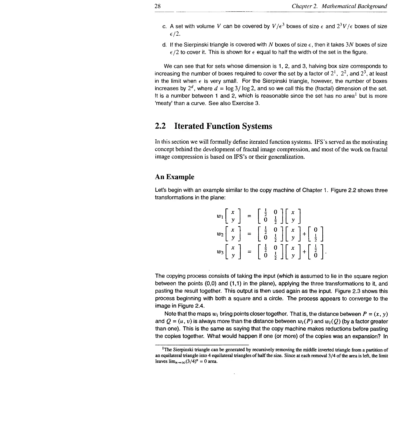
2.2 Iterated Function Systems................................................ 28
2.3 Recurrent Iterated Function Systems ....'................................ 39
2.4 Image Models............................................................. 42
2.5 Affine Transformations................................................... 46
2.6 Partitioned Iterated Function Systems.................................... 46
2.7 Encoding Images.......................................................... 48
2.8 Other Models ............................................................ 52
3 Fractal Image Compression with Quadtrees 55
Y Fisher
3.1 Encoding................................................................. 55
3.2 Decoding................................................................. 59
3.3 Sample Results........................................................... 61
3.4 Remarks.................................................................. 72
3.5 Conclusion............................................................... 75
4 Archetype Classification in an Iterated Transformation
Image Compression Algorithm 79
R.D. Boss and E.W. Jacobs
4.1 Archetype Classification................................................ 79
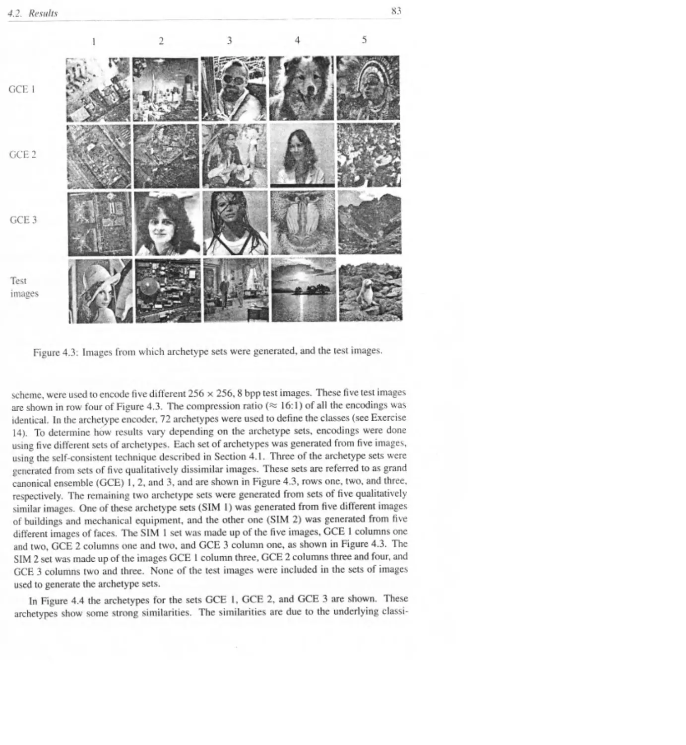
4.2 Results................................................................. 82
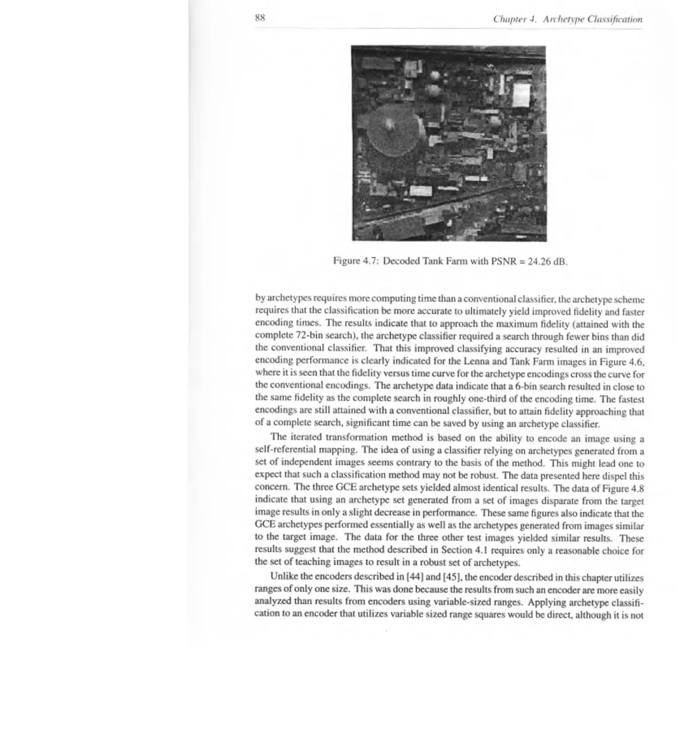
4.3 Discussion.............................................................. 86
5 /Hierarchical Interpretation of Fractal Image Coding and Its Applications 91
Z. Baharav, D. Malah, and E. Karnin
5.1 Formulation of PIFS Coding/Decoding .................................. 92
5.2 Hierarchical Interpretation............................................. 98
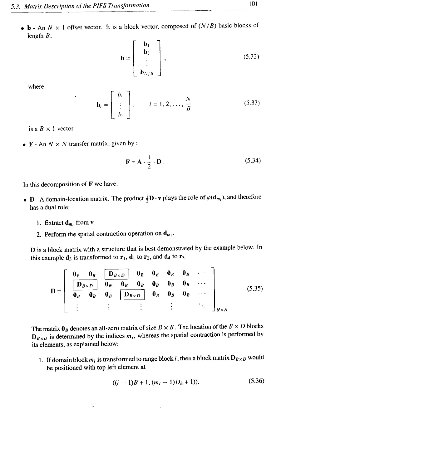
5.3 Matrix Description of the PIFS Transformation...........................100
5.4 Fast Decoding...........................................................102
5.5 Super-resolution........................................................104
5.6 Different Sampling Methods..............................................109
5.7 Conclusions.............................................................110
A Proof of Theorem 5.1 (Zoom).............................................Ill
В Proof of Theorem 5.2 (PIFS Embedded Function)...........................112
C Proof of Theorem 5.3 (Fractal Dimension of the PIFS Embedded Function) . . 115
6 Fractal Encoding with HV Partitions 119
Y Fisher and S. Menlove
6.1 The Encoding Method.....................................................119
6.2 Efficient Storage.......................................................122
6.3 Decoding................................................................123
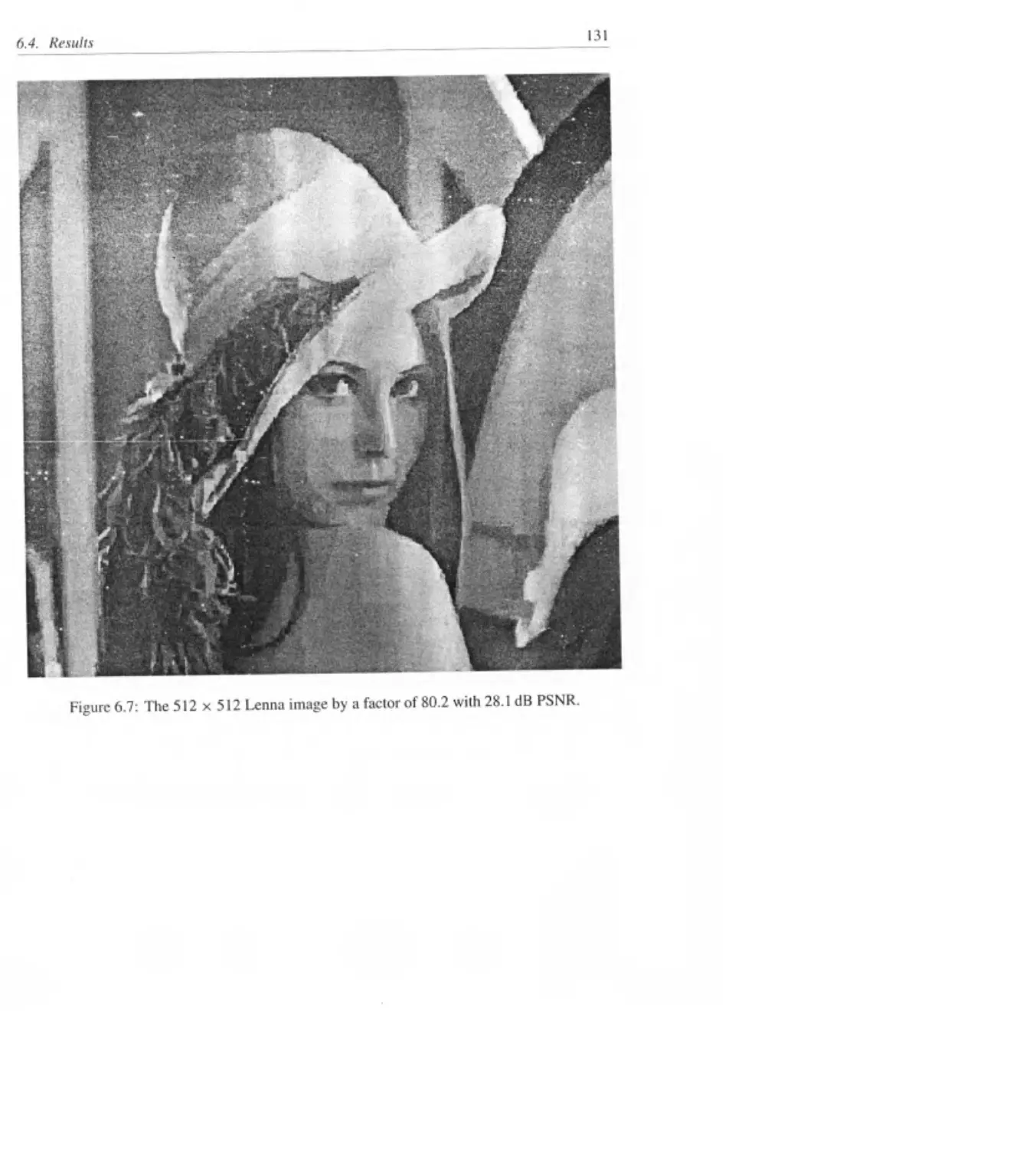
6.4 Results.................................................................126
6.5 More Discussion.........................................................134
6.6 Other Work..............................................................134
7 A Discrete Framework for Fractal Signal Modeling 137
L. Lundheim
7Л Sampled Signals, Pieces, and Piecewise
Self-transformability...................................................138
7.2 Self-transformable Objects and Fractal Coding ..........................142
7.3 Eventual Contractivity and Collage Theorems.............................143
7.4 Affine Transforms.......................................................144
7.5 Computation of Contractivity Factors....................................145
7.6 A Least-squares Method..................................................148
7.7 Conclusion..............................................................150
A Derivation of Equation (7.9)............................................151
8 A Class of Fractal Image Coders with Fast Decoder Convergence 153
G. E. 0ien and S. Lepsdy
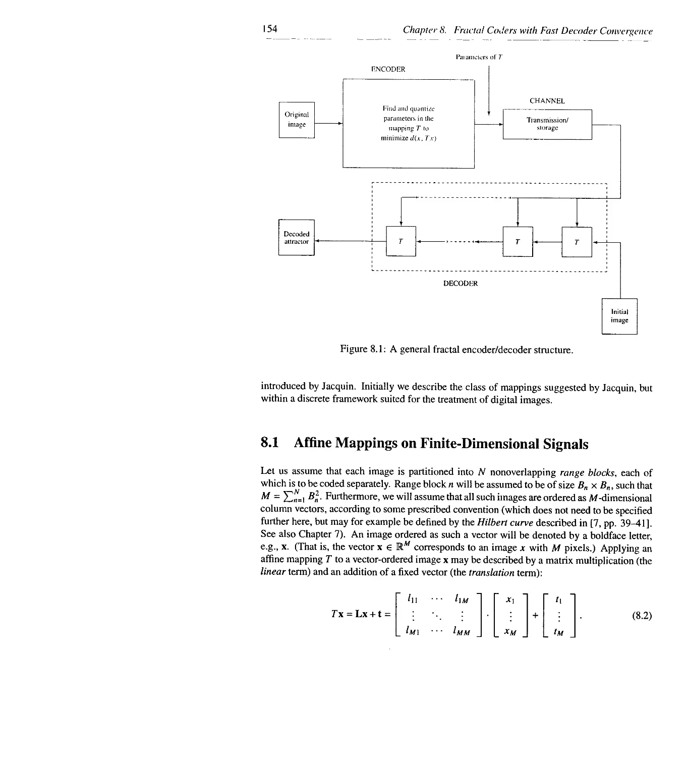
8.1 Affine Mappings on Finite-Dimensional Signals...........................154
8.2 Conditions for Decoder Convergence .....................................156
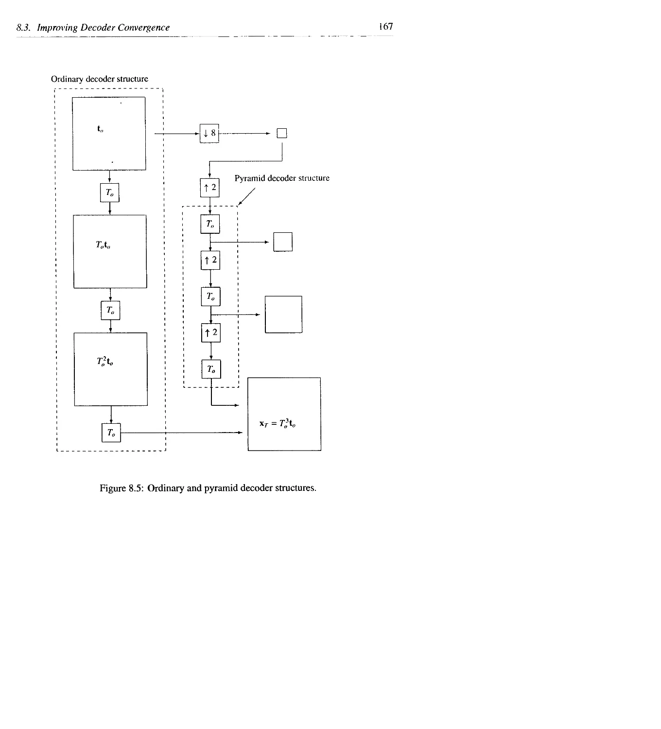
8.3 Improving Decoder Convergence ..........................................157
Contents xvii
8.4 Collage Optimization Revisited..........................................168
8.5 A Generalized Sufficient Condition for Fast Decoding....................172
8.6 An Image Example........................................................174
8.7 Conclusion..............................................................174
9 Fast Attractor Image Encoding by Adaptive Codebook Clustering 177
S. Lepsdy and G. E. 0ien
9.1 Notation and Problem Statement..........................................178
9.2 Complexity Reduction in the Encoding Step...............................179
9.3 How to Choose a Block...................................................181
9.4 Initialization.........................................................182
9.5 Two Methods for Computing Cluster Centers...............................186
9.6 Selecting the Number of Clusters ......................................189
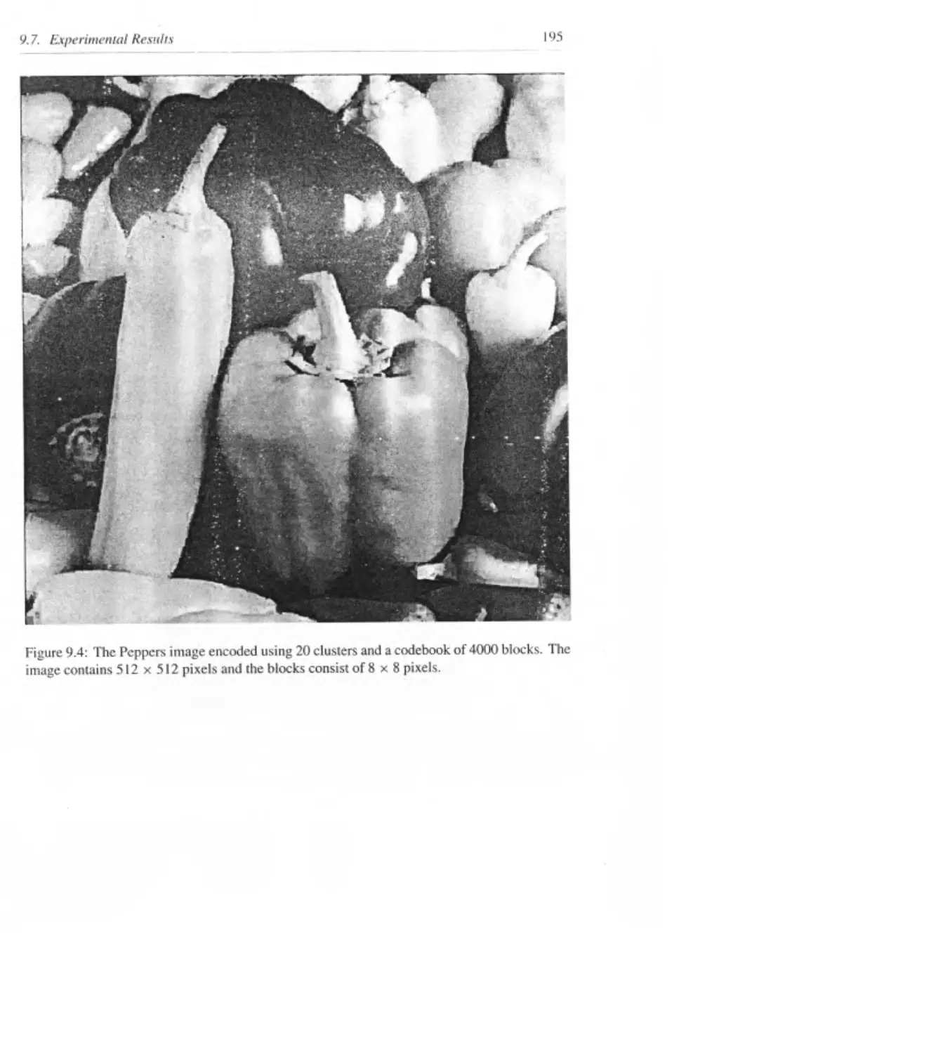
9.7 Experimental Results...................................................192
9.8 Possible Improvements..................................................197
9.9 Conclusion..............................................................197
,10/Orthogonal Basis IFS 199
С/ G. Vines
10.1 Orthonormal Basis Approach ............................................201
10.2 Quantization...........................................................208
10.3 Construction of Coders.................................................209
10.4 Comparison of Results..................................................209
10.5 Conclusion.............................................................214
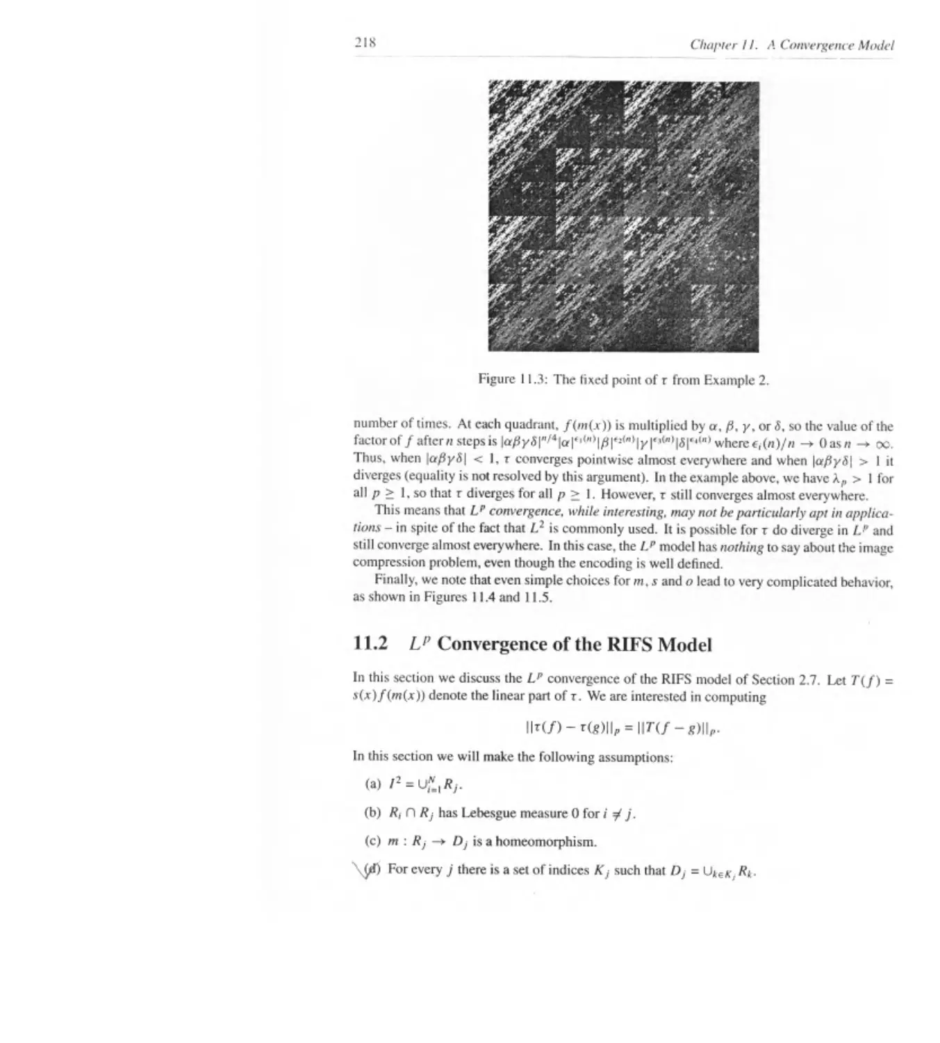
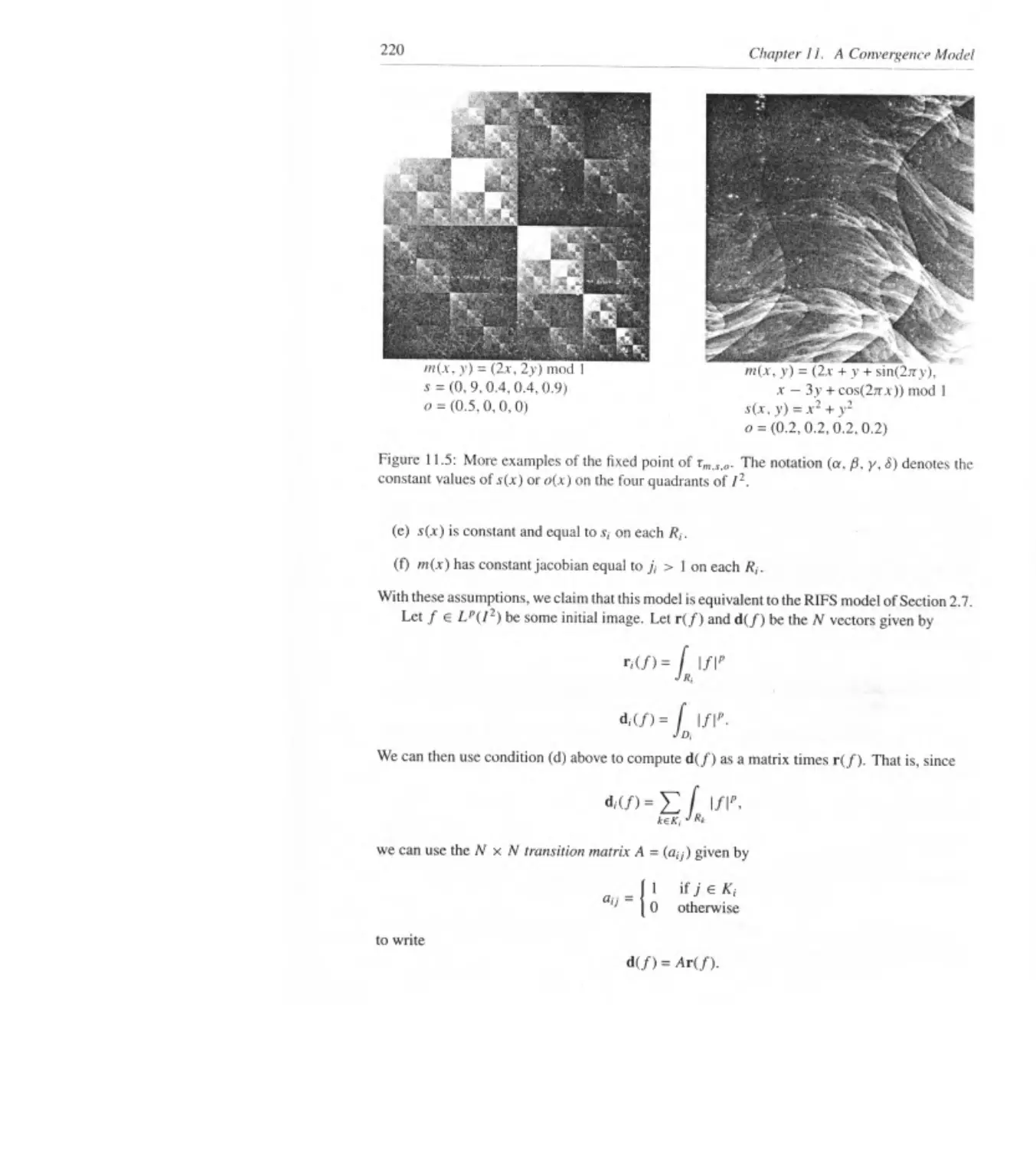
11/ A Convergence Model 215
B. Bielefeld and Y. Fisher
11.1 The r Operator.........................................................215
11.2 Lp Convergence of the RIFS Model.......................................218
11.3 Almost Everywhere Convergence..........................................223
11.4 Decoding by Matrix Inversion ..........................................227
12/Least-Squares Block Coding by Fractal Functions 229
F. Dudbridge
12.1 Fractal Functions......................................................229
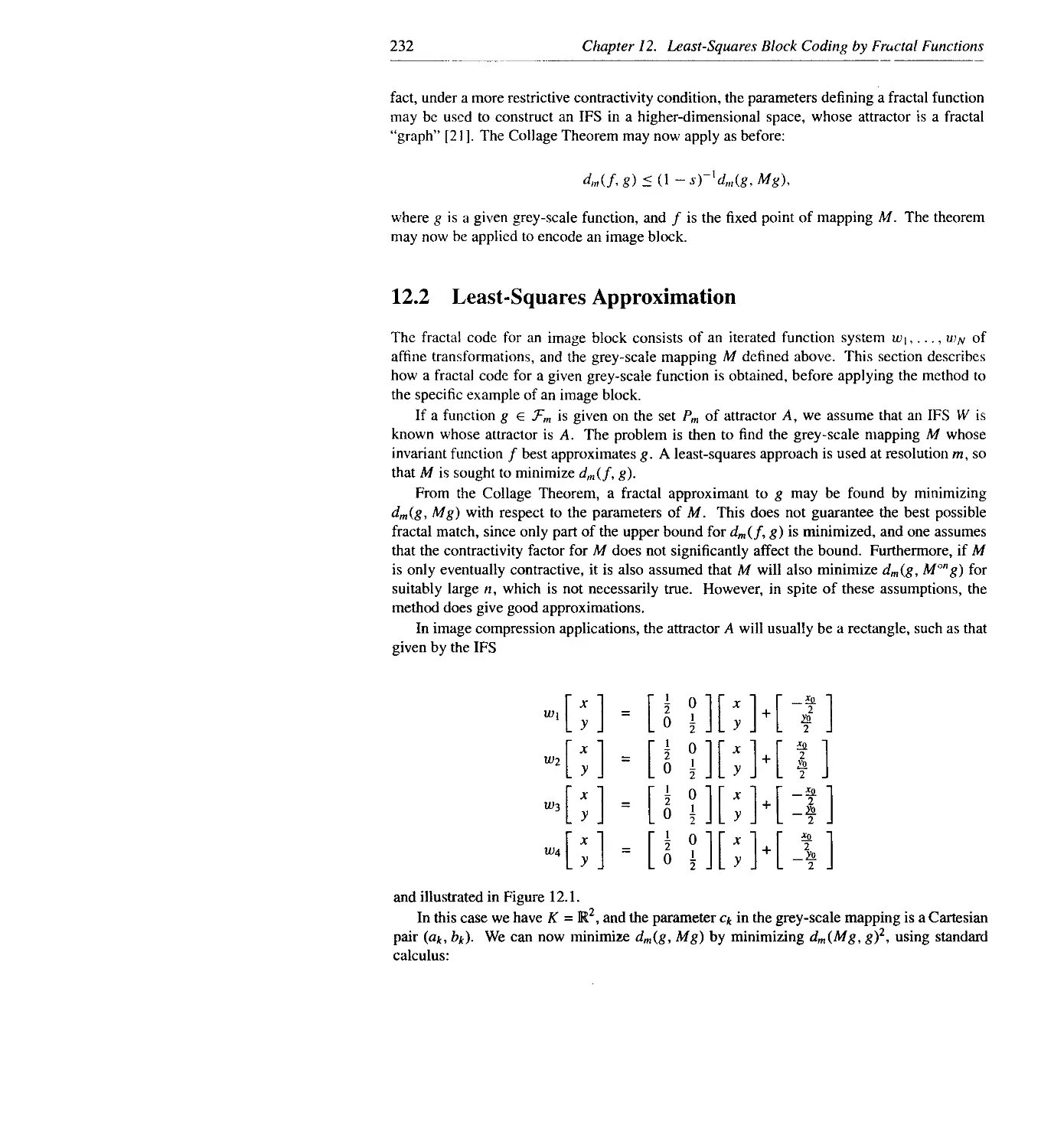
12.2 Least-Squares Approximation............................................232
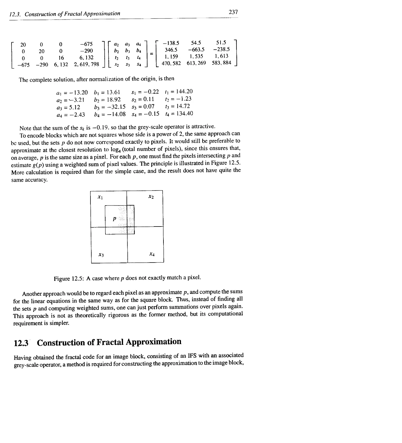
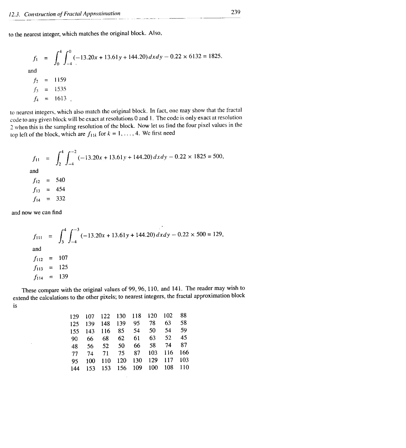
12.3 Construction of Fractal Approximation .................................237
12.4 Conclusion.............................................................240
ДЗ Inference Algorithms for WFA and Image Compression 243
j /*K, Culik II and J. Kari
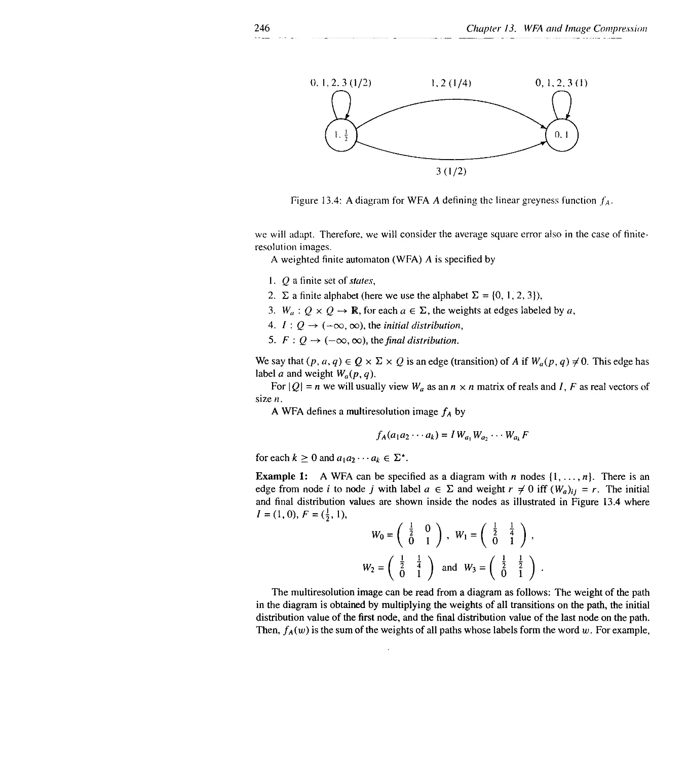
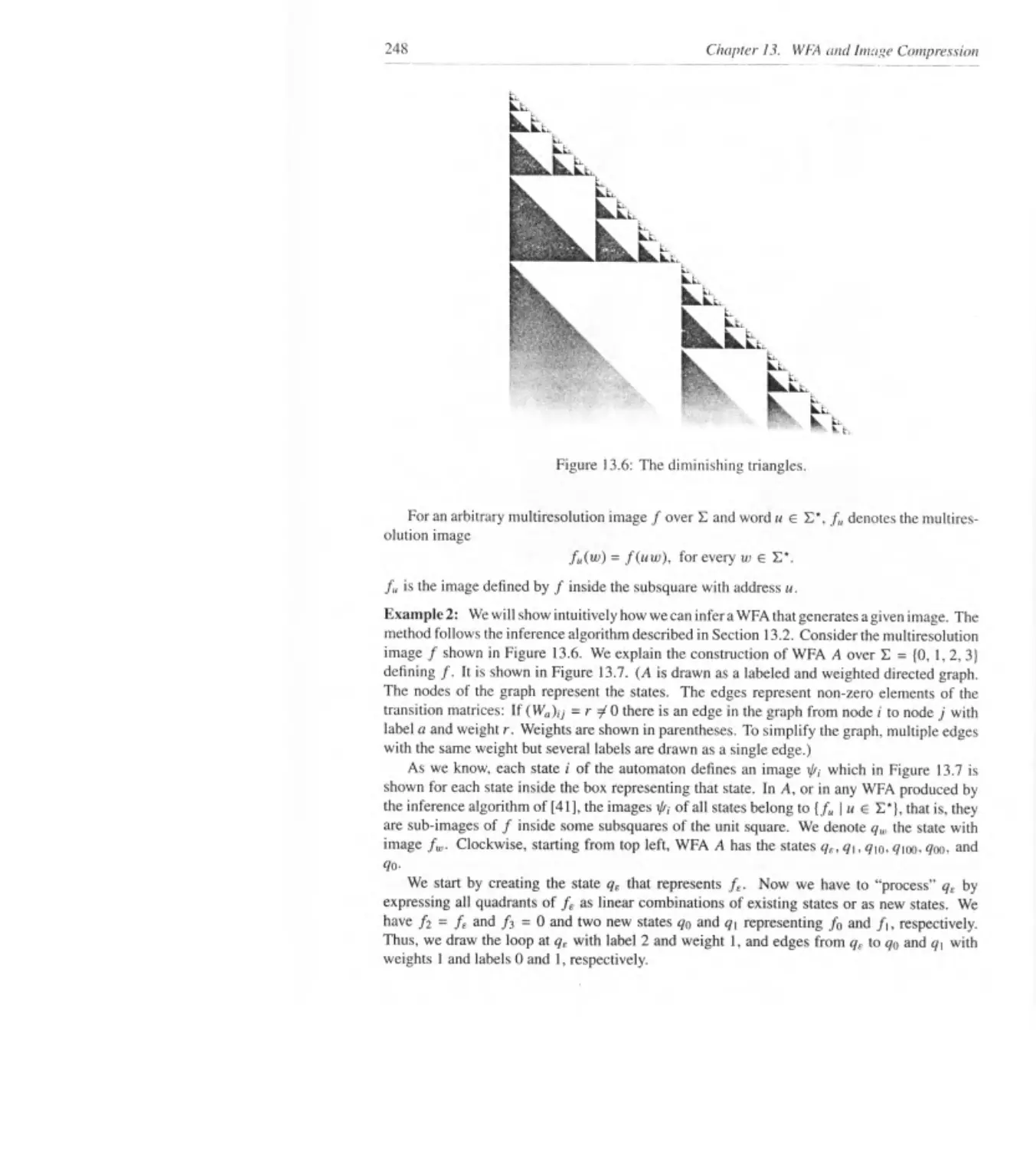
13.1 Images and Weighted Finite Automata....................................244
13.2 The Inference Algorithm for WFA........................................250
13.3 A Fast Decoding Algorithm for WFA......................................253
13.4 A Recursive Inference Algorithm for WFA ...............................254
xviii Contents
A Sample Code 259
Y. Fisher
A.l The Enc Manual Page......................................................259
A.2 The Dec Manual Page......................................................262
A.3 Enc.c....................................................................264
A.4 Dec.c....................................................................278
A.5 The Encoding Program.....................................................286
A.6 The Decoding Program ....................................................289
A.7 Possible Modifications...................................................290
В Exercises 293
Y. Fisher
C Projects 297
Y. Fisher
C.l Decoding by Matrix Inversion.............................................297
C.2 Linear Combinations of Domains...........................................297
C.3 Postprocessing: Overlapping, Weighted Ranges, and Tilt...................298
C.4 Encoding Optimization....................................................299
C.5 Theoretical Modeling for Continuous Images...............................299
C.6 Scan-line Fractal Encoding...............................................300
C.7 Video Encoding...........................................................300
C.8 Single Encoding of Several Frames .......................................300
C.9 Edge-based Partitioning..................................................301
C. 10 Classification Schemes..................................................301
C. 11 From Classification to Multi-dimensional Keys...........................302
D. Saupe
C. 12 Polygonal Partitioning...................................................305
C. 13 Decoding by Pixel Chasing ...............................................305
C.14 Second Iterate Collaging..................................................307
C.15 Rectangular IFS Partitioning..............................................307
C.16 Hexagonal Partitioning....................................................308
C.17 Parallel Processing.......................................................309
C.18 Non-contractive IFSs......................................................309
D Comparison of Results 311
Y. Fisher
E Original Images 317
Bibliography 325
Index
331
Chapter 1
Introduction
Y. Fisher
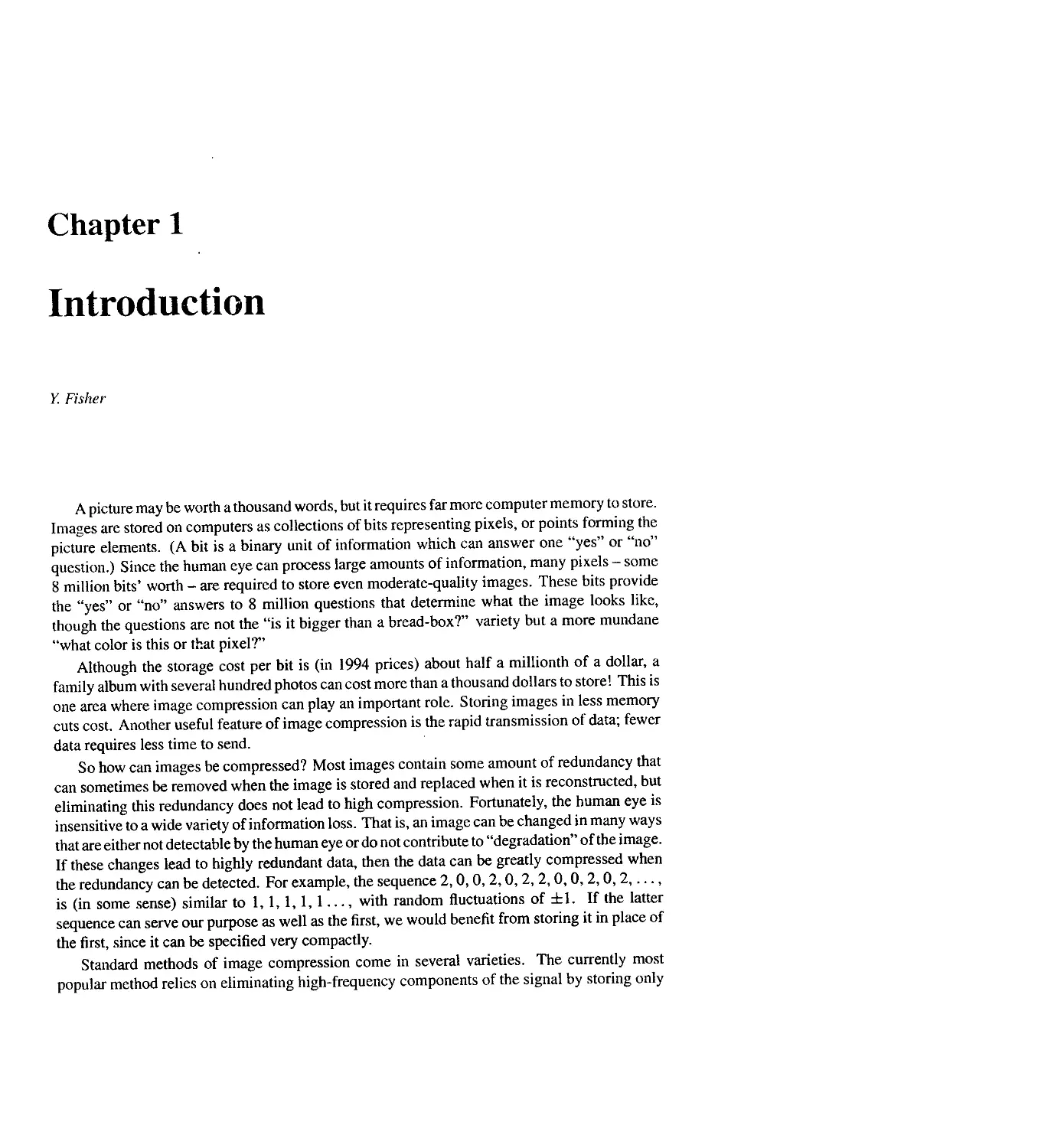
A picture may be worth a thousand words, but it requires far more computer memory to store.
Images are stored on computers as collections of bits representing pixels, or points forming the
picture elements. (A bit is a binary unit of information which can answer one “yes” or “no”
question.) Since the human eye can process large amounts of information, many pixels - some
8 million bits’ worth - are required to store even moderate-quality images. These bits provide
the “yes” or “no” answers to 8 million questions that determine what the image looks like,
though the questions are not the “is it bigger than a bread-box?” variety but a more mundane
“what color is this or that pixel?”
Although the storage cost per bit is (in 1994 prices) about half a millionth of a dollar, a
family album with several hundred photos can cost more than a thousand dollars to store! This is
one area where image compression can play an important role. Storing images in less memory
cuts cost. Another useful feature of image compression is the rapid transmission of data; fewer
data requires less time to send.
So how can images be compressed? Most images contain some amount of redundancy that
can sometimes be removed when the image is stored and replaced when it is reconstructed, but
eliminating this redundancy does not lead to high compression. Fortunately, the human eye is
insensitive to a wide variety of information loss. That is, an image can be changed in many ways
that are either not detectable by the human eye or do not contribute to “degradation” of the image.
If these changes lead to highly redundant data, then the data can be greatly compressed when
the redundancy can be detected. For example, the sequence 2,0,0, 2,0, 2, 2,0,0, 2,0, 2,...,
is (in some sense) similar to 1,1,1,1,1..., with random fluctuations of ±1. If the latter
sequence can serve our purpose as well as the first, we would benefit from storing it in place of
the first, since it can be specified very compactly.
Standard methods of image compression come in several varieties. The currently most
popular method relies on eliminating high-frequency components of the signal by storing only
2
Chapter I. Introduction
the low-frequency Fourier coefficients. This method uses a discrete cosine transform (DCT)
[17], and is the basis of the so-called JPEG standard, which comes in many incompatible flavors.
Another method, called vector quantization [55], uses a “building block” approach, breaking
up images into a small number of canonical pieces and storing only a reference to which piece
goes where. In this book, we will explore several distinct new schemes based on “fractals.”
A fractal scheme has been developed by M. Barnsley, who founded a company based on
fractal image compression technology but who has released only some details of his scheme.
A. Jacquin, a former student of Barnsley’s, was the first to publish a fractal image compression
scheme in [45], and after this came a long list of variations, generalizations, and improvements.
Early work on fractal image compression was also done by E.W. Jacobs and R.D. Boss of the
Naval Ocean Systems Center in San Diego who used regular partitioning and classification of
curve segments in order to compress measured fractal curves (such as map boundary data) in
two dimensions [10], [43].
The goal of this introductory chapter is to explain an approach to fractal image compression
in very simple terms, with as little mathematics as possible. The later chapters will review the
same subjects in depth and with rigor, but for now we will concentrate on the general concepts.
We will begin by describing a simple scheme that can generate complex-looking fractals from
a small amount of information. We will then generalize this scheme to allow the encoding of
images as “fractals,” and finally we will discuss some ways this scheme can be implemented.
1.1 What Is Fractal Image Compression?
Imagine a special type of photocopying machine that reduces the image to be copied by a half
and reproduces it three times on the copy, as in Figure 1.1. What happens when we feed the
output of this machine back as input? Figure 1.2 shows several iterations of this process on
several input images. What we observe, and what is in fact true, is that all the copies seem to
be converging to the same final image, the one in 1.2c. We also see that this final image is not
changed by the process, and since it is formed of three reduced copies of itself, it must have
detail at every scale - it is a fractal. We call this image the attractor for this copying machine.
Because the copying machine reduces the input image, the copies of any initial image will be
reduced to a point as we repeatedly feed the output back as input; there will be more and more
copies, but each copy gets smaller and smaller. So, the initial image doesn’t affect the final
attractor; in fact, it is only the position and the orientation of the copies that determines what
the final image will look like.
Since the final result of running the copy machine in a feedback loop is determined by
the way the input image is transformed, we only describe these transformations. Different
transformations lead to different attractors, with the technical limitation that the transformations
must be contractive - that is, a given transformation applied to any two points in the input image
must bring them closer together in the copy. This technical condition is very natural, since if
points in the copy were spread out, the attractor might have to be of infinite size. Except for
this condition, the transformations can have any form. In practice, choosing transformations of
the form
is sufficient to yield a rich and interesting set of attractors (see Exercise 8). Such transformations
1.1. What Is Fractal Image Compression?
3
Input Image
Output Image
Figure 1.1: A copy machine that makes three reduced copies of the input image.
are called affine transformations of the plane, and each can skew, stretch, rotate, scale, and
translate an input image.
Figure 1.3 shows some affine transformations, the resulting attractors, and a zoom on a region
of the attractor. The transformations are displayed by showing an initial square marked with an
“l=” and its image by the transformations. The U- shows how a particular transformation flips
or rotates the square. The first example shows the transformations used in the copy machine of
Figure 1.1. These transformations reduce the square to half its size and copy it at three different
locations, each copy with the same orientation. The second example is very similar, except that
one transformation flips the square, resulting in a different attractor (see Exercise 1). The last
example is the Barnsley fem. It consists of four transformations, one of which is squashed flat
to yield the stem of the fem (see Exercise 2).
A common feature of these and all attractors formed this way is that in the position of each
of the images of the original square there is a transformed copy of the whole image. Thus,
each image is formed from transformed (and reduced) copies of itself, and hence it must have
detail at every scale. That is, the images are fractals. This method of generating fractals is due
to John Hutchinson [36]. More information about many ways to generate such fractals can be
found in books by Peitgen, Saupe, and Jiirgens [67],[68], [69], and by Barnsley [4].
M. Barnsley suggested that perhaps storing images as collections of transformations could
lead to image compression. His argument went as follows: the fem in Figure 1.3 looks com-
plicated and intricate, yet it is generated from only four affine transformations. Each affine
transformation wt is defined by six numbers, a,, bt, с,-, dt, e-, and f, which do not require much
memory to store on a computer (they can be stored in 4 transformations x 6 numbers per
transformation x 32 bits per number = 768 bits). Storing the image of the fem as a collection
of pixels, however, requires much more memory (at least 65,536 bits for the resolution shown
in Figure 1.3). So if we wish to store a picture of a fem, we can do it by storing the numbers
that define the affine transformations and simply generating the fem whenever we want to see
it. Now suppose that we were given any arbitrary image, say a face. If a small number of affine
transformations could generate that face, then it too could be stored compactly. This is what
this book is about.
4
Chapter I. Introduction
Initial Image
First Copy Second Copy Third Copy
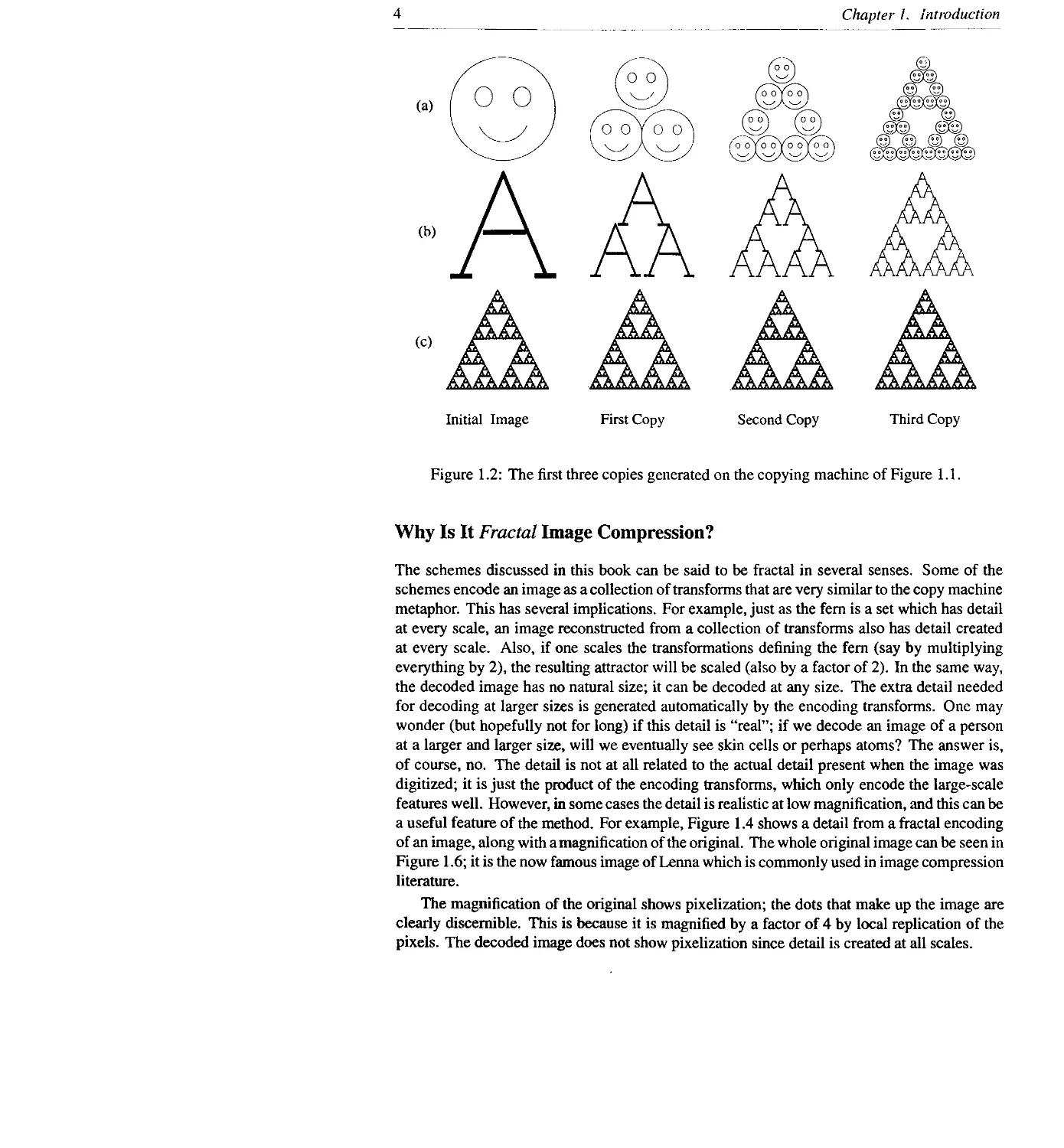
Figure 1.2: The first three copies generated on the copying machine of Figure 1.1.
Why Is It Fractal Image Compression?
The schemes discussed in this book can be said to be fractal in several senses. Some of the
schemes encode an image as a collection of transforms that are very similar to the copy machine
metaphor. This has several implications. For example, just as the fem is a set which has detail
at every scale, an image reconstructed from a collection of transforms also has detail created
at every scale. Also, if one scales the transformations defining the fem (say by multiplying
everything by 2), the resulting attractor will be scaled (also by a factor of 2). In the same way,
the decoded image has no natural size; it can be decoded at any size. The extra detail needed
for decoding at larger sizes is generated automatically by the encoding transforms. One may
wonder (but hopefully not for long) if this detail is “real”; if we decode an image of a person
at a larger and larger size, will we eventually see skin cells or perhaps atoms? The answer is,
of course, no. The detail is not at all related to the actual detail present when the image was
digitized; it is just the product of the encoding transforms, which only encode the large-scale
features well. However, in some cases the detail is realistic at low magnification, and this can be
a useful feature of the method. For example, Figure 1.4 shows a detail from a fractal encoding
of an image, along with a magnification of the original. The whole original image can be seen in
Figure 1.6; it is the now famous image of Lerma which is commonly used in image compression
literature.
The magnification of the original shows pixelization; the dots that make up the image are
clearly discernible. This is because it is magnified by a factor of 4 by local replication of the
pixels. The decoded image does not show pixelization since detail is created at all scales.
1.1. What Is Fractal linage Compression ?
5
Figure 1.3: Transformations, their attractor, and a zoom on the attractors.
Why Is It Fractal Image Compression!
Standard image compression methods can be evaluated using their compression ratio: the ratio
of the memory required to store an image as a collection of pixels and the memory required to
store a representation of the image in compressed form. As we saw before, the fem could be
generated from 768 bits of data but required 65,536 bits to store as a collection of pixels, giving
a compression ratio of 65,536/768 = 85.3 to 1.
The compression ratio for the fractal scheme is easy to misunderstand, since the image can
be decoded at any scale. For example, the decoded image in Figure 1.4 is a portion of a 5.7
to 1 compression of the whole Lenna image. It is decoded at 4 times its original size, so the
full decoded image contains 16 times as many pixels and hence its compression ratio can be
considered to be 91.2 to 1. In practice, it is important to either give the initial and decompressed
image sizes or use the same sizes (the case throughout this book) for a proper evaluation. The
schemes we will discuss significantly reduce the memory needed to store an image that is similar
(but not identical) to the original, and so they compress the data. Because the decoded image
is not exactly the same as the original, such schemes are said to be lossy.
6
Chapter I. hiinxlu< tii>ii
Figure 1.4: Л portion of Lenna's hat decoded at 4 times its encoding size (left), and the original
image enlarged to 4 times its size (right), showing pixelization.
Iterated Function Systems
Before we describe an image compression scheme, we will discuss the copy machine example
wtdt some notation. Later we will use the same notation in the image compression case, but
for now it is easier to understand in the context of the copy machine example.
Running the special copy machine in a feedback loop is a metaphor fora mathematical model
called an iterated function system (1FS). The formal and abstract mathematical description of
IFS is given in Chapter 2, so for now we will remain informal. An iterated function system
consists of a collection of contractive transformations {w, : R? -» R2 | i = 1,.... л) which
map the plane R2 to itself. This collection of transformations defines a map
W() = (_>•()•
i=l
The map IV is not applied to the plane, it is applied to sets - that is, collections of points in the
plane. Given an input set S, we can compute w,(5) for each i (this corresponds to making a
reduced copy of the input image S), take the union of these sets (this corresponds to assembling
the reduced copies), and get a new set IV(S) (the output of the copier). So W is a map on the
space of subsets of the plane. We will call a subset of the plane an image, because the set defines
an image when the points in the set are drawn in black, and because later we will want to use
the same notation for graphs of functions representinging actual images, or pictures.
We now list two important facts:
• When the w, are contractive in the plane, then W is contractive in a space of (closed and
bounded1) subsets of the plane. This was proved by Hutchinson. For now, it is not
’The "closed and bounded” part is one of several techiucaliUes that arise at this point. What are these terms and what
1.2. Self-Similarity in Images 7
necessary to worry about what it means for W to be contractive; it is sufficient to think
of it as a label to help with the next step.
• If we are given a contractive map W on a space of images, then there is a special image,
called the attractor and denoted .rw. with the following properties:
1. If we apply the copy machine to the attractor, the output is equal to the input; the
image is fixed, and the attractor .r« is called the fixed point of W. That is,
W(xw) = xw = W|(x'iv) U U • • U utH(xw)-
2. Given an input image 5(), we can run the copying machine once to get St = W(S«),
twice to get S? = W(Sj) = W(VWo)) = W'2(.S'o), and so on. The superscript
“o” indicates that we are talking about iterations, not exponents: IV 2 is the output
of the second iteration. The attractor, which is the result of running the copying
machine in a feedback loop, is the limit set
xw = S0C= lim W"(So)
л-*оо
which is not dependent on the choice of 5q-
3. хи, is unique. If we find any set S and an image transformation W satisfying
W(S) = S, then S is the attractor of W; that is, S = xlv. This means that only one
set will satisfy the fixed-point equation in property 1 above.
In their rigorous form, these three properties are known as the Contractive Mapping
Fixed-Point Theorem.
Iterated function systems are interesting in their own right, but we are not concerned with
them specifically. We will generalize the idea of the copy machine and use it to encode grey-
scale images; that is, images that are not just black and white but contain shades of grey as
well.
1.2 Self-Similarity in Images
In the remainder of this chapter, we will use the term image to mean a grey-scale image.
Images as Graphs of Functions
In order to discuss image compression, we need a mathematical model of an image. Figure
1.5 shows the graph of a function z = f(x, y). This graph is generated by taking the image of
Lenna (see Figure 1.6) and plotting the grey level of the pixel at position (x, у) as a height, with
white being high and black low. This is our model for an image, except that while the graph
are they doing here? The terms make the statement precise and their function is to reduce complaints by mathematicians.
Having W contractive is meaningless unless we give a way of determining distance between two sets. There is such
a distance function (or metric), called the Hausdorff metric, which measures the difference between two closed and
bounded subsets of the plane, and in this metric W’ is contractive on the space of closed and bounded subsets of the
plane. This is as much as we will say about this now; Chapter 2 contains the details.
8
Chapter I. Introduction
Figure 1.5: A graph generated from the Lenna image.
in Figure 1.5 is generated by connecting the heights on a 64 x 64 grid, we generalize this and
assume that every position (x, y) can have an independent height. That is, our image model
has infinite resolution.
Thus, when we wish to refer to an image, we refer to the function f(x, y) that gives the
grey level at each point (x, y). In practice, we will not distinguish between the function f
and the graph of the function (which is a set in R3 consisting of the points in the surface
defined by /). For simplicity, we assume we are dealing with square images of size 1; that is,
(x, у) e {(и, v) : 0 < u, v < 1} = Z2, and /(x, у) e I = [0,1]. We have introduced some
convenient notation here: I means the interval [0, 1] and Z2 is the unit square.
A Metric on Images
Imagine the collection of all possible images: clouds, trees, dogs, random junk, the surface of
Jupiter, etc. We will now find a map W that takes an input image and yields an output image,
just as we did before with subsets of the plane. If we want to know when W is contractive, we
will have to define a distance between two images.
A metric is a function that measures the distance between two things. For example, the
things can be two points on the real line, and the metric can then be the absolute value of
their difference. The reason we use the word “metric” rather than “difference” or “distance” is
because the concept is meant to be general. There are metrics that measure the distance between
two images, the distance between two points, or the distance between two sets, etc.
There are many metrics to choose from, but the simplest to use are the supremum metric
dsup(f,g)= sup |/(x, y) - g(x, y)|, (1.1)
(x.r)et2
1.2. Self-Similarity in Images
9
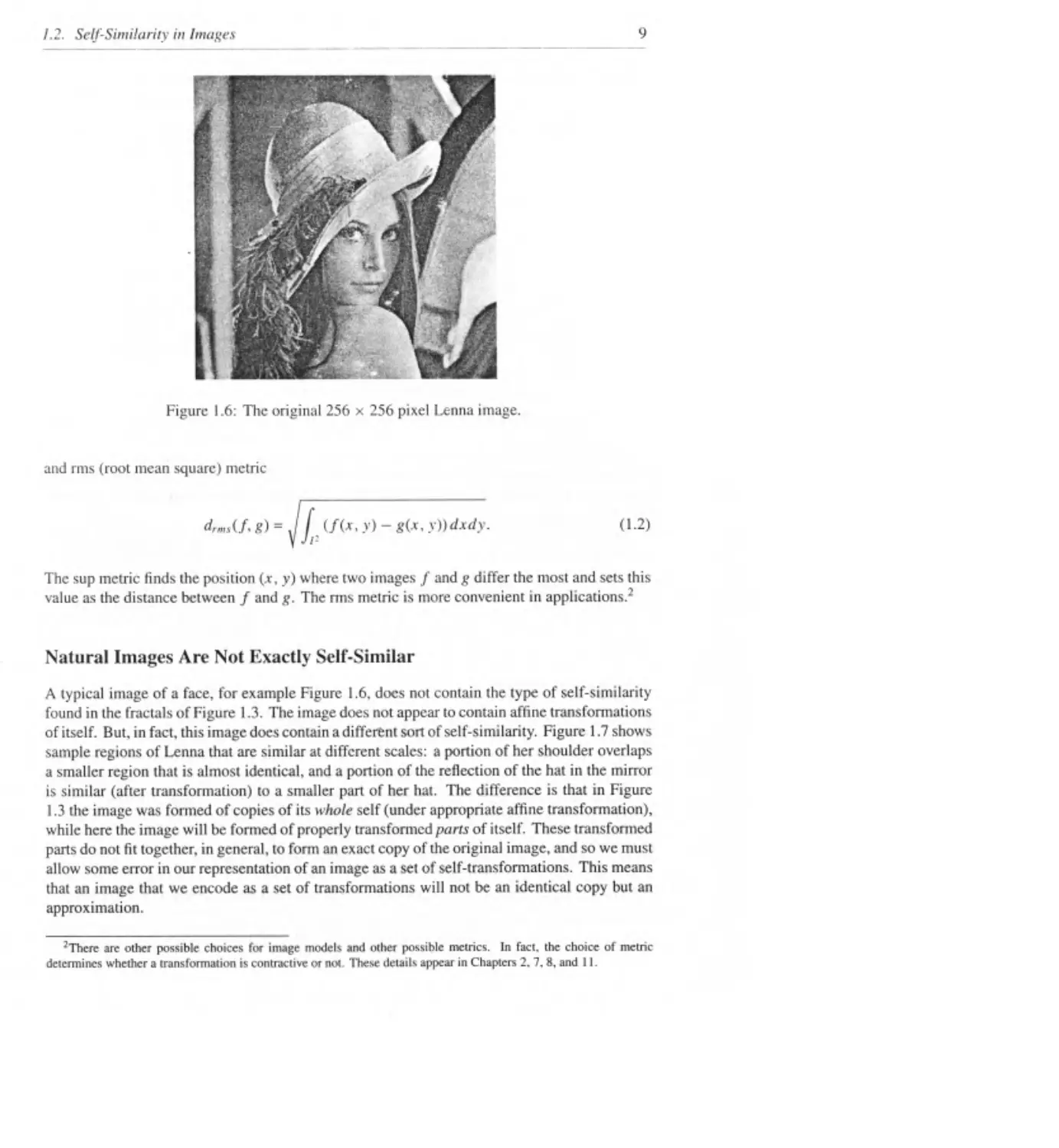
Figure 1.6: The original 256 x 256 pixel Lenna image.
and rms (root mean square) metric
d,mAf. g) = ./ / (/(•». У) - gU, y))dxdy.
(1.2)
The sup metric finds the position (x, y) where two images f and g differ the most and sets this
value as the distance between f and g. The rms metric is more convenient in applications.?
Natural Images Are Not Exactly Self-Similar
A typical image of a face, for example Figure 1.6, docs not contain the type of self-similarity
found in the fractals of Figure 1.3. The image does not appear to contain affine transformations
of itself. But, in fact, this image does contain a different sort of self-similarity. Figure 1.7 shows
sample regions of Lenna that are similar at different scales: a portion of her shoulder overlaps
a smaller region that is almost identical, and a portion of the reflection of the hat in the mirror
is similar (after transformation) to a smaller part of her hat. lite difference is that in Figure
1.3 the image was formed of copies of its whole self (under appropriate affine transformation),
while here the image will be formed of properly transformed parts of itself. These transformed
parts do not fit together, in general, to form an exact copy of the original image, and so we must
allow some error in our representation of an image as a set of self-transformations. This means
that an image that we encode as a set of transformations will not be an identical copy but an
approximation.
‘There are other possible choices for image models and ocher possible metrics. 1л fact, the choice of metric
determines whether a transformation is contractive or not These detail* appear in Chapters 2.7,8, and 11.
10
Chapter I. Introduction
Figure 1.7: Self-similar portions of the Lenna image.
What kind of images exhibit this type of self-similarity? Experimental results suggest that
most naturally occurring images can be compressed by taking advantage of this type of self-
similarity; for example, images of trees, faces, houses, mountains, clouds, etc. This restricted
self-similarity is the redundancy that fractal image compression schemes attempt to eliminate.
1.3 A Special Copying Machine
In this section we describe an extension of the copying machine metaphor that can be used to
encode and decode grey-scale images.
Partitioned Copying Machines
The copy machine described in Section 1.1 has the following features:
• the number of copies of the original pasted together to form the output,
• a setting of position and scaling, stretching, skewing, and rotation factors for each copy.
We upgrade the machine with the following features:
• a contrast and brightness adjustment for each copy,
• a mask that selects, for each copy, a part of the original to be copied.
These extra features are sufficient to allow the encoding of grey-scale images. The last capa-
bility is the central improvement. It partitions an image into pieces which are each transformed
separately. By partitioning the image into pieces, we allow the encoding of many shapes that
are impossible to encode using an IFS.
1.3. A Special Copying Machine
Let us review what happens when we copy an original image using this machine. A portion
of the original, which we denote by £),, is copied (with a brightness and contrast transformation)
to a part of the produced copy, denoted R,. We call the £>,- domains and the R, ranges.3 We
denote this transformation by u.',. This notation does not make the partitioning explicit; each
comes with an implicit £),. This way. we can use almost the same notation as with an
IFS. Given an image /, a single copying step in a machine with N copies can be written as
W(f) = u.'i( f) U w;(/) U • • • U «.>(/). As before, the machine runs in a feedback loop; its
own output is fed back as its new input again and again.
Partitioned Copying Machines Are PIFS
The mathematical analogue of a partitioned copying machine is called a partitioned iterated
function system (PIFS). As before, the definition of a PIFS is not dependent on the type of
transformations, but in this discussion we will use affine transformations. There are two spatial
dimensions and the grey level adds a third dimension, so the transformations w, are of the form,
(1.3)
where s, controls the contrast and o, controls the brightness of the transformation. It is conve-
nient to define the spatial part t>, of the transformation above by
v,(x, y) =
Since an image is modeled as a function f(x, y), we can apply w, to an image f by
wff) = w,(x, y, f(x, у )) Then v,- determines how the partitioned domains of an original are
mapped to the copy, while s, and o, determine the contrast and brightness of the transformation.
We think of the pieces of the image Di and R, as lying in the plane, but it is implicit, and
important to remember, that each w, is restricted to £), x I, the vertical space above £>, . That
is, w, applies only to the part of the image that is above the domain This means that
t>i(D,) = R,. See Figure 1.8.
Since we want W(/) to be an image, we must insist that UR, = I2 and that R, П Rj = 0
when i j. That is, when we apply W to an image, we get some (single-valued) function
above each point of the square I2. In the copy machine metaphor, this is equivalent to saying
that the copies cover the whole square page, and that they are adjacent but not overlapping.
Running the copying machine in a loop means iterating the map W. We begin with an initial
image /о and then iterate fi = f2 = W(/i) = W(W(/o)), and so on. We denote the n-th
iterate by f„ = W°n(fo).
Fixed Points for Partitioned Iterated Function Systems
In the PIFS case, a fixed point, or attractor, is an image f that satisfies W(f) = /; that is, when
we apply the transformations to the image, we get back the original image. The Contractive
Mapping Theorem says that the fixed point of W will be the image we get when we compute
3A domain is where a transformation maps from, and a range is where it maps to.
12
Chapter 1. Introduction
Figure 1.8: The maps w, map the graph above £>, to a graph above
the sequence W(fo), W(W(fo)), W(W(W(/0))), ..., where fo is any image. So if we can be
assured that W is contractive in the space of all images, then it will have a unique fixed point
that will then be some image.
Since the metric we chose in Equation (1.1) is only sensitive to what happens in the z
direction, it is not necessary to impose contractivity conditions in the x or у directions. The
transformation W will be contractive when each s,- < 1; that is, when z distances are scaled by
a factor less than 1. In fact, the Contractive Mapping Theorem can be applied to Wom (for some
m), so it is sufficient for Wom to be contractive. It is possible for Wom to be contractive when
some Sj > 1, because W°m “mixes” the scalings (in this case W is called eventually contractive).
This leads to the somewhat surprising result that there is no condition on any specific s, either.
In practice, it is safest to take s, < 1 to ensure contractivity. But experiments show that taking
Si < 1.2 is safe and results in slightly better encodings.
Suppose that we take all the s, < 1. This means that the copying machine always reduces
the contrast in each copy. This seems to suggest that when the machine is run in a feedback
loop, the resulting attractor will be an insipid, homogeneous grey. But this is wrong, since
contrast is created between ranges that have different brightness levels o(. Is the only contrast
in the attractor between the /?, ? No, if we take the v, to be contractive, then the places where
there is contrast between the Л, in the image will propagate to smaller and smaller scales; this
is how detail is created in the attractor. This is one reason to require that the v, be contractive.
We now know how to decode an image that is encoded as a PIFS. Start with any initial
image and repeatedly run the copy machine, or repeatedly apply W until we get close to the
fixed point xw- The decoding is easy, but it is the encoding which is interesting. To encode an
image we need to figure out R,, D, and w,, as well as N, the number of maps u), we wish to
use.
1.4 Encoding Images
Suppose we are given an image f that we wish to encode. This means we want to find a
collection of maps wi, wj..., with W = UfLjWj and f = xw- That is, we want f to be the
1.4. Encoding Images
13
Figure 1.9: We seek to minimize the difference between the part of the graph f Fl (/?,- x I)
above Rt and the image Wj(f') of the part of the graph above £>,.
fixed point of the map W. The fixed-point equation
f = W(f) = U w2(/) U • • • wN(J)
suggests how this may be achieved. We seek a partition of f into pieces to which we apply
the transforms w, and get back f; this was the case with the copy machine examples in Figure
1.3c in which the images are made up of reduced copies of themselves. In general, this is
too much to hope for, since images are not composed of pieces that can be transformed to fit
exactly somewhere else in the image. What we can hope to find is another image f' = with
drms(f', f) small. That is, we seek a transformation W whose fixed point f = xw is close to,
and hopefully looks like, f. In that case,
f * f = W(/') « W(/) = wj(/) U w2(/) U - • • wN(f).
Thus it is sufficient to approximate the parts of the image with transformed pieces. We do this
by minimizing the following quantities
<U(W,x/),W/(/)) i = \,...,N. (1.4)
Figure 1.9 shows this process. That is, we find pieces D, and maps w,, so that when we apply a
u), to the part of the image over £>,, we get something that is very close to the part of the image
over The heart of the problem is finding the pieces /?, (and corresponding £), ).
A Simple Illustrative Example
The following example suggests how this can be done. Suppose we are dealing with a 256 x 256
pixel image in which each pixel can be one of 256 levels of grey (ranging from black to white).
Let R\,R2,..., /?io24 be the 8 x 8 pixel nonoverlapping sub-squares of the image, and let D
14
Chapter I. Introduction
be the collection of all 16 x 16 pixel (overlapping) sub-squares of the image. The collection D
contains 241 • 241 = 58,081 squares. For each /?,, search through all of D to find a £>, e D
which minimizes Equation (1.4); that is, find the part of the image that most looks like the
image above Л,. This domain is said to cover the range. There are 8 ways4 to map one square
onto another, so that this means comparing 8 58,081 = 464,648 squares with each of the
1024 range squares. Also, a square in D has 4 times as many pixels as an so we must
either subsample (choose 1 from each 2x2 sub-square of £>,) or average the 2 x 2 sub-squares
corresponding to each pixel of R, when we minimize Equation (1.4).
Minimizing Equation (1.4) means two things. First, it means finding a good choice for £),
(that is the part of the image that most looks like the image above /?,). Second, it means finding
good contrast and brightness settings s, and o, for w,. For each D e D we can compute s,
and о, using least squares regression (see Section 1.6), which also gives a resulting root mean
square (rms) difference. We then pick as £>,- the D e D with the least rms difference.
A choice of Di, along with a corresponding s, and o,, determines a map up of the form
of Equation (1.3). Once we have the collection uq,..., шюгд we can decode the image by
estimating xw. Figure 1.10 shows four images: an initial image fo chosen to show texture; the
first iteration which shows some of the texture from fo; W°2(fo~); and Wolo(/o).
The result is surprisingly good, given the naive nature of the encoding algorithm. The
original image required 65,536 bytes of storage, whereas the transformations required only
3968 bytes,5 giving a compression ratio of 16.5:1. With this encoding the rms error is 10.4 and
each pixel is on average only 6.2 grey levels away from the correct value. Figure 1.10 shows
how detail is added at each iteration. The first iteration contains detail at size 8x8, the next at
size 4x4, and so on.
Jacquin [45] originally encoded images with fewer grey levels using a method similar to
this example but with two sizes of ranges. In order to reduce the number of domains searched,
he also classified the ranges and domains by their edge (or lack of edge) properties. This is very
similar to the scheme used by Boss et al. [43] to encode contours.
A Note About Metrics
We have done something sneaky with the metrics. For a simple theoretical motivation, we use
the supremum metric, which is very convenient for this. But in practice we are happier using
the rms metric, which allows us to make least square computations. (We could have developed
a theory with the rms metric, of course, but checking contractivity in this metric is much harder.
See Chapter 7.)
1.5 Ways to Partition Images
The example in Section 1.4 is naive and simple, but it contains most of the ideas of a practical
fractal image encoding scheme: first partition the image by some collection of ranges R,; then for
each Ri, seek from some collection of image pieces a D, that has a low rms error when mapped
4The square can be rotated to 4 orientations or flipped and rotated into 4 other orientations.
5 A byte consists of 8 bits. Each transformation requires 8 bits in each of the x and у directions to determine the
position of Di, 7 bits for o,, 5 bits for s; and 3 bits to determine a rotation and flip operation for mapping D,- to R,.
The position of R, is implicit in the ordering of the transformations.
1.5. Hirw to Partition Images
15
Figure 1.10: The initial image (a), and the first (b), second (c), and tenth (d) iterates of the
encoding transformations.
16
Chapter I. Introduction
to Rj. If we know /?, and then we can determine s, and o, as well as a,-, c(, dt, <?,• and /,
in Equation (1.3). We then get a transformation W = Uu;, that encodes an approximation of the
original image. There are many possible partitions that can be used to select the /?,; examples
are shown in Figure 1.11. Some of these are discussed in greater detail later in this book.
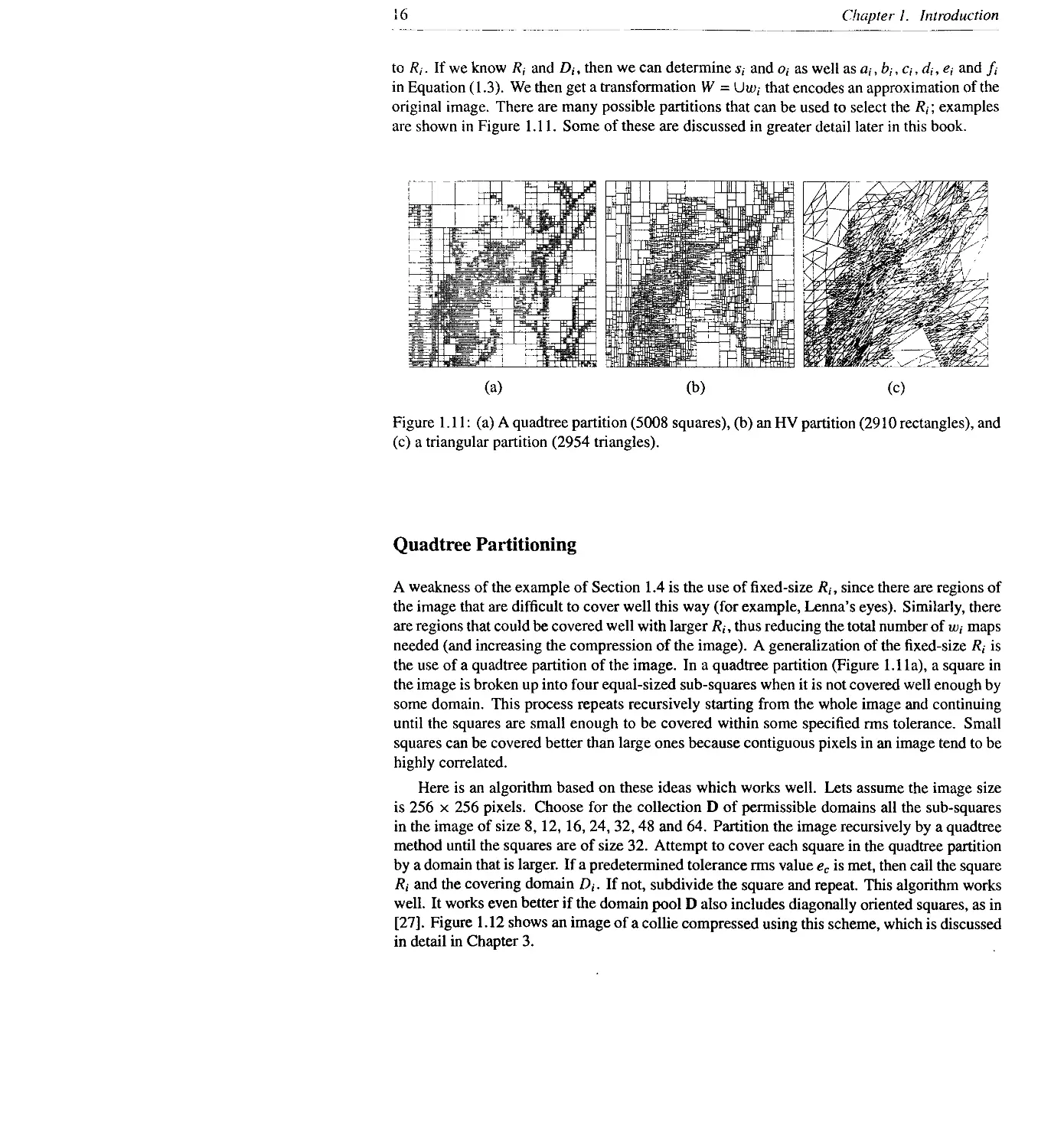
Figure 1.11: (a) A quadtree partition (5008 squares), (b) an HV partition (2910 rectangles), and
(c) a triangular partition (2954 triangles).
Quadtree Partitioning
A weakness of the example of Section 1.4 is the use of fixed-size since there are regions of
the image that are difficult to cover well this way (for example, Lenna’s eyes). Similarly, there
are regions that could be covered well with larger thus reducing the total number of w,- maps
needed (and increasing the compression of the image). A generalization of the fixed-size R, is
the use of a quadtree partition of the image. In a quadtree partition (Figure 1.1 la), a square in
the image is broken up into four equal-sized sub-squares when it is not covered well enough by
some domain. This process repeats recursively starting from the whole image and continuing
until the squares are small enough to be covered within some specified rms tolerance. Small
squares can be covered better than large ones because contiguous pixels in an image tend to be
highly correlated.
Here is an algorithm based on these ideas which works well. Lets assume the image size
is 256 x 256 pixels. Choose for the collection D of permissible domains all the sub-squares
in the image of size 8,12,16, 24, 32,48 and 64. Partition the image recursively by a quadtree
method until the squares are of size 32. Attempt to cover each square in the quadtree partition
by a domain that is larger. If a predetermined tolerance rms value ec is met, then call the square
Ri and the covering domain If not, subdivide the square and repeat. This algorithm works
well. It works even better if the domain pool D also includes diagonally oriented squares, as in
[27]. Figure 1.12 shows an image of a collie compressed using this scheme, which is discussed
in detail in Chapter 3.
1.5. Wavs to Partition Images
17
Figure 1.12: A collie image (256 x 256) compressed with the quadtree scheme at a compression
of 28.95:1 with an rms error of 8.5.
HV-Partitioning
A weakness of quadtree-based partitioning is that it makes no attempt to select the domain pool
D in a content-dependent way. The collection must be chosen to be very large so that a good
fit to a given range can be found. A way to remedy this, while increasing the flexibility of
the range partition, is to use an HV-partition. In an HV-paitition (Figure 1.1 lb) a rectangular
image is recursively partitioned either horizontally or vertically to form two new rectangles.
The partitioning repeats recursively until a covering tolerance is satisfied, as in the quadtree
scheme.
(a)
Figure 1.13: The HV scheme attempts to create self-similar rectangles at different scales.
This scheme is more flexible, since the position of the partition is variable. We can then try
to make the partitions tn such a way that they share some self-similar structure. For example,
we can try to arrange the partitions so that edges in the image will tend to run diagonally through
them. It is then possible to use the larger partitions to cover the smaller ones with a reasonable
expectation of a good cover. Figure 1.13 demonstrates this idea. The figure shows a part of an
image (a); in (b) the first partition generates two rectangles. Rt with the edge running diagonally
18
Chapter I. Introduction
through it, and /С? with no edge; and in (c) the next three partitions of R\ partition it into four
rectangles - two rectangles that can be well covered by R\ (since they have an edge running
diagonally ) and two that can be covered by Ry (since they contain no edge). Figure 1.14 shows
an image of San Francisco encoded using this scheme.
Figure 1.14: San Francisco (256 x 256) compressed with the diagonal-matching HV scheme
at 7.6:1 with an rms error of 7.1.
Other Partitioning
Partitioning schemes come in as many varieties as ice cream. Chapter 6 discusses a variation of
the HV scheme, and in Appendix C we discuss, among other things, other partitioning methods
which may yield better results. Figure 1.11c shows a triangular partitioning scheme. In this
scheme, a rectangular image is divided diagonally into two triangles. Each of these is recursively
subdivided into four triangles by segmenting the triangle along lines that join three partitioning
points along the three sides of the triangle. This scheme has several potential advantages over
the HV-partitioning scheme. It is flexible, so that triangles in the scheme can be chosen to share
self-similar properties, as before. The artifacts arising from the covering do not run horizontally
and vertically, which is less distracting. Also, the triangles can have any orientation, so we break
away from the rigid 90 degree rotations of the quadtree- and HV-partitioning schemes. This
scheme, however, remains to be fully developed and explored.
1.6 Implementation
In this section we discuss the basic concepts behind the implementation of a fractal image
compression scheme. The reader should note that there arc many variations on these methods,
as well as schemes that are completely different. Our goal is to get the interested reader
programming as soon as possible (see also the code in Appendix A).
1.6. Implementation
19
To encode an image, we need to select an image-partitioning scheme to generate the range
blocks R,- С I2. For the purpose of this discussion, we will assume that the R, are generated
by a quadtree or HV partition, though they may also be thought of as fixed-size subsquares.
We must also select a domain pool D. This can be chosen to be all subsquares in the image, or
some subset of this rather large collection. Jacquin selected squares centered on a lattice with
a spacing of one-half of the domain size, and this choice is common in the other chapters. It is
convenient to select domains with twice the range size and then to subsample or average groups
of 2 x 2 pixels to get a reduced domain with the same number of pixels as the range.
In the example of Section 1.4, the number of transformations is fixed. In contrast, the
quadtree- and HV- partitioning algorithms are adaptive, in the sense that they use a range size
that varies depending on the local image complexity. For a fixed image, more transformations
lead to better fidelity but worse compression. This trade-off between compression and fidelity
leads to two different approaches to encoding an image f - one targeting fidelity and one
targeting compression. These approaches are outlined in the pseudo-code in Tables 1.1 and 1.2.
In the tables, size(/?,) refers to the size of the range; in the case of rectangles, size(/?,) is the
length of the longest side. The value rm,„ is a parameter that determines the smallest size range
that will be allowed in the encoding.
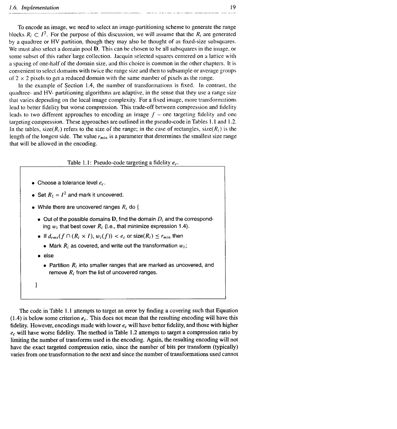
Table 1.1: Pseudo-code targeting a fidelity ec.
• Choose a tolerance level ec.
• Set /?i = I2 and mark it uncovered.
• While there are uncovered ranges /< do {
• Out of the possible domains D, find the domain D, and the correspond-
ing u>i that best cover /?, (i.e., that minimize expression 1.4).
• If drms(f П (/?, x /), < ec or size(/?,) < rmin then
• Mark R, as covered, and write out the transformation wp,
• else
• Partition R, into smaller ranges that are marked as uncovered, and
remove /?, from the list of uncovered ranges.
}
The code in Table 1.1 attempts to target an error by finding a covering such that Equation
(1.4) is below some criterion ec. This does not mean that the resulting encoding will have this
fidelity. However, encodings made with lower ec will have better fidelity, and those with higher
ec will have worse fidelity. The method in Table 1.2 attempts to target a compression ratio by
limiting the number of transforms used in the encoding. Again, the resulting encoding will not
have the exact targeted compression ratio, since the number of bits per transform (typically)
varies from one transformation to the next and since the number of transformations used cannot
20
Chapter i. Introduction
Table 1.2: Pseudo-code targeting an encoding with Nr transformations. Since the average
number of bits per transformation is roughly constant for different encodings, this code can
target a compression ratio.
• Choose a target number of ranges Nr.
• Set a list to contain Ri = I2, and mark it as uncovered.
• While there are uncovered ranges in the list do {
• For each uncovered range in the list, find and store the domain D, e D
and the map w, that covers it best, and mark the range as covered.
• Out of the list of ranges, find the range Rj with size(/?; ) > with the
largest
drms(f D(Rj x I), Wj(f))
(i.e. which is covered worst).
• If the number of ranges in the list is less than Nr then {
• Partition Rj into smaller ranges which are added to the list and
marked as uncovered.
• Remove Rj, Wj and Dj from the list.
)
}
• Write out all the w, in the list.
be exactly specified. However, since the number of transformations is high (ranging from
several hundred to several thousand), the variation in memory required to store a transform
tends to cancel, and so it is possible to target a compression ratio with relative accuracy.
Finally, decoding an image is simple. Starting from any initial image, we repeatedly apply
the Wj until we approximate the fixed point. This means that for each w,, we find the domain
Dj, shrink it to the size of its range /?,, multiply the pixel values by s, and add o,-, and put
the resulting pixel values in the position of /?,. Typically, 10 iterations are sufficient. In the
later chapters, other decoding methods are discussed. In particular, in some cases it is possible
to decode exactly using a fixed number of iterations (see Chapter 8) or a completely different
method (see Chapter 11 and Section C.13).
The RMS Metric
In practice, we compare a domain and range using the rms metric. Using this metric also
allows easy computation of optimal values for s( and o( in Equation (1.3). Given two squares
1.6. Implementation
21
containing n pixel intensities, «|,..., a„ (from £),) and b\,..., b„ (from /?,), we can seek i
and о to minimize the quantity
R = ^(s a,- + о — bi)2.
i = l
This will give us contrast and brightness settings that make the affinely transformed «,• values
have the least squared distance from the /?, values. The minimum of R occurs when the partial
derivatives with respect to s and о are zero, which occurs when
and
In that case,
1
R = -
n
+ 2o a;j+olno — 2 bf
. i=l \ i=l 1 = 1 ;=1 / \ <=1
(1.5)
If n H"=i ~ (EXi at)2 = O’ then s = 0 and 0 = „ S"=i bi- There is a simpler formula for R
but it is best to use this one as we'll see later. The rms error is equal to J~R.
The step “compute drms(,f П (/?, x /), w,(/))” is central to the algorithm, and so it is
discussed in detail for the rms metric in Table 1.3.
Storing the Encoding Compactly
To store the encoding compactly, we do not store all the coefficients in Equation (1.3). The
contrast and brightness settings have a non-uniform distribution, which means that some form of
entropy coding is beneficial. If these values are to be quantized and stored in a fixed number of
bits, then using 5 bits to store s, and 7 bits to store o, is roughly optimal in general (see Chapter
3). One could compute the optimal s, and o, and then quantize them for storage. However, a
significant improvement in fidelity can be obtained if only quantized st and o, values are used
when computing the error during encoding (Equation (1.5) facilitates this).
The remaining coefficients are computed when the image is decoded. Instead of storing
them directly, we store the positions of /?, and D, . In the case of a quadtree partition, /?, can be
encoded by the storage order of the transformations, if we know the size of The domains
Dt must be referenced by position and size. This is not sufficient, though, since there are eight
ways to map the four comers of D, to the comers of So we also must use three bits to
determine this rotation and flip information.
22
Chapter I. Introduction
Table 1.3: Details of the computation of drms(f (T (/?, x /), w,(/)) in the case where £>, is
twice the size of
• Let Di be the domain of w,.
• Take the pixels of D, and average nonoverlapping 2x2 blocks to form a
new collection of pixels F,- that has the same size as .
• If Wj involves a rotation or flip, permute the pixels of F, to the new orien-
tation.
• Compute a and £ne/, a2.
• Compute b and b2.
• Compute ьек a^- 'n ^'S sum> only the elements a and b in the
same pixel position are summed.
• These sums can be used to compute s,-, o, and R. Note that all but the
last sum can be done ahead of time. That is, it is not necessary to
repeat the domain sums for different ranges.
• drms(f П (/?, x /), w,(/)) = y/R.
In the case of the HV partitioning and triangular partitioning, the partition is stored as a
collection of offset values. As the rectangles (or triangles) become smaller in the partition,
fewer bits are required to store the offset value. The partition can be completely reconstructed
by the decoding routine. One bit must be used to determine if a partition is further subdivided
or will be used as an /?,, and a variable number of bits must be used to specify the index of
each Dj in a list of all the partitions. For all three methods, and without too much effort, it is
possible to achieve a compression of roughly 31-34 bits per w,.
Optimizing Encoding Time
Another concern is encoding time, which can be significantly reduced by classifying the ranges
and domains. Both ranges and domains are classified using some criteria such as their edgelike
nature, or the orientation of bright spots, etc. Considerable time savings result from only using
domains in the same class as a given range when seeking a cover, the rationale being that
domains in the same class as a range should cover it best. Chapters 4 and 9 are devoted to this
topic, and other methods can be found in Chapters 3 and 6.
1.7. Conclusion
1.7 Conclusion
The power of fractal encoding is shown by its ability to outperform6 (or at least match) the
DCT. a method which has had the benefit of hundreds of thousands, if not millions, of man-
hours of research, optimization, and general tweaking. While the fractal scheme currently has
more of a cult following than the respectful attention of the average engineer, today’s standards
and fashions become tomorrow’s detritus, and at least some of today’s new ideas flower into
popular use. For the gentle reader interested in nurturing this scheme through implementation
or theory, the remainder of this book presents other theoretical and experimental results, as well
as refinements of the ideas in this chapter and a list of unsolved problems and further research.
Acknowledgments
This work was partially supported by DOE contract DE-FG03-90ER418. Other support was
provided by the San Diego Super Computer Center; the Institute for Nonlinear Science at the
University of California, San Diego; and the Technion Israel Institute of Technology. This
chapter is based on Appendix A of [69] and [24].
6See Appendix D for a comparison of results.
Chapter 2
Mathematical Background
Y. Fisher
Hutchinson [36] introduced the theory of iterated function systems (a term coined by M.
Barnsley) to model collections of contractive transformations in a metric space as dynamical
systems. His idea was to use the Contractive Mapping Fixed-Point Theorem to show the
existence and uniqueness of fractal sets that arise as fixed points of such systems. It was
Barnsley’s observation, however, that led to the idea of using iterated function systems (IFS’s)
to encode images. He noted that many fractals that can be very compactly specified by iterated
function systems have a “natural” appearance. Given an IFS, it is easy to generate the fractal
that it defines, but Barnsley posed the opposite question: given an image, is it possible to find
an IFS that defines it?
After the appearance of the acronym “IFS,” a slew of others appeared on the scene. These
include (but are probably not limited to) RIFS, RFIF, PIFS, WFA, HIFS, and MRCM. The
details of the evolution of the topic are interesting (and possibly sordid); in this chapter we
will simply present a synopsis. This chapter has the misfortune of being aimed at readers with
widely varying background; trivialities and technicalities mingle. Every attempt at rigor is
made, but to help separate the text into thick and thin, most topics are also presented informally
in sans serif font. Finally, this chapter is not completely general nor generally complete; for an
undergraduate-level presentation of the IFS material, the interested reader should refer to [4] or
[69].
2.1 Fractals
Unfortunately, a good definition of the term fractal is elusive. Any particular definition seems
to either exclude sets that are thought of as fractals or to include sets that are not thought of as
fractals. In [23], Kenneth Falconer writes:
25
26
Chapter 2. Mathematical Background
My personal feeling is that the definition of a “fractal” should be regarded in the
same way as the biologist regards the definition of “life.” There is no hard and fast
definition, but just a list of properties characteristic of a living thing.... In the
same way, it seems best to regard a fractal as a set that has properties such as those
listed below, rather than to look for a precise definition which will almost certainly
exclude some interesting cases.
If we consider a set F to be a fractal, we think of it as having (some) of the following
properties:
1. F has detail at every scale.
2. F is (exactly, approximately, or statistically) self-similar.
3. The “fractal dimension” of F is greater than its topological dimension. Definitions for
these dimensions are given below.
4. There is a simple algorithmic description of F.
Of these properties, the third is the most rigorous, and so we define it here. Our interest in
these definitions is lukewarm, however, because there are few results on the fractal dimension
of fractally encoded images.
Definition 2.1 The topological dimension of a totally disconnected set is always zero. The
topological dimension of a set F is n if arbitrarily small neighborhoods of every point of F
have boundary with topological dimension n — 1.
The topological dimension is always an integer. An interval, for example, has topological
dimension 1 because at each point we can find a neighborhood, which is also an interval, whose
boundary is a disconnected set and hence has topological dimension 0.
There are many definitions for non-integral dimensions. The most commonly used fractal
dimension is the box dimension, which is defined as follows.
Definition 2.2 For F C R", let Ne(F) denote the smallest number of sets with diameter no
larger than e that can cover F. The box dimension of F is
log^(F)
hm------------.
«->o — log e
when this limit exists.
The fractal dimension can be thought of as a scaling relationship. Figure 2.1 shows four
examples of sets and the scaling relationship for each (i.e., the way the number of boxes it takes
to cover the set scales with the size of the box). For each example, we describe the scaling
relationship below:
a. A curve of length t can be covered by t/e boxes of size e and 2€/e boxes of size e/2.
b. A region of area A can be covered by A/e2 boxes of size e and ffAfe boxes of size e/2.
2.1. Fractals
Z1
Figure 2.1: Four examples of sets and the number of e boxes required to cover them.
28
Chapter 2. Mathematical Background
c. A set with volume V can be covered by V/e3 boxes of size e and 23V/e boxes of size
e/2.
d. If the Sierpinski triangle is covered with W boxes of size e, then it takes 3W boxes of size
e/2 to cover it. This is shown for e equal to half the width of the set in the figure.
We can see that for sets whose dimension is 1, 2, and 3, halving box size corresponds to
increasing the number of boxes required to cover the set by a factor of 21, 22, and 23, at least
in the limit when e is very small. For the Sierpinski triangle, however, the number of boxes
increases by 2'z, where d = log 3/ log 2, and so we call this the (fractal) dimension of the set.
It is a number between 1 and 2, which is reasonable since the set has no area1 but is more
‘meaty’ than a curve. See also Exercise 3.
2.2 Iterated Function Systems
In this section we will formally define iterated function systems. IFS's served as the motivating
concept behind the development of fractal image compression, and most of the work on fractal
image compression is based on IFS’s or their generalization.
An Example
Let’s begin with an example similar to the copy machine of Chapter 1. Figure 2.2 shows three
transformations in the plane:
W2
mi
У
w3
The copying process consists of taking the input (which is assumed to lie in the square region
between the points (0,0) and (1,1) in the plane), applying the three transformations to it, and
pasting the result together. This output is then used again as the input. Figure 2.3 shows this
process beginning with both a square and a circle. The process appears to converge to the
image in Figure 2.4.
Note that the maps w, bring points closer together. That is, the distance between P - (x, y)
and Q = (и, v) is always more than the distance between w,(P) and w, (<2) (by a factor greater
than one). This is the same as saying that the copy machine makes reductions before pasting
the copies together. What would happen if one (or more) of the copies was an expansion? In
‘The Sierpinski triangle can be generated by recursively removing the middle inverted triangle from a partition of
an equilateral triangle into 4 equilateral triangles of half the size. Since at each removal 3/4 of the area is left, the limit
leaves lim„_oo(3/4)" = 0 area.
2.2. Iterated Function Systems
29
Figure 2.2: Three transformations in the plane.
Figure 2.3: Applying the transformations of Figure 2.2 to a square and a circle.
that case, each successive copy would contain a bigger copy of the whole image, and the limit
copy would have to be infinitely big.2 So we arrive at the following rule:
Rule: The copies produced in the copy machine should be reductions.
Now let’s examine what happens when we start the copying machine with different initial
images. The copies of the input image are reduced at each step, so in the limit copy the initial
image will be reduced to a point. Thus, it doesn’t matter what image we start with; we will
approach the same limit image. Therefore, we arrive at the following observation:
Observation: The limit image obtained by running the copy machine in a feedback loop is
independent of the initial image.
An analogy to keep in mind is the following: The iterates of the map x x/2 will converge to
0 from any initial point on the real line. In the same way, the copying process can be considered
as a map in a space of images. This map converges to a point (which is an image) in this space,
2This reasoning is not quite right. It is possible to have non-contractive copies that nevertheless have limit copies
of finite extent. However, if we want to be certain that the limit copy is finite, then having reductions is sufficient. See,
for example, Section C.18.
30
Chapter 2. Mathematical Background
Figure 2.4: The limit image resulting from running the copy machine infinitely many times.
independent of the starting image.
The following sections are devoted to making these notions precise. We first discuss the
space of images (and associated technical conditions). Next, we define “reduction” and restate
the above rule. We then state the Contractive Mapping Fixed-Point Theorem, which corresponds
to the above observation. The remaining sections generalize this theory and apply it to the image
compression problem.
Complete Metric Spaces
Our goal is to define a subset of the plane (which will often be a fractal) as the fixed point
of a map from a space of subsets of the plane to itself. Following Hutchinson [36], we will
first define a metric on such a space, and then a contractive map that will determine a unique
fixed point. The definition of an IFS makes use of the notions of a complete metric space, and
contractive mappings.
Definition 2.3 A metric space is a set X on which a real-valued distance function d : X x X —r
R is defined, with the following properties:
1. d(a, b) > 0 for all a,b e X.
2. d(a, b) = 0if and only if a = b,for all a,b e X.
3. d(a, b) = d(b, a) for all a, b e X.
4. d(a,c) < d(a, b) + d(b, c)for all a, b, с e C (triangle inequality).
Such a function d is called a metric.
A metric space is a set of points along with a function that takes two elements of the set and
gives the distance between them. The set can be a set of points, or a set of images. One of our
metric spaces will be the collection H of all (closed and bounded) subsets of the plane. This set
can be imagined as the collection of all black-and-white pictures, in which a subset of the plane
is represented by a picture that is black at the points of the subset and white elsewhere. The
space H is very large, containing, for example, a line drawing of you, gentle reader, addressing
the United Nations (as well as many other pictures).
2.2. Iterated Function Systems
31
The Hausdorff Metric
Our first goal is to define the Hausdorff metric on this space. This metric will tell us the “distance’’
between any two pictures. The Hausdorff metric is defined formally below. To find the Hausdorff
distance /t(A, B) between two subsets of the plane, A and B, we carry out the following pro-
cedure. For each point x of A, find the closest3 point v in B. Measure these minimal distances
(both starting from A and staring from B) and choose the largest one. This is the Hausdorff
distance. Figure 2.5 shows three examples of sets A and В and the Hausdorff distance (based
on Euclidean distance) between them, marked with a line. The Hausdorff metric is not sensitive
to content; it can’t decide that the distance between two pictures of people is less than the
distance between a picture of a person and a picture of a fern.
Figure 2.5: Sets A and В and the Hausdorff distance between them, indicated by a line. In
the top example, the longest minimal distance is measured from В to A; in the other two, it is
measured from A to B.
Here are some examples of metrics (see Exercise 4):
1. In the plane, the function
d (<X|, У1), (x2, У2» = У(-Г| — x2)2 + (yi ~ У2)2
is the standard Euclidean metric which gives the distance between the points (xi, yi) and
(x2, yi).
3The astute reader will notice that “close” already makes use of the notion of distance. Here we mean the normal
Euclidean distance.
32
Chapter 2.
Mathematical Background
2. Another metric between these points is max(|xi — x2|, lyi — y2|)-
3. For the (measurable) functions f, g : R2 —> R, the supremum metric is
dsup(f, g) = sup \f(x) - g(x)|,
xeR2
and the Lp metrics are
\\f-g\\p = (f \f~g\pdxdy\ .
Ur2 /
4. If x is a point in the plane and A is a subset of the plane, we can define Sd(x, A) =
infv6/1 d(x, y), where d(-, •) is some metric in the plane. If В is also a subset of the plane,
then we can define the metric
hd(A, B) = max
sup<5j(x, B), sup<5j(y, A)
x€4 yeB
This is the Hausdorff metric. We will give a different (possibly simpler) definition of this
metric later.
Definition 2.4 A sequence of points {x„} in a metric space is called a Cauchy sequence if for
any 6 > 0, there exists an integer N such that
d(xm, x„) < e for all n,m > N.
Definition 2.5 A metric space X is complete if every Cauchy sequence in X converges to a
limit point in X.
/iSefinition 2.6 A metric space X is compact if it is closed and bounded.
We now define the space in which we will work. Let 7f(X) = {5 С X | S is compact}. If
A e 7Y(X), then we write Aj(e) = {x | d(x, y) < e for some у e A}; A^(e) is the set of points
that are of maximal d distance e from A (See Figure 2.6.) We can then define the Hausdorff
distance between two elements A, В e 'H(X) to be
Aj(A, B) = max {inf{e | В C Ad(e)}, inf(e | A C Bd(e)}}.
Notice that hd depends on the metric d. In practice, we drop the subscript d when the context
is clear. The compactness condition in the definition of 7f(X) is necessary for the following
theorem to hold.
Theorem 2.1 Let X be a complete metric space with metric d, then H(X) with the Hausdorff
metric hd is a complete metric space.
Proof: See [4] or [36].
2.2. Iterated Function Systems
33
Figure 2.6: A set A and its thickened version A^(e).
A Cauchy sequence is a sequence of points that converges to a limit point. Our definition of a
Cauchy sequence is dependent on measuring distances, which is why we must have a metric be-
fore we decide if the space is complete. For example, the sequence 1,|,2,12,, • • •
is convergent (see Exercise 5), while 1,2,3,4,... is not. It is sufficient to think of complete
metric spaces as spaces that don’t have “holes” or values missing. For example, the set of
rational numbers can be metrized using d(x, у) = |x — у |. But if is not a complete metric space,
because the first sequence above converges to s/2, which is not rational.
The “compact” part of the definition of 2i(X) is required in order to make HIX) be a complete
space. We are concerned with completeness because we will want to know that a convergent
sequence of images will converge to an image. That is, we want our space of images to be
complete.
Contractive Maps and IFS’s
Definition 2.7 Let X be a metric space with metric d. A map w : X —г X is Lipschitz with
Lipschitz factor 5 if there exists a positive real value s such that
d(w(x), wly)) < sd(x, y)
for every x, у e X. If the Lipschitz constant satisfies s < 1, then w is said to be contractive
with contractivity .v.
Examples:
1. The function fix) = 1/x is Lipschitz on the closed interval [1,2] but not on the open
interval(0,1). On[l,2], |/(x)-/(y)| = |l/x-l/y| = |(x-y)/(xy)| < |x-y|,buton
(0,1) the slope of f becomes unbounded and so even when |x — y| is small, 11/x — l/y|
can be very large. This example suggests that the technicalities, such as closure, are at
least relevant.
2. If f is discontinuous, then f is not Lipschitz because if there is a discontinuity between
x and y, then when x and у get arbitrarily close, fix) and fly) can remain separated.
34
Chapter 2. Mathematical Background
3. If f : R" —> R” is given by /(x) = Ax + b, then f is Lipschitz. In fact, any linear
operator on a finite-dimensional vector space is Lipschitz.
Lemma 2.1 If f : X -» X is Lipschitz, then f is continuous.
Proof: It is sufficient to think of continuous functions as maps that have /(x) and f(y) arbitrarily
close as x gets close to y. But as x and у get close, d(x, y) gets arbitrarily small so that
d(f(x), /(y)) < sd(x, y) must also. H
A map is contractive if it brings points closer together. The contractivity 5 measures how
much closer two points are brought together. As an example, consider the map /(x) = x/2
on the real line (with the usual metric d(x, y) = |x — y|). This map is contractive, because the
distance between /(x) and /(y) is never more than half the distance between x and y. If we
pick any initial x and iterate f, computing /(x), /(/(x)), /°3(x),..., then we will converge to
a fixed point 0 = /(0). This is a general property of contractive maps: if we iterate them from
any initial point, we converge to a unique fixed point.
While all contractive maps have unique fixed points, not all maps with unique fixed points are
contractive. For example, x н» 2x only fixes 0, but it is an expansive map (see also Exercise
6).
Here are some examples of contractive maps:
1. If f : R" -» R” is defined by /(x) - Ax + B, where A is a n x n matrix and x, В are
vectors, then f is contractive if x Ax is contractive. This map will be contractive if
suPxeR" ll^ll/II^H < 1- This value is called the norm of A.
2. Let up : R2 -» R2, i = 1,..., n be a collection of contractive transformations. Then
we can define a map W : H(R2) -> 7f(R2) by
W) = (J wKS).
i=i
(2.1)
The next theorem tells us that this map is contractive also.
Theorem 2.2 If up : R2 —> R2 is contractive with contractivity s, for i = 1,... ,n, then
W = U'LjUi, : 7f(R2) -> 7f(R2) is contractive in the Hausdorff metric with contractivity
s = max,=i....„ {.V;}.
Proof: We will prove this for the case n = 2. The general case can be proved by induction.
Select A, В e 7f(R2), and let c = h(A, B). Then A C B(e) and В c A(e). Let
s = max{.V|, .v2},
Af = up(A),
Bi = up(B),
A' = W(A) = A! U A2, and
B' = W(B) = Bi U B2.
2.2. Iterated Function Systems
35
Figure 2.7: w,(A(f)) c A,(s,e), for i = 1,2
Then we want to show that h(W(A), W(B)) < sh(A, B),or В' C A'(sc)andA' G B'(se). But
this follows from В, C w^Ate)) C Afs/e) G A,(sc) and A, G w,(B(c)) G B,(s,c) G B^se),
for ( = 1,2. See Figure 2.7. H
Recall the copy machine example of Chapter 1. Theorem 2.2 says that if the individual
copies are reductions (that is, if the transformations composing the copies are contractive) then
the resulting copying process W is contractive in the space of all possible images. Why do we
care about this? Because just as the contractive map x x /2 has a unique fixed point 0 which
is the limit of iterating starting from any initial point, so will the contractive map W have a unique
fixed picture, the limit of iterating W from any initial picture.
The Contractive Mapping Fixed-Point Theorem
We are now ready to state one of the main tools of this subject:
Theorem 2,3 (Thfefiumtactive Map»iBg.Fto.ed-]RMnLThMirem) Let x be a complete met-
ric space and f : X —> X be a contractive mapping. Then there exists a unique point Xf e X
such that for any point x e X
xf = Л*/) = lim /“"Л)-
л-»-оо
Such a point is called a fixed point or the attractor of the mapping f.
Proof: Select x e X. Then for n > m,
d(f°m(x), f°n(x)) < sd(f°m-\x), f°n-'(x)) < sm d(x, f°n-m(x)). (2.2)
Now, using this and the triangle inequality repeatedly,
d(x,f°k(x)) < d(x,fok-t(x)) + d(rk-l(x),fok(x))
36
Chapter 2. Mathematical Background
< d(x, /(%)) + d(/(x), /(/(x))) + • • +
d(f°k~l(x), f°kW)
< (1 + s + • • + sk~2+sk~')d(x, f(x))
< —— d(x,/(x)). (2.3)
1 — 5
We can then write Equation (2.2) as
^(/°m(x), /°"(x)) < ~^—d(x, f(x)),
1—5
and since 5 < 1, the left side can be made as small as we like if n and m are sufficiently
large. This means that the sequence x, f(x), /(/(x)),... is a Cauchy sequence, and since X
is complete, the limit point xy = limn->oo f°n(x) is in X. By Lemma 2.1, contractivity of f
implies that f is continuous, and so /(xy) = /(lim /on(x)) = lim /on+1(x) = xy.
To prove uniqueness: suppose Xi and X2 are both fixed points. Then d(/(xi), /(хг)) =
d(xi, X2), but we also have d(/(xi), f(xif) < 5 d(x\, X2), a contradiction.
Wifh the hypothesis of the Contractive Mapping Fixed-
Point Theorem,
d{x, xy) < —d(x, /(x)).
1—5
Proof: This is a consequence of taking the limit as к goes to infinity in Equation 2.3. I
Note that it is not necessary for f to be contractive for it to have a fixed point which attracts
all of X. For example, it is sufficient for some iterate of f to be contractive. This leads to the
following generalization of the previous theorem.
Defining 2.8 Let f be a Lips_chjtz function. If there is a number n such that f°" is contractive,
then we call f eventually contractive. We call n ^PXxpnnc.nl.off.YfiUtJjalCflnlractiy.ily.
Gnrallar8,2^J,fi£aerali86d CttltolllTOraiV f be eventually contractive with exponent
n; then there exists a unique fixed point Xf € X such that for any x e X
xf = Лх/) = ,lim fokM-
K-+OO
In this case,
1 1 - a"
d(x,xf) < --------------d(x, /(x)),
where s is the contractivity of f°n and a is the Lipschitz factor of f.
Proof: Let g = f°n. We want to show that f°k converges to xs; that is, f°k(x) is arbitrarily
close to xg for all sufficiently large k. For any k, we can write к = q n + r, with 0 < r < n. So,
d(f°k(x),xg) = d(f°ft”,xg)
< d(f°<n+r(x), f°<\x» + d(/0’"(x), xg)
= d^{fa\x)), g°«(x)) + d(g°«(x), xg)
< s4d(f°r(x),x) + d(g°4(x),xg).
i . = i /
£ Ac X
2.2. Iterated Function Systems
37
But both of these terms can be made arbitrarily small for 0 < r < n and q sufficiently large.
The fixed-point condition follows from the continuity of f, and uniqueness follows from the
uniqueness of xg.
For the inequality, we know from the Collage Theorem that:
d(x, xg) < —d(x, g(x)) (2.4)
1—5
and
n
d(x, g(x)) = d(x, f°"(x)) < ^(/о'(х), Г~ЧхУ)
n
< /(x))22cr'”1
i=l
< \^-d(x,f(x)). (2.5)
1 — a
The result follows from Equations (2.4) and (2.5). I
Remarks: Note that it is not necessary for f to be contractive for all n that are sufficiently
large. It is sufficient that f be contractive for some n. Also, it is possible for W - Uwf to be
eventually contractive if some of the w, are not contractive; see Section C.18.
Fractals As Fixed Points
Now we are ready to apply the Contractive Mapping Fixed-Point Theorem. Let wi,..., w„ be
contractive transformations. Then the map W = Uw, is contractive and defines a unique fixed
point in H. For example, we may choose w, to be affine transformations of the plane, in which
case the fixed point xw is a subset of the plane which is often a fractal.
Definition 2.9 Let X be a complete metric space. An iterated function system is a collection
of contractive maps w, : X -> X.for i = 1,..., n.
So an IFS is just a collection of maps that, by the Contractive Mapping Fixed-Point Theorem,
defines a unique attractor. The point is that since the attractor is unique, it is completely specified
by the map W. The image encoding problem, or the inverse problem, as it has come to be called,
is: if we are given some set S, can we find an IFS whose attractor is S? No completely general,
or even mildly satisfying, solution to this problem exists to date. However, some insight can be
found in the fixed-point equation
xw = W'(xw') = wifxjy) U • • • U w„(xw)
and the Collage Theorem
d(S,xw)< ——d(S, W(S».
1 — .v
The first says that the fixed point is constructed out of transformed copies of itself, so we should
take the set S, transform it by contractive transformations and attempt to paste these together to
Chapter 2. Mathematical Background
reconstruct S. The uniqueness of the fixed point is important, because if, given S, we can find a
IV (or, if given W, we can find a set 5) satisfying 5 = IV(5), then we will know that S = xw; that
is. .S' is the attractor of IV. The second equation says that even if we can’t paste the pieces to
fit exactly, the better the fit between the original set S’ and the pasted '‘collage” W(S), the closer
the attractor will be to 5 (barring the use of some transformations that are barely contractive,
that is, with л- close to 1).
An obvious question is: why not take W to slightly contract .S', in which case d(S, JV(5)) will
be small, and hopefully </(5, will be small too? This will fail because for such a IV, the
term is very large, so we don’t know that d(S, x>v) must be small. (In fact, it isn’t small because
if it were, there wouldn’t be books on the subject.)
Figure 2.8 shows a simple example of using the fixed-point equation. Here the set 5 is a
square, which can be exactly covered by four copies of itself reduced by a half. The transfor-
mations u?i, W2, n>3, and W4 are shown in Figure 2.8a, and it is clear that S = uq(5) U W2(S) U
w3(S) U umCS) = IV(5), which means that the fixed point x^ for IV is S. The first three iterates
of IV starting from a circle are shown in Figure 2.8b. We can see that the iterates converge to
S, as the Contractive Mapping Fixed-Point Theorem states.
Figure 2.8: (a) The transformations uq, W2, uq, ич that cover a square, and (b) the first three
iterates of W = U*=1 w,.
Figure 2.9 shows two examples of IFS’s, showing both the fixed point and the transforma-
tions. The transformations are shown as the parallelograms which are the images of the large
square. The orientation of the images is shown by the F. Note that each parallelogram con-
tains a transformed (reduced) copy of the whole image, and that the union of the copies in
each parallelogram forms the whole attractor. In the spiral, for example, the small parallelogram
contains a copy of the whole image; the orientation is reversed, however. The transformation
2.3. Recurrent Iterated Function Systems
39
corresponding to the large parallelogram maps the whole attractor into itself, shifted by one
sub-spiral. The union of this spiral and the small spiral forms the whole attractor. This is exactly
what the fixed-point equation says. See Exercise 7 for other examples.
(b)
Figure 2.9: Two examples of IFS’s with their attractors. The transformations of the IFS’s are
shown as the images of the square around the attractor.
2.3 Recurrent Iterated Function Systems
In this section, we review some of the work of Barnsley, Elton, and Hardin [5] on recurrent
iterated function systems (RIFS). A RIFS is a collection wj,..., wn of Lipschitz maps in a
complete metric space X, and an n x n matrix (/>,,-) satisfying pjj = 1 for all i. An
attractor for a RIFS is computed in the following way. Select an initial xq and an initial
io e {1,..., n). Choose a number i„+1 € {1,..., nJ with the probability of i„+l = j equal to
pinj. Set x„+i = U«), and in this way define a sequence {x„). The attractor A is defined as
the set of points x such that every neighborhood of x contains infinitely many x„ for almost all
x0. Reference [5] is concerned with the existence, uniqueness and characterization of the limit
set A. This is the most general definition of a RIFS, and we will not pursue it further. We will
restrict ourselves to an alternative development, given below.
Suppose that for some reason one wished to generate a fern in which the leaves were
constructed out of Sierpinski triangles. Is there a simple generalization to an IFS that would
allow this? Yes. To do this, we could think of two IFS’s working in parallel. One would construct
an IFS for a Sierpinski triangle as before, and this IFS would feed its output into another IFS
which would copy the triangle where the leaves would belong. The second IFS would also be
responsible for making copies of the leaves to fill out the fern. This is shown in Figure 2.10, with
the resulting attractor shown in Figure 2.11. RIFS are a general framework for specifying such
processes.
40
Chapter 2. Mathematical Background
In a RIFS, we imagine some number of disjoint planes, each containing an IFS. We allow
maps between the planes, and these allow us to mix and match the attractors. See Figure 2.12.
Figure 2.10: Two IFS’s which are mixed to form a fem with Sierpinski triangle leaves.
Figure 2.11: The attractor resulting on the right of Figure 2.10.
The theory of recurrent IFS, as far as we are concerned, can fit into IFS theory. Let
Xi,..., Xn be complete metric spaces, and let H, be the set of non-empty compact subsets of
X;, with its associated Hausdorff metric h,. Define
H = H\ x Я2 • • x Hn.
2.3. Recurrent Iterated Function Systems
41
Figure 2.12: A RIFS consists of IFS’s on disjoint planes with maps between the planes.
Then an element of H is an «-tuple of non-empty subsets (A],..., A„). We metrize H with
h((A'.....An), (Bb ..., B„)) = max{/j,(A;, B,)}.
i
With this metric, H is a complete metric space.4
We now define a set of transformations : Hj -> Hit some of which may map to
the empty set.5 The Wij are constructed as a union of transformations Wy = UkWijk where
Wjjk : Xj —> Xi is contractive. Because H has non-empty components, we require that for
each i there is some with non-empty image.
We can now define W : H —> Я by
W(A1;..., A„) = (U7W1;(Ay)..........UyW„/A7)) .
The reader is encouraged to show that the contractivity of W is the maximum of the contrac-
tivities of the Wijk. By the Contractive Mapping Fixed-Point Theorem, W has a unique fixed
point Ху/ = (Ai,..., An) € H.
The generality of the theory allows us to apply it to various types of data. For example,
Barnsley and Jacquin discussed the compression of contour data in [8]. In this scheme, contour
data was partitioned (in some unspecified way) into domain £>, and range R, contour pieces,
as in Figure 2.13. For each domain piece, a map w, was chosen that mapped the endpoints
of Dj onto the endpoints of B, and that minimized the distance between w,(£>,) and R,. The
resulting map V = Uw,- has a fixed point (in a space of curves) that approximates the original
contour.
4This is an immediate consequence of the completeness of the X;.
5We could specify an index set I of pairs, such that (i, j) e I implies that we have some map Wjj. Instead, we let
all pairs have some map, and we allow the case Wjj(-) ~ 0.
42
Chapter 2. Mathematical Background
Figure 2.13: A map w, mapping a contour domain D, onto a contour range Л,.
The details of the partitioning or selection of domain-range pairs were not included in [8],
but they did appear in the work of Boss and Jacobs [43]. In this scheme, the original contour
was segmented and each segment was classified by its curvature at different scales. The
segmentation was regular and classification was used to speed the massive domain-range
comparison. Although the scheme actually resulted in image expansion - that is, more data
was required to store the RIFS than to cleverly store the original contour - the scheme was one
of the first publically available automated schemes to encode measured data using fractals. We
will apply these ideas to encoding images, after we have settled on an appropriate model for an
image.
2.4 Image Models
We are interested in encoding monochrome images, not black-and-white images that are rep-
resentations of subsets of the plane. Color images are typically extensions of the grey-scale
representation of an image, so we will focus only on grey-scale models. Three image models
are generally used: measure spaces, pixelized data, and functions. We discuss these below.
Measures As Image Models
An image can be represented as a measure p, in the plane, in which case the intensity can be
measured on subsets A of the plane by
/х(А) = У dp,.
In this model, it makes no sense to speak of the intensity at a point, which is reasonable. Our
eye, for example, measures the light flux through an area, not at a point. Barnsley and Hurd’s
book [7] stresses this model, but it is not used in this book.
2.4. Image Models
43
Pixelized Data
In this model, an image is represented as a collection of discrete picture elements or pixels. Each
pixel value takes on discrete values (typically ranging from 0 to 255) representing a grey level.6
The number of bits per pixel used to store the pixel values determines the grey-scale resolution,
while the total number of pixels determines the image resolution. Computer implementations
can only work on this type of representation. Chapter 7 contains an analysis and results based
on this representation, as do Chapters 8, 9, and 10.
An image containing M x N pixels can be thought of as a vector in an n = A/A-dimensional
space. Typically, the discrete nature of the pixel values is ignored, so the space is R". Common
norms on R” are the p-norms, defined by
||x||,; = + |x2|" + • • • + |л-„|"р ,
which define metrics by
The oo-norm is given by
dp(x. y) = ||x - y| |p.
11x11,0= max |x,|.
Z = l Il
The 2-norm is also called the f2 norm, and its induced metric is often called the rms metric.
Thus, if x = (л,,..., x„) and у = (y(,..., y„) are images, the I2, or rms, difference between
them is given by
n
drms(x,y) = ||x — y||2
52 (X,- - y,)2.
The rms metric is far more convenient to use than other metrics because if we denote the
standard inner product by (•, •), then drms{x, y) = ,/(x — y, x — y). This means that certain
minimization problems become easy to solve. For example, we can find a, b which minimize
drms(ax + by, z) By minimizing
d2mf(ax + by,z) = {ax + by — г, ax + by — z)
= a2{x, x)+2ab(x, y)+b2{y,y} -
2a{x, z) — 2b{y, z) + (z, z).
Differentiating with respect to a and b to find the maximum and solving the resulting linear
equations gives
(y,z)(x,y) - (y, y)(x, z)
° = -----\2---)---w-----(2-6)
(x, y)2 - (x, x)(y, y)
and
(x,y)(x,z) - (x,x)(y,z)
b=—-----------—------------—. (2.7)
(x, y)2 - (x,x)(y,y)
This is the least squares solution.
6This value can also be an index into a table of colors. Alternatively, pixels may contain three values representing
red, green, and blue levels.
44
Chapter 2.
Mathematical Background
In practice, the Peak signal-to-noise ratio (PSNR) is used to measure the difference between
two images. It is defined as
PSNR = 201og10 | ,
\rms /
—Ниям—
where b is the largest possible value of the signal (typically 255), and rms is the rms difference
between two images. The PSNR is given in decibel units (dB) which measure the ratio of
the peak signal and the difference between two images. An increase of 20 dB corresponds
to a ten-fold decrease in the rms difference between two images. There are many versions of
signal-to-noise ratios, but the PSNR is very common in image processing, probably because it
gives better-sounding numbers than other measures.
Functions on R2
A function / : R2 R can be thought of as an image of infinite resolution. Because real images
are finite in extent, we take the domain of / to be the unit square I1 = {(x, у) | 0 < x, у < 1}
and the range to be I = {x | 0 < x < 1), with the value of / representing the grey level. This
is the model we adopt in this chapter.
For functions, the metric is inherited from the Lp(l2) norms. The Lp metrics are
<W,g) = \\f-g\\P = ,
so that the rms metric corresponds to L2. Equations (2.6) and (2.7) hold in this case too, with
</, g} = fp fg-
There are two other metrics of interest: the L°° metric and the supremum metric. The
supremum metric of two functions / and g is
dsup(f,g)= sup |/(x, y) — g(x, y)|. (2.8)
(jc.y)e/2
It finds the point (x, у) e I2 where / and g differ the most and sets this difference as the
distance between / and g. This metric is very easy to work with, but it is impractical. It is not
reasonable to have the distance between two functions depend on just one point (for example,
if the functions are identical except at one point).
The L°° metric is less sensitive than the supremum metric. To define it, we define the
essential supremum of / to be inf {/3 | /z(/-1(()3, oo])) = 0), where p, is the Lebesgue measure.
The number ft is the smallest value such that /(x) > ft on a set of measure 0. We define the
L°° distance between / and g to be the essential supremum of \f — g|. This metric avoids the
problems of the supremum metric, but is harder to work with.
Note that we are actually concerned with the convergence of an iterative process and not
so much with the distance. For functions, the notions of pointwise convergence and almost
everywhere (a.e.) convergence are important. These notions do not depend on a metric in the
space of functions, just a metric on the range of the functions. We say that /„ converges to
/ pointwise if for each x we have /л(х) -> /(x). Almost everywhere convergence means
pointwise convergence except on a set of measure zero. It is possible, thus, to find a sequence
of convergent images fn without discussing a particular metric at all. In fact, it is possible to
find examples for which fn—>f pointwise but /„ -Д / for any Lp norm (see Chapter 11).
2.4. Image Models
45
Finally, given a function f : R2 -> R, the graph of f is a subset of R3 consisting of all the
triplets (x, y, f(x, y)). Formally, the graph of f is different from f. However, the two contain
the same information, and so we sometimes use them interchangeably.
Color
It is fortunate that the human visual system uses only three color channels to encode color
information that is sent to the brain. This means that colors, which correspond to different
wavelengths of light, can be simulated by a superposition of three primary colors, typically red,
green, and blue. When a'color image is digitized, three filters are used to extract the red, green,
and blue (RGB) intensities in the image, and when these are recombined we perceive them as
some color. This simplifies important things, such as color TV, and less important things, such
as this section. See [12] for more information on the human visual system.
A. method that can encode a monochrome image can be used to encode color images.
We describe one scheme here, but first, here is what not to do: encoding the RGB components
separately is not reasonable. This is because the human visual system is not particularly sensitive
to color information, and there are ways of compressing color information to take advantage of
this insensitivity.
Given a RGB triplet (/?,-, G,, B,) for pixel i, we compute the YIQ values7
- Yi I Г 0.299 0.587
I, = 0.596 -0.274
.Qi J L0.211 -0.523
0.114
-0.322
0.312
G,
-Bi .
This yields the three YIQ channels: the Y, or luminance, signal measures the perceived bright-
ness of the color; the the I, or hue, signal is the actual color; and the Q, or saturation, signal
measures the vividness or depth of the color. The I and Q channels are also called the chromi-
nance signals. The original RGB signals can be computed using the inverse transformation
-R, -
Gi
LB, J
1.000 0.956 0.621 -] Г Yt-
1.000 -0.273 -0.647 /,
1.000 -1.104 1.701 J L Qi.
It is possible to significantly compress the I and Q signals with little to no apparent
degradation.8 The I and Q channels are typically decimated to one-half or one-quarter of
their original size and compressed (usually at a lower bit rate than the Y channel). This means
that the overall compression ratio for color images is significantly greater. When we compress
three channels, there is three times as much data to compress, and this is reduced by a factor
7These matrices have the curious property of never being identical in any two references. The differences are
inconsequential, being in tue third digit; they are due to roundoff errors and the selection of one matrix as definitive
and the other as its inverse.
8This is, roughly, why monochrome and color television sets can operate using the same broadcast signals. In North
America, which uses the NTSC television broadcasting standard, color and monochrome television sets receive YIQ
signals. Only the Y signal is displayed on the black and white set, while the I and Q color information is sent out during
the brief pulse which is used to tell the television to begin scanning the next line. Color sets combine this color signal
with the Y signal to form a color signal. Because the I and Q signals can be highly compressed, there is enough time to
send them during this rapid horizontal sync pulse. This allowed the introduction of color televisions without the need
for a new broadcasting method. The two color-control knobs on color television sets essentially control the I and Q
channels.
Chapter 2. Mathematical Background
of about i.l to 1.5 for compression of the Y1Q signals. So we can expect a color image to
have a compression ratio that is larger by a factor of 2 to 2.7 than the compression ratio of the
same monochrome image at about the same perceived quality. See, for example, [16] for more
information.
The decoding process consists of computing the Y and the reduced I and Q signals; expand-
ing the I and Q signals to the original image size (the resolution independence of the fractal
schemes is convenient here, although not necessary); and computing the RGB components from
the Y and expanded IQ components. This book contains no results on color, but the scheme has
been successfully implemented in conjunction with a fractal scheme, with the expected results:
it works.
2.5 Affine Transformations
An affine transformation w : R" —> R" can always be written as w = Ax+b, where A e R" x" is
an n x n matrix and b G R" is an offset vector. Such a transformation will be contractive exactly
when its linear part is contractive, and this depends on the metric used to measure distances. If
we select a norm 11 • 11 in R" then x Ax is contractive when
||A|| = sup ||AT||/||F|| < 1.
JeR”
We list without proof the norm of A for p = 1,2, oo.
n
ЦА111 = maxY'|a,7|
ЦАЦ2 = square root of the largest eigenvalue of AT A
HAIloo = max V I a,; I
Kisut-f
7=1
See Exercise 8 for an expression for the norm of A in the 2 x 2 case.
When, as is most common, we have an IFS in R2, we can understand the action of A
geometrically, as is shown in Figure 2.14. A linear transformation can scale with Aj, stretch with
A,, skew with A„, and rotate with Ад. Combinations of these maps can map in a variety of ways,
though we can see that linear transformations always map parallelograms to parallelograms.
See also Exercise 9.
2.6 Partitioned Iterated Function Systems
Our goal now is to repeat the “IFS recipe” for generating fractals but in a more general setting.
We will find maps Wj,..., w„, collect them into a transformation W = Uwi, show that under
certain conditions W is contractive, deduce that it has a fixed point, and attempt to select W so
that its attractor is close to some given image.
2.6. Partitioned Iterated Function Systems 47
Figure 2.14: A linear transformation in R2 can (a) scale, (b) stretch, (c) skew, and (d) rotate.
Figure 2.15: (a) A “bow tie” with the domains of a PIFS indicated by shading, and (b) the
ranges of the transformations indicated by shading.
48
Chapter 2. Mathematical Background
The partitioned iterated function system (PIFS) is a generalization of an IFS. In a PIFS, the
domains of the u>, are restricted. This simplifies the encoding of more general, non-self-similar
sets. For example, it is not easy to see how the “bow tie” in Figure 2.15 can be encoded by an
IFS (see Exercise 10), but it is easy to encode it using a PIFS: with eight transformations, four
restricted to the right half and four restricted to the left half, we can generate the two triangles
of the bow tie separately. The formal definition is:
ОРЙвШдаЛи ДП Let X be a complete metric space, and let D, С X for i = 1, ..., n. A
partitioned, iterated function чуч!ет is a collection of contractive maps w, : D, -> X, for
i = 1, ... ,n.
We wish to use the Contractive Mapping Fixed-Point Theorem, as before, to define a unique
fixed point for a PIFS. But this is not possible to do in complete generality. One problem is that
since the domains are restricted, the initial point is very important; if we are not careful, we
may end up with an empty set after one iteration. In the specific case of image representation,
however, this is not a problem. A complete theory of PIFS remains to be developed, but many
special cases are understood; they are discussed in later chapters.
2.7 Encoding Images
In this section we will use the same notation as in the IFS case. This is an advantage for the
novice who understands IFS theory but a disadvantage for a more sophisticated approach. The
notation is cumbersome and hides what is really happening. We discuss better notation in
Section 2.8.
We will work with the space F = {f : I2 —> R] of images defined as the graphs of
(measurable) functions over the unit square I2 with values in 1 = [0, 1]. We allow the range of
f to be in R, however, so that sums and differences of images are still well defined. We will
use the supremum metric, given in Equation (2.8).
2.1 The space F with the metric dsup is complete.
Proof: See [75]. I
Let Di,..., Dn and /?i be subsets of I2 which we will call domains and ranges,
even though these are not exactly domains and ranges. It is natural (or at least it is common
usage) to confuse a subset of I2 and the function that is defined over that subset. Thus, although
we call D, and Л,- the domain and range of w,, the actual domain and range are the Cartesian
products Di x I and Rt x I.
Let tq,..., v„ : /3 —> I2 be some collection of maps. Define w, as the restriction
u>t = vt\DiXl-
The maps uq,..., wn will form the PIFS. The idea is that w, have restricted domains, but can
otherwise be very general. The map ng operates on f by w,(/) = wfx, y, f(x, y)), and we
think of the result as the graph of a function on I2. Not every w, can do this, which is what we
discuss next.
Dafinifinn ? 11 The maps uq,... ,w„ are said to tile I2 if for all f e F, U"=1 wff) e F.
2.7. Encoding Images
This means the following: when u>; is applied to the part of the image f r\(D, x /) above
Di, the result must be a graph of a function over R,, and I2 - U"=1 R-,. See Figure 1.8. page 12.
Tiling implies that the union UJ'=1 w,(/) yields a graph of a function over I2, and that the R,’s
are disjoint.
Encoding Images with Recurrent Iterated Function Systems
The RIFS model can be used for image encoding. Since a RIFS is just a glorified IFS on a large
space, it is possible to claim (for those who are concerned with such details) that this represents
an IFS solution to the inverse problem. However, we must make the simplifying assumption,
that domains are composed of unions of ranges.
If we are given u>i,..., wn : I3 —* I3, then we can let D, С I2 denote the domain of
и), and R, C I2 its range.9 We also assume that w, tile I2, so in particular, U,R, = I2. Our
simplifying assumption is that each D, is exactly equal to a union of some ranges.
If we consider each range R, to be a space disjoint from the other ranges, we can compose
a RIFS ontf = (/?i x x I) by defining
w.. = ( w' ifRj^Di
4 I 0 otherwise.
In an abuse of notation, we think of w, both as a mapping w, : D, x I —> R, x I and as a
mapping on a component of H. We think of the components of H as being spaces of graphs of
functions over each R,, and we use the supremum metric on these spaces. Thus, the metric on
//is
di ((A|,..., A„), (B,, ..., B,,)) = sup№„p(A(, B^},
i
and we claim that H with this metric is a complete metric space. We now define W as in Section
2.3
W(Ab .... A„) = ( (J Wij(Aj),..., (J Wnj(Aj)\ .
\ j J /
This can also be written
W(Ai,...,An)= I (J wi(Aj),..., (J w„(A/) j .
\{J I R;COi) {J | RjCD„} /
The Contractive Mapping Fixed-Point Theorem now assures us that we have a fixed point in
H, and this fixed point can be embedded in R3 by the embeddings of the components of H into
R3.
Since the ui, tile I2, the fixed point can be thought of as the graph of a function f : I2 —> R.
This follows because we know that if our initial point is a function, then each application of
W is a function, and so is the limit. However, we must choose a range to dominate in the case
when the attractor differs on the boundary of adjacent R,. See Exercise 11 for an alternative
method of representing an image in a RIFS model.
9As before, we will refer to D, as the domain and R, as the range, even though the actual domains and ranges are
Di x I and Rt x I.
50
Chapter 2. Mathematical Background
Remark 1: Note that the Hausdorff metric we use is hd,', it is the metric induced by the
supremum metric on each component of H. In this metric, a convergent sequence of graphs
of functions converges to a graph of a function. If we take H = (H\, Hz,..., H„), where H,
consists of the compact subsets of R, x I with the Hausdorff metric hd (d being the Euclidean
metric), then the limit of graphs of functions may not be a graph of a function (although it
is otherwise a perfectly healthy attractor). For example, lim„_>oc arctan(nx) is not convergent
using hd,, but if we use hd, the limit converges to {(0, у) | — тт/2 < у < тг/2| U {(x, у) | л e
R, у = я/2 when x > 0, у = —-nil when x < 0} C R2, which is not the graph of a function.
If we use hd, then it is not necessary to start iterating with the graph of a function. We can
begin iterating with any element of H and reach a unique fixed point. The condition that the
up be contractive changes, in this case, since the contractivity is measured in a different metric.
We don’t have to insist that the w, tile I2, either. At this point, however, there is little relation
between images and the fixed points of such systems.
Remark 2: If we eliminate the simplifying assumption, the definition of W,-, no longer makes
sense; in that case, Rj may be mapped into two different components of H.
Remark 3: Since the supremum metric is only sensitive to what happens in the z direction,
there is no condition on the spatial part - that is, the xy component - of each w,. This part may
be expansive. In fact, we will reach the fixed point by iteration if W is eventually contractive.
Thus, it is possible to choose some w, to be non-contractive without sacrificing the model.
Remark 4: RIFS theory can be used to gain some knowledge about the attractor and the
encoding. The main theoretical results in this book use this model because it is far more
tractable than the more general PIFS model. For example, if all the up are similitudes with
contractivity s, ,10 then the fractal dimension of the attractor can be computed in the following
way (see [5]). Let S(t) be the n x n diagonal matrix composed of the si,
S(t) = diag(s{,..., s').
Then the fractal dimension of the attractor is the unique positive number d such that S(d)C has
a maximal eigenvalue of modulus 1, where C is the connectivity matrix
1 if Rj C Dj
0 otherwise.
Encoding Images with PIFS
In this section, we eliminate the simplifying assumption of the previous section while main-
taining the IFS notation.
Definition 2.12 If w : R3 -> R3 is a map with (x', y', zj) = w(x, y, zi) and (x', y', z'f) =
w(x, y, Z2), then u> is called z contractive if there exists a positive real number s < 1 such that
|zj -Z2I < s|zi -Z2I
and if x' and y' are independent of zi or Z2,for all x, y, zi, Z2-
10A similitude w is a map for which equality always holds in the Lipschitz inequality.
2.7. Encoding Images
Lemma 2.2 Ifw\.........w„ are z-contractive, then
W = |J w,
i=i
is contractive in F with the supremum metric.
Proof: Let 5 = max, v, , where ,v, are the z contractivities of the w, .
dsup(W(f). IV(g)) = sup{|W(/)(x, y) - W(g)(x, y)| : O. v) e I2}
•= sup{z-component of |w,(x, y, fix, y)) — w,(x. y, g(x, y))| :
(x, y) 6 Dj. i =
< sup{s,|/(.v, y) - g(x, y)| : z = l.zz}
< SUp{s|/(X.y)-g(x,y)|)
< 5SUp{|/(x,y)-g(X, y)|}
< sdsup(f, g)
I
Notice that the z independence of the x and у coordinates of w, is used in going from the
equality to the first inequality above. We have shown that if we select the w, to be contractive
in the z direction, for example if w, is of the form
W;
"X “
У
-Z-
a,
Ci
_ 0
(2.9)
with Sj < 1, then IV = U, w, is contractive in dsup. The tiling condition assures us that when
we evaluate IV = Uu;, we get a function again. This is necessary so that we can apply W the
next time (since it takes a function as input). Contractivity of W in F then determines a unique
fixed point in F by the Contractive Mapping Fixed-PointTheorem.
Note that z contractive maps may be expanding in the x and у directions. In fact, as with
the RIFS model, we are happy with an eventually contractive W, so that in practice there are
no a priori conditions on any particular w, .
We are now ready to encode a given image.
Encoding a Given Image
Given a collection of z contractive mappings uq,..., wn that tile I2, we know that W = U, w,
defines a unique attractor xw in the space of images. Given W, it is easy to find the image that
it encodes: begin with any image f0 and successively compute W(fo), W(W(/0)),... until the
images converge to xw. The converse is considerably more difficult: given an image f, how can
a mapping W be found such that xw = f? A general non-trivial solution to this problem remains
elusive. Instead, an image f e F is sought such that d(f, f) is minimal with f = xw. Since
xw = W(xw) = U"=J Wi(xw), it is reasonable to seek domains D\, and corresponding
transformations uq,..., u>„ such that
n
f « W) = U Witf).
(2.10)
Chapter 2.
Mathematical Background
This equation says: cover f with parts of itself; the parts are defined by the D, and the way those
parts cover f is determined by the w,. Equality in Equation (2.10) would imply that f = xy.
Being able to exactly cover f with parts of itself is not likely, so the best possible cover is sought
with the hope that x^ and f will not look too different, i.e. that d(f, хцг) is small. The hope
for this comes from the Collage Theorem. The goal is to find a IV such that d(f, W(f\) is
minimized and such that s is small. In that case, x^ will be close (in d) to f. However, as was
shown in [27], the bound in the corollary is not very good; it provides motivation only, and it is
not a useful bound in practice. In fact, it is possible to generate examples in which the bound
in the corollary is arbitrarily large while d(J, хцг) is bounded. Also, empirical results show that
restricting s to be small results in a larger error d(f, x^). So we lack a good motivation, but
nevertheless, the procedure works. A more motivating Collage Theorem can be found in [65].
Thus, the encoding process is: partition /2 by a set of ranges Л,. For each Rit a D, с I2
and w, : Dj x / -> /3 are sought such that Wj(f) is as close to f П (Л, x I) as possible; that
is,
d(f П (Ri x I), Wi(f)) (2.11)
is minimized. The map IV is specified by the maps ui,-. The w,’s must be chosen such that
W or 1Vom is contractive. Specific partitioning methods and ways of storing W compactly are
presented in later chapters, including the next one.
Eventually Contractive Maps
A brief explanation of how a transformation W can be eventually contractive but not contractive
is in order. The map W is composed of a union of maps w, operating on disjoint parts of an
image. The iterated transform IVom is composed of a union of compositions of the form
W;. О W;, О • • • W, .
‘1 ‘2 *m
The product of the contractivities bounds the contractivity of the compositions, so the composi-
tions will be contractive if each contains sufficiently contractive w,-.. Thus, W will be eventually
contractive (in the supremum metric) if it contains sufficient “mixing” so that the contractive w,-
eventually dominate the expansive ones. In practice, given a PIFS, this condition is relatively
simple to check in the supremum metric.
To check whether W is eventually contractive, we define new maps w-, which have the same
spatial (xy) component as wit but whose z component is s,z, where Sj is the contractivity of w,.
Then we define W = U,-w' and iterate W starting with /(x, y) = 1. If < 1, then W
is eventually contractive with exponent m.
gJiJ Other Models
The^FS notation for PIFS is ugly. Better notation and theory are discussed later in the book;
thus, we only briefly list some of the other approaches.
Chapter 11 discusses the following approach. Consider an image as an element of f e
LP(I2). The goal is to find functions m : I2 —> I2, 5 : I2 —> Rand о : /2 —> R so that a given
function f will be a fixed point for the operator rm,s,e : L₽(/2) -> LP(I2) given by
rm.s,o(f) = s(x)f(m(x)) + o(x).
2.8. Other Models 53
In that case, m, s and о compose an encoding of f. Here s(x) is a generalized version of
the s/ in w,. The function m(x) represents the spatial part of the w( transformation. Given
wi,..., w„, we can select m(.v) and s(x) to be piecewise constant (on the ranges of the wj)
with mix) mapping the range of each w, to its domain. (This has the unfortunate disadvantage
of reversing the meaning of range and domain. Oh well!)
If we consider an image as a vector f e K" then we can write r as an affine matrix operator,
t(/) = 5/ + O,
where О e R" is a vector that plays the role of o(x) and S does several things. First, 5 permutes
the values in f according to the action of m(x) (or the spatial part of each u>, ); second, 5 scales
the values of f according to the action of л(л ) (or the s, in each w,). This model is discussed
in Chapters 7 - 10, as well as briefly in Chapter 11.
Weighted Finite Automata
The weighted finite automata (WFA) appears to be, at first glance, a completely different method
of generating fractals and encoding images. Chapter 13 contains a description of the method,
so we restrict ourselves here to a brief intuitive discussion. In some loose sense, a WFA restricts
the type of transformations used in an IFS and allows more IFS’s to “mix.”
Roughly, a WFA consists of four n x n matrices Wo, Wi, W2, W3, and two n vectors F =
(Fi,..., F„) and I = (/,,..., In). To this we add a collection of square images 1Д1,..., i/r„.
These are not part of the definition, but for now it is instructive to think of them as given.
An image f encoded by the WFA is a linear combination of the (grey levels of the) images
Vi,
i=l
The components F, of F consist of the average grey values for the image . Finally, the images
fa are defined on each of their quadrants by linear combinations of each other. If we divide
each image into four equal squares and label these quadrants by 0,1,2, 3, then the a-th quadrant
of is given by ^2j(Wa)tjfa. The тД,- can be generated from F and these relations, which is
why they are not part of the definition.
Because the 1/r, are defined in terms of themselves, the WFA can easily generate fractals. The
transformations in the WFA can map each image only into aquadrant, but the linear combination
of images compensates for this restriction. The success of WFA encoding of images suggests
that some hybrid consisting of WFA with more generalized transformations may yield even
better results.
Chapter 3
Fractal Image Compression with
Quadtrees
Y. Fisher
This chapter describes a quadtree-based fractal encoding scheme. The scheme is an exten-
sion of the one presented in [45] and is similar to that discussed in [26], [27], and in Chapters
7, 8, and 9. While the results are not optimal, this scheme serves as a reference point for other
fractal schemes. It is also a “typical” fractal scheme and a good first step for those wishing to
implement their own. The code used to generate the results presented in this chapter is given
in Appendix A, along with a detailed explanation of its inner workings.
3.1 Encoding
The encoding step follows the pseudo-code in Table 1.1, page 19. In this case, the collection
of ranges comes from a quadtree partition of the image, and the collection of domains consists
of subsquares of the image that are twice the range size.
The Ranges
A quadtree partition is a representation of an image as a tree in which each node, corresponding
to a square portion of the image, contains four subnodes, corresponding to the four quadrants
of the square. The root of the tree is the initial image. See Figure 3.1.
The ranges are selected as follows: after some initial number of quadtree partitions are made
(corresponding to a minimum tree depth), the squares at the nodes are compared with domains
55
Chapter 3. Fractal Image Compression with Quadtrees
Figure 3.1: A quadtree partition is a representation of an image as a tree in which each node
potentially has four subnodes. Each node of the tree corresponds to a square which is a quadrant
of its parent’s square.
from the domain library (or domain pool) D, which are twice the range size. The pixels in the
domain are averaged in groups of four so that the domain is reduced to the size of the range, and
the affine transformation of the pixel values (that is, a scaling and offset) is found that minimizes
the rms difference between the transformed domain pixel values and the range pixel values (see
Section 1.6). All the potential domains are compared with a range. If the resulting optimal rms
value is above a preselected threshold and if the depth of the quadtree is less than a preselected
maximum depth, then the range square is subdivided into four quadrants (which means adding
four subnodes to the node corresponding to the range), and the process is repeated. If the rms
value is below the threshold, the optimal domain and the affine transformation on the pixel
values are stored - this constitutes one map w,-. The collection of all such maps VV = Uw, -•
constitutes the encoding.
The above description must be revised a bit in order to fit the actual algorithm. First, the
affine transformation on the pixel values consists of a multiplication by a scaling factor s, and an
addition of an offset value о,- (these can be thought of as a contrast and brightness adjustment).
These values must be quantized for efficient storage, and it is these quantized values that are
used when computing the rms difference. Second, if the magnitude of the optimal scaling factor
| лу | is greater than 1 for any of the w,, there is a chance that the resulting map W will not be
eventually contractive. Thus, |.s; | larger than some maximal value smax are truncated.
Other ways of selecting the ranges are discussed in Chapter 6. Conditions on s,- for con-
tractivity of W are discussed in Chapters 7 and 11. See also Sections C.12 and C.16.
3.1. Encoding
57
The Domains
There are three major types of domain libraries - D1. Dj, and Dj. The first has a roughly equal
number of domains of each size. The second domain library has more larg domains and fewer
small domains, the idea being that it is more important to find a good domain-range fit for larger
ranges, since then the encoding will require fewer transformations. The third domain library
has more small domains than large domains. The domains are selected as subsquares of the
image whose upper-left corners are positioned on a lattice determined by a parameter I. The
lattice spacing is selected as follows:
D| has a lattice with a fixed spacing equal to I.
Di has a lattice whose spacing is the domain size divided by I. Thus, there will be more
small domains than large. This is the domain pool used by Jacquin in [45].
Dj has a lattice as above but with the opposite spacing-size relationship. The largest domains
have a lattice corresponding to the smallest domain size divided by I, and vice versa.
It is important to note that each domain can be mapped onto a range in eight different ways
- four rotations and a flip with four more rotations. Thus, the domain pool can be thought of
as containing the domains in eight possible orientations. In practice, the classification scheme
discussed below defines a fixed rotation, so that the domains are only considered in one or two
orientations.
An alternative method of selecting the domains is discussed in Section 6.6. In Chapter
12, the domain pool contains just one domain, leading to fast encoding times and a different
contractivity condition.
The -Classification
The domain-range comparison step of the encoding is very computationally intensive. We
use a classification scheme in order to minimize the number of domains compared with a
range. Before the encoding, all the domains in the domain library are classified; this avoids
reclassification of domains. During the encoding, a potential range is classified, and only
domains with the same (or near) classification are compared with the range. This significantly
reduces the number of domain-range comparisons. By “near” classifications we mean squares
that would have been classified differently if their pixel values were slightly different. The idea
of using a classification scheme was developed independently in [45] and [43].
Many classification schemes are possible (see Section C.10): for example, Jacquin used
a scheme that classified a sub-image into flat, edge, and texture regions. Here we discuss a
scheme similar to the one presented in [26]. A square sub-image is divided into upper left,
upper right, lower left, and lower right quadrants, numbered sequentially. On each quadrant we
compute values proportional to the average and the variance: if the pixel values in quadrant i
are r),..., r' for i = 1, 2, 3, 4, we compute
7=1
Figure 3.2: A square image can always be oriented so that the brightness, or average values, of
its quadrants fall into one of these three canonical positions.
and
j=i
It is always possible to orient the sub-image so that the A, are ordered in one of the following
three ways:
Major Class 1: Ai > A2 > A3 > A4.
Major Class 2: A] > A2 > A4 > A3.
Major Class 3: A] > A4 > A2 > A3.
These correspond to the brightness levels shown in Figure 3.2. Once the rotation of the square
has been fixed, each of the 3 major classes has 24 subclasses consisting of the 24 orderings of
the Vi. Thus, there are 72 classes in all. If the scaling value s, is negative, the orderings in
the classes above are rearranged. Therefore, each domain is classified in two orientations, one
orientation for positive s, and the other for negative s,-.
Chapters'"4and9 give both an implementation and a theoretical motivation for such methods
of classification'”'
The Encoding Parameters
Thus, the parameters for this algorithm are:
• The rms tolerance threshold ec.
• The maximum depth of the quadtree partition.
• The minimum depth of the quadtree partition.
• The type of domain pool and the lattice spacing /.
• The maximum allowable scaling factor smax.
• The number of classes compared with a range.
An encoding of an image consists of the following data:
• The final quadtree partition of the image.
• The scaling and offset values s, and о,- for each range.
3.2. Decoding
• For each range, a domain that is mapped to it.
• The symmetry operation (orientation) used to map the domain pixels onto the range
pixels.
3.2 Decoding
Decoding an image consists of iterating IV from any initial image. The quadtree partition is
used to determine all the ranges in the image. For each range Л,-, the domain D, that maps to it
is shrunk by two in each dimension by averaging nonoverlapping groups of 2 x 2 pixels. The
shrunken domain pixel values are then multiplied by s,-, added to o,, and placed in the location
in the range determined by the orientation information. This constitutes one decoding iteration.
The decoding step is iterated until the fixed point is approximated; that is, until further iteration
doesn’t change the image or until the change is below some small threshold value.
Fast Decoding
Somewhat surprisingly, there are many other methods for decoding an image. It is possible to
find the exact fixed point directly by inverting a large but sparse matrix; see Section 11.4. Sec-
tions 5.4 and 6.3 discuss how the fixed point can be approximated in a lower-dimensional space,
significantly reducing the number of operations required to approximate it. The hierarchical
model described in Chapter 5 makes this point very nicely. Chapter 8 discusses a modification
of the above scheme that allows decoding in a finite number of steps, sometimes just one! See
also Section C.13.
Decoding at a Larger Size
The transformations that encode an image are resolution independent. The underlying model
uses functions of infinite resolution, and the fixed point we reach is such a function. Therefore,
when we decode, we may pick any resolution we wish. Figure 3.3 shows portions of both the
original Lenna image and a version generated by decoding an encoding of Lenna at 8 times the
original size. For comparison, the original version is shown, magnified by a factor of 8 also (by
reproducing each pixel 64 times, and not, for example, by using bilinear interpolation, which
would lead to less blocky artifacts). The original encoding results were: 512 x 512 Lenna,
compressed by a factor of 10.96 at 35.31 dB; the image was encoded with a 24 class search
in 794 CPU seconds. Since the large decoded version requires 64 times the memory of the
original, in some (very loose) sense the compression ratio of the decoded image can be said
to be 64 x 10.96 = 701.4. Continuing in this (very loose) vein, it is possible to suggest that
63/64th of the pixels are artificial data created by the transformations. Section 5.5 discusses
the theory of superresolution.
Postprocessing
Since the ranges are encoded independently, there is no guarantee that the pixel values will be
smooth at the block boundaries. The eye is sensitive to such discontinuities, even when they are
small. It is possible to minimize these artifacts by postprocessing the image (see also Section
Mt
Chapter J. Fractal Image Compression with Quadtrees
Figure 3.3: Several portions of Lenna (original, left; decoded, right) showing the artificially
created detail.
3.3. Sample Results
61
C. 16). In this implementation, we modify only the pixels at the boundary of the range blocks,
using a weighted average of their values. If the pixel values on either size of a boundary are
a and b, then these are replaced by W]O + Wib and w?a + W[b, with + w? = 1. Ranges
that occur at the maximum depth of the quadtree are averaged with weights of uq = 5/6 and
W2 = 1 /6, and those above this depth are averaged with weights of uq = 2/3 and u>2 = 1 /3.
These values are largely heuristic (as is the method itself), but the results seem satisfactory.
Section 6.3 discusses an extension of this method in more detail. Also see Exercise 12.
Efficient Storage
To increase the compression, the following bit allocation schemes are used.
Quadtree. One bit is used at each quadtree level to denote a further recursion or ensuing
transformation information. At the maximum depth, however, no such bit is used, since
the decoder knows that no further division is possible.
Scaling and Offset. Five bits are used to store the scaling and seven for the offset. No form
of adaptive coding is done on these coefficients, even though their distributions show
considerable structure.
Domains. The domains are indexed and referenced by this index. However, when the scaling
value is zero, the domain is irrelevant, and so no domain or orientation information is
stored in this case.1
Orientation. Three bits are used to store the orientation of the domain-range mapping.
3.3 Sample Results
This section consists of various data characterizing the quadtree scheme. Many similar results
were reported first in [44] and [27]. (Appendix D contains a comparison of compression results
for the quadtree method and for other image compression schemes, some of which are described
later in this book.) Unless otherwise stated, the following can be assumed:
• Five bits were used to quantize the scaling coefficient, and seven were used for the offset.
• Domains from three classes were compared with each range; that is, three for positive
scale factors and three for negative scale factors.
• For 512 x 512 Lenna, the maximum range size was 32 x 32 (minimum quadtree depth
4), and the minimum was 4x4 (maximum quadtree depth 7).
• The domain pool used was D2 with a lattice parameter 1=1. That is, the domains
consisted of nonoverlapping subsquares of the image that were twice the range size.
• $max = !•
’On average, more than half the bits in the transformation data are used to store the domain position. This means
that a “smarter” selection of domains could lead to a considerable saving in memory.
62
Chapter 3. Fractal Image Compression with Quadtrees
• Results in which the compression is varied are achieved by letting the rms tolerance crite-
rion ec take on (at least some of) the values 0.5, 1,2, 3, 4, 5, 6, 8, 10, 12, 14, 16, 18, 20,
leading to results ranging from low to high compression.
• PSNR was computed after postprocessing.
• Time results are given in CPU seconds on a personal IRIS 4D/35 workstation.
Varying smax
If we restrict the absolute value of the largest scaling value smax to be less than 1, then we may
ensure contractivity of the encoding. Several questions arise, however: Does a smaller smax
lead to faster convergence? Does smax > 1 imply divergence? How does changing smax change
the fidelity of the encoding?
Figure 3.4: The PSNR versus the number of decoding steps for 256 x 256 Lenna encoded with
smax = 0-5, 1.0,2.0, and 4.0. The initial image was black.
Figure 3.4 shows the PSNR as a function of the number of decoding steps, starting from an
initial black image. For these data, the image of Lenna was encoded with smax =0.5,1,2, and
4. We see that smaller smax does converge in fewer iterations, but to a fixed point which has a
worse signal-to-noise ratio (even though the quantization remained constant, allowing for a finer
resolution of the scaling parameter). The encodings with smax > 1 still converged, because
while they are not contractive, they are eventually contractive. In fact, smax = 2 encodings
3.3. Sample Results
63
reached a higher signal-to-noise ratio than encodings with smax < 1 or smax =4. Some images,
however, will converge very slowly when smax > 1 so that the gain in fidelity may not be worth
the uncertainty in decoding. This also depends on the decoding methods. Methods such as
those in Sections 8.3 and 11.4 are not sensitive to the contractivity of the final encoding, so that
s„lax > 1 may not present a problem.
Scaling and Offset Bit Allocation
Figures 3.5 and 3.6 show plots of PSNR versus compression for various bit allocations used to
store the offset and scaling parameters. The curves show results of using different numbers of
bits (sbils and o/,,,,) to uniformly quantize the scaling and offset parameters. These encodings
were made with one search class and a minimal range size of 8x8. These curves show that
Sbits = 5 and oi,us = 1 represents a reasonable compromise, although = 4 and Obus = 6
(which is not shown) may also be a good value. What is clear is that a sophisticated scheme
would use some form of adaptive bit allocation. Experiments with logarithmic quantization,
which has a non-uniform resolution for the values of st, show no improvement.
Figure3.5: PSNR versus compression for 256x256 Lenna with = 7 and a*, , , = 3, 4, 5, 6, 7.
Figures 3.7 and 3.8 show distributions of the scaling and offset coefficients from a typical
encoding (compare with Figure 8.3). They show that both parameters would benefit from some
adaptive coding, since their distributions show considerable structure. The large number of
|s,| = 1 transformations are due to clipping.2 It is interesting to note that aside from |s, | = 1,
2It is important to note, however, that the domain-range rms value is computed after the clipping. This means
64
Chapter 3. Fractal Image Compression with Quadtrees
Figure3.6: PSNR versus compression for 256x256 Lenna with Sbils = 5andoWrv = 5, 6, 7, 8, 9.
the distribution of s, values is rather uniform. This is not the case when smax > 1, as is shown
in Figure 3.9, in which smax = 2. This means that another advantage to using smar_ > 1 is that
the scaling coefficients can potentially be better encoded.
Classification Matching
Figure 3.10 shows a typical histogram of the number of domains in each of the 72 classes
(summed across all the domain sizes). This distribution leaves much to be desired, since it is
far from uniform. A somewhat better distribution appears in Figure 3.11 in which the three
major first classes have been combined. Somewhat surprisingly, this distribution is roughly
comparable to the one in Figure 9.2 (p. 193).
We now attempt to answer the following questions: How fast can encodings be made? What
is the gain in time and cost in fidelity associated with selecting a small proportion of the possible
domains? PSNR and time versus compression ratio results for the 512 x 512 Lenna image are
given in Figures 3.12 and 3.13. The data in both figures come from the same encodings, so that
the points may be compared for fidelity and time results. The number of classes from which
potential domains were chosen for comparison with a range was varied. The curve marked
“Pos” consists of just one comparison class, using only positive scaling values. Since negative
scaling of the domain leads to a different classification, the other curves represent a comparison
that transformations with |s, | = 1 are optimal and do not, in general, consist of all the transformations which found a
potential |s, | > 1 and were clipped.
3.3. Sample Results
65
Count 31 Count
Scaling Coefficient
3.7: A distribution of the scaling coefficients for 256 x 256 Lenna with smax = 1.
Figure 3.8: A distribution of the offset values for 256 x 256 Lenna with smax
66
Chapter 3. Fractal Image Compression with Quadtrees
Figure 3.9: A distribution of the scaling coefficients for 256 x 256 Lenna with s,„ax = 2.
with twice the number of labeled classes - one for positive scaling and one for negative scaling.
Finally, the curve marked “F 8 x 8” consists of using ranges of minimal size 8x8 (corresponding
to a quadtree depth of 6) with a three class comparison.
As is to be expected, comparing a larger number of classes requires more time and leads to
better fidelity. Referring to Figures 3.12 and 3.13, we see that a moderate compression of 20 at
about 30 dB can be done in about 15 seconds - fairly fast for a fundamentally search-intensive
scheme. The search times are very linear in the compression and progress linearly with the
number of classes searched. A one-class search (meaning one for positive scaling and one for
negative scaling) requires twice the search time; a three class search requires slightly less than
six times the time; and so on. Given the non-uniformity of the class distribution in Figures 3.10
and 3.11, this is somewhat remarkable. It shows that when the whole image is encoded, some
averaging takes place, eliminating this unevenness. The full 72-class search requires somewhat
less time, proportionally, probably because the overhead involved with classifying the range
and preclassifying all the domains doesn’t scale with the number of classes.
Figure 3.12 also shows that the quadtree scheme encodes fine detail poorly. It is not able
to achieve a fidelity better than about 37 dB (in this case, and about 38 dB in the next section).
The encoding made with 8x8 minimum range size reaches a lower maximum of about 30 dB.
However, this encoding requires considerably less time. In fact, most of the time is spent in
attempting to cover the large blocks (which were not well matched), so that the method requires
roughly the same time to encode images at all compression ratios. This means that for high
compression ratios (when the fidelity can be compromised), the 8 x 8 minimum range size is
3.3. Sample Results
67
Figure 3.10: A typical histogram showing the number of domains in each of the 72 classes .
Figure 3.11: A typical histogram showing the number of domains in each of the 24 classes
derived by combining the three major first classes in the 72-class classification.
68
Chapter 3. Fractal Image Compression with Quadtrees
Figure 3.12: Lenna 512x512 PSNR versus compression results for various numbers of domain
classes compared with each range.
Figure 3.13: Lenna 512 x 512 time (CPU seconds) versus compression results for various
numbers of domain classes compared with each range.
3.3. Sample Results
69
the method of choice. We can extrapolate from these data that using it with just one search
class would require only about 10 seconds per encoding over the range of compression ratios
with a loss of 0.25 to 0.5 dB in fidelity.
We can draw the following conclusions from these data:
• The improvement attained by using 72 rather than 24 classes is minimal and comes at
great expense in time.
• The improvement of using both positive and negative scaling values over just positive
scaling is significant, about 1 dB, but doubles the encoding time.
• Using three search classes in place of one gives little gain and triples the encoding time.
• Using a large minimum range size is beneficial when high fidelity is not important.
The Domain Pool
In this section we present results derived by varying the domain pool. We answer the following
questions: Is there some form of local self-similarity in a “typical” image which we can exploit
on to restrict the domain pool and hence increase the compression with minimal loss of fidelity?
Is it a good idea to work hard to encode large ranges so that fewer ranges will be required overall,
leading to high compression? Will increasing the total number of domains compared to a range,
improve or worsen the results? One might argue that it will improve the results, since better
domain-range matches may be found, and so either the fidelity will increase or larger ranges
may be used resulting in higher compression. But the extra domains require more bits to store,
and it may happen that ranges that were previously partitioned and fit well will now fit poorly at
a larger size. We answer these questions and, as a consequence, we also find out what happens
when the domain pool is selected in various ways.
Figure 3.14 shows a distribution of the domain-range distance derived from an encoding of
Lenna. The figure also shows the theoretical probability distribution for the distance between
two randomly chosen points (see Exercise 13). The distributions are almost identical, with a
slight shift on the domain-range distance due (at least in part) to the fact that the smallest ranges
are not just one point. This means that the domains are essentially random and that there is no
preference for local domains.
We can examine this same question by plotting the distributions of the difference in the
x and у positions of the domains and ranges. This is done in Figures 3.15 and 3.16. If
(xr, yr) and (xj, yd) denote the range and domain positions, then the normalized distribution of
dx = xr — Xd looks very much like p(dx) = 1 — |dr| (and similarly for dy). The function p(dx)
is the probability distribution for the difference in the x (similarly for y) coordinates of two
points randomly chosen in the unit square with uniform probability. So even when the points
are chosen randomly, it appears that there is a preference for local domains. However, this is
an artifact. In practice, we can subtract this expected peak from the actual data to see if there is
any effect. Figures 3.15 and 3.16 (in which the subtraction is left to the reader) show that there
is a slight preference for local domains, but the effect is small. This may also partially account
for the left shift of the distribution in Figure 3.14. This means that while there might be a very
slight a benefit to adaptively coding (dx, dy), the domain for a fixed range is not more likely
Chapter 3. Fractal Image Compression with Quadtrees
Figure 3.14: A distribution of the domain-range distance (for 512x512 Lenna) and a theoretical
distribution of distance for two randomly chosen points in the unit square.
to be close to the range. Close domain positions appear more often because there are more of
them overall, not because of local self-similarity.3
PSNR and time versus compression ratio results for the 512 x 512 Lenna image are given
in Figures 3.17 and 3.18. Again, the data in both figures come from the same encodings, so that
the points may be compared for fidelity and time results. The domain pool type is indicated in
the plot, as well as the lattice spacing variable I. Table 3.1 shows the number of domains of
each size for each of the domain pools and lattice parameters used.
These data show that increasing the size of the domain pool results in better compression
and fidelity results. The time cost of having a large number of domains is very high, however.
Also, the encodings done with D3 are comparable in PSNR to those done with D, for high
compression ratios, but the fidelity at that point is too low to be of use. At low compression
ratios, the scheme performs worse than the other schemes in either encoding time or PSNR;
this means that it is not reasonable to select this domain pool scheme. Note that the encoding
time is roughly constant (and large) for this scheme, because the number of operations for a
domain-range comparison is large when the range (and hence the domain) is large. The smaller
ranges have a relatively small number of domains which require fewer operations to match, and
3To further elaborate this point, the question is: given a fixed range, is the domain likely to be close? The answer is
no. The domain is equally likely to be anywhere. Averaged over all the ranges, however, there are more close domain
positions and hence more close domains, and so the probability distribution of the x and у difference shows a peak.
3.3. Sample Results
71
Figure 3.15: A distribution of the difference of the x positions of the domains and ranges (for
an encoding of 512 x 512 Lenna). Also shown is the theoretical distribution of the difference
of two randomly selected points.
Figure 3.16: A distribution of the difference of the у positions of the domains and ranges (for
an encoding of 512 x 512 Lenna). Also shown is the theoretical distribution of the difference
of two randomly selected points.
72
Chapter 3. Fractal Image Compression with Quadtrees
Table 3.1: The number of domains in each of the domain pools for various values of the lattice
parameter /.
Domain Pool Domain Size I No. Domains
Di 32 2 50625
Di 16 2 58081
Di 8 2 62001
D, 4 2 64009
D) 32 4 12769
Di 16 4 14641
D, 8 4 15625
D, 4 4 16129
d2 32 2 225
d2 16 2 961
d2 8 2 3969
d2 4 2 16129
d2 32 1 64
d2 16 1 256
d2 8 1 1024
d2 4 1 4096
D3 32 2 12769
D3 16 2 3721
D3 8 2 1024
D3 4 2 256
hence they do not contribute significantly to the encoding time.
Postprocessing
The effect of postprocessing is shown in Figure 3.19 and in Table 3.2; the first two entries in
the table refer to the data shown in the figure. In general, high-fidelity images have a minor
reduction in PSNR (on the order of 0.1 dB), and all other encodings have an increase in PSNR.
This is not the case when the weighting parameters at the bottom of the quadtree are selected to
be equal to those at the inner nodes. A thorough study of postprocessing weights and methods,
in general, remains to be done.
3.4 Remarks
It is possible to compare Figures 3.12 and 3.17 and Figures 3.13 and 3.18. The “3 class” curves
in Figures 3.12 and 3.13 are identical with the “D2, I = 1” curve in Figures 3.17 and 3.18.
We can see, for example, that searching all the domains of the smaller domain pool (D2 used
in Figures 3.12 and 3.13) is roughly equivalent to searching some small subset (consisting of
three classes searched in Figures 3.17 and 3.18) of the large domain pool D], I = 4. This is
3.4. Remarks
73
Figure 3.17: PSNR versus compression results for 512 x 512 Lenna for various domain pool
selection schemes.
Figure 3.18: time (CPU seconds) versus compression results for 512 x 512 Lenna for various
domain pool selection schemes.
74
Clutpter 3, Fmclal Image Compression with Quadtree*
(a)
(b)
Figure 3.19: The 512 x 512 Lenna image (a) with postprocessing, (b) without postprocessing.
3.5. Conclusion
Table 3.2: Postprocessing results for 512 x 512 Lenna.
Figure Postprocessed dB PSNR Comp. Ratio Enc. Time
3.19a Yes 31.72 22.09 903 sec
3.19b No 31.29 22.09 903 sec
- Yes 29.37 33.36 556 sec
- No 28.85 33.36 556 sec
- Yes 34.87 8.48 56.5 sec
- No 34.56 8.48 56.6 sec
- Yes 37.07 4.68 5244 sec
- No 37.22 4.68 5244 sec
Table 3.3: Sample results for 512 x 512 and 256 x 256 Lenna.
Image Size Comp. Ratio PSNR Enc. Time
256 13.56 29.20 38.9 sec
512 31.48 29.52 237.7 sec
256 7.74 31.19 188.9 sec
512 22.08 31.72 903.5 sec
256 6.59 29.65 5.1 sec
512 25.99 29.38 17.8 sec
also true locally, around the point of intersection of the parameters of these graphs: the gain
in PSNR per change in ratio of computing time is roughly the same as we vary the numbet of
classes (from three to one) and the density of the domains (D2, with I = 1 and I = 2).
Another issue is how the results scale with image size. Some sample comparative results
are given in Table 3.3 and Figure 3.20. These encodings were made with one comparison class.
The encoding time for the 512 x 512 Lenna ranges from three to six times the encoding time
for the 256 x 256 version. The compression ratio for the 512 x 512 image, at a fixed fidelity,
ranges from roughly two to four times the compression ratio of the 256 x 256 image.
3.5 Conclusion
We conclude with a list of ”Do’s,” “Don’ts,” and “Don’t knows.” Results here (or elsewhere)
show that it is reasonable to:
• Select smax large if the decoding method allows, if it is possible to check for eventual
contractivity after the encoding is made, or if the risk (which seems minimal, empirically)
is not overwhelming.
• Have a large domain pool. The larger the domain pool, the better the results.
16
Chapter 3. Fractal Image Compression with Quadtrees
Figure 3.20: The compression time versus PSNR for both the 512 x 512 and 256 x 256 Lenna
images.
• Encode the scaling coefficients using some form of adaptive bit encoding, Huffman coding
or arithmetic coding. Quantize these using 5 and 7 bits, respectively, increasing bothst,,(J
and Obi,s for high-fidelity results.
• Allow small ranges when fine detail is important and use larger ranges when it is not.
• Use one search class for a good compromise between encoding time and fidelity.
• Select a large and uniform domain pool when encoding time is not a factor. Select a
domain pool with more domains for the smaller ranges when time is a factor.
• Postprocess the image, except for high fidelity encodings.
The following are things that are not reasonable to do:
• Do not restrict the domains to be localized in the image. There is no local self-similarity
that can be exploited to increase the chance of a good domain-range match.
• Do not use more domains for the larger ranges in the hope that larger ranges will have a
sufficiently good domain-range rms difference.
Do not increase the domain pool and search fewer classes. It is better to search all the
domains in a smaller pool.
3.5. Conclusion
77
• Do not compute the optimal s, and o, and then quantize them for storage. First quantize
them, and then compute the rms difference of the domain-range map.
The following issues remain to be sorted out:
• It is possible to stop searching as soon as a sufficiently good domain-range match is
found. This will increase the encoding speed, but decrease the fidelity. It will also mean
that the potential domains that occur early in the listing of the domain pool will occur
more frequently as actual domains, and hence there may be a benefit in adaptively coding
the domain used.-
• What is the optimal number of classes? (See Chapter 9.)
• Can some simple model of image complexity suggest optimal parameter values over a
range of compression ratios?
• Is there an automatic way to determine whether postprocessing is beneficial?
• At what point does adding domains worsen the results?
• When doing a 24 class search, there is an incremental improvement in quality derived by
searching classes for both positive and negative scaling, but searching for both types of
scaling takes twice the encoding time. Would it be better to search only one class ?
Chapter 4
Archetype Classification in an
Iterated Transformation Image
Compression Algorithm
R.D. Boss and E.W. Jacobs
Determining a good set of transformations that encode an image well is time consuming because
for each range an extensive search through the candidate domains is required ([47]). The purpose
of classification is to reduce the number of domains that have to be checked in order to find
an acceptable covering. References [11] and [44] use a classification scheme based on the
idea that by orienting blocks in a canonical form (based on brightness), and then subdividing
these primary classes further by the location of strong edges, it should be possible to find good
coverings with minimal computation. In fact, this type of classification method performs quite
well. In this chapter, a different classification method using archetypes is presented (see [11]).
The method for generating a set of archetypes is described, and the archetypes are then used to
classify ranges and domains in an iterated transformation image compression encoder. Fidelity
versus encoding time data are presented, and compared with a more conventional classification
scheme.
4.1 Archetype Classification
Since the goal of the encoding scheme is to find good coverings (i.e., find a domain and
corresponding transformation w which results in an accurate mapping to each range), it is
reasonable to try to base the classification scheme on finding good coverings. This is what the
archetype classification scheme is designed to do. An archetype is that member of a class that is
best able to cover all the other members of the class. The determination of archetypes is similar
79
80
Chapter 4. Archetype Classification
to the determination of a vector quantization (VQ) codebook. However, there are important
differences. Vector quantization is a well-studied technique commonly used to compress digital
images. Because it introduces some of basic ideas that will be used to construct archetypes,
the following section describes, in some detail, a method used to construct a vector codebook.
The specific method discussed is based upon the methodology described by Linde, Buzo, and
Gray [55]. The following discussion will serve to better expose the similarities and differences
between archetypes and VQ codebooks.
Vector Quantization Codebooks
In VQ, an image is subdivided into many smaller sections, called the target vectors. Each
target vector is encoded as a code vector, which is drawn from a list of code vectors, called the
codebook. The storage of the image is then simply a list of the codes that indicates which code
vector in the codebook best matches the sequence of target vectors that make up the image. The
subsequent reconstruction of the image is then simply a pasting together of the indicated code
vectors.
Encoding an image is a simple procedure. For each target vector, a search through the code
vectors is performed to find the one that (measured in a given metric) is closest. Therefore, the
most interesting problem in such an encoding scheme, and the problem that has been the focus
of much of the research in the VQ field, is the construction of the codebook.
A specific method to generate a codebook based on the general method of Linde, Buzo, and
Gray is shown in Figure 4.1. The initial state is assumed to be a single code vector (of all zeros)
and a set of teaching vectors (all of mean zero). A search is then performed to determine those
two vectors that are members of the teaching set which, when used to encode the entire set, give
a minimum square error. The search is not performed for all possible sets of any two vectors
because such a search is too time consuming. For example, a full search for the first step, for
a teaching set of 8 x 8 vectors drawn from five 512 x 512 images requires the computation of
of 20,478 square errors for each of 209,704,960 different combinations. Consequently, the two
vectors are determined from a search of a randomly chosen subset of 200 elements. Each of
the 19,900 possible combinations is checked, with the minimum error pair being used as the
initial code vectors.
The entire set of teaching vectors is then sorted into subsets by determining which of the
new code vectors best encodes them. Each subset is then used to compute a new best code
vector. In this case, the best code vector is simply determined by computing the average of all
the vectors in the subset. This process is then repeated until a self-consistent set of code vectors
is obtained.
If the number of self-consistent code vectors is less than the desired number of code vectors,
then each code vector is bifurcated into two new code vectors by dividing the subset of teaching
vectorsprecisely as described previously. This process of iterating to self-consistency then
bifurcating is continued until the number of desired code vectors is obtained. (Note, the only
problem encountered with this process occurs when a subset of the teaching vectors consists
of exactly one vector, in which case the subset cannot be divided. To continue the bifurcation
process in this case, the subset that has the most members is divided once more, after all other
subsets have been divided. This extra division of the largest subset is performed for all subsets
of size one; then, and only then, is the self-consistency iteration performed.)
4.1. Archetype Classification
81
Figure 4.1: A flow chart showing how to make a codebook.
Archetypes
The archetype A for a set of vectors is determined by searching through the entire set to find
that member of the set which can cover the other members best. That is, for each vector
8i, I e {1, 2,..., n], of length nplxeis the best transform w is found for every other member of
the set Et, к € {1,2,..., n) and к I, such that the rms distance given by
&rmsn
П pixels 1
is minimized. The archetype is then chosen as that vector for which the total error given
by
is minimized. That is, A = Е/ if and only if Ar„IJ( < Armsi for all k.
If some method exists to separate the entire set of vectors into classes (or bins), then the
set of vectors in each class has a definable archetype. The determination of the archetypes for
some set of classes is given by the flow chart in Figure 4.2a.
A more useful set of archetypes can be generated if, rather than stopping once the archetypes
are determined, the archetypes are then used to perform the sorting of the vectors into classes
(i.e., the archetype that best covers a given vector defines the class into which the vector is
classified), with the reclassified vectors then being used to determine new archetypes. This
process can then be iterated to self-consistency. A flow chart of this process is shown in
Figure 4.2b.
The determination of archetypes is obviously similar to the determination of a vector quan-
tization codebook; however, there are major differences. The most fundamental difference is
that the transformation w is included in the process of determining archetypes. In addition, an
archetype is a member of the teaching set. This is different from VQ algorithms, in which the
Chapter 4. Archetype Classification
Figure 4.2: A flow chart showing how to make self-consistent archetypes.
teaching vectors are used as a starting point, but the resulting code vectors are not members of
the set of teaching vectors.
To use the archetypes for classification in an iterated transformation encoder, a set of
archetypes is found from an image or set of images by following the procedure outlined above.
This set of archetypes is then used to define the classes into which ranges and domains are
binned at the start of the iterated transform encoding procedure; i.e., each range and domain is
assigned to the class of the archetype that covers it best. Once the classification has been done,
the encoding of the image proceeds in the normal fashion.
As in VQ, in which the codebook is generated from a set of images which does not typically
include the images that the algorithm will ultimately be used to encode, in the archetype classi-
fication method the classes are defined using images other than the ones that will ultimately be
encoded. The idea of using predetermined archetypes (from images other than the one being
encoded) is somewhat contrary to the basic concept of the iterated transform method. Therefore,
it is necessary to emphasize that the archetypes are used only to classify domains and ranges
in an efficient way so as to reduce encoding time, and they have no other role in the encoding
procedure. If the images used to find the archetypes are sufficiently general, then (as will be
shown in the next section), a set of archetypes which will be useful for encoding a broad variety
of images will result. If, for a specific application, the set of images to be encoded have similar
characteristics, archetypes could be found from a set of images with these same characteristics,
and the classification method might work particularly well.
4.2 Results
The encoder used in this paper used 8x8 ranges. The set D was chosen to be 16 x 16 squares
with comers on a lattice with vertical and horizontal spacing of 8. Two similar encoders, one
using a conventional classification scheme based on the brightness and edge like character
of each quadrant of the domain and range squares, and one using an archetype classification
4.2. Results
83
12 3 4 5
GCE I
GCE 2
GCE 3
Test
images
Figure 4.3: Images from which archetype sets were generated, and the test images.
scheme, were used to encode five different 256 x 256,8 bpp test images. These five test images
are shown in row four of Figure 4.3. The compression ratio (* 16:1) of all the encodings was
identical. In the archetype encoder. 72 archetypes were used to define the classes (see Exercise
14). To determine how results vary' depending on the archetype sets, encodings were done
using five different sets of archetypes. Each set of archetypes was generated from five images,
using the self-consistent technique described in Section 4.1. Three of the archetype sets were
generated from sets of five qualitatively dissimilar images. These sets are referred to as grand
canonical ensemble (GCE) 1.2, and 3, and are shown in Figure 4.3, rows one, two, and three,
respectively. The remaining two archetype sets were generated from sets of five qualitatively
similar images. One of these archetype sets (SIM 1) was generated from five different images
of buildings and mechanical equipment, and the other one (SIM 2) was generated from five
different images of faces. The SIM 1 set was made up of the five images, GCE 1 columns one
and two, GCE 2 columns one and two, and GCE 3 column one, as shown in Figure 4.3. The
SIM 2 set was made up of the images GCE I column three, GCE 2 columns three and four, and
GCE 3 columns two and three. None of the test images were included in the sets of images
used to generate the archetype sets.
In Figure 4.4 the archetypes for the sets GCE I. GCE 2, and GCE 3 are shown. These
archetypes show some strong similarities. The similarities are due to the underlying classi-
Х4
Chapter 4. Archetype Classification
ГХ
иаивлввввввп
bdbbh
BQB
BQ
□ввавяниавцв
аиананиввапв
ивжсйипапа
иаипвввнвввв
bbbdbdbbbbbb
ввинвиннвниа
BUQBUBBBBBDB
1
исааовишаш
Figure 4.4: The archetypes generated from the sets GCE 1 (top), GCE 2 (center), and GCE 3
(bottom).
4.2. Results
85
fication which was used to start the process. This can be easily seen by looking at the first
member of each archetype set. The initial classification method begins by dividing all test
vectors into one of three major classes based upon the orientation of the relative brightness
of the quadrants. The initial classification further divided each of the major classes into 24
subsets based upon the amount of brightness variation (not variance, as in Chapter 3) in the
sub-quadrants. To be specific the first class would have the brightest quadrant in the upper left,
the next brightest in the upper right, the thiid brightest in the lower left, and the darkest in the
lower right. It would also have the most variation of brightness in the upper left, next most
variation in the upper right, third most variation in the lower right, and the least variation in the
lower left. It is seen in Figure 4.4 that the first archetype in each archetype set has the same
overall orientation of brightness as the original classification, and the variation of the brightness
also is maintained. That these properties are maintained results in the strong similarity between
corresponding archetypes. Even in those instances in which the corresponding archetypes do
not appear similar, they still share the same basic underlying properties which were passed on
from the initial classification process. In these cases the classes have relatively few members,
thus resulting in a relatively poorly defined archetype, thereby allowing apparently dissimilar
archetypes.
Figures 4.5 through 4.8 show results for some of the encodings. In Figure 4.5, PSNR versus
the number of classes searched (nc) is shown for encodings of the standard image Lenna (row
4, column 1 of Figure 4.3). Data are shown for the conventional classification scheme for
nc = 1, 4, 6, 12, 24, and 72. Data are shown for the archetype classification scheme using
GCE 1, 2, and 3 archetypes, with nc = 1, 2, 3, 4, 6, 12, 24, and 72. For both conventional
and archetype classification schemes, the accuracy of the encodings increased as nc increased.
For a given nc < 72, the archetype classification scheme results in more accurate encodings
than the conventional classification scheme. In the case of the complete 72~class search, all the
domains are checked; therefore encodings done with the two different classification schemes
yield the same encoding, and thus the same PSNR.
Of more interest are the data of Figure 4.6 where PSNR is plotted as a function of encoding
time for the Lenna and Tank Farm (row 4, column 2 of Figure 4.3) test images. The encoding
times are given in seconds, as performed on an Apollo 4500 work station. (The time difference
between encodings made with the conventional and archetype classifier depends on both the
computer and the compiler being used. Tests were done using several different computers, with
several different compiler optimization levels. The results presented here were typical, and
correlate well with what one might predict based on the actual differences in the codes.)
For a given nc, the total encoding time for the archetype classification encodings is longer
than the conventional classification encodings. This is because sorting the domains and ranges
in the archetype classification scheme requires more time than it does for the standard classifi-
cation method. Therefore, to outperform the conventional classification method, the archetype
method must yield more accurate encodings while searching through fewer classes. Indeed,
Figure 4.6 shows that the curves for the archetype classification and standard classification
crossover, thus indicating that the archetype classification can (by searching fewer classes) re-
sult in improvements in both encoding accuracy and encoding speed. The decoded Tank Farm
image from the encoding done using GCE 1 archetypes with a 6-bin (or class) search is shown
in Figure 4.7. The original Tank Farm image appears in Appendix E.
In Figures 4.5 and 4.6, it is seen that the archetype encodings done with GCE 1, 2, and
3 archetypes yielded almost identical results. This indicates that if a relatively diverse set of
86 Chapter 4. Archetype Classification
Figure 4.5: PSNR vs. number of bins searched for Lenna image.
images is used to generate the archetype sets, then a useful set of archetypes will be obtained. It
is also of interest that all three sets of GCE archetypes yielded good results for Lenna and Tank
Farm, two rather disparate images. In fact, results indicating that archetype classification works
well as compared with conventional classification were obtained from all three of the other test
images that were encoded. To further investigate the importance of the images used to make the
archetype sets, the test images were encoded using the SIM 1 and SIM 2 archetypes classification
sets. In Figure 4.8, PSNR versus encoding time for encodings made with SIM 1, SIM 2, and
GCE 1 archetypes are shown for Lenna and Tank Farm. Figure 4.8a indicates that encodings of
Lenna made using the archetype set made from the images of faces (SIM 2) resulted in slightly
more accurate encodings than encodings made with the GCE 1 classification set. Encodings
made with the archetype set made from images of buildings and machinery (SIM 1) resulted
in slightly poorer encodings than GCE 1 archetype encodings. In Figure 4.8b, it is evident that
the differences between encodings obtained using the different archetype sets on the Tank Farm
image were less distinguishable than for the Lenna image. Fidelity results for the other three
test images also indicated little dependence on the archetype set.
4.3 Discussion
Results have been presented that compare the fidelity and encoding times of two similar iterated
transformation image compression encoders, one utilizing a conventional classification method
and the other an archetype classification method. Because classifying a given range or domain
4.3. Discussion
87
CD
~o
tr
z
CO
CL
time (s)
(a)
CD
~O
CE
z
CO
CL
(b)
Figure 4.6: PSNR vs. time for encodings of (a) Lenna and (b) Tank Farm, using different
number of bins searched.
XX
Chapter 4. Archetype Classification
Figure 4.7: Decoded Tank Fann with PSNR = 24.26 dB.
by archetypes requires more computing time titan a conventional classifier, the archetype scheme
requires that the classification be more accurate to ultimately yield improved fidelity and faster
encoding times. The results indicate that to approach the maximum fidelity (attained with the
complete 72-bin search), the archetype classifier required a search through fewer bins than did
the conventional classifier. That this improved classifying accuracy resulted in an improved
encoding pcrfonnance is clearly indicated for the Lenna and Tank Farm images in Figure 4.6,
where it is seen that the fidelity versus time curve for the archetype encodings cross the curve for
the conventional encodings. The archetype data indicate that a 6-bin search resulted in close to
the same fidelity as the complete search in roughly one-third of the encoding time. The fastest
encodings are still attained with a conventional classifier, but to attain fidelity approaching that
of a complete search, significant time can be saved by using an archetype classifier.
The iterated transformation method is based on the ability to encode an image using a
self-referential mapping. The idea of using a classifier relying on archetypes generated from a
set of independent images seems contrary to the basis of the method. This might lead one to
expect that such a classification method may not be robust. The data presented here dispel this
concern. The three GCE archetype sets yielded almost identical results. The data of Figure 4.X
indicate that using an archetype set generated from a set of images disparate from the target
image results in only a slight decrease in performance. These same figures also indicate that the
GCE archetypes performed essentially as well as the archetypes generated from images similar
to the target image. The data for the three other test images yielded similar results. These
results suggest (hat the method described in Section 4.1 requires only a reasonable choice for
the set of teaching images to result in a robust set of archetypes.
Unlike the encoders described in |441 and [45]. the encoder described in this chapter utilizes
ranges of only one size. This was done because the results from such an encoder are more easily
analyzed than results from encoders using variable-sized ranges. Applying archetype classifi-
cation to an encoder that utilizes variable sized range squares would be direct, although it is not
4.3. Discussion
89
PSNR (dB) PSNR (dB)
(a)
(b)
Figure 4.8: PSNR vs. time for encodings of (a) Lenna and (b) Tank Farm using GCE and SIM
archetype sets.
90 Chapter 4. Archetype Classification
clear that the improvement in encoding time performance would be greater than, or less than,
the improvement demonstrated for the constant-sized range square encoder. In a variable-sized
range square encoder, the number of possible domains in D is increased relative to a constant-
sized range square encoder. Because an archetype encoder takes longer to classify each domain,
increasing the number of domains makes it even more important for the archetype classifier to
classify accurately in order to maintain its advantage over a conventional classification method.
On the other hand, accurate classification achieved using an archetype classifier may result in
good coverings being found for large range squares with a relatively short search. An encoder
using a less accurate classifier would have to partition to small ranges more often, resulting in
increased encoding time.
The method described above results in archetypes that are members of the teaching set.
Because of this, it is possible to apply this archetype concept to the iterated transformation
encoding method in another manner. Given an image to be encoded, a set of archetypes could
be determined from the image using the process of Figure 4.2a. The image could then be
encoded in the normal fashion using the set of archetypes as the set of possible domains (D).
The location of the archetypes would therefore have to be stored as part the encoded image. The
set D would have few, but carefully chosen members. As a result, a large number of relatively
compactly specified w,’s could be used to encode an image.
This method is the opposite extreme of an algorithm in which the set D is large, the w, ’s
require more bits for storage, and fewer u>, ’s are used to encode the image. The problem with
this method is that determining the archetypes entails performing almost the same calculations
necessary in encoding the image with a more general set D. Therefore, even though D is small in
number, the encoding time is not reduced. For reference, encodings using this method yielded
fidelities approximately equivalent to that obtained using the conventional classifier with a one
bin search. The necessary computation is approximately equivalent to that required for a 4-bin
search, while the compression is improved by approximately a factor of 1.2.
In Section 4.1, it was pointed out that one of the difference between archetypes and VQ code-
books is that archetypes are actually members of the set of teaching vectors. If the archetypes
are to be used solely for classification, as is done in this chapter, this need not be the case. One
could conceive of a similar scheme in which the generated archetypes were not members of
the teaching set, but were derived in a more general way, resulting in other pseudo-archetype
sets. Such pseudo-archetype sets may result in improved results. In light of the vast amount of
work done to improve VQ codebooks, there are, no doubt, improvements that can be made to
the archetype selection process presented here.
Chapter 5
Hierarchical Interpretation of
Fractal Image Coding and Its
Applications
Z. Baharav, D. Malah, and E. Karnin
Many interesting features associated with iterated function systems and standard fractals seem
to fade away as the fractal coding of images evolves. For example, the property of self-
similarity at different resolutions, inherent to fractals, does not show up in a simple form in
the image coding problem. In this chapter we will demonstrate a hierarchical model for the
fractal encoding of images, and we will use it to show that the properties of self-similarity
at different resolutions, and the related notion of fractal dimension, exist in fractal coding of
images. Moreover, applications of these properties will be given.
The chapter is organized as follows: Section 5.1 reviews the formulation of partitioned
iterated function systems (PIFS) coding. Notations and illustrative examples are also given.
Section 5.2 presents the main result. It contains a theorem, relating the different resolutions of
a signal to its PIFS code, and gives a hierarchical interpretation of this theorem. Section 5.3
develops a matrix form of the PIFS code; a formulation which is needed for the applications
sections that follow. In Sections 5.4-5.6 various applications are described: Section 5.4 de-
scribes a fast decoding method. Section 5.5 defines the important notion of the PIFS embedded
function, and applies it to achieve super-resolution. Section 5.6 revisits the definition of the em-
bedded function, this time to examine different sampling methods. Conclusions are presented
in Section 5.7. Finally, the proofs of the three main theorems appear in Addenda A, B, and C.
91
92
Chapter 5. Hierarchical interpretations of Fractal Coding
5.1 Formulation of PIFS Coding/Decoding
In this section we discuss and show an example of a different formulation of PIFS coding and
decoding. Also, we will refer to 1-dimensional signals, and we will call them either vectors
or blocks. Extensions to two-dimensions are immediate in most cases. The following notation
will be used: vectors are in boldface letters (like a) and matrices are in bold uppercase (like A).
Encoding
The task of finding the PIFS code of a vector p,0 is the task of finding a contractive transformation
IT, such that its fixed point is as close as possible to p,o. Formally, this task can be described
as follows.
Consider the complete metric space (R'v, d°°), where:
1. R'v denotes the 7V-dimensional Cartesian product of the real numbers. Each point in RN
is a column-vector of size N of real numbers. Thus
xeR*
implies x =
*1
X2
(5.1)
xn
2. d°° is the metric defined by:
x,y e R*
d°°(x, y) = max
1=1, ...,N
(5.2)
The vector to be encoded is p,o e RN. We seek a transformation IT, such that the following
three requirements are fulfilled:
1. W maps the space into itself:
W : Rw -► Rw
v u = W(v).
2. W is a contractive transformation:
3se[0, 1)| Vx, yeR'v d°°(W(x), W(y)) < s<T°(x, y). (5.4)
These first two requirements define the set of allowed transformations, W e Ж
3. Being a contraction in a complete metric space, W has a unique fixed point fw e Rw
such that fiv = W(fw) (Contraction Mapping Theorem 2.3). The third requirement is
that W minimizes the distance between its fixed point fw and p.o\
d°°(p,o, fjy) = min dx(p.o, fv). (5.5)
VeW
That is,
W = arg min d°°(jio, fy). (5.6)
VeW
5.1. Formulation of PIFS Coding/Decoding
93
Finding such a transformation W can be a very complex problem, since it involves a mini-
mization over many transformations. An approach to making this problem solvable is to restrict
the number of allowed transformations ([45], [44]). The W found this way may be suboptimal,
but this is a compromise that one has to make in order to solve the minimization problem.
Thus, we will restrict the allowed transformations W to be systems of MR functions w, .
Each Wi is further restricted to be of the form:
R" -» Rs
d,„, н» r,-= w,(d,„;) = a,<p(d,„,.) + />,ls,
(5.7)
where:
d - is a block of D consecutive elements extracted from v. It is called the domain block. d,„
is thus the m, -th domain block in an enumerated list of all such blocks in v. The use of
the subscript m, stresses the fact that the domain block dm, is mapped to r;. For now, no
specific mechanism for extracting the blocks will be discussed.
r - is a block of В < D consecutive elements of v. It is called the range block, and r, is thus
the i-th range block. r; belongs to the image of W.
<p - is a spatial contraction function which maps blocks of size D to blocks of size В .
a, - is a scalar scaling factor,
at e R,
|a,l < 1.
(5.8)
bj - is a scalar offset value, bi e R.
1 й - is a vector of size В of all 1 ’s.
The three parameters (af, bi, m,) are called the transformation parameters.
By loosely using the union notation to describe concatenation of blocks, we can write :
u = W(v)
MR
W(v) = IJ w,(dm.), dm. e v. (5.9)
i=l
The length of u, which is the result of concatenating MR range blocks of size В each, is therefore:
N = MR-B. (5.10)
Moreover, the concatenation of range blocks can also be written (using r, (j) to mean the
j-th coordinate of r,) as:
u((i-l)-B + j) = r,(j); i = \,...,MR, j = l,...,B. (5.11)
Now the mechanism of computing u = W(v), when all the parameters describing W are
known, can be described as shown in Table 5.1:
94
Chapter 5. Hierarchical Interpretations of Fractal Coding
Table 5.1: Algorithm for Computing the Transformation u = W(v).
1. For i = i to M
(a) Extract the d,„, block from the vector v.
(b) Compute
r, = w,(d„,;) = «,^(dm;) + /t,lB . (5.12)
2. Concatenate the range blocks thus obtained, r,, i = 1,..., Mr, in the
natural order, to get the new vector u. The length of the vector u is
N = Mr- B.
The transformation W described above is called a blockwise transformation, the reason
being evident from the computational algorithm.
So far the discussion of the u>, ’s was quite general. In order to make the discussion both
more practical and lucid at this stage, we will make further restrictions and assumptions about
the different parameters, shown in Table 5.2.
The description of the PIFS code of a vector, namely, the parameters that define W, can
now be summarized. The PIFS code is shown in Table 5.3.
All other relevant parameters needed for decoding, such as D = IB, Dh = B, N = MRB,
and others, are derived from the PIFS code using the previous assumptions.
The process of encoding, namely, the process of finding the MR triplets of transformation
parameters (я,, bj, mf), is shown in Table 5.4. As stated, we seek to minimize f), where
Ho is the original vector, and f is the fixed point of the sought transformation.
Since, by the Collage Theorem,
d°°(.Ha, f) < —— </°°(mo, Wo)), (5.13)
1 — s
one actually tries to minimize the upper bound on the right of Equation (5.13), by minimizing
d°°{p-0, W(/zo)) instead of d°°(p,o, f). (Note that since .v is the contraction factor of W, the
factor depends on W. This factor, however, is not taken into account.) Though this method
will not necessarily lead to a minimum of d°°(p,o, f), it is at present the most practical way of
doing the coding. See [64] §4.4 for a statistical motivation for the minimization goal. Since W
is a blockwise transformation, this minimization can be done in stages, as described below.
The minimization process to be described consists of finding a W that satisfies = W(//.<,).
Thus, p,o is approximately the fixed point of W. Since W uniquely defines its fixed point, storing
W (by storing the parameters that define it) defines a lossy code for p,o. Note that in this case
both the operated-on vector and its image by the transformation W are assumed to be p.o.
Therefore, both dmi e Mo and г, e ц0.
This formulation is now demonstrated with a numerical example. Figures 5. l(a)-(b) present
a vector цо and its PIFS code. The PIFS is given in a table form. By performing the transfor-
mation described by the PIFS on p,„, one can verify that in this example the vector m« is a fixed
5.1. Formulation of PIFS Coding/Decoding
95
Table 5.2 : Parameters, restrictions, and assumptions.
1. N - The size of the vector to be encoded is an integer power of 2.
2. В = 2’"' - The size of a range block. В is therefore also some integer
power of 2.
3. D = IB - The size of a domain block is twice the size of a range block.
4. Di, = В - The value of Dh is defined to be the shift between consecutive
domain blocks. Thus, the number of domain blocks is MD = (^S + 1),
and each domain block is given by
d,„,(J) = v((m, - 1)0/, + j), (5.14)
m, = 1,2. ..., Mu'. j = 1.2, .... D.
Note that the domain blocks are overlapping, since О/, < D.
5. <pf) - The spatial contraction function is defined to be:
^(dm,)(j) = ^(d,„,(2y) + d„,,(2j - 1)), (5.15)
for j = 1,2,..., B. That is, <p( ) contracts blocks of size D = 2B into
blocks of size В by averaging pairs of adjacent elements in dm,.
Table 5.3 : PIFS code.
1.5- The size of the range blocks.
2. Mr - The number of range blocks.
3. Mr triplets of the transformation-parameters (a,-, b,, m,).
96
Chapter 5. Hierarchical Interpretations of Fractal Coding
Table 5.4: PIFS Coding of p.„ .
1. Store В in the code file.
2. Store Mr in the code file, where Mr = N/B, and N is the length of pto.
3. Partition pt0 into Mr range blocks, as described in Equation (5.11),
rI(;) = Ato((r-l)-B + j), (5.16)
i = l,...,MR, j=l,...,B.
4. Extract from p.o the = (Z^S + 1) domain blocks, according to
Equation (5.14)
d/(;) = Ato((Z-1 )£»/, + ;), (5.17)
1= 1,2, ...,MD, J = 1,2........D.
5. For i = 1 to Mr
(a) Find the best parameters (a;, h,, mi), such that
d^aitp^ + bilB) (5.18)
is minimized.
(b) Store the parameters (a,-, fe,, mf) in the code file.
point of the transformation (namely, p,o = W(p.„)'), and thus the coding in this case is lossless.
Indeed, as shown in Figure 5.1(c), the result of computing the first code-line, namely, u>i, on
pto, produces exactly rj.
Decoding
The process of decoding is straightforward, since it involves the finding of a fixed point of a
contractive transformation W. This can be done by repeatedly iterating W on any initial vector
until a desired proximity to the fixed point is reached [4].
In Table 5.5, the decoding of the PIFS code of Figure 5.1b is demonstrated, starting from
an initial vector of all 0’s.
Looking at the example in Figure 5.1, an important fact about the decoding (as well as
the PIFS definition) can be observed. In the example, the PIFS code, with the prescribed
В = B\ = 4, resulted in a transformation W1 : R16 н> R16 with fixed point f1 g R16. Suppose,
however, that the value of В is changed to some other value than the one prescribed in the PIFS
5.7. Formulation of PIFS Coding/Decoding
97
d2
н-----------------d ।-----------------------------------d.3-----------------w
I 23 I 21 I 17 I 19 I 11 I 9 I 15 I 13 1 5 I 7 I 3 I 1 I 15 I 13 I 9 I 11 I
H------Г | ---------------Г 2--------H,-------r3------------------r4--------H
(a)
Range- block index i Scale Domain- block index m,- Offset B,
1 0.5 1 12
2 0.5 3 8
3 0.5 2 0
4 0.5 1 4
В = 4 , Mr = 4
(b)
И = 0.5 • <p(d|) + 12 =
= 0.5 <p([23, 21,17, 19, 11,9, 15, 13])+ 12
= 0.5-[22, 18, 10, 14]+ 12
= [23,21,17,19].
(c)
Figure 5.1: (a) An original vector цо. (b) The PIFS code of /zo. (c) An example of computing
Г1 using the first code line in (b) and d, e (jlo given in (a).
code, e.g., В = | B\ = 2. We have thus created a new transformation, denoted here by IO,
which is clearly a contractive transformation in IR8. The decoding process of will therefore
yield a fixed-point vector ft of length N = Ni = 8, which is half the length of f1. Thus, we
conclude that the PIFS can be decoded in different spaces, yielding a different fixed point in
each space. Through the remainder of the chapter, we will keep using the notation W4 (and
f?) to denote the transformation (and fixed point) which results from the PIFS code when using
В = qB\ \ where В = Bt is the size of the original PIFS code range block corresponding to W1
and f1. In Figures 5.2(a)-(c), three fixed points of the same PIFS code (using different B’s) are
described, each one being in a different space - R16, R8, and R4, respectively.
The exact relation between these different fixed points, and its interpretation, is actually the
main subject of this chapter and is examined in detail next.
Table 5.5: Decoding by iterations.
iter vector
0 0 0 0 0 0 0 0 0 0 0 0 0 0 0 0 0
1 12 12 12 12 8 8 8 8 0 0 0 0 4 4 4 4
2 18 18 16 16 8 8 10 10 4 4 0 0 10 10 8 8
3 21 20 16 17 10 8 13 12 4 5 2 0 13 12 8 9
98
Chapter 5. Hierarchical Interpretations of Fractal Coding
I 20| 12| 4Tf2~|
(a)
Г22П8 I 10 I 14 I 6 I 2 I 14 I 10 I
(b)
I 23 I 21 I 17 I 19 I 11 I 9 I 15 I 13 I 5 I 7 I 3 I 1 | 15 I 13 | 9 I 1 l~l
(c)
Figure 5.2: Decoding of the PIFS code of Figure 5.1 with (a) В = 1 , (b) В = 2 , and (с) В = 4.
5.2 Hierarchical Interpretation
As described in the previous section, each value of В leads to a different transformation with a
different fixed point. The following theorem describes the relation between two different fixed
points that arise when В is halved.
Theorem 5.1 (Zoom) Given a PIFS code that leads to W1 with В = B[, and to W? with
В = Bt/2:
1. Zoom-out: Lerf1 be the fixed point of W'. Then the fixed point f 5 ofW? is given by:
f47)=|{f'(27') + fl(2j-l)), j = l..........................(5.19)
where TV] = Mr B\.
2. Zoom-in: Letfi be the fixed point of W1. Then the fixed point f1 ofW} is given by:
f'((z - 1)B! +7) = a,fj((m/ - 1)dJ +j) + bi, (5.20)
i = 1,..., Mr, 7 = 1,...,B|,
where
The proof of the theorem is given in Addendum A at the end of the chapter.
An interpretation of the theorem is as follows: In order to compute each element of f 5
from a given f1, one has to take the average of two adjacent elements in f1, as described in
Equation (5.19). On the other hand, in order to compute f1 from a given f 2, one follows
Equation (5.20), which is similar to computing W1 itself (compare with Equation (5.12)).
Theorem5.1 establishes a relation between the pair f1 andfL The same relation is carried
over to the pair f 2 and f ’,
f^J) = j {f5(2J) + f5(2j - 1)} , (5.21)
f5((z — 1)B| + j) = a,f + j) + bi .
(5.22)
5.2. Hierarchical Interpretation
99
The relation also holds for the pair f« and f *, and so on. The collection of fixed points can thus
be described in terms of a hierarchical structure, as was shown in Figure 5.2. This structure is
a pyramid of the PIFS fixed points, with f1/21 comprising the p-th level of the pyramid. Thus,
fl/2' has N\/2P elements, and f1 corresponds to p = 0 and is of length AZj. The level with the
coarsest resolution (Figure 5.2c) is called the top level.
The relations between two adjacent levels in the pyramid can be summarized as follows:
1. In order to go up the pyramid, from level p to level p + 1, the operation is as follows
(zoom-out):
fl/2' '(;)= | {fI/2'’(2j) + f ,/2"(2j - 1)} . (5.23)
j = l.....(V|/2',+1.
and is identical to Equation (5.19) for p = 0.
2. In order to go down the pyramid, from level p + 1 to level p, the operation is as follows
(zoom-in):
fl/2"((i - l)B1/2,.+;) = fl,f,/2"*'((m,- - 1)£>л l/2"+' + j) + bh (5.24)
i = 1,..., Mr, j = 1,..., 6|/2<’,
where Dh/V*' = Dr /2,,+1 = B|/2P+I. Here, Equation (5.20) is obtained for p = 0.
An intuitive understanding of the process can be gained by noting that the domain blocks of
f1, after contraction, are actually blocks which are contained infs. Formally, this can be shown
by writing down the expression for the Z-th element in the contraction of the m,-th domain block
off1 (Equations (5.14)-(5.15)):
?«')(/) = {f'((m, - 1)£>Л1 +21 - l) + f'((m; - 1)£>Л1 +2/)} (5.25)
I e 1,..., Bt.
According to Equation (5.19), the right-hand side is exactly f ? ((/и,- — 1 )D/, t/2 + l), and if we
further denote, as before, D/, 5 = Dh, /2 and dm.5 as them,-th domain block of ft, we conclude
that:
<p(d,„,I)(Z) = dm,t(Z), Zel,...,Bi. (5.26)
The question arises: what is the smallest size of the top level such that the above relations
between two adjacent levels still hold? This is answered by the following corollary.
Corollary 5.1 Lett' e RW be a fixed point of a given PIFS, andletB = B, = 2Z, D = D\ = 2Bb
and Dh = B\. Then, the number of levels in the pyramid of PIFS fixed points is
log2(B!)+ 1 =/ + 1, (5.27)
leading to a top-level size of N/2Z(= Mr).
100
Chapter 5. Hierarchical Interpretations of Fractal Coding
Proof: Ascending one level in the hierarchy means halving the size of the range block B. Since
this size must be at least 1 in order that the PIFS can be applied, the corollary follows. I
Table 5.6 summarizes the notation.
In some cases, the top level is directly derivable from the code. For example, if the coding
procedure is modified so that domains are orthogonalized with respect to DC (monotone) blocks,
as in Chapter 8, then the top level is the DC value associated with each range block. Further
relation between this method and the method of Chapter 8 can be found in [65].
Table 5.6: Pyramid of fixed points: Notation summary.
Level-num. P Range-block size В Num. of elements N fixed point f
0 Bi Ni=Mr- B\ f1
1 B\/2 = Bi/2 N\/2 = N\/2 fl/2
log2 B\ = I (top level) Bi/в, = 1 Ni/Bt = MR fl/B,
5.3 Matrix Description of the PIFS Transformation
In this section, a matrix description for the PIFS transformation W described above is given.
We assume that a PIFS code is given. This code includes all the necessary information for
computing IV, as described in Section 5.1.
The transformation u = W(v) is composed of , where each w, operates on a domain
block. The 7-th element of the i-th range block of u is, according to Equation (5.11):
r,(j) = u((t-l)-B + 7); ( = 1......MR- 7 = 1,...,B. (5.28)
This element is, according to Equation (5.12), the result of transforming the appropriate domain
block, as given by the PIFS code:
r/(7) = af.^(draj)U) + fei. (5.29)
Substituting the definition of <p given in Equation (5.15) and using Equation (5.14) gives
r,(j) = у - \)Dh + 2J) + v((m; - l)Dft + 2j - 1)) + b; . (5.30)
Writing the last equations in a matrix form for all the elements in u yields:
u = Fv + b, (5.31)
where F and b are described below:
5.3. Matrix Description of the PIFS Transformation
101
• b - An N x 1 offset vector. It is a block vector, composed of (N/В) basic blocks of
length B,
(5.32)
bw/д
where,
N
( = 1,2,...,—
В
(5.33)
is a В x 1 vector.
• F - An N x N transfer matrix, given by :
F=A - D.
2
(5.34)
In this decomposition of F we have:
• D - A domain-location matrix. The product |D • v plays the role of <p(dm.), and therefore
has a dual role:
1. Extract dm, from v.
2. Perform the spatial contraction operation on dm,.
D is a block matrix with a structure that is best demonstrated by the example below. In
this example d} is transformed to r,, d| to r2, and d4 to Г3
D =
Ob Ob Dfix D Ob Ob Ob Ob
D BxD Ob Ob Ob Ob Ob Ob
Ob Ob Ob D BxD Ob Ob Ob
(5.35)
The matrix Ob denotes an all-zero matrix of size В x В. The location of the В x D blocks
DbxD is determined by the indices mt, whereas the spatial contraction is performed by
its elements, as explained below:
1. If domain block m, is transformed to range block i, then a block matrix De x d would
be positioned with top left element at
((z -l)B+l,(m, -l)DA + l)).
(5.36)
102
Chapter 5. Hierarchical Interpretations of Fractal Coding
2. The spatial contraction mapping is performed by DBxD, which has the following
structure:
1 10 0 0 0 0
0 0 1 10 0 0
0 0 0 0 11 0
(5.37)
0 0 011
Namely, |Dexo maps blocks of size D to blocks of size В by averaging every two
adjacent elements.
• A - A scaling matrix. It is a block-diagonal matrix:
A| 0s 0s
0s Аг 0s
0s 0s A3
NxN
where
A,- - a, Isxs, <-1,2,..., — .
D
(5.38)
(5.39)
The matrix Isxs denotes the В x В identity matrix. If, for a certain code, a, = a for
every i, then A = alstxN-
The size of each of the matrices F, A, D, as well as the size of the vector b, are seen to
depend directly on B. Indeed, as we have already seen before, changing the value of В results in
a different W and therefore leads also to different matrices, though their basic structure remains
the same. For example, the matrix form of the PIFS code described in Figure 5.1(b) with В = 2
is described in Figure 5.3.
5.4 Fast Decoding
A fast decoding method, which we call hierarchical decoding, follows directly from the hierar-
chical interpretation of the PIFS code. In this method, one begins by computing the top level.
This can be done either by computing it directly, when possible (for example, with the method
of Chapter 8), or by iterating the PIFS with В = 1, that is, by applying W to an initial vector
of size Mr until a fixed point is reached (or closely approximated). Then, one follows the
deterministic algorithm Equation (5.24) to advance to a higher resolution. The process of ad-
vancing to a higher resolution is repeated until the desired vector size is achieved. This method
is compared below with the conventional iterative decoding method [48], where the iterations
are done on a full-scale image. The computational savings obtained in using the hierarchical
decoding method stems mainly from the fact that the iterations are done only in order to find
the top level, which is a small-size vector.
5.4. Fast Decoding
103
A=|-ISxX, b = [12. 12, 8,8,0. 0,4,4]r
11 0 0 0 0 11 0 0 0 0 3 0 0 0 0 d| —> Г|
0 0 0 0 0 0 0 0 11 °0 dr n 0 0 11
D -
0 0 11 0 0. 0 0 0 0 0 0 di -+ r3 11 0 0
0 0 0 0 d| -> r4 0 0 0 0
11 0 0 0 0 11
Figure 5.3: The matrices A and D, and the vector b describing the PIFS code of Figure 5.1, for
В = 2.
Computational Cost
A detailed discussion of the computational cost, for both the 1-dimensional (1-D) and 2-
dimensional (2-D) cases, is given in [2]. Here we concentrate on the simple 1-D case, assuming
a floating point processor (which means that addition and multiplication operations take the
same time to perform).
The following notation and definitions are used:
tup - the computation time of a summation or a multiplication operation.
tlo, - the total computation time.
/ - the number of iterations.
In arriving at the following results, multiplications by | or | were not counted (counting them
shows even a greater savings in using the hierarchical decoding, because they occur mainly in
the iterative method, when applying <p).
With N = Ni denoting the input vector length and В = Si the range block size, we have:
• Iterative decoding - Referring to Equations (5.12) and (5.15), for a single iteration, the
computation time is:
Ni [(1 + l)sums + Imult.s] = Ni 3top . (5.40)
Thus, the total computation time is:
t‘ol = I W, 3top . (5.41)
• Hierarchical decoding - Recall that at the top level there are Mr elements (by Corol-
lary 5.1). Hence, according to the result in Equation (5.41), we know the computation
time needed to compute the top level. According to Corollary 5.1, there are log2(S|)
104
Chapter 5. Hierarchical Interpretations of Fractal Coding
levels in the pyramid, excluding the top level, with N\/V elements in the p-th level
(p = log2 В, at the top level). Referring to Equation (5.24), we can compute the cost of
transforming from the top level to f1:
'"^'7 tf,\ N\
x 1 — ) • [Isums + Imult.s] = (B| — 1)—2 2t„p ~ N\ At„p . (5.42)
Bi / Bi
p=\
The total computation time is therefore
1п>1 Ni I ~j^ + 4 ] • Cp
(5.43)
Thus, the ratio of computation times is :
th,
<^+4)_f1 , 4\
3/ \B, 3//
(5.44)
It is seen that the larger the values of / and B,, the more advantageous the hierarchical
decoding method is. For example, for a typical case in which I = 8, Bi = 8, one gets Q = 0.3.
In [2] it is shown that for the 2-D case (assuming B,2 >> /),
8
Qi-d = • (5.45)
Thus, the savings can reach more than an order of magnitude.
5.5 Super-resolution
The subject of resolution is inherently related to the discretization of a function of a continuous
variable. The process of discretization is called sampling. In the following definition we define
a specific method of sampling.
Definition 5.1 Given a function G(x) e L°° [0, 1], define Gr(i) by
Gr(i) = r j' ^G(x) dx, i = l,...,r, (5.46)
r
which is the function G(x) at resolution r. We say that Gn(i) is finer (i.e., having higher
resolution) than Gr2(i) (which is coarser) if ri > Г2-
The following theorem introduces the new notion of the PIFS embedded function and relates
it to the PIFS fixed point.
Theorem 5.2 (PIFS Embedded Function) Given a PIFS code, there exists a unique function
G(x) e L°° [0, 1] such that a vector Vn e is a fixed point of the PIFS iff it is equal to the
function G(x) at resolution r = N,VN, i.e.,
VN(j) = GN(j), j = l,2,...,N. (5.47)
The function G(x) is called the PIFS embedded function.
5.5. Super-resolution
105
The theorem is proved in Addendum B.
In Figure 5.4, an intuitive demonstration of the PIFS embedded function theorem is given.
The PIFS is the one described previously in Figure 5.1. Its fixed points, for В = 1, В = 2, and
В - 4 are shown in Figure 5.4 as functions of a continuous variable x e [0, 1]. For example,
the fixed point using В - 1 is the vector [20. 12.4, 12], which has N = 4 elements. Thus, the
fixed point is drawn as a piecewise constant function:
fix') =
20 x e [0, Ъ
12 xe[l,|)
(5.48)
The embedded function G(x) is also shown. One easily sees that the fixed points “approach”
the PIFS embedded function. Moreover, it is seen that the value of each function, in each of
its intervals, equals the mean of the PIFS embedded function over the appropriate interval as
described by Equations (5.46) and (5.47).
B=1
B=2
Embedded Func.
0 0.5
Figure 5.4: Fixed points for В = 1, В = 2, В = 4, and the corresponding PIFS embedded
function.
Super-resolution deals with finding a higher resolution of a given discrete signal [73]. For
example, suppose that a vector v* with elements v1 (f) = /iw(i), i = 1, 2,..., N is given, where
hx(i) is the unknown signal h(x) e L°°[0,1] at resolution N. The goal is to find a vector
f2 of length 2N, which approximates the signal h(x) at resolution 2N, namely, /i2v(i), t =
1,2,..., 2N. The process of transforming from a given resolution to a higher one is also called
zoom-in (or simply zooming).
The hierarchical representation suggests a simple method for finding higher-resolution rep-
resentations from a given resolution. Given v1, we can find its PIFS code. This PIFS code
106
Chapter 5. Hierarchical Interpretations of Fractal Coding
will be, in general, a lossy one. Thus, its fixed point f1 will only be an approximation of v1.
The PIFS code enables us to build a hierarchical structure, which we called the pyramid of
fixed points. The PIFS code also gives us an algorithm for relating two adjacent levels in the
pyramid (zoom theorem; Equations (5.19)-(5.20)). Thus, after finding the PIFS code and f1,
all that is needed in order to get a vector f'2 of length 2N is to apply the zoom-in algorithm in
Equation (5.24) to f1. The vector f2 is an integral part of the pyramid of fixed points and is the
fixed point of the PIFS code when using В = 2B|. This vector can be used as an approximation
of the higher-resolution representation, namely, an approximation of
The Fractal Dimension of the PIFS Embedded Function
We have already introduced the PIFS embedded function. It is of interest to note that its fractal
dimension can be bounded directly from the matrix representation of the PIFS code, as described
by the following theorem (see also [5]).
Theorem 5.3 (Dimension Bound of the PIFS Embedded Function) ; Given a PIFS code
W, let F, A, D, and b denote its matrix representation, using В = 1 (see Section 5.3), such
that
W(v) = Fv + b = v + b. (5.49)
Let G(x) denote the related PIFS embedded function. The fractal dimension of G(x) is T> where
1 < T> < 1 + log2(A). (5.50)
and where L is the largest real eigenvalue of the matrix (A.abs D), and A.at,s denotes a matrix
whose elements are the absolute values of the corresponding elements in A.
The proof of the theorem is given in Addendum C.
The importance of the fractal dimension stems from the fact that it tells us about the nature
of the super-resolution vectors (see [4] for a detailed discussion concerning fractal interpolation
functions). By introducing certain constraints in the coding procedure (for example, on j and/or
|a,' |), one can change the fractal dimension of the resultant PIFS embedded function. Thus,
the above-described super-resolution method results in fractal curves (vectors) with a fractal
dimension which can be computed from the PIFS code and can be affected by the constraints
on transformation parameters.
An application of the super-resolution method is demonstrated in Figure 5.5, in which one
sees the “fractal nature” of the interpolation. A vector of size If = 256 serves as the original
vector, namely, v1. This vector was used to determine a PIFS code having a fixed point f1. The
fractal dimension of the PIFS embedded function was found (Theorem 5.3) to be 1.16. This
PIFS code was then used to find a vector f4 of length 4 • If = 1024. The first 32 elements of f4
are shown (“+” combined with a dash-dot line) on the same graph with the linear-interpolation
of the first 8 elements of v1 (“o” combined with a dotted line).
The following features of the interpolation are observed:
1. The mean of each 4-elements of f4 is approximately equal to the appropriate element of
v1 (a strict equality would hold if the coding was lossless, i.e., f1 = v1).
5.5. Super-resolution
107
Super-resolution : 4:1 resolution increase
-°'4o
23456789
Figure 5.5: Super-resolution via PIFS code (“+” and a dash-dot line) versus linear interpolation
( “o” and a dotted line).
2. The interpolation function, introduced by the super-resolution method, does not neces-
sarily pass through the given points of v*. Furthermore, if we try to compute f8, it will
not necessarily pass through the points of f4.
3. Linear interpolation tends to smooth the curve, while the PIFS code interpolation pre-
serves the fractal dimension of the curve, which ensures the richness of details even at
high resolutions. This feature is most evident when dealing with textures: while linear
interpolation typically results in a blurred texture, the PIFS code interpolation preserves
the appearance of the texture.
Rational Zoom Factors
After describing the method for achieving super-resolution, the following question arises:
According to the described method, one can only get resolutions which are N\ times
a power of 2, i.e., N\, 2N\, 4W]....Can one also achieve different resolutions
as well, such as |)Vi, for example?
This question is addressed below.
In the description of the decoding process of a PIFS code (see Section 5.1), the possibility
of replacing the prescribed В = B\ by a new value was suggested. In the construction of the
pyramid of fixed points, if super-resolution is desired, the new value of В is taken as B2 ~ 2j5, .
This yields a fixed point of length N2 = 2Nt = 2B} Mr. Suppose, however, that we choose to
108
Chapter 5. Hierarchical Interpretations of Fractal Coding
take В = B| + 1, which we define as Z?( W|+i >/«,. This, in turn, yields a fixed point of length
N(H,+i>/«, = Mr = Nt + Mr . (5.51)
Similarly, taking В = В^-ср/н, = Bt+2 leads to
N(ul+iyn, = В^+^/в, Mr = Nt +2Mr . (5.52)
Pursuing the same reasoning, we see that we get a whole range of resolutions, quantized in steps
of Mr. These resolution levels yield a pyramidal structure, which we call a rational pyramid.
Each level of the rational pyramid is a fixed point of the PIFS, and the earlier pyramid of fixed
points is contained in this rational pyramid.
For example, Figure 5.6(a)-(c) demonstrates the decoding of the PIFS code given in Figure
5.1, with В = 4, В = 3, and В = 2, respectively. In this case, Mr = 4.
I 22 I 18 I 101 141 6 I 2 I 141 10 I
(a)
I 22 | 19 I 18 I 11 I 12 | 13 I 6 I 5 I 2 I 14 I 11 I 10 I
(b)
I 23 121 I 17 1 19 1 11 I 9 I 15 I 13 I 5 I 7 I 3 I 1 I 15 I 13 I 9 I 11 I
(c)
Figure 5.6: Decoding with (a)B = 2 , (b) В = 3 (approximated to the nearest integer value),
and (с) В = 4.
It is easily shown, by the use of Theorem 5.2, that given the PIFS code and some level
of the rational pyramid, one can compute any other level of the rational pyramid, though not
necessarily directly. For example, given the PIFS code and f1 that corresponds to В = Bi = 3,
what is the algorithm for computing f 5 which corresponds to В = 4? The method is to first
compute f2 * from f1 and the given PIFS code, according to Equation (5.24). Here, f2 corresponds
to В = 6. Then, compute f4 in the same manner, with f4 corresponding here to В = 12. Each
element of f з is now directly computable by averaging of every three consecutive elements
from f4 (this follows directly from Theorem 5.2). The method is summarized as follows (see
also Equation (5.46)):
1. Compute f4 from f1 and from the PIFS code, by twice applying Equation (5.24) (note
that p can be negative).
2. Compute f 5 by:
fs(k)= |(f4(3k) + f4(3A:- l) + f4(3k-2)), (5.53)
к = (1,2,..., Mr (Bi + 1)), where Mr • (Bi + 1) = MR 4.
5.6. Different Sampling Methods
109
5.6 Different Sampling Methods
Let G(x) e L°° 10, 1 ] denote a given embedded function of some PIFS code, and let guff). i =
1....A, denotes its sampling by integration at resolution N, according to Equation (5.46),
i.e.,
guff) = N [ G(x)dx, i = ),..., N. (5.54)
'('-Dy
As stated in Theorem 5.2, gN(i) is a fixed point of the corresponding PIFS, with a contraction
function <p as defined in Equation (5.15):
<P(d/)O') = ^(d/(2;) + d/(2j - 1)). (5.55)
Finding the PIFS code for gu with this <p would result in the correct PIFS (the one with
embedded function G(x)), and the coding would be lossless. There could be cases where more
than one PIFS code has the same fixed-point vector at resolution N, but these codes correspond
to different embedded functions. Such cases are not of interest here, so we will not consider
such situations in remaining discussion.
Suppose, however, that now G(x) is sampled in a different manner, denoted point sampling,
to create gsNff)-,
ffN(i) = G (a - 1)1} , i=l,...,N. (5.56)
All the previous results will be shown to hold here too if we define:
^(d/)(;) = d/(2j - 1), (5.57)
meaning that <ps is now also a point sampling operation. An earlier work on the subject can be
found in [53], where a method to compute discrete values of a fractal function is discussed.
Now, let us restate few of the previous theorems and definitions, for this case of point
sampling (the proofs are omitted since they closely follow the previous ones):
Theorem 5.4 (Point-Sampling Zoom) Given a PIFS code with <ps(dt)(J) = d/(2j — 1), which
leads to W{ with В = BitandtoW'- withB = Bi/2. Let thefixed points of these transformations
bef1 andff, respectively, then:
1. Zoom-out:
fj(j) = f1(2j-l), j = ),..., MR(Bff2). (5.58)
2. Zoom-in:
f'((i - 1)B} + j) = - l)Dh^+J) + bi , (5.59)
i=l,...,MK, j = l,...,Bi. (5.60)
where D/ff = = ^.
I 10 Chapter 5. Hierarchical Interpretations of Fractal Coding
Definition 5.2 Let G(x) e Lx [0, 1]. Define G'r(i) by
( 1 \
G(i) = G (/-!)- . / = . (5.61)
\ r /
G'fi) denotes the function G(x) at point sampling resolution r. We say that G), (i) is finer (i.e.,
having higher resolution) than G'ffi) (which is coarser) if rj > г?.
Theorem 5.5 (PIFS Embedded Function) 1 Given a PIFS code with </>' (d/)(j) = d/(2 j — 1),
there exists a unique function G(x) e L'- [0. I ] such that a vector V/f 6 is a fixed point of
the PIFS iff it is equal to the function G(x) at point sampling resolution r = N, i.e.,
VNS(.j) = GsN(j), j = \.2,...,N. (5.62)
The function G(x) is called the PIFS embedded function.
The importance of formulating and treating different sampling methods lies in the fact that
the coding problem can usually be stated as follows: One has a model for a continuous signal,
be it a voice signal, an image, etc. The model states that the continuous signal is of fractal
type. This signal is then sampled, and the work of finding the code is performed on the discrete
signal.
As we have shown, the proper method for coding, namely, the method which enables
finding the correct code, depends on the sampling method. So, given a model and the method
of sampling, one can use the corresponding coding method.
It is worth noting that the embedded function for both sampling methods is the same. This
should not be surprising, since as N grows, gsN(i) and gw(i) approach each other, as seen from
the definitions in Equations (5.56) and (5.54).
5.7 Conclusions
This chapter describes a hierarchical interpretation of the PIFS coding problem. Decoding the
PIFS code at different resolutions results in a pyramid of fixed points. The ideas presented
suggest many directions for future research. Some of them are:
• Fractal image-interpolation - This subject was briefly described in Figure 5.5.
• Tighter Collage Theorem bound - The Collage Theorem 2.1 (see also [4]) uses the
distance between the image and its collage to bound the distance between the image
and the related fixed point. However, the pyramidal structure suggests that the distance
between the image and its collage in different resolutions should also be considered.
Namely, instead of using
d(p.lo,fl) < Y^-sd(p.lo,Wl(p'o)),
one can use
d(^o, f1) < d(p.'o, W'(pl0)) + s d(p'i, W5(Mj)) + • • • .
For further details, see [65].
1 The reason for using the same name for the two sampling methods will be justified below.
Addendum A. Proof of Theorem 5.1
• Fractal image segmentation - The embedded function relates a certain fractal dimension
to the image. However, there may be cases when more then one fractal dimension can
be related to the image. This may be done by investigating more thouroughly the matrix
structre of the transformation. Thus, the image can be segmented into regions with
different fractal dimensions.
We believe that the combination of the evolving area of fractal image coding and the established
use of pyramids in signal processing [13] will provide a useful common ground for future activity
in this area.
Addendum A
Proof of Theorem 5.1 (Zoom)
In this addendum, we will prove Theorem 5.1 (zoom) stated in Section 5.2. The proof is divided
into two parts, according to the two parts of the theorem.
A.l Proof of Theorem Zoom-out
In order to prove that f!, as given by Equation (5.19), is indeed the fixed point of all we
need to show is that it satisfies
fi(Z) = Wi(fb(/), I = (5.63)
In the following, it is convenient to express I as follows:
l=(J- 1)-Bt/2 + k, i = 1,...,МЛ; k = Bi/2. (5.64)
This expression for I emphasizes that the Z-th element of H is actually the A-th element of the
i-th range block off?. Also, let the superscript 1 or ( denotes a symbol as belonging to f1 orf?,
respectively. Thus, for example, we let = BJ2 (in accordance to our basic assumptions
in Section 5.1); it denotes the shift between two adjacent domain blocks in f T We start by
substituting f 5 into the right-hand side of Equation (5.63), and taking the relevant wf,
whfb(Z) = wbfb((Z- l)y+*)
= a, (pid^flk) + bt . (5.65)
Substituting for <p(f) from Equation (5.15), Equation (5.65) becomes:
a, | |f2((zn, - 1)ПЛ5 +2k) + f5((m, - l)£>/j + 2k- 1)} + b,
= | - 1)£>л* + 2к) + Ь,]
+ [a,fb(m, - 1)£>J +2k - 1)4-6,]} . (5.66)
112
Chapter 5. Hierarchical Interpretations of Fractal Coding
Now, let us further explore the first term in the last equation:
a; -H((/n, - 1)0/,5 +2k) + bi
= at | - 1)-2O3 +4Jt) + f'((m; - l)-2Oj +4k - 1)| + b,
= a, • |{f‘((m,- - 1)0?+4/o + fl((m,~ 1)0/,'+4/c- 1)} +0,
= ai-V{&}nj)flk') + bi . (5.67)
but since f1 is the fixed point of W1, it follows that the last equation is equal to
f'((i - 1)B, + 2k). (5.68)
Treating the second term in Equation (5.66) the same way, leads to:
ai Н((т,- - 1)0*5 + 2k — l) + b,=f\(i - 1)B] +2k- 1). (5.69)
Thus, Equation (5.66) can be written as:
\ {f’(O’ - l)Bt + Ik) + f1 (0* - 1)B, + 2k - 1)} (5.70)
which, by the theorem statement (5.19), is just f 5 ((/ — l)-b + k) which, in turn, is the left side
of Equation (5.63).
A.2 Proof of Theorem Zoom-in
The procedure here is similar to the previous one, so we skip most of the details. It is needed
to show that f1 obtained by Equation (5.20) is a fixed point of W1:
^'(f’XG-DBj + j) = a1-^i)(j) + fci
= ai.|{f1((mi-l)Dh1+2j)
+ f1((m/-l)DA1+2y -l)}+b, . (5.71)
By Equation (5.19), which we have just proved, the last equation reduces to
a(f5 ((m; — 1)-^-+ j j + б/ = а;Г5((т,'— 1)D*5 + j) + b;
= f*((i - l)Bi + j). (5.72)
Addendum В
Proof of Theorem 5.2 (PIFS Embedded Function)
The proof is constructive. It is based on finding the PIFS embedded function G(x) and then
showing that Gn(x) is indeed a fixed point of the PIFS at resolution N.
Addendum В. Proof of Theorem 5.2
113
Suppose that the PIFS is composed of Mr transformations. Let (ai,bi,mf) denote the
transformation parameters of each range block r,-, i = 1....Mr,
For operating with the PIFS code on a function of a continuous argument л e [0, 1], we
look at the following analogies between the current continuous variable case (functions) and
the previously discussed discrete case (vectors):
discrete
continuous
discrete
continuous
vN(Z) ie(l,2,...N) В D = 2B
/(x) x e [0. 1] f 2- f
Dh = B
в
/-th range block : v.v(J), j = (! — 1)^ + 1, ...,iB
i-th range block : /(x), x e [(,~rl)fi, y-)
Such a configuration is demonstrated in Figure 5.7, where the i-th range block is
В В
x e [a, b), a = (i — 1)— and b = i~ , (5.73)
r r
and the m,-th domain block is
В В В
x e [c, d), с = (m, — 1)— and d = (m, — 1)— + 2 — . (5.74)
r r r
Figure 5.7: Domain to range transformation.
Define the following transformation w, : L°°[0,1] -> L°°[0,1]:
w,(/(x)) = | aif(2(x + C) + bi “ - X < b (5.75)
0 otherwise.
Then, since |a, | < 1 , w, is contractive. Next, define the transformation
Mr
W = [J w, , (5.76)
which is a contractive PIFS [45], and thus has a unique fixed point defined to be the function
G(x).
114
Chapter 5. Hierarchical Interpretations of Fractal Coding
Now it is left to show that G;V(.r) is indeed a fixed point of the PIFS code. We take
vw(i) = GN(i) (5.77)
and look for consistency with the fixed-point criterion, i.e., verify that v,v = W(vw). Take,
for example, the j-th element in the /-th range block. Let (a,, b,, mf) denote the appropriate
transformation parameters, so the fixed-point equation for this element is:
vw((f - 1)B + j) = a,^(vw((m, - l)B + 2j) +
Vjv((m; - 1)B + 2j - 1)) + bi, (5.78)
j = 1,2,
This time we deal with elements rather then whole blocks, so that the following notation is
used (see also Figure 5.8):
• Boundaries of the j-th element in the i-th range block are
1 - 1
a = ((i — \)B+j — 1)- and b = ((i - 1)B + j)- . (5.79)
r r
• Boundaries of the (2 j — l)-th and the (2j)-th elements in the m, domain block are
1
c = ((m,l)B + 2j -2)- ; (5.80)
e = — = ((m, - \)B + 2j ~ 1)- ; (5.81)
2 r
J = ((m; - l)B + 2y)-. (5.82)
r
Figure 5.8: Elements of transformations.
Substituting G/v(i) for vw(t) in the right side of Equation (5.78) yields:
V/v((t — 1)B + j) = ai^r(f G(x)dx + f G(x)dx) + b,
1 f*
= a,- -r I G(x) dx + bj .
The left side of Equation (5.78) yields
vN((i-V)B + j) = r [ G(x)dx.
(5.83)
(5.84)
Addendum C. Proof of Theorem 5.3
115
Since G(x) = tc,(G(x)), and since the range x e [c, d) is mapped to x e [a, b), we obtain:
r f [a, G(2(x — a) + c) + /?,] dx
Ja
fb ph
= a,r I G(2(x — a) + c) dx + r I b, dx
1 f'1
= ai-r G(x)dx + b,. (5.85)
Thus, since Equations (5.83) and (5.85) agree, we’ve established the consistency of the fixed
point equation for vw, under the theorem assumption that v/v(i) = Gw(i).
Addendum C
Proof of Theorem 5.3 (Fractal Dimension of the PIFS Embedded
Function)
A related formal proof can be found in [3] and [34]. We will follow the informal proof, similar
to the one given in [4] about the fractal dimension of a fractal interpolation function.
Let e > 0, and let G(x) be superimposed on a grid of square boxes of side length e. Let
N(e) denote the number of grid boxes of side length e which intersect G(x). Since G(x) has
fractal dimension T>, it follows that the following relation exits:
N(e) ~ e~v as e 0. (5.86)
Our goal is to evaluate the value of T>.
Denote the number of boxes intersecting G(x), for x e by
M(e), i = \,...,MR. (5.87)
Namely, Ni(e) is the number of intersecting boxes in the i-th range block.
Since e —> 0, the contribution of boxes at the edges of range blocks can be ignored.
Therefore we can write
MK
N(e) S ^2 NM- (5.88)
i=l
Now, let us investigate more thoroughly the value of N,(e). Let m, denote the index of the
domain block mapped to the i-th range block by the PIFS. This domain block is composed of
two adjacent range blocks with indices denoted as mJ and mj.
After transforming the m( -th domain block onto the i-th range block, each column of grid
squares is mapped into a column of grid-rectangles, with height |a,je and width ^e. Let us
define q = , and hence, according to our assumptions, q = j. Therefore, if a column of width
e in the domain block intersects G(x) in L boxes, then after transformation the column will be
of width qe, and the number of boxes of size qe intersecting G(x) in the transformed column
is therefore at most, but possibly less than, |a, | L/q boxes.
Chapter 5. Hierarchical Interpretations of Fractal Coding
Summing on all the domain columns yields
|a, |
Nfqe) < + Nm^)Y (5.89)
q
Denoting by c, the proportionality factor, i.e,
A,(e) = c, eD as e -> 0, (5.90)
we can write
ci (qerV < +cmie~'D). (5.91)
q
With the same reasoning for all others range blocks, we get
Ci-(qrV+i < |a,|(c,„i + cm?), i = l,...,MR. (5.92)
Recalling the definition of the matrix D in Equation (5.35), the last equation, for all the blocks,
can be written as:
c • (qY™ < (Aaij • D) • с, c = [C1, c2,..., cMr\t . (5.93)
It can be shown that (q)~v+l is bounded by the spectral radius Л of (Aa/,v • D), and hence
W™ < X, (5.94)
and hence,
T>< l+logi(X). (5.95)
Since we assume q = A = 1, the theorem follows immediately.
It is worth noting that:
• Equation (5.93) holds even when q f and so does Equation (5.95). For example, it
can be shown immediately that in the case of uniform fractal interpolation of functions
[4], where the whole function is mapped to each interval, the following results:
D = A, q = = MR, (5.96)
(Mr \
121«-1 <5-97)
i=l /
which agrees with the result there.
• The matrix qf> is a stochastic matrix. That is, the sum of the elements in each row equals
1. Thus, all its eigenvalues are equal or smaller then 1 (in magnitude), and at least one
eigenvalue equals 1. For example, if
(5.98)
Addendum C. Proof of Theorem 5.3
117
one can write
1 |a|
D = |a| IMrxmr • -«D = — (<?D)
(5.99)
since \a | lq is a scalar factor, and qD is stochastic, the largest eigenvalue is |a| /q. Thus,
Equation (5.95) results in
T> = 2 + logi |«| . (5.100)
If q = j, then
T> = 2 + log. |«| , (5.101)
which approaches V = 2as |a| approaches l,and77 = 1 if |a| < | (by Equation (5.50)).
Chapter 6
Fractal Encoding with HV
Partitions
Y. Fisher and S. Menlove
In this chapter we describe a way to partition images that gives significantly better results. The
method, which we call fractal encoding with HV partitioning, also includes several optimiza-
tions in the storage of the transformations, the coding, and the decompression algorithm. The
partitioning method used to generate the ranges is based on rectangles. A rectangular portion of
the image is subdivided, either horizontally or vertically, to yield two new rectangles. The main
advantage of this method over the quadtree method is clear: the ranges are selected adaptively,*
with partitions that can correspond to image edges (at least horizontal and vertical ones). This
strength also leads to the main drawback: since the domain size is a multiple of the range size,
the large number of range sizes leads to a large number of domains and thus to a large number
of domain-range comparisons. Also, there are many ways to select the location of the parti-
tion, and we will only describe our final implementation. Our search through all the possible
implementations was neither systematic nor complete, and it is clear that further work could
yield improvements. Nevertheless, this method gives results better than any similar method of
which we are aware.
6.1 The Encoding Method
As with the quadtree method discussed in Chapter 3, an image is encoded by repeating two
basic steps: recursive partitioning and domain search. The partitioning establishes the nonover-
lapping ranges, and the domain search determines the domain that will map onto a particular
1 See also Appendix C.
119
120
Chapter 6. Fractal Encoding with HV Partitions
range. Each pixel in the original image will be assigned to exactly one range (through partition-
ing), but a pixel can exist in multiple domains, regardless of its range assignment. We require
that the domains be strictly larger than the ranges (by a factor of 2 or 3), and that the affine
transformation of the pixel values be contractive.
For example, let’s consider in detail one iteration (the first) in this process. At the outset, the
entire image is defined as one potential range. This range is meaningless, however; there is no
domain that can map to it. In order to map to a range, a domain must exist with dimensions that
are at least twice as large as the range’s, both horizontally and vertically. This potential range
is thus partitioned into two rectangles, each constituting a new potential range. This process is
repeated. When the potential ranges are sufficiently small, they are compared with domains (as
described in Chapter 3 and below, for example). Potential ranges are subdivided further if the
domain-range comparison yields a computed difference below some predetermined threshold.
We now consider these steps in more detail.
The HV Partitioning Method
In order to partition the image, a pixel value average is calculated for each pixel row and column
in the range to be divided. These averages are then used to compute successive differences
between the averages. Next, a linear biasing function is applied to each of these differences,
multiplying them by their distance from the nearest side of the rectangular range. In other
words, if the range contains the pixel values for 0 < i < N and 0 < j < M, then the
horizontal sums r,j and vertical sums rfj- are computed, subtracted, and multiplied by
the biases min(j, M — j — 1)/(M — 1) and min(i, N — i — 1)/(A — 1), respectively. This gives
the biased horizontal differences,
min(y, M - j - 1)
and biased vertical differences,
min(i, N — i — 1)
Vi ~ IV- 1
The first partition is established in the location of maximum value, horizontal or vertical. That
is, we seek the values of j and i such that \hj | and |v,| are maximal, and we make the partition
at horizontal position j or vertical position i, depending on which difference is larger. This
yields two rectangles which tend to partition the given range along strong vertical or horizontal
edges while avoiding partitions that result in narrow rectangles.
The Domain Search
The domain search is almost identical with the domain search in the quadtree method (Chapter
3). Once a rectangle has been divided, a domain is sought for the largest currently uncovered
range. The domains are selected from the image with their centers located on a lattice with
spacing equal to one half the domain size. The chosen domain must have sides that are larger
than the range by a factor of 2 or 3 (though each side can have a different factor). The pixels
6.1. The Encoding Method
121
in the domain are then either subsampled or averaged in groups of 2 x 2 (even if the ratio of
domain to range side is 3). These domain pixels are regressed against the range pixel values
to find the best scaling and offset values in the least-squares sense. This also computes the
matching criterion of the domain and range, discussed below.
The Domain-Range Comparison
Unlike the quadtree method, it is not the rms difference that is compared with a predetermined
threshold to determine when partitioning takes place. Instead, the square difference of the
pixel values is used. If the square difference is smaller than the predetermined threshold, the
transformation is accepted. Otherwise, the range is partitioned into two new ranges. Partitioning
continues until a sufficiently low squared-difference criterion is attained or until the ranges
become smaller than some predetermined size. This particular optimization yields a significant
improvement in the perceived image fidelity.
Optimizing the Encoding
We included several optimizations to speed the encoding time:
• Quadrant classification;
• Encoding by range size;
• Domain-range ratio restriction;
We discuss each of these below.
Quadrant Classification
The quadrant classification method we use is similar to the method discussed in Chapter 3
§3.1. A rectangular portion of the image (which is either a domain or a range) is divided into
quadrants, and each quadrant’s pixel values are averaged. Then, the quadrants are ranked in
order of magnitude, brightest to darkest. Unlike the quadtree method, in this case we get six
different canonical orientations, which have the brightest quadrant in the upper left comer (this
is because the domain-range mapping roughly maintains the aspect ratio of the rectangles). As
before, only domains and ranges that fall into the same canonical group are compared, and only
with the symmetry operations (rotation and flip) that fix or invert (for the negative scaling case)
the ranking of the quadrants. That is, the domain is rotated so that its brightest quadrant maps
to the brightest range quadrant, its second brightest quadrant maps to the second brightest range
quadrant, and so forth. If no rotation results in this match, the domain is not compared with
the range at all. Additionally, a negative-scale search can compare ranges and domains with
inverse-magnitude matches.
Since small differences in the average pixel values of the quadrants can lead to different
classifications, the next best classification was also searched, depending on the desired speed
of the algorithm. The next best classification was taken to be the one resulting from swapping
the two most similar quadrant averages. Combinations of these classification techniques yield
a finer gradient of time versus performance results.
122
Chapter 6. Fractal Encoding with HV Partitions
Encoding by Range Size
The biggest available range is always chosen for comparison with the domains (and then possibly
for partitioning into two new ranges). Here, “biggest” and “size” are measured by the maximal
smaller dimension. Thus, a potential range of size 10 x 8 will be compared to domains before a
potential range of size 20 x 7, even though the first contains fewer pixels. This way, ranges are
mapped in decreasing order, which results in sequential range size repetition. That is, two ranges
of the same size will always be defined one after the other. Same-size ranges will potentially
be compared to the same set of possible domains, and since they are evaluated sequentially,
domain classification is not duplicated. Once a new range size is established, however, domain
information is erased and the new possible domains must be classified. Since the ranges are
mapped in order of decreasing size, the same domain sizes are never classified twice.
Domain-Range Ratio Restriction
Ratio restriction limits the domain-to-range ratios that are evaluated. With no optimization,
ratios of 2 x 2, 3 x 3,3 x 2, and 2 x 3 are compared for an optimal fit. More ratios increase the
search time and increase the resulting fidelity due to a better domain-range match. Restricting
the ratios results in faster encoding and worse fidelity. Adding new ratios (we tried using a factor
of 4 as well as 2 and 3) led to worse compression since the new, potentially better domain-range
matches cannot compensate for the increased transform size.
6.2 Efficient Storage
As in the method discussed in Chapter 3, the transformations are not stored as matrices that define
affine transformations. The range position is stored implicitly by specifying the partition type,
horizontal or vertical, and its position, an offset from the upper or left side. This offset requires
fewer bits to store as the partition gets refined. The range partitions are stored recursively from
the top left to the bottom right, so the position information can be derived from the partition
direction and offset.
The scaling and offset values are quantized and Huffman coded using a fixed code based on
a collection of test images. There are 32 scale values, which require slightly more than 4 bits
each to store after Huffman coding. The 128 possible offset values require roughly 6 bits each
to encode.
Typically, there are many small ranges. The size of the smallest range that was partitioned
for a given compression is stored along with the transformation data. Then, all potential ranges
smaller than this size that occur during the decoding are known to be actual ranges that are not
partitioned. Thus, the bit that specifies whether or not a potential range is partitioned can be
excluded for all these ranges.
The domain position is specified by specifying an index into a list of all possible domains.
Only the domains searched (depending on the optimization) are listed. If more than one domain-
range ratio was used during the encoding, the ratio of a particular domain-range pair is given
implicitly by the domain index. For example, if the range size and image size were such that
the image could produce 100 domains twice as big as the range, and the domain index was 101,
the domain would be the first possible match with domain-range ratio of three. Since there are
significantly more domains twice as big as the range (as opposed to three times as big), this
6.3. Decoding
123
storage method occasionally saves one bit (over simply using one bit to explicitly encode the
ratio). The indexing is organized so that domains with ratio 2 x 2 are specified, then 3x3
domains. The same method is used to differentiate between 2x3 and 3x2 domains.
The rotation information is specified by using two bits per transform to encode the four
possible rotations compared (note that there are eight possible rotations for the quadtree method).
Finally, if the scale value is zero, the rotation and domain data are omitted, since they are
superfluous; all domains give the same result when the pixel scaling value is zero.
6.3 Decoding
We implemented a decoding method that is more efficient than the standard iteration to the fixed
point. There were two central optimizations: pixel referencing and low-dimensional fixed-point
approximation.
Pixel Referencing
Rather than scanning through the domain-range transformations and mapping the domain pixels
to the range pixels, a pointer array is computed ahead of time. This array assigns a domain pixel
in the image to each range pixel in the image. In decoding, this saves the overhead (e.g. deter-
mining a rotation and scanning through a sub-image) of referencing through a transformation
structure.
Since we averaged groups of 2 x 2 domain pixels onto each range pixel, there is a slight
complication. In fact, the value in each array entry was the location of the upper left pixel of that
entry’s referent domain group, the four pixels from the domain whose average is mapped onto
the range pixel. The domain group is made up of four pixels regardless of the range-domain
ratio, so that the ratio itself need not be stored in the structure. (Alternatively, the domain group
can be subsampled to achieve a single range value; however, this method yields inferior results.)
To save memory, the scaling and offset values for each pixel are stored only once per range
and are referenced through another (transform index) array.
The decoding proceeds as before, but using pixel referencing array as follows: A cell in
the pointer array references a group of four pixels in the bitmap, which are then averaged. The
scaling and offset used on this group are derived from the transform index array, and the scale
and offset are applied to the averaged group and mapped into the image. This process repeats
for every pixel in the bitmap, and repeats several times for the image as a whole.
Lower-Dimensional Fixed-Point Approximation
This optimization significantly reduces decoding time. If we consider an N x M image as
an element of RWxAf, then we can approximate the fixed point in a lower-dimensional space.
For example, we can find the fixed point in r'v/2xA//2 by scaling the transformations spatially
by and iterating on an N/2 x M/2 image. We used the image at |, and | of the
final image size. The number of operations is significantly reduced, and the low-dimensional
approximation required only two iterations at the final image size to be indistinguishable from
the final fixed point. For a more sophisticated description of a similar idea, see Chapter 5.
124 Chapter 6. Fractal Encoding with HV Partitions
More specifically, the iterations of the decoding process give a progressively better approx-
imation to the image. In order to save time, these iterations were performed on a small scale.
A major feature of fractal decompression is that the image can be decompressed to any size,
simply by scaling the range and domain of each individual transform by the appropriate amount.
This is used in the early iterations of a decoding by decoding to a small size. So, for example, a
256 x 256 image can be decoded to a 32 x 32 image, then to a 64 x 64 image, then to a 128 x 128
image, and finally to a 256 x 256 image. This process of decoding with ascending sizes greatly
reduces the number of calculations that must be done at the early iterations. In addition, early
iterations can be done using domain subsampling rather than averaging, which further reduces
the computation time. Using ascending decoding sizes, only one or two iterations must be done
at full size, using averaging for optimal results. All the results presented here used two decoding
iterations at full size, which was sufficient for all the test images with which we experimented.
Postprocessing
Depending on the criterion used to determine the allowable error for a domain-range match and
also depending on the image itself, the boundaries of the ranges are sometimes visible in the
reconstituted image. This can give it a blocky appearance, especially in regions which were
covered by large ranges. This problem is effectively addressed by a smoothing technique applied
to the image as the very last step in decoding. Smoothing basically consists of averaging the
pixel values on the range boundaries. There are several factors that come into play during this
process: how the average should be weighted, how many pixels deep into the range averaging
should take place, and how big a range should be in order to warrant smoothing. If too much
smoothing is done (by smoothing small ranges, not weighing the averages, or smoothing too
deeply in the range) the smoothed image looks blurry. If too little smoothing is done the blocky
artifacts are not eliminated. We discuss our (heuristic) approach below. This method provided
good results across a wide range of images.
A typical range has four edges which can be smoothed (this is not the case for ranges on an
edge of the image). It is desirable to smooth the top and bottom of a tall, skinny range while not
altering the long edges. If the long edge were smoothed, it would be possible to replace a great
majority of pixels in the range with averaged values, and this would result in a hazy image. A
good rule of thumb is to smooth the border pixels in a range if it is six or more pixels long in
the dimension being considered. If the range is ten or more pixels long, it is good to smooth
both the pixels on the boundary and their immediate internal neighbors. The weights applied
to these averages can also be altered to control the blocky/blurry tradeoff.
We experimented with different averaging weights and settled on a ratio of 2:1. That is, if
the pixel values a and b occur at the boundary of two different ranges, then a is replaced by
and b is replaced by (see Figure 6.1). For large ranges in which we averaged both the
boundary pixels and their immediate internal neighbors, we used weights of 3:2:1 (see Figure
6.2).
For four pixels on a given border, two border pixels and two internal neighboring pixels,
this would seem to require six additions and four divisions. In fact, it can be done with four
additions and one division. If the pixel values are a, b, c, and d, as in Figure 6.2, then we wish
to find a' = 3a±|&±£, у = 2Ь±с, c, _ 2c±b , an<j j, _ 3<i+2c+b jn orcjer to do this, we smooth ranges
from upper left to lower right. First set pixel b to b'. Next, set a' to be the simple average of a
6.3. Decoding
125
Range boundary
becomes
2a+b 3 a+2b 3
Figure 6.1: The pixels with values a and b in different ranges are smoothed with averaging
weights of ratio 2:1.
126
Chapter 6. Fractal Encoding with HV Partitions
and b',
a + b' a + За + 2b + c
a =------=-------— -------------.
2 2 6
Next, set c' to be the simple average of c and b' and d' to be the simple average of d and c'.
Since simple averages are divisions by two, they can be implemented as an arithmetic shift, so
the whole procedure requires only one division. This process is repeated on all border pixels
of ranges with sufficient size.
6.4 Results
In this section, we present results at a variety of compression ratios and optimization levels.
Since the encoding times for fractal encoding methods are high and of importance, we include
them (as well as the decoding times) for various sample compressions. We conclude by showing
the effect of smoothing on the final image. See Appendix D for a comparison of these results
with others, including JPEG. Times are given in CPU seconds on a Silicon Graphics Personal
IRIS 4D/35.
Figure 6.3: A plot of PSNR versus compression for various optimization levels of the 512 x 512
image of Lenna.
6.4. Results
127
Figure 6.4: A plot of encoding time versus compression for various optimization levels of the
512 x 512 image of Lenna.
Optimization Levels
Figure 6.3 is a plot of the peak signal-to-noise ratio (PSNR) versus compression ratio for a
512 x 512 pixel image of Lenna. The graph shows several lines corresponding to the various
optimizations. These optimization levels consist of the following searches:
Level 0. Compare each range with each possible domain in the image, using every possible
symmetry operation. The ratio of the lengths of the sides of the domain and range blocks
are 2 x 2,2 x 3,3 x 2, and 3x3.
Level 1. As above, but compare only the domains in the two classes (in the quadrant-average
classification scheme) that best match the range class. Each domain is compared using
two orientations, corresponding to positive and negative scale values, respectively.
Level 2. As above, but compare only domains that are factors of 2 x 2 and 3x3 bigger than
the range.
Level 3. As above, but compare only domains that are factors of 2 x 2 bigger than the range.
Level 4. As above, but compare just one domain class.
Level 5. As above, but only positive scale values are used. This means that each range is
compared with a candidate domain in only one orientation.
128
Chapter 6. Fractal Encoding with HV Partitions
Level 6. Decimate the image by two (to one-quarter its original size) and encode it using
optimization level 5.
Level 7. Decimate the image by a three and encode it using optimization level 5.
Level 8. Decimate the image by a four and encode it using optimization level 5.
Figures 6.4 and 6.8 show encoding time versus compression ratio and PSNR for these
levels of optimization, respectively. The encoding times vary greatly, ranging from 167,292
seconds (almost 2 days!) to just a few seconds. The high optimization levels yield very rapid
compression at high compression ratios, but the fidelity leaves something to be desired. We
include these latter cases for comparison and for their academic interest.
Figures 6.5-6.7 show high- to low-fidelity encoding results. Since the meanings of “high”
and “low” depend on the application, perhaps it is better to classify these as low artifacts to
high artifacts results. These results are summarized in Table 6.1; all were postprocessed.
Table 6.T. Results for Figures 6.5-6.7.
Figure Comp. Ratio PSNR (dB) Enc. Time Level
6.5 14.7 34.62 979.9 sec 5
6.6 39.4 30.99 1122.1 sec 2
6.7 80.2 28.15 42.5 sec 6
Discussion
The relationship between the PSNR, compression ratio, and encoding time is remarkably linear
(in the log plots). As expected, encodings with higher compression ratios require less time
to encode and have poorer fidelity; there are fewer transformations to be found, and hence
their necessarily larger ranges contribute more error due to poorer fits with domain. Using
optimization levels 6-8 involves decimating the image, which means that the scheme simply
cannot reach high-fidelity values. However, Figure 6.3 shows that while decimation is inefficient
at low compression ratios, at high compression ratios it works better than using all the image data.
In fact, below about 30 dB (or above 50:1 compression), decimating each 2x2 pixel group in
the image into one pixel and encoding the decimated image (optimization level 6) yields results
that are comparable (in PSNR and compression) to using the whole image. Further decimation
is only useful at much higher compression ratios. (Whether there are applications that can use
images at the resulting miserable signal to noise ratios is a separate point). Optimization levels
0-5 each contribute a slight degradation in image quality (measured by PSNR), with an overall
difference of less than 1 dB. A typical cross section for this data range is shown in Table 6.2,
which contains the compression ratios, PSNR and encoding times for levels 0-5.
The variation in encoding time is large. At high fidelity, the encoding times are very high;
at moderate quality they are just a few minutes. The effect of classification is greatest between
no optimization (level 0) and the first optimization level, which cuts encoding time by a factor
of roughly 4.8. Compared to no optimization, level 5 cuts encoding time by a factor of about
35, with a cost of with a cost of to 1 dB, depending on the compression ratio. This is a
6.4. Results
129
Figure 6.5: The 512 x 512 Lenna image compressed by a factor of 14.7 with 34.62 dB PSNR.
1.30
Chapter 6. Fractal Encoding with HV Partition*
Figure 6.6: The 512 x 512 Lenna image compressed by a factor of 39.4 with 30.99 dB PSNR.
г
6.4. Results ____ 131
Figure 6.7: The 512 x 512 Lenna image by a factor of 80.2 with 28.1 dB PSNR.
132
Chapter 6. Fractal Encoding with HV Partitions
Table 6.2: Sample data from encodings of 512 x 512 Lenna.
Level Comp. Ratio PSNR (dB) Enc. Time (sec)
0 31.61 32.00 13065.4
1 31.18 31.97 2724.8
2 31.18 31.85 1502.3
3 31.39 31.73 1074.6
4 30.66 31.68 600.1
5 30.16 31.59 366.6
significant benefit. At compression ratios above 50:1, there is a further savings in time (with
inconsequential image degradation) if the image is decimated before compression. For this
range of compression, level 6 cuts encoding time by a factor of about 97, compared to no
optimization.
Figure 6.8: A plot of encoding time versus PSNR for various optimization levels of the 512x512
image of Lenna.
Decoding
In this section we discuss decoding time. Figure 6.9 contains a plot of the decoding time for
various compression ratios of both the 512 x 512 and 256 x 256 images of Lenna. These
6.4. Results
133
times do not include disk access to save the image, but they do include disk access to read the
compressed image data. Postprocessing did not affect the times. The time values graphed for
different compressions are measured with a resolution of 0.1 sec.
Figure 6.9: A plot of decoding time versus compression ratio for the 512 x 512 and 256 x 256
image of Lenna.
Discussion
The decompression times scaleroughly with the output image size. However, the decompression
times are almost independent of the original image size and compression ratio. For example,
when a 21:1 compression of the 256 x 256 Lenna image is decompressed at sizes 256 x 256
and 512 x 512, the decompression times are 0.7 seconds and 3.1 seconds, respectively. Only
when the compression ratio is low, corresponding to a large number of transformations, does
the initial overhead of scanning through the transformations to build the pixel pointer array
begin to contribute to the decoding time.
Smoothing
Figure 6.10 shows sample images, with and without postprocessing. In the moderate fidelity
encodings (top pair), postprocessing causes some blurring and some smoothing; the smoothing
reduces the PSNR. In the low-fidelity encodings (middle pair), the decrease in PSNR along
Chapter 6. Fractal Encoding with HV Partitions
Table 6.3: Data showing the effect of postprocessing to smooth encodings of the 256 x 256
Lenna and Collie images in Figure 6.10,_______________________________________
Figure Smoothed Comp. Ratio PSNR (dB) Enc. Time
6.10a Yes 11.0 31.38 156.3
6.10b No 11.0 31.54 156.3
6.10c Yes 34.4 26.67 35.0
6.10d No 34.4 26.62 35.0
6.10e Yes 47.9 28.13 23.3
6.1 Of No 47.9 27.95 23.3
the true edges is canceled by the smoothing of artificial block edges; however, while the post-
processing is helpful, it does not completely overcome the artifacts. In the very low fidelity
encodings (bottom pair), the PSNR is improved slightly. The data for these encodings are
summarized in Table 6.3.
Discussion
Decompression times were identical (that is, within the resolution of the measurement) for
both the smoothed (postprocessed) and unsmoothed images. This is not surprising, since the
smoothing just takes place on the boundaries of the sufficiently large ranges, which means
that the number of affected pixels is small. In some cases, smoothing actually increases the
signal-to-noise ratio slightly. This tends to happen at high compression in which the PSNR is
quite poor to begin with. In high-fidelity encodings, the smoothing does cause some blurring
and reduction of PSNR, but not much, since such images contain many small ranges, and these
are not smoothed.
6.5 More Discussion
A reasonable question is: why does fractal encoding with HV partitions method work better
than the quadtree method? The average number of bits per transformation for this method is
approximately 33, compared with 27 bits per transform for the quadtree method. The improve-
ment in encoding time and fidelity is only partially a result of the Huffman coding of the pixel
transformation coefficients.
Aside from the adaptive nature of the method, which is an inherent improvement, the scheme
has the ability to use larger ranges. When a potential range is partitioned, the resulting potential
ranges are (on average) half the size of the original range, as opposed to a fourth in the quadtree
case. This method, therefore, can and does use fewer ranges. Finally, the relatively larger
domain pool also contributes to the improved results.
6.6 Other Work
There is another approach using HV partitioning, which we only discuss briefly here. In this
scheme (see [25] and [27]), the domains are selected from the partition itself, as opposed to a
6.6. Ollier Work
135
(a) (bl
(c) (d)
(e) (0
Figure 6.10: The effect of smoothing-postprocessing on the 256 x 256 Lenna and Collie images
at various fidelities (encoded at optimization level 4). Data for these images appear in Table
6.3.
136
Chapter 6. Fractal Encoding with HV Partitions
scan of the image. The orientation and position of the partition are chosen so that the partition
tends to occur at positions in the image that are “meaningful” in the following sense. When a
rectangle contains either horizontal or vertical edges, the split should occur along the strongest
such edge; when a rectangle contains other edges, the split should occur in such a way that the
edge runs “diagonally” through one of the generated rectangles, with the other rectangle having
no edge (see Figure 6.11).
Figure 6.11: A rectangle is split vertically so that an edge runs diagonally through one of the
sub-rectangles
Two ideas motivate this scheme. First, the image partitions will tend to be self-similar
at different scale lengths. This facilitates efficient matching of domains and ranges. Second,
the number of domains is very small compared with a domain pool generated by scanning the
image, so encoding times are low. Results from this scheme, however, are considerably worse
than the results presented here.
Finally, there are other adaptive partition schemes possible. These include hexagonal parti-
tions, triangular partitions, and polygonal partitions. See Appendix C for a discussion of some
of these.
Acknowledgments
Spencer Menlove would like to thank Joanna Gardner for her editing help.
Chapter 7
A Discrete Framework for Fractal
Signal Modeling
L. Lundheim
In this chapter we present a description, used in the following three chapters, of fractal signal
modeling in a discrete domain setting using linear algebra. We derive Collage Theorems, and
we show how the contractivity factors of a certain class of affine operators are derived. A least
squares approach for finding the optimal collage is outlined for a broad class of non-linear
operators, including the affine case.
The central idea of fractal data compression is to exploit the redundancy of an information
source by use of a fractal signal model. Such a model is valid if the signals generated by the
source exhibit some kind of self-similarity, or, more generally, piecewise self-transformability.
This means that small pieces of the signal can be well approximated by transformed versions
of some other larger pieces of the signal itself.
To be able to describe, analyze, and use such models, we need a mathematical framework to
define signals, pieces of signals, and allowable transformations of such pieces. The framework
should be chosen to make the description well suited to capture the nature of the signals in
question, to analyze the models and algorithms used in practical compression schemes, and to
facilitate the implementation of the algorithms in software or hardware.
In the literature, three basic frameworks have been used in the investigation of fractal signal
modeling and coding, which in varying degree meet the above requirements:
177
138 Chapter?. Discrete Fractal Signal Modeling
1. Spaces of measures (reducing to spaces of compact subsets of the plane in the case of
representation of two-level images) [4, 45].
2. Spaces of continuous functions defined on R or R2 [63].
3. Discrete frameworks where each signal is modeled as a point in RM [53, 57, 58, 59, 64,
66].
The measure-theoretical approach has the advantage that it elegantly describes what is
actually happening when an image is created, e.g., on a photographic film. It is also useful for
accurately describing the attractor of iterated function systems with probabilities assigned to
the individual mappings. However, the underlying mathematics is rather abstract, and does not
directly reflect what is going on in a practical implementation working on sampled signals or
images.
A description based on continuous functions avoids some of the more difficult mathematics,
but lacks also a direct connection to the sampled domain.
The discrete framework reflects the fact that images and signals to be compressed are
provided in a discrete representation, i.e., in a sampled format, and that all algorithms are to be
performed by digital circuits (e.g., by a general-purpose computer.) Hence, it is natural that the
mathematical framework also reflects these aspects. And, as we shall shortly see, the resulting
analysis may be performed using fairly elementary linear algebra.
7.1 Sampled Signals, Pieces, and Piecewise
Self-transformability
A sampled signal, be that an image, audio, or other signal, may be thought of as a collection
of numbers, where each number represents a grey-tone value, a sound pressure, or another
physical quantity, depending on the origin of the signal.
Each number, or sample, denotes the signal value at a particular time or at a specified spatial
location. Thus, to represent useful information, the samples must be presented in a particular
temporal or spatial order. For audio signals, this order is sequential, resulting in a 1 -dimensional
signal, whereas for an image signal, one needs a 2-dimensional ordering corresponding to two
spatial coordinates. Video sequences require an ordering, or indexing, of the samples in three
dimensions.
Irrespective of the signals being 1-, 2-, or 3-dimensional, we restrict our discussion to signals
of finite length. That is, we seek to model a discrete signal consisting of a finite number M of
real numbers. A 1-dimensional signal will then be thought of as a sequence {x, ; i = 1,..., M}
indexed by one integer i, an image by an array {x,7- ; i = 1,..., Mi, j = 1,..., M2}, and a
video sequence by the indexed set {х,7* ; i = 1,..., Mi, j = 1,..., М2, k = 1,..., М3}.
For the following discussion we want to treat a finite length discrete signal as an element of
RM. For a 1-dimensional signal, this is done simply by considering the sequence of samples as
a column vector x = [xi, x2,..., xM]T e RM, where the T superscript represents the transpose.
For signals of higher dimensions, the procedure is as follows: When the dimensions Mi, М2, or
M1, М2, М3 are decided for a particular class of signals, it is straightforward to define a domain
coordinate mapping from a tuple of domain coordinates such as (i, j) or (1, j, к) to a single
7.1. Sampled Signals. Pieces, and Piecewise Self-transformability
139
index i, arranging all the samples of а 2- or 3-dimensional sequence as a 1-dimensional one.
Thus, a finite-length sampled signal may be thought of as vector x = [x,, X2,. -Xm]t e RM
where M = Mi М2 for a 2-dimensional signal and M = M\M2M3 for a 3-dimensional one.
Pieces and Blocks
Having identified a sampled signal with a vector (or point) in RM, we are now ready to define
precisely what is meant by a piece of a signal.
In a discrete domain setting, a piece of a signal is simply a collection of samples which in
some sense mav be said to" be adjacent to one another. For an image, this could mean that the
samples all belong to a region of a certain shape (rectangular, triangular, etc.), size, and location.
The size of such a piece may be defined by the number of samples it consists of. Depending
on the chosen mapping from domain coordinates to vector indices, the samples constituting a
piece of size Mr will have uniquely determined positions in the vector representation, specified
by a subset of sample indices I = {t'i, «2, • •, »мг} C (1,2, ...,M}. Such a collection of
indices corresponding to the samples of a piece will be called an index block. We will call the
column vector consisting of the actual sample values corresponding to the indices of 7 a block
and denote it X/ = [x,,. л,г,..., XiMr . We say that X/ is the contents of x over the index block
I.
An example is shown in Figure 7.1, where a triangular piece of an image is mapped onto a
block by a zig-zag domain coordinate mapping.
Figure 7.1: Example of domain coordinate mapping for triangular piece.
Piecewise Mappings
A central concept in fractal modeling schemes is a mapping that transforms one piece of a signal
to another (usually of a smaller size). We will call such a transform a piecewise mapping, and we
will call the piece being transformed the domain block and the result of the transformation the
range block. In our setting a piecewise mapping may be defined as a function Tn : R^ ->• R^,
for which we have chosen a domain index block I and a range index block J. The mapping is
characterized by two properties:
1. T„x is dependent only of the values of x belonging to (having indices in) the domain
index block I.
140
Chapter 7. Discrete Fractal Signal Modeling
2. T„x is a vector which is zero for all samples except those belonging to the range index
block J.
In this chapter we will only study piecewise mappings which can be decomposed in the
following way. The transformation of domain block X/ into a range block over J is performed
in four stages:
7„x = Py A^DF/X), (7.1)
where
• F/ : RM —> RM‘/ is a “fetch operator” which selects the Md sample values over a domain
index block /, i.e., F/X = X/.
• D : R^ —> RM' is a “decimation” operator which “shrinks” the chosen block; that is, it
reduces the number of samples in such a way that essential properties of the signal piece
in question are preserved.
• К : RMr —> RMr is the kernel of the mapping which performs the non-trivial part (more
about this later).
• Pj : RMr —> RM is the “put” operator which places the output form К over the proper
range index block J.
The fetch and put operators may be described by matrices consisting of ones and zeros only.
The shrink operation may be performed in several ways, the two most common being “pure”
decimation (subsampling) and “decimation by averaging.” Both strategies require that the ratio
of the domain block length Mj and the range block length Mr be an integer number r, the
decimation ratio. More general schemes involving interpolation may be used when this is not
the case (see [59]).
In the case of subsampling, a block of length Mr = | Md is obtained by picking Mr of
the Md samples from x;. For 1-dimensional signals this means selecting each r-th sample,
while for a 2-dimensional signal with rectangular domain blocks, the picking of samples should
correspond to a regular, two-dimensional subsampling as illustrated in Figure 7.2 a.
Again, in the case of subsampling, D is adequately described by a matrix consisting of
zeros and ones (at most, one zero in each row), the actual arrangement depending on the
domain coordinate mapping. Shrinking by (weighted) averaging is performed by letting each
sample in Dx, be a weighted average of r samples of x, (see Figure 7.2 b). In this case, D is
a matrix with r non-zero entries in each row, each corresponding to the weight each sample is
given in the average.
7.1. Sampled Signals, Pieces, and Piecewise Self-transformability
141
Figure 7.2: Two ways of shrinking a domain block: (a) Subsampling; (b) Averaging. In both
cases the decimation ratio is r = 4.
In the rest of this chapter we shall assume that both domain and range index blocks consist
of a consecutive sequence of indexes from the set 1,..., M. No generality is lost by this,
since, if the blocks are actually distributed over a non-consecutive set of indices, this may be
compensated for by multiplying F and P by suitable permutation matrices.
Thus, the decimation operator will obtain the following shape:
(7.2)
The sequence of weights w = [u>i, w^,..., mr]r will be called the decimation filter. When
subsampling is used, we have a decimation filter w = [1,0,..., 0]r, whereas decimation by
averaging, giving equal weight to each sample, yields w = [|, ..., ~]r.
So far, we have only treated how to fetch a domain block, shrink it, and put the transformed
contents back in the position of a range block. The actual transformation, the kernel К, will be
treated later on. As we shall see in Section 7.4 it is essential that К be a nonlinear operator.
Piecewise Transforms
Note that even if we think of Tn as being an operator working on pieces of a signal, we have
chosen to define it as an operator on the entire signal x, setting all samples to zero except the
ones belonging to one particular range block. The reason for doing this is to facilitate the next
step, which is the definition of a piecewise transform.
Before doing so, we need to define two new terms. An essential step in fractal coding is the
subdivision of a signal into range blocks. When this subdivision consists of nonoverlapping
blocks of the same size Mr, we have a uniform partition of the signal. In our vector representation
this corresponds to a partition of the indices 1,..., M into N = M /Mr subsets {Jn )^=1 = J.
This collection will be called the range partition of the fractal model.
142 Chapter?. Discrete Fractal Signal Modeling
The range partition consists of what will become the “small pieces” when self-transforma-
bility is defined.
In addition to the small pieces, we need a collection of “large pieces” from which the small
ones may be derived. These are the domain blocks mentioned above. For a certain source model
a certain collection of domain blocks will be at our disposal. The corresponding collection of
domain index blocks will be called the library and denoted T = {Л, /2, , Iq }.
When a range partition J and a library Z is defined, a piecewise transform may be defined
as follows: For each of the range index blocks J„ e J a domain index block /ч(„) is chosen
from Z, and a kernel transform K„ is chosen from a predefined family /С. Then a piecewise
mapping Tn is defined by T„x = Pjn K(DF/ x). By summing, the piecewise mappings define
a piecewise transform. That is, the piecewise transform T : is defined by
N
Zx = £ Z„x. (7.3)
n=l
7.2 Self-transformable Objects and Fractal Coding
In the previous section, we demonstrated how to describe an operator that transforms large
pieces of a signal into smaller ones. If an object has the property of being left unchanged
by such an operation we may say that it is piecewise self-transformable or self-similar. This
is a well-known property, possessed in an exact sense by many fractal objects [4, 60] and
approximately by many naturally occurring signals, such as images.
If T is a piecewise transform of the kind described in Section 7.1, a signal x e RM is
piecewise self-transformable under T if Zx = x. In mathematical terms, x is a fixed point
of T. If Xj- is the only fixed point of Z, a specification of Z would indirectly yield an exact
description of xr, provided we have a way of finding fixed points of arbitrary operators. This
is the essence of fractal modeling of images and other signals.
Formally, fractal signal modeling may be described as follows:
1. We consider signals of fixed length M, generated from an information source. Let
.S’ c RM consist of all signals the particular source can possibly generate.
2. We define a family T = {Za : RM —> RM |a e A} of piecewise transforms, where each
Za is constructed according to Equations (7.1) and (7.3). Each transform of the family
is uniquely identified by a parameter vector a belonging to a parameter space A. Fur-
thermore, all operators of T should be of a kind having unique fixed points which are
easily computed once the operator, or, equivalently, the corresponding parameter vector
is known. Each of the operators of 1 now has a fixed point with self-transformability
properties defined by the actual operators. (Many of these will have fractal properties).
3. Now, provided that the source S consists of signals approximately sharing the self-
transformabilities defined by T, the collection of fixed points
S - {xr |Zxr = xr for some Z e T}
constitutes a fractal source model for S.
7.3. Eventual Contractivity and Collage Theorems 143
4. Given a signal x c- S, a fractal signal model xr e S may be found such that xr approx-
imates x in some sense. The process of finding such a model we will call fractal signal
modeling. This is the essential step in a fractal data compression scheme.
As will be shown below, there is one property of operators guaranteeing the uniqueness and
the computability of a fixed point, namely, that the operator be eventually contractive. Then
the fixed point may be found iteratively, and is usually called an attractor of the operator.
7.3 Eventual Contractivity and Collage Theorems
Contractive Operators
In order to evaluate the quality of our approximations, to analyze our methods, and, generally,
to express what is going on, we need some means to measure the distance or difference between
two signals. Having decided to work in Rw it is natural to use norms for this purpose. The
norm of a vector is a real, non-negative number measuring the length of a vector and is denoted
||x||. Thus, the distance between signals x and у can be evaluated by ||x — y||. Various such
norms exist, the most well known being the Euclidean or quadratic norm ||x||2 = ^52(11
Generally, an operator on RM will change the length, or norm, of the vector it operates upon.
Often there is some bound on how much the norm of an arbitrary vector may be increased by
a certain operator. Then the operator is said to be Lipschitz, and the bound is expressed by
the Lipschitz factor defined by the real number s = sup^y, also called the norm of T and
X
denoted || T ||. If the Lipschitz factor of an operator T is strictly less than 1, the operator is
called contractive-, that is, it will essentially reduce the norm of any vector. Then s is called the
contractivity (factor) of T. More generally, if the A'-th iterate TK, К > 1, of an operator is
contractive, then T is said to be eventually contractive (at the К-th iterate).
For such operators the following theorem1 holds:
Theorem 7.1 (Contraction Mapping Theorem) If T : RM ->• RM is an eventually contrac-
tive operator, then T has a unique fixed point xr which is given by xr = lim^oo Tnx, where x
is an arbitrary point in R^.
A proof may be found in Chapter 2.
Thus, we see that eventual contractivity both secures the necessary uniqueness of the fixed
point required for fractal modeling, and provides an iterative method for finding it. Equally
important is the fact that it helps us in actually finding a good fractal approximation for a given
signal, as we shall shortly see.
Collage Theorems
Given a signal x and a family of piecewise similar operators, the problem is to find the operator
having an attractor Xj- closest to the signal, i.e., minimizing the distance ||x — xr ||.
1 This is a finite-dimensional version of the more general Banach's Fixed-Point Theorem, originally valid for general
complete metric spaces (see, for example, [51]).
144
Chapter 7. Discrete Fractal Signal Modeling
Finding this minimum for a non-trivial operator family is in general a very difficult task, and
several methods for finding sub-optimal, but computable solutions have been proposed. Most
of these are based on some kind of Collage Theorem.
In the visual arts, a collage is a collection of pieces cut out from various fabrics and pasted
together in a pattern, often to resemble something. The counterpart in our context consists of
using a piecewise transform T on a signal x to “cut out” or "fetch” the contents of chosen domain
blocks, transforming them and “pasting” them up as range blocks to constitute a “collage”
x(. = Tx. The idea of a Collage Theorem in search for an attractor x7 close to x is to utilize
the fact that under some conditions a collage close to the original signal implies an attractor
approximating the original well.
More precisely:
Theorem 7.2 Let T : RM —» RM be an eventually contractive operator at the К-th iterate,
with fixed point Xy. For a given signal x and positive real number e, if\\x — xc|| < e, then
l|x-xr||< (7.4)
1 - SK
where s^, к = 1, 2,..., К denote the Lipschitz factors of the iterates Tl .
The proof may be found in Chapter 2. In this result the Lipschitz factors of the К -
of T are used. From Equation (7.4) the following result, which depends only on s,
easily derived:
• 1 iterates
and sr, is
(7.5)
In the special case of T being (strictly) contractive, Equation (7.4) is simplified to
||x-xr|| < —L—€. (7.6)
1 -51
All the Equations (7.4)-(7.6) may be referred to as Collage Theorems whose practical
consequence is that if we find an operator whose collage, when applied to a signal x, is close
to the signal itself, the fixed point will also be close to x provided that the right-hand side
expressions are not too large.
The idea of using a Collage Theorem for fractal coding was first presented by Barnsley,
Ervin, Hardin, and Lancaster [6] for strictly contractive operators, giving a result corresponding
to Equation (7.6). The more general result expressed by Equation (7.5) was introduced inde-
pendently by Fisher, Jacobs, and Boss [26] and Lundheim [59]. For special cases of operators,
improved versions have been found by 0ien [64].
7.4 Affine Transforms
We have now demonstrated how a piecewise self-transformable object in RM can be described
as the fixed point or attractor of an eventually contractive piecewise transform. We have seen
that this transform is the sum of a number of piecewise mappings, one for each range block. We
will now return to the inner workings of these mappings. More precisely, we will consider the
7.5. Computation of Contractivity Factors
145
choice of the kernel К (see Equation (7.1)). Apart from the fact that T be eventually contractive,
one additional requirement is necessary for a useful source model, namely, that T be nonlinear.
This follows from the fact that 0 is always a fixed point for a linear transform, and, since we
require that T have a unique fixed point, 0 must be the only one if T were linear. Thus, a linear
transform can not be used to model a non-zero signal in the manner outlined in Section 7.2.
From the construction of T by Equations (7.1)—(7.3), it is easily realized that T is linear if
and only if the kernels of all the piecewise mappings are linear. Thus, our next consideration
will be the selection of a family К. = {К : RM' —> R,w' j of nonlinear kernel transforms.
Among all the possible nonlinear transforms, we will choose the class which - in a sense
- may be said to be the simplest one, namely, the class of affine transforms. If L' is a linear
transform on RM’ (i.e., an Mr x Mr matrix) and t' an arbitrary vector in R,W', then К : RM' -»
RMr given by A"(x) = L'x +1' is an affine transform on RM'. It is easily seen that if /С consists
of affine transforms on RM’, then
N
т = £2 Tn । Г’’(х> = Pj,K„(DF/e„„x); K„ e K.
n=l
will in turn consist of affine transforms on RM.
As an example of a class of such transforms, we will again choose the simplest one, where the
linear part of each of the kernels consists of only a multiplication with a constant ff (amplitude
scaling), and the constant pari is a vector of equal valued samples t = /3i[l, 1,..., 1]’ (a DC
term). This kernel family corresponds to the one used by Jacquin [45].
Then a member of T would correspond to the operation Tx = Lx +1 where the linear term
L is given by the matrix
(7.7)
consisting of zeros except for the outlined sub-matrices, one for each range block. The block
structure arises from the convention of consecutive blocks (see page 141). The horizontal
position of a non-zero sub-matrix P^I) corresponds to the position of the assigned domain
index block /9(n), while the vertical position is determined by the range index block Jn. The
translation term obtains the shape
t = и?;1», p\'\..., p™ p?, .....p?\..., p\N\ p\N\...,
7.5 Computation of Contractivity Factors
We have seen that the Lipschitz factor of an operator is important both for the Collage Theorems
and for the convergence of an iterative decoding algorithm. For analysis purposes, and even
146
Chapter 7. Discrete Fractal Signal Modeling
as part of practical algorithms, it is therefore desirable to be able to compute this factor. We
will now show how this can be done for an affine operator family with uniform range partition,
nonoverlapping domain blocks, and a linear term of the amplitude scaling type described above.
We also assume that the library consist of Q adjacent domain blocks, each of length MjQ. The
results are derived for the Л norm only.
First observe that the Lipschitz factor 5 for an affine operator is equal to the Lipschitz factor
of its linear term L, i.e., the matrix norm of the linear part, 5 = ||L||. In the /2 case, this norm
is given by the square root of the largest eigenvalue of L’ L (see, e.g., [76]). We will therefore
study this latter matrix in more detail.
From the initial assumptions about the linear part, we find that LrL will have a block
diagonal structure
This matrix consists of one sub-matrix L* for each of the domain blocks q = 1, 2,..., Q of the
library. By studying the block nature pictured in Equation (7.7), it is easily realized that each
sub-matrix is made up by a sum over all the range blocks which use that particular domain
block, resulting in
ц = E (^"’di^^’d) = E (^"))2D’D-
t<i(n)—tq t^„y=I^
By inspection of Equation (7.2), we see that each of the sub-matrices will again have a block
diagonal structure, since
wwr
ww’
DrD =
wwr
Now, the eigenvalues of LrL are the roots of the determinant |LrL — AI|. Since the deter-
minant of a block diagonal matrix equals the product of the determinants of the sub-matrices,
we have
|LrL - Al| = |^*wwr - AI| , (7.8)
where we have used the notation
0; = E
7.5. Computation of Contractivity Factors
147
Finally, we need an expression for the determinant |fl*vrwr — Л11 which will depend on the
chosen decimation filter w. We derive the expression for the two special cases of subsampling
and averaging only.
For the subsampling case w = [ 1,0...0]', yielding
j^ww’ - Л1| =
which, inserted into Equation (7.8), gives
</=i
that is, LTL has Q eigenvalues = fl*, each with multiplicity
For the averaging case, all the decimation filter weights are equal to and we get
|ft>w' - Л1| =
It is easily proved (see Addendum 7.7) that the determinant is equal to (—1)ГЛГ '(л — ^),
which inserted into Equation (7.8) yields
e
|LrL — AI| =PJ(-1)?X^M
(7.9)
that is, LrL has Q (possibly) non-zero eigenvalues = —.
The preceding results may now be used to find the Lipschitz factor of an affine, piecewise
similar operator as follows:
Decimation by subsampling:
s =
' max (fl^)2
n=l:N
Decimation by averaging:
s = I- max V (fl^)2
\ Г n-V.N
148
Chapter 7. Discrete Fractal Signal Modeling
To find out whether an operator of the described type is contractive or not, one must for
each of the domain blocks compute the sum of the squared amplitude scaling factors for each
of the range blocks which use the domain block in question. Then one finds the maximum of
all these sums. The square root of the result is the Lipschitz factor in the subsampling case. If
averaging is used, the result is divided by the decimation ratio before taking the square root.
Note that even if the stated results are shown to be valid only for the l2 norm, they may be
used as contractivity tests for any desired norm on RM, since all norms on finite-dimensional
vector spaces are equivalent.
Since the Lipschitz factor is reduced by the ratio 1 /r in the averaging case as compared to
subsampling, the result may explain the fact that using subsampling often results in very slow
convergence [59], whereas decimation by averaging usually converges in a moderate number
of steps.
7.6 A Least-squares Method
The framework introduced so far may now be used to formulate a practical signal modeling
procedure as follows:
• For each range index block J„ :
• Select the domain index block 7?(n) e I and kernel К e К such that
||x7„ - £(ОЕ/?(„,хл)Ц is minimized.
If we are able to complete this procedure, we have found the operator T = giving
the collage xc closest possible to x. By the Collage Theorem, this should also yield a fixed point
X;- approximating x, provided the factor in front of € in one of the Equations (7.4)-(7.6) is not
too large.
For each range block, the procedure consists of two tasks: find the right domain block, i.e.,
establish the function q(n), and the right kernel. The former problem is dealt with in Chapter 8,
while the latter will be considered in the following.
To begin with, we will make as few assumptions about the kernel family JC as possible.
For instance, we shall not demand that it consist of affine transforms, only that the transforms
be nonlinear. However, the family as a whole shall fulfill another kind of linearity condition,
in the sense that if K\ and К 2 both are members of the family, then the one defined by Kx =
01К i x+02 Kix should also be a member, when 0\ and 02 are arbitrary real numbers. This implies
(by an elementary property of linear spaces) that K. must have a basis {Kt, K2,.. , К p} such
that any member of /С may be written as a linear combination К = 0iK^+ 02K2 + • • • + 0pKP.
Thus, we have found a way to parametrize the kernel family K..
Now, given a signal x to be modeled, for each range block we must find the optimal domain
block, and the optimal set of coefficients 0\,... 0p. Assuming a domain index block I is
chosen, and omitting the indices on P and F for readability, the collage over a given range index
block Jn may be expressed by
T„x =
PK(DFx)
7.6. A Least-squares Method
149
p
= p£/3;,tf,,(DFx)
p=i
= PHb
where we have introduced the matrix
H = fA'i(DFx) A'i(DFx) KP(DFx)] (7.10)
and b is the parameter vector |/3| /3? - ftp}'.
Thus, for each range block, we have to solve the minimization problem of finding the vector
b minimizing the distance |]xy„ — Hb||.
Assuming that a quadratic norm is used, we have from elementary linear algebra (see [76])
that the solution is given by solving the normal equation
ННЬ = Н'хл (7.11)
Note that in this section we have not assumed that the kernel family consist of affine oper-
ators. This means that the outlined method for finding the (collage-) optimal kernel is valid for
all kinds of nonlinear operators, as long as the kernel family is allowed to encompass all linear
combinations of the nonlinear transforms in question.
If the function q(n), assigning a domain block to each range block, is given, the optimal
parameter vector b is now found by solving Equation (7.11). To find the best assignment pattern
of domain blocks to range blocks requires a search of the library. This method will give an
operator producing the optimal collage. However, it is not guaranteed that the operator will be
(eventually) contractive. This must be checked separately by computing the Lipschitz factor
by the method described earlier, for example.
By an exhaustive search of the whole library, the best domain block is found for each of
the range blocks by finding the optimal parameter kernel for each combination of range and
domain block, and calculating the resulting distance between range block and collage by the
following algorithm:
• Initialize q(n) := 1 for all n.
• For each domain index block f?:
• Compute the matrix H according to Equation (7.10)
• For each range index block J„ :
• Find the optimal b by solving Equation (7.11).
• Compute ||xj„ — Hb||, and update q(n) if the result is improved.
As an example, consider again the kernel family of affine operators:
A"(x) = )32x + £iu,
where u = [1, 1,..., l]r e RM', i.e., we have a kernel family of dimension P = 2.
150
Chapter 7. Discrete Fractal Signal Modeling
Using the notation x*"* = xj„ (range block») and y(,,> = DF/X (the decimated domain block),
we get
H = [у'">и|
which, inserted into Equation (7.11) gives the normal equation for range block n:
(y<")>y(n))^i"’ + (y<").u)^n) =
(u, y("Vin) + (U, u)$n) = (u,x<n)).
where ( , ) denotes the inner (dot) product. These equations have the solution
a 2-tm=\ •**«’ 2-/w=l Ут У,п 2—<т=1 *тУт
Pl = --------------------------------- ---------
мгЕ^у2т(Х^ут)
о _ Mr 12m=l хтУт ~ Xm ZZm=l У"'
Pt- / \ 2 ’
where superscripts <'1) are omitted for readability.
7.7 Conclusion
By using a discrete domain description for the theory of fractal signal modeling and coding,
we are immediately able to use the powerful tools of linear algebra for the design of analy-
sis/synthesis algorithms. The present chapter presents only some examples of how this might
be done. Other instances can be found in the other chapters of this book (for example Chapter
8), and in the theses by Lepspy, Lundheim, and 0ien [59, 64, 53]. In particular, note how
orthogonalization is utilized in 0ien’s work as a sophistication of the least squares method
presented above.
Almost all literature on fractal coding until now has been focused on affine transforms.
Further progress in the field depends perhaps on using other kinds of nonlinearities. In that case
some of the tools from linear algebra will be of no use, but the discrete domain framework should
still have much to offer in clarity and by bringing the theory close to actual implementations.
Acknowledgments
I would like to thank Geir Egil 0ien and Yuval Fisher for proofreading the manuscript and for
offering several valuable suggestions.
Addendum A. Derivation of Equation (7.9)
Addendum A
Derivation of Equation (7.9)
In the derivation of Equation (7.9) we needed an expression for the r-th order determinant with
the following structure:
Dr(a) =
a — л a a a
a a — л a a
a a ' a
a a a a
a a a • • • a — к
By subtracting the second row from the first one, and developing the determinant by the first
row, we find
a a a a
a a ~ к a a
Dr(a) =-7D,._\(a)-7. a a a (7.12)
a a a a
a a a • - a — Л
Subtracting the first row from all the remaining ones, the determinant of Equation (7.12) becomes
triangular and equal to the product of its diagonal, and we obtain the recurrence relation
Dr(a) = a\r~\-\y+' - Wr_|(a).
(7.13)
Defining Do(fl) = 1, it is easily shown by induction from Equation (7.13) that
Ог(а) = (-1)гГ-|(Л-га)
(7.14)
In the derivation of Equation (7.9) we have used Equation (7.14) for Dr(^).
Chapter 8
A Class of Fractal Image Coders
with Fast Decoder Convergence
G. E. 0ien and S. Lepspy
In this chapter we introduce a class of fractal image coders which have the remarkable property
of giving exact decoder convergence in the lowest possible number of iterations (which is image
independent). The class is related to that introduced by Jacquin [45,46,47,48], employing sim-
ple affine mappings working in a blockwise manner. The resulting decoder can be implemented
in a pyramid-based fashion, yielding a computationally very efficient structure. Also, a coder
offering non-iterative decoding and direct attractor optimization in the encoder is included as a
special case. Other benefits of the proposed coder class include more optimal quantization and
an improved Collage Theorem.
The encoder/decoder structure in a fractal image coder is depicted in Figure 8.1. The
encoder optimizes a mapping T such that the distance between the image j: to be coded, and
the collage Tx of x with respect to T is minimized. The decoder generates the attractor xt of
T by the iterative equation
Xt = hm TkXQ for an arbitrary л0. (8.1)
The attractor will generally not be exactly equal to the collage, but the two images can
be made close to each other by constraining the mapping 7". This can be seen from the Col-
lage Theorem 2.1, which traditionally has been the justification behind the coder structure in
Figure 8.1.
In this chapter we shall limit ourselves to considering affine mappings, operating on the
space of discrete images of a given size M pixels. The main purpose is to introduce and
describe a certain limited class of such mappings that secures fast, image independent decoder
convergence, without impairing the image quality relative to that obtained with the coder class
153
154
Chapter 8. Fractal Coders with Fast Decoder Convergence
Paiamcicrs of T
Figure 8.1: A general fractal encoder/decoder structure.
introduced by Jacquin. Initially we describe the class of mappings suggested by Jacquin, but
within a discrete framework suited for the treatment of digital images.
8.1 Affine Mappings on Finite-Dimensional Signals
Let us assume that each image is partitioned into N nonoverlapping range blocks, each of
which is to be coded separately. Range block n will be assumed to be of size Bn xB„, such that
M = Bn- Furthermore, we will assume that all such images are ordered as M-dimensional
column vectors, according to some prescribed convention (which does not need to be specified
further here, but may for example be defined by the Hilbert curve described in [7, pp. 39-41].
See also Chapter 7). An image ordered as such a vector will be denoted by a boldface letter,
e.g., x. (That is, the vector x e corresponds to an image x with M pixels.) Applying an
affine mapping T to a vector-ordered image x may be described by a matrix multiplication (the
linear term) and an addition of a fixed vector (the translation term):
Tx = Lx +1 =
(8.2)
8.1. Affine Mappings on Finite-Dimensional Signals
155
For the mappings introduced by Jacquin, the linear term may be decomposed as a sum over all
range blocks,
L = £l„. (8.3)
n=l
where L„ is given by
L„ =$'”P„D„F„. (8.4)
In this decomposition,
• F„ : RM R°" fetches the correct domain block, here assumed to be of size D„ x D„ =
D2 pixels, and may also shuffle its pixels internally in a prescribed manner
• D„ : R°" —> Rs-; shrinks (decimates) the domain block to range block size B„ x B„ = B2
pixels
• P„ : R®» -> Rw puts the decimated domain block in the correct range block position,
and sets the rest of the image to zero
• e ® scales the dynamic range of the decimated domain block.
The collage approximation to the п-th range block is thus a sum of adecimated, grey-tone-scaled
domain block found by a systematic search through the set of all allowed decimated domain
blocks for range block n (denoted £„), and a translation term. In his work, Jacquin constrained
the translation term t to be a blockwise constant (DC) term. It has been demonstrated how this
can be generalized [59, 64,66], but here we will constrain ourselves to Jacquin’s choice, which
is the most important special case for image coding purposes. We may then write
t = £ (/1''*>Р„Ь(1я)) , (8.5)
H = 1
where b1"’ is a constant -vector,1 e.g., containing only 1’s. For each domain block that we
consider for a given range block, we then have an optimization problem in a 2-dimensional
linear subspace of the range block space. The decimated domain block, which we will denote
as Ьг, acts as a second basis vector in the approximation of the range block in question.
^-optimization
When optimizing the model coefficients and we shall use the t2-metric,
defined by the expression
(в2 V 2
y^fxj - yf)2 j for all x, у e R®2 (8.6)
J=i /
as the range block space metric. This metric has several advantages:
1 We will often omit the subscript and use В for the range size and D for the domain size.
156
Chapter 8. Fractal Coders with Fast Decoder Convergence
• it is easily computed.
• for block sizes that are not too large.2 it is known to correspond reasonably well with our
visual perception.
• it is uniquely minimized over the elements in a linear subspace by an orthogonal projection
onto the subspace.
The projection theorem [51] states that the optimal ^-approximation to a vector x e X within
a linear subspace S of a linear vector space X is the x;, e 5 making the error vector x — x;,
orthogonal to the subspace. If we define the inner product on Rfl' as
s2
(x, y) = '^XjVj for all x, у e Rs" (8.7)
;=i
the f2-distance between x and у is simply
dB(*, У) = ||х - у||2 = (x - y, x - y) t (8.8)
where || • ||2 denotes the f2-norm,
l|x||2 = <x,x)5. (8.9)
Here, we are to find two optimal coefficients, fa and fa. Invoking the projection theorem,
we find that we must solve the normal equations
(x-^jb,-ftb2,bz) =Ofor/= 1,2. (8.10)
The resulting approximation vector xp = /fib] + fafa is called the orthogonal projection of
x onto the subspace span{b|, b2).
8.2 Conditions for Decoder Convergence
The mappings used for signal representation in fractal coding must be contractive - either strictly
or eventually - in order for the decoding process to converge toward the correct reconstructed
image. However, unconstrained ^-optimization of the collage with respect to the parameters
in mappings of the type described in the previous section does not necessarily provide us with
a mapping having this property.
For that class of mappings, Lundheim has derived (see Chapter 7) the following condition
for strict contractivity in the f2-metric3 *:
max
lg£
Jt€l/
D
~B
(8.11)
^Typically up to 8 x 8 pixels.
3Lundheim’s proof holds for the case when all range blocks are of size В x B, and the domain blocks are nonover-
lapping and of size D x D.
8.3. Improving Decoder Convergence
157
In the above equation, I) is the set of indices for those range blocks that use 1 as a domain block,
and £ is the set of all allowed decimated domain blocks.
It is seen that securing convergence involves constraining the sizes of the grey-tone scalings.
This can impair the image quality, since the £2-optimal values generally may not fulfill the above
constraint. The speed of convergence is also linked to the absolute values of the grey-tone
scalings. Generally, the convergence will be faster the smaller these factors are constrained
to be. However, if only very small factors are allowed, this may very well have a significant
negative influence on the model quality, resulting in bad collages, and hence also bad attractors.
On the other hand, if unconstrained £2-optimal model coefficients are used, the collages will
be optimal, but then there is at least a theoretical possibility that the decoding algorithm may
fail, i.e.. that divergence occurs, or that the convergence becomes too slow to yield a practically
useful decoder. Slow convergence is especially serious in applications where a simple decoding
algorithm is essential, such as in image sequence coding for broadcasting purposes.
Eventual Contractivity
As has been demonstrated independently in [27], [28], and [66], constraining an affine image
mapping to be a strict contraction can be a drawback as far as image quality is concerned.
Eventual contractivity imposes weaker constraints on T - that is, greater freedom in parameter
choices - than does strict contractivity. Thus, we might in principle derive slacker constraints
on the grey-tone scaling coefficients when taking into consideration that eventual contractivity
is all we need.
This again implies that the distance between the original image and the collage can be made
smaller if eventually contractive mappings are allowed. As concerns the attractor, the Collage
Theorem bound on its distance to the original image essentially depends on three factors, one
which is a function of the Lipschitz factor sL of the mapping T, one which is a function of the
contractivity factor sr of TK, and one which is a function of the quality of the collage Tx. If
the latter factor can be made much smaller by slightly increasing one of the first two, we might
in fact obtain a stricter Collage Theorem bound.
The problem with allowing for eventually contractive mappings within the framework used
so far is that it is difficult to find suitable constraints on the linear term such that eventual
contractivity is secured. Also, the speed of convergence might again decrease when the strict
contractivity constraint is relaxed, leading to a more complex decoder. However, the next
section introduces a trick that allows us to obtain complete control of the decoder complexity
and to significantly reduce it.
8.3 Improving Decoder Convergence
In this section we introduce a modification of the linear term, L —> Lo, designed to yield a
decoding algorithm with exact convergence in a finite number of iterations. This is done by
applying an additional operator, an orthogonalization operator, to each decimated domain block
before it is inserted in its proper range position. We will show that this modification - under
certain mild constraints - gives:
158 Chapter 8. Fractal Coders with Fast Decoder Convergence
• an unchanged attractor,
• existence of an integer К > 1 such that L^’ = 0, meaning that exact convergence in a
finite number of steps is always secured,4
• a number of decoder iterations that is only dependent on the domain and range block
sizes,
• decoder convergence that is at least as fast as before (in most cases faster),
• existence of a pyramid-structured decoding algorithm with low computational complexity
compared to all related algorithms previously published,
• no constraints necessary on the grey-tone scaling coefficients.
Orthogonalization of Collage Subspace Bases
Many signal processing applications involve decomposing vectors into separate components in
a linear space. In such cases it is mostly desirable - for example, for reasons of computational
complexity or coding efficiency - to use an orthogonal basis. For a given subspace and an
arbitrary given basis for this space, an orthogonal basis may be derived by applying the well-
known Gram-Schmidt orthogonalization procedure [51, 76].
In the fractal coding scheme we have described, the second basis vector b2 for each range
block approximation is blockwise dependent on the image we perform the mapping on. There-
fore, the bases employed in the mapping T described at the outset of this chapter are not
completely orthogonal. We proceed to modify the mapping T to obtain orthogonality.
In the linear algebraic description of the mapping T, the linear term was decomposed as
N
L=£^")P„D„Fn. (8.12)
n=l
We now want to make all the decimated domain blocks orthogonal to the translation subspace
basis vectors. If the decimated domain block does not lie within the translation subspace
(in which case it should be excluded from the set of useful domain blocks, as it provides
no information that cannot be expressed with the translation term alone), this can always be
obtained by means of the Gram-Schmidt procedure. This corresponds to left-multiplying each
D„F„x with an orthogonalizing matrix, O„ : RB" -> Rfl", given as
O„ =I-b(1")b(1")r, (8.13)
where I is the identity matrix of dimension B„ x B*. The modified linear term can thus be
written
N
Lo = ^a<n)P„O„D„F„ (8.14)
n=l
4Such an Lo is termed nilpotent.
8.3. Improving Decoder Convergence
159
and the total mapping is expressible as
7],x = L„x + t„, (8.15)
where t„ is the modified translation term, which can be expanded as
= E (“i"- p«b<r’)- (8-16)
The matrix O„ can be interpreted as a projection onto the orthogonal complement of
span{b(">). Such a projection matrix is known to possess a number of useful properties [76]:
1. It is symmetric, i.e.. o; = o„. (8.17)
2. It is idempotent, i.e.. O„2 = o„. (8.18)
3. It has unit matrix norm, i.e., ||O„||2= max ||O„x||2 = 1. I|X||2=I (8.19)
4. For all vectors v e RB,;, O„v ± b(1n>. (8.20)
We shall now use Properties (8.17) and (8.18) to compute the coefficients {<* , {°!2',)«,=i
corresponding to the orthogonalized collage subspace basis. Let us consider a given range block
x, with which there is associated an optimal decimated domain block b2 (we omit the index n
in this derivation). Orthogonalization of b2 with respect to the translation basis can be written
as
b2 = Ob2. (8.21)
Thus, {bi, b2) replaces {b,, b2} as the basis for the collage approximation. The resulting
collage block c - which is the same for both bases5 - can now be expanded as
c = aib1+a2b2 (8.22)
The normal equations we must solve in order to find the optimal ot| and a2 can be written
' 1 0‘ . 0 ||b2||2 _ . “2 . = (b|,x) ' . (b2,x) _ , (8-23)
which directly yields a = Mi) (8-24)
and (X, b2) _ xrOb2 xrOb2 (8.25)
l|b2||2 b^OrOb2 b2'()b2
’This is trivial, since span{b|, Ob2) = spanjbi, b2). We have not changed the collage subspace itself, only its basis.
160
Chapter 8. Fractal Coders with Fast Decoder Convergence
Expression (8.25) may be expanded as
(x, b2) -аЛЬьЬг)
“2" I|b2|p-(b,.b2) ’
(8.26)
which shows that there is no need to explicitly perform the orthogonalization of the decimated
domain blocks.
The model coefficients for the case of the nonorthogonal basis in Jacquin’s mappings are
related to ai, a2 through the equations
Рг - a2
(8.27)
and
= «i - (b|,b2)02
(8.28)
It is seen that both f}\ and /32 vary with both range and domain block. Hence we would have
had to compute both coefficients - not just a2, as is now the case - for each combination of
range and domain block, had we not introduced orthogonalization.
Decoder Convergence with Orthogonalization
We will now state and prove the main result of this chapter - how the orthogonalization operator
improves the convergence properties of the decoding algorithm. We do this by proving two
important properties of the new mapping T„, under the following constraints:
1. We assume a quadtree range partition which allows blocks of size 2fc| x 24',..., 2fc’ x 2fc«.
The corresponding allowed domain block sizes are 2d| x 2d|,..., 2rf’ x 2d«. We assume the
ordering b\ = h2 +1 = ••• = bq+q — 1. The decimation factors used are 2rfi ,..., 2rf«
in both the x- and у-directions, with dt > b, for all i. An example of a quadtree range
partition with q = 4 and bi = 5 is given in Figure 8.2.
2. The range partition and domain construction is such that every domain block in the
image (before the 2di~b‘-decimation) is made up of an integer number of range blocks.
In practice this holds for the quadtree partition defined above if every allowed domain
address is also a position for a range block on the top level, and if min,- d, > max, b,.
3. The 2rf,“*'-decimation is to be done by pure averaging over 2di~bi x 2d‘~b' domain block
pixels for each range pixel. If we assume that the vector ordering of pixels is such that
pixels that are averaged together during the domain-to-range decimation lie as successive
vector elements, we may write the decimator matrix on level i as
jy(<) _ 22<*<-4)
1 0 ........ O'
0 1 0 0
0 0 1
(8.29)
where 1 is a row vector of 2ад 4,) l’s, and 0 is a row vector of 22W' 4i) 0’s.
8.3. Improving Decoder Convergence
161
Figure 8.2: Four-level quadtree target block partition allowing for blocks of width 32, 16, 8,
and 4 pixels.
It is possible that the following properties can be proved under more general constraints.
However, these constraints seem to provide us with sufficient freedom in design, while making
the proofs simple.
The properties of T„ are:
Property 1 T„ and T have the same attractor X;.
Proof: Let x be the original image to be coded. The collage of x with respect to T is by
definition
x< = Lx +1 = L„x 4- tt. (8.30)
while the attractor of T is xj = Lxy ♦ t. (8.31)
We now define the attractor error e = x — Xy (8.32)
and the collage error ef = x - x<-. (8.33)
162
Chapter 8. Fractal Coders with Fast Decoder Convergence
Using Equations (8.30)- (8.33) it is easy to show that e and e,. are related by the equation
e = ec + Le.
(8.34)
By expanding this equation we obtain
e = er + Le( + L2e( + L3er + •. (8.35)
If T„ is used instead of T then we have the attractor error
e„ = ec + Loec + L2ec + L3ec + • • •.
(8.36)
Now, since the collage is 12-optimized, the content of ec over each range position is orthog-
onal to b|. Thus it has zero DC component. Due to the second constraint above this also holds
for each domain block, since a sum of zero sums is itself zero. Applying either of the linear
terms L or Lo to an image in which all the domain blocks have a zero DC component will not
introduce a nonzero DC component in the decimated domain blocks: The averaging decimator
(constraint 3) does not change the DC component in the domain blocks - it just sums and then
weighs all pixels by the same factor. Hence there is no DC component to remove in any of the
decimated domain blocks, so the action of Lo and L is the same on the collage error signal.
Thus the two series expansions above yield equal results in this case, i.e., e = eo, which implies
that the attractors are equal. I
Comment. When coefficient quantization is introduced, the above conclusion will have to be
modified somewhat, but not dramatically. As long as the DC quantization is “fine enough,”
there is no change in practice.
Thus the introduction of orthogonalization does not affect the quality of the decoded attractor
in any negative way. We proceed to prove that the attractor can be reached in very few iterations.
Property 2 Xy can always be reached exactly in a finite number of iterations of To from an
arbitrary initial image.
Proof: The attractor xr can be written
00
xT = ^Lkoto (8.37)
jt=O
if this series converges. Since Lo orthogonalizes all decimated domain blocks with respect
to the DC component before placing them in their proper place, Loto has range-sized blocks
of zero DC. Hence, again due to the second of the three constraints stated above, the domain
blocks in this image also have zero DC. Since Lo also shrinks 2d‘ x 2d‘ blocks to size 2b‘ x 2bi,
has zero DC blocks of size x 2^k., and generally L^t„ consists of zero DC blocks
of size x pixels. When this size becomes less than or equal to 1 x 1 pixel
for all i, then every pixel in the image Lkt0 must be zero. After some simple manipulations we
thus obtain that Lk is zero for all к greater than or equal to
К = 1 + max
bi
di - bi
(8.38)
8.3. Improving Decoder Convergence
163
where [и] denotes “the smallest integer larger than и.”
This means that the attractor is simply given as
Л--1
xr = £L*t„ (8.39)
*.=<>
with К as given by Equation (8.38). Hence, we have proved that the introduction of orthogo-
nalization secures decoder convergence in a finite number of steps that is only a function of the
factors di and 6,. I
Comment 1. The above conclusion holds also when coefficient quantization is introduced.
This is because the elements of the orthogonalizing matrix О are image-independent and not
part of the image code, and need not be quantized.
Table 8.1: Decoder expression for some choices of b and d.
b d Xy к
2 3 Z2it=o Lpto 2
2 4 Hk=0 L& = Tot„ 1
3 4 zLr=0 Lkoto 3
3 5 Хл=о L*to 2
3 6 lCk=oLgto = Toto 1
4 5 4
Table 8.1 shows the expression (8.39) for xr for uniform range partitions (bj = b for all i)
and all domain blocks of equal size (d, = d for all i). From the table we also see that if the
domain blocks are large enough compared to the range blocks, the decoding in fact becomes
noniterative-, it is simply performed by applying the mapping To once to the image t0. This fact
has previously been published in [54]; the above is a direct generalization of the example in
that paper.
Comment 2. It is worth noting that the above convergence result is obtained without any
constraints whatsoever on the absolute values of the grey-tone scalings. This implies that we are
free to optimize the collage in an unconstrained manner, without having to worry about violation
of the contractivity property. Figure 8.3 shows an example of a typical distribution of 12-optimal
grey-tone scaling factors. It is seen that amplitudes up to about 8-10 may occur, which makes
it clear that the freedom to use large grey-tone scalings is useful also in practice. Also, note that
we may now use the unconstrained distribution of the grey-tone scaling coefficient to design
an optimal quantization strategy for this parameter, instead of merely postulating a quantizer
characteristic that fulfills the strict contractivity constraint [64]. We also mention that the
introduction of the orthogonalization operator decorrelates the coefficients ai, a2> thus making
the setting more optimal for scalar quantization [64].
Choice of Initial image
Iteration from an arbitary initial image x0 will produce the iterate sequence {x0, X! = L0xo + to,
x2 = L2x0 + Loto + to,...,xj= Lkto + Цхо,...}. The last term in the (j + 1 )-th image
164
Chapter 8. Fractal Coders with Fast Decoder Convergence
Figure 8.3: Histogram for grey-tone scaling coefficients.
\j in the sequence is here zero for j > К as given by Equation (8.38). In the special case
of Xq = to, however, this occurs already in the i-th image in the sequence. Hence, we need
one additional iteration if we start from any initial image other than to. Therefore, to must be
deemed the best choice of initial image in a practical implementation.
Comparisons and Experiments
The iteration procedure will always converge at least as fast with orthogonalization as without.
If we start with constant grey-tone blocks of size В x В and decimate them by a factor j in
each iteration, image details the size of one pixel cannot be created in fewer steps than we have
outlined here - much less, correct details. In practice, iteration of To converges much faster
than iteration of T, for most cases. Use of T may give wildly image-varying convergence rates.
The two examples in Table 8.2 illustrate this. Here Io denotes the number of iterations with
To, and Ino the number of iterations with T. (Without orthogonalization, the chosen criterion
for convergence in this experiment was a change in PSNR (original, iterate) that was less than
10'2 dB.). Both experiments were conducted with a 2-level quadtree range block partition,
with = 2, pure averaging in the decimation and range blocks of size 8x8 and 4x4 pixels.
The initial image was the translation term in both cases, so we know in advance that Io should
be К — 1 = 3. Unconstrained t2-optimal coefficients were used in both cases.
We see that the number of iterations of T„ is consistent with the theory that we have just
8.3. Improving Decoder Convergence
165
Table 8.2: Decoder iterations when applying To and T to two sample images.
Image (512 x 512 pixels) Io I no
Lenna 3 5
Kiel Harbor 3 49
developed. For the mapping T, the number of iterations is heavily image dependent, and may
be very high. In general, the tendency here seems to be that images with high activity (more
small details) need more iterations than images with low activity. Jacquin and Fisher have
both reported that even with contractivity-constrained grey-tone scalings, 8 to 10 iterations are
needed for most images [45, 27].
Figure 8.4 depicts excerpts of the iterates of the Kiel Harbor image when To is applied. The
figure demonstrates the fact that when t„ is used as an initial image (iterate 0), iterate к has
correct DC over square blocks of size (p^r x (D^ )t pixels. The translation term t„ gives the
iteration a “flying start” by providing the correct DC component over each range block, and each
succeeding term adds new detail on a finer scale (high-frequency content in each block) while
leaving the DC over the areas that were uniform in the previous iterate unchanged. This can be
attributed to the fact that the succeeding terms are orthogonal to each other: (L*)rLot„ = 0
for all j у к. This is easily realized by noting that areas that are uniform in one term in the
sum (8.39) are DC-less in all higher terms.
Decoder Implementation and Complexity
The computational complexity of the decoder is of vital importance, because in many applica-
tions the encoding is done once and for all, while the decoding is to be repeated many times,
often in man-machine interaction situations - or even in real-time applications. This is typical
in the generation and use of compressed image data bases, and in processing of video sequences,
respectively. In such situations, it is of utmost importance that the decoding can be done fast.
Although we have seen that fractal coding can be done noniteratively in a special case, there is
no guarantee that the restrictions inherent in that particular implementation (very large domain
blocks compared to range blocks) will always give satisfactory coding results. Experiments
indicate that for finely detailed images such as “Kiel Harbor,” the noniterative solution is as
good - or even better - than those obtained for the other cases, but for smoother images such as
“Peppers” or “Lenna” it performs slightly worse [64]. We therefore seek a fast implementation
of the decoding algorithm within the most general restrictions stated in this chapter.
The decoding algorithm produces iterates to, Toto,..., T/-1to that consist of blocks that
are constant-valued over 2b‘ x 2bi pixels, x pixels,..., 1x1 pixels, respectively.
But this implies that the iterates may be subsampled by factors min,- 2bl x 2b‘,
max | min, 2^t. x 2^t., lxl|,...,lxl without loss of information. Hence, the Jr-th
iteration may be performed on an image of min {max, <2 > 1 x 1| of the original size.
The resulting decoder structure is depicted in Figure 8.5, for the example of an image with
uniform range partition В = 8 and D = 16.
Comment. Note that the use of the name “To” for the mappings applied in the pyramid structure
l(>6
Chapter 8. Fractal Coders with Fast Decoder Convergence
Figure 8.4: Successive iterates for the Kiel Harbor image. PSNRs are 23.29 dB between Oth
(upper left) and 1st (upper right) iterate, 29.42 dB between 1st and 2nd (lower left), and 43.53
dB between 2nd and 3rd (lower right).
8.3. Improving Decoder Convergence
167
Ordinary decoder structure
Figure 8.5: Ordinary and pyramid decoder structures.
168
Chapter 8.
Fractal Coders with Fast Decoder Convergence
in Figure 8.5 is not really mathematically correct, as these mappings operate on images of
different sizes than the one T„ operates on. However, they perform exactly the same type
of operations on the images on which they operate. With these reservations, there hopefully
should not occur any confusion because of our lack of mathematical precision in the naming
convention.
Computational Complexity
One iteration on an image of the original size can be performed with approximately one mul-
tiplication and three additions per pixel [53]. Hence the number of multiplications per pixel in
the above “pyramid” decoder structure is
mj
К 1 (2м'/22Ь'/-1
= > min < max--------r------, 1
fcr I -
(8.40)
with К given by Equation (8.38), while the number of additions is approximately three times
as high. Table 8.3 shows the resulting number of arithmetic operations for a uniform range
partition, for various choices of b and d. It is seen that the decoder complexity in these examples
is comparable to that of the fastest established compression techniques for all choices.
Table 8.3: Pyramid decoder complexity for some choices of b and d.
b d Multiplications per pixel Additions per pixel
2 3 1.25 3.75
2 4 1 3
3 4 1.3125 3.9375
3 5 1.25 3.75
3 6 1 3
8.4 Collage Optimization Revisited
For a mapping with orthogonalization, we can obtain a new Collage Theorem. Let us again
assume an f2-optimized model. Then, ec, and hence e, are DC-less over each range block even
before we start applying Lo. Hence, for these particular images the attractor series expansion
will have only К — 1 terms instead of К. With this in mind, we get
</B(x,xr) =
l|x-xr||
||x — Tox|| + HT^x — xr ||
||x — Tox|| + ||e — ec||
IIк~2 II
ne-n+
8.4. Collage Optimization Revisited
169
K—2
4
2
*=0
• d(x, T„x),
(8.41)
which is our new Collage Theorem bound. For a uniform range partition, with nonoverlapping
domain blocks, this Collage Theorem bound can be explicitly calculated, as ||L„||2 in this case
is given by (see Chapter 7)
IIU||2 = --тмУХа^У-. (8.42)
. V
Figure 8.6 depicts the bound Equation (8.41) gives on p = > as a function of the
matrix norm ||LO||2 for various К > 1. From the figure it is seen that the bound grows fast
in ||L„ ||2 if К >2. Thus, the Collage Theorem does not really justify the optimization of the
collage for other mappings than those with a small Lipschitz factor and a small K, although
practical results show that better results can be obtained by allowing for larger Lipschitz factors,
and maybe also larger К. In [28] it was demonstrated through practical encodings that the gap
between the Collage Theorem bounds and the actual distance between collage and attractor
can be very large - indeed, the best coding result was there provided by a mapping with an
extremely pessimistic Collage Theorem bound.
Figure 8.6: Collage theorem bound as a function of the norm of Lo for various К.
Hence, since the bounds given by the Collage Theorem are very pessimistic for many cases
of practical interest, the theorem should be viewed mainly as an initial motivation. It is desirable
170 Chapter 8. Fractal Coders with Fast Decoder Convergence
to find a better justification of why the collage quality is used as an optimization criterion. In
[64], a statistically based argument on the relationship between the attractor and the collage is
given. Space does not permit reproducing this argument in its entirety here, but it basically says
that the difference between the attractor and the collage in an arbitrary pixel can be interpreted
as an estimator of the expected value of the collage error in this pixel, which is zero for f2-
optimized code and a blockwise DC translation term. The estimator is unbiased, and has lower
variance the more domain block pixels the linear term averages over to obtain each range pixel.
Thus, when an averaging decimator is used, the collage-attractor difference is closer to zero the
higher the domain-range decimation ratio, and the attractor converges towards the collage as
we increase this ratio. Of course, this does not say anything about the quality of the collage, but
it indicates that using this quality as an optimization criterion in the encoder is more valid the
larger the decimation factor is. If equality between attractor and collage is the only concern,
one should use a large ratio
The above argument is supported by experimental results [59, 64]. The absolute difference
in PSNR between original and collage, and PSNR between original and attractor, has been
measured - for different values of j - on the image “Lenna.” Decimation by averaging and
unconstrained grey-tone scaling coefficients was used in all experiments,6 and the range block
size was held constant at 8 x 8 pixels. The results are collected in Figure 8.7.
Figure 8.7: Example of the influence of on the degree of collage-attractor equality.
As is seen from this figure, the difference in quality in collage and attractor, as measured
through the PSNR, monotonically and rapidly decreases as is increased. This effect, also
observed for other images, supports the conclusion drawn from the analysis above. In fact the
6For the cases when is not an integer, the sub-pixel averaging scheme of Jacquin was used [45].
8.4. Collage Optimization Revisited
171
tendency toward equality between attractor and collage is even stronger than what we could
predict by means of statistics.
Comment. When D = B, it is in fact easy to see that the attractor is simply x7 = t„. In this
case every domain block in t„ is also a block in the translation space, and is thus set to zero by
O.
Direct Attractor Optimization
There exists a special case in which both the Collage Theorem and the statistical analysis referred
to above become redundant. This solution, first discovered by Lepspy [53, 54], provides direct
attractor optimization in the encoder. This is a simple consequence of the fact that the encoding
algorithm produces a collage error which is blockwise orthogonal to the translation space, and
of specific constraints made on the domain-to-range decimation factor. We illustrate this by a
simple example.
Let the constraints stated earlier in this chapter be fulfilled. It can be shown that the attractor
error e in pixel m can be written as
= ecnl + (8.43)
j€l,.
where ec is the collage error ec in pixel m, Tm is the set of domain pixels used in obtaining
range pixel m (the averaging mask), and {£mj} are the corresponding linear term elements
(multipliers).
By substituting this expression back into itself once, we obtain
em = ec,m +
j+ZL ^mj (8-44)
\k^'j J
Doing similar back-substitutions over and over again will produce a series that contains only
ec,n plus linear combinations of terms of the form tjkec.k for various j. Now, suppose the
averaging mask for each pixel is itself a range block in the image. In this case, I = D = В x В
and
52^c.* = (b,ec(Zy),) (8.45)
к el,
where 1; is the relevant set of elements in Lo ordered as a B2-vector, and ec(Ij) is the collage
„</>
error restricted to the В x В filter mask considered. Furthermore, we have that since
we have let the decimator be a pure averaging filter. Then,
(1у,еДу)) = -1-.Ум. (8.46)
B kelj
But, since we have orthogonalized the error with respect to the DC component, вс к = 0
in this case. Hence, em = ec.,„ for all pixels m, which implies that the attractor and the collage
are identical.
172
Chapter 8. Fractal Coders with Fast Decoder Convergence
Comment 1. The above result does not assume a linear part with orthogonalization, but if
we choose the orthogonal basis solution, we also obtain a noniterative decoder, as shown in
Table 8.1. We may also point out that the Collage Theorem bound given by Equation (8.41) is
in this case fulfilled with equality: dg(x, x?) = dB(x, T„x).
Comment 2. When quantized coefficients are used, the above proof no longer holds exactly,
since it exploits the fact that the linear term in this case operates in the same way on the original
image x and on its exact projection onto the translation subspace. After quantization, the
translation component t„ no longer is this exact projection. But the attractor may still be written
as xT = Lot„ +1„, and since the fully quantized to is available when we start optimizing L„, we
may perform the optimization directly on this image instead of on the original x. If we do that,
we still optimize the same image in the encoder that is synthesized in the decoder. However,
the term “collage of x” is no longer an accurate name for this image - it is instead the “collage
of to.”
8.5 A Generalized Sufficient Condition for Fast Decoding
It should be mentioned that a more general way of expressing a sufficient condition for decoding
with finitely many iterations has also been expressed. First, note that for any affine mapping
Ту = Ly +1, the decoder expression used can be written
хг = L*t = t + Lt + L2t + •
(8.47)
t=o
Therefore, a sufficient condition for decoding with finitely many iterations is simply that
there exists some К such that L*t = 0. In our case, the affine mapping may be rewritten as
Toy = Loy + to = SOBy + (I - O)x,
(8.48)
where у is arbitrary and x is the original image the mapping was optimized with respect to;
В : RM -> RM fetches all the individual domain blocks, decimates them, and inserts them in its
proper range position; О : RM -> RM performs orthogonalization of the individual range-sized
blocks; and S : RM -> RM is a diagonal matrix performing blockwise scalar multiplication.
Now, suppose that there exists some integer К such that
L* = Lf(I-O).
(8.49)
The operator P = I — О is simply the projection onto the translation subspace, so condition
(8.49) simply means that Lf “sees” only the translation component of any signal on which it
operates. This implies that for any image y,
Lf (I - O)y = Lf у
or, equivalently,
L*Oy = 0
(8.50)
(8.51)
8.5. A Generalized Sufficient Condition jar Fast Decoding
173
Figure 8.8: Excerpt from coding (top) and original (bottom) of “Boat," for a two-levcl quadtree
partition. Overall PSNR= 30.80 dB. Overall bit rate = 0.66 bpp.
174
Chapter 8. Fractal Coders with Fast Decoder Convergence
which simply states that the range of О lies in the nullspace of L*. Moreover, note that
SOy = OSy for any y, since S only amounts to a blockwise scalar multiplication. This implies
that for any positive integer i,
L*+'t„ = L'-'L*L(,x
= l;,-'l*osbx
= L'-’.0 = 0
(8.52)
Thus the decoder series expansion has only К terms, as we desired. The theory derived
earlier in this chapter is but one way of implementing the sufficient condition - L;^P; other
ways may also exist.
8.6 An Image Example
In Figure 8.8, a coding result for the image “Boat” is depicted. Here, = 2, and a 2-level
quadtree partition with 8x8 and 4x4 blocks has been used. For the grey-tone scaling, pdf-
optimized scalar quantization [50,64] with 5 bits has been used, and 8-bit uniform quantization
has been used for the DC component. The complexity reduction algorithm outlined in Chapter 9
has been applied during the encoding.
Comments. The overall visual appearance of the coded image is very good. The most disturbing
degradations are the “staircase” effects in some of the masts, and the partial disappearance of
some thin ropes. The overall level of detail accuracy is high - for example, the lettering on the
back of the boat is clearly legible after coding.
8.7 Conclusion
The contributions described in this chapter serve to further emphasize one of the strongest
points of fractal coding, namely, the efficiency of the decoding scheme. This may be of vital
importance if the method is to become a viable compression algorithm in the future. At present,
the quality-versus-compression ratio of fractal coding does not outperform the state-of-the-
art standard methods such as subband coding or transform coding. However, its efficiency of
decoder implementation (as well as its multiresolution properties, which have not been discussed
here, see Chapter 5) may still justify it being the method of choice in applications where the
encoding is performed off line, and decoding speed is of the essence. It remains to be seen how
widely used it will be, since the technique is still a young one. It is likely that its full potential
has not yet been explored.
Acknowledgments
The authors would like to express their thanks to the following:
Professor Tor A. Ramstad, the Norwegian Institute of Technology, for his enthusiastic,
inspirational, and knowledgeable guidance, and for his abundance of ideas.
8.7. Conclusion
175
Dr. Lars Lundheim, Trondheim College of Engineering, and Dr. Arnaud Jacquin, AT&T
Bell Labs, for the inspiration they have given us through their groundbreaking work on fractal
signal modeling and coding.
Dr. Yuval Fisher, University of California, San Diego, for fruitful discussions and clarifying
comments, and for giving' us the opportunity to participate in this book.
Zachi Baharav. Technion, for eagerness to cooperate, infectious enthusiasm, shared insights,
and discussions.
All the graduate students we have collaborated with at the Norwegian Institute of Technol-
ogy, and who have contributed many valuable and useful results.
The Royal Norwegian Council for Scientific Research (NTNF), for generous financial sup-
port during our Dr. Ing. studies at the Norwegian Institute of Technology.
Chapter 9
Fast Attractor Image Encoding by
Adaptive Codebook Clustering
S. Leps0y and G. E. 0ien
In attractor image compression systems, the encoders are often computationally intensive. An
attractor encoder involves comparisons between two sets of blocks, called range blocks and
domain blocks. The most basic type of encoder compares these sets exhaustively in the sense
that every possible pair of range and domain domain blocks is examined. Unless the complexity
of this task can be reduced, attractor coding may be excluded from many applications. This
problem is recognized, and previous publications have presented strategies to overcome it.
Jacquin [45, 46, 48] employed a scheme for classifying domain blocks and range blocks.
For each range block, only the domain blocks within the corresponding class are considered.
The classes and classification schemes were introduced by Ramamurthi and Gersho [72]. The
classes are visually quite distinct: blocks with edges, smooth blocks, and blocks with some
detail but no dominant orientation. Fisher, et al. [27] used a similar scheme with more classes,
also chosen to distinguish between blocks of different appearance. These methods of block
classification and fast encoding are related to classified vector quantization (CVQ) and tree-
structured vector quantization (TSVQ). CVQ was proposed by Ramamurthi and Gersho as
a method of image coding, aimed at preserving visually important properties like edges in
blocks [72]. TSVQ was first proposed by Buzo etal. in the context of speech coding [14].
Block classification methods for attractor image coding have usually relied on heuristically
chosen criteria. If more analytical or perhaps adaptive methods can be found, better control
of the involved trade-offs (encoding time, number of classes, image quality) may be possible.
This chapter presents a theory and technique for block classification, in which the definition of
the classes is adapted to the original image. The adaptation attempts to maximize the attainable
image quality while keeping the total complexity of adaptation, classification and subsequent
encoding low.
177
178 Chapter 9. Fast Encoding by Adaptive Codebook Clustering
9.1 Notation and Problem Statement
In the encoder, a block in the original image is to be approximated by a collage block. The
collage block is a linear combination of two or several basis blocks, of which one is extracted
from the original image itself and the rest are fixed, known both in the encoder and the decoder.
Let the original image be denoted by r„ and the /j-th block in this image be denoted by
|x„|„. The block in the original image is called a range block. Let the collage image be denoted
by xc and its n-th block be denoted by [x(.]„. The collage block can be expressed as
(D
i=3
The a’s are scalar coefficients, b^ is the block extracted from the original image, and the £’s
are the fixed basis blocks.
The block bk is usually produced by a linear operation that copies a domain block (larger
than the range block) from somewhere in the image, shrinks it and shuffles that pixels around.
This corresponds to the original scheme by Jacquin. There will be a set of such operations to
choose from, yielding a codebook of blocks
bk e {B|XO,..., BKxo],
where each operator Bk produces a block.
Encoding
A range block is encoded by projecting it tentatively onto all the subspaces offered by the
codebook and the fixed basis [66]. That is, it is projected onto the subspaces spanned by
{b*, I2, • • , Id] for к = 1,..., К. The resulting coefficients are quantized, and the codebook
block that yields the smallest error is chosen. The code for one range block is thus
{b(n),al>n, ...,aD,„},
where k(n) indicates the choice of codebook block and the a’s are the quantized coefficients.
Clustering
The codebook is to be divided into subsets or clusters. This organization of the codebook
permits efficient encoding. The general procedure is:
1. Initialization. Subdivide the codebook into clusters £>i,..., Dm, by computing cluster
centers c,, ...,cm and grouping the codebook blocks around the centers. (The centers
have the same size as the blocks.)
2. Encoding. For each original block: find the center that most resembles the original; this
determines a cluster. Within this cluster, find the codebook block that most resembles
the original.
To use such a procedure, we need a function to measure how much blocks resemble each other,
we need a function that expresses how good a set of cluster centers is, and we need a procedure
for finding good cluster centers. Each of these problems is treated in this chapter.
9.2. Complexity Reduction in the Encoding Step
179
9.2 Complexity Reduction in the Encoding Step
A set of cluster centers implies a clustering of the original blocks as well as of the codebook
blocks (cluster X,„ of original blocks consists of the blocks that most resemble cluster center
<•„,). The sizes of the clusters control the number of block comparisons that must be made during
the encoding. In this section, we shall see how these sizes influence the encoding complexity.
Let us introduce the following notation:
N
К
M
x,„
mx„,
Ф,„ = iX„,/N
Dm
$Dm
Ут = HD,,,/К
- The number of original blocks.
- The number of codebook blocks.
- The number of cluster centers.
- Cluster number in of original blocks.
- The number of blocks in X»,.
- Size of X,„ relative to the total number of original blocks.
- Cluster number m of codebook blocks.
- The number of blocks in D,„.
- Size of D,„ relative to the total number of codebook blocks.
For the encoding of an image, the total number of comparisons to find optimal clusters is
NM, and the total number of comparisons to find optimal codebook blocks is
м м
= NK ^фтут-
m=l m=l
(9.1)
Note that the relative cluster sizes satisfy
м м
^Фт = 1; Фт >0 and ^2 У« = Ут - °-
m=]
From Equation (9.1), the number of comparisons to find optimal codebook blocks can be made
zero, by letting the vectors
Ф\
Фм
Y\
Ум
be orthogonal. This is, of course, meaningless, as it implies that there will be no codebook
vectors in any chosen cluster. Therefore, we must demand that no codebook cluster is empty,
i.e., that all ym > 0. If all clusters do contain codebook vectors but ф and у are still nearly
orthogonal, the effective codebook size is very small and the coding results will be accordingly
bad. The vectors ф and у should thus be far from orthogonal.
If these vectors are parallel, the number of block comparisons may vary between a minimum
discussed below and a maximum close to the case of full codebook search. The maximum occurs
when almost all vectors are grouped in one cluster. Intuitively, the relative sizes of Xm and Dm
180 Chapter 9. Fast Encoding by Adaptive Codebook Clustering
should be nearly equal to obtain good coding results.1 * * * This would reflect a certain similarity in
the way original and codebook blocks are distributed, as measured by the criterion function for
codebook search. Let us suppose that the relative sizes are equal,
Ф = У,
and see which ф minimizes the number of comparisons. This is equivalent to minimizing
ф -ф = ||0||| under the constraints that ф is in the first quadrant and that ||</>|| । = 1. The solution
is that all clusters must be equally large
Ф„, = m = i,..., m.
м
Actually, the number of block comparisons is the same even if this only holds for one of the
cluster size distributions. If all фт = l/M, the number of comparisons is independent of ym
because
We can now make some preliminary conclusions about three cases of cluster size distribution.
Free adjustment of ф and y. If the cluster sizes can be adjusted freely to minimize total
search time, almost arbitrary reductions are possible at the cost of worse coding results (collage
error).
Uniform size distribution of either original block clusters or codebook block clusters.
In this case, the number of block comparisons during the encoding phase becomes roughly
NM + NK/M instead of N K. Suppose that we have the following values, which are typical
for a 256 x 256-image segmented into blocks of 4 x 4 pixels;
N = 4096
К = 4000
M = 20.
Then the number of block comparisons is reduced from about 16 • 106 down to about 9 • 105, a
reduction factor of about 18.
Equal ф and y. If neither the original nor the codebook blocks are grouped into clusters of
uniform size, but still ф = у, smaller reduction factors must be expected than stated above.
This discussion has not considered the amount of computation in the initialization phase.
The overall complexity of both initialization and encoding is what counts, hence the number
M of clusters must be chosen after the method for initialization has been chosen.
1 Suppose that the original image and the codebook contain the same number of blocks, and suppose that the collage
is a perfect copy of the original image. In such a case, any clustering of the codebook would imply a clustering of the
original blocks with the same sizes for Xm and Dm. Small deviations from this ideal should in most cases lead to small
differences in the sizes of Xm and Dm.
9.3. How to Choose a Block
181
9.3 How to Choose a Block
This section considers the criterion for comparing a range block to a cluster center or a codebook
block, i.e., for measuring how well two blocks resemble each other. This “similarity measure” is
large when two blocks are'nearly parallel and small when the two blocks are nearly orthogonal.
After this has been demonstrated, we make the tree-structured encoding plausible by invoking
a “triangle inequality” for image blocks.
The methods discussed in this chapter rely on a condition of orthogonalized codebook
blocks.2 By this we mean that the mapping Bk that provides a codebook block bk - Bkx„
also removes components in the subspace spanned by the fixed basis blocks {$,},%. This is
accomplished when the provided mapping is a composition of two mappings: a mapping Fk
that copies a domain block from somewhere in the image, shrinks it, and shuffles pixels; and
an orthogonalizing mapping О that removes components in the subspace of the fixed basis
blocks.3 Thus, Bk = О о Fk.
Under the given condition, the similarity measure is the squared inner product
I b \2
s(x,h) = lx.----) . (9.2)
\ \\b\\l
Here, x denotes the range block to be approximated ([x„]„ ) and b denotes a codebook block.
Proof: Suppose that the quantization of the coefficients is fine enough to be neglected, i.e., that
the coefficients that weigh the basis blocks result from projecting the range block onto each
basis block.4 In the case of the codebook block, the coefficient is
The goal is to minimize the collage error. By the assumptions of orthogonality and projection,
the collage error for one block is
e(k,ai, a2) = II* - «1^ - a2£l|2
= ||x||2 - ||a,ZM2 - ll«2^ll2- (9.4)
The codebook block can thus be chosen to make the second term large, independently of the
other terms. By inserting Equation (9.3),
2 I bk \2
II«1M =U. 77—j?) •
\ hl/
which was to be demonstrated. И
Note that
I b \2 22
(x,-----) = ||x||2 cos2 Z(x, b).
2The condition of orthogonalization is not only fundamental to the clustering procedure; it is also beneficial in other
respects. See, for example, Chapter 8.
3In this case, performs the operations proposed by Jacquin. This only serves as an example; any mapping that
produces a block’could be used.
4We shall assume fine quantization throughout this chapter.
182
Chapter 9. Fast Encoding by Adaptive Codebook Clustering
The similarity measure therefore concerns an angle; it expresses how close to parallel a codebook
block is to the range block x.
We thus arrive at the procedure for search in the tree. The procedure relies on a kind of
“triangle inequality” for angles between blocks.
Lemma 9.1 (A Rationale for Clustering) Let x, b and c be vectors in an inner product space.
Let e, 8 > 0 and 8 + e < л /2. Suppose that
cos2 Z(x, c) > cos2 8
and
cos2 Z(c, b) > cos2 e.
Then,
cos2 Z(x, b) > cos2(i5 + e).
Proof: See [53]. I
Let C = {<?i, be the cluster centers, and let Dm denote the codebook cluster that
descends from the center cm. The procedure for search in such a structure is:
1. At C; select cm = arg maxcec cos2 Z(x, c).
2. At Dm; select bt = argтахьео,„ cos2 Z(x, b).
This procedure can be interpreted in view of Lemma 9.1. Suppose that range block x and cluster
center c„ are nearly parallel. Suppose also that the center is nearly parallel to the codebook
blocks in its cluster Dm. Then, the codebook blocks in D„, will also be nearly parallel to the
range block. This is the rationale for the whole idea of codebook clustering.
In the remainder of the chapter, we will express the cosines by inner products:
I c \2
||x||2cos2 L(x, c) = lx,--) .
\ Ml/
The factor ||x||2 does not matter, as the original block x is the same during one search for a
codebook block. To avoid division with the norms of the centers, we require that they have unit
norm, ||c|| = 1.
9.4 Initialization
So far, we have investigated the complexity of the encoding step as a function of the cluster
sizes, and we have expressed a criterion for choosing a codebook block. This section introduces
a method for the initialization step.
The collage errors for each block can be added to yield the collage error for a whole
image. According to Equation (9.4), the (negative) contribution from the codebook blocks
when clustering is used, is
м
m=l xeX,,i
max
beDm
(9.5)
Л w\l
9.4. Initialization
183
where X„, is a cluster of original blocks around center e,„
X,„ = (x : (.v. c„,)2 > {x. c„}2, in У n} ,
and D„, is a cluster of codebook blocks around center c,n
D,„ = [b : {b. c,„}2 > {b, c„)2, in у n} .
There are two main reasons for not attempting to find cluster centers that maximize the function
in Equation (9.5) (i.e., that minimize the collage error).
• A true maximization of this function will probably not lead to a faster encoding step. One
way of maximizing the function is simply to put all blocks in one cluster, since encoding
by an exhaustive search always yields the best image quality.
• For a given set of cluster centers, one evaluation of the function is (almost) identical to
one complete encoding of an image. We believe that the centers must be computed using
an iterative procedure, where the function is evaluated once for each step. Several of
these steps may have to be carried out with non-optimal centers, and such a procedure
may therefore be much heavier than the encoding itself. If so, little or nothing is gained.
What to Maximize
The computation of cluster centers will involve the original blocks and not the codebook blocks.
This should seem plausible, as all the original blocks contribute to the expression for the collage
error, whereas not all codebook blocks do. Which codebook blocks count and how many times
is known only after encoding.
We shall use Lemma 9.1 to find a lower bound on the error term that Equation (9.5) expresses
and arrive at a useful objective function for the clustering.
Suppose that an original block x belongs to a cluster Xm with center cm. Suppose that x
forms an angle 8X or тг — ЗГ with the center c,„. Then
(x,c„,)2 = ||л-||2 cos2 <SV, (9.6)
since ||cm || = 1. Such an angle 8X exists for all original blocks, and if we add the equations, we
have
££(x,c„,)2 = ££ ||x||2cos4. (9.7)
m xeXm m xeXm
Suppose that a codebook block b belongs to a cluster Dm with center cm. Suppose that b
forms an angle less than c„, or larger than тг — cm to the center cm and that cm is the largest angle
deviation from the cluster center among all the chosen blocks in the cluster. Suppose that b is
the block most parallel to a given x in the cluster Xm, denoted by b = b(x). Then
( , cm)2 > cos2 em, (9.8)
W)ll “
since || || = 1. We can sum over all the original blocks and get the inequality
184
Chapter 9. East Encoding by Adaptive Codebook Clustering
(As we shall invoke Lemma 9.1, we must assume that the angles obey 8Л, e,„ > 0 and <5, +e„, <
тг/2. The second assumption is rather arbitrary, and there is no reason to believe that it will
always hold. Any shortcomings of the algorithms that are proposed later in this section must
partly be ascribed to this flaw.)
For any original block, Equations (9.6) and (9.8) comply with the premises in Lemma 9.1.
The corresponding conclusions for all the original blocks can be added to yield the inequality
h"2“sl<S' +<')‘ <91C”
ttt л^Л/fi * tn лсЛщ
The left side of this inequality is exactly the sum in Equation (9.5) which expresses the negative
term of the collage error. Since we cannot maximize the left side directly we shall instead try
to maximize its lower bound.
The lower bound given by Equation (9.10) must be maximized indirectly by maximizing
the left sides in Equations (9.7) and (9.9). Equation (9.9) involves the codebook blocks that are
chosen to approximate the original blocks during the encoding. These blocks are not known
during the initialization. We do certainly know that if the codebook is larger than the set of
original blocks, not all of the codebook blocks can be chosen. As the codebook is not in any
way adapted to the original blocks, we must expect that some codebook blocks remain unused
even in a smaller codebook. Before encoding we do not know which blocks are unused, so we
cannot find cluster centers that maximize the left side and minimize the angles c,„. Fortunately,
the sum in Equation (9.9) tends to be large if the sum in Equation (9.7) is large.
All the variables that enter Equation (9.7), the original blocks and the cluster centers, are
known before encoding, so that we may try to maximize this equation. If the centers are adapted
to the original blocks by maximization of Equation (9.7), that is if the centers form small angles
8X with the corresponding original blocks, the centers will probably also be well adapted to
those codebook blocks that will eventually be selected in the encoding. These codebook blocks
are selected because they are nearly parallel to the original blocks, and by Lemma 9.1, they
should also be nearly parallel to the centers. In short, if we succeed in making the small, we
expect to make the em small as well.
Before we state the optimization problem, we introduce another constraint on the cluster
centers. The codebook blocks are orthogonalized, i.e.,
bk = Bkxo = О о Fkx0.
Now, since b = Ob and x = (O + P)x,5
(x, b) = (Ox, Ob) + (Px, Ob) = (Ox, b).
We see that the component Px of the original block is irrelevant for the selection of a codebook
block. It should therefore not be permitted to influence the selection of a cluster center. This can
be done through demanding that any cluster center be orthogonal to this component, c ± Px,
which will be the case if c = Oc.
5 P projects onto the space of the fixed basis. The orthogonalization operator О is idempotent, and the sum of
orthogonalization and projection equals the identity operator.
9.4. Initialization
185
We conclude that the left side of Equation (9.7) should be the objective function for the
initialization of the cluster structure. The task is therefore to maximize
м
G(c,.....Gw) = 52 52'л’'"'G' (9.11)
m=l reX„,
under the constraints that = 1 and c,„ = Oc,„.
The constraint that any cluster center must obey c = Oc can be fulfilled without any special
attention by a simple modification of the objective function. As this constraint ensures that
(x, c) = {Ox, c),
the original block x in Equation (9.11) will be replaced by orthogonalized original blocks Ox.
We arrive at the objective function
м
E(C|,..., cw) = 52 52 (9-12)
m=l xeX,,,
which is to be maximized under the constraints that ||cm|| = 1. Section 9.5 shows that any
cluster centers that maximize this function indeed obey c = Oc.
An Iterative Algorithm
We may state two necessary conditions for a cluster structure to maximize the objective function
in Equation (9.12).
1. Assume that the cluster centers are given. Every original block can be assigned freely to
any cluster, and the assignments that maximize each term in the objective function, will
maximize the sum. Original block x is assigned to the cluster center c, if
(Ox, Cj}2 > {Ox, Cj)2; j = l,...,M.
2. Assume that the clusters Xm; m = 1,..., M are given. Theclustercenters that maximize
each of the inner sums in Equation (9.12)
cm maximizes 52 (Ox, cm}2,
will maximize the objective function.
Equivalent conditions exist for the problem of vector quantizer design. In the context of
quantization, condition 1 describes how to find an optimal encoder for a given decoder, and the
condition is called the nearest neighbor condition. Condition 2 concerns finding an optimal
decoder for a given encoder, and it is called the centroid condition.
These conditions have been employed successfully for design of both scalar and vector
quantizers [55, 56, 62]. The design algorithm, called the generalized Lloyd algorithm or the
LBG algorithm, is iterative and produces a sequence of quantizers. The iteration is interrupted
when some convergence criterion is met.
186
Chapter 9. Fast Encoding by Adaptive Codebook Clustering
The LBG-procedure is designed for codebook training. It does not partition the given
training set into clusters of exactly equal size, but for most practical sources the cluster sizes
will be fairly equal.6 In Section 9.2, it was demonstrated that a uniform cluster size distribution
leads to substantial savings of complexity.
Unfortunately, the resulting quantizer depends on the initial quantizer. This is a fundamental
problem that cannot be overcome. In our experiments we shall use randomly generated cluster
centers to specify the initial conditions.
For our purpose, the algorithm will be as follows:
Algorithm 9.1 (Finding cluster centers)
Let an initial set of cluster centers be given.
1. For the centers, group the blocks into clusters.
2. Stop if the objective function has increased by less than a given
threshold since the last iteration.
3. For the resulting clusters, compute new centers.
4. Go to 1.
Finally, the codebook blocks are grouped into clusters according to the resulting cluster
centers. Steps 1 and 2 are quite simple, but step 3 requires a close examination. The next
section examines step 3 for two different objective functions.
9.5 Two Methods for Computing Cluster Centers
Optimal solution of step 3 in Algorithm 9.1 above involves the maximization of /2-norms. We
shall argue that this requires too much computation, and we shall replace the /2-norm with an
Zi-norm. We can verify that this is acceptable by comparing the the resulting collage error for
the two cases.
Step 3 in the initialization algorithm requires that such a norm is maximized for each of
the given cluster centers. With the condition ||c|| = 1, this is an eigenvalue problem, as shown
below.
We define a linear operator
H :RN R',
given by the blocks in the cluster
(Ox1;c)
{Ox,,c)
6If not, there would have been much to gain in entropy-coding the codewords emitted by a VQ encoder.
9.5. Two Methods for Computing Cluster Centers
187
I is the number of blocks in the cluster, x,,..., x/ are the blocks in the cluster, and N is the
block size. Then the function to maximize is the squared /2-norm of He,
\\Hc\\l= ^{Ox.c}2. (9.13)
vex,,,
It is to be maximized under the constraint that ЦсЦ? = 1.
This amounts to computing the squared operator norm of H. which is given by ttie largest
eigenvalue of H1 И (76J. The cluster center that yields the wanted maximum is the eigenvector
of H1 H that corresponds to the largest eigenvalue. The equation
H1 He = Amaxc
is therefore to be solved for c, which is a relatively complex task. A method recommended
in [70, pp. 367-381] is reduction of HT H to tridiagonal form and application of the QL
method. Below, we propose a modification of the objective function that leads to a much
simpler solution. The ^-solution given here can be used to check the success of maximizing
the following modified objective function.
Before we go on to the next objective function, we show that any c that maximizes || Hc\\2,
will obey c - Oc. Suppose that a candidate for a maximizing c does not obey this, i.e., that it
has a non-zero component Pc. Then, || Oc|| < 1, since c must have norm equal to one. Thus,
Since c = Oc/||Oc|| is itself a valid candidate ( ||c|| = 1 and c = Oc), we conclude that a
candidate c with non-zero Pc cannot maximize || 77c ||.
Let us replace the objective function (9.13) by the function
м
Fl(cl.....cM) = ^ |(Ox,c„,)| (9.14)
and keep the constraint that ||cm ||г = L
As before, step 3 of the initialization algorithm concerns computation of the cluster centers
by maximization of each of the inner sums. Using the same construction of a linear operator
H as above, each of the inner sums is an Zi-norm;
!|//c|h = |(Ox,c)|.
As for the maximization of the/2-norm, any c that maximizes ||/7c||i will obey c = Oc, bythe
same argument.
For a general H, maximization of || He || 1 under the constraint || c||2 = 1 seems to be an open
problem. Attempts at solving it are investigated by Eikseth in [22]. We propose a procedure
for suggesting a maximizing c below.
Here we write Ox = h for simplicity. We begin by noting that
||/7c|| 1 = max {sHc : 4 = [±1,..., ±1]}.
(9.15)
188 Chapter 9. Fast Encoding by Adaptive Codebook Clustering
Equation (9.15) holds since
IlWclIi = |<Л, c-)| = ^(й.с) -sgn(A,c),
and
sT = sgnHc =
Sgn(/1] , c)
Sgn(ft/,c)
where
sgn у =
У >o
У <0
Any other choice of 5 would make some terms in the sum negative. Thus,
max ||He||i = max {sHc : ЦсЦг = 1, s = [±1,..., ±1]}.
We shall propose an iterative procedure to seek a maximum of || He || । such that the execution
of Algorithm 9.1 will eventually meet its stop criterion. First, the procedure must stop after a
finite (and small) number of steps. Second, the cluster center returned by the procedure must
make the considered partial sum larger than did the previous cluster center accepted as input.
This is necessary for the LBG procedure to yield a sequence of steadily better (never worse)
codebooks with a reasonable computational load.
The principle is to construct a non-decreasing sequence of numbers
{5n Hc„ }
by alternating between two operations.7 The first is to keep c fixed and to maximize for .v; the
second is to keep 5 fixed and to maximize for c.
Algorithm 9.2 (Computation of one cluster center)
Let co be given.
1. Compute
= sgnrWc„_i
2. Compute
_ HTs„
" IIH4rll2
3. Repeat the two above steps until sn = .r„-i .
The first step ensures that
SnHCn-t > Sn-iHcn-i,
7The procedure presented here is concerned with computing one cluster center. The index on the center c means
iteration number, not cluster number.
9.6. Selecting the Number of Clusters
189
as s„ makes all terms in the sum
i
' $n.i (hj, ।)
i=l
positive. The second step ensures that
> S„
as is seen from Cauchy-Schwarz inequality
\sHc\ < ||/77Уг||2|к1|2
where equality holds and ЦсЦ? = 1 by
HTsT
С-±||Н7'У||2'
Thus, the sequence {.v„/7c„} is non-decreasing. It is also bounded above by max ||Hc\\i, hence
it converges. When it is applied in initializing a codebook structure, our experiments indicate
that the procedure stops after less than seven iterations; it usually stops after 3 iterations.
We may note that any cluster center returned by this procedure is a linear combination of
the orthogonalized blocks in one cluster. Therefore c = Oc.
Eikseth [22] has studied the properties of this procedure. He has found a family of examples
for which the procedure stops at sHc < max || Hc\\ j. However, a common feature of these
examples seems to be that the rows of H are quite far from being parallel. In our case, the rows
are the image blocks in one cluster, and they are assigned to their cluster because they are less
parallel to any other cluster centers than to the chosen one. We therefore expect the blocks in a
cluster to be roughly parallel. Also, the starting point co is the cluster center around which the
rows are grouped. This may account for the success of the overall initialization procedure as it
is reported in Section 9.7.
9.6 Selecting the Number of Clusters
With a given initialization procedure, we may find the number M of clusters that minimizes the
total time of initialization and encoding. This section treats this problem for the simple case of
one given block size, without considering the collage error.
The operation of taking an inner product is fundamental to both initialization and encoding,
and those operations undoubtedly dominate the computational burden. While other operations,
such as addition of blocks and multiplication of a block by a scalar contribute less, we shall
take them into account by translating them into “inner product equivalents,” that is expressing
their complexity as fractions of the complexity of the inner product. Table 9.1 shows that
block addition and scalar multiplication of a block both require half the number of arithmetic
operations as does an inner product. Thus the number of inner product equivalents may be
minimized.
With this approach, the computational burden can be expressed as a function of the number
M of clusters, with:
100
Chapter 9. Fast Encoding by Adaptive Codebook Clustering
Table 9.1; Complexity for some basic operations. L denotes the block width.
Operation Multiplications Additions
Inner product L1 L2 - 1
Mult, of block by a scalar I.1 0
Addition of blocks 0 L1
N the number of original blocks;
К the number of codebook blocks;
I the expected number of iterations before convergence of the LBG algorithm;
J the expected number of iterations in finding cluster centers;
as parameters. The subdivision below refers to the steps in Algorithm 9.1.
Step 1 of the Initialization Algorithm. This step concerns the grouping of N blocks into M
clusters by comparing each block to a cluster center through an inner product. This step hence
involves NM inner products.
Step 2 of the Initialization Algorithm. This step is a summation of a few scalars computed
in step 3, and is not counted.
Step 3 of the Initialization Algorithm. This step concerns computation of new cluster cen-
ters. It is done by iterating the procedure proposed in Section 9.5. The first step in the procedure
is computation of a vector of signs;
s„ = sgnT
As H is an operator built up by the blocks in the cluster, this step requires as many inner products
as there are blocks,
The second step is computation of a new cluster center;
HTsT
Cn= \\HT si \\,
The numerator here is simply an addition of the blocks in the cluster, hence this involves
fjXra — 1 block additions which corresponds to (jjXm — l)/2 inner products. Computation of
the denominator involves 1 inner product, and division of the numerator by the denominator is
one scalar multiplication, which corresponds to 1 /2 inner product.
We assume that this procedure is iterated J times. As there are M clusters, the computation
of cluster centers should then require
A /3 \ 3
JY + = +
7 2
inner products.8
8There are N original blocks, hence the sum of the cluster sizes is Wm = W.
9.6. Selecting the Number of Clusters
191
Final Clustering of the Codebook Blocks. This step concerns grouping К codebook blocks
into M clusters by comparing a block to a cluster center through an inner product. This step
involves M К inner products.
Encoding. For simplicity we assume that the codebook clusters or the original block clusters
are uniformly distributed. Then, from Section 9.2, the encoding involves N M + N К/М inner
products.
Total Complexity. The LBG-algorithm is assumed to require I iterations. Then the above
considerations yield a sum
/ 3 \
C(M) = 1 \ NM + -JN + JM\ + MK + NM + NK/M. (9.16)
This sum is plotted for the examples of
К = 2000, I = 4, J = 3
and an image size of 1024 blocks in Figure 9.1 for M = 1,..., 100. (An image ofsize 256x256
pixels consists of 1024 blocks of 8 x 8 pixels.)
Figure 9.1: Total count of inner products as a function of the number of clusters. The image
consists of 1024 blocks and the codebook consists of 2000 blocks.
192
Chapter 9. Fast Encoding by Adaptive Codebook Clustering
With 1024 original blocks and 2000 codebook blocks as in Figure 9.1, the minimum com-
plexity is attained with 17 clusters. Compared to the complexity of a full search (N К inner
products), a cluster structure with 17 yields a complexity reduction by 8 compared to a full
search encoder.
9.7 Experimental Results
The experiments have been aimed at finding the complexity reduction and the loss of image
quality that result from the clustering, compared to the full search case. All experiments have
been carried out using the l\-version of the initialization. The initial cluster centers have been
selected at random, but such that they fulfill the given constraints. We have used a SUN SPARC
workstation.
Complexity Reduction
The 256 x 256 pixel Kiel test image has been encoded with a block size of 8 x 8, a codebook
of 2000 blocks and 20 clusters. In 15 attempts, the time consumption was the following
Average: 21.7 seconds
Minimum: 21 seconds
Maximum: 23 seconds.
A full search encoding of the same image with the same block size takes 160 seconds. The
complexity is thus reduced by 7.4 by the clustering procedure. The expression in Equation (9.16)
predicts a reduction by 7.8 in this case.
Cluster Sizes
Section 9.2 treats the effect of the distribution of cluster sizes on the complexity of the encoding
phase. The complexity of this sub-task is proportional to the inner product of two vectors. The
elements of one vector ф are the relative sizes of the clusters of original blocks, the elements
of the other vector у are the relative sizes of the clusters of codebook blocks.
In Section 9.4, we remarked loosely that the clustering procedure would yield “fairly equal”
cluster sizes. This is contrasted to the undesirable case of all blocks in one cluster; thus, the
emphasis should be on the word “fairly.” Figure 9.2 shows a histogram of the sizes of clusters
for the original blocks. The encoded image is Peppers of size 512 x 512 pixels and there are
20 clusters. Even though the cluster sizes vary, the computational complexity is close to the
prediction that assumed uniform sizes also in this case.
Loss of Image Quality
The initialization procedure is designed to minimize the loss of image quality (in the sense of
the norm). The effect is examined here for two test images; 256 x 256 pixel Kiel and 512x512
pixel Peppers. Table 9.2 summarizes the results. Images are shown in Figures 9.3-9.5. The
drop in image quality is visible but not annoying. We judge this loss to be comparable to the
loss experienced with complexity-reduced vector quantization.
9.7. Experimental Results
193
Figure 9.2: Sizes of the clusters of original blocks, when coding the Peppers image using 20
clusters. The image contains 512 x 512 pixels and the blocks consist of 8 x 8 pixels.
Table 9.2: Peak signal-to-noise ratios with and without clustering.
Image Block size Codebook size Clustering PSNR [dB]
Kiel 4x4 2000 Full search 27.43
20 clusters 26.75
Peppers 8x8 4000 Full search 28.83
20 clusters 28.19
194
Chapter 9. Fast Encoding by Adaptive Codebook Clustering
Figure 9.3: The image Kiel encoded using a codebook of 2000 blocks. The image contains
256 x 256 pixels and the blocks consist of 4 x 4 pixels. The upper image is encoded with a
full search, the lower image is encoded using 20 clusters.
9.7. Experimental Results
195
Figure 9.4: The Peppers image encoded using 20 clusters and a codebook of 4000 blocks. The
image contains 512 x 512 pixels and the blocks consist of 8 x 8 pixels.
196
Chapter 9. Fast Encoding by Adaptive Codebook Clustering
Figure 9.5: The Peppers image encoded using a full search of a codebook of 4000 blocks. The
image contains 512 x 512 pixels and the blocks consist of 8 x 8 pixels.
9.8. Possible Improvements
197
0ien [64] has found experimentally that the image quality drops steadily as the number of
clusters increases to about 25, and that it remains almost constant for numbers above 25.
9.8 Possible Improvements
Precomputed Initial Cluster Centers The initialization method presented here shares the
weaknesses of the LBG algorithm. For example, the resulting cluster centers are sensitive to
the initial cluster centers. Even though this problem cannot be entirely overcome, it may be
made less serious.
The technique can employ a fixed, predesigned set of initial cluster centers. This set can
be designed for a large set of training blocks. As it is designed once, computation time is
not critical. There exist good alternatives to the LBG type of algorithm for this use. For
example, Zeger, et al. [84] and Cocurullo, et al. [19] report on methods that produce better
vector quantizers than LBG algorithms do.
Fixed Centers and Shrunken Blocks In our algorithm the cluster centers are adapted to the
blocks in the original image. The initialization phase is rather slow because of this adaptivity.
0ien [64] and Waldemar [82] have investigated methods that use fixed cluster centers that are
adapted to a training set by the methods proposed in this chapter. As this method of initialization
is fast, more clusters may be used. The resulting image quality is almost indistinguishable from
the image quality obtained by adaptive cluster centers, while the computing time is reduced
substantially.
The complexity can be reduced further by doing the search on shrunken blocks (shrunken
by pixel averaging.) This method, investigated by 0ien, chooses a small set of candidate blocks
for search and encoding at the full resolution. This reduction of dimension seems beneficial for
the LBG algorithm, and the image quality is actually improved in experiments.
With the two improvements mentioned here, the complexity is reduced by two orders of
magnitude compared to encoders with exhaustive codebook search.
9.9 Conclusion
We have introduced a theory and technique for reducing the complexity in an attractor image
encoder. The method uses classification of the blocks in both the codebook and the original
range blocks, so that each range needs only be compared to codebook blocks in its own class.
The classes are adaptive and can be tuned to the original image or to a fixed training set.
This chapter has treated the case of adaptation to the original image, and we have found an
approximate expression for the complexity as a function of the number of classes.
The computational load can be reduced by a factor of eight when using image-adaptive
classes. With refinements such as fixed trained classes and reduced block dimension, the
method promises complexity reductions of two orders of magnitude.
The image quality is slightly affected, and this loss must be weighed against the advantage
of a fast encoder.
Chapter 10
Orthogonal Basis IFS
G. Vines
The accurate coding of a range block is dependent upon there being a domain block which is
self-similar in the library. As we have seen, this is normally true. However, while coding an
image a range block will occasionally be encountered for which no suitable domain block can
be found. Normally this situation would result in some reduction of the reconstructed signal
quality in the location where the domain block resides. With more complex signals, this can
happen more frequently.
Because the piecewise self-similar model is an approximation of real-world data, there is
no guarantee that perfect maps can be found. As an example, in early PIFS coders the quality of
the reconstructed image seems to reach an upper limit of around 32 dB PSNR for the 512 x 512
Lenna image. This trend was illustrated in a report comparing the so-called IFS image coding
technique to the JPEG standard [18]. In this comparison, it was seen that the IFS coding
technique seems to have a limit in the accuracy that an image can be coded. Lowering the
compression ratio does not increase the reconstructed image quality significantly. This is due
to the nature of IFS coding methods, in contrast to the JPEG standard, which is a DCT-based
approach, the affine IFS is not a paradigm for an arbitrary waveform. A typical SNR versus
compression ratio curve is shown in Figure 10.1.
In this section, we will look at a different way to construct the maps that code each range
block. The goal of this method will be to make the maps more flexible to represent any range
block. One consequence of this approach is that the reconstructed data will no longer have
to have the self-similar characteristic that is a feature of fractals. This is not necessarily a
detriment, as not all images are truly piecewise self-similar. As with any coding technique,
compression is achieved by reducing the dimensionality of the data being coded. By finding
a lower-dimensional representation of the data that maintains all of the characteristics of the
original, the storage requirements are reduced. The problem is to find a set of basis vectors to
best represent the signal in the sense of achieving the highest fidelity with good compression.
199
200
Chapter 10. Orthogonal Basis IFS
Figure 10.1: Typical SNR versus compression ratio for IFS coded image.
In the examples given in Chapters 8 and 7, each range block has been represented with a
2-dimensional approximation. For example, the kernel
tf(x) = /32x + /3iu (10.1)
consists of two basis vectors, x and u. A more accurate approximation of the target range block
may potentially be found by increasing the dimensionality of the kernel. Such an approach
can reduce the compression. However, if care is taken in selecting the dimension for each
range block, a more accurate model can be built. For example, some blocks may require only
one dimension to accurately represent them, thereby achieving an even higher compression
ratio without sacrificing signal quality. Thus, the goal is to represent each range block in the
minimum number of dimensions to achieve a desired reconstructed signal quality.
The idea of increasing the complexity of the transformation may be thought of as using a
linear combination of two separate domain blocks. Thus, the kernel can be written as
L„ = ^PnDnF^ + /?<2)P„D„F<2>, (10.2)
where n is the range block number and the superscript is an index to the domain block, not an
exponent. In fact, this idea may be carried to even larger numbers of domain blocks,
Ьп = £^я'ЧояГя(,). (10.3)
1=1
The problem with this approach is the search for the appropriate domain blocks rapidly be-
comes infeasible for as few as two domain blocks in the map using a simple search. However,
10.1. Orthonormal Basis Approach
201
by returning to the interpretation of the range blocks as being vectors in an Mr = B„ x B„
dimensional vector space, this problem becomes more manageable.
At this point it should be mentioned that there are other ways to increase the flexibility of the
maps. For the 1-dimensional case a variety of nonlinearities have been used with success [35,
81, 80]. However, these approaches do not work as well for the 2-dimensional case and will
not be discussed further [78].
The set of potential domain blocks is not necessarily restricted to a nonoverlapping tiling
of the image as the range blocks are. Instead, the domain blocks may overlap one another.
Therefore, there are many more potential domain blocks than range blocks. With this potential
overlap in the domain blocks, there are
Nd = (L — 2LW + I)2 (10.4)
domain blocks to choose from for each range block, where the image being coded is of size
L x L and the range blocks are of size LR x Lr. For this value, we assume that the domain
blocks are decimated by two in each dimension of the image.
10.1 Orthonormal Basis Approach
In this orthonormal basis approach, a set of orthonormal basis vectors will be created by the
Gram-Schmidt procedure and the range blocks will be coded by projecting the blocks onto
this basis [33, 78, 79]. The goal in determining the orthonormal basis will be to create a basis
that allows each range block to be accurately represented with a minimum number of the basis
vectors. By reducing the dimensionality of the representation of the range blocks, compression
can be achieved. In addition, the amount of compression will vary automatically with the
complexity of the range block. More complicated range blocks will require a higher-dimensional
subspace to be represented. In this manner, this new model will be able to accommodate widely
differing range blocks. First, we will discuss the generation of the orthonormal basis vectors and
the encoding and decoding processes. Once the basic algorithm has been introduced, several
approaches will be discussed for selecting a set of domain blocks to use.
Let the elements of a range block, whose upper left comer is at (xR), yR.), be referenced as
rxK ,yK [•*, yl- Then each of the elements in the range block can be ordered sequentially to form
a vector of length L2R as outlined earlier,
r, = [/зд [0,0] , rXp^[1,0] ,... , гх^ [Lr -\,LR- 1]]Г , (Ю.5)
Each range block can then be interpreted as a vector in an L^-dimensional vector space. A
similar interpretation can be applied to the decimated domain blocks to form domain vectors
d,-. Thus, for the typical 8x8 block size, we are working in a 64-dimensional vector space.
The simple affine map that transforms a single domain block into a range block with a
scaling factor and a translation may also be placed in this setting and viewed as the linear
combination of two vectors in this space,
г,- = bi vi + st di,
(10.6)
202
Chapter 10. Orthogonal Basis IFS
where Vj is a vector with all ones in it, and d, is the decimated domain block in vector form.
It is also possible to have other fixed vectors in addition to Vi. For example, the map may be
written as,
r> = hi vi + • vx + • Vy +S, • di, (10.7)
where vx and v, are vectors which provide the “tilt” in each of the x and у axes, respectively.
vx = [01234 5 6701234567 •••01234567 f, (10.8)
vv = [0000000 0 1 1 1 1 1 1 1 1 •••77777777 f. (10.9)
The advantage of viewing the problem in this manner is that now we can take advantage of
well-known vector space properties. In particular, we are interested in forming an orthonormal
basis from the domain vectors. With these vectors, the range blocks can be encoded with a
simple projection operation, and the map parameters will be the weights for this orthonormal
basis. The set of basis vectors will consist of several vectors which are determined a priori, as
well as those derived from the domain blocks. As long as the maps form contraction mappings
we are assured of convergence and better control over the reconstructed image error.
Because the domain blocks are decimated early in the process, we are assured of a contraction
in two of the three dimensions present in the block. To achieve a contraction in all three
dimensions, domain vectors will be chosen which are large in an L2 sense. Selection of large
vectors will help in achieving contractive maps because large maps will have a better chance
of having a large component in the direction of the range vector being coded. For example,
consider in the 1-dimensional case, two domain vectors [0.1] and [1.3]. The larger vector [1.3]
has a better chance of using a contractive map in forming an arbitrary range vector, say [1.0].
For a range block of size Lr x Lr, let Mr = L2R be the length of the range and decimated
domain vectors. The collections of all such vectors will be denoted by {r,- for the range
vectors and {d,- for the decimated domain vectors. The set of three fixed basis vectors can
be orthonormalized to form the first three of the required Mr orthonormal basis vectors. The
remaining basis vectors will be chosen to span the Ns = (Mr — 3)-dimensional subspace S°
orthogonal to the space spanned by these three vectors.
A projection operator for the subspace spanned by a vector V,- can be written:
Pv, = v,(v1rv,)“1v,r. (10.10)
Therefore, the operator to project a vector into the desired subspace S° is given by
Ps» = I - (Pv, + PV2 + Pv,), (10.11)
where I is the identity matrix, and V|, V2, and v3 are the a priori basis vectors. Using this
projection operator, the projected versions of the range vectors can be computed as:
s° = Psorj. (10.12)
Figure 10.2 illustrates this process for a simple 1-dimensional a priori vector subspace in a
2-dimensional example.
The three fixed vectors Vi, V2, v3 and the Ns domain vectors form a set of Mr vectors which
will span the space of the range vectors. If the selected Ns domain vectors are denoted as
(b,)"*, then this set of vectors can be written as a matrix 5, where
S = [V|, V2, v3, bl, ... , btfs], (10.13)
JO. J. Orthonormal Basis Approach
203
Figure J 0.2: An example of the projection of a range vector onto a subspace orthogonal to an
a priori basis vector subspace. This example uses only one a priori vector V| for a simplified
2-dimensional example.
To achieve rapid computation of the weights with which these vectors represent each range
vector, these basis vectors are orthonormalized with the Gram-Schmidt procedure, resulting in
a Q matrix containing the orthonormal basis vectors for the space.
Once the set of basis vectors is determined, the coding process is straightforward. Thus, to
represent a given range vector r, with a set of weights w, , the following must hold,
r, = gw,. (10.14)
Therefore, premultiplying by QT yields
w, = QTti, (10.15)
which is used to determine the weights. These weights can be quickly calculated for each r, ,
and these two equations define the basic encoding and decoding process.
The remaining task to implement the coder is an algorithm to select the Ns domain vectors
to use. The desired characteristics are that the vectors should:
• provide contractive mappings,
• be as orthogonal as possible, and
• form a set of basis vectors, which allows each range vector to be represented best with
as few vectors as possible.
Several methods were developed based on these three criteria and are discussed below.
Covariance Method
Rather than search through the relatively large set of domain vectors, the range vectors are
analyzed to determine the optimal basis vector directions. Then the domain vectors are searched
204
Chapter JO. Orthogonal Basis IFS
to find the largest vector in each of these directions. This approach has two advantages: first,
we are primarily interested in representing the range vectors; thus, the directions for the basis
vectors should be based on the range vectors themselves. Second, there are far fewer range
vectors than domain vectors, and so the computational task of determining the basis vectors is
reduced.
The range vectors are searched iteratively to find the “best” direction for the next basis
vector. After each direction is selected, the remaining range vectors are projected into the
subspace orthogonal to this vector. The algorithm begins by projecting all of the range vectors
into the subspace S° perpendicular to the subspace spanned by the a priori vectors. At the
A'-th iteration, the i-th projected range vector is noted by sj which resides in a corresponding
subspace Sk. The optimal basis vector direction is determined by taking the sf vector with
the largest correlation to all of the other s* vectors. Thus, the vector s* which maximizes the
equation,
Hu
Ci= £ |(sf,s*)| (10.16)
is selected, where | (s*, s*)| is the absolute value of the inner product of sk and s*.
Once each basis vector direction is determined, the remaining s* vectors are projected onto
the subspace orthogonal to s*, using a projection operator of the form:
PSl = J -sk(sfs1rlsf. (10.17)
The chosen basis vector direction is saved as t*. and the process is repeated until the necessary
Ns vectors are obtained. Essentially the Gram-Schmidt procedure is performed on the range
vectors. However, the vector used in each step is the vector with the largest correlation with
the other remaining vectors. In this manner, we find the set of Ns selected vectors, or direction
vectors, {t,}^ which best represents the subspace S°. In addition, these direction vectors are
orthogonal. Thus, the last two criteria in the list above are satisfied. Figure 10.3 illustrates this
process for a simple 2-dimensional, 3-vector case. In this example, is chosen as the vector
with the largest correlation. Therefore, the remaining vectors are projected into the subspace
Sk+l. Effectively, the component in the remaining vectors which can be represented by s* is
removed.
However, domain vectors are needed for the contractive mappings, and a search must be
performed through the domain vectors to find the best set of domain vectors for these direction
vectors. Because the order in which the t; vectors are selected is important, with the most
significant vector coming first, the same order is used in finding the domain vectors. The
domain vector with the largest component in the direction of the direction vector is used, where
the projection of a domain vector d7 onto a direction vector t, may be written as:
(10.18)
where 11 • 11 indicates the L2 norm. Because it is possible that one domain vector has the largest
component on more than one direction vector, each domain vector is only allowed to be used
once. Figure 10.4 shows how the domain vector with the largest component in the direction of
the direction vector t, is selected.
10.1. Orthonormal Basis Approach
205
Figure 10.3: An example of choosing the vector with the largest correlation to the other vectors
and projecting the remaining vectors into the orthogonal subspace. After the selection of tt,
the remaining vectors are projected into the space Sk+'.
In summary, this algorithm proceeds as follows:
1. Loop Ns times to find the direction vectors, t,
(a) Find vector with largest correlation using Equation (10.16).
(b) Save vector as t;.
(c) Project remaining into subspace using Equation (10.17).
2. Loop Ns times for each t, to find best domain vector:
(a) Find domain vector with largest component in direction of t, using
Equation (10.18).
(b) Save vector and eliminate from list of domain vectors.
The final result is the set of domain vectors to use for encoding the image. The complete
encoding algorithm is provided in Section 10.1.
K-Means-Based Approach
The previous approach is optimal in an incremental sense. That is, the optimal additional
basis vector is selected at each iteration. This does not provide the best set of two, or n,
vectors to represent the subspace S°. For example, if each of the range vectors is going to be
coded with a single arbitrary vector from a collection of 64 vectors, then a К-means approach
would be optimal, with Л = 64. Essentially, К-means is a clustering algorithm that guarantees
convergence to a local minimum in grouping a set of vectors into к clusters. A complete
206
Chapter 10. Orthogonal Basis IFS
Figure 10.4: Selection of the domain vector with the largest projection on the direction vector
t, . In this example, d| is the selected domain vector.
discussion of the К-means algorithm can be found in [77]. Better overall results might be
obtained by looking at the range vectors in groups. Thus, we do not try and find the best single
vector to represent the entire set of range vectors. Instead, the range vectors are first clustered
into a fixed number of groups, then each of these groups is represented by a single range vector.
The К-means algorithm groups the vectors into clusters. Thus the vectors r7 and —r; are
very different as perceived by this algorithm. However, because we are interested in finding a
set of basis vectors, it would be preferable to treat these two vectors as equivalent. A simple
modification to the data prior to running the К-means algorithm eliminates this problem. All
of the vectors are forced to reside in the same half-space. The selected half-space is the one
that included the positive axes, and any vector which is outside of this half-space is set to its
negative. This can easily be checked by examining the sign of the sum of the elements in each
vector,
M,
= (10.19)
i=i
If hj < 0, then the negative of that vector is used.
Figure 10.5 illustrates this modification for a simple 2-dimensional example. In this exam-
ple, vectors c and d on the left side of the dashed line are changed to their negative to form the
corresponding vectors c and d in the right half-plane.
In addition, the magnitude of each of the range vectors is not significant, therefore the
vectors are normalized prior to running the К-means routine. Once the к means are determined,
the domain vectors are searched to find the set that matches these direction vectors.
Search Method
While the covariance method is optimal in the sense that each additional basis vector best
represents the remaining subspace, there is a cost associated with this optimality. Performing
the Gram-Schmidt process on the range vectors and the ensuing search through the domain
vectors can be computationally expensive for large images. Similarly, the К-means algorithm
begins to be computationally taxing with larger numbers of vectors. A sub-optimal approach
was developed which is based on finding a smaller set of domain vectors from which the basis
vectors are selected.
10.1. Orthonormal Basis Approach
207
Figure 10.5: An example of moving vectors to the same half-space.
The set of domain vectors is first reduced by discarding those vectors whose projection in
the subspace 5° has a magnitude less than a threshold 7~e. This forms a set of projected “large”
vectors (e,). Once the domain vectors are reduced to this subset, the set of Ns vectors is chosen
to span the subspace S°. The first Ns vectors are selected as,
b, = e, (10.20)
for i = 1,..., Ns. Then, a quality factor, defined by
Vs Ns
* = EE |b,-bj, (10.21)
,=i J=i+l
is determined for this set of basis vectors. Essentially, the desired set of vectors should be as
orthogonal as possible. This is accomplished by finding the set of vectors that minimize q.
Once an initial set is collected, each of the remaining e,- ’s are substituted with the closest b,,
and a new q is calculated. If the quality factor is reduced, then this new basis vector is kept,
otherwise the next e, is examined, until all of the e,- have been checked. The final set of e, ’s is
a set of nearly orthonormal basis vectors for the subspace 5°. These can be combined with the
a priori vectors to form the В matrix as in Equation (10.13).
Searchless Method
Because any search over the domain vectors will tend to be time consuming for large images,
a searchless approach was implemented which simply takes the required number of domain
vectors from the domain blocks evenly spaced across the image. While this method does not
insure that the set of vectors will span the space, and consequently the performance can be
expected to be less than the other methods, it is extremely fast for small blocks. In coding an
image with 8x8 blocks, after the Gram-Schmidt procedure is complete, there are 64 multiplies
to code each pixel.
Encoding
The encoding method is based on Equation (10.15), which provides the weights that specify the
vector in the rotated coordinate system. In order to achieve a compression, the weights must
208
Chapter 10. Orthogonal Basis IFS
be quantized. Ideally we would like to discard most of the weights. The encoding algorithm
consists of the following steps.
1. Determine the domain vectors to use by one of the above methods.
2. Form the В matrix and use the Gram-Schmidt procedure to get Q.
3. Determine the map parameters w,- with Equation (10.15).
4. Save those weights that exceed a threshold Tw.
The final encoded image consists of the indices for the Ns domain vectors and the quantized
weights for each map which exceeded the threshold. By adjusting the threshold, the accuracy
of the reconstructed image can be controlled. In addition, the quantization approach can be
different for the a priori vectors, which will tend to have a different distribution as compared
to the weights for the b,- vectors.
Decoding
In order to reconstruct the r,, which will provide the reconstructed image, Equation (10.14)
is used. This requires the Q matrix, which can be obtained by performing a Gram-Schmidt
procedure on the В matrix.
The reconstruction process is much simpler than the encoding procedure, and begins with
any initial image Vo- It iteratively performs the following steps.
1. Gather the basis vectors d, from the image.
2. Form В as given in Equation (10.13).
3. Perform the Gram-Schmidt procedure on В to get Q.
4. Compute each rf = <2w, and save in the image.
5. Go to step 1.
The image will converge in a few iterations.
10.2 Quantization
In order to compute the compression ratios for this approach, the parameters need to be quantized
for each map. After the quantization of the map parameters a comparison of coding results is
10.3. Construction of Coders
209
given.
Each of the maps for all of the methods consists of weights which must be quantized for
storage. A uniform quantization method was not always efficient due to the distribution of these
parameters, and therefore, a Lloyd-Max quantizer was implemented. The Lloyd-Max quantizer
is basically a 1-dimensional К-means algorithm [56], which was discussed in Section 10.1.
10.3 Construction of Coders
The Orthonormal Basis Coder was implemented with 8x8 pixel range blocks. The coded
image consists of the index for the domain blocks that constitute the basis vectors, followed by
the indices and weights for the vectors that are used in each of the maps. Because the weights
for the first three a priori basis vectors are always saved, the indices do not need to be saved
for these weights.
Table 10.1: Image coding results for the Lenna image.
Search Method BPP PSNR
Orthonormal basis: Covariance 0.44 30.5
Orthonormal basis: K-means 0.47 30.2
Orthonormal basis: Search method 0.49 29.6
Orthonormal basis: Searchless method 0.50 27.0
10.4 Comparison of Results
Each of the approaches was tested with the standard Lenna image and the results are given in
Table 10.1. In Figures 10.6 and 10.7 the orthonormal basis approach results are given prior to
and after quantizing, respectively. This illustrates the noise artifact introduced with this method,
as well as the extremely high quality of the image. To see how this method works, the basis
vectors are shown in Figures 10.8 and 10.9. In the first figure, the blocks are shown prior to
the Gram-Schmidt process, and in the second figure the orthonormal vectors and their noiselike
appearance is illustrated.
It is interesting that the image reconstructed using all of the weights and without any quan-
tization is not perfect (see Exercise 15). As it turns out, examination of the weights in the
mappings shows that many are not contractions. While the existence of some expansive maps
does not necessarily cause a problem as discussed in Section 8.3, the maps here apparently have
an excessive number. It is possible to look at the actual contraction factors for the maps through
the relationship between the В and Q matrices. The matrix R relates the orthonormal basis to
the original domain vectors: В = QR. Therefore, Q = BR~l, and Equation (10.14) can be
written
r, = BR-'v/j = B(R~'vt,). (10.22)
Thus, the contraction factors are the elements of the vector R-1W;.
210
('hapier 10. Orthogonal Ha.six IFS
Figure 10.6: Lenna image coded with orthonormal basis method prior to quantizing.
10.4. Cimiparison of Rexults
211
Figure 10.7: Lenna image coded with orthonormal basis method at 0.44 bpp, PSNR = 30.5 dB.
212
Chapter 10. Orthogonal Basis IFS
V fi К
fl n r ¥
N fl 4 ft
» а к в
й H H 9
в н a
ft Я IT
LI Л II E
И ft hi »
№ ’ll fl
К Г( ft ft
'Г R£ fl
fl & H fl
fl № fl D
S fl K9
Figure 10.8: Basis vector blocks for covariance method: before Gram-Schmidt.
10.4. Comparison of Results
w « ж
И й
В & ft
№ £ В
UBS
й £ &
V LI Я 111 IB
BJf И ¥5 № И
за @ ss @3 в
& £ J9I SS ft
@ 2» as a s
3 & & & S3
£ 0g £ £ ft
£ S3 В @B
Figure 10.9: Basis vector blocks for covariance method: orthonormalized vectors.
214
Chapter 10. Orthogonal Basis IFS
The error in the reconstructed images is concentrated around the edges in the image and is
a “salt and pepper” type of high-frequency noise, as can be seen in Figure 10.6. In an attempt
to attenuate this noise, the weights which were not contraction mappings were scaled down to
be contraction mappings during the reconstruction process. Then, just prior to the last iteration
of the reconstruction, the weights were restored to their full magnitude. Unfortunately, this
reduced the final PSNR even further.
To facilitate comparisons with other coding methods, several different images were coded
using the orthonormal approach with the covariance method. Table 10.2 provides these results.
Table 10.2: Coding results for several images.
Image Orthonormal Basis w/ Covariance
PSNR bpp
Peppers 30.8 0.551
Boat 28.4 0.622
Mandrill 19.7 0.672
Moffett 28.0 0.972
10.5 Conclusion
This approach is still in its infancy. As mentioned above, there is no guarantee of a contraction
in the maps. In addition, the computational cost has not been the focus of these efforts. Much
work still needs to be done in the area of selecting the domain blocks from which the basis is
formed. The four methods discussed here are just a starting point. See Section C.2 also.
Acknowledgment
This work was supported in part under the Joint Services Electronics Program, Grant No.
DAAH-0493G0027.
Chapter 11
A Convergence Model
B. Bielefeld and Y. Fisher
Irrespective of the underlying model, most fractal compression methods, including most of
those discussed in this book, use the following approach: A contractive map r : F -> F is
sought on a complete metric space F of all possible images. The Contractive Mapping Fixed-
Point Theorem then implies that |r | = lim,,-»,*, r°" exists and is unique. The transformation r
then serves as an encoding of the image |r|. The difficulty lies in finding r and, when the goal
is image compression, specifying it compactly.
In this chapter, we apply a new notation to this model with Lp spaces and their associated
metrics. We then note that it is not necessary to use the Contractive Mapping Fixed-Point
Theorem, and give several examples. The main results of this chapter must be considered
preliminary, however, because they rely on several simplifying assumptions. In spite of this
weakness, we believe the approach to be promising from both an applied and theoretical point
of view.
11.1 The r Operator
In particular, we consider an image as an element of f e Lp(/2) where I2 = [0, 1] x [0, 1]
is the unit square. In this model fix) represents the grey level at the point x e I2. Thus, it
only makes sense to have f take values in I = [0,1], since then we can take 0 to mean black
and 1 to be white, with grey levels in between. However, in practice we will not restrict f
with the understanding that f will be truncated when needed. The goal is to find functions
m : I2 —> I2, s : I2 —> R and о : I2 —> R so that a given function f will be a fixed point for
the operator Tm,s,o : Lp(/2) -> Lp(/2) given by
Г»лЛ) = + o(-Q.
215
216
Chapter 11. A Convergence Model
In that case, m, s and о compose an encoding of f, and when these functions can be specified
compactly then we can then encode f compactly. When r has1 a fixed point that attracts all of
LP(I2), then a simple way to find f is to iterate r from any initial point until the fixed point is
approximated.
It is possible to insist that r be contractive, in which case the Contractive Mapping Fixed-
Point Theorem implies that it will attract all of Lp, but this is not necessary. For example, we
would be perfectly happy with pointwise or almost everywhere (a.e.) convergence of r°"(/)
without using any metric at all. In fact, it is arguable that a.e. convergence is visually more
meaningful than convergence in Lp.
Finally, it is worth noting that the case of non-overlapping iterated function systems2 with
condensation can be handled as a special case3 when we restrict the space of images to the
characteristic functions of compact subsets of I2 and restrict o(x), y(x) e {0. 1) with compact
support. See Example 1 below.
We begin with several examples. We then discuss a criterion for Lp convergence of the RIFS
model of Section 2.7. The special case m(x) = 2x is discussed, followed by a generalization to
the standard fractal compression methods (e.g., those discussed in Chapter 1).
Examples.
The following examples illustrate the encoding idea. For x = (и, v) e I2, let
m(x) = m(u, v) = (2u( mod 1), 2v( mod 1)).
This is a four-to-one piecewise affine map, which we often denote m(x) = 2x. Let л(х) = a on
the upper left subsquare, (} on the upper right, у on the lower left, and 8 on the lower right.
ггг
Figure 11.1: The first three iterates of r from Example 1. Here, black represent the value 1 and
white the value 0.
Example 1: Let f(x) = 1, which is the characteristic function of I2, and take a = fl = у = 1
with 8 = 0 and o(x) = 0. Figure 11.1 shows the support of f, r(f), ro2(/) = r(r(/)) and
ro3(/). Figure 11.2 shows an approximation of the support of limn^oo r°"(/), a Sierpinski
triangle. Since /(x) and s(x) have compact support with /(x), s(x) e {0,1} and o(x) = 0, the
image r(/) is also a characteristic function and so are the iterates r°n(f). In fact, in this case,
The limit function, or attractor, is the characteristic function of a Sierpinski triangle, since r is
a representation of an iterated function system with this fixed point.
1 We will not write the subscript when the context is clear.
2 An IFS is nonoverlapping if there exists a non-empty bounded open set A such that the disjoint union Uw,(A) c A.
3Some typical IFS’s define fractals with zero measure, which have a 0 characteristic function in Lp; so an Lp space
is not an apt model.
11.1. The r Operator
217
Figure 11.2: . A Sierpinski triangle generated as the fixed point of r from Example 1.
Example 2: For f e LP(I2), we show that r satisfies
l|r(/) - r(s)llP = М/ ~ Slip.
where
_ Z[«|P + |^|₽ + |X|P + |S|P\
p V 4 ) ’
so that < 1 is the condition for r to have a fixed point that attracts all of Lp(l2) (by the
Contractive Mapping Fixed-Point Theorem). Compute,
11r(/) - r(g)||£ = |s(x)(/ - g)(m(x))|₽ = X£|\f - g||£,
and the result follows. Figure 11.3 shows the fixed point for r when a = —1.9, fl = 0.8, у =0.8,
and 8 = —0.8 with о(л) = 0.1.
Remarks: When each of a, fl, y, and 8 is less than 1, then Xp < 1 for all p, and when they are
all greater than 1, then r diverges for all p. But otherwise, it is possible for ron(/) to converge
for some values of p and not for others. There are two distiguished values: a value pn such that
r converges in Lp for p < po, and r diverges in Lp for p > pa; and a value pi for which Xp is a
minimum. It is possible that these values are relevant measures of image content. For example,
larger values of a, fl, y, and 8 give smaller values of po', it may be that this corresponds to an
image that contains a lot of variation.
It turns out that r converges almost everywhere when
|orjf?y<S| < 1.
This is proved later, but the following argument suggests why this is the case. Under iteration of
r, the iterates of m(x) starting at almost all points x visit each quadrant an approximately equal
218
Chapter 11. A Convergence Model
Figure 11.3: The fixed point of r from Example 2.
number of times. At each quadrant. /(zn(x)) is multiplied by a, fl. y. or 3. so the value of the
factor of / aftern stepsis |а0у3|л/4|а|‘|*л,|/1|*=<л,|у|,,<л,|3|**,л> whcrcr,(n)/n -» Oasn -» oc.
Thus, when \afiy81 < I, r converges pointwisc almost everywhere and when |or/iy3| > 1 it
diverges (equality is not resolved by this argument). In tire example above, we have > 1 for
all p > 1. so that r diverges for all p > 1. However, r still converges almost everywhere.
This means that Lp convergence, while interesting, may not be particularly apt in applica-
tions - in spile of the fact that L1 is commonly used. It is possible for т do diverge in L" and
still converge almost everywhere. In this case, the Lp inode) has nothing to say about the image
compression problem, even though the encoding is well defined.
Finally, we note that even simple choices for m, s and о lead to very complicated behavior,
as shown in Figures 11.4 and 11.5.
11.2 Lp Convergence of the RIFS Model
In this section we discuss the Lp convergence of the RIFS model of Section 2.7. Let T(f) =
s(x)f(m(x)) denote the linear part of r. We arc interested in computing
Цг(Л-г(в)||, = ||Г(/-«)||,.
In this section we will make the following assumptions:
(a) l2 = U^Rj.
(b) R, Г) Rj has Lebesgue measure 0 for i j.
(c) m . Rj -v Dj is a homeomorphism.
\$4) For every j there is a set of indices К, such that Dj = U*6x; .
11.2. L1' Convenience oflhe КI IS Model
219
m(x, y) = (2x, 2y) mod I
j = (0.6.0.6,0.6,0.6)
o(.t,y) = |sin(^x)cos(2ny)
m(x, y) = (2x. 2y) nuxi 1
j = (0.7,0.7,07.0.7)
o(x.y) = 4|x - j| |y - ||
5 = (1.4,0.1,0.9,09)
о = (0.5. 0,0. 0)
Figure 11.4: Various examples of the fixed point of rMJ.„. The notation (a, fl, y, 6) denotes the
constant values of s(x) or <Hx) on the four quadrants of I2.
220
Chapter II. A Convergence Model
mix. y) = (2x. 2y) mod I
s = (6.9.0.4,0.4,0.9)
о = (0.5.0,0,0)
m(x, у) = (2л + у + sin(Ziry),
л — Зу + cos(2?rx )) mod I
x(x, y) = x2 + y2
о = (0.2,0.2,0.2.0.2)
Figure 11.5: More examples of the fixed point of rmJtO. The notation (a. fi. y, <5) denotes the
constant values of s(x) or o(x) on the four quadrants of I1.
(e) s(x) is constant and equal to s, on each R,.
(f) m(x) has constant jacobian equal to j, > 1 on each /?,.
With these assumptions, we claim that this model is equivalent to the RIFS model of Section 2.7.
Let f e f/(/2) be some initial image. Let rtf) and d(/) be the N vectors given by
r,(/)
«*.(/)= [ lf\p.
Jo,
We can then use condition (d) above to compute d(/) as a matrix times r(/). That is, since
d,(/)= Xf
uk.Jk.
we can use the N x N transition matrix A = (a,y) given by
a4 =
( 1
1°
if j e K,
otherwise
to write
d(/) = Ar(/).
11.2. Lp Convergence of the RIFS Model
221
We also define the N x N diagonal matrix C = (c,-, ) given by cf/ = ly-. We use 1 to denote
the N vector containing all Is.
Then we can compute
r,(T(/)) = fR\s(x)f(m(x))\p (11.1)
= fK:\Si\’’\f(ndxW (11.2)
= \f(x)\” (11.3)
Thus, we have that r(7’(/)) = Cd(/), and so r(T(/)) = CAr(f). Iterating this equation then
Gives
r(T°”(/)) = (CA)"r(f).
The p norm of f is given by
WP = (11.4)
= 1 •!•(/) (11.5)
and so
11 Ton(/)l lpp = 1 • r(Ton(/)) = 1 • (CA)"r(/).
We are interested in bounding 11T°"(/)||p, so that means we want to know the growth rate of
(CA)nr(f). In the following section, we will state some results that will allow us to bound this
growth rate in some special cases. The general case remains to be derived.
The Perron-Frobenius Theorem
TUfinittzin ill A matrix (or vector) A = (a,j) is said to be positive, denoted A > 0, if a,^ > 0
for each i, j. A square matrix A is called primitive
Theorem 11J iFinite.DimensinnalPerronrFrnheninns Theorem) Let Q be a primitive ma-
trix. Then Q possesses an eigenvalue X called the leading eigenvalue such that
(a) X > \p.\for all eigenvalues p. f X.
(b) The eigenspace for X is I-dimensional.
(c) The eigenvector q for X, satisfies q > 0.
Proof: See [32]. I
Iemma ill Let Q be a primitive matrix. Then for any x there exists h > 0 such that
lim X-" Qnx = (h • x)q,
n—>oo
where X and q are the leading eigenvalue and eigenvector.
222
Chapter 11. A Convergence Model
Proof: Let Y be the eigenspace for the all the eigenvalues other than X, and h| be a non zero
vector perpendicular to Y. We can write
x = «q + y,
where у e Y. Taking the dot product with h| we get
(ht -x) = a(h, q) + 0.
We can thus solve for a to get
(h| • x\
------ I .
h, q/
We now let
h=PM-
\hi -q/
Then we have
x = (h x)q + y.
Multiplying by X~n Qn we get
X~" Q"x = (h • х)л’" 2"q + X~n Q”y = (h • x)q + X~” Q"y.
Since у has no component in the eigenspace spanned by q we have X~n Qny -> 0, giving the Ct)
desired result.
It still remains to show that h > 0. Let e,- be the vector with a 1 in the i-th component and
0 everywhere else. Since Л_',2ле, > 0 for all n we must have the limit (h e,)q > 0. Since
q > 0, we must have that h • e, >0 showing h > 0. We now prove by contradiction that
h • е,- у 0. If h • e, = 0 then e,- is in Y. Since Q is primitive we must have for large n that
<2"e, > 0. Since Y is invariant under Q we have that Qnet is in Y and thus <2"e, • h = 0. This is
a contradiction since the dot product of a strictly positive vector with a positive non-zero vector
is strictly positive. В
We are now in a position to give a theorem about the growth rate of the operator T in the
case where CA is a primitive matrix.
Theorem 112 if C A is a primitive matrix with leading eigenvalue Xp, then there exist ci > 0
and C2 > 0 which are independent of f such that
С1Г||/||Р < 1|Г/11Р < с2Г||/||р,
where X = XXpP.
Proof: Recall that
||Тл/||£ = 1 • (CA)”r(/) and ||/||₽ = 1 r(/).
Let Q be the transpose of the matrix CA. We then have that
1 • (CA)"r(/) = e"l • r(/).
11.3, Almost Everywhere Convergence 223
It thus suffices to prove that
The matrix Q is also primitive and has the same leading eigenvalue X,, as CA. Applying the
previous corollary we have
A/e''l = (h.l)q + y„.
where q > 0, h > 0, and y„ —>• 0 as /г oo. Since 1 > 0 we have that every vector in the
sequence > 0.. In addition the limit (h l)q > 0. Thus, every component of every
vector is bounded away from 0 and infinity. So there exist cj’ > 0 and cp > 0, so that every
component of the sequence is between them. Sybolically we can write
Since r(/) > 0, it makes sense to take dot products of the above with r(/), giving
^1-г(/)<л;'е''1.г(/)<с2р1.г(/),
finishing the theorem. В
When Q is not primitive, the situation is more complicated, as the following examples show:
Example 3: The matrix
А = Г‘ H
A |_0 1
is not primitive with eigenvalue 1. In this case, the above theorem fails, since, in general, the
growth rate Ax is bounded by nx, not 1" = 1.
Example 4: It is easy to see that the matrix
2 O'
.° 3.
has two growth rates.
The details of the general case can be found in [32].
11.3 Almost Everywhere Convergence
We now focus on deriving conditions for almost everywhere convergence of r. Again, we must
restrict to a special case. However, this should not be necessary, so that an interesting and
complete theory can be derived.
We begin with pointwise convergence. We define
Л-1
Sn M = PpfX'Cv)),
/=0
with So(x) = 1.
224
Chapter ILA Convergence Model
Lgrqpui 11.2 Suppose |s(x)| < r < 1 and suppose that f and о are bounded. Then t°"s o(f)
converges pointwise to some bounded function in Cl!2).
Proof: We compute,
tm.s.off) = six') f (m(x)) + o(x)
rv.«(Z) = (s(m(x)) flmo2(.x)) + o(m(x))) + o(x)
= s(x)s(m(x)) f (m°2(x)) + s(x)o(m(x)) + o(x)
П-1
С.,п(/) = S„(x)/(m°"(x)) + ^S,-(x)0(m°'(x))
But 5„(x) < rn, so r°", „(/) converges. I
In fact, having |j(x)| < r < 1 is sufficient for Lp convergence as well; but this condition
does not imply contractivity of r, just eventual contractivity. The pointwise convergence is just
as good (if not better) as a theoretical model, and considerably simpler. The hypothesis that f
is bounded is necessary, however, as the following example shows.
Example 5: Suppose f is not bounded. Let x„ e I2 be a sequence such that r" f(x„) diverges
to oo. Then if we let m(xn) = xn+) and m(x) = x, for all other x, we see that the leading term
in Cr.o(/) diverges-
The following section provides some background from ergodic theory.
The Ergodic Theorem
Definition 11We say that a p measurable map T : X —> X is measure preserving, and
that p is invariant under T, if for every А С X we have p(A) = p(T~l(A)). A set A is called
T-invariant if T~l (A) = A. T is ergodic with respect to p if every T-invariant set has p measure
0 or I.
ThmemlLIXBkkhoffi. IfT is measure preserving for p, and if f e L'(/z), then the limit
J n—1
/(x)= lim -V/(T°7(x))
n^°°n
exists for p almost all x, and f(x) is in L1 (/z).
Proof: See [61] Theorem ILLI. В
Theorem 11,4 If T is measure preserving and ergodic with respect to p, then f(x) = f fdp
for p almost all x.
Proof: See [61] Proposition II.2.1. В
These theorems will give results about p almost all points, but from an engineering point
of view we are interested in almost all points with respect to Lebesgue measure. We will thus
11.3. Almost Everywhere Convergence
225
only be interested in measures /z which have the same a-algebra and sets of measure zero as
Lebesgue measure in which case we will say /z is regular with respect to Lebesgue measure.
Such measures are characterized by Radon-Nikodym Theorem (see [61] 0.4.1) as follows.
g(A) = [ f(x)dx,
J A
where /(x) > 0 and the set f~1 (0) has Lebesgue measure 0.
So we will be interested in /z-measure preserving, ergodic maps which are regular with
respect to Lebesgue measure. A simple example given in the next section is when /z is Lebesgue
measure.
The Case m(x) = 2x mod 1
In this section we consider the special case mix) = 2x mod 1. It should be noted that this
corresponds to the IFS consisting of the four transformations
U)j
им
W2
У
W4
In particular, the results of this section can be easily generalized to any non-overlapping IFS.
First, note that mix) preserves Lebesgue measure: if A G I2, then m~l(A) consists of four
smaller copies of A, each with one forth the measure of A. Next, note that mix) is ergodic. We
can therefore apply the theorems above to show that:
Theorem 11.5 Assume m(x) = 2x, log |s(x)| e Ll(J2) and o(x) is bounded. Let
log у = f log |slx)\d/z,
where /z is the Lebesgue measure. The iterates ron(/o) converge to a fixed point f, independent
of fo, almost everywhere if у < 1, and diverge almost everywhere (with the exception of the
case f0(x) = o(x) = 0) if у > 1.
Proof: By Theorems 11.3 and 11.4, we know that lim i log |5„(x)| converges a.e. to the
constant log(y). If у < 1 then for almost every x there exist C > 0 and < 1 (C and X
depend on x) so that |S„(x)| < CX". Similarly, if у > 1, there exist C > 0 and X > 1 so that
|5„(x)| > CX".
The iterates
Л —1
r°"(/o)(x) = 5„(x) /o(/n°"(x)) + 22 5;(x)o(m°;(x)).
i=0
226
Chapter ll. A Convergence Model
will thus converge for almost every x if у < I, and diverge for almost every x if у > 1 (with
the exception of the case ,/o(x) = o(.v) = 0).
What happens in the case log.v(x)c/p = 0? In this case the growth rate for S„ could
(without further proof) be n or 1 /n. The first case diverges, the second converges.
The General Case
Now assume that m(x) preserves some measure p that is regular with respect to Lebesgue
measure and that nt(.v) is ergodic with respect to p. We get the same theorem as we did in the
previous section with no significant change in the proof.
Theorem 11.6 Assume log |.s(.v)l £ L'(/2, p) and o(x) is bounded. Let
log / = f log |s(x)|J/T.
The iterates r°"(/o) converge a.e. to a fixed point f, independent of fo, if у < 1, and diverge
a.e. (with the exception of the case fo(x) = o(x) = 0)ify> 1.
The question is, given a map m how do we find a p satisfying all the conditions above?
Results from dynamical systems theory imply that such maps are common. They are called
expanding maps.
Definition 11.4 A partition P of a set X is a set of subsets of X such that
x=Up-
subject to the condition that for A f В both in P we have A A В has measure 0.
For example, the set of ranges described earlier form a partition of I1.
X>fcfiaitina„l1 A We say a map m : I2 -> I2 is expanding if there exist a sequence ofpartitions
of I2, Po, Pi,..., such that
I) For every n > 0 and P e P„+i, w(P) is a union (mod sets of measure 0) of elements of
Pn, and m restricted to P is one to one.
2) The map m is eventually expanding. That is, there exist К > 0 and л > 1 such that for
every n > 0, for every P e Pn, and for every x and у in P,
\m"(x) — mn(y)\ > К)T\x — y\.
3) The map m is primitive. That is there exists a к > 0 such that for any two elements P
and Q ofPn we have m~k(P)C\ Q is not empty.
4) The function log J is Holder continuous. That is, the jacobian J exists on every element
ofP0, and there exist C > 0 and 0 < у < 1 such that for any x and у in any element ofP„ we
have
Ay)
J(x)
< C\m(x) - tn(y)|>'.
11.4. Decoding by Matrix Inversion
227
Let us take a closer look at each of these conditions. A typical way of satisfying condition
1 would be to have m(P} be an element of rather than a union of many elements. Thus, take
Po to be a partition of l~ into small sets. The elements of 'P„+i will then be the components
of the inverse image of the elements of P„. For example in the RIFS model described earlier
we let Po be the partition into ranges. Since every range R; maps to a union of other ranges
R;,,.... /?,; in a 1-to-l way. the range P, will be made up of a union of inverse images ш"1 (/?,-,).
Those inverse images will form T7,.
Condition 2 is the standard condition used throughout the book that the map is eventually
expanding (i.e., the inverses are eventually contracting). The easiest way to satisfy this is to
just have the map be expanding after 1 step.
Condition 3 says that the map mixes things up well. In the RIFS model this condition is
exactly the same as the condition that C A is primitive. The value for к is the smallest value for
which (CA)k > 0.
Condition 4 is just a technical condition needed for the proof of the following theorem. If
J is bounded away from 0 and differentiable on each element of each partition, the condition
will be satisfied.
Thmroni 117 jf m is an expanding map, there exists a unique measure p which is regular
with respect to Lebesgue measure, and m preserves p and is ergodic with respect to p.
Proof: See [61] theorem III. 1.3. В
The next question is how do we find p and compute
\s(x)\dp.?
First, partition I2 into very small sets P,. The pixels used to make the image would be an
obvious choice for P,. Using Birkhoff’s ergodic theorem we can estimate pCP,') as
л=0
where xp, is the characteristic function for Р,- and x is a random starting point. In other words
iterate m from a random starting point, and count how many iterates land in each pixel. Next,
divide each count by the total number of iterates (which should be very large) to get the measure
of each pixel. Note that the counts can be used to create a computer picture of the measure.
The integral can be estimated by
log|s(x)|dg « £1оё|5(х,)|М(Р,),
where x, is a point in pixel P,.
11.4 Decoding by Matrix Inversion
When we deal with an M x N pixel image f(i, j), 0 < i < M, 0 < j < N we write the
finite-dimensional version of r as
r(/(', J)) = s(i, j)f(m(i, ;)) + o(i, j).
228
Chapter II. A Convergence Model
When decoding, we take an initial pixel image fa and compute
Г = (И.6)
until we are sufficiently close to the fixed point.
Denote by (i 4- A) the integral number of times N divides i and let (i mod A) denote the
remainder. Suppose we wish to decode an image /(t, j) of resolution M x N. We can write f
as an M N column vector
fi = f(i 4- N, i mod N).
Encode both .v and m as an MN x MN matrix by letting
$ _ ( s(m(i 4- N, i mod N)) if ((N. 1) • m(i 4- N, i mod A)) = j
'* I 0 otherwise
where • is the standard dot product, (a, b) (c. d) = ac + bd. Set the MN column vector
Оi = o(t 4- N ,i mod M).
Equation (11.6) can then be written as the matrix equation
fn = Sf"-' + O.
Note that by assuming that m(i, j) exists, we are assuming that each pixel of t(f) depends
on just one pixel value of f. In that case, S contains at most one non-zero number per row.
This is a fine assumption, though in practice it is also useful to allow a pixel of r(/) to depend
on several pixel values.4
Then
fn = s"f° + ^sj-'o.
When the first term is 0 in the limit, and when I — S is invertible, the fixed point is
/°° = ^SjO =(J - S)-'O,
1=0
where I is the identity matrix.
When each pixel value fn(i, j) depends on only one other pixel value У"-1 (m(i, ;'))> this
matrix is very sparse and can be readily inverted.
A non-optimized version of this method was implemented with expected results and decod-
ing times comparable to the iterative decoding method.
4ln this case, the notation should be modified to
r(/)(x) = rCr) /(m,(x)) + o(x),
where the sum can be used to average over the dififerent pixels refered to by several functions m, (x).
Chapter 12
Least-Squares Block Coding by
Fractal Functions
F. Dudbridge
The image coding scheme described in this chapter represents an attempt to achieve image
compression using, as closely as possible, the “classical” theory of strictly self-similar fractals.
Image compression is achieved by establishing a partition of an image into adjoining rectangular
blocks, and coding each block individually by an iterated function system together with a type
of fractal function. The method differs from other fractal compression techniques in that an
image is regarded as an assembly of essentially independent blocks, so that any block will have
the same code regardless of the rest of the image. In this respect the method is necessarily
inferior to others when encoding an entire image, but the work is of interest since it provides a
nearly optimal code for a single block, which may be obtained in linear time. Moreover, this
work has the theoretical interest of being the only direct solution to an inverse problem in fractal
geometry yet known.
We will set up a theory of fractal functions, and will describe how a fractal code may
be associated with a grey-scale image block. It will then be possible, using a least-squares
technique, to obtain fractal codes for any given block. We will show how this may be achieved,
and we will give an efficient decoding algorithm for constructing the fractal approximation
block. Certain implementation issues will also be addressed.
12.1 Fractal Functions
We consider functions defined on particular sub-attractors of iterated function systems. In the
graphical case, these sub-attractors will correspond to pixels. Let К be a complete normed
vector space and let u)|..wN be an IFS of order W with attractor A С K. Let m be a
229
230
Chapter 12. Least-Squares Block Coding by Fractal Functions
nonnegative integer, termed the resolution. We consider the set
/’„r = .....1,„ = 1......N}.
where j,„ denotes o-•-ош*т(Л). Agrey-scalefunction is any function f : P,„ —> R. The
space of all grey-scale functions at resolution m is denoted by We define fractal functions
in a similar way to IFS, by introducing a contraction mapping on fi,,. We use mappings of the
form
f N
Mf(Akl...km) = / (q, x + tkf)dx + skl f(Ak,...kmf)
J A,., , = 1
The parameters of the mapping are the .s*. and tk, which are real constants, and the ck which
are elements of K. This may be interpreted graphically as meaning that the new value of a pixel
depends upon the current values of those pixels mapped into it by the IFS, and on the position
of the pixel. Note that M is affine in f.
To obtain a least-squares approximation with respect to the parameters ck, sk and tk, we
define the Euclidean metric on fin and then derive the contractivity condition in that metric.
Definition 12.1 Let w,,..., , A,m, Jfi, be as above. The Euclidean metric at resolution
m is defined by
dm(fig) =
N 2
for two grey-scale functions fig & Fm.
Theorem 12.1 Let M be a mapping on J-m, of the above form, defined for an IFS u)|,..., wn.
If\ sk | < 1, then M is eventually contractive in the Euclidean metric at any resolution.
Proof: First notice that
N
M°m f(Akl...kJ = 5*, + a term indePendent of f
(f=l
N
= SL---St„ E +
il - im=l
Now
M^f(Akv..kJ
N
Sk,---Sk„ E Mf(Au •••/.) + •••
11 = l
N N
th---sk„ E E )+• • •
* 1 '"im — । f'm+l “I
12.1. Fractal Functions
231
and similarly we can write
- sk, -.skm £ s,- + • •
ii in+ii = 1
In the Euclidean metric at resolution m. consider
M'1{"‘+nig)= £2 - M:'{n'+n)g)(Akl...k,„)]2
N Г N ~|2
= 22 5a"' 12 Si>'' Si"^ ~
= 1 _ i\"hn+n = l _
- 2 г -|2 1 5
si, • • • «i,. 22 ~ I
Now
22
f3m
2
< Nmdm{f, gf-
from the inequality [22”=i x']2 — n XXi xf- Also,
Thus
dm(M°(m+n) f, M'*n+nyg) <N'i
(s-t, •••s^,)2
dm(f, gf
Hence, if | sk | < 1, one can find a sufficiently large n so that
22
implying that Д/о(т+'1* is contractive on lFm. Hence, M is eventually contractive. В
A grey-scale mapping that is eventually contractive in all Euclidean metrics at all resolutions
is termed attractive. It is found in practice that the condition on M above is sufficiently generous
that the codes we obtain for image blocks are almost always attractive. By the Contractive
Mapping Fixed-Point Theorem, there is a unique invariantfunction for each M, and the recursive
definition of this function implies a fractal character similar to that for the attractor of an IFS. In
232
Chapter 12. Least-Squares Block Coding by Fractal Functions
fact, under a more restrictive contractivity condition, the parameters defining a fractal function
may be used to construct an IFS in a higher-dimensional space, whose attractor is a fractal
“graph” [21]. The Collage Theorem may now apply as before:
dm(f, g) < (1 - s)-ld,„(g, Mg),
where g is a given grey-scale function, and f is the fixed point of mapping M. The theorem
may now be applied to encode an image block.
12.2 Least-Squares Approximation
The fractal code for an image block consists of an iterated function system W|,..., wN of
affine transformations, and the grey-scale mapping M defined above. This section describes
how a fractal code for a given grey-scale function is obtained, before applying the method to
the specific example of an image block.
If a function g e is given on the set Pm of attractor A, we assume that an IFS W is
known whose attractor is A. The problem is then to find the grey-scale mapping M whose
invariant function f best approximates g. A least-squares approach is used at resolution m, so
that M is sought to minimize dn(f, g).
From the Collage Theorem, a fractal approximant to g may be found by minimizing
dm(g, Mg) with respect to the parameters of M. This does not guarantee the best possible
fractal match, since only part of the upper bound for dm(f, g) is minimized, and one assumes
that the contractivity factor for M does not significantly affect the bound. Furthermore, if M
is only eventually contractive, it is also assumed that M will also minimize dm(g, M°ng) for
suitably large n, which is not necessarily true. However, in spite of these assumptions, the
method does give good approximations.
In image compression applications, the attractor A will usually be a rectangle, such as that
given by the IFS
Wl
W2
U>3
U>4
and illustrated in Figure 12.1.
In this case we have К = R2, and the parameter q in the grey-scale mapping is a Cartesian
pair (at, bk). We can now minimize dm(g, Mg) by minimizing dm(Mg, g)2, using standard
calculus:
12.2. Least-Squares Approximation
233
Figure 12.1: Tiling of a rectangle by reduced rectangles.
dm(Mg,g)2
N
^•1 ‘"km~ 1
aktx + bk}y + tkidxdy
2
N
+ S*. - g(.Ak,...k„) .
We can economize on notation by letting v(p) = Ezli g(Ak2...kmi) and к = k\ when p = Akt...km.
Then
dm(Mg,g)2
(akx + bky + tk) dxdy + skv(p) - g(p)
2
-12
(akx + bky + tk) dxdy + skv(p) - g(p)
This may be minimized by minimizing
q2
(akx + bky + tk) dxdy + sk v(p) - g(p)
p€wt(Pm_|) t-J p
for each k, because these sums are independent for a nonoverlapping attractor. We are therefore
minimizing the sum separately for each tile of the attractor. This yields the system
Lp (tp *)
Ep fpx fp У
izp fpx Jpl
_ Y.p v(p) fp x
Ep fpx /рУ
^p Up y)
Ер /рУ fpl
Ep v(p)fpy
^~-p fpx fp 1
Ep fpyfpi
Lp(!p'}2
T.pv<p>fp1
Ep^p)/px П r
ak
ZP^p)fpy h
Y,p»<p)fp' Ц
Ep(v<p))2 J
Ep 8(P)Jpx
"Lp Mjfy
LpgWJpi
Ep g(pWp)
(12.1)
234
Chapter 12. Least-Squares Block Coding by Fractal Functions
which can be solved for each к to obtain the approximating grey-scale operator. Note that all
the sums are for p e wk(Pm-\).
Now consider a square image block of side R pixels, where R is a power of 2. The
coordinates of the pixels in the block are normalized so that the block is represented by a square
centered on the origin, with a corner at (4- 4)- Then A is a square; each A, = w*(A) matches
a quadrant of the block, and each At| matches an individual pixel, where in = log,(/?); see
Figure 12.2. Thus, if M is minimized at resolution log2(/?)> we are performing least-squares
optimization at the sampling resolution.
- >A
A422
Figure 12.2: Tiling of an 8 x 8 block at resolution 3.
In this case P„, is the set of pixels in the image block, and the summations over
are over the pixels in a quadrant. Each g(p) is the value of the corresponding pixel in the given
block, and v(p) is the sum of the pixel values in '(/?).
To simplify the solution of the Equation (12.1), we can move the origin to the center of each
quadrant. We will then have 'Epfpxfpl=O and fp У f„ 1 = °- also Ep fp x fp У = °,
making the inversion of the matrix easier. We then obtain the best grey-scale mapping having
the form
Mg(p) = I ak(x — xk) + bk(y — yk) + tkdxdy + skv(p),
dp
where (xk, yk) is the center of the quadrant k, so on renormalizing we just subtract the obtained
value of akxk + bkyk from the obtained value of tk to get the correct value of tk.
The method can now be illustrated on an image block taken from the image of the Mandrill
which appears in Appendix E. The block is on the edge of the mouth on the left-hand side,
about halfway down the image:
12.2. Least-Squans Approximation
235
Figure 12.3: The decoded Mandrill image.
99 96 121 168 151 119 96 65
110 141 167 156 115 60 48 47
153 153 109 58 64 54 50 84
113 99 54 28 30 40 57 79
79 63 47 19 44 72 52 76
69 45 70 80 90 124 113 138
85 124 129 149 134 140 121 124
124 154 159 139 106 103 82 94
A rendering of this block is given in Figure 12.4.
This is an 8 x 8 block, so the appropriate IFS is given by Equation (12.1) with (x«, yo) = (4, 4).
To obtain least-squares per pixel, we approximate at resolution 3. Let us find a», bi. h and j*
for к = I. The sums in the matrix equation are then for p = Ац,*2, 4| and ki taking values
between I and 4.
u(Atn) = 99 + 96+110+141=446
236
Chapter 12. Least-Squares Block Coding by Fractal Functions
v(Alt2) = 121 + 168+167+156 = 612
и(Аш) = 153+153+ 113 + 99 = 518
V(A*I4) = 109 + 58 + 54 + 28 = 249
for each k, for example; we use all these quantities to obtain
52 (v(P)>2 = 4462 + 6122 + 5182 + 2492 + •• = 2.619.798.
The computation of the other terms in this summation is left as an exercise to the reader.
Shifting the origin to (—2. 2), we have
[ xdxdy = f f xdxdy = —3/2.
Jx„t J-2 Jl
The other integrals can be worked out similarly, so that Equation (12.1) for t = 1 is
20 0 0 -675 ' ’ «1 " -116.5
0 20 0 -290 bi 335.5
0 0 16 6. 132 t| — 1,825
-675 -290 6. 132 2,619,798 645,457
with the solution
ai = -13.20, bi = 13.61.Л = -0.22, f| = 197.81.
This is for the origin at (—2,2), so the correct solution for к = 1 conies from subtracting
-2«| + 2Z>| from t|, giving <| = 144.20.
The matrix in the left-hand side above will be the same for all the other values of k, because
of tlie symmetry of A. We therefore need only calculate the right-hand side for the other к in
the same manner as for к = I. This gives
12.3. Construction of Fractal Approximation
237
20 0 0 -675 ‘ a2 аз a4 -138.5 54.5 51.5
0 20 0 -290 bi Ьз b> 346.5 -663.5 -238.5
0 0 16 6, 132 t2 t3 <4 — 1. 159 1,535 1,613
-675 -290 6, 132 2,619,798 *2 S3 54 470,582 613,269 583, 884
The complete solution, after normalization of the origin, is then
a, = -13.20
a2 =-3.21
аз = 5.12
ад = —2.43
Zq = 13.61
b2 = 18.92
i>3 = -32.15
Z?4 = -14.08
ii = -0.22
s2 = 0.11
s3 = 0.07
S4 = —0.15
r, = 144.20
t2 = -1.23
t} = 14.72
r4= 134.40
Note that the sum of the is —0.19. so that the grey-scale operator is attractive.
To encode blocks which are not squares whose side is a power of 2, the same approach can
be used, but the sets p do not now correspond exactly to pixels. It would still be preferable to
approximate at the closest resolution to log4 (total number of pixels), since this ensures that,
on average, p is the same size as a pixel. For each p, one must find the pixels intersecting p and
estimate g(p) using a weighted sum of pixel values. The principle is illustrated in Figure 12.5.
More calculation is required than for the simple case, and the result does not have quite the
same accuracy.
Figure 12.5: A case where p does not exactly match a pixel.
Another approach would be to regard each pixel as an approximate p, and compute the sums
for the linear equations in the same way as for the square block. Thus, instead of finding all
the sets p and computing weighted sums, one can just perform summations over pixels again.
This approach is not as theoretically rigorous as the former method, but its computational
requirement is simpler.
12.3 Construction of Fractal Approximation
Having obtained the fractal code for an image block, consisting of an IFS with an associated
grey-scale operator, a method is required for constructing the approximation to the image block,
238
Chapter 12. Least-Squares Block Coding hy Fractal Functions
that is, a decoding algorithm. A simple method exists for finding the fractal pixel values that is
non-iterative and thus exact and fast.
Consider again the square block of side R, a power of 2. Then, at resolution in = log2( R),
each set p e Pm corresponds to a pixel in the block. If f is the invariant function for the
grey-scale operator M, one must evaluate f(p) for each p, and round to the nearest integer.
Let ./i,...*,, = +l ...x„=i when n < in. Thus is the sum of all the pixel values
in quadrant k\. We have
A, = £
b-L,=l
= £ (Mf)(Ah...O
N » N
= E / ak,x + bkly + tkldxdy + sk, f(Aky..kmi)
k2-k,„=l <=1
= ak, / xdxdy + bk, / ydxdy + tk] / \dxdy + skt'S~\ f.
JAkl JAt, J Ah i=1
Hence, summing for k\ = 1,..., N we have
iXi ak fAl x + bk fAi y + tk fAt 1
This quantity, the total sum of pixel values in the decoded block, may be found directly
from the fractal code. Moreover, we can then use it in the above to obtain fk, for each k\. Now
we can find fklkl in a similar way, because fkl = fkik2, and so, in a recursive fashion, we
obtain all ftp}.
We may now apply this method to the fractal code obtained in the last section. We have
w -
^ak / x = -13.20 x -32 - 3.21 x 32 + 5.12 x-32 - 2.43 x 32 = 78.22
*=1 JAk
and similarly
N f
У = 2520.11
k=l •'At
N f
y^tk 1 = 4673.45
t=i JAt
so that
Ел =
k=t
78.22 + 2520.11 +4673.45
1 +(-0.19)
= 6132
12.3. Conitruction of Fractal Approximation
239
to the nearest integer, which matches the original block. Also,
fi = f ( (-13.20x4-13.61y 4-144.20)dxdy-0.22 x 6132 = 1825.
Л) J-4 .
and
Л = H59
/з = 1535
Л = 1613
to nearest integers, which also match the original block. In fact, one may show that the fractal
code to any given block will be exact at resolutions 0 and 1. The code is only exact at resolution
2 when this is the sampling resolution of the block. Now let us find the four pixel values in the
top left of the block, which are /, ц for к = 1,..., 4. We first need
= 1^1 (-13.20x4- 13.61.У 4- 144.20) u'xo'y — 0.22 x 1825 =500,
and
/12 = 540
/13 = 454
/14 = 332
and now we can find
/1H = 1^1 (-13.20x 4-13.61y 4-144.20)dxdy-0.22 x 500= 129,
and
/112 = Ю7
/из = 125
/Н4 = 139
These compare with the original values of 99, 96, 110, and 141. The reader may wish to
extend the calculations to the other pixels; to nearest integers, the fractal approximation block
is
129 107 122 130 118 120 102 88
125 139 148 139 95 78 63 58
155 143 116 85 54 50 54 59
90 66 68 62 61 63 52 45
48 56 52 50 66 58 74 87
77 74 71 75 87 103 116 166
95 100 110 120 130 129 117 103
144 153 153 156 109 100 108 110
240
Chapter 12. Least-Squares UM Coding by Fractal Functions
Figure 12.6: Decoded approximation to example block.
which has a PSNR of 22.7 dB of from the original block. The approximation block is rendered
in Figure 12.6.
For more general rectangles, the same method is used to find the Д, but these do not
directly give pixel values. The value of a pixel will instead be a weighted sum over those sets
p which intersect the pixel, as in Figure 12.5. The weights are determined by the sizes of the
intersections. Again, more calculation is required, and the rendering is not exact, although still
accurate.
Finally, consider the practical problem of storing the coefficients of the grey-scale operator.
These are all unbounded real numbers; even the attractiveness condition | st | < 1 does
not impose any bound on the individual rj. It is therefore difficult to assign a fixed number of
bits to each coefficient, particularly as the decoding algorithm may be unstable with respect to
M. However, a practical solution to this problem is possible. The fractal code for an image
block consists of sixteen real numbers, and a resolution 2 block has sixteen pixels. By decoding
the fractal function to resolution 2, we have an alternative representation for the code which
proves to be more stable with respect to truncation error. Since the coding algorithm is exact at
resolution 2. we may recover the original code at the decode stage by performing least-squares
on the reduced resolution block.
In Figure 12.3 we give the decoded fractal approximation to the Mandrill’s face. The original
image is at 512 x 512 pixel resolution, with 8 bpp. The image is coded in 8 x 8 blocks; in
each case the fractal code has been decoded to resolution 2 and then quantized to eight bits.
The resultant bit rate is two bits per pixel, with a PSNR of 22.5 dB. The bit rates achieved by
this method arc usually inferior to those of other methods, at a given SNR, but may improve
with furtlier research. The method retains the advantage of linear complexity, which may prove
useful in real-time applications.
12.4 Conclusion
We have described the theory and methods for encoding an image block using a standard
iterated function system together with an affine grey-scale operator which defines a fractal
12.4. Conclusion
241
approximation to the block. The methods are most exact for square blocks whose side length
is a power of 2, but are easily extended to apply to general rectangular blocks. Encoding
is achieved by solving a linear equation for each of four transformations in the IFS, and the
coefficients of these equations are computed in linear time with the number of pixels in the
block. The decoding algorithm is recursive and accurate, and is non-iterative, unlike other
fractal construction algorithms. In order to make the storage of fractal codes more practical,
it is preferable at the encoding stage to decode to resolution 2, and at the decoding stage to
encode the resolution 2 block to recover the fractal code. This work is expected to be most
applicable to real-time situations such as video compression and virtual reality, because of the
computational efficiency of both encoding and decoding. One may also regard this work as
completing the study of standard iterated function systems applied to image compression.
Acknowledgments
This work was supported in part by a SERC-NATO postdoctoral fellowship. The author wishes
to thank Henry Abarbanel of the Institute for Nonlinear Science for the use of research facilities,
and also thanks G. Dudbridge and A. P. Gaskell for their help in preparing the text. Yuval Fisher
is also thanked for identifying an inconsistency in the original theory.
Chapter 13
Inference Algorithms for WFA and
Image Compression
K. Culik II and J. Kari
In this chapter we will survey the encoding (inference) and decoding algorithms for weighted
finite automata developed in [41] and [42], and their application to image-data compression.
In Section 13.1 we give a formal definition of finite resolution and a multiresolution image.
Then we introduce our tool for image definition, namely, weighted finite automata (WFA). In
general, WFA compute real functions of n variables - more precisely, functions [0, 1]" —> R.
Their mathematical properties were studied in [39].
In Section 13.2 we discuss the “theoretical” inference algorithm from [41] that for a given
multiresolution image infers a WFA that (approximately) regenerates the image. The inferred
WFA has the minimal number of states but a relatively large number of edges. It is useful for
theoretical applications [40], but not for efficient image compression. In [38] we have shown
that WFA can easily implement Debauchies’ wavelets or the whole wavelet transforms. We
tried to explore this for image compression: First, we expressed the wavelet transform as a
WFA and then simplified it using a modified version of our inference algorithm.
This approach produced better results than wavelets alone, but only marginally so.
In Section 13.3 we describe an efficient decoding algorithm for WFA, i.e., an algorithm that
given a WFA and к > 1 generates the 2k x 2k resolution image. Essentially, the same algorithm
can also be used to generate the zooming image into any “binary” subsquare of the unit square.
It is an important feature of WFA image representation that it is not only multiresolutional,
i.e., it allows the regeneration of the image at any finite resolution, and it also allows efficient
zooming. Section 13.4 is the most important one. Here we discuss the recursive inference
algorithm for WFA introduced recently in [42]. Using this algorithm alone (without wavelets)
we have obtained results comparable or better than wavelets alone. However, the best results
are obtained by computing first the wavelets coefficients, representing them as an image (Mallat
243
244
Chapter 13.
WFA and Image Compression
1 3
0 2
Figure 13.1: The addresses of quadrants.
form) and then applying our new inference algorithm to this image and approximating it by a
WFA. The decoding is the reverse of this process, using first the decoding algorithm for WFA
and then the decoding algorithm for wavelets.
13.1 Images and Weighted Finite Automata
By a finite-resolution image we mean a digitized grey-scale picture that consists of 2"' x 2"'
pixels (typically, 7 < m < 11), each of which takes a real value (in practice, digitized to a value
between 0 and 2* — 1, typically, к = 8). By a multiresolution image, we mean a collection of
compatible 2" x 2" resolution images for n = 0, 1,.... We will assign to each pixel at 2" x 2"
resolution a word of the length n over the alphabet S = {0, 1,2, 3). Each letter of S refers
to one quadrant of the unit square as shown in Figure 13.1. We assign e as the address of the
root of the quadtree representing an image. Each letter of S is the address of a child of the
root. Every word in E* of length k, say w, is then an address of a unique node of the quadtree
at depth k. The children of this node have addresses wO, wl, w2, and w3. Therefore, in our
formalism a multiresolution image is a real function on S*. The compatibility of the different
resolutions is formalized by requiring that f : E* -> R is an average preserving function. A
function f : S* -> R is average preserving (ap) if
f(w) = 1 [/(w0) + /(wl) + /(w2) + /(w3)] (13.1)
for each w G S*.
An ap-function / is represented by an infinite labeled quadtree. The root is labeled by /(e),
its children from left to right by /(0), /(1), /(2), /(3), etc. Intuitively, /(w) is the average
greyness of the subsquare w for a given grey-tone image.
We consider the set of functions / : S* -> R as a vector space. The operations of sum and
multiplication with a real number are defined in a natural way :
(/i+/>)(w) = /i(w) + /2(w), for any /j, /2 : E* -> Rand w g E‘,
(c/)(w) = c/(w), for any function / : E* —> R and c g R.
The set of ар-functions forms a linear subspace, because any linear combination of ap-functions
is average preserving. The sum of two ap-functions represents the image obtained by summing
the grey values of the two images, and the multiplication with a real number corresponds to the
change of the contrast.
13. /. Images and Weighted Finite Automata
245
We can view the addresses of the nodes of the quadtree as the addresses of the corresponding
subsquares of the unit square [0, I]2. For example, the whole square [0, I]2 has the address £
and the marked square in Figure 13.2 has the address 320. All subsquares with their addresses
for resolution 4 x 4 are shown in Figure 13.3.
By an infinite-resolution image we mean a local-greyness function g : [0, I]2 —> R. For ev-
ery integrable local-greyness function g we can find the corresponding multiresolution function
f : E* -> R by computing f (w) as the integral over the square with the address w, divided by
the size of the square 1 /4|ш|, for each w e E*. Conversely, for a point p e [0,1]2, g(p) is the
limit of the subsquare values containing p, if such a limit exists. Thus, not every multiresolution
image can be converted into an infinite-resolution image.
The distance between two functions f and g (the error of approximating f by g) is usually
measured by
Wf-g\\P = \ Г ('
.Jo Jo
\f(x,y) - g(x,y)\pdxdy
(13.2)
In practice, one desires a metric that parallels the human perception, i.e., such that the image
differences that seem larger to the human eye are numerically large and those perceived as
insignificant are numerically small. The usual choice is Equation (13.2) with p = 2, which
246
Chapter 13. WFA and Image Compression
Figure 13.4: A diagram for WFA A defining the linear greyness function fA.
we will adapt. Therefore, we will consider the average square error also in the case of finite-
resolution images.
A weighted finite automaton (WFA) A is specified by
1. Q a finite set of states,
2. E a finite alphabet (here we use the alphabet E = {0, 1, 2, 3}),
3- Wu : Q x Q —> R, for each a G E, the weights at edges labeled by a,
4. I : Q —> (—oo, oo), the initial distribution,
5. F : Q —> (—oo, oo), the final distribution.
We say that {p, a, q) e Q x E x Q is an edge (transition) of A if Wa(p. q) у 0. This edge has
label a and weight Wa(p, q).
For | Q | = n we will usually view Wa as an n x n matrix of reals and I, F as real vectors of
size n.
A WFA defines a multiresolution image fA by
fA(aia2---ak) = IWaiWa2--WakF
for each к > 0 and aia2 • • ak G E*.
Example 1: A WFA can be specified as a diagram with n nodes {1,..., nJ. There is an
edge from node i to node j with label a G E and weight г у 0 iff (Wa)ij = r. The initial
and final distribution values are shown inside the nodes as illustrated in Figure 13.4 where
/ = (1,0), F = (|, 1),
( 1 о \ ( 1 i \
Wn = I 2 I Wi = I 2 4 I
0 \ 0 1 J ’ 1 \ 0 1 J ’
/ 1 1 \ / 1 1 \
W2 = ( 2 4 j and W3 = ( 2 2 j .
The multiresolution image can be read from a diagram as follows: The weight of the path
in the diagram is obtained by multiplying the weights of all transitions on the path, the initial
distribution value of the first node, and the final distribution value of the last node on the path.
Then, /a(w) is the sum of the weights of all paths whose labels form the word w. For example,
13.1. Images arul Weighted Finite Automata
247
(a) <b) <c)
Figure 13.5: The image f\ at resolution (a) 2x 2,(b)4 x 4. and (c) 256 x 256.
/л(()3) = / W0WiF = J, or alternately /д(03) = sum of the weights of three paths labeled by
w = » + 3*0=j-
The image /д for resolutions 2 x 2.4 x 4. and 256 x 256 is shown in Figure 13.5.
If
(Wo + W, + W2 + Wj)F = 4 F, (13.3)
then /д(иЮ) + /д(ш!)+ /д(ш2) + /л(шЗ) = 4/д(и>) for all w 6 E‘. In other words, if
Equation (13.3) holds then the multiresolution image f is average preserving. In this case we
will also call WFA A average preserving (ар-WFA). Note that Equation (13.3) states that 4 is an
eigenvalue of Wo + W| + W2 + W\ and F is the corresponding eigenvector. All WFA considered
here will be average preserving.
In the special case F = (1, 1...1) considered in [39), Equation (13.3) is reduced to the
requirement that for each slate the sum of the weights of all the outgoing edges is 4.
The matrices W'„. a e £, and the final distribution F define a multiresolution to for every
stale i e Q by
(ai«2 <h) = (W„, W„, • • WU1F), .
Equivalently, for every i e (7, a € S. and w € I’ we have
to(a“') = 52(W«),7^(w). (13.4)
We call to the image of state i. It is average preserving if the WFA A is. The final distribution
value Fi = to(®)< the average greyncss of image to-
The transition matrices Wu, a € E, specify how the four quadrants of each image to are
expressed as linear combinations of 1Д1. to. • •. to- specifically, the image in quadrant a of to
is expressed as (We), । + (W„),2to + • • • + (Wa)„to- The initial distribution / specifies how
the multiresolution image f, computed by WFA A, is expressed as a linear combination of the
images to. to......to. clearly.
j-l
248
Chapter 13. WFA and 1пш"е Compression
Figure 13.6: The diminishing triangles.
For an arbitrary multircsolution image f over E and word и G E*. /„ denotes the multires-
olution image
/»(“') = f(uu>), for every w 6 E*.
/„ is the image defined by f inside the subsquare with address u.
Example 2: We will show intuitively how we can infer a WFA that generates a given image. The
method follows the inference algorithm described in Section 13.2. Consider the multiresolution
image f shown in Figure 13.6. We explain the construction of WFA A over E = {0, 1,2,3)
defining f. It is shown in Figure 13.7. (A is drawn as a labeled and weighted directed graph.
The nodes of the graph represent the states. The edges represent non-zero elements of the
transition matrices: If (Wa)(j = г у 0 there is an edge in the graph from node i to node j with
label a and weight r. Weights are shown in parentheses. To simplify the graph, multiple edges
with the same weight but several labels are drawn as a single edge.)
As we know, each state i of the automaton defines an image which in Figure 13.7 is
shown for each state inside the box representing that state. In A, or in any WFA produced by
the inference algorithm of [41], the images 1Д, of all states belong to {/„ | и € E*], that is. they
are sub-images of / inside some subsquares of the unit square. We denote q„, the state with
image fw. Clockwise, starting from lop left, WFA A has the states qf,q\, 9io>9io»> q»>. and
qo-
We start by creating the state qr that represents ft. Now we have to “process" q, by
expressing all quadrants of fe as linear combinations of existing states or as new states. We
have fz = ft and /3 = 0 and two new states qn and q\ representing /0 and f\, respectively.
Thus, we draw the loop at q, with label 2 and weight I, and edges from q, to q^ and q\ with
weights I and labels 0 and I, respectively.
13.1. Images and Weighted Finite Automata
249
Figure 13.7: A WFA generating the diminishing triangles.
Next, we process q^; the image j\ is again self-similar, namely, fn = fn = ft- Hence, we
draw the loop at qi with labels 1 and 2 and weight 1. Quadrant 3 of f\ is empty and quadrant 0
contains a new image, a black triangle fto- Next we process qo which yields the first nontrivial
linear combination, namely, /bi = |/o + | fto- Hence, there are two edges, each with label 1
and weight | starting at q0: one loops back to qo and the other to gio-
We repeat this process for each new created state and each a e £. If it terminates, that is,
if all created states have been processed so that each quadrant of each state is expressed as a
linear combination of the states (implemented by the edges), then we have constructed a WFA
that perfectly represents the given image. The initial distribution at state qo is 1 and at all other
states is 0. The final distribution at each state is the average intensity of the image of that state.
Note that WFA A is average preserving.
250
Chapter 13. WFA and Image Compression
13.2 The Inference Algorithm for WFA
First, we consider briefly the deterministic WFA. We say that a weighted automaton A is deter-
ministic if the underlying finite automaton obtained by omitting the weights is deterministic,
formally if for each pair of state g and a e S there is at most one state p such that Wa(q, p) / 0.
Besides the existence of a short description of an image, it is also important that this descrip-
tion can be easily found from the given image (existence of an efficient encoding program) and
that it is easy to regenerate the image from the description (existence of an efficient decoding
program). Both of these requirements are excellently satisfied by the deterministic ap-WFA.
An encoding algorithm restricted to the deterministic WFA is not difficult to construct; see [41].
The decoding (for resolution corresponding to the к-th level of the quadtree) can be done by
multiplying the weights on every path from the root to a node at А-level (a pixel).
However, experiments have shown that deterministic ap-WFA are not powerful enough
for encoding practical images (e.g., photographs) and there is a good theoretical reason for it.
Indeed, in contrast to (non-probabilistic) generators for black-and-white images discussed in
[37], the nondeterministic ap-WFA are much more powerful than the deterministic ones. The
image /д from Figure 13.5 is generated by the nondeterministic ap-WFA from Figure 13.4
but not by a deterministic ap-WFA. Actually, the deterministic ap-WFA can generate only
countable unions of fractals or constant-level greyness functions, not smoothly growing greyness
functions.
In [41] we gave an WFA inference algorithm which takes advantage of the power of nonde-
terminism. In [41] we described both a “theoretical” version of this algorithm which takes as
an input an ideal infinite multiresolution image and a “practical” version that takes as an input
a finite-resolution image. Here, we will describe only the theoretical multiresolution version
since for the practical finite-resolution problem we now have a better recursive inference algo-
rithm from [42] described in Section 13.4. The input of the (theoretical) inference algorithm
is an ideal multiresolution image, i.e., an average-preserving function f : S* —> R where
S = {0, 1,2,3}.
We assume that the executor of the algorithm can find out if a given ар-function can be
expressed as a linear combination of elements from a given finite collection of ap-functions.
We also assume that we can compute the coefficients of such a linear combination as we have
done in Example 13.1.
We recall the following notation introduced before Example 13.1. For an ар-function f and
word w G S‘, fw denotes the ар-function defined by
fw(u) = f(wu) for all и G S*.
The function fm represents thus the image that the ар-function f defines on the subsquare w.
It is obtained from f by zooming in the subsquare.
Inference Algorithm:
For an image given by ар-function f : S' -> R, we construct an ap-WFA A such that f,\=f provided
such an ap-WFA exists. During the construction we use
N, the index of the last state created,
i, the index of the first unprocessed state,
у : Q -> S*, a mapping of states to subsquares.
1. Set N = 0, i = 0, F(q0) = f(e\ у (q0) = e.
13.2. The Inference Algorithm for WFA
251
2. Process qt, that is, for w = ylqA and each a e {0, 1,2, 3) do
(a) if there are <o,..., cN such that f„.„ = c(1V4> + • • • + cN\[rN where i/rj = fr4i,> for j = 0...., N
then set W„(q,. qfi = c, for j = 0,..., N,
(b) otherwise set у(<?^+1) = wa, F(qN+A = f(wa), where F is the final distribution of A.
Wa(qi,qNW) = 1, TV = 7V + I.
3. Set i = i + 1, if i < TV, then go to 2.
4. Set /(r/o) = 1. /(</,) = 0 for / = 1.N, where I is the initial distribution of A.
It is easy to see that the algorithm terminates if and only if the set {| to G S’| generates a
linear space of finite dimension. The number of states in the ар-WFA produced by the algorithm
is the same as the dimension of the linear space. According to the next theorem the algorithm
gives an ap-WFA with the minimal number of states defining the given image exactly, provided
such an automaton exists.
Theorem 13.1 Let f : S* R be a function.
(i) The function f can be defined using a WFA if and only if the set of functions defined in
all the subsquares of 2* by f (that is, the set {/u>| w G S’}j generates a linear space of
finite dimension d.
(ii) If f is defined by a WFA and is average preserving, then it can be defined by an ap-WFA,
and the ap-WFA produced by the inference algorithm has the smallest number of states
(namely, d states) among all WFA defining f.
Proof: (i) Assume first that f is defined by a WFA A. Let Q = {q\,qz, , qs} be the set of
states of A. Consider the images (not necessarily ар) тДь fit, ..,fis of the states q\,... ,qs.
In the following, we show that for each w G S* the function fw defined by f in the square
w can be expressed as a linear combination of the functions fi\, fi2, , fis- We show this
using induction on the length of w. Because fe = f and
f = I (q\)fi\ + I (qfilfil + • + ! (qs)fis,
the claim is true for w = e.
Assume then that the function defined by f in the subsquare w is
fw = Cjfii +c2fi2 + • • +csfis,
whereCi are some real numbers. Let a 6 Ebe arbitrary. Obviously, fwa = (fw)a, that is, the
function defined by f in the subsquare wa is the same as the one defined by fw in the subsquare
a. Noting that the sub-image of fit, for i = 1,2,..., s, in the subsquare a is
(fii)a = Wa(qt,qi)fii + Wa(qt, qtlfii + ... + Wa(qt,qs)fis
we conclude that the function defined by f in the subsquare wa is
( 5 \ S
<=l /a -=l
252
Chapter 13. WFA and linage Compression
0(—0.25); 1(—0.5)
0(0.5); 3(—0.5) 2(—0.5); 3(—0.75) 0(1); I(1.5); 2(1.5); 3(2)
1(1); 2(1); 3(2)
Figure 13.8: The ар-WFA for z = produced by the encoding algorithm.
У 5 У
= Z2c; ZLWa(9;’ = Z2 qMj
M >1 M=l
This is a linear combination of functions , У'г, • • •. as required.
We have shown that the functions defined by f in the subsquares w G S* are all included in
the linear space generated by the functions i/q, 1Д2,..., 1/q. This proves the first implication of
(i). Note that if d denotes the dimension of the linear space generated by the set {/,„ |w G S'),
then d < s.
Assume then conversely that the functions fw defined by f in the subsquares w g S*
generate a linear space of finite dimension d. Then, using the inference algorithm, one can
construct a WFA with d states defining the function f. Note that the inference algorithm can be
used also for functions f which are not average preserving — in this case the WFA produced
is not average preserving either. This completes the proof of (i).
(ii) Assume then that f is average preserving and that i/UJ|w G E‘| generates a subspace
of finite dimension d. In this case the inference algorithm produces an ар-WFA with d states
which defines f. It was shown above that if .v is the number of states in an arbitrary WFA
defining f, then s >d. This proves (ii). I
Example 3: Consider the linearly sloping ар-function /л introduced in Example 1. Let us
apply the inference algorithm to find a minimal ар-WFA generating fA.
First, state qo is assigned to the square s and we define F(q0) = |. Consider then the
four subsquares 0.1,2, 3. The image in the first subsquare 0 can be expressed as | • fA (it is
obtained from the original image fA by decreasing the contrast by one-half) so that we define
Wo(<7o> qo) = 0.5.
The image in the subsquare 1 cannot be expressed as a linear combination of fA so that we
have to use a second state qi. Define W|(<?o> qi) = 1 and F(q\) = | (the average greyness of
the subsquare 1 is |). Let ft denote the image given by fA into the square 1.
The image in the subsquare 2 is the same as in the subsquare 1, so that W2(<?o> qi)= 1 • In the
quadrant 3 we have image which can be expressed as 2 /1 — | • /л. We define И(з(<?о, qo) = — 5
and №3(90, 9i) = 2. The outgoing transitions from state qo are now ready.
Consider then the images in the squares 10, 11, 12, and 13. They can be expressed as
13.3. A Fast Decoding Algorithm for WFA
253
/1 ~ I ’ /a, 5 ft - 5 • /a, I • fi - I fA and 2 fi - I fA, respectively. This gives us the
ap-WFA of Figure 13.8.
The initial distribution / is defined by I(qd) = 1 and l(qt) = 0.
13.3 A Fast Decoding Algorithm for WFA
Assume we are given a WFA A by Wa, a =0, 1,2. 3. 1 and F, and we want to draw a finite-
resolution approximation of the image it represents, that is, to compute /л(ш) for all w e S",
for a given n > 0. The most straightforward approach is to find all paths of length n in the
automaton A, to compute the weights of the paths and to add the weights to the greyness values
of the corresponding pixels. However, in the worst case there can be m (4ш)" paths of length
n in A, where m is the number of states of A. So the time complexity of this simple algorithm
can be very high if the number of states in the automaton is big.
The algorithm presented below is much faster. However, the space complexity is higher
than in the algorithm above. There is a clear trade-off between time and space.
Using Equation (13.4) the algorithm computes values tlrp(w) for p G Q and w g S*, where
is the image of state p.
Decoding Algorithm:
Input: A WFA A specified by Wo, a = 1, 2,3, / and F, and a non-negative integer n.
Output: The values fA(w) for all w g S".
1. Set фр(е) = F(p) for all p e Q.
2. Do the following step 3 for i = 1,2,..., n:
3. For all p 6 Q, w G J?-1 and a G S compute
tAp(aw) = w°(p, q) ФдМ-
4. For each w e E" compute
fAW = ^l(q)-
Let us analyze the time complexity of the decoding algorithm. Let m denote as before
the number of states. The time complexities of steps 1, 3, and 4 of the algorithm are O(m),
O(m2 4') and O(m 4”), respectively. Step 3 is repeated for i = 1,2,... ,n so that the time
complexity of steps 2 and 3 together is O(m2(4+42+- -+4")) = O(m2-4"). Altogether, the time
needed by the algorithm is O(m+m2 4" +m 4") = O(m2 4"). This means O(m2) operations
for each pixel in the image in comparison with O(mn+1) per pixel in the trivial algorithm.
On the other hand, space is needed for storing O(m 4") numbers (the values
whereas in the trivial algorithm 0(4") numbers are enough.
In practical situations, the decoding algorithm can still be improved if many of the values
I(p) and weights Wa(p, q) are zero. Let us call nodes q for which I(q) f 0 initial nodes.
Compute for each node p the length of the shortest path from an initial node to p (along
transitions with non-zero weights). Let depth(p) denote this length. Note that in the decoding
algorithm the value i/q>(uO is needed only if | w| < n-depth(p), otherwise it does not contribute
254
Chapter 13. WFA and Image Compression
anything to /д(») for any и e S". So in step 3 the values ф1,(аи;') need to be computed only
for nodes p satisfying depth(p) < n — i.
The following theorem shows that zooming is easily done with WFA. We remind the notion
from Section 13.1. For image (function) f and w e S*, denotes the zoomed image in the
subsquare w of the unit square.
Theorem 13.2 Let A be a WFA given by matrices a = 0, 1,2. 3, initial distribution I,
and final distribution F. Let w = at /u, = I W„, • • • WUr, and A„, be the WFA given by
matrices W',. a = 0, 1,2, 3, initial distribution and final distribution F. Then (fA)u. = fA„
Proof: The claim follows immediately from the definition of multiresolution image defined by
WFA. Clearly, the quadtree fAn is the subtree of the quadtree fA which has the node addressed
w as the root. I
Therefore, in order to compute the zoomed image in subsquare with address w for WFA A
we just compute the new initial distribution Iw and then use the decoding algorithm for A with
I replaced by
If we want to zoom to an area other than a “binary” subsquare, then we can always approx-
imate (cover) such an area by a union of “binary” subsquares. Note that zooming for WFA is
much more efficient than for IFS [4] where the whole image has to be computed even if only a
small part is to be shown.
13.4 A Recursive Inference Algorithm for WFA
In the following we describe a recursive inference algorithm that is intended for finite-resolution
images. It produces a WFA with possibly a non-optimal number of states, but with sparse
transition matrices. In practice, we are given an image, e.g., a grey-tone or color photograph,
with finite resolution. In the terms of a quadtree we are given all the values at one level, say
level k. By computing for each parent the average value of the labels of all its children, for
all the nodes at the higher levels, we get the labels everywhere above the given resolution, and
leave “don’t cares” below it. By assigning a different state at level к and higher we trivially get
(too large) ap-WFA that (perfectly) defines the given image. The practical problem therefore
is not whether it is possible to encode a given image but rather whether we can get a good
trade-off between the size of the automaton and the quality of the regenerated approximation of
the given image. This trade-off, of course, depends on the “nonrandomness” or “regularity” of
the image. It is a well-known fact in the descriptive (Kolmogorov) complexity of strings [15]
that most strings are algorithmically random and cannot be encoded (compressed) by a shorter
program. However, the “interesting strings” are not random and possibly can be compressed.
The same holds for images.
Our algorithm needs to compute the distance dk of two multiresolution functions at level k.
This distance could be any additive function
dk : RE‘ x R£‘ -> R ,
where additive means that there exists d : R2 -> R such that
dk(f, g) = 52 g(w))
13.4. A Recursive Inference Algorithm for WFA 255
for every f.g e RE' and к = 0, 1.........Therefore the distance between two images at ievel
к is the sum of the distances between their corresponding quadrants at level к — 1. In our
implementation dt is the square of the Z.2-metric:
dk(.f. g) = [ ~ 8(w^2
Recursive Inference Algorithm:
The algorithm produces a small WFA A such that the /.-th level of the input f and the function computed
by A are close to each other. More precisely, we want the value of
<k(f, f,\) + G • size(A)
to be as small as possible, where size! A) denotes the storage space required to store the WFA A. and
G e R is a parameter. The parameter G controls the quality of the approximation. With large values of G
a small automaton with poor approximation of f is produced. When G is made smaller, the approximation
improves while the size of the automaton increases.
Table 13.1 contains an outline of the recursive inference algorithm. The global variable n indicates
the number of states so far, and denotes the multiresolution function of state t, 1 < i < n. A call
make _wfa(i,k,max) to the recursive function tries to approximate the multiresolution function at level
к as well as possible by adding new transitions and (possibly) new states to the automaton. The value of
cost = ddfi, ft) + 6 • s is minimized, where is the obtained approximation of f, and s is the increase
in the size of the automaton caused by the new edges and states. If cost > max the value oo is returned,
otherwise cost is returned.
Initially, before calling the recursive function for the first time, one sets n <- 1 and «— f, where
f is the function that needs to be approximated at level k. Then one calls make.wfa(l,k,oa). The call
make.wfa(i,k,max) tries to approximate the functions (x//,)„, a 6 £, (the four quadrants of the image у/,
when Г = {0, 1, 2, 3)) in two different ways: by a linear combination of the functions of existing states
(step 1 in Table 13.1), and by adding a new state and recursively calling make.wfa to approximate
(steps 2 and 3). Whichever alternative yields a better result is chosen (steps 4 and 5).
The initial distribution of the WFA produced by the algorithm is /[ = 1, /, = 0 for all 1 > 2, and the
final distribution is F, = ffe) for all i > 1.
The compression achieved by the recursive algorithm can be further improved by introducing
an initial basis. Before calling make.wfa for the first time, set n +- N with fixed images
^1,1^2, • • •, ft-i- The functions in the basis do not need even to be defined by a WFA. The
choice of the functions can, of course, depend on the type of images one wants to compress.
Our initial basis resembles the codebook in vector quantization [71], which can be viewed as a
very restricted version of our method.
Another modification of the algorithm that yields good results is to combine the WFA with
a wavelet transformation (see [20]): Instead of applying the inference algorithm directly to the
original image, one first makes a wavelet transformation on the image and writes the wavelet
coefficients in the Mallat form [20]. The Mallat form can be understood as an image itself,
on which our inference algorithm can be applied. In this case WFA can be understood as a
fancy way of quantizing the wavelet coefficients. Decoding is, of course, done in the opposite
order: first the decoding of the WFA, and then the inverse wavelet transformation. Because the
wavelets we use are orthonormal, the Z.2-error done on the Mallat form by the WFA is equal to
the error caused to the original image.
Let us describe shortly how a WFA is stored efficiently to get a good final compression.
There are two types of edges in the automaton: edges created in step 2 of the algorithm when
256
Chapter 13. WFA and Image Compression
Table 13.1: Outline of the recursive inference algorithm for WFA. (See the text for details.)
makeM’J'a(i,k,max) :
If max < 0 then return(oo);
cost <- 0;
If к = 0 cost <- do(f, 0);
else do the steps 1-5 with for aH « e X:
1. Find n, r2,... r„ such that the value of
costl <- r,/t + - - + г„ф„) + 6 s
is small, where j denotes the increase in the size of the automaton caused
by adding edges from state i to states j with non-zero weights r2 and label
a, and denotes the distance between two multiresolution images at
level к - 1.
2. n0 <- n, n <- n + 1, <- ф and add an edge from state i to the new state
n with label a and weight 1. Let v denote the increase in the size of the
automaton caused by the new state and edge.
3. cost2 <— G • 5 + tnake-wfa(n,k— 1 ,min{max—cost,costl}—G • s);
4. If cost2 < costl then cost <- cost + cost2\
5. If costl < cost2 then cost «- cost + costl, remove all outgoing transitions from
states n0+1.........n (added during the recursive call), as well as the transition
from state i added on step 2. Set n <- n0 and add the transitions from state
i with label a to states j = 1,2,..., n with weights rt whenever rt у 0.
If cost < max return(cosr)
else return(oo);
a new state is added, and edges created in step 1, which express the linear combinations. The
former ones form a tree, and they can be stored trivially using 4 bits per state, where each bit
indicates for one label which of the two alternatives was chosen in steps 4-5. Even fewer bits
are enough if a coding with variable-length codewords is used. For example, most states are
typically leaves of the tree, that is, the alternative with linear combinations was chosen for all
quadrants, and therefore it is wise to use a 1-bit codeword instead of 4 bits for leaves.
For the second type of edge, both the weight and the endpoints need to be stored. According
to our experiments the weights are normally distributed. Using this fact, an effective encoding
with variable length codewords has been done. Storing the endpoints of the edges is equivalent
to storing four sparse binary matrices. This has been done using run-length coding. If an initial
basis is used, some states in the initial basis tend to be used more frequently than others. In
particular, according to our experiments, if the completely black square is one of the images in
the basis, it is used more frequently than other states. In such cases we further improved the
encoding of the matrices.
13.4. A Recursive Inference Algorithm for WFA
257
Figure 13.9; 160 times compressed Lenna.
The recursive inference algorithm alone seems to be competitive with any other method
for image compression, especially for high compression rates. Its combination with wavelets
seems to be the best high-compression method available. It not only gives a very good ratio
between compression rate and the quality of the regenerated images, but also it is relatively
simple and time-efficient compared to the other fractal methods.
In Figure 13.9 are examples of 160 times compressed images of Lenna (resolution 512 x
512). The figure shows, clockwise starting at toplcft, the original image, the regenerated images
using WFA only, the combination of Debauchies’ wavelets W6 with WFA, and the W6 wavelets
only. The quality of the images as signal-lo-noise ratios are 25.38 dB for WFA, 25.99 dB for
the combination of WFA and W6. and 24.91 dB for W6 alone.
258
Chapter 13. WFA and Image Compression
Acknowledgments
Reported research was supported by the National Science Foundation under Grant No. CCR-
9202396.
Appendix A
Sample Code
У. Fisher
This appendix contains the sample code that was used in to generate the results of Chapter
3. Before the actual code listing, we present a UNIX style manual page describing the use of
the code, its peculiarities, and its shortcomings. The code itself consists of some 1500 lines of
vanilla C. The C language has been both praised and derided: the good thing about C, goes the
saying, is that it is so portable, but its main drawback is its lack of portability. This code has
been compiled on several standard UNIX workstations, but no guarantee of any type is made
about its compilability, freedom from bugs, or even its ability to compress images. After the
code listings, we present a detailed line-by-line explanation of how the code works.
A.l The Enc Manual Page
Name
enc - use a quadtree-partition-based fractal method to encode a file of consecutive byte
data representing an image.
Synopsis
enc [-t tolerance} [-m minimum recursion depth] [-M maximum recursion depth]
[-S stripchars] [-w width] [-h height] [-d domain pool step size]
[-D domain pool type (0, 1, 2)] [-s scaling bits] [-o offset bits]
[-N maximum scale] [-HepfF] [ input file name] [ outputfilename]
Description
Enc encodes a file of sequential byte values which represent an image in row first order.
Various flags can alter the time and fidelity of the resulting encoding, which can be
259
260
Appendix A. Sample Code
decoded with the program dec. All input flags are optional, including the input and
output file names. Output files typically have an extension of .trn, to denote a transform
file containing the coefficients of the partitioned iterated transform which encodes the
image.
Ranges are selected in the image using a recursive quadtree partitioning of square sub-
images of the input image. For each range, a domain sub-image is sought which is twice
the range side length. If a domain is not found which can be mapped onto a range with
rms error less than the tolerance set with the -t flag, then the range is partitioned into four
quadrants, and the process is repeated. The maximum and minimum recursion depth are
set using the -m and -M flags, and these refer to the maximal square sub-image. For
example, a 256 x 256 pixel image with -m 4 and -M 6 will have ranges of maximum
size 16 and minimum size 4 (note that maximum range size corresponds to the minimum
recursion depth). A 300 x 400 image with the same flag values will have the same size
ranges, since the largest square sub-image which fits in a 300 x 400 image is 256 x 256.
The -D, -e, and -d affect the selection of domains that are compared with ranges. The
-D flag can take values of 0, 1, and 2, which select among different schemes (described
below) for defining a pool of domains for comparison with each range. The number of
domains is also affected by the -d flag, which takes a value (0-15) that determines the
domain density. The -e flag changes the meaning of the -d value from a divisor to a
multiplier (see below). In general, -D and -e are not of interest to the casual user. With
no -D or -e flag, higher -d flag values give better encodings that take longer to compute.
The -f and -F flag determine how many domains are searched for each range. The -f flag
searches 24 classes and the -F flag searches 3. Both cause the program to run longer and
result in better encodings. The -p flag causes only positive scalings to be used, which
means that only one class (as opposed to 2 normally) is searched. It causes the program
to run faster and give somewhat poorer encodings.
The -s and -o flags are not of interest to the casual user.
Options
- t tolerance. A real value (typically in the range 2-15) which is a loose target for the
final rms error of the encoded image. Lower values result in better-looking encoded
images which are larger (i.e., have lower compression ratio).
- m minimum recursion depth. This is the minimum number of times that the largest
square sub-image will be recursively quadtree partitioned. Using larger values will
result in higher compression ratios when the file is easy to encode.
- M maximum recursion depth. This is the maximum number of times that the largest
square sub-image will be quadtree partitioned recursively. Using larger values will
help encode the fine detail in the image at the cost of smaller compression ratio.
Using too large a value will result in waste of memory, since ranges of size 2x2
or less should not be encoded.
- S stripchars. The number of bytes skipped at the beginning of the input data file.
This is useful with some image formats which store the image after a header that
can be skipped. Care should be taken that the image data correspond to the actual
grey-scale values (and not a reference through a color lookup table).
A. I. The Enc Manual Page
261
-w width. The width of the input image, assumed to be the height if -w is not used.
-h height. The height of the input image, assumed to be the width if -h is not used.
-d domain pool step size. The domain pool step size. See -D.
-D domain pool type (0, 1, 2). This flag selects a method for determining the domain
pool. The domain pool consists of sub-images of the image which are equally
spaced vertically and horizontally. The step size is determined by the value to this
flag, the value to the -d flag, and the -e flag. Below, d denotes the domain size, and
,s denotes the domain pool step size - the value in the -d flag.
0. Use sub-images of the image of size d x d centered on a grid with vertical and
horizontal spacing of d/s. Here, the largest domains get the largest grid size.
1. Use sub-images of the image of size d x d centered on a grid with vertical and
horizontal spacing of t. The value t depends on the maximum and minimum
quadtree partitions. The grid size is essentially inverted with respect to domain
size from the 0 case above. The largest domains get the smallest grid, and vice
versa.
2. Use sub-images of the image of size dx d centered on a grid with vertical and
horizontal spacing of s. Here the grid size is fixed.
- e Change the division to a multiplication in the domain pool definition above.
- s scaling bits. The number of bits used to quantize the scale factor of the affine
transformation of the pixel values between the domain and range. While the default
of 5 bits is roughly optimal, high-fidelity encodings give better results with more
bits (e.g., 6) and low-fidelity encodings give better results with fewer bits (e.g., 4).
This value is not stored in the encoding, and so files encoded with this flag must be
decoded using the -s flag in dec.
- o offset bits. The number of bits used to quantize the offset of the affine transformation
of the pixel values between the domain and range. While the default of 7 bits is
roughly optimal, high-fidelity encodings give better results with more bits (e.g., 8)
and low-fidelity encodings give better results with fewer bits (e.g., 6). This value
is not stored in the encoding, and so files encoded with this flag must be decoded
using the -o flag in dec.
- N maximum scale. The maximum allowable scale factor that can be used. Using values
greater than the default value of 1.0 may result in encodings which don’t converge
in very rare cases. However, encodings with up to -N 3.0 can be marginally better
than without. This value is not stored in the encoding, and so files encoded with
this flag must be decoded using the -N flag in dec.
- p Use positive scale values only. This also causes the program to search only one
domain class out of the 72. Normally, two classes are searched. This results in
faster encoding times with worse encodings.
- f Search 24 domain classes. This results in slower encoding times with better encod-
ings. The -f flag can be combined with the -F flag. The -p flag shouldn’t be used
with the -f flag.
- F Search 3 domain classes. This results in slower encoding times with better encod-
ings. The -F flag can be combined with the -f and -p flags.
262
Appendix A. Sample Code
- H Print out a help message showing a brief explanation of the input options and their
default values.
Files
The default input file name is lenna.dat. The default output file name is lenna.trn. The
dec program decodes files encoded with enc.
Bugs
• There is no dummy proofing of input flags.
• The input file format should accept various image formats rather than raw byte data.
• The encoding of the domain position, the scaling, and the offset is not efficient.
• The output file name should be the input file name with the extension changed to
be .trn.
• Using a high -d flag can cause the program to not work properly, and there is no
warning of this. The value of the flag is divided into the domain size, so if the value
is too large and the domains too small, the domain lattice may attempt to have zero
spacing.
A.2 The Dec Manual Page
Name
dec - decode a file encoded by enc and output a file of consecutive byte data representing
an image.
Synopsis
dec [-n number of iterations] [-f scale factor] [-i file name] [-N maximum scale]
[-s scaling bits] [-o offset bits] [-HPp] [ input file name] [ outputfilename]
Description
Dec decodes a file containing output data from enc and outputs a file of sequential byte
values that represent an image in row first order. Input files typically have an extension
of .tm, to denote a transform file containing the coefficients of the partitioned IFS that
encodes the image. Output files typically have an .out extension.
Since the representation of images encoded using enc contains no resolution information,
the image can be decoded at any resolution. Images decoded at resolutions greater than
the encoded resolution will have artificial detail automatically created. The -f flag changes
the output image size. The output image is typically postprocessed to eliminate some
blocky artifacts that are side effects of the encoding method. This can be suppressed with
the -p flag. Finally, if the input data file was encoded using the -N, -s, or -o flags of enc,
the same flags must be passed to dec.
A.2. The Dec Manual Page
263
Options
- n number of iterations. An integer specifying the number of iterations to perform in
approximating the fixed point, which is the output image. This typically does not
need to be changed from the default of 10, unless a large maximum scale factor was
used, (see -N) and the convergence is slow.
- i file name. A file containing image data (bytes in row sequential order) which is
used as the initial image from which the partitioned iterated function is iterated.
The image size should be the same as the output size of the input image.
- f scale factor. A real value which scales the output image. For example, -f 2.0 will
yield an image that is 2 times the side length (and 4 times the area) of the original
encoded image.
- s scaling bits. The number of bits used to quantize the scale factor of the affine
transformation of the pixel values between the domain and range. This flag needs
to be used only if the input data was encoded with a non-default -s flag in enc.
- o offset bits. The number of bits used to quantize the offset of the affine transformation
of the pixel values between the domain and range. This flag needs to be used only
if the input data was encoded with a non-default -o flag in enc.
- N maximum scale. The maximum allowable scale factor that was used during the
encoding. Encodings made with this flag must be decoded with this flag also.
- p Suppress postprocessing of the output image.
- P Output data that can be plotted to show the range partition of the image. The
data contain sequential coordinates of endpoints of line segments, with blank lines
separating segments that are not contiguous. The data appear in the output file, and
are suitable for plotting with plot or gnuplot.
- H Print out a help message showing a brief explanation of the input options and their
default values.
Files
The default input file name is lenna.tm. The default output file name is lenna.out. The
enc program encodes files that are decoded with dec.
Bugs
• There is no check to see if the iterations have converged.
• There is no dummy proofing of input flags.
• The output file format should allow various image formats rather than raw byte data.
• As in enc, the encoding of the domain position, the scaling, and the offset is not
efficient.
• The output file name should be the input file name with the extension changed to
be .out.
• There are various methods of decoding images rapidly, of which this is one of the
slowest.
• There should be a stripchar option for the -i option.
264
Appendix A. Sample Code
A.3 Enc.c
1
2
3
4
5
6
7
8
9
10
11
12
13
14
15
16
17
18
19
20
21
22
23
24
25
26
27
28
29
30
31
32
33
34
35
36
37
38
39
40
41
42
43
44
45
46
47
48
49
50
51
52
53
54
55
56
57
58
59
60
61
62
63
64
65
66
/♦**♦***♦****»*************************************♦*♦*************♦*******/
/♦ Encode a byte image using a fractal scheme with a quadtree partition */
/♦ */
/* Copyright 1993,1994 Yuval Fisher. All rights reserved. */
/♦ */
/* Version 0.03 3/14/94 */
/***«*♦*♦♦***********♦***♦****»*♦*#****»*******♦**♦************************/
#include <stdio.h>
#include <math.h>
«define DEBUG 0
«define GREY.LEVELS 255
«define bound(a) ((a) < 0.0 ? 0 : ((a)>255.0? 255 : a))
«define IMAGE.TYPE unsigned char /* may be different in some applications */
/* various function declarations to keep compiler warnings away. ANSI */
/* prototypes can go here, for the hearty. */
void fatalO ;
char *malloc();
char *strcpy();
/* The following «define allocates an hsize x vsize matrix of type TYPE */
«define matrix.allocate(matrix, hsize, vsize, TYPE) {\
TYPE *imptr; \
int _i; \
matrix - (TYPE **)malloc((vsize)*sizeof(TYPE *));\
imptr e (TYPE*)malloc((long)(hsize)*(long)(vsize)*sizeof(TYPE));\
if (imptr -= NULL) \
fatal("\nNo memory in matrix allocate."); \
for (_i » 0; _i<vsize; ++_i, imptr +• hsize) \
matrix[_i] = imptr; \
}
«define swap(a,b,TYPE) {TYPE .temp; _tempeb; b=a; a= .temp;}
IMAGE.TYPE **image; /» The input image data */
double **domimage[4]; /♦ Decimated input image used for domains */
double max.scale ® 1.0; /* Maximum allowable grey level scale factor */
int s.bits « 5, /* Number of bits used to store scale factor ♦/
o_bits =7, /* Number of bits used to store offset */
min.part = 4, /* Min and max .part determine a range of */
max.part “6, /* Range sizes from hsize»min to hsize»max •/
dom.step • 1, /* Density of domains relative to size ♦/
dom_step_type я 0, /♦ Flag for dom.step a multiplier or divisor */
dom.type s 0, /♦ Method of generating domain pool 0,1,2.. */
only.positive ® 0, /* A flag specifying use of positive scaling ♦/
subclass.search = 0, /* A flag specifying classes searched ♦/
fullclass.search = 0, /* A flag specifying classes searched */
♦bits.needed, /* Number of bits to encode domain position. ♦/
zero.ialpha, /* The const ialpha when alpha «0 ♦/
max.exponent; /» The max power of 2 side of square image */
/♦ that fits in our input image. ♦/
/* The class.transform gives the transforms ♦/
/» between classification numbers for ♦/
/* negative scaling values, when brightest */
/* becomes darkest, etc... */
int class.transform[2][24] - {23,17,21,11,15,9,22,16,19,5,13,3,20,10,18,
4,7,1,14,8,12,2,6,0,
16,22,10,20,8,14,17,23,4,18,2,12,11,21,5,
19,0,6,9,15,3,13,1,7};
А.З. Enc.c
265
67
68 /* rot.transform gives the rotations for */
69 /* domains with negative scalings. */
70 71 72 int rot.transform[2][8] ж struct domain..data { {7,4,5,6,1,2,3,0, 2,3,0,1,6,7,4,5};
73 int *no_h_domains, /♦ The number of domains horizontally for */
74 *no_v_domains, /♦ each size. »/
75 ♦domain.hsize. /♦ The size of the domain. »/
76 ♦domain.vsize, /♦ The size of the domain. »/
77 ♦domain.hstep, /* The density of the domains. */
78 *domain.vstep; /* The density of the domains. */
79 struct domain.pixels { /♦ This is a three (sigh) index array that •/
80 int dom_x, dom.y; /♦ dynamically allocated. The first index is */
81 double sum,sum2; /* the domain size, the other are two its «/
82 int sym; /* position. It contains the sum and sum~2 •/
83 } ♦♦♦pixel; /♦ of the pixel values in the domains, which */
84 85 } domain; /* are computed just once. */
86 87 struct classified.domain { /* This is a list which containes »/
88 struct domain.pixels *the; /* pointers to the domain data */
89 struct classified.domain *next; /* in the structure above. There */
90 } **the_domain[3][24]; /* are three classes with 24 sub- */
91 /* classes. Using this array, only */
92 /♦ domains and ranges in the same */
93 /♦ class are compared.. »/
94 /♦ The first pointer points to the */
95 /♦ domain size the the second to */
96 /♦ list of domains. */
98 FILE *output;
/♦ Output FILE containing compressed data */
100
101
102
103
104
105
106
107
108
109
110
111
112
113
114
115
116
117
118
119
120
121
122
123
124
125
main(argc.argv)
int argc;
char **argv;
/* Usage: quadfrac [tol [inputfilename [outputfilename [hsize [vsize]]]]] ♦/
/* Defaults are set initially */
double tol - 8.0; /♦ Tolerance value for quadtree. »/
char inputfilename[200];
char outputfilename[200];
int i,j,k,
hsize -1, /* The horizontal and vertical */
vsize ж -1; /* size of the input image. »/
long stripchar«0; /♦ chars to ignore in input file. */
FILE ♦input;
inputfilename [01 *= 1;
outputfilename[0] 1;
/• We initially set the input to this and */
/• then check if the input/output names ♦/
/* have been set below. */
/♦ scan through the input line and read in the arguments */
for (i«l; i<argc; ++i)
if (argv[i][0] != )
if (inputfilename[0] •« 1)
strcpy(inputfilename, argv[i]);
else if (outputfilename[0] жж 1)
strcpy(outputfilename, argv[i]>;
126 else;
127
128
129
130
131
132
133
else { /♦ we have a flag •/
if (strlen(argv[i]) «» 1) break;
8witch(argv[i] [ID {
case ’t’: tol atof (argv[++i));
break;
case 'S': stripchar atoi(argv[++i]);
break;
134 case ’x’:
266
Appendix A. Sample Code
135
136
137
138
139
140
141
142
143
144
145
146
147
148
149
150
151
152
153
154
155
156
157
158
159
160
161
162
163
164
165
166
167
168
169
170
171
172
173
174
175
176
177
178
179
180
181
182
183
184
185
186
187
188
189
190
191
192
193
194
195
196
197
198
199
200
201
202
case >v>: hsize = atoi(argv[++i]);
break;
case ’y’:
case ’h’: vsize = atoi(argv[++i]);
break;
case ’D': dom.type = atoi(argv[++i]);
break;
case ’d’: dom.step = atoi(argv[++i]);
if (dom_step < 0 I! dom_step > 15)
fatal("\n Bad domain step.");
break;
case ’s': s_bits = atoi(argv[++i]);
break;
case ’o’: o_bits = atoi(argv[++i]);
break;
case ’dj’: min.part = atoi (argv [++i]);
break;
case ’M’: max.part = atoi(argv[++i]);
break;
case ’e’: dom_step_type= 1;
break;
case ’p’: only_positive « 1;
break;
case ’f’: subclass_search - 1;
break;
case ’F’: fullclass.search = 1;
break;
case ’N’: max_scale = atof(argv[++i]);
break;
case ’?’:
case ’H’:
default:
printf("\nUsage: enc -[options] [inputfile [outputfile]]");
printf("XnOptions are: (# = number), defaults show in ()");
printf("\n -t # tolerance criterion for fidelity. (7,lf)", tol);
printf ("\n -m # minimum quadtree partitions, (7,d) " ,min_part) ;
printf("\n -M # maximum quadtree partitions. (7.d)* ,max_part) ;
printf("\n -S # number of input bytes to ignore. (7,ld)",stripchar);
printf("\n -w # width (horizontal size) of input data. (256)");
printf("\n -h # height (vertical size) of input data. (256)");
printf("\n -d # domain step size. (74)*, dom_step);
printf("\n -D # method {0,1,2} for domain pool (7.d) * ,dom_type);
printf("\n -s # number of scaling quantizing bits. (7,d) * ,s_bits);
printf ("\n -o # number of offset quantizing bits. (7,d)" ,o_bits);
printf("\n -N # maximum scaling in encoding. (%lf)",max_scale);
printf("\n -e domain step as multiplier not divisor, (off)");
printf("\n -p use only positive scaling (for speed), (off)");
printf("\n -f search 24 domain classes (for fidelity), (off)");
printf(H\n -F search 3 domain classes (for fidelity), (off)");
fatal("\n -F and -f can be used together.");
}
}
if (inputfilename[0] == 1) strcpy(inputfilename, "lenna.dat");
if (outputfilename[0] == 1) strcpy(outputfilename, "lenna.trn");
if (hsize == -1)
if (vsize “ -1) hsize » vsize = 256;
else hsize = vsize;
else
if (vsize == -1) vsize = hsize;
/♦ allocate memory for the input image. Allocating one chunck saves ♦/
/♦ work and time later. */
matrix_allocate(image, hsize, vsize, IMAGE.TYPE)
matrix_allocate(domimage[0], hsize/2, vsize/2, double)
matrix_allocate(domimage[1] , hsize/2, vsize/2, double)
matrix_allocate(domimage[2], hsize/2, vsize/2, double)
А.З. Enc.с
267
203
204
205
206
207
208
209
210
211
212
213
214
215
216
217
218
219
220
221
222
223
224
225
226
227
228
229
230
231
232
233
234
235
236
237
238
239
240
241
242
243
244
245
246
247
248
249
250
251
252
253
254
255
256
257
258
259
260
261
262
263
264
265
266
267
268
269
270
matrix.allocate(domimage[3], hsize/2, vsize/2, double)
/* max. & min. part are variable, so this oust be run time allocated ♦/
bits_needed = (int *)malloc(sizeof(int)*(l+max_part-min_part));
if ((input = fopen(inputfilename, "r")) == NULL)
fatal("Can’t open input file.");
/* skip the first stripchar chars */
fseek(input, stripchar, 0);
i = fread(image[0], sizeof(IMAGE.TYPE), hsize*vsize, input);
fclose(input);
if (i < hsize*vsize)
fatal("Not enough input data in the input file.");
else
printf ("7,dx7,d=7.d pixels read from 7.S.", hsize,vsize,i,inputfilename) ;
/* allcate memory for domain data and initialize it */
compute_sums(hsize,vsize);
if ((output = fopen(outputfilename, "w")) == NULL)
fatal("Can’t open output file.");
/♦ output some data into the outputfile. ♦/
pack(4,(long)min.part.output);
pack(4,(long)max.part,output);
pack(4,(long)dom.step,output);
pack(l,(long)dom.step.type,output);
pack(2,(long)dom.type,output);
pack(12,(long)hsize,output);
pack(12,(long)vsize,output);
/♦ This is the quantized value of zero scaling.. needed later */
zero.ialpha e 0.5 + (max_scale)/(2.0*max_scale)*(l«s_bits);
/♦ The following routine takes a rectangular image and calls the */
/* quadtree routine to encode square sum-images in it. ♦ /
/* the tolerance is a parameter since in some applications different ♦/
/* regions of the image may need to be compressed to different tol’s */
printf(“\nEncoding Image.....*);
fflush(stdout);
partition_image(0, 0, hsize,vsize, tol);
printf("Done.”);
fflush(stdout);
/* stuff the last byte if needed */
pack(-l,(long)0,output);
fclose(output);
i = pack(-2,(long)0,output);
printf("\n Compression e 7.1f from 7.d bytes written in %s.\n",
(double)(hsize*vsize)/(double)i, i, outputfilename);
/♦ Free allocated memory*/
free(bits_needed);
free(domimage[0]);
free(domimage[1]);
free(domimage[2]);
free(domimage[3]);
free(domain.no_h_domains);
free(domain.no_v.domains);
free(domain.domain.hsize);
free(domain.domain.vsize);
free(domain.domain.hstep);
free(domain.domain.vstep);
for (i»0; i <= max.part-min.part; ++i)
free(domain.pixel[i]);
268
Appendix A. Sample Code
271
272
273
274
275
276
277
278
279
280
281
282
283
284
285
286
287
288
289
290
291
292
293
294
295
296
297
298
299
300
301
302
303
304
305
306
307
308
309
310
311
312
313
314
315
316
317
318
319
320
321
322
323
324
325
326
327
328
329
330
331
332
333
334
335
336
337
338
free(domain.pixel);
free(image[0]);
for (i=0; i <= max_part-min_part; ++i)
for (k=0; k<3; ++k)
for (j=0; j<24; ++j) list_free(the_domain[kj [j][i]);
return(O);
}
/* ************************************************************** ♦/
/* free memory allocated in the list structure the_domain ♦/
/* I************************************************************** */
list_free(node)
struct classified_domain *node;
if (node->next 1= NULL)
list_free(node->next);
free(node);
/♦ ************************************************************** ♦/
/* return the average pixel value of a region of the image. */
/* *************************************** *********************** */
void average(x,y,xsize,ysize, psum, psum2)
int x,y,xsize,ysize;
double *psum, *psum2;
{
register int i,j,k;
register double pixel;
♦psum - *psum2 = 0.0;
к « ((x*/,2)«l) + y7,2;
x »= 1; у »= 1;
xsize »“ 1; ysize »e 1;
for (i=x; i<x+xsize; ++i)
for (j=y; j<y+ysize; ++j) {
pixel = domimage[k] [j] [il;
♦ psum + pixel;
* psum2 += pixel♦pixel;
}
/* ************************************************************** */
/♦ return the average pixel value of a region of the image. This */
/♦ routine differs from the previous in one slight way. It does */
/♦ not average 2x2 sub-images to pixels. This is needed for clas- */
/♦ sifying ranges rather than domain where decimation is needed. ♦/
/♦ ************************************************************** */
void averagel(x,y,xsize,ysize, psum, psum2)
int x,y,xsize,ysize;
double *psum, ♦psum2;
register int i,j;
register double pixel;
♦ psum = ♦psum2 = 0.0;
for (i=x; i<x+xsize; ++i)
for (j»y; j<y+ysize; ++j) {
pixel (double)image[j][i];
♦psum += pixel;
♦psum2 + pixel*pixel;
}
/* ******* *********** ********************** ****** **************** */
/* Take a region of the image at x,y and classify it. ♦/
/♦ The four quadrants of the region are ordered from brightest to ♦/
/♦ least bright average value, then it is rotated into one of the ♦/
/♦ three cannonical orientations possible with the brightest quad ♦/
/♦ in the upper left corner. ♦/
А.З. Enc.c
269
339
340
341
342
343
344
345
346
347
348
349
350
351
352
353
354
355
356
357
358
359
360
361
362
363
364
365
366
367
368
369
370
371
372
373
374
375
376
377
378
379
380
381
382
383
384
385
386
387
388
389
390
391
392
393
394
395
396
397
398
399
400
401
402
403
404
405
406
/♦ The routine returns two indices that are class numbers: pfirst ♦ /
/* and psecond; the symmetry operation that bring the square into */
/* cannonical position; and the sum and sum~2 of the pixel values ♦/
/* ************************************************************** */
classify(x, y, xsize, ysize, pfirst, psecond, psym, psum, psum2, type)
int x,y,xsize,ysize, /* position, size of subimage to be classified */
♦pfirst, *psecond, /*• returned first and second class numbers */
♦psym; /♦ returned symmetry operation that brings the */
/♦ subimage to cannon-iral position. */
double *psum, *psum2; /* returned sum and sum” 2 of pixel values ♦/
int type; /* flag for decimating (for domains) or not */
int order[4], i,j;.
double a [4] , a2[4] ;
void (*average_func)();
if (type =« 2) average_func = average; else average_func « average!;
/* get the average values of each quadrant
C*average_func)(x,y, xsize/2,ysize/2, &a[0] , fta2[0]);
(*average_func)(x,y+ysize/2, xsize/2,ysize/2, &a[l], &a2[l]);
(*average_func)(x+xsize/2,y+ysize/2, xsize/2,ysize/2, &a[2] , &a2[2]);
(♦average.func)(x+xsize/2,y, xsize/2,ysize/2, fta(3], &a2[3]);
♦psum = a[0] + a[l] + a[2] + a[3] ;
*psum2 = a2[0] + a2[l] + a2[2] + a2[3] ;
for (i«0; i<4; ++i) {
/* after the sorting below order [i] is the i-th brightest */
/♦ quadrant. */
order[i] i;
/♦ convert a2[] to store the variance of each quadrant */
a2[i] -» (double)(l«(2*type))*a[i]*a[i]/(double)(xsize*ysize);
/* Now order the average value and also in order [], which will ♦/
/* then tell*us the indices (in a[]) of the brightest to darkest ♦/
for (i«2; i>»0; —i)
for (j=0; j<”i; ++j)
if (a[j]<a[j+l]) {
swap(order [j], order [j+11, int)
swap(a[j], a[j+l] .double)
/* because of the way we ordered the a[] the rotation can be ♦/
/* read right off of order[]. That will make the brightest */
/* quadrant be in the upper left corner. But we must still */
I* decide which cannonical class the image portion belogs */
I* to and whether to do a flip or just a rotation. This is */
/<• the following table summarizes the horrid lines below »/
/* order class do a rotation */
/* 0,2,1,3 0 0 */
/* 0,2,3,1 0 1 ♦/
/» 0,1,2,3 1 0 */
/* 0,3.2,1 1 1 •/
/* 0,1,3,2 2 0 */
/» 0,3,1,2 2 1 */
*psym « order[0];
/* rotate the values ♦/
for (i-0; i<4; ++i)
order[i] • (orderti) - (*psym) + 4)%4;
for (i»0; order[i] !« 2; ++i);
♦pfirst « i-1;
270
Appendix A. Sample Code
407
408
409
410
411
412
413
414
415
416
417
418
419
420
421
422
423
424
425
426
427
428
429
430
431
432
433
434
435
436
437
438
439
440
441
442
443
444
445
446
447
448
449
450
451
452
453
454
455
456
457
458
459
460
461
462
463
464
465
466
467
468
469
470
471
472
473
474
if (order[3] ==111 (*pfirst == 2 fcfc order[2] == 1)) *psym += 4;
/* Now further classify the sub-image by the variance of its */
/* quadrants. This give 24 subclasses for each of the 3 classes */
for (i=0; i<4; ++i) order[±] = i;
for (i=2; i>=0; —i)
for (j=0; j<=i; ++j)
if (a2[j]<a2[j + l]) {
swap(order[j], order[j+l],int)
swap(a2[j], a2 [j + 1].double)
/* Now do the symmetry operation */
for (i=0; i<4; ++i)
order [i] = (order[i] - (*psym7,4) + 4)7,4;
if (*psym > 3)
for (i=0; i<4; ++i)
if (order [i] 7.2) order[i] = (2 + order [i] )7.4;
/* We want to return a class number from 0 to 23 depending on */
/* the ordering of the quadrants according to their variance ♦/
♦psecond = 0;
for (i=2; i>=0; —i)
for (j=0; j<=i; ++j)
if (ordertj] > order[j+1]) {
swap(order[j] ,order[j+l] , int);
if (order[j] == 0 11 order [j+1] == 0)
♦psecond += 6;
else if (order [j] == 1 | | order [j+1] == 1)
♦psecond += 2;
else if (order[j] «« 2 I I order [j+1] == 2)
♦psecond += 1;
}
>
/* ************************************************************ */
/♦ Compute sum and sum"2 of pixel values in domains for use in ♦/
/* the rms computation later. Since a domain is compared with ♦/
/* many ranges, doing this just once saves a lot of computation */
/♦ This routine also fills a list structure with the domains ♦/
/♦ as they are classified and creates the memory for the domain */
/♦ data in a matrix. */
/* ************************************************************ */
compute_sums(hsize,vsize)
int hsize,vsize;
int i,j,k,l,
domain.x,
domain_y,
first_class,
second.class,
domain.size,
domain_step_size,
size,
x_exponent,
y.exponent;
struct classified.domain ♦node;
printf("XnComputing domain sums... ");
fflush(stdout);
/♦ pre-decimate the image into domimage to avoid having to ♦/
/* do repeated averaging of 2x2 pixel groups. */
/* There are 4 ways to decimate the image, depending on the */
/♦ location of the domain, odd or even address. ♦/
for (i=0; i<2; ++i)
А.З. Енс.с
271
475
476
477
478
479
480
481
482
483
484
485
486
487
488
489
490
491
492
493
494
495
496
497
498
499
500
501
502
503
504
505
506
507
508
509
510
511
512
513
514
515
516
517
518
519
520
521
522
523
524
525
526
527
528
529
530
531
532
533
534
535
536
537
538
539
540
541
542
for (j=0; j<2; ++j)
for (k=i; k<hsize-i; к += 2)
for (l=j; l<vsize-j; 1 += 2)
domimage[(i«l)+j] [1>>1] [k»l] =
((double)image[1][k] + (double)image[1+1][k+1] +
(double)image[1] [k+1] + (double)image[1+1][k])*0.25;
/* Allocate memory for the sum and sum“2 of domain pixels */
/* We first compute the size of the largest square that fits in */
/* the image. */
x_exponent = (int)floor(log((double)hsize)/log(2.0));
y.exponent - (int)floor(log((double)vsize)/log(2.0));
/* exponent is min of x_ and y_ exponent */
max.exponent = (x.exponent > y.exponent ? y.exponent : x_exponent);
/* size is the size of the largest square that fits in the image */
/* It is used to compute the domain and range sizes. */
size = l<<max_exponent;
if (max_exponent < max_part)
fatal("Reduce maximum number of quadtree partitions.");
if (max_exponent-2 < max.part)
printf("\nWarning: so many quadtree partitions yield absurd ranges.");
i = max.part - min.part + 1;
domain.no.h.domains = (int *)malloc(sizeof(int)*i);
domain.no.v.domains = (int *)malloc(sizeof (int)*i);
domain.domain.hsize = (int *)malloc(sizeof(int)*i);
domain,domain_vsize = (int *)malloc(sizeof(int)*i);
domain.domain.hstep = (int *)malloc(sizeof(int)*i);
domain.domain.vstep = (int *)malloc(sizeof(int)*i);
domain.pixel» (struct domain_pixels ***)
malloc(i*sizeof(struct domaia_pixels **));
if (domain.pixel ea NULL) fatalC'No memory for domain pixel sums.");
for (i=0; i <= max.part-min.part; ++i) {
/» first compute how many domains there are horizontally ♦/
domain.domain_hsize[i] = size » (min_part+i-l);
if (dom_type == 2)
domain.domain.hstep[i] я dom.step;
else if (dom.type =s 1)
if (dom.step.type == 1)
domain.domain.hstep[i] = (size » (max.part - i-l))*dom_step;
else
domain.domain.hstep[i] - (size » (max.part - i-l))/dom_step;
else
if (dom_step_type == 1)
domain.domain.hstep[i] ж domain.domain.hsize[i]*dom_step;
else
domain.domain_hstep[i] = domain.domain.hsize[i]/dom.step;
domain.no.h.domains[i] s l+(hsize-domain.domain.hsize[i])/
domain.domain_hstep[i];
/* bits_needed[i] [0] = ceil(log(domain.no.h.domains[i])/log(2.0)); ♦/
/♦ now compute how many domains there are vertically. The sizes */
/♦ are the same for square domains, but not for rectangular ones */
domain.domain.vsize[i] s size » (min_part+i-l);
if (dom.type -- 2)
domain.domain.vstep[i] * dom.step;
else if (dom.type »» 1)
if (dom_step_type e= 1)
domain.domain.vstep[i] = (size » (max.part - i-l))*dom_step;
else
domain.domain_vstep[i] = (size » (max.part - i-1))/dom.step;
272
Appendix A. Sample Code
543
544
545
546
547
548
549
550
551
552
553
554
555
556
557
558
559
560
561
562
563
564
565
566
567
568
569
570
571
572
573
574
575
576
577
578
579
580
581
582
583
584
585
586
587
588
589
590
591
592
593
594
595
596
597
598
599
600
601
602
603
604
605
606
607
608
609
610
else
if (dom.step.type == 1)
domain.domain.vstep[i] = domain.domain.vsize[i ]*dom_step;
else
domain.domain.vstep[i] = domain.domain.vsize[i]/dom.step;
domain.no.v.domains[i] = l+(vsize-domain.domain.vsize [i])/
domain.domain.vstep[i];
/* Now compute the number of bits needed to store the domain data */
bits_needed[i] = ceil(log((double)domain.no.h.domains[i]*
(double)domain.no_v_domains[i])/log(2.0));
matrix_allocate(domain.pixel[i], domain.no.h.domains[i],
domain.no.v.domains[i], struct domain.pixels)
}
/* allocate and zero the list containing the classified domain data */
i = max.part - min.part + 1;
for (first.class - 0; first.class < 3; ++first.class)
for (second.class • 0; second.class < 24; ++second_class) {
the_domain[first.class][second.class] =
(struct classified.domain **)
malloc(i*sizeof(struct classified.domain *));
for (j=0; j<i; ++j)
the.domain[first class][second.class] [j] • NULL;
}
/♦ Precompute sum and sum of squares for domains ♦/
/* This part can get faster for overlapping domains if repeated ♦/
/* sums are avoided ♦/
for (i=0; i <- max.part-min.part; ++i) {
for (j=0,domain_xe0; j<domain.no_h_domains[i]; ++j,
domain_x+edomain.domain.hstep[i])
for (k=0,domain_ye0; k<domain.no_v_domains[i]; ++k,
domain_y+=domain.domain.vstep[i]) {
classifу(domain.x, domain.y,
domain.domain_hsize[i] ,
domain.domain.vsize [i],
&first.class, fcsecond.class,
fcdomain.pixel[i][k][j].sym,
fedomain.pixel[i] [k] [j] .sum,
fcdomain.pixel[i] [k] [j] .sum2, 2);
/* When the domain data is referenced from the list, we need to */
/* know where the domain is., so we have to store the position ♦/
domain.pixel[i][k][j].dom.x e j;
domain.pixel[i][k][j].dom.y = k;
node e (struct classified.domain *)
malloc(sizeof(struct classified-domain));
/♦ put this domain in the classified list structure ♦/
node->the = fcdomain.pixel[i] [k] [j] ;
node->next • the_domain[first.class][second.class][i];
the.domain[first.class][second.class][i] » node;
}
/* Now we make sure no domain class is actually empty. */
for (i=0; i <= max.part-min.part; ++i)
for (first.class « 0; first.class < 3; ++first.class)
for (second.class « 0; second.class < 24; ++second_class)
if (the.domain[first.class][second.class][i] == NULL) {
node » (struct classified.domain *)
malloc(sizeof(struct classified.domain));
node->the « ftdomain.pixel[i][0][0];
node->next » NULL;
А.З. Enc.с
273
611
612
613
614
615
616
617
618
619
620
621
622
623
624
625
626
627
628
629
630
631
632
633
634
635
636
637
638
639
640
641
642
643
644
645
646
647
648
649
650
651
652
653
654
655
656
657
658
659
660
661
662
663
664
665
666
667
668
669
670
671
672
673
674
675
676
677
678
the_domain[first.class] [second_class][i] « node;
printf("Done.");
fflush(stdout);
}
/* *********i|t*********i********************«*********«********* */
/* pack value using size bits and output into foutf */
/* *******************************************T**************** */
int pack(size, value, foutf)
int size; long int value;
FILE *foutf;
int i;
static int ptr • 1, /♦ how many bits are packed in sum so far */
sum • 0, /* packed bits */
num_of_packed_bytes = 0; /* total bytes written out */
/* size == -1 means we are at the end, so write out what is left •/
if (size == -1 && ptr != 1) {
fputc(sum«(8-ptr) , foutf);
++num_of_packed_bytes;
return(0);
/* size == -2 means we want to know how many bytes we have written ♦ /
if (size es -2)
return(num_of_packed_bytes);
for (i=0; i<size; ++i, ++ptr, value = value»l, sum = sum«l) {
if (value к 1) sum 1= 1;
if (ptr == 8) {
fputc(sum,foutf);
++num_of_packed_bytes;
sum=0;
ptr=0;
}
}
/* ************************************************************ */
/* Compare a range to a domain and return rms and the quantized ♦/
/* scaling and offset values (pialhpa, pibeta). ♦/
/* ************************************************************ */
double compare(atx,aty, xsize, ysize, depth, rsum, rsum2, dom_x,dom_y,
sym_op, pialpha,pibeta)
int atx, aty, xsize, ysize, depth, dom_x, dom_y, sym.op, *pialpha, *pibeta;
double rsum, rsum2;
int i, j, il, j1, k,
domain_x,
domain_y; /* The domain position */
double pixel,
det, /* determinant of solution ♦/
dsum, /* sum of domain values ♦/
rdsum “0, /* sum of range*dornain values ♦/
dsum2, /♦ sum of domain~2 values ♦/
w2 в 0, /♦ total number of values tested ♦/
rms * 0, /* root means square difference ♦/
alpha, /* the scale factor */
beta; /* The offset */
/* xsize e hsize » depth; */
274
Appendix A. Sample Code
679
680
681
682
683
684
685
686
687
688
689
690
691
692
693
694
695
696
697
698
699
700
701
702
703
704
705
706
707
708
709
710
711
712
713
714
715
716
717
718
719
720
721
722
723
724
725
726
727
728
729
730
731
732
733
734
735
736
737
738
739
740
741
742
743
744
745
746
/* ysize = vsize » depth; */
w2 = xsize * ysize;
dsum » domain.pixel[depth-min.part] [dom.y][dom.xl.sum;
dsum2 = domain.pixel[depth-min.part][dom.y][dom.x].sum2;
domain_x = (dom.x * domain.domain.hstep[depth-min.part]);
domain_y = (dom_y * domain.domain.vstep[depth-min.part]) ;
к = ((domain_x7.2)«l) + domain.y’/,2;
domain_x »= 1;
domain_y »- 1;
/* The main statement in this routine is a switch statement which */
/* scans through the domain and range to compare them. The loop */
/* center is the same so we «define it for easy modification */
«define COMPUTE.LOOP { \
pixel = domimagefk] [j 1] [il] ; \
rdsum += image[j] [i] *pixel; \
switch(sym_op) {
case 0: for (i=atx, il = domain.x; i<atx+xsize; ++i, ++il)
for (j=aty, jl = domain.y; j<aty+ysize; ++j, ++jl)
COMPUTE.LOOP
break;
case 1: for (j=aty, il = domain_x; j<aty+ysize; ++j, ++il)
for (i=atx+xsize-l, jl = domain.y; i>=atx; —i, ++jl)
COMPUTE.LOOP
break;
case 2: for (i=atx+xsize~l, il - domain_x; i>=atx; —i, ++il)
for (j=aty+ysize-l, jl = domain_y; j>=aty; —j, ++jl)
COMPUTE.LOOP
break;
case 3: for (j=aty+ysize-l, il s domain.x; j>=aty; —j, ++il)
for (i=atx, jl = domain.y; i<atx+xsize; ++i, ++jl)
COMPUTE.LOOP
break;
case 4: for (j=aty, il я domain.x; j<aty+ysize; ++j, ++il)
for (i=atx, jl = domain.y; i<atx+xsize; ++i, ++jl)
COMPUTE.LOOP
break;
case 5: for (i=atx, il я domain.x; i<atx+xsize; ++i, ++il)
for (j=atyvysize-l, jl = domain.y; j>=aty; —j, ++jl)
COMPUTE.LOOP
break;
case 6: for (j»aty+ysize-l, il = domain.x; j>eaty; —j, ++il)
for (i=atx+xsize-l, jl я domain.y; i>=atx; —i, ++jl)
COMPUTE.LOOP
break;
case 7: for (ieatx+xsize-l, il я domain.x; i>eatx; —i, ++il)
for (j=aty, jl я domain.y; j<aty+ysize; ++j, ++jl)
COMPUTE.LOOP
break;
det = (xsize*ysize)*dsum2 - dsum*dsum;
if (det я= 0.0)
alpha я 0.0;
else
alpha = (w2*rdsum - rsum*dsum)/det;
if (only.positive Aft alpha < 0.0) alpha * 0.0;
♦pialpha « 0.5 + (alpha + max_scale)/(2.0*max_scale)*(l«s_bits);
if (*pialpha < 0) *pialpha - 0;
if (*pialpha >= l«s_bits) *pialpha - (i«s_bits)-l;
/* Now recompute alpha back */
alpha = (double)*pialpha/(double) (l«s_bits)*(2.0*max_scale)-max_scale;
А.З. Enc.с
275
747
748
749
750
751
752
753
754
755
756
757
75S
759
760
761
762
763
764
765
766
767
768
769
770
771
772
773
774
775
776
777
778
779
780
781
782
783
784
785
786
787
788
789
790
791
792
793
794
795
796
797
798
799
800
801
802
803
804
805
806
807
808
809
810
811
812
813
814
/* compute the offset */
beta = (rsum - alpha*dsum)/w2;
/* Convert beta to an integer ♦/
/* we use the sign information of alpha to pack efficiently */
if (alpha >0.0) beta +« alpha*GREY_LEVELS;
*pibeta - 0.5 + beta/
((1.0+fabs(alpha))*GREY_LEVELS)*((l«o_bits)-l) ;
if (*pibeta< 0) *pibeta 0;
if (*pibeta>= l«o_bits) *pibeta = (l<<o_bits)-l;
/* Recompute beta from the integer */
beta = (double)^pibeta/(double) ((l«o_bits)-i)*
((1.0+fabs(alpha))*GREY_LEVELS);
if (alpha >0.0) beta -= alpha*GREY_LEVELS;
/* Compute the rms based on the quantized alpha and beta! */
rms= sqrt((rsum2 + alpha*(alpha*dsum2 - 2.0*rdsum + 2.0*beta*dsum) +
beta*(beta*w2 - 2.0*rsum))/w2);
return(rms);
/* ************************************************************ • /
/* Recursively partition an image, computing the best transfoms */
/* ************************************************************ */
quadtree(atx,aty,xsize,ys ize,tol,depth)
int atx, aty, xsize, ysize, depth;
double tol; /* the tolerance fit */
{
int i,
sym.op, /* A symmetry operation of the square */
ialpha, /* Intgerized scalling factor */
ibeta, /♦ Intgerized offset */
best.ialpha, /♦ best ialpha found */
best.ibeta, best.sym.op, best.domain.x, best.domain.y, first.class, the.first.class, first.class.start, /* loop beginning and ending values */
first.class.end, second.class[2], the_second_class, second.class.start, /* loop beginning and ending values ♦/
second.class.end, range.sym.op[2], /* the operations to bring square to ♦/
domain.sym.op; /* cannonical position. ♦/
struct classified.domain *node; /* var for domains we scan through ♦/
double rms, best.rms, sum=0, sum2=0; /» /» rms value and min rms found so far */
sum and sum"2 of range pixels »/
/♦ keep breaking it down if (depth < min.part) ( until we are small enough ♦/
quadtree(atx,aty, xsize/2, ysize/2, tol,depth+1);
quadtree(atx+xsize/2,aty, xsize/2, ysize/2,tol,depth+i);
quadtree(atx,aty+ysize/2, xsize/2, ysize/2,tol,depth+1);
quadtree(atx+xsize/2,aty+ysize/2, xsize/2, ysize/2,tol,depth+1);
return;
>
/* now search for the best domain-range match and write it out ♦/
best.rms = 10000000000.0; /* just a big number */
276
Appendix A. Sample Code
815
816
817
818
819
820
821
822
823
824
825
826
827
828
829
830
831
832
833
834
835
836
837
838
839
840
841
842
843
844
845
846
847
848
849
850
851
852
853
854
855
856
857
858
859
860
861
862
863
864
865
866
867
868
869
870
871
872
873
874
875
876
877
878
879
880
881
882
classify(atx, aty, xsize,ysize,
ftthe.first.class, fethe.second.class,
&range_sym_op[0], tsux, &sum2, 1);
/♦ sort out how much to search based on ~f and -F input flags */
if (fullclass_search) {
first_class_start » 0;
first.class.end = 3;
} else {
first.class.start = the.first.class;
first.class.end = the.first.class+1;
if (subclass.search) {
second.class.start = 0;
second_class_end = 24;
} else {
second_class_start « the_second_class;
second_class_end = the_second_class+l;
/♦ these for loops vary according to the optimization flags we set */
/* for subclass.search and fullclass_search==l, we search all the */
/* domains (except not all rotations). */
for (first.class = first.class.start;
first.class < first.class.end; ++first.class)
for (second.class[0] = second.class.start;
second_class[0] < second.class.end; ++second_class[0]) {
/* We must check each domain twice. Once for positive scaling, */
/* once for negative scaling. Each has its own class and sym.op ♦/
if (’only.positive) {
second.class[1] =
class_transform[(first.class == 2 ? 1 : 0)] [second.class[0]];
range.sym_op[l] =
rot_transform[(the_first.class == 2 ? 1 : 0)] [range_sym_op[0]] ;
/♦ only.positive is 0 or 1, so we may or not scan */
for (i®0; i<(2-only_positive); ++i)
for (node * the.domain [first.class][second.class[i]][depth-min.part];
node .’« NULL;
node » node->next) {
domain_sym_op ® node->the->sym;
/* The following if statement figures out how to transform ♦/
/♦ the domain onto the range, given that we know how to get */
/* each into cannonical position. */
if (((domain.sym_op>3 ? 4: 0) + (range_sym_op[i]>3 ? 4: 0))7.8 == 0)
sym.op « (4 + domain.sym.op7,4 - range_sym_op[i]%4)7,4;
else
sym.op (4 + (domain.sym.op7,4 + 3*(4-range_sym_op[i]7.4))7.4)7.8;
rms = compare(atx,aty, xsize, ysize, depth, sum,sum2,
node->the->dom_x,
node->the->dom_y,
sym.op, &ialpha,&ibeta);
if (rms < best.rms) {
best.ialpha = ialpha;
best.ibeta « ibeta;
best.rms = rms;
best.sym.op » sym.op;
best.domain.x node->the->dom_x;
best domain.y node->the->dom_y;
}
A.3. Enc.c
277
883
884
885
886
887
888
889
890
891
892
893
894
895
896
897
898
899
900
901
902
903
904
905
906
907
908
909
910
911
912
913
914
915
916
917
918
919
920
921
922
923
924
925
926
927
928
929
930
931
932
933
934
935
936
937
938
939
940
941
942
943
944
945
}
if (best.rms > tol && depth < max.part) {
/* We didn’t find a good enough fit so quadtree down */
pack(l,(long)1.output); /♦ This bit means we quadtree’d down */
quadtree (atx, aty,, xsize/2, ysize/2, tol,depth+l);
quadtree(atx+xsize/2,aty, xsize/2, ysize/2, tol,depth+l);
quadtree(atx,aty+ysize/2, xsize/2, ysize/2, tol,depth+l);
quadtree(atx+xsize/2,aty+ysize/2, xsize/2, ysize/2, tol,depth+l);
} else {
/* The fit was good enough or we just can’t get smaller ranges */
/* So write out the data */
if (depth < max.part) /* if we are not at the smallest range */
pack(l,(long)0,output);/* then we must tell the decoder we */
/♦ stopped quadtreeing */
pack(s_bits, (long)best.ialpha, output);
pack(o_bits, (long)best.ibeta, output);
/♦ When the scaling is zero, there is no need to store the domain ♦/
if (best.ialpha !» zero.ialpha) {
pack(3, (long)best.sym.op, output);
pack(bits_needed[depth-min_part], (long)(best.domain.y*
domain.no.h.domains[depth-min.part]+best_domain_x), output);
}
/♦ ************************************************************* */
/♦ Recursively partition an image, finding the largest contained ♦/
/* square and call the quadtree routine the encode that square. */
/♦ This enables us to encode rectangular image easily. */
/* ************************************************************* ♦ /
partition_image(atx, aty, hsize,vsize, tol)
int atx, aty, hsize,vsize;
double tol;
int x.exponent, /* the largest power of 2 image size that fits */
y.exponent, /* horizontally or vertically the rectangle. */
exponent, /* The actual size of image that’s encoded. ♦/
size,
depth;
x.exponent = (int)floor(log((double)hsize)/log(2.0));
y.exponent *= (int)floor(log((double)vsize)/log(2.0));
/* exponent is min of x_ and y_ exponent */
exponent (x.exponent > y.exponent ? y.exponent : x.exponent);
size l«exponent;
depth » max.exponent - exponent;
quadtree(atx,aty,size,size,tol,depth);
if (size !e hsize)
partition_image(atx+size, aty, hsize-size,vsize, tol);
if (size !« vsize)
partition_image(atx, aty+size, size,vsize-size, tol);
/* fatal is for when there is a fatal error... print a message and exit ♦/
void fatal(s)
char *s;
printf("%s\n",s);
exit(-l);
278
Appendix A. Sample Code
A.4 Dec.c
1 /**************************************************************************/
2 /* Decode an image encoded with a quadtree partition based fractal scheme ♦/
3 /♦ */
4 /* Copyright 1993,1994 Yuval Fisher. All rights reserved. */
5 /* */
6 /* Version 0.04 3/14/94 */
7 /********************************************************«**♦*»**«»«*******/
8
9 /* The following belong in a encdec.h file, but nevermind... ♦/
10 /* ------------------------------------------------------------------------♦/
11 #include <stdio.h>
12 #include <math.h>
13
14 «define DEBUG 0
15 «define GREY.LEVELS 255
16
17 «define IMAGE.TYPE unsigned char /♦ may be different in some applications */
18
19 /♦ The following «define allocates an hsize x vsize matrix of type type */
20 «define matrix_allocate(matrix, hsize,vsize, TYPE) {\
21 TYPE *imptr; \
22 int .i; \
23 matrix - (TYPE **)malloc(vsize*sizeof(TYPE *));\
24 imptr - (TYPE*)malloc((long)hsize*(long)vsize*sizeof(TYPE));\
25 if (imptr == NULL) \
26 fatal("\nNo memory in matrix allocate."); \
27 for (_i = 0; _i<vsize; ++_i, imptr += hsize) \
28 matrix[_i] = imptr; \
29 }
30
31 «define bound(a) ((a) < 0.0 ? 0 : ((a)>255.0? 255 : a))
32
33 /♦ various function declarations to keep compiler warnings away */
34 void fatal();
35 char *malloc();
36 char *strcpy();
37
38 /*--------------------------------------------------------------------------♦/
39
40 IMAGE.TYPE ♦♦image,♦imptr,♦♦imagel;
41 /* The input image data and a dummy */
42
43 double max.scale =1.0; /* maximum allowable grey level scale factor ♦/
44
45 int s.bits =5, /* number of bits used to store scale factor ♦/
46 o.bits = 7, /* number of bits used to store offset */
47 hsize = -1, /♦ The horizontal size of the input image •/
48 vsize = -1, /♦ The vertical size •/
49 scaledhsize, /♦ hsize*scalefactor »/
50 scaledvsize, /♦ vsize*scalefactor */
51 size, /♦ largest square image that fits in image */
52 min.part = 3, /♦ min and max .part determine a range of */
53 max.part = 4, /♦ Range sizes from hsize»min to hsize»max */
54 dom.step = 4, /♦ Density of domains relative to size */
55 dom.step.type = 0, /♦ Flag for dom.step a multiplier or divisor »/
56 dom.type = 0, /♦ Method of generating domain pool 0,1,2.. */
57 post.process = 1, /* Flag for postprocessing. */
58 num_iterations= 10, /♦ Number of decoding iterations used. */
59 ♦no.h.domains, /♦ Number of horizontal domains. */
60 ♦domain.hstep, /♦ Domain density step size. */
61 ♦domain.vstep, /♦ Domain density step size. */
62 ♦bits.needed, /♦ Number of bits to encode domain position. */
63 zero.ialpha, /♦ the const ialpha when alpha = 0 »/
64 output.partition»0, /♦ A flag for outputing the partition */
65 max.exponent; /♦ The max power of 2 side of square image »/
66 /♦ that fits in our input image. */
A.4. Dec.c
279
67
68
69
70
71
72
73
74
75
76
77
78
79
80
81
82
83
84
85
86
87
88
89
90
91
92
93
94
95
96
97
98
99
100
101
102
103
104
105
106
107
108
109
110
111
112
113
114
115
116
117
118
119
120
121
122
123
124
125
126
127
128
129
130
131
132
133
134
struct transformation„node {
int rx,ry, /* The range position and size in a trans. */
xsize, ysize,
rrx.rry,
dx,dy; /* The domain position. */
int sym_op; /* The symmetry operation used in the trans. */
int depth; /* The depth in the quadtree partition. */
double scale, offset; /♦ stalling and offset values. */
struct transformation.node *next; /* The next trans, in list */
} transformations, *trans;
FILE *input,*output,*other_input;
/* fatal is for when there is a fatal error... print a message and exit */
void fatal(s)
char *s;
printf ("\n'/.s\n" ,s) ;
exit(-l);
}
/* ************************************************************ */
/* unpack value using size bits read from fin. */
/* ************************************** ********************** */
long unpack(size, fin)
int size;
FILE *fin;
{
int i;
int value = 0;
static int ptr = 1; /* how many bits are packed in sum so far */
static int sum;
/* size e= -2 means we initialize things */
if (size == -2) {
sum = fgetc(fin);
sum <<= 1;
return((long)0);
/* size == -1 means we want to peek at the next bit without */
/* advancing the pointer ♦/
if (size == -1)
return( (long) ((sum&256)»8));
for (i=0; i<size; ++i, ++ptr, sum «= 1) {
if (sum & 256) value |= l«i;
if (ptr == 8) {
sum = getc(fin);
ptr=0;
}
return((long)value);
main(argc,argv)
int argc;
char **argv;
{ '
/♦ Defaults are set initially */
double scalefactor s 1.0;
char inputfilename[200];
char outputfilename[200];
char other_input_file[200];
/* Scale factor for output */
280
Appendix A. Sample Code
135
136
137
138
139
140
141
142
143
144
145
146
147
148
149
150
151
152
153
154
155
156
157
158
159
160
161
162
163
164
165
166
167
168
169
170
171
172
173
174
175
176
177
178
179
180
181
182
183
184
185
186
187
188
189
190
191
192
193
194
195
196
197
198
199
200
201
202
int i,j, x.exponent, y_ exponent;
int domain.size, no.domains;
inputfilename[0] = 1; /* Ke initially set the input to this and ♦/
outputfilename[0] = 1; /* then check if the input/output names ♦/
other.input.file[0] » 1; /* have been set below. */
/* scan through the input line and read in the arguments */
for (i=l; i<argc; ++i)
if (argvfi] [0] != )
if (inputfilename[0] == 1)
strcpydnputfilename, argv[i]);
else if (outputfilename[0] == 1)
strcpy(outputfilename, argv[i]);
else;
else { /* we have a flag */
if (strlen(argv[i]) == 1) break;
switch(argv[i] [1]) {
case ’i’: strcpy(other.input.file,argv[++i]);
break;
case ’n’: num.iterations = atoi(argvf++i]);
break;
case : scalefactor = atof(argv[++i]);
break;
case ’P’: output.partition = 1;
break;
case ’p’: post.process » 0;
break;
case ’s': s.bits = atoi(argv[++i]);
break;
case ’o’: o.bits = atoi(argv[++i]);
break;
case ’N’: max.scale = atof(argv[++i]);
break;
case :
case *H*:
default:
printf("\nUsage: dec -[options] [inputfile [outputfile]]’');
printf("\n0ptions are: (# = number), defaults show in ()");
printf("\n -f # scale factor of output size. (7.1f)", scalefactor);
printf(H\n -i file name. An initial image to iteration from.");
printf("\n -n # no. of decoding iterations. (7.d)", num_iterations);
printf("\n -N # maximum allowed scaling. (7,lf) *,max.scale) ;
printf("\n -s # number of scaling quantizing bits. (7,d)", s.bits);
printf("\n -o # number of offset quantizing bits. (7.d) " ,o_bits);
printf("\n -P output the partition into the output file, (off)");
printf("\n -p supress artifact postprocessing, (off)");
fatal(" ");
if (inputf ilename[0] === 1) strcpy(inputfilename, "lenna.trn");
if (outputfilename[0] »= 1) strcpy(outputfilename, "lenna.out");
if ((input « fopen(inputfilename, "r")) »= NULL)
fatal("Can’t open input file.");
unpack(-2,input); /♦ initialize the unpacking routine */
/♦ read the header data from the input file. This should probably */
/♦ be put into one read which reads a structure with the info ♦/
min.part я (int)unpack(4,input);
max.part e (int)unpack(4,input);
dom.step (int)unpack(4,input);
dom.step.type (int)unpack(1,input);
dom.type m (int)unpack(2,input);
hsize « (int)unpack(12,input);
А.4. Dec.c
281
203
204
205
206
207
208
209
210
211
212
213
214
215
216
217
218
219
220
221
222
223
224
225
226
227
228
229
230
231
232
233
234
235
236
237
238
239
240
241
242
243
244
245
246
247
248
249
250
251
252
253
254
255
256
257
258
259
260
261
262
263
264
265
266
267
268
269
270
vsize = (int)unpack(12,input);
/* we now compute size */
x.exponent = (int)floor(log((double)hsize)/log(2.0));
у.exponent = (int)floor(log((double)vsize)/log(2.0));
/* exponent is min of x_ and y_ exponent */
max.exponent = (x.exponent > y.exponent ? y_exponent : x_exponent);
/* size is the size of the largest square that fits in the image */
/* It is used to compute the domain and range sizes. */
size = !<<max_exponent;
/* This is the quantized value of zero scaling */
zero.ialpha = 0.5*+ (max_scale)/(2.0*max_scale)*(l«s_bits) ;
/* allocate memory for the output image. Allocating one chunck saves */
/* work and time later. */
scaledhsize = (int)(scalefactor*hsize);
scaledvsize = (int)(scalefactor*vsize);
matrix_allocate(image, scaledhsize,scaledvsize, IMAGE.TYPE);
matrix.allocate(image1, scaledhsize, scaledvsize, IMAGE.TYPE);
if (other_input_file[0] != 1) {
other.input = fopen(other.input.file, "r");
i = fread(image[0], sizeof(IMAGE.TYPE),
scaledhsize*scaledvsize, other.input);
if (i < scaledhsize*scaledvsize)
fatal("Couldn’t read input... not enough data.");
else
printf ("\n‘/.d pixels read from 7,s.\n", i.other.input.file);
fclose(other.input);
/♦ since max_ and min_ part are variable, these must be allocated ♦/
i = max.part - min.part + 1;
bits.needed = (int *)malloc(sizeof(int)*i);
no.h.domains « (int *)malloc(sizeof(int)*i);
domain.hstep = (int *)malloc(sizeof(int)*i);
domain.vstep » (int *)malloc(sizeof(int)*i);
/* compute bits needed to read- each domain type */
for (i«0; i < max.part-min.part; ++i) {
/♦ first compute how many domains there are horizontally */
domain.size » size » (min_part+i-l);
if (dom.type 2)
domain.hstepfi] dom.step;
else if (dom.type «• 1)
if (dom_step_type =«1)
domain.hstep[i] = (size » (max.part - i-l))*dom_step;
else
domain.hstep[i] = (size » (max.part - i-l))/dom_step;
else
if (dom.step.type ==1)
domain.hstep[i] s domain_size*dom_step;
else
domain.hstep [i] s domain.size/dom.step;
no.h.domains[i] - l+(hsize-domain_size)/domain_hstep[i];
/♦ bits_needed[i] [0] ceil(log(no_domains)/log(2)); */
/♦ now compute how many domains there are vertically */
if (dom.type 2)
domain.vstep[i] • dom.step;
else if (dom.type 1)
if (dom.step.type “D
domain.vstep[i] • (size » (max.part - i-l))*dom_step;
else
domain.vstep[i] B (size » (max.part - i-l))/dom_step;
282
Appendix A. Sample Code
271
272
273
274
275
276
277
278
279
280
281
282
283
284
285
286
287
288
289
290
291
292
293
294
295
296
297
298
299
300
301
302
303
304
305
306
307
308
309
310
311
312
313
314
315
316
317
318
319
320
321
322
323
324
325
326
327
328
329
330
331
332
333
334
335
336
337
338
else
if (dom_step_type ==1)
domain.vstep[i] = domain.size+dom.step;
else
domain.vstep[i] = domain.size/dom.step;
no.domains » l+(vsize-domain_size)/domain_vstep[i];
bits.needed [i] - ceil(log((double)no.domains*(double)no.h.domains [i])/
log(2.0));
}
if ((output = fopen(output!ilename, "w")) == MULL)
fatal(“Can’t open output file.'1);
/* Read in the transformation data ♦/
trans = fetransformations;
printf("\nReading transformations.....");
fflush(stdout);
partition.image(0, 0, hsize,vsize );
fclose(input);
printf("Done.;
fflush(stdout);
if (scalefactor ’= 1.0) {
printf ("\nScaling image to 7,d x 7.d.", scaledhsize,scaledvsize);
scale.transformat ions(scalefactor);
/* when we output the partition, we just read the transformations */
/* in and write them to the outputfile */
if (output.partition) {
fprintf(output,’’\n'/.d 7,d\n 7,d 7,d\n7,d 7»d\n\n“,
0, 0, scaledhsize, 0, scaledhsize, scaledvsize);
printf (“XnOutputed partition data in 7,s\n" .outputfilename);
fclose (output);
return;
}
for (i=0; i<num_iterations; ++i)
apply.transformationsO ;
if (post.process)
smooth.imageO;
i = fwrite(image[0] , sizeof(IMAGE_TYPE), scaledhsize*scaledvsize, output);
if (i < scaledhsize*scaledvsize)
fatalCCouldn’t write output... not enough disk space ?.");
else
printf("\nXd pixels written to output file.Xn", i);
fclose(output);
/* ************************************************************ */
/* Read in the transformation data from *input. */
/♦ This is a recursive routine whose recursion tree follows the */
/♦ recursion done by the encoding program. ♦/
/♦ ************************************************************ */
read.transformations(atx,aty,xsize,ysize,depth)
int atx,aty,xsize,ysize,depth;
<
/* Having all these locals in a recursive procedure is hard on the */
/♦ stack., but it is more readable. */
int i.j,
sym_op, /* A symmetry operation of the square */
ialpha, /* Intgerized scalling factor */
ibeta; /♦ Intgerized offset ♦/
A. 4. De с. с
283
339
340
341
342
343
344
345
346
347
348
349
350
351
352
353
354
355
356
357
358
359
360
361
362
363
364
365
366
367
368
369
370
371
372
373
374
375
376
377
378
379
380
381
382
383
384
385
386
387
388
389
390
391
392
393
394
395
396
397
398
399
400
401
402
403
404
405
406
long domain.ref;
double alpha, beta;
/* keep breaking it down until we are small enough */
if (depth < min.part) {
read_transformations(atx,aty, xsize/2, ysize/2, depth+1);
read_transformaticns(atx+xsize/2,aty, xsize/2, ysize/2, depth+1);
read_transformations(atx,aty+ysize/2,xsize/2, ysize/2, depth+1);
read.transformations(atx+xsize/2,aty+ysize/2,xsize/2,ysize/2,depth+1);
return;
if (depth < max.part && unpack(l,input)) {
/* A 1 means we subdivided.. so quadtree */
read_transformations(atx,aty, xsize/2, ysize/2, depth+1);
read_transformations(atx+xsize/2,aty, xsize/2, ysize/2, depth+1);
read_transformations(atx,aty+ysize/2, xsize/2, ysize/2, depth+1);
read.transformations(atx+xsize/2,aty+ysize/2,xsize/2,ysize/2,depth+1);
} else {
/* we have a transformation to read */
trans->next = (struct transformation.node *)
malloc(sizeof(struct transformation_node ));
trans = trans->next;
ialpha = (int)unpack(s.bits, input);
ibeta = (int)unpack(o.bits, input);
alpha = (double)ialpha/(double)(l<<s_bits)*(2.0*max_scale)-max_scale;
beta = (double)ibeta/(double) ((l«o_bits)-l)*
((1.0+fabs(alpha))*GREY.LEVELS);
if (alpha >0.0) beta -= alpha*GREY_LEVELS;
trans->scale = alpha;
trans->offset • beta;
if (ialpha Iе zero.ialpha) {
trans-> sym.op = (int)unpack(3, input);
domain.ref unpack(bits_needed[depth-min_part], input);
trans->dx = (double) (domain.ref 7. no.h.domains[depth-min.part])
♦ domain.hstep[depth-min.part] ;
trans->dy = (double)(domain.ref / no.h.domains [depth-min.part] )
♦ domain.vstep[depth-min.part] ;
} else {
trans-> sym.op = 0;
trans-> dx ® 0;
trans-> dy = 0;
}
trans->rx • atx;
trans->ry = aty;
trans->depth depth;
trans->rrx ж atx + xsize;
trans->rry a aty + ysize;
if (output-partition)
fprintf (output, "\n7.d %d\n 7.d %d\n7.d 7.d\n\n",
atx, vsize-aty-ysize,
atx, vsize-aty,
atx+xsize, vsize-aty);
/* ************************************************************ */
/* Apply the transformations once to an initially black image. ♦/
/* ************************************************************ */
apply.transformationsO
IMAGE-TYPE **tempimage;
284
Appendix A. Sample Code
407
408
409
410
411
412
413
414
415
416
417
418
419
420
421
422
423
424
425
426
427
428
429
430
431
432
433
434
435
436
437
438
439
440
441
442
443
444
445
446
447
448
449
450
451
452
453
454
455
456
457
458
459
460
461
462
463
464
465
466
467
468
469
470
471
472
473
474
int i, j , i1,j1,count=0;
double pixel;
trans = transformations;
while (trans->next NULL) {
trans = trans->next;
++count;
/* Since the inner loop is the same in each case of the switch below */
/* we just define it once for easy modification. */
«define COMPUTE.LOOP { \
pixel - (image [jl] [il]+image [j 1] [il+1]+image [jl+1] [il] + \
image[j1+1][il+1])/4.0; \
imagel[j][i] = bound(0.5 + trans->scale*pixel+trans->offset);\
switch(trans->sym_op) {
case 0: for (i=trans*>rx, il = trans->dx;
i<trans->rrx; ++i, il += 2)
for (j=trans->ry, jl = trans->dy;
j<trans->rry; ++j, jl += 2)
C0MPUTE_L00P
break;
case 1: for (j=trans->ry, il = trans->dx;
j<trans->rry; ++j, il += 2)
for (i=trans'>rrx-l,
jl = trans->dy; i>=(int)trans->rx; —i, jl += 2)
COMPUTE.LOOP
break;
case 2: for (i=trans->rrx-l,
il - trans->dx; i>=(int)trans->rx; —i, il += 2)
for (j=trans~>rry-l,
jl = trans->dy; j>=(int)trans->ry; —j, jl += 2)
COMPUTE_LOOP
break;
case 3: for (j=trans->rry-l,
il = trans->dx; j>=(int)trans->ry; —j, il += 2)
for (i=trans~>rx, jl = trans->dy;
i<trans->rrx; ++i, jl += 2)
COMPUTE.LOOP
break;
case 4: for (j=trans~>ry, il e trans->dx;
j<trans->rry; ++j, il += 2)
for (i=trans->rx, jl = trans->dy;
i<trans->rrx; ++i, jl +• 2)
COMPUTE.LOOP
break;
case 5: for (i=trans->rx, il = trans->dx;
i<trans->rrx; ++i, il +• 2)
for (j=trans->rry-l,
jl = trans->dy; j>»(int)trans->ry; —j, jl += 2)
COMPUTE.LOOP
break;
case 6: for (jetrans->rry-l,
il « trans->dx; j>=(int)trans->ry; —j, il +» 2)
for (i=trans->rrx-l,
jl “ trans->dy; i>»(int)trans->rx; —i, jl += 2)
C0MPUTE_L00P
break;
case 7: for (i»trans->rrx-l,
il » trans->dx; i>=(int)trans->rx; —i, il += 2)
for (j=trans->ry, jl = trans->dy;
j<trans->rry; ++j, jl +« 2)
COMPUTE.LOOP
break;
}
А.4. Dec.с
285
475
476
477
478
479
480
481
482
483
484
485
486
487
488
489
490
491
492
493
494
495
496
497
498
499
500
501
502
503
504
505
506
507
508
509
510
511
512
513
514
515
516
517
518
519
520
521
522
523
524
525
526
527
528
529
530
531
532
533
534
535
536
537
538
539
540
541
542
tempimage - image;
image = image1;
imagel = tempimage;
printf C’\n%d transformations applied.", count);
}
/* This should really be done when they are read in. */
/* I***»**»****»****»******»»*»***»**************************** */
scale.transformations(scalefactor)
double scalefactor;
trans = fctransfcreations,
while (trans~>nex*t ’= NULL) {
trans = trans->next;
trans->rrx *= scalefactor;
trans~>rry *= scalefactor;
trans->rx *= scalefactor;
trans->ry *= scalefactor;
trans->dx *= scalefactor;
trans->dy *= scalefactor;
}
/if **»**»»*♦****************»**»»****♦*****»*»»***«***♦**»****** */
/* Recursively partition an image, finding the largest contained */
/* square and call read-transformations . */
/* ************************************************************* */
partition.image(atx, aty, hsize,vsize )
int atx, aty, hsize,vsize;
{
int x.exponent, /* the largest power of 2 image size that fits */
y.exponent, /* horizontally or vertically the rectangle. */
exponent, /* The actual size of image that’s encoded. ♦/
size,
depth;
x.exponent - (int)floor(log((double)hsize)/log(2.0));
y.exponent (int)floor(log((double)vsize)/log(2.0));
/* exponent is min of x_ and y_ exponent */
exponent » (x.exponent > y.exponent ? y.exponent : x.exponent);
size = l«exponent;
depth x max.exponent - exponent;
read.transformations(atx,aty,size.size,depth);
if (size !“ hsize)
partition_image(atx+size, aty, hsize-size,vsize );
if (size !» vsize)
partition_image(atx, aty+size, size.vsize-size );
}
/* ************************************************************* */
/* Scan the image and average the transformation boundaries. */
/* ************************************************************* */
smooth.imageO
IMAGE.TYPE pixell, pixel2;
int i,j ;
int wl,w2;
printf("XnPostprocessing Image.");
trans = ^transformations;
while (trans->next !e NULL) {
trans x trans->next;
286
Appendix A. Sample Code
543 if (trans->rx == О 11 trans->ry == 0)
544 continue;
545
546 if (trans->depth == max.part) {
547 wl = 5;
548 w2 = 1;
549 } else <
550 wl = 2;
551 w2 = 1;
552 }
553
554
555
556
557
558
559
560
for (i=trans->rx; i<trans->rrx; ++i) {
pixell = image[(int)trans->ry] [i];
pixel2 ~ image[(int)trans->ry-l] [i];
image [(int)trans->ry][i] = (wl*pixell + w2*pixel2)/(wl+w2);
image[(int)trans->ry-l][i] = (w2*pixell + wl*pixel2)/(wl+w2);
}
561 for (j=trans->ry; j<trans->rry; ++j) {
562 pixell = imagetj][(int)trans->rx];
563 pixel2 » imagetj]E(int)trans->rx-l];
564 image[j] [(int)trans->rx] = (wl*pixell + w2*pixel2)/(wl+w2);
565 image[j] [(int)trans->rx-l] = (w2*pixell + wl*pixel2)/(wl+w2);
566 }
567 }
568 }
A.5 The Encoding Program
We will follow the code in execution order, as opposed to line-by-line. The line numbers dis-
cussed in the text appear in the margins to aid the reader who is just interested in particular
sections of the code. The explanation here is detailed, but knowledge of C is assumed. Knowl-
edge of the algorithm described in Chapter 3 is also assumed. Finally, the comments in the
program complement the text below.
00-277 The main routine ranges between lines 100 and 277. It parses the command line, sets up the
input/output, and calls the partition-image routine to do all the real work. Lines 120 through
20-186 186 parse the command line by looping through argc. Lines 188 and 189 set the default files
91-195 names, and the default image size is set in lines 191 to 195.
99-203 Lines 199-203 allocate space for the input image (in image) and for decimated copies of the
is-34,199 image (in doimage []). The macro matrix-allocate is defined on lines 25-34; it allocates
a section of memory and assigns it to a handle so that a matrix can be doubly indexed. For
example, after line 199, image can be indexed by image [row] [column] . Matrix.allocate
takes as arguments the handle, the number of columns, the number of rows, and the type of the
elements of the matrix.
The doimage [] variable holds a copy of the image reduced by a factor or 2 in four ways.
Each nonoverlapping group of 2 x 2 pixels is averaged into one value and stored into the variable.
There are four ways of selecting the initial 2x2 group, depending on whether the row and
column position are odd or even, and these four ways correspond to the indices of doimage.
Later, when domains must be averaged to range size, there is no repetition of averaging, since
the domains will be chosen from this preaveraged array.
206 Line 206 allocates memory for the bits .needed array which holds the number of bits
needed to encode the domain position. Since the domain lattice may be different at different
domain sizes, we precompute the number of bits required for each domain size and store this
ahead of time.
А.5. The Encoding Program
287
Lines 208-219 open the input file, read in the file, and complain if some error has occurred. 208-219
The routine compute.sums on line 222 pre-computes various data for the domains, avoiding 222
recomputation later. It is discussed below. On lines 224-234. some data are packed into the 224-234
output file. The pack routine appears on lines 621-651, but we will not discuss it in detail. The 621-051
written data are essentially a header which allows the decoding program to know some of the
encoding parameters; the choice of parameters written, as opposed to those that are not passed
to the decoding program, is somewhat arbitrary.
The zero, ialpha variable is computed on line 237. It is the quantized value corresponding 237
to a zero scaling factor. It is needed for later comparison because zero scaling factors do not
require any domain data to be stored.
The routine part it ion.image is called on line 245, surrounded by some diagnostic printf 245
statements. It converts a rectangular image into a union of square regions and calls the encoding
routine on each. It is discussed below. Lines 258-275 free the allocated memory and conclude 258-275
the main routine.
We now discuss compute_sums, which ranges between lines 451 and 616. The variable 415-6I6
doimage [] is assigned values on lines 474-480. Next, memory is allocated for the domain 474-480
variable, which is defined on lines 72-84. This monster contains all the information about all 72-84
of the domains. Since domains come in several sizes, and since the domain lattice depends on
the domain size, and since the number of domain sizes depends on the number of range sizes
(which depends on the maximum and minimum partition sizes), everything in sight must be
dynamically allocated. In order to know the range sizes, we must know the size of the largest
square with size length a power of 2 that fits in the image. This is computed on lines 486^494. 486-494
Lines 496-499 complain if the maximum or minimum partition depths, given by max_part and 496-499
min-part are too small or large. The value of i on line 499 is the number of different domain
(or range) sizes, and arrays of this length are allocated on lines 502-507. The contents of these 502-507
arrays is described on lines 73-78. Domain. pixel is allocated on lines 509-511. This variable 73-78
is discussed later.
Lines 513-559 assign values to the various arrays just allocated. The dom.type is assigned 513-559
on line 140, and dom.step on line 142. Dom.type determines the type of domain pool, and 140,142
dom.step along with dom.step.type, the domain pool lattice. There are variables for differing
vertical and horizontal lattices, but only the horizontal is used. If the program is modified to
handle rectangular image differently, the vertical lattice data would differ from the horizontal,
and this could be easily changed on lines 535-557. 535-557
The variable the_domain is defines on lines 87-90. It holds the classified domain data. 87-90
This means that after each domain is classified, it is added to a list in the right class. There
are two class numbers, the first and second class. The first class has 3 bins and the second 24.
The .domain is allocated and initialized on lines 563-570. Lines 575-600 classify the domains 563-570
and enter the data into a list structure in the.domain. Line 575 loops over the domain sizes; line
576 loops horizontally over the domains of a fixed size in the lattice (which is size dependent);
line 578 loops vertically.
Lines 580-586 call classify. This routine takes a domain (specified by its 580-586
position: domain_x,domain.y) and its size (specified by domain. domain_hsize [i]),
and it returns the classification of the domain (in first-class and second-class),
the symmetry operation needed to bring the domain into canonical position (in the structure
domain.pixel [ij [j] [k] . sym), and the sum and sum squared of the pixel values in the do-
main. These are stored in the domain.pixel variable as well. Once this data is known, the
288
Appendix A. Sample Code
variable node is allocated and node->the is made to point to the domain data, while the node
is entered into a linked list which is pointed to by the.domain [f irst.class] [second--
class] [i]. This way. when a range is found of a certain first and second class, all the domains
with the same class can easily be compared to it by running through the linked list from this
point. It is probably just as reasonable, however, to store the actual domain data in the linked
list, rather than referencing it though the the field of the list elements.
,3—441 We now consider the routine classify from lines 343—441. Along with the parameters
discussed above, classify also takes one last parameter, type. This is used to distinguish
between classifying domains (which must use the data in doimage) and ranges (which must use
the data in image). This is done on line 356; the variable average.f unc points to the function
which is used to compute the sum and sum squared of the pixels in the square at position xy.
S6.293-309 The functions average (lines 293-309) and averagel (lines 317-331) differ only by which
17 331 variable they take their data from.
61-364 The variables a and a2, computed on lines 361-364, hold the sum and sum squared of
the pixels in the quadrants of the sub-image at position x,y with size xsize,ysize. These
69-375 are summed to be returned in psum and psum2. Lines 369-375 assign order, used later, and
convert a2 to hold the variance rather than the sum-squared values. After ordering the a values
79-384 on lines 379-384, it is possible to read the symmetry operation on lines 400 and 407 right from
1Г413-418 the order. The first class is set on line 406. Line411 resets order, and lines 413-418 order
30-440 a2 for computation of the second class on lines 430-440.
14-937 We can now continue with lines 914-937 containing partition-image, the next important
routine called from main. This routine again computes the largest square with size a power
<24-929 of 2 on lines 924—929. It then calls the quadtree routine on each square of that type in the
(possibly rectangular) image. After each square is quadtree-ed, the remaining rectangles of
<32-936 the image are handled by a recursive call to partition-image on lines 932-936.
774-907 The quadtree routine, lines 774—907, does the main work. Lines 805-810 call quadtree
recursively on each quadrant of the sub-image passed to quadtree if the current depth is below
min.part. This means that the initial square passed to quadtree will be partitioned at least
min.part many times, and each piece will be considered as a potential range. Line 816 classifies
the potential range using classify. Note that the last parameter to classify is 1, signifying
816, 822-836 the range type. Lines 822-836 use the values set on lines 158 and 160 to determine how many
48i 483,856 classes are looped through on lines 481 and 483. Line 856 loops once or twice, depending on
whether we are searching only positive scaling values or not. If the loop is repeated twice, lines
848-853 848-853 compute the class and symmetry operation needed when a domain is multiplied by a
negative scaling value (and hence the ordering of its average quadrant values changes). Line
857,869 8 57 runs through the linked list containing the classified domains. Line 869 calls compare,
which takes a domain and range and returns the rms value and the quantized scaling and offset
values in ialpha and ibeta.
874-880,130 The best values found so far are stored in lines 874-880. If the best rms found is greater than
tol, set on line 130, then the current range is partitioned into four pieces by calling quadtree
888-891 recursively on its quadrants on lines 888-891 (provided this will not make the depth greater
887 than max.part, the maximum number of allowed recursions). Line 887 outputs one bit set to 1
895-904 to signal the decoding program that another partition was made. Finally, on lines 895-904 the
90i data for the current range are written out. On line 901, we check if the scaling value is zero, in
which case no information for the range position is written out.
To complete the description of the encoding program, we now discuss compare, from lines
А.6. The Decoding Program
289
657-769. To compute the regression we need the sum and sum squared of the pixels, as well 657-769
as the cross terms. The sum and sum squared are precomputed, and they are extracted on lines
682-683. The variable k, assigned on line 686, indexes the doimage [] array, depending on the 682-683.686
parity of the domain position. The COMPUTE-LOOP macro on lines 693-696 is just shorthand 693-696
for the inner loop which takes place for each of the 8 possible orientations of mapping domain
onto range. These are handled in the switch statement on lines 698-731. From the cross term 698-731
drsum, and the precomputed sums and squared sums, we can compute the scaling alpha and
offset beta. These are quantized and clipped on lines 741-743 and 754-757. The rms value is 741-743
computed on line 765 from the unquantized values of alpha and beta, computed on lines 746
and 760. 746.760
A.6 The Decoding Program
The decoding program contains some overlap with the encoding program. We will not discuss
identical (e.g., lines 10-38) code fragments again. 10-З8
The main routine runs from line 126 to 297. It scans the command line, assigns the default 126-297
file names (lines 144-188), sets up the IO (lines 190-193), and reads, on lines 197-203, the 187-188
header information from the file to be decoded using the unpack routine. The unpack routine 197-203
is listed on lines 93-124; it is straightforward. Lines 206-213 compute the largest square image 93—124
with a side that is a power of 2. Line 216 computes the quantized value corresponding to zero
scaling. Lines 220-221 scale the image size by scaledsize, set on line 158. Lines 225-234 220-221
° J 158 225-234
read in an optional input image, depending on the value of other.input.f ile, set on line 154.
Lines 237-280 are similar to lines 501-559 in enc.c. 154,237-280
Partition-image, called on lines 289, is also almost identical to the routine with the
same name in enc.c. It is listed in lines 504-528; the only change is that read_transfor- 289,504-528
mations is used in place of quadtree. Lines 294—297 scale the transformations using 294-297
scale-transformations, and lines 301-307 output an initial piece of the quadtree parti- 301-307
tion when output-partition is set on line 160. Lines 309-310 apply the transformations to 160,309-310
the initial image num-iterations times using apply.transf ormations. Num-iterations
is set on line 156. If postprocess is not set on line 162, then the image is postprocessed using 156,162
smooth-image. Finally, the final image is written out with some diagnostics on lines 315-321. 315-321
We now turn our attention to each of the routines just mentioned.
Read-transformations, lines 329-399 reads the input stream using unpack. It is anal- 329-399
ogous to quadtree, reading the transformation data when quadtree writes it, but otherwise
transversing the quadtree partition identically. It first partitions a virtual image recursively
when the partition depth is below min.part on lines 344-349. On line 352 it reads one bit 344-349,352
from the input stream and decided if further partitioning is necessary on lines 354—357. If not, 354-357
it allocates space in a linked list containing the transformation data (line 360) and reads and sets
the transformation parameters (lines 363-390). The transformations variable is defined on збо, З6З-390
lines 68-77 and set on line 286. It is the root of the linked list containing all the transformation 68-77
data. Lines 365 and 367 compute the scaling alpha and offset beta from their quantized values 365,367
ialpha and ibeta. Lines 392-397 output the quadtree partition when output-partition is 392-397
set.
Next we look at scale-transformations, listed on lines 484—498. This routine simply 484-498
multiplies the position of the range and domain by the scale factor. The range position ranges
290
Appendix A. Sample Code
from trans->rx to trans->rrx in the x-direction, and similarly for the у-direction. The size
of the domain is twice the range size, so only its upper left corner must be multiplied. Doing
this multiplication is sufficient to scale the image to any resolution.
; 4s<> flic apply .transformations routine is listed on lines 404-480. It scans through the
linked list starting at transformations and maps the pixels in the array image into the array
s 42ii image 1. This is done on lines 418-420, which define a macro that is identical for each of the
8 possible domain-range orientations handled in the switch statement of line 423. The pixels
s 414.42! are decimated on lines 418-419. and they are scaled and offset on line 420. Each of the case
" statements loops through the pixels of the range, applying the decimation and scaling and offset.
So that we can apply the same routine again, the pointers to image and image 1 are swapped
'5-177 on lines 475^477.
u-568 Finally, the smooth-image routine is listed on lines 533-568. This routine also scans
и through the linked list stalling at transformations. On line 543, transformations whose
ranges have a boundary that is either at the left or top edge of the image are excluded from
smoothing. This allows smoothing of the lower and right boundaries of every other range,
46-552 for a complete smoothing of all the boundaries. Lines 546-552 set the smoothing weights,
54-559 depending on the depth of the cunent range in the quadtree. Finally, lines 554-559 smooth
61-566 the horizontal edges (of both ranges adjacent to a boundary), while lines 561-566 smooth the
vertical edges.
A.7 Possible Modifications
Aside from the list of “bugs” for each program in the manual pages, there are various optimiza-
tions which can be attempted on this code. Here is a list of possible modifications/optimizations/
improvements:
Enc.c:
• If scaling values that are close to zero are forced to zero, then the bits needed to store the
domain data would not need to be saved for a larger number of ranges.
• Rectangular image can be decomposed into subsquares which are not necessarily powers
of 2 in size. It is probably a good idea to allow decomposition into squares which are
power of 3, 4, or 5 as well.
• It is not necessary to use square domains and ranges at all, in fact. The code is largely
set up to handle this already.
• When the image is such that the number of domains just barely requires an extra bit to
index all the domains, it is probably better to just save the bit and ignore those domains.
• The bit allocation for the scaling should change with the -p option.
• When the domains overlap, it is possible to save summation of the same pixel values
during the domain classification.
• A lookup table would save some multiplcations time (at least on some hardware archi-
tectures.
A. 7. Possible Modifications
291
Dec.c:
• The scaling operations should be done when the transformations are read in.
• The code that is common to enc.c and dec.c should be combined in a separate file, and a
header file should incorporate the common headers.
• There should be an option to check the difference between iterations and stop on a
threshold condition.
Appendix В
Exercises
Y. Fisher
This appendix contains exercises that are meant to complement the main text in various
places, and so the page on which an exercise is mentioned is listed at the end of each.
1. How many geometrically distinct attractors can be generated from the transformations in
Figure 2.2 if rotations and flips are allowed also ? (Hint: See [69], page 246).
Pg. 3
2. Why is the orientation of the step in the Barnsley fem important ?
Pg. 3
3. When an IFS is composed ofsimilitudes, that is, Lipschitz maps that satisfy <f(u?,(x), wi(y')) =
Sid(x, y) for st < 1, and when the IFS is nonoverlapping, then the Hausdorff and Box dimension
can be computed directly (see [36]).
In this case, the Hausdorff and box dimensions are the same; they are equal to the number
D satisfying
12i5,iD = i.
i
Figures 2.2 and 2.9 show such IFS’s composed of similitudes. Compute the fractal dimension
of their attractors.
Pg. 28
4. Why isd(x, у) = x—у not a metric on the real line? Show that in the plane, <Z(x, y) = ||x—y||2
isnotametric. If Lis the space offunctions that are square integrable, why is d(f,g) = /(/—g)2
not a metric ?
Pg. 31
5. Show that the sequence l,|,j,...,|, converges to V2. (Hint 1: Write
Pn+I
+1
294
Appendix В. Exercises
p„
ч„
, where A is a matrix. Solve for the eigenvectors and eigenvalues of A to get expressions
for p„ and <7,,. Hint 2: Note that if .v = 5—- then v = 577 = etc-)
Pg. 33
6. Is the map - i-> contractive in the Euclidean metric ? Does it converge to a fixed point ?
P+‘‘ Pg. 34
7. Figure В. 1 shows examples of IFS’s with their fixed points, but without the orientation
information. Determine the orientation of the mappings.
(c)
Figure B.l: Three examples of IFS’s with their attractors. The transformations of the IFS’s are
shown as the images of the square around the attractor.
Pg. 39
8. Show that the norm of
, a b
A = ,
c d
is
11A11 = (a2 + b2 + c2 + d2 + у/(a2 + b2 + c2 + d2)2 — 2{ad — be)} .
Pg. 46
9. Show that if
d\
c d
then A can be decomposed into
A = AsAtAuAg,
its component scaling, stretching, skewing, and rotation as in Figure 2.14, with
ad — be
y/c2 +d2
c2+d2
ad — be
Exercises
295
Figure В.2: In Ramstad and Leps0y’s postprocessing scheme, boundary pixels are forced to
lie on a parabola that intersects their neighbor’s value and that minimizes the distance to their
original values.
и
e
ac + bd
ad — be
arccos
Pg. 46
10. Find an IFS encoding the “bow tie” of Figure 2.15. What is the minimum number of
transformations that is needed ?
Pg. 46
11. Construct a RIFS model of image encoding as in Section 2.7 but using domains instead of
ranges. Note that the domains are not necessarily distinct, so that the space H may have less
than n components.
Pg. 49
12. A postprocessing scheme due to Ramstad and Leps0y appears in [52]. In this scheme the
boundary pixels are forced to lie on a parabola that passes through the pixel values adjoining
the boundary pixels and that minimizes the rms distance to the original boundary pixel values,
as shown in Figure B.2.
Show that if four pixels have the values aj, аг, аз, ад with the boundary of a range falling
between values аг and аз, then this scheme corresponds to substituting the value
1111
-й| + -a2 + ~«3 - -ад
6 2 2 6
296
Appendix В. Exercises
for «2 and the value
1111
-7«l + 7«2 + + 7«4
6 2 2 6
for «3.
Pg. 61
13. Show that the probability distribution for the distance r between two randomly chosen
points in the unit square (with uniform distribution) is
2лт — 8r2 + 2r3 if 0 < r < 1
Г 8rarcsin (£) + 8rVr2 — 1 — 2r3 — 2r(2 + тг) if 1 < r < %/2
Pg. 69
14. Explain how to construct an archetype method with an arbitrary number of classes.
Pg. 83
15. Explain why the encoding described in Chapter 10 using 64 domain basis vectors is not
exact.
Pg. 209
Appendix С
Projects
Y. Fisher
This appendix contains “projects,” that is, potential further work, both theoretical and ap-
plied. The projects consist of various suggestions and algorithms of varying value and difficulty
which may (or may not) extend the ideas presented in this book. Like the exercises, these end
with the pages numbers from which they are referred (when there is a reference). If you, gentle
and ambitious reader, actually work out any of these problems, I would be interested in seeing
your results.
C.l Decoding by Matrix Inversion
Section 11.4 discusses how the fixed point of a PIFS can be found by matrix inversion. The
matrix I — 5 is very sparse, but its inverse is not, in general. Of course, the equation
f°° = |r| = (/ - S)-'O
is not solved by inverting I — S but by partial pivoting. It should be possible to find a pivoting
scheme that attempts to bring I — S into upper triangular form with the smallest number of
pivoting operations. Are there bounds on the number of operations required to pivot I — S into
this form ? A clever scheme can probably require only as many operations as the rapid pyramidal
decoding method discussed in Chapter 5 or the pixel chasing scheme discussed below.
Pg. 227
C.2 Linear Combinations of Domains
Chapter 10 discusses ways to use linear combinations of domains. Doing a true search of all
possible pairs (or larger numbers) of domains mapped to ranges is too computationally intensive.
297
298
Appendix C. Projects
(b)
Figure C.l: (a) A (grey-level-histogram equalized) difference between a smoothed and un-
smoothed encoding of Lenna. Darker portions correspond to a bigger difference, (b) A quadtree
partition of Lenna in which the squares have roughly equal variance.
However, another possibility is to find the best domain and then find another domain to encode
the difference between the transformed domain and range. That is, encode the collage error
using another domain. The offset of this encoding can be combined with the offset from the
first encoding of the range, so that this is equivalent to using a total of three coefficients.
Pg. 199
C.3 Postprocessing: Overlapping, Weighted Ranges, and Tilt
All of the schemes discussed in this book partition images into nonoverlapping pieces and then
attempt to encode each piece independently. Artificial discontinuities at the range boundaries
may arise because each range piece is matched with a domain independently of the other ranges.
One possible remedy is to select overlapping ranges. The overlap can then be averaged,
hopefully resulting in a better image. Of course, each range must then contain more pixels,
or more ranges must be used - either way, there is some cost. An alternative solution is to
weigh the pixels at the boundary of a range more heavily than the internal pixels when seeking
a domain-range fit. Doing this, however, will reduce the signal-to-noise ratio.
Figure C.la shows the difference between a smoothed and unsmoothed image. Brighter
portions in the image correspond to a bigger difference. This image shows that the schemes
above should really be adaptive. It is clear that regions of high complexity required more
adjustment on the range boundary than relatively smooth regions. Figure C.lb is a quadtree
partition of Lenna in which each square has a roughly equal variance. This image shows that
the variance is a reasonable measure of the image complexity and can be used to predict which
squares will require special treatment.
Another postprocessing method consists of adding “tilt” to the blocks after they are rendered.
С.4. Encoding Optimization
299
The tilt is added to each pixel in the block - it is a term of the form a x + h у + c, where x
and у range over the block. The a, h and c coefficients can be computed using least squares to
minimize the error along the block boundary. Since both blocks along a boundary contribute
to this correction, the tilt for each can be computed to minimize half the error.
C.4 Encoding Optimization
Figure C.lb also shows that it is quite reasonable to base the partition on the variance and not
on how well a candidate range is matched with a domain. Doing this seems to miss some of
the larger squares, but it would result in a significant reduction in encoding time because none
of the previously rejected ranges would have to be compared to domains.
C.5 Theoretical Modeling for Continuous Images
The other schemes discussed in this book do not give a bounded error in the value of the decoded
image at any point. In some applications, for example in encoding of elevation data, it may
be useful to specify the value of the encoded function exactly at some set of points. For such
applications, a different theoretical model can be developed along the following lines.
As before, we find a contractive transformation composed of a union of affine maps in a
space of images. In this case, we can take the space to consist of all functions over the unit
square. However, the affine maps are defined differently. Given a function f : I2 -+ R,
we can break up f over squares (or regions with other shapes). We can then define a map
between a square R\ with coordinates (x, , y,), i = 1,..., 4, and a square R2 with coordinates
(щ, Vi), i = 1,..., 4. We can then use a general affine transformation
w у
- Z -
’an
021
-031
a]2h
azz
«32
«13 '
«23
O33 _
У
-Z-
'bj"
b2
-b] -
and require that
w(x,, yt, fix;, y,)) = (Ui, V(, f(Uj, Vi)), i = 1,2, 3, 4.
This defines all 12 coefficients. As before, a w that minimizes some metric can be found by a
search procedure, and the collection of all w defines a transformation W. For a slightly more
general model, w can be taken to be an affine map in R4. In this case, there are four degrees
of freedom that can be used to minimize the distance (in some metric) between the values of f
above Ri and the values of f above R2. For example, a central point can be also be matched
or positioned to minimize the error.
Since the functional values over the vertices of the R, remain fixed, they remain invariant
under iteration of W and must therefore belong to the fixed point. Thus, these values can be
encoded exactly. The proper encoding and quantization of the mappings remain to be worked
out, as does a solid theoretical foundation.
300
Appendix C. Projects
С.6 Scan-line Fractal Encoding
Consider the image as a collection of scan lines where each / : R —> R is a function
determining the grey level along the scan line. The first function /, can be encoded in one
dimension using a scheme similar to the others presented in this book. For i > 1, f can be
encoded using domains from the decoded f_\. Thisisakindof 1-dimensional video encoding.
C.7 Video Encoding
The obvious generalization to video encoding is to use 3-dimensional range blocks, with two
spatial dimensions and a temporal dimension. This would lead to infinite frame rate resolution,
which might be interesting. Would motion smoothing occur? However, this would require
buffering of the decoded signal, and this, coupled with decoding that would no longer be
particularly computationally simple, may leave this approach on the weak side.
Current methods of video encoding attempt to use previous (and future) frames to compose
the current frame. This is called motion compensation. When parts of a frame are copied from
a previous frame, the memory required to store the data is greatly reduced. This falls very
naturally into the fractal scheme.
Initial frames (I frames, in MPEG parlance) can be stored using some fractal (that is, self-
referential) scheme. Successive frames are then built up from the decoded version of the previous
frame. Motion compensation corresponds to having no contraction in the spatial directions.
The parts of the frame that can’t be encoded using motion compensation are encoded using
some partition and spatially contracting transformations from the previous frame. Since this is
not always possible (for example, if the previous frame is monotone), when the error becomes
too high, the frames can be encoded self-referentially again.
Decoding of I frames is standard. Decoding of the other frames consists of simply copying
the proper piece of the previous frame into the current frame, with any decimation that might
be necessary. Since non-I frames are not self-referenced, the decoding for each requires just
one iteration. When encoding the frame after the I frame, it is important to use the decoded (as
opposed to the original) frame, since this will avoid some error. See [30].
C.8 Single Encoding of Several Frames
Consider a short sequence of several images f\, ft, , fn- It would be interesting to devise a
method for finding an encoding r (using the notation of Chapter 11) that would optimally encode
fn+\ in terms of fn, for each n = 1,..., N. That is, we seek gi fi, gt ft, , gN fN
such that r(gn) = g„+i- If the original sequence shows some periodic motion, for example a
ferris wheel turning, then we can set fN+\ = f and repeated application of r will lead to a
short video sequence which may be very highly compressed. Such a scheme may also lead to
a method for adding compression to video encodings (while adding to the encoding time), by
encoding more than one frame at a time.
С.9. Edge-based Partitioning
301
C.9 Edge-based Partitioning
Most, if not all, of the fractal schemes described in this book have most of their errors con-
centrated at the edges in an image. This is very reasonable because we don’t expect to find
exact local self-similarity 'at different scales. Moreover, the metrics used to measure the local
self-similarity are insensitive to edges.
Nothing can be done about the lack of self-similarity at different scales, but we can try to fix
the metrics. Even better, we can structure the algorithm to be sensitive to edges. The algorithm
suggested below should encode image edges very sharply.
• Find the edges in the image.
• Vectorize them and form chains of points.
• Use a 2-dimensional fractal method to encode the edge chains, as in
[43], for example. This will map arcs of a curve to arcs of a curve, but
these can be turned into domains and ranges by “boxing” the domain arc
as shown in Figure C.2.
• Over each box, compute the optimal grey-level scaling and offset.
• The portion of the image that is not in any range must then be partitioned
and fit using some other scheme, such as the quadtree scheme. This
region will contain no edges, so it may be possible to encode it well using
a simple low-order polygonal fit of the grey shades.
The decoding algorithm must make some decision about precedence or averaging of over-
lapping ranges. Also, there is no longer any implicit ordering to the transformations, so that
storing them will require more memory.
C.10 Classification Schemes
Chapters 4 and 9 are devoted to optimizing the classification of domains and ranges. Other
approaches are possible. For example:
• Use variance (or some other method) to classify sub-images into “texture” or “non-
texture” blocks. This is an easy extension of the code in Appendix A.
• Moments: The first moment is the average, which is not relevant. The second moment
is the variance, which is what the scheme discussed in Chapter 3 attempts to use. Higher
moments may yield better results.
• Large number of bins: A large number of bins may becreated by subsampling oraveraging
a sub-image to a (relatively) small number of values, considered as a vector. These vectors
can be classified by solid angle.
302
Appendix C. Projects
Figure C.2: The 2-dimensional transform can be “boxed” to yield a domain D and a range R.
The curve shows an image edge and a transformation w derived from a 2-dimensional fractal
encoding. The domain curve is surrounded by a rectangle, which becomes the domain block
D. The range block R is the image of the domain block.
• Wavelet or Fourier methods: It is possible that some other representation of the sub-image
may yield a small data set which can be used to gauge “similarity” between image pieces.
• One-dimensional relations: A sub-image is mapped onto the real line (using some scheme
such as the one presented in the following project). The domain pool can then be chosen
to be all the domains that fall in some interval about the range position on the real line.
Pg. 57
C.ll From Classification to Multi-dimensional Keys
D. Saupe
Fractal image compression allows fast decoding but tends to suffer from long encoding
times. This project introduces a new twist for the encoding process. During encoding a large
domain pool has to be repeatedly searched, which by far dominates all other computations
in the encoding process. If the number of domains in the pool is N, then the time spent for
each search is linear in N, 0(A). Previous attempts to reduce the computation times employ
classification schemes for the domains based on image features such as edges or bright spots
(from 3 in [48] up to 72 in [27]). Thus, in each search only domains from a particular class
need to be examined. However, this approach reduces only the factor of proportionality in the
0(A) complexity.
In this project, we replace the domain classification by a small set of real-valued multi-
dimensional keys for each domain. These keys are carefully constructed such that the domain
C.l 1. From Classification to Multi-dimensional Keys
303
pool search can be restricted to the nearest neighbors of a query point. Thus, we may substitute
the sequential search in the domain pool (or in one of its classes) by multi-dimensional nearest
neighbor searching. There are well known data structures and algorithms for this task which
operate in logarithmic time O(logA'), a definite advantage over the O(N) complexity of the
sequential search. These time savings may provide a considerable acceleration of the encoding
and. moreover, facilitate an enlargement of the domain pool, potentially yielding improved
image fidelity.
For simplicity, we present the approach for a special one-dimensional case and generalize
later. We consider a set of N vectors x11’.......v('v’ 6 R‘; (representing d pixel values in
each of the N domains of the pool) and a point z e K* (represending a range with d pixels).
We let E(x{'\ z) denote the smallest possible least squares error of an approximation of the
range data z by an affine transformation of the domain data x1'1. In terms of a formula, this is
E(xlz), z) = min(j ||z — (ae + bx{lf\p, where e = ^=(1........1) 6 Rz/ is a unit length vector
with equal components. Computing the optimal a, band the error E(x{'\ z) is a costly procedure,
performed for all of the domain vectors x(l),..., xW) in order to arrive at the minimum error
тт|5,</у E(x(,), z). This staggered minimization problem needs to be solved for many query
points z in the encoding process (i.e., for all ranges). We now show that this search can be done
in logarithmic time O(log /V). The following lemma provides the mathematical foundation for
the solution. We use the notation <7(-, •) for the Euclidean distance and (•, •) for the inner product
in Rd, thus, ||x|| = d(x, 0) = ^(x,x).
Lemma C.l Let d > 2, e = -Jj(l, •••,!) 6 Rz/ and X = Rd\{re | r e R). Define the
normalized projection operator </> : X —> X and the function D : X x X -> [0, \/2] by
Ф(х) = and D(x> z) = min (<Z(0(x), </>(z)), <Z(-0(x), </>(z))).
||x - (x,<?)<?||
For x, z e X the least squares error E(x,z) = mina ||z — (ae + bx)||2 is given by
E(x, z) = (z, 0(z))2 g(D(x, z)) where g(D) = D2(l - D2/4).
Proof: The least squares approximation of z by a vector of the form ae + bx (resp. ae + Ьф(хУ)
is given by the projection
Proj(z) = (z, e)e+ (z, ф(х)) ф(х) = (z, e) e + (z, ф(г)) (ф(х), ф^У) ф(х),
where the last equation is derived from z = (z, e) e + (z, </>(z)) </>(z) (see Figure C.3). The least
squares error in this approximation is calculated as
E(x, z) = ||z - Proj(z)||2 = (z, ф(z))2 (1 - (</>(x), 0(z))2).
Since ф(±ф(х), ф(гУ) = V2(l =F (Ф(х), </>(z))) we have D(x, z) = V2(l - \{ф(х). </>(z))|).
Solving the last equation for |(ф(х), </>(z))| and inserting the square of the result in the for-
mula for E(x, z) completes the proof.
The lemma states that the least squares error E(x, z) is proportional to the simple function g
of the Euclidean distance D between the projections ф(х) and </>(z) (or — ф(х) and ФО). Since
g(D) is a monotonically increasing function forO < D < >/2 we conclude that the minimization
304
Appendix C. Projects
Figure C.3: Illustration of the geometry underlying the lemma.
of the least squares errors E(x(‘\ z)for i = 1,..., /V is equivalent to the minimization of the
distance expressions D(x(l), z). Thus, we may replace the computation and minimization of N
least squares errors E(x(,), z) by the search for the nearest neighbor of 0(z) 6 1RJ in the set of
2N vectors ±0(x(/)) €
The problem of finding closest neighbors in Euclidean spaces has been thoroughly studied
in computer science. For example, a method using к-d trees that runs in expected logarithmic
time is presented in [31] together with pseudo code. After a preprocessing step to set up the
required к-d tree, which takes O(N log N) steps, any search for the nearest neighbors of query
points can be completed in expected logarithmic time О (log N). An even more efficient method
that produces a list of so-called approximate nearest neighbors is presented in [1].
We conclude with some remarks on generalizations and implications.
1. In the above we have made the assumption that the number of components in all vectors is
the same, namely d. This is not the case in practice, where small and large ranges need to be
covered by domains that can be of a variety of sizes. To cope with this difficulty, we settle for a
compromise and proceed as follows. We down-filter all ranges and domains to some prescribed
dimension of moderate size, for example, d = 8 or 16. This allows the processing of arbitrary
domains and ranges, however, with the implication that the formula of the lemma is no longer
exact but only approximate.
2. For a given range, not all domains from the pool are admissible. There are restrictions on
the resulting number b, the contraction factor of the affine transformation. This is necessary in
order to ensure convergence of the iteration in the image decoding. Also, one imposes bounds
on the size of the domain. To take that into consideration, we search the entire domain pool
not only for the nearest neighbor of the given query point but also for, say, the next 10 or 20
nearest neighbors (this is called the all-nearest-neighbors problem and can still be solved in
logarithmic time using a priority queue). The non-admissible domains are discarded from this
set, and the remaining domains are compared using the ordinary least squares approach. This
also alleviates the problem mentioned in the previous remark: that the estimate by the lemma
is only approximate. Some preliminary empirical tests (using a 256 x 256 image) have shown
that although the best domain for a given range is often not the first entry in the priority queue,
it usually is among the first six or so. Thus, the result is identical to a search through the entire
С. 12. Polygonal Partition ing
305
domain pool.
3. Our technique for encoding one-dimensional image data readily carries over to (two dimen-
sional) images. There are two possible approaches. The first is simply to represent an image
by a one-dimensional scan, for example, by the common scan-line method or (better) using
a Hilbert or Peano-scan. However, in most implementations, image domains and ranges are
squares or rectangles. In that case image data from a rectangle, for example, can first be trans-
formed to a square, then down-filtered to, say, an array of 3 x 3 or 4 x 4 intensity values. After
applying the normalized projection operator ф we can use the result as a multi-dimensional key
in the exact same fashion as described before.
4. We make two technical remarks concerning memory requirements for the к-d tree. First, it
is not necessary to create the tree for the full set of IN keys in the domain pool. We need to
keep only one multi-dimensional key per domain if we require that this key has a non-negative
first component (multiply the key by —1 if necessary). In this set-up a к-d tree of all 2N
vectors has two symmetric main branches (separated by a coordinate hyperplane). Thus, it
suffices to store only one of them. Second, there is some freedom in the choice of the geometric
transformation that maps a domain onto a range. A square, for example, may undergo any of
the 8 transformations of its symmetry group. This will create 7 additional entries in the k-d
tree, enlarging the size of the tree. However, we can get away without this tree expansion. To
see this, just note that we may instead consider the 8 transformations of the range (or just some
of them) and search the original tree for nearest neighbors of each one of them.
5. The O(AlogA) preprocessing time required to create the data structure for the multi-
dimensional search is not a limitation of the method. To see that, observe that the number of the
ranges to be considered is of the same order O(N) as the number of domains. Thus, the sum of
all search times, including the preprocessing, is О IN log A), to be compared with O(№) for
the method using sequential search.
6. Another approach that uses several real numbers as keys for domains and ranges is given in
terms of so-called Rademacher labellings in [9]. These labels are used to make a pre-selection
of the domain blocks much in the spirit of the usual classification. Another concept using a
similarity measure related to the above lemma is presented in Section 9.3.
C.12 Polygonal Partitioning
The scheme described in Chapter 6 partitions ranges into rectangles. It is possible to generalize
this to a method that is much more versatile, but not particularly memory intensive. Rather
than being partitioned only horizontally or vertically, the image may be partitioned along lines
that run at angles of 0,45,90, or 135 degrees, as in [83]. This still leads to a tree-structured
partitioning of the image, and only one extra bit is required per node to specify the orientation
of the partition.
C.13 Decoding by Pixel Chasing
, Consider a modification of the notation of Chapter 11 in which x e Z2 represents a coordinate
in a matrix representing an image. Also, let f(x) represent the value of the matrix element, or
pixel, at position x. When the domain decimation consists of subsampling, a decoding iteration
306
Appendix C. Projects
consists of computing
f(x) = s(x)f(m(x)) + o(x)
for each x. Note that when this equation is satisfied, then we have found the fixed point. Rather
than computing this equation once for each pixel and repeating, we can compute it repeatedly
for each pixel. That is, fix x, and choose some random initial image Now “chase” the pixel
values through the action of in. Compute
/l(x) = x(x) /о(/»(х)) + o(x).
We really want to know the fixed point fx, but if m(x) = у and /i(y) is known, then we can
write the fixed point equation
/,(x) = .s(x)fi(y) + o(x).
We are then done for /(x). and must go on to the next value of x. If we don't know (ni(x)),
which is the case initially, we compute
fi(y) = f\{m{x)) = s(ni(x))/0(m(m(x))) + o(m(x)),
so that
f2{x) = s(x)f\(y) + o(x)
= s(x) [s(m(x))f0(m(m(x))) + o(m(x))] + o(x)
= i(x)i(m(x)) fo(m(m(x))) + s(x)o(m(x)) + o(x),
and so on. Again, if we know f2(m(m(x))), we can substitute this for /0(nr(m(x))) and we will
be done. (Eventually we will find a loop, leading to a system that can be solved, but this is not
the point here. This is discussed, however, in (59].) Even though each /о(тс"(х() is not well
known, we can find an excellent estimate of the fixed point /<ю(х). We know (empirically, for
example) that 10 iterations are sufficient to decode the image to a close approximation of the
fixed point, so that /ю(х) will be nearly equal to /co(x). As the algorithm progresses, the first
pixels will require computation of /ю(х), but eventually, the image will get filled up so that it
will be sufficient to compute fn(x) for n < 10. On average, for example, when half the image
is computed, there is a 50% chance that the /i(x) will be nearly exact for an x which is not yet
computed. This means that there is some reduction in the number of computations that must
be carried out.
We can compute how many operations this will take. Assume that the proportion of un-
decided pixels is p and that the action of tn is random. Then the proportion of pixels whose
value will be determined through one reference of m is p. The proportion that will require two
references through m is p(l — p); three references requires p(l — p)2, and so on. But since
we allow a maximum of 10 references, the proportion of the pixels requiring 10 references is
(1 — p)9. So the average pixel will require 10(1 — p)9 n p(l — p)"”1. Since the proportion
ranges from 0 to 1, we can estimate the average number of references by
С. 14. Second Iterate Collaging
307
That means that on average, each pixel will require 3 references, not 10. Each reference
is equivalent to an iteration, so that the computational burden of this scheme is comparable to
doing just 3 iterations in a normal iterative decoding method. However, this model just accounts
for two sorts of pixels - “known,” with 10 references or more, and “unknown,” whose number
of references is considered 0. The number of operations can be significantly reduced if we keep
track of populations of pixels with 0, 1, ...,9,10 computed references. With these improvements,
the decoding scheme should be significantly improved. It should also be pointed out that most
of the pixels will have values that arc equivalent to doing more than 10 references, since they
will be iterates of pixels that have a minimum of 10 references.
Pg. 59
C.14 Second Iterate Collaging
Given an image /, the Collage Theorem motivated the minimization of dif. W(/)). However,
what we really want to minimize is d(f,xw), where a'iv is the fixed point of VV. Unfortunately,
this is not usually possible. However, it may be possible to minimize </(/, Since
W(W(/)) is closer to the fixed point than W(/), this should improve the encoding. One
approach might be to find proper domains and ranges using the collage minimization, but to
find the optimal scaling and offset values using the second iterate condition.
C.15 Rectangular IFS Partitioning
Figure C.4; An encoding of 256 x 256 Lenna using a simple IFS on 8 x 8 blocks.
Figure C.4 shows an encoding of 256 x 256 Lenna using a simplification of Dudbridge’s scheme
in [21]. The original image was partitioned into 8x8 blocks, each of which was encoded using
308
Appendix C. Projects
a simple square IFS as in Figure 12.1 with an affine transformation of the grey levels. This is
equivalent to finding a fixed point for the operator
r(f) = 5(x)/(zn(x)) + 6>(x).
as in Chapter 11, with x(x) and <>(x) piecewise constant over the quadrants of the block and
with m(x) = 2x mod 1. In this notation, x = («, v) represents a point in R2, so that
in
2u mod 1
2v mod 1
и
и
Notice that edges in the image that run at 0. 45, and 90 degrees are well encoded, but that the
other edges are not. This is because the map m(x) = 2x mod 1 has a natural affinity for such
things. For example, if two of the diagonal ,v(x) values are zero, then the attractor for the set
will naturally be a line along the other diagonal of the block. If edges at other angles are also
well encoded, the scheme may be viable.
To do this, we can consider a more general m(x). For example, if
и
v
m
3u mod 1
2v mod 1
then we should be able to encode edges with slopes of —2/3 and 2/3 well. In this case, .s(x)
and o(x) would be piecewise constant over six rectangles, not four as before. To encode an
image, a small set of possible m(x)-functions can be tested, with the optimal one used for the
encoding.
C.16 Hexagonal Partitioning
Consider the following process, shown in Figure C.5, which constructs a hexagonal tiling of
the plane. Begin with a subset of the plane Ao which is a filled hexagon; surround Ao with six
copies of itself, laid adjacent to Ao; scale the new subset to exactly fit in Ao and call this Aj.
Now repeat. The limit is a fractal that forms a tiling of the plane and which is built up of seven
copies of itself.
Just as the square is a basic tile for the quadtree partition, we can make a hept-tree partition
based on this shape. As shown in Figure C.6, if the pixels on every other row are shifted one
half of a pixel width, the centers of the pixels now lie on a roughly hexagonal tile; the aspect
ratio is not 1, but the connectivity is the same. There are several obvious difficulties; it is easier
to think of pixels as squares which fit nicely to form larger squares than it is to think of them as
hexagonal tiles.
The potential advantages of this scheme are:
• The overlap between ranges can be used to minimize artifacts along range boundaries.
(This follows the long tradition of claiming bugs as features.)
• Since the range boundaries are not straight edges, artifacts will be less distracting.
• The domain-range map can take on 12 orientations. This breaks away from the strict
vertical and horizontal self-similarity of the quadtree scheme.
Pg. 56
C.l7. Parallel Processing
309
Figure C.5: The first steps in building a hexagonal tile of the plane. The tiles are displayed
slightly separated to show how they fit together. The steps are: (1) an initial hexagon At), (2)
seven hexagons, (3) the seven hexagons reduced to form Ab (4) seven copies of At, (5) the
seven copies of A\ reduced to form A2, and (6) seven copies of Ai.
Figure C.6: A way of generating hexagonal tiling on a square lattice.
C.17 Parallel Processing
While computationally demanding and not well suited to vectorization, the compression meth-
ods discussed in this book can fortunately be readily parallelized: they can be implemented in
parallel on separate processors sharing the same memory. The most straightforward method
simply assigns a separate piece of the image to each processor.
A better approach might incorporate some form of pipelining. For example, a master pro-
cessor could determine ranges and deal with input/output, while each of several sub-processors
compares a range to some subset of the domain pool. Each subprocessor would find the best
domain in its subset, and return it to the master processor, which would find the optimal domain
and send the next range for matching.
C.18 Non-contractive IFSs
The image in Figure C.7a shows an expansive IFS which is eventually contractive. One of
the transformations, shown by the larger rectangle, is expansive. Therefore, the W map is not
310 Appendix С. Projects
(а)
Figure С.7: (a) An expansive IFS which is eventually contractive, (b) An expansive IFS which
is not eventually contractive, but still has an interesting attractor. Both IFS’s are shown as the
image of a square (marked to indicate orientation).
contractive in the Hausdorff metric. However, the second iterate of VV
W2 = Wl O W] U W] O W2 U W2 O Wl U U)2 о W2
is contractive.
Figure C.7b shows another expansive IFS. In this case, the attractor is not bounded (so the
figure shows only a part of the attractor, and not well). Nevertheless, the attractor exists and
has interesting properties.
There should be interesting theory of non-contractive IFS’s.
Pg. 37
Appendix D
Comparison of Results
Y. Fisher
In this appendix we briefly compare the results in this book with other results, such as
wavelets, JPEG, and Iterated Systems, Inc. software. Some of these comparisons appear also
in [29]. The results should be taken with a grain, or more aptly a large mountain, of salt for the
reasons listed below.
• PSNR is not a measure of perceived quality.
• Encoding time is not considered as a factor.
• Almost none of the code has been written with optimal bit allocation. The degree of
optimization varies greatly and may overwhelm any potential strength of the compared
method.
• The Iterated Systems, Inc. code is written to compress color images, and therefore its
performance on grey-scale images must be estimated.
• While the quadtree, HV, wavelet, and JPEG results were done on the same images, the
other results used the same images in name but not necessarily in content. Even the
same scheme will give varying results if the image is slightly modified, for example, by
changing its contrast even slightly.
The compared methods consist of the results from this book, as listed in the Table D.l, and
the following:
JPEG. The Independent Group’s public domain JPEG routines were used. This uses the
JFIF standard (which has the misfortune of sounding like, but being very different from,
the FIF format of Iterated Systems. Inc.) This code was written by Tom Lane, Philip
Gladstone, Luis Ortiz, Lee Crocker, Ge’ Weijers, and other members of the Independent
311
312 Appendix D. Comparison of Results
JPEG Group. Their disclaimers state that “THIS SOFTWARE IS NOT COMPLETE
NOR FULLY DEBUGGED. It is not guaranteed to be useful for anything, nor to be
compatible with subsequent releases, nor to be an accurate implementation of the JPEG
standard." (The uninitiated to the world of disclaimers should not view this as meaning
that the code is not excellent).
Wavelets. The wavelet compression results used the public domain EPIC (Efficient Pyramid
Image Coder) routines. The compression algorithms are based on a biorthogonal critically
sampled wavelet, subband decomposition, and a combined run-length/Huffman entropy
coder. This code was designed by Eero P. Simoncelli and Edward H. Adelson, and
was written by Eero P. Simoncelli at the Massachusetts Institute of Technology Media
Laboratory, in the Vision Science Group.
FIF. Iterated Systems Fractal Image Format (FIF) compression method was also used for
comparison (Images Inc. Version 3.10, “best quality” compression). This code encodes
color images only, and so the results must be interpreted somewhat. Since their routines
are proprietary, the interpretation is essentially a “best guess” of their color encoding
method. In the comparison, it is assumes that the color data is converted to YIQ or YUV
representation and that the chrominance signals are decimated by a factor of 2 or 4 and
compressed to a bit rate in the range of one-third to one times the bit rate of the luminance
channel. This leads to a range of compression values for the Y signal. The data is shown
with error bars along the compression axis. The error bars represent the range of 0% to
33% of the compressed image size used for color information. The data point is at 16%.
We present results for 512 x 512 Lenna and for 512 x 512 Boat. The results span a wide range
of compression, with fidelities falling far below the useful range. Nevertheless, the strengths
and weaknesses of each scheme can be seen at the extremes.
Figure D.l shows PSNR versus compression results for 512 x 512 Lenna using the com-
pression methods discussed above. The quadtree results are the best results from Chapter 3. It
is possible to slightly improve these results by comparing all the domains in a very large lattice,
but this is pointless, since the computation time would be enormous, if not prohibitive. The
quadtree results are worse than both the JPEG and wavelet results, at least over the range of
fidelities that are useful. The HV-partitioned results, however, are better than, or comparable
to, all the other results, except at low compression ratios. The wavelet method has the potential
advantage of perfect reconstruction at a compression ration of 1, something that JPEG and the
fractal methods cannot do.
Figure D.2 is very similar. Figure D.3 shows sample results from encoding the Boat image
using the above methods. Again, the HV scheme performs well, especially given the crude
nature of its bit allocation and quantization.
Acknowledgment
Dr. Fisher would like to thank Joel Goldberger of Infomagic, Inc. for providing the FIF data.
Comparison of Results
313
PSNR (dB)
Figure D.l: Comparison of results for 512 x 512 Lenna.
Table D.l: Key to symbols in Figures D.l and D.2.
Symbol Source
A В c D Al Chapter 10 Chapter 13 [49] [27] Chapter 8
314
Appendix D. Comparison of Results
PSNR (dB)
Figure D.2: Comparison of results for 512 x 512 Boat.
Comparison of Results
515
Quadtree Fractal Encoding
512x512 Boat Image
Compression • 57-17:11.140 bppl
PSNR = 25 MB
JPEG
512x512 Boal Image
Compression • 54.3:1 (0.14? bppl
PSNR = 23.7dB
HV Fractal Encoding
512x512 Boat Image
Compression = 58 I: I (0 I37 hppi
PSNR = 27.2dB
Epic Wavelet
512x512 Boat Image
Compression • 58.0:1 (0.138 bpp)
PSNR = 26.4dB
Figure D.3: The Boat image compressed using four methods.
Appendix E
Original Images
Figure E.l: 256 x 256 San Francisco.
317
318
Appendix E. Original Images
Figure E.2: 256 x 256 Collie.
Figure E.3: 256 x 256 Tank Farm.
Original linages
319
Figure E.4: 512 x 512 Lenna.
320
Appendix E. Original Images
Figure E.5: 512 x 512 Mandrill.
Original Images
321
Figure E.6: 512 x 512 Kiel Harbor.
322
Appendix E. Original linages
Figure E.7: 512 x 512 Peppers.
Original Image.*
323
Figure E.8: 512 x 512 Boat.
Appendix E. Original Images
Figure E.9: 256 x 256 String Cheese.
Bibliography
[1] S. Arya, M. M. Mount, N.S. Netanyahu, R. Silverman, and A. Wu. An optimal algorithm
for approximate nearest neighbor searching. In Proc. 5th Annual ACM-SIAM Symposium
on Discrete Algorithms, pages 573-582, 1994.
[2] Z. Baharav, D. Malah, and E. Karnin. Hierarchical interpretation of fractal image coding
and its application to fast decoding. In Inti. Conf, on Digital Signal Processing, Cyprus,
July 1993.
[3] M.E Barnsley. Fractal functions and interpolation. Constr. Approx., 2:303-329, 1986.
[4] M.E Barnsley. Fractals Everywhere. Academic Press, San Diego, 1988.
[5] M.F. Barnsley, J.H. Elton, and D.P. Hardin. Recurrent iterated function systems. Constr.
Approx., 5(1):3^18, 1989.
[6] M.E Barnsley, V. Ervin, D. Hardin, and J. Lancaster. Solution of an inverse problem for
fractals and other sets. Proc. Natl. Acad. Sci. USA, 83:1975-1977, April 1986.
[7] M.E Barnsley and L.P. Hurd. Fractal Image Compression. AK Peters, Ltd., Wellesley,
Ma., December 1992.
[8] M.F. Barnsley and A. Jacquin. Applications of recurrent iterated function systems to
images. SPIE Visual Communications and Image Processing, 1001:122-131, 1988.
[9] T.J. Bedford, F.M. Dekking, and M.S. Keane. Fractal image coding techniques and con-
traction operators. Nieuw Arch. Wisk. (4), 10(3): 185-218, 1992.
[10] R.D. Boss and E.W. Jacobs. Fractal-based image compression. Technical Report 1315,
Naval Ocean Systems Center, San Diego, CA, September 1989.
[11] R.D. Boss and E.W. Jacobs. Studies of iterated transform image compression, and its
application to color and DTED. Technical Report 1468, Naval Ocean Systems Center,
San Diego, CA, 1991.
[12] R. Boynton. Human Color Vision. Optical Society of America, 1992.
[13] P.J. Burt and E.H. Adelson. The Laplacian pyramid as a compact image code. lEEETrans.
on Communications, 31 (4):532-540, April 1983.
325
326
Bibliography
[14] A. Buzo, A.H. Gray, R.M. Gray, and J.D. Markel. Speech coding based upon vector
quantization. IEEE Trans, on Acoustics. Speech and Signal Processing, 28:562-574,
October 1980.
[15] G. J. Chaitin. Algorithmic information theory. IBM Journal of Research and Development.
21:350-359. 1977.
[16] W. Chen and W.K. Pratt. Scene adaptive coder. IEEE Transactions on Communications.
32:225-232, 1984.
[ 17] W.H. Chen, C.H. Smith, and S.C. Fralick. A fast computational algorithm for the discrete
cosine transform. IEEE Trans. Commun., COM-25(9): 1004-1009, September 1977.
118] K.-M. Cheung and M. Shahshahani. A comparison of the fractal and JPEG algorithms.
TDA Progress Report 42-107, pages 21-26, November 15, 1991.
[19] F. Cocurullo, F. Lavagetto, and M. Moresco. Optimal clustering for vector quantizer
design. In J. Vandewalle, R. Boite, M. Moonen, and A. Oosterlinck, editors, SIGNAL
PROCESSING VI: Theories and Applications. Elsevier Science Publishers, 1992.
[?()]' R.A. DeVore, B. Jawerth, and B.J. Lucier. Image compression through wavelet transform
coding. IEEE Transactions on Information Theory, 38:719-746, 1992.
[21] F. Dudbridge. Image approximation by self-affine fractals. PhD thesis, University of
London, 1992.
[22] H.M. Eikseth. /|//z-normen til en endelig-dimensjonal lineaer avbildning (in norwegian).
Diploma Thesis, Norges Tekniske Hpgskole, 1992.
[23] K. Falconer. Fractal Geometry - Mathematical Foundations and Applications. John Wiley
and Sons, Chichester, 1990.
[24] Y. Fisher. Fractal image compression. In SIGGRAPH’92, 1992. Fractal Course Notes.
[25] Y. Fisher. Fractal image compression. In Chaos and Fractals: New Frontiers of Science.
Springer-Verlag, New York, 1992. Appendix A. Heinz-Otto Peitgen, Dietmar Saupe, and
Hartmut Jurgens, Authors. See [69].
[26] Y. Fisher, E.W. Jacobs, and R.D. Boss. Fractal image compression using iterated trans-
forms. Technical Report 1408, Naval Ocean Systems Center, San Diego, CA, 1991.
[27] Y. Fisher, E.W. Jacobs, and R.D. Boss. Fractal image compression using iterated trans-
forms. In James A. Storer, editor, Image and Text Compression, pages 35-61. Kluwer
Academic Publishers, Boston, MA, 1992.
[28] Y. Fisher and A. Lawrence. Fractal image encoding: S.B.I.R. Phase 1, Final Report, 1990.
Technical report.
[29] Y. Fisher, T. P. Shen, and D. Rogovin. A comparison of fractal methods with det (jpeg)
and wavelets (epic). In SPIE Procedings, Neural and Stochastic Methods in Image and
Signal Processing III, volume 2304-16, San Diego, CA, July 28-29 1994.
Bibliography
327
[30] Y. Fisher, T.P. Shen, and D. Rogovin. Fractal (self-vq) video encoding. In Visual commit-
nicationa and image processing ’94 (VCIP’94), volume 2304-16, Chicago, IL, September
28-29 1994.
[31 ] J.H. Friedman, J. L. Bentley, and R. A. R. A. Finkel. An algorithm for finding best matches
in logarithmic expected time. ACM Trans. Math. Software, 3(3):209-226, 1977.
[32] F. Gantmacher. The Theorey of Matrices. Chelsea, New York, 1960.
(33] M. Gharavi-Alkhansari and T. Huang. A fractal-based image block-coding algorithm. In
Proc. ICASSP, volume 5, pages 345-348, 1993.
[34] D.P. Hardin and PR. Massopust. The capacity for a class of fractal functions. Communi-
cations in Mathematical Physics, 105:455-460, 1986.
[35] M.H. Hayes, G. Vines, and D.S. Mazel. Using fractals to model one-dimensional signals. In
Proceedings of the Thirteenth GRETSI Symposium, volume 1, pages 197-200, September
1991.
[36] J. E. Hutchinson. Fractals and self-similarity. Indiana University Mathamatics Journal,
3(5):713-747, 1981.
[37] K. Culik II and S. Dube. Rational and affine expressions for image description. Discrete
Applied Mathematics, 41:85-120, 1993.
[38] K. Culik II, S. Dube, and P. Rajcani. Efficient compression of wavelet coefficients for
smooth and fractal-like data. In J. A. Storer and M. Cohn, editors, Proceedings of the Data
Compression Conference, pages 234-243. IEEE Computer Society Press, 1993. CDD’93,
Snowbird, Utah.
[39] K. Culik II and J. Karhumaki. Automata computing real functions. SIAM J. on Computing,
to appear. Tech. Report TR 9105, University of South Carolina, Columbia (1991).
[40] K. Culik II and J. Kari. Computational fractal geometry with wfa, 1993. manuscript.
[41] K. Culik II and J. Kari. Image compression using weighted finite automata. Computer
and Graphics, 17(3):3O5—313, 1993.
[42] K. Culik II and J. Kari. Image-data compression using edge-optimizing algorithm for wfa
inference. Journal of Information Processing and Management, To Appear.
[43] E.W. Jacobs, R.D. Boss, and Y. Fisher. Fractal-based image compression ii. Technical
Report 1362, Naval Ocean Systems Center, San Diego, CA, June 1990.
[44] E.W. Jacobs, Y. Fisher, and R.D. Boss. Image compression: A study of the iterated
transform method. Signal Processing, 29:251-263, 1992.
[45] A. Jacquin. A Fractal Theory of Iterated Markov Operators with Applications to Digital
Image Coding. PhD thesis, Georgia Institute of Technology, August 1989.
328
Bibliography
[46] A. Jacquin. Fractal image coding based on a theory of iterated contractive image transfor-
mations. In Proc. SPIE's Visual Communications and Image Processing, pages 227-239,
1990.
[47] A. Jacquin. A novel fractal block-coding technique for digital images. IEEE ICASSP
Proc., 4:2225-2228, 1990.
[48 ] A. Jacquin. Image coding based on a fractal theory of iterated contractive image transfor-
mations. IEEE Transactions on Image Processing, 1( 1): 18-30, January 1992.
[49] A. Jacquin. Fractal image coding: Areview. Proceedings of the IEEE,8\(f0):145l-\465,
October 1993.
[50] N.S. Jayant and P. Noll. Digital Coding of Waveforms - Principles and Applications to
Speech and Video. Prentice-Hall, Englewood Cliffs, NJ, 1984.
[51] E. Kreyszig. Introduction to Functional Analysis with Applications. Robert E. Krieger
Publishing Company, Malabar, FL, 1989 (reprint edition).
[52] S. Lepspy. Removal of blocking effects by FIR filtering, 1991. Internal note (in Norwe-
gian), The Norwegian Institute of Technology.
[53] S. Lepspy. Attractor Image Compression - Fast Algorithms and Comparisons to Related
Techniques. PhD thesis, Norwegian Institute of Technology, Trondheim, Norway, June
1993.
[54] S. Leps0y, G.E. 0ien, and T.A. Ramstad. Attractor image compression with a fast non-
iterative decoding algorithm. In Proc. ICASSP, pages 5:337-340, 1993.
[55] Y. Linde, A. Buzo, and R. M. Gray. An algorithm for vector quantizer design. IEEE Trans,
on Communications, COM-28(1):84—95, January 1980.
[56] S.P. Lloyd. Least squares quantization in PCM. IEEE Trans. Information Theory, IT-
28:127-135, March 1982.
[57] L. Lundheim. An approach to fractal coding of one-dimensional signals. In
KOMPRESJON-89, pages 11-25, Oslo, 1989.
[58] L. Lundheim. Filters with fractal root signals suitable for signal modelling and coding. In
The 1990 Digital Signal Processing Workshop, pages 1.3.1-1.3.2, New Paiz, 1990. IEEE.
[59] L. Lundheim. Fractal Signal Modelling for Source Coding. PhD thesis, The Norwegian
Institute of Technology, September 1992.
[60] B.B. Mandelbrot. The Fractal Geometry of Nature. W. H. Freeman and company, New
York, 1983.
[61] R. Mane. Ergodic Theory and Differentiable Dynamics. Springer-Verlag, New York,
1987.
[62] J. Max. Quantizing for minimum distortion. IEEE Trans. Information Theory, 6:7-12,
March 1960.
Bibliography 329
[63] D.S. Mazel and M. H. Hayes. Fractal modeling of time-series data. In Proceedings of the
Twenty-Third Asilomar Conference of Signals, Systems and Computers, 1989.
[64] G.E. 0ien. L2-0ptimal Attractor Image Coding with Fast Decoder Convergence. PhD
thesis, Norwegian Institute of Technology, Trondheim, Norway, June 1993.
[65] G.E. 0ien, Z. Baharav, S. Lepsdy, E. Karnin, and D. Malah. A new improved collage
theorem with applications to multiresolution fractal image coding. In Proc. ICASSP, 1994.
[66] G.E. 0ien, S. LepsOy, and T. Ramstad. An inner product space approach to image coding
by contractive transformations. In ICASSP-91, pages 2773-2776. IEEE, 1991.
[67] H.-O. Peitgen and D. Saupe, editors. The Science of Fractal Images. Springer-Verlag,
New York, 1989.
[68] H.-O. Peitgen, D. Saupe, and H. Jiirgens. Fractals for the Classroom. Springer-Verlag,
New York, 1991.
[69] H.-O. Peitgen, D. Saupe, and H. Jurgens. Chaos and Fractals: New Frontiers of Science.
Springer-Verlag, New York, 1992.
[70] W.H. Press, B.P. Flannery, S.A. Teukolsky, and W.T. Vetterling. Numerical Recipes in C.
Cambridge University Press, New York, 1988.
[71] M. Rabbani and P.W. Jones (ed.). Digital Image Compression Techniques. SPIE Press,
Tutorial Texts in Optical Engineering, Vol. TT7, Bellingham, Washington, 1991.
[72] B. Ramamurthi and A. Gersho. Classified vector quantization of images. IEEE Trans.
Comm., COM-34:1105-1115, November 1986.
[73] A. Rosenfeld, editor. Multiresolution Image Processing and Analysis. Springer-Verlag,
1984.
[74] H. L. Royden. Real Analysis. Macmillan, New York, 1988.
[75] W. Rudin. Real and Complex Analysis. McGraw-Hill, New York, 1972.
[76] G. Strang. Linear Algebra and Its Applications. Harcourt Brace Jovanovich, San Diego,
3rd edition, 1988.
[77] J.T. Tou and R.C. Gonzalez. Pattern Recognition Principles. Addison-Wesley, Reading,
MA, 1974.
[78] G. Vines. Signal Modeling With Iterated Function Systems. PhD thesis, Georgia Institute
of Technology, Atlanta, GA, 1993.
[79] G. Vines and M.H. Hayes. Orthonormal basis approach to IFS image coding.
[80] G. Vines and M.H. Hayes. Nonlinear interpolation in a one-dimensional fractal model. In
Proceedings of the Fifth Digital Signal Processing Workshop, pages 8.7.1-8.7.2, Septem-
ber 1992.
330 Bibliography
[81] G. Vines and M.H. Hayes. Nonlinear Address Maps in a One-Dimensional Fractal Model.
IEEE Trans, on Signal Processing, 41 (4): 1721-1724, April 1993
[82] P. Waldemar. Kompleksitetsreduksjon i enkoderdelen av en attraktorkoder for bilder (in
norwegian). Term project, Norges Tekniske Hogskole, 1992.
[83] X. Wu and C. Yao. Image coding by adaptive tree-structured sementation. In Data
Compression Conference Proceedings, Snowbird Utah, pages 73-82. IEEE Computer
Society Press, Los Alamitos, CA, 1991.
[84] K. Zeger, J. Vaisey, and A. Gersho. Globally optimal vector quantizer design by stochastic
relaxation. IEEE Transactions on Signal Processing, 40(2):310-322, February 1992.
Index
adaptive
bit allocation, 63
block classification, 177
classes. 197
cluster centers, 197
coding, 61,63, 69, 76, 77
partitioning, 19, 134, 136
smoothing, 298
Adelson, E.H., 312
adjacent
domains, 111, 146
hexagons, 308
pixels, 95, 98, 102
pyramid levels, 99, 106
range boundary, 290
ranges, 11,49, 115
signal samples, 139
adjusting pixels on range boundary, 298
affine
image mapping, 157
maps, 153, 154, 172, 201, 216, 299
in R4, 299
matrix operator, 53
operator, 137, 146, 149, 230
example, 149
Lipschitz factor of, 146, 147
transformation, 3,9.37,46,145,145,148, 150,
232,299
fem, 3
in PIFS, 11
local, 9
minimizing rms, 21
of pixel values, 56, 120, 240, 261, 263, 308
algorithm
adaptive, 19
decoding, 243, 244, 301
encoding, 16, 20, 243,250
targeting fidelity, 19
inference, 243, 244, 248, 250, 250,255-257
quadtree parameters, 58
relating pyramid levels, 106
termination, 251
unstable, 240
VQ, 81
zoom-in, 102, 106
algorithmic description of fractals, 26
alphabet Z, 244. 246
ap-function. 244. 244. 250-252
ap-WFA, 247, 247, 249, 251
approximating
an image. 232, 243
contour pieces, 41
fixed point. 20, 59, 94, 102, 143
fixed point in lower-dimensional space, 123
image in lower-dimensional space, 59
image pieces, 13
original image block, 178
pieces of a signal, 137
range block, 181, 184
signal, 105
archetype, 81
archetypes, 79-81,81, 82, 83,90
comparison with conventional scheme, 85, 86,
88
comparison with different teaching images, 88
determining, 81
dissimilar, 85
diverse images to generate, 86
encoding time, 85
example, 84
flow chart, 82
in iterated transformation encoder, 82
number of, 83
similarity to VQ, 81
variable number of, 296
arcs, 301
arithmetic
coding, 76
operations, 168, 189
shift, 126
artifacts, 128,134
blocky, 59,124, 262
in Orthogonal Basis scheme , 209
in quadtree scheme, 59
in triangular partitioning, 18
minimizing, 308
attractive
mappings, 231
operator, 237
attractiveness condition, 240
attractor, see also fixed point, 2, 3,35, 37-39, 46, 49,
50, 138, 143, 144, 153, 157, 158, 161-
ЧЧ1
332
Index
163, 168-171, 177, 216. 229, 231, 232,
293, 308
хт, 153
ли.7,38.51
X/. 161. 162, 172
affect of grey-tone scalings on, 157
contrast in, 12
detail in, 12
direct optimization, 153,171
error, 161. 162, 171
example, 5, 39,294
for copy machine, 2, 7
for non-contractive IFS, 2
for operator, 143
for PIFS, 11
for RIFS, 39
example, 40
fractal dimension of, 50
fractal dimension of, 293
identical to collage, 171
nonoverlapping, 233
quality with orthogonalization, 162
scaling, 4
unbounded, 310
audio signal, 138
automata, see WFA
average of quadrants, 121
average preserving
function, see ap-function
image, 247
WFA, see ap-WFA
averaging
decimation, 14, 19, 22, 56, 98, 121, 123, 140,
160, 286
pixels, 61, 124
Baharav, Z., ix, 91, 175
Barnsley, M., 2, 3, 25,39,41,42, 144
basis, see orthonormal basis, 148,155,158-160,172,
178, 184, 199, 201-204, 206-209, 214,
256,296
a priori, 202, 203, 209
additional, 205,206
block, 178
initial in WFA, 255,256
Bielefeld, B., ix,215
bilinear interpolation, 59
bin search, 85, 88,90
binary matrices, 256
binary subsquare, 243,254
Birkhoff’s Ergodic Theorem, 224
bit, 1,22,122, 123, 305
allocation, 63,69
in comparison of results, 311
in quadtree, 61
in simple example, 14
in WFA, 256
encoding, 76
quantization. 174, 240
rate, 45
in FIF, 312
of block coding method. 240
bits, 3,5, 21.22, 76, 122. 123
per transform. 19,22. 134
block, 139
8 x 8, 235, 240, 307
classification, 177
codebook, 178
collage, 178
comparisons, 179, 180
diagonal matrix, 102, 146
diagonal structure. 146
edges, 134
image, 232, 234. 240
index, 139, 139-151
matrix, 101
structure, 145
blocks, see ranges, domains, 79, 92
2 x 2, 22
3-dimensional, 300
constant, 164, 165
independent, 229
nonoverlapping, 141, 169
orthogonal, 181
parallel, 181
texture, 301
blockwise
constant, 155
mapping, 153
orthogonal, 171
scalar multiplication, 174
transformation, 94, 94
blocky artifacts, 59, 124, 262
blue, 45
blurred texture, 107
blurring, 124, 133, 134
Boat image, 173, 174, 312, 314, 323
border, 124, 126
Boss, R.D., ix, 2, 14,42, 79, 144
bound, 52,94, 110,143,157,169,172,183,184,232,
240
boundary
block, 59
of point, 26
pixels, 124, 295
political, 2
range, 49, 124, 134, 290, 298, 308
bounded, 6,7,30, 189, 216,223, 224, 299, 310
bounds on operations, 297
bow tie
example, 48
figure, 295
bpp, see bits per pixel
brain, 45
Index
333
bright, 22
brightest, 85, 121
brightness, 10-12, 14. 21.56. 58, 79. 82, 85
Buzo, A., 80
byte, 14, 259. 260, 262, 263
canonical
ensemble, 83
form, 79
group. 121
orientations, 121
pieces,2
position, 58, 287
Cartesian
pair, 232
product, 48, 92
Cauchy sequence, 32, 32, 33, 36
Cauchy-Schwarz inequality, 189
cell, 4, 123
center, see cluster center, 178, 182. 183
of quadrant, 234
centroid condition, 185
channels, 45, 312
characteristic functions, 216
chasing pixels, 306
children, 244, 254
chrominance, 45, 312
circle, 28, 38
class, 63, 64, 66, 69, 75, 76, 79, 127, 261, 287, 288
comparison, 66
first and second, 287
search, see also bin search, 59,66, 85
classes, 58, 61,64,66, 68, 69, 72, 75, 76, 79, 81, 82,
85, 127, 177, 197,261,288, 296
24 subclasses, 58, 85, 260
3 major, 58, 260
optimal number, 77
three major, 85
classification, 57, 64, 79, 82, 85, 88, 121, 122, 127,
128, 177, 197, 287, 290, 301, 302
block, 177
by archtypes, 79-90
conventional, 79, 82,85, 86, 90
in HV method, 121
in Jacquin’s scheme, 57, 177
in quadtree scheme, 57,58
near, 57
of curves, 42
sets, 86
classified VQ, 177
clipping, 63, 289
cluster.
center, 181-184, 187-191
computation of, 188
centers, 178, 179, 182-187, 190, 192
adaptive, 197
finding, 186
fixed, 197
precomputed initial, 197
size, 180, 186, 190, 192
adjusting, 180
clustering
a rationale for, 182
K-means, 205
clusters, 178. 205
coarser resolution, 104, 110
coarsest resolution. 99
Cocurullo. E, 197
code, 18, 19,301.311
C.259-291
fractal, 229, 232, 237. 239-241
PIFS, see PIFS-code
vectors, 80-82
codebook, 80, 80, 81,82, 90, 178-197, 255
size, 179
coder, 153, 199, 203
codewords, 256
coding by projection, 201
coefficients, 21,61, 134,148,155, 156, 159,160,163,
178, 240, 241,250, 260, 262, 298, 299
f2-optimal, 157, 164
distribution, 63
Fourier, 2
of PIFS, 21
quantization, 162, 163, 181,255
quantized, 172, 178
scaling, 64,76, 157, 158, 163, 170
scaling and offset, 61
wavelet, 243,255
collage, 38, 110, 137, 144, 148, 149, 153,153, 155-
157,161, 162, 163, 169-172, 180, 307
approximation, 159
block, 178
error, 161, 162, 170, 171, 180-184, 186, 189,
298
subspace, 159
subspace basis, 158,159
Collage Theorem, 36, 37,52, 94, 110, 137, 143-145,
148, 153, 157, 168, 169, 171, 172, 232,
307
Generalized, 36
new, 169
Collie image, 16, 134, 135,318
color
encoding, 45
images, 42, 312
television, 45
compact, 32,32, 33,40,50, 138, 216
comparing domains and ranges, 20, 42, 55-58, 61,
69,70,119-123,127,163,165,177-197,
260, 288,309
comparison of results, 199, 311
complete metric space, 32, 32, 33, 35-37, 39-41,48,
92, 143,215, 229
334
Index
complexity, 157, 158, 165, 168, 174, 177. 179. 180,
182, 189, 192, 197,240.302
compression ratio. 5
computational cost, 103
condensation, 216
condition
attractiveness, 240
centroid, 185
contractivity, 12, 50. 52, 156. 230. 232
fast decoding. 172
nearest neighbor, 185
orthogonalized codebook blocks, 181
tiling. 51
constraint on cluster centers, 184
continuous
functions, 34, 36, 37, 104, 105, 113. 138
signal, 110
contours. 14, 41,42
contraction, spatial, 50, 93, 95, 101, 102. 300
contractive
50
maps, 2, 33, 34, 37,48, 92, 156, 202. 203, 215,
230
examples, 34
operator, 143,216
Contractive Mapping Fixed-Point Theorem. 7,11,12,
25,30,35,36-38,41,48,49,51.92,143,
215-217
contractivity, 33, 34, 36,50
condition, 12,14,46,50,57,62,156, 163,230,
232
eventual, 36, 50, 52, 56, 143, 149, 157, 165,
230, 231,310
factor, 143
of W, 34
contrast, 10-12, 14,21,56,244,252,311
convergence, 28, 29, 32, 33, 38, 51, 145, 153, 160,
185,202
Lp, 216, 218
almost everywhere, 44,216, 223
conditions, 157
exact, 153, 157
pointwise, 44,216, 223
speed of, 62, 148,157, 158,263
copy machine, see IFS, 2,4, 6, 7, 10, 11, 28,29, 35
correlation, 204, 205
cost, 255
covariance method, 203,206, 214
cover, 14
Crocker, L., 311
Culik II, K.,x, 243
curve, 26, 107, 301,302
curves
fractal, 2, 106
Hilbert, 154
space of, 41
dB,44
DCT, 2
Debauchies’ wavelets, 243
dec.c
explanation. 289
listing. 278-286
decibel, 44
decimated
chrominance, 45, 312
domain. 150. 155. 157-160, 162. 172,201,202.
290. 305
image. 128. 132. 286
decimation. 140
averaging. 98, 121. 123. 140, 160,286
decoder, 61
decoding. 12, 20. 59, 96. 123. 244
at larger size, 4. 5, 59. 262
by matrix inversion. 228, 297
by pixel chasing, 305
C code, 262
complexity. 165
exact, 157. 238
example. 108
fast, 59, 102, 123, 172. 238, 253. 307
hierarchical, 103
in finite number of steps, 163
non-iterative, 153, 172,238
PSNR in, 62
time, 123, 126, 132, 133
video, 300
with pyramid structure, 165
detail, artificial, 4, 60
deterministic WFA, 250
dimension
box, 26
fractal, 26, 50,91, 106, 107, Ill, 115,293
reduction of, 197, 199, 201
topological, 26
discrete
cosine transform, 2
picture elements, 43
signal, 105, 110, 138
distance, see metric
distance, domain-range, 69
distribution, 21, 64
divergence, 217, 218, 224-226
of decoding, 62, 157
domain, see also nonoverlapping, linear, comparing,
11, 14, 48, 48, 53, 59, 77, 82, 93, 123,
134, 148,155,177, 181,302
adjacent, 111, 146
binning, 82
classification, 57-58, 64,66, 79, 85, 121,122
coordinate mapping, 138
decimated, see decimated
distance to range, 69
in PIFS, 48
in quadtree scheme, 57
Index
in RIFS, 49, 295
index block, see index block
lattice, see lattice
location matrix, 101
optimal, see optimal
pool. 16, 17, 19, 55, 58, 69-72, 75, 134. 136,
201,261,303
rectangular, 140
reducing search, 79, 302
size, 16, 19,55,57,93,95. 119. 120, 123. 127,
155, 158, 160. 163, 165. 260-262. 286.
287
storage. 61, 122
Dudbridge, F, x, 229, 307
edge
graph. 243, 246-249, 255. 256
image, 14, 17, 18,22,57,79, 82, 134, 136. 177,
234, 301, 308
eigenvalue, 46, 50, 106, 117, 146, 147, 186, 187,247,
294
Eikseth, H.M., 187, 189
Elton, J., 39
enc.c
explanation, 286
listing, 264-277
encoding
by edges, 301
C code, 259
color, 45
fast, 177
images, 12, 19, 25,51, 153, 178,215
optimization, 57, 121,299, 302
scan lines, 300
time, 22, 57, 64, 69, 70, 75, 76, 79, 82, 85, 86,
88,90,121, 126, 128, 134, 136, 177,261
video, 300
with block coding scheme, 232
with hierarchical scheme, 92
with HV method, 119
with orthogonal basis method, 207
with quadtree, 55
with WFA, 250
entropy coding, 21
ergodic, see transformation, ergodic
error, see also attractor error, collage error, 9, 52, 81,
124,202, 214, 245, 255, 299, 301
Ervin, V., 144
Euclidean
distance, 31
norm,143
eventually contractive, 12, 36, 36, 37, 56, 62, 143,
144, 149, 156, 157, 230-232, 309, 310
expanding map, 226
expansive
IFS, 309
maps, 34, 50, 52, 209
exponent of eventual conti activity, 36
Falconer, K.. 25
feedback, 2.6. 7, 11. 12
fern, 3-5, 31. 39, 293
fetch operator. 140, 155
fidelity
limit. 66
targeting. 19
filler
averaging. 171
decimation, 141. 147
mask. 171
RGB. 45
finer resolution. 62. 104, 110
Fisher, D., 324
Fisher. Y., x. 1, 25, 55, 119, 144, 150, 165, 175. 177.
215. 259.293,297,311,312
fixed basis, see basis
fixed point, see also attractor, 7, 34,35,36-38.50.52,
59, 92. 96, 98, 123, 215, 217, 225. 228.
232, 263, 294, 297, 306, 307
fixed-point pyramid, 110
flip, 3, 14,21,22,57, 121,293
flying start, decoding, 165
fractal, 2, 25
code, see code
curves, 2
dimension, see dimension
example of, 3
fixed points, 37
functions, 229
image format (FIF), 312
interpolation, 106
set, 25, 26
signal, 137
signal model, 143
Gardner, J., 136
gentle reader, 23, 30
Gersho, A., 177
Gladstone, L., 311
Goldberger, J., 312
Gram-Schmidt orthogonalization, 158,201,203,204,
206-209
Gray, R.M., 80
grey-scale, 7
grey-scale operator, 234,237, 240
growth rate, 221,222
Hardin, D., 39, 144
Hausdorff metric, 7, 31, 32,32, 34,40, 50, 310
hept-tree, 308
hexagonal partitioning, 308
hierarchical
decoding, 102, 104
model, 91
336
Index
Hilbert curve, 154
histogram
of classes, 64
ofclusters. 192
horizontal
partition, 17, 119
sums, 120
hue, 45
Huffman coding, 76. 122, 134, 312
Hurd, L.. 42
Hutchinson, J., 3, 6, 25, 30
I signal, 45
IFS, 6-7, 25, 37, 28-39, 229-232, 237, 293, 308
as copy machine, 2
encoding images with, 229
example, 39, 294
non-contractive, 309
partitioned, see PIFS
recurrent, see RIFS
index block, 139-151
domain, 139
range, 139, 140, 141
initial
basis in WFA, 255, 256
classification, 85
distribution of WFA, 246, 247, 249, 253-255
function, 49
hexagon, 309
image, 12, 14, 20, 59, 62, 162, 164, 165, 208,
306, 307
choice, 163
in copying machine, 2, 11,29
root of quadtree, 55
size, 5
translation term, 164
LBG code vectors, 80
nodes of WFA, 253
quadtree partitions, 55
state of LBG algorithm, 80
vector, 96, 102, 207
interpolation, fractal, 106, 115,116
interval, unit I = [0,1], 8
invariant
function, 231, 232
measure, 224
invariant function, 238
Iterated Function Systems, see IFS
Iterated Systems, Inc., 311
iterating, to convergence, 29, 35,59, 80,96,208
iterations
example, 2
needed to decode, 20, 62, 123, 157, 162, 163,
165,208,263,300, 306, 307
iterative
codebook algorithm, 81, 185
search for basis vectors, 204
Jurgens, H., 3
Jacobs. E.W.. x, 79, 144
Jacquin, A.. 2. 14, 19,41.57, 145, 153-155. 160, 165.
170, 175. 177, 178, 181
Kari. J., xi, 243
Karnin, E., xi, 91
kernel, 140, 141, 142, 145, 148, 149, 200
Kiel Harbor image, 165, 166, 192, 194, 321
Kolmogorov complexity, 254
Lancaster, J., 144
Lane, T., 311
lattice, 19, 57, 58,61,70, 82, 120, 261,262. 286, 287.
312
LBG algorithm, 185
Lebesgue measure, 44, 225
Lenna, 4, 5, 7, 9, 10, 16. 59-62, 64, 69, 70. 73-76.
85, 86, 88, 127, 132-135, 165. 170, 199,
209, 257,298, 307,312, 319
Lepspy, S., xi, 150, 153, 171, 177, 295
limit
copy, 29
of graphs of functions, 50
point, 32, 33, 36
set, 7, 39
Linde, Y., 80
linear
algebra, 138, 149, 158
combination of domains, 200,297
complexity, 240, 302
interpolation, 106, 107
operator, 34, 186, 187
subspace, 155, 156,244
term, 145, 146, 154, 155, 157, 158, 162, 170-
172
transformations, 47, 145
Lipschitz
condition, 50
factor, 33, 36, 143-149,157, 169
map, 33, 34, 36, 39, 143,293
Lloyd algorithm, 185
Lloyd-Max quantizer, 209
lossless code, 96, 106, 109
lossy
code, 94, 106
compression, 5
luminance, 45, 312
Lundheim, L., xi, 137, 144, 150, 156, 175
magnification, 4
major classes, 57, 58, 64,85,260
Malah, D., xii, 91
Mallat form, 244, 255
Mandrill image, 234, 240,320
manual
dec.c, 262
Index
337
enc.c, 259
matrix
B, 202, 207-209
Q, 203, 208, 209
W(, in WFA, 246, 247, 254
averaging, 140
binary, 256
block, see block matrix, 146
block diagonal. 146
color, 45
connectivity, 50
decoding by inversion. 297
description of PIFS, 100
norm, 146,159, 169
operator, 53
orthogonalizing, 158, 163
permutation, 53, 141
positive, 221
primitive, 221
projection, 159
scaling, 102
stochastic, 116
storage, 122
subsampling, 140
transfer, 101
maximal eignvalue, 50
maximizing, objective function, 185, 187
maximum
quadtree depth, 56, 58, 61, 260, 261, 287
range size, 61
scaling, 56, 58, 261,263,287
measurable function, 32, 48
measure
preserving, 224
spaces, 42, 138
Menlove, S., xii, 119
metric, 7, 8,30, 293, 299
L°°,44
ZA32,44,215
€2,43, 155, 156
Euclidean, 31, 50,230, 231, 294
examples, 31
Hausdorff, see Hausdorff metric
induced by norm, 43
rms, 9, 14,20,44
space, see also complete metric space, 25, 30,
30,33
supremum, 8, 14, 32,44, 48-52,92
minimal
range size, 63,66
WFA states, 243
minimization, 149
collage, 13,41, 52, 55,92,94, 153, 181,232
comparisons, 180
over transforms, 93
search time, 180
square difference, 21,43
minimum
quadtree depth, see also maximum quadtree
depth, 55
range size, 66, 69
motion compensation, 300
multiresolution
function, 245, 247, 255
image, 243-247, 254
negative scaling, 58, 61,64, 66, 69, 121. 127, 288
neighborhood, 26, 39
nilpotent, 158
nondeterministic WFA, 250
noniterative decoding, 163
nonlinear
kernel, 145
operator, 141, 149
transforms, 145
nonorthogonal basis, 160
nonoverlapping
2x2 blocks, 22, 59, 286
domains, 61, 146, 156, 169
IFS, 216, 293
ranges, 13, 119, 141, 154,201,298
norm, 46, 143, 182, 187
L2, 204
LP, 44
t2, 43
P, 43
equivalent, 148
matrix, 34, 46, 146, 159, 169,294
operator, 143, 187
quadratic, 149
quadratic, 143
normally distributed, 256
normed vector space, 229
nullspace, 174
objective function, 183-187
offset, see scaling, coefficient
bits, 261,263
in HV-partition, 22, 122
vector, 46, 101
0ien, G., xii, 144, 150, 153, 177, 192, 197
open interval, 33
optimal
basis, 203, 204, 206
bit allocation, 21,261,311
classification, 301
clusters, 179
codebook, 179
collage, 137, 149, 163, 169
domain, 56, 122, 123, 148, 159, 309
kernel, 149
number of classes, 77
quantization, 153,163
scaling and offset, 20,21,56,77,148,156,157,
159, 164, 307
338
Index
transformations, 64
optimization
decoding, 123
direct attractor. 153. 171
encoding, 57, 121, 127,290, 299
least-squares, 234
orientation, 2, 14.22,38,57-59,61,79,85, 121. 127.
136, 289, 290, 293. 294, 305, 308
orthogonal, see basis. Gram-Schmidt, matrix, etc.
Ortiz, L., 311
parallel
blocks. 181-184. 189
matrix rows. 189
vectors, 179
parallelization, 309
parallelogram, 38, 46
partition, 226
cluster, 186
curve, 2, 41
edge based, 301
hexagonal, 308
HV, 17, 22, 119-120, 122, 134
image, 10, 13, 14, 19,52,90,96, 154, 229, 298
polygonal, 305
quadtree, 16,21,55-56,59, 160, 174, 259-261,
289, 298
range, 122, 142, 160, 163-165, 168, 263, 288
rectangular, 119
signal, 141
triangular, 18, 22, 136
path, 246, 250, 253
Peitgen, H.-O., 3
Peppers image, 165, 192,322
perception, 156, 245,311
permutation matrix, 53, 141
Perron-Frobenius Theorem, 221
photocopying machine, see copy machine
photograph, 1, 138,254
piece of signal, 139
piecewise, 105, 137, 139-147, 199
PIFS, 25,48,48,50,52,91,92,96,97,100, 104, 105,
108, 112
as a copying machine, 11
bow tie, 47
contractive, 113
decoding, 12
early coders, 199
encoding image with, 50
eventually contractive, 52
example, 94
finding fixed point by matrix inversion, 297
fixed point, 11,99, 109, 114
iterating, 102
matrix description, see also PIFS-code, 100
pyramid of fixed points, 99
PIFS code, 91,94, 96-98, 100, 102, 104-110, 113
coding, 96
decoding example. 96
description. 94
example. 94
finding. 92
hierarchical. 102
matrix. 106
matrix example. 103
zooming, 109
PIFS embedded function. 104. 104. 105. 106. 110,
112
example, 105
fractal dimension, 106
pivoting, 297
pixel. I
pixelization. 4
pointwise convergence, 44, 216
polygonal
fit, 301
partition, 305
postprocessing, 59,62, 72, 76. 77, 124, 128, 133, 134,
262, 263. 289. 290, 295, 298
precision, 168
primary
classes, 79
colors, 45
probability, 39,69, 70, 296
programs
dec.c, 278
enc.c, 264
projection operator, 202,204
pseudo-archetype, 90
pseudo-code, 19,55
PSNR, 44, 62-64, 70, 75, 85, 86, 128, 164, 166, 170,
173, 193,240, 257, 298,311
pyramid of the PIFS, 99-111
Q signal, 45
quadrant, see also classification, 53, 55-57, 82, 85,
180, 234, 238, 247-249, 256, 260, 288,
308
quadrant address, 244
quadtree
partition, see partition
scheme, 55-77
quantization, 21, 56, 61-63, 76, 77, 122, 153, 162,
163, 172, 174, 178, 181, 208, 209, 240,
255, 261,263,287, 289, 299
Rademacher labellings, 305
Radon-Nikodym Theorem, 225
Ramamurthi, B., 177
Ramstad, T, 174, 295
random
cluster centers, 186, 192
fluctuations, 1
junk,8
Index
339
points, 69, 296
strings, 254
subset of vectors, 80
range, 11, 19, 20, 48, 49, 52, 55. 59, 64, 93,139,177,
182,302
adjacent, 11, 115
approximation by linear combinations of do-
mains, 200, 298
boundary. 61. 124
classification, see classification, domain classi-
fication
comparing, see comparing
complexity. 201
concatenation. 93
contrast. 12
covering, 14
distance to domain, 69
Gram-Schmidt on, 206
in HV scheme, 120
in quadtree scheme, 160. 260
index block, see index block
nonoverlapping, 13, 119. 141, 154, 201, 298
number of, 20, 95
partition, see partition
quadtree, 55-56
size, 14, 19, 21, 55, 56, 61, 63, 66, 69, 76, 82,
88, 90, 93, 95, 100, 103, 120-122, 134,
140, 141, 154-156, 162, 178, 192, 201,
202, 260, 286,287, 290
storing, 122
using a particular domain, 146
reclassification of domains, 57
rectangle
grid, 115
size, 19
tiling, 233
rectangular
domain, 140, 302
image, 287, 290
image sample, 139
partition. 308
partitioning, 17, 22, 119
ranges. 229
recurrent iterated function systems, see RIFS
recursion depth in quadtree scheme, see also maxi-
mum, mimimum, 260
recursive
decoding, 241
function definision, 231, 238
generation of Sierpinski Triangle, 28
image partition, 16-18, 119, 260
inference algorithm, 243, 250,254,255, 257
reducing
complexity, see complexity
dimensionality of data, 199, 201
domains, 14, 57, 79, 180, 207
the image, see copy machine
redundancy, I, 10. 137
regression, 14. 289
regular, 225, 226. 227
resolution, 3, 43, 62, 63, 91.99, 102, 107. 109, 230,
231, 240, 243, 244, 250, 253. 254
nj. 230-232, 235, 238, 240, 241
coarser,finer. 110
grey-scale, 43
independence, 46. 59
infinite. 8.44. 245,262. 300
super, 104-107
restricted self-similarity, 10
restricting
w,, 11,48
domain range size ratio, 122
scaling, 52. 62
results, 10,61,82. 126, 169, 170, 192, 209. 257.311
RGB signal, 45
RIFS, 39, 39, 42, 49-51.216, 218, 227, 295
rigor, 25
rms, see metric
robust archetypes, 88
rotation, 3, 10, 14, 18, 21, 22, 46, 57, 121, 123. 293,
294
sampled signal, 138, 139
sampling, 104, 109, 110, 138
resolution, 234, 239
San Francisco image, 18,317
saturation, 45
Saupe, D., 3, 302
scalar
multiplication, 172, 174, 189, 190
quantization, 163, 174, 185
scaling, 3, 10, 20, 21, 38, 52, 56, 62, 63, 121-123,
145, 146, 148, 155, 163, 165, 174, 201,
261-263, 289, 290, 294, 301, 307
constrained, 157
histogram, 63, 163
matrix, 53, 102
positive, 260, 288
relationship, 26
see also contractivity, maximum, negative, co-
efficient, 52
zero, 123,289
search, 14, 72, 79, 80, 85, 88,90, 119, 120, 127, 144,
149, 155, 179, 180, 182, 192, 197, 200,
203, 204, 206, 207. 260, 261, 288, 297,
299
class, 63, 76
time, 66, 122
self-similarity, 9, 10, 17, 18, 26, 69, 70, 76, 91, 136,
142, 199, 229,249, 301,308
self-transformable, 137, 142,144
sequence, see also Cauchy sequence, 1, 39, 44, 139,
141, 163, 188, 189
convergent, 33
340
Index
of quantizers, 185
scries, 162, 168, 171, 174
set, see also limit set, attractor, 3, 4, 6-9. 26. 30-32,
37. 40, 41.232, 234, 237, 238
empty, 48
of ap-functions. 244
of archetypes. 79, 82, 86
of cluster centers, 178, 183, 197
of domain pixels, 171
of images, 82. 85, 88
of measure zero, 44
of rationals, 33
of states, 251
of teaching vectors, 80. 90
shrink, see also decimate, 20. 140, 141, 155, 162, 178,
181
shuffle, see also permute, 155, 178, 181
Sierpinski triangle, 28, 39, 216
signal
discrete, 138
piece, 137
signal to noise ratio, see PSNR
similitude, 50, 293
Simoncelli, E.P., 312
size, see also range, domain, cluster, codebook, 19,
255
automaton, 254-256
covering, 115
of covering, 26
of decoding image, 4
skewing, 3, 10,46,294
slow
convergence, 63, 148, 157
decoding, 263
encoding, 261
initialization, 197
smooth motion, 300
smoothing, see postprocessing
weights, see weights
sorting
domains and ranges, 56, 70, 85
vectors, 80, 81
source code, see code
span, 202, 207
sparse matrix, 59, 254, 256, 297
spatial
contraction, see contraction
transformation, 11, 50, 53
speech coding, 177
spiral, 38
states, WFA, 243, 246-248, 250, 252,255,256
statistical
collage argument, 170
self-similarity, 26
stochastic, 116
storage, 1-3, 14, 21, 22, 52, 56, 61, 77, 80, 90, 94,
119, 122, 123, 199, 209, 240, 241, 253,
255, 256, 261,300,301
stretching, 3, 10, 46. 294
strictly contractive, 143. 144, 156, 157, 163
String Cheese image, 324
subnodes. 55. 56
subsamplc. see also decimation. 14, 19, 123. 124. 140.
141, 147, 148, 165.301.305
subsampling matrix, see matrix
subspace, .see also linear, translation, 158. 178. 181,
201-207, 252
subtree, 254
superposition, 45
supremum
metric, see metric
norm, see norm
Tank Farm image, 85, 86, 88, 318
target vector, 80
teaching
images, 88
vectors, see also set, 80, 80, 82
television, 45
temporal, 138, 300
texture, 14,57, 107, 301
threshold, 56, 58,59, 120. 121, 186, 207. 208,291
adjusting, 208
tile, 48,49-51,201,233, 308
tilt, 202, 298
time, see encoding, decoding, 62
tradc-off between compression and fidelity, 19
trade-off between time and space, 253
training set, 186, 197
transformation
ergodic, 224, 224, 225-227
transformations, see affine, contractive
affine, 3
contractive, see contractive maps
transition, see also edge, 246, 252, 253, 255, 256
matrix, 247, 248
translate, 3
translation
subspace, 172
subspace basis, 158, 159
term, see also offset, 145, 154, 155, 158, 159,
164, 165,201
tree, 55, 182, 256, 305
structured encoding, 181
structured VQ, 177
triangle inequality, 30, 181, 182
triangular
form, 297
image piece, 139
partition, see partition
tridiagonal form, 187
unbounded, 33, 240, 310
uniform
Index
341
areas, 165
cluster size, 186
distribution. 296
domain pool. 76
fractal interpolation. 116
partition, 141, 146. 163, 165, 168. 169
probability, 69
quantization, 174, 209
size. 180, 192
union. 6, 38. 41,49. 52, 93. 250. 254. 287. 299
unique fixed point. 7, 12. 30. 34. 35, 35. 36-38. 41,
50, 51,92, 94. -104, 113. 142. 143. 145,
231
unstable algorithm, 240
upper
bound, 94, 232
limit, 199
triangular matrix, 297
variable
length codewords, 256
partition, 17
sized ranges, 88
variance, 57, 85, 170, 288, 298, 299, 301
vector
quantization, see VQ
quantizer design, 185
vectors, see blocks
vertical
partition, 17, 119
position, 145
sums, 120
video. 138, 165, 241,300
Vines. G., xiii, 199
voice signal, 110
VQ. 2. 80-81,90, 177. 186, 192. 197,255
Waldemar. P., 197
wavelet, 243, 255, 257. 311,312
weighted decimation. 140, 141, 147
weights
of WFA, 246-248, 250, 253, 256
orthonormal basis, 202, 203, 207-209, 214
smoothing, 61, 124, 290
Weijers, G., 311
WFA, 53, 246, 243-257
Y signal, 45, 312
Zeger, K., 197
zoom, 3, 98, 243, 250, 254
zoom-in, 106