Techniques in
Fractal Geometry
Kenneth Falconer
University of St Andrews
JOHN WILEY & SONS
Chichester ¦ New York ¦ Weinheim ¦ Brisbane ¦ Singapore • Toronto

Copyright ? 1997 by John Wiley & Sons Ltd,
Baffins Lans, Chichester,
West Sussex PO19 1UD, England
National 01243 779777
International ( + 44) 1243 779777
e-mail (for orders and customer service enquiries): cs-books@wiley.co.uk.
Visit our Home Page on http://www.wiley.co.uk
or http://www.wiley.com
All Rights Reserved. No part of this publication may be reproduced, stored in a retrieval system, or
transmitted, in any form or by any means, electronic, mechanical, photocopying, recording,
scanning, or otherwise, except under the terms of the Copyright, Designs and Patents Act 1988 or
under the terms of a licence issued by the Copyright Licensing Agency, 90 Tottenham Court Road,
London, UK W1P 9HE, without the permission in writing of the publisher
Other Wiley Editorial Offices
John Wiley & Sons, Inc., 605 Third Avenue,
New York, NY 10158-0012, USA
VCH Verlagsgesellschaft mbH, Pappelallee 3,
D-69469 Weinheim, Germany
Jacaranda Wiley Ltd, 33 Park Road, Milton,
Queensland 4064, Australia
John Wiley & Sons (Asia) Pte Ltd, 2 Clementi Loop #02-01,
Jin Xing Distripark, Singapore 129809
John Wiley & Sons (Canada) Ltd, 22 Worcester Road,
Rexdale, Ontario M9W 1L1, Canada
British Library Cataloguing in Publication Data
A catalogue record for this book is available from the British Library
TSBN0 471 95724 0
Typeset in 10/12pt Times by Thomson Press (India) Ltd., New Delhi
Printed and bound in Great Britain by Biddies Ltd., Guildford and King's Lynn
This book is printed on acid-free paper responsibly manufactured from sustainable forestation,
for which at least two trees are planted for each one used for paper production.

Contents
Preface ix
Introduction xi
Notes and references xvi
Chapter 1 Mathematical background 1
1.1 Sets and functions 1
1.2 Some useful inequalities 3
1.3 Measures 6
1.4 Weak convergence of measures 13
1.5 Notes and references 16
Exercises 16
Chapter 2 Review of fractal geometry 19
2.1 Review of dimensions 19
2.2 Review of iterated function systems 29
2.3 Notes and references 39
Exercises 39
Chapter 3 Some techniques for studying dimension 41
3.1 Implicit methods 41
3.2 Box-counting dimensions of cut-out sets 51
3.3 Notes and references 56
Exercises 57
Chapter 4 Cookie-cutters and bounded distortion 59
4.1 Cookie-cutter sets 59
4.2 Bounded distortion for cookie-cutters 62
4.3 Notes and references 69
Exercises 69
Chapter 5 The thermodynamic formalism 71
5.1 Pressure and Gibbs measures 71
5.2 The dimension formula 75
5.3 Invariant measures and the transfer operator 79

vi Contents
5.4 Entropy and the variational principle 84
5.5 Further applications 88
5.6 Why 'thermodynamic' formalism? 92
5.7 Notes and references 94
Exercises 95
Chapter 6 The ergodic theorem and fractals 97
6.1 The ergodic theorem 97
6.2 Densities and average densities ^ 102
6.3 Notes and references 111
Exercises 112
Chapter 7 The renewal theorem and fractals 113
7.1 The renewal theorem 113
7.2 Applications to fractals 123
7.3 Notes and references 128
Exercises 128
Chapter 8 Martingales and fractals 129
8.1 Martingales and the convergence theorem 129
8.2 A random cut-out set 136
8.3 Bi-Lipschitz equivalence of fractals 143
8.4 Notes and references 146
Exercises 146
Chapter 9 Tangent measures 149
9.1 Definitions and basic properties 149
9.2 Tangent measures and densities 155
9.3 Singular integrals 163
9.4 Notes and references 167
Exercises 167
Chapter 10 Dimensions of measures 169
10.1 Local dimensions and dimensions of measures 169
10.2 Dimension decomposition of measures 177
10.3 Notes and references 184
Exercises 184
Chapter 11 Some multifractal analysis 185
11.1 Fine and coarse multifractal theories 186
11.2 Multifractal analysis of self-similar measures 192

Contents vii
11.3 Multifractal analysis of Gibbs measures on
cookie-cutter sets 201
11.4 Notes and references 204
Exercises 205
Chapter 12 Fractals and differential equations 207
12.1 The dimension of attractors 207
12.2 Eigenvalues of the Laplacian on regions with
fractal boundary 223
12.3 The heat equation on regions with fractal boundary 230
12.4 Differential equations on fractal domains 236
12.5 Notes and references 244
Exercises 245
References 247
Index 253

Preface
This book describes a variety of techniques in current use for studying the
mathematics of fractals. It is an instructional and reference work for those
researching in fractal geometry and for those who encounter fractals in other
areas of mathematics or science, and it contains material suitable for advanced
courses. The book is a sequel to 'Fractal Geometry — Mathematical Founda-
Foundations and Applications' which was published in 1990, and which contains
central material on the mathematics of fractals. 'Fractal Geometry' was
originally aimed at a postgraduate audience, but with the explosion of interest
in the subject it has also been used as the basis of undergraduate courses.
This book presupposes a reasonable competence in mathematical analysis,
and in several places some knowledge of probability theory will be helpful.
Familiarity with the basic material in 'Fractal Geometry' is assumed,
particularly that on dimensions and iterated function systems; the main ideas
and notation are reviewed here in Chapters 1 and 2. Specific references to
'Fractal Geometry' are often made and these are denoted by FG.
Much of the material presented in this book has come to the fore in the last
few years. This includes a variety of methods for studying dimensions and
other parameters of fractal sets and measures, as well as more sophisticated
techniques, such as the thermodynamic formalism and tangent measures,
which are now used routinely in fractal geometry and have many applications.
The book also includes several 'big theorems' from probabilistic analysis, such
as the ergodic theorem and renewal theorem, which have been applied effec-
effectively to fractals. As well as general theory, many examples and applications
are described, in areas such as differential equations and harmonic analysis.
Some results appear for the first time, and proofs have often been simplified.
The style of 'Techniques in Fractal Geometry' is similar to that of 'Fractal
Geometry'. The book is mathematically precise, but aims to give an intuitive
feel for the subject without getting unnecessarily involved in formal detail. The
underlying concepts are presented as simply as possible and much of the theory
is developed in detail in fairly specific cases with more general analogues
summarised afterwards. For example, the thermodynamic formalism is
presented for a simple non-linear generalisation of the Cantor set. As in
'Fractal Geometry', technicalities of measure theory are played down, with the
existence of 'intuitively obvious' properties of measures taken for granted. An
asterisk * indicates parts that can be omitted on first reading without losing
the intuitive development.

x Preface
No attempt has been made to include the most general results known. The
author believes strongly that it is more important to communicate ideas and
concepts than technical detail. Too often in mathematical writing, simple but
elegant ideas are concealed by excessive generality. Often if the underlying
ideas are understood then it is clear how they can be developed or combined to
give more general results. It is hoped that readers will be able to extrapolate
from the cases discussed here to more general situations.
Each chapter ends with brief notes on the history and current state of the
subject. Given the scope of the topics covered, a comprehensive bibliography
would be enormous, so we merely reference recent and key works for those
interested in pursuing any topics furtfter. Exercises are included to reinforce the
text and to indicate further theory and examples.
With the wide range of topics included it is impossible to be entirely
consistent as regards notation. In places a compromise has been made between
standard notation and self-consistency within the book. There are some
differences in notation from that in 'Fractal Geometry'.
Inevitably errors will have crept into the text during writing and rewriting.
I regret this, and express the hope that such errors are obvious rather than
misleading! I struggled to cope with correcting and revising an electronic
version of the book. From experience with both approaches I can assure
potential authors that the traditional method of correcting a double-spaced
typescript by hand, whilst curled up in an armchair, is far less effort and less
stressful and probably more accurate than working at a computer screen!
I am most grateful to all those who have assisted with the preparation of this
book. In particular, John Howroyd, Maarit Jarvenpaa, Pertti Mattila, Lars
Olsen and Toby O'Neil made very useful comments on early drafts of the
book. Ben Soares produced some of the diagrams and, with Toby O'Neil,
designed and produced the cover picture. I am greatly indebted to Gill Gardner
for converting my almost illegible handwriting into an electronic form, and to
the staff of John Wiley and Sons, in particular Stuart Gale, David Ireland and
Helen Ramsey, for overseeing the production of the book.
Finally, I thank my family for their considerable patience and understanding
whilst I was writing the book.
Kenneth J. Falconer
St Andrews, April 1996
Notes
References to the author's earlier book 'Fractal Geometry—Mathematical
Foundations and Applications' are indicated by FG.
Parts of the book which may be omitted on a first reading are indicated by
an asterisk *.

Introduction
The name 'fractal', from the latin 'fractus' meaning broken, was given to highly
irregular sets by Benoit Mandelbrot in his foundational essay in 1975. Since
then, fractal geometry has attracted widespread, and sometimes controversial,
attention. The subject has grown on two fronts: on the one hand many 'real
fractals' of science and nature have been identified. On the other hand, the
mathematics that is available for studying fractal sets, much of which has its
roots in geometric measure theory, has developed enormously with new tools
emerging for fractal analysis. This book is concerned with the mathematics of
fractals.
Various attempts have been made to give a mathematical definition of a
fractal, but such definitions have not proved satisfactory in a general context.
Here we avoid giving a precise definition, prefering to consider a set E in
Euclidean space to be a fractal if it has all or most of the following features:
(i) E has a fine structure, that is irregular detail at arbitrarily small scales,
(ii) E is too irregular to be described by calculus or traditional geometrical
language, either locally or globally,
(iii) Often E has some sort of self-similarity or self-affinity, perhaps in a
statistical or approximate sense,
(iv) Usually the 'fractal dimension' of E (defined in some way) is strictly
greater than its topological dimension.
(v) In many cases of interest E has a very simple, perhaps recursive, definition,
(vi) Often E has a 'natural' appearance.
Examples of fractals abound, but certain classes have attracted particular
attention. Fractals that are invariant under simple families of transformations
include self-similar, self-affine, approximately self-similar and statistically self-
similar fractals, examples of which are shown in Figure 0.1. Certain self-similar
fractals are especially well known: the middle-third Cantor set, the von Koch
curve, the Sierpinski triangle (or gasket) and the Sierpinski carpet, see Figure
0.2. Fractals that occur as attractors or repellers of dynamical systems, for
example the Julia sets resulting from iteration of complex functions, have also
received wide coverage.
Fractal geometry is the study of sets with properties such as (i)-(vi). Many
of the questions that are of interest about fractals are parallel to those that have
been asked over the centuries about classical geometrical objects. These include:

xii Introduction
*«;;»*
^
(а)
(Ь)
(с)
г*.
:»•
(е)
(О
Figure O.I Fractals that are invariant under families of transformations, (a) and (b) are
self-similar, (c) and (d) are self-affine, (e) is self-conformal, and (f) is statistically self-
similar

Introduction xiii
(a)
(b)
Ш
П П П
В
в
и
в
н!
Б в
U
В Н н
(с)
(d)
Figure 0.2 Well-known self-similar sets, (a) The von Koch curve (dimension
log 4/log 3 = 1.262), (b) the middle-third Cantor set (dimension log 2/log 3 = 0.631),
(c) the Sierpinski triangle or gasket (dimension log 3/log 2= ] .585), (d) the Sierpinski
carpet (dimension log 8/log 3 = i .893)
(a) Specification. We seek efficient ways of defining fractals. For example,
iterated functions systems provide one way of specifying fractals of certain
classes.
(b) Local description. Locally a smooth curve looks like a line segment. Whilst
fractals do not have such simple local structure, notions such as densities
and tangent measures provide some local information.
(c) Measurement of fractals. The usual way of 'measuring' a fractal is by
some form of dimension. Nevertheless dimension provides only limited

xiv Introduction
information and other ways of quantifying aspects of fractality are being
introduced. For example iacunarity' and 'porosity' are used to describe the
small-scale preponderance of 'holes' in a set. For such quantities to have
more than just descriptive use, their definitions and properties need a sound
mathematical foundation.
It may be argued that there is too much emphasis on dimension in fractal
analysis. Certainly, dimension (with its various definitions) tends to be
mathematically tractable and can often be estimated experimentally.
Moreover, the dimension of an object is often related to other features,
for example the rate of heat flow through the boundary of a domain
depends on the dimension of the boundary, and the dimension of the
attractor of a dynamical system is related to other dynamical parameters
such as the Liapunov exponents. However, many fractal aspects of an
object are not reflected by dimension alone and other suitable measures of
fractality are much needed.
(d) Classification. We seek ways of classifying fractals according to significant
geometrical properties. One approach is to regard two sets as 'equivalent' if
there is a bi-Lipschitz mapping between them (just as in topology two sets
are considered equivalent if they are homeomorphic) and to seek
'invariants' for equivalent sets. For example two sets that are bi-Lipschitz
equivalent have the same dimension, but dimension is far from a 'complete
invariant' in that, except for certain rather specific classes of sets, there can
be many non-equivalent sets of the same dimension.
(e) Geometrical properties. Properties of orthogonal projections, intersections,
products, etc., are often of interest.
(f) Occurrence in other areas of mathematics. Fractals arise naturally in many
areas of mathematics, for example dynamical systems or hyperbolic geo-
geometry. The general theory of fractals ought to relate easily to these areas.
(g) Use of fractals to model physical phenomena. There are many 'approximate
fractals' in physics and nature, and these can often be modelled by
'mathematical' fractals. Ideally the mathematical theory should then tell us
more about the physical situations.
In some areas the mathematics and physics tie together nicely, for
example, Wiener's model of Brownian motion gives a reasonable
probabilistic description of the irregular path described by a particle
moving under molecular bombardment. However in other areas there is
often a gulf between the fractals that are encountered in science or nature
and the mathematics that is available. In many instances questions such as
'Why does an object have a fractal structure?' or 'If certain fractal features
are present, what can we deduce?' have not been entirely satisfactorily
answered. Nevertheless, progress is being made. Increasingly fractals
are being studied in a 'dynamic' context, for example phenomena such
as the diffusion of heat through fractal domains are being modelled
mathematically.

Introduction xv
Fractal features are often exhibited by measures rather than just by sets.
'Multifractal analysis' reveals a (sometimes very rich) fractal structure of
measures, and a single measure may lead to a whole spectrum of fractal sets.
Many of (a)-(g) above apply to measures just as to sets and multifractal
measures are being studied in ways parallel to those for fractal sets.
This book presents some of the techniques that have been developed for
studying aspects of fractals and multifractals. We briefly outline the material
covered.
Chapter 1 brings together some general definitions and notation which will
be needed throughout the book. Some inequalities involving submultiplicative
sequences and convex functions are discussed. Basic ideas from measure theory
are presented, and some results on convergence of measures are derived for
later reference.
Chapter 2 reviews some standard aspects of fractal geometry which are
discussed in much more detail in the earlier volume, FG. The basic definitions
of dimension (Hausdorff, packing and box dimensions) and methods for their
calculation are reviewed, and there is a discussion on representing fractals by
iterated function systems.
In Chapter 3 we introduce two useful techniques for studying dimension.
Firstly, implicit methods enable properties of certain fractals to be investigated
without the need for a handle on the actual value of their dimension. In
particular, sets that are 'approximately self-similar' in a weak sense must
display considerable regularity from the point of view of dimension. Secondly,
we address the relationship between the box dimension of sets of real numbers
and the lengths of the complementary intervals of the set. In a certain sense, the
box dimension describes the complement of a set whereas the Hausdorff
dimension describes the set itself.
The next two chapters take the notion of approximate self-similarity further,
leading to the 'thermodynamic formalism'. This powerful technique (which has
roots in statistical mechanics) extends the 'linear' theory of strictly self-similar
sets to the 'non-linear' setting of 'approximately self-similar' sets. We develop
the thermodynamic formalism in the special case of 'cookie-cutter' sets, which
may be thought of as 'non-linear Cantor sets'. After deriving the 'bounded
distortion' principle for such sets, we obtain a formula for their dimension in
terms of the 'pressure' of a certain function.
Chapters 6-8 present three corner-stone results of probabilistic analysis:
the ergodic theorem, the renewal theorem and the martingale convergence
theorem. These results are proved and applied to topics such as average
densities of fractals, box-counting numbers of self-similar sets, and the
classification of fractals under bi-Lipschitz mappings.
Tangent measures, described in Chapter 9, are essentially limits of a
sequence of enlargements of a measure about a point. Tangent measures are not
unlike derivatives, in that they contain information about the local structure
of a set or measure, but they have more regular behaviour than the original

xvi Introduction
measures. We give sample applications to densities of sets; in particular we
give a tangent measure proof that sets of non-integral dimension fail to have
densities almost everywhere. We indicate how tangent measures can be applied
to problems in harmonic analysis.
Often it is natural to study fractal properties of measures rather than
sets, indeed many fractal sets, such as attractors of dynamical systems, are
in essence already measures. Chapters 10 and 11 discuss fractal properties
of measures. In particular we consider sets such as Ea, the set of x at which
a given measure /x has local dimension a, that is where the measure of a
small ball centred at x is (roughly) equal to the radius of the ball to the
power a. For certain /x the sets Ea may be 'large' for a range of a, and the
'size' of Ea may be measured by either /x or by dimension. In Chapter 10
we consider ц(Еа), leading to the 'dimension decomposition' of /x, and
in Chapter 11 we look at the dimension of Ea, leading to the 'multifractal
spectrum' of \i. The thermodynamic formalism is used to extend the theory to
non-linear cases.
Chapter 12 describes several ways in which fractal geometry interacts with
differential equation theory. This is an area where a number of important
methods have been developed and where some of the techniques from earlier in
the book may be applied. We describe a general approach for bounding the
dimension of attractors of dynamical systems and of differential equations.
Then the effect of a fractal boundary of a region on the solutions of partial
differential equations is discussed, in particular the way in which fractality
affects the asymptotic form of the solutions and the asymptotic distribution of
eigenvalues. The final section is concerned with setting up differential equations
on a region that is itself fractal. This chapter is selective and far ranging, and
full proofs are not included.
Fractal geometry may be studied from many viewpoints, and inevitably the
approach adopted in this book reflects the author's own background and
experience. The topics included have been selected according to the author's
interests and whim, but there are many other worthy techniques in use in fractal
analysis, such as wavelet methods and the variants of iterated function systems
used in image compression. Nevertheless, the methods described here are widely
applicable, and, hopefully, will find further applications in the future.
Notes and references
Since the pioneering essays of Mandelbrot A975, 1982), a wide variety of
books have been written on fractals. The books by Edgar A990), Falconer
A990), Mehaute A991) and Peitgen, et al. A992) provide basic mathematical
treatments. Federer A969), Falconer A985) and Mattila A995) concentrate on
geometric measure theory, Rogers A970) addresses the general theory of
Hausdorff measures, and Wicks A991) approaches the subject from the

Introduction xvii
standpoint of non-standard analysis. Books with a computational emphasis
include Peitgen and Saupe A988) and Devaney and Keen A989). Several
books, including those by Barnsley A988) and Peruggia A993), are particularly
concerned with iterated function systems, those by Barnsley and Hurd A993)
and Fisher A995) concentrating on applications to image compression.
Massopust A994) discusses fractal functions and surfaces, and Tricot A995)
considers fractal curves. The books by Kahane A985) and Stoyan and Stoyan
A994) include material on random fractals. The anthology of 'classic papers'
on fractals by Edgar A993) helps put the subject in historical perspective.
Much of interest may be found in the proceedings of conferences on fractal
mathematics, including the volumes edited by Cherbit A991), Belair and
Dubuc A991), Bedford, et al. A991), Bandt, et al. A992) and Bandt, et al.
A995).
A great deal has been written on physical applications of fractals, for a
sample see Pietronero and Tosatti A986), Feder A988), Fleischmann, et al.
A990), Smith A991), Vicsek A992) and Hastings A993).

Chapter 1 Mathematical background
In this chapter we collect together several topics of a general mathematical
nature for future reference. The first section sets out basic terminology and
notation. We then discuss some inequalities that will be especially useful:
the subadditive inequality and some properties of convex functions. The last
two sections are concerned with measure theoretic ideas which play a
fundamental role in fractal geometry. We sketch the rudiments of measure
theory, and then go into a little more detail on weak convergence, perhaps a
less familiar topic.
1.1 Sets and functions
We remind the reader of some standard definitions and notation that will
frequently be encountered.
We use the usual notation for the real numbers R, the integers Z, and the
rational numbers Q, with U+, Z+ and Q+ for their positive subsets.
We normally work in и-dimensional Euclidean space, R", where R = Ul is
just the real line and U2 is the Euclidean plane. Points in R" are denoted by
lower case letters, x,y, etc. We write x + y for the (vectorial) sum of x and у
and Ax for x multiplied by the real scalar A. We work with the usual Euclidean
distance or metric on R"; thus the distance between points x,y€ U" is
x - У\ — (S?=i \xt ~ Ji|2I//2' where, in coordinate form, x = (xu... ,х„) and
We generally use capitals, A,E,X, Fete, to denote subsets of R". The dia-
diameter of a non-empty set X is given by |1"| = sup{|x- y\ : x,y € X} with
the convention that |0| = 0. We write dist(lr, Y) = inf {|x - у \ : x € X, у € Y}
for the distance between the non-empty sets X and Y. For r > 0 the r-neigh-
bourhood or r-parallel body of a set X is given by
Xr =
We define the closed and open balls with centre x eW and radius r > 0 as
B(x, r) = {y € R" : \y - x\ < r}
and
B°(x,r) = {y€ U" : \y-x\ <r}

2 Mathematical background
respectively. Of course balls in R1 are just intervals, and in R2 are discs. A set
X с R" is bounded if X с 5(x, r) for some x and r; thus a non-empty set X is
bounded if and only if |A"| < oo.
Open and closed sets are defined in the usual way. A set А с U" is open if for
all x € A there is some r > 0 with 2?(x, г) с Л. A set А с R" is closed if it
contains all its limit points, that is if whenever (xk)^=] is a sequence of points of
A converging to x € R" then x € A. A set is open if and only if its complement
is closed. The interior of a set A, written int A, is the union of all open subsets of
A, and the closure of A, written A, is the intersection of all closed sets that
contain A. The boundary of A is defined as dA = A\int A.
Formally a set A is defined to be compact if every collection of open sets
which cover A has a finite subcollection which covers A. A subset A of W is
compact if and only if it is closed and bounded, and this may be taken as the
definition of compactness for subsets of R".
The idea of constructing sets as unions or intersections of open or closed sets
leads to the concept of Borel sets. Formally, the family of Borel subsets of W is
the smallest family of sets such that
(a) every open set is a Borel set and every closed set is a Borel set,
(b) if А\,Аг,... is any countable collection of Borel sets then и^,Л,, П^Л,
and А\\Аг are Borel sets.
Any set that can be constructed starting with open or closed sets and taking
countable unions or intersections a finite number of times will be a Borel set.
Virtually all subsets of R" that will be encountered in this book will be Borel
sets.
Occasionally we use the symbol # to denote the number of points in a
(usually finite) set.
As usual, /: X —> Y denotes a function or mapping f with domain X and
range or codomain Y. A function/: X —> Г is an injection or is one-one A-1) if
f{x\) ^ fixi) whenever x\ ^ хг, and is a surjection or onto iff(X) = Y. It is a
bijection or a 1-1 correspondence if it is both an injection and a surjection. If
/: X —> Г and g : Z —> W where FcZwe define the composition gof-.X-^> W
by (g of)(x) = g(f(x)). For/: X -> X we define/* : X -> X, the fc-th iterate of
/by/°(x) = x, and/fc(x) =/(/*-! (x)) for A; = 1,2,3,...; thus/* is the A;-fold
composition of/with itself. For a bijection /: Z—> У, the inverse of/is the
function/^1 : Г-> JTsuch that/~1(/(jc)) = x for all x € JTand/t/"^y)) =y
for all j € Y.
For id, the function \A ¦ X -+ {0, 1} given by \a{x) = 0 if хф A and
1л(х) = 1 if x € A is called the indicator function or characteristic function of A;
its value 'indicates' whether or not the point x is in the set A.
Certain classes of function are of particular interest. We write C(X) for the
vector space of continuous functions/: X —> R, and Co (A"") for the subspace of
functions with bounded support (the support of/: X —» R is the smallest closed
subset of X outside which f(x) = 0). For a suitable domain IcR"we write

Some useful inequalities 3
CX(X) for the space of functions/: A"—> R with continuous derivatives and
C2(X) for those with continuous second derivatives. Of particular interest in
connection with fractals are the Lipschitz functions. We call/: X—> Um a
Lipschitz function if there exists a number с such that
for all x,yeX. A.1)
The infimum value of с for which such an inequality holds is called the Lipsch-
Lipschitz constant of/ written Lip/. We also write Liplr to denote the space of
Lipschitz functions from X to Um for appropriate m.
Statements such as lim^oo^ = a or limx^of(x) — a will always imply that
the limit exists as well as taking the stated value.
There are some useful conventions for describing the limiting behaviour of
functions. For/: U+ —> R+ wewrite/(x) = o(g(x)) to mean that/(x)/g(x) —> 0
as x —> oo, and /(x) = 0(g(x)) to mean that f(x)/g(x) remains bounded as
x —» oo. Similarity, we write/(x) ~ g(x) if/(x)/g(x) —» 1, and/(x) x g(x) if
there exists numbers c\,C2 such that 0 < c\ < f(x)/g(x) < сг < oo for all
x e R+. We occasionally write/(x) ~ g(x); this is used in a loose fashion to
indicate that /(x) is 'roughly comparable' to g (x) for large x. We adapt this
notation in the obvious way for functions on other domains and for x appro-
approaching other limiting values.
1.2 Some useful inequalities
We now discuss some simple but very useful inequalities.
Subadditive sequences occur surprisingly often, in analysis in general, and in
fractal geometry and dynamical systems in particular. A sequence of real
numbers {ак)^=1 is subadditive if it satisfies the inequality
dk+m S Ofe + dm \V-4
for all k, m € Z+. The fundamental property of such a sequence is that (ak/k)^=l
converges.
Proposition 1.1
Let (a*)?li be a subadditive sequence. Then Ит^ооОк/к exists and equals
infk>\ak/k (which may be a real number or -oo).
Proof Given a positive integer m we may write any integer к in the form
k — qm + r where q el. and 0 < r < m - 1. Using A.2) q times gives, for
k> m,
cll. fl«™i, qam + ar am ar
< = — H .
к qm + r ~ qm m qm

4 Mathematical background
As к —> oo, so q —> oo, giving
limsupa^/A: < am/m.
k—>oc
This is true for all m € Z+, so lim sup^^at/k < mikak/k. We conclude that
the limit exists and equality holds. ?
Corollary 1.2
Let b be a real number such that (ak)™=x satisfies
dk+m < dk + am + b
for all k,m— 1,2,— Then a = Ит^^пк/к exists and ak > ka - b for
all к.
Proof We have (ak+m + b) < (ak + b) + (am + b), so applying Proposition 1.1
to the sequence (ak + ?)?!, gives that limfc_>ooaife/fc = limk^oo(ak +b)/k =
inffc>i (ak + b)/k. Writing a for this limit, a < (ak + b)/k for all k. ?
In the same way, we say that a sequence F/0ь=1 of positive real numbers is
submultiplicative if bk+m < bkbm for all k, m € Z +.
Corollary 1.3
Let {bkf^x be a submultiplicative sequence. Then lirn^oo^I^ exists and equals
Proof The sequence ak = logbk is subadditive, so logft^ = ak/kis convergent
by Proposition 1.1, so b['k is convergent. ?
Next we consider some inequalities associated with convex functions. Let
X с R be an interval. A function ф : X —> R is convex if for all x\, x2 € X and
all numbers a\, a2 > 0 with «i + «2 = 1,
ф(а\Х\ + a2x2) < а\ф(х\) + а2ф(х2); A.3)
geometrically this means that every chord of the graph of ф lies above the
graph (Figure 1.1). If ф has a continuous second derivative then ф is convex if
and only if ф"(х) > 0 for all x € X. The function ф is strictly convex if the
inequality A.3) is strict for all x\ / x2; this will happen if ф"(х) > О for all
x € X. A function ^0 : X —> R is called concave if - ^ is convex.
The convexity condition A.3) implies a similar inequality for more terms;
this extension is known as Jensen's inequality.

Some useful inequalities
Proposition 1.4
Let ф : X —> IR be convex, let x\,..., xm e X and let a\,..., am > 0 satisfy
5Xia/=l- Then
ф\ 53«л < 53Q'^x')- (L4)
V 1=1 / «=i
If ф is strictly convex then equality holds if and only if x\ — X2 — ... = xm.
Proof For m > 3, we use the inductive step
ф
m-l
/m-l
amxm
< {\-ат)ф[^a.i(\-am) 1хЛ+атф{хт) A.5)
by A.3), so A.4) follows from the inequality for m—\, since
V^m— 1 /1 \ — 1 1
Z^,= l Qi A - am) = 1-
If ф is strictly convex, then equality in A.5) implies that xm =
Y^\ Q*(l ~ остуххи that is xm — Y17=i a'x'- ^У renumbering, we could work
with any of the x, as 'xm'; thus equality in A.4) implies Xk — J2?=i a'xi f°r
all к. П
Note that if ф : X —> IR is a concave function then the opposite inequality
holds in A.4).
Suitable choice of ф in A.4) yields the well-known arithmetic-geometric
mean inequality, see Exercise 1.2.
xj a,x, + a2x2 x2
Figure 1.1 Graph of a convex function ф

6 Mathematical background
The following application will be especially important in Chapter 5 in
connection with entropy. We make the convention that OlogO = 0.
Corollary 1.5
Let ^i,... ,pm be 'probabilities' with pt > 0 for all i and Y^tLiPi — Ь апа* ^et
q\,..., qm be real numbers. Then
A-6)
with equality if and only if pt = e'7E,"ie* for aH '¦
Proof Defining ф(х) = xlog x (x > 0), ^@) = 0 gives that ф : [0, oo) —> U is a
continuous strictly convex function, since ф' (x) > Oforx > 0. For convenience,
write s — (J2JLi e*)~ . Applying A.4) with q, = seg> and x, =^,/e?1 we have
which is A.6). Since ф is strictly convex, equality requires that^,/e?l = с where
с is independent of i, and 1 = YULiPt = c YZ\ z4i- ?
1.3 Measures
Measures or 'mass distributions' have a central place in fractal geometry. They
are a major tool in the mathematics of fractals, but also, measures may exhibit
fractal features which may be studied in their own right. Basically, a measure is
a way of ascribing a numerical size to sets so that the priniciple 'the whole is the
sum of the parts' applies. Thus if a set is decomposed into a finite or countable
number of pieces in a reasonable way then the measure of the whole set is the
sum of the measures of the pieces. A measure is often thought of as a 'mass
distribution' or a 'charge distribution', an interpretation that may be helpful to
those less familiar with formal measure theory.
In general we try to play down the more technical aspects of measure theory.
Since we shall just work with measures defined on subsets of U" many of the
awkward features of measures that can occur in a more general topological
setting may be avoided. We give a formal definition of a measure to ensure

Measures 7
precision, but it is perhaps more important that the reader develops an intuitive
feel for the basic properties of measures.
Let X С U". We call ц a measure on X if ц assigns a non-negative number,
possibly oo, to each subset of X such that
(a)M@)=O, A.7)
(b) if Л С В then ц(А) < ц{В), and A.8)
(c) if Ai, A2,... is a countable sequence of sets then
1=1
Thus (a) requires the empty set to have zero measure, and (b) states that 'the
bigger the set the larger the measure'. Property (c) ensures that the measure of
any set is no more than the sum of the measures of the pieces in any countable
decomposition. For a measure to be useful we require more than this, namely
that equality holds in A.9) for 'nice' disjoint sets At. This leads to the idea of
measurability.
Given a measure fi there is a family of subsets of X on which ц behaves in a
nice additive way: a set А с Xis called fi-measurable (or just measurable if the
measure in use is clear) if
fj,(E)=fi{EnA)+fi(E\A) for all E с X. A.10)
We write M for the family of measurable sets which always form a a-field, that
is Q)eM,XeM, and if AUA2,... € M then Ug^,- € M, П^Л,- е М and
v4i\v42 € M.. For reasonably defined measures, M. will be a very large family of
sets, and in particular will contain the сг-field of Borel sets.
Proposition 1.6
Let ц be a measure on X and let M be the family of all ^.-measurable subsets
ofX.
(a) If Ai, A2,... € M. are disjoint then
A.11)
1=1
(b) If A\ С At с ... is an increasing sequence of sets in M then
4 СИ) =ИтАф4,)- A.12)
(c) If Ai D A2 D ... is a decreasing sequence of sets in M and fi(Ai) < 00 then
J f\A-\ = Jim цЩ. A.13)

8 Mathematical background
The continuity properties (b) and (c) follow easily from (a). Property (a) is
the crucial property of a measure: that fi is additive on disjoint sets of some
large class M. For all the measures that we encounter M includes the Borel
sets. However, in general M does not consist of all subsets of X, and (a) does
not hold for arbitrary disjoint sets A\,Ai, ¦ ¦ ¦ ¦
(Technical note: What is termed a 'measure' here is often referred to as
an 'outer measure' in general texts on measure theory. Such texts define a
measure /i only on the sets of some сг-field M, with A.7) —A.9) holding for
sets of M, with equality in A.9) if the At are disjoint sets in M. However, /i
can then be extended to all А С Xby setting ц(А) — inf{52(-/i(/4,-) : А С U,v4,
and A, e M}. In work relating to Hausdorff measures, etc., it is convenient
to assume that measures are defined on all sets in the first place.)
In this book we will be concerned with measures on W, or on a subset of U",
that behave nicely on the Borel sets. We term a measure ц a Borel measure on
X С W if the Borel subsets of X are /i-measurable. It may be shown that /i is a
Borel measure if and only if
fj,(A U В) = fj,(A) + ц(В) whenever А, В с X and dist(^,B) > 0. A.14)
A Borel measure ц is termed Borel regular if every subset of X is contained in a
Borel set of the same measure; for such measures we can, for all practical pur-
purposes, work entirely with Borel sets.
Virtually all the measures that we will encounter (including Hausdorff and
packing measures) will be Borel regular on U" or on the pertinent subset there-
thereof. Therefore, to avoid tedious repetition, we make the convention throughout
this book that the term 'measure' means 'Borel regular measure'. Thus, for our
purposes, a measure is a set-function that behaves nicely with respect to Borel
sets. To avoid trivial cases we also assume that ц{Х) > 0 for all measures ц.
A measure ^ on X with (J,(X) < oo is called finite; if fi(A) < oo for every
bounded set A it is locally finite. We call fi a probability measure if ц(Х) — 1
(this standard terminology does not necessarily mean that fi has probabilistic
associations).
If /x is a locally finite (Borel regular) measure, we can approximate the
measure of sets by compact sets and open sets, in the sense that
fi(U) = sup{^(A) : А С U with A compact} A.15)
for every non-empty open set U, and
ц{Е) =inf{/i(t/) :EC U with U open} A.16)
for every set E, see Exercise 1.5.
The support of/i, written spt/i, is the smallest closed set with complement of
measure 0, that is
spt/i = X\U{U : U is open and/i(?/) =0}.

Measures 9
We list below some basic examples of measures.
A) For each А С R" let fi(A) be the number of points in A (which may be oo);
this is the counting measure on W.
B) For given a € U" let fi(A) = 0ifa<?A and fj,(A) = 1 if a € A. Then fj, is a
measure with support {a} that we think of as a unit point mass
concentrated at a.
C) Lebesgue measure on U" is the natural extension to a large class of sets of
'и-dimensional volume' ('length' if n = 1, 'area' if n = 2 and 'volume' if
n — 3). We define the n-dimensional volume of the 'coordinate parallele-
parallelepiped' A = {(jci, ..., xn) e Rn : at < xt < bt} by
vol"(A) = (b[~al)(b2-a2)...(bn-an).
Then n-dimensional Lebesgue measure С is defined by
foe oo ^
Y,™r(A,): A c\J АЛ,
i=i i=i J
where the infimum is over all coverings of A by countable collections of
parallelepipeds. With some effort it may be shown that С is indeed a
(Borel regular) measure on W such that Cn(A) equals the «-dimensional
volume of A if A is a parallelpiped or any other set for which the volume
can be calculated using the usual rules of mensuration.
D) Let (i be a measure on X and let E С X. The restriction of ц to E, denoted
by fi\E, is defined by
ti\E(A)=ti(AnE) A.17)
for all А с X. It is easy to check that every /i-measurable set is
/immeasurable and, provided E is measurable and fj,(E) < oo, then ц is a
(Borel regular) measure.
E) A very useful method of defining a measure is by repeated subdivision,
see Figure 1.2. For m > 2 we take a hierarchy of subsets of U" indexed
by sequences {(/b ..., 4) : к > 0 and 1 < ij < m for each j}. For every
(h,..., ik) let X,, ...,iifc be a bounded non-empty closed subset of W, and
write ? for the family of all such sets. We assume that these sets are nested
so that
m
*i,,...A=>LK-*,' A-18)
1=1
(frequently this union is disjoint, though it need not be). Suppose that
№ ,.-л) < oo is defined for Xix ,...л € ? in such a way that
..Л,/) A-19)
1=1

10 Mathematical background
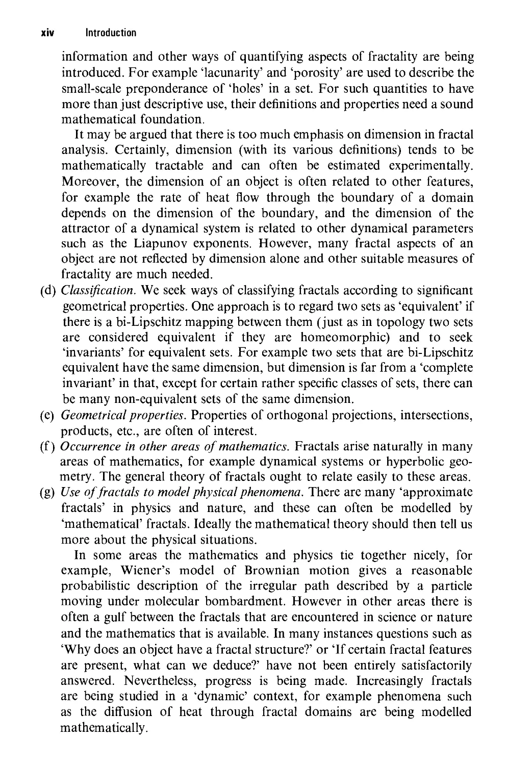
Figure 1.2 Construction of a measure by repeated subdivision. The measure on each
set of $ is divided between its subsets in the hierarchical construction
for each (i{,... ,^), that is the 'mass' n(Xiu_jk) is subdivided between
the subsets ХцI...j,tj,-, A < i < m). We assume that for every sequence
(i[,i2,---) both the diameters of the sets |X;b...,J and their measures
fJ-(X,,...,k) tend to 0 as к —> oo. We write Ek = U,-,,...,,^,,...^ for each к, and
E = D^L0Ek, so that ?is the intersection of a decreasing sequence of closed
non-empty sets, and is therefore closed and non-empty. For А с W we
define
fj,{A) = inf
U,-Vt and F, e S1.
A.20)
It is not hard to show that ц is a measure with support contained in E, such
that fi(Xtlr..j,J is the preassigned value for all {i\,..., 4). Thus if/i is defined
by this 'repeated subdivision' procedure it may be extended to a measure
on?.
For a simple instance of this procedure, let m = 2 and for each к let
Xju^jk comprise the set of 2k closed binary subintervals of [0,1] of length
2~k, nested in the obvious way. Taking fj,(Xily,,jik) = 2~k for each such
interval, A.19) is readily verified and A.20) then defines the restriction of
Lebesgue measure to [0,1].
We say that a property holds for almost all x or almost everywhere (with
respect to a measure /j) if the set for which the property fails has /i-measure 0.

Measures 11
For example, with respect to Lebesgue measure, almost all real numbers are
irrational.
Occasionally we need the following density result, to the effect that almost
all points of a set E are, from the point of view of measure, 'well inside' E. A
point x at which A.21) holds is called a density point of E.
Proposition 1.7
Let fibe a locally finite Borel measure on №. Then, for every ^-measurable set E,
we have that
Итц(ЕПВ(х,г))/ц(В(х,г)) A.21)
r—>0
exists and equals 1 for ^.-almost all x e E and equals Ofor ^.-almost all x?E.
Proof Since this is a local result, we may assume that fj, is a finite measure.
Take с < 1, and define
A = {x e E : fj,(Et~\ B(x, r)) < cfi(B(x, r)) for arbitrarily small r};
we will show that ц(А) = 0. Given e > 0 there exists an open set U D A such
that fj,(U) < fj,(A) + e. Define a class V of balls by
V = {B : fihas centre in A, with В с U and fi(E П В) < сц(В)}.
Then V is a Vitali cover for A, which means that for all x e A and 6 > 0 there is
a ball in V with centre x and radius less than 6. The Vitali covering theorem
asserts that there is a sequence of disjoint balls B[,B2,... in V such that
fj,(A\ U,- Bt) = 0. Then
= ц{А П utBt) + fi{A\Ui Bt)
e).
This is true for all e > 0 so ц(А) < сц(А), implying that fj,(A) = 0. We
conclude that for all с < 1, for /i-almost all x e E we have cfj,(B(x,r))
< (j,(En B(x,r)) < fj,(B(x, r)) for all sufficiently small r. Thus for /i-almost all
x e E the limit A.21) exists and equals 1.
Applying this with ? replaced by IR"\?now gives that the limit A.21) equals
0 for /i-almost all x^E. ?
Sometimes we will work with several measures on the same set. We say that
the measures fi and i/onl are equivalent if there--exist numbers c\, c2 > 0 such
that
A.22)
for all A CX.

12 Mathematical background
Integration with respect to a measure /i on Xis denned using the usual steps.
A simple function f: X —> U is a function of the form
1=1
where сц,..., a^ e U and Ai,..., At are /i-measurable sets, with \Ai the indi-
indicator function of At. We define the integral of the simple function / with
respect to ц as
1=1
Integration of more general functions is defined using approximation by simple
functions. We term /: X —> M. a measurable function if for all с е R the set
{x e X :f(x) < c} is a measurable set (in particular for a Borel measure /i all
continuous functions are measurable). We define the integral of a measurable
f:X^U+U{0} by
f ( f 1
/ fdfj, = supi / gdfj,: g is simple, 0 < g <П
J \ J J
(this value may be infinite). Finally, for a measurable function/: X —> U we
write/+(jc) = max{/(jc),0} and/_(jc) — max{—/(jc),O}, and define
provided both Jf+ d/i and //_ d/i are finite. This happens if / \f\dfi = Jf+ d/i
+ //_ d/i < oo; such functions are called fi-integrable. All the usual properties
of the integral hold, for example J(f+g)dfi — Jfdfi + Jgdfi and J(A/)d/i
= Л //d/i for real A.
For a measurable set A we define the integral of f over A by JAfdfi
Some basic convergence theorems hold, that is conditions on a sequence of
functions fk-X —> M. with lim^oofk{x) =f(x) for almost all x that guarantee
that
lim ffk dM = //dM. A.23)
This is the case if (/^) is a monotonic sequence of non-negative functions
(the monotone convergence theorem), or if fi(X) < oo and for some с we
have \ft(x)\ < с for all к and x e X (the bounded convergence theorem).
The limit A.23) is also valid if there is a function g : X^ U+ U {0} with
Jgdfi < oo and |//t(x)| < g(x) for all к and x (the dominated convergence
theorem).

Weak convergence of measures 13
Closely related is Fatou's lemma, that for any sequence (/t) of measurable
functions
/liminf/fcd/i < liminf I fkd(i.
k—>oc /:—>oc J
We will often wish to interchange the order of integration in a double
integral, and this is generally permitted by versions of Fubini's theorem. If (i
and v are locally finite measures on subsets of Euclidean space then
Д Jf(x,y)d(i(x)^j dv{y) = Д j
for continuous/: X x Y —> IR+ U {0}. (This also holds if/is a Borel function,
that is if {(x,y) :f(x,y) < c} is a Borel subset of X x Y for all real numbers c.)
As usual, integration is denoted in a variety of ways, such as Jfd(i, // or
Jf(x)d(i(x) depending on the emphasis required. When (i is «-dimensional
Lebesgue measure C", we usually write //dx or //(jc)dx in place of JfdC(x).
We write Ll((i) for the vector space of /i-integrable functions, that is
functions/: X —> IR with J\f\d(i < oo, and L'(IR) for the Lebesgue integrable
functions, that is/: IR -> IR with / \f\dC < oo.
*1.4 Weak convergence of measures
We collect together here some properties of weak convergence of measures that
will be needed mainly in Chapter 9. This section may be deferred until the pro-
properties are needed. Alternatively, the proofs may be omitted on a first reading
with little loss of feeling for the subject.
Let (i,(n,(i2,... be locally finite measures on IR". We say that the sequence
/ы=1 converges weakly to (i if
lim fd(ik— fd(i A.24)
for every/e Co(IR") (i.e. for every continuous/of compact support), and we
denote this by (ik —> (i or lim^oo/it = (i.
For a simple example on IR, if (ik{A) = \ {#г G Z : i/k e A}, so that (ik is an
aggregate of point masses of l/k, then (ik —> jC1.
Although weak convergence does not imply that (ik(A) —> /i(y4) for every set
A, some useful inequalities hold for open or compact sets.
Lemma 1.8
Let (/i,t)b=i be a sequence of locally finite measures on IR" with (ik —> /i. 77геи if A
is compact
A.25)

14 Mathematical background
and if U is open
A.26)
fc-юс
Proof Writing A°6 — {x : dist(jc, A) < 6} for the open 6-neighbourhood of
a compact set A, we have that A°6 \ A as <5 \ 0 so fi(A^) ^ fi(A) by
A.13). Thus, given e > 0 we may take 6 > 0 such that fi(A°6) < ц(А) + е.
Let fe C0{Un) be any function satisfying 0 <f{x) < 1 with f(x) = 1 for
jcG^ and/(jc) = 0 for x<?A°s (f(x)=max{0,\-6~ldist(x,A)} will do).
Then
fj,(A) + e > n{A°g) > / fdfi = lim / fdfit > Iimsup/i^(y4);
J k—>oo J i—>oo
since this is true for arbitrarily small e, A.25) follows. Inequality A.26) is
similar using A.12). ?
The importance of weak convergence lies in the following compactness
property which allows us to extract weakly convergent subsequences from
general sequences of measures.
Proposition 1.9
Let fii, fj,2, ¦ ¦ ¦ be locally finite measures on U" with supkfJ-k{A) < oo for all
bounded sets A. Then (fik)kLi has a weakly convergent subsequence.
* Proof We note that C0(M") has a countable dense subset of functions (Л)ь=1
under the norm \\/\\ж = max{|/(x)| : x e U11}. (For example, setting gm(x) =
max{0,m — \x\}, the set of functions {pgm ¦ P is a polynomial with rational
coefficients and meZ+} is easily seen to be countable and dense using the
Weierstrass approximation theorem.) A diagonal argument, using induction on
k, gives sequences (/ijt,iJi w^h Мо,< = M< ancl with (/i/t,0?i a subsequence of
(Att-u)fci f°r ^ = 1,2,..., such that Jf^dfikj -> at as i -> oo for some ak € U.
Thus, jfkdnii —> a,t as / —> oo for all fe. Since the (/*) are dense it follows that
for all/G СО'AЙИ)
-«(/) A-27)
for some a(f) e U. Moreover, a is linear, that is a(f+g) — a(f) + a(g) and
a(Xf) = Xa(f), and bounded, that is \a(f)\ < (sup/t/it(-4))||/l!oo if spt/c A.
The Riesz representation theorem states that under these conditions there
is a locally finite measure /i such that a(f) = Jfdfi for all/G Cq(U"); thus by
A.27) fly —> /i, with (/ii,;)Si a subsequence of (/i/fc)it°=i- ^
It is sometimes convenient to express weak convergence of measures in terms
of convergence with respect to metrics. For R > 0 we define d^ on the set of

Weak convergence of measures 15
locally finite measures on IR" by
JJ | A.28)
where here 1лрл denotes the set of Lipschitz functions/: W —> [0,oo) with
spt/c 5@, R) and with Lip/<1 (that is with \f(x) -f(y)\ < \x-y\
for x,y € W). Then for each R we have that dR is a pseudo-metric (that is,
it is non-negative, symmetric and satisfies the triangle inequality). However,
dR(fi, v) = 0 need not imply /i = v. Nevertheless, dR is a metric on the set of
locally finite measures with support contained in the open ball B°@,R), see
Exercise 1.10. Clearly, if Ri < R2 then dRl(n,v) < dRl(n,v).
Lemma 1.10
Let fi\, fi2, ¦ ¦ ¦ and ц be measures on W. Then fik —> /i weakly if and only if
dR(fik,fi)-*0forallR>0.
* Proof Suppose first that dR(nk,v) ~h 0 f°r some R. By passing to a sub-
subsequence and renumbering, there exists e > 0 and functions/*; e Lip^ such that
ffkdn/c - Jfkdfi\ >e for all к. By the Arzela-Ascoli theorem there is a
subsequence of (fk), which by renumbering we may again take to be the whole
sequence, such that J\ —> /uniformly for some /which must be in Lip^, using
that the fk vanish outside B°@, R). Then
- Jfdn - (JfdHk ~ Jfk dw) + Ufk d№ - J fk
As к —> ос, the first term of this sum tends to 0 (since fk —>/uniformly and
(fik(B@, R)))^=l is bounded by A.25)), the third term tends to 0 (as/ft -^ f
uniformly), but the absolute value of the middle term is bounded below by
e, so \ik ¦/* [i weakly.
For the converse suppose that dR(fik, A*) —* 0 for all R > 0. Let/: W —> U be
continuous, with spt/c B(Q,R). Then given e > 0, there exists a Lipschitz
g : W —> U with spt^ с B(Q,R) that approximates /in the sense that \f(x)-
g(x)\ < e for all x € W. (Using the mean value theorem, g can be any
sufficiently close approximation to /that is continuously diiferentiable.) Then
using the triangle inequality and that g has Lipschitz positive and negative parts
j fdfi < J \f-g\d^ + \J gdfik- J gdn+ J \g-f\dn
< €fik(B@, R)) + 2{Lipg)dR{tik, fi) + ец(В@, R))
<3en(B(Q,R))+2(Upg)c
if к is sufficiently large, using A.25). Hence fj,k —> ц weakly. П

16 Mathematical background
The other property we need is that the dR are separable, that is there exists a
countable set of measures that is dense in these pseudo-metrics.
Lemma 1.11
There is a countable set of locally finite measures щ, цг, • • • on U" such that, for
every locally finite measure fi on W and all R, rj > 0, there exists к such that
dR(n,Hk) < V-
* Proof It is enough to show that such a set of measures exists for each
R = 1,2,... and use that a countable union of countable sets is countable. For
j = 1,2,... let Суд,... Cj<mj be the (half-open) binary cubes of side-lengths 2~j
which meet B@,R), and let 8jti be a unit point mass at the centre of Q,. Let
(wOfcli be an enumeration of the set of all measures of the form J27=i 4jj,pfy,u
where for each j and i the sequence (^,.1,^,2,.. •) is an enumeration of the
non-negative rational numbers.
Given fi, let Vj — Yl7=i KCj^fyf' by choosing у large enough we may ensure
that dR(n,Vj) <\r}. Now choose цк = Y,7i\ Ф,<А<' so that dR(vh\ik) <\r],
which may be achieved by taking qJtip sufficiently close to n(Cjj) for each /.
Then dR(n,nk) < rj, as required. П
1.5 Notes and references
Most of the material in this chapter may be found in much more detail in any
basic text on measure theory, for example Doob A994) or Kingman and
Taylor A966). The treatments in Falconer A985) and Mattila A995a) are
specifically directed towards fractal geometry, and also include more details of
Vitali covering results and density properties.
Exercises
1.1 Let/: [0,1] -» [0,1] be a differentiable function. Show that the limit
exists, where bk = supo<x<i|^/*(^)| and/* is the feth iterate of/. (Hint: use the
chain rule to show that (bk) is submultiplicative.)
1.2 Use A.4) to prove the arithmetic-geometric mean inequality: that (П/=1 xif^m
— iEti x' where x\,... ,xm > 0. (Hint: -log* is convex.)
1.3 Let Q = (q\,q2,--.) be an enumeration of the rational numbers. For А С U
define ц(А) = J2qi€A 2 '¦ Verify that /i is a measure with all subsets of IR
measurable. Show that spt/i = IR, even though /i(IR\Q) = 0, that is /i is
'concentrated' on Q.
1.4 Let fj, be a measure on IR" such that for all x e IR" there is a ball B(x,r) with
ц(В(х,г)) < 00. Show that /j, is locally finite.
1.5 Verify A.15) and A.16) from the definition of a locally finite (Borel regular)
measure and Proposition 1.6.

Exercises 17
1.6 For each k, let {X,b...,t : ц. = 1 or 2} be the set of2fcfe-th level intervals of length Ъ~к
that occur in the usual construction of the middle-third Cantor set E, nested in the
usual way. Verify that setting д(Х„ .. ,J = 2~k and using A.20) leads to a measure
on?. Show that the same is true setting n{Xiw..A) = A/3)щB/3) whereni andn2
are the number of occurrences of the digits 1 and 2 respectively in (i[,..., ik).
1.7 Let /: [0,1] -> R+ be continuous, and define ц on [0,1] by ц{А) = JAf(x)dx.
Show that fi is equivalent to C, where С is Lebesgue measure. (Note that
0 < ci < J[x) < c2 for all x ? [0,1] for some cuc2.)
1.8 Let /i,t be the measure on U that assigns unit mass to the point 1 + \jk. Find the
weak limit /i of the sequence of measures (цк)- Does ^([0,1]) —* /i([0,1])?
1.9 Show that if ^ —* M and if A is a bounded set with д(<ЗЛ) = 0, where dA is the
boundary of A, then Цк{А) —* д(Л)-
1.10 Verify that dn defined by A.28) is a pseudo-metric on the locally finite measures
and a metric on the measures with support in B°@,R).

Chapter 2 Review of fractal
geometry
In this chapter we review some of the basic ideas of fractal geometry that will
crop up frequently throughout this book. We first discuss fractal dimensions,
and in particular the definitions and properties of Hausdorff, packing and box-
counting dimensions. We then review iterated function systems which provide
a convenient way of representing many fractals and fractal measures.
These basic definitions, properties and notation are collected together here
for convenient reference; almost all of this material is discussed in much more
detail and with full proofs in FG.
2.1 Review of dimensions
The notion of 'fractal dimension' of a set is central to nearly all fractal
mathematics. We shall usually be interested in the dimensions of subsets of W,
though essentially the same definitions hold in general metric spaces.
Most definitions of dimension depend on a 'measurement at scale f of a set
E, which quantifies the irregularity of the set when viewed at that scale. The
dimension is then usually defined in terms of the power law behaviour of these
measurements as r \ 0.
We shall mainly be concerned with the Hausdorff, packing and box-
counting dimensions of sets; these are by far the most common definitions of
dimension in use, although a variety of other definitions have been proposed. It
should be emphasised that the value of the dimension of a set may vary
according to the definition used, although the usual definitions often give the
same values for 'reasonably regular' sets. Thus it is important to be clear about
the definition of dimension in use in any particular context.
Box-counting dimension
Box-counting dimension (also variously termed entropy dimension, capacity
dimension, logarithmic density, etc.) is conceptually the simplest dimension in
use, see FG, Section 3.1. For E a non-empty bounded subset of W let Nr(E) be
the smallest number of sets of diameter r that can cover E. (Recall that the
diameter of a set U is defined as \U\ = sup{|x-y\ : x,y 6 U}, that is the
19

20 Review of fractal geometry
greatest distance apart of any pair of points in U.) The lower and upper box-
counting (or box) dimensions of E are defined as
l BЛ)
-logr
and
log Nr{E)
dimB? - limsup b 'ry J B.2)
respectively. If these are equal we refer to the common value as the box-
counting dimension or box dimension of E
8^ B.3)
Thus the least number of sets of diameter r which can cover E is roughly of
order r~s where s = dime!?.
There are a number of equivalent forms of these definitions which are often
useful. The value of the limits B.1)—B.3) remain unaltered if Nr(E) is taken to
be any of the following:
(i) the smallest number of sets of diameter r that cover E,
(ii) the smallest number of closed balls of radius r that can cover E,
(iii) the smallest number of cubes of side r that cover E,
(iv) the largest number of disjoint balls of radius r with centres in E,
(v) the number of r-mesh cubes that intersect E, hence the name 'box-
counting'.
(An r-mesh cube is a cube of the form [m\r, (m\ + l)r) x ¦ • • x [mnr, (mn + 1))
where nt\,...,mn are integers).
The equivalence of these forms of the definition follows on comparing the
values of Nr(E) in each case, see FG, Equivalent definitions 3.1.
An equivalent definition of box dimension of a rather different nature
involves the и-dimensional volume of the r-neighbourhood or r-parallel body Er
of E, given by
Er = {x e W : \x - y\ < r for some у € E}.
Then for E с W
dimB? = n - lim sup —-—-—- B.4)
B.5)
logr
and
dimB? = и - lim1Ogr(J?r) B.6)
r^O logr

Review of dimensions 21
if this limit exists, where C" is и-dimensional volume or и-dimensional
Lebesgue measure. In the context of this definition, box dimension is
sometimes referred to as Minkowski dimension.
Hausdorff and packing dimensions
Hausdorff and packing dimensions are more sophisticated than box dimen-
dimensions, being defined in terms of measures. A finite or countable collection
of subsets {[/,•} of W is called a 6-cover of a set E С W if |C/,-| < 6 for all
i and E С U^! Ut. Let ? be a subset of U" and s > 0. For all 6 > 0 we
define
f 1
Щ(Е) = Mi ^ Iui\s ¦ {ui}is a <5-cover ofE\. B.7)
As 6 increases, the class of 5-covers of E is reduced, so this infimum increases
and approaches a limit as ё \ 0. Thus we define
Н\Е) = \\тЩ{Е). B.8)
This limit exists, perhaps as 0 or oo, for all E С W. We term HS{E) the s-dimen-
sional Hausdorff measure of E.
It may be shown that HS(E) is a Borel regular measure on W (see A.14)), so
in particular
(
1=1 / 1=1
for all sets E\,E2,. ¦., with equality if the Et are disjoint Borel sets.
Hausdorff measures generalise Lebesgue measures, so that Hl (E) gives the
'length' of a set or curve E, and H2(E) gives the (normalised) 'area' of a region
or surface, etc. In general, C" = 2~nvnHn, where vn is the volume of the n-di-
mensional unit ball.
We often wish to consider the Hausdorff measure of the image of a set under
a Lipschitz mapping. For a Lipschitz/: E—> U" such that
\f(x)~f(y)\<c\x-y\ for all x,y€E, B.10)
we have
Hs(f(E))<csHs{E). B.11)
Similarily, if/: E —> IRm is bi-Lipschitz, so that for some cb c2 > 0
ci|x - j>| < |/(x) -/(j)| < C2| x - y\ for all x,y € E,
then
ns(f(E)) < c\ U\E). B.12)

22
Review of fractal geometry
A special case of this is when / is a similarity transformation of ratio r, so
\f(x) —f(y)\ = r\x - y\ for all x,y € E, in which case
This is the scaling property of Hausdorif measures, which generalises the
familiar scaling properties of length, area, volume, etc.
It is easy to show from B.7) and B.8) that for all sets E С U" there is a
number dim^E, called the Hausdorff dimension of E, such that HS(E) = oo if
s < dimH? and W{E) = 0 if s > dimH?. Thus
dimH? = inf{,s: HS(E) = 0} = sup{.?: HS(E) = oo},
so that the Hausdorif dimension of a set E may be thought of as the number s
at which HS(E) 'jumps' from oo to 0, see Figure 2.1. When s = dimH-E the
measure H"(E) can be zero or infinite, but in the nicest situation (which occurs
in many familiar examples) 0<Hs(?')<oo, in which case E is sometimes
termed an s-set.
The definition of packing dimension parallels that of Hausdorif dimen-
dimension. Here we define a ё-packing of E с W to be a finite or countable collection
of disjoint balls {Bt} of radii at most 6 and with centres in E. For 6 > 0 we
define
Vsg(E) = sup
: {Bt} is ай-packing of?
J
<=i
о
Figure 2.1 The Hausdorff dimension of ?7 is the number .s at which HS(E) jumps from
oo to 0

Review of dimensions 23
Then VSS(E) decreases as 6 increases, so we may take the limit
Unfortunately Vs0 is not a measure (it need not be countable subadditive); to
overcome this difficulty we define
which is a Borel measure on U", called the s-dimensionalpacking measure of E.
Again Vх, V2, give the length, area, etc. of smooth sets, but for fractals Hs and
Vs can be very different measures.
Packing measures behave in the same way as Hausdorff measures in respect
of Lipschitz mappings, and B.11)-B.13) remain valid with Hs replaced by
Vs. It may be shown that HS(A) < VS(A) for all sets A.
As for Hausdorff dimension, there is a number dimpij, called the packing
dimension of E, such that PS{E) =- oo for s < dimP? and Vs(E) =0 for
s > dinip?. Thus
dimP? = inf{s : V{E) = 0} = sup{s : Vs{E) = oo}.
It is sometimes convenient to express packing dimension in terms of upper
box dimension. For E с W it is the case that
¦ \ — м 1
dimp? = inf< sup diiriB?, : E с I IE, >
I ¦ ^"^ I
I ' <=i )
(the infimum is over all countable covers {?,} of E), see FG, Proposition 3.6.
Basic properties of dimensions
We will have frequent recourse to certain basic properties of dimensions. The
following properties hold with 'dim' denoting any of Hausdorff, packing, lower
box or upper box dimension.
Monotonicity. If E\ С E2 then dim^ < dim?2-
Finite sets. If E is finite then dim? = 0.
Open sets. If E is a (non-empty) open subset of W then dim? = n.
Smooth manifolds. If ? is a smooth m-dimensional manifold in Mn then
dim? = m.
Lipschitz mappings. If /: ?—> Um is Lipschitz then dim/(?) < dim?. (For
Hausdorff and packing dimensions this follows from B.11) and its packing
measure analogue, for box dimensions it may be deduced from the
definitions.) Note in particular that this is true if ? с X for an open set X

24 Review of fractal geometry
on which/:X—> W is differentiable with bounded derivative, using the
mean value theorem.
Bi-Lipschitz invariance. If/: E—* f{E) is bi-Lipschitz then d\mf(E) = dimE.
Geometric invariance. If / is a similarity or affine transformation then
dim/(?') = dimis (this is a special case of bi-Lipschitz invariance).
Hausdorff, packing and upper box dimensions are finitely stable, that is
dim uf=1 Ei = тахкк^ dim Et for any finite collection of sets {E\,..., Ek}.
However lower box dimension is not finitely stable.
Hausdorff and packing dimensions are countably stable, that is
dim ug, Ei = sup1<1<0O dim?,. (This may be deduced from the count-
countable subadditivity of Hausdorff and packing measures). Countable stability is
one of the main advantages of these dimensions over box dimensions;
in particular it implies that countable sets have Hausdorff and packing
dimensions zero.
We also recall that dimBi? — dimBi? and dimBE = dimBE where E is the
closure of E. In fact this is a disadvantage of box dimensions, since we often
wish to study a fractal E that is dense in an open region of W and which
therefore has full box dimension n.
There are some basic inequalities between these dimensions. For any non-
nonempty set E
dimH? < dimpi? < dimB? and dim^ < dimBi? < dimB,E B14)
(for the inequalities involving box dimensions we assume E is non-empty and
bounded). In practice, most definitions of dimension take values between the
Hausdorff and upper box dimensions, so if it can be shown that
dimH E = dimB E then all the normal definitions of dimension take this
common value.
Calculating dimensions
We frequently wish to estimate the dimensions of sets; usually it is harder to
get lower estimates than upper estimates. There are various approaches to
finding the dimension of a set, but most methods involve studying a suitable
measure supported by the set (other methods can usually be reduced to this
process). One basic but very useful technique is termed the 'mass distribution
principle'.
Proposition 2.1 (mass distribution principle)
Let ECU." and let /i be a finite measure with ц(Е) > О. Suppose that there are
numbers s > 0, с > 0 and 6q > 0 such that
»(U)<c\U\s

Review of dimensions 25
for all sets U with \U\<S0. Then HS(E) > ц{Е)/с and
s < dimn^ < dim^E < di
Proof We recall the very simple proof from FG, Principle 4.2. If {C//} is any
cover of E by sets of diameter at most 80 then
so that fi(E) < с Щ(Е) for 6 < 60. The result follows on letting 6^0. П
Developing this idea we can estimate the HausdorflF and packing measures
and dimensions of a set E if we can find a measure рь satisfying certain 'local
density' conditions on E. Observe the (near) symmetry between HausdorflF
and packing measures and lower and upper estimates in the following
propositions.
Proposition 2.2
Let E с U" be a Borel set, let fi be a finite Borel measure on U" and 0 < с < oo.
(a) Iflimsupr^otJ,{B(x,r))/rs < с for all x ? E then HS{E) > fJ,{E)/c.
{b) Iflimsupr^ov{B{x,r))/rs > с for all x e E then HS{E) < 2'ц{Е)/с.
(с) //liminf^oMfi(*,'-))/'-s < с far allxGE then VS{E) > 2*ц{Е)/с.
{d) у\{тМг^оКв(х,г))/г* > c for all x & E then VS(E) < 2>(?)/c.
Proof Parts (a) and (b) are proved in FG, Proposition 4.9; part (a) requires
little more than the definition of HausdorflF measure, whilst (b) requires the
Vitali covering lemma. The packing measure analogues are proved in a very
similar way, with (d) following easily from the definition of packing measure
and with (c) requiring a covering lemma. ?
We shall more often be interested in the dimension rather than the
measure of sets, so we give a version of Proposition 2.2 for dimensions.
This may be conveniently expressed in terms of local dimensions of mea-
measures. We define the lower and upper local dimension s of fi at x € W (also
called the pointwise dimension or Holder exponent) by
B.15)
log Г
)!. B.16)
These local dimensions express the power law behaviour of fi(B(x, r)) for small
r. Note that dim\nc fi(x) = dimioc/i(x) = oo if ц{В(х, г)) — 0 for some r > 0.

26 Review of fractal geometry
Proposition 2.3
Let E с U" be a Borel set and let \i be a finite measure.
(a) If dim\nrjj,(x) > s for all x e E and ц{Е) > 0 then drniH-E > s.
(b) If dimloc fi(x) < s for all x e E then dim^E < s.
(c) If'dimiocfi(x) > s for all x e E and ц{Е) > 0 then dimpis > s.
(d) If dim ioc/-*(*) < s for all x G E then dimp^ < s.
Proof This follows from Proposition 2.2 noting that the hypothesis in (a)
implies that \imsupr_^ofi(B(x,r))/rs-e = 0 for all e > 0, and similarly for (b),
(c) and (d). ?
We remark that in (a) and (c) of Proposition 2.3 it is enough for the
hypothesis to hold for л: in a subset of E of positive /i-measure.
We record the following partial converses to these results which stipulate
that a set of given dimension carries a measure with corresponding local
dimensions.
Proposition 2.4
Let E С U" be a non-empty Borel set.
(a) IfdimftE > s there exists ц with 0 < fi(E) < oo and dimioc^(x) > s for all
xeE.
(b) IfdimftE < s there exists fj, with 0 < fi(E) < oo and dimioc^(x) < s for all
xeE.
(c) If dimpE > s there exists /i with 0 < fi(E) < oo and dimioc/i(A) > s for fi-
almost all x.
(d) If dimpE < s there exists fj, with 0 < fi(E) < oo and dimioc/i(x) < s for all
x G E.
Proof Part (a) is FG, Corollary 4.12 ('Frostman's Lemma') expressed in local
dimension form. Parts (b), (c) and (d) require similar delicate arguments, and
the technical details may be found in the literature. ?
Note that, in Propositions 2.3 and 2.4, it is the lower local dimensions that
relate to the Hausdorff dimension of a set, and the upper local dimensions to
the packing dimension of a set.
Propositions 2.3(a) and 2.4(a) may be 'integrated' to get potential theoretic
criteria which are often useful when calculating Hausdorff dimensions and
measures. For s>0we define the s-energy of a measure /i on U" by
= J J

Review of dimensions 27
Proposition 2.5
Let E С R".
(a) If there is a finite measure ц on E with Is(n) < oo then 7is(E) = oo and
divcinE > s.
(b) If E is a Borel set with HS(E) > 0 then there exists a finite measure ц on E
with It(fi) < oo for all t < s.
Proof See FG, Theroem 4.13. ?
Densities and rectifiability
Densities have played a major role in the development of geometric measure
theory. Although it is possible to define the densities of any finite measure, we
restrict attention here to densities of an s-set, that is a Borel set E с R" with
0 < HS(E) < oo, where s — din^is. The lower and upper (s-dimensional)
densities of E at x are given by
Ds(x) =Ds(E,x)= lim inf Hs{E П B(x, r))/BrY B.17)
r—>0
and
Ds(x) =Ds(E,x) =\imsupHs{EnB(x,r))/{2r)s B.18)
(we write Ds(x) rather than Ds(E,x) when the set E under consideration is
clear). When Ds(E,x) =Ds(E,x) we say that the density Ds(E,x) of E at x
exists and equals this common value. (It is possible to define the densities of a
more general measure ц by replacing 7is by ц in B.17) and B.18).)
We remark that if X is an open subset of R and/: X —> R is a C1 mapping,
then for E с R we have
Ds(E,x)=D\f(E)J{x)) and Ds(E,x) = Ds(f(E),f(x)) B.19)
for all x where/'(x) ф 0. Intuitivily this is because/may be regarded as a local
similarity of ratio |/'(x)| near x, scaling the diameter of B(x,r) by a factor
|/'(x)| and the W-'-measure of B(x,r) by a factor \f'(x)\s, using the scaling
property B.13), see Exercise 2.6. In fact B.19) also holds for a differentiable
conformal mapping/: X —> R" where Ici". (The mapping/is conformal if
f'(x), regarded as a linear transformation on R", is a similarity transformation
for all x G R".)
The classical result on densities is the Lebesgue density theorem. This states
that if E is a Lebesgue measurable subset of R" then for ?"-almost all x
if ill; (z2°)
11 ACL

28
Review of fractal geometry
this is a special case of Proposition 1.7 taking
densities this is
as ?". Expressed in terms of
B.21)
for W"-almost all x, since C" = 2"nvnHn, where vn is the volume of the
и-dimensional unit ball. It is natural to ask to what extent analogues of B.21)
hold for general values of s.
For ?cK"an s-set, it is easy to show that Ds(E,x) = 0 for W5-almost all
x?E. Moreover, 2~s < Ds(E,x) < 1 for almost allx € E, see FG, Proposition
5.1. A rather deeper property is that unless s is an integer Ds(E,x) < Ds(E,x)
for Ws-almost all x G E. We will prove this in Corollary 9.8 using tangent
measures; a special case is given in FG, Proposition 5.3. In some ways, this
non-existence of densities is a reflection of fractality.
The situation when s is an integer is more involved. In this case an s-set
?cfi" may be decomposed as E = ?r U Ei, where ?r is regular, that is, with
D*(ER,x) = Ds(ER,x) - 1 for Hs-a\most all x G EK, and EY is irregular, with
Ds(Ei, x) < cDs(E\,x) for ?P-almost all x G E\, where с < 1 depends only on n
and s, see Figure 2.2.
Regular and irregular sets have geometrical characterisations in terms of
rectifiability. If E is regular then E is rectifiable, which means that almost all of
E may be covered by a countable collection of Lipschitz pieces Е\,Ег,... such
that HS{E\\J?LX Et) = 0. (A set Eo is a Lipschitz piece if Eo =f{A) where
Figure 2.2 Decomposition of a 1-set E into a regular part .Er and an irregular part E\

Review of iterated function systems 29
А С W and/: A —> U" is a Lipschitz mapping.) Thus a rectifiable set is built
up from a countable number of Lipschitz pieces which look like subsets of
curves, surfaces or classical ^-dimensional sets.
On the other hand, if E is irregular then E is totally unrectifiable. This means
that Hs(EnE0) = 0 for every Lipschitz piece Eo, so that E has negligible
intersection with rectifiable ^-dimensional sets. Thus, irregular s-sets might be
considered to be fractal and the regular, or rectifiable, sets non-fractal, with
non-existence of the density being a characteristic fractal property for sets of
integer dimension. The relationship between the metric or density properties of
i-sets and the geometric or rectifiability structure of sets is difficult, and has
been central in the development of geometric measure theory; see FG, Chapter
5 for more details.
2.2 Review of iterated function systems
Iterated function systems (or schemes) provide a very convenient way of
representing and reconstructing many fractals that in some way are made up of
small images of themselves. We work in a non-empty closed subset X of W,
often X = U". An iterated function system (IFS) consists of a family of
contractions {F\,..., Fm} on X, where m > 2. Thus for i = 1,..., m we have
Ft¦: X -> X and
\F,{x) - Fi(y)\ < n\x - y\ for all x,y?X, B.22)
where r,- < 1. We write
''max = max r, B.23)
1 <i<m
SO rmax < 1.
The fundamental property of an IFS is that it determines a unique non-
nonempty compact set E satisfying E = U^F^E); these sets are frequently
fractals. For example, with F\, F2 : U —> U given by
F,(x)=l* and F2{x)=\x + l B.24)
the set satisfying E = F\ (E) U F2 (E) is the middle-third Cantor set, see Figure 2.3.
To establish this fundamental property, we work with the class S of non-
nonempty compact subsets of X. We may define a metric or distance d on S by
d(A, B) = inf{<5 :AcBs and В с As} B.25)
where As is the ^-neighbourhood of A. Thus d satisfies the three requirements
for a metric ((i) d(A, B) > 0 with equality if and only if A = B, (ii)
d(A,B)=d(B,A), (iii) d{A,B) < d{A, C) + d(C, B) for all A,B,C), and is
termed the Hausdorff metric on S.
It may be shown that d is a complete metric on S, that is every Cauchy
sequence of sets in S is convergent to a set in iS. We use this fact to give the slick

30 Review of fractal geometry
о
¦¦ it it •¦ ¦¦ ¦¦ ti ¦¦ ¦¦ ¦¦ ¦¦ •¦ ¦¦ ¦¦ ¦• ¦¦
E
F2(E)
Figure 2.3 The middle-third Cantor set is made up of two scale ^ copies of itself; thus
E = F^E) UF2(E) where Fi and F2 are given by B.24)
'contraction mapping theorem' proof of the fundamental property of IFSs; an
alternative proof is given in FG, Theorem 9.1.
Theorem 2.6
Let {F[,..., Fm} be an IFS on X с U". Then there exists a unique, non-empty
compact set E с X that satisfies
m
E={jF,(E). B.26)
Moreover, defining a transformation F: S —> S by
m
F(A)=\jF,(A) B.27)
for A 6 S, we have that for all A e S
Fk{A) -> E
in the metric das к —> oo, where Fk is the k-th iterate ofF. Furthermore, if A G S
is such that Ft{A) с A for all i, then
ОС
E=f)Fk{A). B.28)
Proof If A, Be S then
d(F(A),F(B)) = d[
<
\<i<m
using the definition of the metric d and noting that if the ^-neighbourhood
{Fi(A)N contains Ft(B) for all i then (u™ xFi{A)N contains U™ xFt(B) and vice
versa. By B.22)
d(F(A),F(B)) < (max rAd(A,B). B.29)
\<i<m

Review of iterated function systems 31
Since maxi<,<mr, < 1, the mapping Fis a contraction on the complete metric
space {S,d). By Banach's contraction mapping theorem Fhas a unique fixed
point, that is to say, there is a unique set E ? S such that F(E) — E, which is
B.26), and moreover Fk(A) —> E as к —> oo. In particular, if Ft (А) С A for all i
then F(A) с A, so that Fk(A) is a decreasing sequence of non-empty compact
sets containing E with intersection ^kxL0Fk{A) which must equal E. ?
The unique non-empty compact set E satisfying B.26) is called the attractor
or invariant set of the IFS {F\,..., Fm}. The IFS may be thought of as defining
or representing the set E.
There are two main problems that arise in connection with IFSs. The first is,
given a fractal E, to find an IFS with attractor E or, at least, a close
approximation to E. In many cases, including many familiar self-similar sets, a
suitable IFS with a small number of contractions can be written down by
inspection, for example B.24) for the middle-third Cantor set. In such instances
the IFS provides a very efficient way of representing or 'coding' the set. This
has led to the more general problem of fractal image compression: how to find
a relatively small family of contractions that represent any given set or picture,
see FG, Section 9.5.
The inverse problem is to reconstruct the attractor ? of a given IFS.
Computationally this is very easy, since it follows by iterating B.29) that
d(Fk(A),E) < (max rt)kd(A,E) B.30)
1 <i<m
for every A € S. Thus Fk(A) converges to E at a geometric rate, so plotting
Fk(A) — U/tF,-[ о F,2 о ¦ • • о Fik [A) for a suitable к gives an approximation to E
(the union is over the set Ik of all /c-term sequences {i\,h,--.ik) with
ij € {1,2,... ,m}). These sets Fk(A) are sometimes called pre-fractals for E, see
Figures 2.4 and 2.5 for examples. An alternative, but often effective, way of
reconstructing E is to take any initial point xq, and select a sequence F,-,, F,-2,...
independently at random from {F\, ...,Fm}, say with equal probability. Then
the points defined by
xk = Fik(xk_l) for к =1,2,... B.31)
are indistinguishably close to E for large enough k, and also appear randomly
distributed across E. A plot of the sequence (xk) starting, say, with к = 100,
may give a good impression of E. In some instances better results will be
obtained by weighting the probabilities of choosing the F,. The reason for the
name 'iterated function system' should be obvious from these reconstruction
procedures.
An IFS provides a natural way of coding the attractor E and the
components of the pre-fractals for E, analogous to the way in which the
points of the middle-third Cantor set may be identified with the numbers whose
base 3 expansions contain only the digits 0 and 2. Let {F[,... ,Fm} be an IFS

32 Review of fractal geometry
Figure 2.4 The usual sequence of pre-fractals in the construction of the Sierpinski
triangle, with Ek = Fk(A) where A is an equilateral triangle
with attractor E. For к = 0,1,2,... we define Д to be the set of all /c-term
sequences of integers selected from {1,2,..., m}, that is
Ik = {(iuh,.--,ik): \<ij<m}; B.32)
we regard /o as just containing the empty sequence. We often abbreviate a
sequence of Д by
i=(il,i2,...,ik)- B.33)
We write
B.34)
k=0
for the set of all such finite sequences, and 1Ж for the corresponding set of
infinite sequences, so
I00 = {(iui2,...):l<iJ<m}. B.35)
It is convenient to write i, j for the sequence defined by juxtaposition of i and/
In particular, with i = (i{,..., г'^), we have i, i — (i[,..., 4, i).
Let A e S be such that Ft(A) с A for all i, so that F(A) с A. From B.28) E
is the intersection of the decreasing sequence of sets
= \jFho-..oFik(A),
B.36)

Review of iterated function systems 33
(a)
F(A)
F2(A)
Figure 2.5 An IFS consisting of three affine transformations {^1,^2,^3} which map
the square A onto the rectangles in (a) in the obvious way. The convergence of the pre-
fractals Fk(A) to E is apparent in (b)

34
Review of fractal geometry
with the union over (гь...,4) E 4. Moreover, for all (i\,...,ik) we have
Fh о • • ¦ о Fik (А) С Fh о ¦ ¦ ¦ о Fik_x {A) and also that |F,- о • • • о Fik (A) | < rmax
Fho---o F/t_, {A)\. Thus for all (i,, i2, ...)?/Mwe have |F,-, о ¦ ¦ • о Fk(A)\ -> 0
as /с —> oo with
B.37)
the single point of intersection of this decreasing sequence of sets. Since every
point of E is in such an intersection for at least one sequence (iu i2,...) ? Ix,
„*,...}¦ B-38)
We conclude that E may be constructed using the hierarchy of sets
Fj, о ¦ ¦ • о Fik{A) for (г'ь ..., ik) ? /, see Figure 2.6; this is analogous to the
usual construction of the middle-third Cantor set.
This coding of the components Fh о ¦ ¦ ¦ о Fik(A) and of points xiuh is very
useful indeed in analysis of attractors of IFSs. For convenience we shall write
Ai = Ail_ik=Fito...oFik(A) B.39)
for i = (i\,..., ik) e / and А с X.
In the simplest situation the sets F\ [A),...,Fm(A) may be mutually disjoint,
in which case the unions B.36) will be disjoint and each point of E will have a
Figure 2.6 Notation for iterated function systems. The contractions Fi and F2 map
the large ellipse A onto the regions Fi(A) and F2(A) respectively. The sets
Fk(A) = UFj, о • • • о Fik(A) decrease to the IFS attractor E

Review of iterated function systems
35
unique representation as x,-b,-2i.... In fact, if this happens then Fi(E),... ,Fm(E)
are mutually disjoint, since E с A for any A with F(A) с A. When the union
E = \j^Fi(E) is disjoint we say that the IFS {Fh ... Fm) satisfies the strong
separation condition. This is the case with the middle-third Cantor set IFS
B.24) and with other IFSs with a totally disconnected attractor. However,
strong separation is rather too strong for many purposes, and we often work
with a weaker separation condition. An IFS {F\, ...,Fm} satisfies the open set
condition (OSC) if there exists a non-empty bounded open set U с X such that
(jF,(U) С U
B.40)
with this union disjoint. The OSC is easily verified for sets such as the von
Koch curve, see Figure 2.7, and the Sierpinski carpet.
In the particularly nice situation when Fi(X),...,Fm(X) are mutually
disjoint, we may define/: U^F^X) —> X by
f(x)=Fj\x) if xeFi{X). B.41)
(If the Ft(X) are not disjoint, but the strong separation condition holds, then
this situation will pertain on replacing X by an appropriate subset, perhaps
even E itself.) For certain purposes it is more convenient to work with this
single mapping/rather than the m mappings Ft; we make considerable use of
this approach in Chapters 3 and 4. In particular the attractor E is invariant for
/in the sense that E=f(E) =f~\E).
There are many classes of IFS of special interest. If the {Ft,... ,Fm} are
similarities, the attractor E is called self-similar, if they are affine transforma-
transformations E is called self-affine, and if they are conformal transformations (so that
the derivatives F\(x) are similarities for all i and all x e X) then E is called self-
conformal: see Figures 0.1 and 0.2 for some examples. In Chapter 4 we shall see
Figure 2.7 The open set condition for the von Koch curve. The open set U is the
interior of the bounding triangle with F\,..., F4 the obvious similarities

36 Review of fractal geometry
how 'cookie-cutter' sets associated with certain dynamical systems may be
identified with attractors of IFSs.
A great deal of effort has been devoted to calculating the dimensions of IFS
attractors. A variety of estimates are given in FG, Chapter 9, and others will be
obtained in this book. We recall perhaps the most important result, the
dimension formula for self-similar sets.
Theorem 2.7
Let E be the attractor of a family of similarity transformations {F\,... ,Fm}
where Ft has similarity ratio rt. If the open set condition B.40) is satisfied then
dimH?=dimp?'=dimB?'=dimB?=i' and moreover 0< Tis(E),Vs(E) < oo,
where s is the unique positive solution of
m
УУ = 1. B.42)
Proof The standard proof of this is given in FG, Theorem 9.3. For an
alternative approach see Example 3.3 later in this book. ?
Theorem 2.7 immediately gives, for example, that the von Koch curve has
(box and Hausdorff) dimensions log 4/log 3 and that the Sierpinski carpet has
dimensions log 8/log 3, these sets satisfying the OSC. Of course, Theorem 2.7
holds in particular for systems for which the strong separation condition
applies, giving that the middle-third Cantor set has dimensions log 2/log 3.
The notion of an iterated function system may be extended to define
natural invariant measures supported by the attractor of the system. Let
{Fi,..., Fm) be an IFS onlcR" and let pi,-.. ,pm be probabilities, with
0 < pi < 1 for all i and YlT=\Pi — ^ such a system is called a probabilistic
iterated function system. At least in the strong separation case, it is not
hard to see how this leads to a measure on E. Here the sets F\{E),..., Fm(E)
are disjoint, so that Ец,..., Eifn are disjoint subsets of Et for all i e I. We
may define a measure fi on this hierarchy of sets by repeated subdivision of
the measure in the ratio p\ : /72 : ... : pm, so that
At(?ibi2,.,iJ = PhPh ¦ ¦ -Pik, B-43)
and this extends to a Borel measure supported by E in the usual way, see
Section 1.3. In the general case the existence of such measures is assured by the
following result.
Theorem 2.8
Let {F\,... ,Fm} be an iterated function system on X С U" with associated
probabilities {py,... ,pm}. Then there exists a unique Borel probability measure

Review of iterated function systems
37
[that is with ц(Х) = 1) such that
B-44)
B-45)
for all Borel sets A, and
/m /»
g (х)фх(х) = J> g (Ъ
1=1 J
for all continuous g : X —> U. Moreover, spt/i — E, where E is the attractor of
the IFS {Ft: 1 < / < m and/7, ф 0}. If the strong separation condition is
satisfied then B.43) holds.
Proof The easiest way to prove this is using the contraction mapping theorem.
Let M be the class of Borel probability measures on X with bounded support.
Endow ЛЛ with the metric
d{vhv2) = sup I / gdvi - / gdu2 : Lipg < 1 I B.46)
where Lip^ is the Lipschitz constant of g, see A.1). It is easily verified that dis
a metric on M, and with a little bit of effort it may be shown that d is a
complete metric. We define a mapping ф : АЛ —> Ad by
B-47)
B.48)
for all Borel sets A. This implies that
gd^(i/) = ^/>,- /
1=1 ^
for every measurable function g : X —> R. To see that ^ is a contraction on
we note that
= sup
= sup
/ gd^(i/i) - / gdip(i/2) : Lipg < 1 \
V" ( f f }
~x \J J ' /
v^ f f f,
< У o,sup^ / (gо Fjidi/i — / (gо Fi)dv2
U \J J
J ' J
< 1
1=1
< rmaxd(iyuiy2)
:Lipg< 1
: Lipg < 1
- / gdi/2
: Lipg < 1

38
Review of fractal geometry
with rt and rmax as in B.22) and B.23), since Lip(r1- l(g о F,-)) < 1 for all i. Thus
ф is a contraction on M, so by the contraction mapping theorem there is a
unique ^ ? M satisfying ф(ц) = /x, that is, satisfying B.44) and B.45).
From B.44) we have that spt/x = U.^-(spt/x) where the union is over those i
with pi Ф 0, so that spt/x is the unique non-empty compact attractor of the IFS
{Fi : \ <i <m and/7, ф 0}. Finally, if the strong separation condition holds,
then taking A as ?,-,,...A in B.44) gives /x(?',-1]...,/J = pu^{Eilr..ik), so iterating
gives B.43). ?
The probability measure /x satisfying B.44) is called the invariant measure for
the probabilistic IFS. We remark that in the strongly separated case, /x is
invariant under the mapping / given by B.41), in the sense that
n(f-l(A)) = ц(А) for all Borel sets A.
There is a random algorithm for constructing the invariant measure /x. Let
(/i,i2, •••) be a random sequence such that г) = i with probability />,-,
independently for each/ Fixing x e spt/i, we define for each Borel set A
= lim \ф{к' < к such that Fh, о • • • о Fh (x) e
B.49)
Then for /i-almost all x we have fj,x(A) = fi(A), see Exercise 2.10. Thus on
iir..-.-
/,. .¦.
Figure 2.8 A self-similar measure supported on the Sierpinski triangle (the density of
the measure is indicated by the concentration of dots). Here pi = 0.8, рг = 0.05,
Рз = 0.15

Notes and references 39
iterating x under a random sequence of mappings with Ft chosen with
probability /?,-, the proportion of iterates lying in a set A approximates ц(А).
This property is very useful for computer study of invariant measures.
Certain classes of invariant measures are of particular interest. A measure \i
resulting from a family {Fu... ,Fm} of similarity transformations is called a
self-similar measure. For example, taking F\ and F2 as in B.24) and/7] = p2 = \
gives the 'Cantor measure', evenly distributed over the middle-third Cantor set.
For an example based on the Sierpinski triangle, see Figure 2.8. In the same
way a measure resulting from a family of affine transformations is called a self-
affine measure.
2.3 Notes and references
The material on dimensions, densities and rectifiability may be found in FG,
Chapters 2-5; for a fuller discussion see the books by Falconer A985) and
Mattila A995a). A detailed treatment of the local dimension characterisations
of dimensions, Propositions 2.2-2.4, is given by Cutler A986, 1995). Interes-
Interestingly, Hausdorff A919) introduced the measures bearing his name many years
before Tricot A982) proposed packing measures.
The idea of representing sets by IFSs is due to Hutchinson A981), although
much of the theory was given by Moran A946). For more detailed discussions
of IFSs see, for example, FG, Chapter 9, Barnsley A988), Bamsley and Demko
A985) and Edgar A990). There is a very considerable literature on the
dimensions of sets represented by certain IFSs. Many results on self-similar sets
may be found in these references; for self-affine sets see, for example, Bedford
and Urbanski A990), Falconer A988, 1992) and Hueter and Lalley A995).
Exercises
2.1 Verify the dimension inequalities B.14).
2.2 Let {F\,...,Fm} be an IFS consisting of similarity transformations satis-
satisfying the open set condition, with attractor E of dimension 5. Show that
Hs(Fi(E) П Fj(E)) =0 if i^j.
2.3 Find the Hausdorff and box dimensions of the set {(\/p, l/q) : p,q G Z+} С IR2.
2.4 Let E be the middle-third Cantor set. Use Proposition 2.2 to find estimates for
HS(E) and Vs(E) where s = log2/log3.
2.5 Show that the lower density DS(E, x) is a Borel function of x, that is for all с G IR
we have that {x : Ds(E,x) < c] is a Borel set. Show that the same is true for the
upper density.
2.6 Verify the mapping properties for densities B.19).
2.7 Fix 0 < Л < \ and let F\,F2 : R -» IR be given by Fj(x) = Ax, F2(x) =\x + \.
Describe the attractor of {F\,F2} and find an expression for its Hausdorff and
packing dimensions.

40 Review of fractal geometry
2.8 Find IFSs for the fractals depicted in Figure 0.2 and hence find expressions for
their Hausdorff and box dimensions.
2.9 Verify that B.25) and B.46) define metrics.
2.10 Prove that for /u-almost all x the random measure /лх given by B.49) equals the
invariant measure ц, in the case where spt/л satisifies the strong separation
condition. (Hint: Define/: spt/u —> spt/u by B.41), so that/^,-,^,...) = xi2,;3,....)
2.11 Verify that if E is the attractor of an IFS satisfying the strong separation
condition, then there exist numbers 0<c,,C2<oo such that cxrs <
H"(EnB(x,r)) < c2rs for all x € E and 0 < r < 1. Extend this to the case of
an IFS satisfying the open set condition. (Hint: look for similar copies of E
contained in, and containing, En B(x, r).)

Chapter 3 Some techniques
for studying dimension
As we have remarked, there are many possible ways of defining 'fractal
dimension'. Being based on a measure, Hausdorff dimension is particularly
suited for developing general mathematical theory. On the other hand, box-
counting dimension is often rather easier to calculate or estimate in practice,
and a variety of other definitions of dimension only apply to sets of specific
types, for example to curves. Many familiar examples of fractals, including
self-similar sets such as the von Koch curve, have equal Hausdorff, lower
and upper box-counting dimensions. However, other fractals, such as self-
affine sets, may have Hausdorff dimension strictly less than their box
dimensions.
Since almost all definitions of dimension that have been proposed give
values between the Hausdorff dimension and upper box dimension, these
dimensions are perhaps of special interest. It can be particularly useful to
know that a set has equal Hausdorff and upper box dimensions, with the
intermediate definitions also taking this value. In Section 3.1 we give some
'approximate self-similarity' conditions on a set that ensure that these
dimensions are equal and that often allow a straightforward evaluation of
the dimension. In Section 3.2 we obtain expressions for the box dimensions of a
set in terms of the geometry of its complement, leading to a criterion for
equality of lower and upper box dimensions. These techniques complement the
more direct approaches to dimension calculation discussed in FG.
3.1 Implicit methods
The usual method for finding the Hausdorff dimension of a set E is to calculate
the ^-dimensional Hausdorff measure HS(E) for s > 0 and find the value of s at
which this jumps from infinity to zero. Such calculations, and the correspond-
corresponding calculations for box dimensions, can be quite intricate. In this section we
discuss a different approach. We give geometrical conditions on a set E that
guarantee that 0 < TLS(E) or TLS(E) < oo where s = dimnE, without the need
of first calculating s. With this knowledge s can often be found easily. (For
example, given that the middle-third Cantor set has positive finite Hausdorff
measure at the dimensional value, it is very easy to show that its Hausdorff
41

42 Some techniques for studying dimension
Figure 3.1 A set E satisfying the conditions of Theorem 3.1, with mappings from small
neighbourhoods of E into E satisfying C.1)
dimension is log 2/ log 3 using the scaling property of Hausdorff measure.) We
give similar conditions that guarantee that dimH^ = dimB?' = dime^s.
Theorems that enable us to draw conclusions about dimensions without
their explicit calculation are called implicit theorems. We prove two such
theorems here which apply to sets with small parts 'approximately similar' to
large parts in a sense that can be made precise in terms of Lipschitz functions.
Theorem 3.1 applies to a set E if every small neighbourhood of E may be
mapped into a large part of E under a Lipschitz mapping with the Lipschitz
constant controlled by the size of the neighbourhood, see Figure 3.1.
Theorem 3.1
Let E be a non-empty compact subset ofW and let a> 0 and r$ > 0. Suppose
that for every set U that intersects E with | U \ < щ there is a mapping
g : En U —> E satisfying
a\U\-l\x-y\<\g(x)-g(y)\ (x,yeEnU). C.1)
Then, writing s = dirriH-E, we have HS(E) > as > 0 and dimBE = <ИтвЕ — s.
Proof It is enough to show that for all d > 0, if Hd{E) < ad then НипцЯ < d,
and so by B.14) dim^ < d. By taking d arbitraily close to dim^ this also
implies that din^is < dim^, giving equality.
If Hd{E) <ad, there are sets Uu...Um which intersect E with \Щ <
min{\a,r0} such that Ec U^t/,- and J2?=i \uif < a<1- (since we таУ take
the Ui to be open in estimating these sums, the compactness of E allows a
finite collection of covering sets.) By taking t close to d, we may find 0 < t < d

Implicit methods 43
such that
m
fl-'?|tf,|'<l- C.2)
By hypothesis there exist gt: EnUt —> E (i= 1,2,..., m) such that
\x-y\<a-l\Vt\\gt(x)-gi{y)\ (х,уеЕпЩ. C.3)
We treat the inverses of these functions {gf1,. •. ,g^1} taken on appropriate
domains rather like an iterated function system. Let Ik = {(h,- ¦¦Jk) '¦
1 < ij < m) be the set of fc-term sequences formed using the integers
{1,2,... ,m}, and let /= и?0Д. For each i = (h, ...,ik)e h define
Note that some of these sets may be empty, since we have gi\A) = 0 if
A ng;(?n Ui) — 0, but nevertheless E с U/^C/,- for each k. For x,y e ^,,...,1(.
repeated application of C.3) gives
\x-y\< a~k\Uh | • • • \Uik\\gh о ... ogk(x) - gi, о ¦ ¦ ¦ ogk{y)\.
In particular,
\Uil,...A[\<a-k\Ull\---\Ulk\\E\.
Let b = a~lmmi<i<m\Ui\. Given r < \E\, for all x e E there exists
i = (i\,..., ik) e I such that x e Ui and br < a~k\Uu | • • ¦ 117/JI^I < r. Hence,
with N(r) denoting the least number of sets of diameter at most r which can
cover E, we have
N{r) < #{i el:br< а-к\Щ \ ¦ ¦ ¦ \Uik\\E\}
iel
к=0
k=0 ^ i-l
for some c\ < oo, using C.2). It follows from B.2) that dimBE < t < d, as
required. ?
The hypotheses of the preceding theorem involves mappings from small
neighbourhoods into large parts of a set. The next theorem is complementary,
in that we require that all small neighbourhoods contain 'not too contracted'
images of the whole set, see Figure 3.2.

44
Some techniques for studying dimension
Figure 3.2 A set E satisfying the conditions of Theorem 3.2, with mappings from E
into small balls satisfying C.4)
Theorem 3.2
Let E be a non-empty compact subset of U" and let a > 0 and r0 > 0. Suppose
that for every closed ball В with centre in E and radius r < ro there is a mapping
g : E —> ЕГ\В satisfying
ar
x-y\<\g(x)-g(y)\ (x,y€E).
C.4)
Then, writing s — dimH?, we have that HS(E) < 4sa s < oo and d\mBE
= dimBE — s.
Proof For the purposes of this proof we take N(r) to be the maximum number
of disjoint closed balls of radius r with centres in E. We suppose that for some
r < minfuT1,^} we have
N(r) > a~sr-s C.5)
and derive a contradiction. Given C.5), there exists t > s such that
m = N(r) > a-'r'; C.6)
thus there are disjoint balls B\,...,Bm of radii r with centres in E.
By hypothesis there exist mappings g{: E —> E П B,¦( 1 < i < m) such that
ar\x - y\ < \gi(x) - gi(y)\. C.7)

Implicit methods 45
Essentially, {gi,... ,gm} is a (not necessarily contracting) IFS with an attractor
that is a subset of E. We find a lower bound for the dimension of the attractor,
and thus of E, by a routine method.
Let d— min,w distB?,-, 2?,-) > 0. Using C.7) (q - 1) times, we see that
distfe, о • • • оgik(E),gh о • • ¦ оgjk(E))> (or)"-' dist(Biq,Bjq)
> {arL C.8)
where q is the least integer such that iq ^jq, recalling that r < a~l. Let \i be
the measure on E defined by repeated subdivision (see A.19)) such that
KSh ° ''' °gik{E)) — m k f°r aU (г'ь ¦ ¦ ¦, h)- Let U be any subset of R" that
intersects E with | U\ < d, and let к be the least integer such that
{ar)k+ld<\U\ <{arfd. C.9)
By C.8) U intersects git о ¦ ¦ ¦ о gik(E) for at most one &-term sequence
(U,...,ik), so
m~k < (arf < (dar)-'\U\'
by C.6) and C.9). It follows by the mass distribution principle, Proposition 2.1,
that dimn^ > t > s.
We conclude that if dim^ = s, then N(r) < a~sr~s for all sufficiently small
r. This implies din^is < s, so equality of the dimensions follows from B.14).
Moreover, by using balls of double the radius, E can be covered by N(r) balls
of radius 2r (otherwise the N(r) disjoint balls of radius r with centres in E
would not be a maximal collection). Hence ЩГ(Е) < a~sr~s(Ar)s = 4sa~s,
giving HS(E) < 4sa-s. D
The hypotheses of Theorem 3.2 also imply that VS(E) < сю, see Exercise 3.2.
The middle-third Cantor set E illustrates very simply how these theorems
can be used. If U intersects E and 3~k~l < \U\ < 3~k for к е Z+ then there is
an obvious similarity mapping of ratio 3k from UHE into E, so C.1) is
satisfied with a = \. Similarly, if В is an interval (one-dimensional ball) with
centre in E and length 2r with 3 k < r < 3~k+l there is a similarity
transformation of ratio 3~k of E into ЕПВ, giving C.4) with a = \. We
conclude from Theorems 3.1 and 3.2 that, with s = <ИтцЕ, we have
dimB?'= dimE-E^ s and 0 < HS(E) < oo. Writing EL and ER for the left
and right 'parts' of the Cantor set E, we obtain
HS(E) = HS(EL) + HS(ER) = 3~sns{E) + 3~SHS(E)
by the scaling property B.13) of Hausdorff measures, see Figure 2.3. Thus
1 = 2 x 3~s, giving immediately that the dimension of the middle-third Cantor
set is s = Iog2/log3.
The next example extends this argument to more general self-similar sets,
providing an alternative proof for Theorem 2.6 under the strong separation
condition.

46 Some techniques for studying dimension
Corollary 3.3 (self-similar sets)
Let E be the self-similar set defined by the IFS consisting of similarities
{Fb...,Fm} where F, has ratio rt with 0<r,-<l. If dimHF=.? then
HS(E) < oo and dimBF = dimBF = s. Moreover if {Fi(E)}™=l are disjoint sets,
then 0 < HS(E) ands satisfies Y.?=i »"? = 1-
Proof Write rmjn = mini<f<mri, Let xeE and r<\E\. There is a (not
necessarily unique) sequence (i\,h,. ¦ ¦) such that x e F,-, о • • ¦ о Fik(E) for all
k. Choose к so rminr < /-,-, • ¦ ¦ rik \E \ < r. Then F,-, о ¦ • • о Fik : E —> E П 2?(x, r) is
a similarity of ratio at least rmin\E\~lr so Theorem 3.2 gives equality of the
dimensions and that HS(E) < oo.
Now suppose min,-# dist(F,-(F),Fj(F)) = rf> 0. Then we have that
dist(F,, о • ¦ ¦ о Fik(E), F^, о • ¦ ¦ о Fjk(E)) > ru ¦ ¦ ¦ rik_xd if (ju ... Jk) is distinct
from (z'i,..., 4). If U intersects E with \U\ < d and x e En U, we may find
(h,..., ik) such that x e Fh о ¦ ¦ ¦ о Fik (E) and drh ¦ ¦ ¦ rik < \ U\ < drh ¦ • ¦ rikX.
Thus U is disjoint from Fy, о • • • о FJk(E) for all (yi,... ,д) ^ (ii,..., 4) and
so Fn t/ с F,, о ¦ • • о F/t(F). Hence (F,-, о ¦ • ¦ о Ft)~' : Fn U -+ F is a simi-
similarity of ratio (/-,, • ¦ ¦ rikyl >d\U\~\ and Theorem 3.1 implies that 0 < HS(E)
as well as equality of the dimensions again.
Finally, in the disjoint case, the scaling property B.13) of Hausdorff measure
gives HJ(?) = Х!ы ^№(?)) = ЕГ=1 ^Н!(?); since 0 < HS(E) < oo we
get 1 = Yj?=\ r% where s — dimHF. ?
In fact the conclusion that 0<Hs(E) is true if {Fi,...,Fm} satisfies
the open set condition; this may be deduced in a similar manner using a
strengthened version of Theorem 3.1, see Exercise 3.3.
Note that for a self-similar set E we have dimHF — dimBF = dimBF and
HS(E) < oo without any separation condition on the IFS. In particular this is
true even if the sets {F^E)} overlap substantially enough for the dimension to
be strictly less than the solution of YllLi r\ = 1-
A trivial modification of the last proof allows the implicit theorems to be
applied to many subsets of self-similar sets. The sets in the next corollary might
be termed super-self-similar C.10) and sub-self-similar C.11), see Figure 3.3.
Corollary 3.4 (super-self-similar and sub-self-similar sets)
Let {Fu ... ,Fm} be contacting similarities with attractor E.
(a) If A is a non-empty compact subset of E satisfying
C.10)
1=1
and dimH^ = s then dimB^ — dimB^ = s and HS(A) < oo.

Implicit methods
47
/4/4/4/4
дд дд
/4/4/4/4
/4/4
/4/4 /4/4 /4/4
дддддддддддддддд
/4/4/4/4/4/4/4/4/4/4/4/4/4/4/4/4
Дд
дддЗ
дддд
/4/4
ДД ДД
дддд
ДД ДД
/4/4/4/4/4/4/4/4
дд
./4/4
/4/4
/4/4/4^4
ДД дд
/4/4/4/4
/4/4 /4/4
/4/4
ДА АД
дддд
ДД ДД
Л/4/4/4/4/4/4/4
АА АА
/4/4/4/4
/4/4 /4/4
?ХХ4./4/4/4/4/4.^4,
ДД ДД
/4/4/4/4
дддд дддд
/4/4/4/4/4/4/4/4
(а)
Figure 3.3 Examples of (a) a sub-self-similar set and (b) a super-self-similar set, based
on the Sierpinski triangle
(b) If A is a non-empty compact set satisfying
m
Ac\jFi(A)
C.11)
1=1
and dimH^ = s then, provided that the sets {Fi(E)ILi are disjoint,
dimB^ — dimB/4 = s and HS(A) > 0.

48 Some techniques for studying dimension
Proof (a) If x e А С Е and r is small enough, the restriction of the mapping
Fix о ¦ ¦ ¦ о Fik : A —> А П B(x, r) defined in the proof of Corollary 3.3 satisfies
the conditions of Theorem 3.2, giving the result.
Ф) Condition C.11) implies that А с ?(see B.28)). Thus if U is a set of small
enough diameter that intersects A, the restricted mapping (/",-, о • • • о Fik)~l :
АП U —> A from the proof of Corollary 3.3 satisfies the conditions of Theorem
3.1, and the conclusion follows. ?
Graph-directed sets, which generalise self-similar sets, provide our next
example. Let V be a set of 'vertices' which we label {1,2 ,...,<?}, and let ?
be a set of 'directed edges' with each edge starting and ending at a vertex
so that (V, ?) is a directed graph. A pair of vertices may be joined by several
edges and we also allow edges starting and ending at the same vertex. We
write ?ij for the set of edges from vertex i to vertex j, and ? f • for the set
of sequences of к edges (e\,e2,.--, e/t) which form a directed path from vertex
i to vertex j. We assume a transitivity condition, that there is a positive integer
po such that for all ij there is an integer p with 1 <p<po such that ?Pj is non-
nonempty; this means that there are paths in the graph joining every pair of
vertices.
For each edge e € ?, let Fe : W —> K" be a contracting similarity of ratio re
with 0 < re < 1. Then there is a unique family of non-empty compact sets
Eu... ,Eq such that
Ei = {J\jFe(Ej). C.12)
(The proof of this is similar to that of Theorem 2.6 for a conventional IFS, see
Exercise 3.6.) The set of contractions {Fe : e € ?} is called a graph-directed
iterated function system and the sets {Eu ... ,Eq} are called a family of graph-
directed sets. By iterating C.12) we see that
( U Feio...oFek{Ej). C.13)
We assume that the unions in C.12) are disjoint for all z; this separation
condition may be relaxed to an open set condition.
We shall find the dimension of graph-directed sets in terms of associated
q x q matrices A^ with (i,f)-th entry given by
4y - E <¦ C-14)
We write p(A^) to denote the largest eigenvalue of A^ (in absolute value)
which must be real; in fact p(A^) — lim^oo || (A^)k \\l/k, which is the spectral

Implicit methods
49
v. V
Figure 3.4 A pair of graph-directed sets, with its graph labelled by the similarity ratios.
Thus E\ comprises a scale \ copy of itself rotated by 90° together with a scale \ copy of
E2, and E2 comprises a § scale copy of itself rotated by 90° and a \ scale copy of Ex
radius of A^s\ It may be shown (see Exercise 3.7) that p(A^) is strictly
decreasing in s, so that there is a unique positive s such that p(A^) = 1. This
value of s turns out to be the dimension of each Et, a fact which follows easily
once we establish (in Corollary 3.5) that 0 < Hs(Ei) < oo for all /.
A pair of graph-directed sets Е\,Ег is displayed in Figure 3.4. In this case
- ^2
(*)'(*)'
It is easy to check that p(A^) = 1, so Corollary 3.5 will imply that
= dimBEi = 1 for i = 1,2.
The following analysis of graph-directed sets parallels that of self-similar
sets in Corollary 3.3.
Corollary 3.5 (graph-directed sets)
Let E\,..., Eq be a family of graph-directed sets as above. Then there is a
number s such that dimH^, = dimB.g, = dimB^, = s andO < Hs(Ei) < oo for all
i~ 1,... ,q. Moreover, sis the unique positive number satisfying p(A^) — 1, where
A^ is given by C.14).

50 Some techniques for studying dimension
Proof A consequence of the transitivity condition is that for each pair
г,_/ A < i, j < m) there is a similarity
Feio---oFep:Ej^Ei C.15)
with (e\,... ,ep) ? ?fj and p <po- In particular, this implies that
dimH?'j > dimH?/ for all i,j, so that there is a number s with dining = s for
all i.
Let rmin = mmee?jJre. Given x ? Et and r < \Et\, there is an integer j and a
sequence of edges (eu ..., ek) ? ?kj such that x ? Fei о ¦ ¦ ¦ о Fek(Ej), by C.13).
Choose к so that птт\Е^\ < reire2 ¦ ¦ ¦ ret < r\Et\ . By C.15) we may
find {ek+i,..., ek+p) ? ?pu where p <po, so x ? Fei о ¦ ¦ ¦ о Feic+p (?,). Since
r\Et\~l > rer-- retret+l ¦ ¦ ¦ rek+p > rrmin\Ei\~lr^in, the similarity Fei о ¦ ¦ ¦ о Fet+p :
Ei -> Et П B(x±r) is of ratio at least rr^\Et\ \ By Theorem 3.2, s = &тнЕ{
= dimB.E, — dimB^j and Hs(Ei) < oo.
Now fix / and write d = min dist(Fe(?)•), Fe/ (?,')) > 0 where the minimum is
over distinct e and e' such that e ? ?,-j and e' ? ?tji. Then
distGv, о ... о Fek(Ej), Fe[o-..o FeL{Ej.)) > drei ¦ • • ret_, C.16)
for distinct edge sequences (е\,...,еи) ? ?fj and (e\,...,e'k) ? ?ktу If Uinter-
Uintersects Д- and | U\ < d and x ? E,• П t/, we may by C.13) findy, & and (^,..., e^)
€ ?kj such that jc € Fei о ¦ ¦ ¦ о Feic(?,) and drer--ret < |U\ < drei ¦ ¦ ¦ rek_x. By
C.13) and C.16) Ejr\UcFeio---oFek(Ej), that is (Fei о • • • о Feic)~l :
EjflU —> Ej. Using C.15) we may find Fek+l о • • • о Fek+p : Ej —> Et with p < po
so (-/vt+l о ¦ ¦ ¦ о Fet+/,)(Fe, о • • • о Fek)~l : Et П U —> Et is a similarity of ratio
(ret+l ¦ ¦ ¦ rek+,){rei ¦ ¦ ¦ rek)~l > r^d\U\-1. By Theorem 3.1, 4'{Et) > 0.
The unions in C.12) are assumed to be disjoint, so for each i
In matrix form
where A& is the matrix given by C.14). By the Perron-Frobenius theorem any
matrix which has non-negative entries has an eigenvector with non-negative
components that is unique to within a scalar multiple and which corresponds to
the unique eigenvalue of largest absolute value. In this case, taking s —

Box-counting dimensions of cut-out sets 51
(for all г), we know that {HS{EX),..., Us{Eq))T is an eigenvector of A& with
positive components and eigenvalue 1, which must therefore be the largest
eigenvalue. Thus p(A^) — 1. Since p(A^) is strictly decreasing with s (see
Exercise 3.7), s is completely specified by this condition. ?
We give an application of these implicit methods to cookie-cutter sets in
Corollary 4.6.
3.2 Box-counting dimensions of cut-out sets
In this section we investigate how the box-counting dimensions of certain
fractals can be found. We will be particularly concerned with fractals that
may be obtained by removing or 'cutting out' a sequence of disjoint regions
from an initial set. All compact subsets of U can be obtained in this way.
For example, the middle-third Cantor set may be obtained from [0,1] by
removing the sequence of open intervals E, f), E, |), (|, |), (jy, ^), • • ¦ •
Similarity, in the plane, the Sierpinski triangle is obtained by removing a
sequence of equilateral triangles from an initial equilateral triangle. We treat
subsets of U in some detail, and then briefly discuss higher-dimensional
analogues. We shall see that the box dimensions of a subset of U depend only
on the size of the complementary intervals and not on their arrangement. Thus,
in a sense, box dimension describes the complement of a set rather than the
set itself.
Let A be a bounded closed interval in U, and let A1, A2,... be a sequence of
disjoint open subintervals of A with \A\ = J2^i Mil- (Of course \At\ is just the
length of At). Let E= А\и™{ At so that E is a compact set of Lebesgue
measure (or length) zero, with complementary intervals Ak. We call such a set a
cut-out set when we wish to emphasise its construction by cutting out a
sequence of intervals. We write at — \At\ for the length of At, and assume that
these intervals are ordered by decreasing length, so that a\ > ai > a3 >..., see
Figure 3.5(a).
Whilst we could work with any of the equivalent definitions of lower and
upper box dimension (see Section 2.1) it is convenient to use the Minkowski
definition in terms of the size of the /--neighbourhood Er of E, see B.4)-B.6).
We write V(r) — Cx(Er) for the 1-dimensional Lebesgue measure (or length) of
Er. It is easy to express V(r) in terms of the lengths of the intervals At.
Assuming r<^a\, let к be an integer such that ak+\ <2r<ctk. Then Er
consists of all the intervals At with i > к + 1, together with two intervals of
length r inside each At with I < i < k, and an interval of length r at each end of
the set E, see Figure 3.5(b). Thus
00
V(r) = 2(k+l)r + ^2aj where ak+\ < 2r < ak. C.17)

52 Some techniques for studying dimension
al a4 °2 a6 al a5 «3
H I 1 I 1 H I 1 H I 1
¦и и in in и in и in in и in in ii
ь
(a)
жишшш жиктш тгишжих» msmsmmmm
н Er
(b)
Figure 3.5 (a) The gap lengths of a cut-out set E. (b) The r-neighbourhood Er of E
In principle, this formula in conjunction with B.4)-B.6) enables us to
find the box dimensions of E from a knowledge of the lengths ak. In
particular, the dimensions depend only on these lengths and not on the
arrangement of the corresponding disjoint intervals At within A. The next
proposition bounds the box dimensions of is in terms of the limiting behaviour
of the at.
We will need the following inequality. If (a/t)?°=1 is a decreasing sequence
convergent to 0 and 0 < a < 1 then
<{\-аУак-а. C.18)
i=k
To see this, note that the left-hand side is a lower sum for the integral of x~a
over the interval [0,ak].
Proposition 3.6
Write
. log ak log ak
a — — lim ml and b — — lim sup .
k^oo log к к^ж log к
Then 1 < b < a and
Proof Since kak < \E\, we have 1 < b < a. Using approximation it is enough
to deduce C.19) from the assumption that
cik~" <ak< c2k~b C.20)
for all sufficiently large к where 0 < C\, сг < oo. If r is small enough and
ak+i<2r<ak C.21)

Box-counting dimensions of cut-out sets 53
then C.17), C.20) and C.21) give
V{r) > 2(k + \)r > 2c\/aa-kl{ar > 2c\/a2-l'arl-l'a.
Using B.4) it follows that I/a < dimB?.
For the upper bound we can assume b > 1 in C.20). If r is small enough and
к is chosen to satisfy C.21), identity C.17) gives
k+\
= (k'+l)Br-
k+\
k+\
J2
k+\
< С3Г '
for a constant C3, using C.20), C.21) and C.18). The estimate dimBif< \/b
follows using B.5). ?
Of course C.19) remains true for b = 00, where 'l/oo = 0'.
It is immediate from Proposition 3.6 that длт^Е = -l/lim(loga,t/log k) if
this limit exists, a formula which allows the box dimension of many sets to be
found. For example, if E is the middle-third Cantor set, the lengths (aic)kxLl
of the complementary intervals are given by ak — 3~m~' where m is the integer
such that 2m < к < 2m+l - 1. Then we have that lim^oologafc/logA: =
limm^oo - (m+ 1) Iog3/w log 2 = -Iog3/log2, so dimB?'= Iog2/log3.
Similarly, for the 'convergent sequence sets' denned by E^ — {0, \,2~p)
3~p,4-p,...} for p>0, we have ak = k-p - (k + l)~p ~pk~p-x (using the
mean value theorem), so lim^oolog at/log к = lim^^oo \og pk~p~l /log к =
-(/>+l), giving drniB^) = l/(p+l).
The following partial converse to Proposition 3.6 indicates what we may
deduce about the complementary interval lengths (flfc)^ given the box
dimensions.
Proposition 3.7
Suppose
t — dimp.E and s = dimB^ C.22)

54 Some techniques for studying dimension
where 0 < t < s < 1. Then
-A - t)l[tl\ - s)) < lim inf ^-^ < lim sup^^ < -\ls. C.23)
Proof From the Minkowski definition of the box dimension B.5)-B.6) it is
enough to derive C.23) on the assumption that for all small enough r
Clr1-' < V{r) < c2rl-s C.24)
for positive constants c\,C2 with 0 < t < s < 1. Using C.17) this gives
00
c\rl~' <2(k+ l)r + ^a,< c2rl~s where ak+x < 2r < ak. C.25)
k+\
Taking r = \ak, the right-hand inequality gives ak(k+ 1) < C22s~l ak~s, for the
right-hand inequality of C.23).
Now write 7 = A - s)/(l - t) and choose b > 1 such that
сф1-' > 2c2- C.26)
Take r = baj. and let q be the integer such that aq+l <2r < aq (so q < к).
Provided that к is large enough, C.17) gives
00 OO
V{r) - V(\ak) = 2{q+\)r + Y.a> ~ (k + l)ak " Ea'
q+\ k+\
к
= 2(q+ l)r-(k+ 1)а4
k-\
= {q+\){2r- aq+l) + 5^(i+ \){a, - ai+
q+\
< kBr - aq+l) + k(aq+x - ak)
- kBr - ak)
<2kr.
Hence from C.26) and C.24)
< V(r) - V(ak)
< V{r) - V{\ak)
2kba\.
Thus ак-1 < al~1+s = 4l-sW~'\ giving ak > с^1-^1^ where c3,c4 are
independent of k, as required for the left-hand inequality of C.23). ?

Box-counting dimensions of cut-out sets
55
It is easy to check that the right-hand inequality C.23) holds if s — 0 or
s — \, and if t = s = 1 then limloga/t/logfc = -1.
It can be shown that the bounds stated in C.23) are the best that can be
achieved. In particular, taking at to be constant for blocks of rapidly increasing
length of consecutive к shows that the lower bound is best-possible.
A satisfying corollary of Propositions 3.6 and 3.7 is that the box dimension
of E exists precisely when the limit of log ak/ log к does.
Corollary 3.8
Let E с U be a cut-out set, as above. Then
xjlogafc/logA: exists, in which case
if and only if
E— -l/( lim log ak/log k).
k—>oo
Proof From Proposition 3.6, if 1 < a — b < <x> then I/a < dimB < dir
\/b= I/a.
Conversely, if 0 < t = s < 1, Proposition 3.7 and the remark following give
that lim log a^/log к = -\/s. ?
A similar analysis may be carried out for cut-out sets in higher-dimensional
space, though the applicability is less general. We illustrate this for a set
constructed by removing a sequence of discs from a plane region.
Figure 3.6 A cut-out set in the plane. Here, the largest possible disc is removed at each
step. The family of discs removed is called the Apollonian packing of the square, and the
cut-out set remaining is called the residual set, which has Hausdorff and box dimension
about 1.31

56 Some techniques for studying dimension
For convenience let A be a plane compact convex region of perimeter length
p, and let A\,Ai,- ¦¦ be a sequence of disjoint open discs contained in A with
total area equal to that of A. Let E = A\\J^X Aj, so that ? is a set of area zero
with a cellular appearance, see Figure 3.6. Let r, be the radius of At, and
assume that r\ > гг > r3 > ... .
Just as in the case of subsets of the line we can find the area V(r) of the
/¦-neighbourhood Er of E. If rk+\ <r<rk then Er\E consists of a band of
points outside A but within distance r of A, an annulus with inner and outer
radii r, — r and r, inside each At for 1 < i < k, together with the discs At for
i >k+\. Thus
к oo
V(r) = (pr + nr2) + J>(r? - (r, - rf) + ]T w1
1=1 l=fc+l
OO
i + -K Y^ r2 + nr2(\ -k).
i=\
It is possible to relate V(r), and thus dimeE, to the r, as in the one-dimensional
case. For example, suppose /> x k~a where \ < a < 1. (Recall that ak x ^
means that for some с\,сг > 0 we have ci < ак/Ьк < сг for all k.) Then for
'"/t+i < r < rk we have
r
l fc+i
From B.6) dimB^ = I/a.
Clearly a similar approach may be adopted to find the box dimensions of
sets obtained by cutting out regions of other shapes.
3.3 Notes and references
A basic 'implicit theorem' was given by McLaughlin A987) with further results
and applications in Falconer A989). For further details of graph-directed sets
see Bedford A986), Mauldin and Williams A988) and Edgar A990) and for
sub-self-similar sets see Bandt A989) and Falconer A995a). The Perron-
Frobenius theorem is discussed, for example, in Bellman A960). Besicovitch
and Taylor A954) studied the relationship between the lengths of complemen-
complementary intervals and the dimension of a subset of U. Results on box dimension
akin to Propositions 3.6 and 3.7 may be found in Lapidus and Pommerance
П99П япН Ffllrnner П9 5W

Exercises 57
Exercises
3.1 Give examples to show that Theorems 3.1 and 3.2 fail without the stipulation that
E is compact.
3.2 Show that the hypotheses of Theorem 3.2 imply that Vs(E) < VSO(E) < oo where
Vs and V% are the packing measure and pre-measure, see Section 2.1. (Modify the
proof of Theorem 3.2 by replacing C.5) with the assumption Vr{E) > a~s to get
disjoint balls Bx,...,Bm with ? W > a~' for l > s- Then take Si '¦ E ~> EnBj
satisfying a\Bi\\x — y\ < \gt(x) — gt(y)\ and deduce in a similar way that
dimyiE > s.)
3.3 Show that Theorem 3.1 remains true with the second sentence replaced by:
'Suppose that there is a number q such that for every set U that intersects E with
\U\ < ro, there exist, for/ = 1,..., q, sets Ut such that U С U*=] С/,-, and mappings
#:?Т1 [/,-->?¦ satisfying a\U\~]\x-y\ < \gi(x) -g,(y)\.'
3.4 Show using Exercise 3.3 that the final conclusion of Corollary 3.3 holds if we
merely require that E satisfies the open set condition B.40).
3.5 Let E be the subset of the middle-third Cantor set consisting of those numbers in
[0,1] with base 3 expansion containing only the digits 0 and 2, and where two
consecutive digits 2 are not allowed. Let E\ = En [0,|] and Ei = En [f ,0]. Show
that Ei, Ег may be represented as a system of graph-directed sets, and show that
dimH^i = dimH?2 = log((l + \/5)/2) /log 3.
3.6 Show that there is a unique family of non-empty compact sets Et satisfying C.12).
(Hint: define a metric on <jr-tuples of sets so that the distance between two ^r-tuples
is the maximum of the Hausdorff distances between corresponding pairs of sets,
and mimic the proof of Theorem 2.6).
3.7 In the case of a family of two graph-directed sets with associated matrices A^s\
show that the largest eigenvalues are given by
\ мй+4i)+\ «<i - 4i
By examining the effect on p{A^) of decreasing each term AfJ, show that p(A^) is
strictly decreasing in .s.
3.8 Let E be the (compact) subset of [0,1] consisting of those numbers with decimal
expansions containing only the digits 0, 2, 4, 6, 8. Deduce from Theorem 3.1 (or
Theorem 3.2) that dimH^1 = dimB^1. Deduce from Proposition 3.6 that
dim^E = log 5/ log 10.
3.9 Let V{r) be the area of the /--neighbourhood of the Sierpinski triangle of height 1.
Show that F(r)x3*2"a where 2~k < r < 2~к~1, and deduce that the box
dimension of the Sierpinski triangle is log 3/log 2.
3.10 Let E be a compact subset of U, and let E' be obtained from E by adding a single
point inside each complementary interval of E. Show that dim^E' = dim^E
(assuming that dim^E exists).

Chapter 4 Cookie-cutters
and bounded distortion
In this chapter we introduce cookie-cutter sets, which may be thought of as
'non-linear Cantor sets'. This leads onto Chapter 5 where we shall use cookie-
cutters to show how the theory of self-similar sets may be extended to non-
nonlinear analogues. Working with cookie-cutters allows the essential ideas of
some very general theory to be presented in a relatively simple setting.
4.1 Cookie-cutter sets
We study a simple form of dynamical system called a cookie-cutter. A cookie-
cutter has a fractal repeller, called a cookie-cutter set, that can be thought of as
the attractor of a related iterated function system. For simplicity, we set this up
so that the IFS has just two mappings, although extending the theory to more
mappings requires few changes. We work in a subset X of U, though the theory
generalises to subsets of U".
Let ХЪе a bounded non-empty closed interval, and let X\ and X2 be disjoint
subintervals of X. Let/: X} U X2 —> X be such that X\ and X2 are each mapped
bijectively onto X (see Figure 4.1). We assume that / has a continuous
derivative (later we will require a stronger differentiability condition) and is
expanding, so that | f'{x)\ > 1 for all x e X\ U X2. (Often,/will be the restric-
restriction to a set X of a function defined on a larger domain, perhaps even the whole
of U. For example, / might be the restriction to X of a unimodal function as
in Figure 4.2.)
We study the dynamical system given by iterating points by /. Of particular
interest is the set
E = {x ? X:fk(x) is defined and in Xx U X2 for all к = 0,1,2,...} D.1)
where/* is the k-th iterate of/ Thus E is the set of points that remain in
X\ U X2 under iteration by/ Since E = r\%LQf~k(X), a decreasing sequence of
compact sets, the set E is compact and non-empty.
Clearly, E is invariant under/, in that
= E=f~\E), D.2)
since x ? E if and only if f(x) ? E. Moreover E is a repeller, in the sense that
59

60
Cookie-cutters and bounded distortion
Xhl ,2
4,1,1
Figure 4.1 A cookie-cutter function/: X\
Х2Л X2a
X with repelling cookie-cutter set
points not in E (however close to E they may be) are eventually mapped outside
X\ U X2 under iteration by /. Indeed, in examples such as Figure 4.2,
fk(x) -» -oo for all x g E, see FG, Section 13.1.
An equivalent way of viewing this situation is as the 'inverse' of an iterated
function scheme. We define Fi, F2 : X —> X as the two branches of the inverse
of/. Thus
F2(x)=f-\x)nX2
so Fi and F2 map X bijectively onto X\ and X2 respectively. Then
•i (x) (xeXi)
Since / has a continuous derivative with |/'(x)| > 1 on the compact set
X\ U X2, there are numbers 0 < ст\п < cmax < 1 such that 1 < c~?x < |/'(x)|
— cmin < °° ^Or a'' I?^iU X2. It follows that the inverse functions F,, F2 are

Cookie-cutter sets 61
Figure 4.2 A unimodal function/: U —> U gives rise to a cookie-cutter system. In
this example the cookie-cutter set E = n^Lof~k[O,l] is a repeller for / with
lmik^oofk(x) = —oo for all x ? E
< |.Fi(jt)|, \F2{x)\ < cmax for x ? X. By the mean value
<cmax|*->1 (x,yeX). D.4)
differentiable, with cm\n
theorem, for i = 1,2
Cnm\x-y\<\Fi(x)-F,(y)
From D.1) the repeller E of/satisfies
E^Fl(E)UF2(E). D.5)
Since F\ and F2 are contractions on X, equation D.5) is satisfied by a unique
non-empty compact set E, using the fundamental IFS property, Theorem 2.5.
Thus the repeller E of/is the attractor of the IFS {Fi,F2}.
As in Section 2.2, we index the intervals associated with the IFS by the
sequences Ik = {(iu..., ik) : ij = 1 or 2} formed by Is and 2s, with / = U?l0 /*.
In particular, for each i = (i\,..., ik) we write Xi — Xiu.,^k = Fh о ¦ ¦ ¦ о Fik(X).
Thus fk : X( —> X is a bijection between closed intervals with inverse
Fix о ¦ ¦ ¦ о Fik, and more generally, /* : Xiu,,jm -^ Xik+U...tim is a bijection for
each к <m. Since X D X\ U X2 with the union disjoint, we have Xi D Хц U Xii2

62 Cookie-cutters and bounded distortion
with the union disjoint for all i. Thus Ek = U^X,- consists of 2k disjoint closed
intervals, with (-?/t)b=o a decreasing sequence of compact sets. As in B.28)
E = nfL^Ek, and E is totally disconnected and topologically equivalent to a
Cantor set.
We note, using D.4), that
CminM < \XtA < Cmax|^/| D.6)
for all i ? I and i — 1,2.
In the simplest case, the IFS consisting of similarity transformations B.24)
corresponds to the map /: [0,3] U [|, l] —> [0,1] given by f(x) = 3x(mod 1).
Then the repeller E is the middle-third Cantor set and Ek consists of
2k intervals of length Ъ~к. However, we shall be more interested in the case
where F\,F2 are not similarity maps. For example, FhF2 = [0,1] —> [0,1]
defined by
Fl(x)=\x + ^x2, F2{x)=\x + \-^x2 D.7)
gives an invariant set E that is a 'non-linear perturbation' of the
middle-third Cantor set. Equivalently, E is the repeller of a non-linear
function / defined on a pair of subintervals of [0,1] in terms of F\ and F2 by
D.3).
A dynamical system /: X\ U X2 —> X of this form, or the equivalent IFS
{^ь ^2} on X, is termed a cookie-cutter system and the set E is called a cookie-
cutter set. In general the mappings F\ and F2 are not similarity transforma-
transformations, and E is a 'distorted' Cantor set, which nevertheless is 'approximately
self-similar'.
4.2 Bounded distortion for cookie-cutters
The principle of bounded distortion makes precise the idea of a set being
'approximately self-similar', in that any sufficiently small neighbourhood may
be mapped onto a large part of the set by a transformation that is not unduly
distorting.
We first prove the 'principle of bounded variation' for a general function
ф defined on a cookie-cutter set E, and then choose ф in a way that relates
to the geometry of E to obtain the bounded distortion result. Let
/: X\ U X2 —> X be a cookie-cutter system with corresponding IFS {Fi,F2}
and repeller E, as in Section 4.1. Let ф : X\ U X2 —> U be a Lipschitz function,
satisfying
\ф(х)-ф(у)\<а\х-у\ (x,yeXlUX2) D.8)
for some a > 0. (In fact the theory merely requires ф : E —> U, but in practice ф
is usually defined naturally on a larger set than E.)

Bounded distortion for cookie-cutters 63
We are interested in the values of ф at successive iterates of points under/. In
particular we shall estimate the sums
Бкф(х) = ф(х) + ф(/х) + ф(/2х) + ¦¦¦
for к — 1,2,..., where f'x is they'-th iterate of x under/. (To avoid excessively
clumsy notation we often write fix forfi(x) in this context.) Note that Бкф(х)
is defined provided x ? Xt for some i ? Ik. If x = Fix о ¦ ¦ ¦ о Fikw for w e X, we
have the alternative form
к
S^(Fh о ¦ ¦ ¦ о Fikw) = ]Г<^. о • ¦ ¦ о Fhw). D.10)
We may think of \_Бкф(х) as the average of ф at x and its first к - 1 iterates.
The principle of bounded variation is a consequence of the Lipschitz
condition on ф. The principle asserts that the sums Бкф(х) do not vary too
much with x in a sense that is uniform in k.
Proposition 4.1 (principle of bounded variation)
Let ф : X —> U be a Lipschitz function.
(a) There exists a number b such that for all к = 1,2,... and all (i\,..., ik) ? Ik
we have
\5кф(х) ~ 5кф{у)\ < b D.11)
whenever x,y ? Хц i...i,t.
(b) More generally for all q > к and all (i\,..., iq) ? Iq we have
\Sk<f>(x) - Бкф(у)\ < b\X\-x\Xik+u...,iq\ D.12)
whenever x, у ? ДГ,, . ,?.
Proof By repeated application of D.4) we have lA',-,,...^! = \Fh о • • • о Fik(X)\
< ckmjX\ for all («b..., ik) el. If x, ye *i,,...A then 'fix,fiy ? Xij+U... k for
7 = 0,l,...,A:-l,sobyD.8)
\<Kfix)-<l>{fiy)\<a\fix-py\

64 Cookie-cutters and bounded distortion
Hence
k-l
7=0
k-l
k-l
7=0
7=0
7=0
giving D.11) with b = acmax|^|/(l - cmax)-
The proof of (b) is very similar, noting that if x,y e Xiu
pxJJyeXij+l_iq so that
then
It is sometimes convenient to write D.11) in the form
b<CKpSk<Kx) b
-e*pSk<f>(y)- K '
We now assume that/: Xl U X2 ~^> Xis of differentiability class C2, that is,
twice differentiable with continuous second derivative (in the one-sided sense at
the interval ends). Equivalently, F\ and F2 are of class C2 on X We choose
ф(х) = -1ое\/'(х)\ D.14)
for xeliU X2. Since 0 < |y'(jc)j, the function ф has a bounded continuous
first derivative on X\ \jX2. By the mean value theorem, ф satisfies a Lipschitz
condition on both X\ and X2 and so on X\ U X2.
The sums S/сф turn out to be just what we need to estimate the size of the Xt.
Applying the chain rule for the derivative of a composition of functions to fk
we get
where dashes denote differentiation. Taking logarithms,
^
D.15)
D-16)
. D.17)
using D.14) and D.9). (This is valid provided we have f'x e X\ U X2 for
7=0
7=0

Bounded distortion for cookie-cutters 65
^2,1,1, -^2,1,2,2 ^2,2,1,1,1
I • ) 11 и [in I liii ¦¦ •¦•¦
hi II пи пи ми пи ¦¦¦ наш
englargement of E, 2
• • ¦¦¦ ¦•
englargement of ? 2,,
III II Mil II II III
englargement of Я 212 2
iiи in пи iii
¦ III III III ¦¦ III HI IIИ
Illl II I ¦ I Mill
III 111 Mil II III II «III
¦ни 1111 ¦ ii mil
englargement of E2 2 \ \ \
Illl III III! III HIM НИ
Figure 4.3 The principle of bounded distortion for a cookie-cutter set E. The figure
shows similar copies of some of the components Eiu...<it, which look like 'distorted'
versions of E. The 'amount' of distortion is bounded over all к and (i'i, • • •, ik)
j = 0,1,..., к — I, that is for x e U,-€/tA/.) Thus, the sums S*0 have a nice
interpretation in terms of the derivative of iterates of/.
The mapping/* : Xiu,^ik —> Xis a bijection, but much more than this, it is a
bi-Lipschitz mapping with constants not too different from \X^i...,,l.|~1; in
particular |ЛГ,-,,...А| x \X \\{f k)'(x)\~l for all x e Xt A, see Figure 4.3. This is
made precise in the following proposition in which we apply the principle of
bounded variation taking ф as in D.14).
Proposition 4.2 (principle of bounded distortion)
There are numbers bo and b\ such that for all ? = 0,1,2,... and for all
(iu...,ik) e Ik, we have
b-ol<\Xiu..Jk\\{fk)\x)\<b,
for all x e Xiu,,,tik. Moreover, fk : Xiu,,jk —> X satisfies
b{1\y-z\<\fk(y)-fk(z)\\Xiu...tik\<bl\y-.
for all y,z e Xiu^ik.
D.18)
D.19)
Proof We have Xhr.Jk = Fh о ¦ ¦ ¦ о Fik(X), so fk : Xiu,,Jk -> X is a differenti-
able bijection. Applying the mean value theorem to fk gives that for

66 Cookie-cutters and bounded distortion
y, z G Xily..}ik there exists w G Xiu...,ik such that
V)- D.20)
Choosing jf and z to be the end-points of Xiu..jk then fk(y),fk(z) are the
end-points of X, so
for some w G Xily,jk. Using the bounded variation principle in the form D.13)
with D.17) we see that for all x, w G Xily,,jk
-b < 1С/ ) (*)l < eb /4_22)
Combining this with D.21) gives D.18), and then D.20) gives D.19), where
b0 and b\ depend only on \X\ and b. ?
In the form D.19), the principle of bounded distortion says that the/* may
be uniformly approximated by similarity transformations.
It is sometimes useful to write D.18) in the alternative form
L-l
° -\(Fko--.oFiky(x)\-
for all x e X. Note that in the special case where Fi,F2 are similarities with
ratios ci,C2, then/'(x) is constant on Xixr.,tik, and the argument reduces to give
\Xh,-,k\ — chch ¦ ¦ ¦ cik\xV as would be expected for a self-similar set.
The crucial point of Proposition 4.2 is that b0 and b\ do not depend on k.
Although the mean value estimate is applied to the composition of к functions,
fj{x), and thus/'(/;(x)), does not vary much as x ranges over X,lr.. Jyl except
when у is close to k. This controls the variation of (fk)'(x) over Xix ik, using
D.15).
One useful consequence of the bounded distortion principle is that for each /,
the sets X,;i and Хц are reasonably well separated inside X,-. Furthermore the X,-
are comparable with balls (intervals) in a uniform way.
Corollary 4.3
Let E be a cookie-cutter set and let d = dist(Xi, X2).
(a) For all i G /
db^l\Xi\ < dist(XM,X,;2) < |X,-|. D.23)
(b) Let A = dbilcmin. For all i, if x G X, П E and |X,| < r < \X;\c^m, then
В(х,\г)ПЕсХ{ПЕсВ(х,г). D.24)

Bounded distortion for cookie-cutters 67
Proof The mapping/* : X/ —> X is a differentiable bijection satisfying D.19).
Taking у e Xiti and z e Хц so that /*0>) G Xi and /*(z) e Z2 satisfy
dist(fk(y),fk(z)) = d, the right-hand inequality of D.19) yields the left-hand
inequality of D.23). The right-hand inequality of D.23) is clear, since
For (b) we note that if i ? Ik and \r < db^\Xi\, then by (a) B(x,\r) is
disjoint from Xj for ally ? Ik withy ф i. Thus the left-hand inclusion of D.24)
holds; the right-hand inclusion is immediate. ?
We now deduce that small parts of E may be mapped onto large parts
'without too much distortion'. More precisely, there exists a bi-Lipschitz
mapping from each small ball with centre in ? to a large part of E, with the
Lipschitz constants comparable with the size of the ball. A set that satisfies the
conclusion of Corollary 4.4 is sometimes called approximately self-similar or
quasi-self-similar.
Corollary 4.4
Let E be a cookie-cutter set. Then there are numbers с > 0 and ro > 0 such that,
for every ball В with centre in E and radius r < ro, there exists a mapping
g : ЕП В —> E satisfying
c->r'l\x-y\<\g(x)-g(y)\<cr-l\x-y\ (х,уеЕПВ). D.25)
Proof Let r < ro = db^l\X\ and let x ? E. Then by D.6) we may find к and
i=(iu...,ik)elk such that x ? Xt and cmiadb^\Xi\ < r < db^l\X{\. By
Corollary 4.3F) ЕПВ{х,г) С Xh and using D.19) fk: EnB(x,r) ^ E satisfies
b-'\Xi\-x\y - z\ < \fk(y)-fk(z)\<bl\Xi\-l\y-z\
so
cmmdb;2r-i\y-z\<\fk(y)-fk(z)\<dr-i\y-z\,
which is D.25), taking g=fk. ?
A cookie-cutter set E is also approximately self-similar in the 'opposite'
sense, in that the whole of E may be mapped into small neighbourhoods of E
without too much distortion.
Corollary 4.5
Let E be a cookie-cutter set. Then there are numbers с > 0 and r^ > 0 such that
for every ball В with centre in E and radius r < ro there exists a mapping
g : E —> En В satisfying
c~lr\x-y\<\g(x)-g(y)\<cr\x-y\ (x,y?E). D.26)

68
Cookie-cutters and bounded distortion
Proof Let x e E and r < r0 — \X\. We may find i — {i\,..., k) such that x ? Xi
and cminr < \Xi\ < r, so Xt С B(x,r). Using D.19) with у = Ftl о ¦ ¦ ¦ о Fik{x)
and z = Ftl о ¦ ¦ ¦ о Fiw (w) ? Xt we have
¦ - w\ < \FU о ¦ ¦ ¦ оFk(x) - Fh о ... о Fik{w)\ <
- w\
so
¦\x -w\< \Ftl о ••• о Fik(x) - Fh о ¦ ¦ ¦ о Fik{w)\ < hr\x - w\,
which is D.26), taking g as the restriction of F,-, о • • • о Fik to E. ?
These results on approximate self-similarity allow the implicit theorems of
Section 3.1 to be applied to cookie-cutter sets.
Corollary 4.G
Let E be a cookie-cutter set with
= s andO <HS{E) < oo.
— s. Then dimB? = dim^E — dimp?
Proof Corollary 4.4 together with Theorem 3.1 gives that these dimensions are
equal and that 0 < W{E), and Corollary 4.5 and Theorem 3.2 give that
ns{E) <oo. ?
These dimensional properties will also follow, together with a formula for
the dimension itself, from the more sophisticated approach of Chapter 5.
Figure 4.4 A 'four-part' cookie-cutter/with repeller E= Г\™=0/ к{Х)

Notes and references 69
Just as in Example 3.4, we can also get information on subsets of cookie-
cutter sets which satisfy f(A) С A orf(A) D A, see Exercise 4.3.
Note that the theory of this chapter (and the next) applies in many other
situations, which are summarised in Section 5.5. In particular only trivial
modification is required for m-part cookie-cutters f: X\ U ¦ ¦ ¦ It Xm ^> X where
/: X,< —> X is an expanding bijection for i = 1,2,..., m, see Figure 4.4.
4.3 Notes and references
The bounded distortion principle has been derived in various contexts, see, for
example, Bedford A986), Falconer A989), Ruelle A982) and Sullivan A983) as
well as other references listed in Section 5.7 in connection with the thermo-
dynamic formalism.
Exercises
4.1 Find the function/corresponding to F\,F2 given by D.7).
4.2 Show directly that the middle-third Cantor set is approximately self-similar, and
find the least number с which can be used in D.25) in this case.
4.3 Let A be a non-empty compact subset of a cookie-cutter set E with s = dim^.
Show analogously to Corollary 3.4, using D.25) and D.26), that if А С f~l(A)
then s = dimB^ and HS(A) > 0, and that if f(A) D A then s = dimB^ and
HS(A) < oo.

Chapter 5 The thermodynamic
formalism
There are many problems in mathematics which may readily be solved in 'linear'
cases, but which have non-linear counterparts that are much harder to analyse.
For instance, the middle-third Cantor set E is the attractor of the IFS with the
two similarity transformations on U given by B.24). Many properties of the
Cantor set follow quickly from this 'linear' description, for example its
Hausdorff dimension is log2/ log 3, using Theorem 2.7. However, we may wish
to work with 'non-linear' sets such as the cookie-cutters described in Chapter 4,
for example the subset of [0,1] determined by the IFS D.7). These non-linear
constructions are much harder to analyse; there is no simple expression for the
dimension of E, nor is it even clear how to obtain accurate dimension estimates.
This chapter describes a procedure which allows many results and ideas
from the linear or piecewise-linear situation to be extended to non-linear cases.
A major objective is to derive formulae for the dimension of fractals denned by
non-linear systems, but many other aspects of dynamical systems and fractals
may be treated using this approach.
For ease of exposition we present the thermodynamic formalism in the
context of the cookie-cutter system described in Section 4.1. Nevertheless this
illustrates the essential ideas of the thermodynamic formalism which are much
more widely applicable.
Many of the notions in this chapter were first developed in the context of
statistical mechanics, a subject which has remarkable parallels to dynamical
systems theory, see Section 5.6. This is the reason for the name 'thermo-
'thermodynamic formalism' and terms such as 'pressure', 'Gibbs measure' and 'entropy'.
It should be emphasised that a knowledge of statistical mechanics is not a
prerequisite here!
5.1 Pressure and Gibbs measures
Two ingredients are required for the thermodynamic formalism: a suitable
dynamical system or IFS and a Lipschitz function defined on an associated
invariant set.
Here we treat the cookie-cutter system described in Section 4.1. Recall
that X is a real closed interval with disjoint subintervals X\ and X2 and
71

72 The thermodynamic formalism
/: X\ U Xi —> Xis an expanding mapping with a continuous second derivative
that maps both Xt and Xi bijectively onto X. This dynamical system has a
cookie-cutter repeller E which equivalently may be regarded as the attractor of
the IFS given by a pair of contractions {Ft,F2} on X. We use the notation of
Section 4.1; in particular we recall the hierarchy of nested intervals Xt indexed
by sequences of 1 s and 2s.
We also require a Lipschitz function ф : Xx U Xi —> U, satisfying
\ф(х) - ф(у)\ < a\x - y\ (x,yeXlUX2) E.1)
for some a > 0. The bounded variation theory of Section 4.2 applies, and as
there we write
k-\
р) E.2)
for x G U,-e/tAfj. We recall from Proposition 4.1 that there is a number b such
that
\<b E.3)
or, equivalently,
for all x, у ? A}, for all i ? 4 and all к.
Initially, we work with a general Lipschitz function ф. In the next section
appropriate choice of ф will lead to the dimension formula for E.
Our first objective is to find a measure ц supported by E and a number Р(ф)
such that
fi(Xi) x ехр(-кР(ф)) exp(S^(x))
for all i ? У* and x e X/. The number Р(ф) is of considerable importance and is
called the pressure of ф, and the measure /x is called a Gibbs measure for ф.
We prove part (a) of the following theorem now; this is enough to establish
the formula for the dimension of E in the next section. Part (b) asserts that we
can impose further stipulations on fi; the proof of this involves more
sophisticated functional analysis and is deferred until Section 5.3.
Theorem 5.1
(a) For all к and i G Ik let jc,- G Xt. Then the limit
Р(ф) = lim j log V exp S^(xi) E.5)
exists and does not depend on the jc,- G Xj chosen. Furthermore there exists a
Borel probability measure fi supported by E and a number oq > 0 such that,

Pressure and Gibbs measures 73
for all к and all i = ii,..., ik 6 Ik, we have
0 - ехр(-ВД) + Бкф{х)) ~ "°
(b) It is possible to choose /j, satisfying E.6) so that in addition, either
(i) ji satisfies the transformation property
— exp Р(ф) / exp(—ф(х)Nц(х)
J A
for all Borel sets A, or
(ii) ц, is invariant under f that is for all g G C(E)
j g{x)dn{x) = j g(f{x))dn{x).
Proof of (a) Fix w ? E. From E.2)
x:fk+mx=w x:fk+mx=w
= Y, E
z:fmz=w x:fkx=z
z:fmz=w x:fkx=z
eb J2 exp(Sm0(z)) J2
z:f»z=w x:fkx=w
by E.4). Writing
) E.7)
for к, m — 1,2,..., so taking exponentials and summing,
sk= J2 «P(S*0W) E-8)
x:fkx=w
this becomes the right-hand inequality of
e~bsksm < sk+m < ebsksm. E.9)
The left-hand inequality follows in the same way, using the other inequality of
E.4). Taking logarithms and writing ak — logsk gives
ak + am- b< ak+m < ak + am + b.
By Corollary 1.2 we have that Нт^^оо^а*. = lim^^oo | log sk exists, that is, the

74 The thermodynamic formalism
limit E.5) exists in the case where jc,- — F,-, о • • • о Fikw for each i — (i"i,..., 4).
Using E.4) it follows that the limit E.5) exists and is the same for any choice of
jc,- e Xt. We also note that Corollary 1.2 applied to the sequences (од) and
(-од) gives that кР(ф) - b < од < кР(ф) + b for all k, that is
e-bехр(кР(ф)) <sk< еьехр(кР(ф)). E.10)
We now construct a measure ц, satisfying E.6) by defining discrete mea-
measures fim on U and taking a limit as m —> oo. For m = 1,2,... and any set A,
define
Hm(A) = — y, expEm<^)(jc))
Smx€A:f»x=w
(thus the sum is over the points Fh о • • • о Fimw that lie in Л). Clearly \xm is a
discrete measure supported by E (since w ? ? we have jc ? ? for all jc with
/mx = w) and цт{Е) = 1. Thus there is a Borel measure д supported by E that
is a weak limit of a subsequence of the measures ц,т (see Proposition 1.9).
Certainly ц(Е) = 1. Moreover, if i ? 4 and к < т
1 ^
using E.7). Thus, if у is any point of X,- we have by E.4) that
x€Xt:fmx=w
or
е-"цт(Х,) < sml ехрCкф(у)) ^
zeX:f"-kz=w
since/* : Xt —> Zis a bijection. Using E.8) gives
so by E.9)
eV
This is true for all m > k, so for the weak limit ц of a subsequence of
Inequality E.6) follows using E.10).

The dimension formula 75
Part (b) follows from Theorem 5.5 which will be proved in Section 5.3. ?
The number Р(ф) denned by E.5) is called the topological pressure or
pressure of ф and a measure satisfying E.6) for some ao > 0 is termed a Gibbs
measure for ф. By definition any two Gibbs measures for ф are equivalent. We
have shown that a cookie-cutter set supports a Gibbs measure.
In E.5) we may take x,- to be any point of Z,-. As F{l о • • • о Fik :I-»I,-Cl
is a contraction, there is a unique x,- ? Z,- with Ftl о • • • о FikXi = x,-, or
equivalently with/**,- = x,-. Thus, we may choose the points x,- ? Z,- for / ? 4
to be the set of 2k fixed points of/*, that is the periodic points of/which have
periods dividing k. This leads to the following expression for the pressure,
which avoids reference to the Z,-:
J2 ) EЛ1)
xeFixfk
where Fix/* denotes the set of fixed points of/*
5.2 The dimension formula
By appropriate choice of the Lipschitz function ф, the theory of the previous
section specialises to give an elegant formula for the Hausdorff dimension of
the cookie-cutter set E in terms of pressure.
To find the Hausdorff measure and dimension of a set we need to estimate
the sums in B.7). For a cookie-cutter set E it is natural to utilise the coverings
of E provided by the intervals {Z,-: i ? 4}. Certainly
E.12)
ieh
provided that к is chosen so that max,-64|Z,-| < 6. Letting 6 —> 0 gives
HS(E) < liminf^ |Z,f. E.13)
It follows that dirriH E < s for any s for which this lower limit is finite.
However, as we shall see, much more is true. Under very general conditions on
/these sums are very well behaved, with Ylieh l^'l* x exP(^i) where Ps is the
pressure of a certain function. Thus the pressure Ps is the exponential growth
rate of the sums of the s-th powers of the interval lengths at the k-th level of the
hierachy. Moreover, the limit in E.13) provides a lower as well as an upper
estimate for HS(E), so the Hausdorff dimension is given by the number s which
makes Ps — 0, and furthermore the restriction of Hs to E is a Gibbs measure.

76 The thermodynamic formalism
For jeiwe take
<l>(x) = -slog\f(x)\ E.14)
in E.1) and consider the pressure P(-slog \f'\) as s varies, where/' is the
derivative of/. Then E.5) becomes, for any choice of x,- e I",-,
1 Л \
|) =?m-log^exp ^-5log|/'(/>x,-)| E.15)
^°° ieh \j=0 )
К/ )ЫГ E-16)
= lim -log^|Z,|s E.17)
^°° ieh
using E.2), D.16) and D.18). (Observe the resemblance between this and
E.13).) We examine the behaviour of P(-slog |/'|) as s varies.
Lemma 5.2
For s ? U and 6 > 0 we have
-6m2 < P{-{s + 6) log I/'!) - P(-slog |/'|) < -Smi E.18)
0 < mi = inf^e^u^ log \f'{x)\ < supxeXlUX2 log \f'{x)\ =m2<oo.
In particular, P{-s\og\f'\) is strictly decreasing and continuous in s, with
Ъп^-Х P(-slog\f'\) = oo am/linw^-slogl/'l) = -oo.
Proof For 6 > 0
• eh \j=0 )
((
leh\ \j=0
Ve4 \j=o //
Letting fc —» сю and using E.15) gives the right-hand inequality of E.18). The
left-hand inequality follows in a similar way. ?
Thus the graph of P(-s\og\f'\) has the form indicated in Figure 5.1 (the
function is convex, see Exercise 5.5). In particular, there is a unique number s

The dimension formula 77
such that P(-s\og\f'\) — 0. This number turns out to be the Hausdorff
dimension of the cookie-cutter set E.
Theorem 5.3
Let s be the unique real number satisfying
P{-s\og\f'\)=Q.
E.19)
Then <ИтцЕ — s and 0 < HS(E) < oo. Moreover, the restriction ofHs to E is a
Gibbs measure, and in particular there is a number a\ > 0 such that
E.20)
for all i e Ik and all k.
Proof Let s be given by E.19), take ф(х) = -slog |/'(x)| for this s and let /i be
an associated Gibbs measure given by Theorem 5.1. Since Р(ф) = 0, E.6)
becomes
< a0
for all x e Xh for all i e h, and all к, so
I Y^)\\ =v(Xi)/\(fk)'(x)\-s<a0
using the chain rule D.16). Combining this with D.18) there is a number
log 2
Figure 5.1 Form of the pressure function P{-s\og \ f |) for a (two-part) cookie-cutter
system

78 The thermodynamic formalism
such that
a2 <-гщг<а2 E.21)
for all i. Thus, (i is a probability measure supported by i? with the measure of
every interval X,- comparable to \Xi\s.
The measure /л may be related to Hausdorff measure on E as a consequence
of the bounded distortion principle. Let x G E and r < cm'n|Z| (in the notation
of Section 4.2); we estimate ц(В(х,г)) where B(x,r) is the interval (one-
dimensional ball) with centre x and length 2r. Using D.6) we may find an
integer k and i G h, such that x G X{ and
From D.24)
where A = fi^f'cmm is independent of x and r, so from E.21)
а?ц{В{х,Хг)) < \X;\S < a2fi{B{x,r)).
Thus, for some b2 > 0,
&Г V < m(.S(x, r)) < b2^ E.22)
for all x G E and r sufficiently small. It follows from Proposition 2.2 that
Щ1 < H'iE) < 2sb2 and dimHE - dimBE = s. Similarly, it follows that ц is
equivalent to the restriction of s-dimensional Hausdorff measure to E, that is
for every Borel set A we have Ъ^Н^ЕпА) < ц(А) < 2sb2Hs{EnA). Taking
A — Xt and combining this with E.21) gives E.20). ?
The dimension formula E.19) may be viewed in several ways. Choosing the
x{ in E.16) to be the fixed points of/*, as in E.11), dimH^ is given in
dynamical terms as the value of s such that
0=limilog
кк
Alternatively, using E.17), dimn^ is the value of s such that
lim ^|Z(|M =1, E.23)
""°° \ieh /
and furthermore 0 < a[lHs{E) < J2ierk Ш* < aiHs{E) < сю for all k, by
summing E.20) over i G Д. Thus these natural sums give bounds for Hausdorff
measures; compare this with E.13).
In the special case when E is a self-similar set and F\ and F2 are similarity
transformations of ratios r\ and r2, dim^ is the number s such that
r\+rs2 = 1, see B.42). Here /* : Xiu...A —> X is a similarity of ratio

Invariant measures and the transfer operator 79
(rh ¦¦¦rik) \ so
E К/*)'(*)Г = I>. • • • **)' = ('i + ''г)* = !•
ieh ieh
Using E.16) 5 satisfies P(—slog \f'\) = 0 so the pressure formula does indeed
generalise the dimension formula B.42) for self-similar sets to a non-linear
setting.
It is worth noting that, by inspecting the derivation of the pressure formula,
there is control over the rate of convergence in E.16). In fact, if b is such that
s\ log|(/*)'(jc)| - log|(/*)'(jO|| < b for x,y e X, and i e Ik, then
P{-s\og\f'\) -\\
<2±
for all k, see Exercise 5.2, and this together with E.18) enables the accuracy of
corresponding approximations to diiriHi? to be gauged.
*5.3 Invariant measures and the transfer operator
This section presents some slightly more sophisticated aspects of the
thermodynamic formalism, leading to an alternative characterisation of
pressure. A major role is played by measures that are invariant under the
cookie-cutter function /, that is measures ц supported by E which satisfy
J
gif(x))d^x) = I g(x)dfi(x) E.25)
for every continuous g : E —> U. This is equivalent to ц(/~1(А)) = ц(А) for
every Borel set A. In the next section we will derive the variational principle,
that the pressure is the supremum of a certain expression over all invariant
probability measures ^ on E.
In order to proceed, we must show that the measure ц in Theorem 5.1 may
be chosen to be invariant. This extra, rather delicate, requirement is usually
achieved by a functional analytic approach utilizing properties of an operator
Ьф.
Let E be the cookie-cutter repeller for/and let and ф : E —> U be a Lipschitz
function as above. Write C(E) for the space of real valued continuous
functions on E. We define the transfer operator or Sinai-Bowen-Ruelle
operator Ьф : C(E) —> C{E) by
F^ E.26)
E-27)
y.f(y)=x

80 The thermodynamic formalism
The operator Ьф is linear (that is Ьф^ + g2) — L^g\ + L^g2 and
for scalars A) and is positive (that is if g(x) > 0 for all x ? E then
We will sometimes need to apply the operator Ьф repeatedly. Writing L^ for
the A>th iterate of Ьф (so that L^g — Lф(Lфg), etc), we get by repeated
substitution of E.26) into itself that
+ 0(F,2 о • • • о Fikx)
= Y, g(Fi1°---°Fikx)exp{Sk<l>{FllO---OFkx)). E.28)
('i,...'t)e/t
The following identity which relates Ьф to /will be useful. Let g\,g2 e C(E).
Then
f) x
1=1,2
/=1,2
= gi(x)(Ltg2)(x). E.29)
The principal properties of the transfer operator are given by the following
theorem, which is a version of the Ruelle-Perron-Frobenius theorem.
Theorem 5.4
(a) There exists A > 0 and w e C(E) with w(x) > 0 for all x ? E such that w is
an eigenfunction of Ьф with eigenvalue A, that is
= \w. E.30)
(b) There exists a Borel probability measure fi supported by E such that
J(^g)dfi = xjgdfi, E.31)
for all ge C(E).
(c) The measure v on E defined by
E.32)
for all g e C(E) is invariant under f (We assume that w is normalised so that

Invariant measures and the transfer operator 81
Proof Since ф is Lipschitz, there is a number a > 0 large enough so that
QW,X)^(Fty)\ < ea\x-y\ for ^ j, e ? and / = 1,2. Let cmax < 1 be as in D.4), and
fix a > 0 such that acmax + a < a. Let /3 = e~a\E^ > 0 where \E\ is the diameter
of E. Define
В = {g ? C(E) : Ц < g(x) < 1 andg(x) < g(y)ea^ for all x,y ? E}.
Then В is a convex set (that is tgi + A - t)g2 ? В it ghg2 ? В and 0 < t < 1)
and В is an equicontinuous subset of C(E), so 5 is a || Ц^-compact subset of
C(E) by the Arzela-Ascoli theorem. We show that a normalised version of Ьф
maps В into itself and so has a fixed point.
Let g satisfy
^ (x,y?E). E.33)
Then, if x, у ? E, we have \Ftx — Fty\ < cmax|x - y\, so by E.26)
E.34)
Define the normalised mapping Тф on В by T^x) = ^g(x)/ || L^g Ц^. By
the above (Г0^)(дс) < е°1*-*1(ЗД(у) for jc,jh e Д and so, since || T^g 1^= 1,
we have 0 — e"al?l < {Tlj>g){y) < 1 for all у ? E. Thus Тф maps the convex
compact set В into itself, so by the Schauder fixed point theorem, there exists
w ? В with Тф-w — w, or Ьф-w = \w where A =|| Ьф\м Ц^. Since w ? Bit follows
that w(x) > 0 and A > 0, completing the proof of (a).
Now define a set of measures M = {(i: sptfi с E and / wdfi = 1}, where w
is as in (a). We regard M as a subset of the space C(E)* of continuous linear
functional on E which may be identified with the signed measures on E. Let L*
denote the dual mapping to Ьф defined on C(E)* by
>| E.35)
for g? C(E). Then for ц ? M
Hence |L* maps ЛЛ into itself. Since A'l is a convex and a compact subset of
C(E)* in the weak-* topology, the Schauder fixed point theorem gives a
measure ц ? M such that \Ь*фц = ц. Thus E.31) holds using E.35);
multiplying ц by a constant to get /x(i?) = 1 then ensures that /j is a
probability measure as required for (b).

j
= \-l\
82 The thermodynamic formalism
To check that v given by E.32) is invariant under/, let g e C(E). Then
J g{x)dv(x) = J g(x)w{x)d^{x) by E.32)
= A-1 jg(x)(L^)(x)dn(x) by E.30)
(L<i>((gof)xw))(x)dfi(x) by E.29)
J{gof){x)w{x)d^x) by E.31)
= j g(f(x))dv(x) by E.32). ?
The transfer operator has many other important spectral properties which
we do not pursue here, for example A is an eigenvalue of multiplicity one with
the remainder of the spectrum of Ьф inside a disc of radius strictly less than A.
The transfer operator is intimately related to the pressure Р(ф). The
eigenvalue A of Theorem 5.4 turns out to be ехрР(ф), and /л, and thus v, are
Gibbs measures for ф. This is expressed in the next theorem, which extends
Theorem 5.1 by showing that the Gibbs measure may be chosen to be
invariant.
Theorem 5.5
With А, ц and v as in Theorem 5.4 we have that log A = Р(ф) and that ц and v are
Gibbs measures for ф. Thus fi and v are Borel probability measures on E such that
for some ao > 0
0 -
ехр(-кР(ф) + Sk<l>(x)y ехр{-кР(ф)
^ * '
for all к and i e h and x e Xi. The measure v is invariant under f. The measure [i
satisfies
fi{fk{A)) = ехркР{ф) f exp(-St0(x))dM(jc) E.37)
Ja
for every Borel set А с Е and к — 1,2,... .
Proof We write I a for the indicator function of the set A. Let i — (/i,..., 4)
e Ik. Since Fh о • • • о Fjkx e Xht...A if and only if jx = h,... Jk = ik, we get
from E.28) that for А с Х,ь...л П Е
L*(e-s*(xHA(x)) = exp(-Sk<l>(Fh о • • ¦ о Fhx))\A{Fh о ... о F,kx)
o.--oFikx))

Invariant measures and the transfer operator 83
since x ?fk(A) if and only if F,-, о • • • о Fik(x) ? A for А С Xiu...jk. Integrating
and using E.31) к times
fi(fk(A)) = J \f4A)(x)dfi(x)
= J L
= A* /
= A* f e-s^«dM(x). E.38)
Ja
This holds for any Borel set A contained in Xt П E for i e ft, so by addition
E.38) follows for any Borel set А с E. Putting A = Xt П E in E.38) and using
E.4),
e"* < А*е"**М/х(ЛГ,) < e*
for all у ? Xj. By summing over i ? 4 and comparing with E.5) it is clear that
Р(ф) = log A so E.38) gives E.37). The inequality E.36) for fx also follows, and
holds for the equivalent measure v, since from E.32)
(inf w(*))M(*i) < v{Xi) < (suPh>(x))m(Z,-)
where 0 < infxe? w(x) < supxg? w(x) < сю. П
Note that part (b) of Theorem 5.1 follows immediately from Theorem 5.5.
It is now easy to deduce a further important property of Gibbs measures,
namely ergodicity. We say that a measure fi is ergodic for/if every measurable
set А с X which is invariant (in the sense that f^1 (A) = A) has either ц(А) = О
or fi(X\ A) = 0. Thus in the ergodic situation, the only invariant sets are the
ones that are trivial when measured by ц.
Observe that if A is an invariant set, then A = nf=of-k(A) с r\fLof~k(X)
= E so AcE. Moreover, A = l)iehFh о ¦ ¦ ¦ о Fk(A), so that AnXt =
Fho-..oFk(A) and
fk(AnXi)=A. E.39)
Corollary 5.6
Any Gibbs measure fi satisfying E.6) is ergodic for f
Proof First let fi be the measure of Theorem 5.5 which satisfies E.37). If A is
an invariant set then AcE, and by E.39) and E.37)
П Xt)) = ехркР(ф)
JAnXj

84 The thermodynamic formalism
for all i e Ik. Thus by E.4)
e~VM) < ехр(кР(ф) -
for any x e X(. In exactly the same way, replacing A by the invariant set E,
ехр{кР{ф) - V
But n(E) — 1 and [i is supported by E, so combining these inequalities
gives
) )) 2Ь П Z,-)
for all X(. Since {Xt П E : i e Ik, к = 0,1,...} generates the Borel subsets of E,
we have that
fi{A)fi(B) < е2Ьц(А П B)
for every Borel set В с E. Taking В = E\A gives ц(А)ц(Е\А) <
е2Ьц(А П {E\A)) = 0 so that either ц(А) = 0 or fi{E\A) — 0, as required.
Any other Gibbs measure v corresponding to a given ф is, by definition E.6),
equivalent to this ц in the sense of A.22). Hence if A is an invariant set, then
either v(A) = 0 or v(E\ A) =0. ?
One conclusion of this section is that Gibbs measures may be chosen to be
both invariant and ergodic under /. Such measures play a particularly
important role in ergodic theory, as we shall see in Chapter 6.
5.4 Entropy and the variational principle
Entropy quantifies the rate at which information can be gleaned about a
dynamical system from a sequence of repeated observations. Systems that are
equivalent in a certain sense have the same entropy, and consequently entropy
is an important invariant in dynamical systems theory. We first define entropy
and then obtain the variational principle: that pressure is the maximum of an
expression involving entropy.
We continue with the cookie-cutter system introduced in Section 4.1, with
/: X\ U 22 —> X and repeller E. Let ^ be a probability measure on E which
we assume to be invariant under /. Consider the following 'experiment'
to determine the position of a point x e E by observing whether its
iterates lie in X\ or X2. For j = 0,1,2,... let г) be the integer 1 or 2 such
that fix ? Xy. Thus, regarding fjx as the position of a particle, originally
at x, after time j, we think of Xtj as an observation of whether the particle
is to the left (in X\) or right (in X2) at time j. A natural question to ask
is how accurately a sequence of к observations (Z,o, ZA,... ,Xik_,) deter-

Entropy and the variational principle 85
mines the initial position x of the particle. In particular, what is the
measure
ф :fx e Xb for j = 0,1,... ,k - 1} = д(**,...A_,) E.40)
of the set of x which corresponds to a given set of observations? If this measure
is small, then x is closely determined (according to the measure /л) by these к
observations.
If for a given x e E we find that Л,.4_,)-с1 for large k, where
0 < с < 1, then with each successive observation we improve our knowledge of
the location of x by a factor of about c. Thus the rate of acquisition of
information about x is roughly
-logс = -11оём(Х,0,...л_,) = -ilog^(*i), E.41)
where here i — z'o, h, ¦ ¦ ¦, k-i- Of course this value depends on x which is not
known a priori in our experiment. Nevertheless we can average E.41) over all
x e E with respect to the measure ц by forming the sums
This represents the average rate of information gain over time 0 < j < к - 1
and taking the limit as к —> oo gives an average over all time.
This heuristic argument leads us to define the entropy of/with respect to the
measure \x to be
= lim -I
Of course, this presupposes that the limit exists; to prove this we use the
subadditive inequality.
Proposition 5.7
Let /j, be an invariant probability measure supported by the repeller E off. Then
the entropy h^f) given by E.42) exists.
Proof We show that the sequence Y.ieh ~^Х') 1°8 К^д is subadditive so that
the limit E.42) exists by Proposition 1.1.
For brevity, we write 4>(t) = -/log t(t > 0), ф@) = 0; then ф is a
concave function on [0, oo), that is, — ф is a convex function. For positive
integers / and j and each i 6 /, and j e Ij we have, assuming that fj,(Xj) > 0 for

86 The thermodynamic formalism
using the concavity of ф (see Proposition 1.4) and that $3y6/ ?i(A)) = 1- From
the definition of ^
If/z(A}) = 0 for some у e 7,-, the same inequality may be obtained by summing
over those у e Ij with /x(A}) ф 0. Now summing over i e /,¦ we have
noting that 53ie/,- А'(-^у) = A<(^}) since /z is invariant. Thus,
In other words, the sequence щ = Е;6/, ^(м(^)) = J2iei,.-fJ,(Xi) log
satisfies the subadditive property A.2) so the limit E.42) exists by Proposition
1.1. ?
In fact, entropy is much more general than suggested by E.42). If
X = Y\ U ... U Ym is any partition of X into a finite number of (measurable)
'boxes', we can observe the sequence of boxes (У,-о,..., Yik_,) occupied by the
iterates of x, so that px e Y^ for each j, and estimate the rate of information
gain as
i™) ~ к ^ ^ Г'0'-'1*-1 ^l0g ^ Г'»--л-')
where ^,-0,...,it_, = {x :fJx e Yt. for7 — 0,1,... ,k - 1}. Remarkably, this limit
exists and equals h^f) for any reasonable partition Y\ U ... U Ym (reasonable

Entropy and the variational principle 87
in the sense that the observations (Yio,..., Ytk) distinguish between almost all
x e E if к is sufficiently large). For our purposes, however, it is adequate to
take E.42) as the definition of entropy.
The variational principle characterises pressure as the maximum of a certain
expression over all invariant probability measures. Preparatory to proving this,
we need the following expression for an integral with respect to an invariant
measure.
Lemma 5.8
Let E be a cookie-cutter set as above, let ф : E —> U be a Lipschitz function and
let /j, be an invariant probability measure on E. Then for any choice of xi G Xj we
have
/¦
- lim I ? S^(xi)^(X,). E.43)
Proof First observe that if /z is invariant then /ф(х)й/л = /</>(/Jx)d/z for ally
(applying E.25) repeatedly), so that
J
lj E.44)
Hence, if xi ? X,- for each i e h, we have on splitting the range of
integration
<b/k
using the bounded variation estimate E.3) and that ц{Е) = 1. Letting к —> oo
gives E.43). ?
Theorem 5.9 (variational principle)
Let ф : E -> U be Lipschitz. Then
Р(ф) = sup{AM + ?фйц : /j, is an invariant probability measure on E}.
The supremum is attained by the invariant Gibbs measure v of Theorem 5.5.

88 The thermodynamic formalism
Proof Choose x,- e Xt for all i e I. For к — 0,1,2,... and /z an invariant
probability measure, define
Рк{ц) =т2_^ A*(^i")[~ l°g A*(^») + Sk<t>(xi)] E.45)
<-e4
<IloS
«64
by Corollary 1.5. Letting к —> oo, and noting that the limits of the three parts
of this last inequality are given by E.42), E.43) and E.5) respectively, we get
J фйц<Р(ф).
To see that equality holds for the invariant Gibbs measure v of Theorem 5.5,
note that from E.36)
Pkiy) > \^v(Xi)\-log(a0ехр(-кР(ф)
= Р(ф)-
Combining with E.45) (with ц replaced by v) and letting к —> oo, again using
E.42) and E.43), gives hv + jфйи > Р(ф). П
Taking ^> = —slog|/'| and using Theorem 5.3 we get the variational
formula for the Hausdorff dimension of the repeller E. It is the unique real
number s such that
0 — sup{AM - sflog \f\dfj,: fj, is an invariant probability measure on E}.
5.5 Further applications
The methods of this chapter, and the underlying bounded variation principle of
Section 4.2, adapt to many other dynamical systems and iterated function
systems. We list some further situations for which the dimension of the attrac-
tor or repeller may be found in terms of a pressure, with an invariant Gibbs
measure supported by the set concerned, and satisfying a variational condition.
Weaker differentiability conditions
The thermodynamic theory holds with little modification under weaker
conditions on ф and /. For the bounded variation principle to hold it is

Further applications 89
enough that ф is a Holder continuous function of exponent e for some e > 0 (so
that
\ф{х)-ф{у)\<а\х-у\* E.46)
rather than the Lipschitz condition E.1)), see Exercise 5.1. Consequently, for
the bounded distortion principle and the dimension formula, it is enough for
f'(x) to satisfy an e-H61der condition; in this case / is said to be of
differentiability class Cl+e.
More general iterated function systems
Let X be a closed subset of U" and let F\,..., Fm be C2 contractions (or C1+?
contractions for some e > 0), with non-empty compact attractor E satisfying
E = U^F^F). If n = 1 and X can be chosen so that {Fi{X)}l=l are disjoint
sets, a trivial modification of the analysis of Chapters 4 and 5 shows that the
'w-part cookie-cutter E' is approximately self-similar and has dimension given
by P(—slog |/'|) = 0, where the sums in the definition E.5) of P are now over
index sets 4 — {(i\,..., ik) : 1 < г) < m), see Figure 4.4.
In higher dimensions the situation is more complicated. Let X be a 'nice'
domain in W, for example W itself or a convex set or a connected domain with
a smooth boundary. We say that a differentiable mapping F: X —> X is
conformal if its derivative F'(x) (regarded as a linear mapping) is a similarity
transformation. Thus a conformal mapping is a 'local similarity' that
transforms small regions to nearly similar images. Let Fi,..., Fm : X—> X be
injections that are C2 conformal contractions. If Xt — F,(Z) for i = 1,..., m,
and X\,...,Xm are disjoint, we may regard the attractor E of this IFS as the
repeller of a function/: X\ U ... U Xm -> Zwhere/(x) = F;"'(x) if x e Xt. The
analysis proceeds more or less as in Chapters 4 and 5, but using higher-
dimensional versions of the chain rule and mean value theorem, to give
bounded variation and distortion principles and approximate self-similarity of
E. The dimension of E is found by solving P(~s\og ||/'||) — 0, where ||/'|| is
the expansion ratio of the derivative /', with E supporting an invariant Gibbs
measure /z with ii{Xt) ж \Xt\s.
If X\,..., Xm are not disjoint but E satisfies the open set condition, the IFS
attractor E cannot always be identified with the repeller of a dynamical system.
Nevertheless, by working in terms of conformal mappings F\,...,Fm
throughout rather than with / (so that occurrences of/* : Xiu..jk —> X are
replaced by (F,-, о • • • о Fikyl with Бкф defined by D.10)) the theory proceeds in
the same way.
Graph-directed systems
The thermodynamic formalism allows a non-linear version of the graph-
directed systems defined by C.12) to be treated. For e e ?jj we take

90 The thermodynamic formalism
Fe : Xj —> Xj to be C2 contractions on appropriate sets X\,..., Xq с W and
obtain a family of sets Ei,...,Eq satisfying C.12). Under certain conditions the
aggregate of these sets may be the repeller of a certain dynamical system / with
local inverses given by the Fe. In the case of Xt с IR1, or for Xt с W with the
mappings Fe conformal, the thermodynamic formalism leads to a 'pressure
analogue' of the formula p(A^) = 1 of Corollary 3.5 together with Gibbs
measures on the ?,.
Julia sets
Julia sets of certain complex analytic functions/: С —> С give a very important
class of approximately self-similar sets. (Note that/being analytic implies the
corresponding real function /: IR2 —> IR2 is conformal). Then /may have a
repeller E, so that there is a neighbourhood Xof E (with E с int(Z)) such that
E = {z e X: fk(z) e X for all к = 1,2,...}, with / expanding on X, in that
|/'(z)| > 1 for z G X. Such an Eis the Julia set of/. This situation occurs, for
example, for/(z) = z2 + с for 'most' complex numbers c; in particular if \c\ is
small when E is homeomorphic to a circle, or if \c\ is large when E is totally
disconnected, see FG, Section 14.3. In the simplest case, with/(z) = z2 + с and
c\ large, the set X may be chosen so that the inverse/"' has two branches
F,, F2 : X —> X which are conformal contractions, see Figure 5.2. Then the
Julia set E is the attractor of the conformal IFS {Fi,F2}. Thus E is
a. ;
*
Figure 5.2 The Julia set of /(z) = z2 + 0.5 + О.Зг, which is a self-conformal set under
the IFS consisting of the two branches of the inverse of/

Further applications 91
Figure 5.3 The Julia set E of/(z) = z2 + 0.279 + 0.3г. Such a set may be regarded
as a graph-directed set using a Markov partition E = E\ и E2. With F\ and F2 as the
'north-east' and 'south-west' branches of/, we have E\ = F\(E\) UF\(E2) and
E2=F2(El)l)F2(E2)
approximately self-similar and has Hausdorff and box dimensions given by
For other analytic functions /: С —> С it is often possible to find a
decomposition E = E\ U ... U Em (called a Markov partition of E), a matrix
(?ij) of 0s and Is, and functions Ftj : Ej —> Et, defined when ?,-j = 1, such that
for each i the branches of/ near Et are given by F,-;-. This is essentially a
graph-directed system of conformal mappings, see Figure 5.3, and as before the
thermodynamic theory gives the dimension of the Julia set E as the solution of
P(-slog|/'|) =0, withO< HS(E) < 00.
The thermodynamic approach leads to many further properties of Julia sets.
For instance, dimH(Julia set of z2 + c) is asymptotic to 1 + |c|2/41og2 for small
c, and to 2log 2/ log |c| for large с The theory extends to more general
polynomials and other analytic functions.
Non-conformal repellers in U"
The thermodynamic formalism does not generalise so easily to mappings that
are not conformal, though some progress has been made in a few special cases.

92 The thermodynamic formalism
Figure 5.4 Repeller of the non-conformal mapping (x,y) —» (x2 — y2, 6xy)
For instance, let S denote the interval [0,1] made into a circle by identifying 0
and 1, and let /: S x U —> S x U be an expanding map that preserves vertical
lines, that is with/(x,j) = (fi(x),f2(x, y)) for suitable/i and/2. Then/has a
repelling curve that encircles the cylinder SxR. Under certain conditions this
repeller is a fractal curve with dimension given by P(s4>i + ф2) = 0 where P is a
pressure and ф\ and ф2 are functions involving the expansion rates of/in the x
and у directions.
For certain diffeomorphisms of two-dimensional regions where there is a
local decomposition of the mapping into one expanding and one contracting
component, there is a formula involving pressure that gives the dimension of
the invariant horseshoe that occurs.
For functions / without some sort of decomposition into 'independent'
directions, for example that of Figure 5.4, the situation is much more complex.
A certain amount of progress towards a dimension formula has been made;
one approach that leads to upper bounds for dimension is sketched in
Section 12.1.
5.6 Why 'thermodynamic' formalism ?
A question frequently asked by mathematicians involved with dynamical
systems is why the name 'thermodynamic' is given to this approach. Although

Why 'thermodynamic' formalism ? 93
2 -#
position
I
particles
Figure 5.5 The configuration of the particle system (h,...,ik) has energy ?,b...,,t and
probability of occurrence proportional to exp(-¦$?,, ...,-J
the analogues are formal rather than physical, many of the ideas, such as the
existence of Gibbs measures, were originally developed in statistical mechanics,
and translated to dynamical systems many years later.
For simplicity, we consider a one-dimensional particle chain with particles
situated at integer points A,2,3,... ,k). Each particle is in one of two possible
positions, which we label 1 or 2 (see Figure 5.5). Thus a configuration of the
system is specified by a fc-term sequence i = (it,..., ik) where ;}• = 1 or 2 for
j = 1,..., k. Each configuration has an associated energy, denoted by ?,-,,...,;*,
and for real numbers s we define the partition function
where the sum is over all 2k possible state configurations.
When the number of particles is large, the particles interact and exchange
energy in the process. The fundamental principle governing such interactions is
Boltzmann's Law, that the probability of a small part of the system being in a
particular configuration is proportional to a power of the energy of that
configuration. Thus
exp (—sE- ¦ )
Probability of configuration (h,..., ik) — ——— '''"''
for a number s which may be identified with the reciprocal of the absolute
temperature of the system (multiplied by Boltzmann's constant).
In the simplest situation, the energy of each particle depends only on its
own state, so that ?;,,.. ,,t is the sum of the individual energies of the particles.
Thus, writing ф(ц,..., 4) for the energy of the first particle (depending only
on ;'i) and / for the 'shift' f(i\, i2,..., ik) = (/2, • • •, k,j\), where j\ is chosen
arbitrarily, we have that Eiu...A = 0(i) + 0(/(i)) + ... + ф(/к~1A)) = БкфA).
Thus

94 The thermodynamic formalism
and
Probability of configuration^') =
zk
for ie Ik.
We allow the particle chain to become infinite, by letting к —> oo; this is
known as taking the thermodynamic limit. Provided that the energies satisfy
certain reasonable physical conditions, such as some form of translation
invariance, an argument parallel to that used to establish the bounded
variation principle and existence of Gibbs measures for dynamical systems
shows that
Zsk ж exp(kPs)
and that
probability (a configuration G1 ,j2,...) with j\ = iu ¦ ¦ ¦, jk — ik occurs)
for all finite sequences i = (i\,...,ik). The number Ps is the pressure of the
physical system and this probability is the classical Gibbs distribution for
states.
The parallels with the formulae and relationships that occur in the cookie-
cutter dynamical systems are now apparent. We have the following
correspondences:
statistical mechanics dynamical systems
finite particle configuration interval Xt
infinite particle configuration point of E
energy Ei Sk<t>(x)
inverse temperature dimension
partition function the sum J2ieit exP(S/t</>(*f))
pressure topological pressure
Gibbs distribution on configurations Gibbs measure on E.
Whilst it may be inappropriate to say that 'the dimension of a repeller is the
reciprocal of the temperature that renders the pressure zero', many features of
dynamical systems may be studied to advantage using parallels from statistical
mechanics.
5.7 Notes and references
The remarkable insight that thermodynamic methods could be applied to
dynamical systems began with Sinai A972) and was developed by Bowen
A975) and Ruelle A978). These last two books provide quite technical

Exercises 95
accounts as do Parry and Pollicott A990) who extend the work via zeta
functions to study periodic orbits of continuous systems. A nice survey of this
material is given by Bedford A991) and a variety of related survey articles are
included in Bedford et al. A991). For a very general treatment of entropy and
pressure see Walters A982). For the functional analytic properties used in
proving Theorem 5.4 see Dunford and Schwartz A958).
Ruelle A982) treats the case of conformal maps in regions of IR" with special
reference to Julia sets. Bedford A986) and Mauldin and Williams A988)
analyse graph-directed or recurrent IFSs, and Bedford and Urbanski A990)
study maps preserving vertical lines. McClusky and Manning A983) obtain the
formula for horseshoe attractors, and Falconer A994) considers general non-
conformal repellers.
Exercises
5.1 Prove the bounded variation principle, Proposition 4.1, with the Lipschitz
condition D.8) replaced by the t-Holder condition E.46).
5.2 Verify E.24) which gives a bound on the rate of convergence in the pressure
definition.
5.3 Let/: X\ U Хг —> X be a cookie-cutter system of the usual form, so that/is a 2-1
function on E. Show that if fi is any invariant probability measure on E then
hfi < log 2, and that we can always find ц with hfl = log 2.
5.4 Consider the system B.24) so that f(x) = 3x (mod 1) and E is the middle-third
Cantor set. Find P(—slog\f'\) for all real numbers s. Let ц be the 'uniformly
distributed' probability measure on E (so that fi(Xi) = 2~k if i e h)- Find hfl and
verify directly that /гм + f 4>dfi = Р(ф) when ф = — slog \f'\.
5.5 Show that P(-slog |/'|) given by E.15) is a convex function of s.

Chapter 6 The ergodic theorem
and fractals
The ergodic theorem is one of the most fundamental and useful results in
probability theory and dynamical systems. In this chapter we prove the ergodic
theorem and show how it may be applied to fractal geometry, in particular to
local properties of fractals such as densities and average densities. Other
applications of the ergodic theorem will be encountered later in the book.
6.1 The ergodic theorem
The setting for the ergodic theorem is as follows. There is a set X, a mapping
f:X—*X, and a finite measure /j, on X. We assume for every measurable set
А с X the inverse image/ (A) is measurable and
F.1)
that is, ц is invariant under for /is measure preserving for ц. Condition F.1) is
equivalent to
f g(x)dfi(x) = I g{f(x))dn F.2)
f
for all measurable g : X —» R. We assume, as always, that ^ is a Borel regular
measure so F.1) is equivalent to F.2) holding for all continuous g : X —* R.
Recall that the measure ц is ergodic for/if every measurable set A such that
A =f~l(A) has ц(А) — 0 or ц(Х\А) = 0. Essentially, this means that the
system is indecomposable: if there is a set A with A=f~l(A) and
0 < ц(А) < ц(Х), then we can consider separately the two independent
systems obtained by restricting/ to A and to X\A.
If ц is ergodic and ф : X —» R is a measurable function such that
ф(х) — ф(/(х)) for all x, then there is a number Л such that
ф(х) = Л F.3)
for almost all x. To see this, note that for each Л е R, the set
A — {x e X: ф(х) < X} is measurable and satisfies f~l(A)=A, so by
ergodicity either /j,(A) = 0 or /j,(X\A) — 0, that is either ф(х) < Л for almost
all x or ф(х) > Л for almost all x.
97

98 The ergodic theorem and fractals
We regard /: X —> X as a dynamical system, so that the k-th iterate fkx
represents the position at time к of a particle at x at time 0. For ф : X —> U, we
think of j X^=o Ф{1^х) as tne "we average of (/> evaluated at the first к iterates
of x. The ergodic theorem asserts that for almost all x these averages approach
a limit as к —> oo. Furthermore, if ц is ergodic, the limit is independent of x
and equals the space average of ф, that is /^(j^d/u^). Thus in the ergodic
case, the time average of ф for almost all initial points x equals the space
average of ф.
Theorem 6.1 (ergodic theorem)
Let f: X —* X, let ц be a finite measure on X that is invariant under f, and let
ф е L{(ii). Then the limit
| F-4)
exists for ц-almost all x. Moreover, if /i is ergodic then
for ц-almost all x.
Proof For simplicity we give the proof on the assumption that for some M we
have \ф(х)\ < Mfor all x e X. For the extension to ф ? Ll(x), see Exercise 6.1.
Write
«*(*)= г X>(/'*) F-6)
for the average of ф over the first к iterates, anda(x) = lim supfc^0Oat(x). The
crux of the proof is to show that for all e > 0
a{x)dfi{x) < I ф(хN(х(х) + б. F.7)
To verify this define
t(x) = min {k > 0 : а*(х) > a(x) - e},
so t(x) < oo for all x by definition of a. Should we be fortunate enough for
there to exist T < oo such that т(х) < T for all x, then the sum F.6) may be
broken into blocks of length at most T such that the average of the ф(рх) over
they in each block is at least a(x) - e. More precisely, for each x we define a
sequence (kuk2,...) inductively, by taking k{ = т(х) and k{ = t(/*1+ +t|1x)

The ergodic theorem 99
for i = 2,3,..., so that
/t,+•¦¦+*,-1
= ki(a(x)-e), F.8)
since a(x) = a(fhx) for all k. Summing over i,
fc-i
whenever к is of the form k\ + h kt. For an arbitrary integer k, by
comparing with the sum to kx + \-kt terms for the largest i such that
ki + \-ki<k,we get
k-\
Р x) - e) - TM,
since 0 < к - (kx л \-kt) < T. Integrating (noting that
— i'<j>(x)d(i(x) by F.2)), dividing by k, and letting к —* oo gives F.7) in this
case.
Now suppose we are less fortunate and r(x) is unbounded. We may choose
Г large enough to make fi(A) < e, where A = {x : r(x) > T}, and modify ф on
A by defining ф* : X -> R by
Г
m (xe4
We define o? as in F.6) but with ф replaced by ф*. Letting
т*(х) = minik > 0 : al(x) > a(x) - e\,
we now have r* (x) < T for all x (since r* (x) = 1 for x e Л). Proceeding just as
before we obtain
J a(x)dfi(x) < J ф*(
= J ф{
< / ф(х)Ац{х) + 2Me + e
which gives F.7) since e may be chosen arbitrarily small.
Since 6 is arbitrary F.7) implies J a(x)d/u(x) < f ф(х)йц(х). A symmetrical
argument gives /(/>(x)d/x(x) < / g(x)d/x(x), where a(x) = lira. mfk->oo(*k{x),

100 The ergodic theorem and fractals
and combining these inequalities J(a(x) - a(x))d/j,(x) < 0. As 0 < a(x) —
a{x) it follows that a{x) = a(x) for almost all x, so the common value equals
the limit F.4).
Clearly, ak(fx) - at{x) — {ф^кх) - ф(х))/к, so Ф(/х) = Ф(х) whenever
either limit exists. Thus if ц is ergodic, F.3) implies that Ф(х) = Л for almost all
x for some Л. Using the dominated convergence theorem and the invariance
Of/i,
Xfi(X) = J Ф(х)с1м(х) = Um J ak{x)Mx) = j ф(хNф),
which is F.5). ?
Whilst this form of the ergodic theorem is suited to our applications to self-
similar sets, we need the following generalisation, which may be thought of as
an 'approximate ergodic theorem', for studying non-linear cookie-cutter sets.
Corollary 6.2
Let f: X —* X, let /j, be a finite invariant measure on X, and let ф„ G Ll(fi) for
n= 1,2,... . Suppose that for all positive integers к and n and all x E X
\ф„{^х)-фп+к(х)\<еп F.9)
where е„\0. Then the limit Ф(х) = limm^0O(l/w) Х)ыо Фк(х) exists for
ц-almost all x. If /_i is ergodic, then Ф(х) is almost everywhere constant.
Proof For m > 1 and n > 1 we have identically that
1 m+n— 1 i и—1
i m—\
№-*»(/**)] F-n)
i m-l
+ -^~-Уфп(^х). F.12)
m + nmf^ y ' v '
Fixing n and letting m—*oo, F.10) converges to 0 for almost all x, F.11) is
bounded in modulus by е„ and F.12) converges for almost all x to a number,
Ф*(х) say, using Theorem 6.1. Thus for almost all x,
. m—\
1 T~\
< lim sup-У2 Фк(х) < K(x) + e«

The ergodic theorem 101
Letting n —> oo, it follows that
1 n}~\
lim — S^ фк(х) = lim Ф*(х) = Ф(х),
m~><x
for almost all x.
If ^ is ergodic, then Ф* is almost everywhere constant, by Theorem 6.1, so Ф
is almost everywhere constant. ?
A simple application of the ergodic theorem concerns the Liapounov
exponents of a dynamical system. Let X с U be a closed interval and let
/: X —* X be a C1 mapping. The Liapounov exponent reflects the local rate of
expansion or contraction under iteration by /. We define the Liapounov or
characteristic exponent \(x) of/at x by
A(x) = lim Uog\{fk)'{x)\ F.13)
kooK
using the chain rule D.16). Thus for a small interval J centred at x, we have
\fk(J)\ ^ exp(fcA(x))|/|. Of course, this definition assumes that the limit F.13)
exists; under reasonable conditions this follows from the ergodic theorem.
Proposition 6.3
Let /j, be an invariant ergodic measure for a C1 mapping/: X —* X, and suppose
that /log \f'(x)\dn(x) > -oo. Then there is a number Л such that the Liapounov
exponent A(x) exists and equals Xfor [i-almost all x.
Proof This is immediate from Theorem 6.1, on taking ф(х) — log |/'(x) |. ?
Thus under these conditions we refer to the Liapounov exponent Л of/.
Liapounov exponents may be generalised to differentiable mappings
/: X-> X where X is a suitable subset of W. The derivative (/*)'(x) is a
linear mapping on W, and we may write a\{x) > а\{х) > ... > akn{x) for the
lengths of the principal semi-axes of the ellipsoid (fk)'(B) where В is the unit
ball in W. The Liapounov exponents are defined as the logarithmic rates of
growth with к of these semi-axis lengths:
Xj{x) = lim -log ak(x) {j = 1,...,«).
k—>ooK J
Thus the Liapounov exponents describe the distortion of an infinitesimal ball
under iteration by / Using a more sophisticated version of the ergodic
theorem, it may be shown that if ц is invariant and ergodic with respect to/

102 The ergodic theorem and fractals
then there are numbers Ai > Л2 > • • • > А„ > 0 such that A/(x) = Ay for
^-almost all x for all j.
6.2 Densities and average densities
Self-similar sets and cookie-cutter sets support natural measures that are
invariant and ergodic with respect to their defining transformations. It is this
that makes the ergodic theorem such a useful tool in their study. We first
summarise the properties of these measures.
Lemma 6.4
(a) Let EcW be a self-similar IFS attractor of dimension s satisfying the
strong separation condition (see Section 2.2) and let /j, = HS\E be the restric-
restriction of s-dimensional Hausdorff measure TLS to E. Then [i is invariant and
ergodic with respect tof: E —> E (where f is given by the inverse map B.41)).
(b) More generally, let ^ be the self-similar measure on the self-similar set E
given by B.43)-B.44), where E satisfies the strong separation condition.
Then /j, is invariant and ergodic with respect tof:E—*E.
(c) A cookie-cutter set E of dimension s supports an invariant ergodic probability
measure ц that is equivalent to TLS\E.
Proof
(a) With the usual notation for IFSs (see Section 2.2) we have that
f-l(A)=\jF,(A)
1=1
for А С Е, with this union disjoint. By the scaling property B.13) of Tis,
and hence of /л, and by B.42)
(=1 1=1
so that ц is invariant under /.
Now suppose that А с Е is measurable and A —f~l(A), so that
A =f~k(A) = Ц.е4 Fh о ... о ^(Л) for all к and i = (ih ..., ik). Then
А П ?;,,...,;* = F,-, о ¦ ¦ ¦ о ^(^4) and by the scaling property
[i(A П Ej) = (гц ... rik)sfi(A) = [i(Ei)[i(E)~l/j,(A).
Let С be the class of sets U с Е such that
F.15)

Densities and average densities 103
We have shown that ?,• e С for all i e I, and by additivity any countable
union of such sets is in С By the regularity of ц, given any measurable set
U с E, we may find a sequence of these sets decreasing to U, so that F.15)
holds for any such U. In particular, taking U = A, we have
fx{A) = ц{А ПА)= n(A)fi(A)fi(E)~l giving fj,(A) = 0 or fj,(A) = fx(E), so
ц is ergodic.
(b) We note that we have a scaling property of the form n(Fj(A)) =pin(A)for
any А с E. The proof proceeds as in (a) with r \ replaced by pt.
(c) This non-linear analogue of (a) was proved in Chapter 5: Theorem 5.3
shows that the restriction of Hs to E is a Gibbs measure, Theorem 5.5
shows that there is an equivalent invariant Gibbs measure, and Corollary
5.6 shows that these measures are ergodic. ?
It follows from Lemma 6.4(c) that the Liapounov exponents of a cookie-
cutter system exist and are constant Ws-almost everywhere on E.
We now examine some consequences of ergodicity for densities of certain
fractals. Let E с U" be a Borel set of Hausdorff dimension s with
0 < HS{E) < oo. Again, for convenience, we write /j, = Tis\E for the restriction
of .«-dimensional Hausdorff measure to E, so that
l_i(A)=ns{EnA). F.16)
Recall from B.17)-B.18) (see also FG, Chapter 5) that the (^-dimensional)
lower and upper densities of E at x are defined as
Ds(x) = Ds{E,x) = lim MHs(En B(x,r))/Br)s = lim Mn(B(x,r))/Br)s
r—»0 r—>0
F.17)
and
Ds(x)=Ds(E,x) =lim supHS{EП B(x,r))/{2r)s= lim supfx(B(x,r))/{2r)s
F.18)
for x e R". These densities indicate the concentration of the set ? around the
point x. Clearly, Ds(x) < Ds(x) for all x, but for irregular 'fractal' sets, this
inequality is strict for /^-almost all x e Я (see Section 2.1). Nevertheless, a
consequence of ergodicity is that, in the case of self-similar sets and cookie-
cutter sets, the lower densities and the upper densities are almost everywhere
constant.
Proposition 6.5
Let E be either a self-similar set satisfying the strong separation condition or a
cookie-cutter set, and let s = dimn^- Then there exist numbers d and d with

104 The ergodic theorem and fractals
О < d < d < 1 such that
Ds(x) = d and Ds(x) = d
for W-almost all x ? E.
Proof Let /: X —* X be the function defining the self-similar set or cookie-
cutter set E. We assume that X is such that E is in the interior of X, so
Ds(x) = Ds(f(x)) for all x ? E by B.19).
By Lemma 6.4 (a) or (c) there is an ergodic measure ц equivalent to the
restriction of Hs to E. Since Ds is a measurable function of x (see Exercise 6.4),
it follows from F.3) that Ds(x) is constant ^-almost everywhere and thus for
Ws-almost all x ? E. A similar argument applies to Ds(x).
We note that 0 < Ds{x) for all x ? E (see E.22)) and that Ds(x) < 1 for Hs-
almost all x (indeed this is so for all x, see FG, Proposition 5.1), so
0<d <d <\. ?
A classical result in the theory of densities (FG, Section 5.1) states that if
0 < H"(E) < oo and s is non-integral, then Ds(x) < Ds(x) for WJ-almost all x,
that is, the density fails to exist, so d< d in Proposition 6.5. This means that
the ratio
1л(В(х,г))/BгУ = Н'(ЕпВ(х,г))/BгУ F.19)
'oscillates' more or less between d and d when r is small. It is natural to try and
describe this oscillation, and in particular to find the 'average' value of F.19)
for small r. Since self-similar sets exhibit similarities at scales that approach 0 at
a geometric rate (for example, the middle-third Cantor set has self-similarity
ratios 5, |, yj, ...) it is appropriate to use a form of averaging that assigns equal
weight to each such scaling step.
Thus, we introduce the logarithmic averages
г=0
т
fj,(B(x,e~') estdt. F.20)
We define the lower and upper average densities of E or /j, at x by
Л5(х) Himinfi'fxJ)
and
A\x) = lim 8ирЛ*(х, Т).
If ^4*(x) =A (x), we term the common value the average density or order-two

Densities and average densities 105
density, which we denote by As(x). Then
As(x)=lm^-J /JeV ^ ^
(Of course, these average densities may be defined for more general measures //
than just the restriction of Hausdorff measures.)
It is easy to see that for all x
Ds{x) < As{x) < As{x) < Ds(x). F.22)
The densities and average densities are defined locally in that they are
determined by the restriction of // to B(x, r) for any r > 0; thus they reflect the
local structure of E at x.
We have remarked that for a fractal set E the density Ds(x) does not in
general exist. However, for many fractals, including self-similar sets and
cookie-cutter sets, the average density As(x) does exist and takes the same
value at almost all x. We demonstrate this using the ergodic theorem. We first
illustrate the method in the particularly simple setting when E is the middle-
third Cantor set.
Theorem 6.6
Let E be the middle-third Cantor set, let s = log 2/log 3, and let ^i — Hs\E (that
is the natural uniformly distributed measure on E). Then for ^-almost all x ? E
the average density As(x) exists with
1 ' ' ' -' =0.62344... . F.23)
Proof For к = 0,1,2,... write
rk+1 n.(R(r 3-'))
7—^ d?. F.24)
t=k z
(Of course, B(x, r) is just the interval [x — r, x + r] in this case.) Let/: E —> E
be given by f(x) = 3x(mod 1); then / reflects the self-similarity of E in a
natural way (for r <\, the 'picture' of/(?Tl B(x, r)) is just that of ED B(x, r)
enlarged by a factor 3). Using this and the scaling property of //, we note that
replacing x by/(x) and t by t - 1 in F.24) has the effect of doubling both the
numerator and denominator of the integrand. Thus фк(х) = <j>k-i(f(x)), and
iterating
фк(х) = фк-iifx) = фк-iifx) = ¦¦¦= фо(/кх).
Since // is invariant and ergodic for / (by Lemma 6.4(a) or by checking

106 The ergodic theorem and fractals
directly), the ergodic theorem, Theorem 6.1, tells us that for //-almost all x e E,
I.
k~x
1 Г
*Zk
=
к
= 2М*(х)
using F.24); the boundedness of the integrand enables us to pass from the
discrete to the continuous limit. Thus for //-almost all x, the average density
As(x) exists and equals a, where
a = 2-' f
Je
It is convenient to put a in the form F.23). Substituting F.24), and writing
lx for the indicator function of the set X,
2sa= f f 2'fj,(B(x,3-'))dtdfj,(x)
Je Jt=o
= f f [ 2'l{lx-yl<i-,}dv(y)dtdv(x
Je Jt=o Je
Ш> min{l,—log);
=0
"ЕЛ // ld"'
1
+ :
log 2
\x-y\>l/l
1
log 2
j J \x-y\-sd»(x)d»(y),
for F.23). (Here we have split the integral with respect to t and used that
(// x fi){(x,y) :\x-y\< 1/3} — (fi x fi){(x,y) :\x-y\> 1/3} by virtue of
the similarity of the left and right parts of the Cantor set.)
The integrand F.23) is non-singular over the domain of integration, and is
not too awkward to evaluate numerically. The integrand may be thought of as

Densities and average densities
107
the expectation of a random variable with distribution given in terms of
the measure // x fi, and may be evaluated roughly using a Monte Carlo
method, or more precisely as a series involving the moments of the random
variable. ?
The above proof adapts without difficulty to the case where E is an
'w-part Cantor set' obtained from the unit interval by repeated subdivision
into equal and equally spaced subintervals of Л times the length of the
parent interval. Thus E is the invariant set of the IFS consisting of the
similarities Ft{x) — Xx + (i — 1) A — A)/(w — 1) for i—l,...,m. Then,
s = dimH? = -log w/log A, with HS(E) = 1 and
j J \
for //-almost all x, where fj, is the restriction of Hs to E and where the double
integral is evaluated over (x,y) € U(yy^i x Щ-
Average densities for sets of this form are plotted in Figure 6.1. In
particular, it can be seen that sets of the same dimension have different average
densities; thus the average density is a parameter that can distinguish between
sets of equal dimension.
For sets that are self-similar under similarities of several different ratios the
proof that As(x) exists and is constant almost everywhere is more involved,
and for general cookie-cutter sets there are further complications, requiring the
0.8 —
0.6 —
0.4 —
0.2 —
0.2
I
0.4
I
0.6
0.8
I
1.0
dim jjE = - log m / log к
Figure 6.1 The average density of an га-part Cantor set E for various values of m and

108 The ergodic theorem and fractals
approximate ergodic theorem, Corollary 6.2. Nevertheless, the proof of
Theorem 6.6 is the prototype for these generalisations.
Let/: X\ U X2 —> X be a C2 cookie-cutter system with repeller E, which we
assume to lie in the interior of X. Let s = сИтн-Е, so that 0 < HS(E) < oo, and
let fj, = HS\E. For convenience, we collect together the facts we need to study
average densities of E.
We may find r$ so that if 0 < r < r$ and x e X then
B(x,r)cX F.25)
so, in particular, FA о • • • о Fik is defined on all such B(x, r) for all
(i\,..., ik) G h for all k. From E.20) we have that for some number d > 0
n(B(x,r))r-s <d F.26)
for all x e E and r > 0. We note from D.12) and D.17) that for some b > 0
for all x,y e Xityiiii, for all q > к and all (i\,...,iq). In particular, if
x,y e Xiu_jk and q is the greatest integer such that/k(x), fk(y) ? Xik+U__jq, then
|log|(/*)'(x)| -log| (/*)'(>>) 11 < bxd-l\fk{x) -fk(y)\ F.27)
by virtue of D.23).
Theorem 6.7
Let E be a cookie-cutter set and let v be any invariant ergodic measure on E.
Then there is a number a such that the average density As(x) exists and equals a
for v-almost all x € E.
*Proof The basic argument is parallel to that of Theorem 6.6, but the non-
linearity of the cookie-cutter system requires the extension of the ergodic
theorem, Corollary 6.2.
For л = 0,1,2,... and x e E let
ф„(х)= f eslv(B(x,e-'))dt, F.28)
Jtog\(f)'(x)\
where // = HS\E. We show that condition F.9) of Corollary 6.2 is satisfied by
the ф„.
For the time being fix x e E and integers л and k. Write
/„ = log |(/")'(/**)I F.29)
(so the derivative of/" is evaluated atfkx) and assume that л is large enough
to ensure e~'n < r0. Let F,-, о ... о Fik be the branch of f~k such that
Fho...oFik(fkx)=x.

Densities and average densities 109
Let x_, x+ be points of the interval
Ftlo...oFk{B(Jkx,e-'-))
such that
F.30)
and
I (/*)'(*+) I =
*)'
(*) I
where the infimum and supremum are over the interval F.30). By the Lipschitz
property of Hausdorff measure B.11), with the Lipschitz constant obtained
from the mean value theorem in the usual way, we have for t > tn,
е-Ч(/кУ(х.)Г)) F.31)
(the inclusion in the last step follows from an application of the mean value
theorem to F,-, о • • • о Fik, noting that (F,-, о • • • о Fik)'(fk(x)) = (fk)'(x)~x).
From F.28), F.31) and then substituting и = t + \og\(fk)'(x_)\
фп(/кх) =
r
I
J u
tn+t+log\(fk)'(x_)\
i fk\i(x \
U ) \X+)
(/*)'(*-)
du
„+lOg
where е„ —> 0 as л —> oo uniformly in к and x, using F.26) and F.27) and
noting that \fkx — fkx^\, \fkx — fkx+\ —> 0 uniformly as n —> oo, by virtue of
F.30). Since tn + log \(fk)'(x)\ = log \(f"+k)'(x)\ by the chain rule, this is
4>n(fkx) < фп+к{х) + en
where en —> 0 as n —> сю. This is half of the inequality
\Фп(/кх) - фп+к{х)\ < en (xeE),
and the other half follows in exactly the same way.
By Corollary 6.2
\og\(f")'(x)\
m-\
k=0

110 The ergodic theorem and fractals
for some oq > 0 for i/-almost all x, since v is an invariant ergodic measure.
By Proposition 6.3 ^log |(/m)'(x)| —> Л for /x-almost all x, where Л is the
Liapounov exponent, so
log ](/"•)'(x)\
as m —> oo. Using that the integrand is bounded (see F.26)) we may change
from the discrete limit as m —> oo to the continuous limit as T —> oo of F.21) to
get that As(x) = ao\~l2~s for i/-almost all x. ?
By choosing v appropriately, we get the natural result on the existence of
average densities for cookie-cutters.
Corollary 6.8
Let E be a cookie-cutter set of Hausdorff dimension s. Then there is a number
a > 0 such that
for W-almost all x e E.
Proof By Lemma 6.4(c) there is an invariant ergodic measure v on E equivalent
to W\E, so F.32) is a restatement of Proposition 6.7 in this case. ?
Unlike density, average density is a well-defined and natural parameter for
describing a wide class of fractals. Unfortunately, average densities are usually
difficult to calculate or even to estimate numerically. It might be possible to
estimate the average densities of certain cookie-cutters in a way analogous to
that indicated in Theorem 6.6 for the Cantor set, but this would be quite
involved.
An alternative way of expressing the average density As(x) is in terms of the
behaviour of the singular integral / |x — y\~sdfi(y).
Proposition 6.9
Let ц be a finite measure on U", and let x e W be such that
n(B(x,r))<drs F.33)
for x s Eandr > 0 and such that the average density As(x) of ^ exists at x. Then
F.34)

Notes and references
Proof We have, after writing m(r) = fj,(B(x,r)) in F.20),
rT
As(x, T) = 2'ST'1 / estm{e-')dt.
Jo
Substituting r = e~l and e = e~r and then integrating by parts gives
A'(x, -log e) = 2-f|log ef1 f r's-lm(r)dr
m{e)e~s - mil) + f r!dm(r)
111
-1*-1
-1*-1
0A)+/ \x-y\
J\x-y\>(
using F.33) and that f™ r~sdm(r) < oo. Thus F.34) follows. ?
Conversely, the singular integrals may be expressed in terms of average
densities, so that F.34) becomes
L
F.35)
'\x-y\>e\x-y\
as e —> 0. Since the average density, or equivalently, this singular integral,
depends only on // in arbitrarily small neighbourhoods of x, it is easy to see
that for any continuous/:?-»Kwe have that
f(y)My)
'\x-y\>e \X ~ yV
L
Ts\\oge\f(x)As(x).
F.36)
In fact F.36) holds for //-almost all x if/e Ll(n) (that is, if/is measurable
with J \f\dfj, < oo). This result, which lies in the realms of harmonic analysis,
may be proved using a version of the Hardy-Littlewood maximal theorem to
transfer the formula from continuous to integrable functions. In the case when
s = log 2/log 3, E is the middle-third Cantor set and // = HS\E, F.36) becomes
Пу)Му)
I
|log e|/(x) x 0-60912...
for almost all x, using F.23).
6.3 Notes and references
For a full treatment of the ergodic theorem and its variants see the books by
Parry A981) and Petersen A983). The ergodic theorem was first proved by
Birkhoff A931); the proof given here is essentially that of Katznelson and
Weiss A982).

112 The ergodic theorem and fractals
Applications of the ergodic theorem to dynamical systems, and in particular
to Liapounov exponents, are described in Pollicott A992).
Salli A985) gave a non-ergodic proof of Proposition 6.5. Average densities
were introduced by Bedford and Fisher A992) who demonstrated their
existence for cookie-cutter sets. The approach described here was given by
Falconer A992b). Values of average density were calculated by Patzschke and
Zahle A993) in the case of the middle-third Cantor set and by Leistritz A994)
for the w-part Cantor sets. Average densities of Brownian paths and other
random sets are considered in Bedford and Fisher A992) and in Falconer and
Xiao A995). Patzschke and Zahle A993) study local properties of fractal
functions using similar techniques.
Exercises
6.1 Deduce the ergodic theorem in the case ф е Ll(fi) (rather than with the restriction
\ф(х)\ < M for all x). To do this, first assume that ф(х) > 0 for all x, and apply
Theorem 6.1 to the function ф'(х) = тах{ф(х), M }. Alternatively, modify the
proof of Theorem 6.1 to allow for ф to be unbounded.
6.2 Verify the inequalities F.22).
6.3 Let E be a compact subset of a real interval [a, b] with 0 < HS{E) < oo and assume
that the average density As(x) exists at some x ? E. Let/: [a, b] —> R. Show that if/
is an injection with continuous derivative, then As(x) equals the average density of
f(E) at/(x), but that this need not be true if/: [a,b] ->f([a,b]) is merely bi-
Lipschitz.
6.4 Verify that the densities Ds(x) and Ds(x) given by F.17) and F.18) are fi-
measurable functions.
6.5 Let s = Iog2/log3, let E be the middle-third Cantor set and ц = HS\E, and let
p > 0. Show, similarity to Theorem 6.6, that the />-th power average densities
Игпт^асТ^ Jq fi(B(x,e~'))p epsldt exist and are constant for ^-almost all x.
6.6 Define the (right) one-sided average density of fi by AR(x)=limT^acJ^z0
(i([x, x + е~'])/е~'Мл Show, with fi as the usual measure on the Cantor set, that
AsR(x) exists and is almost everywhere constant. How are this value, and the
corresponding almost sure left one-sided density, related to the average density of
6.7 Verify F.36) in the case of a continuous function/.

Chapter 7 The renewal theorem
and fractals
The renewal theorem is another major theorem of probabilistic analysis that
has been applied with advantage to fractal geometry. The self-similarity of
certain fractals is reflected in relationships equivalent to the renewal equation,
and the conclusions of the renewal theorem then translate to give information
about the structure of the fractals.
7.1 The renewal theorem
Let g: U —> U be a given function and let д be a given Borel probability
measure with support in [0, сю). The integral equation
f(t)=g(t)+ f(t-y)dfi(y) (teU) G.1)
Jo
is called the renewal equation. We shall be interested in 'solutions' / of this
equation; in particular the renewal theorem will tell us about the behaviour of
f(t) as t —> oo. We often think of the variable t as 'time', so that G.1) relates
the value of/at time t to its earlier values.
The renewal equation has been studied extensively as an integral equation
in its own right, but it is also of fundamental importance in probability
theory. The example usually quoted concerns the renewal or replacement
of light bulbs. At time 0, a new light bulb is installed, the instant it blows
it is replaced by another bulb, and so on. With // as the probability
measure giving the distribution of lifetimes of the bulbs (so that /х([<1,<2])
is the probability of a failure in the time interval [t\, t?\) and taking
g(t) = 0 (t < 0) and g(t) =\{t> 0), equation G.1) is satisfied by f(t), the
expected number of replacements up to time t. To see this note that,
conditional on the first replacement occurring at time у > 0, we have for t > у
that
# (replacements up to time t) = 1 + # (replacements up to time t - y).
The renewal equation may conveniently be expressed in the language of
convolutions. Recall that, if /x is a Borel measure on [0, oo) and / a Borel
113

114 The renewal theorem and fractals
measurable function on U, the convolution f * fi is defined by
p OO
{f*fj)(t)= / f(t - y)dfi(y), G-2)
Jo
assuming that this integral exists. In this notation G.1) becomes
f=g+f*H- G-3)
We will need to take repeated convolutions of such equations with ц. The
A;-th order convolution, fi*k, is defined inductively, taking //° as the unit point
mass at 0 (so/* //° =/), with /Z1 = fi, and, in general for к = 1,2,... ,
r oo
Jo
Г OO P OO
= / •••/ f{t~y\ yk)dfiiyx)...dfiiyk). G.5)
jo Jo
(Convolution is easily seen to satisfy the associative law, so brackets are not
required in G.4).) The form G.5) is obtained by substituting G.2) in itself
(k - 1) times; the distribution of the sums y\ + ¦ ¦ ¦ + yk is central to renewal
theory.
We first show that, under suitable conditions, the renewal equation has a
unique solution. We take fi to be a Borel probability measure with support
contained in [0, oo) such that
/• OO
A = / tdfj.it) < oo. G.6)
Jo
To avoid trivial cases we assume that fi is not concentrated at 0, that is
fi({0}) < 1, which clearly implies that for every a > 0
p OO
la= / e-fl'd/i@<l. G.7)
Jo
We assume throughout that g: U —> U is a function with a discrete set of
discontinuities, and such that for some с > 0 and a > 0
In particular, g is bounded and integrable. (In fact the theory goes through
under rather weaker conditions on g: it is enough for g to be 'directly Riemann
integrable'.)
Given conditions G.6) —G.8) we may exhibit the solution of the renewal
equation. We write T for the space of Borel measurable functions /: U —> U
such that lim/^_oo/(?) = 0 and such that/is bounded on the half-line (—oo,a]
for every a G U. The space T is a natural one in which to seek solutions of
G.1).

The renewal theorem 115
Proposition 7.1
Let g and /j, satisfy G.6) —G.8). There is a unique fe T that satisfies the renewal
equation G.1), given by
oo
/=?>*/Л G-9)
k=0
that is
/(') = ? Г ¦¦¦ ГЖ-У! yk)d^{yx).. A^{yk). G.10)
t^Jo Jo
Moreover, f(t) is bounded for (ei, and if g is continuous, then f is uniformly
continuous on U.
Proof We prove this result under the simplifying assumption that there exists
r > 0 such that
/i[0,T]=0. G.11)
(This is true in all our applications, for the proof without this extra assumption
see Exercise 7.1.)
Using that /x is a probability measure and G.8), we have for t e R
k=o
o k=0
k=0
P OO /'OO
<c •••/ 2/(l-e—)d/x(ji)---d/x(jm) G.13)
Jo Jo
= 2c/(l-e"QT). G.14)
(In summing to get G.13) we note that, by G.11), the numbers y\,..., ym are all
at least r, except for a set of (y\,..., ym) of /x x • • • x /j, measure 0. Thus the
series G.10) is absolutely uniformly convergent with
|/@l <2c/(l-e--) G.15)
for all t e U.
For t < 0, the bound G.12) becomes
rn л oo л oo
У2 ••• / \g(
k=oJo Jo
p OO
=
Jo
Л OO W
• • • / ? e-al'-"---*ld/i0,,) • • -d^ym) G.12)
Jo k=0
л oo л oo fn
•••/ Ve^'---^d/i(j1)---d/i(jm)<ce(*7(l-e--)I G.16)
Jo Jo k=0

116 The renewal theorem and fractals
again using G.11). Applying this to G.10) gives
|/@l <Ce*'/(l-e—) G.17)
for t < 0, so lim,__oo/@ = 0, giving /e T.
For all t, we have identically that
m-\
'* jJL*k){t) = g(t) -+
k=0
Letting w —> oo and noting G.14), the dominated convergence theorem gives
that/satisfies G.1).
Suppose now that /i^ef are both solutions of G.1). Then
/o =/ -/2 G J7 satisfies/0 =/0 * //, so by repeated convolution with // we have
/0 =/0 * /x** for all )t. Hence for all и e R and к - 1,2,...
I ¦¦¦ j fo(t-yi yk)dfi(yi)...dfi(yk)
00 /¦ 00
/
< sup()/ /
v<(-m JO JO
p|/o(v)|+/
-m JO
< sup |/o(v)| + sup|/o(v)|e"
v<t-u
Given e > 0 we may choose м large enough to make the first term less than | e
(since limv^_oc/o(v) = 0), and then choose к large enough to make the second
term less than \e (using G.7) and that/0 is bounded). Thus |/o(/)| < ? for all
? > 0, so/o(O = 0 giving/i@ =/2@ for all t.
Finally we show that if g is continuous then/is uniformly continuous. Given
? > 0, it follows from G.8) that \g(t)\ < ere^'l for all |/| > T, if Г is chosen
large enough. Together with uniform continuity of g on the interval
[-T— l,T+ 1], this implies that there is a number h0 > 0 such that for all
t e U and 0 < h < h0
|g(r + A)-g@|<2ee-H'l. G.18)
Replacing g(-) by g(h + •) - g(-) in G.9) or G.10) we get
f{t + h) -/@ = J ((*(* + •) " «(¦)) * A***)@-

The renewal theorem 117
Thus applying the estimate G.15) to f(t + h) -/(?), using the bounds on
\g (t + h) - g (t)\ given by G.18) in place of G.8), gives
for all t G U and 0 < h < ho. Since e may be chosen arbitrarily small, it follows
that / is uniformly continuous on U. ?
Two contrasting situations arise in renewal theory. On the one hand, ц,
may be supported by a discrete set consisting of integer multiples of a
number т > 0, in which case ц*к is supported by the same set for all k.
Then by G.10) f(t) depends only on g(t - кт) for к = 0,1,2,... . On the
other hand there may be no such number r. To see the significance of
this distinction, consider again the light bulb replacement example. If the
bulbs happen to be manufactured in such a way that they always blow
after some exact multiple of 24 hours, then, if the first bulb is fitted at
midnight, renewals will only occur at midnight. On the other hand, if the
bulb lifetime is not distributed with some such underlying periodicity
then in the long term a bulb may require changing at any time of the day
or night.
Thus we define a measure ц to be т-arithmetic if r > 0 is the greatest positive
number such that the support of /x is contained in the additive group
rZ = {тк : к G Z}. If there is no such r > 0 then we call /x non-arithmetic. For a
simple example, suppose that /x is supported by the two point set {y\, J2},where
Jbj2 > 0. Then /x is non-arithmetic if J1/J2 is irrational, and r-arithmetic if
Ji/j2 is rational with y\ —к\т and y2 = ku where k\, ki are co-prime integers.
Similarly, fi is non-arithmetic if, for example, the support of /x contains an
interval.
The renewal theorem concerns the limiting behaviour of solutions / of the
renewal equation as t —> 00. The main conclusion is that in the non-arithmetic
case lim,^0O/(?) exists, and in the r-arithmetic case / is asymptotic to a
function that is periodic with period r.
Various proofs of the renewal theorem have been devised, none particularly
elementary. Here we describe two approaches: the first proof uses ideas from
probability theory and has an intuitive interpretation in terms of a 'game', and
the second proof uses Fourier transforms and requires the power of a
Tauberian theorem.
Theorem 7.2 (renewal theorem)
Let g and ц satisfy G.6)-G.8), and let/e T satisfy the renewal equation G.1).
If jjl is non-arithmetic then
r 00
\imf(t)=\-lj g(y)dy. G.19)

118 The renewal theorem and fractals
If [i is T-arithmetic then for all у € [0,r)
lim f{kr
= A

G.20)
J=-OO
First proof This proof uses probabilistic ideas. We give the proof in the
arithmetic case, though it may be adapted to the non-arithmetic situation. By
scaling the time coordinates, we may assume that /j, is 1-arithmetic and by
translating the origin we may assume that у — 0 in G.20).
We express the solution of the renewal equation G.10) in probabilistic terms.
We let (Yi,Y2,...) be a sequence of independent identically distributed
random variables each with probability measure /л (so for all j, fj,(A) is the
probability that Yj € A). We write P for the product probability measure on
the set of sequences (Y\, Y2, ¦..) and E for expectation with respect to P. In this
notation we may write G.10) as
-Yl Yk))
(t=0
= t-j for some к).
G.21)
y=-oo
Fix meZ+ and consider the following 'game' played by two players A and
В on a 'board' consisting of 'squares' numbered by the integers
{—m, —m + 1,..., —1,0,1,2,...}, see Figure 7.1. Player A starts at square
—m and player В starts at 0. The players repeatedly throw a 'die' to determine
the number of places moved: there is a probability ц({х}) of throwing an x and
thus advancing x integers. It is intuitively obvious (at least to anyone that
plays board games!) that, if у is a large integer, then A and В have virtually the
same chance of landing on square у at some stage of the game, despite
starting on different squares. To see this, suppose for simplicity that
the probability measure ц is supported by a finite set of positive integers
{l,...,q} with //({!}) > 0, so the players always move between 1 and q
PlayerA
-m+1
-1
Player В
Figure 7.1 The 'game' in the proof of the renewal theorem. With probability one the
players eventually land on the same square

The renewal theorem 119
places and have a positive probability of moving exactly one place. The
players take consecutive turns as follows. Player A's first turn consists of
repeated throws and moves until he lands on or passes B's position. Then
player В has a turn of several throws until he lands on or passes A, then A has
another such turn, and so on. Then, with probability 1, one player will
eventually land on the square actually occupied by the other. This is because
at the start of each turn, the players must be within q places of each other,
so there is a probability of at least e = n({\})q > 0 of the players coinciding
at the end of that turn, independently of what has happened before. Thus
the probability of the players not coinciding before n turns have passed is
at most A - ?•)" —> 0 as n —> oo. This argument adapts to the case of general
fj,; the 1-arithmetic condition means that there is a positive probability of
the players coinciding within a finite number of turns, with condition
G.6) ensuring that the expected number of squares moved on any throw is
finite.
Clearly, once A and В have landed on the same square the probability
of visiting any given subsequent square is the same for both players. Thus, if
Sn is the event 'the first square visited by both A and В is square ri and
r > n, then
P(A lands on r \Sn) = P(B lands on r \Sn),
where these probabilities are conditional on Sn. By the 'translation invariance'
of the game, for r > m > 0,
\P(B lands on r + m) - PE lands on r)\
= \P(A lands on r) ~ P{B lands on r)\
lands опт-IS,,) - P(B lands on r\Sn))P(Sn]
ос
n~ r-fl
p( Q *«
^и=г+1
uniformly in m as r —> oo, by the preceding paragraph. Thus we have that
(P(B lands onr))"j is a Cauchy sequence, so
P(B lands on r) ->r] G.22)
asr-t oo, for some r\ > 0. But the average number of squares moved by В on
each throw is X^o 'm(W) = A by G.6), so clearly r/ = A. Interpreting G.22)
in terms of the random variables У,-,
P (Yi H h Yk = r for some
t-1

120 The renewal theorem and fractals
as r —> oo. Thus the 7-th' term of the sum G.21) converges to g(j)X~l as
t —> 00, so since XX-00 \sU)\ < °°> ^ G-8), and /x is a probability measure,
the dominated convergence theorem implies that/(/) —> J2jl-oo s(j )^~l ¦
* Second proof This method depends on properties of Fourier transforms and
Wiener's Tauberian theorem.
This concerns the existence of limits as x —> 00 of convolutions of functions
(/* Ф)(х) = JTqo f(x - у)Ф(у)&у- Wiener's Tauberian theorem states that if/
is a bounded function on U and there is a function ^ei'(R) such that
(/* V0(x) "^ I as ^ —> oo, then
У™ OO / /• OO
<A(j)dj / / V(j)dj G.23)
—00 / J —00
for every ф е Ll(U), provided that the Fourier transform of ф does not vanish,
that is provided that
ф(и) ф 0 for all и е U, G.24)
where ф(и) = /^ ешхф(х)<1х is the Fourier transform of ф.
[An intuitive way of thinking of this theorem for 'sufficiently nice' functions
is that, if ф(и) ф 0 and ф is a function with rapidly decreasing Fourier
transform ф, then we may define h(u) by ф(и) = ф{и)к(и), so that by the
convolution theorem, ф = ф* h, where h is the function with Fourier transform
h. Then, formally,
(/* ф){х) = ((/* ф) * h){x) = Г (/* ф)(х ~ y)h(y)dy. G.25)
J —00
Provided that Ael'fR), the major contribution to this integral comes
from 'relatively small' values of y, so if x is very large, (/* ф)(х - у) is close to
/ for у where h(y) is significant, and thus the integral is close to //^ h{yNy.
Since ф = И*ф we have /^ <A0>)dj = /^ Му)&У fZ, h{y)Ay "so G.23)
follows.]
We present the Tauberian proof of the renewal theorem in the case where /x
is non-arithmetic. We first assume that g is continuous so that/is uniformly
continuous by Proposition 7.1. Rearranging G.1) and integrating gives
f g(t)dt= Г Г [f(t)-f(t-y)]dtdn(y)
J t = -OO J y=0 J t=— ОС
/OO r X
/ /(Od/d/if»
=0 J t=x—y
= Г Г f(t)dn(y)dt
J t— — 00 J y=x—t
= Г f(t)^x-t,oo)dt.
J (=—00

The renewal theorem 121
Hence, defining ф{{) — 0 for t < 0 and фA) = //([*, oo)) for t > 0, we have
r x r oo
/ g(t)dt= Д1)ф(х-№=(/*ф)(х), G.26)
ь/ —OO ь/ —OO
so in particular
/* OO
G.27)
as x —> oo. Wiener's theorem G.23) tells us that, provided that the Fourier
transform condition G.24) is satisfied, then for every ф е Ll(U)
r oo p oo I r oo
(/*ф)(х)-> g(t)dt Ф№у/ V(j)dj
ь/ —OO J —OO / •/ —OO
ф(у)йу, G.28)
since by G.6) /^ ^(j)dj = /0°° //([?, oo))dr = /0°° td^t) = A. To check G.24)
we use that ц is non-arithmetic. For и = 0 we have ^@) = /f^ V'(j)dj= A > 0,
as above. For и ф 0, integration by parts gives
Since /i([0, oo)) = 1, it is only possible to have 1 = /0°° e""d/x(f) for some м ф О
if eIH( = 1 for almost all t. This would require that for /л-almost all t, there is an
integer n such that t = In-n/u, so that /j, would be B7r/M)-arithmetic. We
conclude that ф(и) ф 0 for all и е U, so G.24) and thus G.28) holds.
To replace (/*ф)(х) by f(x) in G.28) we choose ф to be close to a
'Dirac delta function'. By Proposition 7.1,/is uniformly continuous on U, so
given e > 0 there exists 6 > 0 such that |/(x + h) -f{x)\ < e for all x e U. and
0<h<6. Choosing ф > 0 such that /^ ^(j)dj = 1 and such that ф(у) - О if
|j| > f>, we have |/(x) - (/* ф)(х)\ < е for all x. Since ?• may be
chosen arbitrarily small, G.28) implies that/(x) -> A f^gfydt, as x —> oo,
which is G.19).
Finally we extend the theorem to the case where g has a discrete set
of discontinuities. Given e > 0 we may find g-o,^i : fS —> FS with g = go+ gi,
such that go is continuous and such that g\ > 0 and J^gi^dt < e.
Similarly, we may find a continuous g2 : К —> К such that g2 > gi
and j<x'oog2(t)dt < 2e. We may choose go,gi and gi so that they all satisfy
the bound G.8) for some constant с Let /o,/i and fi be the solutions to
the renewal equation (given by G.9)) corresponding to go,g\ and g2. We

122 The renewal theorem and fractals
have established that the renewal theorem holds for the continuous functions
go and g2, so
i f°°
fo(x) -> A / go(t)dt
J —oo
as x —> oo, and
/¦OO
0 < limsup/i(x) < limsup/2(x) = A / ?2(')d' < 2A~'e.
X—*OO X—*OO У —OO
Thus
Дх) - А
- A
-l
go(t)dt
v-l
go(t)dt
+\
-1
/• oo
gl(
ь/ —OO
t)dt
<
if x is large enough, so the conclusion G.19) holds in this case. ?
For our applications, /x will be of a rather special form, with support on a
finite set, allowing the renewal theorem to be expressed in the following way.
We say that a set {y\,... ,ym} of positive real numbers is т-arithmetic if r > 0 is
the greatest number such that each y} is an integer multiple of r, and non-
arithmetic if no such r > 0 exists.
Corollary 7.3
Let m>2, let yi,... ,ym> 0 be 'times', and let p\,... ,pm > 0 be 'probabilities',
so that YljLi Pj = 1 • Let g be as in G.8) and letf e T satisfy the renewal equation
in the form
m
~~ yj)- G-29)
V {jb • • • iJm} is non-arithmetic then
and if {л,..., ym} is т-arithmetic then
lim f(kT + y) = >
k—*oo
for all у € [0, т), where A = X^ii
g(y)dy,
g(jr + y)
y=-oo

Applications to fractals 123
Proof This is just a restatement of Theorem 7.2, taking /x to be the probability
measure supported by {yi,- ¦ .,ym} such that /i({j/}) = Pj for j = l,...,m.
The definitions of {y\,- ¦ ¦ ,ym} and /j, being т-arithmetic or non-arithmetic
coincide. ?
7.2 Applications to fractals
Let q(r) be some measurement of a self-similar fractal E at scale л It may be
possible to use self-similarity to write down a relationship expressing q{r) in
terms of q(r') for r' > r, and a substitution may convert this relationship into a
renewal equation. The limiting behaviour of the solution assured by the
renewal theorem may then correspond to the behaviour of q{r) as r —> 0.
This is best illustrated by an example. Let {F\,.. .,Fm} be an iterated
function system, where Ft is a similarity of ratio rh with attractor E С W, see
Section 2.2. Thus E = ^Jf=xFt{E), where for convenience we assume that this
union is disjoint. As in definitions B.1)—B.3), N(r) = Nr(E) will denote the
covering number function of E, that is the least number of sets of diameter r that
can cover E. We know that the box dimensions dimBE = dim^E = s, where
J21L\ rt = 1' see Theorem 2.7, so that lirrv^o logN(r)/ — logr = s, and it is
not hard to show that there are c{,c2 > 0 such that cxrs < N(r) < c2rs for all
r < 1. The renewal theorem enables us to obtain much more precise
information about N(r) for small r. Recall that /(/¦) ~ g(r) means that
\imr^of(r)/g(r) = 1.
Proposition 7.4
Let E be a self-similar set as above, with covering number function N(r). If
{log rj,..., log r} is a non-arithmetic set, then for some с > 0
N(r) ~ с/-"* G.30)
as r -> 0, аи^ г/ {log r^1,..., log r} is т-arithmetic then
N{r) ~ r-'p{-logr) G.31)
ase->0, where p is a positive function with period т.
Proof Let d= rmni:?jdist(Fi(E),Fj(E)) and let JV,-(r) be the minimum number
of sets of diameter r that can cover Ft(E). We observe that if r < d a set of
diameter /¦ cannot intersect more than one of the Ft(E), but if r > d such a set
may cover parts of several of the Ft(E). Thus counting the number of sets of
diameter r needed to cover E,

124 The renewal theorem and fractals
x \lr
X 1/Г,
rlr2
Figure 7.2 The set E shown is a self-similar set constructed using ratios rx and гг.
Scaling the left and right parts of E by 1/n and l/гг relates an r-cover of ? to r/ri- and
г/гг-covers of E, and this gives relation G.32)
where h{r) = 0 for 0 < r < d and h(r) > 0 for r > d. Since Fi(E) is similar to E
at scale r,-, we have Nj(r) = N(r/n), so
G.32)
1=1
an equation that reflects the self-similarity of E, see Figure 7.2. We transform
G.32) using the substitutions
-'); g(t) = e"MA
G.33)
so
thus after multiplying by e st we get,
G.34)
With s = dimBE we have J21Li r' — I, so this is the renewal equation G.29)
with 'times' yt — logr, and 'probabilities' pi — rst.
Since N(f) is integer valued and increasing, /, and thus h, has discrete
discontinuities. Since h(r) = 0 for 0 < r < d, so g(t) =0 for t> -log d.
Unfortunately, g(t) is unbounded as t —> — oo so we cannot apply the renewal
theorem to G.34) as it stands. To get round this problem, we modify/and g by
defining
0 (t < 0)
(o (, > o)

Applications to fractals 125
and
[0 (t<0)
S0\4 ) „ia v^ „sf(, . log r~l) (t >0).
Then
m
?bg^-SoW G.35)
1=1
for t e U, where go{t) = 0 if t g [0, -log min{rb ..., rm, </}].
Corollary 7.3 now implies that/(г) = /o@ -+ с for some с > 0 in the non-
arithmetic case, and that/(г) is asymptotic to a positive periodic function in
the arithmetic case; inverting the substitutions G.33) leads to G.30) and
G.31). ?
Note that the constant с in G.30) is given by the renewal theorem in terms
of go, so that the limit of N(r) as r —> 0 may be expressed in terms of
the values of N(r) over the range 1 > r > min{ri,... ,rm,d}, and similarly
for the function p in G.31). Since {logrf1,... , logr} is 'usually' a non-
arithmetic set (as it will be if logr^'/logr^1 is irrational for some i
the 'usual' conclusion is that rsN(f) approaches a limit. Asymptotic periodi-
periodicity G.31) is the 'exceptional' possibility, although it occurs for self-similar
sets with all the similarity ratios r,- equal, such as for the middle-third Cantor
set.
To obtain more precise asymptotic forms, we specialise to subsets of the
line. Let ? be a self-similar subset of [0,1] constructed using similarities of
ratios ri,...,rm and assume that at the first stage of the construction, the
gaps between the intervals have lengths b\,...,bm-\. We define the
gap-counting function of E by
G(r) = #{complementary intervals of E with length > r}.
(Thus for the middle-third Cantor set r\ = r2 = b\ = 1/3 and G(r) = 2k — 1 if
3-(fc+0 < r < 3~k.) The renewal theorem method is well suited to estimating
G(r) for small r.
Proposition 7.5
Let E be a self-similar subset of [0,1 ] as above. If {log r^x,..., log r} is a non-
arithmetic set, then
G(r) ~ r~*s-1 /
1=1 ' 1=1

126 The renewal theorem and fractals
as r —> 0. If {log rf1,..., log r} is т-arithmetic, then, for each a > 0,
G{apk) ~ (a/p(l -e-^'^exp^loga-irL^ogftr1 +loga)/rj)
logrrM G.37)
as к —> oo, where p — e~T and here [J denotes 'the greatest integer less than or
equal to'.
Proof We note that for each i the gap lengths within the components F,-(E) are
those of E multiplied by rit so counting the gaps in E by counting those within
each Fi{E) together with those between the Ft(E), we have
m
= '?lG{r/ri)+#{i:bt>r}.
1=1
This formula is valid for all r > 0, and the right-hand term vanishes for r > 1.
Substituting
r = е-'; f(t) = e-"G(e-'); ^@ - e"w#{i: Й,- > e"'}
we get, just as in G.34),
ДО = $>/.Я'-logrr'RsC). G-38)
1=1
with /(?) = g(t) =0 for ? < 0. Taking s = dimB^ = dim^, we have
J2?LirSi = 1) and 1^@1 < im - l)^", so we may apply the renewal theorem
directly to G.38). Since
/ g(t)dt = ^2
7 -oc ?_i 7 -
log 6,
Corollary 7.3 gives
„-1
1=1 ' 1=1
and substituting back gives G.36). The т-arithmetic formula follows in a
similar manner. ?
Proposition 7.5 enables us to deduce the asymptotic behaviour of V(r), the
Lebesgue measure of the r-neighbourhood of E, see Section 3.2.

Applications to fractals 127
Corollary 7.6
Let E be a self-similar subset of [0,1] as above, and assume that
{log r\',..., log r} is non-arithmetic. Then as r ¦—> 0
m / m
/Voo/ We sketch the proof; the exact estimates required are easily completed.
As in C.17)
V(r) = 2r(GBr) + 1) + 2_^{\A\ : A is a gap of length < 2r}, G.39)
where G is the gap-counting function. With G(r) ~ cr^s, where с is the
coefficient of r~s in G.36), we have
: A is a gap of length < 2r} = —
Jo
JO
cs
From G.39)
K(r) ~cBr)l~s-
as required. П
Of course there is an analogue of Corollary 7.6 (with an even messier
formula!) in the arithmetic case.
The renewal theory method may be applied to many other sets and
quantities. The basic idea is always to use self-similarity to write down a
recursion relation and to transform this into a renewal equation to enable the
renewal theorem ra be applied. The method may be applied to sets with a
weaker separation condition, such as the open set condition, see Exercise 7.4. A
more sophisticated version of the renewal theorem has been developed to study
approximately self-similar sets such as cookie-cutter sets or attractors of
conformal iterated function systems.
The method may be used to examine the infinitesimal limits of a variety of
quantities reflecting the fractality of self-similar sets. An application to the
asymptotic form of solutions to the heat equation on fractal domains is given
in Section 12.3.

128 The renewal theorem and fractals
7.3 Notes and references
Accounts of renewal theory may be found in many probability texts, see for
example Feller A966) or Grimmett and Stirziker A992). The Tauberian proof
of the renewal theorem is given in Rudin A973) and a version of the
probabilistic proof in Lalley A991). For other proofs see Lindvall A977) and
Levitin and Vassiliev A996).
Renewal theory was applied to covering functions of fractals by Lalley
A988, 1991); the first of these papers treats self-similar sets with the open set
separation condition. Renewal methods were applied to the gap counting
functions and the length of the r-neighbourhood of self-similar sets in Kigami
and Lapidus A993) and Falconer A995b). A generalisation of the renewal
theorem suited to attractors of non-linear IFSs, such as cookie-cutter sets, was
proved in Lalley A989) where many applications are given.
Exercises
7.1 Prove Proposition 7.1 without the assumption G.11). (Hint: A little more work
is needed to estimate the sum J2k=o е~а|'~я л| in G.12) to get estimates
like G.15) and G.17). This may be achieved by using G.7) to bound
f---f#{k:a<yl+---+yk<b} dfi{yi)... Щут) for a < b.)
7.2 Adapt the first proof of Theorem 7.2 to the arithmetic case. (The 'game' now needs
to be played on the real line, with the distance moved along the line determined by
the probability measure ц.)
7.3 Find N(r) explicitly for the middle-third Cantor set, and verify that G.31) holds
where p is a (non-constant) function with period Iog3.
7.4 Let E be the von Koch curve, and let N(r) be the covering number function for E.
Show that N(r) = 4/VCr) - h(r), where |/i(r)|<6 for r < 1/6. Deduce that
N(r) ~ r-log4/log3p(—log/-) where p has period log 3. Thus the renewal theory
method may be used for self-similar sets without strict separation of the parts.
7.5 Let E be the middle-third Cantor set and fi the restriction of Tis to E, where
s = log2/log3. Define M(r) = (p x ti){{x,y) :\x - y\ < r} = f ц(В(х,г))йц(х).
Show that M(r) = \М(Ъг) + q(r), where q{r) = (/ix n){(x,y) : \ < \x - y\ < r}.
Hence investigate the behaviour of M(r) as r —> 0.
7.6 Let ?cR"be the self-similar attractor of the IFS with similarities {Fh ..., Fm} of
ratios r\,...,rm with the components Ft(E) disjoint. Fix x $ E, and define
N(r) = #{(i'i ,...,ik): dist(F,, о • • ¦ о Fitx,E) > r}. Study the asymptotic behaviour
of N(r) as r -> 0.

Chapter 8 Martingales and fractals
The martingale convergence theorem gives general conditions that guarantee
convergence of sequences of random variables or functions. In this chapter we
prove the theorem and give two rather different applications to fractal
geometry.
8.1 Martingales and the convergence theorem
Although the martingale convergence theorem can be formulated as a result in
mathematical analysis, and indeed one of our applications will be in an analytic
context, martingales are very naturally thought of in probabilistic terms. The
word 'martingale' comes from the name of a classical gambling system
(involving doubling one's stake after every lost game), and it is natural to think
intuitively of martingales in the context of gambling.
A gambler plays a sequence of games against a casino, the games being fair
in the sense that whatever amount is betted, the expected or average gain is
zero. (Thus a game might involve throwing a die, with the gambler losing his
stake unless a 6 is thrown, in which case he gets back 6 times his stake.) If the
gambler's capital after the A>th game is denoted by the random variable Yk
then the fairness of the game requires that the expected value of Yjt+i equals
Yk, regardless of how much is betted and the outcomes of earlier games. One
version of the martingale convergence theorem states that if Yk > 0 for all к
(that is if the player is not allowed to run into debt) then, with probability one,
Yk converges to a random variable У satisfying Е(У) < E(Y0), where Yo is the
initial capital and E denotes expectation. (In the gambling example Y has a
high probability of being zero, unless the gambler is extremely cautious, in
which case there might just be a positive probability that Y > 0!) Whatever
'system' the gambler uses to determine his stake for the A>th game (which
may depend on the outcome of the first к - 1 games) there is almost sure
convergence to an ultimate capital Y which has expectation no more than the
initial capital. In particular this means that there is no gambling system that
yields an expected profit ior the gambler.
Analogues of this idea occur in a wide variety of situations in probabilistic
analysis. We work in a sample space Г2 with T a cr-field of events (so T is closed
under countable unions and intersections and under taking complements) on
which a probability measure P is defined. Let foCfiC'-'Cf be an
129

130 Martingales and fractals
increasing sequence of cr-fields of events, and assume that T is the smallest
cr-field that contains Tk for all к. For к — 0,1,2,... let Yk be a random variable
on Tk- We call Yk or, more precisely, (Yk,Tk) a martingale if for all
оо (8.1)
and
?(Yk+l\Fk) = Yk. (8.2)
Condition (8.2), that the expectation of Yk+i conditional on Tk equals Yk,
means essentially that, whatever happens in the first к steps of the process, the
expectation of Yk+\ nevertheless equals Yk.
[Note: the technical measure theoretic definition of conditional expectation
with respect to a cr-field is quite complicated. For our purposes it is enough to
think of E(Ffc+i \Fk) as the mean value of Yk+\ calculated as though Yo,..., Yk
are already known. The properties of conditional expectation that we shall use
are very natural in terms of this interpretation.]
In the gambling example, J-k represents the set of all possible outcomes of
the first к games. Then (8.2) says that regardless of what happens in the first к
games, the expected value of the gambler's capital Yk+\ after the (k+ l)-th
game equals the capital Yk before that game; this reflects the fairness of the
game.
From (8.2) we get the unconditional expectation
. (8-3)
that is, the average of Yk+\ will equal that of Yk when no reference is made to
what has gone before.
Much of the theory goes through if (8.2) is weakened to inequality. We say
that (Yk,Tk) is a supermartingale if for к = 0,1,2,... we have E(| Yk\) < oo
and
< Yk (8.4)
or a submartingale if
E(Yk+l\Tk) > Yk. (8.5)
(Thus, in the supermartingale case, the game favours the casino, and in the
submartingale case, the gambler has an advantage.)
Martingales may be thought of in an analytic rather than a probabilistic
way, as a sequence of functions defined on a hierarchy of sets. A simple case
may be visualised graphically, as in Figure 8.1. Let ? be a set, let /jbea finite
Borel measure on E, and let Co,C],... be finite collections of disjoint Borel
subsets of E of positive measure such that E = U{A e Ck} for each k, with
every set of Ck a disjoint union of sets in Ck+\. We let Tk be the cr-field
generated by Ck, which in this case is the finite family of sets formed by
unions of sets in Ck- For к = 0,1,2,... let gk : E —> [0, oo) be such that for

Martingales and the convergence theorem 131
1 Co
I 1 1 1 \C2
I 1 1 1 1 1 1 1 IC3
Figure 8.1 The sequence of funtions {g>} is a martingale: gk is constant on each
interval of C*, and the average oigk+\ over an interval A of C* equals gk{x) for all x e A
each A eCk
gk(x) is constant for x ? A, (8.6)
with
gk(x) = ц(А)~1 [ gk+i(y)d»(y) (8.7)
for all x e A, that is the value of gk at any point of a set A of Ck equals the
average of gt+\ over A.
Here we have interpreted the probabilistic notions analytically, with random
variables replaced by functions, and expectations by integrals. Condition (8.6)
says that gk is ^-measurable, and (8.7) is the martingale condition (8.2), so
that (gk,Fk) may be considered a martingale.

132 Martingales and fractals
The main reason why martingales and supermartingales are important is
that, under very weak assumptions, they converge with probability 1 (or, in the
analytic formulation, for almost all x). The standard proof of the martingale
convergence theorem depends on the notion of upcrossings. We fix numbers
a < b and consider the number of upcrossings of the interval [a,b], that is the
number of times Yk changes from less than a to more than b. More formally,
we define the number Un of upcrossings of [a, b] made by Yk up until time n to
be the largest integer M such that there are integers Rt, S,- with
0 < Ri < S: < R2 < S2 < ¦ •. < RM < SM < n (8.8)
and
YRi < a and YSl > b for all \ <i <m.
We assume that the random integers S,- and Ri are chosen so that S,- is the least
integer greater than Rh and Rj is the least integer greater than S,_b for which
(8.8) is true.
The key to the proof of the martingale convergence theorem is the following
bound on the expected number of upcrossings.
Proposition 8.1 (upcrossing lemma)
Let Yk be a supermartingale and let Un be the number of upcrossings of [a, b] up
until time n. Then
E(iM±!?i (8.9)
b-a '
Proof We define a new process Zk that 'shadows' Yk. In the gambling context
we think of Zk as the capital (which is allowed to be negative) after the k-ih
game of a second gambler В whose stake in each game depends on that of
gambler A (the gambler with capital Yk described above) as follows. Gambler
В has initial capital Zo — 0 and does not bet until the first time R\ that gambler
/4's capital is less than a. Gambler В then stakes equal amounts to A in each
game until the time Si is reached when ,4's capital exceeds b (if this ever
happens) and then stops betting. When ,4's capital next falls below a, gambler
В recommences betting, staking equal amounts to A until ^4's capital again
exceeds b, and so on, see Figure 8.2. There cannot normally be too many
upcrossings, otherwise gambler B's system of shadowing A would lead to a
profit above the odds. Mathematically, with the upcrossings as in (8.8), we
define
Zk (if 0 < к < Ri or Sj<k< Ri+l) .
к + I k+\ xk yn Ki i 4 < "Jjj-
(The first case is when gambler В 'sticks', and in the second case B's winnings

Martingales and the convergence theorem 133
V
Gambler ,-1's capital
Gambler ? 's capital
Figure 8.2 Proof of the upcrossing lemma. Gambler В (with capital Z^ after the A>th
game) bets during the 'upcrossings' of gambler A (with capital Y^) indicated by a solid
line. A sequence of upcrossings leads to a profit for B. If upcrossings are too likely, this
would mean that В had a 'winning system', which is not possible in the martingale or
supermartingale situation
are the same as ^4's.) Since Yk is a supermartingale, (8.10) and (8.4) give
E(z
or
E(Yk+l\Fk)-Yk (if Rs < к < St)
<Zk.
(This says that whatever the outcome of the previous games, gambler U's
expected capital after each game is at most his capital before that game. The
system that В has been playing, even though it depends on ^4's system, still
cannot yield an expected profit.) On taking unconditional expectations
E(Zt+i) < E(Zk) so that E(ZH) < E(Z0) = 0.
Since Zfc increases by at least (b - a) for each upcrossing of [a,b], we have
Zn>(b-a)Un+min{0,Yn-a} (8.11)
(the second term allows for the possibility that Yn is less than a at time n).

134 Martingales and fractals
Taking the unconditional expectation of (8.11),
0 > E(ZH) >{b- a)E{Un) + E(min{0, Yn - a})
>(b-a)E(Un) + E(-\Yn\-\a\),
giving (8.9). ?
The convergence theorem for supermartingales now follows easily.
Theorem 8.2 (supermartingale convergence theorem)
Let Yk be a martingale or supermartingale with
supE(|yt|)<oo. (8.12)
к
Then there is a random variable {i.e. a P-measurable function) Y such that
Yk-+Y almost surely. Moreover, E(|F|) < liminft-,ooE(| Yk\), so |F|<oo
almost surely.
Proof Proposition 8.1 together with (8.12) implies that for every pair of
rational numbers a < b, the random variable Yk makes finitely many
upcrossings of the interval [a, b] with probability one. Thus, since there are
countably many rational pairs, there is probability one that Yk makes finitely
many upcrossings of every rational interval [a, b]. However, if a real sequence
(jfc)b=o fa^s to be convergent, we may find rationals a,b such that
lim inft^oo yk < a < b < lim sup^^ yk, so that in particular О>&)ь=о makes
infinitely many upcrossings of [a,b]. We conclude that Yk converges with
probability one. Define Y = lim inf^^F;., so that Yk —> Y almost surely. By
Fatou's lemma
= E(liminf |n|) < liminfE(\Yk\) < sup
к—»ос к—>oo k
so | Y\ < oo almost surely. ?
Our applications will concern non-negative (super-)martingales (that is with
yjt > 0 for all k) to which the following corollary applies.
Corollary 8.3
Given a non-negative supermartingale Yk, there exists a non-negative random
variable Y, such that Yk converges to Y almost surely. Moreover,
0< E(F) <MkE{Yk).
Proof Since 0 < Е(|У*|) = E(Yk) < E(Y0) < oo for all k, the result follows
immediately from Theorem 8.2. ?

Martingales and the convergence theorem 135
A disadvantage of the martingale convergence theorem in the form of
Theorem 8.2 or Corollary 8.3 is that it is possible to have a non-negative
martingale Yk with Е(У*) = E(F0) > 0 for all k, but with limit Y= 0 almost
everywhere. For many applications we need to be able to conclude that Y > 0,
at least with positive probability. We now add conditions to ensure that this
is so.
A martingale Yk is called an L2-bounded martingale if
sup E{Y\)<oo. (8.13)
0<(fc<oc
Corollary 8.4
Let Yk be an L?-bounded martingale. Then there is a random variable Y such that
Yk —> Y almost surely, with
E(\Y-Yk\)<E((Y-YkJ)l/2^0.
as к —> oo. In particular E(Y) = E(Yk) for all k.
Proof Observe that if; > к then E(YjYk\Tk) = E(Yj\Tk)Yk = Y\, so taking
unconditional expectations E(YjYk) = E(Y\). Thus for m > 1
tn m
? E((Yj - YhXf) =
7=1 7=1
m
7=1
so
J2
]]li Е((У/ - I/-i) ) < сю, using (8.13). In the same way, for m > к
m
¦m - Ykf) = E(Y2J - E{Y\) = Yl E((F> " ^-iJ)'
j=k+\
so letting m —> oo and using Fatou's lemma,
as A: —> oo. Using the Cauchy-Schwartz inequality,
|E(|F|) - E(\Yk\)\ < E(\Y- Yk\) < E((Y- YkJ)xl2 -+ 0.
As Yk is a martingale, E(Yk) is constant by (8.3), so the final conclusion
follows. ?

136 Martingales and fractals
The martingale convergence theorems may be interpreted analytically to
give conditions for a sequence of functions to converge almost everywhere.
Corollary 8.5
For к = 0,1,2,... let Ck be finite collections of disjoint Borel sets of positive
measure, as above, and let gk : E —> [0, сю) satisfy (8.6) and (8.7). Then there is a
(Borel measurable) g-E —> [0,oo) such that gu(x) —> g(x) for ^-almost all
xEE.
Proof This is just Corollary 8.3 expressed analytically. Condition (8.6) implies
that gk is ^-measurable, where Tk is the a-algebra generated by Ck, and (8.7)
says that the average of gk+\ over A is gk{x), which is (8.2). Thus Corollary 8.3
tells us that gk(x) is convergent /x-almost everywhere. ?
8.2 A random cut-out set
A variety of random fractal constructions have been proposed, for one class of
examples see FG, Section 15.1. Random fractals may often be analysed using
martingale techniques: the usual procedure is to define a random measure on
the random set as the limit of a sequence of measures associated with the
construction, and to use martingales to deduce properties of the limiting
measure. Here we find the dimension of a random fractal obtained by removing
a sequence of random intervals of decreasing length from the unit interval.
(Note that this construction differs from that of Section 3.2 in that the intervals
removed may overlap.)
Let (fl/O^L, be a given decreasing sequence of numbers convergent to 0,
with 0 < ak < \. Let A\,Ai,... be a sequence of random open subintervals
of [0,1] such that Ak has length ak with the midpoints of the intervals
independently uniformly distributed on [0,1]. It is convenient to identify
the ends 0 and 1 of the interval [0,1], so if Ak has centre x and 0 < x < \ak
(respectively 1 — x < \ak < 1) then Ak is taken to consist of the two end
intervals [0,x + ^ak) U A - \ak + x, 1] (respectively [0,x + ^ak-l)
U(x - \пк, 1]). We define a sequence of random closed sets Ek by 'cutting
out' the intervals Ak, so that Eo — [0,1] and Ek = Ek-\\Ak for A: = 1,2,... .
Then the cut-out set
=f| Ek = [0,l]\ U Ak (8.14)
is a random closed set, see Figure 8.3. It is easy to see that if ^^° ak < oo then
there is positive probability that C(E) > 0 (where L is Lebesgue measure or
'length') and if ^^° ak — oo then C(E) = 0 almost surely. It turns out that the

0
Ax
Л2
АЪ
1
0
A random cut-out set
Ш
l
Г°
Е3
Figure 8.3 Construction of the random cut-out set E by repeated removal of randomly
placed intervals. The sequence of intervals shown on the left are cut out to form the sets
on the right
critical case is when
«4 (8.15)
as к —> oo for some constant t with 0 < t < 1. We show that in this case E is
generally a fractal, provided it is non-empty, and we show that with probability
one its HausdorfF dimension is at most 1 - t and frequently equals 1 — t.
We first estimate the probabilities that a given point, and a given pair of
points, are in Ek. Clearly for all x e [0,1] we have P(x e At) = a,. We define
Pk = f[(l-ai) (к =1,2,...). (8.16)
Our calculations depend on estimates of this product. Since X)/=i a' = oowe
have that
к к к
logpk = yjl°g(l ~ ai) ~ ~ yjfl' ~ ~ A-j */* ~ —flog A:. (8-17)
i=l i=l i=l
Thus by (8.15)
logpk ~ — f logA: ~ tlogfljt- (8.18)
For x,j G [0,1] write d(x,y) =vom{\x —y\, 1 - |x — j|}, that is the distance
between x and у with 0 and 1 identified.

138 Martingales and fractals
Lemma 8.6
(a) For all x G [0,1] and к = 1,2,...
к
P(xeEk)=Jl(l-ai)=pk. (8.19)
(b) Given e > 0 there exists с > 0 such that
2 ^ «„y~,y)~'Ki+t> (8.20)
Pk
for all x,y G [0,1] and k= 1,2,... .
Proof We have that x G Ek if and only if x ^ Л,- for all г = 1,..., A:. But the
events (x ф Aj)k=l are independent, so
к к
P{x G Ek) = Y[ P{x ? At) = JJA - fl,) = />k.
1=1 i=i
Given e > 0 we have from (8.18) that there exists c\ > 0 such that
?) (8.21)
7=1
for all A: = 1,2,... . By considering the positions of Aj for which Aj excludes
both x and y, and using the uniform distribution of the centre of Aj, we have
J 1 - a,- - a*(x, y) <\ — aj if a,- > d (x, j)
= \l-2a/ <(l-tf7'J if о,-<^(л:,^).
Thus
P(jc ? Ajundy ? Aj) < f (l _ a/)-' if fl/
A -ajJ ~ \l if ay
so by independence of the cut-outs,
,-1
P(j??t and у G ?*) -Л- P(x ? Aj and j ^ Aj)
< П ('-
j:aj>d(x,y)
= (Pj(d(x,y))V
, _1 -t(l+e)

A random cut-out set 139
for a suitable c\ by (8.21), where j(d(x,y)) is the largest integer; such that
aj > d(x,y). From (8.15) аш/ак -> 1, so aj{d{x<y)) ~ rf(x,j), giving (8.20) for a
suitable c. ?
With \EkxEk as the indicator function of Ek x 2^, inequality (8.20)
becomes
Pi2 ЦикхЕк{х,у)) = Pk2 P{x G Ekandy G Ek)
<cd{x,y)~t(l+t). (8.22)
We introduce a sequence of random measures by setting fj,k = pklC\E , that
is the restriction of Lebesgue measure to Ek scaled by a factor/?^1, so that for a
set A
We use the martingale convergence theorem to show that fik converges to a
random measure fj, with probability one. Recall that a binary interval is an
interval of the form [pl~m, (p + lJ~m) for integers m and p.
Lemma 8.7
With probability one there exists a Borel measure ц supported by E with
0 < fi(E) < oo such that fik(A) —> fi(A) for every set A that is a finite union of
binary intervals. Moreover, ц{Е) > О with positive probability.
Proof Write Tk for the a-field underlying the random positions of the centres
of Au... ,Ak. (Formally Tk is the a-field generated by a A>fold product of
Borel subsets of [0,1].) For each binary interval A we have by independence
that
= PbllC([O,l]\Ak+i)C(AnEk
~ ак+\)ркцк(А)
Thus /j,k{A) is a non-negative martingale for each binary interval A, so
by Corollary 8.3 there are random variables fi(A) such that, with proba-
probability one, fik(A) —> fi(A) for each of the countably many binary intervals.
Then /x extends to a Borel measure supported by E in the usual way,
and by additivity, цк(А) —> fi(A) whenever A is a finite union of
binary intervals. (In fact, almost surely, this convergence occurs for all
Borel sets.)

140 Martingales and fractals
Now consider (//fc[0,1]J. We have
= pk2E{{?x?,)(x,y) :xeEkandy?Ek))
/1 r
/
Jo
-t{l+c)
/
/ d(x,y)-t{l+c)uxdy<oo
J
using (8.22), where e is chosen so that t(\ + e) < 1. (Note that d(x,y)~l has a
singularity like |x —j|~' for x near y.) Thus /x^[0,1] is an L2-bounded
martingale, so E (>(?)) = E(/x[0,1]) = E(/xo[O,1]) = 1 by Corollary 8.4, giving
that P (fi(E) > 0) > 0. ?
Proposition 8.8
With probability one the random cut-out set E has dimH^ < dim^E < 1 — t, and
with positive probability 1 — t <
Proof Let 6 be given, and let kF) be the greatest integer к such that
ak = \Ak\ > 26 . We note that if x € Es, where E$ is the ^-neighbourhood of E,
and у < kF), then x 0 Aj, where Aj is the open interval with the same mid-
midpoint as Aj and length a, - 28 . By the independence of the cut-outs we have
that for all x G [0,1]
P(x G Es) < P(x # Aj for all j = 1,..., kF))
k(S)
7=1
Щ)
\[{\-{a]-28)). (8.23)
7=1
But
Щ Щ)
\-{a]-2b))<-YJ
7=1 /=1
7-1
t log kF) + 26k{6)
log6 + t (8.24)

A random cut-out set 141
as 6 —> 0, using (8.17) and that t/k{6) ~ ащ ~ 26 (a consequence of (8.15) and
that a^i/ak —> 0). It follows from (8.23) that, given e > 0, there exists с such
that
Е(ОД)) = P(* e Es) < сб'-'
for all 6 < 1. Thus
«=2-*: k=\,2,... ' 6=2-k : ?=1,2,.¦¦
We conclude that with probability one, X)«=2-*:t=i,2 ?{Es)8~t+2e < oo, so that
C(Es)S~'+2e is bounded above for <5 of the form 2~k, and thus (since ?(?«)
increases with S) for all 0 < 6 < 1. It follows from B.5) that dimB^ <
I - t + 2e. Since e > 0 is arbitrary, we conclude that dimeis < I — t with
probability one.
For the lower bound we use a potential theoretic calculation. Let e > 0 and
let Цк and /x be the random measures on Ek and E introduced above.
Since, almost surely, 1Лк{А) —»• /j,(A) on binary intervals, we get, using Fatou's
lemma,
y j\x-yld&nk(x)&vk{y)
_ . . , \x-y\ \Ek*Ek{x,y)dxdy
k^oo \J J
/1 r\
/ d(x)yydd(x,y)-'{X+t)dxdy
Jo
< 00
provided that d < 1 - t(l + e), using (8.22). It follows that, for alld < I - t, we
have J J\x — y\"d dfj,(x)dfj,(y) < oo with probability one, where \i is a random
measure supported by E. By Proposition 2.5, dimH?> 1 —t provided that
fj,(E) > 0, an occurrence of positive probability. ?
There are many natural variations and extensions of this random cut-
cutout construction. For example, in two dimensions, we can remove a
sequence of discs (or indeed any convex sets), with radii a\ > a2 > ...
and independent uniformly distributed centres, from the unit square
(with opposite sides identified) to get a fractal subset E of the square, see

142
Martingales and fractals
Figure 8.4 A random cut-out set obtained by cutting out discs of decreasing radius and
random centres. Here the &-th disc has radius \k~xl2 and the cut-out set has dimension
1.87
Figure 8.4. A similar analysis enables the dimensions of the cut-out set to be
found, see Exercise 8.4.
A variety of other random sets may be studied by using martingales to define
random measures on the sets. For example, instead of cutting out intervals, one
can consider the points that are covered by infinitely many intervals. With
suitable conditions on the interval lengths, it is possible to calculate the almost
sure dimension of the set of points that belong to infinitely many random
intervals.
Again, martingale techniques may be used to investigate the natural random
generalisations of self-similar sets. Such statistically self-similar sets are
discussed in FG, Section 15.1, where a random measure is defined on the set
using an L2-bounded martingale.

Bi-Lipschitz equivalence of fractals 143
8.3 Bi-Lipschitz equivalence of fractals
In this section we apply martingales in a very different way, to study the
existence of bi-Lipschitz mappings between two (non-random) self-similar sets.
The sets E and F are called Ы-Lipschitz equivalent if there exists a bi-
Lipschitz mapping /: ? —> F, that is, a bijection satisfying
ci\x-y\<\f{x)-f{y)\<c2\x-y\ (x,yeE), (8.25)
where 0 < c\ < ci- Bi-Lipschitz mappings preserve many 'fractal properties' of
sets; in particular dimF, — dimF where 'dim' denotes Hausdorff dimension,
lower or upper box dimension, or indeed any other reasonable definition of
dimension, see B.12). Just as a major aim in topology is to classify sets to
within homeomorphism (regarding two sets as equivalent if there is a
continuous bijection with continuous inverse between them), one approach
to fractal geometry is to classify sets to within bi-Lipschitz equivalence. In
topology one seeks homeomorphism invariants for sets, that is, quantities
associated with sets (such as the Euler-Poincare characteristic) that are equal
for homeomorphic sets. In the same way, a dimension may be thought of as a
bi-Lipschitz invariant. For two sets to be bi-Lipschitz equivalent they must
certainly be homeomorphic and have the same dimensions. However, in
general this is far from enough to guarantee equivalence.
We use martingales to show that certain self-similar sets of equal dimension
are not bi-Lipschitz equivalent. For ease of exposition, we give the proof for
a particular pair of sets, but the method works for much more general self-
similar sets.
Let E be the middle-third Cantor set and let Fbe the self-similar set obtained
from the unit interval by repeated replacement of intervals by three equally
spaced subintervals of lengths /3 = 3~log 3/log 2 times that of the parent interval,
see Figure 8.5. Then E and F are homeomorphic, see Exercise 8.6, and /3 has
been chosen so dirriH.E = dmiHF = log 2/log 3, so that bi-Lipschitz equiva-
equivalence cannot be ruled out on topological or dimensional grounds.
x
4 XR
¦ I I №- > I"
E F
Figure 8.5 The mapping/between two self-similar sets. For X a k-th level subset of E,
the image f(X) is a complete union of m(k)-th level subsets of F

144 Martingales and fractals
Proposition 8.9
The sets E and F described above are not bi-Lipschitz equivalent.
Proof We assume that there is a bi-Lipschitz mapping /: ? —> F satisfying
(8.25), and derive a contradiction. By a k-th level subset of E we mean EnX,
where X is one of the intervals of length 3~* that occur in the usual
construction of the Cantor set; we let Ck denote the family of A>th level subsets
of E. Similarily, a k-th level subset of Fis one of the form Fn 7 where 7 is one
of the 3* intervals of length f3k in the construction of F.
Let c\, ci be as in (8.25). For ? = 0,1,2,... define m{k) to be the least integer
such that
/3m«<ci3-*. (8.26)
A consequence of/ being bi-Lipschitz is that, if X is a A>th level subset of E,
then/(A") is a complete union of some n of the m{k)-t\i level subsets of F where
n is an integer satisfying
Cl < n < 3m«2-*c2. (8.27)
To see this, note that iff(X) contains any point of an m(k)-ih level subset 7 of
F, then/pf) d 7; otherwise there would be points x G X and w ? E\X such
that/(x),/(w) G 7, giving
/3m« = |7| > \f{x) -f(w)\ >Cl\x-w\> Cl3-*,
contradicting (8.26). The bounds on n in (8.27) follow since
using B.12) and that 7^(?) = W(F) = 1.
For к = 0,1,2,... we define g* : ? -> R by
gk(x) = Hs{f{X))/ns{X) (8.29)
where X is the ?-th level subset of E with x ? X. Thus, g^ is constant on each
k-th level subset of E. Moreover, if x G X, and 1/, and Xr are the (A: + l)-th
level subsets of the A>th level set X,
gk{x) = 2kHs{f{X))
= \[2k+lHs(f(XL))+2k+lHs(f(XR))}
+ gk+i(xR)]
f gk+l(x)uns(x), (8.30)
Jx
where xi and xR are any points of XL and Xr respectively. This is just the

Bi-Lipschitz equivalence of fractals 145
martingale condition (8.7), and we conclude from Corollary &.5_that gk(x)
converges for almost all x G E.
Choose x to be any such point of convergence, with gk{x) —> c, say. By
(8.28) and (8.29) cx<c<c2.
From (8.28) and (8.29),
gk(x) = 2k3-m^n (8.31)
where n satisfies (8.27). Thus
gk+\(x) _2k+xTm(k+^ri 2ri
gk(x) ~ 2*3-mW« ~ T,m(k+l)-m(k)n
where cj"lo62/1°63 <«,«'< 36 c7log2/log3 using (8.26) and (8.27), and
m(k + 1) — m{k) is bounded for all k, by virtue of the definition (8.26). Thus
gk+i{x)/gk(x) can only take finitely many distinct values; since gk{x) converges
to a non-zero limit, this requires that gk{x) is eventually constant, that is
gk(x) = с for all sufficiently large k. For all such k, there are, by (8.31), integers
nk with
c=gk(x) = 2k3-ml-k)nk, (8.32)
so с is rational, say с = p/q where p and q are co-prime positive integers. Hence
2кЪ~т^К]Пк = p/q for all sufficiently large k, that is
2knkq = T^p, (8.33)
so p is divisible by 2k for arbitrarily large integers k, which is absurd. We
conclude that our hypothesis that/ is bi-Lipschitz is false. ?
In the above proof, we used martingales to deduce that/ was 'differentiable
with respect to the measures' in a certain sense, and the geometry of the sets E
and F to deduce that/was 'locally linear'.
In a very similar way, we can show that if E, respectively F, are self-similar
sets constructed by replacing intervals by m, respectively n, equal and equally
spaced subintervals, then for E and F to be bi-Lipschitz equivalent, it is
necessary (and, indeed, sufficient) that дхтацЕ = dimHF and either
m = nq or n = mq for some positive integer q.
More generally, a similar method gives necessary conditions for the
equivalence of self-similar sets constructed using unequal similarity ratios.
We write E(r\,... ,rm) for the attractor of some IFS on U" consisting of
similarities of ratios r\,... ,rm and satisfying the strong separation condition,
so that E(r\,..., rm) is totally disconnected.
Proposition 8.10
The following conditions are necessary for the sets E(r\,... ,rm) and
E(t\,... ,tq) to be bi-Lipschitz equivalent.

146 Martingales and fractals
(a) dimH?(n,...,rm) = dimH?(?1 ,...,tq)=s, say;
(b) Q(r\,. ..,rsm) = Q(t\,..., tsq), where Q{ah. ..,am) denotes the sub-field of
(U, +, x) consisting of the rational functions of a\,... ,am;
(c) there exist positive integers p and p' such that
sgp(rpv...,rpm) csgp{tu...,tq),
sgP(^',---,^') csgp(rb...,rm),
where sgp(ai,... ,am) denotes the sub-semigroup of (R+, x) generated by
a\,..., am, that is, the set of products of the form a"' • ¦ ¦ a0^1 with the a,- non-
negative integers.
Proof The idea of the proof is similar to that of Proposition 8.9; we omit the
details. ?
The general problem of determining whether two sets are bi-Lipschitz
equivalent is complicated. The approach above applies to certain self-similar
sets that are homeomorphic to Cantor sets and in particular are totally
disconnected. At the other extreme, equivalence amongst a large class of quasi-
self-similar fractals that are homeomorphic to the circle is completely
determined by Hausdorff dimension; this is discussed in FG, Section 14.4.
8.4 Notes and references
The book by Williams A991) gives a detailed treatment of martingales with
some nice applications. Many texts on probability, such as Grimmett and
Stirziker A992), include introductions to martingale theory.
Mandelbrot A972, 1982) introduced the random cut-out model, or random
trema model, as he termed it. His dimension calculations were based on a birth
and death process; the approach here is due to Zahle A984), who gives many
generalisations. For other constructions based on random translates of
intervals, etc, see Kahane A985) and the references therein. The natural
random analogues of the Cantor set and other self-similar constructions are
described in FG, Chapter 15.
The martingale approach to bi-Lipschitz equivalence of self-similar sets is
that of Falconer and Marsh A992); see Cooper and Pignataro A988) for a
different approach.
Exercises
8.1 Check that if Yk is a martingale then E(Yk) = E( Yo) for all k. Verify that if Yk is a
martingale, then E(Ym+k\Fk) = Yk for all m,k>0.

Exercises 147
8.2 Let Yk be a supermartingale with respect to Tu- Verify that Y\ is also a
supermartingale, provided that sup^?(y|) < oo.
8.3 In the random cut-out model, show that if Y1T a* < °° then C(E) > 0 with
positive probability, and if ?] J° a* = сю then ?(?) = 0 almost surely.
8.4 Let uk be a decreasing sequence with я^ ~ /A:/2 where 0 < t < B/тгI''2. Let ? be
the random cut-out set obtained by removing from the unit square (with opposite
sides identified) a sequence of discs of radii я/t and independent uniformly
distributed random centres. Modify the arguments of Section 8.2 to show that
dircinE < dim^E < 2 - тг/2, with a positive probability of equality.
8.5 Let E and F be self-similar subsets of U constructed by replacing intervals by m,
respectively n, equal and equally spaced subintervals. Show that there exists a bi-
Lipschitz map between E and F if and only if dimn? = dimnF and either m = nq
or n = mi for some positive integer q. (Hint: mimic the proof of Proposition 8.9;
for a simpler problem show that no such map exists in the case when m has a prime
factor that does not divide n.)
8.6 Verify that the two sets considered in Proposition 8.9 are homeomorphic. (Hint:
map the 'gaps' of the sets to each other in a systematic way.)

Chapter 9 Tangent measures
Tangent measures provide a means of. studying infinitesimal features of sets
and measures. In particular, many of the classical results in geometric measure
theory concerning densities, rectifiability and projections of sets may be proved
in a natural way using tangent measures. Some very powerful and technical
results have been obtained using these methods; here we are content to describe
the basic properties of tangent measures and give a few simple but elegant
applications.
9.1 Definitions and basic properties
Tangent measures describe the structure of a set in the neighbourhood of a
point that becomes apparent when viewed through a microscope with ever-
increasing magnification. Thus we look at the limiting sets or measures that can
be realised by a sequence of enlargements about a point. These limits or
'tangent measures' are in some way like derivatives: they carry a great deal of
information about the local form of a set or a measure, but certain regularity
properties of tangent measures mean that they are often easier to work with
than the original sets or measures.
Throughout this chapter, /x will be a finite (or locally finite) Borel measure
on W; by far the most important instance is where /x is the restriction of s-
dimensional Hausdorff measure to an j-set E (that is a Borel set E С Un with
0 < HS(E) < oo), so that /x = HS\E. We also assume throughout this chapter
that there is a number s such that the ^-dimensional densities of ц are bounded
away from 0 and oo at /x-almost all x, that is
0 < Vfax) = liminf Mf(*'r)) < limsup^y^ = D'fax) < oo. (9.1)
(In the case when ц is the restriction of Hs to an s-set then Ds(fi,x) < oo
necessarily holds at /x-almost all x.)
For x G U" and r > 0 we define the similarity mapping FX>T : U" —> U" by
РхЛУ) = (У- x)/n (9-2)
thus FXyr translates x to the origin and scales by a factor 1 /r, so the ball B(x, r)
is mapped onto the unit ball 5@,1). We are particularly interested in the way
these similarities transform measures, and we define the induced similarity
149

150 Tangent measures
mapping between measures by
(Fx,[n])(A) = n(x + rA) (9.3)
where /x is a measure on U" and x + rA — {x + ra : a G A} for all sets
А с №". Thus Fxr[fi] is thought of as the enlargement of/x about x by a factor
1/r.
To define tangent measures we examine possible limits of FXtr\pi\ as r \ 0.
To obtain limiting measures that are positive and locally finite, the
magnitudes of these measures need to be scaled appropriately. Thus we define
v to be a tangent measure of /x at a point x G 1R" if there is a sequence rk \ 0
such that
v=\\mrksFx,M (9-4)
where the limit is the weak limit of the sequence of measures, see Section 1.4.
The set of all tangent measures of /x at x is termed the tangent space of /x at x
and denoted by Tan(/x, x). [Note that what we term tangent measures are
referred to as 'standardised tangent measures' in some accounts.] Of course,
Tan(/x, x) depends on the value of s, but for every /x there is at most one s for
which (9.1) is satisfied.
Using (9.3) and the definition A.24) of a weak limit, (9.4) says that for every
continuous g : U" —> IR with bounded support
f
J
g((y - х)/гк)йц(у). (9.5)
Tangent measures are locally finite, but in general are infinite measures of
unbounded support, even though this need not be so for /x.
Some examples should help in understanding this concept. Fix E as
a bounded Borel subset of R" with 0 < C"(E) < сю, where C" is n-
dimensional Lebesgue measure, and let /x = C\E. The Lebesgue density
theorem B.20) states that ?"{B(x,r)n E)/C"(B(x,r)) -> 1 as r -> 0 for ?"-
almost all x ? E. Intuitively, this means that at almost all x G E, small balls
centred at x are nearly filled by E, so that enlargements of /x about such x
approach Lebesgue measure, the unique tangent measure. To see this formally,
if g is continuous with support in B@, R), then
r-n j g&Fx/[n] = Г" j g{(y-x)/r)&n(y)
= Jg(z)\E(x+rz)dz
-+ Jg(z)dz
as r —> 0. (For the last step we use that by the Lebesgue density theorem

Definitions and basic properties 151
Jbior) \^e{x + rz) — l|dz —> 0, for almost all x ? E, where R is chosen so
sptg С 5@, R).) Thus \imr^or~"FXtr[fi] = C" for almost all x G E, so C" is the
unique tangent measure of /x at x.
For a second example let /x be 'length measure' on the unit circle С in 1R2,
that is fi(A) = Hl\c where Hl is 1-dimensional Hausdorff measure. For x e C,
the portion of С near x approaches a line segment under increasing
magnification, so the unique tangent measure might be expected to be one-
dimensional measure restricted to the line through the origin parallel to the
tangent to С at x. Again, this may be verified formally using (9.5). More
generally, this is true if С is any smooth curve.
A more interesting situation arises when /x is a fractal measure. Let
H = HS\E, where s = Iog2/log3 and E is the middle-third Cantor set. In this
case, the tangent space has a very rich structure. For almost all x, Tan(/x, x)
contains infinitely many measures, each the restriction of Hs to an unbounded
extension of the Cantor set E that looks locally like E itself. Writing
E = {0 ¦ Z>iZ>2 •.. in base 3, where Z>, = 0 or 2 for all i}, almost every x e E has a
base 3 expansion which contains every finite sequence of 0s and 2s infinitely
often, and thus at such x the tangent space Tan(/x, x) contains measures
supported by enlargements of E about all of its points. In particular, Tan(/x, x)
contains the restriction of the measure Hs to the extended Cantor set
E' — {anan-\... a\ ¦ bxb2 ... in base 3, where a,-, bt = 0 or 2 for all i}, together
with its restriction to all similar copies of E' that contain the origin. For a
further example, see Figure 9.1.
Observe in all these examples that, whenever и е Tan(/x, x) and z G spti^
(where spti^ is the support of u), the translate Fz^[u] of v that brings z to the
origin is also in Tan(/x,x). (In the first two examples this is because the unique
measure in Tan(/x, x) is unchanged by such translation, in the third example it
depends on the wealth of measures in Tan(/x, x).) As we shall see in Proposition
9.3, this 'shift invariance' holds for all tangent spaces, and this is one of the
properties that makes tangent measures such a useful tool.
We now derive some general properties of tangent measures. Taking A as a
ball in (9.3) we have that for r, R > 0,
r-'(FXir[n])(B@,R))=r-sn(x +
= Rs(rR)-sii(B(x,rR)). (9.6)
This observation leads to several basic properties of tangent measures,
including their relationship with densities.
Lemma 9.1
Let ц be a measure on W. Then for all x satisfying
0<Ds{n,x)<Ds{n,x)<oo (9.7)

152
Tangent measures
v e Tan (ц,х)
Figure 9.1 A tangent measure veTan((i,x) is obtained as the weak limit of a
sequence of enlargements about x of (scalar multiples of) the measure ц. Here ц is
Lebesgue measure restricted to the region under a 'devil's staircase' and the tangent
measure v is Lebesgue measure restricted to a half-plane
we have:
(a) Tan(/x,x) is non-empty,
(b) Ds(n,x) < BR)'si/{B@,R)) < Ds(fi,x)for all v G Tan(/x,x) and R>0,
(c) 0 G sptv for all v G Tan(/x, x).
Proof
(a) If (9.7) holds at x, then by (9.6) there is a number d > 0 such that for each
R, if r is sufficiently small,

Definitions and basic properties 153
By weak compactness (Proposition 1.9) there is a sequence гь \ 0 and a
measure v such that r^sFx<rk[pi] —> v, so v G Tan(/x, x).
Let г/ be given by (9.4) for some г* \ 0. Then for all R > 0
BR)sDs(n,x) = Rs liminf (rR)-sn{B(x,rR))
r—>0
k—>oo
<v(B@,R))
using (9.1), (9.6) and A.25). In the same way, but using A.26), we see that
z/E°@, R)) < BR)sDs(n,x) for the open ball 5°@, R). Since z/(.8@, R)) <
v(B°@,R\)) for all R\ > R, the upper bound follows on taking R\
arbitrarily close to R.
(c) Since 0 < Ds(n,x), part (b) gives that 0 < v(B@,R)) for all R > 0, so
0 G sptz/. ?
Our remaining aim in this section is to prove the shift invariance of tangent
spaces. Recall that, for a measure /x and measurable set E in U", a point
x G spt/x is a density point of ? if
0^1=l. (9.8)
In particular, according to Proposition 1.7, /x-almost all x G E are density
points. It is easy to see that if v G Tan(/x, x) and z G sptz/ then there exists a
sequence x^ G spt/x with Fxn(xk) —> z. The following lemma extends this to
allow the Xk to be chosen from a prescribed set ?.
Lemma 9.2
Let E be a fi-measurable set and let x G spt/x be a density point of E. Let
v — lim^^0Or^iFxrfe[/x] GTan(/x,x). Then for a//zGsptz/ there exist points
such that
^^^z (9.9)
rk
as к —> oo.
For (9.9) to hold we must arrange for Xk to be 'near' x + r^z. Thus for
all k, choose Xk&E such that
\x + rkz-xk\ < dist(x+ rkz,E) +k~lrk (9.10)
If z = 0, then dist(x + rkz, E) = 0, and (9.9) is immediate. Suppose that (9.9) is
false and z ф 0. Then there exists 6 with 0 < 6 < \z\ such that
\x + rkz-xk\>2Srk (9.11)

154 Tangent measures
for infinitely many k. For such к with к > 6~l, (9.10) and (9.11) give
rk6 < rk{26 - AT1) < dist(x + rk z, E),
so in particular
B(x + rk z, rk6) С B(x, rk\z\ + rk6) \ E С В(х, 2rk\z\)\E.
Since x is a density point of E,
fc->oc n(B{x,2rk\z\))
lim fi(B{x,2rk\z\)) -
n(B{x,2rk\z\))
= l-mninf
(F
using A.25), A.26) and that v(B°(z, 6)) > 0 since z e sptz/. This contradiction
means that (9.11) cannot hold for infinitely many k, so (9.9) follows. ?
The following proof of shift invariance uses properties of weak convergence
of measures in a delicate way.
Proposition 9.3
For ^-almost all x, the tangent space Tan(/x, x) is shift invariant, that is
Ez,\ [v] ? Tan(/x, x) for all ve Tan(/x, x) and zG sptz/.
Proof Let R, 6, 6 be positive numbers and let
E(R, e, 6) = {x : there exists vx e Tan(/x, x) and z(x) G sptz/jc with
^№W,iN, г-^,гМ) > e for all г < 6}. (9.12)
(See A.28) for the definition of the pseudo-metric dR on measures.) The result
will follow easily once we have shown that p(E(R, e, 6)) = 0 for all such R, e
and 6.
Suppose to the contrary, that f/,(E(R, 6, 6)) > 0 for some R, e and 6. For all
x e E(R, 6,6) choose vx e Tan(/x, x) andz(x) e sptz^ such that the condition in
(9.12) holds. We may find a Borel set E с E(R, e, 5) with ц,(Е) > О such that
for all x,y e E. This follows from the separability by Lemma 1.11: if (^k) is a

Tangent measures and densities 155
countable dense sequences of measures then
E= {x G E(R,e,S) : dR(Fz{x)tl[iyx},^k) < ±e}
has positive //-measure for some k.
Choose x to be any density point of E, with vx = limfc^oor^-sFxrJ/x]. By
Lemma 9.2 we may find x^GE such that (xk — x)/rk —> z(x). Since
F*k,n = F(xk-x)/n,i ° Fxn, it follows that
rk'FXk, rt[fA= F(xk-x)/rk,\ VlSFx,rk [ ft]]
^^W,iN (9.14)
as к —> oo. Since Xk G E(R, e, 6), if к is sufficiently large
б < dR(Fz{xkll[iyXk],r^FXk,rt[n})
using (9.13), Lemma 1.10 and (9.14), which is the contradiction sought.
We conclude that n(E{R, e, 6)) — 0 for all R,e,6> 0. By Lemma 1.10, the set
{x : there exists a non-shift-invariant measure vx?Tan(fi,x)}
oo oo
= \J\jE(m,l/m,l/n)
and this has //-measure 0, as required. ?
9.2 Tangent measures and densities
Tangent measures are a natural tool for studying local properties of sets
and measures, such as their densities and average densities. The idea is
to convert a problem involving a set or measure into a more tractable one
involving tangent measures. We give some typical examples of this procedure,
starting with the classical result that the density of an s-set cannot exist on a set
of positive measure, unless s is an integer. (Recall that the non-existence of
density is a manifestation of fractality.) We work with a general measure \x, but
the main example that we have in mind is the restriction of Hs to an s-set E in
W, so that Ц — HS\E for a Borel set E with 0 < US(E) < oo.
To illustrate the use of tangent measures in a particularly simple case, we
first prove that the density fails to exist if 0 < s < 1. After that, we develop the
more complicated proof for general non-integral я.
Proposition 9.4
Let 0 < s < 1 and let ц be a measure onU" with 0 < Ds(/j,, x) < Ds(fj,, x) < oo
for \i-almost all x. Then Ds(/i,x) < D s(n, x) for ^-almost all x.

156 Tangent measures
Proof Suppose that 0 < Ds(n,x) = Ds(n,x) for a set of x of positive measure.
By Proposition 9.3 we may select such an x such that Tan(/x,x) is shift
invariant; let d = Ds(/i, x) — Ds(/i, x) > 0 be the density at this particular x. By
Lemma 9.1F), d = BR)~sv(B(Q, R)) for all v G Tan(/x, x) and all R > 0. Fixing
any ^ G Tan(/x, x), there exists z G spt v with |z| = 1 (otherwise v(B@,R))
would be constant for R near 1). By Proposition 9.3, Fz\[u\ G Tan(/x,x), so
</= BR)-*(FZti[i/])(B@,R)) = BЛ)~^(Л(г,Л)) for all R > 0. For 0 < Л < ±
we have B(z, R) С 5@,1 + 2R) \ 5@,1-2R), so
+ 2Л)) - i/(B°@,1 - 2R))
= 2sd[(l+2R)s -(l-2R)s]
= O(R)
for small R, a contradiction since 0 < s < 1. We conclude that
Ds(n,x) < Ds(n,x) for //-almost all x. D
Thus in particular, the density Ds(E,x) of an s-set E fails to exist almost
everywhere if 0 < s < 1.
To extend this result to general non-integral s, we introduce 'i-uniform'
measures. We show that such measures can only exist if s is an integer, and then
show that if the density Ds(/i, x) exists on a set of positive measure, then /л has
an ^-uniform tangent measure, so that s must be an integer.
We define a measure v on W to be s-uniform for s > 0 if there exists с > 0
such that
v(B(x,r)) = cr"Tor all* G spUv and r > 0. (9.15)
Lemma 9.5
Let v be an s-uniform measure on U". If x&spiv and v\ GTan(^,x) then щ is
s-uniform on W.
Proof Suppose v\ =\m\k-+oorj_sFx/k[v\ and zGspt^i. We may find points
ZkGsptFxЛ\v] with Zk^>z, so there exist x^Gsptt/ with (х/с—
— Fx/k(xk) = г^ —> z. Then for all R > 0
(Fx/k[v])(B(z, R)) = u(B(x + rkz, rkR))
= v(B(xk + rk(z-zk),rkR)
>v(B(xk,rk{R-\z-zk\))
= crl(R-\z-zk\)s
by (9.15). Hence by A.25)
Vx{B{z,R)) > lim suprksFxn[v\{B{z,R)) > cRs.

Tangent measures and densities 157
That щ (B°(z, R)) < cRs for all R > 0 follows in a similar way using A.26), and
these inequalities combine to give v\(B(z,R)) = cRs for all R, so that v\ is
.s-uniform. ?
In fact .s-uniform measures are very regular indeed: they can only exist if s is
an integer.
Proposition 9.6
Let v be an s-uniform measure on U", so that for some s > 0 and с > 0 we have
v(B(x, r)) = cr' for all x G sptiv and r > 0. (9-16)
Then s is an integer with 0 < s < n.
* Proof Let g(r) G W be the centre of mass of the restriction of an .s-uniform
measure v to B@, r), so that for all z G U"
JB@,r)
y)&v{y), (9.17)
where '•' denotes the usual scalar product on W. The proof depends on the
estimate that if v is any .s-uniform measure and 0 G sptzv then
\z.g(r)\/\z\^0 (9.18)
as z —> 0 through points z in the support of u.
To derive (9.18) we consider the 'potential integral'
Qr(x)= f {r2-\x-y\2)du{y). (9.19)
J B(x,r)
Differentiating under the integral sign at x — 0, we have
Ver@) = -2 / уЩу) (9.20)
MO) =  /
JB@,r]
where 'V is the usual 'grad' operator. (Note that the contribution to the
derivative from the boundary vanishes, since
B(x,r)
00-
[ (r2-
B(O,r)
<
?@/4
< 2r\x\
= 2r\x\
= O(\x
I
|x|)\?(O/-|x|
(v(B(O,r +
c((r+\x\)s
I2)
jI2)<4j)
(r2-(r-
x\)) - v(B{
-{r-\AT,
\r-\x\))

158 Tangent measures
as \x\ ->0, using (9.16).) Thus, from (9.17) and (9.20) and the directional
derivative formula,
-2z-g(r)=z-VQr@)
- Qr(z) - gr@) + o(z)
= <>{z),
since if 0,z G spt^ we have 6r@) = gr(z) (= 2cr2+s/B + s) by direct calcula-
calculation from (9.19) using (9.16)). Thus (9.18) follows.
We now assume that the stated proposition is false, so that for some non-
integral s and some integer n with 0 < s < n there exists an ^-uniform measure
щ on W. Let n be the least integer for which this is possible; we obtain a
contradiction by exhibiting an ^-uniform measure in W~l (where U° = {0}).
We must have that spt^o is a proper subset of U"; otherwise packing the unit
ball 5@,1) with small balls and using (9.16) with s < n would imply that
vo(B@,1)) = oc. (Note that this is where we use that s is non-integral.) Choose
у G U" \ spt^o, let r > 0 be the least number such that B(y, г) П spt^0 ф 0, and
take x G B{y,r) П spt^o- Then choosing v g Tan(^o,x) it is easy to see that
0 G sptiv с H, where H is the half-space {z G U" : z ¦ e > 0} with e as the
outward unit normal to B( j, r) at x. (Under magnification about x, the ball
B(y, r), which contains no points of spt^ in its interior, enlarges to the
half-space U"\H.) Using Lemma 9.5 it follows that v is s-uniform, that
is u(B{z,r)) — Cors for all z G spt^ and r > 0. By Lemma 9.1 (c), 0 G sptiA
Defining g(r) to be the centre of mass of this measure v restricted to B@,r),
(9.18) holds.
Ifg(r) = 0 for all r > 0, then since spt^ lies in the half-space H and the centre
of mass of v restricted to 5@, r) is in the bounding hyperplane dH, we must
have sptiv П .8@, г) С дН for all r > 0. Thus spt^ С дН, so by identifying dH
with IR"^1 we have that v is an s-uniform measure on R".
On the other hand, if g(f) ф 0 for some r > 0, we may take v\ =
limt^oo^ FoaH G Тап(г^, 0), so that v\ is ^-uniform by Lemma 9.5. Given
r) > 0 and R > 0 define i = {z? B°@, R) : \z ¦ g(r)\ > rj\z\}. Then by the weak
convergence property A.26)
v\{A) <
= liminf^Vfz G 5@, rt/?) : \z ¦ g(r)\ > ф\]
k^oo
since if z G 5@, гЛ) П spt^ and r is sufficiently small then \z ¦ g(r)\ < r\\z\ by
(9.18). Thus щ{А) = 0 for all rj > 0 and Л > 0, so spt^i С {z : z ¦ g{r) = 0},
and again by identifying this hyperplane with Rn~' we get an s-uniform
measure on M"~l. П
Given this property of s-uniform measures, it is straightforward to deduce
the density result.

Tangent measures and densities 159
Theorem 9.7
Let \x be a finite measure on № and let s > 0. Suppose that
0<Ds(n,x) =Ds(n,x) <oo (9.21)
(that is the density exists and is positive and finite) for a set of x of positive \x-
measure. Then s is an integer with 0 < s < n.
Proof By Lemma 9.1(a) /л has a tangent measure at all x for which (9.21)
holds, so by Proposition 9.3 we may choose such an x for which there is a shift
invariant v e Tan(/x, x). Thus for all z G spt^ we have FZt\ [u] G Tan(/x, x), and
so by Lemma 9.1F)
?>,*) < BRys(FzA[v])(B@,R)) = BR)~^(B(z, R)) < Ds(M,x)
for all R > 0. It follows from (9.21) that is(B(z, R)) = 2sDs(n, x)Rs for all z G
and all R > 0, so j is an integer by Proposition 9.6. ?
The corresponding result for densities of j-sets follows easily.
Corollary 9.8
Let E be an s-set in Un where s is not an integer. Then for W-almost all x e E we
have Ds(E,x) <Ds(E,x).
Proof Let n = Hs\E. Then 0 < Ds(/j,,x) = Ds(E,x) < oo for //-almost all
x (see Exercise 9.1). Thus either 0< Ds(/i:x) < Ds(/i,x) for //-almost all
x, as required (since Ds(fj,,x) = Ds(E,x) and В*(ц,х) = Ds(E,x)), or
0 < Ds(/j,,x) = D (ц,х) for a set of positive measure, in which case ?
would be an integer by Theorem 9.7. ?
The existence of the density Ds(n,x) almost everywhere implies not only
that s is an integer, but also that /л is an s-rectifiable measure. (A measure ц
is s-rectifiable if it is absolutely continuous with respect to Tis, so that ц{А) — О
whenever HS(A) — 0 and there exists an s-rectifiable set E with n(Un \ E) = 0,
see Section 2.1.) Let s be an integer and ц a measure satisfying
0 < Ds(/i,x) < Ds(/i,x) < oo for almost all x. It may be shown that /л is
s-rectifiable if and only if for almost all x the tangent space Tan(/*,x)
contains a single measure v that is the restriction of a scalar multiple of Hs
to an .y-dimensional subspace of №. It is perhaps not surprising that
developing further properties of .y-uniform measures and applying them
to tangent measures leads to the following difficult theorem and its
corollary.

160 Tangent measures
Theorem 9.9
Let \ibe a measure on W such that for ц-almost all x the density Ds(/i, x) exists
with 0 < Ds(n: x) < oo. Then s is an integer and /x is s-rectifiable.
Proof Omitted. ?
Corollary 9.10
Let E be an s-set in W. Then E is s-rectifiable if and only if Ds(E,x) exists for
Tis-almost all x ? E.
Proof Taking /x = H"\E in Theorem 9.9 shows that this condition is sufficient,
since Ds(E,x) > 0 almost everywhere. ?
The interplay between the 'metric' concept of density and the 'geometric'
concept of rectifiability is at the heart of geometric measure theory, and
tangent measures are a major tool for relating these concepts.
Next we use tangent measures to compare densities and average densities for
non-integral s. For this we study the 'density function' g: U —> IR of /x at x
given by
(9.22)
Be-<)'
By definition the (.y-dimensional) lower density of /x at x is given by
Ds(n,x) =lim Mg(t) (9.23)
and the lower average density by
A'(^,x)=limM^J g(t)dt, (9.24)
with similar expressions for upper densities, see F.21).
We first show that if a density and the corresponding average density are
equal, then g(t) is 'nearly constant' over long intervals.
Lemma 9.11
Let ц be a measure on W, let s > 0, and let x be such that
0 < Bs(n, x) < Ds(n,x) < oo. (9.25)
Suppose that for some d > 0 either
ds(n,x) = Ds(ii:x)=d (9.26)

Tangent measures and densities 161
or
A\lx1x)^Ds{lx,x) = d. (9.27)
Then given e > 0 and Ao > 0 there exist arbitrarily large T such that for all
te[T,T+\o]
d-e<g(t) <d+e. (9.28)
Proof We give the proof under hypothesis (9.27); the case (9.26) is similar. We
have control over the rate of increase of/: for t > и
< е*-">*(и). (9.29)
Clearly the right-hand inequality of (9.28) holds for all sufficiently large
t by (9.27). In particular, given 0 < 6 < 1 we may find To such that if
t> To
g(t) < d+ \rj(X0 + l)~l (9.30)
where ц = dF — A - e~sS)/s) > 0. Suppose that r > To and there exists
wG[t,t + A0] with g(u) < de~sS. By (9.29) g(t) < dz^'-"-^ < d for u<
t < и + 6, so
И+.5 /• u+S
(g(t) - d)dt < / d(es{'-"-^ - l)d? = d((\ - e~sS)/s -6) = -rj.
J и
Writing A — Ao + 1,
»r+A
/r+A /• w+6 /•
(g@ - d)dt < / (g(o - d)dt + / (g(o - d)dt
Ju J [t,t+A] \[u,u+6]
(9.31)
using (9.30). Suppose that for some T\ > To it is the case that for all
m = 0,1,2,... there exists и G [Tx + m\ T\ +m\ + Ao] with g(u)<de~sS.
Then, if Г> Ti and M is the greatest integer such that MX < T- Th
I rT I f
- (g(t)-d)dt = -
1 JO 1 JO
- d)dt
'0 1 JO
¦ T
(g(t) - d)dt.
* Ti+M\

162 Tangent measures
As T —> oo, the first and third terms in this sum tend to 0, so by (9.31)
i M-\
{g{t)-d)dt
mX
—Mn —n n
which contradicts (9.27). We conclude that there exist arbitrarily large T such
that g{u) > de'sS for all и e [T, T+ Ao], which is the left-hand inequality of
(9.28) if 6 > 0 is chosen small enough so that d- e < de~sS. П
We may interpret Lemma 9.11 in terms of tangent measures.
Lemma 9.12
Let /л, x ands be as in Lemma 9.11, satisfying (9.25) and either (9.26) or (9.27).
Then there exists v e Tan(/x,x) such that v(B@,R)) - BR)sd for all R > 0.
Proof By Lemma 9.11 we may find a sequence (t/oo such that
d- \/k<g{t) <d+\/k
for all t G \tk - log A:, tk + bg?], so letting r^ — e~'k and using the definition
(9.22) of*
d- \/k<n(B(x,r))/Br)s < d+ \/k
for all r e [гк/k, krk]. For all R > 0 there exists ко such that for all к > ко we
have rk/k < rkR < krk giving
(,rkR)) -> 2sRsd
as к —> oo. The same is true for the open ball B°@, Л), so taking v G Tan( /x, jc)
to be the weak limit of a subsequence of r^sFx/k[/j] we get that
is(B@,R)) = BR)sd, using A.25) and A.26). ?
With Lemma 9.12 at our disposal, the proof of Proposition 9.4 is easily
adapted to yield a stronger result involving average densities.
Theorem 9.13
Let ц be a measure onW with 0 < Ds(/j,, x) < Ds(/j,, x) < oo for ц-almost all x.
IfO<s< 1 then
Ds{n, x) < As(n,x) < AsXii, x) < ?>,x) (9.32)
for ц-almost all x.

Singular integrals 163
Proof Suppose that 0 < Ds(n,x) = As(/i,x) for a set of x of positive measure.
By Proposition 9.3 we may select such an x such that every v e Tan(/x,x) is
shift invariant; let d = Ds(n, x) = Л*(/х, x) > 0 for this particular x. By Lemma
9.12 we may choose some v e Тап(/х,л:) such that гу(Я@,Л)) - dBR)s. By
shift invariance, for all z e spt^ we have Fzi[t/] e Tan(/u,x), so by Lemma
9.1F) d< BRys(FZti[v])(B@,R)) = BR)-sv(B(z,R)) for all R > 0. We may
choose zG sptiv with |z| = 1, otherwise v(B@,R)) would be constant over an
interval for R close to 1. For 0 < R < 1, we have B(z,R) с B@,1 + R)\
B°@,1 - R) so
</BЛ)' < v(B(z,R))
< v(B@,1 + R)) - v(B@,1 - R))
= 2sd[(\+Ry-(l-R)s}
= O(R)
for small R, a contradiction, since 0 < s < 1. We conclude that the left-hand
inequality of (9.32) holds; the proof of the right-hand inequality is similar. ?
Just as with Corollary 9.8 we can specialise this result to s-sets.
Corollary 9.14
Let Ebe an s-set in Un with 0 < s < 1. Then As(E,x) < Ds(E,x)for W-almost
all xeE.
Proof With \x = HS\E we have 0 < 5\ц, x) = DS(E, x) < oo for //-almost all x
(see Exercise 9.1). Thus either 0 < As(n,x) < Ds(n,x) for //-almost all x as
required, or 0 < As(/j,, x) = Ds(n, x) on a set of positive measure, which cannot
happen by Theorem 9.13. D
In fact it has been shown that the conclusion of Theorem 9.13 holds for all
non-integral s.
9.3 Singular integrals
We give a very brief introduction to the use of tangent measures in another
area where they have proved a powerful tool, namely the theory of singular
integrals.
One of the most familiar singular intergrals is the Hilbert transform, denned
by the real integral
l^y (9.33)

164 Tangent measures
for/e Ll(U). This integral must be interpreted in terms of its principal value,
that is,
(Hf)(x) = lim / ^-dy. (9.34)
f^° J\y-x\>cy - X
The fundamental property of the Hilbert transform is that the integral (9.33)
does indeed exist and is finite for almost all x e R, provided that/G L^IR). In
other words, at a typical point x the singular contributions to the integral on
either side of x more or less cancel.
It is natural to consider analogues of the Hilbert transform on fractal
domains. For a simple example, let E be the middle-third Cantor set, of
dimension s = log 2/log 3, and let /x = HS\E be the 'Cantor measure'. For
define
\y-x\>€ \y-x\ +
[Since
Clrs <n(B(x,r))<c2rs (9.36)
for x e E and r < 1 where 0 < c\ < Сг < ос, see Exercise 2.11, it is natural to
consider a kernel with exponent —s; use of (y - x)/\y - x\s+l is merely a device
to express the sign change across the singularity. Recall that we considered the
singular behaviour of the absolute integral of (9.35) in F.36).] We use tangent
measures to show that (9.35) fails to exist for almost all x.
Proposition 9.15
Let ц = HS\E be the Cantor measure and let fe Ll(/x). Then for ц-almost all x
such thatf(x) ^0
lim sup
У-х\>е \У~.
and so {Hf) (x) does not exist.
= oo (9.37)
Proof To avoid unnecessarily awkward notation, we make the convention
of writing (j - x)~s for (y - x)\y - x\~s~l, so that (y - x)s is understood
to be real with the sign of y — x. We give the proof in the case when
f(x) = 1 for all x; little modification is needed for general f?Ll(n), see
Exercise 9.8.
Suppose that there exists a set Xq с Е with ц(Х0) > О such that for all
x G Xq the integral J, _x\>e(y - x)~sdfi(y) is bounded for 0 < e < 1, that is

Singular integrals
there are numbers c(x) such that for all 0 < 6 < e < 1
1.
6<\y-x\<e
<c(x)
for all x ? Xo. Then we may find a number с < oo and a compact set X z X
with /i(Z) > 0 such that c(x) < с for all x e X. Fix x e spt/i as any densit>
point of X (see (9.8)); we examine the tangent measures of /л at x. Choo-e
z/ = lim/fc_oor^-?F_t/iJ/i] e Tan (/л, л:) and let z e sptiA By Lemma 9.2 there is a
sequence xk ? X such that z^ = (xk - x)/rk —> z. By Lemma 9.1F) and (9.?61:
has no atoms (that is, v({y}) = 0 for all y), so
I
r<\y-z\<R
= lim /
k^°cJr<\
(y-zk)-'dv(y)
*-°° Jr<\(y-x)/rk-zk\<R
= lim Г
k^oo Jrr
(9.39
vk<\y-Xk\<Rrk
using an extension of (9.5) and the definition of zk- Since xk ? Zit follows from
(9.38) that
<\y-z\<R
(y-zysdu(y)
< limsupc(x,t) < с
(9.40
for all ve Tan (р,х), all zesptz/ and 0 < r < R.
But for /i-almost all л: e E the measure z/ given by the restriction of Hs to the
extended Cantor set
E' = \am ... a\ ¦ Ъ\Ъг ¦ ¦ ¦ in base 3, where at, bt = 0 or 2 for all /}
is in Tan(/i, x). Taking such an x e Z and 0 e sptz/, we have on integrating by
parts and using that c\rs < v{B{Q, r)) < c2rs for some c\, c2 > 0 by Lemma
9.1F),
I {y- O)-Sdv(y) = [y-'v{B(O,y))]f + s f y-s~\
Jr<y<R Jr
(B@,y))dy
> —c2 + c\s I y dy
I
Jr
which may be made arbitrarily large by taking r small enough. This contradicts
(9.40) and the result follows. ?

166 Tangent measures
The proof of Proposition 9.15 used (9.38), the boundedness of the
integral with respect to /л, to imply (9.40), the boundedness of the
integral with respect to the tangent measures. For a suitable choice of tangent
measure, the latter property is more readily shown to be false. Proposition
9.15 and its proof hold for a very much wider class of measure ц, for
example the restriction of Hs to any self-similar s-set in U" with the
strong separation condition. In fact the following even more general result
concerning vector integrals is true. Note that (9.42) is a very strong statement
to the effect that the centre of mass of v restricted to each ball centred in sptz/ is
at the centre of the ball.
Proposition 9.16
Let s > 0 and let ц be a finite measure on W such that for almost all x we have
0 < Ds{fi, x) < Ds(fx, x) < oo, with the limit
(9-41)
existing and finite. Then for almost all x
ydv(y)=zv(B(z,r)) (9.42)
Jbi
lB{z,r)
for all v ? Tan(^, x) and for all z ? sptu and r > 0. In particular, this implies
that s is an integer and that ц is an s-rectifiable measure.
Sketch of proof The existence of the limit (9.41) implies that
0<Ьт_0У iy-x)l\y-x\s+1&li{y)=Q, (9.43)
and using Egoroff's theorem we may find a set Zwith fi{X) > 0 on which this
convergence is uniform. Proceeding just as in the proof of Proposition 9.15 we
again get (9.39), so on passing to tangent measures, (9.43) gives
f (y-z)/\y-z\s+1du(y)=0 (9.44)
Jr<\y-z\<R
for all v € Tan(/i, x), all z e sptu and all 0 < r < R. To deduce (9.42) consider
the integral
where ф : [0,oo) -> R. By (9.44) 1ф = О if фA) = Г5-ЧМ](О, where 1 is the
indicator function, and approximating l[o, д](?) by a linear combination of such
functions gives /0<b,_Z|<Jl0' - z)du(y) = 0, which is (9.42).

Notes and references 167
Now suppose that с is a measure satisfying (9.42) with C\rs <
v{B{z, r)) < cirs for zesptv (as before, this latter condition follows for
v e Tan(/i, x) from Lemma 9.1F) and the density bounds on /л). It may be
shown, using an argument in the spirit of Proposition 9.6, that s is an integer
and that v is the restriction of Hs to an ^-dimensional subspace of U". Pulling
this tangent measure property back to the original measure fi gives that spt/i is
rectifiable, with /л absolutely continuous with respect to 7is restricted to spt/i.
We omit the details. ?
Given the existence almost everywhere of the integral (9.41) when s = n and
/i is the restriction of n-dimensional Lebesgue measure to a bounded Borel set,
it may be verified that the principal value integral (9.41) exists when /л is the
restriction of Hs to a rectifiable s-set in R" where s is an integer, and further for
any /i that is absolutely continuous with respect to such measures. (Remember
that a rectifiable set is made up of pieces that are subsets of ^-dimensional C1
sets (see Section 2.1). Thus Proposition 9.16 lends to a pleasing characterisation
of those measures on R" for which singular integrals (9.35) exist. Typically,
singular integrals do not exist for fractal measures.
9.4 Notes and references
Tangent measures were introduced in the fundamental paper of Preiss A987)
which unified and extended the theory of densities, tangents and rectifiability
that had developed over the previous 60 years. For a comprehensive account of
this work and many further applications of tangent measures, see the book of
Mattila A995a) which also contains a very substantial bibliography for this
area of geometric measure theory. Preiss A987) and Mattila A995a) derive
strong properties of ^-uniform measures, and use these to relate densities to
rectifiability. The original proof of Proposition 9.4 and Theorem 9.7 on density
and integral dimension were due to Marstrand A954) with extensions to
average density by Falconer and Springer A995), and for general .? by
Marstrand A996). The use of tangent measures to study singular integrals was
pioneered by Mattila A995b) and Mattila and Preiss A995) and again a full
account of this area may be found in Mattila A995a). A related topological
theory for the local form of sets is given by Wicks A991).
Exercises
9.1 Verify that if E is an s-set then 0 < DS(E, x) < oo for «'-almost all xeE.
9.2 Find Tan(/i,x) for all x e IR2 where /i is the restriction of plane Lebesgue measure
to the unit disc .8@,1) С IR2.
9.3 Let /i be the middle-third Cantor set, let s = log 2/log 3 and let /i be the restriction
of Hs to E. Describe Tan(/i,0).

168 Tangent measures
9.4 Let fi be a measure on IR", let/: IR" -+ [0, oo) be continuous, and define a measure
fif on IR" by fif(A) = JAfdfi for Borel sets A. Show that if /(x) > 0 then
v e Тап(д,х) if and only if f{x)v e Тап(д/,х). Show that if/: IR" -+ [0,oo) is
merely locally integrable, this remains true for /u-almost all x such that f(x) > 0.
(Hint: for the final part use Lusin's theorem, that for e > 0 there is a set A with
fi(W\A) < e, such that the restriction of/to Л is continuous.)
9.5 Let E be the middle-third Cantor set, let s = log 2/log 3 and let ц = HS\E. Let
/: ? —> ? be given by/(x) = 3x (mod 1). Show that Tan(/u,x) = Тап(д,/(х)) for
all x e E. (This observation leads to various ergodic properties of Тап(д, x).)
9.6 Extend Proposition 9.3 to show that for д-almost all x and every v e Тап(д, х) we
have that Fz/[v] e Tan(/u, x) for all z e spt ^ and r > 0.
9.7 Tangent measures may be used to study the angular distribution of sets. Let E be an
s-set in IR" with 0 < s < n. Let rj > 0 and for each x e W and unit vector в define
the cone C(x,в, т)) = {у e IR" : (у - x) ¦ в > ф - x|}. Show that for "W^-almost all
x ? E there exists a unit vector в such that
liminfr"' ns(Er\B(x, г)Г\С(х,в,г])) = 0.
(Hint: As in the proof of Proposition 9.6 there must exist a tangent measure of
fj, contained in a half-space. This is not possible if the result stated here is false.)
9.8 Prove Proposition 9.15 for all/e Lx{^i). (Use Lusin's theorem given in Exercise
9.4.)
9.9 Show that if/: IR -+ IR is a Lipschitz function of compact support then the Hilbert
transform (9.34) exists at all x e U. (Hint: show that Jly_x^>ef(y)(y - x)~ldy
satisfies the Cauchy criterion for convergence as e -+ 0.)

Chapter 10 Dimensions of measures
Measures have been a fundamental tool in the study of the sets now termed
'fractals' ever since such irregular sets first attracted the attention of mathe-
mathematicians early in the 20th century. We have already seen many instances
where a set is analysed by studying properties of measures supported on the set.
Often however, fractal structures are in essence already measures. For example,
if the attractor of a dynamical system is displayed on a computer screen by
plotting a sequence of iterates of a point, what is actually observed is a measure
rather than an attracting set: the measure of a region is given by the proportion
of the iterates lying in that region.
In the next two chapters we study measures as fractal entities in their own
right, relating their properties to those of associated sets. We develop the idea
of the dimension and local dimension of measures. We examine sets such as Es
at which the local dimension of a given measure /i is s; these sets may be 'large'
for a range of 5. We measure such sets by /л itself in this chapter, and by
dimension in Chapter 11 leading to the multifractal spectrum.
10.1 Local dimensions and dimensions of measures
Much of the theory of Hausdorff and packing dimensions of sets depends on
local properties of suitably defined measures. We now study such properties
in their own right. Throughout this chapter /л will be a finite Borel regular
measure on R", so that in particular 0 < /i(R") < 00.
Recall from B.15) and B.16) that the lower and upper local or pointwise
dimensions of /i at x G W are given by
1^»^ A0.1)
iminf
and
A0.2)
and we say that the local dimension exists at x if these are equal, writing
dim]oc/i(x) for the common value. Thus, the local dimensions describe the
power law behaviour of fJ-(B(x, r)) for small r, with dim,oc/i(x) small if/i is
'highly concentrated' near x. Note that dimloc/i(x) — 00 if x is outside the
169

170 Dimensions of measures
support of /i and dimioc/i(x) = 0 if x is an atom of /i. For technical
completeness, we remark that routine methods show that the mapping
xi—>dimloc/i(x) is Borel measurable, so that sets such as {x : dimioc/i(x) < c}
are Borel sets for all c, with similar properties for upper local dimensions.
Writing ц\Е for the restriction of /i to the Borel set E (so that р\Е(А) =
fi(Er\A)), we note that for /u-almost all x e E
/i|?(x) = dimloc /i(x) and dimioc /i|?(x) — dim^ /л(х). A0.3)
This follows easily from Proposition 1.7, that almost all points of a set are
density points, see Exercise 10.2.
The fundamental relationships between Hausdorif and packing measures of
sets and local properties of measures supported on the sets were stated in
Propositions 2.3 and 2.4. We rewrite these relationships to give explicit
expressions for the dimensions of sets.
Proposition 10.1
Let ECU." be a non-empty Borel set. Then
dirriH-E = sup{.?: there exists цwith 0 < ц{Е) < oo
and dimloc/i(x) > s for /i-almost all x e E} (Ю.4)
— inf{.?: there exists /i with 0 < /i(?) < сю
and dimloc/i(x) < s for all x € E} A0.5)
and
dimpis = sup{.?: there exists /u with 0 < /i(?) < oo
and dimioc/i(x) > s for /i-almost all x ? E} A0.6)
= inf{.?: there exists /i with 0 < /i (Ё) < схэ
and dimioc/i(x) < s for all x e Я}. (Ю-7)
Proof These expressions follow directly from Propositions 2.3 and 2.4. ?
Note that it is the lower local dimension that relates to the Hausdorif
measure of a set and the upper local dimension to the packing measure.
Moreover, lower bounds for the local dimensions of measures lead to lower
bounds for the dimensions of the sets, and similarily for upper bounds.
These relationships suggest that it might be appropriate to use local
dimensions to assign dimensions to the measures themselves. Thus we define
the Hausdorff and packing dimensions of a finite Borel measure ц by
dimH/i = sup{s : dimloc/i(x) > s for/i-almost allx} A0.8)

Local dimensions and dimensions of measures 171
and
dinip /i — sup{5 : dim ioc /л(х) > sfor /л-almost allx}. (Ю.9)
It is hardly surprising that these dimensions of measures may be expressed in
terms of the dimensions of associated sets.
Proposition 10.2
For a finite Borel measure fi
dimH /i = inf{dimH? : E is a Borel set with ц(Е) > 0} A0.10)
and
dimp/i = inf{dimP? : E is a Borel set with fi(E) > 0}. A0.11)
Proof We apply Proposition 10.1 tcbdefinitions A0.8) and A0.9). First take
^ < dimH /i, so that dimloc/i(x) > .? for all x e Eo for some Borel set Eo with
fj,(Un\E0) = 0. Given a Borel set E with fi(E) > 0, it follows that djmloc/i(x)> .?
for all x ? ЕП Eo where /л(?П ?0) = КЮ > 0> so by Proposition 2.3(a) or
A0.4) л < dimH(?n Eo) < dimH? for all such E, so dimH/i is no greater than
the right-hand side of A0.10).
For the opposite inequality, let s > dimH/i, so by A0.8) dimloc/i(x) < .? for
all x in some Borel set E with ц{Е) > 0. By Proposition 2.3F) or A0.5)
dimH E < s, as required.
The proof of A0.11) is similar, using Proposition 2.3(c), (d) or A0.6) and
A0.7). ?
It is occasionally useful to work with the upper Hausdorff and packing
dimensions of measures defined by
fi = inf{s : dimloc/i(x) < .? for /i-almost allx} A0.12)
and
dimP/u = inf{.?: dimioc/u(x) < sfor /i-almost allx}. A0.13)
Clearly
dimH/i < dimj^/i and dimP/i < dim*Hfi.
These dimensions may also be expressed in terms of dimensions of sets.
Proposition 10.3
For a finite Borel measure fi
dim^ fi = inf{dimH? : E is a Borel set with (i(M"\E) = 0} A0.14)

172
and
Dimensions of measures
imp/i = inf{dimP? : E is a Borel set with fj,(W\E) = 0}.
A0.15)
Proof This is rather similar to the proof of Proposition 10.2, see Exercise
10.4. ?
To illustrate these notions we calculate the dimensions and local dimensions
of a family of self-similar measures on [0,1]. For 0 < p < j we define a self-
similar probability measure fip on [0,1] by repeated subdivision of measure
between binary intervals in the ratio p : A — p), see Figure 10.1. Writing ^ ...,(i
for the closed interval of numbers with binary expansion beginning 0 • i\ ... 4,
where /, = 0 or 1 for j = 1,..., к we have
where щ and щ denote the number of times that the integers 0 and 1,
respectively, occur in the sequence [i\,..., 4). Thus the self-similar measure fip
is that denned by B.44)-B.45) where Fx(x) =\x, F2(x) =\{x+ 1), px =p
and p2 = 1 - p.
Figure 10.1 Construction of the self-similar measure of Proposition 10.4 by repeated
subdivision of measure in the ratio |: |, that is with p=\

Local dimensions and dimensions of measures 173
The following argument to calculate the dimensions of the measure fip is
similar to that in FG, Proposition 10.1. The final conclusion of this proposition
will be needed in Section 10.2.
Proposition 10.4
For 0 < p < 5 let fxp be the probability measure defined above and write
s{p) = -{p\ogp+(\-p)\og(\-p))/\og2. A0.17)
Then
dim^Hfip = dimj^ = s(p) = dimP/u^ = dirrip^ A0.18)
and
dimiocAvW = s(p) = dimioc fj,p(x) A0.19)
for ц-almost all x. Moreover, there is a family of Borel sets Fp that increases with
p such that dimHFp — s(p) and vp(Fp) = 1.
Proof First we note that /Uo is the unit point mass located at 1 and s@) = 0, so
setting Fq = {1} gives the result when p = 0.
Now fix 0 < p < ?. We may think of \ip as the probability measure on [0,1]
that gives rise to a random number x such that the fc-th binary digit of x equals 0
with probability p and equals 1 with probability 1 — p, independently for all
digits. For / = 0,1 we let ъ(х\к) denote the number of occurences of the digit /in
the first к digits of the binary expansion of x e [0,1]. The strong law of large
numbers tells us that 'with probability 1', that is for /^-almost all x, we have that
/k~^p and щ{х\к)/к-^{\-р)
as к —> oo. Defining Borel sets by К о — Fo — 1 and
Kp = {xe [0,1] : lir
к—>
for 0 < p < \ it follows that \ip(Kp) = 1.
[] Xk{x) for th
6)
= n0{x\k)\ogp + m(x\k)log(l -p).
= {xe [0, 1] : lim щ{х\к)/к =р}, A0.20)
к—юо
For each x € [0,1] write Xk{x) for the binary interval Xiu...jk of length 2~k
that contains x. From A0.16)
If x G Kp then for t > 0
= {no(x\k)\ogp + {гщ{х\к)log(l -p) + flog2 A0.21)
{\ -p)\og{\ -p) + t\og2
as к -^ oo. Thus if г < j(/>) (see A0.17)) then lim^^ цр{Хк{х))/\Хк{х)\1 = 0,
so by a straightforward variant of Proposition 2.3(a) with the balls centred at x

174 Dimensions of measures
replaced by the binary intervals containing x, we get that dirriH E > s(p) for
every Borel set E with fJ,p(E) > 0, so in particular dining > s(p), and also
dimH fJ.p > s(p) by A0.10).
On the other hand, if 0 < q <p and x e Kq then A0.21) gives
>plogp+(\ -/>)log(l -/>) + /log 2,
since q (log/; — log A — p)) — q\og (p/(l — p)) decreases as q increases if/? < \.
Thus if t>s{p) then \\тцр{Хк{х))/\Хк{х)\' = oo for all x e Fp = U0<q<pKq.
Again, the analogue of Proposition 2.3F) for binary intervals gives that
dimftFp <s(p) and equality follows since s(p) <dimH^, <dimnFp from
above. Noting that np{Fp) > цр{Кр) = \ it follows from A0.14) that
dim^ np <s (p), so recalling that s(p) < dime цр < dim^ цр we get the first
two equalities of A0.18). That dim |nr fi(x) — s(p) for /i-almost all x is now
immediate using A0.8) and A0.12).
The right-hand two equalities of A0.18) may be obtained by a parallel
argument (which we leave to the reader) using the parts of Proposition 2.3
pertaining to packing measures, and the corresponding definitions and
properties of dimPfip and dim*pfip. It then follows from A0.9) and A0.13)
that dimioc/i(x) = s(p) for /i-almost all x. ?
In the above examples, dimloc/i(x) and dim\ocfi(x) are both constant for
/i-almost all x. Measures with this property occur frequently in practice and are
termed 'exact-dimensional' or 'unidimensionaF: we say that a measure /i has
exact lower dimension s if dimioc/i(x) = s for /i-almost all x, and exact upper
dimension s if dimioc/i(x) — s for /i-almost all x. Clearly from A0.8), A0.12),
A0.9) and A0.13) fi has exact lower dimension s if and only if
dimn /i = dimH \i — s
and /i has exact upper dimension s if and only if
dimp/i = dimp/i = s.
As might be expected, exactness may be expressed in terms of dimensions of
sets.
Proposition 10.5
The measure \i is of exact lower dimension s if and only if there exists a Borel set
Eo with ц(Шп\Е0) = 0 and dimH? = s for every E С Eo with ц(Е) > 0. (We
may take Eo = {x : dimloc/i(x) = s}). Similarly, /i is of exact upper dimension s
if and only if there exists a Borel set Eo with fi(W\E0) — 0 and dimPE — s for
every E С Eo with fi(E) > 0.

Local dimensions and dimensions of measures 175
Proof If /i is of exact lower dimension s then, by definition, there is a Borel set
Eq with fi(U"\E0) — 0 such that dim \0C(J,(x) = s for all x e ?o- Thus if E с Eo
and /i(?) > 0 then dimH? = s by A0.4) and A0.5).
Conversely, if there exists ?o with fi(U"\Eo) = 0 and dimH?' = s for all
E с Eo with /i(?) > 0, then dimH/i = s by A0.10), so dimloc/i(x) > s for
/i-almost all x by A0.8). On the other hand, dim^/i < s by A0.14) so
dimloc/i(x) < s for /i-almost all x by A0.12), and thus /i is of exact lower
dimension s.
The proof for exact upper dimension is parallel, using the corresponding
properties of upper local dimension and packing dimension. ?
In the example analysed in Proposition 10.4 the measures цр are of exact
lower and upper dimensions s(p). It may be shown in a similar way that the
more general self-similar measures defined by B.43)-B.45) with the strong
separation condition holding are exact-dimensional.
Another method for demonstrating exact dimensionality, which also may be
applied to self-similar measures, uses ergodicity. Recall from Section 6.1 that a
measure /i is invariant under/: X —> X if whenever А с Xis /i-measurable then
so is f~x(A) with n(f~x(A)) = ц(А), and that рь is ergodic if whenever
/~' (Л) = A for a measurable set A then either fi(A) = 0 or /i(JSf\^) = 0.
Proposition 10.6
Let X be a closed subset ofUn, letf: X-* X be a Lipschitz function, and let fxbe
a finite measure on X that is invariant and ergodic under f Then fi has exact
lower dimension and exact upper dimension.
Proof The proof utilises the ergodic theorem. Let a be the Lipschitz constant
of / so that |/(z) -f(w)\ < a\z - w\ for all z, w e X. Thus for x,y e X and
r>0we have that \f(x) -/y'+1(>0l < a\x -fJ{y)\ (where f> is the;-th iterate
of/) so if fJ{y) eB(x,r) then fJ+l(y) eB(f(x),ar). In terms of indicator
functions this is
()) (Ю.22)
Applying the ergodic theorem, Theorem 6.1, to the indicator functions 1в{х,г)
and \b(/(x) or) (for fixed x and r) it follows from F.4) and F.5) that for /i-almost
allj
ц(В(х,г))= / lB(jc/)d/i =/i(x) lim
J /C-+OO К J=Q
and
f 1 *"'
= / b(/w,ar)d/i = fi(x) lim - V lB(f(x),ar)(fJf(y))

176 Dimensions of measures
(in the second instance we have applied the ergodic theorem at/(j), noting
that 'almost all/( j)' corresponds to 'almost all y" using the invariance of /i).
By A0.22) it follows that ц(В(х, r)) < n(B(f(x), ar)) for all x e X and r > 0.
Then
ФШюсМ/М) = limmf log (i{B(f(x),r))/log r
= liminf logfi(B(f (x),ar))/log ar
r—>0
< lim inf log fi(B(x, r))/(log r + log a)
r—>0
= dimloc/i(x).
Since /i is invariant under/,
/ dimloc/i(/(x))d/i(x) = / dimloc/i(x)d/i(x),
so we conclude that dimloc/i(/(x)) — dimloc/i(x) for /i-almost all x, that is /i
has exact lower dimension. Exactness of the upper dimension follows in the
same way, using upper limits in the final sequence of inequalities. ?
We saw in Lemma 6A(b) that the self-similar measures defined by
B.43)-B.45) and satisfying the strong separation condition are invariant
and ergodic under the mapping /:?¦—>? defined by Fr1 on Et, so by
Proposition 10.6 they have exact lower and upper dimensions. Similarly, many
invariant ergodic measures may be defined on cookie-cutter sets, and such
measures are therefore exact-dimensional. For another ergodicity criterion for
exact dimensionality, see Exercise 10.6.
Most approaches to calculating the dimensions of sets involve estimating the
dimension of a measure concentrated on the set. However, finding such
measures with dimensions equal to or close to that of the set under con-
consideration can be a major problem.
One situation in which fractal properties of measures rather than sets are
important is in dynamical systems. In a computer experiment to display the
attractor of a dynamical system x^f(x), one might hope to represent the
attractor by plotting a large number of iterates x,f(x),f2(x),... ,fk(x) of an
initial point x. Essentially, what is displayed on the computer screen is
the residence measure fi defined by fJ.(A) = limi^oo|:#{y < к :f'x ? A}
(assuming that this converges in some sense), which is supported by the
attractor of the system. It is this measure that is observed rather than the
attracting set itself, parts of which may be very sparsely occupied by the
iterates. Methods of finding the dimension of an attracting set often lead to
estimates of the dimension of this measure rather than of the set. Certainly,
many results that relate the dimension of an attractor to other parameters of a
dynamical system concern the dimension of an attracting measure rather than
of the set itself.

Dimension decomposition of measures 177
10.2 Dimension decomposition of measures
If a measure does not happen to be exact-dimensional, it is natural to try to
decompose it into measures which are of exact dimension s for a range of s. In
this section we describe one approach to this problem. We give the details for
lower local dimensions and Hausdorff dimension; there is a parallel theory for
upper local dimensions and packing dimension. As before, /i is a finite Borel
regular measure on U".
For s>0we consider the sets on which the (lower) local dimension is at
most s:
/i(x)<4. A0.23)
Then E<s is a Borel set and by Proposition 2.3F)
&mnE<s<s. A0.24)
Clearly, E<s increases with s and we have the upper continuity property
E<s = П ?<,. (Ю.25)
t>s
We write Es for the set of points at which the (lower) local dimension is exactly
s, so that
Es = {x : dimloc ц(х) = s} A0.26)
<t. A0.27)
To obtain the desired decomposition of /i we first study the measures /i,
obtained by restricting /i to the sets E<s. Thus /a, = fi\E is denned by
цг(А)=ц(АПЕ<,). A0.28)
for all sets A. Clearly
fis(Mn\E<s)=0
and from A0.25) and the continuity of measures A.13),
\im fi,(A) = \imfi(ADE<l) = fi(Af)E<s) = fis(A). A0.29)
We may express fis in terms of dimensions of sets.
Proposition 10.7
For 0 < s < n and all Borel sets A
(is(A) = sup{fi(A П E) : E is a Borel set with dim^ < s}.

178 Dimensions of measures
Proof Using A0.24)
fis(A) = fi{A П ESs) < sup{fi(A П E) : dimBE < s}.
On the other hand, for /i-almost all x ? E<t, that is for /i|(R^? ^-almost all x,
we have dimloc/i|(R»y? Jx) = dimloc/i(x) > t, using A0.3) and A0.23). Thus,
by A0.8)dimHA*|(R*y? ) ^ <> so by A0.10) if ?" is any Borel set with dimH? < t
then 0 = /i|(R«\? JE) — fi(E\E<l). Hence if A is a Borel set, (л(АПЕ) =
fi(A П Е П ?<,)< А*,(Л), so
П ?) : dimH-E < t} < fjLt(A).
Thus for all t > s
{( П
and using A0.29) completes the proof. ?
Taking s = n in Proposition 10.7 gives
A0.30)
for all Borel sets A.
Next we define a finite Borel measure jl on the real interval [0,и] by
setting
/l([0,J]) = Ml(R-) A0.31)
and extending this to subsets of [0, n] in the usual way. From A0.28)
A([0,s])=/i(?<J. A0.32)
The measure /i is sometimes called the dimension measure of /i, since fl(B)
records the //-measure of the set of points with (lower) local dimension in the
set of real numbers B.
The following 'dimension disintegration formula' expresses the measures fis
as integrals of certain measures u, with respect to jl; the measures v, are termed
the dimension derivative family of /i.
Proposition 10.8
There exist real numbers vt(A) defined for each Borel subset AofU" and for all
0 < t < n, with 0 < vt{A) < 1, and such that
(a) v, is a Borel probability measure on Ш" for 0 < t < n, and
(b) for all 0 < s < n and all Borel sets A
fis(A) = f ut{A)dfi{t). A0.33)

Dimension decomposition of measures 179
Proof For each Borel set A we may, analogously to A0.31), define a Borel
measure fiA on [0, и] by fiA([Q,s\) — fis(A) = fi(A P\E<s), and extending this to
subsets of [0,и]. For 0 < s < t we have
0 < Ms, t] = fit(A) - iis{A) = ц(А П (E<t\M<s)) < K?<,\E
<s)
so that
0 < jkA{B) < fi(B) A0.34)
for all В с [0, и]. Thus fiA is absolutely continuous with respect to /i so that we
can represent (iA in the form
(B) = fv,(A)dfi(t)
JB
where vt{A) is the Radon-Nikodym derivative ut(A) — d(iA{t)/d(i. In
particular, taking B=[0,s] and using P,a([0,s]) = fis(A), A0.33) holds
for 0 < s < n.
There is a technical difficulty in showing that u, is a measure on W since
dfJLA(t)/dfJL is defined only to within /t-almost all t. We may cope with this as
follows. Let
Л = {[k\2-m, (*, + \J~m) x • • • x [кп2~т, {К + \J~m)
be the collection of binary cubes in W. For each A e Л choose a representation
v,{A) = d/i^(?)/d/i of the Radon-Nikodym derivative; by virtue of A0.34) we
may assume that 0 < v,(A) < 1 for all A e Л and t e [0,n]. If Ax,..., Ak are
disjoint sets with A = ujL^,-, then
dfiA(t)/dfi = dfiAl @/d/l + • • • + dfiAli(t)/dfi A0.35)
or
vl(A) = vl(Ai) + --- + vl(Ak) A0.36)
for /i-almost all t. Since Л contains countably many binary cubes, each a
disjoint union of 2" binary cubes of half of their side-length, there is a set
Wc[0,n] with p,([0,n]\W]) = 0 such that for all teW A0.36) holds
whenever A is a binary cube and Ал,... ,Ак are the 2" binary sub-cubes of
half the side-length. Thus for all t e W, we may extend vt(A) in a consistent
additive manner to the family of sets A that are finite unions of binary cubes,
with A0.33) remaining valid for these sets. We may continue this extension
process in the usual way so that for all t ? W the measure v, is countably
additive on the Borel sets, with 0 < v,(U") < 1 and with A0.33) extending to
the Borel sets. From A0.30) /i((R") = ц„(№) - /[On] u,(U")dfl(t), so z^([Rn) = 1
for /i-almost all t, since /2([0,и]) = fi(U"). Thus for /i-almost all t e [0,w] the
measure v, is a probability measure. By redefining v, on a set of t of /i-measure

180 Dimensions of measures
zero we may take v, to be a probability measure for all t e [0, и], with A0.33)
remaining valid. ?
The next proposition summarises the principal properties of the measures vt.
Proposition 10.9
Let v, satisfy the conclusions of Proposition 10.8. Then
(a) for every Borel set A we have vt{A) = 0 for fi-almost all t e (dimH/4,w],
(b) for all s we have u,(E<s) = 1 for fi-almost all t e [0,s],
(c) for fi-almost all t, we have vt(Et) = \ and u,(U"\Et) = 0.
Proof
(a) Let A be a Borel set and write s = dimH/4. From A0.33)
v,(A)dp,(t) - цп{А) - fis(A)
L
< ц(А) - fi(A nA) — 0,
using A0.30) and Proposition 10.7. Thus ut(A) = 0 for /i-almost all
te (s,n].
(b) Using A0.33), A0.28) and A0.31)
!/,(?< Jd/i@ = /*,(?<,) = ft(R") = /i([0, s}) = / \dfi(t).
Since 0 < vt{E<s) < 1 for all t, this implies that vt{E<s) = 1 for /i-almost
d\\te[Q,s].
(c) We note that
{t € [0,и] : щ{Е<({) < 1 for some rational^ > t]
= U {': ^ (E<q) < landr<^r}. A0.37)
From (b) the sets in this union have /i-measure 0, so we conclude that for
/i-almost all t we have vt(E<q) = 1 for all rationale q > t. Using A0.25)
Vt(E_<t) = \vaii/t(E<a) = 1 A0.38)
q\t
for /i-almost all t.
In the same way,
{t e [0,и] : vt(E<q) > 0 f°r some rational^ < t}
= \]{t: vt{E<q) >0andr>^r},
qeQ

Dimension decomposition of measures 181
so by (a) this has /i-measure 0, since dining? < q by A0.24). Thus for
/i-almost all t we have vt{E<q) = 0 for all rational q < t, so
v,(Et) = vt(E<t) - lim i/,(?) = 1-0
using A0.27) and A0.38).
Finally we note that
vt(W\E,) = vt(Rn)-vt(Et) = l-l=0. П
Proposition 10.9(c) says that A0.33) is a decomposition of the measure /л
into components v, concentrated on Et, the set on which ц has local dimen-
dimension t. Ideally, one would like vt itself to have exact dimension t for p-
almost all t. However, since vt(E<t) = 1, A0.10) implies that dimHf( <
^<r Should 6xva.yiE<t be strictly less than t, as can happen, then
vt < t, so by A0.8) dim loc v,(x) < t for a set of x of positive frmeasure. It
would be interesting to have precise conditions that ensure that v, is exact for
certain t. We shall see that this is the case at least when y,(Et) > 0.
We now obtain an alternative decomposition of (i into components of
differing local dimensions, utilising the nature of the measure p on [0, n]. Recall
that a number s is an atom of p, if p,({s}) > 0. By summing these point measures
it is clear that the set S of atoms of a finite measure p is at most countable. The
restriction of p to S is called the atomic part of p and the restriction of p to
[0, n]\S is the non-atomic part of p.
We shall see that a finite measure рь has exact-dimensional components
corresponding to the atoms s of p. On the other hand, the component yP of ц
corresponding to the non-atomic part of p has diffuse dimension distribution,
that is nD{x : dimioc/^M = s\ — ° for a1' s-
From A0.27) and A0.33), for a Borel set A,
n(AnEs) = (i(AnE<s) - lim fit A nE<r)
r/s
= (is(A) - Mm [ir(A)
r/s
= lim / v,(A)dp(i).
'S* J(r,S\
Taking A — R" gives /j,(Es) = 0, unless s is an atom of p in which case
). A0.39)
Thus the atoms of p correspond to those s for which (i(Es) > 0; this leads us to
decompose ц into exact-dimensional components by restricting ц to Es for
such s.

182 Dimensions of measures
Proposition 10.10
Let fi be a finite Borel measure on W. There exists a finite or countable set
S С [0, n], a measure // of exact dimension sfor all s ? S, and a measure fjP with
diffuse dimension distribution, such that
/i = ^// + ,/>. A0.40)
seS
In fact we may take
S = {s e [0, n] : fi(Es) > 0} A0.41)
and
fis(A) = n(AnEs) A0.42)
and
Iid(A) = Ja\\JesJ A0.43)
for А СЙ", where (as before)
Es = {x : dimloc/i(x) = s}. A0.44)
Proof The set S in A0.41) must be countable since fi(W) < oo. For s e S
define Borel measures fis by A0.42) and define pP by A0.43). By A0.3) and
A0.44) we have that dimioc/^(x) = dimioc/^(x) = s for /^-almost all x e Es.
Thus diminr/iJ(x) = ^ for /i^-almost all x, so (is is of exact dimension s.
Using A0.42) and A0.43)
nEs) + Ja
seS
for А с W. To show that ц° has a diffuse dimension distribution we again use
A0.3) to note that dm\]nrpD(x) — dimioc/i(x) for /xD-almost all x. Thus for
each г е [0, и]
1осМд(дс) = t}) = fiD{E,) = Je\ \JeA = 0,
since if/i (Et) > 0 then г would be an atom of/t so that E, = Es for some s e S.
Thus /лл has diffuse dimension distribution. ?
Measures with exact dimensions are readily found; Propositions 10.4 and
10.6 provide many examples. However, measures with diffuse dimension

Dimension decomposition of measures 183
distribution occur less naturally. We show how such measures may be
constructed; in fact we show that there is a measure /i on U such that the
dimension measure /i equals any given probability measure on [0,1].
Essentially, we aggregate measures of the form introduced in Proposition
10.4 to obtain measures with the desired dimension measure.
Lemma 10.11
There exist Borel probability measures us and sets F/ for all 0 < s < 1 such that
the F/ are increasing with s, and such that dimu F^' = dimu vs = s andvs{F's) — 1
for all 0 <s< 1.
Proof These sets and measures were essentially constructed in Proposition
10.4. We note that for 0 < s < 1 we may find a unique p — p(s) such that
0<p<\ands = -(plogp + (l -p)\og(l -/>))/log 2. Setting F^ = Fp(s) and
us = fip(S), where Fp^ and fip^ are as in Proposition 10.4, gives sets and
measures with the desired properties. ?
Proposition 10.12
Let rj be a probability measure on [0,1]. Then there exists a Borel measure /i onU
such that p, = r].
Proof We let us and F/ be as in Lemma 10.11 and define a Borel measure by
ц(А) = f v,(A)dri(t). A0.45)
•/[0,1]
Since u,(U) = 1 for all t e [0,1] we have that fi(U) = 1. Since dimH^ = t it
follows from A0.10) that vt{E) — 0 for every Borel set E with dimH-E < t. Thus
for 0 < s < 1, using A0.31), Proposition 10.7, A0.45) and Proposition 10.9(a),
— sup^ / iy,(E)dij(t) : di
ist(E)dr,(t) : di
/[0,,] J
= V([0,s])
since vt(E) < 1 for all E, and г^(Я/) = 1 for ? < s with dimHF/ = s. It follows
that Д = 77. ?
These arguments may be generalised to obtain a measure /i on U" such that
jl — r] for any given probability measure 77 on [0, и].

184 Dimensions of measures
10.3 Notes and references
Local dimensions of measures have been around in some form, though not by
that name, almost since the birth of geometric measure theory. In particular,
Frostman A935) and Billingsley A965) use local dimensions of measures to
study dimensions of sets. The relationships between Hausdorff and packing
measures and local dimensions are discussed in Tricot A982), Cutler A986),
Haase A992) and Hu and Taylor A994). Ergodic criteria for exact dimension-
dimensionality are given by Cutler A990) and Fan A995).
Rogers and Taylor A959, 1962) obtained a decomposition theorem very like
Proposition 10.10 and also constructed measures with diffuse dimension
distribution. The approach followed in Section 10.2 is that of Cutler A986,
1992). Kahane and Katznelson A990) use Riesz potentials to obtain a similar
decomposition.
Exercises
10.1 Let ц be a finite measure on U" and let/: U" —» Ш" be a Lipschitz mapping. Show
that dim]nr.i/( f(x)) < dimloc/x(x) for all x e U", where v is defined by
v(A) = fi(f "' (A)). Deduce that if /is a similarity or affine transformation then
dimloci/(/(x)) = djmiocM*) for a11 * e R"-
10.2 Verify A0.3) using the density property, Proposition 1.7.
10.3 Verify that {x : dimloc//(x) < c} is a Borel set, for ц a finite Borel measure on U"
and с е U.
10.4 Prove Proposition 10.3.
10.5 Let 0 <p < 1, let E be the middle-third Cantor set and let p be the self-similar
measure supported by E obtained by repeated subdivision of the measure on each
interval in the usual Cantor set construction in the ratio p:\~p between the
subintervals at the next stage. Show that p has exact lower dimension
-(plogp+(l-p)log(l-p))/log3.
10.6 (Another criterion for exactness.) Let X be a closed subset of W and let p be an
ergodic invariant measure for/: X —» X. Suppose that for all Borel sets E we have
drniH/^'CE1) < dimy^E. Show that p is of exact lower dimension. (Hint: if
ц,{Е) > 0 use the definition of ergodicity to show that ц(и^\/~^Е) = 1 and then
use A0.10) and A0.14).)
10.7 Let fi\ and Ц2 be finite measures on U" with disjoint support. Show that the
dimension measures satisfy (pi + Ц2У= Ai + №¦
10.8 Show directly that (to within a set of t of Д-measure) the measure p defined by
A0.45) has dimension derivative family vt.
10.9 With ?<, as in A0.23), show that dxm*uE<s < s.

Chapter 11 Some multifractal analysis
As we saw in the last chapter, a single measure ^ of widely varying intensity
may define a whole 'spectrum' of fractal sets, determined by those points at
which the local dimension takes particular values. In the last chapter we were
concerned with the //-measure of such sets. Here we undertake a 'finer'
analysis, by examining sets which, although they may have //-measure zero, are
nevertheless significant as sets of positive dimension. Multifractal analysis aims
to quantify the singularity structure of measures and provide a model for
phenomena in which scaling occurs with a range of different power laws.
Recall that for a finite measure /j,onW the local dimension (or local Holder
exponent) of /j, at x is given by
dimloc/i(x) =limlog//E(x,r))/logr, A1.1)
r—>0
if this limit exists. For each a > 0 we consider the set Ea of points x at which
dimioc/i(x) exists and equals a. (In multifractal analysis the use of 'a rather
than У in this context is almost universal, and we adhere to this convention in
this chapter.) For certain measures /j, the sets Ea may be non-empty and fractal
over a range of a, and when this happens /j, is often termed a multifractal
measure. It is natural to study the multifractal spectrum or singularity spectrum
of/x defined by/(a) = dimis^ (for some suitable definition of dimension). For
example, self-similar measures (see Section 2.2) are generally multifractal
measures; their spectra are analysed in detail in Section 11.2.
This idea of getting many fractals for the price of one measure is at first very
attractive, but it is beset by technical difficulties when it comes to analysing
mathematical properties and when attempting to calculate multifractal spectra
in specific cases. For example, it is not always clear when it is more appropriate
to work with upper or lower local dimensions, or which definition of dimension
should be used in defining/(a). Care is needed in relating the behaviour of
/j,(B(x, r)) in the limit as r —> 0 with its values at small but finite scales, and this
leads to fine and coarse multifractal theories. Difficulties also arise from
estimates involving ц(АL where q is negative and /j,(A) is small.
Despite this, or perhaps because of it, an enormous amount has been done
on the mathematics of multifractals, much of which parallels earlier work on
fractal sets. The aim is to give satisfactory definitions and interpretations of
multifractal dimension spectra, to study geometrical behaviour (for example by
relating the spectra of a measure and its projections onto subspaces), to find
185

186 Some multifractal analysis
general methods of calculating multifractal spectra, and to find the spectra of
specific measures.
In this chapter we can do no more than touch on a few mathematical aspects
of multifractals. Section 11.1 concerns general theory applicable to general
measures and in particular discusses the fine and coarse approaches to
multifractals. In Section 11.2 we calculate the spectra of self-similar measures,
and in Section 11.3 we use the thermodynamic formalism to extend these
calculations to non-linear analogues, that is to Gibbs measures on cookie-
cutter sets.
Measures with multifractal features have been observed in many situations.
Multifractals have been used to describe residence measures on the attractors
of dynamical systems, turbulence in fluids, rainfall distribution, mass
distribution in the universe, viscous fingering, neural networks and many
other phenomena. Nevertheless, it is not always easy to relate these examples to
the mathematical and computational theory.
11.1 Fine and coarse multifractal theories
There are two basic approaches to multifractal analysis: the fine theory where
we examine the geometry of the sets Ea themselves, and the coarse theory where
we consider the irregularities of distribution of /j,(B(x, r)) for small but positive
r. Thus in the fine theory we look at the local limiting behaviour as r —> 0 of
/j,(B(x, r)) and examine global properties of the sets thus defined, whereas in the
coarse theory we quantify the global irregularities of /j,(B(x, r)) for small r and
then take the limit as r —> 0. There are many parallels between the fine and the
coarse approaches to multifractal analysis, for example both involve Legendre
transformation, and both approaches lead to the same multifractal spectra for
many basic measures.
The fine theory is perhaps more suited to mathematical analysis, requiring
ideas close to those used in studying the Hausdorff dimension of sets. On the
other hand, the coarse theory is more convenient when it comes to finding
multifractal spectra of physical examples or estimating spectra from computer
experiments, and this approach is more reminiscent of box-counting dimension
calculations.
We discuss both the fine and coarse approaches and their relationship for
general measures. It must be emphasised that many variations are possible in
the definitions and conventions adopted, and that similar but different
definitions may be encountered elsewhere in the literature.
Let /j, be a finite Borel regular measure onR". For a > 0 define
Ea = {xe U" :dimioc/i(jc) = a}, A1.2)
= {x€Un : \im\ogij(B(x,r))/\ogr = a}; A1.3)
r—>0

Fine and coarse multifractal theories 187
thus Ea is the set of points at which the local dimension exists and equals a.
The basic aim of the fine approach to multifractal analysis is to find dim Ea for
a>0. (Note that some variants of multifractal theory work with upper or
lower local dimension, or replace '= a' with '> a or '< a' as in the last
chapter.)
In most examples of interest Ea is dense in spt/x for values of a for which Ea
is non-trivial. Then dimB.E'Q = dimBi?Q = dimB spt/x (and similarly for upper
box dimension), so box-counting dimensions are of little use in discriminating
between the sizes of the Ea. Thus it is more natural to work with
/H(a) = dimH^a and fy(a) = &im?Ea, A1.4)
which we term respectively the Hausdorff and packing (fine) multifractal
spectra of /к.
Clearly 0 < /h (a) < dimH spt/x for all a > 0, with similar inequalities for
packing dimensions. By Proposition 2.3F) we also have
0</h(«)<q A1.5)
for all a.
The definition of the coarse spectrum is along the lines of box-counting
dimension. We work with the r-mesh cubes in IR", that is cubes of the form
[гп{Г, (ml + \)r) x • • • x [mnr, (mn + \)r) where m\,...,mn are integers. For /j, a
finite measure on IR" and a>0we write
Nr(a) = #{r-mesh cubes A withM(^) > ra) A1.6)
and define the coarse multifractal spectrum of /j, as
/cH^nmlim1Og+^^+ie)-^^-e» A1.7)
y l ' mom -log/- v '
if the double limit exists. (We write log+x = max{0, logx}; this is merely a
device to ensure fc{a) > 0.) Definition A1.7) implies that if r\ > 0, and e > 0 is
small enough, then
r-Ma)+1 < Ща + e) _ Ща _ ?) < r-/c(»)-1 A1.8)
for all sufficiently small r. Roughly speaking -fc(a) is the power law exponent
for the number of r-mesh cubes A such that ц(А) ~ ra. Note that/c(a) is not
the box dimension of the set of x such that /j,(Ar(x)) ~ ra as r —> 0 where Ar(x)
is the r-mesh cube containing x; the coarse spectrum provides a global overview
of the fluctuations of ц at scale r but gives no information about the limiting
behaviour of /j, at any point.
In case the limit in A1.7) fails to exist, we define the lower and the upper
coarse multifractal spectra of /j, by
a) =
>

188 Some multifractal analysis
and
Ma) = hmlimsup Ъ+Ш«+ е)-Ща - e)) {пщ
for a > 0.
The following lemma gives the basic relationship between the fine and coarse
spectra.
Lemma 11.1
Let (x be a finite measure on W. Then
/нИ</сИ</сИ (li.ii)
for all a>0.
Proof We need only prove the left-hand inequality in A1.11); the right-hand
inequality is obvious. For simplicity we take /j, to be a measure on U; the proof
is similar in higher-dimensional spaces except that measures of balls and cubes
have to be compared instead of measures of intervals.
For fixed a > 0 write for brevity f = fn(a) = dimH^; we may assume
/> 0. Given 0 < e </then Hf~€(Ea) = oo. By A1.3) there is a set E°a с Ea
with Hf~c(El) > 1 and a number r0 > 0 such that
г)) < r-ara~e A1.12)
for all x € E°a and all 0 < r < r0. We may choose S with 0 < 8 < \rG such that
{1
For each r<6we consider r-mesh intervals (of the form [mr, (m + 1 )r) with
m e Z) that intersect E°a. Such an interval A contains a point x of E°a, with
B(x,r)cAUALUARC B(x,2r)
where AL and AR are the r-mesh intervals immediately on either side of A. By
A1.12)
3ra+c < fi(B(x, r)) < ft(A UALU AR) < ц(В(х, 2r)) < ra~*
so that
+ < ra~e A1.13)
where Ao is one of A,AL and AR. By definition of H^~e there are at least
r^H1^(EQa) > re~fof the r-mesh intervals that intersect E°a, so there are at least
\г^r-meshintervals Ao that satisfy A1.13) (note that two intervals A separated
by 2r or more give rise to different intervals Ao). We conclude that for r < 8
so from A1.9)/c(a) >/ = /н(а)- ?

Fine and coarse multifractal theories
189
In fact, just as many sets encountered have equal box and Hausdorff
dimensions, many common measures have the same coarse and fine spectra.
This is so for self-similar measures as we shall see in the next section.
Multifractal spectra are related by Legendre transformation to certain
moment sums, and this can provide an alternative way of calculating spectra.
Indeed many measures have spectra that are actually equal to the Legendre
transforms of a natural auxiliary function.
Let /3 : U —> IR be a convex function. Then there is a range of a, say
a € [amin, «max] for which the graph of /3 has a line of support La of slope -a,
and for such a this support line is unique. (When a — am{D or amax we take La
to be the asymptote of the graph.) The Legendre transform of /3 is the function
/: [amin, «max] —> IR given by the value of the intercept of La with the vertical
axis. By inspecting Figure 11.1,
f{a)= inf {0(q) + aq} A1.14)
-oo«?<oo
and / is continuous in a.
The coarse spectrum is related to the Legendre transform of the power law
exponents of moment sums. For q € IR and r>0we consider the q-th power
moment sums of a measure /к, given by
Mr(q) = \^ц(АL, A1.15)
where the sum is over the r-mesh cubes A for which ц(А) > 0. (There is a
problem of stability here for negative q: if a cube A just clips the edge of spt/x,
p(<?) curve
Figure 11.1 The Legendre transform of E{q) is f(a), the intersect of the tangent La of
slope — a with the /3 axis

190 Some multifractal analysis
then /j,(AL can be very large. There are ways around this difficulty, for example
by restricting the sums to cubes with a central portion intersecting spt/x, but we
do not pursue this here.)
These moment sums are related to the Nr(a): using A1.6) it follows that for
all a > 0
_ >г<°Ща) A1.16)
if q > 0 and
Mr{q) = ^2m(AL > r«tt#{r-mesh cubes withO < ц{А) < ra} A1.17)
if q < 0. We identify the power law behaviour of Mr{q) by defining
/3(q) = limMlogMAq)/ -logr A1.18)
and
/3(q) = \imsuplogMr(q)/ -logr.
r-,0
(Note that many texts use —r(q) in place of our fi(q).) The following lemma
relates the / and /c to the Legendre transforms of the /3 and /3.
Lemma 11.2
Lei /x be a finite measure on W. Then for all a > 0
/c(a) < /L(a) = _ Jnf<oo{^(?) + aq} A1.20)
Proof First take ^ > 0. Then, given e > 0, A1.16) and A1.9) imply that
Mr(q) > rq{a+e)Nr(a + e) > ri(^)r-fc(a^ (Ц.22)
for all sufficiently small r. It follows from A1.18) that
so /c(a) < C(q) + aq by taking e arbitrarily small. This inequality also holds
when q < 0 by a parallel argument, using A1.17) with a replaced by a - e.
The argument for the upper spectra is similar: instead of A1.22) we use
that
Mr(q) > r^a+^Nr(a + e) > r<?(Q+?),--/cH+e
for arbitrarily small values of r. ?

Fine and coarse multifractal theories 191
The Legendre transforms / and /L defined by A1.20) and A1.21) are
sometimes termed the lower and upper Legendre spectra of ц. There are many
measures for which equality occurs in A1.20) and A1.21), indeed the lower and
upper values are often all equal, as in the case of self-similar measures. Very
often the coarse spectrum is the Legendre transform of a function /3(q) that can
be defined in a more explicit way than as a limit.
The Legendre transform also plays a major role in the fine theory of
multifractals. Again the aim is to define a suitable C function with a transform
that is a good candidate for the multifractal spectrum. A continuous analogue
of the mesh cube sum is
= timlogJp{B{x,r))«-ldv{x)/logr A1.23)
(or an upper or lower limit if this limit fails to exist). For nicely behaved
measures the Legendre transform of /3 gives the multifractal spectrum.
An alternative approach uses measures of Hausdorff type tailored for
multifractal purposes. Briefly, given a measure /j, on W and q, /? € IR we define
measures H4'^ using the following steps:
Hf(E) = infJ ^2ц(В(Х1,п))9Bг,H :Ec\jB(Xi,rt), xt € E,n < Л,
Hf(E) = li
HqJi(E) = sup H<f (?'). A1.24)
E'CE
(The use of covers by balls centred in E is to avoid difficulties when q is
negative. The final step is needed to ensure monotonicity, that is H4^{E{) <
W'P (E2) when E\ с Е2.) For each q we define /3(q) analogously to Hausdorff
dimension, as the value of /3 at which H9^(U") jumps from oo to 0, so that
nq^(Utt) = oo if P<j3(q) and H^(Utt)=0 if j3 > /3(q). Then the 'fine'
analogue of Lemma 11.2 holds:
Ma) < _Jnf<oo{/%) + qa}. A1.25)
Again, there is equality for 'nice' measures ц.
This approach to the fine theory using the measures H4'13 (and also 'packing'
analogues) is mathematically sophisticated, but seems the most appropriate
version of multifractal theory for geometrical properties such as the relation-
relationship between multifractal features of measures and their projections onto, or
intersections with, lower-dimensional subspaces.
In practical situations multifractal spectra are often awkward to estimate
and work with. One might hope to compute the coarse spectrum /c by 'box-
counting'. For instance, if /j, is a residence measure on the attractor of a
dynamical system in the plane, a count of the proportion of the iterates of an

192 Some multifractal analysis
initial point that lie in each r-mesh square A might be used to estimate the
number of squares for which ak < log/j,(A)/log r < a^+i, where 0 < a\
< ... < а^- Examining this 'histogram' for various r enables the power law
behaviour of Nr(a + e) — Nr(a + e) to be studied and f(a) to be estimated.
However, this histogram method tends to be computationally slow and awkward.
In general it is more satisfactory to use the method of moments for
experimental determination of a multifractal spectrum. This uses Legendre
transformation: the moment sums A1.15) are estimated for various q and r and
the power law behaviour in r examined to find /3(q) as in A1.18) or A1.19).
Legendre transformation of C gives a Legendre spectrum /L (a) of /j,, and there
are often good reasons for considering this to be the coarse spectrum. The
method of moments is usually more manageable numerically than the
histogram method, but even so, practical computation of multifractal spectra
is fraught with difficulties.
11.2 Multifractal analysis of self-similar measures
In this section we calculate the multifractal spectra of the self-similar measures
introduced in Section 2.2. We do this not only because self-similar measures are
important in their own right, but also because the method to be described is a
prototype for multifractal calculations for many classes of measures. Self-
similar measures are well-behaved, in that the various multifractal spectra
introduced in the last section are all equal.
We take /j, to be the self-similar measure defined by the probabilistic IFS
with similarities {F\,..., Fm} on W with ratios r\,...,rm and with associated
probabilities p\,... ,pm (where pt > 0 and ^2,^L\Pi = 1); thus \x satisfies
(Ц.26)
1=1
for all sets A, see B.43)-B.45). Then E = spt/x is the attractor for the IFS
{F\,... ,Fm}, and we assume that the strong separation condition is satisfied,
that is Fi(E) П Fj(E) = 0 for all i ф j, so that E is totally disconnected.
We recall the usual notation, with Ik = {(i\,... ,k) ¦ 1 <i<m} and a
typical sequence (i\,..., 4) abbreviated to i. We take X to be any non-empty
compact set with Ft(X) с X for all i and Ft(X) П Fj(X) - 0 if 1ф} (taking
X — E would suffice), and write
Xi = Xlu...ilk=Flio...oFik{X). A1.27)
For convenience we assume that \X\ — 1, so for / = (i\, h, ¦ ¦ •, k) we have
Щ = n = rhri2 ¦ ¦ ¦ rik A1.28)
and
lx{Xi)=pi=phPil---pk. A1.29)

Multifractal analysis of self-similar measures 193
We will obtain the multifractal spectrum /н (а) — dimE^ as the Legendre
transform of an auxilliary function /3. Given a real number q, we define
/3 =/3(q) as the positive number satisfying
m
I>?rf(9) = l. (П-30)
It is easy to see that /3 : IR —> IR is a decreasing real analytic function with
\\m /3(q) = oo and lim /3(q) = -oo. A1.31)
q—*— oo q—*oo
Differentiating A1.30) implicitly twice gives
0 =
so /3 is convex in q. Assuming that log/>;/logr, is not the same for all
i= 1,..., m, then /3 is strictly convex; we assume that this is the case from now
on to avoid degenerate cases. Writing/for the Legendre transform of/3, given
by
f(a) = Jnf<oo{/3(?) + aq}, A1.32)
then /: [amin,amax] —> IR where — am;n and -amax are the slopes of the
asymptotes of the convex function /3. Since /3 is strictly convex, for a given a
the infinium in A1.32) is attained at a unique q — q(a); by differentiation this
occurs when
so that
We note that if any one of q G IR, /3 G IR and a G (am\n, amax) is given, the other
two are determined by A1.30) and A1.33). In particular on differentiating A1.30)
a = ———'—l-j -. A1.35)
On inspecting this expression, we see that
аш„= min log/>,-/logr,- and amax = max log^/logr, A1.36)
corresponding to q approaching oo and -oo respectively.
From the geometry of the Legendre transform, it is easy to see that /
is continuous on [а,шп,атн]. Moreover, provided that the numbers
r,-}^, are all different,/(amjn) =/(amax) = 0, see Exercise 11.2.

194 Some multifractal analysis
Differentiating A1.34) we get, using A1.33),
f = J + q+f = q. A1.37)
da da dqda
Since q decreases as a increases, it follows that /is a concave function of a.
There are some values of q that are of special interest. If q = 0 then
C(q) = diiriH spt/x = dimPspt/i, using A1.30) and the formula B.42) for the
dimension of the attractor spt/j, of the underlying IFS. Moreover, by A1.37)
q = 0 corresponds to the maximum of f(a); hence dimH spt/x — dimPspt/x =
maxa/(a).
When q = 1 A1.30) implies 0{q) = 0 so f(a) = a by A1.34). Moreover
^ (/ (a) — a)) = q — 1 = 0, so that the/(a) curve lies under the line/= a and
touches it just at the point corresponding to q = 1. It will follow later that
a(l) =/(a(l)) — dimH // = dimP/x (see A0.8) and A0.9) for the definitions of
the dimensions of a measure). The main features of 0{q) and/(a) for a typical
self-similar measure are indicated in Figure 11.2.
Our main aim is to show that the Hausdorff and packing spectra of /j, are
given by the Legendre transform A1.32) of C(q), that is
M<*)=Ma)=f(a) A1.38)
for a € [amin,amax], where Ea is the set of points A1.2) of local dimension a,
and/H(a) — dimH^a and/p(a) =
Writing
for q and /3 real, j3{q) is defined by ${q,C(q)) — 1, see A1.30). We require the
following estimate of Ф near (q,[3(q)).
Lemma 11.3
For all e > 0,
Ф(д + 6,0(я) + (-а + е)8)<1 A1.40)
and
for all sufficiently small S > 0.
Proof Recalling that dC/dq = -a,
S)= 0(q) -аё + OF2) < 0{q) + (-a + eN
if 8 is small enough. Since $(q + 8,0(q + 8)) = 1 and Ф is decreasing in its

Multifractal analysis of self-similar measures 195
slope-a
) = dimH spt (i
(a)
slope-a
dimH spt (i
dim(i
«min
(b)
Figure 11.2 Form of the multifractal functions for a typical self-similar measure, (a)
The f5{q) curve, (b) the 'multifractal spectrum'/(a) = dim^a, which is the Legendre
transform of f3(q)
second argument, A1.40) follows. Inequality A1.41) is derived in a similar
way. ?
To prove A1.38) we concentrate a measure v on Ea and examine the power
law behaviour of v(B(x, r)) as r —> 0, so that we can use Proposition 2.3 to find

196 Some multifractal analysis
?'/. :.
A /
L?.L. L>.
/¦
?j. L.
t fa
j.?i.i'¦¦&/. i ¦ ¦ 61 l / ¦
Figure 11.3 This self-similar measure /x supported by the Sierpinski triangle is
constructed using probabilities p\ = 0.8, /72 = 0.05, /73 =0.15. The analysing measure
v, concentrated on the set Ea where fi has local dimension a = 0.6 (corresponding to
g=1.4), is self-similar with probabilities 0.896, 0.018 and 0.086, giving that
dimH?a=/(a) = 1-138
the dimensions of Ea. For given q e U and /3 = f3{q) we define a probability
measure v on spt/i by
v[Xh,...fk) = (phPi2 ¦ ¦ -Л,)?(г,,г,2 ¦ • • rikf A1.42)
and extend this to a Borel measure in the usual way, see Figure 11.3 for one
instance of this. Together with A1.28) and A1.29) this gives three ways of
quantifying the Xt for i E I:
\Xi\ = rh ii{Xi)=pi, v{Xi)^pqirl A1.43)
For x e spt/i we write Xk(x) for the &-th level set .STi, ,...,& that contains x. We
shall go back and forth between the set Xk(x) and the ball B(x, r) where | A^ (x) |
is comparable with r. In particular, for any a,
= a ifandonlyif Ит1оёмад)=
i lOg|^(x)|
see Exercise 11.3.
Proposition 11.4
With q, /3, a and f as above, and with и defined by A1.42),
(a) v(Ea) = \,
(b) for all x € Ea we have log v(B(x, r))/\og r —> f(a) as r —> 0.

Multifractal analysis of self-similar measures 197
Proof Let e > 0 be given. Then for all <5 > 0
u{x : ц{Хк{х)) >
< J\i{Xk{x)f\Xk{xt-aNdu{x)
J2WN (П.45)
'•?4
q+S e+{e-a)S
P r
Eq+S e
Pi ri
ч 1=1
6,C+(е-аN)}к A1.46)
where Ф is given by A1.39), using A1.43) and a multinominial expansion.
Choosing 6 small enough and using A1.40) gives that
v{x : /х(ВД) > 1ВДГ'} < 7* (П-47)
where 7 < 1 is independent of к. Thus
: ц{Хк{х)) > \Хк(х)Г€ for some ^>М<^7'< 7*7A - 7).
It follows that for ^-almost all x we have
liminf \ogfj,(Xk(x))/\og\Xk(x)\ > a - e.
к—»оо
Since this is true for all e > 0, we get the left-hand inequality of
a < liminf logц{Хк(х))/log |1^(х)|
A:—>oo
< limsup logfj,(Xk{x))/log\Xk{x)\ < a.
k^oo
The right-hand inequality follows in the same way, using A1.41) in estimating
v{x : ц(Хк(Х)) < \Xk(x)\a+t}. Using A1.44) we conclude that for ^-almost
all x,
limlog/x(B(x,r))/logr= lim logfj,(Xk(x))/log\Xk{x)\ = a;
since v is a probability measure it follows that v{Ea) = 1.
For (b) note that from A1.43)
log/x^W) MXk(x)\
x)\ K ¦ '
\og\Xk(x)\ q \og\Xk{x)\

198 Some multifractal analysis
so for all x e Ea
\ogv{Xk(x))
C=f A1.49)
log IX* (x) |
as к —> oo, using A1.34). Part (b) follows, since A1.44) remains true with v
replacing //. ?
Our main result on the multifractal spectrum of self-similar measures
follows easily.
Theorem 11.5
Let [i be a self-similar measure as above and let
Ea = {x: \imlogfj,(B(x, r))/logr- a}.
Ifag [amin,amax] then Ea = 0, and if a € [amin,a;max] then
dimH^a = AivapEa =f(a), A1.50)
that is
Ma)=Ma)=f{a).
Proof From A1.43)
к I k
log//(Z,-)/log \Xt\ = /
where i= (iu...,ik), so by A1.36) logfi(Xt)/\og\Xi\ € [amin,amax] for all i.
Thus the only possible limit points of log//(Z,)/log|Z,|, and so (analogously
to A1.44) of logfj.(B(x,r))/logr, are in [amjn,amax]- In particular Ea = 0 if
a ? [Q!min,amax]-
If a e (amin, «max) then by Proposition 11.4 there exists a measure v
concentrated on Ea with limr^0logv(B(x,r))/logr=f(a) for all x e Ea, so
A1.50) follows from Proposition 2.3. For the cases a = am\n and a = атях, see
Exercise 11.5. ?
Thus, for a self-similar measure, the dimension of Ea may be calculated by
finding C(q) and taking its Legendre transform. A specific example of a
multifractal spectrum is shown in Figure 11.4.
We remark that instead of Ea we might consider
Ga = {x : limlogfi(B(x,rA)/logrj = a for some r, \ 0}, (H-51)
I—»OO
that is the set of x which have a as a limit point of logц(В(х, r))/\ogr. Clearly
Ea С Ga, so from Theorem 11.5 f(a) is a lower bound for the dimensions of

Multifractal analysis of self-similar measures 199
1.5-
l.o —
0.5-
1.0
2.0
3.0
4.0
Figure 11.4 Multifractal spectrum of the self-similar measure /j, on the Sierpinski
triangle shown in Figure 11.3
Ga; in fact little more calculation is required to show that/(a) = dimHGQ =
dimpGQ, see Exercise 11.6.
The dimensions of spt/x and the measure ц may easily be found from the
multifractal spectrum.
Proposition 11.6
Let ц be a self-similar measure as above. Regarding a — a(q) as a function of q,
(a) f(a) takes its maximum when a — a@), with /(a@)) = dimn spt/x =
dimp spt/i
(b) f{a(\)) = a{\) = dimH/x = di
Proof Part (a) and that /(a(l)) = a(l) were noted as a consequence of
A1.37). For the dimensions of the measures, if q = 1 then /3 = 0 from
A1.30), so from A1.42) the measure v is identical to /i. By Proposition 11.4
ц(Еат) — 1 and dimioc/i(x) = \imr^0log^(B(x,r))/logr =/(a(l)) for all
x ? i?a(i), so (b) follows from the definitions of the dimensions of a measure
A0.8) and A0.9). ?
Next we show that the coarse spectrum of a self-similar measure is also equal
to/(a) given by A1.32) if a < a@).
Proposition 11.7
Let ц be a self-similar measure as above. Then
fc(a)>f(a) A1.52)
for all a, with equality if a — a{q) where q > 0.

200 Some multifractal analysis
Proof We first note that by Theorem 11.5 and Lemma 11.1 we have
f(a) =/н(а) < /c(a) <7c(a)> where the coarse spectra are given by A1.9)
and A1.10).
To prove the opposite inequality, let d be the minimum separation of Xt and
Xj for / ф), and write a — 2^/n/d. Given r < a~l\X\, let / be the set of all
sequences i = (iu ..., ik) such that |lr,1,...,,J < ar but \Xhг„л_, | > ar. Then
acminr < \Xi\ = n < ar A1.53)
if i € /, where cm;n = mini<,<mr,. We note that each point of E lies in exactly
one set X{ with i e J, and also that for distinct i,j e J the sets X,- and 1} have
separation at least ard = 2^/nr.
Suppose q > 0 and let /3, a and / be the corresponding values given by
A1.30), A1.33) and A1.34). Then
а-аЩа} =#{/€/: 1 < aa^r7a"}
ieJ
< aai{acmin)-fr-f A1.54)
using A1.53), A1.34) and that J2ieJp1rf = 1, an identity that follows by
repeated substitution of YJi-\Pqn ru — P]r4 m itself. Every r-mesh cube is of
diameter л/пг so intersects at most one of the sets X; for i € /. With Nr(a) as in
A1.6)
Nr(a) = #{r-mesh cubes A : ц{А) > ra}
It follows that there is a number с such that for sufficiently small e and r
Nr(a + e) - Nr(a - e) < Nr(a + e) < crfl-a+t\
so, using A1.10) and that/is continuous, gives/c(a) </(«) and thus equality
in A1.52). ?
The coarse spectra, as we have defined it, is not well-enough behaved for
equality to hold in A1.52) for a corresponding to q < 0. The problem is that in
this case we would need to estimate the number of r-mesh cubes A with
0 < ц{А) < ra and this may bear little resemblence to the number of sets X,-
of comparable size with /j,(Xj) < \Xi\a. This difficulty can be overcome by
redefining Nr(a) in A1.6) to be the number of r-mesh cubes A with ц(А) > ra
and such that ц(А') > 0 where A' is the mesh cube with the same centre as A
and of half the side-length. Then with the coarse spectra defined by A1.9) and

Multifractal analysis of Gibbs measures on cookie-cutter sets 201
A1.10) using this Nr(a), the argument of Proposition 11.7 may be extended to
give equality in A1.52) for all a.
11.3 Multifractal analysis of Gibbs measures on cookie-cutter sets
A rather similar analysis to that of the previous section enables us to calculate
the multifractal spectrum of a Gibbs measure supported by a cookie-cutter set
of the form introduced in Section 4.1. This is another instance where the
thermodynamic formalism enables the theory for self-similar sets to be
extended to non-linear analogues.
We assume that/: X —> X is a cookie-cutter system of the form described in
Section 4.1, where Xis a closed real interval and/^1 : X —> Zhas two branches
given by F\ and F2. We index the iterated sets Fh о ¦ ¦ ¦ о Fik(X) = Xily,,jk — Xt
in the usual way. Theorem 5.3 showed that the dimension dim^ of the cookie-
cutter attractor E is given in terms of the pressure functional P by the number s
satisfying P(-slog\f'\) = 0. Recall that this pressure gives the exponential
growth rate in к of Х^д 1-^/Г- Here we obtain an analogous pressure formula
for the multifractal spectrum of a Gibbs measure ц supported by E; in this case
we use pressure to estimate the growth rate of ^2Шк \Xif(i(Xi)q.
Let /x be a Gibbs measure on E associated with a C2 function ф : X —> IR. We
assume that ф has pressure 0 so that by E.6)
ц(Х,) >с ехр(Бкф(х)) A1.55)
for all i e / and x ? Xt, where Бкф(х) = Y^t=o Ф(/'х) (If the pressure of ф is
non-zero then we may replace ф by ф - Р(ф) which has pressure zero and the
same Gibbs measures.) We assume that
ф(х) <0 for all xeX; A1.56)
this ensures that ^(Xt) satisfying A1.55) remains bounded.
In Section 11.2 we defined f3{q) for self-similar measures by the requirement
that J^ti ^(ЪУШ0 = !> which implies that J2ieik v{xi)"\xif = l for a11 k-
Here we will use pressure to define /3 = f3(q) to ensure that
/xi; (П.57)
/ел
for any other choice of C this sum converges at an exponential rate to 0 or oo.
By D.16)-D.18)
|*i|xexp(-(S*log|/'!)(*)), A1.58)
for all x ? Xj, so combining this with A1.55) the condition A1.57) becomes
that

202 Some multifractal analysis
where (x,-) ? X; for each i € /*. By E.5) this is achieved by defining 8(q) by
P{-8{q)\og\f'\ + дф) = О, A1.59)
where i5 is the pressure functional. To see that A1.59) defines a unique в we
note that the function
(q,C)^P(-p\og\f'\+qcf>) A1.60)
is strictly decreasing and continuous in both 8 and q; this may be verified just
as in Lemma 5.2, noting that there exist m\,ni2 < 0 such that
/hi <-log\f'(x)\,<f>(x)<m2
for all x in the compact set X. Again as in Lemma 5.2, for all q
lim P(-
/3—>±oo
We conclude that q >—>/?(#) is continuous and strictly decreasing, and
lim B(q) = oo and lim 8{q) = —oo.
q->-oo q->oc
It may be shown (see Exercise 11.11) that the function A1.60) is convex, that
is its graph is a convex surface. Thus q^>8(q) is a convex function (with its
graph obtained by taking the plane section P = 0 of the surface). It may also be
shown (though this is rather harder) that в is a differentiable, and indeed a real
analytic, function of q. Thus the overall form of 8 is very much like that
indicated in Figure 11.1 for a self-similar measure. To avoid a degenerate
analysis, we again assume that в is strictly convex.
To find the dimension of the set
Ea = {x: lim log a*(?(*,/¦))/log r = a}
r—»0
we again look to the Legendre transform
/(<*)= inf {d(q)+qa}.
—oo«7<oo
Just as in A1.33)-A1.34) for the self-similar case we have
f(a) = d(q)+qa where a = -^, A1.61)
and that/: [amin,?*max] —> 1R+ U {O}isacontinuousconcavefunction. Moreover,
the values q = 0 and q = 1 have the same significance as in the self-similar case.
The proof that f{a) — dimH-E'a = dimp^ is very similar to that presented
for self-similar measures in Section 11.2. Again the crucial step is to introduce a
measure v analogous to A1.42) that is concentrated on Ea; this time, however,
the measure we require occurs naturally as a Gibbs measure.
Thus for a given q, we define в, a and / as above, and let с be a Gibbs
measure of the function -8 log | /' | + дф. Since 8 is defined so that the pressure

Multifractal analysis of Gibbs measures on cookie-cutter sets 203
of this function is zero, we have from E.6) that
u{Xi) x exp(-/?(u log \f'\){x) + ч{Бкф){х))
for all i ? h and к e Z+ and x ? Xt. Using A1.55) and A1.58) it follows that
v(Xi) x \Xtfn(X,y A1.62)
For x e spt/i we write l&(x) for the set Xiu...}tk containing x. As in the case of
self-similar measures we may, by virtue of Corollary 4.3, go back and forth
between Xk[x) and B(x, r) where |l^(x)| is comparable with r. Thus for
example
logn(B(x,r)) logii(Xk(x)) ,,,,..
hm , v " = a if and only if hm , ,; , // = a. A1.63)
r-o logr i-oo loglZ^x)! v '
The following property of pressure is the analogue of Lemma 11.3.
Lemma 11.8
For all e > 0,
(e - aN)log\f'\ + (q + 6)ф) < 1
and
P(- (C(q) + (e + aN)\og \f'\ + {q- 6)ф) < 1
for all sufficiently small 6.
Proof Given that dC/dq = -a, see A1.61), the proof is almost identical to that
of Lemma 11.3. ?
Proposition 11.9
With /3, a and/ defined in terms of q, and и as above,
(a) v{Ea) = l,
(b) for all x e Ea we have logv(B(x,r))/logr —>/'(a) as r —> 0.
Proof Lete> 0 be given. Then, just as for A1.45) but using A1.62), for all 6 > 0
u{x : /х(ВД) > 1ВДГ6}
ielk
<cak A1.64)
where 7 = P{—(C + (e - aN) log |/'| + (q + 6)ф) and с and c\ are independent

204 Some multifractal analysis
of k, using A1.62), A1.55), A1.58) and the definition of pressure E.5). By
Lemma 11.8 we have 7 < 1 for 6 sufficiently small, so (a) now follows from
A1.64) exactly as part (a) of Proposition 11.4 follows from A1.47).
From A1.62)
so
| к^оо4 \og\Xk(x)\ +P
= qa + C
for x e Ea. Part (b) follows by using A1.63) first for /x and then for v. ?
Theorem 11.10
Let ц be a Gibbs measure associated with ф as above. With
Ea = {jt
r—>0
we have that
for a e (amin,amax)-
Proof Just as in Theorem 11.5, this follows from Proposition 2.3 using the
measure v on Ea and (a) and (b) of Proposition 11.9. ?
Note that Proposition 11.6 on the significance of q = 0 and q= 1 also
applies in the Gibbs measure situation.
11.4 Notes and references
Much has been written on multifractals, and multifractal spectra have been
calculated for many specific measures. We can do no more than mention a
selection of references where further details may be found.
The idea of studying measures from a fractal viewpoint is implicit in
Mandelbrot's essay A975, 1982). Legendre transformation was introduced into
multifractal analysis in Frisch and Parisi A985) and Halsey, et al. A986).
Various approaches to multifractals are described at a fairly basic level by
Falconer (FG), Feder A988), Evertsz and Mandelbrot A992) and Tel A988). A
substantial bibliography on multifractals may be found in Olsen A994).
Detailed rigorous approaches to multifractal theory, including measures of
Hausdorff type A1.24) and the relationships between different types of spectra,

Exercises 205
are given by Brown, et al. A992) and Olsen A995). A careful treatment of the
coarse theory is given by Riedi A995).
Self-similar measures are analysed by Cawley and Mauldin A992), and
Edgar and Mauldin A992) extend this to graph-directed constructions of
measures. The multifractal spectra of measures on cookie-cutters is found by
Rand A989), and Lopes A989) studies invariant measures of rational maps on
the complex plane. King A995) and Olsen A996) consider self-affine measures,
and Mandelbrot and Riedi A995) consider self-similar measures constructed
from IFSs consisting of infinitely many similarity transformations. Falconer
and O'Neil A996) introduce vector-valued multifractal measures.
There are natural random analogues of self-similar measures, when both
the similarity ratios and the ratios of division of measure are random variables
that are independent and identically distributed at each subdivision. In this case
the /3 function is defined by the expectation equation E(?™i PfR^) = 1
(where P,- and Rt are the random variables underlying the statistically self-similar
measure and the geometry of the construction) and the almost sure multifractal
spectrum of the random measure is then given by Legendre transform of/3. Such
measures are considered by Mandelbrot A974), Kahane and Peyriere A976),
Olsen A994) (who also considers a randomised version of graph-directed
measures) and Arbeiter and Patzschke A996) who work with a rather weaker
separation condition (which relates to the open set condition in the non-random
case).
There are many other ways of studying multifractal aspects of measures. For
example, the generalised dimensions introduced by Hentschel and Procaccia
A983) defined by dq = f3(q)/(q - 1), where /3 is given by A1.18) or A1.19) in
the coarse case or by A1.23) in the fine case, are often studied. (The
normalisation by \/{q — 1) ensures that dq = n for all q for measures uniformly
distributed over an open region of и-dimensional space.) Multifractal proper-
properties of measures are also manifested in the behaviour of their Fourier
transforms, see Strichartz A993), and in the behaviour of their wavelet
transforms, see Holschneider A995).
There are many aspects of multifractal behaviour that are only starting to be
understood, such as the interpretation of negative dimensions, see Mandelbrot
A991), and the rigorous geometrical properties of multifractals, such as their
behaviour under projection, section or products, see Olsen A996).
Exercises
11.1 Find the Legendre transform of j3(q) = e~4.
11.2 For the self-similar measures defined by A1.26) or A1.29), show that both
asymptotes of the graph of j3{q) pass through the origin, provided that the
numbers {log^/logg,}^ are all different. Deduce that in this case
/(Omin) = /(umax) = 0.

206 Some multifractal analysis
11.3 Verify A1.44) directly in the case of a self-similar measure satisfying the strong
separation condition. (Note that the more general result for a cookie-cutter
measure A1.63) follows easily from Corollary 4.3.)
11.4 Construct a proof of Proposition 11.4 along the lines of that of Proposition 10.4,
using the strong law of large numbers.
11.5 Prove A1.50) when a = am;n. (Hint: Take a close to am;n, and note that
Proposition 11.4 remains true with (b) replaced by 'for all x such that
logn(B(x, r))/logr < a we have limr^olog^(fi(x, r))/logr </(«)')•
11.6 With ц as the self-similar measure defined by A1.26) or A1.29) and Ga defined by
A1.51), show that dimHGa =f(a). (Hint: show that
Ш1 ¦ i e 4 and /л(Х,) > \X,\°-e\ <
11.7 Let ц be a self-similar measure supported by the middle-third Cantor set (so
r\ = ri = j) with the measure divided between the left and right parts in the ratio
Pi ¦ Pi-, wherep\ + рг = 1. Find an expression for f3(q) and hence find a and/in
terms of the parameter q.
11.8 Let ц be a self-similar measure constructed by repeated subdivision of the support
in the ratios rx = \ and ri=\ and of the measure in ratios p\ and рг. Obtain an
explicit formula for C(q).
11.9 Let ц be a finite measure on U" and let g : R" —> R" be a bi-Lipschitz function.
Define the image measure v on R" by v(A) = ij,{g~x(A)). Show that/H(a) (given
by A1.4)) is the same for both v and ц. (Hint: see Exercise 10.1.)
11.10 Let Hi, Ц2 be finite measures on R" with disjoint supports and define v = \i\ + Щ-
Show that/^(a) = max{/'H(a),/^(a)} where/J^,/^ and/^, are the Hausdorff
spectra of и, ц\ and цг- Deduce that/n(a) need not be concave over the range of
a for which it does not vanish.
11.11 Show that A1.60) defines a convex function of two variables (q,C). (Hint: use
differentiation to show that the sums in the definition of pressure are convex for
all k, and take the limit as к —> oo.)

Chapter 12 Fractals and differential
equations
Fractal geometry can interact with the theory of differential equations in many
ways. For example, solutions of a differential equation can approach a fractal
attractor, or we might wish to seek solutions on a domain with fractal
boundary, or even a domain that is itself a fractal.
This chapter touches on some of the fascinating interplays between fractal
geometry and differential equations. This topic could easily fill a book in its
own right and here we merely give a taste of the subject and indicate some basic
ideas in a few specific cases. The mathematics in this area is often sophisticated;
we make no attempt to give full proofs and we omit many technical details. For
instance, solutions to the differential equations ought properly to be considered
(and, indeed, shown to exist) in appropriate spaces of functions or distributions.
12.1 The dimension of attractors
In this section we describe a method for estimating the dimension of attractors
(which are often fractal) of dynamical systems and differential equations. This
method of finding upper bounds for the dimension has been applied to a wide
variety of systems, including many of the fundamental partial differential
equations of physics, giving an insight into the nature of the attractors. Here
we can do little more than state the basic estimate, and illustrate its use in some
simple situations.
The underlying idea is simple. We work with an open set X and continuous
f:X-*X and study a compact invariant set E с X; thus f(E) = E. The set E is
often an attractor of the system in the sense that iterates of points in a
neighbourhood U of E approach the set E, so that E= П^Lofk{U). The
Hausdorff measures and dimension of E were defined in terms of the sums
X); \Ui\s for covers of E by small sets {?/,•},¦. However, if {?/,•},¦ covers E, then so
does the iterated cover {/*(?/,-)},¦ for each к = 1,2,..., by invariance of E.
Dividing the sets/*(?/,-) into appropriate small pieces often gives a cover of E
that provides a much better bound for the Hausdorff measures and dimension
than the original cover. We estimate the size and shape of/*([/,•) in terms of
the derivative of /, which may be thought of geometrically as an affine
transformation that is a local approximation to /.
207

208 Fractals and differential equations
UB)
Figure 12.1 Singular values of a linear mapping L
First we consider how a linear mapping (which we will eventually take to be
a derivative) transforms a ball into an ellipsoid. Let L : W —> W be linear. We
define the singular values a^ (L) > a2(L) > ... > an(L) > 0 to be the lengths of
the (mutually perpendicular) principal semi-axes of the ellipsoid L(i?),where В
is the unit ball in W, see Figure 12.1. Equivalently, the o,-(L) are the positive
square-roots of the eigenvalues of L*L, where L* is the adjoint of L. We define
the singular value function ujs for 0 < s < n by
us(L)=a](L)---am_l(L)am(L)s-m+1 A2.1)
where m is the integer such that m - 1 < s < m. Then ujs(L) is continuous in s
and is increasing at values of s with m - 1 < s < m and am (L) > 1 and
decreasing at values of* with m - 1 < s < m and am{L) < 1. Note that if m is
an integer then ujm(L) is the maximum of Cm(L(D))/Cm(D) over all m-
dimensional discs D in U", where Cm is the w-dimensional volume of a subset
of an w-plane. In particular, uj\(L) = \\L\\, where || || is the norm induced by
the Euclidean norm on W, and un(L) = |detL|, where det denotes the
determinant.
It may be shown (see Exercise 12.1) that ujs is submultiplicative for each s,
that is for all linear Lx, L2
и8{ЬхЬ2)<и3{Ц)и8{Ь2). A2.2)
Our dimension calculations depend on covering images of small balls, which
are approximate ellipsoids, by small sets.
Lemma 12.1
Let A be an ellipsoid with semi-axes of lengths C\ > C2 > For m = 1,2,...
there is a covering of A by at most
sets each of diameter at most (m + 3I//2/3m.
Proof Note that the y'-th principal axis of A has length 2/3,. For each
j = 1, 2,..., m - 1, slice A by at most 4/3///3m - 1 parallel hyperplanes distance

The dimension of attractors
209
2p2
Figure 12.2 Division of an ellipse into slices
Cm apart and perpendicular to they'-th principal axis, see Figure 12.2. These
cuts decompose A into at most
pieces. Each piece projects to they'-th principal axis in a segment of length at
most j3m forj = 1,2,... ,m- 1. Moreover, if Fis the subspace perpendicular to
these first m — 1 principal axes, then the projection of each piece onto V is
contained in a ball of radius /Зш. Thus the diameter of each piece is at most
(("» " !)/# + B/3mJI/2 = (m + ЗУ/2/Зт, as required. ?
Let X be open in R" and/: X —> X be continuously differentiable. Let E be a
compact invariant subset of X so that f(E) — E. We aim to estimate the
Hausdorff dimension of E in terms of parameters involving/. We assume that
/is uniformly differentiable on E, so that the derivative of /at x is a linear
mapping /'(x) : R" -> R" satisfying
lim
-/(*) -
- x\ = 0
A2.3)
with convergence uniform over all x G E.
In the following proof we cover E by small balls Bt and note that the sets
fk{Bi) are, roughly, ellipsoids with semi-axes of lengths \ \Bi\otj((fk)' (x)) where
x is the centre of Bt. By covering each of these ellipsoids according to Lemma
12.1 we get a refined covering of the invariant set E =fk(E), see Figure 12.3.
We define
us = sapws(f'(x)) < oo
xeE
where u>s(-) is the singular value function A2.1).
A2.4)
Theorem 12.2
Let f be as above, with invariant set E. If ujs < 1 for some 0 < s < n then
i < s.

210
Fractals and differential equations
(c)
Figure 12.3 Estimation of dimH? for a set E that is invariant under a mapping /: (a)
E is covered by discs to estimate the dimension, (b) The discs are mapped by/(or more
generally by /*) to approximate ellipsoids, (c) These ellipsoids are sliced into fairly
square pieces to get a cover of E giving a better dimension estimate

The dimension of attractors 211
Proof Let m be the integer such that m — 1 < s < m, and set a = 2(m + 3)'^ .
Let к be an integer sufficiently large to ensure that
w* < min{Ba)-', Al-ma~s}. A2.5)
For all x e E,
<^*, A2.6)
using the chain rule, A2.2) and A2.4). Note that by A2.1) and A2.5) this
implies
"„((/*)'(*)) < w,((/*)'M)I/j < Ba)-1. A2.7)
Since/is uniformly differentiable on E so is/*. Thus there exists ro > 0 such
that for all 0 < r < r0 and x ? E the setfk(B(x, r)) is contained in an ellipsoid
with semi-axes of lengths 2rai((fk)'(x)),2ra2((fk)'{x)),.... We also assume
that ro is small enough so that B{x,tq) С Zfor all x G E. By Lemma 12.1 we
may cover such an ellipsoid by at most
'(х))-^ A2.8)
sets of diameters at most raam((fk)'(x)). For 0 < 6 < tq suppose {[/,} is a
<5-cover of E (as in B.7)); we may assume that each [/,- intersects ?. Then for
each /, Uj С Bv for some ball B{ of radius |[/,-| and centre x G ?. By virtue of
A2.8), /*(?T1 Щ С/к(ЕПВ() с UyC/ij for sets {Uid}j of diameter at most
\Щаат{{/к)'(х)) < Щ\ < \8 (using A2.7)), such that
x (\Щаат((/к)'(х))У
= \Ui\s4m~lasus((fk)'(x))
<4m-las\Ui\suk< \Ut\s,
using A2.1) and A2.5). Thus ?=/l(?)cUf/t(?n[/i)cU,;j[/,;i where
Е,-,7-|^|,;Г<Е,-|^«Г and \Uij\<{6 for all ij. It follows that' 4{6{E)
<Щ(Е) for all 6 < r0, which implies that W*(?) < oo and dimn.E' < s. 2 ?
For one way of interpreting this estimate of dimn^1, write a, = w,/a;,_i, so
that a, reflects the /-th singular values a,-(/'(x)), at least in a 'reasonably
uniform' situation. Theorem 12.2 gives, on expressing us = 1 in terms of
the аи
dimH?<(w-l)+ (^ log a,-) /|logam+1|, A2.9)
where m is the least integer such that Y^7=i '°8ai < 0-

212 Fractals and differential equations
There are many ways in which Theorem 12.2 can be improved, for example
by applying the theorem to/* rather than to/, noting that/fc(?) — E. A
similar approach leads to bounds for dimB?.
Theorem 12.2 and its variants have been used to estimate the dimensions of
attractors of a wide variety of dynamical systems and differential equations,
though considerable effort is often needed to estimate us. We give three
examples of increasing sophistication that show how the method may be
used.
The Henon attractor
Consider the Henon mapping f: U2 —> IR2 given by
f(x,y) = (y+\-ax2,bx). A2.10)
Then/has Jacobian b for all (x,y), so that it contracts area by a constant
factor b throughout IR2. The Henon mapping is, to within a change in
coordinates, the most general quadratic mapping with this property, see FG,
Section 13.4.
With a =1.4 and b= 0.3, the values usually chosen for study, / has an
attractor E which looks locally like the product of a Cantor set and a line
segment, see Figure 12.4. Taking X to be the quadrilateral region with vertices
A.32,0.133), (-1.33,0.42), (-1.06,-0.5) and A.245,-0.14),
it may be verified directly that / maps X into itself. The attractor is given by
E=C\fLofk(X) with the fine structure of E resulting from the repeated
stretching and folding effect of iteration by/.
Writing и = (x,y) e U2, the derivative f'(u) : U2 -> IR2 is given by the
matrix
In this two-dimensional situation ш\ and uj2 are easy to calculate. For
a= 1.4,6 = 0.3 and«= (x,y) e X,
">iC/») - II/'MII = |4«2*2 + ! +Ь2\У2 < 3-868
Thus for 1 < s < 2, using A2.1),
w,(/'M)=wi(/'(B)Jw2(/'(«)r1 < 3.8682-' x 0.3'
which is less than 1 if s = 1.53. Hence dimH? < 1.53 by Theorem 12.2.
Numerical estimates suggest that dimH? ~ 1.26; our estimate is reasonable
given the approximation introduced by taking the worst values of
ujs(f'(u)) over и G X.

The dimension of attractors 213
I--0.4
Figure 12.4 The Henon attractor. The banded fractal structure is becoming apparent
in the enlarged square
* The remainder of this section may be omitted on a first reading.
Our next two examples concern attractors of continuous dynamical systems
defined by differential equations. We need some more general theory to
estimate how infinitesimal line segments, parallelograms and parallelepipeds
develop under the system.
Let g: IR" —> IR" be sufficiently differentiable, say C2. We consider the
autonomous initial value problem on IR"
~(t)=g(u(t)) (t>0) A2.11)
«@) = «0; A2.12)
thus u(t) G IR" is the position at time / of a particle moving under the system
which is at щ at time 0. It is useful to write//(ио) = u{t), so that/, : IR" —> IR"
specifies where each point of IR" has moved to at time t. We think of the
solutions as defining a 'flow' щ —>ft{uo) on R". In our applications, ft (for

214 Fractals and differential equations
suitable t) will play the role of /in the earlier theory. In this notation A2.11)
becomes
?tM«o) = g(M«o))- A2ЛЗ)
We examine the evolution of infinitesimal vectors and, more generally,
w-dimensional volume elements under this flow. For t > О, щ G U" and ? G U"
we define (assuming sufficient differentiability)
where a dash denotes differentiation with respect to the space variable. For
small e
so ?(?) may be thought as the evolution of a vector element being carried by the
flow/,, starting as ? = ?@) and located at щ when t = 0, see Figure 12.5(a).
Assuming that the interchange of order of differentiation is valid and
using A2.13),
= ШЫЮ'
= g'(M«o))°fi(.«o)Z
A2-15)
Equation A2.15) is called the first variation equation of the system.
Next we consider the development of an infinitesimal w-dimensional volume
element(Figurel2.5(b)). For vectors ?i,... ,fm G U", we write |?i Л?2Л---Л?Ш|
for the w-dimensional volume of the w-dimensional parallelepiped defined by
?i, • • •, ?m- (This notation is used since this volume is the norm of the exterior
product ?i Л • • • Л ?n> though for our brief treatment we avoid any exterior
algebra.) With ?i@>?2@i ¦. ¦ as 'infinitesimal vectors' given by A2.14) taking
f = fi@),&@)>---, we have that |fi(f) Л - - - Л?ш(?)| is the w-dimensional
volume of the infinitesimal parallelepiped that evolves from that spanned by
?b?2, ••• and located at «o att — 0. We need to extend the first variation
equation to a differential equation for |?i(f) Л • ¦ ¦ Л ?m(?)|-
We write ( , ) for the usual scalar product onR", and recall that the trace
of a linear mapping L : U" -> U" is defined by Tr(L) = Y,"=\(Leuei) where
{е\,ег,...) is any orthonormal basis of W. This definition is independent of the
orthonormal basis chosen, and if L is represented by a matrix with respect to
an orthonormal basis then Tr(L) is the sum of the elements on the leading
diagonal.

The dimension of attractors 215
Figure 12.5 (a) Evolution of an infinitesimal vector f = ?@) under the flow/(. (b) Evo-
Evolution of an infinitesimal rectangle under the flow_/t
Lemma 12.3
The m-dimensional volume of an infinitesimal parallelpiped evolves according to
~ \Ш л • • • л Ut)\ = I6M л • • ¦ л
'(/, «о) о е»@) A2.16)
where Qm(t) : W —> W is orthogonal projection onto span{?i (?),... ,?m(t)}.
Thus
\Ш Л • • • Л WOI = 16@) Л • • • Лб„@)|ехр /'Tr(g'(/r«o) о Qm(r))dr
Jo
A2.17)
for t > 0.

216 Fractals and differential equations
Sketch of proof First assume that ?, = ?,-(*) (i — 1,..., m) are orthonormal (we
supress the dependence on t for brevity). Using A2.15), in the time interval
[t, t + 6t] the cube spanned by the infinitesimal vectors ?i,... ?m is mapped to
the parallelepiped spanned by ?i +g'{ftw)€i6t,... ,?m+ g'(ftuo)&n8t. To the
first order, the change in the m-dimensional volume of the cube results from the
component of the increase of each ?,• in the direction of ?,-. Thus to order 6t the
volume of the new parallelepiped equals that of the rectangular parallelepiped
spanned by
This parallelepiped has volume
m
1 + &?<*'(/»«oN>&> + O{6t2) = 1 + 8tTi(g'(ftu0) о Qm) + OFt2),
compared with the original volume |& Л ¦ ¦ • Л ?m| = 1. Thus A2.16) holds if
?i,..., ?m are orthonormal.
If V is an ш-dimensional subspace of IR" and L a linear mapping on IR", then
the m-dimensional volume of L(A) is proportional to that of A for all regions
А с V. Thus the scaling effect of g on the volume of an infinitesimal
parallelpiped defined by 6, • ¦ ¦, Cm depends only on the space spanned by
?i,..., ?m and not on the choice of spanning vectors. Thus we have lost nothing
by assuming ?i,...,?m to be orthonormal, and A2.16) holds in the general
case.
Equation A2.16) is a first order linear ordinary differential equation which
integrates to A2.17). ?
To relate this to singular value functions, we note that for a linear mapping
L:Un^Un and for m = 1,2,...
um(L)= sup \L(^)A---AL(^m)\ A2.18)
where В is the unit ball in IR". This is because the m-dimensional volume of the
parallelepiped defined by L(?\),..., L(?m) is maximal when these vectors are
the m longest principal semi-axes of L(B).
Proposition 12.4
With notation as above
M//M)< SUP exP / Tr{g'{fTu0)oQm(T))dT. A2.19)
fr,...,tmeB Jo
where Qm(r) is orthogonal projection onto span{?i(r),... ,?m(r)}.

The dimension of attractors 217
Proof From A2.18) and A2.14)
M//M) = sup 1/>о)(б) л • • • л/;(ио)(б»)|
66я
sup
so A2.19) follows from A2.17) since sup?i^ ? (о)ед16@) Л ••• A?m@)| = 1.
?
Using Proposition 12.4 to estimate ws, Theorem 12.2, gives reasonable upper
bounds for the dimension of the attractors of many differential equations.
The Lorenz attractor
The Lorenz equations give an approximate description of the behaviour of
fluid convection in cylindrical rolls in a two-dimensional layer heated from
below (see FG, Section 13.5). With an appropriate choice of origin, the
equations may be written
x = <r(y-x)
y=-ox-y-xz A2.20)
z = xy - bz — b(r + a).
Here x is the rate of rotation of the cylinder, у is the temperature difference
between opposite sides of the cylinder, z measures the deviation from a linear
vertical temperature gradient, and a 'dot' denotes differentiation with respect
to time. The positive constants a, b and r represent respectively the Prandtl
number of the fluid (which depends on the viscosity and thermal conductivity),
the width to height ratio of the layer, and the fixed temperature difference
between the bottom and top of the system. We assume that a > b + 1. Lorenz
demonstrated that with
CT= 10, 6 = §, r = 2S A2.21)
there is a chaotic attractor with two 'wings', with trajectories flipping between
the wings in a seemingly arbitrary manner (see Figure 12.6).
We regard и = (x,y, z) as a function of time, и : U ->• IR3. From A2.20)
i d , ,2 • • •
\— \u\ = + +
= -ах2 -у2 -bz2 - bz(r + a)
< -{x2 +y2+ z2) - {b - l)z2 - bz(r + g)
~~H + 4F-1) '

218 Fractals and differential equations
Figure 12.6 A view of the Lorenz attractor for a = 10, b = 8/3 and r = 28. The
trajectory spirals round the two 'wings' and 'jumps' from one to the other
using that a > 1 and the usual estimate for the maximum of a quadratic
expression. Then
and integrating
In particular,
limsup|M(/)| < 2p0 A2.22)
t—>oc
say, where p0 = b{r + a)/4(b - 1I/2. Thus u{t) is close to, or inside the ball
B@,2po) when t is large, and this implies that there is a (maximal) compact set
E с В@,2p0) that is invariant under the solution trajectories, that is with
f,E = E for all / > 0, where/,щ is the solution u(t) such that м@) = щ. With
parameter values A2.21) the set E is the Lorenz attractor shown in Figure 12.6.
We apply Theorem 12.2 to estimate the dimension of E, using Proposition
12.4 to estimate W2(/««o) and и^(/,щ) for large t. Thinking of A2.20) as
и = g(u), where и = (x,y,z), the derivative g'(u) : U3 —> IR3 has matrix
/ -a a 0
g'(u)= [-G-Z -1 -X
\ у x -Ъ,
Thus Tr(g'(/,M0)) = -(a + b+ 1) for all / and щ (representing a constant

The dimension of attractors 219
volume contraction rate), and бз@ 'S the identity, so by A2.19)
^з(/,'М) ^ exp(-(cr + b + Щ. A2.23)
To estimate u2 write
g'(u) =Li + L2+L3 A2.24)
where the linear mappings L\, Li and L3 are given by
'-«7 0 0 \ / 0 «7 0 \
= | 0 -1 0 L2= -cr 0 -x
0 0-6/ VOxO/
Then if Qi denotes projection onto some two-dimensional subspace,
Tr(Z-i о Q2) <—b—l (since<r>b+l) and Tr(L2 о Q2) = 0 (since anti-symmetric
mappings have zero trace). For L3, let Qi{i) denote orthogonal projection onto
span{?i(/),?2@) an(i "et vbv2,V3 be an orthonormal basis of R3 such that
spanjvi, v2} = 62@(r3)- Then writing v,- = (x,-,j,-,z,)
Tr(L3 о Q2(t)) = (Z,3vi, vi) + (L3V2, n)
= -ZX\y\ +}>X\Z\ -
since (x\,X2,x-i),(y\,y2,yi) and (zi,z2,z^) are also orthonormal. By Cauchy's
inequality followed by the arithmetic-geometric mean inequality
Given 8 > 0, if t is large enough,
Tr{L3oQ2(t))<p0+{6
using A2.22). Thus for such t the decomposition A2.24) gives
Tr(*'(/,(«„)) ° Qi{t)) < -b - 1 + a, + \S,
so from A2.19)
w2(/,'M) < exp((-6 - 1 + po + «)/) A2.25)
for sufficiently large ?, provided -b - I + po > 0.

220 Fractals and differential equations
By A2.1), A2.23) and A2.25), for all щ е Е and sufficiently large t, if
2<s<3
< exp(C - s)(-b -l+po + 6)t-(s- 2)(«7 + b + \)t)
< exp((j - 2)(-p0 -o--*) + (po-*-l+ «))/.
Thus if (j — 2) < (po - b - 1 )/(pn + <r) we see by choosing 5 small enough that
u>s = supUoe? bjs(f't(uo)) < 1 for sufficiently large t. It follows from Theorem
12.2 that
dimHE<2+(po-b-l)/(po+(T) where po = b(r + a)/4(b - 1I/2.
A2.26)
With the usual values A2.21) for the Lorenz attractor E, we get
dimH-E < 2.539. These calculations may be refined to give better estimates;
numerical evidence suggests that the dimension is actually about 2.05.
A similar method may be used to examine spatial attractors of certain other
autonomous systems of differential equations.
The basic method may be extended to estimate dimensions of functional
attractors of certain spatio-temporal partial differential equations. Thus we
regard a solution u(x, i) with x e D с W and t > 0 as a point u(-, t) in a space
of functions on W, and look at the dimension of the set of functions that are
limit points as t —> oo of such solutions. We indicate this procedure in the case
of a simple non-linear partial differential equation.
A reection-diffusion equation
Let D be a bounded open domain in W with smooth boundary dD, let p be a
polynomial of odd degree with a positive leading coefficient, and fix e > 0. We
consider the solutions u(x, t) of the reaction-diffusion equation
^--eV2u+p(u)=0 for xGD,t>0 A2.27)
with boundary condition
u(x, t)=0 for xedD,t>0 A2.28)
and initial condition
u(x,0)=uo(x) for x?D. A2.29)
Equation A2.27) is known as the Allen-Cahn equation and has been used to
model phase transitions. To apply the method to this situation, we replace Un
by the Hilbert space H of square integrable functions on D endowed with the
usual inner product (vi, vj) = JD V](x)v2(x)dx. We think of the time develop-
development of the solution A2.27)-A2.29) as a flow in H. Thus we write f,(u0) for the

The dimension of attractors 221
solution u(-, t) at time t, regarded as a point in H, corresponding to the initial
condition w(-,0) = щ. Then A2.27) may be written in the form of A2.11) as
^(O=*W.O) with g(u) = eV2u-p(u), A2.30)
where du/dt is now the Frechet derivative of a Hilbert space valued function of t.
It may be shown that for each щ g Н, the problem A2.27)-A2.29) has a
unique solution u(x, t) that is continuous in x and t, with/,(M0) = u(-, t) G H
for all t > 0. Moreover, м(-,?)еЯ' where Я1 is the space of Frechet
differentiable functions with derivative in H.
The system A2.27)-A2.29) may be shown to have a maximal attractor E
that is a compact subset of H such that f,(E) = E for all t > 0, with the Hilbert
space distance dist(/,(Mo), E) —> 0 as t —> oo for all mo G H.
The dimension of E may be estimated in a way parallel to that followed for
the Lorenz attractor. We are now working in an infinite dimensional space H,
but nevertheless the singular values and singular value function u>s(L) of a
linear operator L on H may be defined for s > 0 in just the same way as in a
finite dimensional space. Moreover, Theorem 12.2 remains valid with minimal
modification to the proof. As before, we can examine the development of the
infinitesimal vectors to get the first variation equation A2.15) for
?(?) =//(wo)? G H which in this case is
with
?(t) = OondD and ?@) = ?onZ>. A2.32)
(This formal assertion needs justification in the appropriate function spaces.)
Using the first variation equation we can examine the development of
infinitesimal parallelepipeds spanned by ?i(?),... ,?m{t), where ?,(?) G H is the
infinitesimal vector evolving from ?,-@) =(еЯ. There is no problem in
defining the m-dimensional volume of an m-dimensional parallelepiped in the
Hilbert space H, and Lemma 12.3 and Proposition 12.4 are valid just as in the
finite dimensional case.
To apply Proposition 12.4 in the Hilbert space situation we estimate
Tr(g'(/<(Mo)) о Qm(t)) where Qm(t) denotes orthogonal projection onto
span{?i (t),...,?m(t)}. Fixing t for the time being, let vi, vi... be an orthonormal
basis of H, with spanjvi,..., vm} = span{?,(?),... ,?m(?)} = spangm(?)#.
Since ?j(t) G Я1 for all j and t > 0 we have v, G Я1 for all / Then
Qm(t)vj — vj (if j < m) = 0 (otherwise), so for/ < m
(g'{ft(«0)) О Qm{t)Vj, Vj) = {g'{f,(«0))Vj, Vj)
= e(V2Vj,Vj)~{p'(ft(u0))vj,Vj)
Jd

222 Fractals and differential equations
using A2.31). Since p is an odd degree polynomial with positive leading
coefficient, there is a number к > 0, depending only onp, such that p'(s) > —к
for all s€U. Thus
(g\M«o)) о Qm{t)vj, vj) < e(V2vy, VJ) + к
since JD vjdx = 1 by orthonormality of the v,. Hence
Tr(*'(/«(«о)) о Qm{t)) = ]>>'(/,M) о Qm(t)Vj, Vj)
y,v/) + /tw. A2.33)
7=1
Let 0 < Ai < A2 < • ¦ ¦ be the eigenvalues of -V2 for the Dirichlet problem in
D (that is V2m + Am = 0 with и — 0 on dD). Then for any orthonormal
sequence vi, V2,... ? H we have
(V2vy,v7)>A1+--- + Am. A2.34)
7=1
(This may be established by noting that
vi Л ¦ ¦ ¦ Л vm^(-V2vi) Л v2 Л ¦ ¦ ¦ Л vm H Ь vi Л v2 Л ¦ ¦ ¦ Л (-V2vm)
is an (unbounded) self-adjoint transformation on the m-fold exterior product
of H which has A! + ¦ ¦ • + Am as its least eigenvalue.) By Weyl's theorem (see
A2.40)) the asymptotic distribution of the eigenvalues is given by
Ay ~ c0Cn(DyVnj2ln, so summing, A! + ¦ ¦ • + Am > ciC"{D)~2/"ml+2/n, where
со and c\ depend only on n, and C"(D) is the и-dimensional Lebesgue measure
of the domain D. Thus from A2.33) and A2.34)
TT{gf{ft{uo)) о Qm(t)) < -a eCn{D)-2lnmx+2l" + кт. A2.35)
If the integer m is chosen to make the right-hand side of this expression
negative, less than —6, say, then from A2.19)
Then by Theorem 12.2, which remains valid in the Hilbert space setting,
dirriH-E' < m where E is the functional attractor of the system. By equating the
right-hand side of A2.35) to 0,
dimnE<l+ce-"/2k"/2C"(D), A2.36)
where с = c^2 depends only on n and the shape of D. (In fact с can be found
quite accurately by careful consideration of the distribution of the eigenvalues
of V2.) Inequality A2.36) shows clearly the dependence of the dimension of
the functional attractor on the volume of D, the constant e in the partial
differential equation A2.27), and к which depends explicitly on the
polynomial p.

Eigenvalues of the Laplacian on regions with fractal boundary 223
The dimension of functional attractors of many other differential equations
may be studied using extensions of the methods sketched in this section, for
example the Navier-Stokes equation, pattern formation equations and non-
nonlinear Schrodinger equations. The functional attractor represents the per-
permanent regime that can be observed when the system starts at any point in
function space. Its dimension indicates the degree of complexity of the flow,
and may be thought of as the number of degrees of freedom of the
phenomenon that it represents.
12.2 Eigenvalues of the Laplacian on regions with fractal boundary
Let D с Rn(n > 1) be a bounded open region with boundary dD (we do not
insist that D is connected). We consider the eigenvalue problem
V2u=-Xu in D A2.37)
with Dirichlet boundary condition
u(x) = 0 for x?dD A2.38)
so that the (real) eigenvalues 0 < Ai < A2 < ... are those Л for which there is a
non-trivial solution. The eigenvalues may be thought of as the principal
frequencies of vibration of an (и-dimensional) membrane stretched across the
region D.
We define the eigenvalue counting function
N{\) = ф{к : Xk < A). A2.39)
We are interested in the behaviour of N(X) for large A, and in particular how
this reflects the nature of the boundary of D. A classical result of Weyl states
that if dD is sufficiently smooth then
N(X) ~ cnCn{D)\nl2 A2.40)
as n ->• 00, where cn = Bтг)""?"(?), and В is the unit ball in U" and С is
и-dimensional volume. Moreover, if the boundary dD is sufficiently smooth,
N(X) = cnCn{D)\nl2 + bnCn-\dD)\^n-1^2 + o(A("-1)/2), A2.41)
for a constant bn depending only on n. Thus the 'surface area' of dD determines
the second term in the asymptotic expansion of N(X); notice that the exponent
(n - l)/2 is half the dimension of the (smooth) boundary.
We seek analogues of A2.41) for regions with fractal boundaries. In
particular 'can one hear the dimension of a fractal?', that is, can the dimension
of dD be recovered from a knowledge of the eigenvalues? Here we can do little
more than indicate that there is often a connection between the dimension of
the boundary and the second term of the expansion for N(X).
We first consider a one-dimensional version of the problem A2.37)-A2.38),
which is rather artificial since the region is not connected, but which is

224 Fractals and differential equations
H-H H-H \ / «-H H-H H-H H-H H-H H-H
H-H H-H H-H H-H / \ / \ / "-H H-H H-H H-H
Figure 12.7 Two of the eigenfunctions of the Laplacian on the complement of the
Cantor set. These may be thought of as resonances of a string stretched across the
Cantor set.
reasonably tractable since it is possible to express N(X) in a closed form. We
use the notation of Section 3.2. Let А с IR be a bounded closed interval, and
let Ai, Ai... be a sequence of disjoint open subintervals in order of decreasing
length with
,\. A2.42)
We work on the region D = и^,Л,- which is a 'cut-out set' with boundary
\ ОС
dD = A\{jA,; A2.43)
w=i
recall that the box dimensions of dD were studied in Proposition 3.6. The
eigenvalue problem on D may be thought of as finding the resonant frequencies
of a string stretched across A and fixed at the points of dD so that it can vibrate
independently on each interval At. Thus we seek solutions of
^ = -Am in D with u(x) = 0 on dD. A2.44)
ox1
Non-trivial solutions occur at the resonant frequencies of each interval At: for
X= (-irk/\Aj\J (k= 1,2,...), A2.44) has a sinusoidal solution of frequency
irk/\At\ which vanishes off Aj (Figure 12.7). Counting these eigenvalues for all
intervals At gives
(=1 t=\
A2.45)

Eigenvalues of the Laplacian on regions with fractal boundary 22S
using A2.42), where
oo
|}. A2.46)
(Here we use [ J to mean 'the greatest integer less than' and { } to mean 'the
fractional part of.) The first term in A2.45) is just the Weyl expression A2.40)
when n — 1; we show that under certain conditions the remainder term ф(Х) is
of order XsI2.
Proposition 12.5
Let D = U°^, С U be constructed as above. Let
A2.47)
Then
(a) if \Ai\ x i"lls for some 0 < s < 1 then гр(\) x \sl2 as A —> oo,
(b) ifdjmBdD = dimBd?> = s where 0 < s < 1 then limA^oolog^(A)/logA = \s.
Proof
(a) Given A > tt2|^4i|~2, let A; be the greatest integer such that
n-l\l/2\Ak\>l. From the hypothesis of (a)
C-l\sl2 <k<c\sl2 A2.48)
when с > 0 is independent of A. Using A2.46)
i\ < V(A) < k+
i=k+\
Thus there exists c\ > 0 such that
i=k+l
and hence сг > О such that
c2l\ll2kx-x's < ф{\) <к +
using the 'integral test estimate' X)St+i'"'^ ж ^1~1^- Incorporating
A2.48) immediately gives ^(A) ж \s'2.
(b) By Corollary 3.8 the condition dim^dD = s implies lim
= —\/s, so that for all e > 0 we have
i-t-V' < \At\ < ie-l/s

226 Fractals and differential equations
for sufficiently large i. Proceeding just as in (a) we get
if A is large enough. П
Thus, for highly disconnected regions in U, the second term in the expansion
of N(\) does indeed depend on the box dimension of the boundary.
These arguments may be taken further. For example if the condition (a) of
Proposition 12.5 is strengthened to \At\ ~ ci~xls then
ф(Х) = tt-scX(s)\s/2 + o(Xs/2) A2.49)
where ? is the Riemann zeta function; this may be established by number-
theoretic type estimates on the sum A2.46). For self-similar sets, this may be
combined with the renewal theorem estimates of Chapter 7. Let dD be a self-
similar set of dimension s constructed from [0,1] so that the first step of the
construction consists of intervals of lengths r\,..., rm with gaps of lengths
b\,..., bm-\ in between. Provided {log rj,..., log r} is a non-arithmetic set
it may be shown using Corollary 7.3 (see Exercise 12.5) that
^ A2.50)
i=\ I
where A, is the j-th longest gap in dD, so
(ш-1 / m \
^^/^rjlogrr1 )\°/2 + o(\*/2). A2.51)
c=i / fci /
In the arithmetic situation, ip(\) = \s/2p(\og\) +o(A-*/2) for a periodic
function p.
For plane regions D, we have the Weyl estimate N(X) ~ \k~xC2{D)\ for
large A, and one might hope that the second term of the expansion would again
reflect the fractality of dD. However, the situation is more complicated in the
plane, since in general regions cannot be decomposed into parts which may be
regarded as independent as was possible in one dimension. Nevertheless, some
progress has been made, and the asymptotic behaviour of the eigenvalues of
A2.37) —A2.38) on certain bounded regions D in U" has been related to the
interior Minkowski dimension of dD, given by
dimjdD = n- limlog?"(?r)/log r A2.52)
r—>0
assuming that this limit exists, where here Er is the interior r-neighbourhood of
dD denned as
Er = {xeD: dist(jc, dD) < r}, A2.53)
see Figure 12.8. (The interior Minkowski dimension may be thought of as a
'one-sided box dimension', compare B.4)-B.6).)

Eigenvalues of the Laplacian on regions with fractal boundary
227
dD
Figure 12.8 The interior r-neighbourhood Er of dD
Most estimates of eigenvalue counting functions for plane regions are based
on explicit calculations that are possible in the case of a square domain. For D
a square of side a, the problem
w~i + w-^=-Ам in?> with u(x,y) = O on dD A2.54)
has eigenvalues A = n2(k2 + m2)/a2 and corresponding eigenfunctions of the
form u(x,y) = sm(knx/a)sin(mny/a) for k,m e Z+. Thus for the square of
side a,
N(X) = #{{k,m) eZ+x Z+ : k2 +m2 < Л^А},
that is the number of integer coordinate lattice points in 2@,атгА1/2) where
6@, r) denotes the strictly positive quadrant of radius r and centre the origin.
It is easy to see that
#{lattice points in g@, r)} = 0 if r < 1
and
0 < area Q@, r) - #{lattice points in Q@, r)} < 2r
for all r > 0, see Exercise 12.3. Thus for a square of side a
where
A2.55)
A2.56)
A2.57)
A2.58)

228 Fractals and differential equations
and
^(A)=iaVA for A<ttV2 A2.59)
(so that N(X) = 0 for A < -к2а~2).
Estimates of eigenvalue counting functions for (rather artificial) fractal
regions consisting of an infinite sequence of disjoint squares may now be
obtained in the same way as in Proposition 12.5. For example, let At be an
open square of side a,, where a\ > a2 > ..., and suppose D = U^At is a
disjoint union with D bounded. If a, >c i~xls where 1 < s < 2 then dimjdD = s,
and by proceeding just as in Proposition 12.5 but using A2.57) A2.59) we
get
jV(A) = \n-1C2(D)X - ф(Х) A2.60)
where ф(Х) ~ XsI2. By using more delicate estimates for the number of lattice
points in Q@,r) rather closer estimates for ф(Х) may be found. Moreover, if
the squares At are arranged to abut and small gaps of rapidly decreasing
lengths are made between neighbouring squares, these estimates may be
extended to certain connected domains D.
An extension of this idea leads to a lower bound for N(X) for more general
regions. We define the upper interior Minkowski dimension of the boundary dD
of plane region by
dimidD = 2 - liminf log C2(Er)/log r, A2.61)
where Er is the interior r-neighbourhood of dD.
Proposition 12.6
Let D С U2 be a bounded open region and let s = dimi<9Z>. Then given e > 0,
N(X) - \n-lC2(D)X > -Xs/2+e, A2.62)
for all sufficiently large A.
Proof We term a square {mi2~k, {mx + \J~k) x (m22~fc, (т2 + \J~k) where
m\,m2 ? Z an (open) binary square of side 2~k. We take a Whitney decom-
decomposition of D into binary squares as follows. Let S\ be the union of the binary
squares of side 2~x contained in D. Let 5г be the union of the binary squares of
side 2~2 contained in D\S{. Continuing in this way, Sk is the union of the
binary squares of side 2~k contained in D\Uk~^ St. Then the unions of squares
L)f=15,- give a sequence of increasingly good approximations to D from the
inside, with D — U^S*, see Figure 12.9.
For к > 2, every square of Sk is contained in the interior neighbourhood
?2_tA+v5), since any square of Sk not in ?2-*(i+V2) would be contained in
a square of 5,- for some i < k. Thus if Пк is the number of squares comprising
Sk, we have by considering areas

Eigenvalues of the Laplacian on regions with fractal boundary 229
Figure 12.9 The Whitney decomposition of a domain into binary squares, used in
estimating the asymptotic distribution of eigenvalues of the Laplacian
for all sufficiently large k, using A2.61), so
A2.63)
A classical result on the eigenvalues of A2.37) satisfying the Dirichlet
condition A2.38) is 'the larger the region the smaller the eigenvalues', that is if
D' с D then the k-th eigenvalue of D is no more than that of D' for
к = 1,2,... . Thus, writing Dk = Uk=xSk and JV(A) and Nk(X) for the eigen-
eigenvalue counting functions of D and Dk, we have Nk(X) < N(X) for all k. As Dk is
a union of disjoint squares, we can find Nk(X) by counting the eigenvalues of
each component square, as before. Using A2.56)-A2.58) we get that for к
sufficiently large
ЩХ) > Nk(X)
к к
i=\
i=k+\
)i(s-l+c)
i'=l

230 Fractals and differential equations
with c\ independent of k. Thus given A > 1, taking к as the integer such that
2k-\ < Д1/2 < j
N(X) > \tt-1\C2(D) - c2\{s+c)/2.
Inequality A2.62) follows. П
These methods have been developed to give considerably more information
2
p
about the 'discrepancy' N(\) - ^n~lC2(D)\. For example, the method of
Dirichlet-Neumann bracketing may be used to show that the discrepancy also
has \sl2 as an asymptotic upper bound. In special cases the coefficient of As/2
has been calculated in terms of the geometry of dD to give an expression for
N(\) with error o(\sl2). The work extends to regions D с U" for all n > 1, as
well as to eigenvalue problems for other elliptic partial differential equations.
12.3 The heat equation on regions with fractal boundary
The flow of heat into or out of a region may depend on the fractality of its
boundary. We consider a heat conduction problem on a plane domain to
illustrate how the heat flow across the boundary is related to its dimension.
Let D be a (bounded open) region in U2 with boundary dD. We assume that
initially D has zero temperature throughout, and the boundary dD is
maintained at unit temperature for all time. The region warms up as heat
enters through the boundary and diffuses through D. (Imagine that an object at
temperature zero is suddenly placed in a constant temperature oven.) We wish
to estimate how rapidly D gains heat.
Formally, for a region D we write uD(x, t) for the temperature at x e D at
time t > 0 and V2 for the Laplacian operator. Then uD satisfies the heat equation
V2uD(x,t)=^(x,t) (xeD,t>0) A2.64)
uD(x,0) = 0 (xeD) A2.65)
uD{x,t) = \ (xedD,t>0), A2.66)
where the initial condition A2.65) represents the initial zero temperature of D,
and the boundary condition A2.66) represents the boundary being kept at unit
temperature. The total heat content of D at time t is
M0= I uD{x,t)dx. A2.67)
Jd
We are interested in the behaviour of hD for small /.
For plane domains D with smooth (say C3) boundary, it has long been
known that
hD{t) = 2<K-ll2tll2C\dD) + 0{t) A2.68)

The heat equation on regions with fractal boundary 231
as / —> 0, where Cl is 'length'. This estimate also holds if D has a polygonal
boundary. (In fact the 'order /' term has been found explicitly in terms of the
geometry of D in both smooth and polygonal cases.) The exponent 5 in the
leading term of A2.68) is characteristic of the boundary of D being one-
dimensional. It turns out that for domains with fractal boundary the exponent
is in general smaller, corresponding to a faster rate of heat flow through
a 'larger' boundary. (This effect is relevant in meteorology in relation to
the heat gain or loss by clouds, which might be regarded as having fractal
boundaries).
Here we shall be content to show that the boundary dimension provides an
upper bound to the heat gain, and then obtain more precise behaviour of hD(t)
in the very special case of the von Koch snowflake domain. We require a
bound for the solution of the heat equation in the case of a disc, which leads to
a bound for the solution in a general region.
Lemma 12.7
The solution o/A2.64)-A2.66) in the case ofD = B(z, r), the disc of centre z and
radius r, satisfies
( +\ ^ ^ „— r /At /1л /:Q\
uB(z,r)[zitj S -^C ' . ^1Z.U7J
Proof The function defined by
u(x,t) = BTTt)~1 f exp(-\x-y\2/4t)dy A2.70)
JR2\B(z,r)
is continuous and easily seen to satisfy V2u = ди/dt for x e intB(z,r) and
/ > 0, with u(x, t) —>0 as / —> 0 for x eint B(z, r), and u(x,t)>\ for
x e dB(z, r) and t > 0. (For this last property, integrating the Gaussian
kernel gives Bnt)~1 /r2 exp(-|x - y\2/4t)dy = 2; on replacing the domain of
integration U2 by U2\B(z, r), which contains a half-plane with boundary
through each x e dB(z,r), at least half of this value of retained.) Since the
temperature at a point of B(x, r) given by the heat equation solution does not
decrease if the boundary temperature is increased, uB^zr^{x,t) <u(x,t) for
x e B(x,r), so
UB(z,r)(z, t) < Birtyl / exp(-|z -y\2/4t)dy
JR2\B(z,r)
/00
exp(-p2/4t)pdp = 2e"r Iм. A2.71)
, -r
?

232 Fractals and differential equations
Corollary 12.8
The solution o/A2.64)-( 12.66) satisfies
uD{z,t)<2e-uist^dDJ^' A2.72)
for z e intD and / > 0.
Proof Writing r = dist(z, 3D), we have B(z, г) с D. The solutions of A2.64) —
A2.66) for the two regions B(z, r) and D are related by uD(x, t) < uB^r^(x, t)
for x G B(z, r) (since the interior of B(z, r) will heat up faster if its boundary
rather than the more distant boundary of D is held at unit temperature). By
A2.69)
uD{z,t)<uB{Ztr)(z,t)<2e-r2^'. ?
We bound the heat content of D in terms of the upper interior Minkowski
dimension of 3D, which we recall from A2.61) is given by
= 2- liminf log C2(Er)/log r, A2.73)
r—>0
where Er is the interior r-neighbourhood of 3D.
Proposition 12.9
Let D be a plane region with dimjSZ) < s. There is a number с such that
hD(t) < ctl~s/2 A2.74)
for all t > 0.
Proof From the definition of dimidD there is a number c\ such that C2(Er) <
c\r2~s for all r > 0. Using A2.72), integrating by parts and then substituting
и = r2/t,
MO = / uD{z,t)dz
Jd
<
-
—
<
—
which is of the form
2 / e-dis1
Jd
/.00
2 e"'
Jr=O
[2e-V^
^oc
С1Г1 /
A2.74).
t(z, 9O
J/4'dz
2/4'd?2(?r)
i
/¦00
Л=0
П
-,00 /-c
2/4V2"M,
e-/4M'-V2dM

The heat equation on regions with fractal boundary 233
Thus the (interior Minkowski) dimension of dD gives an upper bound for
the heat content of D for small /. For many domains there is a lower bound of
a similar order of magnitude, so that
hD(t) ~ tx'sl2 A2.75)
for small /, where s is the interior Minkowski dimension (assumed to exist)
of dD.
We shall prove this (and rather more) in one special case, namely for a
domain bounded by the von Koch snowflake curve (consisting of three
congruent snowflake curves joined end to end). We shall use the self-similarity
of the boundary to write down a recursive relationship for the heat content.
To do this we need two properties of heat equation solutions: the first
concerns scaling a region and the second concerns dividing a region into
subregions.
Lemma 12.10
Let D be a region and let D' be a similar copy of D scaled by factor A. Then
hD,{t) = \2hD{\-2t).
Proof We may assume that D' is obtained from D by scaling by a factor A
about the origin. Let uD and uD> be the solutions to the problem A2.64) —
A2.66) for the regions D and D' respectively. By differentiation uD(\~lx, \~2t)
satisfies A2.64) for x e D' and / > 0, equals 1 if x e dD' and equals 0 at / — 0.
Thus uD'(x, t) = uD(\~1x, \~2t). Hence
hD.(t)= f uD{\-lx,\-2t)dx
JD'
-A2 [
D
on substituting у — \~lx. ?
Lemma 12.11
Suppose a region D is divided into subregions D\,..., Dm by a number of
polygonal cuts, for example as in Figure 12.10(a),(b). Then
m
hDi(t) + O{tl/2)- A2.76)
Proof This is a version of what is known as the 'principle of not feeling the
boundary'. It expresses the plausible fact that the error in comparing the heat
gained by D with the sum of the heat gains of the Д considered individually is

234 Fractals and differential equations
Figure 12.10 Decomposition of the von Koch snowflake domain into (a) three
subdomains, and (b) 13 subdomains

The heat equation on regions with fractal boundary 235
no more than the heat that would flow across the polygonal cuts, which by
A2.68) is O(txl2). We omit the technical details. ?
We use these two lemmas to estimate the heat content of the domain D
bounded by the von Koch snowflake curve. Recall that dimH9D =
dimBdD = log 4/log 3.
Theorem 12.12
Let D be the von Koch snowflake domain. Then the heat content A2.67) of D in
the problem A2.64)-A2.66) satisfies
hD(t) = tap(- log t) + O{t1'2) A2.77)
as t \ 0, where a — 1 — 5 log 4/log 3 = 0.369 and p is a positive continuous
function of period log 9.
Proof We cut up the domain D in two ways, as indicated in Figure 12.10. In
Figure 12.10(a) D is divided into three congruent parts Di,D2,D^ so by
Lemma 12.11
1=1
= ЗАД1@ + О(*1/2). A2.78)
In Figure 12.10(b) D is divided into twelve congruent parts D[,...,D'n
together with a hexagon H, so again by Lemma 12.11
= 12Ад;@ + O(t1'2)
since A2.68) is valid for a hexagon. Combining with A2.78)
by Lemma 12.10, since D\ is similar to D\ at scale \. Thus by A2.78)
M0 = fM90 + ?@ A2-79)
for t > 0, where q(t) = O{txl2) for small t.
Just as in the renewal theory examples of Section 7.2, on writing
t = e~r, f(r) = <rhD(e-r), g(T)=e^?(e-T), A2.80)
where a = 1 - ±log 4/log 3, A2.79) becomes
/(r)=/(r-log9)+g(r). A2.81)

236 Fractals and differential equations
Since hD is bounded and continuous, so are q, /and g, with
\g{r)\ < ce(a-xl2) A2.82)
for т > 0, for some constant с
Define p : U -> R by
By virtue of A2.82) this series is uniformly absolutely convergent, so p is
continuous. Using A2.81)
so p has period log 9. Moreover
00
|/(т)-.р(т) I <X>(t +/log 9I
1=1
for some cj, since a < 5. Transforming back using A2.80) gives A2.77). ?
Notice that A2.81) is a very special case of the renewal equation in the form
G.19) with just one 'time'. Applying Corollary 7.3 directly to A2.81) gives
hD(t) ~ tap(-\og t), but the above analysis gives the error estimate O{txl2).
With considerably more effort A2.77) may be improved to
МО = tap(\og t) — tq(\og t) + O(t
where p and q have period log 9, an estimate that is remarkable for the
exponential error bound.
12.4 Differential equations on fractal domains
In the previous two sections we considered differential equations on regions in
W with fractal boundary. However, there are certain circumstances when it is
appropriate seek solutions of a 'differential equation' defined on a set that is
itself a fractal, for example when modelling conduction of heat or electricity
through a highly porous material.
There are many technical difficulties in working with differential equations
on fractals, not least in defining differential operators such as the Laplacian on
fractal regions. By way of introduction to this complex subject we give a brief
account of the heat equation and the distribution of eigenvalues of the

Differential equations on fractal domains 237
Laplacian on the Sierpinski triangle which has good enough regularity and
connectivity properties to allow reasonable progress.
Most approaches to differential equations on a fractal E depend on discrete
difference equations on graphs that approximate E. The aim is to take a limit
of the difference equation solutions normalised in such a way to give a non-
degenerate solution of the limiting 'differential equation' on E.
First we consider how to define Brownian motion on the Sierpinski triangle
E, leading to solutions of the heat equation on E. Recall that one way of
defining standard Brownian motion on U is as a limit of suitably scaled random
walks, see FG, Section 16.1. Let Xk(t) be the random walk on the set
{j2~k :jeZ} starting with Xk@) = 0 and taking steps at time intervals of
4~k, so that given the position Xk{m4~k) of the walker at time m4~k, his
position Хь((т+ lL~k) at time (m+lL~k is equally likely to be
Xk(m4~k) - 2~k or Xk(m4-k) + 2~k. It may be shown that as к -> оо the
sequence of random walks Xk(t) converges to a process X{t) on U, namely
one-dimensional Brownian motion. (Scaling the time variable as the square
of the space variable is essential for convergence to a non-degenerate process.)
Thus if к is large Xk{t) and X(t) look very similar on all but the finest
scales. The increments of Brownian motion, X(t + h) — X(t), are normally
distributed with mean 0 and variance h for all t and h > 0 so 'typically'
the motion travels distance /г1/2 in a time interval of duration h. More-
Moreover, Brownian motion has independent increments, that is, there is no
historical memory of the path. More generally for Brownian motion on W
(which may be constructed as the limit of scaled random walks on n-
dimensional cubic lattices) X(t + h) - X(t) has mean 0 and \X(t + h) - X{t)\
has variance h.
We attempt to mimic this construction of Brownian motion on the
Sierpinski triangle. For the time being, it is convenient to take E to be the
extended Sierpinski triangle, thus E extends outwards to infinity using self-
similarity, see Figure 12.11. (This avoids the need to regard the three corner
vertices of the usual 'bounded' Sierpinski triangle as exceptional.) There is a
natural sequence of geometrical graphs Eq,E\,... that approximate the
extended Sierpinski triangle, see Figure 12.11. As geometrical sets,
E0C Ei с E2C ... and E = (Uf=lEk). We write Vk for the set of vertices
of Ek. Thus the graph Ek has edges of length 2~k and each vertex in Vk is
adjacent to four others. For к = 0,1,2,... the vertices of Vk+\ are obtained by
augmenting Vk by additional vertices at the midpoints of the edges of Ek, with
appropriate additional edges added to form Ek+\.
For к — 0,1,2... we define random walks Xk(t) on Vk by travelling along
the edges of Ek, taking steps at time intervals of ak (where ak is to be specified)
and starting at Xk@) = 0. Thus if Xk(mak) is the vertex of Vk occupied by the
random walker at time так, then Xk((m + l)aj is one of the 4 vertices of Vk
adjacent to Xk(mak) in Ek chosen with equal probability \ independently of all
previous steps.

238
Fractals and differential equations
Figure 12.11 The extended Sierpinski triangle and approximating graphs
For к > 1 this random walk Xk(t) on Ek induces a random walk on Ek-\\
simply note the sequence of vertices of Vk-\ visited by Xk(t) (ignoring
consecutive occurrences of the same vertex) and regard these as the sequence of
vertices visited by a random walk on Ek-\. By the symmetry of Ek there is
equal probability of moving to each of the 4 adjacent vertices of Vk-\ in this
random walk on Ek-\, so this induced random walk is just Xk-\(t) undertaken
with steps of varying time interval. For the random walks Xk to have a chance
of converging to a reasonable limiting process we should ideally choose the
time intervals a\, ai,... so that, for each k, the time for Xk(t) to move from a
vertex of Vk-\ to a neighbouring vertex of Vk-\ is ak-\ ¦ We can at least achieve
this on average by ensuring that the expected time of such a step is ak-\.
It follows from the following lemma that this requires that ak-\ = 5ak.
(Whilst a coefficient 4 might be expected since each vertex of Ek is adjacent
to four others, the geometry of the Sierpinski triangle makes 5 the right
number.)

Differential equations on fractal domains 239
~2
al
Figure 12.12 The random walk on E^ from x
Lemma 12.13
Let Xk(t) be the random walk on Ek as above, let x be a vertex of Vk-\ and let A
be the set of four vertices in Fjt-i adjacent to x. Then, conditional on the random
walker being at x, the expected number of steps to reach a point of A is 5
Proof By the symmetry of Ek, the portion of Ek near x is always equivalent to
that shown in Figure 12.12, where A — {ai,a2,^3,^4} and b\,b2 and с are as
indicated. Write E(p, A) for the expected number of steps in a random walk on
Ek to get from a point p e Vk to a point of A. Given that a random walker
starts at x, symmetry allows us to assume that the first step is to b\ when
determining the expected number of steps E(x,A) to reach a point of A from x.
Thus
E(b2,A) = E(buA) = 1 +\E(x,A) +\E{b2,A) +\E{c,A) +\ x 0
E(c,A) = 1+^x0 + jE(b{,A) +^Е(Й2,^4)
on examining the probabilities of the possible steps from b\, b2 and с Solving
these equations gives that E(x, A) =5. ?
Thus if the random walk X^ on Ek is undertaken with time interval q^
between each step, this induces a random walk on Ek-\ with mean time interval
5ak between each step. To take a non-degenerate limit of Xk as к —> oo, the
random walk on ?t_i induced by Xk must, at large scales, be close to the
random walk Xk-\, so to achieve this we need a^_i = 5ayt for each k.
Hence to ensure scaling compatability, we set ak = 5~k for к — 0,1,2,
Then it may be shown, analogously to standard Brownian motion on U or U",
that the sequence of random walks Xk(t) converges to a random process X(t)
which we call Brownian motion on the extended Sierpinski triangle E.
The basic properties of standard Brownian motion on U are mirrored in
Brownian motion on E but the exponents are different. One might expect that

240 Fractals and differential equations
the dimension diniH^ = log 3/log 2 = 1.585 would be crucial for determining
the progress of X(t) through E. In fact, what is more relevant is what is known
as the walk dimension dw which reflects the rate at which X(t) moves at different
scales. From Lemma 12.13, A*(f), and thus in the limit X(t), takes on average
time Sotk = 5"*+1 to move between adjacent vertices of Vk-i which are distance
2~k+l apart, so X(t) 'typically' moves distance /zlog 2/log 5 in time interval h. This
leads to denning the walk dimension dw = log 5/log 2 = 2.322; it is at least
plausible that the mean square of the increments satisfes
E(\X(t + h) - X(t)\2) x h2'4" A2.83)
for h>0. (This should be compared with E(\X(t + h) - X(t)\2) = h for
standard Brownian motion — the loss of equality is an inevitable consequence
of the fractality of the domain.)
This and much more can be proved rigorously, in particular there are
key estimates for the probability that X(t) lies in a set A given that X@) — x.
Let /j, be the restriction of ^-dimensional Hausdorff measure to E,
where s = dim^ = log 3/log 2 (so /j, is the natural locally finite measure
on E). There exists a transition density p,(x,y) that determines the
probability density for the position у reached after time t by Brownian motion
starting at x:
h)?A\X{t)=x) = [ ph(x,y)d»(y) A2.84)
Ja
if x ? E&nd A is a measurable set. A knowledge ofp,(x,y) allows the statistics
of the motion to be studied. By careful analysis of the underlying random
walks Xk it may be shown that there are constants c\, c2, C3, ca > 0 such that for
all x,y G ?and t > 0
y\r^)d^d"-l)) <Pt(x,y) A2.85)
(This should be compared with standard Brownian motion on U", where
dw = 2, fi — ?," and the transition density is given by
p,(x,y) = Bтг0-"/2ехр(-|х - y\2/2t); A2.86)
A2.85) is the analogue of the familiar Gaussian kernel in this setting.)
By parallel methods to those for standard Brownian motion, compare FG,
Section 16.1, it may be shown that with probability 1 the sample path X{t)
satisfies a Holder condition
№)-ВД|<ф1-*2|7 A2.87)
for all 7 < \/dw, and 0 < t\, h < T where с depends on 7 and T. Moreover,
the Hausdorff dimension of the sample path is log 3/log 2, so the path 'fills' the

Differential equations on fractal domains 241
Brownian motion on U" is intimately connected with solutions of the heat
equation. Diffusion of heat on U" may be thought of as the aggregate effect of
a large number of 'heat particles' following independent Brownian paths. If v
is the heat distribution on U" at t = 0, then the temperature at point x at time
«is
= Jp,(x,y)du(y) A2.88)
where pt is the standard transition density A2.86). It may be checked by
differentiation that
dt ~ 2 v *yt
and thus A2.88) satisfies the heat equation
dt 2
on Ш", with fA u(x, t)dx -> i^(v4) as г -> 0.
In a similar way, Brownian motion on the extended Sierpinski triangle E
may be regarded as modelling heat diffusion on E. Thus an initial heat
distribution v on ? would yield the temperature distribution A2.88) at time t,
but with p, now the transition density on E given by A2.84).
To obtain a meaningful analogue of the heat equation on E which has
A2.88) as solution, we must say what is meant by the Laplacian V2 on E.
Again we use discrete approximation. Recall that the Laplacian on Ш, d2/dx2,
is the limit of differences
(x) Hm/r[(/(x + h) -/(*)) + (f(x - h) -/(*))] A2.89)
y = x±h
For a continuous/: E —> U we use discrete approximation via the geometric
graphs Ek, see Figure 12.11. Writing C(E) for the continuous functions on E,
we define V2/G C(E) by the requirement that, for every bounded set A
lim sup
= 0, A2.90)
where Vk{x) comprises the four vertices of Vk adjacent to x. (Note that V2 is
denned only on a subspace of C(E).) The number '5' is exactly what is needed
for A2.90) to be meaningful; as indicated below, this is a consequence of the
walk dimension of E being log 5/log 2.
For given к, let x,y & Vk. On the assumption that Brownian motion on E
starting at x at time 0 reaches one of the four adjacent vertices of Vk at time

242 Fractals and differential equations
6t = 5"* (we know this is true on average), consideration of transition densities
to у gives
Pt+6t(x,y) ^ J2 \pt{w,y)
wevk(x)
where x\,..., x4 e Vk(x) are adjacent to x. Thus
(p,+s,{x,y) -p,{x,y))/6t ~\5k Y^ (pt(w,y) -
wevk(x)
so letting 6t —> 0 and invoking A2.90) gives
We infer that и given by A2.88) satisfies the heat equation on E
f = ivV A2-91)
where /?,(x,j) is the transition density for Brownian motion on E. Clearly,
pt(x, •) is concentrated near x when t is small (since X(t) will not have moved
far), so fA u(x, t)d^(x) —> i/(y4) as г —> 0. Thus the Brownian motion integral
A2.88) solves A2.91) on E for a heat distribution v at t — 0. With considerable
effort, these arguments can be made rigorous.
We move to the related problem of finding eigenvalues of the Laplacian on a
fractal domain. Here we need the domain to be bounded, so from now on we
take E to be the (usual non-extended) Sierpinski triangle and adapt our
previous notation in an obvious way to the bounded setting. Thus Ek is the
graph with a finite vertex set Vk and edges of lengths 2~k that approximates E.
The definition of the Laplacian A2.90) is modified slightly to require
V2/G C(E) to satisfy
lim sup
5" ? №)-/«)-V2/(x)
wevk(x)
= 0. A2.92)
where Vk{x) is the set of vertices in Vk adjacent to x, other than the vertices of
Vq. We are interested in eigenfunctions of the Dirichlet problem in this context,
that is, for functions vanishing on Vo, the three corners of E. The eigenvalues
of
V2m = -Am with ueC(E) and u(x) = 0 for x e Vo A2.93)
may be shown to be real and non-negative, and in the spirit of Section 12.2 we
seek estimates for the size of the A>th eigenvalue.
We define the spectral dimension of E as ds = 2 log 3/log 5 = 1.365. It may
be shown that the eigenvalue counting function N(\) satisfies
N(X) = #{eigenvalues of A2.93) at most Л} ж Л4/2. A2.94)

Differential equations on fractal domains 243
(This should be compared with Weyl's theorem for open domains in U" where
ds is replaced by n, see A2.40).) Roughly speaking, this is because the Sierpinski
triangle splits into sub-triangles which are joined only at the corners and which
therefore are essentially independent, similarly to the eigenvalue problem on
the cut-out sets in U, see Proposition 12.5.
To get some feel for this, let Fi,F2, F3 be the three similarity transformations
of ratio I that map E onto its three principal component triangles. We note
that if и is an eigenfunction of A2.93) with eigenvalue Л and u(x) —> 0
sufficiently rapidly as x approaches a point of Vq, then for all i = (iu ..., ip),
where 1) e {1,2, 3}, the functions
Ui(x) = u{Fj\x)) (ifx G Fi(E)) A2.95)
= 0 (if* G Е\Ъ(Е))
are eigenfunctions with eigenvalues 5^A where F,- = F,-, о • • • о Fip. To see
this, note that for x a point of F,(F) П Ek that is not a vertex of Vp and for
{u{F;\W))-u{Fj\x))
)
= 5^x5^ Y, (u(w')-u(Fr'(x))
wevk-P(F7\x))
~ 5pV2u{Fj\x))
= 5p\u(Fr\x)) = 5рХщ(х).
It may be shown that there exists an eigenfunction и that tends to 0 sufficiently
rapidly near Vo with eigenvalue Ao > 0, so there are at least Ър independent
eigenfunctions with eigenvalue 5^ for p= 1,2, Thus NE^0) > 3P so
Л^(А) > constAlog3/log5, which is half of A2.94). The opposite inequality
depends on showing that a complete family of eigenfunctions may be obtained
from a basic non-negative eigenfunction и using A2.95) for all i e I.
Much more precise information may be obtained on the asymptotics of
N(X). The renewal theorem method (see Section 7.2) gives a positive function/?
with period log 5 such that N(X) ~/?(logA)A*/2.
The approach described here for denning Brownian motion and the
Laplacian on the Sierpinski triangle extends to any post-critically finite self-
similar set, that is, roughly speaking, any self-similar set E denned by an IFS
{F\,...,Fm} for which Ft(E) П Fj(E) is finite whenever i ф j. For example, for
the 'hexakun' of Figure 12.13 we have the Hausdorff dimension
dimHF = log 6/log 3 = 1.631, walk dimension dw = (log 360-log 19)/log 3 =
2.678 and spectral dimension ds — 21og 6/(log 360 - log 19) = 1.218. In these
examples the walk dimension indicates the scaling behaviour of the rate of
diffusion through E and the spectral dimension indicates the coefficient needed
in the definition of the Laplacian A2.92), which is twice the exponent in the
power law for the eigenvalue counting function. In general dw = 2 dimnE/dSj

244 Fractals and differential equations
Figure 12.13 The 'hexakun' E is a post-critically finite self-similar set. Heat diffusion
and the Laplacian on E may be set up using the approximating graphs Ek in a similar
way to the Sierpinski triangle
just as in the case of standard Brownian motion and the Laplacian on IR"
where ds = dimu^ = n and dw — 2.
In this section we have just touched on the involved topic of partial
differential equations on fractal domains. There are further difficulties in
constructing partial differential operators on many domains, even as 'simple' as
the Sierpinski carpet (which is not post-critically finite). With the variety of
fractal domains and physical processes that might be modelled by appro-
appropriately defined differential equations, this is an area with exciting potential
for future development.
12.5 Notes and references
The methods of Section 12.1 have been applied to a wide variety of systems.
The basic estimate for the dimension of an invariant set, Theorem 12.2, was
given by Douady and Oesterle A980). This theory is developed in much greater
detail in the books by Ladyzhenskaya A991) and Temam A988). These books

Exercises 245
contain many further applications to dynamical systems and differential
equations, as well as historical information and many further references.
The suggestion that the second term in the asymptotic expansion of the
eigenvalue counting function N(\) might reflect the fractal dimension of the
domain boundary originated with Berry A979), and this led to the question
'Can one hear the dimension of a fractal?' discussed by Brossard and Carmona
A986). The problem for one-dimensional domains, including the relationship
with the Riemann zeta function, was studied by Lapidus and Pomerance
A993); see also Lapidus and Maier A995) for a connection with the
Riemann hypothesis. Bounds for the discrepancy in the eigenvalue counting
function in higher-dimensional domains (also valid for more general elliptic
equations) were obtained by Lapidus A991). More exact estimates have been
obtained for certain domains, see Fleckinger-Pelle and Vassilev A993) and
Chen and Sleeman A995). Surveys of this subject are given by Lapidus A993)
and Sleeman A995).
For the heat loss estimate A2.68) for the heat equation on polygonal
domains, see van den Berg and Srisatkunarajah A990). The asymptotic form
for the snowflake domain was derived by Fleckinger, et al. A995), and the
estimate A2.75) for more general domains by van den Berg A994).
Diffusion processes on the Sierpinski triangle were constructed by Goldstein
A987) and Kusuoka A987), and a detailed analysis of the transition densities
was given by Barlow and Perkins A988). Barlow and Bass A992) extended
the theory to the (non-post-critically finite) Sierpinski carpet. Kigami A989)
defined the Laplacian on the Sierpinski triangle and Fukushima and Shima
A992) determined its eigenvalues and eigenfunctions. Kigami and Lapidus
A993) found the asymptotic distribution of eigenvalues for general post-
critically finite self-similar sets. For a survey of this material see Kigami A995).
Exercises
12.1 Show that the singular value function ws given by A2.2) is submultiplicative.
(Hint: show this first in the case of j an integer.)
12.2 Improve the estimate for the dimension of the Henon attractor by working with
the second iterate f2{x,y) rather than f(x, y). (Some numerical calculations are
needed here.)
12.3 Verify A2.56). (Hint: use that the average number of lattice points in the quadrant
Q(x, r) as x ranges over the unit square equals the area of Q@, r), and consider the
extreme values of Q(x, r).)
12.4 Show that the eigenvalue counting function for a domain D that is a disjoint
union of squares of sides щ x ; ~xls is given by A2.60) with i/)(A) x AJ/2.
12.5 Prove A2.50) by using self-similarity to obtain a recurrence for #{i: \Aj\ > r} and
applying Corollary 7.3.
12.6 Let D be the domain formed as the union of the bounded components of the
complement of the Sierpinski carpet E of unit side-length. Show that the

246 Fractals and differential equations
eigenvalue counting function N(\) >\w~l\ — c\~s?2 for some constant c, where
j = dimB? = log 8/log 3.
12.7 Heat is distributed on a plane domain according to a finite measure v at time
t = 0, and diffuses according to the two-dimensional heat equation V2« = du/dt.
Verify that
u(x, t) = (Amy1 J exp(-|x - y\2/4t)du(y)
gives the temperature at x at time t. Now take v to be the restriction of s-
dimensional HausdorfF measure to a self-similar set ? С U" satisfying the strong
separation condition, where j = dimuE. Show that u(x, t) x t s^~x for small t for
z/-almost all x. (Hint: Use Proposition 6.5.)
12.8 Let D be the union of the bounded components of the complement of the
Sierpinski triangle, so that dD is the Sierpinski triangle. Show that in this case the
heat content hD(t) at time t in the problem A2.64)-A2.66) satisfies hD{t) x tl~s/2
for small t where s = dim^dD = log 3/log 2.
12.9 Extend the proof of Lemma 12.13 to show that E(tN) = t2D-3t)~l is the
probability generating function of the random variable N, the number of steps of
a random walk on Et taken to travel between adjacent vertices of Vt-\- Check
that this gives Е(ЛГ) = 5.
12.10 Use A2.85) to establish the almost sure Holder condition A2.87) for Brownian
motion on the Sierpinski triangle.
12.11 Let EcK3 be the Sierpinski tetrahedron (the three-dimensional analogue of
the Sierpinski triangle, obtained from a tetrahedron by repeatedly removing
inverted tetrahedra). Mimic the Sierpinski triangle theory to infer that
dirriH? = dim^E = 2, dw = log 6/log 2 and ds = 2 log 4/log 6.
12.12 Let E be the hexakun of Figure 12.13. Verify the values stated for dim^, dw and
ds in this case.

References
Arbeiter, M. and Patzschke, M. A996) Random self-similar multifractals. Math. Nachr, 181, 5-42.
Bandt, C, A989) Self-similar sets 3. Constructions with sofic systems. Monatshefte fur Mathematik
108, 89-102.
Bandt, C, Flachsmeyer, J. and Haase, H. (eds.) A992) Topology, Measures and Fractals. Akademie
Verlag.
Bandt, C, Graf, S. and Zahle, M. A995) Fractal Geometry and Stochastlcs. Birkhauser.
Barlow, M.T. and Bass, R.F. A992) Transition densities for Brownian motion on the Sierpinski
carpet. Probab. Th. Rel. Fields 91, 307-330.
Barlow, M.T. and Perkins, E.A. A988) Brownian motion on the Sierpinski gasket. Probab. Th. Rel.
Fields 79, 543-624.
Barnsley, M.F. A988) Fractals Everywhere. Academic Press.
Barnsley, M.F. and Demko, S.G. A985) Iterated function systems and the global construction of
fractals. Proc. Roy. Soc. A399, 243-275.
Barnsley, M.F. and Hurd, L.P. A993) Fractal Image Compression. A.K. Peters.
Bedford, T. A986) Dimension and dynamics of fractal recurrent sets. J. London Math. Soc. B) 33,
89-100.
Bedford, T. A991) Applications of dynamical systems to fractals - a study of cookie-cutter Cantor
sets. In Fractal Geometry and Analysis (eds. J. Belair and S. Dubuc), pp 1-44, Kluwer.
Bedford, T. and Fisher, A. A992) Analogues of the Lebesgue density theorem for fractal sets of
reals and integers. Proc. London Math. Soc. C) 64, 95-124.
Bedford, Т., Keane, M. and Series, C. A991) Ergodic Theory - Symbolic Dynamics and Hyperbolic
Spaces. Oxford University Press.
Bedford, T. and Urbanski, M. A990) The box and Hausdorff dimension of self-affine sets. Ergodic
Th. Dynam. Sys. 10, 627-644.
Belair, J. and Dubuc, S. (eds.) A991) Fractal Geometry and Analysis. Kluwer.
Bellman, R. A960) Introduction to Matrix Analysis. McGraw-Hill.
Berg, van den M. A994) Heat content and Brownian motion for some regions with a fractal
boundary. Probab. Th. Related Fields 100, 439-456.
Berg, van den M. and Srisatkunarajah, S. A990) Heat flow and Brownian motion for a region in R2
with a polygonal boundary. Probab. Th. Related Fields 86, 41-52.
Berry, M.V. A979) Distribution of modes in fractal resonators. In Structural Stability in Physics
(eds. W. Gilttinger and H. Eikemeier), pp 51-53, Springer-Verlag.
Besicovitch, A.S. and Taylor, S.J. A954) On the complementary intervals of linear closed sets of
zero Lebesgue measure. J. London Math. Soc. 29, 449-459.
Billingsley, P. A965) Ergodic Theory and Information. John Wiley.
Birkhoff, G.D. A931) Proof of the ergodic theorem. Proc. Nat. Acad. Sci. U.S.A. 17, 656-660.
Bowen, R. A975) Equilibrium States and the Ergodic Theory of Anosov Differmorphisms. Lecture
Notes in Mathematics 470, Springer-Verlag.
Brossard, J. and Carmona, R. A986) Can one hear the dimension of a fractal? Commun. Math.
Phys. 104, 103-122.
Brown, G., Michon, G. and Peyriere, J. A992) On the multifractal analysis of measures. J. Stat.
Phys. 66, 775-790.
Cawley, R. and Mauldin, R.D. A992) Multifractal decomposition of Moran fractals. Adv. Math.
92, 196-236.
Chen Hua and Sleeman, B.D. A995) Fractal drums and the n-dimensional modified Weyl-Berry
conjecture. Commun. Math. Phys. 168, 581-607.
Cherbit, G. (ed) A991) Fractals: Non-integral dimensions and applications. John Wiley.
247

248 References
Cooper, D. and Pignataro, T. A988) On the shape of Cantor sets. J. Differential Geom. 28,
203-221.
Cutler, CD. A986) The Hausdorff dimension distribution of finite measures in Euclidean space.
Can. J. Math. 38, 1459-1484.
Cutler, CD. A990) Connecting ergodicity and dimension in dynamical systems. Ergodic Th.
Dynam. Sys. 10, 451-462.
Cutler, C.D. A992) Measure disintegrations with respect to c-stable monotone indices and
pointwise representation of packing dimension. Supp. Ai. Rend. Cir. Math. Palermo (II) 28,
319-340.
Cutler, C.D. A995) Strong and weak duality principles for fractal dimension in Euclidean space.
Math. Proc. Cambridge Philos. Soc. 118, 393-410.
Devaney, R.L. and Keen, L. (eds.) A989) Chaos and Fractals - The Mathematics Behind the
Computer Graphics. Proc. Symp. Applied Math. 39, American Mathematical Society.
Doob, J.L. A994) Measure Theory. Springer-Verlag.
Douady, A. and Oesterle, D. A980) Dimension de Hausdorff des attracteurs. C.R. Acad. Sci. Paris,
Sir A290, 1135-1138.
Dunford, N. and Schwartz, J.T. A958) Linear Operators, Pt I. Interscience.
Edgar, G.A. A990) Measure, Topology, and Fractal Geometry. Springer-Verlag.
Edgar, G.A. A993) Classics on Fractals. Addison-Wesley.
Edgar, G.A. and Mauldin, R.D. A992) Multifractal decompositions of digraph recursive fractals.
Proc. London Math. Soc. C) 65, 604-628.
Evertsz, C.J.G. and Mandelbrot, B.B. A992) Multifractal measures. Appendix В in Chaos and
Fractals (H.-O. Peitgen, H. Jiirgens, and D. Saupe), Springer-Verlag.
Falconer, K.J. A985) The Geometry of Fractal Sets. Cambridge University Press.
Falconer, K.J. A988) The Hausdorff dimension of self-affine fractals. Math. Proc. Cambridge
Philos. Soc. 103, 339-350.
Falconer, K.J. A989) Dimensions and measures of quasi self-similar sets. Proc. Amer. Math. Soc.
106, 543-554.
Falconer, K.J. A990) Fractal Geometry — Mathematical Foundations and Applications. John Wiley.
Falconer, K.J. A992a) The dimension of self-affine fractals II, Math. Proc. Cambridge Philos. Soc.
Ill, 169-179.
Falconer, K.J. A992b) Wavelet transforms and order-two densities of fractals. J. Statistical Physics
67, 781-793.
Falconer, K.J. A994) Bounded distortion and dimension for non-conformal repellers. Math. Proc.
Cambridge Philos. Soc. 115, 315-334.
Falconer, K.J. A995a) Sub-self-similar sets. Trans. Amer. Math. Soc. 347, 3121-3129.
Falconer, K.J. A995b) On the Minkowski measurability of fractals. Proc. Amer. Math. Soc. 123,
1115-1124.
Falconer, K.J. and Marsh, D.T. A992) On the Lipschitz equivalence of Cantor sets. Mathematika
39, 222-233.
Falconer, K.J. and O'Neil, T.C A996) Vector-valued multifractal measures. Proc. Royal Soc.
London A 452, 1-26.
Falconer, K.J. and Springer, O.B. A995) Order-two density and measures with non-integral
dimension. Mathematika 42, 1-14.
Falconer, K.J. and Xiao, Y.M. A995) Average densities of the image and zero set of stable
processes. Stochastic Processes Appl. 55, 271-283.
Fan, A.H. A994) On ergodicity and unidimensionality. Kyushu J. Math. 48, 249-255.
Feder, J. A988) Fractals. Plenum Press.
Federer, H. A969) Geometric Measure Theory. Springer-Verlag.
Feller, W. A966) An Introduction to Probability Theory and its Applications. Vol. 2, 2nd Edition,
John Wiley.
Fisher, G. A995) Fractal Image Compression: Theory and Applications. Springer-Verlag.
Fleckinger, J., Levitin, M. and Vassiliev, D. A995) Heat equation on the triadic von Koch
snowflake: asymptotic and numerical analysis. Proc. London Math. Soc. C) 71, 372-396.
Fleckinger-Pelle, J. and Vassilev, D. A993) An example of two term asymptotics for the "counting
function" of a fractal drum. Trans. Amer. Math. Soc. 337, 99-116.
Fleischmann, M., Tildesley, D.J. and Ball, R.C (eds.) A990). Fractals in the Natural Sciences.
Princeton University Press.

References 249
Frisch, U. and Parisi, G. A985) Fully developed turbulence and intermittancy. In Turbulence and
Predictability of Geophysical Flows and Climate Dynamics (eds M. Ghil, R. Benzi and G.
Parissi), pp 84-88, North Holland.
Frostman, O. A935) Potential d'equilibre et capacite des ensembles avec quelques applications a la
theorie des fonctions. Meddel. Lunds Univ. Mat. Sem. 3, 1-118.
Fukushima, M. and Shima, T. A992) On a spectral analysis for the Sierpinski gasket. Potential
Analysis 1, 1-35.
Goldstein, S. A987) Random walks and diffusions on fractals. In Percolation theory and ergodic
theory of infinite particle systems, IMA Math. Appl. 8, 121-128, Springer.
Grimmett, G.R. and Striziker, D.R. A992) Probability and Random Processes. 2nd Edition,
Clarendon Press.
Haase, H. A992) A survey of the dimensions of measures. In Topology, Measures and Fractals,
Math. Research 66, 66-75, Academie Verlag.
Halsey, T.C., Jensen, M.H., Kadanoff, L.P., Procaccia, I. and Shraiman, B.J. A986) Fractal
measures and their singularities: the characterization of strange sets. Phys. Rev. A33,
1141-1151.
Hastings, H.M. A993) Fractals: A User's Guide for the Natural Sciences. Oxford University Press.
Hausdorff, F. A919) Dimension und ausseres Mass. Math. Ann. 79, 157-179.
Hentschel, H. and Procaccia, I. A983) The infinite number of generalized dimensions of fractals
and strange attractors. Physica 8D, 435-444.
Holschneider, M. A995) Wavelets—An Analysis Tool. Clarendon Press.
Hu, X. and Taylor, S.J. A994) Fractal properties of products and projections of measures in Rd.
Math. Proc. Cambridge Philos. Soc. 115, 527-544.
Hueter, I. and Lalley, S.P. A995) Falconer's formula for the Hausdorff dimension of a self-affine
set in R2. Ergodic Th. Dynam. Sys. 15, 77-97.
Hutchinson, J.E. A981) Fractals and self-similarity. Indiana Univ. Math. J. 30, 713-747.
Kahane, J.-P. A985) Some Random Series of Functions. Cambridge University Press.
Kahane, J.-P. and Katznelson, Y. A990) Decomposition des mesures selon la dimension. Colloq.
Math. 58, 269-279.
Kahane, J.-P. and Peyriere, J. A976) Sur certaines martingales de Benoit Mandelbrot. Adv. Math.
22, 131-145.
Katznelson, Y. and Weiss, B. A982) A simple proof of some ergodic theorems. Israel J. Math. 42,
291-296.
Kigami, J. A989) A harmonic calculus on the Sierpinski spaces. Japan J. Appl. Math. 6,
259-290.
Kigami, J. A995) Laplacians on self-similar sets and their spectral distributions. In Fractal
Geometry and Stochastics, Progress in Probability 37, 221-238, Birkhauser.
Kigami, J. and Lapidus, M.L. A993) Weyl's problem for the spectral distribution of Laplacians on
p.c.f. self-similar fractals. Commun. Math. Phys. 158, 93-125.
King, J. A995) The singularity spectrum for general Sierpinski carpets. Adv. Math. 116, 1-11.
Kingman, J.F.C. and Taylor, S.J. A966) Introduction to Measure and Probability. Cambridge
University Press.
Kusuoka, S. A987) A diffusion process on a fractal. In Probabilistic Methods in Mathematical
Physics, Proc. Taniguchi Symp., Katata 1985, pp 251-274, Kino Kuniya-North Holland.
Ladyzhenskaya, O. A991) Attractors for Semigroups and Evolution Equations. Cambridge
University Press.
Lalley, S.P. A988) The packing and covering functions of some self-similar fractals. Indiana Univ.
Math. J. 37, 699-709.
Lalley, S.P. A989) Renewal theorems in symbolic dynamics, with applications to geodesic flow,
non-Euclidean tessellations and their fractal limits. Acta Math. 163, 1-55.
Lalley, S.P. A991) Probabilistic methods in certain counting problems of ergodic theory. In
Ergodic Theory, Symbolic Dynamics and Hyperbolic Spaces, pp 223-258, Oxford University
Press.
Lapidus, M.L. A991) Fractal drum, inverse spectral problems for elliptic operators and a partial
resolution of the Weyl-Berry conjecture. Trans. Amer. Math. Soc. 325, 465-529.
Lapidus, M.L. A993) Vibrations of fractal drums, the Riemann hypothesis, waves in fractal media
and the Weyl-Berry conjecture. In Ordinary and Partial Differential Equations IV, Pitman
Research Notes in Mathematics 289, pp 126-209, Longman Scientific.

250 References
Lapidus, M.L. and Maier, H. A995) The Riemann hypothesis and inverse spectral problems for
fractal strings. J. London Math. Soc. B) 52, 15-34.
Lapidus, M.L. and Pomerance, C. A993) The Riemann zeta function and the one dimensional
Weyl-Berry conjecture for fractal drums. Proc. London Math. Soc. C) 66, 41-49.
Leistritz, L. A994) Geometrische und analytische Eigenschaften singularer Strukturen in Rd. Ph.D.
Dissertation, University of Jena.
Levitin, M. and Vassiliev, D. A996) Spectral asymptotic, renewal theorem, and the Berry conjective
for a class of fractals. Proc. London Math. Soc. C) 72, 188-214.
Lindvall, T. A977) A probabilistic proof of Blackwell's renewal theorem. Ann. Probab. 5, 482^85.
Lopes, A.O. A989) The dimension spectrum of the maximal measure. SIAM J. Math. Anal. 20,
1243-1254.
Mandelbrot, B.B. A972) Renewal sets and random cutouts. Z. Warsch. Very/. Geb. 22, 145-157.
Mandelbrot, B.B. A974) Intermittent turbulence in self-similar cascades: divergence of high
moments and dimension of the carrier. J. Fluid Mech. 62, 331-358.
Mandelbrot, B.B. A975) Les Objects Fractals: Forme, Hasard et Dimension. Flammarion.
Mandelbrot, B.B. A982) The Fractal Geometry of Nature. W.H. Freeman.
Mandelbrot, B.B. A991) Random multifractals: negative dimensions and the resulting limitations
of the thermodynamic formalism. Proc. Roy. Soc. A434, 79-88.
Mandelbrot, B.B. and Riedi, R. A995) Multifractal formalism for infinte multinomial measures.
Adv. Appl. Math. 16, 132-150.
Marstrand, J.M. A954) Some fundamental geometrical properties of plane sets of fractional
dimensions. Proc. London Math. Soc. C) 4, 257-302.
Marstrand, J.M. A996) Order-two density and the strong law of large numbers. Mathematika
43, 1-22.
Massopust, P.R. A994) Fractal Functions, Fractal Surfaces and Wavelets. Academic Press.
Mattila, P. A995a) Geometry of Sets and Measures in Euclidean Spaces. Cambridge University
Press.
Mattila, P. A995b) Cauchy singular integrals and rectifiability of measures in the plane. Adv. Math.
115, 1-34.
Mattila, P. and Preiss, D. A995) Rectifiable measures in R™ and existence of principal values for
singular integrals. J. London Math. Soc. B) 52, 482-496.
Mauldin, R.D. and Williams, S.C. A988) Hausdorff dimension in graph directed constructions.
Trans. Amer. Math. Soc. 309, 811-829.
McCluskay, H. and Manning, A. A983) Hausdorff dimension for horseshoes. Ergodic Th. Dynam.
Sys. 3, 251-260.
McLaughlin, J. A987) A note on the Hausdorff measures of quasi-self-similar sets. Proc. Amer.
Math. Soc. 100, 183-186.
Mehaute, A. (ed.) A991) Fractal Geometries: Theory and Applications. Penton Press.
Moran, P.A.P. A946) Additive functions of intervals and Hausdorff measure. Proc. Cambridge
Philos. Soc. 42, 15-23.
Olsen, L. A994) Random Geometrically Graph Directed Self-similar Multifractals. Longman
Scientific and Technical.
Olsen, L. A995) A multifractal formalism. Adv. Math. 116, 82-196.
Olsen, L. A996) Multifractal dimensions of product measures. Math. Proc. Cambridge Philos. Soc.
120, 709-734.
Parry, W. A981) Topics in Ergodic Theory. Cambridge University Press.
Parry, W. and Pollicott, M. A990) Zeta Functions and the Periodic Orbit Structure of Hyperbolic
Dynamics. Asterisque 187-188, Societe Mathematique de France.
Patzschke, N. and Zahle, M. A993) Fractional differentiation in the self-affine case III. The density
of the Cantor set. Proc. Amer. Math. Soc. 117, 132-144.
Peruggia, M. A993) Discrete Iterated Function Schemes. A.K. Peters.
Petersen, K. A983) Ergodic Theory. Cambridge University Press.
Peitgen, H.-O., Jiirgens, H. and Saupe, D. A992) Chaos and Fractals: New Frontiers of Science.
Springer-Verlag.
Peitgen, H.-O. and Saupe, D. (eds.) A988) The Science of Fractal Images. Springer-Verlag.
Pietronero, L. and Tosatti, E. (eds.) A986) Fractals in Physics. North Holland.
Pollicott, M. A992) Lectures on Pesin theory and ergodic theory on manifolds. Cambridge University
Press.

References 251
Preiss, D. A987) Geometry of measures in R": distribution, rectifiability and densities. Ann. of
Math. 125, 537-643.
Rand, D. A989) The singularity spectrum f(a) for cookie-cutters. Ergodic Th. Dynam. Sys. 9,
527-541.
Riedi, R. A995) An improved multifractal formalism and self-similar measures. J. Math. Anal.
Appl. 189,492-490.
Rogers, C.A. A970) Hausdorff Measures. Cambridge University Press.
Rogers, C.A. and Taylor, S.J. A959) Additive set functions in Euclidean space. Acta Math. 101,
273-302.
Rogers, C.A. and Taylor, S.J. A962) Functions continuous and singular with respect to a
Hausdorff measure. Mathematika 8, 1-31.
Ruelle, D. A978) Thermodynamic Formalism: the Mathematical Structures of Classical Equilibrium
Statistical Mechanics. Addison-Wesley.
Ruelle, D. A982) Repellers for real analytic maps. Ergodic Th. Dynam. Sys. 2, 99-107.
Rudin, W. A973) Functional Analysis. McGraw-Hill.
Salli, A. A985) Upper density properties of Hausdorff measures on fractals. Ann. Acad. Sci. Fenn.
Ser. A.I. Math. Dissertationes 55.
Sinai, Y.G. A972) Gibbs measures in ergodic theory. Russian Math. Surveys 27, 21-70.
Sleeman, B.D. A996) Some contributions to the Weyl-Berry conjecture for fractal domains. Int. J.
Appl. Sci. Сотр. 2, 344-361.
Smith, J.M. A991) Fundamentals of Fractals for Engineers and Scientists. John Wiley.
Stoyan, D. and Stoyan, H. A994) Fractals, Random Shapes and Point Fields: Methods of Geometric
Statistics. John Wiley.
Strichartz, R.S. A993) Self-similar measures and their Fourier transforms III. Indiana Univ. Math.
J. 42, 367^11.
Sullivan, D. A983) Conformal dynamical systems. In Geometric Dynamics; Lecture Notes in
Mathematics, 1007, 725-752, Springer-Verlag.
Tel, T. A988) Fractals, multifractals and thermodynamics. Zeit. Naturforsch 43A, 1154-1174.
Temam, R. A988) Infinite-dimensional Dynamical Systems in Mechanics and Physics. Springer-
Verlag.
Tricot, С A982) Two definitions of fractional dimension. Math. Proc. Cambridge Philos. Soc. 91,
54-74.
Tricot, С A995) Curves and fractal dimensions. Springer-Verlag.
Vicsek, T. A992) Fractal Growth Phenomena, 2nd Edition, World Scientific.
Walters, P. A982) An Introduction to Ergodic Theory. Springer-Verlag.
Wicks, K.R. A991) Fractals and Hyperspaces. Lecture Notes in Mathematics 1492, Springer-
Verlag.
Williams, D. A991) Probability with Martingales. Cambridge University Press.
Zahle, U. A984) Random fractals generated by random cutouts. Math. Nachr. 116, 27-52.

Index
Entries in bold type refer to definitions.
Allen-Cahn equation 220
almost all 10
almost everywhere 10
Apollonian packing 55
approximately self-similar set 62, 67
-arithmetic 117, 122
arithmetic-geometric mean inequality
16
asymptotic eigenvalue distribution 222
atom 18
attractor
of dynamical system 207-223
of iterated function system 31
average density 102-112,114, 160-163
one-sided 112
ball 1
bi-Lipschitz mapping 21, 24, 143
bi-Lipschitz equivalent 143, 143-146
binary interval 139
binary square 228
boundary 2
bounded convergence theorem 12
bounded distortion 62-69, 65
bounded set 2
bounded variation 63
Borel measure 8
Borel regular 8
Borel set 2
box-counting dimension 19-22, 20,
51-56
Brownian motion 237-245
Cantor set, middle-third xi, xiii, 29, 45,
105, 107, 111, 128, 151, 164
chain rule 64
characteristic exponent 101
characteristic function 2
closed ball 1
closed set 2
closure 2
coarse multifractal spectrum 187
coarse multifractal theory 186-192
codomain 2
compact 2
composition 2
concave function 4
conditional expectation 130
conformal mapping 27, 89
convergence theorem 12
convex function 4
convolution 114
cookie-cutter 56-69, 108-110
cookie-cutter set 62
cookie-cutter system 59-69, 62, 71-88
dimension of 68, 77, 88
m-part 69
correspondence, one-one 2
-cover 21
covering number function 123
cut-out set 51-56, 136-142, 147, 224
density 27, 27-29, 102-111, 155-160
lower 27, 103
upper 27, 103
density function 160
density point 11, 153
diameter 1, 19
differential equation 207-246
diffuse dimension distribution 181-183
dimension 19-29
box-counting 19-22, 20, 51-56
calculation of 24-27, 41-57
capacity 19
entropy 19
Hausdorff 21-23, 22
253

254
Index
dimension (cont.)
interior Minkowski 226, 232
local 25, 169, 169-183, 185
lower box-counting 20
Minkowski 21, 51
of attractor 207-223
of IFS attractor 36
of measure 169-176,170,171
packing 22-23, 23
pointwise 25, 169, 185
pressure formula 75-79, 77, 88
spectral 242
upper box-counting 20
dimension decomposition 177-183
dimension derivative family 178-181
dimension disintegration formula 178
dimension measure 178, 183
Dirichlet-Neumann bracketing 230
disc 2
distance (between sets) 1
domain 2
domain, fractal 236-245
dominated convergence theorem 12
eigenvalues 222-230, 236-245
eigenvalue counting function 223,
223-230, 243
ellipsoid 208
(j-)energy 26
entropy 84-88, 85
equivalent measures 11
ergodic measure 83, 97, 102-103, 175,
175-176
ergodic theorem 97-112, 98
approximate 100
Euclidean distance 1
Euclidean space 1
exact dimensional 174,174-176
expectation 129
exterior product 214
Fatou's lemma 13
ff-field 7, 129
fine multifractal spectrum 187
fine multifractal theory 186-192
first variation equation 214
flow 213
Fourier transform 120
fractal, definition of xi
fractal geometry xi-xiv, 19-40
Frechet derivative 221
Fubini's theorem 13
function 2
functional attractor 220
gap-counting function 125
gap length 51
Gaussian kernel 231,240
Gibbs measure 71-75, 75, 82-84, 87
multifractal analysis of 201-204
graph-directed set 47, 47-51, 57, 89-90
Hausdorff dimension 21-23,22
of a measure 170, 170 - 174
Hausdorff measure 21, 24, 36, 77
Hausdorff metric 29
Hausdorff-type measure 191
heat content 230
heat equation 230-236, 241-245
Henon attractor 212
Henon mapping 212
hexakun 241-244
Hilbert transform 163, 167, 168
histogram method 192
Holder continuous 89
Holder exponent 25
implicit methods 41-51
indicator function 2
infinitesimal vector 214
injection 2
integrable 12
integral 12
integration 12-13
interior 2
interior Minkowski dimension 226, 232
interior r-neighbourhood 226
interval 2
invariant measure 38, 79, 79-84, 97,
102-103, 175, 175-176
invariant set
of iterated function system 31
of dynamical system 207, 209
inverse 2
irregular set 28
iterate 2
iterated function system/scheme (IFS)
29, 29-39, 60, 89
attractor of 31
dimension of attractor 36

Index
255
graph-directed 47
invariant set of 31
probabilistic 36
Jensen's inequality 4
Julia set 90
Koch curve—see von Koch curve
Laplacian 230, 241, 243
eigenvalues of 223-230, 236-245
Lattice points 227
Lebesgue density theorem 27
Lebesgue integrable 13
Lebesgue measure 9, 21, 150
Legendre spectrum 191
Legendre transform 189, 190, 198, 202
Liapounov exponent 101
limit 3
Lipschitz constant 3
Lipschitz function 3,21,23,42-45
Lipschitz piece 28
local dimension 25, 169, 169-176
logarithmic density 19
Lorenz attractor 217-220
lower box-counting dimension 20
manifold 23
mapping 2
Markov partition 91
martingale 129-147, 130
convergence theorem 135
L2 bounded 135
mass distribution 6
mass distribution principle 24
measurable function 12
measurable set 7
measure 6-16, 7
Borel 8
counting 9
finite 8
Hausdorff 21, 21-23
Lebesgue 9
locally finite 8
packing 23, 22-23
probability 8
restriction of 9
measure preserving transformation 97
mesh cube 20
method of moments 192
moment sums 189
monotone convergence theorem 12
monotonocity 23
multifractal analysis 185-206
of Gibbs measures 201-204
of self-similar measures 192-201
multifractal measure 185,185-206
multifractal spectrum 185, 185-206
coarse 187
fine* 187
Hausdorff 187
packing 187
Navier-Stokes equation 223
-neighbourhood 1, 20
interior 226
non-arithmetic 117, 122
one-one mapping 2
onto mapping 2
open ball 1
open set 2
open set condition 35
order-two density 104
-packing 22
packing dimension 23
of a measure 170, 170-174
packing measure 22-23, 23
-parallel body 1, 20
Perron-Frobenius theorem 50
point mass 9
post-critically finite set 243
potential 26
pre-fractal 31, 31-33
pressure 71-79, 75, 82, 87, 202
principle of not feeling the boundary 233
probabilistic IFS 36, 36-39
probability measure 8
pseudo-metric 15
quasi-self-similar set 67
random cut-out set 136-142, 147
random walk 237-245
range 2
reaction-diffusion equation 220-223
rectifiability 27-29
rectifiable 28, 159, 159-160, 166
regular set 28

256
Index
renewal equation 113, 115-117,236
renewal theorem 113-128, 117, 122
repeated subdivision 9, 9-10
repeller 59
residence measure 176
restriction of measure 9
Riemann zeta function 226
Ruelle-Perron-Frobenius theorem 80
scaling property 22
Schauder fixed point theorem 81
Schrodinger equation 223
self-affine measure 19
self-affine set 33, 35
self-conformal set 35, 90
self-similar measure 39,102,172
multifractal analysis of 192-201
self-similar set xiii, 35, 46, 123-127,
143-146
approximately 62, 67
quasi- 67
statistically 142
sub- 46, 46-48
super- 46, 46-48
sequence notation 32
shift invariance 154
Sierpinski carpet xi, xiii
Sierpinski gasket—see Sierpinski triangle
Sierpinski triangle xi, xiii, 32, 57,
236-245
extended 237
similarity transformation 22
simple function 12
Sinai-Bowen-Ruelle operator 79
singular integral 110,163-167
singularity spectrum 185
singular value 208
singular value function 208
spectral dimension 242
stable, countably 24
stable, finitely 24
statistically self-similar set 142
strong separation condition 35
subadditive sequence 3, 85
submartingale 130
submultiplicative sequence 4
sub-self-similar set 46, 46-48
supermartingale 130, 132-135
supermartingale convergence theorem
134
super-self-similar set 46, 46-48
support of function 2
support of measure 8
surjection 2
tangent measure 149-168, 150
tangent space 150,150-155
Tauberian theorem 120-121
thermodynamic formalism 71-95
topological pressure 75
trace 214
transfer operator 79, 79-84
transition density 240
transitivity condition 47
unidimensional 174
uniformly differentiable 209
uniform measure 156,156-158
unrectifiable 28
upcrossing 132
upper box-counting dimension 20
variational principle 87
Vitali cover 11
von Koch curve xi, xiii, 35, 128
von Koch snowflake domain 234-236
walk dimension 240-243
weak compactness of measures 14
weak convergence of measures 13,
13-16, 150
Weyl's theorem 222, 223, 242
Whitney decomposition 228
Wiener's Tauberian theorem 120-121