Oleg Salychev
Applied
Inertial Navigation:
Problems and Solutions
11
Ж
Applied Inertial Navigation
Problems and Solutions
Oleg S. Salychev
Laboratory of Inertial Geodetic Systems at
the Bauman Moscow State Technical University
Published by the BMSTU Press
Moscow, Russia
2004
Dr. Oleg S. Salychev
The Bauman Moscow State Technical University
Moscow, Russia
The new book by professor Oleg S.Salychev, head of the Laboratory of
Inertial Geodetic Systems (LIGS), is dedicated to the latest achievements
of the author’s leaded team in the field of inertial navigation system deve-
lopment and INS/GPS integration techniques. Great scientific and research
experience of the LIGS is implemented in practical developments, which are
described in details in the present book. Meeting actual challenges in de-
sign of a compact low-cost inertial device, the author introduces the readers
into the specifics of the MEMS/GPS navigation system functioning. The
book is intended to the engineers and postgraduate students, practically
involved in the inertial instrumentation development and INS/GPS inte-
gration techniques.
BMSTU Press,
5, 2-nd Baumanskaya str., Moscow, 105005, Russia.
This work is a subject of copyright. All rights are reserved, whether the whole part
of the material is concerned, specifically these of translation, reprinting, re-use of
illustrations, broadcasting, reproduction by the photocopying machines or similar
means, and storage in data banks.
ISBN 5-7038-2395-1
©Oleg Salychev, 2004
Printed in Russia
Contents
Introduction	7
1.	Coordinate Frames	9
1.1.	Inertial Frame...................................... 9
1.2.	Earth-Fixed Frame.................................. 10
1.3.	Local-Level Frame ................................. 12
1.4.	Wander Frame ...................................... 14
1.5.	Body Frame......................................... 16
1.6.	Navigation Frame................................... 17
1.7.	Platform Frame..................................... 17
1.8.	Sensor Frame....................................... 18
2.	Coordinate Transformation	20
2.1.	Direction Cosine Matrix............................ 20
2.2.	Puasson Equation................................... 27
2.3.	Rotation Vector and Quaternions.................... 30
3.	Principles of Inertial	Navigation	42
3.1.	General Navigation Equation ....................... 42
3.2.	Classification of Inertial Navigation	Systems...... 51
3.2.1.	Local-Level INS............................. 51
3.2.2.	Strapdown Inertial Navigation	System........ 54
3.2.3.	Principle of INS Alignment	................. 55
4.	Applied Navigation Algorithm	61
4.1.	Strapdown System Navigation Algorithm.............. 61
4
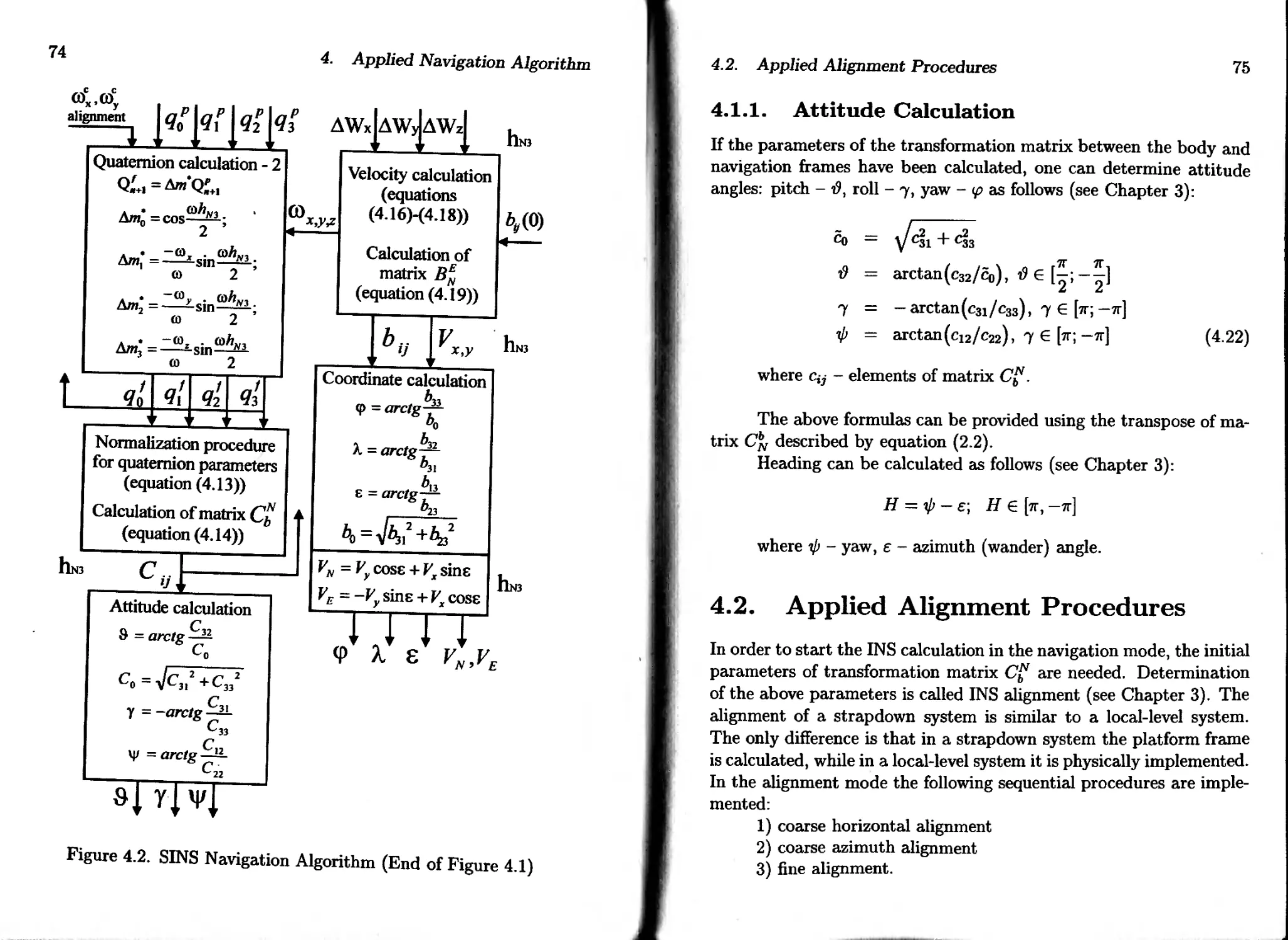
4.1.1.	Attitude Calculation......................... 75
4.2.	Applied Alignment Procedures........................ 75
4.2.1.	Stored Azimuth Alignment..................... 82
4.2.2.	Alternative Fine Alignment Procedure......... 82
4.3.	Description of SINS Functional Scheme............... 85
4.4.	Alignment Accuracy Analysis......................... 87
4.5.	Multi-Step Alignment Procedure ..................... 91
5.	INS	Error Model	94
5.1.	Strapdown and Local-Level Error Model...............102
5.2.	Schuler Loop .......................................109
5.3.	Influence of Azimuth Misalignment...................Ill
5.4.	Relation between Ф#, Ф/v, Фир and Pitch, Roll, Heading 114
5.5.	Error Model of Vertical Channel.....................117
6.	INS Calibration Procedures	121
7.	Applied Estimation Theory	133
7.1.	State Space Representation of Linear Systems........133
7.2.	Introduction to Traditional Estimation Methods .... 138
7.2.1.	Kalman Filter................................138
7.2.2.	Kalman Filter with Control Signal ...........155
7.2.3.	Kalman Filter with Coloured Measurement and
Input Noise..................................156
7.3.	Kalman Filter Adjustment............................158
7.3.1.	Influence of Initial Condition on Accuracy of
Kalman Filter.......................................158
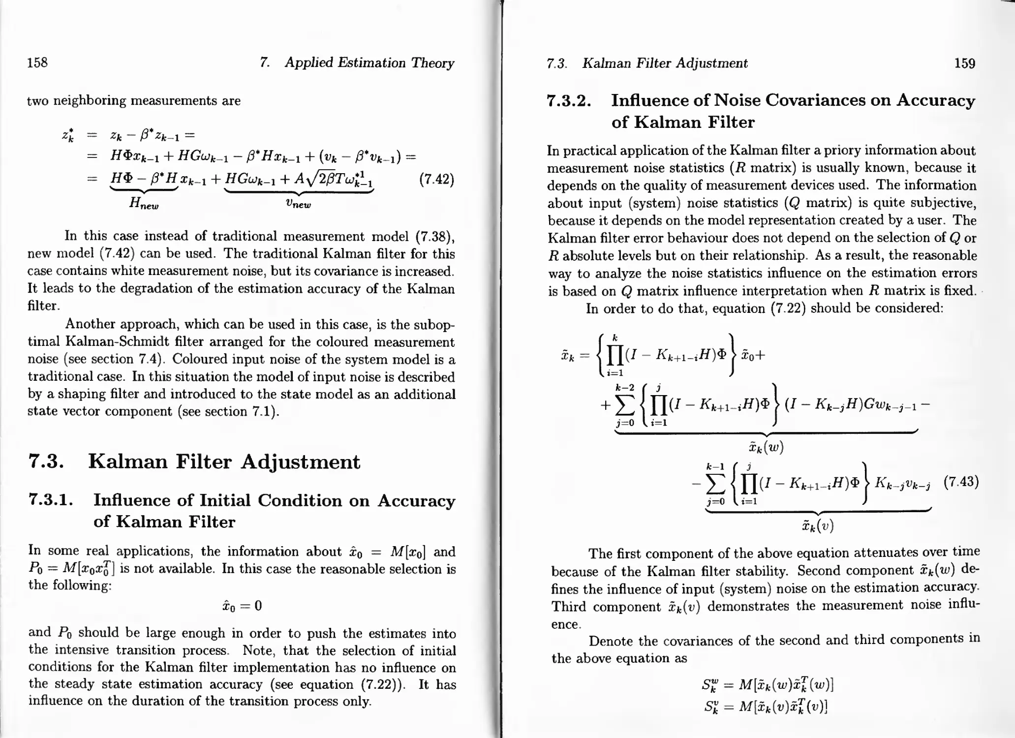
7.3.2.	Influence of Noise Covariances...............159
7.4.	Kalman-Schmidt Approach.............................165
7.5.	Estimation Modes....................................174
7.6.	Adaptive Filtering..................................178
8.	INS	testing	183
8.1.	INS Lab Testing Procedures..........................183
8.1.1.	Day-to-Day Accelerometer
and Gyro Bias Stability ............................183
5
8.1.2.	Lab Checking of Calibration Errors..........185
8.1.3.	Calibration of Gyro Drift Bias..............186
8.2.	Bias and Azimuth Misalignment Influence............188
8.3.	INS Field Testing..................................190
9.	INS/GPS Integration	191
9.1.	INS/GPS Integration Methods........................191
9.1.1.	Cascade Scheme of INS/GPS Integration .... 192
9.1.2.	Loosely Coupled Approach of INS/GPS
Integration .......................................194
9.1.3.	Tightly Coupled Approach of INS/GPS
Integration .......................................197
9.2.	Observability of INS Errors Using GPS Measurements . 198
9.3.	Calibration of Non-Stationary Component of INS Error 202
9.4.	Kinematic Azimuth Alignment........................208
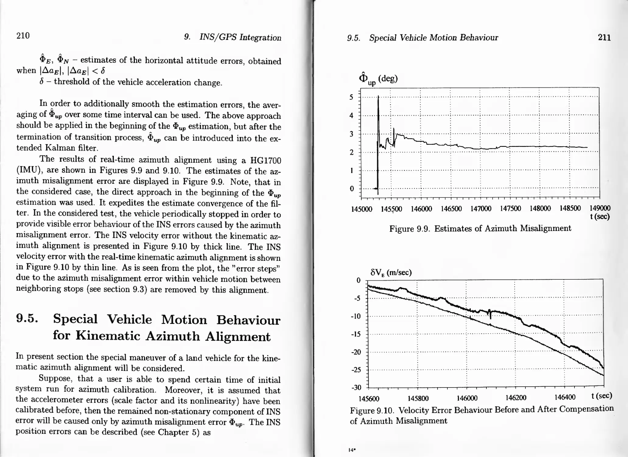
9.5.	Special Vehicle Motion Behaviour...................210
10.	Low-Cost INS/GPS Integration	214
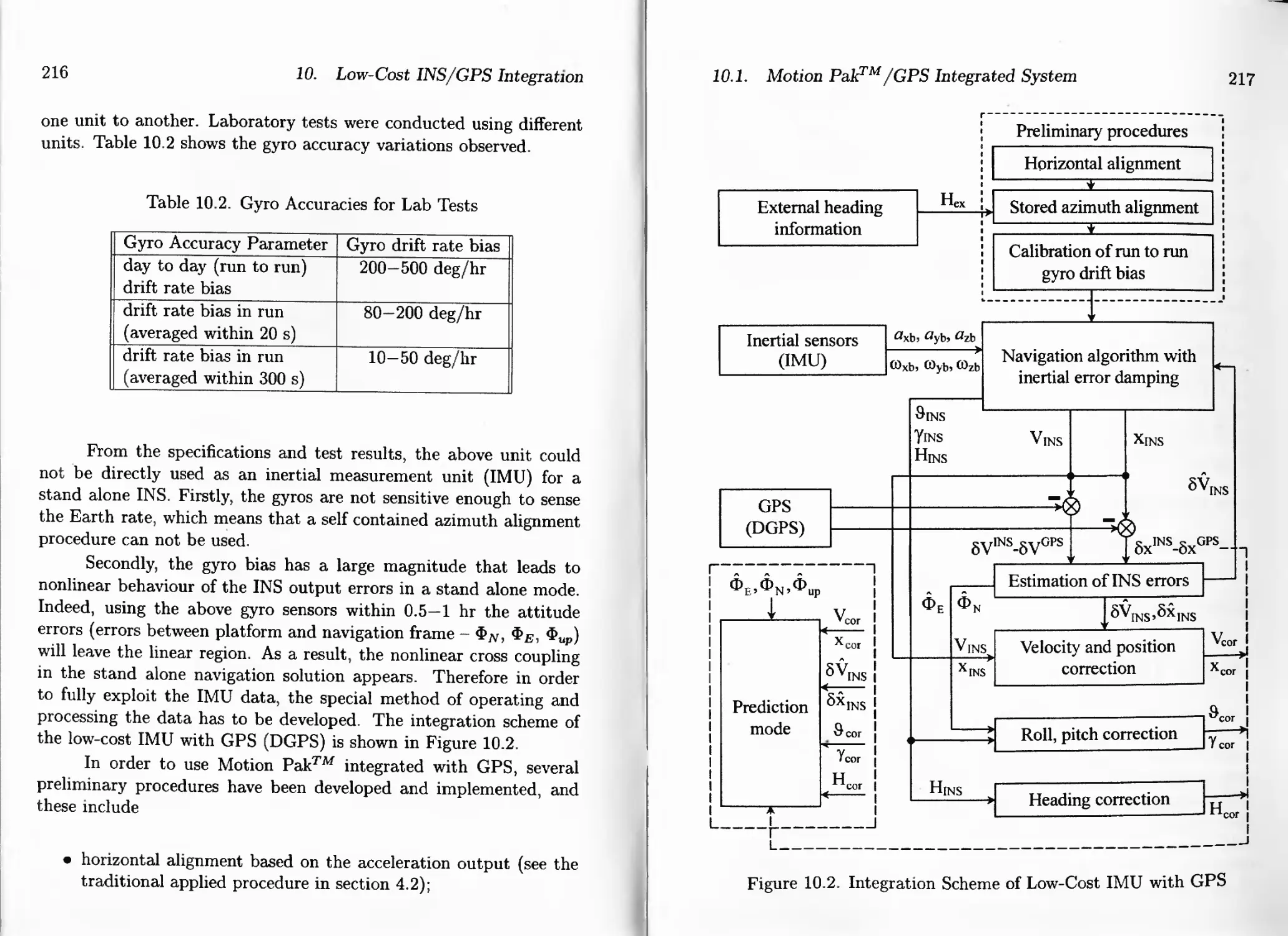
10.1.	Motion Pak™/GPS Integrated System.................214
10.2.	INS Error Damping.................................218
10.3.	Analysis of Error Damping Behaviour...............222
10.4.	Estimation of Low-Cost INS Errors.................224
10.5.	Roll, Pitch Correction Loop Implementation........228
10.6.	Heading Correction Loop Implementation ...........229
10.7.	Implementation of Prediction Mode.................231
10.8.	Position and Velocity Correction Loop.............232
10.9.	Test Description and Result Analysis..............232
10.9.1.	Land Vehicle Tests.........................232
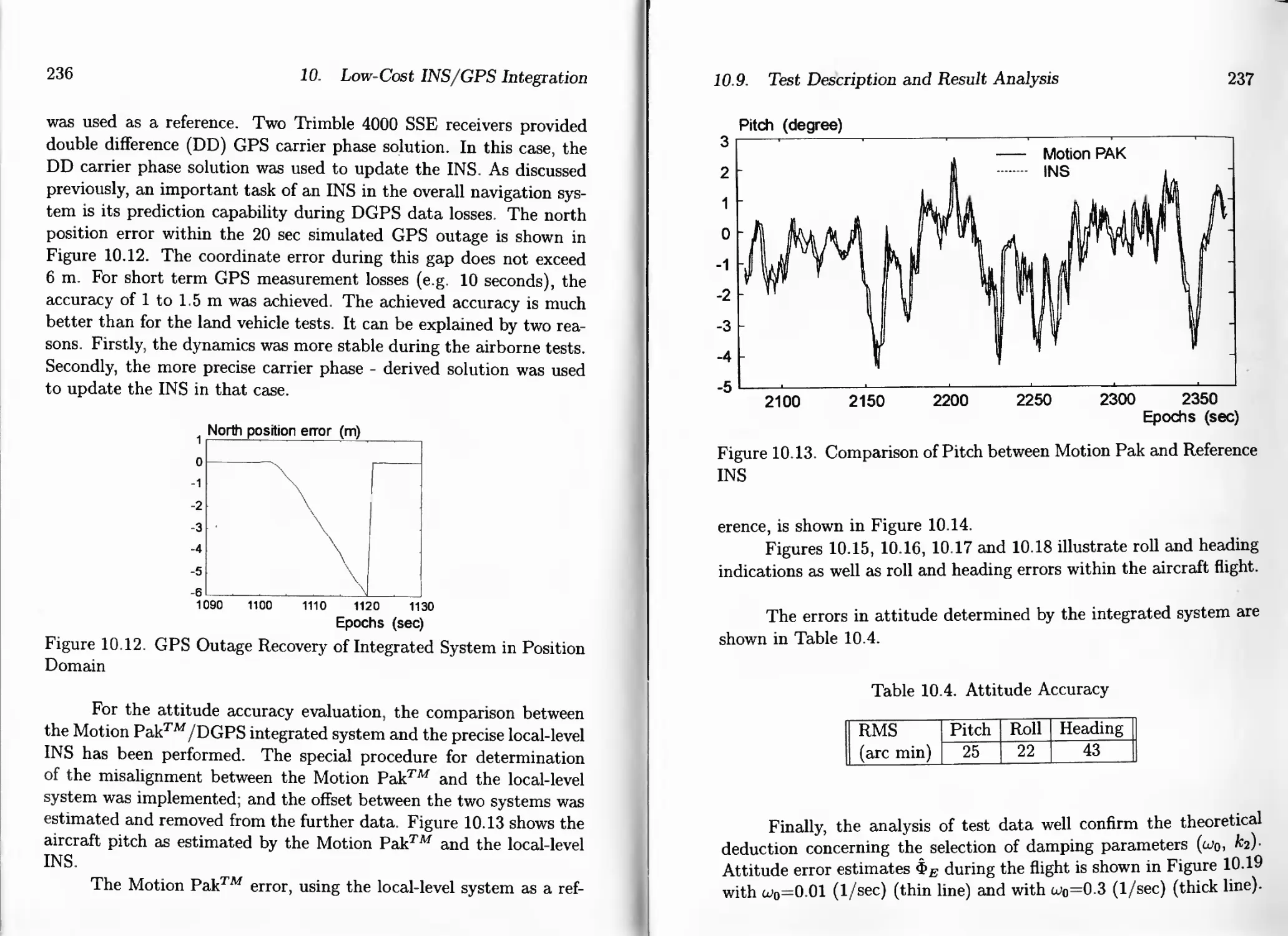
10.9.2.	Airborne Tests ............................235
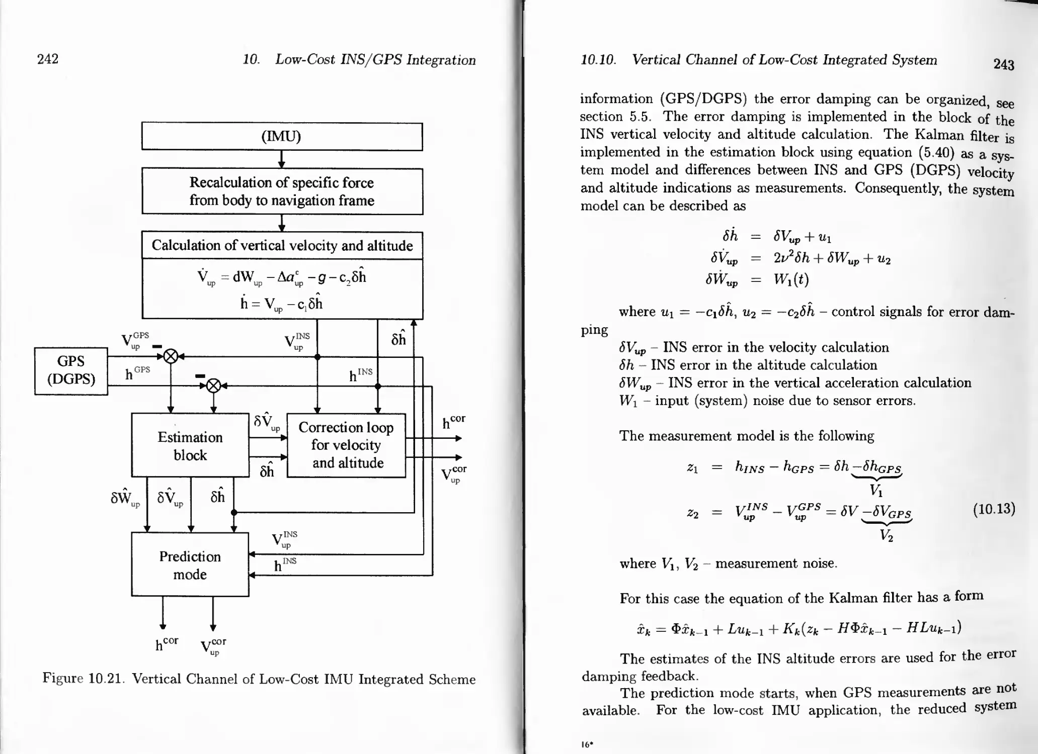
10.10V	ertical Channel of Low-Cost Integrated System . . . . 240
10.llU	ltra Compact Integrated Navigation System.......244
11.	Medium-Level Accuracy IMU/GPS Integration	249
11.1.	Honeywell HG1700/GPS Integrated System............249
11.2.	Estimation Block Implementation...................252
11.3.	Output INS Error Correction.......................258
6
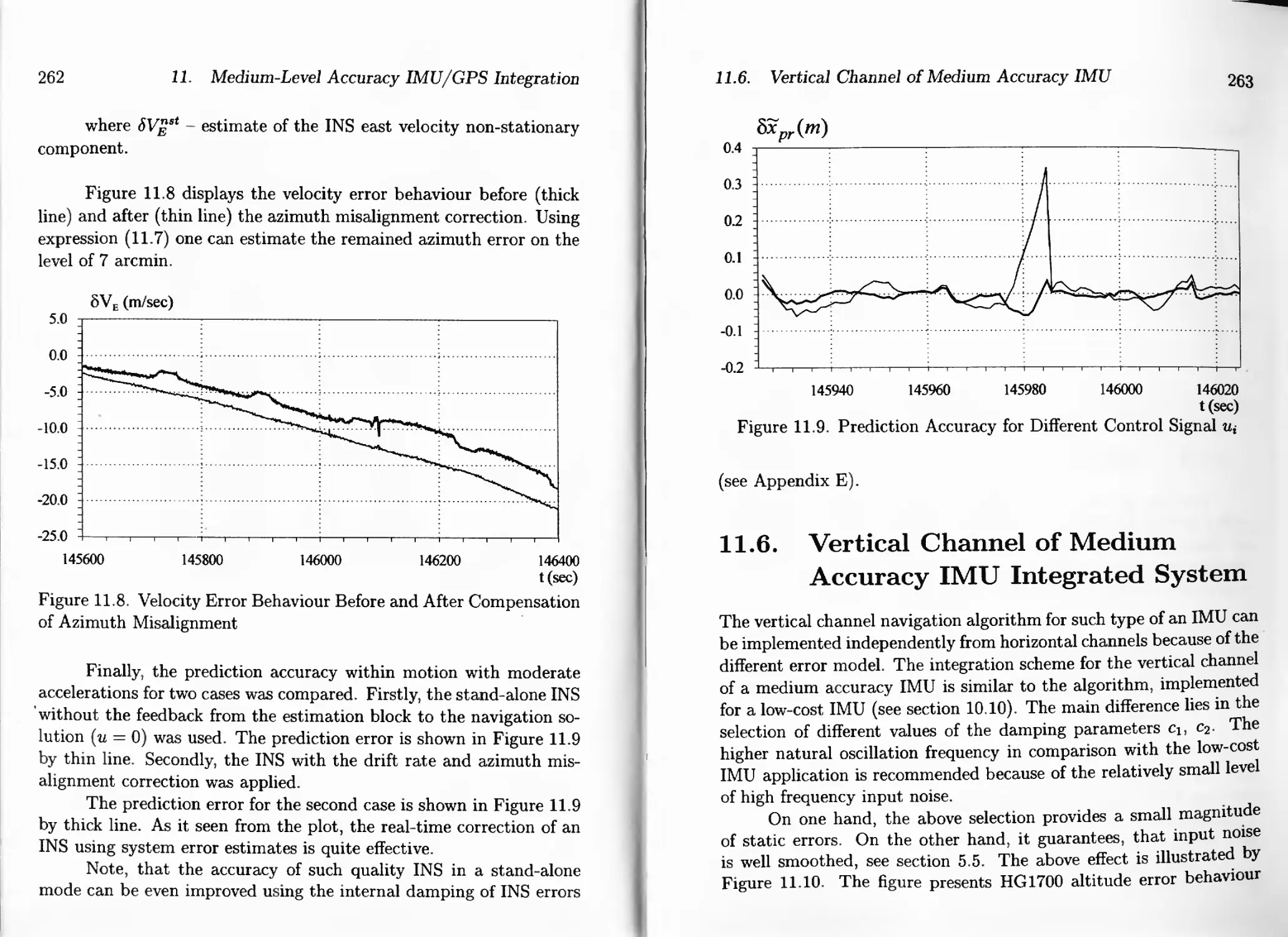
11.4.	Prediction Mode Implementation.............258
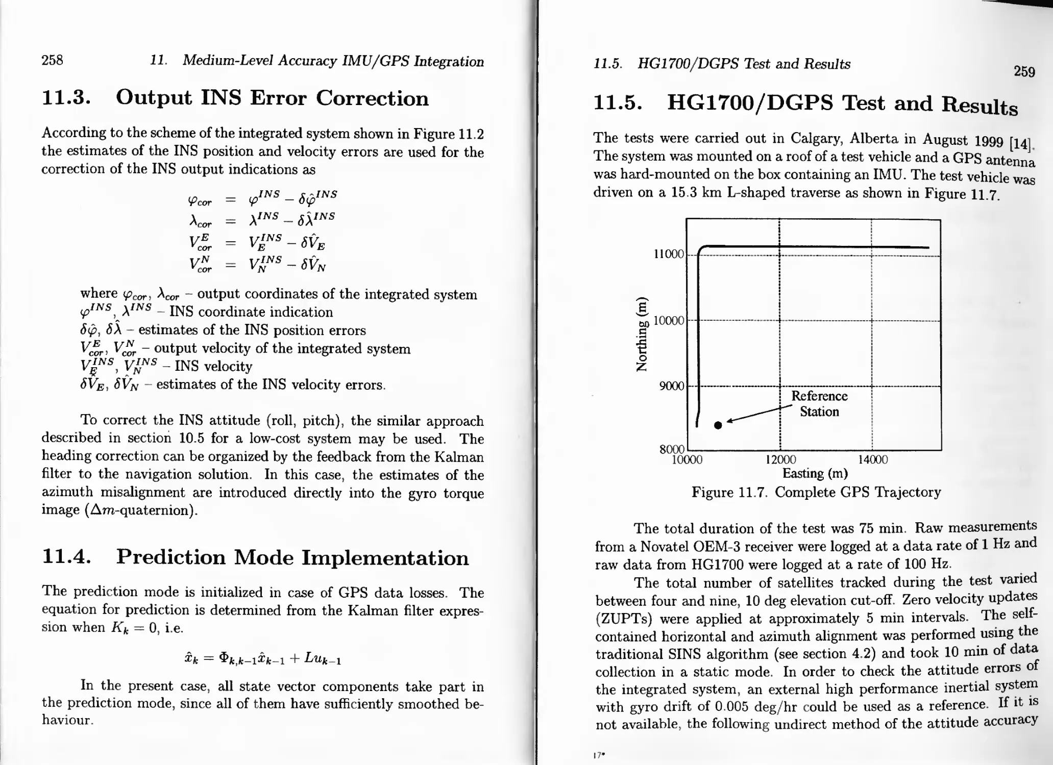
11.5.	HG1700/DGPS Test and Results...............259
11.6.	Vertical Channel of Medium Accuracy IMU ...263
11.7.	Low-Cost and Medium Accuracy Systems Comparison 264
11.8.	Land Navigation Using INS/GPS/Odometer Information266
A.	Mathematics of GPS	270
B.	Relationship Between Attitude Errors of INS	273
C.	Measurement Model in Second Calibration Procedure276
D.	Coning Calculation	284
E.	Possibility of Autonomous Mode Improvement	293
F.	Companav II	295
Introduction
Five years have passed since previous book ’’Inertial Systems in
Navigation and Geophysics” was published. Five years is an epoch for
modern technology development. The common direction of high tech-
nology evolution these days is to meat individual needs and to make
affordable the usage of high technologies in every day life. Many inex-
pensive products, such as mobile phones, pocket PCs, personal GPS
receivers, have become available in the market for common people. So
these tools appear to be standard outdoor kit of XXI century.
The innovations taking place in the inertial technology and
INS/GPS integration field have a large variety of implementations
nowadays. The stand-alone usage of GPS provides accurate naviga-
tion information, but is limited to open area applications and moreover
is unable to cover all the areas of tasks related to navigation and espe-
cially attitude determination. The usage of an inertial system, which
operates autonomously, solves many of these problems, however large
INS errors make challengeable its stand-alone operation. From the
above discussion, the integration of GPS and INS technologies is ap-
propriate since each system compensates for the other’s shortcomings.
A high performance INS cannot be used in many civil applications due
to its high price, therefore the latest investigations are focused on inte-
gration GPS with low-cost inertial systems. Micro-Electro-Mechanical
(MEM) technology has brought to the market the inexpensive sensors,
which can be used to create a low-cost navigation system. A number
of companies worldwide produces motion sensors, which provide a user
with 3-axis acceleration and angular rate raw information, but with-
out applying special adaptive techniques they cannot be utilized for
8
Introduction
the design of a ready-to-use navigation system. The Laboratory of
Inertial Geodetic Systems (LIGS) has accumulated great experience
in the inertial navigation system development and INS/GPS integra-
tion field. These knowledge and experience are now implemented into
the full-performance integrated inertial system based on MEM sen-
sors. Such a system fits the total navigation solution in a pocket size,
and is affordable for an average user.
The developed technology, which is discussed in this book, is ap-
plicable for the wide range of inertial systems. We think, we can claim
to have a new line of integrated inertial products opened. The actual
book presents the new technologies of the inertial sensor data pro-
cessing and the new approaches in the field of INS/GPS integration.
It introduces the fundamentals of inertial technology and follows up
to the algorithmic implementations. It is important to outline, that
all described methods and algorithms are implemented in the soft-
ware and hardware. The book content is dedicated to the people, who
were practically involved in that project: researchers, engineers and
scientists.
I would like to express my gratitude to the staff of the Lab-
oratory of Inertial Geodetic Systems and my colleagues in TeKnol
Ltd. company, namely Leonid Gushturov, Ilya Shakhov, Dr. Vladimir
Voronov, Dr. Vadim Lukianov for the long time productive joint work
and also to Mr. Valery M. Pissarev for help in the book publication
and effective project management. I also want to thank my daughter
Anastasia for text editing and inspiration in this book working.
Oleg Salychev
November, 2003
We would appreciate your comments of this book contents,
e-mail : contact@ligs.ru
FAX : (7-095)504-4500 (INTECHNOL 2540)
Phone : (7-095)263-6891
WWW : http://www.ligs.ru
Chapter 1
Coordinate Frames
In surveying and navigation positioning, the final output required by
a client usually includes the coordinates of a point namely latitude,
longitude and height, and their accuracies. The measurements sensed
by an Inertial Navigation System (INS) are three orthogonal compo-
nents of the body rotation rates and three accelerations in a coordi-
nate frame, which is not directly related to any geodetic curvilinear
coordinate frame. These measurements have to be analytically in-
tegrated and transformed through several coordinate frames, which
yields changes in the ellipsoidal coordinates. It is, therefore, impor-
tant that all coordinate frames involved in the transformation of the
measurements, and results of integrations are well defined before any
discussion of an inertial navigation system is presented. The defini-
tion of various coordinate frames associated with an inertial navigation
system is given in this section.
1.1. Inertial Frame
According to the Newtonian definition, an inertial frame is a frame,
which does not rotate or accelerate. Such a frame is easy to define
in theory, but it is almost impossible to realize in practice. The best
approximation of the truly inertial frame would be one, that is inertial
with respect to the distant stars. One approximation of such is a frame
10
1. Coordinate Frames
Figure 1.1. Inertial Frame
used in surveying applications, which is a right ascension system. The
right ascension system as given in a catalogue precesses and nutates
at the rate of less than 3.6 • 10~7 arc sec/s, which is well bellow the
noise level of sensors in present inertial survey systems. Thus, for all
practical inertial surveying purposes, the right ascension system can
be treated as the inertial coordinate frame.
The definition of the inertial frame is the following:
origin - at the center of the Earth
X/-axis - towards mean vernal equinox at To
Yaxis - complete a right handed system
Z/-axis - towards the north celestial pole at epoch t0.
A graphical representation of the inertial frame is shown in Fi-
gure 1.1. Note that this is an abstract definition of the inertial frame
for computation purposes. Measurements in the inertial frame, ob-
tained from gyros have much poorer accuracy.
1.2 Earth-Fixed Frame
The Earth-fixed frame is a frame, in which the output coordinates of
the inertial survey system are given. This frame is not inertial. It is re-
volving around the sun and rotating at a rate of 7.292115 • 10-5 rad/sec
1.3. Local-Level Frame
11
Figure 1.2. Earth-Fixed Frame
The definition of the Earth-fixed frame is the following:
origin - at the mass centre of the Earth
Xe-axis - pointing towards the Greenwich meridian, in the equa-
torial plane
Ye-axis - 90° east of Greenwich meridian, in the equatorial plane
Ze-axis - axis of rotation of the reference ellipsoid.
The coordinates in the Earth-fixed frame can be transformed
to the inertial frame by a negative rotation about the Z-axis by the
amount of the Greenwich Mean Sidereal Time (GMST). The reference
ellipsoid used in this research is the WGS 84 system. The semi-major
and semi-minor axes are:
а = 6378137.0 m
and
b = 6356752.3 m
respectively.
The direction of the axes of the Earth-fixed frame are illustrated
in Figure 1.2.
12
1.	Coordinate Frames
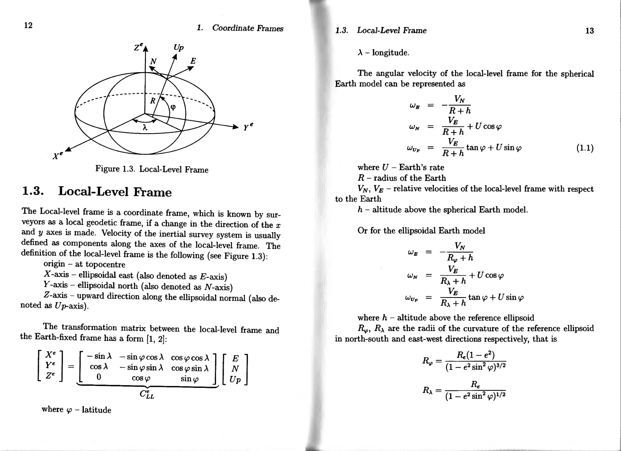
Figure 1.3. Local-Level Frame
1.3.	Local-Level Frame
The Local-level frame is a coordinate frame, which is known by sur-
veyors as a local geodetic frame, if a change in the direction of the x
and у axes is made. Velocity of the inertial survey system is usually
defined as components along the axes of the local-level frame. The
definition of the local-level frame is the following (see Figure 1.3):
origin - at topocentre
X-axis - ellipsoidal east (also denoted as E-axis)
Y-axis - ellipsoidal north (also denoted as X-axis)
Z-axis - upward direction along the ellipsoidal normal (also de-
noted as Ep-axis).
The transformation matrix between the local-level frame and
the Earth-fixed frame has a form [1, 2]:
' Xе ‘
Ye
Z€
— sin A — sin p cos A
cos A
0
— sin <p sin A
cosip
cos <p cos A
cos p sin A
sin<p
N
L up

where p - latitude
1.3. Local-Level Frame
13
A - longitude.
The angular velocity of the local-level frame for the spherical
Earth model can be represented as
VN
О/E =	R 4- h VE . Tr
=	= R + h ,CZCOSV
^Up =	Vjg = ——- tan <p 4- U sin p	(1.1) R + h
where U - Earth’s rate
R - radius of the Earth
Vjv, Ve - relative velocities of the local-level frame with respect
to the Earth
h - altitude above the spherical Earth model.
Or for the ellipsoidal Earth model
VN
=	R^ 4- h VE
WN =	= R. + h lf/coS^ Vb
^Up ~	= —		 tan ip 4- U sm Rx + h
where h - altitude above the reference ellipsoid
Rv, R\ are the radii of the curvature of the reference ellipsoid
in north-south and east-west directions respectively, that is
Д.(1-е2)
(1 — e2sin2 <^>)3/2
Re
(1 — e2sin2 «p)1/2
14
1. Coordinate Frames
Here, Re is the equatorial radius of the Earth and e is an eccen-
tricity given by e2 = 1 — b2/а2 (a is a semi-major axis of the reference
ellipsoid and b is a semi-minor axis).
1.4.	Wander Frame
Figure 1.4. Wander Frame
The local-level frame is convenient for expressing directions but
it is not the best coordinate frame to perform integration of data from
the inertial survey system. The Y axis of the local-level is always
pointing towards the North. At very high latitudes, a large rotation
about the Z axis is necessary to maintain the orientation of the local-
level frame whenever it is moved towards the East, even by a small
movement. This problem may be avoided by performing all the com-
putations in a coordinate frame that does not point to the North. Such
a coordinate frame is called a Wander Frame. The wander frame is
the same as the local-level frame in all aspects except that its Y axis
is not slaved to the North direction. Therefore, it is allowed to wander
off the North axis at a rate chosen by a user. The angle between the
Y and North axes is called the wander or azimuth angle.
The correspondence between the local-level and wander frames,
as well as the positive direction of wander angle e is shown in Fi-
gure 1.4. According to the introduction of wander angle e, the equa-
1.4. Wander Frame
15
tion for ё is the following:
VE
ё = — —------- tan
Rx + h
The definition of the wander frame is the following:
origin - at topocentre
X\v-axis - rotated in the level plane by angle £ from the East
towards the North. Angle e is called the wander or azimuth angle.
It is chosen to be equal to the meridian convergence from a point of
alignment
Yw-axis - orthogonal to the X-axes in the level plane
Zw-axis - upwards along the ellipsoidal normal.
The transformation matrix between the wander frame and the
local-level frame can be described as
N = Yw cos e 4- Xw sin e
E = —Yw sin e 4- Xw cos e
The transformation matrix between the Earth-fixed frame and
the wander frame has a form [1]:
Xw		5ц	512	5i3		’ Xе '
Yw	=	&21	&22	5гз		Ye
Zw		5з1	5з2	5зз		Ze
						
			су			
5ц = — sin cos A sin e — sin Л cos e
512 = sin sin A sin e -I- cos A cos e
513 = cos </> sin E
b2i = — sin cos A cos e 4- sin A sin e
b22 = — sin <p sin A cos e — cos A sin e
b23 = cos tp cos E
531 — cos <p cos A
b32 = cos <p sin A
b33 = sin <p
16
1. Coordinate Frames
The absolute angular velocity of the wander frame can be de-
scribed as
u>xW = cos e 4- u)N sin e
u)yw ~ sin e 4- ujn cos E
wzW = U sin <p
where	- absolute angular velocities of the local-level
frame described by equations (1.1)
U - Earth rotation rate
ip - latitude.
1.5.	Body Frame
Figure 1.5. Body Frame Representation
The body frame is an orthogonal frame, in which the measure-
ments of a strapdown inertial navigation system are made. Its axes
coincide with the output axes of the sensor block, which is called an
Inertial Measurement Unit (IMU). Thus, the IMU raw data contains
the components of the rotation rate and the accelerations experienced
by a sensor unit along its body axes. The local-level frame can be
rotated to the body-frame by three consecutive right-handed rota-
tions about its three axes. The first rotation is made about its Z-axis
1.6. Navigation Frame
17
and the angular change is called heading of an INS (in Russian system
heading has an opposite direction). The second rotation is made about
the rotated X-axis by an angle, which is called pitch of an INS. The
third rotation about the rotated У-axis completes the total rotation
between the two frames. The amount of this rotation is defined as roll
of an INS. The three angles: roll, pitch and heading are commonly
referred to the Euler angles. The definition of the body frame of an
inertial survey system is the following (see Figure 1.5):
origin - at the center of a strapdown inertial survey system
Хь-axis - towards the right side of an INS
Yt,-axis - towards the front of an INS
Zb-axis - upwards and perpendicular to the XY plane.
An INS box is installed in a vehicle such a way, that the Yb axis
coincides with the vehicle longitudinal axis, the Zb axis coincides with
the vertical vehicle body and the Xb axis completes a right handed
system.
The transformation matrix between the local-level frame and
the body frame is described by equation (2.1).
1.6.	Navigation Frame
Х^У/у,^ axes of the navigation frame can be optionally coincided
with the local-level frame or with the wander frame.
1.7.	Platform Frame
The platform frame was created mainly for the derivation of the error
equations. The platform frame is an image of the navigation frame,
which is established on an on-board computer using the real output
from sensors. For the ideal sensors, the platform frame coincides with
the navigation frame. However, in reality the platform frame has a
small deviation from the navigation frame due to the sensor errors.
2 - 9437
18
1. Coordinate Frames
The above angular deviations are called platform attitude errors. The
definition of the platform frame is listed below:
origin - at the centre of the inertial navigation system
Xp-axis - slightly misaligned due to attitude errors with the
X axis of the navigation frame
Yp-axis - slightly misaligned with the Y axis of the navigation
frame and orthogonal to the X axis mentioned above
Zp-axis - complete a orthogonal right-handed system.
The transformation matrix between the navigation and platform
frames has a form
where Фж, Фу, Фг - INS attitude errors.
1.8.	Sensor Frame
The sensor frame coincides with sensitivity axes of accelerometers and
gyros. Actually, the above frames are close but do not coincide with
the body frame because of installation errors of sensors in an IMU.
During the factory calibration the above errors can be estimated and
compensated (see Chapter 6). As a result, in the INS algorithm the
coincidence between sensor frame and body frame is actually assumed.
The transformation matrix between the sensitivity axes of ac-
celerometers and the body frame can be described as
Xb~
Yb
Zb
1
C*yx
OLZX
&xz
Olyz
1
xa
Ya
Za
1
where otxy, axz, ayx, ayz, azx, azy - installation errors of the
accelerometer axes with respect to the body frame.
I 8. Sensor Frame
19
The transformation matrix between the gyro sensitivity axes
and the body frame has a similar form
' xb
Yb
Zb
1
Pyx
Bzx
Pxy
1
fizy
(3XZ
Pyz
1
Xg
Yg
Zg
where ftxy, fiXZi fiyXi /3yz, (3ZXi fizy - installation errors of gyro
axes with respect to the body frame.
The above errors are estimated and compensated due to the
factory calibration (see Chapter 6).
2*
Chapter 2
Coordinate Transformation
2.1. Direction Cosine Matrix
In order to transform an arbitrary vector from one coordinate frame
to another one, the transformation matrix between the above frames
can be introduced as
where Cj - transformation matrix between the I frame and b
frame.
Frequently, the transformation matrix is called a direction cosine
matrix.
The most commonly employed method for generation a coordi-
nate transformation matrix is based on the computation of the direc-
tion cosines in between each pair of axes of two frames respectively.
One of the most used methods of the direction cosine matrix determi-
nation is based on the three ordered right-handed rotations [2, 3, 4].
The angles of rotation are called Euler angles. The above an-
gles are three independent quantities, which are capable to define the
position of one coordinate frame with respect to another.
2.1. Direction Cosine Matrix
21
Let’s introduce the following Euler angles: Фх, Фу, Ф2. Using
a series of three ordered right-handed rotations on the Euler angles,
the coincidence between two arbitrary frames can be achieved.
Let’s coincide XYZ coordinate frame with ХьУъ^ъ coordinate
frame.
The first rotation of XYZ system is made about the Z axis by
angle Ф2. The rotation about Z axis of Ф2 results in a new set of axes
X1Y1Z1 as shown in Figure 2.1. This rotation and the subsequent
rotations are made in a positive, that is, anti-lock wise, direction,
when looking down the axis of rotation towards the origin. A position
vector in the new system can be expressed in terms of the original
coordinates as
Xi = X cos Ф2 4- Y sin Ф2
Yi = —X sin Ф2 4- Y cos $z
Z, = Z
or in matrix form
cos $z sin Фг 0
— sin $z cos $z 0
0	0	1
Figure 2.1. Rotation by $z Angle
22
2.	Coordinate Transformation
2.1.	Direction Cosine Matrix
23
The second rotation is made by rotating XiYiZi system about
the Xi axis by angle Ф1} see Figure 2.2. As a result new coordinate
frame X2Y2Z2 is introduced. The transformation between the X2Y2Z2
and XiYiZi systems can be described as
or
and
X2 = Хг
Y2 = Yi cos Фд. 4- Zi sin Фх
Z2 = — Ki sin Фх + Zi cos Фж
’ Xb'
Yb
J
’ COS Фу
0
sin Фу
0
0
— sin Фу
0
COS Фу
Z2
— C3

0	0
cos Фд. sin Фд.
— sin Фя cos Фд.
Figure 2.2. Rotation by Фд. Angle
Z2
Figure 2.3. Rotation by Фу Angle
The total transformation matrix can be defined using multipli-
cation of C3, C2l Ci matrices, then
Finally, third rotation about the Y2 axis by angle Фу moves
X2Y2Z2 system to XbYbZb, see Figure 2.3. The corresponding trans-
formation has a form
C = C3C2Ci
Xb = X2 cos Фу — Z2 sin Фу
Yb = Y2
Zb = X2 sin Фу + Z2 cos Фу
where
C =
Cll	C12	C13
C21	C22	C23
C31	C32	C33
24
2. Coordinate Transformation
and
Сц = cos Фу cos Ф2 — sin Фх sin Фу sin Ф2
Ci2 = cos Фу sin Ф2 + sin Фх sin Фу cos Ф2
Ci3 = - cos Фх sin Фу
c2i = — cos Фх sin Ф2
C22 = cos Фх COS Ф2
с2з = sin Фх
c3i = sin Фу cos Ф2 4- sin Фх cos Фу sin Ф2
Сз2 = sin Фу sin Ф2 - sin Фх cos Фу cos Ф2
C33 = cos Фх cos Фу	(2.1)
It should be pointed out, however, that the Euler angles are not
uniquely defined, since there is an infinite set of choices.
Unfortunately, there is no standardized definition of the Euler
angles. For a particular choice of the Euler angles, the rotation order
selected and defined must be used consistently. That is, if the order
of the rotations is interchanged, different direction cosine matrix C
representation is defined.
Let’s consider the properties of direction cosine matrix C. The
above matrix in between two arbitrary chosen coordinate frames has
the following properties.
1.	Determinant of matrix C equals to identity
det C — 1
2.	C-1 = CT
Using the above properties one can easily transform a vector
from one coordinate system to another one.
Introduce, for example, the transformation matrix between the
body frame and the local-level frame as

2.1. Direction Cosine Matrix
25
where CfL - direction cosine matrix of the transformation from
b frame to LL frame.
For the backward transformation the above equation can be
rewritten as
= (W
A matrix, which has the above property in the matrix algebra,
is called an orthogonal matrix. Hence, direction cosine matrix C is an
orthogonal matrix.
In order to define orientation of a vehicle body with respect to
the local-level frame, the Euler angles, namely, pitch, roll and heading
(19, 7, H) are usually introduced. Assume, that one has the infor-
mation about direction cosine matrix C|L between the local-level and
body frames. The elements of the above matrix can be represented
via ?9, 7, H angles. Substituting Фх, Фу, Фг angles by pitch, roll and
heading in equation (2.1), such representation can be defined.
In Russian inertial systems the positive direction of heading an-
gle H is opposite with respect to Фг angle, then H = — Фг [1].
Using last remark, the transformation matrix between the local-
level frame and the body frame can be represented as
CbLL =
C11
C21
C31
c12 c13
C22 Сгз
C32 c33
(2.2)
26
2. Coordinate Transformation
where
Cu = cos 7 cos H 4- sin $ sin 7 sin H
C12 = — cos 7 sin H 4- sin ‘O sin 7 cos H
C13 = — cos & sin 7
c2i = cos $ sin H
C22 = cos cos H
C23 = sin
c3i = sin 7 cos H — sin $ cos 7 sin H
C32 = — sin 7 sin H — sin cos 7 cos H
C33 = cos $ cos 7
and $, 7, H - pitch, roll, heading of the vehicle body frame.
Let us consider the case of small deviations between xyz and
xbybzb frames. It means that Euler angles Фх, Фу, Фх can be con-
sidered as small angles. In this case transformation matrix C can be
rewritten (совФ, « 1; вшФ, « Ф,) as
1
. Ф»
фг -ф,
1 Фх
-ф«	1
	 1 0 0 		Г о фг -ф„
= / 4-C =	0 1 0	4-	1 ф н О ф н
	0 0 1		Ф» -Фх 0
(2.3)
It can be shown, that for the small rotations, angles Фх, Фу, Фх
can be represented as a vector, and for them the vector addition rule
is valid. It means, that if three ordered sequential small rotations are
made from an original frame, then for the linear approximation of the
total transformation matrix between the initial and final systems, the
following formula is valid:
C = G C2C3 = I 4- Сг 4- C2 4- C3
where (14- Ci) - transformation matrix of a small rotation.
2.2.	Puasson Equation
2.2.	Puasson Equation
27
Let us introduce an important rule for the differentiation of any vector
with respect to the inertial space. This rule can be described by the
following formula:
dR\ _ dR
dt I/ dt
+ umx R
m
(2-4)
- derivative (total) of vector R with respect to the
inertial frame
dR\
dt Im
- derivative (local) of vector R with respect to m -
arbitrary frame
bjm - absolute angular velocity of m frame.
Mathematically, the derivative of some vector with respect to
the certain frame can be achieved by the following operation. At first,
the projections of some vector on the certain coordinate frame have
to be calculated. The next step is the differentiation of the above
projections. As a result, the above projections describe the derivative
of the considered vector with respect to the certain coordinate frame.
In literature [3, 4] the equation (2.4) is called Coriolis formula.
Equation (2.4) can be rewritten in a matrix form as
R™ — Rm + ^m^
(2.5)
where
0
^2
0

U)y
-Ux
0
and R™ - total derivative of vector R in projection on m frame.
28
2. Coordinate Transformation
In order to define the differential equation for the transformation
matrix between non-inertial frame m to inertial frame I, the following
relationship can be used:
Ri —
By differentiating of both sides of the above equation, one can
define
Ri ~	=
=	+ An)
Let us assume that the following formula is valid:
or
C‘m = С‘тй>т	(2.6)
then
R{ ~ Cmtfim + &mRm)	(2-7)
Obtained equation (2.7) is valid because of Coriolis for-
mula (2.5), thus equation (2.6) is valid as well.
Expression (2.6) is known as Puasson equation. The above equa-
tion describes behaviour of the transformation matrix between an ar-
bitrary non-inertial frame and the inertial frame.
Usually in inertial navigation systems, the transformation ma-
trix between two non-inertial systems is needed.
The behaviour of the direction cosine matrix between m and
n arbitrary non-inertial systems can be described in a form of equa-
tion (2.6), as
=	(2-8)
where wm_n - matrix, which elements are relative angular
velocities between m and n coordinate frames.
Equation (2.8) is not usually applied for attitude determination,
because for its implementation relative, but not absolute, angular ve-
locities are needed, while inertial sensors provide the absolute angular
2.2. Puasson Equation
29
velocity of the body. But the above equation will be used for the
coordinate determination in the navigation algorithm, see Chapter 4.
Another representation of equation (2.8) can be defined using
the following relationship:
СП   {-ins'll
(2.9)
and equations for C^, C\ in form (2.6)
= crc‘m
<in = c?c'
(2.10)
By differentiating of both sides of equation (2.9), one can deter-
mine
C" = C?C‘ + c?c£
m 1 m 1 i
and substituting equations (2.10)
C' n   ргт/	s-'m/’il
m —	-b On Uj °m
Cn Wm &n
or
Here
= C”u,m -
(2.11)
and cj™, cj” - absolute angular velocities of m and n frames.
30
2. Coordinate Transformation
2.3.	Rotation Vector and Quaternions
Instead of the three ordered rotations for coincidence of two coordinate
frames, it is possible to use one rotation around a single, fixed axis. Let
us introduce rotation vector Ф, which defines such operation. Rotation
vector Ф is directed along the axis of rotation and has a magnitude
equal to the rotation angle in radians.
The equation of the rotation vector can be defined as
Ф = |Ф|г =
cos a
cos/3
cos 7
(2.12)
where |Ф| - magnitude of the rotation vector
a, 0, 7 - angles between the axis of rotation and a coordinate
frame.
It can be defined [12, 13] that the rotation vector satisfies the
following differential equation:
i _ 1-e _	1 Л Ф sin Ф ,=	.
Ф = ш + -Фхш +	I 1 - -7—!--IФ x (Ф x w)
2 Ф 2\	2(1 - cos Ф )/ v 7
where w - angular velocity between frames.
For small Ф angle it can be rewritten in a form
Ф = бй4-^Фха> + -^-(Ф x (Ф x w))
Z	LZi
(2-13)
Usually, for convenience of the transformation operations,
Hamilton quaternion algebra is used, which implements the rotation
vector idea.
Hamilton’s quaternion is defined as a hyper-complex number of
the form [2]:
Q = <7o + Qii +	+ Язк
2.3. Rotation Vector and Quaternions
31
where go, Qi> Q2, дз are real numbers and set {1, i, j, k} forms
a basis for a quaternion vector space.
9o =
gi =
Я2 =
дз =
Conceptually, gb q2, дз define a vector in space and g0 is the
amount of rotation about that vector.
In other words, the quaternion elements can be described as
Д
cos —
2
• M
sin — cos а
2
u
sin — cos p
. Д
sm-cos7
where p is the amount of rotation
a, (3, у - angles between the axis of rotation and a coordinate
system.
Obviously, the quaternion elements can be represented through
the parameters of rotation vector Ф. Using expression (2.12), the
quaternion elements can be described as
Qo
gi
Q2
дз
|ф|
C°S 2
. |ф|
sin 2
. |ф|
sm 2
. |ф|
sin 2
|Ф|
Фу
|Ф|
Ф2
|ф|
(2.14)
ф
In order to use the quaternion technique, the following algebraic
properties of a quaternion have to be introduced.
Norm of quaternion N(Q) = gj 4- gj 4- gf 4- gf = 1
32
2. Coordinate Transformation
Addition The sum of two quaternions [Q] and [5] is as fol-
lows:
[Q] 4- [S] = (g0 + qii 4- 92 j 4- Чзк) + (s0 + sii + s2j + s3k) =
— (<7o 4- ®o) 4- (qi 4- $i)i 4- (q2 4- s2)j + (q3 4- s3)k
Subtraction Quaternion subtraction is merely addition of a
negative quaternion
-(<?] = (-i)lQ]
or
[Q] - [S] = Q 4- (-l)S = ((to - So, 91 ~ Si, q2 - s2,9з - s3)
Multiplication The product of two quaternions [Q] and [S]
is
[Q][S] - (go 4- qii 4- q2j 4- g3^)(s0 4- sp 4- s2j 4- s3k) =
= GfoSo — 9isi — q2s2 — g3s3) 4-
4“ (9osi 4- 9i$o 4- g2s3 — q3s2)i 4-
4" (9oS2 — 9is3 4- q2sG 4- 9sSi)J 4-
4- (90S3 4- q\S2 — q2Si 4- q3s0)k
In general, quaternion multiplication is not commutative, that
is, [Q][S] 0 [S][Q]- Multiplication by a scalar Л yields
A[Q] = Ago 4- Agii 4- Xq2j 4- Xq3k
Quaternion multiplication is defined by using the distributive
law on the elements as in ordinary algebra, except that the order of
unit vectors must be preserved. The bases г, j, к are generalizations
of л/—1, which satisfy the relationships
i2=j2 = k2 = _1
2.3. Rotation Vector and Quaternions	33
and by cyclic symmetry
U = k
jk - -kj = i
ki = —ik — j
Conjugate The conjugate [Q]* of a quaternion is defined as
follows:
[Q]* = Qo - <hi -	- Язк
Moreover, norm (or length) of quaternion N(Q) is a scalar de-
fined as the product of the quaternion and its conjugate. Thus,
N(Q) = [<?][<?]• = [<?]*[«] =
= 9о+91+9г + 9з	(215)
Using the isomorphism one can get [Q][Q]* = det(Q).
Conventionally, det(Q) is called norm, denoted by N(Q),
so that [Q][Q]* = N(Q). Similarly, [Q]*[Q] = N(Q), or
[Q][Q]* = N(Q) = [Q]*[Q]. The norm of the product of two quater-
nions is equal to the product of these norms. Hence, N(QS) =
N(Q)N(S) and consequently, |[Q][S]| — |[Q]||[S]|. By the mathe-
matical induction, the product of n quaternion factor is
N(QiQ2  •Qn) = N(Q1)N(Q2)... JV(Qn)
Inverse If [Q] is not zero, then inverse quaternion [Q]-1 is
defined as
[QHQ]’1 = IQ]’*[Q] = i
Using the norm concept, one can obtain
[Q]"1 = [Q]71V(Q)
where N(Q) / 0. Thus,
3	9437
34
2. Coordinate Transformation
Identities
1. Zero quaternion [Qo] is a quaternion with zero scalar and
zero vector
[0] = 0 4- 0г 4- 0j + Ok
2. Unit quaternion is defined as any quaternion whose norm
is 1. Thus
[1] = 1 4- 0г 4- 0j 4- Ofc
Since there is a single redundancy in the four-parameter descrip-
tion of coordinate rotations, as opposed to six for the direction cosines,
the quaternion parameters satisfy a single constraint equation. The
constraint equation on a unit quaternion is
<Zo + Qi + + Яз — [Q][Q]* — 1
Computationally, (qq 4- qJ 4- q2 + <Й)1/2 can be used as a
normalizing factor for each parameter. This is analogous to the
periodic orthogonalization procedure used in conjunction with the
direction cosine propagations.
Equality The equality of two quaternions [Q] and [S] is de-
fined when their scalars are equal and their vectors are equal. Thus,
[Q] = [S'] if and only if
9o = so, Qi = «1, q2 = s2, 9з = $з, or [Q], = [S]», г = 0,1,2,3
From the preceding discussion, a unit quaternion can now be
defined in the similar transformation, in which vector R in the inertial
coordinate frame is transformed into the body frame as
MG] = 1
(2.16)
Now consider {г, j, fc} as the orthogonal basis for real-vector
space R3. Then, any vector x = xii + x2j+ x$k in R3 can be expressed
2.3. Rotation Vector and Quaternions
35
in the quaternion form with zero scalar term. Similarly, from the
previous definition of a quaternion, any quaternion
[Q] = Qo + 9i« + Q23 + Чзк
can be expressed as a sum of a scalar and a vector ([Q] = qo + q).
Figure 2.4 depicts the spatial orientation of a quaternion.
Figure 2.4. Spatial Representation of Quaternion
Next, how the quaternions are used in coordinate transforma-
tions will be discussed.
Consider the two coordinate systems illustrated in Figure 2.5.
Furthermore, it will be assumed that the coordinate system (X, У, Z)
is fixed in space, while the coordinate system (X', У', Z') is moving
in some arbitrary manner, however, both coordinate systems have
the same origin. Using Euler’s theorem, the (X', У', Z') coordinate
system is rotated by the angle д about some fixed axis, which makes
angle a, /3 and 7 with the (X, У, Z) axes, respectively. Note that this
axis of rotation makes the same angles a, /3, у with the (X', Y', Z')
axes, also. From the four-parameter system (д, a, /3, 7) another
transformation matrix will be derived that aids in the development of
the differential equations of the four quaternion parameters.
The transformation of vector R from one coordinate frame - b
to another - i, can be described through quaternion Q as follows:
Ri; = Q • Rb • <Z =
= (<7o + qii + q2j + qsty(rbxi + rbj + rbk)(q0 - qj - q2j - q3k)
36
2. Coordinate Transformation
Figure 2.5. Rotation Axis of ’’Vector” about which System XYZ is
Rotated in order to Coincide with System X’V’Z’
Using the above expression and multiplication rules of i, j, fc,
the above quaternion transformation can be determined in a matrix
form as
where
9o + 9i “ 9г ~ 9?
2(9192 + 9о9з)
2(919з — 9о9г)

2(9192 ~ 9з9о) 2(gi<fo + 9092)
9o - <A + 92 - 9з 2(4293 - 9o9i)
2(9293+ 9b9i)	.
(217)
Formula (2.17) gives the correspondence between the direction
cosine matrix and the quaternion. In other words, if the quaternion
elements 91, Q2, <7з are determined, then the direction cosine matrix
components can be defined by expression (2.17).
2.3. Rotation Vector and Quaternions
37
The quaternion can also be expressed as a 4 x 4 matrix. Thus
Qo	Qi	9г	9з
q =	“91	9o	-9з	92
—92	9з	9o	~91
~9з	“92	91	9o
where, as before, ft, ft, ft, 93 are quaternion components.
A primary advantage of using the quaternion technique lies in
the fact, that only four unknowns are necessary for calculation of
new transformation matrix, while the direction cosine method requires
nine.
It can be shown [2], that the quaternion analog of Puasson equa-
tion has a form
(2.18)
The recurrent solution of the above equation can be determined
as
Qk+l = Qk + yQkWT
or
Q*+1 = Qk(l +	= Qk&Q	(2.19)
&
where T - sampling period
AQ = 14-	- quaternion of a small rotation (updating
quaternion).
Let’s deduce the quaternion expression of a small rotation de-
38
2. Coordinate Transformation
fined beyond. By the definition, one get
Qo
9i
92
9з
= cos	|ф|
	2
	|Ф| Ф»
= sin	2 |Ф|
	|Ф| Ф»
= sin	2 |Ф|
= sin	|Ф| Фх
	2 |Ф|
Using only first component of expression (2.13) which is valid for
small angle Ф, the quaternion of a small rotation can be determined
as
9o	= 1
9i	—
^4
1
92	= ^yT
9з	= ^zT
Let’s compare the Puasson equation solutions in the direction
cosine matrix representation with ones in the quaternion form for small
rotations (see equation (2.19)). Puasson equation between some non-
inertial coordinate frame - b and the inertial coordinate frame - I has
a form (see (2.6)):
Cl = Cfa
where - absolute angular velocity of frame b.
The recurrent solution of Puasson equation can be defined as
Cb(tk+i) — Qfafc) = Cl(tk)tib(tk)T
or
Cl (ifc+1) = Cl(tk)(I + 0>b(tk)T) = Cl(tk) ACl	(2.20)
2.3. Rotation Vector and Quaternions
39
where &Cb = I + wb(tk)T can be considered as a direction cosine
matrix of a small rotation (see equation (2.3)). Comparison of equa-
tions (2.19) and (2.20) shows the similar form of Puasson equation in
the direction cosine matrix and quaternion representation.
It is important to note, that equation (2.19) is valid for the
transformation from non-inertial frame - b to the inertial frame - I.
In case, when the transformation between I and b frames is needed,
the above formula can be rewritten as
Qk+i — ^Q*Qk
where AQ* - conjugate of quaternion Qk.
The similar expression can be defined in the Puasson equation
form. Indeed, the transformation matrix between I and b frames can
be written as
cb, = (C')T
and
(C')T = (С'йь)т = -wb(*
or
Cb! = -UbCb!
The solution in a recurrent form can be defined as
C?(t*+I) = (I - ^T)C?(tt) = AC? • Cb,(tk) (2.21)
where AC, = (7 — wbT) is a direction cosine matrix of a
small rotation on angles ojbT and can be considered as an analog of
quaternion conjugate - AQ*.
The comparison of the transformation algebra in the direction
cosine matrix and quaternion forms is shown in Table 2.1.
The reason of the quaternion application instead of the direction
cosine method lies in the following quaternion algebra advantages.
40
2. Coordinate Transformation
At first, only four quaternion unknowns are necessary for calculation
of the new transformation matrix, while the direction cosine method
requires nine. Moreover (which is more important), Puasson equation
in the quaternion form provides an orthogonal direction matrix while
the direct cosine matrix approach requires the special normalization
procedure. As a result, the calculation error in the quaternion solution
is smaller than in the direct cosine approach implementation.
2.3. Rotation Vector and Quaternions
41
Table 2.1. Comparison Table of Transformation Algebra in Direction
Cosine Matrix and Quaternion Forms
Direction cosine matrix	Quaternion
Transformation of vector R from b to I frame	
rx	rx ry — Cl Ty	R1 = QRbQ* = x (rbi 4- rbj 4- rbk) x x (go - qii - <hj - дз&)
Puasson equation	
Cl = cfo	Q —
Recurrent solution of Puasson equation	
Cl(tk+l) = C‘(tk)M[ ЬС1 = (1 + йьТ) Cj(tt+1) = AC?C?(t*) AC| = (I-й>ьТ)	Qk+1—Qk^Q inertial (	body Qk+^Q'Qk body	inertial
Chapter 3
Principles of Inertial
Navigation
3.1. General Navigation Equation
The main idea of the inertial navigation is based on the acceleration
integrations. A device, which can measure vehicle acceleration is
called accelerometer. First integration of the vehicle acceleration
provides velocity. Second integration gives vehicle position increments
with respect to an initial point. For the determination of the naviga-
tion parameters (velocity, position, attitude) in a certain navigation
frame, the acceleration projections on that frame have to be provided.
In order to coincide sensitive axes of accelerometers with a certain
navigation coordinate frame, different types of gyroscopes are used.
There are two approaches for the navigation frame simulations in
the inertial system technique. First one deals with the physical
implementation of the navigation frame using a three-axes gyro-
stabilized platform with three orthogonally placed accelerometers.
Such type of a system is called platform or gimbaled INS. The second
one, called strapdown INS (SINS), provides the analytical image of
the navigation frame in on-board computer, using measurements
from accelerometers and rate gyros installed directly on a vehicle body.
3.1. General Navigation Equation
43
In order to define the navigation equations for the position and
velocity determination, accelerometer measurements have to be intro-
duced.
Accelerometer measures specific force /, which can be described
as
f ~ О 9m
(3.1)
dr
(It
/J I
Л- d
О —
- absolute acceleration (acceleration with respect
to the inertial frame)
9m ~ gravitational acceleration due to the mass attraction,
considered positive towards the center of the Earth.
In other words, the specific force is proportional to the inertial
(absolute) acceleration of a system due to all forces except gravity.
Let us define the equation for absolute acceleration a. Using
Coriolis formula (2.4) (see Chapter 2), one can determine
d [dr
dt dt
= -y- V + Uxr
dt
(3-2)
where
V - vehic
_ dr
Ht
i
+ U x r = V 4- U x r
E
e velocity with respect to the Earth-fixed frame
U - Earth angular velocity.
J i
Equation (3.2) can be rewritten in a form
	dV a = —r~ dt	i	- dr 1- и X — at	I	(3.3)
and - dr U x — dt	= U x (V + U x i	f)	= U x V + U x (U x r)		(3.4)
	dV _dV dt j dt		+ X V N		(3-5)
44
3. Principles of Inertial Navigation
dV
~3t
frame
CjN - absolute angular velocity of the navigation frame.
- derivative of vector V with respect to the navigation
Substituting equation (3.4) (3.5) into expression (3.3), one can
define
dV	_____
a = — + wNxV + UxV + Ux(Uxf) (3.6)
at N
Using the above expression, the equation for the specific force
can be rewritten as
/ = — +wjvxV + t7xV + C7x(Nxr)-5m
at N
or
jr dV _	— у —	_
/ = — + uNxV + UxV-g
dt N
(3.7)
(3-8)
where g = gm — U x (U x r) - apparent gravity.
Apparent gravity is a vector difference between the gravitational
acceleration and centripetal acceleration due to the Earth rotation.
Equation (3.8) is a general navigation equation.
In order to define velocity and position of a vehicle, one can
integrate this equation. The integration can be implemented with re-
spect to the navigation frame because, as it was mentioned above,
an INS provides (physically or mathematically) the coincidence of ac-
celerometer axes with this frame. Consequently, for the position and
velocity determination the first component in equation (3.8) is use-
ful only, whereas other ones must be compensated. The second and
third components of the above equation, called Coriolis correction, can
be removed by analytical computation. The fourth component, which
includes the apparent gravity vector, can be compensated by the phys-
ical or analytical mechanization of the horizontal plane an INS. In this
case, for the horizontal channels, the projections of apparent gravity
will be zero.
3.1. General Navigation Equation
45
Let’s apply the local-level frame as a navigation frame and define
the projections of equation (3.8) on the local-level axes. In order to
do that, the following vector multiplication rule must be introduced:
	' i j к '	
m x n — det{	mx my mz	} =
	Tlx	
= (mynz — mzny)i - (mxnz - mznx)j 4- (mxny — mynx)k (3.9)
Using the above rule, the projection of the specific force on the
local-level frame can be described as
fE =	+ WjvKp — ^up^N + UtfVup — UupVN
~	~ ШЕ^ир + WupVe — UeVup + UupVe
CLb
fup = “+ weVn — ^'nVe 4- UeVn ~ UnVe 4- д (3.10)
at
Let’s define the projections of absolute angular velocity cu on the
local-level frame for the spherical Earth model (see equation (1.1))
	VN
U/£	—	R 4~ h
	VE
(Vjv =	R + h + Uc°SV
^up =	V»?	z . ——- tan (p 4- V sin ip	(3-11) R 4“ h
The Earth rate projections are
UE = 0; UN = U cos<p; Uup = Usiny?
Substituting the angular velocity expressions into equa-
tion (3.10), it is possible to define
fE =	~ tan <p - 2U sin <pVN 4- Vup(	4- 2U cos tp)
at R + n,	rt + fi
Sn = RTXtan¥’ + 2l7sin‘*’VE + V“pyTT
at it ~r a	rt ~r fi
f" = ^-l^-^h-VE2u™*+9	Ш2)
46
3. Principles of Inertial Navigation
In real applications the ellipsoidal Earth model is used. In this
case, the projections of the local-level angular velocity on its axes can
be rewritten, as
VN
WE Rv + h
Ve
uN = ——— + U cos 99
R\ + h
VE
wUp ~ Ъ-------Гtan sin </9	(3.13)
лд + h
where h - altitude above the reference ellipsoid
Ry, R\ are the radii of curvature of the reference ellipsoid in
north-south and east-west directions, respectively.
That is
=	74(1 - e2)
v (1 — e2 sin2 9?)3/2
^A = 77-------2 A2 -U/2	(3-14)
(1 — e2 siir 9?)1'2
Here, Re is the equatorial radius of the Earth and e is the ec-
centricity given by e2 = 1 — b2/a2 (a is the semi-major axis of the
reference ellipsoid and b is the semi-minor axis).
For the ellipsoidal model equation (3.10) has a form
« dVp FpF/v	Vp
fE = -777- rtan^-2[/sin^VN +Vup(—— 4-217 cos <p)
at 4- ri	/Сд 4- ti
, dVN V2	VN
fu = -j- + „ tan <p + 20 sin <pVE + V ———-
at K\ + h	R^ + h
, dVuv VS VZ
fup ~ dt R^ + h" Rx + h~ Vb2Ucosv + 9	(3.15)
Let us consider instead of the local-level frame the wander frame.
The relationship between the local-level frame and the wander frame
as well as a positive direction of azimuth (wander) angle e are demon-
strated in Figure 3.1.
3.1. General Navigation Equation
47
Figure 3.1. Relationship between Local-Level Frame and Wander
Frame
According to the introduced relationship, one can get
N = Yw cos e + Xw sin e
E = —Yw sine + Xw cose	(3.16)
where e - azimuth (wander) angle, which can be determined as
VE
In order to simplify the notation, new symbols can be introduced
as
E Rv + h
о = Ve
N Rx + h
(317)
ЛД + n
and lje —	=	+ U cos wUp —	4- U sin <p.
Here Qjv, Qup can be considered as the projections of relative
angular velocity of the navigation (local-level) frame with respect to
the Earth-fixed frame.
48
3.	Principles of Inertial Navigation
Using the introduced wander frame axes (see equation (3.16)),
one can write the relative angular velocity of the wander frame cis
= Q# cos e +Qjv sine
flyw — —Qe sine+ Q;v cose
(3.18)
or
VN . VE
— —------ cos e 4- —--- sin e
Rip 4- h R\ 4- h
VN .	, VE
~------ sin e + —---- cos e
Rip 4- h R\ 4~ h
(3.19)
The above expression can be rewritten through the relative wan-
der frame velocity as
1 — —/(1 — 3 cos2 e cos2 — sin2ecos2<p) 4-
Re
[2/ sin e cos e cos2 (/?]
I'xlV -	x f-t r» ‘ 2	2	2	2 \
— 1 — —--------- 3 sm e cos 92 — cos e cos ip) 4-
Y Re
[2/ sin e cos e cos2 </>]
J.Le
VxW
Re
•*ce
+ Re
(3.20)


=
=
where f is flattening (/ = 1 — b/a, a is the semi-major axis and
b is the semi-minor axis of the reference ellipsoid)
Re - equatorial radius of the Earth
V®vv, Vyw ~ relative linear velocity of the wander frame with
respect to Earth.
3.1. General Navigation Equation
49
In Russian INSs the above formulas have a form
—
=
1
1
VyW , VcW 2	2
—----1----e COS ip Sin E COS E
а
VVW 2	2
——e cos <p sm £ cos e
а
n Sin ip 2	2-2
1 — e------1- e cos <p sin e-
2	а
•) sin ip 2	2	2 h
1 — e------1- e cos ip cos e-
2	a
Vxw
Rx
1
a
1
a
(3.21)
;«2
where e - eccentricity of the reference ellipsoid
h - altitude
а - semi-major axis of the reference ellipsoid.
Using the introduced wander frame definition and rotation, the
following relations between the absolute and relative velocities can be
derived:
WXW —	+ UxW
UyW = ^yW +Uyw
^zW = UzW
(3.22)
and UxW — U cos ip sine; Uyw — U cos ip cose; UzW — U sin ip.
Let’s remind (see section 1.4.), that the wander frame absolute
angular velocity is wzW = U sin ip and = 0. Using that, one can
write general navigation equation (3.8) for the wander frame as
fxW —	,	2(7^ H/W + (Ц/w + ^Uyw)Vzw
fyW =	^^+2UtWVxW-^xw + 2UlW)VzW	(3.23) at
fzW =	-i- Vywi^xW + 2Uaciv) — UxW(Qvly 4- 2t7yw) + 9 at
4 — 9437
50
3. Principles of Inertial Navigation
After the determination of wander frame relative velocities Vxw,
Vyw, it is possible to recalculate them into the local-level frame as
follows:
V/v — Vyw cos £ + Vxw sin £
VE — —VyW sin 8 + Vxw COS 8
(3.24)
The coordinate values (latitude, longitude) can be calculated as
Vn
R<p 4- h
Ve
(Rx 4- h) cos 9?
(3.25)
Using the parameters of the transformation matrix between the
local-level frame and the body frame (see expression (2.2)), one can
determine the attitude angles: pitch - tf, roll - 7, heading - H as
follows:
* = arctan (g) , ,9 e g; -g]
/Ci3\
7 = — arctan l — I , 7 € [тг; — тг]
\Ь33/
(C \
~~ I , H € [тг; —тг]
С22/
Co =	+ С32з	(3.26)
If instead of the local-level frame the wander frame is used as
a navigation frame, then attitude angles can be calculated by same
equation (3.26). But in this case, instead of the heading angle yaw
angle V’ is calculated.
Let us introduce definition of yaw angle ф. The heading angle
is an angle between the longitudinal axis of the vehicle body (y-axis
of the body frame) in projection on the horizontal plane and north
direction. Yaw angle ф, in general, is an angle between the longitudinal
axis of a vehicle in projection on the horizontal plane and the y-axis
3.2. Classification of Inertial Navigation Systems
51
Figure 3.2. Definition of Heading and Yaw
of the wander frame. Consequently if the local-level system is used as
a navigation frame, then H = гр. If the wander frame is used, then
H — гр — e
(3.27)
where гр - yaw angle; e - azimuth angle.
The corresponding picture is shown in Figure 3.2.
In this chapter the usually applied in Russia definitions of yaw,
and heading positive directions, is used as shown in Fi-
azimuth
gure 3.2.
3.2.
Classification of Inertial Navigation
Systems
3.2.1.	Local-Level INS
A local-level (platform) system contains a three-axis gyro-stabilized
platform with three orthogonally placed accelerometers. The main
property of uncontrolled gyrostabilizer is the ability to maintain con-
stant orientation relative to fixed stars. It means that the uncontrolled
3-dimensional gyroplatform physically implements the inertial frame
4*
52
3. Principles of Inertial Navigation
and accelerometer axes, in principle, coincide with this frame. Ac-
celerometer indications in projections on a certain navigation frame
are actually needed for the implementation of equation (3.8). In order
to provide that, the platform frame (we assume, that the accelerom-
eter axes coincide with the platform axes) must simulate a certain
navigation frame, for example, the local-level. For the above purpose
the gyroplatform has to be controlled by the same angular velocity as
the local-level frame. In order to do that, the control signal propor-
tional to the local-level absolute angular velocity must be introduced
into gyro torques. The above angular velocity is calculated in the
on-board computer, using accelerometer measurements as an input.
As a result, the platform axes precess with the same angular velocity
as the local-level frame. Consequently, if at the beginning the plat-
form axes are aligned with respect to local-level frame, then when
the system starts to move, the platform axes will coincide with the
local-level frame due to the feedback from the accelerometers output
through the computer to the gyro torques. Such type of a system is
called undisturbed INS, since the platform orientation, in principle,
does not depend on vehicle motion due to the platform imitation of
the local-level frame.
The functional scheme of the local-level INS is shown in Fi-
gure 3.3.
Here, using the output of accelerometers and Coriolis correc-
tions, the angular velocity of the local-level frame can be calculated
as
Wfi =
<^N —
WUp =
Vn
Rip 4- h
VE
r-.. +Ucos<p
fix 4- h
VE
------- tan (p 4- U sin <z>
Rx 4- h
(3.28)
and introduced as a control signal for the gyro torques. At the same
time, using acceleration projections on the local-level frame velocity
Viv, Ve and coordinates <p, X can be calculated. Attitude information
3.2. Classification of Inertial Navigation Systems
53
~v-(r^+2Ucos<p)+
+(Usin(p+colip)VN
VE(0)
Gyroplatform
Accelerometer E
Gyro E
Accelerometer Up
Gyro Up
GyroN
Accelerometer N
On VN
1
-(Usintp+coJVg VN(0)

1
Rx+h
Figure 3.3. Local-Level System
54
3. Principles of Inertial Navigation
(pitch, roll, yaw) can be defined by direct measuring of the angles
between the INS system block and the platform. The similar scheme
can be designed for the wander frame orientation of the platform. For
this purpose equations (3.23) have to be used.
3.2.2.	Strapdown Inertial Navigation System
A strapdown navigation system contains three accelerometers and
three rate gyroscopes, which measure the projections of specific force
and the projections of absolute angular velocity on their sensitive axes.
The sensors are fixed in the box and such configuration is called an
inertial measurement unit (IMU). In this case the IMU axes coincide
with the body axes and the projections of specific force and angular
velocity on the body frame are available. In order to recalculate the
above projections into the navigation frame, the direction cosine ma-
trix between the body and navigation frames is needed. This matrix
can be defined from the Puasson equation, see (2.11), which has a
form
С? =	-	(3.29)
where - transformation matrix from the body frame to the
navigation frame
o)b ~ matrix with projections of absolute angular velocity on the
body frame
&n ~ matrix with projections of absolute angular velocity on
the navigation frame.
Here, u)b and have a following form:
	0	— wj *	у	
&b =	шьг 0	
		
	0 -wf ы"	
Wjv =	ы? 0	-w"	
	0	
(3.30)
3.2. Classification of Inertial Navigation Systems
55
In order to solve the above equation, the information of
is needed. The absolute angular velocity of the body frame can be
measured directly as an output of rate-gyros, whereas the absolute
angular velocity of the navigation frame has to be calculated. Above
calculation is based on the application of accelerometer measurements.
The functional scheme of a strapdown inertial navigation system is
shown in Figure 3.4. Here, the local-level frame is used as a navigation
frame. Let’s interpret the above scheme. Assume, that the initial
value of C* matrix is known. Using this information, the projections
of specific force can be transformed from the body frame to the local-
level frame and absolute angular velocity of the local-level frame
can be calculated.
Using gyro measurements and the calculated above local-level
angular velocity, it is possible to solve Puasson equation (3.29). As
a result, transformation matrix will be available for next steps.
The position and velocity calculation scheme is absolutely the same
as in the local-level system. Attitude information can be calculated
directly from the elements of matrix. In philosophical meaning,
the local-level system and strapdown system has the identical oper-
ational scheme. Indeed, in strapdown configuration, the block with
Puasson equation calculation can be considered as an analytical im-
age of a gyroplatform and a feedback from uj? calculation block to
the Puasson equation is physically implemented by a computer to the
gyro torque loop in the local-level system.
3.2.3.	Principle of INS Alignment
In order to start the navigation computations, the initial coincidence
between the accelerometer sensitive axes and the local-level axes has
to be provided. Such procedure is called INS alignment. For a strap-
down system the alignment purpose is to estimate the initial value of
the direction cosine matrix between the body and local-level (naviga-
tion) frames C^L. The elements of the above matrix (see Chapter 2)
can be rearranged through three attitude angles ($ - pitch, 7 - roll,
H - heading). It means that for the SINS alignment the magnitudes
56
3. Principles of Inertial Navigation
Body frame	Navigation frame
Figure 3.4. Strapdown System
3.2. Classification of Inertial Navigation Systems
57
of ?9(0), 7(0), H(0) have to be provided. The alignment contains two
stages. The first stage is horizontal alignment, while the second one is
azimuth alignment. Let’s consider the first stage. Assume, that hori-
zontal misalignment angles $(0), 7(0) are relatively small (3—5 deg).
Such assumption is reasonable due to the INS box installation on the
horizontal plane of a vehicle body. An accelerometer measures the
specific force (see equation (3.1)):
f = а - дт
On the unmoving foundation with respect to the Earth, the
above formula can be rewritten as
f = ~9
where д — дт — U x (U x f) - apparent gravity.
The above formula in projections on the local-level frame has a
form
fE
fN
fup
0
0
9
Accelerometer sensitive axes coincide with the body frame and
consequently accelerometer measurements can be written as
fxb
fyb
fzb
0
(3.31)
9
where - transformation matrix between the local-level
frame and the body frame, represented by formula (2.2). Substitu-
ting formula (2.2) in equation (3.31) and using representation of small
angles - $(0), 7(0) as
cos 7(0) = cos$(0) — 1
sin 7(0) = 7(0)
sin i?(0) = t9(0)
58
3. Principles of Inertial Navigation
one can get
fxb = -fT7(O)
fvb = 9<Kty
(3.32)
The above formulas can be directly obtained from Figure 3.5,
which describes the initial orientation of the body frame with respect
to the local-level frame under the definition of specific force (/ = — g).
Indeed, if at the beginning the body frame have the small deviations
from the local-level frame then the projections of apparent gravity will
appear and the accelerometers can measure above deviations.
plane
Ль=-5У(0)
(accelerometer
measurement)
b
/ \L'
Horizontal gv-*
plane
Figure 3.5. Horizontal Alignment Principle
/yb~ff3(0)
(accelerometer
measurement)
3.2. Classification of Inertial Navigation Systems	59
The real accelerometer measurements contain errors as well, that
is
zXb = -gy(ty + Bxb
zyb = ptf(O) + Byb	(3.33)
where Bxb, Byb - accelerometer biases.
Hence, using the accelerometer output as a measurement, one
can estimate horizontal misalignment angles 7(0), $(0). Equa-
tion (3.33) yields, that the accuracy of the horizontal alignment is
restricted by the level of the accelerometer biases, i.e.
7(0) =
tf(0) =	(3.34)
9
where 7(0), $(0) - errors of horizontal alignment.
The purpose of azimuth alignment is to estimate the initial value
of heading angle.
Figure 3.6. Azimuth Alignment Principle
The principle of azimuth alignment is illustrated in Figure 3.6.
In case when misalignment angle Я(0) between the body frame and
60
3. Principles of Inertial Navigation
local-level frame does exist, rate gyros measure the projection of the
Earth rotation rate on their axes as
= —{/cosy? sin H(0)
Шу — U cos y> cos 77(0)	(3.35)
and
u)b
H(0) = — arctan	(3.36)
%
Consequently, using the output of хъ and уь rate gyros, the
estimate of azimuth misalignment angle (initial heading angle) H(0)
can be provided.
The usual azimuth alignment includes two steps (coarse align-
ment and fine alignment) because of the possibly large magnitude of
H(0). After the coarse alignment (first step) the approximate value of
H(0) is provided. The target of the fine alignment (second step) is to
estimate remained after the first step heading angle
For the implementation of the second step the same gyro mea-
surements are used but under the condition of small remained angle
Keeping in mind, that real gyro measurements include the drift
rate bias, equation (3.35) can be rewritten for small 67/(0) angle as
z(wi) = cos ^<5Я(0) + w*	(3.37)
where - gyro measurements
~ ёУго drift rate bias.
Consequently, the accuracy of the azimuth alignment is re-
stricted by the level of gyro drift rate bias, i.e.
,.dr
(3.38)
U cos
where - misalignment error.
Indeed, using the gyro indications it is impossible to separate
azimuth misalignment angle 6H(0) from the drift rate bias.
Chapter 4
Applied Navigation
Algorithm
4.1. Strapdown System Navigation
Algorithm
The total algorithm can be divided into two parts. The first part deals
with the information processing of accelerometer indications. The se-
cond one is connected with the gyro output measurement prepara-
tion. Using the estimates of accelerometer biases, scale factors and
installation errors, obtained by the factory calibration procedure (see
Chapter 6), the compensation of the above errors are implemented to
raw accelerometer indications. After the above errors compensation
one can calculate velocity increments using the following formula
дш
xb,ybtzb
rtk+hNl
axb,yb,zb^t
(4.1)
where x^, уъ, гъ - body frame
aXj(>yb,Zb - accelerometer output
hNl - sampling period.
The similar procedure is used for raw gyro output data. Here,
gyro biases, scale factors and installation errors are compensated as
62
4. Applied Navigation Algorithm
well. Angle increments can be calculated by the equation:

rtk+h/ii
''tk
(4-2)

where uXbiVbiZb - gyro output.
Usually, the output frequency of raw data (accelerometer and
gyro output) is sufficiently high (from 400 to 800 Hz). For most appli-
cations, such a high frequency of navigation solution is not required.
Traditionally, the frequency of INS output signals is about 40 — 50 Hz.
In order to reduce the frequency of raw data, the preliminary integra-
tion of accelerometer and gyro indications is used.
Let’s consider the preliminary integration of accelerations. The
absolute object acceleration can be written in a form (see Coriolis
formula):
dVI	dV _	-
~	x V
dt I/ dt ь
(4.3)
—— - ’’total” derivative of the absolute velocity vector
dt 11
with respect to the inertial frame
dV\
—— - ’’local” derivative of the absolute velocity vector
dt I ъ
with respect to the body frame
Wb - absolute angular velocity of the body frame.
The projections of specific force on the body frame are available
as an output of accelerometers. Consequently, their integration can
be considered as integration with respect to the body frame. Hence
equation (4.3) has to be rewritten with respect to local derivative of
velocity
dV dV\ -
~тг ~ "лГ - x V
dt ъ dt I/
The integration of the above equation within time interval
hyv3 = gives
ftk+hNS лСг	ftk+hN3
/	^Td<=/ ~^dt+l
4.1. Strapdown System Navigation Algorithm	63
/	^dt = Jtk dt j	4-/^3 ЛХ/	rtk+hN3 /	-^dt + /	(uXbV4 - ulbVXb)dt hk	at	Jtk
Jtk	dt	j	rtk+bf/з jy	rtk+^Na 1	dt dt + I	(^уь^хь ^xb^yb^dt tk	Ilk
The recurrent solution of these equations can be defined as
=	1	4"	JVyb)fc_iQ2l>,k	“	1ауь,к	4"	Af^a:b,fc
Wybjfc	—	^УьЛ—1 4” ^Z|>,k-	^хь,Л—l^zb,fc	4“
Wzb.k	=	Wzb,k—1 4" Wxb,k~ l^yb,fc	^УьЛ~l®xb,fc	4"	^^zb,k
f^zb,fc	=	Wzb,k—1 4" Wa;bЛ^УьЛ	4"	AlVZbjfc
^УьЛ	=	^уьЛ-1 4" ^zbtkaxbtk	~ ^Xb,kazb,k	4" AWyb>fc
Wxb,k	~	Wxb,k—1 4“ ^yb,fc^zb,fc	^zb,fc®i/b,fc	4“ AlV^fc	(4-4)
with initial conditions WXb = WVb = WZb = 0.
The above procedure contains certain steps (here, for instance,
m steps). The integration in such manner in literature is called the
sculling compensation.
After the above procedure velocity increments can be recalcu-
lated into the navigation frame, as
’ aw; ‘		Г ^Xb 1
	= c^	
aw2		»	О X
where - transformation matrix from the body frame
xb, Уъ> 4 to the navigation frame x, y, z.
The determination of the above transformation matrix is a goal
for the attitude algorithm calculation.
The next step of the navigation algorithm is based on the de-
termination of the direction cosine matrix between the body and nav-
igation frames. As it was shown beyond, for this procedure Puasson
64
4. Applied Navigation Algorithm
equation can be used. But for real applications, the quaternion tech-
nique is usually applied. For the considered navigation algorithm such
procedure is implemented in two steps.
First step deals with the determination of the quaternion be-
tween the body and navigation frames under the condition that the
navigation frame has not changed its position since the last sample.
It means that the navigation frame can be considered as the inertial
frame during one sample. The quaternion equation for the transfor-
mation from non-inertial (body) frame to the inertial frame has a form
(see section 2.3):
Qn+i = Qi ДА	(4.5)
where Qf - final quaternion
Qp - preliminary quaternion
ДА — Ao + ДА11 + ДА27 4- ДА3А;
- quaternion of a small rotation (update quaternion) which can
be represented using the rotation vector as
ДА0 =	ДФ = c°s^-
ДА! =	ДФжь . ДФ -	7 , Sin —— ДФ	2
ДА2 =	ДФуь . ДФ =	sin —- ДФ	2
ДА3 -	ДФг6 . ДФ = - —sin	 ДФ	2
The second step can be considered as the correction of the
quaternion according to the change of the navigation frame with re-
spect to the inertial space within last sample. Such correction can be
considered as a transformation from the inertial to navigation frames.
Using the quaternion equation for such procedure (see section 2.3),
one can define
Qn+l = ^m*Qn+i	(4.6)
4.1. Strapdown System Navigation Algorithm
65
where
Am* = Amo — Атгг — Am2j — Am3fc
- quaternion of a small rotation between the navigation frame
and the inertial frame. It can be also represented through the rotation
vector between the above frames. The rotation vector in this case can
be described by the first component of equation (2.13) due to the fact,
that the transformation between the navigation and inertial frames can
be considered as a slow motion. Consequently, Am can be described
as
Am = cos —-----------sm —-—г-------- sin —-—j------sin------к
2 и 2 w 2 и 2
where wx, wz - projections of the absolute angular velocity
of the navigation frame x, t/, z on its axes
hyv3 - sampling interval.
The considered procedure has a recurrent form and the output
from equation ( 4.6) is an input to equation (4.5) for the next sample,
see the following diagram:
<&. = Qf
Q^+i = Aw* Q?+1
Splitting up the quaternion calculations on two steps has a cer-
tain reason. Indeed equation (4.5), which describes the transformation
between the body frame and the inertial frame can be called as fast
motion. The angles between the above frames may have large mag-
nitudes, whereas the transformation between the inertial frame and
the navigation frame can be called as slow motion, because of the
slow orientation change of the navigation frame with respect to the
inertial space. The implementation of the quaternion calculations in
5 - 9437
66
4. Applied Navigation Algorithm
one formula leads to addition of two different magnitudes of the an-
gular velocities. One of them by three or four order is greater than
another, which causes calculation errors. Moreover such splitting of
the calculation scheme provides clear physical interpretation of the
platform simulation in the on-board computer. Indeed, the first equa-
tion (4.5) provides the simulation of the space stable (uncontrolled)
platform. The second equation reflects the control signal to coincide
it with the navigation frame and quaternion Am* can be considered
as a calculated image of the gyro torques.
Using the quaternion rule of multiplication, equa-
tions (4.5), (4.6) can be rewritten in matrix form as
КI		AAq —AAi	—ДА2	—ДА3		' 9o '
9f		AAr AAq	AA3	-aa2		9i
		ДА2 — A A3	AAq	AAi		?2
. 9f .	Л+1	ДА3 ДА2	—AAi	AAq		- Чз -
(4.7)
and
’ 9o ‘ 9i		9o” 9f	-9f 9o	-92 9з	1 1 	1		AmJ AmJ
92			-9f	9o	9f		AmJ
. 9з -	fc+1		<12	~9i	9o .	fc+1	. Дтз .
(4.8)
In order to implement quaternion equation (4.5), the increments
of rotation vector ДФ have to be calculated. Equation (2.12) describes
the rotation vector behaviour, as
Ф = а> + |фха? + ^-(Ф x (Ф x w))
and for small Ф angle
Ф = w + -Ф x ш
Integrating the above equation within sampling interval hNi,
one can get
_	rtn+hp/3	£ rtn+hff3 ~
ДФ = I wdt + - / (Ф x w)dt
2 Jt_
(4.9)
4.1. Strapdown System Navigation Algorithm
67
The second component, referred as ’’coning correction” or ’’non-
commutability rate correction” [5, 6], reflects the fact, that in general
vector 4 does not coincide with vector a).
The above correction is computed by sampling the gyro outputs
at a substantially higher rate than the basic attitude matrix update
frequency. By doing that, accuracy of the attitude reference solution
is preserved from relatively high-frequency angular rate inputs, such
as might arise in vibrational environments. Different algorithms repre-
senting the coning correction is based on the numerical approximation
of equation (4.9) [5, 6]. In present publication the four-step algorithm
is used (deduction see in Appendix D).
In a matrix form the above algorithm can be represented by
4
£ <*xb(j)
4
£ <*vb(j)	+
j=i
£ ttzb(j)
Myb
№zb
ДФ
where
sb
<*yb(2)
®zb(2)
^xb(3)
Qyfr(3) +
ttzfr(3)
<W3)
0
ttzbO)
. -ttybO)
’ otxb(j)
a(j) = Qyb(j)
_ <*zb(j)
_ ttzb(3)
-ttzbO)
0
’ »xi>(4) 1
г +
. <*zb(4) J
’ «хь(4) I
<M(4) }	(4.1C
_ ®zb(4) J
(*yb(j)
-<*xb(j)	; j = 1,2,3,4
0
- angle increments.
|(A + P2

j
68
4. Applied Navigation Algorithm
Consequently, four-step algorithm can be used for the rotation
vector calculation. In order to synchronize the angle and velocity
calculations with the same time step = mhjvi, each a(j) contains
sum of m/4 neighboring measurements with hm sampling.
Using the determined value of the rotation vector one can obtain
the quaternion expression as follows:
ДА = ДАо 4- ДА1? + ДА2^ 4“ ДА3А;
where
ДАо -	,ДФА = cos(-H
ДА1 =	ДФхь . ,ДФ, = ~л sin(-—) ДФ v 2 7
ДА2 =	ДФу6 . ,ДФХ ДФ v 2 7
। ДА3 =	ДФгЬ . ,ДФ« =	sin(—-)	(4.11) ДФ v 2 7	v 7
The series expansion gives the following formula for the quater-
nion components:
ДАо = ДАг = да2 = ДА3 =	ДФ2 Дф4 1	8	1 384 гДФхь гДФуЬ гДФгЬ 1 ДФ2 ДФ4
г =	2	48	3840	^4'12^
According to the quaternion property, a quaternion norm equals:
9o + 9i + 9г + ?з = 1
Above equality can be violated due to calculation errors. In
order to remove this effect, the following normalization procedure can
be applied. If the condition
Д — 1 — (<7o 4- 9? 4- 92 4- <73) > Ao
4.1. Strapdown System Navigation Algorithm	69
is satisfied, then
qn+i = Ji - A ~	+ y)	(413)
otherwise
Qn+i = Qn+i
Taking into account the relationship between the quaternion
and transformation matrix parameters (see equation (2.17)), one can
describe
Си = Й +	
Ci2 = 2(qiq2 — <7о<7з) С1з = 2(<71<?з + Qoft) c2i = 2(qiq2 + 9о9з) -2 , -2	-2	-2 c22 = q0 + q2 - <h - <7з C23 = 2(q2Q3 ~ <7o9i) c3i = 2(<7i</3 — qoq2) C32 = 2(q2?3 + tfoQi) C33 = 9o+?3 “Si “92	(4.14)
where cu, Ci2j ci3, c2i, c22, с2з, c31, c32, c33 - elements of the
transformation matrix between the body and navigation frames.
Let’s introduce the navigation frame as the wander frame (see
section 1.4). The axes x and у of the above frame are situated in
horizontal plane, while the axis z has an azimuth angle with respect
to the north direction described by
Vetanip
70
4. Applied Navigation Algorithm
The transformation matrix between the Earth-fixed frame
Xje, Ye, Ze and the navigation frame x, y, z can be described by
&11	&12	&13
^21 &22 &23
&31 &32 &33
XE
Ye
Ze
The elements of this transformation matrix can be represented
via latitude 99, longitude Л and azimuth (wander) e angle by the ex-
pressions (see section 1.4.):
Ьц = — sin p cos Л sin e — sin A cos e
bi2 = sin p sin A sin e + cos A cos e
bn = cos p sin E
bzi = — sin 99 cos A cos e + sin A sin e
622 — — sin p sin A cos e — cos A sin e
Ь2з = cos p cos E
631 = cos p cos A
Z>32 = cos p sin A
Ьзз = sin p
(415)
The projections of vehicle velocity with respect to the Earth on
the navigation frame have a form (see Chapter 3):
/•t
Vx = AWX* + / (Vv2C4 - Vz(tty + 2Uy))dt
J to
Vy = AW; - [ (VX2UZ - VZ(QX + 2Ux))dt (4.16)
Jto
where AW*, AW; - sum of velocity increments calculated be-
yond
Ux, Uy, Uz- projections of the Earth rotation on the navigation
frame
£lx, $ly ~ projections of relative angular velocity of the naviga-
tion frame with respect to the Earth, which can be described by (see
4.1. Strapdown System Navigation Algorithm	71
Chapter 3)
V V «
Qa; =	---~e &13&23
йу а
fly —	4—^е2Ь1зЬ23
Rx а
К = ^1-еу + Л--7)
2.	= l(1_e2^+e2^_2)	(4.17)
о	а	а
where e - eccentricity of the reference ellipsoid
а - semi-major axe of the reference ellipsoid
H - object altitude.
The projections of absolute angular velocity of the navigation
frame on its axes have a form (see Chapter 3):
CJjp =	+ Ux
^y = ^y Uy
= Uz	(4.18)
where Ux = Ub13, Uy = Ub23, Uz — Ub33
U - angular velocity of the Earth rotation.
In order to define coordinates in the applied navigation algo-
rithm, direct integration of velocity is not used. The reason of that
lies in the integration of a large magnitude of - j CQg~ *п case °f
high latitudes. Usually, for the coordinate calculation Puasson equa-
tion is used.
Let’s consider transformation matrix between the navigation
frame and Earth-fixed frame. Puasson equation for the above matrix
can be described as (see Chapter 2)
B& — BE&wn_e
72
4. Applied Navigation Algorithm
where	E		HxT d
and			
		0	0
		0	0 -Q
			0
A recurrent solution of the above Puasson equation has a form:
ВД = b12(N - 1) - (lvb32(N - l)hN3
&22(N) = b22(N — 1) 4-	— l)hjv3
632(A) = &32(N — 1) + (Qy6i2(N — 1) — fla;622(N — 1))^V3
613 (N) = b13(N-l)-Qyb33(N-l)hN3
623(a) = M^-i) + <U33(iv~ W3
633(A) = 63з(А-1)4-(Пу613(А-1)-ПАз(А-1))^з
631(A) = 612(A)623(A) - 622(A)613(N)	(4.19)
After determination of the transformation matrix elements, one
can calculate geographic navigation parameters as follows:
<p — arctan	[0 4- ±90°]
bo
A = arctan	[0-r-±180°]	(4.20)
631
where
bo = \Д?3 + Ь23
£ = arctan ~ [0 4- 360°]
623
East and north velocity components can be calculated by
Vn — Vy cos e 4- Vx sin e
VE = — sin £ 4- Vx cose	(4.21)
Consequently the INS output information is updated with step
Hn3. The calculation scheme of the navigation algorithm is shown in
Figures 4.1, 4.2.
4.1. Strapdown System Navigation Algorithm
73
IMUGxb Gyb Gzb
Azb Ayb Axb
COxb^ (Oyb^ r (Dzb
^xbv ^ybv ^zb
Ию
Compensation
of gyro
errors according
to model (6.1)
Compensation
of acceleration
errors according
to model (6.1)
Calculation of
angle increments
tk+hNI
= j* ^xb’>b’zb^t
Calculation of
velocity increments
Ct xb,yb,zb —
Ct xb,yb,zb
Coning correction
(equation 4.10)
дфДдфДдфД
alignment
Я9,Я?
я?
Quaternion
calculation -1
A) — АФ
£аЛо — cos 2
ДХ, =
1 АФ 2
^=^sinAT
A^=^sin^
A Ffxb,yb,zb — J
tk
Figure 4.1. SINS Navigation Algorithm (Begin)
74
4. Applied Navigation Algorithm
Figure 4.2. SINS Navigation Algorithm (End of Figure 4.1)
4.2. Applied Alignment Procedures
75
4.1.1. Attitude Calculation
If the parameters of the transformation matrix between the body and
navigation frames have been calculated, one can determine attitude
angles: pitch - roll - 7, yaw - as follows (see Chapter 3):
co = ycii + cia
0 = arctan (c32/c0), i? G
£ £
7 = - arctan(сз1/с33), 7 е [тг;-7г]
ip = arctan(C12/C22), 7 € [тг; —тг]
(4.22)
where - elements of matrix .
The above formulas can be provided using the transpose of ma-
trix Cx described by equation (2.2).
Heading can be calculated as follows (see Chapter 3):
H = -0 — H G [тг, — тг]
where ip - yaw, e - azimuth (wander) angle.
4.2. Applied Alignment Procedures
In order to start the INS calculation in the navigation mode, the initial
parameters of transformation matrix are needed. Determination
of the above parameters is called INS alignment (see Chapter 3). The
alignment of a strapdown system is similar to a local-level system.
The only difference is that in a strapdown system the platform frame
is calculated, while in a local-level system it is physically implemented.
In the alignment mode the following sequential procedures are imple-
mented:
1)	coarse horizontal alignment
2)	coarse azimuth alignment
3)	fine alignment.
76
4. Applied Navigation Algorithm
The goal of SINS alignment is to estimate the initial parame-
ters of the direction cosine matrix between the body frame and the
navigation frame. Two possible solutions of the alignment problem
can be introduced. The first one deals with the direct estimation of
the initial parameters of the direction cosine matrix between the body
frame and the navigation frame. In this case the values of $(0), 7(0),
H(0) angles have to be defined. In order to implement such procedure,
the navigation frame is not simulated in an on-board computer. This
procedure is called open-loop alignment. The second one is based on
the simulation of the navigation frame in a computer using the origi-
nal navigation algorithm. Note, that instead of the navigation frame,
the INS implements platform frame, which is misaligned with respect
to the ’’true” navigation frame due to unknown initial angles and sen-
sor errors. In this case the parameters of the direction cosine matrix
between the platform and navigation frames are searched.
Using the certain control law, the coincidence of the platform
frame with the navigation frame has to be achieved. Consequently,
this procedure uses the same navigation calculations as in the navi-
gation mode (see section 4.1), but for the coincidence of the platform
frame with the navigation frame, the additional control signal is intro-
duced. Such procedure is called close-loop alignment. In real systems
the close-loop alignment usually is applied.
Let us consider the close-loop alignment scheme as an applied
procedure, whereas for the open-loop procedure necessary remarks will
be done bellow.
The transformation matrix between the platform and navigation
frames (in alignment mode it coincides with the local-level frame) can
be described as (see equation (2.1) under the assumption that ФХ,ФЙ
are small angles)
СО8Ф2
— sin $z
Фу cos Фг + Фх sin Фг
sin Фх
cos Фг
Фу sin Ф2 — Фж cos Фг
-ф„
Фх
(4.23)
4.2. Applied Alignment Procedures
77
where Фх, Фу - horizontal misalignment angles between the
local-level and platform frames, assumed to be sufficiently small
(1 — 3 deg). Such assumption is reasonable due to the box instal-
lation on the ’’horizontal plane” of a vehicle body
Ф2 - azimuth misalignment angle between the local-level and
platform frames which can be large.
The alignment goal is to reduce misalignment angles Фх, Фу,
Ф2 to zero. When Фх = Фу = Ф2 = 0, the quaternion parameters
converge to true values, it means, that the initial matrix between the
body frame and the local-level frame is determined and
0(о) = адо), 7(0) = 7<r(0), н(о) = нег(о)
where $tr(0), 7tr(0), V’tr(O) - true initial values of pitch, roll,
heading.
Puasson equation for the direction cosine matrix between the
navigation and platform frames has a form (see Chapter 2)
On —	— wpCtf
where
- absolute angular velocity of the navigation frame
- absolute angular velocity of the platform frame.
The above equation can be rewritten as
C?C£ = C%uNCp - uP
78
4. Applied Navigation Algorithm
Substituting the parameters and Cp from expression (4.23)
into left side of the above equation, one can get (under the condition
that Фг ~ 0) the following scalar equations for the horizontal channels
Ф® + шх cos &z + шу sin &z — ш2Фу = ш£
Фу - шх sin Ф2 + Шу cos Фг + о>2Фж = ш£	(4.24)
The above equation is called general alignment equation. Let
introduce some remarks to the values of platform absolute angular
velocities , ш^, ш2. The platform frame simulates the navigation
frame using the navigation algorithm calculations. It means, that the
platform frame rotates with the same angular velocity as the naviga-
tion frame. In order to provide that, angular velocities of the navi-
gation frame are calculated and introduced as a control law into the
Am quaternion.
If the calculated platform is not controlled (the first block of
quaternion calculations is used only), then the platform axes will
simulate the space-stable (inertial) system and the projections of
, ш^, ш? are equal to zero.
In the considered case, the calculated platform is controlled by
introduction of the navigation frame angular velocity. Moreover, in
alignment mode, the additional control signals шсх, ш^ are provided.
Consequently, the expression for ш?, ш£, шх here can be rep-
resented as
+ ^+ш*
=
+
where on an unmoving basis
ш* = 0, Шу =U cos <p, шх ~U sin <p
(шх, ш*, ш*т - components of gyro drift rate.
4.2. Applied Alignment Procedures	79
Let us introduce the following low for the additional angular
velocity wj
wcx = —kb6Vy
= kbSVx	(4.25)
and
6VX	= AWx — k6Vx
6Vy	= AWy — k6Vy	(4.26)
where ДЖХ, &Wy - projections of acceleration on the platform
frame, which on an unmoving basis can be described as
AWX = -дФу
ли; = дФх	(4.27)
Substituting expressions (4.25)—(4.27) into equation (4.24) and
using the Laplace transform of the alignment equation, one can define
$x(s)s2 + &x(s)sk + кьдФх(з) = a(s)
Фу(в)в2 + Фу(з)зк + кьдФу(з) = /?($)
where a(s), /3(s) - Laplace transform of equation (4.24) cross
coupling and initial conditions. In time domain the above equations
has a form
Фх + 2£do$x + и$Фх = a*(t)
Фу + 2£ш0Фу+ш2Фу = /?*(«)	(4.28)
where к = 2£wo> kbg = Wq.
Equations (4.28) describe the second order oscillator, where the
initial horizontal misalignment errors attenuate with time. The be-
haviour of these angles is illustrated in Figure 4.3.
80
4. Applied Navigation Algorithm
Figure 4.3. Horizontal Misalignment Angle Attenuation
After termination of the horizontal alignment, the following con-
ditions are satisfied Фх = Фу = 0. As a result equations (4.24) can be
rewritten as follows:
шхсов(Ф2) + ojy sin Ф2 - а^Фу =
-UJX sin Ф2 + tdy cos Фг + ujz$x = Vy + U cos(<p) (4.29)
where wx — 0, wy = U cos (</?). In above equations bjyr were
neglected.
Azimuth misalignment angle Фг can be estimated under the
assumption that wz$y,wz$x are neglected such as
or	- Ф — arctan	-	 ^ + I7cos(y>) Ф2 = arctan	(4.30) Py + U cos(<p)
т	т
where /3X = £ f c^dt; = ^ / Uydt
о	о
4.2. Applied Alignment Procedures
81
T - alignment time.
Expression (4.30) is written in an integral form in order to
smooth measurement noise.
In oder to correct the platform frame by the obtained estimate
of the azimuth misalignment, one can introduce an additional control
signal to Am quaternion within only one sample as
As a result the calculated platform frame turns to the navigation
frame on Ф2 angle.
After the termination of the coarse azimuth alignment and in-
troduction of the quaternion correction, the fine azimuth alignment
starts. The fine alignment can be described by equation (4.29) under
the condition, that Фг is a small angle (совФг ~ 1, 8шФг ~ ФД i.e.
шуФг = wx
After the termination of the fine azimuth alignment, one can
specify azimuth angle by the formula
5Ф2 =
U cos<p
T
where px — - f Cfxdt
о
T - time of the fine alignment.
At the end of the alignment procedure, the obtained coarse az-
imuth orientation is specified by the estimate of 5Фг. Such procedure
can be implemented by the final Am quaternion correction, using a
control signal within one sample h/уз as
6Ф,
6 — 9437
82
4. Applied Navigation Algorithm
A functional alignment scheme is shown in Figure 4.4. Note,
that in case when the navigation algorithm is not used (platform frame
is not simulated), general alignment equation (4.24) has to be rewrit-
ten for the direction cosine matrix between the navigation and body
frames and the expression for the azimuth misalignment estimation,
defined from equation (4.24) will coincide with the formula, obtained
in Chapter 3.
4.2.1. Stored Azimuth Alignment
In order to organize the stored azimuth alignment mode the informa-
tion about the initial azimuth or heading have to be introduced into
the system. In this case the accuracy of azimuth determination is
defined by the accuracy of the external heading information applied.
The above external information has to be introduced into quaternion
Am within one sample as
where Ф2 - introduced external heading.
After that, the considered above close-loop horizontal alignment
starts. During this procedure the horizontal misalignment angles are
attenuated.
4.2.2. Alternative Fine Alignment Procedure
In the considered above alignment procedure, all stages for the close-
loop scheme are described by introduction of control angular velocities
шу. It means, that during the whole alignment procedure, quater-
nion Am contains absolute angular velocities wx, ljz and control
angular velocities uij. Let us consider the case, when the coarse
alignment procedure remain unchanged, whereas the fine alignment
deals with removing of the control angular velocities, i.e.	= 0.
4.2. Applied Alignment Procedures
83
Figure 4.4. SINS Alignment Functional Scheme
6*
84
4. Applied Navigation Algorithm
In this case the model for the misalignment angles in the fine alignment
has a form:
Фж + Фгии - с^Фу =
Фу + Фха>г - шжФг = и*
Фг + Фушх - шуФх =
where Фх, Фу, Ф2 - misalignment angles
cjyr, о^г - gyro drift rates
wx = 0; ujy = U cos (p;	ujz = U sin (p.
The measurement model can be described as follows:
Wx = zx = —дФу 4- 6WX + Vx
Wy = zy^x + 8Wy + Vy
where zx, zy - acceleration measurements in projections on the
navigation frame
<5WX, 6Wy - accelerometer errors
Vx, Vy - vibration errors due to external environment.
The problem statement is to estimate misalignment angles using
current measurements. However, the east-component of drift rate is
not observable (see Chapter 3).
Let’s consider estimation of the misalignment angles only using
Kalman filter. The equations of the three order Kalman filter has a
form (see Chapter 7):
Xk
Pk/k-l
Kk
Pk
Фхк-\ + Kk(zk - НФхк^)
*pk-'*T
Pk/k_lHT(HPk/k_lHT + Я]-1
(I-KkH)Pk^
where
x =
Фх
- state vector
4.3. Description of SINS Functional Scheme
85
Xk - estimate of state vectors;*
1 uzT
-cjzT 1
ujyT —wxT
-Шут
UXT
1
- transition matrix
M[8WX + Vx]2 0
0 M\8Wy 4- Vy]2
- covariance matrix of measurement noise
0 —g 0
g о о
- observation matrix.
H =
The preferable alignment method has to be selected by a user.
It depends on the applied IMU parameters as well as on environments.
4.3. Description of SINS Functional
Scheme
The theoretical analysis of the SINS navigation and alignment
algorithms has been considered beyond. Functional schemes of the
above algorithms are shown in Figures 4.1, 4.2, 4.4. The first mode for
SINS is an alignment, which can be started just after the introduction
of initial point coordinates (see Figure 4.4). The initial condition for
the quaternion initialization is:
1
0
It is assumed, that the platform frame coincides with the nav-
igation frame because of the unknown misalignment angle values. In
reality, some deviations between the above frames are present and the
alignment problem is to reduce them to zero. In order to solve this
problem, the control angular velocity can be added to the absolute
86
4. Applied Navigation Algorithm
angular velocity and introduced into quaternion Дтп. Such opera-
tion provides damping process for the horizontal misalignment angles.
This procedure is called coarse horizontal alignment. After the ter-
mination of the above procedure the horizontal misalignment angles
have been attenuated to small values, and the quaternion parameters
for horizontal orientation converge to ’’true” attitude angles.
Coarse azimuth alignment starts after the termination of the
previous stage. During this procedure, control angular velocities are
averaged and rough azimuth misalignment angle is estimated. After
termination of the coarse azimuth alignment, one can correct quater-
nion q by the obtained azimuth misalignment angle.
The next stage (fine alignment) is implemented similarly to last
one but with the previously obtained quaternion. At the end of the
alignment procedure, previously obtained coarse azimuth estimate
is specified by fine correction <$Ф2 and introduced into quaternion Am.
It is important to note that during all alignment stages the naviga-
tion algorithm works in traditional manner, except the calculation of
quaternion Am* which can be described as follows:
AmJ =	. (j) 4- ujc . = c°s( 2 )
AmJ =	. zw4-o/\ =	-sin(—-—) w4-wc 4 2 7
AmJ =			v sm(	 	\ uj 4- ojc	2
Дшз =	wz . zw4-o/c. =	u, Sm( 2	) UJ	z
Navigation mode starts after the termination of the alignment
procedure. Functional scheme of the navigation mode is shown in Fig-
ures 4.1, 4.2. According to the above scheme, the parameters of ac-
celerometer and gyro error models are compensated in raw accelerom-
eter and gyro data. The next step of the navigation algorithm deals
with coning (non-commutativity) and sculling compensations. After
that, the attitude determination is implemented in the quaternion
form. As a result, the direction cosine matrix between the body and
4.4. Alignment Accuracy Analysis .
87
navigation frames is obtained. Using the above matrix, it is possible
to recalculate accelerometer indications from the body frame to the
navigation frame. Roll, pitch, yaw and heading are calculated from the
obtained direction cosine matrix parameters. Current coordinates can
be determined using the Puasson equation solution. Puasson equa-
tion describes the behaviour of the transformation matrix between
the Earth-fixed frame and the navigation frame. The solution of such
equation is implemented in recurrent form. It is important to empha-
size that the navigation computer simulates the platform frame by the
quaternion solution and all further navigation calculations are similar
to a gimbaled system.
4.4. Alignment Accuracy Analysis
In order to analyze the alignment accuracy, the error model of the
above procedure has to be determined. This model is given according
to the general alignment equation (see equation 4.24) under the con-
dition that Фх, Фр, Ф2 are small angles.
Фх 4- шуФг - шгФу	=	ш?	-шх
Фу - шхФг + шгФх	=	Шу	- Шу
Фх -Ь шхФу - ШуФх	=	wf	- ш2	(4-31)
where шх = 0, шу = U cos <р, шг	— U sin <р - local-level angular
velocity on an unmoving basis
Фх, Фу, Фг - errors remained after the alignment
, Шу , ш? - angular velocity of the platform frame.
Angular velocity of the platform frame can be described as
88
4. Applied Navigation Algorithm
Here шуг, - gyro drift rate in projections on the
local-level frame.
Substituting the above relationship into equation (4.31) one can
get
Фж + шуФг - шгФу =	+ w*
Фу - ШхФг + шгФх = и* + ШуГ
Фг + шхФу-шуФх -	(4.32)
Control angular velocities wj according to the alignment
procedure (see equations (4.25), (4.26)) are formed as
= -kbdVy
6Vy = SWy-k8Vy
шсу = kb5Vx
6VX = &Wx-k6Vx
Here AWZ, ДИу - projections of specific force on the local-level
frame, which on an unmoving basis can be described as
AH"Z = -рФу + Bx
аи; = дФх + Ву
where Bx, By - accelerometer biases.
Substituting the control angular velocity expression into the first
two equations (4.32), one can get the solution (Bx= const, By— const,
89
4.4. Alignment Accuracy Analysis
w*r= const, o^r= const)
MO =
kb9
Ml
fc6<>
(4.33)
where оц, а2 - initial phases.
The steady state value of the above solution can be obtained as
Ф«*
X
ф«*
У
ВУ 1 к ,,dr
д кьд х
. к ,dr
д кьд у
The second components in the expressions for steady state
horizontal alignment errors Ф**, Ф£* can be neglected in comparison
with the first ones.
As a result
Ф**
X
ф«*
У
By
9
Bx
9
Hence, the accuracy of horizontal alignment is restricted by the
level of accelerometer bias. The above deduction corresponds to the
analysis of the alignment principle considered in section 3.2.3.
90
4. Applied Navigation Algorithm
The first equation of (4.32) at the steady state (Фх = 0) can be
rewritten as
- о?хфу =	+ w*
and neglecting ЧгФу one can get
U cos <p	U cos <p
Here, the first component describes the estimation equation for
azimuth misalignment angle, whereas the second one is the error.
Hence, the accuracy of azimuth misalignment is restricted by
the level of gyro drift rate bias (see section 3.2.3).
Finally, certain remarks for the selection of damping parameters
к and kb have to be done. The above parameters depend on natural
frequency of undamped oscillation as
kbg = and к = 2£lu0
(see equation (4.28)).
On one hand high magnitudes of kb and к provide the fast at-
tenuation of the misalignment errors, which is important within coarse
alignment mode. On the other hand, in fine alignment mode, when the
errors are already at the steady state, the selection of high magnitude
of kb and к leads to the extension of the system bandwidth.
According to equations (4.32) the gyro drift rates are input dis-
turbances for the alignment procedure. If the system has a wide band-
width, the high frequency component of drift rates (random walk)
passes through the system. It leads to the degradation of alignment
accuracy. Consequently, the reasonable strategy of fc, kb selection
should be the following. Within coarse alignment the magnitudes of
fc, kb have to be relatively high in order to reduce the alignment time.
Within fine alignment the magnitudes of fc, kb should be reduced
for the effective high frequency noise smoothing. Of course, the con-
crete selection of к and kb depends on the alignment task statement
as well as on the parameters of gyro sensors.
4.5. Multi-Step Alignment Procedure	91
4.5. Multi-Step Alignment Procedure
From the alignment error analysis, it’s clear that the azimuth align-
ment accuracy is restricted to the level of gyro drift rate bias, i.e.
, .dr
Ф,(0) =
U cos<p
where ФДО) - azimuth misalignment error.
Even for a high performance gyro (wdr = 0.01 deg/hr) the az-
imuth misalignment error has magnitude of 3.6 arc min for moderate
latitude (99 = 50 deg). In order to improve the accuracy of azimuth
alignment, a multi-stage procedure can be suggested.
N
Y ь	position)
Figure 4.5. IMU Body Position
Assume, that an INS box is installed into a vehicle as shown
in Figure 4.5. According to equations (4.29) and (4.32) for the fine
alignment (совФ^ ~1,8тФгя 1)
W, =	(-0 + U COS <p + u* (/)
92
4. Applied Navigation Algorithm
On an unmoved basis for the local-level system (u>x = we = 0;
= ujn = Ucosy?, w* — cvj,	at the first position one
can get
Ф.И .
U cos y? U cos y?
<*£(/) =	(434)
The relationship between the projections of drift rate bias on
the local-level frame and the body frame has a form
CO ~ ^b C0S HQ + ^yb sin Ho
- ^yb cos Hq - sin HQ .	(4.35)
where Hq - initial value of heading
ujyrb - gyro drift rate bias in the projections on the body
frame (own gyro drift rate bias).
Assume, that the vehicle (or the IMU box) turns by 90 deg in
the positive direction. At the new position (2nd position), the fine
alignment can be repeated. The equations for the second azimuth
alignment are
W . gw+•&!!
U cos y?	U cos y?
«£(п) =	(4.36)
where the gyro drift bias for the second vehicle position can be
arranged as
w^(/I) = w*bcos(Ho+900) + w*sin(H0 + 900) =
= -w$,sin	cos H„
(II) = w*cos(H0 + 90°)-w*sin(Ho + 900) =
= -w^sinH0 - ш^совЯо	(4.37)
In equation (4.37), it is assumed that own gyro drift rate biases
have no significant change during the vehicle turn. Hence,
4.5. Multi-Step Alignment Procedure
93
using four measurements (4.34), (4.36) at two body positions, it is
possible to find four unknowns - ФД/),	as
Ф^(0)
, c, , (w‘cos#0-o£sinH0)
= z(ucx)n + —------------------
U cos 9?
= z(wj)I sin Ho + z(w‘ )n cos Ho
= -z(Wy)i cos Ho + z(u}y)n sin Ho
where
z(.ux)l
z(ux)ll
г(шу)п
= ^(1)
U cos 9?
= ucx(")
U cos 99
=
= ЩИ)
Hence, using two positions of an IMU with the double azimuth
alignment, the accuracy of the azimuth estimation can be improved
under the condition that ’’body gyro biases” at both positions have
similar magnitudes. In principle, the considered process can contain
the multi-stage alignment procedure with more than two vehicle turns.
Chapter 5
INS Error Model
Let us introduce small angles Ф^, Фдг, Фир between the platform and
local-level frames. The above angles can be considered as an indicator
of the system attitude errors. It is easy to explain using the fact,
that the ideal physical or calculated platform axes must coincide with
the local-level frame or navigation frame. The transformation matrix
between the local-level and platform frames can be described by the
following formula (see equation (2.3))
(5.1)
Puasson equation for the direction cosine matrix between the
navigation and platform frames has a form (see Chapter 2 and sec-
tion 4.2)
('ll — (Jll&ll ~
where - skew-symmetric matrix of the local-level frame ab-
solute angular velocity
tjp - skew-symmetric matrix of the platform frame absolute
angular velocity.
The above equation can be rewritten
C^lC^ =
95
Substituting into the left side of the above equation the param-
eters of CPLL and CpL from expression (5.1), one can get the following
linear approximation
	= cpLL	b)E bJN	+
Wup	p	_ W«P	LL
Фе
Фдг
- Ф«р .
(5.2)
The difference between the platform and local-level frames an-
gular velocities is caused by the platform gyro drift wj, w* and
calculation errors of the above velocities, Aw^, Alj/v, Awup:
bJpj —	=	+ bJtf
- шир = Дш-Ч> + Ш *
(5-3)
Generally, the platform gyro drift rates contain the total gyro
error parameters according to the error model (see equation (6.1)).
The errors in calculation of angular velocity can be obtained
from the variations of their expressions in the projection on the local-
level frame (see equation (3.11)) by neglecting the altitude influence
clS
AuJE =	SVn R
Aujn =	— U sin <p6<p	(5.4) R
Aivup =	tan <p 4- (U cos <p +	8ес2(^))<5^ R	R
where VE, Vjv» WE, Wn - projections of vehicle velocity of the
local-level frame and their errors
<p,	- latitude and its error
U - angular rate of the Earth.
96
5. INS Error Model
Substituting expressions (5.3), (5.4) into the equation (5.2), one
can obtain
$E + $up^N ~ ^up^N —---------
Л
d
~ ^E^up = -БГ +	~ U SIH (p5<p
it
•	SVe	Hr	^E 2
+ $nUe - un$e = tan p +	4- (U cos <p 4- — sec (p)6p
it	it
(5.5)
Accelerometer measurements in the platform frame can be writ-
ten via specific force in the local-level frame and accelerometer errors
as
aE		0-E		CLEl^E		' BE '	
on		on	4-	O-NP-N	4-	Bjv	
®up	p	^up	LL	Q'UpPup	p	Bup	p
or
Да# = a£. — a^L = амФир — аирФн 4- леРе 4- Be
= aPN —	= aup$E — o-E^up 4- O/vpw 4- Bn
^O-up ^up ^up — O’E^N O'N^E ”Ь Q>upPup H- Bup
where p.£, pn, pup - accelerometer scale factors
BE, Bn, Bup - accelerometer biases.
Here it is assumed that the projections of accelerometer errors
on the local-level frame and on the platform frame don’t differ because
of small variations between the above frames.
In present consideration, only sacle factor and bias components
are taken into account by neglecting the influence of other components
of accelerometer errors (see equation (6.1)).
Considering the errors in calculation of the Coriolis corrections,
97
it is possible to determine
Vf
6Ve = o-N^up ~ aup$N + о-еР-е 4 Be 4- (217 sin <p + — tan p)6Vn +
R
5Ve	Vf
4 VNU cos <p6<p 4-	• tan^Vw 4- (Ucosip 4- — sec2
R
svN =	=	~ aE&up + o-nPn 4 Bn — (2U sin p 4- tan p)6Ve — R - VEU cos рбр —	• tan pVE - (U cos p 4	sec2 p)VE&p R	R
(5-6)
The position of the local-level frame can be calculated using
equations (3.25), which for the spherical Earth model and neglecting
altitude has a form
	VN V = -R i _ Y? A	—	у-»	" Rcosp
By variation of the parameters in the above expressions, one can
get the error model for coordinates:
6p -	6VN R
6X =	Ve	. = о	+ D	tanv?(fy?	(5.7) R cos <p R cos p
Eventually, the total error model of an inertial system is de-
scribed by equations (5.5)—(5.7).
The sensor errors contain the accelerometer and gyro biases as
well as random walk of the accelerometer and gyro error model.
It can be shown, that for the relatively short time of autonomous
7 - 9437
98
5. INS Error Model
work (1—1.5 hr) the INS error equations can be simplified as
SVe — CbN^up ~	+ O'EP'E + BE
= aup$E ~~ aE$up + ajvMw + Bn
6VN dr
Фе + Фир1*^ — ФNlлJup —---ъ—Ь ше
it
i -	л	6VE dr
+ ФЕ^ир ~ Фир^Е —	----1-
it
•	,	, 5Ve ,	dr
Фир + Ф^^JE —	tan <p 4- ufup
In practical applications, for short-term analysis it is expedient
to use the following simplification of the INS error model
6VE
• dr
BE
6VN
Фе
• dr
^E
Bn
&N
0<N^up ~ CLup^N + (LeHe + Be
We t dr
0
0
0
ctup^E ~ а^Фир + cln^n + Bn
svn+^
---5~+шв
0
0
0
The inertial system error model can be decoupled in two parts.
The first part called Schuler component, does not depend on object
motion parameters, while another part, called non-stationary com-
ponent, does depend on object accelerations. The solution of such
decoupled model consists of the sum of the two component solutions.
The mentioned decomposition can be described by 6V =
99
o«p ~ 9
SV£h = -g*$ + BE
ф# = ц?-+<4
«# = 0
Be = 0
svAh = a^B +bn
$5? = -^-+^
wg- = 0
Bjv = 0
(5.8)
+ а^Фир + аЕцЕ
xvnst
ФХ?‘ = **£-
6V™* = дФ’Ё’* — авФир + ajv/z^
AVn,f
фп„ = _W$_
(5-9)
The solution of Schuler error components can be described as
<5V^h = — $jv(O)/?i/sini/t 4- <5Ve(0) cos pt —
—	/2(1 — cos Pt) 4- — sin vtBE
SVffh = ФБ(0) Rp sin pt 4- <5V/v(0) cos pt 4-
4- tJ^r/2(1 — cos pt) 4- — sin i/tBtf
(5.10)
where p =
The solution of first component 6V8h contains sensor errors os-
cillation with the large time period of 84 min, which is called Schuler
period. Obviously, this component has a rather narrow bandwidth
in low frequency range. Then, the response to input disturbances
has a form of slowly varying oscillations. Second component solution
6Vnst can approximately be described by the simple formula (under
the condition of Фир — const, p, = const)
W£6t $upVN + iiEVE 6V]}et « -ФирУв + p,NVN (5.11)
The above expression indicates that accelerometer scale factors
and azimuth misalignment error Фир are modulated in the
7*
100
5. INS Error Model
error model solution by accelerations of object motion. In real appli-
cations, one can observe that the INS output error contains the slowly
varying Schuler component as well as high frequency non-stationary
component. Figure 5.1 presents the INS velocity error behavior in the
real aircraft testing. It well illustrates the above deduction.
11) under the assumption that	tan dtp
The position error can be determined using the integration of
equations (5.10) and (5.
is negligible:
f	= — $e(0)(cos vt — 1) + tfVWO) Д- sin vt +
Jo R	vR
(* - - sin vt) - BN-^~ (cos vt - 1) -
v	Vя R
ФирАЕ-~ -I- hnAN—
rc	к
(512)
101
sx
Ja Rcostp
= Фдг(0)---(cos i/i — 1) + 6Ve(0)	*-sin id —
cost?	vRcosip
-	— (t - - sin id) - Be-^-----(cos id - 1) +
cost? v	idRcosip
+ ФирД7У—-— + реДЕ-—^—	(5.13)
Rcostp	Rcos(p	'
where Д7У, ДЕ - increments of distance from an initial point
in the north and east directions described as
AN = Дт?(/^ + /г)
ДЕ = ДА(/?л + h) cos <p
where Дт?, ДА - increments in latitude and longitude from an
initial point.
The analysis of equations (5.12)—(5.13) shows, that the INS po-
sition errors grow with time due to the gyro drift rates (Schuler part)
and increase with respect to the distance increments due to azimuth
misalignment Фир and accelerometer scale factors (nonstation-
ary part). Usually the error time growth has much higher magnitude
than the distance rise. Consequently, the magnitude of gyro drift rate
can play role an indicator of the INS quality.
The considered solution of the INS errors in the form of equa-
tions (5.10)—(5.13) is valid within the time duration of 1—1.5 hr. For
long-term operation of an INS (10 hrs and more), the INS error so-
lution should contain the oscillations of the Earth rotation rate fre-
quency as well [2, 3, 4].
It is important to note that the above INS error model has been
obtained in the projections on the local-level frame and is correct for
strapdown systems as well. But the input disturbances, such as drift
rates, accelerometer scale factors and biases in the error model of a
strapdown system are not own sensor errors, but their projections
on the local-level frame. The relationship between the own gyro and
102
5. INS Error Model
accelerometer errors and their projections on the local-level frame can
be described by the following expression
w* 		\C^	0	0		 UJdr '	
ца	—	0	ciL	0		ца	
В	LL	0	0			В	в
where - body frame to local-level frame transformation
matrix, see Chapters 3-4
wLL;	Bll ~ projections of gyro drifts, accelerometer
scale factors and biases on the local-level frame
шв, (да)в, В в - projections of gyro drifts, accelerometer scale
factors and biases on the body frame.
Obviously, that in the strap down error model the own sensor
errors are modulated by the attitude change of object motion.
The comparison between the strapdown and platform INS error
models with respect to the gyro drift rate bias will be considered in
details in section 5.1.
5.1.	Comparison between Strapdown
and Local-Level Error Model
The main idea of this comparison is based on the possibility of strap-
down system interpretation as a local-level INS with analytical image
of the gyro platform. The above possibility can be illustrated by the
representation of the strapdown system calculation through the local-
level system image as shown in Figure 5.2.
Here, the scheme of the strapdown system calculation can be
divided into two branches. The left branch can be considered as an
analytical image of the gyro platform in the local-level system. The
right branch is the image of on-board computer in the local-level sys-
tem. According to such representation of the strap down system its
error model in projections on the navigation frame is the same as in
the local-level system. But the own errors of gyros and accelerometers
5.1. Strapdown and Local-Level Error Model
103
a y н
Figure 5.2. Calculation Scheme of Strapdown Navigation System
104
5. INS Error Model
have to be recalculated from the body frame to the navigation frame
through matrix as
1 Г or
—	0
Да L 0
, .dr
Bb
. Jb
(5-14)
0
0
0
0
If the gyroplatform image in a strapdown system is splitted on
the IMU and the calculation block, the above error model analogy
between the strapdown and local-level systems is broken.
Indeed, in a strapdown system own positive gyro drift rate
of an IMU leads to negative attitude errors of $e,n,uP> whereas in
the local-level system positive attitude errors $e,n,uP are caused by
positive gyro drift rates , 0$, (see equation (5.8)). Let’s show,
that the above deduction is correct.
For simplicity of the consideration, one can assume that the
inertial frame is selected as a navigation frame. In this case, the
following Puasson equations (see section 2.2) can be introduced:
C^=C^b	(5.15)
Cf =	+	(5-16)
where - cosine direction matrix between the body and nav-
igation frames
C?1 - cosine direction matrix between the body and calculated
platform frames.
Remind, that the calculated platform frame is the navigation
frame which is generated in on-board computer using real sensor indi-
cations, which contain errors. It leads to the difference in the Puasson
equation representation. Let’s introduce the error in cosine matrix
calculation els
ЛС = cf - of = cf - cficf =
(5-17)
5.1. Strapdown and Local-Level Error Model
105
where
[Ф] =
10 0
0 10
0 0 1
1 -Фг Фу
Фг 1 -Фх
-Фу Фх 1
о
-Фх
ф
L и
Фг ~Фу
0
-Фх 0
Lpl
The derivative of matrix AC has a form
(5.18)
ДС = [Ф]С?‘ + [Ф]С?‘
and using equation (5.16)
ДС = [Ф]С* + [Ф]С^о>ь + [Ф)С? й?	(5.19)
Neglecting the last component in the right side of equa-
tion (5.19), one can get
ДС = [Ф]С? + [Ф]С^ь	(5.20)
The expression for AC can be also obtained from the difference
between equations (5.16) and (5.15).
ДС = (C? - С?)йь + Cfitf	(5.21)
ДС
Substituting equation (5.17) into expression (5.21), one can get
ДС = [Ф]с?'йь + C^r	(5.22)
Equating the right sides of equations (5.20) and (5.22), the fol-
lowing expression can be determined
Йе?"+дос? +дм
or
[Ф] =
106
5. INS Error Model
The last expression can be rewritten in a vector form as
 Фт ‘
Ф»
, .dr
, .dr
ШуЬ
. ^zb _
(5.23)
Obtained result shows that in a strapdown system, the negative
gyro drift rates, passed through the system from an IMU to the gyro
platform image, lead to positive attitude errors Ф^, Ф^, Фир. The
above model is used in many publications for the strapdown system
error model [12, 13]. In principle, it is correct, but if a strapdown
system is considered as an analytical image of the local-level system
then positive wj, cuj lead to positive attitude errors Ф^, Ф^,
Ф
In other words, the sign of gyro drift rates in equations (5.8)
depends on the method of their compensation. In case, when a user
wants to compensate gyro drift rates in raw data, the above errors
have a negative sign in error model (5.8). If the correction is orga-
nized by the compensation of drift rate in the gyro torque image (Am
quaternion), the sign for drift rates in the error model remains positive
as in the local-level system.
In the future consideration of this book, the error model for the
strapdown system with the positive sign of gyro drift rates as in the
local-level system will be used, but their compensation is optionally
implemented by the scheme shown in Figure 5.3.
Here, the positive sign of gyro drift rates is used (according to
model (5.5) or (5.8)). But for the compensation in rawr data their sign
has to be inverted (it means adding estimates of a)^r to raw gyro indi-
cations). For their compensation by the introduction of to the gyro
torque the sign must be positive (estimates have to be subtracted).
Mathematically the above judgment of the drift rate sign can
be illustrated by the following deduction. Let’s consider the effect of
the gyro drift rate influence only. For a strapdown system, the source
of drift rate is the own gyro drift rate in the body frame. As a result,
the platform frame has small deviations with respect to the navigation
frame due to the above gyro drift rates. It means that the direction
5.1. Strapdown and Local-Level Error Model
107
Figure 5.3. Scheme of Gyro Drift Rate Compensation
108
5. INS Error Model
cosine matrix between the body frame and the platform frame can be
described as
СГ = СГ(йь + й£)-йР1С?	(5.24)
Here a)pi differs from due to the calculation errors only.
Assume that the strapdown system is considered as an analytical
image of the local-level system. In this case, the above equation for
Cbl can be rearranged through the drift rate of the platform system.
It means that the body drift rates are reduced to the platform drift
rates and equation (5.24) can be rewritten as
+	(5.25)
Equating the right sides of equations (5.24) and (5.25) one can
get
-L	/*, rPl — Г'Р1,\ Г^Р1 , .drsiPl
'-'b	+ t-'b 4 — LUpiCb — Cb b)b — U)piCb —Wp^h
or
syPl-dr _	dr ft Pl
Gb ШЬ ~ ~ШР1СЬ
and
CPI?' dr fb _	' dr
b Pl — ~^Р1
In a vector form the last equation can be rewritten
, .dr
^pl x
и ,
L wpl up J
a)
dr
bx
bJ
bJ
dr
%
bz _
5.2. Schuler Loop
109
Taking into account, that the platform frame has small devia-
tions from the navigation frame, the first order error model can be
rearranged
. •Ar
wdr
up J
' .dr "
, ,dr
_ ^bz _
= -cf
The obtained equation confirms the deduction determined be-
yond, that the navigation frame gyro drift has to the body frame gyro
drift sign.
5.2.	Schuler Loop

The single channel Schuler component of the INS error can be de-
scribed by the diagram shown in Figure 5.4.
The above diagram has clear physical meaning. The analytical
image of the gyro platform (or the physical gyro platform) has devi-
ation from the true local-level frame Фдг due to sensor errors. As a
result, the accelerometer measures the projection of apparent gravity
on its sensitivity axis with its own bias BE. The integration of
the above signal gives the INS error in velocity. The second integration
leads to the INS position error 6E. In order to provide the coincidence
between the platform and navigation frames, the absolute angular ve-
locity of the navigation frame has to be introduced as a control signal
to gyro torques (or for a strap-down system - Am quaternion). The
above signal is calculated through linear velocity VE. As a result, the
errors in linear velocity disturb the gyro platform, which causes error
angle Фдг between its attitude and the true navigation frame. This
feedback is called ’’Schuler loop”.
As shown before, the Schuler frequency of INS error change is
v — The reason lies in a feedback from the accelerometer, which
measures the projection of apparent gravity gt to the calculation of
the control angular velocity, which is defined by linear velocity divided
by the Earth radius R.
110
5. INS Error Model
5.3. Influence of Azimuth Misalignment
111
As a result, the INS velocity error 6Ve behaviour can be de-
scribed as oscillation with a constant magnitude, which does not grow
with time because of the feedback from the ’’first integrator”. The
second integrator, which generates position errors 6E does not have a
feedback and these errors grow over time. The considered type of an
INS (Schuler turned INS) is usually called as an undisturbed inertial
system. It means, that in primitive analysis, when only the Schuler
error component is considered, the error behaviour does not depend
upon vehicle motion parameters.
The physical interpretation of this effect is a pendulum with an
arm of the Earth radius, so that the platform maintains the horizontal
plane in any type of motion, see Figure 5.5.
Figure 5.5. Interpretation of Gyro Platform as Pendulum
5.3.	Influence of Azimuth Misalignment
on Output INS Errors
Two aspects of the azimuth misalignment influence on the output INS
errors can be considered.
112
5. INS Error Model
1.	According to the navigation algorithm, accelerations are re-
calculated from the body frame to the navigation frame. In real imple-
mentations, instead of the navigation frame, the ’’calculated platform
frame” (xpt yp, zp) is created in a on-board computer. The platform
frame is slightly misaligned with the navigation frame due to sensor
errors. In the azimuth direction, xp and yp axes are turned with re-
spect to N and E axes by small azimuth error angle Фир. As a result,
the underlined components appear in the INS error model:
8Ve = ~9$n 4- a>N$up + Q-ePe + Be
SVN — g$E — a-E^up 4- aNp,N 4- Bjv	(5.26)
The above components are called non-stationary, because they de-
pend on vehicle accelerations and a#. Using external information
azimuth misalignment Фир can be estimated in case of substantial
vehicle acceleration change.
2.	According to the principle of inertial navigation, the calcu-
lated or physical gyro platform is controlled by angular velocity of
the navigation frame. In case, when Фир is present, the recalculation
w in the platform frame instead of the navigation frame leads to the
underlined error appearance in the model, see equation (5.5):
Ф#
Фдг
&up$N------~ WN$up + Ыд
JTL V-
reduced drift
rate ш^г
_	ж	dr
~&up$E 4—5—Ь сЧвФир 4"
(5.27)
reduced drift
rate
For a vehicle with moderate dynamics, the above errors can be
included in reduced gyro drift rates. If external information is used,
the above errors together with own drift rates can be estimated and
compensated.
5.3. Influence of Azimuth Misalignment
113
In addition, the influence of vertical gyro drift bias o^p *n case of
vehicle motion with constant speed has to be explored. Assume that
the vehicle speed and acceleration behavior is shown in Figure 5.6.
Figure 5.6. Velocity and Acceleration Behaviour
The short term solution of azimuth error has the following form
*up(t) « Фир(0) +
Assuming that (ti — to) is small enough, the first type of the Фир
influence, mentioned above, can be described as (East channel)
pt	rh	ft
6VE ~ / aN$updt^ / an$up(0)dt+ / а^(Фир(0) 4- w*)dtw
JtQ	Jto	Jtl
« ^Фир(О)
As it seen from the above equations, this influence is negligibe
for the considered case (steady motion). It’s easy to explain by the
fact that if vehicle accelerations equal to zero, there is no impact of
the first type of the Фпр influence, while the second type remains. In
case of Фдг, Фе estimation, the influence of can be compensated
together with the influence of the horizontal gyro drift rate biases.
Finally, the possibility of the Фир kinematic estimation using
external velocity or position information has to be discussed.
From the present analysis, the possibility of the above angle
estimation depends on vehicle maneuvers. Using the second type of
Фир influence (see equations (5.27)), the ability of the precise azimuth
error estimation is problematic. In considered case ш^Фир, ^Фър are
slightly separable from own drift rates wfi. Whereas the first type
8 - 9437
114
5. INS Error Model
of the Фир influence (equations (5.26)) provides the reasonably precise
estimation of the azimuth error in case of a substantial acceleration
change of a vehicle. In this case the underlined components in equa-
tions (5.26)) have ’’large or variable influence” in comparison with the
other error sources.
5.4.	Relation between Фе, Ф.у, Фир and
Pitch, Roll and Heading Errors
According to the INS error model (5.5) the angles between the calcu-
lated platform and navigation frames (Фе, Фдг, Ф«р) are called altitude
errors. It can be explained by the fact that the actual platform axes
have angular deviations from the navigation axes due to sensor errors,
which disturb the navigation solution. However, the actual attitude
errors, namely the errors in calculations of pitch, roll and heading (5$,
fry, Mf), cannot be easily rearranged via Фе, Ф?у Ф«р angles for arbi-
trary position of the body frame with respect to the navigation frame
(see Appendix B). Let’s determine the relationship among the above
errors for the special initial orientation of the body frame.
Assume, that using INS indications in navigation mode, the
body axes are aligned with respect to the local-level (navigation) axes.
It means that the attitude indications of SINS equal to zero, i.e.
$cal — Уса! — Heal — 0
and
0 0
1 0
0 1
0
The true body frame orientation with respect to the local-level
frame due to sensor errors can be described as
CLL ______ s'lLLs'-ip! ____riLL
b — '-'pl '-'ь — Upl
(5.28)
5.4. Relation between ФЕ, Фдг, Ф„р and Pitch, Roll, Heading 115
where C^L - direction cosine matrix between the calculated plat-
form and the local-level frame described by equation (5.1), i.e.
	1	Ф«р	Ф#
/"iLL 		Фир	1	—Фе
	—Флг	Ф.Е	1
Using the relationship between the elements of matrix C^L and
pitch, roll, heading angles (see equation (4.22)), one can get
co =
dftrue) —
7 (true) =
H(true) —
Усз1+4з
arctan(c32/co) = ФЕ
- arctan(c3i/c33) = Ф^
arctan (ci2/c22) = -Фир
(5.29)
where - elements of matrix C^L.
The calculated values of у, H can be arranged as a sum of
true values of the above angles plus errors, i.e.
deal = 0 = titrue + 8d
7cal ~ 0 = 7true 4" ^7
Heal — 0 = Htrue + 6H
(5.30)
Substituting expressions (5.29) into equation (5.30), one can get
6d = —ФЕ
—	— фдг
6H = Фир
(5.31)
The above relationship can be interpreted by geometrical illus-
tration shown in Figure 5.7.
8*
116
5. INS Error Model
Zb
Figure 5.7. Relation Between d'd and Фв
Assume that the INS body is turned in the pitch direction by
angle The INS implements the platform frame instead of the navi-
gation frame. It means that the output INS indication of pitch is $C(j,
as shown in Figure 5.7.
The INS measurements of pitch include errors as well, i.e.
$cal — $true “t”
(5.32)
where di? - error of pitch angle
dtrue ~ true value of pitch angle.
In order to satisfy expression (5.32), the positive direction of 6$
must be from the y-platform axis to the TV-axis as shown in Figure 5.7,
whereas the positive direction of Фв angle by definition is from the
W-axis to the ^/-platform axis.
Consequently, and Фв have opposite signs.
5.5. Error Model of Vertical Channel
117
5.5.	Error Model of Vertical Channel
According to the general navigation equation in the projections on the
local-level frame, one can get (see equation (3.15))
dV
f»P = -1г + Д“ор + 9
CiC
V2 V2
= -R^k-R^h-2VEUC^
where fup - specific force for the vertical channel
Vup - vertical velocity with respect to the Earth
g - apparent gravity.
The formula for the vertical channel velocity and position can
be arranged from equation (5.33) as
The variation of equation (5.33) provides the error model for
the vertical channel
Жр = <5 fup ~ 5Aacup - 5g
Neglecting the error in calculation of Да' , one can get
5Vup = &fuP ~ 5g	(5 34)
The apparent gravity is calculated by the following formula
9 = 9<>(r4t)2	<5'35)
zto ' ™
where gG - equatorial gravity
h - altitude with respect to the sea level
Rq - equatorial radius.
118
5. INS Error Model
The variation of equation (5.35) gives
o R% 6h _ 2g8h	_	2g6h _ Q
Sg = ~29o(Ro + h)2 (Ro + h) = ~(Ro + h}	~	R~ ~~ V
(5.36)
where v — yf^ ~ Schuler frequency.
Substituting expression (5.36) into equation (5.34), the error
model for the vertical channel can be rearranged as
8h =	= 2v28h + 8fup
Assuming that 8fup is caused only by accelerometer error Bup,
the final expression for the vertical channel error model is
8h - 2v28h = Bup	(5.37)
The solution of equation (5.37) under the condition of
Bup — const is
6h(t) = 8h(fi) ^_sh\/2t/t + h(0)ch\/2i/t + ^y(chv^i/t — 1) (5.38)
where
shV2vt = |[exp(V2t/t) — exp(—V2vt)]
chv^^t = i[exp(\/2z4) + exp(—\/2i4)]
From the solution of (5.38) it is obvious, that the vertical channel
of an INS is unstable It can be explained by the fact, that the vertical
channel has a positive feedback to both integrators due to the errors
in the apparent gravity calculation. While for the horizontal channels,
the first integrator has a negative feedback due to the control signal
from an accelerometer to a gyro torque
It is a reason, that the vertical channel in a stand-alone naviga-
tion mode cannot be used. Usually, for the vertical channel stability,
5.5. Error Model of Vertical Channel
119
an external navigation device is applied (for instance, baro-altimeter
or GPS).
The error damping for the vertical channel, when external in-
formation is used, can be described by the following algorithm:
V = dWup - Aacup - g — c26h
h = Vv-crfh	(5.39)
where
V2 у2
Aa-=-^-^-2t7cos^
dWup - specific force of vertical axis
g - apparent gravity
6h - difference between the INS and external navigation device
altitude indications
Vup - vertical velocity with respect to the Earth
h - altitude with respect to the sea level.
Equation (5.39) is illustrated by a diagram shown in Figure 5.8.
According to the above diagram the error model can be repre-
sented as
SVup = Bup - c26h +
6h = 8Vup-Cl8h	(5.40)
or
8h 4- Ci6h + (c2 — 2v2)8h = Bup
The above equation describes the second order oscillator, so al-
titude error attenuates over time. The ideology of Ci, c2 selection is
similar to the approach considered in section 4.4. The selection of large
magnitudes of Ci, c2 provides small static errors. However, in this case
the system has a wide bandwidth that leads to poor smoothability of
high frequency noise. In contrary, in case of small magnitudes of Ci,
c2 static errors are large, but the system bandwidth is narrow in the
120
5. INS Error Model
Figure 5.8. Error Diagram of INS Vertical Channel Damping
low frequency range, that provides strong noise smoothing. In real
applications the compromise between the two considered options has
to be implemented.
Chapter 6
INS Calibration Procedures
In order to implement the navigation and alignment algorithms, cali-
bration of sensor errors has to be done previously (see Chapter 4).
Let’s introduce the sensor error model
8ciify Scibz	—	d- СХ-хх^Ъх d- ^xy^by d- ^xz^bz OLy “I- Oiyx^bx d” ayyaby d” ^yz^bz — Otz “I- OLzx^'bx d~ ^zy^by d" O^zzCLbz
8tiJbx = fix	d” fixx^bx d" fixy^by d" /^xz^bz d" d" (fixyxClbx d" ftxyyQ’by d” ^xyz^bz)^by d" d" (J^xzxO’bx d" /3XZyCLby d" ^xzz^'bz'j^bz
= /3y	d" fiyxtdbx d~ 0yy^by d" flyz^bz d- d- (^ухх^Ъх d- ftyxy^by d- fiyxzQ'bz'jbJbx d* d~ (J3yzx&bx d- Pyzy^by d- ^yzz^bz'j^bz
8tUbz = $z	d- ^zx^bx d" fizyt^bz d- ftzz^bz d- d- (J^zxxGbx d" l^zxy^by d- (^zxz^bz^^bx d" d" {J3zyxabx d“ fizyyaby d" ^zyz^bz}^by
(6-1)
Here 8аы,8ыы, (i = x,y,z) - accelerometer and gyro errors in
projections on body frame
on - accelerometer biases
ац - accelerometer scale factors
122
6. INS Calibration Procedures
aij - accelerometer installation errors (i / j)
Obi - specific force projections
(3i - gyro biases
ft, ~ gyro scale factors
Pij ~ gyro installation errors (г j)
Pijk - gyro drift depending on acceleration (flexure errors)
u)bi ~ absolute angular velocity in projections on the body frame.
In the future discussion the gyro flexure errors are not consid-
ered.
Model parameters at and ft are assumed to be constant un-
known values. The goal of the calibration is to estimate the above
parameters. Such procedure can be implemented by installation of an
inertial measurement unit (IMU) into the turning table, which axes
are oriented precisely with respect to the local-level frame. By rotat-
ing the IMU axes with respect to the local-level frame by the different
angles, the measurement model for calibration can be created. The
extraction of a,, Pi parameters is possible due to the different pro-
jections of Earth rotation rate U and apparent gravity vector g on
the body frame in the different IMU positions. Two calibration pro-
cedures can be implemented for the a, and ft estimation. The first
procedure uses raw indications of accelerometers and gyros. The sec-
ond one deals with velocity indications of a SINS in the navigation
mode.
Let us consider the first type of calibration procedure. The
initial position of the IMU axes is the following (see Figure 6.1):
Xb = E,Yb = N- Zb = Up
Projections of the Earth rotation rate on the body axes are
= 0; Wy = U cos ubz = U sin tp
Projections of specific force on the body frame are
аьх = 0; Пу = 0; abz = g
123
Figure 6.1. Initial Position of IMU
The accelerometer and gyro measurements in this case according
to error model (6.1) can be written as
z(ax)	=	ax + axzg
z(ay)	=	ay d- otyzg
z(az)	=	az + azzg + g
z(ljx)	=	&. + 0xyU cos <p	+ 0XZU sin <p
z(u)y)	=	(3y + fiyyU cosip	+ (3yzU sirup +	U cosip
z(ljz)	=	flz + fizyU cos ip	+ fizzU sin ip +	U sin	ip
Let’s rotate the IMU axes with respect to the local-level frame
by 7 = 90°. In a new position the body axes will be
Xb = -Up- Yb = N- Zb = E
Projections of specific force and absolute angular velocity (Earth
rate) on the body frame are
ax — —g\ au = 0; az = o
JL	I у	1 Ar
ljx = — U sin ip-, wby = U cos ip\ ujbz = 0
124
6. INS Calibration Procedures
The accelerometer and gyro measurements in this case can be
described as
2(0®)	—	otx	otxxg g
z(av)	==	ay ~	ayx9
--- «z &гхд
z(ujx)	=	(3X-	(3XXU sin 9?	+	(3xyU cos <p	-	U	sin <p
z((Jy)	=	Py~	PyzU Sin	+	(3yyU cos <p	+	U	cos p
z(ujz)	-	fiz-	$ZXU Sin <p	+	PzyU COS (p
Using the above method to create a measurement model, it is
possible to define the accelerometer and gyro indications for the dif-
ferent rotation angles of an IMU. Designing the measurement model
for the different IMU rotations and using the least squares method,
one can estimate parameters o?,, fli.
Let’s consider an example of the accelerometer scale factor and
bias estimation.
Accelerometer X
lsf measurement Rotation by 7 = 90°
z1 (abx) = ax - axxg - g
2nd measurement Rotation by 7 = 270°
z2(abx) = ax 4- axxg 4- g
Using the above measurements, the estimates of
A’-accelerometer scale factor and bias can be estimated as
& _ 21(“‘) + z2(a‘)	z^a^-z^a^-^g
x	2	’	““--------------------
J
125
Accelerometer Y
1st measurement Rotation by $ = 90°
^(aby) = ay + ayyg + g
2nd measurement Rotation by -d = 270°
z2(4) = ay - ang - g
The Y-accelerometer scale factor and bias estimates are
. _ 2l(a‘) + *2(<^)	.	_ z'(fiby) - z2(ab)-2g
ay	2	’ ayy~	2g
Accelerometer Z
1st measurement	Initial position
^(az) = ocz^-azzg + g
2nd measurement	Rotation by 7 = 180°
z2(a*) = az - otzzg - g
and
z2(a>) + ?(<4)	z\ab)-z\ab)-2g
az = ------------- azz = ——-----------------
The considered calibration approach has at least two main draw-
backs. The first one deals with a small magnitude of the Earth rotation
rate which leads to the difficulties of the extraction of gyro error model
parameter Д. The second one is connected with the requirements of
the IMU block precise orientation with respect to the local-level frame,
126
6. INS Calibration Procedures
otherwise the orientation errors influence the calibration accuracy. In
order to remove the above disadvantages the second calibration pro-
cedure has to be used.
This calibration approach uses indication of SINS output ve-
locities as measurements in the navigation mode. In this case, the
IMU block has to be turned by different angles also, but during whole
calibration procedure a user deals with the velocity output in the nav-
igation mode.
The orientation accuracy of the IMU block with respect to the
local-level frame is not critical in this case due to the fact, that the
SINS velocity indications are available after the termination of the
system alignment and the misalignment errors take place as unknowns,
which has to be estimated together with other parameters.
In order to consider this calibration procedure the simplified
SINS error model has to be formed. As it is shown in Chapter 5, the
single channel INS error model has a form
East channel
= ~~9^n + SaE
Фдг =
North channel
= g$E + ^o>n
Фе == —	+ 6o)e
where 8aN, 8шЕ, Sljn - accelerometer and gyro errors in
the projections on the local-level frame.
For the simplicity of the INS error model, an INS works in the
navigation mode (after each rotation) not more than 2—5 min
Neglecting
hVE
R ’
SVn
R
components in the error model, one can
127
get
rt
SVe — —g$N(ty + SaE — gl dajNdt
J to
<5Vyv = 5^e(0) 4“ fictN + 9 I Slje^
J to
(6-2)
where Ф/ДО), ФЕ(О) - horizontal misalignment errors, which
can be defined using equation (6.2) and error model (6.1) as
$n(0) = -(as + OwP)
g
Фе(0) = --(ау4-а^р)
(6.3)
The direction cosine matrix between the body frame and the
local-level frame can be written via pitch, roll, heading (see equa-
tion (2.2)) as
	Сц C12 С13
c“ =	C21 C22 C23
	C31 C32 C33
(6.4)
where
Сц = cos 7 cos H + sin d sin 7 sin H
C12 = cos d sin H
C13 = sin 7 cos H — sin d cos 7 sin H
c2i = — cos 7 sin H + sind sin 7 cos H
c22 = cos d cos H
C23 = — sin 7 sin H — sin d cos 7 cos H
C31 = — cos d sin 7
c32 = sin d
C33 = cos d cos 7
and 7, -H - pitch, roll, heading of the vehicle body frame.
128
6. INS Calibration Procedures
The second calibration procedure contains a certain sequence of
the IMU rotations by different angles in the navigation mode. After
each one-two turns, a SINS has to be switched off in order to guar-
antee short enough time for the navigation mode (otherwise the error
model (6.2) is not valid).
Let us consider an example of the IMU rotation by $ angle. The
navigation error model during the above rotation can be created in the
following manner. The absolute angular velocity of the body frame
during the rotation has a form
Wb =
(6-5)
where $ - angular velocity of rotation.
In the above equation the projections of the Earth rate are ne-
glected in comparison with the magnitude of $. The direction cosine
matrix between the body frame and the local-level frame can be rewrit-
ten assuming that angles H, у are relatively small due to the initial
orientation of the body frame with respect to the local-level frame.
It is not necessary to align the body axes with high accuracy as in
the first calibration scheme, but the approximate initial orientation
(1—3 deg) of the body frame with respect to the local-level frame has
to be done.
Under the above assumptions, the transformation matrix be-
tween the body and the local-level frames has a form:
	 1	0	0
	0	costf	— sin#
	0	sintf	COST?
Using gyro error model (6.1) and body angular velocity equa-
tion (6.5), one can define
M
6ijbz = /3Z + /3ZX#	(6.6)
129
and recalculate gyro errors from the body frame to the local-level
frame as
8uje		Su)^.			
6(jJN Scdlfp	= C^L	4	=	<5aib cos fl — 8(jjbz sin d 61Л sin d 4- Swb cos d L.	</	x	(6.7)
Substituting equation (6.6) into equation (6.7), the projections
of gyro errors on the local-level frame can be defined as
— flx -|- ftxx$
6u)N = Py cos $ 4- (3yxti cosd — sin d - (3zxd sin $
Integrating the above equations, one can determine
6u)Edt = /3xt 4- ftxxti
(6.8)
[ 6uNdt = sin д + /3yx sin & 4- ^-(cos $ - 1) 4- /32X(cos $ - 1) (6.9)
Jo	1?
The similar procedure can be used for the accelerometer errors.
Indeed, the projections of specific force on the body frame are
’ 0 '
0
1
0
0
a?,
0
costf
— sintf
0
sintf
COST?
0
t/sintf
gcosd
a
L 9 J
The projections of accelerometer error on the body frame can
be described as
6ab = ax 4- ctXy9 sin $ + axzg cos d
6ab = ay 4- ayyg sin $ 4- ayzg cos d
Sab = az 4- azyg sin d 4- azzg cos $
(6.10)
The projections of acceleration errors on the local-level frame
have a form
6aE = Sab
6aN = 8ab cos fl — 5ab sin fl
у	*
(6.11)
9 - 9437
130
6. INS Calibration Procedures
Substituting equations (6.10) into the equations (6.11), one can
define
6aE = ax 4- axyg sin ti 4- axzg cos ti
6aN = ay cos ti 4- sin $ cos 19 + ayzg cos2 ti —
-azsin?9 — azy g sin2 ti — azzg cos ti sin 19	(6.12)
Using equations (6.2), (6.3), (6.8), (6.9), (6.12), the velocity
measurement model can be designed as
6VE = - axzg+ axyg sin ti + otxzg cos ti - g^-sinti -
v
-g/3yx sinti - g^(costi - 1) - g/3zx(costi - 1) (6.13)
ti
6VN = —ay — ayzg 4- ay cos ti 4- ayyg sin ti cos ti 4-
+ayzg cos2 ti — az sin ti — azyg sin2 ti —
—azzg cos ti sin ti 4- gfixt 4- g(3xxti	(6-14)
For ti = 90° the above equations can be rewritten as
== &xzg “Ь ^xyQ	gfiyx 4" g-r I- gflzx
ti	ti
7Г
— o^y oiyzg az oczyg 4~ gflxxt ~b g^xx^z
and for ti = 180°
2Z?z
(% = -^-g 4- 2g(3zx - 2axzg
ti
6VN = -2ay 4- g/3xt 4- д/Зххтг
The equations of velocity measurements for other two rotation
angles, 7, H as a example of the gyro installation error calibration are
considered in Appendix C.
131
It is important to note, that the defined equations describe the
error behaviour within the rotation process only. The total error ve-
locity model contains
SV* = 8V1 + 8V11	(6.15)
8V1 - velocity errors within the rotation process, described by
equations (6.13), (6.14)
8V11 - velocity errors just after rotation within the process of
the measurement accumulation (2—3 min).
The second component of equation (6.15) is negligible in the
comparison with the first one, then for the calibration procedure equa-
tions (6.13), (6.14) are used.
The second calibration procedure contains the following stages:
1.	A system box is installed on the turning (rotational) table
approximately oriented with respect to the local-level frame.
2.	First, the SINS operates in the alignment mode. After its
termination the system switches to the navigation mode.
3.	The system box is sequentially turned by different (one or
two) angles and the SINS output velocities (during 2—3 min) are
stored in a file.
4.	The system is switched off and returned to the initial position.
5.	The procedure has to be repeated for different rotation an-
gles in order to accumulate enough measurements for the calibration
parameter identification.
6.	The velocity measurement model is created for all rotation
positions: to use it the stored velocity indications should be smoothed
previously.
7.	Using the smoothed velocity measurements and measurement
model, obtained from the previous stage, the gyro and accelerometer
error model parameters are estimated.
For the estimation procedure, the traditional least squares
method or Kalman filter can be used.
The main problem of calibration is to select the appropriate
rotation angles in order to provide the observability of all gyro and
accelerometer error model parameters. In real applications the pure
9»
132
6. INS Calibration Procedures
first or second calibration procedures are not usually used. A mixed
scheme is the eligible solution for the calibration problem. Tradition-
ally, total calibration process contains two stages. The first stage,
called a preliminary calibration, is based in general on the application
of the first calibration approach. As a result, the estimates of unknown
calibration parameters in first approximation are determined.
The second stage, known as a post calibration procedure, uses
the second approach in order to specify the initial estimates of a,, [Зг.
In this chapter the calibration of gyro flexure errors was not considered
in order to simplify the material exposition. The above parameters
can be defined using the similar approach, but for their observability
the rotation angles have to be multiple of 45 deg.
The final remark deals with the fact, that the gyro and ac-
celerometer model can not be considered as a ’’true model”. Equa-
tions (6.1) reflect only some physical interpretation of the real error
processes. The application of SINS’s velocities as measurements in
the navigation mode provides, in averaged sense, right fitting of error
model to the reality.
Chapter 7
Applied Estimation Theory
7.1. State Space Representation of Lin-
ear Systems
The state space representation converts a n-order system of differen-
tial equations into a n-coupled first-order differential equations. Such
representation is often desirable in many applications, because it al-
lows the usage of vector-matrix techniques. In the state space form
any linear system can be described as
x(t) = A(t)x(t) + B(t)w(t)	(7.1)
where x(t) is (n x 1) state vector; A(t) is (n x n) system matrix;
w(t) is (r x 1) input (system) noise, assumed to be white with zero
mean; B(t) is (n x r) input matrix.
The part of state vector components or its linear combinations
can be physically measured according to the model
z(t) = H(t)x(t) 4- v(t)	(7.2)
where z(t) is (m x 1) measurement vector; H(t) is (m x n)
measurement matrix; v(t) is (m x 1) measurement noise, assumed to
be white with zero mean.
134
7. Applied Estimation Theory
Let’s consider the following example of the state space represen-
tation of the system. Assume that the system model is described by
the following differential equations
x + ay + bx = Wi
y = w2
The number of the state vector components equals to the order
of the system.
Let’s introduce the state vector components as
Xi = x x2 = x x3 = x x4 = у x5 = у
and
X1 = x2
i2 = x3
x3 = —ax4 — bxi + Wi
x4 = X5
= w2
0 O'
0 0
1 0
0 0
0 1
The homogeneous matrix differential equation corresponding to
equation (7.1) is
x(t) = A(t)x(t)	(7.3)
The solution of the above equation has a form
x(t) = <£(t,to)z(o)
where Ф(£,£о) is transition matrix.
7.1. State Space Representation of Linear Systems
135
The transition matrix allows calculation of the state vector at
some time t, when in the absence of forcing (or disturbing) functions
the complete knowledge about the state vector at t0 is given.
The transition matrix has the following properties:
1.	Ф(М) = /
2.	Ф(£,т) = ф-1(т,£)
3.	Ф(«,А)Ф(А,т) = Ф(«,т)	(7.4)
4
The solution of equation (7.3) can be obtained as
x(t) = exp [A(t - t0)] x(t0)	(7.5)
and
Ф(Мо) = exp [Л(£ - t0)]
is an exponential of a matrix A, which can be found by means of the
power-series expansion as
A2t2 A3t3
exp At = I + At +	-I-	+ ...	(7.6)
The total solution of equation (7.1) is
x(t) = Ф(Мо)ж(*о) + / Ф(Л	(7.7)
J t0
Often a system of interest is naturally defined by continuous-
time differential equations, but the system implementation is more
convenient in discrete time. In discrete time, the equation can be
rearranged as
z*+i = Ф*г+1,лж* + Gk+i,kWk	(7.8)
where Фьыл = Ф(**+ьМ and
Gk+i,kWk= f $(tk+i,r)B(r)w(T)dT	(7.9)
Jtk
136
7. Applied Estimation Theory
The first order approximation of Ф^+1ь, Gk matrices can be
obtained by the application of the state vector derivative as
i(t ) = u gfa+1) ~ xfa)
v '	T->0 T
For a short time sampling, T = tk+i — tk, one can get
*£fc
T

(7.Ю)
where xk+l = x(tk+1), xk = x(tk).
Writing equation (7.1) for some time epoch t = tk gives
x(tk) = A(tk)x(tk) 4- B(tk)w(tk)
Substituting in last equation expression (7.10), one can get
Gk+yk
^fc+i — (7 4- A(tk)T) xk 4- B(tk)Twk
®k+l,k
(7-11)
Here, transition matrix Ф^+1,ь is described by the first two mem-
bers of series expansion (7.6).
The discrete form of the measurement model can be directly
obtained from equation (7.2) as
zk = Hkxk + vk	(7.12)
Note, that in equation (7.11) vector wk assumed to be white
noise. The appearance of wk in equation (7.11) can be explained by
the fact that some state vector components have random behaviour.
Such components are called input disturbances. Usually, in practical
applications, the following state vector decomposition can be used
X1	zzz	Фи	Ф12		X1	4-	’0‘	
x2	fc+1	. 0	Фгг.	fc+i,fc	X2	k		
7.1. State Space Representation of Linear Systems
137
where zj. is a state subvector, which includes components de-
scribed by deterministic equations; x% is a state subvector, which con-
taines components with random behaviour.
The last subvector can be described by a shaping filter, which
can be defined as a differential equation with white noise input and
output of a certain correlation function.
For example, let some vector component has the following cor-
relation function
R(T,Xi) = A2 exp(-/?|r|)
The shaping filter corresponding to that correlation function has
a form
Xi = — @Xi 4- Ay/2ftw(t)	(7-13)
where w(t) is white noise with identity intensity; A, (3 are pa-
rameters of the correlation function.
Note that for any type of correlation function, the corresponding
shaping filter can be specified.
Obviously, the level of input white noise in system model (7.11)
can be interpreted as intensity of system uncertainties. It means that
the accuracy of model representation depends on the level of input
noise. Rough model description corresponds to high level of input
(system) noise.
The random part of state vector component cannot be described
in deterministic bounds only. In order to improve the accuracy of
system model description, influence of the random part has to be
reduced. Obviously, the level of the random part depends on the
knowledge of physical process taking place in the system as well as on
the time scale for the system representation.
138	7. Applied Estimation Theory
7.2.	Introduction to Traditional Estima-
tion Methods
7.2.2.	Kalman Filter
Let us consider any linear system, which can be described by the
following space-state model (see section 7.1)
xk — $k,k-lxk-l + Gk,k-l^k-l	(7-14)
where з;* - (n x 1) state vector
” (n x n) transition matrix
Gk,k-i - (n x r) input matrix
Wfc-i - (r x 1) input white noise with zero mean and known
covariance matrix	= Q.
A part of the state vector components or their linear combina-
tions are directly observable according to the equation:
zk = Hxk + vk	(7.15)
where zk - (m x 1) measurement vector
vk ~ (m x 1) measurement white noise with zero mean and
known covariance matrix ] = R.
Let us estimate state vector xk using the system model and
physical measurements vector zk from the condition
tr M[(Tjt - xk)(xk - zfc)T] = tr M[xkxk] = min
where xk - estimate of the state vector
xk - estimation error.
For the problem statement it is assumed that
M[£o^] = 0
= 0
= 0 for any k.
7.2. Introduction to Traditional Estimation Methods
139
The algorithm of optimal Kalman filter describes the solution of
the above problem. The Kalman filter equations are well known and
it will be introduced here without deduction 7, 8, 9, 10]. The main
Kalman equation has the following form:
%k ~~ *&k,k—l^k—1 d* Kk(zk H^k,k—l^k—1)	(7.16)
Here xfc - optimal estimate of the state vector
Kk - optimal gain matrix.
Let’s form the equation for the estimation errors as
— Xk %k
Substituting into the above expression equations (7.14), (7.15)
and (7.16), one can get
%k — $k,k-l%k-l + Gk,k-l^>k-l —
Фк,к—l^fc-1 Rk %к НФк,к—1&к-1)
=	+ Gk,k-l^k-l ~
— Kk(H$k,k-lXk-l + HGk,k-lWk-i + Vk ~ НФк,к-1^к-1) =
= (7 — КкН)Фк,к-л%к-1 + (7 — KkH)Gk,k-iUk-\ — Kkvk
Using the above, the covariance matrix of the estimation errors
can be formed as
Pk = M[xkxl] = (7 - КкН)Фкл_1Рл_1Ф?л_1(7-К]кЯ)т +
+(7 — KkH)Gkk_iM wfc_i^_i]Gfijb_1(7 “ KkH) +
+KkM\ykv£]K%
Taking into account the notification of input and measurement
covariances as
= Q and M= R
140
7. Applied Estimation Theory
one can get
pk = (/ - к*я)фм_1р*_1ф?>*_1(/ - ккн)т +
+(Z - KkH)Gk^QGlk_AI - KkH)T + KkRKl =
= (Z - KkH) ^.k-iPk-^^ + G^QC^^I - KkH)T +
Pk/k—1
+KkRKTk
(7.17)
where Pk/k-i - Фк,к^Рк-1Ф^к^ + Gt.t-iQGT.t-i “ covariance
matrix of a priory estimation errors.
The Kalman filter provides minimization of the following crite-
rion
J = tr M[ffc£J] = tr Pk = min
Let’s determine gain matrix Kk from minimization of the above
criterion as
— =	= 0	(7.18)
dK dK	'	’
Substituting expression (7.17) into equation (7.18) one can get
= -2Рк/к^Нт + 2КкНРк/к^Нт + 2KkR = 0
(Li\
or
Kk = Pklk-kHT\HPk/k^HT + J?]-1	(7.19)
In order to obtain expression (7.19), the following rules for the
matrix trace differentiation are used [8, 12]:
d tr(AB)
dA
d tr(ABAT)
dA~
= BT
= 2ABT
Using expression (7.19) in equation (7.17), it is possible to re-
calculate expression (7.17) as
Pk = (7 - KkH)Pk/k^
7.2. Introduction to Traditional Estimation Methods
141
As a result gain matrix Kk can be determined from the equations
Pk/k-Y	=	^к,к-1Рк-1^к,к-1 ^k,k-lQG^k-l
Kk	=	Pk/k-lHT[HPk/k.1HT + R]-1
Pk	=	(I - KkHk)Pk/k_i	(7.20)
where Pk = Af[(.rt - xk)(xk — in)7-] =	- covariance
matrix of final estimation errors
Л/*-1 = Af[(s* -
- covariance matrix of a-priory estimation errors.
For the Kalman filter initialization the following initial condi-
tions are used:
Xq = M[a?0]
Po = M[a;o^ol
The above algorithm has clear physical meaning. Indeed, the
first component of equation (7.16) describes homogeneous solution of
the system model. Forced solution is impossible to determine be-
cause of unknown input disturbance vector w. Input vector u)k-i is
described by white noise (absolutely random process). Such repre-
sentation is mathematical fiction and used only to emphasize the fact
that the system model cannot be described with absolute accuracy
by deterministic equations, therefore, input noise is introduced in the
right hand side of equation (7.14). The level of input noise reflects the
order of uncertainties in the system model representation. In order
to simulate the forced system reaction on input disturbance vector
cdfc_i, the second component has to be added into equation (7.16).
The mentioned component consists of the difference between actual
and predicted measurements.
The calculation scheme of the Kalman filter is shown in Fi-
gure 7.1.
142
7. Applied Estimation Theory
Figure 7.1. Calculation Scheme of Kalman Filter
7.2. Introduction to Traditional Estimation Methods
143
The first step of the calculation is based on the determination
of a priory state vector estimate £k/k-i- In order to provide the above
estimate, the deterministic part of the model equation (7.14) is used
only. The next step of the calculation illustrates the estimation accu-
racy of a priory estimate ik/k-i- On this step the covariance matrix of
a priory estimation errors Pk/k-i is defined. After the determination
of Pk/k-i, optimal gain matrix Kk can be calculated. The norm of Kk
reflects the relationship between the level of useful signal and the inten-
sity of measurement noise. That is, if ||ЯМ[£/г/*_1Ё^к_1]Нт|| »II fill >
then HKk will be close to identity matrix. Conversely, ||K|| will be
close to zero, if ||E|| » ||НМ[£Л/*_1£^_^ЯТ||.
The fourth step is the correction of a priory estimate ik/k-i
using current measurement vector zk. As a result, final estimate xk is
defined.
The accuracy of the final estimate is indicated by the last step
of the algorithm implementation. Here, posterior covariance matrix
of estimation errors Pk is determined.
Let’s consider a simple example to demonstrate the Kalman
filter features. Let’s introduce the constant system model as
Xk = Sfc-i
and measurement
Zk = xk 4- vk
where vk - zero mean white noise with known variance
r = M[v2].
In order to estimate xk, simple averaging can be used
or in a recurrent form
xk ^fc-i ~r\.zk ~	к = 1,2,...
144
7. Applied Estimation Theory
where jr - analog of gain coefficient.
The variance of the estimation errors in this case can be de-
scribed as
Pi = M[(x* - £°fc)2] = M[(i£)2] =	= £
The usage of the Kalman filter equations provides the following
estimation equation:
Po - x
%k — %k—1 d* . j-j \%k	%k—1)
kP0 + T
p
where , p ?_---optimal gain coefficient of the Kalman filter
Avj о ~r T
Po = M[x2].
The variance of estimation errors:
p£ = M[(£*)2] =
Ppr _ r
kP0 + r k+ —
Po
The comparison of Pg and Pg shows, that the Kalman filter is
more accurate, than averaging, especially in case of large measurement
noise. Indeed,
if Po » т Pi « Р^
and if r » Po Pi < Pi
The reason of the precise estimate of the Kalman filter is based
on the fact that the Kalman filter is more intellectual algorithm in
comparison with the averaging due to the usage of a priory knowledge
of the measurement noise variance and the variance of useful signal.
Generally, the accuracy of the estimation algorithm depends on a pri-
ory information about the system and measurement models, which is
used in its calculation procedure.
7.2. Introduction to Traditional Estimation Methods
145
Observability
The estimation of the total state vector is possible if all com-
ponents of the state vector are observable by current measurements.
Observability of the state vector is an ability of its initial condition
reconstruction using current measurements within some time interval
to < t < t^.
Let’s write the measurement equation for different time epochs:
zi = Hxi + Vi	= НФх0 + V,
z2 = Hx2 + V2	= ЯФ2г0 + V2
= HX2 + V3	= НФ3х0 + V3
zn =Hxn + Vn = НФпх0 + Уп
In the above equations simplified system model Xk = is
used, that is not critical in the current consideration.
In a matrix form the above equations can be rewritten as follows:
Z2	= АФжо +	v2 V3	, where A =	H НФ
				НФп~1
If matrix A is nonsingular, state vector x is observable. In lit-
erature this matrix is called the observability matrix [7, 8, 9, 10].
For non-stationary systems the condition for the uniform com-
plete observability is [7, 9]:
fc
i=k—N
for some value of N > 0, where Qi > 0,	> 0.
The property of the observability leads to abstract possibility
of the state vector estimation. In practical applications, users do
10 - 9437
146
7. Applied Estimation Theory
not deal with the abstract observability, but with the estimation
convergence. In other words the duration of the estimation transition
process can be an indicator of an ’’observability degree”. But it is
necessary to note that such term is not strictly proper. Indeed the
observability depends on the structure of transition matrix Ф and
measurement matrix H only, whereas the duration of the estimation
transition process depends on the level of measurement noise as well.
However, the ’’observability degree” can be used as a tool for the
analysis of real estimation properties for each state vector component.
Convergence
The estimation process of the Kalman filter contains two stages.
The first stage is a transition process of the estimation, the second
one is a steady state. The covariance matrix of the estimation error
behaviour in case of a stationary system is shown in Figure 7.2.
Figure 7.2. Covariance Matrix of Estimation Eerror Behaviour
Here, within the transition process all estimates of state vector
components have to converge to true values. At the steady state the
Kalman filter provides the estimates with constant accuracy, which
cannot be improved with time. Obviously, the time of transition pro-
cess for different state vector components is different. Intuitively one
can guess, that the fastest convergence have the state vector compo-
nents, which are directly measured. The nearest components to them
7.2. Introduction to Traditional Estimation Methods
147
converge next. The farthest components start to converge at the end
of the transition process of the other components. Using the above ter-
minology, the components with the fastest convergence can be called
’’strong observable”, whereas the slowly converged components are
’’weak observable’
Let’s consider an example of the transition process estimation
for the system:
x— 0
or in the state space form
x = Ax, where A =
1 0‘
0 1
0 0
= x; X2 = x; X3 = x
0
0
0
The directly measured component is x^ then
z = Hx + V = [1 0 0]a? + V
RMSs of the estimation errors for each component are shown in
Figure 7.3.
It is quite obvious, that the Kalman filter has rather sequential
behaviour of the convergence for different state vector components.
Mathematically, such transition behaviour can be described using the
estimation error equation.
Let us form estimation error, as a difference between the esti-
mate and true state vector:
% к — % к &k
Substituting the Kalman filter equation and system model into
the above expression, the estimation error can be described as
xk = Ф^к-i +	- Ф£л_! - Kk(zk - НФхк-1) =
= Фх^-i + Gwk~i — Kk(H$xk-i + HGujk-i + Vk — НФхк_1) =
= (I- КкН)Фхк_1 + (I - KkH)Gcjk^ - KkVk	(7.21)
10*
148
7. Applied Estimation Theory
7.2. Introduction to Traditional Estimation Methods
149
Restoring equation (7.21) in backward time, one can define
k~2 ( i	1 J=0 ^»=1	' k-1 ( i	1 j=0 f i=l	[(/ - Kk4H)Gwk^ - Kt-yU-j	(7.22)
The first component of the above equation shows the be-
haviour of initial estimation error attenuation. It was shown [9], that
к
|| HU — Kk+i-iH)&\ tends to zero. It means that Kalman filter is in
i=i
principle stable.
The second component shows the influence of input noise on
the estimation accuracy. Third component illustrates the process of
measurement noise smoothing.
к
Obviously, the diagonal elements of matrix П(^ — ^л+1-гЕ')Ф
i=l
can be used as an indicator of the ’’observability degree” individually
for each state vector component. Let’s illustrate the above considera-
tion by a simple example, where the system model has a form
x = 0
or
xk = Efc-l "h '^'Xk-1
2	_ „2
Xk — Xk-1
The measurement model is
Zfc = 4 + vk
150
7. Applied Estimation Theory
Introducing the observability criterion, as
к
diag Ц(/ - Кк+1-.Н)Ф	(7.23)
1=1
one can analyze the convergence for each state vector component esti-
mate. The behaviour of the above matrix diagonal elements is shown
in Figure 7.4. Presented plots well demonstrate that the second com-
ponent starts to converge after the termination of the transition pro-
cess of the first (directly measured) one.
Innovation sequence
In literature the difference between current measurement and a
priory estimate [9, 10] is called an innovation sequence:
vk = Zk - НФжк_1
(7-24)
vk - innovation sequence.
Substituting into expression (7.24) the measurement equation,
one can define
vk = Hxk + vk - H$xk_i =
= H(xk - Фя*_1) +	= Hxk/k-V + vk
7.2. Introduction to Traditional Estimation Methods
151
Consequently, the innovation sequence contains the information
of a priory estimation errors, but it is corrupted by measurement noise.
Let’s consider the main properties of the innovation sequence:
1.	vk is white noise for the optimal Kalman filter.
2.	Covariance matrix of the innovation sequence can be defined
as
= HP^H7 + R
3.	M[я*ц] = 0 for I < k.
The innovation sequence play an important role for the adaptive
algorithm designing (see section 7.6) and can be selected as an indica-
tor of real estimation errors [9]. The Kalman filter determines within
its calculation procedure covariance matrix of estimation errors Pk,
which can be considered as a theoretical idea of estimation accuracy.
In practical applications one can observe the gap between the
real estimation errors and theoretically predicted. It can be explained
by the fact, that the applied system model is never exactly correct.
In order to provide the information about real estimation errors the
innovation sequence can be used.
Divergence
Theoretically, the Kalman filter is stable. But as mentioned be-
yond, the operation of the filter in practical implementations is usually
degraded from the theoretical projections.
This discrepancy, commonly referred as divergence, can conve-
niently be separated into two categories: apparent divergence and true
divergence [7].
In the apparent divergence, the estimation errors are bounded,
but they increase with time and are generally greater, than those
predicted by theory. In the true divergence, true estimation errors
eventually become infinite. This is illustrated in Figure 7.5.
As mentioned, the cause of the divergence is a gap between the
true system model and its applied representation.
Let’s define mathematical conditions for the true and appar-
ent divergences. In order to do that, the real system model can be
152
7. Applied Estimation Theory
introduced as:
х{г = Фа:£*_1 + Gek-i
ek = Tek-i
(7-25)
Let’s assume that for the algorithm implementation, the follow-
ing reduced model is used (the information of e vector is absent):
xk = Ф^-1
(7.26)
and the measurement model is
zk = Hxk + vk
(7.27)
In other words, Kalman filter equation (7.26) is used as a system
model.
In this case, the following equation for the estimation errors can
be determined:
7Сь+1-»77)Ф	+
fc-i z 3	\
+ 52] П(7 “	Wh - ф^0 (7-28)
з=о 4=i	'
where
Ф* = (/ - К*Я)ФФк_1 + K„HGLk-ifi - GLk~lfi (7.29)
7.2. Introduction to Traditional Estimation Methods
153
with Ф(0) = 0
Ф& - matrix of vector e influence on the estimation error xk.
Third additional component Ф*ео appears in equation (7.28) in
comparison with the optimal case due to the incorrect model used for
the estimation.
Obviously, if the influence of vector cq on the estimation error
has the restricted norm, i.e
11**11 < а
(7.30)
then the only apparent divergence can occur
и 11**11 is unbounded, then the estimation errors will be unre-
stricted as well. It is a condition for the true divergence.
Consider an example of the true divergence. Assume that the
state model is the following
X = 0 or Xk = Xk-l
(7.31)
and the measurement model
Zk = xk + vk
The true state model is described by
i = 0 or 4 = 4_, + x^T; x2 =
(7.32)
where x = x = x2.
Assume that in the Kalman filter incorrect model (7.31) is used
instead of true model (7.32). The expression for Фь in the considered
case can be obtained as (see equation (7.29))
*k = (1 - Ш-г - (1 - K8t)T
(7.33)
where Kst - steady state value of the gain coefficient.
154
7. Applied Estimation Theory
In the considered example, the state model is free from input
noise (W = 0). As a result, Kst —> 0, then Ф* = —kT. Consequently,
||Фк|| is unbounded when к —> oo. Hence, in the above case the
Kalman filter has the true divergence. Figure 7.6 illustrates the above
process. In order to remove the above estimation error behaviour the
introduction of input noise to the state model (7.31) is enough. It
means that the pessimistic evaluation of the state model used in the
Kalman filter leads to inaccurate but robust estimation.
Figure 7.6. True Divergence of Kalman Filter
Accuracy limit of Kalman filter
Let us analyze the accuracy limit of the Kalman filter applica-
tions. The covariance matrix of the estimation errors in the steady
state can be described by the following equation [1]:
Pst = А(ФА)п+1АРг((Фт)п+1 + А52(ФА)‘С<ЭСТ(ФТ)(
i=0
where A = I — KstH
Pst, К si ~ steady state matrices of Pk and Kk-
The first component of the above equation attenuates with time,
while the second tends to the steady state value (for the stationary sys-
tem), which is defined by the level of input noise. The above deduction
has clear physical meaning. The Kalman filter cannot estimate the
7.2. Introduction to Traditional Estimation Methods
155
state vector with absolute accuracy. The estimation accuracy should
be in principle restricted by the level of input uncertainties Q in the
system model description. The state vector of the stochastic model,
which includes unpredictable white input noise can be estimated with
restricted by the above noise accuracy. On the contrary, the state vec-
tor of the deterministic model, which is free from input noise can be
estimated, in principle, with the absolute accuracy. Hence, the filter
designing skill depends on the possibility of the system model rep-
resentation in more deterministic form. But the deterministic model
description depends on the knowledge about the real system behaviour
as well as time scale.
7.2.2.	Kalman Filter with Control Signal
Assume, that the system model includes known control signal as
+ Cufc_i + Gwk-i	(7-34)
where Uk - known control signal.
The measurement model has a form of equation (7.15).
The structure of the Kalman filter algorithm in this case is the
following
Xk = ^k,k-iXk-i + Cuk-i + Kjt(zfc — H$k,k-iXk-i — HCuk-i) (7.35)
and Kk calculated by traditional equation (7.20).
Note, that the introduction of known control signal to the sys-
tem model has no influence on the calculation equations for gain ma-
trix Kk and only a priory estimate of the state vector in equation (7.35)
changes as
Хк/к-l = $k,k-lXk-l + Cuk-l	(7-36)
It is easy to show, that the above deduction is correct by forming
156
7. Applied Estimation Theory
the estimation error equation for this case such as
%k = % к % к =
=	i«£fc—i 4~ Cuk—i 4~ Kk(zk НФк'к_\хк_\ HCuk_i)
—	$k,k-lXk — Cuk-i — GWk-1 =
—	^к,к-1^к-1 + Кк(НФк,к-\%к-1 + HCUk-1 + HGWk-\ +
+ Vk - H$k,k-iXk-\ ~ HCuk-i) - Gwk-r =
—	(I — KkH)($k,k-lXk-l — GWk-1) 4- AjfeVfc
The equation for the estimation errors for the considered case
is the same as for the traditional Kalman filter without control signal
in the system model. It means that the equation for the gain matrix
remains the same.
7.2.3.	Kalman Filter with Coloured Measurement
and Input Noise
Kalman filter assumes that measurement noise is white. But in real
applications it may be coloured. In order to use the traditional Kalman
filter approach, the state and the measurement models have to be
rearranged.
Assume that the state model has a form
4- Gci)k-i	(7.37)
and the measurement model is
zk = Hxk 4- vk	(7.38)
where zk - scalar measurement, which is not critical in this
consideration
vk - coloured measurement noise.
Let’s introduce the shaping filter (see section 7.1) for the mea-
surement noise description as
v = —fiv 4- Ay/2fiuJi(t)
7.2. Introduction to Traditional Estimation Methods
157
where Wi - white noise with identity intensity or in discrete time
Vk = (1 - ЦТ) Vk-i +
Ц*
(7.39)
Let’s introduce the additional component, which describes the
measurement noise in the state vector. As a result, the extended state
model can be rearranged as
xk
Vk
new
Xk
Xk-1
Vk-1
G	:	0
0	:	Ay/2@
G new
(7.40)
According to the above modification of the state model, the
measurement model can be rewritten as
Zk
Vk
— 11new‘Lk
(7.41)
Pnew
„new
xk
H
1
Using the obtained new state model and measurement model
(see equations (7.40), (7.41)), the traditional Kalman filter can be
implemented. But the above filter in considered case is free from mea-
surement noise, i.e. R = 0. It is dangerous situation when ||Q|| is
small. For this case the covariance update becomes ill-conditioned,
i.e. Рк/k-i ~ Pk It means that measurements are not available to im-
prove the final estimate of the state vector. To alleviate this problem,
measurement differencing may be employed. The difference between
158
7. Applied Estimation Theory
two neighboring measurements are
4 =	=
= НФхк_1 4- HGukl - (3*Hxk-i + (vk - 0*vk^) =
= НФ-/УН xk^ + EGwjt-i + А^Т^к1 1	(7.42)
z - -	j
Hnew	vnew
In this case instead of traditional measurement model (7.38),
new model (7.42) can be used. The traditional Kalman filter for this
case contains white measurement noise, but its covariance is increased.
It leads to the degradation of the estimation accuracy of the Kalman
filter.
Another approach, which can be used in this case, is the subop-
timal Kalman-Schmidt filter arranged for the coloured measurement
noise (see section 7.4). Coloured input noise of the system model is a
traditional case. In this situation the model of input noise is described
by a shaping filter and introduced to the state model as an additional
state vector component (see section 7.1).
7.3.	Kalman Filter Adjustment
7.3.1.	Influence of Initial Condition on Accuracy
of Kalman Filter
In some real applications, the information about xq = M[a?o] and
Po — M[xqxJ] is not available. In this case the reasonable selection is
the following:
zo = 0
and Po should be large enough in order to push the estimates into
the intensive transition process. Note, that the selection of initial
conditions for the Kalman filter implementation has no influence on
the steady state estimation accuracy (see equation (7.22)). It has
influence on the duration of the transition process only.
7.3. Kalman Filter Adjustment
159
7.3.2.	Influence of Noise Covariances on Accuracy
of Kalman Filter
In practical application of the Kalman filter a priory information about
measurement noise statistics (R matrix) is usually known, because it
depends on the quality of measurement devices used. The information
about input (system) noise statistics (Q matrix) is quite subjective,
because it depends on the model representation created by a user. The
Kalman filter error behaviour does not depend on the selection of Q or
R absolute levels but on their relationship As a result, the reasonable
way to analyze the noise statistics influence on the estimation errors
is based on Q matrix influence interpretation when R matrix is fixed.
In order to do that, equation (7.22) should be considered:
k—2 f j	j
j=o t=l	J
J
ifc(w)
The first component of the above equation attenuates over time
because of the Kalman filter stability. Second component £jt(w) de-
fines the influence of input (system) noise on the estimation accuracy.
Third component Xk(y) demonstrates the measurement noise influ-
ence.
Denote the covariances of the second and third components in
the above equation as
sk = M[xk(w)x^w)]
S% = M[xk(v)xl(v)]
160
7. Applied Estimation Theory
The propagation of the above covariances can be determined
using original equation (7.43)
S? = (I-KkH)$S£.^T[I-KkH)T + (I-KkH)GQGT(I-KkH)T
for k = 2,3,4,... (7.44)
where SJ" = 0, Q =	and
SJ = (/ - Л'кЯ)Ф5^_1Фт(7 - KkH)T + KkRKk
for k = 1,2,3,... (7.45)
where SJ = 0, R =
At the steady state, the Kalman filter accuracy is
P.t = S” + S“	(7.46)
because the first component of equation (7.43) is already attenuated.
The Kalman filter is optimal from the condition
tr(P,() = tr(SS) + tr(S» ) = min	(7.47)
Let’s optimize individually each component in criterion (7.47)
tr(S'J’) = min	(7-48)
and
tr(S£) = min	(7-49)
The minimization of criterion (7.48) by the selection of optimal
gain matrix Kk can be determined from the condition
rftr(Sr)
dKk
The solution of the above equation with respect to the gain
matrix gives
КГХ = Pk/k-iHT [HPk/k-iHT] 1	(7.50)
7.3. Kalman Filter Adjustment
161
Equation (7.50) can be determined from the general expression
for Kalman filter gain matrix (see equation (7.20)) under the condition
of R = 0. The above effect can be explained by the fact that the
minimization of expression (7.48) has been done individually for each
component which is affected by input noise only.
It means that influence of the measurement noise component
assumed to be zero. Obviously, that the gain matrix for the considered
case has maximum norm.
The minimization of criterion (7.49) by selecting optimal
gain Kk can be determined from
rftr(Sg)
dKk
as
А'Г‘" = Л/*-1Нт [HPk/k^HT + Я] -1	(7.51)
where Pk/k-i = ФЛ-1ФТ-
Equation (7.51) can be reached from optimal gain matrix equa-
tion (7.20) in the Kalman filter under the condition of Q = 0. For
this case minimum norm of gain matrix Kk is achieved. Indeed, when
Q = 0 then Pk —> 0, Kk —> 0 (see section 7.2.1).
In order to minimize the sum of two criteria (expression (7.47)),
the balance between the considered cases has to be provided as
Jibril IICTI
The influence of input (system) noise level of Sk can be inter-
preted as the estimation error due to the time lag between the estimate
and the true state vector component.
The above deduction can be explained by the analysis of system
model (7.14). Indeed, the above model includes deterministic part of
the system which is predictable as well as random part which can be
estimated through the real measurements only (because random part
contains unpredictable white noise), see Figure 7.7.
11 - 9437
162
7. Applied Estimation Theory
Xk — x% 4- x{
Deterministic part	Random part
Homogenous solution	Forced solution
Xhk =	t x{ = J$(t,T)GW(r)d 0
System reaction on nonzero initial condition - з?о	System reaction on input disturbance vector - W
W = 0	Xq = 0
Figure 7.7. System Model Representation
7.3 Kalman Filter Adjustment
163
In order to reduce the influence of input noise on current es-
timates (it means the minimization of the norm of S™) the weight
of measurements in estimation process has to be high. It means
that ||/Cfc|| in the Kalman filter has to be close to ||K£WX||. But in
this case, the estimates have noisy behaviour due to the ’’free pas-
sage” of measurement noise (because of large gain matrix norm).
The covariance matrix S% demonstrates the results of measure-
ment noise smoothing. It is expectable that for the effective measure-
ment noise smoothing the gain matrix norm has to be close to ||K™,n||.
But in this case, the estimates have a time lag due to the weak connec-
tions between a priory estimates and current measurements. In other
words the estimate remains behind the current state vector because
the algorithm trusts more to the model (which includes unpredictable
input white noise) rather than to measurements.
Consequently, the selection of the large norm of Q matrix (with
respect to fixed R matrix) leads to reducing of the estimate time lag
(norm of matrix) and to amplification of the measurement noise
influence (norm of matrix).
Figure 7.8 illustrates the above process.
Figure 7.8. Influence of Q Selection on Estimation Accuracy
The optimal selection of Q matrix guarantees the balance be-
tween the estimation errors due to the time lag on one hand and the
measurement noise smoothing on the other hand.
Using the considered analysis, it’s possible to suggest applied
adjustment for Kalman filter with respect to Q selection.
In practical applications, true behaviour of some state vector
components is unknown. In order to select the reasonable magnitude
и*
164
7. Applied Estimation Theory
of Q matrix, the following procedure can be suggested. The first stage
of the Kalman filter adjustment is selection of the knowingly large ele-
ments of Q matrix. As a result, the noisy estimates but with the small
time lag are obtained. On the second stage the magnitude of the ele-
ments of Q matrix should be significantly reduced. The Kalman filter
estimates in this case have substantial time lag but smooth behaviour.
Varying the magnitudes of Q elements in both directions (am-
plification and reduction) the reasonable compromise can be achieved.
Consider an example of the INS error model estimation. The
simplest single channel INS error model has a form (see equation (5.8))
5Ve =
—
• dr
=
~9$n
dr
N
4- A\/2j3w(t)
or in a state space form as
0
1
R
0
-9
0
0
X2
хз
A	X В
where хг = 5VE, x2 = x3 =
Хз
where v - measurement noise.
X1
x2
0
1
+ V
The results of the Kalman filter estimation (third component of
state vector) for the different magnitudes of input noise Q are shown
in Figure 7.9. Here, the true gyro drift rate (third state vector com-
ponent) is shown by the thickest line. The estimate of the drift rate
with large Q is shown by medium thick line. The estimate with small
7A. Kalman-Schmidt Approach
165
Q is shown by dashed line. The estimates of the optimal (true) value
of Q is shown by thin line.
The comparison of different estimates leads to the following de-
duction. If Q is large, the estimate has noisy behaviour but without
time lag. For small Q the estimate has a time lag with respect to the
true drift rate behaviour. Even for the optimal Q the estimate still
has some time lag. The considered deduction corresponds well with
the analysis made beyond.
Figure 7.9. Gyro Drift Estimates for Different Q
7.4.	Kalman-Schmidt Approach
In practical applications some state vector components of the total
system model are weakly observable or unobservable at all. In this
case the total state vector model has to be reduced [8, 9, 10].
166
7. Applied Estimation Theory
Consider the total system model as
and the measurement model as
•^k+l
zk+l “ Hk+1  0
(7.53)
+ ^k+l
Here Xk+i is a subvector, which includes the strongly observable
state vector components only; fk+i is a subvector, which containes the
weakly observable or unobservable state vector components.
The statement of a problem is to design the reduced Kalman
filter, which containes the estimates of subvector xk+1 only.
The traditional equations of the Kalman filter for the total
model has a form (see equation (7.16))
Фл+1,л
0
0
$fc+i,fc • t4+i,fc
~xk'
LAJ
0

or for each subvector
&k+l =$k+l,k%k +
+ ^k+Azk+i —	— нмимм
/fc+1 — ^fc+l,fc/fc+
^k+1 Hk+l&k+l,k%k -^7fc4-lf7fe+l,fcA)
(7-54)
7A. Kalman-Schmidt Approach
167
Assume, that subvector fk+i is not estimated at all. It means
that fk = 0. Substituting the above condition into equation (7.54) it
can be rearranged as
ffc+i = $k+i,kXk + Kfc+i(zfc+i - Нк+1Фк+11кхк) (7.55)
The covariance matrix of the estimation errors for the total state
vector model has a form
where
Рк = М{хкх1)
ск =
d„ = m(A/7)
Keep in mind that
fk = fk ~ fk — fk
because fk subvector in the considered case is not estimated (Д = 0).
The gain matrix equations (see equation (7.20)) can be splitted
up on Pfc, Ck, Dk covariances as
Pjfc+l/fc = ^k+l,kPk^k+l,k + ^k+l,kCkU^+1 k +
+ик+1^Ск фТ+1к + Uk+ijcDkUk+l k
CM/k — $fc+i,к^кФк+1,к + Uk+itkDktyT+1 k
Dk+l/k = ^fc+l,kDk^+ltk + rk+iikQT'k+iik (7.57)
and
Kl+1 = Pk+l/kHl+1[Hk+lPk+l/kHl+1 + Я]-1	(7.58)
= C^+iH^+l{Hk+1Pk+t/kHl+1 + Я]-1	(7.59)
168
7. Applied Estimation Theory
for final covariances
Pk+i = (J —
Gt+i = (7 — Kk+iHk+i)Gt+i/fc
Dk+1 — Dk+l/k — ^k+l^k+lCk+1/k	(7.60)
where R = M and Q = M[wfcWjf].
For the considered case equation (7.59) for Kk+l matrix has
to be removed because subvector fk+1 is not estimated as well
as Kk+1 = 0 in equation (7.60).
As a result, the reduced Kalman filter called Kalman-Schmidt
algorithm is described by equations (7.55), (7.57), (7.58), (7.60).
The above algorithm can be interpreted as a traditional Kalman
filter implemented for subvector Xk with the reduced input noise. In-
deed, the reduced Kalman filter equations can be rearranged as
&k+l = $k+l,k%k + -Kfc+i(Zfc+1 — Hk+i$k+l,k£k)
and
Pk+l/k = $k+ltkPk+l$k+i,k + Qk
Kfc+1 = Pk+l/kPk+l[Pk+lPk+l/kHk+l + ^fc+1]1
Pfc+i = (7 — A'fc+1Hfc+i)Pjfc+i/fc
where
Qk — $k+i,kCkUk+lk + Uk+i,kCk^k+i л + Uk+i,kDkUk+lk
is the covariance matrix of the reduced input noise.
Actually the reduced Kalman filter takes into account the mag-
nitude of un-estimated subvector Д through covariance of the reduced
input noise Qk.
It is expectable that accuracy of the reduced Kalman filter, in
principle, has to be less than accuracy of the Kalman filter imple-
mented for the total model. It can be explained by increase of the
7.4. Kalman-Schmidt Approach
169
input noise covariance. However, in many practical applications the
total Kalman filter may have poorer accuracy due to the inadequate
system model as well as influence of non-observable components on
the estimates of subvector x^.
The cross influence of Xk (estimation error of Xk) on Д (estima-
tion error of fk) - (forward) and fk on Xk (backward) in case of the
total model application is illustrated by Figure 7.10.
As shown before, the Kalman filter has a sequential manner of
the convergence. It means that the estimates of strongly observable
components of the state vector (subvector x^) converge first. After the
termination of the transition process for subvector Xk the estimates of
subvector fk start to converge. Consequently, the remained estimation
errors of subvector Xk disturb the estimates of subvector Д. At the
same time, the backward process of the fk influence on Xk is also
present.
___________
Estimation error
of x - subvector
к
backward influence
Estimation error
of/k- subvector
___ Зл(хЪ1)
forward
influence
Figure 7.10. Estimation Error Influence
In publication [1] the above influence is described by the
170
7. Applied Estimation Theory
following expression:
xk(fk) =
К2Я)СД(х0) + ... + (/- KkH)Gfk(xk^)
The considered process has the same behaviour as the influence
of input noise on the estimation errors of subvector xk. In case of the
Kalman-Schmidt algorithm, subvector fk is not estimated and reduced
to input noise and, if the magnitude of fk exceeds the magnitude of fk
then accuracy of the total Kalman filter degrades in comparison with
the reduced Kalman filter. It is the reason for the usage of the Kalman-
Schmidt approach instead of the traditional Kalman filter with the
total system model.
Let’s consider the Kalman-Schmidt filter application for the
case, when measurement noise is coloured. Assume, that the state
model has a form
xk = Фхл_1 + Gwfc_i
and the measurement model is
zk = Hxk + vk
where vk - measurement noise, which is assumed to be coloured
and zk is a scalar measurement.
The traditional approach in the considered case is to introduce
the shaping filter for measurement noise as (see section 7.2.3)
v = —flv + Ay/2j3w*(t)
or for discrete time
= (1 - /3T)vk_Y + A\fifiTw*k_x
and to add an additional component to the state model.
7.4. Kalman-Schmidt Approach
171
As a result the extended state model has a form
Ф
0
xk
Vk
0
(1 - /ЗТ)
xk-i
Vk-l
AyffiT
wk-i
(7.61)
According to the above state model, the measurement model
can be rearranged as
Zk = [ H : 1 ]
xk
Vk
The extended traditional Kalman filter for the considered case
can be described as
Pn	:	P12
P21	:	P22 J L
ф 0
0	:	(1-/3T)
Mlwk-iW^] :
0	
Ф :	0	pn
0	: (1 - (3T) J L P21
P12
P22 .
AfHJ2] J L 0	; Ay/2pT .
(7.62)
172
7. Applied Estimation Theory
where
Pll	— Pk/k—1
P12 — M[zjfc/jfc_1(0jfc/fc_1)T] = Ck/k~l
Р21 = •^l^k/k-l(^fc/fc-1)7'] ~ (''k/k-l
p22 = ^[^Jt/Jfc-l(^Jfc/Jfc-l)T] = -Djfc/fc-l
= Q
MKwJ-J2] = 1
Equation (7.62) can be splitted up on P, C and D covariances
as
Р^-! = *Pk-PS>T + GQGT
Ck/k-i = ФСк^(1-0Т)
Dk/k-i = (1-(3T)2Dk^PA22^T2	(7.63)
The equation for the gain matrix has a form
	' КГ .Kl.	—	Pfc/Jfc-I z^T L °fc/fc i	: Ск/к-л  Dk/k-l			 HT 1	-	X
			Рк/к-Л	Ck/k-i		-	HT 		-1
X< H : 1			...	.					>
k.				Dk/k-i .		-	1		
or
Kk — (Pk/k-iHT + Ck/k-i)(H Pk/k-iHT +
+KCk/k-\ + Ckik_YHT + Dk/k-iY1 (7.64)
Kk — {Pk/k-\KT + ^k/k-l)(HPk/k-lHT +
PPGk/k-i + Ck/k-iHT + Dk/k-\)~x	(7.65)
7.4. Kalman-Schmidt Approach
173
The final covariance matrix of the estimation errors can be rep-
resented as
Pk = (/ -	- ^kCk/k-l
Ck = (I-KDCk/k-i-K'kDk/k-i
Dk = -KlHCk/k-k + tl-K^Dk/k-i (7.66)
The extended state vector estimate can be obtained as
xk = Ф£*_1 + Kk(zk - НФхк^ - (1 -/3T)vk_i)	(7.67)
vk = (1 - /3T)vk_i + K%(zk - НФ^-i - (1 - ^T)vJfe_1)(7.68)
Assume, that measurement noise is not estimated (vk = 0),
then K% = 0 and the Kalman-Schmidt algorithm is described
by (7.63), (7.64), (7.66) with Kk = 0 and (7.67) equations. If vk
is weakly correlated (it means that the magnitude of (1 — /?T) is small
enough), the influence of Ck can be neglected in comparison with Dk.
In this case the Kalman-Schmidt algorithm equations can be rear-
ranged as
xk = Ф^_1 + Kk(zk - НФхкл)
where
Pk/k-i = $Pk-l$T + GQGT
Dk/k-i = (l-pTYDk-x + A^T2
Kk = Pk/k-lHT(HPkik-lHT + Dk/k-i)-1
Pk = (I - KkH)Pk/k-!
Dk — Dk/k-\
Hence, in this particular case the traditional Kalman filter equa-
tions can be used, but instead of covariance matrix of white measure-
ment noise 7?, actual covariance matrix of coloured measurement noise
Dk/k-i is applied.
174
7. Applied Estimation Theory
7.5.	Estimation Modes
Let us consider different modes of the state vector estimation.
Prediction
The estimation of state vector Xk+N at current epoch tk+N using mea-
surements in the past z*., where tk+N > tk- The Kalman predictor can
be used for solution of the above problem.
Filtering
The real time estimation of state vector Xk using current measurement
vector Zk- This problem can be solved by the traditional Kalman filter.
Fixed time interval smoothing
The post-mission estimation of state vector re*, where to < tk < t^
using the total number of measurements within fixed time interval to <
tk < t^. For this case, the Kalman smoother can be used. It is clear
by the trivial logic that smoothing provides the more accurate state
vector estimates than filtering and filtering in turn is more accurate
than prediction. Apparently estimation accuracy depends on the scope
of the measurements used for the determination of the state vector
estimates at each epoch. The traditional filtering algorithm has been
considered beyond.
Solution of Prediction Problem
Let us consider the prediction problem solution. The prediction mode
will start when the measurements of the state vector are not available.
In this case, the last estimate of the state vector is an initial condition
for the prediction process. It is clear by the logic that the prediction
equations can be determined from the Kalman filter in case of the
absense of measurements, i.e. 7? —> oo. In this case, the measurement
correction equals to zero, i.e. К = 0.
The above equations are
%k+N = $k+N,k+N-lXk+N-l = $k+N,kXk	(7.69)
where $k+N,k = $k+N,k+N-l  • • 3>fc+l,k-
7.5 Estimation Modes
175
The prediction accuracy depends on the precise knowledge
about the mentioned initial conditions and the ’’order of determin-
istic representation” of the system model (input noise). The covari-
ance matrix of the prediction errors can be described by the following
equation
N
Pk+N/k = $k+N,kPk$l+Nk + 52	(7.70)
1=1
where F*. - covariance matrix of the estimation errors at time
epoch t = tk
Q - covariance matrix of input noise.
Obviously, for the accurate prediction, the deterministic repre-
sentation of the system model is needed.
Solution of Smoothing Problem
Let us consider the solution of the fixed time interval (to < tk < tjv)
smoothing. In order to form the state vector estimate at certain time
epoch tk all future and past measurements within fixed time interval
(£o < tk < t^) can be used. Measurements ^(tj, to < ti < tk can be
applied in the forward time filtering procedure, while measurements
z(ty), (tk < tj < tjv) can be used in the backward time filtering proce-
dure. The smoothed estimates can be determined using the optimal
linear combination of the forward time and backward time estimates.
The estimation error behaviour for the forward time and back-
ward time filtering is illustrated in Figure 7.11.
Figure 7.11. Estimation Error Behaviour for Smoothing Procedure
176
7. Applied Estimation Theory
In other words, the estimation for the optimal smoothing can
be described as
i’km = Ак£{ + (7 - Ak)ib	(7.71)
The optimal value of А-matrix is searched from the condition
tr P£m = tr M[(xk —	= mm
Using the optimization procedure one can get
Ak = Pk[P% + Pk]~l	(7.72)
where p£ - covariance matrix of the forward time estimation
errors
P* - covariance matrix of the backward time estimation errors.
In order to use the above procedure the forward time and back-
ward time estimation processes as well as their combination have to
be implemented.
The more convenient smoothing procedure, which includes the
forward time filtering and backward time smoothing, can be repre-
sented by the following equations [7, 10]:
= 4 + КГ (iJ7, - $k+lJcxl}
and
+ Q]-1	(7 73)
where x[ - forward time estimate of the state vector
xs™ - smoothing estimate of the state vector
- smoothing optimal gain
Р/ - forward time covariance matrix of the estimation errors
Q - covariance matrix of input noise.
Initial conditions:
xff = xn (last estimate of the forward time filtering)
7.5. Estimation Modes
177
- last covariance matrix of estimation errors for the forward
time filtering.
By the comparison between the equations for К к and
the smoothing algorithm can be interpreted as the traditional Kalman
filter with the following parameters:
[Covariance matrix
of input noise]
smoothing
II
Q
[Covariance matrix of
measurement noise]
filtering
II
R
[System transition matrix]
smoothing
[Observation matrix]
filtering
II
H
Ф
Consequently, the above procedure is able to reduce the influ-
ence of input noise (uncertainties in the system model) on the esti-
mation and therefore on the restoring errors in backward time. If the
system representation is free from input noise i.e. Q = 0 then
&k/N ~	=	(7.74)
In other words, the smoothing algorithm degenerates into the
simple restoring procedure if the system model does not include input
noise
Physical meaning of the input noise smoothing can be repre-
sented through the mechanism of the input noise influence on the
estimation errors. Indeed, the influence of input noise (uncertainties)
can be interpreted as the estimation error due to the time lag between
the estimate and the true value of the state vector component. For
the forward time filtering the estimate has the time lag in one direc-
tion, for the backward time filtering it has the time lag in the opposite
direction.
12 - 9437
178
7. Applied Estimation Theory
The combination of the forward time and backward time fil-
tering procedures removes the above time lag. However, in case of
high frequency behaviour of the true state vector components, the
smoothed estimates lose such information due to the ” averaging of for-
ward time and backward time estimates”. As a result, has smooth
nature without time lag with respect to the true state vector. It is
expectable that shifted forward time Kalman filter should have more
accurate estimate that even the optimal smoothing procedure [1].
7.6.	Adaptive Filtering
As mentioned beyond, the estimation accuracy depends on a priory
knowledge about the system model and noise statistics. If the above
knowledge is not accurate enough, the estimation accuracy degrades
from the theoretical prediction. Let’s consider the case of unknown
precise information about covariance matrix of measurement noise
Rk =	The covariance matrix of the innovation sequence
has a form (see section 7.2):
Ck = M[vkvl ] = НРк/к_кНт + Rk	(7.75)
Pk/k-i =	~ covariance matrix of a priory esti-
mation error.
Let’s define Ck from the condition of maximum probability den-
sity of processes i/1} v2,  Vk
max p(pl, z/2, •••^)
For a stationary system and noise, one can determine the fol-
lowing estimate of Ck [9]:
1 - -
Ck = jT 52
or in recurrent
h —— 1	1 rrf	,
Ck = —г—Ck-i	+	v^k^k	(7.76)
rv	К
7.6. Adaptive Filtering
179
Substituting the estimate Ck into equation (7.75), the covariance
matrix of measurement noise can be determined as
Rk = Ck- HPklk_lHT
(7.77)
At the beginning of the estimation process, the estimate of Rk
can be negative definite due to small statistics of Ck estimation. In
order to avoid this situation, a normalization procedure such as
if diagRk < 0, then diagRk = 0
can be introduced.
The calculation procedure of the considered adaptive algorithm
is shown in Figure 7.12.
For nonstationary case, the covariance matrix of the innovation
sequence can be defined from the condition
max р(иь)

Using the formula for the Gaussian probability density, one can
define [9]:
Ck = M[uki%] = vkvk
The above approach can be used, if the covariance matrix of
measurement noise is unpredictable or environmentally dependent.
For instance, it can be used for the removing of GPS (DGPS) jumps
coursed by a fast change of a satellite constellation [1].
Let’s consider the case, when covariance matrix of input noise
Q = M[wwT] is unknown. In order to define the estimate of Q, one can
rewrite the system equation with respect to the estimates of included
variables
xk =	+ Gwk-i
12*
180
7. Applied Estimation Theory
or
ik - Ф£л_1 = Gwk_i	(7.78)
The Kalman filter estimation equation can be written in a form
xk - Ф^к-! = Kkvk	(7.79)
Equating the right-hand parts of equations (7.78) and (7.79),
one can get
Gwk_i = Kkvk
and	_
GAf[wfc_1<_1]GT = KkM[yk^]Kl	(7.80)
For the estimation of the innovation sequence covariance matrix,
the defined above formula can be used
Ct = M[^] = ———Ck-i +	(7-81)
к	к
The above formula is valid for a stationary system. For non-
stationary case, the covariance matrix of the innovation sequence can
be defined as
C„ =	= ^Vk	(7.82)
As a result, the formula for Q estimation has a form
GQk-iGT = KkCkKl
Assuming that variation of the gain matrix elements for neigh-
bouring time epochs is negligibly small, that is Kk « A\i, one can
eventually get
GQk^<f =	(7.83)
The calculation scheme of the adaptive algorithm for unknown
Q matrix is shown in Figure 7.13.
Generally adaptive algorithms provide lower accuracy than the
traditional one, especially in case of small statistics. In order to im-
prove the accuracy of the adaptive approach, the adjustment of Q and
R estimates with respect to the innovation sequence can be performed,
only in case when the statistics of the innovation sequence does not
correspond to the reality.
7.6. Adaptive Filtering
181
Figure 7.12. Calculation Scheme of Adaptive Estimation Algorithm
(1? is unknown)
182
7. Applied Estimation Theory
Figure 7.13. Calculation Scheme of Adaptive Estimation Algorithm
(Q is unknown)
Chapter 8
INS testing
8.1. INS Lab Testing Procedures
8.1.1. Day-to-Day Accelerometer
and Gyro Bias Stability
Let’s consider the procedure for the day-to-day gyro and accelerome-
ter bias stability testing. For this purpose, first initial alignment for
an INS (which body axes are close to the local-level axes) should be
performed and attitude angles tf, 7, V’ should be stored in a file. The
indications of attitude angles can be described as
1 = $true + &
71 = Itrue + 71
H1 = Htrue + H1
where	у true, 4’true - pitch, roll and heading true values
tf1, 71, H1 - attitude angle indications of first INS run
tf1, 71, H1 - alignment errors of first INS run.
The alignment errors can be expressed via accelerometer and
184
8. INS testing
gyro biases, see Chapter 3 and 4 as
у =
9
& =
9
where B\b, B2b - accelerometer biases in projections on the body
frame
- gyro drift rate bias in projection on the body frame.
Before a second run, the INS should be switched off and back
on respectively in order to restart the alignment procedure. At the
end of the INS alignment, the attitude indications $2, 72, H2 for the
second run should be stored again.
The difference between the first and second run attitude indica-
tions can be described as (see equation (8.1)):
— R1 I
- ti2 = & - & = ---------y±-. vb
9
1	^2 _	-1	-2 &xb ~ &xb
9
. ,ldr _ . ,2dr
H1 - H2 = H1 - H2 =	(8.2)
U costp
Consequently, using two independent runs of an INS, variations
of the accelerometer and gyro biases can be evaluated. In order to
define variation of уь gyro bias, the INS body has to be turned by
heading angle H = 90° with respect to the local-level frame and similar
procedure should be repeated again.
Variation of vertical gyro bias Zb can be evaluated using the
increments of yaw indications from different INS runs.
8.1. INS Lab Testing Procedures
185
Variation of vertical accelerometer bias Zb can be determined
using the following equation
(8.3)
where B}b, B2b - accelerometer bias from different INS runs
az, a2 - accelerometer indications in projection on the vertical
axis of the local-level frame from different INS runs
C|L - transformation matrix between the local-level frame and
body frame.
8.1.2. Lab Checking of Calibration Errors
In order to check the accuracy of INS calibration, the following pro-
cedure can be performed.
Assuming, that raw accelerometer and gyro data is available,
one can form a measurement model for the calibration errors as
З&хЬ		’ z(axb) ‘		 0 ‘	
^Uyb	—	*(м)	— Cb ^LL	0	(8-4)
^dzb		_ z(azb) _		_ 9 .	
&&xb
^zb
— Cb
^LL
0
U costp
U sin 9?
(8.5)
where 6axb, 8ayb, 5azb, &^xb, ^zb _ estimates of the ac-
celerometer and gyro calibration errors according to model (6.1)
z(axb), z(ayb), z(azb), z(wxb), z(uyb), z(wzb) - accelerometer and
gyro indications (raw data)
C^L - transformation matrix between the local-level and body
frames.
186
8. INS testing
In order to provide the information about the elements of CbLL
matrix, an INS should operate in the navigation mode. The IMU body
should be turned by different angles and corresponding errors should
be evaluated.
Equations (8.4) and (8.5) provide a basic idea about the calibra-
tion quality, but cannot provide the exact magnitude of the particular
parameter in calibration model (6.1).
The alternative approach for lab checking of the calibration
quality is based on the analysis of velocity error behaviour with IMU
rotations on a turning table. In this case ’’velocity jumps” within the
rotations show the accuracy of INS calibration.
8.1.3. Calibration of Gyro Drift Bias
Gyro bias is not observable during the fine calibration procedure;
therefore, it should be calibrated independently. Let’s assume, that
the INS body axes are close to the local-level axes. In order to estimate
gyro drift bias after coarse factory calibration, SINS should firstly op-
erate in the alignment and secondly in the navigation modes. Output
system indications in the navigation mode are the SINS errors, since
the system is unmoving with respect to the Earth. In this case, the
velocity errors are used as measurements. The simplified SINS error
model (see Chapter 5) for East channel can be described as follows:
d^ = 0
where 6Ve - SINS velocity error
Фдг - attitude error
~ gyro drift rate.
8.1. INS Lab Testing Procedures
187
Using the above system model, the Kalman filter can be used:
xk = $xk-i + Kk(zk - НФхк^)
Pk/k-l =
Kk = Pk/k^HT[HPk/k^HT + R]~l
Pk = (/ - KkH)Pk/k^i
where Ф - transition matrix, which has a form
~дт о
i т
о i
zk - current measurements (velocity indications Ve)
H = [1 0 0 - measurement matrix
Pk/k-i ~ covariance matrix of the a priory estimation errors
Pk-i - final covariance matrix of the estimation errors
Kk - gain matrix
R - covariance matrix of measurement noise
x - state vector, which contains velocity error (£V), attitude
error (Ф) and gyro drift rate (wdr).
As a result, the estimate of the gyro drift north component cor-
responding approximately to is defined. Such approach can be
used for the East channel only, because for the North channel 0$
(corresponds to cj^b) cannot be separated from the azimuth misalign-
ment, see Chapter 3. Fbr the estimation of cu^b an INS box should
be rotated with respect to the local-level frame by 90 deg and similar
procedure for the East channel should be repeated, but in the new
INS box position corresponds to ufy
In order to estimate the drift rate of a vertical gyro. INS yaw
indications in the navigation mode can be used. The differentiation
of yaw indications provides the estimates of
188	8. INS testing
8.2. Effect of Accelerometer Biases and
Azimuth Misalignment Influence on
Output Errors During Laboratory
Testing of INS
Let’s consider the simplified single channel INS error model (see
Chapter 5)
East channel
4- Be
= ф +	(8.6)
it
North channel
= g$E 4- B^
=------- Фир<^А 4- W*E	(8-7)
it
The considered model is assumed to be accurate enough for lab
testing, because the influence of the non-stationary error component is
negligible (static mode). Let’s rewrite Фдг, Ф#, Фир attitude errors as
a linear combination of the horizontal misalignment errors and their
increments due to sensor errors as
Фа(^л)	=	Фдг(О) 4- ДФдг^о, tk)
$E<tk)	=	Фе(0) 4-ДФя(£о>£*:)
Фир(^)	=	Фир(0) 4- ДФир(^о,^)	(8.8)
where Ф/<(0), Ф^(0), Фир(0) - misalignment errors of INS.
According to the error analysis of the alignment procedure (see
Chapter 3), the misalignment errors can be rearranged through the
8.2. Bias and Azimuth Misalignment Influence
sensor errors as
Ф„(0) =
9
189
(8-9)
Фе(0) =	Byb
	9
	
Ф„р(0) =	ШхЬ
	U cos 92
where Вхъ, Вуъ - accelerometer biases
^хь ~ ёУг0 drift rate bias.
Assume, that an INS box is not moving and is aligned with
respect to the North direction i.e. H « 0 (which does not affect the
generality of the problem solution). In this case, the misalignment
angles can be rearranged as
Флг(О)
Фе(0)
M)
Be
9
Bn
9
U cos <p
(8.10)
and wn = Ucosy?.
Substituting expressions
tions (8 6), (8.7), one can get
(8.8) and (8.10) into the equa-
6VE =	—рДФ^(<о, it)
ФдГ =	SVe + u* ~r+Un
5Vn =	дДФя^о,^)
Фе =	wn
From the new expressions of the INS errors, it is obvious that
the INS output errors on an unmoving base (lab conditions) are not
190
8. INS testing
disturbed by accelerometer biases. Moreover, for North channel the
above errors are not affected even by gyro drift rates. It is not suprising
that for a relatively stable INS North channel contains much smaller
output errors than East channel for case of the unmoved INS body.
8.3. INS Field Testing
Figure 8.1. Functional Scheme of INS Field Testing
In order to evaluate the INS errors in real environment, field test-
ing has to be performed. In this case external information is needed.
A GPS receiver can be used as an external source of navigation in-
formation. The functional scheme of the INS field testing is shown in
Figure 8.1. Here, the differences between the INS and GPS positions
and velocities are used as measurements for an estimation algorithm.
An estimation algorithm, such as the Kalman filter, provides estimates
of the observable components of the INS error model. Hence, using
the considered procedure, the INS error behaviour in real environment
can be defined.
The estimation procedure of the azimuth misalignment and ac-
celerometer scale factor for land applications using field data will be
considered in section 9.3.
Chapter 9
INS/GPS Integration
9.1. INS/GPS Integration Methods
The comparison between the INS and GPS properties is shown in
Table 9.1.
Table 9.1. INS and GPS Properties Comparison
Properties	INS	GPS
Output rate	High (50—100 Hz)	Low (1—10 Hz)
Long term accuracy	Low	High
Short term accuracy	High	High
Independence	Self-contained unit	Depended on direct satellite observability
Possibility of attitude measurements	Compact and reliable	Depended on environment
From the above comparison it is obvious that a GPS receiver and
an INS have complementary characteristics. An INS is self-contained
192
9. INS/GPS Integration
unit, which provides position, velocity and attitude regardless of ex-
ternal environment. Moreover, an INS has a high output rate, which
is limited primary by the choice of computational approach and equip-
ment. High frequency noise of inertial instruments is attenuated by
the INS low-pass nature. As a result, the INS error has a quite pre-
dictable low (Schuler) frequency behaviour, so that the relatively high
accuracy can be achieved for short periods of time. However, the low
frequency noise and especially sensor bias lead to poor accuracy in
long term. In contrary, GPS provides accurate with respect to an
INS measurements, which are corrupted by high frequency noise. The
combination of the advantages of both systems motivates the design
of the unique integration navigation complex.
The above complex provides the reliable position, velocity and
attitude information even for GPS outages as well as the output of a
high rate. This chapter discusses advantages and disadvantages of the
variety of different integration methods.
9.1.1. Cascade Scheme of INS/GPS Integration
The cascade scheme of INS/GPS integration is shown in Figure 9.1.
The INS in a stand-alone mode provides the position, veloc-
ity and attitude information. The differences between INS and GPS
velocity and position indications are used as measurements for the es-
timation block. Using the INS error equations as a system model and
the above differences as a measurement model, the estimation block
provides the estimates of all observable INS errors. The estimates of
INS errors are applied for the correction of INS raw measurements. In
case when GPS measurements are unavailable, the prediction of INS
errors is used. Moreover, the estimates of INS errors can be option-
ally applied for the real-time INS calibration (shown in Figure 9.1 by
dashed line). The main advantage of this approach is the simplicity
of the integration as well as the universality of the integration scheme
for different types of INS and GPS units. However, by simplicity this
method loses in the system performance.
9.1. INS/GPS Integration Methods
193
Figure 9.1. INS/GPS Integration. Cascade Scheme
13 - 9437
194
9. INS/GPS Integration
9.1.2. Loosely Coupled Approach of INS/GPS
Integration
The structure of the loosely coupled integration scheme is shown in
Figure 9.2.
Figure 9.2. Loosely Coupled Scheme
The main feature of the loosely coupled approach in comparison
with the cascade scheme is the different measurement model, which
instead of positions and velocities uses pseudoranges calculated by an
INS and measured by a GPS receiver. In this case the measurement
model is based on the difference between INS and GPS pseudoranges
9.1. INS/GPS Integration Methods
195
(see Appendix A) as
j J	(Xr “ Xi) s^ins , (.Уг ~ уГ) x^.ins ,
Pins ~ Pgps = --------------6x +--------------бу +
ri	ri
axi	ciyi
+ (2г ~ г?) 6zINS + cA7 - V^PS (9.1)
________
dzi
where
ri = \/(z- - zr)2 + (yf - yr)2 + (zf - zr)2
- range between «-satellite and receiver
AT - time bias
c - speed of light
a?®, «/®, z® - coordinates of «-satellite in the Earth-fixed frame
xr, Уri zr - coordinates of a receiver in the Earth-fixed frame
V^ps - GPS errors
6xINS, dyINS, 6zINS - INS position errors in the Earth-fixed
frame.
The relationship between the Earth-fixed coordinates and the
geographical coordinates has a form [12, 13]:
x = (N + h) cos tp cos Л
у = (N + h) cos sin A
z — [N(l — e2) + h]sin<£>
(9-2)
where A, h - geographical latitude, longitude, height
N - radius of curvature in the prime vertical
e - eccentricity of the reference ellipsoid.
The relationship between the INS errors in the Earth-fixed frame
and the geographical coordinates can be determined by the variation
13*
196
9. INS/GPS Integration
of equation (9.2) as
<5x	=	— (N 4-	h) sin 92 cos A592 — (N 4- h) cos 92 sin X5X	4- cos 92 cos A
3y	=	— (N 4-h) sin 92sin A^ 4-(N 4-h) cos 92cos A£A	4-(Vicos92 sin A
8z	=	[N(l	— e2) 4- h] 00592692 + 6/isin 92
(9.3)
Substituting expression (9.3) into measurement model (9.1), one
can get
P1ins ~ Pgps = [~axi(N + Л) sin 92 cos A-
-ayi(N 4- h) sin sin A 4- azi(N(l - e2) 4- h) cos 92] 6924-
bxi
4- [—axi(N 4- h) cos 92 sin A 4- ayi(N 4- h) cos 92 cos A] 6A4-
^yi
4- [ttjt cos 92 cos A 4- ayi cos 92 sin A 4- azi sin 92] dh 4- c/XT — VqPS
bzi
— ЬХг$<Р 4~ byt8X 4- bzi6h 4- сДТ — Vqps	(9-4)
Consequently, the
measurement model in the considered case
can be represented as
21
22
Zi
p\ns Pgps
Pins ~ Pgps
P'ins ~ Pgps
z
VGPS
—V2
VGPS
H
X
GPS
(9.5)
V
9.1. INS/GPS Integration Methods
197
In the considered case, the system model in the Kalman filter
application is based on the INS error equations. Hence, the Kalman
filter for the loosely coupled approach has the similar form as for
the cascade scheme except the new structure of H matrix (see equa-
tion (9.5)). Clearly, the loosely coupled integration is more forgiving
for losses in GPS measurements.
In case of the cascade integration scheme, position solution de-
pends on a sufficient number of satellites tracked (at least four). If
this minimum condition is not satisfied, no solution is obtained and,
therefore, a GPS receiver is not able to update the stand-alone INS
solution. Oppositely, the loosely coupled integration makes use of any
GPS signal even if it is only one measurement. For these reasons,
generally the loosely coupled approach is widely applied. However,
there are also advantages of the cascade integration. Should there
be a sensor failure or other significant unforeseen degradation in the
either system, the cascade integration, operating essentially on two
independent solutions, is more likely to detect these faults or conse-
quent outliers and is better able to take appropriate remedial action.
The second advantage concerns the computational simplicity of the
cascade scheme comparing to the loosely coupled integration.
9.1.3. Tightly Coupled Approach of INS/GPS
Integration
In such approach, the integrated navigation solution has a feedback
to a GPS receiver to aid the carrier tracking loops. Incorporating the
range acceleration information into the tracking loop, the bandwidth
of the tracking loop can be significantly decreased. The reduced track-
ing bandwidth increases the signal-to-noise ratio at the output of the
tracking loop and makes the system more immune to interference and
jamming. The main drawback comes from necessity of a system de-
signer to have an access to hardware and variables used in the carrier
tracking loops. Therefore this approach is not available to the general
user community [12].
198
9. INS/GPS Integration
9.2. Observability of INS Errors Using
GPS Measurements
Let’s split up the observability analysis on different stages. First of all
the observability of only the Schuler component error will be consid-
ered. The above analysis corresponds to the INS error behaviour for
stationary vehicle motion. For this purpose, the single-channel error
model of the Schuler component can be used (see Chapter 5)
E-channel
r 6Ё = 6VE
8Ve — ~9$n + &e
<	=	+	(9.6)
BE = 0
= 0
N-channel
' 6N = 6VN
^Vjv — 9$e + Вдг
< Фе = -^-+^е
Bn = 0
= 0
(9-7)
Consider the case, when the INS position and velocity errors
are directly measured (for instance, GPS is used). It is clear from the
error model structure than observability analysis is similar for both
channels.
Let’s show that ^Фдг(О), ^Фе(О) are not separated from BE,
BN when measurements of the position or velocity errors are used.
It is clear under the consideration of the second equation in (9.6)
and (9.7). Here, using the measurements of velocity error 6VE or
6VN the sum of two constants are observable: — дФд/О) 4- BE and
<?Фе(0) 4- Bjv, but the separation of two constants is impossible. It
means that in the estimation process one of the two above constants
has to be removed from the model. Usually, the accelerometer bias
is selected as unobservable component, while attitude errors Ф/v and
9.2. Observability of INS Errors Using GPS Measurements
199
ФЕ are estimated in the filter. However, in this case it is expected,
that the estimates of Фдг and Фе will have a bias with respect to true
values due to the existence of BE and BN.
Let’s analyze the observability of the all other components of the
INS error model. To simplify the consideration, the reduced model for
one channel of the INS errors, when Be is removed, can be used
— ~9$n
4	। dr
~ —R + bJN
= 0
Measurement model
z = 6Ve + V noise
The above models in the space-state recurrent form are
o:i
^3
1 -gT 0
T/R 1 T
0	0	1
xi

Хз J fc-i
X2
Яз
4- V noise
where = SVe, X2 = Ф/v, #з — un-
Let’s create observability matrix A (see Chapter 7) as
and
‘ H
НФ
НФ2
1
1
0
-дт
-2дТ
0
0
-дт2
det А = д2Т3 ± 0
200
9. INS/GPS Integration
Consequently, the all components of the considered state vector
are observable. It’s easy to understand that the above deduction is
also correct of measurements of the position error.
Another problem, that need to be analyzed is the ’’observability
degree” of each state vector component. As was shown in 7.2, the
’’strong observable” state vector components are the nearest to the
directly measured ones. The further components are ’’weak observ-
able’. The physical interpretation of ’’observability degree” can be
illustrated by the following diagram (see Figure 9.3).
6VE ----------------► <J>N © Be----------------------► CO*
5Vn----------► ФЕ © BN--------------► CO*
Directly
measured
components
*______Scale of “observability degree”
strong	weak
observable	observable
Figure 9.3. Observability Diagram
Obviously, that the longest chain of the diagram corresponds
to the smallest ’’observability degree”. The similar diagram can be
determined for the position error measurements (see Figure 9.4)
5E----------► 6VE ---------► On © BE------------► CO *
5N----------► 6VN----------► Фе © Bn------------► CO £
Directly
measured
components
Figure 9.4. Observability Diagram
9 2. Observability of INS Errors Using GPS Measurements 201
The above diagram analysis confirms, that the attitude errors
and gyro drift rates are stronger observable (shorter length of the
chain) for the velocity error measurements than for the position er-
ror measurements. Note that the level of the ’’observability degree”
corresponds to the duration of the estimation transition process.
In addition, some remarks concerning the features of a strap-
down system have to be done. For the strapdown mechanization the
own gyro drift rate bias and accelerometer bias are correlated with
their projections on the local-level frame through direction cosine ma-
trix C£L as (see Chapter 7)
The above relationship shows that the own gyro and accelerom-
eter biases are observable, if a vehicle moves out of their initial orien-
tation in the local-level frame (for instance, maneuvers in the azimuth
direction only).
Let’s consider the observability analysis of the non-stationary
components of the INS errors. Adding the azimuth misalignment angle
in equations (9.6), (9.7), one can get
6Ё =
+ адгФир 4- Be
6N = 6VN
= 9$e ~ Qe&up + &n
Here, it is assumed that the accelerometer scale factor errors
have been calibrated before. The above equations show that Ф«Р can
be separated from Фдг, Ф# and	only in case when the vehicle
has a substantial acceleration change during motion (see section 5.3).
Note, if Фир is observable, vertical gyro drift rate bias bJup is
observable as well.
202
9. INS/GPS Integration
Hence, the final diagram for illustration of the INS error observ-
ability has a form shown in Figure 9.5.
Finally, the observability of the non-orthogonality of the sensor
installation error has to be considered. As shown in Chapter 6, the
installation error influence depends on the body accelerations, angular
velocities and vehicle attitude. It means, that for substantial maneu-
vers of the vehicle, one can expect to estimate the above errors as
well, but for such complicated error model the above possibility can
be problematic.
9.3. Calibration of Non-Stationary
Component of INS Error
Note that the non-stationary components are weakly observable us-
ing external information in real time. The reasonable way for their
removing is to use a special preliminary calibration procedure.
The non-stationary component of the INS velocity errors can be
9.3. Calibration of Non-Stationary Component of INS Error
203
described as (see Chapter 5)
dV“at
6V£at
$upVN + PeVe + P*EaE
—$upVe 4- PnVn + P*NaN
(9.8)
where p*E, p*N - additionally introduced nonlinearities of the
accelerometer scale factors.
Note, that Фпр is different for each system turn and has to be
estimated for each run. Accelerometer errors pE, pN, p*N car.
be assumed constant at least for some time of INS exploitation. It
means that the above errors can be estimated and compensated using
a special calibration procedure. One of the best approaches for their
calibration is make use of the special behaviour of vehicle motion.
Assume, that an INS is installed on a land vehicle, which moves along
the trajectory shown in Figure 9.6.
t N
О ZUPT3
О ZUPT2
<> ZUPT1
• ZUPTO
t N
<> ZUPT3
ZUPT2
I> ZUPT 1
• ZUPT 0
4 Уь
a) 1st stage	b) 2nd stage
Figure 9.6. IMU Installation on Vehicle for Field Calibration
204
9. INS/GPS Integration
Here, at the first stage of the system calibration, the IMU is
installed such a way, that уь axis coincides with the longitudinal vehicle
axis. The vehicle periodically stops at some points. When the vehicle
is not moving, the true vehicle velocity equals to zero. Hence, the INS’s
velocity indications are velocity errors. The above indications are
called zero velocity updates (ZUPT). 2.5—3 min is a usual time interval
between neighboring ZUPTs. The time within ZUPT is generally
about 10—15 sec. Using the certain estimation procedure, the INS
velocity error behaviour between ZUPTs can be restored [1, 13]. The
above errors include the Schuler component only, because the non-
stationary component within ZUPT equals to zero (Ve = V^ = 0).
Consequently, Schuler components of INS velocity errors 6V/cf\ 8VEch
can be determined using ZUPT measurements.
Assume that for field calibration GPS or DGPS is used as well,
then the difference between INS and DGPS velocity indications are
the following:
zE = v™s - VGGPS = 6V£NS - GPS =
= 6V2ch + svsst - 6V°GPS
Ci	Ci	Ci
ZN = V-NS -v£GPS = 6vfrNS -w°GPS =
= SV$ch + 5V£st - 6V$eps	(9.9)
where <5У5сЛ, iV"s< - Schuler and non-stationary components of
the INS velocity errors.
Using the Schuler component estimates obtained from ZUPTs,
the non-stationary part can be measured as
4 = ZE - 6V^ch = SVS‘* - WPGPS
z'N = ZN - SV™ = <5	- 5 VS°PS	(910)
Using the model for the non-stationary components of INS ve-
locity errors (equation (9.8)) with respect to the vehicle traverse shown
in Figure 9.6, the above measurements can be rewritten as
4 = zE - 8V^h = ФирК„ - &V°GPS
z‘N = zN - 6V™ = fiNVN + v'NaN - 6VPGPS	(9.11)
9.3. Calibration of Non-Stationary Component of INS Error 205
The INS velocity error behaviour between ZUPTs is illustrated
in Figure 9.7.
Here the Schuler component coincides with the total INS ve-
locity error within ZUPT, since the non-stationary component for an
unmoved vehicle is absent. Within motion for East channel, the influ-
ence of the azimuth misalignment appears. For North channel in this
case, except the influence of the accelerometer scale factor, one can ob-
serve blunders due to the nonlinearity of the accelerometer scale factor,
when the vehicle accelerates The east measurements cannot provide
206
9.	INS/GPS Integration
any useful information except azimuth misalignment Фир which is not
interesting because it is dependent on system runs. North measure-
ments can be used for the estimation of px and p*N. For this purpose,
the system model is described by
PN — 0 p*N — 0
and the measurement model

fljv ]
PN
Using the traditional Kalman filter, accelerometer errors
can be estimated. For IMU installation on a vehicle body as shown in
Figure 9.6.a, one can get
Pyb PN Pyb Pn
In order to estimate the accelerometer errors for хь channel, the
IMU has to be installed as shown in Figure 9.6.b and the considered
test must be repeated again (2nd stage) for the new direction of хь axis.
As a result, the estimates of the accelerometer errors for хь-channel
can be determined as
Pxb — PN Pxb — Pn
Note, that the selection of vehicle traverse aligned with respect
to the North-South or West-East is not necessary, but the above ori-
entation provides the best observability of the estimated errors.
Moreover, the considered calibration procedure can be rewritten
with respect to the INS position errors. In this case, the model for
non-stationary components of the INS coordinate errors has to be
used.
In a summary, the considered calibration procedure is able to
provide the estimation and compensation of the non-stationary com-
ponent of the INS errors except azimuth misalignment error Фир. The
above error has to be estimated in kinematic mode in each system
9.3. Calibration of Non-Stationary Component of INS Error 207
run using external navigation information, for instance, GPS mea-
surements (see section 5.3).
The considered method of the accelerometer error field calibra-
tion was verified by the real testing of a HG1700 (IMU). The estimates
of py, p*b have been obtained. Using the above estimates, the compen-
sation of the non-stationary error components in a stand-alone solution
has been implemented. The INS velocity error without calibration of
the non-stationary component is presented in Figure 9.8 by solid line.
The velocity errors with the calibration are shown by dashed line in
Figure 9.8. Obviously, the INS calibration provides the compensation
of the non-stationary component, so the remained error has smooth
behaviour caused by the Schuler error component only. In this case,
the good predictability of the INS error, when GPS measurements are
not available, can be provided.
Figure 9.8 Velocity Error Behaviour Before and After Calibration
208
9. INS/GPS Integration
9.4.	Kinematic Azimuth Alignment
The simplified INS error model has a form (see Chapter 5)
{SVe — ~g&N + aN<&np + &E (	— 9$E ~ aE<^up + Bn
__ $Ve i , .dr	| Я) ___ <5VjV । . ,dr
+ ^Nr	I —---------+ ШЕг
(912)
where шЕг, u$r - reduced gyro drift rates, which include the
own drift rates as well as the azimuth misalignment angle multiplied
by the angular velocities of the local-level frame. The reason of such
consideration is the fact, that the own drift rates are slightly separable
from the influence of the azimuth misalignment angle (see section 5.3).
In the above equations, the accelerometer scale factor and its
nonlinearity are absent. Here, it is assumed, that the above errors
have been calibrated before (see section 9.3).
From the analysis of the above INS error model, it is obvious
that the observability of azimuth misalignment Фир strongly depends
on vehicle maneuvers (the magnitudes of a^, ole change). It means,
that the precise estimation of Фир is questionable in case of stationary
motion of carrier.
The obvious approach of Фир estimation is the Kalman filter
application. Equations (9.12) are used as a system model. The mea-
surement model is based on the difference of the velocity indications
between an INS and an external navigation device (for instance, GPS).
In this case the measurement model is
,	_	\fINS rrGPS гт/	X\fGPS
ze	=	vE ~ ve = oVe-	ove
Vе — measurement noise
zN	=	V™s -VgPS = WN-	6V^
VN — measurement noise
The above measurements can be rewritten with respect to the
9.4. Kinematic Azimuth Alignment
209
state vector of the INS error model (9.12) as
(9.13)
Using system model (9.12) and measurements (9.13), the
Kalman filter is able to estimate the state vector, which contains az-
imuth misalignment angle Фир.
Note, that the transition process of the Фир estimation may be
significantly long. The main drawback of the extended Kalman filter
implementation lies in the large size of the total state vector, which
includes not only Фир but also all other components of the INS error.
As a result, the Kalman filter spends additional time for the conver-
gence of the components, which are closer to the directly measured
ones (see section 9.2). In order to reduce the convergence time for the
Фир estimation, it is possible to create a direct approach.
The idea of the above approach is to initialize the estimation
process only when Фир is strongly observable. In other words, the
estimation process starts, when the magnitude of the vehicle accel-
eration change reaches a certain value. Moreover, in this case the
estimation problem statement is reformulated so that Ф„р starts to be
a directly measured component.
The estimation algorithm for Фир can be determined directly
from equations (9.12) as
if |Aqn| or |Aue| > 6 then
-	EaN —	g^EaE
^up —	?	;	9
aN + aE
where 6Ve, 3V n - estimates of the acceleration errors
14 _ 9437
210	9. INS/GPS Integration
Фе, $n ~ estimates of the horizontal attitude errors, obtained
when |ДаЕ|, |Age| < <5
5 - threshold of the vehicle acceleration change.
In order to additionally smooth the estimation errors, the aver-
aging of Фир over some time interval can be used. The above approach
should be applied in the beginning of the Фпр estimation, but after the
termination of transition process, Фир can be introduced into the ex-
tended Kalman filter.
The results of real-time azimuth alignment using a HG1700
(IMU), are shown in Figures 9.9 and 9.10. The estimates of the az-
imuth misalignment error are displayed in Figure 9.9. Note, that in
the considered case, the direct approach in the beginning of the Фир
estimation was used. It expedites the estimate convergence of the fil-
ter. In the considered test, the vehicle periodically stopped in order to
provide visible error behaviour of the INS errors caused by the azimuth
misalignment error. The INS velocity error without the kinematic az-
imuth alignment is presented in Figure 9.10 by thick line. The INS
velocity error with the real-time kinematic azimuth alignment is shown
in Figure 9.10 by thin line. As is seen from the plot, the ’’error steps”
due to the azimuth misalignment error within vehicle motion between
neighboring stops (see section 9.3) are removed by this alignment.
9.5. Special Vehicle Motion Behaviour
for Kinematic Azimuth Alignment
In present section the special maneuver of a land vehicle for the kine-
matic azimuth alignment will be considered.
Suppose, that a user is able to spend certain time of initial
system run for azimuth calibration. Moreover, it is assumed that
the accelerometer errors (scale factor and its nonlinearity) have been
calibrated before, then the remained non-stationary component of INS
error will be caused only by azimuth misalignment error Фир. The INS
position errors can be described (see Chapter 5) as
9.5. Special Vehicle Motion Behaviour
211
t(sec)
Figure 9.9. Estimates of Azimuth Misalignment
Figure 9.10. Velocity Error Behaviour Before and After Compensation
of Azimuth Misalignment
14*
212
9. INS/GPS Integration
5N = -$upNE + 6NSch
6E = ФирДЛГ + 6ESch
where 6N, 5E - total INS position errors, i.e. 8N = $VN,
6Ё = 6VE
NN, NE - increments of vehicle distance with respect to the
initial point (point A), i.e.
NN = NtpR^ NE = NXR\ cos <p
or
NN = VN NE = VE
8NSch, 8ESch - Schuler component of the INS position errors,
i.e.
6NSch = 6V$ch 6ESch = 5Vgch
Assume, that during motion a vehicle periodically stops in order
to accumulate ZUPT measurements (see the previous section). In
order to organize the precise azimuth alignment, at least three ZUPTs
are needed. The approximate time between neighboring ZUPTs is 3
minutes. Using measurements within ZUPT, Schuler components of
the INS velocity error 6Vfich, 6V/ch can be restored [1, 9].
The integration of restored 6V/ch gives Schuler compo-
nent of the INS position error 6ESch, 5N 'ch. At the end of the cal-
ibration traverse (point B), the difference between the INS and GPS
(DGPS) positions is created as
6E(B) = NEins(B) - NEGPS(B)
6N(B) = NNins(B) - NNGPS(B)
Using the above estimates as well as the restored Schuler com-
ponents of the INS position errors, one can estimate the azimuth mis-
alignment error as
-	[6E(B) - 6ESch(B)]NN(B, A) - [6N(B) - 6NSch(B)]NE(B, A)
up ~	(NN(B, A))2 + (NE(B, A))2
9.5. Special Vehicle Motion Behaviour
213
where AN(B, A), AE(B, A) - vehicle distance in the North and
East directions from initial point A to final point B, see Figure 9.Ц.
It’s obvious, that accuracy of the azimuth alignment in this case
depends mainly on the distance between the initial and final points of
the calibration traverse. Indeed, even if the INS errors are estimated
with accuracy of 1—2 m on the distance of 8—10 km, then the azimuth
alignment errors will be less than 1 arc min. Consequently, the con-
sidered special procedure of the kinematic azimuth alignment should
be more accurate than the alignment based on velocity measurements
(see the previous section). The misalignment errors in the considered
procedure decrease with the distance growth, which depends only on
motion time and velocity. The drawback of the considered approach
is the necessity of the special calibration run with ZUPTs.
Figure 9.11. Vehicle Calibration Trajectory
Chapter 10
Low-Cost INS/GPS
Integration
High cost of inertial units is the main obstacle for wider implemen-
tation of these sensors to augment GPS for precise navigation. A
low-cost inertial measurement unit which contains low precision sen-
sors, is currently available on the market. Given the weak stand-alone
accuracy and poor run to run stability, such devices are not applica-
ble as a sole inertial navigation system. Even the integration of such
inertial unit into a navigation system as a supporting device demands
the development of special approaches and algorithms.
10.1. Motion Pak™/GPS Integrated
System
The objective of this section is to consider the certain procedure for
the integration of a low-cost inertial unit with GPS or DGPS.
A good example of a low-cost inertial unit is the Systron Don-
ner’s series of inertial sensors. Systron Donner’s Motion Pak™ is
a ’’solid-state” six degree of freedom inertial sensing system used for
measuring linear accelerations and angular rates in instrumentation
and control application. The unit is shown in Figure 10.1.
10.1. Motion Рак™ /GPS Integrated System
215
Figure 10.1. Systron Donner’s Motion Pak™
This is a highly reliable, compact and fully self contained mo-
tion measurement package. It uses three orthogonally mounted ’’solid-
state” micro-machined quartz angular rate sensors, and three linear
servo accelerometers mounted in a compact, rugged package, with iner-
tial power regulation and signal conditioning electronics. It dimensions
are 7.75x7.75x9.15 cm and it weights less than 0.9 kg. The parameter
specifications of Motion Pak™ sensors are shown in Table 10.1.
Table 10.1. Motion Pak™ Parameter Specification
Performance	Rate channels	Acceleration channels
Range	±100 deg/sec	5g
Bias	<2 deg/sec	<12.5 mg
Alignment to base	<1 deg	<1 deg
Resolution	<14 deg/hr	<10-4g
It important to note that the equipment accuracy varies from
216
10. Low-Cost INS/GPS Integration
one unit to another. Laboratory tests were conducted using different
units. Table 10.2 shows the gyro accuracy variations observed.
Table 10.2. Gyro Accuracies for Lab Tests
Gyro Accuracy Parameter	Gyro drift rate bias
day to day (run to run) drift rate bias	200-500 deg/hr
drift rate bias in run (averaged within 20 s)	80—200 deg/hr
drift rate bias in run (averaged within 300 s)	10-50 deg/hr
From the specifications and test results, the above unit could
not be directly used as an inertial measurement unit (IMU) for a
stand alone INS. Firstly, the gyros are not sensitive enough to sense
the Earth rate, which means that a self contained azimuth alignment
procedure can not be used.
Secondly, the gyro bias has a large magnitude that leads to
nonlinear behaviour of the INS output errors in a stand alone mode.
Indeed, using the above gyro sensors within 0.5—1 hr the attitude
errors (errors between platform and navigation frame - Фд, Фд, Фир)
will leave the linear region. As a result, the nonlinear cross coupling
in the stand alone navigation solution appears. Therefore in order
to fully exploit the IMU data, the special method of operating and
processing the data has to be developed. The integration scheme of
the low-cost IMU with GPS (DGPS) is shown in Figure 10.2.
In order to use Motion Pak™ integrated with GPS, several
preliminary procedures have been developed and implemented, and
these include
• horizontal alignment based on the acceleration output (see the
traditional applied procedure in section 4.2);
10.1. Motion Рак™/GPS Integrated System
217
Figure 10.2. Integration Scheme of Low-Cost IMU with GPS
218
10. Low-Cost INS/GPS Integration
•	stored azimuth alignment using a magnetic compass or any ex-
ternal heading information (can be used simple rough azimuth
device);
•	calibration of run to run gyro drift rate bias.
All these procedures can be implemented in real-time and take
1—5 min. After that, the data processing switches to the navigation
mode, which includes the following procedures:
•	INS algorithm with error damping
•	estimation of INS error
•	position, velocity correction
•	roll, pitch correction
•	heading correction
•	prediction mode implementation.
Consider at first, the INS error damping algorithm when the
GPS velocity is used.
10.2.	INS Error Damping
The stand alone INS error behaviour is undamped oscillations with
the Schuler frequency. In order to reduce the amplitude of error os-
cillation the damping procedure can be suggested. Here, the damping
process of the INS errors using the external velocity information will
be considered. Note, that the error damping can be organized using
the internal INS information, but in this case, the INS error model
will be disturbed by the nominal value of the vehicle velocity or ac-
celeration. In other words, the INS will lose such important property
as un-disturbance with respect to the nominal value of carrier motion
10.2. INS Error Damping
219
parameters (see section 5.2). Using external information, the INS er-
ror can be extracted and necessary feedbacks for the damping can be
done with respect to errors. In this case INS un-disturbing property
will be saved.
The scheme of the stand alone INS algorithm with damping
feedback (dashed line) is shown in Figure 10.3.
Two additional control signals are introduced to the stand alone
INS scheme. The first one is introduced to the input on the velocity
calculation block. The above signal provides damping of the velocity
error itself (feedback to the first integrator). The second one is added
to the absolute angular velocity of the navigation frame and introduced
to the calculated image of gyro platform torque (Am - quaternion).
The above control signal increases the natural oscillation frequency
of the INS error. It means, that for the damped system, the error
behaviour is the attenuating oscillations with a frequency higher than
Schuler one. Consider the error behaviour diagram (single channel)
for the damped INS, which is shown in Figure 10.4.
According to the considered diagram, the INS error model can
be determined as
— — g$N — kiSVs + Be
= ^.+ш^ + k26VE	(10.1)
£1
By rearranging the above equation, one can get
6Ve + kiSV^E + (^2 + ^2^)^Ve =	+ Ёе (10.2)
The left side of equation (10.2) describes the second order oscil-
lator, then the horizontal velocity errors attenuate over time. In this
case, the INS errors become stable. The similar control signals have
to be introduced to the another horizontal channel (North channel):
-ki(V£NS — Vn) ~ to the first integrator
—k2(y^NS —	~ to the gyro platform torque.
220
10. Low-Cost INS/GPS Integration
Figure 10.3. Scheme of Damped INS
10.2. INS Error Damping
221
Figure 10.4. Diagram of Damped INS Errors
222
10. Low-Cost INS/GPS Integration
The analysis of the error behaviour here is similar to the hori-
zontal alignment case (see section 4.4). On the one hand, the selection
of large magnitudes of ki, k2 provides fast attenuation of the velocity
errors and the small steady state (static) error value. On the other
hand, large magnitudes of ki, k2 lead to the extension of system band-
width. It means, that high frequency input disturbances (for instance,
random noise of gyro drift) pass through the system.
The optimal selection of кг and k2 is based on the compro-
mise between the two considered above cases, that provides reason-
able static errors and at the same time well smoothed high frequency
input disturbances. Note, that the third order oscillator for the veloc-
ity error behaviour can be implemented as well, but in this case the
third control signal has to be introduced into the gyro torque, which
is described by
±k3 [ (V'nns - V£N)dt
J to
10.3.	Analysis of Error Damping
Behaviour
Using the Laplace transform of equations (10.1) under the condition
of <5Ve(0) = 0 and Фдг(О) — 0, one can get
4?jv(s)[s2 4- k^s 4- (-^ -f- &2<?)] — un(s)(s 4- &i) 4- Be(s)(— 4- k2)
ft	rt
Consider the attitude error reaction on the gyro drift rate as the
more critical error. For this purpose the gyro drift rate is described as a
linear combination of harmonical oscillations with different amplitude
and frequency
N
0$ =	COSCJjt
i=l
In the Laplace transform it will be
N
= E
EiS
s2 4- tu?
10.3. Analysis of Error Damping Behaviour
223
Using the above gyro drift rate representation, the Laplace
transform of the attitude error has a form
= V__________+ 2^o)______________
“ (s2 + w?)(s2 + 2£w0$ + Wq)
where w0 — y/dt'k + ^2) _ natural oscillation frequency of
undamped oscillations
£ = —j=A .... = - parameter of damping.
2V p +
V rt
In time domain, the above equation under the condition of op-
timal £ = 0.707 has a form
N
$N(t) = У2----------£г^°л exp(-£wot) sin(O.7O7wo + Qi) +
<=1 0.707^/^ +
Afa)
+ 52	 sin(wit + a2)	(10-3)
i=i v уЦ +^о
where ai, a2 - initial phases.
Consequently, the attitude error behaviour can be described as
a linear combination of the attenuating oscillations with natural fre-
quency - O.7O7uo and the undamped oscillations with disturbed fre-
quencies - UJi.
The amplitude Л(с^) and F(cj,) behaviour (e, is fixed) versus
the disturbed frequency cj, is shown in Figure 10.5.
Obviously, the selection of cjq defines the system bandwidth. For
weak damping (cjo, &2 have small magnitudes) the static attitude error
1.41^ is high but the system has a small bandwidth, which leads to
effective smoothing of the high frequency gyro drift rate.
224
10. Low-Cost INS/GPS Integration
turbed Frequency cc?
In contrary, when strong damping (large magnitude of a?0, ^2)
is selected, then the static errors are small but the bandwidth is wide.
As a result, the system has poor smoothability for high frequency
components of the gyro drift. This effect is illustrated in Figure 10 6.
For the low cost IMU application, the magnitude of the high
frequency gyro drift is critical. It is a reason for the selection of w0
as small as possible. The lowest limit of u»0 can be selected from the
maximum static errors, which guarantees the existence of Ф/y in a
linear region. In other words, the lowest limit of cj0 can be selected as
cjq > 1.46
(Ю4)
|Фдг,е| - magnitude of attitude error linear region (|Фдг|, |Фе| < 2—3°).
10.4.	Estimation of Low-Cost INS Errors
Consider the structure of the estimation block in case of the low-cost
IMU and GPS (DGPS) integration.
10.4. Estimation of Low-Cost INS Errors
225
Figure 10.6. The Amplitude of and F(wj) Versus Disturbed
Frequency w, for Different Damping Parameters
15 - 9437
226
10. Low-Cost INS/GPS Integration
For this purpose, the INS error equations with damping have to
be used (see Chapter 5)
' 6Ё = 6VE
6N = 6VN
6VE = —g$N +	+ ^E + Wil
< 6Vn = g$E —	+ Un + wi2	(10 5)
Фе = —	+ W21
Ф.Л/ —	+ ^n +	+ W22
Фир = -jf'tgv +	+ w23
where Wn, W12 - input noise caused by accelerometer bias, scale
factor as well as accelerometer installation errors
W21, w22, w23 - input noise caused by gyro installation errors
wE - first component of CbL
rate on E-axis
, .dr
ШхЬ
i >dr
ШуЬ
i ,dr
L Uzb
- second component of CbL
drift rate on N-axis.
- projection of gyro drift
^xb
yb
, ,dr
^zb J
- projection of gyro
The remarks about the sign of gyro drift have been done in
section 5.1.
uE = -k-tSVE ulN = —ki^VN — control signals for
u2E = k26VE u2n = —k26VE INS error damping
Note, that for civil applications, a land vehicle has a substantial
change of heading angle H only. Taking into account the above, the
projections of gyro drift rates on the local level frame can be rear-
ranged as
dr
dr
wdrb cos H + udrb sin H
(jjdb cos H — sin H
(10.6)
10.4. Estimation of Low-Cost INS Errors
227
where	- own gyro drift rates, which can be described
by the shaping filter:
^xb = ~^Uxb +
4* = ~^уь + A^/2^w41	(10.7)
Hence, the system model for the Kalman filter is based on the
application of equations (10.5)—(10.7).
The differences between INS and GPS indications are used as a
measurement model
2i = AEins - AEGPS = 6E —8EGPS
z2 = &Nins - &Ngps = 5N —6Egps
""^7”
z3 = V£NS - VGPS = 6VE -6VGps
~~V3~
24 = V™s -VGPS = 8VN-6VGPS	(10.8)
~~v7~
where Vi, v2, v3, щ - measurement noise caused by GPS errors.
Using system model (10.5)—(10.7) as well as measure-
ments (10.8), the Kalman filter for the INS error estimation can be
implemented as
%k —	+ Luk-l + Kfc(Zfc — H$k,k-lXk-l ~ HLUk-1)
where Флд-_1 - transition matrix of the system model (equa-
tion (10.5) —(10.7))
Zfc - measurement vector
H - measurement matrix
Uk-\ - control signal for the INS error damping.
Note, that GPS error is not white, but time correlated. For this
case the Kalman-Schmidt filter for colored measurement noise can be
used (see Chapter 7).
15*
228
10. Low-Cost INS/GPS Integration
10.5.	Roll, Pitch Correction Loop
Implementation
Using the Kalman filter, the estimates of Ф^ can be determined.
The above angles are actually the angles between the platform and
local level axes. Note, that the platform frame is the navigation frame
(in considered case: local level), which is implemented in an on-board
computer using real data from inertial sensors. In other words, in the
navigation algorithm matrix Cfl is calculated instead of C/L. The
platform frame has a small angular deviation from the navigation
frame due to the presence of sensor errors. The above deviations are
called platform attitude errors. In order to compensate the attitude
errors, the correction of matrix C?1 has to be done as
(10.9)
where C? - direction cosine matrix between the body and plat-
form frames calculated in the on-board computer
C/L - direction cosine matrix between the body and local level
frames (after the attitude error correction)
Ср/ - direction cosine matrix between the platform and local
level frames described as (see Chapter 5)
fLL _
pi
1
Фе
Ф;у
—Фе
1
Фе, Ф?/ - estimates of the horizontal attitude errors obtained
by the Kalman filter.
Note, that the estimate of Фгф in the considered matrix is absent,
because for the Фир correction the special heading correction loop is
used.
After the determination of C/L, roll and pitch angles can be cal-
culated using the elements of corrected matrix C/L (see equation 4.22)
10.6. Heading Correction Loop Implementation
229
as
C()
7cor = — tan-1(—),	7€[тг;-тг]
Сзз
Co = V c3i + c|3
where ci7 - elements of matrix C^L.
10.6.	Heading Correction Loop
Implementation
For the initial azimuth alignment an external heading device has to be
used. In case of rough heading information, the azimuth misalignment
angle may be significantly large. In order to correct the azimuth error,
GPS or DGPS measurements can be used
For a land vehicle, the heading angle can be calculated using
GPS velocity information according to Figure 10.7 as
\/GPS
HGPS = tan-1
Vn
(10.10)
Figure 10.7. Definition of Heading Angle
230
10. Low-Cost INS/GPS Integration
Using variations of the parameters in the above equation, the
variance of the heading error is determined as
VN + 'E
or with respect to standard deviation
c(5H) =
a(6VGPS)
(10.11)
where cr(6VGPS) - standard deviation of GPS velocity error.
Consequently, the heading error in the considered case depends
on GPS velocity error as well as the nominal value of vehicle speed.
Assume that cr(dVGPS) = 0.1 — 0.2 m/sec and land vehicle
speed is ||V|| =20 m/sec, then the heading error according to equa-
tion (10.11) will be = 0.3 — 0.6 deg. Note, that the above
approach can be used for an aircraft as well, but in this case the ad-
ditional angle between уь and V appeares (drift angle).
Using GPS measurements, the INS correction of the heading
angle is given by
6H,NS = (H1NS - HGPS)
(10.12)
where HGPS is calculated only in case, when the vehicle has a
sufficient magnitude of speed. Certainly, the estimate of 6H^.NS can
be additionally smoothed by any type of low pass filter
For the heading correction, the one step control signal for gyro
torque (Am quaternion) can be arranged as
6HINS
where hN3 - time sampling.
Note, that instead of the calculation of 6HINS from equa-
tion (10.12), the estimate of Фпр from the Kalman filter can be used.
10.7. Implementation of Prediction Mode
231
Figure 10.8. Estimation Behaviour of Azimuth Misalignment Angle
But for the low-cost IMU, the estimate of Фпр has a noticeable time
lag with respect to the true value due to the large magnitude of
vertical gyro bias (see Chapter 7). The above effect is illustrated
by the plots shown in Figure 10.8. The thin line displays the true
value of Фир and thick line is the estimate obtained from the real test
processing of Motion Pak™.
10.7.	Implementation of Prediction
Mode
The prediction mode starts, when GPS measurements are not avail-
able. In this case, the last estimates of the state vector components
are used as the initial conditions for prediction. It means, that in the
Kalman equation Kk = 0. For a low-cost IMU, the estimates of gyro
drift rates have high frequency behaviour, which is weakly predictable.
A reasonable set of the state vector components, which can be utilized
for prediction, includes position, velocity and attitude errors. Conse-
232
10. Low-Cost INS/GPS Integration
quently, the reduced state vector and the reduced transition matrix
are applied for prediction.
10.8.	Position and Velocity Correction
Loop
The estimates of the INS position and velocity errors can be used for
correction of the INS output iiidications as
Per = JNS-6<PINS
Acor = XINS-SXINS
K® = V™S-6VB
= V^NS-6Vn
where </?cor, Acor - output coordinates of the integrated system
tpINS, XINS - INS coordinate indications
Kot “ output velocity of the integrated system
Vf75, V/NS - INS velocity
<5VE, 6V^ - estimates of the INS velocity errors
XXINS - estimates of the INS position errors.
10.9.	Test Description and Result
Analysis
In order to demonstrate the accuracy of the integrated low-cost
IMU/GPS system, series of tests were conducted in both a land ve-
hicle and an aircraft. The test procedures and results are described
below.
10.9.9 Land Vehicle Tests
Test runs were carried out in Calgary, Alberta in August 1999 [15]. A
Motion Pak™ and an Ashtech GG-24 GPS/GLONASS receiver were
10.9. Test Description and Result Analysis
233
installed in a passenger vehicle and driven throughout suburban areas.
The test trajectory, shown in Figure 10.9, is approximately 24 km in
length, which requires about 50 minutes to complete one run. The
Easting (m)
Figure 10.9. Calgary Test Trajectory
Seven runs were conducted over a three day period. One of them
was selected for the further discussion however, the results from the
others were used to generate outage statistics.
Figure 10.10 presents the number of visible satellites, which var-
ied from 0 to 12, along with GDOP (the GDOP is set to zero, when
no satellites were tracked). As seen from the plot, there were several
periods of poor coverage and there was no solution 11.5% of time.
The outages typically occurred, when the vehicle went under over-
passes. Apparently, these results indicate one of the advantages of
using an INS during GPS/GLONASS outages. From an operational
point of view, it is desired to avoid the significant degradation in per-
formance during outages and to have the INS accurately predicted
output during this time. In order to verify the prediction capability
of the integrated system, DGPS/GLONASS measurement gaps were
234
10. Low-Cost INS/GPS Integration
simulated in the data set. Since the DGPS/GLONASS information
was still available, it was used as a reference for comparison with the
INS-predicted values.
GPS Time / Local Time (Sec / Hr min)
Figure 10.10. Satellite Geometry and Availability
Table 10.3 presents the INS prediction accuracy obtained from
the test data collected over the seven runs. As seen from the table,
the results are sub-divided into two categories: (1) for periods, when
the vehicle was traveling at a constant speed before and during the
outage; and (2) for periods, when the vehicle underwent acceleration
during the outage, hence the vehicle dynamics was changing.
Table 10.3. RMS Position Accuracy of Integrated System
Outage (s)	Constant dynamics during prediction	Acceleration during prediction
10	3 m	10 m
20	10 m	23 m
The INS prediction accuracy is strongly dependent on changes
10.9. Test Description and Result Analysis
235
in the vehicle dynamics during the DGPS/DGLONASS gaps. When
the vehicle acceleration changes within the prediction interval, the
prediction accuracy is 10 m over 10 seconds; whereas when the ve-
hicle dynamics is constant, the results improve up to 3 m over 10
seconds. For the 20 sec outage, the prediction accuracy degrades to
10 m and 23 m for the two cases. This can be explained by the fact,
that the behaviour of the non-stationary inertial error, component (i.e.
azimuth misalignment, accelerometer scale factors, nonorthogonality
of installation errors) strongly depends on vehicle dynamics within the
prediction period. This is well illustrated by an example shown in Fi-
gure 10.11, where the predicted positions of the integrated system and
the DGPS/DGLONASS positions are compared for two 20 sec outage
periods.
Figure 10.11. Position Error between Predicted and
DGPS/DGLONASS Positions
Direct evaluation of the system attitude accuracy has been done
for the airborne tests using this integrated system.
10.9.2. Airborne Tests
Flight tests were performed in 1999 in Nevada, USA (Battle Moun-
tain), thanks to the Newmont Gold Company (USA). For that tests,
the system was installed beside the precise local-level gimbal INS. The
highly accurate aircraft attitude data was available for the entire flight
236
10. Low-Cost INS/GPS Integration
was used as a reference. Two Trimble 4000 SSE receivers provided
double difference (DD) GPS carrier phase solution. In this case, the
DD carrier phase solution was used to update the INS. As discussed
previously, an important task of an INS in the overall navigation sys-
tem is its prediction capability during DGPS data losses. The north
position error within the 20 sec simulated GPS outage is shown in
Figure 10.12. The coordinate error during this gap does not exceed
6 m. For short term GPS measurement losses (e.g. 10 seconds), the
accuracy of 1 to 1.5 m was achieved. The achieved accuracy is much
better than for the land vehicle tests. It can be explained by two rea-
sons. Firstly, the dynamics was more stable during the airborne tests.
Secondly, the more precise carrier phase - derived solution was used
to update the INS in that case.
North position error (m)
1
о
-1
-2
-3
-4
-5
-6
1090	1100	1110	1120	1130
Epochs (sec)
Figure 10.12. GPS Outage Recovery of Integrated System in Position
Domain
For the attitude accuracy evaluation, the comparison between
the Motion Pak™/DGPS integrated system and the precise local-level
INS has been performed. The special procedure for determination
of the misalignment between the Motion Pak™ and the local-level
system was implemented; and the offset between the two systems was
estimated and removed from the further data. Figure 10.13 shows the
aircraft pitch as estimated by the Motion Pak™ and the local-level
INS.
The Motion Pak™ error, using the local-level system as a ref-
10.9. Test Description and Result Analysis
237
Figure 10.13. Comparison of Pitch between Motion Pak and Reference
INS
erence, is shown in Figure 10.14.
Figures 10.15, 10.16, 10.17 and 10.18 illustrate roll and heading
indications as well as roll and heading errors within the aircraft flight.
The errors in attitude determined by the integrated system are
shown in Table 10.4.
Table 10.4. Attitude Accuracy
RMS	Pitch	Roll	Heading
(arc min)	25	22	43
Finally, the analysis of test data well confirm the theoretical
deduction concerning the selection of damping parameters (wo, to)-
Attitude error estimates ФЕ during the flight is shown in Figure 10.19
with cjo=O.O1 (1/sec) (thin line) and with cjo=O.3 (1/sec) (thick line).
238
10. Low-Cost INS/GPS Integration
Figure 10.15. Comparison of Roll between Motion Pak and Reference
INS
10.9. Test Description and Result Analysis
239
Error (degree)
1.5
1.0
0.5
0
-0.5
-1.0
-1.5
2100	2150	2200	2250	2300	2350
Epochs (sec)
Figure 10.16. Roll Error (Deg)
Figure 10.17. Comparison of Heading between Motion Pak and
Reference INS
240
10. Low-Cost INS/GPS Integration
The above plots confirm, that the strong damping (o?0=0.3
(1/sec)) guarantees a small magnitude of the low frequency error com-
ponent, but a large magnitude for high frequency due to the wide
bandwidth of the damped system. For the weak damping (wo=O.Ol
(1/sec)), the inverse situation is observed. Certainly, that the high
frequency error behaviour leads to the poor prediction accuracy, when
GPS measurements are absent. The plots in Figure 10.20 illustrate the
prediction accuracy for different values of w0 (thick line for iv0=0.01
and thin hne for wo=O 3).
10.10.	Vertical Channel of Low-Cost
Integrated System
The vertical channel for the IMU/GPS integrated system can
be considered individually because of the different, in comparison with
horizontal channels, error model. The integrated scheme of the vertical
channel is shown in Figure 10.21.
It has been shown in section 5.5, that the vertical channel of
an INS is unstable with respect to errors. Using external altitude
10.10. Vertical Channel of Low-Cost Integrated System
241
Ф e (degree)
1100	1150	1200	1250	1300	1350	1400	1450	1500	1550
t(sec)
Figure 10.19. Estimates of Attitude Errors for Different Damping
Frequencies
Figure 10.20. Prediction Accuracy for Different Damping Parameters
16 - 9437
242
10. Low-Cost INS/GPS Integration
cor Х/СОГ
Figure 10.21. Vertical Channel of Low-Cost IMU Integrated Scheme
10.10. Vertical Channel of Low-Cost Integrated System 243
information (GPS/DGPS) the error damping can be organized, see
section 5.5. The error damping is implemented in the block of the
INS vertical velocity and altitude calculation. The Kalman filter is
implemented in the estimation block using equation (5.40) as a sys-
tem model and differences between INS and GPS (DGPS) velocity
and altitude indications as measurements. Consequently, the system
model can be described as
Sh = <5Vup + ui
SVup = 2p2 6 h + 3WUp + u2
<5Wup = W,(t)
where щ = —ci$h, u2 = — c26h - control signals for error dam-
ping
- INS error in the velocity calculation
8h - INS error in the altitude calculation
6Wup - INS error in the vertical acceleration calculation
Wi - input (system) noise due to sensor errors.
The measurement model is the following
= hiNS — hops = 5h —Shops
И
Z2 = V'PNS - V°ps = SV^SVgps (10 13)
V2
where Vi, V2 - measurement noise.
For this case the equation of the Kalman filter has a form
xk =	+ Ьик_1 + Kk(zk - НФхк-i ~ HLuk-i)
The estimates of the INS altitude errors are used for the error
damping feedback.
The prediction mode starts, when GPS measurements are not
available. For the low-cost IMU application, the reduced system
i6*
244
10. Low-Cost INS/GPS Integration
model for the error prediction is applied because of random behaviour
of the estimates caused by the high level of sensor errors. The
prediction accuracy of this system was analyzed as well. The altitude
error RMS was on the level of 2—7 m within 10—20 sec GPS data gaps.
10.11.	Ultra Compact Integrated
Navigation System
An integrated navigation system of a pocket size has been developed
by Teknol Ltd. (www.teknol.ru), see Appendix F. This system in-
cludes the following sensors:
-	3 MEMS rate gyros
-	3 MEMS accelerometers
-	high sensitivity GPS chipset
-	magnetometer
-	baroaltimeter.
The above unit implements the full navigation solution in its
own processor and can be applied for air, land and sea navigation,
vehicle location, attitude determination (without GPS) as well as a
personal navigator. Different modifications of such system are shown
in Figure 10.22 and Figure 10.23.
Obviously, in the above system the traditional sole navigation
scheme cannot be applied because of the rough sensors used. In order
to implement navigation reckoning, the different type of INS error
damping can be used (see, for instance, section 10.2).
In case, when GPS measurements are unavailable, the measured
accelerations can be applied for the error damping; however, in this
case the INS error model is disturbed by true vehicle accelerations.
Nevertheless, for moderate motion this effect is not substantial (more-
over it can be smoothed), especially for the attitude determination.
The comparison between the attitude indications of the above
unit and the reference (obtained by a high performance INS) has
been carried out. In this case, GPS measurements are not used, but
10.11. Ultra Compact Integrated Navigation System
245
Figure 10.22. Companav II (Heavy Duty Implementation)
246
10. Low-Cost INS/GPS Integration
Figure 10.23. Companav II (Light Implementation)
10.11. Ultra Compact Integrated Navigation System
247
for moderate motion the roll and pitch accuracy of 0.7—1 deg was
achieved
Angle, deg
25000	26000	27000	28000	29000
Time, sec
Figure 10.24. Comparison between Integrated Ultra Compact INS and
High Performance INS
For the GPS integration with inertial sensors, the attitude accu-
racy does not significantly depend on vehicle accelerations, because of
external information (see section 10.2). In this case for moderate mo-
tion the attitude accuracy (roll, pitch) of 0.2—0.3 deg was achieved. In-
deed, the comparison of plots in Figure 10.24 well illustrates the above
accuracy. The obtained accuracy of such unit is shown in Table 10.5.
248
10. Low-Cost INS/GPS Integration
Table 10.5. Pocket Integrated GPS Specification
Accuracy	GPS integrated mode	Sole inertial mode	
		Moderate motion (a <0.4 m/sec2)	Dynamic motion
Roll, pitch Heading Velocity Position	0.5—0.7 deg 1 deg 0.2 m/sec 5-7 m	0.7-1 deg 2—3 deg	1.5—2 deg 3 deg
		GPS outages wit 20—30 m positior	lin 40 sec: i error
Data output Power	RS232 10-5( 1W 12VDC	Hz	
Fast cold start <10 sec			
Moreover, such pocket INS can be used even for indoor appli-
cations, but it requires the additional techniques implemented in the
software.
Chapter 11
Medium-Level Accuracy
IMU/GPS Integration
A medium-level accuracy inertial measurement unit (IMU) usually
includes a rate gyro with an in-run gyro bias stability of 0.5—1 deg/hr
and an accelerometer bias on the level of 10-3g to IO-4#. Such IMU
can be used in a stand-alone mode with self-contained horizontal and
azimuth alignment. However, the standard azimuth alignment is not
accurate enough for a stand-alone mode and can provide the accuracy
dr
on the level of 3—6 deg (Фир =	, see section 4 4).
The usage of a stand-alone IMU provides poor accuracy for
position and attitude. However, integration of this unit with GPS
(DGPS) gives reasonable accuracy of the navigation parameters and
is useful for a wide spectrum of applications.
11.1. Honeywell HG1700/GPS
Integrated System
A good example of a medium class IMU is Honeywell HG1700 (see
Figure 11.1).
This unit contains laser gyros with a ” run to run” bias stability
250
11. Medium-Level Accuracy IMU/GPS Integration
Figure 11.1. Honeywell HG1700
of 1—3 deg/hr. A functional scheme of the integrated system for this
case is shown in Figure 11.2.
For the above unit, initialization of the navigation process con-
sists of the self-contained horizontal alignment and azimuth alignment
considered in section 4.2.
In the navigation mode, the stand-alone navigation algorithm is
implemented. For the long-term application of the integrated system,
the error damping can be used as well (see section 10.2). The estima-
tion block provides the estimates of all observable components of the
INS error model using the difference between INS and GPS velocity
and coordinate indications as measurements. The attitude is corrected
by attitude error estimates obtained from the estimation block. The
prediction block is implemented during the GPS outages.
The stand-alone INS navigation algorithm and the correction
loops are implemented in parallel procedures, which helps to provide
predictable behaviour of the estimated navigation errors. Note, that
the integrated system provides the low frequency (Schuler frequency)
error behaviour, which leads to the good smoothing property of the
estimation algorithm. Moreover, the Schuler behaviour of the INS
11.1. Honeywell HG1700/GPS Integrated System
251
Figure 11.2. Medium Accuracy IMU Integrated Scheme
252
11. Medium-Level Accuracy IMU/GPS Integration
errors can be considered as a low-pass filter, which is able to smooth
well random noise of sensor errors.
11.2. Estimation Block Implementation
For the estimation block, the INS error model has to contain only
observable components of the state vector. The INS error model for
the considered case can be represented as (see Chapter 5)
6Ё =	6VE
6N =	6VN
5VE =	~~9&N + aN^up + UE +
SVN =	дФЕ - аЕФир +	+ w2
Фе =	Фцр^К + Ф/^up	+ ШЕ 4- UN + W3 (11-1) гС
Ф-V =	5 Ve — ФЕШир 4- Фир^Е 4			1-	4- u2e 4- w4 rt
Ф — ^up —	6VE	d -Фдг^Е 4- Фе^я +	tan </? 4-	4- uup + w5
where 6E, 6N - INS error of position
6VE, 6VN - INS error of velocity
Фе, $n, Фир ~ INS attitude errors
Wi, w2 - input noise caused by the accelerometer bias, scale
factor and accelerometer installation errors
w3, w4, w5 - input noise caused by the gyro scale factor and
gyro installation errors
^'e, wup - absolute angular velocities of the local-level frame
ex’# , 0$,	- gyro drift rates reduced to the local-level frame
ize, uNi uup - vector of the control signal of the feedback from
the estimation block to the navigation solution.
In general case, the relationship between the above drift rates
and the own gyro drift rate of the body frame are related through
11.2. Estimation Block Implementation
253
matrix CbL, i.e.
. ,dr		. ,dr
		^xb
, ,dr	_ r<LL —	. .dr Uyb
, ,dr _ ^up _		. .dr L ^zb J
(11.2)
Note, that to compensate the gyro drift rates directly in raw
data, the estimates of cu^rb, ufy should have the opposite sign (see
section 5.1). If for the gyro drift compensation the introduction of the
estimates into the gyro torque image is used, the original sign has to
be saved (section 5.1).
For civil applications, a vehicle usually have a substantial change
of heading angle only, so equation (11.2) can be rewritten as
= ccsHu^ + snH'i^
4' = - sin H 	+ cos H •
(11.3)
The model for the gyro drift rates can be defined by the shaping
filter as
<	4 =	+	Ay/tf  v6(t)
<	% = -i3w^b +		w7(t)
<	1$ = +
(11.4)
where w6(t), w7(t), w&(t) - white noise with identity intensity
A, /3 - parameters of the gyro drift rate correlation function
R(wdr) = A2exp(-/3\r\).
Consequently, the INS error model, which is used in the estima-
tion block, can be described by equations (11.1) —(11.4).
The measurement model is based on the differences between INS
and GPS (DGPS) position and velocity indications
Z1 =	= AEINS - A.Egps =6E + vi
^2 =	= &Nltis - &Neps = SN + v2
^3 =	= V^NS - V$ps = 6VE + v3
Z4 =	= V'NS -VGPS = 6VN + v4	(11-5)
254
11. Medium-Level Accuracy IMU/GPS Integration
(	= —6Egps
where < v2 = —8NGPSV3 = —8VGPS - measurement noise
( v4 = —6Ngps
(GPS errors).
Using equations (11.1) —(11.4) as a system model and equa-
tion (11.5) as a measurement model, the Kalman filter for this case
can be created as
% к — *&k,k—l&k—1 4“ Lu^-i 4~ Kjfc(Zfc	1 H LlLk—i)
where Xk - estimate of the state vector (INS errors)
“ transition matrix of the INS error model
L - input matrix
Ufc_i - vector of the control signal of the feedback from the
estimation block to the navigation solution. Control signal и may
include the estimates of gyro drift rates, azimuth misalignment
correction as well as the damping signals if necessary (shown by
dashed line in Figure 11.2).
Let’s consider an example of the Honeywell 1700/DGPS inte-
grated system field testing, when Uk-\ is used.
Let’s analyze the possibility of the real-time estimation and com-
pensation of the gyro drift rates and azimuth misalignment error. The
estimates of the gyro drift rates and azimuth misalignment from the
system tests on a land vehicle are shown in Figure 11.3 and Figure 11.4.
Obviously, after termination of the transition process, the above esti-
mates can be used for the INS real-time calibration.
The INS velocity error behaviour for different values of control
signal (ufc_i) is shown in Figure 11.5. The original INS velocity error
for Uk-i = 0 is displayed by thick line. The velocity error, when w*._i
includes the estimates of the gyro drift rates and azimuth misalign-
ment correction is presented by thin line. The velocity errors, when Uk
includes the estimates of the gyro drift rates, azimuth misalignment
correction and damping signals (—к\8У, ±к28У) is shown by dashed
line.
11.2. Estimation Block Implementation
255
t(sec)
Figure 11.3. Estimates of Gyro Drift Rate Biases
t(sec)
Figure 11.4. Estimate of Azimuth Misalignment
256
11. Medium-Level Accuracy IMU/GPS Integration
Figure 11.5 Velocity Error Behaviour for Different Control Signal иг
Apparently for the INS drift rate and azimuth calibration, the
velocity errors have lower amplitude than for a stand-alone mode. But
the smallest velocity errors correspond to the calibrated and damped
INS system. For a medium accuracy INS system, the reduced mag-
nitudes of the damping parameters are used in comparison with a
low-cost system. In the present case, the strategy of the cj0 selection
is the same as for a low-cost INS (see section 10.2, 10.3), but the level
of gyro drift rates is much smaller.
The application of the error damping for such type of an INS
depends on time of the system in use. For relatively short time of
the system application (1—1.5 hr), the error damping should not be
used, but gyro drift rate and azimuth calibration is quite useful. It
is understandable, because the Schuler behaviour of the INS errors
provides good smoothability of random noise. However, for the long
term application, the error damping guarantees a reasonable level of
the INS errors within total time of the system exploitation.
Finally, the selection of input noise level for the estimation pro-
cess has to be analyzed. Let’s introduce the practical way for selection
of the input covariances on the example of the Фд, Ф£ estimation.
The estimates of attitude error Фдг for different input noise covari-
11.2. Estimation Block Implementation
257
ances > q2 > q3 are displayed in Figure 11.6. As was shown in
section 7.3.2, the real-time estimates of the Kalman filter have a time
lag with respect to the true state vector components. The above time
lag depends on the selection of the level of the input noise covariance.
The large input noise covariance corresponds to the small time
lag Assume, that magnitude of input noise covariance qr is larger
than a real value. In this case, the estimate has noisy behaviour
(measurement noise passes through the filter) but the small time lag.
It is well illustrated by the estimate of shown in Figure 11.6. If the
magnitude of input noise covariance q3 is smaller than the true value,
the estimate for q3 (see Figure 11.6) will have the large time lag with
respect to the estimate for Qi, but it is well smoothed. The reason-
able selection of input noise covariance q2 is based on the compromise
between the large time lag g3 and noisy behaviour q^.
(deg)
145500	146000	146500	147000	147500	148000
t(sec)
Figure 11.6. Estimates of Horizontal Attitude Error for Different
Levels of Input Noise
The above approach can be used for the practical selection of all
input (system) noise covariances based on the analysis of the estimates
obtained for different <&.
17 - 9437
258	11. Medium-Level Accuracy IMU/GPS Integration
11.3. Output INS Error Correction
According to the scheme of the integrated system shown in Figure 11.2
the estimates of the INS position and velocity errors are used for the
correction of the INS output indications as
фсог -	= (p,NS-6<prNS
-Vor Vе = r COT yN = * cor	= x,NS - sx,NS = V^S-6VE -- vJ,NS-svN
where (pcor, Xcor - output coordinates of the integrated system
<pINS, XINS - INS coordinate indication
8X - estimates of the INS position errors
Кот > Kot “ outPut velocity of the integrated system
V*NS, YnNS " INS velocity
514;, 8VN - estimates of the INS velocity errors.
To correct the INS attitude (roll, pitch), the similar approach
described in section 10.5 for a low-cost system may be used. The
heading correction can be organized by the feedback from the Kalman
filter to the navigation solution. In this case, the estimates of the
azimuth misalignment are introduced directly into the gyro torque
image (Am-quaternion).
11.4. Prediction Mode Implementation
The prediction mode is initialized in case of GPS data losses. The
equation for prediction is determined from the Kalman filter expres-
sion when Kk = 0, i.e.
% к ~ *&k,k—l%k—1 T I^k-l
In the present case, all state vector components take part in
the prediction mode, since all of them have sufficiently smoothed be-
haviour.
11.5. HG1700/DGPS Test and Results	25g
11.5. HG1700/DGPS Test and Results
The tests were carried out in Calgary, Alberta in August 1999 [14]
The system was mounted on a roof of a test vehicle and a GPS antenna
was hard-mounted on the box containing an IMU. The test vehicle was
driven on a 15.3 km L-shaped traverse as shown in Figure 11.7.
Figure 11.7. Complete GPS Trajectory
The total duration of the test was 75 min. Raw measurements
from a Novatel OEM-3 receiver were logged at a data rate of 1 Hz and
raw data from HG1700 were logged at a rate of 100 Hz.
The total number of satellites tracked during the test varied
between four and nine, 10 deg elevation cut-off. Zero velocity updates
ZUPTs) were applied at approximately 5 mm intervals. The self-
contained horizontal and azimuth alignment was performed using the
traditional SINS algorithm (see section 4.2) and took 10 min of data
collection in a static mode. In order to check the attitude errors о
the integrated system, an external high performance inertial system
with gyro drift of 0.005 deg/hr could be used as a reference. If it
not available, the following undirect method of the attitude accuracy
17’
260
11. Medium-Level Accuracy IMU/GPS Integration
evaluation can be suggested.
The simplified INS error model has a form (shown for the East
channel, see Chapter 5)
= —g$N 4-
The integration of the above equation gives
rt	rt	rt
6VE = - I g$Ndt 4- I aN$updt 4- / aEfj,Edt
J to	J to	J to
Under the condition of a constant vehicle speed and small mag-
nitude of (t — to) > the following equation can be rewritten to give
dVE ~ —g$N(t — t0)
or
SE =
To asses the prediction accuracy of the system, the prediction
error over a short time interval (10 to 20 sec) can be approximately
described as
t2
6Ё = -<zM0)-£	(u.6)
where 6E - position prediction error
Фдг(0) - estimation error of the horizontal misalignment angle
at the beginning of prediction
tpr - prediction time interval.
In order to determine the prediction accuracy of the integrated
system, simulation of DGPS gaps was performed. Since the DGPS
information was still available it was used as a reference to define the
system errors in prediction mode.
The prediction accuracy for the data with 20 GPS gaps is pre-
sented in Table 11.1.
11.5. HG1700/DGPS Test and Results
261
Table 11.1. Prediction Accuracy of HG1700/DGPS Integrated System
Outage (sec)	RMS (m) Prediction Accuracy
10	0.3
20	0.8
Using equation (11.6) and the prediction errors from Table 11.1,
approximate accuracy of the horizontal attitude angles can be esti-
mated as
2RMS(6E)
RMS(*N(O)) =---------
gtpr
Implementing this approach, the estimated accuracy of the hor-
izontal attitude (roll, pitch) errors is on a level of 2—3 arcmin. Note,
that the present evaluation is performed for moderate vehicle acceler-
ation. The attitude accuracy for high dynamics depends of the quality
of the preliminary calibration of the SINS non-stationary component.
In order to evaluate the heading accuracy, the error behaviour
of the SINS east non-stationary component, when vehicle moves along
the north direction can be used (see section 9.3)
6V^st = aN$up
The integration of the above expression gives
<5V£5< = $upVN
During the test ZUPTs were performed at each 4—5 min inter-
val. Analyzing the error behaviour between neighboring ZUPTs it s
possible to estimate the azimuth accuracy (according to Figure 9.7)
after the azimuth misalignment correction, as
- _ 6VE -	= 6V£st	(11.7)
up VN	VN
262
11. Medi um-Le vel Accuracy IM U/GPS Integration
where <5V£st - estimate of the INS east velocity non-stationary
component.
Figure 11.8 displays the velocity error behaviour before (thick
line) and after (thin line) the azimuth misalignment correction Using
expression (11.7) one can estimate the remained azimuth error on the
level of 7 arcmin.
t(sec)
Figure 11.8. Velocity Error Behaviour Before and After Compensation
of Azimuth Misalignment
Finally, the prediction accuracy within motion with moderate
accelerations for two cases was compared. Firstly, the stand-alone INS
without the feedback from the estimation block to the navigation so-
lution (u = 0) was used The prediction error is shown in Figure 11.9
by thin line. Secondly, the INS with the drift rate and azimuth mis-
alignment correction was applied.
The prediction error for the second case is shown in Figure 11.9
by thick line. As it seen from the plot, the real-time correction of an
INS using system error estimates is quite effective.
Note, that the accuracy of such quality INS in a stand-alone
mode can be even improved using the internal damping of INS errors
11.6. Vertical Channel of Medium Accuracy IMU
263
Figure 11.9. Prediction Accuracy for Different Control Signal щ
(see Appendix E).
11.6.	Vertical Channel of Medium
Accuracy IMU Integrated System
The vertical channel navigation algorithm for such type of an IMU can
be implemented independently from horizontal channels because of the
different error model. The integration scheme for the vertical channel
of a medium accuracy IMU is similar to the algorithm, implemented
for a low-cost IMU (see section 10.10). The main difference lies in the
selection of different values of the damping parameters Ci, C2- The
higher natural oscillation frequency in comparison with the low-cost
IMU application is recommended because of the relatively small level
of high frequency input noise.
On one hand, the above selection provides a small magnitude
of static errors. On the other hand, it guarantees, that input noise
is well smoothed, see section 5.5. The above effect is illustrated by
Figure 11.10. The figure presents HG1700 altitude error behaviour
264
11. Medium-Level Accuracy IMU/GPS Integration
during field tests.
In order to verify the prediction capability of the above inte-
grated system, DGPS measurement gaps were simulated in the data
set. Since the DGPS information was still available, it was used as a
reference to estimate the prediction accuracy. The achieved accuracy
was in the order of 0.2—0.4 m within 10—20 sec GPS data gaps.
11.7.	Comparison between Low-Cost
and Medium Accuracy Integrated
Systems
A medium accuracy IMU can be used in a stand-alone mode. It means
that the considered above methods of INS calibration and compensa-
tion can be implemented for such type of an inertial system, while
a low-cost IMU cannot operate in a stand alone mode because of its
poor sensor stability (see Chapter 10).
The difference between the low-cost and medium accuracy inte-
grated systems is shown in Table 11.2.
11.7. Low-Cost and Medium Accuracy Systems Comparison 265
Table 11.2. Comparative Analysis
Low-cost IMU	Medium accuracy IMU
1.	The estimation of azimuth misalignment ($up) is possible but not accurate enough. The reliable way is to use directly heading information from GPS 2.	Necessary to organize the error damping 3.	Application of calibration procedures can not guarantee significantly stable estimates	1.	Possible to estimate the azimuth misalignment in case of a substantial acceleration change 2.	For short term applications the stand-alone INS solution can be used 3.	Possible to implement the preliminary calibration procedures
266
11. Medium-Level Accuracy IMU/GPS Integration
Note, that the accuracy of the sole navigation solution for a
medium accuracy INS can be improved close to the level of a high
performance INS. In order to provide such improvement, the special
self-contained error damping procedure should be introduced into the
pure navigation solution (see Appendix E).
11.8	Land Navigation Using INS/GPS
and Odometer Information
Odometer is a device, which calculates the increment of position along
the longitudinal axis of a vehicle. It means that the local-level coor-
dinate increments in north-east directions can be rearranged through
the odometer measurement as shown in Figure 11.11.
Figure 11.11. Vehicle Body Position
AEO = &yb sin H
ANO = куь cos H
(11.8)
11.8. Land Navigation Using INS/GPS/Odometer Information 267
where ДЛ^, AEO - increments of a vehicle position in north-east
direction
Д?/ь - increment of a vehicle position along уь axis measured by
an odometer
H - heading.
In order to provide the local-level coordinates using an odome-
ter, the information about heading angle is needed, which can be ob-
tained for instance from an INS.
Let’s determine the odometer error model from variation of the
equations (11.8).
6EO = 6Ауъ$1пН 4- Дт/bCosH6H = бАуьътН 4- AN6H
6NO = 6 Ауъ cos H — Дэд, sin H6H = <5Ayb cos H — AE6H
where 8Ayb - odometer error
8H - error of a heading angle
6EO, 6NO - total odometer position errors.
Odometer error, 8Ayb can be calibrated preliminary or in real-
time using GPS measurements. In this case the difference between
the odometer and GPS indications provides the information about
heading error, i.e.
ZG(E) = AEo-AEGps = 6Eo-6Egps = ANSH-6EGps
Zg(N) = ANO — ANGPs $NO — 6NGps — —AE6H — 6NGps
where 8EGPS, 5NGPs - position errors of GPS.
Note, that the GPS errors can be smoothed preliminary by any
type of a filter. Combining the measurements, one can estimate the
heading error as
6Й = ZG(E)AN - ZG(N)AE	9)
AN2 4- AE2
268
11. Medium-Level Accuracy IMU/GPS Integration
where 6H - estimate of the INS heading error.
The calculation according to formula (11.9) can be implemented
in real time using the GPS and odometer information. Obviously,
the estimation accuracy of 6H improves with the traveled distance.
The above approach can be considered as a reliable tool for the real-
time azimuth error calibration, which is not very sensitive to a vehicle
acceleration change (see sections 9.4, 9.5).
The functional scheme of INS/GPS/odometer integration is
shown in Figure 11.12.
Figure 11.12. Functional Scheme of INS/GPS/Odometer Integration
In principle, the above scheme is similar to the traditional one
for INS/GPS integration, however it has two advantages.
Firstly, this scheme provides the more precise INS azimuth cali-
bration due to the odometer data. Secondly, as a consequence, better
accuracy can be achieved in prediction, when there are some gaps in
11.8. Land Navigation Using INS/GPS/Odometer Information 269
the GPS data. Actually, in the considered case, the prediction mode is
actually restoring of the INS errors, because odometer measurements
are constantly available. It means, that the accuracy of such scheme
with gaps in the GPS data can be improved using accurate odome-
ter information when the permanent real-time odometer calibration
is applied.
Appendix A
Mathematics of GPS
Figure A.l. Pseudorange Measurements of GPS
Pseudorange measurements can be made using only a code, be-
cause only the use of a particular code can give the indication of a time
mark sent out from a GPS satellite and detected by receiver firmware
[12, 13].
Knowing the transmit time of event (a) when a signal is sent
out; and the received time of event (b) when a signal is received, one
271
can compute the pseudorange
p* = c[T(fr) - f(a)J
where plr - pseudorange between a GPS receiver and i-satellite
T(b) - received time when a signal is received
t' (a) - transmit time when a signal is sent
c - speed of light.
Relating the two different time scales with the reference GPS
time, one get
plr = plr 4- cAtr
where plr - geometric distance between the receiver and i-
satellite
Atr - receiver clock offset from the satellite system time.
Arbitrary pseudorange can be rearranged through the coordi-
nates of г-satellite and coordinates of the receiver as
p* = у/(xi - zr)2 4- fa - yr)2 4- (z< - zr)2 4- cAtr (A.l)
where xly ytZi - coordinates of г-satellite in the Earth-fixed frame
з?г, Уг, zr - coordinates of the receiver in the Earth-fixed frame.
The above equation includes four unknowns xr,yr,zr and Air,
which can be defined, if four measurements are available (see Fi-
gure A.l). It is assumed that the coordinates of all GPS satellites
are known.
Linearization of equation (A.l) gives
(5Д = pj. - #(0) = (xr - zr(0)) 4-j- (yr ~ 3/r(Q)^ +
axr >---------------------v——' dyr s--------
ад ад
+^-(гг-гг(0))+сД4г	(A.2)
dzr "---v-----'
8zr
272
where
dp'
dxr
dp1
dyr
dp'
dzT
A. Mathematics of GPS
— (хг — Xr)
y/(xi - xr)2 4- (yi - yr)2 4- (Zi - zr)2
_______________~(^ ~ Уг)________
у/(Xi - zr)2 4- (yi - Ут)2 4- (Zi - zr)2
_______________~(zi - Zr)________________
у/(Xi - xr)2 4- (yi - Ут)2 4- (Zi - Zr)2
If a few satellites are observable, pseudorange measurements can
be described by the following linear vector equation
Spi
5p2
dp1	dp1	dp1
dxr	dyr	dzr
dp2	dp2	dp2
dxr	dyr	dzr
6xr
tyr
6zT
cAtr
(A.3)
1
1
H
or
zk = Hxk + VGPS	(A.4)
where VGPS - GPS errors in measurements (A.4).
Using the Least Square method, solution of equation (A.4) can
be obtained as
x = (HTH)~1HT z	(A.5)
Я#
where H# - pseudoinversion of measurement matrix H
x - estimates of receiver coordinates
z - pseudorange measurements.
Appendix В
Relationship between
$up and Roll, Pitch,
Heading Errors
In order to determine the relationship between INS errors Фж, Фу, Фг
and true attitude errors 6$, fry, SH the expressions for roll, pitch,
heading angles have to be used (see Chapter 4)
$ = arctan—	(B.l)
co
7 = — arctan —	(B.2)
C33
H = arctan —	(B.3)
C22
where Cq = у/4- c|3
and Cij - elements of C^L matrix.
The expressions for roll, pitch, heading errors can be determined
from variations of equations (B.l) - (B.3) with respect to c^. For in-
stance, the roll error can be obtained from variation of expression (B.2)
18 - 9437
274
В. Relationship Between Attitude Errors of INS
as
1 Г
1 + (^)2 L сзз '
<^c31c33 — c31^c33
r2 ,r2
c33	C31
C31^C33'
r2
c33
(B.4)
where <5сз!, <5сз3 are the errors in calculation of the elements of
matrix CbL.
The above errors can be specified from the equation
6CbLL = c” - cbLL = of - c#cf' = (i -	(B.5)
Here, matrix Cpf is the direction cosine matrix between the
platform frame and the local-level frame, introduced in Chapter 5 as
	1	Фир	
z-xLL _ —	Фир	1	—Фе
		Фе	1
Substituting the last expressions into equation (B.5), one can
get
0 Фир	Фир 0	—Фдг Фе	r^Pi
ФдГ	—Фе	0	
(B-6)

where Cbl is the actual direction cosine matrix between the body
and local-level frames, which is calculated in an INS on-board com-
puter. It should be reminded, that a real INS unit actually calculates
Cbl instead of Cb due to INS sensor errors. The similar formulas can
be defined for the heading and pitch errors as
6H =
Sti =
<fcl2C22 — с12^с22
<^c32c0 — C32^CO
C32 + C0
(B.7)
(B.8)
275
where
co = Vc3i + сзз
C31/C31 4- сзз^сзз
OCn = ------f '.... ' =--
л Л2 I r2
V c3i + сзз
Hence, the relations between Ф£, Фл, Фир and the pitch, roll
and heading errors can be described by equations (B.4), (B.7) (B 8).
18*
Appendix С
Measurement Model
for 7, H Angles Rotation
in Second Calibration
Procedure
Measurement Model for 7, H
Let us consider the measurement model for the second type of the
calculation procedure, when rotations of an IMU unit by 7, H angles
are used.
1. Rotation by 7 angle.
Angular velocity of the body frame during rotation has a form:
Mb =
0
(C.l)
Assuming, that ip angles are small, the transformation matrix
277
between the body and navigation frames has a form
CbN =
cos 7
0
— sin 7
0 sin 7
1	0
0 cos 7
Substituting equation (C.l) into gyro error model (-6.1), one can
define
M = &4-&/У
M = ft+fts/7
M = ft + fty7
Projections of the gyro errors on the navigation frame can be
determined as

6(лЗе
6(dUp
= CbN
cos 7 + 5wz sin 'y
—дшьх sin 7 4- 6ojx cos 7
and
5uje — fix cos 7 4- /3^7 cos 7 4- fiz sin 7 4- fizy sin 77
6uN = fiy + fiyyi
Integrating the above equations, one can determine
f c j, fix . p
I duiEdt = —sm 7 4-pxlz sm 7
Jo	7
ft
I SlOjydt — fiyt "b fiyy'Y
Jo
^(cos7 — 1) — fty(cos7 - 1)
7
(C.2)
278
C. Measurement Model in Second Calibration Procedure
Projections of the gravity vector on the body frame are the
following
«x 		 0 '		—(/sin 7
n	0- 1		cb — С'дг	0	—	0
		_ 9 .		geos 7
and using accelerometer error model (6.1), one can define pro-
jections of the accelerometer errors on the body frame as
6аьх	=	ах - аххд sin 7 4- axzg cos 7
6aby	=	ay- ayxg sin 7 4- ayzg cos 7
dab	—	otz — azxg sin 7 4- azzg cos 7	(C.3)
Projections of the accelerometer errors on the navigation (local-
level) frame are
6aE = 6ab cos 7 4- 8ab sin 7
6aN = 6ab
(C.4)
Substituting equations (C.3) into equations (C.4), one can de-
termine
6aE = Qxcos7 — axxg sin 7 cos 7 4- axzgcos2y 4-
4-q2 sin 7 — azxg sin2 7 4- otzzg cos 7 sin 7
6aN = ay - ayxg sin 7 4- ayzg cos 7	(C.5)
Using equations (C.2) and (C.5) in the INS error model (6.2),
279
the velocity error measurements can be described as
dVE =	- Orz# + <*xC0S7 - QXIpsin7C0S7 4-
+axzg cos2 7 4- olz sin 7 - a.zxg sin2 7 4-
+azzg cos 7 sin 7 - g/3yt - д0ууу
bVN = -fty - ayzg + Oy - ayxg sin 7 4-
+ayzg cos 7 4- g~ sin 7 4- g(3xy sin 7 -
7
-6^(cos7 - 1) - £7&y(cos7 - 1)	(C.6)
For 7 = 90° the above equations can be rewritten as
7Г
— dx &xz9 T az azxg gPyt 9Pyy~^
8Vn = —ayz9 ~ ayx9 + 9^ + 9&xy 4- g-r- 4- gfizy
and for 7 = 180°
6VE = ~2ax - g/3yt - д^уутг
2/3z
5V;v = — 2ayzg 4——g 4- 2flzyg
(C.7)
2. Rotation by H angle.
Angular velocity of the body frame is
0
0
H
Ub =
The direction cosine matrix between the body and navigation
frame:

cos H sin H 0
— sin H cos H 0
0	0	1
280
C. Measurement Model in Second Calibration Procedure
Projections of the gyro errors on the body frame:
M = Px + PzzH
+
M = Pz+PzzH
Projections of the gyro errors on the navigation frame are:
= &Л cos H 4- Sid?, sin H
&	J/
tfwyv = — дшьх sin H 4- bwby cos H
Swup = bwb
or
<5оЛе = fixcosH 4- fixzH cos H 4 fiy sin Я 4- fiyzH sin H
Sojfj = -fix sin H - fixzH sin H + fiy cos Я 4- fiyzH cos H
Integration of the above equations leads to
— sin Я 4- fixzs\nH — ^-(cosH — 1) — fiyz(cosH — 1)
Я	Я
= ^-(cosH — 1) +fixz(cosH — 1) 4- ^-sinH + fiyz sin H
Projections of the accelerometer errors on the body frame are
otx 4^ &xz9
^^y — d- ayzg
6abz = az + azzg
281
Projections of the accelerometer errors on the navigation (local-
level) frame
Scle = 8abx cos H 4- 8ab sin H
8a^ = —6ab sin H 4- 8ab cos H
x	у
or
6cle = OLX cos H 4- axzg cos H 4- ay sin H + ayzg sin H
6aN = -Од. sin Я - axzg sin H 4- aycosH 4- ayzg cos H
The measurement model in this case has a form
8Ve = -ax - axzg 4- cos H 4- axzg cos H 4-
4-ay sin H 4- ayzg sin H —
-	g^fcosH - 1) - g(3xz(cosH - 1) -
-	g^sinH - 0yzg sin H
H
8Vn = -ay — ayzg — ax sin H — axzg sin H 4-
4-cty cos H 4- ayzg cos H 4-
4-д^Ь sin H 4- g{3xz sin H -
H
—	g~(cos H — 1) — gfiyz(cos H — 1)	(C.8)
282
C Measurement Model in Second Calibration Procedure
For H = 90°
dVE —	O!x	&xz9 + <%y "f" <-%yz9 d"
+#77 + 9&xz ~9^~ 9&yz
5V/V —	^y	&yz9 &x &xz9 “Ь
+9^t + 9&xz + 9^ + 9&yz	(C.9)
H	H
For H = 180°
6VE = -2ax-2axzg + 20xzg + 2‘-^g
H
SVN = —2ay — 2ayzg + 2/Зугд + 2^д	(С.10)
3. Example of calibration of the gyro installation errors.
Let’s assume, that all calibration parameters except the gyro in-
stallation errors have been estimated and compensated before. The
following procedure can be used in order to estimate /3^-.
ls< step. Rotation by d — 90°
Measurement model:
SVE($ = 90°) = -g/3yx + g/3zx
2nd step Rotation by d = 180°
Measurement model:
6VE^ = 180°) = 2д/Згх
3rd step. Estimation of I3ZX and /3yx
-	<5Vb(i? = 180°)
283
- _ <5Ve(j5 = 90°) ЙЁвр = 180°)
~	9	+ 2g
4*л step. Rotation by 7 = 90°
Measurement model:
= 90°) = g(3xy + g/3zy
5th step. Rotation by 7 = 180°
Measurement model:
5^(7 = 180°) = 2/3zyg
6th step. Estimation of (3zy and /3xy
. _ ^(7 = 180°)
Zy	2g
Z 6VN(y = 90°)	= 180°)
9	2g
7th step. Rotation by H = 180°
Measurement model:
SVE(H = 180°) = 2/3xzg
6VN(H = 180°) = 2/3yzg
8th step. Estimation of (3XZ1 fiyz
SVE(H =	180°)
^xz	2g
-	dVN(H=	180°)
^yz	2g
Here, to create the measurement model equa-
tions (С.6), (С.7), (C.9), (C.10) were used.
Appendix D
Coning Calculation
The main problem of the attitude algorithm implementation is to up-
date properly the quaternion and rotation vector. Quaternion update
q(T + can be determined by the following quaternion multiplica-
tion with respect to the inertial space (see section 2.3):
я(т 4- h/уз) — q(T) * ДЛ
(D.l)
where ДЛ is an updating quaternion and can be described by
the following expression:
A .	.	ДФ	ДФ
ДА = (cos ——, — - sin——,
v 2 ’ ДФ 2 ’
ДФУ1 . ДФ ДФН . ДФ.
—-^-sin-—, —-  sin )
ДФ 2 ДФ 2 ’
(D.2)
where ДФ - rotation vector, which can be expressed using gyro
output.
The rotation vector can be described by the following formula
(see section 2.3):
дф(^) = lj + ^ДФ(г) x cj(t)
2
(D.3)
where w - gyro output.
285
The solution of the above equation in Taylor series has a form
ДФ(Т + hN3) = ДФ(Г) + ЛдгзД4(Г) + (^3/2!)ДФ(Т) ... (D.4)
Let’s use four samples of gyro output to find solution for
ДФ(£ 4- hN3). Using four points, integration of the gyro outputs within
a small time interval can be described as follows:
'^N3
a(t) — I cj(r)d
It — at 4- bt2 4- ci3 4- dt4
(D.5)
where a, b, c, d - constant vectors.
Repeated differentiation of the above equation with respect to
time gives the following relation at time T(t = 0):
a>(T)
2b
d2a>(T)
dt2
d3w(T)
dt3
d*w(T)
dt4
24d
(D.6)
By differentiating equation (D.3) repeatedly over time and using
286
D. Coning Calculation
equation (D.6) with initial condition ДФ(Т) = 0 one can obtain
( <1ДФ(Г) _
at ~a
^Щ = 2б
at2
а3ДФ(т) ± _ r
---rv—- = 6c 4- a x b
dC
d4M>(T)	.
—	’ - 24d 4- 6 (a x c)
= 36(a x d) + 12(6 x c)
-	^(Г) = 120(5 X d)
а7ЛФ(т)	у,
—	7 = 360 (c x d)
<	*8 W) _
dt8 ' " 0
Substituting equation (D.7) into equation (D.4), it is possible
to determine
ДФ(71 4* /tjv3) —	4~ 6/i^3 4~ c/i^3 4" dh^3 4~
+ t(3 x b)h3N3 + i(a x c)/i^3 + -1(5 x c)h3N3 +
V	a	1U
+ Tn (a X + ~(b x 4- — (c x d)h7N3
10	о	14
(D 8)
Let the incremental gyro outputs at t = h/4, h/2, 3h/4, h be
«1, a2, d3, a4 respectively, then щ 4- o2 4- 63 4- 04 = d.
Using this relationship in equation (D.5), one can derive four
equations for determination of the values of a, b, c, d. Substituting
these values into equation (D.8), one cam get
ДФ(7’ 4- Ьдгз) — cl 4- k\ I di x a2 4~ С13 x q4) 4~
+k2(di x d3 4- d2 x a4) 4- fc3(di x q4) 4- k4(a2 x q3)	(D.9)
287
where kx = 736/945; k2 = 334/945; k3 = 526/945*
k4 = 654/945.
However, the rotation vector defined by equation (D.9) contains
large errors. Its estimate needs to be further improved through the er-
ror analysis. It can be obtained from the optimal values of coefficients
ki, k2, k3, k4.
Once base motion is choosen, the corresponding exact quater-
nion can be computed. In this approach, coning motion is selected
as base motion, and then the corresponding true quaternion is ana-
lytically computed for the chosen motion. The described above four-
sample algorithm is applied to the motion to obtain an approximate
quaternion. The difference between two gives an error quaternion.
After the error rotation vector is calculated from the error quater-
nion, fcj, k2, k3, k4 values in (D.9) can be determined to minimize the
magnitude of the error vector.
To analyze the performance of the attitude algorithm, coning
motion of cone half-angle ДФ and coning frequency w are used. Re-
sulting body quaternion q(t) due to the coning motion is given by [6]:
?(«) =
cos(^)
0
sin(A^) cos(wt)
sin(Ap) sin(o>t)
(D.10)
If ДЛ represents an incremental quaternion during update time
interval hN3 of the coning motion, q(t + hw3) can be determined from
q(t) using ДЛ:
+ hN3) = q(t) * ДЛ
288
D. Coning Calculation
or
AA = q(t) 1 *q(t + hN3) =
A Aq
AAX
AA2
AA3
1 — 2sin2(A^ sin2(a;/iAr3/2)
— sin2(A^) sin(w/i^3)
— 8ш(АФ) sin(^) sin[w(t + /1^3/2)]
зт(АФ) sin(^i^-) sin[w(t + Адг3/2)]
(D.ll)
where q(t) and АЛ represent the exact quaternions of coning
motion.
Now, the approximate quaternion can be calculated by employ-
ing the proposed algorithm. The quaternion differential equation is
generally written by
«(t) = !?(<) * Mt)]
Therefore,
[0}(t)] = 2q 1(t)-q(t) =
-2cu sin2(^)
—cj sin f At) sin(wt)
cu sin(^) cos(ut)
(D.12)
where [w(t)] represents gyroscope outputs in the body coordi-
nates. The output vector of rate integrating gyroscopes sensing body
movements between time t and t + hN3 is:
rt+hN3	Г	~2uhN3 sin2 (At)
a(hN3) = I [сй(т) dr —	—2 8ш(ДФ) • sin(5£^La) sin[td(i-b ^)
4	2 8ш(АФ) sin(^^-) cos[w(t -I- ^)]
(D.13)
When four-sample sets per update period are considered, the
289
values can be obtained from (D.13). They are given by
Q/V =
_^sin2(^)	-|
sin(A$){cos[w(t 4- ^n)] - cos[w(t 4-	-- hjva)]}
_ sin(A$){sin[w(t + ^ta)] - sin[w(t 4- ^т^туз)]}
(D.14)
where N is 1,2,3,4 for ab a2, a3, o4 respectively. By substi-
tuting these values into (D.9) and assuming small ДФ, one can get
ДФ = [ДФжЬ ДФУ1, ДФН]
(D.15)
where
ДФХ1 = -2w/zjv3 зт2(ДФ/2) 4-
4- 8т2(ДФ)[(4/с1 — 2к2 4- 2fc4) sin 4.
4-(—2ki 4- 4/c2 — ^3 — ^4) sin(2cuhjv3/4) 4~
+(-2fc2 4- 2fc3) sin(3wh^3/4) — k3 sin(whN3)]
ДФУ1 = — 2бт(ДФ) sin(uh/v3/2) sin[cu(i 4- ^з/2)] 4-
4- (^~^) sin2 8т(ДФ)[(Л1 4- k2 4- k3) sin(wt) 4-
+(—2ki — k3 4~ fc4) sin(w(t 4- h>N$/4)) 4-
4-(2fcj — 2k2 — 2/с4) sin(o;(t 4" h/y3/2)) 4~
4-(—2A?i — fc3 4" ^4) sin(w(/ 4" З/г^з/4)) 4-
4"(fci 4" k2 4" k3} sin(tu(£ 4- ^/уз))]
ДФх1 = 2 зт(ДФ) sin(o>h/v3/2) cos[w(t 4-/ijv3/2)] 4-
+ (^y^) s“2(^r) 81П(ДФ)[-(к! + k2 + k3) cos(wt) -
-(-2/ci — fc3 4- k4) cos(cj(t 4- /1^з/4)) -
— (2ki — 2k2 — 2Ar4) cos(w(t 4- hN3/2)) -
— (—2ki - k3 4- fc4) cos(cj(t 4- 3/гдгз/4)) -
~(ki 4- k2 4- fc3) cos(cd(t 4- hN3))]
19 - 9437
290
D. Coning Calculation
It should be pointed out that, to maintain the requird accu-
racy of this approximation, the computer iteration rate must be high
enough, so that ДФ remains small while a vehicle is experiencing high
rotation rates.
Quaternion estimate ДЛ due to the rotation vector in (D.15) is
given by
соз(ДФ/2)
ДФ11/ДФ 8ш(ДФ/2)
ДФУ1/ДФ 8ш(ДФ/2)
ДФХ1/ДФ зш(ДФ/2)
С
ДФУ15
ДФг15
Now ДЛ is defined as follows:
ДЛ = ДЛ * (ДЛ)-1
or
’ ДА0 ' ДА!		ДА0С — 5(—ДА1ДФх1 — ДА2ДФ^1 — ДАзДФ^х) ДАХС - 5(ДА0ДФХ1 - ДА3ДФУ1 + ДА2ДФН)
да2		ДА2С — 5(ДА3ДФХ1 + ДА0ДФУ1 — ДА1ДФи)
. ДАз .		ДА3С — 5(-ДА2ДФХ1 + ДА1 ДФу! + ДА0ДФг1)
(D.16)
where ДЛ is the true quaternion shown in (Dll). If ДЛ
does not contain an error, ДЛ becomes unity. Therefore, the terms
representing ДАо, ДА1, ДА2 and ДА3 in (D.16) imply an estimation
error.
Inspection of ДЛ and ДФ in (D.ll) and (D.15) shows, that
ДАг, ДА3, ДФУ1 and ДФП are all periodic with a frequency equal to
the coning frequency. Equation (D.16) shows that ДА2 and ДА3 are
also periodic, and they contribute a reciprocating error. One should
be interested in the non-periodic errors in ДЛ only, because they are
the ones, which cause the drift rate error during the quaternion update
of q(t 4- h/y3). Such terms appear in ДА0 and ДА1.
Since ДФ is assumed to be small, C = 1 and S = 1/2 can
be used as an approximation in (D.16). The non-periodic terms ДА0
291
in (D.16) is ДА0С, which equals to one as can be derived from (D.ll)
The non-periodic term of ДАХ is (ДА1С — ЗДАоДФ^), which can be
reduced to the following form:
Д^ = ДА! - |дФх1	(D.17)
Quaternion error ДАХ may be written in the quaternion stan-
dard form such as
ДА1 = ДФХ1/ДФС • 8т(ДФс/2) = 8т(ДФб/2)
where ДФХ1/ДФ6 equals to one, since the error is concentrated
over xl axis. Variable ДФС is a magnitude of error rotation. If
ДФС is small, approximately ДФС = 2ДАТ. Substitution of the re-
sult into (D.17) gives
ДФС = 2ДА1 - ДФХ1	(D.18)
Substituting the values of ДА1 and ДФХ, obtained from (D.ll)
and (D.15), into (D 18), one can obtain:
ДФе = 28т2(ДФ/2)[а?/1;7з — sin(cjA/v3)] —
— зп12(ДФ)[(4&1 — 2k2 -I- 2A:4) sin(td/ijV3/4) + (2fci 4- 4fc2 —	— k4)
sin(cj/z^3) -t- (—2fc2 + 2&з) sin(3ojh/v3/4) — fc3 sin(cjhjvs)]
(D.19)
Expanding the sine terms in (D.19) by power series, ( D.19) can
be rewritten as
ДФе = A$2[(whN3)3(- 1/384){12fci 4- 24fc2 4- 18k3 4- 6fc4 - 32} +
+(cuhN3)5(l/122.88){60fci + 360fc2 + 570fc3 + 30fc4 - 512} 4-
4-(tu/iJV3)7(-l/82.575360){252fc1 4-3864fc2 + 12.138fc3 4- 126fc4 - 8192} 4-
4-(w/in3)9(1/95.126814720)[1020fci 4- 37.320fc2 4- 223.29fc3 + 510fc4 - 131.072]
(D.20)
19*
292
D. Coning Calculation
Now, one can solve the above equation setting it to zero. How-
ever, the preceding four equations are dependent. Hence, the coeffi-
cients are not uniquely determined. In order to avoid the ambiquity
in selection of the above coefficients, the following assumptions can be
introduced. Let’s assume that k3 = k4 and provide the strict equality
of the first two members in expression (D.20) as the biggest ones. As
a result, one can obtain:
,	2	8 ,	7
fci — -: fco — —:	— кл — —
3	15’	15
Eventually, the final expression for the rotation vector is
^2	2	8
ДФ = ttfc + o(«l X «2) + -(«3 X «4) + —(«1 X Q3) +
z'	0	3	10
fc=l
(D.21)
In a matrix form, the above equation can be represented by
4	2
ДФ =	+ -(piq(2) +p3a(4)) +
fc=i
+|(Pi +P2)(«(3) + a(4)) + ^-(p, - P2)(a(3) - й(4))
Z	OU
(D.22)
where
0
-ttxl(j)
0
0
3 = 1,2,3,4
Consequently the four-step algorithm can be used for the rota-
tion vector calculation. Time period hN3 is divided into four samples
and 12 values of q(j) are applied for the ЛФ calculation.
Appendix E
Possibility of Autonomous
Mode Improvement for
Medium Accuracy INS
Using the internal navigation information only, the special error damp-
ing procedure can be implemented for a medium accuracy INS. The
above innovation leads to the accuracy improvement of the stand alone
navigation solution up to the level of a high performance INS. For ex-
ample, the accuracy of the stand-alone solution of a Honeywell-1700
(which gyro drift rates in the order of 1—3 deg/hr) can be improved
up to 2—2.5 nautical mile. The above approach is effective for the ap-
plications with moderate motion of a carrier. The test results of the
above innovation for an IMU Honeywell-1700 are shown m Figure E.l.
The plots demonstrate the improvement of the position accuracy
using the error damping in comparison with the traditional navigation
solution.
The above technology has been developed in Russia, Moscow by
the research group of ’’Teknol” Ltd. company (see Appendix F) and
now it is implemented for medium accuracy INS units.
294
E. Possibility of Autonomous Mode Improvement
Figure E.l. Comparison of Sole and Damped INS Errors
Appendix F
Ultra-Compact MEMS-GPS
Navigation System
Teknol Ltd develops the integrated (inertial-satellite based) navigation
systems for a wide range of land, air and sea applications. Fifteen year
experience in designing of the integrated navigation systems and deep
understanding of the inertial technology are implemented in the new
original algorithms applied in the innovative technology. Teknol Ltd
has developed a new line of the integrated navigation systems using
low cost sensors for a ultra-compact personal navigator and using a
medium accuracy INS for vehicle, airborne and marine applications.
296
F. Companav II
CompaMw //
ULTRA-COMPACT MEMS-&PS MAI
__________________- :_____
Specification
Data Sheet
ТёШол.
#79-2, Warshavskoye shosse,
117556 Moscow RUSSIA
+7(095)718-9566
+7(095)718-9577
www. teknol. ru
e-mail: contact@teknol.ru
TECHNOLOGY & KNOWLEDGE
297
SPECIFICATION
О A x ~ йЖ 9 ' Й 1 ' •Й ! M	..	-1 J- -	I < "!ГЗ?Я??PJ’J:ЯЦ
Format Transfer protocol Transfer rate Alignment time	ASCII (NMEA-like protocol) RS 232 10 Hz 2... 15 sec (upon operating mode)
Environment	
Operating temperature Shock (20 msec ’/2 sine pulse)	-40... +70 °C Light impl.	Heavy duty impl. 10 g	20 g
MBHM	
Input voltage Power consumption	12+3VDC >1,5 W
Btfr^sical '	
Dimensions, mm Weight Data connector Power connector	Light impl.	Heavy duty impl. 110x84,6x34,6	125x80x57 >0,15 kg	>0,25 kg DB9F pin serial connector Car lighter plug
298
F. Companav II
PERFORMANCE
Attitude
0,2....0,5
Fitch, Roll:
Resolution
* Static accuracy
Dynamic accuracy
Low dynamic motion	0,5.. 0,7°
High dynamic motion	1*5... 2°
Heading
Resolution
Undisturbed magnetic field	2...3U
10 min of GPS outage
0,2o.0»4°
0,7... Г
0,1*
U.2°
Position
Operating range
Angular rate
Acceleration
Angular attitude
Pitch
Roll
Heading
±150 deg/sec
±2g
±90°
±180°
0...3600
299
POSITION
The plots demonstrate operational ability of CompaNav II in prediction
during GPS outages in real-time mode. GPS data gaps were simulated
for 2...3 minutes during urban area motion. The testing reference
trajectory is obtained from clean GPS data. The test results are
interpreted in position and time domains.
Distance, m
300
F. Companav II
ATTITUDE
The results of a comparative test using CompaNav II and a high
performance INS are presented. The side by side run of two systems
demonstrates the attitude determination performance in inertial/GPS
integrated mode for standard car motion with accelerations and
decelerations (stop and go mode).
The achieved accuracy is better then 0.5°.
25000	26000	27000	28000	29000	30000
Time, sec
301
ATTITUDE
When GPS is not available Companav II is capable to determine the
attitude in stand-alone inertial mode. The accuracy of autonomous
attitude determination is about 2° or better.
HEIGHT
A barometric altimeter provides altitude increment information in real-time.
When atmospheric pressure drift is compensated, the altitude accuracy is
better then 2 meters. The origin of altimeter measurement assures the
more sensitive and less latent data with respect to real-time GPS altitude
information.
302
F. Companav II
HEADING
In the integrated mode CompaNav II provides accurate, not latent
heading information The plot demonstrates the heading accuracy of
CompaNav II in comparison with high performance INS ( better then 1°).
When GPS measurements are not available, CompaNav II maintains
effectively relatively high accuracy of the heading information in
stand-alone mode
Bibliography
[1]	Salychev O.S.: Inertial Systems in Navigation and Geophysics,
Bauman MSTU Press, 1998.
[2]	Siouris G.M.: Aerospace Avionics Systems: A modern synthesis,
Academic Press, INC, 1993.
[3]	Britting K.P.: Inertial Navigation Systems Analysis, Wiley- In-
terscience, New York, 1971.
[4]	Broxmeyer C.: Inertial Navigation Systems, McGraw-Hill, New
York,1964.
[5]	Miller R.: A new strapdown attitude algorithm, Journal of Guid-
ance, Control and Dinamics, vol.6 July-Aug., 1983.
[6]	Ignagni M.: Optimal strapdown attitude integration algorithms,
Journal of Guidance, Control and Dinamics, vol. 13, #2, March-
April, 1990.
[7]	Gelb A.: Applied optimal estimation, The M.I.T. Press, 1977.
[8]	Leondes C.T.: Control and dinamic systems, Academic Press,
1976.
[9]	Jazwinski A.H.: Stochastic Processes and Filtering Theory. Aca-
demic Press, New York, 1970.
[10]	Sage A.P., Melsa J.L.: Estimation Theory, Academic Press, New
York, 1971.
[11]	Salychev O.S.: Inertial Surveying: ITC ltd. Expirience, Bauman
MSTU Press, 1995.
[12]	Farrell J.A., Barth M.: The Global Positioning System and Iner-
tial Navigation, McGraw-Hill, New York, 1998.
[13]	Jekeli C.: Inertial Navigation Systems with Geodetic Applica-
tions, Walter de Gruyter, Berlin, New York, 2001.
[14]	Salychev O., Cannon M.E., Attitude determination with GPS
Aided Inertial navigation system, World Congress of the Interna-
tional Association of Institutes of Navigation, San Diego, 2000.
[15]	Salychev O., Cannon M.E., Low-cost INS/GPS integration: con-
cepts and testing, ION, Anaheim, 2000.