/

Author: Alvarez P.M Ayala M.L. Cisneros S.O.
Tags: programming informatics databases
ISBN: 978-3-031-13294-0
Year: 2022


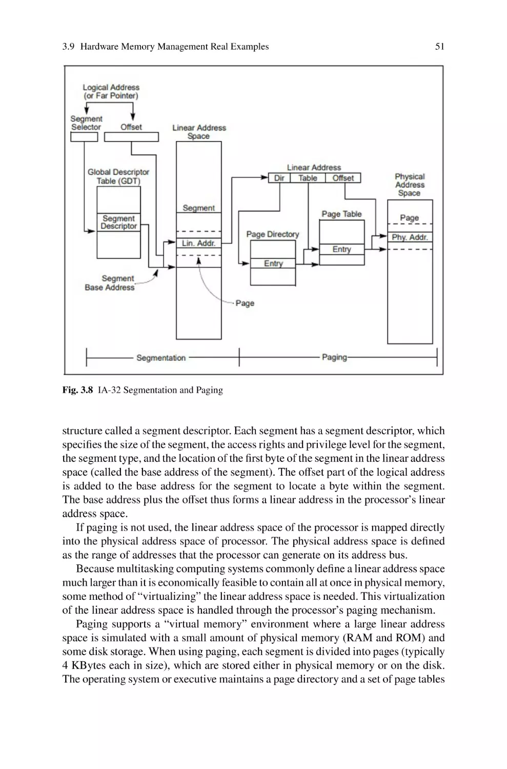
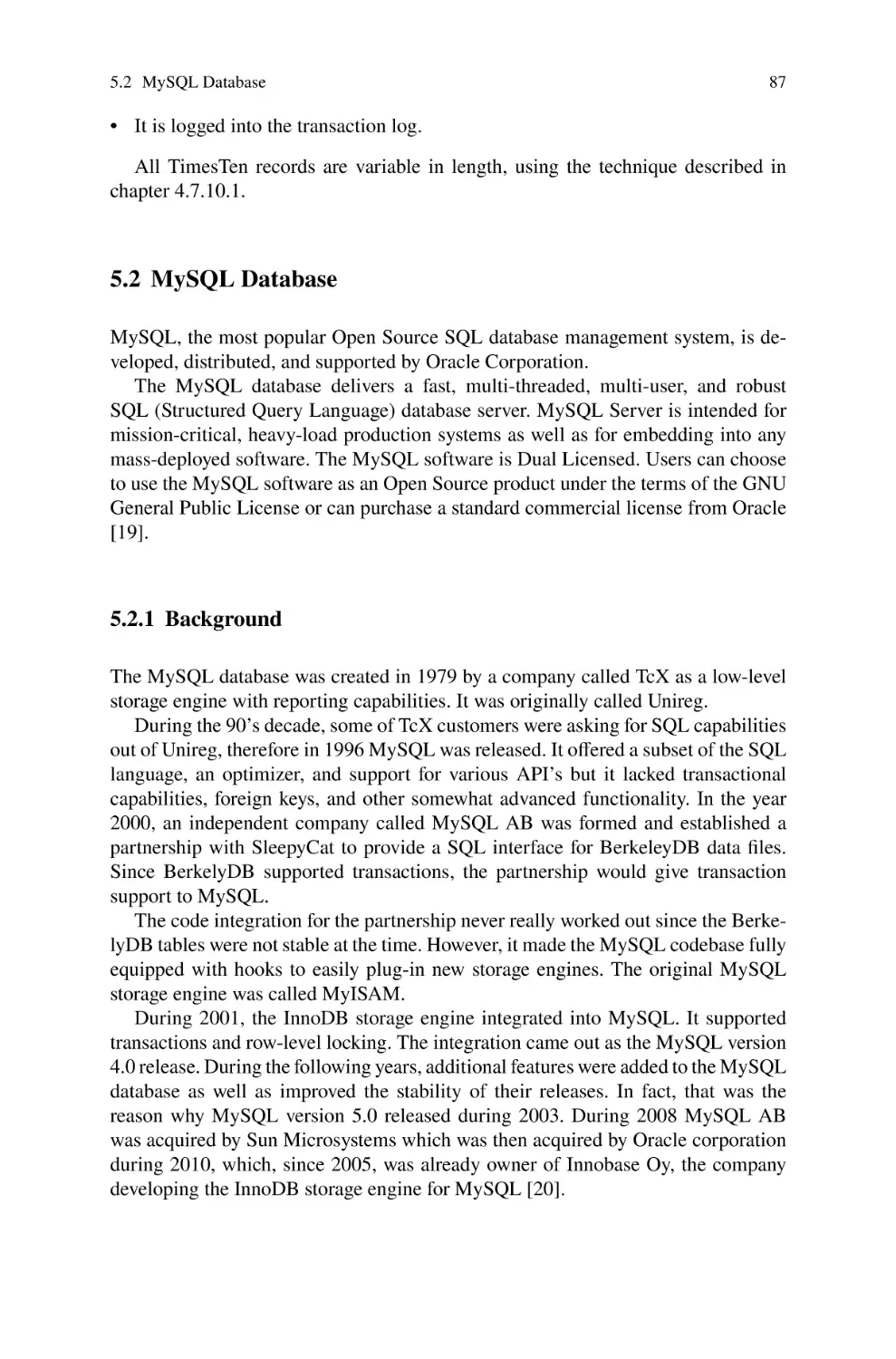
Text
SpringerBriefs in Computer Science
Pedro Mejia Alvarez · Marcelo Leon Ayala
Susana Ortega Cisneros
Main Memory
Management on
Relational
Database
Systems
SpringerBriefs in Computer Science
Series Editors
Stan Zdonik, Brown University, Providence, RI, USA
Shashi Shekhar, University of Minnesota, Minneapolis, MN, USA
Xindong Wu, University of Vermont, Burlington, VT, USA
Lakhmi C. Jain, University of South Australia, Adelaide, SA, Australia
David Padua, University of Illinois Urbana-Champaign, Urbana, IL, USA
Xuemin Sherman Shen, University of Waterloo, Waterloo, ON, Canada
Borko Furht, Florida Atlantic University, Boca Raton, FL, USA
V. S. Subrahmanian, University of Maryland, College Park, MD, USA
Martial Hebert, Carnegie Mellon University, Pittsburgh, PA, USA
Katsushi Ikeuchi, University of Tokyo, Tokyo, Japan
Bruno Siciliano, Università di Napoli Federico II, Napoli, Italy
Sushil Jajodia, George Mason University, Fairfax, VA, USA
Newton Lee, Institute for Education, Research and Scholarships, Los Angeles,
CA, USA
SpringerBriefs present concise summaries of cutting-edge research and practical
applications across a wide spectrum of fields. Featuring compact volumes of 50 to
125 pages, the series covers a range of content from professional to academic.
Typical topics might include:
• A timely report of state-of-the art analytical techniques
• A bridge between new research results, as published in journal articles, and a
contextual literature review
• A snapshot of a hot or emerging topic
• An in-depth case study or clinical example
• A presentation of core concepts that students must understand in order to make
independent contributions
Briefs allow authors to present their ideas and readers to absorb them with minimal
time investment. Briefs will be published as part of Springer’s eBook collection,
with millions of users worldwide. In addition, Briefs will be available for individual
print and electronic purchase. Briefs are characterized by fast, global electronic
dissemination, standard publishing contracts, easy-to-use manuscript preparation
and formatting guidelines, and expedited production schedules. We aim for publication 8–12 weeks after acceptance. Both solicited and unsolicited manuscripts
are considered for publication in this series.
**Indexing: This series is indexed in Scopus, Ei-Compendex, and zbMATH **
Pedro Mejia Alvarez • Marcelo Leon Ayala
Susana Ortega Cisneros
Main Memory
Management on
Relational
Database
Systems
Pedro Mejia Alvarez
Computacion
CINVESTAV-Guadalajara
Zapopan, Mexico
Marcelo Leon Ayala
Oracle
Redwood City, CA, USA
Susana Ortega Cisneros
CINVESTAV-Guadalajara
Zapopan, Mexico
ISSN 2191-5776 (electronic)
ISSN 2191-5768
SpringerBriefs in Computer Science
ISBN 978-3-031-13294-0
ISBN 978-3-031-13295-7 (eBook)
https://doi.org/10.1007/978-3-031-13295-7
© The Author(s), under exclusive license to Springer Nature Switzerland AG 2022
This work is subject to copyright. All rights are solely and exclusively licensed by the Publisher, whether
the whole or part of the material is concerned, specifically the rights of translation, reprinting, reuse of
illustrations, recitation, broadcasting, reproduction on microfilms or in any other physical way, and
transmission or information storage and retrieval, electronic adaptation, computer software, or by similar
or dissimilar methodology now known or hereafter developed.
The use of general descriptive names, registered names, trademarks, service marks, etc. in this publication
does not imply, even in the absence of a specific statement, that such names are exempt from the relevant
protective laws and regulations and therefore free for general use.
The publisher, the authors, and the editors are safe to assume that the advice and information in this book
are believed to be true and accurate at the date of publication. Neither the publisher nor the authors or
the editors give a warranty, expressed or implied, with respect to the material contained herein or for any
errors or omissions that may have been made. The publisher remains neutral with regard to jurisdictional
claims in published maps and institutional affiliations.
This Springer imprint is published by the registered company Springer Nature Switzerland AG
The registered company address is: Gewerbestrasse 11, 6330 Cham, Switzerland
This book is dedicated to my daughter
Carolina Mejia-Moya.
Preface
Big Data applications has initiated much research to develop systems for supporting
low latency execution and real-time data analytics. Existing disk-based systems can
no longer offer timely response due to the high access latency to hard disks. The
low performance is now also becoming an obstacle for organizations which provide
a real-time service (e.g., realtime bidding, advertising, social gaming). For instance,
trading companies require to detect sudden changes in the trading prices and react
instantly (in several milliseconds), which is impossible to achieve using traditional
disk-based processing-storage systems. To meet the strict real-time requirements for
analyzing mass amounts of data and servicing requests within milliseconds, an inmemory database system that keeps the data in the random access memory (RAM)
all the time is necessary.
Nowadays, there is a trend where memory will eventually replace disk and the
role of disks must inevitably become more archival. Also, multi-core processors
and the availability of large amounts of main memory at low cost are creating new
breakthroughs, making it viable to build in-memory systems where a significant part,
of the database fits in memory.
Similarly, there have been significant advances in non-volatile memory (NVM)
such as SSD and the recent launch of various NVMs such as phase change memory
(PCM). The number of I/O operations per second in such devices is much greater
than hard disks. Modern high-end servers have multiple sockets, each of which have
tens or hundreds of gigabytes of DRAM, and tens of cores, and in total, a server may
have several terabytes of DRAM and hundreds of cores. Moreover, in a distributed
environment, it is possible to aggregate the memories from a large number of server
nodes to the extent that the aggregated memory is able to keep all the data for a
variety of large-scale applications.
Database systems have been increasing their capacity over the last few decades,
mainly driven by advances in hardware, availability of large amounts of data, collection of data at an unprecedented rate, emerging applications and so on. The
landscape of data management systems is increasingly fragmented based on application domains (i.e., applications relying on relational data, graph-based data, stream
data).
vii
viii
Preface
In business operations, real-time predictability and high speed is not an option,
but a must. Hence every opportunity must be exploited to improve performance,
including reducing dependency on the hard disk, adding more memory to make
more data resident in the memory, and even deploying an in-memory system where
all data can be kept in memory.
Most commercial database vendors have recently introduced in-memory database
processing to support large-scale applications completely in memory. Therefore,
efficient in-memory data management is a necessity for various applications. Nevertheless, in-memory data management is still at its infancy, and is likely to evolve
over the next few years.
In this book, we focus on in-memory Relational Data Base systems; readers are
referred to [65] for a survey on disk-based systems.
CINVESTAV-Guadalajara, Mexico
Oracle, Redwood City California, USA,
CINVESTAV-Guadalajara, Mexico
Pedro Mejia Alvarez
Marcelo Leon Ayala
Susana Ortega Cisneros
Acknowledgements
We would like to thank, CONACYT and Secretaría de Innovación, Ciencia y Tecnología del Estado de Jalisco, Mexico, for their support in the project: Centro de
Innovación, Desarrollo y Tecnológico y Aplicaciones de Internet de las Cosas.
Project No.Jal-2015-C03- 272478.
ix
Contents
1
The Memory System . . . . . . . . . . . . . . . . . . . . . . . . . . . . . . . . . . . . . . . . . . . 1
1.1 Von Neumann Architecture . . . . . . . . . . . . . . . . . . . . . . . . . . . . . . . . . . 1
1.2 Memory . . . . . . . . . . . . . . . . . . . . . . . . . . . . . . . . . . . . . . . . . . . . . . . . . . 2
1.3 Memory Organization . . . . . . . . . . . . . . . . . . . . . . . . . . . . . . . . . . . . . . . 3
1.4 Memory Technologies . . . . . . . . . . . . . . . . . . . . . . . . . . . . . . . . . . . . . . 4
1.4.1 Register . . . . . . . . . . . . . . . . . . . . . . . . . . . . . . . . . . . . . . . . . . . . 5
1.4.2 Cache . . . . . . . . . . . . . . . . . . . . . . . . . . . . . . . . . . . . . . . . . . . . . . 5
1.4.3 SRAM: Static Random Access Memory . . . . . . . . . . . . . . . . . 6
1.4.4 DRAM: Dynamic Random Access Memory . . . . . . . . . . . . . . 7
1.4.5 Flash Memory . . . . . . . . . . . . . . . . . . . . . . . . . . . . . . . . . . . . . . . 8
1.4.6 NVM: Non Volatile Memory . . . . . . . . . . . . . . . . . . . . . . . . . . 8
1.4.7 Magnetic Disks . . . . . . . . . . . . . . . . . . . . . . . . . . . . . . . . . . . . . . 9
1.5 NUMA: Non-Uniform Memory Access . . . . . . . . . . . . . . . . . . . . . . . . 10
2
Memory Management . . . . . . . . . . . . . . . . . . . . . . . . . . . . . . . . . . . . . . . . . .
2.1 Background . . . . . . . . . . . . . . . . . . . . . . . . . . . . . . . . . . . . . . . . . . . . . . .
2.2 Address Binding . . . . . . . . . . . . . . . . . . . . . . . . . . . . . . . . . . . . . . . . . . .
2.3 Logical and Physical Address Space . . . . . . . . . . . . . . . . . . . . . . . . . . .
2.4 Dynamic Loading . . . . . . . . . . . . . . . . . . . . . . . . . . . . . . . . . . . . . . . . . .
2.5 Dynamic Linking and Shared Libraries . . . . . . . . . . . . . . . . . . . . . . . .
2.6 Swapping . . . . . . . . . . . . . . . . . . . . . . . . . . . . . . . . . . . . . . . . . . . . . . . . .
2.6.1 Standard Swapping . . . . . . . . . . . . . . . . . . . . . . . . . . . . . . . . . . .
2.7 Cache Management . . . . . . . . . . . . . . . . . . . . . . . . . . . . . . . . . . . . . . . . .
2.7.1 Cache Misses . . . . . . . . . . . . . . . . . . . . . . . . . . . . . . . . . . . . . . .
2.7.2 Writing into the Cache . . . . . . . . . . . . . . . . . . . . . . . . . . . . . . . .
2.7.3 Cache Associativity . . . . . . . . . . . . . . . . . . . . . . . . . . . . . . . . . .
2.7.4 Block Replacement . . . . . . . . . . . . . . . . . . . . . . . . . . . . . . . . . .
2.7.5 Multilevel Caches . . . . . . . . . . . . . . . . . . . . . . . . . . . . . . . . . . . .
2.8 Contiguous Memory Allocation . . . . . . . . . . . . . . . . . . . . . . . . . . . . . .
2.9 Fragmentation . . . . . . . . . . . . . . . . . . . . . . . . . . . . . . . . . . . . . . . . . . . . .
2.10 Segmentation . . . . . . . . . . . . . . . . . . . . . . . . . . . . . . . . . . . . . . . . . . . . . .
13
13
14
15
16
16
17
18
18
19
20
20
20
21
21
22
22
xi
xii
3
Contents
2.11 Paging . . . . . . . . . . . . . . . . . . . . . . . . . . . . . . . . . . . . . . . . . . . . . . . . . . . .
2.11.1 Hardware Support . . . . . . . . . . . . . . . . . . . . . . . . . . . . . . . . . . .
2.11.2 Shared Memory . . . . . . . . . . . . . . . . . . . . . . . . . . . . . . . . . . . . .
2.12 Page Table Organization . . . . . . . . . . . . . . . . . . . . . . . . . . . . . . . . . . . . .
2.12.1 Hierarchical Paging . . . . . . . . . . . . . . . . . . . . . . . . . . . . . . . . . .
2.12.2 Hashed Page Table . . . . . . . . . . . . . . . . . . . . . . . . . . . . . . . . . . .
2.12.3 Inverted Page Table . . . . . . . . . . . . . . . . . . . . . . . . . . . . . . . . . .
2.13 Memory Protection . . . . . . . . . . . . . . . . . . . . . . . . . . . . . . . . . . . . . . . . .
2.13.1 Protection in Contiguous Memory Allocation . . . . . . . . . . . . .
2.13.2 Protection in Paged Memory . . . . . . . . . . . . . . . . . . . . . . . . . . .
23
24
24
25
25
26
26
26
27
27
Virtual Memory . . . . . . . . . . . . . . . . . . . . . . . . . . . . . . . . . . . . . . . . . . . . . . .
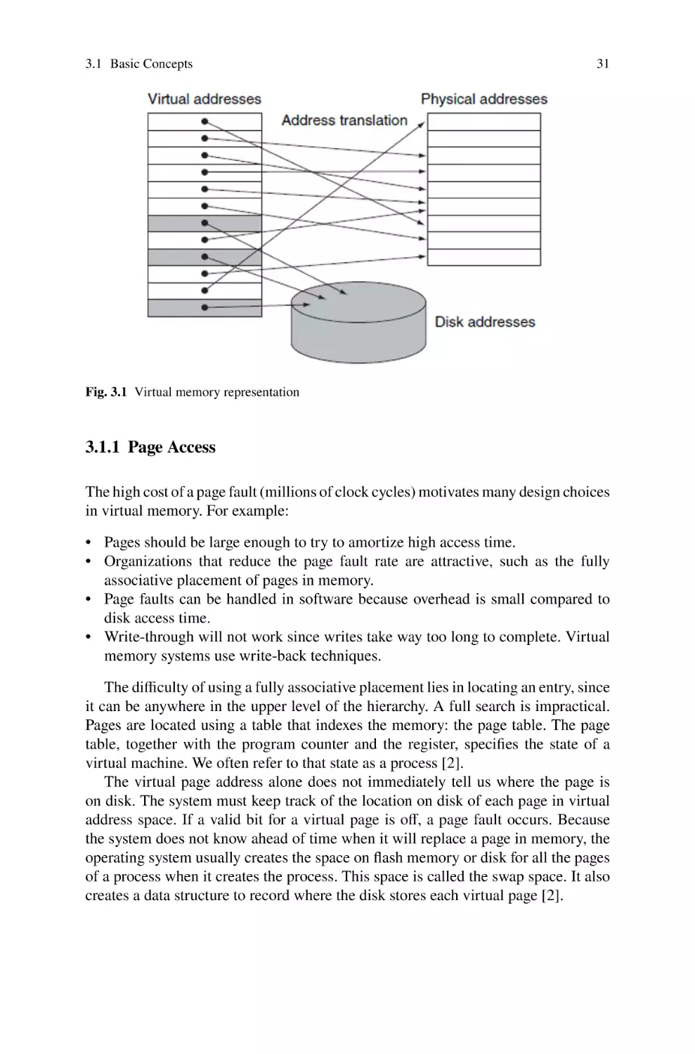
3.1 Basic Concepts . . . . . . . . . . . . . . . . . . . . . . . . . . . . . . . . . . . . . . . . . . . .
3.1.1 Page Access . . . . . . . . . . . . . . . . . . . . . . . . . . . . . . . . . . . . . . . . .
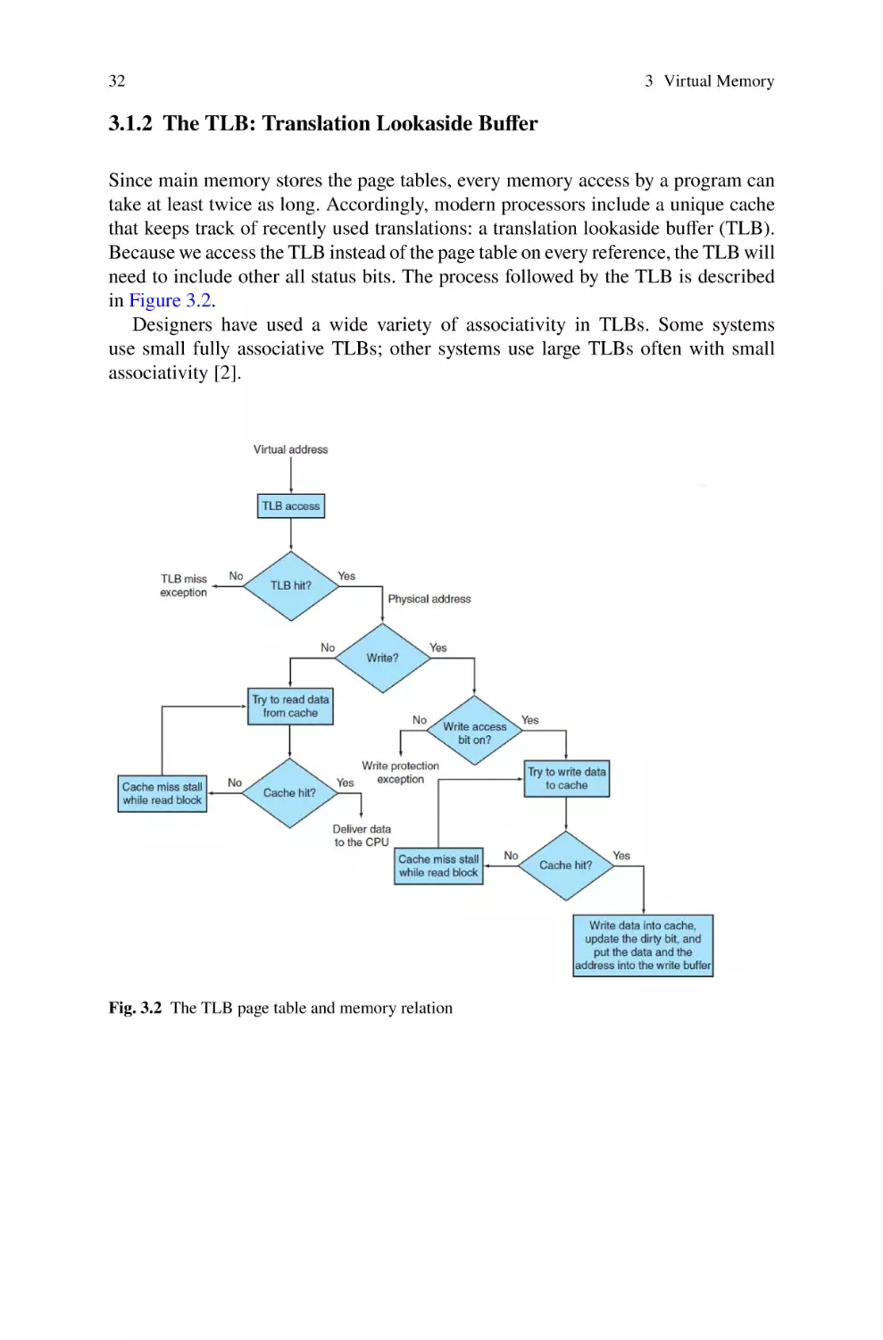
3.1.2 The TLB: Translation Lookaside Buffer . . . . . . . . . . . . . . . . .
3.1.3 Virtualization Challenges . . . . . . . . . . . . . . . . . . . . . . . . . . . . .
3.2 Demand Paging . . . . . . . . . . . . . . . . . . . . . . . . . . . . . . . . . . . . . . . . . . . .
3.2.1 Basic Concepts . . . . . . . . . . . . . . . . . . . . . . . . . . . . . . . . . . . . . .
3.2.2 Performance Considerations . . . . . . . . . . . . . . . . . . . . . . . . . . .
3.3 Page Replacement . . . . . . . . . . . . . . . . . . . . . . . . . . . . . . . . . . . . . . . . . .
3.3.1 Basic Page Replacement . . . . . . . . . . . . . . . . . . . . . . . . . . . . . .
3.3.2 FIFO and Optimal Page Replacement . . . . . . . . . . . . . . . . . . .
3.3.3 LRU Page Replacement . . . . . . . . . . . . . . . . . . . . . . . . . . . . . . .
3.3.4 LRU Approximation Page Replacement . . . . . . . . . . . . . . . . .
3.3.5 Counting Based Page Replacement . . . . . . . . . . . . . . . . . . . . .
3.3.6 Page Buffering . . . . . . . . . . . . . . . . . . . . . . . . . . . . . . . . . . . . . .
3.3.7 Applications and Page Replacement . . . . . . . . . . . . . . . . . . . . .
3.4 Allocation of Frames . . . . . . . . . . . . . . . . . . . . . . . . . . . . . . . . . . . . . . . .
3.4.1 Allocation Algorithms . . . . . . . . . . . . . . . . . . . . . . . . . . . . . . . .
3.4.2 Allocation Scope . . . . . . . . . . . . . . . . . . . . . . . . . . . . . . . . . . . .
3.4.3 Non Uniform Memory Access considerations . . . . . . . . . . . . .
3.5 Memory Protection on Virtual Memory . . . . . . . . . . . . . . . . . . . . . . . .
3.6 Thrashing . . . . . . . . . . . . . . . . . . . . . . . . . . . . . . . . . . . . . . . . . . . . . . . . .
3.6.1 The Working Set Model . . . . . . . . . . . . . . . . . . . . . . . . . . . . . . .
3.6.2 Page Fault Frequency . . . . . . . . . . . . . . . . . . . . . . . . . . . . . . . . .
3.7 A Common Framework for Managing Memory . . . . . . . . . . . . . . . . . .
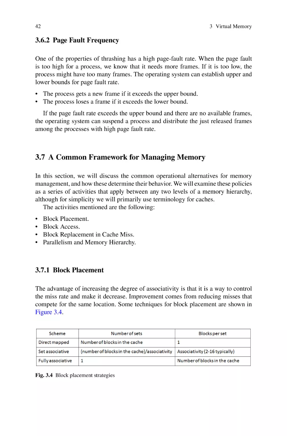
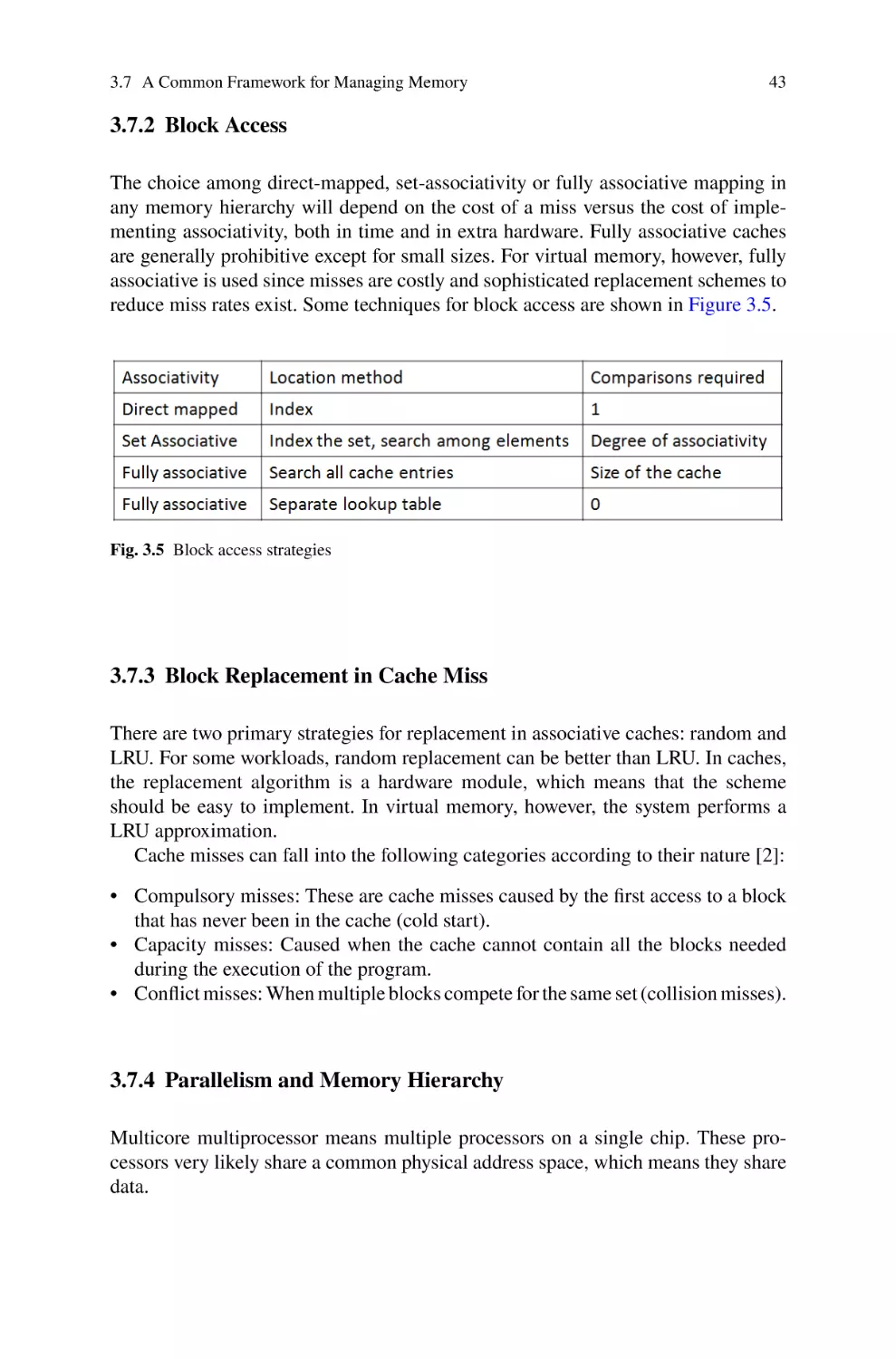
3.7.1 Block Placement . . . . . . . . . . . . . . . . . . . . . . . . . . . . . . . . . . . . .
3.7.2 Block Access . . . . . . . . . . . . . . . . . . . . . . . . . . . . . . . . . . . . . . . .
3.7.3 Block Replacement in Cache Miss . . . . . . . . . . . . . . . . . . . . . .
3.7.4 Parallelism and Memory Hierarchy . . . . . . . . . . . . . . . . . . . . .
3.8 Other Considerations . . . . . . . . . . . . . . . . . . . . . . . . . . . . . . . . . . . . . . .
3.8.1 Pre-Paging . . . . . . . . . . . . . . . . . . . . . . . . . . . . . . . . . . . . . . . . . .
3.8.2 Page Size . . . . . . . . . . . . . . . . . . . . . . . . . . . . . . . . . . . . . . . . . . .
3.8.3 TLB Reach . . . . . . . . . . . . . . . . . . . . . . . . . . . . . . . . . . . . . . . . .
3.8.4 Inverted Page Table . . . . . . . . . . . . . . . . . . . . . . . . . . . . . . . . . .
29
29
31
32
33
33
33
34
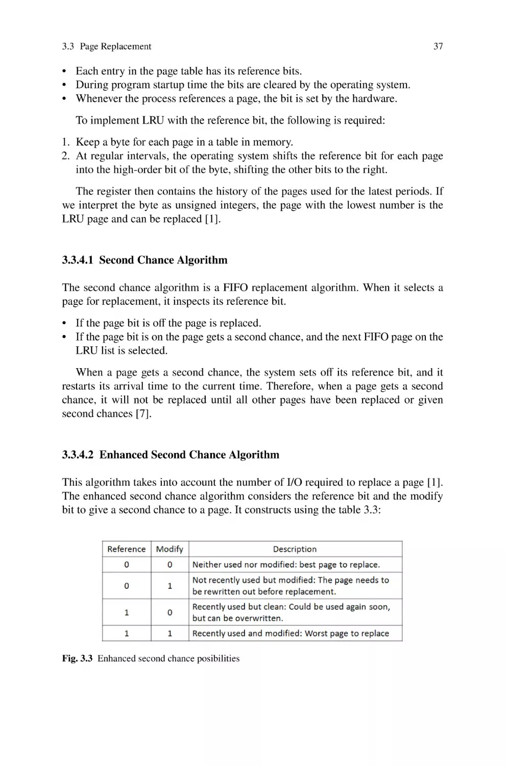
34
35
35
36
36
38
38
38
38
39
39
40
40
40
41
42
42
42
43
43
43
45
45
45
46
46
Contents
4
xiii
3.8.5 Program Structure . . . . . . . . . . . . . . . . . . . . . . . . . . . . . . . . . . .
3.8.6 Page Locking . . . . . . . . . . . . . . . . . . . . . . . . . . . . . . . . . . . . . . .
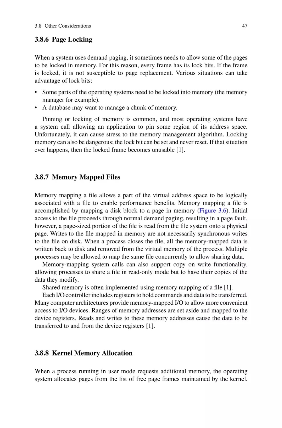
3.8.7 Memory Mapped Files . . . . . . . . . . . . . . . . . . . . . . . . . . . . . . . .
3.8.8 Kernel Memory Allocation . . . . . . . . . . . . . . . . . . . . . . . . . . . .
3.8.9 Virtual Machines . . . . . . . . . . . . . . . . . . . . . . . . . . . . . . . . . . . .
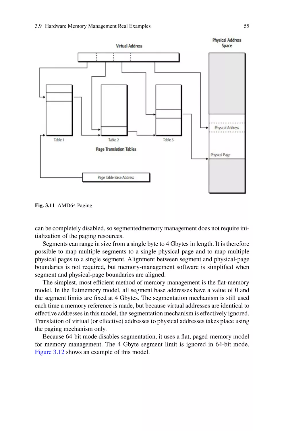
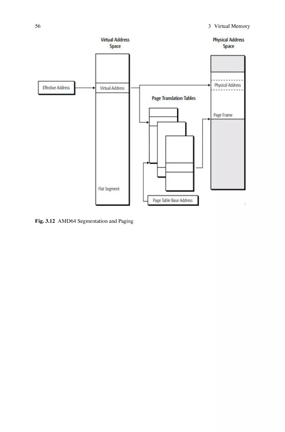
3.9 Hardware Memory Management Real Examples . . . . . . . . . . . . . . . . .
3.9.1 Memory Management in the IA-32 Architecture . . . . . . . . . .
3.9.2 Memory Management in the AMD64 Architecture . . . . . . . .
46
47
47
47
49
50
50
52
Databases and the Memory System . . . . . . . . . . . . . . . . . . . . . . . . . . . . . . .
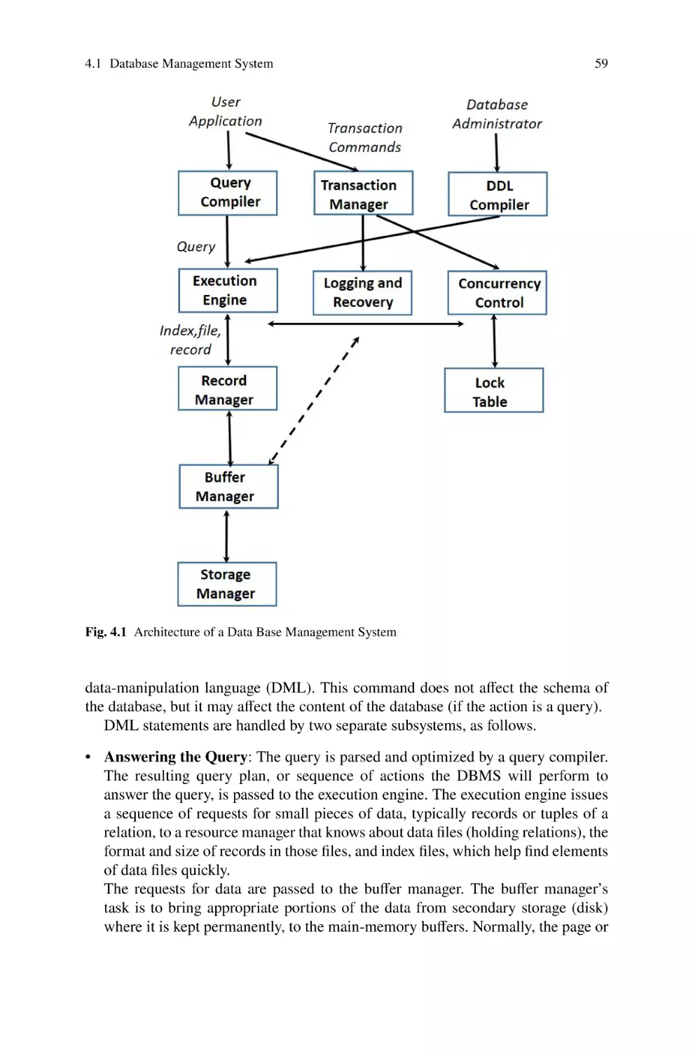
4.1 Database Management System . . . . . . . . . . . . . . . . . . . . . . . . . . . . . . . .
4.1.1 Data-Definition Language Commands . . . . . . . . . . . . . . . . . . .
4.1.2 Query Processing . . . . . . . . . . . . . . . . . . . . . . . . . . . . . . . . . . . .
4.1.3 Storage and Buffer Management . . . . . . . . . . . . . . . . . . . . . . . .
4.1.4 Transaction Processing . . . . . . . . . . . . . . . . . . . . . . . . . . . . . . .
4.1.5 The Query Processor . . . . . . . . . . . . . . . . . . . . . . . . . . . . . . . . .
4.2 In-Memory Data Bases . . . . . . . . . . . . . . . . . . . . . . . . . . . . . . . . . . . . . .
4.3 Types of Databases . . . . . . . . . . . . . . . . . . . . . . . . . . . . . . . . . . . . . . . . .
4.3.1 The Object Model . . . . . . . . . . . . . . . . . . . . . . . . . . . . . . . . . . . .
4.3.2 In-Memory NoSQL Databases . . . . . . . . . . . . . . . . . . . . . . . . .
4.4 The Relational Model . . . . . . . . . . . . . . . . . . . . . . . . . . . . . . . . . . . . . . .
4.4.1 Relational Database Storage Structures . . . . . . . . . . . . . . . . . .
4.4.2 User Interface . . . . . . . . . . . . . . . . . . . . . . . . . . . . . . . . . . . . . . .
4.4.3 Database Workload . . . . . . . . . . . . . . . . . . . . . . . . . . . . . . . . . .
4.5 Database Storage Management . . . . . . . . . . . . . . . . . . . . . . . . . . . . . . .
4.5.1 Data on External Storage . . . . . . . . . . . . . . . . . . . . . . . . . . . . . .
4.5.2 File Organization . . . . . . . . . . . . . . . . . . . . . . . . . . . . . . . . . . . .
4.5.3 Indexing . . . . . . . . . . . . . . . . . . . . . . . . . . . . . . . . . . . . . . . . . . . .
4.6 Index Data Structures . . . . . . . . . . . . . . . . . . . . . . . . . . . . . . . . . . . . . . .
4.7 Storing Data: Disks and Files . . . . . . . . . . . . . . . . . . . . . . . . . . . . . . . . .
4.7.1 The Memory Hierarchy . . . . . . . . . . . . . . . . . . . . . . . . . . . . . . .
4.7.2 Disks . . . . . . . . . . . . . . . . . . . . . . . . . . . . . . . . . . . . . . . . . . . . . .
4.7.3 Redundant Array of Independent Disks . . . . . . . . . . . . . . . . . .
4.7.4 Disk Space Management . . . . . . . . . . . . . . . . . . . . . . . . . . . . . .
4.7.5 Buffer Management . . . . . . . . . . . . . . . . . . . . . . . . . . . . . . . . . .
4.7.6 Data Storage Implementation . . . . . . . . . . . . . . . . . . . . . . . . . .
4.7.7 Page Formats . . . . . . . . . . . . . . . . . . . . . . . . . . . . . . . . . . . . . . . .
4.7.8 Fixed Length Records . . . . . . . . . . . . . . . . . . . . . . . . . . . . . . . .
4.7.9 Variable Length Records . . . . . . . . . . . . . . . . . . . . . . . . . . . . . .
4.7.10 Record Formats . . . . . . . . . . . . . . . . . . . . . . . . . . . . . . . . . . . . . .
4.8 Tree Structured Indexes . . . . . . . . . . . . . . . . . . . . . . . . . . . . . . . . . . . . .
4.8.1 Indexed Sequential Access Method (ISAM) . . . . . . . . . . . . . .
4.8.2 B+Trees . . . . . . . . . . . . . . . . . . . . . . . . . . . . . . . . . . . . . . . . . . . .
4.9 Hash Based Indexes . . . . . . . . . . . . . . . . . . . . . . . . . . . . . . . . . . . . . . . .
4.9.1 Static Hashing . . . . . . . . . . . . . . . . . . . . . . . . . . . . . . . . . . . . . . .
57
57
58
58
60
61
61
62
63
63
64
64
65
65
66
66
67
67
68
69
70
70
70
71
73
73
74
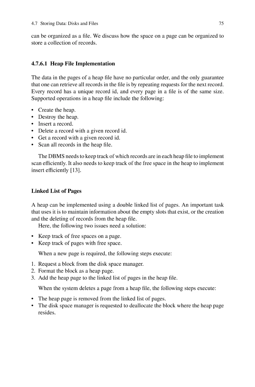
76
76
77
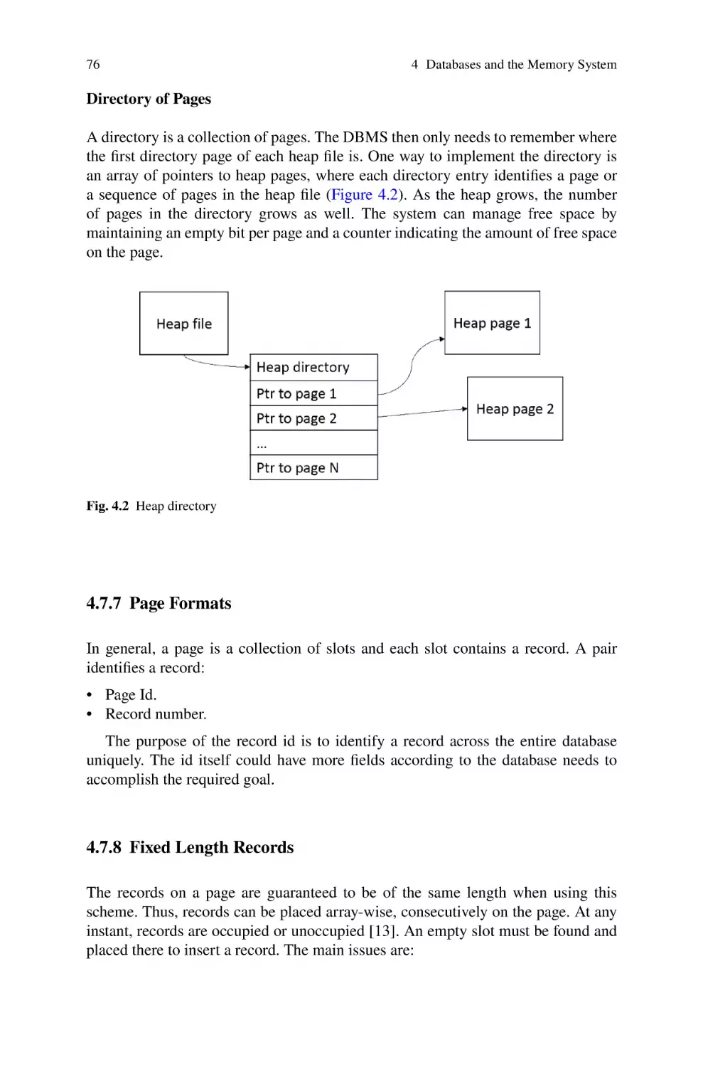
77
78
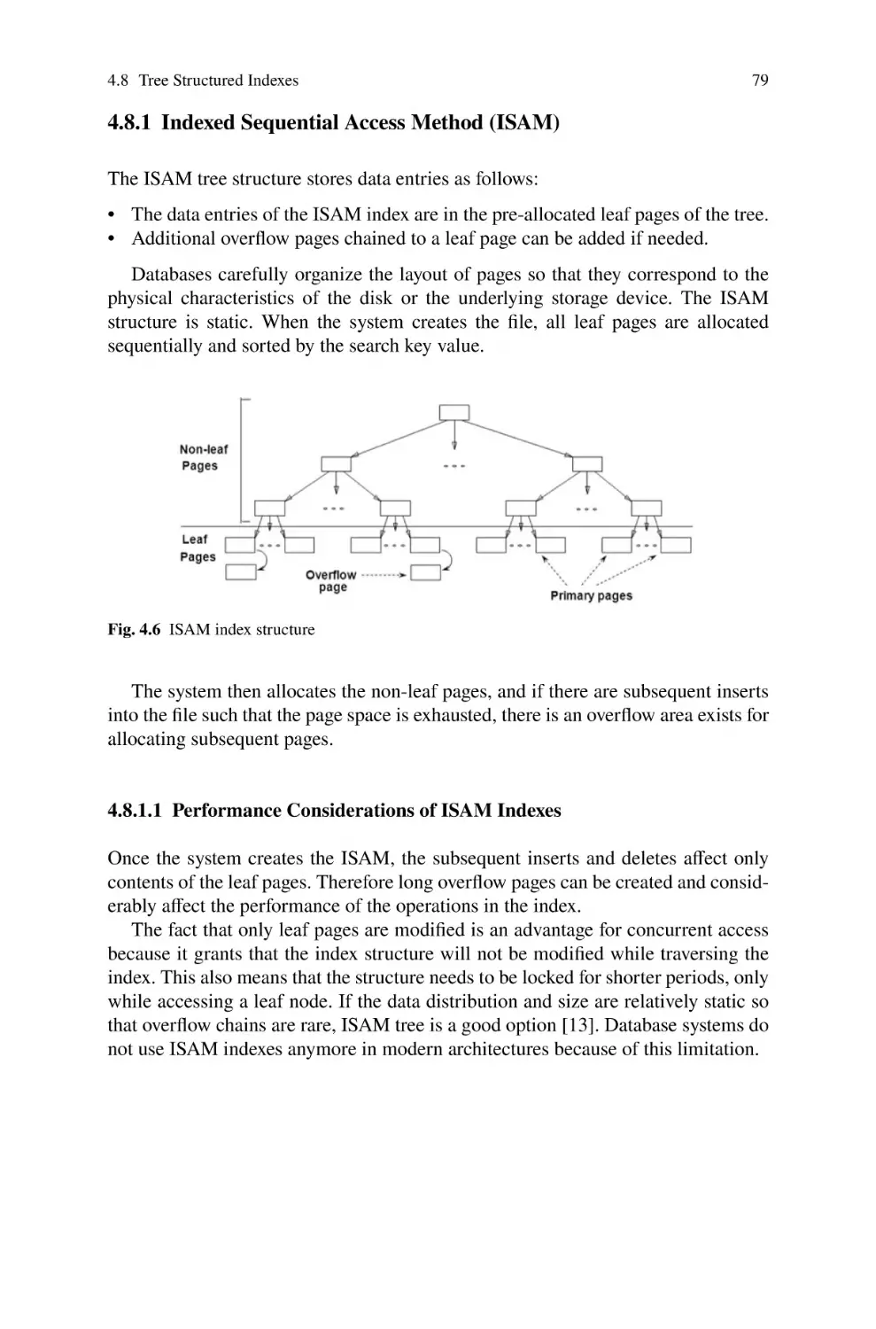
79
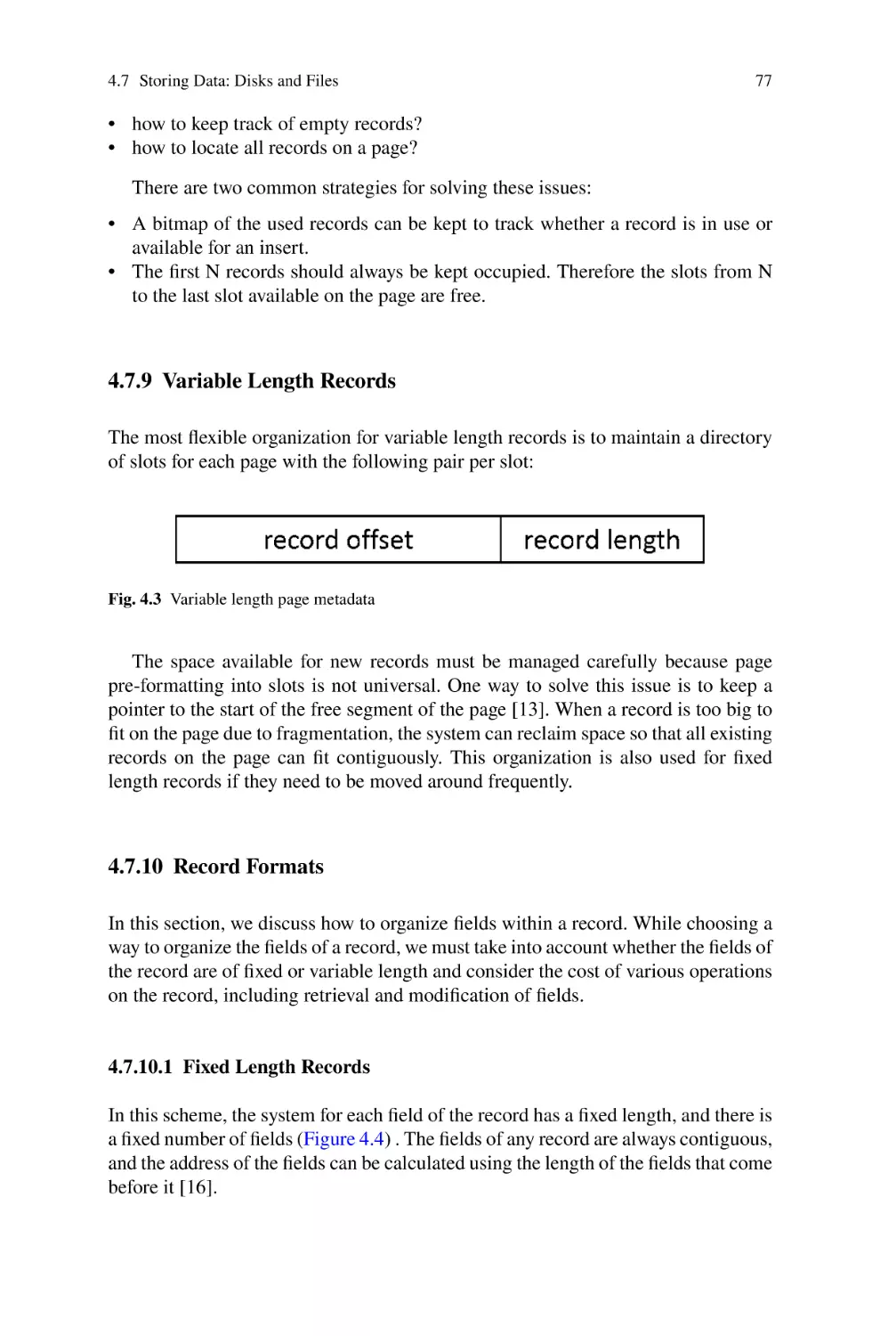
80
81
81
Contents
xiv
4.9.2
4.9.3
5
Extensible Hashing . . . . . . . . . . . . . . . . . . . . . . . . . . . . . . . . . . . 81
Linear Hashing . . . . . . . . . . . . . . . . . . . . . . . . . . . . . . . . . . . . . . 82
Database Systems: Real Examples . . . . . . . . . . . . . . . . . . . . . . . . . . . . . . .
5.1 TimesTen In-Memory Database . . . . . . . . . . . . . . . . . . . . . . . . . . . . . . .
5.1.1 Overview . . . . . . . . . . . . . . . . . . . . . . . . . . . . . . . . . . . . . . . . . . .
5.1.2 Memory Management . . . . . . . . . . . . . . . . . . . . . . . . . . . . . . . .
5.2 MySQL Database . . . . . . . . . . . . . . . . . . . . . . . . . . . . . . . . . . . . . . . . . .
5.2.1 Background . . . . . . . . . . . . . . . . . . . . . . . . . . . . . . . . . . . . . . . . .
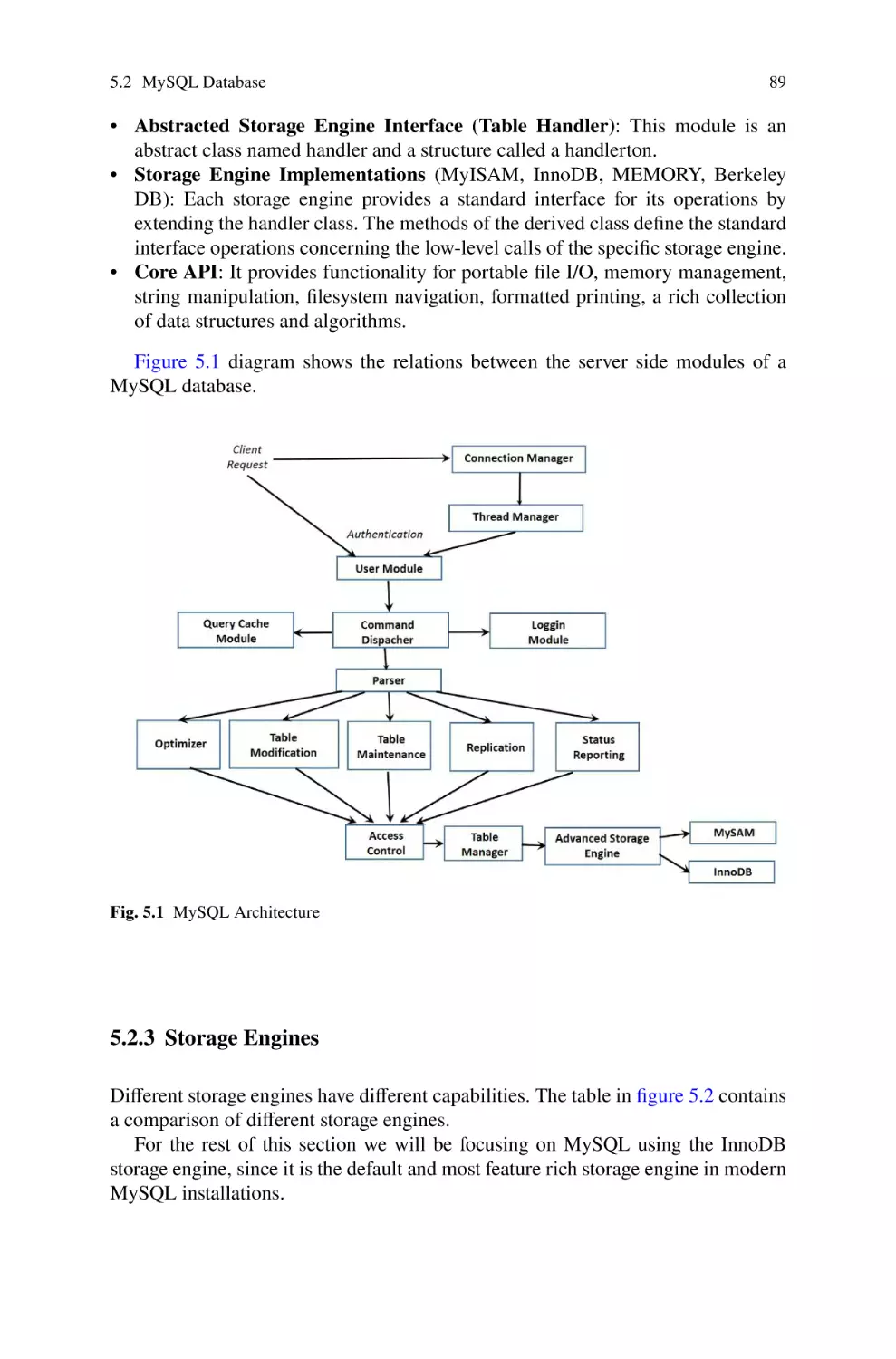
5.2.2 Architecture . . . . . . . . . . . . . . . . . . . . . . . . . . . . . . . . . . . . . . . .
5.2.3 Storage Engines . . . . . . . . . . . . . . . . . . . . . . . . . . . . . . . . . . . . .
5.3 H-Store / VoltDB Data Base Systems . . . . . . . . . . . . . . . . . . . . . . . . . .
5.3.1 Transaction Processing . . . . . . . . . . . . . . . . . . . . . . . . . . . . . . .
5.3.2 Data Overflow . . . . . . . . . . . . . . . . . . . . . . . . . . . . . . . . . . . . . .
5.3.3 Fault Tolerance . . . . . . . . . . . . . . . . . . . . . . . . . . . . . . . . . . . . . .
5.4 Hekaton Data Base System . . . . . . . . . . . . . . . . . . . . . . . . . . . . . . . . . .
5.4.1 Multi-version Concurrency Control . . . . . . . . . . . . . . . . . . . . .
5.4.2 Latch-Free Bw-Tree . . . . . . . . . . . . . . . . . . . . . . . . . . . . . . . . . .
5.4.3 Siberia in Hekaton . . . . . . . . . . . . . . . . . . . . . . . . . . . . . . . . . . .
5.5 HyPer/ScyPer Data Base Systems . . . . . . . . . . . . . . . . . . . . . . . . . . . . .
5.5.1 Snapshot in HyPer . . . . . . . . . . . . . . . . . . . . . . . . . . . . . . . . . . .
5.5.2 Register-Conscious Compilation . . . . . . . . . . . . . . . . . . . . . . . .
5.5.3 ART Indexing . . . . . . . . . . . . . . . . . . . . . . . . . . . . . . . . . . . . . . .
5.6 SAP HANA Data Base System . . . . . . . . . . . . . . . . . . . . . . . . . . . . . . .
5.6.1 Relational Stores . . . . . . . . . . . . . . . . . . . . . . . . . . . . . . . . . . . . .
5.6.2 Rich Data Analytics Support . . . . . . . . . . . . . . . . . . . . . . . . . . .
5.6.3 Temporal Query . . . . . . . . . . . . . . . . . . . . . . . . . . . . . . . . . . . . .
83
83
84
86
87
87
88
89
90
91
92
92
93
93
94
95
95
96
97
97
98
98
99
99
References . . . . . . . . . . . . . . . . . . . . . . . . . . . . . . . . . . . . . . . . . . . . . . . . . . . . . . . . . 101
Chapter 1
The Memory System
This chapter contains some concepts and techniques used for efficient in-memory
data management, including memory hierarchy, non-uniform memory access (NUMA),
and non-volatile random access memory (NVRAM). These are the basics on which
the performance of In-Memory data management systems heavily rely.
1.1 Von Neumann Architecture
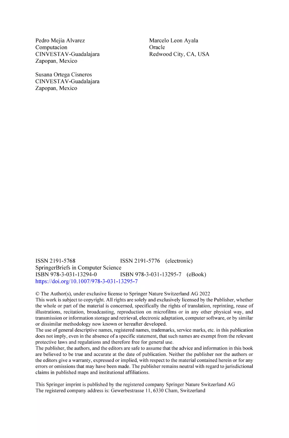
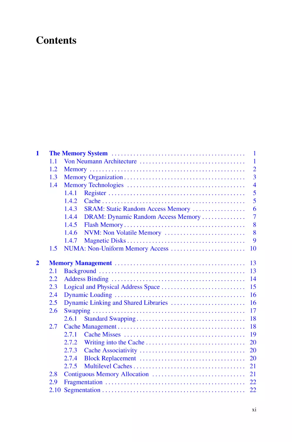
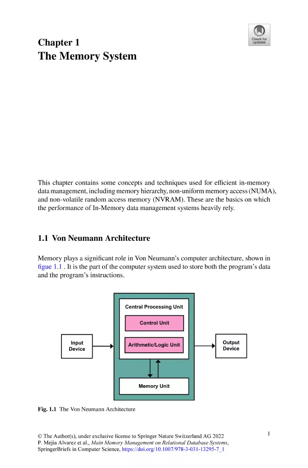
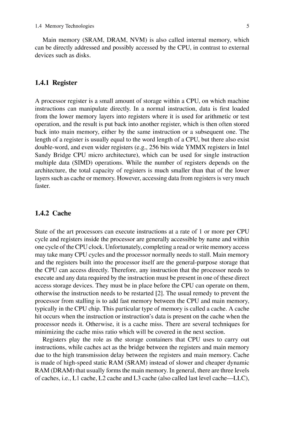
Memory plays a significant role in Von Neumann’s computer architecture, shown in
figue 1.1 . It is the part of the computer system used to store both the program’s data
and the program’s instructions.
Fig. 1.1 The Von Neumann Architecture
© The Author(s), under exclusive license to Springer Nature Switzerland AG 2022
P. Mejia Alvarez et al., Main Memory Management on Relational Database Systems,
SpringerBriefs in Computer Science, https://doi.org/10.1007/978-3-031-13295-7_1
1
1 The Memory System
2
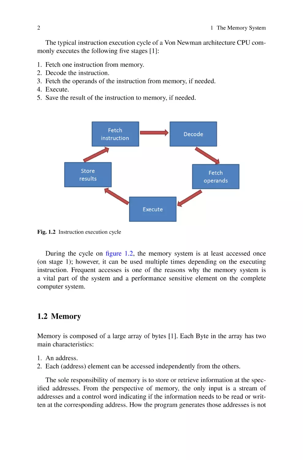
The typical instruction execution cycle of a Von Newman architecture CPU commonly executes the following five stages [1]:
1.
2.
3.
4.
5.
Fetch one instruction from memory.
Decode the instruction.
Fetch the operands of the instruction from memory, if needed.
Execute.
Save the result of the instruction to memory, if needed.
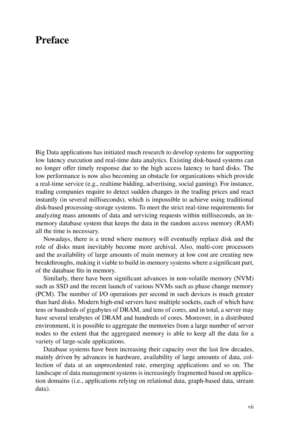
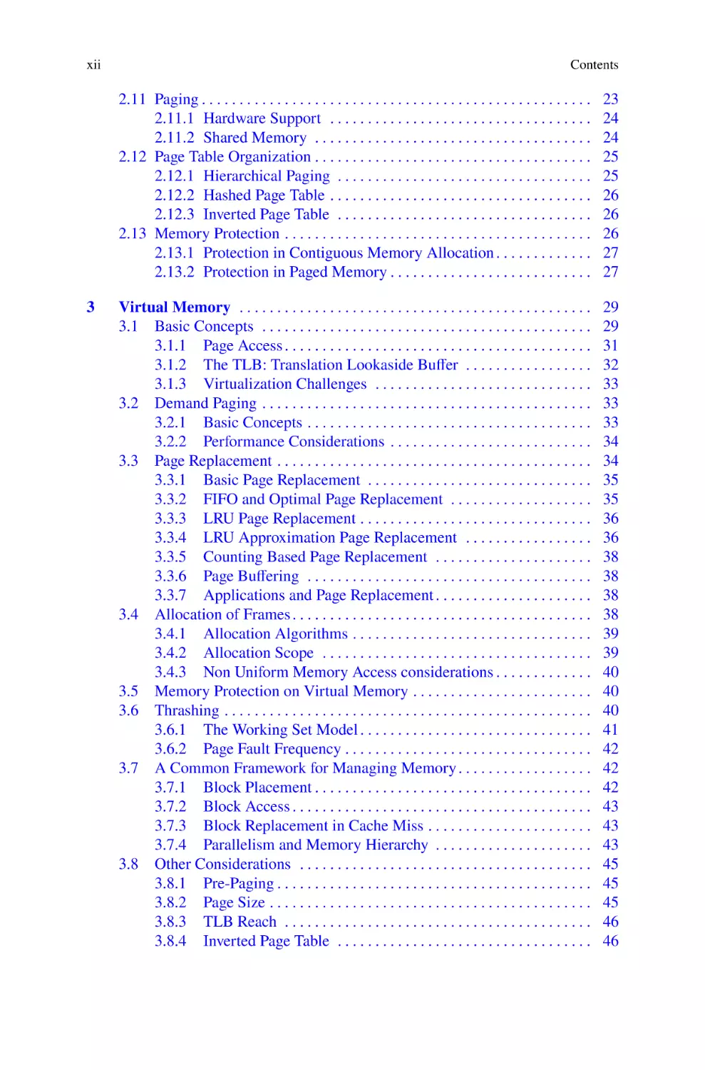
Fig. 1.2 Instruction execution cycle
During the cycle on figure 1.2, the memory system is at least accessed once
(on stage 1); however, it can be used multiple times depending on the executing
instruction. Frequent accesses is one of the reasons why the memory system is
a vital part of the system and a performance sensitive element on the complete
computer system.
1.2 Memory
Memory is composed of a large array of bytes [1]. Each Byte in the array has two
main characteristics:
1. An address.
2. Each (address) element can be accessed independently from the others.
The sole responsibility of memory is to store or retrieve information at the specified addresses. From the perspective of memory, the only input is a stream of
addresses and a control word indicating if the information needs to be read or written at the corresponding address. How the program generates those addresses is not
1.3 Memory Organization
3
essential: they could come from the program counter, array indexing, indirections,
real addresses, among others. That information is irrelevant. The behavior expected
from the memory systems is the same: to retrieve the information stored at the
specified address.
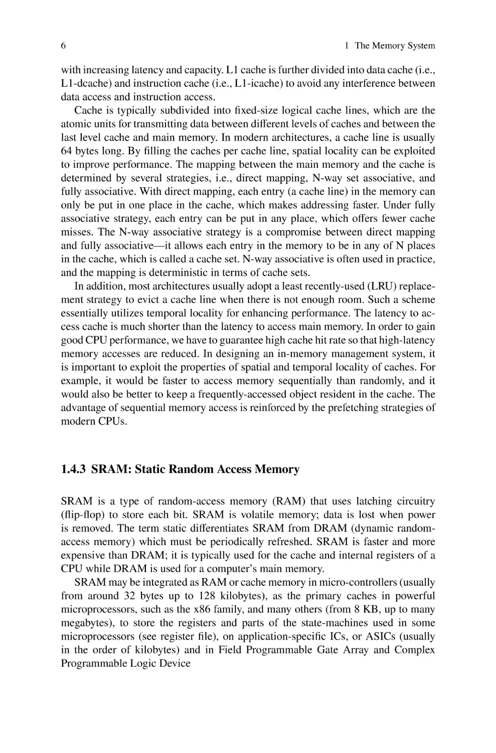
1.3 Memory Organization
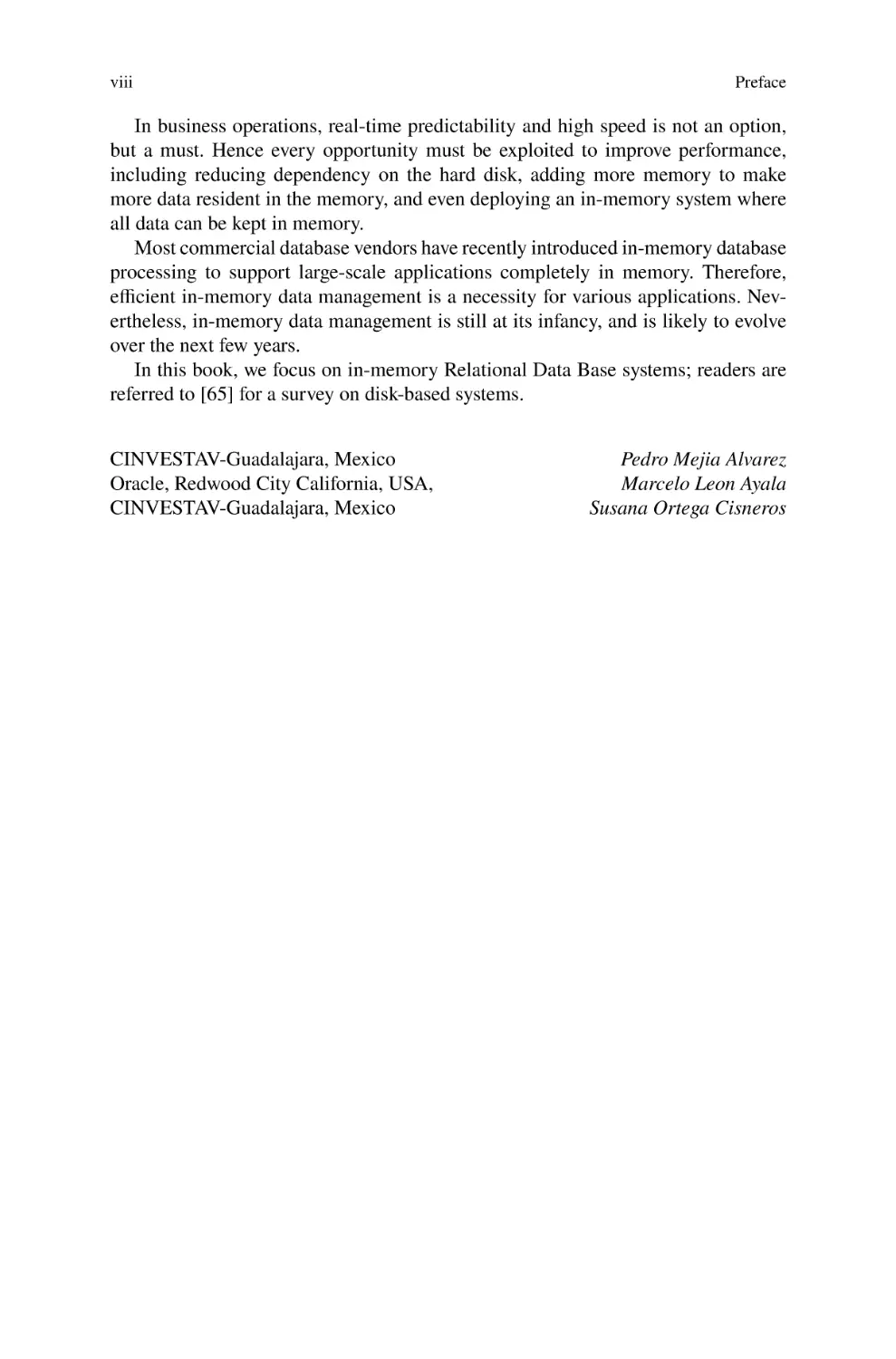
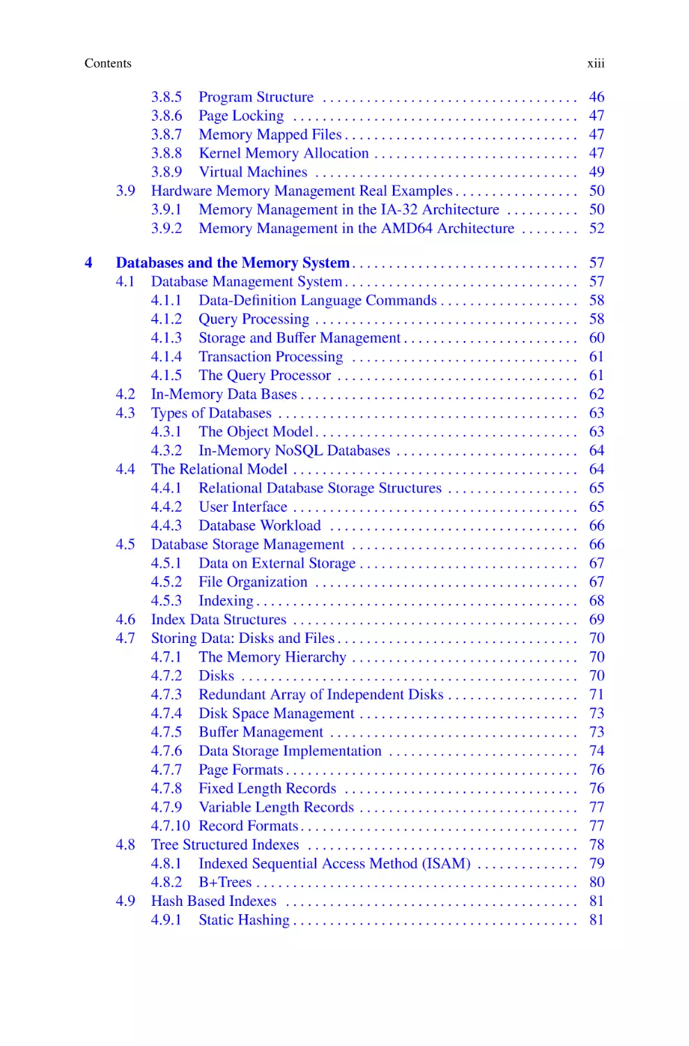
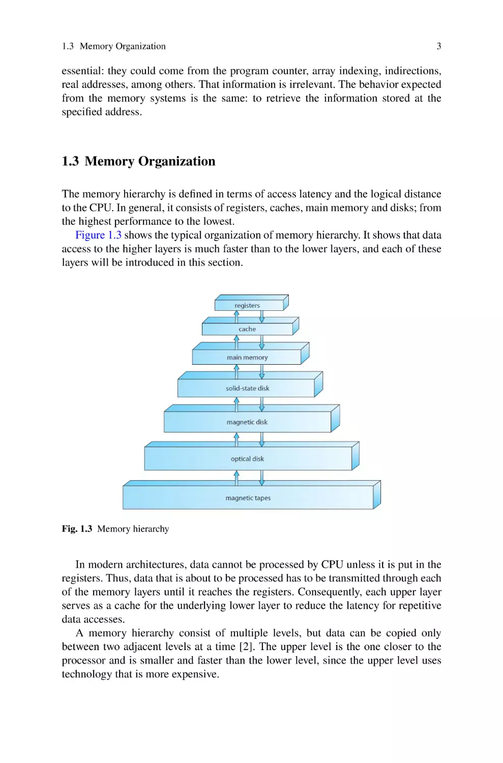
The memory hierarchy is defined in terms of access latency and the logical distance
to the CPU. In general, it consists of registers, caches, main memory and disks; from
the highest performance to the lowest.
Figure 1.3 shows the typical organization of memory hierarchy. It shows that data
access to the higher layers is much faster than to the lower layers, and each of these
layers will be introduced in this section.
Fig. 1.3 Memory hierarchy
In modern architectures, data cannot be processed by CPU unless it is put in the
registers. Thus, data that is about to be processed has to be transmitted through each
of the memory layers until it reaches the registers. Consequently, each upper layer
serves as a cache for the underlying lower layer to reduce the latency for repetitive
data accesses.
A memory hierarchy consist of multiple levels, but data can be copied only
between two adjacent levels at a time [2]. The upper level is the one closer to the
processor and is smaller and faster than the lower level, since the upper level uses
technology that is more expensive.
1 The Memory System
4
The minimum unit of information that can be either present or not present in the
two-level hierarchy is called a block or a line. If the data requested by the processor
appears in some block in the upper level, this is called a hit. If the data is not found
in the upper level, the request is called a miss. The lower level in the hierarchy is
then accessed to retrieve the block containing the requested data. The hit rate, or hit
ratio, is the fraction of memory accesses found in the upper level; it is often used as
a measure of the performance of the memory hierarchy. The miss rate is the fraction
of memory accesses not found in the upper level.
The performance of a data-intensive program highly depends on the utilization of
the memory hierarchy [2]. How to achieve both good spatial and temporal locality
is usually what matters the most in the efficiency optimization. In particular, spatial
locality assumes that the adjacent data is more likely to be accessed together, whereas
temporal locality refers to the observation that it is likely that an item will be accessed
again in the near future. Performance is the major reason for having a memory
hierarchy, so the time to service hits and misses is important. Hit time is the time
to access the upper level of the memory hierarchy, which includes the time needed
to determine whether the access is a hit or a miss. The miss penalty is the time to
replace a block in the upper level with the corresponding block from the lower level,
plus the time to deliver this block to the processor. Because the upper level is smaller
and built using faster memory parts, the hit time will be much smaller than the time
to access the next level in the hierarchy, which is the major component of the miss
penalty.
The concepts used to build memory systems affect many other aspects of a computer, including how the operating system manages memory and I/O, how compilers
generate code and even how applications use the computer [5].
1.4 Memory Technologies
There are several primary technologies of memory used nowadays in a modern
computer system [2]:
•
•
•
•
•
•
•
Register.
Cache.
SRAM: Static Random-Access Memory.
DRAM: Dynamic Random-Access Memory.
Flash Memory.
NVM: Non-Volatile Memory.
Magnetic storage.
Each category of memory has its requirements and can be implemented using
different underlying physical technologies. The classification of memory represents
an abstraction of memory technologies.
1.4 Memory Technologies
5
Main memory (SRAM, DRAM, NVM) is also called internal memory, which
can be directly addressed and possibly accessed by the CPU, in contrast to external
devices such as disks.
1.4.1 Register
A processor register is a small amount of storage within a CPU, on which machine
instructions can manipulate directly. In a normal instruction, data is first loaded
from the lower memory layers into registers where it is used for arithmetic or test
operation, and the result is put back into another register, which is then often stored
back into main memory, either by the same instruction or a subsequent one. The
length of a register is usually equal to the word length of a CPU, but there also exist
double-word, and even wider registers (e.g., 256 bits wide YMMX registers in Intel
Sandy Bridge CPU micro architecture), which can be used for single instruction
multiple data (SIMD) operations. While the number of registers depends on the
architecture, the total capacity of registers is much smaller than that of the lower
layers such as cache or memory. However, accessing data from registers is very much
faster.
1.4.2 Cache
State of the art processors can execute instructions at a rate of 1 or more per CPU
cycle and registers inside the processor are generally accessible by name and within
one cycle of the CPU clock. Unfortunately, completing a read or write memory access
may take many CPU cycles and the processor normally needs to stall. Main memory
and the registers built into the processor itself are the general-purpose storage that
the CPU can access directly. Therefore, any instruction that the processor needs to
execute and any data required by the instruction must be present in one of these direct
access storage devices. They must be in place before the CPU can operate on them,
otherwise the instruction needs to be restarted [2]. The usual remedy to prevent the
processor from stalling is to add fast memory between the CPU and main memory,
typically in the CPU chip. This particular type of memory is called a cache. A cache
hit occurs when the instruction or instruction’s data is present on the cache when the
processor needs it. Otherwise, it is a cache miss. There are several techniques for
minimizing the cache miss ratio which will be covered in the next section.
Registers play the role as the storage containers that CPU uses to carry out
instructions, while caches act as the bridge between the registers and main memory
due to the high transmission delay between the registers and main memory. Cache
is made of high-speed static RAM (SRAM) instead of slower and cheaper dynamic
RAM (DRAM) that usually forms the main memory. In general, there are three levels
of caches, i.e., L1 cache, L2 cache and L3 cache (also called last level cache—LLC),
6
1 The Memory System
with increasing latency and capacity. L1 cache is further divided into data cache (i.e.,
L1-dcache) and instruction cache (i.e., L1-icache) to avoid any interference between
data access and instruction access.
Cache is typically subdivided into fixed-size logical cache lines, which are the
atomic units for transmitting data between different levels of caches and between the
last level cache and main memory. In modern architectures, a cache line is usually
64 bytes long. By filling the caches per cache line, spatial locality can be exploited
to improve performance. The mapping between the main memory and the cache is
determined by several strategies, i.e., direct mapping, N-way set associative, and
fully associative. With direct mapping, each entry (a cache line) in the memory can
only be put in one place in the cache, which makes addressing faster. Under fully
associative strategy, each entry can be put in any place, which offers fewer cache
misses. The N-way associative strategy is a compromise between direct mapping
and fully associative—it allows each entry in the memory to be in any of N places
in the cache, which is called a cache set. N-way associative is often used in practice,
and the mapping is deterministic in terms of cache sets.
In addition, most architectures usually adopt a least recently-used (LRU) replacement strategy to evict a cache line when there is not enough room. Such a scheme
essentially utilizes temporal locality for enhancing performance. The latency to access cache is much shorter than the latency to access main memory. In order to gain
good CPU performance, we have to guarantee high cache hit rate so that high-latency
memory accesses are reduced. In designing an in-memory management system, it
is important to exploit the properties of spatial and temporal locality of caches. For
example, it would be faster to access memory sequentially than randomly, and it
would also be better to keep a frequently-accessed object resident in the cache. The
advantage of sequential memory access is reinforced by the prefetching strategies of
modern CPUs.
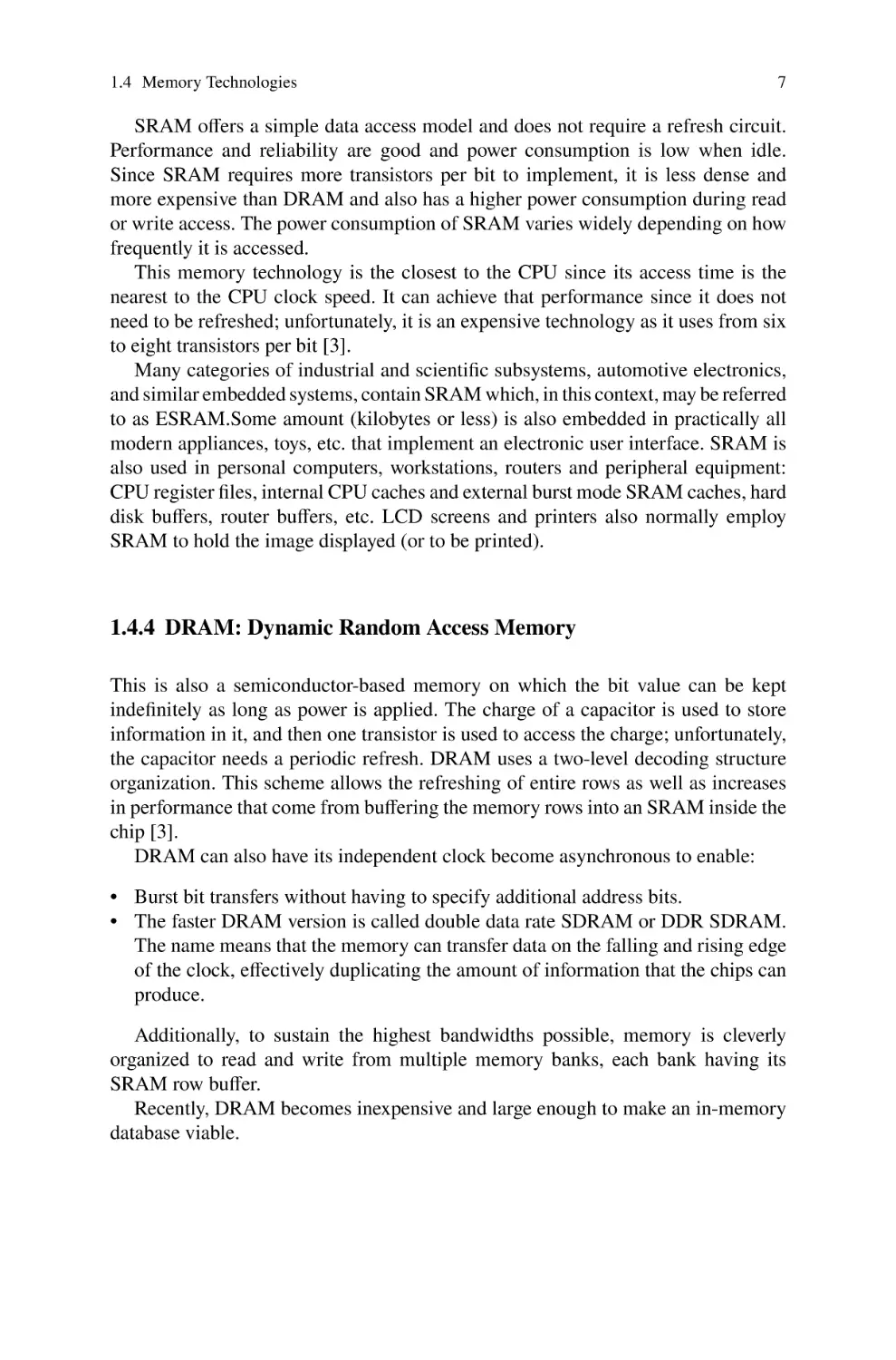
1.4.3 SRAM: Static Random Access Memory
SRAM is a type of random-access memory (RAM) that uses latching circuitry
(flip-flop) to store each bit. SRAM is volatile memory; data is lost when power
is removed. The term static differentiates SRAM from DRAM (dynamic randomaccess memory) which must be periodically refreshed. SRAM is faster and more
expensive than DRAM; it is typically used for the cache and internal registers of a
CPU while DRAM is used for a computer’s main memory.
SRAM may be integrated as RAM or cache memory in micro-controllers (usually
from around 32 bytes up to 128 kilobytes), as the primary caches in powerful
microprocessors, such as the x86 family, and many others (from 8 KB, up to many
megabytes), to store the registers and parts of the state-machines used in some
microprocessors (see register file), on application-specific ICs, or ASICs (usually
in the order of kilobytes) and in Field Programmable Gate Array and Complex
Programmable Logic Device
1.4 Memory Technologies
7
SRAM offers a simple data access model and does not require a refresh circuit.
Performance and reliability are good and power consumption is low when idle.
Since SRAM requires more transistors per bit to implement, it is less dense and
more expensive than DRAM and also has a higher power consumption during read
or write access. The power consumption of SRAM varies widely depending on how
frequently it is accessed.
This memory technology is the closest to the CPU since its access time is the
nearest to the CPU clock speed. It can achieve that performance since it does not
need to be refreshed; unfortunately, it is an expensive technology as it uses from six
to eight transistors per bit [3].
Many categories of industrial and scientific subsystems, automotive electronics,
and similar embedded systems, contain SRAM which, in this context, may be referred
to as ESRAM.Some amount (kilobytes or less) is also embedded in practically all
modern appliances, toys, etc. that implement an electronic user interface. SRAM is
also used in personal computers, workstations, routers and peripheral equipment:
CPU register files, internal CPU caches and external burst mode SRAM caches, hard
disk buffers, router buffers, etc. LCD screens and printers also normally employ
SRAM to hold the image displayed (or to be printed).
1.4.4 DRAM: Dynamic Random Access Memory
This is also a semiconductor-based memory on which the bit value can be kept
indefinitely as long as power is applied. The charge of a capacitor is used to store
information in it, and then one transistor is used to access the charge; unfortunately,
the capacitor needs a periodic refresh. DRAM uses a two-level decoding structure
organization. This scheme allows the refreshing of entire rows as well as increases
in performance that come from buffering the memory rows into an SRAM inside the
chip [3].
DRAM can also have its independent clock become asynchronous to enable:
• Burst bit transfers without having to specify additional address bits.
• The faster DRAM version is called double data rate SDRAM or DDR SDRAM.
The name means that the memory can transfer data on the falling and rising edge
of the clock, effectively duplicating the amount of information that the chips can
produce.
Additionally, to sustain the highest bandwidths possible, memory is cleverly
organized to read and write from multiple memory banks, each bank having its
SRAM row buffer.
Recently, DRAM becomes inexpensive and large enough to make an in-memory
database viable.
8
1 The Memory System
1.4.5 Flash Memory
Flash memory [2] is a type of electrically erasable programmable read-only memory
(EEPROM).
There are two main types of flash memory: NOR flash and NAND flash, which
are named for the NOR and NAND logic gates. NOR and NAND flash use the same
cell design, consisting of floating gate MOSFETs. They differ at the circuit level
depending on whether the state of the bit line or word lines is pulled high or low.
In NAND flash, the relationship between the bit line and the word lines resembles a
NAND gate; in NOR flash, it resembles a NOR gate.
Flash memory was invented at Toshiba in 1980 and is based on EEPROM technology. Toshiba began marketing flash memory in 1987. EPROMs had to be erased
completely before they could be rewritten. NAND flash memory, however, may be
erased, written, and read in blocks (or pages), which generally are much smaller than
the entire device. NOR flash memory allows a single machine word to be written – to
an erased location – or read independently. A flash memory device typically consists
of one or more flash memory chips (each holding many flash memory cells), along
with a separate flash memory controller chip.
The NAND type is found mainly in memory cards, USB flash drives, solidstate drives (those produced since 2009), feature phones, smartphones, and similar
products, for general storage and transfer of data. NAND or NOR flash memory is also
often used to store configuration data in numerous digital products, a task previously
made possible by EEPROM or battery-powered static RAM. A key disadvantage of
flash memory is that it can endure only a relatively small number of write cycles in
a specific block [2].
Flash memory is used in computers, PDAs, digital audio players, digital cameras, mobile phones, synthesizers, video games, scientific instrumentation, industrial
robotics, and medical electronics. Flash memory has fast read access time, but it is
not as fast as static RAM or ROM. In portable devices, it is preferred to hard disks
because of its mechanical shock resistance.
1.4.6 NVM: Non Volatile Memory
The term Non-Volatile Memory (NVM) is used to address any memory device
capable of retaining state in the absence of energy [22]. NVMs provide performance
speeds comparable to those of today’s DRAM (Dynamic Random Access Memory)
and, like DRAM, may be accessed randomly with little performance penalties.
Unlike DRAM, however, NVMs are persistent, which means they do not lose data
across power cycles. In summary, NVM technologies combine the advantages of
both memory (DRAM) and storage (HDDs - Hard Disk Drives, SSDs - Solid State
Drives).
NVMs present many characteristics that make them substantially different from
HDDs. Therefore, working with data storage in NVM may take the advantage of
1.4 Memory Technologies
9
using different approaches and methods that systems designed to work with HDDs
do not support. Moreover, since the advent of NAND flash memories, the use of
NVM as a single layer of memory, merging today’s concepts of main memory and
back storage, has been proposed [22], aiming to replace the whole memory hierarchy
as we know. Such change in the computer architecture would certainly represent a
huge shift on software development as well, since most applications and operating
systems are designed to store persistent data in the form of files in a secondary
memory and to swap this data between layers of faster but volatile memories.
Even though all systems running in such an architecture would inevitably benefit
from migrating from disk to NVM, one of the first places one might look at, when
considering this hardware improvement, would be the database management system.
Although these recent NVM technologies have many characteristics in common,
such as low latency, byte-addressability and non-volatility, they do have some key
differences. These differences have direct impact over fundamental metrics, such as
latency, density, endurance and even number of bits stored per cell.
Most commonly avaliable NVM technology include [22]:
•
•
•
•
•
Flash memory.
Magnetoresistive RAM.
Spin-Torque Transfer RAM.
Phase-Change Random Access Memory (PCRAM, PRAM or PCM).
Resistive RAM (RRAM).
1.4.7 Magnetic Disks
Magnetic disks are a collection of hard platters covered with a ferromagnetic recording material. Disks are the largest capacity level; however, they are also the slowest
technology.
Magnetic disks are organized as follows[4]:
• Each disk surface is divided into concentric circles called tracks.
• Each track is divided into sectors that contain information.
• Sectors typically store from 512 to 4096 bytes.
To read or write on them an electromagnetic coil called a head is placed on a
moving arm just above the surface of the platters. The disk must execute the following
three step process to access the data it contains:
• Seek: Move the arm to the proper track.
• Rotational latency: Wait for the desired sector to rotate under the head.
• Transfer time: Read the complete consecutive blocks desired.
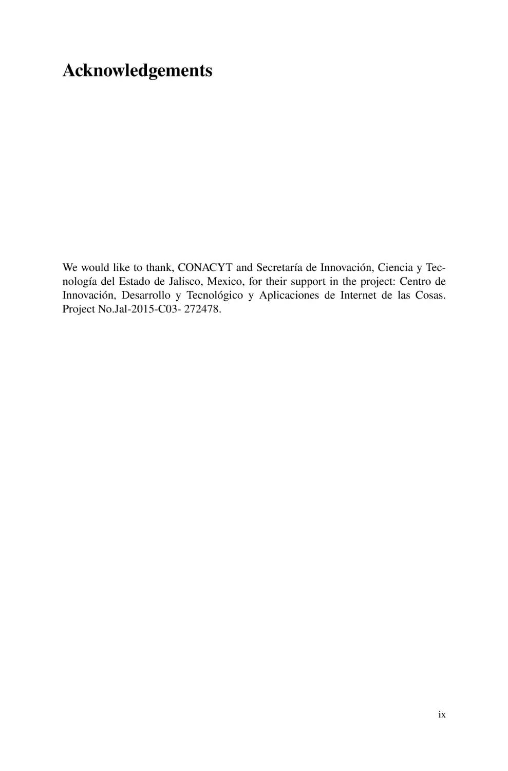
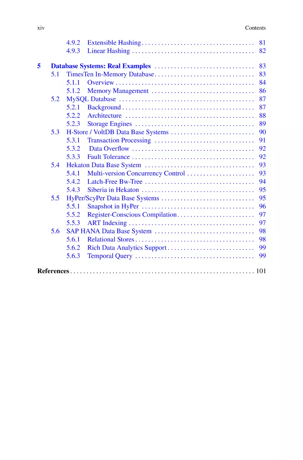
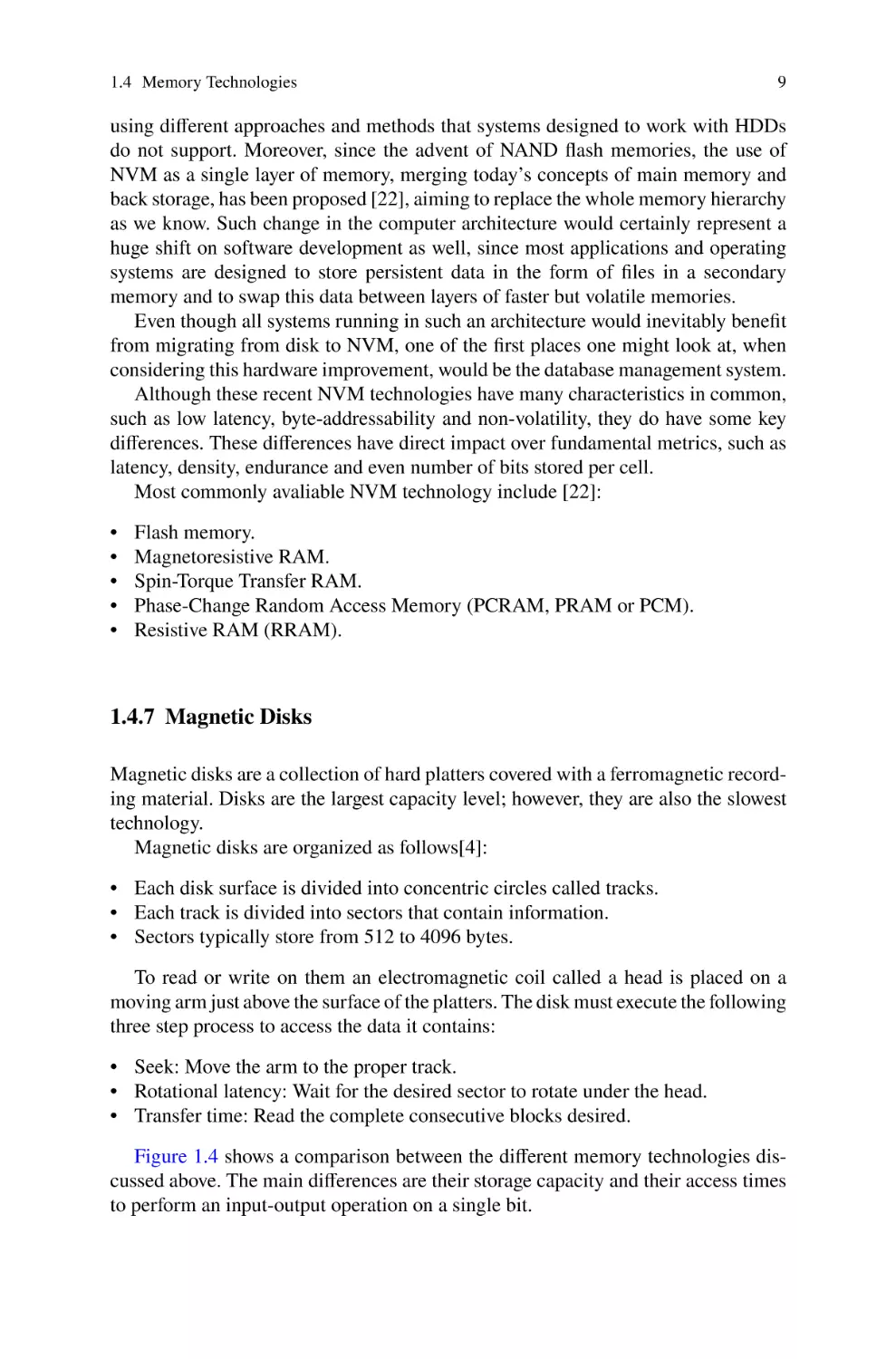
Figure 1.4 shows a comparison between the different memory technologies discussed above. The main differences are their storage capacity and their access times
to perform an input-output operation on a single bit.
10
1 The Memory System
Fig. 1.4 Memory classes characterization
Even though memory becomes the new disk [21], the volatility of DRAM makes it
a common case that disks are still needed to backup data. Data transmission between
main memory and disks is conducted in units of pages, which makes use of data
spatial locality on the one hand and minimizes the performance degradation caused
by the highlatency of disk seek on the other hand. A page is usually a multiple
of disk sectors which is the minimum transmission unit for hard disk. In modern
architectures, OS usually keeps a buffer which is part of the main memory to make
the communication between the memory and disk faster. The buffer is mainly used
to bridge the performance gap between the CPU and the disk. It increases the disk
I/O performance by buffering the writes to eliminate the costly disk seek time for
every write operation, and buffering the reads for fast answer to subsequent reads
to the same data. In a sense, the buffer is to the disk as the cache is to the memory.
And it also exposes both spatial and temporal locality, which is an important factor
in handling the disk I/O efficiently.
1.5 NUMA: Non-Uniform Memory Access
Non-uniform memory access is an architecture of the main memory subsystem where
the latency of a memory operation depends on the relative location of the processor
that is performing memory operations. Broadly, each processor in a NUMA system
1.5 NUMA: Non-Uniform Memory Access
11
has a local memory that can be accessed with minimal latency, but can also access
at least one remote memory with longer latency.
The main reason for employing NUMA architecture is to improve the main memory bandwidth and total memory size that can be deployed in a server node. NUMA
allows the clustering of several memory controllers into a single server node, creating several memory domains. Although NUMA systems were deployed as early as
1980s in specialized systems [185], since 2008 all Intel and AMD processors incorporate one memory controller. Thus, most contemporary multi-processor systems
are NUMA; therefore, NUMA-awareness is becoming a mainstream challenge.
In the context of data management systems, current research directions on NUMAawareness can be broadly classified into three categories[21]:
• partitioning the data such that memory accesses to remote NUMA domains are
minimized.
• managing NUMA effects on latency-sensitive workloads such as OLTP transactions.
• efficient data shuffling across NUMA domains.
Chapter 2
Memory Management
Memory management is part of the operating system responsible for the administration of memory. In this chapter we discuss several techniques to manage memory.
This techniques vary from a primitive bare-machine approach to paging and segmentation techniques. Each approach has its own advantages and disadvantages. The
selection of the most appropriate technique for memory management depends on
many factors, especially on the hardware design of the system. As we shall discuss,
many techniques require hardware support, although recent designs have closely
integrated the hardware and operating system.
2.1 Background
In modern computer systems, the operating system resides in a part of main memory
and the rest is used by multiple processes. The task of organizing the memory
among different processes is called memory management. Memory management is
a method in the operating system to manage operations in main memory and disk
during process execution.
The operating system is responsible for the following activities in connection with
memory management:
•
•
•
•
•
Allocate and deallocate memory before and after process execution.
To keep track of used memory space by processes.
To minimize fragmentation issues.
To achieve efficient and safe utilization of memory.
To maintain data integrity while executing of process.
The selection of a memory-management strategy is a critical decision that needs to
be addressed depending on the system. Some of these algorithms require hardware
© The Author(s), under exclusive license to Springer Nature Switzerland AG 2022
P. Mejia Alvarez et al., Main Memory Management on Relational Database Systems,
SpringerBriefs in Computer Science, https://doi.org/10.1007/978-3-031-13295-7_2
13
14
2 Memory Management
support and lead to a tightly integrated environment between the hardware and
operating system memory management. Memory management is an important task
that needs to be addressed by different parts of the computer system: hardware,
operating system, services, and applications.
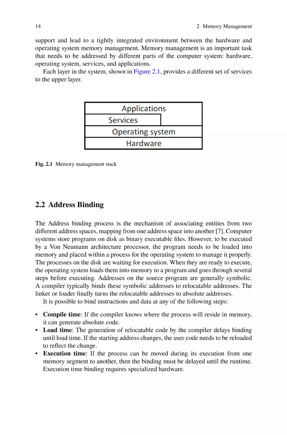
Each layer in the system, shown in Figure 2.1, provides a different set of services
to the upper layer.
Fig. 2.1 Memory management stack
2.2 Address Binding
The Address binding process is the mechanism of associating entities from two
different address spaces, mapping from one address space into another [7]. Computer
systems store programs on disk as binary executable files. However, to be executed
by a Von Neumann architecture processor, the program needs to be loaded into
memory and placed within a process for the operating system to manage it properly.
The processes on the disk are waiting for execution. When they are ready to execute,
the operating system loads them into memory to a program and goes through several
steps before executing. Addresses on the source program are generally symbolic.
A compiler typically binds these symbolic addresses to relocatable addresses. The
linker or loader finally turns the relocatable addresses to absolute addresses.
It is possible to bind instructions and data at any of the following steps:
• Compile time: If the compiler knows where the process will reside in memory,
it can generate absolute code.
• Load time: The generation of relocatable code by the compiler delays binding
until load time. If the starting address changes, the user code needs to be reloaded
to reflect the change.
• Execution time: If the process can be moved during its execution from one
memory segment to another, then the binding must be delayed until the runtime.
Execution time binding requires specialized hardware.
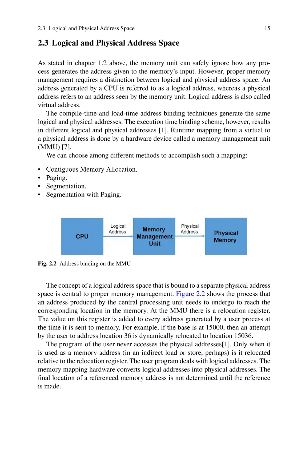
2.3 Logical and Physical Address Space
15
2.3 Logical and Physical Address Space
As stated in chapter 1.2 above, the memory unit can safely ignore how any process generates the address given to the memory’s input. However, proper memory
management requires a distinction between logical and physical address space. An
address generated by a CPU is referred to as a logical address, whereas a physical
address refers to an address seen by the memory unit. Logical address is also called
virtual address.
The compile-time and load-time address binding techniques generate the same
logical and physical addresses. The execution time binding scheme, however, results
in different logical and physical addresses [1]. Runtime mapping from a virtual to
a physical address is done by a hardware device called a memory management unit
(MMU) [7].
We can choose among different methods to accomplish such a mapping:
•
•
•
•
Contiguous Memory Allocation.
Paging.
Segmentation.
Segmentation with Paging.
Fig. 2.2 Address binding on the MMU
The concept of a logical address space that is bound to a separate physical address
space is central to proper memory management. Figure 2.2 shows the process that
an address produced by the central processing unit needs to undergo to reach the
corresponding location in the memory. At the MMU there is a relocation register.
The value on this register is added to every address generated by a user process at
the time it is sent to memory. For example, if the base is at 15000, then an attempt
by the user to address location 36 is dynamically relocated to location 15036.
The program of the user never accesses the physical addresses[1]. Only when it
is used as a memory address (in an indirect load or store, perhaps) is it relocated
relative to the relocation register. The user program deals with logical addresses. The
memory mapping hardware converts logical addresses into physical addresses. The
final location of a referenced memory address is not determined until the reference
is made.
16
2 Memory Management
2.4 Dynamic Loading
If the computer system requires the entire program and data to be in physical memory
for a process to execute, then the system has a hardware limit on the programs that
can run on the system, since the size of a process must never exceed the size of
physical memory. Dynamic loading can overcome this limitation, where the load
time of a routine is the first time it is active. The operating system keeps all routines
on disk in relocatable format; then when a program calls a routine, the calling routine
first checks if the other routine is in memory. If not, the relocatable linking loader is
called to load the desired routine into memory and to update the program’s address
tables to reflect the change. Finally, the newly loaded routine takes control of the
system.
The advantage of dynamic loading is that a routine is loaded only when it is
needed. This method is useful when large amounts of code are needed to handle
infrequently occurring cases, such as error routines. In such a situation, although the
total program size may be large, the portion that is used (and hence loaded) may be
much smaller.
Dynamic loading does not require special support from the operating system. It
is the responsibility of the users to design their programs to take advantage of such a
method. Operating systems may help the programmer, however, by providing library
routines to implement dynamic loading.
2.5 Dynamic Linking and Shared Libraries
Dynamically linked libraries (DLLs) are system libraries that are linked to user
programs during execution [1]. Some operating systems support only static linking,
in which system libraries are treated like any other object module and are combined
by the loader into the binary program image. Dynamic linking, in contrast, is similar
to dynamic loading. Here, linking is postponed until execution time. This feature is
usually used with system libraries, such as the standard C language library. Without
this facility, each program on a system must include a copy of its language library
(or at least the routines referenced by the program) in the executable image. This
requirement not only increases the size of an executable image but also may waste
main memory. Another advantage of DLLs is that these libraries can be shared
among multiple processes, so that only one instance of the DLL can be in main
memory. For this reason, DLLs are also known as shared libraries, and are used
extensively in Windows and Linux systems.
When a program references a routine that is in a dynamic library, the loader
locates the DLL, loading it into memory if necessary. It then adjusts addresses that
reference functions in the dynamic library to the location in memory where the DLL
is stored.
DDLs can be extended to library updates (such as bug fixes). In addition, a library
may be replaced by a new version, and all programs that reference the library will
2.6 Swapping
17
automatically use the new version. Without dynamic linking, all such programs
would need to be relinked to gain access to the new library. So that programs will
not accidentally execute new, incompatible versions of libraries, version information
is included in both the program and the library. More than one version of a library
may be loaded into memory, and each program uses its version information to
decide which copy of the library to use. Versions with minor changes retain the
same version number, whereas versions with major changes increment the number.
Thus, only programs that are compiled with the new library version are affected by
any incompatible changes incorporated in it. Other programs linked before the new
library was installed will continue using the older library.
Unlike dynamic loading, dynamic linking and shared libraries generally require
help from the operating system. If the processes in memory are protected from one
another, then the operating system is the only entity that can check to see whether
the needed routine is in another process’s memory space or that can allow multiple
processes to access the same memory addresses.
2.6 Swapping
Until this point in this chapter, a process needs to be in memory for execution.
However, it can be swapped out of memory temporarily and brought back to memory
for continued executing if it is not the only program running in the system. This
technique allows the physical address space of all processes to exceed the real
physical memory of the system. This technique is called swapping [1].
Fig. 2.3 Basic swapping mechanism
18
2 Memory Management
2.6.1 Standard Swapping
Standard swapping involves moving a process between main memory and a sufficiently large backing store. Figure 2.3 illustrates swapping.
The system maintains a ready queue consisting of all processes whose memory
images are in the backing store or already in memory and are ready to run. Whenever
the CPU scheduler decides to execute a process, it calls the dispatcher. The dispatcher
checks whether the next process in the queue is in memory. If not and if there is no
free memory region, the dispatcher swaps out a process currently in memory and
swaps in the desired process. It then reloads the registers and transfers control to the
process.
The context switch time in such a swapping system is relatively high. Modern
operating systems do not use swapping since it requires too much time and provides
too little execution time to be reasonable. Swapping is constrained by other factors
as well. If we want to swap a process, we must be sure that it is completely idle. Of
particular concern is any pending I/O.
2.7 Cache Management
Cache was the name given to represent the level of memory hierarchy between main
memory and the processor in the first commercially available system with this extra
level. The term is also used to refer to any management of storage using the locality
principle for increased performance [7].
Two fundamental questions require an answer when using a cache: How do we
know if an item is in the cache? How do we find the item in the cache? The simplest
way to answer those questions is to assign a location in the cache for each word
in memory based on its address, such as a simple hash structure without collision
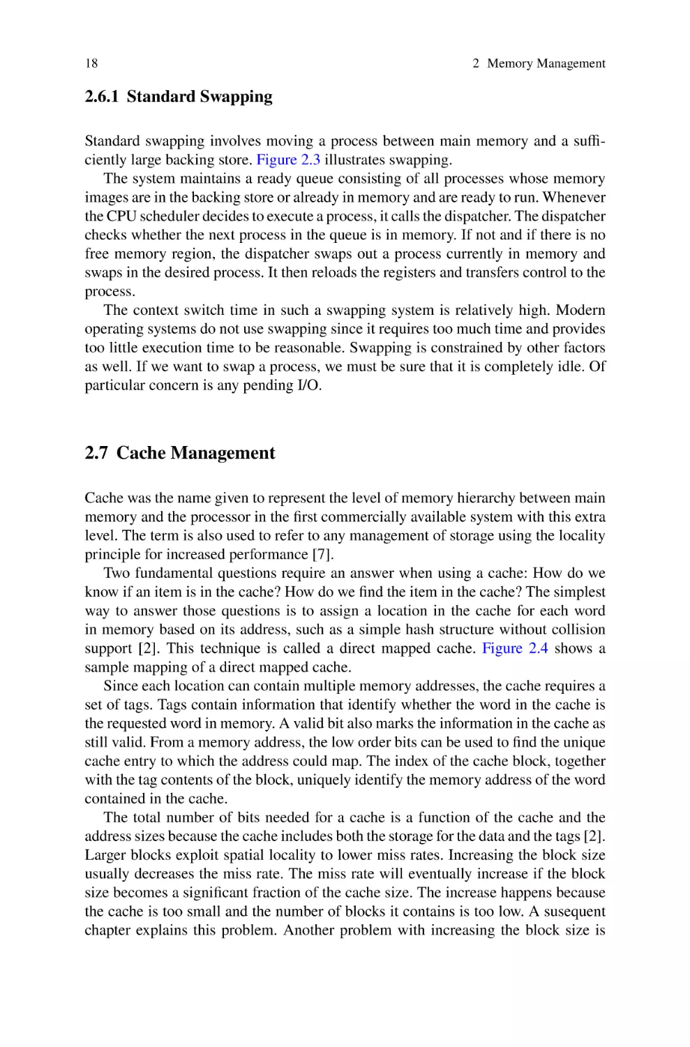
support [2]. This technique is called a direct mapped cache. Figure 2.4 shows a
sample mapping of a direct mapped cache.
Since each location can contain multiple memory addresses, the cache requires a
set of tags. Tags contain information that identify whether the word in the cache is
the requested word in memory. A valid bit also marks the information in the cache as
still valid. From a memory address, the low order bits can be used to find the unique
cache entry to which the address could map. The index of the cache block, together
with the tag contents of the block, uniquely identify the memory address of the word
contained in the cache.
The total number of bits needed for a cache is a function of the cache and the
address sizes because the cache includes both the storage for the data and the tags [2].
Larger blocks exploit spatial locality to lower miss rates. Increasing the block size
usually decreases the miss rate. The miss rate will eventually increase if the block
size becomes a significant fraction of the cache size. The increase happens because
the cache is too small and the number of blocks it contains is too low. A susequent
chapter explains this problem. Another problem with increasing the block size is
2.7 Cache Management
19
Fig. 2.4 Direct mapped cache
that it also increases the time cost of a miss. This cost can be partially improved if
the memory transfers are designed to be more efficient for big chunks of memory. A
technique used for doing this is called early restart, where the process regains control
just after the missing hit is already present in the cache, that way the process does
not need to wait for the complete memory transfer.
2.7.1 Cache Misses
The control unit must detect a cache miss and process the miss by fetching the
requested data from memory. If the cache reports a hit, the computer continues using
the data as if nothing happened [7].
Processing a cache miss creates a pipeline stall instead of an interrupt that would
require saving the state of all registers. More sophisticated out of order processors
can allow instructions while waiting for cache misses. If an instruction access results
in a miss, then the contents of the instruction register is invalid. To get the proper
instruction into the cache, we must instruct the lower level of the memory hierarchy
to perform a read.
The following steps must be taken by the hardware on a cache miss [2]:
1. Send the desired memory address to the memory.
2. Instruct the main memory to perform a read and wait for it to perform the access.
3. Write the cache entry, putting the data from memory into the data portion, write
the upper part of the address to the tag field and set the valid bit.
4. Restart instruction execution cycle.
20
2 Memory Management
2.7.2 Writing into the Cache
Suppose on a store instruction we wrote the data only into the data cache, then
after the write, the cache and the memory would have different values. They are
said to be inconsistent [2]. One way to avoid this is to always write to cache and
memory. This scheme is called write-through. This is straightforward, but it does
not provide outstanding performance. To solve this, we could use a write buffer.
The write buffer’s responsibility is to wait for the data to reach memory. After the
processor has written the data into the cache and the buffer, it can continue execution.
Another scheme is called write-back: When a write occurs, the new value is
written only into the cache block, and the modified block is only written to the lower
memory level when it is replaced [7]. Considering a miss, implementing stores
efficiently in a cache that uses write back strategy is more complicated than in a
write-through cache since the processor must first write the block back to memory
if the data in the cache is modified, and then it can attend the cache miss. If the
processor only overwrote the block, it would destroy the contents of the block, which
is not backed up to the next lower level of the memory hierarchy. Write-back caches
usually include write buffers that are used to reduce the miss penalty when a miss
replaces a modified block.
2.7.3 Cache Associativity
At one extreme, there is the direct mapping technique which maps any block to a
single location in the upper level of the memory hierarchy. At the opposite extreme
is a scheme where any location in the cache can contain any given block. The name
of this scheme is fully associative because any block in memory associates to any
other entry in the cache. This scheme also means that to find a block in the cache
the processor needs to search all the entries. The search is done in parallel using a
comparator on hardware, which makes fully associative placement only viable on
caches with a small number of blocks [2].
Another scheme is called set associative, where a block can belong only to a fixed
number of locations. The cache divides into n sets. The advantage of increasing the
level of associativity is that it usually decreases the miss rate. The choice between a
direct-mapping, a set associative or a fully associative mapping in any memory hierarchy will depend on the cost of a miss versus the cost of implementing associativity
both in time and in extra hardware and many other related factors [7].
2.7.4 Block Replacement
In the associative cache, we have a choice of where to place the requested block and
hence a choice of which block to replace. The most commonly used scheme is least
2.8 Contiguous Memory Allocation
21
recently used (LRU). It keeps track of the usage history of each element set relative
to the other elements in the set.
2.7.5 Multilevel Caches
Modern processors use multiple levels of cache to close the gap between fast clock
rates and memory access times. The second level of caching is normally located on
the same chip and is accessed whenever a miss occurs on the primary cache; figure
2.5 illustrates this.
If neither the primary nor the secondary cache contains the data, one memory
access is required, and a more substantial miss penalty is incurred [7].
Fig. 2.5 Direct mapped cache
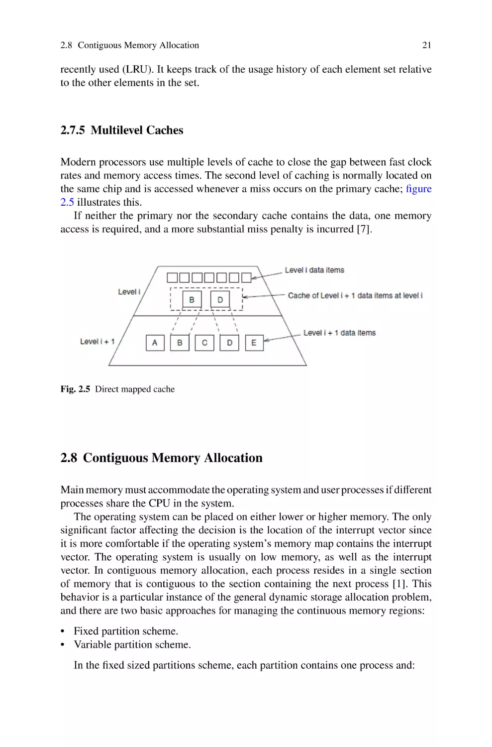
2.8 Contiguous Memory Allocation
Main memory must accommodate the operating system and user processes if different
processes share the CPU in the system.
The operating system can be placed on either lower or higher memory. The only
significant factor affecting the decision is the location of the interrupt vector since
it is more comfortable if the operating system’s memory map contains the interrupt
vector. The operating system is usually on low memory, as well as the interrupt
vector. In contiguous memory allocation, each process resides in a single section
of memory that is contiguous to the section containing the next process [1]. This
behavior is a particular instance of the general dynamic storage allocation problem,
and there are two basic approaches for managing the continuous memory regions:
• Fixed partition scheme.
• Variable partition scheme.
In the fixed sized partitions scheme, each partition contains one process and:
22
2 Memory Management
• When a partition is free, a process is selected from the input queue and is loaded
into the free partition.
• When a process terminates, its partition becomes free.
In the variable partition scheme, the operating system keeps a table indicating
which parts of memory are available.
• Initially all memory is available. When a process starts, it loads into memory, and
it can then compete for CPU time.
• At any given time, there is a list of available block sizes and an input queue. The
operating system can order the input queue according to a scheduling algorithm.
• The memory blocks available comprise a set of holes of various sizes scattered
throughout memory.
• When a process needs memory the system searches for a block that is large
enough. If the hole is too large, then it is split into two: one for the process and
the other for the set of available blocks. When a process terminates, it releases its
block of memory, and it returns to the available blocks.
• When the operating system searches the available blocks to assign a memory
block to a process it can take three basic approaches: first fit, best fit, worst fit.
2.9 Fragmentation
Operating systems usually allocate memory on multiples of a block size. The difference between the allocated size and the requested size is called internal fragmentation.
There is also external fragmentation, where there is enough total memory space
to satisfy a request but the available spaces are not contiguous. First-fit and best
fit suffer from external fragmentation [1]. A solution for external fragmentation is
called compaction. This is not always possible,however. As an example, if relocation
is static (done at assembly or load time), compaction cannot be done. If relocation is
dynamic and delayed until execution time, compaction is possible. Another solution
to external fragmentation is to permit the logical address space of the process to be
non-contiguous.
2.10 Segmentation
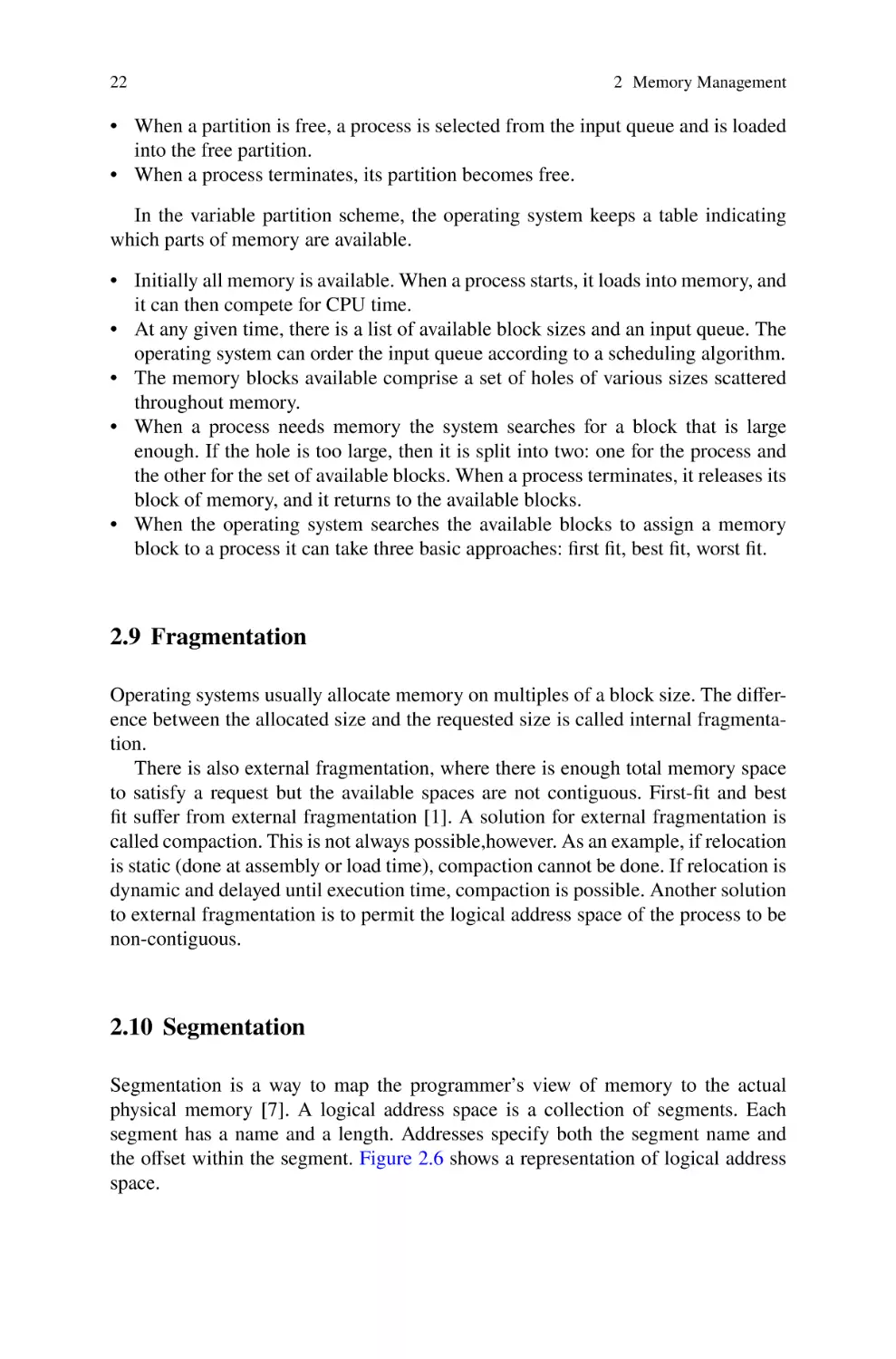
Segmentation is a way to map the programmer’s view of memory to the actual
physical memory [7]. A logical address space is a collection of segments. Each
segment has a name and a length. Addresses specify both the segment name and
the offset within the segment. Figure 2.6 shows a representation of logical address
space.
2.11 Paging
23
The programmer specifies each address by two quantities: a segment name and an
offset. When using segmentation, objects are referred as two-dimensional addresses,
but the actual memory is a one-dimensional array. To solve this problem a table
called the segment table does mapping between the object space and the memory
space. Each entry on the segment table contains the segment base and the segment
limit, which represent the starting physical address and the size of the segment when
the segment resides in memory [2].
Fig. 2.6 Logical address
2.11 Paging
Paging is another memory management technique that allows physical address space
to be non-contiguous. Therefore paging has the huge advantage of avoiding external
fragmentation and the need for compaction.
When swapping out fragments to the backing store, the backing store also gets
fragmented, but its access is much slower, making compaction impossible [1].
Paging involves breaking physical memory into fixed blocks called frames and
breaking logical memory into blocks of the same size called pages. When a process
loads, its pages load into any available memory frames before the process starts
executing.
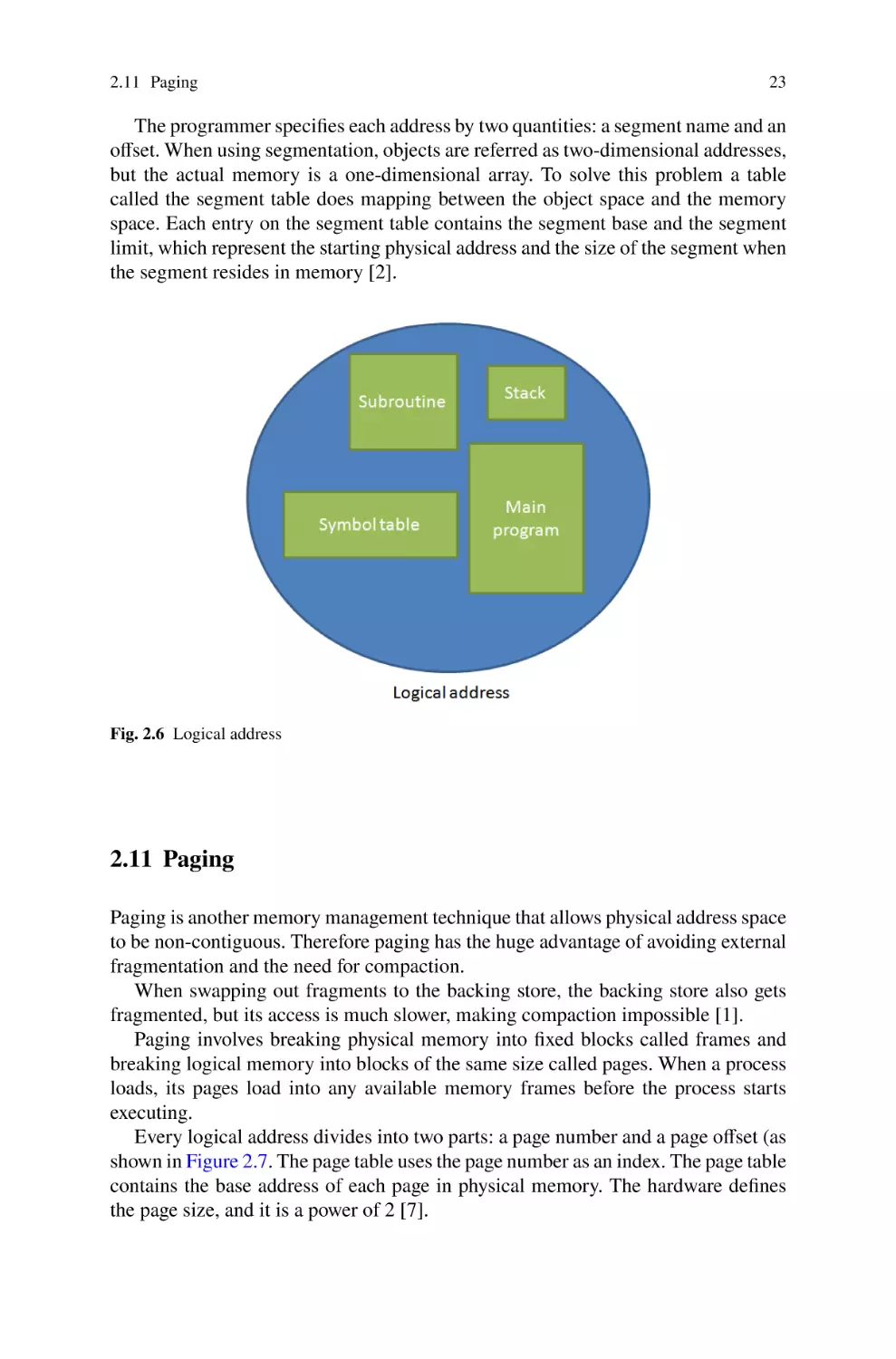
Every logical address divides into two parts: a page number and a page offset (as
shown in Figure 2.7. The page table uses the page number as an index. The page table
contains the base address of each page in physical memory. The hardware defines
the page size, and it is a power of 2 [7].
24
2 Memory Management
Note that the size of memory in a paged system is different from the maximum
logical size of a process.
Fig. 2.7 Page address break down
2.11.1 Hardware Support
Most contemporary computers allow the page table to be huge (as many as 1 million
entries). The memory contains the page table and a register points to the base of the
page table. Unfortunately, this scheme slows memory access by a factor of two.
The standard solution to this problem is to use a specialized, small, and fast
lookup hardware cache (or translation look-aside buffer, the TBL). The TBL takes as
an input the page number from the logical address and compares it simultaneously
against all keys.
• If the page number matches with a key, then its frame number is returned and
immediately available to access memory.
• If the page number is not in the TBL, a memory reference to the page table must
be made.
• If the TBL is already full of entries, an existing entry must be selected for
replacement. Replacement policies range from least recently used, through roundrobin to random.
The hit ratio refers to the percentage of times that the TBL contains the page
number of interest [1].
2.11.2 Shared Memory
An advantage of paging is the possibility of sharing common code. This consideration
is particularly important in a time-sharing environment.
A reentrant code is a non-self-modifying code. It never changes during execution
so two or more processes can execute the same code at the same time.
Each process has its copy of registers and data to hold the data for process
execution; however, the operating system needs to enforce the read-only nature of
shared code [1].
2.12 Page Table Organization
25
2.12 Page Table Organization
Most modern computer systems support a significant, 64 bit, logical address space.
In such an environment, the page table becomes excessively large. For this reason, it
becomes unfeasible to allocate the page table contiguously in main memory.
2.12.1 Hierarchical Paging
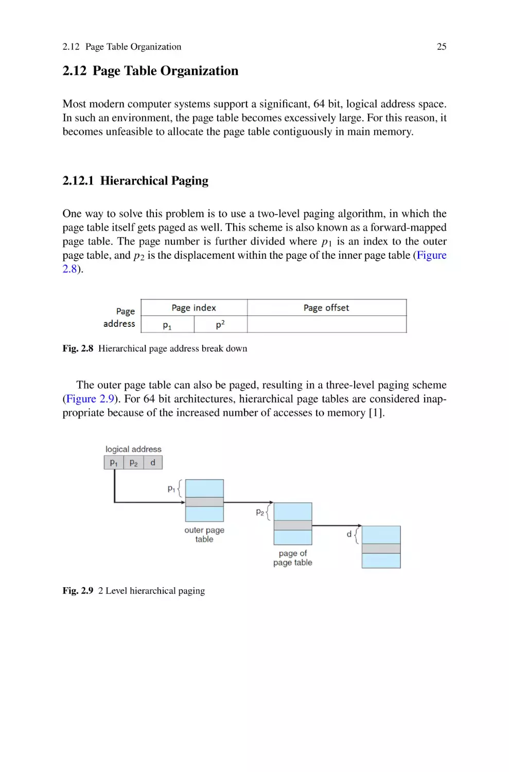
One way to solve this problem is to use a two-level paging algorithm, in which the
page table itself gets paged as well. This scheme is also known as a forward-mapped
page table. The page number is further divided where 𝑝 1 is an index to the outer
page table, and 𝑝 2 is the displacement within the page of the inner page table (Figure
2.8).
Fig. 2.8 Hierarchical page address break down
The outer page table can also be paged, resulting in a three-level paging scheme
(Figure 2.9). For 64 bit architectures, hierarchical page tables are considered inappropriate because of the increased number of accesses to memory [1].
Fig. 2.9 2 Level hierarchical paging
26
2 Memory Management
2.12.2 Hashed Page Table
If we consider the page number to be the hashed value, each entry in the hashed table
contains a linked list of frames that map to the same page number. Each element
consists of the following three fields:
• 𝑃1 page number
• 𝑃2 page frame
• 𝑃3 next node on the linked list.
The "clustered page tables" is a proposed variation of this in which each entry in
the hash table refers to several pages rather than a single page [1].
2.12.3 Inverted Page Table
Inverted page tables are another way to solve this problem. There is exactly one
entry for each frame of memory and each entry consists of the logical address of the
page stored at exactly that physical address. Thus, just one single page table is in the
system, and it has only one entry for each page of physical memory.
Unfortunately, the systems that use inverted page tables have more difficulties in
implementing shared memory since shared memory is usually implemented using
several logical addresses that map to one physical address. This technique cannot be
used with inverted page tables because there is only one virtual page entry for every
physical page [1].
2.13 Memory Protection
Another requirement that memory sharing introduces in the operating system is
memory protection. For proper system operation, the Operating System must protect
different processes from another. That is, the operating system area should only
be accessible by the operating system, and each user process should only access
its area. Hardware must provide this protection of the processor; otherwise, the
operating system needs to interfere between the processor and each of its memory
accesses [2].
There are different techniques that the operating system can use to implement
memory protection. For example, to separate memory areas, we need the ability to
identify a range of legal addresses for each process and ensure that each process only
accesses its legal addresses.
This protection can be provided using two registers: base and limit [6]. The
protection of a memory region requires the CPU hardware compare every address
generated in user mode with these two registers. The operating system can only load
the base and limit registers by using a privileged instruction that is only allowed
2.13 Memory Protection
27
to execute in kernel mode. This strategy also allows the operating system to have
unrestricted access to process spaces and to load 2 or more processes on overlapping
memory areas for debugging purposes [1].
2.13.1 Protection in Contiguous Memory Allocation
Since memory regions are contiguous, it is crucial for the operating system to ensure
that a process can only access its memory. To accomplish this, when the scheduler
selects a process for execution, the dispatcher loads the relocation and limit registers
with the correct values as part of the context switch. Since relocation and limit
registers are used to protect memory, this method protects the operating system and
user processes from each other.
The relocation register scheme provides an effective way to allow the operating
system’s size to change dynamically. This register is particularly useful for device
drivers. Such a code is a transient operating system code since it comes and goes as
needed [1].
2.13.2 Protection in Paged Memory
In a paged environment each frame has a set of specially purposed protection-bits to
accomplish memory protection. Normally these bits are kept in the page table. One
bit can mean that the frame has read-write or read-only permissions. Since every
reference to memory must pass through the page table to find its frame number, the
protection bits can be verified to ensure that no invalid access is being intended [7].
There is one page table per running process and a different one for the operating
system, so this scheme allows the operating system to have access to user processes
page tables and pages as well as prevent a process from accessing the frames and
page tables of a different process.
Chapter 3
Virtual Memory
In previous chapter we discussed several memory management techniques used in
modern operating systems. All these tecniques share the same goal: to keep many
processes in memory simultaneously to allow multiprogramming. However, they
require the entire process to be in memory before the process can execute. Virtual
memory is a technique that allows the execution of the processes that may not be
completely in memory. One major advantage of this scheme is that processes can be
larger than the available physical memory. This technique abstracts main memory
into a very large , uniform array of storage, separating logical memory as viewed by
the user from physical memory. This technique frees programmers from taking care
of main memory limitations. Virtual memory also allows processes to share files
and address spaces. Virtual memory is not easy to implement, however, and may
substantially decrease preformance if it is used carelessly. In this chapter, we discuss
virtual memory management.
3.1 Basic Concepts
The cache is a special fast memory buffer, typically within the CPU chip, used to
increase access speed to main memory. We can apply the same technique to main
memory and to secondary storage so that the main memory can act as a cache for
the secondary storage (hard disks). This technique is called virtual memory. Unfortunately, virtual memory is not easy to implement and may substantially decrease
performance if it is used carelessly [2]. There are various major motivations for
virtual memory:
• Efficient and safe sharing of memory among multiple programs.
• Allows the execution of processes that are not completely in memory.
• Allows processes to share files and to implement shared memory easily.
© The Author(s), under exclusive license to Springer Nature Switzerland AG 2022
P. Mejia Alvarez et al., Main Memory Management on Relational Database Systems,
SpringerBriefs in Computer Science, https://doi.org/10.1007/978-3-031-13295-7_3
29
30
3 Virtual Memory
The ability to execute a program that is partially in memory offers the following
advantages:
• A program would not be constrained to execute by the amount of physical memory.
• Increased concurrency since each program could take less physical memory;
therefore more programs could fit in memory.
• Less I/O would be needed to load user programs into memory initially.
• In many cases, the entire program is not needed, for example:
Code to handle unusual error conditions.
Arrays, lists, and tables usually allocate more memory than they need.
Rarely used features.
The entire program might not be needed all at the same time.
The principle of locality enables virtual memory as well as caches. Virtual memory enables efficient sharing of the processor as well as of the main memory. For
example:
• The behavior of multiple virtual machines sharing the memory changes dynamically. Because of this interaction, each program compiles into its address space
a separate range of memory locations available only to this program. The virtual
address space of a process refers to the logical view of how a process sees the
memory.
• Virtual memory is responsible for implementing the translation of the program’s
virtual address space to the physical address space.
• This translation enforces protections of program’s address space from other virtual
machines.
• Virtual memory involves the separation of the logical memory address as perceived by the user from physical memory.
Althought the concepts at work in virtual memory and caches are the same, their
different historical roots have led to the use of different terminology. A page is the
name of a virtual memory block. A virtual memory miss is called a page fault. With
virtual memory, the processor produces a virtual address, which is translated by a
combination of hardware and software into a physical address, which can then be
used to access memory.
In virtual memory (shown in Figure 3.1), the address contains the virtual page
number and a page offset. Having a larger number of virtual pages than physical
pages is the basis for the illusion of an essentially unbounded amount of virtual
memory [7]. Virtual memory also simplifies loading of the program for execution by
providing relocation and enables a more straightforward implementation of shared
libraries.
Relocation maps the virtual address used by the program to a different physical
address before the address is used to access memory. It allows for loading the program
anywhere in memory, instead of in a contiguous block.
Several processes can share system libraries through the mapping of the shared
object into their virtual address space. Shared libraries enable a computer system to
save space on disk and memory.
3.1 Basic Concepts
31
Fig. 3.1 Virtual memory representation
3.1.1 Page Access
The high cost of a page fault (millions of clock cycles) motivates many design choices
in virtual memory. For example:
• Pages should be large enough to try to amortize high access time.
• Organizations that reduce the page fault rate are attractive, such as the fully
associative placement of pages in memory.
• Page faults can be handled in software because overhead is small compared to
disk access time.
• Write-through will not work since writes take way too long to complete. Virtual
memory systems use write-back techniques.
The difficulty of using a fully associative placement lies in locating an entry, since
it can be anywhere in the upper level of the hierarchy. A full search is impractical.
Pages are located using a table that indexes the memory: the page table. The page
table, together with the program counter and the register, specifies the state of a
virtual machine. We often refer to that state as a process [2].
The virtual page address alone does not immediately tell us where the page is
on disk. The system must keep track of the location on disk of each page in virtual
address space. If a valid bit for a virtual page is off, a page fault occurs. Because
the system does not know ahead of time when it will replace a page in memory, the
operating system usually creates the space on flash memory or disk for all the pages
of a process when it creates the process. This space is called the swap space. It also
creates a data structure to record where the disk stores each virtual page [2].
32
3 Virtual Memory
3.1.2 The TLB: Translation Lookaside Buffer
Since main memory stores the page tables, every memory access by a program can
take at least twice as long. Accordingly, modern processors include a unique cache
that keeps track of recently used translations: a translation lookaside buffer (TLB).
Because we access the TLB instead of the page table on every reference, the TLB will
need to include other all status bits. The process followed by the TLB is described
in Figure 3.2.
Designers have used a wide variety of associativity in TLBs. Some systems
use small fully associative TLBs; other systems use large TLBs often with small
associativity [2].
Fig. 3.2 The TLB page table and memory relation
3.2 Demand Paging
33
3.1.3 Virtualization Challenges
I/O is the most complex part of the architecture to virtualize due to the increasing
diversity of devices that can be attached to a system. Another challenge is the
virtualization of virtual memory. For this to work the VMM separates the notion of
real and physical memory:
• Real memory is a separate and intermediate level between virtual and physical
memory.
• The guest OS maps virtual memory to real memory using its page tables.
• The VMM pages tables map the guest OS’s real memory to physical memory.
3.2 Demand Paging
3.2.1 Basic Concepts
With demand-paged virtual memory, pages are loaded into frames in physical memory only when program execution demands this. Thus, not all the pages that are
accessed are therefore never loaded into main memory. In some sense, a demandpaging system is similar to a paging system where processes reside in secondary
memory. When the operating system swaps in a process, the pager guesses which
pages it will use before the OS swaps out the process again, but instead of swapping
in the whole process, the pager brings only those pages into memory.
This scheme requires some hardware support to distinguish between the pages
that are in memory and the pages that are on disk. The page table often contains a
valid-invalid bit for this reason [1]. As usual, the system sets the page table entry
when a page loads into memory, but the one for a page that is not currently in
memory is either marked invalid or contains the address of the page on disk. If
the pager guesses right and pages in all the pages that are needed, the process will
run correctly, as if it has all its pages in memory. Otherwise, if the process tries to
access a page that the system did not load into memory, a page fault occurs. The
paging hardware will notice the setting of the valid-invalid bit, causing a trap to the
operating system [7].
The operating system will handle the page fault as follows.
1.
2.
3.
4.
5.
6.
Check whether the memory access qualifies as being valid or invalid.
If the reference is invalid, terminate the process.
Find a free frame.
Read the desired frame from disk to the available frame.
Modify the page table to indicate that the page is now in memory.
Restart the instruction that was interrupted by the trap.
3 Virtual Memory
34
A pure-demand paging system would not bring pages into memory until program
execution needs them. However, this would result in unacceptable system performance.
The hardware support needed for demand paging is: Paging table and Secondary
memory.
Paging is added between the CPU and the memory in a computer system and
should be transparent for the user process. People often assume that any system can
use paging. The assumption is only correct for non-demand-paging environments
where a page fault represents a fatal error, and no instructions would require a restart
operation.
3.2.2 Performance Considerations
Demand paging can significantly affect the performance of a computer system because the effective access time is directly proportional to the page fault rate. Disk
IO to swap is generally faster than the file system. It is faster because swap space
allocates much larger blocks and it does not use file lookups or indirect allocation
methods.
Mobile operating systems typically do not support swapping. Instead, these systems demand-page from the file system and reclaim read-only pages from applications if memory becomes constrained.
3.3 Page Replacement
If we increase the degree of multiprogramming beyond the system’s available memory, we are over allocating memory. If the system is over allocating more memory
than a certain threshold, the following can occur:
• Page faults can occur while a user’s process is executing.
• The operating system, therefore, determines that the desired page resides on disk
and realizes that there are no free frames on the free-frame list.
In this case, the operating system has two main options:
• Terminate the user process.
• Swap out a different process, to release all its frames and to reduce the level of
multiprogramming.
It is easy to expect that giving more memory to a process would improve its
performance. This however, is not always the case: When an algorithm does not show
the property, it is said to suffer from the Belady’s anomaly, and it is undesirable [1].
3.3 Page Replacement
35
3.3.1 Basic Page Replacement
Page replacement is essential to the demand paging scheme. It completes the separation between logical memory and physical memory. In general, page replacement
takes the following approach:
1. Find the location of the desired page on disk.
2. Find a free frame.
If there is a free frame, use it.
If there is no free frame, use a page-replacement algorithm to select a victim
frame.
Write the victim frame to the disk: change the page and frame table accordingly.
3. Read the desired page into the newly freed frame, change the page and frame
tables.
4. Continue the process from where the page fault occurred.
Notice that if there are no free frames, two-page transfers are required. The pages
table contains a bit to indicate modifications to reduce overhead. The hardware sets
the modify bit for a page whenever any byte in the page changes in memory [7].
When the system selects a page for replacement, it examines the modify bit.
• The system knows that the page contains differences between the version in
memory and on disk when the bit is on. Therefore the system must write the page
to disk.
• If the modify bit is off, the page has not been modified since it was read into
memory so we can save one memory access.
The paging system designer must solve two major problems to implement demand
paging:
• The system must decide how many frames to allocate to each process: this is
known as a frame allocation algorithm.
• The system must choose the frames for replacement when it is required: a page
replacement algorithm.
3.3.2 FIFO and Optimal Page Replacement
The simplest page replacement algorithm is a first-in, first-out (FIFO) algorithm. It
associates each page with the time when that page loaded into memory. The system
uses the timestamp to choose the oldest page for replacement. FIFO page replacement
algorithm performance is not always right: If we select a page that is in active use
by the executing process, the replacement algorithm will select some other page for
replacement, and a new fault occurs almost immediately.
A lousy replacement decision increases the page fault rate and slows process
execution; however, it does not cause incorrect execution [1].
36
3 Virtual Memory
Optimal page replacement requires future knowledge. However, if available it
provides the lowest possible page fault rate for a fixed number of times. The main
idea of OPT or MIN algorithms is to replace the page that the process will not use
for the longest period [1].
3.3.3 LRU Page Replacement
If we use the recent past to get an approximation of the near future, then we can
replace the page that the process has not used for the longest period. LRU replacement
associates each page with the time of the page’s last use. When the system selects a
page for replacement, LRU chooses the page unused for the most extended period.
LRU then becomes an approximation to the OPT page replacement strategy [7]. LRU
usually requires substantial hardware assistance. Two possible implementations are:
• Counters: Associate each page table entry a time-of-use field and add a logical
clock to the CPU.
The clock is incremented for every memory reference.
Whenever the process references a page, the hardware copies the clock register
to the time-of-use field in the page table entry for that page.
The page is replaced with the smallest time value. To accomplish this, it requires
a search of the page table the LRU page and a write to memory for each memory
access.
• Stack: Keep a stack of page numbers, and whenever the process references a page,
its entry gets to the top of the stack.
The top of the stack will always have the most recently used page, and the
LRU page will always be at the bottom of the stack. Both ’counters’ and ’stack’
implementations of LRU require hardware assistance beyond TLB registers [1].
LRU like optimal replacement belongs to a set of page replacement algorithms
called stack algorithms. All stack algorithms share the following characteristics:
• The set of pages in memory for N frames is always a subset of the set of pages
that would be in memory with N+1 frames.
• Stack algorithms do not exhibit Belady’s anomaly.
3.3.4 LRU Approximation Page Replacement
Few computer systems provide sufficient hardware support for true LRU page replacement. However, many systems provide a reference bit, which is set by the
hardware, whenever a page is referenced [1]. Although it does not tell the order
of use, many page replacement algorithms use the reference bit. These algorithms
approximate LRU because of the following:
3.3 Page Replacement
37
• Each entry in the page table has its reference bits.
• During program startup time the bits are cleared by the operating system.
• Whenever the process references a page, the bit is set by the hardware.
To implement LRU with the reference bit, the following is required:
1. Keep a byte for each page in a table in memory.
2. At regular intervals, the operating system shifts the reference bit for each page
into the high-order bit of the byte, shifting the other bits to the right.
The register then contains the history of the pages used for the latest periods. If
we interpret the byte as unsigned integers, the page with the lowest number is the
LRU page and can be replaced [1].
3.3.4.1 Second Chance Algorithm
The second chance algorithm is a FIFO replacement algorithm. When it selects a
page for replacement, it inspects its reference bit.
• If the page bit is off the page is replaced.
• If the page bit is on the page gets a second chance, and the next FIFO page on the
LRU list is selected.
When a page gets a second chance, the system sets off its reference bit, and it
restarts its arrival time to the current time. Therefore, when a page gets a second
chance, it will not be replaced until all other pages have been replaced or given
second chances [7].
3.3.4.2 Enhanced Second Chance Algorithm
This algorithm takes into account the number of I/O required to replace a page [1].
The enhanced second chance algorithm considers the reference bit and the modify
bit to give a second chance to a page. It constructs using the table 3.3:
Fig. 3.3 Enhanced second chance posibilities
38
3 Virtual Memory
3.3.5 Counting Based Page Replacement
Counting based page replacement keeps a counter of the number of references that
each page has. The algorithm can use any of the following two schemes:
• Least frequently used (LFU). The page with the smallest count is replaced.
• Most frequently used (MFU). The page with the smallest count was probably just
brought in memory and has yet to be used.
This algorithm reports good performance for sequential file reads such as data
warehouses [1].
3.3.6 Page Buffering
In addition to page replacement algorithms, the system can use page buffering. This
consists of having a pool of free frames. The free frames pool is then used to increase
system performance in the following scenarios [7]:
• At page fault time, a victim frame is selected for replacement by a newly required
frame; however, the new frame is read into a free frame from the pool before the
victim is written out.
• Finally, when the victim frame has finished being written out, its frame is moved
into the free frames pool.
3.3.7 Applications and Page Replacement
Some applications perform worse when accessing data through the operating system’s virtual memory system than if the operating system provided no buffering at
all. A typical example of this is a database that provides its memory management
and I/O buffering. Operating systems provide ’raw disk’ which allows programs to
use a disk partition as a sizable sequential array of logical blocks, without any file
system structure to address this [1].
3.4 Allocation of Frames
If we now consider that a computer system can handle multiple processes running
concurrently, we need to answer the following question: How do we allocate the
fixed amount of free memory among various processes? [7]
One reason for allocating at least a minimum number of frames involves performance:
3.4 Allocation of Frames
39
• As the number of frames allocated to each process decreases, the page fault rate
increases, slowing process execution.
• A process must have enough frames to hold all the different stages that any instruction can reference during the complete instruction execution cycle. Otherwise,
the instruction execution needs to restart.
The amount of available physical memory defines the maximum number of frames
[1].
3.4.1 Allocation Algorithms
The easiest way to split M frames among N process is to give everyone an equal share
MxN frames. The leftover frames can form a buffer of free frames. This technique is
called equal allocation. Another option is proportional allocation where the available
memory allocated to each process depends on the process’s size. Therefore, all
process share the available frames according to their needs. Some drawbacks of
equal and proportional allocation are:
• The allocation may vary according to the multiprogramming level. When the
operating system creates a new process, each existing process will lose some
frames to provide the memory needed for the new process.
• There is no prioritization of processes. A high priority process gets the same
treatment as a low priority process.
Proportional allocation could consider the program size and the process priority to
follow process priorities [1].
3.4.2 Allocation Scope
Global page replacement allows a process to select a replacement frame from the set
of all frames, even if a different process gets that frame. Global page replacement
means that one process can take frames from another one. Alternately, local page
replacement requires each process to select from its set of allocated frames only.
An allocation scheme where a process can select a replacement from among its
frames and the frames of any lower priority process is also possible.
With global page replacement, a process may happen to select only frames allocated to other processes, thus increasing the number of frames allocated to it. One
problem with global page replacement is that a process cannot control its pagefault rate, meaning that the same process can perform quite differently according to
the multiprogramming level. Global replacement generally results in higher system
throughput and is, therefore, the more commonly used method [1].
40
3 Virtual Memory
3.4.3 Non Uniform Memory Access considerations
In systems with multiple CPUs, a given CPU can access some sections of main
memory faster than it can access others. These performance differences are caused by
how CPUs and memory are physically wired and interconnected. NUMA systems are
slower than systems in which memory and CPU colocate on the same motherboard. In
NUMA systems, optimally locating page frames can significantly affect performance.
The same type of exceptional management is also required on the scheduling system
to get a well behaved NUMA system. The required managing changes consist of
tracking the last CPU on which each process ran. The historical information is used
by the scheduler to schedule each process onto its previous CPU. Then the memory
management system allocates frames that are the closest to the CPU on which the
process will be executing. This strategy improves cache hits and decreases memory
access times in the system [1].
Solaris OS solves the problem by creating lgroups (locality groups) in the kernel.
Each lgroup keeps together close CPUs and memory. It creates a hierarchy of lgroups
based on the latency between them. Solaris tries to schedule all threads of a process
and to allocate all the memory from a process within its lgroup. If it is not possible,
it uses the closest lgroup using the hierarchy [10].
3.5 Memory Protection on Virtual Memory
The TBL or translation lookaside buffer is a special purpose cache on the processor
used to speed up accesses to the page table in virtual memory.
The TBL plays an essential role in memory protection for virtual memory. To
accomplish this when the operating system decides to change from running process
P1 to running process P2, if there is no TLB loaded into the processor’s cache, it is
sufficient to change the page table register to point to P2’s page table (rather P1’s).
However, if a TLB is already loaded, then all entries from P1 need to be cleared. A
different common alternative to memory protection is to extend the virtual address
space by adding a process identifier or task identifier into the address [2].
3.6 Thrashing
When a process has high paging activity, the CPU spends most of its time in juggling
pages between the main memory and the swap device. This situation is called
thrashing. When a severe thrashing scenario occurs, a process could be spending
more time paging than executing.
Thrashing results in severe performance degradation and the system responsiveness may collapse. The operating system needs to prevent thrashing at all costs [7].
When the number of frames allocated to a low-priority process falls below the min-
3.6 Thrashing
41
imum required by the computer architecture, the operating system must suspend the
low-priority process, then the process gets paged out, and its frames can be released.
The operating system monitors CPU optimization as a way to control the level of
multiprogramming. If the CPU is underutilized, the scheduler can increase the level
of multiprogramming. If global page replacement is being used at process creation
time, frames are taken from other processes when it starts page faulting. The process
needs those pages, so it also faults.
As the processes queue up on the paging device, the ready queue empties and
CPU utilization decreases. The CPU scheduler sees the decreasing CPU utilization
and increases the degree of multiprogramming again. At this point, to increase CPU
utilization and stop thrashing, the operating system must decrease the degree of
multiprogramming. Unfortunately, the CPU scheduler has done the opposite.
Using local page replacement or priority replacement, the effects of thrashing can
be limited only. To prevent thrashing, approaches like the locality model of process
execution must be used [1]. A locality is a set of pages that are active together, and
the locality model states that, as a process executes, it moves from one locality to
another. Therefore, a program is generally composed of several different localities.
The program structure and its data structures define localities. The locality model
states that all programs will exhibit this basic memory reference structure [7].
3.6.1 The Working Set Model
This model uses a parameter delta to define the working set window. Calculating the
working set is hard [1].
• If a page is active in the process execution, the page will be in the working set.
When the page is not active anymore, the working set will drop the page after n
time units of its last reference.
• The working set is an approximation of the program’s locality.
• The most important property of the working set is its size, which can vary over
time.
• The demand of the computer memory system is the sum of the working set sizes
of every process.
• If the demand is greater than the number of available frames, then thrashing will
occur.
The operating system monitors the working set of each process. If there are enough
extra frames, another process can start. If the demand of the system exceeds the total
number of available frames, the operating system selects a process to suspend. The
working set model is successful but is a somewhat clumsy way to control thrashing
[7].
3 Virtual Memory
42
3.6.2 Page Fault Frequency
One of the properties of thrashing has a high page-fault rate. When the page fault
is too high for a process, we know that it needs more frames. If it is too low, the
process might have too many frames. The operating system can establish upper and
lower bounds for page fault rate.
• The process gets a new frame if it exceeds the upper bound.
• The process loses a frame if it exceeds the lower bound.
If the page fault rate exceeds the upper bound and there are no available frames,
the operating system can suspend a process and distribute the just released frames
among the processes with high page fault rate.
3.7 A Common Framework for Managing Memory
In this section, we will discuss the common operational alternatives for memory
management, and how these determine their behavior. We will examine these policies
as a series of activities that apply between any two levels of a memory hierarchy,
although for simplicity we will primarily use terminology for caches.
The activities mentioned are the following:
•
•
•
•
Block Placement.
Block Access.
Block Replacement in Cache Miss.
Parallelism and Memory Hierarchy.
3.7.1 Block Placement
The advantage of increasing the degree of associativity is that it is a way to control
the miss rate and make it decrease. Improvement comes from reducing misses that
compete for the same location. Some techniques for block placement are shown in
Figure 3.4.
Fig. 3.4 Block placement strategies
3.7 A Common Framework for Managing Memory
43
3.7.2 Block Access
The choice among direct-mapped, set-associativity or fully associative mapping in
any memory hierarchy will depend on the cost of a miss versus the cost of implementing associativity, both in time and in extra hardware. Fully associative caches
are generally prohibitive except for small sizes. For virtual memory, however, fully
associative is used since misses are costly and sophisticated replacement schemes to
reduce miss rates exist. Some techniques for block access are shown in Figure 3.5.
Fig. 3.5 Block access strategies
3.7.3 Block Replacement in Cache Miss
There are two primary strategies for replacement in associative caches: random and
LRU. For some workloads, random replacement can be better than LRU. In caches,
the replacement algorithm is a hardware module, which means that the scheme
should be easy to implement. In virtual memory, however, the system performs a
LRU approximation.
Cache misses can fall into the following categories according to their nature [2]:
• Compulsory misses: These are cache misses caused by the first access to a block
that has never been in the cache (cold start).
• Capacity misses: Caused when the cache cannot contain all the blocks needed
during the execution of the program.
• Conflict misses: When multiple blocks compete for the same set (collision misses).
3.7.4 Parallelism and Memory Hierarchy
Multicore multiprocessor means multiple processors on a single chip. These processors very likely share a common physical address space, which means they share
data.
44
3 Virtual Memory
Caching shared data introduces a new problem because the view of memory held
by individual processors is through their caches. This behavior is known as the cache
coherence problem. Coherence defines the values that a read operation can return.
Consistency determines when a read will return a written value. A memory system
is coherent if it shows the following characteristics:
• A read by processor P to a location X that follows a write by P to X, with no
other writes of X by a different processor between the write and the read, always
returns the value written by P.
• A read by a processor to location X that follows a write by another processor to
X returns the written value if the read and write have enough separation in time,
and no other writes to X occur between the two accesses.
• Writes to the same location are serialized: Two writes to the same location by any
two processors are seen in the same order by all processors.
The first property preserves program order and the second property defines the
notion of what it means to have a coherent view of memory [2].
3.7.4.1 Basic Coherence Enforcement
In a coherent cache multiprocessor, caches provide both migration and replication
of shared data items:
• Migration: A data item can be moved to a local cache and used there transparently.
Migration reduces latency and bandwidth demand on the shared memory to access
shared data items that come from a remote allocation.
• Replication: While simultaneously reading shared data, caches make a copy of
the data item in the local cache. Replication reduces both latency of access and
contention for a read shared data item.
The protocols to maintain coherence for multiple processors are called cache
coherence protocols. Key to implementing a cache coherence protocol is tracking
the state of any sharing data of a data block [2].
3.7.4.2 Snooping Protocols
One method of enforcing coherence is to ensure that a processor has exclusive access
to a data before it writes that item. This style of protocols is called a write invalidate
protocol because it invalidates copies in other caches on a write.
Consider one write access followed by one read access by another processor: since
the write requires exclusive access, any copy held by the reading processors must
be invalidated, and the cache is forced to fetch a new copy of the data. One insight
is that block size plays an essential role in cache coherency since most protocols
exchange full blocks between processors, thereby increasing coherency bandwidth
demands. Large blocks can cause what is called false sharing: when the same cache
3.8 Other Considerations
45
block contains two independent shared variables, the full block is exchanged between
processors even though the processors are accessing different variables. False sharing
should be considered at the programming time and during the compilation process.
In addition to the snooping cache coherence protocol, where it distributes the
status of the shared blocks, a directory-based cache coherence protocol keeps the
sharing status of the block of physical memory in just one location called the
directory.
Directory-based cache coherence protocols have slightly higher implementation
overhead than snooping but they can reduce traffic between caches and thus scale to
larger processor counts [2].
3.8 Other Considerations
The selection of a replacement algorithm and memory allocation policy are the major
decision that we make for a paging policy. However, in this section we will discuss
otehr considerations as well.
3.8.1 Pre-Paging
Pre-paging is an attempt to prevent a high level of initial paging. The strategy is to
bring all the needed pages into memory at one time. In a system using the working
set model, the operating system stores a list of the pages in the working set when it
suspends the process, and it brings them all back together when the process can be
resumed [1].
3.8.2 Page Size
While building a new CPU, the designer can consider the page size to use. Page sizes
are invariably a power of two. There is, however, a set of factors that support various
page sizes:
• Page table size: For a fixed virtual memory space, decreasing the page size
increases the number of pages and the size of the page table.
• Since each process needs a page table, a big page size is desirable.
• Memory is better utilized using smaller page sizes due to reduced internal fragmentation.
• Smaller page sizes reduce the number of I/O because better memory granularity
achieves better program locality.
• A big page size decreases the number of page faults.
46
3 Virtual Memory
3.8.3 TLB Reach
The hit ratio for a TLB refers to the percentage of virtual address translations that
are resolved in the TLB rather than on the page table. A way to increase the hit ratio
is to increase the number of entries in the TLB; this is expensive, however. TLB
reach refers to the amount of memory that is accessible from the TLB and is the
number of entries multiplied by the page size. Doubling the number of TLB entries
also doubles the TLB reach. If the page size can increase, then the TLB reach also
increases. Applications like databases take advantage of huge pages. To increase
page size, the TLB needs to be managed by software instead of hardware which is
costly; however, the cost is often surpassed by the performance gains that come from
the increased TLB hit ratio [1].
3.8.4 Inverted Page Table
Inverted page table management needs to store information about frames to pages
into a separate page. This separate page is just another regular page. The purpose of
this form of page management is to reduce the amount of physical memory needed to
track virtual-to-physical address translations. Unfortunately, a page fault may cause
the virtual memory manager to generate an additional page fault [1].
3.8.5 Program Structure
Demand paging is designed to be transparent to the user; however, system performance can be greatly improved if the user has an awareness of the underlying demand
paging.
Careful selection of data structures can increase the locality and hence lower the
page fault rate and the number of pages in the working set.
• Stack data structures have good locality since accesses are only made to the top.
• Hashes data structures have bad locality since they are designed to scatter references.
Locality is yet another measurement of the efficiency of a data structure.
The compiler and loader can have a significant effect on paging. Separating the
code and data and generating reentrant code means that code pages can be read-only
and hence will never be modified. The loader and related routines can fit on the
same page. This strategy is an instantiation of the bin-packing problem of operations
research [1].
3.8 Other Considerations
47
3.8.6 Page Locking
When a system uses demand paging, it sometimes needs to allow some of the pages
to be locked in memory. For this reason, every frame has its lock bits. If the frame
is locked, it is not susceptible to page replacement. Various situations can take
advantage of lock bits:
• Some parts of the operating systems need to be locked into memory (the memory
manager for example).
• A database may want to manage a chunk of memory.
Pinning or locking of memory is common, and most operating systems have
a system call allowing an application to pin some region of its address space.
Unfortunately, it can cause stress to the memory management algorithm. Locking
memory can also be dangerous; the lock bit can be set and never reset. If that situation
ever happens, then the locked frame becomes unusable [1].
3.8.7 Memory Mapped Files
Memory mapping a file allows a part of the virtual address space to be logically
associated with a file to enable performance benefits. Memory mapping a file is
accomplished by mapping a disk block to a page in memory (Figure 3.6). Initial
access to the file proceeds through normal demand paging, resulting in a page fault,
however, a page-sized portion of the file is read from the file system onto a physical
page. Writes to the file mapped in memory are not necessarily synchronous writes
to the file on disk. When a process closes the file, all the memory-mapped data is
written back to disk and removed from the virtual memory of the process. Multiple
processes may be allowed to map the same file concurrently to allow sharing data.
Memory-mapping system calls can also support copy on write functionality,
allowing processes to share a file in read-only mode but to have their copies of the
data they modify.
Shared memory is often implemented using memory mapping of a file [1].
Each I/O controller includes registers to hold commands and data to be transferred.
Many computer architectures provide memory-mapped I/O to allow more convenient
access to I/O devices. Ranges of memory addresses are set aside and mapped to the
device registers. Reads and writes to these memory addresses cause the data to be
transferred to and from the device registers [1].
3.8.8 Kernel Memory Allocation
When a process running in user mode requests additional memory, the operating
system allocates pages from the list of free page frames maintained by the kernel.
48
3 Virtual Memory
Fig. 3.6 Memory mapped file
The kernel itself allocates memory from a free-memory pool different from the list
used to satisfy conventional user-mode processes for the following reasons:
• To minimize waste due to fragmentation. This optimization is especially important
since the operating system does not page its code or data.
• Pages allocated for user-mode processes do not necessarily have to be a contiguous
physical memory area; however, certain hardware devices may require memory
residing in physically contiguous pages.
3.8.8.1 Buddy System
The buddy system allocates memory from a fixed-size segment consisting of physically contiguous pages. Memory is allocated from this segment using a power of 2
allocators.
An advantage of the buddy system is that adjacent buddies can be merged to
form larger segments using a technique called coalescing. The drawback to the
buddy system is that rounding to the highest power of 2 is very likely to cause
fragmentation within allocated segments. It cannot guarantee that less than 50% of
the allocation unit will be wasted due to internal fragmentation [1].
3.8 Other Considerations
49
3.8.8.2 Slab Allocation
A slab is made up of one or more physically contiguous pages, and a cache consists of
one or more slabs (Figure 3.7). Each unique kernel data structure has its cache. Each
cache populates with an object that is an instantiation of the kernel data structures
associated with the cache. The slab allocation algorithm uses caches to store kernel
objects. When the operating system creates a cache, It preallocates some free objects
into the cache. When a new object for a kernel data structure is needed, the allocator
can assign any free object from the cache and marks it as used [11].
The slab allocator provides two main benefits:
• No memory is wasted due to fragmentation.
• Memory can be assigned very quickly. This behavior is particularly effective for
managing memory when creation and destruction of objects are frequent.
Fig. 3.7 Slab allocator data structure
3.8.9 Virtual Machines
The broadest definition of a VM includes all emulation methods that provide standard
software interface, such as the Java VM. VMs provide at least two benefits that are
commercially significant:
• Managing software: An abstraction to run a complete software stack.
• Managing hardware: A complete software stack can run on independent servers
that share hardware.
The cost of processor virtualization depends on the workload.
• User level processor-bound programs have no virtualization overhead.
• OS intensive programs have great virtualization overhead.
The qualitative requirements for a virtual machine monitor (VMM) are:
50
3 Virtual Memory
• The guest software should behave on an MV exactly as in native hardware.
• The guest software should not be able to change the allocation of real system
resources directly.
Because the VMM must ensure that the guest system only interacts with virtual
resources, a conventional guest runs as a user-mode program on top of the VMM.
Then if a guest OS attempts to use a privileged instruction, it will trap to the VMM,
which can then affect the appropriate action on the real resources.
In the absence of this support, a VMM must take special precautions to locate all
problematic instructions, increasing the complexity of the VMM and reducing the
performance of the guest software [2].
3.9 Hardware Memory Management Real Examples
3.9.1 Memory Management in the IA-32 Architecture
The memory management facilities of the IA-32 architecture are divided into two
parts [49]: segmentation and paging. Segmentation provides a mechanism of isolating individual code, data, and stack modules so that multiple programs (or tasks)
can run on the same processor without interfering with one another. Paging provides
a mechanism for implementing a conventional demand-paged, virtual-memory system where sections of a program’s execution environment are mapped into physical
memory as needed. Paging can also be used to provide isolation between multiple
tasks. When operating in protected mode, some form of segmentation must be used.
There is no mode bit to disable segmentation. The use of paging, however, is optional.
These two mechanisms (segmentation and paging) can be configured to support
simple single-program (or singletask) systems, multitasking systems, or multipleprocessor systems that used shared memory. As shown in Figure 3.8[49], segmentation provides a mechanism for dividing the processor’s addressable memory space
(called the linear address space) into smaller protected address spaces called segments. Segments can be used to hold the code, data, and stack for a program or
to hold system data structures (such as a TSS or LDT). If more than one program
(or task) is running on a processor, each program can be assigned its own set of
segments. The processor then enforces the boundaries between these segments and
insures that one program does not interfere with the execution of another program by
writing into the other program’s segments. The segmentation mechanism also allows
typing of segments so that the operations that may be performed on a particular type
of segment can be restricted.
All the segments in a system are contained in the processor’s linear address space.
To locate a byte in a particular segment, a logical address (also called a far pointer)
must be provided. A logical address consists of a segment selector and an offset. The
segment selector is a unique identifier for a segment. Among other things it provides
an offset into a descriptor table (such as the global descriptor table, GDT) to a data
3.9 Hardware Memory Management Real Examples
51
Fig. 3.8 IA-32 Segmentation and Paging
structure called a segment descriptor. Each segment has a segment descriptor, which
specifies the size of the segment, the access rights and privilege level for the segment,
the segment type, and the location of the first byte of the segment in the linear address
space (called the base address of the segment). The offset part of the logical address
is added to the base address for the segment to locate a byte within the segment.
The base address plus the offset thus forms a linear address in the processor’s linear
address space.
If paging is not used, the linear address space of the processor is mapped directly
into the physical address space of processor. The physical address space is defined
as the range of addresses that the processor can generate on its address bus.
Because multitasking computing systems commonly define a linear address space
much larger than it is economically feasible to contain all at once in physical memory,
some method of “virtualizing” the linear address space is needed. This virtualization
of the linear address space is handled through the processor’s paging mechanism.
Paging supports a “virtual memory” environment where a large linear address
space is simulated with a small amount of physical memory (RAM and ROM) and
some disk storage. When using paging, each segment is divided into pages (typically
4 KBytes each in size), which are stored either in physical memory or on the disk.
The operating system or executive maintains a page directory and a set of page tables
52
3 Virtual Memory
to keep track of the pages. When a program (or task) attempts to access an address
location in the linear address space, the processor uses the page directory and page
tables to translate the linear address into a physical address and then performs the
requested operation (read or write) on the memory location.
If the page being accessed is not currently in physical memory, the processor
interrupts execution of the program (by generating a page-fault exception). The
operating system or executive then reads the page into physical memory from the
disk and continues executing the program.
When paging is implemented properly in the operating-system or executive, the
swapping of pages between physical memory and the disk is transparent to the correct
execution of a program. Even programs written for 16-bit IA32 processors can be
paged (transparently) when they are run in virtual-8086 mode.
3.9.2 Memory Management in the AMD64 Architecture
by The AMD64 Architecture uses segmentation and/or paging memory management
methods. Usually, memory management is not visible to application software. It is
handled by the system software and processor hardware.
3.9.2.1 AMD64 Segmentation
The AMD64 architecture [50] is designed to support all forms of legacy segmentation. However, most modern system software does not use the segmentation features
available in the legacy x86 architecture. Instead, system software typically handles
program and data isolation using page-level protection. For this reason, the AMD64
architecture dispenses with multiple segments in 64-bit mode and, instead, uses
a flat-memory model. The elimination of segmentation allows new 64-bit system
software to be coded more simply, and it supports more efficient management of
multi-processing than is possible in the legacy x86 architecture.
Segmentation is, however, used in compatibility mode and legacy mode. Here,
segmentation is a form of base memory-addressing that allows software and data to be
relocated in virtual-address space off of an arbitrary base address. Software and data
can be relocated in virtual-address space using one or more variable-sized memory
segments. The legacy x86 architecture provides several methods of restricting access
to segments from other segments so that software and data can be protected from
interfering with each other.
In compatibility and legacy modes, up to 16,383 unique segments can be defined.
The base-address value, segment size (called a limit), protection, and other attributes
for each segment are contained in a data structure called a segment descriptor.
Collections of segment descriptors are held in descriptor tables. Specific segment
descriptors are referenced or selected from the descriptor table using a segment
3.9 Hardware Memory Management Real Examples
53
selector register. Six segment-selector registers are available, providing access to as
many as six segments at a time.
Figure 3.9 [50] shows an example of segmented memory.
Fig. 3.9 AMD64 Segmentation
One special case of segmented memory is the flat-memory model [50]. In the
legacy flat-memory model, all segment-base addresses have a value of 0, and the
segment limits are fixed at 4 Gbytes. Segmentation cannot be disabled but use of the
flat-memory model effectively disables segment translation. The result is a virtual
address that equals the effective address. Figure 3.10[50] shows an example of the
flat-memory model.
Software running in 64-bit mode automatically uses the flat-memory model. In
64-bit mode, the segment base is treated as if it were 0, and the segment limit is
ignored. This allows an effective addresses to access the full virtual-address space
supported by the processor.
3.9.2.2 AMD64 Paging
Paging allows software and data to be relocated in physical-address space using
fixed-size blocks called physical pages. The legacy x86 architecture supports three
54
3 Virtual Memory
Fig. 3.10 AMD64 Flat Segmentation
different physical-page sizes of 4 Kbytes, 2 Mbytes, and 4 Mbytes [50]. As with
segment translation, access to physical pages by lesserprivileged software can be
restricted.
Page translation uses a hierarchical data structure called a page-translation table
to translate virtual pages into physical-pages. The number of levels in the translationtable hierarchy can be as few as one or as many as four, depending on the physicalpage size and processor operating mode. Translation tables are aligned on 4-Kbyte
boundaries. Physical pages must be aligned on 4-Kbyte, 2-Mbyte, or 4- Mbyte
boundaries, depending on the physical-page size.
Each table in the translation hierarchy is indexed by a portion of the virtualaddress bits. The entry referenced by the table index contains a pointer to the base
address of the next-lower-level table in the translation hierarchy. In the case of the
lowest-level table, its entry points to the physical-page base address. The physical
page is then indexed by the least-significant bits of the virtual address to yield the
physical address.
Figure 3.11 shows an example of paged memory with three levels in the
translation-table hierarchy
Software running in long mode is required to have page translation enabled.
3.9.2.3 AMD64 Mixing Segmentation and Paging
Memory-management software can combine the use of segmented memory and
paged memory [50]. Because segmentation cannot be disabled, paged-memory management requires some minimum initialization of the segmentation resources. Paging
3.9 Hardware Memory Management Real Examples
55
Fig. 3.11 AMD64 Paging
can be completely disabled, so segmentedmemory management does not require initialization of the paging resources.
Segments can range in size from a single byte to 4 Gbytes in length. It is therefore
possible to map multiple segments to a single physical page and to map multiple
physical pages to a single segment. Alignment between segment and physical-page
boundaries is not required, but memory-management software is simplified when
segment and physical-page boundaries are aligned.
The simplest, most efficient method of memory management is the flat-memory
model. In the flatmemory model, all segment base addresses have a value of 0 and
the segment limits are fixed at 4 Gbytes. The segmentation mechanism is still used
each time a memory reference is made, but because virtual addresses are identical to
effective addresses in this model, the segmentation mechanism is effectively ignored.
Translation of virtual (or effective) addresses to physical addresses takes place using
the paging mechanism only.
Because 64-bit mode disables segmentation, it uses a flat, paged-memory model
for memory management. The 4 Gbyte segment limit is ignored in 64-bit mode.
Figure 3.12 shows an example of this model.
56
Fig. 3.12 AMD64 Segmentation and Paging
3 Virtual Memory
Chapter 4
Databases and the Memory System
Databases today are essential to every business. Whenever you visit a major Web
site, such as Google, Ebay, Amazon.com, or thousands of other sites that provide
information, there is a database serving up the information requested. Corporations maintain all their important records in databases. Also, Databases are found
at the core of many scientific investigations. They represent the data gathered by
astronomers, by investigators of the human genome, and by biochemists exploring
properties of proteins, among many other scientific activities.
An In-Memory Database Management System is a database management system
that predominantly relies on main memory for data storage, management and manipulation. This eliminates the latency and overhead of hard disk storage and reduces
the instruction set that’s required to access data. To enable more efficient storage and
access, the data may be stored in a compressed format.
Traditional DataBase Management Systems move data from disk to memory in
a cache or buffer pool when it is accessed. Moving the data to memory makes
re-accessing the data more efficient, but the constant need to move data can cause
performance issues. Because data in an In-Memory Database Management Systems
already resides in memory and doesn’t have to be moved, application and query
performance can be significantly improved.
In this chapter, we will discuss Database storage techniques used mainly in Relational In-Memory and File Database Management Systems.
4.1 Database Management System
A database is a collection of information that exists over a long period of time, often
many years. The term database refers to a collection of data that is managed by a
Data Base Management System (DBMS). The DBMS is expected to:
© The Author(s), under exclusive license to Springer Nature Switzerland AG 2022
P. Mejia Alvarez et al., Main Memory Management on Relational Database Systems,
SpringerBriefs in Computer Science, https://doi.org/10.1007/978-3-031-13295-7_4
57
4 Databases and the Memory System
58
1. Allow users to create new databases and specify their schemas (logical structure
of the data), using a specialized data-definition language.
2. Give users the ability to query the data (a query is database question about the
data) and modify the data, using an appropriate language, often called a query
language or data-manipulation language.
3. Support the storage of very large amounts of data (many terabytes or more) over a
long period of time, allowing efficient access to the data for queries and database
modifications.
4. Enable durability, the recovery of the database in the face of failures, errors of
many kinds, or intentional misuse.
5. Control access to data from many users at once, without allowing unexpected
interactions among users (called isolation) and without actions on the data to be
performed partially but not completely (called atomicity).
In Figure 4.1 we see an outline of a complete DBMS[16].
At the top of the Figure, there are two distinct sources of commands to the DBMS:
1. Conventional users and application programs that ask for data or modify data.
2. A database administrator: a person or persons responsible for the structure or
schema of the database.
4.1.1 Data-Definition Language Commands
The second kind of command is the simpler to process, and we show its trail beginning
at the upper right side of Figure 4.1. For example, the database administrator, or DBA,
for a university registrar’s database[16] might decide that there should be a table or
relation with columns for a student, a course the student has taken, and a grade for
that student in that course. The DBA might also decide that the only allowable grades
are A, B, C, D, and F.
This structure and constraint information is all part of the schema of the database.
It is shown in Figure 4.1 as entered by the DBA, who needs special authority
to execute schema-altering commands, since these can have profound effects on
the database. These schema-altering data-definition language (DDL) commands are
parsed by a DDL processor and passed to the execution engine, which then goes
through the index/file/record manager to alter the metadata, that is, the schema
information for the database.
4.1.2 Query Processing
The great majority of interactions with the DBMS follow the path on the left side
of Figure 4.1. A user or an application program initiates some action, using the
4.1 Database Management System
59
Fig. 4.1 Architecture of a Data Base Management System
data-manipulation language (DML). This command does not affect the schema of
the database, but it may affect the content of the database (if the action is a query).
DML statements are handled by two separate subsystems, as follows.
• Answering the Query: The query is parsed and optimized by a query compiler.
The resulting query plan, or sequence of actions the DBMS will perform to
answer the query, is passed to the execution engine. The execution engine issues
a sequence of requests for small pieces of data, typically records or tuples of a
relation, to a resource manager that knows about data files (holding relations), the
format and size of records in those files, and index files, which help find elements
of data files quickly.
The requests for data are passed to the buffer manager. The buffer manager’s
task is to bring appropriate portions of the data from secondary storage (disk)
where it is kept permanently, to the main-memory buffers. Normally, the page or
60
4 Databases and the Memory System
disk block is the unit of transfer between buffers and disk. The buffer manager
communicates with a storage manager to get data from disk. The storage manager
might involve operating-system commands, but more typically, the DBMS issues
commands directly to the disk controller.
• Transaction Processing: Queries and other DML actions are grouped into transactions, which are units that must be executed atomically and in isolation from
one another. Any query or modification action can be a transaction by itself. In
addition, the execution of transactions must be durable, meaning that the effect
of any completed transaction must be preserved even if the system fails in some
way right after completion of the transaction. We divide the transaction processor
into two major parts:
1. A concurrency-control manager, or scheduler, responsible for assuring atomicity and isolation of transactions, and
2. A logging and recovery manager, responsible for the durability of transactions.
4.1.3 Storage and Buffer Management
The data of a database normally resides in secondary storage. In today’s computer
systems secondary storage generally means magnetic disk. However, to perform any
useful operation on data, that data must be in main memory. It is the job of the
storage manager to control the placement of data on disk and its movement between
disk and main memory.
In a simple database system, the storage manager might be nothing more than
the file system of the underlying operating system. However, for efficiency purposes,
DBMS’s normally control storage on the disk directly, at least under some circumstances. The storage manager keeps track of the location of files on the disk and
obtains the block or blocks containing a file on request from the buffer manager.
The buffer manager is responsible for partitioning the available main memory
into buffers, which are page-sized regions into which disk blocks can be transferred.
Thus, all DBMS components that need information from the disk will interact with
the buffers and the buffer manager, either directly or through the execution engine.
The kinds of information that various components may need include:
1. Data: the contents of the database itself.
2. Metadata: the database schema that describes the structure of, and constraints
on, the database.
3. Log Records: information about recent changes to the database; these support
durability of the database.
4. Statistics: information gathered and stored by the DBMS about data properties
such as the sizes of, and values in, various relations or other components of the
database.
5. Indexes: data structures that support efficient access to the data.
4.1 Database Management System
61
4.1.4 Transaction Processing
It is normal to group one or more database operations into a transaction, which is a
unit of work that must be executed atomically and in apparent isolation from other
transactions. In addition, a DBMS offers the guarantee of durability: that the work of
a completed transaction will never be lost. The transaction manager therefore accepts
transaction commands from an application, which tell the transaction manager when
transactions begin and end, as well as information about the expectations of the
application (some may not wish to require atomicity, for example). The transaction
processor performs the following tasks:
1. Logging: In order to assure durability, every change in the database is logged
separately on disk. The log manager follows one of several policies designed to
assure that no matter when a system failure or “crash” occurs, a recovery manager
will be able to examine the log of changes and restore the database to some
consistent state. The log manager initially writes the log in buffers and negotiates
with the buffer manager to make sure that buffers are written to disk (where data
can survive a crash) at appropriate times.
2. Concurrency control: Transactions must appear to execute in isolation. But in
most systems, there will in truth be many transactions executing that the individual
actions of multiple transactions are executed in such an order that the net effect is
the same as if the transactions had in fact executed in their entirety, one-at-a-time.
A typical scheduler does its work by maintaining locks on certain pieces of the
database. These locks prevent two transactions from accessing the same piece of
data in ways that interact badly. Locks are generally stored in a main-memory lock
table, as suggested by Figure 4.1. The scheduler affects the execution of queries
and other database operations by forbidding the execution engine from accessing
locked parts of the database.
3. Deadlock resolution: As transactions compete for resources through the locks
that the scheduler grants, they can get into a situation where none can proceed
because each needs something another transaction has. The transaction manager
has the responsibility to intervene and cancel (rollback or abort) one or more
transactions to let the others proceed.
4.1.5 The Query Processor
The portion of the DBMS that most affects the performance that the user sees is the
query processor. In Figure 4.1 the query processor is represented by two components:
1. The query compiler, which translates the query into an internal form called a
query plan. The latter is a sequence of operations to be performed on the data.
Often the operations in a query plan are implementations of relational algebra
operations. The query compiler consists of three major units:
62
4 Databases and the Memory System
• A query parser, which builds a tree structure from the textual form of the
query.
• A query preprocessor, which performs semantic checks on the query (e.g.,
making sure all relations mentioned by the query actually exist), and performing some tree transformations to turn the parse tree into a tree of algebraic
operators representing the initial query plan.
• A query optimizer, which transforms the initial query plan into the best
available sequence of operations on the actual data.
The query compiler uses metadata and statistics about the data to decide which
sequence of operations is likely to be the fastest. For example, the existence of an
index, which is a specialized data structure that facilitates access to data, given
values for one or more components of that data, can make one plan much faster
than another.
2. The execution engine, which has the responsibility for executing each of the
steps in the chosen query plan. The execution engine interacts with most of the
other components of the DBMS, either directly or through the buffers. It must get
the data from the database into buffers in order to manipulate that data. It needs
to interact with the scheduler to avoid accessing data that is locked, and with the
log manager to make sure that all database changes are properly logged.
4.2 In-Memory Data Bases
In main memory database system (MMDB) data resides permanently in main physical memory; while in a conventional database system (DRDB) it is disk resident
[64]. In a DRDB, disk data may be cached into memory for access; in a MMDB
the memory resident data may have a backup copy on disk. So in both cases, a
given object can have copies both in memory and on disk. The key difference is that
in MMDB the primary copy lives permanently in memory, and this has important
implications (to be discussed) as to how it is structured and accessed.
As semiconductor memory becomes cheaper and chip densities increase, it becomes feasible to store larger and larger databases in memory, making MMDB’s
a reality. Because data can be accessed directly in memory, MMDB’s can provide
much better response times and transaction throughputs, as compared to DRDB’s.
This is especially important for realtime applications where transactions have to be
completed by their specified deadlines.
A computer’s main memory clearly has different properties from that of magnetic disks, and these differences have profound implications on the design and
performance of the database system. Although these differences are well known, it
is worthwhile reviewing them briefly[64].
1. The access time for main memory is orders of magnitude less than for disk storage.
2. Main memory is normally volatile, while disk storage is not. However, it is
possible (at some cost) to construct nonvolatile main memory.
4.3 Types of Databases
63
3. Disks have a high, fixed cost per access that does not depend on the amount of
data that is retrieved during the access. For this reason, disks are block-oriented
storage devices. Main memory is not block oriented.
4. The layout of data on a disk is much more critical than the layout of data in main
memory, since sequential access to a disk is faster than random access. Sequential
access is not as important in main memories.
5. Main memory is normally directly accessible by the processor(s), while disks are
not. This may make data in main memory more vulnerable than disk resident data
to software errors.
These differences have effects on almost every aspect of database management,
from concurrency control to application interfaces [64].
4.3 Types of Databases
Over the past fifty years, data management using computerized systems has taken
many approaches like:
•
•
•
•
•
Instant small systems that use a single file to store all data.
File processing systems, that store data in multiple files.
Relational databases.
Object databases.
NoSQL Databases.
Since the seventies (1970), relational database systems have dominated the
database system field. However, more recently, object and NoSQL databases have
been used to complement the missing gaps of the rational systems [12].
In this chapter, we will discuss only relational databases.
4.3.1 The Object Model
In the object model, a database system uses the object-oriented paradigm to represent
information in the form of objects. This approach differs from the relational model
which is table-oriented. Object-oriented database management systems try to combine database systems with object-oriented programming languages. Because of this,
programmers can maintain consistency within one environment. The OO approach
to database design and implementation is preferable for complex applications where
relations between the objects is low, as in [12]:
• Computer Aid Design
• Geographic information systems
• Artificial intelligence and expert systems
64
4 Databases and the Memory System
4.3.2 In-Memory NoSQL Databases
NoSQL is short for Not Only SQL, and a NoSQL database provides a different
mechanism from a relational database for data storage and retrieval. Data in NoSQL
databases is usually structured as a tree, graph or key-value rather than a tabular
relation, and the query language is usually not SQL as well. NoSQL database is
motivated by its simplicity, horizontal scaling and finer control over availability, and
it usually compromises consistency in favor of availability and partition tolerance
[51].
With the trend of “Memory is the new disk”, in-memory NoSQL databases are
flourishing in recent years. There are key-value stores such as Redis [52], RAMCloud
[53], MemepiC [54], Masstree [55], and MICA [64]. Also there are document stores
such as MongoDB [56], Couchbase[57], graph databases such as Trinity [58], Bitsy
[59], RDF databases such as OWLIM [60] and WhiteDB [61].
There are some systems that are partially in-memory, such as MongoDB [56],
MonetDB [62], MDB [63], as they use memory-mapped files to store data such that
the data can be accessed as if it was in the memory.
4.4 The Relational Model
On the relational model, a database system is a collection of time-varying relations with desirable constraints and features that enhance the effective and efficient
management of the database. The following are some characteristics of relations:
• The relations are conceptualized and implemented as files. Each relation contains
one record type. Each relation has a primary key, chosen from a set of candidate
keys.
• Each relation type is made up of atomic attributes. Therefore each attribute is
defined in a domain (or data type) and can only have valid values within that
domain.
• Relations organize in sets containing the same type of relations.
The relational model bases heavily on set theory, and it defines the possible
operations that can be exercised with the sets, for example [12]:
•
•
•
•
•
•
Projection
Join
Product
Union
Intersect
Difference
Relational databases implement the operations defined in the relational model.
4.4 The Relational Model
65
4.4.1 Relational Database Storage Structures
4.4.1.1 Tables
In a relational database system, tables are used to physically instantiate relations sets.
Therefore tables are an unsorted collection of records (or relations) of the same type
[13]. The system offers management features for tables, such as:
•
•
•
•
•
Table creation
Table deletion
Tuple insertion
Tuple deletion
Tuple selection
4.4.1.2 Indexes
Indexes are structures that derive from database tables. They are the answer to the
need to optimize access to table records. Tables contain unsorted records. However,
indexes organize table’s records according to the applications access needs. There
are two index families [13]:
• Range indexes, suited to optimize range selection of records.
• Matching indexes, suited to optimize the matching selection of records.
Indexes are a better option than storing the records in a sorted table since they
have better performance characteristics on Insertion, deletion, and traversal.
4.4.2 User Interface
The database management system defines a data sub-language (DSL) to operate on
data, for example, SQL or Structured Query Language is the industry standard to
define tables and access data. DSL is the typical method used as an external user
interface; it is concerned specifically with database objects and operations. This
characteristic makes it a fourth generation language (4GL) [14].
Data sub-language can be subdivided into the following categories [12]:
• DDL or data definition language is used to define all database objects that make
up the conceptual schema, e.g., create table statement.
• DML or data manipulation language is used to facilitate manipulation of data.
DML usually includes a query language, e.g., insert into table statement.
• DCL or data control language is used to set up control environments for data
management by the end user, e.g., set variable statement.
66
4 Databases and the Memory System
4.4.3 Database Workload
The workload in a database system is defined as a complete set of requests that
the database system receives at a time frame. It does not matter if the petitions are
evaluated or executed. The type of petitions that are received by the database system
is utterly dependent on the application that lives on top of the database. The workload
can be characterized, however, to optimize the access patterns of the database and
provide the best performance characteristics to the application. The characterization
of database workloads is also used by database administrators to compare all the
different database management systems that are commercially available because its
quantitative description is a fundamental part of all performance evaluation studies
[15]. Some usual types of database workloads are the following:
• OLTP: Online transaction processing. Shopping cart applications mainly use
OLTP workload.
• Analytic: These are read-only systems that store historical data of a business to
get reports.
• Data-driven decision support: These are systems that integrate inferencing capabilities provided by the management system or use the aggregation function in
the database.
• Batch/ELF: ELF stands for Efficient, lightweight, fast transactions. This type of
applications applies small transactions to a typically huge set of data.
4.5 Database Storage Management
The data stored in a database management system (DBMS) must persist across
program executions, machine reboots and database reloads. Therefore it must be
stored in external storage devices. However, for the DMBS to be able to operate on
the data, it must be in memory.
The basic abstraction of data in a DBMS is a collection of records, or a file, and
each file consists of one or more pages. The files and access methods organize data
carefully to support fast access to desired subsets of records. Understanding how
records are organized is essential to using a database system effectively,
A page is the minimum unit of information on the disk, and all transfers of data
between main memory and the secondary storage device have to be are done in
one-page units. Typically, the cost of page IO dominates the total cost of all database
operations. Therefore, database systems are carefully optimized to minimize this
cost [13].
A technique called indexing can help when we have to access a collection of
records in multiple ways, in addition to efficiently supporting various kinds of selection. In this section, we introduce indexing, an important aspect of file organization
in a DBMS.
4.5 Database Storage Management
67
4.5.1 Data on External Storage
A DBMS stores vast quantities of data, and the data must persist across program
executions. Therefore, data is stored on external storage devices such as disks and
tapes, and fetched into main memory as needed for processing. The unit of information read from or written to disk is a page. The size of a page is a DBMS parameter,
and typical values are 4KB or 8KB.
The cost of page I/O (input from disk to main memory and output from memory
to disk) dominates the cost of typical database operations, and database systems are
carefully optimized to rninimize this cost. While the details of how files of records
are physically stored on disk and how main memory is utilized are covered bellow
in this chapter.
The following statements have guided database development:
• Disks are the most important storage devices.
• Tapes are sequential access devices and force the system to read one page after
another.
• Each record in a file has a unique identifier called a record id.
• Data is only read into memory for processing and written to disk for persistence1.
• Buffer management fetches the page from disk if it is not already in memory.
Data is read into memory for processing, and written to disk for persistent storage,
by a layer of software called the buffer manager. When the files and access methods
layer (which we often refer to as just the file layer) needs to process a page, it asks
the buffer manager to fetch the page, specifying the page’s rid. The buffer manager
fetches the page from disk if it is not already in memory.
Space on disk is managed by the disk space manager, according to the DBMS
software architecture. When the files and access methods layer needs additional
space to hold new records in a file, it asks the disk space manager to allocate an
additional disk page for the file. It also informs the disk space manager when it no
longer needs one of its disk pages. The disk space manager keeps track of the pages
in use by the file layer. If a page is freed by the file layer, the space rnanager tracks
this, and reuses the space if the file layer requests a new page later on.
4.5.2 File Organization
The file of records is an important abstraction in a DBMS, and is implemented by
the files and access methods layer of the code.
A database system can execute the following five main operations in a file:
• Creation
1 This statement is false for In-Memory databases, where all data resides in memory at all times
and secondary storage is only accessed for disaster recovery purposes.
68
•
•
•
•
4 Databases and the Memory System
Destruction
Insertion
Deletion
Scan
Scan operation is a special operation that allows the user to step through all the
records in a table, one at a time. This scan operation is critical since it is the basis of
more complex relational algebra operations, like projections.
The most straightforward table structure is an unordered file or heap. In this
scheme, the heap-based table stores its records in random order across the pages of
the heap. The database can create a different data structure on top of a table like
an index, which is a data structure that organizes data records on disk to optimize
certain kinds of retrieval operations [13]. A single collection of records can have
multiple indexes using different search keys to optimize different sets of retrieval
operations. An index that includes the primary key is called a primary index, and it
is guaranteed to not contain duplicates; other indexes are called secondary indexes.
4.5.3 Indexing
An index is a data structure that organizes data records on disk to optimize certain
kinds of retrieval operations. An index allows us to efficiently retrieve all records
that satisfy search conditions on the search key fields of the index. We can also
create additional indexes on a given collection of data records, each with a different
search key, to speed up search operations that are not efficiently supported by the file
organization used to store the data records.
The term data entry is used to refer to the records stored in an index file. A data
entry with search key value k, denoted as k*, contains enough information to locate
(one or more) data records with search key value k. We can efficiently search an
index to find the desired data entries, and then use these to obtain data records (if
these are distinct from data entries).
There are three main alternatives for what to store as a data entry in an index:
1. A data entry h is an actual data record (with search key value k).
2. A data entry is a (k, rid) pair, where rid is the record id of a data record with
search key value k.
3. A data entry is a (k. rid-list) pair, where rid-list is a list of record ids of data
records with search key value k.
Note that if the index is used to store actual data records. Alternative (1), each
entry b is a data record with search key value k. We can think of such an index as a
special file organization. Such an indexed file organization can be used instead of,
for exarnple, a sorted file or an unordered file of records.
Alternatives (2) and (3), which contain data entries that point to data records,
are independent of the file organization that is used for the indexed file (i.e., the file
4.6 Index Data Structures
69
that contains the data records). Alternative (3) offers better space utilization than
Alternative (2), but data entries are variable in length, depending on the number of
data records with a given search key value.
If we want to build more than one index on a collection of data records- for
example, we want to build indexes on both the age and the sal fields for a collection
of employee records - at most one of the indexes should use Alternative (1) because
we should avoid storing data records multiple times.
4.5.3.1 Clustered Index Organization
A clustered index is a file organization for the underlying data records. Data records
can be of any size; hence replicating them is not desirable. Clustered indexes are
less expensive to maintain than a fully sorted file. However, they are still expensive
to maintain. Clustering should be used with responsibility and only when various
queries benefit from it directly [13].
Clustering can be useful in the following scenarios:
• The information in the index search key is enough to resolve the query.
• Several data entries can have the same key value.
4.5.3.2 Composite Search Key
The search key for an index can contain several fields; those search keys are called
composite or concatenated keys. Composite keys are useful in the following scenarios:
• Equality queries where each field in the search key bound to a constant.
• An index matches a selection condition if the index can be used to retrieve only
the tuples that satisfy the condition.
• Aggregate queries where the index can resolve them.
Composite search key indexes support a broad range of queries because they
match more conditions than single search key indexes. This capability increases the
opportunities for index-only evaluations. Unfortunately, a composite index needs
maintenance in response to any operation that modifies any field in the search key.
Also, composite indexes are likely to be larger [13].
4.6 Index Data Structures
There are two basic ways to organize data entries:
• Hash-based indexes: In this scheme, records are organized using a hash to find
records that have a given search key value quickly. The index structure internally
70
4 Databases and the Memory System
contains a set of buckets. Each bucket consist of at least one primary page and
possibly additional secondary pages. The pages store the records identifiers (ids)
from the file. The system applies a hash function to the search key to find the
bucket that a record belongs to. Note that the search key can be any sequence of
fields and it does not need to identify records uniquely. If it does, then the index
is called a unique index [16].
• Tree based indexes: Tree indexes arrange data records in a sorted order determined by the search key value, and a hierarchical data structure is maintained to
map the searches to the data records. On the tree structure there is a root node as
an entry point for the searches. The leaf nodes of the tree contain the data entries
or record ids. The non-leaf pages contain node pointers separated by search key
values. This structure is best for locating all data entries with a search key value
in the desired range [16].
4.7 Storing Data: Disks and Files
4.7.1 The Memory Hierarchy
As seen in previous chapters memory is arranged in a hierarchy: At the top, we have
the processors registers, then the main memory, after that the secondary memory
which consists of disks and finally tertiary storage devices like tapes.
Slower storage devices such as tapes and disks play a significant role in database
systems because the amount of data is typically massive and only such devices can
completely contain it. However for a system to operate on any data; the data needs
to be present in memory.
4.7.2 Disks
Disks support direct access to any desired location. Database applications use disks
widely. On them, everything is stored as blocks since the block is the smallest data
unit. A disk controller interfaces a disk drive to a computer. It implements commands
to read and write a sector.
The unit for data transfer between disk and memory is a block. Data needs to
be transferred from disk to memory and vice versa for the DBMS to operate on it.
Unfortunately, if a single byte is needed, the entire block is transferred. The time
to read a block stored on a disk varies depending on the physical location of the
data itself. These observations imply that the time taken for database operations is
affected significantly by the organization of data on disks.
In essence, two records frequently used together should also be kept close together.
Exploiting record organization on disk so that the system preferably reads or writes
4.7 Storing Data: Disks and Files
71
records sequentially is very important for reducing the overall IO time of the database
system [13].
4.7.3 Redundant Array of Independent Disks
Disks are potential bottlenecks for performance and storage system reliability since
they contain mechanical elements. Disks have a much higher rate of failure than any
other electronic parts of a computer system. A disk array is an arrangement of several
disks, organized to increase performance or improve the reliability of the resulting
storage system.
Disks arrays enable:
• Increased performance through data stripping
• Increased reliability through redundancy
RAID or redundant arrays of independent disks are disk arrays that implement a
combination of data stripping and redundancy [13].
4.7.3.1 Data Stripping
Data striping is a technique by which data spread across multiple disks. The system
segments data into partitions of equal size distributed over multiple disks. The
stripping unit is the size of the partition, and the partitions are usually distributed
using a simple round robin algorithm.
The result of data stripping is improved read and write performance since the
different disks can be accessed concurrently [18].
4.7.3.2 Redundancy
While having more disks used for data stripping increases storage system performance, it also lowers overall storage system reliability (the mean time to failure)
since more disks can fail independently. The system increases the reliability of a disk
by storing redundant information. If a disk fails, the redundant information is used
to reconstruct the data contained on the failed disk. The redundant information can
be either stored on a small number of checked disks or distributed uniformly over all
the disks. To save space on the disks, most redundant disk systems store the parity
bit as its redundant information. In the parity scheme, an extra check disk can be
used to recover from the failure of any disk in the array.
The RAID system partitions the disk arrays into reliability groups. A reliability
group is a set of disks and a set of check disks [18].
72
4 Databases and the Memory System
4.7.3.3 Levels of Redundancy
Each system has its requirements for redundancy and performance. Thus a RAID
system can be set up using one of the following five specifications offering various
compromises between performance and data redundancy [18]:
• Level 0: Non-redundant RAID system. Uses only data stripping to increase the
maximum bandwidth available.
• Level 1: Mirrored. Instead of having one copy of the data, two different disks
store identical copies of the data.
• Level 0+1: Striping and mirroring. Sometimes also referred to as RAID level
10, it combines stripping and mirroring.
• Level 2: Error correcting codes. The stripping unit is a single bit. The redundancy scheme used is hamming code. Due to the stripping unit, all disks
require a read operation every time; therefore level 2 shows good performance for
workloads with many large requests.
• Level 3: Bit interleaved parity. Single check disk with parity information and
single bit as the data-stripping unit. This level has the lowest reliability overhead
possible, a single disk.
• Level 4: Block interleaved parity. Single check disk with parity information and
block as the data-stripping unit.
• Level 5: Block-interleaved distributed parity. This level evenly distributes the
parity information across disks, and the block is the data-striping unit. This
level removes the single disk bottleneck of level four. This level shows the best
performance for a RAID system.
• Level 6: P+Q redundancy. The motivation of this level is to be able to recover
from more than one disk failure. The level 6 special capability is particularly
useful for huge disk arrays. RAID level 6 uses red-Solomon codes to recover
from disk failures.
4.7.3.4 Selecting a RAID Level
The different RAID configurations are useful in different scenarios. Depending on
the system requirements, the system administrator can choose one level over another.
The following is a summary of how a system designer can choose one level over
another [13]:
• Level 0: If data loss is not an issue, it improves system performance.
• Level 0+1: Useful for small storage subsystems and provides the best write
performance.
• Level 3: Is appropriate for workloads consisting mainly of large transfer requests
of contiguous blocks.
• Level 5: It is appropriate for any workload with small or large requests.
• Level 6: It is good when higher levels of reliability are required.
4.7 Storing Data: Disks and Files
73
4.7.4 Disk Space Management
The disk space manager of a database system supports the concept of a page as a unit
of data and provides commands to allocate or deallocate a page or write a page. It is
often used to allocate a sequence of pages as a contiguous sequence of blocks to hold
data frequently accessed in sequential order. The disk space manager hides all the
details of the underlying hardware and allows the upper layer hardware to think of
the data as a collection of pages [13]. However, the disk space manager keeps track
of used blocks on the disk as well as which pages are on which blocks. It is likely that
sub-sequential allocations and deallocations create external fragmentation; however,
the holes in the disk can be added to a free list for future use [13] without any user
action required.
Typically, an OS supports the disk as a file of sequential bytes that is then translated
into reading or write operations to a block on disk. The disk space manager is
responsible for managing the space in these OS files if it is built using the operating
system.
4.7.5 Buffer Management
The buffer manager is the software layer responsible for bringing pages from disk
into main memory as they are needed. To do so the buffer manager partitions the
available memory into a collection of pages. The buffer pool is the name of this
collection. In addition to the buffer pool, the buffer manager also stores information
about each page, like a dirty byte and a pin count. The dirty bit informs the buffer
pool that the page has modifications. The pin count contains the count of how many
processes are currently using a page. Initially, the dirty bit is off and the pin count
is zero for any page. When the system requests a page, the buffer manager does the
following:
1. Checks the buffer pool to see if some frame contains the requested page and, if
so, increments the pin count of that frame. If the page is not in the pool, the buffer
manager brings it in as follows:
2. Chooses a frame for replacement, using the replacement policy, and increments
its pin count.
3. If the dirty bit for the replacement frame is on, writes the page it contains to disk
(that is, the disk copy of the page is overwritten with the contents of the frame).
4. Reads the requested page into the replacement frame.
5. Returns the (main memory) address of the frame containing the requested page
to the requestor.
Incrementing the pin count is called pinning, and decrementing it is called unpinning. The buffer manager will not read another page into the frame until its pin
count is zero [13].
74
4 Databases and the Memory System
4.7.5.1 Buffer Replacement Policies
In the operating systems world, the best-known replacement policy is least recently
used (LRU). However, LRU and its approximations algorithms discussed previously
are not always the best replacement strategies for a database system; this is especially
true if many users require sequential scans of the same data [16].
Suppose that a scan requires at least one more page than what is available in the
buffer pool. In this situation, every scan will read every page from disk. In fact, LRU
is the worst possible page replacement strategy for this situation. The problem is
called sequential flooding.
Other replacement policies are: first in first out (FIFO) and most recently used
(MRU). For the scan operation, MRU is the ideal policy [13].
4.7.5.2 Buffer Management in DBMS vs OS
Many similarities exist between the problems exposed in the virtual memory section
and the ones faced by the buffer management system of a database. A DBMS can
often predict reference patterns because most page references generate from higherlevel operations like scans or other relational algebra operations. The ability to
predict the access pattern allows for far better choices of pages for replacement and
makes the idea of specialized buffer replacement policies more attractive. Since the
buffer manager can anticipate the next several pages requested, prefetching becomes
very relevant. If a page is pre-fetched correctly, it will be available in the buffer pool
when the system requests it. This behavior is something that was very complicated
in virtual memory layer but trivial at the DBMS level.
Another available strategy with the anticipation of the future is to read contiguous
blocks of memory into the buffer pool, which is much faster than reading them
independently.
A DBMS also requires the ability to explicitly force a page to disk, since it needs
warranties that the copy on disk is up to date with the copy in memory. In fact, the
WAL protocol requires the ability to order how specific pages in the buffer pool are
persisted on disk before other pages for adequately handling crash recovery of the
system.
4.7.6 Data Storage Implementation
We will discuss now about the way pages are stored on disk and brought into
main memory to the way pages are used to store records and organized into logical
collections or files. Higher levels of the DBMS code treat a page as effectively being
a collection of records, ignoring the representation and storage details. In fact, the
concept of a collection of records is not limited to the contents of a single page; a
file can span several pages. In this section, we consider how a collection of pages
4.7 Storing Data: Disks and Files
75
can be organized as a file. We discuss how the space on a page can be organized to
store a collection of records.
4.7.6.1 Heap File Implementation
The data in the pages of a heap file have no particular order, and the only guarantee
that one can retrieve all records in the file is by repeating requests for the next record.
Every record has a unique record id, and every page in a file is of the same size.
Supported operations in a heap file include the following:
•
•
•
•
•
•
Create the heap.
Destroy the heap.
Insert a record.
Delete a record with a given record id.
Get a record with a given record id.
Scan all records in the heap file.
The DBMS needs to keep track of which records are in each heap file to implement
scan efficiently. It also needs to keep track of the free space in the heap to implement
insert efficiently [13].
Linked List of Pages
A heap can be implemented using a double linked list of pages. An important task
that uses it is to maintain information about the empty slots that exist, or the creation
and the deleting of records from the heap file.
Here, the following two issues need a solution:
• Keep track of free spaces on a page.
• Keep track of pages with free space.
When a new page is required, the following steps execute:
1. Request a block from the disk space manager.
2. Format the block as a heap page.
3. Add the heap page to the linked list of pages in the heap file.
When the system deletes a page from a heap file, the following steps execute:
• The heap page is removed from the linked list of pages.
• The disk space manager is requested to deallocate the block where the heap page
resides.
76
4 Databases and the Memory System
Directory of Pages
A directory is a collection of pages. The DBMS then only needs to remember where
the first directory page of each heap file is. One way to implement the directory is
an array of pointers to heap pages, where each directory entry identifies a page or
a sequence of pages in the heap file (Figure 4.2). As the heap grows, the number
of pages in the directory grows as well. The system can manage free space by
maintaining an empty bit per page and a counter indicating the amount of free space
on the page.
Fig. 4.2 Heap directory
4.7.7 Page Formats
In general, a page is a collection of slots and each slot contains a record. A pair
identifies a record:
• Page Id.
• Record number.
The purpose of the record id is to identify a record across the entire database
uniquely. The id itself could have more fields according to the database needs to
accomplish the required goal.
4.7.8 Fixed Length Records
The records on a page are guaranteed to be of the same length when using this
scheme. Thus, records can be placed array-wise, consecutively on the page. At any
instant, records are occupied or unoccupied [13]. An empty slot must be found and
placed there to insert a record. The main issues are:
4.7 Storing Data: Disks and Files
77
• how to keep track of empty records?
• how to locate all records on a page?
There are two common strategies for solving these issues:
• A bitmap of the used records can be kept to track whether a record is in use or
available for an insert.
• The first N records should always be kept occupied. Therefore the slots from N
to the last slot available on the page are free.
4.7.9 Variable Length Records
The most flexible organization for variable length records is to maintain a directory
of slots for each page with the following pair per slot:
Fig. 4.3 Variable length page metadata
The space available for new records must be managed carefully because page
pre-formatting into slots is not universal. One way to solve this issue is to keep a
pointer to the start of the free segment of the page [13]. When a record is too big to
fit on the page due to fragmentation, the system can reclaim space so that all existing
records on the page can fit contiguously. This organization is also used for fixed
length records if they need to be moved around frequently.
4.7.10 Record Formats
In this section, we discuss how to organize fields within a record. While choosing a
way to organize the fields of a record, we must take into account whether the fields of
the record are of fixed or variable length and consider the cost of various operations
on the record, including retrieval and modification of fields.
4.7.10.1 Fixed Length Records
In this scheme, the system for each field of the record has a fixed length, and there is
a fixed number of fields (Figure 4.4) . The fields of any record are always contiguous,
and the address of the fields can be calculated using the length of the fields that come
before it [16].
78
4 Databases and the Memory System
Fig. 4.4 Heap page containing fixed length records
Fixed length record strategy is similar to the slab allocator studied in section
3.8.8.2.
4.7.10.2 Variable Length Records
A record can be of variable size if one of the fields is of variable size, or the number of
fields in the record can vary. The later, however, is not allowed in relational algebra.
One possible file organization is to store the fields consecutively and use a particular symbol as a separator (Figure 4.5). Alternatively, space can be reserved at the
beginning of the block to store the offset of the beginning of the fields, so that the
i’th integer is the offset to the beginning of the i’th field of the record [16].
Fig. 4.5 Variable length record format
4.8 Tree Structured Indexes
Tree-based indexes also provide support for equality selections although not as good
as a hash-based indexed. This type of indexes excel in range selections. The B+Tree
is a dynamic structure that adjusts to changes in the file gracefully. It is the most
widely used index structure because it adjusts well to changes.
4.8 Tree Structured Indexes
79
4.8.1 Indexed Sequential Access Method (ISAM)
The ISAM tree structure stores data entries as follows:
• The data entries of the ISAM index are in the pre-allocated leaf pages of the tree.
• Additional overflow pages chained to a leaf page can be added if needed.
Databases carefully organize the layout of pages so that they correspond to the
physical characteristics of the disk or the underlying storage device. The ISAM
structure is static. When the system creates the file, all leaf pages are allocated
sequentially and sorted by the search key value.
Fig. 4.6 ISAM index structure
The system then allocates the non-leaf pages, and if there are subsequent inserts
into the file such that the page space is exhausted, there is an overflow area exists for
allocating subsequent pages.
4.8.1.1 Performance Considerations of ISAM Indexes
Once the system creates the ISAM, the subsequent inserts and deletes affect only
contents of the leaf pages. Therefore long overflow pages can be created and considerably affect the performance of the operations in the index.
The fact that only leaf pages are modified is an advantage for concurrent access
because it grants that the index structure will not be modified while traversing the
index. This also means that the structure needs to be locked for shorter periods, only
while accessing a leaf node. If the data distribution and size are relatively static so
that overflow chains are rare, ISAM tree is a good option [13]. Database systems do
not use ISAM indexes anymore in modern architectures because of this limitation.
80
4 Databases and the Memory System
4.8.2 B+Trees
The B+Tree is a widely used search tree structure. It is a balanced tree in which its
internal nodes direct the search, and the leaf nodes contain all the data entries or
keys. The following are the main characteristics of the B+Tree:
• The tree structure grows dynamically. It is not possible to allocate pages sequentially.
• Leaf pages are linked using page pointer for efficient scan operation.
• Inserts and deletes keep it balanced.
• The algorithms guarantees a minimum occupancy of 50% for each node except
the root, therefore it is a dense structure.
• Searching for a record only requires a traversal from the root to 1 leaf.
• B+Trees are likely to perform better than ISAM trees.
In B+Trees, every node contains m entries, where d <= m <= 2d and the value is
called the order of the tree and measures the capacity of a node. The ordering concept
of B+Trees usually needs to be relaxed in practice to fit physical space criteria related
to the underlying storage devices [16].
The formatting of a node is the same as for ISAM: Non-leaf nodes contain m
index entries and contain m+1 pointers to children. Besides, leaf nodes contain data
entries [13].
Operations of the B+Trees are the following:
• Search a key: Suppose we have a B Tree index and we want to find a record with
the search key of the index. To do so, we need to recursively call the search node
function into the appropriate child node until the appropriate leaf node is reached.
Reference shows the pseudocode for this operation.
• Insert a Key: The basic idea is to recursively call the insert function into the
appropriate child node until it reaches the appropriate leaf node. For a B+Tree
insert, the system needs to find the leaf node where it needs to belong. If the node
that needs to hold the entry is full, a split of the node is required. If a node splits,
the parent node metadata gets an entry pointing to the new node. A B+Tree node
is full when we try to insert the 2d+1 element into the node. The node then splits
in half, and the middle key goes to the parent node up the tree. Reference [13]
shows the pseudocode for this operation.
• Delete a Key: The basic idea is to recursively call the delete function into the
appropriate child node until it reaches the appropriate leaf node. For a delete
operation from the tree, the system needs to find the leaf node that contains
the entry. If the node that contains the entry does not meet the minimum node
occupancy, a merge of two nodes is required. If two nodes are merged, its parent
needs to be updated. Reference [13] shows the pseudocode for this operation.
4.9 Hash Based Indexes
81
4.9 Hash Based Indexes
Hash indexes use a hashing function to map values from the search field to a range
of bucket numbers to find the page on which the desired entry belongs. There are
various hash indexing schemes like
• Static hashing. It is similar to ISAM tree-based indexing.
• Extendible Hashing. It uses a directory to support insert and delete efficiently
with no overflow pages.
• Linear Hashing. It uses a policy for bucket creation that supports inserts and
deletes efficiently without using a directory.
Hash indexes do not support range scans. However, they have proved to be very
efficient in implementing other relational algebra operations like joins. The index
nested loop join method uses many equality selections queries, and the cost difference
between the hash index and tree indexes can be significant [13].
4.9.1 Static Hashing
Pages containing data form a collection of buckets. There is only one original page,
and possibly multiple additional overflow pages, per bucket.
The system applies a hash function h to search for data entries. The hash function
enables the system to identify the bucket where it belongs and then search the bucket.
The system could store the data entries sorted to speed up the searches. The hash
function is also used to identify the correct bucket to place data in when inserting
data entries. If the page is full, an overflow page needs to be allocated and chained
to the primary page for inserting the entry. The hash function is also used to identify
the correct bucket when deleting data entries. The system searches the bucket for the
entry, and if it finds it, the record is finally deleted. If the data entry happened to be
the last one on an overflow page, the system also deleted the overflow page. A list of
free pages can be kept for future use or reclaim.
Since the system knows the number of buckets when it creates the static hash
index, the primary pages can be stored contiguously on disk. Unfortunately, this also
restricts the number of buckets.
If a file shrinks considerably, the space in the file is wasted, and if the file grows,
the overflow pages can grow unbounded, resulting in performance deterioration [13].
4.9.2 Extensible Hashing
Extensible hashing tries to solve the need to add overflow pages from static hashing.
To do so, it needs to reorganize the file by doubling the number of buckets. A
directory of pointers to buckets is used to double the size of the file without needing
82
4 Databases and the Memory System
to read every bucket and write the double of each one. Finally, it only needs to split
the bucket that overflowed. Using this technique to double the file calls for allocating
a new bucket page and writing the new and old buckets. The directory is much
smaller than the complete file itself since each element on it is a page id and can be
doubled only by copying it over.
The basic technique used by extensible hashing is to treat the result of applying
a hash function as a number and interpret the last d bits (where d depends on the
size of a directory) as an offset from the directory, and it needs to be stored and
incremented every time the directory doubles.
In summary, data entries can be found by computing their hash value, then taking
the last d bits to look at the buckets pointed to by this directory element.
For deletes, the system locates and deletes the data entries. If a bucket is empty,
it can be merged. However, this step is often omitted [13].
4.9.3 Linear Hashing
Linear hashing is another dynamic hashing technique; however, it does not require a
directory. It uses a family of hash functions h1, h2, h3... with the property that each
function range is twice the one of its predecessor [13].
Chapter 5
Database Systems: Real Examples
Relational databases have been developed and enhanced since 1970s, and the relational model has been dominating in almost all large-scale data processing applications since early 1990s. Some widely used relational databases include Oracle,
IBM DB2, MySQL and PostgreSQL. In relational databases, data is organized into
tables/relations, and ACID properties are guaranteed. More recently, a new type of
relational databases, called NewSQL (e.g., Google Spanner [8], H-Store [29]) has
emerged. These systems seek to provide the same scalability as NoSQL databases for
OLTP while still maintaining the ACID guarantees of traditional relational database
systems.
Other examples of commercial in-memory relational databases include SAP
HANA [23], VoltDB [24], Oracle TimesTen [25], SolidDB [26], IBM DB2 with
BLU Acceleration [27], Microsoft Hekaton [28], NuoDB [30], eXtremeDB [31],
Pivotal SQLFire [32], and MemSQL [33]. There are also well known research/opensource projects such as HStore [34], HyPer [35], Silo [36], Crescando [37], HYRISE
[38], and MySQL Cluster NDB [39].
In this chapter we focus in TimesTen [25], MySQL [19], H-Store / VoltDB [24],
Hekaton [28], HyPer/ScyPer [35], and SAP Hana [23] Data Base Systems.
5.1 TimesTen In-Memory Database
Oracle TimesTen In-Memory Database is a memory optimized relational database
that provides applications with extremely fast response time and very high throughput. Oracle TimesTen In-Memory Database (TimesTen) delivers real-time performance by changing the assumptions around where data resides at run time. By managing data in memory, and optimizing data structures and access algorithms accordingly, database operations execute with maximum efficiency. TimesTen deployments
© The Author(s), under exclusive license to Springer Nature Switzerland AG 2022
P. Mejia Alvarez et al., Main Memory Management on Relational Database Systems,
SpringerBriefs in Computer Science, https://doi.org/10.1007/978-3-031-13295-7_5
83
84
5 Database Systems: Real Examples
commonly have multi-user and multi-threaded applications using row-level locking
and read-committed isolation. Applications access TimesTen databases using standard SQL via JDBC, ODBC, ODP.NET, OCI (Oracle Call Interface), Pro*C/C++,
and Oracle PL/SQL programming interfaces. Running TimesTen linked with the
application achieves the best performance (also known as "direct mode"). However
conventional client/server access is commonly used when several applications running on different servers share a database. TimesTen databases are persistent and
recoverable. A combination of transaction logging and database checkpointing to
disk enables durability. High Availability is provided using TimesTen Replication
to replicate transactions between TimesTen databases in real-time. Most enterprise
deployments add TimesTen Replication for availability and disaster recovery. For
example, telecommunications and web-accessible global systems such as onlinecharging, subscriber session management, e-commerce, online stores, travel and
reservation websites cannot tolerate application/service downtime; financial services
and securities trading systems must remain continuously available while financial
markets are open. TimesTen Replication uses memory-optimized, transaction logbased replication technology over a network efficient and stream-based protocol for
high performance, reliability, and robustness.
Key features of TimesTen include:
• Asynchronous replication, providing maximum performance, and completely decoupling the application from the subscriber receipt process of replicated elements.
• Synchronous replication, providing a higher level of confidence for data consistency between the active and standby databases; the application blocks until
the replicated transaction has been both received and committed on the standby
database.
• Hot read availability in the standby database; additional read capacity can be
provided by configuring additional read-only subscribers.
• Parallel replication for applications that require very high transaction throughput.
• Automated failure detection and failover to the standby database.
• Online upgrades, allowing individual servers to be taken offline for software
upgrades, while other servers continue uninterrupted.
5.1.1 Overview
TimesTen has many familiar database features as well as some unique features. The
following is a non-comprehensive list of them:
• TimesTen API support: The run time architecture of TimesTen supports connectivity through the ODBC, JDBC, OCI, Pro*C/C++ Precompiler and ODP.NET
APIs. TimesTen also provides built-in procedures, utilities and the TTClasses API
(C++) that extend ODBC, JDBC and OCI functionality for TimesTen-specific operations, as well as supporting SQL and PL/SQL.
5.1 TimesTen In-Memory Database
85
• Access Control: Allow only users with specific privileges to access particular
TimesTen database features.
• Database connectivity: TimesTen supports direct driver connections for higher
performance, as well as connections through a driver manager. TimesTen also
supports client/server connections.
• Durability: TimesTen achieves durability through a combination of transaction
logging and periodic refreshes of a disk-resident version of the database. Log
records are written to disk asynchronously or synchronously to the completion of
the transaction and controlled by the application at the transaction level.
• Performance through query optimization: TimesTen has a cost-based query
optimizer that chooses the best query execution plan based on factors such as the:
Presence of indexes.
Cardinality of tables.
ORDER BY query instructions.
• Concurrency: TimesTen provides full support for shared databases. Options
are available so users can choose the optimum balance between response time,
throughput and transaction semantics for an application.
Read-committed isolation provides nonblocking operations and is the default
isolation level.
For databases with rigorous transaction semantics, serializable isolation is
available.
• Database character sets and globalization support: TimesTen provide globalization support for storing, retrieving, and processing data in native languages.
• In-memory columnar compression: TimesTen provides the ability to compress
tables at the column level, thus storing the data more efficiently. This mechanism
provides space reduction for tables by eliminating the redundant storage of duplicate values within columns and improves the performance of SQL queries that
perform full table scans.
• Data replication between servers: TimesTen replication enables real-time data
replication between servers for high availability and load sharing.
• Business intelligence and online analytical processing: TimesTen provides
analytic SQL functions and aggregate SQL functions for business intelligence
and similar applications.
• Large objects: Data aging is an operation to remove data that is no longer needed.
There are two general types of data aging: removing old data based on some time
value or removing data that has been least recently used (LRU).
• Automatic data aging: Data aging is an operation to remove data that is no longer
needed. There are two general types of data aging: removing old data based on
some time value or removing data that has been least recently used (LRU).
• System monitoring, administration, and utilities.
86
5 Database Systems: Real Examples
5.1.2 Memory Management
TimesTen is a memory resident database; therefore, the complete database must fit
in the computer system memory. TimesTen reserves a shared memory segment that
is used to store the following database areas:
• Database metadata: It contains general information about the database, as well
as required information for the database connections and bookkeeping.
• Database transaction log: The system keeps an in-memory transaction log for
increased performance. It is flushed to disk and used for crash recovery and
replication.
• Database permanent segment: The permanent database segment is the memory
area reserved to store the system and user’s objects, e.g., tables, indexes and other
parts of the database schema.
• Temporary database segment: The temporary database segment is the memory
area reserved to work on the database operations during query execution. All
the data inside the temporary segment does not survive after system failures and
crash recovery.
5.1.2.1 Memory Blocks
The very first memory organization for the permanent and temporary segments in
the TimesTen database is using linked lists of blocks. The memory blocks can vary
in size, from a minimum lower limit; however, the blocks should be multiples of the
underlying disk block size. All database objects map into blocks.
5.1.2.2 TimesTen Heap
To implement tables and indexes, TimesTen uses unsorted heap files organized by a
dictionary, as explained on 4.4.2. The unsorted heaps contained heap buffers, which
can be of variable length and are organized using a directory. The technique used for
the directory is described in chapter 4.7.6.1 The TimesTen heaps and the TimesTen
heap buffers are allocated from memory blocks, to preserve memory organization
and to be able to store them on disk easily.
5.1.2.3 Records Format
TimesTen records are organized into record pages. Each record page has the following
characteristics:
• It contains 256 records for row major organization.
• It is allocated from a heap buffer.
• It can be either temporary or permanent
5.2 MySQL Database
87
• It is logged into the transaction log.
All TimesTen records are variable in length, using the technique described in
chapter 4.7.10.1.
5.2 MySQL Database
MySQL, the most popular Open Source SQL database management system, is developed, distributed, and supported by Oracle Corporation.
The MySQL database delivers a fast, multi-threaded, multi-user, and robust
SQL (Structured Query Language) database server. MySQL Server is intended for
mission-critical, heavy-load production systems as well as for embedding into any
mass-deployed software. The MySQL software is Dual Licensed. Users can choose
to use the MySQL software as an Open Source product under the terms of the GNU
General Public License or can purchase a standard commercial license from Oracle
[19].
5.2.1 Background
The MySQL database was created in 1979 by a company called TcX as a low-level
storage engine with reporting capabilities. It was originally called Unireg.
During the 90’s decade, some of TcX customers were asking for SQL capabilities
out of Unireg, therefore in 1996 MySQL was released. It offered a subset of the SQL
language, an optimizer, and support for various API’s but it lacked transactional
capabilities, foreign keys, and other somewhat advanced functionality. In the year
2000, an independent company called MySQL AB was formed and established a
partnership with SleepyCat to provide a SQL interface for BerkeleyDB data files.
Since BerkelyDB supported transactions, the partnership would give transaction
support to MySQL.
The code integration for the partnership never really worked out since the BerkelyDB tables were not stable at the time. However, it made the MySQL codebase fully
equipped with hooks to easily plug-in new storage engines. The original MySQL
storage engine was called MyISAM.
During 2001, the InnoDB storage engine integrated into MySQL. It supported
transactions and row-level locking. The integration came out as the MySQL version
4.0 release. During the following years, additional features were added to the MySQL
database as well as improved the stability of their releases. In fact, that was the
reason why MySQL version 5.0 released during 2003. During 2008 MySQL AB
was acquired by Sun Microsystems which was then acquired by Oracle corporation
during 2010, which, since 2005, was already owner of Innobase Oy, the company
developing the InnoDB storage engine for MySQL [20].
88
5 Database Systems: Real Examples
5.2.2 Architecture
The following is a non-comprehensive list of the MySQL database modules from
the server side:
• Server Initialization Module: During server initialization, it parses the configuration file and the command-line arguments, allocates global memory buffers,
initializes global variables and structures, loads the access control tables, and
performs a number of other initialization tasks.
• Connection Manager: When a client connects, it handles low-level network
protocol tasks and handles the control to the thread manager.
• Thread Manager: It supplies a thread to handle the connection. The connection
thread might be created or retrieved from the thread cache and called to active
duty.
• User Authentication: Verifies the credentials of the connecting user and allows
the client to issue requests.
• Command Dispatcher: It handles MySQL native commands or redirected to a
specialized module.
• Parser: It is responsible for parsing queries and generating a parse tree.
• Query Cache module: It caches query results, and tries to short-circuit the
execution of queries by delivering the cached result whenever possible.
• Logging module: It is responsible for maintaining logical logs. A storage engine
may additionally maintain its own lower-level (physical or logical) logs for its
purposes, but the Logging Module would not be concerned with those. The logical
logs at this point include the binary update log (replication logs), command log
(used mostly for server monitoring), and slow query log (used for tracking down
poorly optimized queries).
• Optimizer: It is responsible for creating the best strategy to answer the query,
and executing it to deliver the result to the client.
• Table Manager: It is responsible for creating, reading, and modifying the table
definition files (.frm extension), maintaining a cache of table descriptors called
table cache, and managing table-level locks.
• Table Modification: It is responsible for operations such as creating, deleting,
renaming, dropping, updating, or inserting into a table.
• Table Maintenance: It is responsible for table maintenance operations such as
check, repair, back up, restore, defragment, and analyze statistics.
• Status Reporting: It is responsible for answering queries about server configuration settings, performance tracking variables, table structure information,
replication progress, the condition of the table cache, etc.
• Replication Module: It is responsible for delivering a continuous feed of replication log events to the slave upon request. The role of the slave is to retrieve
updates from the master and apply them.
• Access Control: It verifies that the client user has sufficient privileges to perform
the requested operation.
5.2 MySQL Database
89
• Abstracted Storage Engine Interface (Table Handler): This module is an
abstract class named handler and a structure called a handlerton.
• Storage Engine Implementations (MyISAM, InnoDB, MEMORY, Berkeley
DB): Each storage engine provides a standard interface for its operations by
extending the handler class. The methods of the derived class define the standard
interface operations concerning the low-level calls of the specific storage engine.
• Core API: It provides functionality for portable file I/O, memory management,
string manipulation, filesystem navigation, formatted printing, a rich collection
of data structures and algorithms.
Figure 5.1 diagram shows the relations between the server side modules of a
MySQL database.
Fig. 5.1 MySQL Architecture
5.2.3 Storage Engines
Different storage engines have different capabilities. The table in figure 5.2 contains
a comparison of different storage engines.
For the rest of this section we will be focusing on MySQL using the InnoDB
storage engine, since it is the default and most feature rich storage engine in modern
MySQL installations.
90
5 Database Systems: Real Examples
Fig. 5.2 Different MySQL storage engines
5.2.3.1 The InnoDB Storage Engine
InnoDB is one of the most complex storage engines currently present in MySQL.
It supports transactions, multi-versioning, row-level locks, and foreign keys. It has
an extensive system for managing I/O and memory. It has internal mechanisms for
deadlock detection and performs a quick and reliable crash recovery. InnoDB uses
tablespaces. A tablespace can be stored in a file or on a raw partition. All tables
could end up in one common tablespace, or every table may have its own tablespace.
The engine stores the data in a particular structure called a clustered index, which is
a B+Tree with the primary key acting as the search key value and the actual record.
The disk stores the B+Tree. However, when buffering an index page, InnoDB will
build an adaptive hash index in memory to speed up the index lookups for the cached
page. InnoDB buffers both b-tree keys and data. To locate keys in a page efficiently,
InnoDB maintains an additional structure known as the page directory. It is a sparse
sorted array of pointers to keys within the page. The system uses a binary search to
locate a given record. Afterward, since the index is sparse, it may still be necessary
to examine a few more keys in the linked list of records.
5.3 H-Store / VoltDB Data Base Systems
H-Store [34] or its commercial version VoltDB [24] is a distributed row-based inmemory relational database targeted for high-performance OLTP processing. It is
motivated by two observations: first, certain operations in traditional disk-based
databases, such as logging, latching, locking, B-tree and buffer management operations, incur substantial amount of the processing time (more than 90 percent)
when ported to in-memory databases; second, it is possible to re-design in-memory
database processing so that these components become unnecessary. In H-Store,
5.3 H-Store / VoltDB Data Base Systems
91
most of these “heavy” components are removed or optimized, in order to achieve
high-performance transaction processing.
Transaction execution in H-Store is based on the assumption that all (at least most
of) the templates of transactions are known in advance, which are represented as a
set of compiled stored procedures inside the database. This reduces the overhead of
transaction parsing at runtime, and also enables pre-optimizations on the database
design and light-weight logging strategy. In particular, the database can be more easily partitioned to avoid multi-partition transactions, and each partition is maintained
by a site, which is single-threaded daemon that processes transactions serially and
independently without the need for heavy-weight concurrency control (e.g., lock) in
most cases. Next, we will elaborate on its transaction processing, data overflow and
fault-tolerance strategies.
5.3.1 Transaction Processing
Transaction processing in H-Store is conducted on the partition/site basis [34]. A site
is an independent transaction processing unit that executes transactions sequentially,
which makes it feasible only if a majority of the transactions are single-sited. This is
because if a transaction involves multiple partitions, all these sites are sequentialized
to process this distributed transaction in collaboration (usually 2PC), and thus cannot
process transactions independently in parallel. H-Store designs a skewaware partitioning model — Horticulture — to automatically partition the database based on the
database schema, stored procedures and a sample transaction workload, in order to
minimize the number of multi-partition transactions and meanwhile mitigate the effects of temporal skew in the workload. Horticulture employs the large-neighborhood
search (LNS) approach to explore potential partitions in a guided manner, in which
it also considers read-only table replication to reduce the transmission cost of frequent remote access, secondary index replication to avoid broadcasting, and stored
procedure routing attributes to allow an efficient routing mechanism for requests.
The Horticulture partitioning model can reduce the number of multi-partition
transactions substantially, but not entirely. The concurrency control scheme must
therefore be able to differentiate single partition transactions from multi-partition
transactions, such that it does not incur high overhead where it is not needed (i.e.,
when there are only single-partition transactions). H-Store designs two low overhead
concurrency control schemes, i.e., light-weight locking and speculative concurrency
control. Light-weight locking scheme reduces the overhead of acquiring locks and
detecting deadlock by allowing single-partition transactions to execute without locks
when there are no active multi-partition transactions. And speculative concurrency
control scheme can proceed to execute queued transactions speculatively while waiting for 2PC to finish (precisely after the last fragment of a multi-partition transaction
has been executed), which outperforms the locking scheme as long as there are few
aborts or few multi-partition transactions that involve multiple rounds of communication.
92
5 Database Systems: Real Examples
In addition, based on the partitioning and concurrency control strategies, H-Store
utilizes a set of optimizations on transaction processing, especially for workload
with interleaving of single- and multi-transactions. In particular, to process an incoming transaction (a stored procedure with concrete parameter values), H-Store
uses a Markov model- based approach to determine the necessary optimizations
by predicting the most possible execution path and the set of partitions that it may
access. Based on these predictions, it applies four major optimizations accordingly,
namely (1) execute the transaction at the node with the partition that it will access
the most; (2) lock only the partitions that the transaction accesses; (3) disable undo
logging for non-aborting transactions; (4) speculatively commit the transaction at
partitions that it no longer needs to access.
5.3.2 Data Overflow
While H-Store is an in-memory database, it also utilizes a technique, called anticaching, to allow data bigger than the memory size to be stored in the database, without much sacrifice of performance, by moving cold data to disk in a transactionallysafe manner, on the tuple-level, in contrast to the page-level for OS virtual memory
management. In particular, to evict cold data to disk, it pops the least recently used
tuples from the database to a set of block buffers that will be written out to disks,
updates the evicted table that keeps track of the evicted tuples and all the indexes, via
a special eviction transaction. Besides, nonblocking fetching is achieved by simply
aborting the transaction that accesses evicted data and then restarting it at a later
point once the data is retrieved from disks, which is further optimized by executing a
pre-pass phase before aborting to determine all the evicted data that the transaction
needs so that it can be retrieved in one go without multiple aborts.
5.3.3 Fault Tolerance
H-Store uses a hybrid of fault-tolerance strategies, i.e., it utilizes a replica set to
achieve high availability [34], and both checkpointing and logging for recovery in
case that all the replicas are lost. In particular, every partition is replicated to k sites,
to guarantee k-safety, i.e., it still provides availability in case of simultaneous failure
of k sites. In addition, H-Store periodically checkpoints all the committed database
states to disks via a distributed transaction that puts all the sites into a copy-onwrite
mode, where updates/deletes cause the rows to be copied to a shadow table. Between
the interval of two checkpointings, command logging scheme is used to guarantee
the durability by logging the commands (i.e., transaction/stored procedure identifier
and parameter values), in contrast to logging each operation (insert/delete/ update)
performed by the transaction as the traditional ARIES physiological logging does.
Besides, memory-resident undo log can be used to support rollback for some abort-
5.4 Hekaton Data Base System
93
able transactions. It is obvious that command logging has a much lower runtime
overhead than physiological logging as it does less work at runtime and writes less
data to disk, however, at the cost of an increased recovery time. Therefore, command
logging scheme is more suitable for short transactions where node failures are not
frequent.
5.4 Hekaton Data Base System
Hekaton [28] is a memory-optimized OLTP engine fully integrated into Microsoft
SQL server, where Hekaton tables 1 and regular SQL server tables can be accessed
at the same time, thereby providing much flexibility to users. It is designed for
high-concurrency OLTP, with utilization of lock-free or latch-free data structures
(e.g., latch-free hash and range indexes), and an optimistic MVCC technique. It also
incorporates a framework, called Siberia, to manage hot and cold data differently,
equipping it with the capacity to handle Big Data both economically and efficiently.
Furthermore, to relieve the overhead caused by interpreter-based query processing
mechanism in traditional databases, Hekaton adopts the compile-once-and-executemany-times strategy, by compiling SQL statements and stored procedures into C
code first, which will then be converted into native machine code [28]. Specifically,
an entire query plan is collapsed into a single function using labels and gotos for code
sharing, thus avoiding the costly argument passing between functions and expensive
function calls, with the fewest number of instructions in the final compiled binary.
In addition, durability is ensured in Hekaton by using incremental checkpoints, and
transaction logs with log merging and group commit optimizations, and availability
is achieved by maintaining highly available replicas [28].
We shall next elaborate on its concurrency control, indexing and hot/cold data
management.
5.4.1 Multi-version Concurrency Control
Hekaton adopts optimistic MVCC to provide transaction isolation without locking
and blocking. Basically, a transaction is divided into two phases, i.e., normal processing phase where the transaction never blocks to avoid expensive context switching,
and validation phase where the visibility of the read set and phantoms are checked
2, and then outstanding commit dependencies are resolved and logging is enforced.
Specifically, updates will create a new version of record rather than updating the ex1 Hekaton tables are declared as “memory optimized” in SQL server, to distinguish with normal
tables.
2 Some of validation checks are not necessary, depending on the isolation levels. For example, no
validation is required for read committed and snapshot isolation, and only read set visibility check
is needed for repeatable read. Both checks are required only for serializable isolation.
94
5 Database Systems: Real Examples
isting one in place, and only records whose valid time (i.e., a time range denoted by
start and end timestamps) overlaps the logical read time of the transaction are visible.
The uncommitted records are allowed to be speculatively read/ignored/updated if
those records have reached the validation phase, in order to advance the processing,
and not to block during the normal processing phase. But speculative processing enforces commit dependencies, which may cause cascaded abort and must be resolved
before committing.
It utilizes atomic operations for updating on the valid time of records, visibility
checking and conflict detection, rather than locking. Finally, a version of a record
is garbagecollected (GC) if it is no longer visible to any active transaction, in a
cooperative and parallel manner. That is, the worker threads running the transaction
workload can remove the garbage when encountering it, which also naturally provides
a parallel GC mechanism. Garbage in the never-accessed area will be collected by a
dedicated GC process.
5.4.2 Latch-Free Bw-Tree
Hekaton proposes a latch-free B-tree index, called Bw-tree, which uses delta updates
to make state changes, based on atomic compare-and-swap (CAS) instructions and
an elastic virtual page 3 management subsystem—LLAMA. LLAMA provides a
virtual page interface, on top of which logical page IDs (PIDs) are used by Bw-tree
instead of pointers, which can be translated into physical address based on a mapping
table. This allows the physical address of a Bw-tree node to change on every update,
without requiring the address change to be propagated to the root of the tree. In
particular, delta updates are performed by prepending the update delta page to the
prior page and atomically updating the mapping table, thus avoiding update-in-place
which may result in costly cache invalidation especially on multi-socket environment,
and preventing the in-use data from being updated simultaneously, enabling latchfree access. The delta update strategy applies to both leaf node update achieved
by simply prepending a delta page to the page containing the prior leaf node, and
structure modification operations (SMO) (e.g., node split and merge) by a series of
non-blocking cooperative and atomic delta updates, which are participated by any
worker thread encountering the uncompleted SMO. Delta pages and base page are
consolidated in a later pointer, in order to relieve the search efficiency degradation
caused by the long chain of delta pages. Replaced pages are reclaimed by the epoch
mechanism, to protect data potentially used by other threads, from being freed too
early.
3 The virtual page here does not mean that used by OS. There is no hard limit on the page size, and
pages grow by prepending “delta pages” to the base page.
5.5 HyPer/ScyPer Data Base Systems
95
5.4.3 Siberia in Hekaton
.
Project Siberia [40] aims to enable Hekaton to automatically and transparently
maintain cold data on the cheaper secondary storage, allowing more data fit in
Hekaton than the available memory. Instead of maintaining an LRU list like HStore Anti-Caching, Siberia performs offline classification of hot and cold data by
logging tuple accesses first, and then analyzing them offline to predict the top K
hot tuples with the highest estimated access frequencies, using an efficient parallel
classification algorithm based on exponential smoothing. The record access logging
method incurs less overhead than an LRU list in terms of both memory and CPU
usage. In addition, to relieve the memory overhead caused by the evicted tuples,
Siberia does not store any additional information in memory about the evicted tuples
(e.g., keys in the index, evicted table) other than the multiple variable-size Bloom
filters and adaptive range filters that are used to filter the access to disk. Besides, in
order to make it transactional even when a transaction accesses both hot and cold
data, it transactionally coordinates between hot and cold stores so as to guarantee
consistency, by using a durable update memo to temporarily record notices that
specify the current status of cold records [40].
5.5 HyPer/ScyPer Data Base Systems
HyPer [35] or its distributed version ScyPer [41] is designed as a hybrid OLTP and
OLAP high performance in-memory database with utmost utilization of modern
hardware features. OLTP transactions are executed sequentially in a lock-less style
which is first advocated in and parallelism is achieved by logically partitioning the
database and admitting multiple partition-constrained transactions in parallel. It can
yield an unprecedentedly high transaction rate, as high as 100,000 per second [35].
The superior performance is attributed to the low latency of data access in inmemory
databases, the effectiveness of the space-efficient Adaptive Radix Tree and the use of
stored transaction procedures. OLAP queries are conducted on a consistent snapshot
achieved by the virtual memory snapshot mechanism based on hardware-supported
shadow pages, which is an efficient concurrency control model with low maintenance
overhead. In addition, HyPer adopts a dynamic query compilation scheme, i.e., the
SQL queries are first compiled into assembly code, which can then be executed
directly using an optimizing Just-in-Time (JIT) compiler provided by LLVM. This
query evaluation follows a datacentric paradigm by applying as many operations on
a data object as possible, thus keeping data in the registers as long as possible to
achieve register-locality.
The distributed version of HyPer, i.e., ScyPer [41], adopts a primary-secondary
architecture, where the primary node is responsible for all the OLTP requests and
also acts as the entry point for OLAP queries, while secondary nodes are only used
to execute the OLAP queries. To synchronize the updates from the primary node
96
5 Database Systems: Real Examples
to the secondary nodes, the logical redo log is multicast to all secondary nodes
using Pragmatic General Multicast protocol (PGM), where the redo log is replayed
to catch up with the primary. Further, the secondary nodes can subscribe to specific
partitions, thus allowing the provisioning of secondary nodes for specific partitions
and enabling a more flexible multi-tenancy model. In the current version of ScyPer,
there is only one primary node, which holds all the data in memory, thus bounding
the database size or the transaction processing power to one server.
Next, we will elaborate on HyPer’s snapshot mechanism, register-conscious compilation scheme and the ART indexing.
5.5.1 Snapshot in HyPer
HyPer constructs a consistent snapshot by fork-ing a child process (via fork() system
call) with its own copied virtual memory space [42], which involves no software
concurrency control mechanism but the hardware-assisted virtual memory management with little maintenance overhead. By fork-ing a child process, all the data in
the parent process is virtually “copied” to the child process. It is however quite
light-weight as the copyon- write mechanism will trigger the real copying only when
some process is trying to modify a page, which is achieved by the OS and the memory management unit (MMU). As reported in [43], the page replication is efficient
as it can be done in 2 ms. Consequently, a consistent snapshot can be constructed
efficiently for the OLAP queries without heavy synchronization cost.
In [44], four snapshot mechanisms were benchmarked: software-based Tuple
Shadowing which generates a new version when a tuple is modified, software-based
Twin Tuple which always keeps two versions of each tuple, hardware based Page
Shadowing used by HyPer, and HotCold Shadowing which combines Tuple Shadowing and hardware-supported Page Shadowing by clustering update-intensive objects.
The study shows that Page Shadowing is superior in terms of OLTP performance,
OLAP query response time and memory consumption. The most time-consuming
task in the creation of a snapshot in the Page Shadowing mechanism is the copying
of a process’s page table, which can be reduced by using huge page (2 MB per
page on x86) for cold data. The hot or cold data is monitored and clustered with a
hardware-assisted approach by reading/resetting the young and dirty flags of a page.
Compression is applied on cold data to further improve the performance of OLAP
workload and reduce memory consumption.
Snapshot is not only used for OLAP queries, but also for long-running transactions, as these long-running transactions will block other short good-natured transactions in the serial execution model. In HyPer, these ill-natured transactions are
identified and tentatively executed on a child process with a consistent snapshot, and
the changes made by these transactions are effected by issuing a deterministic “apply
transaction”, back to the main database process. The apply transaction validates the
execution of the tentative transaction, by checking that all reads performed on the
snapshot are identical to what would have been read on the main database if view
5.5 HyPer/ScyPer Data Base Systems
97
serializability is required, or by checking the writes on the snapshot are disjoint from
the writes by all transactions on the main database after the snapshot was created if
the snapshot isolation is required. If the validation succeeds, it applies the writes to
the main database state. Otherwise an abort is reported to the client.
5.5.2 Register-Conscious Compilation
To process a query, HyPer translates it into compact and efficient machine code using
the LLVM compiler framework [45], rather than using the classical iterator-based
query processing model. The HyPer JIT compilation model is designed to avoid
function calls by extending recursive function calls into a code fragment loop, thus
resulting in better code locality and data locality (i.e., temporal locality for CPU
registers), because each code fragment performs all actions on a tuple within one
execution pipeline during which the tuple is kept in the registers, before materializing
the result into the memory for the next pipeline. As an optimized high-level language
compiler (e.g., C++) is slow, HyPer uses the LLVM compiler framework to generate
portable assembler code for an SQL query. In particular, when processing an SQL
query, it is first processed as per normal, i.e., the query is parsed, translated and
optimized into an algebraic logical plan. However, the algebraic logical plan is not
translated into an executable physical plan as in the conventional scheme, but instead
compiled into an imperative program (i.e., LLVM assembler code) which can then
be executed directly using the JIT compiler provided by LLVM. Nevertheless, the
complex part of query processing (e.g., complex data structure management, sorting)
is still written in C++, which is pre-compiled. As the LLVM code can directly call
the native C++ method without additional wrapper, C++ and LLVM interact with
each other without performance penalty [45]. However, there is a trade-off between
defining functions, and inlining code in one compact code fragment, in terms of code
cleanness, the size of the executable file, efficiency, etc.
5.5.3 ART Indexing
HyPer uses an adaptive radix tree [46] for efficient indexing. The property of the
radix tree guarantees that the keys are ordered bit-wise lexicographically, making
it possible for range scan, prefix lookup, etc. Larger span of radix tree can decrease the tree height linearly, thus speeding up the search process, but increase the
space consumption exponentially. ART achieves both space and time efficiency by
adaptively using different inner node sizes with the same, relatively large span, but
different fan-out. Specifically, there are four types of inner nodes with a span of 8 bits
but different capacities: Node4, Node16, Node48 and Node256, which are named
according to their maximum capacity of storing child node pointers. In particular,
Node4/Node16 can store up to 4/16 child pointers and uses an array of length 4/16
98
5 Database Systems: Real Examples
for sorted keys and another array of the same length for child pointers. Node48 uses a
256-element array to directly index key bits to the pointer array with capacity of 48,
while Node256 is simply an array of 256 pointers as normal radix tree node, which
is used to store between 49 to 256 entries. Lazy expansion and path compression
techniques are adopted to further reduce the memory consumption.
5.6 SAP HANA Data Base System
SAP HANA [23] is a distributed in-memory database featured for the integration
of OLTP and OLAP [47], and the unification of structured (i.e., relational table),
semi-structured (i.e., graph) and unstructured data (i.e., text) processing. All the
data is kept in memory as long as there is enough space available, otherwise entire
data objects (e.g., tables or partitions) are unloaded from memory and reloaded into
memory when they are needed again.
HANA has the following features:
• It supports both row- and column-oriented stores for relational data, in order to
optimize different query workloads. Furthermore, it exploits columnar data layout
for both efficient OLAP and OLTP by adding two levels of delta data structures
to alleviate the inefficiency of insertion and deletion operations in columnar data
structures.
• It provides rich data analytics functionality by offering multiple query language
interfaces (e.g., standard SQL, SQLScript, MDX, WIPE, FOX and R), which
makes it easy to push down more application semantics into the data management
layer, thus avoiding heavy data transfer cost.
• It supports temporal queries based on the Timeline Index naturally as data is
versioned in HANA.
• It provides snapshot isolation based on multi-version concurrency control, transaction semantics based on optimized two-phase commit protocol (2PC), and
fault-tolerance by logging and periodic checkpointing into GPFS file system.
We will elaborate only on the first three features, as the other feature is a fairly
common technique used in the literature.
5.6.1 Relational Stores
SAP HANA supports both row- and column-oriented physical representations of
relational tables. Row store is beneficial for heavy updates and inserts, as well as
point queries that are common in OLTP, while column store is ideal for OLAP
applications as they usually access all values of a column together, and few columns
at a time. Another benefit for column-oriented representation is that it can utilize
compression techniques more effectively and efficiently. In HANA, a table/partition
5.6 SAP HANA Data Base System
99
can be configured to be either in the row store or in the column store, and it can also
be re-structured from one store to the other.
HANA also provides a storage advisor to recommend the optimal representation
based on data and query characteristics by taking both query cost and compression
rate into consideration. As a table/partition only exists in either a row store or a
column store, and both have their own weaknesses, HANA designs a three-level
column-oriented unified table structure, consisting of L1-delta, L2-delta and main
store, to provide efficient support for both OLTP and OLAP workloads, which shows
that column store can be deployed efficiently for OLTP as well [41]. In general, a
tuple is first stored in L1-delta in row format, then propagated to L2-delta in column
format and finally merged with the main store with heavier compression. The whole
process of the three stages is called a lifecycle of a tuple in HANA term.
5.6.2 Rich Data Analytics Support
HANA supports various programming interfaces for data analytics (i.e., OLAP),
including standard SQL for generic data management functionality, and more specialized languages such as SQL script, MDX, FOX, WIPE and R. While SQL queries
are executed in the same manner as in a traditional database, other specialized queries
have to be transformed. These queries are first parsed into an intermediate abstract
data flow model called “calculation graph model”, where source nodes represent
persistent or intermediate tables and inner nodes reflect logical operators performed
by these queries, and then transformed into execution plans similar to that of an SQL
query. Unlike other systems, HANA supports R scripting as part of the system to
enable better optimization of ad-hoc data analytics jobs. Specifically, R scripts can
be embedded into a custom operator in the calculation graph. When an R operator
is to be executed, a separate R runtime is invoked using the Rserve package. As
the column format of HANA column-oriented table is similar to R’s vector-oriented
dataframe, there is little overhead in the transformation from table to dataframe. Data
transfer is achieved via shared memory, which is an efficient inter-process communication (IPC) mechanism. With the help of RICE package, it only needs to copy
once to make the data available for the R process, i.e., it just copies the data from the
database to the shared memory section, and the R runtime can access the data from
the shared memory section directly.
5.6.3 Temporal Query
HANA supports temporal queries, such as temporal aggregation, time travel and
temporal join, based on a unified index structure called the Timeline Index [48].
For every logical table, HANA keeps the current version of the table in a Current
Table and the whole history of previous versions in a Temporal Table, accompanied
100
5 Database Systems: Real Examples
with a Timeline Index to facilitate temporal queries. Every tuple of the Temporal
Table carries a valid interval, from its commit time to its last valid time, at which
some transaction invalidates that value. Transaction Time in HANA is represented by
discrete, monotonically increasing versions. Basically, the Timeline Index maps each
version to all the write events (i.e., records in the Temporal Table) that committed
before or at that version. A Timeline Index consists of an Event List and a Version
Map, where the Event List keeps track of every invalidation or validation event, and
the Version Map keeps track of the sequence of events that can be seen by each version
of the database. Consequently due to the fact that all visible rows of the Temporal
Table at every point in time are tracked, temporal queries can be implemented by
scanning Event List and Version Map concurrently. To reduce the full scan cost for
constructing a temporal view, HANA augments the difference-based Timeline Index
with a number of complete view representations, called checkpoints, at a specific
time in the history. In particular, a checkpoint is a bit vector with length equal to
the number of rows in the Temporal Table, which represents the visible rows of the
Temporal Table at a certain time point (i.e., a certain version). With the help of
checkpoints, a temporal view at a certain time can be obtained by scanning from the
latest checkpoint before that time, rather than scanning from the start of the Event
List each time.
References
[1] Avi Silberschatz, Peter Baer and Galvin Greg Gagne, Operating System
Concepts, 10th ed., John Wiley & Sons, 2013, p. 10.
[2] David A. Patterson and John L.Hennessy, Computer Organization and Design.
The hardware/software interface, 5th ed., Elsevier, 2014, p. 378.
[3] B. Lincoln, Digital Electronics, 1/e, Pearson India, 2014.
[4] ITL Limited ITL Education Solutions Limited, Introduction to Computer
Science, Pearson Education India, 2011.
[5] A. N. Kamthane and R. Kamal, Computer Programming and IT, Pearson
India, 2012.
[6] J. S. Warford, Computer systems, 5th ed., Jones & Bartlett Learning, 2016.
[7] S. Haldar and A. Aravind, Operating Systems, Pearson India, 2009.
[8] R. Sedgewick and K. Wayne, Computer Science: An Interdisciplinary
Approach, Addison-Wesley Professional, 2016.
[9] R. e. O’Neill, Learning Linux Binary Analysis, 2016.
[10] Oracle, "Locality Groups Overview," 28 09 2017. [Online].
[11] M. K. McKusick, G. V. Neville-Neil and R. N. Watson, "The Slab Allocator,"
in The Design and Implementation of the FreeBSD Operating System,2nd ed.,
Addison-Wesley Professional, 2014.
[12] E. C. Foster and S. V. Godbole, Database Systems, Apress, 2014.
[13] J. G. Raghu Ramakrishnan, Database Management Systems, 3th ed.,
McGraw-Hill, 2002.
[14] S. Naik, Concepts of Database Management System, Pearson India, 2013.
[15] G. S. M. Calzarossa, "Workload characterization: a survey," Proceedings of
the IEEE ( Volume: 81, Issue: 8, Aug 1993 ), pp. 1136 - 1150, 1993.
[16] H. Garcia-Molina, J.Ullman, J.Widom, Database Systems: The complete
Book, Second Edition, New Jersey: Prentice Hall, 2009.
[17] R. A. Steward and J. Goodson, The Data Access Handbook: Achieving
Optimal Database Application Performance and Scalability, Prentice Hall, 2009.
[18] D. Vadala, Managing RAID on Linux, O’Reilly Media, Inc, 2002.
[19] Oracle Corporation, MySQL 5.7 Reference Manual, Oracle Corporation,
2018.
© The Author(s), under exclusive license to Springer Nature Switzerland AG 2022
P. Mejia Alvarez et al., Main Memory Management on Relational Database Systems,
SpringerBriefs in Computer Science, https://doi.org/10.1007/978-3-031-13295-7
101
102
References
[20] S. Pachev, Understanding MySQL Internals, O’Reilly Media, Inc, 2007.
[21] H. Zhang, G. Chen, B. Chin Ooi, K. Tan, M. Zhang, "In-Memory Big Data
Management and Processing: A Survey", IEEE Transactions on Knowledge
and Data Engineering, ( Volume: 27, Issue: 7, July 1 2015 ) .
[22] Gianlucca O.Puglia, Avelino F.Zorzo, Cesar A.F. de Rose, Taciano D.Perez,
and Dejan Milojicic, "Non-Volatile Memory File Systems: A Survey".
IEEE Access, Vol. 7, 2019.
[23] V. Sikka, F. Farber, A. Goel, and W. Lehner, “SAP HANA: The evolution
from a modern main-memory data platform to an enterprise application platform",
Proc. VLDB Endowment, vol. 6, pp. 1184–1185, 2013.
[24] M. Stonebraker and A. Weisberg, “The voltDB main memory DBMs,” IEEE
Data Eng. Bull., vol. 36, no. 2, Jun. 2013.
[25] T. Lahiri, M.-A. Neimat, and S. Folkman, “Oracle timesten: An in-memory
database for enterprise applications,” IEEE Data Eng. Bull., vol. 36, no. 2,
pp. 6–13, Jun. 2013.
[26] J. Lindström, V. Raatikka, J. Ruuth, P. Soini, and K. Vakkila, “IBM solidDB:
In-memory database optimized for extreme speed and availability,” IEEE
Data Eng. Bull., vol. 36, no. 2, pp. 14–20, Jun. 2013.
[27] V. Raman, G. Attaluri, R. Barber, N. Chainani, D. Kalmuk, V. KulandaiSamy,
J. Leenstra, S. Lightstone, S. Liu, G. M. Lohman, T. Malkemus, R. Mueller,
I. Pandis, B. Schiefer, D. Sharpe, R. Sidle, A. Storm and L.Zhang,
“DB2 with BLU acceleration: So much more than just a column store”
Proc. VLDB Endowment, vol. 6, pp. 1080–1091, 2013.
[28] C. Diaconu, C. Freedman, E. Ismert, P.-A. Larson, P. Mittal, R. Stonecipher,
N. Verma, and M. Zwilling, “Hekaton: SQL server’s memory-optimized OLTP
engine,” in Proc. ACM SIGMOD Int. Conf. Manag. Data, 2013, pp. 1243–1254.
[29] R. Kallman, H. Kimura, J. Natkins, A. Pavlo, A. Rasin, S. Zdonik, E. P. C.
Jones, S. Madden, M. Stonebraker, Y. Zhang, J. Hugg, and D. J. Abadi, “H-store:
A high-performance, distributed main memory transaction processing system,
” Proc. VLDB Endowment, vol. 1, pp. 1496–1499, 2008.
[30] B. Brynko, “Nuodb: Reinventing the database,” Inf. Today, vol. 29, no. 9, p.
9, 2012.
[31] McObject, “extremedb database system,” 2001. [Online]. Available:
http:// www.mcobject.com/extremedbfamily.shtml
[32] Pivotal. (2013). Pivotal SQLFire [Online]. Available: http://
www.vmware.com/products/vfabric-sqlfire/overview.html
[33] MemSQL Inc. (2012). Memsql [Online]. Available:
http://www.memsql.com/
[34] FoundationDB. (2013). Foundationdb[Online]. Available:
https://foundationdb.com
[35] A. Kemper and T. Neumann, “HyPer: A hybrid OLTP & OLAP main memory
database system based on virtual memory snapshots,” in IEEE 27th Int. Conf.
Data Eng., 2011, pp. 195–206.
[36] S. Tu, W. Zheng, E. Kohler, B. Liskov, and S. Madden, “Speedy transactions
in multicore in-memory databases,” in Proc. ACM Symp. Operating Syst. Prin-
References
103
ciples, 2013, pp. 18–32.
[37] P. Unterbrunner, G. Giannikis, G. Alonso, D. Fauser, and D. Kossmann,
“Predictable performance for unpredictable workloads,” Proc. VLDB Endowment, vol. 2, pp. 706–717, 2009.
[38] M. Grund, J. Krüger, H. Plattner, A. Zeier, P. Cudre-Mauroux, and S. Madden,
“HYRISE: A main memory hybrid storage engine,” Proc. VLDB Endowment,
vol. 4, pp. 105–116, 2010.
[39] Oracle. (2004). MySQL cluster NDB [Online]. Available: http://
www.mysql.com/
[40] A. Eldawy, J. J. Levandoski, and P. Larson, “Trekking through Siberia:
Managing cold data in a memory-optimized database,” in Proc. Int. Conf. Very
Large Data Bases, 2014, pp. 931–942.
[41] T. Mühlbauer, W. Rödiger, A. Reiser, A. Kemper, and T. Neumann, “ScyPer:
Elastic OLAP throughput on transactional data,” in Proc. 2nd Workshop Data
Analytics Cloud, 2013, pp. 11–15.
[42] A. Kemper and T. Neumann, “HyPer: A hybrid OLTP & OLAP main memory
database system based on virtual memory snapshots,” in IEEE 27th Int. Conf.
Data Eng., 2011, pp. 195–206.
[43] A. Kemper and T. Neumann, “One size fits all, again! the architecture of the
hybrid oltp & olap database management system hyper,” in Proc. 4th Int.
Workshop Enabling Real-Time Bus. Intell., 2010, pp. 7–23.
[44] H. Mühe, A. Kemper, and T. Neumann, “How to efficiently snapshot transactional data: Hardware or software controlled?” in Proc. 7th Int. Workshop Data
Manag. New Hardware, 2011, pp. 17–26.
[45] T. Neumann, “Efficiently compiling efficient query plans for modern hardware,” Proc. VLDB Endowment, vol. 4, pp. 539–550, 2011.
[46] V. Leis, A. Kemper, and T. Neumann, “The adaptive radix tree: ARTful
indexing for main-memory databases,” in Proc. IEEE 29th Int. Conf. Data Eng.,
2013, pp. 38–49.
[47] H. Plattner, “A common database approach for OLTP and olap USING an
in-memory column database,” in Proc. ACM SIGMOD Int. Conf. Manag. Data,
2009, pp. 1–2.
[48] M. Kaufmann and D. Kossmann, “Storing and processing temporal data in
a main memory column store,” Proc. VLDB Endowment, vol. 6, pp. 1444–1449,
2013.
[49] Intel® 64 and IA-32 Architectures Software Developer’s Manual Volume
3A: System Programming Guide, Part 1.
https://www.intel.es/content/www/es/es/architecture-and-technology/
64-ia-32-architectures-software-developer-vol-3a-part-1-manual.html
[50] AMD64 Architecture, Programmer’s Manual, Volume 2: System Programming, https://www.amd.com/system/files/TechDocs/24593.pdf
[51] F. Chang, J. Dean, S. Ghemawat, W. C. Hsieh, D. A. Wallach, M. Burrows,
T. Chandra, A. Fikes, and R. E. Gruber, “Bigtable: A distributed storage system
for structured data,” ACM Trans. Compu. Syst., vol. 26, pp. 4:1–4:26, 2008.
[52] S. Sanfilippo and P. Noordhuis. (2009). Redis [Online]. Available:
104
References
http://redis.io
[53] J. Ousterhout, P. Agrawal, D. Erickson, C. Kozyrakis, J. Leverich, D.
Mazieres, S. Mitra, A. Narayanan, G. Parulkar, M. Rosenblum, S. M. Rumble, E.
Stratmann, and R. Stutsman, “The case for RAMClouds: Scalable high performance storage entirely in dram,” ACM SIGOPS Operating Syst. Rev., vol. 43,
pp. 92–105, 2010.
[54] Q. Cai, H. Zhang, G. Chen, B. C. Ooi, and K.-L. Tan, “Memepic: Towards
a database system architecture without system calls,” NUS, 2014.
[55] S. Ramachandran. (2013). Bitsy graph database [Online]. Available:
https://bitbucket.org/lambdazen/bitsy
[56] MongoDB Inc. (2009). Mongodb [Online].
Available: http://www.mongodb.org
[57] M. C. Brown, Getting Started with Couchbase Server. Sebastopol, CA, USA:
O’Reilly Media, 2012.
[58] B. Shao, H. Wang, and Y. Li, “Trinity: A distributed graph engine on a
memory cloud,” in Proc. ACM SIGMOD Int. Conf. Manag. Data, 2013, pp.
505–516.
[59] S. Ramachandran. (2013). Bitsy graph database [Online]. Available:
https://bitbucket.org/lambdazen/bitsy
[60] B. Bishop, A. Kiryakov, D. Ognyanoff, I. Peikov, Z. Tashev, and R. Velkov,
“OWLIM: A family of scalable semantic repositories,” Semantic Web, vol. 2, pp.
33–42, 2011.
[61] WhiteDB Team. (2013). Whitedb [Online]. Available: http://whitedb.org
[62] P. A. Boncz, M. Zukowski, and N. Nes, “Monetdb/x100: Hyperpipelining
query execution,” in Proc. CIDR, 2005, pp. 225–237.
[63] H. Chu, “MDB: A memory-mapped database and backend for openldap,” in
Proc. LDAPCon, 2011.
[64] Hector Garcia-Molina, "Main Memory Database Systems: An Overview".
IEEE Transactions on Knowledge and Data Engineering, Vol. 4, No. 6, December.
[65] F. Li, B. C. Ooi, M. T. Özsu, and S. Wu, “Distributed data management using
MapReduce,” ACM Computing Surveys, vol. 46, pp. 31:1–31:42, 2014.