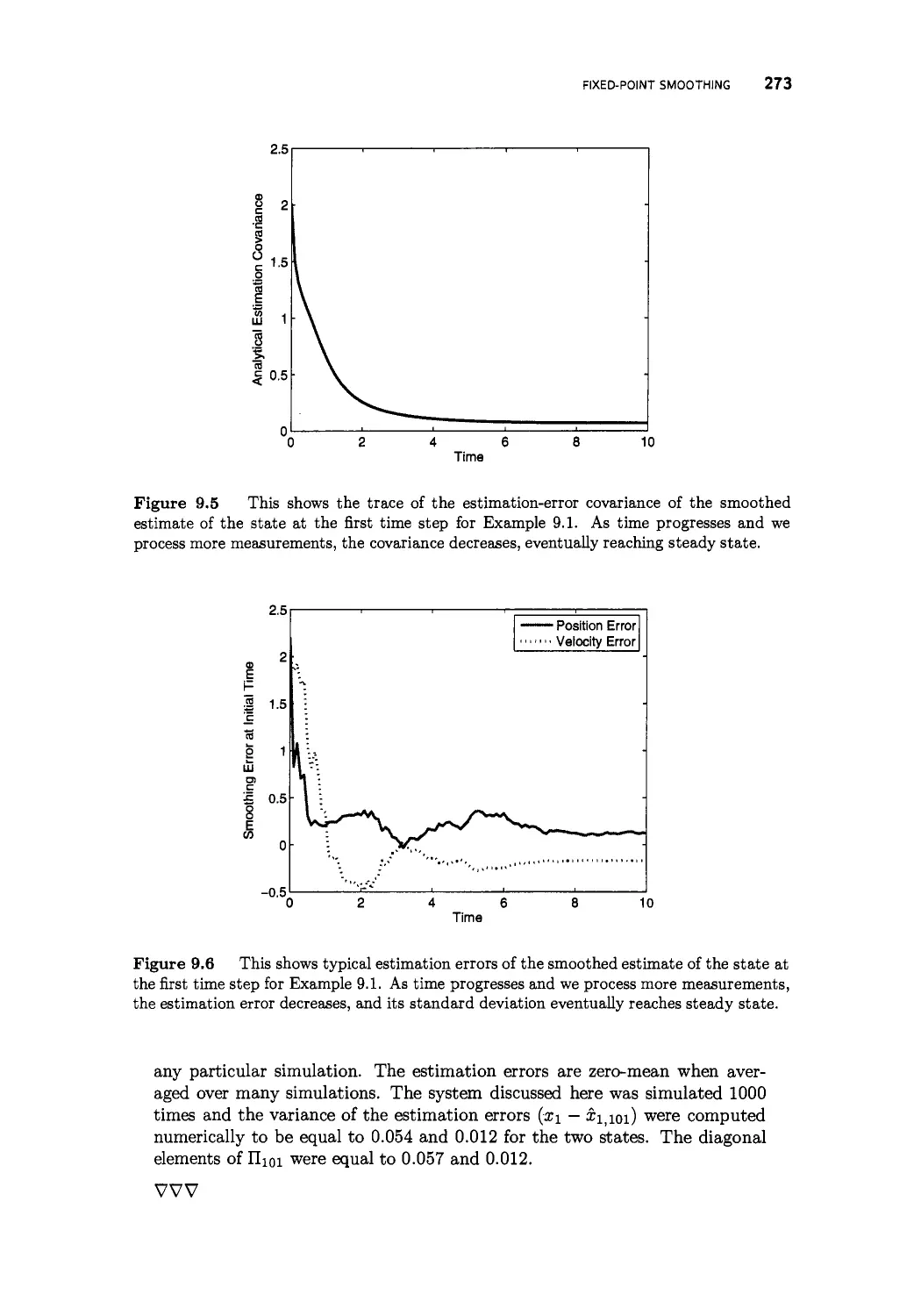
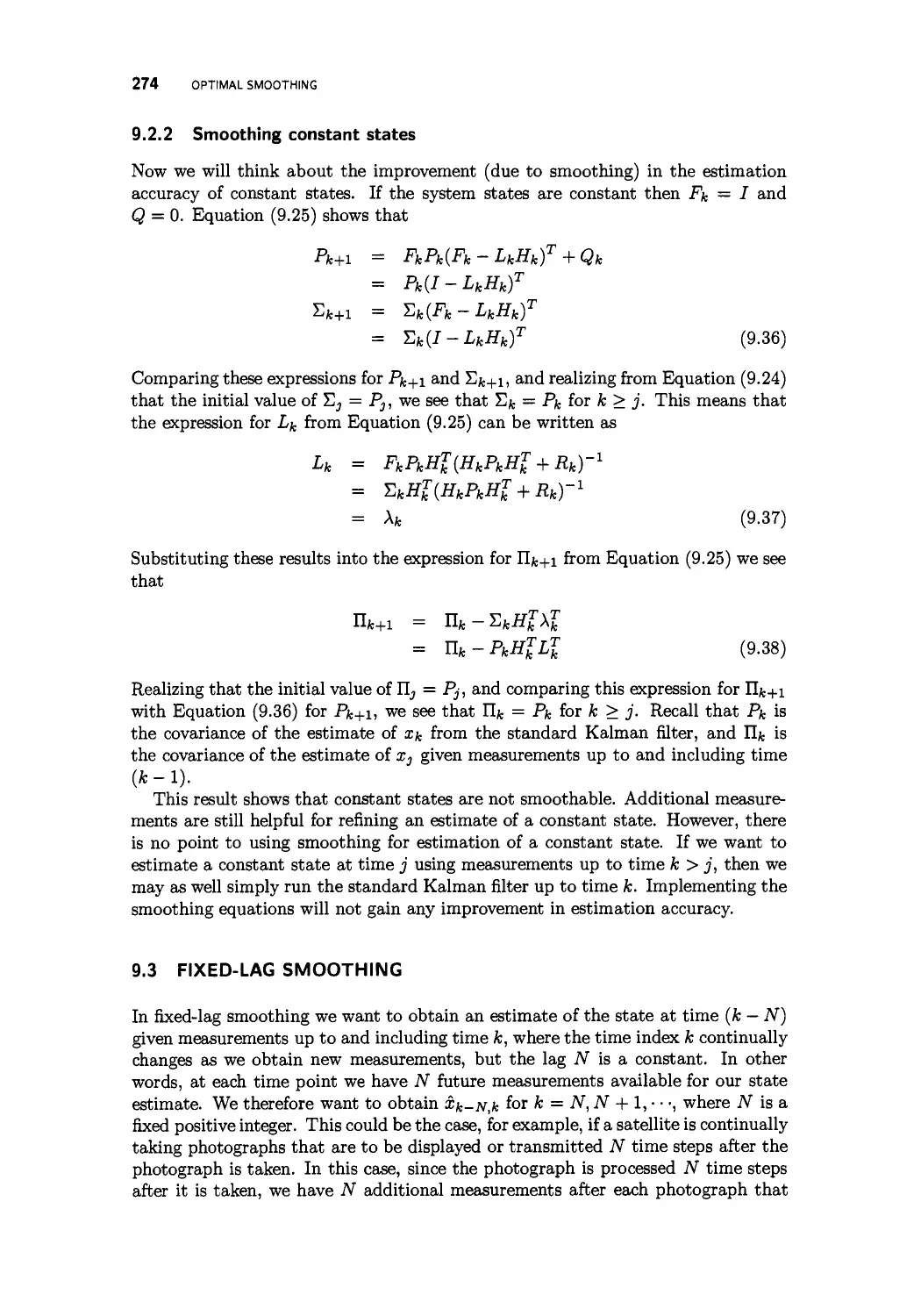
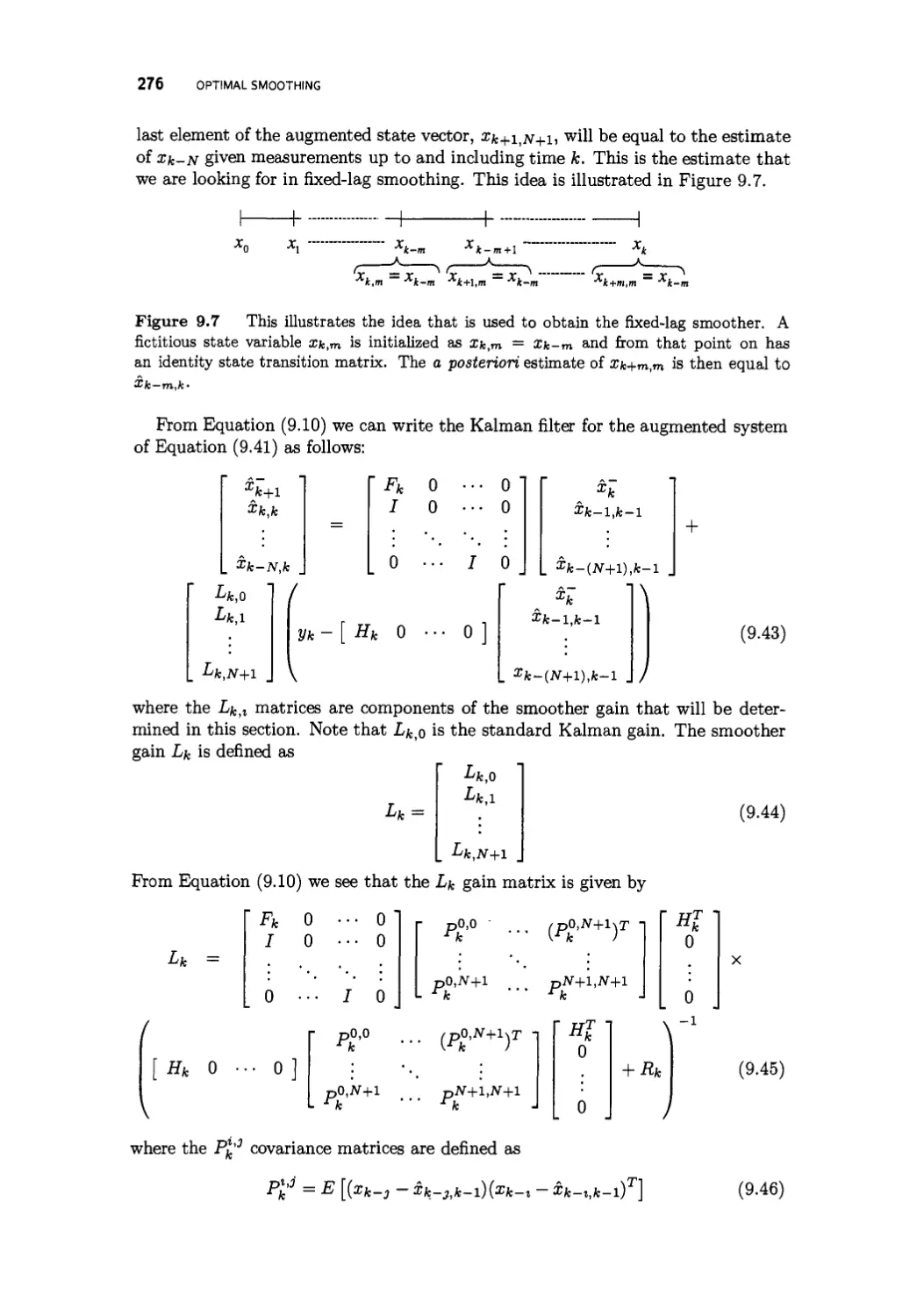
/


Author: Simon D.
Tags: mathematics statistics mathematical statistics
ISBN: 978-0-471-70858-2
Year: 2006


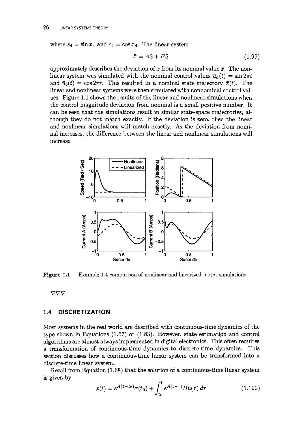
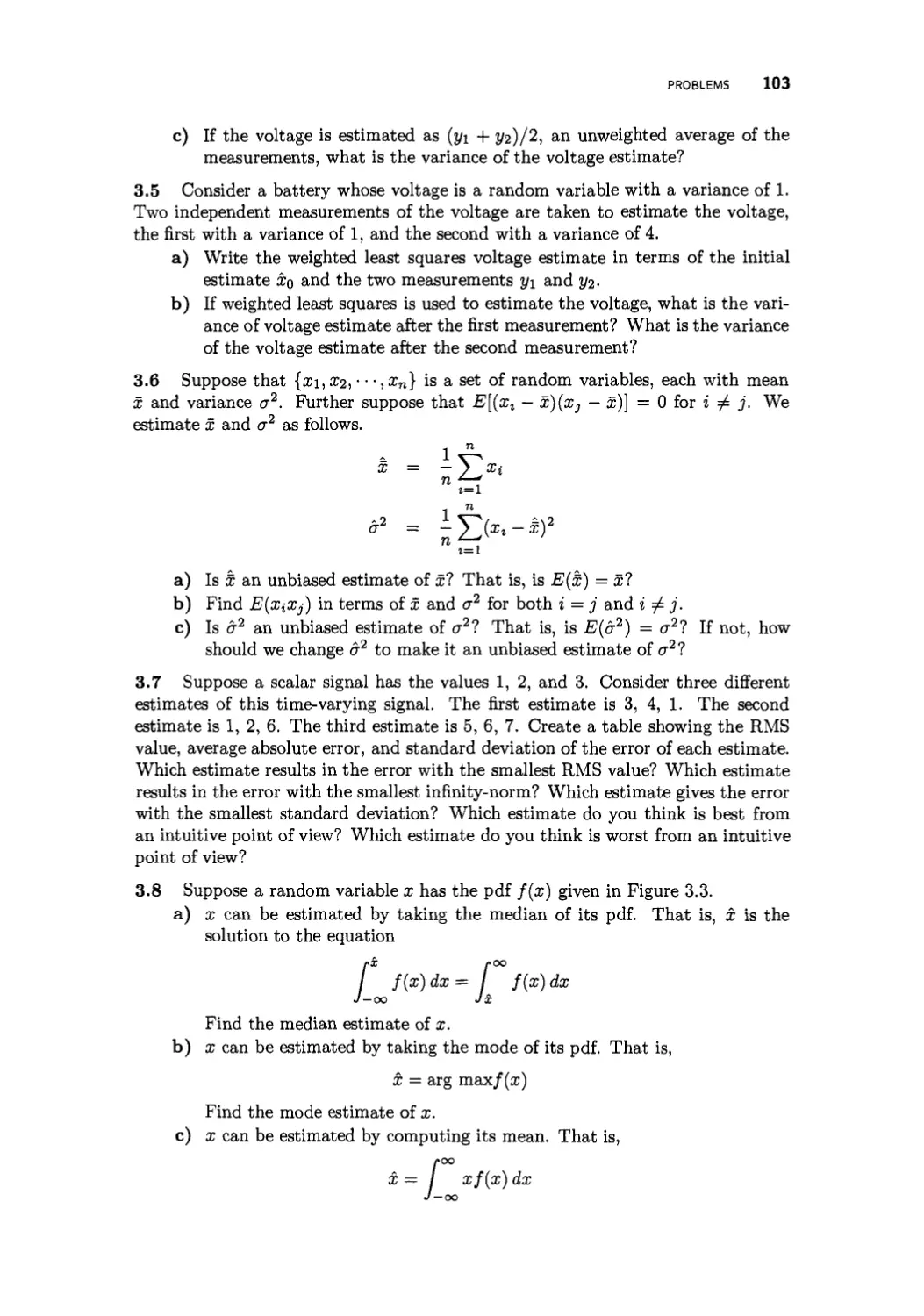
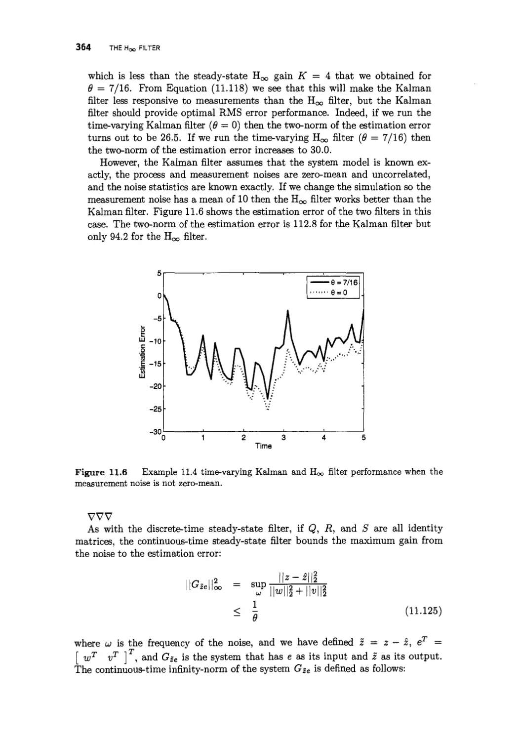
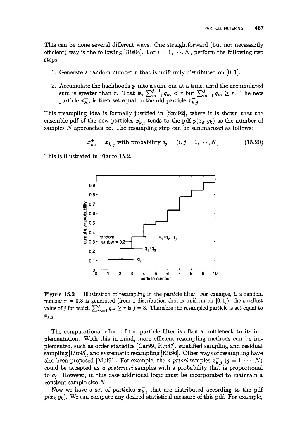
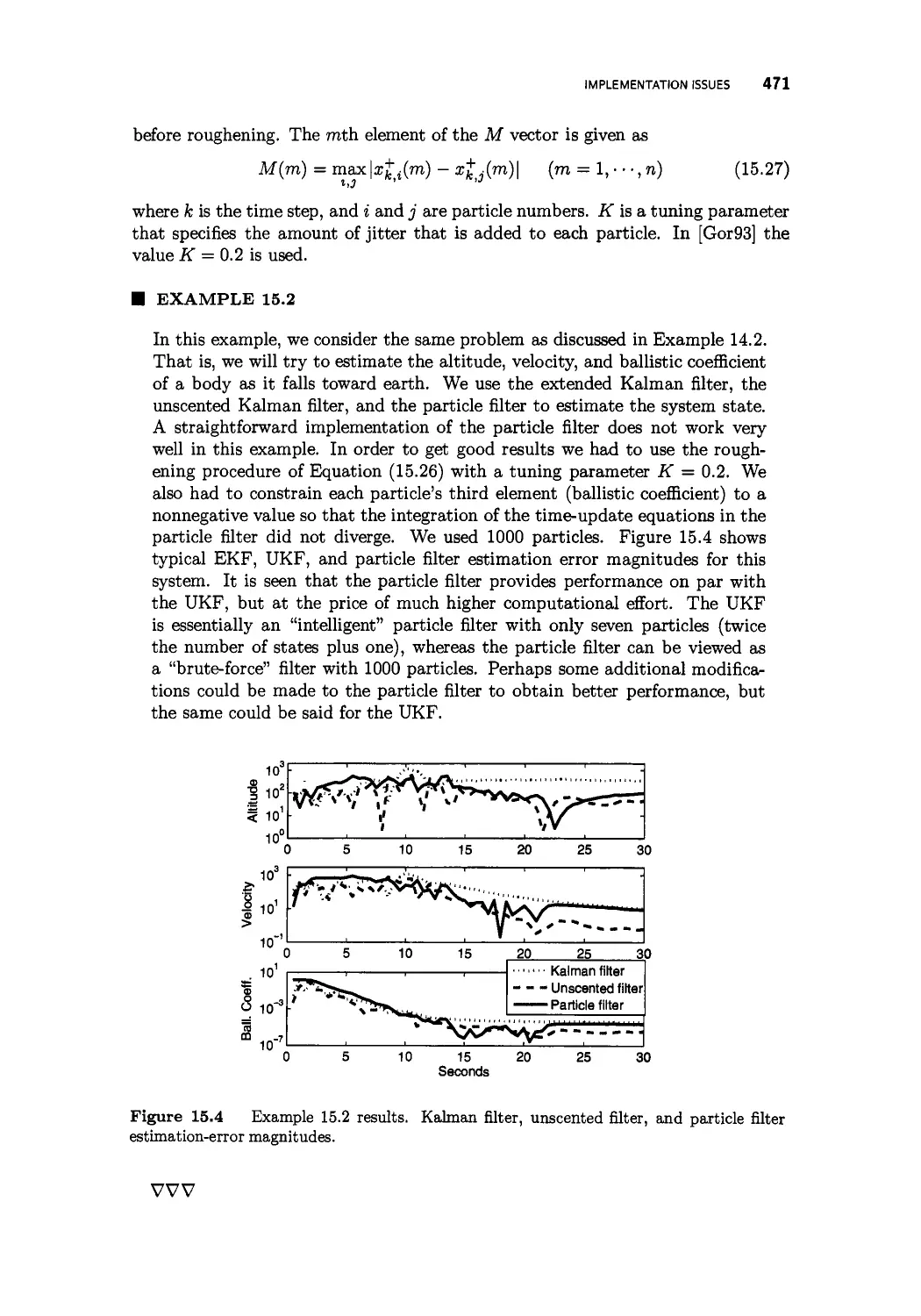
Text
^•WILEY
OPTIMAL
STATE
ESTIMATION
KALMAN,Hoo,
ano NONLINEAR APPROACHES
Dan Simon
Optimal State Estimation
Optimal State Estimation
Kalman, H*,, and Nonlinear Approaches
Dan Simon
Cleveland State University
WILEY-
INTERSCIENCE
A JOHN WILEY & SONS, INC., PUBLICATION
Copyright © 2006 by John Wiley & Sons, Inc. All rights reserved.
Published by John Wiley & Sons, Inc., Hoboken, New Jersey.
Published simultaneously in Canada.
No part of this publication may be reproduced, stored in a retrieval system or transmitted in any form
or by any means, electronic, mechanical, photocopying, recording, scanning, or otherwise, except as
permitted under Section 107 or 108 of the 1976 United States Copyright Act, without either the prior
written permission of the Publisher, or authorization through payment of the appropriate per-copy fee
to the Copyright Clearance Center, Inc., 222 Rosewood Drive, Danvers, MA 01923, (978) 750-8400,
fax (978) 646-8600, or on the web at www.copyright.com. Requests to the Publisher for permission
should be addressed to the Permissions Department, John Wiley & Sons, Inc., 111 River Street,
Hoboken, NJ 07030, (201) 748-6011, fax (201) 748-6008 or online at
http://www.wiley.com/go/permission.
Limit of Liability/Disclaimer of Warranty: While the publisher and author have used their best
efforts in preparing this book, they make no representations or warranties with respect to the
accuracy or completeness of the contents of this book and specifically disclaim any implied
warranties of merchantability or fitness for a particular purpose. No warranty may be created or
extended by sales representatives or written sales materials. The advice and strategies contained
herein may not be suitable for your situation. You should consult with a professional where
appropriate. Neither the publisher nor author shall be liable for any loss of profit or any other
commercial damages, including but not limited to special, incidental, consequential, or other
damages.
For general information on our other products and services or for technical support, please contact
our Customer Care Department within the U.S. at (800) 762-2974, outside the U.S. at (317) 572-
3993 or fax (317) 572-4002.
Wiley also publishes its books in a variety of electronic formats. Some content that appears in print
may not be available in electronic format. For information about Wiley products, visit our web site at
www.wiley.com.
Library of Congress Cataloging-in-Publication is available.
ISBN-13 978-0-471-70858-2
ISBN-10 0-471-70858-5
Printed in the United States of America.
10 987654321
CONTENTS
Acknowledgments xiii
Acronyms xv
List of algorithms xvii
Introduction xxi
PART I INTRODUCTORY MATERIAL
1 Linear systems theory 3
1.1 Matrix algebra and matrix calculus 4
1.1.1 Matrix algebra 6
1.1.2 The matrix inversion lemma 11
1.1.3 Matrix calculus 14
1.1.4 The history of matrices 17
1.2 Linear systems 18
1.3 Nonlinear systems 22
1.4 Discretization 26
1.5 Simulation 27
1.5.1 Rectangular integration 29
1.5.2 Trapezoidal integration 29
1.5.3 Runge-Kutta integration 31
1.6 Stability 33
vi CONTENTS
1.6.1 Continuous-time systems 33
1.6.2 Discrete-time systems 37
1.7 Controllability and observability 38
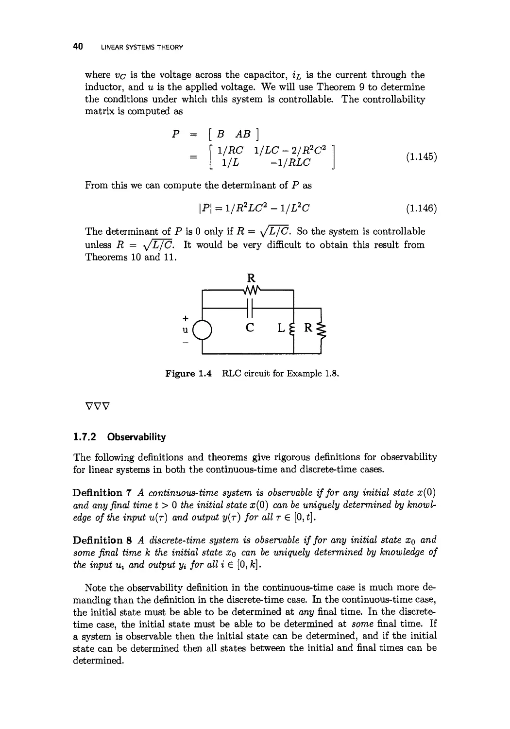
1.7.1 Controllability 38
1.7.2 Observability 40
1.7.3 Stabilizability and detectability 43
1.8 Summary 45
Problems 45
2 Probability theory 49
2.1 Probability 50
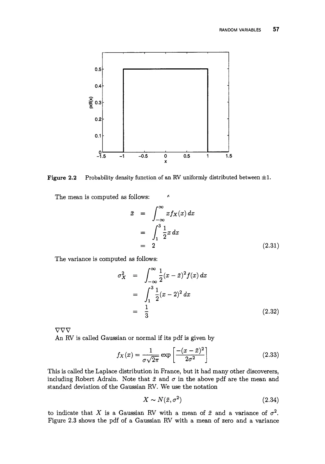
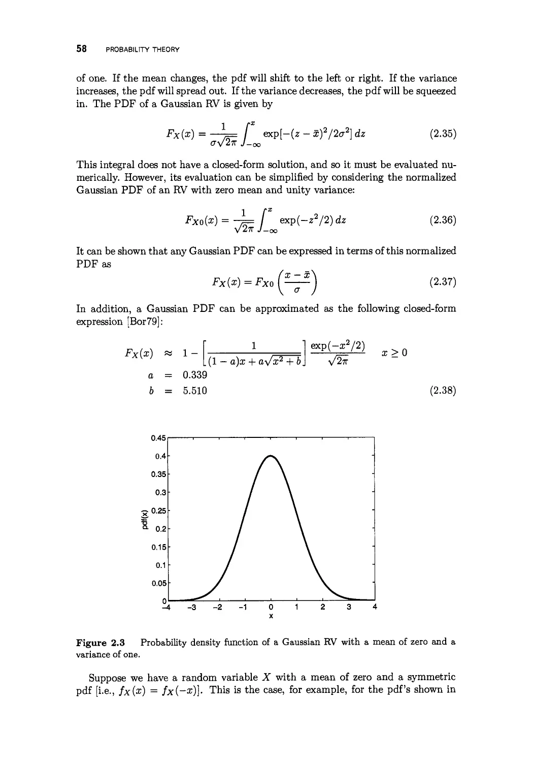
2.2 Random variables 53
2.3 Transformations of random variables 59
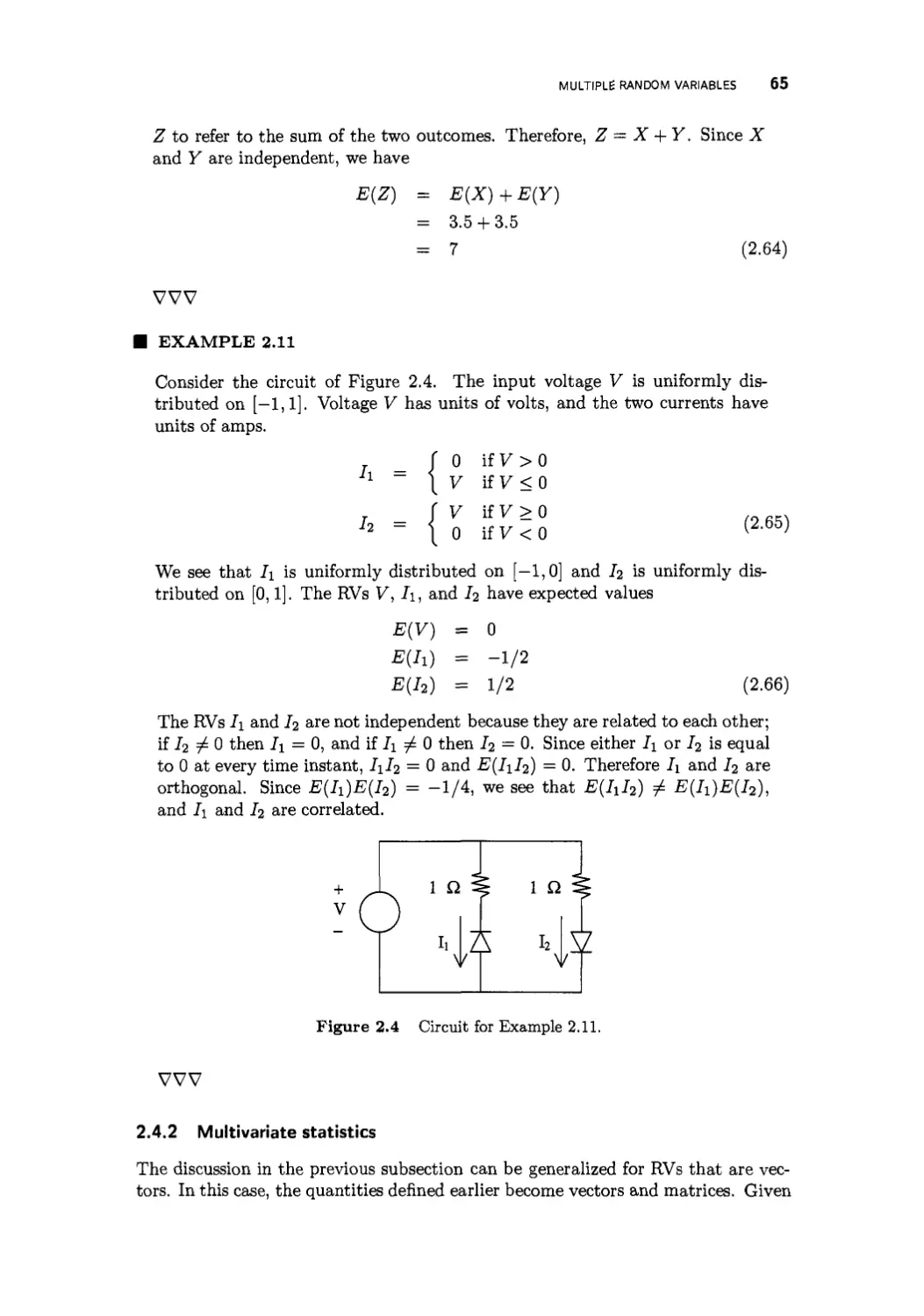
2.4 Multiple random variables 61
2.4.1 Statistical independence 62
2.4.2 Multivariate statistics 65
2.5 Stochastic Processes 68
2.6 White noise and colored noise 71
2.7 Simulating correlated noise 73
2.8 Summary 74
Problems 75
3 Least squares estimation 79
3.1 Estimation of a constant 80
3.2 Weighted least squares estimation 82
3.3 Recursive least squares estimation 84
3.3.1 Alternate estimator forms 86
3.3.2 Curve fitting 92
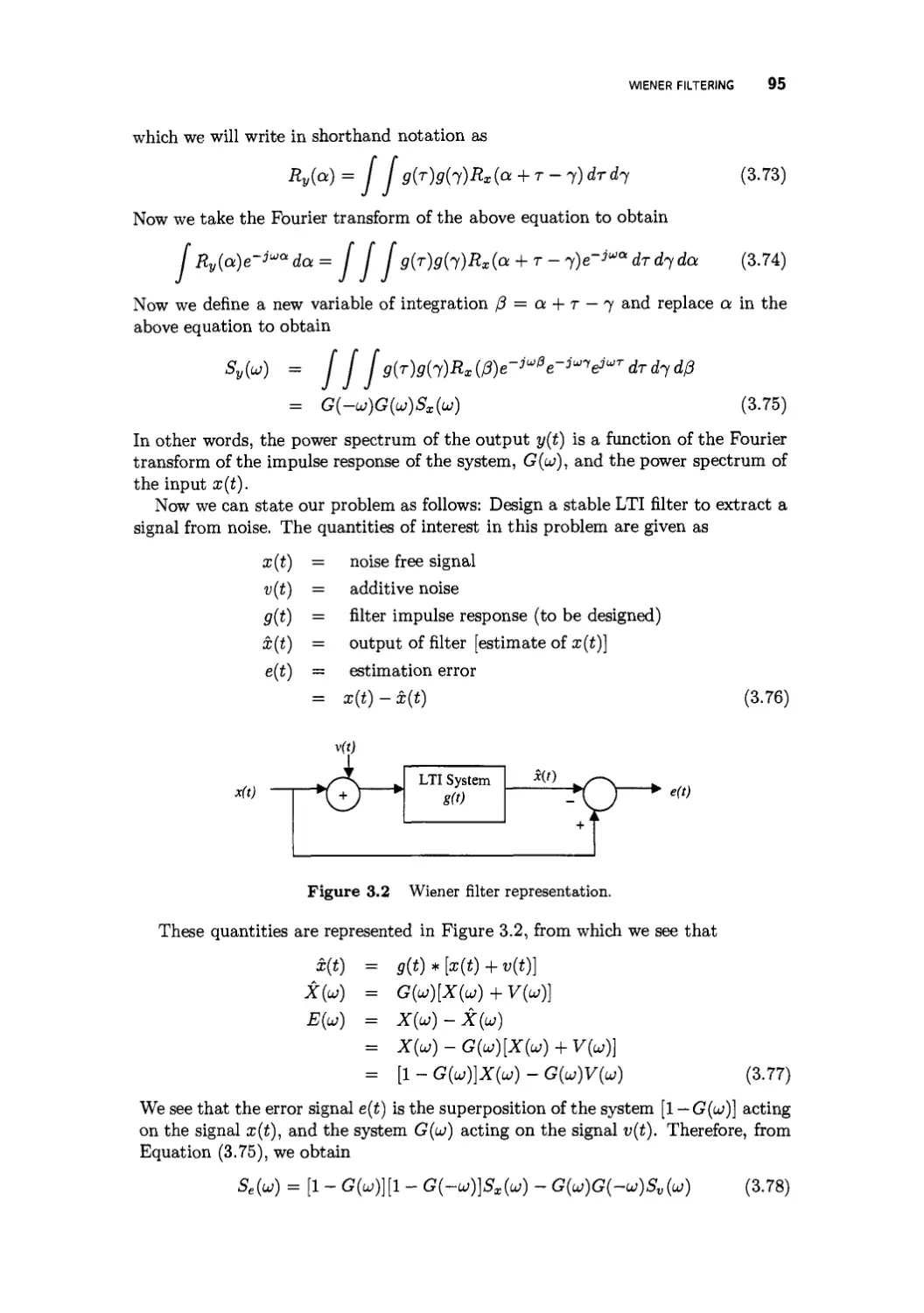
3.4 Wiener filtering 94
3.4.1 Parametric filter optimization 96
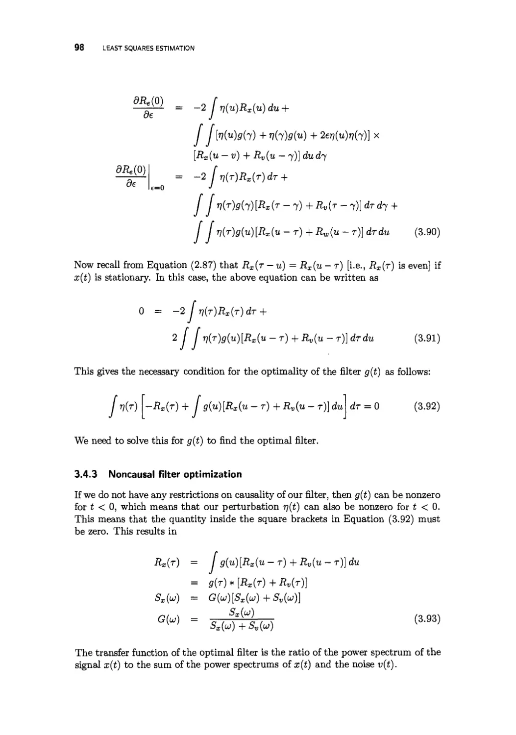
3.4.2 General filter optimization 97
3.4.3 Noncausal filter optimization 98
3.4.4 Causal filter optimization 100
3.4.5 Comparison 101
3.5 Summary 102
Problems 102
4 Propagation of states and covariances 107
4.1 Discrete-time systems 107
4.2 Sampled-data systems 111
4.3 Continuous-time systems 114
CONTENTS vii
4.4 Summary 117
Problems 117
PART II THE KALMAN FILTER
5 The discrete-time Kalman filter 123
5.1 Derivation of the discrete-time Kalman filter 124
5.2 Kalman filter properties 129
5.3 One-step Kalman filter equations 131
5.4 Alternate propagation of covariance 135
5.4.1 Multiple state systems 135
5.4.2 Scalar systems 137
5.5 Divergence issues 139
5.6 Summary 144
Problems 145
6 Alternate Kalman filter formulations 149
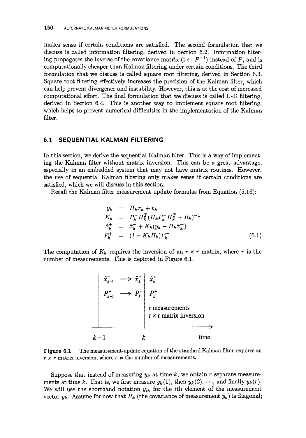
6.1 Sequential Kalman filtering 150
6.2 Information filtering 156
6.3 Square root filtering 158
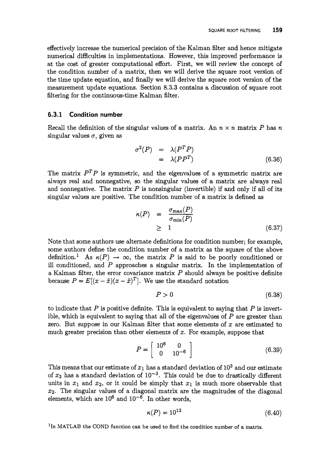
6.3.1 Condition number 159
6.3.2 The square root time-update equation 162
6.3.3 Potter's square root measurement-update equation 165
6.3.4 Square root measurement update via triangularization 169
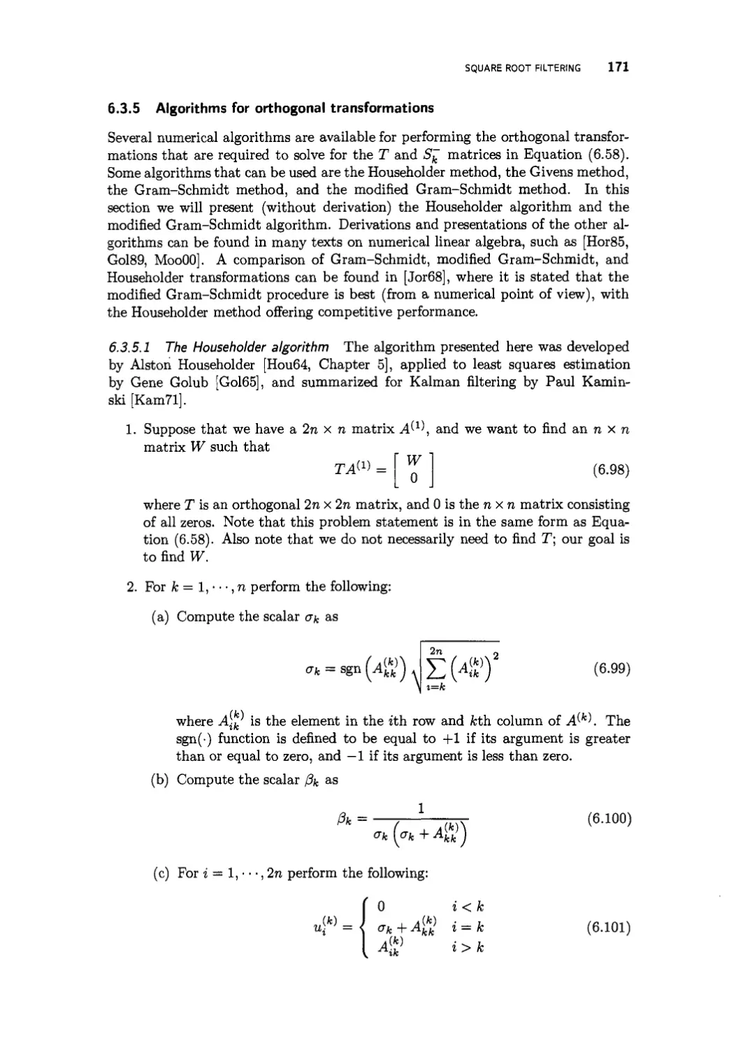
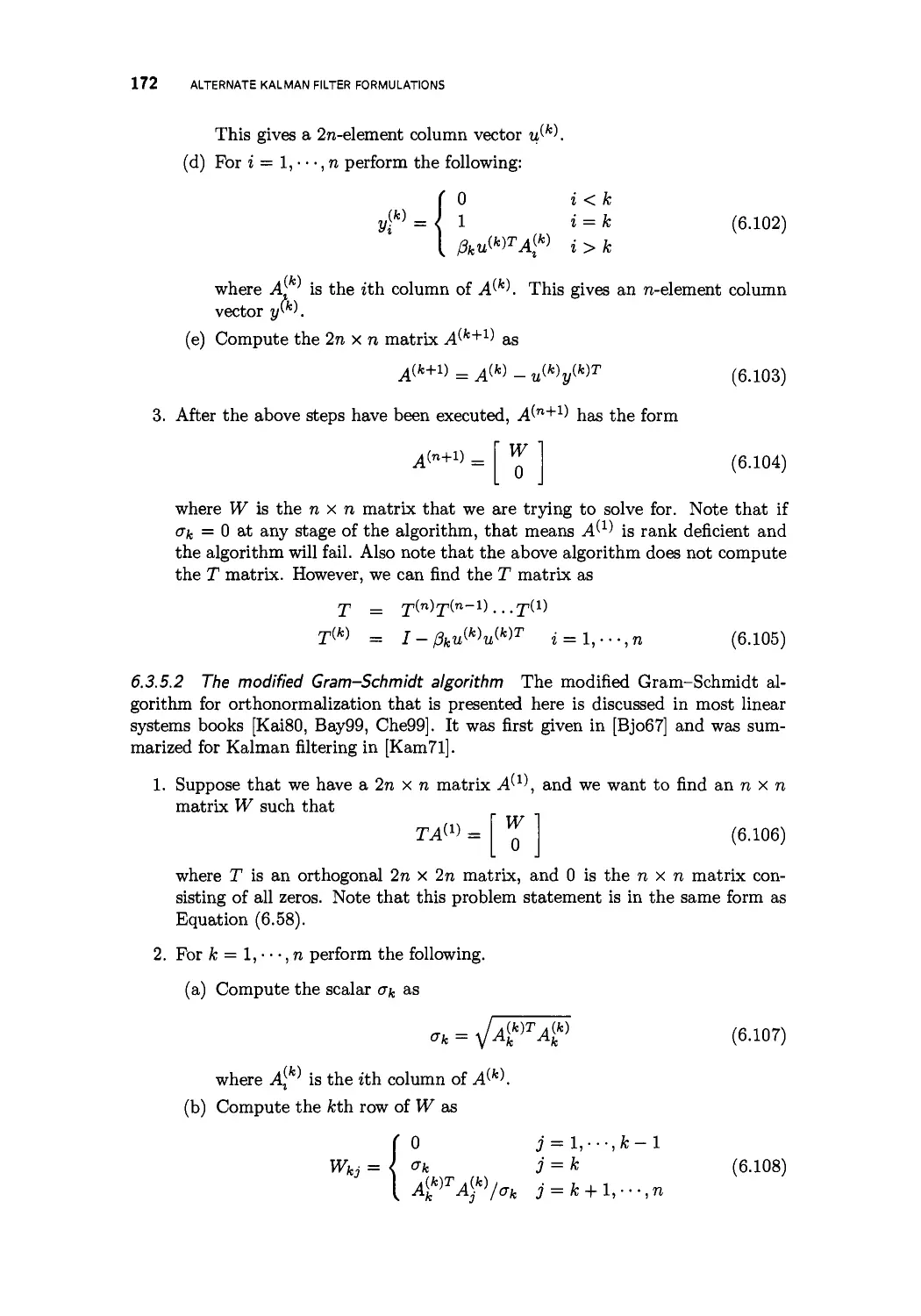
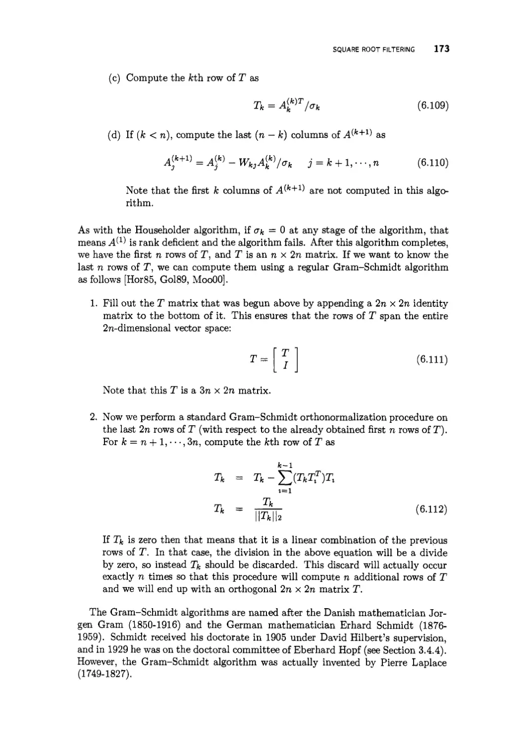
6.3.5 Algorithms for orthogonal transformations 171
6.4 U-D filtering 174
6.4.1 U-D filtering: The measurement-up date equation 174
6.4.2 U-D filtering: The time-update equation 176
6.5 Summary 178
Problems 179
7 Kalman filter generalizations 183
7.1 Correlated process and measurement noise 184
7.2 Colored process and measurement noise 188
7.2.1 Colored process noise 188
7.2.2 Colored measurement noise: State augmentation 189
7.2.3 Colored measurement noise: Measurement differencing 190
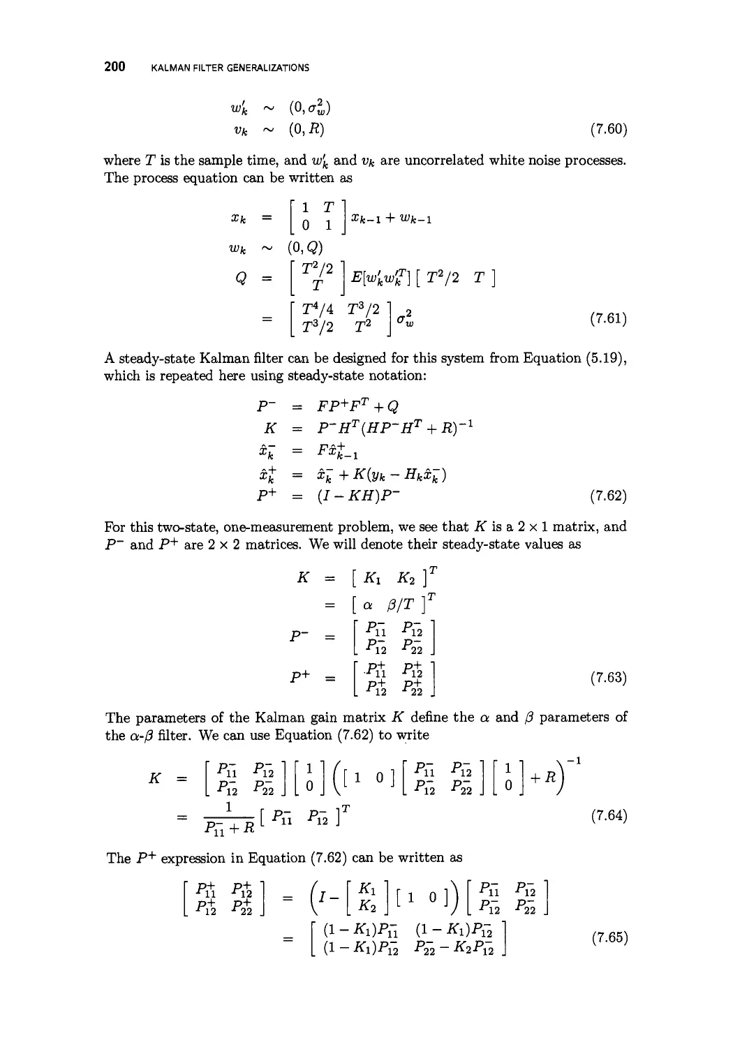
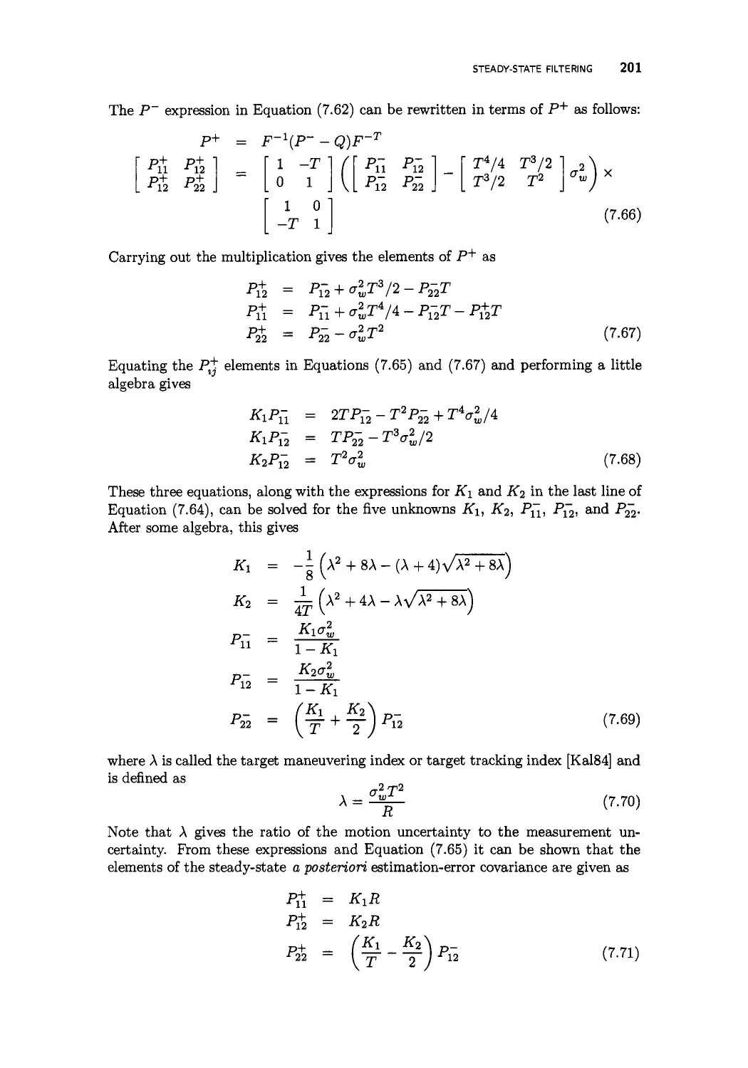
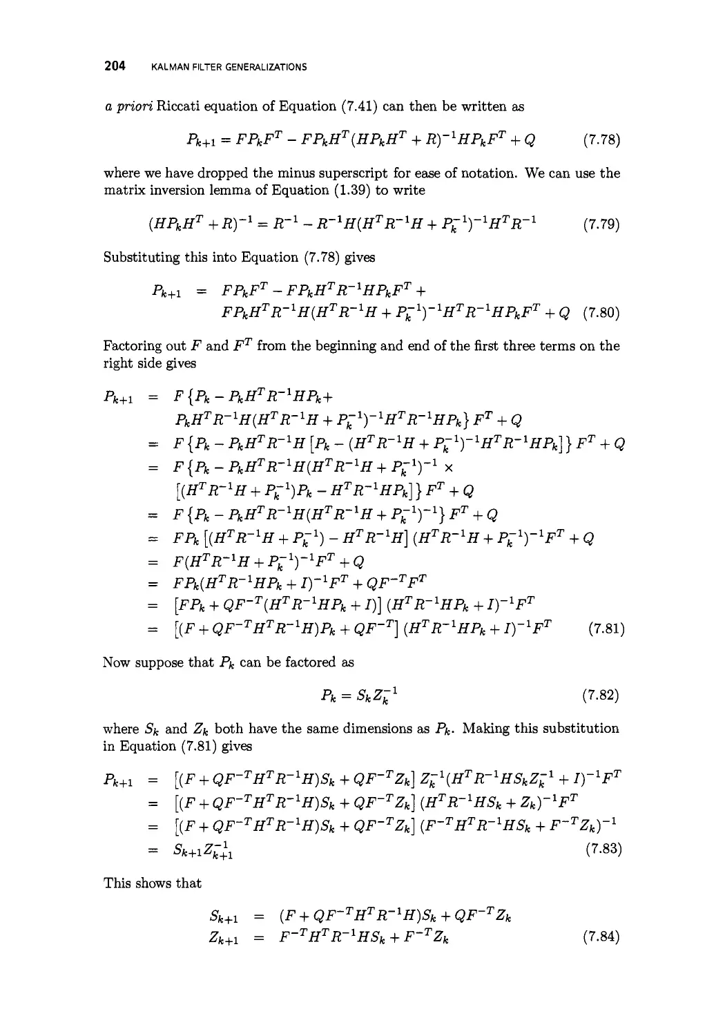
7.3 Steady-state filtering 193
7.3.1 a-(3 filtering 199
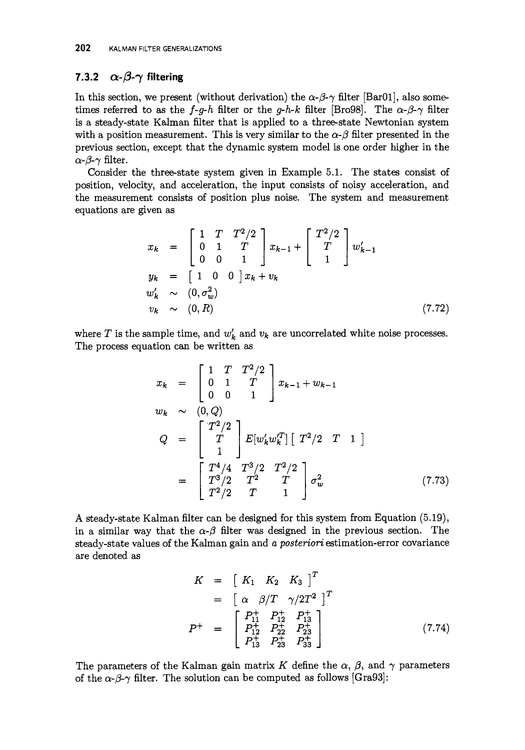
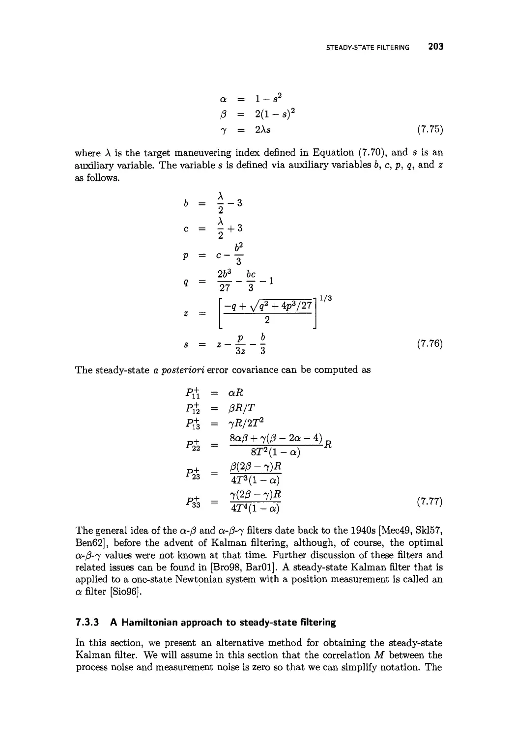
7.3.2 a-/3-7 filtering 202
7.3.3 A Hamiltonian approach to steady-state filtering 203
7.4 Kalman filtering with fading memory 208
viii CONTENTS
7.5 Constrained Kalman filtering 212
7.5.1 Model reduction 212
7.5.2 Perfect measurements 213
7.5.3 Projection approaches 214
7.5.4 A pdf truncation approach 218
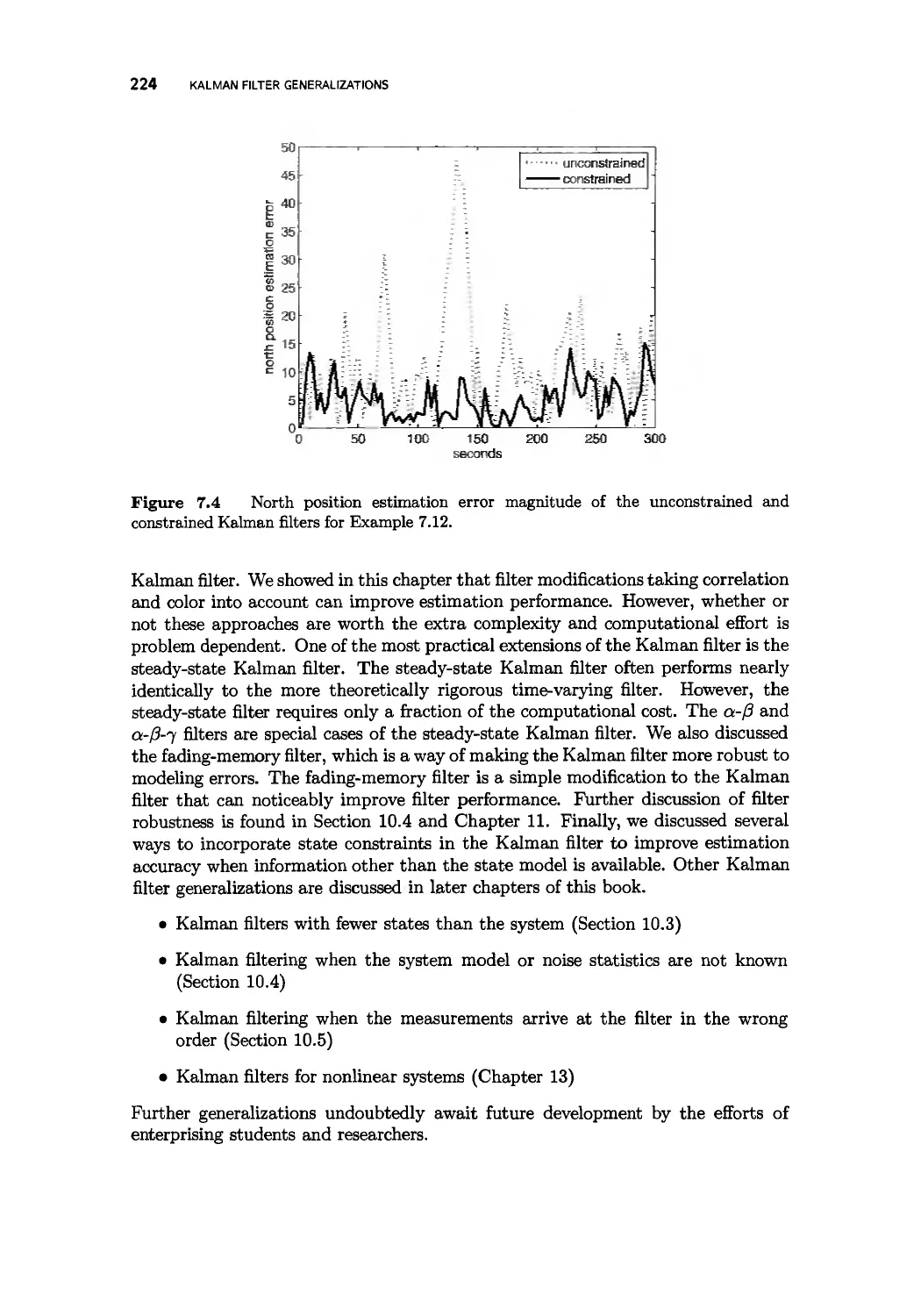
7.6 Summary 223
Problems 225
The continuous-time Kalman filter 229
8.1 Discrete-time and continuous-time white noise 230
8.1.1 Process noise 230
8.1.2 Measurement noise 232
8.1.3 Discretized simulation of noisy continuous-time systems 232
8.2 Derivation of the continuous-time Kalman filter 233
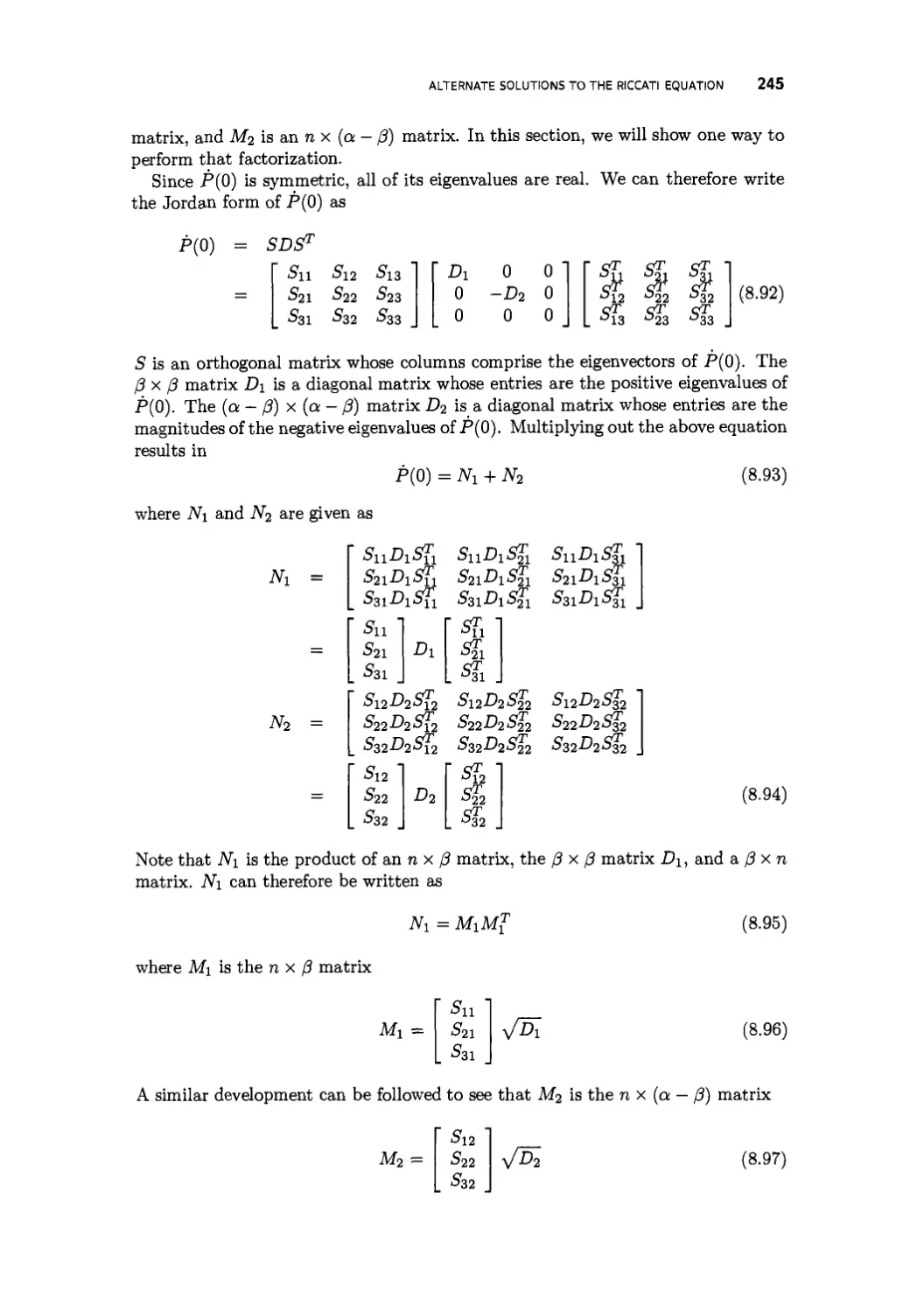
8.3 Alternate solutions to the Riccati equation 238
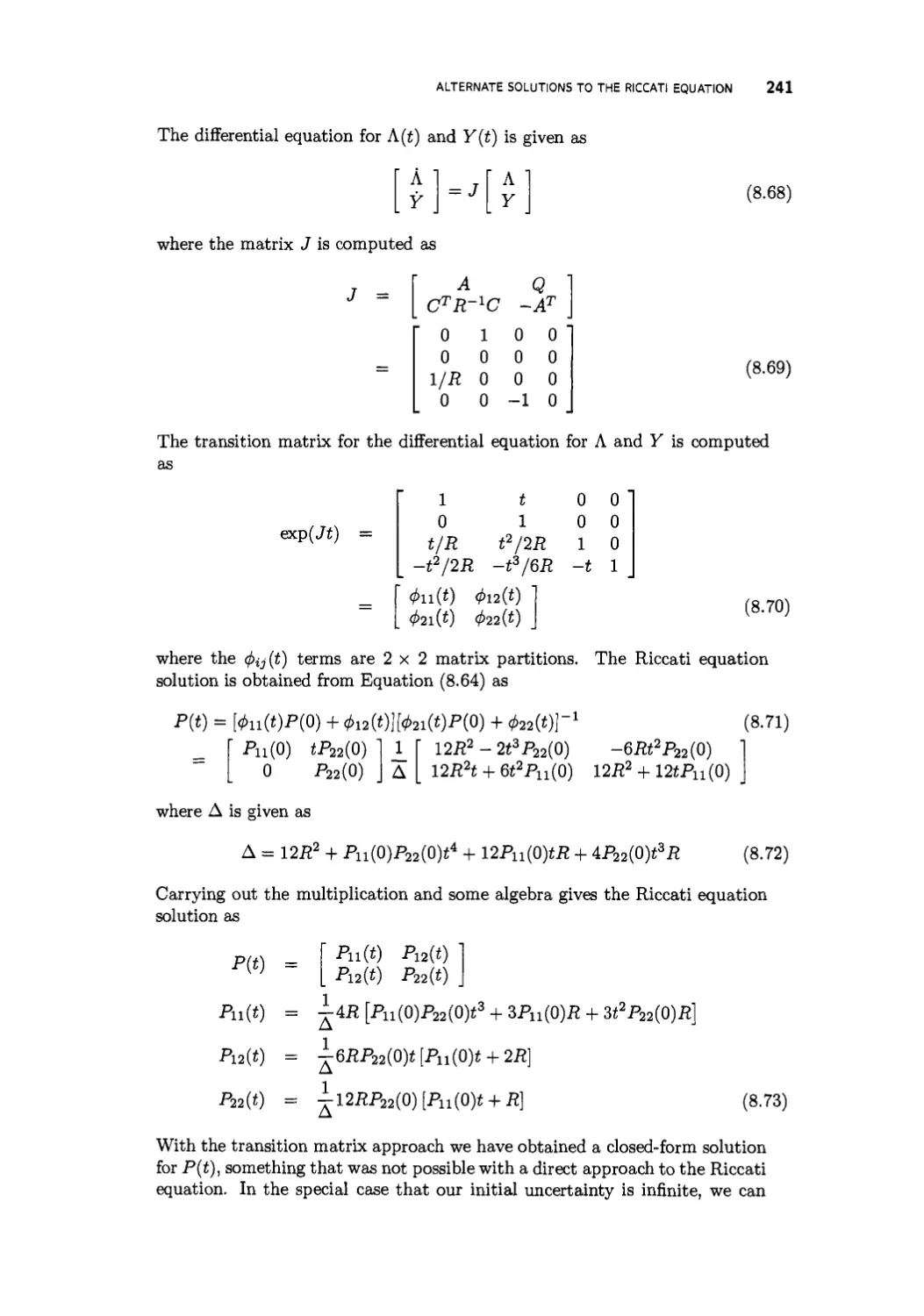
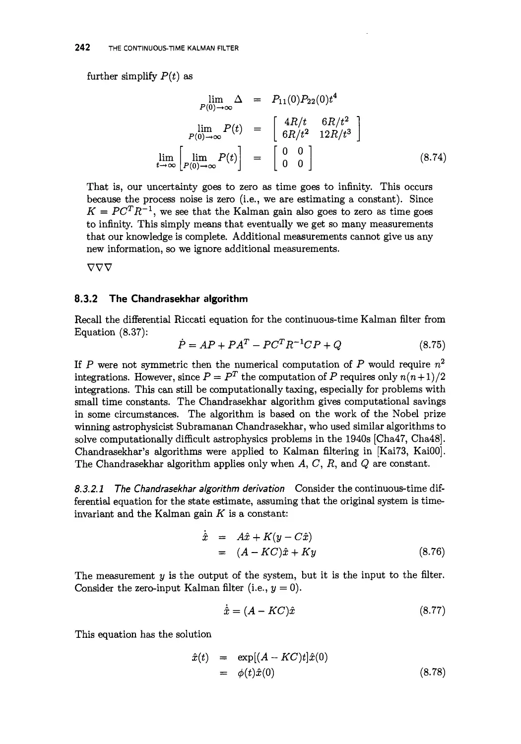
8.3.1 The transition matrix approach 238
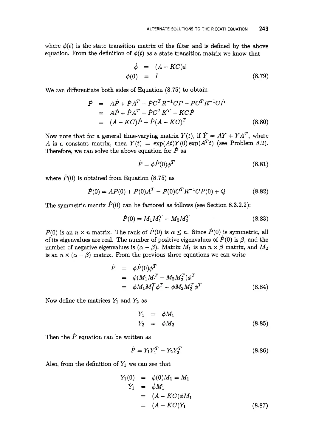
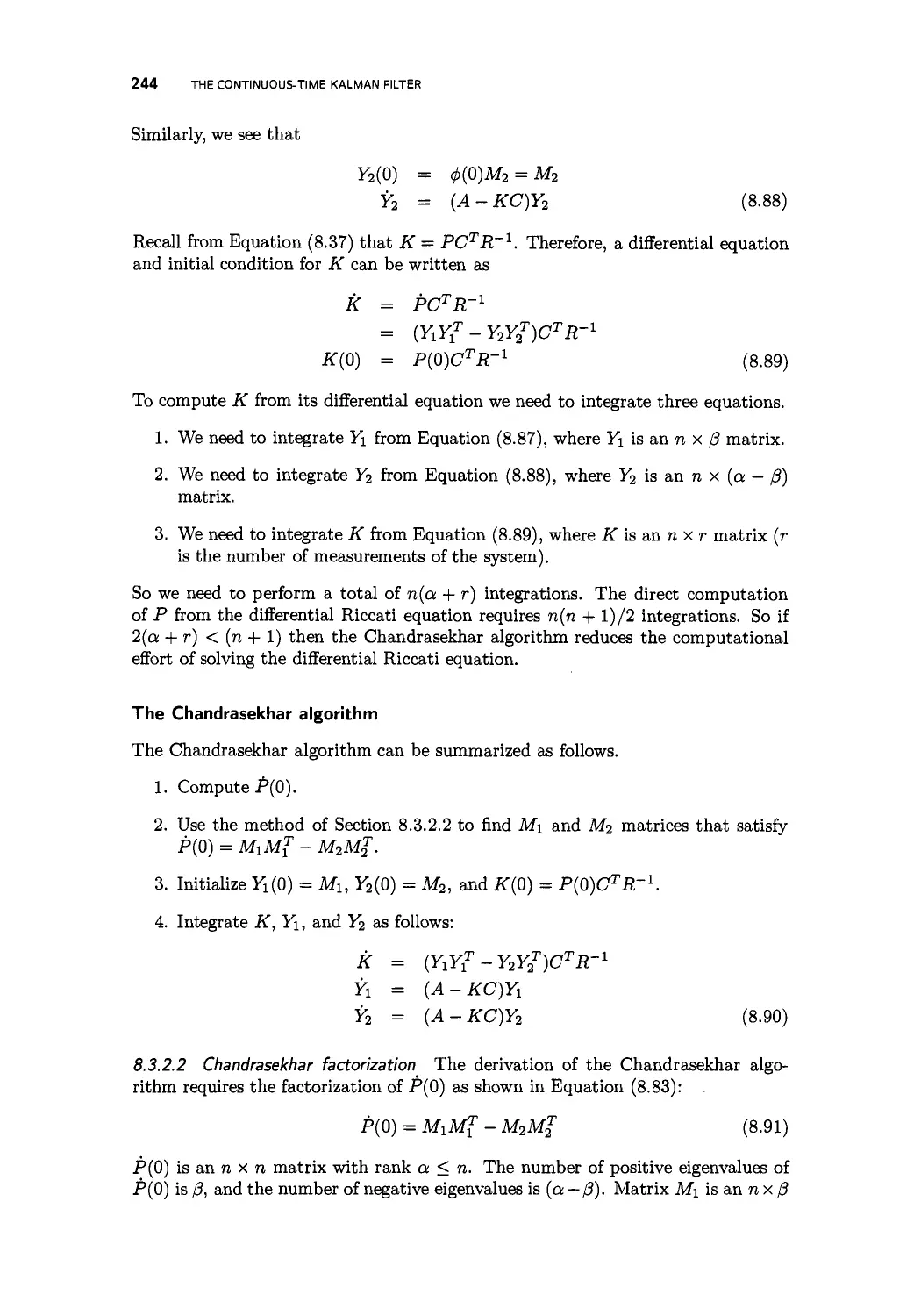
8.3.2 The Chandrasekhar algorithm 242
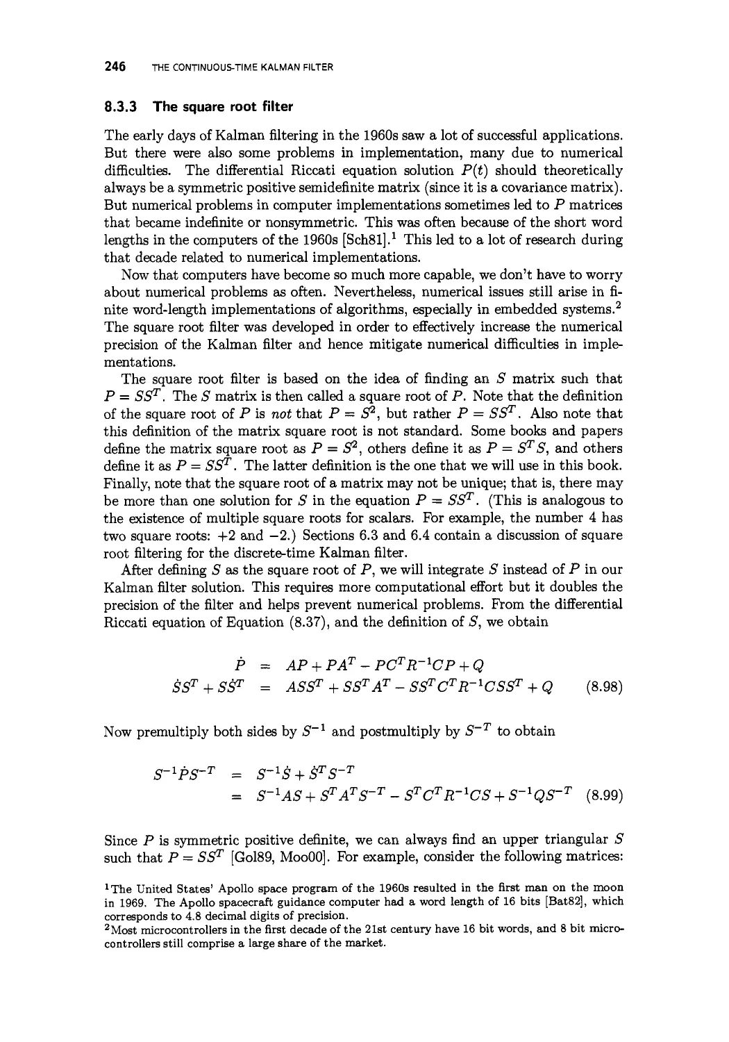
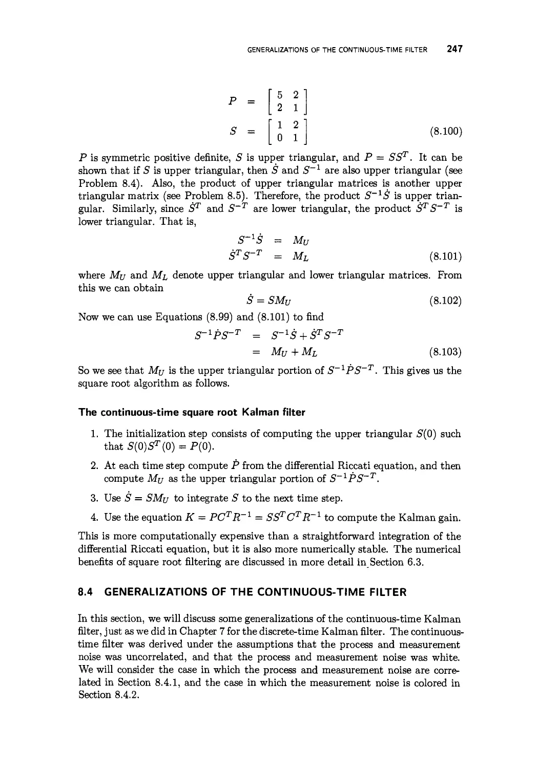
8.3.3 The square root filter 246
8.4 Generalizations of the continuous-time filter 247
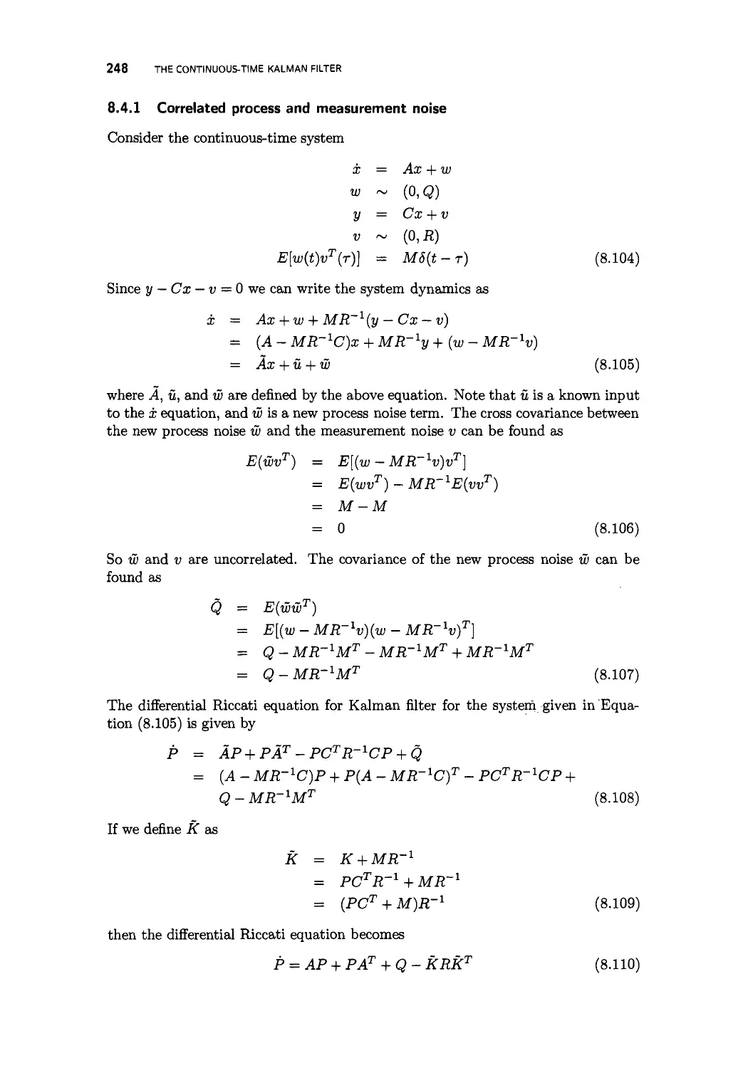
8.4.1 Correlated process and measurement noise 248
8.4.2 Colored measurement noise 249
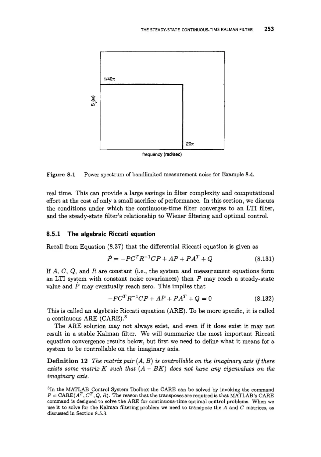
8.5 The steady-state continuous-time Kalman filter 252
8.5.1 The algebraic Riccati equation 253
8.5.2 The Wiener filter is a Kalman filter 257
8.5.3 Duality 258
8.6 Summary 259
Problems 260
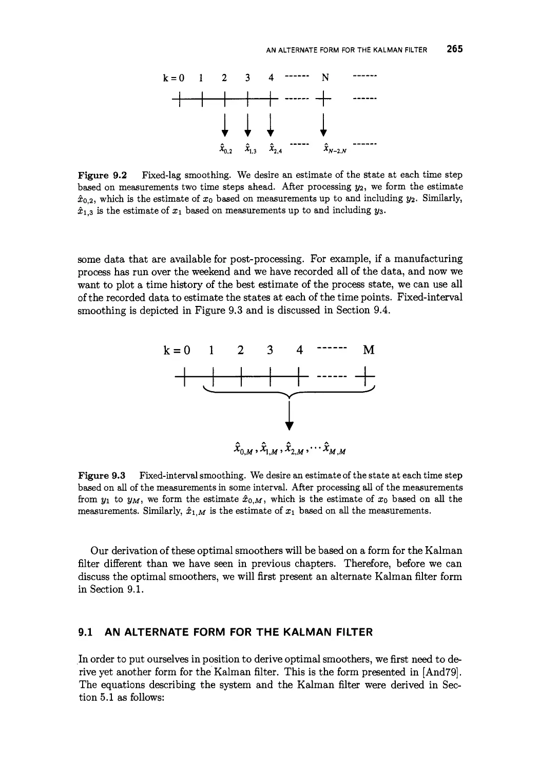
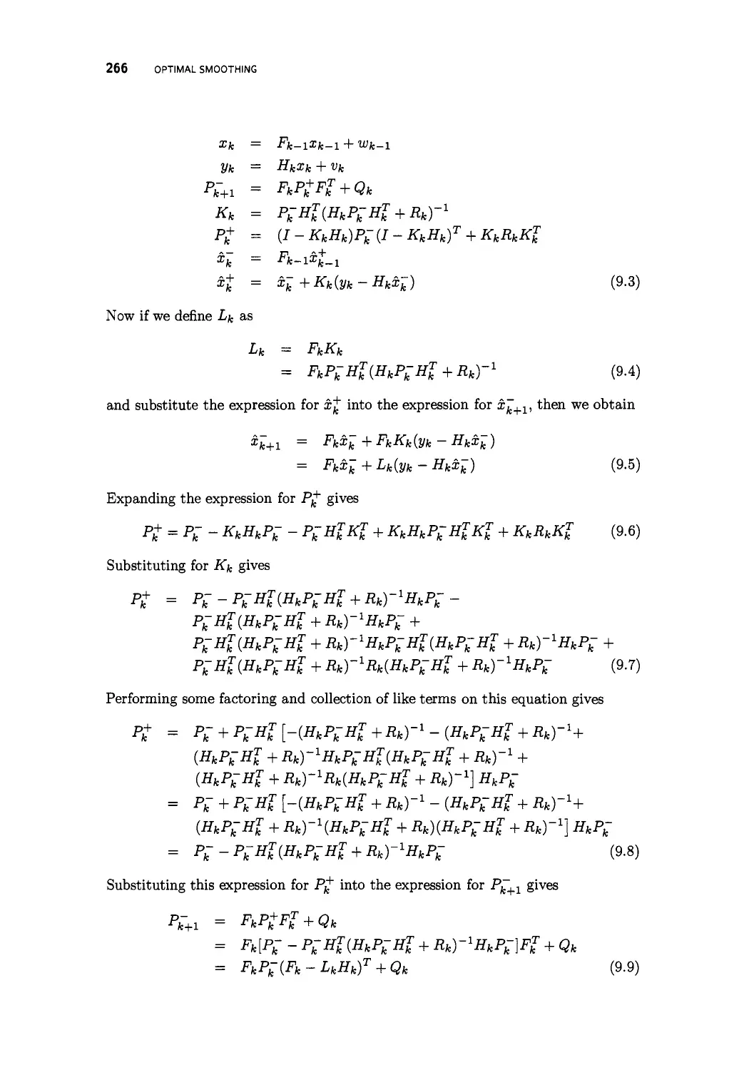
Optimal smoothing 263
9.1 An alternate form for the Kalman filter 265
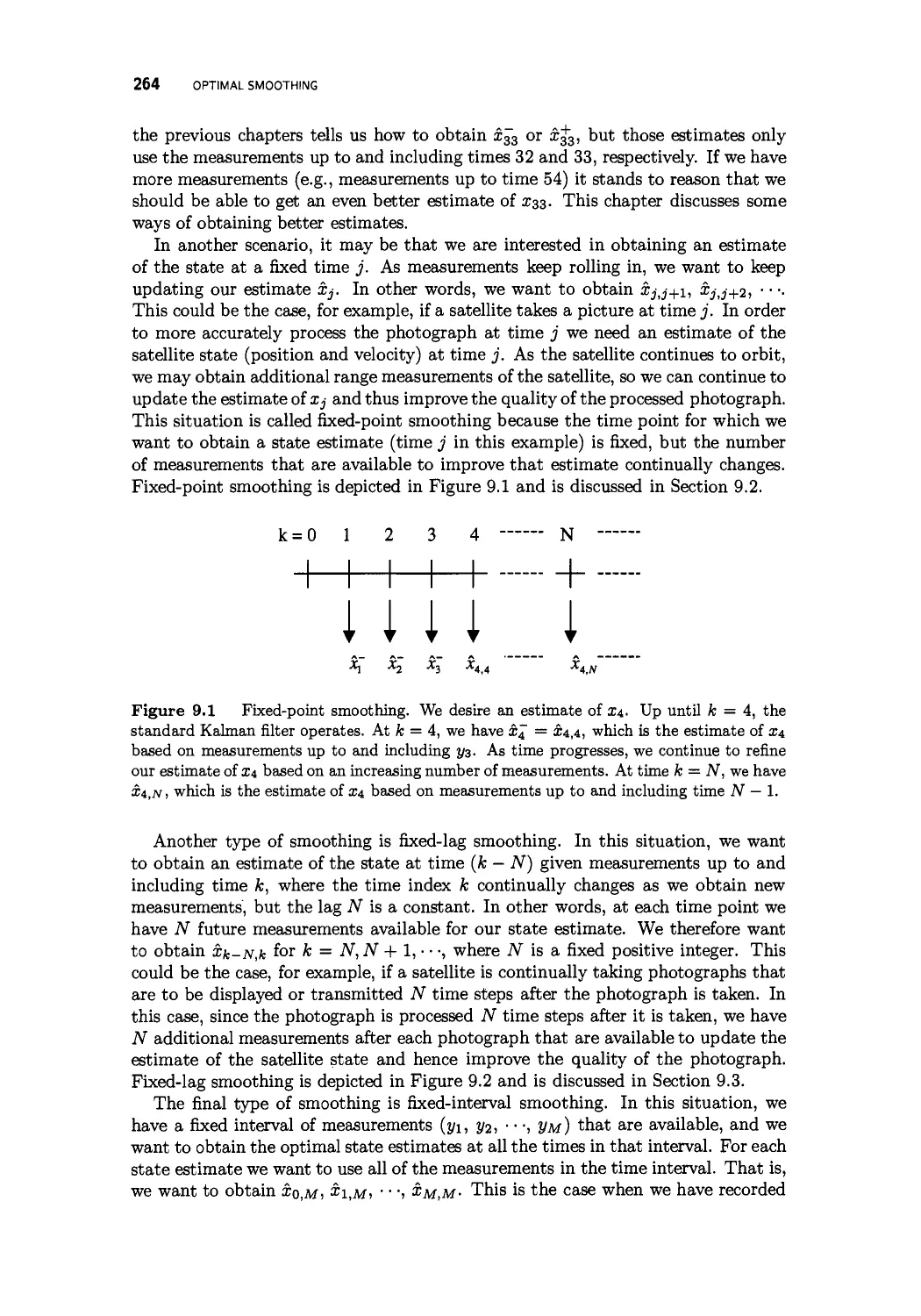
9.2 Fixed-point smoothing 267
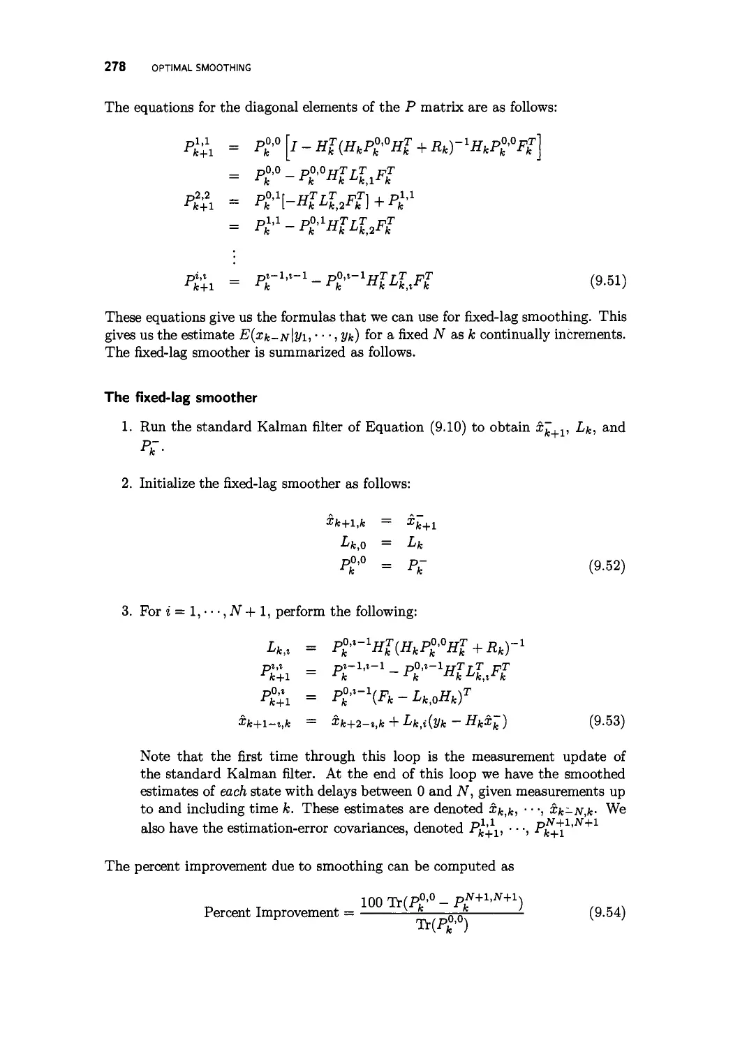
9.2.1 Estimation improvement due to smoothing 270
9.2.2 Smoothing constant states 274
9.3 Fixed-lag smoothing 274
9.4 Fixed-interval smoothing 279
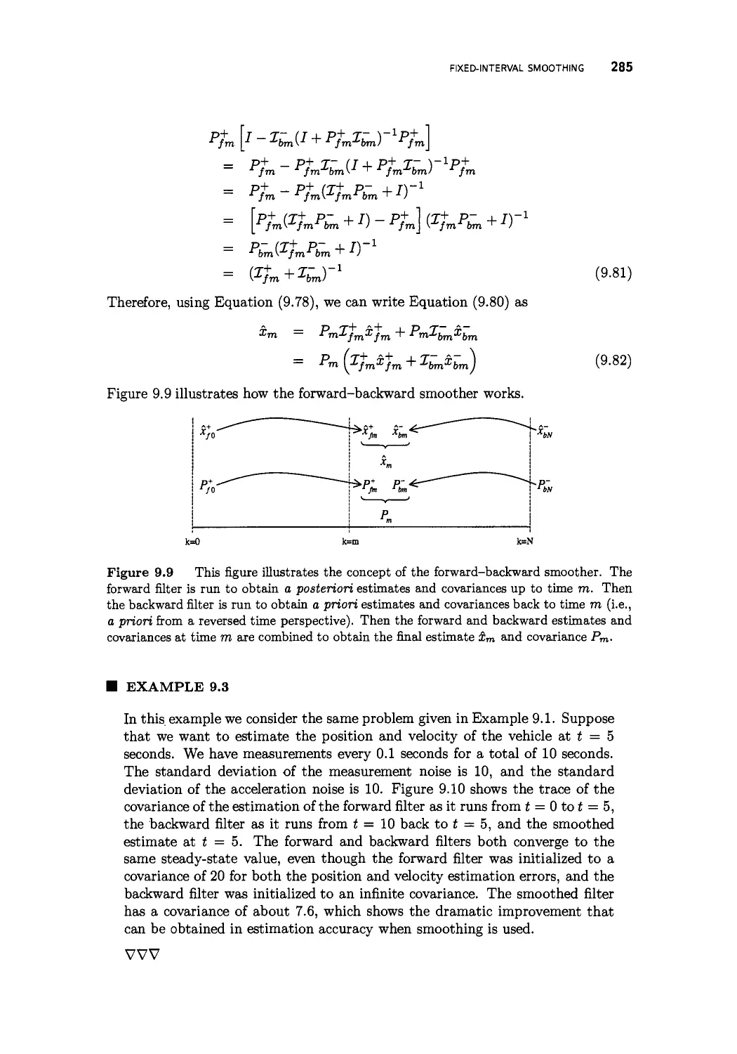
9.4.1 Forward-backward smoothing 280
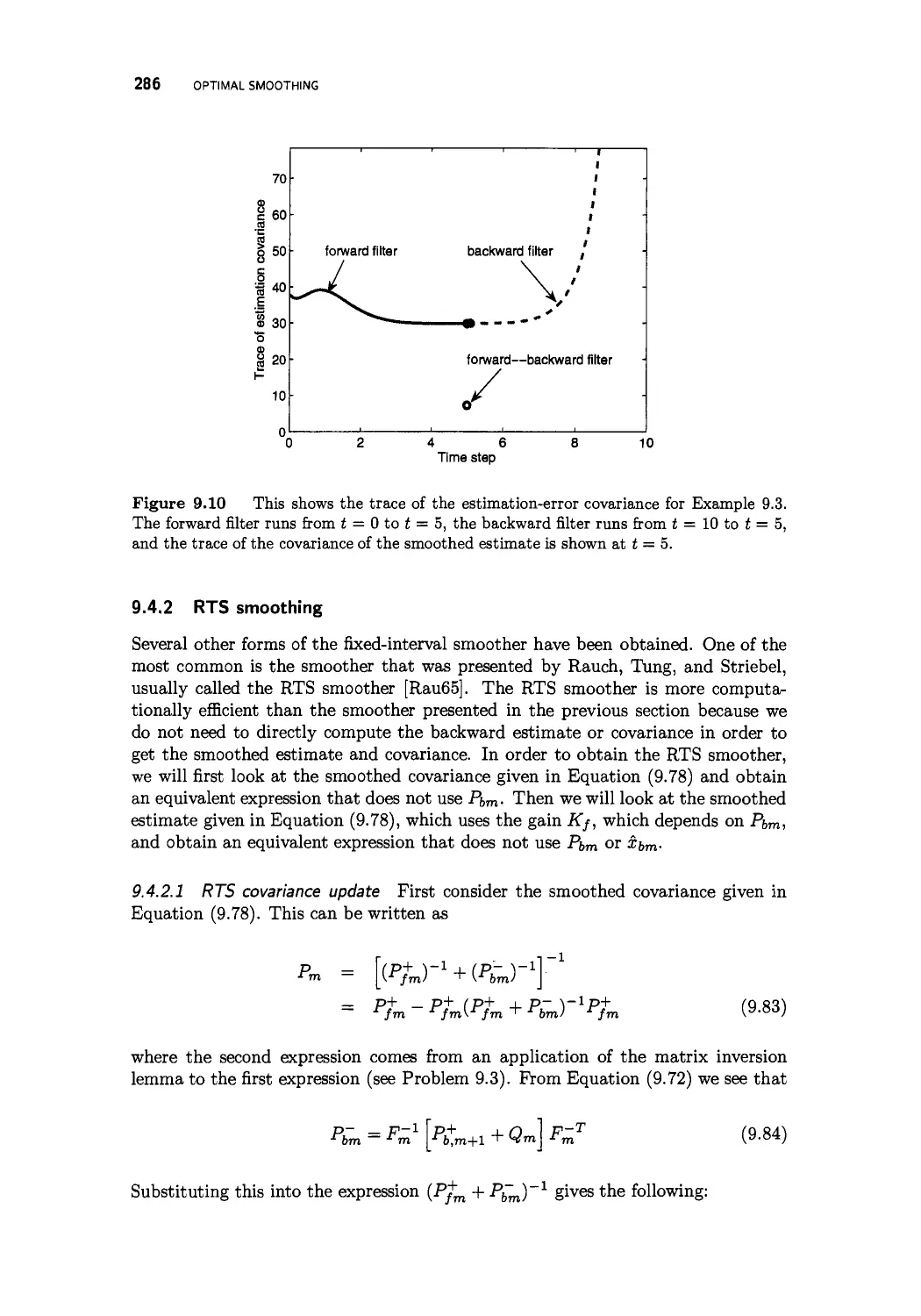
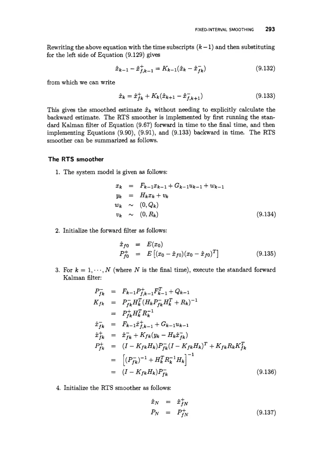
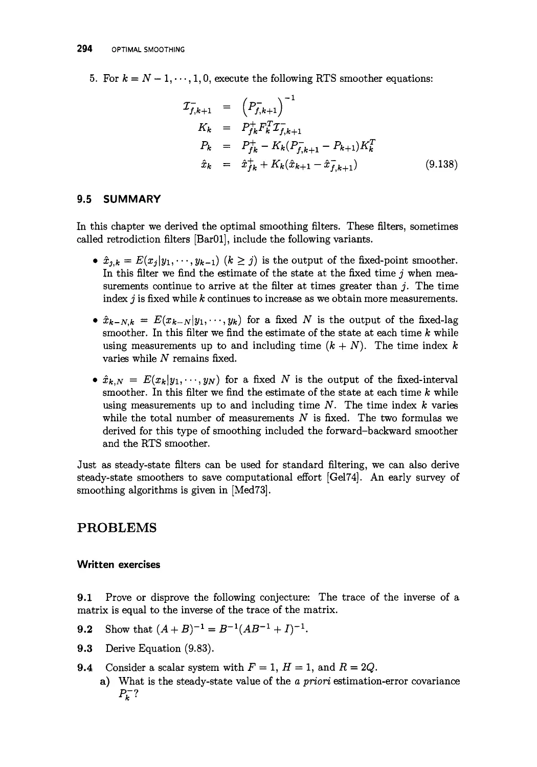
9.4.2 RTS smoothing 286
9.5 Summary 294
Problems 294
CONTENTS
10 Additional topics in Kalman filtering 297
10.1 Verifying Kalman filter performance 298
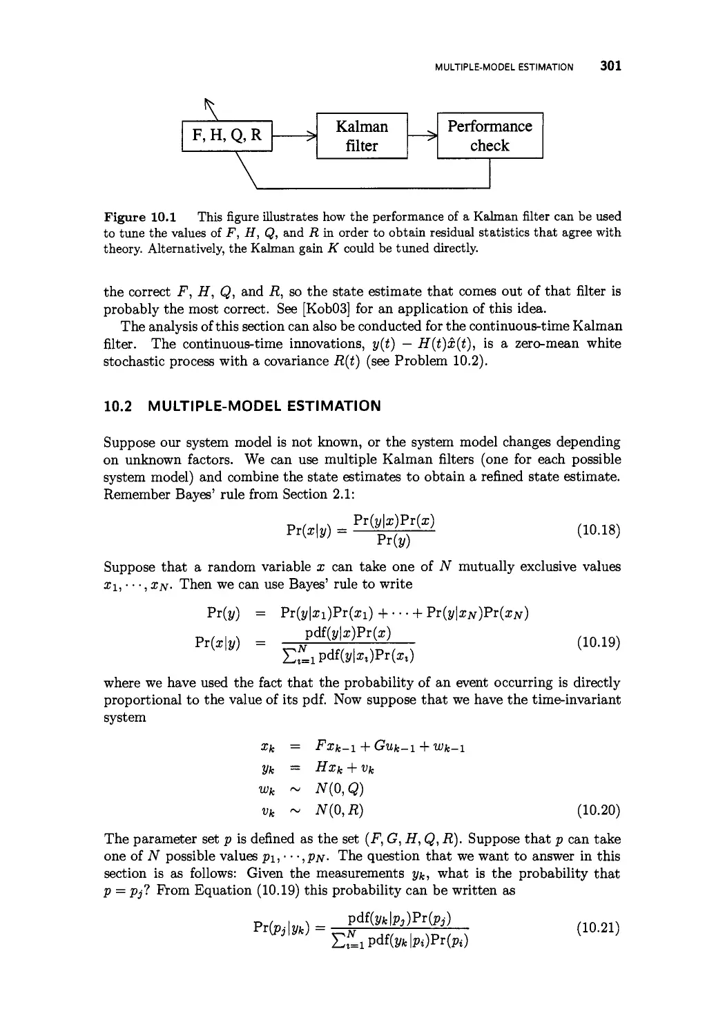
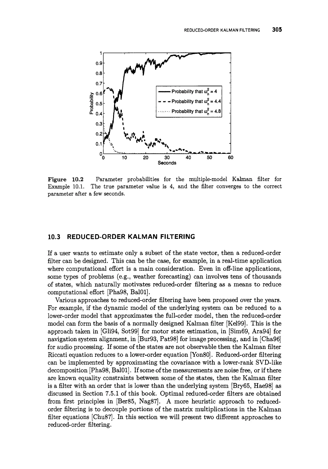
10.2 Multiple-model estimation 301
10.3 Reduced-order Kalman filtering 305
10.3.1 Anderson's approach to reduced-order filtering 306
10.3.2 The reduced-order Schmidt-Kalman filter 309
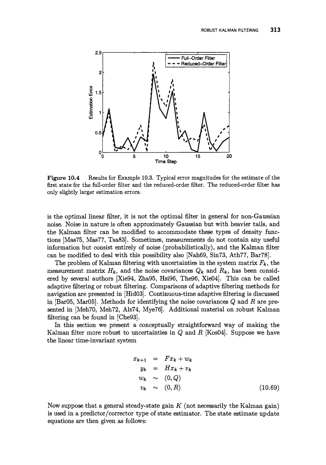
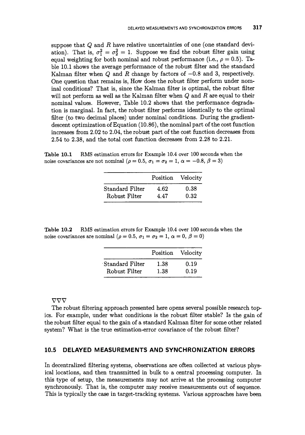
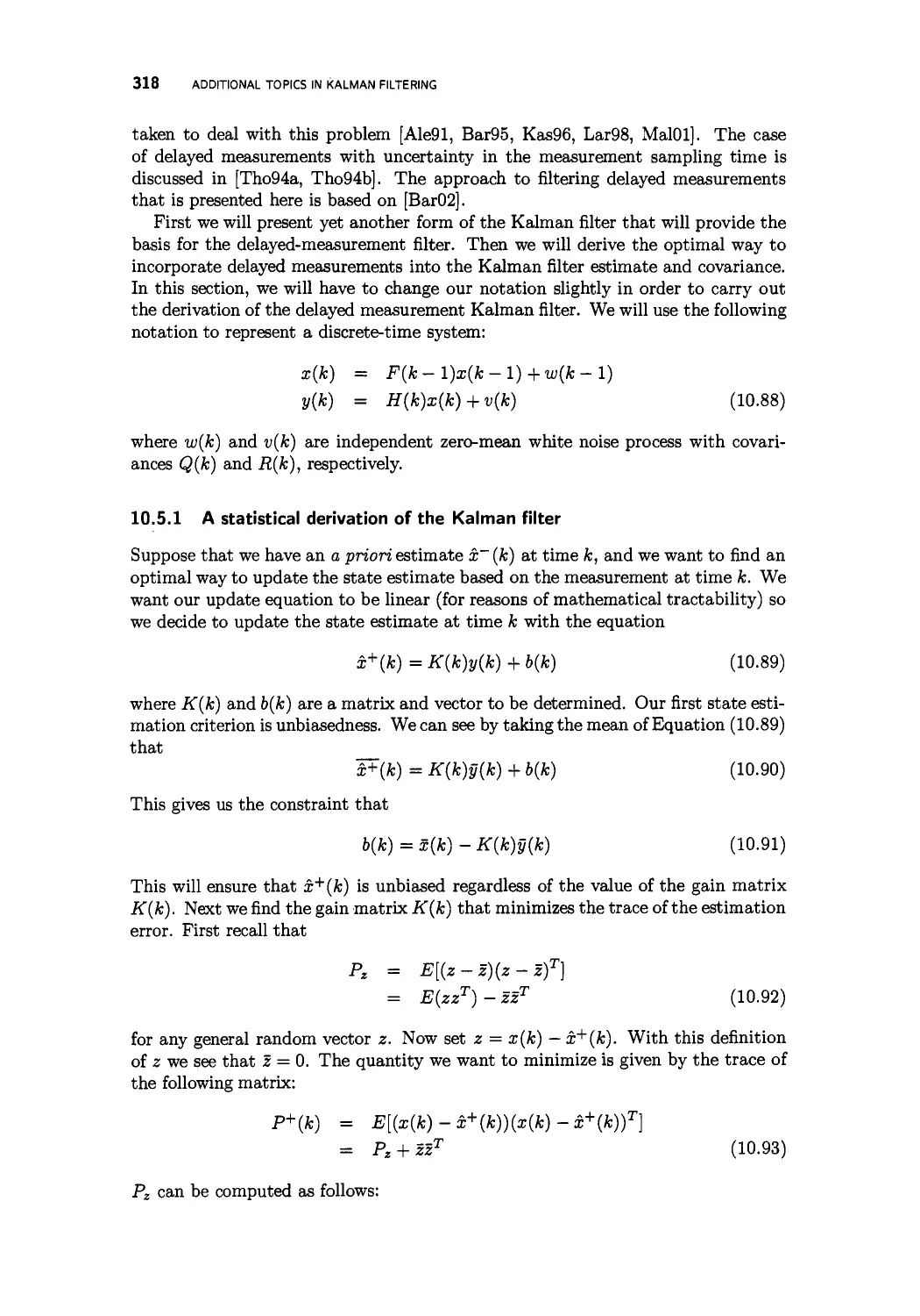
10.4 Robust Kalman filtering 312
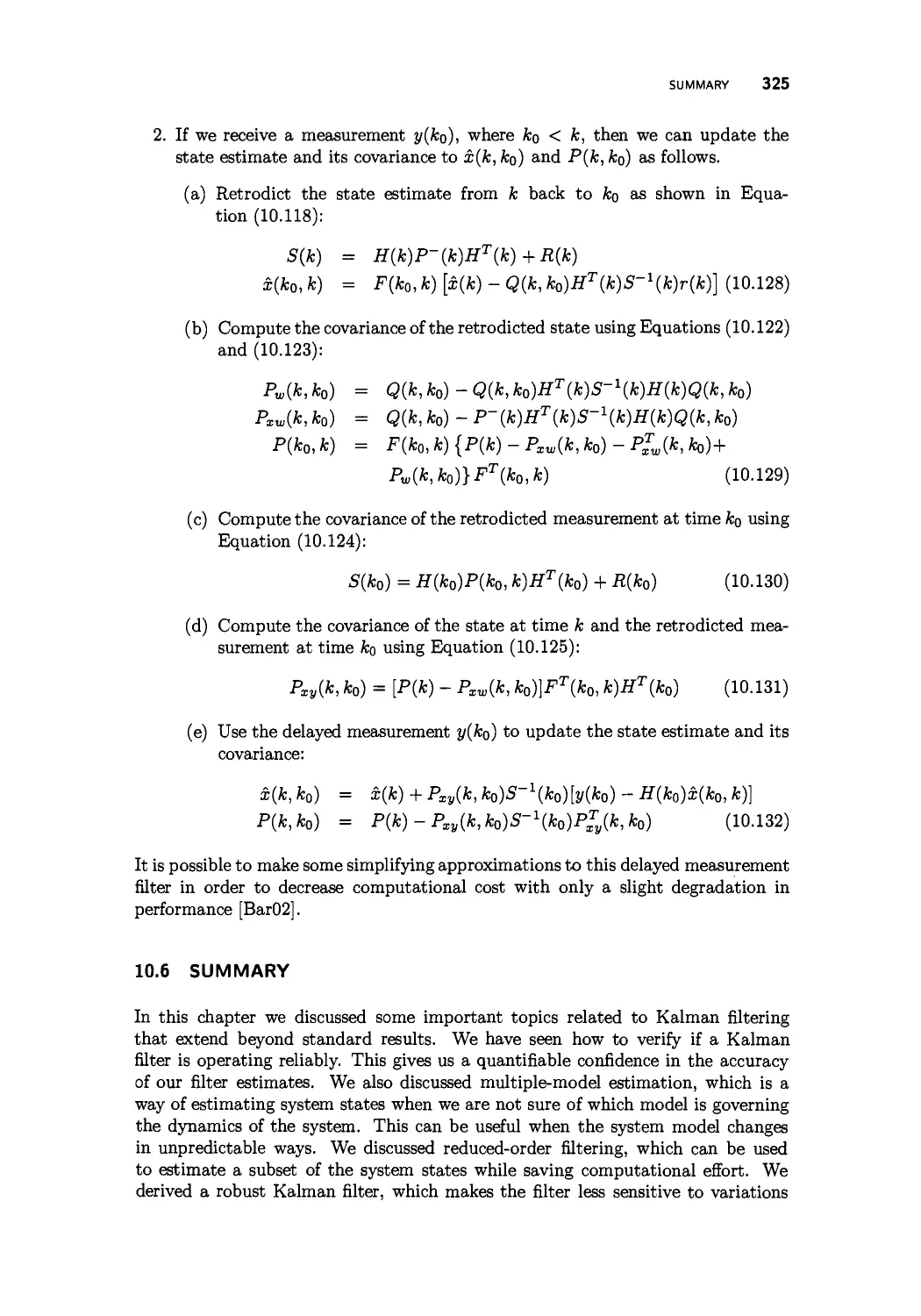
10.5 Delayed measurements and synchronization errors 317
10.5.1 A statistical derivation of the Kalman filter 318
10.5.2 Kalman filtering with delayed measurements 320
10.6 Summary 325
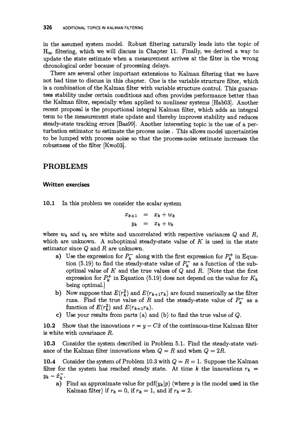
Problems 326
PART III THE Hoc FILTER
11 The Hoo filter 333
11.1 Introduction 334
11.1.1 An alternate form for the Kalman filter 334
11.1.2 Kalman filter limitations 336
11.2 Constrained optimization 337
11.2.1 Static constrained optimization 337
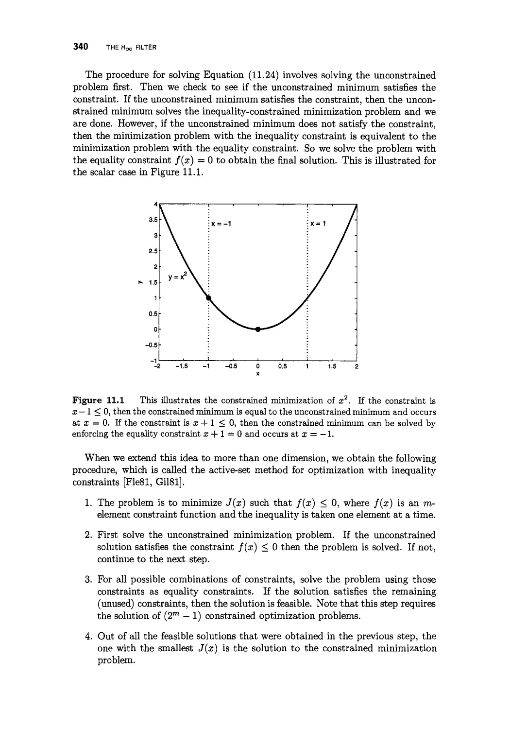
11.2.2 Inequality constraints 339
11.2.3 Dynamic constrained optimization 341
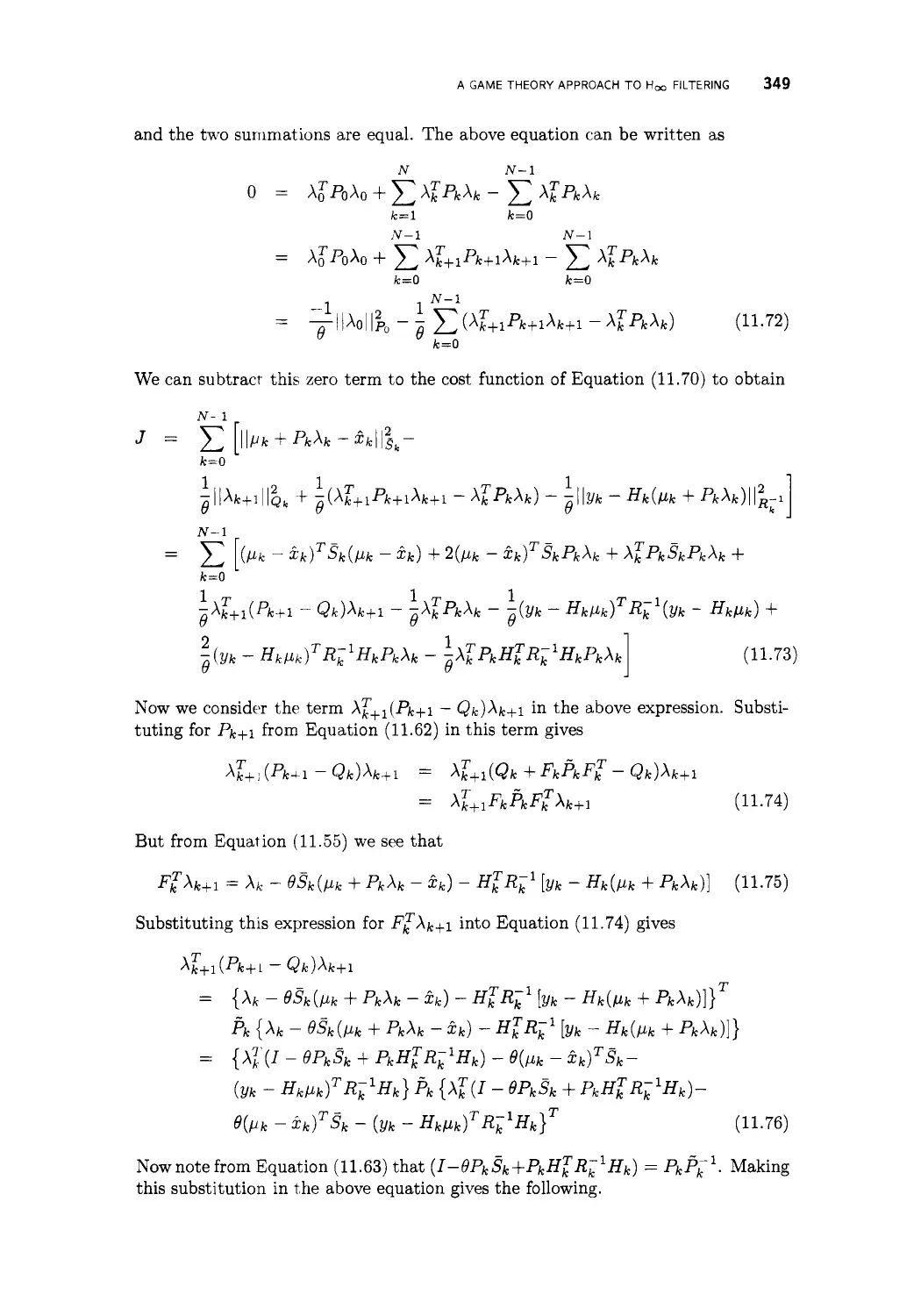
11.3 A game theory approach to H^ filtering 343
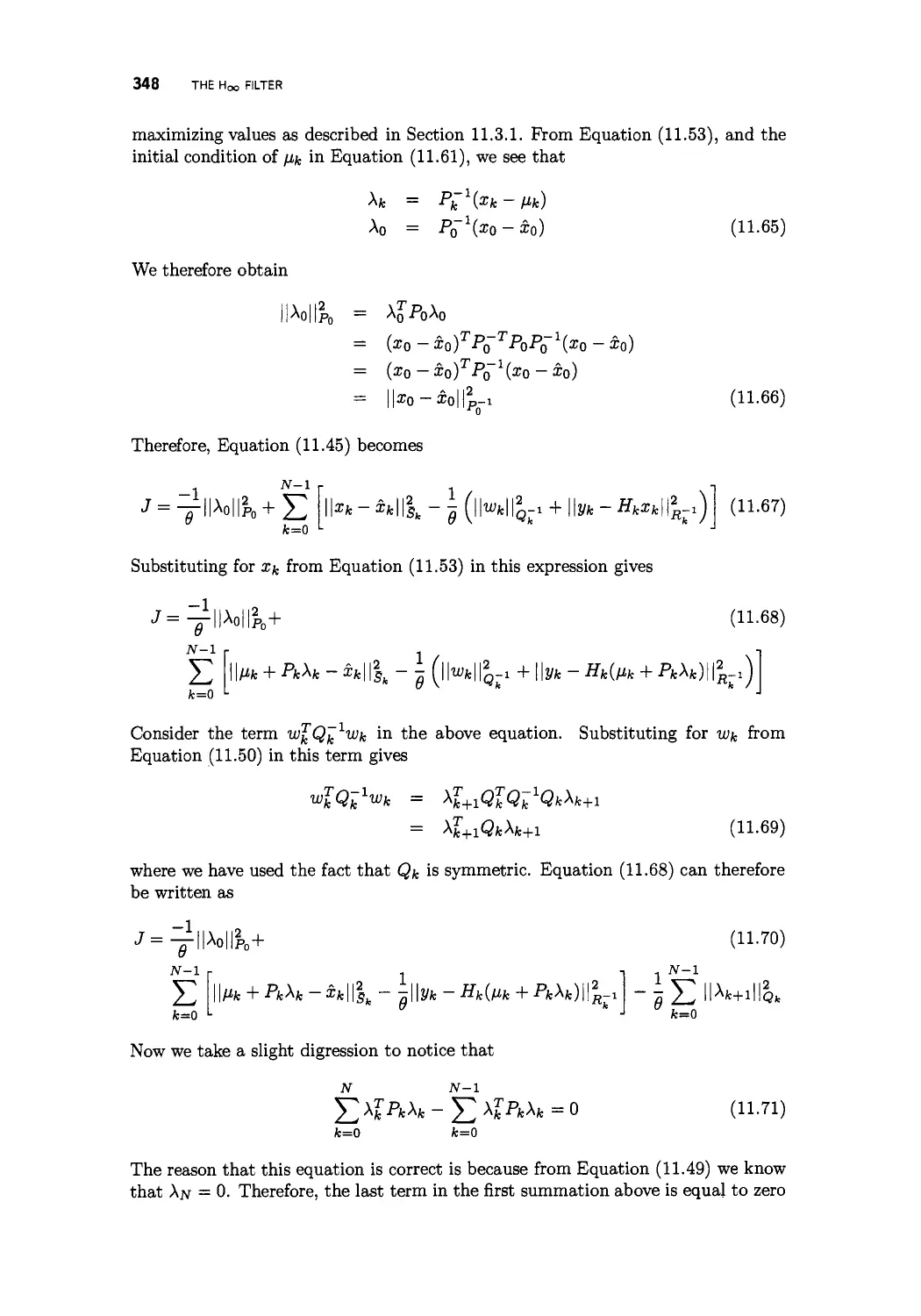
11.3.1 Stationarity with respect to xo and Wk 345
11.3.2 Stationarity with respect to x and y 347
11.3.3 A comparison of the Kalman and Hoc niters 354
11.3.4 Steady-state Hqo filtering 354
11.3.5 The transfer function bound of the Hoc filter 357
11.4 The continuous-time Hqo filter 361
11.5 Transfer function approaches 365
11.6 Summary 367
Problems 369
12 Additional topics in H^ filtering 373
12.1 Mixed Kalman/Hoo filtering 374
12.2 Robust Kalman/Hoo filtering 377
12.3 Constrained Hoc filtering 381
12.4 Summary 388
Problems
X CONTENTS
PART IV NONLINEAR FILTERS
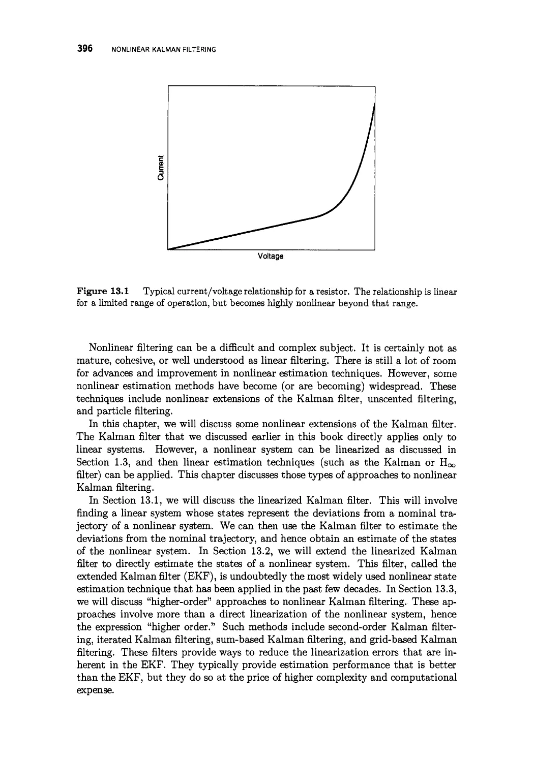
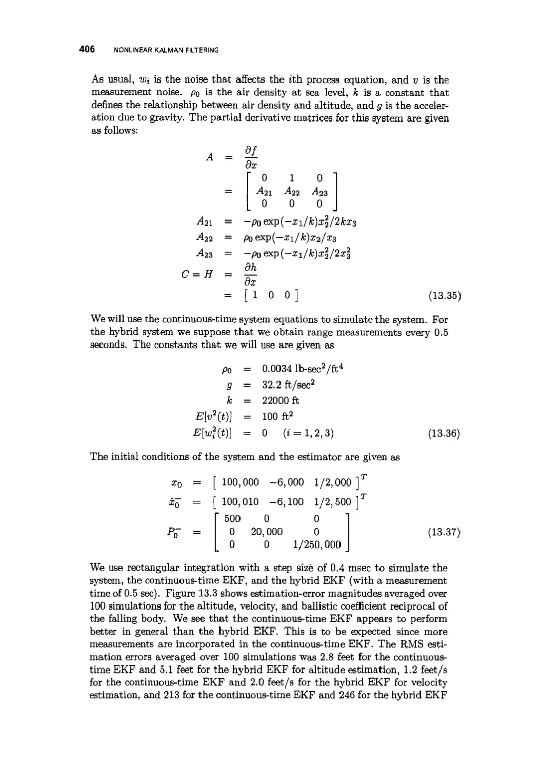
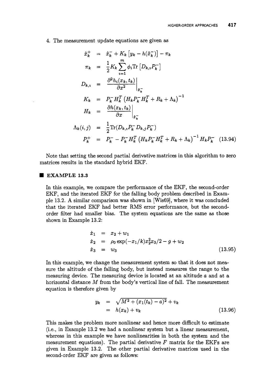
13 Nonlinear Kalman filtering 395
13.1 The linearized Kalman filter 397
13.2 The extended Kalman filter 400
13.2.1 The continuous-time extended Kalman filter 400
13.2.2 The hybrid extended Kalman filter 403
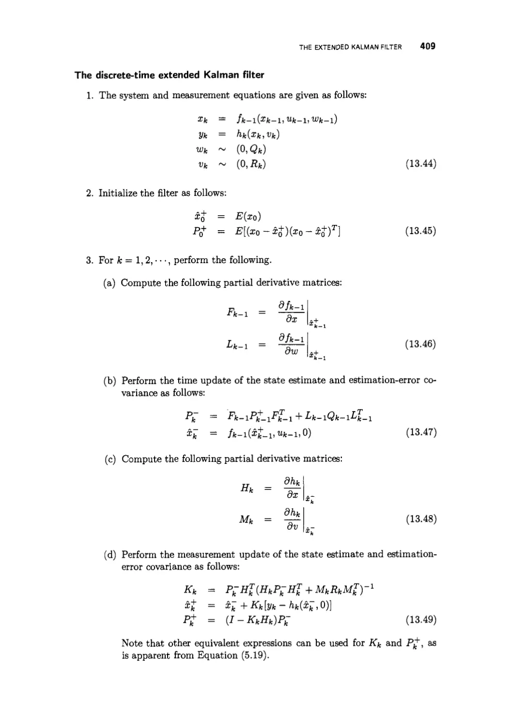
13.2.3 The discrete-time extended Kalman filter 407
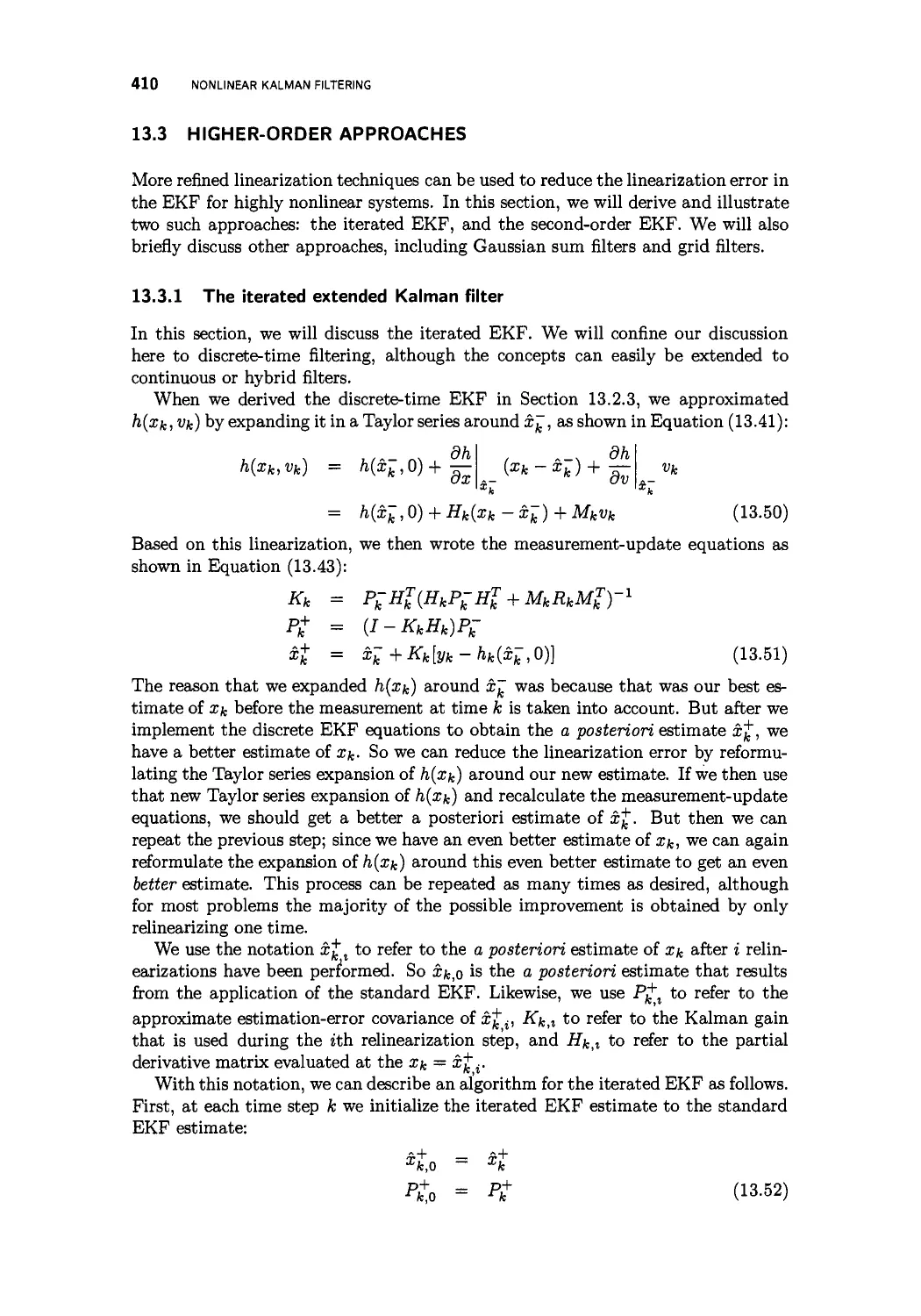
13.3 Higher-order approaches 410
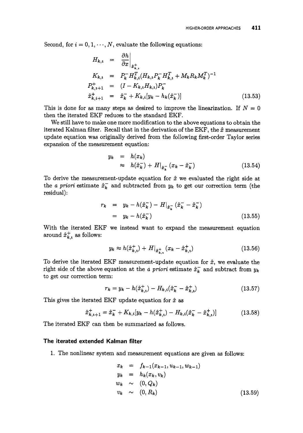
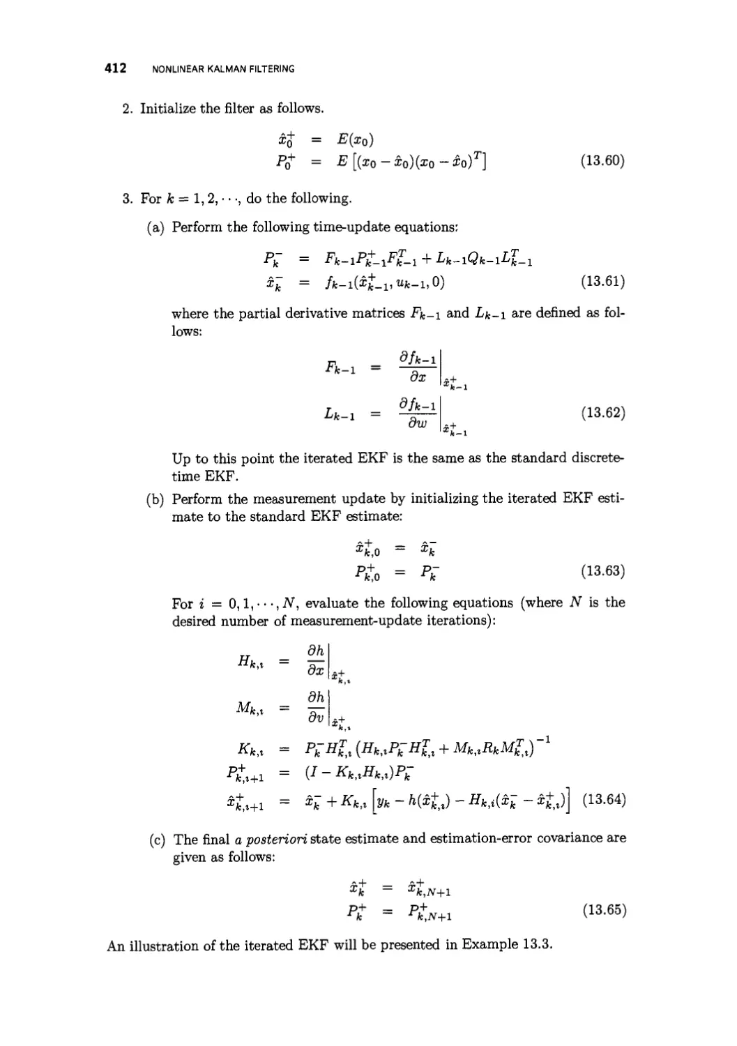
13.3.1 The iterated extended Kalman filter 410
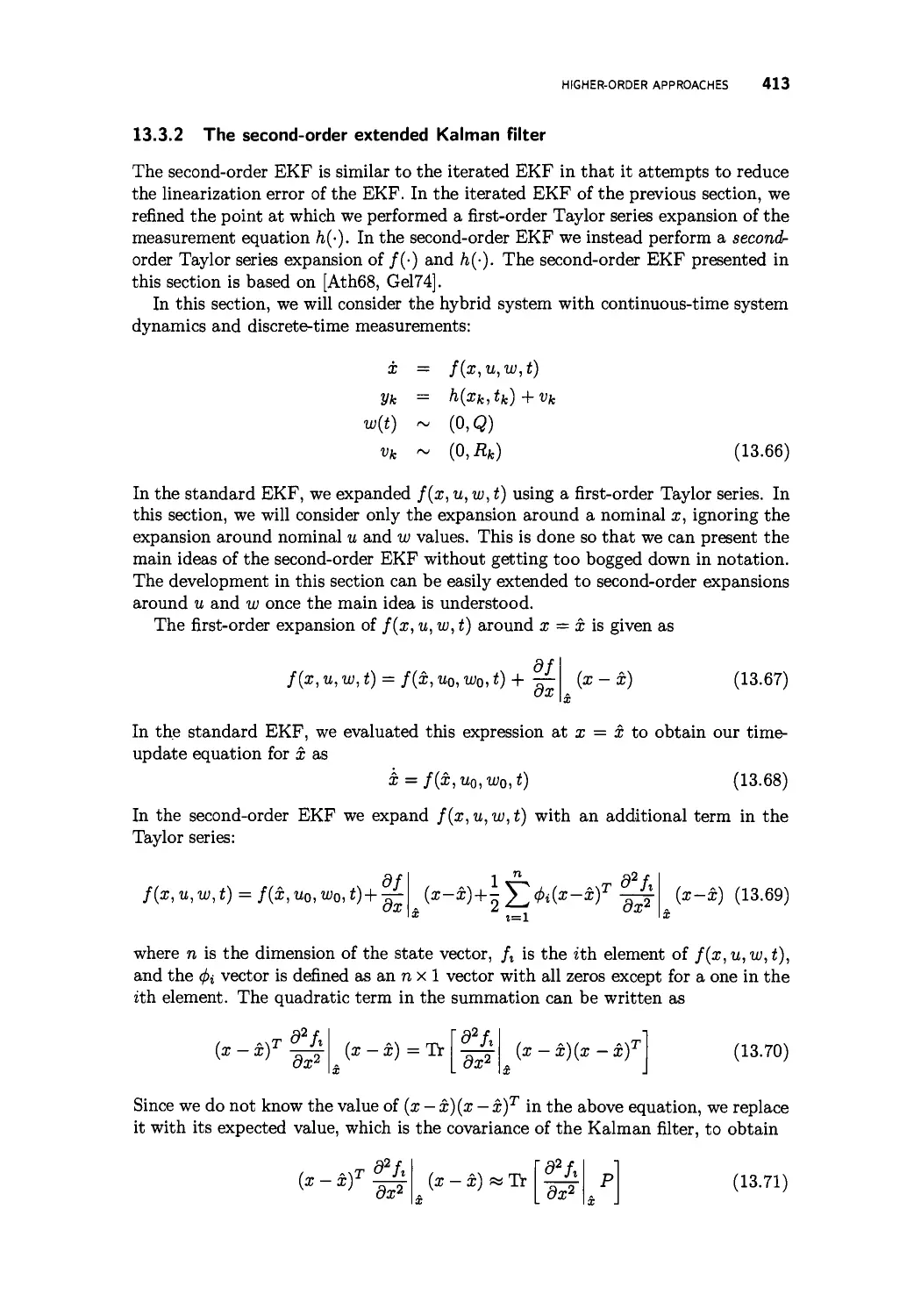
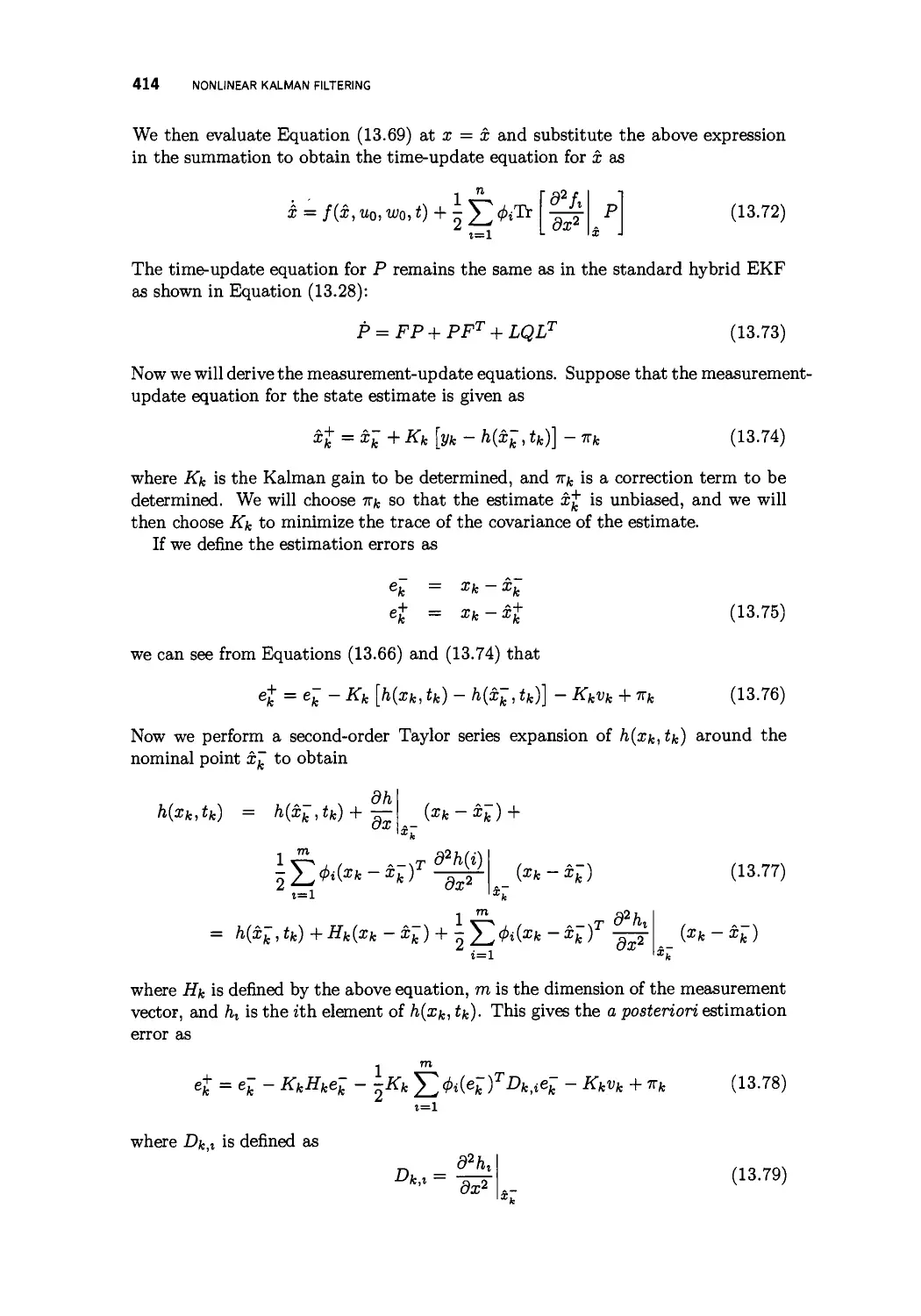
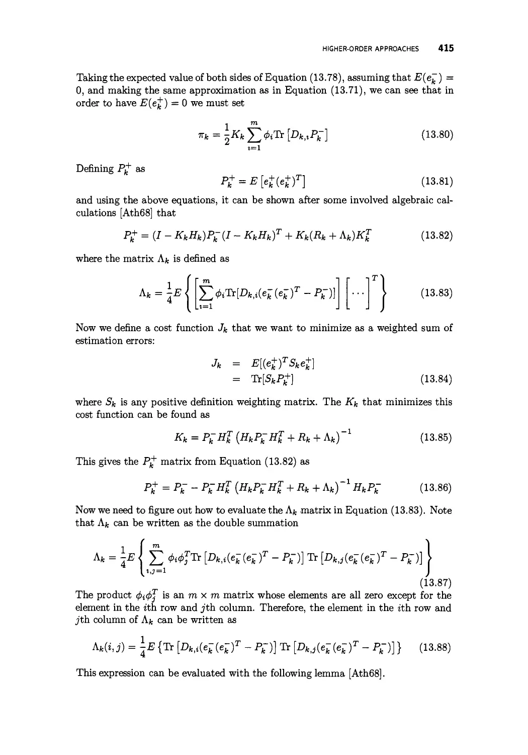
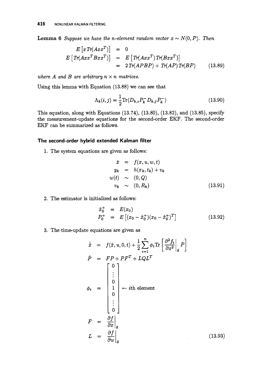
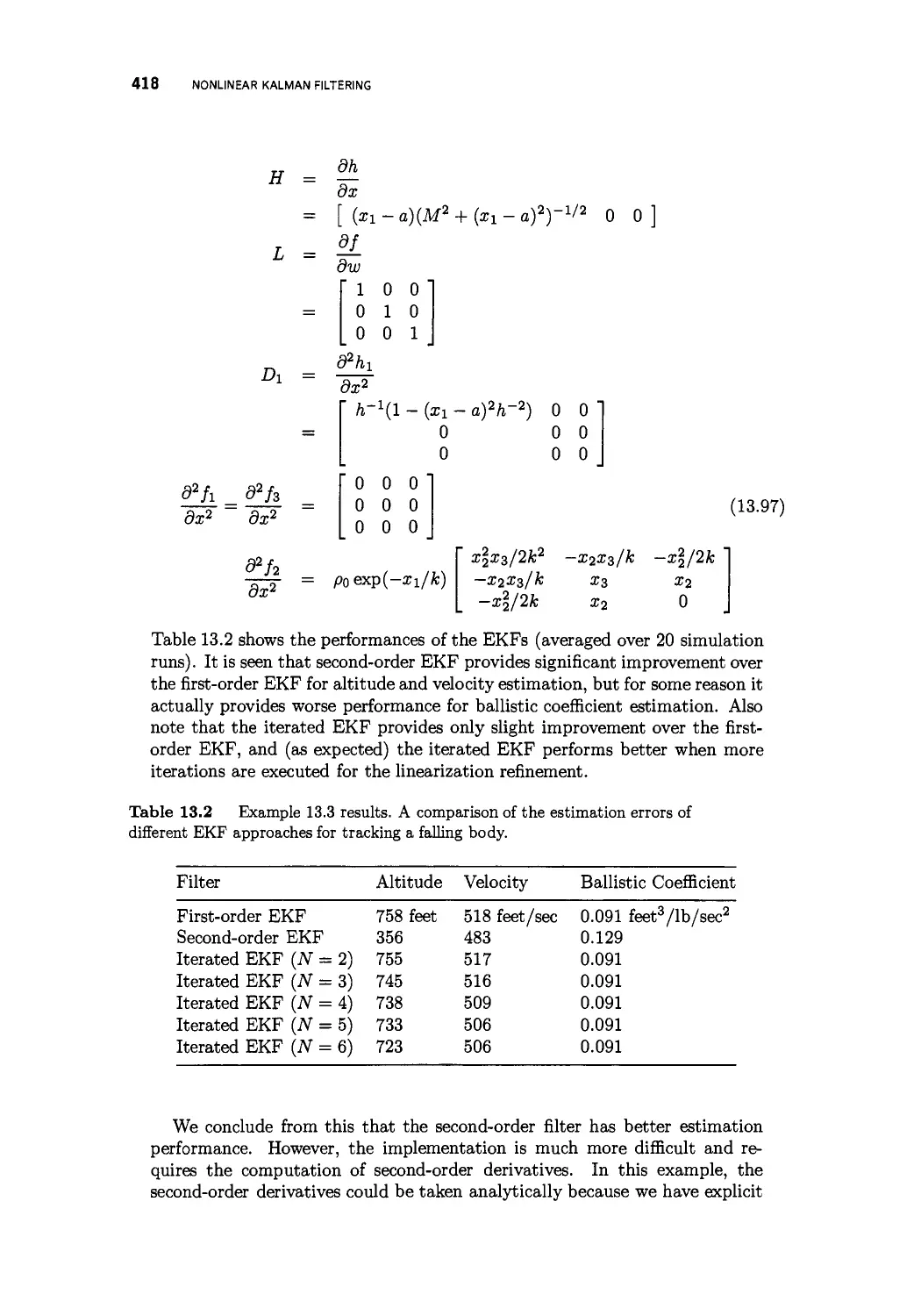
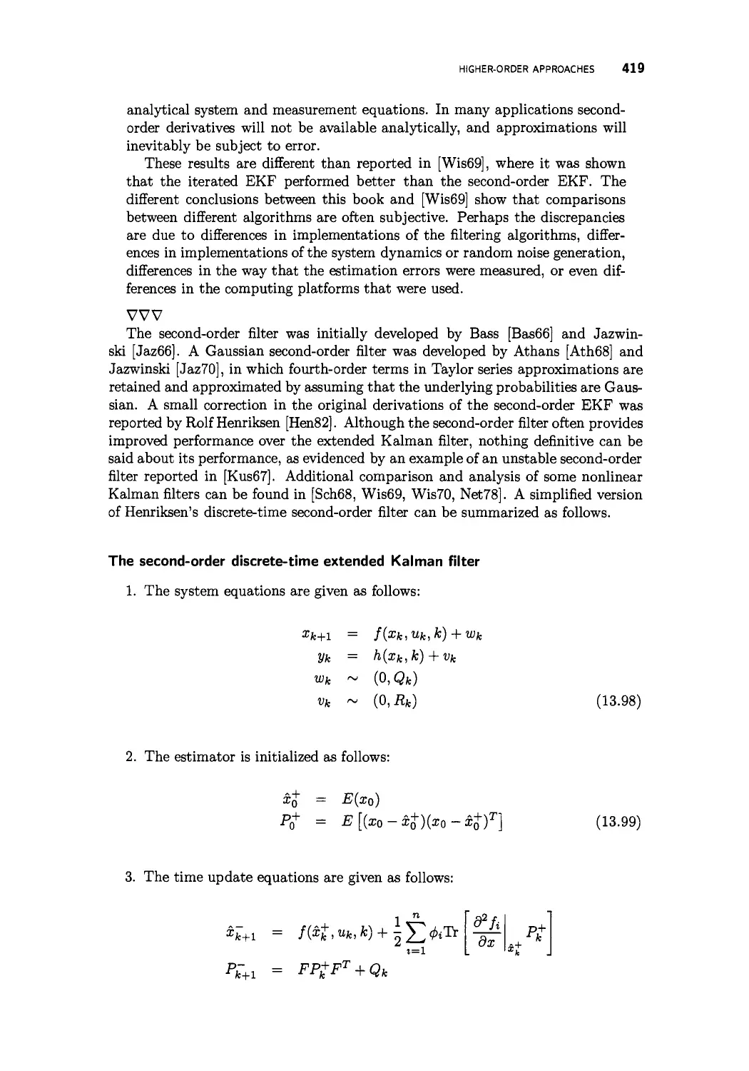
13.3.2 The second-order extended Kalman filter 413
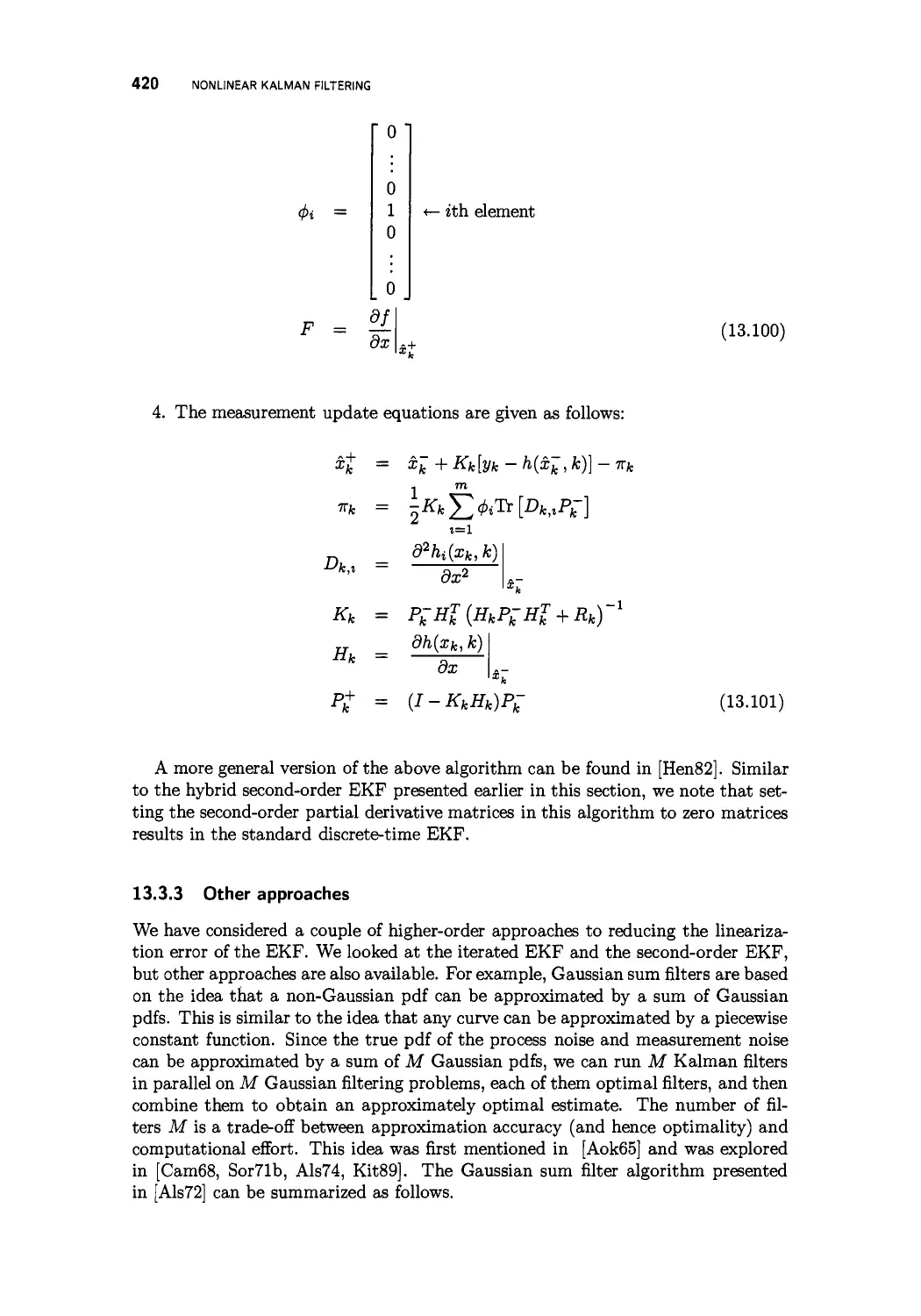
13.3.3 Other approaches 420
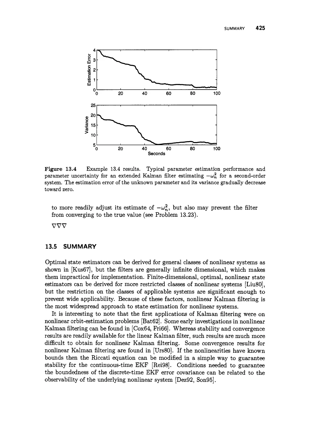
13.4 Parameter estimation 422
13.5 Summary 425
Problems 426
14 The unscented Kalman filter 433
14.1 Means and covariances of nonlinear transformations 434
14.1.1 The mean of a nonlinear transformation 434
14.1.2 The covariance of a nonlinear transformation 437
14.2 Unscented transformations 441
14.2.1 Mean approximation 441
14.2.2 Covariance approximation 444
14.3 Unscented Kalman filtering 447
14.4 Other unscented transformations 452
14.4.1 General unscented transformations 452
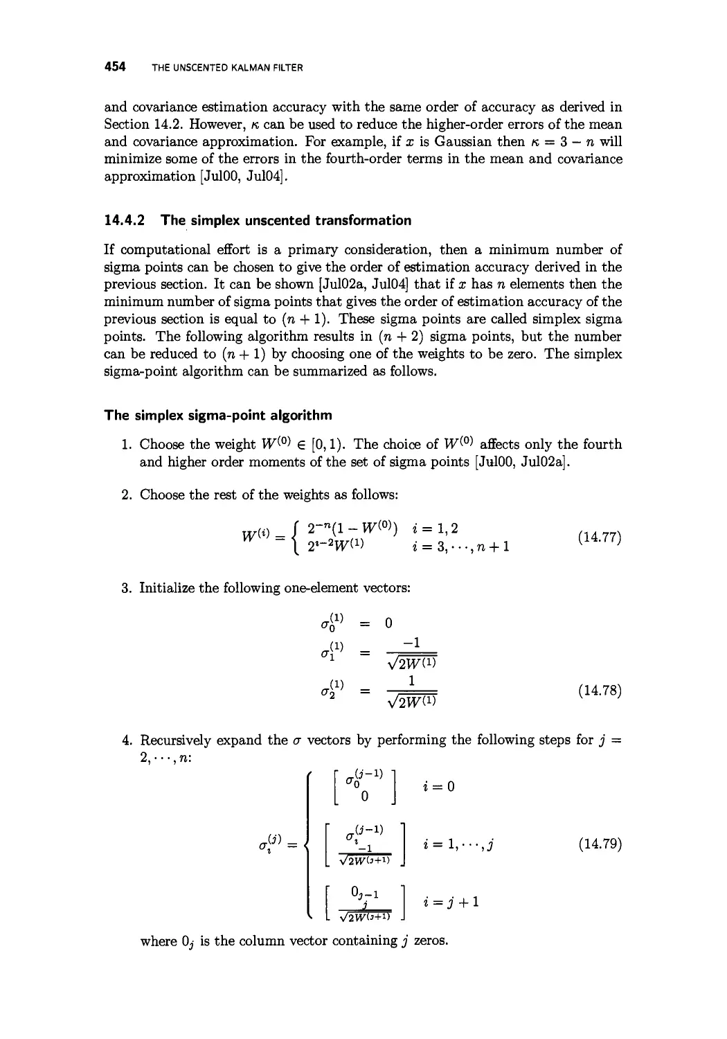
14.4.2 The simplex unscented transformation 454
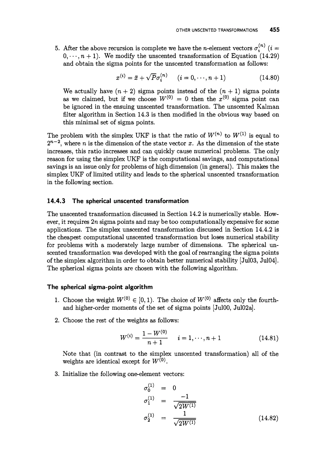
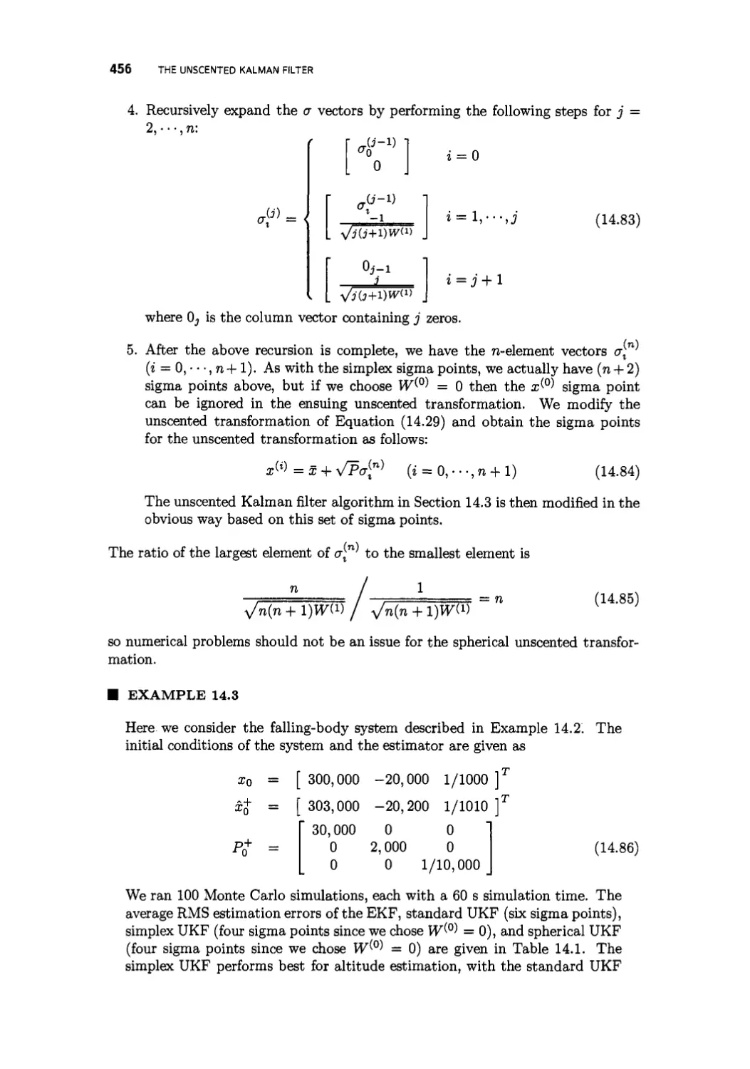
14.4.3 The spherical unscented transformation 455
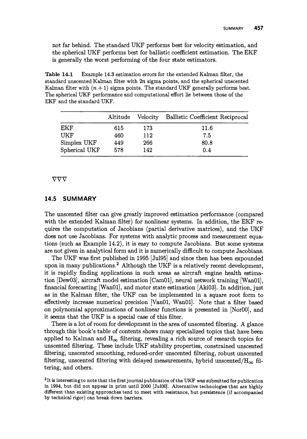
14.5 Summary 457
Problems 458
15 The particle filter 461
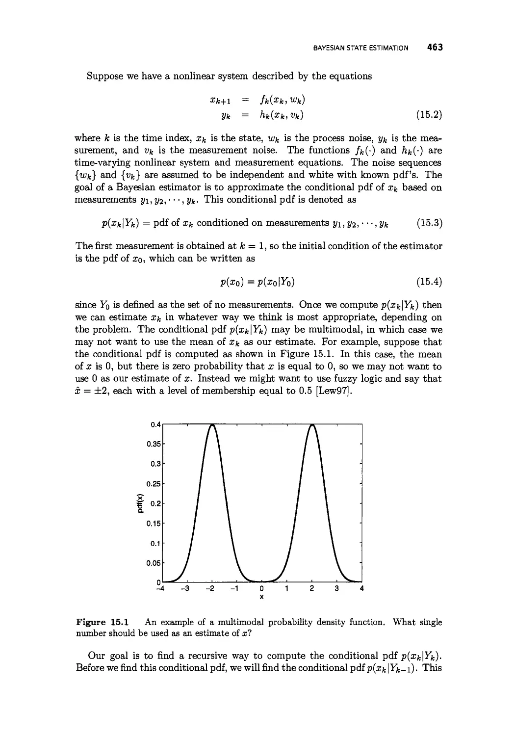
15.1 Bayesian state estimation 462
15.2 Particle filtering 466
15.3 Implementation issues 469
15.3.1 Sample impoverishment 469
15.3.2 Particle filtering combined with other niters 477
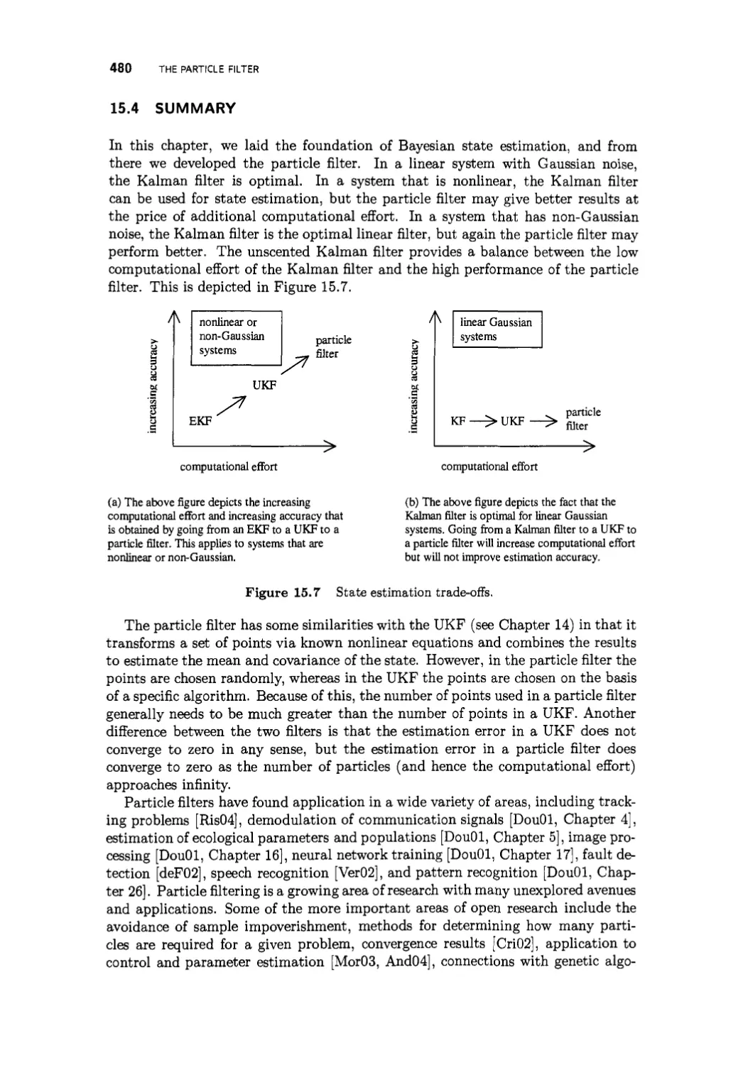
15.4 Summary 480
Problems 481
CONTENTS XI
Appendix A: Historical perspectives 485
Appendix B: Other books on Kalman filtering 489
Appendix C: State estimation and the meaning of life 493
References 501
Index 521
ACKNOWLEDGMENTS
The financial support of Sanjay Garg and Donald Simon (no relation to the
author) at the NASA Glenn Research Center was instrumental in allowing me to
pursue research in the area of optimal state estimation, and indirectly led to the
idea for this book. I am thankful to Eugenio Villaseca, the Chair of the
Department of Electrical and Computer Engineering at Cleveland State University, for
his encouragement and support of my research and writing efforts. Dennis Feucht
and Jonathan Litt reviewed the first draft of the book and offered constructive
criticism that made the book better than it otherwise would have been. I am also
indebted to the two anonymous reviewers of the proposal for this book, who made
suggestions that strengthened the material presented herein. I acknowledge the
work of Sandy Buettner, Joe Connolly, Classica Jain, Aaron Radke, Bryan Welch,
and Qing Zheng, who were students in my Optimal State Estimation class in Fall
2005. They contributed some of the problems at the end of the chapters and made
many suggestions for improvement that helped clarify the subject matter. Finally
I acknowledge the love and support of my wife, Annette, whose encouragement of
my endeavors has always been above and beyond the call of duty.
D. J. S.
xiii
ACRONYMS
ACR
ARE
CARE
DARE
EKF
erf
FPGA
GPS
HOT
iff
INS
LHP
LTI
LTV
MCMC
MIMO
N(a, b)
pdf
Acronym
Algebraic Riccati equation
Continuous ARE
Discrete ARE
Extended Kalman filter
Error function
Field programmable gate array
Global Positioning System
Higher-order terms
If and only if
Inertial navigation system
Left half plane
Linear time-invariant
Linear time-varying
Markov chain Monte Carlo
Multiple input, multiple output
Normal pdf with a mean of a and
Probability density function
a variance of b
List of acronyms
PDF
QED
RHP
RMS
RPF
RTS
RV
SIR
SISO
SSS
SVD
TF
U{a,b)
UKF
wss
Probability distribution function
Quod erat demonstrandum (i.e., "that which was to
demonstrated")
Right half plane
Root mean square
Regularized particle filter
Rauch-Tung-Striebel
Random variable
Sampling importance resampling
Single input, single output
Strict-sense stationary-
Singular value decomposition
Transfer function
Uniform pdf that is nonzero on the domain [a, b]
Unscented Kalman filter
Wide-sense stationary
LIST OF ALGORITHMS
Chapter 1: Linear systems theory-
Rectangular integration 29
Trapezoidal integration 31
Fourth-order Runge-Kutta integration 32
Chapter 2: Probability theory
Correlated noise simulation 74
Chapter 3: Least squares estimation
Recursive least squares estimation 86
General recursive least squares estimation 88
Chapter 5: The discrete-time Kalman filter
The discrete-time Kalman filter 128
Chapter 6: Alternate Kalman filter formulations
The sequential Kalman filter 151
The information filter 156
The Cholesky matrix square root algorithm 160
Potter's square root measurement-update algorithm 166
The Householder algorithm 171
The Gram-Schmidt algorithm 172
The U-D measurement update 175
The U-D time update 177
XVII
xviii List of algorithms
Chapter 7: Kalman filter generalizations
The general discrete-time Kalman filter 186
The discrete-time Kalman filter with colored measurement noise 191
The Hamiltonian approach to steady-state Kalman filtering 207
The fading-memory filter 210
Chapter 8: The continuous-time Kalman filter
The continuous-time Kalman filter 235
The Chandrasekhar algorithm 244
The continuous-time square root Kalman filter 247
The continuous-time Kalman filter with correlated noise 249
The continuous-time Kalman filter with colored measurement noise 251
Chapter 9: Optimal smoothing
The fixed-point smoother 269
The fixed-lag smoother 278
The RTS smoother 293
Chapter 10: Additional topics in Kalman filtering
The multiple-model estimator 302
The reduced-order Schmidt-Kalman filter 312
The delayed-measurement Kalman filter 324
Chapter 11: The H^ filter
The discrete-time Hoc filter 353
Chapter 12: Additional topics in Hqq filtering
The mixed Kalman/Hoo filter 374
The robust mixed Kalman/Hoo filter 378
The constrained Hoc filter 385
Chapter 13: Nonlinear Kalman filtering
The continuous-time linearized Kalman filter 399
The continuous-time extended Kalman filter 401
The hybrid extended Kalman filter 405
The discrete-time extended Kalman filter 409
The iterated extended Kalman filter 411
The second-order hybrid extended Kalman filter 416
The second-order discrete-time extended Kalman filter 419
The Gaussian sum filter 421
Chapter 14: The unscented Kalman filter
The unscented transformation 446
The unscented Kalman filter 448
The simplex sigma-point algorithm 454
The spherical sigma-point algorithm 455
List of algorithms XJX
Chapter 15: The particle filter
The recursive Bayesian state estimator 465
The particle filter 468
Regularized particle filter resampling 473
The extended Kalman particle filter 478
INTRODUCTION
This book discusses mathematical approaches to the best possible way of
estimating the state of a general system. Although the book is firmly grounded in
mathematical theory, it should not be considered a mathematics text. It is more of an
engineering text, or perhaps an applied mathematics text. The approaches that we
present for state estimation are all given with the goal of eventual implementation
in software.1 The goal of this text is to present state estimation theory in the most
clear yet rigorous way possible, while providing enough advanced material and
references so that the reader is prepared to contribute new material to the state of
the art. Engineers are usually concerned with eventual implementation, and so the
material presented is geared toward discrete-time systems. However, continuous-
time systems are also discussed for the sake of completeness, and because there is
still room for implementations of continuous-time filters.
Before we discuss optimal state estimation, we need to define what we mean by
the term state. The states of a system are those variables that provide a complete
representation of the internal condition or status of the system at a given instant
of time.2 This is far from a rigorous definition, but it suffices for the purposes of
1l use the practice that is common in academia of referring to a generic third person by the word
we. Sometimes, I use the word we to refer to the reader and myself. Other times, I use the
word we to indicate that I am speaking on behalf of the control and estimation community. The
distinction should be clear from the context. However, I encourage the reader not to read too
much into my use of the word we; it is more a matter of personal preference and style rather than
a claim to authority.
2In this book, we use the terms state and state variable interchangably. Also, the word state could
refer to the entire collection of state variables, or it could refer to a single state variable. The
specific meaning needs to be inferred from the context.
xxi
XXJi INTRODUCTION
this introduction. For example, the states of a motor might include the currents
through the windings, and the position and speed of the motor shaft. The states
of an orbiting satellite might include its position, velocity, and angular orientation.
The states of an economic system might include per-capita income, tax rates,
unemployment, and economic growth. The states of a biological system might include
blood sugar levels, heart and respiration rates, and body temperature.
State estimation is applicable to virtually all areas of engineering and science.
Any discipline that is concerned with the mathematical modeling of its systems is
a likely (perhaps inevitable) candidate for state estimation. This includes electrical
engineering, mechanical engineering, chemical engineering, aerospace engineering,
robotics, economics, ecology, biology, and many others. The possible applications of
state estimation theory are limited only by the engineer's imagination, which is why
state estimation has become such a widely researched and applied discipline in the
past few decades. State-space theory and state estimation was initially developed in
the 1950s and 1960s, and since then there have been a huge number of applications.
A few applications are documented in [Sor85]. Thousands of other applications can
be discovered by doing an Internet search on the terms "state estimation" and
"application," or "Kalman filter" and "application."
State estimation is interesting to engineers for at least two reasons:
• Often, an engineer needs to estimate the system states in order to implement
a state-feedback controller. For example, the electrical engineer needs to
estimate the winding currents of a motor in order to control its position. The
aerospace engineer needs to estimate the attitude of a satellite in order to
control its velocity. The economist needs to estimate economic growth in
order to try to control unemployment. The medical doctor needs to estimate
blood sugar levels in order to control heart and respiration rates.
• Often an engineer needs to estimate the system states because those states are
interesting in their own right. For example, if an engineer wants to measure
the health of an engineering system, it may be necessary to estimate the
internal condition of the system using a state estimation algorithm. An engineer
might want to estimate satellite position in order to more intelligently
schedule future satellite activities. An economist might want to estimate economic
growth in order to make a political point,. A medical doctor might want to
estimate blood sugar levels in order to evaluate the health of a patient.
There are many other fine books on state estimation that are available (see
Appendix B). This begs the question: Why yet another textbook on the topic of
state estimation? The reason that this present book has been written is to offer a
pedagogical approach and perspective that is not available in other state estimation
books. In particular, the hope is that this book will offer the following:
• A straightforward, bottom-up approach that assists the reader in obtaining a
clear (but theoretically rigorous) understanding of state estimation. This is
reminiscent of Gelb's approach [Gel74], which has proven effective for many
state estimation students of the past few decades. However, many aspects
of Gelb's book have become outdated. In addition, many of the more recent
books on state estimation read more like research monographs and are not
entirely accessible to the average engineering student. Hence the need for the
present book.
INTRODUCTION XXhi
• Simple examples that provide the reader with an intuitive understanding of
the theory. Many books present state estimation theory and then follow with
examples or problems that require a computer for implementation. However,
it is possible to present simple examples and problems that require only paper
and pencil to solve. These simple problems allow the student to more directly
see how the theory works itself out in practice. Again, this is reminiscent of
Gelb's approach [Gel74].
MATLAB-based source code3 for the examples in the book is available at
the author's Web site.4 A number of other texts supply source code, but it
is often on disk or CD, which makes the code subject to obsolescence. The
author's e-mail address is also available on the Web site, and I enthusiastically
welcome feedback, comments, suggestions for improvements, and corrections.
Of course, Web addresses are also subject to obsolescence, but the book also
contains algorithmic, high-level pseudocode listings that will last longer than
any specific software listings.
• Careful treatment of advanced topics in optimal state estimation. These
topics include unscented filtering, high-order nonlinear filtering, particle
filtering, constrained state estimation, reduced-order filtering, robust Kalman
filtering, and mixed Kalman/Hoo filtering. Some of these topics are mature,
having been introduced in the 1960s, but others of these topics are recent
additions to the state of the art. This coverage is not matched in any other
books on the topic of state estimation.
Some of the other books on state estimation offer some of the above features, but
no other books offer all of these features.
Prerequisites
The prerequisites for understanding the material in this book are a good foundation
in linear systems theory and probability and stochastic processes. Ideally, the
reader will already have taken a graduate course in both of these topics. However,
it should be said that a background in linear systems theory is more important
than probability. The first two chapters of the book review the elements of linear
systems and probability that are essential for the rest of the book, and also serve
to establish the notation that is used during the remainder of the book.
Other material could also be considered prerequisite to understanding this book,
such as undergraduate advanced calculus, control theory, and signal processing.
However, it would be more accurate to say that the reader will require a moderately
high level of mathematical and engineering maturity, rather than trying to identify
a list of required prerequisite courses.
3MATLAB is a registered trademark of The MathWorks, Inc.
4http://academic.csuohio.edu/simond/estimation - if the Web site address changes, it should be
easy to find with an internet search.
XXJV INTRODUCTION
Problems
The problems at the end of each chapter have been written to give a high degree
of flexibility to the instructor and student. The problems include both written
exercises and computer exercises. The written exercises are intended to strengthen
the student's grasp of the theory, and deepen the student's intuitive understanding
of the concepts. The computer exercises are intended to help the student learn how
to apply the theory to problems of the type that might be encountered in industrial
or government projects. Both types of problems are important for the student to
become proficient at the material. The distinction between written exercises and
computer exercises is more of a fuzzy division rather than a strict division. That is,
some of the written exercises include parts for which some computer work might be
useful (even required), and some of the computer exercises include parts for which
some written analysis might be useful (even required).
A solution manual to all of the problems in the text (both written exercises and
computer exercises) is available from the publisher to instructors who have adopted
this book. Course instructors are encouraged to contact the publisher for further
information about out how to obtain the solution manual.
Outline of the book
This book is divided into four parts. The first part of the book covers introductory
material. Chapter 1 is a review of the relevant areas of linear systems. This
material is often covered in a first-semester graduate course taken by engineering
students. It is advisable, although not strictly required, that readers of this book
have already taken a graduate linear systems course. Chapter 2 reviews probability
theory and stochastic processes. Again, this is often covered in a first-semester
graduate course. In this book we rely less on probability theory than linear systems
theory, so a previous course in probability and stochastic processes is not required
for the material in this book (although it would be helpful). Chapter 3 covers least
squares estimation of constants and Wiener filtering of stochastic processes. The
section on Wiener filtering is not required for the remainder of the book, although
it is interesting both in its own right and for historical perspective. Chapter 4 is
a brief discussion of how the statistical measures of a state (mean and covariance)
propagate in time. Chapter 4 provides a bridge from the first, three chapters to the
second part of the book.
The second part of the book covers Kalman filtering, which is the workhorse of
state estimation. In Chapter 5, we derive the discrete-time Kalman filter, including
several different (but mathematically equivalent) formulations. In Chapter 6, we
present some alternative Kalman filter formulations, including sequential filtering,
information filtering, square root filtering, and U-D filtering. In Chapter 7, we
discuss some generalizations of the Kalman filter that make the filter applicable to a
wider class of problems. These generalizations include correlated process and
measurement noise, colored process and measurement noise, steady-state filtering for
computational savings, fading-memory filtering, and constrained Kalman filtering.
In Chapter 8, we present the continuous-time Kalman filter. This chapter could
be skipped if time is short since the continuous-time filter is rarely implemented in
practice. In Chapter 9, we discuss optimal smoothing, which is a way to estimate
INTRODUCTION XXV
the state of a system at time r based on measurements that extend beyond time
r. As part of the derivation of the smoothing equations, the first section of
Chapter 9 presents another alternative form for the Kalman filter. Chapter 10 presents
some additional, more advanced topics in Kalman filtering. These topics include
verification of filter performance, estimation in the case of unknown system models,
reduced-order filtering, increasing the robustness of the Kalman filter, and filtering
in the presence of measurement synchronization errors. This chapter should
provide fertile ground for students or engineers who are looking for research topics or
projects.
The third part of the book covers Hoo filtering. This area is not as mature as
Kalman filtering and so there is less material than in the Kalman filtering part of
the book. Chapter 11 introduces yet another alternate Kalman filter form as part
of the Hqo filter derivation. This chapter discusses both time domain and frequency
domain approaches to Hoc filtering. Chapter 12 discusses advanced topics in H^
filtering, including mixed Kalman/Hoo filtering and constrained H^ filtering. There
is a lot of room for further development in Hqo filtering, and this part of the book
could provide a springboard for researchers to make contributions in this area.
The fourth part of the book covers filtering for nonlinear systems. Chapter 13
discusses nonlinear filtering based on the Kalman filter, which includes the widely
used extended Kalman filter. Chapter 14 covers the unscented Kalman filter, which
is a relatively recent development that provides improved performance over the
extended Kalman filter. Chapter 15 discusses the particle filter, another recent
development that provides a very general solution to the nonlinear filtering problem.
It is hoped that this part of the book, especially Chapters 14 and 15, will inspire
researchers to make further contributions to these new areas of study.
The book concludes with three brief appendices. Appendix A gives some
historical perspectives on the development of the Kalman filter, starting with the least
squares work of Roger Cotes in the early 1700s, and concluding with the space
program applications of Kalman filtering in the 1960s. Appendix B discusses the many
other books that have been written on Kalman filtering, including their distinctive
contributions. Finally, Appendix C presents some speculations on the connections
between optimal state estimation and the meaning of life.
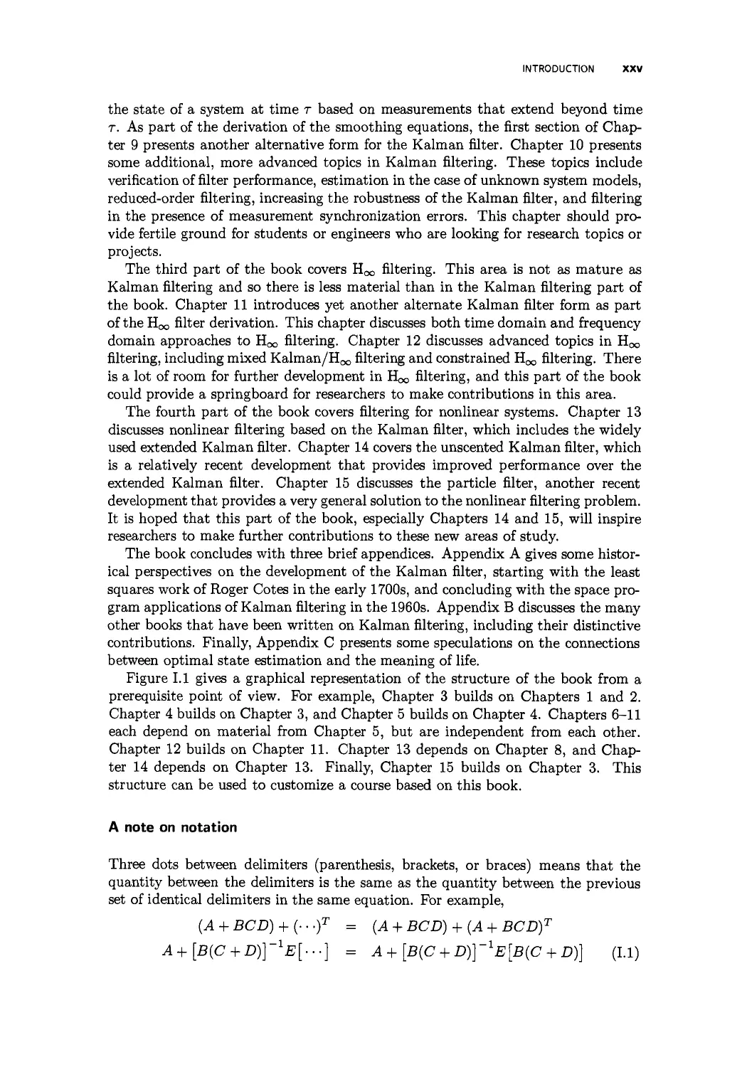
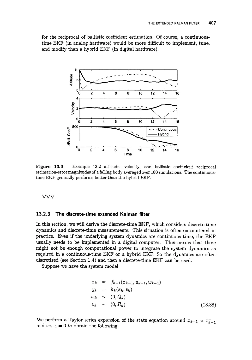
Figure 1.1 gives a graphical representation of the structure of the book from a
prerequisite point of view. For example, Chapter 3 builds on Chapters 1 and 2.
Chapter 4 builds on Chapter 3, and Chapter 5 builds on Chapter 4. Chapters 6-11
each depend on material from Chapter 5, but are independent from each other.
Chapter 12 builds on Chapter 11. Chapter 13 depends on Chapter 8, and
Chapter 14 depends on Chapter 13. Finally, Chapter 15 builds on Chapter 3. This
structure can be used to customize a course based on this book.
A note on notation
Three dots between delimiters (parenthesis, brackets, or braces) means that the
quantity between the delimiters is the same as the quantity between the previous
set of identical delimiters in the same equation. For example,
(A + BCD) + (• • .)T = {A + BCD) + {A + BCD)T
A+[B(C + D)}~1E[---} = A+[B{C + D)YlE[B{C + D)\ (1.1)
XXVI
INTRODUCTION
Chapter 14: The unscented Kalman filter
Chapter 13: Nonlinear Kalman filtering
Chapter 5: The discrete-time Kalman filter
Chapter 4: Propagation of states and covanances
Chapter 12: Additional
topics in H_ filtering
I
Chapter 3: Least squares estimation
Chapter 1: Linear systems theory
Chapter 2: Probability theory
Figure I.l Prerequisite structure of the chapters in this book.
PART I
INTRODUCTORY MATERIAL
Optimal State Estimation, First Edition. By Dan J. Simon
ISBN 0471708585 ©2006 John Wiley k Sons, Inc.
CHAPTER 1
Linear systems theory
Finally, we make some remarks on why linear systems are so important. The answer
is simple: because we can solve them!
—Richard Feynman [Fey63, p. 25-4]
This chapter reviews some essentials of linear systems theory. This material is
typically covered in a linear systems course, which is a first-semester graduate level
course in electrical engineering. The theory of optimal state estimation heavily
relies on matrix theory, including matrix calculus, so matrix theory is reviewed in
Section 1.1. Optimal state estimation can be applied to both linear and nonlinear
systems, although state estimation is much more straightforward for linear
systems. Linear systems are briefly reviewed in Section 1.2 and nonlinear systems are
discussed in Section 1.3. State-space systems can be represented in the continuous-
time domain or the discrete-time domain. Physical systems are typically described
in continuous time, but control and state estimation algorithms are typically
implemented on digital computers. Section 1.4 discusses some standard methods for
obtaining a discrete-time representation of a continuous-time system. Section 1.5
discusses how to simulate continuous-time systems on a digital computer.
Sections 1.6 and 1.7 discuss the standard concepts of stability, controllability, and
observability of linear systems. These concepts are necessary to understand some
of the optimal state estimation material later in the book. Students with a strong
Optimal State Estimation, First Edition. By Dan J. Simon 3
ISBN 0471708585 ©2006 John Wiley & Sons, Inc.
4 LINEAR SYSTEMS THEORY
background in linear systems theory can skip the material in this chapter.
However, it would still help to at least review this chapter to solidify the foundational
concepts of state estimation before moving on to the later chapters of this book.
1.1 MATRIX ALGEBRA AND MATRIX CALCULUS
In this section, we review matrices, matrix algebra, and matrix calculus. This
is necessary in order to understand the rest of the book because optimal state
estimation algorithms are usually formulated with matrices.
A scalar is a single quantity. For example, the number 2 is a scalar. The number
1 + 3j is a scalar (we use j in this book to denote the square root of —1). The
number tv is a scalar.
A vector consists of scalars that are arranged in a row or column. For example,
the vector
[ 1 3 7T ] (1.1)
is a 3-element vector. This vector is a called a 1 x 3 vector because it has 1 row
and 3 columns. This vector is also called a row vector because it is arranged as a
single row. The vector
" -2
7T2
3
0
is a 4-element vector. This vector is a called a 4 x 1 vector because it has 4 rows
and 1 column. This vector is also called a column vector because it is arranged as
a single column. Note that a scalar can be viewed as a 1-element vector; a scalar
is a degenerate vector. (This is just like a plane can be viewed as a 3-dimensional
shape; a plane is a degenerate 3-dimensional shape.)
A matrix consists of scalars that are arranged in a rectangle. For example, the
matrix
' -2 3
0 7T2
. 3 0
is a 3 x 2 matrix because it has 3 rows and 2 columns. The number of rows and
columns in a matrix can be collectively referred to as the dimension of the matrix.
For example, the dimension of the matrix in the preceding equation is 3 x 2. Note
that a vector can be viewed as a degenerate matrix. For example, Equation (1.1) is
a 1 x 3 matrix. A scalar can also be viewed as a degenerate matrix. For example,
the scalar 6 is a 1 x 1 matrix.
The rank of a matrix is denned as the number of linearly independent rows. This
is also equal to the number of linearly independent columns. The rank of a matrix
A is often indicated with the notation p{A). The rank of a matrix is always less
than or equal to the number of rows, and it is also less than or equal to the number
of columns. For example, the matrix
(1.2)
(1.3)
A =
1 2
2 4
(1.4)
MATRIX ALGEBRA AND MATRIX CALCULUS 5
has a rank of one because it has only one linearly independent row; the two rows
are multiples of each other. It also has only one linearly independent column; the
two columns are multiples of each other. On the other hand, the matrix
A =
1 3
2 4
(1.5)
has a rank of two because it has two linearly independent rows. That is, there are
no nonzero scalars ci and Ci such that
ci [ 1 3]+c2[2 4 ] = [ 0 0
(1.6)
so the two rows are linearly independent. It also has two linearly independent
columns. That is, there are no nonzero scalars C\ and Oi such that
c\
' 1 "
2
+ C2
' 3
_ 4 ^
=
" 0 '
0
(1.7)
so the two columns are linearly independent. A matrix whose elements are
comprised entirely of zeros has a rank of zero. An n x m matrix whose rank is equal
to min(n,m) is called full rank. The nullity of an n x m matrix A is equal to
[m-P(A)}.
The transpose of a matrix (or vector) can be taken by changing all the rows to
columns, and all the columns to rows. The transpose of a matrix is indicated with
a T superscript, as in AT} For example, if A is the r x n matrix
then AT is the n x r matrix
A1 =
An
irl
An
Aln
Am
(1.8)
Arl
(1.9)
Note that we use the notation A%3 to indicate the scalar in the ith row and jth
column of the matrix A. A symmetric matrix is one for which A = AT.
The hermitian transpose of a matrix (or vector) is the complex conjugate of the
transpose, and is indicated with an if superscript, as in AH. For example, if
A =
1 2 j 3
4j 5+j 1-
-J
3j
then
A =
1
3 + j
l + 3j
A hermitian matrix is one for which A = AH
-4j
5-i
(1.10)
(1.11)
1Many papers or books indicate transpose with a prime, as in A', or with a lower case t, as in A*.
6 LINEAR SYSTEMS THEORY
1.1.1 Matrix algebra
Matrix addition and subtraction is simply defined as element-by-element addition
and subtraction. For example,
1 2 3
3 2 1
+
0 4
1 -1
1
1 6
4 1
-1
(1.12)
The sum (A + B) and the difference {A — B) is defined only if the dimension of A
is equal to the dimension of B.
Suppose that A is an n x r matrix and B is an r x p matrix. Then the product of
A and B is written as C = AB. Each element in the matrix product C is computed
as
CtJ = 2J MkBkj i = 1,,
J = h---,P
(1.13)
fc=i
The matrix product AB is defined only if the number of columns in A is equal to
the number of rows in B. It is important to note that matrix multiplication does
not commute. In general, AB ^ BA.
Suppose we have an n x 1 vector x. We can compute the lxl product xTx, and
the nx n product xxT as follows:
x x
= [ xi
c„ ]
Xi
= xl + --. + xl
T
XX —
Xi
[ Xi
•Cn }
X\XTl
XfiX 1
(1.14)
Suppose that we have apxn matrix H and annxn matrix P. Then HT is a
n x p matrix, and we can compute the p x p matrix product HPHT.
HPH1
Hn
H
In
H,
pi
H,
pn
11
• nl
In
Yjhk HUPjkHlk ■ ■ • 52j,k HljPjkHpk
£j,fc HpjPjkHik ■ • ■ Y.j,k HpjPjkHpk
H\\ ■ ■ • Hpi
■"In ' ' ' *lpn
(1.15)
This matrix of sums can be written as the following sum of matrices:
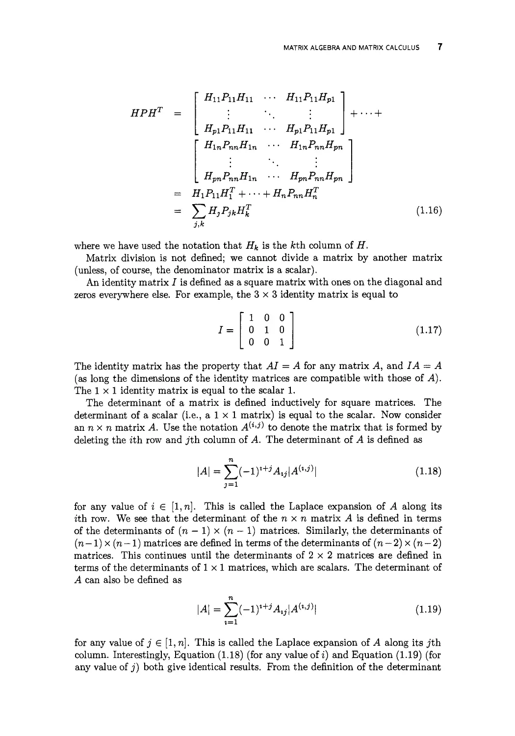
MATRIX ALGEBRA AND MATRIX CALCULUS 7
HPH1
HiiPiiHn
HpiPuHu
■"In-* nn"ln
"pn-* nn-"ln
HuPuHpi
HpiPnHpi
ii\n.rnntipn
flpn*nn*lpn
+ ••• +
H\PuH1 + • ■ • + HnPnnHn
(1.16)
where we have used the notation that H^ is the fcth column of H.
Matrix division is not defined; we cannot divide a matrix by another matrix
(unless, of course, the denominator matrix is a scalar).
An identity matrix I is denned as a square matrix with ones on the diagonal and
zeros everywhere else. For example, the 3x3 identity matrix is equal to
1 =
1 0 0
0 1 0
0 0 1
(1.17)
The identity matrix has the property that AI = A for any matrix A, and IA = A
(as long the dimensions of the identity matrices are compatible with those of A).
The lxl identity matrix is equal to the scalar 1.
The determinant of a matrix is denned inductively for square matrices. The
determinant of a scalar (i.e., a 1 x 1 matrix) is equal to the scalar. Now consider
annxn matrix A. Use the notation A^'^ to denote the matrix that is formed by
deleting the ith row and jth column of A. The determinant of A is denned as
w = x>ir+jA^
*.j) i
(1.18)
j=i
for any value of i £ [l,n]. This is called the Laplace expansion of A along its
ith row. We see that the determinant of the n x n matrix A is denned in terms
of the determinants of (n — 1) x (n — 1) matrices. Similarly, the determinants of
(n— 1) x (n— 1) matrices are denned in terms of the determinants of (n — 2) x (n — 2)
matrices. This continues until the determinants of 2 x 2 matrices are denned in
terms of the determinants of 1 x 1 matrices, which are scalars. The determinant of
A can also be denned as
\M = £(-1)-^,-1^
(1.19)
i=i
for any value of j £ [l,n]. This is called the Laplace expansion of A along its jth
column. Interestingly, Equation (1.18) (for any value of i) and Equation (1.19) (for
any value of j) both give identical results. From the definition of the determinant
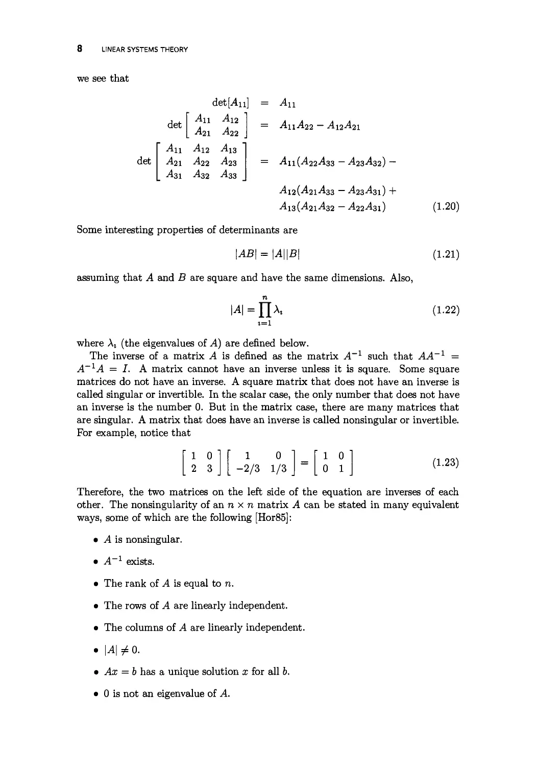
8 LINEAR SYSTEMS THEORY
we see that
det
det
det [.An
An A12
Mi A22
An Mi Axz
M\ A22 A2Z
Azx AZ2 Azz
= AX1
= M\Mi - A12A21
= ^11(^22^33 - -423-432) -
-4l2(-421-433-A23-431) +
-4l3(-42l-432-A22-43i)
(1.20)
Some interesting properties of determinants are
|AB| = |;4||£| (1.21)
assuming that A and B are square and have the same dimensions. Also,
14 = 11^
(1.22)
i=i
1 0
2 3
1 0
_ -2/3 1/3
1 0
0 1
where \t (the eigenvalues of A) are denned below.
The inverse of a matrix A is denned as the matrix A'1 such that AA~l =
A~XA = I. A matrix cannot have an inverse unless it is square. Some square
matrices do not have an inverse. A square matrix that does not have an inverse is
called singular or invertible. In the scalar case, the only number that does not have
an inverse is the number 0. But in the matrix case, there are many matrices that
are singular. A matrix that does have an inverse is called nonsingular or invertible.
For example, notice that
(1.23)
Therefore, the two matrices on the left side of the equation are inverses of each
other. The nonsingularity of an n x n matrix A can be stated in many equivalent
ways, some of which are the following [Hor85]:
• A is nonsingular.
• A~x exists.
• The rank of A is equal to n.
• The rows of A are linearly independent.
• The columns of A are linearly independent.
• W/o.
• Ax = b has a unique solution x for all b.
• 0 is not an eigenvalue of A.
MATRIX ALGEBRA AND MATRIX CALCULUS 9
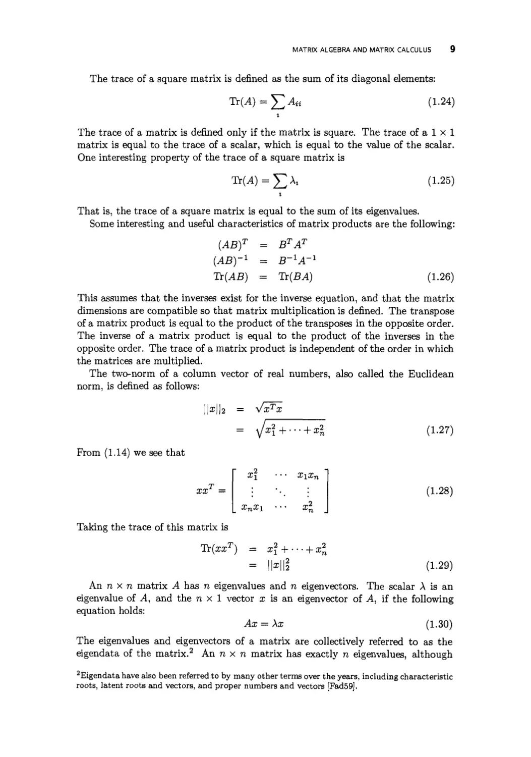
The trace of a square matrix is denned as the sum of its diagonal elements:
Tr(A) = ^^ (1.24)
The trace of a matrix is defined only if the matrix is square. The trace of a 1 x 1
matrix is equal to the trace of a scalar, which is equal to the value of the scalar.
One interesting property of the trace of a square matrix is
Tr(A) = Y/^
(1.25)
That is, the trace of a square matrix is equal to the sum of its eigenvalues.
Some interesting and useful characteristics of matrix products are the following:
(ABf
(AB)-1
Tr(AB)
= BTAT
= B~lA~l
= Tr(BA)
(1.26)
This assumes that the inverses exist for the inverse equation, and that the matrix
dimensions are compatible so that matrix multiplication is denned. The transpose
of a matrix product is equal to the product of the transposes in the opposite order.
The inverse of a matrix product is equal to the product of the inverses in the
opposite order. The trace of a matrix product is independent of the order in which
the matrices are multiplied.
The two-norm of a column vector of real numbers, also called the Euclidean
norm, is denned as follows:
F 2
= VxTa
= \[a
From (1.14) we see that
xx
x1
XjiX\
+ --- + xi
X\Xji
(1.27)
(1.28)
Taking the trace of this matrix is
Tr(a;a;r) = x\ + ••• + x\
Mil
(1.29)
Annxn matrix A has n eigenvalues and n eigenvectors. The scalar X is an
eigenvalue of A, and the nxl vector x is an eigenvector of A, if the following
equation holds:
Ax = Xx (1.30)
The eigenvalues and eigenvectors of a matrix are collectively referred to as the
eigendata of the matrix.2 An n x n matrix has exactly n eigenvalues, although
2Eigendata have also been referred to by many other terms over the years, including characteristic
roots, latent roots and vectors, and proper numbers and vectors [Fad59].
10 LINEAR SYSTEMS THEORY
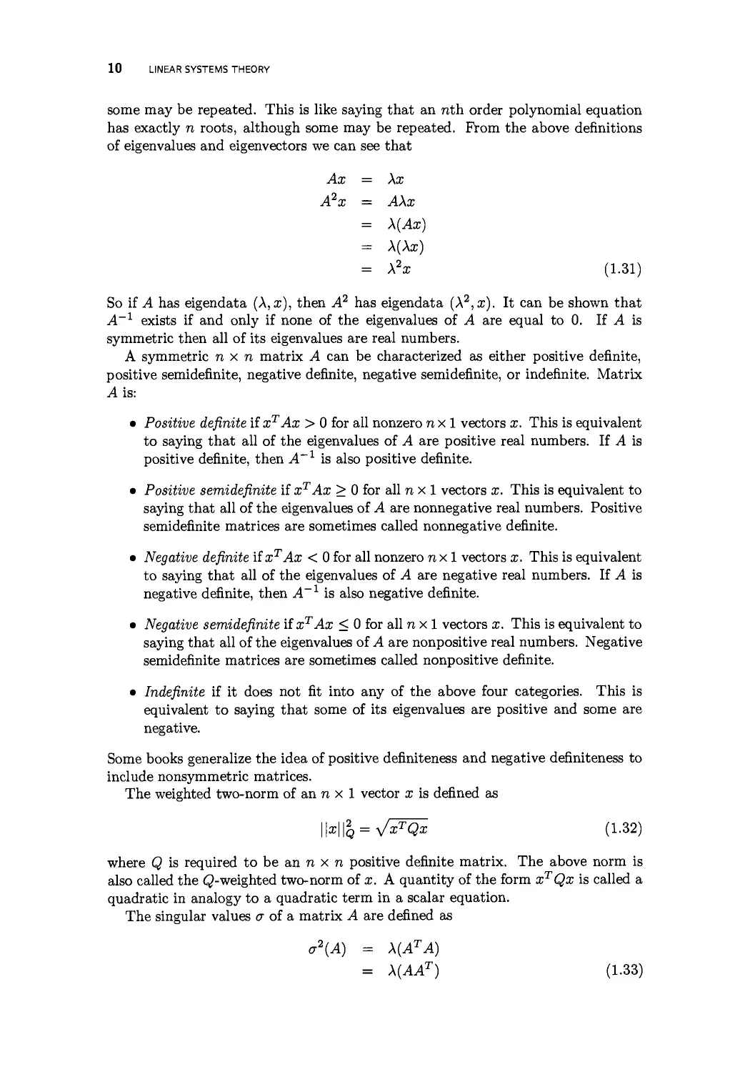
some may be repeated. This is like saying that an nth order polynomial equation
has exactly n roots, although some may be repeated. From the above definitions
of eigenvalues and eigenvectors we can see that
Ax = Xx
A2x = AXx
= X(Ax)
= X(Xx)
= X2x (1.31)
So if A has eigendata (X,x), then A2 has eigendata (X2,x). It can be shown that
A-1 exists if and only if none of the eigenvalues of A are equal to 0. If A is
symmetric then all of its eigenvalues are real numbers.
A symmetric n x n matrix A can be characterized as either positive definite,
positive semidefinite, negative definite, negative semidefinite, or indefinite. Matrix
A is:
• Positive definite if xTAx > 0 for all nonzero n x 1 vectors x. This is equivalent
to saying that all of the eigenvalues of A are positive real numbers. If A is
positive definite, then A~l is also positive definite.
• Positive semidefinite if x1Ax > 0 for all n x 1 vectors x. This is equivalent to
saying that all of the eigenvalues of A are nonnegative real numbers. Positive
semidefinite matrices are sometimes called nonnegative definite.
• Negative definite if xTAx < 0 for all nonzero nxl vectors x. This is equivalent
to saying that all of the eigenvalues of A are negative real numbers. If A is
negative definite, then A~* is also negative definite.
• Negative semidefinite if xTAx < 0 for all n x 1 vectors x. This is equivalent to
saying that all of the eigenvalues of A are nonpositive real numbers. Negative
semidefinite matrices are sometimes called nonpositive definite.
• Indefinite if it does not fit into any of the above four categories. This is
equivalent to saying that some of its eigenvalues are positive and some are
negative.
Some books generalize the idea of positive definiteness and negative definiteness to
include nonsymmetric matrices.
The weighted two-norm of an n x 1 vector x is denned as
\\x\\2Q = y/xTQx (1.32)
where Q is required to be an n x n positive definite matrix. The above norm is
also called the Q-weighted two-norm of x. A quantity of the form xTQx is called a
quadratic in analogy to a quadratic term in a scalar equation.
The singular values a of a matrix A are denned as
a2(A) = X(ATA)
= X(AAT) (1.33)
MATRIX ALGEBRA AND MATRIX CALCULUS 11
If A is an n x m matrix, then it has min(n, m) singular values. AAT will have
n eigenvalues, and ATA will have m eigenvalues. If n > m then AAT will have
the same eigenvalues as ATA plus an additional (n — m) zeros. These additional
zeros are not considered to be singular values of A, because A always has min(n, m)
singular values. This knowledge can help reduce effort during the computation of
singular values. For example, if A is a 13 x 3 matrix, then it is much easier to
compute the eigenvalues of the 3x3 matrix ATA rather than the 13 x 13 matrix
AAT. Either computation will result in the same three singular values.
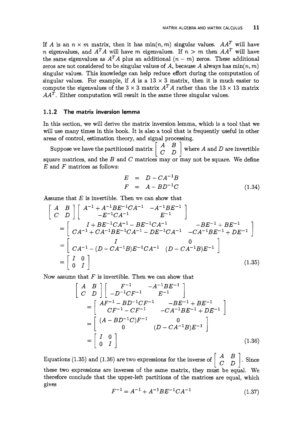
1.1.2 The matrix inversion lemma
In this section, we will derive the matrix inversion lemma, which is a tool that we
will use many times in this book. It is also a tool that is frequently useful in other
areas of control, estimation theory, and signal processing.
\ A B ~\
Suppose we have the partitioned matrix „ n where A and D are invertible
square matrices, and the B and C matrices may or may not be square. We define
E and F matrices as follows:
E = D-CA~XB
F = A-BD~XC
Assume that E is invertible. Then we can show that
(1.34)
A
C
B
D
A-1 +A-1BE~1CA-1
-E-lCA~l
I + BE^CA-1
CA-1 + CA~1BE-1CA-1
I
CA'1 -(D- CA-1B)E~1CA-1
I 0 "
-A-lBE~l
E-1
BE-lCA~l
DE-lCA~l
-BE-1 + BE-1
-CA~1BE-1 + DE-1
0
(D-CA~1B)E
r-i
0 I
Now assume that F is invertible. Then we can show that
A B
(1.35)
C D
F-1 -A-lBE~l
-D^CF-1 E-1
AF-i-BD-i-CF-1 -BE-i+BE-1
-CA^BE-1 +DE-1
0
(D-CA-1B)E~1
(A
CF^-CF-1
-BD-lC)F~l
0
I 0
0 I
Equations (1.35) and (1.36) are two expressions for the inverse of
A
C
B
D
(1.36)
Since
these two expressions are inverses of the same matrix, they must be equal. We
therefore conclude that the upper-left partitions of the matrices are equal, which
gives
F-1 = A-1 + A~1BE-1CA-
(1.37)
12 LINEAR SYSTEMS THEORY
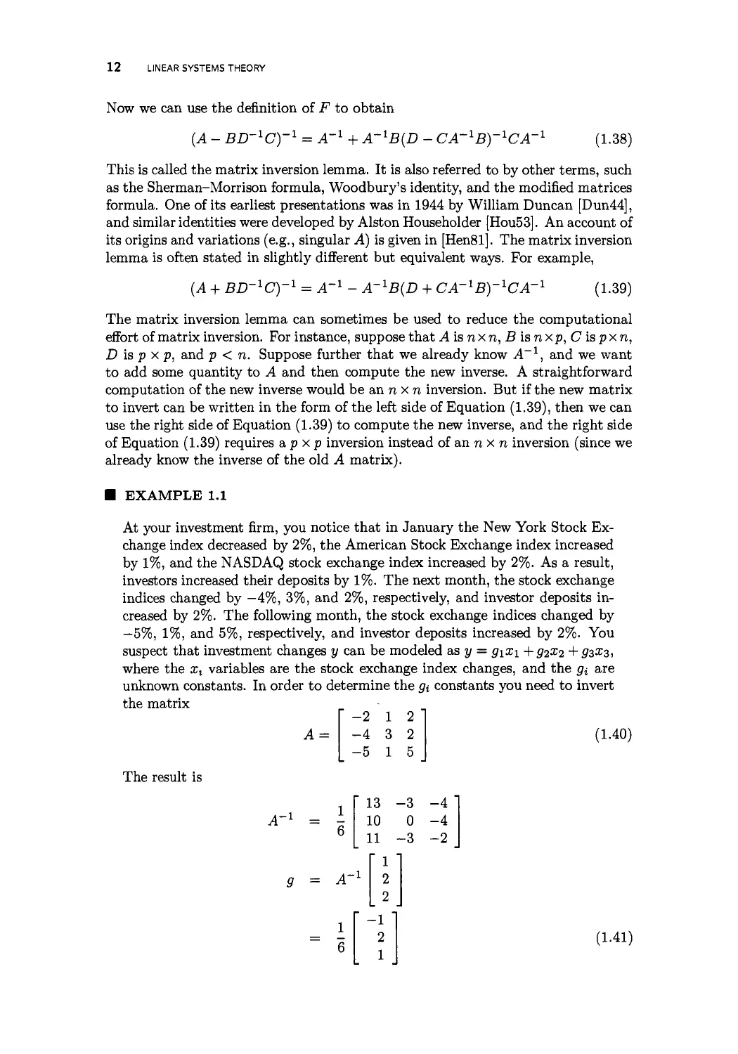
Now we can use the definition of F to obtain
(A - BD~lC)-1 = A'1 + A~1B{D - CA^B^CA
-l
(1.38)
This is called the matrix inversion lemma. It is also referred to by other terms, such
as the Sherman-Morrison formula, Woodbury's identity, and the modified matrices
formula. One of its earliest presentations was in 1944 by William Duncan [Dun44],
and similar identities were developed by Alston Householder [Hou53]. An account of
its origins and variations (e.g., singular A) is given in [Hen81]. The matrix inversion
lemma is often stated in slightly different but equivalent ways. For example,
(A + BD~lC)-1 = A-1 - A-XB{D + CA~1B)-1CA
-l
(1.39)
The matrix inversion lemma can sometimes be used to reduce the computational
effort of matrix inversion. For instance, suppose that A is nxn, B is nxp,C is pxn,
D is p x p, and p < n. Suppose further that we already know A~1, and we want
to add some quantity to A and then compute the new inverse. A straightforward
computation of the new inverse would be an n x n inversion. But if the new matrix
to invert can be written in the form of the left side of Equation (1.39), then we can
use the right side of Equation (1.39) to compute the new inverse, and the right side
of Equation (1.39) requires apxp inversion instead of an n x n inversion (since we
already know the inverse of the old A matrix).
■ EXAMPLE 1.1
At your investment firm, you notice that in January the New York Stock
Exchange index decreased by 2%, the American Stock Exchange index increased
by 1%, and the NASDAQ stock exchange index increased by 2%. As a result,
investors increased their deposits by 1%. The next month, the stock exchange
indices changed by —4%, 3%, and 2%, respectively, and investor deposits
increased by 2%. The following month, the stock exchange indices changed by
—5%, 1%, and 5%, respectively, and investor deposits increased by 2%. You
suspect that investment changes y can be modeled as y = giXi +52^2 +53^3,
where the xx variables are the stock exchange index changes, and the gx are
unknown constants. In order to determine the g% constants you need to invert
the matrix
-2 1 2
-4 3 2 (1.40)
-5 1 5
The result is
1-1
13 -
-3
10 0
11 -3
" 1 '
2
2
-1 "
2
1
-4
-4
-2
(1.41)
MATRIX ALGEBRA AND MATRIX CALCULUS 13
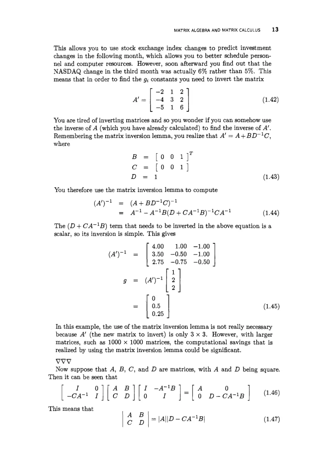
This allows you to use stock exchange index changes to predict investment
changes in the following month, which allows you to better schedule
personnel and computer resources. However, soon afterward you find out that the
NASDAQ change in the third month was actually 6% rather than 5%. This
means that in order to find the §i constants you need to invert the matrix
A'=
-2 1 2
-4 3 2
-5 1 6
(1.42)
You are tired of inverting matrices and so you wonder if you can somehow use
the inverse of A (which you have already calculated) to find the inverse of A'.
Remembering the matrix inversion lemma, you realize that A' = A + BD~1C,
where
B
C
D
=
=
=
[
I
1
0
0
0
0
1
1
You therefore use the matrix inversion lemma to compute
{A')-1 = (A + BD-XC)-1
= A
-l
A~lB(D + CA^B^CA'1
(1.43)
(1.44)
The (D + CA lB) term that needs to be inverted in the above equation is a
scalar, so its inversion is simple. This gives
(A')
/\-i
4.00
3.50
2.75
r1
0
0.5
0.25
1.00
-0.50
-0.75
' 1 '
2
2
-1.00
-1.00
-0.50
(1.45)
In this example, the use of the matrix inversion lemma is not really necessary
because A' (the new matrix to invert) is only 3x3. However, with larger
matrices, such as 1000 x 1000 matrices, the computational savings that is
realized by using the matrix inversion lemma could be significant.
vvv
Now suppose that A, B, C, and D are matrices, with A and D being square.
Then it can be seen that
I I
-CA-1 .
This means that
' A
B '
CD
' I
0
A B
C
D
I -A~lB
I
A 0
0 D- CA~lB
= [AWD-CA^B
(1.46)
(1.47)
14 LINEAR SYSTEMS THEORY
Similarly, it can be shown that
A B
C D
= \D\\A-BD-1C\
(1.48)
These formulas are called product rules for determinants. They were first given by
the Russian-born mathematician Issai Schur in a German paper [Schl7] that was
reprinted in English in [Sch86].
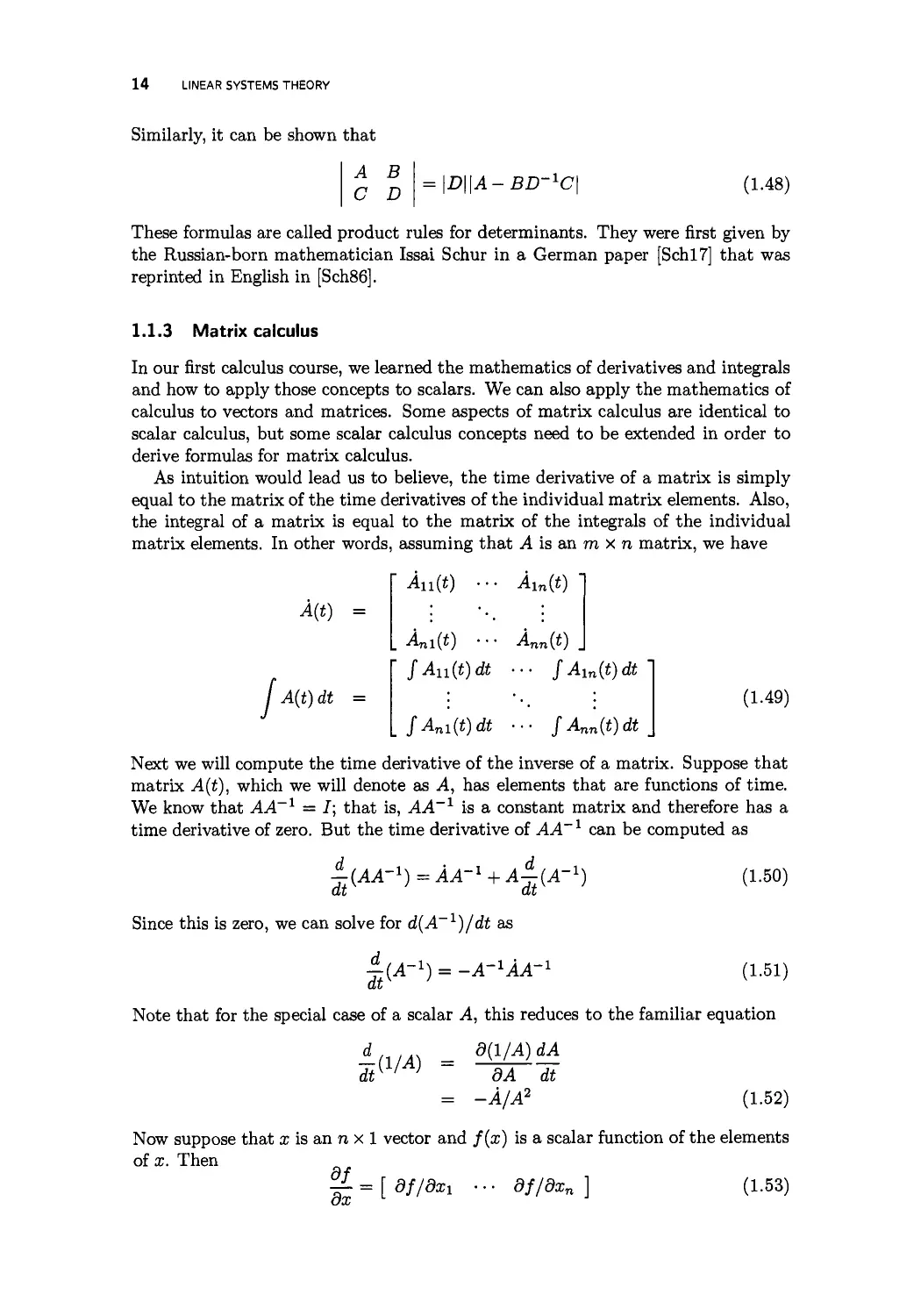
1.1.3 Matrix calculus
In our first calculus course, we learned the mathematics of derivatives and integrals
and how to apply those concepts to scalars. We can also apply the mathematics of
calculus to vectors and matrices. Some aspects of matrix calculus are identical to
scalar calculus, but some scalar calculus concepts need to be extended in order to
derive formulas for matrix calculus.
As intuition would lead us to believe, the time derivative of a matrix is simply
equal to the matrix of the time derivatives of the individual matrix elements. Also,
the integral of a matrix is equal to the matrix of the integrals of the individual
matrix elements. In other words, assuming that A is an m x n matrix, we have
/
A(t) =
A(t) dt =
An(t)
Aln(t)
Ani(t) ■■■ Ann(t)
jAu(t)dt ■■■ jAln(t)dt
jAnl(t)dt ••• /Ann(*)eft
(1.49)
Next we will compute the time derivative of the inverse of a matrix. Suppose that
matrix A(t), which we will denote as A, has elements that are functions of time.
We know that AA~X = J; that is, AA~X is a constant matrix and therefore has a
time derivative of zero. But the time derivative of AA~ * can be computed as
l(AA^) =^ AA~X + A^(A^)
Since this is zero, we can solve for d(A~1)/dt as
d
dt
(A-1) = -A~XAA
-1 A A-l
(1.50)
(1.51)
Note that for the special case of a scalar A, this reduces to the familiar equation
= -A/A2
(1.52)
Now suppose that x is an n x 1 vector and f(x) is a scalar function of the elements
of x. Then
g = [ df/dxi ■ ■ ■ df/dxn ] (1.53)
MATRIX ALGEBRA AND MATRIX CALCULUS 15
Even though a; is a column vector, df/dx is a row vector. The converse is also
true - if x is a row vector, then df/dx is a column vector. Note that some authors
define this the other way around. That is, they say that if a; is a column vector then
df/dx is also a column vector. There is no accepted convention for the definition of
the partial derivative of a scalar with respect to a vector. It does not really matter
which definition we use as long as we are consistent. In this book, we will use the
convention described by Equation (1.53).
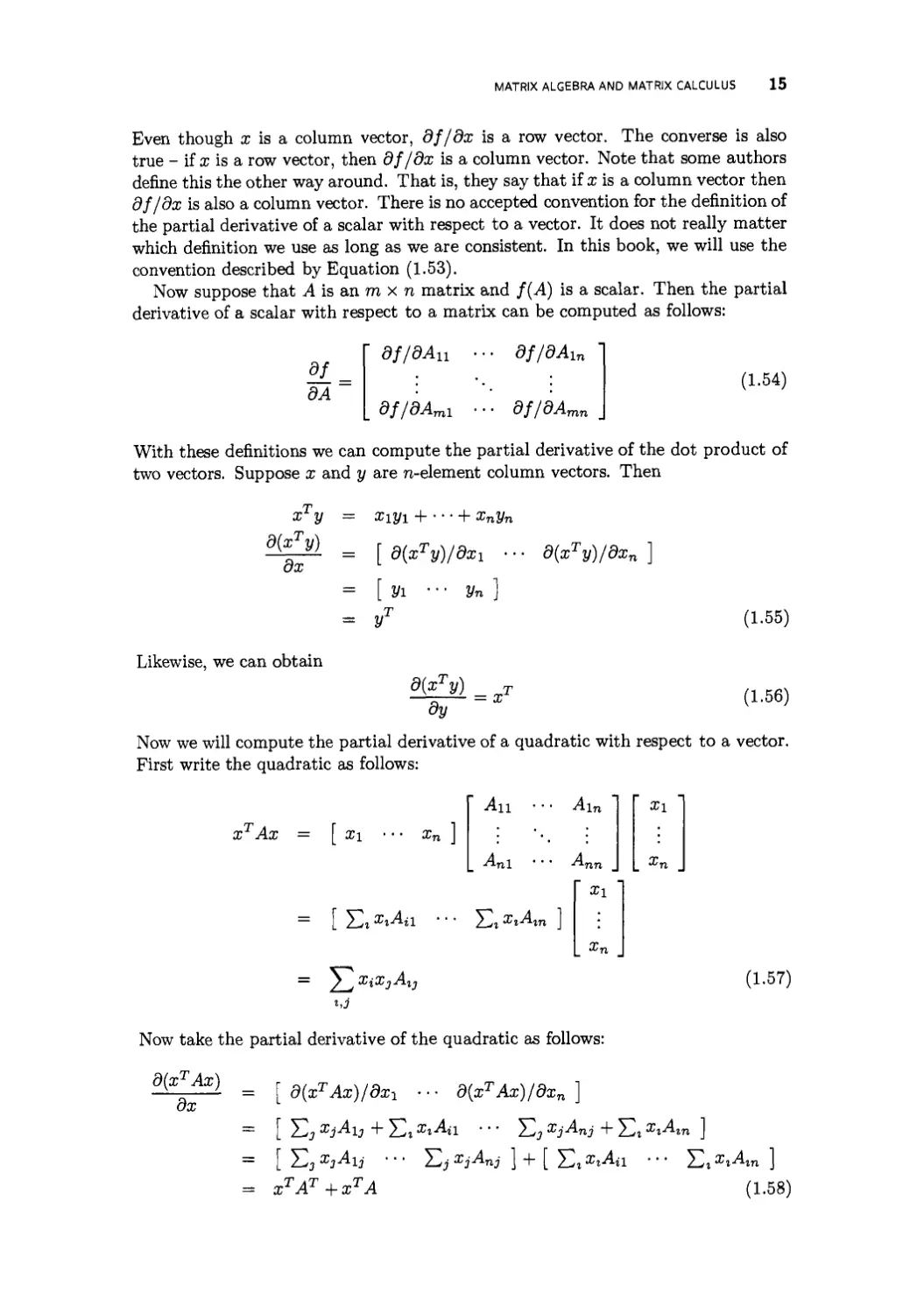
Now suppose that A is an m x n matrix and f(A) is a scalar. Then the partial
derivative of a scalar with respect to a matrix can be computed as follows:
2L
dA
df/dAn
df/dA
In
df/dA
ml
df/dA,
(1.54)
With these definitions we can compute the partial derivative of the dot product of
two vectors. Suppose x and y are n-element column vectors. Then
dx
Likewise, we can obtain
xly = xiy! H + xnyn
&- = [d{x?y)/dxl ••
d(xTy)/dxn
= [ yi
T
= y
yn
d{xTy) =xT
dy
(1.55)
(1.56)
Now we will compute the partial derivative of a quadratic with respect to a vector.
First write the quadratic as follows:
rAx = [ xi
c„ ]
Hi
lln
■"■nl ' ' ' ^nn
Xi
= [ Z^ii xiAil • ■ • 2-a xi-"-m J
Xi
— / _j %iXjA.iy
(1.57)
«..?
Now take the partial derivative of the quadratic as follows:
d(xTAx)
dx
= [ d{xTAx)/dx1 ■ ■ ■ d{xTAx)jdxn ]
= [ T,j XjAu + J2t XiAn ■■■ ^ XjAnj + £t xxAin ]
= [ EjZj^ij •■• Ej XjAnj } + [ £, XtAa ••• J2iXiAn ]
= xTAT+xTA (1.58)
16 LINEAR SYSTEMS THEORY
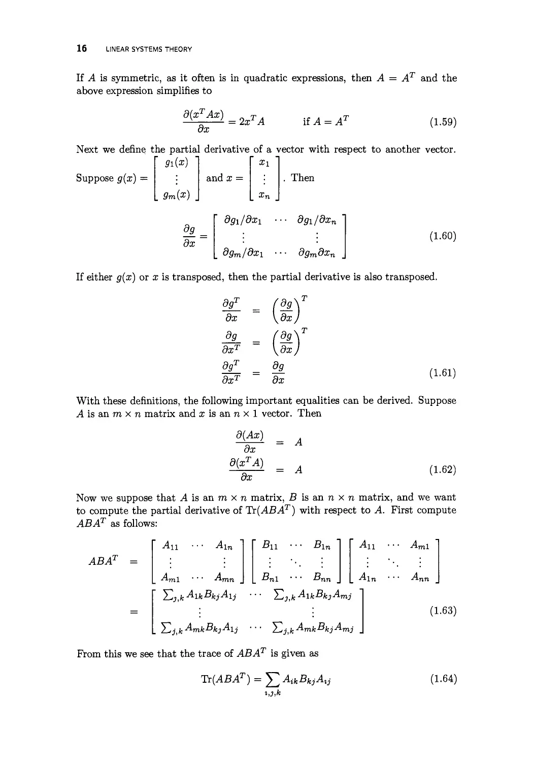
If A is symmetric, as it often is in quadratic expressions, then A = AT and the
above expression simplifies to
d(xTAx)
dx
= 2xTA
if A = AT
(1.59)
Next we define t
Suppose g(x) =
le partial derivative of a vector with respect to another vector.
Xi
and x = '■ . Then
9m(x) _
dj_
dx
dgi/dxi
d9i/dxn
(1.60)
dgm/dxi ■■ ■ dgmdxn
If either g{x) or x is transposed, then the partial derivative is also transposed.
d_l_
dx
dg
dxT
dgT
dxT
{dx~J
{dx~J
dj_
dx
(1.61)
With these definitions, the following important equalities can be derived. Suppose
A is an m x n matrix and x is an n x 1 vector. Then
d(Ax)
dx
d(xTA)
dx
= A
= A
(1.62)
Now we suppose that A is an m x n matrix, B is an n x n matrix, and we want
to compute the partial derivative of Tr(ABAT) with respect to A. First compute
ABAT as follows:
ABA1
An
■"■ml
lln
Bn
•Bnl
•Bin
-4ln
■ft-nri
Ej.fe AikBkjAij ■ ■ ■ J2,,k MkBk]Amj
/ jj k AmkBki A\ j ••• 2^i:jf.Arn}cB}.jArnj
From this we see that the trace of ABAT is given as
(1.63)
Tr(ABAT) = Y,A*BVA
i,3,k
i]
(1.64)
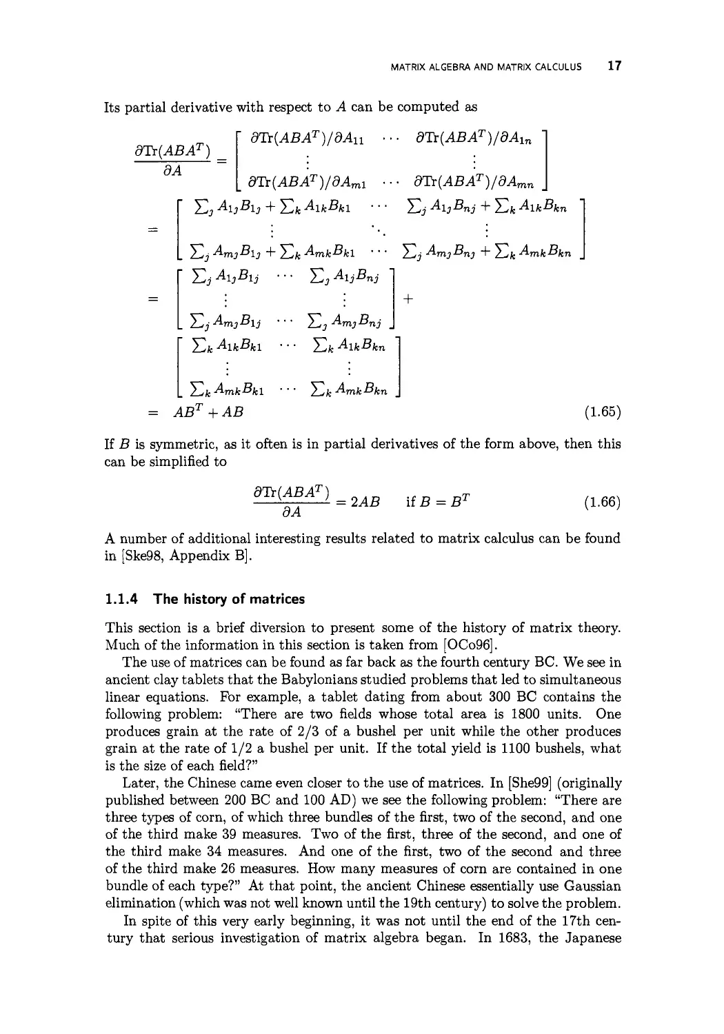
MATRIX ALGEBRA AND MATRIX CALCULUS 17
Its partial derivative with respect to A can be computed as
dTr{ABAT)/dAu ■ ■ ■ dTi (ABAT)/dAln
dTr(ABAT)
8A
dTr{ABAT)/dAml ■■■ dTr(ABAT)/dAmn
J2j AmjBij + J2k AmkBkl ••• Ej AmjBnj + J^k AmkBkn
J2j AijBij ■■■ ^23 AijBnj
Z^ijAmjBij ••• 2^j Am}Bnj _
J2k MkBkl •■■ Hk AlkBkn
= ABT+AB
(1.65)
If B is symmetric, as it often is in partial derivatives of the form above, then this
can be simplified to
dTr (ABAT)
3A
= 2AB i{B=B7
(1.66)
A number of additional interesting results related to matrix calculus can be found
in [Ske98, Appendix B].
1.1.4 The history of matrices
This section is a brief diversion to present some of the history of matrix theory.
Much of the information in this section is taken from [OCo96].
The use of matrices can be found as far back as the fourth century BC. We see in
ancient clay tablets that the Babylonians studied problems that led to simultaneous
linear equations. For example, a tablet dating from about 300 BC contains the
following problem: "There are two fields whose total area is 1800 units. One
produces grain at the rate of 2/3 of a bushel per unit while the other produces
grain at the rate of 1/2 a bushel per unit. If the total yield is 1100 bushels, what
is the size of each field?"
Later, the Chinese came even closer to the use of matrices. In [She99] (originally
published between 200 BC and 100 AD) we see the following problem: "There are
three types of corn, of which three bundles of the first, two of the second, and one
of the third make 39 measures. Two of the first, three of the second, and one of
the third make 34 measures. And one of the first, two of the second and three
of the third make 26 measures. How many measures of corn are contained in one
bundle of each type?" At that point, the ancient Chinese essentially use Gaussian
elimination (which was not well known until the 19th century) to solve the problem.
In spite of this very early beginning, it was not until the end of the 17th
century that serious investigation of matrix algebra began. In 1683, the Japanese
18 LINEAR SYSTEMS THEORY
mathematician Takakazu Seki Kowa wrote a book called "Method of Solving the
Dissimulated Problems." This book gives general methods for calculating
determinants and presents examples for matrices as large as 5 x 5. Coincidentally, in the
same year (1683) Gottfried Leibniz in Europe also first used determinants to solve
systems of linear equations. Leibniz also discovered that a determinant could be
expanded using any of the matrix columns.
In the middle of the 1700s, Colin Maclaurin and Gabriel Cramer published some
major contributions to matrix theory. After that point, work on matrices became
rather regular, with significant contributions by Etienne Bezout, Alexandre Vander-
monde, Pierre Laplace, Joseph Lagrange, and Carl Gauss. The term "determinant"
was first used in the modern sense by Augustin Cauchy in 1812 (although the word
was used earlier by Gauss in a different sense). Cauchy also discovered matrix
eigenvalues and diagonalization, and introduced the idea of similar matrices. He
was the first to prove that every real symmetric matrix is diagonalizable.
James Sylvester (in 1850) was the first to use the term "matrix." Sylvester
moved to England in 1851 to became a lawyer and met Arthur Cayley, a fellow
lawyer who was also interested in mathematics. Cayley saw the importance of the
idea of matrices and in 1853 he invented matrix inversion. Cayley also proved that
2x2 and 3x3 matrices satisfy their own characteristic equations. The fact that a
matrix satisfies its own characteristic equation is now called the Cayley-Hamilton
theorem (see Problem 1.5). The theorem has William Hamilton's name associated
with it because he proved the theorem for 4 x 4 matrices during the course of his
work on quaternions.
Camille Jordan invented the Jordan canonical form of a matrix in 1870. Georg
Frobenius proved in 1878 that all matrices satisfy their own characteristic equation
(the Cayley Hamilton theorem). He also introduced the definition of the rank of
a matrix. The nullity of a square matrix was denned by Sylvester in 1884. Karl
Weierstrass's and Leopold Kronecker's publications in 1903 were instrumental in
establishing matrix theory as an important branch of mathematics. Leon Mirsky's
book in 1955 [Mir90] helped solidify matrix theory as a fundamentally important
topic in university mathematics.
1.2 LINEAR SYSTEMS
Many processes in our world can be described by state-space systems. These include
processes in engineering, economics, physics, chemistry, biology, and many other
areas. If we can derive a mathematical model for a process, then we can use the tools
of mathematics to control the process and obtain information about the process.
This is why state-space systems are so important to engineers. If we know the state
of a system at the present time, and we know all of the present and future inputs,
then we can deduce the values of all future outputs of the system.
State-space models can be generally divided into linear models and nonlinear
models. Although most real processes are nonlinear, the mathematical tools that
are available for estimation and control are much more accessible and well
understood for linear systems. That is why nonlinear systems are often approximated as
linear systems. That way we can use the tools that have been developed for linear
systems to derive estimation or control algorithms.
LINEAR SYSTEMS 19
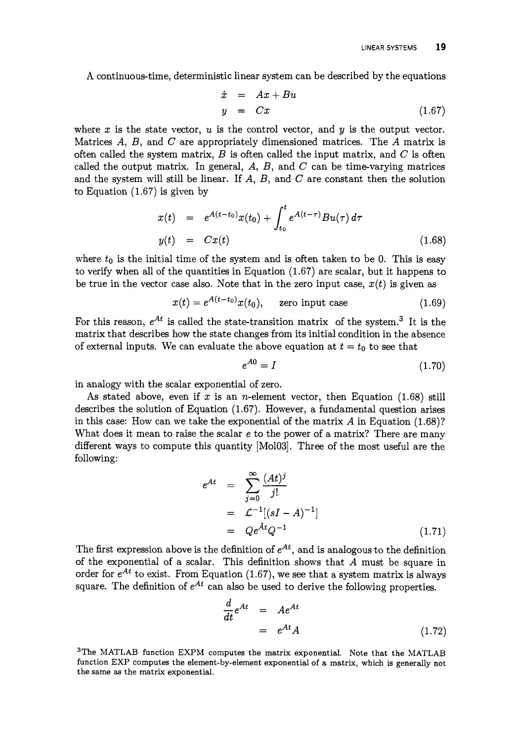
A continuous-time, deterministic linear system can be described by the equations
x = Ax + Bu
y =■ Cx (1.67)
where x is the state vector, u is the control vector, and y is the output vector.
Matrices A, B, and C are appropriately dimensioned matrices. The A matrix is
often called the system matrix, B is often called the input matrix, and C is often
called the output matrix. In general, A, B, and C can be time-varying matrices
and the system will still be linear. If A, B, and C are constant then the solution
to Equation (1.67) is given by
x(t) = eA{t-to)x{t0) + I eA{t-^Bu{T)dT
J to
y(t) = Cx(t) (1.68)
where to is the initial time of the system and is often taken to be 0. This is easy
to verify when all of the quantities in Equation (1.67) are scalar, but it happens to
be true in the vector case also. Note that in the zero input case, x(t) is given as
x(t) = eA^-toh(t0), zero input case (1.69)
For this reason, eAt is called the state-transition matrix of the system.3 It is the
matrix that describes how the state changes from its initial condition in the absence
of external inputs. We can evaluate the above equation at t — to to see that
eA0 = I (1.70)
in analogy with the scalar exponential of zero.
As stated above, even if x is an n-element vector, then Equation (1.68) still
describes the solution of Equation (1.67). However, a fundamental question arises
in this case: How can we take the exponential of the matrix A in Equation (1.68)?
What does it mean to raise the scalar e to the power of a matrix? There are many
different ways to compute this quantity [Mol03]. Three of the most useful are the
following:
eAt
^(Aty
3=0 •>■
= ^[{sl - A)-1}
= QeAtQ~l (1.71)
The first expression above is the definition of eAt, and is analogous to the definition
of the exponential of a scalar. This definition shows that A must be square in
order for eAt to exist. From Equation (1.67), we see that a system matrix is always
square. The definition of eAt can also be used to derive the following properties.
±eAt = AeAt
dt
= eAtA (1.72)
3The MATLAB function EXPM computes the matrix exponential. Note that the MATLAB
function EXP computes the element-by-element exponential of a matrix, which is generally not
the same as the matrix exponential.
20 LINEAR SYSTEMS THEORY
In general, matrices do not commute under multiplication but, interestingly, a
matrix always commutes with its exponential.
The first expression in Equation (1.71) is not usually practical for computational
purposes since it is an infinite sum (although the latter terms in the sum often
decrease rapidly in magnitude, and may even become zero). The second expression
in Equation (1.71) uses the inverse Laplace transform to compute eAt. In the
third expression of Equation (1.71), Q is a matrix whose columns comprise the
eigenvectors of A, and A is the Jordan form4 of A. Note that Q and A are well
denned for any square matrix A, so the matrix exponential eAt exists for all square
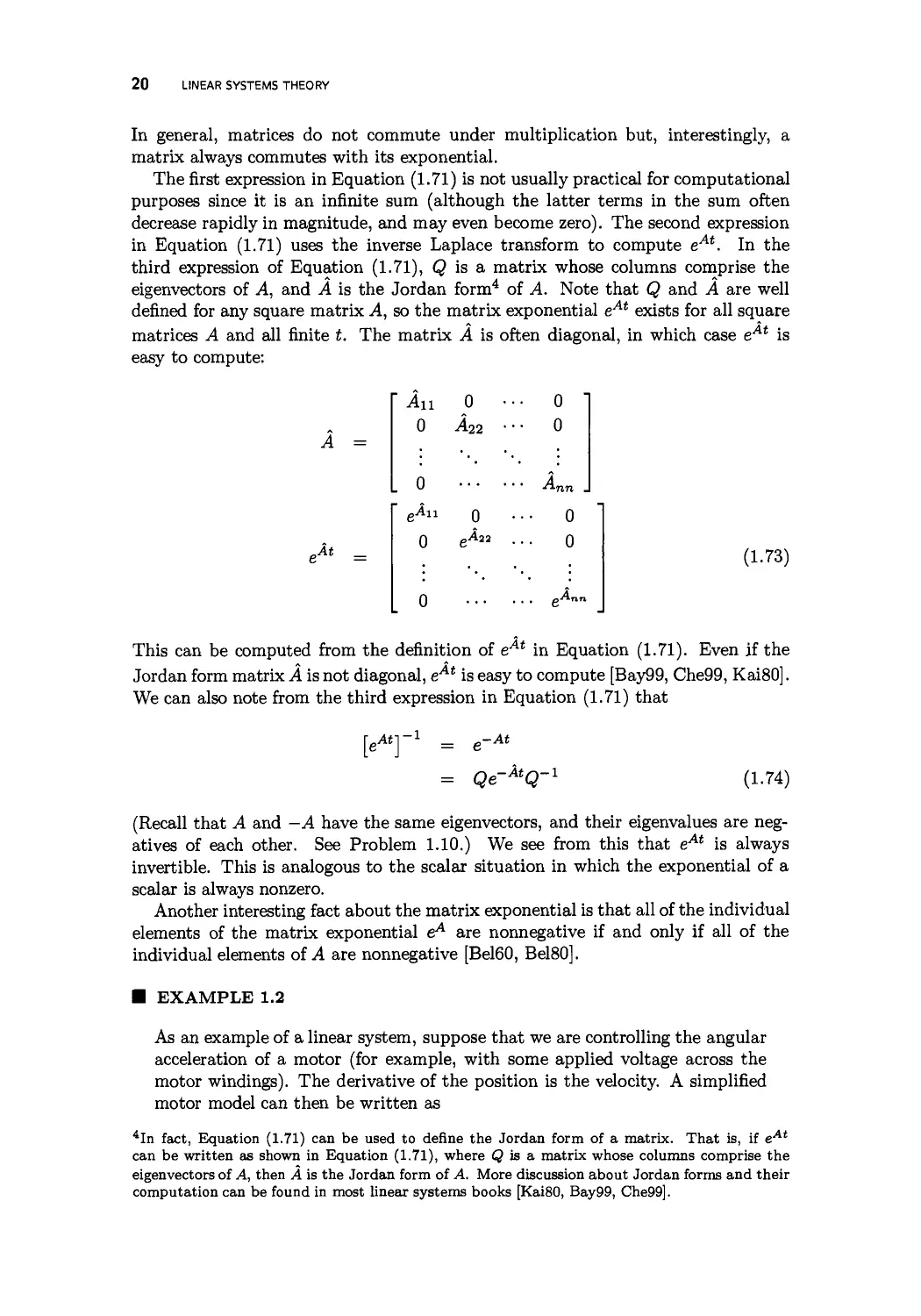
matrices A and all finite t. The matrix A is often diagonal, in which case eAt is
easy to compute:
A =
„At
'An
0
0
' eAu
0
0
0 •
A22 ■
0
eA22
• 0 "
■ 0
. A
0
0
.. eA™
(1.73)
This can be computed from the definition of eAt in Equation (1.71). Even if the
Jordan form matrix A is not diagonal, eAt is easy to compute [Bay99, Che99, Kai80].
We can also note from the third expression in Equation (1.71) that
[eMYl = e
-At
-Atn-i
= Qe~mQ-
(1.74)
(Recall that A and —A have the same eigenvectors, and their eigenvalues are
negatives of each other. See Problem 1.10.) We see from this that eAt is always
invertible. This is analogous to the scalar situation in which the exponential of a
scalar is always nonzero.
Another interesting fact about the matrix exponential is that all of the individual
elements of the matrix exponential eA are nonnegative if and only if all of the
individual elements of A are nonnegative [Bel60, Bel80].
■ EXAMPLE 1.2
As an example of a linear system, suppose that we are controlling the angular
acceleration of a motor (for example, with some applied voltage across the
motor windings). The derivative of the position is the velocity. A simplified
motor model can then be written as
4In fact, Equation (1.71) can be used to define the Jordan form of a matrix. That is, if eAt
can be written as shown in Equation (1.71), where Q is a matrix whose columns comprise the
eigenvectors of A, then A is the Jordan form of A. More discussion about Jordan forms and their
computation can be found in most linear systems books [Kai80, Bay99, Che99].
LINEAR SYSTEMS 21
e = w
UJ = U + Wi
(1.75)
The scalar w\ is the acceleration noise and could consist of such factors as
uncertainty in the applied acceleration, motor shaft eccentricity, and load
disturbances. If our measurement consists of the angular position of the motor
then a state space description of this system can be written as
" 9 ]
U)
0 1'
0 0
' 9 '
U)
+
" 0 "
1
u +
0
Wl
y = [1 0]x+v
(1.76)
The scalar v consists of measurement noise. Comparing with Equation (1.67),
we see that the state vector x is a 2 x 1 vector containing the scalars 6 and u.
vvv
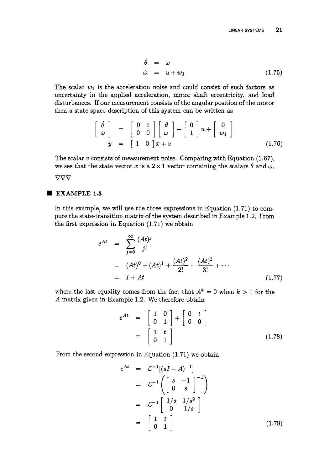
EXAMPLE 1.3
In this example, we will use the three expressions in Equation (1.71) to
compute the state-transition matrix of the system described in Example 1.2. Prom
the first expression in Equation (1.71) we obtain
„At
(Aty
J=0 J
= (At)0 + (At)1 + ^/- + ±J- +
2!
3!
I + At
(1.77)
where the last equality comes from the fact that Ak = 0 when k > 1 for the
A matrix given in Example 1.2. We therefore obtain
eAt =
From the second expression in Equation (1.71) we obtain
'10'
0 1
'it'
0 1
+
' 0 t '
0 0
(1.78)
„At
C-^sI-A)-1
(1.79)
22 LINEAR SYSTEMS THEORY
In order to use the third expression in Equation (1.71) we first need to obtain
the eigendata (i.e., the eigenvalues and eigenvectors) of the A matrix. These
are found as
This shows that
\(A) =
v(A) =
A --
Q =
{0,0}
0
(1.80)
' 0
0
' 1
0
1 "
0
0 "
1
(1.81)
Note that in this simple example A is already in Jordan form, so A = A and
Q = I. The third expression in Equation (1.71) therefore gives
eAt = QeAtQ-x
"10'
0 1
'it'
0 1 _
'it'
0 1
'10'
0 1
T -1
(1.82)
VVV
1.3 NONLINEAR SYSTEMS
The discussion of linear systems in the preceding section is a bit optimistic, because
in reality linear systems do not exist. Real systems always have some nonlinearities.
Even a simple resistor is ultimately nonlinear if we apply a large enough voltage
across it. However, we often model a resistor with the simple linear equation
V = IR because this equation accurately describes the operation of the resistor
over a wide operating range. So even though linear systems do not exist in the
real world, linear systems theory is still a valuable tool for dealing with nonlinear
systems.
The general form of a continuous-time nonlinear system can be written as
x = f(x,u,w)
y = h(x,v)
(1.83)
where /(•) and h(-) are arbitrary vector-valued functions. We use w to indicate
process noise, and v to indicate measurement noise. If /(■) and h(-) are explicit
functions of t then the system is time-varying. Otherwise, the system is time-
invariant. If f(x, u, w) = Ax + Bu + w, and h(x, v) = Hx + v, then the system is
linear [compare with Equation (1.67)]. Otherwise, the system is nonlinear.
In order to apply tools from linear systems theory to nonlinear systems, we need
to linearize the nonlinear system. In other words, we need to find a linear system
NONLINEAR SYSTEMS 23
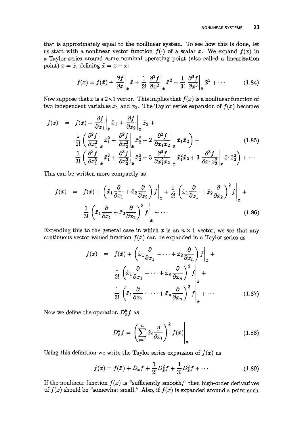
that is approximately equal to the nonlinear system. To see how this is done, let
us start with a nonlinear vector function /(•) of a scalar x. We expand /(a?) in
a Taylor series around some nominal operating point (also called a linearization
point) x = x, denning x = x — x:
f(x) = f(x) +
dx
x +
2! da;2
*2 * ^!Z
. 3! 9a;3
x3 + .
(1.84)
Now suppose that x is a 2 x 1 vector. This implies that f{x) is a nonlinear function of
two independent variables X\ and x2- The Taylor series expansion of f(x) becomes
nx) = m +
df
dxi
Xl +
3X2
x2 +
2! \dxl
3! V dx\
^3
9V
dx32
^ + 9 d2f
x2 + 2 "5
ax\x2
-3 93/
, 2 dxjx2
X\X2 ) +
2 d3/
^1^2 + 3 2
(1.85)
i\i\ I +
This can be written more compactly as
1 f. d . flV
+
1 (- 9 .6..
z\\Xl^l + x"W2] f
+
(1.86)
Extending this to the general case in which x is an n x 1 vector, we see that any
continuous vector-valued function /(a;) can be expanded in a Taylor series as
f{x) = /0)+(^ + ...+^)/
+
1 (- d -9..
2!
1
9
311/^ + - + ^
«—V
ndxnJ
+
+ ■
(1.87)
Now we define the operation D|/ as
^/= E
u=l
Xiwt) f{x)
(1.88)
Using this definition we write the Taylor series expansion of f(x) as
f(x) = f(x) + D-Xf + \-D\f + ±-Mf + • • •
2!
3!
(1.89)
If the nonlinear function f(x) is "sufficiently smooth," then high-order derivatives
of f(x) should be "somewhat small." Also, if f(x) is expanded around a point such
24 LINEAR SYSTEMS THEORY
that x is "close" to x, then x will be "small" and the higher powers of x in
Equation (1.89) will be "small." Finally, the higher-order derivatives in the Taylor series
expansion of Equation (1.89) are divided by increasingly large factorials, which
further diminishes the magnitude of the higher-order terms in Equation (1.89). This
justifies the approximation
f{x) » f(x) + Dif
« f(x) + Ax
(1.90)
where A is the matrix denned by the above equation.
Returning to our nonlinear system equations in Equation (1.83), we can
expand the nonlinear system equation f(x, u, w) around the nominal operating point
(x, u, w). We then obtain a linear system approximation as follows.
x = f(x,u,w)
f(x,u,w)+ —
{x-x)+%
au
o + M;
(w
w)
= x + Ax + Bu + Lw
(1.91)
where the 0 subscript means that the function is evaluated at the nominal point
(x, u, w), and A, B, and L are denned by the above equations. Subtracting x from
both sides of Equation (1.91) gives
x = Ax + Bu + Lw
Since w is noise, we will set w = 0 so that w = w and we obtain
x = Ax + Bu + Lw
(1.92)
(1.93)
We see that we have a linear equation for x in terms of x, u, and w. We have a
linear equation for the deviations of the state and control from their nominal values.
As long as the deviations remain small, the linearization will be accurate and the
linear equation will accurately describe deviations of x from its nominal value x.
In a similar manner we can expand the nonlinear measurement equation given
by Equation (1.83) around a nominal operating point x = x and v = v = 0. This
results in the linearized measurement equation
dh
V = Tx
. dh
x+
flat;
Cx + Dv
(1.94)
where C and D are denned by the above equation. Equations (1.93) and (1.94)
comprise a linear system that describes the deviations of the state and output from
their nominal values. Recall that the tilde quantities in Equations (1.93) and (1.94)
are defined as
u = u — u
y = y-y
(1.95)
NONLINEAR SYSTEMS 25
EXAMPLE 1.4
Consider the following model for a two-phase permanent magnet synchronous
motor:
la =
lb =
U)
e
-R. u\ ua
lTla + Tsm9 + T
-R.
-tb-
u;A . ub
— cos 0 + —
L L
■^-Jasin^+-Jbcos^- —-7
= u
(1.96)
where ia and % are the currents through the two windings, R and L are the
resistance and inductance of the windings, 6 and u are the angular position
and velocity of the rotor, \ is the flux constant of the motor, ua and uy, are
the voltages applied across the two windings, J is the moment of inertia of
the rotor and its load, F is the viscous friction of the rotor, and Ti is the
load torque. The time variable does not explicitly appear on the right side of
the above equation, so this is a time-invariant system. However, the system
is highly nonlinear and we therefore cannot directly use any linear systems
tools for control or estimation. However, if we linearize the system around
a nominal (possibly time-varying) operating point then we can use linear
system tools for control and estimation. We start by denning a state vector
as x = [ ia ib u> 6 ] . With this definition we write
x =
[ *i ±2
f(x, u)
X3 £4
=j£xi + ^sina;4 + ^
=£x2- ^ cos 3:4 + ^
-3A • 3A T
-ffxi sin £4 + J3X2 cos X4- —
J
xz
(1.97)
We linearize the system equation by taking the partial derivative of f(x, u)
with respect to x and u to obtain
A =
B =
^1
dx
-R/L 0 \si/L
0 -R/L -Xa/L
-3As4/2/J 3Ac4/2/J -F/J
0 0 1
d±
du
■ 1/L
0
0
0
0
1/L
0
0
x^Xci/L
X3XS4/L
-3A(:riC4 +x2S4)/2/J
0
(1.98)
26 LINEAR SYSTEMS THEORY
where S4 = sinX4 and C4 = cos X4. The linear system
x = Ax + Bu
(1.99)
approximately describes the deviation of x from its nominal value x. The
nonlinear system was simulated with the nominal control values ua(t) = sin27rt
and Ub{t) = cos27rt. This resulted in a nominal state trajectory x(t). The
linear and nonlinear systems were then simulated with nonnominal control
values. Figure 1.1 shows the results of the linear and nonlinear simulations when
the control magnitude deviation from nominal is a small positive number. It
can be seen that the simulations result in similar state-space trajectories,
although they do not match exactly. If the deviation is zero, then the linear
and nonlinear simulations will match exactly. As the deviation from
nominal increases, the difference between the linear and nonlinear simulations will
increase.
20
10
0
-10
V
Nonlinear
Linearized
0.5
I-
f.
ol
is
j\
0.5
0.5
Seconds
0.5
Seconds
Figure 1.1 Example 1.4 comparison of nonlinear and linearized motor simulations.
VVV
1.4 DISCRETIZATION
Most systems in the real world are described with continuous-time dynamics of the
type shown in Equations (1.67) or (1.83). However, state estimation and control
algorithms are almost always implemented in digital electronics. This often requires
a transformation of continuous-time dynamics to discrete-time dynamics. This
section discusses how a continuous-time linear system can be transformed into a
discrete-time linear system.
Recall from Equation (1.68) that the solution of a continuous-time linear system
is given by
' sa^-^Bu{t)(It
x(t) = eA^-toh(t0) + f ,
(1.100)
SIMULATION 27
Let t = tk (some discrete time point) and let the initial time to = tk-i (the previous
discrete time point). Assume that A(t), B(t), and u(t) are approximately constant
in the interval of integration. We then obtain
x(tk) = eA^-tk-^x{tk-i) + f " eA('k-T) dTBu(tk-i) (1.101)
Jtk-i
Now define At = tk — ifc-i, define a = r — tk-i, and substitute for r in the above
equation to obtain
x(tk) = eAAtx(tk-i)+ [ e^-^daBuitk-i)
Jo
= eAAtx(tk-i) + eAAt f e-AadaBu(tk-i)
Jo
Xk = Fk-iXk-i+Gk-iUk-i (1.102)
where Xk, Fk, Gk, and Uk are defined by the above equation. This is a
linear discrete-time approximation to the continuous-time dynamics given in
Equation (1.67). Note that this discrete-time system defines Xk only at the discrete time
points {tk}\ it does not say anything about what happens to the continuous-time
signal x(t) in between the discrete time points.
The difficulty with the above discrete-time system is the computation of the
integral of the matrix exponential, which is necessary in order to compute the G
matrix. This computation can be simplified if A is invertible:
/•At /.At oo
/ e^dr = / £
Jo Jo ,=n
<-^>' *r
f
Jo
,=0 ^
At
[I-At + A2t2/2\ ]dr
At
0
= [It - At2/2\ + A2t3/Z\ ]
= [lAt-A(At)2/2\ + A2(At)3/Z\ ]
= [AAt - {AAt)2/2\ + (AAt)3/Z\ ] A'1
= [l-e-AAt}A~x (1.103)
The conversion from continuous-time system matrices A and B to discrete-time
system matrices F and G can be summarized as follows:
F = eAAt
/•At
G = F e~ATdrB
Jo
= F [I - e~AAt] A~XB (1.104)
where At is the discretization step size.
1.5 SIMULATION
In this section, we discuss how to simulate continuous-time systems (either linear
or nonlinear) on a digital computer. We consider the following form of the general
28 LINEAR SYSTEMS THEORY
system equation from Equation (1.83):
x = f(x,u,t) (1.105)
where u(t) is a known control input. In order to simulate this system on a computer,
we need to program a computer to solve for x(tf) at some user-specified value of
tf. In other words, we want to compute
x(tf) = x(t0)+ f[x(t),u(t),t]dt (1.106)
Jto
Often, the initial time is taken as to = 0, in which case we have the slightly simpler
looking equation
x(tf) = x(0)+ f[x(t),u(t),t]dt (1.107)
Jo
We see that in order to find the solution x(tf) to the differential equation x =
f(x,u,t), we need to compute an integral. The problem of finding the solution
x(tf) is therefore commonly referred to as an integration problem.
Now suppose that we divide the time interval [0, tf] into L equally spaced
intervals so that tk = kT for k = 0, ■ • •, L, and the time interval T = tf/L. From
this we note that tf =ti. With this division of the time interval, we can write the
solution of Equation (1.107) as
x(tf) = x(tL)
^ rtk+i
= x(0) + 22 f[x(t),u(t),t]dt (1.108)
fc=0^tfc
More generally, for some n £ [0, L — 1], we can write x(tn) and x(tn+i) as
x(tn) = x(0) + YI+f\x(t),u(t),t]dt
(tn) = x(0) + J2 [k+1 f[x(t),u(t),t]<
"+1 ptk+i
x(tn+1) = x(0) + ^2 f[x(t),u(t),t]dt (1.109)
l n Jtk
k=0Jt*
which means that
x(tn+1) = x{tn) + f "+1 f[x(t), u(t), t] dt (1.110)
If we can find a way to approximate the integral on the right side of the above
equation, we can repeatedly propagate our x{t) approximation from time tn to
time tn+i, thus obtaining an approximation for x(t) at any desired time t. The
algorithm could look something like the following.
SIMULATION 29
Differential equation solution
Assume that a?(0) is given
for t = 0 : T : tf - T
Find an approximation I(t) « Jt f[x(t), u(t), t] dt
x(t + T)= x(t) + TI(t)
end
In the following sections, we present three different ways to approximate this
integral. The approximations, in order of increasing computational effort and
increasing accuracy, are rectangular integration, trapezoidal integration, and fourth-order
Runge-Kutta integration.
1.5.1 Rectangular integration
If the time interval (tn+i — tn) is small, then f[x(t), u(t), t] is approximately constant
in this interval. Equation (1.110) can therefore be approximated as
/■tn+i
x(tn+i) « x(tn)+ f[x(tn),u(tn),tn]dt
« x(tn) + f[x(tn),u(tn),tn]T (1.111)
Equation (1.109) can therefore be approximated as
" rtk+i
x{tn) « x(0) + J2 f{x(tk),u(tk),tk]dt
k=0''t>'
n
= x(0) + ^f[x(tk),u(tk),tk]T (1.112)
fc=o
This is called Euler integration, or rectangular integration, and is illustrated in
Figure 1.2. As long as T is sufficiently small, this gives a good approximation for
x{tn).
This gives the following algorithm for integrating continuous-time dynamics
using rectangular integration. The time loop in the algorithm is executed for
t = 0, T, 2T, ■ ■ ■, tf - T.
Rectangular integration
Assume that a;(0) is given
for t = 0 : T : tf - T
Compute f[x(t),u(t),t]
xit + T)= x(t) + f[x(t), u(t), t]T
end
1.5.2 Trapezoidal integration
An inspection of Figure 1.2 suggests an idea for improving the approximation for
x(t). Instead of approximating each area as a rectangle, what if we approximate
each area as a trapezoid? Figure 1.3 shows how an improved integration algorithm
can be implemented. This is called modified Euler integration, or trapezoidal
integration. A comparison of Figures 1.2 and 1.3 shows that trapezoidal integration
30 LINEAR SYSTEMS THEORY
Figure 1.2 An illustration of rectangular integration. We have x = f(x), so x(t) is the
area under the f(x) curve. This area can be approximated as the sum of the rectangular
areas A,. That is, x(0.5) w Ai, x(l) « Ai + A2, ■ • •.
Figure 1.3 An illustration of trapezoidal integration. We have x = f(x), so x(t) is the
area under the f(x) curve. This area can be approximated as the sum of trapezoidal areas
A,. That is, x(l) » Au x{2) w Ai + A2, and x(3) w Ai + A2 + A3.
appears to give a better approximation than rectangular integration, even though
the time axis is only divided into half as many intervals in trapezoidal integration.
With rectangular integration we approximated f[x(t),u(t),t] as a constant in
the interval t £ [tn,tn+i\. With trapezoidal integration, we instead approximate
f[x(t),u(t),t] as a linear function in the interval t € [£n,£n+i]. That is,
SIMULATION 31
f[x(t)] « f[x(tn),u(tn),tn} +
ff[x(tn+i), u(tn+i), tn+1] - f[x(tn),u(tn), tn] \ _ t
forte [tn,tn+1] (1.113)
Equation (1.110) can therefore be approximated as
x(tn+1) » x(tn)+ <f[x(tn),u(tn),tn] +
ff[x(tn+i), u(tn+i), tn+i] - f[x(tn), u(tn), tn] \ t . 1 ^
= x(tn) + ^(f[x(tn),u(tn),tn]T + f[x(tn+1),u(tn+1),tn+i]T) (1.114)
This equation to approximate x(tn+i), however, has x(tn+i) on the right side of
the equation. How can we plug x(tn+i) into the right side of the equation if we
do not yet know x(tn+i)? The answer is that we can use the rectangular
integration approximation from the previous section for x(tn+i) on the right side of the
equation. The above equation can therefore be written as
An = f[x{tn),u(tn),tn]T
Ax2 = f[x(tn+i),u(tn+1),tn+i]T
« f[x(tn) + Azi, u(tn+i), tn+i]T
x(tn+i) w x(tn) + -(Axi + Ax2) (1.115)
This gives the following algorithm for integrating continuous-time dynamics
using trapezoidal integration. The time loop in the algorithm is executed for
t = 0,T,2T,---,tf-T.
Trapezoidal integration
Assume that x(0) is given
for t = 0 : T : tf - T
AXl = f[x{t),u{t),t]T
Ax2 = f[x(t) + Asi, u(t + T),t + T]T
x(t + T) = x(t) + (Azi + Aa;2)/2
end
1.5.3 Runge-Kutta integration
From the previous sections, we see that rectangular integration involves the
calculation of one function value at each time step, and trapezoidal integration involves
the calculation of two function values at each time step. In order to further improve
the integral approximation, we can perform additional function calculations at each
time step, nth-order Runge-Kutta integration is the approximation of an integral
32 LINEAR SYSTEMS THEORY
by performing n function calculations at each time step. Rectangular integration
is therefore equivalent to first-order Runge-Kutta integration, and trapezoidal
integration is equivalent to second-order Runge-Kutta integration.
The most commonly used integration scheme of this type is fourth-order Runge-
Kutta integration. We present the fourth-order Runge-Kutta integration algorithm
(without derivation) as follows:
Aii = f[x{tk),u{tk),tk}T
Ax2 = f[x(tk)+Ax1/2,u(tk+1/2),tk+1/2]T
Ax3 = f[x(tk)+Ax2/2,u(tk+1/2),tk+1/2]T
Ax4 = f[x(tk)+Ax3,u(tk+1),tk+1]T
x(tk+i) « x(tk) + (Axi + 2Ax2 + 2Ax3 + Ax4)/6 (1.116)
where tk+i/2 = tk + T/2. Fourth-order Runge-Kutta integration is more
computationally demanding than rectangular or trapezoidal integration, but it also provides
far greater accuracy. This gives the following algorithm for integrating continuous-
time dynamics using fourth-order Runge-Kutta integration. The time loop in the
algorithm is executed for t = 0,T,2T, ■ ■ ■ ,tf —T.
Fourth-order Runge-Kutta integration
Assume that a?(0) is given
for t = 0 : T : tf - T
h=t+ T/2
Ax1=f[x(t),u(t),t]T
Ax2 = f[x(t) + An/2, u(ti), ti]T
Ax3 = f[x(t) + Aa:a/2, u(h), h]T
AxA = f[x(t) + Ax3, u(t + T),t + T]T
x(t + T) = x(t) + (Azi + 2Aa;2 + 2Aa;3 + Az4) /6
end
Runge-Kutta integration was invented by Carl Runge, a German
mathematician and physicist, in 1895. It was independently invented and generalized by
Wilhelm Kutta, a German mathematician and aerodynamicist, in 1901. More
accurate integration algorithms have also been derived and are sometimes used, but
fourth-order Runge-Kutta integration is generally considered a good trade-off
between accuracy and computational effort. Further information and derivations of
numerical integration algorithms can be found in many numerical analysis texts,
including [Atk89].
■ EXAMPLE 1.5
Suppose we want to numerically compute x(t) at t = 1 based on the differential
equation
x = cost (1-117)
with the initial condition a?(0) = 0. We can analytically integrate the
equation to find out that a;(l) = sin 1 w 0.8415. If we use a numerical integration
scheme, we have to choose the step size T. Table 1.1 shows the error of the
rectangular, trapezoidal, and fourth-order Runge-Kutta integration methods
for this example for various values of T. As expected, Runge-Kutta is more
accurate than trapezoidal, and trapezoidal is more accurate than rectangular.
STABILITY 33
Also as expected, the error for given method decreases as T decreases.
However, perhaps the most noteworthy feature of Table 1.1 is how the integration
error decreases with T. We can see that with rectangular integration, when T
is halved, the integration error is also halved. With trapezoidal integration,
when T is halved, the integration error decreases by a factor of four. With
Runge-Kutta integration, when T is halved, the integration error decreases by
a factor of 16. We conclude that (in general) the error of rectangular
integration is proportional to T, the error of trapezoidal integration is proportional
to T2, and the error of Runge-Kutta integration is proportional to T4.
Table 1.1 Example 1.5 results. Percent errors when numerically integrating
x = cos t from t = 0 to t = 1, for various integration algorithms, and for various time
step sizes T.
T = 0.1 T = 0.05 T = 0.025
Rectangular 2.6 1.3 0.68
Trapezoidal 0.083 0.021 0.0052
Fourth-order Runge-Kutta 3.5 x 10⁻⁶ 2.2 x 10⁻⁷ 1.4 x 10"
vvv
1.6 STABILITY
In this section, we review the concept of stability for linear time-invariant systems.
We first deal with continuous-time systems in Section 1.6.1, and then discrete-time
systems in Section 1.6.2. We state the important results here without proof. The
interested reader can refer to standard books on linear systems for more details and
additional results [Kai80, Bay99, Che99].
1.6.1 Continuous-time systems
Consider the zero-input, linear, continuous-time system
x = Ax
y = Cx (1.118)
The definitions of marginal stability and asymptotic stability are as follows.
Definition 1 A linear continuous-time, time-invariant system is marginally stable
if the state x(t) is bounded for all t and for all bounded initial states x(0).
Marginal stability is also called Lyapunov stability.
Definition 2 A linear continuous-time, time-invariant system is asymptotically
stable if, for all bounded initial states x(0),
limx(t)=0 (1.119)
34 LINEAR SYSTEMS THEORY
The above two definitions show that a system is marginally stable if it is
asymptotically stable. That is, asymptotic stability is a subset of marginal stability.
Marginal stability and asymptotic stability are types of internal stability. This is
because they deal with only the state of the system (i.e., the internal condition of
the system) and do not consider the output of the system. More specific categories
of internal stability (e.g., uniform stability and exponential stability) are given in
some books on linear systems.
Since the solution of Equation (1.118) is given as
x(t) = ex.p(At)x(0)
we can state the following theorem.
Theorem 1 A linear continuous-time, time-invariant system is marginally stable
if and only if
lim exp(At) < M < oo (1-121)
for some constant matrix M. This is just a way of saying that the matrix exponential
does not increase without bound.
The "less than or equal to" relation in the above theorem raises some questions,
because the quantities on either side of this mathematical symbol are matrices.
What does it mean for a matrix to be less than another matrix? It can be interpreted
several ways. For example, to say that A < B is usually interpreted to mean that
(J5 — A) is positive definite.5 In the above theorem we can use any reasonable
definition for the matrix inequality and the theorem still holds.
A similar theorem can be stated by combining Definition (2) with Equation (1.120).
Theorem 2 A linear continuous-time, time-invariant system is asymptotically
stable if and only if
km exp(At) = 0 (1.122)
t—*oo
Now recall that ex.p(At) = Qexp^AtyQ-1, where Q is a constant matrix
containing the eigenvectors of A, and A is the Jordan form of A. The exponential
ex.p(At) therefore contains terms like exp(Xit), texp(Xit), t2exp(\it), and so on,
where \% is an eigenvalue of A. The boundedness of exp(At) is therefore related to
the eigenvalues of A as stated by the following theorems.
Theorem 3 A linear continuous-time, time-invariant system is marginally stable
if and only if one of the following conditions holds.
1. All of the eigenvalues of A have negative real parts.
2. All of the eigenvalues of A have negative or zero real parts, and those with
real parts equal to zero have a geometric multiplicity equal to their algebraic
multiplicity. That is, the Jordan blocks that are associated with the eigenvalues
that have real parts equal to zero are first order.
Theorem 4 A linear continuous-time, time-invariant system is asymptotically
stable if and only if all of the eigenvalues of A have negative real parts.
5 Sometimes the statement A < B means that every element of A is less than the corresponding
element of B. However, we will not use that definition in this book.
(1.120)
STABILITY 35
EXAMPLE 1.6
Consider the system
x =
0 1 0
0 0 0
0 0-1
(1.123)
Since the A matrix is upper triangular, we know that its eigenvalues are on
the diagonal; that is, the eigenvalues of A are equal to 0, 0, and — 1. We
see that the system is asymptotically unstable since some of the eigenvalues
are nonnegative. We also note that the A matrix is already in Jordan form,
and we see that the Jordan block corresponding to the 0 eigenvalue is second
order. Therefore, the system is also marginally unstable. The solution of this
system is
x(t)
exp(At)x(0)
'it 0
0 1 0
0 0
o-t
x(0)
(1.124)
The element in the first row and second column of exp(At) increases without
bound as t increases, so there are some initial states a?(0) that will result in
unbounded x(t). However, there are also some initial states a?(0) that will
result in bounded x(t). For example, if a?(0) = [ 1 0 1 ] , then
x(t) =
" 1 t
0
0 1 0
. ° ° e_t .
1
0
e~*
" 1 "
0
1
(1.125)
and x(t) will be bounded for all t. However, this does not say anything about
the stability of the system; it only says that there exists some a?(0) that results
rp
in a bounded x(t). If we instead choose a?(0) = [ 0 1 0 ] , then
x(t)
' 1 t
0 1
. ° °
" t '
1
0
0
0
e~*
' 0 "
1
0
(1.126)
and x(t) increases without bound. This proves that the system is
asymptotically unstable and marginally unstable.
vvv
36 LINEAR SYSTEMS THEORY
EXAMPLE 1.7
Consider the system
'00 0
x = 0 0 0 x (1.127)
_ 0 0 -1 J
The eigenvalues of A are equal to 0, 0, and — 1. We see that the system is
asymptotically unstable since some of the eigenvalues are nonnegative. In
order to see if the system is marginally stable, we need to compute the
geometric multiplicity of the 0 eigenvalue. (This can be done by noticing that A
is already in Jordan form, but we will go through the exercise more completely
for the sake of illustration.) Solving the equation
(XI - A)v =
(1.128)
(where X = 0) for nonzero vectors v, we see that there are two linearly
independent solutions given as
v =
" 1 "
0
0
1
" 0 "
1
0
(1.129)
This shows that the geometric multiplicity of the 0 eigenvalue is equal to 2,
which means that the system is marginally stable. The solution of this system
is
x(t)
exp(At)x(0)
1 0 0
0 1 0
0 0 e~*
¢(0)
(1.130)
Regardless of a?(0), we see that x(t) will always be bounded, which means that
the system is marginally stable. Note that x(t) may approach 0 as t increases,
depending on the value of a;(0). For example, if a?(0) = [ 0 0 — 1 ] , then
x(t) =
1 0
0 1
0 0
0
0
e~*
0
0
-1
=
0
0
—e"
(1.131)
and x(t) approaches 0 as t increases. However, this does not say anything
about the asymptotic stability of the system; it only says that there exists
some :r(0) that results in state x(t) that asymptotically approaches 0. If we
instead choose a;(0) = [ 0 1 0 ] , then
x(t) =
1 0 0
0 10
0 0 e~*
' 0
1
0
=
0
1
0
(1.132)
and x(t) does not approach 0. This proves that the system is asymptotically
unstable.
VVV
STABILITY 37
1.6.2 Discrete-time systems
Consider the zero-input, linear, discrete-time, time-invariant system
Zfc+i = Fxk
yk = Hxk (1.133)
The definitions of marginal stability (also called Lyapunov stability) and asymptotic
stability are analogous to the definitions for continuous-time systems that were
given in Section 1.6.1.
Definition 3 A linear discrete-time, time-invariant system is marginally stable if
the state xk is bounded for all k and for all bounded initial states Xo ■
Definition 4 A linear discrete-time, time-invariant system is asymptotically stable
if
lim xk = 0 (1.134)
k—>oo
for all bounded initial states xq.
Marginal stability and asymptotic stability are types of internal stability. This
is because they deal with only the state of the system (i.e., the internal condition of
the system) and do not consider the output of the system. More specific categories
of internal stability (e.g., uniform stability and exponential stability) are given in
some books on linear systems.
Since the solution of Equation (1.133) is given as
xk = Akx0 (1-135)
we can state the following theorems.
Theorem 5 A linear discrete-time, time-invariant system is marginally stable if
and only if
lim Ak < M < oo (1.136)
k—i-oo
for some constant matrix M. This is just a way of saying that the powers of A do
not increase without bound.
Theorem 6 A linear discrete-time, time-invariant system is asymptotically stable
if and only if
lim Ak = 0 (1.137)
Now recall that Ak = QAkQ~l, where Q is a constant matrix containing the
eigenvectors of A, and A is the Jordan form of A. The matrix Ak therefore contains
terms like Xk, kXk, k2 Xk, and so on, where \t is an eigenvalue of A. The boundedness
of Ak is therefore related to the eigenvalues of A as stated by the following theorems.
Theorem 7 A linear discrete-time, time-invariant system is marginally stable if
and only if one of the following conditions holds.
1. All of the eigenvalues of A have magnitude less than one.
38 LINEAR SYSTEMS THEORY
2. All of the eigenvalues of A have magnitude less than or equal to one, and
those with magnitude equal to one have a geometric multiplicity equal to their
algebraic multiplicity. That is, the Jordan blocks that are associated with the
eigenvalues that have magnitude equal to one are first order.
Theorem 8 A linear discrete-time, time-invariant system is asymptotically stable
if and only if all of the eigenvalues of A have magnitude less than one.
1.7 CONTROLLABILITY AND OBSERVABILITY
The concepts of controllability and observability are fundamental to modern control
theory. These concepts define how well we can control a system (i.e., drive the state
to a desired value) and how well we can observe a system (i.e., determine the initial
conditions after measuring the outputs). These concepts are also important to some
of the theoretical results related to optimal state estimation that we will encounter
later in this book.
1.7.1 Controllability
The following definitions and theorems give rigorous definitions for controllability
for linear systems in the both the continuous-time and discrete-time cases.
Definition 5 A continuous-time system is controllable if for any initial state x(0)
and any final time t>0 there exists a control that transfers the state to any desired
value at time t.
Definition 6 A discrete-time system is controllable if for any initial state Xq and
some final time k there exists a control that transfers the state to any desired value
at time k.
Note the controllability definition in the continuous-time case is much more
demanding than the definition in the discrete-time case. In the continuous-time
case, the existence of a control is required for any final time. In the discrete-time
case, the existence of a control is required for some final time. In both cases,
controllability is independent of. the output equation.
There are several tests for controllability. The following equivalent theorems can
be used to test for the controllability of continuous linear time-invariant systems.
Theorem 9 The n-state6 continuous linear time-invariant system x = Ax + Bu
has the controllability matrix P defined by
P=[B AB ■■■ An~1B ]
The system is controllable if and only if p{P) = n.
Theorem 10 The n-state continuous linear time-invariant system x = Ax + Bu
is controllable if and only if the controllability grammian defined by
/ eATBBTeA T dr (1.139)
Jo
6The notation n-state system indicates a system that has n elements in its state variable x.
(1.138)
CONTROLLABILITY AND OBSERVABILITY 39
is positive definite for some t £ (0, oo).
Theorem 11 The n-state continuous linear time-invariant system x — Ax + Bu
is controllable if and only if the differential Lyapunov equation
W(0) = 0
W = WAT + AW + BBT
(1.140)
has a positive definite solution W(t) for some t £ (0,oo). This is also called a
Sylvester equation.
Similar to the continuous-time case, the following equivalent theorems can be
used to test for the controllability of discrete linear time-invariant systems.
Theorem 12 The n-state discrete linear time-invariant system xy. = Fxk-i +
Guk-i has the controllability matrix P defined by
P=[G FG ••• Fn-XG
The system is controllable if and only if p(P) = n.
(1.141)
Theorem 13 The n-state discrete linear time-invariant system Xk = Fxk-i +
Guk-i is controllable if and only if the controllability grammian defined by
Y/Ak-lBBT(AT)k-i
(1.142)
1=0
is positive definite for some k £ (0, oo).
Theorem 14 The n-state discrete linear time-invariant system x^ — Fx^-i +
Guk-i is controllable if and only if the difference Lyapunov equation
W0 = 0
Wl+1 = FWlFT + GGT
(1.143)
has a positive definite solution Wk for some k € (0, oo). This is also called a Stein
equation.
Note that Theorems 9 and 12 give identical tests for controllability for both
continuous-time and discrete-time systems. In general, these are the simplest
controllability tests. Controllability tests for time-varying linear systems can be
obtained by generalizing the above theorems. Controllability for nonlinear systems is
much more difficult to formalize.
EXAMPLE 1.8
The RLC circuit of Figure 1.4 has the system description
vc
-2/RC 1/C
-l/L 0
vc
+
l/RC '
l/L
(1.144)
40 LINEAR SYSTEMS THEORY
where vq is the voltage across the capacitor, ij, is the current through the
inductor, and u is the applied voltage. We will use Theorem 9 to determine
the conditions under which this system is controllable. The controllability
matrix is computed as
P = [B AB ]
' l/RC l/LC-2/R2C2
(1.145)
1/L -1/RLC
From this we can compute the determinant of P as
\P\ = 1/R2LC2 - 1/L2C (1.146)
The determinant of P is 0 only if R = ^/LjC. So the system is controllable
unless R = ^/LjC. It would be very difficult to obtain this result from
Theorems 10 and 11.
R
R
Figure 1.4 RLC circuit for Example 1.8.
VVV
1.7.2 Observability
The following definitions and theorems give rigorous definitions for observability
for linear systems in both the continuous-time and discrete-time cases.
Definition 7 A continuous-time system is observable if for any initial state x{Q)
and any final time t > 0 the initial state x(0) can be uniquely determined by
knowledge of the input u(r) and output y(r) for all r € [0,t].
Definition 8 A discrete-time system is observable if for any initial state Xq and
some final time k the initial state Xq can be uniquely determined by knowledge of
the input ux and output yi for all i £ [0, k].
Note the observability definition in the continuous-time case is much more
demanding than the definition in the discrete-time case. In the continuous-time case,
the initial state must be able to be determined at any final time. In the discrete-
time case, the initial state must be able to be determined at some final time. If
a system is observable then the initial state can be determined, and if the initial
state can be determined then all states between the initial and final times can be
determined.
CONTROLLABILITY AND OBSERVABILITY 41
There are several tests for controllability. The following equivalent theorems can
be used to test for the controllability of continuous linear time-invariant systems.
Theorem 15 The n-state continuous linear time-invariant system
x = Ax + Bu
y = Cx
has the observability matrix Q defined by
Q
c
CA
CAn~l
The system is observable if and only if p{Q) = n.
Theorem 16 The n-state continuous linear time-invariant system
x = Ax + Bu
y = Cx
is observable if and only if the observability grammian defined by
rt
I
Jo
iA TCTCeATdr
is positive definite for some t £ (0, oo).
Theorem 17 The n-state continuous linear time-invariant system
x — Ax + Bu
y = Cx
is observable if and only if the differential Lyapunov equation
W(t) = 0
-W = WA + ATW + CTC
(1.147)
(1.148)
(1.149)
(1.150)
(1.151)
(1.152)
has a positive definite solution W(t) for some r S (0,£). This is also called a
Sylvester equation.
Similar to the continuous-time case, the following equivalent theorems can be
used to test for the observability of discrete linear time-invariant systems.
Theorem 18 The n-state discrete linear time-invariant system
Xk = Fxk-i + Guk-i
yk = Hxk
(1.153)
42 LINEAR SYSTEMS THEORY
has the observability matrix Q defined by
Q =
H
HF
(1.154)
HFn-l
The system is observable if and only if p(Q) = n.
Theorem 19 The n-state discrete linear time-invariant system
xk = Fxk-i + Guk-i
yk = Hxk
is observable if and only if the observability grammian defined by
Y^{FTyHTHFl
(1.155)
(1.156)
i=0
is positive definite for some k £ (0, oo).
Theorem 20 The n-state discrete linear time-invariant system
xk = Fxk-i + Guk-i
yk = Hxk
is observable if and only if the difference Lyapunov equation
Wk = 0
Wt = FTWl+1F + HTH
(1.157)
(1.158)
has a positive definite solution Wo for some k € (0, oo). This is also called a Stein
equation.
Note that Theorems 15 and 18 give identical tests for observability for both
continuous-time and discrete-time systems. In general, these are the simplest
observability tests. Observability tests for time-varying linear systems can be obtained
by generalizing the above theorems. Observability for nonlinear systems is much
more difficult to formalize.
■ EXAMPLE 1.9
The RLC circuit of Example 1.8 has the system description
vc
ih
-2/RC 1/C
-1/L 0
vc
ih
+
1/RC
1/L j
y = [-10]
vc
ih
(1.159)
where vc is the voltage across the capacitor, ii, is the current through the
inductor, and u is the applied voltage. We will use Theorem 15 to determine
CONTROLLABILITY AND OBSERVABILITY 43
the conditions under which this system is observable. The observability matrix
is computed as
Q =
c
CA
-1 0
2/RC -1/C _
The determinant of the observability matrix can be computed as
101 = i/c
(1.160)
(1.161)
The determinant of Q is nonzero, so the system is observable. On the other
hand, suppose that R = L = C = 1 and the output equation is
vc
(1.162)
v=[ -i 1 ]
Then the observability matrix can be computed as
|_ l -l
101 = 0 (1.163)
So the system is unobservable. It would be very difficult to obtain this result
from Theorems 16 and 17.
vvv
1.7.3 Stabilizability and detectability
The concepts of stabilizability and detectability are closely related to controllability
and observability, respectively. These concepts are also related to the modes of a
system. The modes of a system are all of the decoupled states after the system is
transformed into Jordan form. A system can be transformed into Jordan form as
follows. Consider the system
x = Ax + Bu
y = Cx + Du
(1.164)
First find the eigendata of the system matrix A. Suppose the eigenvectors are
denoted as v\,- ■ ■ ,vn. Create annxn matrix M by augmenting the eigenvectors
as follows.
M=[v1 ••• vn] (1.165)
Define a new system as
V =
M~lAMx + M-
Ax + Bu
CMx + Du
Cx + Du
lB
(1.166)
The new system is called the Jordan form representation of the original system.
Note that the matrix M will always be invertible because the eigenvectors of a
matrix can always be chosen to be linearly independent. The two systems of
Equations (1.164) and (1.166) are called algebraically equivalent systems. This is because
they have the same input and the same output (and therefore they have the same
transfer function) but they have different states.
44 LINEAR SYSTEMS THEORY
EXAMPLE 1.10
Consider the system
x — Ax + Bu
"11 2
0 13
_ 0 0 -2 _
x +
y = Cx + Du
= [ 1 0 0 ] + 2u
This system has the same transfer function as
x = Ax + Bu
'11 0
0 10
0 0-2
x +
" 1 '
1
_ 0 _
' 1 "
1
0
y = Cx + Du
= [ 1 0 1 ] x + 2u
The eigenvector matrix of A is
M --
Note the equivalences
vi v2 vn
1 0 1
0 1 3
0 0-3
A = M~lAM
B = M~lB
C = CM
(1.167)
(1.168)
(1.169)
(1.170)
The Jordan form system has two decoupled modes. The first mode is
xi +
xx
yi
l l
o 1
[ 1 0 ] 2i
The second mode is
22
V2
-2x2 + 0u
xi
(1.171)
(1.172)
VVV
Definition 9 If a system is controllable or stable, then it is also stabilizable. If
a system is uncontrollable or unstable, then it is stabilizable if its uncontrollable
modes are stable.
SUMMARY 45
In Example 1.10, the first mode is unstable (both eigenvalues at +1) but
controllable. The second mode is stable (eigenvalue at —2) but uncontrollable. Therefore,
the system is stabilizable.
Definition 10 If a system is observable or stable, then it is also detectable. If a
system is unobservable or unstable, then it is detectable if its unobservable modes
are stable.
In Example 1.10, the first mode is unstable but observable. The second mode is
both stable and observable. Therefore, the system is detectable.
Controllability and observability were introduced by Rudolph Kalman at a
conference in 1959 whose proceedings were published in an obscure Mexican
journal in 1960 [Kal60b]. The material was also presented at an IFAC conference in
1960 [Kal60c], and finally published in a more widely accessible format in 1963 [Kal63]
1.8 SUMMARY
In this chapter we have reviewed some of the basic concepts of linear systems
theory that are fundamental to many approaches to optimal state estimation. We
began with a review of matrix algebra and matrix calculus, which proves to be
indispensable in much of the theory of state estimation techniques. For additional
information on matrix theory, the reader can refer to several excellent texts [Hor85,
Gol89, Ber05]. We continued in this chapter with a review of linear and nonlinear
systems, in both continuous time and discrete time. We regard time as continuous
for physical systems, but our simulations and estimation algorithms operate in
discrete time because of the popularity of digital computing. We discussed the
discretization of continuous-time systems, which is a way of obtaining a discrete-
time mathematical representation of a continuous-time system. The concept of
stability can be used to tell us if a system's states will always remain bounded.
Controllability tells us if it is possible to find a control input to force system states
to our desired values, and observability tells us if it is possible to determine the
initial state of a system on the basis of output measurements. State-space theory
in general, and linear systems theory in particular, is a wide-ranging discipline
that is typically covered in a one-semester graduate course, but there is easily
enough material to fill up a two-semester course. Many excellent textbooks have
been written on the subject, including [Bay99, Che99, KaiOO] and others. A solid
understanding of linear systems will provide a firm foundation for further studies
in areas such as control theory, estimation theory, and signal processing.
PROBLEMS
Written exercises
1.1 Find the rank of the matrix - .
1.2 Find two 2x2 matrices A and B such that A ^ B, neither A nor B are
diagonal, A ^ cB for any scalar c, and AB = BA. Find the eigenvectors of A and
46 LINEAR SYSTEMS THEORY
B. Note that they share an eigenvector. Interestingly, every pair of commuting
matrices shares at least one eigenvector [Hor85, p. 51].
1.3 Prove the three identities of Equation (1.26).
1.4 Find the partial derivative of the trace of AB with respect to A.
1.5 Consider the matrix
A =
a b
b c
Recall that the eigenvalues of A are found by find the roots of the polynomial
P(X) = \XI - A\. Show that P(A) = 0. (This is an illustration of the Cayley-
Hamilton theorem [Bay99, Che99, KaiOO].)
1.6 Suppose that A is invertible and
' A A '
B A
' A '
C
=
' 0 "
I
Find B and C in terms of A [Lie67].
1.7 Show that AB may not be symmetric even though both A and B are
symmetric.
1.8 Consider the matrix
a b
b c
where a, b, and c are real, and a and c are nonnegative.
a) Compute the solutions of the characteristic polynomial of A to prove that
the eigenvalues of A are real.
b) For what values of b is A positive semidefinite?
1.9 Derive the properties of the state transition matrix given in Equation (1.72).
1.10 Suppose that the matrix A has eigenvalues \t and eigenvectors Vi (i =
1, • ■ •, n). What are the eigenvalues and eigenvectors of —A?
1.11 Show that \eAt\ = e^l' for any square matrix A.
Show that if A = BA, then
d\A\
1.12
dt
Tt(B)\A\
1.13 The linear position p of an object under constant acceleration is
1 2
p = Po + pt + -zpr
where po is the initial position of the object.
a) Define a state vector as x = [ p p p ] and write the state space
equation x = Ax for this system.
b) Use all three expressions in Equation (1.71) to find the state transition
matrix eM for the system.
c) Prove for the state transition matrix found above that eA0 = I.
PROBLEMS 47
1.14 Consider the following system matrix
A--
Show that the matrix
1 0
0 -1
S(t) =
e* 0
0 2e"*
satisfies the relation S(t) = AS(t), but S(t) is not the state transition matrix of
the system.
1.15 Give an example of a discrete-time system that is marginally stable but not
asymptotically stable.
1.16 Show (H, F) is an observable matrix pair if and only if (H, F-1) is observable
(assuming that F is nonsingular).
Computer exercises
1.17 The dynamics of a DC motor can be described as
JO + F6 = T
where 6 is the angular position of the motor, J is the moment of inertia, F is the
coefficient of viscous friction, and T is the torque applied to the motor.
a) Generate a two-state linear system equation for this motor in the form
x = Ax + Bu
b) Simulate the system for 5 s and plot the angular position and velocity.
Use J = 10 kg m2, F = 100 kg m2/s, ¢(0) = [ 0 0 ]T, and T = 10 N
m. Use rectangular integration with a step size of 0.05 s. Do the output
plots look correct? What happens when you change the step size At to
0.2 s? What happens when you change the step size to 0.5 s? What are
the eigenvalues of the A matrix, and how can you relate their magnitudes
to the step size that is required for a correct simulation?
1.18 The dynamic equations for a series RLC circuit can be written as
u = IR + LI+ VC
I = CVC
where u is the applied voltage, I is the current through the circuit, and Vc is the
voltage across the capacitor.
a) Write a state-space equation in matrix form for this system with xi as the
capacitor voltage and a?2 as the current.
b) Suppose that R = 3, L = 1, and C = 0.5. Find an analytical expression
for the capacitor voltage for t > 0, assuming that the initial state is zero,
and the input voltage is u(t) = e~2t.
48 LINEAR SYSTEMS THEORY
c) Simulate the system using rectangular, trapezoidal, and fourth-order Runge-
Kutta integration to obtain a numerical solution for the capacitor voltage.
Simulate from t = 0 to t = 5 using step sizes of 0.1 and 0.2. Tabulate the
RMS value of the error between the numerical and analytical solutions for
the capacitor voltage for each of your six simulations.
1.19 The vertical dimension of a hovering rocket can be modeled as
X\ = X2
Ku - gx2 GM
x2 =
x3 (R + Xi)2
±z = -u
where X\ is the vertical position of the rocket, x2 is the vertical velocity, £3 is
the mass of the rocket, u is the control input (the flow rate of rocket propulsion),
K = 1000 is the thrust constant of proportionality, g = 50 is the drag constant,
G = 6.673E - 11 m3/kg/s2 is the universal gravitational constant, M = 5.98E24
kg is the mass of the earth, and R = 6.37.E6 m is the radius of the earth radius.
a) Find u(t) = uo(t) such that the system is in equilibrium at Xi(t) = 0 and
¢2(0 = 0.
b) Find X3(t) when xi(t) = 0 and x2(t) = 0.
c) Linearize the system around the state trajectory found above.
d) Simulate the nonlinear system for five seconds and the linearized system
for five seconds with u(t) = uo(t) + Aucos(t). Plot the altitude of the
rocket for the nonlinear simulation and the linear simulation (on the same
plot) when Au = 10. Repeat for Au = 100 and Au = 300. Hand in
your source code and your three plots. What do you conclude about the
accuracy of your linearization?
CHAPTER 2
Probability theory
The most we can know is in terms of probabilities.
—Richard Feynman [Fey63, p. 6-11]
While writing my book [Stochastic Processes, first published in 1953] I had an argument
with Feller. He asserted that everyone said "random variable" and I asserted that
everyone said "chance variable." We obviously had to use the same name in our books,
so we decided the issue by a stochastic procedure. That is, we tossed for it and he won.
—Joseph Doob [Sne97, p. 307]
Probabilities do not exist.
—Bruno de Finetti [deF74]
In our attempt to filter a signal, we will be trying to extract meaningful
information from a noisy signal. In order to accomplish this, we need to know something
about what noise is, some of its characteristics, and how it works. This chapter
reviews probability theory. We begin by discussing the basic concept of probability
in Section 2.1, and then move on to random variables (RVs) in Section 2.2. The
chapter then continues with the following topics:
• An RV is a general case of the normal scalars that we are familiar with, and
so just as we can apply a functional mapping to a number, we can also apply
Optimal State Estimation, First Edition. By Dan J. Simon 49
ISBN 0471708585 ©2006 John Wiley & Sons, Inc.
50 PROBABILITY THEORY
a functional mapping to an RV. We discuss functions (transformations) of
random variables in Section 2.3.
• Just as we can have vectors of numbers, we can also have vectors of RVs, and
so we discuss groups of random variables and random vectors in Section 2.4.
• Just as we can have scalar functions of time, we can also have RVs that are
functions of time, and so we discuss RVs that change with time (stochastic
processes) in Section 2.5.
• Stochastic processes can be divided into two categories: white noise and
colored noise, and we discuss these concepts in Section 2.6.
We conclude in Section 2.7 with a high-level discussion of how to write a computer
simulation of a noise process.
This chapter is only a brief introduction and review of probability and stochastic
processes, and more detail can be found in many other books on the subject, such
as [Pap02, PeeOl].
2.1 PROBABILITY
How shall we define the concept of probability? Suppose we run an experiment a
certain number of times. Sometimes event A occurs and sometimes it does not. For
instance, our experiment may be rolling a six-sided die. Event A may be denned
as the number 4 showing up on the top surface of the die after we roll the die.
Common sense tells us that the probability of event A occuring is 1/6. Likewise,
we would expect that if we run our experiment many times, then we would see
the number 1 appearing about 1/6 of the time. This intuitive explanation forms
the basis for our formal description of the concept of probability. We define the
probability of event A as
_, .. Number of times A occurs .„ .
P(A) = ; ; ; (2.1)
Total number of outcomes
This commonsense understanding of probability is called the relative frequency
definition. A more formal and mathematically rigorous definition of probability
can be obtained using set theory [Bil95, Nel87], which was pioneered by Andrey
Kolomogorov in the 1930s. But for our purposes, the relative frequency definition
is adequate.
In general, we know that there are n-choose-fc different ways of selecting fc objects
from a total of n objects (assuming that the order of the objects does not matter),
where n-choose-fc is denoted and denned as
( n \ _ nl
V k J ~ (n-k)\k\
For instance, suppose we have a penny (P), nickel (N), dime (D), and quarter (Q).
How many distinct subsets of three coins can we pick from that set? We can pick
PND, PNQ, PDQ, or NDQ, for a total of four possible subsets. This is equal to
4-choose-3.
(2.2)
PROBABILITY 51
EXAMPLE 2.1
What is the probability of being dealt four of a kind1 in poker? The total
number of possible poker hands can be computed as the total number of
subsets of size five that can be picked from a deck of 52 cards. The total
number of possible hands is 52-choose-5 = 2,598,960. Out of all those hands,
there are 48 possible hands containing four aces, 48 possible hands containing
four kings, and so on. So there are a total of 13 x 48 hands containing four of
a kind. Therefore the probability of being dealt four of a kind is
P(A) =
(13)(48)
2,598,960
1/4165
0.024% (2.3)
vvv
The conditional probability of event A given event B can be denned if the
probability of B is nonzero. The conditional probability of A given B is denned as
P(A\B) = ^1 (2.4)
P(A\B) is the conditional probability of A given B, that is, the probability that A
occurs given the fact that B occurred. P(A, B) is the joint probability of A and
B, that is, the probability that events A and B both occur. The probability of a
single event [for instance, P(A) or P{B)\ is called an a priori probability because it
applies to the probability of an event apart from any previously known information.
A conditional probability [for instance, P(j4|B)] is called an a posteriori probability
because it applies to a probability given the fact that some information about a
possibly related event is already known.
For example, suppose that A is the appearance of a 4 on a die, and B is the
appearance of an even number on a die. P(A) = 1/6. But if we know that the die
has an even number on it, then ?(A) = 1/3 (since the even number could be either
a 2, 4, or 6). This example is intuitive, but we can also obtain the answer using
Equation (2.4). P(A, B) is the probability that both A occurs (we roll a 4) and B
occurs (we roll an even number), so P(A, B) = 1/6. So Equation (2.4) gives
iW» = $
= 1/3 (2.5)
The a priori probability of A is 1/6. But the a posteriori probability of A given B
is 1/3.
■ EXAMPLE 2.2
Cnsider the eight shapes in Figure 2.1. We have three circles and five squares,
so P(circle) = 3/8. Only one of the shapes is a gray circle, so P(gray, circle)
1Once I was dealt four sevens while playing poker with some friends (unfortunately, I was not
playing for money at the time). I don't expect to see it again in my lifetime.
52 PROBABILITY THEORY
= 1/8. Of the three circles, only one is gray, so P(gray | circle)
last probability can be computed using Equation (2.4) as
1/3. This
P(gray| circle) =
P(gray, circle)
P(circle)
1/8
3/8
1/3
(2.6)
>'«.
8
o
Figure 2.1 Some shapes for illustrating probability and Bayes' Rule.
vvv
Note that we can use Equation (2.4) to write P(B\A) = P(A,B)/P(A). We
can solve both this equation and Equation (2.4) for P(A, B) and equate the two
expressions for P(A, B) to obtain Bayes' Rule.
P{A\B)P{B) = P(B\A)P(A)
Bayes' Rule is often written by rearranging the above equation to obtain
P(B\A)P(A)
P(A\B) =
P(B)
(2.7)
(2.8)
As an example, consider Figure 2.1. The probability of picking a gray shape given
the fact that the shape is a circle can be computed from Bayes' Rule as
P(gray|circle)
P(circle|gray)P(gray)
P(circle)
(1/5)(5/8)
3/8
= 1/3
(2.9)
We say that two events are independent if the occurrence of one event has no effect
on the probability of the occurrence of the other event. For example, if A is the
appearance of a 4 after rolling a die, and B is the appearance of a 3 after rolling
another die, then A and B are independent. Mathematically, independence of A
and B can be expressed several different ways. For example, we can write
P(A,B) = P(A)P(B)
P(A\B) = P{A)
P(B\A) = P(B)
(2.10)
RANDOM VARIABLES 53
if A and B are independent. As an example, recall from Equation (2.5) that if A
is the appearance of a 4 on a die, and B is the appearance of an even number on
a die, then P(A) = 1/6 and P(A\B) = 1/3. Since P{A\B) ^ P(A) we see that A
and B are dependent events.
2.2 RANDOM VARIABLES
We define a random variable (RV) as a functional mapping from a set of
experimental outcomes (the domain) to a set of real numbers (the range). For example,
the roll of a die can be viewed as a RV if we map the appearance of one dot on the
die to the output one, the appearance of two dots on the die to the output two,
and so on.
Of course, after we throw the die, the value of the die is no longer a random
variable - it becomes certain. The outcome of a particular experiment is not an
RV. If we define X as an RV that represents the roll of a die, then the probability
that X will be a four is equal to 1/6. If we then roll a four, the four is a realization
of the RV X. If we then roll the die again and get a three, the three is another
realization of the RV X. However, the RV X exists independently of any of its
realizations. This distinction between an RV and its realizations is important for
understanding the concept of probability. Realizations of an RV are not equal to
the RV itself. When we say that the probability of X = 4 is equal to 1/6, that
means that there is a 1 out of 6 chance that each realization of X will be equal to
4. However, the RV X will always be random and will never be equal to a specific
value.
An RV can be either continuous or discrete. The throw of a die is a discrete
random variable because its realizations belong to a discrete set of values. The
high temperature tomorrow is a continuous random variable because its realizations
belong to a continuous set of values.
The most fundamental property of an RV X is its probability distribution
function (PDF) Fx(x), denned as
Fx(x)=P(X<x) (2.11)
In the above equation, Fx{x) is the PDF of the RV X, and a; is a nonrandom
independent variable or constant. Some properties of the PDF that can be obtained
from its definition are
Fx(x) G [0,1]
Fx(-oo) = 0
Fx(oo) = 1
Fx(a) < Fx{b) iia<b
P(a<X<b) = Fx(b)-Fx{a) (2.12)
The probability density function (pdf) fx(%) is denned as the derivative of the
PDF.
54 PROBABILITY THEORY
Some properties of the pdf that can be obtained from this definition are
Fx(x) = [ fx(z)dz
J — oo
fx(x)
/•OO
/ fx(x)dx
l-oo
P(a <x<b)
>
=
=
0
1
1
x(x)dx (2.14)
J a
The Q-function of an RV is denned as one minus the PDF. This is equal to the
probability that the RV is greater than the argument of the function:
Q(x) = 1-Fx(x)
= P(X>x) (2.15)
Just as we spoke about conditional probabilities in Equation (2.4), we can also speak
about the conditional PDF and the conditional pdf. The conditional distribution
and density of the RV X given the fact that event A occurred are denned as
Fx{x\A) = P{X<x\A)
P{X<x,A)
P(A)
fx{x\A) , £kgl4 (2.16)
Bayes' Rule, discussed in Section 2.1, can be generalized to conditional densities.
Suppose we have random variables X\ and X2. The conditional pdf of the RV X\
given the fact that RV X2 is equal to the realization X2 is denned as
fXl\X2(.Xl\X2) = P[(Xx < X1)\(X2 = x2)]
_ fXuX2(Xl,X2)
fx2(X2)
(2.17)
Although this is not entirely intuitive, it can be derived without too much
difficulty [Pap02, PeeOl]. Now consider the following product of two conditional pdf's:
f[xi\(x2,X3,X4)}f[(x2,X3)\x4] =
f(X\ , X2, X3, Xj) f(X2, X3, Xj)
f{x2,xz,xi) /(2:4)
_ f(X\,X2,X3,X4)
f(X4)
= f[(xUX2,X3)\X4\ (2.18)
Note that in the above equation we have dropped the subscripts on the /(•)
functions for ease of notation. This is commonly done if the random variable associated
with the pdf is clear from the context. This is called the Chapman-Kolmogorov
equation [Pap02]. It can be extended to any number of RVs and is fundamental to
the Bayesian approach to state estimation (Chapter 15).
The expected value of an RV X is denned as its average value over a large number
of experiments. This can also be called the expectation, the mean, or the average of
RANDOM VARIABLES 55
the RV. Suppose we run the experiment N times and observe a total of m different
outcomes. We observe that outcome A\ occurs ni times, A?, occurs ni times, • • •,
and Am occurs nm times. Then the expected value of X is computed as
1 m
E{X) = -Y,A^ (2-19)
E(X) is also often written as E(x), X, or x.
At this point, we will begin to use lowercase x instead of uppercase X when the
meaning is clear. We have been using uppercase X to refer to an RV, and lowercase
x to refer to a realization of the RV, which is a constant or independent variable.
However, it should be clear that, for example, E{x) is the expected value of the RV
X, and so we will interchange x and X in order to simplify notation.
As an example of the expected value of an RV, suppose that we roll a die an
infinite number of times. We would expect to see each possible number (one through
six) 1/6 of the time each. We can compute the expected value of the roll of the die
as
E(X) = lim l[(l)(AT/6) + .--+(6)(^/6)]
N-*oo I\
= 3.5 (2.20)
Note that the expected value of an RV is not necessarily what we would expect
to see when we run a particular experiment. For example, even though the above
expected value of X is 3.5, we will never see a 3.5 when we roll a die.
We can also talk about a function of an RV, just as we can talk about a function
of any scalar. (We will discuss this in more detail in Section 2.3.) If a function,
say g(X), acts upon an RV, then the output of the function is also an RV. For
example, if X is the roll of a die, then P(X = 4) = 1/6. If g(X) = X2, then
P{g(X) = 16] = 1/6. We can compute the expected value of any function g(X) as
/oo
g(x)fx(x)dx (2.21)
-oo
where fx(%) is the pdf of X. If g{X) = X, then we can compute the expected
value of X as
/oo
xfx{x)dx (2.22)
-oo
The variance of an RV is a measure of how much we expect the RV to vary from
its mean. The variance is a measure of how much variability there is in an RV. In
the extreme case, if the RV X always is equal to one value (for example, the die
is loaded and we always get a 4 when we roll the die), then the variance of X is
equal to 0. On the other extreme, if X can take on any value between ±oo with
equal probability, then the variance of X is equal to oo. The variance of an RV is
formally denned as
ax = E[(X-x)2]
/oo
{x - xf fx{x) dx (2.23)
-oo
56 PROBABILITY THEORY
The standard deviation of an RV is cr, which is the square root of the variance.
Sometimes we denote the standard deviation as ax if we need to be explicit about
the RV whose standard deviation we are discussing. Note that the variance can be
written as
a2 = E[X2-2Xx + x2}
= E(X2)-2x2+x2
= E(X2)-x2 (2.24)
We use the notation
X~(x,<72) (2.25)
to indicate that X is an RV with a mean of x and a variance of a2.
The skew of an RV is a measure of the asymmetry of the pdf around its mean.
Skew is denned as
skew = E[(X - xf] (2.26)
The skewness, also called the coefficient of skewness, is the skew normalized by the
cube of the standard deviation:
skewness = skew/cr3 (2.27)
In general, the zth moment of a random variable X is the expected value of the
ith power of X. The zth central moment of a random variable X is the expected
value of the zth power of X minus its mean:
zth moment of X = E(Xl)
zth central moment of X = E[(X - x)1] (2.28)
For example, the first moment of a random variable is equal to its mean. The
first central moment of a random variable is always equal to 0. The second central
moment of a random variable is equal to its variance.
An RV is called uniform if its pdf is a constant value between two limits. This
indicates that the RV has an equally likely probability of obtaining any value between
its limits, but a zero probability of obtaining a value outside of its limits:
Figure 2.2 shows the pdf of an RV that is uniformly distributed between ±1. Note
that the area of this curve is one (as is the area of all pdf's).
■ EXAMPLE 2.3
In this example we will find the mean and variance of an RV that is uniformly
distributed between 1 and 3. The pdf of the RV is given as
"m-i^^l <2-3o)
RANDOM VARIABLES 57
0.5
0.4
f.,
0.2
0.1
.
■
■
■
-1.5 -1
-0.5
0.5
1 1.5
Figure 2.2 Probability density function of an RV uniformly distributed between ±1.
The mean is computed as follows:
/oo
xfx
-oo
-I
[x) dx
—x dx
2
The variance is computed as follows:
/oo ^
-(x-x)2f(x)dx
- L
\{x-2)2dx
VVV
An RV is called Gaussian or normal if its pdf is given by
fx(x) =
aVZir
exp
—(a; — x)2
2a2
(2.31)
(2.32)
(2.33)
This is called the Laplace distribution in France, but it had many other discoverers,
including Robert Adrain. Note that x and a in the above pdf are the mean and
standard deviation of the Gaussian RV. We use the notation
X ~N(x,a2)
(2.34)
to indicate that X is a Gaussian RV with a mean of x and a variance of a2.
Figure 2.3 shows the pdf of a Gaussian RV with a mean of zero and a variance
58 PROBABILITY THEORY
of one. If the mean changes, the pdf will shift to the left or right. If the variance
increases, the pdf will spread out. If the variance decreases, the pdf will be squeezed
in. The PDF of a Gaussian RV is given by
Fx(x) = -^= [ exp[-(z - x)2/2a2} dz (2.35)
OV27T J-oo
This integral does not have a closed-form solution, and so it must be evaluated
numerically. However, its evaluation can be simplified by considering the normalized
Gaussian PDF of an RV with zero mean and unity variance:
™=w*L
exp(-z2/2)dz
(2.36)
It can be shown that any Gaussian PDF can be expressed in terms of this normalized
PDF as
Fx{x) = Fxo (j-y^-J
(2.37)
In addition, a Gaussian PDF can be approximated as the following closed-form
expression [Bor79]:
(x) '
a =
b --
0.45
0.4
0.35
0.3
-j-0.25
B
a 0.2
0.15
0.1
0.05
0
—4
s 1-
-(1-
= 0.339
= 5.510
'
•
■
•
■
,
/
\ -3 -2
1 ]
a)x + a\Jx2 + b.
'
-1 0 1
X
exp(-a;2/2)
y/2n
'
-
-
-
.
-
y
\
\
2 3 4
x >0
(2.38)
Figure 2.3 Probability density function of a Gaussian RV with a mean of zero and a
variance of one.
Suppose we have a random variable X with a mean of zero and a symmetric
pdf [i.e., fx{x) = fx(-x)]. This is the case, for example, for the pdf's shown in
TRANSFORMATIONS OF RANDOM VARIABLES 59
Figures 2.2 and 2.3. In this case, the ith moment of X can be written as
ml = E{Xl)
/oo
xlfx(x)dx
-oo
/0 /"oo
xlfx(x)dx+ / xlfx(x)dx (2.39)
oo JO
If i is odd then xl = -(-x)1. Combined with the fact that fx(x) = fx(-x), we
see that
/0 />oo
xifx(x)dx = / (-xYfx(-x)dx
■oo ./0
/•OO
= - / xlfx{x)dx (2.40)
Jo
So for odd i, the zth moment in Equation (2.39) is zero. We see that all of the odd
moments of a zero-mean random variable with a symmetric pdf are equal to 0.
2.3 TRANSFORMATIONS OF RANDOM VARIABLES
In this section, we will look at what happens to the pdf of an RV when we pass the
RV through some function. Suppose that we have two RVs, X and Y, related to
one another by the monotonic2 functions g(-) and h(-):
Y = g(X)
X = g-1(Y) = h(Y) (2.41)
If we know the pdf of X [fx(x)], then we can compute the pdf of Y [/y(j/)] as
follows:
P(X £[x,x + dx]) = P(Y £[y,y + dy]) (dx > 0)
fx+dxf ,,, i IyV+dV fv(z)dz i(dy>0
/ fx(z)dz = ( y+dy
Jx { - Jy fv{z)dz \idy<0
fx(x)dx =
Mv) =
=
Mi
dx
dy
h'(l
i)\dv\
fx[h(y)}
i)\fx[h(y)]
(2.42)
where we have used the assumption of small dx and dy in the above calculation.
2A monotonic function is a function whose slope is either always nonnegativeor always nonpositive.
If the slope is always nonnegative, then the function is monotonically nondecreasing. If the slope
is always positive, then the function is monotonically increasing. If the slope is always nonpositive,
then the function is monotonically nonincreasing. If the slope is always negative, then the function
is monotonically decreasing.
60 PROBABILITY THEORY
EXAMPLE 2.4
In this example, we will find the pdf of a linear function of a Gaussian RV.
Suppose that X ~ N(x, a2) and Y = g(X) = aX + b, where a ^ 0 and b are
any real constants. Then
X = h(Y)
= (Y-b)/a
h'(y) = 1/a
fy(y) = W(y)\fx[h(y)}
1
exp'
:exp
-{{y-b)/a-xf
I ^x
-\y - (ax + b)}2 \
2a2a2x
In other words, the RV Y is Gaussian with a mean and variance given by
y = ax + b
a\ =
2 2
a ax
(2.43)
(2.44)
This important example shows that a linear transformation of a Gaussian RV
results in a new Gaussian RV.
vvv
EXAMPLE 2.5
Suppose that we pass a Gaussian RV X
function Y = g(X) = X3:
N(0, a2) through the nonlinear
X =
h'(y)
fy(y)
h(Y)
yl/3
y-2/3
h'(y)\fx[h(y)]
-2/3 X
y
y
3 ctxv^tF
-2/3 1
3 axV2n
eM-x2/(2a2x)]
exp[-j/2/3/(2CT2)]
(2.45)
We see that the nonlinear transformation Y = X3 converts a Gaussian RV
to a non-Gaussian RV. It can be seen that fy(y) approaches oo as y —> 0.
Nevertheless, the area under the fy(y) curve is equal to 1 since it is a pdf.
VVV
In the more general case of RVs related by the function Y = g(X), where g(-) is
a nonmonotonic function, the pdf of Y (evaluated at y) can be computed from the
pdf of X as
fY(y) = '£fx(xl)/\g'(xl)\ (2.46)
MULTIPLE RANDOM VARIABLES 61
where the xx values are the solutions of the equation y = g{x).
2.4 MULTIPLE RANDOM VARIABLES
We have already defined the probability distribution function of an RV. For
example, if X and Y are RVs, then their distribution functions are denned as
Fx(x) = P{X<x)
FY(y) = P(Y<y) (2.47)
Now we define the probability that both X < x and Y < y as the joint probability
distribution function of X and Y:
FXY{x,y)=P{X<x,Y<y) (2.48)
If the meaning is clear from the context, we often use the shorthand notation
F(x,y) to represent the distribution function Fxy(x,y). Some properties of the
joint distribution function are
F(x,y) e [0,1]
F{x,-oo) = F{-oo,y) = 0
F(oo, oo) = 1
F(a,c) < F(b,d) if a < b and c< d
P(a<x<b,c<y<d) = F(b,d) + F(a,c) - F(a,d) - F(b,c)
F(x,oo) = F{x)
F(oo,y) = F(y) (2.49)
Note from the last two properties that the distribution function of one RV can be
obtained from the joint distribution function. When the distribution function for a
single RV is obtained this way it is called the marginal distribution function.
The joint probability density function is defined as the following derivative of
the joint PDF:
As before, we often use the shorthand notation f(x, y) to represent the density
function /xy(i, y). Some properties of the joint pdf that can be obtained from this
definition are
/x ry
/ f(zi,z1)dz1dz2
-oo J—oo
f(x,y) > 0
/OO /-OO
/ f(x,y)dxdy = 1
■oo J—oo
pd pb
P(a < x <b,c<y < d) =// f(x,y)dxdy
J c J a
/oo
f{x, y) dy
■oo
/oo
f(x, y) dx (2.51)
-oo
62 PROBABILITY THEORY
Note from the last two properties that the density function of one RV can be
obtained from the joint density function. When the density function for a single
RV is obtained this way it is called the marginal density function. Computing the
expected value of a function g(-, •) of two RVs is similar to computing the expected
value of a function of a single RV:
/OO /-OO
/ g(x,y)f(x,y)dxdy (2.52)
•OO J — oo
2.4.1 Statistical independence
Recall from Section 2.1 that two events are independent if the occurrence of one
event has no effect on the probability of the occurrence of the other event. We
extend this to say that RVs X and Y are independent if they satisfy the following
relation:
P(X <x,Y <y) = P(X < x)P(Y < y) for all x, y (2.53)
From our definition of joint distribution and density functions, we see that this
implies
FXy{x,y) = Fx(x)FY(y)
fxy(x,y) = fx(x)fY(y) (2.54)
The central limit theorem says that the sum of independent RVs tends toward a
Gaussian RV, regardless of the pdf of the individual RVs that contribute to the
sum. This is why so many RVs in nature seem to have a Gaussian distribution.
Many RVs in nature are actually the sum of many individual and independent RVs.
For example, the high temperature on any given day in any given location tends
to follow a Gaussian distribution. This is because the high temperature is affected
by clouds, precipitation, wind, air pressure, humidity, and other factors. Each of
these factors is in turn determined by other random factors. The combination of
many independent random variables determines the high temperature, which has a
Gaussian pdf.
We define the covariance of two scalar RVs X and Y as
Cxy = E[(X-X)(Y-Y]
= E(XY) - XY (2.55)
We define the correlation coefficient of two scalar RVs X and Y as
p=?™. (2.56)
axay
The correlation coefficient is a normalized measurement of the independence
between two RVs X and Y. If X and Y are independent, then p = 0 (although the
converse is not necessarily true). If Y is a linear function of X then p = ±1 (see
Problem 2.9).
We define the correlation of two scalar RVs X and Y as
Rxy = E{XY) (2.57)
Two RVs are said to be uncorrelated if Rxy = E(X)E(Y).
MULTIPLE RANDOM VARIABLES 63
From the definition of independence, we see that if two RVs are independent
then they are also uncorrelated. Independence implies uncorrelatedness, but un-
correlatedness does not necessarily imply independence. However, in the special
case in which two RVs are both Gaussian and uncorrelated, then it follows that
they are also independent.
Two RVs are said to be orthogonal if Rxy = 0. If two RVs are uncorrelated,
then they are orthogonal only if at least one of them is zero-mean. If two RVs are
orthogonal, then they may or may not be uncorrelated.
■ EXAMPLE 2.6
Two rolls of the dice are represented by the RVs X and Y. The two RVs are
independent because one roll of the die does not have any effect on a second
roll of the die. Each roll of the die has an equally likely probability (1/6) of
being a 1, 2, 3, 4, 5, or 6. Therefore,
E(X) = E(Y) = 1 + 2 + 3 + 4 + 5 + 6
= 3.5 (2.58)
There are 36 possible combinations of the two rolls of the die. We could get
the combination (1,1), (1,2), and so on. Each of these 36 combinations have
an equally likely probability (1/36). Therefore, the correlation between X
and Y is
Rxy = E{XY) = ^£5>
1=1 j=l
= 12.25
= E(X)E{Y) (2.59)
Since E(XY) = E(X)E(Y), we see that X and Y are uncorrelated. However,
Rxy 7^ 0, so X and Y are not orthogonal.
vvv
■ EXAMPLE 2.7
A slot machine is rigged so you get 1 or -1 with equal probability the first spin
X, and the opposite number the second spin Y. We have equal probabilities of
obtaining (X, Y) outcomes of (1, -1) and (-1,1). The two RVs are dependent
because the realization of Y depends on the realization of X. We also see that
E(X) = 0
E{Y) = 0
E{XY) = (1)(-1) + (-1)(1)
= -1 (2.60)
We see that X and Y are correlated because E(XY) ^ E(X)E(Y). We also
see that X and Y are not orthogonal because E(XY) ^ 0.
VVV
64 PROBABILITY THEORY
EXAMPLE 2.8
A slot machine is rigged so you get — 1, 0, or +1 with equal probability the
first spin X. On the second spin Y you get 1 if X = 0, and 0 if X ^ 0. The
two RVs are dependent because the realization of Y depends on the realization
of X. We also see that
EOT) = °±I±°
= 1/3
E{XY) = (-1)(0) + (0)(1) + (1)(0)
o
= 0 (2.61)
We see that X and Y are uncorrelated because E(XY) = E(X)E(Y). We
also see that X and Y are orthogonal because E(XY) = 0. This example
illustrates the fact that uncorrelatedness does not necessarily imply
independence.
vvv
EXAMPLE 2.9
Suppose that x and y are independent RVs, and the RV z is computed as
z = g{x) + h(y). In this example, we will calculate the mean of z:
E(z) = E[g(x)+h(y)]
[g(x) + h(y)]f(x,y)dxdy
= 11 9(x)f(x)f(y) dx dy + f f h(y)f(x)f(y) dx dy
= f g(x)f(x) dx J f(y) dy + J h(y)f(y) dy J f(x) dx
= E\g(x)](l) + E[h(y)](l)
= E[g(x)]+E[h(y)} (2.62)
As a special case of this example, we see that the mean of the sum of two
independent RVs is equal to the sum of their means. That is,
E(x + y) = E(x) + E(y) if x and y are independent (2.63)
VVV
EXAMPLE 2.10
Suppose we roll a die twice. What is the expected value of the sum of the two
outcomes? We use X and Y to refer to the two rolls of the die, and we use
MULTIPLE RANDOM VARIABLES 65
Z to refer to the sum of the two outcomes. Therefore, Z — X + Y. Since X
and Y are independent, we have
E(Z)
E(X)+E(Y)
3.5 + 3.5
7
(2.64)
VVV
EXAMPLE 2.11
Consider the circuit of Figure 2.4. The input voltage V is uniformly
distributed on [—1,1]. Voltage V has units of volts, and the two currents have
units of amps.
h
h
ifF>0
if V <0
0
V
V HV>0
0 if V < 0
(2.65)
We see that I\ is uniformly distributed on [—1,0] and I2 is uniformly
distributed on [0,1]. The RVs V, h, and h have expected values
E{V) = 0
E(h) = -1/2
E(I2) = 1/2
(2.66)
The RVs ii and Ii are not independent because they are related to each other;
if I2 ^ 0 then Ii = 0, and if I\ ± 0 then h = 0. Since either ii or I2 is equal
to 0 at every time instant, /1/2 = 0 and E(IiI2) = 0. Therefore /1 and I2 are
orthogonal. Since E{h)E{I2) = -1/4, we see that E{IXI2) ^ E{h)E{I2),
and /1 and I2 are correlated.
Figure 2.4 Circuit for Example 2.11.
VVV
2.4.2 Multivariate statistics
The discussion in the previous subsection can be generalized for RVs that are
vectors. In this case, the quantities defined earlier become vectors and matrices. Given
66 PROBABILITY THEORY
an n-element RV X and an m-element RV Y (assuming that both X and Y are
column vectors), their correlation is denned as
Rxy = E(XYT)
' E{X1Y1)
. E(XnYi)
E{XxYm)
E(XnYm)
(2.67)
Their covariance is denned as
Cxy = E[(X-X)(Y-Yf]
= E(XYT)-XYT
The autocorrelation of the n-element RV X is defined as
(2.68)
Rx = E[XXT]
E[Xl]
E\XnXx\
E[XxXn]
E[Xl\ .
(2.69)
Note that E(XlX3) — E(X:1Xl) so Rx = Rx- An autocorrelation matrix is always
symmetric. Also note that for any n-element column vector z we have
zTRxz = zTE[XXT]z
= E[zTXXTz]
= E[{zTXf]
> 0
(2.70)
So an autocorrelation matrix is always positive semidefinite.
The autocovariance of the n-element RV X is defined as
Cx = 1
3[(X-X)(X-X)T]
£[(Xi-Xi)2]
_E[(Xn-Xn)(X
a\ ■■■ (Jl„
. <yn\ •■• °l
l-*l)] •
• ekx! - X!)(xn - xn)} ■
E[(Xn-Xn)2}
(2.71)
Note that alj = <Jjl so Cx = Cjt- An autocovariance matrix is always symmetric.
Also note that for any n-element column vector z we have
zTCxz = zTE[(X - X)(X - X)T]z
= E[zT{X - X){X - X)Tz]
= E[(zT(X-X))2}
> 0 (2.72)
MULTIPLE RANDOM VARIABLES 67
So an autocovariance matrix is always positive semidefinite.
An n-element RV X is Gaussian (normal)3 if
pdf(X)
1
(27T)«/2|Cx|l/2eXP
-1
(x-xyc^(x-x)
(2.73)
Now consider a Gaussian RV X that undergoes a linear transformation:
Y = g(X)
= AX + b
(2.74)
where A is a constant n x n matrix, and b is a constant n-element vector. If A is
invertible, then
X = h(Y)
= A-lY-A~lb
(2.75)
Prom Equation (2.42) we obtain
Mv) = \h'(y)\fx[h(y)]
1 _
1
= lA-'l
l{A-ly-A-lb-x)TCxl{---)
exp
(27^/21^/2
1
(270^/21410^1/2
exp
L ^
1
-y (^ - A-'yfC^iA-'y - A^y)
(270^1^/2^11/21^/2
exp
J-{y-yfA-TC^A-\y-y)
(27r)n/2\ACxAT\1/2
y ~ N(Ax + b, ACXAT)
exp
-j-(y-yf(ACxAT)-\y-y)
(2.76)
This shows that normality is preserved in linear transformations of random
vectors (just as it is preserved in linear transformations of random scalars, as seen in
Example 2.4).
3Prancis Edgeworth (1845-1926), an Irish economist and mathematician, first provided a general
description and study of the multivariate Gaussian probability distribution in 1892 [Sor80].
68 PROBABILITY THEORY
2.5 STOCHASTIC PROCESSES
A stochastic process, also called a random process, is a very simple generalization
of the concept of an RV. A stochastic process X(t) is an RV X that changes with
time.4 A stochastic process can be one of four types.
• If the RV at each time is continuous and time is continuous, then X(t) is a
continuous random process. For example, the temperature at each moment of
the day is a continuous random process because both temperature and time
are continuous.
• If the RV at each time is discrete and time is continuous, then X(t) is a discrete
random process. For example, the number of people in a given building at
each moment of the day is a discrete random process because the number of
people is a discrete variable and time is continuous.
• If the RV at each time is continuous and time is discrete, then X(t) is a
continuous random sequence. For example, the high temperature each day is
a continuous random sequence because temperature is continuous but time is
discrete (day one, day two, etc.).
• If the RV at each time is discrete and time is discrete, then X(t) is a discrete
random sequence. For example, the highest number of people in a given
building each day is a discrete random sequence because the number of people
is a discrete variable and time is also discrete.
Since a stochastic process is an RV that changes with time, it has a distribution
and density function that are functions of time. The PDF of X(t) is
Fx(x,t) = P(X{t) < x) (2.77)
If X(t) is a random vector, then the inequality above is an element-by-element
inequality. For example, if X(t) has n elements, then
Fx(x,t) = P[X1(t) < xl and • • -Xn(t) < xn(t)} (2.78)
The pdf of X(t) is
fx{Xit) = W&L (2.79)
If X(t) is a random vector, then the derivative above is taken once with respect to
each element of x. For example, if X(t) has n elements, then
fx^t) = dx1..-dxn (2'80)
The mean and covariance of X(t) are also functions of time:
/oo
xf(x,t)dx
■oo
4Actually, the independent variable does not have to be time; for example, it could be spatial
location or something else. But typically the independent variable is time, and in this book it will
always be time.
STOCHASTIC PROCESSES 69
Cx(t) = E{[X{t)-x{t)]\X{t)-x{t)\T}
/oo
[x-x(t)][x-x(t)]T f(x,t)dx (2.81)
■oo
Note that X(t) at two different times (ti and t2) comprise two different random
variables [X(ti) and X(t2)]- Therefore, we can talk about the joint distribution
and joint density functions of X(t\) and X(t2). These are called the second-order
distribution function and the second-order density function:
F(zi, x2, ti, t2) = P(X(ti) < xi, X{t2) < x2)
ti * * ^ d2F{Xl, sa, ti, t2)
^.^'1.'») = dxTdi-2 (2"82)
As discussed earlier, if X(t) is an n-element random vector, then the inequality
that defines F(xi, x2, t\,t2) actually consists of 2n inequalities, and the derivative
that defines f(xi,x2, h,t2) actually consists of In derivatives.
The correlation between the two RVs X(ti) and X(t2) is called the
autocorrelation of the stochastic process X(t):
Rx(ti,t2) = E[X(t1)XT(t2)} (2.83)
The autocovariance of a stochastic process is defined as
Cx(ti,t2)=E{[X(t1)-X(t1)] [X(t2)-X(t2)]T} (2.84)
For some stochastic processes, the pdf does not change with time. For example,
if we flip a coin ten times then we can view that process as a stochastic process
with the statistics of the process being the same at each of the ten time instances.
In this case, the stochastic process is called strict-sense stationary (SSS), or just
stationary for short. In this case, the mean of the stochastic process is constant
with respect to time, and the autocorrelation is a function of the time difference
t2 - t\ (not a function of the absolute times):
E[X(t)] = x
E[X(t1)XT(t2)] = Rx{t2-t{) (2.85)
For some stochastic processes, these two conditions are true even though the pdf
does change with time. Stochastic processes for which these two conditions are
true are called wide-sense stationary (WSS). A stationary process is wide-sense
stationary, but a wide-sense stationary process may or may not be stationary. From
the definition of autocorrelation, it can be shown that for a wide-sense stationary
process the following properties hold:
Rx(0) = E{X(t)XT(t)}
Rx(-t) = Rx(t) (2.86)
For scalar stochastic processes, it can be shown that
\Rx(r)\ < Rx(0)
(2.87)
70 PROBABILITY THEORY
■ EXAMPLE 2.12
1. The high temperature each day can be considered a stochastic process.
However, this process is not stationary. The high temperature on a day in July
might be an RV with a mean of 100 degrees Fahrenheit, but the high
temperature on a day in December might have a mean of 30 degrees. This is
a stochastic process whose statistics change with time, so the process is not
stationary.
2. Electrical noise in a voltmeter might have a mean of zero and a variance of
one millivolt. If we come back the next day and measure the noise again,
the mean and variance may be the same as before. If the statistics of the
noise are the same every day, then the electrical noise is a stationary process.
Note that in reality the noise statistics will eventually change. For example,
after a few decades the instrument will begin degrading and the electrical
noise mean and variance will change. In this sense, there is no such thing
as a stationary random process. Eventually, the universe will freeze and all
signals will change. But for practical purposes, if the statistics of a random
process do not change over the time interval of interest, then we consider the
process to be stationary.
3. Tomorrow's closing price of the Dow Jones Industrial Average might be an
RV with a certain mean and variance. However, 100 years ago the closing
price had a mean that was much lower. The closing price of the stock market
is an RV whose mean generally increases with time. Therefore, the stock
market price is a nonstationary stochastic process.
vvv
Suppose we have a stochastic process X(t). Further suppose that the process
has a realization x(t). The time average of X(t) is denoted as A[X(£)], and the
time autocorrelation of X(t) is denoted as R[X(t)]. These quantities are denned
for continuous-time random processes as
A[X(t)] = lim -L
1 v n T-oo 2T
R[X(t),r] = A[X(t)XT(t+T)} (2.88)
The definitions for discrete-time random processes are straightforward extensions
of the continuous-time definitions.
An ergodic process is a stationary random process for which
A[X(t)} = E(X)
R[X(t),r] = Rx(r) (2.89)
In the real world, we are often limited to only a few realizations of a stochastic
process. For example, if we measure the fluctuation of a voltmeter reading, we
are actually only measuring only one realization of a stochastic process. We can
compute the time average, time autocorrelation, and other time-based statistics
of the realization. If the random process is ergodic, then we can use those time
averages to estimate the statistics of the stochastic process.
/ x(t) dt
WHITE NOISE AND COLORED NOISE 71
■ EXAMPLE 2.13
1. Suppose each unit of an electrical instrument is manufactured with a small
random bias. Is the noise of the instrumentation ergodic? If we measure
the noise of one instrument then we measure its bias, which is equal to its
mean. However, if we measure the noise of another instrument it might
have a different mean because it has a different bias. In other words, we
cannot obtain the mean of the stochastic process by simply investigating one
instrument (i.e., one realization of the stochastic process). Therefore, the
stochastic process is not ergodic.
2. Suppose each unit of an electrical instrument is manufactured identically,
each with zero-mean stationary Gaussian noise. Is the noise ergodic? In this
case we could measure the mean of the process by measuring the noise of
many separate instruments at one instant of time, or by measuring the noise
of one instrument over an extended period of time. Either experiment would
correctly inform us that the mean of the stochastic process is zero. We could
find the statistics of the stochastic process using all the instruments at a
single time, or using a single instrument at many different times. Therefore,
the stochastic process is ergodic.
vvv
The definitions of correlation and covariance can be extended to two stochastic
processes X(t) and Y(t). The cross correlation of X(t) and Y(t) is defined as
RxY(ti,t2) = E[X(t1)YT(t2)} (2.90)
Two random processes X(t) and Y(i) are said to be uncorrelated if Rxy(ti, t2) =
E[X(h)}E[YT{t2)} for all h and t2. The cross covariance of X(t) and Y(t) is
defined as
CXY(ti,t2) = E {[X(t!) - XihWfa) - Y(t2)f} (2.91)
2.6 WHITE NOISE AND COLORED NOISE
If the RV X(ti) is independent from the RV X(t2) for all t\ ^ t2 then X(t) is called
white noise. Otherwise, X(t) is called colored noise.
The whiteness or color content of a stochastic process can be characterized by its
power spectrum. The power spectrum Sx (w) of a wide-sense stationary
stochastic process X(t) is defined as the Fourier transform of the autocorrelation. The
autocorrelation is the inverse Fourier transform of the power spectrum.
Sx
/oo
Rx{T)e-^TdT
-oo
Rx(r) = ^j°° Sx{u>)e>UTdu (2.92)
These equations are called the Wiener-Khintchine relations after Norbert Wiener
and Aleksandr Khinchin. Note that some authors put the term l/2ir on the right
side of the <Sx(w) definition, in which case the l/2ir term on the right side of the
72 PROBABILITY THEORY
Rx{t) definition disappears. The power spectrum is sometimes referred to as the
power density spectrum, the power spectral density, or the power density. The
power of a wide-sense stationary stochastic process is denned as
Px
^J™Sx(w)du> (2.93)
The cross power spectrum of two wide-sense stationary stochastic processes X(t)
and Y(t) is the Fourier transform of the cross correlation:
/oo
RXY(T)e-^TdT
-oo
l r°°
Rxy(t) = 2^J SxyWt<Lj (2.94)
Similar definitions hold for discrete-time random processes. The power spectrum
of a discrete-time random process is denned as
oo
Sx(uj) = Y, Rx(k)e~^k ue[-7r,7r]
k=—oo
i r°°
Rx(k) = 2^J Sx(u)eJk"dtJ (2.95)
A discrete-time stochastic process X(t) is called white noise if
D ,,. f a2 if fc = 0
Rx^ = { 0 iffc^O
= a26k (2.96)
where 5k is the Kronecker delta function, denned as
5k = \o if mo (2-97)
The definition of discrete-time white noise shows that it does not have any
correlation with itself except at the present time. If X(k) is a discrete-time white noise
process, then the RV X(n) is uncorrelated with X(m) unless n = m. This shows
that the power of a discrete-time white noise process is equal at all frequencies:
Sx{w) = Rx(0) for all w £ [-it, it] (2.98)
For a continuous-time random process, white noise is defined similarly. White noise
has equal power at all frequencies (like white light):
Sx(u) = Rx(0) for all w (2.99)
Substituting this expression for Sx(v) into Equation (2.92), we see that for continuous-
time white noise
Rx(r) = Rx(0)S(t) (2.100)
where 5(t) is the continuous-time impulse function. That is, 6(t) is a function
that is zero everywhere except at r = 0; it has a width of 0, a height of oo, and
an area of 1. Continuous-time white noise is not something that occurs in the
real world because it has infinite power, as seen by comparing Equations (2.93)
and (2.99). Nevertheless, many continuous-time processes approximate white noise
and are useful in mathematical analyses of signals and systems.
SIMULATING CORRELATED NOISE 73
EXAMPLE 2.14
Suppose that a zero-mean stationary stochastic process has the
autocorrelation function
Rx(T)=a2e-flT\ (2.101)
where /3 is a positive real number. The power spectrum is computed from
Equation (2.92) as
/oo
ff2e-/J|r|e-ju,rdT
-oo
/0 /-00
a2e(P-J")r dT + a2e-^+j^Tdr
-oo J0
Jl
-oo
Jl
+ '
P-ju) /3 + jw
2a2f3
LJ2+{32
The variance of the stochastic process is computed as
1 r°° 2a2p
E[X2(t)}
=
=
=
2W-0O
o2f3\l
■k [/3
a2
Rx(0)
u2
tan
+ /32
/3.
du;
(2.102)
(2.103)
VVV
2.7 SIMULATING CORRELATED NOISE
In optimal filtering research and experiments, we often have to simulate correlated
white noise. That is, we need to create random vectors whose elements are
correlated with each other according to some predefined covariance matrix. In this
section, we will present one way of accomplishing this.
Suppose we want to generate an n-element random vector w that has zero mean
and covariance Q:
r n
Q
°\
&ln
(2.104)
Since Q is a covariance matrix, we know that all of its eigenvalues are real and
nonnegative. We can therefore denote its eigenvalues as /z2.:
\(Q) = H2k (k = l,...,n)
(2.105)
Suppose the eigenvectors of Q are found to be d\, ■ ■ ■, dn. Augment the d% vectors
together to obtain antixn matrix D. Since Q is symmetric, we can always choose
74 PROBABILITY THEORY
the eigenvectors such that D is orthogonal, that is, D x = DT. We therefore obtain
the Jordan form decomposition of Q as
Q = DQDT (2.106)
where Q is the diagonal matrix of the eigenvalues of Q. That is,
Q = diag(/i?,- --,/4) (2.107)
Now we define the random vector v as v = D~lw, so that w = Dv. Therefore,
E{vvT) = E{DTwwTD)
= DTQD
= Q
= diagOi?, •■•,/£) (2.108)
This shows how we can generate an n-element random vector w with a covariance
matrix of Q. The algorithm is given as follows.
Correlated noise simulation
1. Find the eigenvalues of Q, and denote them as fil, ---,/^
2. Find the eigenvectors of Q, and denote them as d\, ■ ■ •, dn, such that
D = [di ■■■ dn]
D~l = DT (2.109)
3. For i = 1, • • •, n compute the random variable 1¾ = /^7%, where each r% is an
independent random number with a variance of 1 (unity variance).
4. Set w = Dv.
2.8 SUMMARY
In this chapter, we have reviewed the basic concepts of probability, random
variables, and stochastic processes. The probability of some event occurring is simply
and intuitively denned as the number of times the event occurs divided by the
number of chances the event has to occur. A random variable (RV) is a variable whose
value is not certain, but is governed by the laws of probability. For example, your
score on the test for this chapter is not deterministic, but is a random variable.
Your actual score, after you take the test, will be a specific, deterministic number.
But before you take the test, you do not know what you will get on the test. You
may suppose that you will probably get between 80% and 90% if you have a decent
understanding of the material, but your actual score will be determined by random
events such as your health, how well you sleep the night before, what topics the
instructor decides to cover on the test versus what topics you study, what the
traffic was like on the way to school, the mood of the instructor when she grades the
test, and so on. A stochastic process is a random variable that changes with time,
PROBLEMS 75
such as your performance on all of the quizzes and homework assignments for this
course. The expected value of your test grades may be constant throughout the
duration of the course if you are a consistent person, or it may increase if you tend
to study harder as the course progresses, or it may decrease if you tend to study
less as the course progresses. Probability, random variables, stochastic processes,
and related topics form a huge area of study that we have only touched on in this
chapter. Additional information on these topics can be found in many textbooks,
including [Pap02, PeeOl]. A study of these topics will allow a student to delve into
many practical engineering subjects, including control and estimation theory, signal
processing, and communications theory.
PROBLEMS
Written exercises
2.1 What is the Oth moment of an RV? What is the 0th central moment of an
RV?
2.2 Suppose a deck of 52 cards is randomly divided into four piles of 13 cards
each. Find the probability that each pile contains exactly one ace [GreOl].
2.3 Determine the value of a in the function
f i \ _ / ax0- ~ x) ie [o> 1]
Jx{x) - | Q otherwise
so that fx(%) is a valid probability density function [Lie67].
2.4 Determine the value of a in the function
fx(x)
ex + g-X
so that fx (x) is a valid probability density function. What is the probability that
1*1 < 1?
2.5 The probability density function of an exponentially distributed random
variable is denned as follows.
, , . f ae~ax x>0
fxW = { 0 x<0
where a > 0.
a) Find the probability distribution function of an exponentially distributed
random variable.
b) Find the mean of an exponentially distributed random variable.
c) Find the second moment of an exponentially distributed random variable.
d) Find the variance of an exponentially distributed random variable.
e) What is the probability that an exponentially distributed random variable
takes on a value within one standard deviation of its mean?
76 PROBABILITY THEORY
2.6 Derive an expression for the skew of a random variable as a function of its
first, second, and third moments.
2.7 Consider the following probability density function:
b2 + x1
a) Determine the value of a in the so that fx (x) is a valid probability density
function. (The correct value of a makes fx(x) a Cauchy pdf.)
b) Find the mean of a Cauchy random variable.
2.8 Consider two zero-mean uncorrelated random variables W and V with
standard deviations aw and crv, respectively. What is the standard deviation of the
random variable X = W + V?
2.9 Consider two scalar RVs X and Y.
a) Prove that if X and Y are independent, then their correlation coefficient
/9 = 0.
b) Find an example of two RVs that are not independent but that have a
correlation coefficient of zero.
c) Prove that if Y is a linear function of X then p = ±1.
2.10 Consider the following function [Lie67].
,,./ ae-2xe-3v x>0,y>0
fxylx>v) = { 0 otherwise
a) Find the value of a so that fxyfa, y) is a valid joint probability density
function.
b) Calculate x and y.
c) Calculate E(X2), E(Y2), and E(XY).
d) Calculate the autocorrelation matrix of the random vector [ X Y ] .
e) Calculate the variance a2, the variance a2, and the covariance Cxy-
f) Calculate the autocovariance matrix of the random vector [ X Y ] .
g) Calculate the correlation coefficient between X and Y.
2.11 A stochastic process has the autocorrelation Rx(t) — Ae~k\T\ where A and
k are positive constants.
a) What is the power spectrum of the stochastic process?
b) What is the total power of the stochastic process?
c) What value of k results in half of the total power residing in frequencies
less than 1 Hz?
2.12 Suppose X is a random variable, and Y(t) = X cost is a stochastic process.
a) Find the expected value of Y(t).
b) Find A[F(t)], the time average of Y(t).
c) Under what condition is y(t) = j4[Y(£)]?
2.13 Consider the equation Z = X + V. The pdf's of X and B are given in
Figure 2.5.
a) Plot the pdf of (Z\X) as a function of X for Z = 0.5.
PROBLEMS 77
b) Given Z = 0.5, what is conditional expectation of XI What is the most
probable value of XI What is the median value of XI
1.51 1 1 1 < 1
„ 1- I I -
x
^0.5
0I 1 1 1 1 1
-1.5 -1 -0.5 0 0.5 1 1.5
x
— I I I at I
-1.5 -1 -0.5 0 0.5 1 1.5
v
Figure 2.5 pdf's for Problem 2.13 [Sch73].
2.14 The temperature at noon in London is a stochastic process. Is it ergodic?
Computer exercises
2.15 Generate TV = 50 independent random numbers, each uniformly distributed
between 0 and 1. Plot a histogram of the random numbers using 10 bins. What
is the sample mean and standard deviation of the numbers that you generated?
What would you expect to see for the mean and standard deviation (i.e., what are
the theoretical mean and standard deviation)? Repeat for N = 500 and N = 5,000
random numbers. What changes in the histogram do you see as N increases?
2.16 Generate 10,000 samples of (a?i + 2:2)/2, where each %h\ IS a random number
uniformly distributed on [-1/2,+1/2]. Plot the 50-bin histogram. Repeat for
(xi +0:2 + ^3 + £4)/4. Describe the difference between the two histograms.
°-0.5
CHAPTER 3
Least squares estimation
The most probable value of the unknown quantities will be that in which the sum of
the squares of the differences between the actually observed and the computed values
multiplied by numbers that measure the degree of precision is a minimum.
—Karl Friedrich Gauss [Gau04]
In this chapter, we will discuss least squares estimation, which is the basic idea
of Karl Gauss's quote above.1 The material in this chapter relies on the theory
of the previous two chapters, and will enable us to derive optimal state estimators
later in this book.
Section 3.1 discusses the estimation of a constant vector on the basis of several
linear but noisy measurements of that vector. Section 3.2 extends the results of
Section 3.1 to the case in which some measurements are more noisy than others;
that is, we have less confidence in some measurements than in others. Sections 3.1
and 3.2 use matrices and vectors whose dimensions grow larger as more
measurements are obtained. This makes the problem cumbersome if many measurements
are available. This leads us to Section 3.3, which presents a recursive way of
estimating a constant on the basis of noisy measurements. Recursive estimation in
this chapter is a method of estimating a constant without increasing the computa-
1 Gauss published his book in 1809, although he claimed to have worked out his theory as early
as 1795 (when he was 18 years old).
Optimal State Estimation, First Edition. By Dan J. Simon 79
ISBN 0471708585 ©2006 John Wiley & Sons, Inc.
80 LEAST SQUARES ESTIMATION
tional effort of the algorithm, regardless of how many measurements are available.
Finally, Section 3.4 presents the Wiener filter, which is a method of estimating
a time-varying signal that is corrupted by noise, on the basis of noisy
measurements. Until 1960, Wiener filtering was the state of the art in signal estimation.
The paradigm of signal estimation was shattered with the publication of Rudolph
Kalman's work and related papers in the early 1960s, but it is still worthwhile
understanding Wiener filtering because of its historical place in the history of signal
estimation. Furthermore, Wiener filtering is still very useful in signal processing
and communication theory.
3.1 ESTIMATION OF A CONSTANT
In this section, we will determine how to estimate a constant on the basis of several
noisy measurements of that constant. For example, suppose we have a resistor but
we do not know its resistance. We take several measurements of its resistance using
a multimeter, but the measurements are noisy because we have a cheap multimeter.
We want to estimate the resistance on the basis of our noisy measurements. In this
case, we want to estimate a constant scalar but, in general, we may want to estimate
a constant vector.
To put the problem in mathematical terms, suppose a; is a constant but unknown
n-element vector, and y is a fc-element noisy measurement vector. How can we find
the "best" estimate x of xl Let us assume that each element of the measurement
vector y is a linear combination of the elements of x, with the addition of some
measurement noise:
y\ = HnXi + ■■■ + Hinxn + vi
yk = Hkixi-] + Hknxn + vk (3.1)
This set of equations can be put into matrix form as
y = Hx + v (3.2)
Now define ey as the difference between the noisy measurements and the vector
Hx:
ey = y - Hx (3.3)
ey is called the measurement residual. As Karl Gauss wrote [Gau04], the most
probable value of the vector x is the vector x that minimizes the sum of squares
between the observed values y and the vector Hx. So we will try to compute the x
that minimizes the cost function J, where J is given as
J = eyl~\ 1- eyk
= fry (3-4)
J is often referred to in control and estimation books and papers as a cost
function, objective function, or return function. We can substitute for ey in the above
equation to rewrite J as
J = (y-Hx)T(y-Hx)
= yTy - xTHTy -yTHx + xTHTHx (3.5)
ESTIMATION OF A CONSTANT 81
In order to minimize J with respect to x, we compute its partial derivative and set
it equal to zero:
83 = -yTH-yTH + 2xTHTH
dx
0
(3.6)
Solving this equation for x results in
HTy =
x =
HTHx
{HTH)-lHTy
HLy
(3.7)
where HL, the left pseudo inverse of H, exists if fc > n and H is full rank. This
means that the number of measurements fc is greater than the number of variables
n that we are trying to estimate, and the measurements are linearly independent.
In order to prove that we have found a minimum rather than some other type of
stationary point2 of J, we need to prove that the second derivative of J is positive
semidefinite (see Problem 3.1).
■ EXAMPLE 3.1
Let us go back to our original problem of trying to estimate the resistance x of
an unmarked resistor on the basis of fc noisy measurements from a multimeter.
In this case, a; is a scalar so our fc noisy measurements are given as
V\
X + V\
yk = x + vk
These fc equations can be combined into a single matrix equation as
" yi '
. yk.
—
" i"
_ i _
X +
' vx
. Vk .
(3.8)
(3.9)
Equation (3.7) shows that the optimal estimate of the resistance x is given as
x =
" 1
1
[1 ... 1]
V\
yk
(3.10)
In this simple example, we see that least squares estimation agrees with our
intuition to simply compute the average of the measurements.
vvv
2 A stationary point of a function is any point at which its derivative is equal to zero. A stationary
point of a scalar function could be a maximum, a minimum, or an inflection point. A stationary
point of a vector function could be a maximum, a minimum, or a saddle point.
82 LEAST SQUARES ESTIMATION
3.2 WEIGHTED LEAST SQUARES ESTIMATION
In the previous section, we assumed that we had an equal amount of confidence in all
of our measurements. Now suppose we have more confidence in some measurements
than others. In this case, we need to generalize the results of the previous section
to obtain weighted least squares estimation. For example, suppose we have several
measurements of the resistance of an unmarked resistor. Some of the measurements
were taken with an expensive multimeter with low noise, but other measurements
were taken with a cheap multimeter by a tired student late at night. We have
more confidence in the first set of measurements, so we should somehow place more
emphasis on those measurements than on the others. However, even though the
second set of measurements is less reliable, it seems that we could get at least some
information from them. This section shows that we can indeed get some information
from less reliable measurements. We should never throw away measurements, no
matter how unreliable they may be.
To put the problem in mathematical terms, suppose a; is a constant but unknown
n-element vector, and y is a fc-element noisy measurement vector. We assume that
each element of y is a linear combination of the elements of x, with the addition
of some measurement noise, and the variance of the measurement noise may be
different for each element of y:
V\
Vk
Etf)
H
11
■fffci
Hln
Hkn
' Xi '
xn
+
" Vi
. V>* .
= 1,..., k)
(3.11)
We assume that the noise for each measurement is zero-mean and independent.
The measurement covariance matrix is
R = E{vvT)
*2 j
(3.12)
Now we will minimize the following quantity with respect to x.
J = eljal + ■■■ + eljal
(3.13)
Note that instead of minimizing the sum of squares of the ey elements as we did in
Equation (3.4), we will minimize the weighted sum of squares. If yi is a relatively
noisy measurement, for example, then we do not care as much about minimizing
the difference between yi and the first element of Hx because we do not have much
confidence in yi in the first place. The cost function J can be written as
J
e,. it cv
= {y - Hx)TR~\y - Hx)
= yTR-^y-xTHTR-1y-yTR-1Hx + xTHTR-1Hx (3.14)
WEIGHTED LEAST SQUARES ESTIMATION 83
Now we take the partial derivative of J with respect to x and set it equal to zero
to compute the best estimate x:
dJ_
dx
^R^H + xF^R^H
0
IFR-Xy = HTR~lHx
x = {HTR^H^HTR-^
(3.15)
Note that this method requires that the measurement noise matrix R be nonsin-
gular. In other words, each of the measurements yi must be corrupted by at least
some noise for this method to work.
EXAMPLE 3.2
We return to our original problem of trying to estimate the resistance x of an
unmarked resistor on the basis of k noisy measurements from a multimeter.
In this case, x is a scalar so our k noisy measurements are given as
yi = x + Vi
„2\ _ Jl
E(v{) = ^ (i= 1,..., k)
(3.16)
" 2/1 "
. Vk .
=
" 1 "
_ 1 _
x +
' vx
. Vk .
The k measurement equation can be combined into a single matrix equation
as
" 2/1 ] |" 1 ] |" vi
(3.17)
and the measurement noise covariance is given as
R = dmg{a\,...,al) (3.18)
Equation (3.15) shows that the optimal estimate of the resistance x is given
as
x = {HTR-lH)-xHTR-ly
(
[1
V
[1
iiV1
y\
Vk
= (E1/«?)"1(w/^ + --+»/«2)
(3.19)
We see that the optimal estimate x is a weighted sum of the measurements,
where each measurement is weighted by the inverse of its uncertainty. In
other words, we put more emphasis on certain measurements, in agreement
84 LEAST SQUARES ESTIMATION
with our intuition. Note that if all of the a% constants are equal, this estimate
reduces to the simpler form given in Equation (3.10).
VVV
3.3 RECURSIVE LEAST SQUARES ESTIMATION
Equation (3.15) gives us a way to compute the optimal estimate of a constant, but
there is a problem. Note that the H matrix in (3.15) is a fc x n matrix. If we obtain
measurements sequentially and want to update our estimate of x with each new
measurement, we need to augment the H matrix and completely recompute the
estimate x. If the number of measurements becomes large, then the computational
effort could become prohibitive. For example, suppose we obtain a measurement
of a satellite's altitude once per second. After one hour has passed, the number
of measurements is 3600 and growing. The computational effort of least squares
estimation can rapidly outgrow our resources.
In this section, we show how to recursively compute the weighted least squares
estimate of a constant. That is, suppose we have x after (fc — 1) measurements,
and we obtain a new measurement yk. How can we update our estimate without
completely reworking Equation (3.15)?
A linear recursive estimator can be written in the form
yk = Hkx + vk
xk = xk-i +Kk(yk -Hkxk-i) (3.20)
That is, we compute xk on the basis of the previous estimate xk-\ and the new
measurement yk- Kk is a matrix to be determined called the estimator gain matrix.
The quantity (yk-Hkxk-i) is called the correction term. Note that if the correction
term is zero, or if the gain matrix is zero, then the estimate does not change from
time step (fc - 1) to fc.
Before we compute the optimal gain matrix Kk, let us think about the mean of
the estimation error of the linear recursive estimator. The estimation error mean
can be computed as
E(eXik) = E{x-xk)
= E[x - Xfc_i - Kk(yk - Hkxk-i)]
= E[ex,k-i-Kk(Hkx + vk- Hkxk-i)]
= E[ex,k-i - KkHk(x - xk-i) - Kkvk]
= (I - KkHk)E{ex,k-X) - KkE(vk) (3.21)
So if E(vk) = 0 and E(eXik-i) = 0, then E(eXik) = 0. In other words, if the
measurement noise vk is zero-mean for all fc, and the initial estimate of x is set
equal to the expected value of x [i.e., Xo = E(x)], then the expected value of xk
will be equal to xk for all fc. Because of this, the estimator of Equation (3.20) is
called an unbiased estimator. Note that this property holds regardless of the value
of the gain matrix Kk. This is a desirable property of an estimator because it says
that, on average, the estimate x will be equal to the true value x.
Next we turn our attention to the determination of the optimal value of Kk.
Since the estimator is unbiased regardless of what value of Kk we use, we must
RECURSIVE LEAST SQUARES ESTIMATION 85
choose some other optimality criterion in order to determine Kk. The optimality
criterion that we choose to minimize is the sum of the variances of the estimation
errors at time k:
Jk = E[(x1-x1)2)] + --- + E[(xn-xn)2)}
= E (exl>k H h exnfc)
= E(elkeXtk)
= E [Tr(eXtkelk)]
= TrPfc (3.22)
where Pk, the estimation-error covariance, is denned by the above equation. We
can use a process similar to that followed in Equation (3.21) to obtain a recursive
formula for the calculation of Pk:
Pk = E{tx<ktlk)
= E{[(I-KkHk)ex,k-1-Kkvk][---]T}
= (I- KkHk)E{eXtk^elk_x){I - KkHk)T -
KkE{vktlk^){I - KkHk)T -(I- KkH^Eie^^vDKl +
KkE{vkvl)Kl (3.23)
Now note that ex,fc-i [the estimation error at time (k — 1)] is independent of vk
(the measurement noise at time k). Therefore,
£(«fc£,fc-i) = £(«fc)£(e*,fc-i)
= 0 (3.24)
since both expected values are zero. Therefore, Equation (3.23) becomes
Pk = (I- KkHk)Pk^(I - KkHk)T + KkRkKl (3.25)
where Rk is the covariance of vk. This is the recursive formula for the covariance
of the least squares estimation error. This is consistent with intuition in the sense
that as the measurement noise increases (i.e., Rk increases) the uncertainty in our
estimate also increases (i.e., Pk increases). Note that Pk should be positive definite
since it is a covariance matrix, and the form of Equation (3.25) guarantees that Pk
will be positive definite, assuming that Pk-i and Rk are positive definite.
Now we need to find the value of Kk that makes the cost function in
Equation (3.22) as small as possible. The mean of the estimation error is zero for any
value of Kk. So if we choose Kk to make the cost function (i.e., the trace of Pk)
small then the estimation error will not only be zero-mean, but it will also be
consistently close to zero. In order to find the best value of Kk, first we need to recall
from Equation (1.66) that aTr^fAT^ = 2AB if B is symmetric. With this in mind
we can use Equations (3.22), (3.25), and the chain rule to obtain
= 2(1 - KkHk)Pk^(-H^) + 2KkRk (3.26)
86 LEAST SQUARES ESTIMATION
In order to find the value of Kk that minimizes Jk, we set the above derivative
equal to zero and then solve for Kk as follows:
KkRk = (I - KkHk)Pk-iH%
Kk(Rk+HkPk-iH^) = Pk-XHl
Kk = Pk^Hl{HkPk^Hl + Rkyx (3.27)
Equations (3.20), (3.25), and (3.27) form the recursive least squares estimator. The
recursive least squares estimator can be summarized as follows.
Recursive least squares estimation
1. Initialize the estimator as follows:
x0 = E(x)
P0 = E[(x - x0)(x - x0)T] (3.28)
If no knowledge about x is available before measurements are taken, then
Pq = ool. If perfect knowledge about x is available before measurements are
taken, then P0 = 0.
2. For k = 1,2, • • ■, perform the following.
(a) Obtain the measurement yk, assuming that yk is given by the equation
yk = Hkx + vk (3.29)
where vk is a zero-mean random vector with covariance Rk. Further
assume that the measurement noise at each time step k is independent,
that is, E(viVk) = Rk5k-X. This implies that the measurement noise is
white.
(b) Update the estimate of x and the estimation-error covariance P as
follows:
Kk = Pfc_1i?fcT(JffcPfc_1i?fcT+J?fc)-1
xk = xk-i + Kk(yk - Hkxk-i)
Pk = (I - KkHk)Pi<-i(I - KkHkf + KkRkKTk (3.30)
3.3.1 Alternate estimator forms
Sometimes it is useful to write the equations for Pk and Kk in alternate forms.
Although these alternate forms are mathematically identical, they can be beneficial
from a computational point of view. They can also lead to new results, which we
will discover in later chapters.
First we will find an alternate form for the expression for the estimation-error
covariance. Substituting for Kk from Equation (3.27) into Equation (3.25) we
obtain
Pk = [l~ Pk-xHlS^Hk] Pfc_![- ■ ]T + KkRkKTk (3.31)
RECURSIVE LEAST SQUARES ESTIMATION 87
where we have introduced the auxiliary variable Sk = (HkPk-iH£ + Rk). We again
substitute for Kk at the end of this equation, and expand terms to obtain
Pk = Pk_1-Pk-lHlSk-1HkPk-i-Pk-iHZSk-lHkPk-i+ (3.32)
Pk-xHlS^HkPk-iHlS^H^-, + Pk-xHlS^RkS^HkPk-i
Combining the last two terms in this equation gives
Pk = Pfc_! - 2Pk-iHZSk-lHkPk-i + Pk-iHlS^SkS^HkPk-i
= Pfe_! - 2Pk-iHkTSk-1HkPk-i + Pk-iHlS^HkP^
= P^-P^HlS^HkP^ (3.33)
Now notice from the expression for Kk in Equation (3.27) that Kk appears implicitly
in the above equation. We can therefore rewrite this equation as
Pk = Pfe-i - KkHkPk-i
= {I-KkHk)Pk-i (3.34)
This is a simpler equation for Pk [compared with Equation (3.25)] but numerical
computing problems (i.e., scaling issues) may cause this expression for Pk to not
be positive definite, even when Pk-i and Rk are positive definite.
We can also use the matrix inversion lemma from Section 1.1.2 to rewrite the
measurement update equation for Pk. Starting with Equation (3.33) we obtain
Pk = Pk-i - Pk-XHl{HkPk-iHl + Rk)-lHkPk-i (3.35)
Taking the inverse of both sides of this equation gives
Pk~l = [P^ - Pk-iHliHkPk-xHl + Rk)-lHkPk-i]-1 (3.36)
Applying the matrix inversion lemma to this equation gives
pkl = Pk^ + P^Pk-iH^iHkPk-^ + Rk)-
HkPk-xPk^Pk-iHDY1 HkPk-iPk^
= P^ + HlR^Hk (3.37)
Inverting both sides of this equation gives
Pk ^[P^ + HlR-^HkY1 (3.38)
This equation for Pk is more complicated in that it requires three matrix inversions,
but it may be computationally advantageous in some situations, as will be discussed
in Section 6.2.
We can use Equation (3.38) to derive an equivalent equation for the estimator
gain Kk. Starting with Equation (3.27) we have
Kk = Pk-xHl(HkPk-iHZ + flfc)-1 (3.39)
Premultiplying the right side by PkPk~l, which is equal to the identity matrix, gives
Kk = PkPklPk-iHl{HkPk-iHl + Rk)'1 (3.40)
88 LEAST SQUARES ESTIMATION
Substituting for Pk 1 from Equation (3.38) gives
Kk = Pfc(Pfc-_\ + H^R^Hk)Pk-iH^(HkPk-iH^ + i?fc)_1 (3-41)
Note the Pk-iH^ factor that is on the right of the first term in parentheses. We
can multiply this factor inside the first term in parentheses to obtain
Kk = Pk{Hl + HlR^HkPk^HT^HkPk^Hl + R^1 (3.42)
Now bring H% out to the left side of the parentheses to obtain
Kk = PkHl{I + R?HkPk-1Hl){HkPk-1H% + i?fc)_1 (3.43)
Now premultiply the first parenthetical expression by R^1, and multiply on the
inside of the parenthetical expression by Rk, to obtain
Kk = PkHlR^Rk + HkPk^HDiHkP^Hl + Rk)-1
= PkHlRl1 (3.44)
General recursive least squares estimation
The recursive least squares algorithm can be summarized with the following
equations. The measurement equations are given as
yk = Hkx + vk
x = constant
E(vk) = 0
E(vkvf) = Rk6k-t (3.45)
The initial estimate of the constant vector x, along with the uncertainty in that
estimate, is given as
x0 = E(x)
P0 = E[(x - x0)(x - xof] (3.46)
The recursive least squares algorithm is given as follows.
For fc = 1,2,---,
Kk = Pk-tfZiHkPk-xHT + Rk)-1
= PkHTkR-kl
Xk = xk-i + Kk(yk-HkXk-i)
Pk = (I - KkHk)Pk-i(I - KkHk)T + KkRkKl
= (P^ + H^R^Hk)-1
= (I-KkHk)Pk-i (3.47)
RECURSIVE LEAST SQUARES ESTIMATION 89
EXAMPLE 3.3
Once again we revisit the problem of trying to estimate the resistance x of
an unmarked resistor on the basis of noisy measurements from a multimeter.
However, we do not want to wait until we have all the measurements in order
to have an estimate. We want to recursively modify our estimate of x each
time we obtain a new measurement. At sample time k our measurement is
yk = Hkx + vk
Hk = 1
Rk = E(vl) (3.48)
For this scalar problem, the measurement matrix Hk is a scalar, and the
measurement noise covariance Rk is also a scalar. We will suppose that each
measurement has the same covariance so the measurement covariance Rk is
not a function of fc, and can be written as R. Initially, before we have any
measurements, we have some idea about the value of the resistance x, and this
forms our initial estimate. We also have some uncertainty about our initial
estimate, and this forms our initial covariance:
x0 = E{x)
P0 = E[{x - x0){x - x0)T]
= E[(x-x0)2} (3.49)
If we have absolutely no idea about the resistance value, then P(0) = oo. If we
are 100% certain about the resistance value before taking any measurements,
then P(0) = 0 (but then, of course, there would not be any need to take
measurements). Equation (3.47) tells us how to obtain the estimator gain,
the estimate of x, and the estimation covariance, after the first measurement
(fc = l):
Kk = Pk-iHl{HkPk^Hl + Rk)-1
Kx = PoiPo + R)-1
xk = £k-i +Kk{vk - HkXk-i)
Pk = (I - KkHk)Pk-i{I - KkHkf + KkRkKl
Repeating these calculations to find these quantities after the second
measurement (fc = 2) gives
Pi Po
K2
Pi + R 2P0 + R
PiR _ P0P
Pi + R ~ 2P0 + R
X2 = P +R^V2~Xl'
P0+R . , Pp
»*! + OP , D^ (3-51)
2P0+Jl 2P0 + P'
90 LEAST SQUARES ESTIMATION
By induction, we can find general expressions for Pk-i, Kk, and Xk as follows:
P0R
Pk-x =
Kk =
%k =
(k - 1)P0 + R
Po
kPo+R
xk-i + Kk(yk -xk-i)
(1 - Kk)xk-i + KkVk
(k - 1)P0 + R .
kPo + R
-Xk-i +
Po
kP0 + R
Vk
(3.52)
Note that if a; is known perfectly a priori (i.e., before any measurements are
obtained) then Po = 0, and the above equations show that Kk = 0 and xk =
Xo- That is, the optimal estimate of x is independent of any measurements
that are obtained. On the other hand, if x is completely unknown a priori,
then Pq —> oo, and the above equations show that
Xk
(k - 1)P0 . , Po
kP0 kP0
(fc"l).
1
k
Xk-l + TVk
= -[(k - l)£k-i + Vk]
(3.53)
In other words, the optimal estimate of x is equal to the running average of
the measurements yk, which can be written as
M = fcZ!%
Vk
^=1
(fc-1)
T fc-1
3-\
Vj + Vk
= t; [(fc - l)j/fc-i +Vk]
(3.54)
VVV
EXAMPLE 3.4
In this example, we illustrate the computational advantages of the first form
of the covariance update in Equation (3.47) compared with the third form.
Suppose we have a scalar parameter x and a perfect measurement of it. That
is, Hi = 1 and Pi = 0. Further suppose that our initial estimation covariance
P0 = 6, and our computer provides precision of three digits to the right of the
decimal point for each quantity that it computes. The estimator gain K\ is
RECURSIVE LEAST SQUARES ESTIMATION 91
computed as
Ki = P0(P0 + i?1)-1
= (6)(0.167)
= 1.002 (3.55)
If we use the third form of the covariance update in Equation (3.47) we obtain
Pi = (l-tfi)Po
= (-0.002)(6)
= -0.012 (3.56)
The covariance after the first measurement is negative, which is physically
impossible. However, if we use the first form of the covariance update in
Equation (3.47) we obtain
Pi = (1 - Ki)P0(l - Kt) + KiRiKi
= (l-Ki)2P0+KfRi
= 0 (3.57)
The reason we get zero is because (1 - K\)2 = 0.000004, but our computer
retains only three digits to the right of the decimal point. Zero is the
theoretically correct value of Pi. The form of the above expression for Pi guarantees
that it will never be negative, regardless of any numerical errors in Po, Ri,
and K\.
vvv
■ EXAMPLE 3.5
Suppose that a tank contains a concentration X\ of chemical 1, and a
concentration 2?2 of chemical 2. You have some instrumentation that can detect the
combined concentration [x\ + x?) of the two chemicals, but your
instrumentation cannot distinguish between the two chemicals. Chemical 2 is removed
from the tank through a leaching process so that its concentration decreases
by 1% from one measurement time to the next. The measurement equation
is therefore given as
yk = Xi+Q.mk-lx2+vk
= [ 1 0.99^-1 ] x + vk (3.58)
where v^ is the measurement noise, which is a zero-mean random variable
with a variance of R = 0.01. Suppose that xi = 10 and X2 = 5. Further
suppose that your initial estimates are xi = 8 and £2 = 7, with an initial
estimation-error variance Po that is equal to the identity matrix. A recursive
least squares algorithm can be implemented as shown in Equation (3.47) to
estimate the two concentrations. Figure 3.1 shows the estimate of Xi and X2 as
92 LEAST SQUARES ESTIMATION
measurements are obtained, along with the variance of the estimation errors.
It can be seen that after a couple dozen measurements the estimates become
quite close to their true values of 10 and 5. The variances of the estimation
errors asymptotically approach zero, which means that we have increasingly
more confidence in our estimates as we obtain more measurements.
10
9
a
13 °
I 7
to
8
10
20
30
40
50
20 30
time step
Figure 3.1 Parameter estimates and estimation variances for Example 3.5.
VVV
3.3.2 Curve fitting
In this section, we will apply recursive least squares theory to the curve fitting
problem. In the recursive curve fitting problem, we measure data one sample at a
time (yi, yi, ■ ■ •) and want to find the best fit of a curve to the data. The curve
that we want to fit to the data could be constrained to be linear, or quadratic, or
sinusoid, or some other shape, depending on the underlying problem.
■ EXAMPLE 3.6
Suppose that we want to fit a straight line to a set of data points. The linear
data fitting problem can be written as
Vk = xi+ x2tk + Vk
E{v\) = Rk
(3.59)
tk is the independent variable (perhaps time), yk is the noisy data, and we
want to find the linear relationship between yk and tk- In other words, we
want to estimate the constants x\ and X2- The measurement matrix can be
written as
Hk=[l tk] (3.60)
RECURSIVE LEAST SQUARES ESTIMATION 93
so that Equation (3.59) can be written as
yk = Hkx + vk
Our recursive estimator is initialized as
Xq
(3.61)
Zl,0
£2,0
Po -
E(x)
E(x2)
E[(x - x0)(x - x0)T]
E[xi - xi,0)2] E[(xi - xi,0)(x2 - £2,0)]
E[(xi - xi,0)(x2 - x2,o)] E[x2 - x2,o)2]
(3.62)
The recursive estimate of the two-element vector x is then obtained from
Equation (3.47) as follows:
For k = 1,2,---,
K,
-- Pk^H^HkPk-^ + Rk)-1
Xk = Xk-i ■¥ Kk{yk - HkXk-\)
Pk = (I - KkH^Pk-iil - KkHk)T + KkRkKl
(3.63)
VVV
EXAMPLE 3.7
Suppose that we know a priori that the underlying data is a quadratic function
of time. In this case, we have a quadratic data fitting problem. For example,
suppose we are measuring the altitude of a free-falling object. We know from
our understanding of physics that altitude r is a function of the acceleration
due to gravity, the initial altitude and velocity of the object ro and vo, and
time t, as given by the equation r = ro + vot + (a/2)t2. So if we measure r
at various time instants and fit a quadratic to the resulting r versus t curve,
then we have an estimate of the parameters ro, vo, and a/2. In general, the
quadratic data fitting problem can be written as
Vk
„2
EH) -
xi + x2tk + x3rk + Vk
Rk
(3.64)
ife is the independent variable, yk is the noisy measurement, and we want to
find the quadratic relationship between yk and tk- In other words, we want
to estimate the constants x\, x2, and £3. The measurement matrix can be
written as
Hk=[l tk t\] (3.65)
so that Equation (3.64) can be written as
yk = Hkx + vk
Our recursive estimator is initialized as
x0 = E(x)
Po = E[(x - x0)(x - x0)T]
(3.66)
(3.67)
94 LEAST SQUARES ESTIMATION
where Pq is a 3 x 3 matrix. The recursive estimate of the three-element vector
x is then obtained from Equation (3.47) as follows:
For fc = 1,2,---,
Kk = Pk^HliHkPk-tfl + Rk)-1
£k = Xk-i + Kk(yk -HkXk-i)
Pk = (I - KkHk)Pk-i(I - KkHkf + KkRkKl (3.68)
vvv
3.4 WIENER FILTERING
In this section, we will give a brief review of Wiener filtering. The rest of this book
does not assume any knowledge on the reader's part of Wiener filtering. However,
Wiener filtering is important from a historical perspective, and it still has a lot
of applications in signal processing and communication theory. But since it is not
used much for state estimation anymore, the reader can safely skip this section if
desired.
Wiener filtering addresses the problem of designing a linear, time-invariant filter
to extract a signal from noise, approaching the problem from the frequency domain
perspective. Norbert Wiener invented his filter as part of the World War II effort
for the United States. He published his work on the problem in 1942, but it was not
available to the public until 1949 [Wie64]. His book was known as the "yellow peril"
because of its mathematical difficulty and its yellow cover [Deu65, page 176]. An-
drey Kolmogorov actually solved a more general problem earlier (1941), and Mark
Krein also worked on the same problem (1945). Kolmogorov's and Krein's work
was independent of Wiener's work, and Wiener acknowledges that Kolmogorov's
work predated his own work [Wie56]. However, Kolmogorov's and Krein's work
did not become well known in the Western world until later, since it was
published in Russian [Kol41]. A nontechnical account of Wiener's work is given in his
autobiography [Wie56].
To set up the presentation of the Wiener filter, we first need to ask the following
question: How does the power spectrum of a stochastic process x(t) change when
it goes through an LTI system with impulse response g(t)? The output y(t) of the
system is given by the convolution of the impulse response with the input:
y(t) = g(t) * x(t) (3.69)
Since the system is time-invariant, a time shift in the input results in an equal time
shift in the output:
y(t + a) = g(t) * x(t + a) (3.70)
Multiplying the above two equations and writing out the convolutions as integrals
gives
y(t)y(t + a) = J g(r)x{t -r)dr J g{j)x{t + a-j)dj (3.71)
Taking the expected value of both sides of the above equation gives the
autocorrelation of y(t) as a function of the autocorrelation of x(t):
E[y(t)y(t + a)} = f f g(T)g(j)E[x(t - r)x{t + a - 7)] dr dj (3.72)
WIENER FILTERING 95
which we will write in shorthand notation as
Rv(a) = J Jg(T)g(j)Rx(a + T-1)drd1 (3.73)
Now we take the Fourier transform of the above equation to obtain
f Ry{a)e-j"ada = f f f g(T)g(j)Rx(a + r - j)e~jua drdfda (3.74)
Now we define a new variable of integration /3 = a + r — 7 and replace a in the
above equation to obtain
Sv(u) = j J jg{T)g{1)Rx{(3)e-^e-^e?»rdTd1d(3
= G{-w)G{w)Sx{u) (3.75)
In other words, the power spectrum of the output y(t) is a function of the Fourier
transform of the impulse response of the system, G(u), and the power spectrum of
the input x(t).
Now we can state our problem as follows: Design a stable LTI filter to extract a
signal from noise. The quantities of interest in this problem are given as
x(t) = noise free signal
v(t) = additive noise
g(£) = filter impulse response (to be designed)
x(t) = output of filter [estimate of x(t)]
e(t) = estimation error
= x(t)-x(t) (3.76)
Mt)
vM
1
^
"I + I
LTI System
8(0
m r
+
e(t)
Figure 3.2 Wiener filter representation.
These quantities are represented in Figure 3.2, from which we see that
x{t) = g(t)*[x(t)+v(t)]
X{u) = G(w)[X(lj)+V(lj)}
E{uj) = X(u)-X(w)
= X(lj)-G(lj)[X(lj) + V(u)]
= [1- G(u)]X(u) - G(u)V(u) (3.77)
We see that the error signal e(t) is the superposition of the system [1 — G(u>)] acting
on the signal x(t), and the system G(u) acting on the signal v(t). Therefore, from
Equation (3.75), we obtain
Se(u) = [1 - G(u)][l - G(-u>)]Sx(w) - G{u)G(-uj)Sv(w)
(3.78)
96 LEAST SQUARES ESTIMATION
The variance of the estimation error is obtained from Equation (2.92) as
E[e2{t)] = ±-j Se{u)du (3.79)
To find the optimal filter G(u) we need to minimize E[e2(t)], which means that we
need to know Sx(u) and Sv(u), the statistical properties of the signal x(t) and the
noise v(t).
3.4.1 Parametric filter optimization
In order to simplify the problem of the determination of the optimal filter G(u),
we can assume that the optimal filter is a first-order, low-pass filter (stable and
causal3) with a bandwidth \/T to be determined by parametric optimization.
GM = ^- (3.80)
This may not be a valid assumption, but it reduces the problem to a parametric
optimization problem. In order to simplify the problem further, suppose that Sx(u)
and Sv (u) are in the following forms.
Sx(u) =
U2+(32
Sv(u) = A (3.81)
In other words, the noise v(t) is white. From Equation (3.78) we obtain
Tju \ ( -Tju \ ( 2a2/3
1 + Tjuj \l - TjljJ \lj2 + j32
1 \ ( 1
\x-tJ.jw/ \x — ±jwy \ uj - -t- p- j
/ 1 \ / 1 \
(3.82)
I + Tjuj \1-Tju
Now we can substitute Se(u) in Equation (3.79) and differentiate with respect to
T to find
Va
^ = cV2? -PVA (3-83)
■ EXAMPLE 3.8
HA=a = P=l then the optimal time constant of the filter is computed as
1
T =
\/2-l
« 2.4 (3.84)
and the optimal filter is given as
1
G(u)
1+juT
3 A causal system is one whose output depends only on present and .future inputs. Real-world
systems are always causal, but a filter that is used for postprocessing may be noncausal.
WIENER FILTERING 97
i/r
l/T + ju
g(t) = ±<r'/r *>0 (3.85)
Converting this filter to the time domain results in
k = ±(-x + y) (3.86)
vvv
3.4.2 General filter optimization
Now we take a more general approach to find the optimal filter. The expected value
of the estimation error can be computed as
e(t) = x(t) - x(t)
e2(t) = x2(t)-2x(t)x{t)+x2(t)
= x2(t) - 2x(t) / g{u)[x(t -u)+ v(t - u)] du +
J I 9(u)g("f)[x(t - u) + v(t - u)] x
[x(t — v) + v(t - v)] du dy
E[e2{t)] = E[x2(t)}-2 [g{u)Rx{u)du +
/ / 9(u)g{i)[Rx{u -v)+ Rv{u - v)] du df (3.87)
Now we can use a calculus of variations approach [FomOO, Wei74] to find the filter
g(t) that minimizes E[e2(t)]. Replace g(t) in the above equation with g(t) + eq(t),
where e is some small number, and T)(t) is an arbitrary perturbation in g(t). The
calculus of variations says that we can minimize E(e2{t)) by setting
dE(e2(t))
8e
= 0 (3.88)
€=0
and thus solve for the optimal g(t). From Equation (3.87) we can write
Re(0) = Rx(0)-2 f[g(u) + eT](u)}Rx(u)du+ (3.89)
//[»(") + e7?(u)lb(7) + e»7(7)][^x(u -7)+Rv{u- 7)] du d7
Taking the partial derivative with respect to e gives
98 LEAST SQUARES ESTIMATION
gfle(O)
de
= -2
I r](u)Rx(u)du +
I I [»?(«)ff(7) + Vh)9{u) + 2«7(u)»7(7)]
[.Rx(u — v) + i2u(u — 7)] ciu 0(7
9e
^°) = -2fv(T)Rx(T)dr +
€=0 •/
y y «?(t)5(7) lRx (t - 7) + fl« (t - 7)] ^ <*7 +
/ / r}{T)g{u) [Rx (« - r) + i2«, (u - t)] cir ciu (3.
90)
Now recall from Equation (2.87) that Rx(t — u) = Rx(u- t) [i.e., Rx(t) is even] if
x(t) is stationary. In this case, the above equation can be written as
0 = -2 J T](T)Rx(T)dT +
2 J J T](T)g(u)[Rx(u-T) + Rv(u-T)]dTdu (3.91)
This gives the necessary condition for the optimality of the filter g(t) as follows:
fT](T)\-Rx(T)+lg{u)[Rx{u-T)+Rv(u-T)]du dr = 0 (3.92)
We need to solve this for g(t) to find the optimal filter.
3.4.3 Noncausal filter optimization
If we do not have any restrictions on causality of our filter, then g(t) can be nonzero
for t < 0, which means that our perturbation T)(t) can also be nonzero for t < 0.
This means that the quantity inside the square brackets in Equation (3.92) must
be zero. This results in
Rx(t) = g(u)[Rx(u-T)+Rv(u-T)]du
= g(T)*[Rx(T)+Rv(T)}
G(w){Sx(lj) + Sv(u)}
Sx(u)
Sx(w)
G{w)
Sx(u)+Sv(u>)
(3.93)
The transfer function of the optimal filter is the ratio of the power spectrum of the
signal x(t) to the sum of the power spectrums of x(t) and the noise v(t).
WIENER FILTERING 99
EXAMPLE 3.9
Consider the system discussed in Example 3.8 with A = /3 — a = 1. The
signal and noise power spectra are given as
Sv(lj) = 1 (3.94)
From this we obtain the optimal noncausal filter from Equation (3.93) as
2
G(w)
LJ2+Z
1 ( 2v/3
9{t) = -Le-^LI
w 0.58e-°-58l'l, te [-00,00] (3.95)
In order to find a time domain representation of the filter, we perform a partial
fraction expansion of G(w) to find the causal part and the anticausal4 part of
the filter5:
G(w) = -7=— =- + -= =- (3.96)
1 v r ' v ■
causal filter anticausal filter
From this we see that
X(u) = -= 7=-Y(a) - -= 7=-Y(s)
= Xc{u) + Xa(w) (3.97)
Xc{uj) and Xa(w) (defined by the above equation) are the causal and
anticausal part of X(u), respectively. In the time domain, this can be written
as
X(t) = Xc(t)+Xa(t)
xc = -Vixc + y/Vz
xa = \fZxa-y/\fz (3.98)
The xc equation runs forward in time and is therefore causal and stable. The
xa equation runs backward in time and is therefore anticausal and stable. (If
it ran forward in time, it would be unstable.)
VVV
4An anticausal system is one whose output depends only on present and future inputs.
BThe MATLAB function RESIDUE performs partial fraction expansions.
100 LEAST SQUARES ESTIMATION
3.4.4 Causal filter optimization
If we require a causal filter for signal estimation, then g(t) = 0 for t < 0, and the
perturbation r}{t) must be equal to 0 for t < 0. In this case, Equation (3.92) gives
Rx(t) - / g(u)[Rx(u - r) + Rv(u -r)]du = 0, t>0
(3.99)
The initial application of this equation was in the field of astrophysics in 1894 [Sob63].
Explicit solutions were thought to be impossible, but Norbert Wiener and Eber-
hard Hopf became instantly famous when they solved this equation in 1931. Their
solution was so impressive that the equation became known as the Wiener-Hopf
equation.
To solve Equation (3.99), postulate some function a(t) that is arbitrary for t < 0,
but is equal to 0 for t > 0. Then we obtain
Rx(t) - g(u)[Rx(u - t) + Rv(u - r)] du = a(r)
Sx{uj)- G(u)[Sx(u>) + Sv{lj)} = A{u) (3.100)
For ease of notation, make the following definition:
Sxv(lj) = Sx{lj) + Sv(lj) (3.101)
Then Equation (3.100) becomes
Sx(w) - G(w)S+v(w)S£v(w) = A(w) (3.102)
where S+V(w) is the part of Sxv(u>) that has all its poles and zeros in the LHP (and
hence corresponds to a causal time function), and Sxv(u) is the part of Sxv(u) that
has all its poles and zeros in the RHP (and hence corresponds to an anticausal time
function). Equation (3.102) can be written as
The term on the left side corresponds to a causal time function [assuming that
g(t) is stable]. The last term on the right side corresponds to an anticausal time
function. Therefore,
G(w)S+V(u>) = causal part of -^-
G(w)
Sx~v(u)
bXv\<-i>)
Sx(lj)
causal part of
Sxv (u>) _
(3.104)
This gives the TF of the optimal causal filter.
■ EXAMPLE 3.10
Consider the system discussed in Section 3.4.1 with A = /3 = a = 1. This was
also discussed in Example 3.9. For this example we have
WIENER FILTERING 101
Splitting this up into its
sXvH
Sx(u)
Sxv(u)
Equation (3.104) gives
G(u>)
9(t)
This gives the TF and impulse response of the optimal filter when causality
is required.
VVV
3.4.5 Comparison
Comparing the three examples of optimal filter design presented in this section
(Examples 3.8, 3.9, and 3.10), it can be shown that the mean square errors of the
filter are as follows [Bro96]:
• Parameter optimization method: E[e2(t)] = 0.914
• Causal Wiener filter: E[e2(t)] = 0.732
• Noncausal Wiener filter: E[e2(t)} = 0.577
As expected, the estimation error decreases when we have fewer constraints on
the filter. However, the removal of constraints makes the filter design problem
more difficult. The Wiener filter is not very amenable to state estimation because
of difficulty in extension to MIMO problems with state variable descriptions, and
difficulty in application to signals with time-varying statistical properties.
Sv(w) = 1
u2+3
u;2+l
S*v(") = zfri (3-105)
:ausal and anticausal factors gives
fju + y/3 \ f-ju) + y/2\
\ juj + 1 J ^ -JLJ + 1 J
< v " „ '
S+„(w) S~v(u))
2{-ju + 1)
(u2 + l)(-jw + \/3)
2
(-ju + y/3){ju + 1)
\/3-l
-JUS + y/Z
causal part anticausal part
'\/3-l\
( J" + 1 A A
JU3 + \
y/Z-\
(3.106)
jw + y/S
(>/3-l)e_>/5*, t>0 (3.107)
102 LEAST SQUARES ESTIMATION
3.5 SUMMARY
In this chapter we discussed least squares estimation in a couple of different
contexts. First we derived a method for estimating a constant vector on the basis of
several noisy measurements of that vector. In fact, the measurements do not have
to be direct measurements of the constant vector, but they can be measurements
of some linear combination of the elements of the constant vector. In addition, the
noise associated with each measurement does not have to be the same. The least
squares estimation technique that we derived assumed that we the measurement
noise is zero-mean and white (uncorrelated with itself from one time step to the
next), and that we know the variance of the measurement noise. We then extended
our least squares estimator to a recursive formulation, wherein the computational
effort remains the same at each time step regardless of the total number of
measurements that we have processed. Least squares estimation of a constant vector
forms a large part of the foundation for the Kalman filter, which we will derive
later in this book.
In Section 3.4, we took a brief segue into Wiener filtering, which is a method
of estimating a time-varying signal that is corrupted by noise. The Wiener filter
is based on frequency domain analyses, whereas the Kalman filter that we derive
later is based on time domain analyses. Nevertheless, both niters are optimal
under their own assumptions. Some problems are solvable by both the Wiener and
Kalman filter methods, in which case both methods give the same result.
PROBLEMS
Written exercises
3.1 In Equation (3.6) we computed the partial derivative of our cost function with
respect to our estimate and set the result equal to 0 to solve for the optimal estimate.
However, the solution minimizes the cost function only if the second derivative of
the cost function with respect to the estimate is positive semidefinite. Find the
second derivative of the cost function and show that it is positive semidefinite.
3.2 Prove that the matrix Pfc that is computed from Equation (3.25) will always
be positive definite if Pk-i and Rk are positive definite.
3.3 Consider the recursive least squares estimator of Equations (3.28)-(3.30). If
zero information about the initial state is available, then Pq = oo/. Suppose that
you have a system like this with Hk = 1. What will be the values of K\ and Pi?
3.4 Consider a battery with a completely unknown voltage (Po = oo). Two
independent measurements of the voltage are taken to estimate the voltage, the
first with a variance of 1, and the second with a variance of 4.
a) Write the weighted least squares voltage estimate in terms of the two
measurements y\ and y^.
b) If weighted least squares is used to estimate the voltage, what is the
variance of voltage estimate after the first measurement? What is the variance
of the voltage estimate after the second measurement?
PROBLEMS 103
c) If the voltage is estimated as (j/i + 2/2)/2, an unweighted average of the
measurements, what is the variance of the voltage estimate?
3.5 Consider a battery whose voltage is a random variable with a variance of 1.
Two independent measurements of the voltage are taken to estimate the voltage,
the first with a variance of 1, and the second with a variance of 4.
a) Write the weighted least squares voltage estimate in terms of the initial
estimate Xq and the two measurements y\ and j/2-
b) If weighted least squares is used to estimate the voltage, what is the
variance of voltage estimate after the first measurement? What is the variance
of the voltage estimate after the second measurement?
3.6 Suppose that {2:1, a?2, • • ■, xn} is a set of random variables, each with mean
x and variance a2. Further suppose that E[{xl — x)(xJ — x)] = 0 for i ^ j. We
estimate x and a2 as follows.
x =
cr
1 ™
~Y\xi
n *—'
4 = 1
1 n
1
n
2 _ x V^/„ Z\2
1=1
a) Is x an unbiased estimate of xl That is, is E(x) = xl
b) Find E(XiXj) in terms of x and a2 for both i = j and i ^ j.
c) Is a2 an unbiased estimate of u2? That is, is E(a2) = a2? If not, how
should we change a2 to make it an unbiased estimate of a2?
3.7 Suppose a scalar signal has the values 1, 2, and 3. Consider three different
estimates of this time-varying signal. The first estimate is 3, 4, 1. The second
estimate is 1, 2, 6. The third estimate is 5, 6, 7. Create a table showing the RMS
value, average absolute error, and standard deviation of the error of each estimate.
Which estimate results in the error with the smallest RMS value? Which estimate
results in the error with the smallest infinity-norm? Which estimate gives the error
with the smallest standard deviation? Which estimate do you think is best from
an intuitive point of view? Which estimate do you think is worst from an intuitive
point of view?
3.8 Suppose a random variable x has the pdf /(a?) given in Figure 3.3.
a) x can be estimated by taking the median of its pdf. That is, x is the
solution to the equation
/X /-0O
f(x) dx = / f(x) dx
■00 Jx
-00
Find the median estimate of x.
b) x can be estimated by taking the mode of its pdf. That is,
x = arg max/(a;)
Find the mode estimate of x.
c) x can be estimated by computing its mean. That is,
/00
xf(x) dx
■00
104 LEAST SQUARES ESTIMATION
Find the mean of x.
d) x can be estimated by computing the minimax value. That is,
x = minmax \x — x\
X
Find the minimax estimate of x.
2
1
0.9
0.8
0.7
0.6
0.5
0.4
0.3
0.2
0.1
0
Figure 3.3 pdf for Problem 3.8.
3.9 Suppose you are responsible for increasing the tracking accuracy of a radar
system. You presently have a radar that has a measurement variance of 10. For
equal cost you could either: (a) optimally combine the present radar system with a
new radar system that has a measurement variance of 6; or, (b) optimally combine
the present radar system with two new radar systems that both have the same
performance as the original system [May79]. Which would you propose to do?
Why?
3.10 Consider the differential equation
x + 3x — u
If the input u(t) is an impulse, there are two solutions x(t) that satisfy the
differential equation. One solution is causal and stable, the other solution is anticausal
and unstable. Find the two solutions.
3.11 Suppose a signal x(t) with power spectral density
1 -s2
Sx{$) = S4_5s2+4
is corrupted with additive white noise v(t) with a power spectral density Sv(s) — 1.
a) Find the optimal noncausal Wiener filter to extract the signal from the
noise corrupted signal.
b) Find the optimal causal Wiener filter to extract the signal from the noise
corrupted signal.
3 0.25 0.5 0.75 1 1.25 1.5 1.75 2
x
PROBLEMS 105
3.12 A system has the transfer function
If the input is an impulse, there are two solutions for the output x(t) that satisfy
the transfer function. One solution is causal and unstable, the other solution is
anticausal and stable. Find the two solutions.
Computer exercises
3.13 The production of steel in the United States between 1946 and 1956 was
66.6, 84.9, 88.6, 78.0, 96.8,105.2,93.2,111.6, 88.3,117.0, and 115.2 million tons [Sor80].
Find the least squares fit to these data using (a) linear curve fit; (b) quadratic curve
fit; (c) cubic curve fit; (d) quartic curve fit. For each case give the following: (1) a
plot of the original data along with the least squares curve; (2) the RMS error of
the least squares curve; (3) the prediction of steel production in 1957.
3.14 Implement the Wiener niters for the three examples given in Section 3.4
and verify the results shown in Section 3.4.5. Hint: Example 8.6 shows that if
x = -x + w where w(t) is white noise with a variance of Qc = 2, then
From Sections 1.4 and 8.1 we see that this system can be simulated as
x(t + At) = e~Atx(t) +w(t)^/QcAt
y{t) = x{t) + v{t)y/Rc/At
where w(t) and v(t) are independent zero-mean, unity variance random variables.
CHAPTER 4
Propagation of states and covariances
In this chapter, we will begin with our mathematical description of a dynamic
system, and then derive the equations that govern the propagation of the state
mean and covariance. The material presented in this chapter is fundamental to the
state estimation algorithm (the Kalman filter) that we will derive in Chapter 5.
Section 4.1 covers discrete-time systems. Section 4.2 covers sampled-data
systems, which are the most common types of systems found in the real world. In
this type of system, the system dynamics are described by continuous-time
differential equations, but the control and measurement signals are discrete time (e.g.,
control based on a digital computer and measurements obtained at discrete times).
Section 4.3 covers continuous-time systems.
4.1 DISCRETE-TIME SYSTEMS
Suppose we have the following linear discrete-time system:
Xk = Fk-iXk-i +Gk-iuk-i + wk-i (4.1)
where u^ is a known input and Wk is Gaussian zero-mean white noise with covariance
Qk- How does the mean of the state Xk change with time? If we take the expected
value of both sides of Equation (4.1) we obtain
xk = E(xk)
= Fk-iXk-i + Gk-iUk-i (4.2)
Optimal State Estimation, First Edition. By Dan J. Simon 107
ISBN 0471708585 ©2006 John Wiley & Sons, Inc.
108 PROPAGATION OF STATES AND COVARIANCES
How does the covariance of xk change with time? We can use Equations (4.1)
and (4.2) to obtain
(xk - xk)(-■-)T = (Fk-iXk-i + Gk-iUk-i + wk-i -xk)(---)T
= [Ffc_i(a;fc_i-£fc_i)+iufc_i][---]r
= Fk-i(xk-i - xk-i)(xk-i ~ 5fc-i)ri?fcT_1 + wk-iwl_x +
Fk-i{xk-x - xk-i)wl_x + Wk-iixk-i - xfc_i)TFfcT_1 (4.3)
We therefore obtain the covariance of xk as the expected value of the above
expression. Since (xk-i — xk-i) is uncorrected with wk-i, we obtain
Pk = E[(xk-xk)(---)T]
= Fk-iPn-i^ + Qk-i (4.4)
This is called a discrete-time Lyapunov equation, or a Stein equation [Ste52]. We
will see in the next chapter that Equations (4.2) and (4.4) are fundamental in the
derivation of the Kalman filter.
It is interesting to consider the conditions under which the discrete-time
Lyapunov equation has a steady-state solution. That is, suppose that Fk = F is a
constant, and Qk — Q is a constant. Then we have the following theorem, whose
proof can be found in [KaiOO, Appendix D].
Theorem 21 Consider the equation P = FPFT + Q where F and Q are real
matrices. Denote by \i (F) the eigenvalues of the F matrix.
1. A unique solution P exists if and only if \i(F)Xj(F) ^ 1 for all i,j. This
unique solution is symmetric.
2. Note that the above condition includes the case of stable F, because if F is
stable then all of its eigenvalues are less than one in magnitude, so Xi(F)Xj(F) ^
1 for all i,j. Therefore, we see that if F is stable then the discrete-time
Lyapunov equation has a solution P that is unique and symmetric. In this case,
the solution can be written as
oo
P = YJFlQ{FT)1 (4.5)
1=0
3. If F is stable and Q is positive (semi)definite, then the unique solution P is
symmetric and positive (semi)definite.
4- If F is stable, Q is positive semidefinite, and (F, Q1^2) is controllable, then P
is unique, symmetric, and positive definite. Note that Q1'2, the square root
of Q, is defined here as any matrix such that Q1^2(Q1^2)T = Q.
Now let us look at the solution of the linear system of Equation (4.1):
fc-i
xk = Fkfixa + Y^ (Fk,,+iiVi + -Ffc,»+iGjUj) (4.6)
i=0
DISCRETE-TIME SYSTEMS 109
The matrix Fk,% is the state transition matrix of the system and is denned as
FkA = { I k = i (4.7)
Fk-1Fk-2---Fl k>i
I k = i
0 k <i
Notice from Equation (4.6) that xk is a linear combination of Xo, {wi}, and {ui}.
If the input sequence {ux} is known, then it is a constant and can be considered to
be a sequence of Gaussian random variables with zero covariance. If Xq and {wi}
are unknown but are Gaussian random variables, then Xk in Equation (4.6) is a
linear combination of Gaussian random variables. Therefore, Xk is itself a Gaussian
random variable (see Example 2.4). But we computed the mean and covariance of
Xk in Equations (4.2) and (4.4). Therefore
xk~N(xk,Pk)
(4.8)
This completely characterizes xk in a statistical sense since a Gaussian random
variable is completely characterized by its mean and covariance.
■ EXAMPLE 4.1
A linear system describing the population of a predator a;(l) and that of its
prey x(2) can be written as
sfc+i(l) = a*(l)-0.8a:fc(l) + 0.4a:fc(2)+u;fc(l)
xk+i{2) = xk{2)-0Axk(l) + uk+wk(2)
(4.9)
In the first equation, we see that the predator population causes itself to
decrease because of overcrowding, but the prey population causes the predator
population to increase. In the second equation, we see that the prey
population decreases due to the predator population and increases due to an
external food supply uk. The populations are also subject to random
disturbances (with respective variances 1 and 2) due to environmental factors. This
system can be written in state-space form as
Zfc+l =
Wk
0.2
-0.4
0.4
1
Xk +
Uk +wk
(0,Q) Q = diag(l,2)
(4.10)
Equations (4.2) and (4.4) describe how the mean and covariance of the
populations change with time. Figure 4.1 depicts the two means and the two diagonal
elements of the covariance matrix for the first few time steps when uk = 1
rp
and the initial conditions are set as xq = [ 10 20 ] and P$ = diag(40,40).
It is seen that the mean and covariance eventually reach steady-state values
given by
x —
P »
Gu
(I-F)-
[2.5 5 j
2.88 3.08
3.08 7.96
(4.11)
110 PROPAGATION OF STATES AND COVARIANCES
The steady-state value of P can also be found directly (i.e., without
simulation) using control system software.1 Note that since F for this example is
stable and Q is positive definite, Theorem 21 guarantees that P has a unique
positive definite steady-state solution.
c
| 15
2 10
2 e
£5
0
(
g60
c
| 40
c
2
a 20
3
) 2
''-._
4
,,
6
prey
predator ■
■
8 10 12 1
i
-
0 2 4 6 8 10 12 14
time step
Figure 4.1 State means and variances for Example 4.1.
VVV
In Equation (4.1), we showed the process noise directly entering the system
dynamics. This is the convention that we use in this book. However, many times
process noise is first multiplied by some matrix before it enters the system dynamics.
That is,
Xk = Fk-iXk-i + Gk-iuk~i + Lk-iWk-i, u>k ~ (0,Qk)
(4.12)
How can we put this into the conventional form of Equation (4.1)? Notice that the
rightmost term of Equation (4.12) has a covariance given by
E [(Lk-iWk-i)(Lk-iWk-i)T] = Lk-iE(wk-ii2k-i)Lk-i
= Lk-iQk-iLk_x
Therefore, Equation (4.12) is equivalent to the equation
xk = Fk-ixk-i + Gk-\uk-i + wk-i, wk ~ (0, LkQkL\)
(4.13)
(4.14)
This idea is illustrated in Sections 7.3.1 and 7.3.2. The same type of transformation
can be made with noisy measurement equations. That is, the measurement equation
yk = Hkxk + Lkvk, vk ~ (0, Rk) (4.15)
is equivalent to the measurement equation
yk = Hkxk + vk, vk ~ (0,LkRkLTk) (4.16)
aFor example, we can use the MATLAB Control System Toolbox function DLYAP(.F, Q).
SAMPLED-DATA SYSTEMS 111
4.2 SAMPLED-DATA SYSTEMS
Now we move on to sampled-data systems, which are the most frequently
encountered systems in practice. A sampled-data system is a system whose dynamics are
described by a continuous-time differential equation, but the input only changes
at discrete time instants, because (for example) the input is generated by a digital
computer. In addition, we are interested in estimating the state only at discrete
time instants. We are interested in obtaining the mean and covariance of the state
only at discrete time instants. The continuous-time dynamics are described as
x = Ax + Bu + w (4-17)
From Chapter 1 we know that the solution of x(t) at some arbitrary time, say tk,
is given as
x(tk) = eA^-tk-^x{tk^) + f " eAitk-T^ [B{t)u(t) + w{t)} dr (4.18)
Jtk-!
Now assume that u(t) — uk for t £ [tk,tk+i]; that is, the control u(t) is piecewise
constant.2 If we make the definitions
At = tk -tk-\
Xk = x(tk)
uk = u(tk) (4.19)
then Equation (4.18) becomes
xk = eAMxk-i + f eA{tk~T)B{T) druk-i + I " eA{tk~T)w{T) dr (4.20)
Jtk-i Jtk-i
Now if we define Fk and Gk as
Fk = eAAt
Gk - [k+\A{-tk^-^B{T)dT (4.21)
Jtk
then Equation (4.20) becomes
xk = Fk-iXk-i + Gk-iUk-i + f " eA^tk-T^w(T) dr (4.22)
Jtk-i
eA{tk-T) -1S ^g state transition matrix of the system from time r to time tk- Now
take the mean of the above equation, remembering that w(t) is zero-mean, to obtain
xk = E(xk)
= Fk-iXk-i + Gk-iUk-i (4.23)
2This assumes that a first-order hold is used for the control inputs. Other types of holds can be
used in sampled data systems, but in this book we assume that first-order holds are used.
112 PROPAGATION OF STATES AND COVARIANCES
We can use the previous equations to obtain the covariance of the state as
Pfc = E[(xk - xk){xk - xk)T]
= E
Fk-iXk-i + Gfc_iufc_i+
Ffc_iPfc_iFfcr_i + E
[ eA{t«-T)w{T)dT-xk
Jtk-X
f" e^tk-T)u;(r)dr) ( ••• J
(4.24)
- Ffc-iPfc-iF^i + [ [ " eA^"-^E [w(T)wT(a)] e^T(**-«*) dr da
Now, if we assume that w(t) is continuous-time white noise with a covariance of
Qc(t), we see that
E [w(T)wT(a)] = Qc{t)S{t - a) (4.25)
This means that we can use the sifting property of the impulse function (see
Problem 4.10) to write Equation (4.24) as
Pk = Fk-1Pk-1F?_1+ [*" eA^-^Qc(r)eAT^'rUr
= Fk-xPk-xF^ + Qk-x (4.26)
where Qk-i is denned by the above equation; that is,
rtk
Qk-
= f " eA^-^Qc(r)eAT^-T^ dr
Jtk-i
(4.27)
In general, it is difficult to calculate Qk-i, but for small values of (tk — tfc-i) we
obtain
eA(tk-T) w JforTe[tfc-i,tfc]
Qk-i « Qc(tk)&t
(4.28)
EXAMPLE 4.2
Suppose we have a first-order, continuous-time dynamic system given by the
equation
x = fx +w
E[w(t)w(t + t)} = qc6(T)
(4.29)
First-order equations can be used to describe many simple physical processes.
For example, this equation describes the behavior of the current through a
series RL circuit that is driven by a random voltage w(t), where f = —R/L.
Suppose we are interested in obtaining the mean and covariance of the state
x(t) every At time units; that is, tk - tfc-i = At. For this simple scalar
SAMPLED-DATA SYSTEMS 113
example, we can explicitly calculate Qk-i in Equation (4.27) as
Qk-
= / exp[/(*fc - r)]qcexp[f(tk - t)] dr
•/ifc-i
rtk
= exp(2/tfc)gc / exp(-2/r)dr
"exp(-2/tfc_i)-exp(-2/*fc)
= exp(2/*fc)gc
2/
= 0[exp(2/(tfc-tfc_i))-l]
= 0[exp(2/At)-l]
(4.30)
For small values of At, we can expand the above equation in a Taylor series
around At = 0 to obtain
Qk-i = £ [<Kp(2/A0 - 1]
, nt. (2/Ai)2
1 + 2/At + v ' ; + ■
2/
2/ L
0[l + 2/At-l]
5cAt
■)
(4.31)
This matches Equation (4.28), which says that for small At we have Qk-i «
gcAt. The sampled mean of the state is computed from Equation (4.23)
[noting that the control input in Equation (4.29) is zero] as
Zfc = Fk-iXk-i + Gk-iUk-i
= exp[/(ifc -tk-i)]xk-i + 0
= exp(/At)xfc_i
= exp(kfAt)x0 (4.32)
We see that if f > 0 (i.e., the system is unstable) then the mean Xk will
increase without bound (unless So = 0). However, if / < 0 (i.e., the system is
stable) then the mean Xk will decay to zero regardless of the value of Xq. The
sampled covariance of the state is computed from Equation (4.26) as
Pk = Fk-iPk-iF^ + Qk-i
« (l + 2fAt)Pk-i+qcAt
Pk-Pk-i = {2fPk-1 + qc)At
(4.33)
From the above equation, we can see that Pk reaches steady state (i.e., Pk —
Pfc_i = 0) when Pk-i ~ ~Qc/^f, assuming that f < 0. On the other hand,
if f > 0 then Pk — Pk-i will always be greater than 0, which means that
limfc^oo Pk = oo.
vvv
114 PROPAGATION OF STATES AND COVARIANCES
4.3 CONTINUOUS-TIME SYSTEMS
In this section, we will look at how the mean and covariance of the state of a
continuous-time linear system propagate. Consider the continuous-time system
x = Ax + Bu + w (4.34)
where u(t) is a known control input and w(t) is zero-mean white noise with a
covariance of
E[w(t)wT(T)} = Qc5(t - t) (4.35)
By taking the mean of Equation (4.34), we can obtain the following equation for
the derivative of the mean of the state:
x = Ax + Bu (4.36)
This equation shows how the mean of the state propagates with time. The linear
equation that describes the propagation of the mean looks very much like the
original state equation, Equation (4.34). We can also obtain Equation (4.36) by using
the equation that describes the mean of a sampled-data system and taking the limit
as At = tk — tk-i goes to zero. Taking the mean of Equation (4.18) gives
xk = eAAtxk-i + f " eA^-T^B(T)u(T)dT
Jtk-i
(4.37)
The state transition matrix can be written as
F = eAM
= I + AAt+{-^t + --- (4.38)
For small values of At, this can be approximated as
F&I + AAt (4.39)
With this substitution Equation (4.37) becomes
xk = (I + AAt)xk-i + !k eA{tk-T)B{T)u{T)dT
Jtk-i
(4.40)
Subtracting Xk-i from both sides and dividing by At gives
rtk
Xk - Xk-1
= Axk-i + 4r / ' eA^-T^B{T)u{T) dr (4.41)
At
Taking some limits as At goes to zero gives the following:
,. Xk — Xk-l i.
hm t = x
At-*o At
lim eA{tk-T^> = /forr £ [tk-i,tk] (4.42)
Making these substitutions in (4.41) gives
x = Ax + Bu (4.43)
CONTINUOUS-TIME SYSTEMS 115
which is the same equation as the one we derived earlier in Equation (4.36) by a more
direct method. Although the limiting argument that we used here was not necessary
because we already had the mean equation in Equation (4.36), this method shows us
how we can use limiting arguments (in general) to obtain continuous-time formulas.
Next we will use a limiting argument to derive the covariance of the state of a
continuous-time system. Recall the equation for the covariance of a sampled data
system from Equation (4.26):
Pk = Fk^Pk-iF^ + Qk-i (4.44)
For small At we again approximate F^-i as shown in Equation (4.39) and substitute
into the above equation to obtain
Pk « (1 + AAt)Pk-i(I + AAt)T + Qk-x
= Pk_1 + APk-iAt + Pk.1ATAt + APk^1AT{At)2 + Qk_1 (4.45)
Subtracting Pk-i from both sides and dividing by At gives
Pk~£k-X = ^-i + Pk-iAT + APk^ATAt + ^gl (4.46)
Recall from Equation (4.28) that for small At
Qk-i * Qc(tk)&t (4.47)
This can be written as
%f « Qc(tfc) (4.48)
Therefore, taking the limit of Equation (4.46) as At goes to zero gives
P = AP + PAT + Qc (4.49)
This continuous-time Lyapunov equation, also sometimes called a Sylvester
equation, gives us the equation for how the covariance of the state of a continuous-time
system propagates with time.
It is interesting to consider the conditions under which the continuous-time
Lyapunov equation has a steady-state solution. That is, suppose that A{t) = A is
a constant, and Qc{t) = Qc is a constant. Then we have the following theorem,
whose proof can be found in [KaiOO, Appendix D].
Theorem 22 Consider the equation AP + PAT + Qc = 0 where A and Qc are real
matrices. Denote by \i (A) the eigenvalues of the A matrix.
1. A unique solution P exists if and only if \i(A) + Xj(A) ^ 0 for all i,j. This
unique solution is symmetric.
2. Note that the above condition includes the case of stable A, because if A is
stable then all of its eigenvalues have real parts less than 0, so \i(A)+\j(A) ^
0 for all i,j. Therefore, we see that if A is stable then the continuous-time
Lyapunov equation has a solution P that is unique and symmetric. In this
case, the solution can be written as
f
Jo
ATrn „At
eA TQceATdr (4.50)
116 PROPAGATION OF STATES AND COVARIANCES
3. If A is stable and Qc is positive (semi)definite, then the unique solution P is
symmetric and positive (semi)definite.
4- If A is stable, Qc is positive semidefinite, and A, (Qc )T is controllable,
1/2
then P is unique, symmetric, and positive definite. Note that Qc , the square
root of Qc, is defined here as any matrix such that Qj (Qc )t = Qc-
EXAMPLE 4.3
Suppose we have the first-order, continuous-time dynamic system given by
Equation (4.29):
x = fx + w
E[w(t)w(t + T)} = qcS(T) (4.51)
where w(t) is zero-mean noise. The equation for the continuous-time
propagation of the mean of the state is obtained from Equation (4.36):
x = fx (4.52)
Solving this equation for x(t) gives
x(t) = ex.p(ft)x(0) (4.53)
We see that the mean will increase without bound if f > 0 (i.e., if the system
is unstable), but the mean will asymptotically tend to zero if f < 0 (i.e., if
the system is stable). The equation for the continuous-time propagation of
the covariance of the state is obtained from Equation (4.49):
P = 2fP + qc (4.54)
Solving this equation for P(t) gives
P(t) = (P(0) + 0) exp(2/t) - 0 (4.55)
We see that the covariance will increase without bound if f > 0 (i.e., if the
system is unstable), but the covariance will asymptotically tend to —qc/2f if
f < 0 (i.e., if the system is stable). Compare these results with Example 4.2.
The steady-state value of P can also be computed using Equation (4.50).
If we substitute f for A and qc for Qc in Equation (4.50), we obtain
/•00
P = / e^TqcdT
Jo
00
= %*/r (4.56)
zi 0
The integral converges for f < 0 (i.e., if the system is stable), in which case
P = -9c/2/.
vvv
SUMMARY 117
4.4 SUMMARY
In this chapter, we have derived equations for the propagation of the mean and
covariance of the state of linear systems. For discrete-time systems, the mean and
covariance are described by difference equations. Sampled-data systems are
systems with continuous-time dynamics but control inputs that are constant between
sample times. If the dynamics of a sampled-data system does not change between
sample times, then the mean and covariance are described by difference equations,
although the factors of the difference equations are more complicated than they
are for discrete-time systems. For continuous-time systems, the mean and
covariance are described by differential equations. These results will form part of the
foundation for our Kalman filter derivation in Chapter 5.
The covariance equations that we studied in this chapter are named after Alek-
sandr Lyapunov, James Sylvester, and Philip Stein. Lyapunov was a Russian
mathematician who lived from 1857 to 1918. He made important contributions in the
areas of differential equations, system stability, and probability. Sylvester was an
English mathematician and lawyer who lived from 1814 to 1897. He worked for a
time in the United States as a professor at the University of Virginia and Johns
Hopkins University. While at Johns Hopkins, he founded the American Journal of
Mathematics, which was the first mathematical journal in the United States.
PROBLEMS
Written exercises
4.1 Prove that
d_
dt
(E[x]) = E
dx
It
4.2 Suppose that a dynamic scalar system is given as Xk+i = fxk + Wk, where
Wk is zero-mean white noise with variance q. Show that if the variance of Xk is a2
for all k, then it must be true that f2 =
4.3 Consider the system
l)l°2
Xk
Wk
1
0
(0,1)
1
1/2
Xk-1 +
Wk-l
where Wk is white noise.
a) Find all possible steady-state values of the mean of Xk-
b) Find all possible steady-state values of the covariance of Xk-
4.4 Consider the system of Example 1.2.
a) Discretize the system to find the single step state transition matrix F/,,
the discrete-time input matrix Gk, and the multiple-step state transition
matrix Ffc ,.
118 PROPAGATION OF STATES AND COVARIANCES
b) Suppose the covariance of the initial state is Pq = diag(l, 0), and zero-mean
discrete-time white noise with a covariance of Q = diag(l,0) is input to
the discrete-time system. Find a closed-form solution for Pfc.
4.5 Two chemical mixtures are poured into a tank. One has concentration c\ and
is poured at rate F\, and the other has concentration C2 and is poured at rate F2.
The tank has volume V, and its outflow is at concentration c and rate F. This is
typical of many process control systems [Kwa72]. The linearized equation for this
system can be written as
x —
0
"2V0
0 -t
x +
1
1
ci —Co ci — cn
Vo Vo
W
where Fo, Vo, and (¾ are the linearization points of F, V, and c. The state x
consists of deviations from the steady-state values of V and c, and the noise input
w consists of the deviations from the steady-state values of Fl and F2. Suppose
that Fo = 2Vb, c\ — cq = Vo, and C2 — (¾ = 2Va- Suppose the noise input w has an
identity covariance matrix.
a) Use Equation (4.27) to calculate Qk-i-
Use Equation (4.28) to approximate Qk-i-
Evaluate your answer to part (a) for small (tk — tfc-i) to verify that it
matches your answer to part (b).
4.6 Suppose that a certain sampled data system has the following state-transition
matrix and approximate Qk-i matrix [as calculated by Equation (4.28)]:
b)
c)
Fk-i =
Qk-i =
' e~T 0 '
0 e~2T _
' 2T ZT '
2,T 5T
where T = tk -ifc-i is the discretization step size. Use Equation (4.26) to compute
the steady-state covariance of the state as a function of T.
4.7 Consider the tank system described in Problem 4.5. Find closed-form
solutions for the elements of the state covariance as functions of time.
4.8 Consider the system
Zfc + l = ~'n~ , ~,r, Xk + Wk
wk ~
Q =
Use Equation (4.5) to find the steady-state covariance of the state vector.
4.9 The third condition of Theorem 21 gives a sufficient condition for the discrete-
time Lyapunov equation to have a unique, symmetric, positive semidefinite solution.
Since the condition is sufficient but not necessary, there may be cases that do not
meet the criteria of the third condition that still have a unique, symmetric, positive
semidefinite solution. Give an example of one such case with a nonzero solution.
'1/2
0
0 1/2
(0,Q)
'11'
0 1 _
PROBLEMS 119
4.10 Prove the sifting property of the continuous-time impulse function 5(t),
which can be stated as „
/oo
f(t)S(t-a)dt=f(a)
-oo
Computer exercises
4.11 Write code for the propagation of the mean and variance of the state of
Example 4.2. Use m0 = 1, Pq — 2, f = —0.5 and qc = 1. Plot the mean and
variance of x for 5 seconds. Repeat for Pq = 0. Based on the plots, what does
the steady-state value of the variance appear to be? What is the analytically
determined steady-state value of the variance?
4.12 Consider the RLC circuit of Example 1.8 with R — L = C = 1. Suppose
the applied voltage is continuous-time zero-mean white noise with a variance of
1. The initial capacitor voltage is a random variable with a mean of 1 and a
variance of 1. The initial inductor current is a random variable (independent of the
initial capacitor voltage) with a mean of 2 and a variance of 2. Write a program
to propagate the mean and covariance of the state for five seconds. Plot the two
elements of the mean of the state, and the three unique elements of the covariance.
Based on the plots, what does the steady-state value of the covariance appear
to be? What is the analytically determined steady-state value of the covariance?
(Hint: The MATLAB function LYAP can be used to solve for the continuous-time
algebraic Lyapunov equation.)
4.13 Consider the RLC circuit of Problem 1.18 with R = 3, L = 1, and C =
0.5. Suppose the applied voltage is continuous-time zero-mean white noise with
a variance of 1. We can find the steady-state covariance of the state a couple of
different ways.
• Use Equation (4.49).
• Discretize the system and use Equation (4.4) along with the MATLAB
function DLYAP. In this case, the discrete-time white noise covariance Q is related
to the continuous-time white noise covariance Qc by the equation Q = TQC,
where T is the discretization step size (see Section 8.1.1).
a) Analytically compute the continuous-time, steady-state covariance of the
state.
b) Analytically compute the discretized steady-state covariance of the state
in the limit as T —► oo.
c) One way of measuring the distance between two matrices is by using the
MATLAB function NORM to take the Frobenius norm of the difference
between the matrices. Generate a plot showing the Frobenius norm of
the difference between the continuous-time, steady-state covariance of the
state, and the discretized steady-state covariance of the state for T between
0.01 and 1.
PART II
THE KALMAN FILTER
Optimal State Estimation, First Edition. By Dan J. Simon
ISBN 0471708585 ©2006 John Wiley k Sons, Inc.
CHAPTER 5
The discrete-time Kalman filter
The Kalman filter in its various forms is clearly established as a fundamental tool for
analyzing and solving a broad class of estimation problems.
—Leonard McGee and Stanley Schmidt [McG85]
This chapter forms the heart of this book. The earlier chapters were written
only to provide the foundation for this chapter, and the later chapters are written
only to expand and generalize the results given in this chapter.
As we will see in this chapter, the Kalman filter operates by propagating the
mean and covariance of the state through time. Our approach to deriving the
Kalman filter will involve the following steps.
1. We start with a mathematical description of a dynamic system whose states
we want to estimate.
2. We implement equations that describe how the mean of the state and the
covariance of the state propagate with time. These equations, derived in
Chapter 4, themselves form a dynamic system.
3. We take the dynamic system that describes the propagation of the state mean
and covariance, and implement the equations on a computer. These equations
form the basis for the derivation of the Kalman filter because:
Optimal State Estimation, First Edition. By Dan J. Simon 123
ISBN 0471708585 ©2006 John Wiley & Sons, Inc.
124 THE DISCRETE-TIME KALMAN FILTER
(a) The mean of the state is the Kalman filter estimate of the state.
(b) The covariance of the state is the covariance of the Kalman filter state
estimate.
4. Every time that we get a measurement, we update the mean and covariance
of the state. This is similar to what we did in Chapter 3 where we used
measurements to recursively update our estimate of a constant.
In Section 5.1, we derive the equations of the discrete-time Kalman filter. This
includes several different-looking, but mathematically equivalent forms. Various
books and papers that deal with Kalman filters present the filter equations in
ways that appear very different from one another. It is not always obvious, but
these different formulations are actually mathematically equivalent, and we will
see this in Section 5.1. (Sections 9.1, 10.5.1, and 11.1 also derive alternate but
equivalent formulations of the Kalman filter equations.) In Section 5.2, we will
examine some of the theoretical properties of the Kalman filter. One remarkable
aspect of the Kalman filter is that it is optimal in several different senses, as we
will see in Section 5.2. In Section 5.3, we will see how the Kalman filter equations
can be written with a single time update equation. Section 5.4 presents a way to
obtain a closed-form equation for the time-varying Kalman filter for a scalar time-
invariant system, and a way to quickly compute the steady-state Kalman filter.
Section 5.5 looks at some situations in which the Kalman filter is unstable or gives
state estimates that are not close to the true state. We will also look at some ways
that instability and divergence can be corrected in the Kalman filter.
5.1 DERIVATION OF THE DISCRETE-TIME KALMAN FILTER
Suppose we have a linear discrete-time system given as follows:
%k = Fk-iXk-i + Gk-iUk-i + wk-i
yk = Hkxk + vk (5.1)
The noise processes {wk} and {vk} are white, zero-mean, uncorrelated, and have
known covariance matrices Qk and Rk, respectively:
vk ~ (0,Rk)
E[wkwf] = Qk5k-j
E[vkvj] = Rk5k-j
E[vkwJ] = 0 (5.2)
where 5k-3 is the Kronecker delta function; that is, 5k-j = 1 if k = j, and 5k-3 = 0
if k ^ j. Our goal is to estimate the state xk based on our knowledge of the system
dynamics and the availability of the noisy measurements {yk}- The amount of
information that is available to us for our state estimate varies depending on the
particular problem that we are trying to solve. If we have all of the measurements
up to and including time k available for use in our estimate of xk, then we can form
an a posteriori estimate, which we denote as xjj". The "+" superscript denotes that
DERIVATION OF THE DISCRETE-TIME KALMAN FILTER 125
the estimate is a posteriori. One way to form the a posteriori state estimate is to
compute the expected value of Xk conditioned on all of the measurements up to
and including time k:
x£ = E[xk\yi, 2/2, ■ ■ • i Vk] = o, posteriori estimate (5.3)
If we have all of the measurements before (but not including) time k available for
use in our estimate of Xk, then we can form an a priori estimate, which we denote
as xk. The "-" superscript denotes that the estimate is a priori. One way to form
the a priori state estimate is to compute the expected value of Xk conditioned on
all of the measurements before (but not including) time k:
zj~ = E{xk\yi, 2/2,---) Vk-i] = a priori estimate (5.4)
It is important to note that xk and xjj" are both estimates of the same quantity; they
are both estimates of Xk- However, xk is our estimate of Xk before the measurement
yis is taken into account, and xk is our estimate of Xk after the measurement j/fc
is taken into account. We naturally expect xk to be a better estimate than xk,
because we use more information to compute xk:
xk = estimate of Xk before we process the measurement at time k
xk = estimate of Xk after we process the measurement at time k (5.5)
If we have measurements after time k available for use in our estimate of Xk, then
we can form a smoothed estimate. One way to form the smoothed state estimate is
to compute the expected value of Xk conditioned on all of the measurements that
are available:
^k\k+N = E[xk\yi,y2,---,yk,---,yk+N}= smoothed estimate (5.6)
where N is some positive integer whose value depends on the specific problem that
is being solved. If we want to find the best prediction of Xk more than one time
step ahead of the available measurements, then we can form a predicted estimate.
One way to form the predicted state estimate is to compute the expected value of
Xfc conditioned on all of the measurements that are available:
Xk\k-M = E[xk\yuV2, ■ • -,%-m] = predicted estimate (5.7)
where M is some positive integer whose value depends on the specific problem that
is being solved. The relationship between the a posteriori, a priori, smoothed, and
predicted state estimates is depicted in Figure 5.1.
In the notation that follows, we use Xq to denote our initial estimate of Xq before
any measurements are available. The first measurement is taken at time k = 1.
Since we do not have any measurements available to estimate Xq, it is reasonable
to form £q as the expected value of the initial state Xq:
x$ = E(x0) (5.8)
We use the term Pk to denote the covariance of the estimation error. P^ denotes
the covariance of the estimation error of x^, and Pk+ denotes the covariance of the
estimation error of x£:
Pk~ = E[{xk-x-k){xk-xl)T]
P+ = E[(xk-x+)(xk-xi)T} (5.9)
126 THE DISCRETE-TIME KALMAN FILTER
smoothed estimate x\/5
a posteriori estimate JC5
a priori estimate JcJ
prediction jc9/5
\' w
I
♦ ♦ ♦ ♦ ♦
I I 1 I I
1 23456789
time
Figure 5.1 Time line showing the relationship between the a posteriori, a priori,
smoothed, and predicted state estimates. In this figure, we suppose that we have received
measurements at times up to and including k = 5. An estimate of the state at k < 5 is called
a smoothed estimate. An estimate of the state at k — 5 is called the a posteriori estimate.
An estimate of the state at k = 6 is called the a priori estimate. An estimate of the state
at k > 6 is called the prediction.
These relationships are depicted in Figure 5.2. The figure shows that after we
process the measurement at time (fc-1), we have an estimate of Xk-i (denoted x%_i)
and the covariance of that estimate (denoted -P^li). When time k arrives, before we
process the measurement at time k we compute an estimate of xk (denoted x^) and
the covariance of that estimate (denoted P^). Then we process the measurement
at time k to refine our estimate of x^. The resulting estimate of Xk is denoted xjj",
and its covariance is denoted P£.
**-l
-- T-l
r
rk-l
"> Xt
■» p:
k-\
time
Figure 5.2 Timeline showing a priori and a posteriori state estimates and estimation-
error covariances.
We begin the estimation process with Xq, our best estimate of the initial state
2?o. Given Xq, how should we compute x^l We want to set x^ = E(x\). But note
that xjj" = E(xo), and recall from Equation (4.2) how the mean of x propagates
with time: Xk = Fk-iXk-i + Gk-iUk-i- We therefore obtain
xx = F0x J + G0uo
(5.10)
This is a specific equation that shows how to obtain xx from Xq. However, the
reasoning can be extended to obtain the following more general equation:
xk =Ffc_ixjJ_1+ Gfc_iUfc_i
(5.11)
This is called the time update equation for x. From time (k — 1)+ to time k~, the
state estimate propagates the same way that the mean of the state propagates. This
makes sense intuitively. We do not have any additional measurements available to
DERIVATION OF THE DISCRETE-TIME KALMAN FILTER 127
help us update our state estimate between time (k —1)+ and time k~, so we should
just update the state estimate based on our knowledge of the system dynamics.
Next we need to compute the time update equation for P, the covariance of the
state estimation error. We begin with P0+, which is the covariance of our initial
estimate of x$. If we know the initial state perfectly, then Pq" = 0. If we have
absolutely no idea of the value of Xo, then P0+ — col. In general, P0+ represents
the uncertainty in our initial estimate of Xq:
P0+ = E[(x0 - xo)(x0 - x0)T]
= E[(x0-x+)(x0-x+)T] (5.12)
Given P0+, how can we compute Pf? Recall from Equation (4.4) how the co-
variance of the state of a linear discrete-time system propagates with time: Pk =
Fk-iPk-iFk-i +Qk-i- We therefore obtain
P,- = FoPj-FT + Qo (5.13)
This is a specific equation that shows how to obtain Pf from Pq". However, the
reasoning can be extended to obtain the following more general equation:
Pfc" = Fk-iP+L^ + Qk-i (5.14)
This is called the time-update equation for P.
We have derived the time-update equations for x and P. Now we need to derive
the measurement-update equations for x and P. Given x^, how should we compute
xjj"? The quantity x^ is an estimate of x^, and the quantity xjj" is also an estimate
of Xk- The only difference between x^ and xjj" is that xjj" takes the measurement
yk into account. Recall from the recursive least squares development in Section 3.3
that the availability of the measurement yk changes the estimate of a constant x as
follows:
Kk = Pk-iHl{HkPk-iHl + Rk)-1
= PkHlR^
£k = ik-i + Kk{yk - HkXk-i)
Pk = (I - KkH^Pk-^I - KkHk)T + KkRkKl
= {P^+HlR^Hk)-1
= (I-KkHk)Pk-i (5.15)
where Xk-i and Pfc-i are the estimate and its covariance before the measurement
yk is processed, and x^ and Pk are the estimate and its covariance after the
measurement yk is processed. In this chapter, x^" and P^ are the estimate and its
covariance before the measurement yk is processed, and xjj" and P£ are the
estimate and its covariance after the measurement yk is processed. These relationships
are shown in Table 5.1.1
We can now generalize from the formulas for the estimation of a constant in
Section 3.3, to the measurement update equations required in this section. In
xWe need to use minus and plus superscripts on Xk and P^ in order to distinguish between
quantities before y^ is taken into account, and quantities after y^ is taken into account. In
Chapter 3, we did not need superscripts because x was a constant.
128 THE DISCRETE-TIME KALMAN FILTER.
Table 5.1 Relationships between estimates and covariances in Sections 3.3 and 5.1
Section 3.3 Section 5.1
Least squares estimation Kalman filtering
Xk-i = estimate before yk is processed =>■ xk = a priori estimate
Pfc_i = covariance before yk is processed =*► Pk = a priori covariance
Xk — estimate after yk is processed =*► xk = a posteriori estimate
Pfc = covariance after yk is processed =>■ Pk = a posteriori covariance
Equation (5.15), we replace Xk-i with xk , we replace Pk-i with Pfc , we replace Xk
with x£, and we replace Pfc with P£. This results in
Kk = Pk-Hl{HkPk-Hl + Rk)-1
*fc = *fc + Kk(Vk ~ Hkxl)
P+ - (I-KkHk)Pk-(I-KkHk)T + KkRkKkr
= [{Pk)-X + HlR^HkYX
= (I-KkHk)Pk- (5.16)
These are the measurement-update equations for Xfc and Pfc. The matrix Kk in the
above equations is called the Kalman filter gain.
The discrete-time Kalman filter
Here we summarize the discrete-time Kalman filter by combining the above
equations into a single algorithm.
1. The dynamic system is given by the following equations:
Xk = .Ffc_i:rfc_i + Gfc_iUfc_i + u;fc_i
yk = Hkxk + vk
E(wkwj) = Qkh-j
E(vkvf) = Rk5k-,
E(wkvJ) = 0 (5.17)
2. The Kalman filter is initialized as follows:
xt = E(x0)
P+ = E[(x0 - x$)(x0 - x+f] (5.18)
3. The Kalman filter is given by the following equations, which are computed
for each time step k = 1,2, • ■ ■:
Pk = Fk-iPkUFk-i + Qk-i
Kk = Pk-Hkr(HkPk-Hkr + Rk)-1
KALMAN FILTER PROPERTIES 129
xk = Fk-ixk_x + Gk-iUk-i = a priori state estimate
x+ = #~ + Kk(yk — Hkxk) = a posteriori state estimate
P+ = (I-KkHk)Pk(I-KkHk)T +KkRkK%
= mr'+HiR-^H,}-1
= (I-KkHk)Pk- (5.19)
The first expression for Pk+ above is called the Joseph stabilized version of the
covariance measurement update equation. It was formulated by Peter Joseph in
the 1960s and can be shown to be more stable and robust than the third expression
for P£ [Buc68, Cra04] (see Problem 5.2). The first expression for P£ guarantees
that Pk will always be symmetric positive definite, as long as Pk is symmetric
positive definite. The third expression for Pk is computationally simpler than the
first expression, but its form does not guarantee symmetry or positive definiteness
for Pk . The second form for Pk is rarely implemented as written above but will
be useful in our derivation of the information filter in Section 6.2.
If the second expression for Kk is used, then the second expression for Pk must
be used. This is because the second expression for Kk depends on Pk, so we need
to use an expression for Pk that does not depend on Kk.
Note that if xk is a constant, then Fk = J, Qk = 0, and uk = 0. In this case, the
Kalman filter of Equation (5.19) reduces to the recursive least squares algorithm
for the estimation of a constant vector as given in Equation (3.47).
Finally we mention one more important practical aspect of the Kalman filter. We
see from Equation (5.19) that the calculation of Pk, Kk, and Pk does not depend
on the measurements yk, but depends only on the system parameters Fk, Hk, Qk,
and Rk. That means that the Kalman gain Kk can be calculated offline before the
system operates and saved in memory. Then when it comes time to operate the
system in real time, only the xk equations need to be implemented in real time. The
computational effort of calculating Kk can be saved during real-time operation by
precomputing it. If the Kalman filter is implemented in an embedded system with
strict computational requirements, this can make the difference between whether or
not the system can be implemented in real time. Furthermore, the performance of
the filter can be investigated and evaluated before the filter is actually run. This is
because Pk indicates the estimation accuracy of the filter, and it can be computed
offline since it does not depend on the measurements. In contrast, as we will see in
Chapter 13, the filter gain and covariance for nonlinear systems cannot (in general)
be computed offline because they depend on the measurements.
5.2 KALMAN FILTER PROPERTIES
In this section, we summarize some of the interesting and important properties of
the Kalman filter. Suppose we are given the linear system of Equation (5.17) and
we want to find a causal filter that results in a state estimate xk ■ The error between
the true state and the estimated state is denoted as xk:
xk = xk - xk (5.20)
130 THE DISCRETE-TIME KALMAN FILTER
Since the state is partly determined by the stochastic process {wk}, xk is a random
variable. Since the state estimate is determined by the measurement sequence {yk},
which in turn is partly determined by the stochastic process {vk}, xk is a random
variable. Therefore, Xk is also a random variable.
Suppose we want to find the estimator that minimizes (at each time step) a
weighted two-norm of the expected value of the estimation error xk\
mmE[xlSkxk] (5.21)
where 5¾ is a positive definite user-defined weighting matrix. If 5¾ is diagonal with
elements Sfc(l), ■ • ■, Sk(n), then the weighted sum is equal to Sk{l)E[xl(l)] H \-
Sk(n)E[xl(n)\.
• If {wk} and {vk} are Gaussian, zero-mean, uncorrelated, and white, then the
Kalman filter is the solution to the above problem.
• If {wk} and {vk} are zero-mean, uncorrelated, and white, then the Kalman
filter is the best linear solution to the above problem. That is, the Kalman
filter is the best filter that is a linear combination of the measurements. There
may be a nonlinear filter that gives a better solution, but the Kalman filter is
the best linear filter. It is often asserted in books and papers that the Kalman
filter is not optimal unless the noise is Gaussian. However, as our derivation
in this chapter has shown, that is simply untrue. Such statements arise from
erroneous interpretations of Kalman filter derivations. Even if the noise is
not Gaussian, the Kalman filter is still the optimal linear filter.
• If {wk} and {vk} are correlated or colored, then the Kalman filter can be
modified to solve the above problem. This will be shown in Chapter 7.
• For nonlinear systems, various formulations of nonlinear Kalman niters
approximate the solution to the above problem. This will be discussed further
in Chapters 13-15.
Recall the measurement update equation from Equation (5.19):
&t = &k + Kk(yk - Hkxj;) (5.22)
The quantity (yk — Hkxk) is called the innovations. This is the part of the
measurement that contains new information about the state. In Section 10.1, we will prove
that the innovations is zero-mean and white with covariance (HkPk~H% + Rk). In
fact, the Kalman filter can actually be derived as a filter that whitens the
measurement and hence extracts the maximum possible amount of information from the
measurement. This was first proposed in [Kai68]. When a Kalman filter is used
for state estimation, the innovations can be measured and its mean and covariance
can be approximated using statistical methods. If the mean and covariance of the
innovations are not as expected, that means something is wrong with the filter.
Perhaps the assumed system model is incorrect, or the assumed noise statistics
are incorrect. This can be used in real time to verify Kalman filter performance
and parameters, and even to adjust Kalman filter parameters in order to improve
performance. An application of this idea will be explored in Section 10.2.
ONE-STEP KALMAN FILTER EQUATIONS 131
5.3 ONE-STEP KALMAN FILTER EQUATIONS
In this section, we will see how the a priori and a posteriori Kalman filter equations
can be combined into a single equation. This may simplify computer
implementation of the equations. We start with the a priori state estimate expression from
Equation (5.19), with the time index increased by one:
*k+i = Fkit + Gkuk (5.23)
Now take the a posteriori expression for xk from Equation (5.19), and substitute
it into the above equation to obtain
£fc+i = Fk [xk + Kk(yk ~ Hkxk)] + Gkuk
= Fk(I-KkHk)xk+FkKkyk+Gkuk (5.24)
This shows that the a priori state estimate can be computed directly from its value
at the previous time step, without computing the a posteriori state estimate in
between. A similar procedure can be followed in order to obtain a one-step expression
for the a priori covariance. We start with the a priori covariance expression from
Equation (5.19), with the time index increased by one:
Pk+i = F«PkFk + Qk (5.25)
Now take the expression for Pk from Equation (5.19), and substitute it into the
above equation to obtain
Pk+1 = Fk{Pk-KkHkPk)F^ + Qk
= FkPk-F^-FkKkHkPk~F^ + Qk
= FkPkF^ - FkPkHl{HkPkHl + Rk)-1HkPk~FkT + Qk (5.26)
This equation, called a discrete Riccati equation, shows how Pk+l can be computed
on the basis of Pk~ without an intermediate calculation of Pk+.
Similar manipulations can be performed to obtain one-step expressions for the
a posteriori state estimate and covariance. This results in
x£ = (7 - KkHkXFk-ixt.! + Gk-iuk-i) + Kkyk
P+ = (I-ICHMFk-iP^F^ + Qk-ti (5.27)
One could imagine many different ways of combining the two expressions for Kk
and the three expressions for Pk in Equation (5.19). This would result in a
number of different expressions for one-step updates for the a priori and a posteriori
covariance.
132 THE DISCRETE-TIME KALMAN FILTER
EXAMPLE 5.1
Suppose we have a noise-free Newtonian system2 with position r, velocity v,
and constant acceleration a. The system can be described as
r
V
a
=
0 1 0
0 0 1
0 0 0
r
V
a
x = Ax
(5.28)
The discretized version of this system (with a sample time of T) can be written
as
xk+i = Fxk (5.29)
where F is given as
F = exp(AT)
1 T T2/2
0 1 T
0 0 1
The Kalman filter for this system is
(5.30)
= Fxt-i
= FPJL^ + Qk-i
= FP+_XFT
(5.31)
We see that the covariance of the estimation error increases between time
(fc —1)+ [that is, time (fc — 1) after the measurement at that time is processed],
and time k~ (i.e., time k before the measurement at that time is processed).
Since we do not obtain any measurements between time (fc — 1)+ and time
fc~, it makes sense that our estimation uncertainty increases. Now suppose
that we measure position with a variance of a1:
yk = HkXk + Vk
= [1 0 0 ] xk + vk
vk ~ (0, Rk)
Rk = v2
The Kalman gain can be obtained from Equation (5.19) as
Kk = P^Hl{HkPkHl + Rk)-1
(5.32)
(5.33)
If we write out the 3x3 matrix Pk~ in terms of its individual elements, and
substitute for Hk and Rk in the above equation, we obtain
2 The system described in this example is called Newtonian because it has its roots in the
mathematical work of Isaac Newton. That is, velocity is the derivative of position, and acceleration is
the derivative of velocity.
ONE-STEP KALMAN FILTER EQUATIONS 133
Kk
fc,n
fc,12
fc,13 J
1
The a posteriori covariance can be obtained from Equation (5.19) as
(5.34)
(5.35)
If we write out the 3x3 matrix Pk in terms of its individual elements, and
substitute for Hk and Kk in the above equation, we obtain
Pk+
Pk p
fc.ii
+ az
fc,n
fc,12
°fc,13
= Pu -
Pk-,n + °2
(Pk~ii?
■*fc,12°fc,ll
■*fc,13°fc,ll
°fc,ll°fc,21
(Pfc"12!2
-^,13-^,12
p- p-
^fc.ll fc.31
-^,12-^,31
(^
fc,13
(5.36)
We will use this expression to show that from time k~ to time k+ the trace
of the estimation-error covariance decreases. To see this first note that the
trace of Pfc~ is given as
Tr^fc ) — Pk,n + -Pfc,22 + Pk,3Z
From Equation (5.36) we see that the trace of P£ is given as
Tr(Pfc+) = Pjt,ii + K22 + K*s
(5.37)
p- _ (-Pfc.n)
M1 Kn + °*
- ^2
+ Pk.22 ~ T^
(Pk,12)
PkM + ^2
+
- ^2
Pk,33
Tr(Pfc-) -
(Pk,13)
Pk,xx + °2)
{PkM)2 + {Pk,X2? + {Pk,l3?
Pk-,n + °2
(5.38)
When we get a new measurement, we expect our state estimate to improve.
That is, we expect the covariance to decrease, and the above equation shows
that it does indeed decrease. That is, the trace of P£ is less than the trace
of Pk-
This system was simulated with five time units between discretization steps
(T = 5), and a position-measurement standard deviation of 30 units.
Figure 5.3 shows the variance of the position estimate (Pfc~n and Pfc+n) for the
first five time steps of the Kalman filter. It can be seen that the variance
(uncertainty) increases from one time step to the next, but then decreases at
each time step as the measurement is processed.
Figure 5.4 shows the variance of the position estimate {Pku and P£n)
for the first 60 time steps of the Kalman filter. This shows that the variance
increases between time steps, and then decreases at each time step. But it
134 THE DISCRETE-TIME KALMAN FILTER
3500
g 3000^
c
OS
1 2500 ■
S
£ 2000-
|
J 1500 ■
<s
.2 1000-
lip* K p*
i ' 2 3 4
/ P+
'Pl . 1 . . .
500 ■ i
0 12 3 4 5
time step
Figure 5.3 The first five time steps of the a priori and a posteriori position-estimation-
error variances for Example 5.1.
3500
20 30 40
time step
60
Figure 5.4 The first 60 time steps of the a priori and a posteriori position-estimation-
error variances for Example 5.1.
can also be seen from this figure that the variance converges to a steady-state
value.
Figure 5.5 shows the position-measurement error (with a standard
deviation of 30) and the error of the a posteriori position estimate. The estimation
error starts out with a standard deviation close to 30, but by the end of the
simulation the standard deviation is about 11.
vvv
ALTERNATE PROPAGATION OF COVARIANCE 135
80
60
measurement error
■estimation error
20 30 40
time step
60
Figure 5.5 The position-measurement error and position estimation error for
Example 5.1.
5.4 ALTERNATE PROPAGATION OF COVARIANCE
In this section, we derive an alternate equation for the propagation of the estimation-
error covariance P. This alternate equation, based on [GreOl], can be used to find
a closed-form equation for a scalar Kalman filter.3 It can also be used to find a fast
solution to the steady-state estimation-error covariance.
5.4.1 Multiple state systems
Recall from Equation (5.19) the update equations for the estimation-error
covariance:
Pk = Fk-iP+^F^+Qk-!
Pt = P;-P;Hl{HkP^Hl + Rk)-'HkP;
If the n x n matrix Pk~ can be factored as
Pk~ = MBkx
(5.39)
(5.40)
where Ak and Bk are nx n matrices to be determined, then Pk+1 satisfies
Pk+1 = Ak+1B^ (5.41)
where A and B are propagated as follows:
Bfc+i
(Fk + QkF^HlR^Hk) QkFlT i
Fk-THTR7iHk Fr*
Ak
Bk
(5.42)
3The equations given in [GreOl] have some typographical errors that have been corrected in this
section,
136 THE DISCRETE-TIME KALMAN FILTER
(5.43)
(5.44)
(5.45)
This can be seen by noting from Equation (5.42) that
£fc-+i = [F^HlR^H^ + F^Bk]-1
= [F^T{HlR^HkAkB^ + I)Bkyl
= B?\H%RZlHkAkB?+I\-iF?
Prom Equation (5.42) we see that
Ak+1B^ = \(Fk + QkF;THlR~klHk)Ak + QkFkTBk]B^x
Substituting the expression for Bk^ into this equation gives
Ak+iB^ = [(Fk + QkFk-TH^R^Hk)Ak + QkF^TBk] x
B-'[HZR-k'HkAkB-' + I\-'FZ
= [(Fk + QkFkTHlR~klHk)AkBkl + QkFkT] x
\H%R?HkA*B?+ ^-^
Substituting Pk~ for AkBkl in the above equation gives
Ak+1Bklx = [{Fk + QkFkTHlR-klHk)Pk +QkFkT]x
[HlR^H^ + I]-^
= [FkPk + QkFkT{HlRk'HkPk + I)} x
[HlR-k^HkPk+I]-'F^
= FkPk[HlR^HkPk + J]-1^ + QkFk-TF*
Applying the matrix inversion lemma to the term in brackets gives
^+1¾ = FkPk[I-Hl{HkPk-Hl + Rk)-1HkPk-}F£ + Qk
= Fk[Pk - PkHl{HkPkHl + RkT'HkP^Ft + Qk
= FkP+Ff + Qk
= -F7+1 (5-47)
So we see that Ak+iBk^ = Pk~+1.
Equation (5.42) can be used to obtain a quick solution to the steady-state covari-
ance for multidimensional systems (although not a closed-form solution). Suppose
that F, Q, H, and R are constant matrices. From Equation (5.42) we obtain
(5.46)
Ak+i
Bfc+i
Ak
Bk
{F + QF-THTR~lH) QF~T
F-THTR-XH F~T
Ak
Bk
(5.48)
= #
Ak
Bk
Pi
I
where we used the fact that A\ = Pf and B\ = I satisfies the original factoring
of Equation (5.40). Now we can successively square * a total of p times to obtain
\1/2, *4, *8, and so on, until ty2" converges to a steady-state value:
B0
«#2"
i
for large p
(5.49)
ALTERNATE PROPAGATION OF COVARIANCE 137
The steady-state covariance is P^ = AooB^. We can also find the steady-state
Kalman gain by simply iterating the filter equations from Equation (5.19), but the
method in this section could be a much quicker way to find the steady-state gain.
Once we find P^ as shown above, we compute Koo = P^oHT{HP^0HT + R)'1
as the steady-state Kalman filter gain. More discussion of steady-state Kalman
filtering is given in Section 7.3.
5.4.2 Scalar systems
Equation (5.42) can be used to obtain a closed-form solution for the scalar Kalman
filter for time-invariant systems. Suppose that F, Q, H, and R are constant scalars.
Then from Equation (5.42) we obtain
' Ak+i '
. Bk+i .
=
V
FR
' Ak 1
. Bk J
F
1
F
' Ak '
. Bk .
(5.50)
where $ is denned by the above equation. Now find the eigendata of ¢. Suppose
that the eigenvalues of $ are X\ and X2, and the eigenvectors of * are combined to
create the 2x2 matrix M. Then
# = M
Ax 0
0 X2
M-
(5.51)
and we obtain
' Ak 1
. Bk .
= tyfc-
= M
-1
" X
' Ax '
Bx
fc-i
0
0 1
\fc-i
A2
M~l
'Pi '
1
(5.52)
where we used the fact that Ai = Px~ and B\ = 1 satisfies the original factoring
of Equation (5.40). Working through the math to obtain Xi, X2, and M gives the
following.
Pk =
Xi =
A2 =
a =
n =
Tl =
Ml =
A*2
r1^-1(2J?i?2Pf-r2)
7-2/4"
\2H2P{ - 7i)
2H2nk1~1(2RH2P1- - t2) - 2H2^~\2H2P1- - n)
H2Q + R(F2 + 1)+a
2FR
H2Q + R(F2 + 1)-a
2FR
= y/H2Q + R(F + 1)2^H2Q + R{F - 1)2
= H2Q + R{F2-l) + a
= H2Q + R{F2 - 1) - a
= H2Q + R{F2 + 1) + a
= H2Q + R(F2 + 1) - a
138 THE DISCRETE-TIME KALMAN FILTER
M =
1
2H*
1
M-
n(R-l)+2a
2RH2 -71
-2RH2 Rn
(5.53)
This is a closed-form equation for the time-varying Kalman filter for a scalar time-
invariant system. This can easily be used to obtain the steady-state value of Pfc~.
Note that fi2 < A*i- As k increases, /^ gets smaller and smaller relative to /^.
Therefore
lim P:
lim
ri^"1(2Pg2Pf - r2) - Ta/i§-1(2H2Pf - n)
= lim
r1^-1(2Pg2P1--r2)
2i?V!
^-^2^2 Pf
n)
fc-oo 2H2iir1(2RH2Pi - t2)
_ n
2#2
This gives the steady-state covariance for a scalar system.
(5.54)
EXAMPLE 5.2
In this example, we will show how a scalar covariance can be propagated.
Consider the following scalar system:
Zfc + l = Xk + Wk
Vk = Xk + Vk
wk ~ (0,1)
vk ~ (0,1) (5.55)
This is a very simple system but one that arises in many applications. For
example, it may represent some slowly varying parameter Xk that we measure
directly. The process noise term Wk accounts for the variations in Xk, and the
measurement noise term Vk accounts for measurement errors. In this system,
we have F = H = Q = R = 1. Substituting these values in Equation (5.53)
gives
Tl
T2
Ml
M2
P~
k
it as
=
=
=
=
=
k-
l + v^
1-VE
3 + v^
3-^
rlMJ-1(2P1-
2/i{-1(2Pf
-> oo gives the
K> =
-75)-
-75)-
" 72/4"
-2^-
"1(2Pf
1(2Pf -
-71)
-71)
steady-state value of P^:
71
2
1 +
y/5
(5.56)
« 1.62
(5.57)
DIVERGENCE ISSUES 139
Now we can use Equation (5.19) to find the steady-state value of Kk:
Kk = P;HTk{HkP;HTk+Rky'
Kan —
1 + v^
3 + v^
« 0.62
(5.58)
Figure 5.6 shows the a priori estimation covariance and the Kalman gain as
a function of time, and illustrates their convergence to steady-state values.
From the equation for the a posteriori estimation covariance, we know that
Pk+ = (J — KkHk)Pk . For this example we therefore see that the steady-state
value of Pk is given as
P+
3 + ^
(5.59)
2
1.8
1.6
1.4
1.2
1
0.8
\
\
. \
■Kalman Gain
■ Estimation Covanance
4 6
time
10
Figure 5.6 Estimation covariance and Kalman gain as a function of time for Example 5.2.
The covariance and gain converge to steady-state values.
VVV
5.5 DIVERGENCE ISSUES
The theory presented in this chapter makes the Kalman filter an attractive choice
for state estimation. But when a Kalman filter is implemented on a real system it
140 THE DISCRETE-TIME KALMAN FILTER
may not work, even though the theory is correct. Two of the primary causes for the
failure of Kalman filtering are finite precision arithmetic and modeling errors [Fit71].
The theory presented in this chapter assumes that the Kalman filter arithmetic
is infinite precision. In digital microprocessors the arithmetic is finite precision -
only a certain number of bits are used to represent the numbers in the Kalman filter
equations. This may cause divergence or even instability in the implementation of
the Kalman filter.
The theory presented also assumes that the system model is precisely known. It
is assumed that the F, Q, H, and R matrices are exactly known, and it is assumed
that the noise sequences {wk} and {vk} are pure white, zero-mean, and completely
uncorrelated. If any of these assumptions are violated, as they always are in real
implementations, then the Kalman filter assumptions are violated and the theory
may not work.
In order to improve filter performance in the face of these realities, the designer
can use several strategies:
1. Increase arithmetic precision
2. Use some form of square root filtering
3. Symmetrize P at each time step: P = (P + PT)/2
4. Initialize P appropriately to avoid large changes in P
5. Use a fading-memory filter
6. Use fictitious process noise (especially for estimating "constants")
These strategies are often problem dependent and need to be explored via
simulation or experimentation in order to obtain good results. Some of these strategies
may be more attractive than others, depending on the specific problem.
Item 1 above, increasing arithmetic precision, simply forces the digital
implementation of the filter to more closely match the analog theory. In a PC-based
implementation, it may require only a trivial effort to increase the arithmetic
precision - change all the variables to double precision. This trivial change may make
the difference between divergence and convergence. However, in a microcontroller
implementation it may not be feasible to increase the arithmetic precision.
Item 2 above, square root filtering, is a way of reformulating the filter equations.
Even though the physical precision of the implementation does not change, square
root filtering effectively increases arithmetic precision. This will be discussed further
in Sections 6.3, 6.4, and 8.3. But square root filtering requires more computational
effort, which may or may not be a major consideration for a given application.
Square root filtering also adds a lot of complication to the filter equations, which
invites software bugs.
Items 3 and 4 above involve forcing P to be symmetric and initializing P
appropriately. These are easy solutions, but they usually do not result in major
improvements to the convergence properties of the filter. However, these steps should
always be implemented since they are straightforward and easy, and since they may
prevent numerical problems. Note from Equation (5.19) that the Pfc~ expression is
already symmetric, and so there is no point to forcing symmetry for Pfc~. However,
depending on which equation is used, P£ may or may not be symmetric. The
DIVERGENCE ISSUES 141
expressions for Pk+ in Equation (5.19) are mathematically equivalent, but they are
not numerically equivalent. One of them has a built-in symmetry, but the others
do not. If an equation for Pk is used that does not have a built-in symmetry, then
it is very easy and may pay large dividends to force symmetry. This has been done
several different ways in the literature. One way is as described in Item 3 above;
that is, after P is calculated, set P = (P + PT)/2. Other ways involve forcing the
terms below the diagonal to be equal to the terms above the diagonal, or forcing
the eigenvalues of P to be positive.
Item 5 above is a simple way of forcing the filter to "forget" measurements in
the distant past and place more emphasis on recent measurements. This causes the
filter to be more responsive to measurements. It theoretically results in the loss of
optimality of the Kalman filter, but it may restore convergence and stability. It is
better to have a theoretically suboptimal filter that works rather than a theoretically
optimal filter that does not work due to modeling errors. The greater responsiveness
of the fading-memory filter to recent measurements makes the filter less sensitive
to modeling errors, and hence more robust. This approach will be discussed further
in Section 7.4.
Item 6 above, the use of fictitious process noise, is also easy to implement. In
fact, it can be implemented in a way that is mathematically equivalent to the
fading-memory filter of Item 5. Adding fictitious process noise is a way of telling
the filter that you have less confidence in your system model. This causes the filter
to place more emphasis on the measurements, and less emphasis on the process
model (which may be incorrect) [Jaz69].
■ EXAMPLE 5.3
Let us illustrate the use of fictitious process noise with an example. Suppose
we are trying to estimate a state that we think is a constant, but in reality is a
ramp. In other words, we have a modeling error. Our assumed (but incorrect)
model, upon which we base the Kalman filter, is given as follows:
Zfc+i = xk + wk
Vk = Zfc + vk
wk ~ (0,0)
vk ~ (0,1) (5.60)
The assumed process noise is zero, which means that we are modeling xk as
a constant. From Equation (5.19) we derive the Kalman filter equations for
this system as
Pk =
=
Kk =
*fc =
-
iViPfct^-i+Q*-!
K-x
Pk-Hl{HkPk-Hl + Rk)-'
Pk
^ + 1
**-i*fc-i
xfc-i
142 THE DISCRETE-TIME KALMAN FILTER
£k = *fc + Kk(Vk ~ Hkx^)
P+ = {I-KkHk)Pk-{I-KkHk)T+KkRkKl
= (l-Kk)2Pk-+K2k (5.61)
Suppose that the true system, although unknown to the Kalman filter
designer, is given as the following two-state model:
Xl,k + 1 = Xlik + X2,k
Z2,fc + 1 = X2, k
Vk = xltk + vk
vk ~ (0,1) (5.62)
The first state is a ramp, which we assumed incorrectly in our system model
to be a constant. Figure 5.7 shows the true state x\tk and the estimated state
Xitk- It can be seen that the estimate is diverging from the true state, and
the estimation error is growing without bound.
600
500
400
300
200
100
0 10 20 30 40 50
time
Figure 5.7 Kalman filter divergence due to mismodeling.
However, if we add fictitious process noise to the Kalman filter, then the
filter will place more emphasis on the measurements, which will improve the
filter performance. Figure 5.8 shows the true state and the estimated state
when various values of Q are used in the Kalman filter. As the fictitious
process noise gets larger, the estimation error becomes smaller. Of course,
this is at the price of poorer performance in case the assumed system model
is actually correct. The designer needs to add an appropriate amount of
fictitious process noise to balance performance under nominal conditions with
performance under mismodel conditions.
Figure 5.9 shows the time history of the Kalman gain Kk for this example
for various values of Q. As expected, the gain Kk converges to a larger
steady-state value when Q is larger, making the filter more responsive to
—— true state
--- estimated state
DIVERGENCE ISSUES 143
600
400
—
- • -
D
■ true state
■ xhat (Q =
■ xhat (Q =
xhat (Q =
xhat (Q -
= 1)
= 0.1)
= 0.01)
:0)
Figure 5.8 Kalman filter improvement due to fictitious process noise.
measurements [see the xjj" expression in Equation (5.61)]. This compensates
for modeling errors. As shown later in Section 7.4, the fading-memory filter
accomplishes the same thing in a different way. Also note from Figure 5.9
that the steady-state Kalman gain is approximately 0.62 when Q = 1. This
matches the results of Example 5.2.
07
0.6
05
04
0.3
0.2
01
0
I
■•-Q 1
-*-Q = 0.1
O Q 0.01
♦ Q. 0
¢.
^fe»=««
anri»ruiu rnoxaeccacoaaaacxxxxxxaEA
_l **"""! t
30 40 50
20
tirra
Figure 5.9 Kalman gain for various values of process noise.
This example illustrates the general principle that model noise is good, but
only to a certain extent. If a system model has too much noise then it is
difficult to estimate its state. But if a system model has too little noise then
144 THE DISCRETE-TIME KALMAN FILTER
our state estimator might be overly susceptible to modeling errors.4 When
designing a model for a Kalman filter, we need to balance our confidence in
our model (low noise resulting in close model tracking; i.e., low bandwidth)
with a healthy self-doubt (high noise resulting in filter responsiveness; i.e.,
high bandwidth).
vvv
Examination of the filter equations shows why adding fictitious process noise
compensates for modeling errors. Recall the Kalman filter equations from
Equation (5.19), some of which we repeat here:
Pk = Fk-iP+.iif-i + Qfc-i
Kk = P^Hl{HkP^Hl + Rk)-1
x+ = xk + Kk(yk - H^) (5.63)
If Qk is small then the covariance may not increase very much between time samples.
In Example 5.3 we had Fk = 1, so Pk~ = Pk_l when Qk = 0. But the covariance
will decrease from Pk down to Pk every time a measurement is obtained due to
the measurement-update equation for the covariance. Eventually Pk will converge
to zero. This can be seen by looking at Equation (5.26), which shows the one-step
equation for Pk:
Pk+l = FkP£FZ - FkKkHkPkFl + Qk (5.64)
If Qk = 0 then this equation has a steady solution of zero. A zero value for Pk
will result in Kk = 0, as seen from Equation (5.63). A zero value for Kk means
that the measurement-update equation (5.63) for x will not take any account of
the measurement - that is, the measurement yk will be completely ignored in the
computation of x+. This is because the measurement noise covariance Rk (assuming
it is greater than zero) will be infinitely times larger than the process noise Qk = 0.
The filter will become sluggish in the sense that it will not respond to measurements.
On the other hand, if Qk is larger, then the covariance will always increase
between time samples - that is, Pk will always be larger than Pk_r When Pk
converges, it will converge to a larger value. This will make Kk converge to a larger
value. A larger Kk means that the measurement update for x in Equation (5.63)
will include a larger emphasis on the measurement - that is, the filter will pay more
attention to the measurements.
5.6 SUMMARY
In this chapter, we have presented the essence of the discrete-time Kalman filter.
Over the past few decades, this estimation algorithm has found applications in
virtually every area of engineering. We have seen that the Kalman filter equations
can be written in several different ways, each of which may appear quite different
than the others, although they are all mathematically equivalent. We have seen that
4Noise, like most things in life, is beneficial in moderate amounts. We also see this in human
psychological responses to noise. Too much noise will drive humans insane, but too little noise
might also result in a loss of sanity. Noise is especially beneficial for controls engineers, who would
not only lose their sanity but would also lose their research funding if not for noise [BarOl, p. 179].
PROBLEMS 145
the Kalman filter is optimal even when the noise is not Gaussian. The Kalman filter
is the optimal estimator when the noise is Gaussian, and it is the optimal linear
estimator when the noise is not Gaussian. We have seen that the Kalman filter
may not perform well if the underlying assumptions do not hold, and we briefly
mentioned some ways to compensate for violated assumptions. The later chapters
of this book will expand and generalize the results presented in this chapter.
PROBLEMS
Written exercises
5.1 A radioactive mass has a half-life of r seconds. At each time step the
number of emitted particles x is half of what it was one time step ago, but there is
some error Wk (zero-mean with variance Q) in the number of emitted particles due
to background radiation. At each time step, the number of emitted particles is
counted. The instrument used to count the number of emitted particles has a
random error at time k oivk, which is zero-mean with a variance of R. Assume that
Wk and Vk are uncorrelated.
a) Write the linear system equations for this system.
b) Suppose we want to use a Kalman filter to find the optimal estimate of
the number of emitted particles at each time step. Write the one-step a
posteriori Kalman filter equations for this system.
c) -Find the steady-state a posteriori estimation-error variance for the Kalman
filter.
d) What is the steady-state Kalman gain when Q = R? What is the steady-
state Kalman gain when Q = 2R? Give an intuitive explanation for why
the steady-state gain changes the way it does when the ratio of Q to R
changes.
5.2 This problem illustrates the robustness that is achieved by the use of the
Joseph form of the covariance measurement update equation. Suppose you have a
discrete-time Kalman filter for a scalar system.
a) Find dPk+/dKk for the third form of the covariance measurement update
in Equation (5.19).
b) Find dPj^/dKk for the Joseph form (the first form) of the covariance
measurement update in Equation (5.19). After you get your answer, substitute
for Kk from the Kalman gain expression.
c) Use the above results to explain why the Joseph form of the covariance
measurement-update equation is stable and robust.
5.3 Prove that E[x£(x£)T] = 0. Hint: Since xt = E[xo] is a constant and
Xq = Xo —x£ is zero-mean, we know that E[x^(x^y] = 0. Given this information,
prove that E[x t(Xi)T] = 0. From this point, use induction to complete the proof.
5.4 Suppose that you have a fish tank with xp piranhas and xg guppies [Bay99].
Once per week, you put guppy food into the tank (which the piranhas do not eat).
Each week the piranhas eat some of the guppies. The birth rate of the piranhas
is proportional to the guppy population, and the death rate of the piranhas is
146 THE DISCRETE-TIME KALMAN FILTER
proportional to their own population (due to overcrowding). Therefore xp(k + 1) =
Xp(k) + kixg{k) — k2Xp(k) + wp(k), where fci and fc2 are proportionality constants
and wp(k) is white noise with a variance of one that accounts for mismodeling. The
birth rate of the guppies is proportional to the food supply u, and the death rate
of the guppies is proportional to the piranha population. Therefore, xg(k + 1) =
xg(k) +u(k) — ksXp(k) +wg(k), where £3 is a proportionality constant and wg(k) is
white noise with a variance of one that accounts for mismodeling. The step size for
this model is one week. Every week, you count the piranhas and guppies. You can
count the piranhas accurately because they are so large, but your guppy count has
zero-mean noise with a variance of one. Assume that fci = 1 and fc2 = fc3 = 1/2.
a) Generate a linear state-space model for this system.
b) Suppose that at the initial time you have a perfect count for xp and xg.
Using a Kalman filter to estimate the guppy population, what is the variance
of your guppy population estimate after one week? What is the variance
after two weeks?
c) What is the ratio of the piranha population to the guppy population when
they reach steady state? Assume that the process noise is zero for this
part of the problem.
5.5 The measured output of a simple moving average process is y^ = Zk + Zfc-i,
where {z3} is zero-mean white noise with a variance of one.
a) Generate a state-space description for this system with the first element
of 2¾ equal to Zk-\ and second element equal to Zk-
b) Suppose that the initial estimation-error covariance is equal to the identity
matrix. Show that the a posteriori estimation-error covariance is given by
p+ - x
^k ~ k + 1
1 -1
-1 1
c) Find E [| \xk — xjj"11|] as a function of fc.
5.6 In this problem, we use the auxiliary variable Sk = HkPk~Hk + Rk. Note
that
~Pk HkSk
Sk
PkHl
HkPk
Sk HkPk~
0 Pk+
Use the product rule for determinants to show that
_ \Pk\\Rk\
lPkl~ \sk\
5.7 In Section 4.1, we saw that Sfc, the covariance of the state of a discrete-
time system, is given as Sfc+i = FfcSfcFj + Qk- Use this along with the one-step
expression for the a priori estimation-error covariance of the Kalman filter to show
that Efc—Pk~ > 0 for all fc. Give an intuitive explanation for this expression [And79].
5.8 Consider the system of Problem 5.1.
a) Use the method of Section 5.4 to find a closed-form solution for Pk~,
assuming that Q = 1, R = 5, and Pq = 0.
b) Use your result from above to find the steady-state value of Pk~.
PROBLEMS 147
5.9 Suppose that a Kalman filter is designed for the system
£fc+i = %k
Vk = Xk + Vk
vk ~ (0,R)
a) Suppose that E(xq) = 1. Design a Kalman filter for the system and find
a closed-form expression for Pk~. What is the limit of Pfc~ as k —► oo?
b) Now suppose that the true process equation is actually Xk+\ = Xk +Wk,
where Wk ~ (0, Q). Find a difference equation for the variance of the a
priori estimation error if the Kalman filter that you designed in part (a)
is used to estimate the state. What is the limit of the estimation-error
variance as k —► oo?
5.10 Suppose that a Kalman filter is designed for a discrete LTI system with
an assumed measurement noise covariance of R, but the actual measurement noise
covariance is (R + AR). The output of the Kalman filter will indicate that the a
priori estimation-error covariance is Pj^, but the actual a priori estimation-error
covariance will be Ej^. Find a difference equation for Afc = (E^ — Pj^). Will A^
always be positive definite?
Computer exercises
5.11 Let Pk denote the wombat population at time k, and fk denote the size of
the wombat's food supply at time k. From one time step to the next, half of the
existing wombat population dies, but the number of new wombats is added to the
population is equal to twice the food supply. The food supply is constant except
for zero-mean random fluctuations with a variance of 10. At each time step the
wombat population is counted with an error that has zero mean and a variance of
10. The initial state is
po = 650
/o = 250
The initial state estimate and uncertainty is
pQ = 600
El(p0-po)2} = 500
/o = 200
£[(/0-/0)2] = 200
Design a Kalman filter to estimate the population and food supply.
a) Simulate the system and the Kalman filter for 10 time steps. Hand in the
following.
• Source code listing.
• A plot showing the true population and the estimated population as a function
of time.
148 THE DISCRETE-TIME KALMAN FILTER
• A plot showing the true food supply and the estimated food supply as a
function of time.
• A plot showing the standard deviation of the population and food supply
estimation error as a function of time.
• A plot showing the elements of the Kalman gain matrix as a function of time.
b) Compare the standard deviation of the estimation error of your simulation
with the steady-state theoretical standard deviation based on Pjf. Why
is there such a discrepancy?
c) Run the simulation again for 1000 time steps and compare the
experimental estimation error standard deviation with the theoretical standard
deviation.
5.12 Consider the RLC circuit described in Problem 1.18 with R = 3, L = 1, and
C = 0.5. The input voltage is zero-mean, unity variance white noise. Suppose that
the capacitor voltage is measured at 10 Hz with zero-mean, unity variance white
noise. Design a Kalman filter to estimate the inductor current, with an initial
covariance Pq = 0. Generate a plot showing the a priori and a posteriori variances
of the inductor current estimate for 20 time steps. Based on the plot, what is the
steady-state value of Pfc~? Use the development of Section 5.4.1 to approximate the
steady-state value of P^ using 1, 2, 3, and 4 successive squares of the \& matrix.
CHAPTER 6
Alternate Kalman filter formulations
Our experiences with estimation and control applications engineers, however, indicates
that they generally prefer the seemingly simpler Kalman filter algorithms for computer
implementation and they dismiss reported instances of numerical failure.
—Gerald Bierman and Catherine Thornton [Bie77a]
In this chapter, we will look at some alternate ways of writing the Kalman filter
equations. There are a number of mathematically equivalent ways of writing the
Kalman filter equations. This can be confusing. You might read two different papers
or books that present the Kalman filter equations, and the equations might look
completely different. You may not know if one of the equations has a typographical
error, or if they are mathematically equivalent. So you try to prove the equivalence
of the two sets of equations only to arrive at a mathematical dead end, because it
is not always easy to prove the equivalence of two sets of equations. This chapter
derives some Kalman filter formulations that are different than (but mathematically
equivalent to) the equations we derived in Chapter 5. This chapter also illustrates
their advantages and disadvantages.
The first alternate formulation that we discuss is called the sequential Kalman
filter, derived in Section 6.1. Sequential Kalman filtering allows for the
implementation of the Kalman filter without matrix inversion. This can be a great benefit,
especially in an embedded system that does not have matrix libraries, but it only
Optimal State Estimation, First Edition. By Dan J. Simon 149
ISBN 0471708585 ©2006 John Wiley & Sons, Inc.
150 ALTERNATE KALMAN FILTER FORMULATIONS
makes sense if certain conditions are satisfied. The second formulation that we
discuss is called information filtering, derived in Section 6.2. Information
filtering propagates the inverse of the covariance matrix (i.e., P-1) instead of P, and is
computationally cheaper than Kalman filtering under certain conditions. The third
formulation that we discuss is called square root filtering, derived in Section 6.3.
Square root filtering effectively increases the precision of the Kalman filter, which
can help prevent divergence and instability. However, this is at the cost of increased
computational effort. The final formulation that we discuss is called U-D filtering,
derived in Section 6.4. This is another way to implement square root filtering,
which helps to prevent numerical difficulties in the implementation of the Kalman
filter.
6.1 SEQUENTIAL KALMAN FILTERING
In this section, we derive the sequential Kalman filter. This is a way of
implementing the Kalman filter without matrix inversion. This can be a great advantage,
especially in an embedded system that may not have matrix routines. However,
the use of sequential Kalman filtering only makes sense if certain conditions are
satisfied, which we will discuss in this section.
Recall the Kalman filter measurement update formulas from Equation (5.16):
yk = HkXk + vk
Kk = PkHl{HkPkHl + RkTl
£t = £k + Kk{Vk ~ -fffcXfc)
P+ = (I-KkHk)Pk (6.1)
The computation of Kk requires the inversion of an r x r matrix, where r is the
number of measurements. This is depicted in Figure 6.1.
/v + /v — /v +
Xk-1 Xk Xk
D+ > p~ D +
rk-l * rk rk
r measurements
rxr matrix inversion
1 >
k-\ k time
Figure 6.1 The measurement-update equation of the standard Kalman filter requires an
rxr matrix inversion, where r is the number of measurements.
Suppose that instead of measuring y^ at time k, we obtain r separate
measurements at time k. That is, we first measure yfc(l), then yfc(2), • • •, and finally yk{r)-
We will use the shorthand notation y^ for the «th element of the measurement
vector yk- Assume for now that Rk (the covariance of measurement yk) is diagonal;
SEQUENTIAL KALMAN FILTERING 151
that is, Rk is given as
Rik
Rk =
(6.2)
0 ••■ Rrk
We will also use the notation that H^ is the zth row of Hk, and Vik is the zth
element of Vk- Then we obtain
Vik = HikXk + Vik
Vik ~ (0,Rik) (6.3)
So instead of processing the measurements at time k as a vector, we will
implement the Kalman filter measurement-update equation one measurement at a time.
We use the notation that Kik ls the Kalman gain that is used to process the zth
measurement at time k, xfk is the optimal estimate after the zth measurement has
been processed at time k, and Pfi. is the estimation-error covariance after the zth
measurement at time k has been processed. We can see from these definitions that
X0k
= Xu
PoX = Pk (6-4)
That is, XQk is the estimate after zero measurements have been processed, so it is
equal to the a priori estimate. Similarly, P^. is the estimation-error covariance after
zero measurements have been processed, so it is equal to the a priori estimation-
error covariance. The gain Kik and covariance P^ are obtained from the normal
Kalman filter measurement-update equations, with the understanding that they
apply to the scalar measurement ytk- For i = 1, • • •, r we have
Kik = PithkHTk(HikPl+_hkHlk + Rik)'1
xtk = xt-i,k + Kik(Vik ~ Hikxt_ltk)
P+ = (I - KikH^P+^k (6.5)
After all r measurements are processed, we set xk = x^k, and Pk = P+k, and
we have our a posteriori estimate and error covariance at time k. The sequential
Kalman filter does not require any matrix inversions because all of the expressions
in Equation (6.5) are scalar operations. This process is depicted in Figure 6.2. The
sequential Kalman filter can be summarized as follows.
The sequential Kalman filter
1. The system and measurement equations are given as
Xk = Fk-iXk-i + Gk-iUk-i + Wk-i
yk = HkXk + Vk
wk ~ (0, Qk)
vk ~ (0,Rk) (6.6)
where Wk and Vk are uncorrelated white noise sequences. The measurement
covariance Rk is a diagonal matrix given as
Rk = dia,g(Rlk, ■ ■ ■, Rrk) (6.7)
152 ALTERNATE KALMAN FILTER FORMULATIONS
r
k-l
P +
k-l
1 measurement
1 x 1 matrix inversion
= x<
Ok
Pk
:P+
r0k
P+ ^ P+ » P+
Mi ^ r2k ^ rrk
time
Figure 6.2 The measurement update equation of the sequential Kalman filter requires
r scalar divisions (where r is the number of measurements) because the measurements at
each time step are processed sequentially. This is in contrast to the standard Kalman filter
processing that is depicted in Figure 6.1.
2. The filter is initialized as
xj = E(x0)
P+ = E[(x0 - x+)(x0 - x+)T]
3. At each time step k, the time-update equations are given as
Pk = Ffc.ii^+^j + Qfc-i
(6.8)
Fk-i^t-i + Gfc-iufc-i
(6.9)
This is the same as the standard Kalman filter.
4. At each time step k, the measurement-update equations are given as follows.
(a) Initialize the a posteriori estimate and covariance as
X0fc
p+
■MJfc
(6.10)
These are the a posteriori estimate and covariance at time k after zero
measurements have been processed; that is, they are equal to the a priori
estimate and covariance.
(b) For i = 1, ■ ■ ■, r (where r is the number of measurements), perform the
following:
Kik =
^i-l,k^ik
HikP+lkH'fk + Rik
xik
?ik
= *t-l,k + Kik(Vik - Hikxt-itk)
= (I- KikHik)P+lik(I - KikHik)T + KikRikKl
SEQUENTIAL KALMAN FILTERING 153
= '(Pf-i^ + HTkHik/RikY
= (I-KikHik)P+ltk (6.11)
(c) Assign the a posteriori estimate and covariance as
xk — Xrk
Pk+ = Pr\ (6-12)
The development above assumes that the measurement-noise covariance Rk is
diagonal. What if Rk is not diagonal? Suppose that Rk = R is not diagonal, but
it is a constant matrix. We perform a Jordan form decomposition of R by finding
a matrix S such that
R = SRS~1 (6.13)
R is a diagonal matrix containing the eigenvalues of R, and S is an orthogonal
matrix (i.e., 5_1 = ST) containing the eigenvectors of R. This decomposition
is always possible if R is symmetric positive definite, as discussed in most linear
systems books [Bay99, Che99, KaiOO]. Now define a new measurement yk as
yk = S~xyk
= S~l{Hkxk + vk)
= Hkxk+vk (6.14)
where Hk and vk are denned by the above equation. The covariance of vk can be
obtained as
E(vkvl) = E(S-1vkvkrS-T)
= E{S-lvkvlS)
= S-'EivkV^S
= S^RS
- £ (6.15)
So we have introduced a normalized measurement yk that has a diagonal noise
covariance. Now we can implement the sequential Kalman filter equations, except
that we use the measurement yk instead of yk, the measurement matrix Hk instead
of Hk, and the measurement noise covariance R.
Note that this procedure would not make sense if R were time-varying, because in
that case we would have to perform a Jordan form decomposition at each step of the
Kalman filter. That would be a lot of computational effort in order to avoid a matrix
inversion. However, if R is constant and it is known before the implementation of
the Kalman filter, then we can perform the Jordan form decomposition offline and
use the sequential Kalman filter to our advantage.
In summary, it only makes sense to use the sequential Kalman filter if one of the
following two conditions holds:
1. The measurement noise covariance Rk is diagonal
2. The measurement noise covariance J? is a constant.
154 ALTERNATE KALMAN FILTER FORMULATIONS
Finally, note that the term sequential filtering is sometimes used synonymously
with the Kalman filter. That is, sequential is often used as a synonym for
recursive [Buc68, Chapter 13], [Bro96]. This can cause some confusion in terminology.
However, sequential filtering is usually used in the literature as we use it in this
section; that is, sequential filtering is a filtering method that processes measurements
one at a time (rather than processing the measurements as a whole vector).
Sometimes, the standard Kalman filter is called the batch Kalman filter to distinguish
it from the sequential Kalman filter.
■ EXAMPLE 6.1
The change xk from one week to the next of an American football team's
ranking is related to the team's performance against that week's opponent.
The expected relationships between various normalized game measures yu,
and the team's ranking change at the fcth week are given as
Vik = xk + v\k = point differential
Vik = 7^fc + V2k = turnover differential
5
Vzk = TTT^fc + V3k = yardage differential (6.16)
where vik ~ (0,2), V2k ~ (0, l)i and v$k ~ (0,50). Before the first game of the
season is played, it is expected that the team ranking will increase by one due
to certain players having returned from injuries. The variance of this a priori
estimate is 4. Uncertainty in ownership conditions is expected to decrease
the team's ranking by 5% each week, with a variance of 2. The system can
therefore be modeled as
:rfc+i = 0.95xk + wk
yk = [1 1/5 1/50 }Txk + vk
wk ~ (0,Q) Q = 2
vk ~ {0,R) R = diag(2,1,50)
x+ = 1
P+ = 4 (6.17)
Suppose that the team plays its first game and wins by six points, gains
three more turnovers than its opponent, and is outgained by 100 yards. That
rp
is, 2/i = [ 6 3 —100 ] . The standard Kalman filter adjusts the team's
ranking as follows:
Pf = FP+FT + Q
= 5.61
Xi ^- u.yoXri
= 0.95
Kx = P^HT{HP{HT + R)-1
= [ 0.6961 0.2785 0.0006 ]
xf = xl + Ki(y1-Hx^)
SEQUENTIAL KALMAN FILTERING 155
= 5.1922
pt = (i-K^pr
= 1.3923 (6.18)
The K\ calculation requires the inversion of a 3 x 3 matrix. On the other
hand, the sequential Kalman filter could be used to update the estimated
team ranking as follows:
Pi
£1
X01
^0+l
=
=
=
=
=
=
FP<fFT + Q
5.61
0.95xJ
0.95
*i
Pi
The first measurement is processed as follows:
JTn = P^Hfi^P+Hf + Rn)-1
= 0.7372
'm
The second measurement is processed as follows:
K21 = P+H^(H2P+H^ + R22)-1
= 0.2785
X21
P2\
The third measurement
#31
= x ji + K21 (y21 - H2x|i)
= 5.2479
= (I-K21H2)P+
= 1.3923
is processed as follows:
= P+Hi(H3P+HT + R33
(6.19)
x^ + Ki^yn -JJixjJi)
= 4.6728
P+ = (I-KnH1)P+
= 1.4744 (6.20)
(6.21)
= 0.0006
X31 = X21 + #31 (2/33 - #3x2l)
= 5.1922
P+ = (I-K31H3)P+
= 1.3923 (6.22)
The sequential Kalman filter requires three loops through the measurement
update equations, but no matrix inversions are required.
vvv
156 ALTERNATE KALMAN FILTER FORMULATIONS
6.2 INFORMATION FILTERING
In this section, we discuss information filtering. This is an implementation of the
Kalman filter that propagates the inverse of P rather than propagating P; that is,
information filtering propagates the information matrix of the system. Recall that
P = E[(x - x)(x - x)T] (6.23)
That is, P represents the uncertainty in the state estimate. If P is "large" then
we have a lot of uncertainty in our state estimate. In the limit as P —► 0 we
have perfect knowledge of x, and as P —► oo we have zero knowledge of x. The
information matrix is denned as
X = P~1 (6.24)
That is, X represents the certainty in the state estimate. If X is "large" then we
have a lot of confidence in our state estimate. In the limit as X —► 0 we have zero
knowledge of x, and as X —► oo we have perfect knowledge of x.
Recall from Equation (5.19) that the measurement update equation for P can
be written as
(■Pfc+)_1 = {PkT1 + HlRllHk (6.25)
Substituting the definition of X into this equation gives
X+=X^ + H^R^Hk (6.26)
This gives the measurement-up date equation for the information matrix. Recall
from Equation (5.19) the time-update equation for P:
Pfc" = Fk-!P+_ X- i + Qk-i (6.27)
This implies that
Xk~ = [Ffc_i(Z+ O"1^-! +Qfc-i]-1 (6.28)
Now we can use the matrix inversion lemma from Section 1.1.2, which we restate
here:
(A + BD~lC)-1 = A'1 - A-XB{D + CA-1B)-1CA~l (6.29)
If we make the identifications A = Qk-i, B = Fk-i, C = FkT_v and D = Xk_v
then we can apply the matrix inversion lemma to Equation (6.28) to obtain
^ = QH-i - Q* Vfc-i(#-i + if-iQfcii^-O-^-iOfcii (6.30)
This gives the time-update equation for the information matrix. The information
filter can be summarized as follows.
The information filter
1. The dynamic system is given by the following equations:
xk = Fk-iXk-i + Gk-iUk-i + Wk-i
yk = Hkxk + vk
■Wk ~ (0,Qk)
INFORMATION FILTERING 157
Vk ~ (0,¾)
E(wkwf) = Qkh-j
E(vkvJ) = Rkh-j
E{wkvl) = 0 (6.31)
2. The Kalman filter is initialized as follows:
x£ = E(x0)
1+ = {E[(x0- x+)(x0 -x+f]}"1 (6-32)
3. The information filter is given by the following equations, which are computed
for each time step k = 1,2, • • •:
**" = Qkli-QkliFk-i^-i + ^-iQkliFk-ir'F^Q^
n = ^ + HlR~klHk
Kk = (1+)-1^¾1
x^ = Ffc-iXfcLi+ Gfc_iUfc-i
£t = H+Kk{yk-Hkxl) (6.33)
The standard Kalman filter equations require the inversion of an r x r matrix, where
r is the number of measurements. The information filter equations require at least
a couple of n x n matrix inversions, where n is the number of states. Therefore,
if r ^> n (i.e., we have significantly more measurements than states) it may be
computationally more efficient to use the information filter. It could be argued
that since the Kalman gain is given as
Kk = P^HlRl1 (6.34)
we have to perform and r x r matrix inversion on Rk anyway, whether we use the
standard Kalman filter or the information filter. But if Rk is constant, then we
could invert it as part of the initialization process, so the Kalman gain equation
may not require this rxr matrix inversion after all. The same thinking also applies
to the inversion of Qfc-i-
If the initial uncertainty is infinite, we cannot numerically set Pq" = oo, but we
can numerically set 2q" = 0. This makes the information filter more mathematically
precise for the zero initial certainty case. However, if the initial uncertainty is zero
(i.e., we have perfect knowledge of xo), we can numerically set P0+ = 0, but we
cannot numerically set Zq" = oo. This makes the standard Kalman filter more
mathematically precise for the zero initial uncertainty case
■ EXAMPLE 6.2
The information filter can be used to solve the American football team ranking
problem of Example 6.1. The information filter equations are given as
Jf = Q-l-Q-1F{lt + FTQ-1F)-1FTQ-1
= 0.1783
158 ALTERNATE KALMAN FILTER FORMULATIONS
2T+ = X^ + HTR-lH
= 0.7183
Kx = {XtTlHTR-1
= [ 0.6961 0.2785 0.0006 ]
x\~ = Fx£
= 0.95
£t = x\~ + Ki(yi - Hx\~)
= 5.1922 (6.35)
The information filter requires the inversion of Q and R, but in many
applications these matrices are constant and can therefore be inverted offline. The
only other matrix inversions are in the T^ and Kk equations. These inversions
are scalar in this example because there is only one state in this example.
VVV
6.3 SQUARE ROOT FILTERING
The early days of Kalman filtering in the 1960s saw a lot of promise and successful
applications in the aerospace industry and in NASA's space program, but sometimes
problems arose in implementation. Many of the problems that were encountered
were due to numerical difficulties. The Riccati equation solution Pk should
theoretically always be a symmetric positive semidefinite matrix, but numerical problems
in computer implementations sometimes led to Pk matrices that became indefinite
or nonsymmetric. This was often because of the short word lengths in the
computers of the 1960s [Sch81]. Numerical problems may arise in cases in which some
elements of the state-vector x are estimated to much greater precision than other
elements of a;. This could be because of discrepancies in the units of the state-vector
elements. For example, one state might be in units of miles and can be estimated
to within 0.01 miles, whereas a second state might be in units of cm/s and can be
estimated to within 10 cm/s. The covariance for the first state would be on the
order of 10-4, whereas the covariance for the second state would be on the order
of 102. This led to a lot of research during the 1960s that was related to numerical
implementations.
Square root filtering is a way to mathematically increase the precision of the
Kalman filter when hardware precision is not available. Perhaps the first square
root algorithm was developed by James Potter for NASA's Apollo space
program [Bat64]. Although Potter's algorithm was limited to zero process noise and
scalar measurements, its success led to a lot of additional square root research
in the following years. Potter's algorithm was extended to handle process noise
in [And68, Dye69], and was generalized in two different ways to handle vector
measurements in [Bel67, And68]. Paul Kaminski gives a good review of square root
filtering developments during the first decade of the Kalman filter [Kam71].
Now that computers have become so much more capable, we do not have to worry
about numerical problems as often. Nevertheless, numerical issues still arise in
finite-word-length implementations of algorithms, especially in embedded systems.
In this section, we will discuss the square root filter, which was developed in order to
SQUARE ROOT FILTERING 159
effectively increase the numerical precision of the Kalman filter and hence mitigate
numerical difficulties in implementations. However, this improved performance is
at the cost of greater computational effort. First, we will review the concept of
the condition number of a matrix, then we will derive the square root version of
the time update equation, and finally we will derive the square root version of the
measurement update equations. Section 8.3.3 contains a discussion of square root
filtering for the continuous-time Kalman filter.
6.3.1 Condition number
Recall the definition of the singular values of a matrix. An n x n matrix P has n
singular values a, given as
a2(P) = \{PTP)
= X(PPT) (6.36)
The matrix PTP is symmetric, and the eigenvalues of a symmetric matrix are
always real and nonnegative, so the singular values of a matrix are always real
and nonnegative. The matrix P is nonsingular (invertible) if and only if all of its
singular values are positive. The condition number of a matrix is denned as
> 1 (6.37)
Note that some authors use alternate definitions for condition number; for example,
some authors define the condition number of a matrix as the square of the above
definition.1 As k(P) —► oo, the matrix P is said to be poorly conditioned or
ill conditioned, and P approaches a singular matrix. In the implementation of
a Kalman filter, the error covariance matrix P should always be positive definite
because P = E[(x — x)(x — x)T\. We use the standard notation
P > 0 (6.38)
to indicate that P is positive definite. This is equivalent to saying that P is
invertible, which is equivalent to saying that all of the eigenvalues of P are greater than
zero. But suppose in our Kalman filter that some elements of x are estimated to
much greater precision than other elements of x. For example, suppose that
P =
106 0
0 10"
(6.39)
This means that our estimate of xi has a standard deviation of 103 and our estimate
of a?2 has a standard deviation of 10-3. This could be due to drastically different
units in xi and a?2, or it could be simply that xi is much more observable that
a?2. The singular values of a diagonal matrix are the magnitudes of the diagonal
elements, which are 106 and 10-6. In other words,
k(P) = 1012 (6.40)
1In MATLAB the COND function can be used to find the condition number of a matrix.
160 ALTERNATE KALMAN FILTER FORMULATIONS
This is a pretty large condition number, which means that the P matrix might
look like a singular matrix to a digital computer. For example, if we have a fixed-
point computer with 10 decimal digits of precision and the 106 term is represented
correctly in the computer, then the 10-6 term will be represented as a zero in the
computer. Mathematically, P is nonsingular, but computationally P is singular.
The square root filter is based on the idea of finding an S matrix such that
P = SS7. The S matrix is then called a square root of P. Note that the definition
of the square root of P is not that P = S2, but that P = SS7. Also note that
this definition of the matrix square root is not standard. Some books and papers
denned the matrix square root as P = S2, others define it as P = 5^5, and others
define it as P = SS7. This latter definition is the one that we will use in this book.
If P is symmetric positive definite then it always has a square root [Gol89, MooOO].
The square root of a matrix may not be unique; that is, there may be more than
one solution for S in the equation P = SS7. (This is analogous to the scalar square
root, which is usually not unique. For example, the number 1 has two square roots;
+1 and —1.) Also note that SS7 will always be symmetric positive semidefinite no
matter what the value of the S matrix. Whereas numerical difficulties might cause
P to become nonsymmetric or indefinite in the Kalman filter equations, numerical
difficulties can never cause SS7 to become nonsymmetric or indefinite.
Matrix square root algorithms were first given by the French military officer
Andre Cholesky (1875-1918) and the Polish astronomer Tadeusz Banachiewicz (1882-
1954) [Fad59]. An interesting biography of Cholesky is given in the appendix
of [Mai84].
The following algorithm computes an S matrix such that P = SS7 for annxn
matrix P.
The Cholesky Matrix Square Root Algorithm {
For i = 1,---,n
{ _
Sa = yPa - Z)j=i Si3
For j = 1,---,n
{
Sji = 0 j < i
Sji = ^- (Pjx - Y!k2i SjkSik) j > i
}
}
}
This is called Cholesky factorization and results in a matrix S such that P =
SST. The matrix S is referred to as the Cholesky triangle because it is a lower
triangular matrix. However, the algorithm only works if P is symmetric positive
definite. If P is not symmetric positive definite, then it may or may not have a
square root.2
In the following example we illustrate the application of Cholesky factorization.
2The MATLAB function CHOL outputs the transpose of the Cholesky triangle that is computed
above.
SQUARE ROOT FILTERING 161
EXAMPLE 6.3
This example is taken from [Kam71]. Suppose we have a P matrix given as
P =
1 2 3
2 8 2
3 2 14
The Cholesky factorization algorithm tells us that, for i = 1,
S\\ = v-Pn
= 1
521 = -^-(P21)
= 2
5si = -^-(Psi)
on
= 3
For % = 2, the algorithm tells us that
£22 =
N
3 = 1
(6.41)
(6.42)
S12 = 0
#32 = -FT- I P32-/] S3kS2k
522 V fcTl J
= -2
For i = 3, the algorithm tells us that
£33
N
3 = 1
So we obtain
=
1
Sis - 0
S23 = 0
s =
" 1
2
3
0 0
2 0
-2 1
(6.43)
(6.44)
(6.45)
and it can be verified that P = SS7.
vvv
After defining S as the square root of P in the Kalman filter, we will propagate S
instead of P. This requires more computational effort but it doubles the precision
162 ALTERNATE KALMAN FILTER FORMULATIONS
of the filter and helps prevent numerical problems. The singular values a of P are
given as
a2(P) = \{PTP)
The singular values of S are given as
a2(S) = X(SST)
(6.46)
(6.47)
Recall that for a general matrix A we have \{A2) = \2(A). Therefore, we see from
the above equations that
a2{P) = [a2{S)]2
<(-P)
c(S)
.(■P)
,(5)
k(P) = k2{S)
(6.48)
That is, the condition number of P is the square of the condition number of S. For
example, consider the P matrix given earlier in this section:
P =
106 0
0 10-
k(P) = 1012
(6.49)
The square root of this matrix and its condition number are
S =
103
0
0
io-3
k(S) = 106
(6.50)
The condition number of P is 1012, but the condition number of the square root
of P is only 106. Square root filtering uses this idea to provide twice the precision
of the standard Kalman filter. Instead of propagating P, we propagate the square
root of P.
6.3.2 The square root time-update equation
Suppose we have an n-state discrete LTI system given as
xk = Fk-iXk-i+Gk-iUk-\+wk-i
E{wkwl) = Qk
(6.51)
The a priori error covariance matrix of the Kalman filter is P^, and its square root
is S^■ The a posteriori error covariance matrix is P£, and its square root is SjJ".
Suppose that we can find an orthogonal 2n x 2n matrix T such that
(Sk-f
= T
(SLifF^
Ql'2
efc-l
= [ Ti T2 }
(si-rfn-i
Q,
,T/2
fc-1
(6.52)
SQUARE ROOT FILTERING 163
Since T is orthogonal we see that
TTT =
If
[Ti T2]
ifH ifr2
Ifli T?T2
I 0
0 /
where Ti and T2 are both n x n matrices. We see from the above that
(6.53)
if T2 = T2TTi
if I\ = T2TT2 = J
Now note that we can use Equation (6.52) to write
[% °]
0
Ti(^_1f^l + T2QIkL\
(6.54)
(6.55)
We can use this equation, along with Equation (6.54), to write
If S^_1 is the square root of P£_v this implies that
^-=-^-1^-1^-1 + ^-1
(6.56)
(6.57)
which is exactly the time-update equation for Pfc that is required in the Kalman
filter, as shown in Equation (5.19). So if we can find an orthogonal 2n x 2n matrix
T such that
(St^fF?
0T/2
fc-i
n x n matrix
0
(6.58)
then the n x n matrix in the upper half of the matrix on the right side is equal
to (S^)T. This assumes that (S£_1)T is available from a square root
measurement update equation, which we will discuss in the following two subsections. The
square root time update equation above is mathematically equivalent to the
original Kalman filter time update equation for P, but the update equation is used to
update S instead of P.
As we noted above, the square root of P^ is not unique, so different algorithms
for solving Equation (6.58) will result in different T and (S^)T matrices. We can use
various methods from numerical linear algebra to find the orthogonal 2n x 2n matrix
T and the resulting square root matrix S£ (e.g., Householder, Gram-Schmidt,
modified Gram-Schmidt, or Givens transformations) [Hor85, Gol89, Str90, M00OO].
A couple of these algorithms are discussed in Section 6.3.5.
164 ALTERNATE KALMAN FILTER FORMULATIONS
EXAMPLE 6.4
Suppose that at time (k — 1) our Kalman filter has a system matrix, process
noise covariance, and a posteriori estimation covariance square root equal to
Fk-i
Qk-i
" 1
0
" 0
0
1 '
1
0 '
2
&k-l
(6.59)
1/2 TV 2
It can be verified that the square root of Qk-i (so that Qk_1Qk_1 = Qk-i)
is given by
o1/2 -
Equation (6.58) can be solved as
0 0
-1 -1
(6.60)
(SU)TF?
r/2
fc-i
QiL\
(s~k)T
0
v/IO
V5 VE
l -l
-2 -2
0 0
-y/5 y/5
" 1
1
0
0
0
1
-1
-1
1
VTo
' v/20 y/E
0 -5
0 0
0 0
(6.61)
As mentioned earlier, algorithms for performing this computation will be
discussed in Section 6.3.5. The upper-right square matrix on the right side of
the above equation is equal to (Sk )T, so this shows that the square root of
the a priori estimation covariance at time k is given as
k vTo
V20
x/5
0
(6.62)
From this it can be inferred that the a priori estimation covariance at time k
is given as
S^(Sk)T
2 1
Pk =
1 3
(6.63)
Indeed, a straightforward implementation of the time-update equation for the
estimation-error covariance gives
^-1^1^-1+<3*-i
(6.64)
which confirms our square root results. However, the square root time update
has essentially twice the precision of the standard time-update equation.
VVV
SQUARE ROOT FILTERING 165
6.3.3 Potter's square root measurement-update equation
The square root measurement-update equation discussed here is based on James
Potter's algorithm, which was developed for NASA's Apollo space program [Bat64,
Kam71] and modified by Angus Andrews to handle vector measurements [And68].
Recall from Equation (5.19) that the measurement update equation for the
estimation covariance is given as
P+ = (I - KkHk)Pk (6.65)
We can process the measurements one at a time using the sequential Kalman filter
of Section 6.1. That is, first we initialize P£k = Pk~. Then, for i = 1, • • •, r (where
r is the number of measurements), we compute
„ ^i-\,k^ik
ftik = —"
P?k = (I- KikHik)P+lik (6.66)
where .¾ is the zth row of Hk and Rik is the variance of the zth measurement.
(We are assuming here, as in Section 6.1, that Rk is diagonal.) Suppose we have
the square root of P^~_x k so that P^_x k = Sf_x kS^_1 k- Then Kik can be written
as
C+ C+T ttT
K = °»-l,fcJi-l,fc-"»fc /g g7N
HMS?-i,kSt-i,kHik +Rik
and Pj£ can be written as
Pik - V HikSt^kSt\kHl+Rik)bi-^bi^k
= S+_ltk(I-aM>T)S+Jlik (6.68)
where <j> and a are denned as
<t> = tf-W
1
(6.69)
(f>T(f> + Rik
It can be shown (see Problem 6.9) that
I - a(fxf>T = (I - aj(fxf>T)2 (6.70)
where 7 is given as
7 = 1^7¾ (6-71)
Either the plus or minus sign can be used in the computation of 7. Comparing
Equations (6.68) and (6.70) shows that
S+k = S+_uk(I-a7HT) (6.72)
This results in a square root measurement-update algorithm that can be
summarized as follows.
166 ALTERNATE KALMAN FILTER FORMULATIONS
Potter's square root measurement-update algorithm
1. After the a priori covariance square root S^ and the a priori state estimate
Xk have been computed, initialize
(6.73)
2. For i = 1, • • • , r (where r is the number of measurements), perform the
following.
(a) Define Hik as the ith row of Hk, y%k as the zth element of yk, and Rik
as the variance of the ith measurement (assuming that Rk is diagonal).
(b) Perform the following to find the square root of the covariance after the
ith measurement has been processed:
<t>i = S^kHl
1
a, =
7« =
(f>f(f>i + Rik
1
Sik
1 ± y/atRik
-S£i,fc(J-°<7i&0f)
(c) Compute the Kalman gain for the ith measurement as
Kik = alSik4n
(d) Compute the state estimate update due to the ith measurement as
*tk = fti,fc + KikiVik ~ Hikxf_hk) (6.76)
3. Set the a posteriori covariance square root and the a posteriori state estimate
(6.74)
(6.75)
as
Sk ~ Srk
+ - A+
XI =
vrk
(6.77)
Although square root filtering improves the numerical characteristics of the Kalman
filter, it also increases computational requirements. Efforts to make square root
filtering more efficient are reported in [Car73, Tho77, Tap80].
EXAMPLE 6.5
This example is based on [Kam71]. Suppose that we have an LTI system with
k
H
F
Q
=
=
=
r 1
0
1
" 1
0
' 0
0
0 1
1
o]
0 "
1
0 "
0
(6.78)
SQUARE ROOT FILTERING 167
If we had an infinite-precision computer, the exact Kalman gain and a
posteriori covariance at time k would be given by
Kk = P^^iHP^^ + R)-1
l
l+R
0
K
(I - KkH)Pk
0
1
R
l+R
0
(6.79)
The a priori covariance and Kalman gain at the next time step (fc + 1) would
be given by
fc+i
= FP+FT + Q
_£_ o
l+R U
0 1
Kk+1 = Pk+1HT(HPk+1HT + R)
-l
l
2+R
0
(6.80)
Now consider implementation in a finite precision digital computer. Suppose
that the measurement covariance R <C 1. The covariance R is such a tiny
number that because of rounding in the computer, 1+ R = 1, but 1 + y/~R > 1.
The rounded values of the Kalman gain and a posteriori covariance at time k
would be given by
Kk
pi
i
l+R
0
(I-KkH)Pk~
0 0 "
0 1
(6.81)
Note that Pk+ has become singular because of the numerical limitations of the
computer. The rounded values of the a priori covariance and Kalman gain at
the next time step (k + 1) would be given by
fe+i
Fp+FT
+ Q
Kk+1 = Pk-+lHT(HPk+1HT + R)
-l
(6.82)
The numerical limitations of the computer have resulted in a zero Kalman
gain, whereas the infinite-precision Kalman gain as given in Equation (6.80)
is about [ 1/2 0 ]T.
168 ALTERNATE KALMAN FILTER FORMULATIONS
Now suppose we implement the measurement-update equation using
Potter's algorithm. We start out with
Sk =
1 0
0 1
(6.83)
We only have to iterate through Equation (6.74) one time since we only have
one measurement. The rounded values of the parameters given in
Equation (6.74) are
1
0
<$>
a =
7
cf>T(f> + R
1
l+R
1
1
1 + VaR
1
l+y/R
S+ = Sfe-(I-a7#r)
0
1
T+7r
0
(6.84)
Note that S£S£T is nonsingular. The rounded values of the square root of
the a priori covariance, the parameters of Equation (6.74), and the Kalman
gain at the next time step (k + 1) would be given by
3fc+i
St
(S,
H1
a =
Kk+1 =
'- \T
k+l)
i+Vr
0
1
<j>T<t> + R
1 + R + 2\rR
R? + 2R + 2Ry/R
l + 2y/R
2R + 2RVR
a5fc+i<£
l + 2y/fl '
2R(l+y/R)
1
2(1 + ^)
0
1+R+2VR
0
(6.85)
SQUARE ROOT FILTERING 169
Note that the rounded Kalman gain is almost identical to the exact Kalman
gain given by Equation (6.80). This shows the benefit that can be gained by
using the square root filter.
VVV
6.3.4 Square root measurement update via triangularization
The previous section derived a measurement update based on Potter's algorithm
that could be performed on the square root of the Kalman filter estimation covari-
ance. This section derives an alternative method for performing the measurement
update. Suppose that we want to design a Kalman filter for a system with n states
and r measurements. Suppose that we can find an orthogonal matrix (n+r) x (n+r)
matrix T such that
(Rk+HkPk-HTf/>
k
(3f)
= T
RT/2
L {S-k)THZ
0
-vr
(¾-)
(6.86)
Sk and S£ are the square roots of the a priori and a posteriori covariances, and
Kk is denned as
Kk = Kk(Rk + HkPk-Hl)T'2 (6.87)
where Kk is the normal Kalman gain matrix. Note that Sk in Equation (6.86) is not
known until after an orthogonal T is found that forces the left side of Equation (6.86)
into the specified form. That is, we need to find a T so that the upper-left rxr block
of the left side of Equation (6.86) is equal to (Rk + HkPkHk)T/2, the upper-right
r xn block is equal to K^, and the lower-left n xr block is equal to 0. After such
a T is found, whatever the lower right nx n block turns out to be is, by definition,
equal to (Sk)T, which is the transpose of the square root of Pk. Now write the
(n + r) x (n + r) matrix T as
t2i
2>
T22
(6.88)
where Tn is an r x r matrix, Ti2 is an r x n matrix, T21 is an n x r matrix, and
T22 is an n x n matrix. Since T is orthogonal we can write
fTf =
2Ti 2?i
nhT nhT
-^12 lr>r>
21
22 J
Tn T12
T21 T22
i&fu + i&fn fTf12 + fif22
f?2TlX + fTf21 fTf12 + Tgf22
I 0 "
0 I
(6.89)
Now we expand Equation (6.86) as
0
(st)T
tnRTk,2+tu{Si)THZ f12(Sk)T
f2lRTk/2 + T22{Sk)THl f22(Sk-f
(6.90)
170 ALTERNATE KALMAN FILTER FORMULATIONS
We will equate the four matrix partitions of this equation to write four separate
equalities. We will then take each equality and premultiply each side by its
transpose to obtain four new equalities. The first two equalities obtained this way are
(Rk+HkPk-H?)^(- .-)^ =
Rl/2fTfnR^ + HkS;fTfnRTk/> +
R^f^f^S-.fHl + HkS^2fn{S-k)THl
0 = ^^^ + ^^(5,-)^ +
HkSZn2f2lRTJ2 + HkSkflf22{Sl )THl (6.91)
Adding these two equations and using Equations (6.87) and (6.89) to simplify the
result gives
Rk + HkPk~Hl = Rk+ HkSk (Sk )THl (6.92)
This shows that the proposed measurement update of Equation (6.86) is consistent
with Sk being the square root of Pk.
The second two equalities that can be written from Equation (6.90) are
kkkl = skf^2f12(skf
St(St)T = Skn2f22{Sk)T (6.93)
Adding these two equations and using Equation (6.89) to simplify the result gives
S+(Stf + Kk(Rk+HkPkH^)K^ = Sk(S^f (6.94)
Substituting the standard Kalman gain equation Kk = Pk H^{Rk + HkPk H^)~x
into this equation gives
st(st)T+p;HiKi = p-
St(S£)T = Pk-PkHlKl (6.95)
Since the left side of the above equation is symmetric and the first term on the right
side is symmetric, the last term on the right side must also be symmetric, which
means that we can transpose it in the above equation to obtain
St(S+f = Pk-KkHkPk (6.96)
The right side of this equation is the Kalman filter measurement-update equation
for P, which means that the left side of the equation must be Pj}~, which means that
SjJ" must be the square root of Pk+. So if we can find an orthogonal (n + r)x (n + r)
matrix T such that
■(Rk+HkPk-HTf/2 Kl
0 (n x n matrix)
then the lower-right n x n matrix on the left side of the equation is equal to the
transpose of the square root of Pk+, and this equation is mathematically
equivalent to the original Kalman filter measurement-update equation for Pk. This
measurement-update method results in numerical precision that is effectively twice
as much as the standard Kalman filter, which helps to avoid numerical problems.
However, the computation of T adds a lot of computational effort to the Kalman
filter. In addition, the form of the transformation given in Equation (6.97) makes
it of questionable practicality (see Problem 6.10).
= T
(6.97)
SQUARE ROOT FILTERING 171
6.3.5 Algorithms for orthogonal transformations
Several numerical algorithms are available for performing the orthogonal
transformations that are required to solve for the T and S^ matrices in Equation (6.58).
Some algorithms that can be used are the Householder method, the Givens method,
the Gram-Schmidt method, and the modified Gram-Schmidt method. In this
section we will present (without derivation) the Householder algorithm and the
modified Gram-Schmidt algorithm. Derivations and presentations of the other
algorithms can be found in many texts on numerical linear algebra, such as [Hor85,
Gol89, MooOO]. A comparison of Gram-Schmidt, modified Gram-Schmidt, and
Householder transformations can be found in [Jor68], where it is stated that the
modified Gram-Schmidt procedure is best (from a numerical point of view), with
the Householder method offering competitive performance.
6.3.5.1 The Householder algorithm The algorithm presented here was developed
by Alston Householder [Hou64, Chapter 5], applied to least squares estimation
by Gene Golub [Gol65], and summarized for Kalman filtering by Paul Kamin-
ski [Kam71].
1. Suppose that we have a 2n x n matrix A^\ and we want to find annxji
matrix W such that
" W
0
TAH)
(6.98)
where T is an orthogonal 2n x 2n matrix, and 0 is the nxn matrix consisting
of all zeros. Note that this problem statement is in the same form as
Equation (6.58). Also note that we do not necessarily need to find T; our goal is
to find W.
2. For k = 1, • • •, n perform the following:
(a) Compute the scalar ak as
2« . 2
CTfc = sgn(4fcfc>)x£(4>) (6.99)
\ x=k
where A\k' is the element in the zth row and fcth column of A^k\ The
sgn(-) function is defined to be equal to +1 if its argument is greater
than or equal to zero, and —1 if its argument is less than zero.
(b) Compute the scalar /¾ as
/¾ = / 1 ,fcA (6-100)
(c) For i = 1, • • ■, 2n perform the following:
0 i< k
a*+4* i = k (6-101)
4P i > *
172 ALTERNATE KALMAN FILTER FORMULATIONS
This gives a 2n-element column vector u^k\
(d) For i = 1, • • •, n perform the following:
{0 i < k
1 i = k (6.102)
/3kuWTA[k) i>k
where A is the zth column of A^h This gives an n-element column
vector y(k\
(e) Compute the 2nxn matrix A^k+l^ as
A(k+D = A(k) _ u{k)y{k)T (6J03)
3. After the above steps have been executed, A^n+1^ has the form
^(n+l) =
w
0
(6.104)
where W is the n x n matrix that we are trying to solve for. Note that if
<jfc = 0 at any stage of the algorithm, that means A^ is rank deficient and
the algorithm will fail. Also note that the above algorithm does not compute
the T matrix. However, we can find the T matrix as
1« = J-A/'/»T i = l,---,n (6.105)
6.3.5.2 The modified Gram-Schmidt algorithm The modified Gram-Schmidt
algorithm for orthonormalization that is presented here is discussed in most linear
systems books [Kai80, Bay99, Che99]. It was first given in [Bjo67] and was
summarized for Kalman filtering in [Kam71].
1. Suppose that we have a 2n x n matrix A-l\ and we want to find an n x n
matrix W such that
" W '
0
taw =
(6.106)
where T is an orthogonal 2n x 2n matrix, and 0 is the n x n matrix
consisting of all zeros. Note that this problem statement is in the same form as
Equation (6.58).
2. For k = 1, ■ • •, n perform the following.
(a) Compute the scalar u^ as
°k = V^F^F (6-107)
where A; ' is the zth column of A^k\
(b) Compute the fcth row of W as
0 j = 1,---, fc- 1
Wkj = { °k__ 3 = k (6.108)
4fc)T4fc)M 3 = k + l,■■■„
SQUARE ROOT FILTERING 173
(c) Compute the fcth row of T as
Tk = A[k)T/ak (6.109)
(d) If (fc < n), compute the last (n — fc) columns of A^-k+x"> as
AV>+i)=AW-Wk3AW/ak j = fc +i,..., n (6.110)
Note that the first k columns of ^4^+1) are not computed in this
algorithm.
As with the Householder algorithm, if ak = 0 at any stage of the algorithm, that
means A^ is rank deficient and the algorithm fails. After this algorithm completes,
we have the first n rows of T, and T is an n x 2n matrix. If we want to know the
last n rows of T, we can compute them using a regular Gram-Schmidt algorithm
as follows [Hor85, Gol89, MooOO].
1. Fill out the T matrix that was begun above by appending a 2n x 2n identity
matrix to the bottom of it. This ensures that the rows of T span the entire
2n-dimensional vector space:
T
I
(6.111)
Note that this T is a 3n x 2n matrix.
2. Now we perform a standard Gram-Schmidt orthonormalization procedure on
the last 2n rows of T (with respect to the already obtained first n rows of T).
For k = n + 1, • • •, 3n, compute the fcth row of T as
fc-i
Tk = Tfc - 5^(Tfc2f )T,
21 = Mb (6'm)
If Tfc is zero then that means that it is a linear combination of the previous
rows of T. In that case, the division in the above equation will be a divide
by zero, so instead Tk should be discarded. This discard will actually occur
exactly n times so that this procedure will compute n additional rows of T
and we will end up with an orthogonal 2n x 2n matrix T.
The Gram-Schmidt algorithms are named after the Danish mathematician Jor-
gen Gram (1850-1916) and the German mathematician Erhard Schmidt (1876-
1959). Schmidt received his doctorate in 1905 under David Hilbert's supervision,
and in 1929 he was on the doctoral committee of Eberhard Hopf (see Section 3.4.4).
However, the Gram-Schmidt algorithm was actually invented by Pierre Laplace
(1749-1827).
174 ALTERNATE KALMAN FILTER FORMULATIONS
6.4 U-D FILTERING
U-D filtering was introduced in [Bie76, Bie77a] as another way to increase the
numerical precision of the Kalman filter. It is sometimes considered as a type
of square root filtering, and sometimes it is considered distinct from square root
filtering (depending on the author). It increases the computational cost of the filter
but not so severely as the square root filter of the previous section.
The idea of U-D filtering is to factor the n x n matrix P as UDUT, where U is
annxn upper triangular matrix with ones along the diagonal, and D is an n x n
diagonal matrix. This can always be accomplished for a symmetric positive definite
matrix P [Gol89, Chapter 4], so it can always be implemented on a Kalman filter.
A U-D factorization routine can be implemented without too much difficulty. For
example, suppose that we want to compute the U-D factorization of a 3 x 3 matrix.
We can then write
P12
Pl3
P12
P22
P23
Pl3
P23
P33
"12
1
0
"13
"23
1
dn
0
0
0
^22
0
dll + 0^22^12 + ^33^13
^22"12 + d33"l3"23
^33"13
0
0
^33
^22"12 + d33"l3"23
^22 + ^33^23
^33"23
1
"12
"13
^33"13
^33"23
^33
0
1
"23
(6.113)
We need to solve for the u,j and da elements. We can begin at the lower-right
element of the matrix equality to see that 633 = P33. Next we can look at the other
elements in the third column to see that
"13 = Pl3/^33
"23 = P23/^33
Now look at the (2,2) and (1,2) elements of the equality to see that
C?22 = P22 - ^33"23
"12 = (Pl2 ~ rf33"l3"23)/^22
Finally look at the (1,1) element of the equality to see that
dn = Pll - ^22"i2 - ^33"l3
(6.114)
(6.115)
(6.116)
This gives us the U-D factorization for a 3 x 3 symmetric matrix, and provides the
outline for a general U-D factorization algorithm.
6.4.1 U-D filtering: The measurement-update equation
Recall from Equation (5.19) the measurement update equation for the covariance
of the Kalman filter:
P+ = P~ - P-HT(HP~HT + R)-XHP-
(6.117)
We have omitted the time subscripts for ease of notation. Now suppose that we
process the measurements sequentially as discussed in Section 6.1. This gives the
equation
P, = P,_i - Pl-iHT{HlPl-1H* + iJ.J-^.P,.! (6.118)
U-D FILTERING 175
where Hx is the zth row of H, .¾ is the ith diagonal entry of R, and Px is the
estimation covariance after i measurements have been processed. Now define the scalar
on = HiPt-iHf + Rx. Suppose that P,_i = C/,_iA-itf£i, and p* = UXDXU^.
With these factorizations we can write the measurement update of Equation (6.118)
as
U%DiUT = tf,_iA-i££.i - —Ut-iDi-iUT^HTHM-iDi-iU?.!
Oii
= ut.
A-i - -{Di-1UtiH^){Di-1Ul1H^)T
OCi
Ul^.119)
The term in brackets in the above equation is symmetric positive definite so it has
a U-D factorization that can be written as
UDUT
A-i - -(A-iCi^XA-it/^f
(6.120)
Combining this with Equation (6.119) gives
UtDtU? = Ul-iUDUTU^_1
= (Ul-iU)D(Ut-1U)T (6.121)
Note that UX-\U is upper triangular with diagonal elements equal to 1, and D is
diagonal. Therefore the above equation means that Ut = Ut-iU, and Dx — D:
Ut = Ux-jJ
Dx = D (6.122)
This gives us a way of performing the measurement update of P in terms of its U-D
factors. The algorithm can be summarized as follows.
The U-D measurement update
1. We start with the a priori estimation covariance P~ at time k. Define Pq =
2. For i = 1, • • •, r (where r is the number of measurements), perform the
following:
(a) Define Hx as the zth row of H, Rx as the ith diagonal entry of R, and
on = HtPi-iH^ +1^.
(b) Perform a U-D factorization of Px-\ to obtain Ux-\ and Dj-i, and then
form the matrix on the right side of Equation (6.120).
(c) Find the U-D factorization of the matrix on the right side of
Equation (6.120) and call the factors U and D.
(d) Compute Ux and Dx from Equation (6.122).
3. The a posteriori estimation covariance is given as P+ = UrDrU^.
Since the U-D measurement-update equation relies on sequential filtering, the
conditions discussed at the end of Section 6.1 apply to U-D filtering. That is, it
probably does not make sense to implement U-D filtering unless one of the following two
conditions is true.
176 ALTERNATE KALMAN FILTER FORMULATIONS
1. The measurement noise covariance Rk is diagonal
2. The measurement noise covariance J? is a constant.
6.4.2 U-D filtering: The time-update equation
Recall from Equation (5.19) the time-update equation for the covariance of the
Kalman filter:
P~ =FP+FT + Q (6.123)
We have omitted the time subscripts for ease of notation. If the Kalman filter is
being used to estimate the state of an n-state system, then the P matrices will be
nxn matrices. Suppose that P+ is factored as U+D+U+T (from the measurement
update equation discussed previously). We need to find the U-D factors of P~ such
that P~ = JJ-D-JJ-T = FP+FT + Q. Note that U~T in this notation is not the
transpose of the inverse of U; it is rather the transpose of U~. The time update of
Equation (6.123) can be written as
= FP+FT + Q
= [FU+ I]
= wbwT
D+
0
0
Q
JJ+TpT
I
(6.124)
where W and D are denned by the above equation. Note that W is an n x 2n
matrix, and D is a 2n x 2n matrix. From the above equation we see that the U-D
factors of P~ need to satisfy
U~D~U-T = WDWT
The transpose of W can be written as
WT
[wj
w„
(6.125)
(6.126)
That is, Wi (a 2n-element row vector) is the zth row of W. Now we find n vectors
vi such that
vkDvJ
0 k^j
(6.127)
The Vi vectors (2n-element row vectors) can be found with the following Gram-
Schmidt orthogonalization procedure [Hor85, Gol89, MooOO]:
Vk =
If we define u(k,j) as
^ wkDvf
Wk~ ^ ~ n ■
Tv*
VjDvj
k = n — 1,
j,,fc = l,---,n
(6.128)
(6.129)
U-D FILTERING 177
then from Equation (6.128) we see that wk can be expressed as
n
wk=vk + Yl U(k>J)VJ k = l,---,11
or equivalently
n
wk=vk+ J2 u(k>i)vJ k = 1,---,n
j=k+l
These n equations can be written as
(6.130)
(6.131)
W\
W2
. Wn .
=
' 1
0
_ 0
"(1,2)
1
0
u(l,n)
u(n — l,n)
1
Vl
V2
. vn
w = u~v
(6.132)
Thenx2n matrix W, the nxn matrixU~, and the nx2n matrix V are defined by
the above equation. Note that U~ is a unit upper triangular matrix. The matrix
product WDWT can then be written as
WDWT = {u-v)b{u-v)T
= U-(VDVT)U-T
= U-D-U~T
(6.133)
where the D~ matrix is defined by the above equation. From Equation (6.127),
we see that the u< vectors are orthogonal with respect to the D inner product. We
therefore know that
D'
VDVT = diag{d1,---,dn)
dk = vkDvk
(6.134)
That is, D~ is a diagonal matrix. From Equations (6.124), (6.125), and (6.133)
we see that U~ and D~ satisfy the conditions of being the U-D factors of P~.
This gives us a way to perform the Kalman filter time-update equation in U-D
factorization form. The algorithm can be summarized as follows.
The U-D time update
1. Begin with P+ = U+D+U+T (from the measurement update equation).
2. Define the following matrices.
W = [ FU+ I}
D+ 0
D =
0 Q
(6.135)
3. Use the rows of W along with the Gram-Schmidt orthogonalization procedure
to generate Vi vectors that are orthogonal with respect to the D inner product.
The algorithm for generating the Vi vectors is given in Equation (6.128).
178 ALTERNATE KALMAN FILTER FORMULATIONS
4. Form the V matrix using the v% vectors as rows; see Equation (6.132).
5. Use D inner products to form the unit upper triangular matrix U~\ see
Equations (6.129) and (6.132).
6. Define D~ as D~ = VDVT.
The U-D filter results in twice as much precision as the standard Kalman filter,
just like the square root filter, but it requires less computation than the square
root filter. If some of the states are missing from the measurement vector, a more
efficient U-D algorithm can be derived [Bar83].
6.5 SUMMARY
In this chapter, we discussed the sequential Kalman filter, which is mathematically
identical to the Kalman filter, but which avoids matrix inversion. This is an
attractive formulation for embedded systems in which computational time and memory
are at a premium. However, sequential filtering can only be used if the noise co-
variance is diagonal, or if the noise covariance is constant. Information filtering is
also equivalent to the Kalman filter, but it propagates the inverse of the covariance.
This can be computationally beneficial in cases in which the number of
measurements is much larger than the number of states. Square root filtering and U-D
filtering effectively increase the precision of the Kalman filter. Although these
approaches require additional computational effort, they can help prevent divergence
and instability. Gerald Bierman's book provides an excellent and comprehensive
overview of square root and U-D filtering [Bie77b].
We see that we have a number of different choices when implementing a Kalman
filter.
• Covariance filtering or information filtering
• Standard filtering, square root filtering, or U-D filtering
• Batch filtering or sequential filtering
Any of these choices can be made independently of the other choices. For instance,
we can choose to combine information filtering with square root filtering [Kam71]
in much the same way as we combined covariance filtering with square root filtering
in this chapter. The choices in the list above gives us a total of 12 different Kalman
filter formulations (two choices in the first item, three choices in the second item,
and two choices in the third item). There are also other choices that are not listed
above, especially other types of square root filtering. A numerical comparison
of various Kalman filter formulations (including the standard filter, the square
root covariance filter, the square root information filter, and the Chandrasekhar
algorithm) is given in [Ver86]. Numerical and computational comparisons of various
Kalman filtering approaches are given in [Bie73, Bie77a]. Continuous-time square
root filtering is discussed in [Mor78] and in Section 8.3.3 of this book.
PROBLEMS 179
PROBLEMS
Written exercises
6.1 In this chapter, we discussed alternatives to the standard Kalman filter
formulation. Some of these alternatives include the sequential Kalman filter, the
information filter, and the square root filter.
a) What is the advantage of the sequential Kalman filter over the batch
Kalman filter? What is the advantage of the batch Kalman filter over
the sequential Kalman filter?
b) What is the advantage of the information filter over the standard Kalman
filter? What is the advantage of the standard Kalman filter over the
information filter?
c) What is the advantage of the square root filter over the standard Kalman
filter? What is an advantage of the standard Kalman filter over the square
root Kalman filter?
6.2 Suppose that you have a system with the following measurement and
measurement noise covariance matrices:
rr - [ 1 °
L° i.
o _ f 2 1 "
R ~ [1 2
You want to use a sequential Kalman filter to estimate the state of the system.
Derive the normalized measurement, measurement matrix, and measurement noise
covariance matrix that could be used in a sequential Kalman filter.
6.3 Consider the two alternative forms for the information matrix time-update
equation. What advantages does Equation (6.28) have? What advantages does
Equation (6.30) have?
6.4 A radioactive mass has a half-life of r seconds. At each time step k the
number of emitted particles x is half of what it was one time step ago, but there
is some error Wk (zero-mean with variance Qk) in the number of emitted particles
due to background radiation. At each time step the number of emitted particles is
counted with two separate and independent instruments. The instruments used to
count the number of emitted particles both have a random error at each time step
that is zero-mean with a unity variance. The initial uncertainty in the number of
radioactive particles is a random variable with zero mean and unity variance.
a) The discrete-time equations that model this system have a one-dimensional
state and a two-dimensional measurement. Use the information filter to
compute the a priori and a posteriori information matrix at k = 1 and
k = 2. Assume that Qo = 1 and Qi = 5/4.
b) Another way to solve this problem is to realize that the two measurements
can be averaged to form a single measurement with a smaller variance than
the two independent measurements. What is the variance of the averaged
measurement at each time step? Use the standard Kalman filter equations
180 ALTERNATE KALMAN FILTER FORMULATIONS
to compute the a priori and a posteriori covariance matrix at k = 1 and
k = 2, and verify that it is the inverse of the information matrix that you
computed in part (a).
6.5 Prove that the singular values of a diagonal matrix are the magnitudes of the
diagonal elements.
6.6 Prove that SS7 is symmetric positive semidefinite for any S matrix.
6.7 Find an upper triangular matrix S (using only paper and pencil) such that
SS? =
1 3
3 9
Is your solution unique?
6.8 Find an upper triangular matrix S (using only paper and pencil) such that
SP
5 2-2
2 2-1
-2 -1 1
How many solutions exist to this problem?
6.9 Verify Equation (6.70). Hint: Equate the two sides of the equation, take the
trace, and solve for 7. Make sure to explain why taking the trace is valid.
6.10 - Suppose that an orthogonal matrix T is desired to satisfy Equation (6.97),
where Cholesky factorization is used to compute the matrix square roots on the left
side of the equation. This equation can then be written as U = TA, where U is an
upper triangular matrix. Show that such a transformation cannot be found unless
the two-norm of the first column of A happens to be equal to \Uu\. [Note that this
does not necessarily prevent the possibility of the transformation of Equation (6.97),
because U could be nontriangular if nontriangular square root matrices are used to
form the U matrix.]
6.11 Use the Householder method (using only paper and pencil) to find an or-
W
thogonal T such that TA
0
where W is a 2 x 2 matrix and
A =
' 1
2
0
2
1 '
2
1
2
6.12 Use the modified Gram-Schmidt method (using only paper and pencil) to
solve Problem 6.11.
6.13 Compute the U-D factorization (using only paper and pencil) for the matrix
P= 1 3
3 9
PROBLEMS 181
Computer exercises
6.14 Consider the RLC circuit of Example 1.8 with R = 100 and L = C = 1.
Suppose the applied voltage is continuous-time, zero-mean white noise with a
standard deviation of 3. The initial capacitor voltage and inductor current are both
zero. Discretize the system with a time step of 0.1. The discrete-time
measurements consist of the capacitor voltage and the inductor current, both measurements
containing zero-mean unity variance noise. Implement a sequential Kalman filter
for the system. Simulate the system for 2 seconds. Let the initial state estimate
be equal to the initial state, and the initial estimation covariance be equal to 0.1 J.
Hint: Set the discrete-time process noise covariance Q = QcAt, where Qc is the co-
variance of the continuous-time process noise, and At is the discretization step size.
Q will be nondiagonal, which means you need to use the algorithm in Section 2.7
to simulate the process noise.
a) Generate a plot showing the a priori variance of the capacitor voltage
estimation error, and the two a posteriori variances of the capacitor voltage
estimation error.
b) Generate a plot showing a typical trace of the true, a posteriori estimated,
and measured capacitor voltage. What is the standard deviation of the
capacitor voltage measurement error? What is the standard deviation of
the capacitor voltage estimation error?
6.15 The pitch motion of an aircraft flying at constant speed can be
approximately described by the following equations [Ste94]:
x =
-0.5680 17.9800
1.0000 -1.2370
y(tk) = x(tk)+vk
x +
0.1750 0.1750
-0.0010 -0.0010
u +
17.9800
-1.2370
w
where Xi is the pitch rate, a?2 is the angle of attack, u consists of the elevator and
flap angles, and w is disturbance due to wind. Suppose that the variance of the wind
disturbance is 0.001, and the measurement variances are 0.3. Discretize the system
with a step size of 0.01 and simulate the system and a square root Kalman filter
for 100 time steps. Use an initial state of zero, an initial state estimate of zero, an
initial estimation-error covariance of 0.01/, and a control input of zero. Hint: Set
the discrete-time process noise covariance Q = QcAt, where Qc is the covariance of
the continuous-time process noise, and At is the discretization step size. Q will be
nondiagonal, which means you need to use the algorithm in Section 2.7 to simulate
the process noise.
a) Generate a plot showing the a posteriori variance of the estimation errors
of the two states.
b) Generate a plot showing a typical trace of the true, a posteriori estimated,
and measured pitch rate. What is the standard deviation of the pitch
rate measurement error? What is the standard deviation of the pitch rate
estimation error?
c) Generate a plot showing a typical trace of the true, a posteriori estimated,
and measured angle of attack. What is the standard deviation of the angle
of attack measurement error? What is the standard deviation of the angle
of attack estimation error?
CHAPTER 7
Kalman filter generalizations
Many practical systems exist in which the correlation times of the random measurement
errors are not short compared to times of interest in the system; for brevity such errors
are called "colored" noise.
—Arthur Bryson and Donald Johansen [Bry65]
In the last two chapters, we derived the discrete-time Kalman filter and presented
some alternate but mathematically equivalent formulations. In this chapter we will
discuss some generalizations of the Kalman filter that will make it more flexible
and effective for a broader class of problems. For example, in our derivation of the
Kalman filter in Chapter 5 we assumed that the process noise and measurement
noise were uncorrelated. In Section 7.1, we will show how correlated process and
measurement noise changes the Kalman filter equations. Our derivation in
Chapter 5 also assumed that the process noise and measurement noise were white. We
modify the Kalman filter to deal with colored process noise and measurement noise
in Section 7.2.
Many Kalman filter implementations are coded in embedded systems (rather
than desktop computers) where memory and computational effort is still a primary
consideration. For this reason, we can replace the time-varying Kalman filter of
Chapter 5 with a steady-state Kalman filter that often performs nearly as well. This
means that we do not have to compute the estimation-error covariance or Kalman
Optimal State Estimation, First Edition. By Dan J. Simon 183
ISBN 0471708585 ©2006 John Wiley & Sons, Inc.
184 KALMAN FILTER GENERALIZATIONS
gain in real time. This is discussed in Section 7.3, which includes a presentation of
a-(3 and a-(3-j filtering.
When the dynamics of the system are not perfectly known, then the Kalman filter
may not provide acceptable state estimates. This can be addressed by giving more
weight to recent measurements when updating the state estimate, and discounting
measurements that arrived a long time ago. This is called the fading-memory filter
and is discussed in Section 7.4. Finally, there may be other information about the
states other than the system model. For example, there may be state constraints
that we know must be satisfied. Section 7.5 discusses several ways to incorporate
state equality constraints and state inequality constraints into the formulation of
the Kalman filter.
7.1 CORRELATED PROCESS AND MEASUREMENT NOISE
Our derivation of the Kalman filter in Chapter 5 assumed that the process noise and
measurement noise were uncorrected. In this section, we will show how correlated
process and measurement noise changes the Kalman filter equations. Suppose that
we have a system given by
xk = Fk-iXk-i + Gk-iuk-i + wk-i
yk = Hkxk + vk
■wk ~ (0, Qk)
vk ~ (0,Rk)
E[wkwJ] = QkSk-j
E[vkvj] = Rk5k-}
E[wkvJ] = Mk5k-J+1 (7.1)
We see that the process noise in the system equation is correlated with the
measurement noise, with the cross covariance given by Mk5k-j+\. Our derivation in
Chapter 5 assumed that Mk was zero, but in this section we will relax that
assumption. For example, suppose that our system is an airplane and winds are buffeting
the plane. We are using an anemometer to measure wind speed as an input to
our Kalman filter. So the random gusts of wind affect both the process (i.e., the
airplane dynamics) and the measurement (i.e., the sensed wind speed). We see that
there is a correlation between the process noise and the measurement noise. From
the above equation, we see that the process noise at time k is correlated with the
measurement noise at time (k + 1); that is, wk is correlated with vk+i. This is
because wk affects the state at time (k + 1), just as vk+i affects the measurement
at time (k + 1).
In order to find the Kalman filter equations for the correlated noise system, we
will define the estimation errors as
efc = xk — xk
e+ = xk-x+ (7.2)
As in our original Kalman filter derivation of Chapter 5, we still assume that our
update equations for the state estimate are given as follows:
CORRELATED PROCESS AND MEASUREMENT NOISE 185
x+ = xk + Kk(yk - Hkxk) (7.3)
The gain matrix Kk will not be the same as we derived in Chapter 5, but the
form of the measurement update equation is still the same. Equation (7.2) can be
expanded using the above equations as
tk = xk- xk
= {Fk-iXk-i + Gk-iUk-i + wk-i) - (Ffc-ixjj".! + Gk-iUk-i)
- Fk-ie^i + wk-i
4 = xk~ [*fc + Kk{Vk ~ Hkxk)}
= ek - Kk (Hkxk + vk- Hkxk)
= ek-Kk(Hkek+vk) (7.4)
The a priori and a posteriori estimation-error covariances can be written as
Pk = E[e-k{t-k)T]
= Fk-^F^ + Qk-i
P+ = E{4(e+)T]
= E{[ek - Kk(Hkek + vk)][ek - Kk(Hkek + vk)]T}
= Pk - KkHkPk - KkE[vk(ek)T] - PkHTkKTk +
KkHkPkHlKl + KkE\vk{e-kf\ETkKl -
E{e-kvTk)Kl + KkHkE(e'kvTk)Kl + KkE{vkvTk)Kl (7.5)
In order to simplify this expression for Pk, we need to find an expression for
E(ekvk). This can be computed as
E{ekvl) = E[{xk-x-k)vl)
= E{xkvl - xkvl)
= E[(Ffc_ia;fc_i + Gfc_iitfc_i + wk-i)vl\ - E[xkvl]
= O + O + Mfc-0 (7.6)
In the above equation, the first term is 0 because xk-\ is independent of vk, and
vk is zero-mean. The second term is 0 because uk-i is independent of vk. The
last term is 0 because the a priori state estimate at time k is independent of vk.
Substituting this expression for E(ekvk) into Equation (7.5) gives
Pk+ = Pk - KkHkPk - KkMl - PkHlKl + KkHkPkHlKl +
KkMlHlKl - MkKl + KkHkMkKl + KkRkKl
= (I- KkHk)Pk (I - KkHk)T + KkRkKl +
Kk (HkMk + MlHl)Kl - MkKl - KkMl (7.7)
Now we need to find the gain matrix Kk that minimizes Tr(P^). Recall from
Equation (1.66) that
dTr(ABAT)
dA
= 2AB if B is symmetric (7.8)
186 KALMAN FILTER GENERALIZATIONS
We can use this fact to derive
9Tr(P+)
dKk
-2(1 - KkHk)PkHl + 2KkRk +
2Kk(HkMk + M%Hl) -Mk-Mk
= 2 [Kk (HkPkHl + HkMk + Ml Hi + Rk)-
PkHl-Mk] (7.9)
In order to make this partial derivative zero, we need to set the gain Kk as follows:
Kk = (P-Hl + Mk)(HkP~Hl + HkMk + Ml Hi + R^1 (7.10)
This gives the optimal Kalman gain matrix for the system with correlated process
and measurement noise. The estimation-error covariance is then obtained from
Equation (7.7) as
P+ = (I-KkHk)P-(I-KkHkf +
Kk(HkMk + Ml Hi + Rk)Kl - MkKl - KkMl
= Pk--KkHkPk--Pk~HlKl +
Kk(HkPk~Hl + HkMk + Ml Hi + Rk)Kl -
MkKl-KkMl
= Pk--Kk(HkPk+Ml)-(PkHl + Mk)Kl +
(PkHl + Mk)(HkPkHl + HkMk + Ml Hi + Rk)-\HkPk + Ml)
= Pk~ - Kk(HkPk + Ml) - (PkHl + Mk)Kl + (PkHl + Mk)KTk
= Pk-Kk(HkPk+Ml) (7.11)
This gives the measurement-update equation for the estimation-error covariance for
the Kalman filter with correlated process and measurement noise. The measurement-
update equation for the state estimate is the same as for the standard Kalman filter
and is given in Equation (7.3). The time-update equations for the state estimate
and the estimation-error covariance are also the same as before. The Kalman filter
for the system with correlated process and measurement noise can be summarized
as follows.
The general discrete-time Kalman filter
1. The system and measurement equations are given as
xk = Fk-ixk-i + Gk-iuk-i+wk-i
yk = Hkxk + vk
■wk ~ (0, Qk)
vk ~ (0,Rk)
E[wkwj] = QkSk-j
E[vkvJ] = Rk5k-j
E[wkvj] = Mk5k-j+1 (7.12)
CORRELATED PROCESS AND MEASUREMENT NOISE 187
2. The Kalman filter is initialized as
= E{x0)
P+ = E[{x0 - x+)(x0 - x+f]
b0
0
(7.13)
3. For each time step k — 1,2, • • •, the Kalman filter equations are given as
Kk' =
xk =
n
= p,
Fk-iP^F^ + Qk-x
{P^HZ + Mk){HkP;Hl + HkMk + MlEl + Rk)'1
P+ {Hi + {PkTlMk) {Rk - Ml(p-)-'Mk)'1
Fk-ix^i + Gk-iUk-i
H +Kk(Vk -Hkxl)
(I - KkHk)Pk(I ~ KkHkf +
Kk(HkMk + Ml Hi + Rk)Kl - MkKTk - KkMl
"(P,-)-1 + {Hi + {Pk-)~xMk) {Rk - M^F-r'Mk)-1 x
{Hk + MKP,-)-1)}-1
Kk(HkPk+Ml) (7.14)
The second form for P£~ and the second form for Kk can be derived by following a
procedure similar to that shown in Section 3.3.1. Note that this is a generalization
of the Kalman filter that was presented in Equation (5.19). If Mk = 0, then the
above equations reduce to Equation (5.19).
■ EXAMPLE 7.1
Consider the following scalar system:
E[wkW
E[vkvj]
E[wkvT]
Xk =
Vk =
T] _
0.8:rfc_i + u;fc_i
Xk +vk
0.l5k-j
M5k-3+i
(7.15)
We can use the method discussed in Section 2.7 to simulate correlated noise.
The Kalman filter equations given above can then be run to obtain an estimate
of the state. Table 7.1 shows (for several values of M) the variance of the
estimation error for the standard Kalman filter (when M = 0 is assumed) and
for the correlated noise Kalman filter (when the correct value of M is used).
When M = 0, the estimation-error variances are the same for the two niters,
as expected. However, when M ^ 0, the filter that uses the correct value of
M performs noticeably better than the filter that incorrectly assumes that
M=0.
VVV
188 KALMAN FILTER GENERALIZATIONS
Table 7.1 Experimental estimation-error variance (50 time steps) for Example 7.1
when there is a cross covariance M between the process noise and the measurement
noise. The standard filter assumes that M = 0, and the correlated filter uses the
correct value of M
Correlation M
Standard Filter
(M = 0 assumed)
Correlated Filter
(correct M used)
0
0.25
-0.25
0.076
0.030
0.117
0.076
0.019
0.052
7.2 COLORED PROCESS AND MEASUREMENT NOISE
Our derivation of the Kalman filter in Chapter 5 assumed that the process noise
and measurement noise were both white. In this section, we will show how to deal
with colored process noise, and we will present two methods for dealing with colored
measurement noise.
7.2.1 Colored process noise
If the process noise is colored, then it is straightforward to modify the system
equations and obtain an equivalent but higher-order system with white process
noise [Buc68], Then the standard Kalman filter equations can be applied. For
example, suppose that we have an LTI system given as
xk = Fxk-i + Wk-x
(7.16)
where the covariance of Wk is equal to Qfc- Further suppose that the process noise
is the output of a dynamic system:
wk = ^-1 +Cfc-1
(7.17)
where Cfc-i is zero-mean white noise that is uncorrelated with Wk-i- In this case,
we can see that the covariance between Wk and Wk-i is equal to
Eiwkivl.j) = Eit/nvk-iWk-! + Ck-iWk-i)
= ^Qk-i+0
(7.18)
The 0 arises because Wk-i is independent from Cfc-ii and Cfc-i is zero-mean. We
see that Wk is colored process noise (because it is correlated with itself at other
time steps). We can combine Equations (7.16) and (7.17) to obtain
(7.19)
' xk
-
' F I '
0 ip
Zfc-l
. ^-1 .
+
0
Cfc-i
= F'x'^ + w'^
This is an augmented system with a new state x', a new system matrix F', and a
new process noise vector w' whose covariance is given as follows:
COLORED PROCESS AND MEASUREMENT NOISE 189
E{w'kw'k)
^(atf)
= Q'k
(7.20)
Now the standard Kalman filter can be run on this augmented system that has white
process noise, as long as we know £(CfcCiT)- Computational effort increases because
the state vector dimension has doubled, but conceptually this is a straightforward
approach to dealing with colored process noise.
7.2.2 Colored measurement noise: State augmentation
Now suppose that we have colored measurement noise. Our system and
measurement equations are given as
Zfc
Vk
Vk
Wk
Cfc
E[wkwj]
E[<k<J]
ElwkCT]
=
=
=
r\j
r\j
=
=
^
Fk-iXk-i + Wk-i
HkXk + Vk
■4>k-ivk-i + Cfc-i
N(0,Qk)
N(0,Qik)
Qkh-j
Qckh-j
0
(7.21)
The measurement noise is itself the output of a linear system. The covariance of
the measurement noise is given as
= tpk-iElvk-iv^i]
(7.22)
There are a couple of ways to solve the colored measurement-noise problem. It was
solved by Richard Bucy for continuous-time problems in [Buc68]. Here we will solve
the discrete-time problem by augmenting the state. This was originally proposed
in [Bry65] in the context of continuous-time systems. We augment the original
system model as follows:
Zfc
Vk
Vk
This can be written as
" Fk-x
0 $h
[Hk I]
0
-l
Zfc
Zfc-l
+
+ 0
X'k = ^fc-lZfc-l+Wfc-l
Vk = H'k
4 +
»'k
' Wfc-i
Cfc-i
(7.23)
(7.24)
This system is equivalent to the original system but has a modified state x', state
transition matrix F', process noise w', measurement matrix H', and measurement
190 KALMAN FILTER GENERALIZATIONS
noise v'. The covariance of the process noise and the covariance of the measurement
noise are computed as
E[w'kw?} = E
[(I) <
Qk o i
0 QCk .
"i cn
m^] = o
(7.25)
We see that there is no measurement noise, which is equivalent to saying that
the measurement noise is white with a mean of zero and a covariance of zero.
Theoretically, it is fine to have zero measurement noise in the Kalman filter. In
fact, Kalman's original paper [Kal60] was written without any restrictions on the
singularity of the measurement-noise covariance. But practically speaking, a
singular measurement-noise covariance often results in numerical problems [May79,
p. 249], [Ste94, p. 365]. For that reason we will present another approach to
dealing with colored measurement noise in the next section.
7.2.3 Colored measurement noise: Measurement differencing
In this section we present a method for dealing with colored measurement noise
that does not rely on augmenting the state vector. This approach is due to [Bry68].
As in the previous section, our system is given as
xk = Fk-ixk-\ + wk-i
yk = Hkxk + vk
Vk = Tpk-lVk-l +Cfc-i
wk ~ (0,Qfc)
Cfe ~ (0,Qcfc)
E[wkwj] = Qkh-]
E[Uj\ = QckSk-j
E[wk£] = 0
(7.26)
(7.27)
Now we define an auxiliary signal y'k as follows:
V'k-i = Vk -i>k-iVk-i
Substitute for yk and yk-i in the above definition of y'k_-y to obtain
v'k-i = {HkXk + vk) - ipk-i(Hk-iXk-i + Wfc-i)
= Hk(Fk-ixk-i + Wk-i) + vk- ipk-\(Hk-ixk-\ + vk-{)
= {HkFk-i - il>k-iHk-i)xk-i + Hkwk-i + vk- ^fc_it;fc_i
= (HkFk-i - ipk-iHk-i)xk-i + (Hkwk-i + Cfc_i)
= Hk_lXk-i+ *,,_! (7.28)
H'k_1 and vj^j are denned by the above equation. We see that we have a new
measurement equation for the measurement y'k_x that has a measurement matrix
COLORED PROCESS AND MEASUREMENT NOISE 191
H'k_l and measurement noise v'k_v Our new but equivalent system can therefore
be written as
Xk = Fk-iXk-i+Wk-i
y'k = H'kxk+v'k (7.29)
The covariance of the new measurement noise v', and the cross covariance between
the process noise w and the new measurement noise v', can be obtained as
E[v'kv'kT] = E{(Hk+1Wk+Ck)(wlHl+1 + ^)}
= Hk+iQkHk+i + Qc,k
E[wkv'kT] = E[wk{wTkHl+l + Cl)]
= QkHl+l (7.30)
where we have used the fact that wk and ¢^ are independent and zero-mean.
Now we will define the a priori and a posteriori state estimates for the system
of Equation (7.29) slightly differently than we have up to this point. The state
estimate xk at time fc is denned as the expected value of the state Xk conditioned
on measurements up to and including time k.
xk=E[xk\ylr--,yk} (7.31)
The state estimate at time xk at time k is denned as the expected value of the state
xk conditioned on measurements up to and including time (fc +1). We assume that
it is given by a standard linear predictor/corrector combination:
xk = E[xk\yi,---,yk+i]
= xk+Kk(y'k-Hkxk) (7.32)
Note that these definitions of xk and xk are slightly different than the definitions
used elsewhere in this book. Usually, xk is based on measurements up to and
including time fc— 1, and xk is based on measurements up to and including time fc.
In this section, these two estimates are both based on one additional measurement.
As in our previous derivations, we choose the gain Kk to minimize the trace of the
covariance of the estimation error. In equation form this is written as
Kk = argmin Tr E [{xk - x+){xk - x£)T] (7.33)
We will not work through the details here, but in [Bry68] it is shown that this
minimization leads to the following estimator equations.
The discrete-time Kalman filter with colored measurement noise
1. Our system and measurement equations are given by Equation (7.26).
2. y'k and H'k are defined by Equations (7.27) and (7.28).
3. At each time step, execute the following equations to update the state
estimate:
192 KALMAN FILTER GENERALIZATIONS
Ck+1 =
Kk =
Mk =
Ck =
p£ =
°k+l =
^k + Kk(y'k - H'kxk)
Fkx+ + Ck(y'k - H'kx+)
P^H'^iH'.p-H'^ + Rk)-1
Mk(HkPkHkT+Rk)-1
(I - KkH'k)Pk-(I - KkH'kf + KkRkKTk
FkP+Fl + Qk- CkM? - FkKkMk - M^K^F?
(7.34)
A similar approach to the continuous-time filter with colored measurement noise is
given in [Ste68].
■ EXAMPLE 7.2
Consider the following linear system with colored measurement noise:
xk
Vk
' 0.70
0.03
" 1 0 1
0 1
-0.15 '
0.79
Xk-l +
xk +vk
' 0.15 "
0.21
Wk-l
Vk =
E[wkwJ]
EKktf]
E[wkCj]
i>vk-i + Cfc-i
' 0.05 0
0 0.05
fa-j
= 0
(7.35)
The scalar tp indicates the correlation of the measurement noise. If tp = 0
then the measurement noise is white. As ip increases, the color of the
measurement noise increases (i.e., it contains more low-frequency components and
less high-frequency components). In this example, we simulate the Kalman
filter for this system in three different ways. First, we simulate the standard
Kalman filter while simply ignoring the colored nature of the measurement
noise. Second, we augment the state vector as described in Section 7.2.2,
which will take the colored nature of the measurement noise into account,
and then simulate the Kalman filter. Third, we implement the measurement-
differencing approach that is described in this section, which again takes the
colored nature of the measurement noise into account, and then simulate the
filter. Table 7.2 shows the experimental values of the trace of the covariance
of the estimation error for the three niters. We can see that if tp = 0 then the
three niters perform essentially identically. (There is some difference in
performance between the niters because the performance measures in Table 7.2
are experimentally determined statistical values.) However, as ip increases
(i.e., the color of the measurement noise increases) we see that the filters that
take this into account provide increasingly better performance compared to
the standard Kalman filter. This example shows the improvement in perfor-
STEADY-STATE FILTERING 193
mance that is possible with the colored measurement-noise filters described
in this section.
Table 7.2 Experimental values of the trace of the covariance of the estimation
error (500 time steps) for Example 7.2. As the color content of the measurement noise
increases (i.e., as ip increases) the colored measurement-noise filters provide
increasingly better performance than the standard Kalman filter
Color tp
0.0
0.2
0.5
0.9
Standard
Filter
0.245
0.260
0.308
0.631
Augmented
Filter
0.245
0.258
0.294
0.407
Measurement
Differencing
0.247
0.259
0.295
0.406
vvv
7.3 STEADY-STATE FILTERING
Many Kalman filter implementations are coded in embedded systems (rather than
desktop computers) in which memory and computational effort is still a primary
consideration. If the underlying system is time-invariant, and the process- and
measurement-noise covariances are time-invariant, then we can replace the time-
varying Kalman filter of Chapter 5 with a steady-state Kalman filter. The steady-
state filter often performs nearly as well as the time-varying filter. Using a steady-
state filter has the advantage that we do not have to compute the estimation-error
covariance or Kalman gain in real time. Note that a steady-state Kalman filter is
still a dynamic system. The term "steady-state" Kalman filtering means that the
Kalman filter is time-invariant; it is the Kalman gain that is in steady state.
As an example, recall the scalar system discussed in Example 5.2:
Zfc+l
Vk
Wk
Vk
= xk + wk
= Xk + Vk
~ (0,1)
~ (0,1)
(7.36)
We saw from Example 5.2 that the Kalman gain converged to a steady-state value
after a few time steps:
lim Kk = Koo
k—»oo
- S3
So instead of performing the measurement-update equation for Pk, the time-update
equation for Pk, and the Kalman gain computation for Kk at each time step, we
194 KALMAN FILTER GENERALIZATIONS
can simply use the constant Koo as our Kalman gain at each time step. For a
system with many states, this can save a lot of computational effort, especially
considering the fact that this will allow us to avoid real-time matrix inversions.
The steady-state Kalman filter for this example is simply given as
xk +#«>(% -Hxl)
Fx+^ + Kooivk-HFxt^)
(I - K^Fx^ + K^ (7.38)
The steady-state Kalman filter is not optimal because we are not using the optimal
Kalman gain at each time step (although it approaches optimality in the limit as
k —► oo). We are instead using the steady-state Kalman gain. However, for many
problems of practical interest, the performance of the steady-state filter is nearly
indistinguishable from that of the time-varying filter. For any particular problem,
the difference between the time-varying and steady-state filters needs to be assessed
by simulation or experimental results.
One way to determine the steady-state Kalman gain is by numerical simulation.
We can simply write a computer program to propagate the Kalman gain as a
function of time, and then observe the value toward which the gain is converging.
Another way to determine the steady-state Kalman gain is to manipulate the
Kalman filter equations from Equation (7.14). Recall the covariance time-update
equation for a time-invariant system:
P;+i=FP£FT + Q (7-39)
Now substitute the expression for P£ from Equation (7.14) into this equation to
obtain
Pfc"+1 = FPk~FT - FKkHPk~FT - FKkMTFT + Q (7.40)
Now substitute the expression for Kk from Equation (7.14) into this equation to
obtain
Pk+i = FPk~FT-
F{PkHT + M){HPkHT + HM + MTHT + R^HP^F7 -
F(PkHT + M)(HPkHT + HM + MTHT + R)-1MTFT + Q
= FP^FT - F(P^HT + M){HP^HT + HM + MTHT + R)~l x
(HPk~+MT)FT + Q (7.41)
If P£ converges to a steady-state value, then Pfc~ = Pk~+i for large k. We will
denote this steady-state value as Poo, which means that we can write
Poo = PPooPT-
F{PooHT + M)(#PooffT + HM + MTHT + R)'1 x
(#Poo + MT)FT + Q (7.42)
This is called an algebraic Riccati equation (ARE), or more specifically a discrete
ARE (DARE).1 Once we have Poo, we can substitute it for Pk~ in the Kalman gain
1In MATLAB's Control System Toolbox, we can solve this equation by invoking the command
DARE(FT, HT,Q, HM + MTHT + R, FM).
£k =
4 =
STEADY-STATE FILTERING 195
formula of Equation (7.14) to obtain the steady-state Kalman gain:
Kx = (PooH7 + M^HP^H7 + HM + MTHT + R)'1 (7.43)
There are systems for which the Riccati equation (and hence the Kalman gain) does
not converge to a steady-state value. Furthermore, it may converge to different
steady-state values depending on the initial condition Pq. Finally, even when it
does converge to a steady-state value, it may result in an unstable Kalman filter.
These issues comprise a rich field of study that has been reported widely in many
books and papers [McG74, And79, Kai81, Goo84, Chu87]. We will summarize the
most important Riccati equation convergence results below, but first we need to
define what it means for a system to be controllable on the unit circle.
Definition 11 The matrix pair (F, G) is controllable on the unit circle if there
exists some matrix K such that (F — GK) does not have any eigenvalues with
magnitude 1.
We illustrate this definition with some simple examples.
■ EXAMPLE 7.3
Consider the scalar system
Zfc+i = xk (7.44)
In this example, F = 1 and G = 0. The system dynamics are independent of
any control signal, and the system has an eigenvalue with a magnitude of 1.
The system is not controllable on the unit circle because its eigenvalue has a
magnitude of 1 regardless of the feedback control input.
VVV
■ EXAMPLE 7.4
Consider the scalar system
xk+i = 2xk (7.45)
In this example, F = 2 and G = 0. As in the previous example, the
system dynamics are independent of any control signal. However, the system
eigenvalue has a magnitude of 2. The system is controllable on the unit circle
because there exists a feedback control gain K such that (F — GK) does not
have any eigenvalues with a magnitude of 1. In fact, regardless of the feedback
control gain, the system eigenvalues will never have a magnitude of 1.
VVV
■ EXAMPLE 7.5
Consider the system
J t* (7.46)
Xk+l
Fi 0
0 1
Xk +
196 KALMAN FILTER GENERALIZATIONS
When the feedback control Uk = —Kxk is implemented, where K = [ K\ Ki ],
the closed-loop system becomes
Zfc + l
Fi 0
-Kx 1 - K2
xk (7.47)
The closed-loop system has eigenvalues at Fl and (1 — Kz). We see that if
Fi = ±1 then there is no feedback control gain K that results in all closed-
loop eigenvalues having a nonunity magnitude, and the system is therefore
not controllable on the unit circle. However, if Fl ^ ±1, then we can find a
feedback control gain K that does result in all closed-loop eigenvalues having
a nonunity magnitude, and the system is therefore controllable on the unit
circle.
VVV
Next we summarize the most important Riccati equation convergence results
from [Bit85, Pou86, KaiOO], where proofs are given. Recall that the DARE is given
as
Poo = FPooFT-
F{PooHT + M)(HPooHT + EM + MTHT + R)-1 x
(HPoo + MT)FT + Q (7.48)
We assume that Q > 0 and R > 0. We define G as any matrix such that GGT =
Q — MR~1MT. The corresponding steady-state Kalman gain Koo is given as
Koo = (PooHT + M)(HPooHT + HM + MTHT + R)-1 (7.49)
The steady-state Kalman filter is given as
x+ = (I - KooH)Fx+_x + KooVk (7.50)
We say that the DARE solution P^ is stabilizing if it results in a stable steady-state
filter. That is, Poo is defined as a stabilizing DARE solution if all of the eigenvalues
of (I — KooH)F are less than one in magnitude.
Theorem 23 The DARE has a unique positive semidefinite solution Poo if and
only if both of the following conditions hold.
1. (F,H) is detectable.
2. (F - MR'1!!, G) is stabilizable.
Furthermore, the corresponding steady-state Kalman filter is stable. That is, the
eigenvalues of (I — KooH)F have magnitude less than 1.
Theorem 23 does not preclude the existence of DARE solutions that are negative
definite or indefinite. If such solutions exist, then they would result in an unstable
Kalman filter. If we weaken the stabilizability condition in Theorem 23, we obtain
the following.
Theorem 24 The DARE has at least one positive semidefinite solution Poo if and
only if both of the following conditions hold.
STEADY-STATE FILTERING 197
1. (F, H) is detectable.
2. (F - MR*1!!, G) is controllable on the unit circle.
Furthermore, exactly one of the positive semidefinite DARE solutions results in a
stable steady-state Kalman filter.
Since controllability on the unit circle is a subset of stabilizability, we see that
Theorem 24 is a subset of Theorem 23. Theorem 24 states conditions for the
existence of exactly one stabilizing positive semidefinite DARE solution. However,
there may be additional DARE solutions (positive semidefinite or otherwise) that
result in unstable Kalman niters. If a time-varying Kalman filter is run in this
situation, then the Kalman filter equations may converge to either a stable or
an unstable filter, depending on the initial condition P0+. If we strengthen the
controllability condition of Theorem 24, we obtain the following.
Theorem 25 The DARE has at least one positive definite solution P^ if and only
if both of the following conditions hold.
1. (F,H) is detectable.
2. (F — MR*1!!, G) is controllable on and inside the unit circle.
Furthermore, exactly one of the positive definite DARE solutions results in a stable
steady-state Kalman filter.
If we drop the controllability condition in the above two theorems, we obtain the
following.
Theorem 26 The DARE has at least one positive semidefinite solution Pqo if
(F, H) is detectable. Furthermore, at least one such solution results in a marginally
stable steady-state Kalman filter.
Note that the resulting filter is only marginally stable, so it may have eigenvalues
on the unit circle. Also note that this theorem poses a sufficient (not necessary)
condition. That is, there may be a stable steady-state Kalman filter even if the
conditions of the above theorem do not hold. Furthermore, even if the conditions
of the theorem do hold, there may be DARE solutions that result in unstable
Kalman niters.
■ EXAMPLE 7.6
Consider again the scalar system of Equation (7.36). We see that F = 1,
H = 1, Q = 1, R = 1, and M = 0. Note that (F, H) is observable, and
(F, G) is controllable for all G such that GGT = Q (recall that M = 0 for
this example). We therefore know from Theorem 23 that the DARE has
a unique positive semidefinite solution. We know from Theorem 25 that the
DARE solution is not only positive semidefinite, but it is also positive definite.
We also know from these two theorems that the corresponding steady-state
Kalman filter is stable. The DARE for this system is given by
P = FPFT-FPHT(HPHT + R)-1HPFT + Q
= P-P(P+1)-JP + 1 (7.51)
198 KALMAN FILTER GENERALIZATIONS
This can be solved to obtain
'-^ (?.52)
So the DARE has two solutions, one of which is negative and one of which is
positive. If we use the negative DARE solution in the steady-state Kalman
filter we obtain
K = PHT(HPHT + R)-1
3- V5
« 2.G23:+_X +Kyk (7.53)
We see that the resulting Kalman filter is unstable. However, if we use the
positive DARE solution in the steady-state Kalman filter we obtain
k = l-±4
3 + v^
« 0.383:+^ +Kyk (7.54)
We see that the resulting Kalman filter is stable.
VVV
EXAMPLE 7.7
Consider a scalar system with F = 1, H = 1, Q = 0, R = 1, and M = 0. Note
(F, H) is detectable. However, it is not true that (F, G) is controllable on the
unit circle for all G such that GGT = Q. We therefore know from Theorem 24
that the DARE does not have a positive semidennite solution that results in
a stable Kalman filter. However, we know from Theorem 26 that the DARE
has a positive semidennite solution that results in a marginally stable Kalman
filter. The DARE for this system is given by
P = FPFT-FPHT(HPHT + R)-1HPFT + Q
= P-P(P+1)_1P (7.55)
This has two solutions for P, both of which are 0 (i.e., positive semidennite).
If we use this solution in the steady-state Kalman filter we obtain
K = 0
x+ = x+_x (7.56)
We see that the resulting Kalman filter is marginally stable (the eigenvalue is
1)-
VVV
STEADY-STATE FILTERING 199
■ EXAMPLE 7.8
Consider a scalar system with F = 2, H — 1, Q = 0, R = 1, and M = 0. Note
(F, H) is detectable. Also (F, G) is controllable on and inside the unit circle
for all G such that GGT = Q. We therefore know from Theorem 24 that the
DARE has exactly one positive semidefinite solution that results in a stable
Kalman filter.
However, we know from Theorem 26 that the DARE has exactly one
positive semidefinite solution that results in a marginally stable Kalman filter is
stable. We also know from Theorem 25 that this DARE solution is positive
definite. The DARE for this system is given by
P = FPFT -FPHT(HPHT +R)~1HPFT + Q
= 4P-4P(P + 1)_1P (7.57)
This has two solutions for P, one of which is 0 (i.e., positive semidefinite), and
one of which is 3 (i.e., positive definite). If we use P = 0 in the steady-state
Kalman filter we obtain
K = 0
x+ = 2x+_, (7.58)
We see that the resulting Kalman filter is unstable (the eigenvalue is 2). If
we use P = 3 in the steady-state Kalman filter we obtain
&i = \&t-i (7-59)
We see that the resulting Kalman filter is stable (the eigenvalue is 1/2). In
this example, we have multiple positive semidefinite solutions to the DARE,
but only one results in a stable Kalman filter.
VVV
7.3.1 a-(3 filtering
In this section, we derive the a-/3 filter [BarOl], also sometimes referred to as the
f-g filter or the g-h filter [Bro98]. The a-/3 filter is a steady-state Kalman filter
that is applied to a two-state Newtonian system with a position measurement. This
is the type of estimation problem that commonly arises in tracking problems, and
so it is well known and has been widely studied since before the invention of the
Kalman filter.
Suppose we have a Newtonian dynamic system with only two states (position
and velocity) and a noisy acceleration input, and we measure position plus noise.
The system and measurement equations are then given as
Xk
1 T
0 1
Xk-1 +
T2/2
T
w,
fc-i
yk = [ 1 0 ] Xk + vk
200 KALMAN FILTER GENERALIZATIONS
Vk
(0,^)
(0,P)
(7.60)
where T is the sample time, and w'k and Vk are uncorrelated white noise processes.
The process equation can be written as
Q
1 T
0 1
(o,Q)
T2/2
Xk-1 + wk-i
E[w'kw'kT}[T2/2 T
T4/4 T3/2
T3/2 T2
(7.61)
A steady-state Kalman filter can be designed for this system from Equation (5.19),
which is repeated here using steady-state notation:
p- = FP+FT + Q
K = P-HT{HP~HT + R)-1
= F&t-i
a+ _
K + K(Vk - Hkxk )
P+ = (I-KH)P-
(7.62)
For this two-state, one-measurement problem, we see that K is a 2 x 1 matrix, and
P~ and P+ are 2x2 matrices. We will denote their steady-state values as
K = [ Id K2 f
= [a P/T]T
(7.63)
The parameters of the Kalman gain matrix K define the a and /3 parameters of
the ot-ft filter. We can use Equation (7.62) to write
p- =
p+ =
'■Pfl
.pn
\ Pn
PL2'
P22
Pi+2]
p+
^22 .
K =
Pn Py_
P\2 P22
12
[1 0]
Pn °i2
12
22
+ R
-1
1 [Pn Pn]T
Pn + R
The P+ expression in Equation (7.62) can be written as
(7.64)
■^11 Pj.2
P\2 P22
I-
K2
1 0]
11
°12
12
22
{l-Kx)Pn (l-ifiJPfa
(l-tfi)Pf2 P22-K2Pn
(7.65)
STEADY-STATE FILTERING 201
The P expression in Equation (7.62) can be rewritten in terms of P+ as follows:
P+
F-^P- - Q)F-
P\l -^12
p+ p+
—
' 1 -T
0 1
[ 1 °
-T 1
Pn p]
12
12
22
T4/4 T3/2
T3/2 T2
(7.66)
Carrying out the multiplication gives the elements of P+ as
P+ = Pr2 + a2wT3/2 - P2~2T
P+ = PT1 + alT*/4-Pr2T-Pt2T
P~ _ ^2 T2
■* 99 °inJ
P+
^22
22
(7.67)
Equating the Pjj elements in Equations (7.65) and (7.67) and performing a little
algebra gives
JTiPfi = 2TPr2-T2P22 + T*a2Jl
KXPX~2 = TP22-T3a2w/2
K2P72 = T2a2w
(7.68)
These three equations, along with the expressions for K\ and K2 in the last line of
Equation (7.64), can be solved for the five unknowns K\, K2, P{[, Px~2, and P22.
After some algebra, this gives
K2 =
Pn =
P_9 =
| (A2 + 8X - (X + 4)\/A2 + 8A)
L(a2+4A-AV/A2 + 8a)
12
22
4T
\-Kx
K2a2w
l-Kx
- (% + %)**
(7.69)
where X is called the target maneuvering index or target tracking index [Kal84] and
is denned as
2T2
X = -xg- (7.70)
Note that X gives the ratio of the motion uncertainty to the measurement
uncertainty. From these expressions and Equation (7.65) it can be shown that the
elements of the steady-state a posteriori estimation-error covariance are given as
P& = KXR
Px\ = K2R
+ _ (K1_K1\
F22 ~ V T 2) '
(7.71)
202 KALMAN FILTER GENERALIZATIONS
7.3.2 a-/3-7 filtering
In this section, we present (without derivation) the a-/3-7 filter [BarOl], also
sometimes referred to as the f-g-h filter or the g-h-k filter [Bro98]. The a-/3-7 filter
is a steady-state Kalman filter that is applied to a three-state Newtonian system
with a position measurement. This is very similar to the a-(3 filter presented in the
previous section, except that the dynamic system model is one order higher in the
a-/3-7 filter.
Consider the three-state system given in Example 5.1. The states consist of
position, velocity, and acceleration, the input consists of noisy acceleration, and
the measurement consists of position plus noise. The system and measurement
equations are given as
Xk =
w
k
Vk
T
1
0
T2/2
T
1
Zfc-l +
yk = [1 0 0 ] xk + vk
(0,^)
(0,R)
T2/2
T
1
w
fc-i
(7.72)
where T is the sample time, and w'k and Vk are uncorrelated white noise processes.
The process equation can be written as
Xk
Wk
Q
1 T T2/2
0 1 T
0 0 1
(0,Q)
T2/2
T
1
T4/4 T3/2 T2/2
T3/2 T2 T
T2/2 T 1
Zfc-i +Wk-1
E[w'kw'kT][T2/2 T 1
(7.73)
A steady-state Kalman filter can be designed for this system from Equation (5.19),
in a similar way that the a-(3 filter was designed in the previous section. The
steady-state values of the Kalman gain and a posteriori estimation-error covariance
are denoted as
K =
P+ =
[ Kx K2 K3 }T
[ a PIT 7/2T2 }T
11
12
13
■^33
12
22
■^13 -¾
(7.74)
The parameters of the Kalman gain matrix K define the a, /3, and 7 parameters
of the a-/3-7 filter. The solution can be computed as follows [Gra93]:
STEADY-STATE FILTERING 203
a
7
= 1-82
= 2(l-s)2
= 2\s
(7.75)
where \ is the target maneuvering index defined in Equation (7.70), and s is an
auxiliary variable. The variable s is defined via auxiliary variables b, c, p, q, and z
as follows.
.-1-.
p = c--
9 =
z =
bl
3
263 be
27
J'1
-q + vV + 4p3/27
-|i/3
p 6
(7.76)
The steady-state a posteriori error covariance can be computed as
Pi\ =
P^2
P+
■^23
-¾
0R/T
1R/2T2
8a/3 + 7(/3 - 2a - 4)
8T2(l-a)
4T3(1 - a)
7(2/3 - 7)^
4T4(l-a)
R
(7.77)
The general idea of the a-/3 and a-/3-7 filters date back to the 1940s [Mec49, Skl57,
Ben62], before the advent of Kalman filtering, although, of course, the optimal
a-/3-7 values were not known at that time. Further discussion of these filters and
related issues can be found in [Bro98, BarOl]. A steady-state Kalman filter that is
applied to a one-state Newtonian system with a position measurement is called an
a filter [Sio96].
7.3.3 A Hamiltonian approach to steady-state filtering
In this section, we present an alternative method for obtaining the steady-state
Kalman filter. We will assume in this section that the correlation M between the
process noise and measurement noise is zero so that we can simplify notation. The
204 KALMAN FILTER GENERALIZATIONS
a priori Riccati equation of Equation (7.41) can then be written as
Pk+1 = FPkFT - FPkHT(HPkHT + R)-lHPkFT + Q (7.78)
where we have dropped the minus superscript for ease of notation. We can use the
matrix inversion lemma of Equation (1.39) to write
(HPkHT +R)-1 = R-1 -R-1H{HTR~lH + P^1)'1^ RT1 (7.79)
Substituting this into Equation (7.78) gives
Pfe+i = FPkFT-FPkHTR~1HPkFT +
FPkHTR-1H{krR-1H + Pk-1y1HTR~1HPkFT + Q (7.80)
Factoring out F and FT from the beginning and end of the first three terms on the
right side gives
Pk+1 = F{Pk-PkHTR~1HPk+
PkHTR-lH{HTR~lH + P^)-lHTR-lHPk) FT + Q
= F {Pfe - PkHTR-xH [Pk - {HTR-XH + Rr^lfR-^HPk]} FT + Q
= F{Pk- P^R^H^R^H + P^1)-1 x
[{H^R^H + P^)Pk - HTR~lHPk] }FT + Q
= F{Pk- PkHTR-lH{HTR~xH + P^1)"1} FT + Q
= FPk [{^R^H + P^1) - HTR-XH} (HTR-XH + Pfe-1)-^ + Q
= Fi^R^H + Rr1)-1^+Q
= FPk{HTR-xHPk + I)-XFT + QF~TFT
= [FPk + QF-T{HTR-xHPk + I)] {HTR-xHPk + I)-XFT
= [{F + QF-THTR-1H)Pk + QF~T] (HTR-xHPk + I)"1^ (7.81)
Now suppose that Pk can be factored as
Pfc = 5-fcZfc 1 (7.82)
where Sk and Zk both have the same dimensions as Pk. Making this substitution
in Equation (7.81) gives
Pk+1 = [(F + QF~THTR-lH)Sk + QF~TZk] Z^1 {HTR~xHSkZ^ + I)~1FT
= [(F + QF^^R-^Sk + QF~TZk} {HTR~lHSk + Zk)~1FT
= [(F + QF-rifR-^Sk + QF-TZk] {F~THTR-lHSk + F~TZkTl
= 5fc+1Zfe-+\ (7.83)
This shows that
Sk+1 = {F + QF-THTR-xH)Sk + QF-TZk
Zk+1 = F-THTR-lHSk + F-TZk (7.84)
STEADY-STATE FILTERING 205
These equations for Sk+i and Zk+i can be written as the following single equation:
Zk+i
Sk+i
= n
F~T F-THTR~lH
QF~T F + QF-THTR-lH
' zk
sk
zk
sk
(7.85)
If the covariance matrix P is an n x n matrix, then H will be a 2n x 2n matrix. The
matrix Ti on the right side of the above equation is called a Hamiltonian matrix
and has some interesting properties. It is a symplectic matrix; that is, it satisfies
the equation
j-lHrj = n-
where J =
0 I
-I 0
(7.86)
Symplectic matrices have the following properties (see Problem 7.7).
• None of the eigenvalues of a symplectic matrix are equal to 0.
• If A is an eigenvalue of a symplectic matrix, then so is 1/X.
• The determinant of a symplectic matrix is equal to ±1.
If a symplectic matrix does not have any eigenvalues with magnitude equal to one,
then half of its eigenvalues will be outside the unit circle, and the other half will
be inside the unit circle. Let us define A as the diagonal matrix that contains all
of the eigenvalues of H that are outside the unit circle (assuming that none of the
eigenvalues are on the unit circle). Then the Jordan form of H can be written as
H = #
A-1
0
= I'D*-1
0
A
#-
(7.87)
where the D matrix is the diagonal matrix of eigenvalues, and is defined by the
above equation. The ty matrix can be partitioned into four n x n blocks as
Note that the 2n x n matrix
# =
¢21
¢21
¢12
¢22
(7.88)
contains the eigenvectors of H that correspond
The 2n x n matrix
to the stable eigenvalues of H (i.e., the eigenvalues that are inside the unit circle).
¢12 1
- contain the eigenvectors of Ti that correspond to the
unstable eigenvalues of Ti (i.e., the eigenvalues that are outside the unit circle).
Equation (7.85) can be written as
#-
Zk+i
Sk+i
Zk+i
Sk+i
Zk
sk
zk
sk
(7.89)
206 KALMAN FILTER GENERALIZATIONS
Now define the n x n matrices Yifc and Yik-, and the 2n x n matrix Yfc, as follows:
= 3T1
Ylk
Y2k
Zk
sk
(*-1)u (¢-1)^
(¢-^21 (¢-1)
22
zk
sk
= Yk
(7.90)
Note in the above equation that (*-1)n is not the inverse of the upper left n x n
partition of $; the matrix (¢^)11 is rather the upper left n x n partition of *_1.
(Similar statements hold for the other partitions.) With these definitions we can
write Equation (7.89) as
Yk+i
Yi,k+i
^2,fc+l
DYk
' A-1
0
0
A
Yik
Y2k
(7.91)
From this equation we see that
Similarly we see that
Y2,k+l
Y2k
Ylk--
Ay2fc
2,0
= AkYo
A-fcyll0
(7.92)
(7.93)
Now note that Equation (7.90) can be written as
Zk
Sk
#11 ¢12
¢21 ¢22
*11 *12
*21 *22
Ylk
Yik
A-fcYi,0
Afcy2,o
(7.94)
As k increases, the A k matrix approaches zero (because it is a diagonal matrix
whose elements are all less than one in magnitude). Therefore, for large k we obtain
Zk
Sk
*n ¢12
*21 *22
0
Afcy2)0
Zk = ¢12¾
Sk = #22*2*:
Solving for Sk for large values of k gives
Sk = #22^21¾
But we also know from Equation (7.82) that
Sk = PkZk
Combining the two previous equations shows that
lim Pk = #22^21
fe—>oo
(7.95)
(7.96)
(7.97)
(7.98)
STEADY-STATE FILTERING 207
This gives us a way to determine the steady-state solution of the Riccati equation
solution. However, this analysis assumed that A was a diagonal matrix with all
elements outside the unit circle. In other words, if the Hamiltonian matrix has
any eigenvalues with magnitude equal to one, then this analysis falls apart. This
gives the following algorithm for computing the steady-state, discrete-time Riccati
equation solution.
The Hamiltonian approach to steady-state Kalman filtering
1. Form the Hamiltonian matrix
QF~T F + QF-THTR-lH {1^>
n =
For an n-state Kalman filtering problem, the Hamiltonian matrix will be a
2n x 2n matrix.
2. Compute the eigenvalues of Ti. If any of them are on the unit circle, then
we cannot go any further with this procedure; the Riccati equation does not
have a steady-state solution.
3. Collect the n eigenvectors that correspond to the n eigenvalues that are
outside the unit circle. Put these n eigenvectors in a matrix partitioned as
*12
#22
(7.100)
The first column of this matrix is the first eigenvector, the second column is
the second eigenvector, etc. ¢12 and ¢22 are both n x n matrices.
4. Compute the steady-state Riccati equation solution as
P~ = ¢22^21
Note that ¢12 must be invertible for this method to work.
(7.101)
The Hamiltonian approach to steady-state filtering is due to [Vau70], which also
derives time-varying DARE solutions using Hamiltonian matrices.
EXAMPLE 7.9
Consider the scalar system of Equation (7.36):
xk+1 = xk + wk
yk = xk + vk
wk ~ iV(0,1)
vk ~ N(0,1) (7.102)
We see that F = H = Q = R = 1. Substituting these values into the
expression for the Hamiltonian matrix gives
f-t F-THTR-lH
QF~T F + QF-THTR-1!!
1 1
H
1 2
(7.103)
208 KALMAN FILTER GENERALIZATIONS
The eigenvalues of H are 0.38 and 2.62. None of the eigenvalues has a
magnitude of one so we are able to continue with the procedure. The
eigenvector of H that corresponds to the eigenvalue outside the unit circle is
[ 0.5257 0.8507 ] . We form the corresponding eigenvector matrix as
*12
*22
0.5257
0.8507
(7.104)
Note that ¢12 is invertible so we are able to continue with the problem. The
steady-state Riccati equation solution is
P = ¢22^1
0.8507
0.5257
= 1.62 (7.105)
The steady-state Kalman gain is therefore computed from Equation (7.14) as
K = PHT(HPHT + R)-1
(1.62)(1)
(1)(1.62)(1) + 1
= 0.62
(7.106)
which is in agreement with Equation (7.37).
vvv
7.4 KALMAN FILTERING WITH FADING MEMORY
In Section 5.5, we discussed the problem of filter divergence due to mismodeling.
That is, if our system model does not match reality, then the Kalman filter estimate
may diverge from the true state. Example 5.3 showed how the addition of fictitious
process noise can compensate for mismodeling. In this section, we show how to
accomplish the same thing with the fading-memory filter. Recall our linear discrete-
time system model:
Fk-iXk-i + Gk-iUk-i + Wk-i
Hkxk + vk
(0,30
(0,¾)
E[wkwJ] = Qkh-j
Rkfa-j
0
Vk
Wk
Vk
..Ti
E[vkvJ]
E[wkvJ]
The Kalman filter finds the sequence of estimates {xx , •
E(Jn), where Jn is given as
(7.107)
£^} that minimizes
N
jn = J2 [(» " H^k)TRk\vk ~ Hkx^) + wlQk xwk}
(7.108)
fc=i
KALMAN FILTERING WITH FADING MEMORY 209
Note that x determines w through the system equation, and vice versa. This
expression for Jn shows how we could give greater emphasis to more recent data. Instead
of finding the filter that minimizes E(Jn), we can find the filter that minimizes
E(Jn), where Jn is given as
N
Jn = Y, [(W - Hkx^)Ta2kR^(yk - Hkxk) + xbla2k+2Qklxbk} (7.109)
fc=i
where a > 1. The a term in the first part of the cost function means that we
are more interested in minimizing the weighted covariance of the residual at recent
times (large values of k) than at times in the distant past (small values of k). This
will force the filter to converge to state estimates that discount old measurements
and give greater emphasis to more recent measurements. The a term in the second
part of the cost function is added for mathematical tractability, as we will see in
the subsequent development. The second part of the cost function is constant as
far as our minimization problem is concerned.
The solution to the minimization of E(Jn) is equivalent to the minimization of
E(Jn) (which is the Kalman filter), except that Rk is replaced with a~2kRk and
Qk is replaced with a~2k~2Qk. The modified Kalman gain can therefore be written
as
Kk = P^HliH^Hl + a-^RkT1
= a2kPj^Hl{Hka2kP;Hl + Rk)-1 (7.110)
The time update for the estimation-error covariance can be written as
= a2Fk.1a^-^Pit.1^1 + Qk-1 (7.111)
The measurement update for the estimation-error covariance can be written as
K = Pk~-KkHkPk-
a2kP+ = a2kPk~ - KkHka2kP^ (7.112)
Now we define P£ and Pk~ as
Pk
We can then write Equations (7.110), (7.111), and (7.112) as
Kk = P.-HtiHkP.HZ + Rk)-1
Pk~ = a^-iP+.X^ + Qfc-i
Pit = Pk~KkHkPk- (7.114)
These are the new Kalman gain equation and covariance-update equations. The
state-update equations remain as before:
xk = Ffc-ixjJ'.i + Gfc-iUfc-i
** = £Ji + Kk(yk - Hkxj;) (7.115)
a2kP+
a2kPr
(7.113)
210 KALMAN FILTER GENERALIZATIONS
We see that the fading-memory filter is identical to the standard Kalman filter, with
the exception that the time-update equation for the computation of the o priori
estimation-error covariance has an a2 factor in its first term. This serves to increase
the uncertainty in the state estimate, which results in the filter giving more credence
to the measurement. This is equivalent to increasing the process noise, which
also results in the filter giving relatively more credence to the measurement. This
strategy, along with other solutions to the filter divergence problem, was suggested
early in the history of the Kalman filter [Sch67, Sor71a]. The fading-memory filter
can be summarized as follows.
The fading-memory filter
1. The dynamic system is given by the following equations:
xk = Fk-.iXk-i + Gk-iUk-i + wk-i
yk = Hkxk + vk
E(wkwf) = Qkfa-3
E(vkvf) = Rkh-]
E(wkvj) = 0 (7.116)
2. The Kalman filter is initialized as follows:
xj = E(x0)
P+ = E[(x0 - x+)(x0 - x+f] (7.117)
3. Choose a > 1 based on how much you want the filter to forget past
measurements. If a = 1 then the fading-memory filter is equivalent to the standard
Kalman filter. In most applications, a is only slightly greater than 1 (for
example, a « 1.01).
4. The fading-memory filter is given by the following equations, which are
computed for each time step k = 1,2, • ■ •:
Kk = P;Hl{HkPk-Hl + Rk)-1
= PtHlRZ1
xk = Fk-ix^ + Gk-iUk-i
P+ = (I-KkHk)Pk(I-KkHk)T + KkRkKkT
= \P;)-l+HTkR-k'Hk]~l
= Pk--KkHkPk (7.118)
Note that P is not equal to the covariance of the estimation error. However, the
fading-memory filter is more robust to modeling errors than the standard Kalman
filter.
KALMAN FILTERING WITH FADING MEMORY 211
EXAMPLE 7.10
In this example, we will show how the fading-memory filter makes the Kalman
filter more responsive to measurements when the process noise is zero.
Consider the following scalar system:
Xk = Xk-l
Vk = Xk + Vk
vk ~ (0,R) (7.119)
In other words, we are trying to estimate a constant on the basis of noisy
measurements of that constant. Applying the fading-memory filter equations
given in Equation (7.118) to this problem, we see that
Kk =
Pk
Pk+R
*2Pk+-i
o?P+_1 + R
Pit = Pk~-KkHkP;
As the filter approaches steady state, P£ approaches a steady-state value that
can be obtained from the above equation as
P+ = a2P+ - (-£&-=) a2P+ (7.121)
.a2P& + R
This can be solved for P+ as
^1^^ v-m
The steady-state Kalman gain Koo can then be solved as
a2P+
Kqo =
a2p£ + R
a2- 1
(7.123)
We see that if a = 1 (i.e., if we use the standard Kalman filter) then P+ =
Koo = 0. However, if a > 1 (i.e., if we use the fading-memory Kalman filter)
then P£ and Koo will both be greater than zero. The measurement update
equation for the state is given as
H = H + Kk{Vk - xk) (7.124)
For the standard Kalman filter, lim^oo Kk — 0, which means that new
measurements will be ignored and will not be used to update the state estimate.
212 KALMAN FILTER GENERALIZATIONS
The Kalman filter may have a false confidence in the certainty of its state
estimate. However, for the fading-memory filter, Kk > 0 for all k, and the
filter will always be responsive to new measurements. A larger value of a will
make the filter more responsive to new measurements. In the limit as a —► oo,
we see from Equation (7.123) that K<x, = 1. This will result in a measurement
update from Equation (7.124) of
= Vk (7.125)
In other words, the fading-memory filter, when carried to an extreme, ignores
the system model and estimates the state solely on the basis of the
measurements. This is the same thing that will happen if the process noise is
extremely large. The Kalman filter will ignore the system model because we
are telling it that we do not have any confidence in the system model.
vvv
7.5 CONSTRAINED KALMAN FILTERING
In the application of state estimators, there is often known information that does
not fit into the Kalman filter equations in an obvious way. For example, suppose
that we know (on the basis of physical considerations) that the states satisfy some
equality constraint Dx = d, or some inequality constraint Dx < d, where D is
a known matrix and d is a known vector. This section discusses some ways of
incorporating those constraints into the Kalman filter equations.
Some researchers have treated state equality constraints by reducing the
system model parameterization [Wen92], and this will be discussed in Section 7.5.1.
Others have handled state equality constraints by treating them as perfect
measurements [Por88, Hay98], and this will be discussed in Section 7.5.2. A third
approach is to incorporate the state constraints into the derivation of the Kalman
filter [Chi85, Sim02], and this will presented in Section 7.5.3. A final approach is
to incorporate the constraints by discarding that portion of the pdf of the state
estimate that violates the constraints [Shi98, Sim06b], and this will be discussed in
Section 7.5.4.
7.5.1 Model reduction
Some researchers have treated state equality constraints by reducing the system
model parameterization [Wen92]. This is straightforward but there are some
disadvantages with this approach. First, it may be desirable to maintain the form and
structure of the state equations due to the physical meaning associated with each
state. The reduction of the state equations makes their interpretation less natural
and more difficult. Second, equality constraints that are formulated this way
cannot be extended to inequality constraints. On the other hand, the model reduction
approach is conceptually straightforward and usually can be easily implemented.
CONSTRAINED KALMAN FILTERING 213
As an example of the model reduction approach, consider the system
Xk+l
1
3
4
2 3
2 1
-2 2
Xk +
Wfci
Wk2
. Wk3
Vk
[2 4 5 ] xk + vk
(7.126)
Now suppose that we also know, on the basis of our understanding of the physics
underlying the problem, that the following constraint is always satisfied between
the states:
[ 1 0 1 ] xk = 0 (7.127)
This means that a?fc(3) = — Xk(l)- If we make this substitution for a?fc(3) in the
original state and measurement equations, we obtain
sfc+i(l) = sfc(l) + 2xfc(2) - 3ifc(l)
= -2zfc(l) + 2:rfc(2)
xk+1{2) = Zxk{l) + 2xk{2)-xk(l)
= 2:cfc(l) + 2:rfc(2)
yk = 2xk(l) + lxk(2) - 5xk(l) + vk
= -Zxk(l) + 4xk(2) + vk
(7.128)
These equations can be written in matrix form as
Zfc + l =
xk +
Wkl
Wk2
Vk
= [ -3 4 ] xk + vk
(7.129)
We have reduced the filtering problem with equality constraints to an equivalent
but unconstrained filtering problem. An advantage of this approach is that the
dimension of the problem has been reduced, and so the computational effort of the
problem is less. One disadvantage of this approach is that the physical meaning of
the state variables has been lost. Also, this approach can only be used for equality
constraints (i.e., constraints of the form Dx = d) and cannot be used for inequality
constraints (i.e., constraints of the form Dx < d).
7.5.2 Perfect measurements
Some researchers treat state constraints as perfect measurements (i.e., no
measurement noise) [Por88, Hay98]. Suppose that our constraints are given as Dxk = d,
where D is a known s x n matrix (s < n), and d is a known vector. We can
solve the constrained Kalman filtering problem by augmenting the measurement
equation with s perfect measurements of the state:
xk+i
Vk
d
Fkxk + wk
Hk
D
Xk +
Vk
0
(7.130)
The state equation is the same as usual, but the measurement equation has been
augmented. The fact that the last s elements of the measurement equation are
214 KALMAN FILTER GENERALIZATIONS
noise free means that the Kalman filter estimate of the state will always be
consistent with these s measurements; that is, the Kalman filter estimate will always
be consistent with the constraint Dx^ — d. Note that the new measurement noise
covariance will be singular - the last s rows and the last s columns of the
measurement noise covariance will be zero. A singular covariance matrix does not present
any theoretical problems [Gee97]. In fact, Kalman's original paper [Kal60] presents
an example that uses perfect measurements. However, in practice a singular
covariance increases the possibility of numerical problems [May79, p. 249], [Ste94, p. 365].
In addition, the use of perfect measurements is directly applicable only to equality
constraints. It can be extended to inequality constraints by adding small nonzero
measurement noise to the "perfect" measurements, but then the constraints will be
soft [Mah04a] and it will be difficult to control how close the state estimate gets to
the constraint boundary.
7.5.3 Projection approaches
Another approach to constrained filtering is to incorporate the state constraints
into the derivation of the Kalman filter [Chi85, Sim02]. We can incorporate the
constraints into a maximum probability derivation of the filter, or a mean square
derivation of the Kalman filter. Also, we can simply project the standard Kalman
filter estimate onto the constraint surface.
7.5.3.1 Maximum probability approach Assuming that xo, wk, and vk are
Gaussian, the Kalman filter solves the problem
xk = argmax^pdf^fclYfc) (7.131)
That is, Xk is the value of Xk that maximizes pdf (xk \Yk). In the above
equation, Yfc is the vector of measurements up to and including time fc; that is, Yk =
[ Vi "■• Vk ] ■ This interpretation of the Kalman filter looks at Xk as a random
variable with a pdf that is conditioned on the measurements up to and including
time k. The Kalman filter estimate is that value of Xk that maximizes its conditional
pdf. If the noise processes are Gaussian, then
,« iv> exp[-(:rfe - xk)TPk\xk - xk)/2]
pdffoin) = (27r)„/2|^|i/2 (7-132)
where n is the dimension of the state, Pk is the covariance of the state estimate,
and xk is defined as the mean of xk conditioned on the measurements Yk ■
Sk = E(xk\Yk) (7.133)
To maximize pdf(a?fc|Yfc), we can maximize lnpdf(a?A:|Yfc), which means minimizing
(xk — xk)TP^~1(xk — xk). Now suppose that we have the additional constraint that
Dxk — d. The solution of this constrained minimization problem is the constrained
state estimate x. That is,
xk = argminjfc(xfc - xk)TPk~1(xk - Sk) such that Dxk = d (7.134)
Constrained optimization problems can be solved using the Lagrange multiplier
method discussed in Section 11.2 [Ste94, MooOO]. We form the Lagrangian L and
CONSTRAINED KALMAN FILTERING 215
find the necessary conditions for a minimum as follows:
L = {xk-xk)TP^(xk-xk)+2XT(Dxk-d)
— = P^(xk-xk) + DTX = 0
^ = Dxk-d = 0 (7.135)
where X is the n-element Lagrange multiplier. Solving these equations gives
X = {DPkDT)-\Dxk-d)
= {DPkDT)-\Dxk-d)
xk = xk- PkDTX
= xk-PkDT{DPkDTYl{Dxk-d) (7.136)
We see that the constrained state estimate x is equal to the unconstrained state
estimate x, minus a correction term.
7.5.3.2 Least squares approach Another way to solve the constrained Kalman
filtering problem is to approach the problem from a least squares point of view. In
this approach, we find the constrained state estimate x as
x = argminjE(||a; - x||2|Y) such that Dx = d (7.137)
where we have dropped the time subscripts for ease of notation. This interpretation
of the Kalman filter looks at random variable. The quantity (x - x) (for
any constant x) is also a random variable. The conditional expected value can be
written as
jB(||a; - x||2|Y) = f (x - x)T{x - x) pdf(:r|Y) dx
= xTxpdf(x\Y)dx-2x xpdi(x\Y)dx + xTx (7.138)
We form the Lagrangian for the constrained optimization problem as
L = E{\\x-x\\2\Y) + 2XT{Dx-d)
= / xTx pdf(z| Y) dx - 2x / x pdf(z|Y) dx + xTx +
2XT(Dx-d) (7.139)
Assuming that Xo, wk, and vk are Gaussian, the standard Kalman filter estimate x
is given by
x = E{x\Y)
= xpdi(x\Y)dx (7.140)
Solving the constrained minimization problem involves setting the partial
derivatives of the Lagrangian of Equation (7.139) equal to zero. This gives the equations
— = -2x + 2x + 2DTX = 0
ox
^. = D£-d = 0 (7.141)
216 KALMAN FILTER GENERALIZATIONS
Solving these equations for X and x gives
X = (DDT)-1(Dx-d)
x = x-DT(DDT)-\Dx-d) (7.142)
We see that the constrained state estimate x is equal to the unconstrained state
estimate x, minus a correction term. This is similar to the constrained estimate
that was obtained by the maximum probability approach in Equation (7.136).
7.5.3.3 General projection approach A third way to derive the constrained state
estimate is to begin with the standard unconstrained estimate x and project it onto
the constraint surface Dx = d. This can be written as
x = argminj(x - x)TW(x - x) such that Dx = d (7.143)
where W is any positive definite weighting matrix. [W is chosen to weight various
elements of the difference (x — x). This is generally based on the designer's relative
confidence in the elements of the unconstrained state estimate.] The solution to
the above problem is
x = x- W-1DT(DW-1DT)-1(Dx - d) (7.144)
This is the most general approach to the problem. Note that the maximum
probability estimate of Equation (7.136) is equal to this if we set W = P-1. The mean
square estimate of Equation (7.142) is equal to this if we set W = I.
It is shown in [Chi85, Sim02] that the constrained state estimate of
Equation (7.144) has several interesting properties.
1. The constrained estimate is unbiased. That is, E{x) = E(x).
2. Setting W = P~l results in the minimum variance filter. That is, if W = P~x
then Cov(a; — x) < Cov(a? — x) for all x.
3. Setting W = I results in a constrained estimate that is always (i.e., at each
time step) closer to the true state than the unconstrained estimate. That is,
if W = I then | \xk - Xfc] b < | \xk ~ &k I b for all k.
The projection approach to constrained filtering has the advantage that it can be
easily extended to inequality constraints. That is, if we have the constraints Dx < d,
then the constrained estimate can be obtained by modifying Equation (7.143) and
solving the problem
x = argmirij(x - x)TW(x — x) such that Dx < d (7.145)
The problem denned above is known as a quadratic programming problem [Fle81,
Gil81]. There are several algorithms for solving quadratic programming problems,
most of which fall in the category known as active set methods. An active set
method uses the fact that it is only those constraints that are active at the solution
of the problem that are significant in the optimality conditions. Assume that we
have s inequality constraints (i.e., D has s rows), and q of the s inequality
constraints are active at the solution of Equation (7.145). Denote by D and d the q
rows of D and q elements of d corresponding to the active constraints. If the correct
CONSTRAINED KALMAN FILTERING 217
set of active constraints was known a priori then the solution of Equation (7.145)
would also be a solution of the equality constrained problem
x = argmini(x - x) W(x — x) such that Dx = d
(7.146)
This shows that the inequality constrained problem of Equation (7.145) is equivalent
to the equality constrained problem of Equation (7.146). Therefore, all of the
properties of the equality constrained state estimate enumerated above also apply
to the inequality constrained state estimate. Standard quadratic programming
routines2 can be used to solve inequality constrained problems that are in the form
of Equation (7.145).
EXAMPLE 7.11
Suppose that we have an unconstrained estimate and covariance given as
" 3
3
'20"
0 1
(7.147)
That is, we are twice as certain of our X2 estimate as we are of our x\ estimate.
We also know (from our understanding of the underlying system) that the
state must satisfy the constraint
Dx
[11]*
d
1
(7.148)
Clearly, the unconstrained estimate does not satisfy this constraint. The least
squares approach to constrained estimation uses Equation (7.142) to compute
the constrained estimate as
XLS
x-DT(DDT)-\Dx-d)
i i]
1/2
1/2
(7.149)
We see that the estimates for Xi and x-i both changed by the same amount
(from the unconstrained values of 3, to the constrained values of 1/2). The
maximum probability approach to constrained estimation uses Equation (7.136)
to compute the constrained estimate as
xMp = x-PDT{DPDT)-\Dx-d)
-1/3
4/3
(7.150)
The estimate for X\ changed by 10/3 (from the unconstrained value of 3, to
the constrained value of -1/3). The estimate for x% changed by 5/3. We see
2For example, the QP function in MATLAB's Optimization Toolbox.
218 KALMAN FILTER GENERALIZATIONS
that the estimate for Xi changed twice as much as the estimate for X2, because
the certainty of the unconstrained X2 estimate was twice the certainty of the
unconstrained xi estimate. This is illustrated in Figure 7.1.
X2
W=P~'
projection
unconstrained estimate
and uncertainty ellipse
constraint
xi + x2 -1 = 0
Xl
Figure 7.1 In Example 7.11, the unconstrained estimate violates the equality constraint.
The least squares approach to constrained estimation projects the estimate in the direction
perpendicular to the constraint surface. The maximum probability approach projects the
estimate in the direction P~x relative to the constraint surface.
vvv
7.5.4 A pdf truncation approach
In the projection approach to constrained estimation discussed in the previous
section, the state estimates are projected onto the constraint surface. In the pdf
truncation approach, we take the probability density function that is computed by
the Kalman filter (assuming that it is Gaussian) and truncate it at the constraint
edges. The constrained state estimate then becomes equal to the mean of the
truncated pdf [Shi98, Sim06b]. This approach is designed for inequality constraints
on the state, although it can also be applied to equality constraints.
Suppose that at time k we have the s scalar state constraints
flfci < 4>k%xk < hi
i = l,.
(7.151)
where a^ < bk%- This is a two-sided constraint on the linear function of the state
fifaXk- If we have a one-sided constraint, then we set a^ = —00 or bk% = +00.
Now suppose at time k that we have a standard Kalman filter estimate Xk with
covariance Pfc. The problem is to truncate the Gaussian pdf N(xk,Pk) at the s
constraints given in Equation (7.151), and then find the mean £k and covariance
Pfc of the truncated pdf. These new quantities, x^ and Pfc, become the constrained
state estimate and its covariance.
In order to make the problem tractable, we will define ikt as the state estimate
after the first i constraints of (7.151) have been enforced, and Pk% as the covariance
CONSTRAINED KALMAN FILTERING 219
of Xfcj. We therefore initialize
* = 0
Zfcj = Xk
Pki = Pk (7.152)
Now perform the following transformation:
zkl = PW-1/2TT(xk-xkl) (7.153)
p is an orthogonal n x n matrix that will be determined later, and T and W are
obtained from the Jordan canonical decomposition of Pki. This transformation will
allow us to solve the pdf truncation problem that we have posed, and find the mean
of the pdf as the estimated state after i constraints have been enforced. From the
description of T and W we know that
TWTT = Pkl (7.154)
T is orthogonal and W is diagonal (therefore, its square root is very easy to
compute). Next we use Gram-Schmidt orthogonalization [MooOO] to find the orthogonal
p matrix that satisfies
PWl/2TT<t>kl = [ ($;/Wk.)1/2 0 ••• 0 f (7.155)
The Gram-Schmidt orthogonalization procedure for computing p is given as follows.
1. Suppose that p is an n x n matrix with rows /¾ (i = 1, • • •, n):
Pi
P =
Pn
The first row of p is computed as
&W1/2
pl {<j>ipki<j>kly/2
2. For k = 2, • • •, n, perform the following.
(a) Compute the fcth row of p as follows:
fc-i
Pk = ek- Y^(ekPi)Pi
(7.156)
(7.157)
(7.158)
where ek is the unit vector; that is, ek is an n-element column vector
comprised entirely of zeros, except that its fcth element is a 1.
0
ek
fcth element
(7.159)
220 KALMAN FILTER GENERALIZATIONS
(b) If the pk computed above is zero, then replace it with the following:
fc-i
Pk = e1- ^2(efPi)pi (7.160)
(c) Normalize pk'
Pk = tA- (7.161)
\\Pk\\2
It can be shown from Equations (7.153)-(7.155) that zkl has a mean of 0 and
covariance matrix of identity. With these definitions we see that the upper bound
of Equation (7.151) is transformed as follows:
rrl
4>k%x*. ^ hi
^lTWi/2pTZki + ^ixk% < bki
(^1^)¾. < bkt-t£xkl
[ i o • • • o 1 zkl < hkl 7 ^iiki
< dkl (7.162)
where dk% is denned by the above equation. Similarly we can see that
> ckl (7.163)
[1 0 • ■ • 0 ] zkl >
where Ckt is denned by the above equation. We therefore have the normalized scalar
constraint
Ckx< [ 1 0 ••• 0 ]zkl<dkl (7.164)
Since Zk% has a covariance of identity, its elements are statistically independent
of each other. Only the first element of Zk% is constrained, so the pdf truncation
reduces to a one dimensional pdf truncation. The first element of Zk% is distributed
as iV(0,1) (before constraint enforcement), but the constraint says that Zk% must
lie between Ck% and dk%- We therefore remove that part of the Gaussian pdf that
is outside of the constraints and compute the area of the remaining portion of the
pdf as
/
"' -j= exp(-C2/2) dC = | [ed(di(k)/V2) - erf(cfcl/v/2)] (7.165)
/cfc, V^ HV 2
where erf(-) is the error function, denned as
r
erf(t) = -i / exp(-72)e27 (7.166)
V71" Jo
(Note that the error function is sometimes defined without the 2/v^F factor, which
can lead to confusion. However, the above definition is the most commonly used
CONSTRAINED KALMAN FILTERING 221
one.) We normalize the truncated pdf so that it has an area of one, and we find
that the truncated pdf (i.e., the constrained pdf of the first element of zkl) is given
by
nitft/-\ - / aexp(-C2/2) Ce[cfc„dw]
P<"UJ ~ \ 0 otherwise
V? [erf((V>/2) - erf(t%,/v^] (7'167)
We define zk,i+i as the random variable that has the same pdf as zkl except that
the pdf is truncated and normalized, so that its pdf lies entirely between the limits
ckl and dkl:
pdf(zfc,,+i) = truncated pdf(zfc)l) (7.168)
We can compute the mean and variance of Zfc,i+i as follows:
fj, = E[zk,i+i]
= af fc'cexp(-C2/2)dC
Jck,
= a[exp(-cg,/2)-acp(-dg,/2)]
a2 = E [(zfc,,+i - m)2]
= a/fc'(C-M)2exp(-C2/2)rfC (7.169)
= a [exp(-c2kl/2)(ckl - 2/i) - exp(-d2kl/2)(dkl - 2/i)] + (i2 + 1
The mean and variance of the transformed state estimate, after enforcement of the
first constraint, are therefore given as
4,1+1 = [a* 0 • • • 0 ]
Cov(zfc)l+i) = diag(<72,1,---,1) (7.170)
We then take the inverse of the transformation of Equation (7.153) to find the mean
and variance of the state estimate after enforcement of the first constraint.
£fc,i+i = TW1/2pTzk,i+i + xkl
Pkti+1 = TW^2pTCov(zkti+i)pW1/2TT (7.171)
We then increment i by one and repeat the process of Equations (7.153)-(7.171)
to obtain the state estimate after enforcement of the next constraint. Note that
xko is the unconstrained state estimate at time k, xk\ is the state estimate at time
k after the enforcement of the first constraint, Xk2 is the state estimate at time k
after the enforcement of the first two constraints, and so on. After going through
this process s times (once for each constraint), we have the final constrained state
estimate and covariance at time k:
Xk ~ -Efts
Pfc = Pks (7.172)
222 KALMAN FILTER GENERALIZATIONS
Figure 7.2 shows an example of a one-dimensional state estimate before and after
truncation. Before truncation, the state estimate is outside of the state constraints.
After truncation, the state estimate is set equal to the mean of the truncated pdf.
Figure 7.3 shows another example. In this case, the unconstrained state estimate
is inside the state constraints. However, truncation changes the pdf and so the
constrained state estimate changes to the mean of the truncated pdf.
I
0.35
0.3
0.25
0.2
0.15
0.1
0.05
1 " —
■
I
I
1
/V ' '
1 \ unconstrained estimate
/ \
r \
. constrained estimate
\
\
__> constraints \
-1
Figure 7.2 The unconstrained estimate at x = 0 violates the constraints. The constrained
estimate, which is at x « —1.38, is the centroid of the truncated pdf.
0.35
0.3
0.25
I02
0.15
0.1
0.05
constrained estimate
Figure 7.3 The unconstrained estimate at x = 0 satisfies the constraints. Nevertheless,
the truncation approach to constrained estimation shifts the estimate to the centroid of the
truncated pdf, which is at x « —0.23.
SUMMARY 223
EXAMPLE 7.12
In this example, we consider a vehicle navigation problem. The first two state
elements are the north and east positions of a land vehicle, and the last two
elements are the north and east velocities. The velocity of the vehicle is in
the direction of 6, an angle measured clockwise from due east. A position-
measuring device provides a noisy measurement of the vehicle's north and
east positions. The process and measurement equations for this system can
be written as
Zfc + l
Vk =
1 0 T 0
0 1 0 T
0 0 10
0 0 0 1
10 0 0
0 10 0
Xk +
Xk +vk
0
0
Tsin0
Tcos6
Uk +wk
(7.173)
where T is the discretization step size. We can implement a Kalman filter to
estimate the position and velocity of the vehicle based on our noisy position
measurements. If we know that the vehicle is on a road with a heading of 9,
then we know that
tan0 = x(l)/x(2)
= ¢(3)/0:(4)
These constraints can be written as
1
0
-tan 5 0
0 1
0
— tan#
Xk =
' 0
0
(7.174)
(7.175)
The constrained filter can be implemented using any of the four approaches
discussed in this section (model reduction, perfect measurements, projection,
or pdf truncation). Figure 7.4 shows the magnitude of the north position
estimation error of the unconstrained and constrained filters (projection approach
using W = I) for a typical simulation. In this example, significant estimation
improvement can be obtained when constraint information is incorporated
into the filter, although the improvement will be problem dependent.
vvv
It is clear from this section that there are a variety of ways to enforce equality or
inequality constraints on state estimation problems. The "best" way is not clear-
cut, and probably depends on the application. Other approaches to constrained
estimation and some discussion of the mathematical meaning of state constraints
can be found in [Hel94, Rao03, Dew04, Goo05a, Goo05b, Ko06].
7.6 SUMMARY
In this chapter, we discussed a variety of Kalman filter generalizations that make
the filter more widely applicable to a broader class of problems. Correlated and
colored process and measurement noise were studied early in the history of the
KALMAN FILTER GENERALIZATIONS
300
Figure 7.4 North position estimation error magnitude of the unconstrained and
constrained Kalman filters for Example 7.12.
Kalman filter. We showed in this chapter that filter modifications taking correlation
and color into account can improve estimation performance. However, whether or
not these approaches are worth the extra complexity and computational effort is
problem dependent. One of the most practical extensions of the Kalman filter is the
steady-state Kalman filter. The steady-state Kalman filter often performs nearly
identically to the more theoretically rigorous time-varying filter. However, the
steady-state filter requires only a fraction of the computational cost. The a-(3 and
a-y8-7 filters are special cases of the steady-state Kalman filter. We also discussed
the fading-memory filter, which is a way of making the Kalman filter more robust to
modeling errors. The fading-memory filter is a simple modification to the Kalman
filter that can noticeably improve filter performance. Further discussion of filter
robustness is found in Section 10.4 and Chapter 11. Finally, we discussed several
ways to incorporate state constraints in the Kalman filter to improve estimation
accuracy when information other than the state model is available. Other Kalman
filter generalizations are discussed in later chapters of this book.
• Kalman filters with fewer states than the system (Section 10.3)
• Kalman filtering when the system model or noise statistics are not known
(Section 10.4)
• Kalman filtering when the measurements arrive at the filter in the wrong
order (Section 10.5)
• Kalman filters for nonlinear systems (Chapter 13)
Further generalizations undoubtedly await future development by the efforts of
enterprising students and researchers.
PROBLEMS 225
PROBLEMS
Written exercises
7.1 Consider the scalar system
1
Xk = rXfc-l + UJfc-l
Vk = xk + Vk
1
Vk = 2Vk~l + &-1
where wk ~ (0, Q) and & ~ (0, Q(). Let Q = Q( = 1.
a) Design a Kalman filter in which the dynamics of the measurement noise vk
are ignored and it is assumed that vk is white noise with a variance of Q$.
Based on the incorrect Kalman filter equations, what does the Kalman
filter think that the steady-state a posteriori estimation covariance is?
b) Based on the incorrect Kalman filter equations, what is the true steady-
state a posteriori estimation covariance E{e\)1 Hint: Find a recursive
equation for E{e2k) in terms of E(e\_x), E(wl_j), E{v\), and E(ek-iVk),
then solve for the steady-state value of E{ekx).
c) Design a Kalman filter using the state augmentation approach in which
the dynamics of the measurement noise are correctly taken into account.
What is the steady-state estimation covariance? Hint: You may need to
use MATLAB's DARE function to solve the steady-state Riccati equation
that is associated with this question.
7.2 Show that the Kalman filter for an LTI system with a noise-free scalar
measurement that satisfies the equation (HQHT)Q = QHTHQ has a steady-state a
posteriori covariance of zero.
7.3 Consider the scalar system
Xk = Xk-l + Wk-l
Vk = Xk+ Vk
where Wk ~ (0, Q) and Vk ~ (0, R) are white noise processes with Q = R = 1.
Suppose that E(wkVk+i) = M = 1.
a) Design a Kalman filter in which the correlation between Wk and Vk+i is
ignored. Based on the incorrect Kalman filter equations, what does it
appear that the steady-state a posteriori estimation covariance is?
b) For the Kalman filter designed above, write a recursive equation for the
a posteriori estimation error e^ = Xk — xjj". Use this equation to find the
steady-state solution to E(el).
c) Design a Kalman filter in which the correlation between Wk and Vk+i
is correctly taken into account. Show that the steady-state a posteriori
estimation covariance is zero. Explain why the estimation covariance goes
to zero in spite of the existence of process noise and measurement noise.
(Hint: Use the correlation between Wk and Vk+i to write an equivalent
two-state system, and then use the results of Problem 7.2.)
226 KALMAN FILTER GENERALIZATIONS
7.4 Consider the system
r 1/2 o i
xk-i +wk-i
%k
1/2 0
0 1/2
yk = [ 1 1 ] xk + vk
where Wk ~ (0, Q) and Q = I.
a) Find one matrix square root of Q.
b) Is (F, H) observable?
c) Is (F, H) detectable?
d) Is (F, G) controllable for all G such that GGT = Q?
e) Is (F, G) stabilizable for all G such that GGT = Q1
f) Use the above results to specify how many positive definite solutions exist
to the DARE that is associated with the Kalman filter for this problem.
g) Use the above results to specify whether or not the steady-state Kalman
filter for this system is stable.
7.5 Prove that the matrix H in Equation (7.85) is symplectic.
7.6 In this problem, we will use the shorthand notation P = P+ and M = P~.
Use the following procedure to find a as a function of /3 for the a-/3 filter [BarOl].
a) Use the time-update equation for M to solve for the three unique elements
of P as a function of the three unique elements of M.
b) Use the measurement-update equation for P to solve for the three unique
elements of P as a function of the three unique elements of M.
c) Equate the sets of equations from the two steps above to get expressions
for MnKi, M12K1, and M12K2, that do not have any P%] terms.
d) Use Equation (7.64) to solve for Mn and M12.
e) Combine the five equations from the two previous steps to get a single
equation with K\ and K2 that does not have any MXj terms.
f) Replace K\ and K2 in the previously obtained equation with a and /3 from
Equation (7.63), then solve for a as a function of /3.
7.7 Prove the properties of symplectic matrices that are listed immediately
following Equation (7.86).
7.8 Recall that the steady-state, zero-input, one-step formulation of the a
posteriori Kalman filter can be written as
x+ = (I-K^Fxt-i + Kyk
Vk = Hx^
Prove that if (F, H) is observable and (I — HK) is full rank, then the Kalman filter
in the above equation is an observable system. Hint: H(I — KH) = (7 — HK)H.
7.9 Suppose you have a two-state Newtonian system of the type described in
Section 7.3.1. The sample time is 1 and the variance of the acceleration noise is 1.
A requirement is given to estimate the position with an a posteriori steady-state
variance of 1 or less. What is the largest measurement variance that will meet the
requirement?
PROBLEMS 227
Computer exercises
7.10 Consider the system described in Problem 7.1. Implement the Kalman
filter that assumes white noise and the Kalman filter that assumes colored noise.
Numerically calculate the RMS a posteriori estimation-error variance and verify
that it matches the analytically calculated values from your answer to Problem 7.1.
7.11 Plot the a and /3 parameters of the a-/3 filter as a function of X. Use a log
scale for X with a range of 10-3 to 103. What are the limiting values of a and /3
as X —► 0? Does this make intuitive sense? What are the limiting values of a and
/3 as X —► oo?
7.12 Plot the a, /3, and 7 parameters of the a-/3-7 filter as a function of X. Use
a log scale for X with a range of 10-3 to 103. What are the limiting values of a, /3,
and 7 as X —► 0? Does this make intuitive sense? What are the limiting values of
a, /3, and 7 as X —► 00?
7.13 A simple model of the ingestion and metabolism of a drug is given as
±1 = —kixi + u
&2 = k\X\ — k2X2
y{tk) = x2{tk)+v(tk)
where the units of time are days, x\ is the mass of the drug in the gastrointestinal
tract, X2 is the mass of the drug in the bloodstream, and u is the ingestion rate of
the drug. Suppose that fci = &2 = 1- The measurement noise v(tk) is zero-mean
and unity variance. The initial state, estimate, and covariance are
¢(0)
x(0)
P(0)
0.8
0
x(0)
1 0
0 1
It is known from physical constraints that xi £ [0.8,1].
a) Discretize the system with a step size of 1 hour.
b) Implement the discrete-time Kalman filter, the projection-based constrained
Kalman filter with W = I, and the pdf truncation constrained filter. Run
simulations of these filters for a three-day period. Plot the magnitude
of the xi estimation error for the three filters. Which filter appears to
perform best? Which filter appears to perform worst?
CHAPTER 8
The continuous-time Kalman filter
Our philosophy here will be to model phenomena with differential equations and then
to form estimates of the physical quantities which also satisfy differential equations.
—Richard Bucy [Buc68, Chapter 1]
James Follin, A. G. Carlton, James Hanson, and Richard Bucy developed the
continuous-time Kalman filter in unpublished work for the Johns Hopkins
Applied Physics Lab in the late 1950s. Rudolph Kalman independently developed the
discrete-time Kalman filter in 1960. In April 1960 Kalman and Bucy became aware
of each other's work and collaborated on the publication of the continuous-time
Kalman filter in [Kal61]. This filter is sometimes referred to as the Kalman-Bucy
filter. Further historical notes are given in Appendix A.
The vast majority of Kalman filter applications are implemented in digital
computers, so it may seem superfluous to discuss Kalman filtering for continuous-time
measurements. However, there are still opportunities to implement Kalman niters
in continuous time (i.e., in analog circuits) [Hug88]. Furthermore, the derivation
of the continuous-time filter is instructive from a pedagogical point of view.
Finally, steady-state continuous-time estimators can be analyzed using conventional
frequency-domain concepts, which provides an advantage over discrete-time
estimators [Bal87, Ste94]. In light of these factors, this chapter presents the continuous-
time Kalman filter.
Optimal State Estimation, First Edition. By Dan J. Simon 229
ISBN 0471708585 ©2006 John Wiley & Sons, Inc.
230 THE CONTINUOUS-TIME KALMAN FILTER
Our derivation of the continuous-time filter starts with the previously developed
discrete-time filter from Chapter 5, and then takes the limit as the time step
decreases to zero. Section 8.1 shows the relationship between continuous-time white
noise and discrete-time white noise, which is the foundation for the derivation of the
continuous-time Kalman filter. Section 8.2 derives the Kalman filter for the case of
continuous-time system dynamics and continuous-time measurements. Section 8.3
shows some creative methods to solve the continuous-time Riccati equation, which
is a key component of the continuous-time Kalman filter. Section 8.4 discusses the
continuous-time Kalman filter for the cases of correlated process and measurement
noise, and for colored measurement noise. Section 8.5 discusses the steady-state
continuous-time Kalman filter, its relationship to the Wiener filter of Section 3.4,
and its relationship to linear quadratic optimal control.
8.1 DISCRETE-TIME AND CONTINUOUS-TIME WHITE NOISE
In this section, we will show the relationship between discrete-time white noise and
continuous-time white noise. We need to understand this relationship because in
the next section we will derive the continuous-time Kalman filter as the limiting case
of the discrete-time Kalman filter as the sample time decreases to zero. First we will
discuss the relationship between discrete-time and continuous-time process noise,
and then we will discuss the relationship between discrete-time and continuous-time
measurement noise.
8.1.1 Process noise
Consider the following discrete-time system with an identity state transition matrix
and a sample time of T:
Xk = Xk-l + Wk-l
wk ~ (0,Q)
x0 = 0 (8.1)
where {wk} is a discrete-time white noise process. Let us see what effect the white
noise has on the covariance of the state. We can solve this discrete-time system for
the state as follows:
xk=w0+wi-l hwfc-i (8.2)
The covariance of the state is therefore given as
E[xkxl] = E[(w0 + wi-i + wk-i)(w0 + wi ■] + wk-i)T]
= E[wow$] + E\wiwl] +■■■ + E[wk-\wl_^
= kQ (8.3)
The value of the continuous-time parameter t is equal to the number of discrete-time
steps k times the sample time T. That is, t = kT. We therefore see that
E[x(t)xT(t)] = E\xkxl)
= kQ (8.4)
DISCRETE-TIME AND CONTINUOUS-TIME WHITE NOISE 231
The covariance of the state increases linearly with time for a given sample time T.
Now consider the continuous-time system with an identity state transition matrix:
x(t) = w(t) (8.5)
where w(t) is continuous-time white noise. We propose (in hindsight) the following
definition for continuous-time white noise:
E{w(t)wT(r)] = p(t-r) (8.6)
where Q and T are the same as they are in the discrete-time system of
Equation (8.1). 5(t - t) is the continuous-time impulse response; it is a function with a
value of oo at t = r, a value of 0 everywhere else, and an area of 1. Let us compute
the covariance of x(t) in Equation (8.5):
E[x{t)xT(t)\ = E\ f w(a)da f wT(P)d/3
= f f E[w(a)wT(f3)] da dp (8.7)
Jo Jo
Substituting Equation (8.6) into the above equation gives
E\x(t)xT(t)} = // p(a-fl dad/3
- i>
= % (8.8)
where we have used the sifting property of the continuous-time impulse function
(see Problem 4.10). Recalling that t = kT, we can write the above equation as
E[x(t)xT(t)\ = kQ (8.9)
Comparing this with Equation (8.4), we see that the covariance of the state of
the continuous-time system increases with time in exactly the same way as the
covariance of the state of the discrete-time system. In other words, discrete-time
white noise with covariance Q in a system with a sample period of T, is equivalent to
continuous-time white noise with covariance QcS(t), where Qc = Q/T. Zero-mean
continuous-time white noise is denoted as
w{t)~(0,Qe) (8.10)
which is equivalent to saying that
E[w{t)wT(T)} = Qc5(t - t) (8.11)
Continuous-time white noise is counterintuitive because w(t) is infinitely correlated
with w(t) at t = r, but it has zero correlation with itself when t ^ t. Nevertheless,
it can be approximately descriptive of real processes. Also, continuous-time white
noise is mathematically well denned and is a useful device that we will use in this
chapter. Additional discussion about the relationship between discrete-time and
continuous-time white noise can be found in [Kai81, Smi78].
232 THE CONTINUOUS-TIME KALMAN FILTER
8,1-2 Measurement noise
Now let us think about measurement noise. Suppose we have a discrete-time
measurement of a constant x every T seconds. The measurement times are tk = kT
(k = 1,2,-.-):
Xk
Vk
Vk
= Zfc-l
= xk + vk
~ (0,R)
(8.12)
From the Kalman filter equations in Section 5.1 we find that the a posteriori
estimation-error covariance is given by
From this it can be shown that
P+ = P*R
■ k
kPo + R
Po™oo " k k
lim P+ = ?
RT
tk
The error covariance at time tk is independent of the sample time T if
(8.14)
R = Y (8-15)
where Rc is some constant. This implies that
lim R = Rc5(t) (8.16)
where 5(t) is the continuous-time impulse function. This establishes the equivalence
between white measurement noise in discrete time and continuous time. The effects
of white measurement noise in discrete time and continuous time are the same if
vk ~ (0,R)
v(t) ~ (0,RC) (8.17)
Equation (8.15) specifies the relationship between R and Rc, and the second
equation above is a shorthand way of saying
E[v{t)v(T)] = RcS{t - r) (8.18)
8.1.3 Discretized simulation of noisy continuous-time systems
The results of the above sections can be combined with the results of Section 1.4 to
obtain a discretized simulation of a noisy continuous-time system for the purpose
DERIVATION OF THE CONTINUOUS-TIME KALMAN FILTER 233
of implementing a discrete-time state estimator. Suppose that we have a system
given as
x = Ax + Bu + w
y — Cx + v
w ~ (0,QC)
t; ~ (0,RC) (8.19)
Both w(t) and v(t) are continuous-time noise, and u(t) is a known input. This
system is approximately equivalent to the following discrete-time system:
/•At
xk = eAMxk^ + eAAt e-^drBuk-i+w,,
Jo
= eAAtxk^ + eAAt [I - e~AAt] A^Bu^ + wk
yk = Cxk + vk
wk ~ (0,QcAt)
vk ~ {0,Rc/At) (8.20)
where At is the discretization step size. The second expression for xk above is valid
if A'1 exists. If we use these discretized equations to simulate a continuous-time
system, then we can simulate a continuous-time state estimator using the resulting
measurements with one of the integration methods discussed in Section 1.5. The
remainder of this chapter discusses continuous-time state estimation.
8.2 DERIVATION OF THE CONTINUOUS-TIME KALMAN FILTER
We will now use the results of the previous section to derive the continuous-time
Kalman filter. Suppose that we have a continuous-time system given as
x = Ax + Bu + w
y — Cx + v
w ~ (0,QC)
v ~ (0,RC) (8.21)
When we write w ~ (0, Qc) we mean exactly what is written in Equation (8.11).
When we write v ~ (0, Rc) we mean exactly what is written in Equation (8.18). Now
suppose that we discretize this system with a sample time of T (see Section 1.4).
We obtain
xk = Fxk-i + Guk-i + Awk-i
yk = Hxk+vk (8.22)
The matrices in this discrete-time system are computed as follows:
234 THE CONTINUOUS-TIME KALMAN FILTER
F = ex.p(AT)
« (1 + AT) for small T
G = (exp(AT) - I)A~XB
« BT for small T
A = (exp(AT) -I)A-1
« IT for small T
H = C
wk ~ (0,Q), Q = QCT
t;fc ~ JV(0,i?), R = RC/T (8.23)
The discrete-time Kalman filter gain for this system was derived in Section 5.1 as
Kk = PkHT(HPkHT + R)-1 (8.24)
From this we can derive
Kk = P^CT{CP^CT + RC/T)-1
Kk_
T
%■ = Pk-CT(CPk-CTT + Rc)-i
Um^ = Pk~CTR-c' (8.25)
The estimation-error covariances were derived in Section 5.1 as
P+ = [I-KkH)Pk
Pk+i = FP+FT + Q (8.26)
For small values of T, this can be written as
Pk~+1 = {I + AT)P+{I + AT)T + QCT
= P+ + (AP++P+AT+ QC)T + AP+ATT2 (8.27)
Substituting for Pk gives
Pk+l = (I-KkC)Pk-+AP+ATT2 +
[A(I - KkC)Pk +(1- KkC)PkAT + QC]T (8.28)
Subtracting Pk from both sides and then dividing by T gives
Pk~+1~Pfc" = =*£3- + AP+ATT +
(APk + AKkCPk + PkAT - KkCPkAT + Qc) (8.29)
Taking the limit as T —► 0 and using Equation (8.25) gives
p = lim^"+^"Pfc"
r-o T
= -PC7rB71CP + J4P + Pi4r + Qc (8.30)
DERIVATION OF THE CONTINUOUS-TIME KALMAN FILTER 235
This equation for P is called a differential Riccati equation and can be used to
compute the estimation-error covariance for the continuous-time Kalman filter. This
requires n2 integrations because P is an n x n matrix. But P is symmetric, so in
practice we only need to integrate n(n + 1)/2 equations in order to solve for P.
In Section 5.1 we derived the Kalman filter equations for x as
** , = Fx^ + Guk-i
x+ = xl+Kk{yk-Hxl) (8.31)
If we assume that T is small we can use Equation (8.23) to write the measurement
update equation as
*fc = F£t-i + Guk-i + Kk(Vk ~ HFxt-i ~ HGv-k-i)
« (I + AT)x^i + BTuk-i +
Kk(yk - C(I + AT)xt_! - CBTuk-x) (8.32)
Now substitute for Kk from Equation (8.25) to obtain
£k = *fc-i + ATik-i + BTuk-i +
P^R^Tiyk - Cx+_i - CATxt-X - C£Tufc_i) (8.33)
Subtracting x~£_x from both sides, dividing by T, and taking the limit as T —► 0,
gives
£ = Um**"**-1
T-*0 T
= Ax + Bu + PCTR-\y-Cx) (8.34)
This can be written as
x = Ax + Bu + K{y - Cx)
K = PCTR~X (8.35)
This gives the differential equation that can be used to integrate the state estimate
in the continuous-time Kalman filter.
The continuous-time Kalman filter
The continuous-time Kalman filter can be summarized as follows.
1. The continuous-time system dynamics and measurement equations are given
as
x = Ax + Bu + w
y = Cx + v
w ~ (0,QC)
v ~ (0,¾) (8.36)
Note that w(t) and v(t) are continuous-time white noise processes.
236 THE CONTINUOUS-TIME KALMAN FILTER
2. The continuous-time Kalman filter equations are given as
x(0) = E[x(0)]
P(0) = E[(x(0)- s(0))(a:(0) - x(0)f]
K = PCTR~cl
x = Ax + Bu + K(y - Cx)
P = -PCTR~1CP + AP + PAT + QC (8.37)
Other methods of deriving the continuous-time Kalman filter also exist. For
example, George Johnson presented a derivation that is based on finding the gain that
minimizes the derivative of the estimation covariance [Joh69].
■ EXAMPLE 8.1
In this example we will use the continuous-time Kalman filter to estimate a
constant given continuous-time noisy measurements:
x = 0
y = x + v
v ~ (0,R) (8.38)
We see that A = 0, Q = 0, and C = 1. Equation (8.37) gives the differential
equation for the covariance as
P = -PCTR-XCP + AP + PAT + Q
= -P2/R (8.39)
with the initial condition P(0) = Po. From this we can derive
dP _ -dr
P2 ~ R
L^dP = -JoRdT
-(P^-Po-1) = -t/R
P-1 = P^ + t/R
(8.40)
Equation
(8.37)
gives
P =
lim P =
t—»oo
the Kalman gain
K =
lim K =
t—»oo
(P^ + t/R)-1
Po
1 + Pot/R
0
as
PCTR~l
Po/R
1 + Pot/R
0
(8.41)
DERIVATION OF THE CONTINUOUS-TIME KALMAN FILTER 237
Equation (8.37) gives the state-update equation as
x = Ax + Bu + K(y - Cx) (8.42)
from which we can derive
x = K(y - x)
lim i = 0 (8.43)
4->oo
This shows that as time goes to infinity, x reaches a steady-state value. This
is intuitive because as we obtain an infinite number of measurements of a
constant, our estimate of that constant becomes perfect and additional
measurements cannot improve our estimate. Furthermore, the Kalman gain goes
to zero as time goes to infinity, which again says that we ignore additional
measurements (since our estimate becomes perfect). Finally, the covariance
P goes to zero as time goes to infinity, which says that the uncertainty in our
estimate goes to zero, meaning that our estimate is perfect. Compare this
example with the equivalent discrete-time system discussed in Example 7.10.
vvv
EXAMPLE 8.2
In this example we are able to obtain measurements of the velocity of an object
that is moving in one dimension. The object is subject to random
accelerations. We want to estimate the velocity x from noisy velocity measurements.
The system and measurement equations are given as
x = w
y = x + v
w ~ (0,Q)
v ~ (0,R) (8.44)
We see that A = 0 and C = 1. From the covariance update of Equation (8.37)
we obtain
P = -PCTR~lCP + AP + PAT + Q
= -P2/R + Q (8.45)
with the initial condition P(0) = Po- From this we can derive
dP = {Q-P2/R)dr
rP(t) dp ft
r*> dp _ r
Jp(o) q-p2/r J0 T
i
pa)
In
'VQ + p/Vr\
2VQ'"\VQ-p/SR)
Solving this for P gives
(8.46)
P(0)
P = JQR
P0 - V3E + (VQR~ + Po) exp(2V£)
. VOX - Po + {VQR~ + Po) exp(2V£) _
lim P = v^R (8.47)
238 THE CONTINUOUS-TIME KALMAN FILTER
The Kalman gain is obtained from Equation (8.37) as
K = PCTR~l
= P/R
lira K = y/Q/R (8.48)
The state estimate update expression is obtained from Equation (8.37) as
x = Ax + Bu + K{y - Cx)
= K(y-x) (8.49)
From these expressions we see that if process noise increases (i.e., Q increases)
then K increases. This is intuitively agreeable, because from the x equation we
see that K defines the rate at which we change x based on the measurements.
If Q is large then we have less confidence in our system model, and relatively
more confidence in our measurements, so we change x more aggressively to
be consistent with our measurements.
Similarly, we see that if we have large measurement noise (i.e., R is large)
then K decreases. This is again intuitively agreeable. Large measurement
noise means that we have less confidence in our measurements, so we change
x less aggressively to be consistent with our measurements.
Finally, we see that P increases as both Q and R increase. An increase in
the noise in either the system model or the measurements will degrade our
confidence in our state estimate.
VVV
8.3 ALTERNATE SOLUTIONS TO THE RICCATI EQUATION
The differential Riccati equation of Equation (8.37) can be computationally
expensive to integrate, especially for systems with small time constants. Also, direct
integration of the Riccati equation may result in a P matrix that loses its positive
definiteness due to numerical problems. In this section we will look at some
alternate solutions to the differential Riccati equation. This first two methods, called the
transition matrix approach and the Chandrasekhar algorithm, are both intended
to reduce computational effort. The third method, called square root filtering, is
intended to reduce numerical difficulties.
8.3.1 The transition matrix approach
Assume that P = Ay-1, where A and Y are n x n matrices to be determined. In
the following we will determine what equalities must be satisfied by A and Y in
order for this factorization to be valid. If the factorization is valid then
P = Ay-1 + A^-(y-1)
OIL
= Ay-1-Ay-1yy_1 (8.50)
where we have used Equation (1.51) for the time derivative of Y_1. We post-
multiply both sides of the above equation by Y to obtain
PY = A-AY~1Y (8.51)
ALTERNATE SOLUTIONS TO THE RICCATI EQUATION 239
Recall from Equation (8.37) that the differential equation for P is given by
P = AP + PAT-PCTR-1CP + Q (8.52)
Substitute Ay-1 for P in this equation to obtain
P = AAY~l + AY-XAT - AY^^R-^AY-1 + Q (8.53)
Post-multiply both sides of this equation by Y to obtain
PY = AA + AY~1ATY - Ay_1CTJl"1CA + QY (8.54)
Now we can equate the right sides of Equations (8.51) and (8.54) to obtain
A-AY-1Y = AA + AY-1ATY-AY-1CTR-1CA + QY
A = AA + QY + AY-1(Y + ATY-CTR-1CA) (8.55)
This equation came from our original factorization of P, and if this equation
reduces to 0 = 0 then we know that the original factorization was valid. So if
Y = CTR~1CA — ATY, and A = AA + QY, then our assumed factorization will be
valid. These differential equations for Y and A can be combined as
(8.56)
where J is denned by the above equation. The initial conditions on A and Y can
be chosen to be consistent with the initial condition on P as follows:
A 1
Y
T
A
CTR
' A '
Y
-xc
Q
-AT
A
Y
A(0) = P(0)
Y(0) = I
(8.57)
Now suppose that A, Q, C, and R are constant (that is, we have an LTI system with
constant process and measurement noise covariances). In this case J is constant
and Equation (8.56) can be solved as
A(t + T)
Y(t + T)
= exp( JT)
A(t)
Y(t)
This can be written as
A(t + T)
Y{t + T)
fciCT) ^ia(T)
<hi(T) 022(T)
A(t)
Y(t)
(8.58)
(8.59)
where the (f>i} matrices are denned as the four nxn submatrices in exp( JT). From
our original factorization assumption we have A = PY, so this equation can be
written as
A(t + T)
Y{t + T)
<hi(T) fo2{T)
P(t)Y(t)
Y(t)
This can be written as two separate equations:
A(t + r) = tu(T)P(t)Y(t)+t12(T)Y(t)
Y(t + T) = <j>2l{T)P{t)Y{t)+<j>22{T)Y{t)
(8.60)
(8.61)
240 THE CONTINUOUS-TIME KALMAN FILTER
Since A(t + T) = P(t + T)Y(t + T), we can write the first equation as
P(t + T)Y(t + T) = <j>n{T)P{t)Y{t) + $i2(T)Y(t) (8.62)
Substituting for Y(t + T) from Equation (8.61) in the above equation gives
P(t + T) [<t>2l{T)P{t)Y{t) + <t>22{T)Y{t)] = <f>n(T)P{t)Y{t) + <t>n{T)Y{t)
P(t + T){t21(T)P(t)+fo2(T)} = fai(T)P(t)+t12(T) (8.63)
This equation is finally solved for P(t + T) as
P(t + T) = [tn(T)P(t) + t12(T)] [foi(T)P(t) + ^22(^)1-1
(8.64)
This may be a faster way to solve for P instead of integrating the Riccati equation.
Note that we do not have to worry about the integration step size with this method.
This method can be used to propagate from P(t) to P(t + T) in a single equation,
for any values t and T.
■ EXAMPLE 8.3
Suppose that we want to estimate a gyroscope drift rate e (assumed to be
constant) given measurements of the gyro angle 9. The system and measurement
model can be written as
e
6 + v
0 1
0 0
y = [ i o ]
v ~ (0, R)
+ v
(8.65)
Direct use of the differential Riccati equation from Equation (8.37) gives
P = AP + PAT-PCTR~1CP + Q
Pn P12
P\2 P22
2P12 - P&/R P22 - P11P12/R
P22 - P11P12/R -Ph/R
(8.66)
We can solve for P by performing three numerical integrations (recall that P
is symmetric). However, it would be difficult to find a closed-form solution for
P(t) from these coupled differential equations. A transition matrix approach
to this problem would proceed as follows, assuming that P(0) is diagonal. We
suppose that P is factored as P = Ay-1, where A and Y are 2x2 matrices.
The initial conditions on A(t) and Y(t) can be chosen as
A(0) = P(0)
J'ii(O)
0
0
P22(0)
Y(0) = I
(8.67)
ALTERNATE SOLUTIONS TO THE RICCATI EQUATION 241
A
Y
A
Y
The differential equation for A(t) and Y(t) is given as
= J
where the matrix J is computed as
J =
(8.68)
A
CTR-
0
0
1/R
0
-xc
1
0
0
0
Q
~AT
0 0
0 0
0 0
-1 0
(8.69)
The transition matrix for the differential equation for A and Y is computed
as
exp(Jt)
1 t
0 0
0 10 0
t/R t2/2R 1 0
_ -t2/2R -t3/6R -t 1
" 01l(O 012(0 '
. 02l(O ^22(0 .
(8.70)
where the (j>ij{t) terms are 2x2 matrix partitions. The Riccati equation
solution is obtained from Equation (8.64) as
Pit) = 0n(t)P(O) + 012(O][02i(OP(O) + 022(0]-1
(8.71)
Pii(0) iP22(0)
0 P22(0)
_1_
A
12P2 - 2i3P22(0) -6P*2P22(0)
\2R2t + 6t2Pu(0) 12R2 + 12tPn(0)
where A is given as
A = 12J?2 + Pn(0)P22(0)*4 + 12Pu(0)tR + 4P22(0)*3P
(8.72)
Carrying out the multiplication and some algebra gives the Riccati equation
solution as
P(t)
Pn(0
Pl2(0
p22(0
Pll(0 Pl2(0
Pl2(0 P22(0 .
^-4R [Pn(0)P22(0)t3 + 3PU(0)P + 3i2P22(0)P]
= -£6RP22(0)t[Pn{0)t + 2R}
= il2PP22(0)[Pn(0)* + P]
(8.73)
With the transition matrix approach we have obtained a closed-form solution
for P(0> something that was not possible with a direct approach to the Riccati
equation. In the special case that our initial uncertainty is infinite, we can
242 THE CONTINUOUS-TIME KALMAN FILTER
further simplify P(t) as
lim
t—»00
lim A
P(0)-KX>
lim P(t)
P(0)->oo
lim P(t)
P(0)—00
= Pn(0)P22(0)t4
m/t 6R/t2
6R/t2 12R/t3
0 0
0 0
(8.74)
That is, our uncertainty goes to zero as time goes to infinity. This occurs
because the process noise is zero (i.e., we are estimating a constant). Since
K = PCTR~X, we see that the Kalman gain also goes to zero as time goes
to infinity. This simply means that eventually we get so many measurements
that our knowledge is complete. Additional measurements cannot give us any
new information, so we ignore additional measurements.
vvv
8.3.2 The Chandrasekhar algorithm
Recall the differential Riccati equation for the continuous-time Kalman filter from
Equation (8.37):
P = AP + PAT - PCTR-lCP + Q (8.75)
If P were not symmetric then the numerical computation of P would require n2
integrations. However, since P = PT the computation of P requires only n{n +1)/2
integrations. This can still be computationally taxing, especially for problems with
small time constants. The Chandrasekhar algorithm gives computational savings
in some circumstances. The algorithm is based on the work of the Nobel prize
winning astrophysicist Subramanan Chandrasekhar, who used similar algorithms to
solve computationally difficult astrophysics problems in the 1940s [Cha47, Cha48].
Chandrasekhar's algorithms were applied to Kalman filtering in [Kai73, KaiOO].
The Chandrasekhar algorithm applies only when A, C, R, and Q are constant.
8.3.2.1 The Chandrasekhar algorithm derivation Consider the continuous-time
differential equation for the state estimate, assuming that the original system is time-
invariant and the Kalman gain K is a constant:
x = Ax + K(y - Cx)
= (A - KC)x + Ky
(8.76)
The measurement y is the output of the system, but it is the input to the filter.
Consider the zero-input Kalman filter (i.e., y = 0).
x = (A - KC)x
This equation has the solution
x(t) = exp[(A - KC)t]x{0)
= t(t)x(0)
(8.77)
(8.78)
ALTERNATE SOLUTIONS TO THE RICCATI EQUATION 243
where <j>{t) is the state transition matrix of the filter and is defined by the above
equation. From the definition of cj){t) as a state transition matrix we know that
j> = {A-KC)cj>
¢(0) = I (8.79)
We can differentiate both sides of Equation (8.75) to obtain
P = AP + PAT -PCFr-^CP-PCFR^CP
= AP + PAT - PCTKT - KCP
= (A - KC)P + P(A - KCf (8.80)
Now note that for a general time-varying matrix Y(t), if Y = AY + YAT, where
A is a constant matrix, then Y(t) = exp(At)Y(0) exp(ATt) (see Problem 8.2).
Therefore, we can solve the above equation for P as
P = <£P(0)<£r (8.81)
where P(0) is obtained from Equation (8.75) as
P(0) = AP(0) + P(0)AT - P(0)CTJl-1CP(0) + Q (8.82)
The symmetric matrix P(0) can be factored as follows (see Section 8.3.2.2):
P(0) = AfiAff - M2Ml (8.83)
P(0) is an n x n matrix. The rank of P(0) is a < n. Since P(0) is symmetric, all
of its eigenvalues are real. The number of positive eigenvalues of P(0) is /3, and the
number of negative eigenvalues is (a - /3). Matrix Mi is an n x /3 matrix, and Mi
is an n x (a — /3) matrix. From the previous three equations we can write
p = <i>pmT
= ^(MiMf - M2M^)(j)T
= <$>MxMlf - (j)M2M^(l)T (8.84)
Now define the matrices Y\ and Y2 as
Yi = 4>MX
Y2 = <j>M2 (8.85)
Then the P equation can be written as
P = YiY? - Y2Y2T (8.86)
Also, from the definition of Yi we can see that
Yi(0) = ^(0)Afi=Afi
= (A - KC)4>MX
= {A-KC)YX (8.87)
244 THE CONTINUOUS-TIME KALMAN FILTER
Similarly, we see that
y2(0) = <£(0)M2 = M2
Y2 = (A-KC)Y2 (8.88)
Recall from Equation (8.37) that K = PCTR~l. Therefore, a differential equation
and initial condition for K can be written as
k = Pctr-1
= (Y1Y1T-Y2Y2T)CTR-i
K(0) = P(0)CTJ?-1 (8.89)
To compute K from its differential equation we need to integrate three equations.
1. We need to integrate Y\ from Equation (8.87), where Y\ is an n x /3 matrix.
2. We need to integrate Y2 from Equation (8.88), where Y2 is an n x (a — /3)
matrix.
3. We need to integrate K from Equation (8.89), where K is an n x r matrix (r
is the number of measurements of the system).
So we need to perform a total of n(a + r) integrations. The direct computation
of P from the differential Riccati equation requires n(n + 1)/2 integrations. So if
2(a + r) < (n + 1) then the Chandrasekhar algorithm reduces the computational
effort of solving the differential Riccati equation.
The Chandrasekhar algorithm
The Chandrasekhar algorithm can be summarized as follows.
1. Compute P(0).
2. Use the method of Section 8.3.2.2 to find Mi and M2 matrices that satisfy
P(0) = MiMf - M2M^.
3. Initialize Yi(0) = Mu Y2(0) = M2, and K{0) = P(0)CTR-K
4. Integrate K, Yi, and Y2 as follows:
K = {Ytf? -Y2Y2T)CTR-X
Y = {A-KC)YX
Y2 = {A-KC)Y2 (8.90)
8,3.2.2 Chandrasekhar factorization The derivation of the Chandrasekhar
algorithm requires the factorization of P(0) as shown in Equation (8.83):
P(0) = AfiAff - M2Ml (8.91)
P(0) is an n x n matrix with rank a < n. The number of positive eigenvalues of
P(0) is /3, and the number of negative eigenvalues is (a — /3). Matrix Mi is an n x /3
ALTERNATE SOLUTIONS TO THE RICCATI EQUATION 245
matrix, and M2 is an n x (a - /3) matrix. In this section, we will show one way to
perform that factorization.
Since P(0) is symmetric, all of its eigenvalues are real. We can therefore write
the Jordan form of P(0) as
P(0) =
SDS?
Sn £12 £13
S2I S22 ^23
S31 S32 ^33
Di 0 0
0 -D2 0
0 0 0
qT oT qT
°11 °21 °31
qT qT qT
°12 °22 °32
qT oT qT
°13 °23 ^33
(8.92)
S is an orthogonal matrix whose columns comprise the eigenvectors of P(0). The
/3 x /3 matrix D\ is a diagonal matrix whose entries are the positive eigenvalues of
P(0). The (a - /3) x (a - /3) matrix D2 is a diagonal matrix whose entries are the
magnitudes of the negative eigenvalues of P(0). Multiplying out the above equation
results in
p(0) = Ni + N2
where N% and N2 are given as
m
N2 =
Di
S2iDiSn
S31-D1S11
Sn
S2i
S31
S\2D2S12
S22D2S12
Sz2D2Sl2
Si2
S22 D2
£32
S2iDiS21
SziDxS?!
. ^31
S\2D2S22
S22D2S22
S32D2Sr
Si2
S22
^32
22
SnDiSzi
S2\Di S31
SziD^
Si2D2S$2
S22D2S$2
S32D2S32
(8.93)
(8.94)
Note that iVi is the product of an n x /3 matrix, the /3 x /3 matrix D\, and a /3 x n
matrix. Ni can therefore be written as
TVi = MiM?
(8.95)
where Mi is the n x /3 matrix
Af 1 =
Sn
S21
S31
fDi
(8.96)
A similar development can be followed to see that M2 is the n x (a — /3) matrix
M2 =
5l2
^22
#32
fD2
(8.97)
246 THE CONTINUOUS-TIME KALMAN FILTER
8.3.3 The square root filter
The early days of Kalman filtering in the 1960s saw a lot of successful applications.
But there were also some problems in implementation, many due to numerical
difficulties. The differential Riccati equation solution P(t) should theoretically
always be a symmetric positive semidefinite matrix (since it is a covariance matrix).
But numerical problems in computer implementations sometimes led to P matrices
that became indefinite or nonsymmetric. This was often because of the short word
lengths in the computers of the 1960s [SchSl].1 This led to a lot of research during
that decade related to numerical implementations.
Now that computers have become so much more capable, we don't have to worry
about numerical problems as often. Nevertheless, numerical issues still arise in
finite word-length implementations of algorithms, especially in embedded systems.2
The square root filter was developed in order to effectively increase the numerical
precision of the Kalman filter and hence mitigate numerical difficulties in
implementations.
The square root filter is based on the idea of finding an S matrix such that
P = SS7. The S matrix is then called a square root of P. Note that the definition
of the square root of P is not that P — S2, but rather P = SS7. Also note that
this definition of the matrix square root is not standard. Some books and papers
define the matrix square root as P = S2, others define it as P = 5^5, and others
define it as P = SS7. The latter definition is the one that we will use in this book.
Finally, note that the square root of a matrix may not be unique; that is, there may
be more than one solution for S in the equation P = SS7. (This is analogous to
the existence of multiple square roots for scalars. For example, the number 4 has
two square roots: +2 and —2.) Sections 6.3 and 6.4 contain a discussion of square
root filtering for the discrete-time Kalman filter.
After defining S as the square root of P, we will integrate S instead of P in our
Kalman filter solution. This requires more computational effort but it doubles the
precision of the filter and helps prevent numerical problems. From the differential
Riccati equation of Equation (8.37), and the definition of S, we obtain
P = AP + PAT-PCTR-1CP + Q
S^ + SP = ASgr + SSTAT- S^C^^CSS7"-!- Q (8.98)
Now premultiply both sides by 5-1 and postmultiply by S~T to obtain
s-'ps-t = s-1s + sTs~T
= S-1AS+STATS-T-STCTR-1CS + S-1QS~T (8.99)
Since P is symmetric positive definite, we can always find an upper triangular S
such that P = SS7 [Gol89, MooOO]. For example, consider the following matrices:
lThe United States' Apollo space program of the 1960s resulted in the first man on the moon
in 1969. The Apollo spacecraft guidance computer had a word length of 16 bits [Bat82], which
corresponds to 4.8 decimal digits of precision.
2Most microcontrollers in the first decade of the 21st century have 16 bit words, and 8 bit
microcontrollers still comprise a large share of the market.
GENERALIZATIONS OF THE CONTINUOUS-TIME FILTER 247
" 5
2
' 1
0
2 "
1
2 "
1
p =
S = J l j (8.100)
P is symmetric positive definite, S is upper triangular, and P = SS7. It can be
shown that if S is upper triangular, then S and S_1 are also upper triangular (see
Problem 8.4). Also, the product of upper triangular matrices is another upper
triangular matrix (see Problem 8.5). Therefore, the product S-1S is upper
triangular. Similarly, since S7 and S~T are lower triangular, the product SFS~T is
lower triangular. That is,
S^S = Mu
STS~T = ML (8.101)
where Mu and Ml denote upper triangular and lower triangular matrices. From
this we can obtain
S = SMu (8.102)
Now we can use Equations (8.99) and (8.101) to find
= Mu+Ml (8.103)
So we see that Mu is the upper triangular portion of S~1PS~T. This gives us the
square root algorithm as follows.
The continuous-time square root Kalman filter
1. The initialization step consists of computing the upper triangular S(0) such
that 5(0)^(0) = P(0).
2. At each time step compute P from the differential Riccati equation, and then
compute Mu as the upper triangular portion of S~1PS~T.
3. Use S = SMu to integrate S to the next time step.
4. Use the equation K — PCTR~l = SSTCTR~1 to compute the Kalman gain.
This is more computationally expensive than a straightforward integration of the
differential Riccati equation, but it is also more numerically stable. The numerical
benefits of square root filtering are discussed in more detail in Section 6.3.
8.4 GENERALIZATIONS OF THE CONTINUOUS-TIME FILTER
In this section, we will discuss some generalizations of the continuous-time Kalman
filter, just as we did in Chapter 7 for the discrete-time Kalman filter. The continuous-
time filter was derived under the assumptions that the process and measurement
noise was uncorrected, and that the process and measurement noise was white.
We will consider the case in which the process and measurement noise are
correlated in Section 8.4.1, and the case in which the measurement noise is colored in
Section 8.4.2.
248 THE CONTINUOUS-TIME KALMAN FILTER
8.4.1 Correlated process and measurement noise
Consider the continuous-time system
x = Ax + w
w ~ (0,Q)
y = Cx + v
v ~ (0, R)
E[w(t)vT(T)} = M5(t-r) (8.104)
Since y — Cx — v = 0 we can write the system dynamics as
x = Ax + w + MR~1(y -Cx-v)
= {A-MR~lC)x + MR-1y+{w-MR-xv)
= Ax + u + w (8.105)
where A, u, and w are denned by the above equation. Note that u is a known input
to the x equation, and w is a new process noise term. The cross covariance between
the new process noise w and the measurement noise v can be found as
E(wvT) = E[(w - MR~1v)vT]
= E(wvT) - MR-1E(vvT)
= M-M
= 0 (8.106)
So w and v are uncorrelated. The covariance of the new process noise w can be
found as
Q = E(wwT)
= EKw-MR^v^w-MR-^f]
= Q-MR~1MT-MR-1MT + MR-1MT
= Q-MR~1MT (8.107)
The differential Riccati equation for Kalman filter for the system given in
Equation (8.105) is given by
P = AP + PAT-PCTR^CP + Q
= (A - MR-XC)P + P(A - MR~lC)T - PCTR-XCP +
Q-MR~XMT (8.108)
If we define K as
K = K + MR-1
= P^R^ + MR-1
= (PCT + M)R~l (8.109)
then the differential Riccati equation becomes
P = AP + PAT + Q-KRKT (8.110)
GENERALIZATIONS OF THE CONTINUOUS-TIME FILTER 249
The differential equation for the state estimate can be written as
x = Ax + u + K(y - Cx)
= {A-MR-lC)x + MR-xy + K{y-Cx)
= Ax-MR-lCx + MR-ly+{K-MR-x){y-Cx)
= Ax + K(y-Cx) (8.111)
We see that the introduction of correlation between the process and measurement
noise has the effect of simply modifying the Kalman gain. The state-update
equation and the differential Riccati equation retain the same form as for the standard
Kalman filter. The Kalman filter for correlated process and measurement noise can
be summarized as follows.
The continuous-time Kalman filter with correlated noise
1. The system dynamics and measurement equation are given as
x = Ax + w
w ~ (0,Q)
y = Cx + v
v ~ (0, R)
E[w{t)vT{T)] = M5(t-r) (8.112)
2. The continuous-time Kalman filter is given as
P = AP + PAT + Q-KRKT
K = (PCT + M)R-1
x = Ax + K{y-Cx) (8.113)
Note that (as expected) this filter reduces to the standard continuous-time filter
of Equation (8.37) if the process and measurement noise are uncorrelated (i.e.,
M = 0). This filter can therefore be considered as a general formulation of the
continuous-time Kalman filter, with the situation M = 0 as a special case.
8.4.2 Colored measurement noise
In this section we will derive the Kalman filter when the measurement noise is not
white. Suppose we have the system
X
w
y
V
4>
-
rsj
=
=
rsj
Ax + w
(0,Q)
Cx + v
Nv + 4>
(0,$)
We will assume that w and (j> are uncorrelated white noise processes. We could
augment v onto the state vector (as suggested in Section 7.2.2 for discrete-time
systems), but then the covariance of the measurement noise of the augmented system
250 THE CONTINUOUS-TIME KALMAN FILTER
would be singular, which could potentially cause numerical problems in the Kalman
filter implementation. Instead, we will define a new signal as
y = y- Ny
= Cx + Cx + v- N(Cx + v)
= Cx + C(Ax + w) + (Nv + <t>)- N(Cx + v)
= (C + CA- NC)x + (Cw + ¢)
= Cx + v (8.115)
where C and v are defined by the above equation. Note that v is a white noise
process (since w and <f> are uncorrelated and white). So we have defined a new
measurement equation that has white noise, but this is at the expense of creating
a correlation between the process noise w and the new measurement noise v. The
correlation can be obtained as
E[w(t)vT(T)\ = E [w(t)(Cw(r) + 4(t))t]
= QCT5(t - r) + 0
= M5(t - t) (8.116)
where the cross correlation matrix M is defined by the above equation. The covari-
ance of the new measurement noise v can be obtained as
E(vvT) = E[(Cw + <j>){Cw + (f>f]
R = CQCT + $ (8.117)
So we have defined a new measurement equation with white noise. We have the
correlation between the process noise and the new measurement noise in
Equation (8.116), and the covariance of the new measurement noise in Equation (8.117).
Now we can use the results from Section 8.4.1 which discussed Kalman filtering for
systems with correlated process and measurement noise. The Kalman filter can be
written from Equation (8.113) as
P = AP + PAT+ Q-KRKT
K = {PCf + M)^1
x - Ax + K(y - Cx)
= Ax + K(y-Ny-Cx) (8.118)
However, the new measurement that we defined in Equation (8.115) could cause
some problems. The original measurement y is already a noisy measurement, so the
new measurement (which contains y) will be even more noisy. How can we avoid
the use of y in the filter? We can attack this problem by looking at the derivative
of the product Ky as follows:
Ky = ^--k, (8.119)
GENERALIZATIONS OF THE CONTINUOUS-TIME FILTER 251
Thedynamic equation for the state estimate in Equation (8.118) can then be written
as follows:
x = Ax+^^L-ky-K(Ny + Cx)
'x-^p- = {A-KC)x-{K + KN)y (8.120)
Now define a new signal z as
z = x-Ky (8.121)
Differentiating z results in the right side of Equation (8.120):
z=(A- KC)x -(K + KN)y (8.122)
Here we have an equation for z that we can integrate to solve for z. We can then
use our solution for z in Equation (8.121) to solve for x. So the only signal we
have to differentiate in the Kalman filter algorithm is the Kalman gain K, because
we need K in the computation of i above. However, this differentiation should be
much easier than differentiating y, because we expect the Kalman gain K to be
much smoother than the noisy measurement y. The Kalman filter for the case of
colored measurement noise can be summarized as follows.
The continuous-time Kalman filter with colored measurement noise
1. The system and measurement equations are given as
x = Ax + w
w ~ (0, Q)
y = Cx + v
v = Nv + <j>
4> ~ (0,$) (8.123)
where w and <j> and uncorrelated white noise processes.
2. Make the following matrix definitions:
C = C + CA-NC
R = CQCT + $
M = QCT (8.124)
3. Initialize the Kalman filter as
K(0) = [P(0)CT + MjR-1
z(0) = x(0) - K(0)y(0) (8.125)
4. Integrate P, K, and z using the following equations:
P = AP + PAT + Q-KRKT
K = jt\{PCT + M)R~1}
z = (A-KC)x-(K + KN)y (8.126)
252 THE CONTINUOUS-TIME KALMAN FILTER
Note that the K equation can be simplified to the following if Q, C, and $
are constant:
K = PCTR-1 (8.127)
5. Compute the state estimate as
x = z + Ky (8.128)
EXAMPLE 8.4
Suppose that it is known that a continuous-time measurement v(t) has a total
power of 1 watt and a power spectrum that is bandlimited to frequencies below
10 Hz. In this example, we will use our knowledge of the frequency content
of v(t) to obtain a dynamic model for v(t). The power spectrum Sv(w) can
be plotted as shown in Figure 8.1. The magnitude of the spectrum, 1/407T, is
obtained by realizing that the total power of the signal (1 watt) is equal to
the integral from — oo to +oo of Sv(u>), and Sv(u>) is an even function of w.
The spectrum shown in Figure 8.1 can be approximated as
Sv{UJ> ~ ^ + (20tt)2
Ju> + 20ir) \-jtJ+20ir) {2^
= G(u)G(-u)S4,(u) (8.129)
This shows that v(t) is the output of a linear system with a transfer function
of G(u>) and an input of ¢(1), where fi(t) is white noise with a variance of 1/2
(see Equation 3.75). This can be written in the sdomain and then translated
to the time domain as follows:
V(s) = G(s)$(s)
*(*)
S + 207T
sV(s) + 20irV(s) = $(s)
sV(s) = -20irV(s) + $(s)
v = -20itv + cj) (8.130)
where ¢(1:) is white noise with variance $ = 1/2. Additional discussion and
examples of this method can be found in [Bur99].
vvv
8.5 THE STEADY-STATE CONTINUOUS-TIME KALMAN FILTER
In some situations, the Kalman filter converges to an LTI filter. If this is the case
then we can often get good filtering performance by using a constant Kalman gain
K in the filter. Then we do not have to worry about integrating the differential
Riccati equation to solve for P and we do not have to worry about updating K in
THE STEADY-STATE CONTINUOUS-TIME KALMAN FILTER 253
3
1/40«
20it
frequency (rad/sec)
Figure 8.1 Power spectrum of bandlimited measurement noise for Example 8.4.
real time. This can provide a large savings in filter complexity and computational
effort at the cost of only a small sacrifice of performance. In this section, we discuss
the conditions under which the continuous-time filter converges to an LTI filter,
and the steady-state filter's relationship to Wiener filtering and optimal control.
8.5.1 The algebraic Riccati equation
Recall from Equation (8.37) that the differential Riccati equation is given as
P = -PCTR-1CP + AP + PAT + Q (8.131)
If A, C, Q, and R are constant (i.e., the system and measurement equations form
an LTI system with constant noise covariances) then P may reach a steady-state
value and P may eventually reach zero. This implies that
-PCTR-XCP + AP + PAT +Q = 0
(8.132)
This is called an algebraic Riccati equation (ARE). To be more specific, it is called
a continuous ARE (CARE).3
The ARE solution may not always exist, and even if it does exist it may not
result in a stable Kalman filter. We will summarize the most important Riccati
equation convergence results below, but first we need to define what it means for a
system to be controllable on the imaginary axis.
Definition 12 The matrix pair (A, B) is controllable on the imaginary axis if there
exists some matrix K such that (A — BK) does not have any eigenvalues on the
imaginary axis.
3In the MATLAB Control System Toolbox the CARE can be solved by invoking the command
P = CARE(AT, CT,Q, R). The reason that the transposes are required is that MATLAB's CARE
command is designed to solve the ARE for continuous-time optimal control problems. When we
use it to solve for the Kalman filtering problem we need to transpose the A and C matrices, as
discussed in Section 8.5.3.
254 THE CONTINUOUS-TIME KALMAN FILTER
This is similar to the concept of controllability on the unit circle for discrete-time
systems (see Section 7.3). Now we summarize the most important Riccati equation
convergence results from [KaiOO], where proofs are given. Recall that the ARE is
given as
-PCTR-1CP+AP+PAT + Q = 0 (8.133)
We assume that Q > 0 and R > 0. We define G as any matrix such that GGT = Q.
The corresponding steady-state Kalman gain K is given as
K = PCTR~1 (8.134)
The steady-state Kalman filter is given as
x={A- KC)x + Ky (8.135)
We say that the CARE solution P is stabilizing if it results in a stable steady-state
filter. That is, P is denned as a stabilizing CARE solution if all of the eigenvalues
of (A — KC) have negative real parts.
Theorem 27 The CARE has a unique positive semidefinite solution P if and only
if both of the following conditions hold.
1. {A, C) is detectable.
2. {A, G) is stabilizable.
Furthermore, the corresponding steady-state Kalman filter is stable. That is, the
eigenvalues of (A — KC) have negative real parts.
This theorem is analogous to Theorem 23 for discrete-time Kalman filters. The
above theorem does not preclude the existence of CARE solutions that are negative
definite or indefinite. If such solutions exist, then they would result in an unstable
Kalman filter. If we weaken the stabilizability condition in the above theorem, we
obtain the following.
Theorem 28 The CARE has at least one positive semidefinite solution P if and
only if both of the following conditions hold.
1. (A, C) is detectable.
2. {A, G) is controllable on the imaginary axis.
Furthermore, exactly one of the positive semidefinite ARE solutions results in a
stable steady-state Kalman filter.
This theorem is analogous to Theorem 24 for discrete-time Kalman filters. This
theorem states conditions for the existence of exactly one stabilizing positive definite
CARE solution. However, there may be additional CARE solutions (positive
definite or otherwise) that result in unstable Kalman filters. If a time-varying Kalman
filter is run in this situation, then the Kalman filter equations may converge to
either a stable or an unstable filter, depending on the initial condition P(0). If we
strengthen the controllability condition of Theorem 28, we obtain the following.
THE STEADY-STATE CONTINUOUS-TIME KALMAN FILTER 255
Theorem 29 The CARE has at least one positive definite solution P if and only
if both of the following conditions hold.
1. {A, C) is detectable.
2. {A, G) is controllable in the closed left half plane.
Furthermore, exactly one of the positive definite CARE solutions results in a stable
steady-state Kalman filter.
This theorem is analogous to Theorem 25 for discrete-time Kalman filters. If
we drop the controllability condition in the above two theorems, we obtain the
following.
Theorem 30 The CARE has at least one positive semidefinite solution P if (A, C)
is detectable. Furthermore, at least one such solution results in a marginally stable
steady-state Kalman filter.
This theorem is analogous to Theorem 26 for discrete-time Kalman filters. Note
that the resulting filter is only marginally stable, so it may have eigenvalues on
the imaginary axis. Also note that this theorem poses a sufficient (not necessary)
condition. That is, there may be a stable steady-state Kalman filter even if the
conditions of the above theorem do not hold. Furthermore, even if the conditions
of the theorem do hold, there may be CARE solutions that result in unstable
Kalman filters.
Additional results related to the stability of the steady-state continuous-time
filter can be found many places, including [Aok67, Buc67, Buc68, Kwa72]. Many
practical Kalman filters are applied to systems that do not meet the conditions of
the above theorems, but the filters still work well in practice.
■ EXAMPLE 8.5
In this example we consider the following two-state system that is taken
from [Buc68, Chapter 5]:
x =
V =
Q
R
ax
0
1 0
0 1
0
a2
x + w
x + v
¢11 ¢12
¢12 ¢22
ri 0
0 r2
(8.136)
In the remainder of this example, we use the symbol G to denote any matrix
such that GGT = Q. The differential Riccati equation for the Kalman filter
is given as
P=-PCTR-lCP + AP + PAT + Q (8.137)
This can be written as the following three coupled differential equations.
256 THE CONTINUOUS-TIME KALMAN FILTER
Pn = 2aipn -p?i/ri -Pia + gil
Pi2 = (ai +02)P12 -P11P12A1 ~ P12P22A2 + ¢12
P22 - ° -2
2a2P22 - Pia/^l - P22/r2 + ¢22
(8.138)
We set these derivatives equal to zero to obtain the steady-state Riccati
equation solution.
If a\ ,^ a2 and ¢12 7^ 0, then [A, C) is detectable and (A, G) is stabilizable
(see Problem 8.8). The results of Theorem 27 therefore apply to this situation.
It can be shown that the unique positive semidefinite ARE solution in this
case is
P11 =
P22 =
Pi 2
7i =
72 = —
r\
T2
¢12
£11
¢22
T2
/ 2 \ I/2
.1+(71- rfaV
V rxr2 J
/ 2 \ V2"
.2+(72-^)
71+72 + 2 (7172 - ?i2/rir2)
-fa2.
-1/2
(8.139)
This results in a stable steady-state Kalman filter.
If 01 = o2 < 0, ¢12 7^ 0, and |Q| = 0, then (A, C) is detectable, and (A, G)
is stabilizable (see Problem 8.9). The results of Theorem 27 therefore apply
to this situation as well. It can be shown that the unique positive semidefinite
ARE solution in this case is given as
Pll
P22
P12
73
=
=
=
=
911/73
¢22/73
¢12/73
-ay + (a2
+ 91
1 /2
l/ri + ¢22/^2)
(8.140)
This results in a stable steady-state Kalman filter.
If ai = a,2 > 0, qi2 i= 0, and \Q\ = 0, then (A, C) is detectable and
(^4, G) is controllable on the imaginary axis, but (^4, G) is not stabilizable (see
Problem 8.10). The results of Theorem 27 do not apply to this situation,
but Theorem 28 does apply to this situation, it can be shown that
Equations (8.139) and (8.140) are both positive semidefinite ARE solutions in this
case. If we integrate Equation (8.138) we may come up with Equation (8.139)
as the steady-state solution, or we may come up with Equation (8.140) as the
steady-state solution, depending on the initial condition P(0). However, only
one of the solutions will result in a stable Kalman filter.4
To be more specific, consider the case a\ = a<i = 1, qn = ¢12 = ¢22 = 0,
and n = r2 = 1. For these values, we can simulate the differential Riccati
If we use MATLAB's CARE function then we will get the stabilizing solution.
THE STEADY-STATE CONTINUOUS-TIME KALMAN FILTER 257
equations of Equation (8.138) to find the steady-state Riccati solution, the
steady-state Kalman gain, and the steady-state estimator, as follows:
P
K
'20'
0 2
PCTR~
2 0'
0 2
or
L
or
"00"
0 0
'00"
0 0
= (A - KC)x + Ky
= (-x + Ky) or (x + Ky)
(8.141)
The ARE solution depends on the initial condition P(0). The first ARE
solution results in a positive semidefinite ARE solution that gives a stable
Kalman filter. The second ARE solution results in a positive semidefinite ARE
solution that gives an unstable Kalman filter. This agrees with Theorem 28.
vvv
8.5.2 The Wiener filter is a Kalman filter
Consider the steady-state continuous-time Kalman filter.
x = Ax + K(y-C£) (8.142)
Taking the Laplace transform of both sides of this equation gives
(sI-A + KC)X(s) = KY(s)
X(s) = {sI-A + KC)-1KY{s) (8.143)
The transfer function from y(t) to x(t) is identical to the transfer function of the
Wiener filter [Buc68, Chapter 5],Sha82, [Sag71, Chapter 7]. In other words, the
Wiener filter is a special case of the Kalman filter. The equivalence of discrete-time
Wiener and Kalman filtering is discussed in [Men87].
■ EXAMPLE 8.6
Consider the scalar system given by
= —x +w
= X + V
(8.144)
where w and v are zero-mean, uncorrelated white noise processes with
respective variances Q = 2 and R = 1. The steady-state Kalman filter for this
system can be obtained by solving Equation (8.37) with P = 0, from which
we obtain
x = -VSx + (V3 - l)y (8.145)
Taking the Laplace transform of this estimator gives
{s + Vs)X(s) = (VS-l)Y(s) (8.146)
258 THE CONTINUOUS-TIME KALMAN FILTER
In other words, the Kalman filter is equivalent to passing the measurement
y(t) through the transfer function G(s), which is given as
0(.) = £3 (8.147)
The impulse response of the Kalman filter is obtained by taking the inverse
Laplace transform, which gives
g(t) = (v/3 - l)e-^, t > 0 (8.148)
Now we will obtain the power spectrum of the state by taking the Laplace
transform of Equation (8.144). This gives
sX(s) = -X(s) + W(s)
1
X(s) =
s +
-W(a) (8.149)
We see that the state x{t) can be obtained by passing the white noise w(t)
(which has a power spectrum Sw (w) = Q = 2) through the transfer function
L(s) = l/(s -f 1). Prom Equation (3.75) we see how to compute the power
spectrum of the output of a linear system. This gives the power spectrum of
x(t) as
Sx(uj) = L(-u)L(u)Sw(u)
1 \ ( 1
-ju + 1/ \ju + 1
2
w2 + l
(8.150)
The causal Wiener filter for a signal with this power spectrum, corrupted
by white measurement noise with a unity power spectrum, was obtained in
Example 3.10. The Wiener filter was found to be identical to the steady-
state Kalman filter of Equation (8.148). This example serves to illustrate the
equivalence of Wiener filtering and steady-state Kalman filtering.
vvv
8.5.3 Duality
It is interesting to note the duality between optimal estimation and optimal control.
The optimal estimation problem begins with the system and measurement equations
x = Ax + w
w ~ N(0,Q)
y = Cx + v
v ~ N(0,R) (8.151)
Recall that Q and R are symmetric matrices. The optimal estimation problem tries
to find the state estimate x that minimizes the cost function
Je = [ ' E[{x - x)T{x - x)} dt (8.152)
Jo
SUMMARY 259
The optimal estimator (the Kalman filter) is given as
Pe(0) = E[(x(0) - x(0))(x(0) - x(0))T)
Pe = APe + PeAT -PeCTR-lCPe + Q
x = Ax+Ke(y-Cx) (8.153)
The differential Riccati equation for the optimal estimator is integrated forward in
time from its initial condition Pe(0).
The optimal control problem begins with the system
x = Ax + Cu (8.154)
where u is the control variable. The finite-time optimal control problem tries to
find the control u that minimizes the cost function
Jc = xT4>x\t + {xTQx + uTRu) dt (8.155)
/ Jo
¢, Q, and R (which are assumed to be symmetric positive definite matrices) provide
user-specified weighting in the performance index. The optimal controller is given
as
Pc(tf) = <t>(tf)
Pc = -ATPC-PCA + PCCR~1CTPC-Q
Kc = jt G rc
u = -Kcx (8.156)
The differential Riccati equation for the optimal control problem is integrated
backward in time from the final condition P(tf). Note the relationships between the
optimal estimation solution of Equation (8.153) and the optimal control solution
of Equation (8.156). The differential Riccati equations have the same form, except
they are negatives of each other, and A and C are replaced by their transposes. The
estimator gain Ke and the controller gain Kc have very similar forms. The Q and
R covariance matrices in the estimation problems have duals in the cost function
weighting matrices of the optimal control problem.
The dual relationship between the estimation and control problems was noted in
the very first papers on the Kalman filter [Kal60, Kal61]. Since then, it has been
used many times to extrapolate results known from one problem to obtain new
results for the dual problem.
8.6 SUMMARY
In this chapter, we derived the continuous-time Kalman filter by applying a limiting
argument to the discrete-time Kalman filter. However, just as there are several
ways to derive the discrete-time Kalman filter, there are also several ways to derive
the continuous-time Kalman filter. Kalman and Bucy's original derivation [Kal61]
involved the solution of the Wiener-Hopf integral equation. Another derivation is
provided in [Joh69].
260 THE CONTINUOUS-TIME KALMAN FILTER
We have seen that the differential and algebraic Riccati equations are key to
the solution of the continuous-time Kalman filter. The scalar version of what is
now known as the Riccati equation was initially studied by such mathematical
luminaries as James Bernoulli and John Bernoulli in the 1600s, and Jacopo Riccati,
Daniel Bernoulli, Leonard Euler, Jean-le-Rond d'Alembert, and Adrien Legendre
in the 1700s. The equation was first called "Riccati's equation" by d'Alembert
in 1763 [Wat22]. Jacopo Riccati originally entered the University of Padua in
1693 to study law, but he found his true calling when his astronomy professor,
Stefano Angeli, inspired him to study math. Additional technical discussion of
Riccati equations can be found in many places, including [Rei72, Lan95, Abo03].
An account of Riccati equations with indefinite quadratic terms is given in [Ion99].
Interesting historical background to the Riccati equation can be found in [Wat22,
Bit91].
The continuous-time Kalman filter applies to systems with continuous-time white
noise in the both the process and measurement equations. Continuous-time white
noise is nonintuitive because it has an infinite correlation with itself at the present
time, but zero correlation with itself when separated by arbitrarily small nonzero
times. However, continuous-time white noise is a limiting case of discrete-time
white noise, which is intuitively acceptable. Therefore, continuous-time white noise
can be accepted as an approximation to reality. This corresponds to many other
approximations to reality that we accept at face value (e.g., our mathematical
system model is an approximation to reality, and our infinite-precision arithmetic
is an approximation to reality).
The continuous-time Kalman filter applies regardless of the statistical nature
of the noise, as long it is zero-mean. That is, the Kalman filter is optimal even
when the noise is not Gaussian. The Kalman filter was extended in this chapter
to systems with correlated process and measurement noise, and with colored
measurement noise. The steady-state Kalman filter provides near-optimal estimation
performance at a small fraction of the computational effort of the time-varying
Kalman filter. The steady-state Kalman filter is identical to the Wiener filter of
Section 3.4, and has an interesting dual relationship to linear quadratic optimal
control.
PROBLEMS
Written exercises
8.1 Suppose you have two discrete-time systems with identity transition matrices
driven with stationary zero-mean white noise. The first system has a sample period
of T, and the second system has a sample period of T/n for some integer n > 1.
The noise in the first system has a covariance of Q. What should the covariance
of the noise in the second system be in order for both states to have the same
covariance at times kT (k = 0,1,2, • • •)?
8.2 Show that for a general time-varying matrix Y(t), if Y = AY + YAT, where
A is a constant matrix, then Y(t) = exp(At)Y(0)ex.p(ATt).
PROBLEMS 261
8.3 Suppose you have a third-order Newtonian system with
'010'
A = 0 0 1
0 0 0
C = [ 1 0 0 ]
2 0 1'
0 1 0
1 0 1
Q =
R = 1
with P(0) = I.
a) What is the rank of P(0)? How much computational savings in integration
effort can be obtained by using the Chandrasekhar algorithm to find the
Kalman gain for this system?
b) Find Mx and M2 such that P(0) = MiM? - M2M%.
8.4 Show that if S is upper triangular, then S and S~x are also upper triangular.
8.5 Show that the product of upper triangular matrices is another upper
triangular matrix.
8.6 Find the steady-state solution of the differential Riccati equation for a scalar
system. Show from your solution how the steady-state solution changes with A, C,
Q, and R, and give intuitive explanations.
8.7 Consider the system of Example 8.3 except with process noise that has a co-
variance of diag(0, q). Find an analytical expression for the steady-state estimation-
error covariance.
8.8 Show that if ai ^ a^ and ¢12 7^ 0 in the system of Example 8.5, then (^4, C)
is detectable and (^4, G) is stabilizable for all matrices G such that GGT = Q.
8.9 Show that if a\ = a% < 0, ¢12 i= 0, and |Q| = 0 in the system of Example 8.5,
then (A, C) is detectable and (^4, G) is stabilizable for all matrices G such that
GGT = Q.
8.10 Show that if ai = a<i > 0, ¢12 ^ 0, and \Q\ = 0 in the system of Example 8.5,
then (^4, C) is detectable and (^4, G) is controllable on the imaginary axis, but (^4, G)
is not stabilizable for all matrices G such that GGT = Q.
Computer exercises
8.11 Consider the discrete-time system Xk+i = Xk + Wk with the initial condition
xq = 0. The sample time is T and the variance of the zero-mean process noise Wk is
equal to 2T. Simulate the system a few thousand times for 10 s with: (a) T = 0.5
s; (b) T = 0.4 s; (c) T = 0.2 s. Use the value of Xk at t = 10 s to obtain a statistical
estimate of P(10) = E[x2(10)}.
a) What is your estimate of P(10) for the three sample times given?
b) What is the analytically derived value for P(10)?
262 THE CONTINUOUS-TIME KALMAN FILTER
8.12 Consider the continuous-time scalar system
x = —x + w
y = x + v
where w(t) and v(t) are continuous-time white noise with variances Qc = 2 and
Rc = 1 respectively. Design a continuous-time Kalman filter to estimate x.
a) What is the theoretical steady-state variance of the estimation error?
b) Simulate the system for 1000 s with discretization step sizes of 0.4, 0.2,
and 0.1 s. What are the resulting experimental estimation-error variances?
8.13 Simulate the system of Problem 8.7 for 10 seconds with q = 2 and R =
3. Plot the elements of the estimation-error covariance matrix as a function of
time. Compare the experimental RMS estimation errors when using a time-varying
Kalman gain and a constant Kalman gain.
8.14 Repeat Problem 8.13 using the correlated noise filter when the process noise
that affects the second state is equal to the measurement noise. How much do the
estimation-error variances decrease due to the correlation between the two noise
terms?
8.15 Consider the system of Example 8.5 with R = I.
a) Integrate the Riccati equation with a\ = 1, a% = 2, ¢11 = ¢12 = ¢22 = 1)
and P(0) = I. Plot the Riccati equation solution as a function of time and
verify that its steady-state value matches the results of Equation (8.139)
and MATLAB's CARE function.
b) Integrate the Riccati equation with 01 = a<i = —1, ¢11 = 1, ¢12 = 2,
922 = 4, and P(0) = I. Plot the Riccati equation solution as a
function of time and verify that its steady-state value matches the results of
Equation (8.140) and MATLAB's CARE function.
c) Integrate the Riccati equation with ai = 02 = 1, ¢11 = 1, ¢12 = 2, ¢22 = 4,
and P(0) = I. Plot the Riccati equation solution as a function of time and
verify that its steady-state value matches the results of Equation (8.139)
and MATLAB's CARE function.
d) Integrate the Riccati equation with 01 — a<i — 1, ¢11 — 1, ¢12 = 2, ¢22 = 4,
and P(0) = 0. [Note that this is the same as part (c) except for P(0).]
Plot the Riccati equation solution as a function of time and verify that
its steady-state value matches the results of Equation (8.140). Does it
match the results of MATLAB's CARE function? Does it result in a
stable steady-state Kalman filter?
CHAPTER 9
Optimal smoothing
In a post mortem (after the fact) analysis, it is possible to wait for more observations
to accumulate. In that case, the estimate can be improved by smoothing.
—Andrew Jazwinski [Jaz70, p. 143]
In previous chapters, we discussed how to obtain the optimal a priori and a
posteriori state estimates. The a priori state estimate at time k, x^, is the state
estimate at time k based on all the measurements up to (but not including) time
k. The a posteriori state estimate at time k, xfc, is the state estimate at time k
based on all the measurements up to and including time k:
£fc = E{xh\yi,---,yk-i)
£fc = E(xk\yu---,yk) (9.1)
There are often situations in which we want to obtain other types of state estimates.
We will define the estimate of x^ given all measurements up to and including
time j. With this notation, we see that
Xk,k-i - £fc
Xfc.fc = x£ (9.2)
Now suppose, for example, that we have recorded measurements up to time index
54 and we want to obtain an estimate of the state at time index 33. Our theory in
Optimal State Estimation, First Edition. By Dan J. Simon 263
ISBN 0471708585 ©2006 John Wiley & Sons, Inc.
264 OPTIMAL SMOOTHING
the previous chapters tells us how to obtain £J3 or x^3, but those estimates only-
use the measurements up to and including times 32 and 33, respectively. If we have
more measurements (e.g., measurements up to time 54) it stands to reason that we
should be able to get an even better estimate of Z33. This chapter discusses some
ways of obtaining better estimates.
In another scenario, it may be that we are interested in obtaining an estimate
of the state at a fixed time j. As measurements keep rolling in, we want to keep
updating our estimate £j. In other words, we want to obtain Xj,j+i, ^jj+2, • • ••
This could be the case, for example, if a satellite takes a picture at time j. In order
to more accurately process the photograph at time j we need an estimate of the
satellite state (position and velocity) at time j. As the satellite continues to orbit,
we may obtain additional range measurements of the satellite, so we can continue to
update the estimate of Xj and thus improve the quality of the processed photograph.
This situation is called fixed-point smoothing because the time point for which we
want to obtain a state estimate (time j in this example) is fixed, but the number
of measurements that are available to improve that estimate continually changes.
Fixed-point smoothing is depicted in Figure 9.1 and is discussed in Section 9.2.
k = 0 1 2 3 4 N
1_ I 1 1 ____ 1 _____
*, x2 x3 x44 x4N
Figure 9.1 Fixed-point smoothing. We desire an estimate of 24. Up until k = 4, the
standard Kalman filter operates. At k = 4, we have xj = £4,4, which is the estimate of X4
based on measurements up to and including 2/3. As time progresses, we continue to refine
our estimate of Xi based on an increasing number of measurements. At time k = TV, we have
£4,n , which is the estimate of X4 based on measurements up to and including time JV — 1.
Another type of smoothing is fixed-lag smoothing. In this situation, we want
to obtain an estimate of the state at time (k — N) given measurements up to and
including time k, where the time index k continually changes as we obtain new
measurements, but the lag TV is a constant. In other words, at each time point we
have N future measurements available for our state estimate. We therefore want
to obtain £k-N,k for k = N, N + 1, • • •, where AMs a fixed positive integer. This
could be the case, for example, if a satellite is continually taking photographs that
are to be displayed or transmitted N time steps after the photograph is taken. In
this case, since the photograph is processed N time steps after it is taken, we have
N additional measurements after each photograph that are available to update the
estimate of the satellite state and hence improve the quality of the photograph.
Fixed-lag smoothing is depicted in Figure 9.2 and is discussed in Section 9.3.
The final type of smoothing is fixed-interval smoothing. In this situation, we
have a fixed interval of measurements (j/i, 2/21 • • •, Vm) that are available, and we
want to obtain the optimal state estimates at all the times in that interval. For each
state estimate we want to use all of the measurements in the time interval. That is,
we want to obtain xq,m, £i,m> • • •> &m,m- This *s *^e case when we have recorded
AN ALTERNATE FORM FOR THE KALMAN FILTER 265
k = 0 1 2 3 4 N
1 i 1 1
Figure 9.2 Fixed-lag smoothing. We desire an estimate of the state at each time step
based on measurements two time steps ahead. After processing jft, we form the estimate
xo,2, which is the estimate of Xo based on measurements up to and including yi. Similarly,
x 1,3 is the estimate of x\ based on measurements up to and including yz.
some data that are available for post-processing. For example, if a manufacturing
process has run over the weekend and we have recorded all of the data, and now we
want to plot a time history of the best estimate of the process state, we can use all
of the recorded data to estimate the states at each of the time points. Fixed-interval
smoothing is depicted in Figure 9.3 and is discussed in Section 9.4.
k = 0 1 2 3 4 M
+
1
XQ,M ' Xxm > X1M '"'XM,
M
Figure 9.3 Fixed-interval smoothing. We desire an estimate of the state at each time step
based on all of the measurements in some interval. After processing all of the measurements
from y\ to yM, we form the estimate £o,m, which is the estimate of xo based on all the
measurements. Similarly, xi,m is the estimate of x\ based on all the measurements.
Our derivation of these optimal smoothers will be based on a form for the Kalman
filter different than we have seen in previous chapters. Therefore, before we can
discuss the optimal smoothers, we will first present an alternate Kalman filter form
in Section 9.1.
9.1 AN ALTERNATE FORM FOR THE KALMAN FILTER
In order to put ourselves in position to derive optimal smoothers, we first need to
derive yet another form for the Kalman filter. This is the form presented in [And79].
The equations describing the system and the Kalman filter were derived in
Section 5.1 as follows:
266 OPTIMAL SMOOTHING
Xk
Vk
■ffc+i
Kk
p£
h
-t
=
=
—
=
=
=
=
Fk-iXk-i + Wk-i
HkXk +vk
FkP+F£ + Qk
Pk-Hl(HkP^Hl + Rk)-1
(I - KkHk)Pk (I - KkHk)T + KkRkKl
ffc-1^-1
£fc + Kk(yk - Hkxk)
(9.3)
Now if we define Lk as
Lk = FkKk
= FkP^HliH^Hl + Rk)-1 (9.4)
and substitute the expression for x£ into the expression for £j~+1, then we obtain
£fc+i = Fkxk + FkKk{yk - Hkxk)
= Fkxk + Lk(yk - Hkxk) (9.5)
Expanding the expression for P£ gives
P+ = Pk - KkHkPk~ - Pfc- ETkKTk + KkHkPk~ HTkKTk + KkRkKl (9.6)
Substituting for Kk gives
Ft = Pk-PkHl{HkPkHl + Rk)-'HkPk--
Pk-Hl{HkPk~Hl + Rkr'H.P, +
PkHl{HkPkHl + Rk)''HkPkHl{HkPkHl + RkylHkPk +
PkHl{HkPkHl + Rk)-lRk{HkPkHl + RkylHkPk (9.7)
Performing some factoring and collection of like terms on this equation gives
Pi = Pk- + Pk-HkT[-(HkPk-HkT+Rk)-i-(HkPkHkT + Rk)-i+
{HkPkHl + RkylHkPkHl{HkPk-Hl + R,)'1 +
{HkPkHl + RkylRk{HkPkHl + flfc)-1] HkPk
= Pk + PkHl [-{HkPkHl + Rk)~i - {HkPkHl + Rk)-'+
{HkPkHl + Rk)~\HkPkHl + Rk){HkP^Hl + Rk)-'} HkPk
= Pk-PkHl{HkPkHl + Rk)-'HkPk (9.8)
Substituting this expression for Pk into the expression for Pk+l gives
^-+i = FkP+F^ + Qk
= Fk[Pk - P^Hl{HkPkHl + Rk)-'HkPk-]FZ + Qk
= FkPk-(Fk-LkHkf + Qk (9.9)
FIXED-POINT SMOOTHING 267
Combining Equations (9.4), (9.5), and (9.9) gives the alternate form for the one-step
a priori Kalman filter, which can be summarized as follows:
Lk = F^HliH^Hl + Rk)-1
Pk+1 = Fkp-(Fk-LkHkf + Qk
ifc+i = FfcZfc + Ifc(ifc - tffcXfc) (9.10)
where Lk is the redefined Kalman gain. This form of the filter obtains only a priori
state estimates and covariances. Note that the Kalman gain, Lk, for this form of
the filter is not the same as the Kalman gain, Kk, for the form of the filter that we
derived in Section 5.1. However, the two forms result in identical state estimates
and estimation-error covariances.
9.2 FIXED-POINT SMOOTHING
The objective in fixed-point smoothing is to obtain a priori state estimates of x0
at times j + 1, j + 2, • • •, k, k + 1, • • •. We will use the notation Xj>k to refer to
the estimate of x3 that is obtained by using all of the measurements up to and
including time (k — 1). That is, x^k can be thought of as the a priori estimate of
Xj at time k:
xj,k = E{xj\yi,---,yk_{) k>j (9.11)
With this definition we see that
xit3 = E{xj\yu---,yj-i)
= x- (9.12)
In other words, xjj is just the normal a priori state estimate at time j that we
derived in Section 5.1. We also see that
^3,3+1 = E{x3\yi,---,yj)
= if (9.13)
In other words, Xjj+i is just the normal a posteriori state estimate at time j that
we derived in Section 5.1. The question addressed by fixed-point smoothing is as
follows: When we get the next measurement at time (j + 1), how can we incorporate
that information to obtain an improved estimate (along with its covariance) for
the state at time j? Furthermore, when we get additional measurements at times
(j + 2), (j +3), etc., how can we incorporate that information to obtain an improved
estimate (along with its covariance) for the state at time j?
In order to derive the fixed-point smoother, we will define a new state variable x'.
This new state variable will be initialized and will have the dynamics
x'k+i = x'k (^ = i> J +1, • - •)■ With this definition, we see that x'k = x3 for all k > j.
So if we can use the standard Kalman filter to find the a priori estimate of x'k then
we will, by definition, have a smoothed estimate of x0 given measurements up to
and including time (k — 1). In other words, the a priori estimate of x'k will be equal
to xJtk. This idea is depicted in Figure 9.4.
Our original system is given as
xk = Fk_ixk-i+wk-i
yk = Hkxk + vk (9.14)
268 OPTIMAL SMOOTHING
x
X
J
= x,
Vi
xi+\ - xj'
= X,
Figure 9.4 This illustrates the idea that is used to obtain the fixed-point smoother. A
fictitious state variable x' is initialized and from that point on has an identity
state transition matrix. The a priori estimate of x'k is then equal to x3tk-
Augmenting the dynamics of our newly defined state x1 to the original system
results in the following:
Zfc
4
Vk
Fk-i 0
0 I
[ Hk 0 ]
Zfc-l
X
+
Xk
x'k
fc-1 .
+ vk
Wk-l
(9.15)
If we use a standard Kalman filter to obtain an a priori estimate of the augmented
state, the covariance of the estimation error can be written as
E
{Xxk0-ilk)^Xk-^T fo-***)T)
Pk ££
sfc nfc
(9.16)
The covariance Pfc above is the normal a priori covariance of the estimate of Xk-
We have dropped the minus superscript for ease of notation, and we will also feel
free to drop the minus superscript on all other quantities in this section with the
understanding that all estimates and covariances are o priori. The Efc and 11¾
matrices are defined by the above equation. Note that at time k = j, Efc and Ilfc
are given as
Sj = EKxj-XjJfa-xJ)1)
= EKxj-xjXxj-xJ)7]
Uj = E [{Xj - xJtj)(x3 - xjt3f]
-\T1
= E^Xj-x^Xj-Xj)
= Pi
(9.17)
The Kalman filter summarized in Equation (9.10) can be written for the augmented
system as follows:
x
bk+l
J,fe+1 J
Fk-i 0
0 I
Li,k
+
Lk
Afc
Vk-[Hk 0 ]
Xj,k J
(9.18)
where Lfc is the normal Kalman filter gain given in Equation (9.10), and Afc is the
additional part of the Kalman gain, which will be determined later in this section.
Writing Equation (9.18) as two separate equations gives
ik+i = Fk-i^k + Lk (yk - Hkxk)
L3,k+1
xjik + Afc (2/fc - Hkxk)
(9.19)
FIXED-POINT SMOOTHING 269
The Kalman gain can be written from Equation (9.10) as follows:
Afc
Fk-i
0
[Hk
Fk-i
0
0 "
I
°]
0 "
7
' Pk Efl
. Sit nfc
\Pk Efl
sfc nfc
\Pk US]
. sfc nfc
\Hl]
0
f ^1
0
\Hl]
0
+ ¾
-1
(9.20)
(HkPkHl+Rk)
-l
Writing this equation as two separate equations gives
Lk = FkPkHl{HkPkHl + Rk)-1
Afc = VkHl{HkPkHl+RkTl (9.21)
The Kalman filter estimation-error covariance-update equation can be written from
Equation (9.10) as follows:
Pk+i
nfc+i j
=
V
Fk 0 "
0 I j
'if o
0 j
r
Pk
Efc
sf 1
nfc
r*r
0
[J£
A£
+
Qk
o
FkPkFZ-FkPkHlLl -FkPkHl\l + Fk??k
VkFZ-VkHlLl -VkHl\l + Tlk
Qk o
0 0
+
(9.22)
Writing this equation as three separate equations gives
Pfc+i = FkPk(Fk - LkHk)T + Qk
Ilfc+i = life - £fc.fffc Afc
££+1 = -FkPkHl\Tk+FkY7k
Efc+i = Zk(Fk-LkHk)T (9.23)
It is not immediately apparent from the above expressions that S^+1 is really the
transpose of £fc+i, but the equality can be established by substituting for Pk and
Lk.
Equations (9.19) - (9.23) completely define the fixed-point smoother. The fixed-
point smoother, which is used for obtaining x0ik = E(xj\yi,- • -,yk-i) for k > j,
can be summarized as follows.
The fixed-point smoother
1. Run the standard Kalman filter up until time j, at which point we have x~
and P~. In the algorithm below, we omit the minus superscript on P~ for
ease of notation.
2. Initialize the filter as follows:
1j4 — r,-
n, =
L3,3
Pi
(9.24)
270 OPTIMAL SMOOTHING
3. Fbrfc = j,j + 1,
•, perform the following:
Lk
Afc
£j,fc+i
xk+i
Pk+i
nfc+i
Sfc+i
=
-
=
=
=
=
=
FkPkHliHkPkHl + Rk)-1
VkHliHkPkHl + Rk)-1
Xj,k + >^k(yk - Hkzk)
FfcZfc + Lk(yk - Hkx^)
FkPk(Fk ~ LkHkf + Qfc
Tlk-VkHl\l
£fc(Ffc - LkHk)T
(9.25)
As we recall from Equation (9.16), Pk is the a priori covariance of the standard
Kalman filter estimate, 11¾ is the covariance of the smoothed estimate of x0 at time
k, and T,k is the cross covariance between the two.
9.2.1 Estimation improvement due to smoothing
Now we will look at the improvement in the estimate of x3 due to smoothing. The
estimate xj is the standard a priori Kalman filter estimate of x0, and the estimate
ij,fe+i is the smoothed estimate after measurements up to and including time k
have been processed. In other words, 3>j<k uses (k + 1 — j) more measurements to
obtain the estimate of x3 than xj uses. How much more accurate can we expect
our estimate to be with the use of these additional (k + 1 - j) measurements?
The estimation accuracy can be measured by the covariance. The improvement in
estimation accuracy due to smoothing is equal to the standard estimation covariance
Pj minus the smoothed estimation covariance Ilfe+i. We can use Equations (9.24)
and (9.25) to write this improvement as
p3 - uk+1 = n, - (n, - £ ntfx]
= X>fl?\r (9.26)
%=o
Now assume for purposes of additional analysis that the system is time-invariant
and the covariance of the standard filter has reached steady state at time j. Then
we have
lim Pr = P (9.27)
fc—>oo
Prom Equation (9.25) we see that
£fc+1 = £fc(F-Ltf)T (9.28)
where E is initialized as T,j — P. Combining this expression for £fc+i with its
initial value, we see that
Sfc+1 = P[(F~LHf]k+1~3
= PJ>TJ (9.29)
FIXED-POINT SMOOTHING 271
where F is defined by the above equation. Now substitute this expression, and the
expression for X from Equation (9.25), into Equation (9.26) to obtain
i=j
" k %-i
^2 (fT) HT{HPHT + Ry'HF'-
1=0
(9.30)
The quantity on the right side of this equation is positive definite, which shows
that the smoothed estimate of Xj is always better than the standard Kalman
filter estimate. In other words, (Pj — Ilfc+i) > 0, which implies that Ilfc+i < Pj.
Furthermore, the quantity on the right side is a sum of positive definite matrices,
which shows that the larger the value of fc (i.e., the more measurements that we use
to obtain our smoothed estimate), the greater the improvement in the estimation
accuracy. Also note from the above that the quantity (HPHT + R) inside the
summation is inverted. This shows that as R increases, the quantity on the right
side decreases. In the limit we see from Equation (9.30) that
Jim (P} - nfc+i) = 0
(9.31)
This illustrates the general principle that the larger the measurement noise, the
smaller the improvement in estimation accuracy that we can obtain by smoothing.
This is intuitive because large measurement noise means that additional
measurements will not provide much improvement to our estimation accuracy.
■ EXAMPLE 9.1
In this example, we will see the improvement due to smoothing that can be
obtained for a vehicle navigation problem. This is a second-order Newtonian
system where x(l) is position and x(2) is velocity. The input is comprised of
a commanded acceleration u plus acceleration noise u. The measurement y is
a noisy measurement of position. After discretizing with a step size of T, the
system equations can be written as
Zfc+l =
1 T
0 1
1 T
0 1
Zfc +
J/*, = [ 1 0 ] xfc + vk
Note that the process noise Wk is given as
T2/2
T
T2/2
T
(Wfc + Ufe)
Uk + Wk
Wk =
T2/2
T
Uk
(9.32)
(9.33)
Now suppose the acceleration noise Uk has a standard deviation of a. We
obtain the process noise covariance as follows:
272 OPTIMAL SMOOTHING
Qk = E{wkwl)
r4/4 r3/2
r3/2 r2
T4/4 r3/2
T3/2 T2
a2
(9.34)
The percent improvement due to smoothing can be defined as
Percent Improvement = n,fp\ (9-35)
where j is the point which is being smoothed, and k is the number of
measurements that are processed by the smoother. We can run the fixed-point
smoother given by Equation (9.25) in order to smooth the position and
velocity estimate at any desired time. Suppose we use the smoother equations to
smooth the estimate at the second time step (k = 1). If we use measurements
at times up to and including 10 seconds to estimate x\, then our estimate is
denoted as £1,101. In this case, Table 9.1 shows the percent improvement due
to smoothing after 10 seconds when the time step T = 0.1 and the
acceleration noise standard deviation a = 0.2. As expected from the results of the
previous subsection, we see that the improvement due to smoothing is more
dramatic for small measurement noise.
Table 9.1 Improvement due to smoothing the state at the first time step after 10
seconds for Example 9.1. The improvement due to smoothing is more noticeable when
the measurement noise is small.
Measurement noise
standard deviation
0.1
1
10
100
1000
Percent
Improvement
99.7
96.6
59.3
13.7
0.2
Figure 9.5 shows the trace of life, which is the covariance of the estimation
error of the state at the first time step. As time progresses, our estimate
of the state at the first time step improves. After 10 seconds of additional
measurements, the estimate of the state at the first time step has improved by
96.6% relative to the standard Kalman filter estimate. Figure 9.6 shows the
smoothed estimation error of the position and velocity of the first time step.
We see that processing more measurements decreases the estimation-error
covariance.
In general, the smoothed estimation errors shown in Figure 9.6 will
converge to nonzero values. The estimation errors are zero-mean, but not for
FIXED-POINT SMOOTHING 273
Figure 9.5 This shows the trace of the estimation-error covariance of the smoothed
estimate of the state at the first time step for Example 9.1. As time progresses and we
process more measurements, the covariance decreases, eventually reaching steady state.
2.5
13
I
I 0.5
E
CO
-0.5
■ Position Error
■ Velocity Error
4 6
Time
10
Figure 9.6 This shows typical estimation errors of the smoothed estimate of the state at
the first time step for Example 9.1. As time progresses and we process more measurements,
the estimation error decreases, and its standard deviation eventually reaches steady state.
any particular simulation. The estimation errors are zero-mean when
averaged over many simulations. The system discussed here was simulated 1000
times and the variance of the estimation errors (xi — £1,101) were computed
numerically to be equal to 0.054 and 0.012 for the two states. The diagonal
elements of II101 were equal to 0.057 and 0.012.
VVV
274 OPTIMAL SMOOTHING
9.2.2 Smoothing constant states
Now we will think about the improvement (due to smoothing) in the estimation
accuracy of constant states. If the system states are constant then Fk = I and
Q = 0. Equation (9.25) shows that
Pfc+i = FkPk(Fk - LkHkf + Qk
= Pk(I-LkHkf
Sfc+i = Sfc(Ffc-LfciJfc)
= Efc(J- LkHk)T (9.36)
Comparing these expressions for Pk+i and Sfc+i, and realizing from Equation (9.24)
that the initial value of T,0 = P0, we see that Sfc = Pk for k > j. This means that
the expression for Lk from Equation (9.25) can be written as
Lk = FkPkHl{HkPkHl + Rk)-1
= VkHl{HkPkHl + RkTl
= Afc (9.37)
Substituting these results into the expression for Ilfc+i from Equation (9.25) we see
that
nfc+i = Tlk-VkHjXl
= Tik-PkHlLTk (9.38)
Realizing that the initial value of IIj = Pj, and comparing this expression for Ilfc+i
with Equation (9.36) for Pfc+i, we see that 11¾ = Pk for k > j. Recall that Pk is
the covariance of the estimate of Xk from the standard Kalman filter, and 11¾ is
the covariance of the estimate of x3 given measurements up to and including time
(fc-1).
This result shows that constant states are not smoothable. Additional
measurements are still helpful for refining an estimate of a constant state. However, there
is no point to using smoothing for estimation of a constant state. If we want to
estimate a constant state at time j using measurements up to time k > j, then we
may as well simply run the standard Kalman filter up to time k. Implementing the
smoothing equations will not gain any improvement in estimation accuracy.
9.3 FIXED-LAG SMOOTHING
In fixed-lag smoothing we want to obtain an estimate of the state at time (k — N)
given measurements up to and including time k, where the time index k continually
changes as we obtain new measurements, but the lag TV is a constant. In other
words, at each time point we have N future measurements available for our state
estimate. We therefore want to obtain &k-N,k for k = N,N + 1,---, where TV is a
fixed positive integer. This could be the case, for example, if a satellite is continually
taking photographs that are to be displayed or transmitted N time steps after the
photograph is taken. In this case, since the photograph is processed N time steps
after it is taken, we have N additional measurements after each photograph that
FIXED-LAG SMOOTHING 275
are available to update the estimate of the satellite state and hence improve the
quality of the photograph. In this section we use the notation
£k-N,k = E(xk-N\yi,---,yk)
Uk-N = E [(Xk-N ~ Xk-N,k)(Xk-N - Xk-N,k)T]
(9.39)
Note that the notation has changed slightly from the previous section. In the
previous section we used the notation Xk,m to refer to the estimate of Xk given
measurements up to and including time (m — 1). In this section (and in the
remainder of this chapter) we use £fc,m to refer to the estimate of Xk given measurements
up to and including time m.
Let us define Xk,m as the state Xk-m propagated with an identity transition
matrix and zero process noise to time k. With this definition we see that
Zk+l,l
Zfc+1,2
Zfc+1,3
^
=
=
=
=
Xk
Zfc-1
Xk,l
Zfc-2
Xk,2
etc.
(9.40)
We can therefore define the augmented system
Zfc+l
Zk+1,1
Zfc+l.AT+l
Fk
I
0
0
2/fc
= [ Hk 0
■ •• 0
• •■ 0
I 0
Xk
Xk,l
Xk,N+l
Xk
Xk,l
+
Wk
+ Vk
(9.41)
. Xk,N+l
The Kalman filter estimates of the components of this augmented state vector are
given as
E(xk+i\yi ■ ■ ■ yk) = £fc+1
= Xk+l,k
E(xk+i,i\yi---yk) = E(xk\yi---yk)
= Xk,k
E{xk+i,2\yi---yk) = E{xk-i\yi---yk)
= Xk-\k
E{xk+i,N+i\yi---yk) = ik-N,k
(9.42)
We see that if we can use a Kalman filter to estimate the states of the augmented
system (using measurements up to and including time k), then the estimate of the
276 OPTIMAL SMOOTHING
last element of the augmented state vector, Zfc+i.w+i, will be equal to the estimate
of Xk-N given measurements up to and including time k. This is the estimate that
we are looking for in fixed-lag smoothing. This idea is illustrated in Figure 9.7.
Figure 9.7 This illustrates the idea that is used to obtain the fixed-lag smoother. A
fictitious state variable Xk,m is initialized as Xk,m = Xk-m and from that point on has
an identity state transition matrix. The a posteriori estimate of Xk+m,m is then equal to
•Efe — T7l,K •
From Equation (9.10) we can write the Kalman filter for the augmented system
of Equation (9.41) as follows:
xfc+i
Fk 0
I 0
... o
• •• o
I 0
Zfc-l,k-l
£fc-(AT+l),fc-l
+
Lk
■,N+1
(
Vk-[ Hk 0
0]
V
Zfc-l,k-l
xk-(N+l),k-l .
\
(9.43)
where the Lk>l matrices are components of the smoother gain that will be
determined in this section. Note that L^o is the standard Kalman gain. The smoother
gain Lk is defined as
£fc,0
Lk,i
U =
Lk
N+l
(9.44)
From Equation (9.10) we see that the Lk gain matrix is given by
Lk =
^fc 0
I 0
0
0
/
V
Hk 0
0]
I 0
po,o
p0,0
(p°k'N+1)T 1
L rk
(p°k'N+1)T
pN+l,N+l
r>N+l,N+l
Hi
0
0
Hi
0
-l
+ Rk
(9.45)
where the P].'3 covariance matrices are defined as
Plk'° = E [{xk-3 - xk-j,k-i){xk-i - xk-i,k-i)T]
(9.46)
FIXED-LAG SMOOTHING 277
The Lk expression above can be simplified to
Lk
FkP°k°Hl
P^Hl
Pt'NHl
(HkPr^ + Rk)-1
(9.47)
From Equation (9.10) we see that the covariance-update equation for the Kalman
filter for our augmented system can be written as
r p°'°
rk+i
L -Nfc+i
/
I
fp0,N+UT -I
l-Nfe+1 )
pN+l,N+l
rk+l -1
0 o '••
o
0
I
0
Fk 0
I 0
-
0 ••
\HZ]
0
0
I
\
Ll
I
0
+
-,0,0
pO,iV+l
L rk
Qk o
0 0
0
(P°k'N+1)T
pN+l,N+l
(9.48)
Substituting for Lk from Equation (9.47) and multiplying out gives
3o,o p. /po.ivr .
p0,0
rk+1
-.O.iV+l
L -1 fc+1
(T>0,N+Ut
\^k+l )
pN+l,N+l
■Nfe+l
Ft I •••
0 0 '••
o
p0,0pT p0,0
0 0
Fkpr Fk(pr)
fc
30,iV-|-lNT
p0,0
■Nfe
(p0.1)r
Fk(pr+Ly
(p°k'N+Y
P0,N
^k
pl.JV
■Nfe
(^,
JV.iV+Kr
- Hl{HkPQk'°Hl + Rk)-lHkx
0
0
pO.^V
0
+
/
Qfc o
o o
o •••
o
(9.49)
This gives us the update equations for the P matrices. The equations for the first
column of the P matrix are as follows:
KS = FkP0k'°
,0,0
fc+i
p0,l
J% - HZ{HkPl>°HTk + RkT'HkP^F^ + Qk
FkP°k'\Fk - Lk,oHk)T + Qk
P°k>°{Fk-Lk,oHk)T
pO.iV+l _ p0,iV/p r tt\T
(9.50)
278 OPTIMAL SMOOTHING
The equations for the diagonal elements of the P matrix are as follows:
s-lrr. pO.OpT'
rk+l
p2,2
■Nfe+1
pi.t
rk+l
=
=
=
=
=
p0,0
■Nfe
p0,0
■Nfe
pfcM[
pl.l
pl-1
'l-Hl(HkP0k'0Hl + l
~ P^HlLl^
~HkLk,2Fk] + Pk'
pO,lrrTTT rpT
~ Fk HkLk,i*k
(9.51)
These equations give us the formulas that we can use for fixed-lag smoothing. This
gives us the estimate E{xk-N\yi, • • •, J/fc) for a fixed N as k continually increments.
The fixed-lag smoother is summarized as follows.
The fixed-lag smoother
Xk+l,k
ifc.O
p0,0
rk
—
=
=
xfc+l
Lk
Pk
1. Run the standard Kalman filter of Equation (9.10) to obtain xk+v Lk, and
2. Initialize the fixed-lag smoother as follows:
;fc+i
(9.52)
3. For i = 1,- • ■ ,N + 1, perform the following:
Lktl = Pl^HZ{HkPl*Hl+RkT'
pM _ pi-l,i-l pO,i-l ttTtT t?T
■Nfe+l — rk ~ -Nfc nk Lk,i*k
P°4i = P°k'l-\Fk-Lkt0Hkf
Zfc+i-i,k = xk+2-tik + Lk<i(yk -Hkxl) (9.53)
Note that the first time through this loop is the measurement update of
the standard Kalman filter. At the end of this loop we have the smoothed
estimates of each state with delays between 0 and N, given measurements up
to and including time k. These estimates are denoted xk<k, ■ ■ -, xk-N,k- We
also have the estimation-error covariances, denoted Pk'+1, ■ ■ -, Pk+[ ' +
The percent improvement due to smoothing can be computed as
100Tr(P°'0-P"+1'"+1) fnBA,
Percent Improvement = ^—* ^ (9.54)
Tr(P°'°)
FIXED-INTERVAL SMOOTHING 279
EXAMPLE 9.2
Consider the same two state system as described in Example 9.1. Suppose
we are trying to estimate the state of the system with a fixed time lag. The
discretization time step T — 0.1 and the standard deviation of the acceleration
noise is 10. Figure 9.8 shows the percent improvement in state estimation that
is available with fixed-lag smoothing. The figure shows percent improvement
as a function of lag size, and for two different values of measurement noise. The
values on the plot are based on the theoretical estimation-error covariance.
As expected, the improvement in estimation accuracy is more dramatic as the
measurement noise decreases. This was discussed at the end of Section 9.2.
90
80
70-
| 60-
g 40
Q.
30
20
10
r
/
i/
— Measurement Noise = 1
Measurement Noise = 10
-
-
■
10 15 20
Number of lag intervals
25
30
Figure 9.8 This shows the percent improvement of the trace of the estimation-error
covariance of the smoothed estimate of the state (relative to the standard Kalman filter) for
Example 9.2. As the number of lag intervals increases, the estimation error of the smoother
decreases and the percent improvement increases. Also, as the measurement noise decreases,
the improvement due to smoothing is more dramatic.
VVV
9.4 FIXED-INTERVAL SMOOTHING
Suppose we have measurements for a fixed time interval. In fixed-interval
smoothing we seek an estimate of the state at some of the interior points of the time
interval. During the smoothing process we do not obtain any new measurements.
Section 9.4.1 discusses the forward-backward approach to smoothing, which is
perhaps the most straightforward smoothing algorithm. Section 9.4.2 discusses the
RTS smoother, which is conceptually more difficult but is computationally cheaper
than forward-backward smoothing.
280 OPTIMAL SMOOTHING
9.4.1 Forward-backward smoothing
Suppose we want to estimate the state xm based on measurements from fc = 1 to
fc = TV, where N > m. The forward-backward approach to smoothing obtains two
estimates of xm. The first estimate, £/, is based on the standard Kalman filter that
operates from fc = 1 to fc = m. The second estimate, xb, is based on a Kalman filter
that runs backward in time from fc = N back to fc = m. The forward-backward
approach to smoothing combines the two estimates to form an optimal smoothed
estimate. This approach was first suggested in [Pra69].
Suppose that we combine a forward estimate if of the state and a backward
estimate xb of the state to get a smoothed estimate of a; as follows:
x = Kf£f + Kbxb (9.55)
where Kf and Kb are constant matrix coefficients to be determined. Note that
if and xb are both unbiased since they are both outputs from Kalman filters.
Therefore, if x is to be unbiased, we require Kf + Kb — I (see Problem 9.9). This
gives
x = KfXf + (I-Kf)xb (9.56)
The covariance of the estimate can then be found as
P = E[{x - x)(x - x)T]
= E {[x - Kfxf - (I - Kf)xb}[- ■ ]T}
= E{[Kf(ef-eb)+eb][---]T}
= E{Kf{e}eT{+ebel)KJ+ebel-K}ebel-ebelK]} (9.57)
where e/ = x — Xf, eb — x — Xb, and we have used the fact that E(efe[) = 0. The
estimates if and £b are both unbiased, and e/ and eb are independent (since they
depend on separate sets of measurements). We can minimize the trace of P with
respect to Kf using results from Equation (1.66) and Problem 1.4:
^1 = 2E{Kf(efej+ebel)-ebel}
= 2[Kf(Pf + Pb)-Pb] (9.58)
where Pf — E(efej) is the covariance of the forward estimate, and Pb = E(ebe[)
is the covariance of the backward estimate. Setting this equal to zero to find the
optimal value of Kf gives
Kf = P^Pf + P,)-1
Kb = Pf{Pf + Pb)~l (9.59)
The inverse of (P/ + Pb) always exists since both covariance matrices are positive
definite. We can substitute this result into Equation (9.57) to find the covariance
of the fixed-interval smoother as follows:
p = pb(Pf + pb)-1(pf + pb)(Pf + pby1pb +
Pb - Pb(Pf + Pi,)-1!), - Pb(Pf + Phy'Ph (9.60)
FIXED-INTERVAL SMOOTHING 281
Using the identity (A + 5)_1
the above equation as
B~l{AB~l +/)-1 (see Problem 9.2), we can write
{PfP;1 + I)-\Pt + Pb)(Pb-'Pf + 7)"1 +
Pb - (PfP,-1 + I)~lPb - {PfPbl + I)~lPb
(9.61)
Multiplying out the first term, and again using the identity (A+B) — B 1 (AB 1 +
I)-1 on the last two terms, results in
p = [(pb-i+pfi)-i + (pbipfpbi+pbiri\(pbipf+iri +
Pb-2(Pb-1PfPb-1 + Pb1)-1
From the matrix inversion lemma of Equation (1.39) we see that
(P^PfP,1 + P,"1)-1 = Pb - {PJ1 + P,"1)-1
Substituting this into Equation (9.62) gives
P = Pb(P6-1P/ + 7)-1+P6-2P6 + 2(P/-1 + P6-1)-1
= {PblPfPb-1 + P,-1)"1 - P» + 2(P/"1 + P,-1)-1
= P6-(P/-1 + P6-1)-1-P6 + 2(P/-1 + P6-1)-
= (P/i + P,-1)-1
(9.62)
(9.63)
-i\-i
(9.64)
These results form the basis for the fixed-interval smoothing problem. The system
model is given as
Xk = Fk-ixk-i + wk-i
j/fe = Hkxk + vk
Wk ~ (0, Qk)
vk ~ (0,Rk) (9.65)
Suppose we want a smoothed estimate at time index m. First we run the forward
Kalman filter normally, using measurements up to and including time m.
1. Initialize the forward filter as follows:
■Vo
E(x0)
E
(xo ~ x~fo)(xo - x%)T
(9.66)
2. For k = 1,
, m, perform the following:
Kfk
Xfk
= Fk-iPf^F^ + Qk-i
= PjkHl{HkPjkHl + Rk)-'
= pfkHkRkl
= Pfc-i^fc-i
= xjk + Kfk(yk - HkxJk)
= (I-KfkHk)Pfk
(9.67)
282 OPTIMAL SMOOTHING
At this point we have a forward estimate for xm, along with its covariance. These
quantities are obtained using measurements up to and including time m.
The backward filter needs to run backward in time, starting at the final time
index N. Since the forward and backward estimates must be independent, none
of the information that was used in the forward filter is allowed to be used in the
backward filter. Therefore, P^N must be infinite:
PbN = °° (9-68)
We are using the minus superscript on P^N to indicate the backward covariance at
time N before the measurement at time N is processed. (Recall that the filtering
is performed backward in time.) So P^N will be updated to obtain P^N after the
measurement at time N is processed. Then it will be extrapolated backward in
time to obtain P^N_V and so on.
Now the question arises how to initialize the backward state estimate xbk at the
final time k = N. We can solve this problem by introducing the new variable
sfc = P^ibk (9.69)
A minus or plus superscript can be added on all the quantities in the above equation
to indicate values before or after the measurement at time k is taken into account.
Since P^N = oo it follows that
s^ = 0 (9.70)
The infinite boundary condition on P^k means that we cannot run the standard
Kalman filter backward in time because we have to begin with an infinite covariance.
Instead we run the information filter from Section 6.2 backward in time. This can
be done by writing the system of Equation (9.65) as
xk-i = Fk\xk + F^Wk-i
= Fj^^Xk + w^k-i
Vk = Hkxk + vk
wbk ~ {Q,Fk-xQkFkT)
vk ~ (0,Rk) (9.71)
Note that F^"1 should always exist if it comes from a real system, because Fk comes
from a matrix exponential that is always invertible (see Sections 1.2 and 1.4). The
backward information filter can be written as follows.
1. Initialize the filter with 1^N = 0.
2. For k = N, N — 1, • • •, perform the following:
1+ = X^ + HlRl'Hk
Kbk = {ib\rlHiR-kl
£bk = Hk + Kbk{yk-HkXbk)
= if-i [(^r1+ Qfc_i]-1 Ffc_!
= if-i [Qk-i - QZ-tftk + Qk-ir'Qk-,} Fk-i
^fc-i = ^-1¾ (9-72)
FIXED-INTERVAL SMOOTHING 283
The first form for 1bk_1 above requires the inversion of Tbk. Consider the first
time step for the backward filter (i.e., at fc = TV). The information matrix 2^ is
initialized to zero, and then the first time through the above loop we set Tbk =
Xbk -f HkRklHk. If there are fewer measurements than states, HkRklHk will
always be singular and, therefore, Tb\ will be singular at k = N. Therefore, the
first form given above for 1bk_i will not be computable. In practice we can get
around this by initializing Xb~N to a small nonzero matrix instead of zero.
The third form for 1bk_1 aDOVe has its own problems. It does not require the
inversion of 2^., but it does require the inversion of Qk-i- So the third form of
■^Tfc-i 's no* comPutable unless Qk-i is nonsingular. Again, in practice we can
get around this by making a small modification to Qk-i so that it is numerically
nonsingular.
Since we need to update sk = Xbk^bk instead of Xbk (because of initialization
issues) as defined in Equation (9.69), we rewrite the update equations for the state
estimate as follows:
*Zk = £bk + Kbk(yk - Hkxbk)
sk = Zbkxbk
= ^bk + ^bk^kiVk-HkX^) (9.73)
Now note from Equation (6.33) that we can write lbk = Xbk + HkRklHk, and
Kbk = Pb\Hk Rkx. Substituting these expressions into the above equation for s£
gives
= sl+HlR^yk (9.74)
We combine this with Equation (9.72) to write the backward information filter as
follows.
1. Initialize the filter as follows:
IbN = 0 (9.75)
2. For k = N, N - 1, ■ • •, m + 1, perform the following:
nk = lbk + HlRk'Hk
4 = sk+HlRklyk
= if-iKr'+Qfc-i]"1^-!
"k-i = Kk-iFk-^tk)-l4 (9-76)
3. Perform one final time update to obtain the backward estimate of x.
284 OPTIMAL SMOOTHING
■*"bm ~ ^m Qm * m \^b,m+l "^ ^ m Qm •*' m ) •*' m Qm
Pbm = V-bm)
sm = ^bmr m (-^&,m+l) sm+l
lbm
-1=-
= &)"1*
(9.77)
Now we have the backward estimate x6m and its covariance Pbm- These
quantities are obtained from measurements m + l,m + 2,- ■ -,N.
After we obtain the backward quantities as outlined above, we combine them with
the forward quantities from Equation (9.67) to obtain the final state estimate and
covariance:
xm = KfX+m + (I-Kf)x~m
Pm = [(P/J-1 + (Pb-J-\
(9.78)
We can obtain an alternative equation for xm by manipulating the above equations.
If we substitute for Kf in the above expression for xm then we obtain
%m = Pbm(Pfm + Pbm) Xfm + I ~ Pbm\Pfm + Pbm) Xbm
= Pbm(Pfm + Pbm) Xfm + \Pfm + Pbm) ~ Pbm (Pfm + Pbm) xbm
= P^m(Pfm + Pblnr1^m + Pf'm(Pf'm + Pb^r%m (9-79)
Using the matrix inversion lemma on the rightmost inverse in the above equation
and performing some other manipulations gives
Xm = [(Pbm + Pfm) ~ Pfm}(Pfm + Pbm) %fm +
Pfm
*~fm +
Pfm
P+
Pfm
r- \-l
X~ x~
bm bm
T-bm ~ ^bmi^fm + ^bm) ^bm
I ~ Pfm\Pfm + Pbm)
I ~ ^bmi^fm + 1-bm)
1 ~ Pfm^bmi1 + Pfrn^bm)
I ~ 2-bm (-^ + Pfm^bm) Pfn
j-^-m(7 + p;m^-j-1p+
^ ~~ l-bm (I + Pfm?bm) Pfn
Hm
Xfm +
Pfm
^bmXbm
Zfmxfm +
■*-bmxbm
(9.80)
where we have relied on the identity (A + B)~l = B~l(AB~l + J)-1 (see
Problem 9.2). The coefficients of xjm and xbm in the above equation both have a
common factor which can be written as follows:
FIXED-INTERVAL SMOOTHING 285
Pfm I ~ Zbm(I + PfmZbm) Pfm
= Pfm ~ Pfmr-bmV + Pfm^bm) Pfm
= Pfm ~ Pfm(ZfmPbm + -0
= Pfm@fmPbm + I)~ Pfm i^fmPbm + "0
= Pbm(ZfmPbm + ^)
= @fm + ^bm)
Therefore, using Equation (9.78), we can write Equation (9.80) as
Xm = Pm1fmXfm + Pmlbm&bm
[Zfmxfri
+ 2*mz
bm^bm
)
(9.81)
(9.82)
Figure 9.9 illustrates how the forward-backward smoother works.
k=0
k=m
k=N
Figure 9.9 This figure illustrates the concept of the forward-backward smoother. The
forward filter is run to obtain a posteriori estimates and covariances up to time m. Then
the backward filter is run to obtain a priori estimates and covariances back to time m (i.e.,
o priori from a reversed time perspective). Then the forward and backward estimates and
covariances at time m are combined to obtain the final estimate xm and
EXAMPLE 9.3
In this example we consider the same problem given in Example 9.1. Suppose
that we want to estimate the position and velocity of the vehicle at t = 5
seconds. We have measurements every 0.1 seconds for a total of 10 seconds.
The standard deviation of the measurement noise is 10, and the standard
deviation of the acceleration noise is 10. Figure 9.10 shows the trace of the
covariance of the estimation of the forward filter as it runs from t = 0 to t = 5,
the backward filter as it runs from t = 10 back to t = 5, and the smoothed
estimate at t = 5. The forward and backward filters both converge to the
same steady-state value, even though the forward filter was initialized to a
covariance of 20 for both the position and velocity estimation errors, and the
backward filter was initialized to an infinite covariance. The smoothed filter
has a covariance of about 7.6, which shows the dramatic improvement that
can be obtained in estimation accuracy when smoothing is used.
VVV
286 OPTIMAL SMOOTHING
70
60
50
£
8 30
"5
§20
10
forward filter
backward filter
forward—backward filter
/
4 6
Time step
10
Figure 9.10 This shows the trace of the estimation-error covariance for Example 9.3.
The forward filter runs from t = 0 to t = 5, the backward filter runs from t = 10 to t = 5,
and the trace of the covariance of the smoothed estimate is shown at t = 5.
9.4.2 RTS smoothing
Several other forms of the fixed-interval smoother have been obtained. One of the
most common is the smoother that was presented by Rauch, Tung, and Striebel,
usually called the RTS smoother [Rau65]. The RTS smoother is more
computationally efficient than the smoother presented in the previous section because we
do not need to directly compute the backward estimate or covariance in order to
get the smoothed estimate and covariance. In order to obtain the RTS smoother,
we will first look at the smoothed covariance given in Equation (9.78) and obtain
an equivalent expression that does not use Pbm- Then we will look at the smoothed
estimate given in Equation (9.78), which uses the gain Kf, which depends on Pbm,
and obtain an equivalent expression that does not use Pbm or xbm.
9.4.2.1 RTS covariance update First consider the smoothed covariance given in
Equation (9.78). This can be written as
■*m —
\PfJ~1 + (PfJ-1
-1
_ Pfm Pfm(Pfm + ^bm) Pfm
(9.83)
where the second expression comes from an application of the matrix inversion
lemma to the first expression (see Problem 9.3). From Equation (9.72) we see that
p— El— 1
rbm rm
Pb,m+l + Qm
?-T
(9.84)
Substituting this into the expression {Pfm + Pbm) 1 gives the following:
FIXED-INTERVAL SMOOTHING 287
- \-l
(Pfm + Pbm)
,1-1
Pfm + Pm (Pb,m+1 + QmjF,
— Pm PmPfmFmFm + Fm (Pbtm+i + Qm)FT
~ Pm \FmPfmFm + Pb,m+1 + Q™)Fm
= Fm(FmPfmFm "+" Pb,m+1 + Qm) Fm
= *m (°/,m+l + ™6,m+l) *"»
Prom Equations (6.26) and (9.76) recall that
lfm = ljm + HmRm Hm
-T
-l
fm
x6m
^bm + HmRm Hm
We can combine these two equations to obtain
T+ — T- A-T+ — T~
x6,m+l ~~ "''b.m+l ^-^/,771+1 "''/.m+l
Substituting this into Equation (9.78) gives
-l
(9.85)
(9.86)
(9.87)
■Pm+l
p-1
rm+l
P+
rb,m+l
=
=
-
=
2/,771 + 1 + -^6,771+1
^b.m+l + 2/,m+l_
2(),771+1 + ^/,771+1
^771+1 X/,77l+l
(9.88)
Substituting this into Equation (9.85) gives
(Pfm+Pbm) = Fm Pf,m+1 + [Pm+l ~ ^f,m+l)
-1
FT1~
^771^/,771+1
2/,,71 + 1 + ^/,771+1 [Pm + 1 ^/,771+1 J 2^,
771 + 1
/,771+1 (^/,
771 + 1 -^771+1
K
77l + lJ
2/,m+i-Pm
(9.89)
where the last equality comes from an application of the matrix inversion lemma.
Substituting this expression into Equation (9.83) gives
Pm — Pfm K™(Pf,m+l Pm+l)Km
where the smoother gain Km is given as
Km = PfmFmAf,m+l
(9.90)
(9.91)
The covariance update equation for Pm is not a function of the backward covariance.
The smoother covariance Pm can be solved by using only the forward covariance
Pfm, which reduces the computational effort (compared to the algorithm presented
in Section 9.4.1).
288 OPTIMAL SMOOTHING
9.4.2.2 RTS state estimate update Next we consider the smoothed estimate xm
given in Equation (9.78). We will find an equivalent expression that does not use
Pbm or Xbm- In order to do this we will first need to establish a few lemmas.
Lemma 1
F^Qk-iF^ = F;\PjkF^ - Pfik_x (9.92)
Proof: From Equation (9.67) we see that
PJk = Fk-XPfik_lF^_1 + Qk-1 (9.93)
Rearranging this equation gives
Qfc_! = Pjk - tt-iP/k-xif-i (9.94)
Premultiplying both sides by Fk}x and postmultiplying both sides by Fk^x gives the
desired result.
QED
Lemma 2 The a posteriori covariance P£k of the backward filter satisfies the
equation
Kk = {Pjk + P^JkPk (9.95)
Proof: From Equation (9.78) we obtain
Pb+k = (I + Pb+kZJk)Pk
= Pk + P&jkpk
= PfkZJkPk + P&JkPk
= {Pjk + Pb+k)lf~kPk (9-96)
QED
Lemma 3 The covariances of the forward and backward filters satisfy the equation
Pjk + Pb+k = Fk-i(FtkTl + Pb,k-iWk-i (9.97)
Proof: From Equation (9.67) and (9.72) we see that
^Tfc-i = ^i^^i + ^/T-iOfc-i^i (9-98)
Adding these two equations and rearranging gives
Pf,k-1 + Pb,k-1 = Pk-l(Pfk + Pbk)Pk-l
Pfk + pb+k = ^-1(^-1 + p67*-i)#-i (9-">
QED
Lemma 4 The smoothed estimate xk can be written as
xk = PkI%iJk - PkHlR^HkxJk + Pkst (9.100)
FIXED-INTERVAL SMOOTHING 289
Proof: Prom Equations (9.69) and (9.82) we have
Zfc = Pklfk^fk + P&bk&bk
= Pkl+kx+k + Pksk (9.101)
From Equation (9.76) we see that
s^=s+-HlR^yk (9.102)
Substitute this expression for sk , and the expression for xtk from Equation (9.67),
into Equation (9.101) to obtain
xk = PkT%x~Sk + Pkl+kKfk{yk - Hk£Jk) + Pks+ - PkHlRklyk (9.103)
Now substitute P^H^R^1 for Kfk [from Equation (9.67)] in the above equation
to obtain
xk = Pk1%^k + PkltkP;kH^Rk\yk - HkxJk) + Pks+ - PkH^R^
= Pk1%x-fk + PkHlRl\yk - HkxJk) + Pks+ - PkH^R^yk
(9.104)
= Pkl%x-fk-PkHlR-k
lHkxJk + Pks+
QED
Lemma 5
(Pt,k-i + P^k-i)-* = Fl-iljkiPjk ~ PkVjkFk-i
Proof: Recall from Equations (6.26) and (9.72) that
2+ = IJk+I$R?Hk
*tk = I£k + HtR?Hk
Combining these two equations gives
Zbk = Zbk + Ifk - lfk
=
(^ + ^)-1] -IJk
= Pk ~ Zfk
P& =
fTk-Xjk)
(9.105)
(9.106)
(9.107)
where we have used Equation (9.78) in the above derivation. Substitute this
expression for Pb+k into Equation (9.97) to obtain
= PFk + fa-ZJkY' (9-108)
290 OPTIMAL SMOOTHING
Invert both sides to obtain
^1(^-1 + ^-1)-1¾ = \pfk+(lk-ljk)
-1
-1
(■f/,fc-l + ^6,fe-l)
fc-1
p7k +
tf-i
fa-tli.)'1
Pjk^lkPjk + Pfkljk (¾ - TJh) ^ZJkPi
fk
Fk-iZfk
Zfk + Zfk y-k - ijk) ifk
IfkFk-l
Fk-i
-1
Fk-i
(9.109)
Now apply the matrix inversion lemma to the term (Ik —1ck) 1 in the above
equation. This results in
(Pf,k-1 + Pb,k-l)
= fciljk [ljk + zjk (-Pfk - PJk{-PJk + ^)-¾) IJk
-1
*JkK-
IfkFk-l
F%_xT]k [ljk - ljk - {Pjk + Pfc)-1]" lJkFk^
F^IJk(Pfk-Pk)lJkFk^
(9.110)
QED
With the above lemmas we now have the tools that we need to obtain an alternate
expression for the smoothed estimate. Starting with the expression for sk_l in
Equation (9.76), and substituting the expression for l^tt-i fr°m Equation (9.72)
gives
sfc-l = ^bkFk-lPbksk
= F,
fc-i
Qfc-i - Qfc-i (¾ + Qk-iV1 Qk-i] Fk-iF^p+s
= Jf-iOfcii [1 - (¾ + Qfcii)-1 Q-k*i] Pb\4
= Jf-iQfc±i (¾ + Qk-i) (¾ + Qk-i - Qk-i) P&4
-1
= ^-1^1(¾+ Qfc"ii) 4
= Jf-iC + z&Qfc-irV (9-111)
Rearranging this equation gives
(/U^-i^-iVi = >t (9-112)
Multiplying out this equation, and premultiplying both sides by Fk2xPb+k, gives
Pk-\Pb+kPk-^k-i + Fk-iQk-iF^a^ = F&P+8+ (9.113)
FIXED-INTERVAL SMOOTHING 291
Substituting for Fk^1Qk-iFkJ1 from Equation (9.92) gives
'fc-l
3fc-l
J?-1 p+o+
KA (9-114)
Fk-\(pfk + pb~k)Fk-l - p?,k-l
'(PFk + Pb+kWk-l-^-lP;tk_y
Substituting in this expression for P^k from Equation (9.95) gives
\Pjk + Kk)^-i - ^-i^tfc-i] sk-i = {Pjk + P&PJkPkst (9.115)
Substituting for (P7fc -f Pb"£) from Equation (9.97) on both sides of this expression
gives
>fc-i(j£fc-i + Ptik-i) ~ ^fc-i^tfc-i] sfc-i = Fk-i{Pf,k-i + Pb,k-i)Pk-^JkPkst
(9.116)
Premultiplying both sides by {Pfk-i + Pb,k-i)~lFk-i gives
I ~ (P/tfc-i + ^fc-ir^/Vi] «fc-i = FLjjkPkst (9.117)
Substituting Equation (9.105) for (P/fc_i + P&7fc-i)-1 gives
*fc-i - Pk-JJkiPfk ~ Pk)Z7kPk-iPf,k-iS~k-i = PfcT-i%Pfc4 (9-118)
Now from Equation (9.105) we see that
-OP/Vi + ^.-1)-¾% = Fk-^Jk(Pk - PfkPj&k (9-119)
So we can add the two sides of this equation to the two sides of Equation (9.118)
to get
«fc_x - FLiiJkiPfk - ^ Wk-i^k-i«k-i - (pm-i + P;,k-iTlK-i*-fk
= FkT_1lJkPks+ + F^lJ^Pk - Pfk)lJkx]k (9.120)
Now use Equation (9.100) to substitute for PkSk in the above equation and obtain
"k-i - Fk-^jk(Pik - PkVhPk-iPt,k-i°k-i - (p/Vi + ^-1)-1¾^
Fk-i1jkPkHlRklHkx-fk + FfcT_i%(-Pfc - PfkVjkZJk (9-121)
Rearrange this equation to obtain
*fc-i - F?-il]k(PJk ~ -Pfc)%^-i-f/tfc-isfc-i +
r0P/Vi + ^-1)-1¾ + Fk-JTkPkltk - FZ_<IJkPkHlR-k'Hk-
F^l^PklJ,] xjk = F^lj^xk - x~fk) (9.122)
292 OPTIMAL SMOOTHING
From Equation (9.106) we see that 2i"fc — lfk — HkRk lHk. Also note that part of
the coefficient of x~,k on the left side of the above equation can be expressed as
(P/tfc-i + ^-1)-¾ = Ib,k-iV + Ptk-iKk-i)'1^-! (9-123)
From Equation (9.67) we see that F^^x^f. = xjk_v Therefore Equation (9.122)
can be written as
Sfc-i - Fk-ilJkiPJk ~ ^W*-ipM-i*fc-i "
(9.124)
Now substitute for Pfc from Equation (9.90) and use Equation (9.91) in the above
equation to obtain
sfc-i ~ Fk-iZfk(Pfk
P+fc + KkPftk+1K% - KkP^KDKl^s^
(9.125)
Premultiplying both sides by Ptk_l gives
"Pjtfc.! " P£k-Sk-il]k{Pjk - P% + KkPlk+1Kl - KkPk+1Kl)Kl_1} ,k_,
-P/Vi^fc-iC + Pt,k-&,k-iTlxlk-i = Kk-x{xk - x-fk) (9.126)
Now use Equation (9.91) to notice that the coefficient of sk_l on the left side of
the above equation can be written as
P/tfc-! " ^ (Pjk - P+ + KkPlk+lKl - KkPk+1Kl) Kl_x (9.127)
Using Equation (9.90) to substitute for KkPk+iKk allows us to write the above
expression as
P/fc.! - tffc-i (Pfk - P/fc + KkPlk+1Kl - Pfc + P+ - KkPfjk+1Kl) KTk_x
Kk-^kKTk_x + Kk.xPkKl_x
- P+ -
= Pjtfc-i - tffc-i'Vd + pfc-i" p/tfc-i + ^-iP/"fc^T-i
= Pfc-i (9.128)
Since this is the coefficient of sk_1 in Equation (9.126), we can write that equation
as
Pfc-iSfc_i - P/Vi^.fc-it7 + -f/Tk-iV-i) l±lk-i = Kk-i(xk - xfk)
Now from Equations (9.78) and (9.82) we see that
= {I+PfkX^k)-lx% + PkSk-
From this we see that
(9.129)
(9.130)
^fc - */fc ~
(I + Ptk^bk)-1-!
bfk
+ Pksl
= 7-(7 + P;klb-k)\ (7 + P/fc^)-1^ + PfcSfc
= -p^w+p^r'ijk+PkSk
(9.131)
FIXED-INTERVAL SMOOTHING 293
Rewriting the above equation with the time subscripts (k — 1) and then substituting
for the left side of Equation (9.129) gives
Zfc-i - Z/,fc_i = Kk-i{xk - xjk) (9.132)
from which we can write
xk = xjk + Kk(xk+i - xjk+i) (9.133)
This gives the smoothed estimate ik without needing to explicitly calculate the
backward estimate. The RTS smoother is implemented by first running the
standard Kalman filter of Equation (9.67) forward in time to the final time, and then
implementing Equations (9.90), (9.91), and (9.133) backward in time. The RTS
smoother can be summarized as follows.
The RTS smoother
1. The system model is given as follows:
xk = Fk-iXk-i + Gk-iUk-i + Wk-i
yk = Hkxk + Vk
Wk ~ (0,Qfc)
vk ~ (0,¾) (9.134)
2. Initialize the forward filter as follows:
xf0 = E(x0)
P+ = E[(xo-Xfo)(xo-xfo)T] (9.135)
3. For k = 1,---,N (where N is the final time), execute the standard forward
Kalman filter:
fk
= Fk-iP^-iF^ + Qk-i
Kfk = PjkHl{HkPjkHl + RkTl
= PfkHk Rk
xfk = Fk-ixjk-i + Gk-iUk-i
*/fc = £]k + Kfk(Vk - Hkx]k)
P% = (I-KfkHk)Pj-k(I-KfkHk)T+KfkRkKJk
= (Pik)~ +HkRk Hk
= (I-KfkHk)Pfk (9.136)
4. Initialize the RTS smoother as follows:
Xtf = Xjpf
Pn = PtN (9.137)
294 OPTIMAL SMOOTHING
5. For k = N - 1, • • •, 1,0, execute the following RTS smoother equations:
Kk = PfkFk ^fc+i
Pfc = Pfk-Kk{Plk+1-Pk+l)Kl
xk = xjk + Kk(xk+1 - x]k+1) (9.138)
9.5 SUMMARY
In this chapter we derived the optimal smoothing filters. These filters, sometimes
called retrodiction filters [BarOl], include the following variants.
• x3tk — E(xj\y\, • • •, j/fc-i) (k > j) is the output of the fixed-point smoother.
In this filter we find the estimate of the state at the fixed time j when
measurements continue to arrive at the filter at times greater than j. The time
index j is fixed while k continues to increase as we obtain more measurements.
• ik-N,k — E(xk-N\yi, • • -, Vk) for a fixed N is the output of the fixed-lag
smoother. In this filter we find the estimate of the state at each time k while
using measurements up to and including time (k + N). The time index k
varies while N remains fixed.
• %k,N = E(xk\yi, • • •, vn) for a fixed N is the output of the fixed-interval
smoother. In this filter we find the estimate of the state at each time k while
using measurements up to and including time N. The time index k varies
while the total number of measurements N is fixed. The two formulas we
derived for this type of smoothing included the forward-backward smoother
and the RTS smoother.
Just as steady-state filters can be used for standard filtering, we can also derive
steady-state smoothers to save computational effort [Gel74]. An early survey of
smoothing algorithms is given in [Med73].
PROBLEMS
Written exercises
9.1 Prove or disprove the following conjecture: The trace of the inverse of a
matrix is equal to the inverse of the trace of the matrix.
9.2 Show that (A + B)'1 = B~l{AB-1 + I)-1.
9.3 Derive Equation (9.83).
9.4 Consider a scalar system with F = 1, H = 1, and R = 2Q.
a) What is the steady-state value of the a priori estimation-error covariance
PROBLEMS 295
b) Suppose that after the Kalman filter has reached steady state, the fixed-
point smoother begins to operate. Find a closed-form solution to the
covariance of the smoothed estimate life as a function of the time index k.
What is the limiting value of 11¾ as k —> oo?
9.5 Repeat Problem 9.4 for the case R = 12Q. What is the percent improvement
in the estimation-error covariance due to smoothing? Explain why the percent
improvement due to smoothing for this case differs in the way that it does from the
results of Problem 9.4.
9.6 Consider a scalar system with F = 1, H = 1, and R = 2Q. Suppose
that the fixed-lag smoother for this system is in steady state so that Pk~+1 = Pk,
Lfc+i,i = Lfci„ Plk'l+1 = Plk'\ and P°'^ = P°'\ for i = 1, • • •, N+1. Find closed-form
expressions for Pk~, Lk,t, Pk\ and P°'1 as functions of i. What is the limit as
i^coofifc,,, P^\ and Pfc0,t?
9.7 Suppose you have a fixed-lag smoother as shown in Equation (9.43) that
is in steady state. How do the eigenvalues of the fixed-lag smoother relate to
the eigenvalues of the standard Kalman filter? What do you conclude about the
stability of the fixed-lag smoother?
9.8 Solve Equation (9.10) for (¾ - HkXk) [assuming that p(Lfc) = r, where r
is the number of measurements in the system]. Substitute the resulting expression
for (j/fc - Hkik) in the fixed-lag smoother equation for Xk-\-i-i,k to show that the
smoothed state estimate can be driven by the state estimates without any input
from the measurements [And79].
9.9 Suppose that x/ and xb are unbiased estimates of x, and x = Kf£f + KbXb-
Show that if x is an unbiased estimate of x, then we must have Kf + Kb = I.
9.10 Consider a scalar system with F = 1, H = 1, and R = 2Q. Use the forward-
backward smoother of Section 9.4.1 to find the steady-state value of the covariance
of the smoothed state estimate.
9.11 Consider a scalar system with F = 1, H = 1, and R = 2Q. Use the RTS
smoother of Section 9.4.2 to find the steady-state value of the covariance of the
smoothed state estimate.
9.12 Consider a scalar system with F = 1, H = 1, and R = 2Q. Suppose that
the forward filter has reached steady state. Use the RTS smoother of Section 9.4.2
to find the covariance of the smoothed state estimate for k = N, N — 1, N — 2, N — 3,
and N - 4. At what point does the covariance of the smoothed state estimate get
within 1% of its steady-state value?
9.13 Repeat Problem 9.12 for R = 12Q. How do you intuitively explain the
quicker convergence of Pfc to steady state?
9.14 Use the RTS smoother equations to show that constant states are not
smoothable. That is, if F = I and Q = 0, then Pfc = PtN for all k.
296 OPTIMAL SMOOTHING
Computer exercises
9.15 Consider the second-order system
xi
±2
0
-J1
1
-2c>
Xl
x2
+
0
1
w{t)
1
1
x(0)
" io-5
0
0
io-2
where u = 6 rad/s is the natural frequency of the system, and £ = 0.16 is the
damping ratio. The input w(t) is continuous-time white noise with a variance of
0.01. Measurements of the first state are taken every 0.5 s:
y(tk)=[l 0 ] x(tk) + v{tk)
where v(tk) is discrete-time white noise with a variance of 10-4. The initial state,
estimate, and covariance are
¢(0) =
4(0) =
P(0) =
a) Discretize the system equation.
b) Implement the discrete-time Kalman filter and the RTS smoother for 10 s
(20 time steps). Plot the variance of the estimation error of the first state
for the forward filter and for the RTS smoother on a single plot. Do the
same for the second state. Why is the second state more smoothable than
the first state?
9.16 Repeat Problem 9.15 with the continuous-time process noise w(t) having a
variance of 1. How does this change the smoothability of the states?
9.17 Design a fixed-interval smoother for the system described in Problem 5.11
to estimate the state at each time on the basis of measurements at all 10 time steps.
a) Plot the a posteriori covariance of the forward state estimate and the
covariance of the smoothed state estimate as a function of time for both
states.
b) What are the percent improvements in the estimation-error variances due
to smoothing for the two states at the initial time? Why is there so much
more improvement for one state than for the other state?
c) Simulate the system and smoother a hundred times or so, each simulation
with a different noise history. On the basis of your simulations, derive a
numerical estimate of the smoother estimation-error variances of the two
states at the initial time. How do your numerical variances compare with
the theoretical variances obtained in part (b)?
CHAPTER 10
Additional topics in Kalman filtering
The use of wrong a priori statistics in the design of a Kalman filter can lead to laxge
estimation errors or even to a divergence of errors.
—Raman Mehra [Meh72]
The previous chapters covered the essentials of Kalman filtering and should
provide a firm foundation for further studies. This chapter discusses some additional
important topics related to Kalman filtering. Section 10.1 talks about how to verify
that a Kalman filter is operating reliably. When we run computer-based simulations
of a Kalman filter, we can tell if the filter is working because we are in control of the
simulation model and so we can compare the true state with the estimated state.
However, in the real world we do not know what the true state is - after all, that is
why we need a Kalman filter. In those situations, it is more difficult to verify that
the Kalman filter's estimates are reliable.
Section 10.2 discusses multiple-model estimation, which is a way of estimating
system states when we are not sure of which model is governing the dynamics of the
system. This can be useful when the system model changes due to events of which
the engineer may not be aware. Section 10.3 discusses reduced-order filtering. Many
system models are of high order, which means that the corresponding Kalman filter
will also be of high order. The high order of the filter may prevent the real-time
implementation of the Kalman filter due to computational constraints. In these
Optimal State Estimation, First Edition. By Dan J. Simon 297
ISBN 0471708585 ©2006 John Wiley & Sons, Inc.
298 ADDITIONAL TOPICS IN KALMAN FILTERING
cases a smaller, suboptimal filter (called a reduced-order filter) can be designed to
give acceptable estimation performance at a lower computational cost. Section 10.4
discusses robust Kalman filtering, which is a way of making the filter less sensitive
to variations in the assumed system model. Section 10.5 discusses the topic of
delayed measurements. Sometimes the measurements do not arrive at the filter in
chronological order because of processing delays. In these cases, we can modify the
filter to optimally incorporate measurements that arrive at the filter in the wrong
sequence.
10.1 VERIFYING KALMAN FILTER PERFORMANCE
We can verify Kalman filter performance, or adjust the gain of the Kalman filter,
using our knowledge of the statistics of the innovations. The innovations is defined
as (j/fc — HkX^), and in this section we will show that it is a zero-mean white
stochastic process with a covariance of (HkP^H^ + Rk)-
Recall our original system model, along with the one-step o priori update
equation for the state estimate:
xk = Fk-iXk-i + iufc-i
Vk = Hkxk + vk
Zfc+i = Fkx~k + FkKk{yk - Hkxl) (10.1)
The innovations is defined as the quantity in parentheses in the update equation.
The innovations can be thought of as the part of the measurement that contains
new information and that is therefore used to update the state estimate (apart from
our knowledge of the state transition matrix). If the innovations was zero then the
state estimate would simply be updated according to the state transition matrix.
A nonzero innovations allows the measurement to affect the state estimate. The
innovations rk can be written as
rk = Vk~ Hkxl
= (Hkxk + vk) - -fffcZfc
= Hk{xk-xk)+vk
= Hkek + vk (10.2)
where Cfc, the a priori estimation error, is defined by the above equation. The
covariance of the innovations is given as
E[rkrJ] = E [(Hkek + vk)(Htet + vt)T] (10.3)
Let us see what the covariance is when k ^ i. We can assume without loss of
generality that k > i. We then obtain
E[rkrl] = HkE(ekel)H? + HkE(ekvf) (10.4)
Note that two of the cross terms reduced to zero because of the whiteness of Vk,
and the fact that the estimation error et is independent of Vk for k > i. In order
to evaluate this covariance, we need to evaluate £(efcef) and E{tkvJ). First we
VERIFYING KALMAN FILTER PERFORMANCE 299
will evaluate E(ekef). In order to evaluate this term, notice that the a priori state
estimate can be written as follows:
Zfc+i = Fkx^ + FkKk(yk - Hk£^)
= Fkxl + FkKk (Hkxk + vk- Hkxl)
= Ffcifc + FkKkHk(xk - ffc ) + FkKkvk
(10.5)
The a priori estimation error can be written as
Efc+l
— xk+i xk+i
= Fk(xk - ffc ) - FkKkHk(xk - ££■) +wk- FkKkvk
= Fk(I - KkHk)ek + (wk - FkKkvk)
= 4>ktk + vk
(10.6)
where <f>k and v'k are defined by the above equation. This is a linear discrete-time
system for ek with the state transition matrix
1 _ / <t>k-l<t>k-2 ■ •■&
,% ~ I I
k > i
k = i
ek can be solved from the initial condition e* as follows:
fc-i
£fc = <t>k,iCi + 2J 4>k,j+lVj
(10.7)
(10.8)
0=1
The covariance of tk£ can be written as
E(tkel) = E
fc-i
4>k,i^i + ^2 4>k,j+iv'j <\
3=1
(10.9)
We see that all of the v' e[ terms in the above expression are zero-mean. This is
because all of the v' noise terms occur at time i or later and so do not affect £j.
[Note from Equation (10.6) that e* is affected only by the noise terms at time (i — 1)
or earlier.] Therefore,
E{vtf) = 0 (j > i) (10.10)
We therefore see that Equation (10.9) can be written as
E(ekel) = fasEien?)
= fa*K (10.11)
Now that we have computed E(ekeJ), we need to solve for E(ekvf) in order to
arrive at our goal, which is the evaluation of Equation (10.4). E(ekvf) can be
written as
E(ekvf) = E
fc-i
4>k,iti + 22<i>k,3+iv'3 v,
3=1
(10.12)
300 ADDITIONAL TOPICS IN KALMAN FILTERING
The eflj term in the above expression is zero-mean, and the Vjvf terms are zero-
mean for j > i. The above covariance can therefore be written as
E(ekvf) = E (j>k,l+Wivj)
= E [J>k,i+i(wi - FlKivi)vJj
= ~4>k,l+iFiKlRl (10.13)
Substituting this equation, along with Equation (10.11), into Equation (10.4) gives
E(rkrf) = HkE{ek<?)Hl + HkE(ekvJ)
= Hk<j>k<lPx~'H.i - •fffc^fc.i+iFj.Kj.Rj
= H^^iP-Hj-F.K.R,) (10.14)
Now use the fact from Equation (10.6) that 4n = Ft(I — KXHX) to obtain
E(rkr?) = Hkfa,x+1(FXP-HT - FxKxHxP~Hj - F.tf.fl.)
= Hkt^+WP-H? - F.KiiH.p-Hj + RJ] (10.15)
Now use the fact that Kx = P~H?(HXP~H? + i?t)-1 (the standard Kalman filter
gain equation) to obtain
E{rkrl) = H^+^P'HJ-F.P-HJ)
= 0 for k > i (10.16)
So we see that the innovations rk is white noise. Our next task is to determine its
covariance. In order to do this we write the covariance as
E{rkrl) = E\{yk-Hkx-k){yk-Hkx-k)T\
= E {[Hk(xk - z;:) + vk][Hk(xk - £fc) + vkf}
= HkE{ekeTk)Hl + E{vkvl)
= HkPk~Hl + Rk (10.17)
We therefore see that the innovations is a white noise process with zero mean and
a covariance of (HkPk~Hk + Rk). While the Kalman filter is operating, we can
process the innovations, compute its mean and covariance, and verify that it is
white with the expected mean and covariance. If it is colored, nonzero-mean, or
has the wrong covariance, then there is something wrong with the filter. The most
likely reason for such a discrepancy is a modeling error. In particular, an incorrect
value of F, H, Q, or R could cause the innovations to statistically deviate from its
theoretically expected behavior. Statistical methods can then be used to tune F,
H, Q, and R in order to force the innovations to be white zero-mean noise with
a covariance of (HkPkHk + Rk) [Meh70, Meh72]. This concept is illustrated in
Figure 10.1. A scalar example is presented in Problem 10.1.
Alternatively, if the engineer is uncertain of the correct values of F, H, Q, and R,
then a bank of Kalman filters can be run in parallel, each Kalman filter with a value
of F, H, Q, and R that the engineer thinks may be likely. Then the innovations
can be inspected in each filter, and the one that matches theory is assumed to have
MULTIPLE-MODEL ESTIMATION 301
F, H, Q, R
\
\
^,
?
Kalman
filter
—>
Performance
check
Figure 10.1 This figure illustrates how the performance of a Kalman filter can be used
to tune the values of F, H, Q, and R in order to obtain residual statistics that agree with
theory. Alternatively, the Kalman gain K could be tuned directly.
the correct F, H, Q, and R, so the state estimate that comes out of that filter is
probably the most correct. See [Kob03] for an application of this idea.
The analysis of this section can also be conducted for the continuous-time Kalman
filter. The continuous-time innovations, y(t) — H(t)x(t), is a zero-mean white
stochastic process with a covariance R(t) (see Problem 10.2).
10.2 MULTIPLE-MODEL ESTIMATION
Suppose our system model is not known, or the system model changes depending
on unknown factors. We can use multiple Kalman filters (one for each possible
system model) and combine the state estimates to obtain a refined state estimate.
Remember Bayes' rule from Section 2.1:
Pv(x\y) =
Pr(y|s)Pr(s)
Pr(tf)
(10.18)
Suppose that a random variable x can take one of N mutually exclusive values
x\, • • •, xn. Then we can use Bayes' rule to write
Pr(tf)
Pv(x\y)
Pi(y\xi)Pr(xi) +■■■ + Pr(y\xN)Pr(xN)
pdf(y\x)Pr(x)
^W
£,=i pdf(j/|a;t)Pr(a;t)
(10.19)
where we have used the fact that the probability of an event occurring is directly
proportional to the value of its pdf. Now suppose that we have the time-invariant
system
Zfc
Vk
wk
Vk
=
=
r\j
r\j
Fxk-i + Guk-i + wk-i
Hxk + vk
N(0,Q)
N(0,R)
(10.20)
The parameter set p is defined as the set (F, G, H, Q, R). Suppose that p can take
one of N possible values pi, ■ ■ -,pn- The question that we want to answer in this
section is as follows: Given the measurements j/fc, what is the probability that
p = pj? From Equation (10.19) this probability can be written as
£t=iPdf(2/fc|Pi)Pr(P«)
(10.21)
302 ADDITIONAL TOPICS IN KALMAN FILTERING
Now think about the probability that measurement yk is observed given the fact
that p — Pj. If p = pj then the state will take on some value Xk that is determined
by the parameter set pj. We therefore see that
Pr(2/fc|Pj) = Pr(j/fc|a;fc)
pdi(yk\pj) = pdf(yfc|xfe) (10.22)
However, if our state estimate is accurate, then we know that Xk « £^. Therefore,
the above equation can be written as
pdf(|fc|pj)«pdf(jfc|£fc) (10.23)
The right side of the equation is the pdf of the measurement yk given the fact that
the state is x^. But since yk « Hx~^ + Vk, this pdf is approximately equal to the
pdf of (yk - Hcbk). We therefore have
pdi(yk\Pj) « pdf(j/fe -Hkxl)
= pdf(rfc) (10.24)
where Tk is the residual defined in Section 10.1. From Section 10.1 we see that if Wk,
Vk, and xq are Gaussian, then the residual Tk is a linear combination of Gaussian
random variables. Recall from Section 2.4.2 that a linear combination of Gaussian
random variables is itself Gaussian. In Section 10.1 we found the mean and variance
of Tk- The pdf of rt, which is approximated by the pdf of yk given pj, can therefore
be approximated as
*l^^|^ (10.2S)
where Tk = yk-HkX^, Sk = HkPj^H^ + Rk, and q is the number of measurements.
Now from Bayes' rule we can write the following equation for the probability
that p = p0 given the fact that the measurement yk-i is observed.
p**->=Pr(T,t-!>rW (10-26)
If we are presently at time k, then the measurement at time (k — 1) is a given. The
value of the measurement at time (fc - 1) is a certain event with a probability equal
to one. Therefore, Pr(yk-i\pj) = Pr(j/fc_i) = 1 and the above equation becomes
Pr(pj|tffc_i) = Pr(pJ) (10.27)
Now in Equation (10.21) we can substitute this equation for Pv(pj), and we
substitute Equation (10.25) for pdi(yk\pj). This gives a time-recursive equation for
evaluating the probability that p = pj given the fact that the measurement was
equal to yk- The multiple-model estimator can be summarized as follows.
The multiple-model estimator
1. For j = 1,---,N, initialize the probabilities of each parameter set before
any measurements are obtained. These probabilities are denoted as Pv(pj\yo)
(j = 1,---,N).
MULTIPLE-MODEL ESTIMATION 303
2. At each time step k we perform the following steps.
(a) Run N Kalman filters, one for each parameter set pj (j = 1, • --,N).
The a priori state estimate and covariance of the jth filter are denoted
as x~k3 and Pfc".
(b) After the measurement at time k is received, for each parameter set
approximate the pdf of j/fc given p0 as follows:
Pdf(»fc|Pj) * (27r)g/2|5fc|i/2 (10-28)
where n = yk - Hkxkj, Sk = HP^.HT + Rk, and g is the number of
measurements.
(c) Estimate the probability that p = pj as follows.
Et=iPdf(yfc|pOPr(Pi|j/fc-i)
(d) Now that each parameter set pj has an associated probability, we can
weight each £7. and P^. accordingly to obtain
N
£k = S1'1^!2"5)^
Pfc" = ^Pr(^|j/fc)Pfc- (10.30)
(e) We can estimate the true parameter set in one of several ways, depending
on our application. For example, we can use the parameter set with the
highest conditional probability as our parameter estimate, or we can
estimate the parameter set as a weighted average of the parameter sets:
{argmax^.Pr(pj|2/fc) max-probability method
_«■ _\ . . .,, ,, (10.31)
l^,j=-\.rT{j)j\yk)Pj weighted-average method
As time progresses, some of the Pv(pj\yk) terms will approach zero. Those pj
possibilities can then be eliminated and the number N can be reduced.
In Equation (10.31), the function argmaXj./(a;) returns the value of x at which
the maximum of f{x) occurs. For example, max(l —x)2 = 0 because the maximum
of (1 - x)2 is 0, but argmaxa.(l - x)2 = 1 because (1 - x)2 attains its maximum
value when x = 1. A similar definition holds for the function argmin.
■ EXAMPLE 10.1
In this example, we consider a second-order system identification problem [Ste94].
Suppose that we have a continuous-time system with discrete-time
measurements described as follows:
304 ADDITIONAL TOPICS IN KALMAN FILTERING
X = Ax + Bwi
Vk
0
"10'
0 1
1
x +
Xk + Vk
0
Wl
vt! ~ N(0,Qc)
vk ~ JV(0,«) (10.32)
The damping ratio £ = 0.1, and the process and measurement noise covari-
ances Qc and R are respectively equal to 1000 and 107. The natural frequency
un = 2, but this is not known to the engineer. The engineer knows that U*
is either 4, 4.4, or 4.8 with the following a priori probabilities:
Pr(<4 = 4)
Pr(u£ = 4.4)
Pr(cj2=4.8) = 0.3 (10.33)
The state equation can be written as
x = Ax + w
w ~ N(0,BQcBT) (10.34)
We can discretize the system using the technique given in Section 1.4. If the
measurements are obtained every 0.1 seconds, then we discretize the state
equation with a sample time of T ■
= 0.1
= 0.6
= 0.3
Xk =
Vk =
F =
A =
0.1 to obtain
Fxk-i + hw'k-i
1 0 "
0 1
exp(AT)
(F-I)F-1
Xk+Vk
(10.35)
From Section 8.1 we know that the covariance Q1 of the discrete-time noise
(10.36)
(10.37)
wk is given as
Q' « BQCBTT
This means that the discrete-time process dynamics can be written as
xk = Fxk-i + Wk-i
wk ~ N(0,Q)
Q = (F-I)F-\BQBTT)F-T(FT-I)
The multiple-model estimator described in this section was run on this
example. Three Kalman filters running in parallel each generate an estimate of the
state. As the filters run, the probability of each parameter is updated by the
multiple-model Kalman filter. Figure 10.2 shows the parameter probabilities
for a typical simulation run. It is seen that even though the correct parameter
has the lowest initial probability, the multiple-model filter estimate converges
to the correct parameter after a few seconds.
vvv
REDUCED-ORDER KALMAN FILTERING 305
q| ^U, .—. ^L , „1—„ _ 1^», ^ rf^ ^ m *m m% — »1
0 10 20 30 40 50 60
Seconds
Figure 10.2 Parameter probabilities for the multiple-model Kalman filter for
Example 10.1. The true parameter value is 4, and the filter converges to the correct
parameter after a few seconds.
10.3 REDUCED-ORDER KALMAN FILTERING
If a user wants to estimate only a subset of the state vector, then a reduced-order
filter can be designed. This can be the case, for example, in a real-time application
where computational effort is a main consideration. Even in off-line applications,
some types of problems (e.g., weather forecasting) can involves tens of thousands
of states, which naturally motivates reduced-order filtering as a means to reduce
computational effort [Pha98, BalOl].
Various approaches to reduced-order filtering have been proposed over the years.
For example, if the dynamic model of the underlying system can be reduced to a
lower-order model that approximates the full-order model, then the reduced-order
model can form the basis of a normally designed Kalman filter [Kel99]. This is the
approach taken in [Gli94, Sot99] for motor state estimation, in [Sim69, Ara94] for
navigation system alignment, in [Bur93, Pat98] for image processing, and in [Cha96]
for audio processing. If some of the states are not observable then the Kalman filter
Riccati equation reduces to a lower-order equation [Yon80]. Reduced-order filtering
can be implemented by approximating the covariance with a lower-rank SVD-like
decomposition [Pha98, BalOl]. If some of the measurements are noise free, or if there
are known equality constraints between some of the states, then the Kalman filter
is a filter with an order that is lower than the underlying system [Bry65, Hae98] as
discussed in Section 7.5.1 of this book. Optimal reduced-order filters are obtained
from first principles in [Ber85, Nag87]. A more heuristic approach to reduced-
order filtering is to decouple portions of the matrix multiplications in the Kalman
filter equations [Chu87]. In this section we will present two different approaches to
reduced-order filtering.
306 ADDITIONAL TOPICS IN KALMAN FILTERING
10.3.1 Anderson's approach to reduced-order filtering
Anderson and Moore [And79] suggest a framework for reduced-order filtering that
is fully developed in [Sim06a] and in this section. This approach is based on the idea
that we do not always need to estimate all of the states of a system. Sometimes,
with a system that has n states, we are interested only in estimating m linear
combinations of the states, where m < n. In this case, it stands to reason that
we could devise a filter with an order less than n that estimates the m linear
combinations that we are interested in. Suppose our state space system is given as
Xfc+i = Fxk + Gwk
j/fe = Hxk + vk
(10.38)
We desire to estimate the following m linear combinations of the state: T^x, T![x,
• • •, T^x, where each TtT is a row vector. Define the n x n matrix T as
T =
tT
(10.39)
where S is arbitrary as long as it makes T a nonsingular nxn matrix. Now perform
the state transformation
x = Tx
(10.40)
This means that x = T xx. Prom these relationships we can obtain a state space
description of the system in terms of the new state as follows:
T-^fc+i = FT~lxk+Gwk_
xk+i = TFT^Xk+TGwk
= Fxk + Gwk
yk = HT-lxk + vk
= Hxk + Vk (10.41)
where F, G, and H are defined by the above equations. Remember that our goal
is to estimate the first m elements of x, which we will denote as x. We therefore
partition x as follows:
x
(10.42)
We can then write equations for 5fc+i, 5fc+i, and yk as follows:
5fc+i = FnXfe + Fi2xk + Giwk
Ifc+i = F2\Xk + F22%k + G2wk
j/ib = Hxxk + H2xk + Vk
(10.43)
where the Fy, Gi, and Ht matrices are appropriately dimensioned partitions of
F, G, and H. Now we propose the following form for the one-step a posteriori
estimator of x:
£fc+i = FnK + Kk{yk+i - #1^1 A ) (10.44)
REDUCED-ORDER KALMAN FILTERING 307
This predictor/corrector form for the estimate of x is very similar to the
predictor/corrector form of the standard Kalman filter. The estimation error is given as
follows:
efc+i = Xk+i
xk+l
= Fn(xk -xk)+ F\2xk + GxWk - Kk(yk+i - HiFnxk )
= (7 - KkHi)Fnek + [F12 - Kk(H,F12 - H2F22)]xk -
KkH2F21xk - Kkvk+1 + [Gi - KkiHid + H2G2)]wk (10.45)
Now we will introduce the following notation for various covariance matrices:
Pfc = E{ekel)
Pk
h
Sfc
flfc
fit
= E{xkx\)
= F(xJk)
= E{xkxk)
= E{ikxl)
- ~T
= E(xkxk)
(10.46)
With this notation and the equations given earlier in this section, we can obtain
the following expressions for these covariances:
Pfc+i
Pfc+i
Sfc+i
rifc+i
iifc+i =
Pfc+i
FnhFK + (FnEfcifj) + (• • -)T + F12PkF?2 + GiQfcGf
F2iPkFl + (F21EfcF2T2) + (• • -)T + ^22/½ + G2QkG%
FiihF& + FnSfcFja + F13PkF& + GxQkGl
(7 - KkH{]Fu{tlkF^ + UkF[2) +
Kk(HiFu + H2F2l){PkFlx + ZkF?2) +
Kk{HxFl2 + H2F33)V:lF?1 + Pfcffa) +
Kk(HiG1+H2G2)QkGl
(7 - KkHJFnfaFZl + nfcF2T2) +
Kk(H,Fn + H2F21)(PkF2T1 + SfcF2T2) +
tfk(tfiFi2 + H2Fn)<J%Ffx + PfcF2T2) +
Kk(H1G1 + H3G3)QkG^
(7 - KkH1)F11PkF^1{I - KkHif +
(I - KkHi)FnCZk ~ nfc)n+i
-\T
+
TvT
+
(7 - fffcffi)Fii(IIfc - Pfc)P2Ji772J ^
+
+
YkT+1~PkYk+i ~ (Y^lFlHlKl) + (■ • ■ )T +
KkH2F21PkF^H^K^ + KkRk+lKl +
[d - Kk{HlGl + 772G2)]Qfc[G1 - 7^(77^ + 772G2)]T
where Yk is defined as
Yk = [F12 - KkiHiFu + H2F22)]T
(10.47)
(10.48)
308 ADDITIONAL TOPICS IN KALMAN FILTERING
Now we can find the optimal reduced-order gain Kk at each time step as follows:
Kk = argmin TrPfc+i
dTrPk+1
dKk
= 0
(10.49)
In order to compute the partial derivative we have to remember from Section 1.1.3
that
dTi(ABAT)
dA
dTi(AB)
dA
dTr(BAT)
dA
= AB + ABT
= BT
= B
(10.50)
Armed with these tools we can compute the partial derivative of Equation 10.49
and set it equal to zero to obtain
K,
fc = Ak Bk
(10.51)
where Ak and Bk are given as follows:
Ak = HiFnPkF&Hi + H1Fn('Lk-Uk)(H1F12 + H2F22f
+
+ ^11^11(^-¾)^¾7
+
-\T
+
(HiFu + H2F22)Pk(HiFi2 + H2F22) +
[(ffiFu + H2F22)TlTkFlHl} + [■ ■-f + ^2F2iPt^if2r +
Rk+i + (Hid + H2G2)Qk{H2Gl + H2G2)T
Bk
*? +
FuPk + F12Zl - F12fPj F&Hl
(FiiEfc - Fnflfc + F^K) {HxFn + H2F22)T +
(FuPk - Fnflfc + F^l) F&H? + GiQfc(ffiGi + H2G2f (10.52)
Equation (10.51) ends up being a long and complicated expression for the reduced-
order gain. In fact, this reduced-order filter is probably more computationally
expensive than the full-order filter (depending on the values of m and n). However,
if the gain of the reduced-order filter converges to steady state, then it can be
computed off-line to obtain savings in real-time computational cost and memory
usage. However, note that the reduced-order filter may not be stable, even if the
full-order Kalman filter is stable.
■ EXAMPLE 10.2
Suppose we are given the following system:
Zfc+i
0.9 0.1
0.2 0.7
xk +
wk
REDUCED-ORDER KALMAN FILTERING 309
Vk = [ o 1
wk ~ (0,0.1)
vk ~ (0,1)
Xk + Vk
(10.53)
We want to find a reduced-order estimator of the first element of x. In this
example the reduced-order gain of Equation (10.51) converges to a steady-
state value after about 80 time steps. The estimation-error variance of the
reduced-order filter converges to a value that is about 10% higher than the
estimation-error variance of the full-order filter for the first state, as shown
in Figure 10.3. The estimation error for the reduced-order filter and the full-
order filter is shown in Figure 10.3 for a typical simulation. In this example,
the standard deviation of the estimation error was 0.46 for the full-order filter
and 0.50 for the reduced-order filter. The steady-state full-order estimator is
given as follows:
■"fe+i
Xr, — X
"k
K
0.9 0.1
0.2 0.7
k+K(yk
0.1983 "
0.1168
[01] ifc)
(10.54)
The steady-state reduced-order estimator is given as follows:
z +
xk+l
Kr
= 0.95fc + Kr
j/fc+i - (0)(0.9)ffc
= 0.9£fe + Kryk+i
= 0.1420
(10.55)
vvv
10.3.2 The reduced-order Schmidt-Kalman filter
Stanley Schmidt's approach to reduced-order filtering can be used if the states are
decoupled from each other in the dynamic equation [Sch66, Bro96, GreOl]. This
happens, for instance, if colored measurement noise is accounted for by
augmenting the state vector (see Section 7.2.2). In fact, satellite navigation with colored
measurement noise was the original motivation for this approach.
Suppose we have a system in the form
Xk+l
Xk+l
Wk
Wk
Vk
Vk
Fi 0
0 F2
(0,Qi)
(0,Q2)
[Hi H2
(0,R)
Xk
Zfc
Xk
Xk
+
Wk
Wk
+ vk
(10.56)
We want to estimate Xk but we do not care about estimating 5¾. Suppose we use a
Kalman filter to estimate the entire state vector. The estimation-error covariance
310 ADDITIONAL TOPICS IN KALMAN FILTERING
i
I
0.8
0.6
0.4
0.2
0
(
1.5
1
0.5
0.
Reduced-order variance
■ Full-order variance
10
20
30
10
20 30
Time Step
40
50
Standard Kalman filter error
—— Reduced-order filter error
K j \_
40
50
Figure 10.3 Results for Example 10.2. The top figure shows the analytical estimation-
error variances for the first state for the full-order filter and the reduced-order filter. As
expected, the reduced-order filter has a higher estimation-error variance, but the small
degradation in performance may be worth the computational savings, depending on the
application. The bottom figure shows typical error magnitudes for the estimate of the first
state for the full-order filter and the reduced-order filter. The reduced-order filter has slightly
larger estimation errors.
can be partitioned as follows:
P =
P E
ET P
(10.57)
We are omitting the time subscripts for ease of notation. The Kalman gain is
usually written as K = P~HT(HP~HT + R)~l. With our new notation it can be
written as follows:
K =
' k'
k
P- e- "
_(E-
)T P
-.- X
HI
HI
(^ H2)
HI
HT
+ R
-l
(10.58)
P~ E"
(E")T ~P~ J \ "a
By multiplying out this equation we can write the formula for k as follows.
K = (P~Hl + E-H^a'1 (10.59)
where a is defined as
a = HxP-Hl+HXT.-HI+ H2{Tt-)THl+ H2~P 11% + R (10.60)
REDUCED-ORDER KALMAN FILTERING 311
The measurement-up date equation for x is normally written as x£ = x k + K(yk —
Hx^). With our new notation it is written as
yk - Hjifc - H2~xk ) (10.61)
xk
i +
£fc J
K
k
Since we are not going to estimate x with the reduced-order filter, we set xk = 0 in
the above equation to obtain the following measurement-update equation for xk :
a-fc = xk +K (yk - Hixk J
(10.62)
The measurement-update equation for P is usually written as P+ = {I—KH)P (I-
KH)T + KRKT. With our new notation it is written as
P+ E+
_ (E+)T P+
YJ c
A° 1
=
■)-(
I 0\
0 I)
K
k
( ff i H2 )
P" E"
(E")r P"
K
k
( ff i ffa )
+ ( I J ^ ( RT *) (10-63)
At this point, we assume that k = 0. This can be justified if the measurement
noise associated with the x states is large, or if H2 is small, or if the elements of x
are small. The x elements are then referred to as consider states, nuisance states,
or nuisance variables, because they are only partially used in the reduced-order
state estimator, and because we are not interested in estimating them. Based on
Equation (10.63), the update equation for P+ can then be written as
P+ = {I - kHx)p-{I - KHif -kH2{Tl-)T{I-kHl)1
(I - KH^-HlK7 + KH2P~HjkT + KRKT
(10.64)
Multiplying out the above equation and then using the definition of a from
Equation (10.60) results in
p+ = P--kHiP--p-H?kT + kakT-kH2(i:-)T -z-H%kT
= P-- KHiP- - p-H?kT + (P-H{ + E-H^K7 - KH2(E-f -
ITHlk?
- (7 - KHX)P~ - KH2(E-y
(10.65)
This gives the measurement-update equation for P+. We can go through similar
manipulations with Equation (10.63) to obtain
E+
.+
P
(7 - T07i)E- - KH2P
P~
(10.66)
Putting it all together results in the reduced-order Schmidt-Kalman filter. We can
summarize the reduced-order filter as follows.
312 ADDITIONAL TOPICS IN KALMAN FILTERING
The reduced-order Schmidt-Kalman filter
1. The system and measurement equations are given in Equation (10.56).
2. At each time step execute the following equations to obtain xk, the estimate
of the desired part of the state:
Kk = (P^ + Ej^K1
ak = H^Hf + H^H^ + ^i^fHl + H^H^ + R
xk = *k + KkiVk - HiXk)
P+ = (J - KkH^P; - KkH2(^f
£+ = (I - KkH{)m - KkH2P~k
K = K
xk+1 = Fiik
fc+i
Su , •, = -FiSfc F2
x +
Pk+1 = F1PkF21+Q2
(10.67)
EXAMPLE 10.3
Consider the following system:
Zfc+i
xk+wk
1 0
0 1
yk = [ 1 1 ]xk + vk
wk ~ (0,Q) Q = diag(l,0)
vk ~ (0,R) R = l
(10.68)
Figure 10.4 shows a typical example of the estimation error of the first element
of the state vector for the full-order filter and the reduced-order filter. It is
seen that the performances of the two estimators are virtually identical. In
other words, we can save a lot of computational effort with only a marginal
degradation of estimation performance by using the reduced-order filter.
vvv
10.4 ROBUST KALMAN FILTERING
The Kalman filter works well, but it assumes that the system model and noise
statistics are known. If any of these assumptions are violated then the filter
estimates can degrade. This was noted early in the history of Kalman
filtering [Soo65, Hef66, Nis66].
Daniel Pena and Irwin Guttman give an overview of several methods of robusti-
fying the Kalman filter [Spa88, Chapter 9]. For example, although the Kalman filter
ROBUST KALMAN FILTERING 313
2.5
1.5-
1
0.5
■
A
i?**
/Y/ v;
S'V *
1
1
J!
1 •'.
,1 li'
— Full-Order Filter
- Reduced-Order Filter
■
V\ A <',
\l «A/
10
Time Step
15
20
Figure 10.4 Results for Example 10.3. Typical error magnitudes for the estimate of the
first state for the full-order filter and the reduced-order filter. The reduced-order filter has
only slightly larger estimation errors.
is the optimal linear filter, it is not the optimal filter in general for non-Gaussian
noise. Noise in nature is often approximately Gaussian but with heavier tails, and
the Kalman filter can be modified to accommodate these types of density
functions [Mas75, Mas77, Tsa83]. Sometimes, measurements do not contain any useful
information but consist entirely of noise (probabilistically), and the Kalman filter
can be modified to deal with this possibility also [Nah69, Sin73, Ath77, Bar78].
The problem of Kalman filtering with uncertainties in the system matrix Fk, the
measurement matrix Hk, and the noise covariances Qk and Rk, has been
considered by several authors [Xie94, Zha95, Hsi96, The96, Xie04]. This can be called
adaptive filtering or robust filtering. Comparisons of adaptive filtering methods for
navigation are presented in [Hid03]. Continuous-time adaptive filtering is discussed
in [Bar05, Mar05]. Methods for identifying the noise covariances Q and R are
presented in [Meh70, Meh72, Als74, Mye76]. Additional material on robust Kalman
filtering can be found in [Che93].
In this section we present a conceptually straightforward way of making the
Kalman filter more robust to uncertainties in Q and R [Kos04]. Suppose we have
the linear time-invariant system
Zfc+i = Fxk + wk
Vk = Hxk + vk
wk ~ (0,Q)
vk ~ (0,R)
(10.69)
Now suppose that a general steady-state gain K (not necessarily the Kalman gain)
is used in a predictor/corrector type of state estimator. The state estimate update
equations are then given as follows:
314 ADDITIONAL TOPICS IN KALMAN FILTERING
Fxt
£k+l + KiVk+l ~ #£fc+l)
Fx$ + K(Hxk+1 + vk+1 - HFxt)
KHxk+i + (1- KH)Fxt + Kvk+i
(KHFxk + KHwk) + (1- KH)Fx+ + Kvk+1 (10.70)
The error in the o posteriori state estimate can be written as
efc+i = Zfc+i - x++1
= (Fxk + wk) - [(KHFxh + KHwk) + (1- KH)Fx+ + Kvk+1]
= (I - KH)Fxk + (1- KH)wk -(I- KH)Fx+ - Kvk+1
= (I-KH)Fek + (I-KH)wk-Kvk+i (10.71)
So the covariance of the estimation error can be written as
Pfc+i = E(ek+1ek+1)
= (7 - KH)FPkFT(I - KHf + (1- KH)Q(I - KH)T +
KRKT (10.72)
The steady-state covariance P satisfies the following Riccati equation:
P = (I - KH)FPFT(I - KH)T + (1- KH)Q(I - KH)T + KRKT (10.73)
Note that we derived this without making any assumption on the optimality of the
filter gain K. That is, this equation holds regardless of what filter gain K we use.
Now we can consider what happens when there is no measurement noise, and what
happens when there is no process noise. Define Pj as the steady-state estimation-
error covariance when R = 0, and P2 as the steady-state estimation-error covariance
when Q = 0. The above equation for P shows that
Pi = (I- KH)FP1FT(I - KHf +(1- KH)Q(I - KH)T
P2 = (I-KH)FP2FT(I-KH)T+ KRKT (10.74)
Adding these two covariances together results in
Pi + Pa = (I- KH)FP1FT(I - KHf + (1- KH)Q(I - KHf +
(I - KH)FP2FT(I - KHf + KRKT
= (I - KH)F(PX + P2)FT(I - KHf +
(I - KH)Q(I - KHf + KRKT (10.75)
Comparing this equation with Equation (10.73) shows that P and the sum (Pi + P2)
both satisfy the same Riccati equation. This shows that
P = Pi + Pa (10.76)
This shows an interesting linearity property of a general predictor/corrector type
of state estimator. The estimation covariance is equal to the sum of the covariance
^fc+i
Jk+1
ROBUST KALMAN FILTERING 315
due to process noise only and the covariance due to measurement noise only. Recall
from Chapter 5 that the Kalman filter was designed to minimize the trace of P. So
the Kalman filter minimizes the trace of (Pi + P2).
Now suppose that the true process noise and measurement noise covariances are
different from those assumed by the Kalman filter. The filter is designed under the
assumption that the noise covariances are Q and R, but the true noise covariances
are Q and R:
Q = (l + a)Q
R = (l + /3)R (10.77)
where a and 8 are unknown scalars. These differences between the assumed and
true covariances will result in a change in the estimation-error covariance of the
filter. The true estimation-error covariance P will be equal to the assumed covariance
P plus some difference A P. This can be written as
P = {I-KH)FPFT{I-KH)T + (I - KH)Q(I - KHf + KRKT
P + AP = (I-KH)F(P + AP)FT(I-KHf +
(1 + a)(I - KH)Q{I - KHf + (1 + B)KRKT (10.78)
Comparing this equation with Equation (10.73) shows that
AP=(I-KH)FAPFT(I-KH)T + a(I-KH)Q(I-KHf+/3KRKT (10.79)
Now we repeat this same line of reasoning for the computation of the true estimation-
error covariance when the process noise is zero (Pi = Pi + APi) and the true
estimation-error covariance when the measurement noise is zero (7¾ = P2 + AP2).
Equation (10.74) shows that
Pi = (7 - KH)FPXFT{I - KHf + (7- KH)Q{I - KHf
P1 + AP1 = (7 -KH)F(P1 + AP1)FT(I - KHf +
(l + a)(I-KH)Q(I-KHf
P2 = (I-KH)FP2FT(I-KHf+ KRKT (10.80)
P2 + AP2 = (I-KH)F(P2 + AP2)FT(I-KHf + (l + 3)KRKT
Comparing these equations with Equation (10.74) shows that
APi = (I-KH)FAP1FT(I-KHf+a(I-KH)Q(I-KH)T
AP2 = (I-KH)FAP2FT(I-KHf +/3KRKT (10.81)
Adding these two equations and comparing with Equation (10.79 shows that
AP = A Pi + AP2 (10.82)
Comparing Equations (10.74) and (10.81) shows that
APi = aPi
AP2 = 3P2 (10.83)
Combining Equations (10.82) and (10.83) shows that
AP = aPi + {3P2
(10.84)
316 ADDITIONAL TOPICS IN KALMAN FILTERING
Now suppose that a and /3 are independent zero-mean random variables with
variances a\ and a2., respectively. The previous equation shows that
£[Tr(AP)]
£{[Tr(AP)]2}
= £(a)Tr(P!) + £(/3)Tr(P2)
= 0
= E {[aTr^) + {3Tr(X2)\2}
= <7?Tra(A) + a2T^(P2)
(10.85)
This gives the variance of the change in the estimation-error covariance due to
changes in the process and measurement-noise covariances. A robust filter should
try to minimize this variance. In other words, a robust filter should have an
estimation-error covariance that is insensitive to changes in the process and measurement-
noise covariances. So the performance index of a robust filter can be written as
follows:
= pTr(P) + (l-p)£{[Tr(AP)]2}
= p[Tr(P!) + Tr(P2)] + (1 - p) [<72Tr2(P0 + a2Tr2(P2)]
(10.86)
where p is the relative importance given to filter performance under nominal
conditions (i.e., when Q and R are as expected), and (1 — p) is the relative importance
given to robustness. In other words, (1 — p) is the relative weight given to
minimizing the variation of the estimation-error covariance due to changes in Q and
R. If p = 1 then we have the standard Kalman filter. If p = 0 then we will
minimize changes in the estimation-error covariance, but the nominal estimation-error
covariance may be poor. So p should be chosen to balance nominal performance
and robustness. Unfortunately, the performance index J cannot be minimized
analytically, so numerical methods must be used. Pi and Pa are functions of the gain
K and can be computed using a DARE function in control system software. The
partial derivative of J with respect to K must be computed numerically, and then
the value of K can be changed using a gradient-descent method to decrease J.
■ EXAMPLE 10.4
Suppose we have a discretized second-order Newtonian system that is driven
by an acceleration input. x(l) represents position, x{2) represents velocity,
Wfc represents the known acceleration input, and Wk represents the noisy
acceleration input. This is the same as the system described in Example 9.1.
The system is described as follows:
Zfc+i =
1 T
0 1
Xk +
r2/2
T
Uk + Wk
Vk =
Wk "
- [i
0 ] xk + vk
- (0,Q)
vk ~ (0,P)
Q ~-
= Q2
■ r4/4 r3/2 "
T3/2 T/2
(10.87)
The sample time T = 0.1. The variance q2 of the acceleration noise is equal
to 0.22, and the variance R of the measurement noise is equal to 102. Now
DELAYED MEASUREMENTS AND SYNCHRONIZATION ERRORS 317
suppose that Q and R have relative uncertainties of one (one standard
deviation). That is, a\ = <j\ = 1. Suppose we find the robust filter gain using
equal weighting for both nominal and robust performance (i.e., p = 0.5).
Table 10.1 shows the average performance of the robust filter and the standard
Kalman filter when Q and R change by factors of —0.8 and 3, respectively.
One question that remains is, How does the robust filter perform under
nominal conditions? That is, since the Kalman filter is optimal, the robust filter
will not perform as well as the Kalman filter when Q and R are equal to their
nominal values. However, Table 10.2 shows that the performance
degradation is marginal. In fact, the robust filter performs identically to the optimal
filter (to two decimal places) under nominal conditions. During the gradient-
descent optimization of Equation (10.86), the nominal part of the cost function
increases from 2.02 to 2.04, the robust part of the cost function decreases from
2.54 to 2.38, and the total cost function decreases from 2.28 to 2.21.
Table 10.1 RMS estimation errors for Example 10.4 over 100 seconds when the
noise covariances are not nominal (p = 0.5, <ti = <T2 = 1, en = —0.8, /? = 3)
Position Velocity
Standard Filter 4.62 0.38
Robust Filter 4.47 0.32
Table 10.2 RMS estimation errors for Example 10.4 over 100 seconds when the
noise covariances are nominal (p = 0.5, <n = <T2 = 1, a = 0, /? = 0)
Position Velocity
Standard Filter 1.38 0.19
Robust Filter 1.38 0.19
vvv
The robust filtering approach presented here opens several possible research
topics. For example, under what conditions is the robust filter stable? Is the gain of
the robust filter equal to the gain of a standard Kalman filter for some other related
system? What is the true estimation-error covariance of the robust filter?
10.5 DELAYED MEASUREMENTS AND SYNCHRONIZATION ERRORS
In decentralized filtering systems, observations are often collected at various
physical locations, and then transmitted in bulk to a central processing computer. In
this type of setup, the measurements may not arrive at the processing computer
synchronously. That is, the computer may receive measurements out of sequence.
This is typically the case in target-tracking systems. Various approaches have been
318 ADDITIONAL TOPICS IN KALMAN FILTERING
taken to deal with this problem [Ale91, Bar95, Kas96, Lar98, MalOl]. The case
of delayed measurements with uncertainty in the measurement sampling time is
discussed in [Tho94a, Tho94b]. The approach to filtering delayed measurements
that is presented here is based on [Bar02].
First we will present yet another form of the Kalman filter that will provide the
basis for the delayed-measurement filter. Then we will derive the optimal way to
incorporate delayed measurements into the Kalman filter estimate and covariance.
In this section, we will have to change our notation slightly in order to carry out
the derivation of the delayed measurement Kalman filter. We will use the following
notation to represent a discrete-time system:
x(k) = F(k-l)x(k-l)+w(k-l)
y(k) = H(k)x(k) + v(k) (10.88)
where w(k) and v(k) are independent zero-mean white noise process with covari-
ances Q{k) and R{k), respectively.
10.5.1 A statistical derivation of the Kalman filter
Suppose that we have an a priori estimate x~ (fc) at time k, and we want to find an
optimal way to update the state estimate based on the measurement at time k. We
want our update equation to be linear (for reasons of mathematical tractability) so
we decide to update the state estimate at time k with the equation
x+(k) = K(k)y(k) + b(k) (10.89)
where K{k) and b{k) are a matrix and vector to be determined. Our first state
estimation criterion is unbiasedness. We can see by taking the mean of Equation (10.89)
that
I+{k) = K(k)y(k) + b(k) (10.90)
This gives us the constraint that
b(k) = x(k) - K(k)y(k) (10.91)
This will ensure that x+(k) is unbiased regardless of the value of the gain matrix
K(k). Next we find the gain matrix K{k) that minimizes the trace of the estimation
error. First recall that
Pz = E[(z - z){z - zf]
= E{zzT)-zzT (10.92)
for any general random vector z. Now set z = x(k) — x+(k). With this definition
of z we see that z = 0. The quantity we want to minimize is given by the trace of
the following matrix:
P+(k) = E[(x(k)-x+(k))(x(k)-x+(k))T]
= Pz + zzT (10.93)
Pz can be computed as follows:
DELAYED MEASUREMENTS AND SYNCHRONIZATION ERRORS 319
Pz = E{[x{k)-x+{k)-E{x{k)-x+{k))][-]T)
= E{[x(k) - (K(k)y(k) + b(k)) - x(k) - (K(k)y(k) + b(k))}[- • f}
= E{[(x(k) - x(k)) - K(k)(y(k) - y(k))}[- ■ -f}
= F-(fc) - K{k)Pyx - PxvKT{k) + K{k)PyKT{k) (10.94)
We are using the symbol Pyx to denote the cross covariance between yk and Xk, Pxy
to denote the cross covariance between Xk and yk, and Py to denote the covariance
of yk- Recall that Pxy = Pyx. We have omitted the subscript k on Pyx, Pxy, and Py
for notational convenience. We combine the above equation with (10.93) to obtain
TrP+(fc) = Tr(p-(k)-K(k)Pyx-PxyK(k)T+ K(k)PyK(kf)+Tr(zzT)
= Tr (P- (k) - K{k)Pyx - PxyK(kf + K{k)PyK{k)T) +
\\x(k)-K(k)y(k)-b(k)\\2
= Tr [(K(k) - P^p-^PyiKik) - P^P'Y] +
Tr (F-(fc) - PxyPy-lPly) + \\x(k) - K(k)y(k) - b(k)\\2 (10.95)
where we have used the fact that Tr(i45) = Tr(B^4) for compatibly dimensioned
matrices [see Equation (1.26)]. We want to choose K{k) and b{k) in order to
minimize the above expression. The second term is independent of K{k) and b(k),
and the first and third terms are always nonnegative. The first and third terms can
be minimized to zero when
K{k) = P^P^1
b{k) = x(k) - K(k)y(k) (10.96)
Note that this is the same value for b(k) that we obtained in Equation (10.91) when
we enforced unbiasedness in the state estimate. With these values of K{k) and b(k),
we see that the first and third terms in (10.95) are equal to zero, so the estimation-
error covariance P+(k) can be seen to be equal to the second term. Substituting
these values into Equation (10.89) we obtain
x+(fc) = K{k)y{k) + x(k) - K(k)y(k)
= K(k)y(k) + x~ (k) - K(k)H(k)x~ (k)
= x-{k) + K(k)(y(k)-H(k)x-(k))
p+(fc) = p-{k)-PxyP;lpry
= p-{k)-K{k)PyKT{k) (10.97)
Straightforward calculations (see Problem 10.8) show that Pxy and Py can be
computed as
Pxy = p-{k)H(k)T
Py = H(k)P-(k)H(k)T + R(k) (10.98)
Now consider our linear discrete-time system:
x{k) = F(k-l)x(k-l)+w(k-l)
y(k) = H(k)x(k) + v(k) (10.99)
320 ADDITIONAL TOPICS IN KALMAN FILTERING
The noise processes w(k) and v(k) are white, zero-mean, and uncorrected, with
covariances Q(k) and R(k), respectively. We saw in Chapter 4 how the mean and
covariance of the state propagates between measurement times. Those equations,
along with the measurement-update equations derived above, provide the following
Kalman filter equations:
x~(k) = F(fc-l)z+(fc-l)
P~(k) = F(fc-l)P+(fc-l)FT(fc-l) + Q(fc)
Pxy = p-(k)HT(k)
Py = H(k)P-(k)HT(k) + R(k)
K{k) = PxyP-x
x+(k) = x-(k) + K(k)(y(k)-H(k)x-(k))
P+(fc) = p-{k)-K{k)PyKT{k)
= P-^-PxyP^Ply (10.100)
These equations appear much different than the Kalman filter equations derived
earlier in this book, but actually they are mathematically identical for linear
systems.
10.5.2 Kalman filtering with delayed measurements
Now we need to complicate the notation a little bit more in order to derive the
Kalman filter with delayed measurements. We will write our system equations as
x{k) = F(k,k-l)x(k-l)+w(k,k-l)
y(k) = H(k)x(k)+v{k) (10.101)
F(k, k — 1) is the matrix that quantifies the state transition from time (k - 1) to
time k. Similarly, w(k, k — 1) is the effect of the process noise on the state from
time (k — 1) to time k. We can then generalize the state-space equation to the
following:
x(k) = F(k, ko)x(k0) + w(k, k0) (10.102)
where fco is any time index less than k. The above equation can be solved for a; (fco)
as
rr(fco) = F(fc0, k)[x{k) - w{k, fc0)] (10.103)
where .F(fco, k) = F~1(k, fco). Note that F(k, fco) should always be invertible if it
comes from a real system, because F(k, fco) comes from a matrix exponential that
is always invertible (see Sections 1.2 and 1.4). The noise w(k, fco) is the cumulative
effect of all of the process noise on the state from time fco to time fc. Its covariance
is defined as Q(k, fco):
w(k, fc0) ~ [0, Q(fc, fc0)] (10.104)
At time fc we have the standard a posteriori Kalman filter estimate, which is the
expected value of the state x(k) conditioned on all of the measurements up to and
including time fc. We also have the o posteriori covariance of the estimate:
x(k) = E[x(k)\y(l),---,y(k)}
= E[x(k)\Y(k)}
P(fc) = E{[x(k)-x(k)][x(k)-x(k)]T\Y(k)} (10.105)
DELAYED MEASUREMENTS AND SYNCHRONIZATION ERRORS 321
where Y(fc) is defined by the above equation; that is, Y(fc) is all of the measurements
up to and including time fc that have been processed by the Kalman filter. (There
may be some measurements before time fc that have not yet been processed by the
filter. These measurements are not part of Y(fc).)
Now suppose an out-of-sequence measurement arrives. That is, we obtain a
measurement from time fco < fc that we want to incorporate into the estimate
and covariance at time fc. The problem is how to modify the state estimate and
covariance on the basis of this new measurement. The modified state estimate and
covariance are given as follows:
x(fc|fc0) = E[x(k)]Y(k),y(k0))
P(fc|fc0) = E{[x(k)-x(k,ko)}[x(k)-x(k,k0)}T\Y(k),y(ko)} (10.106)
The approach here is to use the new measurement at time fco to obtain an updated
state estimate and covariance at time fco, and then use those quantities to update
the estimate and covariance at time fc. We can use Equation (10.103) to obtain
E[x(k0)\Y(k)} = F(ko,k)E[x(k)-w(k,k0)\Y(k)}
= F(k0,k)[x-(k)-w(k,k0)] (10.107)
where w(k, fco) is defined by the above equation; it is the expected value of the
cumulative effect of the process noise from time fco to time fc, conditioned on all
of the measurements up to and including time fc [but not including measurement
j/(fco)]. Now define the vector
z(fc) =
x(k)
w(k,k0)
(10.108)
In general, we define the covariance of vector o conditioned on vector c, and the
cross covariance of vectors a and b conditioned on vector c, as follows:
Cov(a|c) = E[(a- a)(a -a)T\c]
Cov(a,b\c) = E[(a-a)(b-b)T\c] (10.109)
We can then generalize Equation (10.100) to obtain
z(k) = z~(k) +
Cov[z(fc), y(k)\Y(k - l)]Cov-1[j/(fc)|y(fc - 1)] (y(k) - H(k)x-{k))
Cov[z(fc)|Y(fc)] = Cov[z(fc)|Y(fc-l)]- (10.110)
Cov[z(fc), y(k)\Y(k - l)]Cov-1[2/(fc)|y(fc - l)]Cov[y(fc), z(fc)|Y(fc - 1)]
The first covariance on the right side of the above z(fc) equation can be written as
cov[z(fc),j/(fc)|y(fc-i)]
Cov[x(k),y(k)\Y(k-l)}
Cov[w(k,k0),y(k)\Y(k-l))
(10.111)
Now consider the first covariance in the above equation. This can be written as
Cov[x(k),y(k)\Y(k-l)] = Cov {x(k)(H(k)x(k)+v(k)]T\Y(k -1)}
= Cov {x(k)[H(k)x(k)f\Y(k -1)}
= Cov {x(k)}HT(k)
= p-(k)HT(k) (10.112)
322 ADDITIONAL TOPICS IN KALMAN FILTERING
where the covariance of x(k) and v(k) is zero since they are independent. Now
consider the second covariance on the right side of Equation (10.111). This can be
written as
Cov[w(k, fc0), y(k)\Y(k -1)] = E {w(k, k0)[y(k) - y-(k)]T\Y(k - 1)}
= E {w(k, k0)[H(k)(F(k, k0)x(k0) + w(k, k0)) + v(k) - y-(k)]T\Y(k - 1)}
= E{w(k,ko)wT(k,kQ)HT(k)}
= Q(k,kQ)HT(k) (10.113)
where the cross covariances of w(k, fco) with x(ko), v(k), and y~(k) are zero since
they are independent. We are using the notation y~(k) to denote the expected
value of y(k) based on measurements up to (but not including) time k. Now
consider the conditional covariance of y(k) in Equation (10.110). This was derived in
Equation (10.17) in Section 10.1 as
Cov[y(k)\Y(k - 1)] = H{k)P~{k)HT{k) + R(k)
(10.114)
We will write this expression more compactly as
Cov[r(fc)] = S(k)
(10.115)
where the residual r(k) — y(k) — H(k)£~(k) and its covariance S(k) are defined
by the two above equations. Substituting Equations (10.112) and (10.113) into
Equation (10.111), and then substituting into Equation (10.110), gives
z(fc)
This shows that
x(k)
w(k,k0)
x~(k)
w~(k,k0)
+
P-(k)HT(k)
Q(k,k0)HT(k)
S~\k)r(k) (10.116)
(10.117)
measure-
w(k,k0) = w-(k,k0) + Q(k,k0)HT(k)S-1(k)r(k)
= Q(k, k0)HT(k)S- 1(fc)r(fc)
because E[w(k,ko)\Y(k — 1)] = 0 [since w(k, k0) is independent of the
ments]. Substituting this expression into Equation (10.107) gives
E[x(kQ)\Y(k)] = F(k0, k) [x(k) - Q(k, £0)^(¾)^-1^)^)] (10.118)
This is called the retrodiction of the state estimate from time fc back to time fco-
Whereas a prediction equation is used to predict the state at some future time, a
retrodiction equation is used to predict the state at some past time. In this case,
the state estimate at time fc [i.e., x(k)] is retrodicted back to time fco to obtain
the state estimate at time fco, which is denoted above as £[:r(fco)|y(fc)]. Note that
E[x(ko) \Y(fc)] is computed on the basis of all the measurements up to and including
time fc, but does not consider the measurement at time fco-
Now we can write Equation (10.110) as follows:
DELAYED MEASUREMENTS AND SYNCHRONIZATION ERRORS 323
Cov[z(fc)|Y(fc)] = Cov
= Cov
{
{
C°V{ [ wfako) ] <^fc)ly(fc - l^Cov-1^*)!!^ - 1)] x
rr(fc)
w(k,k0)
x(k)
_ w(k,k0)
\Y(k)}
|r(fc-i)}
Cov<N(fc),
x(k)
w(k, fco)
Cov[:r(fc)|Y(fc-l)]
Cov[w(k,k0),x(k)\Y(k-l)}
Cov[x(k),y(k)\Y(k-l)}
Cov[w(k,k0),y(k)\Y(k-l)]
Cov[x(k),y(k)\Y(k-l)}
Cov[w(k,k0),y(k)\Y(k-l)]
Cov[x(fc),u;(fc,fco)|Y(fc-l)]
Cov[u;(fc,fco)|Y(fc-l)]
Cov-'iyWlYik-iyx
(10.119)
Prom Equation (10.102) we can write
Cov[:r(fc),u;(fc,fco)|Y(fc-l)] = E[x(k)wT{k, kQ)\Y(k - 1)]
= E{[F(k, ko)x(ko) + w(k, k0)]wT(k, kQ)\Y(k - 1)}
= E{w(k,k0)wT(k,k0)\Y(k-l)}
= Q(k,k0) (10.120)
where we have used the independence of x(k0) and w(k,k0). Now substitute
this equation along with Equations (10.112), (10.113), and (10.114) into
Equation (10.119) to obtain
Cov/[ X{k) }\Y(k)\ - C P"W ^fc'fc°)
^OV\[w(k,k0) \ir[K)j ~ [Q(k,k0) Q(k,k0)
P-(k)HT(k)
Q(k,k0)HT(k)
S-L(k)
P-(k)HT(k)
Q(k,k0)HT(k)
(10.121)
From this equation we can write the conditional covariance of w(k, fco), and cross
covariance of x(k) and w(k, fco), as follows:
Pw(k,k0) = Cov[w(k,k0)\Y(k)\
= Q(k, fc0) - Q{k, fc0)JH'T(fc)5-1(fc)JH'(fc)Q(fc, fco)
PXw(k,k0) = Cov[x(k),w(k,k0)\Y(k)]
= Q(fc,fc0)-P-(fc)JH'T(fc)5-1(fc)JH'(fc)Q(fc,fco) (10.122)
Using this in Equation (10.103) gives the conditional covariance of the state retro-
diction as follows:
324 ADDITIONAL TOPICS IN KALMAN FILTERING
P(k0,k) = Cov[x{k0)\Y{k)\
= F(k0, k)Cov[x(k) - w(k, k0)\Y(k)]FT(k0, k)
= F(kQ, fc){Cov[:r(fc)|Y(fc)] - Cav[x(k), w{k, k0)\Y(k)] -
CovT[x(k), w(k, k0)\Y(k)] + Cov[w{k, k0)\Y(k)]}FT(kQ, k)
= F(k0, k) {P+(k) - Pxw(k, fc0) - Pjjfc, k0)+
Pw(k,k0)}FT(k0,k) (10.123)
Using the above along with Equation (10.101) we obtain the conditional covariance
of y(k0) as
S(fco) = Cov[y(k0)\Y(k)}
= E {[H(ko)x(k0) + v{ko)][H(ko)x(k0) + v(k0)]T\Y(k)}
= H(k0)P(ko,k)HT(ko)+R(ko) (10.124)
We can use Equations (10.101) and (10.103) to obtain the conditional covariance
between x(k) and y(ko) as
Pxy(k,k0) = CoY[x{k),y{k0)\Y{k)}
= Cov{x(k),H(k0)F(k0,k)[x(k) - w(k,k0)} + v(k0)\Y(k)}
= [P+(k)-Pxw{k,ko))FT(k0,k)HT(kQ) (10.125)
We can substitute this into the top partition of the z (k) expression in
Equation (10.110) to obtain the estimate of x(k) which is updated on the basis of the
measurement y(ko):
x(k, fc0) = x(k) + Pxy(k, ^S'^koMko) - H(k0)x(k0, k)\ (10.126)
where £(ko, k) is the retrodiction of the state estimate given in Equation (10.118).
Prom the top partition of the Cov[z(k)\Y(k)] expression in Equation (10.110) we
obtain
Cov[x(k)\Y(k),y(k0)} = P(k,k0)
= P(fc)-P;tl/(fc,fco)5-1(fco)Pj!;(fc,fco) (10.127)
These equations show how the state estimate and its covariance can be updated on
the basis of an out-of-sequence measurement. The delayed-measurement Kalman
filter can be summarized as follows.
The delayed-measurement Kalman filter
1. The Kalman filter is run normally on the basis of measurements that arrive
sequentially. If we are presently at time k in the Kalman filter, then we
have x~ (k) and P~ (k), the o priori state estimate and covariance that are
based on measurements up to and including time (k — 1). We also have x(k)
and P(k), the a posteriori state estimate and covariance that are based on
measurements up to and including time k.
SUMMARY 325
2. If we receive a measurement y(ko), where fco < fc, then we can update the
state estimate and its covariance to x(k, fco) and P(k, fco) as follows.
(a) Retrodict the state estimate from fc back to fco as shown in
Equation (10.118):
5(fc) = H(k)P-(k)HT(k)+R{k)
x(fco, fc) = F(k0, fc) [x(fc) - Q(fc, fc0)tfT(fc)S-1(fc)r(fc)] (10.128)
(b) Compute the covariance of the retrodicted state using Equations (10.122)
and (10.123):
Pw(k,k0) = Q(k,k0)-Q(k,k0)HT(k)S-1(k)H(k)Q(k,k0)
Pxw(k,k0) = Q(fc,fc0)-P-(fc)//T(fc)5-1(fc)^(fc)Q(fc,fco)
P(fco,fc) = F(fco,fc){P(fc)-P™(fc,fco)-Pjjfc,fco)+
Pw(k,k0)}FT(k0,k) (10.129)
(c) Compute the covariance of the retrodicted measurement at time fco using
Equation (10.124):
S(fco) = H(ko)P(kQ, k)HT(k0) + R(k0) (10.130)
(d) Compute the covariance of the state at time fc and the retrodicted
measurement at time fco using Equation (10.125):
Pxy(k, fc0) = [P(fc) - Pxw(k, fc0)]PT(fco, k)HT(kQ) (10.131)
(e) Use the delayed measurement 2/(fco) to update the state estimate and its
covariance:
x(k,k0) = x(k) + Pxy(k,ko)S-]-(ko)[y(ko)-H(ko)x(ko,k)}
P(fc,fco) = P(k)-Pxy(k,ko)S-\k0)Pjy(k,kQ) (10.132)
It is possible to make some simplifying approximations to this delayed measurement
filter in order to decrease computational cost with only a slight degradation in
performance [Bar02].
10.6 SUMMARY
In this chapter we discussed some important topics related to Kalman filtering
that extend beyond standard results. We have seen how to verify if a Kalman
filter is operating reliably. This gives us a quantifiable confidence in the accuracy
of our filter estimates. We also discussed multiple-model estimation, which is a
way of estimating system states when we are not sure of which model is governing
the dynamics of the system. This can be useful when the system model changes
in unpredictable ways. We discussed reduced-order filtering, which can be used
to estimate a subset of the system states while saving computational effort. We
derived a robust Kalman filter, which makes the filter less sensitive to variations
326 ADDITIONAL TOPICS IN KALMAN FILTERING
in the assumed system model. Robust filtering naturally leads into the topic of
Hoc filtering, which we will discuss in Chapter 11. Finally, we derived a way to
update the state estimate when a measurement arrives at the filter in the wrong
chronological order because of processing delays.
There are several other important extensions to Kalman filtering that we have
not had time to discuss in this chapter. One is the variable structure filter, which
is a combination of the Kalman filter with variable structure control. This
guarantees stability under certain conditions and often provides performance better than
the Kalman filter, especially when applied to nonlinear systems [Hab03]. Another
recent proposal is the proportional integral Kalman filter, which adds an integral
term to the measurement state update and thereby improves stability and reduces
steady-state tracking errors [Bas99]. Another interesting topic is the use of a
perturbation estimator to estimate the process noise . This allows model uncertainties
to be lumped with process noise so that the process-noise estimate increases the
robustness of the filter [Kwo03],
PROBLEMS
Written exercises
10.1 In this problem we consider the scalar system
Vk = Xk + Vk
where Wk and Vk are white and uncorrelated with respective variances Q and R,
which are unknown. A suboptimal steady-state value of K is used in the state
estimator since Q and R are unknown.
a) Use the expression for Pk~ along with the first expression for P£ in
Equation (5.19) to find the steady-state value of Pk~ as a function of the sub-
optimal value of K and the true values of Q and R. [Note that the first
expression for P£ in Equation (5.19) does not depend on the value for Kk
being optimal]
b) Now suppose that E(r\) and E(rk+irk) are found numerically as the filter
runs. Find the true value of R and the steady-state value of P^ as a
function of E{r\) and E{rk+\rk).
c) Use your results from parts (a) and (b) to find the true value of Q.
10.2 Show that the innovations r = y — Cx of the continuous-time Kalman filter
is white with covariance R.
10.3 Consider the system described in Problem 5.1. Find the steady-state
variance of the Kalman filter innovations when Q = R and when Q = 2R.
10.4 Consider the system of Problem 10.3 with Q = R = 1. Suppose the Kalman
filter for the system has reached steady state. At time k the innovations r^ =
2/fc-Zfc-
a) Find an approximate value for pdf(j/t \p) (where p is the model used in the
Kalman filter) if rt = 0, if n, = 1, and if rt = 2.
PROBLEMS 327
b) Suppose that the use of model p\ gives rk = 0, model P2 gives rk = 1,
and model pz gives rk — 2. Further suppose that Pr(pi|j/fc_i) = 1/4,
Pr(p2|ifc-i) = 1/4, and Pr(p3|jfc-i) = 1/2. Find Pr(Pj\yk) for j = 1,2,3.
10.5 Consider the system described in Example 4.1 where the measurement
consists of the predator population. Suppose that we want to estimate x(l) + x(2), the
sum of the predator and prey populations. Create an equivalent system with
transformed states such that our goal is to estimate the first element of the transformed
state vector.
10.6 Consider the system
Zfc+i
" 0
0
1 '
0
Xk +
' 0 "
1
Wk
Vk
= [ 1 0 ] xk + vk
where Wk and Vk are uncorrelated zero-mean white noise processes with variances
q and R, respectively.
a) Use Anderson's approach to reduced-order filtering to estimate the first
element of the state vector. Find steady-state values for P, P, S, ft, ft,
and P. Find the steady-state gain K of the reduced-order filter.
Use the full-order filter to estimate the entire state vector. Find steady-
state values for P and K.
Comment on the comparison between your answer for P in part (a) and
part (b).
Consider the reduced-order filter of Example 10.3 with the initial condition
b)
c)
10.7
a) Find analytical expressions for the steady-state values of K, a, P+, S+,
P , P~, £-, and P
b) What does the reduced-order filter indicate for the steady-state a posteriori
estimation-error variance of the first state? Find an analytical expression
for the true steady-state a posteriori estimation-error variance of the first
state when the reduced-order filter is used. Your answer should be a
function of x{2). Solve for the true steady-state a posteriori estimation-
error variance of the first state when x{2) = 0, when x{2) — 1, and when
x(2) = 2.
c) What is the steady-state a posteriori estimation-error variance of the first
state when the full-order filter is used?
10.8 Verify that the two expressions in Equation (10.98) are respectively equal
to the cross-covariance of x and y, and the covariance of y.
10.9 Suppose you have the linear system Xk+i = Fxk + Wk, where Wk ~ (0, Qk)
is zero-mean white noise. Define w(k + 2, k) as the cumulative effect of all of the
process noise on the state from time k to time (fc + 2). What are the mean and
covariance of w{k + 2, fc)?
10.10 Suppose that a Kalman filter is running with
F =
328 ADDITIONAL TOPICS IN KALMAN FILTERING
[1 0]
"00'
0 1
1
' 1/2 (
0
) "
L
H =
Q =
R =
P+(k) =
An out-of-sequence measurement from time (fc — 1) is received at the filter.
a) What was the value of P~ (fc)?
b) Use the delayed-measurement filter to find the quantities Pw(k,k - 1),
Pxw(k, k - 1), P(k - 1, fc), Pxy(k, k - 1), and P(fc, fc - 1).
c) Realizing that the measurement at time (fc — 1) was not received at time
(fc -1), derive the value of P~ (fc -1). Now suppose that the measurement
was received in the correct sequence at time (fc - 1). Use the standard
Kalman filter equations to compute P+(k - 1), P~(k), and P+(k). How
does your computed value of P+(fc) compare with the value of P(fc, fc - 1)
that you computed in part (b) of this problem?
10.11 Under what conditions will Py in Equation (10.100) be invertible for all fc?
Computer exercises
10.12 Consider the equations
300a; + AOOy = 700
100a; +1332/ = 233
a) What is the solution of these equations?
b) What is the solution of these equations if each constant in the second
equation increases by 1?
c) What is the condition number of the original set of equations?
10.13 Repeat Problem 10.12 for the equations
300a; + 400j/ = 700
100a; + 200j/ = 200
Comment on the difference between this set of equations and the set given in
Problem 10.12.
10.14 Tire tread is measured every r weeks. After r weeks, 20% of the tread has
worn off, so we can model the dynamics of the tread height as Xk+i = fxk + Wk,
where / = 0.8, and Wk is zero-mean white noise with a variance of 0.01. We measure
the tread height every r weeks with zero-mean white measurement noise that has
a variance of 0.01. The initial tread height is known to be exactly 1 cm. Write a
program to simulate the system and a Kalman filter to estimate the tread height.
a) Run the program for 10 time steps per tire, and for 1000 tires. What is
the mean of the 10,000 measurement residuals?
PROBLEMS 329
b) Suppose the Kalman filter designer incorrectly believes that 30% of the
tread wears off every r weeks. What is the mean of the 10,000
measurement residuals in this case?
c) Suppose the Kalman filter designer incorrectly believes that 10% of the
tread wears off every r weeks. What is the mean of the 10,000
measurement residuals in this case?
10.15 Consider the system described in Problem 10.14. Suppose the engineer
does not know the true value of / but knows the initial probabilities Pr(/ = 0.8) =
Pr(/ = 0.85) = Pr(/ = 0.9) = 1/3. Run the multiple-model estimator for 10
time steps on 100 tires to estimate /. The / probabilities at each time step can
be taken as the mean of the 100 / probabilities that are obtained from the 100
tire simulations, and similarly for the f estimate at each time step. Plot the /
probabilities and the / estimate as a function of time.
10.16 Consider a scalar system with F = H — 1 and nominal noise variances
Q = R = 5. The true but unknown noise variances Q and R are given as
Q = (l + a)Q
R = (1 + B)R
E(a2) = a\ = 1/2
E{B2) = ^ = 1
where a and 8 are independent zero-mean random variables. The variance of the a
posteriori estimation error is P if a = /3 = 0. In general, a and 8 are nonzero and
the variance of the estimation error is P+AP. Plot P, E(AP2), and (P+E(AP2))
as a function of K for K e [0.3,0.7]. What are the minimizing values of K for the
three plots?
PART III
THE H^ FILTER
Optimal State Estimation, First Edition. By Dan J. Simon
ISBN 0471708585 ©2006 John Wiley k. Sons, Inc.
CHAPTER 11
The Hoc filter
[Kalman filtering] assumes that the message generating process has a known dynamics
and that the exogenous inputs have known statistical properties. Unfortunately, these
assumptions limit the utility of minimum variance estimators in situations where the
message model and/or the noise descriptions are unknown.
—Uri Shaked and Yahali Theodor [Sha92]
As we have seen in earlier chapters, the Kalman filter is an effective tool for
estimating the states of a system. The early success in the 1960s of the Kalman filter
in aerospace applications led to attempts to apply it to more common industrial
applications in the 1970s. However, these attempts quickly made it clear that a
serious mismatch existed between the underlying assumptions of Kalman filters and
industrial state estimation problems. Accurate system models are not as readily
available for industrial problems. The government spent millions of dollars on the
space program in the 1960s (hence the accurate system models), but industry rarely
has millions of dollars to spend on engineering problems (hence the inaccurate
system models). In addition, engineers rarely understand the statistical nature
of the noise processes that impinge on industrial processes. After a decade or
so of reappraising the nature and role of Kalman filters, engineers realized they
needed a new filter that could handle modeling errors and noise uncertainty. State
estimators that can tolerate such uncertainty are called robust. Although robust
Optimal State Estimation, First Edition. By Dan J. Simon 333
ISBN 0471708585 ©2006 John Wiley & Sons, Inc.
334 THE Hoc FILTER
estimators based on Kalman filter theory can be designed (as seen in Section 10.4),
these approaches are somewhat ad-hoc in that they attempt to modify an already
existing approach. The H^ filter was specifically designed for robustness.
In Section 11.1 we derive a different form of the Kalman filter and discuss the
limitations of the Kalman filter. Section 11.2 discusses constrained optimization
using Lagrange multipliers, which we will need later for our derivation of the Hoc
filter. In Section 11.3 we use a game theory approach to derive the discrete-time
Hqo filter, which minimizes the worst-case estimation error. This is in contrast
to the Kalman filter's minimization of the expected value of the variance of the
estimation error. Furthermore, the Hqo filter does not make any assumptions about
the statistics of the process and measurement noise (although this information can
be used in the Hoc filter if it is available). Section 11.4 presents the continuous-time
Hqo filter, and Section 11.5 discusses an alternative method for deriving the Hoc
filter using a transfer function approach.
11.1 INTRODUCTION
In this section we will first derive an alternate form for the Kalman filter. We do
this to facilitate comparisons that we will make later in this chapter between the
Kalman and H^ filters. After we derive an alternate Kalman filter form, we will
briefly discuss the limitations of the Kalman filter.
11.1.1 An alternate form for the Kalman filter
Recall that the Kalman filter estimates the state of a linear dynamic system defined
by the equations
xk+i = Fkxk + wk
yk = Hkx + vk (11.1)
where {wk} and {vk} are stochastic processes with covariances Qk and Rk,
respectively. As derived in Section 5.1, the Kalman filter equations are given as follows:
£fc+i = Fkxl + FkKk(yk - Hkxk)
Kk = Pk-Hl{HkP^Hl + Rk)-1
Pk = ft-^X-i + Qk-i
Pk+ = (I-KkHk)Pk (11.2)
Using the matrix inversion lemma from Section 1.1.2 we see that
(HkPk~H^ + R,,)-1 = R^1 - R~klHk{lk + HlR-kxHk)-lHlR^
= R~kl - R^Hkil + P.H^R^H^P.HlR^ (11.3)
where Xk is the information matrix (i.e., the inverse of the covariance matrix Pk).
The Kalman gain can therefore be written as follows:
INTRODUCTION 335
Kk = P;Hl{HkP^Hl + Rk)'1
= Pj-H^Rj;1 - Pk-HkrR-kiHk(I+P;HkTR-kiHk)-ipk-HkrR^
= [I - PkHlR-klHk{I + P;HlR-klHk)-'] PkHTkR-k'
= [(7 + PkHlRk'Hk) - PkHlR-klHk] (7 + P£H%R?H^P* H%R?
= (I + P.H^R^Hky'P.H^R,1 (11.4)
Substituting this into the expression for Pk~+1 in Equation (11.2) we get
Pk+1 = FkP+F? + Qk
= Fk(I-KkHk)PkF£ + Qk
= FkPk if - FkKkHkPk-F% + Qk
= FkPk-F* - Fk{I + PkHkrRk-'Hkr1Pk-HkrRkr1HkPkFkT + Qk
= FkPkFl - Fk(lk + HkrRk1Hk)-1HkrRk1HkPk-F£ + Qk (11.5)
Apply the matrix inversion lemma again to the inverse on the right side of the
above equation to obtain
Pk+1 = FkPk~FZ-
Fk [Pk - PkHl{Rk + HkPkHl)-lHkPk) HlRk'HkPkF^ + Qk
= FkPk{l-HlRklHkPk +
H{{Rk + HkPkHl)-lHkPkHlRllHkPk] if + Qk
= FkPk-TkF% + Qk (11.6)
where Tk is defined by the above equation. Apply the matrix inversion lemma to
the inverse that is in Tk to obtain
Tk = I-HlRklHkPk +
Hi [R-kx - R-klHk(lk + HlR-klHkylHTkR-kl) HkPk HlR~klHkPk
= I - HtR^HkP,- + {HlR^HkPrf -
HlRklHk{lk + U%R?Hk)-\H%R?HkPk?
= I - HlR-^H^ + {HlR-klHkPkf -
HlR~klHkPk-{I + HTkR-k1HkPk)-\HlR-klHkPkf
= I - HTkR-klHkPk + {HlR-klHkPkf -
{HlR^H^fV + HlR^HkP,)-1
= [(7 + HlR~k'HkPk) - HlR-klHkPk{I + HTkRk'HkPk)+
{HlR-k'HkPk)\l + HlR-k'HkPk) - [HlR-klHkPkf] x
(I + HZR^HkPt)-1
= (7 + 77^^77^-)-1 (11.7)
Substituting this expression for Tk into Equation (11.6) gives
pk+i = FkPk(I + HlR^HkP^F? + Qk (11.8)
336 THE Hoc FILTER
Prom Equation (11.4) the Kalman gain can be written as
Kk = {I + P^HlR^H^P^HlR^ (11.9)
We can premultiply outside the parentheses by Pk~, and postmultiply each term
inside the parenthesis by P^, to obtain
Kk = W/T + P^kR^HkP^r'P^kRk1 (11-10)
We can postmultiply outside the parentheses by the inverse of Pk~, and premultiply
each term inside the parentheses by the inverse of Pk, to obtain
Kk = P^{I + HlR^HkP^HlR^ (11.11)
Combining this expression for Kk with Equations (11.2) and (11.8) we can
summarize the Kalman filter as follows:
Zfc+i = -Ffc^fc + FkKk{yk - tffcifc )
Kk = P^I + HlR^HkP^HlRl1
pk+i = FkPHI + HZR^HkPj;)-1^ + Qk (11.12)
11.1.2 Kalman filter limitations
The Kalman filter works well, but only under certain conditions.
• First, we need to know the mean and correlation of the noise Wk and Vk at
each time instant.
• Second, we need to know the covariances Qk and Rk of the noise processes.
The Kalman filter uses Qk and Rk as design parameters, so if we do not know
Qk and Rk then it may be difficult to successfully use a Kalman filter.
• Third, the attractiveness of the Kalman filter lies in the fact that it is the one
estimator that results in the smallest possible standard deviation of the
estimation error. That is, the Kalman filter is the minimum variance estimator if
the noise is Gaussian, and it is the linear minimum variance estimator if the
noise is not Gaussian. If we desire to minimize a different cost function (such
as the worst-case estimation error) then the Kalman filter may not accomplish
our objectives.
• Finally, we need to know the system model matrices Fk and Hk-
So what do we do if one of the Kalman filter assumptions is not satisfied? What
should we do if we do not have any information about the noise statistics? What
should we do if we want to minimize the worst-case estimation error rather than
the covariance of the estimation error?
Perhaps we could just use the Kalman filter anyway, even though its assumptions
are not satisfied, and hope for the best. That is a common solution to our Kalman
filter quandary and it works reasonably well in many cases. However, there is yet
another option that we will explore in this chapter: the H^ filter, also called the
minimax filter. The Hqo filter does not make any assumptions about the noise, and
it minimizes the worst-case estimation error (hence the term minimax).
CONSTRAINED OPTIMIZATION 337
11.2 CONSTRAINED OPTIMIZATION
In this section we show how constrained optimization can be performed through
the use of Lagrange multipliers. This background is required for the solution of
the Hqo filtering problem that is presented in Section 11.3. In Section 11.2.1 we
will investigate static problems (i.e., problems in which the independent variables
are constant). In Section 11.2.2 we will take a brief segue to look at problems with
inequality constraints. In Section 11.2.3 we will extend our constrained optimization
method to dynamic problems (i.e., problems in which the independent variables
change with time).
11.2.1 Static constrained optimization
Suppose we want to minimize some scalar function J(x,w) with respect to x and w.
x is an n-dimensional vector, and w is an m-dimensional vector, w is the
independent variable and x is the dependent variable; that is, x is somehow determined by
w. Suppose our vector-valued constraint is given as f(x, w) = 0. Further assume
that the dimension of f(x, w) is the same as the dimension of x. This problem can
be written as
min J{x,w) such that f(x,w) = 0 (11.13)
x,w
Suppose that the constrained minimum of J(x, w) occurs at x = x* and w = w*.
We call this the stationary point of J{x, w). Now suppose that we choose values of
x and w such that x is close to x*, w is close to w*, and f(x,w) = 0. Expanding
J(x, w) and f(x, w) in a Taylor series around x* and w* gives
J(x,w) = J(x*,w*)+ — Ax + —
dx \x.w. dw
f(x,w) = f(X*,W*)+^
X* ,W*
df
Ax+ ■£-
aw
Aw
x*,w*
Aw
x",w*
(11.14)
where higher-order terms have been neglected (with the assumption that x is close
to x*, and w is close to w*), Ax = x — x*, and Aw = w — w*. These equations can
be written as
AJ{x,w)
Af(x,w)
J{x,w) — J(x*,w*)
dJ_
dx
Ax+ a~
ow
f{x,w) - f(x*,w*)
21
dx
Ax+Trow
Aw
Aw
(11.15)
X* ,w*
Now note that for values of x and w that are close to x* and w*, we have AJ(x, w) =
0. This is because the partial derivatives on the right side of the AJ(x, w) equation
are zero at the stationary point of J{x,w). We also see that Af(x,w) = 0 at
the stationary point of J(x,w). This is because f(x*,w*) = 0 at the constrained
stationary point of J(x, w), and we chose x and w such that f(x, w) = 0 also. The
338 THE Hoc, FILTER
above equations can therefore be written as
dJ_
dx
d£
dx
X' ,w'
X* ,w*
dJ
Ax+ «-
dw
df
Ax+ ir
aw
Aw
x*,w"
Aw = 0
(11.16)
X* ,w*
These equations are true for arbitrary x and w that are close to x* and w* and
that satisfy the constraint f(x,w) = 0. Equation (11.16) can be solved for Ax as
1 dw
x*,w* ,
Aw
(11.17)
X' ,w*
This can be substituted into Equation (11.16) to obtain
\ -i
dJ_
dw
x",w"
dJ_
dx
X*,UJ*
°1
dx
0/
dw
0
(11.18)
This equation, combined with the constraint f(x, w) = 0, gives us (m+n) equations
that can be solved for the vectors w and x to find the constrained stationary point
of J(x,w).
Now consider the augmented cost function
Ja = J + XTf (11.19)
where X is an n-element unknown constant vector called a Lagrange multiplier.
Note that
dJa = d£ xTdl
dx dx dx
dJa
dw
dJ +xTdl
dw
dw
dJa = .
dX J
(11.20)
If we set all three of these equations equal to zero then we have
-dJ
dx
an-1
dx)
dJ__9J_ fdj_
dw dx { dx
dw
f
0
(11.21)
The first equation gives us the value of the Lagrange multiplier, the second equation
is identical to Equation (11.18), and the third equation forces the constraint to be
satisfied. We therefore see that we can solve the original constrained problem by
creating an augmented cost function Ja, taking the partial derivatives with respect
to x, w, and X, setting them equal to zero, and solving for x, w, and X. The
partial derivative equations give us (2n + m) equations to solve for the n-element
vector x, the m-element vector w, and the n-element vector X. We have increased
the dimension of the original problem by introducing a Lagrange multiplier, but
we have transformed the constrained optimization problem into an unconstrained
optimization problem, which can simplify the problem considerably.
CONSTRAINED OPTIMIZATION 339
EXAMPLE 11.1
Suppose we need to find the minimum of J{x, u) = x2/2 + xu + u2 + u with
respect to x and u such that f(x, u) = x — 3 = 0. This simple example can
be solved by simply realizing that x = 3 in order to satisfy the constraint.
Substituting x = 3 into J(x, u) gives J(x, u) = 9/2 + 4w + u2. Setting the
derivative with respect to u equal to zero and solving for u gives u = -2.
We can also solve this problem using the Lagrange multiplier method. We
create an augmented cost function as
Ja = J + \Tf
= x2/2 + xu + u2 + u + X(x - 3) (11.22)
The Lagrange multiplier X has the same dimension as x (scalar in this
example). The three necessary conditions for a constrained stationary point of J
are obtained by setting the partial derivations of Equation (11.20) equal to 0.
M = X+U+X=0
ox
^ - z + 2u + l = 0
ou
§5* = £-3 = 0 (11.23)
aX
Solving these three equations for x, u, and X gives x = 3, u = —2, and A =
—1. In this example the Lagrange multiplier method seems to require more
effort than simply solving the problem directly. However, in more complicated
constrained optimization problems the Lagrange multiplier method is essential
for finding a solution.
vvv
11.2.2 Inequality constraints
Suppose that we want to minimize a scalar function that is subject to an inequality
constraint:
min J{x) such that f(x) < 0 (11.24)
This can be reduced to two minimization problems, neither of which contain
inequality constraints. The first minimization problem is unconstrained, and the
second minimization problem has an equality constraint:
1. minJ(:r)
2. min J(x) such that f(x) — 0
In other words, the optimal value of x is either not on the constraint boundary
[i.e., f(x) < 0], or it is on the constraint boundary [i.e., f(x) = 0]. If it is not
on the constraint boundary then f(x) < 0 and the optimal value of x is obtained
by solving the problem without the constraint. If it is on the constraint boundary
then f(x) = 0 at the constrained minimum, and the optimal value of x is obtained
by solving the problem with the equality constraint f{x) = 0.
340 THE Hoc FILTER
The procedure for solving Equation (11.24) involves solving the unconstrained
problem first. Then we check to see if the unconstrained minimum satisfies the
constraint. If the unconstrained minimum satisfies the constraint, then the
unconstrained minimum solves the inequality-constrained minimization problem and we
are done. However, if the unconstrained minimum does not satisfy the constraint,
then the minimization problem with the inequality constraint is equivalent to the
minimization problem with the equality constraint. So we solve the problem with
the equality constraint f(x) = 0 to obtain the final solution. This is illustrated for
the scalar case in Figure 11.1.
3.5
3
2.5
2
> 1.5
1
0.5
0
-0.5
-2 -1.5 -1 -0.5 0 0.5 1 1.5 2
x
Figure 11.1 This illustrates the constrained minimization of x2. If the constraint is
x — 1 < 0, then the constrained minimum is equal to the unconstrained minimum and occurs
at x = 0. If the constraint is x + 1 < 0, then the constrained minimum can be solved by
enforcing the equality constraint x + 1 = 0 and occurs at x = — 1.
When we extend this idea to more than one dimension, we obtain the following
procedure, which is called the active-set method for optimization with inequality
constraints [Fle81, Gil81].
1. The problem is to minimize J{x) such that f{x) < 0, where f(x) is an m-
element constraint function and the inequality is taken one element at a time.
2. First solve the unconstrained minimization problem. If the unconstrained
solution satisfies the constraint f(x) < 0 then the problem is solved. If not,
continue to the next step.
3. For all possible combinations of constraints, solve the problem using those
constraints as equality constraints. If the solution satisfies the remaining
(unused) constraints, then the solution is feasible. Note that this step requires
the solution of (2m — 1) constrained optimization problems.
4. Out of all the feasible solutions that were obtained in the previous step, the
one with the smallest J(x) is the solution to the constrained minimization
problem.
CONSTRAINED OPTIMIZATION 341
Note that there are also other methods for solving optimization problems with
inequality constraints, including primal-dual interior-point methods [Wri97].
11.2.3 Dynamic constrained optimization
In this section we extend the Lagrange multiplier method of constrained
optimization to the optimization of dynamic systems. Suppose that we have a dynamic
system given as
xk+i = Fkxk + wk (k = 0,---, N-l) (11.25)
where xk is an n-dimensional state vector. We want to minimize the scalar function
JV-l
J = i>{x0) + Y,Lk (1L26)
fc=0
where ip(xo) is a known function of xq, and Ck is a known function of xk and wk.
This is a constrained dynamic optimization problem similar to the type that arises
in optimal control [Lew86a, Ste94]. It is slightly different than typical optimal
control problems because ip{xk) in the above equation is evaluated at the initial
time (k = 0) instead of the final time (k = N), but the methods of optimal control
can be used with only slight modifications to solve our problem. The constraints
are given in Equation (11.25). Prom the previous section we know that we can
solve this problem by introducing a Lagrange multiplier X, creating an augmented
cost function Ja, and then setting the partial derivatives of Ja with respect to xk,
wk, and X equal to zero. Since we have N constraints in Equation (11.25) (each
of dimension n), we have to introduce N Lagrange multipliers Ai, • • •, Xn (each of
dimension n). The augmented cost function is therefore written as
N-l
Ja = lp{X0) + Y^ [£fc + Xl+l(FkXk + Wk~ Xk+l)] (11.27)
fc=0
This can be written as
N-l N-l
Ja = lp(Xo) +Y^iCk + Xk+\(FkXk + Wk)] - Y Afc+iXfc+l
fc=0 fc=o
N-l N
= ip(x0) +Y[Ck + Afc+i^kZfc + wk)] - Y Afc xk + XqXo (11-28)
fc=0 fc=o
where Xq is now an additional term in the Lagrange multiplier sequence. It is not in
the original augmented cost function, but we will see in Section 11.3 that its value
will be determined when we solve the constrained optimization problem. Now we
define the Hamiltonian Tik as
Hk = Ck + \l+i{FkXk + wk) (11.29)
With this notation we can write the augmented cost function as follows.
342 THE Hoc FILTER
JV-1 N
Ja = 1p(Xo) +^2^-^2 Xlxk + Xq Xq
fc=0 fc=0
JV-1 JV-1
= *P(xo) + £^ Wfc ~ H AfcXk ~ X"XN + XoXo
fc=0 fc=0
JV-1
= rl>(x0) +^2(nk- A^fc) - \JfXN + \%x0 (11.30)
fc=0
The conditions that are required for a constrained stationary point are
g = 0 (k = 0,..,N)
f£ = 0 (^0,...,^-1)
|^ = 0 (fc = 0,---,iV) (11.31)
These conditions can also be written as
dJa
dx0
dJa
dxx
= 0
= 0
g = 0 (* = l,-,*-l)
J£ = o (fc = 0,..,jV_i)
|^ - 0 (fc = 0,---,JV) (11.32)
The fifth condition ensures that the constraint Xk+i = FkXk+Wk is satisfied. Based
on the expression for Ja in Equation (11.30), the first four conditions above can be
written as
Xl + ^ = 0
dx0
-\TN = 0
g| = 0 (fc = 0,--.,AT~l) (11.33)
This gives us the necessary conditions for a constrained stationary point of our
dynamic optimization problem. These are the results that we will use to solve the
Hqo estimation problem in the next section.
A GAME THEORY APPROACH TO Hx, FILTERING 343
11.3 A GAME THEORY APPROACH TO H^, FILTERING
The Hqo solution that we present in this section was originally developed by Ravi
Banavar [Ban92] and is further discussed in [She95, She97]. Suppose we have the
standard linear discrete-time system
Xk+i = FkXk + wk
yk = HkXk+Vk (11.34)
where Wk and Vk are noise terms. These noise terms may be random with possibly
unknown statistics, or they may be deterministic. They may have a nonzero mean.
Our goal is to estimate a linear combination of the state. That is, we want to
estimate Zk, which is given by
zk = Lkxk (11.35)
where Lk is a user-defined matrix (assumed to be full rank). If we want to directly
estimate Xk (as in the Kalman filter) then we set Lk = I. But in general we may
only be interested in certain linear combinations of the state. Our estimate of z\-
is denoted £fc, and our estimate of the state at time 0 is denoted xq. We want to
estimate Zk based on measurements up to and including time (N — 1). In the game
theory approach to H^ filtering we define the following cost function:
j, = E^yk-zkWi
Iko-foll^x+E^Owi^ + INIi-x)
Our goal as engineers is to find an estimate Zk that minimizes J\. Nature's goal
as our adversary is to find disturbances Wk and Vk, and the initial state xq, to
maximize J\. Nature's ultimate goal is to maximize the estimation error (zfc - 2¾).
The way that nature maximizes (zfc — Zk) is by a clever choice of Wk, Vk, and 2¾.
Nature could maximize (zfc - Zfc) by simply using infinite magnitudes for Wk, Vk,
and xq, but this would not make the game fair. That is why we define J\ with
(xq - £0), Wk, and Vk in the denominator. If nature uses large magnitudes for Wk,
Vk, and xq then (2¾ - Zk) will be large, but Ji may not be large because of the
denominator. The form of J\ prevents nature from using brute force to maximize
(zk - Zk)- Instead, nature must try to be clever in its choice of Wk, Vk, and xq as
it tries to maximize (zfc — 2¾). Likewise, we as engineers must be clever in finding
an estimation strategy to minimize (zfc - Zfc).
This discussion highlights a fundamental difference in the philosophy of the
Kalman filter and the H^ filter. In Kalman filtering, nature is assumed to be
indifferent. The pdf of the noise is given. We (as filter designers) know the pdf
of the noise and can use that knowledge to obtain a statistically optimal state
estimate. But nature cannot change the pdf to degrade our state estimate. In Hoc
filtering, nature is assumed to be perverse and actively seeks to degrade our state
estimate as much as possible. Intuition and experience seem to indicate that
neither of these extreme viewpoints of nature is entirely correct, but reality probably
lies somewhere in the middle.1
1 Nevertheless, it is advisable to remember the principle of perversity of inanimate objects [BarOl,
p. 96] - for instance, when dropping a piece of buttered toast on the floor, the probability is
significantly more than 50% that the toast will land buttered-side down.
344 THE Hoo FILTER
Po, Qk, Rk, and 5¾ in Equation (11.36) are symmetric positive definite matrices
chosen by the engineer based on the specific problem. For example, if the user is
particularly interested in obtaining an accurate estimate of the third element of Zk,
then 5fc(3,3) should be chosen to be large relative to the other elements of 5¾. If
the user knows a priori that the second element of the Wk disturbance is small,
then Qfc(2,2) should be chosen to be small relative to the other elements of Qk-
In this way, we see that Po, Qk, and Rk are analogous to those same quantities in
the Kalman filter, if those quantities are known. That is, suppose that we know
that the initial estimation error, the process noise, and the measurement noise are
zero-mean. Further suppose that we know their covariances. Then we should use
those quantities for P0, Qk, and Rk in the Hoo estimation problem. In the Kalman
filter, there is no analogy to the 5¾ matrix given in Equation (11.36). The Kalman
filter minimizes the Sfc-weighted sum of estimation-error variances for all positive
definite Sk matrices (see Section 5.2). But in the Hoo filter, we will see that the
choice of Sk affects the filter gain.
The direct minimization of J\ is not tractable, so instead we choose a
performance bound and seek an estimation strategy that satisfies the threshold. That is,
we will try to find an estimate ik that results in
1
9
where 9 is our user-specified performance bound. Rearranging this equation results
Ji < - (11.37)
in
N-l r
J = -yllzo-iollp-i + ^2 \\zk - zk\\lk - q (\\wk\\2Q-i + \\vk\
2-i
fc=0
< 1 (11.38)
where J is defined by the above equation. The minimax problem becomes
J* = min max J (11.39)
Zk Wk,Vk,XO
Since Zfc = LkXk, we naturally choose Zk = Lfcifc and try to find the Xk that
minimizes J. This gives us the problem
J* =? min max J (11.40)
Xk Wk,Vk,X0
Nature is choosing xq, Wk, and Vk to maximize J. But xq, Wk, and Vk completely
determine yk, so we can replace the Vk in the minimax problem with j/fc. We
therefore have
J* = min max J (11-41)
Xk wk,Vk,xo
Since yk = HkXk + Vk, we see that Vk = yk - HkXk and
||«fc||]j-i = ||tffc-.Hfca:fc|l5i-i (11.42)
Since Zk = LkXk and Zk = ifcifc, we see that
||Zfc-5fc|||fc = (Zk - Zk)TSk(Zk - h)
= {xk - xk)TLlSkLk{xk - xk)
= \\xk-xk\\2Sk (11.43)
A GAME THEORY APPROACH TO Hoc FILTERING 345
where Sk is defined as
Sk = LTkSkLk (11.44)
We substitute these results in Equation (11.38) to obtain
N-l r
J =
fc=0 L
AT-1
fc=0
where ^(xo) and £k are defined by the above equation. To solve the minimax
problem, we will first find a stationary point of J with respect to Xq and wk, and
then we will find a stationary point of J with respect to xk and yk.
11.3.1 Stationarity with respect to Xq and w^
The problem in this section is to maximize J = ip(xo) + J2k=o ^k (subject to the
constraint xk+i = Fkxk +wk) with respect to xq and wk. This is the dynamic
constrained optimization problem that we solved in Section 11.2.3. The Hamiltonian
for this problem is defined as
2XT
nk = £k + -^±(Fkxk + wk) (11.46)
where 2Xk+\/9 is the time-varying Lagrange multiplier that must be computed
(k = 0, • • •, N - 1). Note that we have defined the Lagrange multiplier as 2Xk+i/9
instead of Afc+i. This does not change the solution to the problem, it simply scales
the Lagrange multiplier (in hindsight) by a constant to make the ensuing math more
straightforward. Prom Equation (11.33) we know that the constrained stationary
point of J (with respect to xq and wk) is solved by the following four equations:
2A[,S* = 0
9 dxQ
9
mk
dwk
9 ~ dxk
Prom the first expression in the above equation we obtain
(11.47)
2Ao 2 j
— -gPo (xo-x0) = 0
PqXq — Xq + Xq = 0
x0 = xq + PqXo (11.48)
From the second expression in Equation (11.47) we obtain
XN = 0 (11.49)
346 THE Hoc FILTER
Prom the third expression in Equation (11.47) we obtain
2 2
-gQkV+gAfc+i = o
Wk = QfcAfc+i (11.50)
This can be substituted into the process dynamics equation to obtain
Zfc+i = Fkxk + QfcAfc+i (11.51)
From the fourth expression in Equation (11.47) we obtain
^ = 2Sk(xk-xk) + ^R^\yk-Hkxk) + ^Xk+1
Xk = F^Xk+i+dSkixk-x^+H^R^iyk-HkXk) (11.52)
At this point we have to make an assumption in order to proceed any further. From
Equation (11.48) we know that xo = ^o + Po^o, so we will assume that
xk = fik + PfcAfc (11.53)
for all k, where //¾ and Pfc are some functions to be determined, with Pq given,
and the initial condition //0 = x0. That is, we assume that Xk is an affme function
of Afc. This assumption may or may not turn out to be valid. We will proceed as
if the assumption were true, and if our results turn out to be correct then we will
know that our assumption was indeed valid. Substituting Equation (11.53) into
Equation (11.51) gives
//fc+i + Pfc+iAfc+i = Ffc/zfc + FkPkXk + QfcAfc+i (11.54)
Substituting Equation (11.53) into Equation (11.52) gives
Xk = FfXk+i + 9Sk(nk + PfcAfc - xk) + Hliq1 [j/fc - Hk(fik + PkXk)} (11.55)
Rearranging this equation gives
Xk - 9SkPk\k + HlR^HkPkXk =
F^Xk+i + 9Sk(nk ~ xk) + HlRl\yk - Hkfik) (11-56)
This can be solved for Xk as
Xk = [i-BSkPk + HlR^HkPkY1*
[F^Xk+i+eSk(fik-Xk)+HlR^(yk-HkHk)} (11.57)
Substituting this expression for Xk into Equation (11.54) gives
/xfc+i + Pfc+iAfc+i = Fknk + PfcPfc [I - 9SkPk + HlR^HkPk}'1 x
[ifAfc+i + eSk(fik - xk) + E%Rk\vk - Hfc/xfc)] + QfcAfc+i (11.58)
This equation can be rearranged as follows:
/zfc+i - Fkfik - FkPk [I - 9SkPk + HlR^HkPk]"1 x
[9Sk(ftk ~ xk) + HlR^iyk - HkHk)] =
-Pfc+i + PfcPfc [I - dSkPk + HlR^HkPkY^Z + Qk] Afc+i (11.59)
A GAME THEORY APPROACH TO Hx, FILTERING 347
This equation is satisfied if both sides are zero. Setting the left side of the above
equation equal to zero gives
/zfc+i = Ffc/zfc + FfcPfc [7 - 9SkPk + HlRllHkPk}~1 x
[9Sk{nk - xk) + HlR^\yk - /ffc/zfc)] (11-60)
with the initial condition
/zo = £o (11.61)
Setting the right side of Equation (11.59) equal to zero gives
Pk+1 = FkPk [I-9SkPk + ¾¾1¾¾]-1 FfcT + Qk
= FkPkF£ + Qk (11.62)
where Pk is defined by the above equation. That is,
Pfc = Pk[l-9SkPk + HlRllHkPk]~l
= [P^-9Sk + HlR-klHk]-1 (11.63)
Prom the above equation we see that if Pk, Sk, and Rk are symmetric, then Pk will
be symmetric. We see from Equation (11.62) that if Qk is also symmetric, then
Pfc+i will be symmetric. So if Pq, Qk, Rk, and Sk are symmetric for all k, then
Pfc and Pfc will be symmetric for all k. The values of xq and wk that provide a
stationary point of J can be summarized as follows:
Xq = Xq + PqXq
wk = QfcAfc+i
\N = 0
Xk = [l-eSkPk + HlRllHkPk)'lx
[if Afc+i + 9Sk(uk - xk) + HZR^iyk - Hkfik)]
Pfc+i = FfcPfc[J-^fcPfc + /ffcrEfc1/ffcPfc]"1PfcT + Qfc
Mo = £o
/Ufc+i = Pfc/zfc + PfcPfc [I- 9SkPk + HlRklHkPk]_1 x
[9Sk(jik - xk) + HlRk\yk - Hknk)] (11.64)
The fact that we were able to find a stationary point of J shows that we were
correct in our assumption that xk was an affine function of Xk. In the following
section, given these values of xq and wk, we will find the values of xk and yk that
provide a stationary point of J.
11.3.2 Stationarity with respect to X and y
The problem in this section is to find a stationary point (with respect to xk and
yk) of J = tp(xk)\k=0 + J2k=o ^fc (subject to the constraint xk+i = Fkxk + wk).
This problem is solved given the fact that xq and wk have already been set to their
348 THE Hoc FILTER
maximizing values as described in Section 11.3.1. Prom Equation (11.53), and the
initial condition of //¾ in Equation (11.61), we see that
*fc = pk1(xk- Mfc)
^o = Pq (zo - £o)
We therefore obtain
I-MIpo = -\)-Po<V)
= (x0 - x0)TP0 TP0P0 \x0 - x0)
= (Xq - x0)tPq1(xq - Xq)
= 3¾ - £0
(11.65)
(11.66)
Therefore, Equation (11.45) becomes
-1 ^-1 r
J = ^HAo||?>0+E
fc=0 L
\Xk-Xk\\sk
JO
w*\\q-* +
\yk - Hkxk\\R^
(11.67)
Substituting for xk from Equation (11.53) in this expression gives
N-l
(11.68)
53 ll/*fc + pk^k - xk\\2Sk - - (||tufc||j-i + lift - Hk(nk + PfcAfc)H^_i)
fc=0 L
Consider the term w^Qk lwk in the above equation. Substituting for wk from
Equation (11.50) in this term gives
w.
QZxwk = \Tk+lQTkQllQk\k+1
fc^fc
Afc+iQfcAfc+i
(11.69)
where we have used the fact that Qk is symmetric. Equation (11.68) can therefore
be written as
J =-f\\*o\\%>+
(11.70)
N-l
£
fc=0 L
|Mfc + -Pfc^fc-ifc|||fc - gWVk - Hk(llk + Pk\k)\\2R-l
N-l
sEPk+ii
fc=0
Now we take a slight digression to notice that
N N-l
J>£PfcAfc-J>£PfcAfc=0
(11.71)
fc=o
fc=0
The reason that this equation is correct is because from Equation (11.49) we know
that Ajv = 0. Therefore, the last term in the first summation above is equal to zero
A GAME THEORY APPROACH TO Hoo FILTERING 349
and the two summations are equal. The above equation can be written as
N N-l
0 = AjPoAo + J2 X*P*X* ~ E Afc P*Xk
fe=l fc=0
N-l N-l
= A0 PqXq + 2^ Afc+1Pfc+iAfe+i - 2^, Xk Pk^k
fc=0 fc=0
-1 l"-1
= T!|Ao||^0-^^(A^+1Pfc+1Afc+1-A^PfcAfc) (11.72)
fc=0
We can subtract this zero term to the cost function of Equation (11.70) to obtain
N- 1
J = J2 [\\Vk + PkXk-£k\\2sk-
fc=0
JllAfc+ill^ + ^(A^+1Pfc+1Afc+1 - XlPkXk) -jWvk- Hk(nk + PfcAfc)||£-i
N-l
= Y, [(A*fc ~ xk)TSk(nk - ifc) + 2(Aifc - XkfSkPkXk + A^Pfc5fcPfcAfc +
fc=0
1 11
T.Xl+1(Pk+i - Q0Afc+i - 7,xlPkXk - T(j/k - Hknk)TRk1{yk ~ Hkiik) +
-Jyk - Hk„k)TRklHkPk\k - \\TkPkHlR^HkPk\k
(11.73)
Now we consider the term A^+1(Pfc+i — Qk)\k+\ in the above expression.
Substituting for Pfc+i from Equation (11.62) in this term gives
Afc+J(Pfc-n - Qk)Xk+i = \k+1(Qk + FkPkFk - Qk)\k+i
= A[+1FfcPfcif Afc+] (11.74)
But from Equation (11.55) we see that
if Afc+1 = Afc - 9Sk(tik + PkXk - xk) - H^R^ [yk - Hk(^k + Pk\k)} (11.75)
Substituting this expression for if Afc+i into Equation (11.74) gives
Afc+1(Pfc+i - Qk)\k+i
= {\k - 9Sk{^k + PfcAfe - xk) - H^Rl1 [j/k - Hk(fik + PfeAfc)]}T
Pfc {Afc - 9Sk(nk + PfcAfc - xk) - HlR^1 [yk - Hk(^k + PfcAfc)]}
= {\l(I - 9PkSk + PkHj^R-'Hk) - 9(nk - xk)TSk-
(yk - Hkixk)TR-kxHk} Pk {\l(I - 9PkSk + IM^R^Hk)-
9{nk - xk)TSk - (yk - Hknk)TR^Hk}T (11.76)
Now note from Equation (11.63) that {I-6PkSk+PkHlR-lHk) = PkP^1- Making
this substitution in the above equation gives the following.
350 THE Hoc FILTER
Xk+i(Pk+i - Qfc)Afc+i
= {xlPkPk1 ~ %fc - ZkfSk - (yk - HkiikfR^Hk)
Pk {XlPkPk1 ~ S{nk - xkfSk - {yk - HkUkfR^HkY
= XlPkPk-lPk\k - 8(j*k - ZkfSkPkXk - (yk - HkHk)TRklHkPk\k -
9\kPkSk(nk - xk) + 82(Hk - XkfSkPkSkfjik ~ xk) +
9{yk - Hktik)TRklHkPkSk{nk - xk) - XlPkH^Rk\yk - Hkfik) +
9(Hk - xk)TSkPkHlR^(yk - Hknk) +
(j/fc - Hktik)TRllHkPkHlRl\yk - Hkfik) (11.77)
Notice that the above expression is a scalar. That means that each term on the
right side is a scalar, which means that each term is equal to its transpose. For
example, consider the second term on the right side. Since it is a scalar, we see
that 8(fik -xk)T SkPkXk = &\k PkSk(fik - xk). (We have used the fact that Pk and
Sk are symmetric, and 9 is a scalar.) Equation (11.77) can therefore be written as
^k+i(pk+i -Qk)^k+i
= \lPkPk-lPk\k - 20(//fc - xk)TSkPkXk -
2(yk - Hkyik)TRklHkPk\k + 02(//fc - xkf SkPkSk(nk - xk) +
29{nk - xk)TSkPkHlRl\yk - Hkfik) +
(yk - Hktik)TRllHkPkHlRll{yk - Hk^k) (11.78)
Now note from Equation (11.63) that
Pfc"1 = [l-9SkPk + HlRk1HkPk]Pki
= Pkl[Pkl-9Sk + HlR-k'Hk)P^
= Pk-l[l-Pk9Sk + PkHlRklHk] (11.79)
We therefore see that
\TkPkPk-lPk\k = XTk[l- 9PkSk + PkHlR~klHk] Pk\k
= \TkPk\k - 9XTkPkSkPkXk + \TkPkHlRllHkPk\k (11.80)
Substituting this into Equation (11.78) gives
\+l{Pk+l - Qk)^k+1
= \TkPk\k - 9\lPkSkPk\k + XlPkHlR^H^Xk -
29(fik - xk)TSkPkXk - 2{yk - Hk^k)TRllHkPkXk +
02(//fc - xk)TSkPkSk(nk - xk) + 20(//fc - XkfSkPkHlR^iyt, - tffcMk) +
(j/fc - H^fR^H^H^R^iyk - Hkfik) (11.81)
Substituting this equation for Aj[+1(Pfc+i - Qk)Xk+i into Equation (11.73) gives the
following.
A GAME THEORY APPROACH TO Hoc FILTERING 351
^-1f _ 1
J = ^2 (tJ-k-xk)TSk(nk-xk) - -g{yk-Hkfik)TRkl{yk-Hkfik)+
k=0 L
9(nk ~ x)lSkPkSk(vk - xk) + 2(/ifc - xk)TSkPkHlRl\yk - Hkfik) +
±(yk - Hktik)TR^lHkPkHlRll{yk - Hkfik)
N-l
= £ [(w - Zk)T(sk + eskPksk)(iik - xk)+
fc=0
2(/xfc - xk)TSkPkHlRll{yk - Hkfik) +
\{yk - Hwkf^HkhHlR? - Rll){yk - Hklik) (11.8
Now recall our original objective: we are trying to find the stationary point of
with respect to xk and yk. If we take the partial derivative of the above expressi<
for J with respect to xk and yk and set them equal to 0 we obtain
Q T
— - 2(Sfc + 9SkPkSk)(xk - /xfc) + 2SkPkHlR^(Hkfik - yk)
axk
= 0
(97 2
— = -(RklHkPkHlR^ - Rk')(yk - HklMt) + 2R^HkPkSk(fik - xk)
= 0 (11.83)
These equations are clearly satisfied for the following values of xk and yk:
Xk = Mfc
Vk = Hkfik (11.84)
These are the extremizing values of xk and yk. However, we still are not sure if
these extremizing values give a local minimum or maximum of J. Recall that the
second derivative of J tells us what kind of stationary point we have. If the second
derivative is positive definite, then our stationary point is a minimum. If the second
derivative is negative definite, then our stationary point is a maximum; If the second
derivative has both positive and negative eigenvalues, then our stationary point is
a saddle point. The second derivative of J with respect to xk can be computed as
d2J - ---
^2 = 2(Sk + 9SkPkSk) (11.85)
Our xk will therefore be a minimizing value of J if (Sk + 9SkPkSk) is positive
definite. The value of Sk chosen for use in Equation (11.36) should always be
positive definite, which means that Sk defined in Equation (11.44) will be positive
definite. This means that our xk will be a minimizing value of J if Pk is positive
definite.
So, from the definition of Pk in Equation (11.63), the condition required for xk
to minimize J is that (P^"1 - 6Sk +H^R^1Hk) be positive definite. This is
352 THE Hoo FILTER
equivalent to requiring that (P^1 - 9§k + H^R^^Hk) be positive definite. The
individual terms in this expression are always positive definite [note in particular
from Equation (11.62) that Pfc will be positive definite if Pfc is positive definite].
So the condition for £k to minimize J is that 9§k be "small enough" so that
(Pfc-1 - 6Sk + HkRklHk) is positive definite. Requiring that 9Sk be small can be
accomplished three different ways.
1. 9Sk will be small if 9 is small. This means that the performance requirement
specified in Equation (11.37) is not too stringent. As long as our performance
requirement is not too stringent then the problem will have a solution. If,
however, the performance requirement is too stringent (i.e., 9 is large) then
the problem will not have a solution.
2. 9Sk will be small if Lk is small. This statement is based on the relationship
between Sk and Lk as shown in Equation (11.44). Prom Equation (11.36) we
see that the numerator of the cost function is given as (xk — Xk)7L7SkLk(xk —
Xk). So if Lk is small we see that the numerator of the cost function will be
small, which means that it will be easier to minimize the cost function. If,
however, Lk is too large, then the problem will not have a solution.
3. 9Sk will be small if Sk is small. This statement is based on the relationship
between Sk and Sk as shown in Equation (11.44). Prom Equation (11.36) we
see that the numerator of the cost function is given as (xk — Xk)TL7SkLk(xk —
ik). So if Sk is small we see that the numerator of the cost function will be
small, which means that it will be easier to minimize the cost function. If,
however, Sk is too large, then the problem will not have a solution.
Note from Equation (11.62) that the positive definiteness of Pfc implies the positive
definiteness of Pfc+i. Therefore, if Pq is positive definite (per our original problem
statement), and Pfc is positive definite for all k, then Pfc will also be positive definite
for all k.
It is also academically interesting (though of questionable utility) to note the
conditions under which the yk that we found in Equation (11.84) will be a
maximizing value of J. (Recall that yk is chosen by nature, our adversary, to maximize
the cost function.) The second derivative of J with respect to yk can be computed
as
-9{R-klHkPkHlR-kl-R-kl)
-eRl\HkPkHl - R^Rl1 (11.86)
Rk and R^1, specified by the user as part of the problem statement in
Equation (11.36), should always be positive definite. So the second derivative above
will be negative definite (which means that yk will be a maximizing value of J) if
(Rk — HkPkHk) is positive definite. This requirement can be satisfied in two ways.
1. (Rk — HkPkHk) will be positive definite if Rk is large enough. A large value
of Rk means that the denominator of the cost function of Equation (11.36)
will be small, which means that the cost function will be large. A large
cost function value is easier to maximize and will therefore tend to have a
&J
H
A GAME THEORY APPROACH TO Hx FILTERING 353
maximizing value for yk- Also note that the designer typically chooses Rk to
be proportional to the magnitude of the measurement noise. If the user knows
that the measurement noise is large, then Rk will be large, which again will
result in a problem with a maximizing value for j/fc. In other words, nature
will be better able to maximize the cost function if the measurement noise is
large.
2. (Rk — HkPkHl) will be positive definite if Hk is small enough. If Hk becomes
smaller, that means that the measurement noise becomes larger relative to
the size of the measurements, as seen in Equation (11.34). In other words,
a small value of Hk means a smaller signal-to-noise ratio for the
measurements. A small signal-to-noise ratio gives nature a better opportunity to find
a maximizing value of yk-
Of course, we are not really interested in finding a maximizing value of yk- Our goal
was to find the minimizing value of Xk- The H^ filter algorithm can be summarized
as follows.
The discrete-time Hqo filter
1. The system equations are given as
Zfc+i = Fk^k + wk
yk = Hkxk + vk
zk = Lkxk (11.87)
where Wk and Vk are noise terms, and our goal is to estimate Zfc.
2. The cost function is given as
J! = U=0 H*fc-*fc|l5» (U88)
||*o - *0|£-i + Zk=0 (lNfcllJ-1 + IM&-1)
where Pq, Qk, Rk, and Sk are symmetric, positive definite matrices chosen
by the engineer based on the specific problem.
3. The cost function can be made to be less than 1/9 (a user-specified bound)
with the following estimation strategy, which is derived from Equations (11.44),
(11.60), (11.62), and (11.84):
Sk = Lk SkLk
Kk = Pk[l-9SkPk + HlR^HkPkYlHlR^
xk+1 = Fkxk + FkKk(yk - Hkxk)
Pk+i = FkPk[l-9SkPk + HlRllHkPk}~lF^ + Qk (11.89)
4. The following condition must hold at each time step k in order for the above
estimator to be a solution to the problem:
P^1 - 9Sk + HlRllHk > 0 (11.90)
354 THE Hoc FILTER
11.3.3 A comparison of the Kalman and Hoc filters
Comparing the Kalman filter in Equation (11.12) and the H^ filter in
Equation (11.89) reveals some fascinating connections. For instance, in the H^ filter,
Qk, Rk, and Pq are design parameters chosen by the user based on a priori
knowledge of the magnitude of the process disturbance Wk, the measurement disturbance
Vk, and the initial estimation error (xq — Xq)- In the Kalman filter, Wk, Vk, and
(xq — xq) are zero-mean, and Qk, Rk, and Pq are their respective covariances.
Now suppose we use Lk = 5¾ = I in the H^ filter. That is, we are interested
in estimating the entire state, and we want to weight all of the estimation errors
equally in the cost function. If we use 9 = 0 then the Hqq filter reduces to the
Kalman filter (assuming Qk, Rk, and Pq are chosen as above). This provides an
interesting interpretation of the Kalman filter; that is, the Kalman filter is the
minimax filter in the case that the performance bound in Equation (11.36) is set
equal to oo. We see that although the Kalman filter minimizes the variance of the
estimation error (as discussed in Section 5.2), it does not provide any guarantee as
far as limiting the worst-case estimation error. That is, it does not guarantee any
bound for the cost function of Equation (11.36).
The Kalman and Hoc filter equations have an interesting difference. If we want
to estimate a linear combination of states using the Kalman filter, the estimator is
the same regardless of the linear combination that we want to estimate. That is, if
we want to estimate LkXk using the Kalman filter, the answer is the same regardless
of the Lk matrix that we choose. However, in the H^ approach, the resulting filter
depends strongly on Lk and the particular linear combination of states that we
want to estimate.
Note that the H^ filter of Equation (11.89) is identical to the Kalman filter
except for subtraction of the term dSkPk in the Kk and Pk+i equations. Recall
from Section 5.5 that the Kalman filter can be made more robust to unmodeled
noise and unmodeled dynamics by artificially increasing Qk in the Kalman filter
equations. This results in a larger covariance Pk, which in turn results in a larger
gain Kk- From Equation (11.89) we can see that subtracting 9SkPk on the right
side of the Pk+i equation tends to make Pk+i larger (since the subtraction is inside
a matrix inverse operation). Similarly, subtracting dSkPk on the right side of
the Kk equation tends to make Kk larger. Increasing Qk in the Kalman filter is
conceptually the same as increasing Pk and Kk- Therefore, the Hoc filter equations
make intuitive sense when compared with the Kalman filter equations. The H^
filter is a worst-case filter in the sense that it assumes that Wk, Vk, and xq will be
chosen by nature to maximize the cost function. The Hoc filter is therefore robust
by design. Comparing the Hqo filter with the Kalman filter, we can see that the
Hqo filter is simply a robust version of the Kalman filter. When we robustified the
Kalman filter in Section 5.5 to add tolerance to unmodeled noise and dynamics, we
did not derive an optimal way to increase Qk- However, Hqo filter theory shows us
the optimal way to robustify the Kalman filter.
11.3.4 Steady-state Hqo filtering
If the underlying system and the design parameters are time-invariant, then it may
be possible to obtain a steady-state solution to the Hqo filtering problem. Suppose
A GAME THEORY APPROACH TO Hx, FILTERING 355
that our system is given as
xk+i = Fxk + wk
j/fe = Hxk + vk
zk = Lxk (11.91)
where wk and vk are noise terms. Our goal is to estimate zk such that
EN — l II * 112 1
mil fe=0 Il*fc-**ll5 < 1 (n-92)
^E^ljKII^ + IHI^) 9
where Q, i?, and 5 are symmetric positive definite matrices chosen by the engineer
based on the specific problem. The steady-state filter of Equation (11.89) becomes
S = LTSL
K = P[I-9SP + HTR-1HP)~1HTR-1
xfc+i = Fxk + FKk(yk-Hxk)
P = FP[I-9SP + HTR-lHP]~l FT + Q (11.93)
The following condition must hold in order for the above estimator to be a solution
to the problem:
P-1-9S + HTR-1H>0 (11.94)
If 9, L, R, or S is too large, or if H is too small, then the Hoc estimator will not
have a solution. Note that the expression for P in Equation (11.93) can be written
as
P = F[P-1-9S + HTR-1H]~1 FT + Q (11.95)
Applying the matrix inversion lemma to the inverse in the above expression gives
P = F{P-P[(HTR-1H-9S)-i + P]~1p\FT + Q
= FPFT-FP[(HTR-1H-9S)-1 + P]~1PFT + Q (11.96)
This is a discrete-time algebraic Riccati equation that can be solved with control
system software.2 If control system software is not available, then the algebraic
Riccati equation can be solved by numerically iterating the discrete-time Riccati
equation of Equation (11.89) until it converges to a steady-state value. The steady-
state filter is much easier to implement in a system in which real-time computational
effort or code size is a serious consideration. The disadvantage of the steady-state
filter is that (theoretically) it does not perform as well as the time-varying filter.
However, the reduced performance that is seen in the steady-state filter is often a
small fraction of the optimal performance, whereas the computational savings can
be significant.
2For example, in MATLAB's Control System Toolbox we can use the command
DAKE(FT, I,Q, (HTR-1H - OS)-1.
356 THE Hoc FILTER
■ EXAMPLE 11.2
Suppose we are trying to estimate a randomly varying scalar on the basis of
noisy measurements. We have the scalar system
Xk+l = Xk+Wk
Vk = xk + Vk
zk = *k (11.97)
This system could describe our attempt to estimate a noisy voltage. The
voltage is essentially constant, but it is subject to random fluctuations, hence
the noise term wk in the process equation. Our measurement of the voltage
is also subject to noise or instrument bias, hence the noise term vk in the
measurement equation. We see in this example that F = H = L = 1. Further
suppose that Q = R = S = 1 in the cost function of Equation (11.88). Then
the discrete-time Riccati equation associated with the H^ filter equations
becomes
Pfc+i = FkPk[l-9SkPk + H^R^HkPkyiFkT + Qk
= Pkil-dPk + Pk^ + l (11.98)
This can be solved numerically or analytically as a function of time for a given
9 to give Pfc, and then the H^ gain can be obtained as
Kk = Pk[l-9SkPk + HlRllHkPkyXHlR^
= Pfc [1 - 9Pk + Pfc]"1 (11.99)
We can set Pfc+i = Pk in Equation (11.98) to obtain the steady-state solution
for Pfc. This gives
P
P(l -9P + P)
(l-9)P2 + (9-l)P-l
P
As we discussed earlier, in order for this value of P to be a solution to the
Hqo estimation problem, P must be positive definite. The first solution for P
is positive if 9 < 1, and both solutions for P are positive if 9 > 5. Another
condition for the solution of the H^ estimation problem is that
P-1-9S + HTR-1H > 0
P-1-0 + l > 0 (11.101)
If 9 < 1 then the first solution for P satisfies this bound. However, if 9 > 5,
then neither solution for P satisfies this bound. Combining this data shows
that the H^ estimator problem has a solution for 9 < 1. Every H^ estimator
problem will have a solution for 9 less than some upper bound because of the
nature of the cost function.
P(l-0P + P)-i + l
P + (1 - 9P + P)
0
l-g±V(g-l)(g-5)
2(1-9)
(11.100)
A GAME THEORY APPROACH TO Hqo FILTERING 357
For a general estimator gain K the estimate can be written as
xk+i = Fxk + FK(yk - Hkxk)
= (1-K)xk + Kyk (11.102)
If we choose 9 = 1/2, then we obtain P = 2 and K = 1. As seen from the above
equation, this results in xk+\ = yk. In other words, the estimator ignores
the previous estimate and simply sets the estimate equal to the previous
measurement. As 9 increases toward 1, P increases above 2 and approaches
oo, and the estimator gain K increases greater than 1 and also approaches oo.
In this case, the estimator will actually place a negative weight on the previous
estimate and compensate by placing additional weight on the measurement.
If 9 increases too much (gets too close to 1) then the estimator gain K will
be greater than 2 and the H^ estimator will be unstable. It is always a good
idea to check the stability of your Hoc filter. If the filter is unstable then you
should probably decrease 9 to obtain a stable filter. As 9 decreases below
1/2, P decreases below 2 and the gain K decreases below 1. In this case, the
estimator balances the relative weight placed on the previous estimate and
the measurement.
A Kalman filter to estimate xk is equivalent to an H^ filter with 9 = 0. In
this case, we obtain the positive definite solution of the steady-state Riccati
equation as P = (1 + n/5J/2. This gives a steady-state estimator gain K =
(1 + ^)/(3 + y/E) = (\/5 - 1)/2 « 0.62. The Kalman filter gain is smaller
than the Hqo filter gain for 9 > 0, which means that the Kalman filter relies
less on measurements and more on the system model. The Kalman filter gives
an optimal estimate if the model and the noise statistics are known, but it
may undervalue the measurements if there are errors in the system model or
the assumed noise statistics.
Figure 11.2 shows the true state xk and the estimate xk when the steady-
state Kalman and H^ filters are used to estimate the state. The H^ filter was
designed with 9 = 1/3, which gave a filter gain K = (3 + 3^)/(8 + 2%/7) «
0.82. The disturbances wk and vk were both normally distributed zero-mean
white noise sequences with standard deviations equal to 10. The performance
of the two filters is very similar. The RMS estimation error of the Kalman
filter is 3.6 and the RMS estimation error of the Hqo filter is 4.1. As expected,
the Kalman filter performs better than the H^ filter. However, suppose that
the process noise has a mean of 10. Figure 11.3 shows the performance of the
niters for this situation. In this case the H^ filter performs better. The RMS
estimation error of the Kalman filter is 15.6 and the RMS estimation error of
the Hoc filter is 12.0.
If we choose 9 = 1/10 then we obtain P = 5/3 and K = 2/3. As 9 gets
smaller, the Hqo estimator gain gets closer and closer to the Kalman filter
gain.
VVV
11.3.5 The transfer function bound of the Hqo filter
In this section, we show that the steady-state H^ filter derived in the previous
section bounds the transfer function from the noise to the estimation error, if Q,
358 THE Hoc FILTER
■ true state
■ Kalman estimate
H estimate
Figure 11.2 Elxample 11.2 results. Kalman and Hoo filter peformance when the noise
statistics are known. The Kalman gain is 0.62 and the Ho-, gain is 0.82. The Kalman filter
performs about 12% better than the Hoo filter.
250
200-
§ 150
3
S 100
50
•
■
'
—— true state
--- Kalman estimate
H estimate
.^^-'* '
o1**
10
time
15
20
Figure 11.3 Example 11.2 results. Kalman and Hoo filter peformance when the process
noise is biased. The Kalman gain is 0.62 and the Hoc gain is 0.82. The Hoo filter performs
about 23% better than the Kalman filter.
R, and 5 are all identity matrices. Recall that the two-norm of a column vector x
is defined as
\\x\\% = xTx (11.103)
Now suppose we have a time-varying vector xq, Xi, X2, ■ ■ •■ The signal two-norm of
x is defined as
mis
= Ei
fc=0
1**112
(11.104)
A GAME THEORY APPROACH TO Hoc FILTERING 359
That is, the square of the signal two-norm is the sum of all of the squares of the
vector two-norms that are taken at each time step.3 Now suppose that we have a
system with input u and output x, and the transfer function is G{z). If the input
u is comprised entirely of signals at the frequency u and the sample time of the
system is T, then we define the phase of u as <f> = Tu. In this case the maximum
gain from u to x is determined as
sup Mk = a \G fj*\] (1L105)
where <7i(G) is the largest singular value of the matrix G. If u can be comprised of
an arbitrary mix of frequencies, then the maximum gain from u to x is determined
as follows:
sup^ = supa1[G(e^)]
<t> ||u||a <t>
= ||G||oo (11.106)
The above equation defines ||G||oo) which is the infinity-norm of the system that
has the transfer function G(z).4
Now consider Equation (11.92), the cost function that is bounded by the steady-
state Hoc filter:
J= lim ^fe=o 11¾ *fcllg (nl07)
^£^(11^112,-1 +lit*
If Q, R, and S are all equal to identity matrices, then
IK
Zk=oU-zk\\22
i1".^,"?,.?",,. (n-108)
Since the Hqo filter makes this scalar less than 1/9 for all Wk and Vk, we can write
n_ sua
l|Gje||L = SUp
■""» - TlHIi + IHii
< \ (11-109)
where we have defined z = z — z, eT = [ wT vT ] , and Gze is the system that has
e as its input and z as its output. We see that the steady-state Hqo filter bounds the
infinity-norm (i.e., the maximum gain) from the combined disturbances w and v to
the estimation error z, if Q, R, and S are all identity matrices. Further information
about the computation of infinity-norms and related issues can be found in [Bur99].
3Note that this definition means that many signals have unbounded signal two-norms. The signal
two-norm can also be defined as the sum from fc = 0 to a finite limit fc = TV.
4Note that the infinity-norm of a matrix has a definition that is different than the infinity-norm
of a system. In general, the expression 11 G| | oo could refer either to the matrix infinity-norm or the
system infinity-norm. The meaning needs to be inferred from the context unless it is explicitly
stated.
360 THE Hoc FILTER
EXAMPLE 11.3
Consider the system and filter discussed in Example 11.2:
Zfc+l = Xk+Wk
Vk = Xk + Vk
Xfc+i = (1 - K)xk + Kyk
The estimation error can be computed as
Zfc+i = Zfc+i-Zfc+i
= (1 - K)xk + wk- Kvk
Taking the z-transform of this equation gives
(11.110)
(11.111)
zX(z)
X{z)
= (1 - K)X(z) + W(z) - KV(z)
1
= G{z)
z-l + K
W{z)
[1 -K]
W(z)
V{z)
V(z)
(11.112)
G(z), the transfer function from wk and vk to xk, is a 2 x 1 matrix. This
matrix has one singular value, which is computed as
i\G) = K
[G(e>*)GH(e>*)]
1 + K2
(d* - 1 + K)(e~'* - 1 + K)
1 + K2
K2 + 2(K-l)(coa$-l)
The supremum of this expression occurs at <f> = 0 when K < 1, so
HGHL = sup<72[G(e^)]
1 + K2
K2
(11.113)
(11.114)
Recall from Example 11.2 that 9 = 1/2 resulted in K = 1. In this case,
the above expression indicates that ||G||^, = 2 < 1/9 = 2. In this case, the
infinity-norm bound specified by 9 is exact. Also recall from Example 11.2
that 9 = 1/10 resulted in K = 2/3. In this case, the above expression indicates
that |-| G\ 1^, = 13/4 <l/9 = 10. In this case, the infinity-norm bound specified
by 9 is quite conservative.
Note that as K increases, the infinity-norm from the noise to the estimation
error decreases. However, the estimator also is unstable for K > 1. So
even though large K reduces the infinity-norm of the estimator, it gives poor
results. In other words, just because the effect of the noise on the estimation
error is small does not necessarily prove that the estimator is good. For
example, we could set the estimate xk = oo for all k. In that case, the noise
THE CONTINUOUS-TIME Hoc FILTER 361
will have zero effect on the estimation error because the estimation error will
be infinite regardless of the noise value. However, the estimate will obviously
be poor. This example shows the importance of balancing H^ performance
with other performance criteria.
vvv
11.4 THE CONTINUOUS-TIME H^ FILTER
The methods of the earlier sections can also be used to derive a continuous-time
Hqo filter, as shown in [Rhe89, Ban91, Ban92]. In this section we consider the
continuous-time system
x = Ax + Bu + w
y = Cx + v
z = Lx (11.115)
where L is a user-defined matrix and z is the vector that we want to estimate. Our
estimate of z is denoted z, and our estimate of the state at time 0 is denoted x(0).
The vectors w and v are disturbances with unknown statistics; they may not even
be zero-mean. In the game theory approach to Hqo filtering we define the following
cost function:
L \\z — z\\%dt
Ji = Jo '' "g c— (11.116)
jz(0)-£(0)11^+/0T(|Ml£-i + l|<-i)
dt
Po, Q, R, and S are positive definite matrices chosen by the engineer based on the
specific problem. Our goal is to find an estimator such that
Ji < \ (11-117)
The estimator that solves this problem is given by
P(0) = Po
P = AP + PAT + Q- KCP + 9PLTSLP
K = PCTRTl
x = Ax + Bu + K(y - Cx)
z = Lx (11.118)
These equations are identical to the continuous-time Kalman filter equations (see
Section 8.2) except for the 9 term in the P equation. The inclusion of the 9 term
in the P equation tends to increase P, which tends to increase the gain K, which
tends to make the estimator more responsive to measurements than the Kalman
filter. This is a way of robustifying the filter to uncertainty in the system model.
The estimator given above solves the Hoc estimation problem if and only if P(t)
remains positive definite for all t € [0, T]. As with the discrete-time filter, we can
also obtain a steady-state continuous-time Hoc filter. To do this we let P = 0 so
that the differential Riccati equation above reduces to an algebraic Riccati equation.
362 THE Hoo FILTER
EXAMPLE 11.4
Consider the scalar continuous-time system
x = x + w
y = x + v
z = x (11.119)
We see that A = C = L = 1. Further suppose that Q = R = S = 1 in the
cost function of Equation (11.116). Then the differential Riccati equation for
the Hoc filter is
P = AP+PAT + Q-PCTR-lCP + 9PLTSLP
= 2P + 1 + (0 - 1)P2 (11.120)
This can be solved numerically or analytically as a function of time for a given
9 to give P, and then the H^ gain K = PCTR~X = P can be obtained. We
can also set P = 0 in Equation (11.120) to obtain the steady-state solution
for P. This gives
(0-l)P2 + 2P+l = O (11.121)
As mentioned above, the solution to this quadratic equation must be positive
definite in order for it to solve the H^ estimation problem. For this scalar
equation, positive definite simply means positive. The equation has a positive
solution for 9 < 1, in which case the steady-state solution is given by
Suppose we choose 9 = 7/16. In this case, the analytic solution for the time-
varying P can be obtained from Equation (11.120) as
= 4 + 160ce5t/2
U -9 + 40ce5t/2
9P(0) + 4
(11.123)
40P(0) - 160
From this analytic expression for P(t) we can see that
lim P(t) = 4 (11.124)
t—>oo
Alternatively, we can substitute 9 = 7/16 in Equation (11.122) to obtain
P = 4. Figure 11.4 shows P as a function of time when P(0) = 1. Note that
in this example, since C = R = 1, the Hoc gain K is equal to P.
Figure 11.5 shows the state estimation errors for the time-varying Hqq
filter and the steady-state H^ filter. In these simulations, the disturbances
w and v were both normally distributed white noise sequences with standard
deviations equal to 10. w had a mean of zero, and v had a mean of 10.
Both simulations were run with identical disturbance time histories. It can
be seen that the performance of the two filters is very similar. There are
some differences between the two plots at small values of time before the
THE CONTINUOUS-TIME Hoc FILTER 363
Figure 11.4 Example 11.4 Hoc Riccati equation solution as a function of time.
time-varying Riccati solution has converged to steady state (note that the
time-varying filter performs better during the initial transient). But after the
Riccati solution gets close to steady state (after about t — 1) the performance
of the two filters is nearly identical. This illustrates the possibility of saving a
lot of computational effort by using a steady-state filter while giving up only
an incremental amount of performance.
I
I "10
3-15
-20
-25
• ': \ k .
— time-varying filter
steady-state filter
J \ sr*^'
Time
Figure 11.5 Example 11.4 time-varying and steady-state Hoo filter performance when
the measurement noise is zero-mean.
If we use the performance bound 8 = 0 in this example then we obtain
the Kalman filter. The steady-state Riccati equation solution from
Equation (11.120) is (l+\/2) when 6 = 0, so the steady-state Kalman gain K ss 2.4,
364 THE Hoo FILTER
which is less than the steady-state H^ gain K = 4 that we obtained for
9 = 7/16. Prom Equation (11.118) we see that this will make the Kalman
filter less responsive to measurements than the H^ filter, but the Kalman
filter should provide optimal RMS error performance. Indeed, if we run the
time-varying Kalman filter [9 — 0) then the two-norm of the estimation error
turns out to be 26.5. If we run the time-varying H^ filter [9 = 7/16) then
the two-norm of the estimation error increases to 30.0.
However, the Kalman filter assumes that the system model is known
exactly, the process and measurement noises are zero-mean and uncorrelated,
and the noise statistics are known exactly. If we change the simulation so the
measurement noise has a mean of 10 then the H^ filter works better than the
Kalman filter. Figure 11.6 shows the estimation error of the two filters in this
case. The two-norm of the estimation error is 112.8 for the Kalman filter but
only 94.2 for the H^ filter.
Figure 11.6 Example 11.4 time-varying Kalman and Hoo filter performance when the
measurement noise is not zero-mean.
VVV
As with the discrete-time steady-state filter, if Q, R, and S are all identity
matrices, the continuous-time steady-state filter bounds the maximum gain from
the noise to the estimation error:
<
sup •
1
9
\z- Z\
\w
l2-l-1
12 + I
lull2
\V\\2
(11.125)
where u is the frequency of the noise, and we have defined z = z — z, eT =
[ wT vT ] , and Gge is the system that has e as its input and z as its output.
The continuous-time infinity-norm of the system Gje is defined as follows:
TRANSFER FUNCTION APPROACHES 365
ll/i II Z 2
[ \Gze |oo = SUp t^t-
w \\e\\2
= sup<7i[GSe0'w)] (11.126)
where Gze(s) 1S the transfer function from e to z.
11.5 TRANSFER FUNCTION APPROACHES
It should be emphasized that other formulations to H^ filtering have been proposed.
For instance, Isaac Yaesh and Uri Shaked [Yae91] consider the following time-
invariant system:
Zfc+l
Xq
Vk
Zk
= Fxk + wk
= 0
= Hxk + vk
= Lxk
(11.127)
where Wk and Vf. are uncorrelated process and measurement noise, 2/¾ is the
measurement, and Zk is the vector to be estimated. Define the estimation error as
zk = zk - zk (11.128)
Define an augmented disturbance vector as
efc =
Wk
Vk
(11.129)
The goal is to find a steady-state estimator such that the infinity-norm of the
transfer function from the augmented disturbance vector e to the estimation error
z is less than some user specified bound:
l|G5e||^<^ (11.130)
The steady-state a priori filter that solves this problem is given as
P = I + FPFT -FPHT{I + HPHT)-1HPFT +
PL{I/9 + LPLT)-lLP
K = FPHT{I + HPHT)-1
xfc+i = Fxk + K(yk-Hxk) (11.131)
These equations solve the H^ estimation problem if and only if P is positive definite.
The steady-state a posteriori filter that solves this problem is given as
E-i = p-i-8LTL + HTH
P = FP(HTHP-9LTLP + I)-lFT + 7
K = (/ + 0/71)-^/^
= P(I + HTHPy1HT
xk+i = Fxk + K(yk+1-HFxk) (11.132)
366 THE Hoo FILTER
Again, these equations solve the H^ estimation problem if and only if P is positive
definite.
Interestingly, the P matrix in the a priori filter of Equation (11.131) is related
to the P matrix in the a posteriori filter of Equation (11.132) by the following
equation:
p-i = p
-l
9LTL
(11.133)
In general, the Riccati equations in these filters can be difficult to solve. However,
the solution can be obtained by the eigenvector method shown in [Yae91]. (This is
similar to the Hamiltonian approach to steady-state Kalman filtering described in
Section 7.3.3.) Define the 2n x 2n matrix
n =
FT + HTHF~1 9FTLTL-HTHF-1(I-dLTL)
-F-1 F-^I - 9LTL)
(11.134)
Note that F-1 should always exist if it comes from a real system, because F comes
from a matrix exponential that is always invertible (see Sections 1.2 and 1.4).
Compute the n eigenvectors of H that correspond to the eigenvalues outside the
unit circle. Denote those eigenvectors as & {i = 1,..., n). Form the 2n x n matrix
[6
£n ] =
x2
(11.135)
where Xi and X% are nx n matrices. The P matrix used in the o priori H^ filter
can be computed as
P = XaXf1 (11.136)
For the a posteriori filter, define the 2n x 2n matrix
F-T F~T{HTH - 9LTL)
H =
F + F~T(HTH - 9LTL)
(11.137)
Compute the n eigenvectors of H that correspond to the eigenvalues outside the
unit circle. Denote those eigenvectors as & (i = 1,..., n). Form the 2n x n matrix
[¢1
in ] =
x2
(11.138)
where X\ and X% are n x n matrices. The P matrix used in the a posteriori Hoc
filter can be computed as
P = XiX^1 (11.139)
The eigenvector method for the Riccati equation solutions works because Ti and
7Y are symplectic matrices (see Section 7.3.3 and Problem 11.9). This assumes
that F is nonsingular and that Ti and H do not have any eigenvalues on the unit
circle. If these assumptions are violated, then the problem becomes more
complicated [Yae91]. A method similar to this for continuous-time systems is developed
in [Nag91].
It is important to be aware that the P and P solutions given by Equations (11.136)
and (11.139) only give one solution each to Equations (11.131) and (11.132).
Equations (11.136) and (11.139) may give solutions to Equations (11.131) and (11.132)
that are not positive definite and therefore do not satisfy the Hoc filtering problem.
However, that does not prove that the Hqo filtering solution does not exist (see
Problem 11.13).
SUMMARY 367
EXAMPLE 11.5
We will revisit Example 11.2, but assume that the initial state is 0:
Zfc+l = Zfc + Wk
xq = 0
J/fe = xk + vk
zk = Xk (11.140)
Prom Equation (11.131) we can find the a priori steady-state filter that bounds
the infinity-norm of the transfer function from e to z by \j\[9. (Recall that
ek = [ Wk Vk 1 •) The algebraic Riccati equation associated with this
problem is given by
P = l + P-P(l + P)-1P + P(l/e + P)~1P
P2 P2
= 1 + J* ^ + -^—« (11.141)
1 + P 1/0+P v y
Solving the above for P we obtain
„_->->*£jm (1,142)
In order for the solution of this equation to solve the Hoc filtering problem,
we must have P > 0. The only solution for which P > 0 is when 0 < 9 < 1/2
and when we use the negative sign in the above solution.5 If we choose
9 = 1/10 then P = 2. The gain of the a priori filter is then computed from
Equation (11.131) as
K = P(l + P)_1
= 2/3 (11.143)
Note that the P value that is obtained for 9 = 1/10 does not match
Example 11.2, but K does match. The Hoc filter equation is computed from
Equation (11.131) as
Xfc+i = xk + K(yk - xk)
= xk + (2/3)(yfc - xk) (11.144)
VVV
11.6 SUMMARY
In this chapter, we have presented a couple of different approaches to Hoc
estimation, also called minimax estimation. Hoc filtering minimizes the worst-case
5Note that Example 11.2 showed that this problem has a solution for 0 < 6 < 1, which indicates
that the game theory approach to Hoo filtering may be more general than the transfer function
approach.
368 THE Hoc FILTER
estimation error and is thus more robust than Kalman filtering, which minimizes
the RMS estimation error. H^ filtering has sometimes been criticized for being too
pessimistic in its assumption about the noise processes that impinge on the system
and measurement equations. After all, H^ estimation assumes that the noise is
worst case, thus attributing a degree of perversity to the noise that intuitively seems
unrealistic. This has led to mixed Kalman/Hoo estimation techniques, which we
will discuss in Chapter 12.
Research in H^ estimation began in the 1980s. During that decade, some work
was directed toward the design of minimax state estimators for systems corrupted by
random noise whose covariances were within known bounds [P008I, Dar84, Ver84].
This was a first step toward H^ filtering, although it still assumed that the noise
was characterized by statistical measurements. The earliest work that could pass
for what we now call H^ filtering was probably published by Mike Grimble [Gri88].
However, unlike the presentation in this chapter, he used a frequency domain
approach. He designed a state estimator such that the frequency response from the
noise to the estimation error had a user-defined upper bound.
Some early tutorials on Hoc filtering can be found in [Gri91b, Sha92]. A
polynomial systems approach to Hoc filtering is presented in [Gri90]. Nonlinear H^
filtering is discussed in [Rei99], where a stable state estimator with a bounded
infinity-norm is derived. System identification using H^ methods is discussed
in [Sto94, Tse94, Bai95, Did95, Pan96].
The effectiveness of the H^ filter can be highly sensitive to the weighting
functions [e.g., Sk, Po, Qfc) and Rk in Equation (11.36), and 9 in the performance
bound]. This sometimes makes H^ filter design more sensitive than Kalman filter
design (which is ironic, considering the higher degree of robustness in H^
filtering). The advantages of H^ estimation over Kalman filtering can be summarized
as follows.
1. Hqo filtering provides a rigorous method for dealing with systems that have
model uncertainty.
2. Hqo filtering provides a natural way to limit the frequency response of the
estimator.
The disadvantages of Hoc filtering compared to Kalman filtering can be summarized
as follows.
1. The filter performance is more sensitive to the design parameters.
2. The theory underlying H^ filtering is more abstract and complicated.
The types of applications where Hqo filtering may be preferred over Kalman filtering
could include the following.
1. Systems in which stability margins must be guaranteed, or worst-case
estimation performance is a primary consideration (rather than RMS estimation
performance) [Sim96].
2. Systems in which the model changes unpredictably, and identification and
gain scheduling are too complex or time-consuming.
3. Systems in which the model is not well known.
PROBLEMS 369
Work by Babak Hassibi, Ali Sayed, and Thomas Kailath involves the solution of
state estimation problems within the context of Krein spaces (as opposed to the
usual Hilbert space approach). This provides a general framework for both Kalman
and Hoc filtering (along with other types of filtering), and is discussed in some of
their papers [Has96a, Has96b] and books [Has99, KaiOO].
PROBLEMS
Written exercises
11.1 Show that (7 + ^)-^ = ^(7 + ^1)-1.
11.2 Consider a scalar system with F = 77 = 1 and with process noise and
measurement noise variances Q and R. Suppose a state estimator of the form
Zfc+l = Zfc + K(Vk ~ Zfc )
is used to estimate the state, where K is a general estimator gain.
a) Find the optimal gain K if R = 2Q. Call this gain Kq. What is the
resulting steady-state a priori estimation-error variance?
b) Suppose that R = 0. What is the optimal steady-state a priori estimation-
error variance? What is the (suboptimal) steady-state a priori estimation-
error variance if K0 is used in the estimator? Repeat for R = Q and
R = 5Q.
11.3 Consider a scalar system with F = 77 = 1 and with process noise and
measurement noise variances Q and R = 2Q. A Kalman filter is designed to
estimate the state, but (unknown to the engineer) the process noise has a mean of
w.
a) What is the steady-state value of the mean of the a priori estimation error?
b) Introduce a new state-vector element that is equal to w. Augment the new
state-vector element to the original system so that a Kalman filter can be
used to estimate both the original state element and the new state element.
Find an analytical solution to the steady-state a priori estimation-error
covariance for the augmented system.
11.4 Suppose that a Kalman filter is designed to estimate the state of a scalar
system. The assumed system is given as
Zfc+i = Fxk + wk
yk = Hxk + vk
where Wk ~ (0, Q) and Vk ~ (0, R) are uncorrelated zero-mean white noise
processes. The actual system matrix is F = F + AF.
a) Under what conditions is the mean of the steady-state value of the a priori
state estimation error equal to zero?
b) What is the steady-state value of the a priori estimation-error variance P?
How much larger is P because of the modeling error AF?
370 THE Hoc FILTER
11.5 Find the stationary point of (x2 + x\X2 + X2X$) subject to the constraint
(0:1+0:2 = 4) [M00OO].
11.6 Maximize (14a; - x2 + 6y — y2 + 7) subject to the constraints (x + y < 2)
and (x + 2y < 3) [Lue84].
11.7 Consider the system
1
Xk = -Xk-l + Wk-l
Vk = xk + vk
Note that this is the system model for the radiation system described in
Problem 5.1.
a) Find the steady-state value of P). for the Hoc filter, using a variable 9 and
L = R = Q = S = 1.
b) Find the bound on 9 such that the steady-state H^ filter exists.
11.8 Suppose that you use a continuous-time H^ filter to estimate a constant on
the basis of noisy measurements. The measurement noise is zero-mean and white
with a covariance of R. Find the H^ estimator gain as a function of Pq, R, 9, and
time. What is the limit of the estimator gain as t —> 00? What is the maximum
value of 9 such that the Hqo estimation problem has a solution? How does the value
of 9 influence the estimator gain?
11.9 Prove that H and H in Equations (11.134) and (11.137) are symplectic.
11.10 Prove that the solution of the a posteriori Hoc Riccati equation given in
Equation (11.132) with 9 = 0 is equivalent to the solution of the steady-state a
priori Kalman filter Riccati equation with R — I and Q = I.
11.11 Prove that £ in Equation (11.132) with 9 = 0 is equivalent to the solution
of the steady-state a posteriori Kalman filter Riccati equation with R = I and
Q = I.
11.12 Find the a posteriori steady-state H^ filter for Example 11.5 when 9 =
1/10. Verify that the a priori and a posteriori Riccati equation solutions satisfy
Equation (11.133).
11.13 Find all possible solutions P to the a priori H^ filtering problem for
Example 11.5 when 9 = 0. Next use Equation (11.139) to find the P solution. Repeat
for 9 = 1/10. [Note that Equation (11.139) gives a negative solution for P and
therefore cannot be used.l
Computer exercises
11.14 Generate the time-varying solution to Pfc for Problem 11.7 with Pq = 1.
What is the largest value of 9 for which Equation (11.90) will be satisfied for all k
up to and including k = 20? Answer to the nearest 0.01. Repeat for k = 10, k = 5,
and k = 1.
11.15 Consider the vehicle navigation problem described in Example 7.12.
Design a Kalman filter and an Hqo filter to estimate the states of the system. Use the
PROBLEMS 371
following parameters.
T
Mfc
Q
R
ing angle
x(0)
=
=
=
=
=
=
3
1
diag(4,4,l,l)
diag(900,900)
0.97T
£(0) =[00
0
of
Simulate the system and the filters for 300 seconds. In the Hqo filter use S = L = I
and 9 = 0.0005.
a) Plot the position estimation errors for the Kalman and H^ filters. What
are the RMS position estimation errors for the two filters?
b) Now suppose that unknown to the filter designer, Uk = 2. Plot the position
estimation errors for the Kalman and H^ filters. What are the RMS
position estimation errors for the two filters?
c) What are the closed loop estimator eigenvalues for the Kalman and Hqo
filters? Do their relative magnitudes agree with your intuition?
d) Use MATLAB's DARE function to find the largest 9 for which a steady-
state solution exists to the Hqo DARE. Answer to the nearest 0.0001. How
well does the Hqo filter work for this value of 9? What are the closed-loop
eigenvalues of the Hqo filter for this value of 91
CHAPTER 12
Additional topics in Hoc filtering
Since [Hoc filters] make no assumption about the disturbances, they have to
accommodate for all conceivable disturbances, and are thus over-conservative.
—Babak Hassibi and Thomas Kailath [Has95]
In this chapter we will briefly introduce some advanced topics in H^ filtering.
Hqo filtering was not introduced until the 1980s and is therefore considerably less
mature than Kalman filtering. As such, there is more room for additional work and
development in Hoc filtering than Kalman filtering. This chapter introduces some
of the current directions of research in the area of H^ filtering.
Section 12.1 looks at the mixed Kalman/Hoo estimation problem. We present a
filter that satisfies an H^ performance bound while at the same time minimizing a
Kalman performance bound. Section 12.2 looks at the robust mixed Kalman/Hoo
estimation problem. This is the same as mixed Kalman/Hoo filtering but with the
added complication of uncertainties in the system matrices. Section 12.3 discusses
the solution of the constrained Hqo filter, where equality (or inequality) constraints
are enforced on the state estimate.
Optimal State Estimation, First Edition. By Dan J. Simon
ISBN 0471708585 ©2006 John Wiley & Sons, Inc.
373
374 ADDITIONAL TOPICS IN Hoc FILTERING
12.1 MIXED KALMAN/Hoo FILTERING
In this section we look at the problem of finding a filter that combines the best
features of Kalman filtering with the best features of H^ filtering. This problem
can be attacked a couple of different ways. Recall from Section 5.2 the cost function
that is minimized by the steady-state Kalman filter:
N
N->oo
h = Jim y\E(\\xk-xk\\2) (12.1)
fc=0
Recall from Section 11.3 the cost function that is minimized by the steady-state
Hqo state estimator if Sk and Lk are identity matrices:
Efc=pl
Ffc - Zfc
2
Joo = lim max ' / r (12.2)
at-oo*.,,»*,«* ||x(0) _ ml^ + E^=o (ll^H^ + 11^11^,)
Loosely speaking, the Kalman filter minimizes the RMS estimation error, and the
Hqo filter minimizes the worst-case estimation error.
In [Had91] these two performance objectives are combined to form the following
problem: Given the n-state observable LTI system
Zk+i = Fxk + wk
yk = Hxk + Vk (12.3)
where {wk} and {vk} are uncorrelated zero-mean, white noise processes with co-
variances Q and R respectively, find an estimator of the form
xfc+i = Fxk + Kyk (12.4)
that satisfies the following criteria:
1. F is a stable matrix (so the estimator is stable).
2. The Hqo cost function is bounded by a user-specified parameter:
Joo < \ (12.5)
3. Among all estimators satisfying the above criteria, the filter minimizes the
Kalman filter cost function J%.
The solution to this problem provides the best RMS estimation error among all
estimators that bound the worst-case estimation error. The filter that solves this
problem is given as follows.
The mixed Kalman/Hoo filter
1. Find the n x n positive semidefinite matrix P that satisfies the following
Riccati equation:
P = FPFT + Q + FP(I/92 - P)-XPFT - PaV-ip? (12.6)
MIXED KALMAN/Hoo FILTERING 375
where Pa and V are defined as
Pa = FPHT+ FP{I/92-P)-1PHT
V = R + HPH1 +HP(I/9*-Py'PH1 (12.7)
2. Derive the F and K matrices in Equation (12.4) as
K = PaV-1
F = F-KH (12.8)
3. The estimator of Equation (12.4) satisfies the mixed Kalman/Hoo estimation
problem if and only if F is stable. In this case, the state estimation error
satisfies the bound
lim£(||a:fc-sfc||a)<Tr(P) (12.9)
Note that if 9 = 0, then the problem statement reduces to the Kalman filter
problem statement. In this case we can see that Equation (12.6) reduces to the
discrete-time algebraic Riccati equation that is associated with the Kalman filter
(see Problem 12.2 and Section 7.3). The continuous-time version of this theory is
given in [Ber89].
■ EXAMPLE 12.1
In this example, we take another look at the scalar system that is described
in Example 11.2:
Zfc + l = Xk + Wk
Vk = xk + vk (12.10)
where {wk} and {vk} are uncorrelated zero-mean, white noise processes with
covariances Q and R, respectively. Equation (12.6), the Riccati equation for
the mixed Kalman/Hoo filter, reduces to the following scalar equation:
02(1 - R92)PS + (Q92 + 1)(R92 - 1)P2 + Q(l - 2R92) + QR = 0 (12.11)
Suppose that (for some value of Q, R, and 9) this equation has a solution
P > 0, and |1 - K\ < 1, where the filter gain K from Equation (12.8) is given
as
K=P + RP-PR9> <12'12)
Then J^ from Equation (12.2) is bounded from above by 1/9, and the
variance of the state estimation error is bounded from above by P. The top half
of Figure 12.1 shows the Kalman filter performance bound P and the
estimator gain K as a function of 9 when Q = R = 1. Note that at 9 = 0 the
mixed Kalman/Hoo filter reduces to a standard Kalman filter. In this case the
performance bound P « 1.62 and the estimator gain K ss 0.62, as discussed
in Example 11.2. However, if 9 = 0 then we do not have any guarantee on
the worst-case performance index Joo-
From the top half of Figure 12.1, we see that as 9 increases, the performance
bound P increases, which means that our Kalman performance index gets
376 ADDITIONAL TOPICS IN Hoc, FILTERING
worse. However, at the same time, the worst-case performance index Jqo
decreases as 9 increases. From the bottom half of Figure 12.1, we see that as
9 increases, K increases, which is consistent with better H^ performance and
worse Kalman performance (see Example 11.2). When 9 reaches about 0.91,
numerical difficulties prevent a solution to the mixed filter problem.
The bottom half of Figure 12.1 shows that at 9 = 0.5 the estimator gain
K « 0.76. Recall from Example 11.2 that the H^ filter had an estimator
gain K = 1 for the same value of 9. This shows that the mixed Kalman/Hoo
filter has a smaller estimator gain (for the same 9) than the pure Hoc filter.
In other words, the mixed filter uses a lower gain in order to obtain better
Kalman performance, whereas the pure Hoc filter uses a higher gain because
it does not take Kalman performance into account.
1 o
*
0.2 0.4 0.6 0.8
H performance bound parameter e
Figure 12.1 Results for Example 12.1 of the estimation-error variance bound and
estimator gain as a function of 6 for the mixed Kalman/Hoo filter. As 6 increases, the
worst-case performance bound 1/6 decreases, the error-variance bound increases, and the
estimator gain increases greater than the Kalman gain (6 = 0). This shows a trade-off
between worst-case performance and RMS performance.
vvv
Although the approach presented above is a theoretically elegant method of
obtaining a mixed Kalman/Hoo filter, the solution of the Riccati equation can be
challenging for problems with a large number of states. Other more straightforward
approaches can be used to combine the Kalman and H^ filters. For example, if
the steady-state Kalman filter gain for a given problem is denoted as K% and the
steady-state Hoc filter gain is denoted as Koo, then a hybrid filter gain can be
constructed as
K = dK2 + (1 - d)Koo (12.13)
where d € [0,1]. This hybrid filter gain is a convex combination of the Kalman and
Hoc filter gains, which would be expected to provide a balance between RMS and
worst-case performance [Sim96]. However, this approach is not as attractive
theoretically since stability must be determined numerically, and no a priori bounds on
ROBUST KALMAN/Hoo FILTERING 377
the Kalman or Hqo performance measures can be given. Analytical determination
of stability and performance bounds for this type of filter is an open research issue.
12.2 ROBUST KALMAN/Hoo FILTERING
The material in this section is based on [Hun03]. In most practical problems, an
exact model of the system may not be available. The performance of the system
in the presence of model uncertainties becomes an important issue. For example,
suppose we have a system given as
zfc+i = (Fk + AFk)xk + wk
yk = (Hk + AHk)xk + vk (12.14)
where {wk} and {vk} are uncorrelated zero-mean white noise processes with covari-
ances Qk and Rk, respectively. Matrices AFk and AHk represent uncertainties in
the system and measurement matrices. These uncertainties are assumed to be of
the form
AFk
AHk
Mlk
M2k
IWfc (12.15)
where M\k, M2k, and Nk are known matrices, and Tk is an unknown matrix
satisfying the bound
rjrfc < I (12.16)
[Recall that we use the general notation A < B to denote that (^4 — B) is a negative
semidefinite matrix.] Assume that Fk is nonsingular. This assumption is not too
restrictive; Fk should always be nonsingular for a real system because it comes from
the matrix exponential of the system matrix of a continuous-time system, and the
matrix exponential is always nonsingular (see Sections 1.2 and 1.4). The problem
is to design a state estimator of the form
xk+1 = Fkxk+Kkyk (12.17)
with the following characteristics:
1. The estimator is stable (i.e., the eigenvalues of Fk are less than one in
magnitude).
2. The estimation error xk satisfies the following worst-case bound:
IXkllo 1
max Ti—n M m m- n n—n— < 7 12.18)
wk,vk ||iUfc||2 + INH2 + ||a?o||s-i + ||a;o||s-i #
3. The estimation error xk satisfies the following RMS bound:
E(xkxl)<Pk (12.19)
The solution to the problem can be found by the following procedure [Hun03].
378 ADDITIONAL TOPICS IN H^ FILTERING
The robust mixed Kalman/Hoo filter
1. Choose some scalar sequence ak > 0, and a small scalar e > 0.
2. Define the following matrices:
-Riifc = Qk + akMikM^k
.Km = afcMifcM2Tfc
fl22fc = Rk + akM2kMZk (12.20)
3. Initialize Pk and Pk as follows:
Po = Si
P0 = S2 (12.21)
4. Find positive definite solutions Pk and Pk satisfying the following Riccati
equations:
Pfc+i = FikTkFlk + Rnk + •Rufc^fc-Riifc —
[FlkTkHfk + RnkR2kRi2k + Riik] Rk1 [• • -f + el
Pfc+i = FkPkF£ + FkPkNkT(akI-NkPkNkTr1NkPkF£ +
Rnk + el (12.22)
where the matrices R\k, Rzk, Fik, Hik, and Tk are defined as
Rik = {Pkl-NlNk/ak)-lF^
-1/6-1 . wTw. /„.. \-1d-T
*» = Rlktt-XkNk/ak)-1^
Fit = Ffc + Piifci?^1
■fflfc = -ff fc + Rl2kR\k
Tk = (Pfc-1-^/)-1 (12.23)
5. If the Riccati equation solutions satisfy
h1 > Pk
akI > NkPkNkT (12.24)
then the estimator of Equation (12.17) solves the problem with
Kk = [FlkTkHlk + RilkR2kRi2k + Ruk] Rk 1
Rk = HikTkHlk + Ri2kR2kRl2k + R22k
Fk = Flk-KkHlk (12.25)
The parameter e is generally chosen as a very small positive number. In the example
in [Hun03] the value is e = 10-8. The parameter ak has to be chosen large enough
so that the conditions of Equation (12.24) are satisfied. However, as ak increases,
Pit also increases, which results in a looser bound on the RMS estimation error.
ROBUST KALMAN/Hco FILTERING 379
A steady-state robust filter can be obtained by letting Pk+i = Pk and Pfc+i = Pk
in Equation (12.22) and removing all the time subscripts (assuming that the system
is time-invariant). But the resulting coupled steady-state Riccati equations will be
more difficult to solve than the discrete-time Riccati equations in Equation (12.22),
which can be solved by a simple (albeit tedious) iterative process. Similar problems
have been solved in [Mah04b, Xie04, Yoo04].
■ EXAMPLE 12.2
Suppose we have an angular positioning system such as a motor. The moment
of inertia of the motor and its load is J and the coefficient of viscous friction
is B. The torque that is applied to the motor is cu + w, where u is the applied
voltage, c is a motor constant that relates applied voltage to generated torque,
and w is unmodeled torque that can be considered as noise. The differential
equation for this system is given as
J(j> + B<p = cu + w
(12.26)
where <f> is the motor shaft angle. We choose the states as x(l) = (f> and
x{2) = <fi. The dynamic system model can then be written as
Ax + Buu + Bww
" 0 1 ]
0 -B/J
x +
0
c/J
u +
0
w
(12.27)
In order to discretize the system with a sample time T, we use the method of
Section 1.4 to obtain
Xk+i = Fxk + GuUk + GwWk
The discrete-time system matrices are given as
F = exp(AT)
Gu
Jo
G,„ = —
a = —
exp(At) dt Bu
T - I/a + e-aT/a
1 - e~aT
T-l/a + e~aT/a
1 0-aT
(12.28)
(12.29)
If our measurement is angular position (f> corrupted by noise, then our
measurement equation can be written as
2/fc
[ 1 0 ] xk + vk
(12.30)
Suppose the system has a torque disturbance Wk with a standard deviation
of 2, and a measurement noise Vk with a standard deviation of 0.2 degrees.
We can run the Kalman filter and the robust mixed Kalman/Hoo filter for
380 ADDITIONAL TOPICS IN Hoo FILTERING
this problem. Figure 12.2 shows the position and velocity estimation errors of
the Kalman and robust mixed Kalman/Hoo filters. The robust filter performs
better at the beginning of the simulation, although the Kalman filter performs
better in steady state. (It is not easy to see the advantage of Kalman filter
during steady state in Figure 12.2 because of the scale, but over the last half
of the plot the Kalman filter estimation errors have standard deviations of
0.33 deg and 1.65 deg/s, whereas the robust filter has standard deviations of
0.36 deg and 4.83 deg/s.)
Now suppose that the moment of inertia of the motor changes by a factor
of 100. That is, the filter assumes that J is 100 times greater than it really is.
In this, case Figure 12.3 shows the position and velocity estimation errors of
the Kalman and robust filters. It is apparent that in this case the robust filter
performs better not only at the beginning of the simulation, but in steady
state also. After the filters reach "steady state" (which we have defined
somewhat arbitrarily as the time at which the position estimation error magnitude
falls below 1 degree) the Kalman filter RMS estimation errors are 0.36
degrees for position and 1.33 degrees/s for velocity, whereas the robust filter
RMS estimation errors are 0.28 degrees for position and 1.29 degrees/s for
velocity. The square roots of the diagonal elements of the Pfc Riccati equation
solution of Equation (12.22) reach steady-state values of 0.51 degrees and 1.52
degrees/s, which shows that the estimation-error variance is indeed bounded
by the Riccati equation solution Pfc.
100
50
-50
Kalman filter
■ Robust filter
10
300
4 6
seconds
Figure 12.2 Position and velocity estimation errors for Example 12.2 for the Kalman filter
and the robust filter, assuming that the system model is perfectly known. The robust filter
performs better at the beginning of the simulation, but the Kalman filter performs better in
steady state. The steady-state Kalman filter estimation errors have standard deviations of
0.33 deg and 1.65 deg/s, whereas the robust filter has standard deviations of 0.36 deg and
4.83 deg/s.
vvv
CONSTRAINED Hoo FILTERING 381
Kalman filter
— Robust filter
_i i i '
2 4 6 8 10
^-^-.
2 4 6 8 10
seconds
Figure 12.3 Position and velocity estimation errors for Example 12.2 for the Kalman
filter and the robust filter, assuming that the system model is not well known. The robust
filter performs better both at the beginning of the simulation and in steady state. The
steady-state Kalman filter estimation errors have standard deviations of 0.36 deg and 1.33
deg/s, whereas the robust filter has standard deviations of 0.28 deg and 1.29 deg/s.
12.3 CONSTRAINED H^ FILTERING
As in Section 7.5, suppose that we know (on the basis of physical considerations)
that the states satisfy some equality constraint DkXk = dk, or some inequality
constraint DkXk < dk, where Dk is a known matrix and dk is a known vector.
This section discusses how those constraints can be incorporated into the Hoc filter
equations. As discussed in Section 7.5, state equality constraints can always be
handled by reducing the system-model parameterization [Wen92], or by treating
state equality constraints as perfect measurements [Por88, Hay98]. However, these
approaches cannot be extended to inequality constraints. The approach
summarized in this section is to incorporate the state constraints into the derivation of the
H^ filter [Sim06c].
Consider the discrete LTI system given by
xk+i = Fxk + wk+5k
yk = Hxk + Vk (12.31)
where yk is the measurement, {wk} and {vk} are uncorrelated white noise sequences
with respective covariances Q and I, and {5k} is a noise sequence generated by an
adversary (i.e., nature). Note that we are assuming that the measurement noise has
a unity covariance matrix. In a real system, if the measurement noise covariance is
not equal to the identity matrix, then we will have to normalize the measurement
equation as shown in Example 12.3 below. In general, F, H, and Q can be time-
varying matrices, but we will omit the time subscript on these matrices for ease
of notation. In addition to the state equation, we know (on the basis of physical
considerations or other a priori information) that the states satisfy the following
100r
oL
| -100 ■".
-200-
-300 —
200
0
-200
-400
-600
382 ADDITIONAL TOPICS IN Hoc FILTERING
constraint:
Dkxk = dk (12.32)
We assume that the Dk matrix is full rank and normalized so that DkD^ = I.
In general, Dk is an s x n matrix, where s is the number of constraints, n is the
number of states, and s < n. If s = n then Equation (12.32) completely defines xk,
which makes the estimation problem trivial (i.e., xk = D^ldk). For s < n, which
is the case in this section, there are fewer constraints than states, which makes the
estimation problem nontrivial. Assuming that Dk is full rank is the same as the
assumption made in the constrained Kalman filtering problem of Section 7.5. For
notational convenience we define the matrix Vk as
Vk = DTkDk (12.33)
We assume that both the noisy system and the noise-free system satisfy the state
constraint. The problem is to find an estimate xk+\ of xk+i given the measurements
{j/i) J/2) • • ■; Vk}- The estimate should satisfy the state constraint. We will assume
that the estimate is given by the following standard predictor/corrector form:
x0 = 0
Zfc+i = Fxk + Kk(yk - Hxk) (12.34)
The noise 5k in (12.31) is introduced by an adversary that has the goal of maximizing
the estimation error. We will assume that our adversary's input to the system is
given as follows:
Sk = Lk[Gk(xk - xk) + nk] (12.35)
where Lk is a gain to be determined, Gk is a given matrix, and {nk} is a noise
sequence with variance equal to the identity matrix. We assume that {nk} is
uncorrelated with {wk}, {vk}, and xq. This form of the adversary's input is not
intuitive because it is based on the state estimation error, but this form is taken
because the solution of the resulting problem results in a state estimator that
bounds the infinity-norm of the transfer function from the random noise terms
to the state estimation error [Yae92].
Gfc in Equation (12.35) is chosen by the designer as a tuning parameter or
weighting matrix that can be adjusted on the basis of our a priori knowledge about the
adversary's noise input. Suppose, for example, that we know ahead of time that
the first component of the adversary's noise input to the system is twice the
magnitude of the second component, the third component is zero, and so on; then that
information can be reflected in the designer's choice of Gk. We do not need to make
any assumptions about the form of Gk (e.g., it does not need to be positive definite
or square). From Equation (12.35) we see that as Gk approaches the zero matrix,
the adversary's input becomes a purely random process without any deterministic
component. This causes the resulting filter to approach the Kalman filter; that is,
we obtain better RMS error performance but poorer worst-case error performance.
As Gfc becomes large, the filter places more emphasis on minimizing the estimation
error due to the deterministic component of the adversary's input. That is, the
filter assumes less about the adversary's input, and we obtain better worst-case error
performance but worse RMS error performance. The estimation error is defined as
efc = xk - xk
(12.36)
CONSTRAINED Hoc FILTERING 383
It can be shown from the preceding equations that the dynamic system describing
the estimation error is given as
eo = Xq
ek+1 = (F-KkH + LkGk)ek + wk + Lknk-Kkvk (12.37)
Since Dkxk = Dkxk = dk, we see that Dkek = 0. But it can also be shown [Sim06c]
that Dk+\Fek = 0. Therefore, we can subtract the zero term D^+1Dk+iFek —
Vk+iFek from Equation (12.37) to obtain
eo = Xq
ek+1 = [(I-Vk+1)F-KkH + LkGk}ek+wk + Lknk-Kkvk (12.38)
However, this is an inappropriate term for a minimax problem because the
adversary can arbitrarily increase ek by arbitrarily increasing Lk. To prevent this, we
decompose ek as
et = ei,fc + e2)fc (12.39)
where e\)k and ti,k evolve as follows:
ei,0 = Xq
ei)fc = [(7 - Vfc+i)F - KkH + LkGk]ei<k +wk- Kkvk
e2,o = 0
e2,fc = [(I-Vk+1)F-KkH+LkGk}e2,k + Lknk (12.40)
We define the objective function for the filtering problem as
N
J(K,L) = trace 5^ Wfc£?(ci,fcc?;fc - ea,fce£fc) (12.41)
fc=o
where Wk is any positive definite weighting matrix. The differential game is for
the filter designer to find a gain sequence {Kk} that minimizes J, and for the
adversary to find a gain sequence {Lk} that maximizes J. As such, J is considered
a function of {Kk} and {Lk}, which we denote in shorthand notation as K and L.
This objective function is not intuitive, but is used here because the solution of the
problem results in a state estimator that bounds the infinity-norm of the transfer
function from the random noise terms to the state estimation error [Yae92]. That is,
suppose we can find an estimator gain K* that minimizes J(K, L) when the matrix
Gfc in (12.35) is equal to 91 for some positive scalar 9. Then the infinity-norm of
the weighted transfer function from the noise terms wk and vk to the estimation
error ek is bounded by 1/9. That is,
£fcUefcefc < I
w^k EfcLo (wk Q~xwk + vlvk) &
where sup stands for supremum.1 The filtering solution is obtained by finding
optimal gain sequences {K£} and {LI} that satisfy the following saddle point:
J{K*,L) < J(K*, L*) < J(K, L*) for all K, L (12.43)
1The supremum of a function is its least upper bound. This is similar to the maximum of a
function, but a maximum is a value that is actually attained by a function, whereas a supremum
may or may not be attained. For example, the supremum of (1 — e~x) is 1, but (1 — e~x) never
actually reaches the value 1. Similar distinctions hold for the operators minimum and infimum
(usually abbreviated inf).
SUP ^iv ,*£?,* t x < 2 (12'42)
384 ADDITIONAL TOPICS IN Hoc FILTERING
This problem is solved subject to the constraint that Dkxk = dk in [Sim06c], whose
result is presented here. We define Pk and Efc as the nonsingular solutions to the
following set of equations:
P0 = E{xQxl)
Efc = {PkHTH-PkGTkGk + I)-xPk
Pfc+1 = {I-Vk+l)FHkFT{I-Vk+l) + Q (12.44)
Nonsingular solutions to these equations are not always guaranteed to exist, in
which case a solution to the H^ filtering problem may not exist. However, if
nonsingular solutions do exist, then the following gain matrices for our estimator
and adversary satisfy the constrained H^ filtering problem:
K*k = (I -Vk+1)FKkHT
L*k = (7 -Vk+l)FHkGl (12.45)
These matrices solve the constrained Hqq filtering problem only if [I—GkPkG\) > 0.
Note that as Gk becomes larger, we will be less likely to satisfy this condition.
Prom Equation (12.35) we see that a larger Gk gives the adversary more latitude
in choosing a disturbance. This makes it less likely that the designer can minimize
the cost function.
The mean square estimation error that results from using the optimal gain Kk
cannot be specified because it depends on the adversary's input 5k. However, we
can state an upper bound for the mean square estimation error [Sim06c] as follows:
E [{xk - xk)(xk - xkf] < Pfc (12.46)
This provides additional motivation for using the game theory approach presented
in this section. The estimator not only bounds the worst-case estimation error, but
also bounds the mean square estimation error.
Now consider the special case that there are no state constraints. Then in
Equation (12.32) we can set the Dk matrix equal to a zero row vector and the dk vector
equal to the zero scalar. In this case Vfc+i = 0 and we obtain from Equations (12.44)
and (12.45) the following estimator and adversary strategies:
Po = E{x0xl)
Pk(I-HTHXk) = (J-PfcG^Gfc)Efc
Pfc+i = FHkFT + Q
K*k = FHkCT
L*k = F£fcG£ (12.47)
This is identical to the unconstrained H^ estimator [Yae92]. The unconstrained
Hqo estimator for continuous-time systems is given in [Yae04].
In the case of state inequality constraints (i.e., constraints of the form Dkxk <
dk), a standard active-set method [Fle81, Gil81] can be used to solve the H^ filtering
problem. An active-set method uses the fact that it is only those constraints that
are active at the solution of the problem that affect the optimality conditions; the
inactive constraints can be ignored. Therefore, an inequality-constrained problem
is equivalent to an equality-constrained problem. An active-set method determines
CONSTRAINED Hoo FILTERING 385
which constraints are active at the solution of the problem and then solves the
problem using the active constraints as equality constraints. Inequality constraints
will significantly increase the computational effort required for a problem solution
because the active constraints need to be determined, but conceptually this poses
no difficulty.
The constrained Hoc filter
The constrained Hoc filter can be summarized as follows.
1. We have a linear system given as
Xfc+i = Fkxk + wk
yk = Hkxk + vk
DkXk = dk (12.48)
where Wk is the process noise, Vk is the measurement noise, and the last
equation above specifies equality constraints on the state. We assume that
the constraints are normalized so DkD% = I. The covariance of wk is equal
to Qk, but wk might have a zero mean or it might have a nonzero mean (i.e.,
it might contain a deterministic component). The covariance of Vk is the
identity matrix.
2. Initialize the filter as follows:
x0 = 0
P0 = E(x0x%) (12.49)
3. At each time step k = 0,1, • • •, do the following.
(a) Choose the tuning parameter matrix Gk to weight the deterministic,
biased component of the process noise. If Gk = 0 then we are assuming
that the process noise is zero-mean and we get Kalman filter
performance. As Gk increases we are assuming that there is more of a
deterministic, biased component to the process noise. This gives us better
worst-case error performance but worse RMS error performance.
(b) Compute the next state estimate as follows:
Vk = DTkDk
Efc = {PkHlHk-PkGTkGk + I)-lPk
Pk+i = {I-Vk+1)FkZkFj[{I-Vk+1)+Qk
Kk = (7-yfc+i)FfcEfc//fcT
xfc+i = Fkxk + Kk{yk - Hkxk) (12.50)
(c) Verify that
(I-GkPkGl)>0 (12.51)
If not then the filter is invalid.
386 ADDITIONAL TOPICS IN Hoc FILTERING
EXAMPLE 12.3
Consider a land-based vehicle that is equipped to measure its latitude and
longitude (e.g., through the use of a GPS receiver). This is the same problem
as that considered in Example 7.12. The vehicle dynamics and measurements
can be approximated by the following equations:
Zfc+l
Vk =
' 1 0 T 0
0 1 0 T
0 0 10
0 0 0 1
"10 0 0"
0 10 0
Zfc +
Xk + V'k
0
0
Tsui a
Tcosa
uk+wk + Sk
(12.52)
The first two components of Xk are the latitude and longitude positions, the
last two components of Xk are the latitude and longitude velocities, Wk
represents zero-mean process noise due to potholes and other disturbances, 5k
is additional unknown process noise, and Wfc is the commanded acceleration.
T is the sample period of the system, and a is the heading angle (measured
counterclockwise from due east). The measurement i/k consists of latitude
and longitude, and v'k is the measurement noise. Suppose the standard
deviations of the measurement noises are known to be g\ and g<i. Then we must
normalize our measurement equation to satisfy the condition that the
measurement noise has a unity covariance. We therefore define the normalized
measurement yk as
" (Ti 0
0 a2
Vk =
-l
V'k
(12.53)
In our simulation we set the covariances of the process and measurement noise
as follows:
Q
Diag(4 m2,4 m2,1 (m/s)2,1 (m/s)2)
R = Diag(crf, a\) = Diag(900 m2,900 m2)
(12.54)
We can use an Hoc filter to estimate the position of the vehicle. There may be
times when the vehicle is traveling off-road, or on an unknown road, in which
case the problem is unconstrained. At other times it may be known that the
vehicle is traveling on a given road, in which case the state estimation problem
is constrained. For instance, if it is known that the vehicle is traveling on a
straight road with a heading of a then the matrix Dk and the vector dk of
Equation (12.32) can be given as follows:
Dk
dk
= [0 0]
1
0
— tana
0
0
1
0
— tana
(12.55)
We can enforce the condition DkD% = I by dividing Dk by \/l + tan2 a. In
our simulation we set the sample period T to 1 s and the heading angle a
to a constant 60 degrees. The commanded acceleration is toggled between
CONSTRAINED H&, FILTERING 387
±10 m/s2, as if the vehicle were accelerating and decelerating in traffic. The
initial conditions are set to
x0 = [ 0 0 173 100 ]T (12.56)
We found via tuning that a Gfc matrix of 91, with 9 = 1/40, gave good filter
performance. Smaller values of 9 make the Hoo filter perform like a Kalman
filter. Larger values of 9 prevent the Hqo filter from finding a solution as the
positive definite conditions in Equations (12.44) and (12.45) are not satisfied.
This example could be solved by reducing the system-model
parameterization [Wen92], or by introducing artificial perfect measurements into the
problem [Hay98, Por88]. In fact, those methods could be used for any
estimation problem with equality constraints. However, those methods cannot
be extended to inequality constraints, whereas the method discussed in this
section can be extended to inequality constraints, as discussed earlier.
The unconstrained and constrained Hqo filters were simulated 100 times
each, and the average RMS position and estimation error magnitudes at each
time step are plotted in Figure 12.4. It can be seen that the constrained
filter results in more accurate estimates. The unconstrained estimator results
in position errors that average 35.3 m, whereas the constrained estimator
gives position errors that average about 27.1 m. The unconstrained velocity
estimation error is 12.9 m/s, whereas the constrained velocity estimation error
is 10.9 m/s.
Table 12.1 shows a comparison of the unconstrained and constrained Kalman
and Hqo filters when the noise statistics are nominal. Table 12.2 shows a
comparison of the unconstrained and constrained Kalman and Hqo filters when
the acceleration noise on the system has a bias of 1 m/s2 in both the north
and east directions. In both situations, the Hqo filter estimates position more
accurately, but the Kalman filter estimates velocity more accurately. In the
off-nominal noise case, the advantage of the Hoo filter over the Kalman filter
for position estimation is more pronounced than when the noise is nominal.
Table 12.1 Example 12.3 estimation errors (averaged over 100 Monte Carlo
simulations) of the unconstrained and constrained Kalman and Hoo filters with
nominal noise statistics. The Hoo filters perform better for position estimation, and
the Kalman filters perform better for velocity estimation. Position errors are in units
of meters, and velocity errors are in units of meters/second.
Kalman Hqo
Pos. Vel. Pos. Vel.
Unconstrained 40.3 12.4 35.3 12.9
Constrained 33.2 10.4 27.1 10.9
VVV
388 ADDITIONAL TOPICS IN Hoo FILTERING
Table 12.2 Example 12.3 estimation errors (averaged over 100 Monte Carlo
simulations) of the unconstrained and constrained Kalman and Hoo filters with
off-nominal noise statistics. The Hoo filters perform better for position estimation, and
the Kalman filters perform better for velocity estimation. Position errors are in units
of meters, and velocity errors are in units of meters/second.
Kalman Hoo
Pos. Vel. Pos. Vel.
Unconstrained 60.8 19.2 45.9 20.6
Constrained 56.2 17.6 39.1 19.1
60
I 40
E.
I 20
A t
— unconstrained H^ filter
., constrained H^ filter
10
20
30
40
50
60
Figure 12.4 Example 12.3 unconstrained and constrained Hoo filter estimation-error
magnitudes. The plots show the average estimation-error magnitudes of 100 Monte Carlo
simulations when the noise statistics are nominal.
12.4 SUMMARY
In this chapter we briefly introduced some advanced topics in the area of Hoo
filtering. We discussed an approach for minimizing a combination of the Kalman
and Hoo filter performance indices. This provides a way to balance the excessive
optimism of the Kalman filter with the excessive pessimism of the Hoo filter. We
also looked at the robust mixed Kalman/Hoo estimation problem, where we took
system-model uncertainties into account. This is an important problem because
(in practice) the system model is never perfectly known. Finally we discussed
constrained Hoo filtering, in which equality (or inequality) constraints are enforced
on the state estimate. This can improve filter performance in cases in which we
know that the state must satisfy certain constraints.
There is still a lot of room for additional work and development in Hoo filtering.
For example, reduced-order Hoo filtering tries to obtain good minimax estimation
performance with a filter whose order is less than that of the underlying system.
PROBLEMS 389
Reduced-order Kalman filtering was discussed in Section 10.3, and reduced-order
Hqo filtering is considered in [Bet94, Gri97, Xu02]. The approach taken in [K0O6]
for constrained Kalman filtering may be applicable to constrained Hoc filtering and
may give better results than the method discussed in this chapter. The use of Krein
space approaches for solving various Hqo filtering problems is promising [Has96a,
Has96b]. Hqo smoothing is discussed in [Gri91a, The94b, Has99, Zha05a], and
robust Hqo smoothing is discussed in [The94a]. An information form for the Hqo filter
(analogous to the Kalman information filter discussed in Section 6.2) is presented
in [Zha05b]. Approaches to dealing with delayed measurements and
synchronization errors have been extensively explored for Kalman filters (see Section 10.5), but
are notably absent in the H^ filter literature. There has been a lot of work on
nonlinear Kalman filtering (see Chapters 13-15), but not nearly as much on nonlinear
Hqo filtering.
PROBLEMS
Written exercises
12.1 Consider the system described in Example 12.1 with Q = R = 1.
a) Find the steady-state a priori estimation-error variance P as a function of
the estimator gain K.
b) Find 11 Gje 11 %>, the square of the infinity-norm of the transfer function from
the noise w and v to the a priori state estimation error x, as a function of
the estimator gain K.
c) Find the estimator gain K that minimizes (P + ||Gxe||ro)-
12.2 Verify that if 9 = 0, the Riccati equation associated with the mixed Kalman/H,
filter in Equation (12.6) reduces to the Riccati equation associated with the Kalman
filter.
12.3 Suppose that the hybrid filter gain of Equation (12.13) is used for the system
of Example 12.1 with 9 = 1/2. For what values of d will the hybrid filter be stable?
12.4 Suppose that the robust filter of Section 12.2 is used for a system with n
states and r measurements. What are the dimensions of Mi, M2, T, and N?
12.5 Suppose that a system matrix is given as
_ r 0.4 ±0.2 0.4"
F =
L _0-4 1
(Note that this is the system matrix of Example 4.1 in case the effect of overcrowding
on the predator population is uncertain.) Give an Mi and N matrix that satisfy
Equation (12.15) for this uncertainty.
12.6 Consider an uncertain system with F = —1, H = 1, Q = R = 1, Mi = 1/5,
M2 = 0, and N = 1. Suppose that e = 0 is used to design a robust mixed
Kalman/Hoo filter.
a) For what values of a will the steady-state value of P in Equation (12.22)
be real and positive?
390 ADDITIONAL TOPICS IN Hoc FILTERING
b) For what values of a will the steady-state value of P satisfy the second
condition of Equation (12.24)?
12.7 Consider a constrained H^ state estimation problem with
F
H
D
Q
=
1 1/
1/2 0
= [Gi 0]
= [11]
=
' Qi o
0 Q2
Find the steady-state constrained Riccati solution for P from Equation (12.50).
For what values of Gi will the condition of Equation (12.51) be satisfied?
Computer exercises
12.8 Consider a two-state Newtonian system as discussed in Example 9.1 with
T = 1, a = 1, and R = 1.
a) What is the steady-state Kalman gain?
b) What is the maximum 9 for which the H^ estimator exists? Answer to
the nearest 0.01. What is the Hoc gain for this value of 91
c) What is the H^ gain when 9 = 0.5? Plot the maximum estimator
eigenvalue magnitude as a function of d for the hybrid filter of Equation (12.13)
when 9 — 0.5.
12.9 Implement the time-varying Riccati equations for the robust mixed Kalman/H0
filter for F = 1/2, H = Q = R = 1, Mx = 1/4, M2 = 0, N = 1, e = 0, 9 = 1/10,
and S1=S2 = 1.
a) At what time do the conditions of Equation (12.24) fail to be satisfied
when a = 2? Repeat for a = 3, 4, 5, and 6.
b) What is the steady-state theoretical bound on the estimation error when
a = 10? Repeat for a = 20, 30, and 40.
12.10 Consider a constrained H^ state estimation problem with
F =
H =
G =
D =
Q =
[1 0]
[ Gi 0
[1 1]
1 0 "
0 1
Implement the Efc and Pfc expressions from Equation (12.50).
a) What is the largest value of G\ for which Pfc reaches a positive definite
steady-state solution that satisfies the condition given in Equation (12.51)?
Answer to the nearest 0.01. What is the resulting steady-state value of P?
PROBLEMS 391
b) Set Gi equal to 1% of the maximum G\ that you found in part (a). What
is the new steady-state value of P? Give an intuitive explanation for why
P gets smaller when G\ gets smaller.
PART IV
NONLINEAR FILTERS
Optimal State Estimation, First Edition. By Dan J. Simon
ISBN 0471708585 ©2006 John Wiley & Sons, Inc.
CHAPTER 13
Nonlinear Kalman filtering
It appears that no particular approximate [nonlinear] filter is consistently better than
any other, though ... any nonlinear filter is better than a strictly linear one.
—Lawrence Schwartz and Edwin Stear [Sch68]
All of our discussion to this point has considered linear filters for linear systems.
Unfortunately, linear systems do not exist. All systems are ultimately nonlinear.
Even the simple I = V/R relationship of Ohm's Law is only an approximation over
a limited range. If the voltage across a resistor exceeds a certain threshold, then the
linear approximation breaks down. Figure 13.1 shows a typical relationship between
the current through a resistor and the voltage across the resistor. At small input
voltages the relationship is approximately linear, but if the power dissipated by
the resistor exceeds some threshold then the relationship becomes highly nonlinear.
Even a device as simple as a resistor is only approximately linear, and even then
only in a limited range of operation.
So we see that linear systems do not really exist. However, many systems are
close enough to linear that linear estimation approaches give satisfactory results.
But "close enough" can only be carried so far. Eventually, we run across a system
that does not behave linearly even over a small range of operation, and our linear
approaches for estimation no longer give good results. In this case, we need to
explore nonlinear estimators.
Optimal State Estimation, First Edition. By Dan J. Simon 395
ISBN 0471708585 ©2006 John Wiley & Sons, Inc.
396 NONLINEAR KALMAN FILTERING
Voltage
Figure 13.1 Typical current/voltage relationship for a resistor. The relationship is linear
for a limited range of operation, but becomes highly nonlinear beyond that range.
Nonlinear filtering can be a difficult and complex subject. It is certainly not as
mature, cohesive, or well understood as linear filtering. There is still a lot of room
for advances and improvement in nonlinear estimation techniques. However, some
nonlinear estimation methods have become (or are becoming) widespread. These
techniques include nonlinear extensions of the Kalman filter, unscented filtering,
and particle filtering.
In this chapter, we will discuss some nonlinear extensions of the Kalman filter.
The Kalman filter that we discussed earlier in this book directly applies only to
linear systems. However, a nonlinear system can be linearized as discussed in
Section 1.3, and then linear estimation techniques (such as the Kalman or H^
filter) can be applied. This chapter discusses those types of approaches to nonlinear
Kalman filtering.
In Section 13.1, we will discuss the linearized Kalman filter. This will involve
finding a linear system whose states represent the deviations from a nominal
trajectory of a nonlinear system. We can then use the Kalman filter to estimate the
deviations from the nominal trajectory, and hence obtain an estimate of the states
of the nonlinear system. In Section 13.2, we will extend the linearized Kalman
filter to directly estimate the states of a nonlinear system. This filter, called the
extended Kalman filter (EKF), is undoubtedly the most widely used nonlinear state
estimation technique that has been applied in the past few decades. In Section 13.3,
we will discuss "higher-order" approaches to nonlinear Kalman filtering. These
approaches involve more than a direct linearization of the nonlinear system, hence
the expression "higher order." Such methods include second-order Kalman
filtering, iterated Kalman filtering, sum-based Kalman filtering, and grid-based Kalman
filtering. These filters provide ways to reduce the linearization errors that are
inherent in the EKF. They typically provide estimation performance that is better
than the EKF, but they do so at the price of higher complexity and computational
expense.
THE LINEARIZED KALMAN FILTER 397
Section 13.4 covers parameter estimation using Kalman filtering. Sometimes, an
engineer wants to estimate the parameters of a system but does not care about
estimating the states. This becomes a system identification problem. The
system equations are generally nonlinear functions of the system parameters. System
parameters are usually considered to be constant, or slowly time-varying, and a
nonlinear Kalman filter (or any other nonlinear state estimator) can be adapted to
estimate system parameters.
13.1 THE LINEARIZED KALMAN FILTER
In this section, we will show how to linearize a nonlinear system, and then use
Kalman filtering theory to estimate the deviations of the state from a nominal
state value. This will then give us an estimate of the state of the nonlinear system.
We will derive the linearized Kalman filter from the continuous-time viewpoint, but
the analogous derivation for discrete-time or hybrid systems are straightforward.
Consider the following general nonlinear system model:
x = f(x,u,w,t)
y - h(x,v,t)
w ~ (0,Q)
v ~ (0,R) (13.1)
The system equation /(•) and the measurement equation ft(-) are nonlinear
functions. We will use Taylor series to expand these equations around a nominal control
wo, nominal state xq, nominal output j/o, and nominal noise values wq and vq. These
nominal values (all of which are functions of time) are based on a priori guesses of
what the system trajectory might look like. For example, if the system equations
represent the dynamics of an airplane, then the nominal control, state, and output
might be the planned flight trajectory. The actual flight trajectory will differ from
this nominal trajectory due to mismodeling, disturbances, and other unforeseen
effects. But the actual trajectory should be close to the nominal trajectory, in which
case the Taylor series linearization should be approximately correct. The Taylor
series linearization of Equation (13.1) gives
f(x0,uo,w0,t) +
21
dx
(x - x0) +
dl
du
(u - wo) +
df_
dw
(w - Wq)
= f(xo,uo,wo,t) + AAx + BAu +LAw
* dh
y « h(x0,Vo,t) + -jr-
{x
, dh
(v - v0)
= h(x0,v0,t) + CAx +MAv
(13.2)
The definitions of the partial derivative matrices A, B, C, L, and M are apparent
from the above equations. The 0 subscript on the partial derivatives means that
they are evaluated at the nominal control, state, output, and noise values. The
definitions of the deviations Ax, Au, Aw, and Av are also apparent from the
above equations.
398 NONLINEAR KALMAN FILTERING
Let us assume that the nominal noise values wo(t) and vo(t) are both equal to
0 for all time. [If they are not equal to 0 then we should be able to write them
as the sum of a known deterministic part and a zero-mean part, redefine the noise
quantities, and rewrite Equation (13.1) so that the nominal noise values are equal
to 0. See Problem 13.1]. Since wo(t) and vo(t) are both equal to 0, we see that
Aw(t) = w(t) and Av(t) = v(t). Further assume that the control u(t) is perfectly
known. In general, this is a reasonable assumption. After all, the control input u{t)
is determined by our control system, so there should not be any uncertainty in its
value. This means that uo(t) = u(t) and Au(t) = 0. However, in reality there may
be uncertainties in the outputs of our control system because they are connected
to actuators that have biases and noise. If this is the case then we can express the
control as uo(t) + Au(t), where uo(t) is known and Au(t) is a zero-mean random
variable, rewrite the system equations with a perfectly known control signal, and
include Au(t) as part of the process noise (see Problem 13.2). Now we define the
nominal system trajectory as
io = f(xo,u0,w0,t)
j/o = h(xo,v0,t) (13.3)
We define the deviation of the true state derivative from the nominal state
derivative, and the deviation of the true measurement from the nominal measurement, as
follows:
Ax = x — x'o
Ay = J/-J/0 (13.4)
With these definitions Equation (13.2) becomes
Ax = AAx + Lw
= AAx+w
w ~ (0,Q), Q = LQLT
Ay = CAx + Mv
= CAx+v
v ~ (0,R), R = MRMT (13.5)
The above equation is a linear system with state Ax and measurement Ay, so we
can use a Kalman filter to estimate Ax. The inputs to the filter consist of Ay, which
is the difference between the actual measurement y and the nominal measurement
2/o- The Ax that is output from the Kalman filter is an estimate of the difference
between the actual state x and the nominal state Xq- The Kalman filter equations
for the linearized Kalman filter are
Ax(0) = 0
P(0) = E [(Ax(0) - Ax(0))(Ax(0) - A£(0))T]
Ax = AAx + K(Ay-CAx)
K = PCTR-1
P = AP + PAT+ Q-PCTR-1CP
£ = rro + Ax (13.6)
THE LINEARIZED KALMAN FILTER 399
For the Kalman filter, P is equal to the covariance of the estimation error. In the
linearized Kalman filter this is no longer true because of errors that creep into the
linearization of Equation (13.2). However, if the linearization errors are small then
P should be approximately equal to the covariance of the estimation error. The
linearized Kalman filter can be summarized as follows.
The continuous-time linearized Kalman filter
1. The system equations are given as
x = f(x,u,w,t)
y = h(x,v,t)
w ~ (0,Q)
v ~ (0, R)
The nominal trajectory is known ahead of time:
x'o = f(xo,uo,0,t)
j/o = h(x0,0,t)
(13.7)
(13.8)
2. Compute the following partial derivative matrices evaluated at the nominal
trajectory values:
3. Compute the following matrices:
A
L
C
M
es:
Q
R
21
dx
df_
dw
dh
dx
dh
dv
0
0
0
0
= LQLT
= MRA
4T
(13.9)
(13.10)
4. Define Ay as the difference between the actual measurement y and the
nominal measurement y0:
Aj/ = 2/-2/0 (13.11)
5. Execute the following Kalman filter equations:
Ax(0) = 0
P(0) = E [(Ax(0) - Ax(0))(Ax(0) - A£(0))T]
Ax = AAx + K{Ay-CAx)
K = PCTR~l
P = AP + PAT + Q-PCTR~1CP (13.12)
400 NONLINEAR KALMAN FILTERING
6. Estimate the state as follows:
x = xq + &x (13.13)
The hybrid linearized Kalman filter and the discrete-time linearized Kalman filter
are not presented here, but if the development above is understood then their
derivations should be straightforward.
13.2 THE EXTENDED KALMAN FILTER
The previous section obtained a linearized Kalman filter for estimating the states of
a nonlinear system. The derivation was based on linearizing the nonlinear system
around a nominal state trajectory. The question that arises is, How do we know
the nominal state trajectory? In some cases it may not be straightforward to find
the nominal trajectory. However, since the Kalman filter estimates the state of
the system, we can use the Kalman filter estimate as the nominal state trajectory.
This is sort of a bootstrap method. We linearize the nonlinear system around the
Kalman filter estimate, and the Kalman filter estimate is based on the linearized
system. This is the idea of the extended Kalman filter (EKF), which was originally
proposed by Stanley Schmidt so that the Kalman filter could be applied to nonlinear
spacecraft navigation problems [Bel67].
In Section 13.2.1, we will present the EKF for continuous-time systems with
continuous-time measurements. In Section 13.2.2, we will present the hybrid EKF,
which is the EKF for continuous-time systems with discrete-time measurements. In
Section 13.2.3, we will present the EKF for discrete-time systems with discrete-time
measurements.
13.2.1 The continuous-time extended Kalman filter
Combine the ±o expression in Equation (13.3) with the Ax expression in
Equation (13.6) to obtain
x0 + Ax = /(so, «o, wq, t) + AAx + K[y - y0 - C{x - x0)\ (13.14)
Now choose Xo(t) = x(t) so that Ax(t) = 0 and Ax(t) = 0. In other words, our
linearization trajectory xo(t) is equal to our linearized Kalman filter estimate x(t).
Then the nominal measurement expression in Equation (13.3) becomes
2/o = h(xo,v0,t)
= h(x,vQ,t) (13.15)
and Equation (13.14) becomes
x = /(£, u, w0, t)+K[y- h(x, v0, t)} (13.16)
This is equivalent to the linearized Kalman filter except that we have chosen xq = x,
and we have rearranged the equations to obtain x directly. The Kalman gain K
is the same as that presented in Equation (13.6). But this formulation inputs the
measurement y directly, and outputs the state estimate x directly. This is often
referred to as the extended Kalman-Bucy filter because Richard Bucy collaborated
with Rudolph Kalman in the first publication of the continuous-time Kalman
filter [Kal61]. The continuous-time EKF can be summarized as follows.
THE EXTENDED KALMAN FILTER 401
The continuous-time extended Kalman filter
1. The system equations are given as
x = f(x,u,w,t)
y = h(x,v,t)
w ~ (0,Q)
v ~ (0, R)
(13.17)
2. Compute the following partial derivative matrices evaluated at the current
state estimate:
A =
L =
C =
M =
21
dx
df_
dw
dh
dx
dh
dv
3. Compute the following matrices:
Q = LQLT
R = MRMT
4. Execute the following Kalman filter equations:
x(0) = E[x(0)]
P(0)
E[(x(0)-x(0))(x(0)-x(0))T]
f(x, u, w0, t) + K[y- h(x, v0, t)]
PCTR~l
AP + PAT + Q- PCTR-lCP
where the nominal noise values are given as wq = 0 and vq = 0.
x
K
P
(13.18)
(13.19)
(13.20)
EXAMPLE 13.1
In this example, we will use the continuous-time EKF to estimate the state
of a two-phase permanent magnet synchronous motor. The system equations
are given in Example 1.4 and are repeated here:
-R. u\ ua + qi
la = -£-«a + -J- Sin 6 -\
-R . LJ\ Ub + Q2
lb = ~J~lb ~ -J- COS 0 H r
-3A. . „ SX „ Fuj
u = -£yiasm6+—ibcos9-—+ q3
UJ
(13.21)
402 NONLINEAR KALMAN FILTERING
where ia and if, are the currents in the two windings, 9 and ui are the angular
position and velocity of the rotor, R and L are the winding resistance and
inductance, X is the flux constant, and F is the coefficient of viscous friction.
The control inputs ua and Ub consist of the applied voltages across the two
windings, and J is the moment of inertia of the motor shaft and load. The
state is defined as
x = [ ia ib u 9)T (13.22)
The qi terms are process noise due to uncertainty in the control inputs (¢1
and 52) and the load torque (¢3). The partial derivative A matrix is obtained
as
-R/L 0 Xs/L x3Xc/L
0 -R/L -Xc/L x3Xs/L
-3Xs/2/J 3Xc/2/J -F/J -SX(x1c + x2s)/2/J
0 0 1 0
where we have used the notation s = sin 24 and c = cos £4. Suppose that
we can measure the winding currents with sense resistors so our measurement
equations are
2/(1) = ta + «(l)
2/(2) = ib + v(2) (13.24)
where v(l) and v(2) are independent zero-mean white noise processes with
standard deviations equal to 0.1 amps. The nominal control inputs are set to
ua(t) — sin(27rt)
ub(t) = cos(27rt) (13.25)
The actual control inputs are equal to the nominal values plus ¢1 and ¢2
(electrical noise terms), which are independent zero-mean white noise processes
with standard deviations equal to 0.01 amps. The noise due to load torque
disturbances (¾) has a standard deviation of 0.5 rad/sec2. Measurements are
obtained continuously. Even though our measurements consist only of the
winding currents and the system is nonlinear, we can use a continuous-time
EKF (implemented in analog circuitry or very fast digital logic) to estimate
the rotor position and velocity. The simulation results are shown in
Figure 13.2. The four states are estimated quite well. In particular, the rotor
position estimate is so good that the true and estimated rotor position traces
are not distinguishable in Figure 13.2.
The P matrix quantifies the uncertainty in the state estimates. If the
nonlinearities in the system and measurement are not too severe, then the
P matrix should give us an idea of how accurate our estimates are. In this
example, the standard deviations of the state estimation errors were obtained
from the simulation and then compared with the diagonal elements of the
steady-state P matrix that came out of the Kalman filter. Table 13.1 shows a
comparison of the estimation errors that were determined by simulation and
(13.23)
THE EXTENDED KALMAN FILTER 403
^ 1
I 0.5
O
-0.5
True
Estimated
-10
0.5
E
<
CO
o
1.5
-0.5
8
I4
Its
§2
/*N
\l
N
0 0.5 1 1.5
Time (Seconds)
0 0.5 1 1.5
Time (Seconds)
Figure 13.2 Continuous extended Kalman filter simulation results for the two-phase
permanent magnet synchronous motor of Example 13.1.
Table 13.1 Example 13.1 results showing one standard deviation state estimation
errors determined from simulation results and determined from the P matrix of the
EKF. These results are for the two-phase permanent magnet motor simulation. This
table shows that the P matrix gives a good indication of the magnitude of the EKF
state estimation errors.
Simulation P Matrix
Winding A Current
Winding B Current
Speed
Position
0.054 amps
0.052 amps
0.26 rad/sec
0.013 rad
0.094 Amps
0.094 Amps
0.44 rad/sec
0.025 rad
the theoretical estimation errors based on the P matrix. We see that the P
matrix gives a good indication of the magnitude of the estimation errors.
vvv
13.2.2 The hybrid extended Kalman filter
Many real engineering systems are governed by continuous-time dynamics whereas
the measurements are obtained at discrete instants of time. In this section, we will
derive the hybrid EKF, which considers systems with continuous-time dynamics
and discrete-time measurements. This is the most common situation encountered
in practice.
Suppose we have a continuous-time system with discrete-time measurements as
follows:
404 NONLINEAR KALMAN FILTERING
X = f(x,u,w,t)
yk = hk(xk,vk)
w(t) ~ (0,Q)
vk ~ (0,/¾) (13.26)
The process noise w(t) is continuous-time white noise with covariance Q, and the
measurement noise Vk is discrete-time white noise with covariance Rk- Between
measurements we propagate the state estimate according to the known nonlinear
dynamics, and we propagate the covariance as derived in the continuous-time EKF
of Section 13.2.1 using Equation (13.20). Recall that the P expression from Equa-
tion (13.20) is given as
P = AP + PAT + LQLT - PCT{MRMTylCP (13.27)
In the hybrid EKF, we should not include the R term in the P equation because
we are integrating P between measurement times, during which we do not have
any measurements. Another way of looking at it is that in between measurement
times we have measurements with infinite covariance (R = oo), so the last term on
the right side of the P equation goes to zero. This gives us the following for the
time-update equations of the hybrid EKF:
x = f(x, u, w0, t)
p = AP + PAT + LQLT (13.28)
where A and L are given in Equation (13.18). The above equations propagate x
from ££_! to x^, and P from P£_1 to P^. Note that Wq is the nominal process
noise in the above equation; that is, wo(t) = 0.
At each measurement time, we update the state estimate and the covariance as
derived in the discrete-time Kalman filter (Chapter 5):
Kk = P^HliHkP^Hl + MkRkMlT1
£fc = £fc + Kk[Vk - hk{x^ , vo, tk)\
Pfc+ = (7 - KkHk)Pk-(I - KkHk)T + KkMkRkMlKl (13.29)
where Vq is the nominal measurement noise; that is, vq = 0. Hk is the partial
derivative of hk{xk,Vk) with respect to Xk, and Mfc is the partial derivative of
hk(xk, Vk) with respect to Vfc. Hk and Mfc are evaluated at £^.
Note that Pfc and Kk cannot be computed offline because they depend on Hk and
Mfc, which depend on x^, which in turn depends on the noisy measurements.
Therefore, a steady-state solution does not (in general) exist to the extended Kalman
filter. However, some efforts at obtaining steady-state approximations to the
extended Kalman filter have been reported in [Saf78].
The hybrid EKF can be summarized as follows.
THE EXTENDED KALMAN FILTER 405
The hybrid extended Kalman filter
1. The system equations with continuous-time dynamics and discrete-time
measurements are given as follows:
x = f(x,u,w,t)
yk = hk(xk,vk)
w(t) ~ (0,Q)
vk ~ (0,Rk) (13.30)
2. Initialize the filter as follows:
x£ = E[x0]
P0+ = E [(x0 - x+)(x0 - 4)T] (13.31)
3. For k = 1,2, ■ • •, perform the following.
(a) Integrate the state estimate and its covariance from time (k — 1)+ to
time k~ as follows:
x = f(x,u,0,t)
p = AP + PAT + LQLT (13.32)
where F and L are given in Equation (13.18). We begin this integration
process with x = £^ and P = Pk_v At the end of this integration we
have x = £^ and P = Pj^.
(b) At time k, incorporate the measurement yk into the state estimate and
estimation covariance as follows:
Kk = P^Hl{HkP^Hl + MkRkM^)-1
x+ = x^+Kk(yk-hk(x^,0,tk)) (13.33)
P+ = {I-KkHk)P^{I-KkHk)T + KkMkRkMlKl
Hk and Mk are the partial derivatives of hk{xk, vk) with respect to xk and
vk, and are both evaluated at x^. Note that other equivalent expressions
can be used for Kk and P£, as is apparent from Equation (5.19).
■ EXAMPLE 13.2
In this example, we will use the continuous-time EKF and the hybrid EKF
to estimate the altitude xi, velocity x%, and constant ballistic coefficient 1/xs
of a body as it falls toward earth. A range-measuring device measures the
altitude of the falling body. This example (or a variant thereof) is given
in several places, for example [Ath68, Ste94, JulOO]. The equations for this
system are
±i = xz+wi
x2 = p0exp (-21/^:)0:2/20:3-5 + ^2
xs = ws
y = x1 + v (13.34)
406 NONLINEAR KALMAN FILTERING
As usual, Wi is the noise that affects the ith. process equation, and v is the
measurement noise, po is the air density at sea level, k is a constant that
defines the relationship between air density and altitude, and g is the
acceleration due to gravity. The partial derivative matrices for this system are given
as follows:
A
A2i
A22
A23
= H
=
=
=
=
=
=
'
V
dx
0 1 0 '
A21 A22 ^23
0 ° °
-po exp(-xi/k)x2/2kxs
poexp(-xi/k)x2/x3
-poexp(-x1/k)xl/2xl
dh
dx
[
1 0 0]
(13.35)
We will use the continuous-time system equations to simulate the system. For
the hybrid system we suppose that we obtain range measurements every 0.5
seconds. The constants that we will use are given as
Po
9
k
E[v2(t)}
E[wUt)]
= 0.0034 lb-sec2 /ft4
= 32.2 ft/sec2
= 22000 ft
= 100 ft2
= 0 (1 = 1,2,3)
(13.36)
The initial conditions of the system and the estimator are given as
Xq
P+ =
[ 100,000 -6,000 1/2,000 ]J
[ 100,010 -6,100 1/2,500 ]T
500 0 0
0 20,000 0
0 0 1/250,000
(13.37)
We use rectangular integration with a step size of 0.4 msec to simulate the
system, the continuous-time EKF, and the hybrid EKF (with a measurement
time of 0.5 sec). Figure 13.3 shows estimation-error magnitudes averaged over
100 simulations for the altitude, velocity, and ballistic coefficient reciprocal of
the falling body. We see that the continuous-time EKF appears to perform
better in general than the hybrid EKF. This is to be expected since more
measurements are incorporated in the continuous-time EKF. The RMS
estimation errors averaged over 100 simulations was 2.8 feet for the continuous-
time EKF and 5.1 feet for the hybrid EKF for altitude estimation, 1.2 feet/s
for the continuous-time EKF and 2.0 feet/s for the hybrid EKF for velocity
estimation, and 213 for the continuous-time EKF and 246 for the hybrid EKF
THE EXTENDED KALMAN FILTER 407
for the reciprocal of ballistic coefficient estimation. Of course, a continuous-
time EKF (in analog hardware) would be more difficult to implement, tune,
and modify than a hybrid EKF (in digital hardware).
0 2 4 6 8 10 12 14 16
6 8 10 12 14 16
500
3
1
Continuous
Hybrid
'''•-. /T. T
2 4 6 8 10 12 14 16
Time
Figure 13.3 Example 13.2 altitude, velocity, and ballistic coefficient reciprocal
estimation-error magnitudes of a falling body averaged over 100 simulations. The continuous-
time EKF generally performs better than the hybrid EKF.
VVV
13.2.3 The discrete-time extended Kalman filter
In this section, we will derive the discrete-time EKF, which considers discrete-time
dynamics and discrete-time measurements. This situation is often encountered in
practice. Even if the underlying system dynamics are continuous time, the EKF
usually needs to be implemented in a digital computer. This means that there
might not be enough computational power to integrate the system dynamics as
required in a continuous-time EKF or a hybrid EKF. So the dynamics are often
discretized (see Section 1.4) and then a discrete-time EKF can be used.
Suppose we have the system model
Zfc = fk-l(Xk-l,Uk-l,Wk-l)
j/fe = hk{xk,vk)
wk ~ (0, Qk)
vk ~ (0,Rk)
(13.38)
We perform a Taylor series expansion of the state equation around Xk-i = %k-i
and Wk-\ = 0 to obtain the following:
408 NONLINEAR KALMAN FILTERING
£fc = ^-1(1^,1^-1,0)+-^1
(Xfc_i - X^_j) +
0/k-
cfc-l
dw
= /fe-i(ife_i, Mfc-i, 0) + Ffc_i(:rfc_i - f J_i) + Lk-iWk-i
= Fk-iXk-i + [/fc-i^fc-!, Wfc-i, 0) - Fk-ix^] + Lk-iWk-i
= Fk-iXk-i + Uk-i + Wk-i
Wk-l
(13.39)
Ffc_i and Lfc-i are defined by the above equation. The known signal uk and the
noise signal wk are defined as follows:
"fe = fk(x£,uk,0)- Fkx£
wk ~ (0,LkQkLl)
(13.40)
We linearize the measurement equation around xk = xk and vk = 0 to obtain
, ,._ „,. . dhk
Vk = hk(xk,0)+ —
, „_,. , dhk
«fc
= /ifc(xfc,0) + iJfc(a;fc-Xfc) + Mfct;fc
= iJfcXfc + [hk(xk,0) - Hkxk] + Mfcvfc
= Hkxk + zk + vk
(13.41)
iJfc and Mfc are defined by the above equation. The known signal zk and the
signal vk are defined as
noise
Zfc = hk(xk,0)-Hkxk
vk ~ (O.MfcEfcMj)
(13.42)
We have a linear state-space system in Equation (13.39) and a linear measurement
in Equation (13.41). That means we can use the standard Kalman filter equations
to estimate the state. This results in the following equations for the discrete-time
extended Kalman filter.
Pk =
Kk =
^ =
zk =
A+ _
Xu —
Pit
Ffc-iPfcti^-i + Ifc_iQfc-ilLi
PkHl{HkPkHl + MfcEfcMj)-1
/k-i(£fc_i,Ufc-i,0)
hk(xk,0)-Hkxk
£fc + Kk(Vk ~ Hkxk - Zfc)
Zfc +Kk[yk-hk(xk,0)]
(I-KkHk)Pk
(13.43)
The discrete-time EKF can be summarized as follows.
THE EXTENDED KALMAN FILTER 409
The discrete-time extended Kalman filter
1. The system and measurement equations are given as follows:
Zfc =
J/fe =
wk ~
vk ~
2. Initialize the filter as follows:
fk-l(Xk-l,Uk-l,Wk-l)
hk(xk,Vk)
(0,Qfc)
(0,¾)
(13.44)
x£ = E(x0)
P0+ = E[(xo-x+)(x0-x+)T]
3. For k = 1,2, • • ■, perform the following.
(a) Compute the following partial derivative matrices:
dfk-i
(13.45)
Fk-i
Lk-i
dx
dfk-i
dw
*u
(13.46)
(b) Perform the time update of the state estimate and estimation-error co-
variance as follows:
Pfc- = "Ffc-iPfc+_iJf-i + Ifc-iQfc-i£Li
£fc = /fe-i(£fe_i,«fe-i,0)
(c) Compute the following partial derivative matrices:
w - dhk
Hk ~ ~dx~
\/r 9flk
Mk = -H-
ov
(13.47)
(13.48)
(d) Perform the measurement update of the state estimate and estimation-
error covariance as follows:
Kk = P^HUHkP^Hl + MkRkMl)-1
£k = x^ +Kk[yk-hk(x^,0)}
P+ = (I-KkHk)Pk
(13.49)
Note that other equivalent expressions can be used for Kk and P£, as
is apparent from Equation (5.19).
410 NONLINEAR KALMAN FILTERING
13.3 HIGHER-ORDER APPROACHES
More refined linearization techniques can be used to reduce the linearization error in
the EKF for highly nonlinear systems. In this section, we will derive and illustrate
two such approaches: the iterated EKF, and the second-order EKF. We will also
briefly discuss other approaches, including Gaussian sum filters and grid filters.
13.3.1 The iterated extended Kalman filter
In this section, we will discuss the iterated EKF. We will confine our discussion
here to discrete-time filtering, although the concepts can easily be extended to
continuous or hybrid filters.
When we derived the discrete-time EKF in Section 13.2.3, we approximated
h(xk, Vk) by expanding it in a Taylor series around xk, as shown in Equation (13.41):
dh
h(xk,vk) = h(xk,0)+ —
-k
(xfc " ** > + dv
Vk
= h(Xk,0) + Hk(xk-Xk) + MkVk (13.50)
Based on this linearization, we then wrote the measurement-up date equations as
shown in Equation (13.43):
Kk = Pk-HkT(HkPk-Hkr + MkRkMkT)-1
P+ = (I-KkHk)Pk-
x% = xk+Kk[yk-hk(xk,0)} (13.51)
The reason that we expanded h(xk) around xk was because that was our best
estimate of Xk before the measurement at time k is taken into account. But after we
implement the discrete EKF equations to obtain the a posteriori estimate x£, we
have a better estimate of Xk- So we can reduce the linearization error by
reformulating the Taylor series expansion of h(xk) around our new estimate. If we then use
that new Taylor series expansion of h(xk) and recalculate the measurement-update
equations, we should get a better a posteriori estimate of x£. But then we can
repeat the previous step; since we have an even better estimate of Xk, we can again
reformulate the expansion of h(xk) around this even better estimate to get an even
better estimate. This process can be repeated as many times as desired, although
for most problems the majority of the possible improvement is obtained by only
relinearizing one time.
We use the notation xkl to refer to the a posteriori estimate of Xk after i relin-
earizations have been performed. So ik,o is the a posteriori estimate that results
from the application of the standard EKF. Likewise, we use Pjtt to refer to the
approximate estimation-error covariance of x^, Kk,x to refer to the Kalman gain
that is used during the ith relinearization step, and Hk<t to refer to the partial
derivative matrix evaluated at the Xk = x£v
With this notation, we can describe an algorithm for the iterated EKF as follows.
First, at each time step k we initialize the iterated EKF estimate to the standard
EKF estimate:
>+ -
'-fc.o
= xl
Kfi = K (13.52)
HIGHER-ORDER APPROACHES 411
Second, for i — 0,1, • • •, N, evaluate the following equations:
dh
9x <.
PkHkAHktlP£HZtl + MkRkMl)-1
(I - KkiXHk,x)Pt
£fc + KkAvk - M*fc)] (13.53)
This is done for as many steps as desired to improve the linearization. If N = 0
then the iterated EKF reduces to the standard EKF.
We still have to make one more modification to the above equations to obtain the
iterated Kalman filter. Recall that in the derivation of the EKF, the x measurement
update equation was originally derived from the following first-order Taylor series
expansion of the measurement equation:
j/fe = h(xk)
« fe(ifc) + ff|4-(a* - Sfc ) (13.54)
To derive the measurement-up date equation for x we evaluated the right side at
the a priori estimate x^ and subtracted from yk to get our correction term (the
residual):
rk = Vk-Kxl)- #U-(Zfc -Zfc)
= ifc-M*k) (13.55)
With the iterated EKF we instead want to expand the measurement equation
around ijj", as follows:
Vk * h(x+x) + H\it (xfc - i+,) (13.56)
To derive the iterated EKF measurement-update equation for £, we evaluate the
right side of the above equation at the a priori estimate x^ and subtract from yk
to get our correction term:
rk = Vk - h{x+x) - Hk,i(x^ - x+J (13.57)
This gives the iterated EKF update equation for x as
*fc,,+i =£k+ KkAVk - M*k,,) - HkA^k ~ *fc,,)l (13.58)
The iterated EKF can then be summarized as follows.
The iterated extended Kalman filter
1. The nonlinear system and measurement equations are given as follows:
Xk = fk-l(Xk-l,Uk-l,Wk-l)
Vk = hk(xk,vk)
Wk ~ (0, Qk)
vk ~ (Q,Rk) (13.59)
Hk,i
Kktl
P+
X
k,i+l
412 NONLINEAR KALMAN FILTERING
2. Initialize the filter as follows.
if = E(x0)
P0+ = E [(xo - x0)(x0 - x0f]
(13.60)
3. For k = 1,2, • • •, do the following.
(a) Perform the following time-update equations:
Pfc" = Ffc-jPfeti^i + Ife-iQfe-ilLi
*fc = /fc-i(*fc_i,t*fc-i,0)
(13.61)
where the partial derivative matrices Fk-\ and Lfc-i are defined as
follows:
Fk-i =
Lk-i =
dfk-
dx
dfk-i
dw
i+
(13.62)
Up to this point the iterated EKF is the same as the standard discrete-
time EKF.
(b) Perform the measurement update by initializing the iterated EKF
estimate to the standard EKF estimate:
A+ _
xfc,0 —
p+ _
rk,0 —
(13.63)
For i = 0,1, • • •, N, evaluate the following equations (where N is the
desired number of measurement-update iterations):
dh
Hk<> ~ dx~
dh
Mk* = Yv
xti+i = xl + **.» »* - &(*£») - Hk,i(xk - xh) (13-64)
(c) The final a posteriori state estimate and estimation-error covariance are
given as follows:
xk ~ Xk,N+l
p+ _ p+
(13.65)
An illustration of the iterated EKF will be presented in Example 13.3.
HIGHER-ORDER APPROACHES 413
13.3.2 The second-order extended Kalman filter
The second-order EKF is similar to the iterated EKF in that it attempts to reduce
the linearization error of the EKF. In the iterated EKF of the previous section, we
refined the point at which we performed a first-order Taylor series expansion of the
measurement equation /i(-). In the second-order EKF we instead perform a second-
order Taylor series expansion of /(•) and /i(-). The second-order EKF presented in
this section is based on [Ath68, Gel74].
In this section, we will consider the hybrid system with continuous-time system
dynamics and discrete-time measurements:
x = f(x,u,w,t)
yk = h(xk,tk)+vk
w(t) ~ (0,Q)
vk ~ (0,.¾)
(13.66)
In the standard EKF, we expanded f(x, u, w, t) using a first-order Taylor series. In
this section, we will consider only the expansion around a nominal x, ignoring the
expansion around nominal u and w values. This is done so that we can present the
main ideas of the second-order EKF without getting too bogged down in notation.
The development in this section can be easily extended to second-order expansions
around u and w once the main idea is understood.
The first-order expansion of f(x, u, w, t) around x — x is given as
f(x, u, w, t) = f(x, «0, wo, t) +
dl
dx
(x — x)
(13.67)
In the standard EKF, we evaluated this expression at x = x to obtain our time-
update equation for x as
x = f(x,uo,wo,t) (13.68)
In the second-order EKF we expand f(x, u, w, t) with an additional term in the
Taylor series:
fix, u, w, t) = f(x, Uq, Wo, 0+0-
(*-*)+5E*(*-*)TTO
i=i
dx2
(x-x) (13.69)
where n is the dimension of the state vector, ft is the ith element of f(x, u, w, t),
and the fa vector is defined as an n x 1 vector with all zeros except for a one in the
ith element. The quadratic term in the summation can be written as
(x — x)
T92ft
dx2
(x - x) = Tr
d2h
dx2
[x - x)(x -x)1
(13.70)
Since we do not know the value of (x — x)(x — x)T in the above equation, we replace
it with its expected value, which is the covariance of the Kalman filter, to obtain
(x — x)
Td2ft
dx2
(x - x) « Tr
9^
dx2
(13.71)
414 NONLINEAR KALMAN FILTERING
We then evaluate Equation (13.69) at x = x and substitute the above expression
in the summation to obtain the time-update equation for x as
1 n
x = f(x, wo, wo, t) + - ^ &Tr
i=i
d2h
dx2
P
x J
(13.72)
The time-update equation for P remains the same as in the standard hybrid EKF
as shown in Equation (13.28):
P = FP + PFT + LQLT
(13.73)
Now we will derive the measurement-update equations. Suppose that the measurement-
update equation for the state estimate is given as
4 = ik + Kk [Vk ~ h(xk , tk)] - TTfc
(13.74)
where Kk is the Kalman gain to be determined, and 7¾ is a correction term to be
determined. We will choose 7¾ so that the estimate xk is unbiased, and we will
then choose Kk to minimize the trace of the covariance of the estimate.
If we define the estimation errors as
efc ~ xk - Zfc
4 = Xk-xt
we can see from Equations (13.66) and (13.74) that
ek =ek ~ Kk [K^k, tk) ~ h{xl,tk)] ~ KkVk + 7Tfc
(13.75)
(13.76)
Now we perform a second-order Taylor series expansion of h(xk, tk) around the
nominal point xk to obtain
dh\
h(xk,tk) = h(xk , tk) + g- _ (xk - xk ) +
1
J2fa(xk-xk)2
1=1
d2h(i)
dx2
(xk - xk)
- T71
= Kxk,tk) + Hk(xk - xk) + - 53^i(xfc -xk )1
d2K
i=i
dx2
(13.77)
(Zfc-Zfc)
where Hk is defined by the above equation, m is the dimension of the measurement
vector, and ht is the ith element of h(xk, tk)- This gives the a posteriori estimation
error as
.. Tn
4 = ek ~ KkHkek - ^Kk^^kf^^k ~ Kkvk + TTfc
where Dk% is defined as
i=i
Dk,t =
d2hz
dx2
(13.78)
(13.79)
HIGHER-ORDER APPROACHES 415
Taking the expected value of both sides of Equation (13.78), assuming that E(ek) =
0, and making the same approximation as in Equation (13.71), we can see that in
order to have E(ek) = 0 we must set
1 m
1=1
Defining P£ as
Pt = E[et(etf]
(13.80)
(13.81)
and using the above equations, it can be shown after some involved algebraic
calculations [Ath68] that
P+ = (1- KkHk)Pk{I - KkHk)T + Kk{Rk + Kk)Kl
where the matrix Afc is defined as
Afc = -E •
^TriDkM^kf-Pk)}
,i=i
(13.82)
(13.83)
Now we define a cost function Jk that we want to minimize as a weighted sum of
estimation errors:
Jk = E[(e+fSket}
= Tr[5fcP+]
(13.84)
where Sk is any positive definition weighting matrix. The Kk that minimizes this
cost function can be found as
.-1
Kk = Pk~Hl (HkPk~Hl + Rk + Afc)-
This gives the P£ matrix from Equation (13.82) as
P+ = Pfc" - PkHl {HkPk-Hl + Rk + Afc)-1 HkPk~
(13.85)
(13.86)
Now we need to figure out how to evaluate the Afc matrix in Equation (13.83). Note
that Afc can be written as the double summation
A* = \E I E <^TTr [D^k(ekf - Pfc")] Tr [DkJ(ek(ek)T - Pk)]
(13.87)
The product ¢^ is an m x m matrix whose elements are all zero except for the
element in the ith row and jth column. Therefore, the element in the ith row and
jth column of Afc can be written as
Ak(i, j) = -E {Tr [Dk>i{e-k{e-k)T - Pk)\ Tr [D^^f - Pk)]} (13.88)
This expression can be evaluated with the following lemma [Ath68].
416 NONLINEAR KALMAN FILTERING
Lemma 6 Suppose we have the n-element random vector x ~ N(0, P). Then
E[xTr(AxxT)] = 0
E[Tr(AxxTBxxT)] = E[Tr{AxxT)Tr{BxxT)}
= 2Tr(APBP) + Tr(AP)Tr(BP) (13.89)
where A and B are arbitrary n x n matrices.
Using this lemma with Equation (13.88) we can see that
Ak(i,j) = -Tr(DktXP£DkljP£)
(13.90)
This equation, along with Equations (13.74), (13.80), (13.82), and (13.85), specify
the measurement-update equations for the second-order EKF. The second-order
EKF can be summarized as follows.
The second-order hybrid extended Kalman filter
1. The system equations are given as follows:
x = f(x,u,w,t)
yk = h(xk, tk) + vk
w(t) ~ (0,Q)
vk ~ (0,Rk)
2. The estimator is initialized as follows:
*o = E(xo)
P+ = E [(x0 - x+)(x0 - x+f]
3. The time-update equations are given as
1 "
x = /(£,«, 0,*) + -£&Tr
P
T , mrT
d2fi
dx2
FP + PF1 +LQL
0
¢1 =
F
L
0
1
0
0
d£
dx .
d£
dw
ith element
(13.91)
(13.92)
(13.93)
HIGHER-ORDER APPROACHES 417
4. The measurement update equations are given as
£fc = £k +Kk[yk-h(x^)]-TTk
1 m
i=l
_ d2hj(xk,tk)
k'1 ~ dx2
Kk = Pk-Hl(HkP^Hl + Rk + Aky
dh(xk,tk)
Hk
dx
Afc(M) = ^(Dfc^Pfc-Dfc^Pfc-)
^fc+ = Pk--pk-Hl{HkPk-Hl + Rk + hk)-lHkP; (13.94)
Note that setting the second partial derivative matrices in this algorithm to zero
matrices results in the standard hybrid EKF.
■ EXAMPLE 13.3
In this example, we compare the performance of the EKF, the second-order
EKF, and the iterated EKF for the falling body problem described in
Example 13.2. A similar comparison was shown in [Wis69], where it was concluded
that the iterated EKF had better RMS error performance, but the second-
order filter had smaller bias. The system equations are the same as those
shown in Example 13.2:
±i = X2+W1
x2 - poex.p(-xi/k)xlxs/2- g + W2
x3 = w3 (13.95)
In this example, we change the measurement system so that it does not
measure the altitude of the falling body, but instead measures the range to the
measuring device. The measuring device is located at an altitude 0 and at a
horizontal distance M from the body's vertical line of fall. The measurement
equation is therefore given by
Vk = \?M2 + {xx{tk) - a)2 + vk
= h(xk) + vk (13.96)
This makes the problem more nonlinear and hence more difficult to estimate
(i.e., in Example 13.2 we had a nonlinear system but a linear measurement,
whereas in this example we have nonlinearities in both the system and the
measurement equations). The partial derivative F matrix for the EKFs are
given in Example 13.2. The other partial derivative matrices used in the
second-order EKF are given as follows:
418 NONLINEAR KALMAN FILTERING
H = ^
L = ^-
D, =
d2h = d2f3
dx2 dx2
dx2
dh
dx
[(*i
21
dw
1
0
0
d2h!
dx2
h~
i){M2 + {x1-a)2)-1'2 0 0]
0 0
1 0
0 1
l{\-{xl-a)2h-2) 0 0
0 0 0
0 0 0
0 0 0
0 0 0
_ 0 0 0 _
p0exp(-xi/
k)
(13.97)
x\xzl2k2
-X2XS/k
-x\j2k
-x2x3/k
x2
-x\/2k
x2
0
Table 13.2 shows the performances of the EKFs (averaged over 20 simulation
runs). It is seen that second-order EKF provides significant improvement over
the first-order EKF for altitude and velocity estimation, but for some reason it
actually provides worse performance for ballistic coefficient estimation. Also
note that the iterated EKF provides only slight improvement over the first-
order EKF, and (as expected) the iterated EKF performs better when more
iterations are executed for the linearization refinement.
Table 13.2 Example 13.3 results. A comparison of the estimation errors of
different EKF approaches for tracking a falling body.
Filter
Altitude Velocity
Ballistic Coefficient
First-order EKF
Second-order EKF
Iterated EKF (JV = 2)
Iterated EKF (JV = 3)
Iterated EKF (JV = 4)
Iterated EKF (JV = 5)
Iterated EKF (JV = 6)
758 feet
356
755
745
738
733
723
518
483
517
516
509
506
506
'eet/sec
0.091 feet3/lb/sec2
0.129
0.091
0.091
0.091
0.091
0.091
We conclude from this that the second-order filter has better estimation
performance. However, the implementation is much more difficult and
requires the computation of second-order derivatives. In this example, the
second-order derivatives could be taken analytically because we have explicit
HIGHER-ORDER APPROACHES 419
analytical system and measurement equations. In many applications second-
order derivatives will not be available analytically, and approximations will
inevitably be subject to error.
These results are different than reported in [Wis69], where it was shown
that the iterated EKF performed better than the second-order EKF. The
different conclusions between this book and [Wis69] show that comparisons
between different algorithms are often subjective. Perhaps the discrepancies
are due to differences in implementations of the filtering algorithms,
differences in implementations of the system dynamics or random noise generation,
differences in the way that the estimation errors were measured, or even
differences in the computing platforms that were used.
VVV
The second-order filter was initially developed by Bass [Bas66] and Jazwin-
ski [Jaz66]. A Gaussian second-order filter was developed by Athans [Ath68] and
Jazwinski [Jaz70], in which fourth-order terms in Taylor series approximations are
retained and approximated by assuming that the underlying probabilities are
Gaussian. A small correction in the original derivations of the second-order EKF was
reported by Rolf Henriksen [Hen82]. Although the second-order filter often provides
improved performance over the extended Kalman filter, nothing definitive can be
said about its performance, as evidenced by an example of an unstable second-order
filter reported in [Kus67]. Additional comparison and analysis of some nonlinear
Kalman filters can be found in [Sch68, Wis69, Wis70, Net78]. A simplified version
of Henriksen's discrete-time second-order filter can be summarized as follows.
The second-order discrete-time extended Kalman filter
1. The system equations are given as follows:
Zfc+i = f(xk,uk,k) + wk
yk = h(xk,k) + vk
wk ~ (0,Qfc)
vk ~ (0,Rk)
(13.98)
2. The estimator is initialized as follows:
x£ = E(x0)
P+ = E [(xo - x+)(x0 - x+f]
(13.99)
3. The time update equations are given as follows:
1 "
i=i
T-H = FP+FT + Qk
d2fi
dx
Pk+
420 NONLINEAR KALMAN FILTERING
dx
ith element
(13.100)
4. The measurement update equations are given as follows:
x£ = xk +Kk[yk-h(xk,k)}-irk
- 771
z 1=1
<92fti(xfc,fc)
£>k,t =
p£
dx2
Kk = PkHl{HkPkHl + Rk)
dh(xk, k)
tlk =
-l
dx
(I-KkHk)Pk
(13.101)
A more general version of the above algorithm can be found in [Hen82]. Similar
to the hybrid second-order EKF presented earlier in this section, we note that
setting the second-order partial derivative matrices in this algorithm to zero matrices
results in the standard discrete-time EKF.
13.3.3 Other approaches
We have considered a couple of higher-order approaches to reducing the
linearization error of the EKF. We looked at the iterated EKF and the second-order EKF,
but other approaches are also available. For example, Gaussian sum filters are based
on the idea that a non-Gaussian pdf can be approximated by a sum of Gaussian
pdfs. This is similar to the idea that any curve can be approximated by a piecewise
constant function. Since the true pdf of the process noise and measurement noise
can be approximated by a sum of M Gaussian pdfs, we can run M Kalman filters
in parallel on M Gaussian filtering problems, each of them optimal filters, and then
combine them to obtain an approximately optimal estimate. The number of
filters M is a trade-off between approximation accuracy (and hence optimality) and
computational effort. This idea was first mentioned in [Aok65] and was explored
in [Cam68, Sor71b, Als74, Kit89]. The Gaussian sum filter algorithm presented
in [Als72] can be summarized as follows.
HIGHER-ORDER APPROACHES 421
The Gaussian sum filter
1. The discrete-time n-state system and measurement equations are given as
follows:
Xk = /fc-l(3fc-l,Ufc-l,Wfc_i)
j/fe = hk(xk,vk)
Wk ~ (0, Qk)
vk ~ (0,Rk) (13.102)
2. Initialize the filter by approximating the pdf of the initial state as follows:
M
pdf(x+) = 5>0,tf(i+, P0+) (13.103)
i=i
The aoi coefficients (which are positive and add up to 1), the x£t means, and
the P0+ covariances, are chosen by the user to provide a good approximation
to the pdf of the initial state.
3. For k = 1,2, ■ ■ •, do the following.
(a) The a priori state estimate is obtained by first executing the following
time-update equations for i = 1,---, M:
Pfc-i,
xkl = fk-i(x+_lti,uk-i,0)
dfk-i
x+
xfc-l,t
dxk-i
Pk'% = Ffc-i,,Pfc+_Mif_M + Qfc-i
akl = afc-i,, (13.104)
The pdf of the a priori state estimate is obtained by the following sum:
M
Pdpfc) = Ea^(^' pki) (13-105)
i=i
(b) The a posteriori state estimate is obtained by first executing the following
measurement update equations for i = 1, • • •, M:
u dhk
OXk
" st
Kkl = P^HUH^P^Hl + Rk)-1
pk% — pk% ~ KkiHkiP^
*fci = Zkx + Kki[Vk-hk{xH,0J\ (13.106)
The weighting coefficients Ofct for the individual estimates are obtained
as follows:
422 NONLINEAR KALMAN FILTERING
rkx = yk-hk(xk%,0)
Ski = HkiPkiHki + Rk
exp [-rlS^rkl/2]
/3fc.
(27T)"/2|5fci|V2
flfc. = =jg T~ (13.107)
2^=i°fc-ij7%j
Note that the weighting coefficient Ofct is computed by using the
measurement j/fc to obtain the relative confidence /3ki of the estimate xki.
The pdf of the a posteriori state estimate is obtained by the following
sum:
M
pdi(x+) = £a^Nix*, Pfc+) (13.108)
i=i
This approach can also be extended to smoothing [Kit94]. Similar approaches
can be taken to expand the pdf using non-Gaussian functions [Aok67, Sor68, Sri70,
deF71, Hec71, Hec73, Mcr75, Wil81, Kit87, Kra88]. A related filter has been derived
for the case where either the process noise or the measurement noise is strictly
Gaussian, but the other noise is Gaussian with heavy tails [Mas75, Tsa83]. This
is motivated by the observation that many instances of noise in nature have pdfs
that are approximately Gaussian but with heavier tails [Mas77].
Another approach to nonlinear filtering is called grid-based filtering. In grid-
based filtering, the value of the pdf of the state is approximated, stored, propagated,
and updated at discrete points in state space [Buc69, Buc71]; [Spa88, Chapter 6].
This is similar to particle filtering (discussed in Chapter 15), except in particle
filtering we choose the particles to be distributed in state space according to the
pdf of the state. Grid-based filtering does not distribute the particles in this way,
and hence has computational requirements that increase exponentially with the
dimension of the state. Grid-based filtering is even more computationally expensive
than particle filtering, and this has limited its application. Furthermore, particle
filtering is a type of "intelligent" grid-based filtering. This seems to portend very
little further work in grid-based filtering.
Richard Bucy suggested yet another approach to nonlinear filtering [Buc65].
Instead of linearizing the system dynamics, compute the theoretically optimal
nonlinear filter, and then linearize the nonlinear filter. However, the theoretically optimal
nonlinear filter is very difficult to compute except in special cases.
13.4 PARAMETER ESTIMATION
State estimation theory can be used to not only estimate the states of a system,
but also to estimate the unknown parameters of a system. This may have first been
suggested in [Kop63]. Suppose that we have a discrete-time system model, but the
system matrices depend in a nonlinear way on an unknown parameter vector p:
PARAMETER ESTIMATION 423
Xk+1 = Fk{p)xk + Gk(p)uk + Lk(jp)V)k
j/fe = Hkxk + vk
p = unknown parameter vector
(13.109)
In this model, we are assuming that the measurement is independent of p, but this
is only for notational convenience. The discussion here can easily be extended to
include a dependence of yu on p. Assume that p is a constant parameter vector.
We do not really care about estimating the state, but we are interested in
estimating p. This is the case, for example, in the aircraft engine health estimation
problem [Kob03, Sim05a]. In those papers it was assumed that we want to estimate
aircraft engine health (for the purpose of maintenance scheduling), but we do not
really care about estimating the states of the engine.
In order to estimate the parameter p, we first augment the state with the
parameter to obtain an augmented state vector x1:
xk
Xk
Pk
(13.110)
If pk is constant then we model Pk+i = Pk+Wpk, where wpk is a small artificial noise
term that allows the Kalman filter to change its estimate of pk- Our augmented
system model can be written as
"-fc+i
Fk{pk)xk + Gk{pk)Uk + Lk{pk)Wk
Pk + Wpk
f(xk,uk,wk,wpk)
Xk
Vk = [Hk 0 ]
Pk
+ Vk
(13.111)
Note that f(x'k,Uk,Wk,wpk) is a nonlinear function of the augmented state x'k.
We can therefore use an extended Kalman filter (or any other nonlinear filter) to
estimate x'k.
■ EXAMPLE 13.4
This example is taken from [Ste94]. Suppose we have a second-order system
governed by the following equations:
Hi + 2£u>nii + J^xi = u^w
(13.112)
where u>n is the natural frequency of the system, ( is the damping ratio, and
the input w is zero-mean noise. A state-space model for this system can be
written as
Xl
±2
x2
-Ll^Xi - 2C,IMnX2 + u^w
Xl
x2
-UZ,
1
-2(un
Xl
x2
+
0
2
. Un .
w
(13.113)
424 NONLINEAR KALMAN FILTERING
Suppose that -2(un is known, but ( and un are unknown. We want to
estimate —u£. Suppose that both xi and X2 are available for measurement.
We define the known parameter as b; that is, b = -2(un. We define a new
state element equal to the parameter that we want to estimate. That is,
x3 = —u*. We then form an augmented system model as follows:
x =
w
Z2
X3X1 + bX2 - X3W
wp
w
y
Wp
1 0 0
0 1 0
X + V
(13.114)
where wp is an artificial noise term that we add to the system that allows
the Kalman filter to modify its estimate of X3. We can use an extended
Kalman filter to estimate the augmented state. First we need to find the
partial derivative matrices:
df
dx'
0 0
Z3
0
1
b
0
1
b
0
0
X\—W
0
0
Xi
0
X'w'n
L =
2L
dw'
x',w'0
0 0
-x3 0
0 1
The continuous-time extended Kalman filter can be written as
x = f(x',0)+K(y-Hx')
K = PHTR~l
P = FP + PFT+ LQLT-PHTR-iHP
(13.115)
(13.116)
Figure 13.4 illustrates the results of a typical simulation of the extended
Kalman filter that is used to estimate —u£ for this system. The true system
parameters are un = 2 and C = 0.1, so —uj[ = —4. Suppose that we begin by
estimating —u£ as -8 with an initial estimation variance of 20. Figure 13.4
shows that the error in our estimate of — ui„ gradually decreases toward zero,
and the estimation variance gradually decreases. We set the variance of the
artificial noise wp equal to 0.1 in this example. This allows the Kalman filter
SUMMARY 425
40 60
Seconds
Figure 13.4 Example 13.4 results. Typical parameter estimation performance and
parameter uncertainty for an extended Kalman filter estimating — w£ for a second-order
system. The estimation error of the unknown parameter and its variance gradually decrease
toward zero.
to more readily adjust its estimate of — lj%, but also may prevent the filter
from converging to the true value (see Problem 13.23).
VVV
13.5 SUMMARY
Optimal state estimators can be derived for general classes of nonlinear systems as
shown in [Kus67], but the filters are generally infinite dimensional, which makes
them impractical for implementation. Finite-dimensional, optimal, nonlinear state
estimators can be derived for more restricted classes of nonlinear systems [Liu80],
but the restriction on the classes of applicable systems are significant enough to
prevent wide applicability. Because of these factors, nonlinear Kalman filtering is
the most widespread approach to state estimation for nonlinear systems.
It is interesting to note that the first applications of Kalman filtering were on
nonlinear orbit-estimation problems [Bat62]. Some early investigations in nonlinear
Kalman filtering can be found in [Cox64, Fri66]. Whereas stability and convergence
results are readily available for the linear Kalman filter, such results are much more
difficult to obtain for nonlinear Kalman filtering. Some convergence results for
nonlinear Kalman filtering are found in [Urs80]. If the nonlinearities have known
bounds then the Riccati equation can be modified in a simple way to guarantee
stability for the continuous-time EKF [Rei98]. Conditions needed to guarantee
the boundedness of the discrete-time EKF error covariance can be related to the
observability of the underlying nonlinear system [Dez92, Son95].
426 NONLINEAR KALMAN FILTERING
PROBLEMS
Written exercises
13.1 Consider the scalar system
x = — x + w
y = x + v
The process noise has a mean value of 2, and the measurement noise has a mean
value of 3. Redefine the noise quantities and the state to obtain an equivalent
system of the form
x' = Ax' + Bu + w'
y = Cx' + v'
so that the new noise quantities w' and v' both have mean values of 0.
13.2 Consider the scalar system
X = —X + U + W
w is zero-mean process noise with a variance of Q. The control has a mean value
of uq, an uncertainty of 2 (one standard deviation), and is uncorrelated with w.
Rewrite the system equations to obtain an equivalent system with a normalized
control that is perfectly known. What is the variance of the new process noise term
in the transformed system equation?
13.3 Suppose that a; is a constant scalar, and j/fc = y/x{\ + Vk) are noisy
measurements, where Vk ~ N(0, R).
a) An intuitive way to estimate x is to set £k = y\- Compute the mean and
variance of the estimation error for this estimate. Your answer should be
a function of x and R. Hint: recall that E(vl) = 0 and E{v\) — 3.R2.
b) Perhaps a better estimate for Xk could be obtained by averaging all
previous values of y\. That is,
1 fc
Compute the mean and variance of the estimation error for this estimate.
Your answer should be a function of fc, x, and R. Note that if you
substitute fc = 1 into your solution, you should get the same answer as part (a).
What is the variance as fc —► oo?
c) Write the extended Kalman filter equations to estimate x. What is the
theoretical mean and variance of the EKF estimate as fc —► oo?
13.4 Consider the system
Zfc+l = xk + wk
yk = xk + v\
PROBLEMS 427
where Wk and Vk are uniformly distributed, uncorrelated, zero-mean white noise
processes with variances Q and R, respectively.
a) What is the mean of the a posteriori estimation error for the discrete EKF?
b) Modify the measurement equation by subtracting the known bias of the
measurement noise so that the modified measurement noise is zero-mean.
What is the variance of the modified measurement noise?
13.5 Consider the nonlinear system
Zfc+i = -x\ + uk + wk
Vk = *x\ + vk
Find the nominal values for Xk and yk when xq = 0 and Wfc = 1.
13.6 Consider the system Xk+i = x\ + Wk, where Wk is zero-mean. The initial
state xq is uniformly distributed between 0 and 1. An EKF is initialized with
£q = E(xq). What is E{x\)l What is xj"? This problem illustrates the fact that
the state estimate of an EKF is not always equal to the expected value of the state.
13.7 Find the terminal velocity of the falling body of Example 13.2 if the terminal
velocity occurs at an altitude of 1 mile.
13.8 Consider the hybrid scalar system
± = f(x) + w, w~N(0,Q)
Vk = h(xk)+vk, vk~N(0,R)
The estimator that is used for the system is
xk = a + byk + cy\
Suppose that the state x(t) is normally distributed with a mean of zero and a
variance of Px.
a) Find an equation relating o, 6, and c that must be satisfied in order for £k
to be an unbiased estimate of x(tk) [Gel74].
b) Find values of a, b, and c so that £k is the minimum-variance estimate.
Assume that h(x) is an odd function of x.
13.9 Suppose for a scalar system that Pk~ = 1, R = 1, and H = 3. What is the
value of P£ as given by Equation (5.19)? What will be the computed value of P£
if H = 2 is used instead? What will be the computed value of P£ if H = 1 is
used instead? This illustrates how the iterated Kalman filter gets a more accurate
estimate of P£ by using a more accurate value for Hk-
13.10 Consider a system with the measurement equation yk = x\ + Vk- At time k
the a priori state estimate is x^ = 1, the true state is Xk = 5, and the measurement
is yk = 25. The a priori estimation-error variance is Pk~ = 1, and the measurement
noise variance is Rk = 4. Use the iterated EKF algorithm to find x^ 1 and x£2.
Although the iterated EKF does not always improve the a posteriori state estimate,
this problem illustrates how it usually does.
13.11 Prove Lemma 6 for scalar random variables x.
428 NONLINEAR KALMAN FILTERING
13.12 Suppose you have the process equation x = x2 + w and the state estimate
x£ = 0. What is the differential equation for propagating x to the next
measurement time using the first-order EKF? What is the differential equation using the
second-order EKF?
13.13 Consider the measurement equation j/fc = x\ + Vk, where Vk ~ (0, R).
Suppose that P^ = 1, and x^ = 1 is unbiased.
a) What is the expected value of zjjt" if the first-order EKF is used for the
measurement update? Based on your expression for E(x~£), how does the
bias of the state estimate change with R? Does this make intuitive sense?
b) What is the expected value of x£ if the second-order EKF is used for the
measurement update?
13.14 Consider the system
Zfc+i = azk + wk, wk ~ (0, Q)
Vk = zk + vk, vk ~ (0, R)
with unknown parameter a. Suppose that an EKF is used to estimate the state
Zfc and the parameter o. Further suppose that the artificial noise term used in the
estimation of a is zero, and the EKF converges to the correct value of o with zero
variance. Show that the EKF in this situation is equivalent to the standard Kalman
filter for the scalar system when a is known.
Computer exercises
13.15 Write a program that implements the moving average filter and the
extended Kalman filter for the system described in Problem 13.3. Use R = 1, x = 1,
P0+ = 1, and x0 = 2. Which filter appears to perform better?
13.16 A planar model for a satellite orbiting around the earth can be modeled
as
hi GM
s = =*£
r
where r is the distance of the satellite from the center of the earth, 9 is the angular
position of the satellite in its orbit, G = 6.6742 x 10⁻¹¹m3/kg/s2 is the universal
gravitational constant, M = 5.98 x 1024 kg is the mass of the earth, and w ~
(0,10-6) is random noise due to space debris, atmospheric drag, outgassing, and
so on.
a) Write a state-space model for this system with xi = r, x<i = r, x% = 9,
and Xi = 9.
b) What must 9 be equal to in order for the orbit to have a constant radius
when w = 0?
c) Linearize the model around the point r = ro, r = 0, 9 = ljqT, 9 = ujq.
What are the eigenvalues of the system matrix for the linearized system
when ro = 6.57 x 10⁶ m? What would you estimate to be the largest
PROBLEMS 429
integration step size that could be used to simulate the system? (Hint:
recall that for a second-order transfer function with imaginary poles ±jo,
the time constant is equal to 1/a.)
d) Suppose that measurements of the satellite radius and angular position are
obtained every minute, with error standard deviations of 100 meters and
0.1 radians, respectively. Simulate the linearized Kalman filter for three
hours. Initialize the system with x(0) = [ ro 0 0 l.lu>o ]> £(0) =
x(0), and P(0) = diag(0,0,0,0). Plot the radius estimation error as a
function of time. Why is the performance so poor? How could you modify
the linearized Kalman filter to get better performance?
e) Implement an extended Kalman filter and plot the radius estimation
error as a function of time. How does the performance compare with the
linearized Kalman filter?
13.17 Implement the hybrid EKF with a measurement period of 0.1s for the
system described in Example 13.1. Assume that the winding current measurement
noises have a standard deviation of 0.1 amps. Create a table showing the
experimental standard deviation of the motor velocity estimation error as a function of
the standard deviation of the control input uncertainties gi and ¢2- Use control
input standard deviations from 0 to 0.1 volts in steps of 0.01 (i.e., ag = 0, aq = 0.01,
• ■ •, aq = 0.1). In order to make a fair comparison, you should either run several
simulations for each value of ag and average the results, or else initialize the
random seed in your software so that each simulation runs with the same random noise
history.
13.18 Derive the first-order EKF, second-order EKF, and iterated EKF (with
one iteration) for the scalar system
Zfc+i = x\ + wk
yk = x\ + vk
where Wk and Vk are independent zero-mean white noise terms with variances 0.1
and 1, respectively. Simulate the first-order, second-order, and iterated extended
Kalman filters for five time steps. Set the initial state to 1, the initial estimation-
error variance to 1, and the initial state estimate to 2. Compute the RMS error of
the filter estimates. How does the performance of the filters compare? (Note that
you need more than one simulation, in general, to obtain a fair comparison of filter
performance.)
13.19 Use the following procedure [Sor71b] to approximate a uniform pdf that is
defined on ±1 with M Gaussian pdfs; that is, U{-\, 1) « J2^Li a»-N(Ait, of)-
• Select the weighting coefficients so that at = 1/M for all i.
• Select the means of the Gaussian pdfs to be equally spaced on the range
[-1,1] with/x,+i-/x, = 2/(M+l).
• Select the variances <7j of the Gaussian pdfs to all be the same and to minimize
the RMS difference between ¢7(-1,1) and Y^=i 0^(//,, of) over the range
[-1,1]-
The above approach reduces the approximation problem to a one-dimensional
optimization problem, which can be solved in a number of different ways (for example,
430 NONLINEAR KALMAN FILTERING
using the golden search method [Pre92]). Plot the true pdf and the approximate
pdf for M = 3, 5, and 10, and compare the RMS errors.
13.20 Suppose you have a scalar system given as
J/fe = x% + vk
Xk
„2
where Vk is white Gaussian noise with a variance of 0.01. The pdf of the initial
state Xq is uniform between —1 and +1. Note from the measurement equation that
there is no way to distinguish between a positive state and a negative state.
a) What will the extended Kalman filter estimate of the system be equal to?
b) The pdf of xo can be approximated with two Gaussian pdfs, each with a
variance of 0.43, and with respective means of -1/3 and +1/3. Suppose
that xq = -1/2. Plot the true state and the individual state estimates of
a two-term Gaussian sum filter for 20 time steps. Plot the Gaussian pdfs
at the final time for each estimate of the two-term Gaussian sum filter.
13.21 Consider the problem of tracking a moving vehicle in two dimensions (north
is one dimension and east is the other dimension). The vehicle's acceleration in the
north and east directions consists of independent white noise. Two tracking
stations, located at north-east coordinates (Ni,Ei) and (^2,^2), respectively,
measure the range to the vehicle. The system model can therefore be written as
efc+i
efc+i
1 0 T 0
0 1 0 T
0 0 10
0 0 0 1
nk
efc
nk
efc
+ Wk
Vk =
V(nk - JV1)2 + (efc - £1)2
. y/(nk - JV2)2 + (efc - £2)2 .
+ Vk
where nfc and efc are the vehicle's north and east coordinates at time step fc, T
is the time step of-the system, Wk is the zero-mean process noise, and Vk is the
zero-mean measurement noise. Suppose that the time step T = 0.1s, the process
noise covariance Q = diag(0,0,4,4), and the measurement noise covariance R =
diag(l, 1). The tracking stations are located at (Ni,E{) = (20,0), and (JV2, JS2) =
(0,20). The initial state of the vehicle xq = [ 0 0 50 50 ] and is perfectly
known. Design an extended Kalman filter to estimate the state of the vehicle. Run
the simulation for 60 s. Plot the estimation error for the four states. What is the
experimental standard deviation of the estimation error for each of the four states?
Based on the steady-state covariance matrix of the filter, what is the theoretical
standard deviation of the estimation error for each of the four states?
13.22 Consider the system
Xk+l = <pxk + wk
Vk = xk
where Wk ~ (0,1), and <j> = 0.9 is an unknown constant. Design an extended
Kalman filter to estimate ¢. Simulate the filter for 100 time steps with xq = 1,
PROBLEMS 431
Po = I, xq = 0, and ¢0 = 0. Hand in your source code and a plot showing <j> as a
function of time.
13.23 Simulate Example 13.4 with artificial parameter noise variance values ct^ =
0, 1, and 100. How does a change in the artificial parameter noise variance affect
the filter's estimate of — u£?
CHAPTER 14
The unscented Kalman filter
We use the intuition that it is easier to approximate a probability distribution than it
is to approximate an arbitrary nonlinear function or transformation.
—Simon Julier, Jeffrey Uhlmann, and Hugh Durrant-Whyte [JulOO]
As discussed earlier, the extended Kalman filter (EKF) is the most widely
applied state estimation algorithm for nonlinear systems. However, the EKF can be
difficult to tune and often gives unreliable estimates if the system nonlinearities are
severe. This is because the EKF relies on linearization to propagate the mean and
covariance of the state. This chapter discusses the unscented Kalman filter (UKF),
an extension of the Kalman filter that reduces the linearization errors of the EKF.
The use of the UKF can provide significant improvement over the EKF.
First, we will take a diversion from filtering in Section 14.1 to investigate how
means and covariances propagate in nonlinear equations. In Section 14.2, we will
present the unscented transformation, which is a way to approximate how the mean
and covariance of a random variable change when the random variable undergoes
a nonlinear transformation. In Section 14.3, we will use the previous results to
derive the UKF and show that it has less linearization error than the EKF. In
Section 14.4, we will present some modifications of the standard UKF which can
be used to obtain more accurate or faster filtering results.
Optimal State Estimation, First Edition. By Dan J. Simon 433
ISBN 0471708585 ©2006 John Wiley & Sons, Inc.
434 THE UNSCENTED KALMAN FILTER
14.1 MEANS AND COVARIANCES OF NONLINEAR
TRANSFORMATIONS
In this section, we will show how linearization approximations can result in errors
in the transformation of means and covariances when a random variable is operated
on by a nonlinear function. This section does not really have anything to do directly
with state estimation, Kalman filtering, or the UKF. However, this section provides
some background that will allow us to develop the UKF later in this chapter. This
section will also give us a more complete background to understand the type of
problems that can arise in the EKF (which relies on linearization).
Consider the nonlinear transformation
2/i = r cos 9
y2 = r sin 9
(14.1)
This is a standard polar-to-rectangular coordinate transformation. For instance, we
might have a sensor that measures range r and angle 9, and we want to convert the
measured data to rectangular coordinates j/i and yi. The coordinate transformation
can be written more generally as
y = h(x)
(14.2)
where y is the two-element output of h(x), and the two-element vector x is defined
as
r
x
9
(14.3)
Suppose that x\ (which is the range r) is a random variable with a mean of 1 and
a standard deviation of oy. Suppose that x<i (which is the angle 9) is a random
variable with a mean of n/2 and a standard deviation of oq. In other words, the
means of the components of x are given as f = 1 and 9 = n/2. In addition, we will
assume that r and 9 are independent, and that their probability density functions
are symmetric around their means (for example, Gaussian or uniform).
14.1.1 The mean of a nonlinear transformation
An initial consideration of the above problem, along with Equation (14.1), would
lead us to believe that j/i has a mean of 0, and j/2 nas a mean of 1. In addition, a
linearization approach would lead us to the same conclusion. If we perform a first-
order linearization of Equation (14.2) and take the expected value of both sides, we
obtain
y
E[h(x)]
E
= k^+d~x
= h(x)
0
1
(x - x)
E(x - x)
(14.4)
MEANS AND COVARIANCES OF NONLINEAR TRANSFORMATIONS 435
Our intuition, along with a first-order linearization analysis, both lead us to the
same conclusion. However, let us pursue this problem with more rigor to check our
previous analysis. We can write r and 9 as
r — r + r
9 = 9 + 9
(14.5)
where f and 9 are simply the deviations of r and 9 from their means. A rigorous
analysis of the mean of 2/1 can be performed as follows:
yi = E(r cos 9)
E
E
(f + r) cos(0 + 9)
(f + f) (cos 9 cos 9 — sin 9 sin 9)
(14.6)
Carrying out the multiplication, remembering that r and 9 are independent with
symmetric pdfs, and taking the expected value, results in
yi = r cos 9
= 0
(14.7)
Our intuition and our first-order approximation of 2/1 have been confirmed by
rigorous analysis. Let us repeat the process for y%:
2/2
E(r sin 9)
= E
= E
(f + r) sin(0 + 9)
(f + f) (sin 9 cos 9 + cos 9 sin 9)
(14.8)
Carrying out the multiplication, remembering that f and 9 are independent with
symmetric pdfs, and taking the expected value, results in
2/2 = 7- sin 9E{cos 9)
= E(cos 9)
(14.9)
We cannot go any further unless we assume some distribution for 9, so let us assume
that 9 is uniformly distributed between ±0m. In that case, we can compute
j/2 = i?(cos 9)
_ singm
9m
(14.10)
We expected to get 1 for our answer in confirmation of Equation (14.4), but instead
we got some number that is less than 1. [Note that (sm9m)/9m < 1 for all 9m > 0,
and Iim0m_„o(sin0m)/0m = 1.] The analysis reveals a problem with our initial
intuition and the first-order linearization that we performed earlier. The mean of
2/2 will indeed be less than 1. This can be seen by looking at a plot of 300 randomly
generated r and 9 values, where f is uniformly distributed between ±0.01, and 9 is
uniformly distributed between ±0.35 radians. The small variance of f and the large
436 THE UNSCENTED KALMAN FILTER
1.01
1
0.99-
0.98-
>? 0.97 ■
0.96-
0.95-
0.94'
•
*■'■•' •■ '.
• ' .'•'i
* s
'-'
..■•'••' •"» V:
■ •• • ^
\
nonlinear
mean
•
1 1
Jinearized
mean
.\it
• .*
• *. \
* < *
0.93
-0.4 -0.3 -0.2
-0.1
0
>1
0.1 0.2 0.3 0.4
Figure 14.1 Linearized and nonlinear mean of 300 randomly generated points with f
uniformly distributed between ±0.01 and 6 uniformly distributed between ±0.35 radians.
variance of 9 result in an arc-shaped distribution of points as seen in Figure 14.1.
This arc-shaped distribution results in j?a < 1.
This is not a Kalman filtering example. But since the EKF uses first-order
linearization to update the mean of the state, this example shows the kind of error
that can creep into the EKF when it is applied to a nonlinear system.
For a more general analysis of the mean of a nonlinear transformation, recall
from Equation (1.89) that y = h(x) can be expanded in a Taylor series around x
as follows:
y = h(x)
fe(S) + D*A + il>iA-r-il>!A + .
where x = x — x. The mean of y can therefore be expanded as
y = E
= h(x)+E
By using D^h from Equation (1.88) we can see that
E\D-Xh) = E
A(a») + DsA + iD|A+i£^A +
£>ift+i£>?/i+i£>lh +
'* Q
t=l
= 0
d_
' dxt'
(14.11)
(14.12)
(14.13)
MEANS AND COVARIANCES OF NONLINEAR TRANSFORMATIONS 437
because E(xt) = 0. Likewise, we can see that
E[Dlh] = E
= 0
X>~- ft(*)
Vl=l
(14.14)
This is because the sum in the above equation consists only of third-order moments
[E(xl), E{x\x2), etc.]. These expected values will always be zero as shown at the
end of Section 2.2. Similarly all of the odd terms in Equation (14.12) will be zero,
which leads to the simplification
y = h(x) + ^E[Dlh] + ^E[Dih} +
(14.15)
This shows why the mean calculation in Equation (14.4) was incorrect; that
calculation was only correct up to the first order. If we approximate y for our
polar-to-rectangular transformation using terms up to the second order from
Equation (14.15), we obtain
y « h(x) + -E[Dlh]
= h(x) + -E
Ev hw
u=i
' dxt
= h(x) + =;(E(xl)d2hiX)
= Mz) + 2
+
dx\
0
0
d2h(x)
^ + 2£(*A)axi8i2
—rcost9
-rsint9
+ °e
x=S/
♦«*mj
1 2
+ 2*3
0
-1
(14.16)
We therefore obtain
l/i » 0
j/2 « 1-
= 1-
E(92)
(14.17)
Note that we found the exact value of j/2 in Equation (14.9) to be equal to i?(cos 9).
The approximate expression found in Equation (14.17) is the first two nonzero
terms of the Taylor series expansion of E(cos9).
14.1.2 The covariance of a nonlinear transformation
Now we turn our attention to the covariance of a random variable that undergoes
a nonlinear transformation. The covariance of y is given as
E[{y-y){y-y)T]
(14.18)
438 THE UNSCENTED KALMAN FILTER
We can use Equations (14.11) and (14.15) to write (y — y) as
y-y =
h(x) + Dxh + -D\h + ■
h(x) + ±E(Dih) + ±E(Dih) + .--
Dxh + 1d|A + •
±E(Dlh) + ±E(Dih)+-
(14.19)
We substitute this expression into Equation (14.18) and use the same type of
reasoning as in the previous section to see that all of the odd-powered terms in the
expected value evaluate to zero (assuming that x is zero-mean with a symmetric
pdf). This results in
Py = E [D-xh{D-xh)T] +
E
Dxh{D\h)T | Dlh{Dlh)T | DlKDjhF
E
3! 2!2!
T
3!
+
f)<f)-
+ ■
(14.20)
The first term on the right side of the above equation can be written as
E [DihiDih)1
= E
v-*> . dh
dxx
1,0
= E
= ^HtEfaxj)!!]
= / .HjPjjH.
dh1
x=x dx0
l0
(14.21)
*j
where the partial derivative vector H% and the expected value P%j are defined by
the above equation. Recall from Equation (1.16) that an equation in this form can
be written as
E\Dxh{p-xhf\ = ~
= HPH
dh1
x=x
T
dx
(14.22)
where the partial derivative matrix H and the covariance matrix P are defined by
the above equation. Ht in Equation (14.21) is the ith column of H, and Ptj in
Equation (14.21) is the element in the ith row and jth column of P = E{xxT). We can
use this in Equation (14.20) to write the covariance of a nonlinear transformation
y = h{x) as follows:
MEANS AND COVARIANCES OF NONLINEAR TRANSFORMATIONS 439
HPHT+E
Dxh{D\h)T , D\h{D\h)T
3!
+
2!2!
+
Dlh{Djh)T
3!
+
'(
2!
)'ffl
+
(14.23)
This is the complete Taylor series expansion for the covariance of a nonlinear
transformation.
In the EKF, we use only the first term of this expansion to approximate the
covariance of the estimation error. For example, if the measurement y = h(x) + v
then we see from Equation (10.98) that the covariance of y is approximated as
Py = HPxH7 + R, where H is the partial derivative of h with respect to x, and R
is the covariance of v. Likewise, if the state propagates as Xk+i = f{xk) + Wk then
we see from Equation (10.100) that the covariance of x is approximately updated
as P^ = FP£_1FT + Q, where F is the partial derivative of f(x) with respect to x,
and Q is the covariance of Wk- However, these covariance approximations can result
in significant errors if the underlying functions h(x) and f{x) are highly nonlinear.
For example, consider the nonlinear transformation introduced at the
beginning of this section. A linear covariance approximation would indicate that Py «
HPXHT, where H and Px are given as
H =
dh
dx
cos 9
sin 9
0 -1
1 0
—r sin 9
rcos9
Px = E
r — r
9-9
4
(14.24)
HPXHT
This gives Py as follows.
P t
(14.25)
This is an approximation of Py. However, a more rigorous analysis of Py can be
conducted using Equations (14.1), (14.7), and (14.10):
Py = E[(y-y)(y-y)T] (14.26)
T"
" 0
1
["3
0
-l "
0
0
°2r \
\o*
0
0 1
°i.
0 1"
-1 0
= E
= E
rcos9
r sin 9 — {sva.9m)/9n
r2 cos2 9
r2 cos 6 sin 9 — r cos 0(sin 9m)/9„
r2 cos 9 sin 9 — r cos 0(sin 9m)/9„
(rsintf - (sin0m)/0m)2
440 THE UNSCENTED KALMAN FILTER
We again use our assumption that r and 9 are independent, r is uniformly
distributed with a mean of 1 and a standard deviation of oy, and 9 = n/2 + 9, with 9
uniformly distributed between ±9m. We can therefore compute
£(r2)
£(cos2 9)
E(cos 20)
£(sin 0)
l+<72
l-£(cos2g)
2
sin 29m
29m
E(cos 0)
sin0m
9r\
(14.27)
We can use these expressions in Equation (14.26) to compute
Pv =
(1 + (72)(1 - sin20n
0
i/29m) 0
i(l + a2r)(l + sin29m/29m) - sin2 9m/92m
(14.28)
This matrix defines a two-dimensional ellipse, where Py(l, 1) specifies the square
of the 2/i axis length, and Py{2,2) specifies the square of the j/2 axis length.
Figure 14.2 shows the linearized covariance defined by Equation (14.25), and the exact
covariance defined by Equation (14.28). The linearized covariance is centered at
the linearized mean, and the exact covariance is centered around at the exact mean.
It can be seen that the linearized covariance is not a very good approximation to
the exact covariance, at least not in the j/2 direction.
1.01
1
0.99
0.96
>? 0.97
0.96
0.95
0.94
nonlinear *. ".
covariance •:• {\
0 931 ' ' '—
-0.4 -0.3 -0.2 -0.1
0.1 0.2 0.3 0.4
Figure 14.2 Linearized and nonlinear mean and covariance of 300 randomly generated
points with f uniformly distributed between ±0.01 and 9 uniformly distributed between
±0.35 radians.
This is not a Kalman filtering example. But since the EKF uses first-order
linearization to update the covariance of the state, this example shows the kind of
error that can creep into the EKF when it is applied to a nonlinear system.
UNSCENTED TRANSFORMATIONS 441
14.2 UNSCENTED TRANSFORMATIONS
The problem with nonlinear systems is that it is difficult to transform a probability
density function through a general nonlinear function. In the previous section, we
were able to obtain exact nonlinear transformations of the mean and covariance,
but only for a simple two-dimensional transformation. The extended Kalman filter
works on the principle that a linearized transformation of means and covariances
is approximately equal to the true nonlinear transformation, but we saw in the
previous section that the approximation could be unsatisfactory.
An unscented transformation is based on two fundamental principles. First, it is
easy to perform a nonlinear transformation on a single point (rather than an entire
pdf). Second, it is not too hard to find a set of individual points in state space
whose sample pdf approximates the true pdf of a state vector.
Taking these two ideas together, suppose that we know the mean x and
covariance P of a vector x. We then find a set of deterministic vectors called sigma points
whose ensemble mean and covariance are equal to x and P. We next apply our
known nonlinear function y = h(x) to each deterministic vector to obtain
transformed vectors. The ensemble mean and covariance of the transformed vectors will
give a good estimate of the true mean and covariance of y. This is the key to the
unscented transformation.
As an example, suppose that x is an n x 1 vector that is transformed by a
nonlinear function y = h{x). Choose 2n sigma points xW as follows:
x + x{i) i = 1, • • •, 2n
(VnPj i = 1,- --,n
-(VnP) i = l,---,n (14.29)
where VnP is the matrix square root of nP such that {VnP)TVnP = nP, and
(VnP)i is the ith. row of VnP.1 In the next couple of subsections, we will see how
the ensemble mean of the above sigma points can be used to approximate the mean
and covariance of a nonlinearly transformed vector.
14.2.1 Mean approximation
Suppose that we have a vector x with a known mean x and covariance P, a
nonlinear function y = h(x), and we want to approximate the mean of y. We propose
transforming each individual sigma point of Equation (14.29) using the nonlinear
function h(-), and then taking the weighted sum of the transformed sigma points to
approximate the mean of y. The transformed sigma points are computed as follows:
2/W=/i(x«) i = l,---,2n (14.30)
1MATLAB's Cholesky factorization routine CHOL can be used to find a matrix square root. See
Section 6.3.1, but note the slight difference between the matrix squaxe root definition used in that
section and here.
442 THE UNSCENTED KALMAN FILTER
The true mean of y is denoted as y. The approximated mean of y is denoted as yu
and is computed as follows:
2n
& = ]TV<V0 (14.31)
1=1
The weighting coefficients W^ are defined as follows:
^W = J- i = 1,..., 2n
2n
Equation (14.31) can therefore be written as
2n
2n
n 'in
(14.32)
(14.33)
i=l
Now let's compute the value of yu to see how well it matches the true mean of y.
To do this we first use Equation (1.89) to expand each j/W in Equation (14.33) in
a Taylor series around x. This results in
1 / 1 \
i=i ^ '
1 2n ( 1 \
i=i ^ ' '
(14.34)
Now notice that for any integer k > 0 we have
2n
2n
3 = 1 j=l
2n
= E
j=l
n
= E
i=i
= 0
m=i
2fc+l
E^J Mx)
(j)\2fc+l 92fc+1
E(*J
1=1
2n
) dx*k+1
h{x)
0 = 1
,x2fc+l 02k+l
) axT~
E(*.0)) ts+rK*)
(14.35)
because from Equation (14.29) x^~> = -5^+^ (j = 1, • • •, n). Therefore, all of the
odd terms in Equation (14.34) evaluate to zero and we have
1 2n /1 1 \
i=i ^ '
l 2" l
i=i
^E (^)^ + ^^+---) (14.36)
i=i ^ '
UNSCENTED TRANSFORMATIONS 443
Now look at the second term on the right side of the above equation:
=(fc) d
^J2yDl"h - 5^51 0! ^f
2n4-< 2
i=l
2n ri2! v i
fc=l \i=l
9xt
2n n
= 5l?«
92
fc=li,j=l
n 2n
dXidXj
h(x)
h{x)
= cEE«
W=(fc)
92
4« • , . ,
1,3=1 fc=l
dxidxj
5 E 5>w4
(fc)a(fc)
92
ij=lfe=l
dxidxj
h{x)
h(x)
(14.37)
where we have again used the fact from Equation (14.29) that x^ = -x(-k+n')
(k = 1, • ■ ■, n). Substitute for £> ' and £} ' from Equation (14.29) in the above
equation to obtain
* ib ib
02/i(:r)
ij=i fe=i
dxidxj
iWJ,3
1,3 = 1 fc=l
1 A #*(*)
2 4-/, '^ dxidxj
1,3=1 J
(14.38)
Equation (14.36) can therefore be written as
1 "
yu = /i(z) + - ^2 P%3
d2h
1,3=1
dxidx-,
+
2nz(hD*«h+hD°«h+--)
1=1 N '
Now recall that the true mean of y is given by Equation (14.15) as
y = h{x) + ^E[Dlh]+^E[Dih]+...
(14.39)
(14.40)
Look at the second term on the right side of the above equation. It can be written
as follows:
a*ra»] = s«
d
5¾ h(x)
= 5£
7 . ^i
d2h
3 dxidxi
1,3 = 1 J
444 THE UNSCENTED KALMAN FILTER
1 "
= 2! S £(¾¾)
d2h
. , dxidxj
1,0=1 J
d2h
Ifp.
2! ^, " dudxi
1,0=1 J
(14.41)
We therefore see that y can be written from Equation (14.40) as
1 n
d2h
1,0 = 1
dxidxj
±E [Djh] + ±15 [Dlh]
+
+
(14.42)
Comparing this with Equation (14.39) we see that yu (the approximated mean of
y) matches the true mean of y correctly up to the third order, whereas linearization
only matches the true mean of y up to the first order (see Section 14.1.1). If we
compute j/u using Equations (14.29), (14.30), and (14.33), then the value of yu will
match the true mean of y up to the third order. The biggest difficulty with this
algorithm is the matrix square root that is required in Equation (14.29). But the
unscented transformation has the computational advantage that the linearization
matrix H does not need to be computed. Of course, the greatest advantage of the
unscented transformation (relative to linearization) is the increased accuracy of the
mean transformation.
14.2.2 Covariance approximation
Now suppose that we want to approximate the covariance of the nonlinearly
transformed vector x. That is, we have an n-element vector x with known mean x and
covariance P, and we have a known nonlinear function y = h{x). We want to
estimate the covariance of y. We will denote the estimate as Pu, and we propose using
the following equation:
2n
P„ = £W(i)(tf(°-tf«)(tf(i)-tf«)3
i=l
., 2n
i=i
(0
yu){y{i)-yu)T
(14.43)
where the j/W vectors are the transformed sigma points that were computed in
Equation (14.30), and the W^ weighting coefficients are the same as those given in
Equation (14.32). Expanding this approximation using Equations (1.89) and (14.36)
gives the following:
P" = Yn £ [^^ ~ Vu\ lh{x(i))
i=i
-\T
J/u
(14.44)
UNSCENTED TRANSFORMATIONS 445
- 2n
In
1=1 L
h(x) + Dm h + |d|(4) h + -D§(J) ft +
ft(*)-^E(^+^0,fc+-)| •
j=i v / j .
(14.45)
Multiplying this equation out gives
i=l I.
(•••)T +
l-Di{i)h) {D\wh)T
+
+
^(^.^(-f-kcoA^i:^)*)5
+
+
(14.46)
Some of the terms in the above equation are zero as noted above because x^ =
_x-(i+n) for i = 1, • • •, n. So the covariance approximation can be written as
2n
P« = ^E(^)ft)(---)T + HOT
(14.47)
i=i
where HOT means higher-order terms (i.e., terms to the fourth power and higher).
Expanding this equation for Pu while neglecting the higher order terms gives
1
2n n
R-sEEK
i=i j,k=\
(i) dh{x) \ f.(i)dh(xY
dx< )\k dxk ,
(14.48)
Now recall that xy = —xj and xk1' = — xk% for i — 1, • • •, n. Therefore, the
covariance approximation becomes
1
Pu ~ » ^ ?i yX) dxJ
^ dh(x) fdh(x)\
- fcj* dxj V dxk )
= HPHT
d)dh(x)\ (Ai)dh{xY
: dxk t
(14.49)
where the last equality comes from Equation (14.22). Comparing this equation for
Pu with the true covariance of y from Equation (14.23), we see that Equation (14.43)
446 THE UNSCENTED KALMAN FILTER
approximates the true covariance of y up to the third order (i.e., only terms to the
fourth and higher powers are incorrect). This is the same approximation order as
the linearization method, as seen on page 439. However, we would intuitively expect
the magnitude of the error of the unscented approximation in Equation (14.43) to
be smaller than the linear approximation HPHT, because the unscented
approximation at least contains correctly signed terms to the fourth power and higher,
whereas the linear approximation does not contain any terms other than HPH7.
The unscented transformation can be summarized as follows.
The unscented transformation
1. We begin with an n-element vector x with known mean x and covariance P.
Given a known nonlinear transformation y = h(x), we want to estimate the
mean and covariance of y, denoted as yu and Pu.
2. Form 2n sigma point vectors j'1' as follows:
x{i) = x + xW i = l,---,2n
iw = (Vn~P) « = l,---,n
x{n+i) = -(Vn~P\ « = l,---,n (14.50)
where VnP is the matrix square root of nP such that (VnP)TVnP = nP,
and (y/nP)l is the ith row of VnP.
3. Transform the sigma points as follows:
yM=h(xw) i = l,---,2n (14.51)
4. Approximate the mean and covariance of y as follows:
. 2n
1=1
2n
1
7.
1=1
p« = ^£(^-^)(^-^) (14-52)
EXAMPLE 14.1
To illustrate the unscented transformation, consider the nonlinear
transformation shown in Equation (14.1). Since there are two independent variables
(r and 9), we have n = 2. The covariance of P is given as P = diag(of, erg).
Equation (14.32) shows that W& = 1/4 for i = 1,2,3,4. Equation (14.29)
shows that the sigma points are determined as
3:(1)
x+(Vn~P}
1 + <7rV2 '
tt/2
UNSCENTED KALMAN FILTERING 447
r(2)
X +
(v^p)
tt/2 + aeV?
= x - (VnP)
1 -oy-v/2
tt/2
1
tt/2 -<jey/2
Computing the nonlinearly transformed sigma points j/M = h{x^) gives
.(1) =
,(3)
rW
(14.53)
„W =
„<3> =
J/'
(4) =
' (1) (1) "
X\ COS X2
(1) • (1)
' (2) (2) "
X\ 'COSX2
(2) • (2)
x\ sinXj
" (3) (3) '
X\ 'COSZj
(3) • (3)
x\ 'sinrr^
(4) (4) "
x\ cos rr2
(4) • (4)
x\ 'sinrr^
=
=
=
=
0
1 + c7r\/2 _
" COs(7T/2 + (70-(/2)
_ sin(7r/2 + a6y/2)
0
1 - c7r\/2
' cos(7r/2-cre\/2)
sm{Tt/2-aey/5)
(14.54)
Now we can compute the unscented approximation of the mean and covariance
of y = h{x) as
Vu
= Y,wl"'v
.0,.(0
1=1
4
= 2w«(»«-».)(»w-»u)J
i=l
(14.55)
The results of these transformations are shown in Figure 14.3. This shows
the improved accuracy of mean and covariance estimation when unscented
transformations are used instead of linear approximations. The true mean
and the approximate unscented mean are so close that they are plotted on
top of each other. The true mean and the approximate unscented mean are
both equal to (0,0.9797) to four significant digits.
vvv
14.3 UNSCENTED KALMAN FILTERING
The unscented transformation developed in the previous section can be generalized
to give the unscented Kalman filter. After all, the Kalman filter algorithm attempts
448 THE UNSCENTED KALMAN FILTER
1.01
1
0.99
0.96
>? 0.97
0.96
0.95
0.94
"-0.4 -0.3 -0.2 -0.1 0 0.1 0.2 0.3 0.4
*1
Figure 14.3 Results of Example 14.1. A comparison of the exact, linearized, and
unscented mean and covariance of 300 randomly generated points with f uniformly
distributed between ±0.01 and 6 uniformly distributed between ±0.35 radians.
to propagate the mean and covariance of a system using a time-update and a
measurement update. If the system is linear, then the mean and covariance can
be exactly updated with the Kalman filter (Chapter 5). If the system is nonlinear,
then the mean and covariance can be approximately updated with the extended
Kalman filter (Section 13.2). However, the EKF is based on linearization, and the
previous section showed that unscented transformations are more accurate than
linearization for propagating means and covariances. Therefore, we simply replace
the EKF equations with unscented transformations to obtain the UKF algorithm.
The UKF algorithm can be summarized as follows.
The unscented Kalman filter
1. We have an n-state discrete-time nonlinear system given by
Zfc+i = f{xk,uk,tk) +wk
Vk = h(xk,tk) + vk
Wk ~ (0,Qfc)
vk ~ (0,Rk)
2. The UKF is initialized as follows.
x£ = E(x0)
P+ = E[(x0-x+)(xo-x+)T} (14.57)
3. The following time update equations are used to propagate the state estimate
and covariance from one measurement time to the next.
1 1—
i
" J *
>. V
•» ' \
." "'
. .
•'• '
V
•
'•%.*' '
* • *■" ."
•
nonlinear J
^ covariance J
unscented
covariance
i i i
-i 1
linearized
l covariance
i*< *
y .*
t%
'i
'•V.
•• ,*
: •
i
(14.56)
UNSCENTED KALMAN FILTERING 449
(a) To propagate from time step (k — 1) to k, first choose sigma points
xk-i ^ specified in Equation (14.29), with appropriate changes since
the current best guess for the mean and covariance of Xk are xk_1 and
K-v
4-i = *fc-i + *(<) * = 1,---, 2n
/ v T
_f."\ I I ■—u
X
(0 = (/¾) t = l,.-.,n
- (\/nPfc+-i) * = l,---,n (14.58)
f("+0
(b) Use the known nonlinear system equation /(•) to transform the sigma
points into xk%' vectors as shown in Equation (14.30), with appropriate
changes since our nonlinear transformation is /(•) rather than /i(-):
4° =/(4-1. «*><*) (14-59)
(c) Combine the xk vectors to obtain the a priori state estimate at time k.
This is based on Equation (14.33):
**=^E*i° (14-60)
i=i
(d) Estimate the a priori error covariance as shown in Equation (14.43).
However, we should add Qk-i to the end of the equation to take the
process noise into account:
2n
' In
i=l
1 2n rp
^ £ (*i° - ** ) (*t° " ** ) + 0*-i (14.61)
4. Now that the time update equations are done, we implement the measurement-
update equations.
(a) Choose sigma points xk1' as specified in Equation (14.29), with
appropriate changes since the current best guess for the mean and covariance
of Xk are xk and Pk:
xW = £-+£<*> t = l,---,2n
5(0 = (V^) » = l,---,n
("+i) = -(v^T). * = l,---,n (14.62)
a;
This step can be omitted if desired. That is, instead of generating new
sigma points we can reuse the sigma points that were obtained from the
time update. This will save computational effort if we are willing to
sacrifice performance.
450 THE UNSCENTED KALMAN FILTER
(b) Use the known nonlinear measurement equation h(-) to transform the
sigma points into yk% vectors (predicted measurements) as shown in
Equation (14.30):
y^ = Hx^,tk)
(14.63)
(c) Combine the yk vectors to obtain the predicted measurement at time
k. This is based on Equation (14.33):
2n
1 v-„
(0
(14.64)
i=i
(d) Estimate the covariance of the predicted measurement as shown in
Equation (14.43). However, we should add Rk to the end of the equation to
take the measurement noise into account:
.. 2n rp
^=2^(^-^)(^-^) +Rk ^1465)
i=i
(e) Estimate the cross covariance between xk and yk based on Equation (14.43):
2n
p*y = t£(*i° -**) (tf} -y>)T (14-66)
i=i
(f) The measurement update of the state estimate can be performed using
the normal Kalman filter equations as shown in Equation (10.100):
P P-1
Kk =
£it = h + Kk(Vk - Vk)
Pfc+ = Pk--KkPyKl
(14.67)
The algorithm above assumes that the process and measurement equations are
linear with respect to the noise, as shown in Equation (14.56). In general, the
process and measurement equations may have noise that enters the process and
measurement equations nonlinearly. That is,
Xk+l = f(Xk,Uk,Wk,tk)
yk = h(xk,vk,tk)
(14.68)
In this case, the UKF algorithm presented above is not rigorous because it treats the
noise as additive, as seen in Equations (14.61) and (14.65). To handle this situation,
we can augment the noise onto the state vector as shown in [Jul04, WanOl]:
»
Xk
Wk
Vk
(14.69)
UNSCENTED KALMAN FILTERING 451
Then we can use the UKF to estimate the augmented state xji . The UKF is
initialized as
i.a+
pa+
E{x0)
0
0
E[(x0 - Xq)(Xq - Xq)T] 0
0 Qo
0 0
0
0
Rq
(14.70)
Then we use the UKF algorithm presented above, except that we are estimating the
augmented mean and covariance, so we remove Qk-i and Rk from Equations (14.61)
and (14.65).
■ EXAMPLE 14.2
Suppose we are trying to estimate the altitude x\, velocity X2, and constant
ballistic coefficient x$ of a body as it falls toward earth. A range
measuring device is located at an altitude o and the horizontal range between the
measuring device and the body is M. This system is the same as the one in
Example 13.3. The equations for this system are
±1 = X2 + W\
±2 = poexp(-x\/k)xlx3/2-g + w2
±3 - ws
y(tk) = ^ + (n(ifc)-a)2+«t (14-71)
As usual, Wi is the noise that affects the ith process equation, and v is the
measurement noise. /¾ is the air density at sea level, k is a constant that
defines the relationship between air density and altitude, and g is the
acceleration due to gravity. We will use the continuous-time system equations to
simulate the system, and suppose that we obtain range measurements every
0.5 seconds. The constants that we will use are given as
Po =
9 =
k =
E[v\] =
E[w*(t)] =
M =
a =
2 lb-sec2/ft4
32.2 ft/sec2
20,000 ft
10,000 ft2
0 « = 1,2,3
100,000 ft
100,000 ft
The initial conditions of the system and the estimator are given as
xo = [ 300,000
Xq = Xq
Po+ =
-20,000 0.001 ]T
' 1,000,000 0 0
0 4,000,000 0
0 0 10
(14.72)
(14.73)
452 THE UNSCENTED KALMAN FILTER
We use rectangular integration with a step size of 1 msec to simulate the
system, the extended Kalman filter, and the unscented Kalman filter for 30
seconds. Figure 14.4 shows the altitude and velocity of the falling body.
For the first few seconds, the velocity is constant. But then the air density
increases and drag slows the falling object. Toward the end of the simulation,
the object has reached a constant terminal velocity as the acceleration due to
gravity is canceled by drag.
Figure 14.5 shows typical EKF and UKF estimation-error magnitudes for
this system. It is seen that the altitude and velocity estimates both spike
around 10 seconds, at which point the altitude of the measuring device and
the falling body are about the same, so the measurement gives less information
about the body's altitude and velocity. It is seen from the figure that the UKF
consistently gives estimates that are one or two orders of magnitude better
than the EKF.
.xio
» ?
T>
3
•S
< 1
0
t
0
8
> -2
-3
t
)
X104
)
5
5
10
10
15
15
Seconds
20
20
25 3
-
25 3
Figure 14.4 Altitude and velocity of a falling body for Example 14.2.
vvv
14.4 OTHER UNSCENTED TRANSFORMATIONS
The unscented transformation discussed in the previous section is not the only one
that exists. In this section, we discuss several other possible transformations. These
other transformations can be used if we have some information about the statistics
of the noise, or if we are interested in computational savings.
14.4.1 General unscented transformations
We have seen that an accurate mean and covariance approximation for a nonlinear
transformation y = h(x) can be obtained by choosing 2n sigma points (where n is
the dimension of x) as given in Equation (14.29), and approximating the mean and
OTHER UNSCENTED TRANSFORMATIONS 453
s10"5
15 20
Seconds
Figure 14.5 Kalman filter and unscented filter estimation-error magnitudes of the
altitude, velocity, and ballistic coefficient of a falling body for Example 14.2.
covariance as given in Equations (14.33) and (14.43). However, it can be shown
that the same order of mean and covariance estimation accuracy can be obtained
by choosing (2n + 1) sigma points x^ as follows:
,(0)
7-W = *
X + X
(0
i = l,
T
-, 2n
x® = (y/(n + n)P\ t = 1, •
rp
The (2n + 1) weighting coefficients are given as
WW =
W(0 =
n + k
1
t = l,-
2n
2(n + k)
The unscented mean and covariance approximations are computed as
/(0 = ft (¢(0)
(0,,(0
2/v
2n
5« = £w<V
i=0
2n
D« = E^0^0-*-)^0-*-)'
i=0
(14.74)
(14.75)
(14.76)
It can be seen that if k = 0 then these definitions reduce to the quantities given in
Section 14.2. Any k value can be used [as long as (n + k) ^0] and will give a mean
454 THE UNSCENTED KALMAN FILTER
and covariance estimation accuracy with the same order of accuracy as derived in
Section 14.2. However, n can be used to reduce the higher-order errors of the mean
and covariance approximation. For example, if x is Gaussian then k = 3 - n will
minimize some of the errors in the fourth-order terms in the mean and covariance
approximation [JulOO, Jul04].
14.4.2 The simplex unscented transformation
If computational effort is a primary consideration, then a minimum number of
sigma points can be chosen to give the order of estimation accuracy derived in the
previous section. It can be shown [Jul02a, Jul04] that if x has n elements then the
minimum number of sigma points that gives the order of estimation accuracy of the
previous section is equal to (n + 1). These sigma points are called simplex sigma
points. The following algorithm results in (n + 2) sigma points, but the number
can be reduced to (n + 1) by choosing one of the weights to be zero. The simplex
sigma-point algorithm can be summarized as follows.
The simplex sigma-point algorithm
1. Choose the weight W^ € [0,1). The choice of WW affects only the fourth
and higher order moments of the set of sigma points [JulOO, Jul02a].
2. Choose the rest of the weights as follows:
W<*>
_ J 2""(1 -
W<°>) « = 1,2
= 3,
-,n + l
(14.77)
3. Initialize the following one-element vectors:
Td)
*P =
*P =
-1
1
(14.78)
4. Recursively expand the a vectors by performing the following steps for j =
2,---,71:
Ttf) _
T0'-i)
0
W-D
-1
i
» = 0
i= 1, ---,3
= 3+1
(14.79)
where 0,- is the column vector containing j zeros.
OTHER UNSCENTED TRANSFORMATIONS 455
5. After the above recursion is complete we have the n-element vectors c, ' {i —
0, • • •, n + 1). We modify the unscented transformation of Equation (14.29)
and obtain the sigma points for the unscented transformation as follows:
ar<'> = x + VPa\n) (i = 0, • • -,n + 1) (14.80)
We actually have (n + 2) sigma points instead of the (n + 1) sigma points
as we claimed, but if we choose W^ = 0 then the x^ sigma point can
be ignored in the ensuing unscented transformation. The unscented Kalman
filter algorithm in Section 14.3 is then modified in the obvious way based on
this minimal set of sigma points.
The problem with the simplex UKF is that the ratio of W(n) to W^ is equal to
2n_2, where n is the dimension of the state vector x. As the dimension of the state
increases, this ratio increases and can quickly cause numerical problems. The only
reason for using the simplex UKF is the computational savings, and computational
savings is an issue only for problems of high dimension (in general). This makes the
simplex UKF of limited utility and leads to the spherical unscented transformation
in the following section.
14.4.3 The spherical unscented transformation
The unscented transformation discussed in Section 14.2 is numerically stable.
However, it requires 2n sigma points and may be too computationally expensive for some
applications. The simplex unscented transformation discussed in Section 14.4.2 is
the cheapest computational unscented transformation but loses numerical stability
for problems with a moderately large number of dimensions. The spherical
unscented transformation was developed with the goal of rearranging the sigma points
of the simplex algorithm in order to obtain better numerical stability [Jul03, Jul04].
The spherical sigma points are chosen with the following algorithm.
The spherical sigma-point algorithm
1. Choose the weight W^ € [0,1). The choice of WW affects only the fourth-
and higher-order moments of the set of sigma points [ JulOO, Jul02a].
2. Choose the rest of the weights as follows:
W^ = — t = 1,.--,71+1 (14.81)
n+ 1
Note that (in contrast to the simplex unscented transformation) all of the
weights are identical except for W^°\
3. Initialize the following one-element vectors:
4] = o
456 THE UNSCENTED KALMAN FILTER
4. Recursively expand the a vectors by performing the following steps for j =
2,-.-,n:
W = <
CTo
0
O-i)
» = 0
1,-
(14.83)
i = j + l
\ [ ^^0 + 1)W'(1,
where 0^ is the column vector containing j zeros.
5. After the above recursion is complete, we have the n-element vectors <r,
(i = 0, ••■, n +1). As with the simplex sigma points, we actually have (n + 2)
sigma points above, but if we choose W^ = 0 then the x^ sigma point
can be ignored in the ensuing unscented transformation. We modify the
unscented transformation of Equation (14.29) and obtain the sigma points
for the unscented transformation as follows:
r(0
= x + VPa[n> (i = 0,..-,n + l)
(14.84)
The unscented Kalman filter algorithm in Section 14.3 is then modified in the
obvious way based on this set of sigma points.
The ratio of the largest element of a[n' to the smallest element is
n I 1
y/n{n + 1)WW j ^n(n + 1)WW
(14.85)
so numerical problems should not be an issue for the spherical unscented
transformation.
EXAMPLE 14.3
Here we consider the falling-body system described in Example 14.2. The
initial conditions of the system and the estimator are given as
x0 = [300,000 -20,000 1/1000 ]T
x£ = [303,000 -20,200 1/1010 ]T
30,000 0 0
0 2,000 0 (14.86)
0 0 1/10,000
p+ _
We ran 100 Monte Carlo simulations, each with a 60 s simulation time. The
average RMS estimation errors of the EKF, standard UKF (six sigma points),
simplex UKF (four sigma points since we chose W^ = 0), and spherical UKF
(four sigma points since we chose W^ = 0) are given in Table 14.1. The
simplex UKF performs best for altitude estimation, with the standard UKF
SUMMARY 457
not far behind. The standard UKF performs best for velocity estimation, and
the spherical UKF performs best for ballistic coefficient estimation. The EKF
is generally the worst performing of the four state estimators.
Table 14.1 Example 14.3 estimation errors for the extended Kalman filter, the
standard unscented Kalman filter with In sigma points, and the spherical unscented
Kalman filter with (n + 1) sigma points. The standard UKF generally performs best.
The spherical UKF performance and computational effort lie between those of the
EKF and the standard UKF.
EKF
UKF
Simplex
UKF
Spherical UKF
Altitude
615
460
449
578
Velocity
173
112
266
142
Ballistic Coefficient Reciprocal
11.6
7.5
80.8
0.4
vvv
14.5 SUMMARY
The unscented filter can give greatly improved estimation performance (compared
with the extended Kalman filter) for nonlinear systems. In addition, the EKF
requires the computation of Jacobians (partial derivative matrices), and the UKF
does not use Jacobians. For systems with analytic process and measurement
equations (such as Example 14.2), it is easy to compute Jacobians. But some systems
are not given in analytical form and it is numerically difficult to compute Jacobians.
The UKF was first published in 1995 [Jul95] and since then has been expounded
upon in many publications.2 Although the UKF is a relatively recent development,
it is rapidly finding applications in such areas as aircraft engine health
estimation [Dew03], aircraft model estimation [CamOl], neural network training [WanOl],
financial forecasting [WanOl], and motor state estimation [Aki03]. In addition, just
as in the Kalman filter, the UKF can be implemented in a square root form to
effectively increase numerical precision [VanOl, WanOl]. Note that a filter based
on polynomial approximations of nonlinear functions is presented in [NorOO], and
it seems that the UKF is a special case of this filter.
There is a lot of room for development in the area of unscented filtering. A glance
through this book's table of contents shows many specialized topics that have been
applied to Kalman and Hqo filtering, revealing a rich source of research topics for
unscented filtering. These include UKF stability properties, constrained unscented
filtering, unscented smoothing, reduced-order unscented filtering, robust unscented
filtering, unscented filtering with delayed measurements, hybrid unscented/Hoo
filtering, and others.
2It is interesting to note that the first journal publication of the UKF was submitted for publication
in 1994, but did not appear in print until 2000 [JulOO]. Alternative technologies that are highly
different than existing approaches tend to meet with resistance, but persistence (if accompanied
by technical rigor) can break down barriers.
458 THE UNSCENTED KALMAN FILTER
PROBLEMS
Written exercises
14.1 Suppose the RV x is uniformly distributed on [—1,1], and y = x2. What is
yl What is the first-order approximation to yl What is the second-order
approximation to yl
14.2 Suppose the RV x is uniformly distributed on [—1,1], and y = ex. What is
yl What is the first-order approximation to yl What is the second-order
approximation to yl What is the third-order approximation to yl What is the fourth-order
approximation to yl
14.3 Suppose the RV x is uniformly distributed on [-1,1], and y = ex. What
is the variance of yl What is the first-order approximation to the variance of yl
What is the fourth-order approximation to the variance of yl
14.4 Suppose the RV x is uniformly distributed on [-1,1], and y = ex. What is
yl What is the unscented approximation to yl
14.5 Consider the matrix
P-f1 3'
[39
Find an upper triangular matrix S (using only paper and pencil) such that S^S =
P. Find a lower triangular matrix S such that SFS = P. (Note the difference
between your solution to this problem and the solution to Problem 6.7.)
14.6 Suppose the RV x is uniformly distributed on [—1,1], and y = ex. What is
the variance of yl What is unscented approximation to the variance of yl
14.7 Show that for a system with an identity transition matrix, the UKF
algorithm gives xj^ = x£_v
14.8 Show that for a system with j/fc = Xk, the UKF gain Kk is positive definite.
14.9 Suppose the RV x is uniformly distributed on [—1,1], and y = ex. What
is yl Use the generalized unscented transformation to approximate y with k = 0,
k = 1, and k = 2.
14.10 Suppose the RV x is uniformly distributed on [—1,1], and y = ex. What
is the variance of yl Use the generalized unscented transformation to approximate
the variance of y with k = 0, k = 1, and k = 2.
14.11 Consider the simplex sigma-point algorithm. Prove that Et W^a[j) = 0
(i.e., the weighted sample mean of the c, vectors is zero).
14.12 Prove that the sum of the weights in the simplex sigma-point algorithm is
equal to 1.
14.13 Consider the simplex sigma-point algorithm. Prove that the ^, W^x^ =
x (i.e., the weighted sample mean of the sigma points is equal to x). (Hint: Use
the results of Problems 14.11 and 14.12.)
PROBLEMS 459
Computer exercises
14.14 Design an unscented Kalman filter for the system described in
Problem 13.21. Simulate the system and the filter for 60 s. Plot the estimation error
for the four states. What is the experimental standard deviation of the estimation
error for each of the four states? Based on the steady-state covariance matrix of
the filter, what is the theoretical standard deviation of the estimation error for each
of the four states? How does this compare with the extended Kalman filter results
of Problem 13.21?
14.15 An inverted pendulum on a cart can be modeled as follows [Bay99, Che99].
■■ mgl sin 9(M + m) — ml cos 9(u + ml92 sin 9 — Bd)
(J + mP)(M + m) - m2Z2 cos2 9
•• u — ml9 cos 9 + ml92 sin 9 - Bd
a =
M + m
The quantities in the system model are as follows:
9(0) = initial angle (0.1 rad)
d(0) = initial cart displacement (0 rad)
m = pendulum mass (0.2 kg)
M = cart mass (1 kg)
g = acceleration due to gravity (9.81 m/s2)
B — coefficient of friction between cart and ground [0.1 N/(m/s)]
I = pendulum length (1 m)
r = pendulum mass radius (0.02 m)
u — external force applied to cart
J = pendulum moment of inertia
= mr2/2
where we have assumed that the pendulum mass is concentrated in a cylinder at
the end of the pendulum. Define the state of the system as x = [ d d 9 9 ] .
The horizontal displacement d is measured every 5 ms with a standard deviation
of 0.1 m. The continuous-time process noise is Qc = diag(0,0.0004,0,0.04). The
system can be linearized (so that an EKF can be used to estimate the state) by
assuming that 9 is small, so cos 9 « 1, sin 5 « 9, and 9 « 0. Suppose that the
feedback control signal is given as u = 409 and the initial state is perfectly known.
Write an EKF and a UKF to estimate the state, where the control is assumed by
the filters to be u = 409. Plot the true states and estimated states for a 2 second
simulation. Which filter appears to perform better?
CHAPTER 15
The particle filter
In view of all that we have said in the foregoing sections, the many obstacles we appear
to have surmounted, what casts the pall over our victory celebration? It is the curse
of dimensionality, a malediction that has plagued the scientist from earliest days.
—Richard Bellman [Bel61]
We want now to point out that modern computing machines are extremely well suited
to perform the procedures described.
—Nicholas Metropolis and S. Ulam [Met49]
Particle filters had their beginnings in the 1940s with the work of Metropolis,
and Norbert Wiener suggested something much like particle filtering as early as
1940 [Wie56]. But only since the 1980s has computational power been adequate
for their implementation. Even now it is the computational burden of the particle
filter that is its primary obstacle to more widespread use. The particle filter is a
statistical, brute-force approach to estimation that often works well for problems
that are difficult for the conventional Kalman filter (i.e., systems that are highly
nonlinear). Particle filtering goes by many other names, including sequential
importance sampling [DouOl, Chapter 11], bootstrap filtering [Gor93], the condensation
algorithm [Isa96, Mac99], interacting particle approximations [Mor98], Monte Carlo
filtering [Kit96], sequential Monte Carlo (SMC) filtering [And04, Cri02], and sur-
Optimal State Estimation, First Edition. By Dan J. Simon 461
ISBN 0471708585 ©2006 John Wiley & Sons, Inc.
462 THE PARTICLE FILTER
vival of the fittest [Kan95]. A short discussion on the origins of particle filtering can
be found in [IbaOl]. Reference books on the particle filter include [DouOl, Ris04].
Particle filters had their origin in Nicolas Metropolis's work in 1949 [Met49],
in which he proposed studying systems by investigating the properties of sets of
particles rather than the properties of individual particles. He used the analogy of
the card game of solitaire. What is the probability of success in a game of solitaire?
The probability may be impossible to compute analytically (because of all of the
possible permutations of play). But if a person plays several hundred games and
succeeds in a certain proportion of those games, then the probability of success can
be approximated on that basis:
_, /r. . Number of successes ,,„ ,n
Pr(Success) « —^—: ;——— (15.1)
v ' Number of trials v '
This simple idea hearkens back to the definition of probability in Section 2.1. Given
the recent invention of the electronic computer at the time, Metropolis's work was
certainly ahead of its time. Now that fast, parallel computers are available, his
work is beginning to see its fruition in the methods described in this chapter.
As discussed in Chapter 13, the extended Kalman filter (EKF) is the most widely
applied state estimation algorithm for nonlinear systems. However, the EKF can
be difficult to tune and often gives unreliable estimates if the system nonlinearities
are severe. This is because the EKF relies on linearization to propagate the mean
and covariance of the state. Chapter 14 discussed the unscented Kalman filter and
showed how it reduces linearization errors. We saw that the UKF can provide
significant improvements in estimation accuracy over the EKF. However, the UKF
is still only an approximate nonlinear estimator. The EKF estimates the mean of
a nonlinear system with first-order accuracy, and the UKF improves on this by
providing an estimate with higher-order accuracy. However, this simply defers the
inevitable divergence that will occur when the system or measurement nonlinearities
become too severe.
This chapter presents the particle filter, which is a completely nonlinear state
estimator. Of course, there is no free lunch [Ho02]. The price that must be paid
for the high performance of the particle filter is an increased level of computational
effort. There may be problems for which the improved performance of the particle
filter is worth the increased computational effort. There may be other applications
for which the improved performance is not worth the extra computational effort.
These trade-offs are problem dependent and must be investigated on an individual
basis.
The particle filter is a probability-based estimator. Therefore, in Section 15.1,
we will discuss the Bayesian approach to state estimation, which will provide a
foundation for the derivation of the particle filter. In Section 15.2, we will derive
the particle filter. In Section 15.3, we will explore some implementation issues and
methods for improving the performance of the particle filter.
15.1 BAYESIAN STATE ESTIMATION
In this section, we will briefly discuss the Bayesian approach to state estimation.
This is based on Bayes' Rule, which is discussed in Chapter 2. This section is
based on the presentation given in [Gor93], which is similar to many other books
and papers on the subject of Bayesian estimation [DouOl, Ris04].
BAYESIAN STATE ESTIMATION 463
Suppose we have a nonlinear system described by the equations
Zk+l = fk(Xk,U>k)
Vk = hk(xk,vk) (15.2)
where k is the time index, Xk is the state, Wk is the process noise, j/fc is the
measurement, and Vk is the measurement noise. The functions /&(•) and ftfc(-) are
time-varying nonlinear system and measurement equations. The noise sequences
{wk} and {vk} are assumed to be independent and white with known pdf's. The
goal of a Bayesian estimator is to approximate the conditional pdf of Xk based on
measurements j/i, j/2> • • • 12/fc• This conditional pdf is denoted as
p(xk\Yk) = pdf of Xk conditioned on measurements j/i, j/2, • • •, Vk (15.3)
The first measurement is obtained at k = 1, so the initial condition of the estimator
is the pdf of xo, which can be written as
p(x0) = p(x0\Y0) (15.4)
since Yq is defined as the set of no measurements. Once we compute p(xk\Yk) then
we can estimate Xk in whatever way we think is most appropriate, depending on
the problem. The conditional pdf p{xk\Yk) may be multimodal, in which case we
may not want to use the mean of Xk as our estimate. For example, suppose that
the conditional pdf is computed as shown in Figure 15.1. In this case, the mean
of a; is 0, but there is zero probability that x is equal to 0, so we may not want to
use 0 as our estimate of x. Instead we might want to use fuzzy logic and say that
x = ±2, each with a level of membership equal to 0.5 [Lew97].
0.4
0.35
0.3
0.25
I °-2
0.15
0.1
0.05
-4-3-2-1 0 1 2 3 4
x
Figure 15.1 An example of a multimodal probability density function. What single
number should be used as an estimate of x7
Our goal is to find a recursive way to compute the conditional pdf p(xk\Yk).
Before we find this conditional pdf, we will find the conditional pdf p{xk\Yk-i). This
464 THE PARTICLE FILTER
is the pdf of Xk given all measurements prior to time k. We can use Equations (2.17)
and (2.51) to write this pdf as
p{xk\Yk-i) = p[(xk,xk-i)\Yk-i\dxk-i
= j p[xk\{xk-i,Yk-i)]p{xk-i\Yk-i) dxk-i (15.5)
But notice from our system description in Equation (15.2) that Xk is entirely
determined by Xk-i and Wk-i\ therefore p[xk\{xk-i, Vfc-i)] = p(xk\xk-i) and we see
that
p(xk\Yk-i) = / p(xk\xk-i)p(xk-i\Yk-i) dxk-i (15.6)
The second pdf on the right side of the above equation is not available yet, but it is
available at the initial time [see Equation (15.4)]. Later in this section we will see
how to compute it recursively. The first pdf on the right side of the above equation
is available. The pdf p{xk\xk-i) is simply the pdf of the state at time k given
a specific state at time (k — 1). We know this pdf because we know the system
equation /fc(-) and we know the pdf of the noise Wk (see Section 2.3). For example,
suppose that the system equation is given as Xk+i = Xk + Wk and suppose that
Xk-i = 1 and Wk-i is uniformly distributed on [-1,1]. Then the pdf p(xk\xk-i) is
uniformly distributed on [0,2].
Now consider the o posteriori conditional pdf of Xk- We can again use
Equations (2.17) and (2.51) to write this pdf as
p(**in) = ^wW)
p[{yk,Yk^)\xk\ p{xk\Yk-x)p{Yk-i)
p(yk,Yk-i) p(Yk-.i\xk)
P(Sfc)
p(xk,yk,Yk-i) p(xk,Yk-i)p(Yk-i)
p(xk)p(yk,Yk-i)p(Yk-i)p(Yk-i\xk)
(15.7)
We can multiply both the numerator and denominator of this equation by p{xk, yk)
to obtain
, iV n _ Pfofc> Vk, Yk-i)p(xk, Yk-i)p{Yk-i) p(xk, yk) , ,
P[Xkin) p(arfc)p(»fc,n-i)p(n_i)p(n-i|a:fc)P(«fc,tffc) [ '
Now we use the ratios of various joint pdfs to marginal pdfs in the above equation
to obtain conditional pdfs. This gives
= p[n-ii(^,y)byp^|yfc-i) (15.9)
p{yk\Yk-i)p{Yk-i\Xk)
Note that yk is a function of Xk, so p[Yk-i\(xk, yk)] = p{Yk-i\xk)- These two terms
cancel in the above equation and we obtain
{xk{Yk) = p(gfc|»fc)iK^in-i) (15.10)
p(yk\Yk-i)
BAYESIAN STATE ESTIMATION 465
All of the pdf's on the right side of the above equation are available. The pdf
p{yk\xk) is available from our knowledge of the measurement equation hk(-) and
our knowledge of the pdf of the measurement noise vk. The pdf p(xk\Yk-i) is
available from Equation (15.6). Finally, the pdf p(j/fc|Yfc_i) is obtained (in the
same way that Equation (15.5) was obtained) as follows:
P(j/fc|*fc-i) = pKVk^k^Yk-^dxk
= I' p[yk\{xk,Yk-l)]p{xk\Yk--L) dxk (15.11)
But j/fc is completely determined by xk and vk, so p[yk\(xk, Yfe-i)] = p{yk\xk) and
p{yk\Yk~i) = j p{yk\xk)p{xk\Yk-i)dxk (15.12)
Both of the pdf's on the right side of the above equation are available as discussed
above. p(yk\xk) is available from our knowledge of the measurement equation h(-)
and the pdf of vk, and p(xk\Yk-{) is available from Equation (15.6).
Summarizing the development of this section, the recursive equations of the
Bayesian state estimation filter can be summarized as follows.
The recursive Bayesian state estimator
1. The system and measurement equations are given as follows:
Zfc+l = fk(xk,Wk)
yk = hk(xk,vk) (15.13)
where {wk} and {vk} are independent white noise processes with known pdf's.
2. Assuming that the pdf of the initial state p{xo) is known, initialize the
estimator as follows:
p(xo\Y0) = p(x0) (15.14)
3. For k = 1,2, • • •, perform the following.
(a) The a priori pdf is obtained from Equation (15.6).
p{xk\Yk-i) = I p{xk\xk-i)p{xk-i\Yk-{) dxfc_i (15.15)
(b) The a posteriori pdf is obtained from Equations (15.10) and (15.12).
p{XklYk) = p(yMP(xk\Yk o
Jp(yk\xk)p(xk\Yk-i)dxk '
Analytical solutions to these equations are available only for a few special cases.
In particular, if /(•) and ft(-) are linear, and xq, {wk}, and {vk} are additive,
independent, and Gaussian, then the solution is the Kalman filter discussed in
Chapter 5. This way of obtaining the Kalman filter is more complicated than the
least squares approach that we used in Chapter 5. The Bayesian derivation of the
466 THE PARTICLE FILTER
Kalman filter can be found in many references, including [Rho71], [Spa88, Chapter
6], [Ho64, Wes85], [Kit96a, Chapter 6]. When the Kalman filter is derived this way,
then no conclusions can be drawn about the optimality of the filter when the noise
is not Gaussian. In fact, other optimal (nonKalman) filters have been derived for
other noise distributions [Ser81]. Nevertheless, the Bayesian derivation proves that
when the noise is Gaussian, the Kalman filter is the optimal filter. However, the
least squares derivation that we used in Chapter 5 shows that the Kalman filter is
the optimal linear filter, regardless of the pdf of the noise.
15.2 PARTICLE FILTERING
In this section, we derive the basic idea of the particle filter. The particle filter was
invented to numerically implement the Bayesian estimator of the previous section.
The main idea is intuitive and straightforward. At the beginning of the estimation
problem, we randomly generate a given number N state vectors based on the initial
pdf p(xo) (which is assumed to be known). These state vectors are called particles
and are denoted as Xq , (i = 1,---, N). At each time step k = 1,2, •• -, we propagate
the particles to the next time step using the process equation /(•):
*fc,t = /fc-i«-M,<-i) (i = l,--',N) (15.17)
where each w\_x noise vector is randomly generated on the basis of the known pdf
of Wk-i- After we receive the measurement at time k, we compute the conditional
relative likelihood of each particle x^v That is, we evaluate the pdf p(yk\x^ J- As
discussed in Section 15.1, this can be done if we know the nonlinear measurement
equation and the pdf of the measurement noise. For example, if an m-dimensional
measurement equation is given as j/fc = /i(xfc) + Vk and Vk ~ N(0, R) then a relative
likelihood ¢, that the measurement is equal to a specific measurement y*, given the
premise that Xk is equal to the particle x^ v can be computed as follows [compare
with Equation (2.73)].
ft = P[{yk = y*)\{xk = xk~,l)]
= P[vk = y* - h(x^)]
1 HtT-Msfc,Xfl~V-M»fc,.)]
~ (27T)W2|jR|l/2eXP \^ 2
The ~ symbol in the above equation means that the probability is not really given
by the expression on the right side, but the probability is directly proportional to
the right side. So if this equation is used for all the particles x^, (i = 1, • • •, N),
then the relative likelihoods that the state is equal to each particle will be correct.
Now we normalize the relative likelihoods obtained in Equation (15.18) as follows.
ft = =#— (15-19)
This ensures that the sum of all the likelihoods is equal to one. Next we resample
the particles from the computed likelihoods. That is, we compute a brand new set of
particles rrjj" t that are randomly generated on the basis of the relative likelihoods ¢¢.
j (15.18)
PARTICLE FILTERING 467
This can be done several different ways. One straightforward (but not necessarily
efficient) way is the following [Ris04]. For i = 1, • ■ •, N, perform the following two
steps.
1. Generate a random number r that is uniformly distributed on [0,1].
2. Accumulate the likelihoods & into a sum, one at a time, until the accumulated
sum is greater than r. That is, Ylm=i Qm < r but ]Cm=i Qm > t. The new
particle x^ , is then set equal to the old particle x^ ■.
This resampling idea is formally justified in [Smi92], where it is shown that the
ensemble pdf of the new particles x£ t tends to the pdf p{xk\yk) as the number of
samples N approaches oo. The resampling step can be summarized as follows:
xk,i = xk,j with probability qj (i, j — 1, • • •, N) (15.20)
This is illustrated in Figure 15.2.
1
0.9
0.8
^0.7
2 0.6
Q
Q.
o 0.5
>
| 0.4
E
3 0.3
0.2
0.1
0123456789 10
particle number
Figure 15.2 Illustration of resampling in the particle filter. For example, if a random
number r = 0.3 is generated (from a distribution that is uniform on [0,1]), the smallest
value of j for which ^Zm=i Qm. > r is j = 3. Therefore the resampled particle is set equal to
The computational effort of the particle filter is often a bottleneck to its
implementation. With this in mind, more efficient resampling methods can be
implemented, such as order statistics [Car99, Rip87], stratified sampling and residual
sampling [Liu98], and systematic resampling [Kit96]. Other ways of resampling have
also been proposed [Mul91]. For example, the a priori samples x^ ■ (j = 1, • • -,N)
could be accepted as a posteriori samples with a probability that is proportional
to qj. However, in this case additional logic must be incorporated to maintain a
constant sample size N.
Now we have a set of particles x£t that are distributed according to the pdf
p{xk\yk)- We can compute any desired statistical measure of this pdf. For example,
random < «« ^1+^2+¾
number = 0." -
" 11+¾
"— q,
468 THE PARTICLE FILTER
if we want to compute the expected value E(xk\yk) then we can approximate it as
the algebraic mean of the particles:
1=1
The particle filter can be summarized as follows.
The particle filter
1. The system and measurement equations are given as follows:
Zfc + l = fk(Xk,Wk)
yk = hk(xk,vk) (15.22)
where {wk} and {vk} are independent white noise processes with known pdf's.
2. Assuming that the pdf of the initial state p(xo) is known, randomly generate
N initial particles on the basis of the pdf p(x0). These particles are denoted
a;+t [i = 1,. •., JV). The parameter N is chosen by the user as a trade-off
between computational effort and estimation accuracy.
3. For fc = 1,2, • • •, do the following.
(a) Perform the time propagation step to obtain o priori particles x^ % using
the known process equation and the known pdf of the process noise:
*fc,t =/fc-i«MX-i) (t = l, ••-,#) (15.23)
where each w\_1 noise vector is randomly generated on the basis of the
known pdf of Wk- i •
(b) Compute the relative likelihood qi of each particle x^, conditioned on
the measurement yk- This is done by evaluating the pdf p(yk\x^,) on
the basis of the nonlinear measurement equation and the pdf of the
measurement noise.
(c) Scale the relative likelihoods obtained in the previous step as follows:
ft = =$*— (15.24)
2^=1 Qj
Now the sum of all the likelihoods is equal to one.
(d) Generate a set of a posteriori particles rrjj" on the basis of the relative
likelihoods ¢,. This is called the resampling step (for example, see
Figure 15.2).
(e) Now that we have a set of particles x£t that are distributed according
to the pdf p(xk\yk), we can compute any desired statistical measure of
this pdf. We typically are most interested in computing the mean and
the covariance.
IMPLEMENTATION ISSUES 469
EXAMPLE 15.1
Suppose that we have a scalar system given by the following equations:
1 , 25xk-i
1+Sfc-l
xk = ogfc-i+i , a +8ooB[1.2(fc-l)]+iUfc
Vk = jfixl + Vk (15.25)
where {wk} and {vk} are zero-mean Gaussian white noise sequences, both with
variances equal to 1. This system has become a benchmark in the nonlinear
estimation literature [Kit87, Gor93]. The high degree of nonlinearity in both
the process and measurement equations makes this a difficult state estimation
problem for a Kalman filter. We take the initial state as xq = 0.1, the initial
state estimate as xq = xq, and the initial estimation covariance for the Kalman
filter as Pq = 2. We can simulate the EKF and the particle filter to estimate
the state x. We used a simulation length of 50 time steps, and 100 particles
in the particle filter. Figure 15.3 shows the EKF and particle filter estimates
of the state. Not only is the EKF estimate poor, but the EKF thinks (on the
basis of the computed covariance) that the estimate is much better than it
really is. The true state is usually farther away from the estimated state than
the 95% confidence measure of the EKF (as determined from the covariance
P). On the other hand, Figure 15.3 shows that the particle filter does a nice
job of estimating the state for this example. The RMS estimation errors for
the Kalman and particle filters were 16.3 and 2.6, respectively.
Note that it might be possible to modify the Kalman filter to obtain better
performance. For example, some of the procedures discussed in Section 5.5 to
prevent divergence could improve the Kalman filter performance in this
example. Sometimes, changing the coordinate system of the state space equation or
measurement equation can improve performance [Aid83]. Nevertheless, this
example shows the type of improvement that can be obtained with the use of
particle filtering.
vvv
15.3 IMPLEMENTATION ISSUES
In this section, we discuss a few implementation issues that often arise in the
application of particle filters. The methods discussed in this section can significantly
improve the performance of the particle filter, and in fact can make the difference
between success and failure.
15.3.1 Sample impoverishment
Sample impoverishment occurs when the region of state space in which the pdf
p(j/fe|xfe) has significant values does not overlap with the pdf p(xk\Vk-i)- This means
that if all of our a priori particles are distributed according to p{xk\Vk-i)i and we
then use the computed pdf p{yk\xk) to resample the particles, only a few particles
will be resampled to become a posteriori particles. This is because only a few of the
470 THE PARTICLE FILTER
• True state
EKF estimate
95% confidence region
50
40
20
0>
-20-
-40
^AAn
• True state
— Particle filter estimate
^SvxA
^
10
20 30
time step
40
50
Figure 15.3 Elxample 15.1 results. Extended Kalman filter and particle filter estimation
performance for a highly nonlinear scalar system.
a priori particles will be in a region of state space where the computed pdf p(yk\^k)
has a significant value. This means that the resampling process will select only a
few distinct a priori particles to become a posteriori particles. Eventually, all of the
particles will collapse to the same value.1 This problem will be exacerbated if the
measurements are not consistent with the process model (modeling errors). This can
be overcome by a brute-force method of simply increasing the number of particles
N, but this can quickly lead to unreasonable computational demands, and often
simply delays the inevitable sample impoverishment. Other more intelligent ways of
dealing with this problem can be used [Aru02, Gor93]. In the following subsections
we discuss several remedies for sample impoverishment, including roughening, prior
editing, regularized particle filtering, Markov chain Monte Carlo resampling, and
auxiliary particle filtering.
15.3.1.1 Roughening Roughening can be used to prevent sample impoverishment,
as shown in [DouOl, Chapter 14], [Gor93]. In this method, random noise is added
to each particle after the resampling process. This is similar to adding artificial
process noise to the Kalman filter (see Section 5.5). In the roughening approach,
the a posteriori particles (i.e., the outputs of the resampling step) are modified as
follows:
xii(m) = ziU™)+AxM (m
Ax(m) ~ {Q,KM{m)N-x/n)
1,---,71)
(15.26)
Ax(m) is a zero-mean random variable (usually Gaussian). K is a scalar tuning
parameter, N is the number of particles, n is the dimension of the state space, and
M is a vector containing the maximum difference between the particle elements
1This is called the black hole of particle filtering.
IMPLEMENTATION ISSUES 471
before roughening. The mth element of the M vector is given as
M{m) = max 1^(771)-2^.(771)1 (m = l,---,n)
1>J
(15.27)
where fc is the time step, and i and j are particle numbers. K is a tuning parameter
that specifies the amount of jitter that is added to each particle. In [Gor93] the
value K = 0.2 is used.
■ EXAMPLE 15.2
In this example, we consider the same problem as discussed in Example 14.2.
That is, we will try to estimate the altitude, velocity, and ballistic coefficient
of a body as it falls toward earth. We use the extended Kalman filter, the
unscented Kalman filter, and the particle filter to estimate the system state.
A straightforward implementation of the particle filter does not work very
well in this example. In order to get good results we had to use the
roughening procedure of Equation (15.26) with a tuning parameter K = 0.2. We
also had to constrain each particle's third element (ballistic coefficient) to a
nonnegative value so that the integration of the time-update equations in the
particle filter did not diverge. We used 1000 particles. Figure 15.4 shows
typical EKF, UKF, and particle filter estimation error magnitudes for this
system. It is seen that the particle filter provides performance on par with
the UKF, but at the price of much higher computational effort. The UKF
is essentially an "intelligent" particle filter with only seven particles (twice
the number of states plus one), whereas the particle filter can be viewed as
a "brute-force" filter with 1000 particles. Perhaps some additional
modifications could be made to the particle filter to obtain better performance, but
the same could be said for the UKF.
10'
8 ic
10"
Kalman filter
--- Unscented filter
Particle filter
^^^^. ....
10 15 20
Seconds
25
30
Figure 15.4 Example 15.2 results. Kalman filter, unscented filter, and particle filter
estimation-error magnitudes.
VVV
472 THE PARTICLE FILTER
15.3.1.2 Prior editing If roughening does not prevent sample impoverishment,
then prior editing can be tried. This involves rejection of an a priori sample if it is
in a region of state space with small ¢¢. If an a priori sample is in a region of small
probability, then it can be roughened as many times as necessary, using a procedure
like Equation (15.26), until it is in a region of significant probability &. In [Gor93]
prior editing is implemented as follows: if the magnitude of [yk - h(x^ J] is more
than six standard deviations of the measurement noise, then it is highly unlikely to
be selected as an a posteriori particle. In this case, x^_ 1, is roughened and then
passed through the system equation again to obtain a new x^v This is repeated
as many times as necessary until x^, is in a region of nonnegligible probability.
15.3.1.3 Regularized particle filtering Another way of preventing sample
impoverishment is through the use of the regularized particle filter (RPF) [DouOl, Chapter
12], [Ris04]. This performs resampling from a continuous approximation of the pdf
P(yk\%k i) rather than from the discrete pdf samples used thus far. Recall in our
resampling step in Equation (15.18) that we used the probability
Qi = PKVk = if)l(sfc = *fc,,)] (15.28)
to determine the likelihood of selecting an a priori particle to be an a posteriori
particle. Instead, we can use the pdf p(xk\yk) to perform resampling. That is, the
probability of selecting the particle x^ x to be an a posteriori particle is proportional
to the pdf p(xk\yk) evaluated at Xk = x^v In the RPF, this pdf is approximated
as
N
P{xk\yk) = ^2wk,iKh(xk - Xfe,,) (15.29)
i=i
where wk,i are the weights that are used in the approximation. Later on, we will see
that these weights should be set equal to the & probabilities that were computed
in Equation (15.18). Kh{-) is given as
Kh{x) = h-nK(x/h) (15.30)
where h is the positive scalar kernel bandwidth, and n is the dimension of the state
vector. K{-) is a kernel density that is a symmetric pdf that satisfies
/
fxK(x)dx = 0
\\x\\lK(x)dx < oo (15.31)
The kernel K{ •) and the bandwidth h are chosen to minimize a measure of the error
between the assumed true density p{xk\yk) and the approximate density p{xk\yk)'-
{K(x), h} = argmin / [p(x\yk) - p(x\yk)f dx (15.32)
In the classic case of equal weights (lUfc,, = 1/JV for i = 1, • • •, N) the optimal kernel
is given as
IMPLEMENTATION ISSUES 473
where vn is the volume of the n-dimensional unit hypersphere. K{x) is called the
Epanechnikov kernel [DouOl, Chapter 12].
An n-dimensional unit hypersphere is a volume in n dimensions in which all
points are one unit from the origin [Cox73]. In one dimension, the unit hypersphere
is a line with a length of two and a "volume" of two. In two dimensions, the unit
hypersphere is a circle with a radius of one and volume it. In three dimensions, the
unit hypersphere is a ball with a radius of one and volume 47r/3. In n dimensions,
the unit hypersphere has a volume vn = 27rvn-2/n.
If p(x\yk) is Gaussian with an identity covariance matrix then the optimal
bandwidth is given as
h* = [8v~\n + 4)(2^)71] 1/("+4) 7V-V(«+4) (1534)
In order to handle the case of multimodal pdf's,2 we should use h = h*/2 [DouOl,
Chapter 12],[Sil86]. These choices for the kernel and the bandwidth are optimal
only for the case of equal weights and a Gaussian pdf, but they still are often used in
other situations to obtain good particle filtering results. Instead of selecting a priori
particles to become a posteriori particles using the probabilities of Equation (15.28),
we instead select a posteriori particles based on the pdf approximation given in
Equation (15.29). This allows more diversity as we perform the update from the a
priori particles to a posteriori particles. In general, we should set the Wk,i weights
in Equation (15.29) equal to the qt probabilities shown in Equation (15.28).
Since this procedure assumes that the true density p(xk\yk) has a unity
covariance matrix, we numerically compute the covariance of the x^, at each time step.
Suppose that this covariance is computed as S (an nxn matrix). Then we compute
the matrix square root of 5, denoted as A, such that AAT = S (e.g., we can use
Cholesky decomposition for this computation). Then we compute the kernel as
Kh{x) = (det A^h^KiA^x/h) (15.35)
The RPF resampling algorithm can be summarized as follows.
Regularized particle filter resampling
This resampling strategy replaces Step (3d) in the particle filter algorithm on
page 468. We have an n-state system, the N a priori particles xjT {, and the N
corresponding (normalized) a priori probabilities ¢¢. Generate the a posteriori
particles x£t as follows.
1. Compute the ensemble mean // and covariance S of the a priori particles as
follows.
1 N
1=1
1 N
S = JTiD1*.. -M)(*fc,t-M)T (15.36)
t=i
Some authors use an N in the denominator of the S equation, but (TV — 1)
gives an unbiased estimate (see Problem 3.6).
2A multimodal pdf is one with more than one local maxima. See, for example, Figure 15.1.
474 THE PARTICLE FILTER
2. Perform a square root factorization of S (e.g., a Cholesky factorization) to
compute the n x n matrix A such that AAT = S.
3. Compute the volume of the n-dimensional unit sphere as vn = 27rvn-2/n.
The starting values for this recursion are V\ = 2, V2 = n, and v$ = 47r/3.
4. Compute the optimal kernel bandwidth h as follows:
h = \ [Sv~\n + 4)(2v^)"]1/(Tl+4) 7V-V("+4) (1537)
The bandwidth /i can be considered a tuning parameter for the particle filter.
5. Approximate the pdfp(xfc| j/fc) as follows:
N
p{xk\Vk) = 5Z9iKh(xk - xk,i) (15.38)
where the kernel K^ (x) is given as
Kh{x) = (det A)-1 h~nK(A'1 x/h) (15.39)
and the Epanechnikov kernel K{x) is given as
^.{^-IMIDi^i (1,40)
Note that other kernels can also be used in the pdf approximation (see
Problem 15.14). Equation (15.38) must be implemented digitally, so the user
must choose a certain number of digital values at which to evaluate
Equation (15.38). As with the number of particles N, the number of digital values
is a trade-off between computational resources and estimation accuracy.
6. Now that we have p(xk|yk) from the previous step, we generate the a posteriori
particles x^t by probabilistically selecting points from the pdf approximation
P(xk\yk)-
EXAMPLE 15.3
Consider the same system as in Example 15.1, except use a process-noise
covariance of 0.001 and only three particles (N = 3). In this case, the particles
in the standard particle filter can quickly degenerate into a single point, but
the use of an RPF can prevent this degeneration, increase diversity among
the particles, and provide a better state estimate. Twenty Monte Carlo runs
of this system result in average RMS errors of 4.6 for the standard particle
filter and 3.0 for the RPF. Figure 15.5 shows the improvement that is possible
with the use of an RPF.
Figure 15.6 shows the difference between the resampling step of the
standard particle filter and the RPF. The standard particle filter has an a priori
pdf approximation that consists of the sum of impulse functions. Therefore,
the a posteriori particles are all set equal to one of the a priori particles.
IMPLEMENTATION ISSUES 475
However, the RPF has a pdf approximation that is a continuous function of
the state estimate. Therefore, the a posteriori particles can be equal to any
value on the horizontal axis. Of course, when we implement the RPF we have
to discretize the horizontal axis in order to choose the a posteriori particles,
but we can use as fine a discretization as our computational resources will
allow.
True state
Particle filter
Regularized particle filter|
20 30
time step
Figure 15.5 Particle filter estimation performance for the highly nonlinear scalar system
of Example 15.3. This shows the improvement that is possible with the use of an RPF.
-5 0 5
state estimate
Figure 15.6 This shows the discrete pdf approximation of the standard particle filter
(with three particles), and the continuous pdf approximation of the RPF. This plot is a
snapshot of the pdf approximations at one time instant.
vvv
476 THE PARTICLE FILTER
15.3.1.4 Markov chain Monte Carlo resampling Another approach for preventing
sample impoverishment is the Markov chain Monte Carlo (MCMC) move step [GilOl,
Ris04]. This approach moves the a priori particle ^, to a new randomly
generated state x^ t if a uniformly distributed random number is less than an acceptance
probability. The acceptance probability is computed as the probability that the a
priori sample is consistent with the measurement, relative to the probability that
the resampled state is consistent with the measurement. The Metropolis-Hastings
acceptance probability [Rob99] is given as
a = min
pd'fckfc.Jp^fc.ikfc-i.i).
x p(yfclgfc,.)p(gfc>fc-i,<
1*1(1/1 I"- I fflfT~ tT
(15.41)
The first fraction in the above equation is the ratio of the measurement probability
conditioned on the new particle to the measurement probability conditioned on
the old particle. The second fraction is the ratio of the probability of the new
particle to the probability of the old particle, both conditioned on the particle at
the previous time. The acceptance probability is the product of these two fractions,
which increases as the probability of the new particle increases. The old a priori
particle x^t is therefore changed to a new particle x^, if the old particle has a
low probability of being selected with the resampling step. This helps to maintain
diversity in the particles that come out of the resampling step.
15.3.1.5 Auxiliary particle filtering Another approach to evening out the
probability of the a priori particles (and thus increasing diversity in the a posteriori
particles) is called the auxiliary particle filter [Pit99, Ris04]. This approach was
developed by augmenting each a priori particle by one element (an auxiliary variable).
This increases the dimension of the problem and thus adds a degree of freedom to
the choice of the resampling weights in Equation (15.19), which allows the
resampling weights to be more evenly distributed. Recall from Section 15.2 that the
resampling step of the standard particle filter is performed by selecting particles
based on their probabilities. These probabilities are given by
ft = P[(ifc = V*)l(*k = **,,)] (15.42)
where y* is the actual measurement at time k. The problem with this is that outliers
in the batch of a priori particles are ignored due to their low probabilities, and
the particles can therefore collapse into a single point. Auxiliary particle filtering
addresses this issue by changing the resampling probability to the following:
P[(yk = y*)\(xk = xiJ]
9i = P[(yk = DM (15-43)
where fik,i is some statistical characterization of Xk based onj^. For example, we
could use nk,i = E(xk\x^J, or fik,t = pdf(xfe|x^,). So compared to the standard
particle filter, the resampling probability of the auxiliary particle filter is smaller by
a factor of P[(yk = y*)\Wc,i]- If the actual measurement is highly likely given //&,„
then the actual measurement is highly likely given x^ti. The auxiliary particle filter
will then tend to decrease q% relative to the standard particle filter. Likewise, the
auxiliary particle filter will tend to increase ft for highly unlikely particles. This
tends to promote diversity in the population of particles.
IMPLEMENTATION ISSUES 477
Another easy way to smooth out the qi probabilities is to use something like the
following formula.
ft = (Q~^ + g" (15.44)
where q is the sample mean of all of the qi probabilities. The parameter a £
[l,oo] controls how much regularization occurs. If a —> oo then the regularized
probabilities ft are equal to the standard probabilities q^. If a = 1 then all of the
regularized probabilities ft are equal.
If the dynamics of the state-space system are linear, then there should not be
any reason to use auxiliary particle filtering. The existence of outliers in the
particles results from nonUnearities. This implies that the use of auxiliary particle
filtering is more appropriate when the system nonUnearities are severe. In fact, if
the nonUnearities are mild or nonexistent, then the use of auxiliary particle filtering
could corrupt the probabilities q^ in an inappropriate way and degrade performance
relative to the standard particle filter.
■ EXAMPLE 15.4
Consider the same system as in Examples 14.2 and 15.2. That is, we will try
to estimate the altitude xi, velocity X2, and constant ballistic coefficient x^
of a body as it falls toward earth. The equations for this system are given
in Example 14.2. We use fourth-order Runge-Kutta integration with a step
size of 0.5 sec to simulate the system for 30 seconds. We estimate the system
states with the standard particle filter and the auxiliary particle filter. As
mentioned in Example 15.2, a straightforward implementation of the particle
filter does not work very well in this example. In Example 15.2, we used
the roughening procedure of Equation (15.26). In this example, we use the
auxiliary particle filter of Equation (15.44) with 200 particles. In the standard
particle filter, the particles quickly collapse to a single point in state space.
In the auxiliary particle filter with a = 1.1 (obtained by manual tuning)
the diversity of the particles is preserved. Averaged over 10 simulations, the
use of the auxiliary particle filter improves altitude estimation by 73%, and
improves velocity estimation by 55%. However, the auxiliary particle filter
makes the estimate of the ballistic coefficient worse. This may be because
the ballistic coefficient is not involved in any nonlinear dynamics in either the
system equation or the measurement equation.
vvv
15.3.2 Particle filtering combined with other filters
One approach that has been proposed for improving particle filtering is to combine
it with another filter such as the EKF or the UKF [WanOl, Ris04]. In this approach,
each particle is updated at the measurement time using the EKF or the UKF, and
then resampling is performed using the measurement. This is like running a bank
of N Kalman filters (one for each particle) and then adding a resampling step after
each measurement. After x^<t is obtained as shown in Equation (15.17), it can be
refined using the EKF or UKF measurement-update equations. For example, if we
want to combine the particle filter with the EKF, then after the measurement is
478 THE PARTICLE FILTER
obtained at time k, xk t is updated to xkl according to the EKF equations shown
in Section 13.2:
Pk,i
Kk>i
xk,i
Pk,i
=
=
=
=
Fk.
PK
xk,
(I-
-^Pk-i,%Fk-
iHk,i{Hk,iPk,
+ Kk,i J/fe -
-KktlHktl)P,
1,1 + Qk-i
iH^ + Rk)-1
%*,,)_
(15.45)
Kk<l is the Kalman gain for the ith particle, and Pkl is the a priori estimation-error
covariance for the ith particle. The partial derivative matrices F and H are defined
as
Fk-
i,i
2i
dx
111-1,.
H** = SZ
dh
dx
(15.46)
Next, resampling is performed as discussed in Section 15.2 to modify the xkl
particles (and their associated covariances P£t). This is another way to prevent sample
impoverishment because the a priori particles x~T x are updated on the basis of the
measurement at time k before they are resampled. The measurement updates of
the particles could be performed with any type of filter - an EKF, a UKF, an Hqo
filter, another particle filter, and so on. The extended Kalman particle filter can
be summarized as follows.
The extended Kalman particle filter
1. The system and measurement equations are given as follows:
Zfc+l = fk(Xk,Wk)
Vk = hk(xk,vk) (15.47)
where {wk} and {vk} are independent white noise processes with known pdf 's.
2. Assuming that the pdf of the initial state p(xo) is known, randomly generate
N initial particles on the basis of the pdf p(xo). These particles are denoted
x£t and their covariances are denoted P£% = P0+ (i = 1, • • •, N). The
parameter N is chosen by the user as a trade-off between computational effort and
estimation accuracy.
3. For k = 1,2, • • •, do the following.
(a) Perform the time propagation step to obtain o priori particles xk~l and
covariances Pk~t using the known process equation and the known pdf of
the process noise:
xk,i —
PZ. =
k,i
Fk-lA
/fc-l(Sfc-l,„WJk-l)
Fk-^P+^F^ + Qk-!
df
dx
1:==1:-^
(15.48)
IMPLEMENTATION ISSUES 479
where each w\_1 noise vector is randomly generated on the basis of the
known pdf of Wk-\-
(b) Update the a priori particles and covariances to obtain a posteriori
particles and covariances:
Hk,i =
dh
dx
Kk,i = Pk,iHk,i(Hk>lPk,iHk,i + Rk)
xk,i — xk,i + Kk,i
■>+
Vk ~ Hxk,i)
P+ = (7 - KkttHkit)P^t (15.49)
(c) Compute the relative likelihood & of each particle xjj"t conditioned on
the measurement yk- This is done by evaluating the pdf p(yk\x£t) on
the basis of the nonlinear measurement equation and the pdf of the
measurement noise.
(d) Scale the relative likelihoods obtained in the previous step as follows:
£,=i Qi
ft = „v* (15.50)
Now the sum of all the likelihoods is equal to one.
(e) Refine the set of a posteriori particles x^ i and covariances P£% on the
basis of the relative likelihoods ¢,. This is the resampling step.
(f) Now we have a set of a posteriori particles ij, and covariances P£t. We
can compute any desired statistical measure of this set of particles. We
typically are most interested in computing the mean and the covariance.
EXAMPLE 15.5
Consider the same system as in Example 15.4. That is, we will try to estimate
the altitude Xi, velocity X2, and constant ballistic coefficient x% of a body as
it falls toward earth. The equations for this system are given in Example 14.2.
We use fourth-order Runge-Kutta integration with a step size of 0.5 sec to
simulate the system for 30 s. We use the standard particle filter and the
EKF particle filter to estimate the states. The EKF particle filter updates
the a priori particles at each time based on the measurement, and then the
resampling step is performed as usual. In this example, we use 200 particles
for the estimator. As mentioned in Example 15.4, in the standard particle
filter the particles quickly collapse to a single trajectory. In Example 15.2,
we used roughening to improve the particle filter. In Example 15.3, we used
the regularized particle filter to improve performance. In Example 15.4, we
used the auxiliary particle filter to improve performance. Here we use an
EKF particle filter to improve performance. Averaged over 10 simulations,
the use of the EKF particle filter improves altitude estimation accuracy by
an astounding 99.6%, almost three orders of magnitude. The velocity
estimation is only marginally improved, and the ballistic coefficient estimation is
marginally degraded.
480 THE PARTICLE FILTER
15.4 SUMMARY
In this chapter, we laid the foundation of Bayesian state estimation, and from
there we developed the particle filter. In a linear system with Gaussian noise,
the Kalman filter is optimal. In a system that is nonlinear, the Kalman filter
can be used for state estimation, but the particle filter may give better results at
the price of additional computational effort. In a system that has non-Gaussian
noise, the Kalman filter is the optimal linear filter, but again the particle filter may
perform better. The unscented Kalman filter provides a balance between the low
computational effort of the Kalman filter and the high performance of the particle
filter. This is depicted in Figure 15.7.
A
nonlinear or
non-Gaussian
systems
particle
filter
UKF
EKF
/*
->
computational effort
A
linear Gaussian
systems
KF-
•UKF
particle
filter
->
computational effort
(a) The above figure depicts the increasing
computational effort and increasing accuracy that
is obtained by going from an EKF to a UKF to a
particle filter. This applies to systems that are
nonlinear or non-Gaussian.
(b) The above figure depicts the fact that the
Kalman filter is optimal for linear Gaussian
systems. Going from a Kalman filter to a UKF to
a particle filter will increase computational effort
but will not improve estimation accuracy.
Figure 15.7 State estimation trade-offs.
The particle filter has some similarities with the UKF (see Chapter 14) in that it
transforms a set of points via known nonlinear equations and combines the results
to estimate the mean and covariance of the state. However, in the particle filter the
points are chosen randomly, whereas in the UKF the points are chosen on the basis
of a specific algorithm. Because of this, the number of points used in a particle filter
generally needs to be much greater than the number of points in a UKF. Another
difference between the two filters is that the estimation error in a UKF does not
converge to zero in any sense, but the estimation error in a particle filter does
converge to zero as the number of particles (and hence the computational effort)
approaches infinity.
Particle filters have found application in a wide variety of areas, including
tracking problems [Ris04], demodulation of communication signals [DouOl, Chapter 4],
estimation of ecological parameters and populations [DouOl, Chapter 5], image
processing [DouOl, Chapter 16], neural network training [DouOl, Chapter 17], fault
detection [deF02], speech recognition [Ver02], and pattern recognition [DouOl,
Chapter 26]. Particle filtering is a growing area of research with many unexplored avenues
and applications. Some of the more important areas of open research include the
avoidance of sample impoverishment, methods for determining how many
particles are required for a given problem, convergence results [Cri02], application to
control and parameter estimation [Mor03, And04], connections with genetic algo-
PROBLEMS 481
rithms [DouOl, Chapter 20], real-time implementation issues [Kwo04], and
hardware implementations of parallel particle filters (e.g., in field programmable gate
arrays).
PROBLEMS
Written exercises
15.1 Consider the scalar system
Xk+1 = Xk+Wk, lUfc ~ [/(-1, 1)
J/fc = Xfc+Ufc, Vfc~ [/(-1,1)
where xq ~ [/(-1,1)- Suppose that the first measurement j/i = 1.
a) Use the recursive Bayesian state estimator to find pdf(xi \Yq) and pdf(xi \Y{).
b) What is the Kalman filter estimate xf? How is if related to pdf(:ri|Yi)?
15.2 Suppose the pdf of an RV x is given as
p *- ' — y 0 otherwise
The value of x can be estimated several ways.
a) The maximum-likelihood estimate is written as x = argmax^pd^a;). Find
the maximum-likelihood estimate of x.
b) The min-max estimate of x is that value of x that minimizes the magnitude
of the maximum estimation error. Find the min-max estimate of x.
c) The minimum mean square estimate of x is that value of x that minimizes
E\{x - x)2]. Find the minimum mean square estimate of x.
d) The expected value estimate of x is given as x = E{x). Find E{x).
15.3 Suppose you have a measurement j/fc = x\ + Vk, where Vk has a triangular
pdf that is given as
f l/2 + vfc/4 «fce[-2,0]
Vdi{vk) = l l/2-vfc/4 vfc€[0,2]
y 0 otherwise
Suppose that five a priori particles x^% are given as —2, —1, 0, 1, and 2, and that
the measurement is obtained as j/fc = 1. What are the normalized likelihoods g, of
each a priori particle x£",?
15.4 Suppose you have a measurement y^ = Vk/xk, where Vk ~ N(9,1). Suppose
that five a priori particles xj~ are given as 0.8, 0.9, 1.0, 1.1, and 1.2, and that the
measurement is obtained as j/fc = 10. What are the relative likelihoods gj of each a
priori particle x^,?
15.5 Suppose that five a priori particles are found to have probabilities 0.1, 0.1,
0.1, 0.2, and 0.5. The particles are resampled with the basic strategy depicted in
Equation (15.20).
482 THE PARTICLE FILTER
a) What is the probability that the first particle will be chosen as an a
posteriori particle at least once?
b) What is the probability that the fifth particle will be chosen as an a
posteriori particle at least once?
c) What is the probability that the five a posteriori particles will be equal to
the five a priori particles (disregarding order)?
15.6 Suppose you have the five particles xjj" t = { 1, 2, 3, —2, 6 }. What
would you propose to use for the estimate of art? What would you estimate as the
variance of £&?
15.7 Suppose that you have five particles -1, —1, 0, 1, and 1. You want to use
the roughening procedure of Section 15.3.1.1 to add a uniform random variable with
a variance of KMN~xln to each particle. What range of K will give a probability
of at least 1/8 that at least one of the roughened particles is less than -2?
15.8 Suppose you have the system equation Xk+i = %k and the measurement
equation yk = x\ + vk, where vk has a triangular pdf that is given as
f l/2 + Ufc/4 ufce[-2,0]
pdf(«fc)=< l/2-«fc/4 ufc€[0,2]
y 0 otherwise
Suppose that five a posteriori particles x^_x x are given as —2, —1, 0, 1, and 2,
and that the measurement is obtained as j/fe = 1. You want to use prior editing to
ensure that the -2 particle has at least a 10% chance (after one roughening step)
of being selected as an a posteriori particle at the next time step. What value of
K should you use in your roughening step?
15.9 Suppose you have two particles —1 and +1, both with a priori probabilities
1/2. Use the kernel bandwidth h = 1 with the regularized particle filter to find
the pdf approximations p(xk = -2\yk), p(xk = -l|j/fe), p(xk = 0\yk), p(xk = l\yk),
and p(xk = 2|j/fe). For what values of xk is the pdf approximation p(xk\yk) equal
to zero?
15.10 Suppose you have N resampling probabilities g* with sample mean // and
sample variance S. What is the sample mean and variance of the auxiliary
probabilities given by Equation (15.44)?
Computer exercises
15.11 Plot the volume of the n-dimensional unit hypersphere as a function of n
for n€ [1,20].
15.12 Consider two particles xi = 1 and x?, = 2, with equal probabilities.
Generate the approximate pdf using the Epanechnikov kernel with bandwidth h = h*.
Generate two separate plots (on the same figure) of the two individual terms in
the summation of Equation (15.29), and also generate a plot (on the same figure)
of their sum. Repeat for three particles Xi = 1, xi = 2, and x% = 3 with equal
probabilities.
PROBLEMS 483
15.13 Repeat Problem 15.12 with h = h*/2 and with h = 2h*. This shows that
the bandwidth selection can have a strong effect on the pdf approximation.
15.14 Kernels other than the Epanechnikov kernel can also be used for pdf
approximation [Sim98, DevOl]. Some of the more popular kernels can be described in
one dimension as follows.
anechnikov:
Gaussian:
Uniform:
Triangular:
Biweight:
K(x) -
K{x) -
K{x) -
K(x) -
K{x) -
__ f f(l -z2) |s| <1
1^ 0 otherwise
= (27r)-1/2exp(-a:2/2)
= / i w < i
^ 0 otherwise
( 1-x2 \x\<l
[ 0 otherwise
= f i§(l-x2)2 \x\<0
| 0 otherwise
Bandwidth selection is another matter, but for this problem you can simply use the
optimal Epanechnikov bandwidth for all of the kernels.
a) Repeat Problem 15.12 using Gaussian kernels.
b) Repeat Problem 15.12 using uniform kernels.
c) Repeat Problem 15.12 using triangular kernels.
d) Repeat Problem 15.12 using biweight kernels.
15.15 In this problem, we will explore the performance of the EKF and the
particle filter for the system described in Example 15.1.
a) Run 100 simulations of the EKF and the particle filter with N = 10,
N = 100, and N = 1000. What is the average RMS state-estimation error
for each case?
b) Run 100 simulations of the EKF and the particle filter with N = 100 using
Q = 0.1, Q = 1, and Q = 10. What is the average RMS state-estimation
error for each case?
APPENDIX A
HISTORICAL PERSPECTIVES
We are like dwarfs on the shoulders of giants, by whose grace we see farther than they.
Our study of the works of the ancients enables us to give fresh life to their finer ideas,
and rescue them from time's oblivion and man's neglect.
—Peter of Blois, late twelfth century1
The Kalman filter has its roots in the early 1700s in the least squares work of
Roger Cotes, who died in 1716.2 However, Cotes's research was vague, without
example, and therefore had little influence on later developments in estimation [Sti86].
Least squares estimation began to be more firmly developed in the middle 1700s
by Tobias Mayer (estimating the motion of the moon in 1750), Leonard Euler
in 1749 and Pierre Laplace in 1787 (estimating the motion of Jupiter and
Saturn), Roger Boscovich in 1755 (estimating the dimensions of Earth), and Daniel
Bernoulli in 1777 [Ken61]. At the age of 77, Daniel Bernoulli developed the idea of
'This quote is usually attributed to Isaac Newton, but as seen from this quote, the idea did not
originate with Newton. Peter of Blois penned this analogy in the context of theological knowledge,
and Newton, who himself spent much time studying theology, may have been familiar with the
idea from Peter of Blois's writings.
2Cotes died at the age of 33, having published only one paper during his entire life. Some of his
work was published posthumously. Isaac Newton said of him, "had he lived we might have known
something."
Optimal State Estimation, First Edition. By Dan J. Simon 485
ISBN 0471708585 ©2006 John Wiley & Sons, Inc.
486 HISTORICAL PERSPECTIVES
maximum likelihood estimation. Recursive least squares was essentially established
by the early 1800s with the work of Karl Gauss (published in 1809, but claimed
to have been completed in 1795), Adrien Legendre (1805), and Robert Adrain
(1808). Gauss and Legendre's application was estimating the locations of planets
and comets on the basis of imperfect measurements, and Adrain's application was
surveying. Additional information on the early history of the development of least
squares estimation can be found in [Sea67, Sor80, Sor85, Sti86].
In 1880 the Danish astronomer Thorvald Nicolai Thiele extended earlier least
squares work and developed a recursive algorithm very similar to the Kalman
filter [Hal81, Lau81]. Thiele's filter is equivalent to the Kalman filter for the special
case of a scalar state, scalar measurement, state transition and measurement
matrices both equal to unity, and deterministic initial state. Thiele also proposed a
way to estimate the variances of the state and measurement noise, a precursor to
adaptive filtering.
It is interesting to note that most of the early contributors to estimation theory
were primarily astronomers rather than mathematicians. They used mathematics as
a means to an end. Then, as now, the most outstanding and lasting contributions to
theory were driven by practical engineering interests. "There is nothing so practical
as a good theory" [Lew51, page 169].
Wiener and Kolmogorov's work in the 1940s was similar to the Kalman filter
(see Section 3.4). However, their work did not arise within the context of state-
space theory. It is more statistical in nature than Kalman filtering, and requires
knowledge of covariances such as E(xixJ) and E(ytxJ). In order to implement a
Wiener filter in a closed form, the theory assumes that the state and measurements
are stationary random processes. Furthermore, Wiener filtering is a steady-state
process; that is, it assumes that the measurements have been generated from the
infinite past. The 1950s saw a lot of work on relaxing the assumptions of the Wiener
filter [Zad50, Boo52]. NASA spent several years investigating Wiener theory in the
1950s, but could not see any practical way to implement it in space navigation
problems [Sch81].
Later in the 1950s, work began on replacing the covariance knowledge required
by the Wiener filter with state-space descriptions. The results of this work were
algorithms that are very close to the Kalman filter as we know it today. Work in
this direction at Johns Hopkins University was motivated by missile tracking and
appeared in unpublished work as early as 1956 [Spa88]. Peter Swerling's work at
the RAND Corporation in the late 1950s was motivated by satellite orbit
estimation [Swe59]. Swerling essentially developed (and published in 1959) the Kalman
filter for the case of noise-free system dynamics. Furthermore, he considered
nonlinear system dynamics and measurement equations (because of his application).
Similar to the dispute between Gauss and Legendre regarding credit for the
development of least squares, there has been a smaller dispute regarding credit for
the development of the Kalman filter. After the Kalman filter became well known,
Peter Swerling wrote a letter to the AIAA Journal claiming credit for the
algorithm that bears Kalman's name [Swe63]. For the most part, Swerling's claim has
been ignored, but his place in the development of the Kalman filter will surely be
remembered. He wrote an appendix to [Bro98] comparing his work with Kalman's.
Ruslan Stratonovich in the USSR also obtained the Kalman filter equations in
1960. Richard Battin independently developed the Kalman filter equations from a
maximum likelihood point of view. He published his results internally at MIT in
487
1961 (MIT Instrumentation Laboratory Report R-341), and in the open literature
in 1962 [Bat62].
Results similar to Kalman filtering were also derived prior to 1960 in fields
other than engineering. For example, work as early as 1950 in statistics and
economics resulted in a recursive least squares "Kalman filter" for the case of
constant parameter estimation with noisy measurements [Pla50, Thi61]. More details
about the relationship between this early work and the Kalman filter can be found
in [Did85, Wel87].
Rudolph Kalman developed the discrete-time Kalman filter that we presented
in this book in 1960 [Kal60]. Kalman and Bucy developed the continuous-time
Kalman filter (discussed in Chapter 8) in 1961 [Kal61],
In view of all the earlier work along the same lines, why was the filter named after
Kalman? There were probably several factors that contributed to this [Spa88]. First
of all, Kalman wrote his papers in a relatively straightforward way and did not focus
on any specific applications. Other similar papers were more application oriented,
which tended to obscure the fundamental nature of the theory.3 Second, Kalman
discussed the duality between state estimation and optimal control, which allowed
him to specify mathematical conditions for filter stability. Third, the increasing
popularity of digital computers at the time of Kalman's papers helped bring his
work into the mainstream. Finally, Kalman made his work known to NASA, which
needed just such an estimator for the Apollo space program [Sch81, McG85]. The
use of the Kalman filter for the Apollo program was facilitated by Stanley Schmidt,
who was the branch chief of the NASA Ames Dynamic Analysis Branch in the
late 1950s and early 1960s when NASA was beginning feasibility studies of lunar
missions. Kalman and Schmidt happened to be close acquaintances during the time
that Kalman developed his theory and Schmidt needed a navigation algorithm.
During the early 1960s, the Kalman filter was often referred to in papers as the
Kalman-Schmidt filter [Bel67]. It is something of an accident of history that the
filter was named after Rudolph Kalman, although it is difficult to overstate his
contributions to the development of modern control and estimation theory.
Additional interesting notes on the early history of the Kalman filter can be
found in [Sor70, Kai74, Lai74, Bat82, Hut84, GreOl].
3This can be a lesson for researchers today. As engineers our goal is to gear our work towards
practical applications. But (as a rule of thumb) it is the more general, theoretical work that has
greater influence on the world and stands the test of time.
APPENDIX B
OTHER BOOKS ON KALMAN FILTERING
Of making many books there is no end, and much study weaxies the body.
—Solomon [Ecclesiastes 12:12]
Many books have been written over the years that include Kalman filtering.
In this appendix, we give a brief review of some of these books in approximately
chronological order.
The earliest book that includes Kalman filtering is probably the one by Richard
Battin [Bat64]. His book deals primarily with orbital dynamics and spacecraft
guidance, but also includes a chapter titled "Recursive navigation theory," which
essentially provides an independent derivation of the Kalman filter and applies it
to spacecraft navigation. Battin's book includes an interesting section that
discusses the determination of the measurement schedule that minimizes the state
estimation-error covariance. Richard Lee's book [Lee64], published a few months
later, gives more extensive coverage of the Kalman filter, also referred to in the book
as the "Wiener-Kalman filter." Ralph Deutsch's book [Deu65] mostly deals with
least squares estimation of constants and Wiener filtering, essentially an expanded
version of Chapter 3 of the present book. Deutsch's book is notable in that it
contains one chapter on "Kalman and Bucy's recently provided alternate approach
to the Wiener-Kolmogorov theory which has certain inviting features." Deutsch's
book also contains an interesting chapter that reproduces part of Karl Gauss's orig-
Optimal State Estimation, First Edition. By Dan J. Simon 489
ISBN 0471708585 ©2006 John Wiley & Sons, Inc.
490 OTHER BOOKS ON KALMAN FILTERING
inal work on least squares estimation. Other early books that include coverage of
Kalman filtering include those by Masanao Aoki [Aok67] and Paul Liebelt [Lie67].
Richard Bucy and Peter Joseph's book [Buc68] deals mostly with continuous-time
filtering. It also discusses the second-order Kalman filter for nonlinear systems (see
Section 13.3 of the present book) and includes a lot of material related to aerospace
applications. James Meditch's book [Med69] was the first to include extensive
coverage of both Kalman filtering and its dual, linear quadratic control. These early
books on estimation theory are interesting because they were written when a lot
of linear systems material that we take for granted today (state-space descriptions,
observability, controllability, etc.) were relatively new concepts in the engineering
literature.
Andrew Jazwinski's book [Jaz70] emphasizes the Bayesian approach to optimal
filtering and includes much material on nonlinear filtering. Andrew Sage and James
Melsa's book [Sag71] includes a chapter on decision theory, which is closely related
to (but distinct from) estimation theory. Arthur Gelb's book [Gel74] is still
considered a classic in the field, probably because it was the earliest readily accessible text
on the topic (in terms of mathematical clarity). The book is dated by now, but still
continues to provide a good introduction to Kalman filtering. Gerald Bierman's
book [Bie77b] is an excellent reference on square root filtering and related topics.
He gives a one chapter review of the Kalman filter, and then spends the rest of the
book delving into topics such as matrix factorizations and transformations, square
root filtering, and U-D filtering. Mark Davis's brief book [Dav77] includes an
interesting section on Kalman filtering for distributed parameter systems (i.e., systems
with an infinite number of states). Thomas Kailath's edited volume [Kai77]
contains reprints of 20 historically important papers on the topics of Wiener filtering
and Kalman filtering. Brian Anderson and John Moore's book [And79] has been
an important text and reference for many students of optimal filtering, and is noted
for its mathematical rigor.
Peter Maybeck wrote a three-volume series covering state estimation and
optimal control [May79, May82, May84] that is another classic in the field. The first
volume covers the standard linear filtering material, along with one of the earliest
discussions of Kalman filtering for GPS/INS integration. The second volume covers
more advanced topics in Kalman filtering, such as smoothing, model uncertainties,
and nonlinear estimation. The third volume deals with optimal control.
Harold Sorenson's text [Sor80] includes interesting notes about the historical
development of parameter estimation techniques, starting with Babylonian
astronomers in 300 BC, continuing with least squares estimation in the 18th and
19th centuries, and concluding with the development of Kalman filtering in the
1960s. Sorenson's later edited volume [Sor85] includes reprints of 45 historically
important papers in the area of Kalman filtering. It includes reprints of Swerling's
paper [Swe59], Kalman and Bucy's papers [Kal60, Kal61], and many other
foundational papers. Prank Lewis's book on state estimation [Lew86b] is notable for the
amount of material devoted to connections between Wiener filtering and Kalman
filtering. Charles Chui and Guanrong Chen's book [Chu87] has a good discussion
of decoupled Kalman filtering, which can reduce computational effort (without
necessarily using a steady-state filter). Donald Catlin's book [Cat89] is interesting in
that it covers Kalman filtering more from a mathematical and statistical point of
view rather than from a systems and engineering point of view.
491
Athanasios Antoulas's edited volume [Ant91] is also worth mentioning. It was
published as a tribute to Rudolf Kalman on the occasion of his 60th birthday. It
contains 31 papers on topics that were invented or largely influenced by Kalman,
such as system theory, Kalman filtering, optimal control, system realization, and
system identification. Guanrong Chen's edited volume [Che93] contains a sequence
of chapters that deal with Kalman filtering when the underlying assumptions of
the filter are not exactly satisfied. These situations include nonlinear systems (see
Chapter 13 of the present book), unknown initial conditions, and unmodeled system
information. Bozic's brief book [Boz94] presents a treatment of Kalman filtering
within the context of digital signal processing. George Siouris's book [Sio96] is
quite useful and contains a chapter on decentralized Kalman filtering, and also
includes several flowcharts and Fortran code listings for various algorithms. Robert
Brown and Patrick Hwang's excellent book [Bro96], currently in its third edition,
is an extensive treatment of Kalman filtering and contains two chapters showing
how it can be applied to navigation problems. Yaakov Bar-Shalom, X.-Rong Li,
and Thiagalingam Kirubarajan's books [Bar98, BarOl] include extensive
discussion of tracking and navigation examples, including adaptive estimation and target
tracking. They also include companion software that is an interactive MATLAB-
based Kalman filter design tool. Eli Brookner's book [Bro98] deals mostly with
tracking applications and includes a lot of discussion of the a-{3 and a-fi-y filters
(see Section 7.3 of the present book). It also includes detailed discussions of the
transformations that are required for square root filtering (see Section 6.3 of the
present book), and concludes with an appendix written by Peter Swerling that
compares his work with Kalman's. Thomas Kailath, Ali Sayed, and Babak Hassibi's
compendious volumes [Has99, KaiOO] are well worth the effort for the serious
researcher. Their first book is more of a research monograph, while their second book
is more suitable for general classroom use and self-study. Their material is mostly
restricted to linear filtering, and is motivated by the Krein space approach that
they pioneered. They also scatter a lot of complementary historical background
throughout the text.
Paul Zarchan and Howard Musoff's book [ZarOO] is light on theory but is full of
practical, real-world examples illustrating applications of the Kalman filter. Mo-
hinder Grewal and Angus Andrews's book [GreOl] contains a useful chapter on
practical considerations in Kalman filter implementations. John Crassidis and John
Junkins's highly recommended book [CraQ4] includes a chapter discussing the
duality between Kalman filtering and optimal control (see Section 8.5 of the present
book). They also have a Web site with MATLAB code for the examples in the
book.
Other books that focus on the topic of Kalman filtering include [Sch73, McG74,
Kai81, Goo84, Kri84, Che85, Ott85, Ruy85, Bal87, Men87, Cai88, Min93, Bra89,
Har89, Ste94], In addition to all of these texts, there are many other books on
topics such as optimal control, signal processing, and time series analysis that
include chapters or sections devoted to Kalman filtering.
APPENDIX C
STATE ESTIMATION AND THE MEANING
OF LIFE
The discipline of the scholar is a consecration to the pursuit of the truth.
—Norbert Wiener [Wie56, p. 358]
The truth will set you free.
—Jesus Christ [John 8:32]
This appendix places state estimation in a larger, more meaningful context in
the life of the reader. At first glance, state estimation may not seem to have much
to do with The Meaning of Life. After all,
• State estimation is the concern of engineers (and in particular, control
engineers). The Meaning of Life is the concern of philosophers.
• State estimation deals with mathematical and physical realities. The Meaning
of Life is concerned with spiritual realities.
• State estimation is concerned with the things of this world (the planet Earth
and its immediate surroundings). The Meaning of Life is concerned with the
things of God.
Optimal State Estimation, First Edition. By Dan J. Simon 493
ISBN 0471708585 ©2006 John Wiley & Sons, Inc.
494 STATE ESTIMATION AND THE MEANING OF LIFE
However, in spite of these superficial differences, it is my contention that state
estimation is intimately connected with The Meaning of Life. After all, there is only
one reality, and both state estimation and The Meaning of Life are both a part of
that reality.1 An analogy from physics can be brought to bear on this point. If
we look at a banana and an airplane, they would appear on the surface to be two
completely different things with very little in common. However, at a deeper level
they are actually similar in many ways. They are both part of the same reality. In
fact, both bananas and airplanes are made up of exactly the same electrons, protons,
neutrons, and other subatomic particles. Similarly, on a superficial level it appears
that state estimation and The Meaning of Life may not have a lot in common.
However, at a deeper level they are closely related. Consider the following:
• The Meaning of Life is based on philosophical and theological truth. State
estimation is based on mathematical truth.
• God created the universe and all that is in it. This includes philosophical and
theological truth, and it also includes mathematical truth.
Many readers will have reasonable doubts about the existence of God, and
whether or not he2 created the universe. Nevertheless, the vast majority of people
believe in something or someone that they call God. Without this assumption, I
don't think we can go any farther, and so we will use God's existence as a working
assumption for now. We will return to the question of this assumption's validity at
the end of this appendix.
To be fair, I should also state that I write as a Christian. That is, I believe that
the Bible is God's Word, I believe that Jesus Christ offers rescue from evil and
death, and I believe the host of other doctrines that historically have characterized
evangelical Christianity. Nevertheless, I believe that other religions and worldviews
also have a lot of truth, and I believe that all religions (including Christianity)
have more similarities with each other than differences (recall the banana/airplane
analogy). So although I am a follower of Jesus, I choose to focus in this appendix
on the commonalities of all religions and worldviews.
Another implicit assumption that I have made is that The Meaning of Life exists.
That is, I am assuming that there is some meaning to life. Again, many readers will
have reasonable doubts about this assumption, but the majority of people believe
that life does have some meaning. So what is the meaning of life? Philosophies
and religions have given a variety of answers to this question. Most of them include
something like the following.
• The meaning of life is to pursue pleasure.
• The meaning of life is to love and serve others.
• The meaning of life is to know God.
• The meaning of life is to grow and improve as a person.
JAt this point I begin making assumptions, such as the assumption here that there is only one
reality. Most of the implicit assumptions made in this appendix are widely accepted, but it should
be noted that they are indeed assumptions rather than proven facts.
2There is no intent here to classify God as male. The pronoun "he" is used for purely historical
reasons.
495
Many religions and worldviews would agree (to at least some extent) with each of
these hypotheses for The Meaning of Life.
If God exists, and he created everything (including philosophical, spiritual, and
mathematical truth), it follows that there may be some underlying connections
between the two seemingly disparate ideas of state estimation and The Meaning of
Life.
Consider another analogy. If a certain artist paints a portrait one week, and a
landscape the next week, the two paintings may appear upon initial examination
to be quite different. But since they were both painted by the same artist, a close
examination of the paintings will reveal similarities in style and other interesting
connections. Similarly if an author writes a novel one year, and a biography the
next year, the two books may appear on the surface to be quite different. But since
they were both written by the same author, a close examination of the books will
reveal similarities in style and other interesting connections. So we see that if the
same God creates both theological truth and mathematical truth, there may not
be any apparent connection between the two sets of truth. But since they were
both created by the same God, a close examination of the two sets of truth will
reveal similarities in style and other interesting connections. Some thought shows
that there are indeed interesting connections between state estimation and The
Meaning of Life. These connections are explored in the following sections.
Forgiveness and noise suppression
Forgiveness is an essential part of The Meaning of Life. God's nature is such that
he forgives humans, and he also requires his followers to forgive others. Many
people have a shallow view of forgiveness, thinking that forgiveness of an offense is
equivalent to ignoring that offense (hence the popular but damaging phrase "forgive
and forget"). A careful examination of religious philosophy shows that forgiveness
is actually active rather than passive. Far from ignoring or forgetting an offense,
true forgiveness consists of confronting the offense, recognizing it as the wrong that
it truly is, actively seeking to benefit the offender, and consciously revoking any
attempts at revenge. A person who refuses to forgive hurts himself more than the
offender, for the unforgiving person allows a destructive root of hate and bitterness
to grow inside him.
Noise suppression in state estimation is similar to forgiveness. A state estimator
that does not consider noise is incomplete and does not reflect an accurate view of
reality. In fact, noise suppression (filtering) can be considered as one of the primary
purposes of state estimation. A state estimator that ignores the presence of noise
might exhibit undesirable oscillatory behavior or even instability. The estimator
might operate wonderfully in a noise-free environment, but the introduction of noise
could render the system useless. A state estimator that is designed to perform well
in the presence of noise is like a person who acknowledges the presence of sin in
the world but does not allow it to ruin him. Just as the spiritual person deals with
offense in a constructive and active way, the optimal state estimator minimizes the
effects of noise.
496 STATE ESTIMATION AND THE MEANING OF LIFE
Discernment and bandwidth
In order to grow spiritually, we need to listen and learn from a variety of sources
(from all religions and worldviews) because we never know when and how God may
try to speak to us. In that sense we need to be essentially open to the data that
comes into our lives from others. But if we listen to everything that is within earshot
we will be "tossed back and forth by the waves, and blown here and there by every
wind of teaching."3 We need to reject unhealthy data in order to prevent ourselves
from being misled. In other words, we can't believe everything we hear or read.4 We
need to strike a healthy balance between skepticism and acceptance of the views of
others. We need to exercise discernment in order to allow ourselves to be influenced
by beneficial information while rejecting data that may be detrimental.
The band-limited frequency response of a state estimator is similar to spiritual
discernment. A state estimator needs to be responsive to input measurements,
yet it also needs to reject those parts of the measurements that consist of noise.
A state estimator that rejects all measurements is clearly ineffective. Yet a state
estimator that is equally sensitive to all measurement data will be "tossed back and
forth by the waves, and blown here and there by every wind of measurement." The
state estimator needs to strike a healthy balance between acceptance of information
content and rejection of the noisy part of measurements.
Fellowship and persistent excitation
People need to be actively involved in fellowship (i.e., spiritually constructive
friendships with others) in order to grow spiritually. We need to interact with others,
share insights and burdens, and receive the encouragement that others offer. Many
people adopt the "Lone Ranger" approach to religion and consider themselves
beyond the need for fellowship. But they are like the scientist who tries to conduct
research without considering the contributions of the past. We need to be aware
that interaction with others will enrich our spiritual lives as we draw on the
variegated experiences and insights of others. We will make more progress in our
spiritual lives if we stand on the shoulders of the giants who went before us (or at
least on the shoulders of the average sized people who accompany us).
Persistent excitation in system identification is similar to spiritual fellowship. In
order to estimate the state of a system, we need to have a mathematical model
of that system (in general). Even in those systems in which estimation can be
performed without a mathematical model, the availability of an accurate system
model will always improve estimation performance. One way to obtain a system
model is to execute some sort of system identification algorithm. But in order
for the system identification algorithm to be effective, it must be excited by an
adequate variety of input signals. This is called the "persistent excitation" condition
for system identification methods [Jua93, Lju98]. The system model will not be
accurate unless the inputs are persistently exciting. Likewise, our lives as spiritual
persons will not be all that they can be unless we receive sufficient input from
others.
3Ephesians 4:14.
4Of course, you can't take my word for it.
497
Spiritual growth and adaptive state estimation
As spiritual beings, we need to grow spiritually in order to be healthy as balanced
individuals. Many people appear to be satisfied with their present spiritual status,
but God requires us to grow on a continual basis throughout our lives. God is
more concerned about the spiritual direction that we are moving in than he is with
our present spiritual condition. In other words, he is more concerned with velocity
than position. We should adopt a mindset that is never complacent but rather
continually looks for areas in our lives where we can grow and improve. One of the
apostles of the early Christian church, Saint Paul, said toward the end of his life,
"Not that I have already obtained all this, or have already been made perfect, but
I press on ... forgetting what is behind and straining toward what is ahead, I press
on toward the goal..."5
Adaptive state estimation is similar to spiritual growth. Some state estimators
are static and unchanging in their dynamic characteristics. But a variety of adaptive
state estimators have been proposed over the past few decades that exhibit
continuous improvement in performance. These adaptive algorithms are never satisfied
with their present performance, but continually adjust their parameters in order
to obtain incremental improvements over time (see Section 10.4). These adaptive
estimators promise the benefit of improved performance and robustness relative
to more traditional estimators. In a similar manner, the person who constantly
maintains a lookout for areas of possible growth has the promise of many spiritual
benefits.
Spiritual perfection and estimator optimality
God requires us to be perfect. To the control engineer, this statement raises the
questions, "Perfect in what way? What is the standard for perfection?" Jesus told
his followers, "Be perfect, therefore, as your heavenly Father is perfect."6 So we
see that it is God himself who provides the standard for perfection. God himself
is the divine objective function. Some people will disagree with the statement that
"God requires us to be perfect" because of its obvious impossibility. But in spite of
its impossibility, it is a standard toward which God requires us to strive. We will
never reach the standard of perfection (at least in this life), but we can continually
get (asymptotically) closer to it throughout our lives.7
Optimality in state estimation is similar to perfection in life. An optimal state
estimator attempts to minimize some objective function. Theoretically, optimality
can be achieved. But practically speaking, optimality will never be attained. This
is because of modeling errors, incomplete knowledge of noise statistics, sampling
and resolution limitations, and other deviations from ideal conditions. Although
optimality will never be completely attained, optimal estimators are still quite
effective in practice. We do not give up on the notion of optimality just because
it is not completely attainable. We continue with our efforts toward optimality,
thankful for the performance that we can obtain. The state estimator churns away
in its quest for optimality, never quite attaining it, yet continually getting closer
5PhiIippians 3:12-14.
6Matthew 5:48.
7Those who claim to have already achieved perfection are referred to the paragraphs above.
498 STATE ESTIMATION AND THE MEANING OF LIFE
and never giving up. In a similar manner, we churn away in our quest for spiritual
perfection, never quite attaining it, yet continually getting closer and never giving
up.
The one true way and the single best estimator
In this book we have discussed a number of different estimators (e.g., Kalman
filtering, Hx filtering, robust filtering, unscented filtering, and particle filtering).
Which filter is the best approach for a given problem? It is not an easy question
because one filter may be computationally more effective, another filter may be
better from an RMS error viewpoint, another filter may be better from a worst-case
error viewpoint, arid yet another filter may be better from some other viewpoint.
Nevertheless, if the problem and the optimality criterion are well defined, then there
is a single filter that is the best. We may not know what the best filter is, but there
is a single best filter for the problem. One reason that we may never find the best
filter for our problem is because we are stuck on a specific filtering approach and are
unable to take the time to learn other competing approaches. If we are comfortable
with filter x and we have never been exposed to competing approaches, then we
will probably use filter x for every problem. This will prevent us from obtaining
the better performance that we might have gotten with a different filter. To some
extent this problem is unavoidable. After all, who has the time or energy to learn
every filtering algorithm that has ever been proposed? But to some extent this
problem is avoidable. After all, with some expenditure of effort on our part we can
learn about new filters and have a better chance of knowing the right filter for new
problems that we encounter.
As we spend our lives searching for The Meaning of Life, we are confronted with
the question of which worldview is the best approach to use in our search. It is not
an easy question because one worldview may be better from one point of view, while
another worldview may be better from another point of view. Nevertheless, there is
a single worldview that is ultimately the best. We may end our lives never having
found the best worldview, but it is out there somewhere. One reason that we may
never find the best worldview is because we are stuck on the specific worldview that
we grew up with and are unable to take the time to learn about others. To some
extent this problem is unavoidable. After all, who has the time or energy to conduct
an exhaustive study of every religion and philosophy that has ever been proposed?
But to some extent this problem is avoidable. After all, with some expenditure of
effort on our part we can learn about the most widely adopted religions and have
a better chance of knowing the best approach to finding The Meaning of Life.
Conclusion
Earlier in this appendix (page 494) I promised to return to the question of the
validity of the assumption of God's existence. In order to deal with this question,
we turn to Occam's razor. William of Occam, who lived in the 14th century, was an
English philosopher and Christian theologian. He is most famous for the invention
of Occam's razor, also called the principle of parsimony. The idea of Occam's
razor is that the simplest explanation is the most reasonable explanation. Occam's
razor is used to "shave off" those concepts that are not really needed to explain
499
some observed phenomenon. This idea is used in system identification to accept
the simplest model structure that fits the observed data. Occam's razor is used
implicitly in all fields of science and engineering (and in everyday life as well) to
support the simplest explanation for observed data.
Consider the following example. If I come home and find crayon marks on the
wall, I can theorize that a mysterious chemical reaction caused the paint on the
wall to change color, or perhaps a burglar broke into the house and colored my
walls, or perhaps my young daughter with a fondness for coloring did it. Which
explanation is most likely? Occam's razor says to accept the simplest explanation.
The simplest explanation is not always correct, but experience has taught us that it
is usually correct, and it is certainly more satisfying (although it is not necessarily
more satisfying to my daughter).
When we look at the complexity of life with its underlying unity, Occam's razor
says to accept the simplest explanation. Bananas and airplanes are both made from
the same stuff, and state estimation and The Meaning of Life have an underlying
commonality. We see two paintings with similar artistic styles. We see two books
with similar writing styles. Is it a coincidence, or is there a simpler explanation?
Occam's razor says to accept God as the simplest explanation. The underlying
unity that we see in the complexity of life is an evidence for the existence of God.
Some would say that God is more complicated than anything that we directly
observe. Therefore, introducing God as an explanation introduces unwarranted
complexity and thus actually violates Occam's razor. In this brief appendix, I have
neither the time nor the ability to delve into the many deep philosophical arguments
for and against the existence of God. Nevertheless, I believe that the existence of
God explains so many things that we observe in life that it is a clear example of
Occam's razor. Although God is certainly complicated and cannot be proven to
be necessary, the addition of one complicated factor to explain a million simple
observations is appealing from both an aesthetic and an engineering viewpoint.
REFERENCES
[Abo03] H. Abou-Kandil, G. Freiling, V. lonescu, and G. Jank, Matrix Riccati
Equations in Control and Systems Theory, Birkhauser, Boston, Massachusetts,
2003.
[Aid83] V. Aidala and S. Hammel, "Utilization of modified polar coordinates for
bearings-only tracking," IEEE Transactions on Automatic Control, AC-
28(3), pp. 283-294 (March 1983).
[Aki03] B. Akin, U. Orguner, and A. Ersak, "State estimation of induction motor
using unscented Kalman filter," Conference on Control Applications, pp. 915-
919 (June 2003).
[Ale91] H. Alexander, "State estimation for distributed systems with sensing delay,"
Proceedings of the SPIE, Data Structures and Target Classification, 1470,
pp. 103-111 (1991).
[Als72] D. Alspach and H. Sorenson, "Nonlinear Bayesian estimation using Gaussian
sum approximations," IEEE Transactions on Automatic Control, AC-17(4),
pp. 439-448 (August 1972).
[Als74] D. Alspach, "Gaussian sum approximations in nonlinear filtering and control,"
Information Sciences, 7, pp. 271-290 (1974).
[Als74b] D. Alspach, "A parallel filtering algorithm for linear systems with unknown
time varying noise statistics," IEEE Transactions on Automatic Control, AC-
19(5), pp. 552-556 (October 1974).
[And79] B. Anderson and J. Moore, Optimal Filtering, Prentice-Hall, Englewood Cliffs,
New Jersey, 1979.
[And68] A. Andrews, "A square root formulation of the Kalman covariance equations,"
AIAA Journal, 6(6), pp. 1165-1166 (June 1968).
Optimal State Estimation, First Edition. By Dan J. Simon
ISBN 0471708585 ©2006 John Wiley & Sons, Inc.
501
502 REFERENCES
[And04] C. Andrieu, A. Doucet, S. Singh, and V. Tadic, "Particle methods for change
detection, system identification, and control," Proceedings of the IEEE, 92(3),
pp. 42-438 (March 2004).
[Ant91] A. Antoulas, Mathematical System Theory, Springer-Verlag, New York, 1991.
[Aok65] M. Aoki, "Optimal Bayesian and min-max control of a class of stochastic and
adaptive dynamic systems," Symposium on Systems Engineering for Control
System Design, pp. 77-84 (1965).
[Aok67] M. Aoki, Optimization of Stochastic Systems, Academic Press, New York,
1967.
[Ara94] J. Aranda, J. De La Cruz, S. Dormido, P. Ruiperez, and R. Hernandez,
"Reduced-order Kalman filter for alignment," Cybernetics and Systems, 25,
pp. 1-16 (1994).
[Aru02] M. Arulampalam, S. Maskell, N. Gordon, and T. Clapp, "A tutorial on particle
filters for online nonlinear/non-Gaussian Bayesian tracking," IEEE
Transactions on Signal Processing, 50(2), pp. 174-188 (February 2002).
[Ath68] M. Athans, R. Wishner, and A. Bertolini, "Suboptimal state estimation for
continuous-time nonlinear systems from discrete measurements," IEEE
Transactions on Automatic Control, AC-13(5), pp. 504-514 (October 1968).
[Ath77] M. Athans, R. Whiting, and M. Gruber, "A suboptimal estimation algorithm
with probabilistic editing for false measurements with applications to target
tracking with wake phenomena," IEEE Transactions on Automatic Control,
AC-22(3), pp. 372-384 (June 1977).
[Atk89] K. Atkinson, An Introduction to Numerical Analysis, John Wiley & Sons, New
York, 1989.
[Bai95] E. Bai, K. Nagpal, and R. Tempo, "Bounded error parameter estimation:
Noise models, recursive algorithms and Hx, optimality," American Control
Conference, pp. 3065-3069, June 1995.
[Bal87] A. Balakrishnan, Kalman Filtering Theory, Optimization Software, New York,
1987.
[BalOl] J. Ballabrera-Poy, A. Busalacchi, and R. Murtugudde, "Application of a
reduced-order Kalman filter to initialize a coupled atmosphere-ocean model:
Impact on the prediction of El Nino," Journal of Climate, 14, pp. 1720-1737
(April 2001).
[Ban91] R. Banavar and J. Speyer, "A linear-quadratic game approach to estimation
and smoothing," American Control Conference, pp. 2818-2822 (1991).
{Ban92] R. Banavar, "A game theoretic approach to linear dynamic estimation,"
Doctoral Dissertation, University of Texas at Austin, May 1992.
[Bar83] I. Bar-Itzhack and Y. Medan, "Efficient square root algorithm for
measurement update in Kalman filtering," Journal of Guidance, Control, and
Dynamics, 6(3), pp. 129-134 (May 1983).
[Bar78] Y. Bar-Shalom, "Tracking methods in a multitarget environment," IEEE
Transactions on Automatic Control, AC-23(4), pp. 618-626 (August 1978).
[Bar95] Y. Bar-Shalom and. X. Li, Multitarget-Multisensor Tracking: Principles and
Techniques, YBS Publishing, Storrs, Connecticut, 1995.
[Bar98] Y. Bar-Shalom and X. Li, Estimation and Tracking: Principles, Techniques,
and Software, YBS Publishing, Storrs, Connecticut, 1998.
[BarOl] Y. Bar-Shalom, X. Li, and T. Kirubarajan, Estimation with Applications to
Tracking and Navigation, John Wiley & Sons, New York, 2001.
REFERENCES 503
[Bar02] Y. Bar-Shalom, "Update with out-of-sequence measurements in tracking:
Exact solution," IEEE Transactions on Aerospace and Electronic Systems, 38(3),
pp. 769-778 (July 2002).
[Bar05] K. Barbosa, C. de Souza, and A. Trofino, "Robust H2 filtering for uncertain
linear systems: LMI based methods with parametric Lyapunov functions,"
Systems and Control Letters, 54(3), pp. 251-262 (March 2005).
[Bas99] 0. Bas, B. Shafai, and S. Linder, "Design of optimal gains for the proportional
integral Kalman filter with application to single particle tracking," IEEE
Conference on Decision and Control, pp. 4567-4571 (December 1999).
[Bas66] R. Bass, V. Norum, and L. Swartz, "Optimal multichannel nonlinear filtering,"
Journal of Mathematical Analysis and Applications, 16(1), pp. 152-164 (1966).
[Bat62] R. Battin, "A statistical optimizing navigation procedure for space flight,"
American Rocket Society Journal, 32, pp. 1681-1696 (November 1962).
[Bat64] R. Battin, Astronautical Guidance, McGraw-Hill, New York, 1964.
[Bat82] R. Battin, "Space guidance evolution - A personal narrative," Journal of
Guidance, 5(2), pp. 97-110 (March-April 1982).
[Bay99] J. Bay, Fundamentals of Linear State Space Systems, McGraw-Hill, New York,
1999.
[Bel67] J. Bellantoni and K. Dodge, "A square root formulation of the Kalman-
Schmidt filter," AIAA Journal, 5, pp. 1309-1314, 1967.
[Bel60] R. Bellman, Introduction to Matrix Analysis, McGraw-Hill, New York, 1960.
[Bel61] R. Bellman, Adaptive Control Processes: A Guided Tour, Princeton University
Press, Princeton, New Jersey, 1961.
[Bel80] R. Bellman, "Some consequences of the nonnegativity of the elements of the
matrix exponential," Nonlinear Analysis, Theory, Methods and Applications,
4(4), pp. 735-736 (1980).
[Ben62] T. Benedict and G. Bordner, "Synthesis of an optimal set of radar track-
while-scan smoothing equations," IRE Transactions on Automatic Control,
AC-7(4), pp. 27-32 (July 1962).
[Ber85] D. Bernstein and D. Hyland, "The optimal projection equations for reduced-
order state estimation," IEEE Transactions on Automatic Control, AC-30(6),
pp. 583-585 (June 1985).
[Ber89] D. Bernstein and W. Haddad, "Steady-state Kalman filtering with an H<x,
error bound," Systems and Control Letters, 12, pp. 9-16 (1989).
[Ber05] D. Bernstein, Matrix Mathematics, Princeton University Press, Princeton,
New Jersey, 2005.
[Bet94] M. Bettayeb and D. Kavranoglu, "Reduced order Hoo filtering," American
Control Conference, pp. 1884-1888 (June 1994).
[Bie73] G. Bierman, "A comparison of discrete linear filtering algorithms," IEEE
Transactions on Aerospace and Electronic Systems, AES-9(1), pp. 28-37
(January 1973).
[Bie76] G. Bierman, "Measurement updating using the U-D factorization," Automat-
ica, 12(4), pp. 375-382 (July 1976).
[Bie77a] G. Bierman and C. Thornton, "Numerical comparison of Kalman filter
algorithms: Orbit determination case study," Automatica, 13(1), pp. 23-35
(January 1977).
504 REFERENCES
[Bie77b] G. Bierman, Factorization Methods for Discrete Sequential Estimation,
Academic Press, San Diego, California, 1977.
[Bil95] P. Billingsley, Probability and Measure, Wiley-Interscience, New York, 1995.
[Bit85] R. Bitmead, M. Gevers, I. Petersen, and R. Kaye, "Monotonicity and stabiliz-
ability properties of solutions of the Riccati difference equation: Propositions,
lemmas, theorems, fallacious conjectures and counterexamples," Systems and
Control Letters, 5(5), pp. 309-315 (April 1985).
[Bit91] S. Bittanti, A. Laub, and J. Willems (eds.), The Riccati Equation, Springer-
Verlag, New York, 1991.
[Bjo67] A. Bjorck, "Solving linear least squares problems by Gram-Schmidt orthogo-
nalization," BIT, 7, pp. 1-21 (1967).
[Bla99] S. Blackman and R. Popoli, Design and Analysis of Modern Tracking Systems,
Artech House, Dedham, Massachusetts, 1999.
[Boo52] R. Booton, "An optimization theory for time-varying linear systems with non-
stationary statistical inputs," Proceedings of the IRE, 40, pp. 977-981 (August
1952).
[Bor79] P. Borjesson and C. Sundberg, "Simple approximations of the error function
Q(x) for communications applications," IEEE Transactions on
Communications, COM-27(3), pp. 639-643 (March 1979).
[Boz94] S. Bozic, Digital and Kalman Filtering, Halsted Press, New York, 1994.
[Bra89] K. Brammer and G. Siffling, Kalman-Bucy Filters, Artech House, Dedham,
Massachusetts, 1989.
[Bro91] P. Brockwell and R. Davis, Time Series: Theory and Methods, Springer-
Verlag, New York, 1991.
[Bro98] E. Brookner, Tracking and Kalman Filtering Made Easy, John Wiley & Sons,
New York, 1998.
[Bro96] R. Brown and P. Hwang, Introduction to Random Signals and Applied Kalman
Filtering, John Wiley & Sons, New York, 1996.
[Bry65] A. Bryson and D. Johanson, "Linear filtering for time-varying systems using
measurements containing colored noise," IEEE Transactions on Automatic
Control, AC-10(1), pp. 4-10 (January 1965).
[Bry68] A. Bryson and L. Henrikson, "Estimation using sampled data containing
sequentially correlated noise," Journal of Spacecraft and Rockets, 5(6), pp. 662-
665 (June 1968).
[Buc65] R. Bucy, "Nonlinear filtering," IEEE Transactions on Automatic Control,
10(1), p. 198 (January 1965).
[Buc67] R. Bucy, "Global theory of the Riccati equation," Journal of Computer and
System Sciences, 1, pp. 349-361 (December 1967).
[Buc68] R. Bucy and P. Joseph, Filtering for Stochastic Processes with Applications to
Guidance, John Wiley & Sons, New York, 1968.
[Buc69] R. Bucy, "Bayes theorem and digital realizations for non-linear filters," The
Journal of the Astronautical Sciences, 17(2), pp. 80-94 (September-October
1969).
[Buc71] R. Bucy and K. Senne, "Digital synthesis of non-linear filters," Automatica,
7(3), pp. 287-298 (May 1971).
REFERENCES 505
[Bur93] J. Burl, "A reduced order extended Kalman filter for sequential images
containing a moving object," IEEE Transactions on Image Processing, 2(3),
pp. 285-295 (July 1993).
[Bur99] J. Burl, Linear Optimal Control, Addison-Wesley, Reading, Massachusetts,
1999.
[Cai88] P. Caines, Linear Stochastic Systems, John Wiley & Sons, New York, 1988.
[Cam68] A. Cameron, "Control and estimation of linear systems with nongaussian a
priori distributions," Sixth Annual Allerton Conference on Circuit and System
Theory (1968).
[CamOl] M. Campbell and S. Brunke, "Nonlinear estimation of aircraft models for
online control customization," IEEE Aerospace Conference, pp. 621-628 (2001).
[Car73] N. Carlson, "Fast triangular formulation of the square root filter," AIAA
Journal, 11(9), pp. 1259-1265 (September 1973).
[Car99] J. Carpenter, P. Clifford, and P. Fearnhead, "Improved particle filter for
nonlinear problems," IEE Proceedings Part F: Radar and Sonar Navigation, 146,
pp. 2-7 (February 1999).
[Cat89] D. Catlin, Estimation, Control, and the Discrete Kalman Filter, Springer-
Verlag, New York, 1989.
[Cha47] S. Chandrasekhar, "On the radiative equilibrium of a stellar atmosphere, Part
XXI," The AstrophysicalJournal, 106, pp. 152-216 (1947).
[Cha48] S. Chandrasekhar, "On the radiative equilibrium of a stellar atmosphere, Part
XXII," The Astrophysical Journal, 107, pp. 48-72 (1948).
[Cha96] S. Charleston and M. Azimi-Sadjadi, "Reduced order Kalman filtering for
the enhancement of respiratory sounds," IEEE Transactions on Biomedical
Engineering, 43(4), pp. 421-424 (April 1996).
[Che99] C. Chen, Linear System Theory and Design, Oxford University Press, 1999.
[Che93] G. Chen, Approximate Kalman Filtering, World Scientific, Singapore, 1993.
[Che85] H. Chen, Recursive Estimation and Control for Stochastic Systems, John
Wiley & Sons, New York, 1985.
[Chi85] T. Chia, Parameter Identification and State Estimation of Constrained
Systems, Doctoral Dissertation, Case Western Reserve University, Cleveland,
Ohio, 1985.
[Chu87] C. Chui and G. Chen, Kalman Filtering with Real-Time Applications,
Springer-Verlag, New York, 1987.
[Coh96] S. Cohn and R. Todling, "Approximate data assimilation scheme for stable
and unstable dynamics," Journal of the Meteorological Society of Japan, 74(1),
pp. 63-75 (1996).
[Cox64] H. Cox, "On the estimation of state variables and parameters for noisy
dynamic systems," IEEE Transactions on Automatic Control, AC-9(1), pp. 5-12
(January 1964).
[Cox73] H. Coxeter, Regular Polytopes, Dover, New York, 1973.
[Cra04] J. Crassidis and J. Junkins, Optimal Estimation of Dynamic Systems, CRC
Press, New York, 2004.
[Cri02] D. Crisan and A. Doucet, "A survey of convergence results on particle filtering
methods for practitioners," IEEE Transactions on Signal Processing, 50(3),
pp. 736-746 (March 2002).
REFERENCES
[Dar84] J. Darragh and D. Looze, "Noncausal minimax linear state estimation for
systems with uncertain second-order statistics," IEEE Transactions on Automatic
Control, AC-29(6), pp. 555-557 (June 1984).
[Dav77] M. Davis, Linear Estimation and Stochastic Control, Chapman & Hall,
London, 1977.
[deF71] R. de Figueiredo and Y. Jan, "Spline filters," Symposium on Nonlinear
Estimation Theory and Its Applications, pp. 127-138 (1971).
[deF74] B. de Finetti, Theory of Probability: A Critical Introductory Treatment, John
Wiley & Sons, New York, 1974.
[deF02] N. de Freitas, "Rao-Blackwellised particle filtering for fault diagnosis," IEEE
Aerospace Conference, pp. 1767-1772 (2002).
[Deu65] R. Deutsch, Estimation Theory, Prentice-Hall, Englewood Cliffs, New Jersey,
1965.
[DevOl] L. Devroye and G. Lugosi, Combinatorial Methods in Density Estimation,
Springer-Verlag, New York, 2001.
[Dew03] P. Dewallef and O. Leonard, "On-line performance monitoring and engine
diagnostic using robust Kalman filtering techniques," ASME Turbo Expo, Paper
GT2003-38379 (2003).
[Dew04] P. Dewallef, O. Leonard, and K. Mathioudakis, "On-line aircraft engine
diagnostic using a soft-constrained Kalman filter," ASME Turbo Expo, Paper
GT2004-53539 (2004).
[Dez92] F. Deza, E. Busvelle, J. Gauthier, and D. Rakotopara, "High gain estimation
for nonlinear systems," Systems and Control Letters, 18, pp. 295-299 (1992).
[Did85] G. Diderrich, "The Kalman filter from the perspective of the Goldberger-Thiel
estimators," The American Statistician, 39(3), pp. 193-198 (August 1985).
[Did95] G. Didinsky, Z. Pan, and T. Basar, "Parameter identification for uncertain
plants using H°° methods," Automatica, 31(9), pp. 1227-1250 (September
1995).
[DouOl] A. Doucet, N. de Freitas, and N. Gordon (eds.), Sequential Monte Carlo
Methods in Practice, Springer-Verlag, New York, 2001.
[Dun44] W. Duncan, "Some devices for the solution of large sets of simultaneous linear
equations (with an appendix on the reciprocation of partitioned matrices),"
The London, Edinburgh, and Dublin Philosophical Magazine and Journal of
Science, Seventh Series, 35, pp. 660-670 (1944).
[Dye69] P. Dyer and S. McReynolds, "Extension of square-root filtering to include
process noise," Journal of Optimization Theory and Applications, 3(6), pp. 444-
459 (1969).
[Fad59] V. Fadeeva, Computational Methods of Linear Algebra, Dover, New York,
1959.
[Fey63] R. Feynman, R. Leighton, and M. Sands, The Feynman Lectures on Physics:
Volume 1, Addison-Wesley, Reading, Massachusetts, 1963.
[Fit71] R. Fitzgerald, "Divergence of the Kalman filter," IEEE Transactions on
Automatic Control, AC-16, pp. 736-747 (December 1971).
[Fle81] R. Fletcher, Practical Methods of Optimization - Volume 2: Constrained
Optimization, John Wiley & Sons, New York, 1981.
[FomOO] S. Fomin and I. Gelfand, Calculus of Variations, Dover, New York, 2000.
REFERENCES 507
[Fra69] D. Eraser and J. Potter, "The optimum linear smoother as a combination of
two optimum linear filters," IEEE Transactions on Automatic Control, 14(4),
pp. 387-390 (August 1969).
[Pri66] B. Friedland and I. Bernstein, "Estimation of the state of a nonlinear process
in the presence of nongaussian noise and disturbances," Journal of the Franklin
Institute, 281(6), pp. 455-480 (June 1966).
[Fri89] B. Friedland, "On the properties of reduced-order Kalman filters," IEEE
Transactions on Automatic Control, 34(3), pp. 321-324 (March 1989).
[Gau04] C. Gauss, Theory of Motion of the Heavenly Bodies Moving About the Sun in
Conic Sections: A Translation of Theoria Motus, Dover, New York, 2004.
[Gee97] J. De Geeter, H. Van Brussel, and J. De Schutter, "A smoothly constrained
Kalman filter," IEEE Transactions on Pattern Analysis and Machine
Intelligence, 19(10), pp. 1171-1177 (October 1997).
[Gel74] A. Gelb (ed.), Applied Optimal Estimation, MIT Press, Cambridge,
Massachusetts, 1974.
[GilOl] W. Gilks and C. Berzuini, "Following a moving target - Monte Carlo inference
for dynamic Bayesian models," Journal of the Royal Statistical Society, B, 63,
pp. 127-146 (2001).
[Gil81] P. Gill, W. Murray, and M. Wright, Practical Optimization, Academic Press,
New York, 1981.
[Gli94] L. Glielmo, P. Marino, R. Setola, and F. Vasca, "Reduced Kalman filtering
for indirect adaptive control of the induction motor," International Journal of
Adaptive Control and Signal Processing, 8, pp. 527-541 (1994).
[Gol65] G. Golub, "Numerical methods for solving linear least squares problems,"
Numerische Mathematik, 7, pp. 206-216 (1965).
[Gol89] G. Golub and C. Van Loan, Matrix Computations, The Johns Hopkins
University Press, Baltimore, Maryland, 1989.
[Goo84] G. Goodwin and K. Sin, Adaptive Filtering, Prediction and Control, Prentice-
Hall, Englewood Cliffs, New Jersey, 1984.
[Goo05a] G. Goodwin, M. Seron, and J. De Dona, Constrained control and estimation,
Springer-Verlag, London, 2005.
[Goo05b] G. Goodwin, J. De Dona, M. Seron, and X. Zhuo, "Lagrangian duality between
constrained estimation and control," Automatica, 41(6), pp. 935-944 (June
2005).
[Gor93] N. Gordon, D. Salmond, and A. Smith, "Novel approach to nonlinear/non-
Gaussian Bayesian state estimation," IEEE Proceedings-F, 140(2), pp. 107-
113 (April 1993).
[Gra93] J. Gray and W. Murray, "A derivation of an analytic expression for the
tracking index for the alpha-beta-gamma filter," IEEE Transactions on Aerospace
and Electronic Systems, 29(3), pp. 1064-1065 (July 1993).
[GreOl] M. Grewal and A. Andrews, Kalman Filtering, John Wiley & Sons, New York,
2001.
[Gri97] K. Grigoriadis and J. Watson, "Reduced-order Hoo and L2 — Loo filtering via
linear matrix inequalities," IEEE Transactions on Aerospace and Electronic
Systems, 33(4), pp. 1326-1338 (October 1997).
[Gri88] M. Grimble, "Hod design of optimal linear filters," in Linear Circuits, Systems
and Signal Processing: Theory and Applications, C. Byrnes, C. Martin, and R.
Saeks (Eds.) North-Holland, Amsterdam, The Netherlands, 1988, pp. 533540.
508 REFERENCES
[Gri90] M. Grimble and A. El Sayed, "Solution of the Hoo optimal linear filtering
problem for discrete-time systems," IEEE Transactions on Acoustics, Speech,
and Signal Processing, 38(7), pp. 1092-1104 (July 1990).
[Gri91a] M. Grimble, "Hoo fixed lag smoothing filter for scalar systems," IEEE
Transactions on Signal Processing, 39(9), pp. 1955-1963 (September 1991).
[Gri91b] M. Grimble and M. Johnson, "Hoo robust control design - A tutorial review,"
Computing and Control Engineering Journal, 2(6), pp. 275-282 (November
1991).
[Hab03] S. Habibi and R. Burton, "The variable structure filter," ASME Journal of
Dynamic Systems, Measurement, and Control, 125(3), pp. 287-293 (September
2003).
[Had91] W. Haddad, D. Bernstein, and D. Mustafa, "Mixed-norm H2/Hoo regulation
and estimation: The discrete-time case," Systems and Control Letters, 16,
pp. 235-247 (1991).
[Hae98] D. Haessig and B. Priedland, "Separate-bias estimation with reduced-order
Kalman filters," IEEE Transactions on Automatic Control, 43(7), pp. 983-
987. (July 1998).
[Hal81] A. Hald, "T. N. Thiele's contributions to statistics," International Statistics
Review, 49, pp. 1-20 (1981).
[Har89] A. Harvey, Forecasting, Structural Time Series Models and the Kalman Filter,
Cambridge University Press, New York, 1989.
[Has95] B. Hassibi and T. Kailath, "H°° adaptive filtering," IEEE International
Conference on Acoustics, Speech, and Signal Processing, pp. 949-952 (1995).
[Has96a] B. Hassibi, A. Sayed, and T. Kailath, "Linear estimation in Krein spaces -
Part I: Theory," IEEE Transactions on Automatic Control, 41(1), pp. 18-33
(January 1996).
[Has96b] B. Hassibi, A. Sayed, and T. Kailath, "Linear estimation in Krein spaces - Part
II: Applications," IEEE Transactions on Automatic Control, 41(1), pp. 34-49
(January 1996).
[Has99] B. Hassibi, A. Sayed, T. Kailath, Indefinite-Quadratic Estimation and Control,
SIAM, Philadelphia, Pennsylvania, 1999.
[Hay98] S. Hayward, "Constrained Kalman filter for least-squares estimation of time-
varying beamforming weights," in Mathematics in Signal Processing IV, J.
McWhirter and I. Proudler (Eds.), Oxford University Press, pp. 113-125, 1998.
[Hec71] C. Hecht, "Digital realization of non-linear filters," Symposium on Nonlinear
Estimation Theory and Its Applications, pp. 152-158 (1971).
[Hec73] C. Hecht, "Systems identification using Bayesian estimation," Symposium on
Nonlinear Estimation Theory and Its Applications, pp. 107-113 (1973).
[Hef66] H. Heffes, "The effect of erroneous models on the Kalman filter response,"
IEEE Transactions on Automatic Control, AC-11, pp. 541-543 (July 1966).
[Hel94] Y. Hel-Or and M. Werman, "Recognition and localization of articulated
objects," IEEE Workshop on Motion of Non-Rigid and Articulated Objects,
pp. 116-123 (November 1994).
[Hen81] H. Henderson and S. Searle, "On deriving the inverse of a sum of matrices,"
SIAM Review, 23(1), pp. 53-60 (January 1981).
[Hen82] R. Henriksen, "The truncated second-order nonlinear filter revisited," IEEE
Transactions on Automatic Control, AC-27(1), pp. 247-251 (February 1982).
REFERENCES 509
[Hid03] C. Hide, T. Moore, and M. Smith, "Adaptive Kalman filtering for low-cost
INS/GPS," The Journal of Navigation, 56, pp. 143-152 (2003).
[Ho64] Y. Ho and R. Lee, "A Bayesian approach to problems in stochastic estimation
and control," IEEE Transactions on Automatic Control, AC-9, pp. 333-339
(1964).
[Ho02] Y. Ho and D. Pepyne, "Simple explanation of the no-free-lunch theorem and
its implications," Journal of Optimization Theory and Applications, 155(3).
549-570. (December 2002).
[Hor85] R. Horn and C. Johnson, Matrix Analysis, Cambridge University Press, New
York, 1985.
[Hou53] A. Householder, Principles of Numerical Analysis, McGraw-Hill, New York,
1953.
[Hou64] A. Householder, The Theory of Matrices in Numerical Analysis, Blaisdell, New
York, 1964.
[Hsi96] F. Hsiao and S. Pan, "Robust Kalman filter synthesis for uncertain multiple
time-delay stochastic systems," Journal of Dynamic Systems, Measurement,
and Control, 118, pp. 803-808 (December 1996).
[Hug88] R. Hughes, Analog Automatic Control Loops in Radar and EW, Artech House,
Dedham, Massachusetts, 1988.
[Hun03] Y. Hung and F. Yang, "Robust Hx, filtering with error variance constraints for
discrete time-varying systems with uncertainty," Automatica, 39(7), pp. 1185-
1194 (July 2003).
[Hut84] C. Hutchinson, "The Kalman filter applied to aerospace and electronic
systems," IEEE Transactions on Aerospace and Electronic Systems, AES-20(4),
pp. 500-504 (July 1984).
[IbaOl] Y. Iba, "Population Monte Carlo algorithms," Transactions of the Japanese
Society for Artificial Intelligence, 16(2), pp. 279-286. (2001).
[Ion99] V. Ionescu, G. Oara, and M. Weiss, Generalized Riccati Theory and Robust
Control, John Wiley & Sons, New York, 1999.
[Isa96] M. Isaard and A. Blake, "Contour tracking by stochastic propagation of
conditional density," European Conference on Computer Vision, Cambridge,
pp. 343-356, 1996.
[Isa98a] M. Isard and A. Blake, "Condensation - Conditional density propagation for
visual tracking," International Journal of Computer Vision, 29(1), pp. 5-28.
(1998).
[Isa98b] M. Isard and A. Blake, "ICondensation: Unifying low-level and high-level
tracking in a stochastic framework," Lecture Notes in Computer Science,
1406, pp. 893-908. (1998).
[Jaz66] A. Jazwinski, "Filtering for nonlinear dynamical systems," IEEE Transactions
on Automatic Control, AC-11(5), pp. 765-766 (October 1966).
[Jaz69] A. Jazwinski, "Adaptive filtering," Automatica, 5(4), pp. 475-485 (July 1969).
[Jaz70] A. Jazwinski, Stochastic Processes and Filtering Theory, Academic Press, New
York, 1970.
[Joh69] G. Johnson, "A deterministic theory of estimation and control," IEEE
Transactions on Automatic Control, 14(4), pp. 380-384 (August 1969).
[Jor68] T. Jordan, "Experiments on error growth associated with some linear least-
squares procedures," Mathematics of Computation, 22, pp. 579-588 (1968).
510 REFERENCES
[Jua93] J. Juang, Applied System Identification, Prentice-Hall, Upper Saddle River,
New Jersey, 1993.
[Jul95] S. Julier, J. Uhlmann, and H. Durrant-Whyte, "A new approach for filtering
nonlinear systems," American Control Conference, pp. 1628-1632 (1995).
[JulOO] S. Julier, J. Uhlmann, and H. Durrant-Whyte, "A new method for the
nonlinear transformation of means and covariances in filters and estimators," IEEE
Transactions on Automatic Control, 45(3), pp. 477-482 (March 2000).
[Jul02a] S. Julier and J. Uhlmann, "Reduced sigma point filters for the propagation of
means and covariances through nonlinear transformations," American Control
Conference, pp. 887-892, 2002.
[Jul03] S. Julier, "The spherical simplex unscented transformation," American
Control Conference, pp. 2430-2434, 2003.
[Jul04] S. Julier and J. Uhlmann, "Unscented filtering and nonlinear estimation,"
Proceedings of the IEEE, 92(3), pp. 401-422 (March 2004).
[Kai68] T. Kailath, "An innovations approach to least-squares estimation - Part I:
Linear filtering in additive white noise," IEEE Transactions on Automatic
Control, AC-13(6), pp. 646-655 (December 1968).
[Kai73] T. Kailath, "Some new algorithms for recursive estimation in constant linear
systems," IEEE Transactions on Information Theory, IT-19(6), pp. 750-760
(November 1973).
[Kai74] T. Kailath, "A view of three decades of linear filtering theory," IEEE
Transactions on Information Theory, IT-20(2), pp. 146-181 (March 1974).
[Kai77] T. Kailath (ed.), Linear Least Squares Estimation, Dowden, Hutchinson &
Ross, Stroudsburg, Pennsylvania, 1977.
[Kai80] T. Kailath, Linear Systems, Prentice-Hall, Englewood Cliffs, New Jersey, 1980.
[Kai81] T. Kailath, Lectures on Wiener and Kalman Filtering, Springer-Verlag, New
York, 1981.
[KaiOO] T. Kailath, A. Sayed, and B. Hassibi, Linear Estimation, Prentice-Hall, Upper
Saddle River, New Jersey, 2000.
[Kal84] P. Kalata, "The tracking index: A generalized parameter for a-P and a-0-
7 target trackers," IEEE Transactions on Aerospace and Electronic Systems,
AES-20(2), pp. 174-182.
[Kal60] R. Kalman, "A new approach to linear filtering and prediction problems,"
ASME Journal of Basic Engineering, 82, pp. 35-45 (March 1960).
[Kal60b] R. Kalman, "Contributions to the theory of optimal control," Boletin de la
Sociedad Matematica Mexicana, 5, pp. 102-119 (1960).
[Kal60c] R. Kalman, "On the general theory of control systems," Proceedings of the 1st
IFAC Congress, pp. 481492, Butterworth's, London, 1960.
[Kal61] R. Kalman and R. Bucy, "New results in linear filtering and prediction theory,"
ASME Journal of Basic Engineering, 83, pp. 95-108 (March 1961).
[Kal63] R. Kalman, Y. Ho, and K. Narendra, "Controllability of linear dynamical
systems," Contributions to Differential Equations, 1(2), pp. 189-213 (1963).
[Kam71] P. Kaminski, A. Bryson, and S. Schmidt, "Discrete square root filtering: A
survey of current techniques," IEEE Transactions on Automatic Control, AC-
16, pp. 727-736 (December 1971).
REFERENCES 511
[Kan95] K. Kanazawa, D. Koller, and S. Russell, "Stochastic simulation algorithms for
dynamics probabilistic networks," Eleventh Annual Conference on Uncertainty
in AI, pp. 346-351, 1995.
[Kas96] E. Kaskurewicz and A. Bhaya, "Discrete-time state estimation with two
counters and measurement delay," IEEE Conference on Decision and Control,
pp. 1472-1476, 1996.
[Kel98] J. Keller and M. Darouach, "Reduced-order Kalman filter with unknown
inputs," Automatica, 34(11), pp. 1463-1468 (November 1998).
[Kel99] J. Keller, "A new strategy for designing a reduced-order Kalman filter,"
International Journal of Systems Science, 30(11), pp. 1161-1166 (1999).
[Ken61] M. Kendall, "Daniel Bernoulli on maximum likelihood," Biometrika, 48, pp. 1-
18 (1961).
[Kit87] G. Kitagawa, "Non-Gaussian state-space modelling of non-stationary time
series (with discussion)," Journal of the American Statistical Association,
82(400), pp. 1032-1063 (December 1987).
[Kit89] G. Kitagawa, "Non-Gaussian seasonal adjustment," Computers and
Mathematics with Applications, 18(6,7), pp. 503-514 (1989).
[Kit94] G. Kitagawa, "The two-filter formula for smoothing and an implementation
of the Gaussian-sum smoother," Annals of the Institute of Statistical
Mathematics, 46(4), pp. 605-623 (1994).
[Kit96a] G. Kitagawa, Smoothness Priors Analysis of Time Series, Springer-Verlag,
New York, 1996.
[Kit96] G. Kitagawa, "Monte Carlo filter and smoother for non-Gaussian nonlinear
state space models," Journal of Computational and Graphical Statistics, 5(1),
pp. 1-25 (1996).
[Ko06] S. Ko and R. Bitmead, "State estimation for linear systems with state equality
constraints," Automatica, 2006.
[Kob03] T. Kobayashi and D.L. Simon, "Application of a bank of Kalman filters for
aircraft engine fault diagnosis," ASME Turbo Expo, Atlanta, paper GT2003-
38550, June 2003.
[Kol41] A. Kolmogorov, "Interpolation and extrapolation of stationary random
sequences," in Selected Works of A. N. Kolmogorov, Volume II, V. Tikhomirov
(Ed.), Kluwer Academic Publishers, Dordrecht, The Netherlands, pp. 272-280
(1992).
[Kop63] R. Kopp and R. Orford, "Linear regression applied to system identification for
adaptive control systems," AIAA Journal, 1, pp. 2300-2306 (October 1963).
[Kos04] S. Kosanam and D. Simon, "Kalman filtering with uncertain noise covari-
ances," Intelligent Systems and Control, Honolulu, Hawaii, pp. 375-379,
August 2004.
[Kra88] S. Kramer and H. Sorenson, "Recursive Bayesian estimation using piece-wise
constant approximations," Automatica, 24(6), pp. 789-801 (November 1988).
[Kri84] V. Krishnan, Nonlinear Filtering and Smoothing: An Introduction to
Martingales, Stochastic Integrals and Estimation, John Wiley & Sons, New York,
1984.
[Kus67a] H. Kushner, "Dynamical equations for optimal nonlinear filtering," Journal of
Differential Equations, 3, pp. 179-190 (1967).
[Kus67] H. Kushner, "Approximations to optimal nonlinear filters," IEEE
Transactions on Automatic Control, AC-12(5), pp. 546-556 (October 1967).
512 REFERENCES
[Kwa72] H. Kwakernaak and R. Sivan, Linear Optimal Control Systems, John Wiley &
Sons, New York, 1972.
[Kwo04] C. Kwok, D. Fox, and M. Meila, "Real-time particle filters," Proceedings of
the IEEE, 92(3), pp. 469-484 (March 2004).
[Kwo03] S. Kwon and W. Chung, "Combined synthesis of state estimator and
perturbation observer," ASME Journal of Dynamic Systems, Measurement, and
Control, 125(1), pp. 19-26 (March 2003).
[Lai74] D. Lainiotis, "Estimation: A brief survey," Information Sciences, 7, pp. 191-
202 (1974).
[Lan95] P. Lancaster and L. Rodman, Algebraic Riccati Equations, Oxford University
Press, New York, 1995.
[Lar98] T. Larsen, N. Andersen, O. Ravn, and N. Poulsen, "Incorporation of time
delayed measurements in a discrete-time Kalman filter," IEEE Conference on
Decision and Control, pp. 3972-3977, 1998.
[Lau81] S. Lauritzen, "Time series analysis in 1880: A discussion of contributions made
by T. N. Thiele," International Statistics Review, 49, pp. 319-331 (1981).
[Lee64] R. Lee, Optimal Estimation, Identification, and Control, The MIT Press,
Cambridge, Massachusetts, 1964.
[Lew51] K. Lewin, Field Theory in Social Science; Selected Theoretical Papers, Harper
& Row, New York, 1951.
[Lew86a] F. Lewis, Optimal Control, John Wiley & Sons, New York, 1986.
[Lew86b] F. Lewis, Optimal Estimation, John Wiley & Sons, New York, 1986.
[Lew97] H. Lewis, Foundations of Fuzzy Control, Plenum, New York, 1997.
[Lie67] P. Liebelt, An Introduction to Optimal Estimation, Addison-Wesley, Reading,
Massachusetts, 1967.
[Liu80] C. Liu and S. Marcus, "Estimator performance for a class of nonlinear
estimation problems," IEEE Transactions on Automatic Control, AC-25(2),
pp. 299-302 (April 1980).
[Liu98] J. Liu and R. Chen, "Sequential Monte Carlo methods for dynamical systems,"
Journal of the American Statistical Association, 93, pp. 1032-1044 (1998).
[Lju98] L. Ljung, System Identification: Theory for the User, Prentice-Hall, Upper
Saddle River, New Jersey, 1998.
[Lue84] D. Luenberger, Linear and Nonlinear Programming, Addison-Wesley, Reading,
Massachusetts, 1984.
[Mac99] J. MacCormick and A. Blake, "A probabilistic exclusion principle for tracking
multiple objects," International Conference on Computer Vision, pp. 572-578,
1999.
[Mah04a] K. Mahata and T. Soderstrom, "Improved estimation performance using
known linear constraints," Automatica, 40(8), pp. 1307-1318 (August 2004).
[Mah04b] M. Mahmoud, "Resilient linear filtering of uncertain systems," Automatica,
40(10), pp. 1797-1802 (October 2004).
[Mai84] J. Maindonald, Statistical Computation, John Wiley & Sons, New York, 1984.
[MalOl] M. Mallick, S. Coraluppi, and C. Carthel, "Advances in asynchronous and
decentralized estimation," IEEE Aerospace Conference, pp. 1873-1888, 2001.
[Mar05] H. Marquez and M. Riaz, "Robust state observer design with application to
an industrial boiler system," Control Engineering Practice, 13(6), pp. 713-728
(June 2005).
REFERENCES 513
[Mas75] C. Masreliez, "Approximate non-Gaussian filtering with linear state and
observation relations," IEEE Transactions on Automatic Control, AC-20, pp. 107-
110 (February 1975).
[Mas77] C. Masrielez and R. Martin, "Robust Bayesian estimation for the linear model
and robustifying the Kalman filter," IEEE Transactions on Automatic
Control, AC-22(3), pp. 361-371 (June 1977).
[May79] P. Maybeck, Stochastic Models, Estimation, and Control - Volume 1, Aca-
demic Press, New York, 1979.
[May82] P. Maybeck, Stochastic Models, Estimation, and Control - Volume 2,
Academic Press, New York, 1982.
[May84] P. Maybeck, Stochastic Models, Estimation, and Control - Volume 3, Acar
demic Press, New York, 1984.
[McG74] T. McGarty, Stochastic Systems and State Estimation, John Wiley & Sons,
New York, 1974.
[McG85] L. McGee and S. Schmidt, "Discovery of the Kalman filter as a practical tool
for aerospace and industry," NASA Technical Memo 86847, November 1985.
[Mcr75] S. McReynolds, "Multidimensional Hermite-Gaussian quadrature formulae
and their application to nonlinear estimation," Symposium on Nonlinear
Estimation Theory and Its Applications, pp. 188-191 (1975).
[Mec49] E. Mechler, J. Russell, and M. Preston, "The basis for the optimum aided-
tracking time constant," Journal of the Franklin Institute, 248, pp. 327-334
(October 1949).
[Med69] J. Meditch, Stochastic Optimal Linear Estimation and Control, McGraw-Hill,
New York, 1969.
[Med73] J. Meditch, "A survey of data smoothing for linear and nonlinear dynamic
systems," Automatica, 9(2), pp. 151-162 (March 1973).
[Meh70] R. Mehra, "On the identification of variances and adaptive Kalman
filtering," IEEE Transactions on Automatic Control, AC-15(2), pp. 175-184 (April
1970).
[Meh72] R. Mehra, "Approaches to adaptive filtering," IEEE Transactions on
Automatic Control, AC-17(5), pp. 693-698 (October 1972).
[Men87] J. Mendel, Lessons in Digital Estimation Theory, Prentice-Hall, Englewood
Cliffs, New Jersey, 1987.
[Met49] N. Metropolis and S. Ulam, "The Monte Carlo method," Journal of the
American Statistical Association, 44(247), pp. 335-341 (September 1949).
[Min93] G. Minkler and J. Minkler, Theory and Application of Kalman Filtering,
Magellan Book Company, Palm Bay, Florida, 1993.
[Mir90] L. Mirsky, An Introduction to Linear Algebra, Dover, New York, 1990.
[Mol03] C. Moler and C. Van Loan, "Nineteen dubious ways to compute the
exponential of a matrix, twenty-five years later," SI AM Review, 45(1), pp. 3-49
(January 2003).
[MooOO] T. Moon and W. Stirling, Mathematical Methods and Algorithms for Signal
Processing, Prentice-Hall, Upper Saddle River, New Jersey, 2000.
[Mor98] P. Moral, "Measure valued processes and interacting particle systems:
Application to non-linear filtering problems," Annals of Applied Probability, 8(2),
pp. 438-495, 1998.
514 REFERENCES
[Mor03] R. Morales-Menendez, N. de Freitas, and D. Poole, "Estimation and control
of industrial processes with particle filters," American Control Conference,
pp. 579-584, 2003.
[Mor78] M. Morf, R. Levy, and T. Kailath, "Square-root algorithms for the continuous-
time linear least-square estimation problem," IEEE Transactions on
Automatic Control, AC-23(5), pp. 907-911 (October 1978).
[Mul91] P. Muller, "Monte Carlo integration in general dynamic models,"
Contemporary Mathematics, 115, pp. 145-163 (1991).
[Mye76] K. Myers and B. Tapley, "Adaptive sequential estimation with unknown noise
statistics," IEEE Transactions on Automatic Control, AC-21(4), pp. 520-523
(August 1976).
[Nag87] K. Nagpal, R. Helmick, and C. Sims, "Reduced-order estimation: Part I.
Filtering," International Journal of Control, 45, pp. 1867-1888 (1987).
[Nag91] K. Nagpal and P. Khargonekar, "Filtering and smoothing in an H°° setting,"
IEEE Transactions on Automatic Control, 36(2), pp. 152-166 (February 1991).
[Nah69] N. Nahi, "Optimal recursive estimation with uncertain observation," IEEE
Transactions on Information Theory, IT-15(4), pp. 457-462 (July 1969).
[Nel87] E. Nelson, Radically Elementary Probability Theory, Princeton University
Press, Princeton, New Jersey, 1987.
[Net78] M. Netto, L. Gimeno, and M. Mendes, "On the optimal and suboptimal
nonlinear filtering problem for discrete-time systems," IEEE Transactions on
Automatic Control, AC-23(6), pp. 1062-1067 (December 1978).
[Nis66] T. Nishimura, "On the a priori information in sequential estimation problems,"
IEEE Transactions on Automatic Control, AC-11, pp. 197-204 (April 1966).
[NorOO] M. Norgaard, N. Poulsen, and O. Ravn, "New developments in state estimation
for nonlinear systems," Automatica, 36(11), pp. 1627-1638 (November 2000).
[OCo96] J. O'Connor and E. Robertson, Matrices and Determinants, http://www-
history.mcs.st-andrews.ac.uk/HistTopics/Matrices.and_determinants.html
(1996).
[Ott85] P. Otter, Dynamic Feature Space Modelling, Filtering and Self-Tuning Control
of Stochastic Systems, Springer-Verlag, New York, 1985.
[Pan96] Z. Pan and T. Basar, "Parameter identification for uncertain linear systems
with partial state measurements under an H°° criterion," IEEE Transactions
on Automatic Control, 41(9), pp. 1295-1311 (September 1996).
[Pap02] A. Papoulis and S. Pillai, Probability, Random Variables and Stochastic
Processes, McGraw-Hill, New York, 2002.
[Pat98] A. Patti, A. Tekalp, and M. Sezan, "A new motion-compensated reduced-
order model Kalman filter for space-varying restoration of progressive and
interlaced video," IEEE Transactions on Image Processing, 7(4), pp. 543-554
(April 1998).
[PeeOl] P. Peebles, Probability, Random Variables, and Random Signal Principles,
McGraw-Hill, New York, 2001.
[Pha98] D. Pham, J. Verron, and M. Roubaud, "A singular evolutive extended Kalman
filter for data assimilation in oceanography," Journal of Marine Systems, 16,
pp. 323-240 (1998).
[Pit99] M. Pitt and N. Shephard, "Filtering via simulation: Auxiliary particle filters,"
Journal of the American Statistical Association, 94(446), pp. 590-599 (1999).
REFERENCES 515
[Pla50] R. Plackett, "Some theorems in least squares," Biometrika, 37, pp. 149-157
(1950).
[P008I] V. Poor and D. Looze, "Minimax state estimation for linear stochastic systems
with noise uncertainty," IEEE Transactions on Automatic Control, AC-26(4),
pp. 902-906 (August 1981).
[Por88] J. Porrill, "Optimal combination and constraints for geometrical sensor data,"
International Journal of Robotics Research, 7(6), pp. 66-77 (December 1988).
[Pou86] M. Poubelle, I. Petersen, M. Gevers, and R. Bitmead, "A miscellany of results
on an equation of Count J. F. Riccati," IEEE Transactions on Automatic
Control, AC-31(7), pp. 651-654 (July 1986).
[Pre92] W. Press, B. Flannery, S. Teukolsky, and W. Vetterling, Numerical Recipes in
C : The Art of Scientific Computing, Cambridge University Press, New York,
1992.
[Rao03] C. Rao, J. Rawlings, and D. Mayne, "Constrained state estimation for
nonlinear discrete-time systems: Stability and moving horizon approximations,"
IEEE Transactions on Automatic Control, 48(2), pp. 246-258 (February 2003).
[Rau65] H. Rauch, F. Tung, and C. Striebel, "Maximum likelihood estimates of linear
dynamic systems," AIAA Journal, 3(8), pp. 1445-1450 (August 1965).
[Rei72] W. Reid, Riccati Differential Equations, Academic Press, New York, 1972.
[Rei98] K. Reif, F. Sonnemann, and R. Unbehauen, "An EKF-based nonlinear
observer with a prescribed degree of stability," Automatica, 34(9), pp. 1119-1123
(September 1998).
[Rei99] K. Reif, F. Sonnemann, and R. Unbehauen, "Nonlinear state observation using
Hoo-filtering Riccati design," IEEE Transactions on Automatic Control, 44(1),
pp. 203-208 (January 1999).
[Rhe89] I. Rhee and J. Speyer, "A game theoretic controller and its relationship to Hoo
and linear-exponential-Gaussian synthesis," IEEE Conference on Decision and
Control, pp. 909-915 (1989).
[Rho71] I. Rhodes, "A tutorial introduction to estimation and filtering," IEEE
Transactions on Automatic Control, AC-16(6), pp. 688-706 (December 1971).
[Rip87] B. Ripley, Stochastic Simulation, John Wiley & Sons, New York, 1987.
[Ris04] B. Ristic, S. Arulampalam, and N. Gordon, Beyond the Kalman Filter:
Particle Filters for Tracking Applications, Artech House, Norwell, Massachusetts,
2004.
[Rob99] C. Robert and G. Casella, Monte Carlo Statistical Methods, Springer-Verlag,
New York, 1999.
[Ruy85] P. Ruymgaart and T. Soong, Mathematics of Kalman-Bucy Filtering,
Springer-Verlag, New York, 1985.
[Saf78] M. Safonov and M. Athans, "Robustness and computational aspects of
nonlinear stochastic estimators and regulators," IEEE Transactions on Automatic
Control, AC-23(4), pp. 717-725 (August 1978).
[Sag71] A. Sage and J. Melsa, Estimation Theory with Applications to Communications
and Control, McGraw-Hill, New York, 1971.
[Sch67] F. Schlee, C. Standish, and N. Toda, "Divergence in the Kalman filter," AIAA
Journal, 5, pp. 1114-1120 (June 1967).
[Sch66] S. Schmidt, "Applications of state space methods to navigation problems," in
C. Leondes (Ed.), Advances in Control Systems, Vol. 3, pp. 293-340, Academic
Press, New York, 1966.
516 REFERENCES
[Sch81] S. Schmidt, "The Kalman filter: Its recognition and development for aerospace
applications," Journal of Guidance and Control, 4(1), pp. 4-7 (January-
February 1981).
[Sch68] L. Schwartz and E. Stear, "A computational comparison of several nonlinear
filters," IEEE Transactions on Automatic Control, 13(1), pp. 83-86 (February
1968).
[Sch73] F. Schweppe, Uncertain Dynamic Systems, Prentice-Hall, Englewood Cliffs,
New Jersey, 1973.
[Sea67] H. Seal, "The historical development of the Gauss linear model," Biometrika,
54(1-2), pp. 1-24 (1967).
[Schl7] I. Schur, "Uber potenzreihen, die in innern des einheitskrises beschrankt sind,"
Journal fuer die Reine und Angewandte Mathematik, 147, pp. 205-232 (1917).
[Sch86] I. Schur, "On power series which are bounded in the interior of the unit circle,
Part I," in I. Gohberg (Ed.), I. Schur Methods in Operator Theory and Signal
Processing, pp. 31-88, Birkhauser, Boston, Massachusetts, 1986.
[Ser81] L. Servi and Y. Ho, "Recursive estimation in the presence of uniformly
distributed measurement noise," IEEE Transactions on Automatic Control,
26(2), pp. 563-564 (April 1981).
[Sha82] W. Shanahan, "Circuit models for prediction, Wiener filtering, Levinson and
Kalman filters for ARMA time series," IEEE International Conference on
Acoustics, Speech and Signal Processing, pp. 266-269 (May 1982).
[Sha92] U. Shaked and Y. Theodor, "Hoo-optimal estimation: a tutorial," IEEE
Conference on Decision and Control, pp. 2278-2286 (December 1992).
[She95] X. Shen and L. Deng, "Discrete Hx, filter design with application to speech
enhancement," IEEE International Conference on Acoustics, Speech, and Signal
Processing, pp. 1504-1507 (1995).
[She97] X. Shen and L. Deng, "Game theory approach to discrete Hoc filter design,"
IEEE Transactions on Signal Processing, pp. 1092-1095 (April 1997).
[She99] K. Shen, J. Crossley, A. Lun, S. Kangshen, and H. Liu, The Nine Chapters
on the Mathematical Art: Companion and Commentary, Oxford University
Press, Oxford (1999).
[Shi98] N. Shimada, Y. Shirai, Y. Kuno, and J. Miura, "Hand gesture estimation and
model refinement using monocular camera - Ambiguity limitation by
inequality constraints," Third IEEE International Conference on Automatic Face and
Gesture Recognition, pp. 268-273 (April 1998).
[Sil86] B. Silverman, Density Estimation for Statistics and Data Analysis, Chapman
& Hall, London, 1986.
[Sim96] D. Simon and H. El-Sherief, "Hybrid Kalman/minimax filtering in phase-
locked loops," Control Engineering Practice, 4, pp. 615-623 (October 1996).
[Sim02] D. Simon and T. Chia, "Kalman filtering with state equality constraints,"
IEEE Transactions on Aerospace and Electronic Systems, 38(1), pp. 128-136
(January 2002).
[Sim05a] D. Simon and D.L. Simon, "Aircraft turbofan engine health estimation using
constrained Kalman filtering," ASME Journal of Engineering for Gas Turbines
and Power, 127(2), pp. 323-328 (April 2005).
[Sim06a] D. Simon, "Reduced order Kalman filtering without model reduction," Control
and Intelligent Systems, 2006.
REFERENCES 517
[Sim06b] D. Simon and D.L. Simon, "Constrained Kalman filtering via density function
truncation for turbofan engine health estimation," submitted for publication.
[Sim06c] D. Simon, "A game theory approach to constrained minimax state estimation,"
IEEE Transactions on Signal Processing, 54(2), pp. 405-412 (February 2006).
[Sim69] K. Simon and A. Stubberud, "Reduced order Kalman filter," International
Journal of Control, 10(5), pp. 501-509 (1969).
[Sim98] J. Simonoff, Smoothing Methods in Statistics, Springer-Verlag, New York,
1998.
[Sim82] C. Sims, "Reduced-order modelling and filtering," in C. Leondes (Ed.), Control
and Dynamic Systems, Vol. 18, pp. 55-103, 1982.
[Sin73] R. Singer and R. Sea, "New results in optimizing surveillance system tracking
and data correlation performance in dense multitarget environment," IEEE
Transactions on Automatic Control, pp. 571-582 (December 1973).
[Sio96] G. Siouris, An Engineering Approach to Optimal Control and Estimation
Theory, John Wiley & Sons, New York, 1996.
[Ske98] R. Skelton, T. Iwasaki, and K. Grigoriadis, A Unified Algebraic Approach to
Linear Control Design, Taylor & Francis, London, 1998.
[Skl57] J. Sklansky, "Optimizing the dynamic parameters of a track-while-scan
system," RCA Review, 18, pp. 163-185 (June 1957).
[Smi92] A. Smith and A. Gelfand, "Bayesian statistics without tears: A sampling-
resampling perspective," The American Statistician, 46(2), pp. 84-88, (May
1992).
[Smi78] M. Smith and A. Roberts, "An exact equivalence between the discrete- and
continuous-time formulations of the Kalman filter," Mathematics and
Computers in Simulation, 20(2), pp. 102-109 (June 1978).
[Sne97] J. Snell, "A conversation with Joe Doob," Statistical Science, 12(4), pp. 301-
311 (November 1997).
[Sob63] V. Sobolev, A Treatise on Radiative Transfer, Van Nostrand, Princeton, New
Jersey, 1963.
[Son95] Y. Song and J. Grizzle, "The extended Kalman filter as a local asymptotic
observer for discrete-time nonlinear systems," Journal of Mathematical Systems,
Estimation, and Control, 5(1), pp. 59-78.
[Soo65] T. Soong, "On a priori statistics in minimum-variance estimation problems,"
ASME Journal of Basic Engineering, 87D, pp. 109-112 (March 1965).
[Sor68] H. Sorenson and A. Stubberud, "Nonlinear filtering by approximation of the
a posteriori density," International Journal of Control, 8(1), pp. 33-51 (1968).
[Sor70] H. Sorenson, "Least squares estimation: from Gauss to Kalman," IEEE
Spectrum, 7, pp. 63-68 (July 1970).
[Sor71a] H. Sorenson and J. Sacks, "Recursive fading memory filtering," Information
Science, 3, pp. 101-119 (January 1971).
[Sor71b] H. Sorenson and D. Alspach, "Recursive Bayesian estimation using Gaussian
sums," Automatica, 7(4), pp. 465-479 (July 1971).
[Sor80] H. Sorenson, Parameter Estimation, Marcel Dekker, New York, 1980.
[Sor85] H. Sorenson (ed.), Kalman Filtering: Theory and Application, IEEE Press,
New York, 1985.
[Sot99] G. Soto, E. Mendes, and A. Razek, "Reduced-order observers for rotor flux,
rotor resistance and speed estimation for vector controlled induction motor
518 REFERENCES
drives using the extended Kalman filter technique," IEE Proceedings - Electric
Power Applications, 146(3), pp. 282-288 (May 1999).
[Spa88] J. Spall (editor), Bayesian Analysis of Time Series and Dynamic Models,
Marcel Dekker, New York, 1988.
[Sri70] K. Srinivasan, "State estimation by orthogonal expansion of probability
distributions," IEEE Transactions on Automatic Control, AC-15(1), pp. 3-10
(February 1970).
[Ste68] E. Stear and A. Stubberud, "Optimal filtering for Gauss-Markov noise,"
International Journal of Control, 8(2), pp. 123-130 (July 1968).
[Ste52] P. Stein, "Some general theorems on iterants," Journal of Research of the
National Bureau of Standards, 48, pp. 82-82 (1952).
[Ste94] R. Stengel, Optimal Control and Estimation, Dover, New York, 1994.
[Sti86] S. Stigler, The History of Statistics: The Measurement of Uncertainty Before
1900, Cambridge, Massachusetts, Harvard University Press, 1986.
[Sto94] A. Stoorvogel and J. Van Schuppen, "An Hx,-parameter estimator and its
interpretation," IFAC Symposium on System Identification, pp. 1223-1226 (July
1994).
[Str90] P. Strobach, Linear Prediction Theory, Springer-Verlag, New York, 1990.
[Swe59] P. Swerling, "First order error propagation in a stagewise smoothing
procedure for satellite observations," The Journal of the Astronautical Sciences, 6,
pp. 46-52 (1959).
[Swe63] P. Swerling, "Comment on 'A statistical optimizing navigation procedure for
space flight'," AIAA Journal, 1, p. 1968 (1963).
[Swe71] P. Swerling, "Modern state estimation methods from the viewpoint of the
method of least squares," IEEE Transactions on Automatic Control, AC-16,
pp. 707-719 (1971).
[Tap80] B. Tapley and J. Peters, "Sequential estimation algorithm using a
continuous UDUT covariance factorization," Journal of Guidance and Control, 3(4),
pp. 326-331 (July 1980).
[The94a] Y. Theodor, U. Shaked, and C. de Souza, "A game theory approach to
robust discrete-time Hx, estimation," IEEE Transactions on Signal Processing,
42(6), pp. 1486-1495 (June 1994).
[The94b] Y. Theodor and U. Shaked, "Game theory approach to floo-optimal discrete-
time fixed-point and fixed-lag smoothing," IEEE Transactions on Automatic
Control, 39(9), pp. 1944-1948 (September 1994).
[The96] Y. Theodor and U. Shaked, "Robust discrete-time minimum-variance
filtering," IEEE Transactions on Signal Processing, 44(2), pp. 181-189 (February
1996).
[Thi61] H. Thiel and A. Goldberger, "On pure and mixed statistical estimation in
economics," International Economic Review, 2(1), pp. 65-78 (January 1961).
[Tho94a] S. Thomopoulos and L. Zhang, "Decentralized filtering with random sampling
and delay," Information Sciences, 81, pp. 117-131 (1994).
[Tho94b] S. Thomopoulos, "Decentralized filtering and control in the presence of delays:
Discrete-time and continuous-time case," Information Sciences, 81, pp. 133-
153 (1994).
[Tho77] C. Thornton and G. Bierman, "Gram-Schmidt algorithms for covariance
propagation," International Journal of Control, 25(2), pp. 243-260 (February
1977).
REFERENCES 519
[Tsa83] C. Tsai and L. Kurz, "An adaptive robustizing approach to Kalman filtering,"
Automatica, 19(3), pp. 278-288 (May 1983).
[Tse94] J. Tse, J. Bentsman, and N. Miller, "Minimax long range parameter
estimation," IEEE Conference on Decision and Control, pp. 277-282, December
1994.
[Urs80] B. Ursin, "Asymptotic convergence properties of the extended Kalman filter
using filtered state estimates," IEEE Transactions on Automatic Control, AC-
25(6), pp. 1207-1211 (December 1980).
[VanOl] R. Van der Merwe and E. Wan, "The square-root unscented Kalman filter for
state and parameter estimation," IEEE International Conference on
Acoustics, Speech, and Signal Processing, pp. 3461-3464 (May 2001).
[Vau70] D. Vaughan, "A nonrecursive algebraic solution for the discrete Riccati
equation," IEEE Transactions on Automatic Control, AC-15(5), pp. 597-599
(October 1970).
[Ver84] S. Verdu and H. Poor, "Minimax linear observers and regulators for stochastic
systems with uncertain second-order statistics," IEEE Transactions on
Automatic Control, AC-29(6), pp. 499-511 (June 1984).
[Ver86] M. Verhaegen and P. Van Dooren, "Numerical aspects of different Kalman
filter implementations," IEEE Transactions on Automatic Control, AC-31(10),
pp. 907-917 (October 1986).
[Ver95] M. Verlaan and A. Hemmink, "Reduced rank square root filters for large scale
data assimilation problem," Second International Symposium on Assimilation
of Observations in Meteorology and Oceanography, pp. 247-252 (1995).
[Ver02] J. Vermaak, C. Andrieu, A. Doucet, and S. Godsill, "Particle methods for
Bayesian modeling and enhancement of speech signals," IEEE Transactions
on Speech and Audio Processing, 10, pp. 173-185 (March 2002).
[WanOl] E. Wan and R. van der Merwe, "The unscented Kalman filter," in Kalman
Filtering and Neural Networks, S. Haykin (ed.), John Wiley & Sons, New
York, 2001.
[Wat22] G. Watson, A Treatise on the Theory of Bessel Functions, Cambridge
University Press, Cambridge, United Kingdom, 1922.
[Wei74] R. Weinstock, Calculus of Variations, Dover, New York, 1974.
[Wel87] M. Welch, "A Kalman filter perspective," The American Statistician, 41,
pp. 90-91 (1987).
[Wen92] W. Wen and H. Durrant-Whyte, "Model-based multi-sensor data fusion,"
IEEE International Conference on Robotics and Automation, pp. 1720-1726,
May 1992.
[Wes85] M. West, P. Harrison, and H. Mignon, "Dynamic generalized linear models
and Bayesian forecasting," Journal of the American Statistical Association,
80(389), pp. 73-97 (March 1985).
[Wie56] N. Wiener, I Am a Mathematician, MIT Press, Cambridge, Massachusetts,
1956.
[Wie64] N. Wiener, Extrapolation, Interpolation, and Smoothing of Stationary Time
Series, MIT Press, Cambridge, Massachusetts, 1964.
[Wil81] W. Willman, "Edgeworth expansions in state perturbation estimation," IEEE
Transactions on Automatic Control, AC-26(2), pp. 493-498 (April 1981).
[Wis69] R. Wishner, J. Tabaczynski, and M. Athans, "A comparison of three non-linear
filters," Automatica, 5(4), pp. 487-496 (July 1969).
520 REFERENCES
[Wis70] R. Wishner, R. Larson, and M. Athans, "Status of radar tracking algorithms,"
Symposium on Nonlinear Estimation Theory and its Applications, San Diego,
pp. 32-54, 1970.
[Wri97] S. Wright, Primal-Dual Interior-Point Methods, SIAM Press, Philadelphia,
Pennsylvania, 1997.
[Xie94] L. Xie, C. Soh, and C. de Souza, "Robust Kalman filtering for uncertain
discrete-time systems," IEEE Transactions on Automatic Control, 39(6),
pp. 1310-1314 (June 1994).
[Xie04] L. Xie, L. Lu, D. Zhang, and H. Zhang, "Improved robust H2 and Hoo filtering
for uncertain discrete-time systems," Automatica, 40(5), pp. 873-880 (May
2004).
[Xu02] S. Xu and T. Chen, "Reduced-order Hoo filtering for stochastic systems,"
IEEE Transactions on Signal Processing, 50(12), pp. 2998-3007 (December
2002).
[Yae91] I. Yaesh and U. Shaked, "A transfer function approach to the problems of
discrete-time systems: Hoo-optimal linear control and filtering," IEEE
Transactions on Automatic Control, 36(11), pp. 1264-1271 (November 1991).
[Yae92] I. Yaesh and U. Shaked, "Game theory approach to state estimation of linear
discrete-time processes and its relation to .Hoo-optimal estimation,"
International Journal of Control, 55(6), pp. 1443-1452 (1992).
[Yae04] I. Yaesh and U. Shaked, "Min-max Kalman filtering," Systems and Control
Letters, 53(3-4), pp. 217-228 (November 2004).
[Yon80] K. Yonezawa, "Reduced-order Kalman filtering with incomplete observability,"
Journal of Guidance and Control, 3(3), pp. 280-282 (June 1980).
[Yoo04] M. Yoon, V. Ugrinovskii, and I. Petersen, "Robust finite horizon minimax
filtering for discrete-time stochastic uncertain systems," Systems and Control
Letters, 52(2), pp. 99-112 (June 2004).
[Zad50] L. Zadeh and J. Ragazzini, "An extension of Wiener's theory of prediction,"
Journal of Applied Physics, 21, pp. 645-655 (July 1950).
[ZarOO] P. Zarchan and H. Musoff, Fundamentals of Kalman Filtering: A Practical
Approach, American Institute of Aeronautics and Astronautics, Reston, Virginia,
2000.
[Zha05a] H. Zhang, L. Xie, Y. Chai Soh, and D. Zhang, "Hoo fixed-lag smoothing for
discrete linear time-varying systems," Automatica, 41(5), pp. 839-846 (May
2005).
[Zha95] X. Zhang, A. Heemink, and J. Van Eijkeren, "Performance robustness
analysis of Kalman filter for linear discrete-time systems under plant and noise
uncertainty," International Journal of Systems Science, 26(2), pp. 257-275
(February 1995).
[Zha05b] Y. Zhang, Y. Soh, and W. Chen, "Robust information filter for decentralized
estimation," Automatica, 41(12), pp. 2141-2146 (December 2005).
INDEX
A
a filter, 203
a-0 filter, 199, 491
Q-/9-7 filter, 202, 491
acronyms, xv
active set method, 216, 340, 384
aircraft, 181, 184, 397, 423, 457, 494, 499
applications of state estimation, xxii
astrophysics, 100
auxiliary particle filter, 470
_
Babylonians, 17, 490
banana, 494
bandwidth, 496
batch filter, 178
battery, 102-103
Bayes' rule, 52
Bayesian estimator, 462, 465
biomedical engineering, 227
black hole, 470
bootstrap filter, see particle filter
C
calculus of variations, 97
Cayley-Hamilton theorem, 18, 46
central limit theorem, 62
Chandrasekhar algorithm, 178, 238, 242, 261
Chapman-Kolmogorov equation, 54
chemicals, 91, 118
Chinese, ancient, 17
Cholesky decomposition, 160, 180, 473
Cholesky triangle, 160
choose function, 50
communication system, 480
condensation algorithm, see particle filter
consider state, 311
constrained filter, 212, 223, 381
Hoc, 381
model reduction, 212
pdf truncation, 212, 218
perfect measurements, 212-213
projection approach, 212, 214
general, 216
least squares, 215
maximum probability, 214
constrained optimization, 337
control vector, 19
controllability grammian, 38-39
controllability matrix, 38-39
convolution, 94
correction term, 84
cost function, 80
augmented, 338
covariance filter, 178
curse of dimensionality, 461
curve fitting, 92
linear, 92
quadratic, 93
Optimal State Estimation, First Edition. By Dan J. Simon
ISBN 0471708585 ©2006 John Wiley & Sons, Inc.
521
522 INDEX
D
decentralized filtering, 317
decision theory, 490
delayed measurement, 317, 320
digital signal processing, 491
discretization, 26, 379
duality, 258, 487, 490-491
E
e-mail address, xxiii
Earth, dimensions of, 485
ecology, 480
error function, 220
estimation
a posteriori, 124
a priori, 125
covariance, 85
frequency domain, 94
gain matrix, 84
least squares, 79
alternate forms, 86
history, 485-486
recursive, 84
weighted, 82
maximum likelihood, 481, 486
mean based, 103, 481
median based, 103
minimax based, 104, 481
minimum mean square, 481
mode based, 103
of a constant, 80
of the mean, 103
of the variance, 103
predicted, 125
smoothed, 125
unbiased, 84
_
f-g filter, see a-0 filter
f-g-h filter, see a-0-~/ filter
fading-memory filter, 140, 143, 208
falling body, 405, 417, 427, 451, 456, 471, 477
479
fault detection, 480
feedback control, xxii
finite precision arithmetic, 140
first order hold, 111
fish, 145
football, 154, 157
Fourier transform, 71
FPGA, 481
free lunch, 462
fuzzy logic, 463
G
g-h filter, see a-0 filter
g-h-k filter, see a-0-~/ filter
game theory, 343, 381
Gaussian elimination, 17
Gaussian sum filter, 420-421
giants, shoulders of, 485
Givens transformation, 163, 171
GPS, 223, 386, 490
Gram-Schmidt transformation, 163, 171, 219
modified, 163, 171-172, 180
grid-based filter, 422
gyroscope, 240, 261-262
ii
Hoc filter, 336, 367
a posteriori, 365
a priori, 365
combined with Kalman, 374, 376-377
comparison with Kalman, 354, 361, 368
constrained, 381
continuous, 361
limitations, 360, 368
model uncertainties, 377
nonlinear, 368
optimality, 374
performance bound, 344, 365
philosophy, 343
polynomial systems approach, 368
sensitivity to design parameters, 368
stability, 357
steady state, 354
system identification, 368
transfer function, 357, 364-365
weighting matrices,. 344
Hamiltonian function, 341, 345
Hamiltonian matrix, 205, 226, 366, 370
Householder transformation, 163, 171
hypersphere, 473, 482
image processing, 480
impulse function, 72
sifting property, 112, 119, 231
infimum, 383
information filter, 156, 178
backward, 282
information matrix, 334
input matrix, 19
interacting particles, see particle filter
inverted pendulum, 459
investments, 12
J
j (complex variable), 4
Jacobian, 457
Johns Hopkins University, 229, 486
Jordan form, 18, 20, 43, 74, 153, 205, 219
Jupiter, 485
K
Kalman-Bucy filter, 229, 400
Kalman-Schmidt filter, 487
Kalman filter
adaptive, 298, 300, 313, 497
bank, 300-301
INDEX
batch, 154
combined with Hoc, 374, 376-377
comparison with Hoo, 354, 361, 368
comparison with Wiener filter, 490
continuous, 229
alternate form, 238
gain, 236
innovations, 301, 326
steady state, 252
decentralized, 491
decoupled, 490
discrete, 123
alternate form, 135, 149, 265, 318,
closed form, 138
gain, 128
innovations, 130, 298, 300, 326
Joseph stabilized version, 145
measurement update, 127
offline calculation, 129
one-step equations, 131
steady state, 137, 193
time update, 126-127
divergence, 140
extended, 400, 416, 462
continuous, 400-401
difficulties, 433, 439, 462
discrete, 407, 409
hybrid, 403, 405
iterated, 410-411
second order, 413, 419
steady state, 404
fictitious process noise, 140, 142
history, 485, 490-491
initialization, 140
Joseph stabilized version, 129
limitations, 336
linearized, 397, 399
multiple model, 301
optimality, 336, 374, 465, 480
philosophy, 343
properties, 129, 145
proportional integral, 326
reduced order, 305
Anderson's approach, 306
covariance approximation, 305
decoupled, 305
model reduction, 305
Schmidt's approach, 309
robust, 312
sequential, 150
square root, 140
stability, 196, 254, 297, 308, 317
symmetrization, 140
transition matrix approach, 238
verification, 298
kernel
bandwidth, 472, 483
biweight, 483
density, 472
Epanechnikov, 473, 483
Gaussian, 483
triangular, 483
uniform, 483
Krein space, 369, 491
Kronecker delta function, 72, 124
Lagrange multiplier, 214-215, 337-338, 345
linearization, 22, 397, 434
covariance approximation, 446
mean approximation, 444
operating point, 23
Lyapunov equation
334 continuous, 39, 41, 115
discrete, 39, 42, 108
M
MATLAB, xxiii, 491
functions
CARE, 253, 256, 262
CHOL, 160, 441
COND, 159
DARE, 194, 225, 355
DLYAP, 110
EXP, 19
EXPM, 19
LYAP, 119
QP, 217
RESIDUE, 99
matrix, 4
matrix inversion lemma, 11
matrix
algebra, 6
calculus, 14
characteristic roots, 9
condition number, 159, 328
degenerate, 4
determinant, 7
product rules, 14
diagonalization, 153
dimension, 4
eigendata, 9
eigenvalues, 8-9
eigenvectors, 9
exponential, 19
hermitian, 5
hermitian transpose, 5
history, 17-18
identity, 7
indefinite, 10
infinity-norm, 359
inverse, 8, 10
derivative, 14
trace, 294
Laplace expansion, 7
latent roots, 9
latent vectors, 9
negative definite, 10
negative semidefinite, 10
noninvertible, 8
nonnegative definite, 10
nonpositive definite, 10
524 INDEX
nullity, 5
positive definite, 10
positive semidefinite, 10
product, 9
proper numbers, 9
proper vectors, 9
rank, 4-5
singular, 8
singular values, 10, 159, 180
square root, 160, 246, 441, 458, 473
symmetric, 5, 10
symplectic, 205, 226, 370
trace, 9
inverse, 294
transpose, 5
triangular, 261
triangularization, 169
MCMC resampling, 470, 476
meaning of life, 493
measurement residual, 80
Metropolis-Hastings acceptance, 476
minimax filter, 336, 367
see also Hoc filter
missile tracking, 486
MIT, 486
model errors, 140
model uncertainties, 377
modified matrices formula, 12
monotonic function, 59
Monte Carlo filter, see particle filter
moon, 485, 487
motor, 20, 25, 47, 379, 401, 429, 457
N
NASA, xiii, 158, 165, 246, 486-487
neural networks, 480
noise
artificial, 423
bandlimited, 252
biased, 369, 398, 426
colored, 71, 183, 188, 247, 249, 309
simulation, 73
control, 398, 426
correlated, 184, 247-248
nonlinear, 450
power spectrum, 252
white, 71, 112, 230-231
zero measurement, 190, 214, 250
nominal operating point, 23, 397
nonlinear filter, 395, 425, 490
benchmark problem, 469
stability, 425
tradeoffs, 396, 480
notation, xxiii, xxv
nuisance state, 311
nuisance variable, 311
numerical difficulties, 158, 246
O
objective function, 80
observability grammian, 41-42
observability matrix, 41-42
Occam's razor, 498
Ohm's Law, 395
open research areas, xxv, 224, 317, 377, 388,
396, 457, 480
optimal control, 258
optimization
constrained, 214
order statistics, 467
output matrix, 19
output vector, 19
P
parameter estimation, 422, 428, 487
parsimony, 498
particle filter, 466, 468
auxiliary, 470, 476
comparison with unscented filter, 480
difficulties, 462, 467
extended,477
Hoc, 478
implementation issues, 469
prior editing, 470, 472
regularized, 470, 472
resampling, 466-468
roughening, 470
sample impoverishment, 469
unscented, 477
pattern recognition, 480
perfection, 497
persistent excitation, 496
perturbation estimator, 326
pleasure, 494
poker, 51
population, 109, 327
prerequisites, xxiii, xxv
primal-dual interior-point method, 341
prior editing, 470
probability density function, 53
conditional, 54
joint, 61
marginal, 62
multimodal, 463, 473
probability distribution function, 53
conditional, 54
joint, 61
marginal, 61
probability
a posteriori, 51
a priori, 51
conditional, 51
definition, 50
independence, 52
joint, 51
proportional integral Kalman filter, 326
pseudo inverse, 81
INDEX 525
Q
Q-function, 54
quadratic programming, 216
quaternions, 18
R
radar, 104
radioactivity, 145, 179, 370
RAND, 486
random process, 68
random sequence
continuous, 68
discrete, 68
random variable, 49, 53
average, 54
Cauchy, 76
central moment, 56
continuous, 53
correlation coefficient, 62
covariance, 62
definition, 53
discrete, 53
expectation, 54
expected value, 54
exponential, 75
function, 55, 59, 67
Gaussian, 57
independence, 62
Laplace, 57
mean, 54
moment, 56
multivariable, 65
normal, 57
orthogonal, 63
realization, 53
skew, 56
skewness, 56
standard deviation, 56
transformation, 59
uncorrelated, 62
uniform, 56
variance, 55
vector, 65
autocorrelation, 66
autocovariance, 66
correlation, 66
covariance, 66
Gaussian, 67
recursion, see recursion
regularized particle filter, 470
research funding, 144
residual sampling, 467
retrodiction, 322
retrodiction filter, 294
return function, 80
Riccati equation
continuous, 235, 248, 253, 259, 361
discrete, 131, 158, 194, 196, 314, 355, 374,
378, 389
RL circuit, 112
RLC circuit, 39, 42, 47, 119, 148, 181
rocket, 48
roughening, 470
running average, 90
_
saddle point, 351, 383
satellite, 264, 274, 309, 428, 486
Saturn, 485
scalar, 4
sequential filter, 178
sequential importance, see particle filter
Sherman-Morrison formula, 12
sigma point, 441, 449, 452
signal, two-norm, 358
simulation, 27, 232
colored noise, 73
Euler integration, 29
rectangular integration, 29
Runge Kutta integration, 31
trapezoidal integration, 29
slot machine, rigged, 63
smoother
constant states, 274
fixed-interval, 264, 279
forward-backward, 280, 285
RTS, 286
fixed-lag, 264, 274
fixed-point, 264, 267
Gaussian sum, 422
improvement, 270
stability, 295
solution manual, xxiv
spacecraft, 400, 489
speech recognition, 480
square root filter, 158, 178, 238, 246, 490-491
Potter's algorithm, 158, 165
triangularization, 169
state, xxi
state space models, 18
state transition matrix, 19, 109, 111, 114, 320
invertibility, 282, 320, 377
state vector, 19
stationary point, 81, 351
steel production, 105
Stein equation, 39, 42, 108
stochastic process, 68
autocorrelation, 69
autocovariance, 69
colored, 71
continuous, 68
cross correlation, 71
cross covariance, 71
cross power spectrum, 72
discrete, 68
ergodic, 70
power, 72
power density, 72
power density spectrum, 72
power spectral density, 72
power spectrum, 71
526 INDEX
probability density function
joint, 69
second-order, 69
probability distribution function
joint, 69
second-order, 69
stationary, 69
strict-sense stationary, 69
time autocorrelation, 70
time average, 70
uncorrelated, 71
white, 71
wide-sense stationary, 69
stock market, 70
stratified sampling, 467
student, tired, 82
superposition, 95
supremum, 360, 383
surveying, 486
survival of the fittest, see particle filter
Sylvester equation, 39, 41, 115
synchronization error, 317
system identification, 303, 496
system matrix, 19
system
algebraically equivalent, 43
anticausal, 99
augmented, 424
causal, 96
continuous
covariance, 114
mean, 114
controllability, 38, 195, 197, 253-254
detectability, 43, 197, 254
discrete
covariance, 108
mean, 107
distributed parameter, 490
infinity-norm, 359
linear, 18-19, 27
nonexistence of, 395
modes, 43
Newtonian, 132, 199, 202, 226, 261, 271,
285, 316, 390
nonlinear, 22, 395
observability, 38
sampled-data
covariance, 111
mean, 111
second order, 296, 303, 423
stability, 33-34, 37
stabilizability, 43, 197, 254
systematic resampling, 467
_
target maneuvering index, 201, 203
target tracking index, 201
Taylor series, 23, 337, 397, 407, 413, 439
tire tread, 328-329
toast, 343
tracking, 317, 480, 491
U
U-D filter, 174, 178, 180, 490
unscented filter, 447
comparison with particle filter, 480
difficulties, 462
simplex, 454
spherical, 455
square root, 457
weighting coefficient, 442, 444, 453
unscented transformation, 441, 446, 452
covariance approximation, 446
mean approximation, 444
V
variable structure filter, 326
vector, 4
calculus, 14
column, 4
Euclidean norm, 9
quadratic form, 10
row, 4
two-norm, 9-10, 358
vehicle navigation, 223, 370, 386, 430, 459
W
weather forecasting, 305
Web site, xxiii
Wiener-Hopf equation, 100, 259
Wiener-Kalman filter, 489
Wiener-Khintchine relations, 71
Wiener filter, 94, 257, 486
causal, 100
comparison to Kalman filter, 490
noncausal, 98
parametric, 96
wombat, 147
Woodbury's identity, 12
workhorse of state estimation, xxiv
World War II, 94
_
yellow peril, 94
A BOTTOM UP APPROACH THAT ENABLES
READERS TO MASTER AND APPLY THE LATEST
TECHNIQUES IN STATE ESTIMATION
the state of a &.-rw<4 system. The author presents state estimation theory
clearly and rigorously, providing the nght amount of advanced material recent
research result-* ard references to enable the reader to apply state estimation
technique* confidently across a variety of fields in science and engineering.
unique perspective and pedagogical approach that speed learning
• Straightforward, bottom-up approach begins with basic concepts and then builds
ttep by stfep to more adv<»nced topics for a clear understanding of stai
an mm t..e understanding of how theory works in p-act ice
MATiAB based source code that corresponds to examples in the book available
on the authors Web site, enables readers to recreate results and experiment with
other simulation setups and par;—-*"-
Aimed with ^ solid foundation in the bate* nadirs are presented with a careful treatm.*t of advanced
topics, tacludhg enscented filtering, high order nonlinear filtering, panicle filtering, constrained state
estimation, reduced oroV filtering, robust Kalman filtering and m>xed Kalman H- filtering.
exercises focus on improving the readers understanding of theory and key concepts whereas
computer exercises help readers apply theory to problems vmilar to ones they are likely to encounter
m industry A solutions manual is available for instructors
With its expert blend of theory and practice, coupled with its presentation of rectnt research results.
Opttmol State tstimotion is strongly recommended for undergraduate and graduate-level courses in
optimal control and state estimation theory It also s
professionals across a wide array of industries.
DAN SIMON, PhD, * an Associate Professor at Cleveland State Unfc
dppo ntmerrt. Dr. Simon spent fourteen yea*> workitg for such firms as Boeing, TRW, and several
smaller companies.
\WILEY-
/INTERSCIENCE